/


Author: Graham R.L. Grotschel M. Lovasz L.
Tags: mathematics combinatorics
ISBN: 0-444-82351-4
Year: 1995

Text
HANDBOOK OF
COMBINATORICS
Volume 2
edited by
R.L. GRAHAM
AT&T Bell Laboratories, Murray Hill, NJ. USA
M. GROTSCHEL
Konrad-Zuse-ZentrumfiirInformationstechnik, Berlin-Wilmersdorf, Germany
L. LOVASZ
Yale University, New Haven, CT, USA
millL
ELSEVIER
AMS I'ERDAM - LAUSANNE - NEW YORK
OXFORD-SHANNON IOKYO
ELSEVIER SCIENCE В V,
Saia Burgerhaibliual 25
PO Box 211. IUO»AbAiibtcrdjin.TheNeiheriands
Co-publidiers forihe ('titled Stales and Canada:
The MIT Pres?.
55 Hayward Sireet
Cambridge, MA 02142, U.S.A.
Elsevier Science В V TheMITPrcss
ISBN. 0-444-82351-4( Volume 2) ISBN-O-262-O7I7I-I (Volume 2)
ISBN:<) 444 88002-XlSetut u>ls I and 2» ISBN 0 262-O7I69-X (Selol vols I and 2)
lb 1995 Elsevici ScicikcB.V. All rights icscrvcd.
No pail oi this publication may beiepioduced, siincdm aretiicval system orlransnuttedinany form oi by any means, electronic, mechanical. photocopy nig, recoiding oi otherwise, without the prior written permission of the publisher. Elsevier Science B.V.. Copyright & Pci missions Department. 14) Box52l, 1001) AM Amsteidam, The Nelhei kinds
Special legulahons lor readers in the U.S.A. 'Ihis publication has been regisieted with the Copyright Cleai once Center Inc (CCC), 222 Rosewood Drive, Dau vers, MA 01923 Information can be obtained from the CCC about conditions under which photocopies ot polls of this puhlicaiitm may be made in the U S A. All other copyright questions, including photocopying outside of the U.S.A., shouldbeielciied to the publisher, unlessothci wise specified.
No responsibility is assumed by the publisher forany injury and/or damage to persons or property as a mattei <>t pioducis liability, negligence or otherwise, or from any useoroperahonotany methods, products, msiruvlionh tn iikas unnamed in the multi ui heic-iu
This book is printed on acid-free paper.
Printed in The Netherlands
Preface
Combinatorics belongs to those areas of mathematics having experienced a most impressive growth in recent years. This growth has been fuelled in large part by the increasing importance of computers, the needs of computet science and demands from applications where discrele models play more and more important roles. But also more classical branches of mathematics have come to recognize that combinatorial structures are essential components oi many mathematical theories.
Despite the dynamic stale of this development, we feel that the time is ripe for summarizing the current status of the field and foi suiveying those major results that in our opinion will be of long-term importance. We approached leading experts in all areas of combinatoi ics to wine chapters for this Handbook. The response was ovetwhchningly enthusiastic and lhe result is what you see here.
The intention of lhe Handbook is to provide the working mathematician or computet scientist with a good overview of basic melhods and paradigms, as well as important resulis and current issues and trends across lhe broad spectrum of combinatorics. However, our hope is that even specialists can benefit from reading this Handbook, by learning a leading expert’s coherent and individual view of the topic.
As the reader will notice by looking at lhe table of contents, we have sliuctured the Handbook into five sections: Structures, Aspects. Methods, Applications, and Horizons. We feel that viewing the whole field fiom dillcicnl perspectives and taking different cross-sections will help to understand the underlying framework of lhe subject and to see the interrelationships more clearly. As a consequence of this approach, a number of the fundamental results occur in moie than one chapter. We believe that this is an asset ralher than a shortcoming, since it illustrates different viewpoints and interpretations of lhe results.
We thank the authors not only for writing the chapters but also for many helpful suggestions on the organization of the book and the presentation of the material. Many colleagues have contributed to the I landbook by reading lhe inilial versions of lhe chapters and by making proposals with respect to the inclusion of lopics and results as well as the structuring of the chapters. We are grateful for the significant help wc received.
Even though this Handbook is quite voluminous, it was inevitable that some areas of combinatorics had to be left out or were not covered in the depth they deserved. Nevertheless, we believe that lhe Handbook of Combinatorics piesents a comprehensive and accessible view ol the present state of the field and that it will prove to be of lasting value.
Ronald Graham
Marlin Grotschel l.as/lo I ovasz
Contents
Volume I
Preface v
/л$/ of Contributors xi
Part I: Structures 1
Graphs
1. Basic Graph Theory: Paths and Circuits 3
J.A. Bondy
2. Connectivity and Network Flows 111
A. Frank
3. Matchings and Extensions 179
IV'./?. Pulleyblank
4. Colouring. Stable Sets and Perfect Graphs 233
B. Toft
Appendix to Chapter 4: Nowhere-Zcro Flows 289
P.D. Seymour
5. Embeddings and Minors 301
C. Thomassen
6. Random Graphs 351
M. Karonski
Finite Sets and Relations
7. Hypergraphs 381
P. Duchet
8. Partially Ordered Sets 433
W.T. Trotter
Matroids
9. Matroids: Fundamental Concepts 481
D.J.A. Welsh
10. Matroid Minors 527
P.D. Seymour
11. Matroid Optimization and Algorithms 551
R.E. Bixby and W.H. Cunningham
vii
viii Contents Contents ix
Symmetric Structures 26. Discrepancy Theory J. Beck and V T. SAs 1405
12. Permutation Groups PJ. Cameron 611 27. Automorphism Groups, Isomorphism. Reconstruction L Babai 1447
13. Finite Geometries 647 28. Combinatorial Optimization 1541
P.J. Cameron M. Grblschel and L. Lovdsz
14. Block Designs A.E. Brouwer 693 29. Computational Complexity D.B. Shmoys and Ё. Tardos 1599
15. Association Schemes 747
A.E. Brouwer and W.H. Haemerx Part III; Methods 1647
16. Codes 773
J.H. van Lint 30. Polyhedral Combinatorics 1649
Combinatorial Structures in Geometry and Number Theory A. Sehrijver
17. Extremal Problems in Combinatorial Geometry 809 31. Tools from Linear Algebra C D. Godsil 1705
P. Erdos and G. Purdy 18. Convex Polytopes and Related Complexes 875 Appendix L. Lovdsz 1740
V. Klee and P. Kleinschmidt 19. Point Lattices 919 32. Toots from Higher Algebra N. Alon 1749
J.C. Lagarias 33. Probabilistic Methods 1785
20. Combinatorial Number Theory 967 J. Spencer
C. Pomerance and A. Sarkozy 34. Topological Methods 1819
Author Index X)]| A. Bjorner
Subject Index L1X Part IV: Applications 1873
35. Combinatorics in Operations Research 1875
Volume II A-W.J. Kolen and J.K. Lenstra
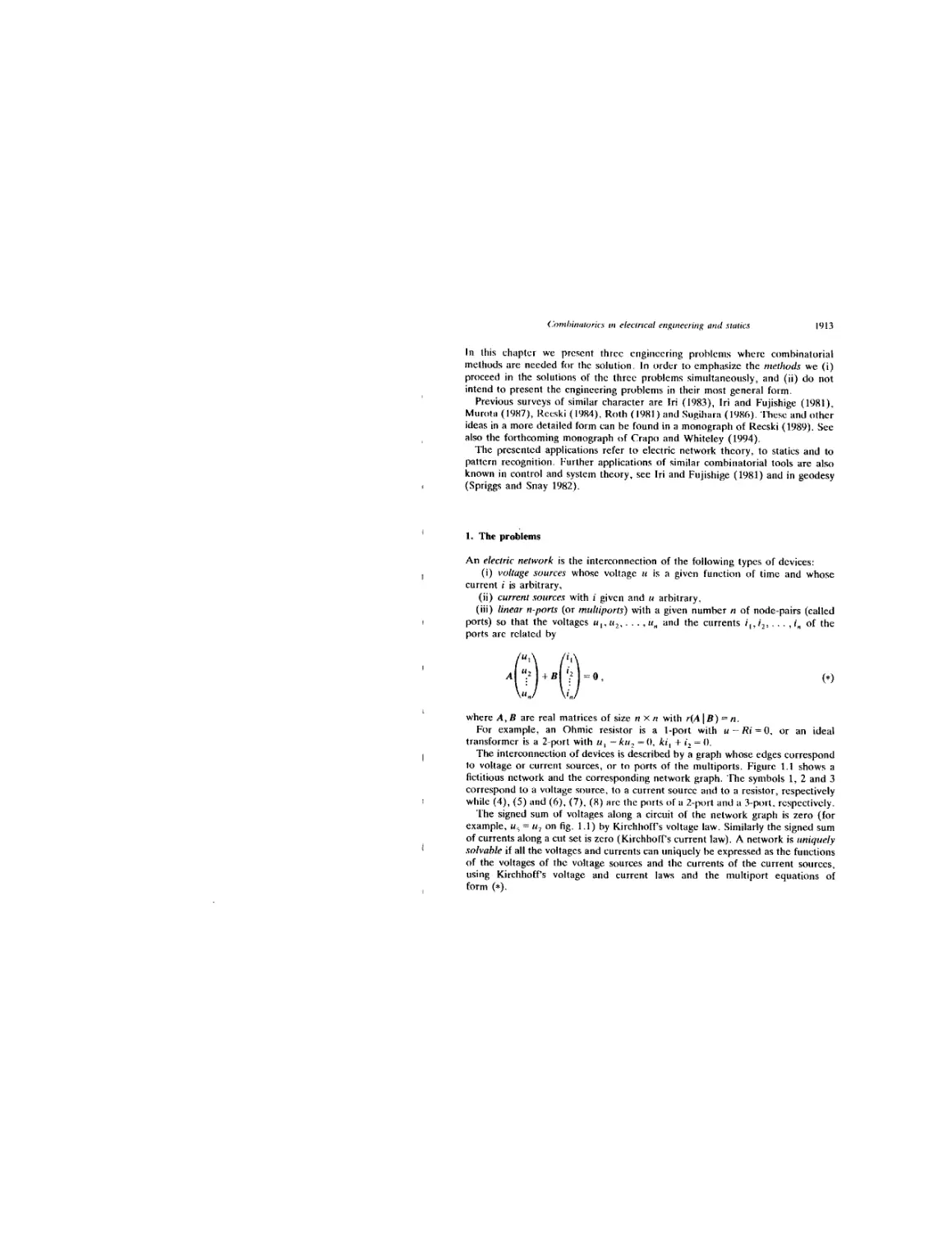
36. Combinatorics in Electrical Engineering and Statics 1911
Preface v A. Recski
37. Combinatorics in Statistical Physics 1925
List of Contributors xi C.D. Godsil, M. Grdtschel and D.J.A. Welsh
38. Combinatorics in Chemistry 1955
Part II: Aspects 1019 D.H. Rouvray 39. Applications of Combinatorics to Molecular Biology 1983
21. Algebraic Enumeration 1021 M.S. Waterman
l.M. Gessel and R.P. Stanley 40. Combinatorics in Computer Science 2003
22. Asymptotic Enumeration Methods 1063 L. Lovdsz, D.B. Shmoys and Ё. Tardos
A.M. Odlyzko 41. Combinatorics in Pure Mathematics 2039
23. Extremal Graph Theory 1231 L. Lovdsz, L. Pyber, D.J.A. Welsh and G.M. Ziegler
B. Bollobds
24. Extremal Set Systems 1293 Part V: Horizons 2083
P. Prank!
25. Ramsey Theory 1331 42. Infinite Combinatorics 2085
J. Nesetril A Hajnal
Contents
43. Combinatorial Gaines
R.K. Guy
44. The History of Combinatorics
N.L. Biggs, E.K. Lloyd and R.J. Wilson
Author Index
Subject Index
2117
List of Contributors
XIII
L1X
Alon, N., Tel Aviv University, Tel Aviv (Ch. 32).
Babai, L., Eotvos University, Budapest and University of Chicago, Chicago, IL (Ch. 27).
Beck, J., Rutgers University, New Brunswick, NJ (Ch. 26).
Biggs, N.L., University of London, London (Ch. 44),
Bixby, R.E., Rice University, Houston, TX (Ch. 11).
Bjdrner, A., Royal Institute of Technology, Stockholm (Ch. 34).
Bollobas, B., University of Cambridge, Cambridge and Louisiana Slate University, Baton Rouge, LA (Ch. 23).
Bondy, J.A., Universite Claude Bernard Lyon I, Vilieurbanne and University of
Waterloo, Waterloo, Ont. (Ch. 1).
Brouwer, A.E., Eindhoven University of Technology, Eindhoven (Chs. 14, 15).
Cameron, P.J., Queen Mary and Westfield College, London (Chs. 12, 13).
Cunningham, W.H., University of Waterloo, Waterloo, Ont. (Ch. 11).
Duchet, P,, IM AG, Laboratoire de Structures Discretes et de Didactique, Grenoble Cedex (Ch. 7).
Erdos, P., Hungarian Academy of Sciences, Budapest (Ch. 17).
Frank, A., Eotvos University, Budapest (Ch, 2).
Frankl, P., CNRS, Paris (Ch. 24).
Gcssel, 1.М., Brandeis University, Waltham, MA (Ch. 21).
Godsil, C.D., University of Waterloo, Waterloo, Ont. (Chs. 31, 37).
Grotschel, M., Konrad-Zuse-Zentrum fur Informationstechnik, Berlin-Wilmersdorf (Chs. 28, 37).
Guy, R.K., University of Calgary, Calgary, Alla. (Ch. 43).
Hacmcrs, W.H., Tilburg University, Tilburg (Ch. 15).
Hajnal, A., Hungarian Academy of Sciences, Budapest (Ch. 42).
Karoriski, M., Adam Mukiewicz University, Poznan and Emory University, Atlanta, GA (Ch. 6).
Klee, V., University of Washington, Seattle, И44 (Ch. 18).
Kleinschmidt, P., Universitdt Passau, Passau (Ch. 18).
Kolen, A.W.J., University of Limburg, Maastricht (Ch. 35).
Lagarias, J.C., AT&T Bell Laboratories, Murray Hill, NJ (Ch. 19).
Lenstra, J.K., Eindhoven University of Technology, Eindhoven and Centre for Mathematics and Computer Science, Amsterdam (Ch. 35),
Lloyd, E.K., University of Southampton, Southampton (Ch. 44).
Lovasz, 1.., Yale University, New Haven, CT (Chs. 28, 31, 40, 41).
Nesetfil, J., Charles University, Prague (Ch. 25).
Odlyzko, A.M., AT&T Bell Laboratories, Murray Hill, NJ (Ch. 22).
Pomerance, C., University of Georgia, Athens, GA (Ch. 20).
xii ' List of Contributors
Pull^yblank, W.R., IBM, Thomas I. Watson Research Center. Yorktown Heights.
NY (Ch. 3).
Purdy. G.. University of Cincinnati, Cincinnati, OH (Ch 57).
Pyber. L., Hungarian Academy of Sciences. Budapest (Ch. 41).
Rccski, A.. Technical University -T Budapest, Budapest (Ch. 36).
Rouvray, D.H., The University of Georgia, Athens. GA (Ch. 38).
Sarkozy, A., Hungarian Academy of Sciences, Budapest (Ch. 20).
Schrijver, A., Centrum voor Wiskunde en Information, Amsterdam (Ch. 30).
Seymour. P.D.. Bell Communications Research, Morristown, NJ (Appendix to Ch. 4, Ch. 10).
Shmoys, D.B., Cornell University, Ithaca. NY (Chs. 29, 40).
Sos, V.T., Hungarian Academy of Sciences. Budapest (Ch. 26).
Spencer, J., New York University, New York, NY (Ch. 33).
Stanley, R.P., Massachusetts Institute of Technology, Cambridge, MA (Ch. 21).
Tardos. Ё., Cornell University, Ithaca, NY (Chs. 29, 40),
Thomasson. C., The Technical University of Denmark, Lyngby (Ch. 5).
Toft, B., Odense University, Odense (Ch. 4).
Trotter, W.T., Arizona State University, Tempe, AZ (Ch. 8).
Van Lint, J.H., Eindhoven University of Technology, Eindhoven (Ch. 16).
Waterman, M.S., University of Southern California, Los Angeles, CA (Ch. 39).
Welsh, D.J.A., University of Oxford, Oxford (Chs. 9, 37, 41).
Wilson, R.J., The Open University, Milton Keynes (Ch. 44).
Ziegler, G.M., Konrad-Zuse-Zentrum fiir Informationstechnik, Berlin-Wilmersdorf (Ch. 41).
Part II
Aspects
CHAPTER 21
Algebraic Enumeration
Ira M. GESSEL*
Department of Malhematict, Brandeis University. Waltham, MA 02254, USA
Richard P. STANLEY’*
Department of Mathematics, Massachusetts Institute of Technology, Cambridge, MA 021.39, USA
Contents
List of symbols and definitions..............................................................1022
1. Introduction............................................................................1023
2. Bijections..............................................................................1023
3. Generating functions ...................................................................1025
4. Free monoids............................................................................1027
5. Circular words........................................................................ 1030
6. Lagrange inversion......................................................................1032
7. The transfer matrix method..............................................................1035
8. Multisets and partitions................................................................1036
9. Exponential generating functions........................................................1040
10. Permutations with restricted position................................................ 1043
11. Cancellation...........................................................................1046
12, Inclusion-exclusion....................................................................1049
13. Mobius inversion.......................................................................1051
14. Symmetric functions....................................................................1056
References...................................................................................1061
’Partially supported by NSF Grant DMS-8902666.
"Partially supported by NSF Grant DMS-840I376.
HANDBOOK OF COMBINATORICS
Edited by R Graham, M. Grdtschel and L. Ijrvasz © 1995 Elsevier Science B.V. All rights reserved
1021
1022
l.M. Gessel and R.P. Stanley
Algebraic enumeration
1023
List of symbols and definitions
Symbol or definition
Meaning
Page
M (1,2, .»} 1023
composition 1023
functional digraph 1024
left-right minimum 1025
lower record 1025
<•'(«,*) unsigned Stirling number of the first kind 1027
free monoid 1027
A* free monoid generated by A 1027
conjugate of a word 1030
(*"№) coefficient of лп in F{x) 1032
ordered tree 1033
ballot number 1033
Catalan numlier 1033
binary tree 1034
Runyon number 1034
Narayana number 1034
transfer matrix method 1035
multiset 1036
partilion 1037
(a)n (1 - u)(l -aq) (! -aq” ’) 1038
[:] (/-binomial coefficient 1034
exponential generating function 1040
S(n,k) Stirling number of the second kind 1041
Bn Bell number 1041
descent (of a permutation) 1042
-Ini') Eulenan polynomial 1042
up-down permutation 1043
D„ tangent and secant numbers 1043
derangement 1044
descent set 1050
w incidence algebra of P 1052
zeta function 1052
Mobius function 1052
lattice 1054
V join 1054
meet 1054
6 minimal element of a lattice 1054
i maximal element of a lattice 1054
atom 1054
geometric lattice 1055
symmetric function 1056
<1A symmetric functions of degree к 1056
monomial symmetric function 1056
«А elementary symmetric function 1056
Лд complete symmetric function 1056
Pa power sum symmetric function 1056
•»a Schur function 1057
Ferrers diagram 1057
plane partition 1057
hook length 1058
Z(G) cycle index 1059
1. Introduction
in all areas of mathematics, questions arise of the form “Given a description of a finite set, what is its cardinality?” Enumerativc combinatorics deals with questions of this sort in which the sets to be counted have a fairly simple structure, and come in indexed families, where the index set is most often the set of nonnegative integers. The two branches of enumerative combinatorics discussed in this book are asymptotic enumeration and algebraic enumeration. In asymptotic enumeration, the basic goal is an approximate but simple formula which describes the order of growth of the cardinalities as a function of their parameters. Algebraic enumeration deals with exact results, either explicit formulas for the numbers in question, or more often, generating functions or recurrences from which the numbers can be computed.
The two fundamental tools in enumeration arc bijections and generating functions, which we introduce in the next two sections. If there is a simple formula for the cardinality of a set, wc would like to find a “reason” for the existence of such a formula. For example, if a set 5 has cardinality 2Л, we may hope to prove this by finding a bijection between S and the set of subsets of an л-element set. The method of generating functions has a long history, but has often been regarded as an ad hoc device. One of the main themes of this article is to explain how generating functions arise naturally in enumeration problems.
Further information and references on the topics discussed here may be found in the books of Comtet (1974), Goulden and Jackson (1983), Riordan (1958), Stanley (1986), and Stanton and White (1986).
2. Bijections
The method of bijections is really nothing more than the definition of cardinality: two sets have the same number of elements if there is a bijection from one to the other. Thus if we find a bijection between two sets, we have a proof that their cardinalities arc equal; and conversely, if we know that two sets have the same cardinality, we may hope to find an explanation in the existence of an easily describable bijection between them. For example, it is very easy to construct bijections between the following three sets: the set of 0-1 sequences of length «, the set of subsets of [л] — (1,2,...,л}, and the set of compositions of л + 1. (A composition of an integer is an expression of that integer as sum of positive integers. For example, the compositions of 3 arc 1 + 1 + 1, 1 + 2, 2 + 1, and 3.) The composition ui + + • • • + of л + 1 corresponds to the sub-
set S — {at,fli + d2> - • - ,«i + иг r • • • + ak J of {1,2,... ,n} and to the 0-1 sequence «]M2 • • -uri in which u, = 1 if and only if i e 5. Moreover, in our example, a composition with к parts corresponds to a subset ol cardinality к - I ones, and to a 0—1 sequence with к - 1 ones, and thus there are (л",) of each of these.
It is easy to give a bijective proof that the set of compositions of n with parts 1 and 2 is equinumerous with the set of compositions of n t- 2 with all parts at least
1024
f.M. Gessel and R.P. Stanley
2: given a composition aj +a2 + • • • + вк of л + 2 with all a, 2, we replace each at with
2 + 1+ + !, a, -2
and then we remove the initial 2. If we let f„ be the number of compositions of n with parts 1 and 2, then fn is easily seen to satisfy the recurrence fn = fn-\+fn 2 for n 2, with the initial conditions /Ь = 1 and f\ = 1. Thus fn is a Fibonacci number. (The Fibonacci numbers are usually normalized by Fq =0 and Fi - 1, so fn =
As another example, if тг is a permutation of [л], then we can express я as a product of cycles, where each cycle is of the form (i rr(r) ir2(r) - №(*))• We can also express tt as the linear arrangement of [и], тг(1) ir(2) • • тг(л). Thus the set of cycles {(1 4), (2),(3 5)} corresponds to the linear arrangement 425 I 3. So we have a bijection between sets of cycles and linear arrangements.
This simple bijection turns out to be useful. We use it to give a proof, due to Joyal (1981, p. 16), of Cayley’s formula for labeled trees. First note that the bijection implies that for any finite set 5 the number of sets of cycles of elements of 5 (each element appearing exactly once in some cycle) is equal to the number of linear arrangements of elements of 5.
The number of functions from |n] to (л] is clearly nn. 'Io each such function f we may associate its functional digraph which has an arc from i to /(i) for each i in [л]. Now every weakly connected component of a functional digraph (i.e., connected component of the underlying undirected graph) can be represented by a cycle of rooted trees. So by the correspondence just given, nn is also the number of linear arrangements of rooted trees on [n]. We claim now that л" = n2r„, where tn is the number of trees on [л].
It is cicar that n2tn is the number of triples (+,y- T), where x,y € [n] and T is a tree on [nJ. Given such a triple, we obtain a linear arrangement of rooted trees by removing all arcs on the unique path from x to у and taking the nodes on this path to be the roots of the trees that remain. This correspondence is bijective, and thus t„ = nn"2.
Priifer (1918) gave a different bijection for Cayley’s formula, which is easier to describe but harder to justify. Given a labeled tree on [n], let q be the least leaf (node of degree 1), and suppose that 0 is adjacent to j\. Now remove q from the tree and let /2 be the least leaf of the new tree, and suppose that i2 is adjacent to j2. Repeat this procedure until only two nodes are left. Then the original tree is uniquely determined by Д • • • jn_2 and conversely any sequence /1 • • • /л-2 of elements of [zi] is obtained from some tree. Thus the number of trees is n"“2.
Both proofs of Cayley’s formula sketched above can be refined to count trees according to the number of nodes of each degree, and thereby to prove the Lagrange inversion formula, which we shall discuss in section 6. (See Labelle 1981.)
There is another useful bijection between sets of cycles and linear arrangements which we shall call Foata’s transformation (see, c.g., Foata 1983) that has interesting
Algebraic enumeration 1025
properties. Given a permutation in cycle notation, we write each cycle with its least element first, and then we arrange the cycles in decreasing order by their least elements. Thus in our example above, we would have rr = (35)(2)(14). Then we remove the parentheses to obtain a new permutation whose 1-line notation is я — 35214.
If a is a permutation of [n], then a left-right minimum (or lower record) of ir is an index i such that <r(i) < o(J) for all j < i. It is clear that i is a left-right minimum of тг if and only if тт(Г) is the least element in its cycle in rr. Thus we have the following.
Theorem 2.1. The number of permutations of [л] with к left-right minima is equal to the number of permutations of [n] with k cycles.
This number is (up to sign) a Stirling number of the first kind. We shall see them again in sections 3 and 9.
In section 10 we shall need a variant of Foata’s transformation in which left-right maxima are used instead of left-right minima.
3. Generating functions
The basic idea of generating functions is the following: instead of finding the cardinality of a set 5, we assign to each a in 5 a weight vv(a). Then the generating function *^(5) for 5 (with respect to the weighting function w) is ^«^(a). Thus the concept of generating function for a set is a generalization of the concept of cardinality. Note that S may be infinite as long as the sum converges (often as a formal power scries).
The weights may be elements of any abelian group, but they are usually monomials in a ring of polynomials or power series. In a typical application each element a of 5 will have a “length” 1(a) and we lake the weight of a to be where x is an indeterminate. Then knowing the generating function *s equivalent
to knowing the number of elements of S of each length.
Analogous to the product rule for cardinalities, |A||fi| = |A x B\, is the product rule for generating functions, ^(A)^(fi) - <S(A x B), where we take the “product weight” on A x B, defined by w((a,fi)) - w(a)w((S).
As an example, suppose we want to count sequences of zeros and ones of length n according to the number of zeros they contain. We can identify the set of 0-1 sequences of length n with the Cartesian product {0,1}". If we weight {0,1} by w(0) = x and w(l) = y, then the product weight on {0,1}" assigns to a sequence with / zeros and к (= n - /) ones the weight x’yk. Thus
(-y)”= E (”W
>\k n
is the generating function for sequences of zeros and ones of length n by the
1026
I.M. Gessel and R P Stanley
Algebraic enumeration
1027
number of zeros and lhe number of ones. If we want to count sequences of zeros and ones of all lengths with this weighting, we sum on n to obtain the generating function
____1
1 -x /
Now suppose we want to count compositions with parts 1 and 2. Rather than picking an integer n and considering the compositions of n, we pick an integer к and consider the set C(. of all compositions of any integer with exactly к parts (each part being 1 or 2). We may identify Ck with {1,2)*. If we assign 1 the weight x and 2 the weight x2, where x is an indeterminate, then the product weight of a composition of n in Ck is x". Thus
S(Ct) = »({1.2}‘) - «({1,2})“ = (л + .г2)‘ = £ („
Thus there are ( *A) compositions of n with к parts, each part 1 or 2. As before, if we do not care about the number of parts, we sum on к to obtain t,(x + x7)* -(1 -x x2)-1 as the generating function for all compositions into parts 1 and 2. By lhe same kind of reasoning, if A is any set of positive integers, then the generating function for compositions with к parts, all in A, is and the generating
function for compositions with any number of parts, all in A, is (1 ~
In particular, if A is the set of positive integers then -x/(l -x) so the generating function for compositions with к parts is
(A)
for к > 0 and the generating function for all compositions is (\ 1 . oo
1--^) =_Lz± = 1 + _JE_ = i + y2" ’x".
1 - X ) 1 - 2x 1 - 2x
' n=l
The generating function for compositions with parts greater than I is
Similarly, the generating function for compositions with odd parts is
Thus we have proved using generating functions two of the results we proved using
bijections in the preceding section. Notice that the generating functions take into account initial cases which did not arise in the bijective appioach.
For our next two examples, we consider another bijection for permutations. Suppose that тг is a permutation of [nJ. We associate to тг a sequence a\<i2- -an of integers satisfying 0 a, < j - 1 for each j as follows: Oj is the number of indices i < j for which ir(i) > l he sequence • • -«n is called the inversion table of it: an inversion of тг is a pair (/,/) with i < j and ir(i) > and thus a} is the number of inversions of тг of the form (/, j). It is not difficult to show that lhe correspondence between permutations and their inversion tables gives a bijection between the set <4, of permutations of fn[ and the set T„ of sequences a}a2 • an of integers satisfying 0 у a, у j - I for each j. Note that Tn is the Cartesian product {0} x {0,1} x • • • x {0,1,..., л - I}. Wc shall use the inversion table to count permutations by inversions and also by cycles.
Let /(тг) be lhe number of inversions of тг. We would like to find the generating function for permutations of [л] where each permutation тг is assigned the weight . To do this we note that /(тг) is the sum of the entries of the inversion table of -л-, and thus if wc assign the weight w(«) = qa'+ to a = а]а? --ап e Тл, then we have
<3(T„) - 1 (1 +<?)(! + + ').
Next wc count permutations by left-right minima. It is clear that j is a left-right minimum of тг if and only if a} — j — 1. Thus if we assign the weight tk to a permutation in .7’,, with к left-right minima, and to a sequence in Tn with к occurrences of aj — j — 1, then we have
«(%) = = t(t + l)(r + 2) • • (f + и - 1) = у f(n,*)r‘,
к -0
where c(n,k) is (by definition) the unsigned Stirling number of the first kind. By Theorem 2.1. it follows that c(n,k) is also the number of permutations in with к cycles.
4. Free monoids
Free monoids provide a useful way of organizing many simple applications of generating functions. Let A be a set of “letters". The free monoid A* is the set of all finite sequences (including the empty sequence) of elements of A, usually called words, with the operation of concatenation. We can construct an algebra from A" by taking formal sums of elements of A* with coefficients in some ring. Wc write 1 for the empty sequence, which is the unit of this algebra. These formal sums are then formal power series in noncommuting variables. The generating function *£(5) for a subset 5 of A* is the sum of its elements.
Algebraic enumeration
1029
1028 l.M. Gessel and R.P. Stanley
If 5 and T arc subsets of A', we write ST for the set {st | s e 5 and t e T}. We say that the product ST is unique if every element of ST has only one such factorization. The fundamental fact about generating functions is that if the product ST is unique, then <S(ST) = ^(Syff(T).
More generally, we may define a free monoid to be a set together with an associative binary operation which is isomorphic to a free monoid as defined above. Let A* = A * \ {1} and suppose that ,V is a subset of A+ such that for each fc, every clement of Sk has a unique factorization 5^2 • • •$* with each s, in S. Such a set S is sometimes called a uniquely decodable code, or simply a code. Then 5” = U^o^' is a free monoid. We call the elements of 5 the primes of the free monoid S*. In this case
<g(S-) = ^(sy --(1 -SS(S))-,-0
In particular, «(Л*) = (1 ЭД(А))"1.
Among the simplest free monoid problems are those dealing with compositions of integers, as we saw in the previous section. A composition of an integer is simply an element of the free monoid P*, where P is the set of positive integers.
As a more interesting example, let A = {X, У), let 5 be the subset of A* consisting of words with equal numbers of Jf’s and K’s, and let T be the subset of A* of words with no nonempty initial segment in 5. Then A* — ST uniquely, so ^(/1’) — (1 - X — У) 1 — ^(5)^(7 ). Moreover, 5 is a free monoid U*, where U is the set of words in 5 which cannot be factored nontrivially in 5. The sets S, T, and 17 have simple interpretations in terms of walks in the plane, starting at the origin. If X and Y are represented by unit steps in the x and у directions, then 5 corresponds to walks which end on the main diagonal, T corresponds to walks that never return to the main diagonal, and U corresponds to walks that return to the main diagonal only at the end.
Il is often useful to replace the noncommuting variables by commuting variables. If we replace the letter X by lhe variable x, we are assigning X the weight x. (More formally, we are applying a homomorphism in which the image of X is x.)
In our example, if we weight X and Y by commuting variables x and y, then <^(A*) becomes l/(l-x-y) and <S(5) becomes ZXoC1)*"/1 — 0 - 4xy)-1^2 since there are (2^) ways of arranging n X's and n K’s. Thus ^(T) becomes y/l - 4xy/(l — x — y). It can be shown that this is equal to
Ё “О H'>
where the constant term is 1. The coefficients in (4.1) are called ballot numbers and we shall see them again in section 6.
If wc replace x and у by the same variable z, the generating function for T becomes
l + 2z
1 - 2г \/l — 4z2
Thus the number of words in T of length 2zi is (2n") and the number of words in T of length 2n + 1 is 2(^1).
Although we usually work with formal power series, it is sometimes useful for variables to take on real values. We derive an inequality called McMillan's inequality which is useful in information theory. (See McMillan 1956.) Let A be an alphabet (set of letters) of size r, and let S be a code in A*, so that S* is a free monoid. Let us weight each letter of A by /. and let ^(S) = /?(/).
We know that *5(5T) = (l — p(t)) as formal power series in t. Since there are rk words in A* of length k, the coefficient of tk in (1 -p(t))-1 is at most r*. If 0 < a < \ /r then the series Y5k-xyrkak converges absolutely to (1 - ra) and thus (1 — p(a)) (1 — ra)-1, which implies p(a') s ra. Taking the limit as
a approaches 1/r from below, we obtain p(l/r) 1.
Thus we have proved the following.
Theorem 4.2. Let S be a uniquely decodable code in an alphabet of size r, and for each к let p^ be the number of words in S of length k. Then Y^k~iPkr~k C L
In some applications of free monoids, the “letters” have some internal structure. For example, consider the set of permutations it of [n] = {1,2,...w) satisfying |тг(/) —/| ^ 1. We can represent a permutation of |n] as a digraph with node set [zi] with an arc from i to ir(i) for each i, If we draw the digraph with the nodes in increasing order, we get a picture like this one. which corresponds to the permutation 2143576:
It is clear that these permutations form a free monoid with the two “letters”, or primes
Thus the generating function (by length) for these permutations is (1 — x — x2) and there is an obvious bijection between these permutations and compositions with parts 1 and 2.
1030
l.M. Gessel and R.P. Stanley
Algebraic enumeration
1031
Sometimes it is easier to count all the elements of a free monoid than just the primes. If we represent arbitrary permutations as in the previous example, then we have a free monoid in which the primes, called indecomposable permutations, are those permutations tt of [n| (for some n) such that for 1 i < n, tt restricted to [/| is not a permutation of [<]. For example, 421 3 is indecomposable:
but 2 I 534 is not:
Thus if g(x) is the generating function for indecomposable permutations, we have
£n!x" = (l-.g(x))-',
so
S(x) = 1
as shown by Comtet (1972).
5. Circular words
We now study some properties of words in which the letters are thought of as arranged in a circle, so that the last letter is considered to be followed by the first. (This should not be confused with the problem of counting equivalence classes of words under cyclic permutation, which we discuss in section 14.)
We define the cyclic shift operator C on words by
Ca^ - Uk
A conjugate or cyclic permutation of a word w is a word of the form С“и' for some m. If 5 is a set of words, then we define 5° to be the set of all conjugates of words in 5.
Suppose that 5* is a free submonoid of the free monoid A*, and let и* = • sk
be an element of Sk, where each s, is in S. It is clear that C'w e Sk whenever i takes on any of the к values 0, /(sj), , /($1*2 si-i), where l(p) denotes
the length of the word If these are the only values of i, with 0 < i < f(w), for which C'w g S', then we call 5’ cyclically free1 *. For example, {ab,b}* is cyclically free, but {ла}* is not.
If 5* is cyclically free, then it is clear that for w e (Sk}° there are exactly к values of /, with 0 i < l(w), for which C'w € Sk.
Theorem 5.1. Suppose that S' is cyclically free and let (> = Sk it A". Then k|Q°| -«Ю1-
Proof. We count pairs (i,w), where C'w e Q and 0 < i < n. First we may choose C'w in |Q| ways. Then w is determined by z, which may be chosen arbitrarily in {0,1, 1}. Thus there are «|Q| pairs. On the other hand, we may choose w
first as an arbitrary element of Q° and by the remark above, there are к choices for i. □
In the next section we shall use a weighted version of Theorem 5.1 which is proved exactly the same way.
From Theorem 5.1 we can easily derive a generating function for (5*)°:
Corollary 5.2. Suppose that S' is cyclically free and let g(z) v Then
«Л=|
Equivalently, 00 \
We can use Theorem 5.1 to count the number of A:-subsets of {«] with no two consecutive elements, where 1 and n are considered consecutive. We take 5 — {aft, ft}. The subsets we want correspond to words in (S"'k П {a, ft}n)°. These words contain n letters, of which n — к are ft’s, and hence к arc a’s. The positions of the a’s in one of these words determines the subset. $* is clearly cyclically free, so by Theorem 5.1, the number of such subsets is (и/(п - k)}{"kk).
Our next example will be useful in proving the Lagrange inversion formula in the next section. Let ф be any function from A to the real numbers. Extend ф to all of A* by defining ф(а\а2 -ak) = ф(а}) + ••• + ф(ак). Define R by
R = { w I if w ~ uu with и / 1 then ф(и) < 0}. (5.3)
1 In the lheory of codes. S' is called a circular code and .S’4 is called a very pure free monoid. See, c.g.,
Bcrslel and Perrin (1983).
1032
l.M. Gessel and R.P. Stanley
Algebraic enumeration
1033
И is easily verified that R is a cyclically free submonoid of A*.
The following description of R° is the key step in our proof of the Lagrange inversion formula in lhe next section.
Lemma 5.4. Let R and ф be as above. Then R° — {1} U { w | ф(н’) < 0}.
Proof. We need only show that if ф(и>) <0, then for some i, C'weR. Of the heads (initial segments) h of w which maximize </>(Л), let и be the longest, and let w = uv. Then vu is easily verified to be in R. □
6. Lagrange inversion
Tn the last example, let A = {х-ьхо.хь^2. • -} and define ф : A’ —* 7L by
ф(хц • • -xMi) - Z] + ••• + /„,.
Let R be as in (5.3) and let 5 — { w | w e R and ф(и>) = — I.}. We claim that R ~ S*. Since we know that R is a free monoid, we need only show that if w is a prime of R, then ф(и') = -1.
To see this, let w be a prime of R. Since ф(и^) < 0 and ф(х,) 5-' -1 for each x,EA,w must have a head h with ф(Л) = -1. Let w = uv, where и is the longest head of w for which ф(и) = —1. Then v must be in R, since otherwise w would have a longer head ft with ф(Л) > —1. Since vv is a prime of R, this means w = u. It follows that if v is any word in R with ф(и) = -к then v e Sk.
Now let и be any word in S and suppose v = их<. Then и is in R with ф(и) + i = —1, so ф(и) — —1 - i, and thus и e S'+1. It follows that
(6.1)
where the union is disjoint. Wc are now ready to prove the Lagrange inversion formula. Wc use lhe notation [x"]F(x) to denote the coefficient of x" in F(x).
Theorem 6.2. Let g(u) = where the g„ are indeterminates. Then there is
a unique formal power series f in the g„ satisfying f = g(f), and for к > 0,
ос .
(63) n-1 n
Proof. It is easily seen that the equation f = g(f) has a unique solution. Let us assign to the letter x, the weight #l+i and let f be lhe image of ^(5) under this assignment. Then from (6.1) we have
f-=8<n-
By the weighted version of Theorem 5.1, the sum of the weights of the words of length n in Sk is k/n times the sum of the weights of the words in (Sfc n Art)'. But by Lemma 5.4, the sum of the weights of the words in (Sk П Anf is
I»-*1
The proof we have just given is essentially that of Raney (1960). It is clear that if the gt are assigned values that are not necessarily indeterminales, then the theorem still holds as long as the sum in (6.3) converges as a formal power series and f is uniquely determined as a formal power series by f — g(f). The usual formulation of Lagrange inversion is obtained by taking g(u) = z’E^QrnU'', where z is an indeterminate and the rn are arbitrary.
One of the most important applications of Lagrange inversion is to the enumeration of ordered trees. (An ordered tree is a rooted unlabeled tree in which the children of any node are linearly ordered.) Let us weight a node with i children in an ordered tree by gt, and weight lhe tree by the product of the weights of its nodes. If f is the sum of the weights of all ordered trees, then, since an ordered tree consists of a root together with some number (possibly zero) of children, each of which may be an arbitrary ordered tree, we have
f = Y,8j‘ =g(f), t-0
where g(u) = The Lagrange inversion formula then yields the following.
Theorem 64. The number of к-tuples of ordered trees in which a total ofnt nodes have i children is
к ( n A i. v-
n\n^n\,n2,--J
if щ + 2n2 Зпз + • • • = n — k, and 0 otherwise.
It is not hard to derive Theorem 6.2 from Theorem 6.4, so any other proof of Theorem 6.4 (for example, by induction), yields a proof of the Lagrange inversion formula. Our approach can also be used to give a purely combinatorial proof of Theorem 6.4 without the use of generating functions.
A few special cases of Theorems 6.2 and 6.4 are especially important. If there are a nodes with 2 children, b nodes with no children, and no other nodes, then with b — a + к the number of к-tuples of such trees is
к /n\ _ к /2а + к\
n\«7 2a + к \ a )’
These numbers arc called ballot numbers, l he special case к — 1 gives lhe Catalan numbers
/2d + l\ 1_ /2«\
2a + 11 \ a / a + 1 \ a )'
1034
l.M. (Jesse! and R.P. Stanlev
Algebraic enumeration
1035
To apply Theorem 6.2 directly to this case, we may take go = 1. g? x. and g, (1 for ,/0.2. Then /satisfies f - 1 + rf2. so/=r (1 - vT- 4x)/2x. and we obtain /1 - v'TlrV А к /2а + к\ 2x 1 ^2a + k\ a J \ / a 0 4 To count all ordered trees we set gi — x for all iy to obtain the equation /(x) = x/(l -/(x)), with the solution ,, ,s /i-vT-4x\‘ = 1 j 1 r у * . Z-'nK п к ) ^2n + k\n J n-a x 7 л-о x 7 so we again obtain the Catalan and ballot numbers. It is an instructive exercise to find a bijection between these classes of trees, and to relate these results to formula (4.1). Our analysis gives a well-known bijection between ordered trees and words in S. The code c(t) for a tree T may be defined as follows: If the root of T has no children, then c(T) = x |. Otherwise, if the children of the root of T arc (in order) the roots of trees 7). T2. ..., 7*, then ctn-ctTO-.-cC/yx^t. For another example, we define a binary tree to be a rooted tree in which every node has a left child, a right child, neither, or both. Thus and arc different binary trees. Let us weight a binary tree with n nodes, i left children, and j right children by xnL‘Rl. Then if f is the generating function for these trees, we have / = x(1+L/)(l + Rf), and thus by Lagrange inversion we have n^k iXI X 7 4 7 For k = l, the numbers (1 /«)(")(,”t) are called Runyon numbers or Narayana numbers. 7. The transfer matrix method Many enumeration problems can be transformed into problems of counting walks in digraphs, which can be solved by the transfer matrix method. Suppose D is a finite digraph. To every arc of D we associate a weight. Let M be the matrix in which rows and columns are indexed by the nodes of D and the (i,j) entry of M is the sum of the weights of the arcs from / to j. Then by the definition of matrix multiplication, the (f, /) entry in Mk is the sum of the weights of all walks of к arcs from i to j. Il follows that (as long as the infinite sum exists) k = (I - M)-1 counts all walks, where / is the identity matrix, and trace (/ — Mcounts walks that end where they begin. For example, consider the following problem: Given integers n and i, what is the number t(n,i) of sequences aja? • • • an of 0’s. 1’s, and — l's with щ + > • • + an = i (mod 6)? Here we take D to be the digraph with node set {0,1,2.3,4,5} and an arc from each j to / — 1, /, and / + 1, reduced modulo 6. We weight each arc by x. So M is /x x 0 0 0 x\ x x x 0 0 0 0 x x x 0 0 0 0 x x x 0 ' 0 0 0 x x x \x 0 0 0 X x/ We find that (/ - M) 1 is the circulant matrix with first column / _J_+ _2 , >.+2\ 1 - 3x 1 - 2x 1 l x ' I 3x 1 - 2r Hr । 1,1. 1 1 - 3x 1 - lx 1 + x 6 1 2 1 + 7 1 — 3x 1 2x 1+x 1 1 1 1 - 3x l lr ’ H r 1 1 , 1 1 . \ 13x l-2r 1+x / Thus for n > 0, r(ri,0) - 13" г 2"*1 + 1 -1 )")/6. t(n, 1) = /(n,5) = (3" +2” - (-l)")/6, 1(л,2) = |(л,4) = (3"-2"+(-1)")/6, t(n,3) = (3" - 2"'1 (-l)")/6.
1036
l.M. Gessel and R.P. Stanley
Algebraic enumeration
1037
As another example, how many 0-1 sequences are there with specified numbers of occurrences of 00, 01. 10, and 11? Here we take D to be the weighted digraph
-*oi
— *oo
-xi«
1 —Xll X()| X10 1 - Xoo
(1 - Xoo)(1 — Xu) - X01X|0
Thus, for example, the generating function for 0-1 sequences beginning with 0 and ending with 1 is
r °° r, + 1 r'
________£oi___________ V’’ЛО1 Jio
(1 — X(X))(1 - Xu) -XOiXio (1 - X(x))1(1(1 -X|1),+1
so ('*'')(***) ’s the number of 0-1 sequences beginning with 0 and ending with 1, with i occurrences of 10 (and thus i +1 occurrences of 01), j occurrences of 00, and к occurrences of 11 (and thus i + / + 1 zeros and i + к + 1 ones).
The transfer matrix method can often be used to show that a generating function is rational. For example, consider the problem of counting the number of ways of covering an m x n rectangle with a fixed finite set of polyominos. It is not hard to show, using the transfer matrix method, that for fixed tn the generating function on n is rational, although it is difficult to give an explicit formula. We will see another example of this type in section 10.
8. Multisets and partitions
We have so far considered problems involving linear arrangements. In this and the next section we turn to unordered collections. We first consider the problem of counting multisets, which arc sets with repeated elements allowed. More formally, a multiset on a set S is a function from 5 to the nonnegative integers; if v is a
multiset then v(s) represents the multiplicity of 5. If each element s in 5 has a weight w(s), then we define the weight of the multiset и to be
For each 5 in S, let be a set of nonnegative integers. Then the sum of the weights of all multisets v on 5 such that p(.v) is in Mx for each x in 5 is easily seen to be
П
sGS ieM,
We give a few examples. Let us take w(.v) = r for all v in 5, and assume |.S'| = n. If M, = {0,1} for each r, we are counting subsets, and the generating function is
О
A=0 41 7
If M, is the set of all nonnegativc integers for each s, we are counting unrestricted multisets, and the generating function is
*=0 ' '
If Ms = {0,1,.. ,,m} for each J, the generating function is
= VV Vf-lV (n\fn + k +
V Ч'Д fc-(m + l)i J-
A multiset of positive integers with sum к is called a partition of k. The elements of a partition are called its parts. It is customary to list the parts of a partition in decreasing order, so a partition of к is often defined as a (weakly) decreasing sequence of positive integers with sum k. To count partitions, we weight i by q', where q is an indeterminate. Then the generating function for all partitions *s FKiO 4')-1 «nd the generating function for partitions with distinct parts is (!+<?')
Many theorems in the theory of partitions assert that one set of partitions is equinumerous with another. The simplest of these, due to Euler, is that the number of partitions of n with odd parts is equal to the number of partitions of n with distinct parts. To prove this, we note that the generating function for partitions with odd parts is
i odd f=l (=t
1038
l.M. Gessel and R.P. Stanley
which is the generating function for partitions with distinct parts.
It is not difficult to give a combinatorial proof of this result: Suppose тг is a partition with odd parts. If тг contains the odd part i with multiplicity k, let к - 2ei + 2е* + • • • + 2*\ where 0 e\ < e2 < • < es. We now replace lhe к copies of part i by the distinct parts 2e'i,2%...,24. Doing this to every part of тг we obtain a partition тг' with distinct parts. The correspondence is easily seen to be a bijection. For example, if тг — {9,9,7,7,7,1,1,1,1}, then тг' — {18,14,7,4}.
One of the most famous results in the theory of partitions is the following.
Theorem 8.1. The number of partitions of n with distinct parts in which any two parts differ by at least 2 is equal to lhe number of partitions of n with pans congruent to I or 4 (mod 5).
This result follows easily from the Rogers-Ramanujan identity
V= fr________________________1______
(1 - ,)(1 - </2) (1 - 7) “ (1 - 7'”1 )(1 - 7'’)'
No simple bijective proof of Theorem 8.1 is known. A complicated bijective proof was found by Garsia and Milne (1981).
We now prove an identity called the q-binomial theorem, which has many applications to partitions. We introduce the notation (a)„ for (1 — ti)(l — aq) •••(1 — aq"-1), where q is understood. In particular, (q)n = (I — q)(l — q2) • • (1 - q"). We also write (a)» for ПХо(1 ~ a4')-
Theorem 8.2 (The ^-binomial theorem).
_ (uQoo
Proof. Let
Then
But also,
(ff)oo
Equaling coefficients of tn, we have
f,. -f„ । q"f« - «</” 7» i, « > 1,
Algebraic enumeration 1039
and thus /„(1 — qn) = /л_[(1 — aqn~l). Since f0 = 1, this gives
1-7 (?)..
Two cases arc particularly worth noting. If a = qm, where m is a positive integer, then we have
The q-binomial coefficient is defined to be
W =
Ы (Л («)»-/
Since (сП, = (</)„,we may rewrite (8.3) as
E°° Гт + л 11 n 1
...I " J' “(1-0(1-»«)•• (8'4)
It follows from (8.4) that ["] is a polynomial in q that reduces to the binomial coefficient (J) for q = 1.
We can use (8.4) to count partitions with at most n parts, each part at most m. It is clear that the desired generating function is the coefficient of tn in
1 1
(l-Z)(l-^)-..(l -tq™}- (r)„1+?
and by (8.4) this is
The case a = q~m of the «/-binomial theorem yields similarly (after changing q to q~' and t to —t/q)
=(!+')(!+«/) (I +Г//"'1). (8.5)
л=0 L 1
which implies that the generating function for partitions with n distinct parts, all less than m, where 0 is allowed as a part, is This result may be derived directly from our previous generating function for partitions with repeated parts allowed, since every partition with distinct parts is obtained uniquely from an unrestricted partition by adding 0 to the smallest part, 1 to lhe next smallest, and so on.
There is an important interpretation for ^-binomial coefficients in terms of vector spaces over finite fields. (See, e.g., Stanley 1986, p. 28, for lhe proof.)
Theorem 8.6. Let q be a prime power. Then the number of к-dimensional subspaces of an n-dimensional vector space over a field with q elements is [J].
A comprehensive reference on the theory of partitions is Andrews (1976).
1040 l.M. Gessel and R.P. Stanley
9. Exponential generating functions
If До,Д(,... is a sequence of numbers, the power series
is called the exponential generating function for the sequence. Exponential generating functions arise in counting "labeled objects”. Their usefulness comes from the fact that
Algebraic enumeration 1041
Thus, for example, (cT — l)*/fc! is the exponential generating function for partitions of a set into к blocks. The numbers S(n,k) defined by
(9.1)
л=0
arc called Stirling numbers of the second kind. If we sum on к we obtain the exponential generating function ехр(ел - 1) for all partitions of a set. The coefficients Bn defined by
If A is an object with label set [m) and В is an object with label set [n], we can combine them in ("£”) ways to get an object (A',B') with label set [m + n]: We first choose an m-element subset 5 of [m + л] and replace the labels of A with the elements of S (preserving their order) to get A', and in the same way we get B1 from В and \5.
Thus if fix) and g(x) are exponential generating functions for classes of labeled objects, then their product f(x)g(x) will be the exponential generating function for ordered pairs of these objects. For example, the exponential generating function for nonempty sets is
since the elements of [zi] can be arranged as a nonempty set in one way if n > 0 and in zero ways if л =0. Thus
(c* l)2 iz<2" 2)^
л=2
is the exponential generating function for ordered partitions of a set into two nonempty blocks. More generally, (еЛ - 1)* is the exponential generating function for ordered partitions of a set into к nonempty blocks, and
oo .
k—0
is the exponential generating function for all ordered partitions of a set.
Now suppose that f(x) is (he exponential generating function for a class of labeled objects and that /(()) — 0. As we have seen, f(x)k is the exponential generating function for fc-tuples of these objects. Every fc-set can be arranged into a A-luple in kt ways, so f(x)k/k\ is the exponential generating function for Л-scls of these objects,
are called Bell numbers.
In general е^(л) counts sets of labeled objects each counted by /(x). Another important application of this principle (often called the “exponential formula”) is to the enumeration of permutations by cycle structure. A permutation may be considered as a set of cycles. If we weight a cycle of length i by u, and weight a permutation by the product of the weights of its cycles, then the exponential generating function for cycles is
°0 xn 00 xn
-!)!«„--52
and thus the exponential generating function for permutations by cycle structure is
ехр(52“„х"/л)-
Л-1
If we set un = и for all n, then we are counting permutations by the number of cycles, and we obtain the generating function for the (unsigned) Stirling numbers of the first kind,
00 rlt x н »
(! - *)'“=+IJ +n - = S
n О ‘ H-0 ‘
which wc derived in a different way in section 3.
fn some cases, there is a simpler expression for c^(x) than for f(x). For example, any labeled graph is a set of connected labeled graphs. Thus if g(x) is the exponential generating function for connected labeled graphs, then ек(л^ is the exponential generating function for all labeled graphs. But there are 2® labeled graphs on [r<], so
(»
n <1
1042 l.M. Gessel and R.P. Stanley
Exponential generating functions often satisfy simple differential equations which can be explained combinatorially. If
00 x"
w-0
then
00 „Л it 0
so an object counted by f'(x) with label set [и| is the same as an object counted by f(x) with label set [n + 1]. For example, let
be the exponential generating function for permutations (considered as linear arrangements of numbers). Then f(x) counts permutations of [л + Ij in which only the numbers in [n] arc considered to be labels. We can consider n +1 to be a “marker” that separates the original permutation into a pair of permutations on [n], and we obtain the differential equation f(x) — f(x)2. This decomposition can be used to obtain more information about permutations, as we shall see next.
A descent of the permutation a 1^2 • an is an i for which a, > anl. It is convenient to count n as a descent also, if /1 > 0. Let
Л(х) = £Л„(')^
n—0
be the exponential generating function for permutations by descents, where a permutation with к descents is weighted r*. If we take a permutation тг = dja2- • -nn+i on [л + lj and remove the element л + l, we are left with two permutations, 7Ti — Я|Л2 • Л/-1 and 7Г2 = where af — n + 1. The number of descents
of tt is the sum of the number of descents of TT] and тг2 unless m is empty, when •л- has an additional descent. Thus we obtain the differential equation
Л'(х) = (Л(х)~ 1)Л(х) + /Л(х),
together with the initial condition A(0) — 1. The differential equation is easily solved by separation of variables, yielding
“ J re(i /)Л
The polynomials An(l) are called Eulerian polynomials and their coefficients are called Eulerian numbers.
Algebraic enumeration 1043
As another example, let us define an up-down permutation to be a permutation «1^2•••an satisfying aj < a-y > ay < a^ - ^an. Let Dn be the number of up-down permutations of [л] and let
BC' r2ml
n <1
Removing 2л + 1 from an up-down permutation of [2л +1 ] for n 1 leaves a pair of up-down permutations of odd length. Taking into account the exceptional case n = 0, we obtain the differential equation T'(x) = T(x)2 + 1, with the initial condition T(0) = 0. Solving the differential equation yields T(x) = tanx. The numbers Dann are called tangent numbers.
For the generating function
л—(I
a similar analysis yields the differential equation S'(x) — T(x)S(x), with the initial condition S(0) — 1, which has the solution S(x) = sccx. The numbers D2„ are called secant numbers. We will show that 5(x) = sccx by a different method in section 11.
Another application of exponential generating functions is to the enumeration of labeled rooted trees. Since a rooted tree can be represented as a root together with a set of subtrees, the exponential generating function r(x) for rooted trees satisfies
t(x) = xer<r>.
We can solve this equation by the Lagrange inversion formula, and we obtain
which for к = 1 gives a formula equivalent to Cayley’s.
10. Permutations with restricted position
In this and the next several sections we discuss methods for dealing with formulas that involve subtraction. One way to deal with such formulas is to replace them with equivalent formulas having only positive terms. The example we give here is based on the fact that the formula Aktk = Rk(t — 1)* is equivalent to the formula Y,kAk(t + 1)* “12л Bktk-
Theorem 10.1. Let R be a subset of |л] x [n]. For any permutation tr of [л], let г(тт) be the number of values of i e [л] for which (r, 7r(i)) € R. Let
«(') = y^aktk = k=0
1044 I.M. Gessel and R.P. Stanley
where w the sei of permutations of pt|. Let bk be the number of к-subsets of R in which no two pairs agree in either coordinate. Then
k-0
In particular,
a„ = a(0) = £ (n - *)’ (-1)*.
*=0
(Note that bA is just the number of k-elemcnt matchings in the bipartite graph determined by R; see also chapters 3 and 31.)
Proof. We prove that
«(? + 1) = *)!/*
*=•0
by counting in two ways pairs [rr,Q')t in which тт e &n and Q С С(тг)П R, where G(tt) — { (i, 7r(j)) | i e [л]}. Wc weight such a pair by rlc?l.
First, we have
Е,Й’=Е £ rM=£(/+i)'<:w,iR’ = a('+i).
(ir,Q) tt
Second, we have
M) QCR
If G(tt) D Q then Q does not contain two ordered pairs which agree in either coordinate, and if this condition is satisfied, Q can be expanded to the graph of a permutation in (n — |Q|)1 ways. Thus the sum is equal to _ k)\ tk. □
Theorem 10.1 is often proved by inclusion-exclusion, which we discuss in section 12. See, e g., Riordan (1958, chapters 7 and 8).
For our first example, let R — {(t,i) I i € |n]}. 'Then u(r) counts permutations by fixed points. Here bk = ("). so
and in particular, a(l = л! Y?k- o(""0k/’s the number of derangements (permutations without fixed points) of [n], denoted dlt.
Next we consider the case R = { (ij) | i — j — 0 or 1 (mod ri)}, which is the classical probletne des menaces. Here we can evaluate bk by a simple trick, but the generalizations in which i - / = 0,1,..., r (mod n) could be solved by the transfer matrix method.
Algebraic enumeration 1045
Let us set p2l = (i,i) for 1 i < л, p2l = (i,i + 1) for 1 < i <: n - 1 and p2n = (л, 1). Then bk is the number of k-subsels of {pi,... ,p2n} containing no p, and p,+t (or pin and pj. Then as we saw in section 5, , 2л /2л -bk = 3—Г r ’
2n — к \ k / and thus
Finally, let us take R — {(Л/) I * > / }• Then is the Stirling number S(n, n — k). We prove this by giving a bijection between к-subsets of R counted by b* and partitions of [nj with n — k blocks: to the subset {(q,/,), (iiifiL • -.(**,/*)} of R counted by bk we associate the finest partition in which i.t and are in the same block for each ,v. Thus
<i(() = £5(n, »-*)(„ *)!(r-l)*.
If we call this polynomial n„(t), then a straightforward computation using (9.1) shows that
=( -e(' ’S'-1 ' ' ' G1 " 1 le'1') j"1 «•=0 v n-1
where z4„(r) is the Eulerian polynomial.
Similarly, if we had taken R = {(//) | i > j }, we would have found a(t) =An(t) for all n.
Thus for л > 1 the three polynomials
5^2 ri+l(‘।"<9>w<'+i) 11, у2 /I'II anj у2 ri+H'lo^')H •пеЭ’я w?-:rn
are all equal. A combinatorial proof is easily found through Foata’s transformation: For example, if
-я- — 57-2-1 6-38-4-
(where the dots represent descents) then Foata’s transformation takes ir to 77, — (57-)(2 )(l 6-38-4-),
in which occurrences of тг{/) > тг(/ + 1) together with the extra descent at the end have been transformed into occurrences of i > 77, (i).
The variant of Foata’s transformation with left-right maxima instead of minima transforms tt to
tt2 = (5)(7-2-l 6-3)(8-4),
in which occurrences of ir(i) > ir(i + l) have been transformed into occurrences Of i > 772(0-
1046
l.M- Gessel and R.P. Stanley
Algebraic enumeration
1047
11. Cancellation
In this section we consider a technique for simplifying sums of positive and negative terms by cancellation. We have two sets A* and A-, which we think of as “positive objects” with sign +1 and “negative objects” with sign —1. We want to find a combinatorial interpretation to |A*| - |A-|. We do this by finding a partial pairing of positive objects with negative objects; then |A+|-|A’| will be equal to the contribution from the unpaired objects.
Theorem 11.1. Let A = A+ и A and suppose that there is a subset В of A and an involution a) defined on A\B which is sign reversing: ifafix) is defined, then x e A+ if and only if ш(х) gA". Then |A+1 - |A“| = |А+П B\ - |A“ AB|.
In most (but not all) applications, В is a subset of either A+ or A".
As an example, we give a combinatorial proof of the identity
Let us first consider the special case m = 0, which we may write as
It is clear that we should take A to be the set of subsets of |nj, with A* the subsets of even cardinality and A the subsets of odd cardinality. For n > 0 we want to find a sign-reversing involution on all of A, so that В - 0. Clearly the map given by u)(K) ~ К A {1) has the right properties, where A denotes the symmetric difference.
Now we consider the general case. Let R be an r-element set disjoint from [л]. We may take A to be the set of all pairs (K,M), where К is a subset of [л] and M is an zn-subset of RuK. Then the number of such pairs with |K| = к is ©Cm)- We take the sign of (K,Af) to be (-1)1*1, it is not immediately obvious what В should be, but wc may try to construct a sign-reversing involution on as large a subset of A as possible, and В will be whatever is left over. Given a pair (К, M) G A, let / be the least element of [nj \M if [n] \M is nonempty. Then we set cu((K,Af)) = (K A {/}, M). This is clearly a sign-reversing involution. The only pairs (X, M) for which it is not delined arc those for which [л] С M. But if [л] С M then since M л [л] С K, we must have К = [л] and M must consist of (nj together with an (m - n)-subsel of R. There are (яДм) of these and they all have sign (—1)". Thus the identity is proved.
For our next example, let Dn be the number of up-down permutations of [л], as defined in section 9. We give a completely different proof that
= iecr (11.2)
w-0
If we multiply both sides of (11.2) by cosx and equate coefficients of x2”/(2n)’, we see that (11.2) is equivalent to the recurrence
p-^6h={o,
if л =0. otherwise.
(ИЗ)
The case л = 0 of (11.3) is clear. To interpret (11.3) for л > 0, let A be the set of all ordered pairs (a,/3) such that for some subset 5 С [2л] of even cardinality, a is an up-down permutation of S and is the increasing permutation of [2л] \S. If |S| has cardinality 2k, then we give (t*,/3) the sign (—1)*. Thus for л = 8, a typical element of A is (1427,3568). Now let у = («>«2- • *-b2«-2k) be an element of A.
If «гл > f’l or k=d, we define <*>(y) to be («1^2 • • and if
a2k < or к — n we define a>(y) to be (aja2• • • • -A>2n-2*)- И
is clear that w is a sign-reversing involution defined on all of A, and thus (11.3) is proved, rhe formula
00 x2«-h
n=0 V ’
can be proved similarly.
Following Zeilberger (1985), we now use a sign-reversing involution to prove the “matrix tree theorem”, which gives a detcrininantal formula for the number of spanning arborescences of a digraph, rooted at a given node. Similar proofs have been found by several people, of whom the first seems to be Temperley (1981).
For each i,j, with 1 < i, / < n, let w4 be an arbitrary weight. We define the weight of a digraph on [л] to be the product w-ti over all arcs (1,/) of the digraph. We shall find a formula for the sum of the weights of all arborescences on [л], rooted al n. (Then given any digraph D on [л], the number of spanning arborescences of D is obtained by setting wlf equal to 1 for arcs (i,j) in D and to 0 for arcs not in D.)
First we observe that a determinant can be interpreted as a sum of signed weights of digraphs. A permutation digraph is a digraph in which every vertex has indegree and outdegree 1, or equivalently, in which every weakly connected component is a directed cycle. Any permutation it of a set corresponds to the permutation digraph in which the arcs are (z, ir(i)), and conversely, every permutation digraph is of this form. Now let M be the matrix (-^),J;=li n-i- Then the determinant of M is equal to the sum over all permutations tt of [л — 1] of
n—1
(sgnir)J]((11.4) i-1
This product is clearly, up to sign, the weight of the permutation digraph corresponding to tt. Now suppose that tt has r cycles, of lengths lt, I2, ..., lr- Then sgn-тг- n^((-t)/,+1 and ( 1)л’ 1 - It-J-l)'', S() (И.4) is (-1)' limes the weight of the permutation digraph corresponding to tt.
1048
I.M. Gessel and R.P. Stanley
Now consider the determinant
This is the determinant of M above, with wti replaced by
- 12
The digraphs that W counts will be obtained from permutation digraphs by replacing each loop (i,i) with an arc (j,i) for some j =£i (with j — n allowed), and the sign of such a digraph is (—1)', where r is the number of cycles of length at least 2 in the original permutation digraph. More precisely, W is the sum of the signed weights of all pairs (P, T) of digraphs on [л] such that:
(1) P is a permutation digraph, with every cycle of length at least 2, on a set of nodes Np £[»-!].
(2) T is a digraph without loops on |л] in which every node in [л - Г|\Л'/; has indegree 1 and every node in NP и {л} has indegree 0.
The signed weight of the pair (P, T) is (-1)' times the product of the weights of P and T, where r is the number of cycles of P. Here is a typical pair (P, T):
We now define the sign-reversing involution tu on all pairs (P,T) such that either P or T contains a cycle: take the cycle containing the least vertex and transfer it from P to T or from T to P. Then to is a weight-preserving signreversing involution that cancels all pairs except those in which P is empty and T is an arborescence rooted at n.
Further examples of cancellation can be found in Stanton and White (1986).
Algebraic enumeration 1049
12. Inclusion—exclusion
The inclusion-exclusion principle is probably the most well-known technique for dealing with subtraction.
Theorem 12.1. Let f and g be two functions defined on lhe subsets of a finite set S such that f(A) = Y.bca8<B). Then g(A) = ^всл(-!),Л-Я|/(в)-
Proof. We have
£(-1)|л “i/(B)= "ig(C)
BCA BCA
ecu
- £s(c> £ (-d1'’-"1 -«co- □
CCA (-CBCA
A dual form of inclusion-exclusion may be proved the same way as Theorem 12.1:
/(Л)= У g(B) if and only if Й(Л) = У (-1)1® (12.2)
S^B^A S^BJA
An important special case of inclusion -exclusion occurs when f(A) and g(A) depend only on |A|, so we may write f(A) — f^i and g(A) = gpi|- Then the relation between f and g may be written
k=Q 4 ' X 7
These relations may be expressed in terms of exponential generating functions: И F(x) - and G(x) - then F(x) - e*G(x) and G(x) -
e’JF(x).
Another form of inclusion-exclusion is often used: Suppose we have a finite set X of elements, each of which has certain ‘‘proporlies/’ and let 5 be lhe set of all such properties. For each subset A of S let f(A) be the number of elements oi X having ail the properties in A (and possibly others).
Theorem 123. Let M, - ^2|Д|_tf(A) and let Nt be the number of elements of X having exactly i properties. Then
and in particular,
Na - Mo - + M2 -
1050
I.M. Gessel and R.P. Stanley
Algebraic enumeration
1051
Proof. For A CS, let g(A) be the number of elements of X having the properties in A and no others. Then /(A) - so by inclusion-exclusion.
g(A) = A4W- Ttlus M — У2и|.-.-; antl result follows by a
straightforward calculation. □
Our first example of inclusion-exclusion is to permutation enumeration. The descent set D(tt) of a permutation rr of [л] is {i | rr(i) > ir(i +1)}. Fix n, and for А С (л - 1], let g(A) be the set of permutations with descent set A. We shall find a simple formula for f(A) — Fet ,4 = {at < a2 < • • • < a*}- Then D(?r) C
A if and only if тг(1) <" rr(2) • • < ir(af), тт(й| +!)<•••< я(а2), . • •, *г(д* + 1) < • • • < тг(л). То construct such a permutation тг, we choose «j elements of [л] to be { rr(l)...., tt(«i)} and arrange them in increasing order, then choose a2 ~ «t of the remaining elements to be {7r(uf + 1),..., я(а?)}, and so on. Thus f(A) is the multinomial coefficient
( ” 'I
\aho2 ~a},.. .,ak - ak_{,n - akJ
sogH) is given explicitly byg(A) - £в<=л(-1)и~|,,/(Д).
If we set «о =0 and = л, then g(A) can be expressed compactly as the determinant
where we interpret 1 jr\ as 0 for r < 0. To see this, suppose that (mi;) is an r x r matrix for which ntij = 0 if j < i - 1. Then, if f[Li Ф 0, every cycle of тг must be of the form (t t — 1 •••.? + I s). If in addition mij_\ — 1 for 2 -<$ i < r, then the contribution to the determinant |zu,,| from lhe permutation (t( /| — 1 • • - 2 1) /i +
1) (Jr -tf i + l), where r, < t2 < - - - < t( = r, is (-I)'-'™, .(|»*/|+I,,2 • • l+,.r.
Wc obtain (12.4) by taking r — к + 1, mtf — l/(«i/ - ,)!.
As another example, we find a formula for the number cn of cyclic permutations тг of |«] satisfying тт(1) i +1 (mod л). For any subset A of [л] let f(A) be the number of permutations тг with -rr(i) = i +1 (mod л) for all i in A and let g(A) be lhe number of permutations тг with ir(i) = i + 1 (mod л) for all i in A but for no other i. Thus c„ Then it is clear that /(A) = so by (12.2),
g(A) = -1)1Й"Х1/(Й). It is easily seen that/(A) — (n - 1 - |Д|)! for |A| < n,
with /([л]) = 1. Thus
g. = ( i-*)!.
*•=0 ' '
If instead of considering only cyclic permutations, wc counted all permutations тг satisfying тг(/) i + 1 (mod л), we would have obtained the derangement number dn. The numbers cn are closely related to the derangement numbers; it can be shown that dn - c„ + r„+1 andc„d ~ (-I)”'1 + £^о( 'Г *Л-
13. Mobius inversion
Consider the following problem: out of 1(X) students who are taking Algebra, Biology, and Chemistry, 23 have Algebra and Biology at the same time, 40 have Algebra and Chemistry at the same time, 42 have Biology and Chemistry al the same lime, and 15 have all three courses at the same time. How many students have no schedule conflict?
Wc can solve this problem by inclusion-exclusion. Let U be lhe set of all 100 students. Let Sj be the subset of students with an Algebra-Biology conflict, and similarly for S2 and Then the answer is
|t/|-E|SJ + £|5,nS,|-|S1,^2n51|.
But in this case
|S1 n.S’zl — 1^1 П 53| = * ' 5з| — |S1 Г1.$2 Fl 53|,
so lhe formula reduces to
|t/| - |5,| - |S2| |53| + 2|5, nS2 nS3| = 25. (13.1)
The theory of Mobius inversion explains formulas like (13.1), and in particular explains the significance of the coefficient 2. Tn this problem there are 5 possibilities for a student’s schedule conflict: no conflict, A-В conflict, A-C conflict, B-C conflict, and A-B-C conflict. These conflicts are partially ordered in a natural way as follows:
Then if we let g(x) be the number of students with conflict of type x (but no worse), then we want to determine g(no conflict) given f(x) for all x, where /(x) = 12,
Algebraic enumeration
1053
1052 l.M. Gessel and R.P Stanley
In the general situation, we have a finite poset P and two functions f and g on P related by
/w=E«w- <13-2)
and we want to find the coefficients m(x,y) which express g in terms of /;
g(x) = £>(*,?)№) (13.3)
Il is convenient to consider the problem from a slightly different point of view. First let P be a finite poset. The incidence algebra &(P) of P is the set of all complex-valued functions f on P x P such that /(x,y) =0 unless x <y. Addition of these functions is pointwise and multiplication is defined by the formula
^(P) is isomorphic to an algebra of matrices in which the rows and columns arc indexed by the elements of P; the function f corresponds to the matrix in which the (x,y) entry is f(x,y). If the rows and columns are ordered consistently with P, then these matrices will all be upper triangular. In particular, if f(x,x) is nonzero for all x, then f is invertible.
There are three particularly important elements of the incidence algebra. First there is the identity element 6 defined by
= {
Next is the zeta function £ defined by
1, ifx^y, 0, otherwise.
The Mobius function /z, of P is the inverse of Л By the remark above, p. must
exist. An easy way to compute p is from the recurrence
g(.v,y) = - E
for x < y, with the initial condition /л(х,х) - 1. This recurrence follows immediately from the formula = 8.
It is easy to give a formula for p(x,y). Wc have f 1 = (6 + £— 3)-t. It is clear that (£ - 8)h(x,y) is the number of chains л = xq < xi < • •1 < xk = у and thus is zero for к sufficiently large. So we have the explicit formula
g =(» + «-a))’1
where only finitely many terms on the right are nonzero. If we define the length of a chain to be one less than its cardinality, we have P. Hall’s theorem:
Theorem 13.4. /x(x,y) — Co - C] + C2 - - • where C, is the number of chains of length i from x to y.
Hall’s theorem implies that /г(х,у) depends only on the interval [x,y] — {z | x < z < у }. An important, but less obvious, aspect of Hall’s theorem is that it provides an interpretation of the Mobius function of a poset P as the reduced Euler characteristic of a topological space associated with P, and thus allows the machinery of algebraic topology to be applied to the study of posets. (See, e.g., Stanley 1986, pp. 120-124 and 1.37-138.)
Let us return to our original problem. We claim that in (13.3) we should take m(x,y) — p(x,y). To sec that this works, set
gW^52^(x,y)f(y). y>x
Then wc have
Esw=EE*ib’.z)/(z)-EAz) E (Xx.yw.z)=/(x).
У>х y^.x Шу z^x x^y^Z
Since g is uniquely determined by (13.2), we must have g = g.
There is a dual form of Mobius inversion in which у x is replaced by у x. We state both forms in the following theorem.
Theorem 133. Let f, g, and h be complex-valued functions on the finite poset P. Then
(а) Л») = Ey,^g(vl if and only if g(x) = n(x,y)f(y);
(b) h(x) = 52,<Jtg(y) if and only if g(x) =
If P and Q are posets, then the product order on P x Q is given by (pi,^i) < (Рг^г) if and only if ;?2 and <?i < <7г- The Mobius function of P x Q is easily expressed in terms of the Mobius functions of P and Q (the straightforward proof is omitted).
Theorem 134». Let P and Q be finite posets. Then
/^((/MihtPz^)) - Р/’(Р1,Р2>сЯ^1Л?)-
It is easily seen that if we consider the set [л] as a poset under the usual order, so that it is a chain, then
{1,
-1,
0,
if«=л
if« + l=7, otherwise.
Since the poset of subsets of a set is a product of 2-element chains, we find that its Mobius function is given by p(A,B) = (-l)lfl-4l for A С B, which with Theorem 13.5 is the inclusion-exclusion formula.
1054 l.M. Gessel and R.P. Stanley
We now prove two theorems on Mobius functions of lattices. A poset P is a lattice if any two elements x,y с P have a unique join, or least upper bound, denoted xvy, and a unique meet, or greatest lower bound. We assume that all posets are finite, so any set S of elements of a lattice has a join which we denote by V5. We denote the unique minimal element of a lattice by 6, and the unique maximal element by 1. An atom is an element that covers 0.
In our example we computed a Mobius function by using inclusion-exclusion. The next theorem generalizes that example, though we give a different proof.
Theorem 13.7. Let P be a lattice. Then p(6,x) = 1)1Л|, where S ranges over
all sets of atoms with join x.
Proof. For each* in F,letg(x) = where 5 ranges over sets of atoms.
Define f(x) by /(x) = Y,yi-xg(y) = ((~~1),Л|- Then, if A is the set of atoms
less than or equal to x, we have
fW = y-(_nls| = p> ИЛ = 0 fl, ifx=6,
Then by Mobius inversion, g(x) - Eys:xf(y)idy,x) - /a(0,x). □
Corollary 13.8. Under the above hypothesis, if x is not a join of atoms, then д.(б,х) = 0.
Next we prove another basic result on Mobius functions of lattices, called Weisner’s theorem.
Theorem 13.9. Let P be a lattice. Fix a and x in P, with a > 6. Then
У м(0,г)-0.
Proof. For fixed a, let g(x) = p(fh z), antl set
/(j<) = 5Zsb')= У
z'jai.x
We shall show that f(x) = 0 tor all x, which implies that g(x) = 0. If a x then f(x) is clearly 0. If a x then x > « > 6, so f(x) = £zO. p(6, z) = 0. □
Corollary 13.10. Let P be a lattice. Suppose that
(i) P has a rank function p with the property that if a is an atom, then for all x in P, p(a vx)^ p(x) + 1.
(ii) Every element of P is a join of atoms.
Then (-1)р(^р,(0, i) > 0.
Algebraic enumeration 1055
Proof. The assertion is trivially true if 0 — 1. Otherwise, in Theorem 13.9 let a be an atom and take x = 1. Then if z V a = I, z must be 1 or a coatom (of rank p(l)-l). So p(0, i) - ^2. p(0,z), where the sum is over all coatoms z with Z V a = 1. The assertion will follow by induction if we can show that a may be chosen so that there is at least one such coatom. But if the sum is empty for all «, then every atom is less than or equal to every coatom, contradicting (ii). □
Lattices satisfying the conditions of Corollary 13.10 are called geometric lattices. (There are many other equivalent characterizations of geometric lattices.)
We can use Theorem 13.9 to compute the Mobius function for the lattice Ln of subspaces of the vector space V„ of dimension n over a finite field of q elements. Since the interval [x, y] is isomorphic to Lm, where m = dimy - dimx, it is sufficient to compute p.(0,1) in L„, which we denote by pn.
As in Corollary 13.10, let us take a to be an atom and take x = 1. Then, if z is a coatom for which z v a — 1, z must be a subspace of Vlt of dimension n — 1 which does not contain a, and the number of these is Д] - = 9" '• Thus we have
the recurrence pn = -q" }р„ b From this recurrence and the initial condition po ~ I, we obtain
= (13.11)
As an application of (13.11), we compute the number g(x) of /н-tuplcs of elements of Vn which span a given subspace x. Let /(x) = Then, if dimx = d, we
have /(x) — qdm, so by Mobius inversion we have
L -1
Using (8.5), we can simplify this to
d-1
- чУ k=0
which can also be found directly. Similarly, the number of m-subsets of Vn with span x (of dimension d) is
Rota (1964) initiated the systematic use of Mobius functions in combinatorics. Further information about them may be found in chapter 3 of Stanley (1986), and in chapter 31 of this Handbook.
1056
I.M. Gessel and R.P. Stanley
Algebraic enumeration
1057
14. Symmetric functions
A formal power series in the variables xbx2, ...,xa is called symmetric if it is invariant under any permutation of the variables. It is convenient to work with infinitely many variables, allowing sums such as x( + x2 + • • •. These symmetric formal power series are traditionally (but somewhat misleadingly) called symmetric functions.
A symmetric function is homogeneous of degree к if every monomial in it has total degree k. It is clear that every symmetric function can be expressed as a (possibly infinite) sum of homogeneous symmetric functions. If we take our coefficients to be complex numbers, then the homogenous symmetric functions of degree к form a vector space, denoted Ak. There are several important bases for Ak, which arc indexed by partitions of A. If A = (A ।,..., Ал) is a partition of к (with the parts listed in decreasing order), then the monomial symmetric function mA is defined to be the sum of all distinct monomials of lhe form x“‘ •••x''" for permutations («i» , «л) of A. It is clear that lhe mA, over all partitions A of k, form a basis for
For each integer r 0, the rth elementary symmetric function er is the sum of all products of r distinct variables, so e0 — 1, and for r > 0,
* = £
h<‘2< <i,
For any partition A ™ (A(, A2,.. ) we define eA = eA|eAa . The “fundamental theorem of symmetric functions” implies that the eA over all partitions A of к form a basis for Ak, or equivalently, that every element of Ak can be expressed uniquely as a polynomial in the er.
The rth complete symmetric function hr is the sum of all monomials of degree r, so ho = 1 and for r > 0,
, E
The rth power sum symmetric function is
^ = E<
For any partition A = (Ai, A2| . ), wc define = fiA|AA; and pA = pA1pA, • • • • The generating functions
0° OO . / OO \
ЕЛ',Г = П ГТ77 = exP (E 71') r=0 *1 1 \,= i /
and
<x> OO / (TO \ - '
£е,Г = И(1 + x,r) = / £*,(-/)' I
r-0 /=1 \,_<j )
are easy to derive. They imply that er can be expressed as a polynomial in the hi and also in lhe p„ and thus jk.bn and {//Лh-i are both bases for A1. (Here Л I- к means that Л is a partition of k.)
There is another important basis for Ak which is less obvious. If Л is a partition with n parts, we define the Schur funclinn (or S-function) s, by
sA = det(fiA: (141)
where we take hm — 0 for m < 0.
The Schur functions (in a finite number of variables) arise very naturally from irreducible representations of general linear groups. The irreducible polynomial representations of the general linear group GL„ (over the complex numbers) may be indexed in a natural way by partitions with at most n parts. If x* ls the character of the representation associated with A, then for any matrix M in GL„ with eigenvalues xt,x2,...,хя, we have ) — aa(xi, ... ,xn).
The expansions of lhe xA in the other bases for Ak are all interesting. The expansion in elementary symmetric functions is a determinant similar to (14.1).
The expansions of Schur functions in power sum symmetric functions are related to irreducible representations of symmetric groups. There is a natural way of associating to each partition of к an irreducible representation of the symmetric group
(see also chapter 12). Let us denote by xA the character of lhe representation associated with A, and by xp ‘ts value at an element of &k of cycle type p. Then, if A is a partition of k,
where zp - П/» ! if P has m, parts equal to i.
The coefficients of sA (which give its expansion into monomial symmetric functions) have an interesting combinatorial interpretation. The Ferrers diagram of a partition A is an arrangements of cells with A, cells, left justified, in the rth row. Thus the Ferrers diagram of the partition (4,3,1) is
A column-strict plane partition of shape A is a filling of the Ferrers diagram of A with positive integers which decrease weakly from left to right and strictly from top to bottom. For example,
544 □
3 3 1
1
1058 IM. Gesseland R.P. Stanley
is a column-strict plane partition of shape (4,3,1). Then the coefficient of x?x2 '' ‘x* ’n ’s ^1c nurr,bcr °1 column-strict plane partitions of shape Л containing r, entries equal to i.
The weight of a plane partition is the sum of its entries. If we set x, = q‘ in ’a, we get the generating function by weight for column-strict plane partitions of shape A. There is a very nice explicit formula for this generating function, which can be stated most elegantly in terms of the hook lengths of A. We define the hook length of a cell in a Ferrers diagram to be the number of cells to its right plus the number of cells below it plus one. Thus the hook lengths for the partition (4,3,1) are
6 4 3 HO
4 2 1
1
Theorem 14.2. The generating function by weight for column-strict plane partitions of shape Л is
0"W fl_____1_____
4 111
where the product is over all cells c of the Ferrers diagram of А, ft(c) is the hook length of c, and TV (A) — ^2, M,.
For the proof of this theorem, and other results on plane partitions, see Stanley (1971) or Macdonald (1979).
One of the most famous theorems of enumerative combinatorics is the theorem of Polya (1937) on counting orbits under a group action. (See also Polya and Read 1987.) Polya’s theorem can be stated in several different ways, but one of the most useful is in terms of symmetric functions.
Suppose that a finite group G acts on a finite set A. Then G also acts on functions f : A -♦ M. where N is the set of positive integers: for g e G and f : A > N, wc define g • f by (g • /)(«) — f(g1 • a). We define the weight of a function f : A —» N to be the monomial П iR clear that two functions in the same orbit of
G have the same weight, so we may define the weight of an orbit to be tbe weight of any of its elements. Polya’s theorem gives a formula for the sum of the weights of all orbits of functions. We may think of a function A —» N as a “coloring” of the elements of A, so Polya’s theorem enables us to count colorings which are distinct with respect to the action of G.
Polya’s theorem is a consequence of an elementary result in group theory, often called Burnside’s lemma:
Lemma 143. Suppose that a finite group acts on a weighted set X, and that weights are constant on orbits. Define the weight of an orbit to be the weight of any of its
Algebraic enumeration 1059
elements. For each g in G let 0(g) be the sum of the weights of the elements of X fixed by G. Then the sum of the weights of the orbits is
1 ' gCG
If G acts on a finite set A, then to each clement g of G wc may associate a permutation irg of A by TTgfpt) = g a for a in A. Wc define the cycle index for the action of G on Д to be the symmetric function
Z<G>=(,4-4)
1 1 seG
where J*(g) is the number of к-cycles in the cycle decomposition of tt*. We may now state Polya’s theorem:
Theorem 145. The sum of the weights of the orbits of functions on A under the action of G is Z(G).
Proof. It is not hard to see that a function f : Л —» M is fixed by g e G if and only if f is constant on each cycle of тгд. Thus the sum of the weights of the functions fixed by g is p^pf^ • • •. Then the theorem follows by applying Lemma 14.3 to the action of G on the set X of functions from Л to M. □
One of the simplest applications of Polya's theorem is to counting equivalence classes of words under the relation of conjugacy introduced in section 5. If we take A to be the set |л], then the functions A —» N may be identified with words of length n in N*. Let G be the cyclic group acting in the usual way on [л]. Then two words arc in the same orbit under the action of C„ if and only if they are conjugates. To evaluate the cycle index of G. let g be a generator for Crt. Then 7t^ has d cycles, each of length n/d, where d is the greatest common divisor of m and n. There are $(n/d) values of m corresponding to each divisor d of л, where
is Euler's totient function, and thus
= a4-6)
In particular, the number of equivalence classes under conjugation of words in [fc]rt is obtained by setting %] = x2 = • • • = xk = 1, x, = 0 for i > k, in (14.6), so that Pt — k, and (14.6) becomes л-1 52^ (frtn/d)^.
For a more complicated example, we count isomorphism classes of graphs on n vertices. We start with the action of the symmetric group on [л]. This action yields in a natural way an action on the set A of unordcrcd pairs of distinct elements of [л], which are the edges of the complete graph Kn on [л). Then a function from A to M may be thought of as a coloring of the edges of Kn. There is a bijection
1060 l.M. Gessel and H.P. Stanley
between 2-colorings of edges of K„ and all graphs on [«]: given a graph G on [л], we assign an edge of Kn color 1 if it is in G and color 2 if it is not in G. Two graphs are isomorphic if and only if their corresponding 2-colorings of Kn are in the same orbit. Thus to count isomorphism classes of graphs we need only find the cycle index for this action of У„, then substitute xf = x2 = 1; xz — 0 for i > 2, which gives p, = 2 for all i.
We shall show that the cycle index is
'* Z* * к к i<j
(14-7)
where the sum is over all mi,m2, • • • satisfyingпц + 2nz2 + •• = «, and 1cm and ged denote the least common multiple and greatest common divisor. To see this, we first observe that the cycle type of trg for g in depends only on the cycle type of g. The number of permutations in Уп with m, cycles of length i for each i, where irni — n is
л!
1т'1щ\2тггпт1- • •’
For such a permutation g we must determine the cycle type of the permutation on pairs induced by g.
First we consider pairs in which both elements lie in the same cycle of g. It turns out that we must consider separately cycles of even length and of odd length. In a cycle of g of even length 2k, the pairs (a,gfc(a)} constitute a single cycle of length k; all the other pairs lie in cycles of length 2k, and there are к — 1 of these cycles. Thus this cycle of g contributes a factor PkPu1 lo l^e Product in (14.7); since thpre are altogether m2k cycles of this length, their contribution is (РкРм1 )mu • For cycles of g of odd length 2k + 1, every pair is in a cycle of rrg of length 2k + I, and there arc к of these, yielding the second product in (14.7).
Next wc consider pairs in which the two elements lie in different cycles of g. First suppose that a and /3 lie in two different cycles of g of the same length k. Then is in a cycle of length к of тгх. The pairs obtained from these two cycles of g will constitute к cycles of 7rg, and there are (”*) ways to choose two cycles of g of length k. This explains the third product in (14.7). Finally, the last product in (14.7) corresponds to the case of a pair of elements from two cycles of g of lengths i and j, with i < j. Each pair will lie in a cycle of tts of length lcm(f,/). The pairs obtained from these two cycles of g will constitute gcd(i,/) cycles of and there are mfij ways to choose two cycles of g of these lengths.
Although (14.7) looks complicated, it is actually useful in computing the number of unlabeled graphs on n vertices, as long as n is not too large. For a comprehensive account of applications of Polya’s theorem to graphical enumeration, see Harary and Palmer (1973).
Algebtaic enumeration 1061
References w
Andrews, G.E.
[1976] The Theory of Partitions, Encyclopedia of Mathematics. Vol. 2 (Addison-Wesley, Reading, MA). Berstcl, J., and D. Perrin л
[1983] Codes Circulaires, in: Combinatorics on Words: Progress and Perspectives, ed. LJ. Cummincs (Academic Press Canada, Toronlo) pp. 133-166.
Cermet, L.
[1972] Sur les coefficients de ('inverse de la serie formelle Ел’Г, C.R. Acad. Sci. Paris A 275, 569-572. tf
[1974] Advanced Combinatorics (Rcidel, Dordrecht).
Foata, D.
[1983] Rearrangements of words, in: Combinatorics on Hbrds, Encyclopedia of Mathematics, Vol. 17, cd.
M. Lothaire (Addison-Wesley, Reading, MA) pp. 184 212.
Garsia, Л.М., and SC. Milne
[1981] A Rogers-Ramanujan bijection, J. Combin. Theory A 31, 289-339.
Goulden, I.P., and D.M. Jackson
[1983] Combinatorial Enumeration (Wiley, New York).
Harary, F., and E. Palmer
[1973] Graphical Enumeration (Academic Press, New York).
Joyal, A.
[1981] Une theorie combinatotre des series formetles, Adv. in Math 42, 1-82.
Labelle, G.
[1981] Une nouvelle demonstration combinatoire des formules d’tnversion de Lagrange Adv. in Math 42 217-247. ’ ’
Macdonald, I.G
[1979] Symmetric Functions and Hall Polynomials (Oxford University Press, Oxford).
McMillan, B.
[1956] Two inequalities implied by unique decipherability, IRE Trans. Inform. Theory IT-2, 115-116.
Polya, G
[1937] Kombinatorische Anzahlbestimmungen fur Gruppen, Graphen und chemische Verbindungen, Acta Math. 68, 145-254.
Polya, G , and R.C. Read
[1987] Combinatorial Enumeration of Groups. Graphs and Chemical Compounds (Springer, New York). Contains a translation of Polya (1937) by Dorothcc Aeppli
Prefer, H
[1918] Neuer Beweis eines Saizes uber Permutationen, Arch. Math. Phys 27, 142-144.
Raney, G.
[19611] Functional composition patterns and power scries reversion, Trans. Amer. Math. Soc 94, 441 -451.
Riordan, J.
[1958] An Introduction, to Combinatorial Analysis (Wiley, New York).
Rota, G.-C.
[1964] On the foundations of combinatorial theory I. Theory of Mobius functions, Z. Wahrscheinltchkeits-theorie и Verw Gebiete 2, 340-368.
Stanley, R P.
[1971] Theory and application of plane partitions, parts I and II, StudiaAppl Math. 50, 167-188, 259-279.
[1986] Enumerotive Combinatorics, Vol I (Wadsworth, Monterey, CA).
Stanton, D., and D. White
[1986] Constructive Combinatorics (Springer, New York).
Temperley, H.N.V
[1981] Graph Theory and Applications (Ellis Horwood/Halsted Press [Wiley], Chichester/New York). Zeilberger, D.
[1985] A combinatorial approach to matrix algebra. Discrete Math 56,61 72.
CHAPTER 22
Asymptotic Enumeration Methods
A.M. ODLYZKO
AT&T Bel! Laboratories, 600 Mountain Avenue, Murray Hill, NJ 07974-0636, USA
Contents
List of examples..............................................................................1065
1. Introduction.............................................................................1067
2. Notation.................................................................................1073
3. Identities, indefinite summations, and related approaches............................... 1074
4. Basic estimates; factorials and binomial coefficients....................................107b
5. Estimates of sums and other basic techniques.............................................1078
5.1. Sums of positive terms.............................................................1080
5.2. Alternating sums and the principle of inclusion-exclusion..........................1087
5.3. Euler-Maclaurin and Poisson summation formulas.....................................1090
5.4. Bootstrapping and other basic methods ............................................. НМЛ
5.5. Estimation of integrals............................................................1094
6. Generating functions .................................................................. 1095
6.1. A brief overview....................................................................1095
6.2. Composition and inversion of power series...........................................1105
6.3. Differentiably finite power series..................................................1109
6.4. Unimodality and log-concavity ..................................................... 1110
6.5. Moments and distributions............................................................1112
7. Formal power series......................................................................1114
8. Elementary estimates for convergent generating functions.................................1117
8.1. Simple upper and lower bounds .......................................................1118
8.2. Tauberian theorems...................................................................1124
9. Recurrences..............................................................................1130
9.1. Linear recurrences with constant coefficients........................................1131
9.2. Linear recurrences with varying coefficients.........................................1135
9.3. Linear recurrences in several variables..............................................1139
9.4. Nonlinear recurrences................................................................1139
9 5. Quasi-linear recurrences...........................................................444
10. Analytic generating functions ...........................................................U46
10.1. Introduction and general estimates...............................................1147
10.2. Subtraction of singularities.....................................................1153
10.3. The residue theorem and sums as integrals........................................1157
HANDBOOK OF COMBINATORICS
Edited by R. Graham, M Grotschel and I. Lovasz (£» 1995 Elsevier Science B.V. All rights rcseivcd
1063
1064 *
A.M. Odlyzku
Asymptotic enumeration methods
1065
10.4 . Locution of singularities, Rouche's theorem, and unimodality ..................... 1158
10.5 . Implicit functions..................................................................1161
11. Small singularities of analytic functions..................................................1163
11.1. Transfer theorems....................................................................1164
11.2. ВагЬоихЪ theorem and other methods...................................................117U
12. Large Singularities of analytic functions..................................................1172
12.1. The saddle point method............................................................. 1172
|2.2. Admissible functions.................................................................1177
12.3. Other saddle point applications......................................................1181
12.4. The circle method and other techniques...............................................1184
13. Multivariate generating functions..........................................................1186
14. Mellin and other integral transforms ......................................................1191
15. Functional equations, recurrences, and combinations of methods.............................1195
15.1. Implicit functions, graphical enumeration, and related topics .......................1195
15.2. Nonlinear iteration and tree parameters..............................................1199
15.3. Differential and integral equations..................................................1204
15.4. Functional equations.................................................................1206
16. Other methods .............................................................................1208
16.1. Permanents...........................................................................1208
16.2. Probability theory and branching process methods.....................................1209
16.3. Statistical physics..................................................................1210
16.4. Classical applied mathematics....................................................... 1210
17. Algorithmic and automated asymptotics......................................................1210
18. Guide to the literature............................... ....................................1212
References.....................................................................................1213
List of examples
Example 3.1. Dixon's binomial-sum identity.
Example 5.1. Sum of primes.
Example 5.2. Sums of the partition function.
Example 53. Sum of cxp(-rvfc2).
Example 5.4 . Bell numbers.
Example 5.5 . Alternating sum of square roots.
Example 5.6 . Derangements of n letters.
Example 5.7 . Balls and cells.
Example 5.8 . Stirling’s formula.
Example 5.9 . Sum of exp(-ak2).
Example 5.10 . Approximation of Bell numbers.
Example 6.1 . Rooted labeled trees.
Example 6.2 . A binomial coefficient sum.
Example 63. Fibonacci numbers.
Example 6.4. Sequences with forbidden subwords.
Example 63. Polyomino enumeration.
Example 6.6. Rooted labeled trees.
Example 6.7. Dominant zero for forbidden-subword generating functions.
Example 63. Waiting times for suhwords.
Example 7.1 . Double set coverings.
Example 7.2 . Indecomposable permutations.
Example 8.1 . Lower bound for factorials.
Example 8.2 . Upper bound for the partition function.
Example 83. Lower bound for the partition function.
Example 8.4. Cycles of permutations.
Example 83. Permutations with distinct cycle lengths.
Example 9.1 . Fibonacci numbers.
Example 9.2 . Sequences with forbidden subblocks.
Example 93. Two-sided generalized Fibonacci sequences.
Example 9.4. An oscillating sequence.
Example 93. Planted plane trees.
Example 9.6. A quadratic recurrence.
Example 9.7. Doubly exponential sequences.
Example 10.L Oscillating sequence.
Example 103. Set partitions with distinct block sizes.
Example 103. Bernoulli numbers.
Example 10.4. Rational function asymptotics.
Example 103. Permutations without long increasing subsequences.
Example 10.6. Sequences with forbidden subblocks.
Example 10.7. Coins in a fountain.
Example 103. Rooted labeled trees.
Example 11.1. Partitions with bounded part sizes.
Example 11.2. 2-regular graphs.
Asymptotic enumeration methods
1067
1066 A.M. Odlyzko
Example 113. Longest cycle in a random permutation.
Example 11.4. Permutations with distinct cycle lengths.
Example 12. 1. Stirling's formula.
Example 12. 2. Bell numbers.
Example 123. Invalid application of the saddle point method.
Example 12.4. Stirling's formula.
Example 123. H-admissible functions.
Example 12. 6. Bell numbers and HS-admissibility.
Example 12. 7. Stirling numbers.
Example 12. 8. Oscillating sequence.
Example 12. 9. Boolean lattice of subsets of {1,..., л].
Example 13.1. Alternating sums of powers of binomial coefficients.
Example 132. Alignments of к sequences.
Example 133. Simple labeled graphs of high degree.
Example 14.1. Runs of heads in coin tosses.
Example 15.1. Rooted unlabeled trees.
Example 152. Leftist trees.
Example 153. Heights of binary trees.
Example 15.4. Enumeration of2,3-trees.
Example 153. Search costs in quadtrees.
Example 15.6. A pebbling game.
Example 16.1. Latin rectangles.
1. Introduction
Asymptotic enumeration methods provide quantitative information about the rate of growth of functions that count combinatorial objects. Typical questions that these methods answer are: (1) How does the number of partitions of a set of n elements grow with n? (2) How does this number compare to the number of permutations of that set?
I There do exist enumeration results that leave nothing to be desired. For exam-
; pie, if an denotes the number of subsets of a set with n elements, then we trivially
j have arl — 2". This answer is compact and explicit, and yields information about all
| aspects of this function. For example, congruence properties of an reduce to well-
studied number-theory questions. (This is not to say that all such questions have been answered, though!) The formula an = 2n also provides complete quantitative information about a„. It is easy to compute for any value of n, its behavior is about as simple as possible, and it holds uniformly for all n. However, such examples are extremely rare. Usually, even when there is a formula for the function we are ’ ’ interested in, it is a complicated one, involving summations or recurrences. The purpose of asymptotic methods is to provide simple explicit formulas that describe the behavior of a sequence for large values of indices. There is no satisfactory def- *’ , inition of what is meant by “simple” or by “explicit”. However, we can illustrate this concept by some examples. The number of permutations of n letters is given by bn ~ л!- This is a compact notation, but only in the sense that factorials are so widely used that they have a special symbol. The symbol л! stands forn-(n-l)-(л - 2) •... • 2 • 1, and it is the latter formula that has to be used to answer questions about the number of permutations. If one is after arithmetic information, such as the highest power of 7, say, that divides л!, one can obtain it from the product formula, but even then some work has to be done. For most quantitative purposes, however, л! = n • (n - 1) •... • 2 • 1 is inadequate. Since this formula is a product of n terms, most of them large, it is clear that л! grows rapidly, but it is not obvious just how rapidly. Since all but the last term are 2, we have л! 2? 2" l,
' and since all but the last two terms are > 3, we have л! 3"-2, and so on. On the t
other hand, each term is л, so л! < л”. Better bounds can clearly be obtained with greater care. The question such estimates raise is: just how far can one go?
’ Can one obtain an estimate for л! that is easy to understand, compute, and ma-
nipulate? One answer provided by asymptotic methods is Stirling’s formula: л! is asymptotic to (2-1тл)1^2(л/е)л as n —» oo, which means that the limit as n —» oo of
, л!(2ил)’ 1/2(л/е)“л exists and equals 1. This formula is concise and gives a useful
representation of the growth rate of л!. It shows, for example, that for л large, the number of permutations on л letters is considerably larger than the number of subsets of a set with [pi log л] elements.
Another simple example of an asymptotic estimate occurs in the “ргоЫёте des rencontres” (Comtel 1974). The number dn of derangements of n letters, which is the number of ways of handing back hats to л people so that no person receives his oi her own hat, is given by
1068 AM. Odlyzko
4=0
This is a nice formula, yet to compute dn exactly with it requires substantial effort, since the summands are large, and at first glance it is not obvious how large dn is. However, we can obtain from (1.1) the asymptotic estimate
— —» e-1 as n —» oo . (1.2)
л!
To prove (1.2), we factor out л! from the sum in (1.1). We are then left with a sum of rapidly decreasing terms that make up the initial segment of the series
k' ’
k-0
and (1.2) follows easily. It can even be shown that dtl is the nearest integer to е'’л! for all n 1, sec (Comtet 1974). The estimate (1.2) does not allow us to compute d>^ but combined with the estimate for л! cited above it shows that dn grows like (2™)’/^" e-"-1. Further, (1.2) shows that the fraction of all ways of handing out hats that results in every person receiving somebody else’s hat is approximately 1/e. Results of this type are often exactly what is desired.
Asymptotic estimates usually provide information only about the behavior of a function as the arguments get large. For example, the estimate for л! cited above says only that the ratio of л! to (2-rm),/2(n/e)" lends to 1 as л gets large, and says nothing about the behavior of this ratio for any specific value of л. There are much sharper and more precise bounds for л!, and they will be presented in section 3. However, it is generally true that the simpler the estimate, the weaker and less precise it is. There seems to be an unavoidable tradeoff between conciseness and precision. Just about the simplest formula that exactly expresses л! is n • (w - 1) •... • 2 • 1. (We have to be careful, since there is no generally accepted definition of simplicity, and in many situations it is better to use other exact formulas for л!, such as the integral formula nl = tfl e~‘ d/ for the Г-function. There are also methods for evaluating л! that are somewhat more efficient than the straightforward evaluation of the product.) Any other formula is likely to involve some loss of accuracy as a penalty for simplicity.
Sometimes, the tradeoffs are clear. Let p(ri) denote the number of partitions of an integer n. The Rademacher convergent series representation (Andrews 1976, Ayoub 1963) for p(ri) is valid for any n > 1:
p(n) A„,(n)ffi1/'2-^-(Au 1 sinh(Cm"1Au))| , (1.3)
*—* du ly-л
/Н 1
where
f1 A„ - (u - 1/24)1'2 , (1.4)
Asymptotic enumeration methods 1069
and the Am(n) satisfy
А|(л) = 1, А?(л) — (-1)" " tor all к > 1 ,
|Am(n)| < m, for all т,л > 1 ,
and are easy to compute. Remarkably enough, the series (1.3) does yield the exact integer value of p(n) for every л, and it converges rapidly. (Although this is not directly relevant, we note that using this series to compute р(л) gives an algorithm for calculating p(n) that is close to optimal, since the number of bit operations is not much larger than the number of bits of p(n).) By taking more and more terms, we obtain better and better approximations. The first term in (1.3) shows that
р(л) = A-> sinh(CAu))| +O(n-’ expCCn‘^/2)), (1.5)
du iv=«
and if we do not like working with hyperbolic sines, we can derive from (1.5) the simpler (but less precise) estimate
valid for all л J? 1. Unfortunately, exact and rapidly convergent series such as (1.3) occur infrequently in enumeration, and in general we have to be content with poorer approximations.
The advantage of allowing parameters to grow large is that in surprisingly many cases, even when there do exist explicit expressions for the functions we are interested in, this procedure does yield simple asymptotic approximations, when the influence of less important factors falls off. The resulting estimates can then be used to compare numbers of different kinds of objects, decide what are the most common objects in some category, and so on. Even in situations where bounds valid for all parameter values are needed, asymptotic estimates can be used to suggest what form those bounds should take. Usually the error terms in asymptotic estimates can be made explicit (although good bounds often require substantial work), and can be used together with computations of small values to obtain universal estimates. It is common that already for л not much larger than 10 (where л is the basic parameter) the asymptotic estimate is accurate to within a few percentage points, and for л > 100 it is accurate to within a fraction of a percentage point, even though known proofs do not guarantee results as good as this. Therefore the value of asymptotic estimates is much greater than if they just provided a picture of what happens al infinity.
Under some conditions, asymptotic results can be used to prove completely uniform results. For example, if there were any planar maps that were not four-colorable, then almost every large planar map would not be four-colorable, as it would contain one of those small pathological maps. Therefore if it could be proved that most large planar maps are four-colorable, we would obtain a new proof of the four-color theorem that would be more satisfactory to many people than the original one of Haken and Appel. Unfortunately, while this is an attractive idea,
1070
A.M. Odlyzko
Asymptotic enumeration methods
1071
no proof of the required asymptotic estimate for the normal chromatic number of planar maps has been found so far.
Asymptotic estimates arc often useful in deciding whether an identity is true. If the growth rates of the two functions that are supposed to be equal are different, then the coincidence of initial values must be an accident. There are also more ingenious ways, such as that of Example 13.1, for deducing nonexistence of identities in a wide class from asymptotic information. Sometimes asymptotics is used in a positive way, to suggest what identities might hold.
Simplicity is an important advantage of asymptotic estimates. They are even more useful when no explicit formulas for the function being studied are available, and one has to deal with indirect relations. For example, let Tn be lhe number of rooted unlabeled trees with n vertices, so that To = 0, Ti = Ti — 1, T3 — 2, T4 = 4,.... No explicit formula for the Tn is known. However, if
rw-E^?" о.?)
n= 1
is the ordinary generating function of Tnt then Cayley and Polya showed that
7(z) = zexp^Er<z‘)/^ (1.8)
This functional equation can be derived using the general Polya-Redfield enumeration method, an approach that is sketched in section 15. Example 15.1 shows how analytic methods can be used to prove, starting with eq. (1.8), that
Т„~Сг"пу1г as л —> oo , (1.9)
where
C = 0.4399237... , r = 0.3383219... , (1.10)
are constants that can be computed efficiently to high precision. For n = 20, 7„ = 12, 826, 228, whereas Cr-20^3/2 = 1.274 ... x 107, so asymptotic formula (1.9) is accurate to better than 1%. Thus this approximation is good enough for many applications. It can also be improved easily by adding lower-order terms.
Asymptotic enumeration methods arc a subfield of the huge area of general asymptotic analysis. The functions that occur in enumeration tend to be of restricted form (often nonnegativc and of regular growth, for example) and therefore lhe repertoire of tools that are commonly used is much smaller than in general asymptotics. This makes it possible to attempt a concise survey of the most important techniques in asymptotic enumeration. The task is not easy, though, as there has been tremendous growth in recent years in combinatorial enumeration and the closely related field of asymptotic analysis of algorithms, and the sophistication of the tools that are commonly used has been increasing rapidly.
In spite of its importance and growth, asymptotic enumeration has seldom been presented in combinatorial literature at a level other than that of a research paper.
There are several books that treat it (Bender and Williamson 1991, Comtet 1974, Graham et al. 1989, Greene and Knuth 1982, Knuth 1973a,b, 1981, Wilf 1990), but usually only briefly. The only comprehensive survey that is available is the excellent and widely quoted paper of Bender (1974). Unfortunately it is somewhat dated. Furthermore, the last two decades have also witnessed a flowering of asymptotic * analysis of algorithms, which was pioneered and popularized by Knuth. Combinatorial enumeration and analysis of algorithms arc closely related, in that both deal with counting of particular structures. The methods used in the two fields are д almost the same, and there has been extensive cross-fertilization between them. The literature on theoretical computer science, especially on average-case analysis of algorithms, can therefore be used fruitfully in asymptotic enumeration. One notable survey paper in that area is that of Vitter and Flajolet (1990). There are also presentations of relevant methods in the books (Greene and Knuth 1982, Hofri 1987, Knuth 1973a,b, 1981, Kemp 1984). Section 18 is a guide to the literature on these topics.
The aim of this chapter is to survey the most important tools of asymptotic enumeration, point out references for lhe results and methods that are discussed, and to mention additional relevant papers that have other techniques that might be useful. It is intended for a reader who has already used combinatorial, algebraic, or probabilistic methods to reduce a problem to that of estimating sums, coefficients of a generating function, integrals, or terms in a sequence satisfying some recursion. How such a reduction is to be accomplished will be dealt with sparingly, since it is a large subject that is already covered extensively in other chapters, especially chapter 21. We will usually assume that this task has been done, and will discuss only the derivation of asymptotic estimates.
The emphasis in this chapter is on elementary and analytic approaches to asymptotic problems, relying.extensively on explicit generating functions. There are other ways to solve sdflfeof the problems we will di'ScussTand probabilistic methods in particular can often be used instead. We will only make some general remarks and give references to this approach in section 16.
The only methods that will be discussed in detail arc fully rigorous ones. There are also methods, mostly from classical applied mathematics (cf. Bender and Orszag 1978) that are powerful and often give estimates when other techniques fail. However, we do not treat them extensively (aside from some remarks in section 16.4) since many of them are not rigorous.
Few proofs are included in this chapter. The stress is on presentation of basic methods, with discussions of their range of applicability, statements of general estimates derivable from them, and examples of their applications. There is some repetitiveness in that several functions, such as л!, are estimated several times. The purpose of doing this is to show how different methods compare in their power and ease of use. No attempt is made to present derivations starting from first principles. Some of the examples are given with full details of the asymptotic analysis, to explain the basic methods. Other examples arc barely more than statements of results with a brief explanation of the method of proof and a reference to where the proof can be found. The reader might go through this chapter, possibly in a
1072
A.M. Odlyzko
Asymptotic enumeration methods
1073
random order, looking for methods that might be applicable to a specific problem, or can look for a category of methods that might fit the problem and start by looking at the corresponding sections.
There are no prerequisites for reading most of this chapter, other than acquaintance with advanced calculus and elementary asymptotic estimates. Many of the results are presented so that they can be used in a cookbook fashion. However, many of the applications require knowledge of complex variables.
Section 2 presents the basic notation used throughout the chapter. It is largely the standard one used in the literature, but it seemed worthwhile summarizing it in one place. Section 3 is devoted to a brief discussion of identities and related topics. While asymptotic methods are useful and powerful, they can often be either augmented or entirely replaced by identities, and this section points out how to use them.
Section 4 summarizes the most important and most useful estimates in combinatorial enumeration, namely those related to factorials and binomial coefficients. Section 5 is the first one to feature an in-depth discussion of methods. It deals with estimates of sums in terms of integrals, summation formulas, and the inclusionexclusion principle. However, it does not present the most powgrful tool for estimation of sums, namelyjtenerat in&~functions.'These are introduced in section 6, which-preetnls suitiebf the basic properties of, and tools for dealing with, generating functions. While most generating functions that are used in combinatorial enumeration converge at least in some neighborhood of the origin, there are also many nonconvergent ones. Section 7 discusses some estimates that apply to all formal series, but are especially useful for nonconvergent ones.
Section 8 is devoted to estimates for convergent power series that do not use complex variables. While not as powerful as the analytic methods presented later, these techniques are easy to use and suffice in many applications.
Section 9 presents a variety of techniques for determining the asymptotics of recurrence relations. Many of these methods are based on generating functions, and some use analytic methodsTKal^are^liscussed later in the chapter. They are presented at this point because they are basic to combinatorial enumeration, and they also provide an excellent illustration of the power of generating functions.
Section 10 is an introduction to the analytic methods for estimating generating functions. Many of the results mentioned here are common to all introductory complex analysis courses. However, there are also many, especially those in sections 10.4 and 10.5, which are not as well known, and are of special value in asymptotics.
Sections 11 and 12 present the main methods used in estimation of coefficients of analytic functions in a single variable. The basic principle is that the singularities of the generating function that are closest to the origin determine the growth rate of the coefficients. If the function does not grow too fast as it approaches those singularities, the methods of section 11 are usually applicable, while if the growth rate is high, methods of section 12 are more appropriate.
Sections 13-15 discuss extensions of the basic methods of sections 10-12 to
multivariate generating functions, integral transforms, and problems that involve a combination of methods.
Section 16 is a collection of miscellaneous methods and results that did not easily fit into any other section, yet are important in asymptotic enumeration. Section 17 discusses the extent to which computer algebra systems can be used to derive asymptotic information. Finally, section 18 is a guide to further reading on asymptotics, since this chapter does not provide complete coverage of the topic.
2. Notation
The symbols O, o, and ~ will have Che usual meaning throughout this paper:
/(z)-O(^(z)) as z w means /(z)/g(z) is bounded as z —> w ;
Z(2) = o(g(z)) as z -» w means Z(z)/g(z)-»0 as z -» w ;
f(z)~g(z) asz-му means /(z)/g(z) —»1 as z -+ w .
When an asymptotic relation is stated for an integer variable n instead of z, it will implicitly be taken to apply only for integer values of n —> w, and then wc will always have w — oo or w — —oo. An introduction to the use of this notation can be found in Graham et al. (1989). Only a slight acquaintance with it is assumed: enough to see that (1 + О(п-1/3))л — exp(O(n2Z3)) and login + n^2) = log(n) + n’— (2n)’* + O(n’3/2).
The notation x —» w’ for real w means that x tends to w only through values x < w.
Some asymptotic estimates refer to uniform convergence. As an example, the statement that f(z) ~ (1 - z)’2 as z —> 1 uniformly in jArg(l - z)| < 2rr/3 means that for every a > 0, there is a 5 < 0 such that
for all z with 0 < |1 z| < 5, |Arg(l - z)| < 2tt/3. This is an important concept, since lack of uniform convergence is responsible for many failures of asymptotic methods to yield useful results.
Generating functions will usually be written in the form
/(z) = E/»r, (2.1)
n=-0
and wc will use the notation [z"j/(z) for the coefficient of z'1 in /(z), so thal if /(z) is defined by (2.1), [z"]/(z) — f„. For multivariate generating functions, |x'”y',|/(x,y) will denote the coefficient of У”/*, and so on. If a„ denotes a sequence whose asymptotic behavior is to be studied, then in combinatorial enumeration one usually uses either the ordinary generating function /(z) defined by (2.1) with fn - an, or else the exponential generating f unction f(z) defined by (2.1) with f„ — an/n\. In this chapter we will not be concerned with the question of which type
1074
A.M. Odlyzko
Asymptotic enumeration methods
1075
of generating function is best in a given context, but will assume that a generating function is given, and will concentrate on methods of extracting information about the coefficients from the form we have.
Asymptotic series, as defined by Poincard, are written as
(2.2)
k=0
and mean that for every К 0,
к
fn =^2akn~k + O(rr*"’) as n -» oo . (2.3)
*=o
The constant implied by the О-notation may depend on K. It is unfortunate that the same symbol is used to denote an asymptotic series and an asymptotic relation, as defined in the first paragraph of this section. Confusion should be minimal, though, since asymptotic relations will always be written with an explicit statement of the limit of the argument.
The notation /(г) « g(z) will be used to indicate that f(z) and g(z) are in some vague sense close together. It is used in this chapter only in cases where a precise statement would be cumbersome and would not help in explaining the essence of the argument.
All logarithms will be natural ones to base e unless specified otherwise, so that log8 = 2.0794... , log28 = 3. The symbol [xj denotes the greatest integer O. The notation x —> 1 means that x tends to 1, but only from the left, and similarly, x -♦ 0+ means that x tends to 0 only from the right, through positive values.
3. Identities, indefinite summations, and related approaches
Asymptotic estimates are useful, but often they can be avoided by using other methods. For example, the asymptotic methods presented later yield estimates for (£)2* as k and n vary, which can be used to estimate accurately the sum of (*)2* for n fixed and k running over the full range from 0 to n. That is a general and effective process, but somewhat cumbersome. On the other hand, by the binomial theorem,
£C02‘=(i *2)'"r (з,)
л=о ' '
This is much more satisfactory and simpler to derive than what could be obtained from applying asymptotic methods to estimate individual terms in the sum. However, such identities are seldom available. There is nothing similar that can be applied to
L , (3.2)
and we arc forced to use asymptotic methods to estimate this sum.
Recognizing when some combinatorial identity might apply is not easy. The literature on this subject is huge, and some of the references for it are Gould (1972), Gradshtcyn and Ryzhik (1965), Hansen (1975), Jolley (1961), and Riordan (1968). Many of the books listed in the references are useful for this purpose. Generating functions (sec section 6) are one of the most common and powerful tools for .proving identities. Here we only mention two recent developments that arc of significance for both theoretical and practical reasons. One is Gosper’s algorithm for indefinite hypergeometric summation (Gosper 1978, Graham et al. 1989). Given a sequence a2,..., Gosper’s algorithm determines whether the sequence of partial sums
bn=^ak, n — (3.3)
has the property that bn/b„^ is a rational function of л, and if it is, it gives an explicit form for bn. We note that if b„lbn_\ is a rational function of n.’then so is
On __ bn/bn I — 1 ZJ ДЧ
an-\ 1 b„ 2/bn_-i
Therefore Gosper's algorithm should be applied only when an/an i is rational. /""The other recent development is the Wilf-Zeilberger method for proving combinatorial identities (Wilf and Zeilberger 1990,1992). Given a conjectured identity, it provides an algorithmic procedure for verifying it. This method succeeds in a surprisingly wide range of cases. Typically, to prove an identity of the form
^U(n,k)=S{n) , л^0, (3.5)
k
where 5(л) 0, Wilf and Zeilberger define F(«, A) - V{n, k)/S(n) and search for a rational function R{n,k) such that if G{n,k) = R{n,k)F{n,k - 1), then
F{n +1, A) - F{n,k) = G(n, A +1) - G(h, A) (3.6)
holds for all integers n,k with n 0, and such that
(i) for each integer k, the limit
fk — lim F(n,k) (3-7)
exists and is finite;
(ii) for each integer n г 0, limfc , G(n, k) - 0;
(iii) lim^-oo 0 G(n, A) = 0.
If all these conditions are satisfied, and eq. (3.5) holds for n = 0, then it holds for all n 0.
Example 3.1 {Dixon’s binomial sum identity). This identity states that
1076
A.M. Odlyzko
Asymptotic enumeration methods
1077
This can be proved by the Wilf-Zeilberger method by taking
2(n + k)(n + b + c+V) (3'9)
and verifying that the conditions above hold. Й
The Wilf-Zeilberger method requires finding a rational function R(«,k) that satisfies the properties listed above. This is often hard to do, especially by hand. Gosper’s algorithm leads to a systematic procedure for constructing such R(n, fc). To conclude this section, we mention that useful resources when investigating sequences arising in combinatorial settings are the books of Sloane (1973) and Sloane and Plouffe (1995), which lists several thousand sequences and gives references for them. Section 17 mentions some software systems that are useful in asymptotics.
4. Basic estimates: factorials and binomial coefficients
No functions in combinatorial enumeration are as ubiquitous and important as the factorials and the binomial coefficients. In this section we state some estimates for these quantities, which will be used throughout this chapter and are of widespread applicability. Several different proofs of some of these estimates will be sketched later.
The basic estimate, from which many others follow, is that for the factorial. As was mentioned in the introduction, the basic form of Stirling's formula is
«! ~ (2тт)1^п'1 e~" as n -» co . (41)
This is sufficient for many enumeration problems. However, when necessary one can draw on much more accurate estimates. For example eq. 6.1.38 in NBS (1970) gives
л! = (2'гтл),/2л"ехр(-«+0/(12л)) (4.2)
for all n 1, where H ~ в (n) satisfies 0 < 0 < 1. More generally, there is Stirling’s asymptotic expansion:
(4.3)
|This is an asymptotic series in the sense of eq. (2.2), and there is no convergent expansion for log{n!(2im)~,/2n яеп) as a power series in и’1.) Further terms in the expansion (4.3) can be obtained, and they involve Bernoulli numbers. Ln most references, such as eq. 6.1.37 or 6.1.40 of NBS (1970), Stirling’s formula is presented for f (x), where Г is Euler’s gamma function. Expansions for Г(х) translate readily into ones for n! because л! — Г(п +• 1).
Stirling’s approximation yields the expansion
(л) = {’ ' 8л + 128л2 + 1024^ + °^'
A less precise but still useful estimate is
(A.)4-Y4 —
(4.5)
This estimate is used frequently. The binomial coefficients are symmetric, so that (J) ~ (,,"4 and unit nodal, so that for a fixed я and к varying, the (J) increase monotonically up to a peak at к — [n/2J (which is unique for n even and has two equal high points at к = (л ± 1 )/2 for n odd) and then decrease.
More important than eq. (4.5) are expansions for general binomial coefficients. Equation (4.2) shows that for I С к ч n — 1,
k\(n - А)!
4—-Г
( 2ттк(п - к) J
4—Г
(2тгА(л к) f
4 exP
(4.6)
where
//(x) = —xlogx - (1 x)log(l-x) (4.7)
is the entropy function. (We set //(0) — /7(1) = 0 to make W(x) continuous for 0 x 1.) Simplifying further, we obtain
=. exp(nH(k/n) + O(logn)) >
(4.8)
an estimate that is valid for all 0 к n. In many situations it suffices to use the weaker but simpler bound
0 к < n .
(4-9)
Approximations of this form are used frequently in information theory and other fields.
A general estimate that can be derived by totally elementary methods, without recourse to Stirling’s formula, is
= expt -2(* - л/2)2/л + O(|fc - л/2р/л2)) , (4.10)
valid for |k - л/2| $ «/4, say. It is most useful for |k - л/2| = o(«2/5), since the error term is small then. Similarly,
- -
Asymptotic enumeration methods
1079
1078 A.M. Odlyzko
uniformly in к provided r (which may be negative) satisfies r2 — o(fc) and r2 — o(n — k). Further, we have
(и + /с)! ~ пк ехр(/с?/(2и))и! as n oo , (4.12)
again uniformly in к provided к = о(л2^3).
5. Estimates of sums and other basic techniques
When encountering a combinatorial sum, the first reaction should always be to check whether it can be simplified by use of some identity. If no identity for the sum is found, the next step should be to try to transform the problem to eliminate the sum. Usually we are interested not in single isolated sums, but parametrized families of them, such as
Ьи=52«л(^), (5.1)
к
and it is the asymptotic behavior of the bn as n —» oo that is desired. A standard and well-known technique (named the “snake-oil” method by Wilf 1990) for handling such cases is to form a generating function f(z) for the bn, use the properties of the an(k) to obtain a simple form for f(z), and then obtain the asymptotics of the bn from the properties of /(z). This method will be presented briefly in section 6. In this section we discuss what to do if those two approaches fail. Sometimes the methods to be discussed can also be used in a preliminary phase to obtain a rough estimate for the sum. This estimate can then be used to decide which identities might be true, or what generating functions to form.
There are general methods for dealing with sums (cf. Knopp 1971), many of which are used in asymptotic enumeration. A basic technique of this type is summation by parts. Often sums to be evaluated can be expressed as
E"A or E"A ’
where the bjf say, are known explicitly or behave smoothly, while the af by themselves might not be known well, but the asymptotics of
к
Л(*) = (5-2)
7-1
are known. Summation by parts relies on the identity
n n—1
Е«А=ЕЛ«А ^л+1) "t" A(n)/)n (5.3)
>1 Ar=1
Example 5.1 (Sum of primes). Let
Sn = ^,p' 15 4)
where p runs over the primes n. The Prime Number Theorem (Ayoub 1963) states that the function
ir(x) = £ 1 <5-5)
satisfies ir(x) ~ y~— as x —> oo . (5.6)
logx
(More precise estimates are available, but we will not use them.) We rewrite
S^±aibj, (5.7)
where
a=Jl (5.8)
1 10 ot^rwise,
and b} = j for all j. Then A (k) = ir(/c) and summation by parts yields
S„ = E 1TA) + ir(n)n • (5.9)
Since
£-1 к n2 > ir(k) ~ > -—- ~ as л —» oo , kt k2 21OgH (5.10)
we have
nf Sn ~ x-j as л —* oo . Zlogn (5.11)
И
Summation by parts is used most commonly in situations like those of Example 5.1, to obtain an estimate for one sum from that of another.
Summation by parts is often easiest to carry out, both conceptually and notationally, by using integrals. If we let
д(х) = E®* ’ <512)
k<x
1080
A.M. Odlyzko
I
Asymptotic enumeration methods
1081
then 4(x) = Л(и) for n x < n +1. Suppose that ft* = b(k) for some continuously differentiable function ft(x). Then
Z*+i
b'W dx , (5.13)
and we can rewrite eq. (5.3) as
^а,Ь] = A(n)b(n) - A(x)h'(x)ix . (5.14)
|One can apply similar formulas even when the b, are not smooth, but this usually requires Riemann-Stieltjes integrals, cf. Apostol (1957).] The approximation of sums by integrals that appears in (5.14) is common, and will be treated at length later.
5.1. Sums of positive terms
Sums of positive terms are extremely common. They can usually be handled with only a few basic tools. We devote substantia! space to this topic because it is important and because the simplicity of the methods helps in illustrating some of the basic principles of asymptotic estimation, such as approximation by integrals, neglecting unimportant terms, and uniform convergence. For readers not familiar with asymptotic methods, working through the examples of this section is a good exercise that will make it easier to learn other techniques later.
Typical sums are of the form
b„=52o„(lc), a„(k)^0, (5.15)
к
where к runs over some range of summation, often O0OorOO<oo, and the an(k) may be given either explicitly or only through an asymptotic approximation. What is desired is the asymptotic behavior of bn as n —> oo. Usually the an(k) for n fixed are unimodal, so that either (i) o„(k) a„(k +1) for all к in the range, or (ii) an(k) > an(k + 1) for all k, or (iii) an(k) < an(k + 1) for к < kQ, and an(k) an(k + 1) for к > k0. The single most important task in estimating bn is usually to find the maximal an(k). This can be done either by combinatorial means (involving knowledge of where the an(k) come from), by asymptotic estimation of the ая(к), or (most common when the an(k) are expressed in terms of factorials or binomial coefficients) by finding where the ratio an(k + 1)/ая(к) is close to 1. If an(k + 1)/ой(к) < 1 for all fc, then we are in case (ii) above, and if an(k + l)/un(k) > 1 for all k, we are in case (i). If there is a ко in the range of summation such that ад(ко + 1) is close to ая(ко), then we are almost certainly in case (iii) and the peak occurs at some к close to k#. The different cases are illustrated in the examples presented later in this section.
Once max ля(к) = an(ko) has been found, the next task is to show that most of
the terms tn the sum are insignificant. For example, if the sum in eq. (5.15) is over О $ к n, and if дя(0) = 1 is the largest term, then
! ^2 a»(fc) <«1.
к 0
which is negligible if we are only after a rough approximation to ftn, say of the j form ft,। ~ cn as n —» oo, or even bn — ca(l + O(n"1)) as n —> oo. Once the small
terms have been discarded, we are usually left with a short range of summation. It can happen that this range is extremely short, and the maximal term ая(ко) is much
, larger than any of its neighbors to the extent that bn ~ ая(ко) as n —» oo. More
commonly, the number of terms that contribute significantly to bn does grow as n -♦ oo, but slowly. Their contribution, relative to that of the maximal term 0N(ko), 1 can usually be estimated by some simple function of к - ко, and the sum of all
of them approximated by an explicit integral. This method is sometimes referred
I to as Laplace’s method for sums (in analogy to Laplace’s method for estimating ,
integrals, mentioned in section 5.5, which proceeds in a similar spirit). There is j extensive discussion of this method in de Bruijn (1958).
Example 5.2 (Sums of the partition function). We estimate
= , (516)
I *-i
I where p(k) is the number of partitions of k. Since any partition of m — 1, say one
I with Vj parts of size j, can be transformed into a partition of m with ci + 1 parts of
| size 1, and c} of size / for / > 2, we have p(m) p(m - 1) for all m > 2. Therefore
I the largest term in the sum in (5.16) is the one with к = n. If the only estimate for
p(k) that we have is the one given by (1.6), then
' р(п)" = ехр(Сл3/2 - n log(4 • 31/2л) + О(л|/2)) . (5.17)
Since the constant implied by the О-symbol is not specified, this estimate is poten- ‘ tially larger than p(n)n by a factor of ехр(сл1/'2), so we can only obtain asymptotics of log/?(n)", not of p(n)n itself. This also means that rough estimates of Un follow easily from (5.17). Since p(k)k < p(n)n for all к < n, and there are n terms in the j sum, we have p(n)n $ Un < np(n)n, and because of the large error term in (5.17),
we obtain
Un = - n log(4 31/2w) + O(nl/2)) . (5.18)
Thus the use of the poor estimate (1.6) for p(n) means that we can obtain only a crude estimate for Un> and there is no need for careful analysis.
Instead of (1.6) we can use the more refined estimate (1.5). Let qn denote the first term on the right side of (1.5). Then we have
p(n) =q„ + О(лг’ ехр(Сл V2/2)) =?„(! + O(exp(- Сл‘/2/2))) , (5.19)
1082
A.M. Odlyzko
Asymptotic enumeration methods
1083
SO
р(л)" = <й(1 + О(лехр(-Сп'/2/2))) = <£(1 + О(ехр(-Сл‘^73))) , (5.20)
say. Also, for some e > 0 we find from eq. (1.5) [or eq. (1.6)] that for large n
Чп-I <q„- еп~'1г<]п .
Thus for large n,
<<7,"exp(- czi1/2/2) ,
and therefore
52p(/c)* < (n - 1)р(л - 1)“ 1 < ^exp(-c«'/2/3) .
Thus we obtain
U„ = ^(1 + О(ехр(йл'”))) (5.21)
for some 8 > 0.
The estimates of Un presented above relied on the observation that the last term in the sum (5.16) defining Un is much larger than the sum of all the other terms. This does not happen often. A more typical example is presented by
T„-£pU). (5.22)
As was noted before, p(n) is larger than any of the other terms, but nof by enough to dominate lhe sum. We therefore try lhe other approaches that were listed at the beginning of this section. We use only the estimate (1.6). Since (1 — x)1^2 < 1 - x/2 for 0 x < 1, we find that for large n,
₽(fc) « "P(" - I'1’7'’I)
$ ехр(С(л - f| )'/2) (5 23l
< ехр(Сл‘/2 - Cn‘/6/2)
= O(p(n)exp(-Cn1/6/3)) .
Thus most of the values of к contribute a negligible amount to the sum. For к = л - j, 0 < j n2/2, we find that
p(n - ;)/p(n) (1 +O(n-,/1))exp(C(n - j)'/2 - Cn1'2) .
Since
(n-j)'12 - «l/2 - jn-'l2/2 + O(;2n-V2) ,
p(n - )}/p(n) = exp(-Cjn 1/2/2 + О(л b'6)) (5.24)
= (1 + O(n-1/6))exp(-C;n-1/2/2) .
Thus the ratios p(n - j)/p(n) decrease geometrically, and so
p(„)- 1 £ P(n - j) ЛрГ-Сл'^/г) ~2C ,"'/2(1 + O(n'/6))
(5.25)
Therefore, combining all the estimates,
= (5.26)
The O(n~|/,ъ) error term above can easily be improved with a little more care to O(«-1/2), even if we continue to rely only on (1.6). S
Before presenting further examples, we discuss some of the problems that can arise even in the simple setting of estimating positive sums. We then introduce the basic technique of approximating sums by integrals.
The lack of uniform convergence is a frequent cause of inconect estimates. If an(k) ~ cn(k) for each к as n —> oo, it does not necessarily follow that
bn - ^an(k) ~ У^ся(/с) as л —* oo . (5.27)
к к
A simple counterexample is given by an(k) = (£) and c«(fc) = (£)(1 + k/n). To conclude that (5.27) holds, it is usually necessary to know that art(A) ~ cn(k) as n —» oo uniformly in k. Such uniform convergence does hold if we replace c„(k) in the counterexample above by dn(k) — (£)(1 + k(n2), for example.
There is a general principle that sums of terms that vary smoothly with the index of summation should be replaced by integrals, so that for a > 0, say,
n entl
ka ~ I ua du as n —> oo . (5.28)
*=i 1/1
The advantage of replacing a sum by an integral is that integrals are usually much easier to handle. Many more closed-form expressions arc available for definite and indefinite integrals than for sums. We will discuss extensions of this principle of replacing sums by integrals further in section 5.3, when we present the Euler-Maclaurin summation formula. Usually, though, we do not need anything
1084
A.M. Odlyzko
Asymptotic enumeration methods
1085
sophisticated, and the application of the principle to situations like that of (5.28) is easy to justify. If an — g(n) for some function g(x) of a real argument x, then
p") - I g(u) du| < „ max , |g(u) - g(n)| , (5.29)
and so
fcg(n) - fg(“) du « 52 max , l«(“) - 8WI • (5-3°)
where the integral is over [a, b +1] if the sum is over a n b, a, b G Z If g(u) is continuously differentiable, then |g(u) - g(n)[ max„^t/$:ri+1 |g'(t>)| for n и У
n +1. This gives the estimate
I h fb+l I ь
52s('1) / «Wd»k£ max |g'(u)| . (5.31)
Often one can find a simple explicit function h(w) such that |g'(u)| h(w) for any и and w with |u - rv| < 1, in which case eq. (5.31) can be replaced by
Ib -b+l I zfr+l
!>(")-/ g(“)d« h(v)dv . (5.32)
For good estimates to be obtained from integral approximations to sums, it is usually necessary for individual terms to be small compared to the sum.
Example 53 (Sum of exp(-afc2)). In the final stages of an asymptotic approximation one often encounters sums of the form
h(a) = УР exp(- afc2) , a > 0 . (5.33)
There is no closed form for the indefinite integral of exp(—au2) (it is expressible in terms of the Gaussian error function only), but there is the famous evaluation of the definite integral
/00
exp(-au2)du = (ir/a)1/2 . (5.34)
oo
Thus it is natural to approximate h(a) by (ir/a)’/2. If g(u) = exp(-au2), then g'(n) = -2awg(«), and so for n > 0,
max |g'(0| < 2а(л + l)g(n) . (5.35)
л^и^п+1
For the integral in eq. (5.30) to yield a good approximation to the sum we must show that the error term is smaller than the integral The largest term in the sum
occurs at n — 0 and equals 1. The cnor bound (5.35) that comes from approximating g(0) — 1 by the integral of g(u) over 0 и 1 is 2a. Therefore we cannot expect to obtain a good estimate unless a —»0. We find that
2a(n + l)g(n) У 4aug(u/2) for л > 1, n < и C n + 1 ,
so (integral approximation again!)
УХ1 "lain + l)g(u) < 4a ug(u/2) du
< 4a JJ” ug(u/2) du = (8a)1/2 .
(5.36)
Therefore, taking into account the error for n = 0 which was not included in the bound (5.36), we have
h(a) = УР ехр(-ал2) = / exp(—au2)dn + O(a^2 + a) «=-00 '"°0
— (ir/a)1''2 + O(a'/2) as a —* 0+ .
(5.37)
For this sum much more precise estimates are available, as will be shown in Example 5,9. For many purposes, though, (5.37) is sufficient. И
Example 5.3 showed how to use the basic tool of approximating a sum by an integral. Moreover, the estimate (5.37) that it provides is ubiquitous in asymptotic enumeration, since many approximations reduce to it. This is illustrated by the following example.
Example 5.4 (Bell numbers (cf. de Bruijn 1958)). The Bell number, B(n), counts the partitions of an л-element set. It is given by (Comtet 1974):
B(n) = e1£^ . (5.38) -
A=1 K'
In this sum no single term dominates. The ratio of the (Л + l)st to the fcth term is ..
М:. *!. = JL A + lY (539)
(к +1)! fc” к +1 \ к) ' ’
As к increases, this ratio strictly decreases. We search for the point where it is about 1. For к > 2,
(1+2) = exp (n log (1 + |)) = exp(n/k + O(n/k2)) , (5.40)
so the ratio is close to 1 for n/к close to log(4 + 1). We choose k$ to be the closest integer to iv, the solution to
n - iv log(»v + 1) . (5.41)
1086 Л.М. Odlyzko
For к — ко + у, 1 j ко/2, we find, since log(l + i/ko) — i/ko i2/(2kj) + O(i3/fc3),
ft" (l + j/M"
*! ^U'n'=|(l+(/W
= exp (jn/ka - j log t0 - Дл + kn)/(2kl) + О(л/3/^ + //*o)) •
(5.42)
The same estimate applies for —ko/2 < j < 0. The term jn/ko - /logfco is small, since |fco - H'| 1/2 and w satisfies (5.41). We find
n/fco-logfco^n/iv -log(w + 1) + O(H/w2 + 1/w)
= O(n/w2 + 1/lv) .
By (5.41), w ~ и/logn as n —► oo. We now further restrict j to |/| < пх/2 logn. Then (5.42) and (5.43) yield
^1 = k„! eXP (“'^Л + + °((1оКл)6л l/!)) . (5.44)
Approximating the sum by an integral, as in Example 5.3, shows that
ЬЛ jt-rt
£ TT = )A*<>(2»)1/2(n + *o)~,/2(l + O((log„/„-'/2)) . (5.45)
к
logn
(An easy way to obtain this is to apply the estimate of Example 5.3 to the sum from —oo to oo, and show that the range |/| > wl^2logn contributes little.) To estimate the contribution of the remaining summands, with |/| > n,/,2logn, we observe that the ratio of successive terms is I, so the range 1 к С ко - [nl//2 logn] contributes at most ко (the number of terms) times the largest term, which arises for к — ко — [л*/2lognj. By (5.44), this largest term is
O(^{M)!)^,exp(-(logn)3)) .
For к ki kQ+ [л1/2 log nJ, we find that the ratio of the (k + l)st to the Arth term is, for large л,
(1 + Г[) ^exp(n/fc, - log(fc, + 1) n/(2fcf)+O(n/fc3))
< e*p(-(ki - krfn/k?, + O(n/*’)) (5.46)
exp(-2n“1/2) l-n~^2,
and so the sum of these terms, for k\ С к < oo, is bounded above by л1/2 times the term for к — kv Therefore the estimate on the right-hand side of (5.45) applies even when we sum on all к, 1 к < oo.
Asymptotic enumeration methods 1087
To obtain an estimate for B(n), it remains only to estimate к^/кц\. To do this, we apply Stirling’s formula and use the property that |/cq - w| 1/2 to deduce that
B(n) - (log w),/2w"-H'ew as n —» oo , (5.47)
where w is given by (5.41).
There is no explicit formula for w in terms of n, and substituting various asymptotic approximations to w, such as
(5.48) logn V(logn)2/
(see Example 5.10) yields large error terms in (5.47), so for accuracy it is usually better to use (5.47) as it is. There are other approximations to B(n) in the literature (see, for example, Bender 1974, de Bruijn 1958). They differ slightly from (5.47) because they estimate B(n) in terms of roots of equations other than (5.41).
Other methods of estimating B(n) are presented in Examples 12.9 and 12.13.
El
5.2. Alternating sums and the principle of inclusion-exclusion
At the beginning of section 5, the reader was advised in general to search for identities and transformations when dealing with general sums. This advice is even more important when dealing with sums of terms that have alternating or irregularly changing coefficients. Finding the largest term is of little help when there is substantial cancellation among terms. Several general approaches for dealing with this difficulty will be presented later. Generating-function methods for dealing with complicated sums are discussed in section 6. Contour-integration methods for alternating sums are mentioned in section 10.3. The summation formulas of the next section can sometimes be used to estimate sums with regularly varying coefficients as well. In this section we present some basic elementary techniques that are often sufficient.
Sometimes it is possible to obtain estimates of sums with positive and negative summands by approximating separately the sums of the positive and of the negative summands. Methods of the preceding section or of the next section are useful in such situations. However, this approach is to be avoided as much as possible, because it often requires extremely precise estimates of the two sums to obtain even rough bounds on the desired sums. One method that often works and is much simpler consists of a simple pairing of adjacent positive and negative terms.
Example 53 (Alternating sum of square roots). Let
S„ = £(-l)^'/2 (5-49)
We have
( / 1 \I/21
(2m)>/2 - (2m - I)1/2 = (2m)'/2 J 1 - (1 - -L ) I
1088
A.M. Odlyzko
Asymptotic enumeration methods
1089
= (2m)’'2{l-(l-^+O(m 2))} (5.50)
= (8m) '/2 + O(m“3/2) ,
SO
2[n/2J [n/2\
£ (—1/2 + °(i) k=] «i-l
(5.51) = n1/2/2 + O(l) .
Hence
nl</2/2 + O(l) if n is even, (5 52)
-«V2/2 + O(l) if n is odd. 7
El
In Example 5.5, the sums of the positive terms and of the negative terms can easily be estimated accurately (for example, by using the Euler-Maclaurin formula of the next section) to obtain (5.52). In other cases, though, the cancellation is too extensive for such an approach to work, This is especially true for sums arising from the principle of inclusion-exclusion.
Suppose that X is some set of objects and P is a set of properties. For RQP, let N_(R) be the number of objects in X that have exactly the properties in R and none of the properties in P \ R. We let N^(R) denote the number of objects in X that have all the properties in R and possibly some of those in P \ R. The principle of inclusion-exclusion says that
N.(R) = Y, (-1)|<М^(е) (5 53)
RCQCP
[This is a basic version of the principle. For more general results, proofs, and references, see Comtet (1974), Goulden and Jackson (1983), and Stanley (1986).]
Example 5.6 (Derangements of n letters). Let X be the set of permutations of n letters, and suppose that P„ 1 in, is the property that the ith letter is fixed by a permutation, and P = {Л,..., Л,}. Then dny the number of derangements of n letters, equals N=($), where 0 is the empty set, and so by (5.53)
d„= £(-l)IOI^(G) (5.54)
0CP
However, N^(Q) is just the number of permutations that leave all letters specified by Q fixed, and thus
</„ “£>')|0|(" Ю1)!
°F / \ , (5.55)
*-0 ' *=0
which is eq. (1.1). И
The formula (1.1) for derangements is easy to use because the terms decrease rapidly. Moreover, this formula is exceptionally simple, largely because N^(Q) depends only on |Q|. In general, the inclusion-exclusion principle produces complicated sums that are hard to estimate. A frequently helpful tool is provided by the Bonferroni inequalities (Comtet 1974, Stanley 1986). One form of these inequalities is that for any integer m 0,
N=(«) S 2 (-1)IOVB|A^(O) (5.56)
G RCQcp
and
N-(R)<£ Y, (~l)leVi4(G). (5.57)
G
Thus in general
£ (-1)|<млуе)|«: £ ^(G) (5.58)
Q {J
Rf.Qcp rcqcp
These inequalities are frequently applied for n = jX| increasing. Typically one chooses к that increases much more slowly than zi, so that the individual terms N^(Q) in (5.58) can be estimated asymptotically, as the interactions of lhe different properties counted by N^(Q) are not too complicated to estimate. Bender (1974) presents some useful general principles to be used in such estimates (especially the asymptotically Poisson distribution that tends to occur when the method is successful). We present an adaptation of an example from Bender (1974).
Example 5.7 (Balls and cells). Given n labeled cells and m labeled balls, let ah(m,n) be the number of ways to place the balls into cells so that exactly h of the cells are empty. We consider h fixed. Let X be the ways of placing the balls into the cells (rf* in total), and P = {/*!>•••>/«}, where Pt is the property that the rth cell is empty. If R — {Л, - ,Ph}> then ah(m,n) = (^)N_(R). Now
AUG) - (« - lei)m , (5.59)
so
£ /vs(G) = (";'')(«-л-/г G RLQCP
= «•е-*"(ле-"'")|(||)-1(1+О((12 + l)mn"2 + (t2 + 1)л“‘)) , (5.60)
provided i1 n and mi2n 2 < 1, say. In the range logn, nlogn < m < n2(logn)~3, we find that the right-hand side of (5.60) is
n’-e “*''(ne "'''-)'(/!) '(1+О(ли 2(logn)2)) .
1090 A.M. Odlyzko
We now apply (5.58) with к = [lognJ, and obtain
ah(m, n) = (JjW (Я) ~ ©n" exp(-mft/n - nermln) ~n'"(A!)-1(ne-",/")',exp(-ne-’”/") 1 '
as m,n —» oo, provided nlogn m n2(logn)"3. Since a>t(m,n)n'm is the probability that there are exactly h empty cells, the relation (5.61) (which we have established only for fixed h) shows that this probability is asymptotically distributed like a Poisson random variable with parameter nexp(—m/n).
Many additional results on random distributions of balls into cells, and references to the extensive literature on this subject can be found in Kolchin et al. (1978).
В
Bonferroni inequalities include other methods for estimating N=(R) by linear combinations of the N^Q). Recent approaches and references (phrased in probabilistic terms) can be found in Galambos (1977). For bivariate Bonferroni inequalities (where one asks for the probability that at least one of two sets of events occurs) see Galambos and Xu (1993) and Lee (1992).
The Chen-Stein method (Chen 1975) is a powerful technique that is often used in place of the principle of inclusion-exclusion, especially in probabilistic literature. Recent references are Arratia et al. (1990a) and Barbour et al. (1992).
5.3. Euler-Maclaurin and Poisson summation formulas
The introduction to section 5 showed that sums can be successfully approximated by integrals if the summands are all small compared to the total sum and vary smoothly as functions of the summation index. The approximation (5.29), though crude, is useful in a wide variety of cases. Sometimes, though, more accurate approximations are needed. An obvious way is to improve the bound (5.29). If g(x) is really smooth, we can expect that the difference
ftlbl
«»- / «(u)d«
Jn
will vary in a regular way with n. This is indeed the case, and it is exploited by the Euler-Maclaurin summation formula. It can be found in many books, such as de Bruijn (1958), Graham et al. (1989), Abramowitz and Stegun (1970), and Norlund (1924). There are many formulations, but they do not differ much.
Euler-Maclaurin summation formula
Suppose that g(x) has 2m continuous derivatives in [a, b], a,b e 2. Then
fb 'n. R r
+ ”(b)-g(2r ”(«))
' (5.62)
+ 2 {«W+g(b)} + K,. ,
Asymptotic enumeration methods 1091
where = . (5.63)
and so
f |g(2m)(x)|15Z!!^_j£!)l dx . (5.64)
Ja (£m)i
In the above formulas, the Bn(x) denote the Bernoulli polynomials, defined by
Z &xz . Zn
(5-65) n=0
The B„ are the Bernoulli numbers, defined by oo n = (5-66)
л-0
so that Bn = Bn(0), and
Bo = l, = -1/2, B2 = l/6,
B3 = B5 - B7 - - - = 0 , (5.67)
в4 = -1/30, B6 = l/42, B8--l/30, ... .
It is known that
W)|«|BU. (5.68)
so we can simplify (5.64) to
|«„,| =$ |B2m|((2,n)!)-' f |g^>(x)| dx . (5.69)
Ju
There are many applications of the Euler-Maclaurin formula. One of the most frequently cited ones is to estimate factorials.
Example 5.8 (Stirling’s formula). We transform the product in the definition of n! into a sum by taking logarithms, and find that for g(x) = logx and m = 1 we have
(5.70) where
«.=/ ^^hJ>dx-C+O(« ') (5.71)
" /-П ||
!ogn! = J^log* = у (logx)dx +- logn+j
1092
A.M. Odlyzko
Asymptotic enumeration methods
1093
for
c=Г - <572)
Therefore
logn! — n logn — n + ^ log n + C + 13/12 + O(n-1) , (5.73)
which gives
n! ~ C'nl/2n" e-rt as n —> oc . (5.74)
To obtain Stirling’s formula (4.1), we need to show that C = (2ir)’^2. This can be done in several ways (cf. de Bruijn 1958). In Examples 12.1,12.7, and 12.9 wc will see other methods of deriving (4.1). S
There is no requirement that the function g(x) in the Euler-Maclaurin formula be positive. That was not even needed for the crude approximation of a sum by an integral given in section 5.0. The function g(x) can even take complex values. [After all, eq. (5.62) is an identity!] However, in most applications this formula is used to derive an asymptotic estimate with a small error term. For that, some high-order derivatives have to be small, which means that g(x) cannot change sign too rapidly. In particular, the Euler-Maclaurin formula usually is not very useful when the g(k) alternate in sign. In those cases one can sometimes use the differencing trick (cf. Example 5.5) and apply the Euler-Maclaurin formula to h(k) = g(2k) + g(2k + 1). There is also Boole's summation formula for alternating sums that can be applied. [See chapter 2, section 3 and chapter 6, section 6 of NOrlund (1924), for example.] Generalizations to other periodic patterns in the coefficients have been derived by Berndt and Schoenfeld (1975/76).
The bounds for the error term Rm in the Euler-Maclaurin formula that were stated above can often be improved by using special properties of the function g(x). For example, when g(x) is analytic in x, there are contour integrals for Rm that sometimes give good estimates (cf. Olver 1974).
The Poisson summation formula states that
co CO yoo
У~^ f(n + й) = УУ ехр(2-тптл) / f(y) exp(—2irimy) dy (5.75)
n=—co m~-oo Joe
for “nice” functions f(x). The functions for which (5.75) holds include all continuous /(x) for which J|/(x)|dx < oo, which are of bounded variation, and for which 52„f(n + й) converges for all a. For weaker conditions that ensure validity of (5.75), we refer to de Bruijn (1958) and Titchmarsh (1948). The Poisson summation formula often converts a slowly convergent sum into a rapidly convergent one. Generally it is not as widely applicable as the Euler-Maclaurin formula as it requires extreme regularity for the Fourier coefficients to decrease rapidly. On the other hand, it can be applied in some situations that are not covered by the Euler-Maclaurin formula, including some where the coefficients vary in sign.
Example 5.9 (Sum of exp(—afc2)). We consider again the function h(a) of Example 5.3. We let f(x) = exp(-ax2), a — 0. Equation (5.15) then gives
h(a) = exp(—an2) - (ir/a),/2 У* exp(—irV/a) . (5.76)
n no m- oo
This is an identity, and the sum on the right-hand side above converges rapidly for small a. Many applications require the evaluation of the sum on the left in which a tends to 0. Equation (5.76) offers a method of converting a slowly convergent sum into a tractable one, whose asymptotic behavior is explicit. В
5.4. Bootstrapping and other basic methods
Bootstrapping is a useful technique that uses asymptotic information to obtain improved estimates. Usually we start with some rough bounds, and by combining them with the relations defining the function or sequence that we are studying, we obtain better bounds.
Example 5.10 (Approximation of Bell numbers). Example 5.4 obtained the asymptotics of the Bell numbers Bn, but only in terms of the solution to eq. (5.41). We now show how to obtain asymptotic expansions for w. As n increases, so does
Therefore log(w + 1) also increases, and so h- < n for large n. Thus
n = w log(w + 1) < w log(n + 1) , and so
n(Iog(n + I))-1 <W <n . (5.77)
Therefore
log(w + 1) — logn +O(loglogn) , (5.78)
and so
- = = Л + • (5.79).
log(H’ + l) logn \ (logn)2 / v 7
To go further, note that by (5.79), log(»+l) = log(— + \logn \ logn )}) (5.80)
= logn - loglogn + O((loglogn)(logn)-1) ,
and so by applying this estimate in eq. (5.41), we obtain
w = n + п1о81о8'1 + "(loglogn)2 / nloglognX logn (logn)2 (logn)3 (logn)3 / ' ' '
This procedure can be iterated indefinitely to obtain expansions for w with error terms O(n(logn)-e) for as large a value of a as desired. S
1094
A.M. Odlyzko
Asymptotic enumeration methods
1095
In the above example, w can also be estimated by other methods, such as the Lagrange-BUrmann inversion formula (cf. Example 6.7). However, the bootstrapping method is much more widely applicable and easy to apply. It will be used several times later in this chapter.
5.5. Estimation of integrals
In some of the examples in the preceding sections integrals were used to approximate sums. The integrals themselves were always easy to evaluate. That is true in most asymptotic enumeration problems, but there do occur situations where the integrals are more complicated. Often the hard integrals arc of the form
g(.t)enp(xh(t))dt , (5.82)
J a
and it is necessary to estimate the behavior of f(x) as x —» oo, with the functions g(r), A(r) and the limits of integration a and 3 held fixed. There is a substantial theory of such integrals, and good references are Bleistein and Handelsman (1975), de Bruijn (1958), Erdelyi (1956), and Olver (1974). The basic technique is usually referred to as Laplace’s method, and consists of approximating the integrand by simpler functions near its maxima. This approach is similar to the one that is discussed at length in section 5.1 for estimating sums. The contributions of the approximations are then evaluated, and it is shown that the remaining ranges of integration, away from the maxima, contribute a negligible amount. By breaking up the interval of integration we can write the integral (5.82) as a sum of several integrals of the same type, with the property that there is a unique maximum of the integrand and that it occurs at one of the endpoints. When a > 0, the maximum of the integrand occurs for large x at the maximum of h(t) (except in rare cases where g(t) = 0 for that t for which h(t) is maximized). Suppose that the maximum occurs at t — a > 0. It often happens that
Л(Г) = Л(а) - с(Г - a)2 + 0(1» - a|3) (5.83)
for a t < 3 and c = -h"(a)/2 > 0, and then one obtains the approximation
f(x) ~ g(a)exp(xft(tr))( -тг/(4хй"(а))]^2 as x —» og , (5.84)
provided g(a) 0. For precise statements of even more general and rigorous results, see for example chapter 3, section 7 of Olver (1974). Those results cover functions h(t) that behave near t — a like h(a) — c(t — a)* for any p. > 0.
When the integral is highly oscillatory, as happens when h(t) — iu(r) for a real-valued function w(f), still other techniques (such as the stationary phase method), are used. We will not present them here, and refer to the references cited above for descriptions and applications. In section 12.1 we will discuss the saddle point method, which is related to both Laplace’s method and the stationary phase method.
Laplace integrals
r°°
F(x) = I /(t)exp(—xr)dr (5.85)
/о
can often be approximated by integration by parts. We have (under suitable conditions on /(/))
F(x) x '/«!)+x 1 [ f (t) exp(-xt') dt
JO
= X~7(O) + X 2Г(0) + х 2 fno exp(-xr)dl , (5.86)
Jo
and so on. There are general results, usually associated with the name of Watson’s kmma, for deriving such expansions. For references, see Erdelyi (1956) or Olver (1974).
6. Generating functions
6.1. A brief overview
Generating functions are a wonderfully powerful and versatile tool, and most asymptotic estimates are derived from them. The most common ones in combinatorial enumeration are the ordinary and exponential generating functions. If
..., is any sequence of real or complex numbers, the ordinary generating function is
= (6-1)
while the exponential generating function is oo л
<6-2’
н 0
Doubly-indexed arrays, for example 0 n < oo, 0 < к < n, are encoded as two-variable generating functions. Depending on the array, sometimes one uses
л-c.y) = ELa”*jc*y" (б.з>
n^-0 *=0
and sometimes other forms that might even mix ordinary and exponential types, as in
= (64) n—Q ‘ k-0
For example, the Stirling numbers of the first kind, $(n,k) ((-1)"+*5(и, к) is the number of permutations on n letters with к cycles) have the generating function (see pp. 50, 212-213, and 234-235 in Comtet 1974):
<» n n
л=1 k=l
(6.5)
1096
A.M. Odlyzko
Asymptotic enumeration methods
1097
In general, a generating function is just a formal power series, and questions of convergence do not arise in the definition. However, some of the main applications of generating functions in asymptotic enumeration do rely on analyticity or other convergence properties of those functions, and there the domain of convergence is important.
A generating function is just another form for the sequence that defines it. There are many reasons for using it. One is that even for complicated sequences, generating functions are frequently simple. This might not be obvious for the partition function p(zj), which has the ordinary generating function
oo oo
/(z) = 52p(«)z" = <66)
н=0 Л=1
The sequence p(n), which is complicated, is encoded here as an infinite product. The terms in the product are simple and vary in a regular way with the index, but it is not clear at first what is gained by this representation. In other cases, though, the advantages of generating functions are clearer. For example, the exponential generating function for derangements [eq. (1.1) and Example 5.6] is
oo , oo n n .
№)=E^”=E^E(-d^
л=0 л=0 л=0
00 00 R-?
-EH^E^-t^- <67)
k=0 ч=к
which is extremely compact.
Reasons for using generating functions go far beyond simplicity. The one that matters most for this chapter in that generating functions can be used to obtain information about the asymptotic behavior of sequences they encode, information that often cannot be obtained in any other way, or not as easily. Methods such as those of section 10.2 can be used to obtain immediately from eq. (6.7) the asymptotic estimate ~ e ’л! as n -» oo. This estimate can also be derived easily by elementary methods from eq. (1.1), so here the generating function is not essential. In other cases, though, such as that of the partition function p(n), all the sharp estimates, such as that of Hardy and Ramanujan given in eq. (1.5), are derived by exploiting the properties of the generating function. If there is any main theme to this chapter, it is that generating functions are usually the easiest, most versatile, and most powerful way to study asymptotic behavior of sequences. Especially when the generating function is analytic, its behavior at the dominant singularities (a term that will be defined in section 10) determines the asymptotics of the sequence. When the generating function is simple, and often even when it is not simple, the contribution of the dominant singularity can often be determined easily, although the sequence itself is complicated.
There are many applications of generating functions, some related to asymptotic questions. Averages can often be studied using generating functions. Suppose, for
example, that аяд, 0^n< oo, is the number of objects in some class
of size n, which have weight к (for some definition of size and weight), and that we know, either explicitly or implicitly, the generating function f(xty) of ank given , by (6.4). Then
g(y)=/(!,.>') = 52 ~гЕа»Л (6.8)-
n=D ‘ i=0
is the exponential generating function of the number of objects of size zi, while я °° « n
hb’) = &/(X’J,)LI=S^E*M (6-9).
л=0 ’ *=0
is lhe exponential generating function of the sum of the weights of objects of size n. Therefore lhe average weight of an object of size n is
[ИЛ(У)
HeW (610)
The wide applicability and power of generating functions come primarily from the structured way in which most enumeration problems arise. Usually the class of objects to be counted is derived from simpler objects through basic composition rules. When the generating functions are chosen to reflect appropriately the classes of objects and composition rules, the final generating function is derivable in a simple way from those of the basic objects. Suppose, for example, that each object of size n in class C can be decomposed uniquely into a pair of objects of sizes к and n — k (for some k) from classes A and B, and each pair corresponds to an object in C. Then c„, the number of objects of size n in C, is given by the convolution
n
с-^Еа*ь'-‘[’ (6.П)
A-0
(where ak is the number of objects of size к in A, etc ). Hence if 4(z) = C(z) = are the ordinary generating functions, then
C(z) = Л(г)В(г) . (6.12)
Thus ordered pairing of objects corresponds to multiplication of ordinary generating functions. If A(z) = Y,u„z" and
bn = 52“* >
к -0
then B(z) — 52bnzn is given by
fit) = , (6.13)
1098
A.M. Odlyzko
Asymptotic enumeration methods
1099
(6.14)
(6.15)
(6.16)
so that the ordinary generating function of cumulative sums of coefficients is obtained by dividing by 1 — z. There are many more such general correspondences between operations on combinatorial objects and on the corresponding generating functions. They are present, implicitly or explicitly, in most books that cover combinatorial enumeration, such as Comtet (1974), Goulden and Jackson (1983), Stanley (1986), and Wilf (1990). The most systematic approach to developing and using general rules of this type has been carried out by Flajolet et al. (1991b). They develop ways to see immediately (cf. Flajolet and Odlyzko 1990a) that if we consider mappings of a set of n labeled elements to itself, so that all nn distinct mappings are considered equally likely, then the generating function for the longest path length is given by where
"k(z) = tt-l(z) + |r*-2(z)2 + • + .
with
'o(z) = z , 0»i(z) = z exp(o,(z)) ,
and t(z) ^limh-^ Oj(z) (in the sense of formal power series, so convergence is that of coefficients). Furthermore, as is mentioned in section 17, many of these rules for composition of objects and generating functions can be implemented algorithmically, automating some of the chores of applying them.
We illustrate some of the basic generating function techniques by deriving the generating function for rooted labeled trees, which will occur later in Examples 6.6 and 10.14. (The rooted unlabeled trees, with generating function given by (1.8), are harder.)
Example 6.1 (Rooted labeled trees). Let tn be the number of rooted labeled trees on n vertices, so that q = 1, b = 2, h — 9. (It will be shown in Example 6.6 that tn = лл “’.) Let
=° 7n
'(z) = £'»jp (6.17)
/1=1
be the exponential generating function. If we remove the root of a rooted labeled tree with n vertices, we are left with к 0 rooted labeled trees that contain a total of n — 1 vertices. The total number of ways of arranging an ordered selection of к rooted trees with a total of n — 1 vertices is
|z"-'k(z)‘.
Since the order of the trees does not matter, we have
^z"-’]<(z)‘
different trees of size n that have exactly к subtrees, and so
o° 1
A=0
= [z""']^'(z)‘A! = [z"]z exp(f(z)) , (6.18)
*=0
which gives
t(z) zexp(z(z)) . (6.19)
As an aside, the function tA(z) of eq. (6.16) is the exponential generating function of rooted labeled trees of height < h. В
The key to the successful use of generating functions is to use a generating function that is of the appropriate form for the problem al hand. There is no simple rule that describes what generating function to use, and sometimes two are used simultaneously. In combinatorics and analysis of algorithms, the most useful forms are the ordinary and exponential generating functions, which reflects how the classes of objects that are studied are constructed. Sometimes other forms are used, such as the double exponential form
00 n -n
= (620)
/1=0 v 'J
that occurs in section 7, or the Newton series
f(z) = -1)-"(z -n + 1) . (6.21)
n=0
Also frequently encountered are various q-analog generating functions, such as the Eulerian
co n
KZ} = (1-«)(1 ~«2) (1 -9") (622)
In multiplicative number theory, the most common are Dirichlet series
/(z) = ]Ta„zrz , (6.23)
Л=1
which reflect the multiplicative structure of the integers. If an is a multiplicative function (so that a,nn = «Я|ам for all relatively prime positive integers rn and n) then the function (6.23) has an Euler-product representation
/(г) = lid + “i,p Z + ар‘Р~1г +)> (624)
p
1100
A.M. Odlyzko
where p runs over the primes. This allows new tools to be used to study f(z) and through it л,,. Additive problems in combinatorics and number theory often arc handled using functions such as
f(z) = Ez°* , (6.25)
n t
where 0 < < л2 < • • • is a sequence of integers. Addition of two such sequences
then corresponds to a multiplication of the generating functions of the form (6.25).
We next mention the "snake-oil” method. This is the name given by Wilf (1990) to the use of generating functions for proving identities, and comes from the surprising power of this technique. The typical application is to evaluation of sequences given by sums of the type
— 5? bn,k - (6.26)
к
The standard procedure is to form a generating function of the an and manipulate it through interchanges of summation and other tricks to obtain the final answer. The generating function can be ordinary, exponential, or (less commonly) of another type, depending on what gives the best results. We show a simple application of this principle that exhibits the main features of the method.
Example 6.2 (A binomial coefficient .sum, Wilf 1990). Let
"" = ±(7/) 2" n>0. (6.27)
A—0 ' '
We define A(z) to be the ordinary generating function of an. We find that
OO CO И z .
^Е^ЕЩак*
л-0 /1=0 A-0 x z
<X OO z .4 OQ СО у . S
~E2 ‘EM"27) = E2*&) ‘E(7
A=0 n=k 4 z A=0 n—0 4 z
1 - 2z 2 1
(I - 4z)(l z) 3(1 - 4z) + 3(1 z) '
Therefore we immediately find the explicit form
a„ - (22,,‘1 + 1)/3 forn^O.
(6.28)
(6.29)
И
Asymptotic enumeration methods 1101
We next present some additional examples of how generating functions are derived. Wc start by considering linear recurrences with constant coefficients.
The first step in solving a linear recurrence is to obtain its generating function. Suppose that a sequence ац,ai,ai,... satisfies the recurrence
d
«n = Et|a”-” n d с630)
1=1
Then oo d-1 oo d
= Ей"г"+Е2"Ес;й"-; <6-31)
n=0 n 0 n=d i—1
d— 1 d co
=Ей"г"+Ес’г'Ей"--г""'
м-0 i=-l n=rf
^Ей"'’"+Ег'г'E •
л=0 i=l \ л=0 /
and so
/U) = , £г) . , (6.32)
1 - S.=l c<z where d-\ d d~/~l
«(г) = Ей"г" - Ее'г' E a"z" (6.33)
л-O r=l л—0
is a polynomial of degree 1. Equation (6.32) is the fundamental relation in • the study of linear recurrences, and 1 — *s called the characteristic polynomial of the recursion.
Example 63 (Fibonacci numbers). We let Fn — 0, F| = 1, Fn — F„ , + F„ 7 for n ' 2, and
F(z) = f W ' n=0
Then by (6.32) and (6.33),
= (6-34)
В
Often there is no obvious recurrence for the sequence an being studied, but there is one involving some other auxiliary function. Usually if one can obtain at
Asymptotic enumeration methods
1103
1102 A.M. Odlyzko
least as many recurrences as there are sequences, one can obtain their generating functions by methods similar to those used for a single sequence. The main additional complexity comes from the need to solve a system of linear equations with polynomial coefficients. We illustrate this with the following example.
Example 6.4 (Sequences with forbidden subwords). Let A—•••<** be a binary string of length k. Define /д(п) to be the number of binary strings of length n that do not contain A as a subword of к adjacent characters. (Subsequences do not count, so that if A — 1110, then A is contained in 1101110010, but not in 101101.) We introduce the correlation polynomial CA(z) of A:
k-i
= 52сл(/)? , (6.35)
/—О
where сл(0) = 1 and for 1 C j С к - 1,
(6.36) 10 otherwise .
As examples, we note that if A = 1000, then CA(z) = 1, whereas CA(z) = 1 + z + z1 + z3 if A = 1111. The generating function
^(z) = (6.37)
n-0
then satisfies
= k , 4 f638)
zk + (l-2z)CA(z)
To prove this, define #л(л) to be the number of binary sequences b\b2 • • bn of length n such that bxb2 • • • bk = A, but such that bjbj^ • • • Ь1+к_} £ A for any / with 2 < j < n — к +1; i.e., sequences that start with A but do not contain it anywhere else. We then have £Л(л) = 0 for n < fc, and gA(k) = 1. We also define
00
(6.39)
We next obtain a relation between GA(z) and FA(z) that will enable us to determine both.
If Ьф2 --hn is counted by fA(n), then for x either 0 or 1, the string xb\b2 • -bn either does not contain A at all, or if it does contain it, then A = xb^bi • • Therefore for л 0,
2Л(п) = Ь(п + 1) + йл(л + 1) (6.40)
and multiplying both sides of eq. (6.40) by z" and summing on О 0 yields
2F4(z) = z^1(F4(z)-1) + z1G4(z) . (6.41)
We need one more relation, and to obtain it we consider any string В = b}b2 - bn that does not contain A anywhere inside. If we let C be the concatenation of A and B, so that С = а,й2 • • -a*bib2 • • brt, then C starts with A, and may contain other occurrences of A, but only at positions that overlap with the initial A. Therefore we obtain,
= 52 ^(n +l) for n 0 , (6.42)
and this gives the relation
F4(z) = г-‘Сл(г)Сл(г). (6.43)
Solving the two equations (6.41) and (6.43), we find that FA(z) satisfies (6.38), while
G^(z) = t .. f . . (6.44)
zk + (1 - 2z)CA(z)
The proof above follows that in Guibas and Odlyzko (1981), except that that paper uses generating functions in z 1, so the formulas look different. Applications of the formulas (6.38) and (6.44) will be found later in this chapter, as well as in Guibas and Odlyzko (1981) and Flajolet et al. (1988). Other approaches to string enumeration problems are referenced there as well. Other approaches and applications of string enumerations are given in the references in Guibas and Odlyzko (1981) and in papers such as Arratia et al. (1990b). S
The above example can be generalized to provide generating functions that enumerate sequences in which any of a given set of patterns are forbidden (Guibas and Odlyzko 1981).
Whenever one has a finite system of linear recurrences with constant coefficients that involve several sequences, say a„\ 1 < i C k, n > 0, one can translate these recurrences into linear equations with polynomial coefficients in the generating functions A(,)(z) = f°r these sequences. To obtain the A<'>(z), one then needs to solve the resulting system. Such solutions will exist if the matrix of polynomial coefficients is nonsingular over the field of rational functions in z. In particular, one needs at least as many equations (i.e., recurrence relations) as k, the number of sequences, and if there are exactly as many equations as sequences, then the determinant of the matrix of the coefficients has to be a nonzero polynomial.
One interesting observation is that when a system of recurrences involving several sequences is solved by the above method, each of the generating functions A(,>(z) is a rational function in z. What this means is that each of the sequences
1 < F, satisfies a linear recurrence with constant coefficients that does not
involve any of the other sequences! In principle, therefore, that recurrence could have been found right at the beginning by combinatorial methods. However, usually the degree of the recurrence for an isolated sequence is high,
1104 AM. Odlyzko
typically about к times as large as the average degree of the к recurrences involving all the a^. Thus the use of several sequences a\P leads to much simpler and combinatorially more appealing relations.
That generating functions can significantly simplify combinatorial problems is shown by the following example. It is taken from Stanley (1978), and is a modification of a result of Klarner (1968) and Polya (1969). This example also shows a more complicated derivation of explicit generating functions than the simple ones presented so far.
Example 6Л (Polyomino enumeration, Stanley 1978). Let an be the number of n-square polyomiiioes P that are inequivalent under translation, but not necessarily under rotation or reflection, and such that each row of P is an unbroken line of squares. Then аг = 1, a2 = 2, n3 = 6. We define a0 = 0. It is easily seen that
a„ = + m2- l)(m2 + m}- !) • (m,., +m, --1) , (6.45)
where the sum is over all ordered partitions mi + • • • + ms — n of n into positive integers m^ Let arn be the sum of terms in (6.45) with ml = r, where we set лЛгЛ = 1, and ar,n = 0 if r > n or n < 0. Then
a» = 22 > (6.46)
r=l
= 22(r +' “ . r<n. (6.47)
1=1
Define
A(x, y) = £ У2’ (6-48)
M-d r=l
so that
Л(1,у) = 2>„у“ (6.49)
is the generating function of the an, which are what we need to estimate.
By (6.47), we find that
a(*. y)=22*v+22 22 2>+/ -1 )«,(„ - <6.5o)
/1 = 1 n=l r=l 1 = 1
= r^+(S?^ + I^G^’ ' <6-51>
where
OO oo о 1
с(у) = 2212“’'^''= аИ^’у)| (6-52)
Asymptotic enumeration methods 1105
We now set x = 1 in (6.50) and obtain an equation involving A(l,y) and G(y), namely
л(1.у) = + + (653)
We next differentiate (6.50) with respect to x, and set x = 1. This gives us a second equation,
cw=(T^ + (i^(1’')+(r^GW- (654)
We now eliminate G(y) from (6.53) and (6.54) to obtain
л(1, у) = -—~1 , • (6.55)
1 - 5y + 7y2 - 4y-’
This formula shows that
яи+з = »n+2 - 7nrt+1 + 4an for n > 2 . (6.56)
Using the results of section 10 we can easily obtain from (6.55) an asymptotic ’ estimate
an ~ can as n —» oo , (6.57)
where c is a certain constant and a = 3.205569... is the inverse of the smallest zero of 1 - 5y + 7y2 - 4y3. И
For other methods and results related to polyomino enumeration, see Privman and Svrakic (1988, 1989).
6.2. Composition and inversion of power series
So far we have only discussed simple operations on generating functions, such as multiplication. What happens when we do something more complicated? There are several frequently occurring operations on generating functions whose results can be described explicitly.
Fad di Bruno's formula (Comtet 1974). Suppose that
a(z) 22й-"^( =22> <6-58)
m=0 ” zi=0
are two exponential generating functions with = 0. Then the formal composition C(z) — A(B(z)) is well-defined, and
00 zn
C«-22c^ (6.59)
n-_()
1106
A.M. Odlyzko
Asymptotic enumeration methods
1107
with
co = 0> Gi = • • ,Ьл_ки) , (6.60)
k=\
where the Яп к are the exponential Bell polynomials defined by
“ / oo tm \
2 . = exp I , (6.61)
n,k=0 у zn=1 /
with the Xj independent variables.
Faa di Bruno’s formula makes it possible to compute successive derivatives of functions such as log4(z) in terms of the derivatives of A(z). For further examples, see Comtet (1974), Riordan (1958, 1968). Faa di Bruno’s formula is derivable in a straightforward way from the multinomial theorem.
Composition of generating functions occurs frequently in combinatorics and analysis of algorithms. When it yields the desired generating function as a composition of several known generating functions, the basic problem is solved, and one can work on lhe asymptotics of the coefficients using Faa di Bruno’s formula or other methods. A more frequent event is that the composition yields a functional equation for the generating function, as in Example 6.1, where the exponential generating function t(z) for labeled rooted trees was shown to satisfy t(z) = z exp(f(z)). General functional equations are hard to deal with. (Many examples will be presented later.) However, there is a class of them for which an old technique, the Lagrange-Biirmann inversion formula, works well. We start by noting that if
00
(6.62) л=0
is a formal power series with fa — 0, ft / 0, then there is an inverse formal power series /<-1>(z) such that
/(/’4z))=/('W)) = z (6.63)
The coefficients of /^“^(z) can be expressed explicitly in terms of the coefficients of f(z). More generally, we have the following result.
Lagrange-Biirmann inversion formula. Suppose that f (z) is a formal power series with |z°]/(z) = 0, |гх]/(г) / 0, and that g(z) is any formal power series. Then for n^l,
^"Hg^1’)^)} =« '(z"-1l{g'(z)(f(z)/:)-"} .
In particular, for g(z) = z, we have
(6.64)
(6.65)
Example 6.6 (Rooted labeled trees). As was shown in Example 6.1, the exponential generating function of rooted labeled trees satisfies t(z) = z exp(r(z)). If we rewrite it as z = t(z)exp(-t(z)), we see that t(z) = /^-14z), where f(z) — z exp(—z). Therefore eq. (6.65) yields
|z"]t(z) = n-1 [z"’1] exp(-nz)
(6.66) = л"1пл“7(п-1)! =nn~'/n\ ,
which shows that in, the number of rooted labeled trees on n nodes, is пл-1. И
Proof of a form of the Lagrange-Burmann theorem is given in chapter 21. Extensive discussion, proofs, and references are contained in Comtet (1974), Goulden and Jackson (1983), Henrict (1974-86), and Whittaker and Watson (1927). Some additional recent references are Garsia and Joni (1977) and Hofbauer (1979). There exist generalizations of the Lagrange-Burmann formula to several variables (Goulden and Jackson 1983, Good 1960, Hofbauer 1979).
The Lagrange-Btirmann formula, as stated above, is valid for general formal power series. If f (z) is analytic in a neighborhood of the origin, then so are f^tz) and g(f(~1 ^)(z), provided g(z) is also analytic near 0 and /’(0) / 0, f(0) = 0. Most of the presentations of this inversion formula in the literature assume analyticity. However, that is not a real restriction. To prove (6.65), say, in full generality, it suffices to prove it for any n. Given n, if we let
F(z) = f>?, G(z) = £g*z‘, k=0 k=0
then we see that
^"W^Xz)} = (z',]G(F<-6)(z) , (6.67)
and F(z) and G(z) are analytic, so the formula (6.65) can be applied. Thus combinatorial proofs of the Lagrange-Burmann formula do not offer greater generality than analytic ones.
While the analytic vs. combinatorial distinction in the proofs of the Lagrange-Btirmann formula does not matter, it is possible to use analyticity of the functions f(z) and g(z) Ю obtain useful information. Example 6.6 above was atypical in that a simple explicit formula was derived. Often the quantity on the right-hand side of (6.64) is not explicit enough to make clear its asymptotic behavior. When that happens, and g{z) and f(z) are analytic, one can use the contour integral representation
[z"-lHg'(z)№)/z)-"} = ± ItfaMzY" dz , (6.68)
where Г is a positively oriented simple closed contour enclosing the origin that lies inside the region of analyticity of both g(z) and /(z). This representation, which is
1108
A.M. Odlyzko
Asymptotic enumeration methods
1109
discussed in section 10, can often be used to obtain asymptotic information about coefficients [zM]^(/<_|>)(z) (cf. Mallows et al. 1975).
The Lagrange-BUrmann formula can provide numerical approximations to roots of equations and even convergent infinite-series representations for such roots. An important case is the trinomial equation у - z(1 + yr), and there are many others.
Example 6.7 (Dominant zero for forbidden-subword generating functions). The generating functions Гл(г) and 6л(г) of Example 6.4 both have denominators
6(z) = z‘ + (l-2z)C(z), (6.69)
where C(z) is a polynomial of degree + к, with coefficients 0 and 1, and with C(0) = 1. It wilt be shown later that 6(z) has only one zero p of small absolute value, and that this zero is the dominant influence on the asymptotic behavior of the coefficients of F4(z) and <7л(г). Right now we obtain accurate estimates for P-
For simplicity, we will consider only large к. Since C(z) has nonnegative coefficients and C(0) = 1, 6(3/4) $ (3/4)‘ - 1/2 < 0 for к > 3. On the other hand, 6(1/2) = 2 *. Therefore h(z) has a real zero p with 1/2 < p < 3/4. As к oo, p —. 1/2, since
pk - (2p - l)C(p) , (6.70)
and p* 0 as A - > oc for 1 /2 < p < 3/4, while 2p -1 and C(p) are bounded. We can deduce from (6.69) that
2p - 1 ~ 2-*C(l/2)-’ as к _ oo , (6.71)
uniformly for all polynomials C(z) of the prescribed type. By applying the bootstrapping technique (see section 5.4) we can find even better approximations. By (6.71),
C(p) = C(l/2) + O(|p-l/2|) = C(l/2)+O(2 ‘), (6.72)
p‘-2 ‘(HO(2 ‘))‘= 2 ‘(1+0(62 *)), (6.73)
so (6.70) now yields
p = l/2 + 2 ‘ 'С(1/2)-'+О(62-2‘) . (6.74)
Even better approximations can be obtained by repeating the process using (6.74). At the next stage we would apply the expansion
C(p) = C(l/2) + (p - l/2)C’(l/2) + O((p - 1/2)2)
(6.75)
= C(l/2) + 2-‘-’C'(l/2) + O(fc2 2‘)
and a similar one for pk.
A more systematic way to obtain a rapidly convergent series for p is to use the inversion formula. If we set и — p — 1/2, then (6.70) can be rewritten as »v(u) = 1, where
w(u) ^2иС(1/2 + и)(1/2 + и)-‘ - У2“,и' , (6.76)
with
= 2*+,C(l/2)^0. (6.77)
Hence и — ’>(1), and the Lagrange-BUrmann inversion formula (6.65) yields
the coefficients of w<_,J(z). In particular, we find that
p = l/2 + uxl/2 + l'k~tC(l/2)~l +k2~2k-'C(l/2)'2
~2~2k~2C'(\/2)С(1 /2)~3 + • (6.78)
as a Poincar£ asymptotic series. With additional work one can show that the series (6.78) converges, and that
p = 1/2 + 2-*'1С(1/2Г1 + k2~2k~,C(l/2)~2 _2-«-2С'(1/2)с(1/2)-3 + О(А22-™) , }
for example. The same estimate can be obtained by the bootstrapping technique.
В
6.3. Differentuibly finite power series
Homogeneous recurrences with constant coefficients are the nicest large set of sequences one can imagine, with rational generating functions, and well-understood asymptotic behavior. The next class in complexity consists of the polynomially recursive or, P-recursive sequences, a0, «i,..which satisfy recurrences of the form
P,/(«)a„.I/+f’,i i(n)u„.d i+ ' |ро(п)а„ <>, n>0, (6.80)
where d is fixed and po(n),... ,ptf(n) are polynomials in n. Such sequences are common in combinatorics, with a„ = n! a simple example. Normally P-recursive sequences do not have explicit forms for their generating functions. In this section we briefly summarize some of their main properties. Asymptotic properties of P-recursive sequences will be discussed in section 9.2. The main references for the results quoted here are Lipshitz (1989) and Stanley (1980).
A formal power series
f(.z) = f^akzk (6.81)
*=0
is called differentiably finite, or D-finite, if the derivatives /^(z) = , n > 0,
span a finite-dimensional vector space over the field of rational functions with complex coefficients. The following three conditions are equivalent for a formal power series f (z)'.
1110
A.M. Odlyzko
Asymptotic enumeration methods
1111
(i) f(z) is D-finite.
(ii) There exist finitely many polynomials qn(z),. •. ,q*(z) and a polynomial j q(z), not all 0, such that ;
'/*(?)/*'(?) + •• । 4<>(z)/(z) 'Ч(г) (6.82) I
(iii) There exist finitely many polynomials po(z),... not all 0, such that
pm(z)/m)(z) + • + po(z)/(z) = 0 . (6.83)
The most important result for combinatorial enumeration is that a sequence , is P-recursive if and only if its ordinary generating function /(z), defined by (6.81), is D-finite. This makes it possible to apply results that are more easily proved for D-finite power series.
If /(z) is D-finite, then so is the power series obtained by changing a finite number of the coefficients of f(z). If /(z) is algebraic (i.e., there exist polynomials qo(z), -, <7d(z), not all 0, such that qrf(z)/(z)rf + + qQ(z)f(z) + g0(*) = 0), then f (z) is D-finite. The product of two D-finite power series is also D-finite, as is any I
linear combination with polynomial coefficients. Finally, the Hadamard product of two D-finite series is D-finite. The proofs rely on elementary linear-algebra constructions. An important feature of the theory is that identity between D-finile series is decidable.
The concept of a D-finite power series can be extended to several variables I
(Lipshitz 1989, Zeilberger 1990), and there are generalizations of P-recursiveness (Lipshitz 1989, Zeilberger 1990). (See also Gessel 1990.) Zeilberger (1990) has used j
the word holonomic to describe corresponding sequences and generating functions.
When we investigate a sequence {аЛ1}, sometimes the combinatorial context |
yields only relations for a more complicated object with several indices. While ।
we might like to obtain the generating function /(z) = we might instead I
find a formula for a generating function f
F(Z1,Z2,--,Z*H ’ (6.84)
«1 I
where an = bn/i,.../i, say. When this happens, we say that /(z) is a diagonal of F(zi, • .., z*). [There are more general definitions of diagonals in Denef and Lipshitz (1987), Lipshitz (1988,1989), and Lipshitz and van der Poorten (1990), which are recent references for this topic.] Diagonals of D-finite power series in any 1
number of variables are D-finite. Diagonals of two-variable rational functions are algebraic, but there are three-variable rational functions whose diagonals are not algebraic (Furstenberg 1967). 1
6.4. Unitnodality and log-concavity
A finite sequence aQ,a},...,a„ of real numbers is called unimodal if for some ।
index k, ao a^ and > • • • > a„. A sequence Oq, ..., an of !
nonnegative elements is called log-concave (short for logarithmically concave) if dj aj-iOj+i holds for 1 C J n — 1. Unimodal and log-concave sequences occur
frequently in combinatorics and are objects of intensive study. We present a brief review of some of their properties because asymptotic methods are often used to prove unimodality and log-concavity. Furthermore, knowledge that a sequence is log-concave or unimodal is often helpful in obtaining asymptotic information. For example, some methods provide only asymptotic estimates for summatory functions of sequences, and unimodalily helps in obtaining from those estimates bounds on individual coefficients. This approach will be presented in section 13, in the discussion of central and local limit theorems.
The basic references for unimodality and log-concavity are Karlin (1968) and Stanley (1989). For recent results, see also Brenti (1989) and the references given there. All the results listed below can be found in those sources and the references they list.
In the rest of this subsection we will consider only sequences of nonnegative elements. A sequence a0,..., an will be said to have no internal zeros if there is no triple of integers 0 < i < j < к < n such that a; = 0, aiOk / 0. It is easy to see that a log-concave sequence with no internal zeros is unimodal, but there are sequences of positive elements that are unimodal but not concave. The convolution of two unimodal sequences does not have to be unimodal. However, it is unimodal if each of the two unimodal sequences is also symmetric. Convolution of two log-concave sequences is log-concave. The convolution of a log-concave and a unimodal sequence is unimodal. A log-concave sequence is even characterized by the property that its convolution with any unimodal sequence is unimodal. This last property is related to the variation-diminishing character of log-concave sequences (see Karlin 1968), which we will not discuss at greater length here except to note that there are more restrictive sets of sequences (the Polya frequency classes, see Brenti 1989, Karlin 1968) which have stronger convolution properties.
The binomial coefficients (J), 0 < к n, are log-concave, and therefore unimodal. The q-binomial coefficients [J] are log-concave for any q > 1. On the other hand, if we write a single coefficient [J] for fixed n and к as a polynomial in q, the sequence of coefficients is unimodal, but does not have to be log-concave.
The most frequently used method for showing that a sequence o0,..., t?n is logconcave is to show that all the zeros of the polynomial
Л(г) = 5>*г‘ (6'85)
k=0
are real and % 0. In that case not only are the ak log-concave, but so are a*(J)-1. Absolute values of the Stirling numbers of both kinds were first shown to be logconcave by this method (Harper 1967). There are many unsolved conjectures about log-concavity of combinatorial sequences, such as the Read-Hoggar conjecture that coefficients of chromatic polynomials are log-concave (cf. Brenti et al. 1994).
A variety of combinatorial, algebraic, and geometric methods have been used to prove unimodality of sequences, and we refer the reader to Stanley (1989) for a comprehensive and insightful survey. In section 12.3 we will discuss briefly some proofs of unimodality and log-concavity that use asymptotic methods. The basic
Asymptotic enumeration methods
1113
1112 А.М. Odlyzko
philosophy is that since the Gaussian distribution is log-concave and unimodal । (when we extend the definition of these concepts to continuous distributions), these properties should also hold for sequences that by the central limit theorem
or its variants are asymptotic to the Gaussian. Therefore one can expect high-order convolutions of sequences to be log-concave at least in their central region, and 1 there are theorems that prove this under certain conditions.
6.5. Moments and distributions
The second-moment method is a frequently used technique in probabilistic arguments, as is shown in chapter 33 and Bollobas (1985), Erdos and Spencer (1974), and Spencer (1987). It is based on Chebyshev's inequality, which says that if X is a real-valued random variable with finite second moment E(X2), then ’
Prob (|X - £(Jf)| S a|£(X)|) < . (6.86) '
агЕ{ХУ (
An easy corollary of inequality (6.86) that is often used is J
Prob^0)<^|W. (6.87) <
[There is a slightly stronger version of the inequality (6.87), in which E(X)2 in the denominator is replaced by £(X2).j The inequalities (6.86) and (6.87) are ।
usually applied for X ~ + • • • + Yn, where lhe Yf are other random variables. i
The helpful feature of the inequalities is that they require only knowledge of the pairwise dependencies among the Yj, which is easier to study than the full joint distribution of the Yf. For other bounds on distributions that can be obtained from I
partial information about moments, see Shohat and Tamarkin (1943). i
The reason moment bounds are mentioned at all in this chapter is that asymp- |
totic methods are often used to derive them. Generating functions are a common J
and convenient method for doing this.
Example 6.8 (Waiting times for subwords).. In a continuation and application of Example 6.4, let A be a binary string of length k. How many tosses of a fair coin (with sides labeled 0 and 1) are needed on average before A appears as a block of к consecutive outcomes? By a general observation of probability theory, this is just the sum over n 0 of the probability that A does not appear in the first n coin tosses, and thus equals
f = £л(1/2) = 2‘Сл(1/2) , (6.88)
л О
where the last equality follows from eq. (6.38). Another, more general, way to derive this is to use G^(z). Note that gA(n)2“ is the probability that A appears
in the first n coin tosses, but not in the first n 1. Hence the rth moment of the time until A appears is
У>'Ы»)2"- (г-) GA(z) . (6.89)
Л7> lz=i/2
If we take г ~ 1, we again obtain the expected waiting time given by (6.88). When wc take r = 2, we find that the second moment of the time until the appearance of A is
£л2«л(П)2-'’ = 22‘(1Сл(1/2)2-(2А-1)2‘Сл(1/2) + 2аС^(1/2), .
л—0
(6.90)
and therefore the variance is
22*Q(l/2)2 - (2k ~ 1)2АСл(1/2) + 2*С;(1/2)
= 2lkCA(l/2)2+O(k2k) , }
since 1 С Сл(1/2) 2. Higher moments can be used to obtain more detailed information. A better approach is to use the method of Example 9.3, which gives precise estimates for the tails as well as the mean of the distribution. В
Information about moments of distribution functions can often be used to obtain the limiting distribution. If Fn(x) is a sequence of distribution functions such that for every integer к > 0, the klh moment
M,.m = p‘dF„(x) (6.92).
converges to p.(k) as n —» oo, then there is a limiting measure with distribution function F(x) whose fcth moment is p.(k). If the moments p(k) do not grow too rapidly, then they determine the distribution function F(x) uniquely, and the Fn(x) converge to F(x) (in the weak star sense, Billingsley 1979). A sufficient condition for lhe /x(k) to determine F(x) uniquely is that the generating function
<6-93>
k=0 ' h
should converge for some x > 0. In particular, the standard normal distribution with
F(x) = (2tt) 1/2 У exp(—u2/2)du (6.94)
has p.(2k) — 1 3 - 5 7.(2k — 1) (and p,(2k + 1) = 0), so it is determined
uniquely by its moments. On the other hand, there are some frequently encountered distributions, such as the log-normal one, which do not have this property.
1114
A.M. Odlyzko
Asymptotic enumeration methods
1115
7. Formal power series
I
This section discusses generating functions f(z) that might not converge in any interval around the origin. Sequences that grow rapidly are common in combinatorics, with an=n\ the most obvious example for which I
/(z) = ^a„z‘ л=0
(7.1)
Example 7.2 (Double set coverings, Bender 1974, Comtet 1968). Let vn be the num ber of choices of subsets Si,..., Sr of an n-element set T such that each t G T is in exactly two of the S,. There is no restriction on r, the number of subsets, and some of the St can be repeated. Let cn be the corresponding number when the S, are required to be distinct. We let C(z) = ^2cnZn/td, V(z) = ^u«z”/n! be the exponential generating functions. Then it can be shown that
does not converge for any z / 0. The usual way to deal with the problem of a rapidly growing sequence an is to study the generating function of an/bn, where bn is some sequence with known asymptotic behavior. When bn = nl, the ordinary generating function of an/bn is then the exponential generating function of an. For derangements [eqs. (1.1) and (6.7)] this works well, as the exponential generating function of dn converges in |z| < 1 and has a nice form. Unfortunately, while we can always find a sequence bn that will make the ordinary generating function /(z) of anfbn converge (even for all z), usually we cannot do it in a way that will yield any useful information about /(z). The combinatorial structure of a problem almost always severely restricts what forms of generating function can be used to take advantage of the special properties of the problem. This difficulty is common, for example, in enumeration of labeled graphs. In such cases one often resorts to formal power series that do not converge in any neighborhood of the origin. For example, if c(n, к) is the number of connected labeled graphs on n vertices with к edges, then it is well known (cf. Stanley 1978) that
C(z) = exp(-l - (e' - l)/2)A(z) , (7Д)
V(z)=exp( 1 + (ег-1)/2)Л(г), (7.5)
where
4(Z) - f>p(fc(fc - l)z/2)/k! . (7.6)
k-()
We see immediately that A(z) docs not converge in any neighborhood of the origin. We have
(7.2)
While the series inside the log in (7.2) does converge for -2 x 0, and any y, it diverges for any x > 0 as long as у 0, and so this is a relation of formal power series.
There are few methods for dealing with asymptotics of formal power series, at least when compared to the wealth of techniques available for studying analytic generating functions. Fortunately, combinatorial enumeration problems that do require the use of formal power series often involve rapidly growing sequences of positive terms, for which some simple techniques apply. We start with an easy general result that is applicable both to convergent and purely formal power series.
I
I
I i j
I
Л=2
(7.7)
By considering the ratio of consecutive terms in the sum in (7.7), we find that the largest term occurs for к = ко with ко log ко ~ 2n, and by the methods of section 5.1 we find that
ir^2kg(k0 - *)" ~ nW'fJto-l)!
as n —» oo .
(7-8)
Therefore an_[/an —> 0 as n —> oo, and Theorem 7.1 tells us that
un ~ e 'n’fln as n —+ oo .
(7-9)
И
Theorem 7.1 (Bender 1974). Suppose that a(z) = £a,iZa and b(z) ~ are power series with radii of convergence a>/3>(), respectively. Suppose that bn .\/bn —> /3 as n > oo. If a(p) / 0, and 52cnzn = a(z)b(z), then
Usually formal power series occur in more complicated relations than those covered by Theorem 7.1. For example, if fn is the number of connected graphs on n labeled vertices which have some properly, and I’n is the number of graphs on n labeled vertices each of whose connected components has that property, then (cf. Wright 1970)
cn ~ a(ff)bn as n -» oo .
(7-3)
The proof of Theorem 7.1, which can be found in Bender (1974), is simple. The condition a > & is important, and cannot be replaced by a = [3. We can have 3 = 0, and that is indeed the only possibility if the series for b(z) does not converge in a neighborhood of z = 0.
°° rn / x"\
1+EF»H = exp
\n=1 /
Theorem 73 (Bender 1975). Suppose that
“W = EZi a-x“, F(x-y) = .
ft(x) = ЕЕЛ-1" - /'(x,a(x)) , O(x) - F,(x,e(x)) ,
(7.10)
(7.И)
1116 A.M. Odlyzko
where Fy(xty) is the partial derivative of F(x,y) with respect to y. Assume that a„ -f 0 and
(i) an_} = o(a„) asn-юо, (7.12)
(") X?“‘e" ‘I ’’Ofo-r) for some r > ti , (7.13)
(iii) for every S > 0 there are M(S) and К(Я) such that for n >. M(S) and h + k >
r + 1, I
l/wA-i.-itil K(5)S'"*|a„ ,| . (7.14)
Then
b" = Y. d^a«-k + О(я„-,) . (7.15)
Л-0
Condition (iii) of Theorem 7.3 is often hard to verify. Theorem 2 of Bender (
(1975) shows that this condition holds under certain simpler hypotheses. It follows |
from that result that (iii) is valid if F(x,y) is analytic in x and у in a neighbor- ।
hood of (0,0). Hence, if F(x,y) = exp(y) or F(x,y) = 1 + y, then Theorem 7.3 becomes easy to apply. One can also deduce from Theorem 2 of Bender (1975) i
that Theorem 7.3 applies when (i) and (ii) hold, b0 = 0, ft„ > 0, and
1+а(г) = ехр^й(г*)/^ , (7.16)
another relation that is common in graph enumeration (cf. Example 15.1). There i
are also some results weaker than Theorem 7.3 that are easier to apply (Wright |
1967). j
Example 7.4 (Indecomposable permutations, Comtet 1974). For every permutation a of {1,.. .,n),let {1,.. ,,n} = (Jlf,, where the If, are the smallest intervals such that
f(4) = 4 for all ft. For example, a = (134)(2)(56) corresponds to 4 = {1,2,3,4}, ]
4 = {5,6), and the identity permutation has n components. A permutation is said I
to be indecomposable if it has one component. For example, if <r has the 2-cycle (In), it is indecomposable. Let cn be the number of indecomposable permutations
of Then (Comtet 1974): ,
°° 1
= + <7Л7>
We apply Theorem 7.3 with = н! for n > 1 and F(x,у) = 1 — (1+y) ’.Weeasily ’ obtain
G, ~ n! as n —* oc , (7.18)
so that almost all permutations are indecomposable. S
Some further useful expansions for functional inverses and computations of formal power series have been obtained by Bender and Richmond (1984).
Asymptotic enumeration methods 1117
8. Elementary estimates for convergent generating functions
The word “elementary” in the title of this section is a technical term that means the proofs do not use complex variables. It does not necessarily imply that the proofs are simple. While some, such as those of section 8.4, are easy, others are more complicated. The main advantage of elementary methods is that they are much easier to use, and since they impose much weaker requirements on the generating functions, they are more widely applicable. Usually they only impose condition^ on the generating function /(z) for z € R*.
The main disadvantage of elementary methods is that the estimates they give tend to be much weaker than those derived using analytic function approaches. It is easy to explain why that is so by considering the two generating functions
/,(Z)=f;^ = (i-Z)-' (8.i)
л=0
and
Л(г) = 3/2 + ^2г2" = 3/2 + 2г2(1 -г2) (8.2)
Л=1
Both series converge for | z | < 1 and diverge for | z | > 1, and both blow up as z —* 1. However,
/.(г)-Л(г) = -2^77)-<> asZ-.l . (8.3)
Thus these two functions behave almost identically near z = 1. Since fi(z) and f2(z) are both ~ (1 - z) ’ as z I-, z € R+, and their difference is O(|z - 1|) for z G R\ it would require exceptionally delicate methods to detect the differences in the coefficients of the /}(z) just from their behavior for z e R+. There is a substantial difference in the behavior of f(z) and /2(2) for real z if we let z -* —1, so our argument does not completely exclude the possibility of obtaining detailed information about the coefficients of these functions using methods of real variables only. However, if we consider the function
Л(г)=2 + £Зг3,' = 2 + Зг3(1-г1)-1 , (8.4)
then f\(z) and 4(z) are both ~ (1 - z)’ as z —»1", z € R+, yet now l/i(z)-/3(z)| = O(|z-l|) forallzGR.
This difference is comparable to what would be obtained by modifying a single coefficient of one generating function. To determine how such slight changes in the behavior of the generating functions affect the behavior of the coefficients we would need to know much more about the functions if we were to use real-variable
1118
A.M. Odlyzko
Asymptotic enumeration methods
1119
methods. On the other hand, analytic methods, discussed in section 10 and later, are good at dealing with such problems. They require less precise knowledge of the behavior of a function on the real line. Instead, they impose weak conditions on the function in a wider domain, namely that of the complex numbers.
For reasons discussed above, elementary methods cannot be expected to produce precise estimates of individual coefficients. They often do produce good estimates of summatory functions of the coefficients, though. In the examples above, we note that
N
~ N asW->oo (8.5)
for 1 j 3. This holds because the f,(z) have the same behavior as z —* 1", and is part of a more general phenomenon. Good knowledge of the behavior of the generating function on the real axis combined with weak restrictions on the coefficients often leads to estimates for the summatory function of the coefficients.
There are cases where elementary methods give precise bounds for individual coefficients. Typically when we wish to estimate fn, with ordinary generating function f(z) = that converges for |z| < 1 but not for |z| > 1, we apply the methods of this section to
gn=f„- fn-t for n > 1, go = fa (8.6)
with generating function
00
«(z) = -- (1 - z)flz) . (8.7)
n=0
Then
n
£>=/«, <8-8) k=0
and so estimates of the summatory function of the gk yield estimates for fn. The difficulty with this approach is that now g(z) and not f(z) has to satisfy the hypotheses of the theorems, which requires more knowledge of the For example, most of the Tauberian theorems apply only to power series with nonnegative coefficients. Hence to use the differencing trick above to obtain estimates for fn we need to know that fn i $ fn for all n. In some cases (such as that of fn = pn, the number of ordinary partitions of n) this is easily seen to hold through combinatorial arguments. In other situations where one might like to apply elementary methods, though, fn_y C fn is either false or else is hard to prove. When that happens, other methods are required to estimate fn.
8.1. Simple upper and lower bounds
A trivial upper bound method turns out to be widely applicable in asymptotic enumeration, and is surprisingly powerful. It relies on nothing more than the nonnegativity of the coefficients of a generating function.
Lemma 8.1. Suppose that f(z) is analytic in |z| < Л, and that (z"]/(z) > 0 for all n > 0. Then for any x, 0 < x < R, and any n > 0,
(8.9)
Example 8.2 (Lower bound for factorials). Let f(z) = exp(z). Then Lemma 8.1 yields
l = (810)
for every x > 0. The logarithm of x'nex is x - nlogx, and differentiating and setting it equal to 0 shows that the minimum value is attained at x = n. Therefore
i "e” , (8.11)
and so n’. > rt" e’n. This lower bound holds uniformly for all n, and is off only by an asymptotic factor of (Zrrn)1^2 from Stirling's formula (4.1). 13
Suppose that /(z) = Lemma 8.1 is proved by noting that for 0 < x < /?, the nth term, fn*n, in the power series expansion of fix), is f (x). As we will see in section 10, it is often possible to derive a similar bound on the coefficients fn even without assuming that they are nonnegative. However, lhe proof of Lemma 8.1 shows something more, namely that
Л>Х я + /1х-+'+ - г/и_|х ' 4-Л^х V(x) (8.12)
for 0 < x < R. When x 1, this yields an upper bound for the summatory function of the coefficients. Because (8.12) holds, we see that the bound of Lemma 8.1 cannot be sharp in general. What is remarkable is that the estimates obtainable from that lemma are often not far from best possible.
Example 8Л (Upper bound for the partition function)» Let p(n) denote the partition function. It has the ordinary generating function
= = ‘ (8-13)
л=0 k=l
Let g(s) ~ log/(e~J), and consider s > 0, 5 —»0. There are extremely accurate estimates of g(.r). ft is known (Andrews 1976, Ayoub 1963), for example, that
g(.x) = -tt2/(6s) + (logs)/2 - (log2ir)/2 - s/24 + O(exp(-47r2/j)) .
(8.14)
>
If we use (8.14), we find that x~nf(x) is minimized at x = exp(-s) with
s = тт/(6п)|/2 - l/(4n) + O(n“3/2) , (8.15)
1120
A.M. Odlyzko
Asymptotic enumeration methods
1121
which yields
p(l) + p(2) + • + p(n) 2^l4~'/4n l/4(l + <>(!)) ехр(2тгб|''2Л2) .
(8.16)
Comparing this to the asymptotic formula for the sum that is obtainable from (1.6) (see Example 5.2), we see that the bound of (8.16) is too high by a factor of n1/4. If we use (8.16) to bound p(n) alone, wc obtain a bound that is too large by a factor of n^4.
The application of Lemma 8.1 outlined above depended on the expansion (8.14), which is complicated to derive, involving modular transformation properties of p(n) that are beyond the scope of this survey. [See Andrews (1976) or Ayoub (1963) for derivations.) Weaker estimates that are still useful are much easier to derive. We obtain one such bound here, since the arguments illustrate some of the methods from the preceding sections.
Consider
l°gd - e “). (8.17)
If we replace the sum by the integral
= l -log(l - e “)du , (8.18)
we find on expanding the logarithm that
/(s) = I ‘e-™’) du = s-'^m 2e “ , (8.19)
\M—1 / Ml-]
since the interchange of summation and integration is easy to justify, as all the terms are positive. Therefore as x —> 0*,
sl(s) -» = ir2/6 , (8.20)
«1=1
so that I(s) ~ as a —* 0*. It remains to show that 1 is indeed a good approximation to g(.v). This follows easily from the bound (5.32), since it shows that
« 00 se~vs \
iZe-». d") (8-2l)
We could estimate the integral in (8.21) carefully, but we only need rough upper bounds for it, so we write it as
/CO t. ~ US ЛЭО
T — du - | -------du
1 - e~Vi J, 1 - e-“
f1 e~“ f00 e"“
=/ I^du+/ l^du <8-22\
f1 du f1 du
=/, v+c=c-lo*s
for some constant c. Thus we find that
g(s) = Z(s) + O(log(s"’)) ass-»0+. (8.23)
Combining (8.23) with (8.20) we see that
g(s) ~ тт2/(6л) as 5 * 01 . (8.24)
Therefore, choosing a = ir/(6n)1^2, x = exp(-s) in Lemma 8.1, we obtain a bound of the form
p(n) exp((l +o(l))ir(2/3)1/2fi1/2) as n co . (8.25)
И
Lemma 8.1 yields a lower bound for n! that is only a factor of about n^2 away from optimal. That is common. Usually, when the function f(z) is reasonably smooth, the best bound obtainable from Lemma 8.1 will only be off from the correct value by a polynomial factor of n, and often only by a factor of n1^2.
The estimate of Lemma 8.1 can often be improved with some additional knowledge about the fn. For example, if fn+1 > fn for all n > 0, then we have
X "f(x) > /» + Л.И + f«t2X2 + > /„(1 X) 1 . (826)
For fn = p(n), the partition function, this yields an upper bound for p(n) that is too large by a factor of
To optimize the bound of Lemma 8.1, one should choose x € ((),/?) carefully. Usually there is a single best choice, in some pathological cases the optimal choice is obtained by leltingx —> 0‘ or x —» 7? . However, usually we have limx_,R- /(x) = oo, and [zm]/(z) > 0 for some m with 0 C m < n as well as for some m > n. Under these conditions it is easy to sec that
lim X r,f(x) — lim x "f(x) = oo . (8.27)
Thus it does not pay to make x loo small or too large. Let us now consider
g(x) = log(x“V(x)) = logf(x) - nlogx . (8.28)
Then
8’(x) = , (8.29)
and the optimal choice must be at a point where g'(x) — 0. For most commonly encountered functions f(x), there exists a constant x0 > 0 such that
(4)W>0 (8.30)
1122
A.M. Odlyzko
Asymptotic enumeration methods
for x0 < x < R, and so g"(x) > 0 for all x G (0, R) if n is large enough. For such n there is then a unique choice of x that minimizes the bound of Lemma 8.4. However, one major advantage of Lemma 8.1 is that its bound holds for all x. To apply this lemma, one can use any x that is convenient to work with. Usually if this choice is not too far from the optimal one, the resulting bound is fairly good.
We have already remarked above that the bound of Lemma 8.1 is usually close to best possible. It is possible to prove general lower bounds that show this for a wide class of functions. The method, originated in Mazo and Odlyzko (1990) and developed in Odlyzko (1992), relies on simple elementary arguments. However, the lower bounds it produces are substantially weaker than the upper bounds of Lemma 8.1. Furthermore, to apply them it is necessary to estimate accurately the minimum of x_"/(x), instead of selecting any convenient values of x. A more general version of the bound below is given in Odlyzko (1992).
Theorem 8.4. Suppose that f(x) -= converges for |x| < 1, f„ 0 for all n, fm0 > 0 for some m^, and oo- Then for n > there is a unique x0 = Xo(n) G (0,1) that minimizes x~Mf(x). Let = — logx0, and
^=^log/(e-')lJle.
If A 106 and for all t with
SO + 20A"1'2 (832)
we have
logf( e-*)|j=(| ss 10 3/t3/- , (8.33)
then
exp(-3OM*/2 - 100) . (8.34)
As is usual for Tauberian theorems, Theorem 8.4 only provides bounds on the sum of coefficients of /(z). As we mentioned before, this is unavoidable when one relies only on information about the behavior of f(z) for z a positive real number. The conditions that Theorem 8.4 imposes on the derivatives are usually satisfied in combinatorial enumeration applications and are easy to verify.
Example 83 (Lower bound for the partition function). Let f(z) and g(j) be as in Example 83. We showed there that g(i) satisfies (8.24) and similar rough estimates show that g'(s)---ir2/^2), g"(s) ~ -^/(З^3), and g"'(i)r—idfs4 as s-> 0+.
Therefore the hypotheses of Theorem 8.4 are satisfied, and we obtain a lower bound for p(0) + p(l) + • • + p(n). If we only use the estimate (8.24) for g(s), then we can only conclude that for x — e_f,
log(x-"/(x)) = ns + s(s) ~ ns + ir27(6s) as л 0 , (8.35)
and so the minimum value occurs al s ~ ir/(6n)^2 as n —» oo. This only allo' to conclude that for every e > 0 and n large enough,
log(p(0) + • • + p(n)) > (1 - e)ir(2/3)’/2n,/2 .
(836)
However, we can also conclude even without further computations that this lower bound will be within a multiplicative factor of exp(cn^4) of the best upper bound that can be obtained from Lemma 8.1 for some c > 0 (and therefore within a multiplicative factor of exp(cn1^4) of the correct value). In particular, if we use the estimate (8.14) for g(s), we find that for some d > 0,
p(0) + +p(zi) > exp(ir(2/3),/2n|/2 - c'rt’/4) .
(837)
Since p(k) < p(k + 1), the quantity on the right-hand side of (8.37) is also a lower bound for p(n) if we increase c\ since (n + 1 )p(n) p(0) + • • • + p(n). 13
The differencing trick described at the introduction to section 8 could also be used to estimate p(n), since Theorem 8.1 can be applied to the generating function of p(n + 1) — p(ri). However, since the error term is a multiplicative factor of exp(cnly'4), it is simpler to use the approach above, which bounds p(n) below by (p(0)+ +p(n))/(n +1).
Brigham (1950) has proved a general theorem about asymptotics of partition functions that can be derived from Theorem 8.4. [For other results and references for partition asymptotics, see Andrews (1976), Ayoub (1963), and Fristedt (1993).]
Theorem 8.6. Suppose that
f(z) = П(1 - - £ a(n)z" , (8.38)
k=l n=D
where the b(k) G 2, b(k) 0 for all k, and that for some C > 0, и >0, we have
£b(Jt)~Cx°(log.r)‘’ oxx-oo. (8.39)
k^x
Then
•°g (£»«».«(«)) ~ и~'(С«Г(и + ади + !)}'/(-»
(u + l)(b-D)/(u+,)m"/'(u+l)(logm),/A“a) 1 ' 7
as m ~+ oo.
If b(k) — 1 for all k, a(ri) is pn, the ordinary partition function. If b(k) = к for all k, a(n) is the number of plane partitions of n. Thus Brigham’s theorem covers a wide class of interesting partition functions. The cost of this generality is that we obtain only the asymptotics of the logarithm of the summatory function of the partitions being enumerated. (For better estimates of the number of plane partitions, for example, see Almkvist (1993), Gordon and Houten (1969), and Wright (1931). For ordinary partitions, we have the expansion (1.3).]
1124 A.M. Odlyzko
Brigham’s proof of Theorem 8.6 first shows that
/(e-w)~Cw "(-!ogH')l7’(«+ !)<(« + !) as w-> 0+ (8.41)
and then invokes the Hardy-Ramanujan Tauberian theorem (Rademacher 1937). Instead, one can obtain a proof from Theorem 8.4. The advantage of using Theorem 8.4 is that it is much easier to generalize. Hardy and Ramanujan proved their Tauberian theorem only for functions whose growth rates are of the form given by (8.41). Their approach can be extended to other functions, but this is complicated to do. In contrast. Theorem 8.4 is easy to apply. The conditions of Theorem 8.4 on the derivatives are not restrictive. For a function f(z) defined by (8.38) we have В -+ oo if ^Ь(к) = oo, and the condition (8.33) can be shown to hold whenever there are constants tj and c2 such that for all w > 1, and all sufficiently large m,
(8.42) ki^mw k<m
say. The main difficulty in applying Theorem 8.4 to generalizations of Brigham's theorem is in accurately estimating the minimal value in Lemma 8.1.
There are many other applications of Lemma 8.1 and Theorem 8.4. For example, they can be used to prove the results of Gardy and Sole (1992) on volumes of spheres in the Lee metric.
Lemma 8.1 can be generalized in a straightforward way to multivariate generating functions. If
f(x,y) = £ а„„х"У (8.43)
and am,n 0 for all m and n, then for any x,y > 0 for which the sum in (8.43) converges we have
am.n <^x~my~nf(x,y) . (8.44)
Generalizations of the lower bound of Theorem 8.4 to multivariate functions can also be derived, but are again harder than the upper bound (Moews 1995).
8.2. Tauberian theorems
The Brigham Tauberian theorem for partitions (Brigham 1950), based on the Hardy-Ramanujan Tauberian theorem (Rademacher 1937), was quoted above in section 8.1. It applies to certain generating functions that have (in notation to be introduced in section 10) a large singularity and gives estimates only for the logarithm of the summatory function of the coefficients. Another theorem that is often more precise, but is again designed to deal with rapidly growing partition functions, is that of Ingham (1941), and will be discussed at the end of this section. Most of the Tauberian theorems in the literature apply to functions with small singularities (i.e., ones that do not grow rapidly as the argument approaches the circle of convergence) and give asymptotic relations for the sum of coefficients.
Asymptotic enumeration methods 1125
References for Tauberian theorems are Feller (1968,1971), Ganelius (1971), Hardy (1949), Ingham (1941), and Postnikov (1980). Their main advantage is generality and ease of use, as is shown by the applications made to 0-1 laws in Compton (1987, 1988, 1989). They can often be applied when the information about generating functions is insufficient to use lhe methods of sections 11 and 12. This is' especially true when the circle inside which the generating function converges is a natural boundary beyond which the function cannot be continued.
One Tauberian theorem that is often used in combinatorial enumeration is that of Hardy, Littlewood, and Karamata. We say a function L(z) varies slowly at infinity if, for every и > 0, L(ut) ~ L(t) as t —* сю.
Theorem 8.7. Suppose that a^ 0 for all k, and that
k-0
converges for 0 $ x < r. If there is a p > 0 and a function L(t) that varies slowly a( infinity such that
f(x) ~ (r -x) "L Q - J as X - . r- , (8.45)
then
^ahrk ~(п/г)рЦп)/Г(р + \) as nco . (8.46)
*=o
Example 8Л (Cycles of permutations, Bender 1974). If S is a set of positive integers, and fn the probability that a random permutation on n letters will have all cycle lengths in S’ (i.e., fn = an/n’, where an is the number of permutations with cycle length in S), then
00
/(z) = П exP(z‘/к) (1 - z) ’ f] exp(-?/к) . (8.47)
rr=0 keS kgS
If |Z+ \Sj < oo, then the methods of sections 10.2 and 11 apply easily, and one finds that
f„ ~ expf-J^l/fc ) as n -> oo . (8.48)
' kgS '
This estimate can also be proved to apply for |Z+ \5| = oo, provided |{l,.. .,m} \ Sj does not grow too rapidly when m —» oo. If |S| < oo (or when |{1,.. .,m}nS| does not grow rapidly), the methods of section 12 apply. When S = {1,2}, one obtains, for example, the result of Moser and Wyman (1955) that the number of permutations of order 2 is
~ (п/е)я^22“1/2ехр(п,'/2 - 1/4) as n -> oo . (8.49)
1126‘
A.M. Odlyzko
Asymptotic enumeration methods
1127
[For sharper and more general results, see Moser and Wyman (1955) and Wilf (1986).] The methods used in these cases are different from the ones we are considering in this section.
We now consider an intermediate case, with
|{1,.. ,,m) nS| ~ pm as m -> oo , (8.50)
for some fixed p, Ocp<l. This case can be handled by Tauberian techniques. To apply Theorem 8.7, we need to show that £(/) = /(1 - t~y)t~fl varies slowly at infinity. This is equivalent to showing that for any и € (0,1),
/(1 - г1) ~/(l-r'«)«p as i -» OO . (8-51)
Because of (8.47), it suffices to prove that
^£-'{(1-r1)* - (1=plogu + o(l) as I -> oo , (8.52)
but this is easy to deduce from (8.50) using summation by parts (section 5). Therefore we find from Theorem 8.7 that
52/«~/(1-1/л)Г(р + 1)-1 as n->oo. (8.53)
[For additional results and references on this problem see Pavlov (1992).] Я
As the above example shows, Tauberian theorems yield estimates under weak assumptions. These theorems do have some disadvantages. Not only do they usually estimate only the summatory function of the coefficients, but they normally give no bounds for the error term. [See Ganclius (1971) for some Tauberian theorems with remainder terms.] Furthermore, they usually apply only to functions with nonnegative coefficients. Sometimes, as in the following theorem of Hardy and Littlewood, one can relax the nonnegativity condition slightly.
Theorem 8.9. Suppose that ak > -c/k for some c > 0,
f(z) = ^a*x‘, (8.54)
and that f(x) converges for 0 < x < 1, and that
limftxf A. (g.55)
Then
= A • (8.56)
Some condition such as a* > —c/k on the is necessary, or otherwise the theorem would not hold. For example, the function
f(x) = b| = l-2x + 2x2----
(8.57)
satisfies (8.55) with A = 0, but (8.56) fails.
We next present an example that shows an application of the above results in combination with other asymptotic methods that were presented before.
Example 8.10 (Permutations with distinct cycle lengths)» The probability that a random permutation on n letters will have cycles of distinct lengths is [z"|f(z), where
00 / 7k\
№) = П(1 + т)
Greene and Knuth (1982) note that this is also the limit as p —> oo of the probability that a polynomial of degree n factors into irreducible polynomials of distinct degrees modulo a prime p. It is shown in Greene and Knuth (1982) that
[z”]f(z) = e 7(1 + n *) + О(л 2 logn) as n —» oo ,
(8.59)
where у = 0.577... is Euler’s constant. A simplified version of the argument of Greene and Knuth (1982) will be presented that shows that
|z"Lf(z) ~ e’r as n -» oo .
(8.60)
Methods for obtaining better expansions, even more precise than that of (8.59), are discussed in section 11.2. For related results obtained by probabilistic methods, see Arratia and Tavare (1992b).
We have, for |z| < 1,
/(z) — (1+ z)exp £log(l + ?/t) \ k-2
= (1 + z) exp (52 ^/к + «(*) j
= (1 + z)(l - z) 1 exp(g(z)) ,
(8.61)
where
g(z) = -z+j2 m-2
00 -mk
У—
к-г
(8.62)
m
1128 A.M. Odlyzko
Since the coefficients of g(z) are small, the double sum in (8.62) converges for z ~ 1, and we have
w 00 (_iw-i
S(l) = lim g(z) = -1 + £ £ ---------k~m
z—*1 — Z—, Z—< m
k—2 /л—2
= ~i+£{iog(i +(863) 1=2
= -log2 + lim(log(« +1) - Hn) = - log2 - у , n-<oo
where H„ = 1 + 1/2 + 1/3 + • • • + 1/n is the nth harmonic number. Therefore, by (8.61), we find from Theorem 8.9 that if fn — [z"]/(z), then
/о +fi + • • • + fn ~ne~y asn->oo. (8.64)
To obtain asymptotics of fn, we note that if hn = [z”| exp(g(z)), then by (8.61),
fn ^2ho + 2hi +-- +2Л„_1+ЙЯ . (8.65)
We next obtain an upper bound for |Л„|. There are several ways to proceed. The method used below gives the best possible result |A„| = O(n“2).
Since g(z) has the power-series expansion (8.62), and h„ = [zn] exp(g(z)), comparison of terms in the full expansion of exp(g(z)) and exp(u(z)) shows that |h„| < exp(u(z)), where v(z) is any power series such that |(zn]g(z)| [zn]u(z). For n 2,
m|rt rn}i2 m<n
The term (rn/n)m is monotone decreasing for 1 < m sC n/e, since its derivative with respect to m is 0 in that range. Therefore
(»Ь7)
say. Hence we can take
v(z) = K>£n-V , (8.68)
n 1
and then we need to estimate
= [zw]exp(u(z)) . . (8.69)
We let h*(z) = exp(v(z)), and note that
w'(z) v’(z)w(z) ; (8.70)
Asymptotic enumeration methods 1129
SO for n 1,
n-1
nwn = . (8.71)
A=0
Further, since u(l) < oo, and w/( 0 for all n, we have wn A = *v(l) = exp(u(l))
for all n. Let В = 10M and note that < Bn~2 for 1 С n < 103. Suppose now that w,n < Bm~2 for 1 m < n for some n 103. We will prove that w„ < Bn~2, and then by induction this inequality will hold for all n 1. We apply eq. (8.70). For 0 < к < 100, we use w* < A, (n - k) 1 < 2n For 100 < к < n/2,
wk(n - k)-i < Bk~\n - k)~y 2Bk~2n~' , (8.72) ’
and so
£ 1 . (8.73).
100^k$n/2
Finally,
УУ wA(n - к)-1 4Вл-2 УУ (n - k)~l 4Bn“2Hf) . (8.74)
n/2<k^n l л/2<кС«—I
Therefore, by (8.71),
nwn < 20004л 1 + B(4n)-‘ + 4BHnn 2 < Bn' , (8.75)
which completes the induction step and proves that wa < Bn~2 for all n 1. И
There are Tauberian theorems that apply to generating functions with rapidly growing coefficients but are more precise than Brigham's theorem or the estimates obtainable with the methods of section 8.1. One of the most useful is Ingham’s Tauberian theorem for partitions (Ingham 1941). The following result is a corollary of the more general Theorem 2 of Ingham (1941).
Theorem 8.11. Let 1 < ui < uj < ... be positive integers such that
|{«7: и, Ц x}| = Bx^ +7?(x) , (8.76)
where Й > 0, /3 > (), and
У = blogy + c + o(l) as у —>oo . (8.77)
Let
a(z) = £a„z" = f[0 - ' (8-78)
/1=1 /--I
o-(z) = £<z" = n(l+z“'). (8.79)
изо
A.M. Odlyzko
Asymptotic enumeration methods
1131
Then, as m —♦ oo,
n= I
(8.80)
in 1
-(2Tr) l"(l «)1'22''(V'’m)-"/!exp(a ‘(l/'m)”) , (8.81) I
I
where ।
e = 0(0 + l) V = {Bprifii-1)^ + 1)}'^ , V‘ = (1 - 2-^'^V . I (8.82) j
If u{ = 1, then as n -* co 1
I
an - (2tt)-'/2(1 -a^eT’^W '/^'-“’“‘^ехр^г’^лГ) , (8.83)
and t/1,2,4,8.... all belong to {u;}, then
a* - (2n)-l/2a - ay^iVy'W2-1 vip(a-\V'ny) . (8.84)
Theorem 8.11 provides more precise information than Brigham’s Theorem 8.6, 1
but under more restrictive conditions. It is derived from Ingham’s main result, Theorem 1 of Ingham (1941), which can be applied to wider classes of functions.
However, that theorem cannot be used to derive Theorem 8.6. The disadvantage of Ingham’s main theorem is that it requires knowledge of the behavior of the generating function in the complex plane, not just on the real axis. On the other hand, the region where this behavior has to be known is much smaller than it is I
for the analytic methods that give more accurate answers, and which are presented ;
in sections 10-12. Only behavior of the generating functions 11(1 - zA')“1 or П(1 + I
zA') in an angle [Arg[(l - z)| sC ir/2 - 5 for some 8 > 0 needs to be controlled. i
Ingham’s paper (1941) contains an extended discussion of the relations between I
different Tauberian theorems and of the necessity for various conditions. !
9. Recurrences I
This section presents some basic methods for handling recurrences. The title is slightly misleading, since almost all of this chapter is devoted to methods that are useful in this area. Almost all asymptotic estimation problems concern quantities 1 that are defined through implicit or explicit recurrences. Furthermore, the most common and most effective method of solving recurrences is often to determine their generating functions and then apply the methods presented in the other
sections. However, there are many recurrences, and those discussed in sections 9.4 and 9.5 require special methods that do not fit into other sections. These methods deserve to be included, so it seems preferable to explain them after treating some of the more common types of recurrences, even though those could have been covered elsewhere in this chapter.
Since generating functions are the most powerful tool for handling combinatorial recurrences, all the books listed in section 18 that help in dealing with combina* torial identities and generating functions are also useful in handling recurrences. Methods for recurrences that are not amenable to generating function methods are presented in Graham et al. (1989) and Greene and Knuth (1982). Lueker (1980) is an introductory survey to some recurrence methods.
Wimp’s (1984) book is concerned primarily with numerical stability problems in computing with recurrences. Such problems are important in computing values of orthogonal polynomials, for example, but seldom arise in combinatorial enumeration. However, there are sections of Wimp (1984) that are relevant to our topic, for example to the discussion of differential equations in section 9.2.
9.1. Linear recurrences with constant coefficients
The most famous sequence that satisfies a linear recurrence with constant coefficients is that of the Fibonacci numbers, defined by Fo = Fj = 1, Fn = Fn_i +Fn_2 for n > 2. There are many others that arc only slightly less well known. Fortunately, the theory of such sequences is well developed, and from the standpoint of asymptotic enumeration their behavior is well understood. [For a survey of number-theoretic results, together with a list of many unsolved problems about such sequences that arise in that area, see Cerlienco et al. (1987).] There are even several different approaches to solving linear recurrences with constant coefficients. The one we emphasize here is that of generating functions, since it fils in best with the rest of this chapter. For other approaches, see Milne-Thomson (1933) or Nbrlund (1924), for example.
Suppose that we have a linear recurrence or a system of recurrences and have found that the generating function f(z) we are interested in has the form
where G(z) and h(z) are polynomials. The basic tool for obtaining asymptotic information about (zn]/(z) is the partial fraction expansion of a rational function (Henrici 1974-86). Dividing G(z) by h(z) we obtain
/t) = P(z) + g, . (92)
where p(z), g(z), and h(z) are all polynomials in z and degg(z) < degA(z). We can assume that Л(0) # 0, since if that were not the case, we would have g(0) — 0 (as in the opposite case f(z) would not be a power series in z> but would have
1132
A.M. Odlyzko
Asymptotic enumeration methods
1133
terms such as z 1 or z 2) and wc could cancel a common factor of z from g(z) and /j(z). Therefore, if d = degh(z), we can write
Л(г) = Л(0) П (1 ~ f
(9.3)
where z,, 1 < / d' are the distinct roots of h(z) = 0, Zj has multiplicity mj > 1, and Ymj = d. Hence we find (Graham et al. 1989, Henrici 1974-86) that for certain constants Cj^,
d' m,
I
rf' m' 00 /It b 1 \
^) + Е£смЕ“;’W. (9.4)
/=1 fc-1 л=о 4 z
Thus
о, = [?"]₽(?) + • (9-5)
When mj = 1,
and explicit formulas for the cjf( when > 1 can also be derived (Graham et al. 1989), but they are unwieldy and seldom used.
The partial fraction expansion (9.4) shows that the first-order asymptotics of sequence an satisfying a linear recurrence of the form (6.30) are determined by the smallest zeros of the characteristic polynomial h(z). 'The full asymptotic expansion is given by (9.5), and involves all the zeros. In practice, using (9J) presents some, difficulties, in that multiplicities of zeros are not always easy to determine, and the coefficients ci k are often- even harder to deal with. Eventually, for large n, their influence becomes negligible, but when uniform estimates are required they present a problem. In such cases the following theorem is often useful.
Theorem 92. Suppose that f(z) = g(z)/h(z), where g(z) and h(z) are polynomi- ' , als, Л(0) 0, degg(z) < degA(z), and that the only zeros of h(z) in |z| < R are Pi,. ..,Pk, each of multiplicity 1. Suppose further that
max]/(z)|<W, (9.10) '
|г|=Я
and that R - |p,| > 8 for some 6 > 0 and 1 k. Then
к
s:w«-'’ + 8-'/?-"E2|g(p>)/M(p;)|.
(9.И)
Theorem 9.2 is derived using methods of complex variables, and a proof is sketched in section 10. That section also discusses how to locate all the zeros Pi,...,p* of a polynomial h(z) in a disk |z| < R. In general, the zero location problem is not a serious one in enumeration problems. Usually there is a single positive real zero that is closer to the origin than any other, it can be located accurately by simple methods, and R is chosen so that |z| < R encloses only that zero.
Example 9.1 (Fibonacci numbers). As was noted in Example 6.3,
Р(г) = £лг” = г^. н=0 4 4
Now
h(z) = 1 - z - z1 = (1 + <£"'z)(l - </»z) , (9.7)
where ф = (1 + 5l/,2)/2 is the golden ratio. Therefore
г(г)=“к(тА7~7тЪ/) (9‘8)
v5 \i ~ <pz 1 + Ф lz;
and for n > 0,
Fn - [zn]F(z) = 5-^(ф" - (-ф) ") . (9.9)
13
Example 93 (Sequences with forbidden subblocks). We continue with the problem presented in Examples 6.4 and 6.8. Both F^(z) and G4(z) have as denominators
й(г) = z* + (1 - 2z)C4(z) ,
(9-12)
which is a polynomial of degree exactly k. Later, in Example 10.11, we will show that for к > 9, h(z) has exactly one zero p in |z| < 0.6, and that for |z| = 0.55, |h(z)| > 1/100. Furthermore, by Example 6.7, p -» 1/2 as к —* oo. On |z| = 0.55,
|Fx(z)| =£ 100 - (0.55)* .
Theorem 9.2 then shows, for example, that for n > к k^
||г"]/’л(г) + Сл(.^Р," ' I 100(0.55)* ” + 40(0.55) "p?(p)|
I I
^50(0.55) " ,
(9.13)
(9.14)
1134 - A.M. Odlyzko
since by Example 6.7, as к —» oo,
Л’(р) = kpk' - 2Сл(р) + (1 - 2р)Сл(р) ~ -2CA(p) ~ -p-' . (9.15)
The estimate (9.14), when combined with the expansions of Example 6.7, gives accurate approximations for p„, the probability that A does not appear as a block among the first n coin tosses. We have
p„ = 2~"[i”\Fdz)
(9.16) = -2 ”Q(p)p "-'(6'(P)) 1 + O(cxp(—0.09n)) .
We now estimate h'{p) as before, in (9.15), but more carefully, putting in the approximation for p from Example 6.7. We find that
Л'(р) = -Р*'+О(Л2-‘), (9.17)
and
p~" = 2" ехр(-п(2‘Сл(1/2))-' + O(nk2~2k)) . (9.18)
Therefore
p„ = ехр(-п(2‘Сл(1/2))-1 + О(пк2-2кУ) + O(exp(-n/12)) . (9.19)
This shows that pn has a sharp transition. It is close to 1 for n = o(2fc), and then, as n increases through 2*, drops rapidly to 0. (The behavior on the two sides of 2* is not symmetric, as the drop towards 0 beyond 2k is much faster than the increases towards 1 on the other side.) For further results and applications of such estimates, see Guibas and Odlyzko (1978, 1980). Estimates such as (9.19) yield results sharper than those of Example 6.8. They also prove (see Example 14.1) that the expected lengths of the longest run of 0’s in a random sequence of length n is log2 n + u(log2 n) + o(l) as n —» oo, where u(x) is a continuous function that is not constant and satisfies u(x + 1) = u(x). [See also the discussion of carry propagation in Knuth (1981).] For other methods and results in this area, see Arratia et al. (1990b). S
Inhomogeneous recurrences with constant coefficients, say, a
Ciani + bn' n^d 1 (9.20)
»=1
are not covered by the techniques discussed above. One can still use the basic-generating function approach to derive the ordinary generating function of an, but this time it is in terms of the ordinary generating function of bn. If b„ does not grow too rapidly, the “subtraction of singularities” method of section 10.2 can be used to derive the asymptotics of an in a form similar to that given by (9.26).
Asymptotic enumeration methods 1135
9.2. Linear recurrences with varying coefficients
Linear recurrences with constant coefficients have a nice and complete theory. That is no longer the case when one allows coefficients that vary with the index. This is not a fault of mathematicians in not working hard enough to derive elegant results, but reflects the much more complicated behavior that can occur. The simplest case is when the recurrence has a finite number of terms, and the coefficients are polynomials in n.
Example 9.4 {Two-sided generalized Fibonacci sequences'). Let tn be the number of integer sequences {bjt.. . ,b2,bi. 1,Л|,Л2,• - - ,«*r) with j + к + 2 = n in which each bi is the sum of one or more contiguous terms immediately to its right, and each a, is likewise the sum of one or more contiguous terms immediately to its left. It was shown in Fishburn et al. (1989) that = t2 = 1 and that
r„., = 2nt„- (n - 1 for nJ; 2. (9.21)
If we let
00 t
'«=£(^1)! (9'22)
be a modified exponential generating function, then the recurrence (9.21) shows that
t'(z)(l-z)2-f(z)(2-z) = l . (9.23)
Standard methods for solving ordinary differential equations, together with the initial conditions 0 = t2 - 1, then yield the explicit solution
t{z) = (1 -z)“'exp((l-z)‘) [c+ (1 - w) 1 exp(-(l - w) ')dwj ,
(9.24)
where
C—e1/ (1 - w) 1 exp(—(1 - w) ’)dw = 0.148495... . (9.25)
Jo
Once the explicit formula (9.24) for t(z) is obtained, the methods of section 12 give the estimate
tn ~ C(n - l)!(e/ir)l/2 exp(2n,/'2)(2n1/'4)1 as n —* 00 . (9.26)
It is easy to show that the absolute value of
(1 - z)-’ exp((l - z)-’) l'(l - w)-1 exp(-(l - w) ’) dw (9.27)
Asymptotic enumeration methods
1137
1136 A.M. Odlyzko
is small for |z| < 1. Therefore the asymptotics of the tn are determined by the behavior of coefficients of
C(1 - z)-' exp((l - z)'1) , / (9.28)
and that can be obtained easily. The estimate (9.26) then follows. 0
To see just how different the behavior of linear recurrences with polynomial coefficients can be from those with constant coefficients, compare the behavior of the sequences in Example 9.4 above and Example 9.5 (given below). The existence of such differences should not be too surprising, since after all even the first-order recurrence an — na„.t for л > 2, fl| = 1, has the obvious solution an — л!, which is not al all like the solutions to constant coefficient-recurrences. However, when an - пап_ъ a simple change of variables, namely an = bnnl, transforms this recurrence into the trivial one of b„ = b„ i • = b| = 1 for all n. Such rescaling is among the most fruitful methods for dealing with nonlinear recurrences, even though it is seldom as simple as for an = n\.
Example 9.4 is typical in that a sequence satisfying a linear recurrence of the form
a„ = , n r , (9.29)
where r is fixed and the c;(n) are rational functions (a P-recursive sequence in the notation of section 6.3) can always be transformed into a differential equation for a generating function. Whether anything can be done with that generating function depends strongly on the recurrence and the form of the generating function. Example 9.4 is atypical in that there is an explicit solution to the differential equation. Further, this explicit solution is a nice analytic function. This is due to the special choice of the form of the generating function. An exponential generating function seems natural to use in that example, since the recurrence (9.21) shows immediately that tn < (2zi — 2)(2« - 4) 2 — 2" 1(л - 1)1, and a slightly more involved induction proves that tn grows at least as fast as a factorial. If we tried to use an ordinary generating function
u(z) = £I„z'1, (9.30)
»=1
then the recurrence (9.21) would yield the differential equation
zV(z) + z3«'(z) + (1 - 2z3)u(z) = z - z1 , (9.31)
which is not as tractable. (This was to be expected, since u(z) is only a formal power series.) Even when a good choice of generating function does yield an analytic function, the differential equation that results may be hard to solve. (One can always find a generating function that is analytic, but the structure of the problem may not be reflected in the resulting differential equation, and there may not be anything nice about it.)
j There is an extensive literature on analytic solutions of differential equations
(cf. Henrici 1974 86, Hille 1969, 1976, Malgrange 1974, Varadarajan 1991, Wasow 1965), but it is not easy to apply in general. Singularities of analytic functions th^t satisfy linear differential equations with analytic coefficients are usually of only a few basic forms, and so the methods of sections 11 and 12 suffice to determine the asymptotic behavior of the coefficients. The difficulty is in locating the singu-
. larities and determining their nature. We refer to Hille (1969, 1976), Malgrange
I (1974), Varadarajan (1991), and Wasow (1965) for methods for dealing with this
( difficulty, since they are involved and so far have been seldom used in combinato-
rial enumeration. There will be some further discussion of differential equations in section 15.3.
Some aspects of the theory of linear recurrences with constant coefficients do carry over to the case of varying coefficients, even when the coefficients are not rational functions. For example, there will in general be r linearly independent ’ solutions to the recurrence (9.29) (corresponding to the different starting condi-
। tions). Also, if a solution an has the property that дл+1/ал tends to a limit a as
л —» oo, then 1/a is a limit of zeros of
i l-£c,(n)z', (9.32)
I '=l
| and therefore is often a root of
Whether there are exactly r linearly independent solutions is a difficult problem, j Extensive research was done on this topic in the early 20th century (Adams 1928,
Batchelder 1927), culminating in the work of Birkhoff and Trjitzinsky (Birkhoff
1 1911,1930, Birkhoff and Trjitzinsky 1932, Trjitzinsky 1933a,b). This work applies to
recurrences of the form (9,29) where the cy(n) have Poincare asymptotic expansions
c,(zi) ~ nk'/k{chn + + Ch2n~2/k + } as n - > oo , (9.34)
where the kj and к are integers and cbQ 0 if сДл) is not identically 0 for all n. I It follows from this work that solutions to the recurrence are expressible as linear
combinations of elements of the form
(n!)^ exp(P(zi,/"'))n‘'(10gzi)/‘ , (935)
' where h,m,p, and q are integers, P(z) a polynomial, and a a complex number.
An exposition of this theory and how it applies to enumeration has been given by Wimp and Zeilberger (1985). (There is a slight complication in that most of the literature cited above is concerned with recurrences for functions of a real argument, not sequences, but this is not a major difficulty.) There is still a problem in identifying which linear combination provides the derived solution. Wimp and Zeilberger point out that it is usually easy to show that the largest of the terms
1138
A.M. Odlyzko
Asymptotic enumeration methods
1139
of the form (9.35) does show up with a nonzero coefficient, and so determines the । asymptotics of an up to a multiplicative constant. However, the Birkhoff-Trjitzinsky method does not in general provide any techniques for determining that constant.
The major objection to the use of the Birkhoff-Trjitzinsky results is that they I may not be rigorous, since gaps are alleged to exist in the complicated proofs j (Immink 1984, Wimp 1991). Furthermore, in almost all combinatorial enumeration applications the coefficients are rational, and so one can use the theory of analytic differential equations.
When there is no way to avoid linear recurrences with coefficients that vary but are not rational, one can sometimes use the work of Kooman (1989, Kooman and Tijdeman 1990), which develops the theory of second-order linear recurrences with almost-constant coefficients.
9.3. Linear recurrences in several variables
Linear recurrences in several variables that have constant coefficients can be at tacked by methods similar to those used for a single variable. If we have
(9.40)
for > d, say, then the generating function
m-^0 n—0
(9.41)
Example 93 {An oscillating sequence). Let
= ......... <9-36)
k=0 v '
Then an satisfies the linear recurrence
an+2 ~ ~ I) + ~ = °’ n 0 (9.37)
The methods of Kooman and Tijdeman (1990) can be used to show that for some constants c and ф
alt - cn",',4sin(2n’/2 + ф) +о(л_,/4) as n —> co , (9.38)
which is a much more precise estimate than the crude one mentioned in Example 10.3.
Another, in some ways preferable, method for obtaining asymptotic expansions for an is mentioned in Example 12.15. It is based on an explicit form for the generating function of an, f{z) = An interchange of orders of summation (easily justified for |z| small, say |z| < 1/2) shows that
=£«<4-^4^)-
The saddle point method can then be applied to obtain asymptotic expansions for an. И
satisfies the relation
= E E a^y
m—0 n—O m>d or n>d
(9.42)
If a>n,n = 0 for 0 < m < d and n > d as well as for 0 < n < d and m > d (so that all the am>n are fully determined by althn for 0 m < d, 0 < n < d), then f{x, y) is a rational function. If this condition does not hold, f{x,y) can be complicated.
The paragraph above shows that under common conditions, constant-coefficient recurrences lead to generating functions that are rational even in several variables. However, even when the rational function is determined, there is no equivalent of partial fraction decomposition to yield elegant asymptotics of the coefficients. Coefficients of multivariate generating functions are much harder to handle than those of univariate functions. There are tools (discussed in section 13), that are usually adequate to handle rational generating functions, but they are not simple.
When the coefficients of the multivariate recurrences vary, available knowledge is extremely limited. Even if the coefficients are polynomials, we obtain a partial differential equation for the generating function. Sometimes there are tricks that lead to a simple solution (cf. Example 15.6), but this is not common.
9.4. Nonlinear recurrences
Nonlinear recurrences come in a great variety of shapes, and the methods that are used to solve them are diverse, depending on the nature of the problem. This section presents a sample of the most useful techniques that have been developed.
1140
A.M. Odlyzko
Asymptotic enumeration methods
1141.
Sometimes a nonlinear recurrence has a simple solution because of a nice algebraic factorization. For example, suppose that zq is any given complex number, and
where Pq(z) = 0, P\(г) = 1. This is a linear recurrence when we regard z as fixed, and so the theory presented before leads to the explicit representation
zrt4i = z* - 2 for n 0 . (9.43)
If we set
rv = (zo + (zg - 4)'/2)/2 , (9.44)
we have z0 — + w ’, and more generally
Zn = W2" + w~2 for n 0 . (9.45)
(9.50)
De Bruijn el al. (1972) use this representation to determine the average height of plane trees. В
Equation (9.45) is easily established through induction. However, this is an exceptional instance, and already recurrences of the type z„+t = z„ + c for c a complex constant lead to deep questions about the Mandelbrot set and chaotic behavior (Devaney 1989).
Since linear recurrences are well understood, the best that one can hope for when confronted with a nonlinear recurrence is that it might be reducible to a linear one. This works in many situations.
Example 9.6 (Planted plane trees). Let a„ h be the number of planted plane trees with n nodes and height < h (de Bruijn et al. 1972, Greene and Knuth 1982), and let
4b(z) = 52<i„/,z" . (9.46)
n=0
Since a tree of height C h +1 has a root and any number of subtrees, each of height < Л,
-4(„i (z) = z(l + ЛА(г) + Лй(?)2 + - • •)
= z(l-Л(г)Г' (9.47)
Iterating this recurrence, we obtain a finite continued fraction that looks like
Л+1(*) = ] Z (9.48)
The general theory of continued functions represents a convergent as a quotient of two sequences satisfying recurrences involving the partial quotients. (For references, see Jones and Thron 1980, Perron 1957.) After playing with this idea, one finds that the substitution
gives
Ph+\(z) = Ph(z) - zPh x(z) , Л^2,
Greene and Knuth (1982, p. 30) note that the continued fraction method of replacing a convergent by a quotient of elements of two sequences in general leads not to a single sequence of polynomials like the Ph(z) of Example 9.6, but to two sequences. This is only slightly harder to handle, and allows one to linearize more complicated recurrences.
There are many additional ways to linearize a recurrence. [A small list is given on p. 31 of Greene and Knuth (1982).] For example, a purely multiplicative relation an = a^_{/an_2 is transformed into the linear log an =21og«„~j - logd„_2 by taking logarithms. One of the most fruitful tricks of this type is taking inverses. Thus an = «„-1/(1 + n«-i) is equivalent to
1
-1
(9.51)
which has the obvious solution a'1 = д01 + n. (This assumes do -1 /к for any ter.)
Linearization works well, but is limited in applicability. More widely applicable, but producing answers that are not as clear, is approximate linearization, where a. given nonlinear recurrence is close to a linear one. The following example combines approximate linearization with bootstrapping.
! Example 9.7 (A quadratic recurrence). The study of the average height of binary
trees in Flajolet and Odlyzko (1982) involves the recurrence
j a„-a„_i(l- a„ i) for n 1 , (9.52)
with do = 1/2. The an are monotone decreasing, so we try th^ inverse trick. We find
j 1--------- 1------- L + 1+ ^.-'.. (9.53)
1 an dn_i(l—d„_j) du-!
11'42
A.M. Odlyzko
Asymptotic enumeration methods
1143
Iterating this recurrence (but applying it only to the first term on the right-hand side of eq. (9.53)] wc obtain
If we assume that the 8k arc small, then
a,
Un—2
— U„ 2
a - «о + V
(9-61)
exists, and
L + n+y _?Z_ “» £(1 “ a>
(9.54)
rn = un-2na^2n^s^
(9.62)
= „ + 2+y_?'_
1 - a.
Equation (9.54) shows that anl > n, so an < 1/n. Applying this bound to a^ for 2 < j C n - 1 in the sum on the right-hand side of eq. (9.54), we find that
n ««;'« n + O(logn) . (9.55)
When we substitute this into (9.54), we find that e~> = n + logn + o(logn), and further iterations produce even more accurate estimates. 0
Approximate linearization also works well for some rapidly growing sequences.
Example 9.8 (Doubly exponential sequences}. Many recurrences are of the form
an.\=u2 + bn, (9.56)
where bn is much smaller than a2 (and may even depend on the an for к C n, as in b„ = an or bn = an_i). Aho and Sloane (1973) found that surprisingly simple solutions to such recurrences can often be found. The basic idea is to reduce to approximate linearization by taking logarithms. We find that if aQ is the given initial value, and an > 0 for all n. then the transformation
M„=logd„ ,
8„ = log(l + b„a„7) , reduces (9.56) to
(9.57)
(9.58)
If the are sufficiently small, the difference r„ in (9.62) will be small, and
an = ехр(м„) = exp(2"o - r„) . (9.63)
The expression (9.63) might not seem satisfactory, since both an and rn are expressed in terms of all the for к < n and for к n. The point of (9.63) is that for many recurrences, rn is negligibly small, while a is given by the rapidly convergent series (9.61), so that only the first few an are needed to obtain a good estimate for the asymptotic behavior of an. We next discuss a particularly elegant case.
Suppose thatdn 1 and |bn| < an/4 for all n O.Thenan+1 an and |й+|| |$n| for n > 0, and so |r„| C |5„|. Hence
dnexp(-|5„|) < exp(2"a) < d„exp(|5n|)
and since
exp(iM) < 1 + 1МЙЙ2 < 1 + »
exp(-|6„|) > (1 + (4a»)-’)-' > 1 - (3«„)-' , we find that
|«„ - exp(2"a)| < «1/2.
(9.64)
(9.65)
(9.66)
Wn+1 — 2u,t +• £>л
Therefore
0 .
(9.59)
ttn — + 2«„ j — + 2S„_2 + 4u,
= У 2^4 / + 2ли0
If a„ is an integer, then we can assert that it is the closest integer to ехр(2яа).
The restriction |6„j < a„/4 is severe. The basic method applies even without it, and the expansion (9.63) is valid, for example, if we only require that |3„+J| |3„| for n но- However, we will not in general obtain results as nice as (9.66) if we only impose these weak conditions.
The method outlined above can be applied to recurrences that appear to be of a slightly different form. Sometimes only a trivial transformation is required. For example, Golomb’s nonlinear recurrence,
an+i = а^а\ • • an + b, uq —
(9.67)
= 2"(t«, + 60/2 + 6!/4 + .- + 3„_1/2") .
(9.60)
for b a constant, is easily seen to be equivalent to an+i = (on - b}an + 6, a0 = l, щ-Ь + 1.
(9.68)
1144
А.М. Odlyzko
Asymptotic enumeration methods
1145
The substitution
xn = an- b/2 (9.69)
transforms (9.68) into
= 4 + (2 - 6)6/4 , (9.70)
which is of the form treated above. [If the xn are integers, the inequality (9.66) with xn replacing an might not apply to the xn because the condition |(2 - b)b/41 < |x*|/4 might fail for some k. The trick to use here is to start the recurrence with some xk, say x^, so that the condition |(2 - ft)b/4| < |хл|/4 applies for к kQ. The new a for which (9.66) holds will then be defined in terms of хко,х^+ь... ,|
In some situations the results presented above cannot be applied, but the basic method can still be extended. That is the case for the recurrence
= ana„~} + 1, d0, fli > 1 (9.71)
of Aho and Sloane (1973). The result is that an is the nearest integer to
rS-fi1'- 1 , (9.72)
where a and Д are positive constants, and the Fk are the Fibonacci numbers. What matters is that the recurrence leads to doubly exponential (and regular) growth of an. Example 15.3 shows how this principle can be applied even when the an are not numbers, but polynomials whose coefficients need to be estimated. И
9.5. Quasi-linear recurrences
This section mentions some methods and results for studying recurrences that have linearity properties, but are not linear. The most important of them are recurrences involving minimization or maximization. They arise frequently in problems that use dynamic programming approaches and in divide-and-conquer methods. An important example, treated in Fredman and Knuth (1974), is that of a sequence given by /о = 1 and
/«4-1 = gn+i + min (o/A + for n 0 , (9.73)
where a, fl >0, and gn is some given sequence. Fredman and Knuth showed that if == 0 for n 1 and a + /3 <1, then
fn > cni+i/7 for some c — c(a,3) > 0 , (9-74)
where у is the solution to
а . (9.75)
They proved that Птл^оо/лП-1'1^ exists if and only if (loga)/(log/3) is irrational. They also presented analyses of this recurrence for a + /3 > 1, as well as of several recurrences that have different gn.
The value of the Fredman-Knuth paper is less in the precise results they obtain for several recurrences of the type (9.73) than in the methods they develop, which allow one to analyze related problems. A crucial role in their approach is played bv the observation that for the gn they consider, the minimum in (9.73) can be located rather precisely. The conditions for such localization are applicable to many other sequences as well.
Further work on the recurrence (9.73) was done by Kapoor and Reingold (1985J, who obtained a complete solution under certain conditions. Their solution is complicated, expressed in terms of the weighted external path length of a binary tree. Il is sufficiently explicit, though, to give a complete picture of the continuity, convexity, and oscillation properties of fn. In some cases their solution simplifies dra-. matically.
Another class of quasi-linear recurrences involves the greatest-integer function. Following Erdos et al. (1987), consider recurrences of the form
d(0) — 1, a(n) — r,a(Ln//nJ), n 1, (9-76)
4 = 1
where r, > 0 for all i, and the m, are integers, tn, 2 for all i. Let т > 0 be the (unique) solution to
= (9.77)
If there is an integer d and integers u, such that m, — du- for 1 < s, then
lim a(n)n~T as n —* oo i does not exist, but the limit of a(dk)d~kT as к —> oo does exist. If there is no such d, then the limit of a(n)n~7 as n —» oo does exist, and can readily be computed. For example, when
a(n) = a([n/2j) +я(|л/3]) +a(pi/6j) for n 1 ,
this limit is 12(log432)"1. Convergence to the limit is extremely slow, as is shown in Erdos el al. (1987). The method of proof used in that paper is based on renewal theory. Several other methods for dealing with recurrences of the type (9.76) are mentioned there and in the references listed in that paper. There are connections to other recurrences that are linear in two variables, such as
b(m,ri) = b(m,n - 1) + b(m — l,n) + b(m — 1, n — 1), m,n 1 .
(9.78)
Consider an infinite sequence of integers 2 < a2 < • • • such that
< 00 >
1146 A.M. Odlyzko
and define c(0) = 0, ।
c(zt) = y^c([n/aj) + 1, zt > 1 . (9.79)
If p is the (unique) positive solution to
then Erdos (1941) showed that
c(n) ~ cnp as n co (9.80) (
for a positive constant c. Although the recurrence (9.79) is similar to that of eq. (9.76), the results are different [no oscillations can occur for a recurrence given by eq. (9.79)] and the methods are dissimilar. (
Karp (1991) considers recurrences of the type T(x) = a(x) + T(h(x)), where x is a nonnegative real variable, a(x) 0, and Л(х) is a random variable, 0 Л(х) x, with m(x) being the expectation of Л(х). Such recurrences arise frequently in the analysis of algorithms, and Karp proves several theorems that bound the proba- j
bility that T(x) is large. For example, he obtains the following result.
Theorem 9.9 . Suppose that a(x) is a nondecreasing continuous function that is strictly increasing on (x: a(x) > 0}, and m(x) is a continuous function. Then for ।
all x € R+ and k € /*,
Prob (Г(х) w(x) + Aa(x)) (zn(x)/x)* ,
where u(x) is the unique least nonnegative solution to the equation u(x) = a(x) + [
u(zn(x)). I
Another result, proved in Greenberg et al. (1988), is the following estimate. !
Theorem 9.10 . Suppose that r,a\,... ,a^ £ F?+ and that b > 0. For n > N, define '
Then
an ~ (n/rf^ as n oo . (9.82)
Theorem 9.10 is proved by an involved induction on the behavior of the an.
10. Analytic generating functions
Combinaiorialists use recurrence, generating functions, and such transformations as lhe Vandermonde convolution; others, to my horror, use
Asymptotic enumeration methods 1147
contour integrals, differential equations, and other resources of mathematical analysis.
J. Riordan (1968)
The use of analytic methods in combinatorics did horrify Riordan. They are widespread, though, because of their utility, which even Riordan could not deny. About half of this chapter is devoted to such methods, as they are extremely flexible and give very precise estimates.
10.1. Introduction and general estimates
This section serves as an introduction to most of lhe remaining sections of the paper, which are concerned largely with lhe use of methods of complex variables in asymptotics. Many of the results to be presented later can be used with little or no knowledge of analytic functions. However, even some slight knowledge of complex analysis is helpful in getting an understanding of the scope and limitations of the methods to be discussed. There are many textbooks on analytic functions, such as Henrici (1974-86) and Titchmarsh (1939). This chapter assumes that the reader has some knowledge of this field, but not a deep one. It reviews the concepts that are most relevant in asymptotic enumeration, and how they affect the estimates that can be obtained. It is not a general introduction to the subject of complex analysis, and the choices of topics, their ordering, and the decision of when to include proofs were all made with the goal of illustrating how to use complex analysis tn asymptotics.
There are several definitions of analytic functions, all equivalent. For our purposes, it will be most convenient to call a function f(z) of one complex variable analytic in a connected open set S С C if in a small neighborhood of every point w £ S, f(z) has an expansion as a power series
/w=52 a"(z - a"=“"M’ <юл)
л=0
that converges. Practically all the functions encountered in asymptotic enumeration that are analytic are analytic in a disk about the origin. A necessary and sufficient condition for f(z), defined by a power series (6.1), to be analytic in a neighborhood of the origin is that |аи| Cn for some constant C > 0. Therefore there is an effective dichotomy, with common generating functions either not converging near 0 and being only formal power series, or else converging and being analytic.
A function f(z) is called meromorphic in S if it is analytic in S except al a (countable isolated) subset S' C S, and in a small neighborhood of every w e S', f(z) has an expansion of the form
/(?) = У7 d*(z “ И" , «« = an(w) . (10.2)
n=-N(tv)
Thus meromorphic functions can have poles, but nothing more. Alternatively, a
1148
AM. Odlyzko
function is meromorphic in 5 if and only if it is the quotient of two functions analytic in 5. In particular, z~5 is meromorphic throughout the complex plane, but sin(l/z) is not. In general, functions given by nice expressions are analytic away from obvious pathological points, since addition, multiplication, division, and composition of analytic functions usually yield analytic or meromorphic functions in the proper domains. Thus sin(l/z) is analytic throughout C\ {0}, and so is z“5, while exp(l/(l — z)) is analytic throughout C \ {!}, but is not meromorphic because of the essential singularity at z — 1. Not all functions that might seem smooth are analytic, though, as neitherf(z) = z (z denoting the complex conjugate of z) nor /(z) = |z| is analytic anywhere. The smoothness condition imposed by (10.1) is very stringent.
Analytic continuation is an important concept. A function f(z) may be defined and analytic in 5, but there may be another function g(z) that is analytic in S' Э S' and such that g(z) = f(z) for z e 5. In that case we say that g(z) provides an analytic continuation of /(z) to S', and it is a theorem that this extension is unique. A simple example is provided by
oo .
£>" = ГГ7- (Ю-3)
The power series on the left side converges only for |z| < 1, and defines an analytic function there. On the other hand, (1 — z) 1 is analytic throughout C \ {1}, and so provides an analytic continuation for the power series. This is a common phenomenon in asymptotic enumeration. Typically a generating function will converge in a disk [z| < r, will have a singularity at r, but will be continuable to a region of the form
{z: |z| < r + S, |Arg(z - r)| > ir/2 - ₽} (10.4)
for 6, e > 0. When this happens, it can be exploited to provide better or easier estimates of the coefficients, as is shown in section 11.1. That section explains the reasons why continuation to a region of the form (10.4) is so useful.
If f(z) is analytic in z is on the boundary of S, but /(z) cannot be analytically continued to a neighborhood of z, we say that z is a singularity of /(z). Isolated singularities that are not poles are called essential, so that z = 1 is an essential singularity of cxp(l/( I - z)), but not of 1/(1 - z). (Note that z = 1 is an essential singularity of f(z) = (1 - z)1^2 even though f (1) — 0.) Throughout the rest of this chapter we will often refer to large singularities and small singularities. These are not precise concepts, and are meant only to indicate how fast the function /(z) grows as z -♦ zo, where Zu is a singularity. If z« = 1, we say that (1 - z)1|/2, log(l -z), (1 — z)-‘° have small singularities, since |/(z)| either decreases or grows at most like a negative power of |1 - z| as z -»1. On the other hand, exp(l/(l -z)) or exp((l — z)_,/5) will be said to have large singularities. Note that for z = 1 + iy, у € R, exp(l/(l - z)) is bounded, so the choice of path along which the singularity is approached is important. In determining the size of a singularity Zo, we will usually be concerned with real zn and generating functions f(z) with
Asymptotic enumeration methods 1149
nonnegative coefficients, and then usually will need to look only at z real, z —» Zq. When the function./(z) is entire (that is, analytic throughout C), we will say that oo is a singularity of f(z) (unless /(z) is a constant), and will use the large vs. small singularity classification depending on how fast f(z) grows as |z| —♦ зо. The distinction between small and large singularities is important in asymptotics because different methods are used in the two cases.
A simple closed contour Г in the complex plane is given by a continuous mapping у : [0,1] —» C with the properties that -y(0) = y(l), and that y(s) / y(t) whenever 0 < s < t C 1 and either s 0 or t 1. Intuitively, Pis a closed path in the complex plane that does not intersect itself. For most applications that will be made in this chapter, simple closed contours Г will consist of line segments and sections of circles. For such contours it is easy to prove that the complex plane is divided by the contour into two connected components, the inside and the outside of the • curve. This result is true for all simple closed curves by the Jordan curve theorem, but this result is surprisingly hard to prove.
In asymptotic enumeration, the basic result about analytic functions is the Cauchy integral formula for their coefficients.
Theorem 10.1. If f(z) is analytic in an open set S containing 0, and
<x>
л*)=£Хг" (10'5)
л-Hl
in a neighborhood of 0, then for any n > 0,
a„ = |z"]f(z) = (2iri)_| / /(Z)Z-" 1 dz , (10.6)
where Г is any simple dosed contour in S that contains the origin inside it and is positively oriented (i.e., traversed in counterclockwise direction).
An obvious question is why should one use the integral formula (10.6) to determine the coefficient a„ of /(z). After all, the series (10.5) shows that
n!^=^)L- (,0-7)
Unfortunately the differentiation involved in (10.7) is hard to control. Derivatives involve taking limits, and so even small changes in a function can produce huge changes in derivatives, especially high-order ones. The special properties of analytic functions are not reflected in the formula (10.7), and for nonanalytic functions there is little that can be done. On the other hand, Cauchy’s integral formula (10.6) does use special properties of analytic functions, which allow the determination of the coefficients of /(z) from the values of /(z) along any closed path. This determination involves integration, so that even coarse information about the size of f(z) can be used with it. The analytic methods that will be outlined exploit
1150
A.M. Odlyzko
Asymptotic enumeration methods
1151
the freedom of choice of the contour of integration to relate the behavior of the coefficients to the behavior of the function near just one or sometimes a few points.
If the power series (10.5) converges for ]z| < R, and for the contour Г we choose a circle z = rexp(ifl), 0 0 2ir, 0 < r < R, then the validity of (10.6) is easily checked by direct computation, since the power series converges absolutely and uniformly so one can interchange integration and summation. The strength of Cauchy’s formula is in the freedom to choose the contour Г in different ways. This freedom yields most of the powerful results to be discussed in the following sections, and later in this section we will outline how this is achieved. First we discuss some simple applications of Theorem 10.1 obtained by choosing Г to be a circle centered at the origin.
Theorem 10.2. lff(z) is analytic in \z\ < R, then for any r with 0 < r < R and any ntZ, n > 0,
|[z"j/(z)| < r "max |/(Z)| . (10.8)
Izl-r
The choice of Г in Theorem 10.1 to be the circle of radius r gives Theorem 10.2. If f(z), defined by (10.5), has an ">- 0 for all n, then
|/(z)|«f>„|zr=/(k|)
n=0
and therefore we obtain Lemma 8.1 as an easy corollary to Theorem 10.2. The advantage of Theorem 10.2 over Lemma 8.1 is that there is no requirement that a„ 0. The bound of Theorem 10.2 is usually weaker than the correct value by a small multiplicative factor such as nx'2.
If f(z) is analytic in |z| < R, then for any 8 > 0, /(z) is bounded in |z| < R - 5, and so Theorem 10.2 shows that a„ = (zn]/(z) satisfies |«„| = O((7? - 5) "). On the other hand, if |dn| = 0(5 "), then the power series (10.5) converges for |z| < 5 and defines an analytic function in that disk. Thus we obtain the easy result that if f(z) is analytic in a disk |z| < R but in no larger disk, then
limsup |a„|,/" = R ' . (10.9)
Example 103 (Oscillating sequence). Consider the sequence, discussed already in Example 9.5, given by
= Л = °Л--- <101°)
fc=0 ' '
The maximal term in the sum (10.10) is of order roughly exp(cn1</2), so an cannot be much larger. However, the sum (10.10) does not show that an cannot be extremely small. Could we have |n„| < exp(-n) for all n, say? That this is impossible is obvious from (9.39), though, by the argument above. The generating function /(г), given by eq. (9.39), is analytic in |z| < 1, but has an essential singularity at
z = 1, so wc immediately see that for any e > 0, |u„| <(! + ₽)" for all sufficiently large n, and that |a„ | > (1 - я)" for infinitely many n. (More powerful methods for dealing with analytic generating functions, such as the saddle point method to be discussed in section 12, can be used to obtain the asymptotic relation for an given in Example 9.5.) 18
There is substantial literature dealing with the growth rate of coefficients of analytic functions. The book of Evgrafov (1961) is a good reference for these results. However, the estimates presented there are not too useful for us, since they apply to wide classes of often pathological functions. In combinatorial enumeration we usually encounter much tamer generating functions for which the crude bounds of Evgrafov (1961) are obvious or easy to derive. Instead, we need to use the tractable nature of the functions we encounter to obtain much more delicate estimates.
The basic result, derived earlier, is that the power-series coefficients an of a generating function f(z), defined by (10.5), grow in absolute value roughly like R~n, if f(z) is analytic in |z| < R. A basic result about analytic functions says that if the Taylor series (10.5) of /(г) converges for |z| < R but for every e > 0 there is a z with |z| = R + e such that the series (10.5) diverges at z, then /(z) has a singularity z with |z| = R. Thus the exponential growth rate of the an is determined by the distance from the origin of the nearest singularity of /(z), with close singularities giving large coefficients. Sometimes it is not obvious what R is. When the coefficients of /(z) are positive, as is common in combinatorial enumeration and analysis of algorithms, there is a useful theorem of Pringsheim (Titchmarsh 1939):
Theorem 10.4. Suppose that f(z) is defined by eq. (103) with an > Ofor alln uq, and that the series (10.5) for f(z) converges for |z( < R but not for any |z| > R. Then z = R is a singularity of /(z).
As we remarked above, the exponential growth rate of the an is determined by the distance from the origin of the nearest singularity. Theorem 10.4 says that if the coefficients a„ are nonnegative, it suffices to look along the positive real axis to determine the radius of convergence R, which is also the desired distance to the singularity. There can be other singularities at the same distance from the origin (for example, /(z) = (1 - z2)-’ has singularities at z = ±1), but Theorem 10.4 guarantees that none are closer to 0 than the positive real one.
Since the singularities of smallest absolute value of a generating function exert the dominant influence on the asymptotics of the corresponding sequence, they are called the dominant singularities. In the most common case there is just one dominant singularity, and it is almost always real. However, we will sometimes speak of a large set of singularities (such as the к first-order poles in Theorem 9.2, which are at different distances from the origin) as dominant ones. This allows some dominant singularities to be more influential than others.
Many techniques, including the elementary methods of section 8, obtain bounds for summatory functions of coefficients even when they cannot estimate the individual coefficients. These methods succeed largely because they create a dominant
1152
AM. Odlyzko
Asymptotic enumeration methods
1153
singularity. If /(z) = YJnzn converges for (z| < 1, diverges for |z| > 1, and has fn 0, then the singularity at z = 1 is at least as large as any other. However, there could be other singularities on |z| = 1 that are just as large. [This holds for the functions f2(z) and f3(z) defined by (8.2) and (8.4).| When we consider the generating function of though, we find that
AU) = S|£Ab” = (i-z)-7W, (10.11)
vо /
so that h(z) has a singularity at z = 1 that is much larger than any other one. That often provides enough of an extra boost to push through the necessary technical details of the estimates.
Most generating functions /(z) have their coefficients an = [z"]/(z) real. If /(z) is analytic at 0, and has real coefficients, then /(z) satisfies the reflection principle,
ZU) =/(?)• (10.12)
This implies that zeros and singularities of /(z) come in complex-conjugate pairs.
The success of analytic methods in asymptotics comes largely from the use of Cauchy’s formula (10.6) to estimate accurately the coefficients an. At a more basic level, this success comes because the behavior of an analytic function /(z) reflects precisely the behavior of the coefficients an. In the discussion of elementary methods in section 8, we pointed out that the behavior of a generating function for real arguments does not distinguish between functions with different coefficients. For example, the functions ft(z) and f3(z) defined by (8.1) and (8.4) are almost indistinguishable for z € R. However, they differ substantially in their behavior for complex z. The function f\(z) has only a first-order pole at z = 1 and no other singularities, while /j(z) has poles at z = 1, exp(2iri/3), and ехр(4тп/3), The three poles at the three cubic roots of unity reflect the modulo 3 periodicity of the coefficients of /3(z). This is a general phenomenon, and in the next section we sketch the general principle that underlies it. (The degree to which coefficients of an analytic function determine the behavior at the singularities is the subject of Abelian theorems. We will not need to delve into this subject to its full'depth. For references, see Hardy (1949) and Titchmarsh (1939).]
Analytic methods are extremely powerful, and when they apply, they often yield estimates of unparalleled precision. However, there are tricky situations where analytic methods seem as if they ought to apply, but do not (at least not easily), whereas simpler approaches work.
Example 103 (Set partitions with distinct block sizes). Let an be the number of partitions of a set of n elements into blocks of distinct sizes. Then an - bn nl, where b„ = [zn]/(z), with
oo /
яг) = П(1 + Ь)- (1013)
The function /(z) is entire and has nonnegative coefficients, so it might appear as an ideal candidate for an application of some of the methods for dealing with large singularities (such as the saddle point technique) that will be presented later. However, on circles |z| = (n + l/2)/e, n € 2+, f(z) does not vary much, so there are technical problems in applying these analytic methods. On the other hand, combinatorial estimates can be used to show (Knopfmacher et al. 1995) that the bn behave in a “regularly irregular” way, so that, for example,
)/2-1 ~ aS ГП —*OO , (10.14)
~ asm-4 co. (10,15)
These estimates are obtained by expanding the product in eq. (10.13) and noting -that
ь„~ У (10.16)
<k, j] k,\ !>-»» r=l
Since factorials grow rapidly, the only terms in the sum in (10.16) that are significant are those with small k,. The term bnzn for n — m(m +1)/2 for example,* comes almost entirely from the product of zk/k\, 1 у к $ m, all other products contributing an asymptotically negligible amount. E5
10.2. Subtraction of singularities
An important basic tool in asymptotics of coefficients of analytic functions is that of subtraction of singularities. If we wish to estimate [z"]/(z), and we know (zrt]g(z), and the singularities of f(z) - g(z) are smaller than those of f(z), then we can usually conclude that [z"]/(z) ~ [zn]g(z) as n —* oo. In practice, given a function f(z), we find the dominant singularities of /(z) (usually poles), and construct a simple function g(z) with those singularities. We illustrate this approach with several examples. The basic theme will recur in other sections.
Example 10.6 (Bernoulli numbers). The Euler-Maclaurin summation formula, introduced in section 5.3, involves the Bernoulli numbers Bn with exponential generating function
OO П
= (10Л7) /2=0
The denominator exp(z) — 1 has zeros at 0, ±2iri, ±4iri,.... The zero at 0 is canceled by the zero of z, so f(z) is analytic for |z| < 2ir, but has first-order poles at z = ±2iri, ±4™,.... Consider
g(z) = 2mf—J— --’ (10.18)
\z - 2тп z + 2th J
1154
A.M. Odlyzko
Asymptotic enumeration methods
11!
Then f(z) - g(z) is analytic for < 4тг, so
lk"](/(z)-g(z))| =O((4ir-e)-") asn (10.19)
for every e > 0. On the other hand,
™={°(2-)" "even. ™
This gives the leading term asymptotics of Bn. By taking more complicated g(z), we can subtract more of the singularities of /(z) and obtain more accurate expansions for Bn. It is even possible to obtain an exponentially rapidly convergent series for Вп. И
Example 10.7 (Rational function asymptotics'). As another example of the subtrac-tion-of-singularities principle, we sketch a proof of Theorem 9.2. Suppose that the hypotheses of that theorem are satisfied. Let
«и = £ i • (1<Ш)
“ рЛ(р/)(1 - г/р,)
Then f(z) - n(z) has no singularities in |z| < R, and for |z| = R, к
l/(z) - u(z)| =£ |/(z)| + |«(Z)| =£ W + S 1 £ |g(p,)/h'(p;)| . (10.22)
Hence, by Theorem 10.2,
I[z-JWz) - «(z))j s: WR- + £ !g(p;)/ft'(p;)| . (10.23)
On the other hand,
[z”]«(z) - - X,Pf" lsW/h'(Pj) (10.24)
The last two estimates yield Theorem 9.2. И
The reader may have noticed that the proof of Theorem 9.2 presented above does not depend on /(z) being rational. We have proved the following more general result.
Theorem 10.8. Suppose that f(z) is meromorphic in an open set containing \z\ < R, that it is analytic, at z = 0 and on |z| — R, and that the only poles of f(z) in |z| < R areat p},...,pk, each of multiplicity 1. Suppose further that
max|/(z)|< W (10.25)
|z|=fi
and that R — |pj 5 for some 8 > 0 and 1 < j k. Then
к к
|z',1/(z)+£gp,-"-1 wr " +8 ’к-"£, /=1 >1
(10.26)
where rs is the residue of f(z) at p;.
In the examples above, the dominant singularities were separated from other ones, so their contributions were larger than those of lower-order terms by an exponential factor. Sometimes the singularity that remains after subtraction of the dominant one is on the same circle, and only slightly smaller. Section 11 presents methods that deal with some cases of this type, at least when the singularity is not large. What makes those methods work is the subtraction-of-singularities principle. Next we illustrate another application of this principle where the singularity is large. (The generating function is entire, and so the singularity is at infinity.)
Example 10.9 (Permutations without long increasing subsequences). Let uk(n) be the number of permutations of {1,2,..., n} that have no increasing subsequence of length > k. Logan and Shepp (1977) and Vershik and Kerov (1977) established by calculus of variations and combinatorics that the average value of the longest increasing subsequence in a random permutation is asymptotic to 2л1/2. Frieze (1991) has proved recently, using probabilistic methods, a stronger result, namely that almost all permutations have longest increasing subsequences of length close to 2л1/2. Here we consider asymptotics of и* (л) for к fixed and n -» oo. The Schensted correspondence and the hook formula express uk(n) in terms of Young diagrams with < к columns. For к fixed, there are few diagrams and their influence can be estimated explicitly using Stirling’s formula, although Selberg-type integrals are involved and the analysis is complicated. This analysis was done by Regev (1981), who proved more general results. Here we sketch another approach to the asymptotics of n*(n) for к fixed. It is based on a result of Gessel (1990). If
= (10.27)
then
Ut(z) = det(/|, ,|(2z))1!1;j44 , (10.28)
where the lm(x) are Bessel functions (chapter 9 of NBS 1970). H. Wilf and the author have noted that one can obtain the asymptotics of the uk(n) by using known asymptotic results about the Im(x\ Equation (9.7.1) of NBS 1970 states that for every H e 2’,
(H—i \
£c(m,h)z ‘+O(|z|-")) , (10.29)
/
1156
A.M. Odlyzko
Asymptotic enumeration methods
115
where this expansion is valid for |z| -»oo with |Arg(z)| < Зтт/8, say. The c(m,h) are explicit constants with c(m,0) — I. Let us consider к = 4 to be concrete. Then, taking H = 7 in (10.29) (higher values of H are needed for larger k) we find from (10.28) that
<Mz) - 6^(3(2561??)-1 + O(|z|“9)) for |z| > 1 . (10.30)
It is also known that /m(-z) — (~l)mIm(z) and Im(z) is relatively small in the angular region |rr/2 - Arg(z)| < ir/8. Therefore U^-z) = Ut(z), and one can show that
|Щг)| = О(|гГ’1Л|(|г|)) (10.31)
for z away from the real axis.
To apply the subtraction-of-singularities principle, we need an entire function /(z) that is even, is large only near the real axis, and such that for x g BL x -» oo,
/(x) - 3(256tt2xr) 1 exp(8x) . (10.32)
The function
f(z) = 3(128TT2z8)-'cosh(8z)
is even and has the desired asymptotic growth, bat is not entire. We correct this defect by subtracting the contribution of the pole at z = 0, and let
Яг) = 3(128Л8)-1(со811(8г) - 1 - 32z2 - 512z4/3 - 16384z6/45
-131O72z’/315) . (10.33)
(It is not necessary to know explicitly the first eight terms in the Taylor expansion of cosh(8z) that we wrote down above, as they do not affect the final answer.) With this definition
|f/4(z) -/(z)| = O(|z|-'/(|z|)) (1034)
uniformly for all z with |z] -5 1, say, and so if we apply Cauchy’s theorem on the circle |z| — say, we find that
[z’^K^fz) - f(z)) = O(n e2”16"n ’) . (10.35)
(The choice of |z| ~ n/4 is made to minimize the resulting estimate.) On the other hand, by Stirling’s formula,
|z2”|/(z) = 3(128^)-’ (|z2”*8]cosh(8z))
= 3(128i?) ’«^'/(гл + в)!
- ИЗбгт-^п-^Ю” съ'п'-г as n —» oo . (10.36)
Comparing (10.35) and (1036), we see that
u4(n) = (п’)2^2"]^^) ~ (п!)21536и_5/2п“2”16л е2яп17/,г
- 1536ir-3%-15/216" as n -*• oo . (1037)
В
Other methods can be applied to Gcssel’s generating function to obtain asymptotics of Uk(n) for wider ranges of к (Odlyzko et al. 1995).
The above example obtains a good estimate because the remainder term in (10.30) is smaller than the main term by a factor of |z|_J. Had it been smaller only by a factor of |z|-1^2, the resulting estimate would have been worthless, and it would have been necessary to obtain a fuller asymptotic expansion of t/4(z) or else use smoothness properties of the remainder term. This is due to the phenomenon, mentioned before, that crude absolute-value estimates in either Cauchy’s theorerfi, or the elementary approaches of section 8, usually lose a factor of n1^2 when' estimating the nth coefficient.
The subtraction-of-singularitie.s principle can be applied even when the generating functions seem to be more complicated than those of Example 10.9. If we consider the problem of that example, but with к = 5, then we find that
U5(z)= 3exp(10z)(5-213 V'VS/2) ’(1+O(|zl *)) (1038)
as |z| —» oo, with |Arg(z)| < 3ir/8, U$(-z) = O5(z), and Us(z) is entire. We now need an entire function with known coefficients that grows as exp(10z)z-25/2. This is not difficult to obtain, as
12
Io(10z)z~12 - У.c,z~i (10.39)
for suitable coefficients cf has the desired properties.
10.3. The residue theorem and sums as integrals
Sometimes sums that are not easily handled by other methods can be converted to integrals that can be evaluated explicitly or estimated by the residue theorem. -If t(z) is a meromorphic function that has first-order poles at z = «, a + 1,..., b, with a g Z, each with residue 1, then
b 1 г
- — Jrf(z)l(z)dz , (10.40)
where Г is a simple closed contour enclosing a,a + 1,.. .,6, provided f(z) is analytic inside Г and t(z) has no singularities inside Г aside from the first-order poles at n,a + 1,.. .,b. If r(z) is chosen to have residue (—1)" at z — n, then wc obtain
*> 1 r
E( 'l)V(n) = 2^ ]rf(z)t(z)dz . (10.41)
A useful example is given by the formula '
t hz~-T^ (1O-42)
1158
A.M. Odlyzko
Asymptotic enumeration methods
1159
The advantage of (10.40) and (10.41) is that the integrals can often be manipulated to give good estimates. This is especially valuable for alternating sums such as (10.41). An analytic function f(z) is extremely regular, so a sum such as that in (10.40) can often be estimated by methods such as the Euler-Maclaurin summation formula (section 5.3). However, that formula cannot always be applied to alternating sums such as that of (10.41), because the sign change destroys the regularity of f(n). (However, as is noted in section 5.3, there are generalizations of the Euler-|VIaclaurin formula that are sometimes useful.) It is hard to write down general rules for applying this method, as most situations require appropriate choice of t(z) and careful handling of the integral. For a detailed discussion of this method, often referred to as Rice’s method, see section 4.9 of Henrici (1974-86). A pair of popular functions to use as t(z) are
'i(z) = ^/(sin-TTz), t2(z) = rr/(tanirz) . (10.43)
One can show (Theorem 4.9a of Henrici 1974-86) that if r(z) = p(z)/q(z) with p(z) and q(z) polynomials such that degq(z) £ degp(z) + 2, and ^(n) / 0 for any n e Z, then
£ '(") 52 Res(r(z)Z|(z)) , (10.44)
»=-no
yz (-!)"'•(«) = - 52 Res(r(z)r2(z)) , (10.45)
л—-ОС
where the sums on the right-hand sides above are over the zeros of q(z).
Examples of applications of these methods to asymptotics of data structures are given in Flajolet and Sedgewick (1986) and Szpankowski (1988).
10.4. Location of singularities, Rouche’s theorem, and unimodality
A recurrent but only implicit theme throughout the discussion in this section is that of isolation of zeros. For example, to apply Theorem 9.2 we need to know that the polynomial h(z) has only к zeros, each of multiplicity one, in |z| < R. Proofs of such results can often be obtained with the help of Rouche’s theorem (Henrici 1974-86, Titchmarsh 1939).
Theorem 10.10. Suppose that f\(z) and fz(z) are functions that are analytic inside and on the boundary of a simple closed contour Г. If
1Л(г)| < |/i(z)| for all z ЕГ, (10.46)
then fi(z) and f\(z) + fz(z) have the same number of zeros (counted with multiplicity) inside Г.
Examplel0.ll (Sequences with forbidden subblocks)» We consider again the topic of Examples 6.4, 6.8, and 9.3, and prove the results that have already been used in Example 9.3. We again set
h(z) = z* + (1 - 2z)Ca(z) , (10.47)
where the only fact about CA(z) we will use is that it is a polynomial of degree < к and coefficients 0 and 1, and СД0) - 1. We wish to show that h(z) has only one zero in |z| 0.6 if к is large. Write
= 1 + , (10.48)
j-1 /=1
where с; = ±1 for each j. Then
Сл(г)^2^=Т)+И(г) ’ (1°-49)
where
|и(г)| 20^11) '
For |z| = r < 1, we have |w(z)| < r/(2(l - r)). On the other hand, z —> (2 - z)/(l -z) maps circles to circles, since it is a fractional linear transformation, so it takes the circle |z| = r to the circle with center on the real axis that goes through the two points (2 - r)/(l - r) and (2 + r)/(l + r). Therefore for |z| — r < 1,
2 4- r r 1_____________r — fi
IcaU)I ? 2(177) “ г7Г 7) = i-r2 ’ (10,50)
and so |CA(z)| Z? 1/16 for |z| — r < 0.6. Hence, if к 9, then on |z| — 0.6,
|(1 -2г)Сл(г)| > 1/80 > (0.6)* , (10.51)
and thus (1 - 2z)CA(z) and h(z) have the same number of zeros in |z| < 0.6. On the other hand, CA(z) has no zeros in |z| < 0.6 by (10.50), while 1 - 2z has one, so we obtain the desired result, at least for к 9. (A more careful analysis shows that h(z) has only one root inside |z| — 0.6 even for 4 к < 9. For 1 С к < 3, there are cases where there is no zero inside |z| 0.6.) Example 6.7 shows how to obtain precise estimates of the single zero.
We note that (10.50) shows that for |z| ~ 0.55, к 9
|ft(z)| > 11 — 1.110.2-(0.55)* г 0.(12 0.01 > 1/100 , (10.52)
a result that was used in Example 9.3. S
Example 10.12 (Coins in a fountain). An (n,k) fountain is an arrangement of n coins in rows such that there are к coins in the bottom row, and such that each coin in a higher row touches exactly two coins in the next lower row. Let be the number of (zi, k) fountains, and an = an,k the total number of fountains of n coins. The values of an for 1 C n 6 are 1,1,2,3,5,9. If we let ao = 1 then it can be shown (Odlyzko and Wilf 1988) that
f(z) = fy„z" = - 1 г . (10.53)
1-Л
1160
A.M. Odlyzko
Asymptotic enumeration methods
1161
This is a famous continued fraction of Ramanujan. [Other combinatorial interpretations of this continued fraction are also known, see the references in Odlyzko and Wilf (1988). For related results, see Privman and Svrakic (1988, 1989).) Although one can derive the asymptotics of the an from the expansion (10.53), it is more convenient to work with another expansion, known from previous studies of Ramanujan's continued fraction:
= (Ю.54)
where
l””>
Clearly both p(z) and q(z) are analytic in |z| < 1, so f(z) is meromorphic there. We will show that q(z) has a simple real zero xo, 0.57 < xft < 0.58, and no other zeros in |z| < 0.62, while p(x0) > 0. Il will then follow from Theorem 10.8 that
an ~ cx~n + O((5/3)n) as n -> oo , (10.57)
where c = ~~p(xQ)/(xoq'(xQ')). Numerical computation shows that c = 0.312 36..., x0 — 0.576148769... .
To establish the claim about x0, let p„(z) and qn(.z) denote the nth partial sums of the series (10.55) and (10.56), respectively. Write «(z) = дз(г)(1 - z)(l - z2)/(l -z3), so that
u(z) — 1 -2z-z2 + z3 + 3z4 + z5-2z6-z7-z9 , (10.58)
and consider
ft(z) = f[(z -z() ,
where the z, arc 0.57577, -0.46997 ± 10.81792, 0.748331 Ю.07523, -1.05926 9 iO.36718,0.49301 ± il.58185, in that order. (The z; are approximations to the zeros of a(z), obtained from numerical library subroutines. How they were derived is not important for the verification of our proof.) An easy hand or machine computation shows that if a(z) = akzk, b(z) - 5л bkzk, then
£>*- M 7 1.7 x 10 * , fc-0
and so [a(z) - b(z)| 1.7 x 10“4 for all jzj 1. Another computation shows that [6(z)( 2? 8 x 10~4 for all [z| - 0.62.
On the other hand, for 0 и 0.62and |z| = «, we have for к 5
I м2ки u9
1 — Zfc+1 | 1 — И**1 1 - M5 ’
(10.59)
Therefore
zk‘ [
(10.60)
and so by Rouche’s theorem, q(z) and b(z) have the same number of zeros in [z[ < 0.62, namely 1. Since q(z) has real coefficients, its zero is real. This establishes the existence of Xo- An easy computation shows that q(0.57) > 0, q(0.58) < 0, so 0.57 < xq < 0.58.
To show that р(хи) > 0, note that successive summands in (10.55) decrease in absolute magnitude for each fixed real z > 0, and p(z) > 1 -z2/(l - z) > 0 for 0 < z < 0-6. И
The method used in the above example is widely applicable to generating func-. tions given by continued fractions. Typically they are meromorphic in a disk centered at the origin, with a single dominant pole of order 1. Usually there is no convenient representation of the form (10.54) with explicit p(z) and <?(z), and one has to work harder to establish the necessary properties about location of poles.
It was mentioned in section 6.4 that unimodality of a sequence is often deduced from information about the zeros of the associated polynomial. If the zeros of the polynomial
»
A(z) =
k-0
are real and C 0, then the ak are unimodal, and even the ak(%) 1 are log-concave. However, weaker properties follow from weaker assumptions on the zeros. If all the zeros of A(z) ate in the wedge-shaped region centered on the negative real axis |Arg(-z)| and the ak are real, then the ak are log-concave, but the ak('£)' 1 are not necessarily log-concave. (This follows by factoring A(z) into polynomials with real coefficients that are either linear or quadratic, and noting that all have logconcave coefficients, so their product does too.) One can prove other results that allow zeros to lie in larger regions, but then it is necessary to impose restrictions on ratios of their distances from the origin.
10.5. Implicit functions
Section 6.2 presented functions, such as fl IJ(z), that are defined implicitly. In this section we consider related problems that arise when a generating function /(z) satisfies a functional equation /(z) = G(z,f(z)). Such equations arise frequently in graphical enumeration, and there is a standard procedure invented by Polya and
1162
A-M. Odlyzko
Asymptotic enumeration methods
1163
developed by Otter that is almost algorithmic (Harary and Palmer 1973, Harary et al. 1975) and routinely leads to them. Typically G(z,w) is analytic in z and w in a small neighborhood of (0,0). Zeros of analytic functions in more than one dimension are not isolated, and by the implicit function theorem G(z,w) — и/ is solvable for w as a function of z, except for those points where
GUz, iv) = ~G{z,w) = 1 . (10.61)
Usually for z in a small neighborhood of 0 the solution w of G(z, w) = w will not satisfy (10.61), and so w will be analytic in that neighborhood. As we enlarge the neighborhood under consideration, though, a simultaneous solution to G(z, w) =- w and (10.61) will eventually appear, and will usually be the dominant singularity of /(z) -= h*(z). The following theorem covers many common enumeration problems.
Theorem 10.13. Suppose that
f^)=y^f„zn (10.62)
is analytic al г = 0, that > 0 for all n, and that f(z.) = G(z,/(z)), where
G(z,w) = У, gM^z™>v" . (10.63)
Suppose that there exist real numbers 8,r,s >0 such that
(i) G(z, w) is analytic in |z| < r + 3 and [w| < s + 8,
(ii) G{r,s) = j, G„(r,s) = 1,
(iii) Gz{r,s) ф 0 and Gww(r,s) 0.
Suppose that gm„ e R+ U {0} for all m and n, gQ0 = 0, gtM - 1, and Sm,n > 0 for some m and some n^2. Assume further that there exist h> j > i 1 such that fhfifj 7^0 while the greatest common divisor of j ~i and h i is 1. Then f{z) converges at z —r, f{r) = s, and
f» (rGz(r,s)/(2TvGwlv(r,s))),/2n~i/2r " as n -> oo .
(10.64)
Example 10.14 {Rooted labeled trees). As was shown in Example 6.1, the exponential generating function t(z) of rooted labeled trees satisfies t(z) ~ z exp(/(z)). Thus we have G(z, w) = z exp(w), and Theorem 10.13 is easily seen to apply with r = e"1, s =• 1. Therefore we obtain the asymptotic estimate
tn/nl = (z"]r(z) - (lir)'1^»'3/2 c" as n oo . (10.65)
On the other hand, from Example 6.6 we know that ifl = пп~г, a much more satisfactory answer, so that the estimate (10.65) only provides us with another proof of Stirling’s formula. И
The example above involves an extremely simple application of Theorem 10.13. More complicated cases will be presented in section 15.1.
The statement of Theorem 10.13 is long, and the hypotheses stringent. All that is really needed for the asymptotic relation (10.64) to hold is that f{z) should be analytic on {z: |z| < r, z / r} and that
f(z) = c{r - z),/2 + O(|r - z|1/2) (10.66)
for |z - r| £, |Arg(r - z)| > гт/2 - £ for some e > 0. If these conditions are satisfied, then (10.64) follows immediately from either the transfer theorems of section 11.1 or (with stronger hypotheses) from Darboux’s method of section 11.2. The purpose of Theorem 10.13 is to present a general theorem that guarantees (10.66) holds, is widely applicable, and is stated to the maximum extent possible in terms of conditions on the coefficients of f{z) and G(z, w).
Theorem 10.13 is based on Theorem 5 of Bender (1974) and Theorem 1 of Meir and Moon (1989). The hypotheses of Bender’s Theorem 5 are simpler than those of Theorem 10.13, but, as was pointed out by Canfield (1984), the proof is faulty and there are counterexamples to the claims of that theorem. 'ГЬе difficulty is that Theorem 5 of Bender (1974) does not distinguish adequately between the different solutions w = w(z) of w = G(z,w), and the singularity of the combinatorially significant solution may not be the smallest among all singularities of all solutions. The result of Meir and Moon (1989) provides conditions that assure such pathological behavior does not occur. {The statement of Theorem 10.13 incorporates some corrections to Theorem 1 of Meir and Moon (1989) provided by the authors of that paper.] It would be desirable to prove results like (10.64) under a simpler set of conditions.
In many problems the function G(z,w) is of the form
G(z, w) - g(z)</>(iv) + ft(z) , (10,67)
where g(z), <£(w), and h(z) are analytic al 0. For this case Meir and Moon (1989) have proved a useful result (their Theorem 2) that implies an asymptotic estimate of the type (10.64). The hypotheses of that result are often easier to verify than those of Theorem 10.13 above. [As was noted by Meir and Moon (1989), the last part of their conditions (4.12a) has to be replaced by the condition that y, > hf, y, > hj, and yk > hk for some к > j > i 1 with gcd(j - i,k - r) - 1.]
Whenever Theorem 10,13 applies, fn = (z"]/(z) equals the quantity on the righthand side of (10.64) to within a multiplicative factor of 1 + O(n-1). One can derive fuller expansions for the ratio when needed.
11. Small singularities of analytic functions
In most combinatorial enumeration applications, the generating function has a single dominant singularity. The methods used to extract asymptotic information
1164 A.M. Odlyzko
about coefficients split naturally into two main classes, depending on whether this singularity is large or small.
In some situations the same generating function can be said to have either a large or a small singularity, depending on the range of coefficients that we are interested in. This is illustrated by the following example.
Example 11.1 (Partitions with bounded part sizes). Let p(n,m) be the number of (unordered) partitions of an integer n into integers m. It is easy to see that
l’m(z) = ^р(п,т)г" = fj(I -z‘) 1 . (II.I)
л=0 i=|
The function Pm(z) is rational, but has to be treated in different ways depending on the relationship of n and m. If n is large compared to m, it turns out to be appropriate to say that Pm(z) has a small singularity, and use methods designed for this type of problems. However, if н is not too large compared to m, then the singularity of Pm(z) can be said to be large. [Since the largest part in a partition of n is almost always O(n’^logn) (Erdds and Lehner 1941), p(n,m) - p(n) if m is much larger than
Although P„(z) has singularities at all the Icth roots of unity for all к m, z - 1 is clearly the dominant singularity, as |Pm(r)| grows much faster as r > I than |Pm(z)| for z = r exp(ifl) for any 0 e (0,2ir). If m is fixed, then the partial function decomposition can be used to obtain the asymptotics of p(n,m) as m -> oo. We cannot use Theorem 9.2 directly, since the pole of Pm(z) at z = 1 has multiplicity 1. However, either by using the generalizations of Theorem 9.2 that are mentioned in section 9.1, or by the subtraction-of-singularities principle, we can show that for any fixed m,
/nt \ '
p(n,m)~|z"] I JJt! j (1 - гГт \k-l /
/ m \ — 1
~|ПА!) (("» 1)!) 1 asn->oo. (11.2)
\*=! /
[See Ayoub (1963) for further details and estimates.] This approach can be extended for m growing slowly with n, and it can be shown without much effort that the estimate (11.2) holds for n —* oo, m < log log n, say. However, for larger values of tn this approach becomes cumbersome, and other methods, such as those of section 12, are necessary. g
7/J. Transfer theorems
This section presents some results, drawn from Flajolet and Odlyzko (1990b), that allow one to translate an asymptotic expansion of a generating function around its dominant singularity into an asymptotic expansion for the coefficients in a direct
Asymptotic enumeration methods 1165
way. These results arc useful in combinatorial enumeration, since lhe conditions for validity arc frequently satisfied. The proofs, which we do not present here, arc based on the subtraction-of-singularities principle, but are more involved than the cases treated in section 10.2.
We start out with an application of the results to be presented later in this section. „
Example 11.2 (2-regular graphs). The generating function for 2-regular graphs is known (Comtet 1974) to be
/(z)^(l-z) l/2exp(~z - jz2) . (11.3)
[A simpler proof can be obtained from the exponential formula, cf. eq. (3.9.1) of • Wilf (1990).) We see that f(z) is analytic throughout the complex plane except for the slit along the real axis from 1 to oo, and that near z = 1 it has the asymptotic expansion
/(z) = e T'4 <[(! <) 1/2 *(t z)l/2 + Z),/2 J . (11.4)
Theorem 11.4 below then shows that as n —> oo,
И
The basic transfer results will be presented for generating functions that have a • single dominant singularity, but can be extended substantially beyond their circle of convergence. For r, tj > 0, and 0 < ф < it/2, we define the closed domain Д, = zl(r, <£,Tj)by
Д(г,ф,1]) = {z: |z| < r mj, |Arg(z - r)| > ф} . (11.6)
In the main result below we will assume that a generating function is analytic throughout 4 \ {r}. Later in this section we will mention some results that dispense with this requirement. We will also explain why analyticity throughout d\ {r} is helpful in obtaining results such as those of Theorem 11.4 below.
One advantage to using Cauchy’s theorem to recover information about coefficients of generating functions is that it allows one to prove the intuitively obvious result that small smooth changes in the generating function correspond to small smooth changes in the coefficients. We will use the quantitative notion of a function of slow variation at oo to describe those functions for which this notion can be made precise. (With more effort one can prove that lhe same results hold with a less restrictive definition than that below.)
1166 A.M. Odlyzko
Definition 113. A function L(u) is of slow variation at oo if
(i) There exist real numbers u(} and cfo with u0 > 0, 0 < <fo < ir/2, such that L(u) is analytic and f- 0 in the domain
{«: |Arg(w - w0)| < it - фо} . (11.7)
(ii ) There exists a function £-(x), defined for x 0 with lim^oo ₽(x) = 0, such that for all 0 e [—(tr — фо), it - фо] and и Uq, we have
and
|L(ulog2u) J . .
<*(«) (11.9)
Theorem 11.4. Assume that f(z) is analytic throughout the domain A \ {r}, where A = 4(r, ф, ?]), r, ?] > 0, 0 < Ф < ir/2. and that L(u) is a function of slow variation at oo. If a is any real number, then
(A) if
uniformly for z G 4\ {r}> then
lz"\f(z) = O(r L(n)) asn-^oo.
(B) If
Пг} = 0^-гУЬ^))
uniformly as z —> r for z e 4 \ (r j. then
Iz'Vtz) = o(r-’’n-‘’-1 L(n]) as n oo .
(C) If a {0,1,2,...} and
uniformly as z r for z e A \ {r}, then r nn- n-\
The restriction that there be only one singularity on the circle of convergence is easy to relax. If there are several (corresponding to oscillatory behavior of the coefficients), their contributions to the coefficients add. The crucial fact is that at each singularity the function /(z) should be continuous except for an angular region similar to that of A(r, ф, rj).
The requirement that the generating function /(z) be analytic in the interior of A(r, ф, i)) is in general harder to dispense with, at least by the methods of Flajolet and Odlyzko (1990b). However, if the singularity at r is sufficiently large, one can obtain the same results with weaker assumptions that only require analyticity inside the disk |z| < r. The following result is implicit in Flajolet and Odlyzko (1990b).
Asymptotic enumeration methods 1167
Theorem 113. Assume that f(z) is analytic in the domain{z: |z] r, z f r} and that L(u) is a function of slow variation at oo. If a is any fixed real number with a < -1, then the implications (A), (B), and (C) of Theorem 11.4 are valid.
Example 11.6 (Longest cycle in a random permutation). The average length of the longest cycle in a permutation on n letters is [z"J/(z), where
flz) = (i-:)-'E
1 - exp I 'z' \
It is easy to see that f(z) is analytic in |z| < 1, and a double application of the Euler-Maclaurin summation formula shows that f(z) ~ 6(1 - z)~2 as z -»1, uniformly for |z| 1, z / 1, where
G =
t~] e f df J dx = 0.624 ....
(11.10)
Therefore, by Theorem 11.5 with L(u) = 1,
[zn]/(z) ~ Gn as n -♦ oo ,
(11.11)
a result first proved by Shepp and Lloyd (1966) using Poisson approximations and Tauberian theorems. The derivation sketched above follows Flajolet and Odlyzko (1990a,b). Flajolet and Odlyzko (1990a) contains many other applications of transfer theorems to random mapping problems. Additional recent papers on the cycle structure of random permutations are Arratia and Tavare (1992a) and Hansen (1994). They use probabilistic methods, not transfer theorems, and contain extensive references to other recent works. Я
In applying transfer theorems, it is useful to have explicit expansions and estimates for the coefficients of some frequently occurring functions. We state several asymptotic series:
«/0,1,2,..., (11.12)
1 ‘ \ fr>1 /
where
2k
4“’ = + !)(“ + 2) .
(11.13)
and the ЛА, are determined by
(11.14)
Asymptotic enumeration methods 1169
1168 А.М. Odlyzko
In particular,
e‘"’ = a(a + l)/2,
e<“’ = a(a + l)(a + 2)(3a + l)/24 .
Also, for a, J3 £ {0,1,2,..
k"](l 110g(l - z))" « ^(log^l + £><“Ji)(logn)-‘),
(11.15) where
^’ = (-n‘g)r(-a)(^r(-s)-4>=ii) . (11.16)
Further examples of asymptotic expansions are presented in Flajolet and Odlyzko (1990b).
Why is the analyticity of a function /(z) throughout d(r, ф, ту) \ {r} so important? We explain this using as an example a function f(z) that satisfies
/(z) = (l + o(l))(l - -z)l/2 (11.17)
as z > 1 with zed-- d(l, ir/8,1). We write
f(z) = (1 -z)1/2+g(z) , (11.18)
so that
k(z)| = o(|l-z|1/2) . (11.19)
Since [zrt](l - z)1/2 grows like n~3/2, we would like to show that
l[z”]g(z)| o(n"3/2) as n -> oo . (11.20)
If g(z) were analytic in a disk of radius 1+3 for some 3 > 0, then we could conclude that |[z”]g(z)| < (1 + 3/2)-л for large n, a conclusion much stronger than (11.20). However, if all we know is that g(z) satisfies (11.19) in |z| 1, then we can only conclude from Cauchy’s theorem that [zn]g(z) = 0(1), since (11.19) implies that |g(z)| < C for all |z| < 1 and some C > 0. Then Theorem 10.2 gives
IUnWl < Cr ” (11.21)
uniformly for all n 0 and all r < 1, and hence |[zn]g(z)| < C for all n, a result that is far from what is required. If we know that g(z) can be continued to Д \ (r) and satisfies (11.19) there, we can do a lot better. We choose the contour Г — Г] U Г2 U Гз и Г4, pictured in fig. 1, with
Г, = {z: |z - 1| = 1/n, |Arg(z - 1)| ft ir/4} , (11.22)
Г2 = {z: z = 1 + rexp(iri/4), 1/n ft r ft 8} , (11.23)
A = {г: |z| = |1 + 8exp(ni/4)|, |Arg(z - 1)| ft ir/4} , (11.24)
ft — (ft z ~1 + гехр(-тт1/4), 1/n sft r < 8} , (11.25)
Figure 1. Domain Д(г, Ф, n) oi section 11.1 and lhe integration contour Г.
where 0 < 3 < 1/2. We will show that the integrals
ft / «(zjz '- 'dz (11.26)
Zin Jr,
on the rf are small. On Г3, g(z) is bounded, so we trivially obtain the exponential upper bound
Iftl = O((l + 8/2)-”) . (11.27)
On Г,, |g(z)| = о(л-’^), |z-“-'| < (1 - 1/n)"' = 0(1), and the length of Г, is 2it/m, so
|gj| = o(»-3/2) as n —к oo . (11.28)
Next, on Г2, for z = 1 + rexp(iri/4),
|z|-" = |1 + r2"1/2 + - (1 + r2l/2 + г2)-"''2
S (1 +r) "/2 <: exp(—nr/10) 1 (11.29)
for О О < 1- Since g(z) satisfies (11.19), for any € > 0 we have
,g(l + rexp(iri/4))| C er1/2 (11.30)
Asymptotic enumeration methods
1171
1170 A.M. Odlyzko
if 0 < r >) for some ?; — < 6. Therefore
\gz\^ef rl/2exp(-nr/10)dr + O^y ехр(-иг/10) dr
С ви1, 2 / r'/2exp(-r/10)dr + O(exp(-n4/10)) , (1131)
Jo
and so
Ы = <>(ri’/2) . (11.32)
Since |g4| = |g2|, inequalities (11.27), (11.28), and (11.32) show that (11.20) holds.
The critical factor in the derivation of (11.20) was the bound (11.29) for |z|~n on the segment z — 1 + rexp(iri/4). Integrating on the circle |z| = 1 or even on the line Re (z) = 1 does not give a bound for |z|-M that is anywhere as small, and the resulting bounds do not approach (11.20) in strength. The use of the circular arc 1\ in the integral is only a minor technical device used to avoid the singularity at z — 1.
When one cannot continue a function to a region like Д \ {1}, it is sometimes possible to obtain good estimates for coefficients by working with the generating function exclusively in |z| < 1, provided some smoothness properties apply. This method is outlined in the next section.
11.2. Darboux’s theorem and other methods
A singularity of f(z) at z = w is called algebraic if f(z) can be written as the sum of a function analytic in a neighborhood of w and a finite number of terms of the form
(1 - z/w)«g(z) , (1133)
where g(z) is analytic near w, g(w) 0, and a g {0,1,2,...}. Darboux’s theorem (Darboux 1878) gives asymptotic expansions for functions with algebraic singularities on the circle of convergence. We state one form of Darboux’s result, derived from Theorem 8.4 of Szego (1959).
Theorem 11.7. Suppose that f(z) is analytic for |z| < г, г > 0, and has only algebraic singularities on |z| = r. Let a be the minimum of Re (a) for the terms of the form (11.33) at the singularities of f{z) on |z| = r, and let Wj, ajf and g;(z) be the w, a, and g(z) for those terms of the form (11.33) for which Re (a) = a. Then, as и —* oo,
fflz) - E +O{r~"n (1L34)
Jungen (1931) has extended Darboux’s theorem to functions that have a single dominant singularity which is of a mixed algebraic and logarithmic form. His
method can be applied also to functions that have several such singularities on their circle of convergence.
We do not devote much attention to Darboux’s and Jungen’s theorems because they can be obtained from the transfer theorems of section 11.1. The only reason for stating Theorem 11.7 is that it occurs frequently in the literature.
Some functions, such as
№) = n<1 + 2‘/*2), (11-35)
A=J
are analytic in |z| < 1, cannot be continued outside the unit circle, yet are nicely behaved on jz| = 1. Therefore there is no dominant singularity that can be studied to determine the asymptotics of To minimize the size of the integrand, it
is natural to move the contour of integration in Cauchy’s formula to the unit circle. Once that is done, it is possible to exploit smoothness properties of f{z) to bound the coefficients. The Riemann-Lebesgue lemma implies that if f(z) is integrable on the unit circle, then as n —» oo,
|z"l/(z) = (2-П-) 'У /(e'")exp(-Hie)d« =o(l) . (1136)
More can be said if the derivative of /(z) exists on the unit circle. When we apply integration by parts to the integral in (11.36), we find
[z"]/U) = (2ТГИ)-1 £Пе‘в)схр(- (и - l)iP)de , (1137)
and so j[zn]/(z)| = о(и ’) if f(z) exists and is integrable on the unit circle. Existence of higher derivatives leads to even better estimates. We do not attempt to state a general theorem, but illustrate an application of this method with an example. The same technique can be used in other situations, for example in obtaining better error terms in Darboux’s theorem (Darboux 1878).
Example 11.8 {Permutations with distinct cycle lengths). Example 8.10 showed that for the function f{z) defined by eq. (8.58), |z"]/(z) ~ exp(-y) as n oo. This coefficient is the probability that a random permutation on n letters has distinct cycle lengths. The more precise estimate (8.59) was derived by Greene and Knuth (1982) by working with recurrences for the coefficients of f(z) and auxiliary functions. Another approach to deriving fuller asymptotic expansions for (z"]/(z) is to use the method outlined above. It suffices to show that the function g(z) defined by eq. (8.62) has a nice expansion in the closed disk |z| I. Since
00 (_ 1W-]
gW = -z + E~— {Li„(zm)-z”}, (1138)
m—2 ,
where the LUfw) are the polylogarithm functions (Lewin 1981), one can use the theory of the Lim(»v). A simpler way to proceed is to note, for example, that
~ -2k
= (1L39)
Л=2 к -2 v '
1172
A.M. Odlyzko
Asymptotic enumeration methods
1173
where
"° z2fc
= 0140)
and so /'(?) is bounded and continuous for |z| I, as arc the terms in (8.62) with nO 3. On the other hand,
00 2k
,) = z2 + (l-z2)log(1 - z2) , (11.41)
so we can write g(z) ~ gi(z) + gz(z), where g^z) is an explicit function [given by eq. (11.41)] such that the coefficients of expfg^z)) can be estimated asymptotically using transfer methods or other techniques, andg2(z) has the property that g'2(z) is bounded and continuous in |z| < 1. Continuing this process, we can find, for every K, an expansion for the coefficients of f(z) that has error term О(и~к). To do this, we write g(z) = Gi(z) + G2(z). In this expansion Gi(z) will be explicitly given and analytic inside |z| < 1 and analytically continuable to some region that extends beyond the unit disk with the exception of cuts from a finite number of points on the unit circle out to infinity. Further, G2(z) will have the property that G2K\z) is bounded and continuous in |z| 1. This will then give the desired expansion for the coefficients of f(z). И
12. Large singularities of analytic functions
This section presents methods for asymptotic estimation of coefficients of generating functions whose dominant singularities are large.
12.1. The saddle point method
The saddle point method, also referred to as the method of steepest descent, is by far the most useful method for obtaining asymptotic information about rapidly growing functions. It is extremely flexible and has been applied to a tremendous variety of problems. It is also complicated, and there is no simple categorization of situations where it can be applied, much less of the results it produces. Given the purpose and limitations on the length of this chapter, we do not present a full discussion of it. For a complete and insightful introduction to this technique, the reader is referred to de Bruijn (1958). Many other books, such as Evgrafov (1961), Fedoryuk (1989a), Olver (1974), and Wong (1989) also have extensive presentations. What this section does is to outline the method and show when and how it can be applied and what kinds of estimates it produces. Examples of proper and improper applications of the method are presented. Later subsections are then devoted to general results obtained through applications of the saddle point method. These results give asymptotic expansions for wide classes of functions without forcing the reader to go through the details of the saddle point method.
The saddle point method is based on the freedom to shift contours of integration when estimating integrals of analytic functions. The same principle underlies other techniques, such as the transfer method of section 11.1, but the way it is applied here is different. When dealing with functions of slow growth near their principal, singularity, as happens for transfer methods, one attempts to push the contour of integration up to and in some .ways even beyond the singularity. The saddle point method is usually applied when the singularity is large, and it keeps the path of integration close to the singularity.
In the remainder of this section we will assume that /(z) is analytic in |z| < R C 00. We will also make the assumption that for some Яо, if Яо < r < Я, then
max |/(z)| = /(r) . (12.1)
|Z|=.
This assumption is clearly satisfied by all functions with real nonnegative coeffi-cients, which are the most common ones in combinatorial enumeration. Further, we will suppose that z = r is the unique point with |z| ~ r where the maximum value in (12.1) is assumed. When this assumption is not satisfied, we are almost always dealing with some periodicity in the asymptotics of the coefficients, and we can then usually reduce to the standard case by either changing variables or rewriting the generating function as a sum of several others, as was discussed in section 10. [Such a reduction cannot be applied to the function of eq. (9.39), though.]
The first step in estimating [z”]/(z) by the saddle point method is to find the saddle point. Under our assumptions, that will be a point r E (Ra,R) which minimizes rnf(r). We have encountered this condition before, in section 8.1. The minimizing r = r$ will usually be unique, at least for large n. (If there are several г e (Яо, R) for which r~nf(r) achieves its minimum value, then /(z) is pathological, and the standard saddle point method will not be applicable. For functions /(z) with nonnegative coefficients, it is easy to show uniqueness of the minimizing r, as has already been discussed in section 8.1.) Cauchy's formula (10.6) is then applied with the contour |z| = ro- The reason for this choice is that for many functions, on this contour the integrand is large only near z - Го, the contributions from the region near z = fo do not cancel each other, and remaining regions contribute little. This is in contrast to the behavior of the integrand on other contours. By Cauchy’s theorem, any simple closed contour enclosing the origin gives the correct answer. However, on most of them the integrand is large, and there is so much cancellation that it is hard to derive any estimates. The circle going through the saddle point, on the other hand, yields an integral that can be controlled well by techniques related to Laplace’s method and the method of stationary phase that were mentioned in section 5.5. We illustrate with an example, which is a totally self-contained application of the saddle point method to an extremely simple situation.
Example 12.1 (Stirling's formula). We estimate (и!) 1 = [z"J exp(z). The saddle point, according to our definition above, is that r e R+ that minimizes r~n exp(r), which is clearly r = n. Consider the contour |z| — n, and set z = nexp(i^). —it $
1174.
A.M. Odlyzko
Asymptotic enumeration methods
1175
в -it. Then
= — / n "exp(ne'e-ni0)d0 . (12.2)
2ir
Since | exp(z)| = exp(Re(z)), the absolute value of the integrand in (12.2) is n~" exp(n cos 0), which is maximized for 0=0. Now
eie =cos0 +isin0 = 1 - 0z/2 + i0 + O(|0|3) ,
so for any € (0, it),
Zfti гв»
n "ехр(ие,в-nie)de = / n” ехр(л - nS2/2 + O(n|S|3))dff .
-ft) /-ft)
(12.3)
(It is the cancellation of the rti0 term coming from ие’в and the -niff term that came from change of variables in z~n that is primarily responsible for the success of the saddle point method.) The О(и|0|3) term in (12.3) could cause problems if it became too large, so we will select ft) = n~2^5, so that n|вp n~^5 for |0| < ft), and therefore
exp(rt - nd2/2 + O(n|0|3)) = exp(n - rt02/2)(l + O(rt“l/5)) . (12.4)
Hence
/во pe
rT"exp(ne,<? -ni0)d0 - (1 + O(n_,/5))n’"e" / exp(-n02/2)d0 .
ftt /-ft,
But
f exp(-rtfl2/2)d0 - f cxp( -«0?/2)di9 - 2 f exp(-n02/2)d0 J ft) J -oa J fa
- (2ir/n)1/2 - O(exp(-rt^5/2)) ,
so
Zft)
л-"ехр(ие'* —zti0)d0 = (1 + O(n’’I/5))(2ir/«)1/2n"'’e" . (12.5)
Л
On the other hand, for ft) < |0| < it,
cos 0 cos ft) ~ 1 0q/2 + O(0q ) ,
so
и cos 0 ^n-«1/s/2 + O(«”3/5) ,
and therefore for large n
[ n ”ехр(ле'в -ni0)d0 < л-пехр(н - rt’^/3) , l/ft) I
and similarly for the integral from —rr to —ft). Combining all these estimates we therefore find that
(и!)-’ = [z"Jexp(x) = (I +О(л ,'',))(2тт)-|-% nc" , (12.6)
which is a weak form of Stirling's formula (4.3). (The full formula can be derived by using more precise expansions for the integrand.)
Suppose we try to push through a similar argument using the contour (z| = 2n. This time, instead of eq. (12.2), we find
|z"]exp(z) = ~ У 2-пл””ехр(2ле'е -nifl)dfl . (12.7)
At 0 = 0, the integrand is 2~nn~n ехр(2л), which is cxp(n) times as large as the value of the integrand in (12.2). Since the two integrals do produce the same answer, and from the analysis above we see that this answer is close to и~"ехр(и) in value, the integral in (12.7) must involve tremendous cancellation. That is indeed what we see in the neighborhood of 0 — 0. We find that
exp(2ne'9 -wi0) — ехр(2и — n02 + ni0 + O(«|0(3)) , (12.8)
and the ехр(ш0) term produces wild oscillations of the integrand even over small ranges of 0. Trying to work with the integral (12.7) and proving that it equals something exponentially smaller than the maximal value of its integrand is not a promising approach. By contrast, the saddle point contour used to produce eq. (12.2) gives nice behavior of the integrand, so that it can be evaluated. В
The estimates for и! obtained in Example 10.1 came from a simple application of the saddle point method. The motivation for the choice of the contour |z| = n is provided by the discussion at the end of the example; other choices lead to oscillating integrands that cannot be approximated by a Gaussian, nor by any other nice function. The example above treated only the exponential function, but it is easy to sec that this phenomenon is general; a rapidly oscillating term exp(nia) for a 0 is present unless the contour passes through the saddle point. When we do use this contour, and the Gaussian approximation is valid, we find that for functions f(z) satisfying our assumptions we have the following estimate.
Saddle point approximation.
Iz"]/(z) ~ (2irb(ro)) 1/2f(r0)r~" as n — oo , (12.9)
where rQ is the saddle point (where r~nf(r) is minimized,so that гр/ЧиО/ЛП)) = «) and 1
Mr} W.,*™
M 7w 7w
(12.10)
1176
A.M. Odlyzko
Asymptotic enumeration methods
1177
Example 12.2 (Bell numbers). Example 5.4 showed how to estimate the Bell number Bn by elementary methods, starting with the representation (538). The exponential generating function
= (12.11)
n-0
satisfies
B(z) = exp(exp(z) I) ,
as can be seen from (538) or by other methods (cf. Comtet 1974). The saddle
point occurs at that r0 > 0 that satisfies j
r0 exp(r0) = n , (12.12)
and j
b(r0) - r0(l + ro) exp(r0) * (12.13) ।
so the saddle point approximation says that as n -> oo,
Bn-я!(2тг^ехр(г0))'1/2ехр(ехр(г0) - 1)гол . (12.14)
The saddle point approximation can be justified even more easily than for the
Stirling estimate of и!. EJ
The above approximation is widely applicable and extremely useful, but care has to be exercised is applying it. This is shown by the next example.
Example 123 (Invalid application of the saddle point method). Consider the trivial example f(z) = (1 - г)"1, so that [z"]f(z) - I for all n > □. Then f(r)/f(r) = (1 - r)“', and so the saddle point is ro = n/(n + 1), and b(rQ) = r0/(l - r0)2 = n(n +1). Therefore if the approximation (12.9) were valid, it would give
|z"J/(z) ~ (2im(n + 1 +1) (1 + iy
~ (2ir)“^2e as n -+ oo . (12.15)
Since (2ir)_,/2e — 1.0844.., / 1 = (z/l]/(z), something is wrong, and the estimate (12.9) does not apply to this function. И
The estimate (12.9) gave the wrong result in Example 12.3 because the Gaussian approximation on the saddle-point-method contour used so effectively in Example 12.1 (and in almost all cases where the saddle point method applies) does not hold over a sufficiently large region for f(z) = (1 z)“‘. In Example 12.1 we used without detailed explanation the choice 8q = n~2/5, which gave the approximation (12.5) for |0| < fy, and yet led to an estimate for the integral over 0q < |0j < that was negligible. This was possible because the third-order term (i.e., 13) in
eq. (12.5) was small. When we try to imitate this approach for /(z) = (1 — z)“l, we fail, because the third-order term is too large. Instead of ne‘e — n\0, we now have
-log(l -roe'e) -nie = — log(l - Го) - ^и(и + 1)в2 - '-иг(л + I)»3+ 2 О
(12.16)
More fundamentally, the saddle point method fails here because the function /(г) = (1 - z)_| does not have a large enough singularity at z — 1, so that when one traverses the saddle point contour jz| = ro. the integrand does not drop off rapidly enough for a small region near the real axis to provide the dominant con- • tribulion.
When can one apply the saddle point approximation (12.9)? Perhaps the simplest, yet still general, set of sufficient conditions for the validity of (12.9) is pro- . vided by requiring that the function f(z) be Hayman-admissible. Hayman admissibility is described in Definition 12.4, in the following subsection. Generally speaking, though, for the saddle point method to apply we need the function f(z) io have a large dominant singularity at /?, so that /(г) grows at least as fast as exp((k>g(7? - r))2) as r -» R~ for R < oo, and as fast as exp((logr)2) as r -► oo for R = oo. The faster the growth rate, lhe easier it usually is to apply the method, so that exp(l/(l - z)) or exp(exp(l/(l - z))) can be treated easily.
In our application of the saddle point method to exp(z) in Example 12.1 wc were content to obtain a poor error term, 1 + O(n-1^5), in Stirling’s formula for л!. This was done to simplify the presentation and concentrate only on the main factors that make the saddle point method successful. With more care devoted to the integral one can obtain lhe full asymptotic expansion of nl. (Only the range' |0| C ft) has to be considered carefully.) This is usually true when the saddle point method is applicable.
This section provided a sketchy introduction to the saddle point method. For -a much more thorough presentation, including a discussion of the topographical view of the integrand and lhe “hill-climbing” interpretation of the contour of integration, see de Bruijn (1958).
12.2. Admissible functions
The saddle point method is a powerful and flexible tool, but in its full generality it is often cumbersome to apply. In many situations it is possible to apply general theorems derived using the saddle point method that give asymptotic approximations that are not the sharpest possible, but which allow one to avoid lhe drudgery of applying the method step by step. The general theorems that we present were proved by Hayman (1956) and by Harris and Schoenfeld (1968). We next describe the classes of functions to which these theorems apply, and then present the estimates one obtains for them. It is not always easy to verify that these definitions hold, but it is almost always easier to do this than to apply the saddle point method from scratch. It is worth mentioning, furthermore, that for many generating func
1178 A.M. Odlyzko
tions, there are conditions that guarantee that they satisfy the hypotheses of the Hayman and the Harris-Schoenfeld theorems. These conditions are discussed later in this section.
The definition below is stated somewhat differently than the original one in Hayman (1956), but can be shown to be equivalent to it.
Definition 12.4. A function
= £ f*" (12.17)
л=0
is admissible in the sense of Hayman (or H-admissible ) if
(i) /(z) is analytic in |z| < R for some 0 < R s' oo,
(ii) /(z) is real for z real, |z] < R,
(iii) for Ro < r < R,
max Lf(z)| = /(r), (12.18)
(iv) for
а(Г)=Г^' (12J9)
Ь(г)=гаЧг) = гШ+г2Ш_2^у , (12.20)
and for some function 8(r), defined in the range RQ < r < Я to satisfy 0 < 8(r) < it, the following three conditions hold:
(a) fire'*) ~ f(r) exp(i0o(r) - b2b(r)/2)
as r R uniformly for |fl| < S(r), (12.21)
(b) /(rei#)=o(/-(r)b(r) ’/2)
as r R uniformly for |fl| < fi(r), (12.22)
(c) b(r) -> oo as r R. (12.23)
For //-admissible functions, Hayman (1956) proved a basic result that gives the asymptotics of the coefficients.
Theorem 12.5. // f(z), defined by eq. (12.17), is H-admissible in |z| < R, then
f„ = (Zvb^Y'^f (г)г"л |exp (aQ^~ ”-L) + 0(l) j (12.24)
as r —> R, with the o(l) term uniform in n.
If we choose r = rn to be a solution to a(r,t) — n, then we obtain from Theorem 12-5 a simpler result. (The uniqueness of r„ follows from a result of Hayman (1956) which shows that a(r) is positive increasing in some range Rx < r < R, Rt > Ro.)
Asymptotic enumeration methods 1179
Corollary 12.6. If f(z), defined by eq. (12.17), is H-admissible tn |z| < R, then
f„ ~ (2ттЫг„У) as n -.00, (12.25)
where rn is defined uniquely for large n by a(ra) = n, Rq < rn < R.
Corollary 12.6 is adequate for most situations. The advantage of Theorem 12.5 is that it gives a uniform estimate over the approximate range |a(r) — n\^b(rf^2. [Note that the estimate (12.24) is vacuous for |a(r) — л| b(r) 1/2 —♦ oo.j Theorem 12.5 shows that the fnrn are approximately Gaussian in. the central region.
There are many direct applications of the above results.
Example 12.7 (Stirling’sformula). Let f(z) — exp(z). Then f(z) is H-admissible for R = oo; conditions (i)—(iii) of Definition 12.4 are trivially satisfied, while a(r) = r, b(r) = r, so (iv) also holds for Ro — 0, S(r) = r'1^3, say. Corollary 12.6 then shows that
/„ ~ (2т)~,/ге"пasn -> oo , (12.26)
since r„ = n, which gives a weak form of Stirling’s approximation to n!. И
In many situations the conditions of H-admissibility are much harder to verify than for f(z) = exp(z), and even in that case there is a little work to be done to verify that condition (iv) holds. However, many of the generating functions one encounters are built up from other, simpler generating functions, and Hayman (1956) has shown that often the resulting functions are guaranteed to be H-admissible. We summarize some of Hayman’s results in the following theorem.
Theorem 12.8. Let f(z) and g(z) be H-admissible for |z| < R < oo. Let h(z) be analytic in |z | < R and real for real z. Let p(z) be a polynomial with real coefficients.
(i) If the coefficients an of the Taylor series of exp(p(z)) are positive for all sufficiently large n, then exp(p(z)) is H-admissible in [z| < oo.
(ii) exp(/(z)) and f(z)g(z) are H-admissible in |z| < R-
(iii) If, for some i? > 0, and Ri < r < R,
max |b(z)l = O(/(r)1-”), (12.27)
|z|-r
thenf(z) + h(z) is H-admissible in jz| < R. In particular, f(z)+p(z) is H-admissible in |z| < R and, if the leading coefficient of p(z) is positive, p(f(z)) is H-admissible in |z| < R.
Example 12.9 (H-admissible functions), (a) By (i) Theorem 12.8, exp(z) is H-admissible, so wc immediately obtain the estimate (12.26), which yields Stirling’s formula, (b) Since exp(z) is //-admissible, part (iii) of Theorem 12.8 shows that exp(z) — 1 is H-admissible, (c) Applying part (ii) of Theorem 12.8, we next find that cxp(exp(z) 1) is //-admissible, which yields the asymptotics of the Bell numbers.
1180
A.M. Odlyzko
Asymptotic enumeration methods
1181
Hayman's results give only first-order approximations for the coefficients of //-admissible functions. In some circumstances it is desirable to obtain full asymptotic expansions. This is possible if we impose additional restrictions on the generating function. We next state some results of Harris and Schoenfeld (1968).
Definition 12.10. A function /(z) defined by eq. (12.17) is HS-admissible provided it is analytic in |z| < R, 0 < R oo, is real for real x, and satisfies the following conditions:
(A) There is an Rq, 0 < Rq < R and a function d(r) defined for r € (Ro, R) such that
0 < d(r) < 1 , r(l + d(r)} < R , (12.28)
and such that /(z) 0 for |z r| < rd(r).
(B) If wc define, for к > 1,
= В‘(г) = йл<‘ °(г)’ BW = |B1U) , (12.29)
then we have
R(r) >0 for Ro < r < R and Bt(r) -> oo as r —* R .
(C) For sufficiently large R\ and n, there is a unique solution r — un to
Bi(r)=« + 1, Ri <r<R. (12.30)
Let
C/(z’r) = B(7i + yvyfiiW} (12.31)
There exist nonnegative Dn, En, and n0 such that for n n0,
|C,(«„,u„)| < RnD'„, /=1,2,.... (12.32)
(D) As n —> oo,
B(un)d(u„)2 oo ,
D„E„B(un)d(u„)* 0 , (12.33)
Dnd(un) -» 0 .
For HS-admissible functions, Harris and Schoenfeld obtain complete asymptotic expansions.
Theorem 12.11. If f(z), defined by (12.17), is HS-admissible, then for any TV 0,
( n x
fn = Jl + £‘ + O(*N(»;rf)) ! as n oo ,
I J
(12.34)
where P„ = B(u„) , (12.35)
(-1)* Г(т + к + 1) „ E %(«)>/.(»), (12.36)
* /[* 'An =2* J|. .
7/(") =Q(u„,u„) , (12.37)
and
with E'„ = min(l, E„), E" = max(l, £„) , (12.38)
(1239)
where k(r;d) is the maximum value of |/'(z)//(z)| for z on the oriented path Q(r) consisting of the line segment from r + ird(r) to (1 — d{r)2)1^ + ird(r) and of the circular arc from the last point to ir to — r.
The conditions for //^-admissibility are often hard to verify. However, there is a theorem (Odlyzko and Richmond 1985c) which guarantees that they do hold for a large class of interesting functions.
Theorem 12.12. If g(z') is H-admissible, then f(z) = exp(g(z)) is HS-admissible. Furthermore, the error term $N(n;d) of Theorem 12.11 is then o(P„N) as n —» oo for every fixed N 0.
Example 12.13 (Bell numbers and HS-admissibility). Since exp(x) - 1 is //-admissible, as we saw in Example 12.9, we find that exp(exp(z) — 1) is HS-admissible, and Theorem 12.11 yields a complete asymptotic expansion of the Bell numbers.
E
Theorem 12.12 does not apply when g(z) is a polynomial. As is pointed out by Schmutz (1989), for g(z) = z4 - z3 + z2 the function /(z) = exp(g(z)) is HS-admissible, but Theorem 12.11 does not give an asymptotic expansion because the error term ^ («;</) is too large. Schmutz (1989) has obtained necessary and sufficient conditions for Theorem 12.11 to give an asymptotic expansion for the coefficients of /(z) = exp(g(z)) when g(z) is a polynomial.
12.3. Other saddle point applications
Section 12.1 presented the basic saddle point method and discussed its range of applicability. Section 12.2 was devoted to results derived using this method that are
1182 A.M. Odlyzko
general and yet can be applied in a cookbook style, without a deep understanding of the saddle point technique. Such a cookbook approach is satisfactory in many situations. However, often one encounters asymptotic estimation problems that are not covered by any of general results mentioned in section 12.2, but can be solved using the saddle point method. This section mentions several such results of this type that illustrate the range of problems to which this method is applicable. Additional applications will be presented in section 15, where other techniques are combined with the saddle point method.
Example 12.14 (Stirling numbers). The Stirling numbers of the first kind, s(n, k), satisfy (6.5) as well as (Comtet 1974):
-z(z - !) (z— n + 1) . (12.40)
к о
Since (-l)"**s(n, k) > 0, {which is reflected in the behavior of the generating function (12.40), which grows faster along the negative real axis than along the positive one], we rewrite it as
£(-l)"+M«, k)zk = z(z +1) • (z + n - 1) . (12.41)
a=o
The function on the right-hand side behaves like a good candidate for an application of the saddle point method. For details, see Moser and Wyman (1958a,b).
0
The estimates mentioned in Example 12.14 are far from best possible in either the size of the error term or (more important) in the range of validity. References for the best currently known results about Stirling numbers of both the first and second kind are given in Temme (1993). Some of the results in the literature are not rigorous. For example, Temme (1993) presents elegant and uniform estimates based on an application of the saddle point method. They arc likely to be correct, but the necessary rigorous error analysis has not been performed yet, although it seems that this should be doable. Other results, like those of Knessl and Keller (1991) are obtained by methods that there does not seem to be any hope of making rigorous in the near future. Some of the results, though, such as the original ones of Moser and Wyman (1958a,b), and the more recent one of Wilf (1993), are fully proved.
The saddle point method can be used to obtain full asymptotic expansions. These expansions are usually in powers of when estimating (гя]У(г), and they hardly ever converge, but are asymptotic expansions as defined by Poincare [as in eq. (2.2)]. The usual forms of the saddle point method are incapable of providing expansions similar to the Hardy-Ramanujan-Rademacher convergent series for the partition function p(n) [eq. (3.1)]. However, the saddle point method
Asymptotic enumeration methods 1183
can be applied to estimate p(n). There are technical difficulties, since the generating function
oo oo
f(z) = = По - г‘)-1 (12.42)
/I 0 Al
has a large singularity at z = I, but in addition has singularities at all other roots of unity. The contribution of the integral for z away from 1 can be crudely estimated to be О(и-1 ехр(Си’12/2)) [the last term in eq. (1.5)]. A simple estimate of the integral near z = 1 yields the asymptotic expansion of eq. (1.6). A more careful treatment of the integral, but one that follows the conventional saddle point technique, replaces the 1 + О(л l,/2) term in eq. (1.6) by an asymptotic (in the sense of Poincar£, so nonconvergent) series £с*л’*/2. To obtain eq. (1.5), one needs to choose the contour of integration near z = 1 carefully and use precise estimates of f(z) near z - 1.
De Bruijn (1958) also discusses applications of the saddle point method when the saddle point is not on the real axis, and especially when there are several saddle points that contribute comparable amounts. This usually occurs when there are oscillations in the coefficients. When the oscillations are irregular, the tricks mentioned in section 10 of changing variables do not work, and the contributions of the multiple saddle points have to be evaluated.
Example 12.15 (Oscillating sequence). Consider the sequence an of Examples 9.5 and 10.3. As is shown in Example 9.5, its ordinary generating function is given by (9.39). It has an essential singularity at z = 1, but is analytic everywhere else. This function is not covered by our earlier discussion. For example, its maximal value is in general not taken on the positive real axis. It can be shown that the Cauchy integral has two saddle points, at approximately z ~ 1 — (2л)-1 ± — (4л)-1)1*'2.
Evaluating [z"]/(z) by using Cauchy’s theorem with the contour chosen to pass through the two points in the correct way yields the estimate (9.38). S
In applying the saddle point method, a genera] principle is that multiplying a generating function f(z) with dominant singularity at R by another function g(z) which is analytic in |z| < R and has much lower growth rate near z = R yields a function /(z)g(z) whose saddle point is close to that of f(z)- Usually one can obtain a relation of the form
imu)g(z)) ~ g(ro)([z"]/(z)) , (12.43)
where r0 is the saddle point for f(z). This principle (which is related to the one behind Theorem 7.1) is useful, but has to be applied with caution, and proofs have to be provided for each case. For fuller exposition of this principle and general results, see Gardy (1995). The advantage of this approach is lhat often f(z) is easy to manipulate, so the determination of a saddle point for it is easy, whereas multiplying it by g(z) produces a messy function, and the exact saddle point for /(z)g(z) is difficult to determine.
1184
A.M. Odlyzko
Asymptotic enumeration methods
1185
Example 12.16 (Boolean lattice of subsets of {1,..., n}). The number an of Boolean sublattices of the Boolean lattice of subsets of {1,.. .,k) has the exponential generating function (Getu et al. 1992):
00 ч 7Л
-4(z) = £e„^y = exP(2z +exp(z) - 1) . (12.44)
n~ 0
We can write A(z) = exp(2z)B(z), where B(z) is the exponential generating function for the Bell numbers (pie 12.2). Since B(z) grows much faster than exp(2z), it is easy to show that (12.43) applies, and so
an ~ exp(2r0)Bn as я -> oo , (12.45)
where r0 is the saddle point for B(z). Using the approximation (12.12) of Example 12.2, we find that
- («/logH)2Bn as n oo . (12.46)
8
The insensitivity of the saddle point approximation to slight perturbations is reflected in slightly different definitions of a saddle point that are used. The saddle point approximation (12.9) for [zrt]/(z) is stated in terms of r0, the point that minimizes f(r)r n. The discussion of the saddle point emphasized minimization of the peak value of the integrand in Cauchy’s formula, which is the same as minimizing f(r)r~n since the contour integral (10.6) involves/(z)z'rt_1. Some sources call the point minimizing f(r)r~n~{ the saddle point. It is not important which definition is adopted. The asymptotic-series coefficients look slightly differently in the two cases, but the final asymptotic series, when expressed in terms of n, are the same. The reason for slightly preferring the definition that minimizes f(r)r~" is that when the change of variable z = rexp(i0) is made in Cauchy’s integral, there is no linear term in 0, and the integrand involves cxp( -c«02 + O(|0p)). If we minimized Дг)г'л-1, we would have to deal with exp(-c'i0 - d'nO2 + O(|0(3)), which is not much more difficult to handle but is less elegant.
The same principle can be applied when the exact saddle point is hard to determine, and it is awkward to work with an implicit definition of this point. When that happens, there is often a point near the saddle point that is easy to handle, and for which the saddle point approximation holds. We refer to Gardy (1995) for examples and discussion of this phenomenon.
12.4. The circle method and other techniques
As we mentioned in section 12.3, the saddle point method is a powerful method that estimates the contribution of the neighborhood of only a single point, or at most a few points. The convergent series of eq. (1.3) for the partition function p(n) (as well as the earlier nonconvergent but asymptotic and very accurate expansion of Hardy and Ramanujan) is obtained by evaluating the contribution of the other
singularities of f(z) to the integral. The mth term in eq. (1.3) comes from the primitive mth roots of unity. To obtain this expansion one needs to use a special contour of integration and detailed knowledge of the behavior of f(z). The details of this technique, called the circle method, can be found in Andrews (1976) and Ayoub (1963).
Convergent series can be obtained from the circle method only when the generating function is of a special form. For results and references, see Almkvist (1991) and Almkvist and Andrews (1991).
Nonconvergent but accurate asymptotic expansions can be derived from the circle method in a much wider variety of applications. It is especially useful when there is no single dominant singularity. For the partition function р(л), all the singularities away from z = 1 contribute little, and it is z = 1 that creates the dominant term and yields eq. (1.6). For other functions this is often false. For example, when dealing with additive problems of Waring’s type, where one studies Л(к]Я|(л), the number of representations of a nonnegative integers as
" = ’ x’ e T u for a117 ’ (12.47)
r-1
the natural generating function to study is
fw = g(:f, (12.48)
n=0
where
00
g(z) = £?‘. (12.49)
л=о
The function g(z) has a natural boundary at |z| = 1, but it again grows fastest as z approaches a root of unity from within |z| < 1, so it is natural to speak of g(z) having singularities at the roots of unity. The singularity at z = 1 is still the largest, but not by much, as other roots of unity contribute comparable amounts, with the contribution of other roots of unity £ diminishing as the order of £ increases. All the contributions can be estimated, and one can obtain solutions to Waring’s problem (which was to show that for every k, there is an integer tn such that > 0 for all n) and other additive problems. For details of this method see Ayoub (1963). We mention here that for technical reasons, one normally works with generating functions of the form Gn(z)m, where
[л-М]
G„U) = £* , ’ (12-50)
A <)
(so that the generating function depends on я), and analyzes them for |z| — 1 (since they are now polynomials), but the basic explanation above of why this process works still applies.
1186
А.М. Odlyzko
Asymptotic enumeration methods
1187
13. Multivariate generating functions
A major difficulty in estimating the coefficients of multivariate generating functions is that the geometry of the problem is far more difficult. It is harder to see what are the critical regions where the behavior of the function determines the asymptotics of the coefficients, and those regions are more complicated. Singularities and zeros are no longer isolated, as in the one-dimensional case, but instead form (к - 1)-dimensional manifolds in к variables. Even rational multivariate functions are not easy to deal with.
One basic tool in one-dimensional complex analysis is the residue theorem, which allows one to move a contour of integration past a pole of the integrand. (We derived a form of the residue theorem in section 10, in the discussion of poles of generating functions.) There is an impressive generalization by Leray (Aizenberg and Yuzhakov 1983, Leray 1959) of this theory to several dimensions. Unfortunately, it is complicated, and with few exceptions [such as that of Lichtin (1991), see also Bertozzi and McKenna (1993)] so far it has not been applied successfully to enumeration problems. On the other hand, there are some much simpler tools that can frequently be used to good effect.
An important tool in asymptotics of multivariate generating functions is the multidimensional saddle point method.
Example 13.1 (Alternating sums of powers of binomial coefficients). Consider
5(х,„)^(-1)‘”'0")\ (Ш)
where s and n are positive integers. It has been known for a long time that 5(1, n) -0,5(2, n) — (2n)!(лг!) 2,5(3, n) — (Зл)’(и!)'3. However, no formula of this type has been known for s > 3. De Bruijn (1958, chapter 4) showed that 5(s,n) for integer s > 3 cannot be expressed as a ratio of products of factorials. Although his proof is not presented as an application of the multidimensional saddle point method, it is easy to translate it into those terms. S(s, n) is easily seen to equal the constant term in
F(zt.....z. t) = (-1)"(1 + zi)2" •(1 + - (z, z, ,
(13.2) and so
5(s,n) = (2xri) f ... IF(zi,. .,z,-i)zrl •• •z;Jldzi dz,-i ,
(13.3) where the integral is taken with each z, traversing a circle, say. De Bruijn’s proof
in effect shows that for s fixed and n —> oo, there are two saddle points at = • • • = zs-i = exp(2ia), with a — ±(2s)_|, and this leads to the estimate
S(s,«) ~ {2cos(^)} 22“I(irn)(1_j)/25-1/2 asп-юо, (13.4)
valid for any fixed integer s ^2. Since cos(ir(2s)-’) is algebraic but irrational for s 4, the asymptotic estimate (13.4) shows that S(s,n) cannot be expressed as a ratio of finite products of (д/«)! for any fixed finite set of integers ar
De Bruijn (1958, chapter 6) derives the asymptotics of S(s,n) as м —* oo for general real s. The approach sketched above no longer applies, and de Bruijn uses the integral representation
сл X- f( Г(2к + 1) Y dz
у r(n + j + 1)Г(п - z +1)/ 2isinirz
where C is a simple closed curve (hat contains the points —n, - n r 1,..., —1,0, 1,..., n in its interior and has no other integer points on the real axis in its closure. A complicated combination of analytic techniques, including the one-dimensional saddle point method, then leads to the final asymptotic estimate of S(s,n). Я
The multidimensional saddle point method works best when applied to large singularities. Just as for the basic one-dimensional method, it does not work when applied to small singularities, such as those of rational functions. Fortunately, there is a trick that often succeeds in converting a small singularity in n dimensions into a large one in n — 1 dimensions. The main idea is to expand the generating function with respect to one of the variables through partial-fraction expansions or other methods. It is hard to write down a general theorem, but the next example illustrates this technique.
Example 13.2 (Alignments of к sequences). Let f(k, n) denote the number of к x m matrices of 0’s and I’s such that each column sum is > 1 and each row sum is exactly n. (The number of columns, m, can vary, although obviously к < m C kn.) We consider к fixed, n —» oo (Griggs et al. 1990). If we let N(r\,... denote the number of 0,1 matrices with к rows, no columns of all 0’s, and row sums и,,.., r*, then it is easy to see (Griggs et al. 1990) that
( \ -1
2 - П(1 + z/) j
M /
(13.5)
We have f(k,n) — N(n,...,n), and so we need the diagonal terms of F — F(zi,- • - ,Zk)- The function F is rational, so its singularity is small. Moreover, the singularities of F are difficult to visualize. However, in any single variable F is simple. We take advantage of this feature. Let
Л-1
Л(г) = П<1 + г'>’ (13.6)
1188
A.M. Odlyzko
Asymptotic enumeration methods
1189
where z stands for (zi,...,z*..|) € C*~’. and expand
A(z)mz"
(2-A(z))’”4 '
(13.7)
Therefore
where each integral is on a circle centered at the origin. Let all the radii be equal to some r > 0. The integrand lakes on its maximum absolute value on the product of these circles al precisely the two points Z\ - Z2 = • • • = zn — r and zi = Z2 = • • • = zn = — r. If dj = d2 = • • • = dn, so that we consider only regular graphs, McKay and Wormaid (1990) show that for an appropriate choice of lhe radius r, these two points are saddle points of the integrand, and succeed through careful analysis in proving that if dn is even, and min(d,n — d — 1) > cn(log«)-1 for some c > 2/3, then
2 - 11» + ^)
=(2-/i(z)(i+Zt))-'=f;
m=0
^,...,^„„0= » f ... _ fc. ... dz^,
(2iri)‘-’ J j (2-Л(г))гаИ г;'^ ’
‘(13.8)
The function whose coefficients wc are trying to extract is now A(z)m/(2 — A(z))w+I, which is still rational. However, the interesting case for us is m -» oo, which transforms the singularity into a large one. We are interested in lhe case П = r2 = • • • = G-i = r = n. Then the integral in (13.8) can be shown to have a saddle point at Zj< — p, 1 j к — 1, where p — 2’A — 1, and one obtains the estimate (Griggs et al. 1990)
f(k,n) = /’n-(^lV2{(pir(^n/2fel/2) 12^-П/(2Л) +O(rt-1/2)} aSH^OO .
(13.9)
M
The examples above of applications of the multidimensional saddle point method all dealt with problems in a fixed dimension as various other parameters increase. A much more challenging problem is to apply this method when the dimension varies. A noteworthy case where this has been done successfully is the asymptotic enumeration of graphs with a given degree sequence by McKay and Wormald (1990).
Example 13.3 (Simple labeled graphs of high degree). Let G’(m; d,,..., d„) be the number of labeled simple graphs on n vertices with degree sequence d\, d2, • • ., dn. Then G{n;d(,..., d„) is the coefficient of z^'z^ - zi in
/' - П<*+г>г‘) ’ (13.10)
and so by Cauchy’s theorem
G(n,d,d,.. .,d) - 2’/2(2wArf*1(1 -Л)л '')
>«р( ''Г^тЪтг+о(« '))
(13.12)
as л —» oo for any £ < min(l/4,1/2 - l/(3c)), where A = d/(n - 1).
McKay and Wormaid (1990) also succeed in estimating the number of irregular graphs, provided that all the degrees d} are close to a fixed d that satisfies conditions similar to those above. The proof is more challenging because different radii are used for different variables and the result is complicated to state. 0
The McKay-Wormald estimate of Example 13.3 is a true tour de force. The problem is that the number of variables is n and so grows rapidly, whereas the integrand grows only like exp(cn2) at its peak. More precisely, after transformations that remove obvious symmetries are applied the integrand near the saddle point drops off like exp(—n ®2). This is just barely to allow the saddle point method to work, and the symmetries in the problem are exploited to push the estimates through. This approach can be applied to other problems (cf. McKay 1990), but it is hard to do. On the other hand, when the number of variables grows more slowly, multidimensional saddle-point contributions can be estimated without much trouble.
So far this section has been devoted primarily to multivariate functions with large singularities. However, there is also an extensive literature on small singularities. The main thread connecting most of these works is that of central and local limit theorems. Bender (1973) initiated this development in the setting of two-variable problems. We present some of his results, since they are simpler than the later and more general ones that will be mentioned at the end of this section.
Consider a double sequence of numbers a„.* 0. (Usually the ari t are 0 only
for 0 к < rt.) We will assume that
A«= < °° к
(13.13)
GM,... ,d„) = (2m)-" I I z-"--' dz, • dz„ ,
(13.11)
for all n, and define the normalized double sequence
Pn(k) — &n.klAn •
(13.14)
1190
A.M. Odlyzko
Asymptotic enumeration methods
1191
We will say that A satisfies a central limit theorem if there exist functions tr„ and pn such that
(iii) for s e R{e) and [z| |/'(.v)|(l + 6), the function defined by (13.17) is analytic and bounded,
lim sup
exp(-t2/2) dt
(13.15)
(iv)
(13.22)
Equivalently, p„ (k) is asymptotically normal with mean pn and variance <r2.
(v) f(z, qS) is analytic and bounded for
|z| |r(Re(s))|(l + 6) and s |Im(s)| it .
Theorem 13.4 (Bender 1973). Let an,k 0, and set
Then
akg(a)
n,k m!r(at)m<тfr(2'П•),/2
(13.23)
MA*. (13.16)
Suppose that there are (i) a function g(s) that is continuous and 0 near s = 0, (ii) a function r(s) with bounded third derivative near s — Q, (iii) an integer m 0,
and (iv) e, 8 > 0 such that
(13.17)
is analytic and bounded for
|z|<s, |z|< |r(0)| + a. (13.18)
Let
p. = —r'(0)/r(0), <? = Д2 - r"(0)/r(0) . (13.19)
If о 0, then (13.15) holds with pn ~ при and = no2.
A central limit theorem is useful, but it only gives information about the cumulative sums of the an<k. It is much belter to have estimates for the individual anJl. We say that pn(k) (and a„^) satisfy a local limit theorem if
,!'?Lsup + - <2ir)-1/2 exp(-x2/2)| - 0 . (13.20)
In general, we cannot derive (13.20) from (13.15) without some additional conditions on the ank, such as unimodality (see Bender 1973). The other approach one can take is to derive (13.20) from conditions on the generating function /(z, w).
Theorem 133 (Bender 1973). Suppose that an k 0, and let f(z, w) be defined by (13.16). Let —oo < a < b < oo. Define
R(«) = {z: a < Re(z) < 6, |Im(z)| С я} - (13.21)
Suppose there exist e > 0, 8 > 0, an integer m > 0, and function g(s) and r(s) such that
(i) g(s) is continuous and / 0 for s e R(e),
(ii) r(s) / 0 and has a bounded third derivative for s € R{e),
uniformly for a < rr < h, where
к z'(q)
и r(a) ’
2_(k\2 ?'(«)
“ \n) r(a)
(1324)
(13.25)
There have been many further developments of central and local limit theorems for asymptotic enumeration since Bender’s original work (1973). Currently the most powerful and general results are those of Gao and Richmond (1992). They apply to general multivariate problems, not only two-variablc ones. Other papers that deal with central and local limit theorems or other multivariate problems with small singularities are Bender and Richmond (1983), Bender et al. (1983), Canfield (1977), Drmota (1994), Flajolet and Soria (1990, 1993), Gutjahr (1992), and Kirschenhofer (1987).
14. Mellin and other integral transforms
When the best generating function that one can obtain is an infinite sum, integral transforms can sometimes help. There is a large variety of integral transforms, such as those of Fourier and Laplace. The one that is most commonly used in asymptotic enumeration and analysis of algorithms is the Mellin transform, and it is the only one we will discuss extensively below. The other transforms do occur, though. For example, if f(x) = ^anxn/nl is an exponential generating function of the sequence an, then the ordinary generating function of an can be derived from it using the Laplace transform
[ /Uy)cxp(-x)dx =Va„v"(n!) 1 f x" exp(-x) dx >
Jo „ Jo
(14.1)
£“"у"
1192
A.M. Odlyzko
Asymptotic enumeration methods
1193
(This assumes that the an are small enough to assure the integrals above converge and the interchange of summation and integration is valid.) Related integral transforms can be used to transform generating functions into other forms. For example, to transform an ordinary generating function F(u) = ^anun into an exponential one, we can use I
f F(u)exp(iv/u)dw . (14.2)
2m J|H|=r
The basic references for asymptotics of integral transforms are Davies (1978), Doetsch (1955), Oberhettinger (1974), and Sneddon (1972). This section will only highlight some of the main properties of Mellin transforms and illustrate how they are used. For a more detailed survey, especially to analysis of algorithms, see | Flajolet et al. (1985).
Let f(t) be a measurable function defined for real t 0. The Mellin transform ]
f(z) of f(t) is a function of the complex variable z defined by
f(z)=- Г/ИУ-'Л . (14.3)
Jo
If = Otr**) as t —» 0* and f{t} = O(r^) as t —+ oo, then the integral in (14.3) l converges and defines f*{z) to be an analytic function inside the “fundamental domain" -a < Re(z) < — {3. As an example, for f(t) — exp(—r), we have f*(z) = F(z) and a — 0, 0 = -oo. There is an inversion formula for Mellin transforms which states that 1
I re* ioo
Я') = 2^/ ™rM'"dz ’ (14'4)
and the integral is over the vertical line with Re(z) = c. The inversion formula (14.4) is valid for — a < c < -p, but much of its strength in applications comes from the ability to shift the contour of integration into wider domains to which f*(z) can be analytically continued.
The advantage of the Mellin transform is due largely to a simple property, namely that if g(f) — af(bx) for b real, b > 0, then
g’(z) = ab~T(z) (14.5)
This readily extends to show that if
(14.6)
(where the A^ and r/t> 0 are such that the sum converges and F(r) is well behaved), then
In particular, if
f(0 = ^/(M. (14.8)’
*=1
then
f(z) = ГЫ = t(z)f(z) , (14.9)
where f(z) is the Riemann zeta function.
Example 14.1 (Runs of heads in coin losses). What is R„, the expected length of the longest run of heads in n tosses of a fair coin? Let p(n,k) be the probability that there is no run of к heads in a coin tosses. Then
R„ = 52k(p(n,k + l)-p(n,k)) . (14.10)
We now apply the estimates of Example 9.3. To determine p(n,k), we take A = 00-- 0, and then Q(z) = z‘“‘ + z‘ 2+ -. + z +1, so СД1/2) = 1 - 2~Л Hence (9.19) shows easily that in the important ranges where к is of order logo, we have
(14.11)
and there Rn is approximated well by
'(«) = 'f^ktexpi- n2 ‘ ‘i - cxp( n2 ‘j) . r.u
The function r(f) is of the form (14.6) with
A*=*, 4i=2"k, fit) = exp((/2) - exp(-t) ,
is easily seen to be well behaved, and so for —1 < Re(z) < 0,
r-(z)= ] Лг) =2г(1 -2гГ2Г(г) .
\*=0 /
Next, to determine f*(z), we note that for Re(z) > 0 we have
foo f<X fOO
f*(z) = I f(t)l‘~'di = I e l/2F~'dt- I e'F'dt
Jo Jo Jo
= (2'-l)T(z).
(14.12)
(14.13)
(14.14)
(14.15)
By analytic continuation this relation holds for -1 < Re(z), and we find that for
-1 < Re(z) < 0,
r‘(z) = 2г(2г - 1) 'l’(z) . (14.16)
1194 A.M. Odlyzko
We now apply the inversion formula to obtain
1 r-l/2+ioo
r(0 = 2г(2г -1)-1 Г(г)гг dz . (14.17)
2ТП J 1/2—ice
The integrand is a meromorphic function in the whole complex plane that drops off rapidly on any vertical line. We move the contour of integration to the line Re(z) = 1. The new integral is O(r-1), and the residues at the poles (all on Re(z) = 0) will give the main contribution to r(r). There are first order poles at z = 2irimlog2 for tn e 2 \ {0} coming from 2Z = 1, and a single second order pole at z = 0, since f’(z) has a first order pole there as well. A short compulation of the residues gives
r(r) = log2r - (log2) 'r(-2-rn/i(l<>g2) ‘)ехр(2тпЛ1ов.,7) +O(r ') .
h- OU
(14.18)
E
There are other ways to obtain the same expansion (14.18) for r(t) (cf. Guibas and Odlyzko 1980). The periodic oscillating component in r(t) is common in problems involving recurrences over powers of 2. This happens, for example, in studies of register allocation and digital trees (Flajolet et al. 1979, Flajolet and Richmond 1992, Flajolet and Sedgewick 1986). The periodic function is almost always the same as the one in eq. (14.18), even when the combinatorics of the problem varies. Technically this is easy to explain, because of the closely related recurrences leading to similar Mellin transforms for the generating functions.
Mellin transforms are useful in dealing with problems that combine combinatorial and arithmetic aspects. For example, if S(n) denotes the total number of l’s in the binary representations of 1,2,... ,n — 1, then it was shown by Delange that
S(h) — i«log2n +«u(log2«) + o(w) asn-ioo, (14.19)
where u(x) is a continuous, nowhere-differentiable function that satisfies u(x) = u(x +1). The Fourier coefficients of u(x) are known explicitly. Perhaps the best way to obtain these results is by using Mellin transforms. See Flajolet et al. (1994) and Stolarsky (1977) for further information and references.
Mellin transforms are often combined with other techniques. For example, sums of the form xn = $2a*(*) with oscillating л*, lead to generating functions
J(z) = ^akw(z)k (14.20)
к
The asymptotic behavior of s(z) near its dominant singularity can sometimes be determined by applying Mellin transforms. For a detailed explanation of the approach, see Flajolet et al. (1985). Examples of the application of this technique can be found in Andrews (1976) and Mcinardus (1954).
Asymptotic enumeration methods 1195
15. Functional equations* recurrences* and combinations of methods
Most asymptotic enumeration results are obtained from combinations of techniques presented in the previous sections. However, it is only rarely that the basic asymptotic techniques can be applied directly. This section describes a variety of methods and results that are not easy to categorize. They use combinations of methods that have been presented before, and sometimes develop them further. In most of the examples that will be presented, some relations for generating functions are available, but no simple closed-form formulas, and the problem is to deduce where the singularities lie and how the generating functions behave in their neighborhoods. Once that task is done, the previous methods can be applied to obtain asymptotics oi the coefficients.
/5.7. implicit functions, graphical enumeration, and related topics
Example 15.1 (Rooted unlabeled trees). We sketch a proof that 7’„, the number of rooted unlabelcd trees with n vertices, satisfies the asymptotic relation (1.9). The functional equation (1.8) holds with T(z) regarded as a formal power series. The first step is to show that T(z) is analytic in a neighborhood of 0. This can be done by working exclusively with eq. (1.8). {There is an argument of this type in Harary and Palmer (1973, section 9.5).] Another way to prove analyticity of T(z) is to use combinatorics to obtain crude upper bounds for Tn. We use a combination of these approaches. If a tree with n 2 vertices has at least two subtrees at the root, we can decompose it into two trees, the first consisting of one subtree at the root, the other of the root and the remaining subtrees. This shows that
Л—I
T.«T.-1+X;n7'^. «>2- (15.1)
A=1
Therefore, if we define at — 1, and
<i—i
i + '£akal, t , n ^2 , (15.2)
*=i
then we have T„ < a„. Now if
^(z) - 52^" ,
Л=1
then the defining relation (15.2) yields the functional equation
A(z) ~ z = zA(z) + A(z)2 , (15.3)
so that
Л(г) = (I - г - (1 - 6г + гг)|/2)/2 . (15.4)
1196
A.M. Odlyzko
Asymptotic enumeration methods
1197
Since Л(г) is analytic in |z[ < 3 - 2 >/2 — 0.17157... , we have
0< 7„ fln — 0(6") . (15.5)
It will also be convenient to have an exponential lower bound for Tn. Let bn be the number of rooted unlabeled trees in which every internal vertex has < 2 subtrees. Then by = 1, = 1, and
t(«- D/2J
> V, bkb„_k_i forn>3. (15.6)
fc-1
We use this to show that bn (6/5)" for n 7. Direct computation establishes this lower bound for 7 n 14, and for n > 15 we use induction and bn bkbn_k_y with к = [(n - 1)/2J.
Since Tn > b„ >. (6/5)", T(z) converges only in )z| < r for some r with r < 1.
Since 7(0) = 0, |7’(z)| < Cs|z| in |z| C r — 5 for every b > 0, and therefore
«(z) = (15.7)
k-2
is analytic in |z| < rl/2, and in particular at z = r. Therefore, although we know little about r and w(z), we see that T(z) satisfies G(z, T(z)) = T(z), where
G(z,w) = zexp(w + «(z)) (15.8).
is analytic in z and w for all w and for |z| < r1^2.
We will apply Theorem 10.13. First, though, we need to establish additional properties of T(z). We have
T(z)exp(-7’(z)) = zcxp(«(z)) -> rexp(u(r)) as z -» r~ , (15.9)
and 0 < rexp(u(r)) < oo. Since T(z) is positive and increasing for 0 < z < r, T(r), the limit of T(z) as z —♦ r~, must exist and be finite.
We next show that T(r) = 1. We have
^G(z, w) = G(z, w) . (15.10)
We know that G(z, T(z)) = 7 (z) for |z| < r, and in particular for some z arbitrarily close to r. If T(r) / 1, then by (15.10)
(15.11)
in a neighborhood of z — r, and therefore T(z) could be continued analytically to a neighborhood of z = r. This is impossible, since r is the radius of convergence of Т(?), and Tn 0 implies by Theorem 10.4 that T(z) has a singularity at z = r. Therefore we must have T(r) ~ 1, and Gw(r, T(r)) = 1.
We have now shown that conditions (i) and (ii) of Theorem 10,13 hold with the r of that theorem the same as the r we have defined and 5 — T(r) = 1,6 — r^2 — r. Condition (iii) is easy to verify. Finally, the conditions on the coefficients of T(z) and G(z, w) are clearly satisfied.
Since Theorem 10.13 applies, we do obtain an asymptotic expansion for Tn of the form (1.9), with C given by the formula (10.64). It still remains to determine r and C. No closed-form expressions are known for these constants. They are conjectured to be transcendental and algebraically independent of standard constants such as it and e, but no proof is available. Numerically, however, they are simple to compute. Note that
G.(r,l)^exp(l + u(r))(l+ru'(r)) = r 1 +u'(r) ,
G„(r, 1) = 1 ,
(15.12)
(15.13)
so we only need to compute r and i/(r). These quantities can be computed along with u(r) in the same procedure. The basic numerical procedure is to determine r as the positive solution to T(r) = l.To determine T(x) for any positive*, we take any approximation to the T(x*), к 1 (starting initially with x* as an approximation to T(xk), say), and combine it with (1.8) (applied with z — xm, m > I) to obtain improved approximations. This procedure can be made rigorous. Upper bounds for r, u(r), and u'(r) are especially easy. Since Ту — 1, T(x) x for 0 < x < 1, and therefore, T(xfe) xk for к > 1. Suppose that we start with a fixed value of x and derive some lower bounds of the form T(xk) >- 0 for к 1. Then the functional equation (1.8) implies
T(xm)^u^ = xexp^^ukm/kj , m>l. (15.14)
This process can be iterated several more times, and to keep the computation manageable, we can always set =- 0 for к > kQ. If we ever find a lower bound T(x) > 1 by this process, then we know that r < x, since T(r) = 1. Lower bounds for r arc slightly more complicated. И
We mention here that if Un denotes the number of unlabeled trees, then the ordinary generating function 17 (z) - Vnzn satisfies
G(z) = T(Z) - T(z)2/2 + T(z2)/2 . (15.15)
Using the results from Example 15.1 about the analytic behavior of T(z), it can be shown that
U„ ~ C'r "n-W , (15.16)
where r - 0.338 3219... is the same as before, while C' = 0.534 948 5 ?...
Example 15.2 (Leftist trees'). Let an denote the number of leftist trees of size n [i.e., rooted planar trees with n leaves, such that in any subtree S, the leaf nearest
1198’
A.M. Odlyzko
Asymptotic enumeration methods
1199
to the root of 5 is in the right subtree of 5 (Knuth 1973b)). Then ai — a? = Дч ~ 1, Д4 = 2, — 4. No explicit formula for an is known. Even the recurrences for the
an are complicated, and involve auxiliary sequences. If
/(?) = n=l
(15.17)
denotes the ordinary generating function of an, then the combinatorially derived recurrences for the an show that (Kemp 1987)
1 1 00
/(z) = z + -/(z)2 + 2 g„(z)2 ,
m=l
(15.18)
where the auxiliary generating functions gm(z) (which enumerate leftist trees with the leftmost leaf at distance m — 1 from the root) satisfy
gl(z) = Z,
S2<z) = zf(z),
gm.l(z) U?)
m-i f(z) -
m > 2 ,
(15.19)
and
00
/(z) = 52g».(z) . m=l
(15.20)
These generating-function relations might not seem promising. If r is the smallest singularity of f(z), then 5jgm(z)2 is not analytic at r, so we cannot apply Theorem 10.13 in the way it was used in Example 15.1. However, Kemp (1987) has sketched a proof that the analytic behavior of /(z) is of the same type as that involved in functions covered by Theorem 10.13, so that it has a dominant square-root singularity, and therefore
an - ac^n ^2 + 5'/2) ,
where
a — 0.250 363 429..., c = 2.749 487 902 ... .
(15.21)
(15.22)
The constants a and c arc not known explicitly in terms of other standard numbers such as it or e, but they can be computed efficiently. The а(лп'3,г term in (15.21) gives an approximation to an that is accurate to within 4% for n = 10, and within 0.4% for n ~ 100. Thus asymptotic methods yield an approximation to an which is factory for many applications. Further results about leftist trees can be found ‘.mp (1990). И
/5.2. Nonlinear iteration and free parameters
Example 153 (Heights of binary trees), A binary tree (Knuth 1973b) is a rooted tree with unlabeled nodes, in which each node has 0 or 2 successors, and left and right successors are distinguished. The size of a binary tree is the number of internal nodes, i.c., the number of nodes with two successors. We let B„ denote the number of binary trees of size и, so that Bq = 1 (by convention), B} = 1, Z?2 = 2, Вз = 5,.... Let
B(z) = f>„zn. (15.23)
л=0
Since each nonempty binary tree consists of the root and two binary trees (the left and right subtrees), we obtain the functional equation
B(z) = l + zB(z)2. (15.24)
This implies that
1 _(1 -4rW2
B(z) = ~2z~ ’ (15'25)
so that
(15.26)
and the Bn are the Catalan numbers. The formula (4.4) (easily derivable from Stirling’s formula (4.1)] shows that
B„ ~ ir'/VW as n -> oo . (15.27)
The height of a binary tree is the number of nodes along the longest path from the root to a leaf. The distribution of heights in binary trees of a given size does not have exact formulas like that of (15.26) for the number of binary trees of a given size. There arc several problems on heights that have been answered only asymptotically, and with varying degrees of success. The most versatile approach is through recurrences on generating functions. Let be the number of binary trees of size n and height h, and let
№) = £>/ (15.28)
л=0
Then
Mz)-0, bi(z) = l, (15.29)
and an extension of the argument that led to the relation (15.24) yields
bM (z) = 1 + <Mz)’ , Л > 0 . (15.30)
1200
A.M. Odlyzko
Asymptotic enumeration methods
1201
The bh(z) are polynomials in z of degree 2h~l — 1 for h > 1. Unfortunately there is no simple formula for them like eq. (15.25) for B(z), and one has to work with the recurrence (15.30) to obtain many of the results about heights of binary trees. Different problems involve study of the recurrence in different ranges of values of z, and the behavior of the recurrence varies drastically.
For any fixed z with |z| 1/4, bh{z) —* B(z) as h —* oo. For |z| > 1/4 the be-
havior of bh(z) is more complicated, and is a subject of of nonlinear dynamics (Devaney 1989). (It is closely related to the study of the Mandelbrot set.) For any real z with z > 1/4, bh(z) —»oo as h —» oo. To study the distribution of the B^ as n varies for h fixed, but large, it is necessary to investigate this range of rapid growth. It can be shown (Flajolet and Odlyzko 1984) that for any Ai and A2 with 0<Aj <A2<l/2,
B, = ^PgHW-'-Wlogr)) _h/2
uniformly as h,n —* 00 with
Л, < h/2'1 < Л2 , (15.32)
where the function fl(x) is defined for 1/4 < x < 00 by
P(x) - logx + 1 log (1 I , ) , (15.33)
and r is the unique solution in (I /4,00) to
. (15.34)
The formula (15.31) might appear circular, in that it describes the behavior of the coefficients of the polynomial bh{z) in terms of the function 0(z), which is defined by bA(z) and all the other й/z). However, the series (15.33) for ft{z) converges rapidly, so that only the first few of the bfl(z) matter in obtaining approximate answers, and computation using (15.33) is efficient. The function 0(z) is analytic in a region containing the real half-line x > 1/4, so the behavior of the Bh,n is smooth. It is also known (Flajolet and Odlyzko 1984) that the behavior of B/t ,, as a function of n is Gaussian near the peak, which occurs at n ~ 2h 1 • 0.628968.. ..The distribution of BA„ is not Gaussian throughout the range (15.32), though.
The proof of the estimate (15.31) is derived from the estimate
Ьй(г) = ехр(2',-'р(г) log г)(1 + О(ехр(-г2А))) , (15.35)
valid in a region along the half-axis x > 1/4. The estimates for the coefficients BArt are obtained by applying the saddle point method. Because of the doubly-cxponential rate of growth of bh{z) for z close to the real axis, it is easy to show that on the circle of integration, the region away from the real axis contributes
a negligible amount to Bhn. The relation (15.35) is sufficient, together with the smoothness properties of /3(z), to estimate the contribution of the integral near the real axis. To prove (15.35), one proceeds as in Example 9.8. However, greater care is required because of the complex variables that occur and the need for estimates that are uniform in the variables. The basic recurrence (15.30) shows that
logft,H,(z) = 21ogbh(z) + Iogz + log
(15.36)
= 2logft*(z) + logz + log 1 +
Iterating this relation, we find that for h 1,
Л-1 ,
log bkll (z) = 2'1*1 log ft, (z) + (2* - 1) log г + £22* log (:
f Л+1 , -
J i____ i I , -t
ha+i-*(z) - 1 /
1о8г
(1537)
The basic equation (15.35) then follows. The technical difficulty is in establishing rigorous bounds for the error terms in the approximations. Details are presented in Flajolet and Odlyzko (1984).
Most of the binary trees of a given height h are large, with about 0.3 • 2h internal nodes. This might give the misleading impression that most binary trees are close to the full binary tree of a similar size. However, if we consider all binary trees of a given size n, the average height is on the order of /z1'2, so that they are far from the full balanced binary trees. The methods that are used to study the average height are different from those used for trees of a fixed height. The basic approach of Flajolet and Odlyzko (1984) is to let
н„»£2ы(Т),
1Л-»
where the sum is over the binary trees T of size и, and ht(T) is the height of T. Then the average height is just Hn/Bn.
The generating function for the Hn is
00
h(z)=£2 н»г"=-n <1
(15.38)
and the analysis of Flajolet and Odlyzko (1984) proceeds by investigating the behavior of H(z} in a wedge-shaped region of the type encountered in section 11.1.
1202 AM. Odlyzko
If we let
e(z) = (1 - 4z),/2 , (15.39)
e*(z) = (B(z) - fth(z))/(2B(z)) , (15.40)
then the recurrence (15.30) yields
е*+1 (г) = (1 — js(z))e-/,(z)(l — eft(z)) , e0(z) = 1/2 . (15.41)
Extensive analysis of this relation yields an approximation to eh(z) of the form
, ~ g(z)(l - e(z))'1
" ’ ~ 1 - (1 - s(z))ft ’ (15 42)
valid for |e(z)| sufficiently small, [Arg e(z)| < ir/4 + 8 for a fixed 8 > 0. [The precise error terms in this approximation are complicated, and are given in Flajo-let and Odlyzko (1984).J This then leads to an expansion for H(z) in a sector [г - 1/4| < a, ir/2 - p < |Arg(z - 1/4)] < ir/2 + p of the form
H(z) - -21og(l - 4z) + K + O(|l -4z|v) , (15.43)
where v is any constant, v < 1/4, and К is a fixed constant. Transfer theorems of section 11.1 now yield the asymptotic estimate
Hn ~ 2zi-14" as n —» oo . (15.44)
When we combine (15.44) with (15.27), we obtain the desired result that the average height of a binary tree of size n is ~ 2(toi)1/2 as n —♦ oo.
Distribution results about heights of binary trees can be obtained by investigating the generating functions
£Л'(Жг)-Ь,.(г)) . (15.45)
This procedure, carried out in Flajolet and Odlyzko (1984) by using modifications of the approach sketched above for the average height, obtains asymptotics of the moments of heights. The method mentioned in section 6.5 then leads to a determination of the distribution. However, the resulting estimates do not say much about heights far away from the mean. A more careful analysis of the behavior of e/,(z) can be used Flajolet et al. (1993a) to show that if x = Л/(2н^2), then
Bh'' B^ 11 ~ 2x" 1/2 £ m2(2,«2j(2 - 3) e“'"V (15.46)
П oi—i
as n,h —♦ oo, uniformly for x — o((logw)1^2), x“’ = o((log л)1/2).
For extremely small and large heights, different methods are used. It follows from Flajolet ct al. (1993a) that
< exp(—с(Л2/л + и/Л2)) (15.47)
Asymptotic enumeration methods 1203
for a constant c > 0, which shows that extreme heights are infrequent. (The estimates in Flajolet et al. (1993a) are more precise than (15.47).] Bounds of the above form for small heights are obtained in Flajolet et al. (1993a) by studying the behavior of the bh(z) almost on the boundary between convergence and divergence, using the methods of Wright et al. (1986). Let Xh be the unique positive root of bh(z) - 2. Note that B(l/4) = 2, and each coefficient of the bh(z) is nondecreasing as h —> oo. Therefore xz > > • • > 1/4. More effort shows (Flajolet
et al. 1993a) that Xh is approximately l/4 + аЛ-2 for a certain a > 0. This leads to an upper bound for by Lemma 8.4. Bounds for trees of large heights arc even easier to obtain, since they only involve upper bounds for the bh(z) — bh_\(z) inside the disk of convergence |z[ < 1/4. S
In addition to the methods of Flajolet and Odlyzko (1982, 1984) and Flajolet et al. (1993a) that were mentioned above, there are also other techniques for studying heights of trees, such as those of Brown and Shubert (1984) and Rdnyi and Szckcrcs (1967). However, there are problems about obtaining fully rigorous proofs that way. [See the remarks in Flajolet et al. (1993a) on this topic.] Most of these methods can be extended to study related problems, such as those of diameters of trees (Szekeres 1982).
The results of Example 15.3 can be extended to other families of trees (cf. Flajolet and Odlyzko 1982,1984, Flajolet et al. 1993a). What matters in obtaining results such as those of the above example are the form of the recurrences, and especially the positivity of the coefficients.
Example 154 (Enumeration of'2,3-lrees (Odlyzko 1982)). Height-balanced trees satisfy different functional equations than unrestricted trees, which results in different analytic behavior of the generating functions, and different asymptotics. Consider 2,3-trees; i.e., rooted, oriented trees such that each nonleaf node has either two or three successors, and in which all root-to-leaf paths have the same length. If aa is the number of 2,3-trees with exactly n leaves, then = az = = 04 = 1,
a5 = 2,..., and the generating function
00
/(z) = £«„z" (15.48)
satisfies the functional equation
/(z)=z+/(? + ?) (15.49)
Iteration of the recurrence (15.49) leads to
. (15.50)
where Qo(z) — z, Qkti(z) = Qk(z2 + z3). provided the series (15.50) converges. The Taylor series (15.48) converges only in |z| < ф-1, where Ф — (1 +5l/*2)/2 is the
1204 A.M. Odlyzko
“golden ratio”. Study of the polynomials Qk(z) shows that the expansion (15.50) converges in a region
D = |z| < Ф'1 + 8, |Aig(z - <f> 1 )| > tt/2 - ₽} (15.51)
for certain 8. > 0, and that inside D,
/(z) =- -clog(0 1 - z) + w(log(<8 1 - z)) + О((ф 1 - z|) , (15.52)
where с = [ф log(4 — ф)]_|, and w(f) is a nonconstant function, analytic in a strip |Im (r)| < n for some 17 > 0, such that w(t + log(4 - ф)) = w(t). The expression (15.52) only has to be proved in a small vicinity of ф~1 (intersected with D, of course). Since
Q^' + v) = ф ' + (4 - + O(H) (15.53)
(so that ф-1 is a repelling fixed point of £?), behavior like that of (15.52) is to be expected, and with additional work can be rigorously shown to hold. Once the expansion (15.52) is established, singularity analysis techniques can then be applied to deduce that
an ~ “-«(log/r) as n —> 00 , (15.54)
where u(t) is a positive nonconstant continuous function that satisfies u{t) u{t + log(4 - ф)), and has mean value (ф log(4 - ф))~1. For details, see Odlyzko (1982). The same methods can be applied to related families of trees, such as those of В-trees. И
The results of Example 15.3 and the generalizations mentioned above all apply only to the standard counting models, in which all trees with a fixed value of some simple property, such as size or height, are equally likely. Often, especially in computer-science applications, it is necessary to study trees produced by some algorithm, and consider all outputs of this algorithm as equally likely. For example, in sorting it is natural to consider all permutations of и elements as equally probable. If random permutations are used to construct binary search trees, then the distribution of heights will be different from that in the standard model, and the two trees of maximal height will have probability of 2/nl of occurring. The average height turns out to be ~ clogn as n 00, for c = 4.311... , a certain constant given as a solution to a transcendental equation. This was shown by De-vroye (1986) (see also Devroye 1987) by an application of the theory of branching processes. For a detailed exposition of this method and other applications to similar problems, sec Mahmoud (1992). The basic generating-function approach that we have used in most of this chapter leads to functional iterations which have not been solved so far.
75.3. Differential and integral equations
Section 9.2 showed that differential equations arise naturally in analyzing linear recurrences of finite order with rational coefficients. There are other settings where
Asymptotic enumeration methods 1205
they arise even more naturally. As is true of nonlinear iterations in the previous section and the functional equations of the next one, differential and integral equations are typically used to extract information about singularities of generating functions. We have already seen in Example 9.4 and other cases that differential equations can yield an explicit formula for the generating function, from which it is easy to deduce what the singularities are and how they affect the asymptotics of the coefficients. Most differential equations do not have a closed-form solution. However, it is often still possible to derive the necessary information about analytic behavior even when there is no explicit formula for the solution. We demonstrate this with a brief sketch of a recent analysis of this type (Flajolet and Lafforguc 1994). Other examples can be found in Mahmoud (1992).
Example 15-5 {Search costs in quadtrees (Flajolet and Lafforgue 1994)). Quadtrees are a well-known data structure for multidimensional data storage Gonnet and Baeza-Yates 1991). Consider a d-dimensional data space, and let n points be drawn independently from the uniform distribution in the d-dimensional unit cube. We lake d fixed and n —* 00. Suppose that the first n — 1 points have already been inserted into the quadtree, and let D„ be the search cost (defined as the number of internal nodes traversed) in inserting the nth item. The result of Flajolet and Lafforgue (1994) is that £>„ converges in distribution to a Gaussian law when n —4 oo. If and an denote the mean and standard deviation of Dny respectively, then
— 2d 'logn, —d 1 (21ogn)1,2 as n —> 00 , (15.55)
and for all real a < as n —* 00,
Pr(ar7)v <D„- p.„ < p<r„) ~ (2-rr) 1/2 / cxp( л'’/2)<1х . (15.56)
J a
The results for /a„ and had been known before, and required much simpler techniques Cor their solution, see Mahmoud (1992). Il was only necessary to study asymptotics of ordinary differential equations in a single variable. To obtain distribution results for search costs, it was necessary to study bivariate generating functions. The basic relation is
У Pr(»„ = = (2"u - 1) 1 . (15-57)
к
where the polynomials фл(и) have the bivariate generating function
ФМ^ФМ? (15.58)
r»=R
which satisfies the integral equation
ФМ = 1+л Г Г f - - -
Jo *l(l - *1) JO *2(1— *2) Jo *з(1 — *3)
Л’ . d^
/ —n—r—i —г •
Jo X<1-1 U — Jo 1 — X<1
1206
A.M. Odlyzko
Asymptotic enumeration methods
1207
This integral equation can easily be reduced to an equivalent differential equation, which is what is used in the analysis. For d = 1 there is an explicit solution
<P(«,z) = (l-z)~2", (15.60)
which shows that £>„ can be expressed in terms of Stirling numbers. This is not surprising, since for d = 1 the quadtree reduces to the binary search tree, for which these results were known before. For d — 2, Ф(и) z) can be expressed in terms of standard hypergeometric functions. However, for d 3 there do not seem to be any explicit representations of Ф(и, z). Flajolet and Lafforgue use a singularity perturbation method to study the behavior of Ф(и, z). They start out with the differential system derivable in standard way from the differential equation associated to (15.59) (i.e., a system of d linear differential equations in z with coefficients that are rational in z)- Since only values of и close to 1 are important for the distribution results, they regard и as a perturbation parameter of this system. For every fixed и, they determine the dominant singularity of the linear differential system in the variable z, using the indicial equations that are standard in this setting. It turns out that the dominant singularity is a regular one at z = 1, and
<₽(u,z)«c(«)(l -г)"2"'" , (15.61)
at least for z and и close to 1. This behavior of 0(u,z) is then used (in its more precise form, with explicit error terms) to deduce, through the transfer theorem methods explained in section 11, the behavior of $„(u):
0„(») и с(и)Г(2и|/'/)-|и2“'/''-1 . (15.62)
This form, again in a more precise formulation, is then used to deduce that the behavior of Dn is normal near its peak, and that the tails of the distribution are small. И
15.4. Functional equations
One area that needs and undoubtedly will receive much more attention is that of complicated nonlinear relations for generating functions. Even in a single variable our knowledge is limited. Some of the work of Mahler (1976, 1981, 1983), devoted to functions f(z) satisfying equations of the form p(/(z),/(zg)) = 0, where p(u, u) is a polynomial, shows that it is possible to extract information about the analytic behavior of /(z) near its singularities. This can then be used to study the coefficients.
Sometimes seemingly complicated functional equations do have easy solutions.
Example 15.6 (Л pebbling game). In a certain pebbling game (Chung et al. 1995), minimal configurations of size n are counted by Tn(0), where Tn(x) is a polynomial that satisfies Tn(x) — 0 for 0 n 2, 7з(л) — 4л + 2л2, and for n > 3,
7„„(x) -x-'(l + x)’7„(x)-x ’ /„(OJ + x/'^O) . (15.63)
The coefficients of Tn(x) are 0, and
T„+1 (1) < 4T„(1) + T„(l) + 1 6T„(1) , (15.64)
so clearly each coefficient of T„(x) is < 6”, say. Let
/(x,y) = 52 Т^х)у" (15.65)
л-U
The bound on Tn(l) shows that f(xty) is analytic in x and у for |л| < 1, |y| < 1/6, say, with x and у complex. Then the recurrence (15.63) leads to the functional equation
(x - y(l + x)2)/(x, y) = 2x2(2 + x)/ - yf(0,y) + x2y/, (0, y) , (15.66)
where fx(xty) is the partial derivative of f(x,y) with respect to x. We now differentiate eq. (15.66) with respect to x and set л = 0. We find that
(l-2y)f(0,y)=yfx(0,y) , (15.67) '
and therefore
(x-y(l + x)2)/(x,y) = 2x2(2+ x)y3 — [у + (2>> — l)x2]y(0,y) . (15.68) '
When
х=Я1+х)2, (15.69)
the left side of eq. (15.68) vanishes, and eq. (15.68) yields the value of /(0,y). Now eq. (15.69) holds for
x = (2j) ' (1 - 2y ± (1 - 4y)'/J) . . .
To ensure that (15.69) holds for x and у both in a neighborhood of 0, we set g(y)-(2y) 1 (1 - 2y — (1 — 4y),/'2) . (15.70) . -
Then g(y) = y(l + g(y))2, g(y) is analytic for |y | small, and so substituting x = g(y) in eq. (15.68) yields
= /((1 - 4y)‘(1 - 3y + /) - 1 + 5y - / - 6/) .
Thus /(0,y) is an algebraic function of y. Equation (15.71) was proved only for |y| small, but it can now be used to continue y(0,y) analytically to the entire complex plane with the exception of a slit from 1/4 to infinity along the positive real axis. There is a first order pole at у — \/r, with r = 4.147899035 7... ,’the positive root of
r3 -7r2 + 14r-9 = 0 , (15.72)
1208
A.M. Odlyzko
Asymptotic enumeration methods
1209
and no other singularities in |y| < 1/4. Hence wc obtain
Л,(()) - Lv"]/(O, y) = cr" + O((4 + e)") (15.73)
as л —* oo, for every e > 0, where c is an algebraic number that can be given explicitly in terms of r.
The value of /(0, y) is determined by eq. (15.71), and together with eq. (15.68) gives f(x,y) explicitly as an algebraic function of x and y. The resulting expression can then be used to determine other coefficients of the polynomials 7’„(x). E
Example 15.6 was easy to present because of the special structure of the functional equation. The main trick was to work on the variety defined by eq. (15.69), on which the main term vanishes, so that one can analyze the remaining terms. The same basic approach also works in more complicated situations. The analysis of certain double queue systems leads to two-variable generating functions for the equilibrium probabilities that satisfy equations such as the following one, obtained by specializing the problem treated in Flalto and Hahn (1984):
Q(z, *v)/(z, w) = 2?(w - l)/(z,0) + 3w(z - 1)/(<>, w) , (15.74)
valid for complex z and w with |z|, |w| < 1, where
Q(z, и') — 6zw - 3w - 2z - z2w2 . (15.75)
The generating function f(z, w) is analytic in z and w. What makes this problem tractable is that on the algebraic curve in two-dimensional complex space defined by Q(z,w) = 0, lhe quantity on the right-hand side of eq. (15.74) has to vanish, and this imposes stringent conditions on /(z,0) and /(0, w), which leads to their determination. Once f(z, 0) and /(0, w) are found, /(z, w) is defined by cq. (15.74), and one can determine the asymptotics of its coefficients. Treatment of functional equations of the type (15.74) was started by Malyshev (1972). For recent work and references to other papers in this area, see Flalto (1989) and Flatto and Hahn (1984). This approach has so far been successful only for two-variable problems with Q(z, w) of low degree. Moreover, the mathematics of the solution is far deeper than that used in Example 15.6.
16. Other methods
This section mentions a variety of methods that are not covered elsewhere in this chapter but are useful in asymptotic enumeration. Most are discussed briefly, since they belong to large and well-developed fields that are beyond the scope of this survey.
16.1. Permanents
Van der Waerdcn’s conjecture, proved by Falikman (1981) and Egorychev (1981), can be used to obtain lower bounds for certain enumeration problems. It states that
if A is an n x n matrix that is doubly stochastic (entries Э 0, all row and column sums equal to 1) then the permanent of A satisfies рег(Л) ^n~nn\. [For most asymptotic problems it is sufficient to rely on an earlier result of Bang (1976) and Friedland (1979) which gives a lower bound of рег(Л) e-" that is worse only by a factor of и1/2.] There is also an upper bound for permanents. Mine’s conjecture, proved first by Bragman and in a simpler way by Schrijver (1978) states that an n x n matrix A with 0,1 entries and row sums rb... ,rn has
рег(Л) < Jprj)'/'' .
We now show how these results can be applied.
Example 16.1 (Latin rectangles). Suppose we are given a к x n Latin rectangle, к < n, so that the symbols are 1,2,...,«, and no symbol appears twice in any row or column. In how many ways can we extend this rectangle to a (k + 1) x n Latin rectangle? To get a lower bound, form an л x л matrix В — (bjj), with bij — 1 if i does not appear in column j of the rectangle, and b,j ~ 0 otherwise. Then the row and column sums of В are ail equal to n - k, so (« - k)~ *B is doubly stochastic. Therefore рег(й), which equals lhe desired number of ways of extending the rectangle, is > (zz — k)"n~nn\ by van der Waerden’s conjecture. By Mine’s conjecture, we also have per(B) ((« — к)\)п^п~к). If we let L(k,n) denote the number of к x л Latin rectangles, then L(l, л) = л!, and the bounds derived above for the number of ways to extend any given rectangle give
i-l
L(k,n)^ Ц{(л -;)ил-ял!) -/Г*я(л!)2"((л -fc)!)“'1 , (16-1)
j=0
JJП" (16.2)
Sharper estimates for L(k,n) have been obtained through more powerful and complicated methods by Godsil and McKay (1990). They obtain an asymptotic relation for L(k,n) that is valid for к — о(л6/7), and improved estimates for other k. [It is known that for any fixed k, the sequence L(fc, л) satisfies a linear recurrence with polynomial coefficients (Gessel 1987).] 13
There are problems in which inequalities for permanents give the correct asymptotic estimates. One such example is presented in Penrice (1991) which discusses a variation on the “probleme des rencontres”.
16.2. Probability theory and branching process methods у
Many combinatorial enumeration results can be phrased in probabilistic language, and a few probabilistic techniques have appeared in lhe preceding sections. However, the stress throughout this chapter has been on elementary and generatingfunction approaches to asymptotic enumeration problems. Probabilistic methods
1210
A.M. Odlyzko
provide another way to approach many of these problems. This has been appreciated more in the former Soviet Union than in the West, as can be seen in the books Kolchin (1986), Kolchin et al. (1978), and Sachkov (1978).
The last few years have seen a great increase in the applications of probabilistic methods to combinatorial enumeration and analysis of algorithms. Many powerful tools, such as martingales, branching processes, and Brownian motion asymptotics have been brought to bear on this topic. General introductions and references to these topics can be found in chapter 33 as well as in Aldous (1989), Alon and Spencer (1992), Arratia and Tavare (1992b, 1994), Barbour et al. (1992), Devroye (1986, 1987), Erdos and Spencer (1974), Louchard (1983, 1986), Louchard et al. (1992), and Mahmoud (1992).
16.3. Statistical physics
There is an extensive literature in mathematical physics concerned with asymptotic enumeration, especially in Ising models of statistical mechanics and percolation methods. Many of the methods are related to combinatorial enumeration. For an introduction to them, see chapter 37 or the books Baxter (1982) and Kesten (1982).
16.4. Classical applied mathematics
There are many techniques, such as the ray method and the WKB method, that have been developed for solving differential and integral equations in what we might call classical applied mathematics. An introduction to them can be found in Bender and Orszag (1978). They are powerful, but they have the disadvantage that most of them are not rigorous, since they make assumptions about the form or the stability of the solution that are likely to be true, but have not been established. Therefore we have not presented such methods in this survey. For some examples of the nonrigorous applications of these methods to asymptotic enumeration, see the papers of Knessl and Keller (1990,1991). It is likely that with additional work, more of these methods will be made rigorous, which will increase their utility.
17. Algorithmic and antomated asymptotics
Deriving asymptotic expansions often involves a substantial amount of tedious work. However, much of it can now be done by computer symbolic algebra systems such as Macsyma, Maple, and Malhematica. There are many widely available packages that can compute Taylor-series expansions. Several can also compute certain types of limits, and some have implemented Gosper’s indefinite hypergeometric summation algorithm (Gosper 1978). They ease the burden of carrying out the necessary but uninteresting parts of asymptotic analysis. They are especially useful in the exploratory part of research, when looking for identities, formulating conjectures, or searching for counterexamples.
Much more powerful systems are being developed. Given a sequence, there are algorithms that attempt to guess the generating function of that sequence
Asymptotic enumeration methods 1211
(Bergeron and Plouffe 1992, Getu et al. 1992). It is possible to go much further than that. Many of the asymptotic results in this chapter are stated in explicit forms. As an example, the asymptotics of a linear recurrence is derived easily from the characteristic polynomial and the initial conditions, as was shown in section 9.1. One needs to compute the roots of the characteristic polynomial, and that is precisely what computer systems do well. It is therefore possible to write programs that will derive the asymptotics behavior from the specification of the recurrence. More generally, one can analyze asymptotics of a much greater variety of generating functions. Flajolet, Salvy, and Zimmermann (Flajolet 1992, Flajolet cl al. 1991b) have written a powerful program for just such computations. Their system uses Maple to carry out most of the basic analytic computations. It contains a remarkable amount of automated expertise in recognizing generating functions, computing their singularities, and extracting asymptotic information about their coefficients. For example, if
/(z) = — log[l + zlog(l - z2)] + (1 - z3)~5 + exp(z e7) , (17.1)
then the Flajolet-Salvy-Zimmermann system can determine that the singularity of /(z) that is closest to the origin is at z = p, where p is the smallest positive root of
l--pt<>g(l p2), (17.2)
and then can deduce that
Iz"l/(z) = n 'p " + O(n 2p ”) as n >oo. (17.3)
The Flajolet-Salvy-Zimmermann system is even more powerful than indicated above, since it does not always require an explicit presentation of the generating function. Instead, often it can accept a formal description of an algorithm or data structure, derive the generating function from that, and then obtain the desired asymptotic information. For example, it can show that the average path length in a general planar tree with n nodes is
^1г,'2л3/2 + |л + О(л1''2) asn-.oo . (17.4)
What makes systems such as that of Flajolet et al. (1991b) possible is the phenomenon, already mentioned in section 6, that many common combinatorial operations on sets, such as unions and permutations, correspond in natural ways to operations on generating functions.
Further work extending that of Flajolet et al. (1991b) is undoubtedly going to be carried out. There are some basic limitations coming from the undecidability of even simple problems of arithmetic, which are already known to impose a limitation on the theories of indefinite integration. If we approximate a sum by an integral
{ r"dx, (17.5)
Ja
1212
A.M. Odlyzko
Asymptotic enumeration methods
1213
then as a next step we need to decide whether ft - 1 or not, since if a = 1, this integral is log(b/fl) (assuming 0 < a < b < oo), whereas if a / I, it is (bl~a — д1-л)/(1 — a). Deciding whether a = 1 or not, when a is given implicitly or by complicated expressions, can be arbitrarily complicated. However, such difficulties are infrequent, and so one can expect substantial increase in the applicability of automated systems for asymptotic analysis.
The question of decidability of asymptotic problems and generic properties of combinatorial structures that can be specified in various logical frameworks has been treated by Compton (1987, 1988, 1989). There is the beautiful recent theory of 0-1 laws for random graphs, which says that certain (so-called first-order) properties are true with probability either 0 or 1 for random graphs. Compton proves that certain classes of asymptotic theories also have 0-1 laws, and describes general properties that have to hold for almost all random structures in certain classes. His analysis uses Tauberian theorems and Hayman admissibility to determine asymptotic behavior. For some further developments in this area, sec also Bender et al. (1992).
18. Guide to the literature ’
This section presents additional sources of information on asymptotic methods I in enumeration and analysis of algorithms. It is not meant to be exhaustive, but is intended to be used as a guide in searching for methods and results. Many !
references have been presented already throughout this chapter. Here we describe ’
only books that cover large areas relevant to our subject. I
An excellent introduction to the basic asymptotic techniques is given in Graham J
et al. (1989). That book, intended to be an undergraduate textbook, is much more '
detailed than this chapter, and assumes no knowledge of asymptotics, but covers fewer methods. A less comprehensive and less elementary book that is oriented towards analysis of algorithms, but provides a good introduction to many asymptotic *
enumeration methods, is Greene and Knuth (1982).
The best source from which to learn the basics of more advanced methods, including many of those covered in this chapter, is de Bruijn (1958). It was not intended particularly for those interested in asymptotic enumeration, but almost all I
the methods in it are relevant. De Bruijn’s volume is extremely clear, and provides insight into why and how various methods work.
General presentations of asymptotic methods, although usually with emphasis on applications to applied mathematics (differential equations, special functions, and so on) are available in the books Bleistein and Handelsman (1975), Erdelyi (1956), Fedoryuk (1987, 1989a), Olver (1974), Sirovich (1971), Szcgd (1959), Wa-sow (1965), Wimp (1984), and Wong (1989). Integral transforms are treated extensively in Davies (1978), Doetsch (1955), Fedoryuk (1989b), Oberhettinger (1974), and Titchmarsh (1948). Books that deal with asymptotics arising in the analysis of algorithms or probabilistic methods include Alon and Spencer (1992), Bollobas
(1985), Erdds and Spencer (1974), Hofri (1987), Kemp (1984), Kolchin (1986), Kolchin et al. (1978), Mahmoud (1992), and Sachkov (1978),
Nice general introductions to combinatorial identities, generating functions, and related topics are presented in Comtet (1974), Stanley (1986), and Wilf (1990). Further material can be found in Andrews (1976), David and Barton (1962), Ego-rychev (1984), Goulden and Jackson (1983), Harary and Palmer (1973), Riordan (1958,1968).
A very useful book is the compilation, Gonnet and Baeza-Yates (1991). While it does not discuss methods in too much detail, it lists a wide variety of enumerative results on algorithms and data structures, and gives references where the proofs can be found.
Last, but not least in our listing, is the three-volume work (Knuth 1973a,b, 1981). While it is devoted primarily to analysis of algorithms, it contains an enormous amount of material on combinatorics, especially asymptotic enumeration.
Acknowledgements
The author thanks R. Arratia, E. A. Bender, E. R. Canfield, H. Cohen, P Flajolet, Z. Gao, D. E. Knuth, V. Privman, L. B. Richmond, E. Schmutz, N. J. A. Sloane, D. Stark, S. Tavar6, H. S. Wilf, D. Zagier and D. Zeilberger for their helpful comments on preliminary drafts of this chapter.
References
Abramowitz, M., and LA. Stegun
[1970] cds.. Handbook of Mathematical Functions. 9th printing (National Bureau of Standards/US Govt. Printing Office, Washington, DC).
Aczel, J.
(1966] Lectures on Functional Equations and Their Applications (Academic Press, New York).
Adams, C.R
[1928] On the irregular cases of linear ordinary difTerence equations. Pans Amer. Math. Soc. 30, 507- 541.
Aho, Л V, and N J A Sloane
[1973] Some doubly exponential sequences, Fibonacci Quart. 11, 429 437.
Aizenberg, J.A., and A.P. Yuzhakov
[1983] Integral Representations and Residues in Multidimensional Complex Analysis. Translations of Mathematical Monographs. Vol. 58, (American Mathematical Society, Providence, RI).
Aldous, D.
[1989] Probability Approximations via lhe Poisson Clumping Heuristic (Springer. Berlin).
Allouche, L-Р., and J. Shallit
[1992] The ring of Л-regular sequences, Theor. Comput. Sci. 98, 163-197.
Almkvist, G.
{19R9] Proof of a conjecture about unimodal polynomials, J. Number Theory 32, 43-57.
[1991] Exact asymptotic formulas Гог the coefficients of nonmodular functions, J.^Number Theory 38, 145-160.
[1993] A rather exact formula for the number of plane partitions, in: A Tribute to Emil (Irosswald. Number Theory and Related Analysis, eds. M. Knopp and M. Shcingom, Contemp. Math. 143, 21-26.
1214 .
A.M. Odlyzko
Asymptotic enumeration methods
1215
Almkvist, G., and G.E. Andrews
[1991] A Ilardy-Ramanujan-Rademacher formula for restricted partitions, J Number Theory 38, 135-144. Alon, N., and J.H. Spencer
[1992] The Probabilistic Method (Wiley, New York).
Andrews, G.E.
[1974] Applications of basic hypcrgcometric functions, SIAM Rev 16. 441-484.
[1976] The Theory of Partitions (Addison-Wesley, Reading, MA).
Apostol, T.M.
[1957] Mathematical Analysis (Addison-Wesley, Reading, MA).
[1976] Introduction to Analytic Number Theory (Springer, Berlin).
Arney. J., and E.D. Bender
[1982] Random mappings with constraints on coalescence and number of origins, Pacific J. Math. 103, 269 294.
Arralia, R., and S Tavare
[1992a] The cycle structure of random permutations, Ann. Probab 20,1567-1591.
[1992b] Limit theorems for combinatorial structures via discrete process approximation. Random Structures Algebra 3, 321-345.
[1994] Independent process approximations for random combinatorial structures. Adv. in Math. 104, 90-154.
Arratia, R., L. Goldstein and L. Gordon
[1990a] Poisson approximation and the Chen Stein method, Statist. Sci. 5, 402-423.
Arratia, R., L. Gordon and M.S. Waterman
[1990b] The Erdos-Renyi law in distribution for coin tossing and sequence matching, Ann. Statist. 18, 539-570.
Auluck, F.C., andC.B. Haselgrove
[1952] On Ingham’s Tauberian theorem for partitions, Proc. Cambridge Philos. Soc. 48, 566-570
Ayoub, R.
[1963] An Introduction to the Analytic Theory of Numbers (American Mathematical Society, Providence, RI).
Baeza-Yates, R., R. Casas, J. Diaz and C. Martinez
[1992] On the average size of the intersection of binary trees, SIAM J. Comput. 21,24-32.
Baeza-Yates, R.A.
[1989] A trivial algorithm whose analysis is not: a continuation, BIT 29, 378 394.
Bang, T.
[1976] Om matrixfunktioner som med et numerisk lillc deficit viser v.d. Waerdens permanenthypotese, Proc. 1976 Turku Scand. Math. Congress.
Barbour, A.D., L. Holst and S. Janson
[1992] Poisson Approximation (Oxford University Press, Oxford).
Barnes, E.W.
[1904] On the homogeneous linear difference equation of the second order with linear coefficients, Messenger Math 34.52-71.
Batchelder, P.M.
[1927] An Introduction to Linear Difference Equations (Harvard University Press). Reprinted: 1967 (Dover, New York)
Baxter, R.J.
[1982] Exactly Solved Models in Statistical Mechanics (Academic Press, New York).
Bender, C.M., and S.A. Orszag
[1987] Applied Mathematical Methods for Scientists and Engineers (McGraw-Hill, New York).
Bender, E.A.
[1973] Central and local limit theorem applied to asymptotic enumeration, J. Combin. Theory A 15, 91-111.
[1974] Asymptotic methods in enumeration, SIAM Леи. 16, 485-515.
[1975] An asymptotic expansion for the coefficients of some formal power series, J. London Math. Soc 9, 451 -458.
Bender, E.A., and J.R. Goldman
[1971] Enumerative uses of generating functions, Indiana Unto Math. J. 20, 753-765.
Bender, E.A., and L.B. Richmond
[1983] Central and local limit theorems applied to asymptotic enumeration. II: Multivariate generating functions, J. Combin. Theory В 34, 255 265.
[1984] An asymptotic expansion for the coefficients of some power series П: Lagrange inversion, Discrete Math. 50, 135-142.
[1986] A survey of the asymptotic behaviour of maps, J. Combin Theory В 40, 297-329.
Bender, Е.Л., and S.G. Williamson
[1991] Foundations of Applied Combinatorics (Addison-Wesley, Reading, MA).
Bender, E.A., L.B. Richmond and S.G. Williamson
[1983] Central and local limit theorems applied to asymptotic enumeration. 111. Matrix recursions, J. Combin. Theory A 35, 263-278.
Bender, E.A., A.M. Odlyzko and L.B. Richmond
[1985] The asymptotic number of irreducible partitions, European J. Combin. 6, 1-6.
Bender, E.A., Z.-C. Gao and L.B. Richmond
[1992] Submaps of maps 1. General 0 -I laws, ./. Combin. Theory R 55, 104-117
Bergeron, F., and G. Cartier
[1988] Darwin: Computer algebra and enumerative combinatorics, in: STACS-88, Lecture Notes in Computer Science, Vol. 294, cds. R Cori and M. Wirsing (Springer, Berlin) pp. 393-394.
Bergeron, F., and S. Ploufle
[1992] Computing the generating function of a series given its first few terms, Exp. Math. 1, 307-312.
Bergeron, F., G. Labelle and P. Leroux
[1988] Functional equations for data structures, in: STACS-88, Lecture Notes in Computer Science, Vol.
294, eds. R. Cori and M Witsing (Springer, Berlin) pp. 73-80.
Berndt, B.C., and L. Schoenfeld
[1975/76] Periodic analogues of the Euler-Maclaurin and Poisson summation formulas with applications to number theory, Acta Arifhm. 28, 23-68.
Berry, M.V., and C.J. Howls
[1990] Hyperasymptotics, Proc. R. Soc. London A 430, 653-667.
Bertozzi, A., and J. McKenna
[1993] Multidimensional residues, generating functions, and their application to queueing networks. SIAM Rea 35, 239-268.
Billingsley, P
[1979] Probability and Measure (Wiley, New York).
Birkhoff, G.D.
[1911] General theory of linear difference equations, frans. Amer. Math. Soc. 12, 243-284.
[1930] Formal theory of irregular linear difference equal ions, Acta Math 54.205 246.
Birkhoff, G.D., and WJ. Trjitzinsky
[1932] Analytic theory of singular difference equations, Acta Math. 60, 1-89.
Blcislein, N., and R.A. Handelsman
[1975] Asymptotic Expansions of Integrals, 2nd Ed. (Holt, Rinehart & Winston, New York).
Bollobas, B.
[1985] Random Graphs (Academic Press. New York)
Brenii, F.
[1989] Unimodal. Log-concaoe. and Polya Frequency Sequences in Combinatorics. Mem. Amer. Math. Soc. no. 413.
Brenti, F., G.F. Royle and D.G. Wagner
[1994] Location of zeros of chromatic and related polynomials of graphs, Canad. J.-fifalh. 46, 55-80.
Brigham, N.A.
[1950] A general asymptotic formula for partition functions, Proc. Amer. Math. Soc. 1, 182-191.
Bromwich, Т.Га. ‘
[1955] An Introduction to the Theory of Infinite Series. 2nd rev. Ed. (Macmillan, London).
1216
A.M. Odlyzko
Asymptotic enumeration methods
1217
Brown, G.G., and 13.0. Shubert
[1984] On random binary trees. Math. Open Res. 9, 43-65.
Canfield, E.R.
[1977] Central and local limit theorems tor the coefficients of polynomials of binomial type, J. Combin. Theory A 23, 275-290.
[1982] The asymptotic behavior of the Dickman-de Bruijn function, Congress. Numeranlium 35, 139-148.
[1984] Remarks on an asymptotic method in combinatorics, J. Combin Theory A 37, 348-352.
Car, M.
[1982] Factorisation dans F,[X], C.R. Acad. Sei. Paris Serie I 294, 147-150.
[1984] Ensembles de polynomes irreductibles el theoremes de densite, Acta Anthm. 44, 323-342.
Carlitz, L.
[1975] Permutations, sequences and special functions, SIAM Rev. 17, 298-322.
Casas, R., D. Diaz and C. Martinez
[1991] Statistics on random trees, in. Automata. Languages, and Programming, Proc. 18th ICALP, Madrid. 1991, Lecture Notes in Computer Science, Vol. 510, eds. J. Leach Albert, B. Momen and M. Rodnguez Artalejo (Springer. Berlin) pp 186 203.
easels, J.w.S.
[i960] On the representation of integers as the sums of distinct summands taken from a fixed set, Acto Set. Math. Hungar. 21, 111-124.
Cerlicnco, L., M. Mignotte and F. Piras
[1987] Suites recurrcntes lineaires, LEnseignemenl Math. 33, 67-108.
Charalambides, Ch.A., and A Kyriakoussis
[1985] An asymptotic formula for the exponential polynomials and a central limit theorem for their coefficients, Discrete Math. 54, 259- 270.
Chen, L.H.Y.
[1975] Poisson approximation for dependent trials, Ann. Probab. 3, 534-545.
Chung, FR.K, R.L. Graham, J.A. Morrison and A.M Odlyzko
[1995] Pebbling a chessboard, Amer. Math Monthly 102, H3-I23
Compton, К J.
[1987] A logical approach to asymptotic combinatorics I. First order properties, Ada in Math 65, 65 96
[1988] 0—I laws in logic and combinatorics, in: Proc. NATO Advanced Study Institute on Algorithms and Order, ed. I. Rival (Reidel, Dordrecht) pp. 353-383.
[ 1989] A logical approach to asymptotic combinatorics 11. Monadic second-order properties, J. Combin. Theory A 50, 110-131.
Comtet, L.
[1968] Birecouvrements et birevelements d’un ensemble fini, Studio Sci. Math. Hungar. 38, 137-152.
[1974] Advanced Combinatorics (Reidel, Dordrecht).
Cooper, C.N., and R.E. Kennedy
[1988] A partial asymptotic formal for the Niven numbers, Fibonacci Quart. 26, 163-168.
Coquet, J.
[1983] A summation formula related to binary digits, Invent. Muth 73, 107-1 15.
Courant, R., and D. Hilbert
[1953/1962] Methods tif Mathematical Physas. Vols 1 (1953) and 2 (1962) (Interscience, New York) Cusick, T.W.
[1989] Recurrences for sums of powers of binomial coefficients, J. Combin. Theory A 52, 77-83.
Daniels, H.E.
[1954] Saddlepoint approximations in statistics, Ann Math Statist. 25, 631-650,
Darboux, G.
[1878] Memoirc sur I'approxiination des functions de tres-grands nonibres, et sue une classe cleiiduc de developpemcnts en sene, J. Muth. Pares Appl. 4, 5-56, 377 416.
David, F.N., and DE. Barton
[1962] Combinatorial Chance (Griffin, London).
Davies, B.
[1978] integral Transforms and Their Applications (Springer, Berlin), de Bruijn, N G.
[1948] On Mahler’s partition problem, Indag. Math 16, 210-220.
[1953] The difference-differential equation F/(x) = F(x - 1), Indag. Math. 15, 449-458
[1958] Asymptotic Methods tn Analysis (North-Holland, Amsterdam).
de Bruijn, N.G., D.E. Knuth and S.O. Rice
[1972] The average height of planted plane trees, in: Graph Theory and Computing, ed R.-C. Read (Academic Press, New York) pp. 15-22.
Denef, 1, and L. Lipshitz
[1987] Algebraic power series and diagonals, J. Number Theory 26, 46 67.
Devaney, R.L.
[1989] An Introduction to Chaotic Dynamical Systems, 2nd Ed (Addison-Wesley, Reading. MA).
Devroyc, L. -
[1986] A note on the expected height of binary search trees, J. ACM 33, 489-498.
[1987] Branching processes in the analysis of the heights of trees. Acta inform. 24, 277 298.
Diaconis, l*. and I) Freedman
[1980] Finite exchangeable sequences, Алл. Probab 8,745 764.
Doetsch, G.
[1955] Handbuch der Laplace Transformation (Birkhauser, Basel).
Drmota, M.
[1994] Asymptotic distributions and a multivariate Darboux method in enumeration problems, J. Combin. Theory A 67, 169-184.
Durrett, R.
[1991 ] Probability: Theory and Examples (Wadsworth and Brooks/Cole, Pacific Grove, CA).
Egorychev, G P.
[1981] The solution of van der Waerden’s problem for permanents, Adv. tn Math. 42,299 305.
[1984] Integral Representation and the Computation of Combinatorial Sums (American Mathematical Society, Providence, RI).
Erdelyi, A.
[1956] Asymptotic Expansions (Dover reprint).
[1961] General asymptotic expansions of Laplace integrals. Arch Rational Meeh. Anal. 7, 1-20 Erdelyi, A , and M Wyman
[1963] The asymptotic evaluation of certain integrals, Arch. Rational Meeh. Anal. 14, 217-260.
Erdos, P.
[1941] On some asymptotic formulas in the theory of‘Faclorisatio numerorum', Ann. of Math. 42, 989-993 Corrections: 1943, 44, 647-651.
Erdos, P., and J. Lehner
[1941] The distribution of the number of summands in the partitions of a positive integer, Duke Math J. 8, 335-345.
Erdos, P, and J.H. Loxton
[1979] Some problems in partitio numerorum, J. Austral. Math. Soc. A 27, 319-331
Erdos, P, and H. Richmond
[1976] Concerning periodicity in the asymptotic behavior of partition functions, J. Austral. Math. Soc. A 21, 447-456.
Erdos, P, and J. Spencer
[1974] Probabilistic Methods in Combinatorics (Academic Press/Akademiai Kiado, flew York) Erdos, I’, and P Turan
[1965] On some problems of a statistical group-thcory, I, Z Wahrscheinlichkeitstheorie u. Verw. Gebiete 4, 175-186
[1967a] On some problems of a statistical group-theory, 11: Acta Math. Acad. Sci. Hungar. 18, 151-163.
[1967b] On some problems of a statistical group-thcory, III, Ada Math Acad Sci. Hungar. 18, 309-320
1218
A.M. Odlyzko
Asymptotic enumeration methods
1219
Erdos, P., and P. Turan
[19681 On some problems of a statistical group-tbeory, IV: Ada Math. Acad. Sci. Hungar. 19, 413-435.
Erdos, P., A. Hildebrand, A. Odlyzko, P. Pudaite and B. Reznick
[1987] The asymptotic behavior of a family of sequences, Pacific J. Math 126, 227-241.
Evgrafov, M.A.
[1961] Asymptotic Estimates and Entire Functions (Gordon and Breach, New York).
[1966] Analytic Functions (Dover, New York).
[1989] Series and integral representations, in: Analysis I, ed. R V. Gamkrelidze (Springer, Berlin) pp. 1-81. Falikman, D.l.
[1981] Proof of the van der Waerden conjecture on the permanent of a doubly stochastic matrix, Mat. Zametki 29. 931-938 (in Russian).
Fedoryuk, M.V.
[1987] Asymptotics: Integrals and Series (Nauka, Moscow) (in Russian).
[1989a] Asymptotic methods in analysis, in; Analysis 1, ed. R.V Gamkrelidze (Springer, Berlin) pp. 83-191
[1989b] Integra! transforms, in: Analysis I. ed, R.V Gamkrelidze (Springer, Berlin) pp. 193 232.
Feller, W.
[1968] An Introduction to Probability Theory, Vol I, 3rd Ed. (Wiley, New York).
[1971] An Introduction to Probability Theory. Vol. II, 2nd Ed. (Wiley, New York).
Fields. J.L.
[1968] A uniform treatment of Darboux’s method. Arch. Rational Meeh. Anal. 27, 289-305.
Fishbum, P.C., and A.M. Odlyzko
[1989] Unique subjective probability on finite sets, J. Ramanujan Math. Soc 4, 1-23.
Fisliburn, P.C., A M Odlyzko and F.S. Roberts
[1989] Two-sided generalized Fibonacci sequences, Fibonacci Quart. 27, 352-361.
Flajolet, P.
[1978] Analyse d'algorithmes de manipulation defichiers, publ. 321 (Institut de Recherche en Informatiquc et en Automatique, Rocquencourt)
[1980] Combinatorial aspects of continued fractions. Discrete Math. 32, 125 161
[1988] Mathematical methods in the analysis of algorithms and data structures, in: Trends in Theoretical Computer Science, ed. E. Borger (Computer Science Press) pp. 225-304.
[1992] Analytic analysis of algorithms, in: Proc. ICALP ‘92. Springer Ledure Notes in Computer Science. Vol. 623 (Springer, Berlin) pp. 186 210.
Flajolet, P., and J. Franyon
[1989] Elliptic functions, continued fractions and doubled permutations, European J. Combin. 10, 235-241.
Flajolet, P., and T. LalTorgue
[1994] Search costs in quadtrees and singularity perturbation asymptotics, Discrete Comput. Geom 12, 151-175.
Flajolet, P., and A.M. Odlyzko
[1982] The average height of binary trees and other simple trees, J. Comput System Sci. 25, 171 213.
[1984] Limit distributions for coefficients of iterates of polynomials with application to combinatorial enumeration, Math. Proc Cambridge Philos. Soc. 96, 237-253
[1990a] Random mapping statistics, in Advances in Cryptology; Proc. Eurocrypt '89. Springer Lecture Notes in Computer Science, Vol. 434, ed. J -J. Quisquater (Springer, Berlin) pp. 329-354.
[1990b] Singularity analysis of generating function, SIAM J Discrete Math 3, 216 240.
Flajolet, P., and B. Richmond
[1992] Generalized digital trees and their difference-differential equations, Random Structures Algor. 3, 305-320.
Flajolet, P., and R. Schott
[1990] Non-overlapping partilions, continued fractions, Bessel functions and a divergent scries, European J Combin. 11, 421 432.
Flajolet, P., and R. Sedgewick
[1986] Digital search trees revisited, SIAM J. Comput. 15, 748 767.
Flajolet, P, and M. Soria
[1990] Gaussian limiting distributions for the number of components in combinatorial structures, J. Combin. Theory A 53, 165-182.
[1993] General combinatorial schemes with Gaussian limit distributions and exponential tails, Discrete Math. 114, 159-180.
Flajolet, P., J.-C. Raoult and J. Vuillemin
[1979] The number of registers required to evaluate arithmetic expressions, Theor. Comput. Sci. 9, 99 -125.
Flajolet, M. Regnier and R. Sedgewick
[1985] Some uses of the Mellin integral transform in the analysis of algorithms, m: Combinatorial Algorithms on Words, eds. A. Apostolico and Z. Gali! (Springer, Berlin) pp. 241-254.
Flajolet, P.. P. Kirschenhofer and R. Tichy
[1988] Deviations from normality in random strings, Probab. Theory Related Fields 80, 139 -150.
Flajolet, P., G. Gonnet, C. Puech and J.M. Robson
[1991a] The analysis of multidimensional searching in quad-trees, in: Proc. 2nd ACM-S1AM Symp on Discrete Algorithms (SIAM, Philadelphia, PA) pp- 100-109.
Flajolet, P, B. Salvy and P. Zimmermann
[1991b] Automatic average-case analysis of algorithms, Theor. Comput. Sci. 79, 37 109.
Flajolet, P., Z. Gao, A.M. Odlyzko and B. Richmond
[1993a] The height of binary trees and other simple trees, Combin. Probab. Comput. 2, 145 156.
Flajolet, P., G. Gonnet, C. Puech and J.M. Robson
[1993b] Analytic variations on quadtrees, Algorithmfca 10,473-500.
Flajolet, P, P. Grabner, P. Kirschenhofer, II. Prodingcr and R.F. Tichy
[1994] Mellin transforms and asymptotics: digital sums, Theor. Comp. Set. 123, 291 314.
Flatto, L.
[1989] The longer queue model, Probab. Eng Inform Sci. 3, 537-559.
Flatto, L., and S Hahn
[1984] Two parallel queues created by arrivals with two demands. I, SIAM J. Appl. Math. 44, 1041 1053 Ford, G W., and G.E. Uhlenbeck
[1956a] Combinatorial problems in the theory of graphs 1, Proc. Nat. Acad. Sci. U.S.A. 42, 122-128 [1956b] Combinatorial problems in the theory of graphs 111, Proc. Nat Acad. Sci. U.S.A. 42, 529-535.
[1957] Combinatorial problems in the theory of graphs IV, Proc. Nat. Acad. Sci. U.S.A. 43, 163-167.
Ford, G.W, G.E. Uhlenbeck and R.Z. Norman
[1956] Combinatorial problems in the theory ot graphs II, Proc. Nat. Acad. Sci. U.S.A. 4j
Fredman, ML, and D.E. Knuth
[1974] Recurrence relations based on minimization, J Math Anal. Appl. 48, 534^ijl^ Friedland, S.
[1979] A lower bound for the permanent of a doubly stochastic matrix, Ann. of Math. (2) 110, 167 -176 Fneze, A.
[1991] On the length of the longest monotone subsequence in a random permutation, AnnfAppl. Probab. 1, 301-305. j»
Fristedt, B.
[1993] The structure of random partitions of large integers. Thins. Amer. Math. Soc. 337, 703 -735.
Furstenberg, H.
[1967] Algebraic function fields over finite fields, J. Algebra 7, 271 -272.
Galambos, J.
[1977] Bonferroni inequalities, Ann. Probab. 5, 577 581.
Galambos, J., and Y. Xu
[1993] Some optimal bivariate Bonferroni-lype hounds. Proc. Amer Math. Soc 117, 523 528
Ganelius, Т.Н.
[1971] Tauberian Remainder Theorems, Ledure Notes in Mathematics, Vol. 232 (Springer, Berlin).
Gao, Z., and L.B Richmond
[1992] Central and local limit theorems applied to asymptotic enumeration. IV: Multivariate generating functions, J Appl. Comput Anal. 41, 177 186
1220
A.M. Odlyzko
Asymptotic enumeration methods
1221
Gardy, D.
fl992] Methodes de col et lots iunites en analyse combinatoire, Theor. Comput. Sci 94, 261-280.
[1995] Some results on the asymptotic behavior of coefficients of large powers of functions, Discrete Math., to be published.
Gardy, D., and P. Sole
[1992] Saddle point techniques in asymptotic coding theory, in: Algebraic Coding. Proc. 1st French Soviet Hbrkyhop, 1991. Lecture Notes in Computer Science. Vol. 573, cds. G. Cohen, S. Litsyn, A. Lobstein and G- Zemor (Springer, Berlin) pp. 75 81.
Garsia, A.M., and S.A. Joni
[1977] A new expansion for umbral operators and power series inversion. Proc, rimer. Math. Soc. 64, 179-185.
Gessel, |.M.
[1987] Counting Latin rectangles. Bull. Amer. Math. Soc. 16, 79-82.
[1990] Symmetric functions and ^-recursiveness, J. Combin. Theory A 53, 257-286.
Getu, S., L.W. Shapiro, W-J. Woan and L.C. Woodson
[1992] How to guess a generating function, SIAM J. Discrete Math. S, 497-499.
Godsil, C.D., and B.D. McKay
[1990] Asymptotic enumeration of Latin rectangles,./ Combin. Theory В 48, 19 44.
Goh, W.M.Y., and E. Schmutz
[1991a] The expected order of a random permutation. Bull. London Math. Soc. 23, 34-42.
[1991b] A central limit theorem on GLe(F?), Rand. Struct. Algebra 2, 47-53.
[1995] Distribution of the number of distinct parts in a random partition, J. Comhin. Theory A. to appear. Goncharov, VL.
[1944] From the domain of combinatorial analysis, Izv. Akad. Nauk SSSR Ser Math. 8(1), 3 48 [1962, Transl. Amer. Math. Soc. 19. 1-46]
Gonnet, G.H., and R. Baeza-Yates
[1991] Handbook of Algorithms and Data Structures, 2nd Ed (Addison-Wesley, Reading, MA).
Good, I J.
[1960] Generalizations to several variables of Lagrange’s expansion, with applications to stochastic processes, Proc. Cambridge Philos. Soc. 56, 367-380.
Gordon, B., and L. Houten
[1969] Notes on plane partitions. HI, Duke Math. J. 26, 801-824.
Gosper Jr, R.W.
[1978] Decision procedure for indefinite hyperguomelric summation, Proc. Nat. Acad Sci. U.S.A. 75, 40 -42. Gould, H.W.
[1972] Combinatorial Identities (private printing).
Goulden, I.P., and D.M. Jackson
[1983] Combinatorial Enumeration (Wiley, New York).
Gradshteyn, I.S., and l.M. Ryzhik 4
[1965] Table of Integrals, Series and Products (Academic Press, New York).
Graham, R.L., DE. Knuth and 0. Patashnik
[1989] Concrete Mathematics (Addison Wesley, Reading, MA).
Greenberg, A.G , B.D. Lubachevsky and Л.М. Odlyzko
[1988] Simple, efficient asynchronous parallel algorithms for maximization, ACM Trans. Programming Languages Systems, pp. 313- 337.
Greene, D.H., and DE. Knuth
[1982] Mathematics for the Analysis of Algorithms, 2nd Ed. (Birkhauser, Boston).
Griggs, J.R., P.J. Hanlon, A.M. Odlyzko and M.S. Waterman
[1990] On the number of alignments of к sequences. Graphs Combin. 6. 133 146.
Grosswald, E
[1966] Generalization of a formula of Hayman and its application to the study of Riemann’s zeta tiinction, Illinois J. Math. 10, 9-23. Correction: 1969, 13, 276-280.
Guibas, LJ., and A.M. Odlyzko
[|978] Maximal prefix-synchronized codes, SIAM J. Appl. Math 35, 401-418.
[1980] Long repetitive patterns in random sequences, Z. Wahrscheinlichkeitslheorie u. Verw. Gebiete 53, 241-262.
[ |981 ] String overlaps, pattern matching, and nontransitive games, J. Coinbin. Theory A 30, 183 208
Guljahr, W.J.
[j992] The variance ol level numbers in certain families of trees. Random Structures Algebra 3, 3b1 -374
Halton, J.H.
[1989] The properties of random trees, Inform. Sci. 47. 95-133.
Handelsman, R.A , and J.S lew
[1970] Asymptotic expansion of Laplace transforms near the origin, SIAM J Math. Analysis I
Hansen, E.R.
[1975] A Table of Series and Products (Prenlicc-IIali, Englewood Cliffs, NJ)
Hansen, J.
[1994] Order statistics for decomposable combinatorial structures, Rand Struct. Algebra 5, 517-533
Harary, F, and L.M. Palmer
[1973] Graphical Enumeration (Academic Press, New York).
Harary, E, R.W Robinson and A.J Schwenk
[ 1975] Twenty-step algorithm for determining the asymptotic number ol trees of various species, J. Austtal Math. Soc Ser. A 20, 483 -503.
Hardy, G.H.
[1949] Divergent Series (Oxford University Press, London).
Hardy, G.H., and J.E. Littlewood
[1914a] Tauberian theorems concerning power series and Dirichlet's senes whose coefficients- are positive. Proc. London Math. Soc (2) 13, 174- 191 Reprinted: 1974, Collected Papers of G.H. Hardy, Vol. 6, pp. 510-527.
[1914b] Some theorems concerning Dirichlet’s senes. Messenger Math. 43, 134 147. Reprinted- 1974, Collected Papers of G.H. Hardy, Vol. 6, pp 542 555.
Hardy, G.H., and S. Ramanujan
[1917] Asymptotic formulae for the distribution of integers of various types. Proc. London Math. Sac. (2)16. 112-132. Reprinted: 1966, Collected Papers of G.H. Hardy. Vol. I, pp. 277-293.
Hardy, G.H., J.E. Littlewood and G. Polya
[1952] Inequalities. 2nd Ed. (Cambridge University Press, Cambridge).
Harper, L.IL
[1967] Stirling behavior is asymptotically normal, Ann. Math Statist 38,410-414.
Harris, B,
[I960] Probability distributions related to random mappings, Ann. Math Statist. 31, 1042 1062.
Harris, B., and C.J. Park
[1971] The distribution of linear combinations of the sample occupancy numbers, Nederl. Akad. Wetensch. Proc. Ser. A 74 [= Indag Math. 33], J21-134.
Harris, B., and L. Schoenfeld
[1968] Asymptotic expansions for the coefficients of analytic functions, Illinois J. Math. 12, 264-277.
Harris, T.E.
[1963] The Theory of Branching Processes (Springer, Berlin).
Harris, WA., and Y. Sibuya
[1964] Asymptotic solutions of systems of nonlinear difference equations, Arch. Rational Meeh. Anal. 15, 277-395.
[1965] General solution of nonlinear difference equations, IVans. Amer. Math Soc. 115, 62 75.
Haselgrove, C.B., and ll.N.V. Temperley
[1954] Asymptotic formulae in the theory of partitions, Proc. Cambridge Philos. Soc. 50, 225 -241.
Hautus, M.L.J., and D.A. Klamer
[1971] The diagonals of a double power senes, Duke Math. J. 38, 229 235
1222
A.M. Odlyzko
Asymptotic enumeration methods
1223
Hayman, w.K.
[ 1956) A generalization of Stirling’s formula, J. Heine Angew. Math. 196, 67-95.
Henrici, R
[1974—1986] Applied and Computational Complex Analysis, Vais. I (1974), 2 (1977), 3 (1986) (Wiley, New York).
Hille, E
[1969] Lectures on Ordinary Differential Equations (Addison-Wesley, Reading, МЛ).
[1976] Ordinary Differential Equations in the Complex Domain (Wiley, New York).
Hofbauer, J J.
[1979] A short proof of the Lagrange-Good formula, Discrete Math. 25, 135-139.
Hofri, M.
[1987] Probabilistic Analysis oj Algorithms (Springer, Berlin).
Hunter, C.
[1968] Asymptotic solutions of certain linear difference equations, with applications to some eigenvalue problems, J. Math. Anal. Appl 24, 279-289.
Immink, G.K.
[1984] Asymptotics of Analytic Difference Equations. Lecture Notes in Mathematics. Vol. 1085 (Springer, Berlin).
Ingham. A.E,
[1941] A Tauberian theorem for partitions, Ann. of Math. 42, 1075-1090.
Jacquet, R, and M. Regnier
[1986] Trie partitioning process: limiting distributions, in- СААР '86, Lecture Notes in Computer Science. Vol. 214, cd. P. Franchi-Zannettacci (Springer, Berlin) pp. 196 210.
[1988] Normal limiting distribution of the size of tries, in: Performance. '87. eds. P.-J. Courtois and G. Latouche (North-Holland, Amsterdam) pp. 209-223.
[1995] Normal limiting distribution for the size and the external path length of tries, in preparation.
Jolley, L.B.W
[1961] Summation of Series. 2nd Ed. (Dover, New York).
Jonassen, A.T., and D.E. Knuth
[1978] A trivial algorithm whose analysis is not, J. Comput Sys. Sci. 16, 301-322.
Jones, W.B., and W.J. Thron
[1980] Continued Fractions- Analytic Theory and Applications (Addison-Wesley, Reading, MA).
Jungen, R.
[1931] Sur les series de Taylor n’ayant que des singularities alg6brico-logarithmiques sur leur cercle de convergence, Comment. Math Helu. 3, 266-306.
Kapoor, S., and E M. Reingold
[1985] Recurrence relations based on minimization and maximization. J. Math. Anal. Appl. 109, 591 604. Karlin, S
[1968] Total Positivity, Vol. 1 (Stanford University Press, Stanford, CA).
Karp, R.M.
[1991] Probabilistic recurrence relations, in: Proc. 23rd ACM Symp. on Theory of Computing (ACM. New York) pp. 190-197.
Kemp, R.
[1984] Fundamentals of the Average Case Analysis of Particular Algorithms (Wiley, New York).
[1987] A note on the number of leftist trees, Inform. Process. Lett. 25, 227-232.
[1990] Further results on leftist trees, in: Random Graphs ‘87, eds. M. Karonski, J. Jaworski and A. Rucinski (Wiley, New York) pp. 103-130.
Kesten, H.
[1982] Percolation Theory for Mathematicians (Birkhauser, Basel).
Kirschenhofer, R
[1987] A tree enumeration problem involving the asymptotics of the 'diagonals’ of a power series Ann Discrete Math. 33, 157-170.
Kirschenhofer, P., and H. Prodinger
[1991] On some applications of formulae of Ramanujan in the analysis of algorithms, Mathematika 38, 14-33.
Klamer, D.A.
[1968] A combinatorial formula involving the Fredholm integral equation, J. Combin. Theory 5, 59-74. Klamer, DA, and R L. Rivest
[1974] Asymptotic bounds for the number of convex n-ominocs, Discrete Math. 8, 31 - 40.
Knessl, C., and J.B. Keller
[1990] Partition asymptotics for recursion equations, SIAM J. Appl. Math. 50, 323-338.
[1991] Stirling number asymptotics from recursion equations using the ray method. Studio Appl. Math. 84, 43-56.
Knopfmacher, A., A.M. Odlyzko, B. Richmond, G. Szekeres and N. Wormaid
[1995] Manuscript, in preparation.
Knopp, K.
[1971] Theory and Application of Infinite Series, 2nd Ed. R.eprinted: Hafner.
Knuth, D.E.
[1973a] The Art of Computer Programming, Vol. I: Fundamental Algorithms, 2nd Ed. (Addison-Wesley, Reading, MA).
[1973b] The Art of Computer Programming, Vol. 3‘ Sorting and Searching (Addison Wesley, Reading, MA).
[1981] The Art of Computer Programming, Vol. 2. Semi-Numerical Algorithms. 2nd Ed. (Addison-Wesley, Reading, MA).
Knuth, D.E., and B. Pittel
[1989] A recurrence related to trees, Proc. Amer. Math. Soc. 105, 335-349.
Knuth, D.E., and A. Schonhage
[1978] The expected linearity of a simple equivalence algorithm, Theor. Comput. Sci. 6, 281-315.
Kolchin, V.F.
[1986] Random Mappings (Optimization Software Inc , New York).
Kolchin, VF., B.A. Scvast’yanov and VP. Chistyakov
[1978] Random Allocations (Wiley, New York).
Komlos, J., A M, Odlyzko, L.H. Ozarow and LA. Shepp
[1990] On the properties of a tree-structured server process, Ann. Appl. Probab. 1, 118-125.
Kooman, R.J.
[1989] Convergence properties of recurrence sequences. Ph.D. Dissertation (University of Leiden).
Kooman, R.J., and R. Tijderaan
[1990] Convergence properties of linear recurrence sequences, Nieuw Arch. Wlsk. (4) 4, 13-25.
Kruskal, M.D.
[1954] The expected number of components under a random mapping function, Amer. Math. Monthly 61, 392-397.
Kuczma, M.
[1968] Functional Equations in a Single Variable (Polish Scientific Publishers, Warsaw).
Labelle, G.
[1981] Une nouvelle demonstration combinatoire des formules d'inversion de Lagrange, Adv. in Math. 42, 217-247.
Lagarias, J.C., A.M. Odlyzko and D.B. Zagier
[1985] On the capacity of disjointly shared networks, Computer Networks and ISDN Systems 10, 275-285. Lee, M.-Y.
[1992] Bivariate Bonferroni inequalities, Aequationes Math. 44. 220-225.
Leray, J.
[1959] Le calcul difierentiel et integral sur une variete analytique complexe, Bull iSoc. Math. France 87, 81-180.
Lewin, L.
[1981] Polylogarithms and Associated Functions (North-Holland, Amsterdam).
1224
A.M. Odlyzko
Asymptotic enumeration methods
1225
Lichtin. В
[1991 ] The asymptotics of a lattice point problem associated to a finite number of polynomials I. Duke Math. J. 63. 139 -192.
Lipshitz, L.
[1988] The diagonal of a D-finite power scries is D-finite. J. Algebra 113, 373-378.
[1989] D-Finite power series, J. Algebra 122, 353 373.
Lipshitz, L., and A. van der Poorten
[1990] Rational functions, diagonals, automata and arithmetic, in: Number Theory, cd. R.A Mollin (Walter de Gruyter, Berlin) pp. 339-358.
Logan, B.F., and L.A. Shepp
[1977] A variational problem for random Young tableaux. Ado. in Math. 26, 206 222.
Logan. В F., J.E. Mazo, A M. Odlyzko and L.A. Shepp
[1983] On lhe average product of Gauss-Markov variables, Rell Sys. Tech. J 62, 2993 3006.
Louchard, G.
[1983] The Brownian motion: a neglected tool for the complexity analysis of sorted table manipulation, RAIRO Theor Infant. 17, 365 385.
[1984] The Brownian excursion: a numerical analysis, Comput. Math. Appl 10, 413-417.
[1986] Brownian motion and algorithm complexity, BIT 26, 17-34,
[1987] Exact and asymptotic distributions in digital and binary search trees, RAIRO Inform. Theor Appl. 21, 479-495.
Louchard, G., B. Randrianarimanana and R. Schott
[1992] Dynamic algorithms in D.E. Knuth’s model; a probabilistic analysis, Theor. Comput. Sci. 93, 201-255.
Luczak, T.
[1994] The number of trees with a large diameter, to be published.
Lueker, G.S.
[1980] Some techniques for solving recurrences, Comput. Surveys 12, 419 436.
Macintyre, A J., and R. Wilson
[1954] Operational methods and the coefficients of certain power series. Math. Ann. 127, 243-250.
Mahler, K.
[1940] On a special functional equation, J. London Math Sac. 15, 115-123.
[1976] On a class of nonlinear functional equations connected with modular functions, J. Austral Muth. Soc. A 22, 65-118.
[1981] On a special nonlinear functional equation, Proc R. Soc. London A 378, 155-178.
[1983] On the analytic relation of certain functional and difference equations, Proc. R. Soc London A 389, 1-13.
Mahmoud. H.M., and В Pittcl
[1989] Analysis of the space of search trees under the random insertion algorithm, J. Algorithms 19, 52 75 Mahmoud, U.S.
[1992] Evolution of Random Search Trees (Wiley, New York).
Malgrange, B.
[1974] Sur les points singulars des equations differenticllcs, L'Enseignement Math. 29, 147-176.
Mallows, C.L., A M. Odlyzko and N.J.A. Sloane
[1975] Upper bounds for modular form, lattices, and codes, J. Algebra 36, 68 76.
Malyshev, V.A.
[1972] An analytic method in the theory of two-dimensional positive random walks, Sibirsk. Mat. Zh. 13, 1314-1329 (in Russian).
Mate, A., and P Nevai
[1984] Sublinear perturbations of the differential equation/”* - 0 and of the analogous difference equation, J. Differential Equations 53, 234-257.
[1985] Asymptotics for solutions of smooth recurrence relations, Proc. Amer. Math. Soc. 93, 423-429.
Mazo, J.E., and A.M. Odlyzko
[1990] Lattice points in high-dimensional spheres, Monatsh. Math. 110, 47- 61.
McKay, В D.
[ 1990] The asymptotic numbers of regular tournaments, ctilenan digraphs, and culenan and oriented graphs, Combinatorica 10, 367 -377.
McKay, В D„ and N.C. Wormaid
[1990] Asymptotic enumeration by degree sequence of graphs of high degree, European J. Comhm. 11. 565-580.
Meinardus, G.
[1954] Asymptotische Aussagen Qber Partitionen, Math. Z. 59, 388 398.
Mcir, Л , and J.W. Moon
[1978] On the altitude of nodes in random trees, Canadian J. Math. 3fl, 997-1015.
[1984] On random mapping patterns. Combinatorica 4, 61 -70.
[1987] Some asymptotic results useful in enumeration problems, Aequationes Math. 33, 260 268.
[1989] On an asymptotic method in enumeration, J. Combin. Theory A 51, 77-89.
[1990] The asymptotic behavior of coefficients of powers of certain generating functions, European J. Combin. 11, 581-587.
Mendelsohn, N.S.
[1956] The asymptotic series for я certain class of permutation problems, Canad. J. Math. 8, 234-244.
Milne-Thomson, L.M.
[1933] The Calculus of Finite Differences (MacMillan, New York).
Mitrinovic, D.S.
[1970] Analytic Inequalities (Springer, Berlin).
Moews, D.
[1995] Explicit Tauberian bounds for multivariate functions, to be published.
Moon, J.W.
[1970] Counting Labeled Trees, Canad. Math. Monograph, No. I (Canadian Mathematical Congress).
[1987] Some enumeration results on series-parallel networks, in. Random Graphs '85. cds. M. Karonski and Z. Palka, Ann. Discrete Math. 33, 199-226.
Moser, L., and M. Wyman
[1955] On lhe solutions of xf I in symmetric groups, Canad. J. Math, 7, 159-168
[1956] Asymptotic expansions, Canad. J. Math 8, 225 233.
[1957] Asymptotic expansions 11, Canad. J. Math. 9, 194-209.
[1958a] Stirling numbers of the second kind, Duke Math. J. 25, 29 43.
[1958b] Asymptotic development of the Stirling numbers of the first kind, J London Math. Soc. 33, 133 146.
Norland, N.E.
[1924] Vorlesungen uber Dijferenzenrechnung (Springer, Berlin). Reprinted. 1954 (Dover, New York). Oberhetlinger, F.
[1974] Tables of Mellin Transforms (Springer, Berlin).
Odlyzko, A.M.
[1982] Periodic oscillations of coefficients of power series that satisfy functional equations, Adu in Math. 44,
180-205.
[1984] Some new methods and results in tree enumeration. Congress. Numerantium 42, 27-52.
[1985a] On heights of monotonically labelled binary trees. Congress. Numerantium 44. 305-314.
[1985b] Enumeration of strings, in: Combinatorial Algorithms on Words, eds. A. Apostolico and Z. Galil (Springer, Berlin) pp. 205 -228.
[1985c] Applications of symbolic mathematics to mathematics, in: Applications of Computer Algebra, cd. R. Pavalle (Kluwer, Dordrecht) pp. 95-111.
[1992] Explicit Tauberian estimates for functions with positive coefficients, J. Comput Appl. Math 41, 187-197.
Odlyzko, A.M., and L.B. Richmond
[1980] On lhe compositions of an integer, in: Combinatorial Mathematics VII, Lecture Notes in Mathematics, Vol. 829, eds. R.-W. Robinson, G.W Southern and W.D. Wallis (Springer, Berlin) pp. 119-210.
[1982] On the unimodality of s>me partition polynomials, European J. Combin. 3, 69-84.
1226 A.M. Odlyzko
(1985a) On the unimodalily of high convolutions of discrete distributions, Ann. Probab. 13, 299-306.
11985b] On the number of distinct block sizes in partitions of a set, J. Combin. Theory A 38, 170 181.
[1985c] Asymptotic expansions for the coefficients of analytic generating functions, Aequationes Math. 28, 50-63.
Odlyzko, A.M., and H.S. Wilf
[1987] Bandwidths and profiles of trees. J. Combin. Theory В 42, 348-370. Condensed summary of results: in: Graph Theory and Us Applications to Algorithms and Computer Science, eds. Y. Atavi et al. (Wiley, 1985) pp. 605-622.
[1988] The editor’s corner: л coins in a fountain, Amer. Math. Monthly 95, 840-843.
[1991] Functional iteration and the Josephus problem, Glasgow Math. J. 33, 235-240.
Odlyzko, A.M., В. Poonen, H. Widom and H.S. Wilf
[1995] Manuscript, in preparation.
Olver, F.WJ.
[1974] Asymptotics and Special Functions (Academic Press, New York).
Otter, K.
[1948] The number of trees, Ann. of Math. 49, 583 -599.
Pavlov, A.!.
[1992] On the number of substitutions with cycle lengths from a given set, Discrete Appl Math. 2, 445-459.
Penrice, S G.
[1991] Derangements, permanents, and Christmas presents, Amer. Math. Monthly 98, 617-620
Perron, O.
[1957] Die Lehre von den Kettenbruchen, 3rd Ed. (Teubner, Stuttgart). Reprinted by Chelsea
Polya, G.
[1937] Kombinatonsche Anzahlbestimmungen fur Gruppen, Graphen und chemische Verbindungen, Acta Math. 68, 145-254.
[1969] On the number of certain lattice polygons, J. Combin. Theory 6, 102-105.
Polya, G., and R.C. Read
[1987] Combinatorial Enumeration of Groups, Graphs, and Chemical Compounds (Springer, Berlin).
Polya, G., and G. Szego
[1972/1976] Problems and Theorems in Analysis, 2 volumes, English translation (Springer, Berlin).
Popken, A.
[1953] Asymptotic expansions from an algebraic standpoint. Indag. Math. 15, 131-143.
Postnikov, A.G.
[1980] Tauberian theory and its applications. Proc. Steklov Inst. Math. 144 (English translation, Amer. Math. Soc. Transl.).
Privman, V, and N.M. Svrakic
[1988] Difference equations in statistical mechanics: t. Cluster statistics models; 11. Sohd-on-solid models in two dimensions, J Statist. Phys. 51, 1091-1110; 1111-1126.
[1989] Directed Models of Polymers. Interfaces, and Clusters: Scaling and Finite-Size Properties, Lecture Noles in Physics, Vol. 338 (Springer, Berlin).
Rademacher, H.
[1937] On the partition function. Proc. London Math. Soc. 13 , 241-254.
Regev, A.
[1981] Asymptotic values for degrees associated with strips of Young diagrams, Adu in Math. 41, 115-136. Renyi, A.
[1962] Three more proofs and a generalization of a theorem of Irving Wriss, Magyar Tud. Ahad. Mat. Kutato Int. Kozl. 7, 203-214.
Renyi, A., and G. Szekeres
[1967] On the height of trees, J. Austral. Math Soc. 7, 497 507.
Richmond, L.B.
[1975a] Asymptotic relations for partitions, J. Number Theory 4, 389-405.
[1975b] The moments of partitions. 11, Acta Arilhm. 28, 229-243.
[1976] Asymptotic relations for partitions, Thins. Amer. Math. Soc 219, 379-385.
Ч Л Asymptotic enumeration methods (227
Riordan, J.
[1958] Introduction to Combinatorial Analysis (Wiley, New York).
[1968] Combinatorial Identities (Wiley, New York).
Roth, K.F., and G. Szekeres
[1954] Some asymptotic formulae m the theory of partitions, Quart. J. Math. Oxford Ser. 2 5, 241-259. Sachkov, VN.
[1978] Probabilistic Methods in Combinatorial Analysis (in Russian) (Nauka, Moscow).
Schmutz, E.
[1989] Asymptotic expansions for the coefficients of Z**1, Bull. London Math. Soc. 21, 482-486.
Schrijver, A.
[1978] A short proof of Minds conjecture, J. Combin. Theory A 25, 80-83.
Sedgewick, R.
[1978] Data movement in odd-even merging, SIAM J. Comput. 7, 239-272.
Shepp, L A., and S.R Lloyd
[1966] Ordered cycle lengths in a random permutation, Trans. Amer. Math. Soc. 121, 340-357.
Shohat, J.A., and J.D. Tamarkin
[1943] The Problem of Moments (American Mathematical Society, Providence, Rl) Sirovich, L.
[1971] Techniques of Asymptotic Analysis (Springer, Berlin).
Sloane, NJ.A.
[1973] A Handbook of Integer Sequences (Academic Press, New York).
Sloane, N.J.A., and S. Plourte
[1995] The Encyclopedia of Integer Sequences (Academic Press, New York) in press.
Sneddon, I.N
[1972] The Uses of Integral Transforms (McGraw-Hill, New York).
Spencer, J.
[1987] Ten Lectures on the Probabilistic Method (SIAM, Philadelphia, PA).
Stanley, R.P.
[1978] Generating functions, in: Studies in Combinatorics, MA.A. Studies in Mathematics. Vol. 17, ed. G.-C. Rota (Mathematical Association of America, New York) pp. 100-141.
[1980] Diflerentiably finite power series, European J. Combin. 1, 175-188.
[1986] Enumerative Combinatorics (Wadsworth and Brooks/Cole, Monterey, CA).
[1989] Log-concave and unimodal sequences in algebra, combinatorics, and geometry, in: Graph Theory and its Applications: East and West, Ann. New York Acad. Sci. 576, 500-535.
Stolarsky, K.B.
[1977] Power and exponential sums of digital sums related to binomial coefficient parity, SIAM J. Appl. Math. 32, 717 730.
SzcgO, G.
[1959] Orthogonal Polynomials, revised edition, Яте»: Math. Soc. Coll. Publ. 23.
Szekeres, G.
[1953] Some asymptotic formulae in the theory of partitions. П, Quart. J. Math. Oxford Ser. 2 4, 96-111.
[1958] Regular iteration of real and complex functions, Ada Math. 100, 103-258.
[1982] Distribution of labelled trees by diameter, in: Combinatorial Mathematics X, Proc. 10th Australian Conf, on Combinatorial Mathematics. Lecture Notes in Mathematics, Vol. 1036 (Springer, Berlin) pp. 392-397.
[1987] Asymptotic distribution of the number and size of parts in unequal partitions, Bull. Aust. Math. Soc. 36, 89 97.
[1990] Asymptotic distribution of partitions by number and size of parts, in: Number Theory, Vol. 1, eds.
К Gyory and G llalasz, Colloq. Math Soc. Janos tialyai 51, 527 538 Szpankowski, W.
[1988] The evaluation of an alternative sum with applications to tbe analysis of some data structures. Inform. Process. Lett 28, 13-19.
1228
A.M. Odlyzko
Asymptotic enumeration methods
1229
Takacs. L.
[1990] On the number ol distinct forests. SIAM.!. Discr. Math. 3, S74 581
[199Ц A Bernoulli excursion and its various applications. Adv in Appl. Probab. 23, 557-585.
Temme, N.M. [
[1993] Asymptotic estimates nf Stirling numbers. Studies Appl. Math. 89, 233 243. j
Titchmarxh, E C.
[1939J Яке Theory of Functions, 2nd Ed. (Oxford University Press, London).
[1948} Fourier Integrals. 2nd Ed. (Oxford University Press, Oxford).
Tijilzinsky, W.J.
[1933a] Analytic theory of linear ^-difference equations, Acta Math. 6*, 1-38.
[1933b} Analytic theory of linear differential equations, Acta Math. 62, 167-226
Varadarajan, V.S.
[1991} Meromorphic differentia) equations, Expositiones Math 9,97-188.
Vaughan, R.C.
[1981] The Hardy-Littlewood Method (Cambridge University Press, Cambridge).
Vershik, A.M., and C.V Kerov
[1977} Asymptotics of the Planchcrcl measure of the symmetric group and a limiting form for Young tableau, Dokl. Akad. Nauk USSR 233, 1024-1027 (in Russian)
Vitter, J., and P. Flajolet
[1990} Analysis of algorithms and data structures, in: Handbook of Theoretical Computer Science. Vol. A: Algorithms and Complexify, ed. J. Van Leeuwen (North-Holland, Amsterdam) ch. 9, pp. 432-524.
Wasow, W,
[1965] Asymptotic Expansions for Ordinary Differential Equations (Wiley, New York).
Wei, W.D., YZ. Cai. C.L. Liu and A.M. Odlyzko
[1986] Balloting labelling and personnel assignment, SIAM J Algebra Discr. Methods 7, 150-158 Whitehead Jt, E.A.
[1979} Four-discordant permutations, J. Aust Math. Sac. Ser. A 28, 369-377.
Whittaker, E.T, and G.N. Watson |
[1927] A Course of Modern Analysis. 4th Ed. (Cambridge University Press, Cambridge). I
Wilf, U.S.
[1986] The asymptotics of ep(;| and the number of elements of each order in S„, Bull. Amer. Math. Soc. 15, |
228-232.
[1990] Generatingfunctionology (Academic Press, New York)
[1993} The asymptotic behavior of the Stirling numbers of the first kind, J. Combin. Theory A 64, 344-349
Wilf, H.S., and D. Zcilberger
[1990] Rational functions certify combinatorial identities, J Amer. Math. Soc. 3, 147-158.
[1992] An algorithmic proof theory for hypcrgcomctric (ordinary and "</”) mnhisum/integral identities, JnveMiones Math 108, 575-633 Wilson, R.
[1953] The coefficient theory of integral functions with dominant exponential parts, Quart. J Math. Oxford Ser. 2 4, 142 149.
Wimp, 1.
[1984] Computation with Recurrence Relations (Pitman, Boston)
[1991] Current trends in asymptotics: some problems and some solutions, J. Comput. Appl. Math. 35, 53-79.
Wimp, J., and D. Zeilberger
[1985] Resurrecting the asymptotics of linear recurrences, J Math. Anal. Appl. Ill, 162-176.
Wong, R.
[1989] Asymptotic Approximations of Integrals (Academic Press, New York).
Wong, R., and M. Wyman
[1974] The method of Darboux, J. Approx. Theory 10, 159-171.
Wright, E.N1.
[1931] Asymptotic partition formulae. !: Plane partitions. Quart. J Math. Oxford 2, 177-189.
[1932] The coetlicients of a certain power scries, J London Muth Soc. 7, 256 262.
[1949] On the coefficients of power scries having exponential singularities,./. London Math. Six. 24, 304 309
[1958] Partitions of large bipartities, Amer J. Math. 80, 643-658.
[1959] The asymptotic behavior of the generating functions of partitions of multipartitics. Quart. J. Math. Oxford (2) 10, 60 69.
[1961] Partitions into к parts. Math. Ann. 142, 311-316.
[1967] A relationship between two sequences. Proc. London Math. Soc. 17, 296-304, 547-552.
[1970] Asymptotic relations between enumerative functions tn graph theory, Proc. London Math. Soc. (3) 20 558-572.
[1971a] Graphs on unlabelled nodes with a given number of edges, Ada Math 126, 1-9.
{1971b] The number of strong digraphs, Bull. London Math. Soc. 3, 348-350.
[1971c] Graphs on unlabelled nodes with a large number of edges. Proc. London Math. Soc. (3)28, 577-594
Wright, E.M., and B.G. Yates
[1950] The asymptotic expansion of a certain integral, Quart. J. Math. Oxford I. 41 53.
Wright, R.A., L.B. Richmond, A.M. Odlyzko and B.D. McKay
[1986] Constant time generation of free trees, SIAM J. Comput. 15, 540 548
Wyman, M.
[1959] The asymptotic behavior of the laurent coefficients, Canad. J. Math. 11, 534-555.
[1964] The method of Laplace, Trans. R. Soc Canada 2, 227-256.
Zcilberger, D.
[1979] Solutions of exponential growth to systems of partial differential equations, J. Differential Equations 31, 287-295.’
[1980] The algebra of linear partial difference operators and its applications, SIAM J. Math. Anal. 11. 919 932.
[1989] Six etudes in generating functions, Int. J. Comput. Math 29, 201-215.
[1990] A holonomic approach to special function identities, J. Comput. Appl. Math. 32, 321-368.
CHAPTER 23
Extremal Graph Theory
Bela BOLLOBAS*
Department of Pure Mathematics, University of Cambridge. 16 Mill Lane, Cambridge, CR2 15R, UK and
Department of Mathematics, Louisiana State University, Raton Rouge, LA, USA
Contents
Introduction .............................................................................. 1233
1. Forbidden subgraphs................................................................... 1233
1.1. Turan's theorem and its extensions............................................... 1234
1.2. The number of complete subgraphs.................................................. 1237
1.3. Complete bipartite graphs......................................................... 1239
I 4. The fundamental theorem of extremal graph theory............................... 1243
1.5. The structure of extremal graphs................................................... 1248
1.6. The asymptotic number of graphs without forbidden subgraphs..................... 1251
1.7. The asymptotic number of graphs without forbidden induced subgraphs ............ 1254
2 Cycles ................................................................................ 1256
2.1. Hamilton cycles................................................................... 1256
2.2. F.ilgc-disjoint Hamilton cycles................................................... 1260
2.3. Long cycles ...................................................................... 1262
2.4 Girth and diameter................................................................ 1264
2.5. The set of cycles in graphs nf given minimal degree .............................. 1266
3. Saturated graphs...................................................................... 1267
3.1. Complete graphs................................................................... 1268
3.2. General families.................................................................. 1271
3.3. Weakly saturated graphs........................................................... 1273
3.4. Hamilton cycles .................................................................. 1275
4. Packing graphs........................................................................ 1276
4.1. Packing graphs with few edges . . ........................................... 1276
4.2. Graphs of small maximal degree. . 1279
4.3. Packing trees................................................................... 1280
* Supported by NSF Grant DMS-8806097.
HANDBOOK OF COMBINATORICS
Ediled by R. Graham, M. Grotschel and L. Ixivasz © 1995 Elsevier Science B.V. All rights reserved
1231
1232
В. Bollobas
Extremal graph theory
1233
4.4. Backing bipartite graphs..............................................................1281
4.5. The complexity of graph properties .................................................. 1284
References .................................................................................. 1286
Introduction
In extremal graph theory one explores in the relations between various graph invariants like order, size, connectivity, chromatic number, diameter, radius, clique number, minimal and maximal degrees, the circumference, the genus. More generally, one is interested in the values of these invariants ensuring that a graph having a certain property has another given property as well. Let us give two examples. Given a graph F, determine cx(n;F), the maximal number of edges in a graph of order n that does not contain F, the forbidden graph, as a subgraph. Given two properties of graphs, 9* and S, say, a number of graph invariants and a natural number n, determine the set А(л) =
{(«!,... , a4): if a graph G of order n with/(G) = a,, i — I,..., k, has property Ф then it also has property .9}.
The first of these is the classical extremal problem which, though important, is rather narrow; lhe second problem, on the other hand, is perhaps too broad a problem to be rightly claimed as a genuine extremal problem, since most problems in graph theory could be formulated in this way. In practice, one stays away from both extremes by considering a problem in giaph theory to be an extremal problem if its “natural” formulation asks for some best possible inequalities among various graph invariants. However, in this chapter we shall take a rather narrow view of extremal problems, mostly for lack of space and also because several problems belonging to extremal graph theory are considered in other chapters of this volume, in chapters on Ramsey theory, Hamilton cycles, colouring, connectivity, matching, etc.
In a typical extremal problem, given a property 0* and an invariant ф for a class CS of graphs, we wish to determine the least value f for which every graph G in 75 with <A(G) > f has property fP. The graphs in without property i? and satisfying фф)^ are the extremal graphs for the problem. More often than not, 75 consists of graphs of the same order n, namely ^ = {G£ %: |G| — n}, where is a class of graphs, and so f is considered to be a function of л, determined by ф and This function /(«) is the extremal function for the problem.
A short review like this is easily overcrowded with a host of results. In order to avoid this, in section 1 we shall study the classical extremal problem, the problem of forbidden subgraphs, at a leisurely pace, giving some of the simpler proofs. The other sections are considerably shorter and are intended to provide the reader with only glimpses of the topics. Our aim is to give the flavour of lhe subject rather than overwhelm the reader with results. This review is based mostly on Bollobas (1978a) and an update of that book, Bollobas (1986).
1. Forbidden subgraphs
Let & = {Fn... , FJ be a family of graphs of order at most л: the family of forbidden graphs. Write ех(л; .‘F) = ех(л; F,,..., F) for the maximal size of a
1234
В. Botiobds
Extremal graph theory
graph of order n containing no forbidden graph Flt i.e., containing no subgraph isomorphic to a forbidden graph F,. In this section we shall take to be a fixed family, independent of n, and we are mostly interested in the asymptotic value of ех(л; .’У) as л—*®.
1.1. Turan'a theorem and its extensions
One of the earliest substantial theorems in graph theory is due to Turan (1941) and it concerns the function ex(n; KJ, where Kr is the complete graph of order r. Turan’s theorem was not only the starting point of extremal graph theory but it also signalled the birth of graph theory as an active subject. Although Mantel (1907) proved that ех(л; KJ = |л2/4], Turan was the first to study ex(n; KJ for all r.
Given l^s^n, denote by ТЛ(«) the complete 5-partite graph with [n/.sj, [(n + 1)isj,. .. , [(л + .? - l)/sj vertices in the various classes. Thus Ts(n) is the unique complete 5-partite graph of order n whose classes are as equal as possible. Equivalently, it is also the unique s-partite graph of order n whose size is as large as possible. The graph Т5(л) is the s-partite Turan graph of order n. Denote the size, i.e., the number of edges, of Тл(п) by г4(л):
where n, - [(л + i — 1) /5J is the number of vertices in the ith smallest class. In particular, г2(л) = ln2/4j.
An (r- l)-partitc graph does not contain a Kr; in particular, Tr_}(n) does not contain a Kr. Consequently, ex(n;KJ^/r t(n). Turan (1941) (see also Turan 1954) proved that, in fact, we have equality, and Tr_,(n) is the only extremal graph.
Theorem 1.1.1. Let r^2. Then ех(л; Kr) = Г,_|(л) and T^fti) is the only extremal graph : it is the only graph of order n and size lr ,(л) that contains no complete graph of order r.
Proof. The graph Тг_}(п) is a maximal K,-free graph: it contains no Kr and if we join two vertices belonging to the same class of T, Дл) then these two vertices, together with r — 2 vertices, one from each of the other classes, form a Kr. Hence it suffices to prove the second assertion: if G has order n, size /г_Дл), and contains no Kr, then G is (isomorphic to) Тг_х(п).
The structure of Tr_{(n) is ideal for proving this by induction on n. Indeed, given that we have /, Дл) edges, the vertices in Tr Дл) have as equal degrees as possible: the minima) degree is й,_Дл)=12гг Дл)/л] = n — [(л + r — 2)/ (r - 1)J — n \n/(r - 1)] and the maximal degree is Дг_ Дл) — [2гг_Дл)/2‘] = n — [n!(r - 1)]. Furthermore, if we delete a vertex x of minimal degree from Tr_t(n) then we obtain Tr x(n - 1). In particular, lr Дл) —6, .|(«) = G \(n ~ 1) Finally,
as 3,_|(n) = n - 1 - [(л — l)/(r - 1 )J, the vertex x is joined to all T,_i(n — 1) except to the vertices in a smallest class.
Let us see then the proof by induction on n. For n r — 1 there is n
prove so let us assume that n^r and the assertion holds for smaller values of nf
Let G be a graph of order n and size tr x(n} that does not contain a Kr. Let x E G be a vertex of minimal degree: d(x) — 5(G) |2e(G)/ztJ = (2rr_ Дл)/л] = 5,_,(n). Set H - G - x. Then e(ff} = e(G) — d(x) ^t^^n) — 8r_t(n) = ;г_Ди — I). Since H contains no Kr, by the induction hypothesis H is Tr ,(zj — 1) and d(x) = 5г_Дл). The vertex x cannot be joined to r - 1 vertices in distinct classes of H — Tr_t(n — 1) because then these r vertices would form a K,. Consequently Tr Дл — 1) has a class, no vertex of which is joined to x. But then this has to be a smallest class and
x has to be joined to all the vertices in all the other classes. Therefore G is precisely T, Дл), □
The proof above is not so much about graphs not containing a complete graph of order r but about the unusual ease with which Tr ^n) can be produced from Tr. Дл — 1). Let us give a slightly different slant to the proof of the induction step above. Since the degrees of the vertices of Tr_ Дл) are as equal as possible, given the number of edges, and since e(G) = гг_Дл), there is a vertex x in G with d(x)^8r_i(n) = 8(Тг_}(п)). Then, by the induction hypothesis, H = G — x must be T, }(n - 1) and d(x) — 8r^{(n). If the vertices not joined to x form a (smallest) class of Tr_x(n - 1) then we are done. Otherwise pick a vertex у in T,_ Дл — 1) which is not joined to x. Then у has degree Дл) in G so, by the induction hypothesis, G - у is also Т,_ Дл - 1). But that is clearly not the case because, for example, G — у contains a Kr.
This version of the proof of the induction step implies the following extension of Theorem 1.1.1.
Theorem 1.1.2. Let Ft,... ,Fk be graphs of order at most t, and let s be such that no T,(n) contains any of the Ft. Suppose л0 > t is such that ех(л0; Ft,.. . , Fk) -ls(n0) and ТДл0) is the only extremal graph. Then the same assertion holds for every n & ntl: ех(л; F{, . . . , Fk) = |Дп) and l\(n) is the only extremal graph.
If we do not care about the uniqueness of the extremal graph Tr Дл) in Theorem 1.1.1, then all we need for the proof is that every graph of order л >r + 1 and size tr Дл) + 1 has minimal degree at most Дл). This observation shows that if G is a graph of order n and size lr Дл) 4 1 then for every л', r+ l^tt’^n, the graph G contains a subgraph of order л' and size at least гг_Дл') + 1. In particular, as shown by Dirac (1963), every graph of order л>г+ 1 and size /,_Дл)4- 1 contains not only a Kr but also a KJp a complete graph of order r+ 1 from which an edge has been deleted.
This observation can be carried over to greater excess size over ls(n). A graph G of order л >(2<? — l)s + 2 and size гДл) 4- q has minimal degree at most ЗДл), so G has a subgraph of order n — 1 and size l,(n !) + </. This implies the following result.
Extremal graph theory
1237
1236 Д. Rollobds
Theorem 1.1.3. Lets ^2, q == 1. nlt^ (2q - l)s + 2 and lei Fj, . . ., Ft be graphs such that ex(nu; Ft,. . ., Fk) « r,(zio) + q. Then ех(л; F,, . . . , Fk) ts(n) + q for all n^n0.
Let us return to Turan’s Theorem 1.1.1. This result claims that the size of a graph G of order n not containing a Kr is dominated by the size of an (r - I )-partitc graph H of order n. Erdos (1970) proved that we can guarantee that this domination holds at every vertex: the edges of G can be rearranged and, perhaps, some more edges can be added to the graph in such a way that the resulting graph H is (r— l)-partite and every vertex is incident with at least as many edges in H as in G. As so often in mathematics (especially in combinatorics), the achievement is the discovery of this beautiful fact: the proof is straightforward.
Theorem 1.1.4. Let G be a graph not containing a Kr, r^2. Then there й an (r — l)-partite graph H with vertex set V(H) = V(G) — Vsuch that dG(x) d„(x) for every .rGV. Furthermore, II can be chosen to satisfy e(G)< e(H). i.e., dG.(x)< d„(x) for at least one vertex x, unless G is a complete (r- Tj-partite graph with r - 1 non-empty classes.
Proof. We apply induction on r. The assertion is obvious for r = 2, so we pass to the induction step. Suppose r > 2 and the assertion holds for smaller values of r. Let v € V be a vertex of maximal degree in G: dG(z) = d(G), and let W-Г(и) be the set of neighbours of v. Then G - G{W], the graph induced by W, does not contain a Kr ,. Hence, by the induction hypothesis, there is an (r — 2)-partite graph H with vertex set W such that dG(w) dp(w) for every wEW.
Let us construct an (r - 1 )-partitc graph H with vertex set V from H by joining all vertices in V\W to all vertices in W. It is easily seen that dG(x)^dH(x) for every ,r€V. Furthermore, it is easily seen that if G is a complete (r — 2)-partite graph and t/G(x) = 4(G) for every x6V\lV then G is a complete (r - l)-partite graph. □
Since Tr_.fn) is the unique (r — l)-partitc graph of order n and maximal size, Theorem 1.1.4 implies Theorem 1.1.1.
Let us say a few words about a natural extension of the function ех(л; .^). For a graph G and a family & of graphs, let ex(G;.^) be the maximal number of edges in a subgraph of G that contains no element of & as a subgraph. Thus, ех(л; ^) = ex(Kn; ^). It would be unreasonable to expect precise results about the function ex(G;cF) or even ex(G;Kr) but, somewhat surprisingly, sharp results can be obtained in the case when G is a random graph G„ p (see Bollobas 1985, and chapter 6). Among other results, Babai ct al. (1990) proved that, for a fixed value of p, with probability tending to 1, ех(6я-д;Кг) is the maximal number of edges in an (r l)-partite subgraph of G„ p. They also conjectured the following result which was proved, a little later, by Frankl and Pach (1988).
Let us say that a graph has property I\k,l) if any к vertices have at most I common neighbours.
Theorem 1.1.5. Let t, r^2 be fixed integers, and let 0<c^ 1 — l/(r — 1). Let G be a Кr-free graph with n vertices, having property P(t,cn). Then
e(G)«c‘"(l л2/2 + о(л2).
As an easy consequence of this result, one finds that ex(G„ p\ Kr) = p(l— 1/(r — l))n2/2 + o(n2) with probability tending to 1.
1.2. The number of complete subgraphs
Wc know from 'Furan’s theorem that a graph of order greater than tr_ t(n) contains at least one Kr, and we know also that it has to contain at least two Kr. Let us go further: given m > tr, Дл), at least how many Kr are in a graph of order n and size m? Even more, if we know that a graph of order n has many Kp subgraphs, what can we say about the minimal number of Kr subgraphs it has to contain?
To formulate this problem precisely, let us introduce some notation. Denote by k,(G) the number of Kr in a graph G. Thus k2(G) is just the size of G, the number of edges of G, and Turan’s theorem tells us that if G has order n and k2(G) > tr _((и) then Ar(G)^l. For natural numbers 2^p<r^n and a real number x>(l define
kt(kp -- r) = min{fc,(G"): Gn is a graph of order л and fc/,(G")^x} .
What can wc say about the function kr(kp S'x)? As shown by Bollobas (1976a), this function is also closely connected with the Turan graphs T2(n), T3(n).
For simplicity, let us suppress the variable n and put Tq — T (n). The graph G — T,_j contains no Kr but it has k {Tf J complete graphs of order p, so kr(kp^x)=0 for О^х^ЛДТ,.,).
Let <(/(x) be the maximal convex Junction defined on the interval к (1
(p) such that
Ф(ке(т,))^к,(т,) ’ (i)
for q = r - 1, r,. .., л. It is easily seen that, in fact, equality holds in (I) for every q. Also, the Turan graph Tq shows that for x = kp(T ) wc have
кг(кр^х)^ф(х). (2)
It turns out that ф(х) is actually a lower bound for kfkp^x) for all values of x.
Theorem 1.2.1. Let 2 ^p < r =£ n. For кр(Тг_^) x ^(”) we have
к,(к^-х)^ф(х).
Extremal graph theory
1239
1238 В. Bollobas
In particular, if a graph of order n has at least as many Kp subgraphs as T (ri) then it also has at least as many Kr subgraphs as T4(n). Also, if a graph of order n has more Kp subgraphs than Tr_t(n) then it contains a Kr.
The last assertion above was lirsl proved by Erdos (1962) and it was rediscovered by Sauer (1971).
Let us state a weaker but more transparent version of Theorem 1.2.1. The bound on the number of triangles given below was conjectured by Nordhaus and Slewart (1963).
Theorem 1.2.2. (i) Let n2/4^.m^.n2t3. Then every graph of order n and size m contains at least n(4m - n2)/9 triangles.
(ii) Every graph of order n and size m contains at least n’~2(2(r — 1 )rn — (r — 2)n2)/r'~] copies of Kr.
The bound above on the minimal number of triangles is fairly good: it is certainly best possible for n — 3n0 and m = n2/3 = 3n^. However, when m is not much greater than t2(n) = |л2/4] then the estimate is rather crude. How can we construct a graph of order n and size m = |n2/4] + I which contains few triangles? For I < n/2 we can join a vertex in a larger class of T2(n) to I vertices of the same class to obtain a graph containing precisely J[n/2J triangles. Erdos (1962) conjectured that we can never do better and proved that this is indeed the case if I < cn for some c'-O. This conjecture was proved by Lovasz and Simonovits (1976. 1983), who also proved a number of results concerning 56 x)» the minimal number of complete r-graphs in a graph of order n, with at least x edges.
Theorem 1.2.3. For 0<l <n/2, a graph with n vertices and t2(n) +1 edges contains at least l[л/2] triangles.
There are a good many results concerning the covering of graphs by complete subgraphs. The first result in this area was proved by Erdos el al. (1966b); this was sharpened by Bollobas (1976a), Chung (1981) and Gyori and Kostochka (1979). The following result was conjectured by Erdos and proved by Pvber (1986).
Theorem 1.2.4. Let G be a graph with n vertices. Then G and its complement can be covered with at most [/Г/4] +2 complete subgraphs. The graph T2(n) shows that this bound is best possible.
A considerable extension of the original theorem of Erdos et al. was conjectured by Winkler, and proved by McGuinness (1994).
Theorem 1.2.5. If maximal cliques are removed one by one from a graph with n vertices, then the graph will be empty after at most n2!4 steps.
In fact, Winkler made a stronger conjecture as well, which is still open: if
maximal cliques are removed one by one from a graph with n vertices, then the graph will be empty after the sum of the number of vertices in the cliques has reached n2/2.
1.3. Complete bipartite graphs
Let us turn to the analogue of the Turan problem for bipartite graphs. Given natural numbers m, n, s and t, what is the maximal size of an m by n bipartite graph not containing a K(s,t), a complete 5 by t bipartite graph? Denote this maximum by z(m, n;sy t) and put z(n; /) = z(n,n; t, t). Zarankicwicz (1951) asked this question for s = t = 3 and m = n = 4, 5, 6 and the general problem has also become known as the problem of Zarankiewicz. The similarity with Turan’s problem is, unfortunately, only superficial: for the general function z(m,n;s,t) there is no beautiful extremal graph and we are far from being able to determine even the order of z(n; t) for a fixed (but large) value of t.
It is worth reformulating lhe Zarankiewicz problem in terms of 0-1 matrices. At most how many Is can a 0-1 matrix of tn rows and n columns contain if it has no 5 by t submalrtx all whose entries are Is?
The following rather trivial Iemma is just about the most one can say about the general function z(m, n;s, t). As, trivially, z(m, н; 1, t) = m(r — 1) for 1 r*s л, it is sufficient to consider the case 2^s^m, 2^t^n.
Lemma 1.3.1. Let tn, n. s, t, r and к be integers. 2^s^m. 2^t^n, O^r^/n, and let G be an m by n bipartite graph oj size z = my - km I r without a K(s\ l). Then
tn
Proof. Let (Vj, V2) be the bipartition of G and let V, = {x,,... ,x„,}, d(xt) — dt. Let us call a set {xy ], xy2,..., xy,} of t edges of G incident with the same vertex x a claw; furthermore, x is the centre of the claw and the z-set {y,,..., y,} is the base.
The graph G has E/=l ('^) claws since there are (''') claws with centre x(. On the other hand, each /-subset of V2 is the base of at most s — 1 claws since G contains no K(s,f). Therefore G has at most (.r — 1)(") claws and so
(2)
Since E.-j d, = z — km + r, 0*s r < m, and (") is a convex function of и for и t, inequality (2) implies (1). □
Theorem 1.3.2. Let m, n, s. t be natural numbers, 2^s^ m, 2^t^n. Then z(m,n ;s, /) < (s - 1)‘"(л — / + l)m‘ 1/1 t- (/ - 1 )r?i .
1240
В. Bollobas
Extremal graph theory
1241
Proof. Let G be an extremal graph for z(m, n;s, t). Set у ~ z(m,n;s, t)/m. Then, since y<n, by Lemma 1 we have
m(y - (z- 1))' <(л - l)(n- (/-1))'. □
For a fixed value of t^2, Theorem 1.3.2 implies that
z(n;r)^(z-l)*V "' + О(л) (3)
and it is conjectured that (3) is essentially best possible. To be precise, it is conjectured that
lim z(h; i)/m2-i/' = r, >0 (4)
lor every I 2=2. So far, the only value of t for which (4) is known to hold is I = 2. In fact, Kovari et al. (1954) and Reiman (1958) determined г(л;2) for infinitely many values of л, but there is no /2=3 for which z(n;l) is known for infinitely many values of л.
Theorem 1.3.3. (i) z(n\2)-<- (л/2){1 + VVi - 3) for all n'^2.
(ii) Lei q be a prime power and let n = q2 4- q + 1. Then
z(n;2)=y {1 + V4n~- 3) = (q - l)(q2 + q + I) .
(iii) lini„ _v г(л;2)/л3/2 = 1.
Proof, (i) Let G be an extremal graph for z(/i; 2) and let the notation be as in the proof of Lemina 1.3.1. By inequality (2),
()»?,©
л2 — n X d2 - У dt (X In - У z2/n z .
This implies the required inequality.
(ii) From the proof of part (i) we see that equality holds in (i) if and only if (1) every vertex in G has the same degree J, (2) for every two vertices in V2 there is precisely one vertex in Ц joined to both, and (3) for every two vertices in V2 there is precisely one vertex in joined to both. Ihis means that lhe graph G can be considered as a finite projective plane: V, is lhe set of points, V2 is the set of lines and ,<EV' is joined to у e К iff the point x is incident with the line y. Now if q is a prime power then there is a projective plane of order q, that is with n = q2 + q 4- 1 points and lines.
(iii) Since for every sulliciently large natural number n, there is a prime between л л2и/10 and л, the assertion follows from (i) and (ii). D
A somewhat weaker form of conjecture (4) is that lim—z(n; t)in2~x!t >0. In addition to f-2, this is known for / = 3. Brown (1966) proved that lim^^ г(л; 3)/л2-,/3 == 1 by making use of the 3-dimensional affine space AG(3, p) over the finite field of order p. 1 lowever, for a general t 4 all we know is that
lim г(л;/)/л2“2'(м1‘>1 - (И) 2. (5)
This is proved by making use of random graphs (see Bollobas 1979, p. 127). The gap between the upper bound, n2’1", and the lower bound, n22Zt,tl>, is alarmingly large; as stated above, it is very likely that the upper bound gives the correct value.
The functions сх(л; K(s,/)) and z(n,n;s,t) are intimately connected; in particular, for fixed values of .$ and l they have lhe same order. It is easily seen that
2 ех(л; K(s, t))^z(n, n;s, /) «cx(2n; K(s, r)). (6)
Indeed, given a graph G of order л and size m = ex(n; K(s, /))> construct an n by л bipartite graph 11 as follows. Take two disjoint copies of V(G), say Vt and V2, and join x' 6 V, to y" G V2 iff xy G E(G), where x and у are the vertices in V(G) corresponding to x' and Then H has 2m edges and contains no K(sy t) (and no K(Ls), for that matter) so the first inequality in (6) holds. The second inequality is trivial.
Combining inequality (6) with Theorem 1.3.2, and noting the analogue of (5), we have the following assertion.
Theorem 1.3.4. If 2**s<n then
|(l-(51)‘2)n2’2Z(l+l)^ex(n;K(4;5))
--((.S - l)IZ'(n — 5 + 1)Л* 1M 4“ |(-S - 1)/1
As (6) holds and we do not know the order of z(n, л; r, t) for i 4, neither do wc know the order of ex(«; K(s,s)) for 5^4. However, we do know that cx(n;K(2,2)) has order nV2 and ex(n;K(3,3)) has order л5/\ In the case ol K(2,2) we can do considerably better. As in the problem of determining ех(л; K(2,2)) we do not care where the classes of K(2,2) arc, it is more natural to write C4 instead of K(2,2), indicating that K(2,2) is just a 4-cycle or quadrilateral.
Inequality (5) and Theorem 1.3.3 (ii) imply that
ex(n, C4)« -" {I + V4^3) . (7)
Erdos et al. (1966a) noticed that certain graphs constructed by Erdos and Rcnyi
1242
В. Bollobas
(1962) show that (6) is asymptotically best possible. The same assertion was proved independently by Brown (1966).
Theorem 1.3 .5. Lei q be a prime power. Then
!?(<? +I)2 =£ex(1?2 + 9 + 1;С4)«19(? + 1)2 + ^-р-. (8)
Furthermore,
Jim ех(л;С4)М3/3= ’ . (Q)
Proof. The second inequality is precisely inequality (6) for n - q2 4- q + I. Let us prove the first inequality by describing the graph G constructed by Erdos and Renyi (1962).
The vertex set V(G0) is the set of q* + q + 1 points of the finite projective plane PG(2, q) over the finite field of order q. A point is joined to all the points on its polar with respect to the conic x2 + у2 4- z2 - (I. Thus two points (a,b,c) and (“> 3, у) are joined iff act 4- bfi + cy = 0. Then a point not on the conic is joined to q + 1 points, i.e., to all the lines on its polar, while each of the q + 1 points on the conic is joined to q points, namely to the points on its polar except itself. Hence G, has 1{<j2(<? + l) + (<? + 1)9) = ]q(4 + I)2 edges.
The graph G4 does not contain a quadrilateral since any two lines meet in exactly one point so every vertex is determined by any two of its neighbours.
Relation (9) follows as Theorem 1.3.3 (ui). □
The bounds in (7) are tantalizingly close. The only reason why the graph G is not ideal for the problem is that it has absolute points, i.e., points lying on their polars. These q + 1 points are joined to only q points, instead of q I 1, as all the others. If we could avoid these absolute points by choosing a more suitable polarity then we would achieve the upper bound in (7). However, this is not to be: Baer (1946) proved that every polarity of a finite projective plane of order q has at least q 4- 1 absolute points. Thus the Erdos-Renyi graph G4 cannot be made to have more edges by choosing a different polarity.
In view of this fact it is not too surprising that the way to improve (8) is to reduce the upper bound. This was achieved by Furedi (1983) (see also the remarks at the end of that paper) who thereby determined ех(л; C4) for infinitely many values of n.
Theorem 1.3 .6. For every natural number q we have
ex(t/2 -Ц + l; C4)=e \q(q + I)2 .
In particular, if q is a prime power then
ex(qz + q+ l;C4)-lf/(^4-l)2.
Extremal graph theory
What happens if we forbid not only C4 but C5 as well? The projectivei graph in Theorem 1.3.3 (ii) contains no C4, and as it is bipartite, it contains no v.5-eilher. Hence if n — 2(q2 4- q 4-1) for some prime power q then ех(л; C4, C5)^= (q — 1)(<?2 4- q 4- 1), so ех(л; (?4, C5) s* (л/2)3'2 4-o(nV2) for all n. Erdos and Simonovits (1982) proved that this inequality is, in fact, an equality.
Theorem 1.3 .7. ex(n; C4, C5) = (n/2)372 4-о(л3/2).
It would be of interest to decide whether ех(л; C4, C5) = (q - I )(q2 4- q 4-1) if q is a prime power and n — 2(q2 4- q 4-1).
1.4. The fundamental theorem of extremal graph theory
For A -' 3, the Turan graph T, Дл) has zr Д«) = (r - 2/2(r - 1 ))л2 + O(n) edges and contains no Kr. On the other hand, every graph of order л and size it Дл) 4- 1 has a Kr, in fact, several Kr. Furthermore, Theorem 1.2.2 implies that if 0 <£< l/2r(r - 1) then every graph of order n and size ((r 2)/2(r 1) I t)H2
contains at least (2(r - l)£/r'-l)nr copies of Kr. Thus there is a sudden jump when the size reaches /,_Дл).
Although this sudden jump is quite startling, Erdos and Stone (1946) proved that a considerably more important change takes place when the size becomes significantly greater than tr Дл). This result, which deserves to be called the fundamental theorem of extremal graph theory, states that for every r>3 and e > 0, there is a function s — s(n) such that $(л)—as n —* 00, and every graph of order n and size (((г -2)/2(r 1))4-е)л" contains a КДл) = K(s, s,... , s) = Tr(rs), a complete r-partite graph with s vertices in each of the classes. Thus we not only get a complete r-partite graph with one vertex in each class, as claimed by Turan’s theorem, but we can guarantee even a complete r-partite graph with Дл) vertices in each class, where s(n)—><* а$л->“>.
The assertion above does make sense for r — 2 as well although in that case Turan’s theorem is completely trivial: every graph of order n and size at least en , 0 < e < 5, contains a complete bipartite graph with at least s(n) vertices in each class, where Дл)-*1* as л-*»». This assertion is immediate from Theorem 1.3.4: if 0 < e < * and 0 < c < log 1 He, are fixed then the assertion is true with s(n} -|c log л], provided л is sufficiently large.
Let us state then the fundamental theorem of extremal graph theory, proved by Erdos and Stone (1946).
Theorem 1.4.1. Let r^2 and e>0 be fixed. Then there is a function s=s(n), with lim„ such that every graph of order n and size at least
((r - 2)/2(r — 1) 4- e)n2 contains a КДх).
As wc arc interested in the growth of s(«), let us introduce the following
1244
В. ВоИоЬач
Extremal graph theory
1245
notation. For 2 and <)<*•<! /2(r 1) define
edges joining К to G — К
л (n) --minjf: every graph of order n and size at least
(77—V? + eV contains a £,(')( \2(r —1) / t
Erdos and Stone (1946) proved that sr ,(л) s (f.-.W)1'2 if n is sufficiently large where I, ,(n) is the r t times iterated logarithm of n. Furthermore, Erdos and Stone conjectured that the order of s, ,(л) is /,,(«)- Later Erdos (1967) announced that s, ,(n)> c(log л)‘,<r " for some constant c>0 and sufficiently large n.
Rather unexpectedly, s, ,(n) turns out to be much larger than these lower bounds. The true order of ,r,,(n) was determined by Bollobas and Erdos (1973).
Theorem 1.4.2. Let r>2 and 0< c < l/2(r- 1). Then there are positive constants c, = c,(r, e) and c2 - c,<r. e) such that
c, log л <s, ,(л) < c2 log n . 0)
In particular, every graph of order n and size at least ((r - 2)/2(r — I) + ejn contains a complete r-patite graph with at least c, logn vertices in each class.
How do c, and c, depend on r and e? As pointed out hy Bollobas and Erdos (1973), the constant c2 can be chosen to be 5/log(l/e), provided n is sufficiently large This can be seen by a simple application of random graphs. What about c,? Improving inequality (1), Bollobas et al. (1976) proved that one can take c, = c/r log( 1 /e) for some absolute constant c > 0, provided л is sufficiently large. Finally, Chvatal and Szemeredi (1981) showed that this is true without the factor r.
Theorem 1.4.3. There is an absolute constant c >0 such that
c 5
log logn
if г 2, 0 < e < 112(r - I) and n is sufficiently large.
First we shall sketch a proof of Theorem 1.4.2 and then we shall return to Theorem 1.4.3. As we remarked above, the upper bound in (1) is very easy: it follows from a straightforward application of random graphs. To prove the lower bound, we shall need the following lemma.
Lemma 1.4.4. Let G be a graph of order n that contains no Kr,, (s) but contains a Kr(q), say K. Then G has at most
((r — l)q 1 s)n + 2qn1 1"
Proof. As in the proof of Lemma 1.3.1, we define a claw with centre reG - к as the set of r edges incident with j such that precisely s of these edges join j to each of the r classes of K. 11 is easily cheeked that if x e O’ - к is joined to (r -!)</ + d vertices in К then there are at least (’)'"’(?) claws with centre r. Hence if there arc (r - l)qn + D>(r - l)qn + sn edges joining G - К to К then there are at least л(’) (",'") claws in G.
Since G contains no K,.,(.’), there arc at most .r - 1 claws with the same base. the same set of vertices joined to the centre. As there are (?)' possible bases, G contains at most (s - 1)(|)' claws. Consequently,
Hence
О' л’ 1"(5-1),"<7«2л| ’V proving the lemma. □
Armed with this lemma, we shall prove the main part of Theorem 1.4.2, the lower bound on sr l(n). To be precise, we shall prove the following assertion.
Theorem 1.4.2'. Let rS=2, (I < e < 1 /2(r- - 1) and 0 < yr < (r - l)!er 1 /log(8/e). Then if n is sufficiently large, every graph of order n and size at least
contains a Kr(s) where s = [yr logn].
Proof. Let us add to Theorem 1.4.2 a trivial assertion concerning the case r = 1: for e > 0, every graph of sufficiently large order contains a K,lr) for j = |y. log л] where y} = 2fe.
Suppose then that the result is true for rs<1 but fails for r + 1: there is a constant y^,. 0 <y't, < r!e7log(8/e), such that for every n„ there is a graph G, of order л, >n„ and size at least ((r - l)/2r + c)n] without a /C,+ I(s,), where si “ lr\i lognj . Such a graph G, has average degree ((r-l)/r + 2е)л, so it contains a subgraph G with ns^len, vertices and minimal degree at least ((r — l)/2r +1 e)n. Let yril < y,,, < rry, < r!e71og(8/e). Then, if л is sufficiently large (and that is the case if n„ is sufficiently large), the graph G contains no where 5 ly, +, logn]. However, it does contain a Kr<q). say K, where ? = It, log л]. By Lemma 1.4.4 there areat most ((r- !)<? +j)n + 2qn’ edges joining К to G - k, so some vertex of К has degree at most
rq + {((r — i)q + sjn + 2qn' ' "p'rq .
1246
В. Bollobas
Extremal graph theory
1247
Hence
/r-1 3 \ r-l sn 2 .
I r fjn— n + rq+ -- + ~ns
This inequality cannot hold if n is large enough since then rq I t-n, s/rq f and (2/г)л u’<je. This contradiction completes the proof. □
The proof Theorem 1.4.3, given by Chvatal and Szcmeredi (1981), is based on i a deep and important lemma due to Szemer&li (1978). This result, to be stated below as Theorem 1.4.5 and usually called the uniform density lemma or regularity lemma, was one of lhe main tools in the proof of Szemeredi’s (1975) theorem, one of the most difficult results in combinatorics, stating that every 1
sequence of integers with positive upper density contains arbitrarily long arithmetic progressions.
For a graph G, and disjoint sets U, W CV(G), denote by e(U, IV) the number of V - W edges. The density of the edges between U and W is
The pair (G, IV) is e-uniform or E-regular if
\d(U',W')-d(U, IV)|<£
whenever [/'Ct/, IV1 CIV, |G'[>ejG| and |1V'|>e|IV|.
Theorem 1.4.5. Given e > 0 and an integer m, there is an M — M(e, m) such that the vertices of every graph of order at least m can be partitioned into classes Vo, »
V),. .., Vk, where tn such that |Vft| || = |V21 = • • • = |Vft | and all but at
most ck2 of the pairs (Ц, V-), 1 i < j fc, are e-uniform.
The following two immediate consequences of Theorem 1.4.1 show why the result is called the fundamental theorem of extremal graph theory. In the spirit of the notation used above, for a graph G and a set U CV(G) define the density d(U) of the subgraph G|G] spanned by V as
where и = |G|. Thus if U spans a complete graph then d(U) — 1, if U consists of independent vertices then J(G) = 0.
Let G be an infinite graph. Define the upper density of G to be
d(G) = sup{a: for every m >0 there is a finite set U satisfying |G| > rn ‘
and d(U)>a} .
Putting it another way, if fi > d(G) then there is an m >0 such that whenever U
has at least m vertices then dffj'fcfi, and d(G) is the smallest such number. Clearly, if G is the empty graph then d(G)~ 0, also, if G contains arbitrarily large complete graphs then d(G)= 1. What arc the possible values of lhe upper densities? It is rather natural to expect the closed interval to be the set of possible upper densities. Surprisingly, this is not the case.
Theorem 1.4.6. The set of upper densities of infinite graphs is {1,0, |, j, |,...}.
Proof. Suppose d(G)> 1 - l/r + e for some rEW and e >0. Then G contains a sequence of subgraphs, say G,, G2,. .. such that G, has order n, and size at least ((r — 1)/г + |е)("у) >((r — l)/2r + I, and «.—><». By Theorem 1.4.1, each G, contains a K, + Js,), where Now d(Kr},(5,)) >rl(r + 1) and the order of Kr tl(s() tends to 'л. so d(G)^r,'(r +1). □
The other immediate consequence of Theorem 1.4.1 concerns the approximate value of ех(л; Fy, F2,. . . , Fk). As observed by Erdos and Simonovits (1966), Theorem 1.4.1 implies that lim1(_^ ех(л; F,,..., Ft)/(”) is a very simple function of the family {Ft,..., Fk}.
Theorem 1.4.7. Let Fif. . . , Fk be fixed non-empty graphs. Set r = min.-j^F)) - 1, i.e., let r + 1 be the smallest chromatic number of an F,. Then
lim cx(„ >/(2) = !-"•
Proof. We may assume that Л'(Л) = г+ 1- The graph Tr(n) contains no Ft so ex(n; F,,..., Fk)^tr(ri) = (1 - l/r)(?) + (л). Hence lim—ex(n; Fy,.. . , Fk)/(S)
1 - Mr.
On the other hand, if e>0 and n is sufficiently large, then by Theorem 1.4.1 every graph G of order n and size at least (1 — Mr + e)(5) contains a Kr+I(j), where s > |FJ. But then Kr)1(.s) contains Fx and, therefore, so does G. As this holds for every e > 0, we have
itaex(n;r,,..../•,)/(")« l-{. П
Although Theorem 1.4.7 is just an immediate corollary of Theorem 1.4.1, at the first sight it is, nevertheless, very surprising: the crude order of ех(л; Fx...., Fk) depends only on the minimal chromatic number of the F,. In particular, the asymptotic value of ex(n; F\,..., Ft) is easily determined if no F, is bipartite. Of course, this leaves several questions unanswered. What is the error term 4»(n) in ех(л; F,,..., Ft) - ((r — 1)/2г)л2 + ф(л)? What is the asymptotic value of ех(л; F>,..., FA) when some Ft is bipartite? We know from section 1.3 that we are far from being able to answer the third question for an arbitrary family, since we do not even know the asymptotic value of ех(л; Кл 4), say, but we shall discuss the first two questions in section 1.5.
1248
В. Boliohas
Extremal graph theory
1249
Let us note an easy application of Theorem 1.4.7, giving the rough solution of a seemingly intractable problem.
Theorem 1.4.8. Let & be the family of graphs of order p and size q. Let r = min {a: C । i(p) }• ^ben
lim ex(n; Ф)1пг = •
Proof. Note that min{x(F)' FE^}-r+l. □
To conclude this section, we state a weak form of Theorem 1.4.6, as it leads to some deep questions concerning r-graphs, i.e., r-uniform hypergraphs. Given r 2 and 0 fis и < 1, wc say that a is a jump value for r-graphs if there is a /3 > « such that if e > 0, m r and n & n(a, e, m) then every r-graph with n n(a, e, m) vertices and al least «(',') hypcrcdges contains a subgraph with m vertices and at least /3(7) hyperedges. Note that c* is a jump value tor graphs if for some 8 >(J the interval (ex, a + 5) contains no upper density of an infinite graph. Hence the following result is immediate from cither Theorem 1.4.1 or Theorem 1.4.6.
Theorem 1.4.9. Every 0-Sa < 1 is a jump value for graphs.
Erdos posed the problem of deciding whether the same is true for г-graphs. The problem was open for several years and was eventually solved by Frankl and Rodl (1984).
Theorem 1.4.10. Let r^3 and s>2r be natural numbers. Then 1 — j1 ' is not a jump value for r-graphs.
This beautiful and difficult problem leaves open a number of important questions. In particular, it would be interesting to determine the set of jump values for r-graphs and the set of upper densities for r-graphs.
1.5. The structure of extremal graphs
For a family &={Ft..........Fk} of forbidden graphs, denote by EX(n;^) =
EX(n; Flt.... Fk) the set of extremal graphs of order n. Thus a graph G belongs to ЕХ(л;^) iff G has ordci n, size ех(м;^) and contains no forbidden graph, i.e., no member of &. Turan’s theorem, Theorem 1.1.1, tells us that EX(n; Kr} — {Tr ((n)} for all r and n, 2^r^n. For a general family Theorem 1.4.6, an immediate consequence of the Erdos-Stone theorem, the fundamental theorem of extremal graph theory, gives us the rough order of cx(n;^). But what is the more precise order of ex(«;£F) for a general family & and what do extremal graphs look like?
These questions were answered, surprisingly precisely, by Erdos and
Simonovits (1966) and by Simonovits (1968); simpler proofs of the results can be found in Bollobas (1978a, pp. 339-345). Here we shall state only of the results.
Theorem 1.5.1. Let F be a graph with *(F) = r f-1 >3, and for n = 1,2,... let Gn be a graph of order n and size (1 - 1 tr + o(l))(3) not containing F. Then the following assertions hold.
(i) There is a K(px, p2,..., p,), p,=n, pt = (1 + o(l))«/r, that can be
obtained from Gn by adding and subtracting o(n2) edges.
(ii) Gn contains an r-partite graph of size (1 - 1 lr + o( 1))(4).
(iii) G” contains an r-parliie graph of minimal degree (1 — 1/r + o(l))n.
The result above claims that if a graph G" not containing F has about as many edges as the Turan graph T,(/i), which trivially fails to contain F, then G" is very close to the graph T,(n). For an extremal graph, considerably more is true.
Theorem 1.5.2. Let & = {F,,. . ., Fk) be a fixed family of graphs, let r 4 1~ min.A^FJ > 2 and suppose that F, has an (r + \)-colouring in which one of the colour classes contains t vertices. Let G" G EX(n; j*7). Then, as
e(G-) = ex(«;.?) = (1 -y)(") + O(„2-") ,
«(X?") = (l-’+o(l))«,
the vertices of G can be partitioned into r classes such that each vertex is joined to at most as many vertices in its own class as in any other class, and for every t >0, there are at most c(e, .'F) vertices joined to al least en vertices of the same class. Furthermore, there are О(гГ ll) edges joining vertices belonging to the same class, and each class has nlr+ O(n2 ,/') vertices.
This result gives us a very good hold on extremal graphs. In fact, the function O(/z lz') can be replaced by O(ex(n; K(s, t)) where s and t arc fixed. In particular, we have the following belter bound on ex(n; F) in terms of ex(m; F()) for some bipartite graph Fo.
Theorem 1.5.3. Let F = Fo+ Kr ,(u) where Fo is a bipartite graph. Then
ex(n; F) (1 - y)(") + (г b <>( 1 ))ex(| ~ ; F„) .
As an illustration of the power of Theorem 1.5.2, let us present a beautiful theorem of SimunoviLs (1968) giving a complete solution to the forbidden subgraph problem for fKr+1, i.e., for у disjoint copies of Kr+1, provided n is sufficiently large.
What is a likely candidate tor an extremal graph for sKrtf! If wc add l- 1 vertices to the Turan giaph 7 = Tr(n -/11) and join these vertices to each other
1250
В. Bollobas
Extremal graph theory
1251
and to the vertices of T then the obtained graph, Ks j + T,(n -t + 1), has quite a few more (about (/ - l)n/r more) edges chan Т,(л), the extremal graph for one copy of Krtl, and still fails to contain s disjoint copies of Af,+ l. Indeed, every Kr+! inK(,( + T,(« — r + 1) must contain at least one of the r — 1 vertices of Kl_i. The following theorem of Simonovits (1968) shows that our hunch is essentially correct.
Theorem 1.5.4. Let r and s be fixed natural numbers, r^2. If n is sufficiently large then Kt_} + Tr(n - i + 1) is the unique extremal graph for tKr + f.
Proof. Let us apply induction on t. The case t — 1 is precisely Turan’s theorem, so let us pass to the induction step.
Let G = Gn be an extremal graph of order n for and consider the partition V] U U • • • Uguaranteed by Theorem 1.5,2. Set F~l/'4/r. Let us distinguish two cases.
Case (i) Some vertex x is joined to at least en vertices in its own class. Let Wt be a set of m = [en] neighbours of x in By Theorem 1.5.2 the r-partite subgraph of G spanned by W, U VV2 U • U W, has (1 - 1 ir 4- o(l»r2m2/2 edges so, rather trivially (or by Theorem 1.4.1, if we wish to conclude it instantly), it contains a Kr(s) for s-r(r-t-l), provided n is sufficiently large. But then G-x cannot contain a (t - 1)K,+I since any (r — l)Kr + I could be extended to a rK,+l so we are done by the induction hypothesis.
Case (ii) Every vertex is joined to at most tn vertices in its own class. In this case, our aim is to arrive at a contradiction. As 8(G) (1 - 1/r + o( l))/i, we may assume that every vertex is joined to all but at most 2en vertices in the other classes. As in case (i), this implies that for every pair (x,y} of vertices in the same class, in particular, for every edge xy joining vertices in the same class, the graph G contains a K, ,(s) for s = t(r + 1) such that both x and у are joined to all vertices ol this Kr_}(s), But then this implies that the graph H obtained from G by deleting all edges joining different classes contains at most t - 1 independent edges.
Recall that the maximal degree of II is at most en. Let {x( у\,. . ., xkyk}, /с =s=f — 1, be a maximal set of independent edges in H. Since every edge of H meets the set {x t, У < ,л2, уг,. .. , хк, ук}, we have е(Н) « 2кеп < 2ten. But then
/г(л) + “- 1 <сх(/1;гЛ; + 1) - e(G)<tr(n) + 2ten , contradicting the choice of e, provided n is sufficiently large. □
A good many substantial general results concerning the structure of graphs in EX(«;F) were proved by Simonovits (1968, 1974).
Another result based on Theorem 1.5.2, a theorem of Bollobas et al. (1978), shows the surprisingly great difference one edge can make.
Let q be a prime power and let n = q2 + q + 1. Let G be the graph obtained from K(n,n) by placing an Erdos-Renyi graph Gq, described in the proof of
Theorem 1.3.5, in each of the classes. Thus
e(G) = n2 + q(q + I)2 = qA + З^1 + 5q2 + 3q + 1 .
As G has maximal degree q + 1 and contains no C4 = K(2, 2), the maximal l for which G contains a K(2,2, t) is precisely q + 1 — V«. One more edge guarantees the existence of a X(2,2, [y/iJ) where 7 >0 is an absolute constant.
Theorem 1.5.5. There is a constant such that if q^qt, is a prime power and n = q2 + q + 1 then
ex(2/i; K(2, 2, q + 2)) = n + q(q + I)2 .
Furthermore, every graph of order 2n and size n2 + q(q + I)2 4 1 contains a K(2,2,t) with
To conclude this section, we present a theorem of Erdos and Simonovits (1983). This result is related to Theorem 1.2.3: it concerns the number of ^-subgraphs of a graph with n vertices and substantially more than ех(п;3₽) i edges. Similarly to the notation kr(G) used earlier, given a family #' of graphs,
denote by ky(G) the number of subgraphs of a graph G isomorphic to elements ! of &. Thus ex (л; S') = max{e(G): G has n vertices and к-(G) = 0}. The following
; result is a special case of a theorem of Erdos and Simonovits (1983), proved for
> hypergraphs.
Theorem 1.5.6. Let S' be a finite family of graphs, with each FE& having at least l vertices. Then for every constant c > 0 there is a constant c' > 0 such that if G is a ' graph with n vertices and at least ex(n; S') + cn~ edges then k^.(G) c’n .
1.6. The asymptotic number of graphs without forbidden subgraphs
* Given a forbidden graph F, denote by f(n\F) the number of graphs on («] =
i {1,2,. not containing F. Whut can we say about f(rv, F) as n—»<»? As ; always, we are particularly interested in the case F — Kr. Extending earlier results
. of Erdos et al. (1976), Kolaitis et al. (1987) proved the following beautiful and
sharp theorem.
Theorem 1.6.1. For r>3, f(n; Kr) is asymptotic to the number of (r I)-partite I graphs on [л]. In particular,
j f(n;K)-2^i)l2^l]-O)}"2
_ 2<1 1 »(1 ))cx(«. X',J
As we shall see, Theorem 1.6.1 and a simple application of Szemeredi’s uniformity lemma (Theorem 1.4.5) enable one to determine the asymptotic value of log/(я; F) for every F of chromatic number at least 3.
1252
ГС Bollobas
Extremal graph theory
1253
Let us start with a trivial lower bound for /(л; F). If a graph G on |nj does not contain our forbidden graph F, then no subgraph of G contains F and so
/(и; .
Since G can be chosen to have ex(«; F) edges, we find that
f(n-t F) 2t’t('': Л1 .
Erdos ct al. (1986) showed that this trivial bound is not far from being best possible. The key to this result is the following property of Е-uniform and fairly dense pairs (see Theorem 1.4.5 and the paragraph preceding it).
Lemma 1.6,2. Let f г* 1, r-2 and 0 < f < (r 1)”l/2, and let ,., . , Vt be disjoint subsets of the vertex set V(G) of a graph G with (I — e)e' *|V<| 1, t = l,...,r, Suppose that each pair (V;.V’) is Ef-uniform with density al least e + e2. Then G contains every r-partite graph on f vertices.
Proof. We apply induction on f. As for f — 1 there is nothing to prove we turn to the induction step: we assume that f =?2 and that the lemma holds for smaller values of f.
For every i, 2^i^r. the set V, has at most ef[| vertices joined to fewer than (d(Vf, V,) - ez)|V,| 5- e|Vj vertices of Ц. Hence there are at least (1 — (r-1)£/)|VI| >0 vertices in V}, each of which is joined to at least «JkJ vertices in V„ i = 2.... ,r. Let A] be such a vertex and set Wj — V, \ {.r,} and W; = Г(Л]) П V', r=2,...,r. Then |Wt| = |Vj - 1 2=f|Vj and |W;>f|V,| for i=2............r. Hence,
the sets W,,.. ., Wr satisfy the conditions of the lemma with f replaced by f— 1. As x, is joined to all vertices in U'-гИ', wc arc done by the induction hypothesis. □
We know from section 1.5 that the structure of an extremal graph for F is rather close to the structure of an extremal graph for Kr, where r=y(F). The following theorem of Erdos et al. (1986) claims that any graph not containing F can be turned into a graph not containing Kr by the deletion of a few edges.
Theorem 1.6.3. For every e > 0 and graph F there is a constant л0 = л0(е, F) with the following property: Let G be a graph of order n^n(i not containing F as a subgraph. Then G contains a set E' of at most ел2 edges such that G\E' contains no Kr, where r = x(F).
Proof. We may assume that r^3 and £<2/(r - 1). Set f = |f|, m = [3/f] and r0 = e/4. Let M = М(е{,гп) be the constant guaranteed by Szemercdi’s uniformity lemma (Theorem 1.4.5).
We claim that лп = n{fe, F) = [(Л/ 4-l)/^] will do. Indeed, let G be a graph of order n^nQ not containing F. By Theorem 1.4.5 there is a partition U*=o V, of V(G) into disjoint sets such that m < к M. |V0| « |Vt| = |V2| = • • • “ |Vj, ar)d
but at most e(,k2 of the pairs (V,, LJ, 1 i < j k, arc uniform. Let E' be the union of the following sets of edges:
(1) the edges meeting
(2) the edges joining two vertices of V,. i - I.r.
(3) the edges joining Vt to Vt for every pair (V. V) which is not r^-uniform, (4) the edges joining Ц to V for every pair (Ц. 1^) of density less than e0 + ej. By Lemma 1.6.2, the graph G\E' contains no Kr since otherwise it would contain F as well. Hence all wc have to check is that E' is small enough. This is indeed the case:
. , n2 (nJkX , т у , ln\
]E']^kTT + k{ 2 ) + e,„C(nlk)2 + (F„ + F;l)[2)
<п2{т+2l + £'l + f4
From here it is a short step to the theorem of Erdos et al. (1976) concerning
Theorem 1.6.4. Let F be a graph with r = ,y(F)>3. Then f(n~ F) = 2*' ‘= 211,-2)/2<r n+'id))«’
Proof. Theorem 1.6.3 implies that if e >0 and л is sufficiently large then
'ЕЛ '
Hence, by Theorem 1.6.1,
/(«• 2(l 2” □
It is easily seen that Theorems 1.6.3 and 1.6.4 hold for families of forbidden graphs. Thus if .'A - {h\,. .. , Fk}, with
min у(^)^3 ,
then, with the obvious definition,
f(n; &) =f(n;F,,..., = 2"+o<.
It is interesting to formulate the last assertion in terms of monotone properties. A property Ф of graphs is an infinite class of (finite) graphs which is closed under isomorphism. A property SP is said to be monotone if every subgraph of every member of is also in and it is hereditary if every induced subgraph of every member of 0* is also in Thus every monotone property is also hereditary,
1254
В. Bollobas
Extremal graph theory
1255
furthermore, the intersection of a family of monotone hereditary properties is monotone, and the intersection of hereditary properties is hereditary.
Monotone properties are characterized by forbidden subgraphs. Indeed, given a family & of finite graphs, let be the class of graphs having no subgraph isomorphic to a member of If 9^ is infinite then it is a monotone property; conversely, every monotone property is obtained in this way.
A monotone property is principal if it is obtained by forbidding a simple graph. Clearly, every property is the intersection of a (possibly infinite) family of principal properties.
Let us write <^'n for the set of graphs in & with vertex set [«]. Thus = The remarks above concerning /(л;.^) have the following reformulation.
Theorem 1.6.5. Let !?*2,... be monotone properties and set Then
for some k. In particular,
|^«| _ 20("2)|<q,’|
for some principal monotone property 2 containing
Returning to f(n,F), let us note that it is not known whether Theorem 1,6.4 holds for every bipartite F as well. In fact, it is not even known whether Theorem 1.6.4 holds for a 4-cyck- C4. Since, by Theorem 1.3.5, ех(л; C4) ~ 1и3/2, one would like to show that
/(n;C4) = 2(,'2*"",,"''i.
While the right-hand side is a (trivial) lower bound for f(n‘, C4), the best upper bound, due to Kleitman and Winston (1980), is only 2cn , with c about 1.08.
1.7. The asymptotic number of graphs without forbidden induced subgraphs
Recently Promel and Steger studied the structure and number of graphs without induced forbidden subgraphs. Given a graph F, let f*(n-,F) be the number of graphs on (и] containing no induced subgraph isomorphic to Г (briefly, containing no induced F).
At least how large is/*(п; F)? Suppose that there are integers к and I such that no Л-partite graph, in which I of the classes have been replaced by complete graphs, contains an induced F. Then, clearly,
/*(л- /i-) 2<<A “+ 1 ,
since the classes can be chosen to be almost equal and the edges between the classes can be freely chosen.
Promel and Steger (1992, 1993a,b) proved that this simple lower bound is essentially best possible. Let t(F) be the maximal integer r such that for к = r - 1 there is an I as above. This somewhat convoluted definition is explained by the fact that r(F) is something like the chromatic number y(F"), which is the maximal integer r such that for к = r - 1 no Л-partitc graph contains F. So the following result, whose proof is based on a generalization of Szemeredi’s uniformity lemma to hypergraphs, is the exact analogue of Theorem 1.6.4.
Theorem 1.7.1. Let F be a graph with r — r(F) 2s 3. Then
r(n;F) = 2,('-?v2<r’lp',(l,’<
For the case F = C4, Promel and Steger (1991) proved much more precise results. It is easily seen that r(C4) = 3. Indeed, if V(G) is the disjoint union of the sets V, and V2, with G[VJ complete and V2 an independent set (such graphs are known as split graphs), then G does not contain an induced C4. Hence, by Theorem 1.7.1, we have /*(п; C4) = 2<и'’+,’<1),л7. In fact, considerably more is true.
Theorem 1.7.2. (i) Almost every graph containing no is a split graph-. f*(n\ C4) is asymptotic to the number of split graphs on [л].
(ii) There are positive constants c, and c2 such that
Г(п;С^с1(2й21ия)1п,<2,
where j = n (mod 2).
What happens if we forbid a family ,^ = {F,, F?,...} of finite graphs as induced subgraphs? Rather surprisingly, unlike the case of forbidden subgraphs, forbidding a family S' induced subgraphs is very different from forbidding just one of them. Let & = be the class of graphs containing an element of as an induced subgraph. If is infinite then it is a hereditary property; conversely, every hereditary property is obtained in this way.
The growth of |0>л| for a hereditary property depends on the colouring number r(&) of defined somewhat similarly to t(F). An (r,s)-c.olouring of a graph H is a map ф : [rj such that ’(f)] is complete for 1 =s i =s.v and
is empty for 5 + 1 i' r. Thus .v of the colour classes induce complete graphs and r — s of them induce empty graphs. The colouring number r(£?) of a property of graphs is the maximal r for which there is an $, such that every
(r, s)-colourablc graph has property Equivalently, r(^«) = max{r: for some .v, no is (r,.v)-colourable}. Note that
inf {т(У) - 1},
with equality if & — {F} but, in general, the inequality may be strict.
1256
В. Bollobas
Extremal graph theory
1257
Alekseev (1993) and Bollobas and Thomason (1994b) determined the asymptotic size of for a hereditary properly, thereby extending Theorems 1.6.4 and 1.7.1, concerning principal properties.
Theorem 1.7.3. Let & be a hereditary properly of graphs and let be the set of graphs in & with vertex set [«]. Then
10) 4 | - 2(l - 1 ,r 1 b’,2/2
where r = r(&) is the colouring number of Ф.
This result implies that the analogue of Theorem 1.6.5 does not hold for hereditary properties: the intersection of two hereditary properties may be substantially smaller than either of the properties. For example, if = {K4), ^2 = {C7}, i = 1,2, and 0* = П then
|0>rt| - 2<’ 1 »":'2 * 4
for < = 1,2, but
|^>"| — 2^'+ ,1( 14
In conclusion, let us note that the analogous problem for uniform hypergraphs is unsolved. If is a property of Л-graphs (Л-uniform hypergraphs) then, as implied by some results of Alekseev (1982) and Bollobas and Thomason (1994a),
= 2U 1 o(l))0
for some constant c. However, for rs*3 the possible values for c are not known.
2. Cycles
Ln section 1 we discussed the forbidden subgraph problem for a fixed family of forbidden graphs .*? and found this problem to be fairly well understood, provided & contains no bipartite graph. What can we say about graphs of order n not containing any member of a family of forbidden graphs, where ^tl depends on /i? The most frequently studied and best understood case of this problem is when consists of cycles. In this section we shall discuss some of the results concerning this problem.
2.1. Hamilton cycles
What values of various gtaph parameters ensure that a graph has a Hamilton cycle? Let us start with the number of edges ensuring a Hamilton cycle: what is cx(«;CZI)? Since a Hamiltonian graph has minimal degree at least 2, every graph of order n and size ex(n; C„) + 1 must have minimal degree at least 2. It is
immediate that the minimal number of edges ensuring that a graph of order n has minimal degree at least 2 is (“ 2 1) + 2: adding a vertex x to K.n_l and joining x to one vertex of Кп_{ we obtain the unique graph of order n, size (я21) + 1, and minimal degree at most 1 (and so precisely 1). A moment’s thought shows that the Hamilton cycle problem has the same solution: ех(л; CM) = (rt 2’) + 2, with the same extremal graph.
Although this seems somewhat disappointing, all it shows that the size in itself is not very effective in forcing a Hamilton cycle. The minimal degree is considerably better. (Contrast this with the remarks following Theorem 1.1.1 in the previous section.) Dirac (1952) proved that a graph of order n and minimal degree al least n/2 is Hamiltonian; the graph K([(n - 1)/2J, [(« + 1 )/2j) shows that the result is best possible. This theorem of Dirac started the search for various degree conditions that, coupled with some other conditions, like a bound on the connectedness, imply that the graph is Hamiltonian.
As shown by Ore (i960), Dirac’s theorem is implied by the following simple lemma, essentially due to Dirac.
Lemma 2.1.1. Let X] and x„ be non-adjacent vertices in a graph G of order n such that d(xt) + d(xt,)>«. Then G is Hamiltonian iff G l is Hamiltonian.
Proof. Suppose there is a Hamilton cycle ш G + xLxn. If this cycle does not contain XjX„ then G is Hamiltonian so we are done. Otherwise G contains a Hamilton path xixi • • • x„. Since d(xf) + d(xn)^n, there is an index i, 2<i < n, such that x1 is joined to x, and xn is joined to x,_i. But then xix1x2 • • -x, 1x„x/l_1
• • -x, is a Hamilton cycle. □
Thus if a graph G is noi Hamiltonian and x, у are non-adjacent vertices such that d(x) + d(y)**n then G‘ - G + xy is not Hamiltonian either. Of course, if in G' we can find non-adjacent vertices x', y' such that d‘(x') + d'(y') n, where d' denotes the degree in G’, then G" = G' + x’y’ is not Hamiltonian cither, and so on. This led Bondy and Chvatal (1976) to introduce the Л-closure of a graph. The k-closure Ck(G) of a giaph G is the minimal graph H conlaining G such that for any two non-adjacent vertices x, у of H we have dfi(x) + dH(y)« Л - 1. In other words, Ca(G) is the unique graph obtained from G by successively joining all vertices the sum of whose degrees is at least Л. Call a property P of graphs k-stable if whenever x, у arc non-adjacent vertices of G such that d(x) + d(y)> k, and G + xy has property P then so does G. By definition, if P is Л-stable and C\(G) has P then G has P.
Lemma 2.1.1 states precisely that the property of being Hamiltonian (for graphs of order «) is «-stable. (In fact, the proof of Lemma 2.1.1 shows that the property of containing a cycle of length at least Л is also «-stable; and it is easily seen chat the property of containing a path of length at least I is (« - l)-stable.) Thus if C„(G) is Hamiltonian so is G. In particular, Lemma 1.1,1 implies Dirac’s theorem, from whose proof the lemma was distilled.
1258 В. Bollobas
Theorem 2.1 .2. Let G be a graph of order n ^3 and minimal degree al least n/2. Then G is Hamiltonian.
Proof. Note that C„(G) is the complete graph Kn. Since Kn is Hamiltonian, so is G. □
The closure operation enables one to prove the theorem of Las Vergnas (1971) for the existence of a Hamilton cycle.
Theorem 2.1 .3. Let G be a graph with vertex set (x1,x2,. .. ,x„). Suppose there are no indices t and j such that xtxf is not an edge, d(xt) I- d(x ) n - 1, d(x.) *£ Л d(xz) - 1 and j max{/‘ + 1, n - i). Then G is Hamiltonian.
As an immediate consequence of this result, one obtains Chvatal’s (1972) theorem answering a very natural extremal question concerning Hamilton cycles: what sequences dt, d2, . . . ,dH guarantee that if the rth vertex of a graph G of order n has degree at least dt then G is Hamiltonian? By Dirac’s theorem, [n/2], [n/2],.., , fn/21 is such a sequence.
Theorem 2.1 .4. (i) Let d^d,^ - dn be the degree sequence of a graph of order n > 3. Suppose
n
dk <k<-^ implies dtl n- к. (I)
Then if G has vertex set ,x„) and d(x,)^dt for every i, then G is
Hamiltonian.
(ii) If (dk}'{ is the degree sequence of a graph and (1) fails then there is a non-Hamiltonian graph with vertex set {.r,,x2,. . . ,x„) such that d{xi}^d, for every i.
Analogous results hold for Hamilton paths: if Cn j(G) has a Hamilton path then so does G, and condition (1) gets replaced hy the condition that dk ^k — 1 < } (n - 1) implies that dn4l_k^n~ k.
There are numerous other sufficient conditions for a graph to be Hamiltonian that do not demand that the vertices have very large degrees. The first notable result of this kind was proved by Nash-Williams (1971). Let us write a(G) for the independence (or stability} number of a graph G, i.e., for the maximal cardinality of an independent set of vertices.
Theorem 2.1 .5. Let G be a 2-connecled graph of order n and minimal degree S((>) == (n I- 2)/3. If 8(G) -- a(G) then G is Hamiltonian.
In proving Theorem 2.1.5, Nash-Williams made use of the following important lemma.
Extremal graph theory
Lemma 2.1.6. Let C be a longest cycle in a non-Hamiltonian graph G with n vertices. If G — C has a component with at least 2 vertices then 8(G) ^ (« + l)/3.
This lemma has several extensions, including those by Jackson (1980) and Jung (1984).
Haggkvist (1980, 1989) proved the following deep and useful characterization of Hamiltonian graphs of fairly large minimal degree.
Theorem 2.1 .7. Every 2-connected non-Hamiltonian graph with n vertices and minimal degree 8 р7(п - 1) contains a set S of m s* 38 — n + 2 > vertices such that in the graph G - S the vertex set cannot be covered by m paths.
Note that in Theorem 2.1.4 one allows d(x,) to he strictly greater than d,. As the following beautiful theorem of Jackson (1980) shows, if we demand that the graph is 2-conneelcd and every vertex has degree precisely d, then a rather small value of d guarantees that the graph is Hamiltonian. The proof of this theorem is based on Jackson’s extension of Lemma 2.1.6.
Theorem 2.1 .8. Let G be a 2-connecled d-regular graph of order n. If d^\n then G is Hamiltonian.
The Petersen graph shows that, as stated, Theorem 2.1.8 is best possible, at least for d~3. It is easily seen that it is close to being best possible for every d^3.
What happens if our graph is not only 2-connectcd but also A-connected for some к & 3? At first sight it seems likely that a considerably smaller degree of regularity will suffice to imply that the graph is Hamiltonian. In particular, as conjectured by Bollobas (1978a, p. 167, Conjecture 36), it seems likely that if G is a d-regular ^-connected graph with n vertices and n/(k + I) then G is Hamiltonian. Jackson and Jung showed that this is false for k^4.
The examples indicate that for a fixed value of k, к-connectedness is hardly any more use in finding Hamilton cycles in regular graphs than 3-connectedness. However, the conjecture may well be true for & = 3: if G is a 3-connected d-regular graph with n vertices and d>n/4 then G is Hamiltonian. This was conjectured by Haggkvist as well.
Recently Li Hao (1989a) took the first step towards proving this conjecture by showing that if we demand 3-conncctcdness then the degree of regularity can be allowed to drop substantially below the я/3 bound in Theorem 2.1.8.
Theorem 2.1 .9. Let G be a 3-connected d-regular graph of order n. If d ^-^n then G is Hamiltonian.
Note that Theorem 2.1.5 is another extension of Theorem 2.1.1. The following rather simple result in the vein of Theorem 2.1.5 is due to Chvatal and Erdos (1972).
1260
В. Bollobas
Extremal graph theory
1261
Theorem 2.1. 10. Suppose (7 has at least three vertices and it i.v a(G)-connected. Then it is Hamiltonian.
Proof. Let к = cr(G'). Then к s- 2 so G has a longest cycle C. Then |C| >8(G) 4-1>A + 1. Assume that C is not a Hamilton cycle, i.c., there is a vertex x e G — C. Since G is Л-connccted, there are к independent paths from x to C, i.c., there are x - x- paths (i ~ k) such that any two of them have only the vertex x in common, and any one of them has only the vertex xf on C.
Giving C some orientation, let x/ be the successor of x, on C for i = 1,. . . , к. Then, since C is a longest cycle, the set .S = {x, x,, x2,.. . , xt} is an independent set, contradicting our assumption that a(G)^k, Непсе C is a Hamilton cycle. □
Given a set 5 of vertices of a graph G. denote by W(5) the set of neighbours of S': /V(5) - {x e G: xy C E(G) for some у £5}. Fraissc (1986) proved the following essentially best possible condition for a ^-connected graph to be Hamiltonian.
Theorem 2.1. 11. Let G be a к-connected graph of order n. Suppose that |N(S)| > k(n — 1 )/(k + 1) whenever S is an independent set of к vertices. Then G is Hamiltonian.
The following graph constructed by Skupien (1979) shows that Theorem 2.1.11 is close to being best possible: let n - (k 4 l)<? + к and let G he obtained from the vertex-disjoint union of Kk and к + 1 copies of Кд, by joining each vertex of Kk to every other vertex. Then G is a ^-connected non-Hamiltonian graph of order n, in which any к independent vertices have n - к - q = kq = k(n — k)/(k + 1) neighbours.
Recently Haggkvist (1989) pioved the following substantial extension of Theorem 2.1.5.
Theorem 2.1. 12. Let G be a non-Hamiltonian 2-connected graph of order n, independence number a (n I I)/2 and minimal degree 8 Ss(n + 2)12. Then, for every k, 1 к ^8 + 1, there exists an independent set S of к vertices such that
|W(S)| « maxja - 1, n - 28 I- к - 2} .
A consequence of Theorem 2.1.12 is that if G is a 2-connected non-Hamiltonian graph of order n with minimal degree 8^(n + 2)/3 then it contains an independent set of at least (n + 14)/6 vertices with at most (n - 1 )/2 neighbours in total.
2.2. Edge-disjoint Hamilton cycles
Suppose the conditions on some set of graph parameters imply that our graph must contain a Hamilton cycle. Does our graph have to have many Hamilton
cycles? Docs it have to have many edge-disjoint Hamilton cycles? The following striking theorem of Nash-Williams (1971), whose proof is based on Theorem 2.1.6, shows that this is the case if the parameter is the minimal degree. To be precise, Nash-Williams proved the following substantial extension of Dirac’s theorem, Theorem 2.1.2.
Theorem 2.2.1. Let G be a graph of order n and minimal degree at least n/2. Then G contains a set of [5(n + 10)/224j edge-disjoint Hamilton cycles.
Once again, if we demand that our graph be regular then we can guarantee considerably more edge-disjoint Hamilton cycles. Jackson (1979) made use of his Theorem 2.1.8 to deduce the following result.
Theorem 2.2.2. Let G be a d-regular graph of order n s* 14. If d<* (n - 1)/2 then G contains a set of |(/1 - 1 )/2j edge-disjoint Hamilton cycles.
Theorem 2.2.1 is rather far from being best possible. In the case when the minimal degree is a little larger than n/2, Haggkvist (1990) proved the following deep results that are essentially best possible.
Theorem 2.2.3. Let k> ). If n is sufficiently large and G is a graph of order n and minimal degree at least An, then G has a set of |n/8j edge-disjoint Hamilton cycles.
Theorem 2.2.4. Let A > -{. If n is sufficiently large and G is a d-regular graph of order n, where d й an even integer not lest than An, then G has a Hamilton decomposition, i.e., the edge set of G can be partitioned into d/2 Hamilton cycles.
To see that, in sonic sense, Haggkvist's theorem 2.2.3 is essentially best possible, consider the following graph G given by Nash-Williams (1970). Take the complete bipartite graph with vertex sets U = {ни..., u4A + l) and W = {и*],..., w4ft_,}. and add to it the edges upt2, и^ил, u^u^,... ,и4к_}иАк and w4tw4J: + i- The obtained graph G has n =8k vertices and minimal degree 2k. Note that every Hamilton cycle in G has to contain two of the 2k + 1 edges in U, so G has at most {(2k + l)/2] =fc = n/8 edge -disjoint Hamilton cycles.
Li Hao (1989b) proved a conjecture of Faudree and Schelp that if Ore’s condition in Lemma 2.1.1 is satisfied and the graph has small minimal degree then there are many edge disjoint cycles.
Theorem 2,2.5. Let G be a graph with n vertices and minimal degree 8 such that n 282 and the degree sum of any two non-adjacent vertices is at least n. Then the graph contains к = ((8 — l)/2j edge disjoint cycles of lengths f. l2,..., l^ for all
1262
В. Bollobas
Extremal graph theory
1263
2.3. Long cycles
For a graph G, let C(G) be the set of lengths of cycles in G. The circumference of G is the length of a longest cycle: c(G) = max C(G), the girth of G is the length of a shortest cycle: g(G) = min C(G). What do various natural graph parameters (size, minimal degree, connectivity, etc.) tell us about c(G), g(G) and (7(G)?
Let XjX2 > • -x, be a longest path in a graph G, and let к = max{<: x, is joined to xj. Then k^d(x{) + 1 ^=3(G) + 1 so, in particular, if 6(G) ^2 then c(G)^ 5(G) + 1. This trivial observation was strengthened considerably by Alon (1986) to a result including Dirac’s theorem (Theorem 2.1.2): if 3(G) 5= nlk then c(G)> («/(A - l)J. The theorem was extended slightly by Egawa and Miyamoto (1989) and Bollobas and Haggkvist (1990) to the following best possible result.
Theorem 2.3 .1. Suppose 2^ к <n are integers and G is a graph of order n and minimal degree at least nlk. Then c(G)>n/(k - 1). Furthermore, for 2^k<n there is a graph G of order n such that 3(G) = [n/(k — 1)] — 1 and c(G) = \nl(k -1)1-
In fact, recently Bollobas and Brightwell (1993) extended Theorem 2.3.1 to the following result, whose proof turned out to be considerably easier than the proofs of Theorem 2.3.1.
Theorem 2.3.1Let G he a graph of order n with a set W of w3 distinguished vertices. Suppose that every vertex of W has degree at least ds*2 and let s = [w/ (|n/rfj - 1] эЗ. Then there is a cycle in G containing at least s vertices of W.
If we demand that our graph is 2-connected then we can guarantee a considerably longer cycle: as proved by Dirac (1952), if G is 2-conncctcd then c(G)5*min{|G|, 23(G)}. The following extension of a theorem of Posa (1963) was proved by Bondy (1971a).
Theorem 2.3 .2. Let З^с^п and let G be a 2-connected graph of order n with vertex set (x15 x2,...,xn} such that 2^ d(x,) d(x2) «5 • • • «*d(x„). Suppose also that if diк < c/2, к <1, d,<l and xkxr £ E(G) then k+l---c I 1. Then c(G) ss
Bondy proved also that if in a graph of order n the degree sum of any three independent vertices is at least m?=n + 2 then c(G) > minfzr, 2m/3}, and conjectured the following much stronger result, proved by Fournier and Fraisse (1985) (cf. Theorem 2.1.8.).
Theorem 2.3 .3. Let G be a к-connected graph of order n, where к ^2, such that the degree sum of any к + 1 independent vertices is at least m. Then c(G) & min{n,2m/(fc + 1)).
Erdos and Gallai (1959) determined the minimal size of a graph of order n guaranteeing that the circumference is nt least c.
Theorem 2.3 .4. Let З^с^п. Then the circumference of a graph of order n and size J(c - l)(n - 1 )/2j 4 1 at least c.
A graph G of order n is pancydic if C(G) = [3, nJ = (3,4,...,«}, i.e., if G contains a cycle of every possible length. Wc do know that [w2/4] edges do not guarantee a triangle Cv and many more edges are needed to guarantee a Hamilton cycle. However, as the following theorem of Bondy (1971b) shows, if a graph has more than [л2/4] edges then a cycle of length I > 3 guarantees a cycle of length I - 1.
Theorem 2.3 .5. Let G be a graph of order n with more than [zj2/4| edges. Then c(G)s® L4(rt4 3)j and C(G) ~ [3, c(G)J. In particular, if G is also Hamiltonian then it is pancydic.
How large a minimal degree ensures that a graph G of order n is pancyclic? In view of Theorem 2.3.5 the answer is [n/2J + I, the degree ensuring the existence of a triangle. If G is not bipartite then, as proved by Haggkvist (1982), already 8(G) ^(2n + 1 )/5 ensures the existence of a triangle. Amar et al. (1983) proved that if G is also Hamiltonian, then the same condition guarantees that the graph is pancyclic, and Shi (1986) showed the following slight extension of this result.
Theorem 2.3 .6. Let G be a nun-bipartite Hamiltonian graph of order n such that for any two non-adjacent vertices x and у we have d(x) + d(y)^ (4zi + l)/5. Then G is pancyclic.
It is easily seen that Theorem 2.3.6 is best possible. Indeed, let G be the 2£-regular graph of order n ^Sk with vertex set U,\i К where |V,| • • • = (V5I = к and with edges joining V, to V/+1 for 1 = 1,..., 5, where Vf> = Vl. Then G is not pancyclic because it contains no 4-cycIes.
Woodall (1972) determined the minimal number of edges ensuring that a graph G of order n and minimal degree 5 satisfies C(G) Э(3,/]. Here we state only a consequence of this result.
Theorem 2.3 .7. Let 3 (n + 3)/2 < I n and let G be a graph of order n and size
Then C(G) Z)[3,/J. The bound is best possible.
Although a graph with fewer than [zr2/4j edges cannot be guaranteed to have any odd cycles, it can be guaranteed to have even cycles, both short and long. The
1264
В. Bollobas
Extremal graph theory
1265
following deep and almost best possible result was conjectured by Erdos (1965) and proved by Bondy and Simonovits (1974).
Theorem 2.3 .8. Let к be a natural number. Every graph of order n and size at least 90knl'1/4 contains a cycle of length 21 for every integer I in the interval к ^l =£ > Ok kn
2.4. Girth and diameter
What forces a graph to have small girth, i.e., short cycles? Many edges, or almost equivalently, large minimal degree. To study the connection between the minimal degree and the girth, for natural numbers 3^2 and g^3 define
n(g,8) = min{|G|: g(G)^g and 8(G)s=S} .
A graph of minimal degree 3, girth at least g and order n(g, 8) is said to be a (3, g)-cage.
It is not entirely immediate that n(g, 8)<», i.e., there are finite graphs of arbitrarily large girth and arbitrarily large minimal degree. However, this does follow from a simple argument using random graphs.
A cycle of length g shows that n(g, 2) = g so we shall assume that 3^3. By estimating the number of vertices at distance d from a vertex or from an edge, one gets the following trivial lower bound on n(g, 5).
Theorem 2.4 .1. If 3^3 then
n(g,8)^
1+5 8-2
2(3-l)*/2-2
8 -2
if g is odd , if g is even .
It is easily seen that in Theorem 2.3.1 equality holds for 3=3, g = 3, 4, 5, 6 and 8, and for g = 4 and all 6^3. For example, n(5,3) = 10 is shown by the Petersen graph; the extremal graph for z(7;4) = 21 (see Theorem 1.3.3) shows that n(6, 3) — 14 (thus the vertices are the 7 points and 7 lines of the projective plane PG(2,2), with a point joined to a line if they arc incident); the graph K(3, 3) shows that л(4, 8)=28.
Suppose that gs*3, 3 :<=3 and Gl( is a graph showing that equality holds in Theorem 2.4.1. If g is odd, say g = 2D + 1, then Go is 3-regular and has diameter D; also n(g,S) is the maximal order of a graph with maximal degree at most 3 and diameter at most D. If g = 2D + 2 then Go is 3-regular and every vertex is within distance D of every edge (in fact, of every pair of vertices); also n(g,3) is the maximal order of a graph with maximal degree at most 3 in which every vertex is within distance D of every edge. Such a graph Gy is called a Moore graph of girth g and degree 8. (If g - 2D + 1 then Gn is also called a Moore graph of diameter D and degree 3.)
There are very few Moore graphs. Results of Hoffman and Singleton (1960), Karteszi (1960), Feit and Higman (1964), Singleton (1966), Bannai and Ito (1973) and Damerell (1973) show that if there is a Moore graph of girth g s* 5 and degree 3^3 then either g = 5 and 3 = 3, 7 or 57, or else g - 6, 8 or 12. For g = 6 and 8 there is a Moore graph for each finite projective geometry of order 3 and dimension 2 and 3.
As there are so few graphs attaining the trivial lower bound in Theorem 2.4.1, what about graphs showing that n(g, 3) is not much larger than the trivial lower bound. Such graphs are not easy to come by either. The following theorem was proved by Erdos and Sachs (1963) without explicitly constructing a graph showing the inequality.
Theorem 2.4 .2. If g^3 and 8 Ss 3 then
£ Й 2 ((6 ir'-l}
n(g,8)=s
if g is odd , if g is even .
Note that for large values of g the upper bound given in Theorem 2.4.2 is about the square of the trivial lower bound in Theorem 2.4.1. This huge gap was narrowed by Margulis (1982) by an explicit construction: a most welcome success of constructive algebraic methods.
Let p 5 be a prime and consider SL>(Z ), the multiplicative group of unimodular 2 by 2 matrices with entries from the field Z Let A = (f, j) and
= (2 ?) be elements of SL2(Zp). The Margulis graph M(4, p) is the Cayley graph over SL2(Zj,) with respect to the set {А, В, А-1, fl-*}, i.e., A/(4, p) has vertex set SL2(Zp) with a matrix C joined to a matrix D iff C~lD e {А, В, A"1, В Margulis proved that the graph M(4,p) has rather large girth.
Theorem 2.4 .3. Let a = 1 + V2, к <2 M and let p 2ak be a prime. Then the graph Af(4, p) is a 4-regular graph of order p(p~ - 1) and girth at least 2k + 1,
Note that for large n = p(p2 — 1) the Margulis graph M(4, p) has girth about (2/3 log a) logn = logbrt, where b - a3'2 = 3.751. . ., while Theorem 2.4.2 guarantees only a graph of girth about log,л.
Margulis (1982) used the same method to construct regular graphs of large girth and arbitrary even degrees. Following Margulis, Inirich (1984) constructed Cayley graphs of factor groups of some subgroups of the modular group to improve the bound in Theorem 2.4.3.
Theorem 2.4 .4. Tor every r > 2 one can effectively construct infinitely many Cayley graphs with n vertices and girth at least
(1.4801 . . (log«)/log(J I) - 2 .
1266 В. Bollobas
Furthermore, for r = 3 one can have girth at least
0.9601. .. (logn)/log 2 - 5 .
It would be of interest to find other explicit constructions for graphs of large girth and large minimal degree.
2.5. The set of cycles in graphs of given minimal degree
A graph G of minimal degree 5^2 contains at least 5 — 1 cycles of different lengths, i.e., |C(G)|»8 - I. Indeed, let x(x2 • xr be a longest path in G and let x2> xi2, - • • ,x,k be the neighbours of xt; then к 5 - 1 and for every /, 1 c k, the graph has a cycle of length namely x,x2 •••*,. The graphs Кй + | and K(8,5) show that this trivial bound on jC(G)| in terms of 5 cannot be improved in general.
However, if 5(G) — 5 >3 and G has large girth then it is easily seen that |C(G)| has to be (much) larger than 5-1. Ibis suggests that if short cycle lengths are taken with large weights and long cycle lengths arc taken with small weights, then the total weight of cycle lengths has to be large if the minimal degree is large. Erdos and Hajnal (see Erdos 1975) proposed taking a cycle of length r with weight }/r. For a graph G, let
S(G) = S(C(G)) = S{1/,: ,6C(G)J.
How large is then
f(k) = inf{5(G): 5(G) ~ k}’>
The graph Kk k, к ^2 has minimal degree к and its set of cycle lengths is {4, 6,... ,2k] so, as k —* °0,
1
f(k) - S(Kk) - I 'Z, -r -- ( + O( 1 ))log к .
Erdos and Hajnal conjectured that f(k) is of order logk. To appreciate the difficulty in proving this conjecture, note that it seems to be difficult to prove that f(k)—>» as
This conjecture was proved by Gyarfas et al. (1984).
Theorem 2.5.1. There are positive constants c and e such that if 8(G)^c then 5(G) log 5(G).
The ingenious and beautiful proof makes good use of the so-called (k, a)-trecs. Let T be a rooted tree of height h and levels LK, Lly..., Llt, where the ith level Lt of T is the set of vertices at distance i from the root. This tree T i.s said to be a (k, a)-tree it for i <h every vertex x at level i has at most к neighbours at level
Theorem 2.5.1 cai
degree of G. For
h(a) = in: .
Since every graph G satisfying e(G)^a|G|, i.e., having average
2a, has a subgraph of minimal degree at least a, Theorem 2.5.1 following result.
Theorem 2.5.1'- There are positive constants c and e such that if а h(a)sseloga.
This result gives no information about h(a) for small values of a. Trivially, h(a) = 0 for a « 1 but a priori it is not clear that there is no a0 > 1 such that h(a) = 0 for a^aG. Gyarfas et al. (1985) proved that, in fact, /(a)>0 for every a > 1.
Theorem 2.5,4. If к is sufficiently large then h(l + l/k)^ (300k logk)
3. Saturated graphs
A property P of graphs is monotone increasing if whenever a graph G has P, so docs every graph obtained from G by the addition of some edges. Clearly, if 3*,, is the set of minimal graphs of order n having property P then P is determined by
' 1268
В. Bollobas
Extremal graph theory
1269
the sequence and conversely, if &ц is a family of graphs for order n then
determines a monotone increasing property P: a graph (7 of order n has P if and only if it contains at least one element of &n. Using the terminology of the previous section, a graph of order n fails to have property P if it contains no forbidden subgraph, i.e.. no element of
A graph G is P-saturated or saturated for P if G does not have P but any graph obtained from P by the addition of an edge has P. In the first two sections we studied P-saturatcd graphs with maximal number of edges. Here we shall turn to the lower bound: at least how many edges does a P-saturated graph of order n have? Usually one writes salfn; P) for this minimum, i.e., sat(n; P) ~ min(e(G): |G( = n and G is P-saturated}. Also, the set of extremal graphs is SAT(/i; P) = {G: |G| - n, e(Gj ~ sat(«; P) and G is P-saturated}. If P is given by the sequence then we may write sat(n, !?„) and SAT(n; for sat(n; P) and SAT(/i; P). Also, if &n - {Ft,... , Fk} then we may write sat(/i; Ft,. .., Fk) and SATQi;Fi,...,F4).
3.1. Complete graphs
Erdos et af, (1964) proved the following analogue of Turan's theorem fur saturated graphs.
Theorem 3.1.1. If 2 r ^n then sat(n; К J] - (r - 2)(/t - I) - (' 2') (r - 2)n -(f j1) and SAT(zi: Kr) = {Kr_2 + r k2}. i-e- the edge set of the unique extremal graph for sat(n; Kr) is the set of all edges incident with a fixed set of r - 2 vertices.
Proof. Call a graph Kr-saturated if it is saturated for the property of containing a Kr subgraph. Furthermore, writing kt(Gj for the number of Kr subgraphs of G, wc call G strongly Kr-saturated if kt(Gj < kr(G ') whenever G ’ is obtained from G by the addition of an edge. Clearly ever Kr-saturated graph is strongly Kf-saturated but a strongly Kr-saturated graph need not be ^-saturated because it may contain a ^-subgraph. Note that if G is strongly Kr-saturated then so is every graph obtained from G by the addition of some edges.
The graph Gn = Kr 24 K„ ,,2 has (r—2)n —(r;2) edges and it is ^-saturated. Instead of the claim of the theorem, we shall prove the stronger assertion that every strongly ^-saturated graph of order n has at least (r - 2)n - (' 21) edges, and Gn is the only strongly fcj-sa.tu.ra.ted graph with и vertices and (r — 2)n - (r 2') edges. In fact, as the propcity of being stiongly A.'r-saturated is a monotone increasing property, it suffices to prove the latter assertion. We shall do this by induction on n + r.
The assertion is trivial if r ~ 2 or n = r. Assume then that 3^/ <n and the result is true for smaller values of n + r. Let G be a strongly ^-saturated graph with n vertices and (r - 2)n - ('21) edges. Let x, and x2 be non-adjacent vertices of G. As G is strongly Kr-saturated, there are vertices x3,... ,xr such that in the set {Xj, x2,... , xr) any two vertices are joined to each other, with the exception of x, and x2. Let H ~G! {xi4 x2} be the graph obtained from G by identifying x}
and x2. Thus V(Hj = {x2,x4,. . . ,x„}. for 3^i<j^n two vertices xt, xf are joined in H if and only if they arc joined in G, and x2 is joined to x, in H if and only if at least one of x-, and x2 joined to x in G. Clearly,
c(G)>e(//) + r~2 .
Also, as G is strongly Kt-saturated, so is H. Hence, by the induction hypothesis,
е(«)й(г-2)(п-1)-(Г“
with equality if and only if // = G„.r Therefore r(G),Mr-2>« (j')
and if equality holds then If - Gn _, and for i ~ 1 and 2 the vertices x3,..., xr arc the only neighbours of x, in G. It is easily checked that this implies that G = G„, as claimed. □
Let us give another proof of the fact that every strongly ^-saturated graph of order n has at least (r — 2)n - ('; 1) edges and so, in particular.
'МЭ-СТ1)
Let G be a strongly Kr-saturated graph with n vertices. Let A t, A2,.. , A, be the (unordered) pairs of vertices not joined to each other. We have to prove that H("'p2)- For each set At there is an r-set C( C V(G) such that А,С C and the only two vertices of C, not joined to each other are the vertices of At. Set B, = V(G) - C;.
Note that |A,| = 2, |B,| = n-r and Furthermore, if then
A ,0 7?, 5^0. Indeed, if wc had А,Г1В; = 0 then the set C,SV'(G) — Bj would contain at least two pairs of non-adjacent vertices, namely A( and Af. Hence Л,ЛЙ =0 if and only if i=j. Thus the required inequality is an immediate consequence of the following theorem of Bollobas (1965).
Theorem 3.1.2, For two поп-negative integers a and b write w(a. bj = (° + b) 1. Let {(A,, BJ: i e 7} be a finite collection of finite sets such that A,(3 B^fl if and only if i = j. For i GI set at - |A,[ and bf = |B,|. Then
S w(at, bt) « 1
with equality if and only if there is a set Y and поп-negative integers a and b, such that | У| = a + b and {(A t, B,): i e /} is the collection of all ordered pairs of disjoint subsets of Y with |A,| “ a and |B, | = b (and so В = Y — A J.
In particular, if a, = a and bt-b for all iel then |7( £ A)- If at~ 2 and
b'- n - r for all i G / then |/| (л 5 + 2).
1270
В. Bollobas
Extremal graph theory
1271
Proof. We shall prove the inequality; the case of equality requires a little more work.
We may assume that the sets A,, Bt are subsets of [nJ. Call a permutation тг = Aj,A2,... ,x„ compatible with a set-pair (Ar, B,) if in тг every element of At precedes every element of B(. Let /V be the number of compatible pairs (тг, (Ah B,)). Clearly each set-pair (Ar-, BJ is compatible with
permutations тг, so
N + n! S bt)
On the other hand, no permutation тг is compatible with two set-pairs, say (A,-, and (A;, By). Indeed, otherwise we may assume that max(k: xk G A,} max{£: xk 6 A,}. Then max{A: xk G A(} max{fc: xk G AJ < min{Jt: xk G Bf) so Arr)Bf = 0, contradicting our assumption. Hence N^nl, so
W = S tv(«,, 6f )л! « л ’ ,
implying the required inequality. □
In fact, Theorem 3.1.2 is an extension of the LYM inequality of Lubell (1966) Yamamoto (1954) and Meshalkin (1963), which, in turn, is an extension of Sperner’s (1928) lemma, and the proof given above is just a variant of LubcII’s proof of the LYM inequality. To be precise, the LYM inequality is simply the case B, = X — At of Theorem 3.1.2 where X is the ground set.
The original reason for proving Theorem 3,1,2 was to extend Theorem 3.1.1 to hypergraphs: with the appropriate definitions, every ^-uniform hypergraph of order n which is saturated for a complete graph with r vertices has at least (*)-(" f *) hyperedges.
The proof of Theorem 3.1.2 can be adapted to give us the bipartite version of Theorem 3.1.1, first proved by Bollobas (1967a,b) and Wessel (1966, 1967). An m by n bipartite graph with classes Vt and V2 *s strongly saturated for K(s, t) if the addition of any edge joining Vf to V2 creates at least one new complete bipartite subgraph with s vertices in Ц and t vertices in V2.
Theorem 3.1.3. Let 2^s^m and 2^t^ n. An m by n bipartite graph which is strongly saturated for K(s, t) has at least mn - (m — s + 1)(л - t + 1) edges. There is only one extremal graph, the m by n bipartite graph containing all edges joining the two classes except those that join a fixed set of n — t + 1 vertices in the first class to a fixed set of n — t 4 1 vertices in the second class.
Duffus and Hanson (1986) studied refinements of the problem of determining
sat(«;K,). Let sat(n;K,,5) be the minimal number of edges in a /^-saturated graph with n vertices and minimal degree at least 6.
Theorem 3.1.4. If n&5 then sat(n; K3,2) ~ 2n - 5 and if n & 10 then sat(n;K,,3) = 3n- 15,
It is easily seen that for 6=2,3 the value of sat(n; Ky, 8) is at most as large as claimed. Given a graph H and a vertex x of H, construct a graph G from H by adding to H a vertex and joining it to the neighbours of x. This graph G is said to have been obtained from H by duplicating the vertex x. Note that if II is K\-saturated then so is G. As the 5-cycle Cs and the Petersen graph P are Кц-saturated, so arc the graphs with n vertices obtained from Cs and P by repeated duplications of their vertices; these graphs have minimal degrees 2 and 3, and 2n - 5 and 3n - 15 edges.
Perhaps for every fixed 5^1 one has sat(n; K3, 6) — 8n — O( I).
3.2. General families
Let us turn to the problem of determining or estimating sat(/i; ^) for a general family S' of graphs. Wc know that if no member of S' is bipartite then ех(л; S') |k2/4J , i.e., there are (maximal) graphs of order n not containing any forbidden graphs which have at least [n2/4j edges. On the other hand, as the following easy estimate shows, sat (л; S') = О(л) for every fixed finite family S'.
Theorem 3.2 .1. Let S' be a (non-empty) finite family of non-empty graphs and let r = max{|F|: FG S'). Then for r we have
Proof. Let us apply induction on r. For r - 2 the assertion is trivial because K2 G S' so the empty graph Kn is ^-saturated. Suppose that г^З and the result holds for smaller values of r. If .’T’ contains a star К1л, л «а г == 1, then a graph containing no member of S must have maximal degree at most 5 — 1 so
Suppose then that no member of S' is a star. Set S', = {F~{x): F^S. x G V(F)}. Then S'’ is a finite family of non-empty graphs, each with at most r — 1 vertices, so by the induction hypothesis,
sat(n - - 1) - (Г f) .
Let H be an extremal graph for sat(n — 1; S'’) and let G be obtained from H by adding to it a vertex x and joining x to all n — 1 vertices in H. It is trivial that G is
1272
В. Bollobas
Extremal graph theory
1273
F-saturated, so
sat(n; F) e(G) = sat(n - 1; &') + n - 1 = (r - 2)л - - D
Note that for & = {Kr} the simple inequality above is, in fact, an equality. Kaszonyi and Tuza (1986) proved the following sharper upper bound for sat(n; &).
Theorem 3.2 .2. Let & be a family of non-empty graphs. Set
и = min{|f7|: F E F, U C VXF), F - U is a srar}
and
s = min{e(F - U): / E F, U C V(F), F - U is a star and \U | - и} .
Furthermore, let p be the minimal number of vertices in a graph EES for which the minimum s is attained. If n 2* p then
/ - x / 1 \ u(s + и)
sat(n; S') =£ ( и 4-—In------.
Proof. We proceed as in prool of Theorem 3.2.1 but this time wc apply induction on u. It is again trivial to start the induction: if и = 0 then я U К $ ,6 F, i.e., F contains the union of a star with л edges and p - s — \ isolated vertices. Hence, if an F-saturated graph G has an n p vertices than its maximal degree is at most s - 1 and so e(G) ^(s - 1)л/2. The induction step is as before: the family F' has parameters и - 1, s and p - 1 instead of u, л and p, so
sat(n; n - 1 + (u - 1 + ^)(л - !) - ' *
/ Л - I \ u(s + u) - («+ 2 D
In the proof above, the star Kt л played a major role; In fact, as pointed out by Kaszonyi and Tuza (1986), it is very easy to find the exact value of sat(n; J. Indeed, if G is Kt ^-saturated, i.e., if G is a maximal graph with maximal degree at most 5 — 1, then any two vertices of degree less than 5 are joined. This remark and simple calculations imply the exact value of sat(n;Kt ,).
Theorem 3.2 .3. If s + 1 «= и =s s + s/2 then
and if n>s + s/2 then
sat(n;K, ,)= - l)»/2 ?/8| .
Note that in Theorem 3.2.2 one also has equality for F = (Kr) since then и - r- s and 5 = 1. Furthermore, if F = {C4}, i.e., if the only forbidden graph is the 4-cycle, then и = 1 and 5 = 2 so, by Theorem 3.2.2, sat(«; C4)=s3(h - l)/2. This bound is also close to being best possible. To obtain a slightly better upper bound, given /1^5, take /=[(н - 3)/2j triangles sharing a vertex, and join p — n — 2t — 1 new vertices to p vertices of one of these triangles, using independent edges. The obtained graph is C4-saturated and has «-vertices and 3t + p = [(3л — 5)/2j edges. As proved by Oilman (1972), this is the best one can do.
Theorem 3.2.4. If n -:--5 then sat(«; C4) = [(3л - 5)/2].
In conclusion, it is worth remarking that, as noted by Kaszonyi and Tuza (1986), the function sat(n; F) lacks the expected regularity properties. Namely, if FCF‘ and F’ C F then we need not have any of lhe relations sat^jF')* sat(«; F), sat(n; F') *£ sat(n; F) and sat(n; F) sat(/i + 1; F). Indeed, let F be a and a K4 sharing a vertex and let F' — K4. The graph consisting a K5 and n - 5 edges incident with one of the vertices of the Ks is F-saturated so sal(«; F) n + 5. On the other hand, sat(«, F’) = In — 3 so if n >8 then sat(n; F) < sat(/i; F'). Also, with F' = {F', F} and F = {F} we have sat(zi; F) n + 5 < sat(n; F') = 2n - 3 for n > 8.
3.3, Weakly saturated graphs
Given a family F of graphs and a graph G, write k#(G) for the number of subgraphs of G that are isomorphic to members of F. If F = {Kr} then, as before, we write kr(G) instead of kK (G). Call a graph G weakly ^-saturated if there is a sequence of graphs Gb = G C Gx C • • • C G,l( such that V(Gt) = V(G), e(Gt) = c(G, J + 1 and k^(Gt) > k^G,^) for every i, l^icm, and Gm is the complete graph on V(G). Thus G is weakly F-saturated if we can add to it edges one by one in such a way that with each edge we strictly increase the number of F-subgraphs and we stop the process only when our graph is complete. Denote by w-sat(/i; F) the minimal number of edges in a weakly F-saturated graph with n vertices.
Since an F-saturatcd graph is also weakly F-saturated, we have w-sat(«;F) ^sat(n;F). As one would expect, w-sat(n; F) can be much smaller than sat(n; F). For example, let F = kK2, i.c., let F be a set of к independent edges. Tulle’s (1947) 1-factor theorem implies easily that every maximal graph with n vertices without к independent edges is of lhe form Ks + U/-i K2u +l, where $ 0, «, s=0, q = n - 2k + 2 and (2и, + 1) = n — у (see Bollobas 1978a, Corollary 1.9, p. 58). This implies that if n (5k - 2)/2 then the maximal number of edges in an /‘-saturated graph with n vertices is
exln.kK.) , *) I (к |)()|-Л + 1),
I
1274
В. Bollobas
as proved by Erdos and Gallai (1961), and if n 3k - 3 then lhe minimal number of edges in an F-saturated graph with n vertices is
sat{n;fcK2) = 3(k- 1),
the minimum being given by к - 1 independent triangles. On the other hand, a graph with n^2fc + l vertices and k-l independent edges is weakly kK2-suturated so I
w-sat(n; kK,) = к - I .
Also, it is easily seen that for n&4 we have w-sat(/t; C4) = n while Theorem 3.2.4 tells us that sat(«; C4) = [(3n — 5)/21 for n & 5. j
It is fascinating that for F = Kr a weakly F-saturated graph must have at least as :
many edges as an F-saturated graph: w-sat(a; Kr) = satin; Kr} - (r - 2)n (r 21).
For very small values of r this is easily seen. For example, a weakly K3-saturated }
graph must be connected so w-sat(n; Kf) n - I and hence w-satQj; K3) = sat(n; Kf) - n - 1. However, while for sat(n; K3) there is Just one extremal graph, the extremal graphs for w-sat(n;kj are precisely the trees. The large size of lhe family of extremal graphs even in this trivial case indicates that it is considerably harder to determine w-sat(n;K,) than sat(n; Kr). This task was accomplished almost twenty years after the original results of Erdos et al. (1964) and Bollobas (1965), by Frankl (1982), Kalai (1984) and Alon (1985).
Theorem 3.3.1. If 2 r -~n then w-sat(n; Kr) = (r ~ 2)« - (' 2 ')•
To see what is needed to obtain this result, let us return to the proof of Theorem 3.1.1 that led us to Theorem 3.1.2, Let G be a weakly K,.-saturated graph with n vertices and let G„ = G C G, C • • • C Gz be the sequence showing this. Let A, be the pair of vertices joined in G, but not in G,_t. Let Ct be the vertex set of a Kr contained in G, but not in G, ,, and let Bt = V(G) — C,. Then IA J = 2 and |B( I = n - r. As A, С C’, we have A( П Bt. Furthermore, none of the pairs A,, j, Ah2, . .., А/ can be contained in C, since the vertices in A, were the last two vertices to be joined in C(. Hence for j > i we have Af П B1 # 0. It turns out that these two conditions imply that l^(n~^ + 2) which is the content of Theorem 3.3.1. In fact, Frankl (1982), Kalai (1984) and Alon (1985) proved the appropriate result for all values of |Af| — a and |tf4| = 6, which implies the extension of Theorem 3.3.1 for uniform hypergraphs.
Theorem 3.3.2. Let (A2, B2),..., (Ah Bt) be pairs of finite sets such
that |Af| = n, |2J;j = b and А, А /I, - 0 for all i. Suppose furthermore that AJ П -0ifi>/. Then I
The proofs of Theorem 3.3.2, given by Fiankl, Kalai and Alon are all rather similar, very beautiful and very unexpected: they make use of exterior powers of
algebras. With hindsight are clearly dimensions of Lovasz (1977) had used exteriOrJB^H Theorem 3.3.2 is tailor-made for* рцИ chapter 24 by Frankl.
The following extension of Theorem Steckin (1982) and proved by Fiiredi (11
Theorem 3.3.3. Let (A,, Bf),..., (Ah В,) Й
I < b and IA, П B, | « c for all i. Suppose Then l^(a+ah'c2c).
3.4. Hamilton cycles
So far we have considered only the function sat(n; &), i.e., we have only the case when our forbidden family & does not depend on n. This devoted to the problem of determining sat(n; &*) for the prime example s family depending on n, namely 3е,, —{C„}. A graph with n vertices Cn-saturated if it is a maximal non-Hamiltonian graph, i.e., if it is non-Hamilto-nian but the addition of any edge creates a Hamilton cycle. The following results were proved by Bondy (1972).
Theorem 3.4.1. Let G be a maximal non-Hamiltonian graph of order n^1 with m vertices of degree 2. Then G has at least (3n + m)/2 edges.
Corollary 3.4.2. If n 2= 7 then sat(n; ('„) f3«/2].
When studying sat(n; &) for a fixed family $» it is usually easy to give an upper bound for sat(n; &) and the difficulty lies in proving that the function is at least as large as claimed. Rather curiously, the situation is quite different for sat(n;Crt): the results above are fairly simple, and, as it happens, the lower bound is the actual value of the function, but it is difficult to construct examples showing lhat sat(»;C4) is indeed [Зн/2] if « is not too small.
If n is even then sat(n; Cn) = [3n/2) - 3n/2 if there is a cubic graph saturated for Hamilton cycles. Since a Hamiltonian cubic graph is 3-edge-colourable, we need a C„-saturated 4-edge-chromatic cubic graph of order n. In fact, 4-edge-chromalic cubic graphs are not easy to come by: Isaacs (1975) was lhe first to construct an infinite family of such graphs. By making use of this family, Clark and Entringci (1983) and (’link cl al. (1988) proved that sal(//; ( „) — 13n!21 tvi most values oi n.
In view of the difficulties with sat(n; C„), it is unlikely lhat one could determine even sat(n;C*) for every pair (k,«). However, getting good bounds on this function may not be hopeless.
1278
В. Bollobas
Extremal graph theory
1279
Corollary 4.1.4. Let G, and G. be graphs with n vertices such that ij one has maximal degree ti — 1 then (he other has an isolated vertex. If e(Gt) I- e(G2) 2n — 3 then there is a packing of Cf and G,.
Proof. If the maximal degrees arc at most n - 2 then the result follows from Theorem 4.1.3. Otherwise we may assume that G, has a vertex x of degree n - 1 and G2 has an isolated vertex y. Placing x on y, there remains to pack GJ = G, -x, with e(GJ - n + 1 edges, and G2 = G2-y, with e(G2) edges. Since e(G;) + e(G2)=5n -2, it is trivial that there is such a packing, for example, by Theorem 4.1.1. П
This corollary implies immediately the result of Sauer and Spencer mentioned above: if e(Gi) + e(G2) 3(n - I)/2 then there is a packing of G, and G2. Teo (sec Yap 1988) extended Theoiem 4.1.3 to graphs having a total of 2n - 2 edges. As expected, the number of exceptional pairs increases substantially. For simplicity, we state the result only for n й 13.
Theorem 4.1.5. Let Gx and G2 be graphs with «5=13 vertices each such that ^(<л)55 n ~ 2 and e(G r) + e(G2) sS 2n -2. For i = 1, 2, 3, let Hi be the disjoint union of a star with n-i-X edges and a If: Ht = Kx U let H4 be a disjoint union of cycles, i.e., a 2-regidar graph, of order n, and for n = ЗА' let H5 be (he disjoint union of к triangles-. Hs - AK, =7\(«). If {G(, G2} is not one of the pairs {Hf, If}, {H2, If} and If} then there is a packing of (f and G2.
If one of the graphs to be packed is a tree then one can do considerably better. Extending various earlier results. Slater et al. (1985), proved that if T is a tree of order л, G is a graph of order n and size n - I, and neither T nor G is a star then there is a packing of T and G. Furthermore, by making use of Theorem 4.1.3 and this result, Feo and Yap (1987) characterized the graphs of order n and size n which can be packed into the complement of any tree of order n.
It is very likely that, in turn. Theorem 4.1.5 can be extended to graphs with a total of 2л - 1 edges at the expense of a further increase in the sci of exceptional pairs hut the proof is likely to be forbiddingly cumbersome. However, for the case when the maximal degree is restricted even more, Eldridge (1976) proved the following result. The bound cannot be improved in general.
Theorem 4.1.6. Let rs-4 and lei G1 and G2 be graphs with n 5*9r1/2 vertices and maximal degrees at most n -r. If e(Gj + e(G2) <2л + r(Vr- 2) - Vr then there is a packing of and G2.
Rather little is known about packing many graphs with few edges. In particular, if true, the following conjecture of Bollobas and Eldridge (1978) is unlikely to be easy to prove.
Conjecture 4.1.7. For every к 5*1 there is an n(k) such that if n>n(fc) and G(,
G2,..., Gk arc graphs with n vertices such that e(G,) n - i and 4(GJ n - к for every /, I - 1,2,.... A, then there is a packing of G,. G?,. .., G*.
i 4.2. Graphs of small maximal degree
The results above show that a trivial obstruction to packing is the existence of vertices of very large degrees. If the maximal degrees are known to be small then the existence of a packing follows from much weaker bounds on the total number of edges. Now we shall look for restrictions on the maximal degree only implying the existence of a matching.
The following simple result was announced by Catlin (1974) and proved independently by Sauer and Spencer (1978).
Theorem 4.2.1. Let G( and G2 be graphs with n vertices such that d(Gl)4(G2) <
' «/2. Then there is a packing of G, and G2.
I
I Proof. As for 4(Gl)d(G2)’Sl there is nothing to prove, we may assume that I 4(Gj)4(G2)»2 and so h -^-5. Choose an identification of the vertex sets V(Gt)
and V(G2) in which G| and G2 have a minimal number of edges in common.
| Suppose V(G,) = {xp... ,x,}, V(G2) « {y.,..., у J and x, is identified with y,. ’ Assume that, contrary to the assertion, G, and G, share an edge in this
identification, say x,x26 E(Gf} and y,y2GE(G2). Let L be the set of indices I such that either x^G/^G’]) and ytytE E((f) or else y2y;GE(G2) and X/, G
* E(G,). Since a,a?G E((f) and we have
]/>| ^(4G?)-1)4(G,) + (d(Gj - 1M(G2)<« - 2 .
I Hence there is a natural number к, 3 к « n, such that к € L. If we flip x2 and
xk, i.e., if we identify x2 with yt and xk with y2. then the number of edges common to Gt and G2 decreases, contradicting our assumption. □
1 How far is this result from being best possible? Let dt<d2<n be natural
numbers such that л '(с/, 1-1 )(d2 <- 1) 2. Let Cf be a graph such that d2 of its components are complete graphs of order d, + 1; similarly, let G2 have d} components that are complete graphs of order t/( + 1. For example, let Gt =
S d2Kd +1 U t and G2 = dxKd^} U Kdi_x. Note that 4(Gj = dx and 4(G2) = d2. Suppose that there is a packing of G/and G2. Then every K,/( + i component of G1 has at least one vertex outside the components of G2. As there are d2 i components of the form Kd V1 in Gx but only d2 - 1 vertices of G2 in the Kd2, t components, this is impossible. Hence there is no packing of G, and G2.
Bollobas, Eldridge and Catlin conjectured (see Bollobas 1978b) that the example above is worst possible, i.e., n/2 in Theorem 4.2.1 can almost be
i replaced by n.
Conjecture 4.2.2. Let G, and G2 be graphs with n vertices such that (4(Gj) + 1)(4(G2) + 1) « n + 1. Then there is a packing of G, and G?.
1280
В. Bollobas
Extremal graph theory
1281
At the moment we are very far from a proof of the above conjecture. The following difficult theorem of Hajnal and Szcmcrcdi (1970) provides some evidence for the truth of the conjecture.
Theorem 4.2.3. Every graph with maximal degree Д has a (A + I )-eolouring in which the cardinalities of any two colour classes differ by at most 1.
Note that the Hajnal-Szemeredi theorem implies Conjecture 4.2.2. in the case i
when G2 is of the form in fact, the theorem is more or less equivalent to the conjecture in this case. Indeed, if G2=7',(h) then d(G?) = [л/г] - 1 so if (4(Gr)4 1)(4(G2)+ l)^n + 1 then 4(G2) t 1 - [л/r] ^(л + I)/(4(G,) + 1).
Therefore r^4(G1)+ I so Theorem 4.2.3 implies that there is a packing of G} 1
and G2
One should emphasize that Theorem 4.2.3 itself is a substantial result; various special cases of the theorem had been proved earlier by Dirac (1952), Corradi and Hajnal (1963), Zelinka (1966), Grunbaum (1968) and Sumner (1969).
Catlin (1977, 1980) proved some special cases of Conjecture 4.2.2, including the following result.
Theorem 4.2.4. There is a function f(n) = O(n2^) such that if G, and G2 are graphs with n vertices such that 4(G,) ^2 and 4(G2) л/3 — f(n), then there is a packing of G, and G2.
4.3. Packing trees
Very little is known about the possibility of packing more than two graphs. The only exception is the case when all lhe graphs to be packed are trees. In fact A. '
Gyarfas made the following beautiful conjecture (see Gyarfas and Lehel 1978).
Conjecture 4.3.1. Any sequence of trees T2, Тл,... ,Tn with 7', having i vertices, can be packed into K„.
Note that the total number of edges of T2, T3,..., Tn is i = (5) so in a packing claimed by the conjecture every edge of Kn must belong to precisely one of the trees.
This conjecture, which has come to be known as the tree packing conjecture, is unlikely to be solved in the affirmative in the near future. At the moment the truth of the conjecture is known only in some very special cases. Here we shall give three examples: the first two are due to Gyarfas and Lehel (1978) and the third to Hobbs (1981). Recall that a star is a tree of the form m, i.e., a tree of diameter 2.
Theorem 4.3 .2. Let T2, T3,.. . ,T„ be trees with T, having i vertices, such that each T' is a path or a star. Then there is a packing of T2. T3,..., T„ into Kn.
Theorem 4.3 .3. Let T2, 7\,. .., Tn be trees with T, having i vertices, such that all but at most two of them are stars. Then there is a packing of T2, T<.. . . T into K„.
Theorem 4.3 .4. Let T2, T3,. .. , Tn be trees of diameter al most 3 such that T, has i vertices. Then there is a packing of T2, T3,... ,Tn into Kn.
The first two results were extended by Straight (1979). In particular, extending Theorem 4.3.3, he proved the existence of a packing if A(T,) i — 2 with at most two exceptions. (Note that T, is a star if d(T,) = / 1.) Furthermore, Straight (1979) verified the tree packing conjecture for n 7, and Fishburn (1983) proved it for n ^9. Theorem 4.3.4 was also considerably extended by Fishburn (1983). These results indicate that even a disproof of Conjecture 4.3.1 is likely to be difficult.
Packing a family (7’,)2 of trees of arbitrary shapes is fairly easy if к is not too large. The following easy result of Bollobas (1983) shows that here wc can take A = [сл] for some c > 0.
Theorem 4.3 .5. Let (7’J? be a sequence of trees where к = [V2n/2J and 7\ has i vertices. Then T2, T^,... ,Tt can be packed into Klt.
In fact this result has very little to do with packing, because under the conditions the trees can be packed into Kri one after the other: first we pack Tk, then Tk ], then 7\.2, etc.; when wc choose a packing of T, we do not take into account the trees T,_2.... ,T2. A packing of Tt exists because the graph into which Tt is packed has fairly many edges. In fact, the bound [V2n/2J could be replaced by [V3n/2J if one could prove the following fascinating conjecture proposed by Erdos and Sos in 1963. As it happens, this conjecture was one of the motivations for the conjecture of Gyarfas.
Conjecture 4.3.6. Every graph with n vertices and more than (k l)n/2 edges contains every tree with к edges.
Note that the number of edges is just sufficient to guarantee that the graph contains a path with к edges and a star with к edges.
Rather than strengthen Theorem 4.3,5, perhaps one could prove the following conjecture which is considerably weaker than the tree packing conjecture.
Conjecture 4.3.7. For every к & 1 there is an n(k) such that if n^n(k) and T4_A, Tn k и,. .., Tn arc trees, with 7’, having i vertices, then they can be packed into
4.4. Packing bipartite graphs
In this section, we shall prove an attractive result of Hajnal and Szegedy about a special type of packing of bipartite graphs.
Let Gj and G2 be n by m bipartite graphs, with bipartitions (G,, W,) and (G2,
1282
В. Bollobas
Extremal graph theory
1283
W2). We say that there is a bipartite packing or simply packing of G, and G2 if the n by m complete bipartite graph with bipartition (U,W) contains
edge-disjoint subgraphs H2 and H2 such that, for 2 = 1, 2, the graph H, is isomorphic to G(, with U, corresponding to U. (Note that, unless « — tn and G, and G2 are rather sparse, a bipartite packing is just a packing of G^ and G2 as bipartite graphs, i.e., into K(n,m). This justifies the abbreviated terminology.) Equivalently, G} and G2 have a packing if there are one-to-one maps/: Ul~~.>U2 and g: Wj—*W2 such that if xy is an edge of Gt, with у G then f(x)g(y) is not an edge of G2. Wc shall call the pair (J\ g) a packing of G, and G2.
In the proof of the theorem below, we shall need the following simple consequence of Hall’s theorem (see chapter 3) about matchings in n by n bipartite graphs.
Lemma 4.4.1. If the minimal degree oj G is al least n/2 then G has a matching.
To keep the notation we need self-explanatory and manageable, for i = I, 2, we denote by J(LA) the average of the degrees of the vertices of G( belonging to U,, and by A(U,) the maximum of these degrees. Define d(Wt) and 4(W() analogously. We are ready to state and prove the promised result of Hajnal and Szegedy (1992).
Theorem 4.4.2. Suppose that the n by m bipartite graphs G}, G2 with bipartition (Ult WJ, (U2, W2), are such that
60^4(W1)<m/20d(fJ2) ,
60^4(W2)<m/20d(Ul),
and, for i=l,2,
A((7,) 5?m!2 log(4/«),
then there is a bipartite packing of G} and G2.
Proof. Let f: > U2 be a one-to-one map. As wc shall sec in a moment, there
is a one-to-one map g: W, —»W2 such that (/, #) is a packing of G, and G2 if and only if a certain rn by n bipartite graph Bf has a matching.
Indeed, define a bipartite graph with bipartition (W(, W2) by making угу2 (yx £ y2 G W2) an edge of B, if g(y,) = y2 does not violate the condition that if xy G E(Gj) then f(x)g(y) £ E(G2). In other words, let y,y2 £ if and only if/(Г(у,)) Г) Г(у_.) — 0, i.e., if y2 £ Г( f(J\yt))), where F(x) denotes the set of neighbours of a vertex x in the appropriate graph.
In view of Lemma 4.4.1, the theorem follows if we show that for some map f the minimal degree of If is at least m/2. Hence it suffices to show that the probability that m/2 for a random map f is strictly positive. In turn, it
suffices to show that the probability, that the degree of a particular vertex of Bf is less than m/2, is less than l/2m. Our aim is then to prove this.
By symmetry it suffices to consider a fixed vertex y, ElVr For simplicity, let L!2= [«1 ~ {1. 2,..., n} and let dl be the degree of vertex i in G2. Then
ds,Oi) ^«1-|Г(/(Г(У1)))| '-m - 2 d, .
Hence, if d(yx) = |f'(ji)l = i.e., Ji has r neighbours in Gj, then р(л/у1)<т)<₽.(£ d. >-f) , (1)
where denotes the probability taken in [nl‘rl, the space of all r-subsets of {1, 2,... , n), and т is a random element of (w| .
With the monotone increasing set system ,s/ = {XGP(«): S,e4d,>«/2}, inequality (1) becomes
p(so1)<y)«p,w)- (2)
Setting p = 5A(Wl)/4n, we see that with q — l-p we have pqn s= 3 and r^pn (Зрцп)'2. A martingale-type inequality implies that, under these conditions,
Рр(^)^(1-{)р.И)®1Р.(^), (3)
where is the binomial probability with probability p:
р1л1ч" |л|.
Furthermore, by a standard estimate of the probability in the tail of the binomial distribution,
' 4m
Combining this with (1), (2) and (3), we find that
as desired. □
The conditions in Theorem 4.4.2 are fairly tight: there are many ways of showing this with the aid of random graphs, but we do not go into the details. Note also that in the theorem we proved more than we claimed: for every U2 there is a g: —> W, such that (f, g) is a bipartite packing.
1284
В. Bollobas
Extremal graph theory
1285
4.5. lhe complexity of graph properties
l he complexity c(&) of a graph property is the minimal number of entries in the adjacency matrix of a graph that must be examined in the worst case in order to decide whether the graph has lhe property or not. It is convenient to spell out this definition in terms of a game (9* between two players, called the Constructor and Algy (or Hider and Seeker). Denote by (Sn the set of all graphs with a fixed set V of n vertices, say V= (1, 2,..., и}. Then a property of graphs on V is a subset of (S" such that G G whenever a graph isomorphic to G belongs to In the game .9* Algy asks questions from the Constructor about a graph G on V. Each question is of the form: “Is ab an edge of GT', and each question is answered by the Constructor. When posing a question, Algy takes into account all the information he has received up to that point. The Constructor need not have any particular graph in mind: he may change his choice of graph he is constructing edge by edge according to the questions asked by Algy. The game is over when Algy can decide whether or not the graph the Constructor has been defining will have property or not. The aim of the Constructor is to keep Algy guessing for as long as possible. On the other hand, Algy tries to pose as pertinent questions as possible: he would like to decide as soon as possible whether lhe graph has or not. The number of moves of Algy (i.e., the number of questions) in this game, assuming that both players play optimally, is the complexity c($?) of the game iA
Needless to say. the complexity of a digraph property is defined analogously. Moreover, the definition easily carries over to properties of subsets. Given a finite set X, a set system on X. i.e., a subset :3е of the power set ^(A), is said to be a property of the subsets of X. Thus a subset of X has property & if it belongs to Algy's questions are of the form: “Is x an element of our subset 3>T'.
Note that a property of graphs on V is precisely a property of the subsets of the set of all unordcrcd pairs of elements of V, which is invariant under the permutations (of /<21 induced by the permutations) of И
A property & C &(X) is trivial if either & — 0 or & = £%¥); needless to say, one is not interested in trivial properties. As shown by Bollobas and Eldridge (1978), Theorem 4.1.3 concerning the packings of graphs implies a lower bound on the complexity of a non-trivial properly of graphs.
Theorem 4.5 .1. The complexity of a non-lrivial property of graphs of order n is at least In — 4.
The bound given in this theorem is unlikely to be best possible although, as the following example due to Best et al. (1974) shows, it does give the correct order of magnitude. A scorpion graph with n vertices is a graph containing a path brnt such that h (the body vertex) has degree n — 2, m has degree 2 and t (the tail vertex) has degree 1. Nole that the graph spanned by the n — 3 neighbours of b different from m is entirely arbitrary.
Theorem 4.5 .2. The graph property of containing a scorpion graph has complexity at most 6n.
For lack of space, in the rest of the section we shall concentrate on elusive properties. A property & of the subsets of X is elusive if c(^) |X|, i.c., if every clement of X must be examined in order to decide whether a subset of X belongs to & or not. Thus a property 9 of graphs of order n is elusive if ) = (5) and a property 3 of digraphs of order n (containing at most one loop at each vertex) is elusive if Best cl al. (1974), Kirkpatrick (1974), Milner and Welsh
(1976). Bollobas (1976b) and Yap (1986) have shown that a good many properties of graphs with n vertices are elusive. These properties include the property of being planar (for n^5). the property of containing a complete graph with r vertices (for 2 "" r n), the property of having chromatic number к (for 2*^ A л), the property of being 2-connectcd, the property of being connected and Eulerian, and the property of being connected and containing a vertex of degree
A property of the subsets of a set X is monotone increasing if A e & and A С H G X imply that H Ga monotone decreasing property is defined similarly. A properly is monotone if it is either monotone increasing or monotone decreasing. After some initial difficulties, Aandcraa. Rosenberg, Lipton and Snyder (see Rosenberg 1973 and Lipton and Snyder 1974) advanced the conjecture that every non-lrivial monotone property of graphs is close to being elusive in the sense that c(^) en2 for some constant e > 0. A little later, Best ct al. (1974) advanced a sharper form of this conjecture: every non-trivial monotone graph property is elusive. The weaker form of the conjecture was proved by Rivest and Vuillcmin (1976).
Theorem 4.5 .3. If Ф is a non-trivial property of graphs of order n then city)** л2/16.
In lacl, Rivest and Vuillcmin deduced this result from a theorem claiming that certain set properties are elusive. Given a property & of subsets of X (i.e., a set system .^Cl?(A'), let Aut(3*) be the group of automorphisms of i.e., the group of permutations of X leaving invariant: Aut(:^) = {л: ir is a permutation of X such that if 4E7 then ir(A)E&}.
Theorem 4.5.4, Let X be a set with pr elements, where p is a prime, and let & be a property of subsets of X. If Aui(.T) is transitive on X, 0 6 & and X£& then & is elusive.
Encouraged by this beautiful result, Rivest and Vuillcmin conjectured that Theorem 4.5.4 was true without any restriction on the number of elements of X. This conjecture has turned out to be false: a counterexample was given by lilies (1978). However, Kahn et al, (1984) proved the exact form of the Best et al. conjecture for prime power values of n.
Theorem 4.5.5. Let n =pr where p is a prime. Then every non-trivial monotone property of graphs with n vertices is elusive.
1286
В. Bollobas
Extremal graph theory
1287
Kahn et al. used techniques from algebraic topology to prove their beautiful theorem. The crucial step in the proof is that if & is a non-eiusive monotone decreasing property of subsets of A then the abstract simplicial complex of X formed by the elements of & is collapsible.
The bound n2/ 16 in Theorem 4.5.3 was improved by Klcilman and Kwiatkowski (1980) to /Г/9; Kahn et al. used their theorem to give the even better lower bound n2/4 + o(n2).
Let us close with a fascinating conjecture of Kahn et al. (1984) claiming that the analogue of the Best et al. conjecture holds for properties of subsets.
Conjecture 4.5.6. Let be a non-trivial monotone property of subsets of X. If Aut(.'>) is transitive on X then 3е is elusive.
References
Alekseev, V.E.
[1982] Hereditary classes and coding of graphs, Probl. Cybern. 39, 151 164 (in Russian).
[1993] On the entropy values of hereditary classes of graphs, Discrete Math. Appl 3, 191-199.
Alon, N.
[1985] An extremal problem for sets with applications to graph theory, J. Combin Theoiy A 40, 82 89,
[1986] The longest cycle of a graph with a large minimal degree, J Graph Theory 1(1, 123-127
Amar, 1), E. Flandnn, I Fournier and A. Germa
[1983] Hamiltonian puncyclic graphs. Discrete Math. 46, 327.
Babat, L., M. Simonovits and J. Spencer
[1990] Extremal subgraphs of random graphs, J Graph Theory 14, 599-622.
Baer, R.
[1946] Polarities in finite projective planes. Bull. Amer. Math Soc. 52, 77 93.
Best, M.R , P. van Emde Boas and H W. Lcnsira
[1974] A sharpened version of the Aanderuu -Rosenberg Conjecture (Mathematisch Centrum, Amsterdam).
Bollobas, B.
[1965] On generalized graphs, Acta Math Acad. Sci lluiigar 16, 447-452
[1967a] On a conjecture of Erdos, Hajnal and Moon, Amer Math Monthly 74, 178-179.
[1967b] Determination of extrema) graphs by using weights, ff'tss. Z. Hochsch. Ilmenau 13, 4194, 21.
[1976a] On complete subgraphs of different orders, Math. Proc. Cambridge Philos. Soc. 79, 19-24.
[1976b] Complete subgraphs are elusive, J. Combiii Theory В 21, 1-7.
[1978a] Extremal Graph Theory. London Mathematical Society Monographs. Vol. 11 (Academic Press, London) xx + 488pp.
[1978b] Problcme, in: Problemes Combinatoires el Theorie des Graphes. eds. J.-C Bermond, J -C. Fournier, M, Lus Vcrgnas and D. Sutteau (Editions du CNRS, 1‘aiis) p. 437.
[1979] Graph Theory - An Introductory Course, Graduate Texts in Mathematics, Vol 63 (Springer, Berlin) x+ 180pp.
[1983] Some remarks on packing trees. Discrete Math. 46, 203-204
[1985] Random Graphs (Academic Press, London) xii t447pp.
[ 1986] Extremal Graph theory with Emphasis on Probabilistic Methods, CRMS Regional Conference Series in Mathematics. Vol 62 (American Mathematical Society, Providence, Rl) vn i 64pp.
Bollobas, B., and G.R. Brightwell
[1993] Cycles through specified vertices, Combinatorica 13, 147-155
Bollobas, B, and SE Eldndgc
[1978] Packing of graphs and applications to computational complexity, J. Cumbin. Theory В 25, 105-124
Bollobas, В , and P. Erdos
[1973] On the structure of edge graphs, Bull. London Math Soc. 5, 317 -321.
Bollobas, B., and R. Haggkvist
[1990] The circumference of a graph with a given minimal degree, m: A TYibute to Paul Erdos, eds A. Baker, B. Bollobas and A Hajnal (Cambridge University Press, Cambridge) pp. 99 106.
Bollobas, В , and A.G. Thomason
[1994a] Projections of bodies and hereditary properties of hypergraphs. Bull. London Math. Soc, to appear
[1994b] Hereditary and monotone properties of graphs, io appear.
Bollobas, Ii., P. Erdos and M. Simonovits
[1976] On the structure of edge graphs II, J. London Math. Soc. 12(2), 219-224.
Bollobas, В., M. Simonovits and E. Szeniercdi
[1978] Extremal graphs without large forbidden subgraphs, in Advances tn Graph Theory, ed. B. Bollobas (North-Holland, Amsterdam) pp. 29-41.
Bondy, J.A
[1971a] Large cycles in graphs. Discrete Math. 1, 121 — 132
[1971b] Pancyclic graphs I. J. Combin Theory В 11, 80-84.
[1972] Variations on lhe hainiltonian theme, Canad. Math. Bull. 15, 57-62.
Bondy, J A., and V. Chvatal
[1976] A method in graph theory, Discrete Math 15, III -135
Bondy, J.A., and M. Simonovits
[1974] On an upper bound of lhe graph’s chromatic number depending on lhe graph’s degree and density, J. Combin Theory В 23, 247 -250.
Brown, W.G.
[1966] On graphs that do not contain a Thomsen graph, Canad. Math Bull 9, 281-285.
Catlin, P.A
[1974] Subgraphs ol graphs. I, Discrete Math. 10, 225-233.
[1977] Embedding subgraphs under extremal degree conditions, in. I’hic Sth Salith-Eastern CauJ on Combinatorics, Graph Theory and Optimization, Congress. Numeiantium XIX, 139 -145
[1980] On lhe Hajtial-Szemeredi theorem on disjoint cliques, Utihtas Math. 17, 163 177.
Chung, ER.K.
[1981] On the decomposition of graphs, SIAM J Alg. Dtscr. Math. 2, 1-12.
Chvatal, V.
[1972] On Hamilton's ideals, J Cornbin. Theory li 12, 163 168.
Chvatal, V, and P Erdos
[1972] A nolc on Hamiltonian circuits. Discrete Math. 2, 111 113.
Chvatal, V, and E. Szemeredi
[1981] On the Erdos Stone theorem, J London Math. Soc. 23, 207 214.
Clark, L.H., and R.C. Entringer
[1983] Smallest maximally non-hamillonian graphs, Period. Math llungar 14,57 -68
Clark, L.H , R.P Crane, R.C. Enlsinger and H D. Shapiro
[1986] On smallest maximally nonhamiltonian graphs, in: Combinatorics, Graph Theory and Computing. Proc. 17th Southeast. Corf. Boca Raton. 1986. Congress Nuuniantium 53, 215 220
Corradi, K., and A. Ilajtial
[1963] On lhe maximal number of independent circuits in a graph, Ada Math Acad. Sci. llungar. 14, 423 439,
Dirac, G.A.
]I952] Some theorems on abstract graphs, Proc London Math Stic 2(3), 69 81
[1963] Extensions ol luraii's llicorcni on gi.iplis, 1< hi Math Sri. llungar. 14,418 422
Duffus, D.A , and D. Hanson
I [1986] Minimal F-saturated and color critical graphs of prescribed minimum degree,./ Graph Theory 10,
' 55 67
1288
В. Bollobas
Extremal graph theory
1289
Egawa, Y, and T. Miyamoto
[1989] The longest cycles in a graph G with minimum degree at least |G|/A J. Combin Theory В 46 356-362.
Eldridge, S.E.
[1976] i‘ackings of graphs, Ph D. Thesis (University of Cambridge, Cambridge)
Erdos, 1’.
[1962] On the number of complete subgraphs contained in certain graphs, Publ. Math Inst Hungar. Acad. Sci. 7, 459 464.
[1965] Extremal problems in graph theory, in- Theory of Graphs and its Applications, ed. M. Fiedler (Academic Press, New York) pp. 29-36.
[1967] Extremal problems in graph theory, m. A Seminar in Graph Theory, cd. E jlarary (Holt, Rinehart & Winston, New York) pp. 54 64.
[1970] On the graph theorem of Turan (in Hungarian) Mat. Lapok 21, 249-251.
[1975] Some recent progress on extremal problems in graph theory, in: Proc Sixth Southeastern Conf, on Combinatorics. Giaph Theory and Computing (Utihtas Math., Winnipeg) pp. 3 14
Erdos, P, and T. Galku
[1959] On maximal paths and circuits of graph. Ana Math. Acad. Set Hungar 10, 337 356
[1961] On the minimal number of vertices representing Hie edges of a graph, Publ. Math. Inst. Hungar. Acad. Sci 6, 181-203.
Erdos. P, and Л. Rcnyi
[1962] On a problem in the theory of graphs (in Hungarian), Publ Math. Inst Hungar Acad. Sci 7.
Erdos, P., and II Sachs
[1963] Regulars Graphen gegebener Taillcnwcite mit minimalur KnrrtcnzaM, Wtss. Z Martin-Luther Univ. Halle-Wittenberg Malh.-Natur Reihe 12, 251.
Erdos, P., and M. Simonovits
[1966] A limit theorem in graph theory, Siudia Sci. Hungar. 1, 51-57.
[1982] Compactness results in extremal graph theory, Combinatorica 2, 275 288
[1983] Supersaturated graphs and hypergraphs. Combinatorica 3, 181-192
Erdos, P., and A.H Stone
[1946] On the structure of linear graphs, Bull. Amer. Muth Soc. 52, 1087-1091
Erdos, P., A Hajnal and J.W Moon
[1964] A problem in graph theory, Amer. Math Monthly 71, 1107 1110
Erdos, P, A. Rcnyi and VT. Sos
[1966a] On a problem of graph theory, Studia Sci. Math. Hungar. 1, 215-235
Erdos, P, A. Goodman and L. Posa
[1966b] The representation of graphs by set intersections, Canad J. Math. 18, 106-112
Erdos, P., D.J. Kleilman and B.L Rothschild
[1976] Asymptotic enumeration of К „-free graphs, in- hit Colloq. on Combinatotics, Atti dei Conuegm Licei 17, Vol. 2, pp. 19-27
Erdos, R, P. Frankl and V. Rddl
[1986] The asymptotic number of graphs not containing a fixed subgraph and a problem for hypergraphs having no exponent. Graphs and Combinatorics 2, 113-121.
Fishbum, P.C.
[1983] Packing graphs with odd and even trees, J. Graph Theory 7, 369-383
Fournier, I., and P. Fraisse
[1985] On a conjecture of Bondy, J. Combin Theory В 39, 17-26.
Fraisse, P.
[1986] Circuits including a given set of vertices, J. Graph Theory 10, 553 557
Frankl, P.
[1982] An extremal problem fortwo families of sets, European J Combin. 3, 125-127.
Frankl, P., and J Pach
[1988] An extremal problem on A.’,-free graphs, J Graph Theory 12, 519-523.
Frankl, P., and V Rodl
[1984] llypergraphs do not jump, Combinatorial 4, 149-159.
Frankl, P., and B.S. Sleckin
[) 982] Problem 6.41, in' Combinatorial Analysis. Problems and Exercises (in Russian) (Nauka, Moscow).
Fiiredi, Z
[|983j Graphs without quadrilaterals. J. Combin Theory В 34, 187-190.
[1984] Geometrical solution of an intersection problem for two hypergraphs, European .1. Combin 5, 133 136.
Grunbaum, В
[1968] A result in graph-coloring, Michigan Math. J. 13, 381 383.
Gyarfas, A., and J. Lehel
[1978] Packing trees ol different orders into Ku, Colloq Math. Soc. Janos Bolyai 18, 463-469.
Gyarfas, A., J Komlos and E. Szemeredi
[1984] On the distribution of cycle lengths in graphs, J. Graph Theory 8, 441-462
Gyarfas, A , И J Prbmel, E Szemeredi and 13. Voigt
[1985] On the sum of reciprocals of cycle lengths in sparse graphs, Combinatorica 5, 41 52.
Gyon, E , and A.V Koslochka
[1979] On a problem ofG O.ll Katona and T. Tarjan, Ada Muth. Acad Sci Hungar. 34, 321-327.
Haggkvist, R.
[1980] A chaiacterizaiion of non-hamdionian graphs with large degrees, in; Combinatorics 79, Purl II. eds. M. Deza, and l.G Rosenberg, Ann Disaete Math. 9, 259.
[1982] Odd cycles of specified length in non-bipartite graphs, in- Advances in Graph Theory, cd. 13. Bollobas, Ann. Discrete Math. 13, 89-100.
[1989] On the structure of non-hamillonian graphs I, H, Manuscript
[1990] Divide and conquer 1-V, Manuscripts.
Hajnal, A., and E. Szemeredi
[1970] Proof of a conjecture of Erdos, in. Combinatorial Theory and its Applications 11. eds P. Erdos, A. Rcnyi VT Sos, Colloq Math. Soc Janos Bulyiti 4, 601 623.
Hajnal, P, and M Szegedy
[1992] Packing bipartite graphs, Combinatorica 12. 295-302.
Hobbs, A.M.
[1981] Packing trees, in Proc. 12th South-Eastern Conf on Cuntbinalurics Graph Theory and Computing (Utihtas Math, Winnipeg) pp 63 -73.
lilies, N
[1978] A counter-example to the Generalized Aandcrda-Roscnberg Conjecture, Inform Process Lett. 7, 154- 155.
Imrich, W.
[1984] Explicit construction of regular graphs without small cycles, Combinatorica 4, 53 59
Isaacs. R
[1975] Infinite families of nontrivial tnvalent graphs which are not Tail colorable, Amer. Math. Monthly 82, 221-239
Jackson, B.
[1979] Edgc-disjoint cycles in regular graphs of large degree, J. London Math. Soc. (2) 19, 13 16.
[1980] Hamilton cycles rn regular 2-connected graphs, J. Combin. Theory H 29, 27-46.
Jung, II.A.
[1984] longest circuits tn 3-connecled graphs, in. Finite and Infinite Sets. eds. A. Hajnal, L. Luvasz and V.T. Sos, Colloq. Muth. Soc. Janos Bolyai 37, 403 438.
Kahn, J, M Saks and D. Sturtevant
[1984] A topological approach to evasiveness, Combinatorica 4, 297-306
Kalai, G
[1984] Intersection patterns of convex sets, Gruel J. Math. 48, 161 174.
J290
В. Bollobas
Extremal graph theory
1291
Kaszonyi, L , and Zs Tuza
[1986] Saturated graphs with minimal number of edges, J Graph Theory 10, 203-210.
Kirkpatrick, D
[1974] Determining graph properties from matrix representations, in- Proc Sixth SIGACT Conf., Seattle, pp. 84-90.
Kleilman, D., and D.J. Kwiatkowski
[1980] Further results on the Aandeiaa Rosenlxug conjecture, ./ Combm Theory Ser В 28, 85-95.
Kleitman, D.J., and KJ. Winston
[1980] The asymptotic number of lattices, in: Combinatorial Mathematics, Optima! Designs and their :
Applications. ed. S Shnvastani, Ann. Discrete Math. 6, 243-249 ;
Kolailis, P.H, HJ. Promel and R L Rothschild |
[1987] /f/.i-frcc graphs: asymptotic structure and a 0 I law, Trans. Amer. Math. Sac. 303, 637 671. ?
Kovari, P. VT. Sos and P. Turdn i
[1954] On a problem of К Zarankicwicz. Colloq. Math 3,50-57 |
Las Vergnas, M. t
[1971] Sur une propricte des arbres maximaux dans un graphe, C R. Acad. Sci Paris Ser А В 272 1297
1300.
Li, Hao
[1989a] Hamiltonian cycles in regular graphs, Chinese Sci Bull. 34, 267 268,
[1989b] Edge disjoint cycles in graphs, J. Graph Theory 13, 313-322.
Lipton, R J., and L Snyder
[1974] On the Aanderaa-Rosenberg conjecture, SIGACT News 6, 30-31
Lovasz, L.
[1977] Flats in matroids and geometric graphs, in: Proc 6lh British Combinatorial Conf, ed. PJ. Cameron (Academic Press, New York) pp. 45-86
Lovasz, L., and M. Simonovits
[1976] On the number of complete subgraphs of a graph, in Proc Wi British Combinatorial Conf. eds.
CSt J A Nash-Williams and J. Sheehan (Uhlitas Math.. Winnipeg) pp. 431 441
[1983] On lhe number of complete subgraphs of a graph, II, in Studies in Pure Mathematics, ed. P. Erdos (Birkhauscr, Basci) pp. 459-495.
Lube 11, D.
[1966] Л short proof of Sperncr’s lemma, J. Comhin. Theory I, 299.
Mantel, W.
[1907] Problem 28, solution by 11 Gouwentak, W. Mantel, J. Teixeira de Mattes, F. Schuh and WA WythofT, Wiskundige Opgaven 1 fl. 60 -61.
Margulis, G.A.
[1982] Explicit constructions of graphs without short cycles and low density codes Combinatorial 2 71-78
McGuinness, S.
[1994] The greedy clique decomposition of a graph,./ Graph Theory 18, 427 430.
Meshalkin. L D
[1963] A generalization of Spemer’s theorem on the number of subsets of a finite set. Tear. Prohah Ver.
Primen 8, 219-220 [1964. Theory Prohah. Appl 8, 204 205].
Milner, E.C., and D.J.A. Welsh
[1976] On the computational complexity of graph theoretical properties, in: Proc Sth British Combinatorial
Conf, eds. C St J.A Nash-Williams and J. Sheehan (Utilitas Math , Winnipeg) pp. 471-487.
Nash-Wilhams, C.St.J.A.
{1970] Hamilton lines in graphs whose vertices have sufficiently large valencies, in- Combinatorial Theory and Its Applications, eds. P. Erdos, Л. Renyi and VT Sos (North-Holland, Amsterdam) pp. 813-819.
[1971] Edge-disjoint Hamiltonian circuits in graphs with vertices of large valency, in: Studies in Pure
Mathematics, eds R. Rado and L. Mirsky (Academic Press, London) pp 157-183
Nordhatts, Е.Л , and В M Stewart
[1963] Triangles in an ordinary graph, Canad. J. Math. 15, 33- 41.
Oilman, L.T.
[1972] K2 j-saturated graphs with a minimal number of edges, in' Proc 3rd South-Eastern Conf on Combinatorics. Graph Theory and Computing (Utilitas Math , Winnipeg) pp. 367-392.
Orc, O.
[I960] Note on Hamiltonian circuits, Amer Math Monthly 67,55.
Posa, L.
[1963] On the circuits of finite graphs, Publ. Math. Inst Hangar. Acad. Sci. 8, 355-361.
Prftmel, HJ., and A Steger
[1991] Excluding induced subgraphs; quadrilaterals, Random Structures and Algorithms 2, 55-71.
[1992] Excluding induced subgraphs HP a general asymptotic. Random Structures and Algorithms 3, 19 31.
[1993a] Excluding induced subgraphs ll: Extremal graph?, Discrete Appl. Math 44, 283-294
[1993b] The assymptotic structure of //-free graphs, in: Graph Structure Theory, Contemporary Mathematics, Vol. 147, eds. N Robertson and P Seymour (AMS, Providence, RI) pp. 167-178
Pyber, L.
[1986] Clique coverings of graphs. Combinatorica 6. 393- 401
Reiman, I
[1958] Uber cm Problem von K. Zarankiewtcz, Acta Math Acad. Sci Hungur. 9, 269-279.
Rivest, R.L., and J. Vuillemin
[1975] A generalization and proof of the Aandcraa-Rosenbcrg conjecture, in. Proc 7th Ипмк. ACM Symp. on Theory of Computing. Albuquerque, NM (Assoc. Comput. Mach, New York) pp. 6-11 Rosenberg, A.G.
[1973] On the time required to recognize properties of graphs, a problem, SIGACT News 5, 15-16.
Sauer, N.
[1971] A generalization of a theorem of Turan, J. Combin. Theory В 10/11, 109- 1 12.
Sauer, N., and J. Spencer
[1978] Edge disjoint placement of graphs..! Combin Theory В 25. 295 302
Shi, Ronghua
[1986] Zentralblatt 566, 30 -31.
Simonovits, M.
[1968] A method for solving extremal problems in graph theory, in: Theory of Graphs, eds P Erdos and T Gallai (Academic Press, New Yoik) pp 279 310.
[1974] Extremal graph problems with symmetrical extremal graphs Additional chromatic conditions. Dice. Math. 7, 349 -376
Skupicn, Z
[1979] On maximal non-Hamillonian graphs, Rostock Math. Kolloq. II, 97-106,
Slater, PJ., S К Teo and H.P Yap
[1985] Packing a tree with a graph of the same size, J Graph Theory 9, 213 216
Spemer, E,
[1928] bin Satz iibcr Un'crmcngcn cincr endhehen Menge. Math. 7, 27. 544 548.
Straight, H.J.
[1979] Packing trees of different sizes into a complete graph, in' Topics in Graph Theory. cd. F. Harary, Ann New York Acad. Sci. 328, 190 192.
Sumner, D P.
[1969] On a problem of Erdos, in: Recent Progress in Combinatorics, cd. WT. Tutte (Academic Press, New Yotk)pp 319-322.
Szemeredi, F.
[1975] On a set containing no к elements in arithmetic progression. Acta Arilhm. 27, 199-245.
[1978] Regular partitions of graphs, in: Problemcs Conibinatoires et Theorie des Graphes, eds. J.-C. Bcrmond, J.-C Fournier, M. Las Vergnas and D. Sottcau (Editions du CNRS. Paris) pp. 399-401.
Teo, S.K.
[1985] Packing of graphs. M Sc. Thesis (Department of Mathematics, National University of Singapore).
Teo, S К , and H.P. Yap
[1987] Two theorems on packing of graphs, European .1. Combin. 8, 199-207.
1292
В. BoliaMs
Turan, P.
[1941] On an extremal problem in graph theory (tn Hungarian), Wat Fix kapok 48, 436-452
[1954] On the theory of graphs. Collotj Math. .1, 19 30
Tuttc. W.l.
[1947] The factorisation оГ linear graphs../ London Math Soc. 22. 107 11).
Wessel, W.
[1966] Uber eine Klasse paarer Graphen, Г Bcwcis eincr Vermutung ven Erdos, Hajnal and Moon, W5.sv. Z. Techn. Hochsch Ilmenau 12, 253-256
[1967] Uber cine Klasse paarer Graphen, II: Bcstimmung tier Minimalgraphen, H7ss. Z. Techn. Hochsch. Ilmenau 13, 423-426.
Woodall. I).R.
[1972] Sufficient conditions for circuits tn graphs. Proc. London Math. Soc. 24(3), 739-755.
Yamamoto, К
[I954J Logarithmic order of free distributive lattices, J. Math. Soc. Jpn 6, 341-353.
Yap, H P.
[1986] Some Topics in Graph Theory. London Mathematical Society Lecture Note Series. Vol. 108 (Cambridge University Press, Cambridge) vi +230pp.
[1988] Packing graphs - a survey, in. Proc First Japan Conf, on Graph Theory and Applications. Hakone. 1986, Discrete Math. 72, 395^104.
Zarankiewicz, К
[1951] Problem P 101, Colloq. Math. 2, 116 131
Zelinka, B.
[1966] On the number of independent complete subgraphs, Publ. Math Debrecen 13, 95-97
CHARIER 24
Extremal Set Systems
P. FRANKL
CNRS, Paris, France
Contents
I. Introduction................................................................................ 1295
2. Basic definitions and conventions........................................................... J295
3. Basic theorems............................................................................... 12%
4, Basic tools ................................................................................ 1298
5. Intersecting families....................................................................... 1301
6. Families with prescribed intersection sizes................................................ 1306
7. One missing intersection .................................................................. 1308
8. s-wise t-jntersecting families............................................................. 1311
9. The covering number........................................................................ 1313
10. т-critical Л-graphs........................................................................ 1314
11. Matchings................................................................................. 1316
12. The number of vertices in r-and p critical Л-graphs ...................................... 1318
|3. Excluded configurations I................................................................... 132(1
14 Excluded configurations IF Л-partite Л-graphs................................................ 1Я2Я
References....................................................................................... |326
HANDBOOK OF COMBINATORICS
Edited by R. Graham, M. Grbtschei and L. Lovdsz © 1995 Elsevier Science B.V. АП rights reserved
1293
Extremal sei systems
1295
1. Introduction
Let X be an н-element set and S C2A a family of distinct subsets of X. Suppose that the members of S satisfy some given conditions. What is the maximum (minimum) value of This is the generic problem in extremal set theory and
we shall try to give an overview of the existing results and methods. Here is the simplest result:
Theorem 1.1. If FCi F’ #0 holds for all F, F’ E S С 2х, then j>| =£ 2" \
Proof. For each A CAr cither A or A VI (or both) are absent from S. Thus |^|^|2" = 2'*”1 . □
2. Basic definitions and conventions
For s,i positive integers, a family & is called j-»w t-interseciing if |Fi Cl - Г1 Fj & t holds for all F\, . . , , F e S. If 1 = 1, then t is omitted. Also if s — 2, then 5-wise is omitted. Thus, “intersecting" means 2-wise 1-intersecling.
A family S is called к-uniform or a Л-graph if |F| - к for all F G S.
The size of a family S is |^| and it is often denoted simply by m. The members of S arc also called edges. Let (£) denote the family of all A-elcment subsets of X.
For S C2a , set S(l> = (F(_ S'-. |F|=-i}, and / = In this case f-(Д, • • • »/я) is called the /-vector of S.
Let [n] denote {1,.. ., n}, [i, -= {/: i -5/ s£/}. Usually we suppose X = [nJ.
For i'GA, define S{i) = {F\{z}: iEFES}, the link of /; &(i) = (FE S: i^F).
The degree d^.(i) is simply |d‘,(f)|; 3(3^) and A(.'F) denote the minimum and maximum degree, respectively.
= {X\F: FES] is the complementary family of S.
S'G2X is called hereditary if EcFES implies EES. (Note that
S C 2a is called a filter it is hereditary.
The /th shadow a,(S) of a family S is defined by:
8(3^) = {G С X: G 3F G S, |G AF| = 1} is called the boundary of S.
v(S}, the matching number of S, is the maximum number of pairwise disjoint edges in S; i'(S) = oo if 0 e S.
r(#), the covering number of 'S, is the minimum cardinality of a set T with T П F / 0 tor all FE & ; r(& ) = «> if 0e S.
S' is called v-crilical if i'(c6) > v(S) holds for evciy family obtained from S by replacing one of its edges by a proper subset of it.
:F is culled т-crttical it t('.9) ' '•(S') for all '.</ G S.
1296
P. Frankl
Extremal set systems
9 is called an antichain if Fff F' holds for all F, F' G 9c
Define the reverse lexicographic order <L on 2х by A<LB if А С В or тах{л6Я\б} <max{xes\<4).
Let &(m,k) (9t(m,k)) be the largest (smallest) m members of (ty1) in the reverse lexicographic order.
Note that ЭД0Л) = (111)-
We call 3, <g cross-intersecting if F G 3 and G G <3 implies F Cl G # 0.
3 is called a sunflower of size rn and with center C if F C\ F' = C for all distinct F, F’^9 and |^| = m.
3 is said to be intersection-closed if F, F' G 5F implies F О F' G 3.
We close this section with a conjecture of Frankl (1979).
Conjecture 2.1. If 3 is intersection-closed, |<F| ==2, then 3(^)^[^[/2 holds.
3. Basic theorems
The oldest result in extremal set theory is Sperner’s Theorem.
Theorem 3.1 (Sperner 1928). If 9 С 2Л is an antichain, then with
equality if and only if 3 ~ (1л*() or 3 ) holds.
Recent research on antichains belongs to the theory of partially ordered sets. We refer the reader to chapter 8 or the book by Engel and Groiiau (1985),
The maximum size of intersecting Л-graphs was determined in 1938 by Erdos, Ko and Rado although they did not publish their result until much later.
Theorem 3.2 (Erdos et al. 1961). If ^C(£) is /-intersecting, k>t^l, n& n„(k,l), then 13е! «(£:;).
From the work of Frankl (1978) and Wilson (1984) we know that the conclusion holds if and only if n (k t + t)(/ + 1).
Another classical result is due to Erdos and Rado (1960).
Theorem 3.3 . If 9 G ( f| > к !(r - 1 )*, (hen 3 contains a sunflower of size r.
Erdos (1981) offers $ 1 (MM) for a proof that the same holds for |.F| > c(r)*, where c(r) is an appropriate constant.
Probably the single most important result in finite set theory is the Kruskal-Katona Theorem, which was proved by Kruskal (1963) and Katona (1966) [sec also Lindstrom (1967), where a somewhat weaker statement is proved].
Theorem 3.4 . If is a family of size in, then for all l<k, |o7(^)| ^
v№(m,k)).
Evaluating ]<rz(£#(w, A))j one can get explicit bounds, which, however, are q unsuitable for computations. The irregular behaviour of the Kruskal-Katoria" function is explained in Frankl et al. (1995c). Lovasz (1979) gives the following weaker but more convenient version.
Theorem 3.5 . Let ?C({), [.9>[ - m, and define the real number x к by m = (*)• Then |cr/(S₽)| s* () ) holds for all I <k.
A simple common proof of Theorems 3.4 and 3.5 was given by Frankl (1984). The values of m and к for which 9l(rn, k) is the unique optimal family in Theorem 3.4 were determined independently by Fiiredi and Griggs (1986) and Mors (1985).
Hilton (1976) noticed that the Kruskal-Katona Theorem can be restated in the following lorm.
Theorem 3.6 . If 3 C (£) and C (f) are cross-intersecting, then so are k) and ^(1^1,1).
Theorem 3.7 (Matsumoto and Tokushige 1989). If ^C(^) and $C(f) are cross-intersecting and n^2k^ 21, then | 55 (* - ! )("2 *).
Another important theorem on shadows is due to Katona (1964).
Theorem 3.8 . If 3 C (f) is l-intersecling, then for all к - t I к one has
Katona used this theorem to determine the maximum size of /-intersecting families С 2х, which we will discuss in section 5. Katona showed also that the case i = 1 of the Erdos-Ko-Rado Theorem 3.2 is an easy consequence of Theorem 3.8.
The discrete isoperimetric problem can be staled as tolluws: given m, determine min{|a^|: 3“'С2Л, =zn}.
A ball with center A and radius r is the family 9(A, r) = (B G X: |A ДВ| < r).
If ЯЦА, г) С 3 C $(A, r 4 1), then 3 is called a generalized ball. Harper (1966) shows that generalized balls have minimum boundary.
Theorem 3.9 . For every 3 C 2* there exists a generalized ball 'F С 2 V of lhe same size with |a($- )| Ss |d(^)|.
A short pi oof of this result was given by Frank! and Fiiredi (1981).
For 3 C (*) one defines its Л-boundary k(3) by:
«(») = {G 6 (*): G& ЗГ e |G ДЛ| = 2}.
,29н Р. Frank!
Extremal set systems
1?
One of the outstanding open problems is the isoperimetric problem for (%).
Open Problem 3.10. Given m. determine 1тп{|к(.^)|: ^C(f), =
The next result is due to Klcitman (1966a).
Theorem 3.11. Let & C2* be hereditary. Then
Proof. Apply induction on n, the case n=() being trivial. Set cH = )Г€(Я)|, ct ~ |^(n)|, d,t ~ |^(w), and dt - |S)(m)|, Then
n ® I - |ВД n <0(л)| + |«(л) n ®(й)|
з* (с//) + c((d())/2" 1 (by induction)
- (G, + c,)^, + <)/2" + (c<, - -di)/2n .
Using ^(и) C ^(n) and @(n) с Э’(и), (c0 - ct)(dn - d}) ^0, which completes the proof. □
By now there arc many generalizations of Theorem 3.11. some of which are discussed in chapter 8.
4. Basic tools
The most useful tool for investigating s-wise /-intersecting families is an operation called shifting, which was introduced by F.rdos et al. (1961).
Definition 4.1. For Ф C 2 V and 1 i < j n, define the (i, j)-shift Slf by $,,(&) = {>S\(F): FC'>). where
\ (F) := (0 =: F if /EF, if.F and F£& ,
M IF otherwise.
Some of the useful properties of the (z. j)-shift are summarized by the next lemma.
Lemma 4.2.
(i) И = |\,(У)| И = |\(О|;
(H) '’/£,;)(*))cs,;(">(O;
(iii) if & is s-wise {-intersecting, then so is Stl(F);
(iv) v(S,7(^)) y(&).
Iterating the (/, /)-shift for all !«/ </^n will eventually produce a family which is invariant with respect to the (/, /)-shift.
Definition 4.3. We call ‘3 stable if 5,,(^) - for all I «i < j =s n. The followii
result is straightforward to show.
Proposition 4.4, is stable if and only if for all G E % 1 «5 i < j «5 n, with / E ( t/G. (G\{/} U (/}) is also in '<>.
К variation of the (z, j)-shift, called down-shift was defined by Kleitma (1966).
Definition 4.5. For $C2A and iEX, define the down-shift If by Ur(l£) {D,(G): GE^}, where
п(С}^С~ W if iEG(^ and (G - {<})£% , '* ’ IG otherwise.
Define the trace r ~ {F П У: F E .
Some important properties of the down-shift are summarized in the ne> lemma; property (ii) is due to Kleilman (1966), and (iii) to Frankl (1983).
Lemma 4.6.
(i) |П,С»)| = |<?|;
(ii) if \F AF’| ^d holds for all F, F' FLty, then the same holds for D,(^);
(iii) |D,(^)|r| |^|J for all i f£ X and Y С X.
Iterating the down-shift again produces an invariant family.
Proposition 4.7. D,(^) - *3 holds for all i E X if and only if 'S is hereditary.
Let us use this proposition to give a simple proof of the following result whicl was discovered independently by three sets of authors: Sauer; Shelah and Perles and Vapnik and Chcrvonenkis.
Theorem 4.8. If |.^| > (?), then there is some R E (*) with ^\н - 2R.
Proof. Suppose that |^|R| <2r for all R E (*). In view of Lemma 4.6 (iii) we nw apply the down-shill to and by Proposition 4.7 obtain a complex 77, slil satisfying |$0|R| <2r for all RE()). However, since is hereditary, this implie-|G| < r for all GE$, whence |^| « (7) follows. I
We point out that the largest r such that there exists a set R E ()) with ^|R = 21 is called the Vapnik-Chcrvonenkis dimension of This concept has fount interesting applications in combinatorial and computational geometry, am learnability theory (e.g.. see Blumcr ct al. 1989, Clarkson et al. 1988, and Linia et al. 1991).
130(1
P. Prank!
Extremal set systems
1301
Another important tool for investigating families of finite sets is the inclusion matrices.
Definition 4.9. For <AC2'V. the |<т,(^)| by |^| matrix M{j, has its rows
indexed by and its columns hy FG.f. and its general entry is
, _ fl if G C F ,
Simple computation gives the next result.
Proposition 4.10. (i) M(j, ^) is an |.*^| by |^| matrix with general entry
7|FnF'l\
"(F.F’H1
(ii) M{j, 9)TM(j, ^l) is an |.^| by |<F| matrix with general entry ,r
Definition 4.11. & C (f) is called k-partite if there exists a partition X = U • • • ij,¥4 with |FПX,| = 1 for all F&9, 1 ni^k.
A simple but useful result of Erdos and Kleitman (1968) is the following lemma.
Lemma 4.12. Every к-graph & contains a k-partite k-graph with |^|/|.'^| '^k\t kk.
Definition 4.13. For a Л-partite and ALA, define H(F,= {11(F Q
F‘): F^F'efr}, where //(/!)=((: ЛПХ,^Л}. (Thus II(F, С 21*1.)
Definition 4.14. Wc call & C 2* r-completc if for all distinct F. F' G & there is a sunflower of size r and with center F О F' formed by members of
Ftiredi (1983) discovered the following lemma which has since proved very useful.
Lemma 4.15. There exists a positive constant c = c(k, /) such that every C (f)
has a k-partite subfamily F* satisfying
0) cin
(ii) is k-partite with П(^*) = II(F, .'F*) being the same for all F G ;
(hi) is l-compleie.
Proposition 4.16 (Deza). If l>k in Lemma 4.15, then Il{ty*) is interseclion-closed.
Proof. Take O', and choose F, F’, F"G^* with D' = 1I(FП F'),
Z>" - ll(FCl F'')_ Let Gj,...,GA(I and lik f । be members of CA*
forming sunflowers with centers C' = FClF' and C = F Cl F", respectively. The sets Gj\C', G^C,.. . ,Gkki\C' arc pairwise disjoint; thus one of them, say Gj\C', is disjoint from C”. Similarly, H^C",. . . ,Hk H\C" are pairwise disjoint, implying that one of them, say Ht\C", is disjoint from Gt. Now G, C\Ht - C Cl C", implying H(C' Ci C") = D' П D"G П(^*) (in the last step we used that .'?* is Л-partite). □
Having some information about J/(^*), one can often use it to get upper bounds on (and thus for j^j).
Proposition 4.17.
.т(П(^*Г)/ •
Proof. Let FC [1, Л] be a minimal set with T П ([1, Л]\Р) #0 for all PE /7(.F*). That is, |/J — t(F7(,°F*)c) and T£P for all PG77(^*). For each Fe.'F, let T(F) be the unique subset of F with Z7(F(F)) = T. Since Tg FI(F Cl F') for distinct F, F' G all the 7(F) are distinct subsets of X, which concludes the proof. □
t)
5. Intersecting families
Let us define the family X(n, /) as follows:
{К С X\ |K| (и I- 1)12} if n 3 t is even,
{KCA': |Fn[2,n]|^((n-l) 4 t)/2} Unit is odd.
It is easy to check that Х(я, г) is ^intersecting. Let us state and prove Katona’s Theorem.
Theorem 5.1 (Katona 1964). If 3C C 2V is t-intersecting, then |X| =£ |^(n, t)|, and moreover, for t ^2. equality holds only if Ж is (isomorphic to) (n, f).
Proof. Let us start with a definition. C 2x has the t-union property if |F U F'|
n -1 for all F, F’ G
Now & - has the Funion property.
Wc shall deal only with the case n ~t odd; the even case is slightly easier. Set s = (n I 1 -1)/2. Recall that f is the number of Fsets in
1302
P. Frankl
Extremal set systems
1303 ’
Claim 5.2.
Proof. Let us consider С7,(Э£,,+'’°). If A is in this family, then A£&l,i since otherwise |A U Bc| — n - t I 1 holds for В E Xl, + '-l\ A С B, violating the hypothesis. Thus, / + |ar(X’' *' n)|^(?). Since X is t-intersccting we may apply Theorem 3.8 to gel
which yields Claim 5.2. □
Proof of Theorem 5.1 (continued). For / =5 one has n - i - t + 1 = i and from Claim 5.2, fs =s ('; |) follows. Adding up this inequality, together with Claim 5.2 applied to 0 «i < 5 and noting /( - 0 for i > n - t, we obtain
,S
If t-2, then (/ + / —thus in the case of equality X1'4 '_|) = 0 and consequently = (•*;•) for i <s, which gives already the bulk of the proof of uniqueness. To conclude the proof one notes that .^b) is intersecting, and
1 )> so hy the uniqueness part of the Erdos-Ko-Rado Theorem (which we will discuss subsequently) ^|s| = {F E (I'd): 1 E F}. This implies & = :K{n, t}\ □
Theorem 5.3 (Klcitman 1966b). Suppose that & С 2х satisfies |FAF'|^/t — t for all F, F' E Then - \tf(n, z)|
Proof. In view of Lemma 4.6 we may repeatedly replace & by L>,(^). Thus by Proposition 4.7 we may suppose that & is hereditary. Since for arbitrary G, G' E we can take subsets F, F' E & with F AF’ = G U G', has the r-union property. Thus Theorem 5.3 follows from Theorem 5.1. □
Let us deline some intersecting families 9f(k,s) tor 2^s^k:
;«(*, s)-{//e (1*1): FH and [2, s+ l| П II up/ef*1): |2,s +
It is easy to check that for n >2k, \Жк, 3)| < • • - < Л)| holds.
Checking the degrees one sees that
1 i
I I
I
Theorem 5.4 (Frankl 1987a). Lei S' C(['(l) be intersecting, n >2k. If
holds for some 2=sy =£ k, then =£ |^(£, $)|. Moreover, equality holds only if 2F is isomorphic to Tf(k, s), or s = 3 and & is isomorphic to Jtfk, 2).
Let ^C(f) be an intersecting family in which the intersection of all sets satisfies П = 0. That is, for each lEA’ there is some FE^ with ifi^F. This implies
, -x (n ~ in- k- \\ <U')=bG.-i)-( k-i )
Thus Theorem 5.4 implies:
Theorem 5.5 (Hilton and Milner 1967). If & C (£) is an intersecting family with П^=0, then for n>2k, |^-| =s |^(n, A)| with equality holding if and only if ftfri, k), or к — 3 and ‘3r=i 'X{n, 2).
Let us mention that the restriction n>2k is essential because for n = 2k a family 3?Е(1^*) is intersecting if^and only if it contains no set together with its complement. Thus there are 2'A ,> distinct intersecting families with (2 **'/) members in (l ). Can they be regular, i.e., d,(/) = d for some d and all i G [2AJ? Simple compulation shows that d - |(2Д* 5/) which is an integer if and only if к is not a power of 2.
Theorem 5.6 (Brace and Daykin 1972). There exists a regular intersecting family of maximum size (V/) m (|2AA|) if and ordy if к is not a power of 2.
Definition 5.7. Let A denote the set of all even integers 2k such that there exists an intersecting family ^C(l2**l) with [${ = (2/ r,1) and such that the automorphism group Aut(^) is transitive on (2А].
Theorem 5.8 (Cameron et al. 1989).
(i) If a E A then ab E A for b E A and for b odd.
(ii) 4a + 2E A for all positive integers a.
(iii) 3-2*£Л for k^2.
Actually, an even number 2k E A if and only if there is a transitive permutation group on [2A] in which every 2-element has a fixed point.
Conjecture 5.9. a-2d£A holds for every fixed a and d>dtfa).
The maximum size of rintersecting families in (f) is determined by the
i304
P. Frankl
Extremal sei systems
1305
Erdos-Ko-Rado Theorem for n n{fk, t). However, for l 2 this leaves open a whole range of cases 2k - t <n <(k - t + l)(r + 1). Define the /-intersecting families dt, = sdfn, k, t) for 0« f« к - / by:
|4 n[2/ + (]| si + r} .
Conjecture 5.10 (Frankl 1978). If 3* C(£) is /-intersecting and n 2k - t, к > t s= 2, then
|^| -<max .
Let us prove a weaker statement.
Proposition 5.11. l]Sk(L(%)is t-inlersecting and n 2k - t, then
Proof. In view of Lemma 4.2 we may assume that '3* is stable. The following lemma is often useful.
Lemma 5.12 (Frankl 1978). If & C (f) is t-intersecting and stable, then |F Q F‘ A [2k - /]| =з/, i.e., « t-iniersecling.
Proof. Suppose that Lemina 5.12 is not true and choose a counterexample (F, F') with |F A [2k - /]| as large as possible. Fix ; E F A F' with ] >2k t. Ifif£FU F' for some ie]2fc —t], then replacing (by Proposition 4,4) F by (F\{/})U{i} contradicts the maximality of (FA (2k - /](. Thus F U F' 2 [2k - /]. However,
|(FUF')A[2/c-z]|«jFj + |F‘| |FAF'A[2k- /]|<2Л -/,
a contradiction. □
Proof of Proposition 5.11 (continued). Apply induction on k. The case к = / is trivial. Also, in the case n = 2k - t one has |.^| «(V') = (**-/)• Let n>2k -1 and define
''): ЭГС.>. Л -ЛГ1[2Л --/|! .
Then by Lemma 5.12 and induction,
holds. This implies
Theorem 5.13 (Kleitman 1966a). Let 1^,. .. ,&rC2x be intersecting. Then U • U « 2" - 2n r.
Proof. Apply induction on r\ the case г — 1 is just Theorem 1.1. We can assume that are filters. Consider 9 = U • • • U &, _ (. By the induction
hypothesis, |^| « 2" — 2’,'f4‘. Also |^| « 2"”1 by Theorem 1.1. Since Ф and &T are both filters, using Theorem 3.11 we obtain A Sf] > |.‘?| • [Sf.[l2n. Summarizing,
1'^ 11^1
1^, u • и Я1 = 1Я1 + kl - & П ^.|«{Я1 + И - -
The right-hand side is monotone increasing in both |^| and |^r|. Thus we get an upper bound by substituting (3*| = 2""1 and = 2" - 2"’rH. This completes the proof. □
Another application of Theorem 3.11 is the following icsult which was proved originally in a different way by Daykin and Lovasz, and Schonheitn.
Theorem 5.14. If & C2A is intersecting and has the ‘'union property" (FU F' X for F, F'^9), then
Proof. Define
y* = {G£%: 3FeSf,FCG} , and 3\ - {G: 3Fe 3, G C F} .
Then i?* is an intersecting filter and is hereditary and has the union property. Using Theorems 1.1 and 3.11 wc deduce
It was shown by Frankl (1975) (proving a conjecture of Katona) that the maximum size of an intersecting family having the /-union properly is |.7£(м — l,r)|.
Example. Let t, /' > 1 and suppose X ~ Y U >" is a partition with |У| Ss t, j У’| s* t’. Let sd C2V be a copy of Х(|У(, /) and (38 C2r be a copy of %(|i"|, t')t. Set (&(Y) =(HCX: H A YG.sd, H П Y'GM}. Then is /-intersecting and has the /’-union property.
Conjecture 5.15. If ^C2'' is /-intersecting and has the /'-union property, then |Г£(У)| for an appropiialc YCX.
This conjecture can be found in Frankl’s dissertation of 1976 and first appeared in English in Bang et al. (1981).
Let us close this section with the following important conjecture of Chvatal.
1306
r. Irvtikl
Hxtre/nof .sci svsicnts
1307
Conjecture 5.16. If 'if, is hereditary. .7 CT, and :> is intersecting, then |:£j *-Д(^).
For some partial results and references on this conjecture see Miklos (1984).
6. Families with prescribed intersection sizes
Let L~ {Zo, . . . ./.jell),* - 1] with /„ < /, <</,
Definition 6.1. A family & C (J) is called an (и. к, L)-system, or an L-system for short, if |FП F'| E /. holds for all distinct F, F' G For example, a t-intcrsecting family is an L-system with L ~ {(, t + I, ... , к - 1}.
Definition 6.2. Let m(n, k,L) denote the maximum size of an (n, k, L)-system.
The next fundamental theorem was first proved by Deza.
Theorem 6.3 (Deza et al. 1978).
m(n,k, П In 1)Цк - I) forn>nM, L).
let.
Wc remark that an L-system & C(£) with L = {(I, 1. . . . ,/ - 1), is called a partial t-design and clearly Theorem 6.3 holds for all n^k in this case. A celebrated result of Rodl (1985) is the following.
Theorem 6.4.
m(n.*.{0.1.......I- 1}) = (1 -<>(!»(")/(,) ,
where к г* / > 0 are fixed and n
Taking L = {/,/+!,....A-l), one sees that for n > nfi(k, L), Theorem 6.3 extends Theorem 3.2.
Definition 6.5. We say that Theorem 6.3 is asymptotically exact (respectively, gives the correct exponent) if
lim sup m(n, A. L) /11 n-»«- / Л I
is equal to one (respectively, is positive). For example, Theorem 6.4 shows that Theorem 6.3 is asymptotically exact for all k?- t>0 and L - {0,1,. . . , t - 1}.
Definition 6.6. L - a ~ {I - a; I EL},
In view of the following result of Deza et al. (1978) wc may suppose in what follows that DE L.
Proposition 6.7. m(n, k, L) = mfn - l„, к - L— /„) for n>n(l(k,L).
The next result gives some values of к and L for which Theorem 6.3 is asymptotically exact.
Theorem 6.8 (Frankl and Rodl 1985). Let d^t>0 and let q be a prime power. Then Theorem 6.3 w asymptotically exact for
к = q'1, L = (0, 1, ... ,«/’}
and
k^-mq - 1), L = {(q‘- \)!q- 1): / = 0.1..................I - 1} .
Definition 6.9. a(k, L) = sup{a; lim supn m(n, k. L)n'a >0).
'ITiat is, a(k, L) «]L| with equality if and only if Theorem 6.3 gives the correct exponent. Clearly a{k, L) 1 for all 0 # L C [0, к - 1].
Conjecture 6.10. There exist positive constants c{k, L) and c(k, L) for all k, L such that
c(k, L)n“{kh) < m(n, k,L)< c(k, L)n"[l,'‘ 1 .
Theorem 6.11 (Frankl 1986b). For every rational number a & 1 there are infinitely many choices of к and L for which Conjecture 6.10 holds with a(ky L) = a.
One can use Lemma 4.15 and Proposition 4.16 to get upper bounds on a(k, L). Let & be an (n, k, L)-system and apply Lemma 4.15 with I = к + 1 to get the intersection-dosed family = П (^*) C 2lfc 1.
We call a set В C a base (foi sd) if B£A for all A E .2/ but no proper subset of В has this property. Also, b(.sd) - min{|ff|: В is a base).
For D C[fc] define (D) = П {Л: D С A G U {|A|})). That is, (£>) = [/c] if and only if D contains some base for rd.
Since9* is an L-systcm, [A| EL for all A G sd. By Proposition 4.16, there is at most one /0-element set in sd and one can prove easily that b{sd) |L|. In fact, more is true. For elementary properties of matroids, wc refer the reader to chapter 9.
Theorem 6.12 (Frankl 1982). b{sd) |L| - 1 unless sd U |A] forms lhe flats of a matroid of rank In (his case b(.<d) = |L|,
Proof. We apply induction on k\ the case к = 1 is trivial. Suppose that b(sd) -
1308
r. Irunkl
Extremal set systems
1309
|L|. Define .tf, - {A G .9/: |A| = /(), 0 «i < s = |L|. We have to show that for every A and x G {F|\A, there is a unique member of ,*f/ +, containing both x and A. Define A - О (Л': (A U {x}) C A' G .9/}. Then A G x$. All wc have to show is A G^z+I. It is easy to see that there exists a set D with (D) = A, |D| «/. Also, if AG.#. then one can find a set E with |F|^.v j and (A U E) = |Aj. Thus {D U {x} U E) = [&], giving i + I + 5 - j « 5, i.c., /«i+1. Since |A|>/(,/ = i + 1 follows. □
Definition 6.13. Define />(4, I.) = max Ь(.’Я), where the maximum is taken over all intersection-closed families хЯ CZ1*1 with |A|G L for all AG,#.
Conjecture 6.14 (Fiiredi 1983). a(k, L) > b(k, L) - 1 for all к and L.
Since a(k. L) b(k, L) by Proposition 4.17. this conjecture would mean that [a(F, L)] = b(k, L) holds.
The smallest open cases are L = {0,1,3), A = 1 or 3 (mod 6), к 13 [b(k, L) = 3 in this case, but a(k, L)>2 is unknown for A^3rf or 2d — 1], and L~ {0,1,2. 3, 5}, к - 11 [h(F, L) = 5 in this case|. Recently, all exponents for к 10 were determined by Frankl et al. (1995b).
In Dcza ct al. (1985), an infinite family of cases where Theorem 6.3 gives the correct exponent is exhibited, e.g.. L = (0,1,2, q + 1), /c = g“ + l, q a prime power.
For к and L with b(k, L) = 1, Conjecture 6.14 is obvious, since then a(k, L) = 1 follows from ci(k, L) «b(k, L). If b(k.L)-2, then a(A,L)>l follows using constructions due to Frankl (sec Fiiredi 1983).
A general upper bound, extending earlier results of Ray-Chaudhuri and Wilson (1975) and Babai and Frankl (1980). is the following.
Theorem 6.15 (Frankl and Wilson 1981). Suppose that p is a prime such that к y^l (mod p) holds for all I C /., Let r be the number of residue classes of L modulo p. Then
m(n, k. .
7. One missing intersection
An important special case of the problem treated in the preceding section is when L = [0, к - 1]\{/} for some IG [0, к - 1].
Set m(n, k, I) = m(n, к, [0, к - 1 ]\{7}).
There are two natural constructions for excluding the intersection size I. One is by taking all ^-subsets of X containing a fixed (/ + l)-element subset. This gives
The other is by taking a partial /-design. By Rodl’s Theorem 6.4 this gives a lower bound of (1 - o( l))('/)/(*). The next result of Frankl and Fiiredi (1985) shows that one of these constructions always gives the correct exponent.
Theorem 7.1. m(n, к, Г) = O(n"*axi' л“'“l}).
Proof. Consider хЯ = Ц (^*) from the preceding section. We have to show that Ь(уЯ)max{/, к - I- 1}. Let В be a base for хЯ and suppose that |B| > I. For x G В consider A, = (/?\{x)) Note that AtAB = B\{x). Define the family (of not necessarily distinct sets)
xEB} C2|lf’ .
Claim 7.2. The size of the intersection of r members of is never r — c, 1 ^r^ |B| = |r<q, where c = |B| -/>().
Proof. Since for distinct elements X]...xrGB one has |AV П---ААС ПВ| =
j/3| - r, |A Cl • • • A Ax I # I implies the claim. □
Proof of Theorem 7.1 (continued). Now a simple result of Frankl and Katona (cf. Frankl and Fiiredi 1985) says that any family of not necessarily distinct subsets of a b-element set and satisfying lhe assertion of Claim 7.2 has |^|« b + c - 1. Since in our case b ~ к — |B|, c ~ |B( — I, we infer that |B| = ]^| « A — I — 1. Since В was an arbitrary base for .9/, the result follows. □
For the case к > 21 + 1, more is true.
Theorem 7,3 (Frankl and Fiiredi 1985). m(n, k.I) — (J { j) holds for к ^21 + 2 and n > tiffk). Moreover, the only optimal family is (>£1): [I + 1) C F}.
For к 2/ + 1 one can improve on the lower bound given by partial /-designs.
Proposition 7.4. Let C (2fc L")_ t) be a partial l-design. Then \F A F'\ * I for all F, rea^).
Proof. Take P, P' G Ф with FC P, F' С P'. IfP^P, then |F A F'| |P A P'| < I.
If P-P'then |FAF'|^|F| + |F'H|P|=/+ 1. □
Using Theorem 6.4 again one obtains
This inequality is partially complemented by the following result of Frankl (1983). Recall that an S(n, a, I) is a partial /-design & C (1'4) with |У| = (7)/(").
1310
P. Frankl
Extremal set systems
1311
Theorem 7.5.
holds if к ^21 + 1 and к — I is a prime power. Moreover, if к - I is a prime, then equality is achieved only for <rk(if) where if is an S(n, 2k — I — 1, /).
Conjecture 7.6. Theorem 7.5 holds even if к — I is not a prime power.
Settling a long-standing open problem of Erdos (cf. Erdos 1981), the following result was proved in Frankl and Rodl (1986).
Theorem 7.7 . Let 0<a«* and I be an integer, an^l ^(-2 ~a)n. Then there exists e = e(o) > 0 such that every family & С 21"* with |^| > (2 — t)" contains two sets whose intersection has size exactly I.
For I fixed and n sufficiently large the problem was solved exactly by Frankl and Fiiredi (1984a). To avoid intersections of size I one can take Л(п, I 1 1) which is (/ + l)-intcrsecting from Katona's Theorem 5.1 and adjoin all subsets of size less than I.
Theorem 7.8 . If '.f С 2х satisfies \F Pl Л”| I for all distinct F, F’ G SF, then
|.#|=s|X(n,/ + l)| + 2 (")
for n>nu(l).
An important tool in the proof is the following result extending Theorem 3.8 on the shadow of /-intersecting families. Recalling the definition of M, we have:
Theorem 7.9 . Suppose that the columns of M(j, ^) are linearly independent over R, where & C (f). Then [ст!(;>)|/|^| for j^s <k.
The following problem was raised by Larman and Rogers (1972). Determine
s(n) = max{|3₽|: С2|я1, \FДЕ'| # n/2 for all F,F'&&} .
It is easy to sec that s(n) - 2" if n is odd and that s(n) = 2"’1 if n = 2 (mod 4). Let n =41 and consider the following family:
й(/)= {Я, R‘: RE21”1, |Я Л |/i - 11|' / - 1} .
Then |«(0|-4 E, ,(4', ') and |R bR'\*2l for all R, R’eStfl).
Theorem 7.10 (Frankl 1986a). s(4l) — 4 2- , (4', 1) if I ix the power of an odd prime.
Conjecture 7.11. Theorem 7.9 holds for all positive integers I.
8. s-wise /-intersecting families
Let q(n,s,t) denote the maximum size of an s-wise /-intersecting family & С2л. For a more complete treatment wc refer the reader to Frankl (1987b).
Proposition 8.1. q(n,s, t)/2~" is monotone increasing and therefore ifis,t) = lim,, ,^ q(n, s, t)/2 r‘ exists.
Proof. If >’ C 2* is s-wise /-intersecting, then so is & ’ =- & U (F U {// + 1}; EG S'}, showing q(n + 1, t) 2q(n, s, /), as desired. The second part of the proposition is a direct consequence of the first part. U
From the proposition we see that efis, /) «£ | for all s^2, /гИ. Since Iim?J ,y [J^(n, /)| 12" - } , q(2, t) = £ for all / .+* 1.
In view of Lemma 4.2 (iii), from now on .PC 2х will be a stable, s-wise /-intersecting family of maximum size. (Consequently, is a filter.) Define the sets:
A, = [n]\{/ + i + ps: O^p ^(n -1 - i)/s)
for 0«i<5 and note that
A((n П А4_, = [/- lj . (8.2)
Lemma 8.3. (i) Aojg&;
(ii) for every FE'f there exists a j 0 with \F Pi [/ + sp|| t + (s - l)p.
Proof. Since S is a stable filter, Ao G S would imply by repealed applications of Proposition 4.4 that A,E^, l«U^s- 1. However, by (8.2) this is impossible, which proves (i). To prove (ii), suppose that E= |л]\{аи,. . ., a,} is in S', 1 a(> < • • • <at. If a / + ps for 0 p (n - t)/p [in particular, I > (n — t)/p\, then A(I E S follows from Proposition 4.4, contradicting (i). Thus for some p we have > / fr ps, i.e., |F Г) [/ + ps]| £*/ + p(s - 1), as desired. □
Let us consider the polynomial x‘ — 2x + 1, for s > 3. Il has exactly one root, say fi(s), in the open interval Q, I). For example, /3(3) = (V5— l)/2.
Theorem 8.4 (Frankl 1976). (fin, s, /) < 2r,fi(s)‘.
Proof (sketch). Consider the probability space of all infinite (II, l)-sequences with
1312
F. Frankl
Extremal set .systems
1313
the uniform distribution. Standard computation shows that the probability of the event {there exists p 0 such that the number ol l*s up to t + ps is z*t + p(.v - 1)} is /?(.?)’. By Lemma 8.3 this is a (strict) upper bound on j.^(/2" [we associate with FG & all the (0, 1 )-sequenccs extending its characteristic vector). □
Define the families:
38z, = (ЙДл.з, г) - {В C [n|: |B О [z + sp]| + f.v - l)p) , p « (n - i)/s .
Then is s-wise f-intersecting and |^/,|/2" is independent of n. The following result combines Theorem 8.4 and some computation involving ]$ |/2".
Corollary 8.5. There exists a positive constant c such (hat cfi(s)' 11 < q(t, s) < B(s)'.
Conjecture 8.6. q(n, s./) = тах{|3вр|: 0 ^p (n -t)ls}.
Let us mention that Conjecture 8.6 holds for s = 2 (Katona’s Theorem) and in general for t <s • 2'/150 (Frankl 1979). It also holds for .$ t > 2 with q(n, s, t) ~ 2n '. Next, we show how to use this last result to give a simple proof of an important theorem of Brace and Daykin (1971).
Theorem 8.7. Let 3> C2*"l be s-wise intersecting with Г'13к~0. Then
|^|^[.(Я[(п,.М)| = (з 4-2)2" T-1
Proof. We may suppose that & is a filter and thus, since П &-0, it contains |n)\{i} for all This will not change by shifting. Therefore, we may
assume that & is stable.
We apply induction on .r. For 3 = 2, one has 2,1)| = 2"-'; thus the statement follows from Theorem 1.1. Let з 3 and suppose that Theorem 8.7 has been proved for smaller values of s. Consider 5F( I) and
Claim 8.8. (t) |.^(1)| ^(s + 1)2" r
(ii) |.^( — ’.
Now the theorem follows from |.^| = |^(1)| + |^(f)| once we prove the claim.
Proof of Claim 8.8. Note that .^(1) is (.$ —l)-wise intersecting on [2, w], since otherwise Fj (3 • • • П = {1} for some F15. . . , Fs_t implying (1) G П Also, (n}\{i))G^ implies ([2. E ^(1) for 2^г^м. Thus fTT(i)-0. Hence, (i) follows from the induction assumption. To prove (ii), we only have to show that .^(1) is л-wise з-intersecting (on [2, n]). Otherwise, since ^(f) is a stable filter, we can find Ff,. . . , F, G ^F(l) C with F( П • Cl Ft = [2,5J. Define (7, == (F,\(i}) U {1} for i = 2,. . . , л. Then Gt G & by Proposition 4.4. However, Q G2 П • • • П G. = 0, which is a contradiction. □
9. The covering number
Recall the definition of r(.^).
Theorem 9.1 (Gyarfas 1977). A к-graph ЗА has at most kr(J) covers T of size r(^).
Proof. Set /=т(^). We prove by backward induction on l^.t that every /-element set is contained in at most k* 1 covers of 3k. The case I - t is trivial and lhe case / = 0 will prove the theorem.
Let ()</<f and consider an /-clement set A. Since /<t = r(^)> there exists an FG3k with 4DF = 0. Every cover of & containing A must contain at least one of the (/ t-1 )-clemcnt sets 4U[.r), xGF. Each of these sets is (by induction) in at most k'~‘~] covers of & of size I. This gives altogether к к’ = к' 1. □
For a generalization see Tuza (1988).
Considering т pairwise disjoint sets of size к shows that Theorem 9.1 is best possible. An important corollary of the theorem is the following.
Theorem 9.2 (Erdos and Lovasz 1975). Let & be an intersecting k-graph with т(&) = к. Then
Proof. Every FF 3 is a cover of size k.
Construction (Erdos and Lovasz 1975). Let X,...........Xk be disjoint sets of size
1,. . . ,k, respectively. Define
£ = {£: |F| - k, X. C F, X, П E 0, i <j k} .
Set # = 8) U • • • U
Now £ is intersecting with т(£) = к and |^| = [k’el. Lovasz conjectured that no intersecting к-graph with covering number к has more edges, but this is disproved in Frankl ct al. (1995b).
How few edges can such a к-graph have?
Let g(k) denote the minimum size of a к-graph 3F with т(^) = к. Erdos and Lovasz (1975) show that g(k)^8k/3 —3 and they conjecture that g(k)i к — ®. However, using an ingenious construction, Kahn (1992) proved that g(k) = O(k) holds.
Let & be the set of lines of a projective plane of order к — 1. Then & has the following strong property.
Claim 9.3. If S is a cover of (A with |5[ = k, then S E ‘.A,
1314
В. Frankl
Extremal set systems
1315
Proof. Suppose that 5' is not a line and let L G f? be a line with |LClS|s=2. I
Choose xEL\S. Then there are к - 1 lines besides L through x, and each of
them has to intersect S. Thus |.S| >2 + Л — I > к. □
Such an intersecting family is called a maximal intersecting family, i.e., the '
addition of any new Л-set destroys the property of being intersecting.
Let f(k) denote the minimum size of a maximal intersecting Л-graph. Meyer (1974) conjectured that f(k)^k2 к 4- 1 with equality if a projective plane of ।
order к - I exists. This was disproved in Fiiredi (1980) by the following construction.
Example 9.4. Let sd be the family of lines of an affine plane of order к and let I
al = U • • • U , । be the partition of lhe lines into parallel classes. Consider three vertex-disjoint copies sdsd2, and of and let L\,. . . , L'k be the lines in hDcliiic:
{LJUL: LG4- 1,2,3,/-1, ... ,Л) .
Then [35! —3k~ and & is a maximal intersecting family, showing /(2Л)!5 3Л2 if an affine plane of order к exists. 1
Theorem 9.5 (Boros et al. 1989). f\q + 1) q1!! + O(<?) for q = -1 (mod 6), q a prime power.
Theorem 9.6 (Blokhuis 1987). f(k)^ks for all k.
Thus, Theorem 9.6 gives a polynomial upper bound for all k. However, it is not ।
even known whether lin\__ f(k)!k = <».
10. т-critical Л-graphs
Let us start with the following result of Bollobas (1965).
Theorem 10.1. Let {A lt . . . , Aw;} and {&. Bm} be two families of subsets of
[n] satisfying
(i) А, ПВ, = 0, I --Si
(ii) а'пй'/Я, I
Then
mj ) '•
Proof. Apply induction on n; the cases n— 0, 1 arc trivial. For notational convenience we shall speak of the two families as a set-pair family {(A,, Bt): 1 satisfying (i) and (ii).
For each xE[n] consider the .set-pair family S*0 = (A,, B,\{x}), where i runs over i with x^.Ar Then 3? satisfies (i) and (ii). Applying the induction hypothesis to & on |nj\{x) and adding up the corresponding inequalities one notes that (!л'||л+|в'1)’' occurs n - |A;| - |Bj times, and (Mi1 ')-1 occurs |B(| times. Thus we have
у , /MJ ' MJV'4 /MJ + MJ-iV1 ,
Dividing by n, the theorem follows. П
Tuza (1984) notes that the inequality of Yamamoto (1954) is a consequence of Theorem 10.1.
Corollary 10.2. Let {A,, . . . , A,,,} be an antichain on X. Then
.3/Jmj) s1-
Proof (Tuza 1984). Set B, — X - A, and note that the hypotheses of Theorem 10.1 are fulfilled. LI
Recall the definition of т-critical families.
Corollary 10.3. If .4 is т-critical with t(sL) - f, then
лей ' ‘ 1 '
Proof. Let sd = {A p , Am) and let If be a cover of size t - 1 for j^\{AJ.
Now, apply Theorem 10.1. □
Note that Corollary 10.3 implies that |г^| «(* +{' 1) for every т-critical Л-graph with ) = t. Considering (,fc 1 { *•) shows that this is best possible.
This result was rc-provcd and extended in several ways. We refer to the survey of Furcdi (1988) for a full account. Here we mention only two related results.
Theorem 10.4 (Furcdi 1984). Let (A ], . . . , A(„) be a collection of а-sets and (BH . . . , Вж) a collection of b-sets such that |AZ Cl Bj t for all i and |A, Cl В J > г for 1 =s / < j ^m. Then 2‘).
Theorem 10.S (Tuza 1985). Let {A t, . . . , ArtJ and {if,... , Bin} be collections of sets with A^lB,—0 for all i and (A, Cl B;) U (A; Cl B,) / 0 for i r j. Then £ 1 holds for all positive p and q with p 1-^ = 1.
Proof. Let («] be the union of all the sets A, U B;. Consider all subsets of pt | with
1316
P. Frankl
Extremal sei systems
1317
a weight function w(E) = p't[q" 'E|. Define rf, = {Ec[n]: At С E, В.ГхЕ^в} I and note that jrf,,. . . ,sdm are pairwise disjoint. Also, note that ;
S w(E)=p^q^.
E^, |
Now we can deduce the result:
S = S S w(E)s X 1. □ i
l-si=sw Imx/ii teal, £cp,| '
For a more general result sec Tuza (1988).
I
11. Matchings
Let j --2 be fixed. How large can a family .“/ c:2 ' be if e(S)<s? For s = 2, this
means that & is intersecting and the answer 2” 1 was given in Theorem 1.1.
Let v(n,s) denote max |t>|, where 9 С 2х, r(.'?)<s. Clearly, <.(« + 1, s) Ss
2e(n,s) holds for all n. Considering X = (К С X: |K| > nls] shows that
Kleitman (1968a) showed that this is best possible for n = -1 (mods). ।
Theorem 11,1. ’
v(bs - 1, s) = Ё (") , I
v(bs, s) - 2u(bs - !,.?).
For л #0, -1 (mod 5), the value of v(n, s) is unknown, except for s = 3, where 1
Quinn (1987) showed that for n = 3b -+ 1 the best construction is
S-Xujce^1): lee} = (ec|4 le| + |£>n[l||ab + l}.
Conjecture 11.2. For n = bs t- r, l^r<s,
p(n,i) = ({KC[(l|: |K| 1 |КГф - r l|j b + 1}|.
A problem with a similar flavor was solved by Kleitman (1968b) for s = 2 and, using the same technique, by Frankl (1977) for all s.
Theorem 11.3. Let n= bs + s - 1 and suppose that & С 21''1 contains no s pairwise
disjoint sets along with their union. Then
|;F|^|GC[«I: b^\G’\<bs}\.
Again, the maximum value is unknown for n^-1 (mods). Let v(n,s,k} denote max|^|, where ^C(f) and p(^)<s. To avoid trivialities, suppose that n sk.
Example. S?u - (h*f l|), = #,(n)= {EC^1): fc’n[r-l]/0}.
Conjecture 11.4 (Erdos 1965). u(n,s, k) = max{|%(l|,
Erdos (1965) proved that for n>nQ(s, k) the conjecture is true and is the only extremal example. Bollobas el al. (1976) show that n0(.y, k) 2sk' holds.
The next proposition is essentially due to Kleitman (1968a).
Proposition 11.5. v(ks, s, k) = (*\ 1) and, for s 3, the only optimal family is
Proof. Take ^C(l\*l) with ) «£s - 1. Consider a random partition P = (P{, . , , , Ps) of X. That is, Pt U - U P, = X, |P,| - A and all P have the same chance of being chosen. Then the probability of the event P.E..F is |^|/(*‘). Thus the expected number of i with P, E 3* is s|&|/(**). On the other hand, ?(&’)<$ implies that this number is always less than s. Thus s|.*^|/(\1) — 1.
[One can come to the same conclusion by the double-counting argument of Kalona (1974).]
Rearranging gives |^| (*Jf 1), with equality holding if and only if out of each partition P, exactly 5 — I sets are in 3T. That is, (£)VF is an intersecting family of size ( *') — (*'* 1) = (V- 11)- Now the uniqueness of & for s^3 follows from the uniqueness part of the Erdos-Ko-Rado Theorem (see Theorem 5.3). □
Proposition 11.6. p(n, s, k)^(s — l)(g z ]) for all n ^sk.
Proof. Use induction on n. The case n -sk is covered by Proposition 11.5. Let & C (f) be a family with |^| v(n, s, A), r(.'F) <5. In view of Lemma 4.2 (iv) we may assume that & is stable. Consider the two families ^(/1), &(n).
Claim 11.7. |ад| ^(5 - l)(rD> |^(H)1^6-l)(rD-
Since |^| = |.‘F(n)| + |^(n)|, this implies the theorem.
Proof of Claim 11.7. The first inequality is true by induction. 'Го prove the second we have to show r(^(/i)) <s. Suppose the contrary and let Gi,...,Gs be pairwise disjoint sets in &(n). Since |GJ + • • • + |6’J = (A - 1)5, we can find distinct elements x,, . . . , x5 Е[п]\(С, U • • • U G\). Since & is stable, G, U {xt} is in That is, ^s, which is a contradiction. П
Formulating Proposition 11.5 for the complements = &c, we obtain that an s-wise intersecting family $ C ([A(^s,tl)) can have at most (A(*f j members. This was generalized by Frankl (1976).
1318
P. Frankl
Extremal set systems
1319
Theorem 11.8. If <8 С (I’,'1) is s-wise intersecting, n^-sl/(y- 1). then |??|^(7 Moreover, unless s = 2, n = 21. equality is achieved only if'$~ {(7 G O'/1): I6G}.
For a new proof see Frankl (1987b).
12. The number of vertices in t- and p-critical Л-graphs
Following Tuza (1985). let us call P= {(As. R,): an (л, b)-systcm if
|/lj— a, |/1J ~ h for all /. and moreover, Theorem 10.1 (i) and (ii) hold.
Let n(a, b) be max|U'-, (A U B,)|, where the maximum is over all (a, b)-systems. Let nt(a,b) be max|U/ । Aj, where the maximum is over all (a,b)-systcins.
As we saw in the proof of Corollary 10.3, to every т-critical к -graph with t(s&) - t one can associate a (k, t - l)-system. This implies:
|U si | n, (k ,t - 1) if si is a т-critical Л-graph with r(^) - t.
Obviously И|(л, b) n(a, b) - n(b, a). The following surprising symmetry relation holds.
Theorem 12.1 (Tuza 1985). nfa.b - l) = Hj(6,n-l) for all a, b^l.
Proposition 12.2 (Tuza 1985).
n^a' + a", b' I b")z?a' + b' + ^nt(a", b").
Proof. Let fP (respectively, .9) be an (a', 6')-systcm ((a", b")-system). For each (A,-, ^/) *= let Л be a copy of 2., where 0, , . . . , 2lm are all vertex-disjoint.
The general element of 2f is denoted by (C]'1. Define:
& = {(Л,иС;0, F U Dj'’): (A,, F,| E .<?. (Cj°, .
Then 3? is an (a' + a", b' + f>’’)-system. which piovcs the theorem. □
Tuza (1985) proves the following surprisingly sharp bounds.
Theorem 12.3.
l/a + 5 + П /a + ft + 1\
0) 4\ & + 1 b + i ) for a b, a I;
,... 1/« + /? + I\ y x (a + b I 1\
(ll) 4\ 6 + 1 b + 1 ) fora^l,b^0.
Let us mention that Tuza proves both the upper and lower bounds in a stronger form. In particular, applying Proposition 12.2 with a' - (ab/(b + 1)J. b' - b, he
obtains
nx(a, b)^ \a!{b + 1)] + [ab/(b + 1)J +b
and he suggests that equality holds here fot a&b + 2. He also conjectures lhat ; nt{a, b) = n(a, b) holds if and only if a b.
Recall the definition of a p-critical family A family Ф is said to have rank к
| if к = maxFeT |F| holds.
* Improving earlier hounds of Lovasz (1975), Inza (1985) shows:
Theorem 12.4. If & is a v-eritical family of rank k, then it has fewer than (->.(.?)* + * vertices.
Proof. Set v = v(f?) and let .% consist of those sets which are the union of v pairwise disjoint edges in .'F. Let X’ = {//r . . . , JI,„} С К be minimal with respect to U-^' = LU. Then for every H, E X' there is a vertex x, E H, such that Hj for i j. By v-criticality there is some F( E & with F{ П H, = {x.} and consequently (FjXfo)) # 0 for all ! t' /. Now {(If, F(\{xJ): 1 aS i < m} is a system satisfy-
ing Theorem 10.1 (i) and (ii), and also j//| vk, |F,\{г,}| к - 1. Thus,
In the case v = 1 we have the following sharper results.
Theorem 12.5 (Tuza I985). Eel v(k) denote the maximum order of a v-critical intersecting family & with rank k. Then
' (2k - 4\ (2k - 1\ (2k - 3\
: 2k - 4 + 2( k _ 2 ) « v(k) «: ( * _ j ) + ( k 2 ) .
Both bounds impiovc earlier results of Erdos and Lovasz (1975). Tuza conjectures that the lower bound - given by the following construction - is
I optimal for к 4.
Example. For each partition [2Л - 4] = F U F' with |F| = |F'[ = к - 2, take four new vertices x,x',y,y' and form the Л-element sets FU{x, y), FU{x', y'}, F’ U (x, y'} and F' U {x', y). These sets form a ^-critical Л-graph.
For к fixed and v large we have the following.
I
Conjecture 12.6 (Lovasz 1975). There exists a constant c =c(k) such that every ^-critical family of rank Л has at most cvifF) vertices. For fc = 2, the best possible bound was shown by Gallai (1963).
1320
P. Frankl
Extremal set systems
1321
13. Excluded configurations I
Let = {sdx,. . ,, } be a collection of к-graphs.
Set ex(n, #) = max|.^|, where the maximum is taken over all ^C(^), & containing no subfamily isomorphic to a family in 'ft. If 'C, = {.t^} then wc also write ex(n, si) instead of ex(n, '6). A classical result of Katona et al. (1964) is the following.
Theorem 13.1. cx(n, )/(”) is monotone decreasing, and therefore p,(7i) = lim„„x cx(«, ^)l('i) exists.
Proof. Let \^h<n and consider a family ^C(f) without any subfamily isomorphic to some sd G and such that = ex(«, (€). Choose a subset at random, with uniform distribution. Then |(*/)Г) cx(/i, holds for all H. On the other hand, the expectation of |(?)rUF| is |^| times the probability that a fixed FG(f) is in (£), i.e., [•Ж*)/(?)• Thus |.*Ж*У(к) = ex(n, ^)(J)/(?) =s ex(A, <£).
Dividing by (J) shows the desired result. □
It follows from a result of Erdos (1964) that д(^) = 0 if 9? contains some k-partite к-graph. Actually, Erdos obtains an upper bound of the form n*“’ir) where c('tf) is a positive constant. The determination of the best possible value of e(^) seems to be very difficult even in very simple cases. In this section we suppose that there are no k-partite к-graphs in Let us first stale Turan’s
well-known problem.
Example. Let (л| = U Xx U X2 be a partition with = [(n + i)/3]. Define:
9Д4,3)-{ге(^: |ТГ1А',.|=1,1-0.1,2}
и{Ге(з): 17'пА',1 = 2,|ТПХ, + ,|= 1 for some «=0,1.2, where denotes Xo|.
It is conjectured by Turan that t(n, 4, 3) - |.7(4, 3)|. Kostoschka (1982) has given exponentially many non-isomorphic 3-graph,s- with |^(4, 3)| edges and without а (Ц1). This suggests, that if Turan’s conjecture is correct, then it could be very hard to prove. Kalai (1985) has proposed a more general algebraic conjecture.
Example. Let [/?] = X(, U Xt U • • • U X, , be a partition with |Л,-| = ((л + i)/t [.
Define:
„и (*)•
Clearly, ,7(n,/(k- 1) I 1, к) contains no (|,,A * ’I). Il is conjectured that for
n > ne(t, к) one has ^(n, t(k - 1) + 1, k)| = t(n, t(k - 1) + 1, k), although Brown (1983) has produced other examples with the same cardinality.
The simplest non-3-partitc 3-graph is = (ft*)\[2, 4|. Even for this 3-graph. cx(n,f5?J is unknown.
Proposition 13.2. | « 1.
Here, the upper bound is due to de Caen (1982), the lower bound to Frankl and Fiiredi (1984b).
With every k-graph let us associate a polynomial q(fF) as follows.
Definition 13.3. Define qi'ek, x) = xr
Then q(&) is a homogeneous polynomial of degree к which is linear in each variable.
Define the Lagrange function A(,^) = max ^(.^, x). where the maximum is then over all x = (X|, . . . ,x„) with x; >0,x( + • • • + x„ = 1.
Using the theory of Lagrange multipliers one obtains:
Lemma 13.4 (Frankl and Rod! 1984). There exists an x — (x,,. . . , x„) with x, 0, x, + • • • + x„ = 1, such that (i) (iii) (following) hold. Set Y ~ supp x — {i: x, > (I).
(i) A(.^)-r/(.Xx);
(ii) Э^(.^,х)/йх- ~ kA(&) for all i G У;
(iii) every pair PG(,) is contained in some edge FC9 with FC Y.
Note that A(.'F) |.'F|/nt. One can use this to show the following simple result:
>*.(<€) k\sup{MfF)-. & is a к-graph without a copy of any
(13.5)
Katona (1974) asked for the determination of the maximum number symm(n,k) of к-subsets of an и-sel such that none of them contains the symmetric difference of two others. This problem can be formulated in terms of ex(n, but for к large 9? will contain many к-graphs (all with three edges).
Conjecture 13.5 (Bollobas 1974). symm(n, к) ~ l(« 1 f)/kj with equality
holding for the complete equipartite k-graph.
Bollobas (1974) solves the case k-3 (the case к = 2 is very easy and was
1322
P. Frankl
Extremal set systems
1323
solved by Mantel in 1906). De Caen (1986) gives a new proof for k-3 and proposes a different problem.
Problem. Determine ex(zt, ^) с(п, к), where % = , .a?t} with =
([i,fr], [i,л - i]u {* +1), M ±i~ i|).
Clearly, symm(zt, k) ^c(n, k) for all к and for к - 2, 3, the two problems arc the same.
Sidorenko (1987) realized the relevance of Lemma 13.4 and proved the following.
Theorem 13.6. c(n, k) = {"J(b f< k «и 4- i)lk\ holds for к = 2, 3, 4 .
Proof. Го avoid technical difficulties wc shall only prove <•(«, k) (n/k)k (which is the same as the theorem if n is a multiple of k), i.e., A(££)=s \lkk if contains no copy of G
In view of Lemma 13.4 in proving the above inequality we may suppose that оч(.^) = (H*), i.e., every air /’e(h}) is contained in some FES'. Now if F, F' C S with \F П /• '| — к 1, then |?г AF'| — 2 and therefore we find b" G S' with F &F' C F'\ i.e., {F, F', Fr\E which is a contradiction. Thus |F (T F'\к - 2 for all F, F' G (Note that this is not true in general for > containing no copy of however, Lemma 13.4 ensures the existence of a subfamily with this properly and the same value for the Lagrange function.) That is, (*.1 ।) \ ) =
0 for distinct F, F'ES. In other words, Hq(S,x)/dxt and x)/bxf have no common term for i -A j. Let
= X П r,
be the (k — l)th elementary symmetric polynomial. Adding up Lemma 13.4 (ii) for 1 i^nt we obtain
Rearranging gives
Now for n^k, the right-hand side of (13.7) is at most k~k, both for к = 2 and к = 3, and also for к - 4 unless n ~ 5. However, the case n - 5 is impossible, because any two 4-subscts of [5] overlap in three elements. This concludes the proof. □
Using the same approach, f rankl and Furedi (1989) determined /i(Z\) for к = 5 and к — 6.
Let (3f12) be the (unique) (11, 5, 4) ((12, 6, 5)) Steiner-system. That is, ^l2 C (l‘62l) and for each A G ('*521) there is a unique set В G 'W\2 with S C and Ж,,^Г1г (12).
Example. For X = X, U • • • U Xl2, |X(| = n! 12, define:
«6 = [й e Q.' {<': в n X, 0) 6 »„] ;
йв5 is defined analogously.
Theorem 13.8. (i) ex(n, <^s)*s66(n/ll)5 with equality iff 111 n, in which case is the only optimal family.
(ii) ex(n, '&<,)«* 132(«/I2)b with equality iff 12 |n, in which case is the only optimal family.
14. Excluded configurations II: k-partite A-graphs
Many of the problems treated earlier can be formulated in the form: determine ex(n, €). For example, the determination of rn{n, k, L) is such a problem. Let us start with three problems which come up in other contexts.
Call a family S C 2A barely overlapping if F£ F' U F" holds for all distinct F, F', F" G S'. Let h(n,k} denote the maximum size of a barely overlapping family ^C(f).
Theorem 14.1 (Erdos et al. 1982). (i) h(n,2l 1) (")/(2'z ’) with equality holding iff there exists an S(n, 21-1,1).
(ii) h(n, 21) < («у l)/(2' 1) with equality achieved for some S' if and only if |Q - 1 (say И З' - {1}) and ^(1) is an S(n - 1, 21 - I, /).
Proof. We only prove (i) and even this only for n 31. Let G C F G S'. We call G a distinguished subset of F if G£F' for all F A F' G S. Let us define a weight function w : x f1"1)—> R , by:
w(F, G)
1 if GG^j and G is an eigen-subset of F,
1/f if G П F H G _ । j and H is an eigen-subset of F , J) otherwise.
Claim. E, iv(FsG)c1,Sgw(F,G)>(2»/ ')
Proof. The first part follows by noting that il G is an cigcn-sulxsct of F, then no
1324
P. Frankl
Extremal set systems
1325
subset of G can be an eigen-subset of some other F' G PF and w(F. G) = Ml can hold for a fixed G at most I times, once for each of its (/ - l)-subscts
To prove the second part, note that if F-AUB, |Д| = I, |B|=/-1, then either A or В (or both) are eigen-subsets of F because & is barely overlapping. If A is an cigen-sub.set, it contributes 1; if В is, then В contributes (n — (к - 1))// > I. Since there arc (?/, 1) such partitions of the inequality follows. LI
Proof of Theorem 14.1 (continued). Using the claim, it is easy to show that
2ShV.-,g) r.erh r
i.e., |^|(7)/(2/; ’). as desired. In case of equality, equality must hold in (i). Thus all G€(,) are eigen-subsets. That is, is a partial /-design. Consequently, 1^1 ~ (7)/(2' 7 1) if and only if PF is an S(n, 2/ - 1, /). □
For further results and problems on barely overlapping and related families we refer to Frankl (1988).
Wc call .7- С 2 Л union-free if F U F' = G U G' implies for F, F’, G, G' e F that {F, F'} - {G, G’}. Let u(n, k) denote max |iF|, where F C (£) is union-free.
Theorem 14.2 (Frankl and Fiiredi 1986a). There are positive constants ck,ck such that
ckn < n(n. fc)<c^n ,
with e(k) = 0, j or | according to whether к ^(J. 1 or 2 (mod 3).
Let us mention that the proof of the lower bound is rather involved. The acquired family F is defined via systems of nonlinear equations over finite fields.
Again, for more information on this and related problems we refer to Frankl (1988).
Wc call F disjoint-union-frcc if it contains no four sets F,G,H,K with F U G = // U К and F C\G = H О К = 0. Let ud(n. k) denote the maximum size of ^C(*), F disjoint-union-frcc.
Clearly, iil3(n,k)^(nk: j) I 1; (take {Ge1,1): 1GG)U{[2,U1]}). It is possible that for к ^4. n>n{fk). equality holds. However, it was unknown for many years whether ud(n,k) = O(/i*-1) held. Fiiredi (1983) gave an ingenious argument to show the following.
Theorem 14.3. ud(/i, k) < j(*" ,) for all n > k^3.
Let us note that in the case of graphs (k ~ 2), the condition is that the graph is C4-free and nd(n.2) is of the order ля'2 (cf. chapter 23).
The paper by Frankl and Fiiredi (1987) gives a rather general treatment (and
often solutions) of a class of excluded-configuration-type problems for Л-graphs. We mention just a few of the results of that paper.
Let ф(ау b) be the maximum size of an а-graph without sunflowers of size b. Also, let <f>(n,k,l,s) be the maximum size of i/G(£), where F contains no sunflower of siz.c ,v whose center has size I.
Theorem 14.4. ф(пу к, I, s) = (ф(1 + 1, .*) + o(l))(£ |) if к >21 + 1.
It is conjectured that the same holds for к = 21 f 1 as well; however, this has only been proved (in (’hung and Frankl 1987) for /- 1. For к <21A 1 it follows from Theorem 7.1 via Lemma 4.15 that ф(п,к.1у v) has order n1; however, the correct coefficient of n1 is unknown.
Conjecture 14.5.
The construction is given by taking F = o-k(F), where F C (, + ) +*(k _ n) is a (partial) /-design.
Let sd be a Л-graph. Set p = |Q | and let q be the number of vertices of sd of degree 2 or more.
Theorem 14.6. If 2p + q + 1 <k, then ex(n, sd) = (y(^) - o(!))('; J’p . [), where yftd) is a positive integer depending only on sd.
In the case p ~ 0, one can define y(sd) by taking y(sd) + 1 to be the size of the smallest .set T satisfying 17* О A| - I for all A E sd. Note that such a T exists if sd is Л-partitc, which - in turn - follows from q<k. In general, ylsd)^ ф{р I I, W)-
Theorem 14.7. Sei si = {{1,2,3,5,7}. {1,2,3.6.8}, {1,2,4,5, 8}). Пеп et[n,si) — o(n ). However, limi( сх(л, sd)!na = » for all a < 4.
This result shows that ex(n, sd) does not always have a proper exponent. The proof extends that of Ruzsa and Szemeredi (1978), where a similar phenomenon is described.
Another type of extremal problem, considered by Kaszonyi and Tuza (1986), is the following.
Definition 14.8. For a Л-graph sd, let sat(n,j8f) denote min|£F|. where ^C(ljl), and F contains no copy of ^d, but adding any new Л-subset of [n] produces a copy of sd.
Conjecture 14.9 (Tuza). sat(n.sd) = O(n*‘') for every Л-graph sd.
1326
P. Frankl
Extremal set systems
1327
References
Bang, C, H. Sharp and P. Winkler
[1984] On coverings of a finite set: depth and subcover, Period Math Hungar 15, 51-60.
Blokhuis, A
[1987] More on maximal intersecting families of finite sets, J Combin Theory A 44, 299 303.
Blumer, A., A. Ehrenfeucht, D. Hausler and M K. Warmuth
[1989] Learnability and lhe Vapnik Chervonenkis dimension, J. ACM 36, 929-965
BollobAs, В
[1965] On generalized graphs, Acta Math Acad. Set Hungar. 16,447-452
[1974] Three graphs without two triples whose symmetric difference is contained in a third. Discrete Math. 8, 21 24.
Bollobas, B, DE. Daykin and P. Erdos
[1976] Sets of independent edges of a hypergraph, Quart. J. Math. Oxford 27, 25-32
Boros, E., Z. Furedi and J. Kalin
[1989] Maximal intersecting families and alline regular polygons tn PG(2, q), J. Combin. Theory A 52, I 9.
Brace, A., and D.E. Daykin
[197Ц Cover theorems for finite sets. Bull. Aust Math. Soc 5, 197 202
[1972] Spenier type theorems for finite sets, in Proc. British Combinatorial Conf.. Oxford (Institute of Mathematics and its Applications, Southend-on-Sea) pp. 18-37
Brown, W.G
[1983] On an open problem of P Turan concerning 3-graphs, in: Studies tn Pure Mathematics to lhe Memory of P Turan, cd. P. Erdos, pp. 91-93.
Cameron, P.J, P. Frankl and WM Kantor
[1989] Intersecting families and permutation groups without fixed-point-free 2-elemcnts, European J Combin. 10.
Chung, F.R.K., and P. Frankl
[1987] The maximum number of edges in a 3-graphs not containing a given star, Graphs and Combin. 3, 111-126.
Clarkson, К.» H Edclsbrunner, L. Guibas, M Sharir and L. Wclzl
[1988] Combinatorial complexity bounds for arrangements ol curves and surfaces, m: Proc. 29th Anna. Symp. on Comput. Geom.. pp. 568-599.
de Caen, D-
[1982] On Turan 's hypergraph problem. Ph D Thesis (University ol Toronto)
Deza, M, P. Erdos and P Frankl
[1978] Intersection properties of systems of finite sets. Proc. London Math. Soc (3) 36,368-384
Deza, M , P. Frankl and J WP llirsehfeld
[1985] Sections of varieties over finite fields as large intersection families, Proc. London Math. Soc 50, 405-425.
Engel, K., and H.D.O.E Gronau
[1985] Sperner Theory of partially ordered sets, Teubner Texte in Mathematik (Teubner, Leipzig).
Erdos, P.
[1964] On extremal problems on graphs and generalized graphs, Israel J. Math. 2, 183-190.
[1965] A problem of independent r-tuples, Ann Univ Budapest 8, 93-95
[1981] On lhe combinatorial problems which 1 would most like to see solved. Combinatorica 1, 25 42.
Erdos, P., and D.J. Klcitman
[1968] On colorings of graphs lo maximize the proportion of multicolored A-edges, Z Contbtn. Theory 5, 164 1 69.
Erdos, P., and L. Lovasz
[1975] Problems and results on 3-chrotmtic hypergr.iphs and some related questions, Colloq Math Soc Janos Bolyai, pp. 609 627
Erdos, P, and R. Rado
[I960] Intersection theorems for systems of sets, J. London Math. Soc. 35, 95 90. Erdos, P. C. Ko and R Rado
[1961] Intersection theorems for systems of finite sets. Quart J. Math Oxford (2) 12,313-320.
Hi dos, P, P. Frankl and Z Furedi
[1982] Families ol finite sets in which no set is covered by the union of two others, J. Combin Theory A 33,158-166.
Frankl, p.
[1975] The proof of a conjecture of Katona, J. Combin Theory A 19, 208-213.
[ 1977] Families of finite sets containing no к sets and their union. Period. Math. Hunger. 8, 29- 31
[1978] The Erdos-Ko-Rado theorem is true for n~ckt, Colloq. Math. Soc. Janos Bolyai U, 365-375.
[1983] On (he trace of finite sets, J. Combin. Theory A 34, 41-45,
[1984] A new short proof for the Kruskal-Katona theorem, Discrete Math 48, 327-329.
[1986a] Orthogonal vectors and codes with missing distances, Combinatorica 6, 279 286
[1986b] All rationals occur as exponents, J. Combin. Theory A 42, 200- 206
[1987a] Erdos Ko Rado theorem with conditions on lhe maximal degree, J. Combin. Theory A 46, 252 263
[1987b] The shifting technique in extremal set theory, m. Combinatorial Surveys /987, cd C. Whitehead (Cambridge University Press, Cambridge) pp 81- 110.
[1988] Intersection and containment problems without quantitative restrictions, m: Algebraic. Extremal and Metric Combinatorics (Cambridge University Press) pp 62 111
Frankl, P, and Z. Fuiedi
[1981] Л short proof for a theorem of Harper about Hamming spheres, Discrete Math 34, 311-313.
[1984a] On hypergraphs without two edges intersecting щ a given number of vertices, ./ Contbtn. Theory A 36, 230-236
[1984b] An exact result for 3-graphs, Discrete Math 50. 323 328.
[1985] Forbidding just one intersection, J Combin. Theory A 39, 160-176.
[1986] Union free families of sets and eqitaliims over fields. J Humber Theo/v 23. 210 218.
[1987] Exact solution ot some Turan-type problems, J Combin Theory A 45. 226 -262
[1989] Extremal problems whose solutions ate the blow-ups of the small Will-designs, J. Combin Theory Л 52, 129-147.
Frankl, P., and V Rbdl
[1984] Hypergraphs do not jump, Combinatorica 4, 149 -159.
[1985] Near perfect coverings in graphs and hypergraphs, European J Combin 6. 317 326.
[1987] Forbidden intersections, Trans Amer. Math. Soc. 300. 259 286
Frankl, P., and R M Wilson
[1981] Intersection theorems with geomelnc consequences, Combinatorica I, 357 368.
Frankl, P, K. Ola and N Tokushige
[1995a] Exponents of uniform /.-systems, J. Combin. Them у A. submitted.
[1995b] Uniform intersecting families with covering restrictions, J Combin. Theory A, to appear.
Frankl, P, M. Matsumoto, I.Z. Ruzsa and N Tokushige
[1995c] Minimum shadows in uniform hypergraphs and a generalization of the Takagi function, J. Combin Theory A 69, 125-148
I iiiudi, Z.
[1980] On maximal intersecting families of finite sets, J. Сотбш. Them у A 28, 282 289.
[1983] On finite systems whose every intersection is a kernel tor a star, Disci ete Muth. 47, 129 132.
[1984] Geometrical solution of an intersection problem for two hypergraphs, European J Combin. 5 H3-136
[1988] Extremal problems concerning the principal parameters of hypergraphs, Graphs and Combin 4
I IS-206
Furedi, Z., and J R Griggs
[1986] Families of finite sets with minimum shadows, Combinatorica 6, 393 402
(iallai, T
[1963] Neuer Bcwcis ernes 'luileschcii Saizes, MIA Mat Km Ini. KuH 135 139
В28 P. Frankl
Gyarfas, Л.
[1977] Partition covers and blocking sets in hypergraphs (in Hungarian), MTA S7.TAKI Tanulmfinyok 71, Budapest.
Harper, L.H.
[1966] Optimal numberings and isopcrimctnc problems on graphs. J Combin Theory I, 385-394.
Hilton. A.J.W.
[1976] unpublished Manuscript.
Hilton, A.J.W., and E.C Milner
11967] Some intersection theorems for systems of finite sets. Quart. J. Math. Oxford (2) 18, 369 384.
Kahn, J.
[1992] On a problem of Erdos and Lovasz, Combinatorica 12, 417- 423
Kalai, G.
[1985] Л new approach to Turan's conjecture. Graphs and Combin. 1. 107 109.
K«7onyi, I., and 7. Tuza
[1986] Saturated graphs with minimal number of edges, J. Graph Theory 10. 203-210.
Kalona, G O.H.
[1964] Intersection theorems for systems of finite seis, Jc fu Hunger. 15, 329 337.
[1966] Л theorem of finite sets, in; Theory of Graphs, Proc. Colloq.. Tihany (Akadcmtai Kiado, Budapest) pp. 187-207
[1974] A simple proof of lhe Erdos-Ko Rado theorem, J. Combin. Theory В 13, 183-184
Kalona, G.O.H., T. Nemetz and M. Simonovits
[1964] On a problem of Turan in the theory of graphs. Mat. Lapok 15, 228-23R (in Hungarian. English summary).
Klcitman, DJ.
[1966a] Families of non-disjoint subsets, J. Comhin. Theory 1, 153-155.
[1966b] On a combinatorial conjecture of Erdos, J Combin. Theory 1, 209-214
[1968a] Maximal number of subsets of a finite set по к of which arc pairwise disjoint, J. Coinbin. Theory 5, 157 163.
[1968b] On families of subsets of a finite set containing no two disjoint sets and their union, J. Combin. Theory 5, 235 -237.
Kostoshka, A.V
[1982] A class of constructions for Turan (3,4) problem, Combinatorica 2, 187 192.
Kniskal, J.B.
[1963] The number of simplices in a complex, in: Mathematical Optimization Techniques (University of California Press, Berkeley, СЛ) pp- 251-278.
Larmaii, D.G.. and C A Rogers
, [1972] The realization of distances within sets in Euclidean space, Mafhematika 19. I 24.
I,mini, N , Y. Mansour and R I. Rivcst
[1991] Results on learnability and the Vapnik-Chervonenkts dimension. Information and Computation 90, 33-49.
Lovasz, L
[1975] On minimax theorems of combinatorics (in Hungarian), Matemankai Lapok 26, 209-264.
[1979] Combinatorial ProNems and Exercises (Akadcmtai Kiado'North-lfolland, Budapcst/Amstcrdam) Matsumoto, M., and N Tokushige
[1989] The exact bound m the Erdos-Ko Rado Theorem for cross-tntersecting families. J. Combin. Theory A 22, 90-97.
Meyer, J C
[1974] Quelqucs problemes concernant les cliques des hypergraplies Л-complcts ct ^-parli Л-complets, iir Ilypergraph Seminar. Columbus. Ohio. IV72. Lecture Noles in Mathematics, Vol. 411, eds C Berge et al. (Springer, Berlin) pp. 127 139.
Miklos, D.
[1984] Great intersecting families of edges tn hereditary hypergraphs, Discrete Math. 48, 95 99.
Extremal .set systems 1329
Мбга, M
[1985] A generalization of a theorem of Kruskal, Graphs and Combtn. 1, 167-183.
Quinn, F.
[1987] Ph.D. Thesis (MIT, Cambridge, MA)
R6dl, V.
[ I98*>] On a packing and covering problem, European J. Combat, ft. 69 78
Ruzsa, l.Z. and E. Szemcrcdi
[1978] Triple systems with no six points carrying three triangles, Colloq Math Soc Janos Bohai 18, 939-945.
Sidorenko, F.
[1987] On a problem of Bollobas on 4-graphs (in Russian). Mat. Zametkl 41, 433-455.
Spcrncr, E
[1928] Ein Satz iiher Untermengen einer endlichen Menge, Math 'L 27, 544-548.
Tuza, Z.
[1984] Helly-type hypergraphs and Spemer families, European J. C.ombin 5, 185-187.
[1985] Critical hypergraphs and intersecting set-pair systems, J Comhin. Theory В .39, 134 145.
[1988] An Inequality far Minimal Сооегищ Yciv in Set Sy\fems of Given Rank. Preprint (МТЛ S/TAKl,
Budapest).
Wilson, R.M.
[1984] The exact bound in the Erdos-Ko-R,ido theorem, Combinatorica 4. 247 257
Yamamoto, K.
[1954] Logarithmic order of free distributive lattices, J. Math Soc. Jpn. 6. 343-353.
CHAPTER 25
Ramsey Theory
Jaroslav NESETRIL
Department of Applied Mathematics. Charles Univeisity, Malostranskc ndm. 25, IIЯ00 Prague. Czech Republic
Contents
1. Ramsey's theorem............... >333
2. Adventures of arithmetic progressions............................................... 1338
3. Some bounds......................................................................... 1346
3.1. Upper asymptotics............................................................... 1348
3.2 Lower asymptotics............................................................... 1350
3.3. Even larger numbers............................................................. 1352
4. Full Ramsey-type theorems......................................................... 1357
4 1. Rado sets of linear equations ........................................... 1357
4 .2. Parameter sets (the Graham-Rothschild theorem)................................ 1360
4 .3. Vector and affine spaces.................................................... 1365
4 4. Finite union theorem and other variations ..................................... 1368
5. Ramsey classes...................................................................... 1372
5.1 Induced theorems............................................................ 1372
5.2 . Restricted theorems ................................................... 1379
6. The Erdos Ramsey problem .... 1381
6.1 Ramsey properties via chromatic number.......................................... 1382
6.2 . Ramsey graphs............................................................... 1386
7. ‘techniques...... ............. ..................... ......................... 1389
7.1. Partite systems (of type 4) .......................................... 1389
7 2. The partite lemma . .......................................... .............. 1390
7.3. The partite construction ... ...... ......................................... 1391
References........................................................................... 1393
This research was partly supported by adjunct professorship at the University of Waterloo and Czech grants GACR 2)67 and GAUK 361.
HANDBOOK OF COMBINATORICS
Edited by R. Graham. M. Grotschel and L. Lovasz © 1995 Elsevier Science BV All rights reserved
1331
Ramsey theory
1333
There are many aspects of combinatorics which arc mirrored by chapters in this Handbook. But few areas form such a compact body of concepts and results (and thus in turn form a theory in the classical sense) as Ramsey theory. When presenting it one could follow the axiom-definition-theorem-corollary scheme.
We decided otherwise and we follow roughly an historical account commented from a contemporary point of view. It seems to us that this is the most appropriate method for the subject.
Our aim is to give a survey of the recent development of Ramsey theory and include proofs of some of the main results. Recently found techniques enable us to do so.
Very few areas of combinatorics display such a variety of techniques from various parts of mathematics. This should not be seen as a surprise. Many results of Ramsey theory (including Ramsey’s theorem itself) have a character of a combinatorial principle which may be viewed as a slructuial generalization of the pigeon-hole principle. Often such principles mirroi profound features of objects studied in various areas of mathematics.
The first version of this paper was written in 1988 and since then it has been updated several times. It is advantageous that wc can build upon several books and surveys which are devoted either to various aspects of Ramsey theory (such as Graham 1981, Graham ct al. 1980, Nesetril and Rodl 1978a, 1979b, 1990a, Rodl 1991, Promel and Voigt 1990) or contain chapters devoted to our subject (Bollobas 1985, 1978, 1979, Alon and Spencer 1992). However, no previous knowledge of Ramsey theory is necessary.
I wish to thank Hillel burstenberg and Vojtech Rodl for valuable discussions and generous help.
1. Ramsey’s theorem
We start with the result which gave the subject its name.
Finite Ramsey theorem 1.1 (Ramsey 1930). Let p, t, n be positive integers. Then there exists a positive integer N with the following property.
If X is a set with at least N elements and af U • • • U at is any partition of the set (*) of all p-elenient subsets of X, then there exists a subset Y of X with at least n elements such that the set (p) is a subset of one of the classes a, of the partition. (1.1)
Admittedly this is a technical statement and several helpful notions and convenient notations will be introduced. Moreover, it is a characteristic of Ramsey’s theorem (and Ramsey theory) that it often occurs hidden or in a different context as might be suggested by the following notions and notations.
The set will be denoted by [л| and the set {Y: YC X and |Y| = p}
by (*). This convenient notation originated in the context of Ramsey theory, and
1534
Nesetril
Ramsey theory
1335
it is due to Lceb (1973). The partition a, U ••• U«, (in the above statement of Ramsey’s theorem) is called a coloring-, it is sometimes written as c: (*)—>[,]• Wc shall see that the most important ease is t = 2. The set Y is called a homogeneous set, or sometimes a monochromatic set.
The validity of statement (1.1) (for particular values n, p, ( and N) is traditionally denoted by the symbol
which is called the Erdos-Rado partition arrow (sec Erdos 1987 or chapter 42). The smallest value of N for which /V—> (n)^ holds will be denoted by r(p, t. n) and is called Ramsey number.
As a warm up let us list some particular cases: It is easy to sec that r(l, t, n) = t(n - 1)+ 1. This is the Anglo-American pigeonhole and continental Schubfach-(also Dirichlet’s) principle. The case p ~ 2 and t = 2 is the most frequent case -the graph case: every graph with at least N vertices satisfies either «(G) n or w(G)^n (i.e. every sufficiently large party contains either n mutual acquaintances or n mutual strangers). In this setting r(2, r, 3) — 1 is the maximum number of vertices in a complete graph which can be decomposed into t triangle-free graphs. Very very few Ramsey numbers are known exactly. We shall return to this aspect, which is perhaps the typical feature for the whole held, in section 3.
Contemporary proofs of Ramsey’s theorem do not differ much from the classical proofs. Wc give two proofs which are similar; nevertheless the mild formalism of the second extends to much more general situations.
Proof I. We proceed by induction on p (for every choice of t. n). The case p = 1 we discussed above. In the induction step let the existence of numbers r(p - 1, t, n) be proved for every choice of t and n. Fix t > 1 and n > p to avoid trivial cases. We prove the existence of r(p, t. n) by giving an upper bound for it.
First put ta = r(l, t, n) and for к = 1,. . . , t(1 - ] define numbers rk hy
' / ,, ~r(p - 1, ) Ь 1
with rx = 1.
We claim that r( p. t. n) <= rt = r. To prove this let X be a set of size r and let c:(p)^ld be an arbitrary coloring. Without loss of generality assume that X = {I, . . . . r}. Proceeding by backward induction for к — f(), - I, ...» I define
sets X = X. D □ Xt, |Xj = rk, and elements 1 = x,o. . . . , x, as follows: If Xk is defined, let xk be the minimal element of Xk. Put X'k = Xk - {xk} and define the induced coloring q of the set (**) by c*(A) ~ c(A U {x*}). By the construction of the number rk there exists a set Xk xQX'k of size гл.( which is homogeneous (with respect to c'k); denote such a set by Xk.v This definition guarantees that Xx ^0. Now consider the set X' - {x, , x, ,xj and define the (induced) coloring с': X' —> {I, . . . , t} by
where A is any (p l)-clcmcnt subset of ,, . . . , x,}. (The above backward induction just guarantees that the coloring c' is well-defined.) Finally, using the choice of r(l, let YС X' be a c'-homogcncous set with n points. We claim that Y is homogeneous. However, this is clear: for if P. P' G(f) then
c(P) = c'(minP) = c'(niinP') = c(P). □
Proof II. Let us recast the above proof of Ramsey’s theorem in different language: By a set we mean now a set of positive integers. The beginning of a set is its minimal element. If X is a set then a coloring of (*) is said to be good if any two sets with the same beginning have the same color.
Ramsey's theorem follows immediately from the following two claims.
Claim A (Sufficiency of good colorings). The following two statements are equivalent (for a fixed p and t):
(1) For any positive integer n there exists a positive integer N with the following property: if X is a set with at least N elements together with an arbitrary t-coloring of(p)then lfiere exists an п subset Y of X such that the coloring restricted to (p) is goodx we denote this by
N ->(n)';; good' '<
(2) For any positive integer n there exists N such that N—» (n)f.
Claim В (Existence of good colorings). For every n there exists N such that
Proof of Claim A is easy since any set Y of size t(n — 1) + 1 for which the coloring of (p) is good contains an n-subset which is monochromatic.
Claim В can be proved easily by induction on n using Ramsey’s theorem for p — 1: Namely if N —> (n)r’ then good
N=\ + r(p- 1,/Л)^(л 4 !)''
One simply considers all//-sets which contain 1 and finds a set X C {2,.. . , JV) of size N with all p-sets of form {1} U Z, Z E (p5,), monochromatic. □
Admittedly Proofs I and II are similar with a few cosmetic changes. However, Ramsey’s theorem is a part of combinatorics where the choice of notions (“language”) matters. Below we shall benefit from this formulation of Ramsey’s theorem by giving a strikingly similar proof of the Graham—Rothschild theorem (see section 4).
F.P. Ramsey discovered this theorem in a sound mathematical context. Perhaps because of this, Ramsey’s theorem was never regarded as a puzzle and combina-torical curiosity. It’s beauty and power are now well established. However, it was largely through the efforts of P. Erdos that the subject enjoys the current high level of popularity and research activity. Erdos together with G. Szekercs
1336
J. Ne.tetrd
Ramsey theory
1337
initiated the applications of Ramsey’s theorem in geometry by proving the ' following (Erdos and Szekeres 1935).
Theorem 1.2. Lei n be a positive integer. Then there exists an N with the following j
properly. If X is a set of at least N points in the plane no three of which are collinear then X contains an n-tuple Y which forms (he vertices of an convex n-gon.
(Classical hint: Prove N « r(4, 5, n).) I
Apart from the problem of a good estimation of the optimal value of N (which
is a common “difficulty” with all Ramsey-type results) there is a peculiar structural problem here:
Call a set Y С X an n-hole in X if Y is the set of vertices of a convex n-gon which docs not contain other points of X.
Problem 1.3. Does there exist X\n) such that if X is any set of at least X(n) i -points in the plane no three of which arc collinear then X contains an n-holc?
It is easy to prove that .¥(«) exists for n<5 (sec Haiborlh 1978); Horton (1983) showed that Л(л) does not exist for n >7. The existence of X(6) is open. See Valtr (1992) and Nesetfil and Valtr (1994) for a recent discussion of this problem.
An easy variant of the above proofs of Ramsey’s theorem lead to the bound ,
г(рЛ.н)^22
where ck is a positive constant and the stack of 2‘s has height p — I. In Ramsey I theory we frequently meet very large numbcis (and the theory is the source of very large cardinals, called Erdos cardinals-, see (Erdos el al. 1965, 1984a or chapter 42). To estimate some of these numbers is sometimes cumbersome which is in the present style resolved by saying “assume that N is sufficiently large”. The meaning of the phenomena of these “large” functions took recently an unexpected turn in the context of mathematical logic and the notions of primitive recursive functions and provably (total) functions invaded finite Ramsey theory. (
We shall touch this in section 3.3.
Let us return for a moment to the origins of Ramsey theory.
It has often been said that although Ramsey discovered the theorem in a meaningful mathematical context, the later development obscured this motivation in the favor of the combinatorial part (of his unique (!)) mathematical paper. As a result of this wide belief, the logical part of his paper is even omitted from a collection of his works (Ramsey 1978). But one never knows. Recently, exactly this part of Ramsey’s research found a very nice application. Let us briefly ‘ mention it.
Ramsey's paper contains a sophisticated application of “Ramsey’s theorem” to the decision problem for a class of first-order formulas. Explicitly, Ramsey proves
that if ф is a first-order formula of the form
where Ф is quantifier-free (such formulas are called Bernays-Schonfinkel formulas) then there exists an algorithm which decides whether ip holds for every finite structure. This seemed to be a dead end project as (shortly after Ramsey’s death) it was shown (by Church) that the decision problem is algorithmically unsolvable, indeed, for first-order formulas (Trakhtenbrot 1950) and even for first-order formulas of the form
Зг.-'-Зх^у.-Уу^Зг.-Эг^Ф,
see Lewis (1979).
However, the whole area got a new turn when Glcbski et al. (1969) and, independently, Fagin (1976) showed that for every first-order formula p. the probability P(A, ip) of the fact that a formula tp is satisfied by a structure A with л points cither tends to 1 or tends to 0 as n tends to infinity (see chaptei 6).
This result (and similar ones) is called a 0-1 law (here for first-order formulas). Howcvci, Glcbski’s et al. result does not cover all instances. In fact the most interesting properties are related to lhe properties desenbed by the second-order formulas, e.g., Hamiltonicity is defined by a second-order formula: “there exists an ordering of lhe vertices which forms a cycle”; P (Hamiltonicity) tends to 1 by a result of Posa (1976), see chapter 6 of this volume.
Efforts were made to extend the 0-1 law to classes of special second-order sentences. (For second-order formulas in general the problem is unsolvable.) Kolailis and Vardi (1987) proved that the class of second-order formulas derived from Bernays-Schonfinkel formulas with only one existential second-order quantifier with its first-order part being Bernays-Schonfinkel, satisfies the 0-1 law and they determined the complexity of the corresponding decision problem. It is possible to say that their proof uses ideas of Ramsey’s original paper with only one “slight” change: one has to replace Ramsey’s theorem with a more modern device, namely the Structural Ramsey theorem, proved by Nesetfil and Rodl in (1977a), see section 5.
It is amazing how persistent the original motivations are.
Since this introductory section is devoted mostly to classical papers, let us mention that the earlier of the widely known theorems of Ramsey-type is the following result due to Schur.
Theorem 1.4 (Schur 1916), For every t there exists a positive integer N such that for every partition of the set {1,... , N} into t classes, one of the classes contains numbers x and у together with their sum x + y.
Proof. Schur’s theorem easily follows from Ramsey’s theorem. Take N = r(2, t, 3). Let c:{1,..., Л/)—>{ 1} be a fixed coloring. Define then lhe coloring c' of pairs by c'({f, j}) = c(|z j\). By the choice of N there exists a
1338
J. Nesetril
Ramsey theory
e'-monochromatic triangle with vertices i <j < k. However, then c(i — /) = c(k — i) and (j - i) + (k -j) = к - i. П
It is fair to say that Schur has been a hidden force behind the development of Ramsey theory in the thirties: he was the first one to formulate the conjecture which Van der Waerden turned into theorem (see Van der Waerden 1927 and the next section). His student R. Rado soon thereafter in 1933 obtained one of the deepest results of Ramsey theory (see Rado 1933).
The motivation for Schur’s research in this area was algebraic (p-adic versions of Fermat’s problem and the distribution of quadratic residues).
2. Adventures of arithmetic progressions
Besides Ramsey’s theorem itself the following result provided constant motivation for the theory. 1
Theorem 2.1 (Van der Waerden 1927). For every choice of positive integer t and n there exits N such that for every partition of the sei {1,2,. . . , N} into t classes one , of the classes contains an arithmetic progression with n terms.
The original proof of Van der Waerden (which arose in a discussion with Artin and Schreier, see Van der Waerden (1971) for the account of the discovery) and 1 which is included in the enchanting and moving book of Chintschin (1951), was until recently principally the only known proof. However, interesting modifications of the proof were also found (see, e.g., Graham and Rothschild 1974, Deuber 1982, and Taylor 1982). Most important of these is probably the 1 combinatorial formulation of the Van der Waerden result found by Hales and Jewett (1963).
Theorem 2.2 (Cube theorem; Hales-Jewett theorem). Let A be a finite set (alphabet) and let t be a positive integer. Then there exists N with the following property: For every partition of the cube A* into t classes one of the classes contains a combinatorial line. i
Here we think of A1'" as the set of all vectors (xp . . . ,xN) with each of its entries belonging to A (i.e., an TV-dimensional cube over A).
A combinatorial line is a set of points of AN of the following form:
{(x.,. . . , x.,): x, = x, for i, j E 7, x, = x" for ,
where (x®, ...,x^) is a fixed point of A* and / is a non-empty subset of
The Hales-Jewett theorem readily implies Van der Waerden’s theorem: If we put A = {(), 1, . . . , n - 1} and with a point x = (x,,. . . , xv), we associate an
integer
N tv(x) = У x, • n
then the mapping w:AN—> К is 1-1 and it is easy to see that every combinatorial line is mapped to an arithmetic progression of length n.
On the other hand, as mentioned earlier the original proof of the Hales-Jewett theorem is closely related to Van der Waerden’s proof and in fact it may be viewed as its combinatorial axiomatization.
However, the distinctive feature of both proofs is that one has to prove a more general statement and then to use a double induction. This procedure does not provide a primitive recursive upper bound for the size of N: Denote by W(n) the minimal number N which satisfies to Van der Waerden’s theorem (for t = 2). Known values are W(2) = 3, W(3) = 9, W(4) = 35, W(5) = 178. The upper bound for W(n) supplied by the original proofs grows like A(n), where A is the Ackermann function. The Ackermann function may be defined by the following procedure.
Ackermann hierarchy 2.3. For each positive integer n, define the function
f,: M—
as follows:
Л(<) = < + 1.
Л(')=2-<, Ш).
(Thus fi(i) = 2' and f4(i) is a stack of 2’s of height i (the tower function).) Thus, Ramsey numbers r(p,k,n) are bounded by the function f4.
The Ackermann function A is the diagonal function
Л(„)=/„(„).
(A fails to be primitive recursive; it cannot be expressed by a combination of the usual function operations).
On the other hand, the best lower bound (for n prime) is (only!) W(n + 1)> n2M (due to Bcrlckamp 1968). Thus, the question of whether such a huge upper bound was necessary, was one of the main research problems in this area.
This feeling was not new and already Erdos and Turan (1936), for the purposes oi improving the estimates tor W(u), got the idea of trying to prove a stronger (now called a density) statement: Denote by rt(n) the smallest r such that an arbitrary sequence
1 a j < • • • < at « n
1340
J. Nesetril
Ramsey theory
1341
must contain an arithmetic progression of length k. Clearly a good upper bound on the function rk(n) implies Van der Waerden’s theorem and it may yield a better bound on W(h).
However, this approach proved to be very difficult and so far did not contribute to the bounding of W(n). Yet it proved to be a very rich source of problems and results. Even the basic question whether
г,(л) = о(л)
appeared to be very difficult. Let us remark that because of the (clear) subadditivity
r,(m+n)srl(m) + rl(n)
the limit
lim/<(«)/«
exists. It was a stunning achievement that the problem was solved affirmatively by Szemercdi (1975) fifty years later. We state his result in the finite form as follows.
Theorem 2.4 (Szemeredi’s theorem). For every e >0 and positive integer n, there exists N such that every subset X of (1,2,. . . , /V} of size at least eN contains an arithmetic progression with n terms.
Szemeredi’s proof is purely combinatorial and very complicated. Several pieces proved to be useful in other contexts, most notably, his so-called Regularity lemma (Szemeredi 1976), see chapter 23.
Szemeredi’s regularity lemma has many beautiful applications to Ramsey theory, see. e.g., Nesetril and Rodl (1979b), Chvatal et al. (1983) or Chen and Schelp (1993) and recent Ajtai et al. (1994) or Erdos et al. (1995). Wc shall mention these on scvcial places below. However a great achievement, it is true lhat Szemeredi’s proof is a mathematical tour de force. Thus great excitement was caused 15 years ago by a new proof of Szemeredi’s theorem by means of ergodic theory. This has been found by Fiirstenberg (1977), see his monograph? (Fiirstenberg 1981). It is beyond the scope of this chapter to describe these methods. Let us just add a few remarks.
Ergodic theorems deal with infinite structures (and yield the finite Ramsey type theorems). In order to start this work one has to properly generalize Ramsey type statements to infinite sets. This is straightforward for the Ramsey theorem itself (see Theorem 3.4) but for number theoretical results less so. It seems that the topological dynamics provides a proper non-elementary setting for many Ramsey type (coloring) questions in combinatorial number theory by systematically using the global properties of structures (such as automorphisms of Z), see Fiirstenberg and Weiss (1978), Hindman (1979), Carlson and Simpson (1990) where this is made explicit (see also section 4.4). Ergodic methods profoundly extend and use the topological dynamics results to yield density results. This comment is
strengthened by a very recent development (the density version of the Hales-Jewett theorem, sec section 4.3). The ergodic methods enabled Fiirstenberg, Katznelson and Weiss to prove various results which were previously too complex or even inaccessible for combinatorial methods. For example one can prove both Van dcr Waerden’s theorem and Szemeredi’s theorem for higher-dimensional lattices). Whereas Van der Waerden’s theorem for «-dimensional lattices is not difficult to derive from the 1-dimensional case (this is known as the Gallai-Witt theorem, see section 4.4) a similar generalization of the Szemeredi’s theorem has been proved first by ergodic theory means and no combinatorial proof is presently known.
Another example arc the so-called iterated density theorems: Observe that neither for Schur’s theorem nor for Ramsey's theorem an analogy of Szemeredi’s theorem holds (for integers from n/2 to n form a sum-free set, and a complete bipartite graph with n vertices may have a positive proportion of the edges of the complete graph with n vertices and yet contains no triangle). However, given a set X of integers one may consider occurrences of these x for which there arc “many” у such lhat x + y is also in the set. This led to the notion of iterated density theorem which was considered and initiated from the point of view of topological dynamics by Bergelson (1986), and Bergelson and Hindman (1988), and from the combinatorial point of view in a scries of papers by Frankl et al. (1988). (However, combinatorial methods, sometimes seem to yield stronger results here.)
One last comment on topological dynamics methods: The basic notion in transforming combinatorial number theory to topological dynamics theory is that of a dynamical system which is a compact metric space Y together with a homeomorphism T : Y—> Y. In combinatorial applications Y is induced by (say) 2-colorings of the set t of all integers and T is the shift operator defined by the shift of the coloring to the right: (7x)(z) = x(i + I).
All topological dynamics versions of combinatorial number-theoretical results involve this interpretation using shift operators and perhaps this led Bergelson to formulate the following conjecture: Let H = (JL, .11) be a hypergraph such that the shift i—»r + 1 is an automorphism of (£,.-«). Suppose lhe chromatic number is infinite. Denote by a„ lhe maximal independent set contained in the subhyper-graph induced by the set {I,. . . , n). Then ntri/n tends to 0 (as n tends to infinity).
If true this conjecture would imply Szemeredi’s theorem. However, it was disproved by Ruzsa and, independently, by Kfiz (1987) who disproved it even for graphs.
All of the above mentioned methods are existential in nature and they do not produce any hounds for the Van der Waerden numbers W(n). The problem of the upper bound for the function W(n) was generally felt as one of the main problems of lhe field and the situation raised speculation relating the problem to the hierarchies of rapidly growing functions (upon which we shall comment in section 3). Thus, the work of Shelah in this area had the effect of a bombshell. Sheiah (1988) found a new proof of Van der Waerden’s theorem and even the Halcs-Jewett theorem which avoids use of double induction and yields a primitive
1342
J. N'esetril
Ramsey theory
1343
recursive upper bound. The method of the proof is remarkably simple and we give it here:
In the proof wc shall use the following technical lemma.
Shelah’s pigeonhole lemma 2.5. For all positive integers n and t, there exists m with the following property. For every choice of colorings ct: m1" '—»(/], / = 1,2,. . . , n, there are integers 1 «= at < b, « m such that for every I = 1,. . . , m. we have
C/ia,.!),... . , a, ,,h, a,, a,Л,,,...., b„)
= c,(a1,6l.. . . .........a„,b„). (2.1)
Denote by f(n, t) the minimal such m.
Proof. Wc proceed by induction on n. Obviously f(\, t) = t + 1. For the inductive step we prove
f(n + 1, /) tfi"+ 1 = N . (2.2)
Put M~f(n,t). Let ct: [Л/]2" *1 —»|_r], I = 1, . . . , n l 1, be arbitrary colorings. Consider the induced coloring
c-J/VHPl1*'1’"
defined by
c'(«) = 10,. ,x2„.«);(.r,,.. . ,x2„)eIM|2") .
By the pigeonhole principle there are 1 a,,_1 < b„ + l N with
c'K.,) =e'(b„ .,). (2.3)
Now we can define r-colorings с": [Л/]2"*[г]. ,n, by
c((ax2/, -1) — сДх|,. . . ,x?„_ ।, an 1, bn (,) .
By the induction hypothesis there are numbers
a, <6,.a2</>2......a„</>„
such that for every I = 1, . . . , n, we have
cJ'faiA.....“i-^b^.a,, a,,,.b,.,, . . . ,a,„b„)
= <(« ,Л......&„ a/+1, .........,a„,b„)
= c^a„b,.. . . ,a, a,+ l, .,>)
= c,(a,,b,, . . . ,a, ,,6, 1,a„a,+ l,b,+ |, . . . ,a„,b„,a„ + ,,b„+1) .
But (2.3) implies
c„ + 1(a,. b,, . . . .«„,Ь„.«„и) = с„ + |(я1.Ь1.a„,b„,b„.t)
which all together give (2.1). LI
Proof of the Hales-Jewett theorem. Denote by the minimal number N
for which the statement of the Hales-Jewett theorem (for A = [л] and f colors) holds.
Obviously HJ(1, t) = 1 and by induction on n we prove
HJ(a + 1, /) « H.l(n, t) /). + "), (2.4)
where f is the function occurring in Shelah’s pigeonhole lemma 2.5.
To simplify the notation, set W-HJ(n.f) and m - f(N. tin* ”*). (Thus the desired upper bound (2.4) is /V- tn.) Also .set M, - {ml + 1, . . . , m{l + 1)}, for
TV.
Now let c: |л * 1|N’”—*[/] be a fixed coloring.
In fact, it suffices to consider a coloring of a subset of pt + 1]N formed by all cascade functions: A cascade function f determined by a family (a,, b,: 1 = 1,. . . , N), a, « bH a,, b, E Mh and a function g E [л + l|w is a function belonging to [n + 1]Л which satisfies
n + 1 n
/(0 =
for / < ut, i E М/ , for i sb, . for bf <i<=M,.
(a,, bp. I — I,. . . , N) is called the schema S of the cascade function f.
For a fixed schema the mapping g*-*f is a 1-1 mapping which carries a line in [n + l]v into a line in f/i + 1 ]'v Wc put f = Hs(g). (See the schematic fig. 2.1.)
Let us define colorings
by
dt(altb.....ar_{, b( ifa, = b{, bul, . . . , aN, bN)
-m^)(^));ge[n + i]v) (2.5)
(if (л;, bj does not correspond to a schema of a cascade function then wc define d, arbitrarily).
1344
J. Nesetril
Ramsey theory
1345
By Shelah’s pigeonhole lemma there exists a schema S
S = (й. < «2 < b2, . . . ,aN<bN}
such that (2.1) holds; explicitly, for every I — 1,. . . , /V, d,(a„b„ . . . ,a, t.b, a,,a,,b,,,,. . . ,a„,bN)
= ‘li(o,,b,, . . . ,a, „b, t.b^a,, . . . ,av,b„). (2.6)
Let us consider all cascade functions with schema 5, i.e., all functions Hs(g), gG[n + l]'v. By the choice Л^Ш(й.г), there exists and x° =
(x'f,. . . , 4) such that if we denote by L the line in |n]'v determined by x° and 1 then HS(L) is a monochromatic subset of [/i + l]'v
Let the points (functions) ol the line L be denoted by xl,. . . ,xn. Observe that all the cascade functions //s(x'), //s(x2), . . . ,//s(x") have schema 5. Define by
11 = J x" for it/1 , ‘ lrt+1 foriGZ.
The cascade functions ZZs(x,M *) has schema 5. However, both cascade functions Hs.(x”) and Нд(х"+1) may be also thought of as having any of the following schemas ((«,, b'): I = 1, . . . , /V) where a, = a;, b't = bt, for I£.1, and
й/ , b\ G {az, bt} , a\ Ь"г for I G I .
From this follows (by repeated use of (2.5) and (2.6)) that
с(Нд.(х"))-с(Нд(х” + '))
and thus x1, x2, . . . ,x,,'rl is a monochromatic line in [и I l]v . LJ
Corollary 2.6.
HJ(«,/)^A(r •(« + /)),
where f5 is the function introduced in the Ackerman hierarchy.
Proof. The function has a growth of the tower function which in our notation is the function fA. The bound on HJ(n, t) then involves the iteration of J(tt,l) as the principal term which gives the function f,. I I
This corollary justifies the subtitle of Shelah’s preprint: indeed “from the Ackerman sphere into the atmosphere”; well, perhaps, stratosphere.
In the spirit of P. Erdos, R.L. Graham recently offered $11X10 for the proof of an /3-typc upper bound for the Van der Wacrdcn function W(n). For a very compact write up of Shelah’s proof, see Nilli (1990). Another version appears in the second edition of Graham et al. (1980).
Let us add one remark. The Hales-Jewett theorem found an effective use in
many proofs of structural extensions of Ramsey’s theorem (sec section 6). Thus we have a primitive recursive bound for all these results. Particularly, this is true for Ramsey’s theorem for set systems (or structural Ramsey theorem) and Ramsey’s theorem for space systems which we slate later in section 5. However, the strongest results in this area fail to fall presently into this category since their proofs use double induction.
To end this chapter let us return once again to the Van der Waerden theorem । from a more number-theoretical point of view:
The most frequently studied case of the Erdos and Turan numbers rk(n) is, of course, к — 3.
Here there are known much stronger results and they are reviewed in chapter i 20. Let us complement this by the following two remarks.
Remark 2.7. Ruzsa and Szemeredi (1978) related the proof r3(n) — o(/i) (i.e., the ( upper bound) to a purely combinatorial problem.
Lemma 2.8. Let (X, be a triple system which contains on any sei of 6 elements at most 3 triples. Then
UfHo(M2).
From this Ruzsa and Szemeredi (1978) derived an o(/i) bound for г3(п) quite easily (see also Erdos et al. 1986). There is a similar combinatorial statement which is known to imply Szemeredi’s theorem. However, this is still a conjecture at present.
Remark 2.9. The best lower bound for r3(«) is a classical result of Behrend (1946) and let us note that even the earlier weaker result of Salem and Spencer (1942), r3(n) >n~l for a positive e >0 recently found a surprising application in a least expected area, namely in the fast multiplication of matrices.
Given two n x n matrices A = (a4), Ii = (61;), one computes their product
A- В = (<•„)
by applying the definition c,t = £ alkbkl by means of O(nj multiplications and additions. To a great surprise Strassen in his classical paper suggested a new method which consisted in breaking the matrices into blocks and recursively performing operations according to a complex pattern. The basis is his famous tabic for multiplying 2x2 matrices. This yielded a total number of operations O(n2,7). Since then there have been numerous improvements of this result by Schdnhage, Strassen, Coppersmith and Winograd. The best result so far was recently obtained by Coppersmith and Winograd (1990) who used the О(л‘ *) lower bound for r^n) to get an O(n2'36) bound. The details are too complex to be presented here. Let us just remark that a dense sequence 5 without 3-term arithmetic piogrcssions is used foi a suitable indexing (hashing) of the very
1346
J. Nesetril
complex schema. Since one needs this for a fixed (very large) n, it does not matter whether one has a good algorithm for producing such a set S.
From the point of view of combinatorics, computer science has been a blessing. Nearly everything which has been studied over the years has found applications in some areas of computer science. In a sense, combinatorics has become a sort of “set theory” for computer science.
3. Some bounds
Perhaps the first question which one is tempted to consider is the problem of the actual size of a set which guarantees the validity of Ramsey’s (and Ramsey type) theorem. One should try to resist this temptation since it is well known that Ramsey numbeis are difficult to determine and even good asymptotic estimates arc difficult to find (and improve).
Wc have already mentioned this in connection with the Van der Waerden numbers lV(n). For Ramsey numbers the situation is not as dramatic: It follows from Erdos and Rado (I960) and Erdos et al. (1965) that both upper and lower bound for r(p, /, n) arc of the form
where tp(x) is lhe two-variables version of the lower function fi'-t>(x)='22 (there are p - 1 2's in the stack. Sec Duffus et al. (1995) for recent improvements.) However, for the most important case r ~ 2, the Ramsey number r(p, 2, n) is bounded from below by the function / , only. The question whether r(3, 2, n) has an exponential lower bound belongs to lhe outstanding problems of the area. The estimates of Ramsey numbers form a rich spectrum of results. Below we state some of them.
Let us mention that this part ol this chapter is expository since there are at least two recent surveys devoted to this area: the paper by Chung and Grinstead (1983) which concentrates on lhe exact results and the extensive paper by Graham and Rodl (1987) which concentrates mainly on the asymptotic bounds for most of the Ramsey-type results.
lhe progress has been rapid recently, and V. Rodl together with his coauthors systematically investigated asymptotic bounds for various Ramsey-related problems, see, e.g., Lefmann and Rodl (1993, 1995), Rodl and Rucinski (1993, 1995), Alon and Spencer (1992), Chen and Schelp (1993).
Recall that we denoted by r(p,t,n) the minimum N which satisfies
Some special cases have a customary notation, e.g., r(n) - r(2, 2, n) and r(tn,n) denotes the minimal number N for which every graph G with N vertices either satisfies <d(G)^/?z or n(G)^n (thus r(n,n) — r(n); r(m,n) is the corresponding off-diagonal number”). All known exact values of r(ni,n) are given in the following table:
Ramsey theory 1347
m 33 3333344
n 345678945
r(m,w) 6 9 14 18 23 28 36 18 25
This is a great progress in this otherwise seemingly untractable problem: Since the first version of this paper two more numbers r(4,5) and r(3,8) were determined together with the first “hypergraph” Ramsey number r(3,2,4). r(3, 8) = 28 is determined by McKay and Zhang (1992), r(3, 2, 4) - 13 in McKay and Radziszowski (1991), r(4, 5) = 25 was announced by McKay and Radziszow-ski in March 1993. They started a massive computer-aided search and obtained strong improvements of bounds. For example for the much studied case r(5) the current bounds are tight 43 r(5) < 49 (completed in June 1993). Sec Radziszowski (1993) for a list of recent results.
Howcvci, the problem of determination of exact values of r(m, n) seems to be intractable in general. Perhaps motivated by this Chvatal and Harary in a series of papers (see, e.g., Chvatal and Harary 1972) suggested studying “generalized Ramsey numbers” defined as follows: r(G,H) is the minimum N with the following property:
If the edges of KN are colored by blue and red then either there exists a blue subgraph isomorphic to G or a red subgraph isomorphic to H. Also set r(G) = r(G, G). Thus r(Kin, Ktl) - r(m, n). However, the number r(G,H) seems to be easier to determine especially if one of the graphs G and H is a sparse graph. Let us list some particularly elegant examples:
(1) r(Ttil, Klt) = (m - 1)(« * I) + 1 (Chvatal 1977) (here TM is a fixed tree with tn vertices).
(2) r(n K.) = 5 n for n > 2 (Burr et al. 1975) (here n K3 is the disjoint union of n triangles; of course for n = 1 we have a different formula).
(3) r(G„)s= l(4n - l)/3] for every connected graph with n vertices and for every н^З there are graphs which prove that this inequality is sharp (Burr and Erdos 1976).
These results were generalized and a great variety of related results was obtained. Sec, e.g., Burr and Erdos (1975), Erdos et al. (1985, 1989, 1995), Faudree and Simonorits (1992), Erdos and Faudree (1992), Chvatal et al. (1983), Sidorenko (1991, 1994). We want to mention the following two striking results (both relying heavily on the Szemeredi’s (1976) regularity lemma.
Theorem (Chvatal et al. 1983). For every к there exists constant ck such chat r(G) ^ck' n for every graph G with n vertices and maximal degree ^k.
Theorem (Chen and Schelp 1993). There exists a constant c such lhat r(G) «c • n for every planar graph G with n vertices.
Very recently Rodl and Thomas (1995) extended this result to graphs not containing a subdivision of Kk.
These results are partial results towards a solution of the following conjecture of Burr and Erdos (1975).
1348
J. Nesetril
Ramsey theory
1349
Conjecture. For every constant к there exists a constant c(k) such that r((7)^ c(k)-n for every graph G with n vertices and at most к n edges.
Let us mention another recent striking conjecture due to Loe bl:
Conjecture. r(Ttl) ^2n for every tree T with n vertices.
If one considers the distribution of papers within Ramsey theory then probably it is fair to guess that the number of papers devoted to generalized Ramsey numbers has the highest frequency. It is only lilting that Burr, Faudree and Schclp are planning to prepare a monograph devoted to this subject.
Let us return to lhe classical Ramsey numbers. We shall list a sample of asymptotic results.
3.1. Upper asymptotics
Generally, there is a big difference between proof of lower and upper bounds for Ramsey numbers. The upper bounds yield a proof of Ramsey’s theorem itself. There arc not many variations here and consequently all upper bounds are inductive proofs. (Particularly there is no probabilistic upper bound.) Let us be more specific.
The classical Erdos and Szckcrcs (1935) bound
is a consequence of the recursion
r(m + I, n 4 1) « r(m, n + 1) + r(m 4- 1, h)
= ((r(m, n + 1) - 1) + (r(/n 4 1, я) - 1) t I) 4 I
and the induction step is indicated in fig. 3.1.
Figure 3.1.
The Erdos-Szekeres bound has been improved several times but only after fifty years was it shown that r(m + 1,л 4 1) = O((m„+ ")). which was proved independently by Rodl and Thomason. Their bounds are the following:
(1) r(m + 1, n + 1) c("'/")Z(log(m + n))‘ for positive constants c and c'
Figure 3.2.
(Rodl 1986a). See Graham and Rodl (1987) for the following weaker result:
r(m + 1. n 4 1) б(Н|^ n)/log log(m + n) .
(2) Ки + 1.и + 1)<(;")/^ (Thomason 1987, 1988).
The basis of both proofs is similar in that they systematically use the following recursion (Walker 1971).
Wc get either a blue Km or a icd Kn if either there exists a blue edge contained in r{m - I, n 4- 1) blue tiiangles or a red edge contained in r(m + 1, n - 1) red triangles. See lig. 3.2.
This approach is convenient since the number of monochromatic triangles is estimated very accurately by the following result of Goodman (1959) which is interesting in its own right.
Theorem 3.1. Denote by ky(G) the number of triangles which are contained in the graph G. Let G be a graph with n vertices and m - pff) edges. 1'hen
c,(G) + c,(G) 5= (P1 + (1 - p)’) (") - p(l -p)(") , (3.1)
where G is the complement of the graph G.
Proof. Let J,,. . . , dri be the degrees of the vertices of G. Wc have S - p(?) and also
v. , d,
Yd^^d,--------
‘ ‘ n
Observe that d, (n - 1 - d;) is the number of triples containing a given vertex x of degree d. which fail to form a triangle in both G and G regardless of whether the edge not containing x belongs to G or G. Summarizing, we get
c,(G) + c,(G) (") - ’ S d,(n - 1 - d,)
= (Л3)-^2^;Х<
t, ln(n ~ 1 )0( *" 2) 3pn(n - 1 )2 4 3p"n(n - I)2]
which gives (3.1). П
Rumsey theory
1351
1350 J. Nesetfil
(3.1) implies that every graph G with и vertices satisfies
This is the expected estimate which wc obtain for c3(G) of the random graph G„ (from 8 graphs on 3 points we are interested in exactly two of them).
More generally, for a fixed /з=2, denote by c,(G) the number of complete subgraphs of order / in G and put
= min((c,(G) + </(G))4'/’)} ,
where the minimum is taken over all graphs G with n vertices.
Ramsey’s theorem implies that cf(n) > 0 providing n is sufficiently large. One can also easily observe that c,(n) is an increasing function and thus let c, denote the e,(w). Erdos (1962) conjectured that cl = 2/2l':i for every 1^2.
This is true for 1-2 (trivially) and for I — 3 by virtue of the above result of Goodman.
Let us remark that this conjecture reflects again the value expected from a random coloring of Kn. However, the Erdos conjecture has been disproved for every / >3 by Thomason (1987).
Let us remark that some off-diagonal numbers have been estimated rather efficiently. Perhaps the most important result is the following bound due- to Shearer (1983) who improved and exploited a fundamental method of Aitai et al (1980).
Theorem 3.2.
This bound and the method of its proof has found many applications (see, e.g., Ajtai et al. 1981a,b and Komlos ct al. 1981).
3.2. Lower asymptotics
Lower bounds use different methods.
In proving r(n) > N we have to exhibit a graph G with N vertices (and N > n) such that neither G nor its complement contains Kn. The search for G is difficult and the best results arc usually obtained by probabilistic methods. In fact it is possible to say that the problem of estimating lower bounds for Ramsey numbers has been the cradle of the probabilistic method in combinatorics. Since this is covered in chapter 33, we only add a few remarks. The best available exponential lower bound for r(n) is
V2
r(n)>(l f 0(1)) — n-2">2 .
However, the search for an explicit graph of size (say) 2"12 which would
demonstrate this lower bound has been so far unsuccessful. This is not an entirely satisfactory situation since it is believed that such graphs share many properties with random graphs and thus they could be good candidates for various lower bounds, for example, in theoretical computer science for lower bounds for various measures of complexity. (See the papers Chung ct al. 1989 and Thomason 1987 which discuss properties of pseudo- and quasi-random graphs also see chapter 6.) This use of Ramsey’s theorem (and Ramsey-type statements) is documented, e.g., by papers of Vilfan (1976), Pudlak (1984), Alon (1986). An interesting application of Ramsey’s theorem is in a paper of Grincuk (1989) where he uses the infinite Ramsey theorem to prove a nonlinear lower bound to the size of switching circuits computing symmetric Boolean functions.
The quasi-random property of graphs involved in the lower bounds for Ramsey numbers was studied in the broader context by a number of authors (Erdos and Hajnal 1977,.Nesetfil and Rodl 1979b, Rodl 1986b, Thomason 1987, Chung et al. 1989, Chung and Graham 1991). This may be viewed also as a part of the recent trend to derandomize (see Alon and Spencer 1992) the non-constructive proofs. As mentioned earlier, apart from the classical counting techniques mostly due to P. Erdos, in Ramsey theory other useful tools involve Lovasz’ local lemma (Erdos and Lovasz 1975) and Szemeredi’s regularity lemma (Szemeredi 1976) both of nonconstructive nature. These results recently found a constructive version (Alon ct al. 1994, Beck 1991) see also an ad hoc argument in a Ramsey geometrical setting (Alon et al. 1995).
The best constructive lower bound for Ramsey numbers r(n) is due to Frankl and Wilson. This improves on an earlier construction of Frankl (1977) who found a first constructive superpolynomial lower bound.
The construction of Frankl-Wilson graphs is simple:
Let p be a prime number, put q = p\ Define the graph Gp = (V, E) as follows:
v= (j!] J = WQП............р'ГИ = р2-П.
{/•, iff |FG F'| 1 (mod q) .
The graph Gp has ( /’ ) vertices. However, the Ramsey properties of the graph G are not trivial to prove: It follows only from deep extremal set theory results due to Ray-Chaudhuri and Wilson (1975) and Frankl and Wilson (1981) that neither G nor its complement contain Kn for « (Д ,). (Compare also a recent article by Frankl 1990 and chapter 24.)
Let us finally remark that until very recently the best lower bound for r(n, 3) was O(n2/(log n2)) (Spencer 1977). Somewhat surprisingly Kim (1995) proved that the upper bound in Theorem 3 2 is tight up to a constant factor:
Theorem 3.3.
пг r(n,3)^c-.----.
’ ’ logn
1352
J. Nesetril
Rumsey theory
1353
r(n, 3) is (he only non-trivial infinite family of (classical) Ramsey numbers with j
known asymptotics. I
The best constructive lower bound for Ramsey numbers r(3, n) is of order n32. :.
This follows from a recent elegant construction given by Alon (1994), see also I
Chung et al. (1993). >
3.3. Even larger numbers
The bounds on Ramsey numbers indicate that Ramsey’s theorem is a rather I
“non-elleclive” statement which involves a study of very large seis. In fact, this non-effective character of Ramsey’s theorem has been known for a long time and especially the following infinite Ramsey theorem (Ramsey 1930) has been studied f
from this point of view.
Infinite Ramsey theorem 3.4. For all positive integers t and p and every partition of (he set (J) of all p-element subsets of an infinite set X into t classes, one of the ।
classes contains all p-element subsets of an infinite set Y.
Symbolically we write -* (o>)^, w standing for lhe order type of the set N of all natural numbers.
I
Proof. The proof of the Infinite Ramsey theorem is similar to the proof of the finite Ramsey theorem and, in fact, conceptually simpler:
We proceed by induction on p. The case p = 1 is the infinite pigeonhole principle: One of the classes of a finite partition of an infinite set has to be *
infinite.
In the induction step let с : (р?1)—>[/] be a given coloring. Define a coloring
e(): *ld by cu(4) = c(AU{0}). Using the induction hypothesis there t
exists an infinite set Xo C IM such that c(l| (’,,”) is a constant mapping; let iu denote the constant. Set Х’„ = X(J - {min X()}, set X; = min X(l, and define the coloring
byc.HJ-cHUU,}).
There exists infinite Л'1СЛ'„ such that Cj | (^') is a constant denoted by
Continuing this way we construct elements x() = 0<x1 <x2 < • • • and numbers t0, !
it, i2, , . . Define the coloring c’: {xn, X], x2, ...}—*[/] by 1
c'(-M) =
Find infinite Y such that c'|y is a constant mapping and check lhat У is a ।
c-homogencous set. П
Only recently has the impact of the Infinite Ramsey theorem on finite combinatorics been recognized. Let us be more precise and let us briefly describe this interesting recent development on the border line of combinatorics and logic.
The theory of finite sets is related to the most frequent axiomatization of the natural numbeis known as Peano arithmetic (PA).
1Ъе Peano axioms consist of the following formulas which express the basic properties of arithmetic:
(i) Vx(x+0 = x)
(ii) VxVy(x + (y +1) = (x + y) +1)
(iii) Vx(x 0)
(iv) VxVyfx (y +1) = (x y) + x)
(v) VxVy(x < у *+ 3z((x + z) + J. = y)
(vi) For any arithmetic formula в(х, у), it holds that
tf.x((e(x, 0) л Vy(0(x, y)—> W(x, у +!)))-> VyH(x, y)).
(Here, a formula is arithmetic if it is built up from binary predicates + ,-,< and constant symbols 0, 1 by logical connectives and quantifiers.)
These axioms express properties of natural numbers and many (in fact, at lhe time of the creation of the system it was believed all) true statements about natural numbers seem to be possible to be deduced from them.
Strictly speaking the formulas about natural numbers do not seem to capture properties of finite sets. However, one can encode finite sets by natural numbers and the finite set theory may be transformed into arithmetic. It appears that PA is equivalent to the theory of finite sets. This means “usual” set theory together with the negation of the axiom of infinity. (This axiom may be expressed as follows: There is no set X which satisfies x E X =>{x) E X.)
Most of the finite combinatorics is carried out within the theory of finite sets. But not all, as is illustrated by the following.
Theorem 3.5 (Paris and Harrington 1977). (1) Let p, t, n be positive integers. Then there exists an N such that N-+(n)!‘. Here the (modified) partition arrow -+ has the following meaning: For every partition (W) into t classes there exists a set A'C|X] with the following properties:
(i) (J) belongs to one of the classes of the partition;
(ii) |Г|эп;
(iii) Ir| = min Y.
(2) The statement (1) cannot be proved within the theory of finite sets (or deduced from the Peano axioms).
Proof of (1). Suppose that (1) fails to be true for a particular choice of p, t, n. This means that for every N there exists a “bad” coloring cN : ('p1)—> [r] such that at least one of the conditions (i), (ii) and (iii) is violated. Observe that a restriction of a bad coloring to a subset is again a bad coloring. Thus for every N we may find a bad coloring cN such that c is a restriction of c1 for i </. Denote by c lhe coloring of (^) which extends all the colorings c. Now invoke the Infinite Ramsey theorem: There exists an infinite set X = {x, < x2 < • • •} such that all p-elcment subsets of X are monochromatic under c. Put r = max{x,, n). Then the set Y - {хи . . . , xr} satisfies conditions (1), (2) and (3). LJ
Ramsey theory
1355
1354 J. Nesetril
Of course, (2) is the important part of the theorem of Paris and Harrington. Their original proof was motivated by a careful study of models of Peano arithmetic.
More combinatorial insight was gained by a different approach due to Kelonen and Solovay (1981). They proceeded as follows:
First, define a hierarchy of rapidly growing functions fa : ш —* a>, a «s ct). Here a is an ordinal number and i.s the first ordinal number Л which satisfies wA =A; thus is the Cower of o>'s of “height w”:
The functions fa arc defined by transfinite induction on a;
/;,(«) =
/,(»)= 2/1 , =/>
for a limit ordinal a wc put
/«(")=/».(«)
Here (for a limit ordinal number a) (aj is the sequence with the quickest convergence to a. It is here where one uses properties of ordinals a <-e„: Every such ordinal can be written uniquely in the Cantor normal form
a = at^ki + wa?k2 + • + ,
where a, > • • • >atl ^0 arc ordinal numbers strictly less than a and kt, . . . ,kti are positive integers. ал is then defined by means of the last term a)"'kr. For example for a = +w“H5 we define
and tor a = ыш + о) ш5 wc define an = + а»2ш*"5 .
Besides of these elements of ordinal arithmetic we shall make use of only one result of mathematical logic.
Theorem 3.6 (Wainer 1970). If f: a> —> w is recursive and provably total (in PA), then there exists a < e(l and a positive integer n0 such that fin) <fQ(n) for all n > n0 (i.e., f is eventually dominated by a function from the hierarchy).
Now finally consider the function r*(p, I, n) defined as follows: r*(p, n) - tnin{/V: /V-^(/t)f} .
It follows from the first part of the Paris-Harrington theorem that r*(p, t, n) is a total function. Ketonen and Solovay (1981) now prove by induction on a that the diagonal function
r'{p.p,p + 1)
eventually dominates every function fu, a < e0. Combining this with the Wainer theorem, this shows that r*(p, p, p + I) fails to be provably total recursive.
The Ketonen-Solovay approach is very interesting from a combinatorial point of view since it provides a combinatorial reason why the Paris-Harrington theorem fails to be provable: the Ramsey function r*(p,t,n) grows so fast that one cannot express it by standard operations.
In other words, the standard combinatorial approach to a problem “estimate numbers r*(p,t, и)” does not always have in general a solution-at least in the sense in which it has been asked.
This is a new phenomenon in our old finite (safe and paradox-free) combinatorics.
This is not to say that one cannot obtain interesting results in special cases. Indeed, this has been done for numbers r*(n) = r*(2, 2, n) by Erdos and Mills (1981), where, in particular, it was proved that
п2ап<г^п)<п^"
for convenient constants a and /3.
Recently, Loebl and Nesetril (1992) found a different and simple proof of the Ketonen-Solovay result. This has been found in a broader context and the author cannot resist mentioning one more result which follows the program of the combinatorial study of undecidability. (See Nesetril and Thomas 1987, Paris 1990, and Loebl and Nesetril 1991 for surveys of this development.)
One such example may be derived from Kruskal’s theorem (see chapter 5 of this book.); Let us denote by KT(c) the following statement: “For every k^O there exists nfik) with the following property. If Tlt.. . , T„lk} are trees which satisfy |Tj к + c log(i) for all i = 1, . . . , nt(k), then there are two distinct indices i and / such that T, contains a subtree homeomorphic to T
Now we have a result obtained by Loebl and Matousek (1987).
Theorem 3.7.
(i) The statement КT(c) is true for every c,
(ii) The statement KT(l/2) is provable in the theory of finite sets.
(iii) The statement KT(2) fails to be provable in the theory of finite sets.
Sketch of Proof, (i) In fact much more is true. If f: fV—Г'У is any function then there exists n(f) such that the tollowing holds: 11 ( are trees
satisfying |Tj f(i) then there are two distinct values i and j such that T, contains a subtree homeomorphic to If
Suppose that this fails to be true for a particular function f. Thus, for every n,
1356
J. Nesetfil
there exists a family 7’", .... 7 ',' of trees which violates (i). But since there arc only finitely many possibilities for 7" we find an infinite set such that 7’7 = 1\ for all « E/r Then wc find an infinite set l2 C /, such that T2 = T2 for all n E Z2 etc. For the resulting sequence T2,. . . , T,......we apply Kruskal’s theorem
and obtain two trees Tt and Tf one of which contains a homeomorphic copy of the other. However, T, = T’-, T = T”, for some n, which is a contradiction.
(ii) Follows from the fact that there are <4" pairwise non-isomorphic trees with n vertices,
(iii) is based on the analysis of the so-called Hercules-Hydra game which was analysed in the papers Kirby and Paris (1982), Loebl (1988, 1992) and Nesetfil (1984). □
Theorem 3.7. strengthens an earlier result of Friedman (see Simpson 1985) and it is perhaps the most striking current combinatorial example of unprovability.
Let us end this chapter by the following remark: However surprising it may be at first glance, it is only fitting to mention in a chapter on Ramsey theorem a result related io well-quasi-ordering theory (WQO). Both theories share many similarities (see, e.g., Leeb 1973) and several results have proved to be mutually fruitful. For example Nash-Williams proved the following strengthening of Ramsey’s theorem in the context of WQO-theory.
Theorem 3.8 (Nash-Williams 1965). Let M be a Sperner-system of .subsets of an infinite set X (i.e., no two distinct elements of M are inclusion-related). Then for every finite partition M — Т/1 U • • • U M, there exists an infinite subset Y of X such that all members of M which are subsets of Y belong to one of the classes of lhe partition.
(This generalizes the Infinite Ramsey theorem; (*) is a Sperner system.)
It is interesting to note (as observed already by Erdos and Rado) that Ramsey’s theorem does not hold for partitions of infinite subsets in a very strict sense.
Theorem 3.9 (Erdos, Rado), Tor every infinite set X of cardinality К holds
Sketch of a proof (Nesetfil and Rodl 1985). For any well ordered set X define a graph G = (V, E) as follows:
V=©- {Л,В}^Е iff A-\a„<a,< •••} .
The graph does not contain a circuit thus ^(G)^2 which in turn induces a 2-coloring of (*) violating K—>(w)2. П
Although a simple argument, yet this involves the axiom of choice. This nonconstructive feature of Ramsey-type theorems has been studied in great detail
Ramsev theory 1357
in lhe context of mathematical logic (Jockush 1972). Also theorems 3.5 and 3.7 can be interpreted in this framework. In another important direction many results were obtained about the validity of w—*(w)2 for constructive partitions. The constructive partitions arc usually defined in topological terms as open, Borel or Bairc-partitions. Theorem 3.8 played an important role in this development of “topological Rainsey theorems” by Galvin, Prikry and others. We shall comment on this later in section 4.4. See the survey article by Carlson and Simpson (1990).
Hiis development has a finite analogy: if we restrict partitions by a structural condition it is expected that a (much) larger homogeneous set will be found. Various types of such restrictions are provided by the following papers: Alon (1990) (solving a conjecture of Babai-partitions defined by polynomials); Erdos et al. (1983), Bahai (1985), Alon et al. (1991) (various local conditions such as “anti-Ramsey” theorems: no intersecting edges get the same color); Sparks (1993) (definable colorings); Larman ct al. (1992) (graphs defined by the intersection of n convex sets have either о» or a >nI/5). The paper by Erdos and Hajnal (1977) is one of the papers who initiated the development of quasi-random graphs and it contains the following problem which may be viewed as a root question for this kind of problem.
Problem (Erdos and Hajnal 1977). Suppose H is a fixed graph and a graph G with n vertices contains no induced subgraph isomorphic to H. Is it then necessarily true that either a(G)^nf or ca(G)^ne for some fixed f>0?
Finally, returning to our main theme, let us remark that recently Kffz and Thomas (1990) have applied the ordinal-type techniques (known in WOO) to countable Ramsey theory.
4. Fnll Ramsey-type theorems
Ramsey’s and Van der Waerden’s theorems together with lhe companion results of Schur and Hales and Jewett are milestones of Ramsey theory. Wc call them full Ramsey-type theorems as they assert that every .w//iciem(y large structure for every partition of a given type contains a given homogeneous structure (graph, cube, segment of integers, etc.).
In others words if we have a “bad partition” of a structure S then there is an absolute bound on size of 5.
Natural examples of full Ramsey-type theorems are difficult to find and the list seems to be finite. With a few variations these are lhe theorems listed in this section.
4.1. Rado sets of linear equations
Both Schur’s theorem and Van der Waerden’s theorem fit the following more general schema: Let A - (atJ.) be an integer m by n matrix. Then for every 1, there exists an integer N = N(A,t) which has the following properties: If the set
Ramsey theory
1359
{1.2,.. . , A} is partitioned into t classes then in one class of the partition there is a solution of a system of equations:
лиХ| + - 4- afxti = 0
«2,-tl 4
(41)
a„,x,+ +a„„-r„=0
For the Schur theorem consider the matrix A consisting of the single row
Д=(1,1,-1).
For the Van der Waerden theorem consider, e.g., the following matrix:
which corresponds to a stronger statement (also conjectured by Schur, see the introduction of Schur 1973) and proved by his student Brauer (1928) lhat in arbitrary finite partition of integers we can find in one of the classes the arithmetic progression a0, a() + d,. . . , + (n — l)d together with the difference d.
We can abbreviate (4.1) by writing
Ax = Q , x = (x,.......x,,)1
and even more considerably wc can denote the system (4.1) of equations by WA).
The basic (and at first glance perhaps too ambitious) problem is to characterize those integral matrices A for which a result analogous to Schur’s and Van der Waerden’s theorems holds. This leads to the following notions:
The set ol equations Ax = (I is said lo be partition regular if for any finite partition of positive integers N there is always a solution of the system (4.1) in one of the classes. (By compactness, it docs not matter whether we formulate the finite or infinite version.)
Note that obviously not every set of equations is partition regular, e.g., consider x ~ 2y — 1 and a parity argument. However, one should say lhat it is surprising that one can characterize all partition regular systems as follows:
An tn by n matrix A = (nl?) is said to satisfy the columns condition if it is possible to order its column vectors a,, . . . , an so that for some choice of indices 1 П] < n2 < • • • < nf = n, if we set
b, = S a,
then
(•) *, -0,
(ii) for 1 < i t, the vector ht can be expressed as a rational linear combination of columns af, 1 ^j^n, t.
Now we can formulate the following.
Theorem 4.1 (Rado 1933). The system Ax =0 is partition regular if and only if A satisfies the columns condition.
In neither direction this is a trivial result. For modern write-up sec Graham et al. (1980).
Perhaps it is interesting to note lhat in one direction (necessity) it is sufficient to use partitions of integers modulo a prime. This is the easier part. In order to prove sufficiency one generalizes tricks which arc involved in a proof of the Hales-Jewett theorem. However, most fitting in this context is to use Deuber’s axiomatization of subsets of positive integers for which the analogue of Rado’s theorem holds. More precisely: a set X of positive integer is called large, if for any partition regular system Ax = 0 and any finite partition of X, one of the classes of partition contains a solution of Ax -G.
Using this terminology Rado’s theorem reduces to saying that the set of positive integers is large. The following proved a long-standing conjecture of Rado (1933).
Theorem 4.2 (Deuber 1973). If X is a large sei then for every finite partition of X, one of the classes is again a large set.
In order to obtain this result, Deuber provided the axiomatization of large sets by means of the following concept:
A set X of positive integers is called an (in, p,c)-set if there are positive integers yp . . . , y,„ such that X is the set of all linear combinations of the form
where the vector {A(,. . . , A,(I) itself has form (for some i < m)
(0,0....,c.A,1|,...,A,„)
and |A | m, j - i + 1,. . . , m.
It has been shown by Deuber (1973) (sec Lccb 1973 for a simplified proof) that for every choice of positive integers m, p, c and t there exist M. P, C such that any Pcoloring of an (M, P, C)-set always contains a monochromatic (m, p, c)-set.
This implies Rado’s theorem and Deuber's theorem since regular sets may be characterized by (m ,p,c)-sels: a set X is large if it contains an (m, p,c)-set for every choice of positive integers (m, p, c).
We do not prove Theorem 4.2 here, see, e.g., Graham et al. (1980). Let us indicate at least how the notion of an (zn, p,c)-set naturally emerges: We prove
1360
J. Nesetril
Ramsey theory
1361
that a regular system of equations always has solutions which form an («1, p, c)-set.
This is a consequence of the columns condition. Let us be more specific. Let 4 be an m by n matrix satisfying the columns condition. Let 1 <n2< • • • <
n, ~ n be the corresponding partition of columns of A (denoted by aan). Since we arc interested in solutions of a system of equations Ax1 = 0, wc may assume that the rows of A are linearly independent. Using the columns condition, a set of n m linearly independent solutions of Ax' =0 has the following form:
n1 n2 n{
(i ГГГ i, oTTTTo, б,..., 6)1
(k2j k2(1i,1 1,0,..., 0,0,..., 0)‘
Ki - • : *9.,,,........ > , 1 I)1
(Kn 1.1 >•;•» Ktn.,,K’ >, •••, */♦!.„)
К ..... <«.н)Г
with rational entries. Thus we may multiply by a sufficiently large integer, say c, to obtain linearly independent integer vectors of the form
x, =(c_____c, 0, 0, ..., 0)1
x2 = (A2J,...,A2/I|,c,...,c,...,0,...,0)T
A........ A„_„,JT.
Set p = |max Aj. Now let x be a solution of Ax =0. Then there arc yn . . . , ynl such that
1 = 1
and thus each entry of x belongs to an (n - m„ p, c)-set. □
The above results were generalized in several directions some of which we shall describe below. Other generalizations are covered by Deuber (1975b), Voigt (1980), Bcrgelson et al. (1991, 1995) (non-homogeneous systems of equations, infinite systems, equations in general algebraic structures).
4.2 Parameter sets (the Graham-Rothschild theorem)
1'hc partition theorem for parameter sets generalizes the Halcs-Jcwctt theorem in the same way that Ramseys’ theorem gcneializes the pigeonhole principle. Parameter sets are higher-dimensional analogues of combinatorial lines. Wc state the theorem after introducing the necessary notions.
Throughout this section let A = {1,2, ...,a} be fixed. We call A the alphabet. Consider the ^dimensional cube A'v over A. An n-parameterset in AN is a set A of the following form: there arc non-empty disjoint subsets Л,, Л2,. . . , Лп of {1, 2,.. . , /V} and a point /° = (/^,. . of such that A is the set of all points f E which satisfy
f'! f.-
for i X U л ,
for i, i' E Af, j - I,. . . , n .
We also say that the parameter set A has been determined by (/°,A1,. . ., A„).
We always choose the order of A,,... ».4 such that
min Aj < min Л2
min A„ .
A, is called the ith moving coordinate. It is clear that |A| = a" and we can schematically visualize A by a picture like fig. 4.1.
An itself is an /^-parameter set. If A is an «-parameter set and p « n denote by („) the set of all p-parainetcr subsets of A.
It is fair to say that one of the turning points in Ramsey theory was the following theorem established by Graham and Rothschild (1971).
Theorem 4.3 (Ramsey’s theorem for parameter sets). Let n, t be positive integers, let p be a nonnegative integer, and let A be a finite alphabet. Then there exists N = GR(A, p,t,n) with the following property. If C is an N-parameter set and (£') is colored by t-colors then there exists an n-parameter set B' for which (“ ) is a monochromatic set.
We denote the validity of this statement again by /V—»(и)? having in mind that this arrow is shorthand notation which should be interpreted for parameter sets. The proof of the Ramsey property of parameter sets was originally rather difficult (Graham and Rothschild 1971); see Leeb (1973) and Deuber and Voigt (1982) for simplified proofs. Wc give here a proof which proceeds by complete analogy with Proof II of Ramsey’s theorem stated in section I.
Figuic 4 i.
1362
J. Nesetfil
Ramsey theory
1363
Proof. The beginning of a p-parameter set A which is determined by (/°, Ab . . . , Ap) is the function f^, . . . , /“ In 1(„,. min A] is the length of the beginning. We say that a coloring of (*) is good or that (*) is well-colored if any two p-parameter sets with the same beginning have lhe same color.
Our proof proceeds by induction on p. The theorem for p =0 reduces to the Hales-Jewett theorem. In the induction step let us assume the validity of the theorem for p - 1 and arbitrary А, л, t. Ramsey’s theorem for parameter sets then follows from the following two claims.
Claim A (Sufficiency of well-coloring), 'the following two ttaietnenis are equivalent’.
(1) For every n, t. there exists V such that if C is an N-parameter set and (^) is colored by t colors then there exists ZC £ („) which is well-colored", we denote this ЬУ N
(2) N—> (tl)1’ (for parameter sets).
Claim В (Good well-coloring lemma). For any n, tn, t there exists an N such that if C is an N-parameter set then lhe following holds: For every t-coloring of (‘ ) there exists an n-parameter set fi£(f,) determined by (f'^A,,. . . , A„) such that if A and A‘ are p-parameter subsets of В with the same beginning of length at most min Am, then A and A' have lhe same color.
We denote this statement by N ,,fnYf Clearly, setting n — m we obtain N^XnYf.
good'- '<
Proof of Claim B. We use the induction assumption for lhe Graham-Rothschild theorem forp - 1 (for arbitrary choice of A, n, m, l) and then (for given p, t, and n arbitrary) we proceed by induction on m. We allow m = 0 in which case the statement is trivial (N = n). Set |Л| = л.
In the induction step, let /, n be given.
7Vl — GR(« + 1, p — 1, ta"', n — tn),
M = /Vj 4" m + 1 ,
We prove
Without loss of generality, set C = AN and let e be a fixed /-coloring of (p).
First apply the definition of V and let B' be an ^-parameter subset of C determined by /", A(,. . . , AN such that any two p-parameter sets in B' with the same beginning of length at most min A,„ have the same color (cf. the definition of
-* ). Set A = min A„, + l.
good,»/ T 1
Now consider the set sd of all p-parameter subsets (g", И,,.. . , /I ) of B' tor which min If ~ A. Every such p-paramcler set A (ovci A) may be considered as a (p 1 )-parametei set A determined by fg",II) over (the enriched
I
I I
I
I I
(
i
alphabet) A U {a 1- 1} = A by simply setting:
-n _ f 8? tf Si is defined ,
8,~|a + i ifient {A).
Now define a coloring of (A^/() by
c(A') - (c(A);A £ sd, A - A') .
Given A’ E (A*1 J there are (exactly) a''1 parameter sets A for which A = A' and thus we apply the definition of /V, to obtain a (n -/n)-parametcr set В in (A*1 J which is c-monochromatic. Let В be determined by (/ , Awu, . . . , AM). Define the «-parameter set В given by (Ji", £Jf. . . , E„) by
hf - f l if/( is defined,
2 = Д for i < tn ,
2 -{/;/"=«+ 1}U{A} ,
У, = A, for i - m + 1,. . . , n .
It can be easily checked (mainly from the definition of c) that any two p-parameler subsets of В with length of beginning «min A,„ + 1 have the same color (in the coloring c). □
Proof of Claim A. Clearly (2)#>(1). The reverse implication follows clearly from the following truncated version of the Hales-Jewett theorem (isolated first by Voigt 198(1) which thus plays the role of the pigeonhole principle in Proof II of Ramsey’s theorem. This we state as Claim C.
First let us introduce the following: Let A^n denote the set U*. । Am. If В is an «-parameter set determined by (/", A>,. . . , A„) then a partial point of В is a point x of Am for an m «n which would become a point of В if we define its coordinates for i>m by suitable constants (either/, or, say, L). Now wc can formulate the following.
Claim C (Hales-Jewett’s pigeonhole). Let A, t, n be fixed. Then there exists N = HJ*(h, t) such that for every t-coloring of A*"* there exist an n-paratneier subset В of AN such that the set of all partial points in В is monochromatic.
Clearly, in order to finish the proof of Theorem 4.3 it suffices to prove Claim C.
Proof of Claim C. Without loss of generality assume t - 2 and denote by Л = N(nt, n2) a positive integer such that for every 2-coloring of A"'N, there exists an /£{1,2} and an nt-parameter subset В of Aa, whose partial points ate monochi omatic. Wc proceed by induction on 4 In the induction step we
1364
J. Nesetril
Ramsey theory
1365
prove
/V(Hlf/i2)^HJ(4,2\ \) + N = M + N ,
where we put _r - 1 I [A' w| and /V- maxj/Vpi, 1,п2), Н.Г(»м«2 •)) To-
wards this end. let c be a 2-coloring of A'M*N. Define a (Z'J-coloring c' of AM by
^V) = (f(Ag):ge4'N)U(cW).
Let B’ be a c'-monochromatic line in AM. fn particular, B' is a c-monochiomatic line, e.g., let c(f) — 1 for any fEB'. Now define the coloring c" by
t'U) = c(M)
for some (any) f ELB'.
By assumption there exists B"E(^ ) for which B"<w is c* monochromatic. If in = n2 and Я"*'” is colored by 2. we are done since all partial points of B" have to be colored by 2.
If m — nx - 1 and B" ”' colored by 1 then we combine B” to а /?Е(л,у,и) with B n* colored by 1. □ '
Let us remark at the end of this section that we could define «-parameter sets in a slightly more technical way: Let A be a non-empty set and В (a possibly empty) subset of A.
An n-parameter set (with respect to B) in AN is a non-empty set A of the following form: there are non-empty disjoint subsets Л„ . . . . An of {1,2, . . . , N} and a point = (f1j, • . - ,/'i) of B* such that A is just the set of all points f £ An which satisfy
f/!' forfxu;'-, д.
' for i, i' 6Ap / = 1. . . . ,/i .
(Thus wc just assume that the “affine shilt’’ belongs to B*.) Note that il В 0 then this definition implies that (Л, .4rl) forms a partition of {1,.... 2V}.
For fixed B, A, denote again by (*) the set of all p-parameter sets (with respect to B) in Л.
Note that the above proof actually gives the following slightly stronger result (also proved by Graham and Rothschild 1971).
Theorem 4.4. Let n, t, p be positive integers, A a finite alphabet, В a subset of A. Then there exists N = GR(A, B, p,t,n) with the following property. If C is an N-parameter set (w.r.t. B) and (^,) is colored by t colors then there exists an n-parameter set B' for which (* ) is a monochromatic set.
We shall make use of this refinement in section 4.4.
In fact. Graham and Rothschild actually prove a version of the parameter set
theorem in which a finite permutation gioup is allowed to act on the entries of the elements (see Graham and Rothschild 1971 for details).
4.3. Vector and affine spaces
The present author thinks that the Graham-Rothschild theorem 4.3 on parameter sets was the first theorem of the “new Ramsey theory” age-the first theorem with a proof which displayed the richness of the field of structural extensions of Ramsey theory and attracted so much attention to it. Moreover, it led directly, using a convenient formalism, to a solution of the following problem which has been responsible for much of the development in the sixties:
Rota’s conjecture. The analogue of Ramsey's theorem holds for finite vector spaces.
This was a nice and natural problem since there arc many similarities between the structure of subsets of a set and the structure of subspaces of a finite vector space. To be more specific, let F = GF(^) be a finite field with q elements, V an «-dimensional vector space over F. Denote by (J) the set of all p-dimensional vector subspaces of V.
Using this, Rota's conjecture looks formally similar to Ramsey's theorem: For every finite field F and every choice of positive integers p, t, n there exists N -= N(p,t,n), such that for every /-coloring of (J.) for an /^-dimensional vector space V over F, there exists an «-dimensional subspace U such that ({,') is monochromatic.
Let us remark that although points of V (i.e., ()>)) form just the set F" (or (V), i.e., the set of all (J-parameler sets) this analogy docs not hold for p>(): Every p-parameter set may be regarded as a p-dimcnsional vector subspace of V; however, this does not hold in the other direction. (Figure 4.2 schematically illustrates a 2-dimcnsional subspace of Vz; compare it with fig. 4.1.) Motivated by this analogy 1-paramcter sets arc called combinatorial lines, etc.
Note that the size of (^), denoted by ("|9, (a Gaussian coefficient) shares many
1366
/. Nesetril
Ramsey theory
1367
properties with binomial coefficients. In particular, a formally similar definition is: •
[pl, = tg" ~ 1ч"'”') (q'? - -q)- (qr -<f ’)
However, these analogies were not of much help in solving the problem and it took nearly 10 years before Rota’s problem was solved. I
j
Theorem 4,5 (Graham ct al. 1972)» For every finite field F and any choice oj j
nonnegative integers p, n. t there exists N - GLR(p,n,t) such that for every j
(-coloring of (p) for an N-dimensional vector space V over F. (here exists an n-dimensional subspace U such that the set (?) is monochromatic. 1
The original proof relied on categorical formalism and was not easy. A simpler ’
proof was given by Spencer 1979) while the proof along the lines given in the i
preceding section (via good colorings) was given by Deuber and Voigt (1982).
A companion result deals with affine spaces and is also due to Graham et al. ] (1972).
The mutual interplay of parameter sets and of vector and affine spaces, or to I put it in other words, of combinatorial and “geometrical” lines, is very interesting. While for the coloring results (Ramsey type theorems) the algebraical structure involved in Rota’s conjecture presented difficulty and thus this conjecture has been solved later than its combinatorial counterpart (i.e., parameter sets) * for density theorems this has been the other way around. The density version of Theorem 4.5 was established by the following:
Theorem 4.6 (Fiirstenberg and Katzncl.son 1985). For every finite field F, positive integer n and a positive real f >0 there exists a positive integer (V = KF(e, F, n) with the following property: If X is a set in an N-dimensional vector space of size at least c • jF|v then X contains an n-dimensional vector space.
But the density of Hales-Jewett’s theorem appeared much harder. Although the boolean case was settled (Brown and Buhler 1982, Rodl 1982) and also some reductions were known (Brown and Buhler 1984) the lack of symmetries of cubes ,4V left the problem open for several years (well after the first version of this paper was written). The problem was solved in the beginning ol 1990:
Theorem 4.7 (Density of Hales-Jewett’s theorem; Fiirstenberg and Katznelson 1991). For every alphabet A, positive integer n and positive real e > 0 there exists a positive integer N = N(e, A, n) with the following property: if X is a subset of AN of size e • |A|‘V, then X contains an n-parameter set.
The difficulty of handling combinatorial lines in density questions is a bit surprising since in most Ramsey-type questions both combinatorial- and vector-
(affinc)-structurcs are usually closely related. In fact there exist just a few instances of problems where these two structures differ.
One of them is so-called selectivity, see, e g., Erdos ct al. (1984b). Namely, if the points of a large dimensional vector-space are colored by an arbitrary number of colors then one of the n-dimensional subspaces is cither monochromatic or totally multicolored (meaning that no two points have the same color).
A similar selective property holds for Van der Wacrden’s theorem (as shown by Erdos and Graham 1980) and for Rado’s theorem (as shown by Lefmann 1986).
However, this does not hold for Hales-Jewett cubes: Consider an arbitrary Hales-Jewett cube Aa, A = {1,2,a^3. Pul c(l) - I and c(2) = c(3) ~ • • = c(a). Define a coloring c of A'v by
c((x.....\,)) = X c(x,) -3'.
One sees easily that while there is no monochromatic line, in every line two points get the same color. Also this instance indicates the lack of symmetries of Hales-Jewett cubes.
The full discussion of coloring patterns which may occur in unrestricted colorings is subject to canonical Ramsey theory, named after the Canonical partition lemma due to Erdos and Rado (1952).
Theorem 4.8 (Canonical Lemma, Erdos and Rado 1952). For every choice of positive integers p, n there exists N(p, л) such that for every set X. |X| > N(p. n) and for every coloring c: (*)—(i.e. coloring by arbitrary many colors) there exists a set YCX. |T| ^n. such that the coloring c restricted to the set (?) is canonical. Here a coloring c is said to be canonical if there exists a set w C [ p ] such that
= ij/ x, = x; forisv.
(Thus there are 2P canonical coloring patterns.)
Coloring patterns for Halcs-Jcwett cubes were determined by Promel and Voigt (1983), see also the survey Promel and Voigt (1985).
Erdos and Rado’s proof yields the upper bound of order t2 (while obviously N(p,n)^ r(p, n - 1, n)). Recently Lefmann and Rodl attacked the problem of estimating the numbers N(p, n). They solved the problem for pairs (Lefmann and Rodl 1993, 1995) and very recently Shclah (1994) solved the problem for every p by showing that both upper and lower bound use p - 1 exponentiations. For an elegant proof of the Erdos-Rado Canonization lemma sec also Rado (1986).
Due to space limitations we cannot describe these interesting results in greater detail. This chapter belongs to the “Aspects” part of this Handbook of Combinatorics but we are unable to cover even one aspect of a single theory.
1368
J. Nesetril
Ramsey theory
1369
4.4. Finite union theorem and other variations
Several particular cases of partition regular systems of equations were studied in their own sake. Apart from Van der Waerden’s theorem this is particularly true of the Finite union theorem.
Theorem 4.9 (Rado 1933, Folkman, Sanders 1968). For every choice of positive J integers n, t, there exists N — F\J(n,t) with the following property. For every partition of {1,. . . , /V) into t classes one of lhe classes contains n distinct numbers ‘ together with all their sums.
The theorem gets its name after an equivalent formulation in terms of partitions , of subsets,
'1 heorem 4.10 (Finite union theorem). For every choice of positive integers n, t, there exists N with the following properly. If X is a set of size al least N and if the I power set 2 is partitioned into t classes then in one of the classes we can find n disjoint sets, together with all their (non-empty) unions.
Let us remark that a weaker version of this result is perhaps chronologically the *
earliest instance of a valid Ramsey-type statement (not counting Dirichlet’s i
pigeonhole principle): Hilbert (1892) published the following result (which we formulate here in modern terms). ,
Theorem 4.11. For any positive integers n, t, there exists N = H(n, t) such lhat for every partition of the power set lattice 2х for |Л'| into I classes, one of the classes contains a sublattice isomorphic to 2". I
Proof. Apply the Hales-Jewett theorem for n and t to show that H(n l) HJ(n,t). □
(In fact a direct approach here yields a much better result, see Brown et al. ’ 1985 and references given there.)
Let us remark that one can apply the Hales-Jewett theorem to prove a similar theorem not only for lattices in general but for all varieties of lattices, e.g., modular lattices, see Jezek and Nesetril (1983) and Promel and Voigt (1981) for details.
The Finite union theorem may also be proved from lhe Graham-Rothschild 1 theorem for parameter sets. Let us give a simple proof as an application of Van der Waerden’s theorem only.
Proof of Theorem 4.9. For simplicity wc prove the statement for t = 2 in the following form; For any pair nx, n2 of positive integers there exists FU(nt, n2) = N with the following properly: For every partilion either ax
contains an n,-set together with all sums or a2 contains an n2-set together with all sums.
Wc proceed by induction on n{ 1 n2, and in the inductive step we show lhal
FU(n1?n2)^VW(l + FUrib,^ - 1),2).
To this end, set FU(wn n2 - I) = FU(n t — 1, n,) = Л/, VW(1 + Л/, 2) = N and let {1,. . . , N} = ax U a2 be a fixed partition. Then there exists and d > 0 with all a(), a(| + d, . . . , a,, + Md in one of the classes, say a2.
Now consider the set {d, 2d, . . . , Md} under the given partition. Then either there exists an n,-set together with all sums in and we arc done, or there exists an (пг~ 1) set dx^,. . . such that all its sums are in a,. But then d, dxx,..., dxn_t is a desired n2-set. О
The Finite union theorem has always been iclated to (a version of) the Halcs-Jcwclt theorem and thus the existence of a good (even of a primitive recursive) bound presented a problem. Using Shelah’s proof one now has such a bound (of the order of the sixth-function of the hierarchy). However, using direct methods one can gel bounds of order j\ (the tower function), sec Taylor (1981), Nesetril and Rodl (1983b) and Graham and Rodl (1987).
The Finite union theorem has a countable analogue, namely Hindman’s (1974) theorem. This is one of the few known partition regular infinite systems of equations, and in fact for infinite systems of equations one cannot hope for a statement similar to Rado’s theorem as shown recently by Deuber et al. (1995). Hindman’s theorem and its ultrafilter proof due to Glazer led to an important line of research. Summarizing, there arc at least three possible approaches to these coloring problems: using topological dynamics (e.g., the linear Van der Waerden theorem proved in Fiirstenberg and Weiss 1978), using Stone—Oech compactification of lhe corresponding structures (Bergelson and Hindman 1988), and using theory of ultrafilters (see, e.g., Carlson 1988). Although these approaches are related several of these results were obtained independently and in different context. And there were found several “master theorems”. One of them is certainly the following very recent result which was conjectured by Fiirstenberg and proved by Bergelson and Leibman (1995).
Theorem 4.12 (Polynomial Van der Waerden Theorem). Let Pi,...,pk be polynomials with rational coefficients taking integer values on integers and satisfying pfO) 0 for i = 1,... ,k. Then for every finite partition of IM and for every choice of numbers v(,...,vA there exist integers n, и and d such that и + p,(<f)v , for 1 ” F • • • Д belong to the same class of the partition.
(Choose pj/i) = • • • - /\(/i) --n, v, == i to get Van der Waerden’s theorem.)
This theorem is proved by a transfinite induction over countable ordinals thus sharing some similarities with section 3.3. Perhaps there is a deeper connection here yet to be discovered.
1370
J. Nesetfil
Ramsey theory
1371
Graham-Rothschild’s theorem has many applications. For example if A — {1,2} then we obtain the Ramsey property of finite Boolean algebras since the n-parametcr word corresponds to a Boolean subalgebra isomorphic to 2". In the terminology of section 5 this proves that lhe finite Boolean algebras form a Ramsey class.
We get another interesting case if we consider В = 0, A = {1,2} (in Theorem 4.4.). As remarked earlier, in this case the moving coordinates of an n-parameter word form a partition into n classes and it is not difficult to check that 4 is a p-paramcter subset of an л-parameter set В if! the partition which corresponds to В is a refinement of the partition which corresponds to 4. Thus in this case we obtain the following result which is of independent interest: Let Eq(2f) denote the set of all equivalences on X. Wc set E E' if the equivalence £' (as a relation) contains E (i.e., if E is a refinement ol E‘). Given an equivalence E and a positive integer p, denote by (') the set of all equivalences with p classes which are coarser than E. Then wc have the following.
Theorem 4.13 (Dual Ramsey theorem). Let p, n, t be positive integers. Then there exists N = DR(p, /, n) with the following properties: If X is a set with at least N vertices and c is a t-coloring of (t4}/°) then there exists an equivalence E with n classes such that (J) is monochromatic.
Proof. Apply the Graham-Rothschild theorem 4.4 for Ь’^0, A = {1,2} for p and n as above. □
Although this is given and proved in Graham and Rothschild (1971) and although one leitmotiv of Leeb’s (1973) work was his interpretation of parameter sets as the dual category to the category of all finite sets, the tempting idea of a dual Ramsey theorem has been rediscovered several times (see Nesetfil and Rodl 1980 and Carlson and Simpson 1984). Carlson and Simpson (1984) proved an important infinite topological dual Ramsey theorem which may be viewed as a culminating result for parameter-set-typc thcoicins; see Carlson and Simpson (1990) for a survey of this development.
There are other applications of the Graham-Rothschild theorem. For example, we already obtain from lhe Hales-Jewett theorem the following (known as the Gallai-Witt theorem).
Theorem 4.14. For every t, n and m and for every t-coloring of lhe m-dimensional integer lattice points, there exists a monochromatic homothetic copy of {!,..., n}n‘. Explicitly there exists (a(1 a2, . . . , am) and d >0 such that all points of the form
(«, + itd, a2 4- i2d, . . . , rf,„ + imd) , i,, ... , im G {0,. . . , n - 1}
are monochromatic.
Proof. Let t, m, n be given. Sei A = {(), 1, . . . , n - 1}, A = A"’. Thus A C Z"'. Using the Hales-Jewett theorem set N = HJ(A, t, nm). Choose positive integers к ।,. . . so that the mapping
f: AN^£m
defined by
/(-«,....M =
is injective (this can be easily guaranteed; e.g., set k,-(A/ + l)'). Now any (-coloring of 2'" induces a /-coloring of A 7 which contains a monochromatic line L determined by g(l G AN and IQ {1, . . . ,N}. The image /(/.) of L induces a configuration in which is homothetic to {0, I,. . . , л ~ 1}'". Explicitly, this configuration is determined by a2, . . . and d where
(«!,...,«„,) = У. k,gtt(i) and rf = S,c/^I. П
It follows from this that for every finite subconfigurations К of Zr" and for every finite coloring of ?"* one can find a monochromatic configuration which is homothetic to K.
However, the situation drastically changes if we insist that we find a monochromatic configuration which is congruent to a given one. This was the starting point of Euclidean Ramsey theory which deals with the following problem: Which finite configuration (up to a Euclidean motion) can we always find monochromatically in any finite coloring of the points in E", where л is sufficiently large depending on the number of colors?) (Such configurations are called Ramsey.)
This problem is far from being solved and several paitial results were obtained in a series of papers by Erdos et al., see, e.g., Erdos et al. (1975a). Recently the pi ogress has been quick: Frankl and Rodl (1986) proved that every triangle and, more generally, that every nondegenerated simplex (Frankl and Rodl 1990) is Ramsey. This has been quickly generalized to trapezoids, pentagons and other notoriously difficult small configurations by Kfiz (1991, 1992a). Kfiz also applied deep methods of algebraic topology to this problem Kfiz (1991, 1992b). Other recent striking results are contained in Bourgain (1986) and Malousck and Rodl (1995) and the description of this recent development is given in Graham (1990, 1995). See also chapter 17 in this Handbook.
Another problem related to the multidimensional generalization of Van der Waerden’s theorem is the density problem.
Theorem 4.15 (Fiirstenbcrg and Katznelson 1978). Let £>0, let d be a positive integer and X a subset of £.d with a positive upper density. Then X contains a homothetic copy of {!,...,«}' for every positive integer n.
1372
J. Nesetril
Ramsey theory
1373
The proof of Fiirstenberg and Katznclson used infinitary methods of ergodic theory. No combinatorial proof is known (even for this “simple" result).
Other geometric density results motivated by Van der Wacrden’s theorem were proved by Pomerance (1980) and Bourgain (1986).
A final comment on density problems: One may ask whether a density theorem is valid for all other partition regular systems of equations Ax - 0.
The answer is negative as has been observed by Frankl et al. (1988).
Theorem 4.16. For a partition regular system Ax = 0 which has a solution consisting of pairwise distinct entries, the following two statements arc equivalent:
(1) A • 1 = 0 where 1=(l,...,l)’.
(2) For every set X of positive integers with a positive upper density the system
Ar - 0
has a solution in X which consists of pairwise distinct entries.
Proof. This follows from Szemeredi’s theorem:
(I)=>(2) Let x = (.rt, . . . , л;т) be a solution of Ax = 0 with all x, distinct. Put N = max.r1 and let с I jd. /^0,. . . ,N be an arithmetic progression in X (by virtue of Szemeredi’s theorem). Now if /11 = 0 then also (by linearity)
Ay - 0,
where y = c- 1 4 dx. AU entries of у have the form c bx,d, are distinct, and belong to X.
(2)=>(1) Set V> S, f |u | (where a is a general term of matrix Л). Consider the set X = [Ny 4-1: у = 1,2,. . X has upper density 1/V. Applying (2), let r = (x (,..., x„) be a solution of Ax - 0 in X. Thus each x = V • у 4- I and
0 - 2 at)xf = 2 4- 1) - N У at)y, + 2 alf
for every i = 1, . . . , m.
This implies £ , a =0 for every i which in turn is just Al =0. U
5. Ramsey classes
5.1. Induced theorems
The examples of full Ramsey theorems which we gave in the previous section share a common “Ramsey pattern". As wc remarked earlier it is difficult to enrich this list by essentially new examples. It seems that there somehow is a limited supply of finite structures (from “real life") with the full Ramsey property. Nevertheless, there is a rich theory of structural extensions of Ramsey theory which is presently perhaps one of the most active areas of the subject.
By now we all tend to consider this as a natural state of the art but the situation
in the early 70s was far less transparent and the new concepts emerged slowly. These concepts then influenced the further development in a profound way.
It seems that one of the significant turns appeared in the late 60s when Erdos, Hajnal and Galvin started to ask questions such as which graphs arrow, say, a triangle. Perhaps the essential parts of the whole development can be illustrated with this particular example.
We say that a graph G = (V,E) is t-Ramsey for the triangle (i.e., K3) if for every rcoloring of E, one of the classes contains a triangle. Symbolically we denote this by G—>(K\)~. Ramsey’s theorem gives us (and
But there are other essentially different examples. For example, a 2-Ramsey graph for need not contain K(,.
This was shown by Graham (1968) who constructed an optimal graph with this property: The graph K3 + Cs (depicted in fig. 5.1) is the smallest graph G for which Gs —*(Л\)? and which docs not contain K(,.
Yet K3 4- C5 contains a and subsequently, Van Lint, Graham and Spencer constructed a graph G4 not containing with Gj^(KJ3. Until recently, the smallest such an example was due to Irving (1973) and had 18 vertices. (It arises from a graph on 17 vertices which proves 17-y*(4)j, by adding one vertex of degree 17.) Very recently two more constructions appeared by Erickson (1993) and Bukor (1994) who found examples with 17 and even 16 vertices (both of them using properties of Graham's graph).
The next question which was asked is whether there exists a K4-free graph G3 for which G?~* (K3)22. This question proved to be considerably harder and it is possible to say that it has not yet been solved satisfactorily.
The existence of a K4-free graph G which is 2-Ramsey for was settled by Folkman (1970). Folkman's proof is complicated and the constructed graph is astronomically large. The same is true for simpler constructions of these graphs as provided by Nesetril and Rodl (1975a, 1981).
Perhaps just to be explicit Erdos (1975) asked whether there exists a graph G3 with <10,° vertices. This question proved to be very accurate and, building on earlier partial results of Szemeredi, Frankl and Rodl, it was shown by Spencer (1988) that there exists such a graph G, with 300- KJ9 vertices.
The proof of this statement is probabilistic. But the probabilistic methods were
1374
J. Nesetril
Ramsey them у
1375
not only applied to get various bounds Гог Ramsey numbers. Recently also the Ramsey properties of the random graph GN were analysed and the problem has been recently solved by Rodl and Ruciriski (1993, 1995). More precicscly, Rodl and Ruciriski determined (up to a multiplicative constant) for every graph G the threshold probability p ~ p(G. /V) for the property that almost every graph GN /t is Ramsey for G: <»\р—*(G)j. These results have further consequences which will be mentioned later.
Let us return to the beginning of the 70s. The situation was of course much less clear. On one side there were several deep and difficult results (Szemeredi’s on r4(n): the Graham-Rothschild theorem, Folkman’s theorem), on the other side the proofs were difficult and provided no insight. There were also strange difficulties: Rota’s conjecture could be solved only for points, Folkman’s proof did not work for 3-colorings, etc.
By means of the intensive research in the beginning of the 70s all these obstacles were resolved. An important part of this development was the fact that the theory got the proper footing in the work of Leeb (1973), Nesetril and Rodl (1975a, 1978a), Deuber and Rothschild (1976) and others.
We shall give the main definitions.
Ixit К be a class of objects which will be denoted by A, C,. . . (such as graphs, subsets of integers, spaces).
Let К be endowed with isomorphisms and subobjects (such as subgraphs, subconfigurations, subspaces).
Given objects A and B, denote by (*) the set of all suhobjccts of В which are isomorphic to A.
Wc say that object C is (/, A)-Ramsey for object В if for every /-coloring of the set (^) there exists a subobject R' of C which is isomorphic to В such that lhe set ( ” ) is monochromatic.
We denote this by C >(B)'t . (11 will be understood from the context in which class К we work.)
For A G К wc say that the class К has the A-Ramsey property if for every object В of К and every positive integer I there exists C of К such that
с-лв);4
In the extreme case where К has the A-Ramsey properly for each of its objects A we say that К is a Ramsey class.
The Ramsey problem for a class К (“prototype theorem” in Nesetril and Rodl 1975a) consists of describing all those objects A for which К for which К has the A-Ramsey property.
These definitions proved to be useful mainly because they provide a concise language for various extensions of Ramsey's theorem.
After reading the initial sections of this chapter one perhaps sees that these definitions are natural for most of the theorems which were introduced.
Every full Ramsey-type theorem induces a particular A-Ramsey property since it assures that every sufficiently large object is Ramsey. Thus we have:
(I) Set: The class of all finite sets together with subset inclusion forms a Ramsey class.
( This is just Ramsey’s theorem.)
(2) A (simplicial class): The class of totally-ordered finite sets together with 1-1 monotone mappings as subobjects is a Ramsey class.
(This is again another formulation of Ramsey’s theorem.)
(3) Compl: The class of all complete graphs is a Ramsey class.
(This is yet another reformulation of Ramsey’s theorem.)
(4) Par(A): The class of all parameter sets over A is a Ramsey class (the Graham-Rothschild theorem 4.3.)
(5) AProg: The class of all finite subsets of integers and affine embeddings has the A-Ramsey property iff |A| = 1. (Here if A = {a( <a2 < • • • <am} and В = {b। <b? < • • • <bn} are two sets of integers then f-.A^B is an affine embedding if there exists d >0 such that b ~ f(at) + j • d iff bt - f(at). 1 «5 j ^m.)
This is the induced fotm of Van der Waerden’s theorem, sec Spencer (1988) and Nesetril and Rodl (1976).
(6) Vcct F-. The class of all finite vector spaces over F is a Ramsey class.
(This is the Graham-Leeb-Rothschild theorem 4.10.)
One can formulate in this language further results which we obtained earlier. However, one does not have to look for full Ramsey theorems only. The weakening of the assumption to an existence of a Ramsey object proved to be both natural and useful: The Ramsey classes form a much richer variety than the (rather solitary) full Ramsey theorems.
Let us list some examples of Ramsey classes together with their (by now canonical) names.
Denote by Gra the class of all finite graphs together with induced subgraphs (as subobjects). Then we have the following solution of the Ramsey problem for graphs.
Theorem 5.1 (Deuber 1975a, Nesetril and Rodl 1975b). Gra has the A-Ramsey property iff A is either a complete graph or the complement of a complete graph (which will be called discrete).
This extends results of Erdos ct al. (1975b) and Rodl (1976) (the case A — K2).
Proof. First we prove that Gra has the A-Ramsey property whenever A is complete or discrete. This is nontrivial and original proofs were difficult. However, one can derive this particular result from the Graham-Rothschild theorem on parameter sets (we follow the proof in Nesetril and Rodl 1985).
Clearly it suffices to consider the case when A is complete. Set |A| =p.
Wc use the easy and well-known fact that every graph G ~ (V, E) may be represented as a subgraph of the graph (;?(Л’)_ {[У, Z]: Y П Z = 0}) for sufficiently large X (it obviously suffices to assume |X| > |E|), say |X| = n. Moreover, this representation may be chosen such that a given order on V coincides with minimal elements of the sets which represent vertices.
1376
J. Nesetril
Ramsey theory
J 377
However, it now suffices to apply the Graham Rothschild theorem 4.4 for B = {1}, A = {1,2) and p -= 2: Lavery л-parameter set in AH gives a monochromatic subgraph (monotone) isomorphic to (j?(X), {[У, Z]: Y П Z - 0}).
The proof of the reverse implications uses the following technique developed in Nesetril and Rodl (1975b).
Ordering lemma 5.2. Let G - (Vz, E) be a graph, an arbitrary linear ordering of lhe set V. Then there exists a graph H — (W, F) with the following property. For every linear ordering < of W, there, exists an embedding f: G-^H which is a monotone mapping with respect to « and <. Explicitly : [x, }']E£ iff I/O). /(>)] G F and x ® у iff /(x) </(y).
Using the Ordering lemma we can prove lhe reverse implication in Theorem 5.1.
Let A be a graph which is noncomplete and nondiscretc. It follows that the vertex-set F(A) of A may be ordered in two different ways, say and =s2 so that (A, s£]) and (A, ®s,) are monotone non-isomorphic. Let (A', be the disjoint union of (A, «4]) and (A, ^2), ordered in such a way that extends both and
Let (B, «) be a graph guaranteed by the Ordering lemma for (A', «;) Wc claim that there is no C with С—>(Я)2: Let C be a graph. Fix an arbitrary linear ordering <1 of V(C) and define a partition (f,) - a, U a2 as follows:
Л6«, iff (A, <I|VM) ) is monotone isomorphic to (A,=st), АЕй, otherwise.
Using the ordering property of В we find that there is no homogeneous copy of В in C. □
Proof of the Ordering lemma. We use the edge-Ramsey property of Gra which wc established in the first part of the proof.
Let G be any graph with a fixed linear ordering =s of its vertices. Let G be any graph with a linear ordering of its vertices such that both (G, and (G, 2?) contain an induced copy of G, monotone isomorphic to (G, ^). Put G = (V, E), V = (<>i < • • < и,,}, Wc may assume without loss ol generality that |t>,, v,, ,] G E for i! — 1,. . . , n - 1 (for otherwise we may add to G a suitably ordered path from l>. to +
Now according to the first part of lhe above proof of Theorem 5.1 there exists a graph H = (IV, F), W = (и'] < • • • < и’л,}, such that for every partition F= F, U F2 one ol the classes contains an induced copy ol G which is, пин cover, monotone isomorphic to G.
We claim that H has the ordering property for (G, ^). Towards this end let =6 be a fixed linear ordering of • • • <v„}. Let < be an arbitrary linear
j ordering of W. Define a partition U«2 °* edges of И as follows:
I [f(, uj G a, iff v, < ur and i <j ,
J [y(, Ea2 otherwise .
We get a monochromatic copy of G in one of the classes. From this it follows that for all edges v ], either the orderings < and < coincide or they are inverse. By I the definition of G this implies that in either case we get a monotone copy of
G. □
Thus the ordering property may be deduced from the nonsingleton Ramsey 1 property. However it is important that wc are able to prove the ordering property
independently of the Ramsey property for “almost” every structure, see Nesetfil and Rodl (1978b).
t This is also mirrored by the fact that one can find small example graphs // with
the ordering property (for G with n vertices one can choose H of order n2 • logn; see Rodl and Winkler 1989; see also Brightwell and Kohayakawa 1993 and Nesetfil 1994 for recent related results).
. For certain structures the validity of an induced Ramsey-type theorem was not
easy to prove.
So it was for hypergraphs and (more generally) relational systems. This development culminated in the proof of Ramsey’s Theorem for structures, proved 1 independently by Abramson and Harrington (1978) and Nesetfil and Rodl
(1977b). We shall state this theorem after introducing the necessary notions:
A type is a sequence (n6;8 GA) of positive integers. A type will be fixed. A structure (set system) of type A is a pair (.V, M) where:
(1) X is a linearly ordered set (this ordering we call standard);
(2) .7/ = (Ж8; 6 G A) and At6 C ) for each Sr A.
Given two structures (A', At) and (У, #), .¥ = (Л8; 8 6 A), a mapping f: Х-» Y is said to be an embedding if
(!') f is 1-1 and monotone with respect to standard orderings;
(2') For cvejy 8 GA and each subset M С X we have
M G iff f(M ) G .
An isomorphism is an invertible embedding.
(X,At) is a substructure of (V, X) iff the inclusion X C Y is an embedding. » Given two structures A and В denote by (*) the set of ail substructures of В
which are isomorphic to A.
Denote by Soc(A) lhe class of all structures of type A together with substructures. Then we have the following result obtained by Nesetfil and Rodl (1977b, 1983a) and, independently, by Abramson and Harrington (1978).
Theorem 5. 3 (Structural Ramsey theorem). Soc(A) is a Ramsey class.
Another way to view a structure (T, M - (Alb; 8 C A), is to consider a
1378
J. Nesetril
Ramsey theory
1379
structural coloring sx of the power set (i.e., a mapping sx: 3?(,X)~*5) defined as follows: the color of a set M is the set of all 8 for which M
Embeddings are then just monotone mappings which preserve structural coloring. Explicitly, if sY is a structural coloring of an ordered set X and is a structural coloring of an ordered set У then f: A'—» Y is an embedding of (X,^) into (У, sr) if f is monotone and l-l and for every set M С X, (2’) holds. The following diagram shows the embedding:
X-^Y
^(X)~* W)
Л'л\ /Sy '
5
If two structures (specified by structural colorings) are isomorphic then wc say that they have the same pattern. ,
This definition of a structure by means of the structural coloring has some advantages, one of Ihcm being that a structure and its “complement” induce (up to a permutation of labels) the same pattern.
With this we can formulate the above theorem as follows. i
The structural Ramsey theorem 5.4 may then be visualized by the following more modern, somewhat Klee-type (Klee 1923) picture shown in fig. 5.3.
Theorems 5.1, 5.3 and 5.4 are called induced Ramsey-type theorems. For every structure with a valid Ramsey property we may consider an induced version (by enriching the objects by the addition of a structural coloring). All these problems have now been solved. For example, the induced theorem for Hales-Jewett has been established in Deuber et al. (1982) and the induced theorem for parameter sets, vector and affine spaces has been established by Promel (1985).
The original proofs of these theorems were not easy. On the other hand as we shall see in the next section, the induced theorems present only the first step on the ladder of difficulty of Ramsey-type theorems. The general methods imply them all....
5.2. Restricted theorems
Wc motivate this chapter by (the chronologically first) example of a restricted Ramsey problem (i.e., Krfree Ramsey graphs for the triangle).
This problem was partially solved by Folkman (19711) and the lull solution was obtained by Nesetril and Rodl (1975a).
Theorem 5. 4 (Structural Ramsey theorem). For every set X endowed with a structural coloring sx: S and for every positive integer t there exists a set Y
endowed with a structural coloring sY: &(Y)—>S such that for every {-coloring of &(Y) there exists a set X' such that sY induces on X' the same pattern as the pattern of X, sx, and moreover, the two subsets of Yr with the same pattern have the same color.
Let us compare Theorem 5.4 with Ramsey’s theorem 1.1. By iterating Ramsey’s theorem we can easily gel the following result: For every t and n there exists N such that for every coloring of the power set .^([A]) by t colors there exists a subset X of [J of size n such that the color of a subset of X depends only on its size. Such a homogeneous set may be visualized by fig. 5.2.
Theorem 5. 5. Let G be a graph not containing a complete graph Kk. Let t be a positive integer. Then there exists a graph H not containing a complete graph Kk such that for every t-coloring of edges of 11 we get a subgraph isomorphic to G with all its edges in one of the classes of the partition.
Results of this type are called restricted Ramsey-type theorems. One should note that this result implies the induced Ramsey theorem foi graphs. This is a general comment: Restricted theorems imply indtued theorems.
We shall justify this claim by proving it for Theorem 5.5, for simplicity, say for к — 3: Thus, let G be a graph without triangles. Find a graph I without triangles, with two vertices a, b of / such that (a, 6| docs not form an edge in /, and if we add the edge [n,bj to I then we get a triangle.
It is easy to find such an /, u.g., a path of length 2 will do.
Now build a graph G’ by amalgamating a copy of / to every pair x, у of independent points of G in such a way that x is identified with a and у with b.
Figure 5 4
See the schematic in fig. 5.4. Obviously G" does not contain a triangle.
1380
J. Nesetril
Ramsey theory
1381
It is easy to sec that if H is a trianglc-frcc graph which for every /-coloring of its edges contains a subgraph isomorphic to 6” then also
н-(с)Г’
in the class of all graphs and (induced) subgraphs.
This leads to the following definition: Let Forb(KA) be the class of all finite graphs which do not contain Kk with induced subgraphs as subobjects. (Thus Forb(/C*) is a subclass of Gra.)
For classes Forb(K*), lhe solution of the Ramsey problem is provided by the following result of Nesetril and Rodl (1975a).
Theorem 5. 6. Tor every к > 1. the class Forb(Kt) has the A-Ramsey property iff A is either discrete or a complete graph with к vertices.
In one direction (necessity) one uses an appropriate version of the Ordering lemma. The sufficiency is harder of course. We shall discuss the relevant proof methods in section 7.
But the development has been rapid and it follows from Rodl and Rucinski (1995) that for any choice k. t, almost all graphs Gn with n vertices which do not contain Kkl] are Ramsey for Kk: G4—»(K4)".
In view of the previous section it is expected that one can prove a more general statement related to subclasses of Soc(J). We shall do so by means of lhe following definitions.
A structure A = (J¥, ), M = (Л{6\8 G Д), (of type J), is said to be irreducible
if for every pair x, у G X, there exists 8 G A and M e. A such that x. \ EM.
Let & be a (possibly infinite) set of structures (of type Д). Denote by Forbd(.^) the class of all structures A (of type A) which do not contain any member of IF as a substructure.
Now we can formulate the principal result for set structures due to Nesetril and Rodl (1977b, 1983a).
Theorem 5. 7 (Ramsey classes of structures). Let A he a type. Let & be a (possibly infinite) set of irreducible structures (of type Д). Then Forb/^) is a Ramsey class.
This is a generalization of the previous theorems. For example, by taking J={2). & = (Kk} we get (a nontrivial) generalization of Theorem 5.1 to partitions of ordered subgraphs.
As we shall sec now, this is in fact as far as wc can go on this level of generality. Let us be more specific and let us analyse lhe Ramsey classes of graphs in more detail.
First, in discussing Ramsey classes we can restrict ourselves to hereditary classes. For nonhereditary classes we have in general no hope for a characterization: any sequence Gp G7, G,. . . with G1 + ) (GJ^'-’ will form a Ramsey class.
Also in view of the Ordering lemma we have to deal with ordered graphs.
If К is a Ramsey class (of structures of type xl) and we permute the colors of structural colorings we get a Ramsey class again. Particularly, if К is a Ramsey class of graphs and К denotes the class of all complements of graphs from K, then К is again a Ramsey class of graphs.
И К and К' arc hereditary Ramsey classes then the class К U K' of all structures which belong either to К or to K' is clearly a Ramsey class again.
We have seen that the class Compl is a Ramsey class. By a simple “product” argument it follows that the class Eq of all equivalences (i.e., of disjoint unions of complete graphs with a linearly ordered set of vertices) is a Ramsey class. By the above remark also the class Eq is also a Ramsey class of graphs. The class Eq consists of all complete multipartite graphs, i.e., lurdn graphs.
A bit surprisingly, these remarks and the previously stated theorems exhaust all Ramsey classes of graphs.
Theorem 5. 8 (Characterization of Ramsey classes of graphs). Tor a hereditary class К of graphs the following two statements are equivalent:
(1) The class of all ordered graphs from К is a Ramsey class of graphs-,
(2) К is a union of classes Кр, i EE I, each of which is either a class Forb(KA) or Forb(KA) (i.e., the class {G; G G Forb(KJ)), or lhe class Eq, or the class Eq.
This result was proved in Nesetril (1989). The proof uses a deep result of Lachlan and Woodrow (1980) on graph-amalgamations.
For types J of different form, i.e., A^{2} (particularly for 4 = {3}) a characterization of Ramsey classes of structures is not known. On the other hand no infinite Ramsey class different from the Forbj(^) above is known. Perhaps even no essentially different Ramsey classes exist.
Various simplified proofs of the main result of this section are known, sec, e.g., Nesetril and Rodl (1981, 1982, 1987b). These results are mostly based on the amalgamation technique, known as “partite construction”, which is due to Nesetril and Rodl (1981, 1982). We give a sample of this method in section 7. Also, restricted Ramsey-type theorems were extended to all other Ramsey classes of structures, such us parameter sets or spaces. This has been done in Frankl cl al. (1987), Nesetril and Rodl (1987b) and Promel and Voigt (1988).
In section 7 wc are going to prove a structural Ramsey theorem (Theorem 5.3) and its forbidden version (Theorem 5.7).
) 6. The Erdos-Ramsey problem
, What is the structure of graphs G which arrow the triangle (i.e., which graphs G
satisfy G->(K3)*7 for a fixed /)?
( Which classes of graphs have the edge-Ramsey property?
Which graphs have to be contained in every graph G which arrows the triangle? For which sets & docs the class Forb(^) have the edge-Ramsey property?
These problems and their analogues for other classes may be regarded as the
1382
J. Nesetril
Ramsey theory
1383
central questions of structural extensions of Ramsey's theorem. Viewing the difficulties which one encounters even when proving the basic Ramsey-type theorems, these problems may be regarded as too ambitious. In fact, they were never formulated (at least explicitly) on this level of generality since one could not solve even particular cases (such as the above triangle case). However, special cases have been asked by Erdos. Hajnal, Galvin in the late 60s. During the development of the field, many particular questions were related to the above problems. We propose to call the above problems Erdos-Ramsey problems as Erdos’ persistence has been largely responsible for the development of this area.
In order to formulate and explain our approach it appears that wc have to investigate Ramsey properties in the context of chromatic number.
6.1. Ramsey properties via chromatic number
In a similar way as one can view most extremal problems as questions concerned with the independence number of a (special) hypergraph one can relate Ramsey-type theorems to the chromatic number of a (special) hypergraph. This can be done in full generality for a class К endowed with subobjects (as introduced in the previous section) by means of the following construct.
Given three objects A, R. C of К denote by (A, B, C) the hypergraph (X, M) defined as follows:
*=(£)•
(А, R, C) is sometimes called the triangle-hypergraph since it arises by considering the scheme
B->C
? / (6.1)
A
Recall that the chromatic number x(H) of a hypergraph H is the minimum number of colors which suffice for a coloring of vertices in such a way that no monochromatic edge occurs, and the independence number o(H) is the maximum number of vertices which do not contain any edge.
If we compare the corresponding definitions then we immediately obtain the following statement valid for every class K.
Proposition 6.1. For every choice of objects А, В, C. of К and every positive integer t we have
iff Х({Л,В,С))>1.
This observation may serve as one of the possible approaches to Ramsey-type statements.
This formulation may be convenient in other contexts as well. Let us give some examples.
(1) We say that an А-density theorem holds (in a class K) if for every e >0 and every В & К there exists С С К with
а«А,в,С»<е|(С)|.
The validity of an A-density theorem always implies the A-Ramsey property since
(2) The above reformulations of Ramsey and extremal (Turan) problems indicate that one could study these problems in a unified way. In fact, this has been done and so-called Ramsey-Turan problems were studied in a series of papers by Erdos, Sos and others, see, e.g., Erdos et al. (1993) and Erdos and Sos (1982).
(3) One can study the quantitative form of Ramsey-type theorems: Given a coloring c: (£)—>[/} denote by ()?)< the size of the subset of (g) formed by all c-homogeneous copies of B. Thus iff («)« >0 every coloring c.
It appears that much more is true: all known Ramsey classes contain objects for which
where e is a positive constant depending on A, B, t (and independent of C). Moreover, wc know that for all full Ramsey theorems, every sufficiently large object has property (6.2).
Such results were obtained in a series of papers by Frankl et al. (1988, 1989).
(The basic idea can be illustrated on Ramsey’s theorem itself: Given it, p, t, set r = r(p, t, л) and consider R > r. Then obviously
(4) As we have seen, Ramsey’s theorem corresponds to the chromatic number of the triangle hypergraph (A,B,C) which in turn, corresponds to diagram (6.1). The dual Ramsey theorem then corresponds to the following diagram:
B*-C
1 Z (6.3)
A
Let us return to our main theme. There is no hope (at least at present) to use
1384
/. Nesetfil
Ramsey theory
1385
Proposition 6.1. for a proof of a Ramsey-type statement which is not related to partitions of singletons. The difficulty lies in the lack of techniques for “forcing” a large chromatic number: The triple hypergraphs (A,B,C) have many special properties which are difficult (and, in full generality, probably impossible) to control.
However, the triangle hypergraphs (А, В, C) may be used rather efficiently for an analysis of the necessary conditions which Ramsey objects have to satisfy.
In fact this approach appears to be the unique tool for characterization of natural local obstacles for Ramsey objects. This is based on the following.
Folklore lemma 6.2. Lei H = (V, E) be a к-uniform hypergraph with an infinite chromatic number. Then H contains every finite k-tree.
An example of a Л-tree is depicted in fig. 6.1 and we may also define Л-trees recursively by means of amalgamations. A set .S' of t edges which pairwise intersect in a single vertex x is called a t-star .S’; x is the center of S.
Proof. We start with the following.
Claim. Let H be a hypergraph with chromatic number t + 1. Then H contains a t-star. I
Proof of Claim. Put H - (V, E). Lei V = V, U • U Ц,, be a coloring such that V( is a maximal independent set in H - etc. It follows that for every «eVtfl, every set V, U {v}, V", U {u},. . . , Ц U {tz) contains an edge of H. These sets form a t-star centered at t>. U
Using the claim, we prove the Folklore lemma quite easily. Fix a finite Л-trcc T with n vertices. Set t — tr. Wc prove that every finite hypergraph H = (У, E) with x(H) >t contains T. Define recursively subsets V(J, Ц,.... Vn of Fas follows: Set
= V and let V4 + ] be rhe set of all vertices of the hypergraph — H | V, which are centers of an ?z-star in Ht. It follows from the claim that ^(H,) > t - n and, generally, 1 ~ in. Consequently, Fix x„E.Vn and let the edges ol
form an л-star at x„. Each vertex x of U," t e"is the
center of an n-star in etc. Some of these edges may then be used for a construction of a tree isomorphic to T. □
The importance of the Folklore lemma is that it characterizes all finite unavoidable subgraphs of liighly chromatic graphs.
Theorem 6.3. For a finite к-uniform hypergraph F, the following two statements are equivalent:
(1) F is a subgraph of every к-uniform hypergraph H with infinite chromatic number;
(2) F is a k-tree.
(In (1) one can assume that F is a subgraph of every Л-uniform hypergraph with a .sufficiently large finite chromatic number.)
Theorem 6.3 is a profound result. Its nontrivial part (1)^(2) asserts that for every choice of positive integers t and /, there exists a Л-uniform hypergraph H with the following properties:
(0
(ii) g(//)>C
where g(H) denotes the girth of H (alternatively, this means that H does not contain cycles of length ^/).
This is a combinatorial classic which started in the 40s with Tutlc (1954) and Zykov (1949) for the case Л = 2, / = 3. The general case Л-2 was solved by Erdos (1959) in his seminal paper by a striking application of the probabilistic method. The same method has been modified in Erdos and Hajnal (1966) to yield the general result.
For many reasons it is desirable to have a constructive proof of Theorem 6.3. This appeared to be difficult and a construction in full generality was finally given by Lovasz (1968). A simplified construction has been found in the context of Ramsey theory by Nesetfil and Rodl (1979a). The graphs and hypergraphs with lhe above properties (i), (ii) are called highly chromatic (locally) sparse graphs, for short.
Their existence could be regarded as one of the true paradoxes of finite set theory and it has always been felt that this result is one of the central results in combinatorics.
Recently it has been realized that sparse and complex graphs may be used in theoretical computer science for the design of fast algorithms. However, what is needed there is not only a construction of these “paradoxical” structures but also their reasonable size. In one of the must striking recent developments, a program for constructing complex sparse graphs has heen successfully carried out. Using several highly ingenious constructions which combine algebiaic and topological methods it has been shown that there are complex sparse giaphs, the size of which in several instances improves the size of random objects. See Margulis (1975), Alon (1986), Lubotzky et al. (1988) and chapter 32.
Particularly, it follows from Lubotzky el al. (1988) that there aic examples of
1386
J. Nesetril
Ramsey theory
1387
graphs with girth /, chromatic numbci t and the size at most til (the Erdos probabilistic bound being t1). Prior to this construction, not even a primitive recursive upper bound was known. But not everything in this direction is presently known. Below wc shall see that for Ramsey structures this is still an upen problem. Also, a bit .surprisingly, the following is still open.
Problem. Find a primitive recursive construction of highly chromatic locally sparse p-uniform hypergraphs. Indeed, even triple systems (i.e.. p - 3) present a problem.
Another implication of Theorem 6.3 is the following result (Nesetril and Rodl 1966).
Corollary 6.4. Let A be a finite set о/ 2-connected graphs. Then the class Furb(A) has the vertex-partition property.
As indicated above (see remarks before Theorem 5.8) if the class К has the vertex-partition properly then the class — К (formed by complements of graphs from K) and the class +K (formed by disjoint unions of graphs from K) have the vertex-partition property as well. These constructions may be iterated (to yield classes I - + —I- -K). Then Corollary 6.4 together with the union of the classes + -••• + — (Compl.) are the only known classes of the form Forb(A) which have the vertex-partition property. The problem is not yet completely solved, see Rodl and Sauer (1992), and Rodl et al. (1995).
6.2. Ramsey graphs
One can view Theorem 6.3 as the solution of the Ramsey problem for partitions of singletons (of set systems). For other Ramsey type questions, lhe situation is less transparent and progress has been slow. Since this is not lhe distant past in which theorems melt into definitions, history is vital and we should review it. Of course, the Folklore Iemma 6.2 gives us a good candidate for the solution of lhe Erdos-Ramsey problem. But this was not the real trajectory of discovery. It took some time before the pattern of the problem was recognized.
Let us illustrate lhe main theorem of this chapter again by the particular example of edge-Ramsey graphs for triangles (compare the introduction to section 5).
Thus, let us study those graphs G which have the edge-Ramsey property for the triangle explicitly, we study G with G->(K,)J. Since we are interested in the structural properties of G, we have to assume that t is sufficiently large (to avoid singular small examples). By the restricted Ramsey theorem 5.5 we know that G may be chusen K4-frce and that lhe class of all X'4-free graphs is in fact a Ramsey class (by Theorem 5.7). According to Theorem 5.8 we know that on this level of generality wc have no other results. However, we are interested in the edgecolorings only and thus we can hope for stronger results.
The first step was taken by Spencer (1975b). He showed that for every choice of positive integers t and /, there exists a graph G and a system ‘J Q (f) such that: (i) every T G S corresponds to a triangle in G;
(ii) the hypergraph (E, :T) has no cycles of length </;
(iii) y(E, lf)>t and thus V is a Ramsey family of triangles in G.
; We call this (and the like) result, a sparse Ramsey family (of copies of A in Я).
One can prove the existence of sparse Ramsey families for every instance of the । full Ramsey theorem since we may use probabilistic means (in the spirit of Erdos’
1959 original ideas; see Spencer 1975b for details).
However, this docs not imply restricted theorems since one constructs У for essentially a complete graph G. l he situation is less clear and more in the spirit of i restricted theorems if we demand in the above result that .7 is lhe triple system
induced by all triangles in G and yet the conditions (ii) and (iii) above are
1 sali.slied. '[’his has been posed as a problem in Spencer (1975b) and solved
affirmatively in Neselril and Rodl (1984, 1989). Again one can prove the • analogous statement for every class with a full Ramsey theorem. However, until
recently this presented a problem for structures different from set systems, especially for parameter sets and spaces. Recently, however, all of these problems ' were resolved. We wish to single uui the following result which has been obtained
। by Rodl (1986a) and Nesetril and Rodl (1987b).
I Theorem 6.5 (Sparse Hales-Jewett theorem). Let t. I be positive integers, A a
• non-empty set. Then there exists an N and a sei X C A“ with the following
properties:
(1) Fur every t-coloring of X there exists a monochromatic line in X\ we denote these by X*(I),1.
! (2) All lines in X (i.e., (*)) do not form cycles of length </; explicitly the
hypergraph (A , ( ,')) has girth ~^l.
Actually, this is a key result from which one can derive other results of this type quite easily, see Nesetril and Rodl (1989, 1990b), and compare also section 7.
One is tempted to call these and the like results sparse Ramsey-type theorems. However, this is misleading. A more appropriate name would perhaps be Ramsey-type theorems for sparse copies. For nonsinglcton partitions there is still a
long way to go.
. Let us illustrate this again on our example of a Ramsey graph G for the triangle Kv
A Ramsey theorem for sparse copies of K3 claims that wc can find G with
) G~*(Кз),2 and yet G does not contain pictures like those depicted in fig. 6.2.
These graphs reflect examples of cycles in edges.
Figure h 2.
I3««
J. Nesetril
Ramwy theory
1389
No information is available about subgraphs whose cycle structure is not induced by edges such as those depicted in fig. 6.3.
Figure 6.3.
The situation is a bit confusing since every graph G with G^(K3)22 has to contain a Сл. However, there is no reason why it should contain a chordless C4.
In this way it became apparent at the end of the 70s (see, c.g., Nesetril and Rodl 1979b) that the following peculiar problem plays a central role: Docs there exist for every bipartite graph G, a bipartite graph H with the following properties:
(i)
(ii) H has the same girth as G.
(6.4)
However, (6.4) appeared to be just as difficult as the Erdos-Ramsey problem and, in fact, Erdos (1975), motivated by the strict finiteness of this problem conjectured that the answer is negative already for girth 5 (i.e., for rectangle-free bipartite graphs).
This particular case (i.e.. of girth 5) of (6.4) has been solved by Nesetril and Rodl in (1987a). Their method docs not gcncialize to girth >6. However, it is related to the following result which is of independent interest.
Theorem 6.6 (Ramsey theorem for simple systems). Let denote the class of all k-umforin hypetgiaphs which are simple (i.e., every two edges meet in at most one point). Then the distinct class has the edge-Ramsey property.
Explicitly, for every BEf. there exists CET\ such that C-»(£)' where e stands for the single-edge hypergraph.
By a theorem of Wilson (see chapter 14) this leads to the following.
Corollary 6.7 (Ramsey theorem for Steiner systems). Let Ук denote the. class of all Steiner k-syslems. Then has the edge-Ratnsey property.
(One can easily sec that Corollary 6.7 does not hold for block designs with AZl.)
These results were essentially the first results which went beyond the classes Forb(.^). Only very recently was the above problem (6.4) solved affirmatively by
Ncsctiil and Rodl. 1'his result is not yet published. As indicated above, in particular, this yields a solution of the Erdds-Ramscy problem for triangles.
7. Techniques
Ramsey theory benefits from most combinatorial (and fortunately also non-combinatorial) methods. Perhaps the very fact that many different tools were applied in order to solve particular problems essentially contributed to the popularity of the field. This diversity is well documented, c.g.. by Erdos ct al. (1984a), Graham (1981), Graham ct al. (1980), Grinstead and Roberts (1982) and Nesetril and Rodl (1979b), and most recently by a collection of papers in Nesetril and Rodl (1990a).
In this paper we followed the mainstream of Ramsey theory formed by efforts to prove the strongest structural Ramsey-type results. Even in this limited scope wc had to omit several interesting and very active areas. Some of them were mentioned earlier. Let us complement this by mentioning that we left out structural extensions of the canonical lemma of Erdos and Rado (1950). These extensions were studied in great detail by Promel and Voigt; sec, c.g., Promel and Voigt (1985). Also wc had to omit various applications of Ramsey theory.
Let us finish this paper by giving a sample of the proof technique which proved to be quite useful in this area. This is the amalgamation technique due to Nesetril and Rodl.
The method originated in 1976 from the analysis of methods of Nesetril and Rodl (1977b), e.g., Nesetril and Rodl 1981, 1982, 1987b for examples of its use).
We shall illustrate this by giving a short proof of the structural Ramsey theorem 5.3.
It is an important feature of the amalgamation technique that it is self-refining and consequently we can derive a number of corollaries such as Theorems 5.7 and 6.5.
The amalgamation technique consists of three basic steps:
(i) Definition of partite systems and their amalgamation.
(ii) The partite lemma.
(iii) The partite construction.
All versions of the amalgamation technique have this structure. The following proof of the structural Ramsey theorem and Ramsey classes of structures follows Nesetril and Rodl (1989).
7.1. Partite systems (of type d)
An a-partlte system A is a pair ((Xi)e^_l, .41) where
(a) X = U“=i X; is an ordered set satisfying X\ < X2 < • • • < Xa,
(b) .« = (Л;5е4),^сф.
(с) \M П Xj 1 for every M G i - 1, . . . , d, S e A.
The sets are called parts of 4, and elements of Л1 arc called edges of A. Properly (c) implies that edges are transversals with respect to the family
139(1
J. Nesetril
Ramsey theory
1391
<¥, < • • • <Xa. Given a subset Y CX, we denote by tr(K) the trace of У, i.e., the set {i: YCiX,^#}. See fig. 7.1.
A is called a transversal if |Aj = 1 for every i = 1, . . . , a. A is a subsystem of В = ((У,),’’,], #) if there exists a monotone injection i.,n}—»{l,...,b} such that Xt C Yt.for i = 1,. . . , a and dts = #s n (* ) for 8 G A. An isomorphism is defined as an order- and parts-preserving isomorphism. A subsystem of B, isomorphic to A is called a copy of A in B, the sei of such copies is denoted (again) by (*).
7.2. The partite lemma
Lemma 7.1. Let t be a positive integer and let A and В be a-partite systems. Moreover, let A be a transversal. Then there exists an a-partite system C such that
C^(B)* .
Here the arrow notation has the same meaning as the one above (with (fH) being the set of all copies of В in C, i.e., as a-partite subsystems).
Proof. Set A = ((X\). B = ((F)* Since A is a transversal we may suppose without loss of generality that the set of all subsets of X
(this may be achieved by adding “dummy” edges to di and Л). Without loss of generality we may also assume that every vertex у G У is contained in a copy of A; this is a general comment: if B* is the subsystem of В induced by (”) and C*-*(B*)* then we may easily construct C such that C—»(B)/ by enlarging every B* £ (д.) to a system B.
Now take N to be sufficiently large (indeed, very large) number. Define an a-partite system C ((Z,)^,. (7), ()' -- (Рд; 8 G A) as follows: Z, = У; x • • • x Y, (N times): i.c., each element of Z( has the form (x.:
Set Z- иГ i Z, :ind for / = 1, . . . .N, define the projection w,: Z-+ Y by тг,(х*: Де — 1,. . . , N) - x;.
Clearly -tt. maps Zk into Yk.
We define (7 - (<7S; 8 e A) as follows: First put = U#j where is the set of all edges of n which belong to a copy of A in В, Л* = Ля — Л'& (note that in
general we cannot assume Л* -0). We put
{(</ = 1, ..^):А: = 1,...,ия}е^
if tr({/: A - 1, . . . .пл}) - tr({x*: к = 1, . . . , nJ) for all j, f^N4 and one of the following possibilities occurs:
(1) {x*: к = 1, . . . , nJ GAT* for every / = 1, . . . , ЛЛ
(2) There exists a non-empty set A G (1,. . . , bl} such that
{x*‘.k = l....мя) = (x*: fc = I, . . . ,«я)
for all /, /'GA and
forall/^A.
(Note that, in general, ??/8; however, r) is uniquely determined by tr({x*:fc = 1,.--,«J)-
We shall prove С—»(B)? provided N is large enough. This easily follows from the two facts stated below as Fact 1 and 2.
Fact J. A' G (J iff irf A') G (") for every j - 1, .... N.
Proof. Obvious by the definition of 6. □
Set (J) = (An . . . ,AJ. Set Л = {1,. . . , r}. Think of the set R‘v endowed with Hales-Jewett (combinatorial) lines. A line is a set L of the following form: Fix j A C {1, . . . , 'V j (non-empty) and a" — («'J, . . . . ot‘^) G R^ and set
L = {(«], . . . , av): a, = a" for i A, a, = af for i. j GA} .
! Clearly |L| - r Given rr - (o,, . . . . rrj F /?", denote by l(<d the set of all
1 vertices x of Z which satisfy тгДх) G Aa). Set V(L) - У(«)- By virtue
'• of Fact 1, the set (4) is in 1-1 correspondence with the set R .
Fact 2. Let L be a line of RN. Then V(L) induces a copy of В in C.
Proof. Check the definition of C. □
Now we invoke the Hales-Jewell theorem 2.2 and choose bl sufficiently large so that for every partition of R* into t classes, one of the classes contains a monochromatic line. This implies C—»(#),'. Indeed, let (J = U • • • U sd, be a partition. By Fact 1 this induces a partition ВЛ =.tfju ••• U.9J, by defining i aGsd, iff V(o) induces a copy belonging to sf. By the Hales-Jewell theorem
there exists a monochromatic line L in RN. This in turn, using Fact 2, yields B'G(J such that (* ) is monochromatic. □
7.3. The partite construction
In this part we prove the structural Ramsey theorem by means of the partite construction. We follow closely the construction given in Nesetril and Rodl (1981,
1392
J. Nesetril
1982). Let k, A, В be tixvd. C.onsidei A as a transversal u-partitc system and В as a transversal /j-partitc system. Set explicitly
в = (Ьр ...,ybMO.
Set p = r(a, t, b) = min{«: n —»(b)"} (the classical Ramsey number). Set q = (£), {У}' pt) ~ 1, . . . , M4}. We shall construct “pictures” P°,
by induction on k. Picture P4 will be the desired system C.
Let P" - ((Az‘‘)f=1,6») be a p-partite system where for each choice of b parts X" ,,. . , x", the subsystem of P1’ induced by them contains a copy of B. Such a “picture” P may be formed as a disjoint union of copies of B.
Suppose picture P1, = ((Xk €A), k<q, is given. Consider Mk + ' and the «-partite system Dk + i induced in Pk by parts Xk where each y, belongs to MA + l. By the partite lemma there exists an «-partite system EA + l such that
Extend each copy uf Dk + i in Ek ‘1 to a copy of Pk in such a way lhat the distinct copies of Pk intersect only in vertices of Ek + i. In this amalgamation lhe parts of distinct copies of Pk are preserved.
Denote the resulting amalgamation by (£*.<)* P*. (For a more explicit definition, see Nesetril and Rodl (1984). Set Pt + I = (JiM)* P* (see fig. 7.2). Finally, put C - P'‘. We claim that C has the desired properties.
Claim 1. Every irreducible subsystem in C is u subsystem of B.
Proof. Induction on k. This being trivial for к = 0, in the inductive step the amalgamation does not create any new irreducible system. □
Claim 2. C^(B)*.
Proof. Backward induction on к - q, <7 - 1,. . . , 1. In the inductive step (k + I) —> к we apply the partite lemma and find a copy of Pk such that all copies of A with trace Mk are monochromatic. This leaves us, for к = 0, with a copy P’ of Pl>
Ramsey theory 1393
in C where the color ol a copy of A In P depends only on its trace. However, such a copy of P" contains a monochromatic copy of В by the construction of P" and the assumption that p —*(b)“. U
Proof of Theorem 6.5 (Ramsey theorem for simple hypergraphs). Note that transversal edges intersect in at most one vertex and that lines form a simple hypergraph. Consequently, for two different lines L and the sets V(L) and L(Z/j intersect either in a single vertex or a single edge (sec the above proof of the partite lemma). □
Only recently has it been discovered that one can apply the amalgamation technique to “algebraic” Ramsey-type theorems (such as the Van der Waerden and vector space theorem). This has been done in Frankl ct al. (1987), Nesetril and Rodl (1987b) and Promel and Voigt (1988). Particularly, Frankl et al. (1987) contains an induced and restricted space theorem, (i.e., the analogues of Theorems 5.1 and 5.5 for spaces) and Nesetril and Rod! (1987b) contains a structural space theorem and a Ramsey classes of structures-theorem (i.e., analogues of Theorems 5.4 and 5.7 for spaces). Let us finally remark that once a proper amalgamation pattern has been realized one can proceed in complete analogy with the methods described in this section. To see this one should compare the papers Nesetril and Rodl (1989, 1990b).
References
Abramson, FO., and L.A. Harrington
[1978] Models without indiscermbles. J. Symbolic Logic 43, 572 600.
Ajlai, M., J. Komlos and E. Szemeredi
[1980] A noie on Ramsey numbers../. Combi». Пеи/у 1 29, 354 360.
[1981a] A dense infinite Sidon sequence, European J Combin 2, 1-15
[1981b] On Turan's theorem lor sparse graphs, Combinatorica 1, 313 317.
Alon, N
[1986] Eigenvalues, geometric expanders, sorting in sounds, and Ramsey theory, Combinatorica G. 3, 207 219.
[1990] Ramsey graphs cannot be defined by polynomials, I Graph Theory 14, 651 661
[1991] Non-constructive proofs tn combinatorics, in: Proc. ICM 1490 (Springer, Berlin) pp 1421- 1429.
[1994] Explicit Ramsey graphs and orthonormal labellings, Election J Coinbin. 1, RI2 (8pp).
Alon, N., and J. Spencer
[1992] I'lobabiliilic Melhtui (Wiley, New York).
Alon, N., II. Lcfmann and V. Rodl
[1991] On an anti-Ramscy type result. CoUoq Muth S'oc. Jdnos Roiyut 6ft, 9-22.
Alon, N., R.A Duke, II Lcfmann. V Rodl and R Vuster
[1994] The algorithmic aspects of the regularity Icuinra, J. Algorithms 16, 80-109.
Alon, N , 1 Knz and J Nesetril
[1995] How to cului shilled hypergraphs, Siiulia Sci. Math llungar. In Appear.
Babai, L
[1985] An anti-Ramsey theorem. Graphs ami Cambin. 1, 23 28
Babai, L, and V.T. Sos
[1985] Sidon sets in groups anil induced subgraphs of Cjylcy graphs. Еиюреич J. Combin 6, 101 114
1394 j Neseifil
Ramsey theory
1395
Beck, J
[1991] An algorithmic approach to lhe Lovasz Local Lemma I, Random Structures and Algorithms 2, 3-13-365.
Behrend, FA.
[1946] On sets of integers which contain no three in arithmetic progression, /'roc Мн. Acad. Sci. 23, 33! 332.
Bergelson, V
[1986] A density statement generalizing Schur’s theorem, J Cornbin Theory A 43, 338-343.
Bergelson, V, and N Hindman
[1988] Л combinatorially Large Cell of a partition of N. J. Cnmbiii Theory A 48, 39 52.
Bergelson, V, and A. Leibnian
[1995] Polynomial extensions of van der Waerden's and Szemeredi’s theorems, J. Anter. Muth Soc. 8, to appear
Bergelson, V, W. Deuber and N Hindman
[1991] Rado’x theorem for finite fields. Colloq. Math Soc Janos Bolyai 60
Bergelson, V, W Deuber, N Hindman and В Lclmann
[ 1995] Rado theorem for commutative rings, J. Combtn. Theory Л. to appear
Bcrlckamp, Ii R
[1968] A construction for partitions which avoid long anthradic progressions, Canad Math. Bull 11, 409 414
Bollobas, В
[1978] Extremal Graph Theoty (Academic Press, New York)
[1979] Graph Theory (Sponger, Berlin).
[1985] Random Graphs (Academic Press, New York).
Bourgain, J.
[1986] A Szemeredi type theorem for sets of positive density in К*1, Israel J. Math 54, 307 316
Brauer, A.
[1928] Uber Sequenzcn von Pnterrzrcsicn, Siiztmgsbcr. Preuss Akad. Wiss , p 9-16.
Brightwell, G.R , and Y. Kohayakawa
[1994] Ramsey properties of orientations of graphs, Random Strucunes and Algoitlhms 4, 413-428.
Brown, TC., and J P. Buhler
[1982] A density version of a geomeiric Ramsey theorem, J Combat. Theory A 32, 20 34.
[1984] Lincs imply spaces m density Ramsey Theory, J. Co/nhtn Theory A 36, 214-220.
Brown, T.C., ER K Chung, P Eidos and R.L. Graham
[1985] Quantitative forms of a theorem of Hilbert, J. Combin Theory A 38, 210-216.
Bukor. J
[1994] A note on Foikman number F(3,3, 5), Math Slouaka 44(4), 479 480.
Burr, S A , and P. Erdos
[1975] On the magnitude of generalised Ramsey number for graphs, Colloq Math Soc. Janos Bolyai 10, 214-240.
[1976] Extremal Ramsey theory for graphs, Uiilitas Math. 9, 247 -258
Burr, S.A., P |*rdds and JII Spencer
[1975] Ramsey theorems for multiple copies of graphs, TTans. Amer. Math Soc. 209, 87-99.
Carlson, T.J.
[1988] Some underlying principles in Ramsey theory, Discrete Math 68, 117-169.
Carlson, T.J., and S.G. Simpson
[1984] A dual form of Ramsey’s- theorem, Ada in Math 53, 265 290
[1990] Topological Ramsey theory, in: Mathematics ofRantsey Theory. eds J Nesetril and V Rodl (Springer, Berlin) pp. 172-183
Chen, G., and R.11 Schclp
[1993] Graphs with linearly bounded Ramsey numbers, J Cornbin Theory H 57, 138 149
Chmtschin, A.J
[1951] Drei Perlen der Zuhlenlheorie (Akademie Verlag, Berlin). Reprinted. 1984 (Verlag Harri Deutsch, Frankfurt).
Chung, F.R.K., and R.L. Graham
1 [1991] Quasi-random set systems, J /Inter. Muth Sol. 4, 15! 196.
Chung, F.R K., and C.M. Grinstead
[1983] A survey of bounds for classical" Ramsey numbers, J. Graph Theory 8, 25-37.
Chung, FR K., R.L Graham and R.M Wilson
[1989] Quasirandoni graphs, Combinatorial 9, 345-362.
' Chung, FR К , R. Clevc and P Dagum
i [1993] A note on constructive lower bounds for lhe Ramsey numbers й(З.г), J. Combin Theory 57, 150-
| 155.
j Chvatal, V.
। [1977] T hree-complete graph Ramsey numbers, J. Graph Theory 1, 93.
| Chvatal, V, and F. Harary
! [1972] Generalized Ramsey theory lor graphs ill. Small olf-diagunal numbers, Pacific J Math. 41, 335 345
Chvatal, V, V. Rodl, E Szemeredi and W.T Trotter
| [1983] 4 he Ramsey number of graph with bounded maximum degree, J. Cumbui Theory В 34, 239- 243
i Coppersmith, D., and S. Winograd
j [1990] Matrix multiplication via arithmetic progressions, J. Symbolic Comput. 9, 251-280
I Deuber, W.
/ [1973] Partitioncn und linearc Glcicliutigssysteine, Math. Z. 133, 109-123
I [1975a] Partition Theorem fur Graphen, Math. Helu, 50, 311-320.
| [1975b] Partition theorems for Abelian groups, J. Combat. Theory A 19, 95-108.
I [1982] On van der Waerden's theorem on arithmetic progressions, J. Combin. Theory A 32, 115-118.
I Deuber, W., and B.L. Rothschild
j [1976] Categories without the Ramsey property, in. Combinatorics, eds. A. Hajnal and V.T. Sos. Colloq.
I Math. Soc Janos Bolyai 18, 225-249.
i Deuber, W, and B. Vuigl
1 [1982] Partitionseigenschaften endlicher altiner und projektiver Raumc, European J. Conthtn .3, 329-340.
j [1983] Dur SaJz von van der Waerden uber Anihmctische Progressionen, Jber. Deutsch. Math.-herein 85,
' 66 85.
Deuber, W., B.L. Rothschild and В Voigt
[1982] Induced partition theorems, J. Combin. Theory A 32, 225-240.
Deuber, W., N Hindman, I Leader and 11, l efmann
[1995] Infinite partition regular matrices, Cumbiitalorira io appear.
Duflus, D, II. Lefmann and V Rod!
[1995] Shift graph and lower bounds on Ramsey numbers rk(T,r). Discrete Math., to appear
Eaton, N , and V Rodl
[1992] A canonical Ramsey theorem, Random Structures and Algorithms 3(4), 427 444.
Erdos, P
[1947] Sonic remarks on (he theory of graphs, Bull Anter Math Soc. S3, 292 294.
[1959] Graph theory and probability, Canad. J. Muth. 11, 34-38.
[1962] On the number of complete subgraphs contained in certain graphs, Publ. Math. Inst. Hungar. Acad Sci. Р7Л Ser. A 3, 459 464.
[1975] Problems and results on finite and infinite graphs, in: Recent Advances in Graph Theoty, ed M Fiedler (Academia, Prague) pp 183 192
[1987] My joint work with R Rado, in: Surveys in Combinatorics 1987. ed. C. Whitehead (Cambridge University Press, Cambridge) pp. 53 80
Erdos, P., and R. Faudree
[1992] Size Ramsey functions, Colloq. Muth Sen Janus Bolyai 60, 219 238.
1396
./. Nesetril
Ramsey theory
1397
Eidi»s, P., and К Graham
[1980] Old and New Problems and Results in Combinatorial Number Theory L'Enseignement Math 28 l2Xpp.
Erdos, P, and A. Hajnal
11966] On chromatic number of set systems, Ada Math Acad Sci. Hangar. 17. 61 99
I1977J On spanned subgraphs nf graphs, in Rein age гиг Graphentheorle und deren Anwendungen (Teubner, Leipzig) pp. 80 -96
Erdos, P., and L. Ixwasz
[1975] Problems and results on 3-chromatic hypergraphs and some related questions, in: Infinite and Finite Sets, eds A Hajnal, R. Rado anil VT Sos (Norlh-llolland, Amsterdam) pp 609 628
Erdos, P, and G Mills
[1981] Some bounds for lhe Ramsey-Paris- Harrington numbers, J. Combin Theory A 30, 53-70
Erdos, P., and R. Rado
[1950] A combinatorial theorem,,/ London Math. Soc. 25, 249-255.
[1952] Combinatorial theorems on classification of subsets of a given set. Prot London Math Soc 2 417 439.
[1953] Л problem on ordered sets, J. London Math. Soc. 28, 426 438.
Erdos, R, and VT. Sos
[19X2] On Ramsey-Turan type theorems for hypergraphs, Combinatorica 2, 289-295.
Erdos, P, and D Szekeres
[1935] Л combinatorial problem in geometry Compos Math 2,463-470
Erdos, P, and P Turan
[1936] (Jn some sequences of integers, J. London Math. Soc 11, 261-264.
Erdos, P., Л Hajnal and R Rado
[1965] Partition relations fur cardinal numbers, Acta Math. Acad Sei. Hangar 16, 93-196.
Erdos, P., R.L Graham, P Montgomery. В I, Rothschild, J Spencer and EG. Straus
[1975a ] Euclidean Ramsey theorems II, III, in infinite and Finite Sets, eds. Л. Hajnal. R. Rado and V I Sos (North-Holland. Amsterdam) pp 529-558. 559-584.
Erdos, P., A. Hajnal and L. Posa
[1975b ] Strong embeddings of graphs into colored graphs, in: Infinite and Finite Sets, eds. A. Hajnal. R. Rado and VT. Sos, Colloq Math Soc. Janos liolvai HI. 585 595
Erdos, P., J. Nesetril and V Rodl
[1983] On some problems related to partitions of edges ol a graph, in' Graphs and other Topics ed M Fiedler (Teubner. Leipzig) pp 54 63.
Iirdos, P„ Л. Hajnal, Л. Mate and R. Rado
(19843] <„«,!,n,.„r f„ ('«rdhuh. .Ы/,: i„ bvl<- md Ле Kmdeh.m
oj Mathematics (Akadctniai Kindo/Nurlh-Holland, Budapcst/Amsterdam)
Erdos, P, J. Nesetril and V Rodl
[1984b] Selectivity of hypergraphs, Colloq Math Soc Janos Rohai 37, 265 284
Iirdos, P, R Faudree, C.C Rousseau and R II Schelp
[19X5] Multipartite graph sparse graph Ramsey numbers, Combinatorica 5. 311-318.
Erdos. P, P. Frankl and V. Rodl
[1986] The asymptotic number of graphs not containing a fixed subraph and a problem for hypergraphs having no exponent, Giaphs and Combin 2. 1)3 121
Erdos, P, R. Faudree, C.C. Rousseau and R.1L Schelp
[1989] Multipartite graph 4rcc Ramsey numbers, Ann. New York Acad. Sci. 576, 146-154
Erdos. P., Л. Hajnal, M. Simonovits, V.T. Sos and F. Szemeredi
[1993] Turan Ramsey theorems and simple asymptotically extremal .structures, Combinatorica 13(|), 3)-
Erdos, P., M. Locbl and VT Sos
[1995] Discrepancy of trees, Studia Sci. Math. llungar. io appear.
Erickson, M
[1993] An upper bound for the Folkman Number F(3. 3;5), J. Graph Theory 17(6). 679 681.
Fagin, R.
[1976] Probabilities finite models, J. Symbolic Logic 41, 50 58
Faudree. F, and M Simonovits
[1992] Ramsey problems and their connection to Turan type extremal problems,./ Graph Theory 16, 2550.
Folkman, J.
[1970] Graph with monochromatic complete subgraphs in every edge coloring, SIAM J Appl Math 18, 19-24.
Frankl, P
[1977] A constructive lower bound for Ramsey numbers, Ars Combin. 2, 297 302.
[1990] Constructive Ramsey bounds and intersection theorems for sets, in: Mathematics of Ramsey Theory, eds. J. Nesetril and V. Rodl (Springer Berlin) pp. 53 56.
Frankl, P., and V Rodl
[1986] All triangles arc Ramsey. Trans Amer Math. Soc. 297. 777 779.
[1990] A partition property of simplices in Euclidean space, J. Amer. Math. Soc 3(1). I 7
Frankl, P.. and R.M. Wilson
[1981] Intersection theorems with geometric consequences. Combinatorica 1, 357-368.
Frankl, P., R.L Graham and V. Rodl
[1987] Induced restricted Ramsey theorems for spaces, J Combin Theory A 120 128.
[1988] Quantitative theorems for regular systems of equations, J. Combin. Theory A 47, 246-261.
[1989] On the distribution of monochromatic configurations, in: Partitions and Irregularities, eds. G Ilalasz and VT Sos (Springer, Berlin) pp 71-87.
Fiirstenberg, H.
[1977] Ergodic behavior of diagonal measures and a theorem of Szemeredi on arithmetic progressions, J. Anal. Math 31, 204-256.
[1981] Recurrence in Ergodic Theory and Combinatorial Number Theory (Princeton University Press. Princeton, NJ).
Fiirstenberg, II, and Y. Katznclson
[1978] An ergodic theorem for commuting transformations,./ Anahse Math. 31, 204-256.
[1985] An ergodic Szemcredi theorem for //’-systems and combinatorial theory, J. Analyse Math. 45, 117-
168
[1989] Idempotents in compact semigroups and Ramsey theory, Israel J. Math. 68, 257-270
[1991] A density version of the Hales-Jewett theorem. J Analyse Math. 57, 64-119.
Fiirstenberg,. IL, and B. Weiss
[1978] Topological dynamics and combinatorial number theory, J Analyse Math 38, 61-85.
Glebskii, Y V, D.l. Kogan, M 1 l.iogonkii and VA Talanov
[1969] Range and degree of realizability of formulas in the restricted predicate calculus, Cybernetics 5, 142- 154.
Goodman. A W.
[1959] On sets uf acquaintances and strangers al any party. Amer Math. Monthly 66, 778 783.
Graham, R.L
[1968] On edgewise 2-colored graphs with monochromatic triangles and containing no complete hexagon, J. Combin. Theory 4, 300
[1980] On partitions of IE", J- Combin. 'theory A 28, 89-97.
[1981] Rudiments of Ramsey Theory, CRMS Regional Conf, in Math . No. 45 (American Mathematical Society, Providence, Rl).
[1990] Topics in Euclidean Ramsey theory, in. Mathematics of Ramsey Theory, eds. J. Nesetnl and V. Rodl (Springer, Berlin) pp. 200-213.
[1995] Recent trends in Euclidean Ramsey theory. Recent Trends in Discrete Mathematics. Discrete Math., to appear.
139S J. N’eiclfil
Ramsey theory
1399
Graham, R.L, and V Rodl
[1987] Numbers rn Ramsey Theory, in' Surveys in Combinatorics, cd C Whitehead (Cambridge University Press, Cambridge).
Graham, R.L., and B.L. Rothschild
[1971] Ramsey’s theorem for n-panmcicr sets, Trans dmei Math ,7or. ISO, 267 292.
[1974] A short pr«if of van der Waerden’s theorem un arithmetic progressions. Proc Amer. Math Soc. 42. 356-386
Graham, R),,K Leeb anil В L. Rothschild
[1972] Ramsey's theorem fur a class of categories. Adv. in Math. 8, 417-433.
Graham, R.L, B.L. Rothschild and J.H. Spencer
[1980] Ramsey Theory (Wiley, New York). 2nd Edition. 1990.
Graver, J Ii., and J. Yackel
[5968] Some graph theoretic results associated with Ramsey’s theorem, J. Combin Theory 4, 125 175.
Greenwood, R.E , and Л M. Gleason
[ 1955] Combinatorial relations and chromatic graphs, (писи/. Math. 7, I 7
Grincuk, M.I.
[1989] On the complexity of realizations of symmetric Boolean functions by contact schemas, Dokl Akad. Nauk 309(4), 787 791.
Grinstead, C., and S. Roberts
[1982] On the Ramsey Numbers W3,8) and R(3,9), J Combin. Theurv fl 33, 27 51
Ha'cs, A.W, and R.l Jewell
[1963] Regularity and positional games, Trans Amer Math Soc 106, 222 -229
Harborth, H
[1978] Konvexc Ftinfecke in cbenen Cunktmengen, Element? Math 335, 116 -118.
Hilbert, D
[1892] Ober die Irreducibilital Ganzer Rationaler Functroncn mil Ganzzahligen CocITicicnien, J. Reine Anges*. Math. HO, 104 129.
Hindman, N.
[1974] Finite sums from sequences within cells nf a partition of Л', J. Cnmhin. Theory A 17, I 11.
[1979] Ultrafilters and combinatorial number tlicwy, in Number Theory, Carbondale, cd. V Nathanson, Lecture Notes in Mathematics. Vol. 751, pp. 119-184.
Horton, J.D.
[1983] Sets with no empty convex 7 gons, Canad. Math. Hull 26(4), 482 484
Irving, R.
[1973] On a bound of Graham and Spencer Cov a graph-coloring constant, J. Combin Theory В 15, 200-203
Jczek, J., and J. Nesetril
[1983] Ramsey varieties, European J Combin. 4, 132-147
Jocknsh, C.G
[1972] Ramsey's theorem and recursion theory, J. Symbolic Logic 37, 268-280.
Ketonen, I, and R Solovay
[1981] Rapidly growing Ramsey functions, Ann. of Math 113, 267 3|4.
Kim, J.H
[1995] The Ramsey Number J?(3,f) has order of magnitude /2/log t. Random Structures and Algorithms, to appear
Kirby, L , and J. Paris
[1982] Accessible independence results for Peano Arithmetic, Bull. Landon Math. Soc. 14
Klee, P.
[1923] Doppelzelt, Coll- Rosengart. Lucerne.
Kolailis, P.G , and M. Vardi
[1987] The decision problem for the probabilities of higher-order properties, in: 19th Anna. ACM Sytnp. (STOC), pp 425 435
1 Komlos. J., J. Pint/, and E. Szemeredi
]198] [ On I Icilbronns triangle problem, J. London Math Soc 24. 385 -396.
Kriz, I
[1987] Large independent sets in shill-invariant graphs, Graphs and Coinbin. 3, 145-158.
1 ]1991] Peiinuhilion groups in Euclidean Ramsey theory. Proc Anter Math Soc. 112, R99 907
' [1992a] All trapezoids arc Rainsey, Discrete Math 108.59 62.
[1992b] Equivariant cohomology and lower bounds for chromatic number, Trans. Amer Math Soc. 333(2). 567-577.
( Kriz, 1, and R Thomas
’ [1990] Ordinal types in Ramsey theory and well-parttal-ordering theory, in: Mathematics oj Ramsey
Theory, eds. J. Nesetril and V Rodl (Springer, Berlin) pp 57-95.
Kruskal, J B.
j [I960] Well-quasi-ordering, the tree theorem, and Vazsonyi’s conjecture, Trans. Amer Math Soc 95,210
j 225
Lachlan. Л IL, and R E. Woodrow
[1980] Countable ultrahomogencous graphs, Trans. Amer Math. Soc. 262, 51 94.
Larmann, D , J. Matousek, J. Pach and I Torocsik
I [1992] Л Ramsey-type result for planar convex sets, to appear.
Leeb. K.
[1973] Varlesungen fiber Pascallheorie (Erlangen, 1973).
Lclmann, II.
( [I986[ A canonical version for partition regular systems of linear equations, J. Combin. Theory A 4t,
95 104.
[1991] On partition regular systems of equations, J. Combin. Theory A 58, 35-53
Lefmann, IL, and V. Rod)
[1993] On canonical Ramsey numbers for complete graphs, J Combin Theory В 58, 1 13.
' [1995] On Erdris-Rado numbers, Combinatorica. to appear.
Lewis, II R.
[1979] Unsaleable Classes of Qitantifcalional Formulas (Addison-Wesley, Reading. MA),
1 Loebl, M.
' [1988] Hercules and Ilydra. Comment Math Un/u Caro/in. 290), 8s-95
[1992] Unprovahlc combinatorial theorems, Discrete Math 108.333 342.
Loebl. M , and J. Matousek
[1987] On undecidability of the weakened Kruskal theorem. Contemporary Math. AMS. pp, 275 280.
I Loebl, M., and J. Nesetril
[1991] Unprovable combinatorial statements, in Surveys tn Combinatorics. Vol 166 (London Mathematical Society, London) pp. 119 160
[1992] An unprovable Ramsey type theorem, Proc. Amer. Math. Soc. 116(3), 819 824.
Lovasz, L.
[1968] On the chromatic number of finite set-systems, Acta Math. Acad. Sci. Hungar. 19, 59-67.
Lubotzky, Л., R Phillips and P. Samak
[1988] Ramanujan graphs, Combinatorica 8(3), 261-277
Margulis. G.A.
[1975] Explicit constructions of concentrators, Problemy Percdachi Informatsii 9(4), 71-80 [Problems Inform, Transmission, pp. 325-332]
Matousek, J, and V Rodl
[1995] On Ramsey sets in spheres, J Combin. Theory A to appear
1 McKay, B.D, and S.P. Radziszowski
[1991] The first classical Ramsey number for hypergraphs is computed, in Proc. 2nd Anna. ACM-SIAM Symp. on Discrete Algorithms, SODA '91, pp. 304-308.
McKay, В D , and Zhang Ke Min
( [1992] The value of the Ramsey number R(3,8)../ Graph Theory 16, 183 -202
1400
J. Nesetril
Ramsey theory
1401
Mills, G.
[1985] Raniscy-Paris-llarrmglon numbers for graphs, J Combm Theory A 38, 30-37 Nash-Williams, C.St.J.A.
[1965] On well-quasi ordering transiimtc sequences, hoc. Cambridge Philos. Soc 61, 33-39 Nesetril, J.
[1984] Sonic non-standard Ramscy-likc applications, Theorei Comput. Sci 84,3-15.
[1989] There arc 4 types of Ramsey classes of graphs, J. Comhin Theory В 46(2), 127-132.
[1994] On ordered graphs and graph orderings. Discrete Appl Math 51,113-116
Nesetril, J, and V Rodl
[1966] Partitions of vertices, Comment. Math, Univ. Carolin 17, 675 681
[1975a] Type theory of partition properties ol graphs, in' Recent Advances ih Graph Theory, ed. M. Fiedler (Academia, Prague) pp. 405 412.
[1975b] Partitions of subgraphs, in Recent Advances- in Graph Theory, ed. M Fiedler (Academia, Prague) pp. 413-423.
[1976] Van der Waerden theorem for sequences of integers not containing an arithmetic progression of A-tenns, Comment Math. Unto Carol. 17(4), 675 682,
[1977a] A structural generalization of the Ramsey Theorem, Hull. Amer. Math. Soc. 83(1), 127-128
[1977b] Partition of relational and set-systems, J. Combm. Theory A 22, 289-312.
[1978a] Partition (Ramsey) theory ' a survey, Colloq. Math. Soc. Janos Bolyai 18, 759-792.
[1978b] A probabilistic graph theoretical method, Proc. Amer Math. Soc. 72, 4)7-421.
[1979a] A short proof of the existence of highly chromatic graphs without short cycles, J Coinbin. Theory В 27, 225-227
[1979b] Partition theory and its applications, in. Surveys in Combinatorics (Cambridge University Press, Cambridge) 96 156.
[1980] Dual Ramsey-type theorems, in. Proc. Tllith Winterschool on Abstract Analysis, Prague 1980, ed. Z. Frolik, pp 121 123.
[1981] A short pinof of the existence ol restricted Ramsey graphs by means of a partite construction, Combinalorica 1(2), 199-202
{1982] Two proofs nf ihe Partition properly of sci systems, European J- Comhin 3. 347 352
[1983a] Ramsey classes ol sei systems, J Cornbtn. Theory A 34, 183 201.
[ 1983b] Another proof of Foikman- Rado Sanders theorem, J. Cornbtn. Theory A 34( I), 108—109.
[1984] Sparse Ramsey graphs, Combinalorica 4(1), 71-78
[1985] Two remarks on Ramsey theorem, Discrete Math. 53, 339 341
[1987a] Strong Ramsey theorems fur Steiner systems, Trans. Amer. Math Soc. 303, 183-192-
[1987b] Partite construction and Ramseyian theorems for sets, numbers and spaces, Comment Math. Univ. Carol. 28, 569-580.
[1989] The partite construction and Ramsey set systems, Discrete Math. 75, 327-334.
[1990a] Mathematics of Ramsey Theory (Springer, Berlin).
[1990b] The parlile construction and Ramsey space systems, in: Mathematics of Ramsey Theory, eds.
J. Nesetril and V Rodl (Springer, Berlin) pp. 98 -112.
NeSetril, J., and R Thomas
[1987] wQO, long games and a combinatorial study of unprovability, in: Logic and Combinatorics, Contemporary Math . Amer. Math Soc. Providence pp 281 293.
Nesetril, J., and P. Valur
[1994] A Ramsey type result in the plane, Combinatorics. Piobabihty and Computing 3, 127-135.
Nesetril, 1. ll.J. Promel, V. Rodl and B. Voigt
[1985] Canonizing ordering theorems lor Hales Jewett structures, J. Combin. Theory A 40, 394 408
Ndli, A
[1990] Shclah^ proof of lhe 1 (ales Jewell Theorem, in. Mathematics oj Ramsey Theory, eds. J. Nesciril and V Rodl (Springer, Berlin) pp 150-151.
Paris, J.
[1990] Combinatorial improvable theorems, in: Mathematics of Ramsey Theory, eds J Neseinl and V. Riidl (Springer, Berlin) pp. 232 -245.
( Paris, J., and L. Harrington
[1977] A mathematical incompleteness in Peano Arithmetic, in: Handbook oj Mathematical Logic, ed.
J Bairwise (North-Holland, Amsterdam) pp. 1133-1142.
Pelant, J , and V Rodl
, [1992] On coverings of infinite dimensional metric spaces, in: Frolik s Memorial Volume, Topics in Discrete
Mathematics. Vol. 8, cd. J Nesetril (Norlh-llolland, Amsterdam) pp 75 81-
Pomerance, C.
[1980] CoDinear subsets of lattice point sequence - an analog of Szemeredi’s theorem, J. Combin. Theory A 28(2). 140 149
! Posa, L.
[1976] Hamiltonian circuits in random graphs, Discrete Math. 14, 359 364.
Promel, H.J.
[1985] Induced partition properties of combinatorial cubes, J Cornhin Theory A 39, 177-208.
i Promel, H.J., and B. Voigt
[1981] Recent results in partition (Ramsey) lheory for finite lattice. Discrete Math. 35, 185 198.
[1983] Canonical parition theorems for parameter sets,Combin Theory A 35, 309-327.
[ 1985] Canonizing Ramsey Theory, Preprint (LJmversitat Bunn).
। [1988] A sparse Graham-Rothschild theorem, Trans Amer Muth. Soc 309(1), 113-138.
[1990] Graham-Rothschild parameter sets, in: Mathematics ofRantsey Theory, eds J Neseinl and V Rodl (Springer, Berlin) pp. 113-149
Pudlak, P
[1984] Bounds liir f lodes Speckcr theorem, in' Logic and Machines. Decision Pivbtenis and Complexity,
• Lecture Noles in Computer Science. Vol 17] (Sponger, Berlin) pp 421 445.
Rado, R.
[1933] Sludien ?ur Kombinatonk. Math Z 36, 425 480.
[1986] Note on canonical partitions. Bull London Math Soc. 18, 123 126 Reprinted. 1990, in: Mathematics of Ramsey Theory, eds J. Ncsclril and V Rodl (Springer, Berlin) pp 29 32.
Radziszowski, b.P
[1993] Small Ramsey Numbers, Preprint (Rochester Institute of Technology, February).
Ramsey. FR
। [1930] On a problem tar lormal logic. Proc London Math. Soc. 30, 264 286
[1978] in: Foundations, cd D.ll. Mellor (Routledge and Kegan Paul, London)
Ray-Chaudhuri, D.K, and R M Wilson
[1975] On /-designs, Osaka J. Math. 12, 735-744.
, Rodl, v.
[1976] A generalization of Ramsey theorem, in' Graphs, Hypergraphs and Block Systems. Zielona Gora. pp. 211-220.
11982] Note on finite Boolean algebras, Acta Iblytechiiicu. CVUT (Pruhu) pp. 47 49.
[1986a] Upper bounds on Ramsey numbers R(k, I), Unpublished Manuscript.
[1986b] On universality of graphs with uniformly distributed edges, Discrete Math 59, 125-134.
[1990] On Ramsey families of sets, Graphs and Coinbin 6,187-195.
11991] Recent results m Ramsey Theory, in' Proc Int Congt. of Mathematicians, 1990 (Spnnger, Berlin) pp 1455 1466.
Rodl, V-, and A. Rucuiski
[1993] Lower bounds on probability thresholds for Ramsey properties, in. Combinatorics, eds D. Miklos.
V.T. Sos and T. Szonyi (J Bolyai Maih Soc., Budapest).
[1995] Threshold functions for Ramsey properties, J. Amer. Math Soc 8, to appear.
Rodl, V. and N. Sauer
[1992] The Ramsey property ol graphs which exclude a given graph, Canad J. Muth. 44(5), 1050 1060
Rodl, V, and R. Thomas
[1995] Airangeabilily and clique subdivisions, in Mathematics af Paul FrdAs. eds R L Graham and J. Nesetril, lo appear.
J. Nesetril
Ramsey theory
1403
, V., and P. Winkler j
)89) Ramsey type theorem tor ordering of a graph, SIAM J Discrete Math 2(3), 402 406. '
Rddl, V, N. Sauer and X Zhu
[1995] Ramsey families which exclude a graph, la appear
Roth. К I
[1953] On certain sets of integers, J. London Math. Soc. 28, 104-109
Ruzsa, I.Z., and E. Szemeredi
[1978] Triple systems with no six points carrying three triangles, Colloq. Math. Soc. Janos Bolyai 18, 939-945
Salem, R., and D.C. Spencer I
[1942] On sets of integer which contain no three terms m arithmetical pnigicssion. Proc Nat Aiad. Sci
USA 28, 561-563
Sanders, 111.
[1968] A generalization oj Schur's theotem. Doctoral Dissertation {Yale University) I
Schur, I.
[1916] Uber die Kongruenz xm < y"‘ = J" (modp), Jlier Deutsch. Math -Ferein 25, 114 117.
[1973] Gesammehe Abhandlungen. eds Л Brauer and II. Rohrbach (Springer, Berlin)
Shearer, J B. ।
[1983] A note on the independence number of a triangle tree-graph, Discrete Math 46, 83 87.
Shelah, S.
[1988] Primitive recursive bounds for van der Waerden numbeis,./ Amer Math Soc 1,683 697
[1994] Finite Canonization. Preprint
Sidorenko, A.l;
[1991] An upper bound on the Ramsey number /?(A.’bG) depending only on the size of the graph G, J. Graph Theory 15, 15-17
[1994] The Ramsey Number of an Ai-edge graph versus mangle is al most 2N + 1, J. Combin. Theory R, to
appear. t
Simonovits, M., and V.T. Sos
[1991] Szemeredi’s partition and quasirandomticsw, Random Structures and Algorithms 2, I 10.
Simpson, S G
[1985] Non-provability of certain combinatorial properties of finite trees, in. Haruey Friedman's Research ।
of the Foundation of Mathematics, eds I.. Ilarnngion, M Morley, A. Scedror and S.G Simpson (North-Holland, Amsierdam) pp. 87 117.
Sparks, N.
[1993] Definable Cases of the Hales dentil Theorem. Piepnnt.
Spencer, J.
[1975a] Ramsey’s theorem - a lower bound, J. Combin. Theory A 18, 108-115
[1975b] Restricted Ramsey configurations, J. Combin Theory A 19, 278 286,
[1977] Asymptotic lower bounds for Ramsey functions, Discrete Math. 20, 69-76.
[1979] Ramsey’s theorem for spaces, Trans Amer. Math. Soc. 249, 363-371
[1981] Extremal problems, partition theorems, symmetric hypergraphs, Combinatorica 1, 303-337
[1983] Ramsey theory and Ramsey theoreticians, J Graph Theory 7, 15 23
[1985] four roads Ui the Ramsey lunction, Япл. Disciele Muth., pp. 243 250.
[1988] Three hundred million points suffice, J Combin. Theory A 49, 210 217.
Szcmeredi, E.
[1975] On sets of integers containing no к elements in arithmetic progression, Acta Arithrn. 27, 199-245.
[1976] Regular partitions of graphs, in Proc Colloq hit CNRS (CNRS, Paris) pp. 399 401.
Taylor, A.D.
[1981] Bounds for the disjoint union theorem, J. Combin Theory A 30, 339-344.
[1982] A note on van der Waerden theorem, J. Combin. Theory A 33, 215-219.
Thomasson, A.
[1987] Random graphs, strongly regular graphs and pseudorandom graphs, in: Stuoey in Combinatorics
1987, ed. C. Whitehead (Cambridge University Press, Caiiibndgc) pp. 173 196.
[1988] An upper bound for some Ramsey numbers, J Graph Theory 12, 509 -517.
Trakhtenbrot, B.A.
[1950] The impossibility of an algorithm for lhe decision problem for finite models, Dokl. Akad. Nuuk SSR 70, 569-572
Tutte, wT (Blanche Descartes)
[1954] Solution to Advanced Problem Nr. 4526. Amer. Math Monthly 61, 352.
Vahr, P.
[1992J Convex independent sets and 7-holes in restricted planar point sets, Discrete Сотри/. Geom 7,
135-152.
van der Waerden, В L
[I927J Bewcis ciner Baudclschcit Vcrinutiing, Nieitw Arch IVisk 15,212 216.
[1971] liow the proof ol Baudot's Conjecture was iound, in. Studies in Puie Mathematics cd. I.. Mirsky (Academic Press, New York) pp 251-260.
Vilfan, B.
[1976] Lower bounds for the size of expressions for certain functions in J-aiy logic. Theot Comput Sci. 2, 249-269.
Voigt, В
[ 1980] The partition problem tor finite abelian groups, J. Combin. Theory A 28, 257 -271
Warner, S
[1970] A classification nf the ordinal recursive functions, Arch. Math. Logic 13
Walker, К
[1971] An upper bound for the Ramsey Number ЛН.5.4), J Combin. Theory A. , pp. I -10.
Zykov, A.
[1949] On some properties of linear complexes, Mat. Sburnik NS 24, 163-188 [1952, AMS Trans! 79] Reprinted. 1962, Translations Senes i. Vol. 7 (AMS, Providence, Rl) pp. 418-449.
CHAPTER 26
Discrepancy Theory
Jozscf BECK
Rutgers University, Department of Mathematics, New Brunswick, NJ 0890.3. USA
Vera T. SOS
Mathematical Research Institute of the Hungarian Academy of Sciences, Reallanoda utca 13-15.
Budapest 1364, Hungary
Contents
i. Introduction............................................................................ 1407
2. Bounds on lhe discrepancy............................................................... 1410
3. Various concepts of discrepancy ........................................................ 1414
4. Vector sums ............................................................................ 1419
5. Arithmetic progressions................................................................. 1423
fi. Measure theoretic discrepancy........................................................ 1426
7. Geometric structures.................................................................... 1435
8. Uniform distribution anil ergodic theory................................................ 1438
9. More versions of discrepancy............................................................ 1440
10 Epilogue................... ... ... ....................................... 1442
References.................................................................................. 1443
HANDBOOK OF COMBINATORICS
Edited by R. Graham, M. Grotschel and L. Lovasz © 1995 Elsevier Science B.V. All rights reserved
1405
Discrepancy theory
14(17
1. Introduction
The concept of uniformly distributed sequences and seis plays a fundamental role in many branches of mathematics (measure theory, ergodic theory, diophantine approximation, mathematical statistics, discrete geometry, numerical integration, etc.) This chapter explores the combinatorial background of many of these results. Sec also the survey article of Sos (1983b), and the monograph by Beck and Chen (1987).
Measure theoretic discrepancy results arc accumulated in two complementary chapters of number theory, called uniform distribution and irregularities of distribution. The object of these theories is to measure the uniformity (or non-uniformity) of sequences and point distributions. For instance: how uniformly can N points in the unit cube be distributed relative to a given family of “nice” sets (e.g., boxes with sides parallel to the coordinate axes, rotated boxes, balls, all convex sets, etc.). The theory was initiated by the following theorem of Aardenne-Ehrenfest (Van der Corput's conjecture): for every infinite sequence of reals in [0,1] and for every к > 0, there exists a beginning section (xb . . . , xn) of the sequence and a subintcrval (<r, /3) such that the number of elements of this beginning section in this .subintcrval differs from n(B--ut) (the number one expects) by at least k. The best possible effective result on this problem is due to Schmidt; it is equivalent to the following basic result in the theory of uniform distribution.
Theorem 1.1 (Schmidt 1972). Let P be an arbitrary set of bl points in the unit square {0,1)2. Then there exists a rectangle BC(0, I)2 with sides parallel to the coordinate axes such that
/* n «I - N area(B) | > c log N
(where c is an absolute constant).
The left-hand side of this inequality measures the “discrepancy” (deviation from the uniform distribution) of P in B. As a fascinating fact, we mention that balls have much greater discrepancy than boxes with sides parallel to the axes. Now we have a good understanding of this phenomenon, as wc shall see later.
The object of combinatorial discrepancy theory is to color a set with two or more colors so that each set in a given lainily be colored as uniformly as possible. As a beautiful example, we mention Roth’s theorem on long arithmetic progressions.
Theorem 1.2 (Roth 1964). For any partition of the integers 1, 2, . . . , N into two sets 5, and there exists an arithmetic progression P — {a, a + d, . . . , a + kd} C {1,2,.... N) such that
| |PnS,| - |/>ns2| |> iN1"1
1408
J. Beck and V.T. Sos
Discrepancy theory
1409
It took more than a decade to realize the close relationship between these areas. We can now say that they represent the continuous and the discrete aspects of the very same coherent theory. A general form of these problems is the following: given a measure space, approximate the measure on a subfamily of the measurable sets by a measure where each point has measure 0 or I. Nontrivial “transference theorems" help to transform combinatorial and measure theoretic results into each other.
Compare Roth’s theorem also to the following fundamental results of Ramsey theory (sec chapter 25).
Theorem 1.3 (Van der Waerden 1927). For any integers к and r there exists an W(k, r) such that if N > W(4, r) then for every r-coloring of {1,2,. . . , N} there exists a monochromatic arithmetic progression of length k.
Theorem 1.4 (Ramsey 1930). For any integers t and r there exists an R(t, r) such that if n> R(t, r) and the edges of Kn are r-colored, then there must be a monochromatic K,.
These theorems have the same structure as Roth’s: given an underlying set .S' and a family of subsets of this set, the claim is that the underlying set has no partition which splits each set contained in the given family “reasonably well" (only in this case any proper splitting is accepted).
Discarding the special structure of the system we can formulate the basic problem in combinatorial discrepancy theory. Let 5 - {x,,. . . ,x„} be a finite set and Ж — {A j,. . . , Am), a family of subsets of S. Our goal is to find a partition S = 5j O52, 5, П S2 = 0 that splits each set in the family Ж as equally as possible. In other words, wc want to find the least integer Г) for which there exists a 2-coloring of the underlying set such that in each Ar, the difference between the numbers of red and blue elements is at most D.
Often wc shall describe the partition by a function f: S-+ {— 1, 1}. Then the discrepancy of Ж is defined by
Ф(Ж)-min max | 2] f(x,)
where the minimum is taken over all functions f: $—> { — 1,1}.
Best and worst families. Although the systematic investigation of combinatorial discrepancy started just a few years ago, there is a fundamental old result which characterizes the “best" families, those for which £0(Ж)«s1, and this is inherited to subhypergraphs. These are lhe unimodular hypergraphs, whose theory was developed for its importance in integer programming (see chapter 30).
A hypergraph Ж is unimodular, if its incidence matrix A is totally unimodular (i.e., every square submatrix of A has determinant 0, +1 or -1). See chapters 7 and 30 for examples of such hypergraphs; here we mention hypergraphs whose
edges are the vertex sets of directed paths in an arboresccncc. For XCS, the restriction is defined as the family (AOA'| А ЕЖ}.
Theorem 1.5 (Ghouila-Houri 1962). Ж is unimodular iff ,Ф(ЖХ)^1 for all restrictions Л\ of Jf.
Unimodular hypergraphs have the following stronger property.
Theorem 1.6. If Ж =(V, E) is unimodular then for any p G [-1, If there exist f G { - 1, l)v such that for every A G E,
(r,-p,)|=sl .
Informally, an arbitrary weight distribution on S can be very well approximated with 0-1 weights.
Furthermore, we have the following.
Theorem 1.7. If 3C is unimodular, then for every r >1 there exists an ^equipartition S = S, U • • • U S, so that for every A G Ж and 1 =>/ < r,
The “worst" families from the point of view of discrepancy arc the “non-2-colorable families", i.e., families with chromatic number х(Ж)>2. (Recall from chapter 7 that a hypergraph is non-2-colorablc iff for any partition S=S, U52 there exists an A G Ж so that Ac 5, or ЛС5',.) An r-uniform hypergraph is 2-colorablc if and only if its discrepancy is less than r. (Note that this remark also shows that the computation of the discrepancy of a hypergraph is NP-hard.)
One of the most extensively studied field of combinatorics is Ramsey theory, which can be viewed as the theory of non-2-colorablc families (see chapter 7). Many of the results and problems there arc relevant to our subject.
Considering the results in Ramsey theory we must realize the white spots and gaps in discrepancy theory. A large variety of Ramsey-type results are available not only for graphs and hypergraphs but for different structures like vector spaces, combinatorial lines, parameter-sets, groups, euclidean spaces, topological spaces, sets of solutions of linear systems, etc. However, an analogous discrepancy theory is missing for most of these structures.
We can say that in the class of hypergraphs unimodular families are at one (at the “good") end and non-2-colorablc families at the other (“bad") end. Wc conclude this section with an example of A.J. Hoffman showing that the union of two unimodular (so best!) families can be non-2-colorabIe (so worst!).
Example 1.8 (Hoffman 1987). Let T be an arbitrary arborescencc rooted at r. Let Ж] consist of the arc-scts of directed paths in T from r to a leaf. Let Ж2 consist of
1410
J. Heck and V.T. Sos
Discrepancy theory
1411
the sets B(x), where Rfx) is the set of edges with their tails at node x, for each non-leaf node x. Obviously and Ж2 arc unimodular, but Ж, U Ж2 is not even 2-colorablc. (Note that wc can choose the tree so that U Ж2’s ^-uniform for a given k.)
A very simple unimodular hypergraph is the hypergraph of all intervals in a permutation (a totally ordered set). How large can be the discrepancy of the union of such hypergraphs? For two permutations, the discrepancy is at most 2; but the following problem, due to Beck, has been open for quite a while.
Problem 1.9. Is it true that the hypergraph consisting of the intervals of three permutations of a set X has discrepancy 0(1), independent of |/¥|?
Recently Bohus (199(1) gave the upper bound O(log |X|) for this discrepancy, not only for three, but for any constant number of permutations.
2. Bounds on 2Z('7f)
Many of the results in this section have applications in different fields. In fact, many of the problems originated in different branches of mathematics.
There is a trivial upper bound on the combinatorial discrepancy:
max | Л |.
If Ж is ^-uniform (i.e., |A| = к for all А E Ж) then equality holds iff Ж is a not 2-colorable.
To bound the discrepancy in terms of the number of edges tn =|^|, observe that a pair of vertices contained in the same set of edges can be deleted without decreasing the discrepancy. Repeating this we end up with a hypergrapb in which every edge has at most 2'" — 1 elements and hence
®(^)^2"' - 1 .
This upper bound can be easily improved. The first result in this direction was the theorem of Olson and Spencer (1978) where they proved the upper bound
Й(^ ) cm1" log tn .
The best possible result is the following.
Theorem 2,1 (Spencer 1985). For every Ж with |5T| = m
®(Ж)^6т!'2.
For a proof, which is an involved application of the probabilistic method, see
chapter 33. This result is best possible (up to a constant): if an Hadamard matrix of order m + 1 exists, then there exists a hypergraph Ж with |Ж| = tn such that ‘УЧЛ) (see Corollary 2.11).
Spencer’s theorem has interesting applications in Fourier analysis to “Rudin-Shapiro sequences’’ (sec Spencer 1985), and to Littlewood’s problem on “flat polynomials’’ (see Beck 1991b).
It is somewhat surprising that there is an upper bound on У(%) depending only on the maximum degree Д(Ж) = тахл€5 6^:х£Л)|.
Theorem 2.2 (Beck and Fiala 1981). Let Л be a finite hypergraph. Then
®(Ж)<2Д(Ж).
In fact, we have the following more general result.
Theorem 2.2'. Let us associate with every iESa real number p, E [- 1, +1]. Then there exist g,. E { — 1, +1} (i ES) such that
max | S (c /’,)| <2Д(Ж) .
Proof. The key idea is to consider variables g, (i ES) lying anywhere in [-1, +1]. Initially e, ~pt; all sets then have zero “discrepancy”. Al the end each f, must he — I or +1, providing the coloration in the theorem. We describe the procedure that is to be iterated to go from lhe initial trivial “coloration” to the final one.
Suppose wc have some current assignment e,. Call i fixed if et = ±1 and floating otherwise. Let A = {a,J denote the incidence matrix of the family Ж. Call row j ignored if T/a^ Д(Ж) (the sum over the floating i) and active otherwise. As each column sum is at most Д(Ж). there are fewer active rows than floating columns. Find y(, for each floating i, with E ajtу. = 0 for each active row j. As this system is undetermined, there is a nonzcio solution. Now replace f, by e, + Ay, where A is chosen so that all e, remain in {-1, +1] and some floating e, becomes ±1 (i.e., fixed).
Iterate the above procedure until all et — ±1. To see that lhe values obtained satisfy the requirement of the theorem, observe that a given row has zero “discrepancy” (i.e., £u;,(f( - p,) = 0) until it becomes ignored. After that, each e, still floating changes by at most 2 and hence the sum S«/;(e, - pf) changes by less than 2Д(Ж). П
Theorem 2.2 was motivated by the following “integer making lemma” (and in fact is a generalization of it).
Lemma 2.3 (Baranyai 1974). Let A = (a(/) be a matrix of real elements. Then there
1412
J. Beck and V.T. Sos
Discrepancy theory
1413
exist an integer matrix A* = (a*,} such that
|a/y - a* | < 1 for all i, j ,
|s«;,-2o,*|<l for alii,
for alii,
and
This lemma was the basic tool in Baranyai’s theorem on the factorization of the complete uniform hypergraph (see chapters 7 and 14). The lemma can also be proved using the integrality theorem of flow theory (see chapter 2).
We suspect that Theorem 2.2 can be essentially improved. The following conjecture would also generalize Spencer’s theorem 2.1.
Conjecture 2.4 (Bcck-Fiala).
If true then it is best possible apart from the constant factor c. Corollary 2.6 below justifies the weaker conjecture &(<#')< (4(3!f)),/2+t when both |5| and |Ж| arc “subexponential” functions of the maximum degree. For later application, we state first a more general result.
Theorem 2.5 (Beck 1981b). Let X be a finite hypergraph with (J X = S. Let M and К be natural numbers such that
Then
WJf ) <c(M + К log K),/2 (logl^l)1 '2 log|.S| .
Choosing M = 1 and К -A(H), we obtain the following.
Corollary 2.6. For any finite hypergraph with A = AfX), н’е have
ЫЖ)<с -л1'2 log|^| log|.S'|.
The following somewhat technical theorem, which is useful in applications, is a generalization of Corollary 2.6.
Theorem 2.7 (Beck 1988). Let X be a finite hypergraph with Suppose
that there is a second family <3 of subsets of S such that
(i) Д(^)=ь£>; and
(ii) every АЕЖ can be represented as the disjoint union of at most К elements of Then
&>(X) < c ((K D log D • log|X\)1 /2 log|A’| .
Note that if & — X then we obtain Corollary 2.6.
We have to remark lhat there are very few general lower bounds on £0($f). The following one is based on linear algebra. To state it in its natural generality, define the ^-discrepancy of a hypergraph X by
= min (X (Sc,)) f€( l.l)A 'дел \ел > '
Clearly ^(Ж)т 1/2 D(X) Й>2(Ж). We denote by Amjn(Af) lhe least eigenvalue of the matrix M. We recall: = m and jS| = n.
Theorem 2.8 (Lovasz-T. Sos). Let M be lhe incidence matrix of X. Then
(i) S2(^)^(nAmill(A7TAf))1/2,
(ii) if for some diagonal matrix D, lhe matrix MlM D is positive semidefinile, then 2^(Ж) (Tr D)’/2. Note that T stands for transpose.
Proof. Let f e {-1,1}5 attain the minimum in the definition of <$2(X). Then
а>2(Ж)г = (S ff = (Ar/)W) -/ cMJMf
This proves (i); the proof of (ii) is similar. □
Corollary 2.9. if X has constant pair-degree, i.e.,
|{Л:1, /еАеЖ)|=л
for every i, j e 5, i # /, and dt denotes the degree of i G 5, then
3(Ж)ЭП 1,2(Ё(</,-Л)) .
Corollary 2.10. Let X be formed by the set of lines in a finite projective plane of order p. Then
Corollary 2.11. Let II be an n x n Hadamard matrix, i.e., a ± 1 matrix whose column vectors are mutually orthogonal and has all Is in lhe first row. Let X be the
1414
J. Beck and V.T. Sos
Discrepancy theory
1415
hypergraph whose incidence matrix is obtained from H by replacing the -15 by Os. Then
This corollary proves that Theorem 2.1 is best possible apart from the constant factor.
l he most important application of Theorem 2.8 is Roth’s theorem (Theorem 1.2, see section 5).
3. Various concepts of discrepancy
Suppose we want to split the sets in Ж in ratio a, 1 — a. In other words, we want to find a system of representatives of Ж so that the number of representatives in every set A G Ж is as close to a|Aj as possible. Then, setting Л = la — 1,
tnin max (e Л) t -i ,i )•' ••’t* Lei'
measures the corresponding discrepancy. Obviously
Э(Ж^)=Э(Ж) .
More generally, we may consider a weight-function p:S—*[—1,1] and lhe corresponding discrepancy
Й)(5^;р)= min tnax S (e - p) 1.1]' Lc.zt
(this value has come up in Theorem 2.2'). The inhomogeneous discrepancy of Ж is defined by
%(Ж) =max p)
and measures how well an arbitrary weight distribution on S can be approximated with 0-1 measures regarding the family Ж. Considering the particular cases Pi = ‘ ‘ ‘ ~ Ph ~ wc define the diagonal discrepancy by
®d(^) =max ®(Ж; Л).
The hereditary discrepancy of Ж is defined by
(у)п(Ж) —sup .
Ghouila-Houri’s theorem 1.5 asserts that a hypergraph is totally unimodular iff its hereditary discrepancy is at most 1.
Observe that adding new elements to some of the sets in Ж appropriately we
can achieve that this enlarged hypergraph will have discrepancy 0. This means, that &(Ж) can be small by accident, while ^(Ж) and 3>и(Ж) depend on more intrinsic properties of Ж. In fact, &>(Ж) can be much smaller then ^(Ж) or &„(Ж). A simple example is the following. Let 5= {1,... , 4n) and
Ж= {A | ACS, |АП{1,. . . ,2n} |=|A|/2) .
Then 3)(Ж) = 0 but 3),(Ж) ~ n and &>и(Ж) = n.
Wc mention the trivial inequalities
^(aO^min^Gr), 9HGT)}
and
&(Ж, Л) ^u(X) а,(Ж) .
The following nontrivial inequality was first explicitly formulated in Lovasz et al. (1986). The proof is identical with that of Lemma 3 in Beck and Spencer (1984b).
Theorem 3.1. For every hypergraph Ж,
21(Ж)^23)11(Ж).
Proof. Let, for each i & S, a weight — 1 1 be given. Let a, = (1 + p,)/2 £
[0,1]. Assume first that all the at have finite binary expansion, i.e., there is a natural number n so that 2*-а,€2 for all f£5. Let n be minimal with this property. Let X C S be the set of points i £ 5 such that a, has 1 for its nth binary digit. As S(af)«9H(5f), there exist e, = ±1 for all ie.X such that
X еЭн(ЯГ)
Lcanx I
for all A £ Ж. Define approximations a,11, aV1, • • • , a**’ by
(!) fa(. + u, • 2"" if reX, "\a(. ii/£.S\X.
For any A £ Ж,
IS («!°-«,)| = I S
кем । Ьелпл' ।
The values have binary expansions of length at most (n - 1). We repeat this procedure (note that X will he a different set), getting a’'1 with
(a[2)-a!,,)|^2’t"-1,^ll(^)
for all A £ Ж.
1416
J. Beck and V.T. Sos
Discrepancy theory
1417
We apply this procedure н times, finally reaching aj'" with binary expansions of length zero, i.e., tr J"1 - 0 or I. Let f — 2a j"’ - I G { - 1, -f 1}. Then for all A E
| S -p,)| =г| S - «,)| «2 2 | S («!'*"-n I
«2 E •9|1(Г)=г2Э,,(Ж)
as required. Finally, a compactness argument implies the truth of Theorem 3.1 for arbitrary p(, . . . , G (- 1, +1]. П
Observe that all the upper bounds in Theorems 2.1, 2.2, 2.6, 2.7 are valid in fact for the hereditary discrepancy.
The discrepancy of a matrix. The concept of discrepancy can be expressed in terms of the incidence matrix M of the hypergraph
min ||A/f|L
rF(-l t l)s
and
max min ||/W(e - p)[|x .
/»6|-1.+ I Is , = + J)'
Note that these definitions are meaningful for any matrix M. Therefore, following Lovasz et al. (1986), we can use the notation ^(Л/) and for an arbitrary matrix M. We can also generalize the hereditary version by letting be the maximum of $(Af') over all submatrices M' of M.
Almost all of the previous results, most notably Theorems 2.2 and 2.8, extend to matrices in a natural way. The following slight generalization of Theorem 2.2 also follows by the same argument.
Theorem 3.2, Assume that every square submatrix of a matrix M has row with f-norm at most 1. Then Т(Л/)^2.
The above generalized versions of the notion of discrepancy may become easier to grasp from the following nice geometric interpretation. Consider the set
i.e., the “unit ball” of the norm ||Лх||те. So UA is a convex polyhedron centrally symmetric with respect to the origin. For t > 0, consider the convex set t • UA and let (/,(/), U2{t), ... be the copies of t • Ua obtained by translating its center by all ±1-vectors. Then
• 9)(A) is the least number t for which some Ufj) contains the origin;
• 9>,(A) is the least number / for which the sets Ц.(/) cover the cube [ — 1, l]s;
• ($(A) is the least number t for which the center of each face F of the cube | I, 1| Sis contained in at least one of the sets U(t) centered at the vertices of F.
। Theorem 1.5 raises the question whether in general the discrepancy of a
I hypergraph (or of a matrix) is related to the determinants of the submatrices of
j the incidence matrix. In this direction there is a lower bound theorem from
Lovasz et al. (1986).
Theorem 3.3. For any matrix 4,
.^(4) '"max max |dct /?(,
where В ranges over ail к x k submatrices of A.
l.et us think of the rows of matrix A as ordered by importance so that we may wish to make the discrepancy in early rows extremely small, perhaps at the expense of the later E,. The following result states that there is an approximation which is extremely good with respect to the early rows and is reasonably good with respect to all.
Theorem 3.4 (Beck and Spencer 1984b, Spencer 1985). Let M = (m/;) E K”'*" be a matrix with |m | « 1. Let p t, . . . , pN G | — 1, +1 ].
(i) There exist et,. . . , f„ G {— 1. +1} so that
|s r,)| <<'1,2 ,
(ii) If (he upper hound is relaxed to 2i then such e are polynomial time computable.
Note that (i) of Theorem 3.4 i.s best possible apart from constant factor (this j again follows by considering Hadamard matrices). Part (ii) follows by applying
। Theorem 3.3 (whose proof, just like the proof of Theorem 2.2, can be followed by
| a polynomial time algorithm) to the matrix (m li).
I In the particular case mи G {0, I} and p ~ (I wc obtain the following.
j
Corollary 3.5. Let У,, Y2, Y3, . . . , YM be a sequence of subsets of a finite set X.
(i) There exist a 2-coloring f: X-* {-1, f 1} so that
j j X /O)| <C-i'-2.
(ii) One can find in polynomial time a 2-coloring f: X-* {-1, +1} so that
S IHsM.
Theorem 3.4 has some nice applications in a matrix balancing problem (see
1418
J. Reck and V.T. Sos
Discrepancy theory
1419
Beck and Spencer 1983. 1989). Let an arbitrary matrix A I r, j n, be given with all e {-I, +1}. By a row shift we mean the act of replacing, for a particular i, all coefficients alf in the /th row by their negatives (-ay). The column shift is defined similarly. A line shift means either a row or a column shift. Consider the following solitaire game. The player applies a succession of line shifts to the matrix A. His object is to make the absolute value of the sum of all the coefficients of A as small as possible. Let || A || denote this minimum value. Komlos and Sulyok (1970), resolving a conjecture of L. Moser, showed that if n is sufficiently large then [|A||ss2 may be achieved (HAU’S! if n is odd). As an illustration, we shall derive this result from (ii) of Theorem 3.4 in the case of even n.
Theorem 3.6 . Let n^2 be an even integer. Given any n*n matrix A = (at/) with all al} E {— 1, +1}, there exist 5,.8„, G { -1, +1} so that
1И| = jx x ^,«„1s2
Proof. It follows from (ii) of Theorem 3.4 that there exist column shifts so that j
the new row sums r, satisfy |r,.| < 2i. l^i^K. For simplicity of notation let us then apply row shifts so that all row sums are nonnegativc. Since all r, are even integers we have r, = 0, and, in genera], 0«s r, «5 2/ - 2. i
We now describe a simple technique lhat will give the final row shifts. Let i
5r . . ., sK he nonnegativc integers and let T be a positive integer such that ,r, -s T and for 1 «i=s n - 1,
5, + 1 ^-5, + - + 5, + T .
Then there exist Л,. . . , 8it - ±1, so that
|Sj5, + + 8„5,J T .
We can find such 5, by reverse induction. Set 8„ = +l. Having found 8„, 8, ,, we choose 5, = ± I so as to minimize the absolute value of the partial sum + ••• + 8| + I.rl + 1 + 8,5,. We shall call this method the greedy technique for the remainder of the proof. ।
Wc may not immediately apply the greedy technique because we may have too many r, = 0 and thereby T large. Reorder the rows in increasing order of row sums. Wc then still have 0 rt *= 2i -2. Suppose the first и rows have sum zero :
and the next v rows have sum two. If и - 1 we may simply apply the greedy technique so wc shall assume и > 1. Let r' be the new absolute value of /th row sum after a single column is shifted. For the first и rows r' =2 regardless of which column is shifted. For the next v rows r' = 0 for (n/2) + 1 of the possible column shifts, these being the cases when an entry +1 switched to —1, and r = 4 for the remaining (n/2) - 1 column shifts. Thus the average value of r', taken over all n possible column shifts, is 2 - (4/n). Now wc conclude that the average value of r' + | + ••• +r',^b is u(2-(4/zi)). If u^n/2 then the greedy technique trivially I
works and hence wc may assume v<n/2. Thus v(2 - (4/n)) > 2v - 2. Since this is lhe average, there must be one specific column change so that
(1) r't, t + • • • + r' , „ > 2v. Wc also have
(2) r' =•••=< = 2, and
(3) 0^ r' 2i for i > и + v .
We observe that r\ + + /;,„? 2{u I- v) and r, 2 for i > и + и since r, 4. Hence
r’j + +r; +2^2r + 2^r;H
for all i&u + v.
Trivially
r\ + +< +2>4^r,'+l ,
when 1 /1 < и + v. Thus we may apply the greedy technique to the row sums r'x, . . . ,r'k, completing the proof. П
Applying the stronger relation (i) of Theorem 3.3, one can prove the following general result (sec Beck and Spencer 1989).
Theorem 3.7 . There exists a constant c > 0 such that for every mxn matrix Л = («,,) mth all |o„| s 1 there exist 8 G {-1, I}" and eg {-1, 1}" such that
|X X S, ер,, I <c .
4. Vector-sums
Wc have seen a geometric interpretation of discrepancy problems in the row space of the corresponding matrix. Now we consider the space of lhe column vectors, which leads to several new and interesting questions. In fact the investigation of value-distributions of vector-sums developed earlier and independently of hypergraph coloring problems or of discrepancy theory.
Let M = (ut, . . . , u„), и,- G R"‘ for Ici^n. Let further ||-|| and ||-||’ denote two arbitrary norms in R”1.
We define the discrepancy (relative to the two norms) by
and
£й([|-||, ||-||')=max ®(Af; ll-ll, U-Ц') -
1420
J. Beck and V. T. Sos
Discrepancy theory
1421
Note that for any matrix M and norm [j*j|',
^(Af) = S(A/; Ц, ||*||') -max ||i>,||'.
The case when ||«|| was the Z2 norm also came up briefly in Theorem 2.8.
Already in 1963 it was asked by Dworctzky what Й(||*||‘||) equals for a given norm. The more general question (where the two norms are not necessarily the same) was formulated first in Barany and Grinberg (1981), who gave the following general upper bound for Dworctzky’s problem.
Theorem 4.1 (Barany and Grinberg 1981). For an arbitrary norm ||-|| in Rm,
3(11-11. Il-Il)
This is sharp when ||-|| is the /, norm.
Now let us consider the special cases when ||*|| and ||*||* arc one of the three most important norms: the T norm, the L norm or the /, norm. Theorem 2.1 has the following generalization in this setting.
Theorem 4.2 (Spencer 1985). /х) ^6v7n.
(Observe that the upper bounds in Theorems 4.1 and 4.2 depend only on the dimension!) Theorem 2.2 is also valid in this more general form.
Theorem 4.3 (Beck and Fiala 1981). ®(/K,l}) « 2.
Grinberg observed, that for any M in R"', й(/2, Л) vTn .
This is sharp. Indeed, consider m pairwise orthogonal unit vectors e},. . . , ein in R"‘. Then j r.-eJIj - tn1/2 foi any choice of e £ {- 1, 1
All but one of the remaining cases are trivial or easy consequences of the above ones. The only nontrivial vase is when ||‘|| = L and ||*||' = l2- In that case nothing nontrivial is known. The conjecture of Komlos refers to this case.
Conjecture 4.4 (Komlos). There exists an absolute constant c such that
The Komlos conjecture implies the Beck-Fiala conjecture 2.4 for set-systems.
Partial sums. The problems we considered in lhe preceding paragraphs are of static character. The dynamic version is when we color the points one by one and wc would like to have a “good” coloiing al each stage. This formulation also
। allows us to study problems in which the underlying set 5 is infinite. The following
theorems are of this “dynamic” character.
I Theorem 4.5 (Barany and Grinberg 1981). Let vt, v2,. . . ,vn be n vectors in UF'
। wit^ h||4 where ||-|| is any norm in R"'. Then there exist a sequence
j t t, . . . , en, g(- G { -1, +1} so that
I ||S 2m , for t = 1, 2, . . . , n .
It is conjectured that if ||• || - f or , then in this theorem, 2rn can be replaced 1 by KVm. For I, norm and if m = n, Spencer proved this conjecture.
Theorem 4.6 (Spencer 1986). For any sequence vlt . . . , u,t of vectors in W'1 with
W- 1, there exists a sequence et, . . . , en, et 6 {+ 1, -1} so that
||S ^KVm for t = 1, . . . , n .
An infinite-dimensional version of Theorem 4.5 is the following.
Theorem 4.7 (Beck 1990). Let u2, u3,... be infinite-dimensional vectors satisfying ||u,||^ 1. Then there exist e|t e2, £j, . . . ; c, G {~ 1, +1} so that
1(2 41"............
for all j and t. Here u/ stands for the jth coordinate of the vector v.
Permutation of vectors. Instead of flipping the sign of vectors, wc may achieve I that all partial sums be small just by rearranging them. In fact, lhe two kinds of
problems are strongly related as the following “transference lemma” of Chobayan shows.
| Theorem 4.8. Let ult. . . ,ua еГ with u, + I va - 0, and let ||-|| be an
arbitrary norm in Rm. Suppose that for every permutation tt = (ii2,. . . , iri) of {1,2, . . . , n) there exist e,» e2, . . . , е?я G { — I, +1} (depending on it) such that
i max J5 ед| A .
) Then there is a permutation тг+ - (/,, l2, . . . ,ZM) о/ {L,2, . . . , such that
max ||j] uj| s A .
Discrepancy theory
1423
1422 J. Beck and V.T. Sos
Proof. Let
В — min max [S v. I .
"-I'l- II, - [ 'll
We have to show that B^A. Let тг* — (7t,l2, . . .,ln) denote the permutation where the minimum is attained. By the hypothesis of the theorem, there exist ,€* e {-1, +1} such that
||5 £*vt || A for all 1 i «г n ,
Let
Л7 ’ = {1 j «s n: £ = I 1} , M - {I n: £ * = -1} .
We have
S V, i S t*vt = 2 S v, , '-I ‘ /-I ' /6М1
and t I
X V, - X I,’ = 2 X I'l . ! 1 ’ / = 1 ' /CM' '
l*O-(
Hence
12
I •»/*/
and
Setting M 1 — {p\<p2< ‘ ‘ ’ <P,} ап<1 M - '' ' <- </,}, we define
the permutation
= (Pl. Pi, •••₽,. Ч.. 4. 41, 4,) .
which wc also denote by (ЛЛи). It follows from the assumption u, + u2 + • + v„ = 0 that
llv II ^A' B
max ||2> %||^—2—’
Since В was the minimum, we must have В ^(A + B)/2, and the desired inequality B^A follows. □
Combining Theorems 4.5 and 4.7 with Chobanyan’s transference lemma, we get the following result.
Corollary 4.9 (Barany and Grinberg 1981). Let vt,. .. ,un be n vectors in R"1 with ||u,|| «s 1 where ||-|| is any norm in R"'. Assume that vx + v2 + • • • + u„ = 0. Then there exists a permutation и , и . . . ,vf of the vectors v, such that
ж|£ u-.h2m
Corollary 4.10. Let ut,.. . tuu be infinite-dimensional vectors satisfying HuJU« 1 and t>, + v2 + • • • + V" = 0. Then there exists a permutation vt , и . . . ,v, of the vectors ut such that
j max v< У | 1,111
for all /<=1.
5. Arithmetic progressions
A structure whose discrepancy properties have been extensively investigated is the family of arithmetic progressions. We have seen Roth’s theorem 1.2 and Van der Waerden’s theorem 1.3, showing the two sides of (qualitatively) the same phenomenon: If we focus on the short arithmetic progressions, we get a monochromatic one; if we focus on longer arithmetic progressions, a weaker preponderance phenomenon (large discrepancy) can be asserted.
Van der Waerden’s theorem and related results on arithmetic progressions are discussed in chapter 25. Here we treat the ramifications of Roth’s theorem 1.2. Let us reformulate it in the language introduced above. Let denote the hypergraph formed by the arithmetic progressions in {1,... ,n}. Then
Theorem 5.1. ®(.^,) > cn1'4.
Proof. Let к « | Vn76j. Wc show that the arithmetic progression can be chosen of length к and of difference at most bk. Let us allow, however, also ‘'wrapped” arithmetic progressions, i.e., subsets of {1,... , n) that arise from an arithmetic progression of length к and difference at most 6k by reduction modulo n. By the choice of k, every “wrapped” progression is the union of two “proper” arithmetic progressions, and hence it suffices to prove that if Ж is the hypergraph formed by “wrapped” arithmetic progressions, then X has discrepancy at least /„я174. Note that ni - |Ж| = 6kn.
1424
J. Heck and V.T. Sos
Discrepancy theory
1425
Let M be the incidence matrix of Ж By Theorem 2.8(i). it suffices estimate A,nlT1(M’Af) from below.
Now the matrix SiM is a circulant (this is where wrapping is needed’), and hence we know that its eigenvectors arc (l,e, e2,.where e is ал л th root of unity. The corresponding eigenvalues arc
rl Aetf IjFA I
Note that for each arithmetic progression A, there arc n 1 others (its translates) that give the same contribution. So we may just select arithmetic progressions starting at 0:
6k I*-I | 2
Л(е)= Ё I 2 e"'| •
By the pigeon hole principle we can find a dlt, i^d^k such that
-n7(3£) arg(cd(') < it/(3k) .
Then Rec'rfr,s*^ for 1 ^t^k - 1, and hence
Thus
1 / n \|/2 / к \l/? 1M
Цй) >i»n u
Note that we have actually proved a stronger, l2 norm version. This gives the following information about the difference d of the arithmetic progressions of large discrepancy.
Corollary 5.2 (Roth). Given any 2-coloring f: N -* {-1, +1} of the natural numbers, for infinitely many values of d, there is an arithmetic progression P = P(d) of difference d such that
I S я*)|>с^. lAe/V) ।
Roth conjectured that the exponent * of N in Theorem 1.2 can be improved to | (which corresponds to the random 2-coloring). This was disproved by Sarkozy (1973). Beck (1981b) proved that Roths’s lower bound is nearly sharp, by a combinatorial argument based on Theorem 2.5.
Theorem 5.3.* -'7’( ArI/) c • n'14 • (log л)\
Proof. For integers satisfying i^j, let
AP(«,d,i,j) = {a + k d:i^k^j} ,
i.e., AP(a, d, i, j) denotes the arithmetic progression with difference d, starting from (a + i-d) and terminating at (a + jd). We shall say that an arithmetic progression is special if it is of the type
M\b,d,i-2\(i + 1)-2' - I),
where d^\, l^b^d, i^O and 5^0, Let Ж* denote the family of special arithmetic progressions contained in {1,2,. .. ,n). By definition,
A(.{A E Ж*: |A| 5s M}) = max [{A E Ж*: (A| M and к E A}|
^max У У Si. . I . 1 2'B.W
W-l WOnodd) h + (2-_I)rf^„
Simple calculation shows that the innermost sum is at most c • log(n/(d • M)). It follows that
А({АеЖ*:|А>М})^с'таХя У , loeG/4w)
6-* (mod <i)
= c- S , л/) '~m-
Now we apply Theorem 2.5 to Ж* with M = D= [(Cjh)1'2]. Then we obtain
®(^:)<cVnl/4-(log«)2.
We claim that
S(^)^(2log2»)-®(^).
To see this, first observe that any arithmetic progression a, a + d,.. ., a + I • d in [1, nj is representable in the form
AP(b, d, 0, p,)\AP(Z>, d, 0, p2),
where a = b + (p2 4 l)d, l-^b^d and p, = p2 + 1 + I. Moreover, both AP(b, d, 0, pj (i = 1,2) are disjoint unions of not more than log2n special
1 Very recently Matousek and Spencer (1994) cancelled lhe factor (log л)’. The new idea is a clever application of a lemma of Haussler. See also Matousek (1994).
1426
J. Beck and V.T. Son
Discrepancy theory
1427
arithmetic progressions, i.e., elements of ЯГ*. Hence the “best” 2-coloring of %* gives a 2-coloring of with discrepancy at most (2 log2n) times as large. □
The following result is a sort of converse of Corollary 5.2.
Theorem 5.4 (Beck and Spencer 1984a). Let n be a positive integer. Then there exists a 2-coloring N—> {-1, +1} of the natural numbers such that for any arithmetic progression P = P(d) = {a, a + d,a + 2d, . . .} of difference d^n and of (
arbitrary length,
I X f(k)\ < c Vd (logn)” (l«rf*n). ;
ifcePCrf) 1 |
Unfortunately, we cannot prove that Theorem 5.4 is true with the right-hand |
side replaced by J(l'2,,o<l). As an upper bound depending only on the difference d of the progression, the weaker estimate jR4o<,) immediately follows from Theorem 4.7.
There is still no answer to the following old conjecture of P. Erdos (worth of >$500).
Conjecture 5.5. For any /: N—»{ —1,4-1} and for every constant C there are a d and n so that
In other words, the family of arithmetic progressions with first term 0 has unbounded discrepancy.
6. Measure theoretic discrepancy
Wc find the roots of discrepancy theory in number theory, in the theory of uniformly distributed sequences, and we give a brief introduction to this theory. (For the general theory of uniformly distributed sequences see the book of Kuipers and Niederreitcr 1974.)
The field originated with the celebrated paper of Weyl (1916), which was intended to furnish a deeper understanding of the results in diophantine approximation and to generalize some basic results in this field. At the beginning of this century, due to the work of Ostrowski, Hccke, Hardy, Littlewood, and others, it became clear that the approximability properties of an irrational a by rationale depends on the partial quotients (the “digits” ak) in its continued fraction expansion
It became also clear that the approximability property of a is closely related to the distribution of the sequence ({на}) in (О, 1). ({x} stands for the fractional part of the real number x.)
For every irrational a, the sequence ({ла}) is everywhere dense in (0,1). The fact that it is uniformly distributed expresses a stronger property. Let us give the definition for arbitrary dimension.
Let а» - (u„), b6N be a sequence in the /с-dimensional unit cube [0,1)*. Let В(а,6) = П,-! [<6,6() be an aligned box in [0,1)*, and the family of all such boxes. Z(B; N) will denote the number of v with u„ E B, 1 v N. Let R([0,1 ]*) denote the set of Riemann-integrable functions on [0, 1]*.
Definition 6.1. The sequence w =• (n/t), n G N is said to be uniformly distributed in [0,1)* if for every aligned box В C [0, I)*
lim '±Z(B-N) = p(B)
(here p stands for the usual fc-dimensional Ixbesgue measure). Note that it would suffice to consider only boxes 6(b) = B(0, b), since the characteristic function of every other box can be obtained by adding and subtracting the characteristic functions of at most 2k of these special boxes.
Equivalent definitions arc given by the following.
Theorem 6.2. For a sequence (u„) in [0, 1)к, the following are equivalent:
(i) (u„) is uniformly distributed in [0, 1/.
(ii) For every f EK([0, Ip),
1 A* r
Mat = J10llJ«dx.
(iii) (Weyl’s criterion) For every integer point zGZ*\{()},
1 N
lim -ту S е2”г = 0 .
Condition (ii) indicates why uniformly distributed sequences are important in the theory of numerical integration. Observe that wc obtain an equivalent condition if we assume that (ii) holds for a dense subset of K|[0, Ip), and Weyl’s criterion is obtained by postulating (ii) for the functions c2”* T (and consequently for all linear combinations of these). (This also suggests how the concept of uniformly distribution sequences can be generalized to topological groups.)
As an illustration, we derive from Weyl’s criterion the following improvement on the classical Kroneckcr theorem.
Corollary 6.3 (Weyl 1916). Suppose that at, . . . , <xk are real numbers such that 1,
1428
J. Beck and V.T. Sos
Discrepancy theory
1429
ап .. , , ak are linearly independent over the rationals. Then lhe sequence I
~ ({««i), - , {««*)) » 1
is uniformly distributed in [О, I)4.
Proof. Let /rr = (wt,,. .., mJ eZ‘\{0}. Then
N N 1
X e2’""''"-= X e2'"'-,
i where у = mlal + mxa2 + + mkak. Observe that у is irrational by the hypolh- |
esis, and hence e’™# 1. Therefore, !
ЙН4-тЯ>тЛ^«'’. j
Thus Weyl’s criterion is satisfied. □
It is easy to see that rhe sequence ю — (un), n G N is uniformly distributed in [0, I)* iff
sup |Z(B, N) - A- pfB)\ = o(N). йс|о,оА aligned box
But how small can o(A) be? To handle this question, put
9>„(B)-Z(N-B)-N\B\,
u>N = »up |3n(B)I;
BCfOJj* aligned box
and
(Warning: this is not lhe pth power of 3>N.)
3iN and &PN measure (in different norms) the discrepancy of the sequence U^...,UN, and their behavior for N-><*> measures the irregularity of the distribution of the infinite sequence {uN). In the quantitative theory of uniform distribution, a central problem is the investigation of the order of magnitude of the discrepancy functions and Zt)N.
The quantitative theory started with the conjecture of Van der Corput (1935a), asserting that for an arbitrary sequence in [0, 1), sup^^ - «. This was proved by Van Aardcnne-Ehrenfest (1945) who showed that for an arbitrary sequence (w„)
for infinitely many A,
> c(log log A)(log log log A) 1 .
Roth (1954) strengthened this result.
Theorem 6.4. (i) For an arbitrary infinite sequence (w„) in [0, 1J* and for every A>%,
niax^ >cA(log A)*'2 .
(ii) For N arbitrary points ut,...,uN in (0,1 ]*, ^>c;(iogiv)“ '>'2.
(Here ck, c'k are positive constants depending only on k.)
For к == 2 (Davenport 1956) and for к --‘3 (Roth 1979, 1980) it is proved that (apart from a multiplicative constant) these results are sharp.
The problem of finding bounds for the discrepancy in the supremum norm is more difficult. Since the preceding results give some lower bounds on
For infinite sequences sharp results are known only for Jt = l, for finite sequences for к =2; the latter is a reformulation of Theorem l.l.
Theorem 6.5 (Schmidt 1972). (i) For an arbitrary infinite sequence (url) in (0, I) and for every A 2,
3>N > c log N .
(ii) For arbitrary N points U --= {и,, . . . , цл,} с [(), I)2, c" log A.
(Here c, C are positive absolute constants.)
This result is best possible apart from the multiplicative constant. If ua - {na} where a is an irrational number of bounded partial quotients (ak ^K, к = 1,2,...), then for every A, cd)N<cK log A. Similarly, for the A points u„ = {{wa},w/A} (1 =£ n A) in {(1, I|2, ^<cKlogA.
There is a “transference principle” between sequences in (0,1)* and sets in [(I, 1) 1 (showing that parts (i) and (ii) in both Theorems 6.4 and 6.5 are equivalent). This is given by the following construction.
(1) For a finite sequence .. ,uN in [0,1)*, take the set
K1'"-') C<°. O‘ + ':
(2) Let l)*+l, l^n^A be A points. Write =- («„,}’,<) where un e [0,1)* and y„ G(0, 1). Arrange the last coordinates y,(, 1 n A in increasing order yl( **y,, Take the sequence w, ,. . . , u( in (0. 1)*.
1430 j. Beck and V.T. Sbs
In both cases the discrepancies are (he same up to a universal constant factor.
All known proofs of the fundamental Theorem 6.5 arc rather hard. We sketch here a proof due to Halasz (1981).
Proof of Theorem 6.5. We prove (ii). Given any x - (x,,x2)E[0, I]2, let 2ИЧ1/ПВД1, and
^(x) = ^(x)-Wx(x2.
Wc shall construct an auxiliary function F(x) such that
II» n! >('i ll’gJV. (<>•<>)
and
(6.7)
These yield max |$(x)| logn , and Theorem 6.5 follows.
Any x E [0, 1] can be written uniquely in the binary form
x-S^(x)2-' l, ' " I
where /ЗДх) = 0 or 1 and the sequence 0(x) does not end with 1, I, 1. For ! m =0,1,2,. . . let j
K,„(x)-( !)*>’
(Rademacher function). Let m = (ml4 m2) be a pair of nonnegativc integers. Let i ||m|| = rn, + m2 and writing x = (xH x2), let j
^w = «(Hl(-Vi)-M^)- I
By an m-box we mean a set of the form *
[п1-2-",1,(я| + 1)‘2-",’]х[л2-2'и\(лг 1-1)2 '"q.
For any m-box A let '
f ( s =
X 10 , otherwise .
Discrepancy theory 1431
Let 21V 2" < 4/V, n integer. Let a = 2 6, and write
F(x)= II (1 + afm(x))~ I.
Using the orthogonality of the modified Rademacher functions f„,(x), we have
f jF(x)|dx^f ( П (1 + «W) + |)<U
= f г II (1 । a/„,W)dx + l = l + l-2.
'I».»2 и»,I-.,
Note that
F(x) = «f\(x)+ S «'F/x), / = 2
where
F,w- X
and for j = 2,. . . , n + 1
r,(x)- S z„,w-
mki4rii if Л /4
It is not hard to prove that for every m satisfying ||m|| =n, we have
[ C(xW)dx=0, (6.8)
f 2fr„(x)x1x3dxldx2^(2"-^2 2fl 4, (6.9)
Чо.ц2
and
If F(x)S)(x)dxL s X 2-"• (б-Ю)
Uio.ij2 I *=r> /-1 M
The proof of relations (6.8)-(6.10) is straightforward calculation.
Now we are able to complete the proof. By (6.10), we have
rf a'f /-(x)3Wdx)Ls "f ‘s «'-г— -w ('zi)
I/-2 -4‘M)2 ‘ I , = 2 A = 0 /=1 Z/
X E2 - ' 2
Л = 0 / = 1 , = 2 Ч-» 1
=sW-a2S i’2’" ‘ll laj'
1432
J. Beck and V.T. Sos
Discrepancy theory
1433
^Nna2-2 " 4£
N n ’-2 ’’ ’
Combining (his with (6.8) and (6.9), wc obtain
|J E(x)Wx) dx| | j F](x)^(x) lit] dx2| - | У J f}(x)S)(x) dx| '~2 p.ie
s«(n+ 1)A(2" - A)-2”?"'4 - A • n a2 - 2
> 2 г л/ - c log A . 1
as required. □ ।
As to the discrepancy in supremum norm, the following is a very difficult old problem. j
Conjecture 6.11. For all к 2 and for N arbitrary points in (О, Ц*, (
^>c(fc)(logA)*”'.
This would mean that the exponent (к - 1 )/2 implied by Theorem 6.4 (using 1
s* 5Й J,) is only half the truth. Note that the case к = 2 is settled by Theorem I
6.5. If true, Conjecture 6.6 is best possible by the Van der Corput-Halton- •
Hammersley sequence, sec, c.g.. Beck and Chen (1987). Recently Beck (1989a) '
improved on the old result of Roth by proving a 2-dimcnsional version of the ।
Aardenne-Ehrcnfest theorem, but Conjecture 6.11 appears still very difficult.
Approximation of measures. One interpretation of Theorem 6.5 is that it is I
impossible to approximate the Lebesgue measure on the system of rectangles “too J
well” with a measure of finite support, There is a more general phenomenon in
the background, as proved by Chen: the same is true for arbitrary measures. ’
Theorem 6.12 (Chen 1984). Let g be a Lebesgue-integrable function in E2, and I
assume that g(.x) # 0 on a subset S С E2 with ju(.v) > 0. Then there exists a constant c(g)>0 such that for every set U of N points in E2 and for every function A:
sup s A(«)-W| g(x)dj >c(g)logW.
Rectangles in the N x N lattice. It is easy to see that Schmidt’s theorem 6.5 has !
the following corollary. Let the hypergraph <i£N be defined on the underlying set
.V= {0, 1.. . . , /V)2 by
:/:N = (5 П B(a, ft) |0 a A. (1 b A J .
Obviously 1. What can he said about 6^(7^), or It
follows easily from Theorem 6.5 that with a positive constant c>()
%(^)>clogA .
Hence by Theorem 3.1,
®h(^n) i адл > < log n.
A related problem concerning balanced 2-colorings of finite sets in the plane was formulated by G. Tusnady. Let be an А-element point set on the plane. Let T = T(£P) be the least integer t such that one can assign ± Is to the points of P so that the sum of these values in any rectangle with sides parallel to the coordinate axes has absolute value at most T. Now Tusnady’s problem is to determine
TN = max T($?) .
|s»|
The following theorem gives the best known bounds; the lower bound is due to Beck (1981a), the upper is a recent result of Bohus (1990), improving a result of Beck.
Theorem 6.13. For N >2,
r, log A < 7\. < r2 - (log A)5 .
Proof. We give the proof of Beck's upper bound of (log A)4 as an application of Theorem 2,2. It suffices to prove the following. Let A - (atj), where a = 0 or 1, be a matrix of size A x A. Then there exist “signs” e { -1, +1} such that
XSp«„|<c(l°8/V)4 (6.14)
for all 1 «in, m =£ A.
We now prove (6.14). Adding a few 0-rows and 0-columns if necessary, wc may assume that N = 2 where I is an integer. For every pair (p,q) of integers satisfying 0 ^p, q^l, we partition A into 2/,+¥ submalrices. splitting lhe horizontal side of the matrix into 2'r equal pieces and the vertical side of the matrix into 2* equal pieces. There arc (/ I I)2 = (log A)2 partitions. Let us call a submatrix of A special if it occurs in one ol these partitions. Let S - {(f, /): alf = 1), and let us associate with every subniatrix R the subset
Уд = {(/, /): a,t belongs to R, a - 1) .
1434
J. Beck and V.T. Sos
Discrepancy theory
1435
Let
X= (Ffl: R is a special submatnx of A) .
Since the maximum degree (f + 1 )2, by Theorem 2.2 there exists an
assignment of ± Is so that the absolute value of the sum of the signed entries in each of the special submatrices is less than 24(3if) « 2(1 + I)2. Note, however, that any submatrix of A containing the lower corner A is the union of at most I disjoint special submatrices. Thus (6.14) follows.
The proof of the lower bound depends on Theorems 3.1 and 6.5. We may clearly assume that N — n1, n integer. Wc need the following reformulation of Theorem 6.5:
Lei P be an arbitrary finite set in the square [0, y)7', y>l. There exists an aligned rectangle A C |0, y)2 such that
||P П Л| - jn(A)| > c log у .
We shall use that for any convex set A C[0, л)2, we have
|лп/гЫл) + о(«)-
Let S = [0, л)3 Cl Z2, Ж = {5 П A: A C [0, л)2 aligned rectangle} and q = 1 - 2 n~\ Let r(s) G { 1, +1} (s eS) be fixed such that
У>СЖ\ д') —max I £ (c(.s) - q) , Л bbSOA 1
and let 5 = {j £ S: r(s) = — I}. Then we have
3(r,fl)-2max ||5 П A| - ± |A П £3|| s=2 max ||5 П A) - — _u(A)| +0(1) .
Apply a contraction of linear ratio n 1/2:1, and apply the reformulation of Schmidt’s theorem given above to the resulting set. We obtain that
q)^2c log(n1/2) O( 1) log N .
Thus by Theorem 3.1,
<?) * G log A .
In other words,
^z>c2-logA
for some Z C S. Since |Z| «|5j = л2 = A, we have 7N 2* T|z| - c2 log A . П
Let X = ((/, )):«(/ = 1}, 7f be the family of submatriccs of A containing the lower left corner of A, be the family of special submatrices, N -2‘, D = (I + 1 )2, К ~ I?. Applying Theorem 2.7, wc obtain the following modest improvement on (6.14):
|i Sf„o„|<c(E)-(logW)|7",+ '
for all 1 n, m A.
In higher dimensions, however, the improvement given by Theorem 2.7 becomes significant. Repeating the proof of 6.13 in higher dimensions, we get the , following result:
Let A = (a„) (n G {1,. .., N} x • • • x (1,. . . , A}) be a Л-dimensional matrix with entries u„ = 0 or 1. Then there exist “signs” en G (-1, + 1} such that
1 | X e„a„| «<#) (log A')4
for all tn = (тр m2. . . . , mA) satisfying 1« mt,. . . , tnk A. Applying Theorem । 2.7 we obtain, however, the following better bound:
' | E E„«„|<c(*,F)'(10gA)*"t5'2),F ,
I
for all m as above. We have strong indications that the true order of magnitude is probably about (logA)*-1.
In contrast to the case of Theorem 2.2, when the proof gives a polynomially i computable algorithm to construct the desired signs t; ~ ±1, the proofs of
* Theorems 2.5 and 2.7 imply only lhe existence of balanced 2-colorings.
j 7. Geometric structures
j In this section we discuss a variety of questions where the underlying set S is
I either the Л-dimensional unit cube [0, I J* or (in the discrete version) the A x A x
s • • • x A lattice.
’ We study generalizations of the classical problem considered in Iheorem 1.1.
} Wc no longer restrict ourselves to the boxes: wc allow rotation, and we also study
( more general shapes. Many problems of this type originated with the paper of
I Erdos (1964).
I Let sT be a family of simple geometric objects, as aligned or tilted rectangles,
j triangles, balls, etc., in Rk. Let PC[0,1]1 be a set of A points. Set
(.'?/) = inf sup ||A H P| - Np(A П [0, 1]*)| . I/’Mac*
We consider first the ease of aligned right triangles.
1436
J. Beck and V.T. Sos
Discrepancy theory
1437
Theorem 7.1 (Schmidt 1969). Let P,, .. . , PN be N points in the unit square [0,1)2. Then there exists a right triangle TC[0, I)2 with two sides parallel to the coordinate axes, and with
||РПТ|-Л-д(7)|>Л(1'4’ ’ .
Beck (1984a, 1987a) slightly improved the lower bound and also proved that the lower bound is nearly sharp.
Theorem 7.Г. Let st be lhe family of right triangles in the plane with two sides parallel to coordinate axes. Then
c..N“' < Зл(.^) < W’^vidgA'.
This theorem exhibits a rather paradoxical phenomenon. Let T’ be a right triangle. There is a unique light triangle T" such that 7 'U 7'" is an aligned rectangle A. We know that there exist A-elemcnt sets P with
||РП A|-A- /£(Л)|<с-log N
for all aligned rectangles A C[0, I)2. This set contains almost the “right” number of points in T’ U Tn but - by Theorem 7.1 - must be quite irregularly distributed in the two halves T‘ and T".
Essentially the same proof gives the following 2-coloring result. Let f be a 2-coloring of the A x A square lattice. Then there exists an aligned right triangle T such that the difference between the number of red points and the number of blue points in T is at least c -A1,2. In other words, the corresponding hypergraph has discrepancy at least c • N1'2.
(Note that the analogous question for aligned rectangles is trivial. The chessboard type 2-coloring of N x N has deviation at most 1 tor any aligned rectangle.)
Consider next the family of balls. Again we have a “large discrepancy” result (for the pioneering result, see Schmidt 1969).
Theorem 7.2 (Beck 1987a). Let si be the fatnily of balls contained in |0, 1 )A. Then
ад^) >ai/2 .
The following result states, roughly speaking, that for rotation invariant families the discrepancy is always “large”.
Theorem 7.3 (Beck 1987a). Let A C [0,1 )* be a k-dimensionul convex body, and let si be the family of convex sets obtained from A by a similarity transformation (rotation, translation, and hornothetic transformation). Then
3>K(jtf)>c(A,e)-N''2~’'2‘:~' .
Wc remark that Theorems 7.2-7.3 are nearly best possible (sec Beck 1984a).
The situation is more complicated if rotation is forbidden (as the difference
between aligned right triangles and rectangles indicates). The discrepancy of the family of hornothetic copies of a given convex shape A depends mainly on the smoothness of the boundary A. We have a fairly good understanding of this phenomenon (for more details, see Beck 1988 and Beck and Chen 1987).
For the discrepancy of congruent sets, see Beck (1987b). For the discrepancy of half-plances, sec Beck (1983), Alexander (1990) and Matousek (1994).
It is worthwhile to mention here that all of these theorems arc essentially independent of the shape of the underlying set - instead of the unit cube one can consider the unit ball, the regular simplex, any “reasonable” convex body, the surface of the unit sphere, etc.
An application in discrete geometry. For which set of A points on the unit sphere is the sum of all (*) euclidean distances between these points maximal, and what is the maximum? Let Sk denote the surface of the unit sphere in R* * ‘. Let P be a set of N points on S*. Let |x| denote the usual euclidean length. We define
ЦК,к,Р)‘ E |p-q|
and
L(N, K) = max L(A, к, P) ,
where the maximum is taken over all PCS*, |P{ - /V. The determination of L(N,k) is a long-standing open problem in discrete geometry. For k — 1, the solution is given by the regular A gon. It is also known that for N-k 1-2, the regular simplex is optimal. For A > к ч 2 and к 2, the exact value of L(N, k) is unknown. The reason for this is that if A is sufficiently large compared to k, then there are no “regular” configurations on the sphere, so the extremal point system(s) is (are), as expected, quite complicated and “ad hoc”.
Since the determination of L(N,k) seems to be hopeless, it is natural to compare the discrete sum L(N. к, P) with the following integral (the solution of lhe “continuous jclaxation” of the distance problem)
№ I f
~2 гЛ J P - Pill do'(p) = N' .
z cr(S ) Js*-
where cr denotes the surface area, dcr(P) represents an element of the surface area on SA, p() = (1,0,0,. . . ,0)cMA + l. The constants clt(A) can be calculated explicitly; e.g., c0(1) = 2/tt, c0(2) = j). Stolarsky (1973) has discovered a beautiful identity saying, roughly speaking, that the discrete sum L(N,k,P), plus a measure of how far the set P deviates from uniform distribution, is constant. Thus the sum of distance is maximized by a well-distributed set of points. Combining Stolarsky’s identity with a result in “irregularities of distribution”, one can obtain some nontrivial information on the order of magnitude of L(N,k) (see Beck 1984b).
1438
J Heck and V.T. Sos
Discrepancy theory
1439
Theorem 7.4. I\N, k) = c„(k) № + O(W'
Finally, we mention the famous Heilbronn’s triangle problem which is, in a broader sense, related to our topic (see Roth 1976 and Komlos et al. 1982).
8. Uniform distribution and ergodic theory
The most important class of uniformly distribution sequences in [0, 1) is the class of sequences ({na}) for a irrational. These arc the basic sequences in the theory of diophantine approximation. Further, these are the best “test-sequences”: very often theorems which were found first for sequences ({ла}) turned out to be true for more general ones. Finally we mention the relation of sequences ({ла}) to topological transformations.
The discrepancy of ((ла}) depends on the partial quotients ak, к = 1,2,. . . of a. For every N and x G (0, 1) there is an “explicit” formula for lhe discrepancy $0N([O.x)) defined in section 6 (Sos 1974). This leads to the following bounds.
Theorem 8.1. Let pk!qk be the kth convergent of at : pklqjk = [a,, . . . , If ql,^N<qll,l then
к k + I
с, S < max $N<c2^ a. .
( j
Consequently, if af « K, i = 1. . . . , then
0„<c-/OlogW.
Much is known about the liner properties of the distribution. Though
max sup £$,(/)> c log/V ,
there arc intervals / in which the distribution is very good.
Theorem 8.2 (Hcckc-Kesten). For the sequence ({ла}) and for a fixed interval I, the discrepancy 3lN(I) remains bounded if and only if р(Г) = {ka} for some integer k.
The “if” part was proved by Hecke (1922) and the much deeper “only if” part by Kcsten (1966). Very elegant proofs and generalizations of this theorem in the framework of ergodic theory are due to Fiirstenberg et al. (1973). Halasz (1976), Petersen (1973).
On the other hand it is remarkable that this theorem and further properties of &N are relevant in ergodic theory (see, e.g., Herman 1976, Deligne 1975).
Schmidt investigated the analogous question for arbitrary sequences in [0,1).
Theorem 8.3 (Schmidt 1974). For an arbitrary sequence (un) in [0, 1) the lengths of all intervals I for which remains bounded form a countable set.
The ergodic theoretical generalization shows the essence of Kesten’s theorem.
Let (Я, .vf, Д.) be a probability space, T:fl —*12 an ergodic transformation (a measure preserving transformation such that every 7-invariant measurable set has measure 0 or 1). For A xE^ let z£(/l;x) denote the number of points ГхЕА, I ^n^N. Set
By Birkhoff’s ergodic theorem, for every fixed Д Gif, for almost all xEfl,
->()
The uniformity or irregularity of the distribution of the orbit is measured by the sequence S»^(X;x). Fiirstenberg et al. (1973). Petersen (1973), Halasz (1976) proved the following very striking generalization of Kesten’s theorem.
Theorem 8.4. If for some A E si, © ^,(Л; x) is bounded on a set X E fl of positive measure, then е2'щ(/1) is an eigenvalue of T; that is, there exists a function such that
g(Tx) = c2l,,fltA}g(x) forxE fl .
Conversely, for every eigenvalue е27Г'ц there exists an A E sd such that p(A) = p and ® ^(Д; x) remains bounded as for almost all xE fl.
Remark. Kesten’s theorem follows from Theorem 8.4. To see this, let fl — R/Z. Let Ra : x-+x + a (mod 1) be the rotation by 2тта). The eigenvalues of Ra arc the numbers e2Tr,|*“); hence Kesten’s theorem follows.
We give another example of the relationship between uniform distribution and ergodic theory, illustrating how results on distribution of the sequences ({na}) imply general results on homeomorphisms of the circle.
Denjoy (1932) proved that for every homeomorphism T: R/Z—*R/Z having no periodic point there exists an irrational a(T)G((), 1) such that T is conjugate to the rotation Rit. By this result, the distribution of 7nx, n~ 1,2....... is
determined by the distribution of lhe sequence ({ла}). In particular,
(a) By Birkhoff’s ergodic theorem the discrepancy $#£(/; jc) = o(W). By Den-joy’s theorem we know much more: ©£(/;x) is the same as the corresponding discrepancy of the sequence ({ла(Т)}).
(b) The order of points {ла}, is very restricted: if rr is the
permutation determined by {тг(1)а} < • • • < {тт(2У)а}, then, for example, for every fixed a and N the difference w(i) - ir(i — 1) takes at most three different values. Now, by Denjoy’s theorem the same holds for an arbitrary homeomorph
1440
J. Reck and V.T. Sos
Discrepancy theory
1441
ism T having no periodic point and every point x, if wc define the permutation it by 7”(1)(x)< T^'U) < • • < TnlN). (See Sos 1957, Swierczkowski 1958.)
One of the most fascinating and deepest relationships between combinatorics and ergodic theory is given by Fiirstenberg. Since there is a recent expository paper by Fiirstenberg et al, (19X2), and lhe book of Fiirstenberg (19X1), wc do not go into the discussion of this. We mention only lhe fascinating recent result of Fiirstenberg and Katznelson (1989) on the density version of the Hales^Jewitt theorem (see chapter 25).
9. More versions of discrepancy
Strong irregularity. In [0,1) the following “strong irregularity" phenomenon holds.
Theorem 9.1. (i) For every f. >0 there exists a 8 >0 (depending only on f) such that for an arbitrary sequence (un) in (0,1) and for every N >0, >8 log n for
all but at most Nf values of n =s= N.
(ii) For every К > 0 there exists an M >0 (depending only on K) such that for an arbitrary sequence (un) in (0, 1) and for every N >0, %, > К for all but at most (\ogN)M values of n^N.
(iii) For an arbitrary sequence (u„) in (0, 1) the set of values of x for which Й^([0,х)) = o(logV) holds, has Hausdorff dimension 0.
This theorem was proved first only for ({na}) sequences (Sos 1979, 1983a), then for arbitrary sequences and in a more general form by Halasz (1981) and Tijdeman and Wagner (198(1).
One-sided irregularities. Measuring the irregularities with or 2 %, we do not have any information on the sign of the discrepancy. Therefore we define
f» *([(), 0))=max{%v([().0)),O},
and
-sup ®i([0, /3)). ii
is defined analogously.
One-sided discrepancies show some new phenomena. Again, the first results on one-sided irregularities were found for ({ла}) sequences. For example, there is no one-sided strong irregularity phenomenon. We mention just the simplest illustration of this. It is easy to see that
sup®i = ®°, sup Э „ = co .
N N
But no explicit lower bound can be given: for an arbitrary sequence 00 there
exists an a such that Э 'N < MN, and also there exists an <r such that Э „ MN, if N is large enough.
Similarly, it is easy to see that the sequence of indices TV with 3)„<K has density 0. However, for an arbitrary sequence MN = о(Л'). there exist an a and a К such that '.ft 'N < К holds for at most MN values of n *^7V, if /V is large enough (Sos 1983a).
Concerning intervals of small discrepancy, first we remark that 9) *([0, 0)) may be bounded even in the case when ft # {kot}, j.e. when p)j is not.
In Dupain and Sos (1978) those intervals (0,0) are investigated for which ^n(|P, 0)) is bounded. Here wc mention just one of the new phenomena: there exists an a for which the set {0: supw^((0. 0))<<») has the cardinality continuum.
As an example in the opposite direction, the assertion in Theorem 8.2 remains true if instead of the boundedness of 9\.(/1) we assume only one-sided boundedness. Halasz (1976) proved that if
sup 9)^(A\x) < »
N
holds on a set XC fl of positive measure, then e3’"'^’ must he an eigenvalue of T.
Tn contrast to aligned boxes, for balls even the simplest results: supvS J = co, supw® ~ - °° are nontrivial. The proof of these, that is, a one-sided version of Theorem 7.2, can be found in Beck (1989b).
The following problem of Erdos, which was recently solved, is essentially a one-sided discrepancy problem.
Let f|, £2, ... be an arbitrary infinite sequence of complex numbers on the
unit circle |z| = 1. For every n e M and complex z, let
Further, let
A„ = A(^,^,...,^)=maxlPJz)|.
Erdos conjectured that for every fixed sequence (£„), lim sup A„ = <», and asked about the correct order of magnitude of
max A„ as TV—»00.
Observe that if the points are just the nth roots of unity, then
P„(z) = zn - 1, and so An = 2. This shows that the relation lim sup A„ = 00 must be a consequence of the impossibility of getting every segment £,, . . . , close to uniform distribution. There seems, therefore, to be an intimate connection with the Van der Corput problem (see section 6).
By realizing this heuristics, Wagner (1980) proved the conjecture lim sup An -
1442
J. Beck and V.T. Sos
Discrepancy theory
1443
». He developed a variation of Schmidt’s original proof of Theorem 6.5, and actually proved the estimate
max An >(log/V)r.
Recently, Beck (1991a) managed to prove the best possible result
max A„ > Nc , i^n-SN "
by developing a version of Halasz’s proof of Theorem 6.5.
10. Epilogue
As we mentioned already in the introduction, discrepancy theory has its roots, as well as its applications, in many different areas. Here wc mention just a few recent applications of discrepancy and uniform distribution.
Squaring the circle. Tarski raised the following question, which is sometimes called “the problem of squaring the circle’’ (misusing the name of an ancient problem): is a disc equidecomposable to a square? In other words, can a disc be decomposed into finitely many parts, which can be arranged to obtain a partition of a square? The answer is in lhe negative under various restrictions, e.g., if the pieces arc restricted to be Jordan domains.
Recently Laczkovich (1990) gave a striking and ingenious construction which answers Tarski’s question in the affirmative, lhe proof is based on a sufficient condition for the equidccomposahility of two bounded measurable sets in terms of the discrepancy of certain special sequences.
Computing the volume. Uniformly distributed sequences are used generally in applications of Monte Carlo methods. A recent success in this area is the computation of the volume of an л-dimensional convex body in polynomial time by Dyer et al. (1989). The basic tool is that a uniformly distributed point in the body can be generated efficiently (using random walk on a grid). It is a surprising fact that in this problem deterministic uniformly distributed sequences cannot give a good approximation in polynomial time (see Eickes 1986, Barany and Fiiredi 1987).
Drawing segments on screen. Luby (1986) studied the question of drawing segments on a screen as paths in a grid. He showed that if certain natural assumptions are made, every scheme to assign a “connecting segment" to every pair of points will necessarily use “bent’’ segments. The amount of deviation from the straight line is determined by Schmidt’s theorem 1.1.
"Gray" areas in photography. Rodl and Winkler (1990) studied the question of representing a gray area as a combination of black and white dots. Modelling the
“smoothness” of the resulting color as a discrepancy problem, he showed that the measure of this “smoothness" can be estimated by the theorem of Beck and its improvement by Bohus (Theorem 6.13).
References
Alexander, R.
[1990] Geometric methods in die study of irregularities of distribution, Combinalorica ID, 115-136
Alon, N., DJ. Kleitman, C. Pomerance, M Saks and P Seymour
[1987] The smallest л-uniform hypergraph with positive discrepancy, Combinalorica 1, 151-160
Barany, I.
, [1981] A vector-sum theorem and its application to improving How shop guarantees. Math. Oper Ros 6(3),
445-452.
Barany, I., and Z. Fiiredi
[1987] Computing the volume is dillicult, Discrete ( ampul. (.room 2.319 326.
Barany, I., and VS. Grinberg
[1981] On some combinatorial questions in finite dimensional spaces. Linear Algebra Appl. 41, I 9.
[1985] A vector-sum theorem in two-dimensional space, Period. Math. Hung. 16(2), 135-138, Baranyai, Zs
[1974] On lhe factorization of the complete uniform hypergraph, in; Infinite and finite Sets, eds. A llajnal, R. Rado and V.T. Sos, Colloq, Muth Soc. Janos Bolyai 10, pp. 91 108.
Beck. J.
[1981a] Balanced two-colorings of finite seis in the square, Combuiatorica 1(4), 327-335.
[1981b] Roth’s estimate of the discrepancy of integer sequences is nearly sharp, Combinalorica 1(4), 319 325.
[1983] On a problem of K.E Roth concerning irregularities of point distributions, Invent Math. 74, 477 487 [1984a] Some upper bounds in the theory of irregularities of distribution, Acta Arithm. 43, 115-130 [1984b] Sums of distances between points on a sphere an application of the theoty of irregularities of distribution to discrete geometry, MathemaHka 31, 33-41
1 [1987a] Irregularities of Distribution I, Acta Math. 59, I 49
[1987b] On a problem of Erdos m lhe theory of irregularities of distributions, Math. Ann. 277, 233-247.
[1988] Irregularities of Distribution II, Proc London Math Soc 56(3), 1-50
[1989a] A 2-dimensional van Aardenne-Ehienfesi theorem in irregularities of distribution, Compos. Math. 72, 1 269 -339.
] 1989b] On a problem of W.M Schmidt concerning one-sided irregularities of point distributions, Math Ann. 285, 29-55
[1990] On Sums of Infinite-Dimensional Vectors. Manuscript, to appear m David Reimer's Ph D. Thesis ] (Rutgers University, Piscataway, NJ).
[1991a] The modulus of polynomials with zeros on the unit circle - a problem of Erdtis, Ann of Math 134, 609 651.
[1991b] Flat polynomials on the unit circle on a problem of Lilllcwood, Hull. London Math Sue. 23, 269 2/7
Beck, I, and W Chen
[1987] Irregularities of Distribution (Cambridge University Press, Cambridge).
Beck, J., and T. Fiala
[1981] '‘Integer-making” theorems, Discrete Appl. Math. 3, I 8
Btck, J., and J. Spencer
[1983] Balancing matrices with line shifts, Combinalorica 3(3 4), 299- 304.
[1984a] Well-dislnbutcd 2-coloruigs of integers relative to long atiiltinelic progressions, Acta Arithm. 43, 287-294.
[1984b] Integral approximation sequences. Math Programming 30, 88 98.
1444
J. Beck and V.T. S6s
Discrepancy theory
1445
|1989] Balancing mairices with line shifts, il, in. irregularities oj Partitions. Algorithms and Combinatorics. Vol. 8 (Sponger, Berlin) pp 23-37.
Bohns, G.
[1990] On lhe discrepancy of 3 permulaliuns, Random Structures and Algoiithms 1, 215 220
Davenport, H. '
[1956] Note on irregularilies of distribution, Mathenialika 3, 131 -135 I
Deiigne, P. I
[1975] Les Diffeomorphismes du Cercle. Seminatre Bourbaki. Lecture Notes in Mathematics, Vol 477, 01 [
(Springer, Berlin). 1
Denjoy, A [1932] Sur les courbes definics par des equations diffcrentielles a la surface du tore, J Math Pures Appl. 11, 1
333-375. Dupain, Y., and V.T. Sos I
[1978] On the one-sided boundedness of discrepancy function of lhe sequence (ла), Acta Arithm 37, I
363 -374. I
Dvoretsky, A [1961] Some results on convex bodies and Banach spaces, in. Proc. Symp. on Linear Spaces, Jerusalem (Pcrgamon Press, Oxford) pp 123- J 60. Dyer, M , A Frieze and R. Kannan [1989] A random polynomial time algorithm for approximating the volume of convex bodies, in. Proc. 21st Anna, ACM Symp. on Theory of Computing (ACM, New York) pp 375-381 Elekes. G.
[1986] A geometric inequality and the complexity of computing volume, Discrete Comput. (leom. I, 289 292.
Iirdos, P. j
[1964] Problems and results on diophanline approximations, Comput Math 16, 52 65. '
Erdos, P., and J. Spencer I
[1972] Inbalanccs in A-colorations, Network 1, 379-385. j
Fiirstenberg, H. I
[1981] Recurrence in Ergodic Theory and Combinatorial Number Theory (Princeton University Press, 1
Princcion, NJ) Furslenberg, H., and Y. Kaiznelson i
[1989] Idempotents in compact semigroups and Ramsey theory, Israel J. Math. 68, 257-270 !
Fiirstenberg, H , H. Keynes and L. Shapiro !
[1973] Prime flows in topological dynamics, Israel J Math. 14(1), 26-38.
Fiirstenberg, H., Y. Kaiznelson and D Omstein
[1982] The ergodic theoretical proof uf Szcmcrcdi's theorem, Bull. Ainer Math Soc 7(3)^447-654 Ghouila-Houri, A.
[1962] Caracterisalion des matrices lolalement untmodulaires, C R Acad. Sci. Parts 254, 1192-1194. llajela, D
11988] On a conjecture of Komlos about signed sums ol vectors inside the sphere, European J. Combin. 9, 33-37.
Halasz, G.
[1976] Remarks on the remainder in Birkhofl’s ergodic theorem, Acta Math llungar. 27, 389-396
[1981] On Roth’s method in the theory of irregularities of point-distributions, in Proc. Conf, on Analytic Number Theory, Durham. Vol. 2 (Academic Press, London) pp 79 94. Hccke, E.
[1922] Uber analytische Funklionen und die Verleilung von Zahlen mod Eins, Abh Math. Sem Hamburg I,
54 76.
Herman, M.R.
[1976] Conjugaison c1-’J des difteoiiiorphismes du ccrcle donl le nomhre de rot al ion sausfait a une condition arilhmelique, C.R. Acad. Sci. Paris 282 j
Hoffman, A.
[1987] Oral communication
Kesten, H
[1966] On a conjecture of Iirdos and Szdsz related to uniform distribution mod I, Acta Arithm 12, 193-212.
Komlos, J., and M Sulyok
[1970] On the sum of elements uf ± I-matrices, in: Combinatorial Theory and Its Applications, Proc. Colloq. Balalonfured. Hungary (North-Holland, Amsterdam) pp. 721 728.
Komlos, J., J. Pint? and Fi. Szemeredi
[1982] A lower bound for Heilbronn’s problem, J. London Math Soc. (2) 25, 13 24.
Kuipers, 1... and II. Nicderreiler
[1974] Uniform Distribution of Sequences, Pure and Applied Mathematics (Wiley Interscience, New York) Laczkovich, M.
[1990] Eqindccomposability and discrepancy; a solution of Tarski's circle squaring problem, J Reine Angew. Math. 494,77 117.
Lovasz, 1., J. Spencer and K. Vesztergombi
[1986] Discrepancy of set-systems and matrices, European J. Cambin 7, 151-160.
Luby, M.
[1986] (irid (ieametries which Preserve Properties of Euclidean Geometry: A Study of Line Drawing Algorithms. Technical Report 190/86 (University of Toronto, Computer Science Department)
Matousek, J
[1994] Tight upper Bounds Jor lhe Discrepancy of Half-planes, Manuscript.
Matousek, J , and J. Spencer
[1994] Discrepancy in Arithmetic Progiessions, Manuscript.
Olson, J.E., and J. Spencer
[1978] Balancing families of sets, J Combin. Theory A 25. 29-37
Petersen, К
[1973] On a senes of cosecants to a problem tn ergodic theory, Comp Math 26(3), 313-317
Ramsey, F.P.
[1930] On a problem of formal logic, Proc. London Math. Soc. (2) 30, 264-285.
Rodl, V., and P. Winkler
[1990] Concerning a matrix approximation problem, Crux Malheinaticoram, March, pp. 76 79.
Roth, K.E
[1954] On irregularities of distributions, Muthematika 1, 73-79.
[1964] Remark concerning integer sequences, Acta Arithm. 9, 257 260.
[1976] Developments in Heilbronn’s triangle problem, Ada in Math 22, 364 385
[1979] On irregularities of distribution III, Acta Arithm. 35, 373-384.
[1980] On irregularities of distribution IV, Acta Arithm 37, 67-75.
Sarkozy, A.
[1973] in: Probabilistic Methods in Combinatorics, eds. P. Erdos and J Spencer (AkadSmiai Kiadd, Budapest, 1974) section 8
Schmidt, WM.
[1969] Irregularities of distribution IV, invent Math. 7, 55 82
[1972] Irregularities of distribution VII, Acta Arithm. 21, 45-50.
[1974] Irregulanties of distribution VIII, Trans Amer. Math Soc 198, I -22
Sos, VT.
[1957] On the theory of diophantine approximation 1. Acta Math Acad. Sci. Hungar 8, 461-472.
[1974] On the discrepancy of the sequence (на), Colloq Muth Soc Jtinos Bolyai t3, 354 367
[1979] On strong irregularities of the distribution of {na} sequences, Tagungsber. Oberwolfach 23, 17 18.
[1983a] Strong irregularities of the distribution of (ла) sequences I. in: Studies in Pure Mathematics (Akadcmiai Kiadd)
[1983b] Irregularities ot partitions, in Surveys in Combinatorics 82, 9th British Combinatorial Conference. I9H3. cd E K. Lloyd (Cambridge University Press, Cambridge) pp. 2(>1 245
1446
J. Heck and К T. Sos
Spencer, J.
(1985] Six standard deviation suffice, Trans Amer. Math. Soc. 289, 679-706.
[1986] Balancing vectors in the max norm, Combinatorica 6, 55 65.
Stolarsky, K.B.
(1973] Sums of distances between points on a sphere II, Proc. Amer Math. Soc. 41, pp. 575 582. Swierczkowski, S.
[1958] On successive settings of an arc on the circumference of a circle. Fund. Math. 46, 187-189. Tijdeman, R., and G. Wagner
[1980] Л sequence has almost nowhere small discrepancy, Monatsh. Math. 90, 315-329.
van Aardcnnc-lihrcnfcst, T
[1945] Proof of the impossibility оГ a just distribution of an infinite sequence ol points over an interval. Proc. Kon. Nederl. Akad Wetensch 48,266-271.
[1949] On the impossibility of a just distribution, Proc. Kon. Nederl. Akad. Wetensch. 52, 734 739.
Van der Corput, LG.
[1935a] Verteilungsfunktionen I. Proc. Kon Nederl Akad. Wetensch. 38, 813-821.
[1935b] Verteilungsfunktionen II, Proc. Kon Nederl. Akad. Wetensch. 38, 1058 1066.
van der Waerden, B.L.
[1927] Beweis einer Baudctschcn Vcrmutung, Niettw Arch WIsk. 15,212-216.
Wagner, G.
[1980] On a problem of lirdos in diophantine approximation, Bull London Math Soc. 12, 81-88.
Wcyl, II.
[I9|6] Uber die Gleichverteilung von Zahlen mod Bins, Math Ann. 77, 313-352.
CHAPTER 27
Automorphism Groups, Isomorphism, Reconstruction
Laszlo ВАВАГ
Department of Algebra, Eotvos University, Budapest H-1088, Hungary and
Department of Computer Science. University of Chicago, Chicago, IL 60637, USA
Contents
0. Introduction.......................................................................... 1449
0.1. Graphs and groups..................................................................1449
0.2. Isomorphisms, categories, reconstruction ..........................................1450
1. Definitions, examples....................................................................1451
1.1. Measures of symmetry................................................................1452
I 2. Reconstruction from line graphs.....................................................1455
13. Automorphism groups: reduction tn 3-connectcd graphs................................1457
1.4. Automorphism groups of planar graphs............................................... 1458
1.5. Matrix representation. Eigenvalue multiplicity .....................................1459
1.6. Asymmetry, rigidity. Almost all graphs. Unlabclled counting.........................1461
2 Graph products......................................................................... 1463
2.1. Prime factorization, automorphism group .......................................... 1465
2.2. l he ('artesian product.............................................................1465
2.3. The categorical product; cancellation laws....... ............................1465
2.4. Strong product......................................................................1466
2.5. Lexicographic product ..............................................................1466
3. Cayley graphs and vertex-transitive graphs ..............................................1467
3.1. Definition, symmetry................................................................1467
3.2. Symmetry and connectivity...........................................................1469
.3.3. Matchings, independent sets, long cycles...........................................1470
3.4. Subgraphs, chromatic number.........................................................1474
3.5. Neighborhoods, clumps, Gallai-Aschbacher decomposition..............................1475
3.6. Rate of growth .................................................................... 1477
3.7. Ends................................................................................1480
3.8. Isoperimetry, random walks, diameter...............................................1481
3.9. Automorphisms of maps...............................................................1486
‘Section 2 was written in collaboration with W. Imnch
HANDBOOK OF COMBINATORICS
Edited by R. Graham, M Grotschel and L. Lovasz © 1995 Elsevier Science B.V. All rights reserved
1447
1448
L. Babai
Automorphism groups, isomorphism, reconstruction
1449
3.10. Embeddings on surfaces, minors ....................................................1491
3.11. Combinatorial group theory.........................................................1494
3-12. Eigenvalues........................................................................
4. The representation problem ..............................................................*
4.1. Abstract representation; prescribed properties .....................................1497
4.2. 'Jbpological properties ............................................................1499
4.3. Small graphs with given group.......................................................1500
4.4. The concrete representation problem, 2-closure......................................1501
5. High symmetry............................................................................1503
5.1. Locally л-arc-lransitive graphs.....................................................1503
5.2. Distance-transitive graphs..........................................................1505
5.3. Homogeneity........,............................................................. 1507
6. Giaph isomorphism .......................................................................1510
6.1. Complexity theoretic remarks........................................................1511
6.2. Algorithmic results, summary ot worst case bounds.................................. 1511
6.3. Canonical forms......................................................................
64. Combinatorial heuristics: success and failure.......................................1512
6.5. Reductions, isomorphism complete problems, Luks equivalence class...................1514
6.6. Groups with restricted composition factors........................................ 1515
6.7. Basic permutation group algorithms..................................................1516
6.8. Complexity of related problems......................................................1518
7. The reconstruction problem...............................................................1520
7.1. Vertex reconstruction...............................................................1520
7.2. Edge reconstruction ................................................................1521
References...................................................................................
Note, While this chapter contains a substantial amount of material on infinite graphs, its focus is on finite graphs. Therefore all graphs will be finite, unless otherwise stated. Exceptions are sections 3.6,3.7, and 3.11, where graphs are generally infinite, and sections 3.9, 3.10, 5.3, where a main theme is the interplay between finite and infinite.
Surveys. A portion of the material discussed in this chapter is covered in two survey articles on automorphism groups of graphs: Cameron (1983) and Babai and Goodman (1993). Chapter 12 of Lovasz (1979a) is a nice introduction to the subject. A beautiful treatment of the basics of higher symmetry is Biggs (1974). Brouwer el al. (1989) is a monumental yet enjoyable work on distance-transitivity and related subjects. Much of our current knowledge on graph isomorphism testing is summarized in Babai and Luks (1983). The general concept of reconstruction (invertibilily of various constructions) is illustrated in chapter 15 of Lovasz (1979a). Recent surveys on the Kelly-Ulam graph reconstruction conjecture include Bondy (1991), Ellingham (1988) (see also Bondy and Hemminger 1977).
0. Introduction
0.1. Graphs and groups
A study of graphs as geometric objects necessarily involves the study of their symmetries, described by the group of automorphisms. Indeed, there has been significant interaction between abstract group theory and the theory of graph automorphisms, leading to the construction of graphs with remarkable properties as well as to a better understanding and occasionally a construction or proof of nonexistence of certain finite simple groups. On the other hand, in contrast to classical geometries, most finite graphs have no automorphisms other than the identity (asymmetric graphs), a fact that is largely and somewhat paradoxically responsible for its seeming opposite: every (finite) group is isomorphic to the automorphism group of a (finite) graph.
The study of graphs via their symmetries is rooted in the classical paradigm, stated in Felix Klein’s “Erlanger Programtn', that geometries are to be viewed as domains of a group action. Although graphs, as incidence structures, may seem to be degenerate geometries, we note that any incidence structure (such as a projective plane) can be represented by a graph. (The Levi graph L of an incidence structure S is a bipartite graph; its vertices correspond to the points and lines of S’; and adjacency of vertices of L corresponds to point-line incidence in 5.) Such representations preserve symmetry and allow fruitful generalizations (such as “generalized polygons”, chapter 13, section 7).
In this chapter we try to illustrate the variety of ways in which groups and graphs interact. The effect of powerful results of group theory (such as the Feit-Thompson theorem on the solvability of groups of odd order) will be evident already in the introductory section 1.1. Consequences of the classification of finite simple groups
1450
L. Babui
Automorphism groups, isomorphism, reconstruction
1451
(CFSG) are required for some of the results in section 4.3 and for the analysis of some of the algorithms in sections 6.6 and 6.7. Many of the results surveyed in section 5 critically depend on the CFSG. On the other hand, some results of graph theoretic nature have played a role in the classification theory itself, as illustrated in sections 3.5 and 5.1.
In spite of these connections, the treatment of the subject will mostly be kept on an elementary level, requiring little more than basic group theory. The main theme of section 3 is the surprisingly strong effect of modest symmetry assumptions on the combinatorial parameters of a graph.
We try also to illustrate some of lhe links of the subject to areas not immediately seen to relate to groups. Sections 1.6 and 7.2 illustrate this point within combinatorics. Several connections to topology are explored in section 3 (see esp. sections 3.6 and 3.7). Random walks feature in section 3.8; linear algebra is visited briefly in sections 1.5, 3.8, 3.12 and 7.2.
Strong links have been forged to model theory (section 5.3) and to the theory of algorithms (sections 6.6 and 6.7). Some of the remote sources of motivation include algebraic topology (section 3.11), differential geometry (sections 3.6 and 3.7), and even quantum mechanics (section 1.5).
0.2. Isomorphisms, categories, reconstruction
Isomorphisms of graphs are bijections of the vertex sets preserving adjacency as well as non-adjacency. In the case of directed graphs, orientation must be preserved; in lhe case of graphs with colored edges and/or vertices, we agree that colors, too, must be preserved. Similar definitions apply to hypergraphs. In the case of incidence structures consisting of "points” and “lines”, linked by incidence relations, we think of an isomorphism as a pair of bijections (one between the points, another between the lines), so that the pair preserves incidence. This view should be applied to graphs as well if multiple edges are allowed.
Automorphisms of the graph X — (V,£) are X —» X isomorphisms; they form the subgroup Aut(A') of the symmetric group Sym(V). Automorphisms of directed graphs, etc., are defined analogously.
The questions of reconstruction are, broadly speaking, questions of invertibility of certain isomorphism preserving operations on structures. A category in which all morphisms are isomorphisms is called a Brandt groupoid. Let 3 be two Brandt groupoids and F:*€ -» 3 a functor. Hence X = Y implies F(X) = F(Y). We call F weakly reconstructible if lhe converse also holds: F(X) = F(Y) implies X = Y. We say that F is strongly reconstructible if for every pair X, Y of objects of <€, F induces a bijection between the sets Iso(X, У) and Iso(F(X), F(Y)) of isomorphisms. In this case, Aul(A') = Aut(F(X)) for every object X. We also say that, within the class <€, lhe object X is (weakly, strongly) reconstructible from F(X).
A classical example is the reconslructibility of a multiset of direct irreducible finite groups from their direct product (unique direct factorization, R. Remak and O. Yu. Schmidt, cf. Baer 1947). The category <€ consists of lhe multisets of direct
irreducible finite groups with lhe natural notion of isomorphism. Let F associate lhe direct product of the members of such a multiset X with X. This functor is weakly but not strongly reconstructible. (To see the latter, consider the pair
Homomorphisms of graphs are defined as adjacency preserving maps, i.e., a map f\V\ —» Vi is a homomorphism of the graph Xj = (VbEj) to the graph A'2 (V2} E>) if (/(x),/(y)) e Fa whenever (x,y) e E). It is not required that nonadjacency be preserved; therefore a bijective homomorphism is not necessarily an isomorphism. It is easy to see that the chromatic number of the graph X is the smallest (cardinal) number m such that the set Hom(X, K„,) of X —* Km homomor-phisms is nonempty. The set End(X) — Hom(X, X) forms a monoid (semigroup with identity) under composition: the endomorphism monoid of X. Aut(X) consists of the invertible elements of End(X). The class of graphs together with the homomorphisms forms a category. These concepts extend naturally to directed graphs (orientation of edges must be preserved), graphs with colored vertices and/or edges (homomorphisms preserve color by definition); and to general relational structures involving relations of arbitrary arities.
The interconnections of these areas arc manifold. The algorithmic problem of deciding whether or not two given graphs are isomorphic is equivalent to determining the automorphism group, and specific automorphism information for certain classes of graphs made it possible to use group theory to surprising depth in the analysis of graph isomorphism algorithms. Isomorphism rejection tools include graph invariants, i.e., functions F such that .Y = Y implies F(X) = F(Y). The construction of combinatorial, algebraic, and topological structures with prescribed automorphism groups and endomorphism monoids usually amounts to constructing strongly reconstructible functors. Reconstruction itself is an isomorphism problem, and automorphism groups have played a role in its study. Finally, establishing reconstructibility of certain functors is a useful tool in determining the automorphism groups of certain derived structures.
1, Definitions, examples
In this section, wc collect some illustrative facts about automorphism groups of graphs and their interplay with reconstruction type problems.
We start with the simplest examples. A graph and its complement have the same automorphisms. The automorphism group of the complete graph Kn and the empty graph Kn is the symmetric group Sn, and these are the only graphs with doubly transitive automorphism groups. The automorphism group of lhe cycle of length n is lhe dihedral group Dn (of order 2и); that of lhe directed cycle of length n is the cyclic group Xi, (of order n). A path of length 1 has two automorphisms. The automorphism group of a graph is determined by the automorphism groups and the isomorphisms of its connected components: if Xi,...,X* are pairwise
1452
L. Bnbai
Automorphism groups, isomorphism, reconstruction
1453
nonisomorphic connected graphs, and X is the disjoint union of m, copies of Xt, i — 1,..k, then
Aut(X) = Aut(*i) I Sw, x ... x Aut(^) ? . (1)
The wreath products occurring here realize their imprimitive action (cf. chapter 12),
1.1. Measures of symmetry
A graph is vertex-transitive if its automorphism group acts transitively on the set of vertices. Such a graph is necessarily regular; the union of a 3-cycle and a 4-cycle show that the converse does not hold. If the group acts transitively on edges, the graph is edge-transitive. A vertex-transitive graph need not be edge-transitive. (Example: triangular prism.) If X is an edge-transitive graph without isolated vertices, and X is not vertex-transitive, then it must be bipartite, with the group acting transitively on each color class. The complete bipartite graphs Kmj, with m / n show lhat this can indeed happen. Regular graphs with edge- but not vertex-transitive automorphism groups are not so easy to construct (cf. Folkmann 1967, Bouwer 1969, 1972, Titov 1975, Klin 1981).
A flag in a graph X is an ordered pair (u,e) where v is a vertex and e is an edge incident with v. If Aut(2f) is transitive on flags then X is flag-transitive. This means transitivity on the set of ordered pairs of adjacent vertices. For graphs without isolated vertices, flag-transitivity implies both vertex- and edge-transitivity. Again, the converse is false (cf. Holt 1981, Cameron 1983). If, however, X has odd degree, then vertex- and edge-transitivity imply flag-transitivity.
A graph X is vertex-primitive if Aut X is a primitive group. Vertex-primitivity by definition implies vertex-transitivity, but it docs not imply edge-transitivity. (Take a cycle of prime length p 7 and add all chords of length 2). For a graph X. let X<-,} denote the graph obtained by joining a pair of vertices of X if their distance in X is t. If X is vertex-primitive and not empty then X'J} is connected for every r C diam(A’). In particular, nonempty bipartite graphs X of order > 3 are never vertex-primitive (since Xl2i is disconnected).
A graph is distance-transitive if Aut(X) is transitive on the set of ordered pairs of vertices at distance t for every t < diam(JV). Nice examples are the Platonic solids (fig. 1 in chapter 1, section 1), Heawood’s, Petersen’s, and Coxeter’s graphs (figs. 4, 8, 9 in chapter 1, sections 1 and 4).
Vertex-primitivity is a very severe restriction on the automorphism group, as seen by the following deep result previously known as the “Sims conjecture (1967)*’.
Theorem 1.1 (Cameron, Praeger, Saxl and Seitz 1983). There exists a function f such that if a vertex-primitive digraph has out-degree к then the vertex-stabilizer in the automorphism group has order $ f(k).
This result immediately implies that there is only a finite number of vertexprimitive distance-transitive graphs of any fixed degree. However, this second statement remains valid even without the vertex-primitivity condition (see section 5.2).
The automorphism group of a finite tournament T has odd order, since otherwise it would contain an involution (an element of order two), which would then illegally reverse at least one edge. This harmless looking observation implies, by the Feit-Thompson theorem, that Aut(T) is solvable, a fact with far reaching consequences, including algorithmic ones (cf. the end of section 6.6). Here we state an immediate corollary (cf. chapter 12 for the definitions).
Proposition 1.2. Let T be a tournament with n vertices.
(a) If T is vertex-transitive then n is odd.
(b) If T is vertex-primitive then n is an odd prime power.
Proof. Part (a) is straightforward: the in- and out-degrees must be equal. As for part (b), let N be a minimal normal subgroup of Aut(T). Then N is transitive (since Aut(T) is primitive); it is abelian (since Aut(T) is solvable); and it is characteristically simple (i.e. the direct product of isomorphic simple groups) (since it is minimal). Therefore N = Z* (Л > 1, p prime). A transitive abelian group being regular, we conclude that n = |7V| = pk. (We note that T is a Cayley digraph of N-) □
While there is no hope Io classify all flag-lransitive graphs, a simple description of all edge-transitive tournaments exists. (For directed graphs, edge- and flagtransitivity mean the same.) Let q = pk be an odd prime power, q = — 1 (mod 4). The Paley tournament P(q) has the field GF(q) for its vertex set; an edge goes from x to у (x / y) if x - у is a square. The group of affine transformations x i-> ax + b (a,b e GF(</),« f 0 a square) acts transitively on the edges of P(q).
Theorem 1.3 (Kantor 1969).
(a) Every edge-transitive tournament with n > 2 vertices is Paley.
(b) Aut(P(q)) consists of the affine semilincar transformations x ►-» axn + b where a,b GF((?), a / 0 is a square, and a .x (0 C ] к — 1) is an automorphism of GF(q).
Proof. Let T be edge-transitive. Since n > 2, T must be vertex primitive and therefore n = pk, p an odd prime. The stabilizer of a vertex x acts transitively on the tournament induced by the (n — 1 )/2 out-neighbors of x; hence n = — 1 (mod 4). Let N be a minimal normal subgroup of G = Aul(7*); then, as before, N can be identified with the vertex set of T. Let r:x w x 1 (x G V); then 7 is an antiautomorphism of T (reverses every edge). Therefore G has index 2 in the doubly transitive group И = (G, r). All solvable doubly transitive groups have been determined by Huppcrt (cf. Huppert 1957); apart from a finite number of exceptions of degrees 32,52,72, ll?,232,34, they all are subgroups of the group ГА\(рк) of semiaffine (affine scmilinear) transformations of GF(pA). The exceptional cases are ruled out because к must be odd (since n = — 1 (mod 4)). This, in particular, proves part (b). Aut(P(p*)) is lhe unique subgroup of index 2 in ГАх(рк), hence G < AutfPfjP*)). Since both G and Aut(P(pk)) have rank 3 (cf. chapter 12), either T or its converse agrees with P(pk), which is self-converse. □
1454
L. Babai
The rth residue digraph P(q, r) is defined for prime powers q and integers r > 2 such that r|(<? - 1). The vertex set of P(q,r) is GF(g); an edge joins x to у if x - у is a rth power in GF(q). This digraph is undirected if either q or (q - l)/r is even. (The Paley graphs are the quadratic residue graphs (r — 2; q = 1 (mod 4)). The Clebsch graph is /*(16,3).) The affine linear group Л|(<?) is flag-transitive on P(q,r). It is not true in general that Aut(P(^,r)) is semiaffine; e.g., if q = q% I
and r = qQ + 1 then P(q,r) is a disjoint union of cliques; if q — and r = qo + <
1, then the neighbors of 0 form a quadric and the graph admits the orthogonal | group. However, the Paley graphs have semiaffine automorphism groups. This is a consequence of the following theorem of Carlitz (1960) and McConnel (1963): |
Let q be a prime power, r\q - 1, and let f be a map of GF(q) to itself such that for |
every x,y € GF(^), x / y, the element (x - y) 1 (/(x) — f(y)) is an rth power. Then I
f is semiaffine. (See also Bruen and Levinger 1973b.) j
A stronger result holds when q is a prime. I
Theorem 1.4. If X is an edge-transitive regular graph of prime order p without | isolated vertices then X is either complete or an rth residue graph for some r|(^ -l)/2. in the latter case, Aut(X) = A] (p).
Proof. X cannot be bipartite (p is odd), hence it is vertex-tiansitive and (being a Cayley graph of the abelian group cf. Corollary 3.6), in fact, flag-transitive. Let G = Aut(A') S/r. If G is not solvable, then it is doubly transitive (cf. Burnside 1911; cf. also Huppert 1967, p. 609), hence X is complete. If G is solvable then G C A](p) (Galois; see Huppert 1967, p.163). A glance at the structure of Aj(p) completes the proof. □
Graphs with higher degrees of symmetry will be discussed in section 5. Distance-transitive graphs have been defined above. We define another important class here. !
An j-arc in a graph is a sequence (x0,. ..,xs) of vertices such that: (a) xz_] and x, are adjacent; (b) xt ] -f x,hl. The graph X is s-arc-transitive, if Aut(X) i
acts transitively on the set of s-arcs. (Note: 1-arc-transitivity is the same as flag- !
transitivity.) Distance-transitivity implies |g/2j-arc-transitivity, where g is thegfrtft. I
Often we are interested in the action of some subgroup G < Aut(A”) on vertices, edges, flags, etc. If this action is transitive (regular), we say that G is vertex-transitive (vertex-regular, resp.), etc., on X.
Graphs with relatively low degrees of symmetry are easy to construct. Every Cayley graph (see section 2) is vertex transitive. There is an abundance of edge-transitive digraphs and even of 2-arc-transitive graphs, as indicated by the following I
result. A map f: (V, /) —> ( VV, F) between two finite digraphs is a Л-fold covering I
if f is a homomorphism (maps vertices to vertices, edges to edges, and preserves incidences); every vertex and edge of (W,F) has exactly к preimages; and f is a local isomorphism, i.e. x and f(x) have the same indegree (out-degree, resp.) for every x e V.
Theorem 1.5 (Babai 1985). (a) Every finite regular digraph has infinitely many edge-transitive finite covering digraphs with (he same number of connected components.
Automorphism groups, isomorphism, reconstruction 1455
(b) Every finite regular graph has infinitely many 2-arc-transitive finite covering graphs with the same number of connected components.
It follows by a result of Godsil (1982) that the minimal polynomial of every digraph divides that of an edge-transitive digraph, hence the adjacency matrices of infinitely many edge-transitive digraphs are not diagonalizable.
Although graphs with higher symmetry are much more difficult to construct (cf. section 4), covering graphs are helpful in moving from an isolated example to infinitely many.
Theorem 1.6 (Biggs 1974, chapter 19). A finite connected s-arc-transitive graph has infinitely many finite connected s-arc-transitive covering graphs.
1.2. Reconstruction from line graphs
Wc illustrate the point made in the last sentence of the introduction by a classical example.
Theorem 1.7 (Whitney 1932). Connected graphs X with 5 vertices are strongly reconstruitible from their line graphs L(X) (within the class of all graphs).
(Whitney proved the result for finite graphs; it was extended to infinite graphs by Bednarek (1985), using Rado’s selection principle (chapter 42, section 3).) In other words, every isomorphism L(X) L(Y) is induced in the natural way by a unique isomorphism X -* У (cf. Lovasz 1979a, p.507). This, in particular, means that if the connected graph X has at least 5 vertices then Aut(%) s Aut(L(A')).
Corollary 1.8. Let P denote the Petersen graph.
(a) Aut(P) = 5S.
(b) P is distance transitive and 3-arc-iransitive.
Proof. The complement of P is T(KS)- □
One can generalize this result to the Kneser graphs KG(«, r) (n 2r + 1). Recall that lhe vertex set of KG(«,r) is the set of /-subsets of an n-set; disjoint subsets correspond to adjacent vertices.
Proposition 1.9.
(a) For n 2r + 1, Aut(KG(«, r)) =
(b) KG(n,r) is distance-transitive.
(c) The “odd graph" Ok ~ KG(2k — 1.Л — 1) is exactly 3-arc-transitive.
For the proof of part (a), we have to consider a reconstruction problem for hypergraphs. The line graph L(H) of the hypergraph H = (V, E) has vertex set two members of E arc adjacent in L(tl) if they intersect, bor a set A, let [A]' denote the complete г-uniform hypergraph on A, consisting of all r-subsets of A. The Kneser graph KG(n,r) is the complement of L({A)') where |A | = n. Part (a) of Proposition 1.9 is thus an immediate consequence of the next observation.
1456 I- Babai
Proposition 1.10 (Berge 1972, Fournier 1974). The complete r-uniform hypergraphs with at least 2r +1 vertices are strongly reconstructible from their line graphs.
Proof. By the Erd6s-Ko-Rado theorem (see chapter 24), the largest cliques of L([A]Z) are in one-to-one correspondence with lhe elements of A. This guarantees that every isomorphism L([A]r) —• L([B]r) is induced by a bijection A —» B. □
This is a special case of the following sufficient condition of reconstructibility.
Theorem 1.11 (Erdos and Furedi 1980). Let H be an r-uniform hypergraph on n vertices. If n >2r + 1 and every vertex of 11 has degree greater than
then H is strongly reconstructible from Ц1Г).
The degree bound v(n,r) is tight for every r 2 and n > 2r2. The quantity v(n,r) comes from the Hilton-Milner theorem (chapter 24, Theorem 5.8). In the particular case when all pairs of edges intersect in at most one point, the bound of Theorem 1.11 can be greatly improved.
Theorem 1.12. Let H be an r-uniform hypergraph on n vertices such that every pair of edges intersects in at most one point. If every vertex of H has degree greater than r2 - r + 1, then H is strongly reconstructible from
The proof follows immediately from Deza’s theorem (1973) (cf. Lovasz 1979a, problem 13.17): If every pair of edges of an r-uniform hypergraph H = (V,£) has exactly X points in common then either H is a sunflower (all edges have the same A points in common), or |£| C r~ — r + 1.
Corollary 1.13. Let S, and S2 be Steiner triple systems of order 15. Then:
(a) Aut(L(S)) = Aut(S).
{'o}lfSx^S2thenl\Sx}^L{S2\
We shall use part (a) of this corollary to construct strongly regular graphs with arbitrary prescribed automorphism groups (Theorem 4.3). Part (b) implies the existence of a large number of isospectral graphs: nonisomorphic graphs with the same characteristic polynomial. The existence of such families shows that the characteristic polynomial, though a useful invariant of graphs, is far from complete. (A complete invariant F(X) is one from which X is (weakly) reconstructible.)
Corollary 1.14. For infinitely many values of n, there exists a set of w"(,+o(|W2 isospectral graphs on n vertices.
Indeed, the parameters of the strongly regular graph L(S) (chapter 15) and therefore its spectrum are uniquely determined by the number of vertices n = u(v — l)/6, where и is the number of vertices of the Steiner triple system S. The
Automorphism groups, isomorphism, reconstruction 1457
estimate of the number of Steiner triple systems required, js jue
Alekseiev (1974) and Wilson (1974), combined with Van der Waerden’s permanent conjecture (now the theorem of Egorychev and Falikman, see chapter 22 section 16.1).
A more direct proof of Corollary 1.14 (also based on the Permanent conjecture) uses Latin square graphs (LSGs). The LSG associated with а к x к Latin square (LS) (chapter 14) has k2 vertices corresponding to the cells of the Latin square; two cells are adjacent in the graph if they are in the same row, or in the same column, or they have lhe same entry. For к > 5, the only к-cliques in an LSG are those corresponding to rows, columns, and identical entries. From this it is easy to deduce that (for к > 5) the LS is strongly reconstructible from its LSG. (Isomorphisms of Latin squares have to be defined carefully: row indices, column indices, and entries play interchangeable roles; so the automorphism group is a subgroup of Sk I S3.)
1.3. Automorphism groups: reduction to 3-connecled graphs
Probably the first nontrivial class of graphs of which the automorphism groups have been studied are finite trees (Jordan 1869). The first observation is that every tree has a center, which is either a vertex or an edge and is fixed under every automorphism. This reduces the problem to rooted trees (the root is fixed by definition). Automorphism groups of rooted trees can be determined recursively: delete the root, designate its neighbors to be roots of the remaining branches, and apply formula (1) to the forest of rooted trees obtained. The conclusion is as follows.
Proposition 1.15 (Jordan 1869). The finite group G is isomorphic to the automorphism group of a finite tree if and only if G G Ж, where the class W of finite groups is defined inductively as follows:
(a) {1} e 7Г;
(b) ifG,H e Ж then Gx 11 6 Ж;
(c) if G € Ж and rn'^2 then G I S„, e W.
In fact, not only the abstract group structure but the permutation action of the automorphism groups of trees can be deduced from these considerations.
Using the block-cutpoint tree T of a l-connected graph X, similar considerations reduce the determination of Aut(A) to the automorphism groups of its blocks via a slight generalization of wreath products. If lhe root of T is a cutpoint, we split it and combine, via eq. (1), the groups of the (rooted) components. If the root is a block, we assign colors to lhe vertices of that block to indicate the isomorphism type of lhe incident branch; apply an arbitrary color preserving automorphism to the block, and move the branches in a wicath-product-like fashion (Robinson 1970).
A canonical decomposition of 2-connected graphs to their 3-connected “components” also exists.
1458 L. Babai
We briefly indicate the idea. Let us call a multigraph basic if it is either 3-connected or a cycle or it has just two vertices and a set of 2 parallel edges between them. A “bipolar multigraph” is a multigraph with two distinct specified endpoints. Call a bipolar multigraph basic if it becomes a basic multigraph after adding a new edge joining the two endpoints.
Let us now lake a basic graph, and repeat the following construction: simultaneously replace every edge by a basic bipolar multigraph.
The result is that every 2-connected graph arises in a canonical way in this manner. Canonicity means that all isomorphisms between two 2-connected graphs induce isomorphisms of each corresponding level of this construction (and in particular it induces an isomorphism of the rooted trees representing the hierarchy of the basic graphs used).
Such a canonical hierarchy of basic graphs is referred to as the decomposition to 3-connectcd components.
A generalization of wreath products (Babai 1975) allows a description of the automorphism group of a 2-connected graph in terms of the automorphism groups of its 3-connecled components with the edges of these components colored and oriented appropriately.
A very efficient (linear time) algorithm for the canonical decomposition to 3-conncctcd components was given by Hopcroft and Tarjan using breadth-first search (Hopcrofl and Tarjan 1973); a parallel algorithm was found by Miller and Ra-machandran (1992).
Problems of great depth arise in lhe study of lhe automorphism groups of infinite trees. Tits (1970) studied the full automorphism groups of (vertex-colored) trees. Groups acting on trees without inverting an edge have been characterized by H. Bass and J.-P. Serre. This theory will be touched upon in sections 3.7 and 3.11.
1.4. Automorphism groups of planar graphs
Finite planar graphs form one of lhe few comparatively rich classes of graphs of which lhe automorphism groups have been satisfactorily determined, both from the algebraic (Babai 1975) and the algorithmic (Hopcrofl and Tarjan 1972; Hopcroft and Wong 1974) points of view.
Every finite group of isometries of the euclidean 3-space has a fixed point and can therefore be identified with a group of isometries of the 2-sphere. Every sense-preserving transformation is a rotation, and every sense-reversing transformation is a rotary inversion, i.e. a rotation followed by a central inversion.
There are two infinite families and 3 sporadic examples of finite rotation groups of the 2-sphere: the rotation groups of the regular A-gonal pyramids (the cyclic group ZA), the regular k-gonal prisms (the dihedral group Dk), the tetrahedron (the alternating group A4), the cube (S4), and the dodecahedron (A5) (see the figures in chapter 1, section 1). The list is understood to include lhe degenerate cases к < 2.
The finite isometry groups of the 2-sphere, other than the rotation groups, can be obtained in one of two ways as follows. Each rotation group G can be extended
Automorphism groups, isomorphism, reconstruction 1459
to G и Gt = G x where т — — I is the central inversion. Moreover, if G is a rotation group with a subgroup H of index 2, then the group G* = H U (G \ H)t is another isometry group. Note lhat G' = G, but the geometric realization is different: for instance, from the rotation group of the cube we obtain the full isometry group of the tetrahedron. (See, e.g., Fejes-T6th 1965, Coxeter 1961.)
Theorem 1.16. Every 3-connected planar graph X has an embedding on the sphere such that all automorphisms are realized by isometries of the sphere.
This is a consequence of Whitney’s (1932) theorem that 3-connected planar graphs are uniquely embeddable on lhe sphere (cf. chapter 2), combined wilh the fact that all finite homeomorphism groups of the sphere are topologically equivalent to a group of isometries (Kerekjarlo 1921, Eilenberg 1934). A stronger version of Theorem 1.16 was obtained by P. Mani.
Theorem 1.17 (Mani 1971). Every 3-connected planar graph X can be realized as the \-skeleton of a convex polytope P in such that all automorphisms of X are induced by isometries of P.
Polyhedral groups arc the isometry groups of convex polytopes and their subgroups. Viewed in their action on they coincide with the finite isometry groups listed above. Either of the above results, combined with the reduction process indicated in the previous section, yields a description of the automorphism groups of planar graphs in terms of generalized wreath products of symmetric groups and polyhedral groups. Two easily stated consequences: If X is planar then Aut X has a subnormal chain Aut(A’) = Go e> Gi > - • • p Gm = 1 such lhat each quotient group Gt_\/G, is either cyclic or symmetric or As- If X is 2-connectcd and jAut(A')| is odd then Aut(X) is cyclic (Babai 1975). We conjecture that lhe first of these statements remains valid for graphs embeddable on an arbitrary fixed surface X (cf. chapter 5) with A$ replaced by a finite list, depending on E (cf. Babai 1973,1974a).
1.5. Matrix representation. Eigenvalue multiplicity
A mechanical system is often represented by a self-adjoint operator A; and its symmetries by a group G of unitary operators (acting on a real or complex Hilbert space H). The fact of symmetry is expressed by the equation AP — PA for each P e G. If H has finite dimension (or more generally, its spectrum is discrete), then it is lhe orthogonal direct sum of the eigcnsubspaces /Л — {и С H: Au = Am} for all eigenvalues A of A.
If the operators В and C commute, then the eigensubspaces of В are invariant subspaces for C. In particular, one can refine the decomposition H = HA to an orthogonal decomposition into subspaces, irreducible under the action of G. This way each irreducible constituent of G falls into an eigensubspace, forcing “degeneracies” (multiple eigenvalues) to occur, and more importantly, the vectors in an orthonormal base of H are classified according to the irreducible constituents of G. This approach, introduced in a seminal paper by Wigner (1927) has been
1460
L. Babai
used extensively both in classical and in quantum mechanics (cf. Wigner 1959, Hamermesh 1962). The classification of eigenvibrations of molecules using the character tables of their symmetry groups (also due to Wigner 1930, cf. Schonland 1965) is particularly instructive because in this case dim H < oo and the matrix A is a variant of the “adjacency matrix of the molecule”.
Let now X denote a graph with edges weighted with real numbers; and let A be its adjacency matrix; so the entry a,., is the weight of the edge {r,/}. Then A is a symmetric real matrix which acts on the space H = R" (n is the number of vertices). The automorphisms of A are represented by precisely those permutation matrices P which commute with A.
Reversing Wigner’s approach, we shall indicate how to use spectral information on A to infer properties of the group G = Aut(X). Let A(,..., Am be the eigenvalues of Л; let m, be the multiplicity of A, = ri). Let G, denote the restriction of G to the eigensubspace //A(. Then G is a subdirccl product of the Gt. (Л subdirect product is a subgroup of the direct product which projects onto each factor.) This proves part (a) of the following result.
Theorem 1.1Я. Let G = A ut(A’) for an edge-weighted graph X with eigenvalue multiplicities m\ C • - • tnt.
(a) (Godsil 1978) G is the subdirect product of groups G\,. ..,Gh where Gt is a subgroup of the orthogonal group O(/n,);
(b) (Godsil 1978) |G,|
(c) (Godsil 1978) if X is vertex-primitive then |G| nm’;
(d) (Babai, Grigoryev and Mount 1982) if X is vertex-transitive then |G| n"1' •;
and more generally, the restriction of G to any of its orbits has order nM-
To see part (b), let S be the projection of the standard basis of H = R" to HAj; and let S' c S be a base of //A(. Then each member of Gz is determined by its restriction to 5' which is a map 5' —» 5. The number of such maps is nm‘. Part (c) follows by observing that the projection of V to each eigensubspace defines an invariant partition of V. [fence if X is vertex-primitive of degree d 1 then this partition must be trivial and G acts faithfully on each eigensubspace of dimension / 1. But the only one-dimensional eigensubspace of a vertex-transitive graph is the one corresponding to A — d. Part (d) is less immediate; an algorithmic version of it is used in Babai et al. (1982) to deduce an algorithm for testing isomorphism of graphs with eigenvalue multiplicity bounded by m.
Part (a), too, has some appealing consequences. Let m — mt be the maximum multiplicity of eigenvalues. Noting that 0(1) 22, wc see that if all eigenvalues of a graph are distinct, then its automorphism group is an elementary abelian 2-group (Mowshowitz, Petersdorf and Sachs 1969, cf. Cvetkovic el al. 1980). Further, ifm < 3 then Aut(X) is solvable. This is immediate for m ~ 2 since every finite subgroup of 0(2) is cyclic or dihedral; but among the finite subgroups of 0(3), there are two nonsolvable ones: lhe group of rotations of the icosahedron (=Л5) and its full group of congruences (~ A5 x Z2). These were ruled out by Cameron (1983) via a closer look at the characters of A5.
Automorphism groups, isomorphism, reconstruction 1461
Our last remark concerns factors of lhe characteristic polynomial. Let G < Aul(A') for some weighted digraph X and consider the weighted quotient graph Y = X/G. The vertices of X/G are the orbits of G; the weight of the directed edge (A,B) of Y is the sum of weights of all edges (u,v) for some fixed и e A over all v б B. Il is easy to see that the characteristic polynomial of Y divides that of X. In particular, if the characteristic polynomial of a digraph X is irreducible then X is asymmetric (| Aut(X)| = 1) (Mowshowitz, cf. Cvetkovic ct al. 1980).
1.6. Asymmetry, rigidity. Almost all graphs. Unlabelled counting
An excellent exposition of the subject of this section is given by Bollobas (1985, chapter IX).
A graph is called asymmetric if it has no nontrivial automorphisms; it is called rigid if it has no nontrivial endomorphisms. (Some authors use the term “rigid” to describe what we call asymmetric.) Construction of asymmetric or rigid graphs and other structures with given properties is often the basis of the construction of such structures with given automorphism group or endomorphism monoid, resp. (Cf. section 4.1.) A notable result in this area is that there exists a rigid graph on every infinite vertex set (Vopenka et al. 1965, cf. Hedrlin and Lambek 1969). Finite rigid graphs exist on n vertices for any n 10 (Hedrlin and Pultr 1965); asymmetric graphs exist for « > 6. Asymmetry/rigidity is actually the typical behavior of finite graphs. It was proved by Polya (1937). Erdos and Renyi (1963) that a random graph is asymmetric with probability 1 — (")2 " 2(1 +o(l)). The dominant part of the error-term comes from the graphs which admit a transposition automorphism (a pair P of vertices with identical neighborhood outside P). The asymptotic expansion can be continued to include terms describing the probabilities of automorphisms with bounded supports. A strong algorithmic version of this result will be mentioned in section 6.4.
It is not difficult to upgrade the proof to yield that almost all graphs are rigid. In this case the error term is O(n7(3/4) ”), dominated by the possibility that the neig-borhood of some vertex v includes the neighborhood of some vertex iv, allowing an endomorphism to map w to v while fixing all other vertices.
Although л-vertex asymmetric trees exists for every n > 7, random trees are typically not asymmetric. Indeed for any finite rooted tree T, almost all labeled trees have T as a limb (Schwenk 1973). In particular, large numbers of cherries (pairs of end-vertices with a common neighbor) occur almost always.
Nontrivial trees (and more generally, bipartite graphs, and indeed perfect graphs) are never rigid (they can be mapped to their largest clique).
E. M. Wright refined the “almost .sure asymmetry” results to show that asymmetry is typical for graphs with density above the connectedness threshold (cf. chapter 6).
Theorem 1.19 (Wright 1971). Let m(n) — ^nlnn + n«A(«). Then the probability that a random graph with n vertices and m(n) edges is asymmetric tends to lifif(n) —» oo assuming m(n) <• у О/ and this probability tends to 0 if ф(п) —» oo.
1462
L Babai
Automorphism groups, isomorphism, reconstruction
1463
The reason of the second statement is obvious: those graphs have, with probability approaching 1, an unbounded number of isolated vertices. If we rule out this possibility, even sparser graphs will be typically asymmetric: for fixed r 3, the probability that a random r-regular graph is asymmetric tends to 1 (Bollobas 1982, McKay and Wormaid 1984, Wormaid 1986).
The results establishing “almost always asymmetry” mentioned above are valid for labeled as well as for unlabeled graphs; the latter is a substantially stronger statement with important consequences to counting unlabeled objects. We shall formalize the connection below.
Let be a class of finite graphs (or digraphs, or other structures), closed under isomorphisms, and let <€(«) be the set of those members of with vertex set [«] = {1,..Let & be a graph property (i.c. an isomorphism-closed class of graphs). We say that “almost all labeled members of have property <?” if lim,, , x, |0* n <#(«)l/l'^(°)l = 1- The term “almost all unlabcled members of is used analogously except that isomorphism classes rather than individual graphs are counted. This annoying distinction disappears if almost all unlabeled members of '€ are asymmetric: under this condition, any graph property will hold for almost all unlabeled members of '6 if and only if it holds for almost all labeled members.
The statement that “almost all unlabeled members of are asymmetric” is equivalent to the following:
“the expected number of automorphisms of a random
labeled member of is 1 +o(l).” ' '
This equivalence follows from lhe observation that the number of unlabeled graphs (isomorphism classes) in ^(n) is exactly |г<(л)|а(л)/л1, where a(n) = |Aut(X)|/|^(n)| is the expected order of the automorphism group of a random labeled member of ''6. (This follows from the Orbit counting lemma, a.k.a. “Burnside’s lemma”, see chapter 21, Lemma 14.3.)
By the results mentioned, (2) is valid for the class of all graphs, for graphs with m(n) edges as in Wright’s theorem (ф -> oo), as well as for regular graphs of given degree r >, 3.
Structures satisfying stronger regularity constraints arc often difficult to count. It seems likely, for instance, that almost all strongly regular graphs are asymmetric, but this may be difficult to prove. It has been shown, however, that almost all (unlabeled) members of the following two classes of strongly regular graphs are asymmetric: the line graphs of Steiner triple systems, and the Latin square graphs (cf. section 4.1) (Cameron 1979, Babai 1979a).
While almost all graphs are asymmetric, one might be interested in what can be said about the graphs known to admit some automorphisms. Related questions will be considered in sections 4.3 and 4.4; here we mention a result of Camcron (1980b). "
Theorem 1.20 (Cameron). For a finite group G let <?(G) be the class of those graphs X admitting a group isomorphic to G as a subgroup of Aut(X). Let an(G) denote the. proportion of those n-vertex labeled members of % which have Aut(A') S G. Then:
(i) lhe limit «(G) := lim,,..^,«„(G) always exists and is rational.
(ii) a(G) — 1 iff G is the direct product of symmetric groups.
(iii) For infinitely many groups, including all abelian groups with exponent 3, «(G) = 0.
(iv) For melabelian groups, the values of a(G) are dense in [0,1].
While almost all finite graphs arc asymmetric, the situation changes to its opposite when we consider countably infinite graphs. Let us generate a random graph on a countably infinite vertex set by deciding independently and with probability 1 whether or not to join two vertices. Then with probability 1, we obtain a graph isomorphic to one specific graph R, the Rado graph (Erd<5s and Rcnyi 1963), discussed in section 5.3. We should mention that |Aut(/?)| -2% and “almost all” automorphisms of R are conjugates (cf. Theorem 3.17).
More generally, the number of automorphisms of a countable graph (or any countable structure over a locally finite language, cf. section 5.3) is always finite, countable, or 2H°. A countable graph (structure) X has 2K|' automorphisms if and only if every finite subset of V(X) is pointwisc fixed by some nontrivial automorphism.
2. Graph products
In this section we introduce the most important graph products, indicate their combinatorial significance, and address tbeir automorphism and factoring problems.
Given two graphs X, — (V„Ej) (i — 1,2), a product graph Y = (W, F) = Xt * X2 can be defined in a variety of sensible ways. Those four which appear most frequently in the literature are the lexicographic, the Cartesian, the categorical, and the strong products. In each case, W = V) x V2 (Cartesian product). Each of the products is associative, and three of the four are commutative in the sense that 1 the map (tq, u2) (v2, f 1) is an isomorphism between * X2 and X2 * X|. (The
I lexicographic product is not commutative.) The 1-vertex graph is a (two-sided)
। identity in three cases (exception: the categorical product; in that case it is natural
to admit loops and the one-vertex graph with a loop becomes the identity). We
I say that a graph P is a prime with respect to a product and a class 7> of graphs if
I P is not isomorphic to the product of two non-identity graphs within *€ and is not
itself the identity.
Next we define the adjacency relation in each product. Let zz,,u(e V,- and ( (z — 1,2) w = («1,1/2), z = (cq,u2) € W. Then w and z are adjacent (a) in the
lexicographic product Y = X|[X2] if either (zq, tq) € E| and u2 / v2, or zq = tq and (u2,V2) Ei- (b) in the Cartesian product Y = Af) x X2 if either u\ — tq and («2, v2) 6 E2 or «2 = v2 and (Mi»ui) £ £): (c) ‘n the categorical product Y = X\ X2 i if (u\,v\) e E\ and (u2,,v2) E E2, (d) the edge set of the strong product Aj ® X2 is
the union of the edge sets of the Cartesian and the categorical products.
Observe that the л-cube is the Cartesian product of n copies of K2; more generally, Cartesian products of paths arc grids. Hamming graphs can be defined as
1464
L. Babai
Automorphism groups, isomorphism, reconstruction
1465
isometric subgraphs of Cartesian products of complete graphs (cf. Graham and Winkler 1985).
Categorical products are the products in the category theoretic sense. They give rise to some of the deepest structural questions (cf. McKenzie 1971, Jonsson 1981). Strong products, their close relatives, are tamer in many ways.
Lexicographic products occur naturally in combinatorial constructions; we shall mention examples below.
Some graph invariants of certain products are easily computed from those of lhe factors; others pose important open questions. We mention two of the latter kind. The first one concerns the chromatic number chr(Y) of the categorical product Y = X2. Since Y has a homomorphism to each factor, clearly
chr(Y) min {chr(X,), chr(AS)}. Hedetniemi’s conjecture asserts that for finite graphs we have equality here (cf. Greenwell and Lovasz 1974). (This is false for uncountably infinite graphs, Hajnal 1985.)
The second problem concerns the independence number a(Y) of the strong product Y - X} ® X2. Clearly a(Y) a(Xt)a(X2) (supermuJtiplicativily). Let Xk — X ®---®X denote the Ath strong power of the graph X. Supermultiplicativity implies that the limit @(X) limK^([r(X1))!/A always exists; this quantity is lhe
Shannon capacity of X (chapter 31, section 6; cf. Knuth 1994). Ils value is unknown even for as simple a graph as C-, the cycle of length 7. Even the case of C$ was open tor decades; it was solved by Lovasz as a special case of the following result: If X is a vertex-transitive self-complementary graph with n vertices then &(X) = y/n (Lovasz 1979b). (This class includes lhe Paley graphs (section 1.1).)
Cartesian products of cycles occur as Cayley graphs of abelian groups. Their genus has been studied in this context (cf. section 3.9).
Some useful observations regarding the lexicographic product: (1) both lhe independence number a(X) and the clique number to(A') are multiplicative under lexicographic products (this fact has a curious application to constructive Ramsey graphs, Abbolt 1972), The following inequality holds for lhe chromatic number of the lexicographic product (Liniai and Vazirani 1989):
(chr(y,) - 1) - chr(X2)/In|V(A'1)| chr(*t [X2]) chr(yt) - chr(AS). (3)
Sometimes the study of vertex-transitive graphs reduces to the study of Cayley graphs via the following observation: If X is vertex-transitive then both A'[K/M] and А^/С,,] are Cayley graphs for a suitable m (Sabidussi 1964). (Examples include the study of isoperimetry, cf. Theorems 3.38, 3.41.)
Among the nicely behaved parameters we mention the spectrum. Let {Aj and {pj} be the multisets of eigenvalues of A^ and X2, resp. Then {pt• + |X2|A,}, {Aj + pi}, {A,p,}, and {A,/ij + A, + pj} are the respective multisets of eigenvalues of the lexicographic, Cartesian, categorical, and strong products. All these products share a base of orthonormal eigenvectors consisting ol lhe pairwise Kronecker products of the orthonormal cigcnbases of each factor. The Kronecker product of the adjacency matrices of Xt and X2 is the adjacency matrix of their categorical product.
2.1. Prime factorization, automorphism group
Now we turn to the problem of unique prime factorization (UPF). We recommend the insightful survey by Imrich (1993) for more details.
For commutative products of finite graphs, UPF is equivalent to the common refinement property. Wc say that a graph G has lhe common refinement properly with respect to a product, if for any iwo representations fLc/A = П/u there exist graphs Q, which satisfy Ap = рЦу Qj and — ГЕс/ Qv-
Let V = V| x ••• x V* be a Cartesian product decomposition of the vertex set V. For v e V, let V? denote the set of vertices differing from v in the zth coordinate only. Suppose this decomposition of V corresponds to a decomposition of the graph X = (V, E) with respect to some commutative product; and V == W| x - • - x corresponds to another decomposition. We say lhat the strict common refinement property (SCR) holds if the intersections V/ n W} with al least two vertices are exactly the C?. with respect to the factors of a common refinement. We say that X has lhe SCR property w.r. to a certain product if any pair of product decompositions of X has this property. In this case it follows that lhe multiset of prime factors is strongly reconstructible. In particular, X has UPF X = Ц Xt and Aut(A”) is obtained from Aut(A'<) via eq. (1) at the beginning of section 1.
For disconnected graphs, UPF does not hold for any of our commutative products, as seen from the identity (1 + x + x2)(l + x3) — (1 +x2 + x4)(l + x). (Plug in a connected prime graph for x and interpret t as disjoint union.)
2.2. The Cartesian product
The product of connected graphs is connected.
Every connected graph has UPF in a strong sense (Sabidussi 1960) which we now state. Every Cartesian product decomposition X = Y| x • • x Yk of the graph X induces an equivalence relation cr(Y\,.. .,Yk) on L'(G); equivalent edges correspond to edges of the same Y,. It turns out that if X is connected then the intersection of two such product relations is a product relation again. The UPF corresponds to the intersection crx of all product relations. The strict common refinement property for connected graphs follows immediately, implying UPF and eq. (1) for the prime (actors.
Several algorithms arc known to construct lhe UPE The simplest one is due to Feder (1992) and runs in O(mn) (m = |E|, n — |V|). The most efficient algorithm, found by Aurenhammer el al. (1992), runs in O(m logrj).
Unique prime factorization holds for infinite graphs as well, and extends to the weak Cartesian product of infinitely many connected graphs (Imrich). For this result and for the connections between prime factorization and isometric embeddings into Cartesian products we refer to Imrich (1989).
2.3. The categorical product; cancellation laws
First of all we have to admit loops so we at least have an identity graph for this product (single vertex with a loop). The categorical product of two connected
1466
L. Babai
Automorphism groups, isomorphism, reconstruction
1467
graphs is bipartite iff at least one of them is bipartite; and it is disconnected iff both t
factors are bipartite. Disconnected products cause non-unique prime factorizations;
but the connected non-bipartite graphs have UPF in the class of graphs with loops (McKenzie 1971). However, the strict refinement property does not hold, not even its consequence, eq. (1). (
A graph is thin if no pair of vertices has precisely the same set of neighbors.
All factors of connected, non-bipartite thin graphs have the same properties. The strict common refinement property holds for connected, non-bipartite thin graphs, with its usual consequences: UPF and eq. (1) for prime decomposition (McKenzie 1971).
The inference AC 'ВС > A = В is called cancellation. The cancellation law is an immediate consequence of UPF; however, it may hold even if UPF fails.
Lovdsz (1971) proved that for cancellation, it suffices to require that the finite graphs A and В both have a homomorphism to C. Moreover A'1 = Bn always implies A = B. In tact, Lovasz (1972a) has shown, using an elegant inclusionexclusion argument, that these statements hold in any finite category. ,
2.4. Strong product
For a simple graph let A'o be the graph obtained by attaching a loop at each vertex. Let У0 be obtained by removing all loops from Y. Now for two simple 1
graphs Y, we have X ® У — (Aq Уо)°. Thus the strong product can be viewed
as a tame special case of the categorical product (imagine a loop at every vertex). It follows that for connected simple graphs, UPF holds. Moreover, the strict common I
refinement property holds for connected graphs with thin complements.
The UPF of connected graphs can be found in polynomial time (Feigenbaum and Schaffer 1992).
2.5. Lexicographic product
This product is right-distributive with respect to disjoint unions (all other products discussed are distributive). It distributes complementation; Л[У] Х(У]. The only pairs of graphs which commute with respect to lhe lexicographic product are (K,i,/Gn), (Кц>К,п), and A'",A'"' for any X. Moreover, the following canceilation law holds for finite graphs: if А[в] АГ[У] and |У(в)| = |У(У)| then A a X and В У. t
Let X + У denote the disjoint union of the graphs X, Y and set X ф У = X + V (Zykov sum).
Observe that + K.„\ = + Km)|Jt9|, and, by complementation, ;
фЛ'и] = (КДА1] +X,n)[Kj, We call these operations elementary trans-
positions. They preserve primality.
Theorem 2.1 (Chang 1961, Imrich 1971). Any two prime factorizations with respect to the lexicographic product can be transformed into each other by elementary ’
transpositions.
For further references, cf. Jonsson (1981).
Clearly, Aut(X[y]) < Aut(Y) I Aut(A) (wreath product in its imprimitive action, cf. chapter 12): we may apply an automorphism of each copy of У separately; and then, apply a single automorphism of X. We state a sufficient condition which guarantees equality here.
Theorem 2.2 (Sabidussi). Let X, Y be finite, graphs. Assume X is thin if Y is disconnected and X is thin if Y is disconnected. Then Aut(A'[y]) = Aut(K) I Aut(A').
Feigenbaum and Schaffer (1992) observed that recognizing composite graphs is polynomial-time equivalent to lhe graph isomorphism problem (section 6) and therefore not known to be solvable in polynomial time.
3. Cayley graphs and vertex-transitive graphs
3.1. Definition, symmetry
In 1878, Cayley introduced a graphic representation of abstract groups. With a group G and a set S c G of generators he associated what we now call a Cayley color diagram: a directed graph with colored edges. The vertex set of the diagram rt(G,5) is G. A color corresponds to each member of 5; and the vertex g e G is joined to sg € G by an edge of color л.
If we ignore colors, we obtain the Cayley digraph I\G,S). If in addition we ignore orientation of the edges, we obtain a simple graph: the Cayley graph HG, S). The degree of its vertices is |(5 U 5 *) \ {1} |.
The Cayley graph l'(G,S) is connected because 5 generates G. Cycles in the Cayley graph correspond to relations among the elements of 5. In particular, if 5 is a set of free generators of a free group G then l\G, S) is a tree. The converse also holds if there arc no involutions (elements of order 2) in S. (Involutions correspond to cycles of length 2 in the Cayley diagram, invisible in the Cayley graph.) More generally, if l\G,S) is a tree then G is a free product of infinite cyclic groups and of cyclic groups of order 2; the members of S generate these free factors.
If no proper subset of 5 generates G, we call I\G,S) a minimal Cayley graph. Infinite groups do not normally have minimal sets of generators. If 5 can be linearly ordered such that no element of 5 is generated by its predecessors, we call T(G,5) semiminimal. Every group possesses semiminimal Cayley graphs.
For g c G, the right translation pg:G G is defined by xpg — xg (л € G). The map p:g >—> pK e Sym(G) is the right regular permutation representation of G. Its image Gp Sym(G) is a regular permutation group (chapter 12). The following statements regarding lhe automorphism groups of Cayley diagrams and graphs are easy to verify. (Recall that automorphisms of colored directed graphs preserve colors and orientation by definition.)
Proposition 3.1. (a) Gp — Aut(Fc(G, 5)) Aut(f(G,S)).
(b) (Sabidussi 1964) A connected graph X = (G, E) is a Cayley graph of the group G if and only if Gp C Aut(A').
1468
Uabai
Automorphism groups, isomorphism, reconstruction
1469
Cayley graphs are thus vertex-transitive; the converse of this statement is false. Indeed, by Proposition 3.1(b), a connected graph X is Cayley precisely if Aut(A') contains a regular subgroup. The smallest example of a vertex-transitive graph with no regular subgroup of automorphisms is Petersen’s graph. This is the first member KG(5,2) of the infinite family of Kneser’s graphs KG(n, r)(n > 2r + 1 5), most
of which arc not even remotely Cayley-like. KG(n,r) has ('*) vertices identified with the set of r-tuples of an и-set; two vertices are adjacent if the corresponding r-luples are disjoint (cf. chapters 4, 24. 34).
Theorem 3.2 (Kantor 1972, Godsil 1980a). (a) Kneser's graph KG(n, r) i.r a Cayley graph precisely if r = 2 and n is a prime power, n = — 1 (mod 4), or r = 3 and n € {8,32}.
(b) If r 4 then, with some exceptions, the only transitive proper subgroup of Aut(KG(n, r)) is the one induced by the alternating group A„. Exceptions occur for / - 5 when n c {12,24} and for r~4 when n c {9,11,12,23,24,33}.
The proof requires the following result of Livingstone and Wagner. A permutation group G C Sym(A) is t-transitive if it is transitive on the set of ordered /-tuples of distinct elements of A. G is /-homogeneous if it is transitive on the set of /-subsets of A.
Theorem 3.3 (Livingstone and Wagner 1965). (a) If G is t-homogeneous then it is (t — intransitive.
(b) If G is (-homogeneous and t 5 then G is t-transitive.
Proof of Theorem 3.2. Assume that KG(n,r) is a Cayley graph of some group G Aut(KG(n,r)). Then, by Proposition 1.9(a), we may view G as a subgroup of S„. Now, G acts regularly on Lhe r-subsets, and is therefore r-homogeneous. By Theorem 3.3, it must be r-transitive if r 5. The case r 5 now follows because of lhe nonexistence of nontrivial 4- and 5-transitive permutation groups of degrees other than those listed.
For r > 3, the result follows by inspection of the list of doubly transitive permutation groups (see chapter 12). (We remark that Kantor’s original proof did not rely on the classification theorem.)
Finally, in the case r 2, we observe that G < Aut(7 ) for some tournament T, and G acts as a regular group on lhe set of edges of 7*. It follows by Theorem 1.3 that T must be a Paley tournament, hence n is a prime power and = -1 (mod 4). To see that in this case KG(n,r) is indeed a Cayley graph, let G be the group of affine transformations x >-* ax 4 b, a,b,x e GF(/t), a a square in GF(zi). □
As this example shows, it is often not easy to decide whether or not a given vertex-transitive graph is a Cayley graph. If the number of vertices is a prime power, the following partial information is useful.
Theorem 3.4. (a) If G is a transitive group of degree pk, p prime, then the Sylow p-subgroups ofG are transitive as well (Wielandt 1964, p. 6).
(b) (MaruSit 1985) Every vertex-transitive (digraph of order pk, к <3, is a Cayley (di)graph. Counterexamples exist for fc > 4.
Let T denote the set of those positive integers n for which there exists a connected vertex-transitive graph of order n which is not a Cayley graph. Considerable effort has gone into determining the set V (see the survey Praeger 1990). It is clear that all multiples of a member of V also belong to V (the complement of the disjoint union of copies of a non-Cayley vertex-transitive graph is again non-Cayley). So wc need to know lhe minimal members of 7Л only (w.r. to divisibility). It is not known whether or not such minimal members can have an arbitrarily large number of distinct prime divisors. It is conjectured that almost all vertex-transitive graphs of order n are Cayley graphs.
Cayley graphs are not edge transitive in general. (The triangular prism is an example.) In fact, their automorphism group often coincides with their group of definition (see the GRR problem in section 4.3). Here is a sufficient condition to guarantee added symmetry.
Proposition 3.5 (Frucht 1952). If a group automorphism at G Aut(G) stabilizes the sei S C G then a e Aut(T(G, 5)).
Corollary 3.6. (a) If S is an orbit of some subgroup H of Aut(G) then l(G,S) is edge-transitive.
(b) If, in addition, S ~ 5 then T(G,S) is flag-transitive.
(c) An edge-transitive Cayley graph of an abelian group is flag-transitive.
Note that the added condition in (b) is automatically satisfied if S’ consists of involutions (elements of order 2). Frucht (1952) employed this observation to construct a flag-regular graph of degree 3. Another application is the construction of 2-arc-transitive covering graphs (Theorem 1.5).
3.2. Symmetry and connectivity
The implications of vertex-transitivity to connectivity properties of graphs were discovered by Mader (1971a,b) and Watkins (1970). Their methods and results were generalized to directed graphs by Ilamidoune (cf. Hamidoune 1981). We state the directed graph versions; undirected graphs are viewed as digraphs with edges oriented both ways. Wc note that a weakly connected finite vertex-transitive digraph is automatically strongly connected so we may omit the adjective. The connectivity k(X) of a strongly connected digraph X Kn is the minimum number of vertices whose deletion destroys strong connectivity. Edge-conncctivity is defined similarly.
Theorem 3.7. Let X be a finite connected vertex-transitive digraph of out-degree d.
(a) The connectivity of X is [(d +l)/2]. If X is undirected then k(X) > f2(d+l)/31.
(b) The edge-connectivity of X is d.
(c) If X is edge-transitive or vertex-primitive, then k(X) = d.
The bounds in part (a) are tight, as shown by the lexicographic product of a (directed or undirected) cycle of length m > 4 and Kr.
1470
L Babai
Automorphism groups, isomorphism, reconstruction
1471
All these results are simple consequences of the theory of atoms, developed by Mader, Watkins, and Hamidoune in the same papers (cf. chapter 2, section 7.5). A positive fragment of a strongly connected digraph X is a subset F C V(X) such that the set X+(F) of out-neighbors of F has cardinality k(X) and FUXfiF) / V(X) (so X+(F) is a minimum cutset). An positive atom is a positive fragment of minimum cardinality.
The key result of Mader, Watkins, and Hamidoune is that if A is a positive atom and F is a positive fragment then either A CF or An F = 0. (For a simple proof, see Hamidoune 1981, Theorem 2.1.) In particular, the positive atoms are pairwise disjoint. Consequently, if X is vertex-transitive then the atoms form a system of imprimilivity. From this, the vertex-connectivity results readily follow. For the edge-connectivity result, edge-atoms are introduced and their disjointness proved. (Cf. also Lovasz 1979a, chapter 12 for these and related results.)
Corollary 3.8 (Cauchy-Davenport). Let 0 A, R c (p a prime). Then |A + J? min (p, |4| + |B|-1}.
Proof. W.l.o.g., 0 € B. Apply part (c) of Theorem 3.7 to the vertex-primitive Cayley digraph X = Г(2р,В\ {0}). Conclude that if A + В / then |X+(A)| > k(X) = |В| - 1. Observe, on the other hand, that X' (А) (Л > B} \A. Q
For this result and other connections with additive number theory, see Hamidoune (1990).
Minimal Cayley graphs do even better than guaranteed by part (a) of Theorem 3.7: If X is a minimal Cayley graph of degree d then k(X) — d (Godsil 1981a).
Infinite connected vertex-transitive graphs of arbitrarily large degree may have connectivity as small as 1, as the example of the regular tree of any degree demonstrates. Yet, analogous results exist. Let K[(X) denote the smallest size of a subset C of the vertex set of a locally finite infinite graph X such that at least one of the connected components of X \ C is finite. If X is connected, vertex-transitive, and it has finite degree d, (hen xfiX) >- [3(d + 1 )/4] (Babai and Watkins 1980). Analogously to the finite case, the proof rests on the disjointness of atoms (finite sets of vertices with neighbors). Wc note that if the graph X has just one end (cf. section 3.7) then k(X) = К[(Х).
3.3. Matchings, independent sets, long cycles
All graphs in this section are finite. The next question concerns matchings.
Theorem 3.9 (Little, Grant and Holton 1975). Let X be a connected vertex-transitive graph on n vertices.
(a) If n is even then X has a perfect matching.
(b) If n is odd then X is matching critical.
(c) (Lovasz, Plummer) If n is even then X is either bicritical (deletion of any pair of vertices leaves a perfect matching) or elementary bipartite (deletion of any pair of vertices of opposite color leaves a perfect matching).
I Proof. Let D be lhe set of those vertices of X which arc left uncovered by at least
one maximum matching. The Gallai-Edmonds structure theorem (see chapter 3, section 4.3) asserts that if D is not empty then it consists of matching critical components. But if X does not have a perfect matching then, by vertex-transitivity, j D is the entire vertex set. This proves (a) and (b). For (c), see Lovasz and Plummer
(1986, Theorem 5.5.24). LJ
| The following two observations on regular uniform hypergraphs come in handy
l in the analysis of various kinds of subsets of vertex-transitive graphs. (A hyper-
graph is regular of degree d if every vertex is contained in exactly d edges.)
Lemma 3.10 (Regular hypergraph counting lemma). Let % and & be r-uniform j and s-uniform regular hypergraphs, resp., on the same set of n vertices.
(a) Assume |£( n F} | > d for every Et e %, F, e Then rs nd.
(b) Assume [E, n Ff\ d for every E, E Ff G Then rs nd.
If % = & andd/n then under condition (a) we have r2 > nd. On the other hand, 1 if E — :'e, d f-- n. and |£( n Efi d for every E,, Ef G i / j, then r2 < 2nd.
Proof, (a) Fix E, e Count the number of pairs (xj) such that x e E,C\ F,. The result is r deg<? d\&| — dn deg? /s. (b) This part, as well as the variants, 1 follows analogously, n
As a corollary, we have a tradeoff between a(Af), the maximum size of independent sets, and o»(X), the maximum size of cliques of the graph X, for vertex-’ transitive graphs. For a generalization in the context of the Shannon capacity of
graphs, see Lovasz (1979b) (cf. chapter 31, section 6).
Corollary 3.11 (L. Lovasz and R. M. Wilson). If X is a vertex-transitive graph then I «(X)w(X) < n.
Proof. Indeed, let # and & be the hypergraphs consisting of the independent sets and cliques, resp., of maximum size. Each of these two hypergraphs is uniform • by definition; they are regular because X is vertex-transitive. Since a clique and
an independent set share at most one vertex, the result follows from part (b) of Lemma 3.10, □
। We note that Delsarte (1973) proves the same conclusion under the condition
that X is the union of classes in an association scheme (cf. chapter 15), in particular, if X is strongly regular. This condition does not imply the presence of any automorphisms, nor is it a consequence of vertex-transitivity.
A related observation concerns the connection between the chromatic number y(G) and the independence number a(G). Clearly, x(G) n/a(G) for all graphs. For vertex-transitive graphs, this inequality is nearly tight, as pointed out to us by M. Szegedy.
Proposition 3.12. If G is a vertex-transitive graph then
n/a(G) C x(G) n(l + lnn)/a(G).
1472
L. Babai
Automorphism groups, isomorphism, reconstruction
1473
Proof (of lhe rightmost inequality). Let A be an independent set of size a = a(G); then the probability that m = fin и] random translates of A (by automorphisms) do not cover V(G) is less than n - (1 — a/n)m < n .e~a»l/n < 1. □
Another corollary to Lemma 3.10, of interest to the theory of computing, concerns Boolean functions f:2x —* {0,1}. Here, X is a set of n Boolean variables xj,..., x„, and 2х represents the set of all possible truth value assignments to X. A partial truth value assignment у: Y —+ {0,1} (У С X) is said to force f to 0 if f(x) — 0 whenever x is an extension of y. We call such a у a ^-certificate for f\ its size is |У|, the cardinality of the domain of y. We define {-certificates analogously. For every x e 2A there exists a smallest restriction у of л which is an /(x)-ccrtificate; let m(/;x) denote its size, and let n,(f) = тахл т(/';л) where the maximum is taken over all x with Дл) = i (< = 0,1). Let N(f) = max{n0(f),ni(f)J-The quantity N(f) is called the nondeierministic decision-tree complexity ol f. (This is a lower bound on the deterministic decision-tree complexity discussed in chapter 34, section 4.4. Incidentally, the “evasiveness” problems considered there relate symmetry to complexity in a remarkable way.)
Automorphisms of f are those permutations of X which leave f invariant.
Corollary 3.13, If f is a non-conslanl Boolean function on n variables with transitive automorphism group then no(f)n](f) n. Consequently, N(f) -/n.
Proof. The domains of a 0-certificatc and a 1-certificatc must intersect. One can thus apply Lemma 3.10 (a) to the hypergraphs formed by an orbit of each kind of domain. □
Our next subject is long paths and cycles. Only four connected vertex-transitive graphs without Hamilton cycles are known (assuming the number of vertices is n 3). Each of them is trivalent; and the first two are 2-arc-transitive (cf. section 5.1): the Petersen graph (10 vertices), and the Coxeter graph (28 vertices) (see figures 8, 9 in chapter 1, section 4). (The automorphism group of lhe latter is PGL(2,7), see Wong (1967); cf. Biggs 1973). The other two are obtained from these by replacing each vertex by a triangle (30 and 84 vertices, resp.). Each of these four graphs possesses a Hamilton path and none of them is a Cayley graph. A conjecture of Lovasz (in 1969) not shared by this author holds that all connected vertex-transitive graphs have Hamilton paths. The problem as to whether all Cayley graphs (n > 3) have Hamilton cycles appears first to have been stated by Rapaport-Strasser (1959). In my view these beliefs only reflect that Hamiltonicity obstacles are not well understood; and indeed, vertex-transitive graphs may provide a testing ground for the power of such obstacles. We conjecture that for some c > 0, there exist infinitely many connected vertex-transitive graphs (even Cayley graphs) without cycles of length (1 — c)n.
We mention a useful Hamiltonicity obstacle. A graph is tough if, after deletion of any к of its vertices, the remaining graph has к connected components. Obviously, any Hamiltonian graph is tough; being non-tough is a Hamiltonicity obstacle. This obstacle breaks down for vertex-transitive graphs: every connected
vertex-transitive graph is tough. Indeed, by Theorem 3.7(b), a (/-regular connected vertex-transitive graph has edge-connectivity d, a circumstance that immediately implies toughness.
At any rate, lhe Hamiltonicity conjectures have been confirmed in a number of cases. One notable Hamilton cycle was even patented in 1953: the one constructed by R Gray for the minimal Cayley graphs of the elementary abelian groups of order 2a (the d-cube). A large number of papers has since referred to Hamilton cycles in Cayley graphs as “generalized Gray codes”. (See the references in Conway et al. 1989.)
In lhe subsequent statements, every graph has л > 3 vertices.
It is easy to see that every Cayley graph of a finite abelian group is Hamiltonian (J. Pelikan, see Lovasz 1979a, Ex. 12.17). MaruSiC, Witte, Keating, Durnberger, and others succeeded in significantly relaxing the condition of commutativity. We refer to the survey by Wille and Gallian (1984) for details. One of the weakest known sufficient conditions for all Cayley-graphs of G to be Hamiltonian is that the commutator subgroup of G is cyclic of prime power order (Keating and Witte 1985; cf. Durnberger 1985). Witte (1986) proved that all Cayley digraphs of a p-group have a Hamilton cycle.
So far, no non-soivable group has been shown to have this properly. Even the following, less ambitious problem is open: does every finite group have a minimal Cayley graph with a Hamilton cycle?
For several reasons (including, as a curiosity, campanology, the study of bell ringing sequences, see While 1985), special classes of Cayley graphs of the symmetric groups are of interest.
Theorem 3.14 (Kompel’macher and Liskovels 1975). Let T be any connected system of transpositions of n elements. Then the Cayley graph T(Stl, 7) is Hamiltonian.
The case of adjacent transpositions (see Johnson 1963) was recently generalized to all finite reflection groups (groups of affine transformations of R", generated by a set of reflections) (Conway, Sloane and Wilks 1989).
The situation for Cayley digraphs is more complicated. Rankin (1948) determined when a Cayley digraph l'(G,S) of a finite abelian group G is Hamiltonian provided |S| = 2 and gave examples of Cayley digraphs of the alternating groups At, and Ai without Hamilton cycles. J. Milnor gave a class of solvable groups with two generators such thal the difference between the order of the group and the longest directed paths in the resulting Cayley digraphs is arbitrarily large (see Witte and Gallian 1984).
Much less is known about vertex-transitive graphs of given order. Trivially, every connected vertex-transitive graph of prime order p is a Cayley graph and is therefore Hamiltonian. MaruSiC’s result (Theorem 3.4(b)) extends this to orders p2 and
Theorem 3.15. (a) Every connected vertex-transitive graph of order n is Hamiltonian if n has one of the following forms: p, 2p, with the exception of the Petersen graph (Alspach 1979); 3/», p1, p\ 2p2 (MaruSic 1985, 1987);
1474
L. Uabai
Automorphism groups, isomorphism, reconstruction
1475
(b) Every connected vertex-transitive graph of order 4p and 5p has a Hamilton path (MaruSid and Parsons 1983).
The only general lower bound on the length of the longest cycles and paths of vertex-transitive graphs is the following. (Nothing better is known for Cayley graphs either.)
Proposition 3,16 (Babai 1979b). If X is a connected vertex-transitive graph on n 5 vertices then X has a cycle of length > 2\/n.
We note that 3-connected trivalent graphs have cycles of length n" 69 (Jack-son 1986) but need not have cycles longer than ni)gh (Bondy and Simonovits 1980).
The proof of Proposition 3.16 is based on the following observation: If X is a 3-connected regular graph of order n > 4 then every pair of longest cycles intersects in 4 vertices. Now, since every connected vertex-transitive graph of degree > 3 is 3-connected (Theorem 3.7(a)), an application of the Regular hypergraph counting lemma 3.10 to the vertex sets of the longest cycles completes the proof of Proposition 3.16. □
3.4. Subgraphs, chromatic number
Every graph Y with n vertices is an induced subgraph of some Cayley graph X of any given group of order спг (Babai 1978b, Babai and S6s 1985, Godsil and Imrich 1987). Every У can be embedded into a Cayley graph of order 2Л such that all automorphisms of У extend to automorphisms of X. The following more general extension theorem holds.
Theorem 3.17 (Hrushovski 1992). Given a finite graph У and a family & of isomorphisms between pairs of induced subgraphs of Y, there exists a finite graph X containing Y as an induced subgraph, such that ail elements of № extend to automorphisms of X.
Here, X may be required to be flag-transitive. This result has applications to the structure theory of the automorphism group of the Rado graph (countable “random graph”, cf. section 5.3). Il follows that “almost all” automorphisms of that graph are conjugates (“almost all” in the sense “comeager” (complement of a set of first Baire category; cf. Oxtoby 1980): there exists a comeager conjugacy class; cf. Truss 1992).
Not all graphs are subgraphs of minimal Cayley graphs. Let X = I\G,S) be a minimal or semiminimal Cayley graph (cf. section 3.1) of the (finite or infinite) group G. Such graphs admit a coloring of the edges with the following properties: (a) every vertex has degree 2 in each color; (b) at least one of the colors occurring in a cycle occurs al least twice on that cycle. (In the minimal case, each color occurring in a cycle occurs at least twice.)
These properties put constraints on the possible subgraphs. In particular, if X is a minimal Cayley graph then it contains no Kf (K4 minus an edge), and no #2,3-
If X is semiminimal, it contains no (Babai 1978a). In both cases it follows that the chromatic number of X is at most countably infinite, according to the following result of Erdds and Hajnal (see chapter 42, Theorem 6.3.): If a graph has uncountably infinite chromatic number then it contains for every positive integer m.
Il is an open problem whether or not the chromatic number of finite minimal Cayley graphs is bounded. We conjecture it is not. A related stronger conjecture is that for every e > 0 there exist minimal Cayley graphs X such that o(X) C V(X)j where «(.¥) denotes the size of the largest independent set of X.
A strong consequence of constraints (a) and (b) above was deduced by Spencer.
Theorem 3.18 (Spencer 1983). For every g >- 3 there exists a finite graph Y of girth g such that Y is not a subgraph of any (semi)minimal Cayley graph.
The proof uses the probabilistic method and does not provide explicit graphs У. It is not known whether or not such excluded subgraphs of girth 5 and degree 3 exist, even for minimal Cayley graphs. (The Petersen graph is a subgraph of a minimal Cayley graph of a group of order 20.)
Every finite group has a Cayley graph of chromatic number 4. (This is a consequence of the fact that every finite simple group is generated by 2 elements.) It is an open question whether or not every infinite group has a Cayley graph of finite chromatic number.
3.5. Neighborhoods, clumps, Gallai-Aschbacher decomposition
In this section we highlight a graph theoretic result that has played a role in lhe classification theory of finite simple groups.
We shall (in this section) consider finite graphs as well as locally finite infinite graphs with uniformly bounded degrees. X will always denote a graph with vertex set V and complement A; the set of neighbors of x e V is denoted by A'(u). The subgraph induced by A(u) is the link at u. We say that X has constant link Y if all of its links are isomorphic to У (a finite graph by the convention above). All vertex-transitive graphs have constant link, and many others, including all triangle-frcc tegular graphs and lheir line graphs. A finite graph У is a link graph if there exists a graph X with constant link У. If such a finite X exists then У is a link of finite type.
Many classes of link-graphs as well as non-link graphs have been found (see Hell 1978, Blass et al. 1980). However, Bulitko (1972) asserts that lhe problem whether or not a given finite graph is a link graph is undecidable. It is shown in Bulitko (1972) and Brown and Connelly (1975) that there exist graphs which are links of infinite vertex-transitive graphs but do not occur as links in finite constant-link graphs. By counting certain triangles, Blass et al. (1980) show that if L is the link in a finite vertex-transitive graph and i is an odd number then the number of vertices of degree i in L is even. This is not true for all link graphs of finite type (Brown and Connelly 1975 provides an infinity of examples), nor does it hold for links of infinite vertex-transitive graphs. Hell (1978) observes that if a (finite or infinite)
1476
L. Babai
Automorphism groups, isomorphism, reconstruction
1477
vertex-transitive graph X has an asymmetric link then % is a Cayley graph (in fact <
a GRR, cf. section 4.3). He also shows that the link of a Cayley graph has an even number of vertices of degree one.
The following fairly general result is implicit in Aschbacher (1976). '
_ i
Theorem 3.19. Assume both X and_X are connected. Then at least one of the links j
of X, say Y, has the property that Y has a unique largest connected component.
A stronger result holds for vertex-primitive graphs.
Theorem 3.20 (Aschbacher, Fischer). Let X be a vertex-primitive graph other than the complete graph. Let У be the graph induced by the neighborhood of a vertex in X. Then the complement of Y is connected.
The proof of these theorems rests on a purely graph theoretical result, part of ’ which was discovered by Gallai (1971) in the context of the characterization of transitively orientable graphs. I
A subset С С V is called a clump if for each w € V \C, if w has a neighbor :
in C then X(w) _> C. The trivial clumps are V, 0, and the singletons. A proper
clump is a clump other than V. A maximal clump is a proper clump not properly contained in any other proper clump. <
We begin with two easy observations, (a) If C,D are clumps and C n£> / 0 then C U D is a clump, (b) If both X and its complement X are connected then V is not the union of two proper clumps. It is immediate from these that maximal clumps are pairwise disjoint, which proves part (i) of the following result. ’
Theorem 3.21 (Gallai-Aschbacher decomposition). Assume both X and X are . connected. Let C\,..., Cm be the maximal clumps of X. Then:
(i) (Gallai 1971, Aschbacher 1976) (Cb...,Сш) form a partition of V. 1
(ii) (Aschbacher 1976) Let N, be the set of common neighbors of C,. (By definition, C, n/V, = 0.) Then there exists i such that the subgraph induced by N, in the complement of X is connected.
'Го see how Theorem 3.20 follows, wc observe that the maximal clumps form a ! system of imprimitivity for Aut(A'); therefore if X is vertex-primitive then each C( | is a singleton. 1
The proof of assertion (ii) is nontrivial. For v G V, consider the components
of the subgraph of X induced by A'(u). Let M be a maximal such component '
(considering all v G V). By definition, M induces a connected subgraph of X. Let i
C be the set of common neighbors of Л/. One can prove that C is a maximal )
clump, and M is the set of common neighbors of C. This completes the proof of Theorem 3.21; and together with (i) above we also see that the choice of M among the components of X(v) in X must be unique (since any other component
is a subset of C, the unique maximal clump containing v). □ 1
Gallai (1971) gives the following equivalent definition of the above decomposition. Let us say that two edges are equivalent if they together form an induced
path of length 2. Take the transitive closure of this relation to obtain the Gallai equivalence. И both X and X are connected, then there will be a unique Gallai class of edges which spans the entire X. The components of the complement of this class can be grouped together in a unique way to produce the maximal clumps; two such components will belong to the same class if they have the same neighborhood in X.
The role of Theorem 3.20 in the classification of finite simple groups is explained by Aschbacher (1976). He shows how Fischer’s (1971) celebrated “3-transpositions theorem” follows from it; in fact, the result arose from one of Fischer’s lemmas. A set of 3-transpositions is a set S of elements of order 2 in a group G such that for any pair g,h g S, the order of gh is C 3. Fischer characterized those almost simple groups which are generated by a conjugacy class of 3-transpositions. These include all the symmetric groups, certain classical (symplectic, orthogonal, unitary) groups, plus three sporadic groups discovered in the process (named M(22), M(23), and M(24)). (M(24) is not simple; like the symmetric groups, it has a simple subgroup of index 2. Cf. Aschbacher 1980.)
Fischer’s central result was that the action of G by conjugation on 5 is a rank 3 permutation group. This is derived from considering lhe vertex-transitive graph with vertex set 5, joining two elements if they commute. G is shown to act as a primitive group on this graph; and Theorem 3.20 is invoked. □
Godsil (1980b) considers the link L of X together with the link L* of X, the dual link. He gives the following remarkable characterization: if X is finite, vertextransitive, both the link L and the dual link L* are disconnected but at least one of them has no isolated vertices, then X = L(Xs„i). He also characterizes the case when both L and L* have isolated vertices. In this latter case, Aut(X) always has an element of the form (12)(34). These results are central to his solution of the GRR problem (cf. section 4.3).
3.6. Rate of growth
Note. Throughout this section, X will denote an infinite, connected, locally finite graph. (A graph is locally finite if all vertices have finite degree.)
Certain properties of groups are best expressed in graph theory language. A foremost example is the growth rate of finitely generated infinite groups.
For a graph X, let B(n,x) denote the ball of radius n about the vertex x, i.e. set of vertices at distance n from л. For a vertex-transitive graph, set f(n) = |/?(n,x)|. This function has a property resembling log-concavity.
Proposition 3.22 (Gromov 1981). If X is vertex-transitive, then f(n)f(5n} ^(f(4n)f
Proof. Let У be a maximal system of vertices in B(3n,x) pairwise at distance > 2n + 1. Now the disjoint balls B(n,y): у g У are contained in B(4n,x), hence lyIH«) ^/(4n)- On the other hand, the balls B(2n,y); yeY cover B(3n,x), and therefore the balls B(4»,y): у g У cover В(5и,л). Hiis implies f(5n) JУ|/(4л), hence the result. П
1478 I.. Babai
X is said to have growth rate g(n) if g(ci«) $ /(и) g(c2fl) for positive constants c(, c2 and every sufficiently large n. Thus, the growth rate is an equivalence class of functions rather than a function. There is a natural partial order on the equivalence classes; when comparing growth rates, we shall always mean comparison of their equivalence classes.
X is said to have polynomial growth rate if its growth rate is bounded by nf for some constant c\ its growth rate is exponential if it is bounded from below by c" for some constant c > 1.
For a finitely generated infinite group G, the growth rate of G is defined as the growth rate of the Cayley graph /’(G,S) for some finite set S of generators of G. Il is easy to see that the growth rate does not depend on the particular choice of S; a change in the generators will only affect the constants <?] and c2.
Finitely generated abelian groups have polynomial growth rates, non-cyclic free groups have exponential growth rates. The following are easy to prove.
Proposition 3.23. (a) If H is a subgroup of G, then the growth rate of G is greater than or equal to the growth rate of H.
(b) If |G :H\ is finite then G and H have the same growth rates.
(c) (Gromov 1981) If H is finitely generated and |G:H\ is infinite then fa(n) where f(; and fn are the growth functions of the respective groups under appropriately chosen sets of generators.
(d) (Milnor 1968a, Wolf 1968) Finitely generated nilpotent groups have polynomial growth rates.
The Bass-Wolf formula gives the exact growth rates of nilpotent groups. Let G be a finitely generated infinite nilpotent group and let G = G| > G2 > - •> G„, = 1 be its descending central series. Let dt be the torsion-free rank of the abelian group G,/G/tl.
Theorem 3.24 (Bass 1972, Wolf 1968). The rate of growth of the nilpotent group G is n'1 where d = 52
The following very deep result settles a problem raised by Milnor (1968a).
Theorem 3.25 (Gromov 1981). A group has polynomial growth rate if and only if it is virtually nilpotent, i.e. it has a nilpotent subgroup of finite index.
Two important particular cases of this result were established earlier; they are ingredients in Gromov’s proof.
Theorem 3.26 (Milnor 1968a, Wolf 1968, Tits 1972). (а) A finitely generated solvable group G has exponential growth unless G is virtually nilpotent.
(b) A finitely generated subgroup G of a connected Lie group has exponential growth unless it is virtually nilpotent.
In fact, Tits proves the following stronger statement.
Automorphism groups, isomorphism, reconstruction 1479
Theorem 3.27 (Tits 1972). If L is a Lie group with finitely many components and G is a finitely generated subgroup of L then either:
(a) G contains a free group of rank 2 and has therefore exponential growth; or (b) G is virtually solvable. In this case it has exponential growth rate unless it is virtually nilpotent.
We give a very rough sketch of the proof of Gromov's theorem 3.25. Let G be a finitely generated group of polynomial growth. Fix a finite set S of generators. Select a sequence rt —» co of integers. Consider the sequence of metric spaces [} on the set G with distance d,(x,y) = (1 /r^)dist(x,y) where “dist” is the distance in the Cayley graph F(G, S). The sequence r, is chosen so as to ensure a fairly regular behavior of the sequence f^r,), i = This is accomplished with the aid of
Proposition 3.22 and using the assumption of polynomial growth. The sequence Г( is then nice enough to have a subsequence that converges in an appropriate sense to a metric space Y. Elementary considerations show that У is locally compact, , connected, and locally connected. Moreover, each ball in Y is path-connected. The
isometry group L of Y is transitive on Y. The choice of the n ensures that the I Hausdorff dimension of Y is finite. A celebrated theorem of Montgomery and
Zippin (1955) now implies that under these conditions, L is a Lie group with a finite number of components. Now a fairly involved argument using the quoted
। result of Tits (Theorem 3.27(b)) completes the proof. □
Other ingredients of this last part of the proof arc the Milnor-Wolf theorem (Theorem 3.26(a)) and the following theorem of Jordan (cf. Raghunathan 1972).
Theorem 3.28 (Jordan 1895). If L is a Lie group with a finite number of components then there exists a number q such that every finite, subgroup of L contains an abelian subgroup of index at most q.
I An appendix to Gromov’s paper contains a relatively simple proof of the subcase
' of the Milnor-Wolf theorem used in Gromov's proof.
I Milnor (1968a) raised the question whether groups with “intermediate growth
; rates” (neither polynomial, nor exponential) exist. The positive answer was given
1 by Grigorchuk.
I Theorem 3.29 (Grigorchuk 1983). There exist 2-generated torsion groups with
| growth rates between 2"" and 21’” where a — | - e for any e > 0 and f} — log32 31.
' Vertex-transitive graphs with polynomial growth rates were characterized by V.I.
I Trofimov.
Theorem 3.30 (Trofimov 1985). Let X be vertex-transitive. The following are equivalent.
(a) X has polynomial growth.
(b) The vertex set V under the action of Aut(zY) admits a system of imprimitivity cr with finite equivalence classes such that Aut(A7<r) is finitely generated, virtually nilpotent, and the stabilizer of any vertex of X !<j in Aut(X/<z) is finite.
1480
L. Babai
Automorphism groups, isomorphism, reconstruction
1481
Here X/cr is the homomorphic image of X under the vertex map V(A*) —» V(X)/ct; hence two equivalence classes are adjacent if they have at least one pair of adjacent representatives.
Related topics are surveyed in Trofimov (1992).
We should mention that these questions were originally motivated by connections between the curvature of a Riemannian manifold and the growth rate of its fundamental group (Milnor 1968b).
3.7. Ends
Note. Throughout this section, X will denote an infinite, connected, locally finite graph. (A graph is locally finite if all its vertices have finite degree.)
Ends are another important graphic notion for finitely generated infinite groups. (For a detailed account, see Cohen 1972.)
The set of ends of a connected, locally connected, locally compact Hausdorff space X is defined as lhe inverse limit of the directed family of the set of components of X \ C for all compact subsets C (Hopf 1944). The analogous concept for connected graphs was developed by Halin (1964).
Ends of a (connected, infinite, locally finite) graph X can be defined analogously as the inverse limit of the sets of infinite components obtained by deleting finite subsets C of the edge set of the graph X. The ends can also be defined as equivalence classes of one-way infinite paths: two such paths are equivalent if lhe deletion of no finite set of edges separates their infinite components.
The ends of a finitely generated group are defined as the ends of its Cayley graphs. Different choices of finite sets of generators result in topologically equivalent sets of ends. Stallings (1971) contains important results on ends of groups.
Proposition 3.31 (Hopf 1944). If X is vertex-transitive then it has 1 or 2 or infinitely many ends. In particular, the same holds for finitely generated infinite groups. Consequently, if X has more than 2 ends then it has exponential growth rate.
A vcrtex-lransilive giaph has two ends if and only if it has linear growth rate. Groups with two ends have been fully characterized.
Theorem 332 (Freudenthal 1945). A finitely generated infinite group G has two ends if and only if G has a finite normal subgroup N such that the quotient group G/N is either cyclic (2) or dihedral (the free product 7L *2?).
Groups with infinitely many ends have also been characterized. We note that they have exponential growth rates; lhe converse is false. Let A be a group, F a subgroup, and <p: F —»A an injection. The HNN-extension G = (A, F, <p) is generated by A and an additional clement x subject to the relations x 'fx — tp(f)
Theorem 333 (Stallings 1971). A finitely generated group G has infinitely many ends if and only if G is
(a) either a free product with amalgamated finite subgroup G — G| */. G2, where F is a finite proper subgroup of each Gy and has index 3 in at least one of them;
(b) or an IINN-extension G — (A, F, <p), where F is a finite proper subgroup of A.
These cases are closely related'to group actions on trees. A theory of such actions was developed by Bass and by Serre (1980). We quote two special cases.
The group G is said to act without inversions on a graph if no element of G inverts any edges. In other words, G preserves an orientation of the graph.
Theorem 334 (Serre 1980, chapter 4). (a) Let G act edge-transitively but not vertex-transitively on a tree T. Let P,Q be two adjacent vertices of X. Then G is the free product of the stabilizers of P and Q amalgamated at their intersection.
(b) Every amalgam of two groups acts on a tree in this way.
Theorem 3.35 (Serre 1980, chapter 5.4). Let G act edge-transiliveiy and vertex-transitively but without inversions on a tree T. Then G is an HNN-extension of the stabilizer of a vertex. Every HNN-extension acts on a tree tn this way.
For lhe general structure theorem, see section 3.11.
MJ. Dunwoody used Theorems 3.34 and 3.35 lo give the following remarkable generalization of the Stallings characterization theorem (Theorem 3.33).
Theorem 3.36 (Dunwoody 1982). Let G be a group acting on a connected graph X with 2 ends. Then G is either an amalgam G — A В or an HNN-extension of a group C, where in each case C contains the stabilizer of two adjacent vertices as a subgroup of finite index.
The proof is based on the construction of a tree T on which G acts without inversions and so that the quotient graph has a single edge. A key tool for the construction of T is the following surprisingly strong statement on the existence of cuts of very special kind.
Theorem 337 (Dunwoody 1982). Let X = (V, E) be a connected graph with 2 ends. Then there exists a nonempty proper subset А С V such that
(a) the set of edges between A and V \ A is finite;
(b) for any g € G, either A or V \ A is included in either A8 or in (V \ A)s.
In this result, the graph X is not required to he locally finite.
3.8. Isoperimetry, random walks, diameter
The boundary of a subset U of the vertex set V of the graph X is the set dU ol vertices in V \ U, adjacent lo al least one vertex in U. The isoperimetnc ratio of a set W c V is defined as £-(W) = |5(W)|/[Wj. We say that IV is s-expanding if e(U) e for every U CW (U / 0). We call X an s-expander if every subset W с V with 1 < |W| I V|/2 is ^-expanding. A -family of linear expanders” is an
1482 L. Babai
infinite sequence of graphs of bounded degree which are «-expanding for some fixed « > 0. ("'Linear” icfers Io the O(V) bound on the number of edges.) Expanders are treated in detail in chapter 32 Some Cayley graphs of linear groups turn out to be particularly stiong expanders (Lubotzky, Phillips and Sarnak 1988, Margulis 1988).
Here we shall focus on more modest expansion properties shared by all vertex-transitive graphs. The generality of the results is important in applications to the analysis of algorithms in groups (cf. Babai I99ta).
It is easy to see that that the diameter of an г-expander on n vertices can be bounded as
diam(X) < lnn/ln(l + «?). (4)
For e £ j, we infer «< (*)(ln n/diam(X)). It is remarkable that for vertex-transitive graphs, this inequality is tight apart from an inn factor.
Theorem 3.38 (Aldous 1987. Babai 1991b, Babai and Szegedy 1992). IfX is a vertex-transitive graph of diameter Д then it is а 2/(24 + Vpexpander.
Aldous' proof (for Cayley graphs) is based on the following observation, due to Erdos and Renyi (1965) (cf. Babai and Erdeis 1982), which we quote in a slightly generalized form (Babai and Sris 1985, Cooperman, Finkelstein and Sarawagi 1990).
Proposition 3.39. Let G be a transitive gt oup acting on a set V. | V'| — n. Let AC V. Then
(1/|С|)£ипл'| = и|2/л. (5)
К' *'
(A set and its translates are “independent on average".)
It follows by greedy selection that G has a transitive subgroup generated by at most log2n + log2Inn + 1 elements (Babai and Sos 1985), and a set of O(logn) random elements are likely to generate a transitive subgroup (Cooperman el al. 1990), a fact with implications to efficient manipulation of permutation groups (cf. Babai, Cooperman, Finkelstein and Scress 1991).
Let now X = T(G,S) where 5 = S'1 generates G and assume diam(X) = A.
И <• )G)/2 then by (5) there exists g € G such that |A\gA] > |A|/2. Aldous observes lhat g — /?, • • -hk for some к < & from which one concludes that \ /1| < |Л|/(24) for some some h, c 5, proving a 1/(24) lower bound for Theorem 3.38. □
By Alon's (1986) theorem (see chapter 32, Theorem 3.2) it follows that for vertex-transitive graphs X of degree d and diameter zi, the eigenvalue gap is d — Az > 1/(24 + 2)2, where A2 is the second largest eigenvalue of X.
This eigenvalue gap is significant in estimating the speed at which a random walk over X approaches lhe uniform distribution. Let us consider a lazy random
Automorphism groups, isomorphism, reconstruction 1483
walk on X. in which at every step we flip a coin; if it comes out heads, we do not move, else we move to an adjacent vertex, each neighbor having equal chance of being visited. (This trick eliminates potentially annoying negative eigenvalues from the matrix of transition probabilities.) A direct consequence of the foregoing considerations is the following rapid convergence (Aldous 1987, Babai, 1991b).
Corollary 3.40. Let u0,V| be vertices of a vertex-transitive graph of degree d and diameter 4 with n vertices. After f steps, the lazy random walk, starting at un, will be at v\ with probability (l/n)(l ± «), where
лехр(-//(&/ (4 + 2)’)). (6)
In particular, if both d and 4 are bounded by (logw)O(,), then so is the time it takes for the lazy random walk to arrive at a nearly uniformly distributed place.
For specific Cayley graphs (related, e.g., to card shuffling), different methods have been used to obtain strong estimates on the time it takes to reach near uniformity (Aldous 1983, Aldous and Diaconis 1987, Diaconis 1988).
While results of this kind necessarily require the graph to have small diameter (cf. (4)), vertex-transitive graphs with large diameter, including infinite graphs, also possess a similar local expansion property.
Theorem 3.41 (Local expansion, Babai 1991b, Babai and Szegedy 1992). Let X be a connected (finite or infinite) vertex-transitive graph with vertex set V. Assume that the finite subset V С V is within the ball of radius t about some vertex; and |Ul < f|/|/2. Then U is a 2/(2/ + 1 )-expanding set.
When X = I'(G,S) is a Cayley graph, again a single generator is responsible: |t/g \ t/| > |U\/(4t) for some generator g € 5 (Babai 1991b).
This result is a tool in lhe rigorous analysis of efficient algorithms for permutation groups (Babai, Cooperman, Finkelstein and Seress 1991). A further consequence is that in vertex-transitive graphs, random walks do not get stuck in a corner for too long. In lhe theorem below. Xk (v) denotes the ball of radius к about vertex v, and we consider how soon a random walk, starling at u, may be expected to be outside this ball.
Theorem 3.42 (Babai 1991b). Let v be the start vertex of a random walk over a connected vertex-transitive graph X of finite degree d. Assume ]X4k(u)| < | V|/2. Let f ck2d • In |X4k (v)|. Then with probability at a random time chosen uniformly from (1,2,...,/}, the random walk will be outside Xk (</). (c is an appropriate constant.)
This result is at the heart of an algorithm which, given a set of generators of a finite group G, constructs nearly uniformly generated random elements of G in O(| log(G)|5) group operations (Babai 1991b). Reducing the exponent 5 would be of great significance, since many algorithms in computational group theory rely on “randomly chosen" elements from the group (see, e.g., Neumann and Praeger 1992,
Automorphism groups, isomorphism, reconstruction
1485
1484 L babai
Beals and Babai 1993). The fast heuristics currently used to select such elements have as yet resisted rigorous analysis (cf. Celler et al. 1995).
Random walks over locally finite infinite graphs such as the J-dimcnsional grid have been of great interest for their many applications which include approximations for partial differential equations and curvature of Riemannian manifolds (see Kesten 1959 and the references in Thomassen 1990, Markvorsen el al. 1994). One of the basic qualitative properties of such graphs is whether they are recurrent (random walks return to their start with probability 1) or transient (with positive probability they never return). A classical tesull of Polya (in 1921) (see Feller 1968, vol. 1, 14.7) asserts that is recurrent, while If is transient For connections of this theory with electrical currents, see Doyle and Snell (1984), Thomassen (1990). Expansion properties play a critical lolc in determining liansicnce; if for some fixed e > 0 we have for every finite U с V then lhe graph is tran-
sient (Varopoulos 1985, 1991). This result is light in the sense that e —0 would not suffice, as lhe plane grid Z2 shows.
For Cayley giaphs of finitely generated groups, transience/rccurrence does not depend on the choice of lhe set of generators. Transience is inherited by subgroups of finite index; recurrence is inherited by all subgroups.
Thomassen and Woess (1994) survey a large body of literature on related topics.
Our next subject is the diameter of Cayley graphs (cf. Babai el al. 1990 for more references). A regular graph of degree r 2 and diameter d has at most
,I<l+r + r(r I) I t r(r -I)'' 1 - 1 n((r !)' l)/(r-2)
vertices, hence d > log, । (zi/3). The construction of Cayley graphs of given degree and small diameter is motivated, among others, by interconnection net-woik design for parallel computer architectures. Bounds on lhe diameter with respect to given generators are relevant for puzzles like Rubik’s cube: in this case, the question is the diameter of a specific Cayley graph of a group of order 43 252 003 274 489 856 000 with respect to a set of 12 generators. (The diameter is known to be j? 19 and a rigorous almost certain probabilistic proof exists that it is no more than 36 (Fiat el al. 1989).)
As noted above, expanders have diameter O(logw). For its simplicity and small diameter, interconnection network designers favor a Cayley graph which is nol an expander: the cube-connected cycles. (Cf. Leighton 1992.) This is lhe Cayley graph of the group 221 (of order n — r2’), with generators r, p where т is an involution from the first copy ol /2, and p is a rotation of order л, pennulmg lhe л copies of Z2. The vertices can be represented by (0, l)-strings of length x with one position marked. The neighbors of such a marked siring are obtained by switching the marked symbol, or moving the mark left or right by one position, viewing the rightmost and leftmost positions adjacent. The graph has degree 3 and diameter [5ar/2J - 2, whereas log2 n = s + log, .v.
We note that not all groups of order n with к generators admit Cayley graphs of degree O(k) and diameter O(logn). Groups with a bounded number of generators and a nilpotent .subgioup of bounded index and bounded class of niipolence
require diameter nl by Proposition 3.23(b) and (d). Using commutator collection, Annexstein and Baumslag obtained the following explicit value.
Theorem 3.43 (Annexstein and Baumslag 1989). Let G be a group of order n with a nilpotent subgroup of index t and class L If S is a set of к generators of G then the diameter of l'{G,S) is al least (n/t)1, where
c = (kt£)~e/2.
(For abelian subgroups, £ = 1.)
Theorem 3.44 (Babai, Kantor and Lubotzky 1989). Every nonabelian finite simple group G of order n has a set S of at most 7 generators such that the diameter of F(G, S) is C logn for some absolute constant.
The Cayley graphs constructed in the proof are unlikely to be expanders; it is not known whether an expander family of bounded degree Cayley graphs of the alternating groups exists, for instance. They have the advantage, however, that, given an element of G in the natural (matrix) representation of G, there is an efficient algorithm (polynomial in log/i) to solve this “generalized Rubik's cube” puzzle, i.c. to compute a path of length O(logn) to the identity. (The explicit expanders mentioned in chapter 32 give no clue, how to find such a short path.) As an illustration, we describe the solution for lhe case G = SL(2,p). With lhe generators
we obtain expanders but no explicit routing. Instead, we choose the generators
and A. It is easy to see that A and C rapidly generate all strict upper triangular matrices because
c,p 1 \0 1 / \ 0 1 /
Conjugating by D wc obtain transposes.
Kantor (1992) proves that for n 10, the groups PSL(n,</) have trivalenl Cayley graphs of logarithmic diameter O(n2iogq).
A particularly elegant construction of a Cayley graph of lhe symmetric group Sn, having diameter < 6.75л log2 n, was given by Quisquater (1986) (cf. Babai, Hetyci, Kantor, Lubotzky and Seress 1990).
If we admit a logarithmic number of generators, the situation becomes favorable for every group. The following result is a consequence of Proposition 3.39 (cf. Babai and Erdos 1982 for a short proof).
1486
L. Babai
Theorem 3.4S (Erdds and Renyi 1965). Given a group G of order n, there exists a set of к log2 n + log2 Inn + 1 elements S = {gi,... ,gt e G) such that every x e G is representable in the form
x = g?g? S?, where e, £{0,1}.
In particular, the diameter of 1\G, S) is C k.
In estimating the diameter of a Cayley graph, one faces much greater difficulties if the generators are prescribed. We conjecture, that for every finite simple group G and every set S of generators, the diameter of /’(G, 5) is at most (log | G[)‘ for some absolute constant c. Even in the case of alternating, or, equivalently, symmetric groups, this has only been verified in very special cases. For permutation groups, the following are known.
Theorem 3.46 . Let G S„ be generated by the set S. Then the diameter of l\G, S) is not greater than:
(a) c\n2, if all members of S are cycles of lengths к (Driscoll and Furst 1987);
(b) cn2k, if all members of S have degree к (McKenzie 1984);
(с) ехр(у/7Лп7г(1 + o(l))), if no assumption on S is made (Babai and Ser-ess 1988).
The bound in (c) is asymptotically tight, as shown by the cyclic group generated by the product of cycles of prime lengths 2,3, ...,Pi where 2 +3 + • • + pt ^n < 2 + 3 + • • • + pJ+1. Unfortunately, however, no better bound is known for G = Sn either.
We can do much better if the generators are chosen al random rather than adversarially.
Theorem 3.47 . Let <т, т be two randomly selected permutations of a set of n elements and G — (cr, t).
(a) With probability 1 — O(l/n), An G < Sn (Dixon 1969). (The error term is from Babai 1989.)
(b) With probability 1 — o(l), the diameter of I'(G,S) is at most и(|“ "(1 +ot 1 W2 (Babai and Hetyei 1992).
To appreciate the difficulty of determining the exact diameter with respect to a given set of generators, we mention two results on the computational complexity of this problem. For a permutation group G < S,„ it is NP-hard to determine the diameter of T(G,S) even if G is an elementary abelian 2-group (Even and Goldreich 1981). For Cayley digraphs of permutation groups, it is a PSPACE-complete problem to determine the directed distance of a given pair of group elements (Jerrum 1985).
3.9. Automorphisms of maps
Note. In this section, both finite and infinite graphs will be considered. All surfaces (2-dimensional manifolds) considered are closed (without boundary) and compact, with the significant exception of lhe plane.
Automorphism groups, isomorphism, reconstruction Is
One has lo make a distinction between the automorphism groups of graphs embeddable on a surface 2 and the automorphism groups of the maps defined by specific embeddings X С 2.
Recall (cf. chapter 5) that a map is a graph X embedded on a surface S such that the components of 2 \ X, the faces of the map, are homeomorphic to an open disc. If the surface 2 is compact, X must be finite. Map-automorphisms preserve incidences between edges and faces in addition to those between edges and vertices. If i>, e, and f denote the number of vertices, edges, and faces, resp., of a map on a compact surface then
u-e+f = X (7)
where x — denotes the Euler characteristic of 2.
Recall that x < 2 is an integer. If X is orientable then x is even; the quantity g — 1 ^/2 is the genus of 2; and 2 is homeomorphic to the "sphere with g
handles”. If 2 is non-orientable then g' = 2 — у is its non-orientable genus; and 2 is homeomorphic to the ’‘sphere with g' crosscaps”. Thus, orientability and lhe Euler characteristic characterize all compact surfaces up to homeomorphism.
The compact surfaces of non-negative Euler characteristic are the following: (a) orientable: the sphere (x -• 2) and the torus (y -- 0); (b) non-orientable: the projective plane (x = 1) and the Klein bottle (* — 0).
Map-automorphisms extend isomorphically to groups of homeomorphisms of 2, and conversely: every finite group G acting on a compact surface 2 acts as a vertex-transitive group of automorphisms of some map. Unless 2 is the sphere, we may require in addition that every face has at least 3 sides. (For inslance, if G is the trivial group and 2 is lhe torus, we shall have a single vertex with two loops, creating a single four-sided face.)
Each non-orientable surface 2i has an orientable double cover 2'2, of Euler characteristic 2^(2|). The action of any group G on 2i can be lifted isomorphically Lo an orientable action on 2z- The action of G on 2г commutes with lhe sense-reversing “antipodal map” which switches Lhe pairs of preimages of the covering map 2> —* 2i, hence <7 xZ2 acts on 2г- These fads follow from the elements of homotopy theoty; cf. Tucker (1983, p. 96).
To understand finite group actions and maps on compact surfaces, we need lo look al lhe three natural geometries: the sphere, the euclidean plane, and the hyperbolic plane. (These are the only simply connected 2-dimensional complete Riemannian manifolds of constant curvature.)
Let G be a finite group of homeomorphisms of lhe compact surface 2 of Euler characteristic x- Then 2 admits a G-invariant Riemannian metric of constant curvature. The curvature will be positive, zero, or negative according to the sign of ^(2). This makes our surface 2 locally isometric to lhe corresponding natural geometry.
Morcovei, if M is a veitcx transitive map on 2, invariant under G, without onesided or two-sided faces, then the metric can be chosen so as to make all cgdes geodetic and all faces regular. (Cf. Jones and Singerman 1978, and the proof of Zieschang et al. 1980, Theorem 6.4.7.)
Automorphism groups, isomorphism, reconstruc tion
1489
1488 /.. Rabat
More about the groups and the maps on X can be found out by lifting them to X, lhe universal covering space of X, which is the natural geometry locally isometric to X.
Wc define a crystallographic group of a natural geometry as a discrete group of isometrics with compact fundamental domain'.
Theorem 3-48. Let G be a finite group acting on the compact surface X. Then G lifts to a crystallographic group G of the natural geometry of its universal cover (sphere, euclidean plane, or hyperbolic plane).
(Cf. Zieschang et al. 1980, Theorem 6.4.7.) The fundamental group iF|(X) is normal in G and G/tti(X) — G.
An Archimedean tiling of a natural geometry is a map of which each face is a regular polygon and the map admits a vertex-transitive group of isometries.
Theorem 3.49. A vertex-transitive map M on a compact surface X lifts to an Archimedean tiling of lhe natural geometry of the universal covering surface X.
(Cf. the proof of Zieschang el al. 1980, Theorem 6.4.7.)
One can classify lhe crystallographic groups of the three natural geometries via canonical codes; each code is associated with a presentation in terms of generators and relations derived from a pair of dual maps. If two such groups are isomorphic as abstract groups then their isomorphisms are also geometrically realizable (Wilkie 1966, Macbeath 1967, cf. Zieschang et al. 1980, Theorems 4.5.6-4.7.1).
The crystallographic groups of the sphere arc finite; they are listed in section 1.4. There are 18 individual types and two infinite one-parameter families of vertextransitive maps on the sphere, corresponding to the Platonic and Archimedean solids and the families of prisms and antiprisms.
By the foregoing remarks, we obtain that the finite group actions on the projective plane are precisely the actions, on the pairs of antipodal points, of the finite rotation groups of the sphere.
Vertex-transitive maps on the projective plane correspond to centrally symmetric vertex-transitive maps on lhe sphere and are obtained from them by identifying,, antipodes.
When x(%) = 0, Theorem 3.48 relates G lo lhe classical crystallographic groups of the euclidean plane. These were classified in the last cenlury (Fedorov 1891). There arc (up to natural equivalence) 17 of them (see Coxclcr and Moser 1972, p. 44). Each crystallographic group G is equivalent to a group of isometries of the plane acting transitively on the points of a regular triangular, square, or hexagonal grid. 11 follows that the index of G is not greater than 12, 8. and 6, resp., in the full group of symmetries of the corresponding grid. Furthermore, G contains a normal subgroup /V generated by two linearly independent translations, and the quotient G/N is a subgroup of the dihedral group of degree 6 or 4.
1 'This deviates hom common usage in lhe hyperbolic case where compactness is usually not required.
Every normal subgroup H of G generated by two linearly independent translations gives rise to a unique action of G/H on the torus R2///; this observation describes all finite group actions on the torus. (Note, in particular, that all these groups are solvable.)
The situation with the Klein brittle is similar except that the normal subgroup H <G must be generated by a translation and a glide-reflection, i.e. a translation followed by a reflection in an axis parallel to the direction of the translation. This implies severe restrictions on G. One can prove, in particular, that the square of any rotation belongs to H, and the subgroup T G of translations has a subgroup 7j of index C 2 such lhat n 11) is cyclic.
Corollary 3.50. (a) Let G be a finite group acting on the torus. Then G has an abelian normal subgroup N with < 2 generators such that G/N = or Dk, к = 6 or к C 4.
(b) Let G be a finite group acting on the Klein bottle. Then G = D,„ x /2-
or D^n x Z2-
There are 11 types of Archimedean tilings of the euclidean plane (see fig. 1). Each of the tilings gives rise to a 2-parameter family of vertex-transitive toroidal maps.
The vertex-transitive maps without one-sided and two-sided faces on the Klein bottle form 13 families corresponding in different ways to 6 out of the 11 vertextransitive euclidean tilings; each of them have “width 4” in the sense that all vertices belong to 4 straight lines parallel to the glide-reflection axis on the Klein bottle (Thomasscn 1991, Babai 1991c). In a similar sense, the degenerate cases have “width” 2 or 1 and arc also known.
When j^(X) < 0, the finite groups acting on X are quotients of discrete subgroups of PGL(2,R), the isometry group of the hyperbolic plane. A classical theorem of Hurwitz (1893) indicates a drastic change compared lo the ease x 0-
Theorem 3.51 (Hurwitz). If the finite group G acts on the compact surface X of Euler characteristic x < 0 then |G| C 84|xl-
For a proof when X is orientable, see, e.g.. Gross and Tucker (1987 p. 496). The general case follows by the foregoing remarks. There are infinitely many values of X where the bound 84|xl's attained (Conder 1980).
The following is a combinatorial generalization of Hurwitz’s Theorem. With each vertex of a map we associate a cyclically ordered list containing the number of sides of each face incident with the vertex. Wc call a map semiregular if the cyclic list associated with each vertex is lhe same (up to inversion).
Theorem 3.52 (Babai 1991c). Let M be a semiregular map on a compact surface of Euler characteristic x < 0. Then M has at most 84|x| vertices.
Each homeomorphism ф of a compact orientable surface X of genus g induces an automorphism ф< of the first homology group (X) = which preserves a skew-symmetric bilinear form (X) x H,(X) -» Z, defined by the intersection numbers
1490
L. Bahai
Figure I. lhe eleven types of Archimedean tilings of the euclidean plane (one of (hem shown in two mirror-symmetrical forms) After Grimbaum and Shephard (1981 p. 144).
Automorphism groups, isomorphism, reconstruction 1491
of curves, cf. Zieschang et al. (1980, Proposition 3.6.3). Another result of Hurwitz (1893) states that if ф has finite order and g 2 then / 1. Consequently, if G is a finite group of homeomorphisms of X then G is isomorphic to a subgroup of Sp(g,2?), the group of 2g x 2g integral symplectic matrices (cf. Zieschang et al. 1980, Corollary 4.15.3, Biggs 1972). This result also holds for lhe homology groups mod n for any n 3 (Serre in 1960, cf. Zieschang et al. 1980, Corollary 4.15.15).
3.10. Embeddings on surfaces, minors
Note. All graphs and groups in this section arc finite, except in the last paragraphs (beginning after Theorem 3.59).
Now we turn to the question of classifying the connected vertex transitive graphs embeddable on a given surface. If an embedding of the graph X on the surface X creates a map and all automorphisms of X extend to map-automorphisms then we call the embedding automorphic. The main difficulty is that embeddings are seldom automorphic. Some of the most surprising results in the area infer the existence of automorphic embeddings from seemingly unrelated asymptotic combinatorial assumptions.
Apart from cycles, vertex p-transitivc graphs have degree 3 and are therefore 3-connected. For planar graphs this implies unique embeddability on the sphere, hence those embeddings are automorphic, and lhe list of 18 types plus two infinite one-parameter families mentioned above applies.
For no other surface X have the vertex-transitive graphs embeddable on X been fully classified. Interest in embedding Cayley graphs on surfaces has been motivated since the last century by the following observation: Cayley graph embeddings help in finding presentations (generators and relations) for G.
Proposition 3.53. Let X = l\G, S) be embedded on X. Let the cycles C|,..., C,„ of X through 1 generate the fundamental group of X. Let further D|,..., Dy_ । denote all but one of the fundamental cycles (face boundaries) of the embedding. Then the C, and the Dp regarded as words in die symbols S U S form a complete set of relations defining G. If the map is vertex-transitive, only those D, passing through 1 have to he taken.
Proof. Every cycle in the Cayley graph indicates a valid relation among the generators. We have to show that every cycle A represents a consequence of the relations listed. We may assume A passes through 1. Then A, as a path on X, is homotopic to some product P of the C,. It follows that AP~l is contractible and therefore representable as a product of the Dp □
Maschke (1896) determined all planar minimal Cayley diagrams. (Recall that we call T(G,S) and rc(G,S) minimal if S generates G with no redundant elements.) Nonplanar toroidal minimal Cayley diagrams have been classified by Proulx. Her list contains 11 infinite classes with two generators, 9 infinite classes with 3 generators, 1 infinite class with 4 generators, and 9 sporadic cases (8 with 2 generators, 1 with three). We state the main consequence.
Automorphism groups, isomorphism, reconstruction
1493
1492 L. Babai
Theorem 354 (Proulx 1977). All but 3 of the groups admitting a toroidal but no planar Cayley graphs are quotient groups of euclidean 2-dimensional crystallographic groups and therefore they actually admit automorphically embedded toroidal Cayley graphs.
The precise sei of 3 exceptions (of orders 24, 48 and 48) has been determined by Tucker (1984). Using in great detail Proulx’s analysis, Tucker went on to proving an extension of Hurwitz’s theorem to Cayley graphs embeddable on surfaces of negative Euler characteristic.
Theorem 355 (Tucker 1984). Let G be a group of order n and F(G,S) a minimal Cayley graph of G, embeddable on a surface 2, of Euler characteristic x < 0 but not embeddable on the torus. Then | G| 84|^|.
We indicate some of the basic tricks of lhe Proulx-Tucker theory on a very simple special case.
Proposition 3.56. Let G be a group of order n where GCD(w,6) = 1. Assume G has a minimal Cayley graph X embeddable on a surface X of Euler characteristic X- If n > —5^, then G is abelian with two generators and X is toroidal.
Proof. Let X = r(G,S) have degree d 3. Since G has no elements of order 3, the girth of G is > 4. Now X has n vertices, e = nd/2 edges, and f ndfb faces. Substituting into the Euler equation (7) we obtain
n(l - d/4) > x-
If d 5, we infer n - 4д\ If d = 3 then one of the generators would have to be an involution, impossible. The only remaining case is d = 4; hence e = 2n and S consists of 2 elements: 5 = {<?, h}.
Assume first that the girth of X is > 5. Let f denote the number of i-sided faces. We then have 2e — if and f = 2c/5 = 4n/5. Hence
X = n- e + f^n-2n + 4n/5 = -л/5.
Theorem 357 (Thomassen 1991, Babai 1991c). There exists a function f such that every connected vertex-transitive graph X with more than f(x) vertices and embeddable on a surface of Euler characteristic x admits an embedding as a vertex-transitive map on a surface of nonnegative Euler characteristic.
The function / is bounded by where c is an absolute constant (Thomassen 1991). With the exception of 4 families of “crossed stripe-like” graphs (Babai 1991c), the embeddings guaranteed by the theorem arc automorphic.
Embeddings of specific Cayley graphs, in particular of complete graphs viewed as Cayley graphs of cyclic groups, have been studied extensively. The original motivation for this was the solution, due mainly to Ringel and Youngs (1968), of the Hcawood map color conjecture. (For details and references, we refer to the monograph of Gross and Tucker 1987.) Subsequently, the following concept gained popularity.
Definition. The genus of a (finite) group G is the minimum of the genera of those orientable compact surfaces X on which some connected Cayley graph of G is embeddable. The non-orientable genus of G is the minimum of (2 — ^(2)) over lhe corresponding not necessarily orientable surfaces X.
Both the orientable and non-orientable genera are monotone for subgroups (Babai 1977a). (This follows immediately from Proposition 3.58 below.) It is an open question whether or not the same holds for quotient groups, as conjectured by White (1973). Jungerman and White (1980) were able to determine the precise genus for surprisingly large classes of abelian groups, demonstrating that those groups admit embeddings with quadrilateral faces. The situation becomes more complicated when factors are present and triangular faces may arise.
Contractions tend to simplify the topological characteristics of a graph. Significantly, they can be related to group actions.
Proposition 358 (The “Contraction lemma”). If the group G acts semiregularly on lhe connected graph X then X has a contraction to some Cayley graph of G. In particular, if G -< H then every Cay Cayley graph of G (Sene 1977, Babai
We conclude that n -5^, thus finishing this case.
We may henceforth assume that the girth of X is 4. By minimality, the implied relation of length 4 must be of one of the following types: (a) с? = I; (b) abab — 1; (c) aba lb — 1; (d) a2b2 = 1; (e) aba xb 1 — 1.
Since G has odd order and 5 is minimal, only case (e) can actually occur. But then, G is abelian with two generators, hence it is toroidal. □
While the arguments that count degrees and use the Euler equation generalize to arbitrary vertex transitive graphs, the “relation chasing’’ that concluded the proof has no analogue. Arguments of a more geometric flavor, however, yield the following.
(Scmiregular action means that the si immediate consequence is the Nielsen groups are free.
The Hadwiger number of a (not ne of those values к such that some con The Hadwiger number of graphs embe for the torus, this bound is 7). The cor give an asymptotic classification of all I Hadwiger numbers.
Theorem 359 (Babai 1994). There exi nected vertex-transitive graph X of //<
“ q S I Я H'S
g " g В £ o’ringly s Я al a^(iv)but g s g
я a ’
g. r. The set of graphs described; their number
1494
L. Babai
Automorphism groups, isomorphism, reconstruction
1495
admitting an automorphic embedding on the torus, or (b) ring-like in lhe following sense: V(Af) has a partition (Vo, ..., Vw_j) into blocks of imprimilivity such that (bl) |Vj| < f(k); (b2) if there is an edge between V, and Vf then |i — < f(k) or m — |ii — j\ < f(k); (b3) the action of Aut X on the set of blocks is either cyclic or dihedral.
The proof requires the study of the local structure of the graphs via an infinite vertex-transitive “limit graph” (cf. Babai 1991c) and distinguishes cases according to the number of ends of the limit graph, using Proposition 3.31. The case of infinitely many ends is disposed of using a sphere packing argument (Babai 1991c) motivated by Thomassen’s proof that graphs of degree 3 and large girth have large Hadwiger number (Thomassen 1983)
The case of two ends yields ring-like graphs, using Dunwoody’s theorem 3.37. The hard case is when lhe limit has a single end. The analysis requires the following result.
Theorem 3.60 (Thomassen 1992). Let X be an infinite locally finite connected vertex-transitive graph with a single end. If X has finite Hadwiger number then X is planar.
Such an infinite graph, then, can be shown to have a natural associated geometry (along lhe lines of Theorem. 3.49, cf. Babai 1994):
Theorem 3.61. Let X be an infinite locally finite connected vertex-transitive planar graph with a single end. Then X has an automorphic embedding as a tiling of the euclidean or hyperbolic plane.
Returning to the sketch of the proof of Theorem 3.59, we observe that euclidean tilings give rise to toroidal graphs. Hyperbolic tilings lead to finite graphs of large Hadwiger number, via another sphere packing argument, using the elements of hyperbolic geometry.
3.11. Combinatorial group theory
Combinatorial group theory investigates presentations of groups defined in terms of generators and relations. Typical constructions in this field are the free product with amalgams, and HNN-extensions (cf. section 3.7). One of the classical results is the Nielsen-Schreier theorem that every subgroup of a free group is free. This, incidentally, follows immediately from the Contraction lemma (Proposition 3.58). Indeed, among lhe groups with no elements of order 2, precisely the free groups have trees for Cayley graphs; and a contraction of a tree is a tree again.
There is no way we could do justice to this vast area here; the reader is referred to the monographs by Coxctcr and Moser (1972), Magnus et al. (1966), Lyndon and Schupp (1977), Scrre (1980), Dicks and Dunwoody (1989). The elementary graph theoretic approach to classical subgroup theorems is emphasized in Imrich’s (1977) friendly notes. When proving subgroup theorems such as Kurosh’s theorem staled at lhe end of this section, the basic geometric object to consider is the quotient of a Cayley diagram of lhe group G by the action of the subgroup H
(Schreier coset diagram). An example of an interesting result in this area proved by an elementary graph theoretic argument is Howson’s theorem: the intersection of two finitely generated subgroups of a free group is finitely generated (Imrich 1977, Dicks and Dunwoody 1989,1.8, Tardos 1992).
Some of the results mentioned earlier in this chapter belong to combinatorial group theory (e.g., Proposition 3.53 or Dunwoody’s theorem 3.36).
A relatively recent highlight is the Bass-Serre theory of group actions on trees. They introduce a construction called a graph of groups in which a group G(u) is assigned to each vertex и of a directed graph and a subgroup G(u,kv) G(v) to every directed edge (u, w), along with an injective homomorphism tv lv:G(v, h’) —♦ G(w). The fundamental group of a graph of groups is defined as a group generated by the disjoint union of the G(v) along with one symbol iv<w for every edge (u, w), subject to the relations defining G(v) for each v, and the relations tv^gtViiV = g'"* for each edge (u, w) and element g e G(vi w). (Note that therefore g ё G(u) and g'u* e G(w).) Moreover, we select an arbitrary maximal subtree of lhe graph, and set — I for every edge (v, w) in the tree.
Observe that if the graph consists of a single directed edge (u, n>) then the fundamental group will be lhe free product of G(u) and G(wf wilh the subgroup G(u, tv) amalgamated. If the graph has a single vertex v wilh a loop (u, u) then the fundamental group is the HNN-extension (G(t>), G(u, и), l;). This is a restatement of Theorems 3.34 and 3.35.
Let now G be a group acting on a tree T without inverting edges. Then the Bass-Serre structure theorem asserts lhat G is isomorphic to the fundamental group of a graph of groups, where the graph is lhe quotient graph of T by the action of G (Serre 1980, section 1.5.4, section 1.4).
Among the immediate consequences is Kurosh’s classical subgroup theorem, asserting that a subgroup of a free product of the groups Gt is a free product of a free group and conjugates of subgroups of the G(.
3.12. Eigenvalues
Let u:G —> C be a function, and consider the n x n matrix A = («Xj/i), whose rows as well as columns are labeled by the elements of G (in the same order, n = |G|), and
“eji “ a(g/i-').
We can think of a as a “color assignment” to the elements of G; thus 4 is the adjacency matrix of a Cayley color diagram. We call 4 a G-circulant, since in the case G = Un we obtain precisely the circulant matrices.
In the circulant case, det A has a well-known expansion into linear factors. Let <o denote a primitive nth root of unity; then the vectors wt = (l,£uz,a>2',.. . ,a/"-1)') form a system of orthogonal eigenvectors of A, with corresponding eigenvalues
(8) к
The determinant of A is Л/.
1496
L Babai
Automorphism groups, isomorphism, reconstruction
1497
Examining the expansion of det A for lhe dihedral groups, Dedekind noticed that (viewing each value a(g) as an independent variable) most irreducible factors were no longer linear but quadratic, and called on Frobenius in a letter to investigate the general case. Frobenius soon found a wealth of structure; his paper “Uber die Primfactoren der Gruppendeterminante”, presented to the Prussian Academy of Sciences in 1896, laid the foundations of character theory for nonabelian groups.
A consequence of this theory is, that, denoting the dimensions of the irreducible characters of G by n ।,..., nfl (h is the number of conjugacy classes in (7; and 52 ~ «), the eigenvalues of any G-circulant can be assigned to irreducible characters in the following way: n? eigenvalues correspond to character xd these fall into n, equal groups, and al! the n, eigenvalues within a group are equal. Moreover, the sum of the potentially different eigenvalues (one from each group of nJ belonging to Xt’s
A;,i 4 • • + A,„, -= J2«(R)x<(g). (9)
xeO’
(See Babai 1979d.) In particular, if G is abelian, then each n( = b and the expression simplifies to
= 52«(g)xAs), (10)
a direct generalization of lhe circulant case (eq. (8)).
As an example, let X — X(n, k) denote the distance-A: graph of the n-dimensional cube. Let A be an и-set and let us represent the elements of the «-cube by subsets of A. With the operation of symmetric difference, this set is the elementary abelian group ancl X - where is the set of all Л-subsets of A. Characters
Xr‘^2 { + 1} are associated with subsets T C A via lhe rule xiffi) = ( 1)',nW|. The corresponding eigenvalue of X is A, — 52|/i|^(~O|/пЯ| ~ K*f|7'|), where
on
is the Krawtchouk polynomial (cf. Bannai and Ito 1984, section 3.2).
A more general class of G-circulants, admitting an explicit expression of their eigenvalues, arc obtained when a is a class function, i.e. a is constant on conjugacy classes. (In other words, a(gh) — a(hg) for every g,h e G.) In this case all the n~ eigenvalues belonging to x> aie equal, and hence their common value is A; — (1/nJ a(#)X<(&) and the matrix A is diagonalizable (via a unitary
transformation).
It follows from the above that if the set S of generators is closed under conjugation then the adjacency matrix of the Cayley digraph 7'(G,5) is diagonalizable. This is not true for general 5; Godsil (1982) has shown that the minimal polynomial of any integral matrix divides the minimal polynomial of some Cayley digraph.
Cayley graphs of cyclic groups of prime order are determined up to isomorphism by their characteristic polynomials (Elspas and Turner 1970). This is not true for general groups; families of isospectral Cayley graphs of the dihedral groups of all odd prime degrees are exhibited in Babai (1979d).
The results discussed above belong to the harmonic analysis over G. For an exposition and a variety of applications (especially to random walks), see Diaconis (1988, chapter 3; 1989), Chillag (1988).
For the extensive literature on the harmonic analysis over locally finite infinite graphs we refer to the survey Mohar and Woess (1989).
4. The representation problem
The material of this section is covered in greater detail in the survey paper by Babai (1981b) where additional references and in many cases complete proofs can be found.
4.1. Abstract representation; prescribed properties
In this section wc consider the following type of problem: given a group G find a graph X (or a block design, a lattice, a ring, etc.) such that the automorphism group Aut(Jr) is isomorphic to G. Such an object X will be said to represent the group G. A class of objects is said to represent a class of groups if, given G C 95 there exists X *= such that Aut(X) ~ G. We call *€ universal, if every group is represented by 9?. We say that 7? is finitely universal if every finite group occurs among the groups represented by finite members of <C.
The natural question, which groups are represented by graphs, was stated by Konig (1936), and soon answered by Frucht.
Theorem 4.1 (Frucht 1938). Given a finite group G there exists a finite graph X such that Aut(AJ = G. fn other words, graphs are finitely universal.
Frucht’s proof has been reproduced in several texts (Ore 1962, Harary 1969, Lovasz 1979a, Bollobas 1979). The idea is (i) to observe that the automorphism group of the (colored, directed) Cayley diagram of G with respect to any set of generators is isomorphic to G; (ii) to get rid of colors and orientation by replacing colored arrows by appropriate small asymmetric (automorphism free) gadgets.
The next problem was to find subclasses of graphs and classes of other (combinatorial, algebraic, topological) objects that are universal. This direction was initiated by Frucht and Birkhoff. Frucht (1949) proved that trivalent graphs are finitely universal. It is immediate from Theorem 4.1 that posets are finitely universal. Since posets are strongly reconstructible from their lattice of ideals (as the poset of join-irreducible elements), it follows that distributive lattices are finitely universal (as well as universal, Birkhoff 1945).
These results already foreshadow the lopsidedness of later developments. Take almost any “reasonably broad” class of combinatorial or algebraic structures; the
1498
Habai
Automorphism groups, isomorphism, reconstruction
1499
class will be universal. (Groups, planar graphs are notable exceptions.) This “universality phenomenon” was first indicated by Sabidussi (1957); he proved that Hamiltonicity, к-regularity, -connectedness are all compatible with any prescribed automorphism group. Universality results in topology and algebra were inspired by De Groot’s (1958, 1959) papers, where topological spaces and commutative rings were shown to be universal. A surprisingly strong version of the latter result was given by E. Fried and J. Kollar.
Theorem 4.2 (Fried and Kollar 1978, 1981). Every group is the automorphism i
group of a field. Every finite group is the automorphism group of an algebraic number field.
(Algebraic number fields are finite extensions of Q.) The proof takes a graph t
X with the given automorphism group and encodes it into a field (not without i
ingenuity). This is the basic scheme of most universality proofs.
The extensions constructed by Fried and Kollar are not normal. Therefore their
result does not bear on the inverse problem of Galois theory (represent a given I
group as a Galois group over a given field; notably, over Q). We note in passing that the inverse problem has had its renaissance in the past decade, inspired by Thompson’s (1984) new approach (cf. Feit 1989, Matzat 1987, several articles in Aschbachcr et al. 1985). One of Thompson’s corollaries states that the Monster, ’ the largest sporadic simple group, is a Galois group over Q.
Of the numerous combinatorial universality results, let me quote two of the more surprising ones. ,
Theorem 4.3 (Mendelsohn 1978a,b). Every finite group is the automorphism group of (a) a finite Steiner triple system and a finite Steiner quadruple system; (b) u finite strongly regular graph.
Universality proofs usually require reconstruction arguments. To illustrate this point, we deduce Mendelsohn’s result (b) from (a). Let X be a Steiner triple system with the prescribed automorphism group G. Take its line graph L(X). L(X) is strongly regular, and, according to Theorem 1.12, X is strongly reconstructive '
from L(X), assuming X has > 15 vertices. In particular, Aut(X) Aut(L(X)) (Corollary 1.13(a)). □
The automorphism group is very sensitive to slight changes in the graph. It is *
known, for instance, that for any pair of groups G and Я there exists a graph X and an edge e e E(X) such that Aul(A') G and Aut(X \ e) = H (Bahai, see Lovasz 1979a, Example 12.11).
It is typical for universality proofs that the group structure plays a small role.
The extent to which group structure can be ignored is demonstrated by generalizations to prescribability of semigroups of endomorphisms and even categories, pioneered by the Prague category theory school, especially Pultr and Hedrlfn. A ,
homomorphism of the graph X to the graph Y is an adjacency preserving map УрО —* V(y). Note that non-adjacent vertices may have the same image. Endomorphisms of a graph X are homomorphisms X —> X. They form lhe monoid
End(X). (Monoid = semigroup with identity.) The basic result is that every monoid is the endomorphism monoid of some graph (finite graphs for finite monoids) (Hedrlfn, Pultr, Vopenka). By encoding graphs, many classes of algebraic and topological structures have been shown to have the same property (sec the monograph by Pultr and Trnkova 1980). A nice introduction to lhe subject is Hedrlfn and Lambek (1969).
Universality-type results are known for some classes of structures that are clearly not universal.
Theorem 4.4. (a) The automorphism groups of (finite) tournaments have odd order; and every finite group of odd order is represented by a tournament (Moon 1964).
(b) G is the automorphism group of a switching class of tournaments if and only if its Sylow 2-subgroups are cyclic or dihedral (Babai and Cameron 1994a). (Two tournaments 7), 7? on the common vertex set V are switching equivalent if V can be partitioned into two classes such that one obtains Tt from Ti by reversing all edges between the two classes. This equivalence relation divides the set of tournaments on V into switching classes.)
(c) Denote by the class of groups G with a subgroup chain G — Go G\ • • • G/n = 1 such that (G, (: G, | d for every i. If X is a connected regular graph of degree d + 1 then the stabilizer of an edge in X belongs to /),; and every group in Tti can be represented this way (Babai and Lovasz 1973).
It is an open problem to show that the finite projective planes are not finitely universal, i.e., not every group is isomorphic to the automorphism group of a finite projective plane. Indeed it seems plausible that most finite groups cannot act on a finite projective plane (as a subgroup of the automorphism group), but no group has been ruled out so far. Hering (1967) proved that for n = 3 (mod 4), any 2-group acting on a projective plane of order n must be cyclic, a (generalized) qualernion group, a dihedral group, or a quasidihedral group.
4.2. Topological properties
Topological properties of a graph (embeddability on a surface, excluded minors) do restrict the abstract group of automorphisms and thus offer a welcome source of connections between the structure of groups and the graphs representing them. The following general non-universality result says that prescribed automorphism groups force arbitrary minors to occur.
Theorem 4.5 (Babai 1974a). Given a finite graph Y there exists a finite group G such that every graph X with Aut(A') “ G has Y as a minor.
Let ^(Y) be the class of finite graphs without У as a minor. It is expected that the finite groups represented by ^(У) have a very restricted structure. In particular, it is conjectured that the list of nonabelian finite simple groups represented by (€(Y) is finite (cf. Babai 1981b).
15(М)
L. Babai
Automorphism groups, isomorphism, reconstruction
1501
Excluding a topological subgraph is, in general, less restrictive than excluding a minor; indeed even the exclusion of vertices of degree > 4 does not restrict the abstract automorphism group. However, prescribed endomorphism monoids do force arbitrary topological subgraphs: another strong non-universality result.
Theorem 4.6 (Babai and Pultr 1980). Given a finite graph Y there exists a finite monoid M such that for every graph X, if End(X) = M then X contains a subdivision of Y.
4.3. Small graphs with given group
The number of orbits is a measure of symmetry. It is natural to ask, how symmetrical the graphs representing a given group can be. By the orbits of a graph, we mean the orbits of its automorphism group on the vertex set. Edge-orbits are orbits on the edge set.
Wilh three exceptions, every finite group can be represented hy a graph wilh 2 orbits (Babai 1974b). (The exceptions are the cyclic groups of orders 3, 4, and 5.)
Most groups even admit a representation by a vertex-transitive graph. Nowitz (1968) and Watkins (1971) described an infinite family of groups without a vertex-transitive representation (abelian groups of exponent greater than 2, and generalized dicyclic groups). Hetzel (1976) and Godsil (1981a) proved that apart from these, there is only a finite number of additional exceptions, each of order < 32. Godsil (1979) extended this result to finitely generated infinite groups.
A graphical regular representation (GRR) of a group G is a graph X such that Aut(G) is regular and isomorphic to G. In other words, X is a Cayley graph of G without “extra” automorphisms (all automorphisms correspond to right translations, cf. section 3.1),
The graphs Hetzel and Godsil construct are actually GRRs and the result stated constitutes the full solution of the GRR problem: the characterization of all finite groups which admit a GRR. For certain classes of groups G, including all nonabclian nilpotent groups of odd order, one can actually show that almost all Cayley graphs of G are GRRs (Babai and Godsil 1982). (To obtain a random Cayley graph one chooses a symmetrical set 5’ — .V 1 C G at random.)
The analogous problem for digraphs is easier: with 5 exceptions, all groups (finite or infinite) have a digraphical regular representation (Babai 1978c, 1980a). (The exceptions are lhe elementary abelian groups of orders 4,8,9,16, and the quaternion group of order 8. For infinite groups, lhe proof employs infinite Ramsey theory, cf. chapter 42.) A consequence is that every infinite group can be represented by a graph X wilh 3 orbits.
The situation is quite different when we wish to minimize the number of edge' orbits. First of all, if X is a graph representing the group G with a semiregular automorphism group (as has been lhe case so far in this section as well as in most constructions related to section 4.1) then the number of edges of X is at least ndf24 where n — |G| and d is the minimum size of a symmetrical set of generators. (This is a consequence of the Contraction lemma 3.58.)
Lei e(G) denote lhe minimum number of edges and mc.(G) lhe minimum number of edge orbits of the graphs representing G. Clearly e{G)/\G\ < tne{G) and it is easy to see lhat me(G) < C log |G|. Two natural questions arise: (a) is me{G) bounded? (b) Is e(G)/|G| bounded? We now have a fairly complete answer lo both questions.
Theorem 4.7. (a) (Babai and Goodman 1991) For all finite groups, f(G)/|G| < 500.
(b) (Babai, Goodman and Lovasz 1991) if и finite group is generated by к abelian subgroups then me(G) < Ck for some absolute constant C. {Note that, e.g., any direct product of finite simple groups is generated by к — 2 abelian subgroups.)
(c) (Goodman 1993) There is a constant c > 0 such that for infinitely many finite groups G, m(.(G) > cyiog lGI.
(d)(S. Thomas 1987) Assuming the generalized continuum hypothesis, for every successor cardinal к there exists a group G of order к such that me{G) = к.
The proof of (b) is related lo a generalization of a result by Gel’fand and Ponomarev (1970) that the subspace lattice of a vector space of finite dimension 3 over a prime field is generated by 4 subspaces. The proof of (c) has a curious nonconstructive element: certain p-groups of class two, demonstrating lhe lower bound, arc shown lo exist by a probabilistic (counting) argument. No explicit family of finite groups with unbounded me{G) is known. The groups required for the proof of (d) are Jonsson groups, i.e. groups having no proper subgroups of their own cardinality. Shelah (1980) proved the existence of such groups for successor cardinals under GCH. Without GCH, no proof is known of the conjecture that me{G) can be an arbitrarily large cardinal, u
Some classes of groups are represented by drastically smaller graphs. This is clear for the symmetric groups (graphs of order k represent the group of order n — k\), but less evident for the alternating groups (graphs of order < 2k+1 represent the alternating group of order £!/2). Liebeck (1983) determines the exact minimum order of graphs representing the alternating group for sufficiently large k (e.g., for k = 0,1 (mod 4) he finds this minimum to be 2A - k - 2). (For small k, there are surprises, e.g., Ац = PSL(4,2) is the automorphism group of a 30-verlex graph: the incidence graph of the projective geometry PG(3,2).) Liebeck also gives strong lower bounds for the minimum order of graphs representing 3 types of classical simple groups (linear, orthogonal, unitary).
We mention related open problems. I .et G be a group of order n. Il follows from part (a) of the above theorem that G can be represented by a lattice of size O{n). Can G be represented (i) by a lattice with a bounded number of orbits? Can G be represented hy a polynomial size (no,1)) (ii) Steiner triple system, (iii) strongly regular graph, (iv) modular lattice? We conjecture the negative answer lo (iv) but positive answers to (i)-(iii).
4.4. The concrete representation problem, 2-closure
Let G < Sym(V) be a permutation group, acting on the set V. The set of graphs X — (V, E) admitting G as a subgroup of Aut(%) is easily described; their number
1502
L. Babai
Automorphism groups, isomorphism, reconstruction
1503
is 2* where к is the number of orbits of the induced action of G on the set of pairs.
The concrete representation problem asks if G = Aut X for some graph (digraph, etc.) with vertex set V. This problem is very difficult in general, as the case of regular permutation groups (the GRR problem, section 4.3) has demonstrated. But there is a simple necessary condition.
Let us consider the colored complete directed graph W with vertex set V obtained from G as follows. Two pairs of vertices receive the same color if and only if they belong to the same orbit of lhe induced action of G on V x V. Vertex и receives lhe color ol the pair (t»,u). This is the coherent configuration corresponding to the group G. We define И7' to be the undirected version of W: unordered pairs receive colors.
We call Aut(W) the 2-closure of G, and Aut(W‘) lhe 2*-closure. In other words, the 2-closure of G is lhe largest subgroup of Sym(V) with lhe same orbits on V x V; and lhe 2*-closure the largest subgroup with the same orbits on points and on unordered pairs.
The group G is 2-closed if G is equal to i,s 2-closure; 24-closed groups are defined analogously. A group is 2-closed if and only if it is the automorphism group of a colored directed graph; and 2*-closedness corresponds to colored undirected graphs. These arc thus necessary (but not sufficient) conditions for the group to be the automorphism group of a digraph (graph).
All regular permutation groups arc 2-closed. Not all of them are 2’-closed; the exceptions are precisely the abelian groups of exponent greater than two and the generalized dicyclic groups (Nowitz 1968, Watkins 1971, Babai 1977b).
For transitive permutation groups G, Godsil (1981b) gives further necessary conditions which for some class of nilpotent groups turn out also to be sufficient.
It is an interesting question, how far the 2-closure cl2(G) is from a group G. Liebeck, Praeger and Saxl (1988) investigate this for the case when G is primitive and almost simple, i.e. L <1 G C Aut(L) for some simple group L. If G is 2-transilive then c]2(G) — Sym(V); but the gap is much smaller in all other cases. Indeed Liebcck et al. (1988) find that cl2(G) normalizes G, with the exception of six sporadic cases (the largest degree occurring in a representation of degree 276 of lhe Mathieu group Af24) plus two surprising infinite families of unbounded ranks with socles L — G2(<?) and resp.
The notion of 2-closure as a tool in the study of permutation groups was introduced by I. Schur, see Wielandt (1969).
A maximal, not doubly transitive subgroup of S„ is necessarily 2-closed. This observation was used by L. A. Kaluzhnin and M. H. Klin in 1972 (cf. Klin et al. 1991) to give elementary proofs of the maximally of several classes of primitive groups, including the induced action of Sm on Л-tuples (n = ('*)), with some restrictions on (m,k). (For a complete study of this question via the classification of finite simple groups, see Licbeck, Praeger and Saxl 1987a.)
It is natural to ask which permutation groups arise as the automorphism groups of a hypergraph. If the sizes of the edges are not restricted, we have a nearly
complete answer for primitive groups. Obviously, An / Aut(Af) for any hypergraph X on n vertices. Apart from the alternating groups and an (unknown) finite family of other exceptions, all primitive groups G occur as Aut(Af) for some edge-transitive hypergraph (Babai and Cameron 1994b). Exceptions include all settransitive groups: the Frobenius group of order 20 (n — 5), PGL(2,5) (n = 6), PGL(2,8), PI’L(2,8) (n = 9). Another exception is the Frobenius group of order 21 (« = 7).
5. High symmetry
As in the Introduction, we shall use the abbreviation CFSG to indicate the classification of finite simple groups. CFSG has played a decisive role in the recent development of some of the subjects to be discussed below; we shall try to indicate where this is the case.
5.1. Locally s-arc-transitive graphs
All graphs in this section will be assumed finite and connected.
Let r > 1. An s-arc starting at a vertex in a graph X is a sequence (vq, ..., t\) of vertices such that u,_i and u, are adjacent (1 C i < s) and / o/+i (1 О s — 1). A group G Aut(.¥) is locally s-arc-transitive on X if for every vertex Uo, the stabilizer of i»u in G acts transitively on the y-arcs starling al u0. If in addition G is vertex-transitive then G is s-arc-transitive. Otherwise X is clearly bipartite and G acts transitively on each color-class. For у = 1, s -arc-lransilivity is the same as flag-transitivity.
X is called (locally) y-arc-transitive if the action of Aut(A") is (locally) s-arc-transitive. We shall always assume that X is not a cycle (which is s-arc-transitive for every s).
Having excluded the cycles, local у-arc-lransitivity implies large girth: the girth must be 2s - 2. Hence in a locally s-arc-transitive graph, all y-arcs are paths.
For trivalent s-arc-transitive graphs, Tutte (1947) proved the surprising result that у must be bounded: у C 5 (cf. Biggs 1974, chapter 18). He showed that у = 5 is attained by a graph C1S called an “8-cage”, a trivalent graph of girth 8 with 1440 vertices; Aut(C«) = Aut(S6) where is the symmetric group of degree 6 (cf. Biggs 1974, p. 125). By the covering construction of Theorem 1.6 we infer that there are infinitely many trivalent 5-arc-transitive graphs.
Tulle’s result was generalized to locally y-arc-transitive graphs in a remarkable self-contained 4-page paper by R.M. Weiss (1976).
Theorem 5.1 (R.M. Weiss). Let G be a locally s-arc-transitive but not (y + l)-arc-transitivc group acting on a trivalent graph. Then s 7 and s / 6.
The bound 7 is attained by the 12-c’nge (Tits 1959, Appendix, cf. Benson 1966).
1504
L. Babai
A group G is (locally) .v-rcgular if G is (locally) л-arc-transitive and the stabilizer , of each 5-arc is the identity. This is a somewhat artificial concept except for degree 3 when it occurs naturally: a trivalent edge-transitive graph is locally л-regular i
for some s. Let G be a locally л-regular group on a trivalent graph, and Gv a j
vertex-stabilizer; then |G(.| = 3 • 2T, the number of л-arcs starting at v. Weiss’ bound |
$ < 7 thus implies that there is only a finite number of possibilities for the vertex i
stabilizer in a trivalent edge-transitive graph. These possibilities were classified by |
Tutte for the flag-transitive (and therefore s-regular) case. j
For the edge-transitive (and therefore locally s-arc-transitive) case the object to j be classified is the pair of vertex-stabilizers of an adjacent pair of vertices together 1 with their intersection (Gllt Gvt G„ П Gb). Goldschmidt (1980) classified all these I
triples and found that there were precisely 15 of them. Goldschmidt's 30-page j
work is motivated by the examples afforded by the (bipartite) incidence graphs of “buildings" associated with rank-2 BN pairs over GF(2), occurring in the study of certain classes of groups of Lie type. Goldschmidt’s “amalgam method” was the starting point of an important new theory (Delgado et al. 1985), used among । others for some aspects of “revisionism”, a project aiming at a clean and simplified proof of CFSG (Gorcnstcin et al. 1994).
Tulle’s 1947 theorem was extended a third of a century later to 5-arc-transitive graphs of arbitrary degree: R. M. Weiss showed, using heavy guns, that л 7 holds । for s-arc-transitive graphs of arbitrary degree (Weiss 1981). Noling that the stabilizer Gv of a vertex v in a locally 2-arc-transitive group G acts doubly transitively on the neighbors of u, he was able to invoke the classification of the doubly transitive permutation groups, available as a consequence of CFSG (cf. chapter 12). Weiss 1 proves that if 5 > 4 then the action of Gv on the set X(i/) of neighbors is either affine (has an elementary abelian normal subgroup; in particular the degree is a ; prime power), or it includes the linear fractional group PSL(2,prt) as a normal subgroup in its action on the projective line of (X(t>)| = Pn + 1 points. Here either 5 = 4, or p C 3 and s ¥ 2p + 1.
One of the key ingredients in much of the work on arc-transitive graphs was the following theorem, magically singling out a prime number, characteristic for i the graph. The result is due to J. G. Thompson and H. Wielandt and was adapted by Gardiner (1973) in this context (cf. Brouwer et al. 1989, chapter 7.2). For a subset 5' C V(X), let X''(S) denote the set of vertices within distance d from 5 (so, e.g„ X°(S) = 5). We use Gti(S) to denote the pointwise stabilizer of Xf,(5) in ‘ G Aut(X).
Theorem 5.2 (Thompson. Wielandt). Let G < Aut(X) act vertex-transitively on the connected graph X which is not a cycle. Assume that the stabilizer Gv of each vertex v acts as a primitive group on the set of neighbors of v. Then there exists a prime p such that Gi (e) is a p-group (possibly the identity) for every edge e of X.
Weiss (1979) eliminated the condition of vertex-transitivity and proved that under this weaker assumption (which is implied by local 2-arc-transilivity) Сг(и) is a p-group for some vertex v.
Automorphism groups, isomorphism, reconstruction 1505
No analog of Weiss’ ,v < 7 bound is known for locally л-arc-transitive graphs of arbitrary degree. The significance of such an extension would be in its wider applicability which would include incidence graphs of geometries of high symmetry. Such an application of the following partial result of Weiss will be indicated in Theorem 5.5. We should stress that Weiss’ proof is elementary.
Theorem 5.3 (Weiss 1979). Let G C Aut(X) be a locally s-arc-transitive group acting on lhe connected graph X of girth g. Assume s >8 and g ^. '2s + 11. Then G$(S) = 1 for every arc S of length 14.
5.2. Distance-transitive graphs
This is one of the deepest and most extensively studied areas. Wc refer to Biggs (1974) for an introduction and to the recent monographs by Brouwer, Cohen and Neumaier (1989) and Bannai and Ito (1984) for technical discussions. The techniques arc partly combinatorial and algebraic (adjacency algebras) and apply in greater generality to distance regular graphs (cf. chapter 15, section 4); partly group theoretic (both elementary and CFSG-dependent).
First we mention that the infinite distance-transitive graphs of finite degree have a very simple structure. For r,s 2, an r-tree of s-cliques is an infinite connected graph all of whose 2-connected blocks are л-cliques and each vertex belongs to exactly r of these cliques.
Theorem 5.4 (Macpherson 1982). Every infinite distance-transitive graph of finite degree is an r-tree of s-cliques for some r.s >. 2.
Macpherson’s proof is based on Dunwoody’s theorem on cuts of graphs with more than one end (Theorem 3.37). (Cf. Ivanov’s theorem below.) In constrast, a great variety of infinite distance-transitive graphs of infinite degree follows by Fraisse’s theorem (Theorem 5.8) (Cameron, cf. Brouwer et al. 1989. p. 233). Henceforth in this section we assume that our graphs are finite. (Exception: Theorem 5.6.)
Recently, a project aiming at the complete classification of all distance-transitive graphs was drawn up (see the survey by Praegcr 1990). There are two phases to this project: to classify vertex-primitive distance-transitive graphs; and lo reduce the general case to these. The program of lhe first phase was layed out by Praeger, Saxl and Yokoyama (1987) who reduced the problem to cases when the automorphism group is either almost simple or affine (has an elementary abelian normal subgroup). As a result of combined efforts of Ivanov, Van Bon, Cohen, Inglis, Licbeck, Praeger, Saxl and others, most of the resulting cases have been settled and this phase now approaches completion (cf. Praeger 1990 for references, and Liebeck, Praeger and Saxl 1987b as an example).
The second phase has not advanced nearly as far but its basic idea is classical.
A graph X of finite diameter d is antipodal if being at distance d is an equivalence relation among the vertices of X. Antipodal graphs X of diameter d 2 are not vertex-primitive since Xw is disconnected. (In X(A), two points arc adjacent if they are at distance к in X.)
1506
liabai
Automorphism groups, isomorphism, reconstruction
1507
The study of distance-transitive graphs can, in a sense, be reduced to the vertex- (
primitive case, by a result of D. H. Smith and N. J. Martinov which asserts that a distance-transitive graph of degree 3 is either primitive, or bipartite, or antipodal.
(Cf. Brouwer et al. 1989, chapter 4.2.) It follows that starting from a distancetransitive graph, two simple operations will eventually lead to a vertex-primitive (
one. If X is antipodal, we identify antipodes and obtain a distance-transitive graph covered by X. If X is bipartite then %(2) has two isomorphic components, both are distance-transitive (.V is a bipartite doubling of these components). Bipartite doublings have been studied in a number of recent papers (see, e.g., Hemmctcr and «
Woldar 1990). Gardiner’s (1974) paper initiated the study of antipodal covers. He showed in particular that the size of lhe antipodal equivalence class is not greater
than the degree. Antipodal coverings of some classes were classified recently (see I
Liebier 1991, Van Bon and Brouwer 1987).
One of lhe remarkable general results in this area, predating the classification project indicated, is a classification of distance-transitive graphs by their degree. In 1974, Biggs and Smith (1971) determined all trivalent distance-transitive (
graphs (there are 12 of them). Smith (1974) went on to determining all tetravalent distance-transitive graphs. Mostly by work of Faradiev et al. (1984) and Ivanov
and Ivanov (1988), all distance-transitive graphs of valency < 13 arc now known. :
Theorem 5-5 (Cameron, Praeger, Saxl and Seitz 1983, Cameron 1982). There are
finitely many distance-transitive graphs of any given degree d >- 3. I
For the primitive case, this is immediate from Sims’ conjecture (Theorem 1.1, depending on CFSG). Cameron (1982) points out lhat the general case rapidly fol- 1
lows, observing that from a distance-transitive graph of degree к 3 the two operations mentioned above (halving, antipodal quotients) lead to a primitive distancetransitive graph of valency 3 < к' k(k — 1) in at most two steps.
Remarkably, Weiss (1985b) found a proof of Theorem 5.5 avoiding the CFSG reference, based on one of his results on a-arc-transitive graphs (Theorem 5.3), combined with the following powerful elementary result of A. A. Ivanov.
A graph X = (V, E} is distance-regular if parameters at, bt,ct exist such that for each vertex ueV, every vertex at distance i from v has c(, n,-, and b, neighbors at distance i - 1, i, and i + 1 from u, resp. Distance-transitive graphs are clearly distance-regular. We consider the parameter t = sup {r: (at, bt,Ct) = («i,bh cj}. (It is clear that g $ 2z + 3 where g is the girth. If g > 4 then (ni,bi,q) = (0Д - 1,1) and 2/ +2 -$ g -< 2r + 3.)
Theorem 5.6 (A. A. Ivanov 1983). If a distance-regular graph has degree к then its diameter is d < Z • 4k.
This result is valid for infinite graphs as well, implying that in that case t = oo, hence the graph is an г-tree of .у-cliques for some r, s 2, thus extending Macpherson’s theorem to distance-regular graphs.
Returning to finite graphs, it is shown in Brouwer el al. (1989, p. 220) via Weiss’ proof, that the diameter of a distance-transitive graph of degree к is d (fc6)!4*. In reality, d 8 for к - 3, and d C 2k - 1 in all known cases for к 4.
We mention two more parameter bounds. Godsil (1988) proves that if a distance-regular graph X has an eigenvalue of multiplicity f > 3 then either X is complete multipartite or X has diameter J < 3/ - 4 and degree к ^(f - 1)(/ + 2)/2. The dodecahedron attains the diameter bound; the icosahedron attains the valency bound.
Using CFSG through the list of doubly transitive groups, Weiss (1985a) classifies the 5-arc-lransitive graphs of girth g 2s + 2 (5 > 4). (Note that g > 2л - 2 always; and g 2s + 2 holds for all distance-transitive graphs.) As a corollary, he finds all distance-transitive graphs of degree к > 3 and girth g > 9. In addition to lhe two largest trivalent distance-transitive graphs (the Biggs-Smith graph on 102 vertices (g = 9) and the Foster graph on 90 vertices (g - 10), he finds an infinite sequence of graphs with g = 12, the incidence graphs of the generalized hexagons of associated with the Chevalley groups G2(q), q a power of 3.
Distance-transitive digraphs arc considered by Bannai, Cameron and Kahn (1981).
5.3. Homogeneity
In this section we consider a very strong symmetry constraint, the study of which has led lo powerful applications of group theory to model theory. A deeper survey is Lachlan (1986); Kantor, Liebeck and Macpherson (1989) is accessible to the reader less versed in model theory.
We shall consider finite and countably infinite graphs, digraphs, and other structures.
A graph X is homogeneous if every isomorphism between finite induced subgraphs extends to an automorphism of X. Homogeneous digraphs, hypergraphs, etc. are defined analogously. Clearly, the complement of a homogeneous graph is again homogeneous.
Gardiner (1976) showed that the only finite homogeneous graphs are m • K„ (the disjoint union of cliques of equal size), their complements, L(K2f), and the pentagon. The finite homogeneous tournaments are just the single point and C3 (the directed 3-cycle) (Woodrow 1979). The list of finite homogeneous oriented graphs (digraphs with no 2-cycles) is the following: lhe single point, C3, C3[K„(] (lexicographic product, section 2), m C3 (m copies of C3), C4, and finally the Cayley digraph of the quaternion group Q& with respect to lhe generating set {i,j, k} in lhe usual notation (Lachlan).
Cameron 1980a (cf. Cameron, Goethals and Seidel 1978) and Gel’fand (unpublished) strengthened Gardiner’s result considerably by relaxing the homogeneity condition. We call the graph X к-homogeneous if isomorphisms of subgraphs of к vertices extend to automorphisms.
Theorem 5.7 (Cameron, Gel’fand). If X is a 5-homogeneous finite graph then X appears on Gardiner’s list; and therefore X is homogeneous.
Actually, lhe result of Cameron and Gel’fand is even more general in that they replace lhe symmetry condition by a regularity condition: X is к-regular if any
1508
L. Babai
Automorphism groups, isomorphism, reconstruction
150"
two isomorphic induced subgraphs of < к vertices have the same number of common neighbors. Observe that “1-rcgularity” means X is regular; and “2-rcgularily” means X is strongly regular. These conditions do not imply the presence of any automorphisms and allow a great variety of examples. This fact is in contrast with the situation for к 5: If the finite graph X is 5-regular then it appears on Gardiner’s list (Cameron, Gcl’fand).
The following generalization allows us to bring graphs of diameter greater than 2 into the picture. Let us call a graph X metrically k-transitive if any A'-distance preserving map between ordered Л-tuples of vertices of X extends to an automorphism of X. Note that for к — 1 this is vertex-transitivity, and for к — 2 it is distance-transitivity. We also note that the neighborhood of a vertex in a metrically Л-transitive graph is (Л - l)-homogencous. Building on this fact and on Theorem 5.7, Cameron classifies all finite metrically 6-transitive graphs, 'l he connected ones are the complement of m • Kn, Kn,n with a perfect matching deleted, lhe cycles, L(Kjj), the icosahedron, and the graph J (6,3) on 20 vertices identified with the set of 3-subsels of a 6-set; two vertices are adjacent if lhe corresponding 3-sets share two elements. It follows that these graphs are automatically metrically Л-transitive for every Л.
Now wc turn to the countably infinite (countable for short) case. The best known example is the Rado graph, or “generic countable graph”, characterized by the following property: given any two disjoint finite subsets A and В of the vertex set, there exists a vertex adjacent to all vertices in A but none in B. This property determines a unique countable graph. The Rado graph contains all finite graphs as induced subgraphs. A countable random graph (each pair is adjacent with probability | independently) has probability 1 to be isomorphic to the Rado graph (Erdos and Renyi 1963).
In addition, for every rn there exists a unique “generic countable graph without Km subgraphs”, In this classification, the Rado graph is 'Sx,. Lachlan and Woodrow (1980) show that the (3 m oo) and their complements exhaust all nontrivial examples of countable homogeneous graphs; the trivial ones arc disjoint unions of cliques of equal size and their complements.
The Rado graph has an obvious tournament analogue, the “generic tournament”. Lachlan showed that there arc only two other countable homogeneous tournaments: the dense linear order (the order-type of the rationals), and the dense circular order. The latter is defined by a countable dense set on the unit circle with no pairs of antipodal points; edges correspond to clockwise walks along the shorter of the two arcs joining a pair of points.
Homogeneous partial orders were classified by Schmerl (1979); a countable number of them was found. In contrast to these results, Henson (1972) found continuum many nonisomorphic countable homogeneous oriented graphs. Notwithstanding, Cherlin (1987) classified all the homogeneous oriented graphs.
Model theorists’ interest in homogeneous structures dates back to a 1954 paper of Fraisse (1954) linking homogeneity, categoricity, and quantifier elimination.
Let us consider a locally finite “language”, i.e. a set L of relation symbols, each associated with a positive integer called lhe arity such that each arity occurs a finite number of times. An L-structure M. is a set M endowed with a relation of
appropriate arity for each symbol in L. (А Л-агу relation is a subset of Mk. Wc allow the case M — 0.) Graphs, digraphs cot respond to the language of a single binary relation. Every subset of M induces a substructure. (We use the term “substructure” to mean induced substructure.) M is homogeneous if all isomorphisms of finite substructures extend to automorphisms of JL The theory Th(J<) consists of all first-order sentences which are true in M. The theories of homogeneous L-structures are precisely those which permit quantifier elimination (first-order statements of the form <р(щ,...,uk) depend only on the substructure induced by "I, чик)-
Let F(M) be the class of structures isomorphic to finite substructures of M. A class T of L-structures is hereditary if it is closed under taking substructures.
has the amalgamation property if, whenever .%, and gt-Fo -» Л arc
embeddings (isomorphisms onto substructures) (r — 1,2), there exist and embeddings fp.F, (i — 1,2) such that gtf} = g2f2. (Note especially that wc allowed the case Fi} — 0, thus taking care of what logicians call the “joinl embed ding property”.) An isomorphism-closed class T of finite L-structures is called an amalgamation class if it is hereditary and has the amalgamation property.
Theorem 5.8 (Fraisse). if.lt is a countable homogeneous L-structure, then ) ri an amalgamation class. Conversely, every amalgamation class of finite L-structures is for a countable homogeneous L-structure At, unique up to isomorphism.
The construction of Ж in the second statement is a direct limit argument, Since the class of finite graphs without K,„ is clearly an amalgamation class, the generii graphs %n of the Lachlan-Woodrow theorem are uniquely determined.
A countable structure At is ^-categorical if (up to isomorphism) is the only countable model of its theory. Every countable homogeneous structure is Ro categorical. (The converse is false.) R()-calegoricity depends solely on Aut(Jf). The к-types of a structure M are the orbits of Aut(Jf) on Mk.
Theorem 5.9 (Ryll-Nardzewski, Engeler, Svcnonius). A countable structure Ji is ^-categorical if and only if it has a finite number of k-lypes for every finite Л.
This result, in a sense, reduces the study of R0-categorical structures to the study of oligomorphic permutation groups (groups which have a finite number of orbit? on Л-sets for every Л; see chapter 12, section 9.5, cf. Cameron 1990). Oligomorphic groups are precisely the dense subgroups (w. r. to pointwise convergence) in the automorphism groups of Ro-calegorical structures over locally finite languages.
X is a smooth substructure of Я if X is a substructure and (i) all automorphism* of X extend to Ж; and (ii) for each Л, two Л-tuples m,v € Nk belong to the same Л-type of X if and only if they belong to the same Л-type of Al.
An R0-categorical L-structure is smoothly approximate if it is the union of a chain of finite smooth substructures. The “trivial examples” in the Lachlan-Woodrow theorem, i.e., the disjoint unions of complete graphs and their com plements, are smoothly approximable. By Theorem 5.9, the approximating finite structures must have a bounded number of Л-types for every fixed Л.
1510
L. Babai
Automorphism groups, isomorphism, reconstruction
1511
In one of the most exciting developments in model theory recently, combined work of Cherlin, Lachlan, Harrington, Kantor, Liebeck, Macpherson, and Hrushovski (Cherlin and Lachlan 1986, Cherlin et al, 1985, Kantor et al. 1989, Cherlin and Hrushovski 1994), heavily relying on CFSG, has led to the classification of all finite I,-structures with a bounded number of 5-types. (The same magic number 5 as in Theorem 5.7.)
Let ^(L, k) denote the class of L-structures with at most к 5-types. The final result is that *€(L, k) can be decomposed into finitely many classes and each class has a simple dimension theory: a finite number of dimensions is identified, and each first-order statement is equivalent to a Boolean combination of finiteness and exact value statements of each dimension. The dimensions can be varied essentially independently. Dimensions correspond to classes of Lie geometries; the classical examples of the latter are linear and projective spaces over finite fields, possibly with forms (symplectic, orthogonal, unitary), and Grassmannians over disjoint unions of these. Pure sets occur as degenerate examples. The ЛЬ Grassmannian over the geometry is the orbit of an /-dimensional subgeometry of under Aut(^). (When is the disjoint union of t pure sets each of size m. the /th Grassmannian is the association scheme defined by the natural action of Sm t Si on a set of size n = Cf)'.)
The proof uses full force of CFSG through the structure theory of primitive permutation groups (O’Nan-Scott theorem, cf. chapter 12), including recent work of Aschbachcr and Licbeck on maximal subgroups of classical groups.
A corollary of this theory is that for every finite language L and every fixed k, membership in ^(L,k) can be tested in polynomial time.
Another curious corollary is the following. Let us say that the graph X has the m-extension property if for any two disjoint subsets A,В of the vertex set there exists a vertex adjacent to all vertices in A but none in B, assuming |A| + |B| $ m. (The Rado graph has this property for all tn. Almost all graphs on n vertices have the m-extension property for m — (1 — ₽) log2«; and the Paley graph P(g,2) (section 1.1) for m = (1 — a?) log? <7 (Bollobas 1985, chapter 13.2.))
Corollary 5.10 (Cherlin and Hrushovski 1994). If for every m, X,„ is a finite graph with the. m-extension property then the. number of orbits of Aut(A',n) on 5-tuples of vertices is unbounded (as m —> oo).
It would be desirable to see a proof of this result which does not require CFSG.
A final note on higher cardinals: Kicrstcad and Nyikos (1989) characterize those и-uniform hypergraphs of cardinality к which have a finite number of isomorphism types of induced subhypergraphs of cardinality Л for some infinite Л < к.
6. Graph isomorphism
Deciding whether or not two explicitly given finite algebraic or combinatorial structures are isomorphic has been a long-standing unsolved question in the theory of
computing. Since all such structures can be canonically encoded in polynomial time by graphs (Hedrlfn and Pultr 1966, Miller 1979), it would suffice to solve it for graphs.
From a practical point of view, backtrack algorithms perform quite well. The leader in the trade is McKay's (1987) program “Nauty”. However, in spite of considerable effort, the theoretical complexity status of graph isomorphism is still unresolved.
6.1. Complexity theoretic remarks
For basic concepts of computational complexity theory we refer to chapter 29; see also Garey and Johnson (1979).
While 'graph isomorphism” (the set of pairs of isomorphic graphs) clearly belongs to NP, it is not known to belong to coNP In other words, it is not known whether or not for all pairs of nonisomorphic graphs, a short (polynomial length) proof of nonisomorphism exists. It is known, however, that nonisomorphism has bounded round interactive proofs (Goldreich et al. 1986), a fact that puts “nonisomorphism” in the class AM, a randomized extension of NP This is considered strong theoretical evidence against NP-complcteness of “graph isomorphism”; if it were NP-complcte, the “polynomial time hierarchy”, a hierarchy of complexity classes between P and PSPACE. would collapse. For further references, see Babai and Moran (1988) (cf. chapter 29).
6.2. Algorithmic results: summary of worst case bounds
The best current worst-case bound for a general graph isomorphism algorithm is exp y/cn log« for «-vertex graphs (Luks and Zemlyachenko, cf. Babai and Luks 1983, and Babai, Kantor and Luks 1983). For some special classes of graphs, substantially better results arc available. For groups given by their multiplication tables, and for Steiner triple systems, isomorphism tests easily follow from the observation that these structures have generating sets of size < log«. For planar graphs, ingenious use of stacks has resulted in a linear time isomorphism test (llopcroft and Tarjan 1972, Hopcroft and Wong 1974). Combinatorial methods in a similar spirit yielded polynomial lime isomorphism tests for graphs of bounded genus (nO(xl time for genus g > 1) (Filotti and Mayer 1980). Group theoretic methods led to polynomial time algorithms for graphs with colored vertices and bounded color-classes (isomorphisms preserve colors by definition) (Babai 1979c), for graphs with bounded multiplicity of eigenvalues (Babai, Grigoryev and Mount 1982), and, with considerably deeper use of group theory, for graphs of bounded degree (Luks 1982) («O(</) time for graphs of degree < d (Babai and Luks 1983); O(«3log«) time for trivalent graphs, Galil et al. 1987). As a consequence of Luks’ methods, isomorphism of block designs (BIBDs) with bounded k and A can be tested in lime nO{,og,') (Babai and Luks 1983) (k is the block size and there are A blocks common to each pair of vertices); isomorphism of tournaments can be tested in time «o9°g") (Babai and Luks 1983); and isomorphism of A-plancs (symmetric designs) with bounded A in no(iogkg<i) tjme (Babai and Luks 1983).
1512 L. liabai
A common generalization of lhe polynomial time results for bounded degree and bounded genus was obtained by Miller (1983a,b).
Luks’ beautiful paper (Luks 1982) is the single most fundamental reading in the area. It introduces the profound links to group theory to be discussed in section 6.6.
6.3. Canonical forms
An algorithmic problem closely related to graph isomorphism is the problem of complete invariants and in particular of canonical forms of graphs. Let denote a class ol objects wilh an equivalence relation Lo be called “isomoiphism”. An invariant on is a mapping f from X to some class 9: of objects such that whenever X, Y € X are isomorphic, f(X) — f(Y). We call f a complete invariant, if the converse also holds: f(X) — f(Y) implies X = K. If, in addition,.^ — and /(X) — X for every X 6 X then the complete invariant f is called a canonical form over X; and f(X) lhe canonical form of X. For graphs, a canonical form f assigns a labeling to lhe vertices, and this assignment is uniquely defined by f up Lo automorphisms of X. We call such a labeling canonical, although strictly speaking it is the coset of the automorphism group consisting of all the labelings corresponding to f which is canonical.
Clearly, if a canonical form for a class of objects is available, then isomorphism testing is accomplished by simply comparing the canonical forms. The converse is not known to be true, but in all classes listed above, canonical forms can be obtained within the same time bound as guaranteed for isomorphism testing {cf. Babai and Luks 1983).
An important invariant of graphs is the characteristic polynomial of their adjacency matrix. This invariant fails to be complete (quite badly, cf. Corollary 1.14), as do all other known polynomial time computable invariants.
An example of a canonical form of a graph is lhe one which produces the lexicographically first adjacency matrix. While this is clearly a complete invariant, unfortunately it is NP-hard to compute (reduction from maximum clique).
6.4. Combinatorial heuristics: success and failure
Testing graph isomorphism is easily seen to be equivalent to determining the orbits of the automorphism group of a graph. It is therefore natural to try to find invariant colorings of the vertex set V(X) (i.e. each color class should be a union of orbits of Aut(Y)), and refine the color partition in the hope lhat eventually we obtain the orbit partition. An ordered partition (Cj,... ,C„() of Y(X) into invariant color classes C, can be refined in a simple way: with each vertex v € C,, we associate the list (i, /3],..., Д„), where /3, denotes lhe number of neighbors of и in C,. Now order these lists lexicographically; vertices with the same list receive the same color in the new coloring. (The first round colors the vertices by their degree.) Eventually the process stops at a stable coloring, characterized by the fact that for every /',/ all vertices in C, have the same number of neighbors in C).
Let denote the class of graphs which are partitioned by this process into
Automorphism groups, isomorphism, reconstruction 1513
singletons. Clearly, these graph have no automorphisms other than the identity, and the refinement process results in a unique canonical labeling of the graphs belonging to 5’.
This naive method is highly successful on average: all but an exponentially small fraction of the graphs on n vertices are partitioned into singletons in the third round (and thus in linear time) (Babai and Kucera 1979). This is a constructive version of the Erdos-Renyi theorem that all but an exponentially small fraction of the graphs are asymmetric (section 1.6).
Perhaps even more surprising is the result of KuCcra (1987) that a modified procedure yields a unique canonical labeling of almost all trivalent graphs (and of graphs of bounded degree) in linear time. One of the difficulties in handling regular graphs in linear lime is how to achieve an initial coloring at all. Киёега achieves this by considering the shortest cycles.
If we allow more time, a simpler way would be to individualize a vertex, i.e. to assign a unique color lo it, thereby creating a nontrivial initial coloring. Even if subsequent refinements lead to complete partitioning into singletons, we still have to repeal the procedure for every vertex, thereby losing a factor of л in time. One can also individualize a set of к vertices at once (giving each of them distinct colors), thereby increasing the running lime by a factor of nk.
This combination is shown in Babai (1980b, 1981c) to succeed for strongly regular graphs as well as for primitive coherent configurations with к < 40г log n (see chapter 41, section 4).
A stronger refinement procedure was proposed in 1968 by Weisfeiler and Lehman (see Weisfeiler 1976): they suggested to color the set of ordered pairs of vertices. Given an ordered partition V x V = 0 x • • • x Cm, into color classes С,, we associate with each pair (n, u) of vertices the list (i, /3^: 1 /, к m), where (u, u) G C, and counts those vertices w with (n, w) e C7 and (h>, v) e Ck. Now again order these lists lexicographically to obtain a refined coloring of V x V. The initial coloring of V x V uses 3 colors: edges, non-edges, and the diagonal.
The class of graphs for which no refinement is obtained is the strongly regular graphs. In general, the stable partitions for the Weisfeiler-Lehman procedure are precisely the coherent configurations (chapter 15, section 3).
One can generalize the Wcisleilcr Lehman procedure to partitioning the set Vd of ordered d-tuples in an analogous way. The stable configuration obtained is canonical and the question is, for what d is the resulting partition of Lhe diagonal necessarily the orbit partition of the vertex set. Such a d would yield a canonical form computable in O(n,/d) time.
The Cameron-Gcriand theorem (theorem 5.7) implies that for r/ > 5, at least one nontrivial partition occurs in all cases except for the unions of complete graphs of equal size and the complements thereof. The result Babai (1980b) mentioned above implies that d = O(s/n log и) completely succeeds for strongly regular graphs.
Yet a surprising negative result of Cai, Furer and Immerman (1992) dashed the hopes for a purely combinatorial isomorphism test in moderately exponential
Automorphism groups, isomorphism, reconstruction
1515
1514 L. Babai
(ехр(и,~‘)) time. They construct a pair of nonisomorphic graphs which force d — in order for the Weisfeiler-Lehman procedure for d-tuples to distinguish them.
Their counterexample still leaves ample room for a combination of combinatorial and group theoretic methods to work. Their graphs are partitioned into vertex classes of size 4, and, as mentioned before, the simplest group theoretic method, based on Babai (1979c), yields canonical forms for graphs with bounded color classes in polynomial time.
We should mention that the current best liming for isomorphism testing and canonical forms for general graphs, cxp(O(^/n logn)), is obtained by combining Luks’ group theoretic method with a combinatorial trick of Zemlyachenko (see Zemlyachenko et al. 1985) (cf. Babai 1981 a). Since Zemlyachenko’s method does not apply for instance to 3-uniform hypergraphs, the best bound for isomorphism testing within this class is Cn (Luks, cf. Babai and Luks 1983).
6.5. Reductions, isomorphism complete problems, Luks equivalence class
The graph isomorphism problem (ISO for short) is polynomial time equivalent to the isomorphism problem for directed, vertex and edge-colored graphs (isomorphisms preserve colors by definition), and more generally to explicit structures with a set of relations of arbitrary arities. This can be proven by the method of encoding colors into gadgets as in Frucht’s theorem (cf. Hedrlfn and Pultr 1966, Miller 1979). A number of restricted classes <€ are known to be isomorphism complete, i.e. ISO can be reduced to isomorphism within 'G. These include commutative semigroups, Л-connected regular bipartite graphs with or without Hamilton cycles, graphs with large girth and chromatic number, etc. Exceptions are those classes which are known to have subexponential (exp(no<11)) isomorphism tests (groups, latin squares, tournaments, polynomial time testable classes), as well as strongly regular graphs.
The following problems arc also known to be equivalent to ISO (see Mathon 1979). Given a graph, determine (i) the orbits of Aut(%); (ii) generators of Aul(A'); (iii) (Babai and Mathon) the order of Aul(X).
Observe that (ii), if applied to the union of a pair of isomorphic connected graphs, yields an isomorphism.
Luks found another, related equivalent e clus.y of group theoretic problems. Let G, H < Sym(f2) be permutation groups given by a list of generators. The following problems are polynomial lime equivalent: (a) find (generators for) GnII (group intersection)', (b) given an element <t e Sym(I2), decide whether or not G П Har — 0 (cosei intersection)', (c) given a subset A Г. 11, find the set-stabilizer of A in G; (d) given A <z ll and tr € Sym(f2), decide whether the set-stabilizer of A intersects the coset Gar; (e) given и, т 6 Sym(f2), decide whether or not ar belongs to the double coset GtH; (f) given т € G, find the centralizer of т in G; (g) given <т, т € G, decide whether or not the centralizer of т in Sym(f?) intersects Ger.
(Note that if “set-stabilizer” is replaced by “pointwise set stabilizer” in problems (c) and (d), they become polynomial time solvable.)
Proposition 6-1 (Luks). ISO reduces to coset intersection in polynomial lime.
For simplicity we prove instead, how to reduce the determination of Aut(A') to group intersection. Let X — (V,E) be a graph and let fl be lhe set of unordered pairs from V. Let G Sym(f?) denote the induced action of Sym(K) on pairs; and let H = Sym(E) x Sym(fi\E) Sym(fi) he the set stabilizer of E in Sym(fi). Then obviously, the induced action of Aut(Af) on P is G n H. □
It is significant that there is strong theoretical evidence suggesting that the decision problems in the Luks equivalence class ((b), (d), (e), (g)) are not NP-complete (Goidreich et al. 1986, Babai and Moran 1988). If any of these problems (and therefore each of them) were NP-complete, this would imply the collapse of the “polynomial lime hierarchy” in complexity theory, just as NP-completeness of ISO would (cf. section 6.1).
Even more significantly, subcases of ISO can be reduced to polynomial time solvable subcases of coset intersection, and thereby they become polynomial time solvable themselves. This is one of the fundamental observations in Luks’ (1982) seminal paper.
6.6. Groups with restricted composition factors
In this section, we sketch the proof of the main result of Luks (1982).
Theorem 6.2 (Luks). Isomorphism of graphs of bounded degree can be tested in polynomial time.
Recall that we used Ftl to denote the class of groups with a chain of subgroups G = Gq Gm = 1 such that | G, t: G, | d. This is the class of groups which occurs as edge-stabilizers in connected graphs of degree < (d +1) (Theorem 4.4 (c)).
Using lhe trivial direction of this characterization, Luks reduced isomorphism of graphs of degree C (d+ 1) to set stabilizers within a coset Go (G < Sym(G), a g Sym(42)), where G t Га and G is given by a list of generators. Next, he solved the latter problem in polynomial time, inventing a permutation group version of the classical algorithmic technique of “divide and conquer”. The idea is to solve lhe problem one orbit al a time, reducing lo a sub-cosel in each round. For transitive G, we break G into blocks of imprimitivity; let TV be lhe stabilizer of a system of maximal blocks. Now GjN acts as a primitive group on the blocks. Gar is the union of |G/1V| cosets of N, and we solve lhe problem separately inside each coset. Formally, fix A C fl, and for any G-invariant set В C 11 let (G(B, Gtr) — {тг e Git: (A n B)17 = A n B). This set is either empty or a coset of a subgroup of G. The identity ^(Bj UB?,G(t) — ^(B^ /^(B^Gar)) is used lo reduce lo the transitive case. For H<Gwe have G = ЦHr, and thus ^(B, Go) = \y€(B,HTt<r)‘> setting H = N, this can be used to reduce the imprim-ilive case lo lhe intransitive case.
The algorithm runs in polynomial time because of lhe following result. It is easy to see that Г<} can be characterized as the class of groups of which each composition factor is a subgroup of lhe symmetric group Sd.
1516 L. Habai
Theorem 6.3 (Babai, Cameron and P^lfy 1982). Let G Sn be a primitive group of degree n and assume G € Г(/. Then |G| nt(i where c is an absolute constant. More generally, if all alternating composition factors of G have bounded orders and all classical groups among the composition factors of G have bounded dimensions then |G| £ n( for some constant C depending only on the bounds in the condition.
Note that in particular, primitive solvable groups have order n‘, where c = 3.24399... (Palfy 1982, Wolf 1982).
Turning back to Luks’ algorithm, Theorem 6.3 guarantees that |G/A/| is polynomially bounded, allowing a recurrence in liming with polynomially bounded solution, completing the proof of Theorem 6.2. (We note that Theorem 6.3 was not available to Luks at the time; instead, in the difficult affine case, he used the second reduction step above with II a Sylow p-subgroup which he showed had polynomially bounded index.) □
Isomorphism of tournaments can be decided in л01*08''1 time (Babai and Luks 1983). This algorithm uses the Palfy-Wolf bound on primitive solvable groups (above) (and the Feit-Thompson theorem through the solvability of lhe automorphism groups of tournaments).
6.7. Basic permutation group algorithms
We assume in this section that a permutation group G Sym(P) is given by a set S of s generators; | Л| = n. Some of the basic algorithmic problems to solve are testing membership in G of a given a 6 Sym(ft); determining the order of G; constructing the normal closure of a subgroup (also given by a list of generators). Once these are solved, solvability and nilpotcnce of G are easily decided. In his pioneering work in computational group theory, Sims (1970, 1971, 1978) constructed algorithms for these problems which ran fast in practice and were later asymptotically analysed to run in polynomial lime in the worst case (see below).
Theory and practice diverge in the areas of more advanced problems, including determining the center, the composition factors, the Sylow subgroups. All these problems arc now solvable in polynomial time. The elegant construction of a composition chain and the composition factors (Luks 1987) uses lhe O'Nan-Scott Theorem (chapter 12) and requires CFSG (the classification of finite simple groups) through Schreier’s hypothesis (the outer automorphism group of a simple group is solvable). Beals (1993b) has recently found an elementary algorithm for composition factors. Kantor's (1985a,b) construction of the Sylow subgroups starts with finding a composition chain via Luks (1987) and rests on detailed knowledge of CFSG and a case-by-case study of the classical groups. Luks’ (1987) algorithm to find the center is elementary.
Many other important problems are not known to be solvable in polynomial time, and in fact often they are at least as hard in general as graph isomorphism (centralizers, intersections, cf. section 6.5). Particularly efficient backtrack procedures have recently been found and implemented by Leon (1991), using partitioning heuristics (cf. section 6.4). Such procedures are often used even for problems
Automorphism groups, isomorphism, reconstruction 1517
solvable in polynomial time (e.g.. finding the center by repeated application of a backtrack routine for centralizers), showing a discrepancy between theoretical and practical measures of efficiency.
For the rest of this section we return to the complexity analysis of the basic problems. Given a chain G = Go > G| - G,„ — 1 of subgroups, a strong gen-
erating set (SGS) with respect to this chain is a set T C G such that (T fl G/) = G, for every i. This concept was introduced by Sims (1970) (with respect to the stabilizer chain) as the fundamental data structure for permutation group algorithms. (Recent algorithms often operate on different chains of subgroups; however, it is possible to switch efficiently from any SGS to one in Sims' sense. Cooperman et al. 1990.) Given an SGS, the problems of membership and order can be solved easily, a presentation (in terms of generators and relations) can be deduced, and slight variations of the SGS methods yield normal closures as well. Variants of Sims' method have been shown to run in polynomial time (O(n6 + .vn2) (Furst, Hopcroft and Luks 1980) and O(w5 i sn7) Knuth 1991, Jcrrum 1986). These elementary algorithms require f2(n5) even on average on large classes of examples (Knuth 1991).
Better asymptotic bounds have been obtained using heavy guns. For two functions f,g let us write /(n) = О"(#(л)) if for sufficiently large n, f(n) -C g(n) logf n for some constant c. With this notation, the best current deterministic asymptotic worst case bound is О'“(ли') (Babai, Luks and Seress 1993). This bound depends on CFSG primarily through estimates of the orders of primitive permutation groups (chapter 12, Theorem 5.8, cf. Cameron 1981). With randomization we can do considerably better and have an entirely elementary O' (n3 + ли) Monte Carlo algorithm to construct an SGS (Babai, Cooperman, Finkelstein, Luks and Seress 1991). (Being Monte Carlo, the algorithm docs not guarantee to construct an SGS but it does so with arbitrarily large probability.) The algorithm includes a particularly efficient normal closure routine, running in О (n2 + sn). The basic technique of the algorithm generalizes lhe following observation: Let g\,... tgk e G generate G and let H be a proper subgroup of G. Then the probability that h $. H for a random subproduut h - g't' - g'/f is Z 4- (The e, G {0,1} arc selected by independent unbiased coin-flips.)
A base of G is a set В С II such that the poinlwisc stabilizer of В in G is the identity. Let g(G) be lhe minimum size of a base. The case of small g(G) is of particular interest. For instance, if G is simple non-alternating then pfG) — O(logzi). It is easy to see that < |G| < Let us say that a class $ of groups has small bases if p.(G) = (logn)0(,) for G Sims style algorithms run in O"(.vn2) on groups with a small base. Using new combinatorial techniques, elementary Monte Carlo algorithms have been found which construct an SGS in nearly linear, O"’(.wi) time for small base groups (Babai, Cooperman, Finkelstein and Seress 1991). The speedup relies on methods capable of handling chains of certain subsets of G which are not subgroups; the subgroup structure of small base groups tends to be too coarse to allow nearly linear time. The key new ingredients are an efficient implementation of Sims' Schreier vector data structure to store coset representatives in a shallow tree (depth guaranteed to be log |G|) via an
1518
L Babai
algorithmic version of the Reachability theorem (Theorem 6.4); and the use of the Local expansion property (Theorem 3.41) to rapidly locate new elements if the current partial SGS misses a substantial portion of G.
Finding domains of imprimitivity seems indispensable when delving deeper into the group structure. Atkinson’s (1975) algorithm finds them in quadratic time. For small base groups, Beals (1993a) improved this to nearly linear time, and in a lour de force, used this with Seress to find a composition series in nearly linear time (Beals and Seress 1992).
A final note on parallelization. An NC algorithm uses nO(,) parallel processors and extremely short, (logn)°<11 time, where n is the length of the input. (So none of the processors has time to read any substantial portion of the input; cf. chapter 29.) Radical departure from the classical methods has allowed the design of an NC algorithm to construct an SGS and solve some of the basic problems in NC, including membership, order, normal closures, solvability, center, composition factors (Babai et al. 1987). Again, the algorithm uses CFSG mainly through Theorem 5.8 of chapter 12. and also requires Luks' composition factors algorithm. The algorithm digs deeply into the normal structure of G. Even the rudimentary task of membership testing requires determining the composition series first.
6.8. Complexity of related problems
Problems related to graph isomorphism (“ISO” for short) and permutation group membership fall into a variety of complexity classes. Groups, semigroups will be given by a list of generators, unless otherwise stated.
A surprising result of Lubiw (1981) asserts that the following problem is NP-complete: Does a given permutation group have a fixed-point-free element? Even the case when G is an elementary abelian 2-group is NP-complcte. Lalonde (1981) used this to show the following problem NP-complete: Does a given bipartite graph have an automorphism of order 2 interchanging the two color classes? In contrast, if we omit the “order 2" restriction, the problem becomes isomorphism complete (equivalent to ISO). The original (equivalent) statement of Lalonde's theorem is this: The star system problem is NP-complete. The “star system problem” has a family .’F of n subsets of an w-set V for input and asks if there exists a giaph X = (V, E) such that & - {X(u): v e V) is lhe family of vertex neighborhoods in X.
Isomorphism of groups of order n, given by their Cayley tables, can be decided in Lime because the groups are generated by C log2n elements and any
mapping of the generators can be extended to a homomorphism in at most one way. This argument generalizes to quasigroups which in turn include Sleinct triple systems.
To decide isomorphism of permutation groups is al least as hard as ISO (Babai, Kannan and Luks 1994). On the other hand this problem is in NP for the following simple reason: Let G = (8) < Sym(/) and H — (T) $ Sym(B) be permutation groups and f:S^> Sym(B) a map. Then / extends to an isomorphism of G onto H if and only if the following two polynomial time testable conditions
1519
Automorphism groups, isomorphism, reconstruction hold: (i) H is generated by the /-image of S; (ii) the orders of G, fl, and the group ((s,f(s)): s eS) agree. On the other hand, isomorphism of permutation groups also belongs to the class coAM (Babai, Kannan and Luks 1994) (cf. section 6.1) and is therefore unlikely to be NP-complete.
If G,H,K < Sym(A) and о € Sym(A) then the double coset membership problem “a G GHV belongs to the Luks equivalence class (is equivalent to coset intersection) (section 6.5). On the other hand, the question “cr 6 GHKT* is NP-complete (Luks).
The membership problem for semigroups of transformations of a finite set is PSPACE-complete (Kozen 1977).
The membership problem for d x d integral matrices is undecidable already for d 4. This is immediate from the following result of Mihailova (1958): The membership problem is undecidable for subgroups of Л? x F2, where F? >s the free group of rank 2. However, finiteness of an integral matrix group (or a matrix group over an algebraic number field) can be decided in polynomial time (Babai et al. 1993), and if the group is finite, lhe usual basic questions (order, center, composition chain, Sylow subgroups) can be answered in Las Vegas polynomial time (Beals and Babai 1993). (A Las Vegas algorithm uses randomization but never outputs a wrong answer.)
For finite groups, the membership problem is in NP under quite general conditions. A black box group is, informally, a group whose elements are encoded by (0,1 )-strings of uniform length, and the group operations are performed by a “black box”. (As all our groups, a black box group is given by a list of generators.) Then membership is in NP, relative to the black box. In particular, membership in matrix groups over finite fields is in NP. This is immediate from the following combinatorial result. A straight line program reaching a group element g G G from a set S of generators of G is a sequence g|,. •., gm of elements of G such that gm = g, and for each i, either g; G S, or gt = gl l, or g, ~ gjgk for some },k < i. The cost of such a program is the number of inversions and multiplications (the calls to S are free). The straight line cost of g 6 G (relative to 5) is the minimum cost of straight line programs reaching g from 5.
Theorem 6.4 (Reachability theorem, Babai and Szcmcrcdi 1984). Given any set S of generators of a group G of order n, the straight line cost of any g e G is less than (l+log2«)2.
We conjecture that membership in matrix groups also belongs to coNP. The proof of this statement and the stronger statement that the order of a matrix group over a finite field belongs to NP (i.e. the correct order has polynomial time verifiable certificates) depends, in essence, on the following conjecture.
Short presentation conjecture. Every group of order n has a presentation (in terms of generators and relations) of length (logn)0^.
(The length of a presentation is the total number of characters required to write down the presentation.) It follows from Theorem 6.4 that it suffices to prove this
1520 L. Babai
conjecture for simple groups. All cases have been confirmed with the exception of the rank 1 simple groups of twisted Lie type (unitary, Suzuki, Ree) (Babai, Goodman, Kantor, Luks and Piilfy 1994).
None of the problems mentioned in this section, with the possible exception of isomorphism of groups given by a Cayley table, is expected to have polynomial lime solution. In particular, the membership problem for 1 x 1 matrix groups is a close relative of the discrete logarithm problem (given a, b e GF(g), find an integer x such that o' = b or decide that no such x exists) which is not expected to be solvable in polynomial time (cf. Adleman and Demarrais 1993).
Modulo this obstacle, howevei, a great deal of stuclure can be found in matrix groups and even in black box groups (Beals and Babai 1993).
7. The reconstruction problem
All graphs in this section are finite unless otherwise stated.
In the Introduction to this chapter we gave a general definition of rcconstructibil-ity; and discussed a number of instances. Examples include Whitney’s theorems on the rcconstructibility of graphs from their line graphs (with known exceptions) (section 1.2), of 3-connected graphs from their cycle matroids (cf. chapter 11, section 7), and from many other functions of graphs (lhe area of graph equations comes under this heading, see Cvetkovic 1979). The unsettled status of the Graph isomorphism problem is related to the non-reconstructibility from any of the known polynomial time computable invariants.
While reconstruction problems (solved and unsolved) seem to pop up in nearly every topic considered, the term “Reconstruction problem” has been reserved for a single notorious member of this species in graph theory: the Kelly-Ulam reconstruction conjecture. It is this problem to which this brief last section is devoted. For more information and references we refer to the surveys mentioned in the preface to this chapter.
7.1. Vertex reconstruction
With every graph X = (V,E] we associate lhe multiset Dv(Af) of isomorphism types of its one-vertex-dclcted subgraphs, i.e. the isomorphism type of .Y\v for each ueV. We call Z>V(JV) the deck of \-vertex-deleted subgraphs. Analogously one can define the multiset DV(X), the deck of 1-edge-delcled subgraphs, and more generally, D\(X) and D“(X), the decks of к-vertex-deleted (k-edgc-deleled, resp.) subgraphs.
The graph X is vertex-reconstructible (or simply reconstructible) if it is determined (up to isomorphism) by DV(X). Edge-reconstructibility is defined analogously. More generally we say that the graph invariant f(X) (cf. section 6.3) is vertex-reconstructible if f(X) is determined by Dv(Ar). The Reconstruction conjecture says that all finite graphs with 3 vertices are reconstructible (Kelly and Ulam in 1942).
Automorphism groups, isomorphism, reconstruction 1521
The answer to the analogous question for directed graphs is negative: an infinite family of pairs of non-isomorphic tournaments with identical decks has been found by Stockmeyer (1977).
It is known that almost every graph is vertex-reconstructible (Erdos). Indeed, this is an immediate consequence of the fact that almost every graph X has lhe following property: no pair of two-vertex-deleled subgraphs of X are isomorphic. This argument generalizes to smaller subgraphs: almost all graphs are reconstructible from their k-vertex-deleted subgraphs for all к < clogn for some constant c > 0.
Some concrete classes of graphs are also known to be reconstructible. These include disconnected graphs, trees (Kelly in 1957), and some families of tree-like graphs. In particular, all graphs with n edges are reconstructible.
Among the reconstructible invariants, one should mention lhe degree sequence and a refinement of this: the sequence of degree sequences of the neighborhoods of the vertices (Nash-Williams 1978). Applying powerful counting techniques to reconstruction theory, Tutte (1979) has shown important polynomials associated with graphs to be reconstructible: the characteristic polynomial, lhe chromatic polynomial, and generalizations of these.
The Reconstruction conjecture is false for infinite graphs (even for forests) but no counterexamples are known to the following variant, Halin’s conjecture: If two (finite or infinite) graphs with at least 3 vertices have the same deck of vertex-deleted subgraphs, then each is isomorphic to a subgraph of the other.
7.2. Edge reconstruction
It is known that a vertex-reconstructible graph with at least 4 edges is also edge-reconstructible (Greenwell 1971). In addition, however, large classes of graphs are known to be edge-reconstructible for which vertcx-reconstructibility is open. The first result in this direction was Lovasz’s (1972h) who proved that if a graph has more edges than its complement then it is edge-reconstructible. Lovasz’s proof used a clever inclusion-exclusion argument which was the basis of rapid further improvements. Miiller (1977) showed that graphs with m edges and n vertices are edge-reconstructible unless 2я1-1 л!, which means m n • log2n. Nash-Williams
(1978) modified Muller’s proof and obtained the following lemma, from which Muller’s bound is immediate.
Lemma 7.1 (Nash-Williams). Suppose that the graph X = (V,/?) is not edge-reconstructible. Then for every subset AGE such (hat |A \ E| is even, there exists a permutation a e Sym(k') such that E A E<r — A.
Lovasz observed that this lemma has the following immediate consequence.
Corollary 7.2. If X — (V, E) is not edge-reconstructible then for every T GE,
|o- € Sym(V): T" C £| > 2'z' l.
Pybcr (1990) used this to derive that all Hamiltonian graphs are edge-reconslructible, with possibly a finite set of exceptions. Indeed, by Corollary 7.2, a
1522 E, Bahai
nonreconstructible Hamiltonian graph with n vertices and m edges would have at least 2m~n'2/n Hamilton cycles. But this is too much: Pyber proves that no graph has more than c"’_” Hamilton cycles, where c = 1.977. □
The arguments used in the proofs of Lovasz, Muller, Nash-Williams lend themselves lo a much more general treatment. The following framework was introduced by Mnukhin (1987).
Let G < Sym(f2) be a permutation group acting on the set f2. We say that two subsets Дь Д2 G 12 arc G-isomorphic if Д\т = Д2 for some <r e G. For any subset Г C 12 let /*’ be the G-orbit of i.e. the set of subsets of 12, G-isomorphic to Г.
For Д G /2 let the /с-deleted deck О^(Д) be the multiset of G-isomorphism classes of the (Щ - £)-element subsets of Д. The set Д is fc-reconstruct-ible if it is determined (up to G-isomorphism) by its A-delcted deck Dk(A).
In particular, taking 12 to be the set of Q pairs of elements of V and G S Sym(lz) be the induced action of Sym(V) on 12. the concept of G-isomorphism of subsets of 12 becomes the ordinary isomorphism of graphs on the vertex set V; and k-reconstructibility turns into the concept of rcconstructibility from the deck of k-edge-deleted subgraphs.
Generalizing Muller’s theorem Mnukhin proves that if 4 c 12 is not 1-reconstructible then2|J| ’ < |G|.
Below we indicate a linear algebra approach introduced by Godsil et al. (1987) to extend Muller’s result to fc-reconstructibility for > 2. Their technique is easily adapted to Mnukhin's situation.
Recall that a hypergraph & C 2P is m-uniform if |£| - m for each E e
Definition. The Vapnik- Chervonenkis dimension or VC dimension of a hypergraph C 2^ is the greatest integer t for which there exists a subset A C 12 with |Л| = t such that every subset В C A occurs as В = A n E for some E e
For ООО the .^-inclusion matrix f(^,s) of a hypergraph С 2n has rows indexed by the members F e columns indexed by subsets A C 12 with |Л| — s, and entry 1 if A C F and 0 otherwise. The ^‘-inclusion matrix Г(&,.v) has all lhe columns of the /-inclusion matrices for t = 0,1,2,..., s.
We say that & is s-independent if the rows of the 5-inclusion matrix are linearly independent (i.e. f(!T,.v) has full row-rank), and it is ^‘-independent if the rows of arc linearly independent. Clearly 5-independcnce implies s*-independencc. and for uniform hypergraphs, the converse also holds (Frankl and Wilson 1981).
Theorem 7.3 (Frankl and Pach 1983). If & is s*-dependent, then its VC dimension is at least s + 1.
The proof follows from the proof of Corollary 4.2 in chapter 31. For a theory of the inclusion matrices, including this result, see Babai and Frankl 1992.
The main lemma of Godsil et al. (1987) follows.
Automorphism groups, isomorphism, reconstruction 1523
Lemma 7.4. If Д\ and Д2 have the same к-deleted deck but are not G-
isomorphic, then the m-uniform set-system ^ = Д\‘^Д(^ is (m — k)-dependenl (where m — |Aj).
Proof. We prove the dependence of the rows of l(&,m - k) by explicitly giving coefficients c(E) (E e for a linear relation among them. For i — 1,2 lei a, — |G{d.} I (the size of the set-stabilizer of Д). If E e Д(}’ let c(E) — and if E e Д2 let c(£) = -a2. To check that this linear combination of the rows is a zero row, consider a column indexed by a set T C <2 with |T| — m — k. The column has zeros except where T СE. So the entry for this column in the indicated linear combination of the rows will be limes the number of E 6 with T с E, minus «2 times the number of E G Д2’ with T С E. This is the number of cr g G for which T G minus the number of tr e G for which T G Af. But this difference is zero because for every set T of size m — k, the number of tr e G for which T(T G Д, is independent of i. □
Using this lemma and Theorem 7.3 we infer the following generalization of Muller’s inequality.
Theorem 7.5 (Godsil, Krasikov and Roditty 1987), If A G 42 is not k-reconstructible, then 2|J| ‘ s’ |G|.
Proof. Combining the foregoing results we obtain that lor as before, the VC-dimension of & is "^m — k + X. Hence \?F\ ^2m *tl, while clearly 2|G|.
□
In particular we obtain that if a graph with n vertices and m edges is not k-reconstructible then nl, or m k+n log2 n.
For к = 1 we also recover Lovdsz’s corollary to the Nash-Williams lemma (slightly improved).
Theorem 7.6. If Д С II is not 1 -reconslructihle, then for every Г C Д
| {«re G: Г" C a) | > 2J 1'1 - 1,
Proof. Let & be as before (now к = 1). Since its VC dimension is > m - fc + 1 = m, there is a set A G II with |A| = m of which every subset is its intersection with some In particular, Л 6^. Now take any proper subset Г of Л.
Since A and Д2 have the same 1-deleted deck, we also have Г17 G Д2 for some tr g G, hence we have Гт C A for some т € G (since A € 9 — Д(' U zAj’). And | {ст E G: Г" C 4} | = | {<7 G G: Гт C |. But this latter is at leasl the number of proper subsets of A which contain Гг, because each of those is A D E for some E G (hence for some E — Д" since the proper subsets arc in the 1-deleted deck which Д and Д2 share). The latter number is 2,n — 1. □
1524
L. Babai
Automorphism groups, isomorphism, reconstruction
1525
References
Abbott, H.L
[1972] A note on Ramsey^ theorem, Canad. Math. Bull. 15, 9 10
Adleman, L.M.. and J. Demarrais
[1993] A subexponential algorithm for discrete logarithms over att finite fields, Math. Comput. 61, 1-15.
Aldous, D
[1983] Random walks on finite groups and rapidly mixing Markov chains, in. Seminaire de Probability XVH, Lecture Notes in Mathematics, Vol. 986 (Springer, Berlin) pp. 243-297.
[1987] On the Markov chain simulation incthixl for uniform combinatorial distributions and simulated annealing, Probab Eng. Inform. Set 1, 33-46
Aldous, D., and P. Diaconis
[1987] Strong uniform times and finite random walks, Adv. in Appl. Math. 8, 69-97
Alekseiev, V.E.
[1974] On the number of Steiner triple systems. Math Notes 15, 461-464.
Alon, N.
[1986] Eigenvalues and expanders, Combinatorica 6, 83-96.
Alspach, В
[1979] Hamiltonian cycles in vertex-transitive graphs of order 2p. in: Proc. 10th South-Eastern Conf. Boca Raton. FL, Congress. Numerantium XXIII, 131 139.
Annexstein, F, and M. Baumslag
[I989J Limitations on Constructing Expanders wilh Cayley Graphs, Manuscript.
Aschbacher, M.
[1976] A homomorphism theorem for finite graphs. Proc. Amer. Math. Soc. 54, 468 471.
[1980] The Finite Simple Groups and Their Classification. Yale Mathematical Monographs, Vol 7 (Yale University Press, New Haven, CT)
Aschbacher, M., et al.
[1985] eds., Proc. Rutgers Group Theory Year, 1983-1984 (Cambridge University Press, Cambridge).
Atkinson, M.D.
[1975] An algorithm for finding the blocks. Math. Comp. 29, 911-913.
Aurenhammer, H, J. Hagauer and W. Imrich
[1992] Cartesian graph factorization at logarithmic cost per edge, Comput. Complexity 2, 331 349.
Babai, L.
[1973] Groups of graphs on given surfaces, Acta Math. Acad Sei Hungar. 24, 215-221.
[1974a] Automorphism groups of graphs and edge-contraction. Discrete Math 8, 13-20.
[1974b] On the minimum order of graphs wilh given group, Canad. Math. Bull 17,467 470 MR 53#IO641
[I975J Automorphism groups of planar graphs II, in. Infinite and Finite Sets, Proc. Conf. Keszthely, eds A. Hajnal, R. Rado and V.T Sos, Colloq Math. Soc. Janos Bolyai 1, 29 84.
[1977a] Some applications of graph contractions,./ Graph Theory I, 125-130.
[1977b] Symmetry groups of vertex transitive polytopes, Geom. Dedicate 6, 33 I -338.
[ 1978a] Chromatic number and subgraphs of Cayley graphs, in- Theory and Applications of Graphs, Lecture Noles in Malhemalivt, Vol 642, eds Y. Alavi and DR. Lick (Springer, Berlin) pp 10 22
[1978b] Embedding graphs in Cayley graphs, in: Combinatorics et Theorie des Graphes, Proc. Conf Puris-Orsay. 1976. eds. J.-C. Bermond et al. (CNRS, Paris) pp. 13-15.
[1978c] Infinite digraphs with given regular automorphism groups, J. Combin Theory В 25, 26-46. MR 58Й16380.
[1979a] Almost all Steiner triple systems are asymmetric, in: Tbpics in Steiner Systems, eds. C.C Lindner and A. Rosa, Ann Discrete Math. 7, 37 39.
[1979b] Long cycles in vertex-transitive graphs, J Graph Theory 3, 301-304. MR 80m:05059.
[1979c] Monte Carlo Algorithms in Graph Isomorphism Testing. Tech. Rep. 79-10 (Dep. Math, et Stat, University de Montreal).
[1979d] Spectra of Cayley graphs, J Combin Theory R 29, 180 189.
[1980a] Finite digraphs wilh given regular automorphism groups, Period. Math. Hungar 11, 257 270.
[1980b] On the complexity of canonical labelling of strongly regular graphs, SIAM J. Comput. 9, 212-216
[1981a] Moderately exponential bound for graph isomorphism, in: Fundamentals of Compulation Theory, Lecture Notes in Mathematics, Vol. 117, ed. F. Gecseg (Springer, Berlin) pp. 34- 50.
[1981b] On the abstract group of automorphisms, in: Combinatorics, London Mathematical Society Lecture Note Series. Vol. 52 (Cambridge University Press, London) pp 1-40.
[1981c] On lhe order of uniprimilive permutation groups, Ann. of Math 113, 553-568.
[1985] Arc transitive covering digraphs and their eigenvalues, J. Graph Theory 8, 363 370.
[1989] The probability of generating the symmetric group, J. Combin. Theory A 52, 148 153.
[1991a] Computational complexity in finite groups, in: Proc. Ini. Congress of Mathematicians, Kyoto 1990 (Springer, Tokyo) pp. 1479 1489
[1991b] Local expansion of vertex-transitive graphs and random generation in finite groups, in. Proc. 21rd ACM Symposium on Theory of Computing (ACM, New York) pp. 164- 174.
[1991c] Vertex-transitive graphs and vcitex-transilive maps, J Graph Theory 15, 587-627.
[1994] Vertex-transitive graphs, excluded minors, and hyperbolic geometry, in preparation.
Babai, L., R. Beals and D Rockmore
[1993] Deciding finiteness of matrix groups in deterministic polynomial tunc, in: Proc. JSSAC'93. Kiev (ACM Press) pp 117-126.
Babai, L , and P.J Cameron
[1994a] Automorphism groups of switching classes of tournaments, to appear.
[1994b] Most primitive groups are automorphism groups of edge-transitive hypergraphs, to appear.
Babai, L, P.J. Cameron and PR Pally
[1982] On the orders ol primitive groups with restricted non-abehan composition factors, J. Algebra 79, 161-168.
Babai, L., G. Cooperman, L. Finkelstein, E.M. Luks and A. Seress
119911 Fast Monte Carlo algorithms for permutation groups, in: Proc. 23rd ACM Symposium on Theory of Computing (ACM, New York) pp. 90-100
Babai, L., G Cooperman, L. Finkelstein and A. Seress
[1991] Nearly linear time algorithms for permutation groups with a small base, in: Proc. ISSAC‘9! (bit. Symp. on Symbolic and Algebraic Computation), Bonn (ACM Press) pp. 200 209.
Babai, L., and P Erdos
[1982] Representation of group elements as short products, in. Theory and Practice of Combinatorics, eds J Turgeon, A. Rosa and G Sabidussi, Ann. Discrete Math. 12, 21 26.
Babai, L., and P. Frankl
[1992] Linear Algebra Methods in Combinatorics (The University of Chicago). Preliminary version 2.
Babai, L., and C.D. Godsil
11982] On the automorphism groups of almost all Cayley graphs. European J Combin. 3, 9 15.
Babai, L., A. Goodman, WM. Kantor, li.M Luks and P.P Pally
[1994] Short Piesenlations Jor Finite Groups, Manuscript
Babai, L , and A.J. Goodman
[1991] Subdirectly reducible groups and edge-minimal graphs with given automorphism group, J. London Math Soc. 47, 417 432
[1993] On lhe abstraci group ol automorphisms, m: Coiling Thwty, Design Theory. Group Theory, Proc Marshall Hall Conf, eds. D Jungnickel and S.A. Vanstone (Wiley, New York) pp. 121 143.
Babai, L., A.J. Goodman and L. Lovasz
[1991] Graphs with given automorphism group and few edge orbits, European J. Combin. 12, 185 203.
Babai, L., D.Yu. Gngoryev and D.M. Mount
[I982J Isomorphism of graphs with bounded eigenvalue multiplicity, in- Proc I4lh ACM Symposium on Theory of Computing (ACM, New York) pp. 310-324.
Babai, L., and G. Hetyei
[1992] On the diameter of random Cayley graphs of the symmetric group, Combin Probab Сотри! 1, 201 208.
1526
L. Babai
Automorphism groups, isomorphism, reconstruction 1527
Babai, L, G. Hetyei, W.M. Kantor, A Lubotzky and A. Seress
[1990] On the diameter of finite groups, in; Proc. 31st IEEE Symp. Found, of Computer Science, pp. 857-865.
Babai, L., S. Kannan and E.M. Luks
[1994] Bounded round interactive proofs for nonisomorphism of permutation groups, in preparation.
Babai, L., WM. Kantor and A. Lubotzky
[1989] Small diameter Cayley graphs for finite simple groups, European J. Combin. 10, 507-522.
Babai, L., W.M. Kantor and E.M. Luks
[1983] Computational complexity and the classification of finite simple groups, in. Proc 24th IEEE Symp. on Foundations of Computer Science, pp. 507-522.
Babai, L., and L. Kucera
[1979] Canonical labeling of graphs in linear average time, in Proc. 20th IEEE Symp. on Foundations of Computer Science, pp. 39-46.
Babai, L., and L. Lovasz
[1973] Permutation groups and almost regular graphs, Studio Sci. Math. Hungar. 8, 145-150.
Babai, L , and E M Luks
[1983] Canonical labeling ol graphs, in: Proc 1 5th ACM Symposium un Theory oj Computing (ACM, New York) pp. 171-183.
Babai, L., E.M. Luks and Л. Seress
] 1987] Permutation groups in NC, in: Proc 19th ACM Symposium on Theory of Computing (ACM, New York) pp 409-420.
[1993] Computing composition scries in primitive groups, in: Groups and Computation, eds L. Finkelstein and W.M. Kantor, DIMACS Ser, Discrete Math. Theor. Comput. Sci 11, 1-16.
Babai, L, and S. Moran
[1988] Arthur-Merlin games: a randomized pioof system, and a hierarchy of complexity classes, J. Comput. Syst. Sci. 36, 254-276.
Babai, L., and A. Puitr
[1980] Endomorphtsni monoids and topological subgraphs of graphs, J. Combin Theory В 38, 278 283. MR 82c:05052.
Babai, L , and A. Seress
[1988] On the diameter of Cayley graphs of the symmetric gioup, J. Combin. Theory A 49, 175-179.
Babai, L, and V.T. Sos
[1985] Sidon sets in groups and induced subgraphs of Cayley graphs, European J. Combin . pp. lOi 114.
Babai, L., and M. b'zegedy
[1992] Local expansion of symmetrical graphs, Combin. Probab. Comput 1, 1-11.
Babai, L., and E Szemeredi
[1984] On the complexity of matrix group problems, in. Pint 21th IEEE Symp Found, oj Computer Science, pp. 229-240.
Babai, L., and M. Watkins
[1980] Connectivity of infinite graphs having a transitive torsion group action. Arch. Math. 34, 90 96.
Baer, R.
[1947] Direct decompositions, Trans Amer Math Soc. 62, 62 98
Bannai, E., P.J. Cumcrun and J Kahn
[1981] Nonexistence of certain distance-transitive digraphs, J. Combin. Theory В 31, 105 110.
Bannai, li., and T. Bo
[1984] Algebraic Combinatorics, I (Benjamtn/Cummings, Menlo Park, CA).
Bass. H
[1972] The degree of polynomial growth of finitely generated nilpotent groups. Proc. London Math. Sue. 25, 603-614.
Beals, R.
11993a] Computing blocks of imprimitivity for small base groups in nearly linear tune, in. Groups and
Computation, eds. L. Finkelstein and W.M. Kantor, DIMACS Ser. Discrete Math Theor. Comput. Sci. II, 17-26
[1993b] An elementary algorithm for computing the composition factors of a permutation group, tn: Proc. ISSAC‘93. Kiev (ACM Press, New York) pp. 127-134.
Beals, R., and L. Babai
[1993] Las Vegas algorithms for matrix groups, in; Prue. 34th IEEE Symp on Foundations of Computer Science, pp. 427-436.
Beats, R._ and A. Seress
[1992] Structure forest and composition factors m nearly linear time, in: Ptoc. 24th ACM Symp. on Theory of Computing (ACM. New York) pp. 116 125.
Bvdnarck, A R.
[1985] Whitney's theorem for infinite graphs, Discrete Math. 56, 83 85. MR 87b:05065.
Benson, C.T.
[1966] Minimal regular graphs of girth eight and twelve, Canad J. Math. 18, 1091 -1094.
Berge, C.
[1972] Une condition pour qii’uii hypergraphe soil foiteinent isoinorphc ii un hypergrapbe complct ou multipart!, C.R. Acad. Sci. Paris 274, 1783-1786.
Biggs, N.L.
[1972] The syinplectic representation of map automorphisms. Bull London Math. Soc. 4, 303-306.
[1973] Three remarkable graphs, Canad J. Math. 25, 397-411.
[1974] Algebraic Graph Theory, Cambridge Tracis in Mathematics. Vol. 67 (Cambridge University Press, Cambridge).
Biggs, N L., and D II Smith
[1971] On trivalent graphs, Bull. Landon Math. Sac. 3, 155-158.
Birkhoff. G
[1945] Sobre tos grupos di automorfismos, Reu Union Math. Argentina H, 155 157.
Blass, A., F. Ilarary and Z Miller
[1980] Which trees are link graphs? J. Combin 'theory В 29, 277-292.
Bollobas, В
[1979] Graph Theory (Springer, New York)
[1982] The asymptotic number of unlabetled regular graphs, .1. London Math. Soc. 26, 201 206
[1985] Random Graphs (Academic Press, London).
Bondy, J A
[1991] A graph rcconstructor's manual, in: Surveys in Combinatorics. Proc. I3lh British Combinatorial Conf. London Mathematical Society Lecture Notes Series, Vol 166, ed. A.D. Kccdwetl (Cambridge University Press, Cambridge).
Bondy, J A , and R.L llemmuigcr
[I977J Graph reconstruction a survey,./ Graph Theory I, 227-268.
Bondy, J A., and M. Simonovits
[1980] Longest cycles in 3-connected cubic graphs, Canad. J. Math. 32, 987-992
Bouwer, I.Z.
[1969] Section graphs for finite permutation groups, J. Combin. Theory 6, 378 386
[1972] On edge but not vertex transitive regular graphs, J. Combin Theory i) 12, 32-40
Brouwer, A.E., A.M. Cohen and A. Ncuntaier
[1989] Distance-Regular Graphs (Springer, Berlin).
Brown, M., and R. Connelly
[1975] On graphs with a constant link, 11, Discrete Math. 11, 199-232.
Bruen, A , and В Levtnger
[1973] A theorem on permutations of a finite field, Canad. J. Math. 25, 1060-1065.
Bulitko, VK.
[1972] On the problem of lhe finiteness of a graph with given vertex neighborhoods, in. General Systems Theory (in Russian) (Akad Nauk Ukraiu. SSR Inst. Kibernet.) pp. 76 83
Automorphism groups, isomorphism, reconstruction
1529
1528 L. Babai
Burnside. W
[1911] Theory of Group* of Finite Order (Cambridge University Press, Cambridge)
Cai, J., M. Furer and N. Immcrman
[1992] An optimal lower bound on lhe number of variables for graph identification, Combinatorica 12, 389 410.
Cameron, PJ.
[1979] unpublished.
[1980a] 6-transilive graphs, J. Combm Theory В 28. 168-179.
[1980b] On graphs with given automorphism group, European J. Comhin. 1, 91-96.
[1981] Finite permutation groups and finite simple groups, Bull. London Math. Soc. 13, 1-22.
[1982] There are only finitely many distance transitive graphs of given valency greater than two. Combinatorica 2, 9 13 MR 83k:O5O5O.
[1983] Automorphism groups of graphs, in: Selected Topic* in Graph Theory, Vol. 2, eds. RJ. Wilson and L.W. Beinekc (Academic Press, New York) pp 89-127, MR 861:05079
[1990] Oligomorphic Permutation Groups, London Mathematical Society Lecture Note Series. Vol. 152 (Cambridge University Press, Cambridge).
Cameron, P.J., J.-M. Goethals and J..I. Seidel
[1978] Strongly regular graphs having strongly regular subconstitrients,./ Algebra 55. 257 280
Cameron, P.J., C.E. Praeger, I Saxl and G.M. Seitz
[1983] On the Sims conjecture and distance transitive graphs. Bull. London Math. Soc. 15, 499-506.
Carlitz, L.
[1960] A theorem on permutalions in a finite field, Proc Amer. Math Soc. 11, 456-459.
Cellcr, E, C.R. Leedham-Green, S.U. Murray, A.C. Niemeyer and E A. O'Brien
[1995] Generating Random Elements of a Finite Group, Res. Rep. MRR-OI3-95 (Australian National University, Canberra).
Chang, C.C.
[1961] Ordinal factorization of finite relations, Trans Amer Math Soc. 101,259293.
Cherlin, G., and L. Hrushovski
[1994] Finite structures with few types, tn preparation.
Cherlin, G L
[1987] Homogeneous directed graphs. The impnmitive case, in: Logic Colloquium ’85 (Elsevier, Amsterdam) pp. 67 -8R
Cherlin, G.L., L Harrington and A ll Lachlan
[1985] N0-categorical, Nn-stab1e structures, Ann Pure Appl. Logic 28, 103 -135.
Cherlin, G.L., and A.II. Lachlan
[1986] Stable finitely homogeneous structures, Trans. Amer. Math. Soc. 296, 815 R50-
Chillag, D.
[1988] Generalized circulanl and class functions of finite groups II, Lin Algebra Appl. 108, 199 212.
Cohen, D E.
[1972] Groups of Cohomological Dimension One, Lecture Notes in Mathematics, Vol. 254 (Springer. Berlin).
Conder, M.D.E.
[1980] Generators of the alternating and symmetric groups, J. London Math Sac. 2, 75-86.
Conway, J.A., N J.A. Sloane and A.R. Wilks
[1989] Gray codes for reflection groups. Graphs Combin 5, 315-325.
Cooperman, G., L. Finkelstein and N. Sarawagi
[1990] A random base change algorithm for permutation groups, in: Proc. Int. Sytnp. on Symbolic and Algebraic Comp. (1SSAC'9O), eds. S. Watanabe and M. Nagala (ACM, New York) pp 161-168.
Coxeter, H.S.M.
[1961] Introduction to Geometry (Wiley, New York).
Coxeter, HSM , and W.O.J. Moser
[1972] Generators and Relations for Discrete Groups, .3rd Ed. (Springer, Berlin).
Cvetkovic. D.M , M Doob and II. Sachs
[ 1980] Spectra of Graphs (Academic Press, New York).
Cvetkovic, D.M , and S.K Sirmc
[1979] A bibliography of graph equations, J. Graph Theory 3, 311-324.
de Groot, J.
[1958] Automorphism groups of rings, in: Int. Congr. of Mathematicians, Edinburgh, p. 18 Abstract.
[1959] Groups represented by homeomorphism groups 1, Math. Ann. 138, 80-102.
Delgado, A., D. Goldschmidt and B. Stellmacher
[1985] Groups and Graphs, New Results and Methods (Birkhauser, Basel).
Delsarte, Ph.
[1973] An algebraic approach to the association schemes of coding theory, Philips Res. Rep. Suppl. 10. MR 52W5187.
Dcza, M
[1973] Une propriety cxtrcmalc des plans projectifs finis dans une classe de codes equidistants. Discrete Math. 6, 343-352.
Diaconts, P
[1988] Group Representations in Probability and Statistics (Institute of Mathematical Statistics, Hayward, CA).
[1989] Patterned matrices, in- Matrix Theory and Application, Proc. Symp on Applied Mathematics. Phoenix. AZ. 1989 (Oxford University Press. Oxford)
Dicks, W, and M J. Dunwoody
[1989] Groups acting an Graphs. Cambridge Studies in Advanced Mathematics, Vol. 17 (Cambridge University Press, Cambridge)
Dixon, J.D
[1969] The probability of generating lhe symmetric group. Math. Z. 110, 199-205.
Doyle, P.G., and J.L. Snell
[1984] Random Walks and Electric Networks (Mathematical Association of America, New York).
Driscoll, J.R., and M.L. Furst
[1987] Computing short generator sequences. Inform, and Comput 72,117 132.
Dunwoody, MJ.
[1982] Culling up graphs, Combinalorica 2, 13-25.
Durnberger, E.
[1985] Every connected Cayley graph of a group with prime order commutator group has a Hamilton cycle, in’ Cycles in Graphs. Burnaby, B.C., 1982. North-Holland Mathematics Studies, Vol. 115 (North-Holland, Amsterdam) pp. 75 80. MR 871'05082
Etlenbcrg, S.
[1934] Sur les transformations periodiques de la surface de sphere. Fund. Math. 22, 28-41.
Ellingham, M.N.
[1988] Recent progress in edge-reconstruction. Congress. Nunierantium 62, 3-20.
Elspas, B., and J. Turner
[1970] Graphs with circulant adjacency-matrices, J. Combin. Theory 9. 297-307 MR 42S7540.
Erdos, P., and A. Rcnyi
[1963] Assymclriu graphs, Acta Math. Acad. Sri Hungar. 14, 295 315 MR 27S3538.
[1965] Probabilistic methods in group theory,./ Anal. Math. 14, 127-138.
Erdos, Peter L., and Z. Furedi
[1980] On automorphisms of line-graphs, European J. Combin. I, 341-345.
Even, S, and O. Gotdreich
[1981] The minimum length generator sequence is NP-hard, J. Algorithms 2, 311-313.
Faradzev. I.A , A.A. Ivanov and A.V Ivanov
[1984] Distance transitive graphs of valency 5, 6, and 7, Zh Vychisi. Mui i Mot. Fiz. 24,1704-17)8 [1986, European J. Combin. 1, 303-319].
1530
L. Babai
Automorphism groups, isomorphism, reconstruction
1531
Feder, T.
(19921 Product graph representations, J Graph Theory 16, 467-488
Feigenbaum, J, and A A. Schaffer
[1992] Finding the prime factors of strong direct product graphs in polynomial time, Discrete Math. 109, 77-102
Feit, W.
[1989] Some finite groups with nontrivial centers which arc Galois groups, in: Group Theory, eds K.N. Cheng and Y.K. Leong (Waller de Gruyter, Berlin) pp. 87 109.
Fejes Toth, L.
[1965] Regular? Figure» (Akademiai Kiado, Budapest). '
Feller. W.
[1968] Лл Introduction to Probability Theory and Its Applications I. 3rd lid. (Wiley. New York).
Fiat, A., S. Moses, A Shamir, I. Shimsoni and G. Tardos
[1989] Planning and learning in permutation groups, in: Proc. 30th IEEE Symp. on Foundations of Computer <
Science, pp. 274-279.
Filotti, L, and J. Mayer
[1980] Polynomial-lime algorithm for determining the isomorphism ol graphsol fixed genus, in. Рюс !2th ACM Symp. on Theory of Computing (ACM, New York) pp 236 243.
Fischer, H 1
[1971] Finite groups generated by 3-transpositions, I, Invent. Math. 13, 232 246.
Folkman, J
[1967] Regular line-symmetric graphs.7 Combin Theory 3,215 232.
Fournier, J.C. 1
[1974] Une condition pour qu’un hypergraphe, ou son complements ire, soit fortement isomorphe a un hypergraphe complet, in: Hypergraph Seminar, Springer Lecture Notes in Mathematics, Vol 411 (Springer, Berlin) pp. 98-98
FraYsse, R. ।
[1954] Sur 1’extension aux relations de quelques propricics des ordres, Ann. Set. Ecole Norm. Sup. 71 361-388
Frankl, P, and J. Pach
[1983] On the number of sets in a null /-design, European J. Combin 4, 205-236.
Frankl, R, and R.M. Wilson *
[1981] Intersection theorems with geometric consequences, Combinatorica 1, 357-368.
Freudenthal, H.
[1945] Uber die Enden diskreter Rainne und Grnppcn, Comment. Math. Helv. 17, I 38.
Fried, Г*, and J. Kollar *
[1978] Automorphism groups of algebraic number fields, Math. Z 163. 121 123
[1981] Automorphism groups of fields, in: Universal Algebra. Proc Conf. Esztergom, 1977. eds. B. Csakany.
13 Fried and E.T Schmidt. Colloq. Math Soc. Janos Bolyai 24
Frucht, R. |
[1938] Hersiellung von Graphen init vorgegebener abstrakter Gnippe, Compos Math. 6, 239-250.
[1949] Graphs of degree 3 wilh given abstract group, Canad J Math 1, 365 378.
[1952] A one-regular graph ol'degree three, Canad. J. Math 4, 240 247.
Furst, M.L, J. Hopcroft and E M. Luks (
[1980] Polynomial time algorithms lor permutation groups, in. Proc. 21st IEEE Symp. on Foundations of Computer Science, pp. 36 41.
Galil, 7., C.M. Hoffmann, E.M. Luks, C.P. Schnorr and A. Weber
[1987] An O(n3 log л) deterministic and an О(л3) Las Vegas isomorphism lest lor trivalent graphs, J. Assoc.
Comput. Mach. 34, 513-531 ‘
Gallai, T.
[1971] Transitiv orientierbare Graphen, Acta Math. Sc.i Hungar. 22, 51 G3.
Gardiner, A.
[1973] Arc-transivity in graphs I. Quart. J. Math. Oxford (2) 24, 399-407.
[1974] Antipodal covering graphs, J. Combin. Theory В 16, 255-273.
[1976] Homogeneous graphs. J. Combin. Theory R 20, 94 102. MR 54#7316.
Garey, M.R., and D.S. Johnson
[1979] Computers and Intradtbility. A Guide to the Theory of NP-Completeness (Freeman, San Francisco). Gel’fand, I.M., and V.A. Ponomarev
[1970] Problems of linear algebra and classification of quadruples of subspaces in a finite-dimensional vector space, in: Hilbert Space operators. Colloq. Math Soc. Janos Bolyai 5, 163-237.
Godsil, C.D.
[1978] Graphs, groups and polytopes, in: Combinatorial Mathematics. Lecture Notes in Mathematics, Vol 6X6 (Springer, Berlin) pp 157 164. MR 80m.05052.
[1979] Graphs with regular groups, Ph D. Thesis (University of Melbourne).
[1980a] More odd graph theory, Discrete Math 32, 205 -207.
[1980b] Neighborhoods of transitive graphs and GRR’s, J. Combin. Theory В 29, 116-140.
[1981a] GRRY for non-solvable groups, in: Algebraic Methods in Graph Theory'. Proc Conf. Szeged.
1978. eds I. Lovasz cl al.. Coll. Math. Soc. Janos Bolyai 25, 221 239
[1981b] On the full automorphism group of a graph, Combinatorica I, 243-256.
[1982] Eigenvalues of graphs and digraphs, Lin. Algebra Appl. 46, 43 50.
[1988] Bounding the diameter of distance-regular graphs, Combinatorica 8, 333 -343
Godsil, C.D, and W. Imrich
[1987] Embedding graphs in Cayley graphs. Graphs Combin. 3, 39 43
Godsil, C.D., L. Krasikov and Y. Roditty
[1987] Reconstructing graphs from their A-edge-deleted subgraphs, 7 Combin Theory В 43, 360-363.
Goldrcich, O., S. Micali and A. Wigderson
[1986] Proofs that yield nothing but lheir validity and a methodology of cryptographic protocol design, in: Proc 27th IEEE Symp. on Foundations of Computer Science pp 168-195.
Goldschmidt, D.M.
[1980] Automorphisms of trivalent graphs, Ann. of Math 111,377 406.
Goodman, AJ.
[1993] The edge-orbit conjecture of Babai, J. Combin. Theory В 57, 26 35.
Gorcnstein, I)., R. Lyons and R. Solomon
[1994] The Classification of Finite Simple Groups, A.M.S. Math. Surveys and Monographs. Wl. 40 (AMS, Providence, Rl).
Graham, R.L., and PM. Winkler
[1985] On isometric embeddings of graphs, Trans. Amer Math. Soc 288, 527-536.
Greenwell, D.L
[1971] Reconstructing graphs. Proc. Amer Math Soc. 30, 431 433.
Greenwell, D I., and L. Lovasz
|I974] Applications ol product colouring, Acta Math Acad Sci. Hungar. 25, 335 340.
Grigorchuk, R.L
[1983] On Milnor's problem of group growth, Soviet Math. Dokl. 28, 23 26.
Gromov, M.
[1981] Groups of polynomial growth and expanding maps, Publ Math IHES 53, 53 73.
Gross. J.L., and TW. Tucker
[1987] Topological Graph Theory (Wiley, New York)
Griinbaum, B., and G.C. Shephard
[1981] The geometry of planar graphs, in. Combinatorics, Proc 8th British Combinatorics Conf, ed. I I.N.V Temperley (Cambridge University Press. Cambridge) pp. 124-150.
Hajnal, A.
[1985] The chromatic number of the product of two Nft-chromatic graphs can be countable, Combinatorica 5, 137 139.
1532
L. Babai
Automorphism groups, isomorphism, reconstruction
1533
Halin, R. (
[1964] Uber unendliche Wege in Graphen, Math. Ann. 157, 125-137. MR 30Й578.
Hamennesh, M.
[1962] Group Theory and its Application to Physical Problems (Addison-Wesley, Reading, MA).
Hantidoune, Y.O.
[1981] An application of connectivity theory in graphs Io factorizations of elements in groups, European ’
J. Combin. 2, 349-355.
[1990] On some graphic aspects of addition theorems, in: Topics in Combinatorics and Graph Theory, eds
R. Bodcndiek and R. Henn (Physica Verlag, Heidelberg) pp, 349-355.
Harary, F. '
[1969] Graph Theory (Addison-Wesley, Reading, MA).
I ledrlin, Z., and J. Lambek
[1969] How comprehensive is the category of semigroups? J. Algebra 11, 195-212.
Hedrlin, Z., and A. Pultr ।
[1965] Symmetric relations (undirected graphs) with given semigroups, Monatsh. Math. 69, 318-322.
[1966] On full embeddings of categories of algebras, Illinois J. Math 10, 392-406.
Hell, P
[1978] Graphs with given neighbourhoods I, in: Proc. Colloq. Int. CNRS. Orsay. 1976 (CNRS, Pans) pp.
219 223. 1
Hanmeter, J., and A. Woldar
[1990] On the maximal cliques of the quadratic forms graph in even characteristic, European J. Combin JI,
I 19 126.
Henson, C.W i
[1972] Countable homogeneous relational structures and R0-categorical theories, J. Symbolic Logic 37,
494 -500.
Hering, C
[1967] Line Bcmeikung uber Aulomorphismengruppen von endlichen projcklivcn Ebcnen und Mobius- ,
ebenen. Arch. Math. 18, 107- 110
Hetzel, D.
[|976] Ober regulars graphische Darstellungen von auflosharen Gruppen, Ph.D Thesis (Technische Universitat Berlin). Diploinarbcit.
Holt, D,F. 1
[1981] A graph which is edge transitive but not arc transitive, J. Graph Theory 5, 201 -204
Hopcroft, J.E., and R E Tarjan
[1972] Isomorphism of planar graphs, in: Complexity of Computer Computations, eds. R.M. Miller and J.W. Thatcher (Plenum Press, New York) pp 131-152. 1
[1973] Dividing a graph into tnconnected components, SIAM J. Comput 2, 135-158.
Hopcroft, J E., and J K. Wong
[1974] Linear time algorithm for isomorphism of planar graphs, in: Proc 6th ACM Symposium on Theory of Computing (ACM, New York) pp. 172-184.
Hopf, H
[1944] linden offener Raumc uud unendliche diskontinuierliclie Gruppen, Comment. Math Helu 16, 81
100
llrushovski, E.
[1992] Extending partial isomorphisms of graphs, Combinatorica 12, 41 1-416.
Huppert, B.
[1957] Zweifach transitive auflosbare Permutationsgruppen, Math. Z 68, 126 150
[1967] Endliche Gruppen I (Springer, Berlin).
Hurwitz, A. '
[1893] Uber algebraische Gebilde mil eindcutigen Transformationen in sich, Math. Ann. 41, 403 -442.
Imrich, W.
[1971] Assoziative Produkte von Graphen, Sitzungsber. II, Osterr Akad. IViss. Math Naturw. KI. 180,
203 239. MR 47//4863
[1977] Subgroup theorems and graphs, in: Combinatorial Mathematics К Springer Lecture Noles in Mathematics, Vol 622 (Springer, Berlin) pp. I 27.
[I989[ Embedding graphs into cartesian products, in; Proc. 1st Chlna-USA Ini. Conf, on Graph Theory and its Applications, eds. M.F. Capobianco et al., Ann. N. F Acad. Sci. 576, 266-274.
[1993] Graph products, a survey, unpublished
Ivanov, A.A.
[1983] Bounding the diameter of a distance regular graph, Soviet Math. Doti. 28, 149-152.
Ivanov, A.A., and A.V. Ivanov
[1988] Distance-transitive graphs of valency 13, in. Algebraic. Extremal and Metric Combinatorics (Cambridge University Press, Cambridge) pp. 112-145
Jackson, В
[1986] Longest cycles in 3-connected cubic graphs, J. Combin. Theory 8 41, 17 26.
Jerrurn, M.
[1985] The complexity of finding minimum-length generator sequences, Theor. Comput Sci. 36, 265-289. Jerrurn, M R.
[1986] A compact representation for permutation groups, J Algorithms 7, 60-78.
Johnson, S M.
[1963] Gcncraliun of permutations by adjacent transpositions. Math. Comput 17, 282 285
Jones, G.A., and D. Singerman
[1978] Theory of maps on orientable surfaces. Proc. London Math. Soc. 37, 273-307.
Jonsson, В
[1981] Aiilliiiietic of ordered sets, in: Order nd Sets, NATO AS! Ser Vol 83, ed. I Rival (Reidel, Dordrecht) pp. 3 -41
Jordan, C.
[1869] Sur les assemblages de lignes, J. Reine Angew. Math. 70, 185-190
[1895] Nouvelles rechcrchcs sur la limite de transitivite des groupes qui ne contienucut pas le groupe alterne, J Math Pans I, 35 60.
Jungerman, M„ and A T. White
[1980] On the genus of finite abelian groups, European J Combin. 1, 243-251.
Kantor, W.M.
[1969] Automorphism groups of designs. Math. Z. 109, 246-252 MR43#71.
[1972] ^-homogeneous groups, Math. Z. 124,261 265.
[1985a] Polynomial-time algorithms for finding elements of prime order and Sylow subgroups, J. Algorithms 6, 478 514.
[1985b] Sylow’s theorem in polynomial time, JCSS 30, 359-394.
[1992] Some large trivalent graphs having small diameters, Discrete Appl. Math. 37/38, 353-357.
Kantor, WM., M.W. Liebeck and H I). Macpherson
[1989] ^-categorical structures smoothly approximable by finite substructures. Proc. London Math. Soc. 59, 439-463.
Keating, К , and D. Witte
[1985] On Hamilton cycles in Cayley graphs in groups with cyclic-commutator subgroup, in- Cycles in Graphs. Burnaby, B.C., 1982, eds B.R, Alspach and C D. Godsil, North Holland Mathematics Studies, Vol. 115 (Norlh-Hulland, Amsterdam). MR 87Г05082.
Kerekjarto, B. v.
[1921] Uber die periodischen Transformationen der Kreisscheibe und der Kugelflache, Math. Ann. 80, 36-38.
Kesten, H.
[1959] Symmetric random walks on groups, Trans Amer. Muth Soc. 92, 336-354.
Kierstead, H A., and P.J. Nyikos
[1989] Hypergraphs with finitely many isomorphism subtypes, Trans. Amer. Math. Soc. 312, 699-718.
Klin, MJ I.
[1981] On edge but not vertex transitive graphs, in: Algebraic Methods in Graph Theory. Proc. Szeged, 1978, eds I. Lovasz and VT. Sos, Colloq. Math Sac Janos llolvai 25, 405 434
1534
L. Babai
Automorphism groups, isomorphism, reconstruction
1535
Klin, M.ll, M.E. Muzychuk and L.A Faradzev
[1991} Cellular rings and groups of automorphisms of graphs, in: Investigations in lhe Algebraic Theory of Combinatorial Objects (Kluwer, Dordrecht).
Knuth, D.E.
[1991} Notes on efficient representation of perm groups, Combinatorica 11, 57-68, Preliminary version circulated since 1981.
[1994] The sandwich theorem, Electron. J. Combm. I. 48pp.
Kompcl’macher, V.L., and V.A. Liskovets
[1975] Sequential generation of permutations by means of a basis of transpositions (in Russian), Kibernetika 3, 17-21.
Konig, D.
[1936] Thearie der endhehen und unendlichen Graphen (Akademische Verlaggcsellschaft Geest u. Portig, Leipzig).
Kozen, D.
[1977] Lower bounds for natural proof systems, in: Proc. 18th ACM Symposium on Theory of Computing (ACM, New York) pp. 254 266.
Kucera, I.
[1987] Canonical labeling of regular graphs in linear average time, in Proc. 28th Anna. IEEE Symp. on Theory of Computing. pp. 271 279.
Lachlan, A.IL
[1986] Homogeneous structures, in. Proc Int. Congr. of Mathematicians. Berkely. CA. ed. A.M. Gleason (AMS, Providence, KI) pp. 314 321
Lachlan, A.IL, and R.L. Woodrow
v [1980] Countable ullrahomogcneous undirected graphs, Trans. Amer. Math. Soc 262, 51-94.
Lalonde, F.
[1981] Le problcme d’etoiles pour graphes est NP-complet, Discrete Math. 33, 271 -280.
Leighton, F.T.
[1992] Introduction lo Parallel Algorithms and Architectures: Arrays. Hees. Hypercubes (Morgan Kaufman, San Mateo, CA).
i.von, J.S.
[1991] Permutation group algorithms based on partitions I. Theory and algorithms, У Symbolic Comput. 12, S33-583.
i icheck, M.W
[1983] On graphs whose full automorphism group is an alternating group or a finite classical group, Proc. London Math. Soc. 47, 337-362.
iebeck, M.W., С K. Praeger and J Saxl
[1987a] A classification of the maximal subgroups of the finite alternating and symmetric groups, J. Algebra 111, 365 383.
[1987b] Distance transitive graphs with symmetric or alternating automorphism group, Bull. Aust Math. Soc. 35, 1 25.
[1988] On the 2-closurcs of finite permutation groups, J London Math. Soc. 37, 241-252.
icbler, R.A.
[1991] The classification of distance-transitive graphs of type q, European J. Comhin 12, 125-128 inial, N., and U. Vazirani
j 1989] Graph products and chromatic numbers, im Proc. 30th IEEE Symp. on foundations of Computer Science, pp. 124-128.
idle, С.П.С., D.D. Grant and D A. Hollon
[1975] On defect-d matching in graphs, Discrete Math. 13, 41-54. Erratum. 1976, 14, 203
ivingslonc, D., and A. Wagner
[1965] Transitivity of finite permutation groups on unordered sets, Math. Z. 90, 393-403.
ovasz, L.
[1971] On the cancellation law among finite relational structures, Period. Math. Hungar I, 145 156.
[J972a] Direct product m locally finite categories, Acta Sci Math. (Szeged) 23, 319-322.
[1972b] A note on the line reconstruction problem, J. Combin. Theory В 13, 309-310.
[1979a] Combinatorial Problems and Exercises (Akademiai Kiado/North-Holland, Budapest/Amsterdam) 2nd Edition: 1993.
[1979b] On the Shannon capacity of a graph, IEEE Trans Inform Theory IT-25, 1-7
1 Lovasz, L., and M.D. Plummer
[1986] eds.. Matching Theory. Ann Discrete Math. 29.
Lubiw, A.
[1981] Some NP-completc problems similar to graph isomorphism, SIAM J Comput. 10, 11 21
• Lubotzky, A , R. Phillips and P. Sarnak
[1988] Ramanujan graphs, Combinatorica 8(3), 261-277.
Luks, L.M.
[1982] Isomorphism of graphs of bounded valence can be tested in polynomial time, J. Comput. Sys. Sci. 25, , 42 65.
[1987] Computing the composition factors of a permutation group in polynomial lime, Combinatorica 7, 87- ‘>9.
Lyndon, R C., and P.E. Schlipp
[1977] Combinatorial Group Theory (Springer, Berlin)
Macbeath, A M
[1967 ] The classification of non euclidean plane crystallographic groups, Canad. J. Math. 19, 1192-1205
Macpherson, II.D
[1982] Infinite distance-transitive graphs of finite valency, Combinatorica 2, 63-70
1 Mader, W.
[1971a] Minimale л-fach kantenzusammenhangende Graphen, Math. Ann. 191, 21-28.
[1971b] Uber den Zusatnmenhang symmetrischer Graphen, Arch. Math. 22, 333-336.
Magnus, W, A. Karrass and D. Solitar
I [1966] Combinatorial Group Theory (Intersciencc, New York)
Mani, P.
[1971] Autornorphismen von polyedrischen Graphen, Math. Ann 192,297 303
Margulis, G.A.
[1988] Explicit group theoretic construction of combinatorial schemes and their application lo lhe construction of expanders and concentrators (m Russian), Prubl Inform Transmission 24, 51 60. English translation. Plenum Press, New York, pp. 39-46 4946
Markvorsen, S., S.Mc Guinness and C. Thomassen
[1994] Transient random walks on graphs and metric spaces with applications to hyperbolic surfaces, to appear.
Marusic, D
[ 1985] Vertex transitive graphs and digraphs of order p^, in: Cycles in Giaphs, Burnaby. B.C., /982. eds
B.R. Alspach and C.D Godsil, North-Holland Mathematics Studies, Vol. 115 (North-Holland, । Amsterdam) pp. 115-128 MR 87b.5067
[1987] Hamiltonian cycles tn vertex symmetric graphs of order 2рг, Discrete Math. 66, 169 174.
Marusic, D, and T.D. Parsons
[1983] Hamiltonian paths in vertex-symmetric graphs of order 4p. Discrete Math. 43, 91-96.
I Maschke, H,
[1896] The representation of finite groups, especially of the rotation groups of the regular bodies of three-and four-dimensional space, by Cayley’s color diagrams, Amer. J. Math. 18, 156-194.
Mathon, R.
[1979] A note on lhe graph isomorphism counting problem, Infoim. Process. Leiters 8, 131 132
1 Matzat, B.H
[1987] Konstruktive Galoislheorie. Lecture Notes in Mathematic':. Vol 1284 (Springer, Berlin).
McConnel, R.
[1963] Pseudo-ordered polynomials over a finite field, Acta Arithm 8, 127 151.
1536
L. Babai
McKay, B.D.
[1987] Nauty User's Guide, version 1.2, Tech. Rep. tr-cs-87-03 (Department of Computer Science, Australian National University, Canberra)
McKay, R D , and N.C. Wormaid
[1984] Automorphism of random graphs with specified degrees, Ars Combin A 19, 15- 26.
McKen/ie, P.
[1984] Permutations of bounded degree generate groups of polynomial diameter. Inform. Proc. Lett. 19, 253-254.
McKenzie, R.
[1971] Cardinal multiplication of structures with a reflexive relation. Fund. Math. 75, 60 101.
Mendelsohn, R.
[ 1978aJ livery (finite) group is lhe group of automorphisms ol a (finite) strongly regular graph, Art Combin. 6, 75-86. MR 81 a:05065.
[1978b] On lhe groups of automorphisms of Steiner triple and quadruple systems, .1 Combin. Theory A 25, 97-104. MR 8Od:O5OIO
Mihailova, К.Д.
[1958] The occurrence problem for direct products of groups, Doki. Akad. Nauk SSSR 119, I 103-1 105 [1966, Mat. ЛД (N.S.) 70, 241-251].
Miller, (i L.
[1979] Graph isomorphism, general remarks, J. Comput Syst Sci. 18, 128-142,
[1983a] Isomorphism of graphs which are pairwise i-separable. Inform and Control 56, 21-33.
[1983b] Isomorphism of A-contractible graphs. A generalization of bounded valence and bounded genus, Inform and Control 56, I 20.
Miller, G L., and Y Ramachandran
[1992] A new graph triconnectivily algorithm and tts parallelization, Combinatorica 12, 53-76.
Milnor, J.
[1968a] Growth of finitely generated solvable groups, J. Differential Geom. 2. 447-449
[1968b] A note on curvature and fundamental groups, J. Differential Geom. 2, 1 7.
Mnukhtn, V.B.
[1987] Reconstruction of A-orbits of a pennutation group. Math Notes 42, 975-980.
Mohar, B., and W. Woess
[1989] A survey on spectra of infinite graphs, Hull. London Math. Soc. 21,209 234.
Montgomery, D, and L. Zippin
[1955] Topological Transformation Groups (Intersctcnce, New York).
Moon, J.W.
[1964] Tournaments with a given automorphism group, Canad. J. Math. 16, 485-489. MR 29.603.
MiiIler, V.
[1977] The edge reconstruction hypothesis is true for graphs with more than nlog^/t edges. J. Combin. Theory 5 22,281-283.
Nash-Wilhams, C.St.J.A.
[1978] The reconstruction problem, in. Selected Topics in Graph Theory (Academic Press, London) pp. 205 236,
Neumann, V.M., and C.F.. Praegcr
[1992] A recognition algorithm for special linear groups. Proc. London Math. Soc. 65, 555-603
Nowitz, L.A.
[1968] On the non-existence of graphs with transitive generalized dicyclic groups, J Combin Theory 4, 49-51.
Ore, О
[1962] ed.. Theory of Graphs. Colloq. Pubi. Amer Math. Soc 38.
Uxtoby, J.C.
[1980] Measure and Category. Graduate Texts in Mathematics. Vol. 2 (Springer, Berlin)
Palfy, P.P.
[1982] A polynomial bound on the orders of primitive solvable groups, J. Algebra 77, 127-137.
Automorphism groups, isomorphism, reconstruction 1537
Polya, G
[I937] Kombinatorische Anzahlbcstimmungen fur Gruppen, Graphen und chemischc Verbindungcn, Ada Math. 68, 145 254.
Praeger, C.E.
[1985] Imprimitjve symmetric graphs, Ars Combin. A 19, 149-163. MR 86k:5058.
|)990] Pinite vertex transitive graphs and primitive permutation groups, in: Codes. Designs, Groups. Proc Marshall Hall Conf, Vermont, eds. D. Jungntckel and S.A. Vanstone (Wiley, New York) pp. 51-65.
Praeger, С.Б., J. Saxl and K. Yokoyama
[1987] Distance transitive graphs and finite simple groups. Proc. London Math. Soc. 55, 1-21.
Proulx, V.K.
[1977] Classification of lhe toroidal groups, Ph.D. Thesis (Columbia University).
Pultr, A., and V Trnkova
[1980] Combinatorial. Algebraic and Topological Representations of Groups, Semigroups and Categories (Academia Praha, Prague).
Pyber, L.
[1990] The edge reconstruction of Hamiltonian graphs, J. Graph Theory 14, 173-179.
Quisquater, J.-J.
[1986] Structures d'interconnexion- constructions et applications. Ph.D. Thesis.
Raghunathan, M.S
[1972] Discrete Subgroups of Lie Groups (Springer, New York).
Rankin, R.A.
[1948] A campanological problem in group theory. Proc. Cambridge Philos. Soc. 44
Rapaport-Strasser, E.
[1959] Cayley color groups and Hamilton lines, Scriplu Math 24, 51-58
Ringel, G , and J W.T. Youngs
[1968] Solution of the Hcawood map-coloring problem. Proc. Nat Acad Sei US.A. 60,438-445.
Robinson, R.W.
[1970] Enumeration ol non-separable graphs, J. Combin. Theory 9, 327 356.
Sabidussi, G.
[1957] Graphs with given automorphism group and given graph theoretical properties, Canad. J. Math. 9, 515 525.
[I960] Graph multiplication. Math. Z. 72, 446 457
[1964] Vertex-transitive graphs, Monatsh Math. 68, 426 -438.
Schmerl, I.
[1979] Countable homogenous partially ordered sets, Algebra Universalis 9, 3 17 321.
Schonland, D.S.
[1965] Molecular Symmetry (Van Nostrand, London)
Schwenk, A J.
[1973] Almost all trees are cospectral, in: New Directions in the Theory of Graphs, ed. F. Harary (Academic Press, New York) pp. 275-308.
Serrc, J.-P.
[1977] Arbres. Amalgames, SL2. Asierisque. Vol 46 (Societe Mathematique de Trance, Pans).
[1980] TYees (Springer, Berlin)
Shelah, S.
[1980] Un a problem of Kurosh, Jonsson groups and applications, in: IVord Problems I], eds. S.I. Adian, W.W. Boone and G. Higman (North-Holland, Amsterdam) pp. 373 394.
Sims, C.C.
[1967] Graphs and finite permutation groups, Math. Z 95, 76 86.
[1970] Computational methods in the study of pcrmutaiion groups, tn: Computational Problems in Abstract Algebra, ed. J. Leech (Pergamon Press, Oxford) pp 169-183.
[1971] Computation with permutation groups, in: Proc 2nd Syntp. on Symbolic Algebraic Manipulation (ACM, New York) pp 23-28
1538
L. Babai
[1978] Some. Group Theoretic Algorithm.';, Leiture Notes in Mathematics Vol. 697 (Springer, Berlin) pp 103-124.
Smith, Dll.
[1974] Distance-transitive graphs of valency four. J London Math. Soc. 8, 377-384
Spencer. J.
(1983] What’s not inside a Cayley graph? Combinatorica 3, 239-241.
Stallings, J
[1971] Group Theory and Ihiee-Dimensional Manifolds (Yale University Press, New Haven, CT).
Stockmeyer, P.K.
[1977] The falsify of the reconstruction conjecture for tournaments, J Graph Theory 1,19- 25
Tardos, G
[1992] Inierscction of subgroups of a free group, Invent Math. 108, 29-36.
Thomas, S.
[1987] The infinite case of the edge-orbit conjeclure, Algebra Universalis 24, 167 168.
Thomassen, C.
[1983] Girth in graphs, J Combin. Theory В 35, 129 141.
[1990] Resistances and currents in infinite electrical networks,./. Combin. В 49, 87-102.
[ 1991 ] Tilings of the torus and the Klein bottle and vertex-transitive graphs on a fixed surface, Tians. Amer Math Soc. 323, 605 635.
[1992] The Hadwiger number of infinite vertex-transitive graphs, Combinatorica 12, 481 -491.
Thomassen, C., and W. Woess
[1994] Vertex-transitive graphs and accessibility,,/ Combin Theory В 26, I- 60.
Thompson, J.G.
[1984] Some finite groups which appear as Gal{lJK} where К C Q{p,n),./. Algebra 89, 437-499.
Tiiov, V.K.
[1975] On the symmetry of graphs, in' Proc 2nd All-1'num Seminar on Combinatorial Mathematics. Moscow. Voprosv Kihernetiki 15, 76 109.
Tits, J.
[1959] Sur la trialitc at certains groupes qui s’en dedmsent, Publ. Math. IHES 2, 14-60
[1970] Sur le groupe des automorphismes d’un arbre, in: Essays on Topology and Related Topics. Memohes dedies a Georges de Rhant (Springer, Berlin) pp. IR8 211
11972] I’rec subgroups ol Ijnciu groups,./. Algebra 20, 250 270,
Irofimov, V.l.
[1985] Graphs with polynomial growth, Muth. USSR Shornik 51,405 417.
[1992] On the action of a group on a graph, Acta Appl Math. 29, 161 170.
Truss, J К
[1992] Generic automorphisms of homogeneous structures, Proc I andon Math. Soc. 65, 121 141 Tucker, TW.
[1983] l inite groups acting on surfaces and the genus ol a group,./ Combin. Theory В 34, 82-98
[1984] On Proulx’s four exceptional toroidal groups, J. Graph Theory 8, 29-33.
Tuttc, W.T.
[1947] Л family of cubical graphs. Proc. Cambridge Philos. Soc. 43, 459-474
[1979] ЛИ the king's horses, in' Graph Theory and Related Topics, eds. J.A. Bondy and US.R. Murty
(Academic Press, New York) pp. 15-33.
van Bon, J., and A E Brouwer
[1987] The distance-regular anlipodal covers of classical distance-regular graphs. Coll Math. Soc. Jdrtos Bolyai 52, 141-166.
Varopoulos, N.Th.
[1985] Isoperimetric inequalities and Markov chains, J. Funct. Anal. 63, 215-239.
[1991] Analysis and geometry on groups, in: Proc. Ini. Congr of Mathematicians. Kyoto, 1990 (Springer, Kyoto) pp. 951 957.
Automorphism groups, isomorphism, reconstruction 1539
Vopcnka, P, A Pultr and Z Hedrlin
[|965| A rigid relation exists on any set. Comment. Math Univ Carol. 6, 149-155
Walkins, M П
[1970] Conneciivity of transitive graphs, J Combin. Theoiy 8, 23 -29.
[1971] On the action of non-abclian groups on graphs, J Combin. Theory В I, 95- 104.
Wcisfeiler, R
[1976] On Construction and Identification of Graphs, Lecture Notes in Mathematics, Vol. 556 (Springer, Berlin)
Weiss, R.M.
1 [1976] Uber lokal s-rcgulare Graphen. J. Combin. Theory В 20, 124-127.
[1979] I’.lations of graphs. Aria Math. Acad Sri Hungar 34, 101 -103.
J1981 ] The nonexistence of 8-lransilive graphs, Combinatorica 1, 309 31 I. MR 84105050
[1985a] Distance-transitive graphsand generalized polygons. Arch. Math. (Basel) 45. 186-192. MR 87aO5O81.
[1985b] On distance transitive graphs, Bull London Math. Soc 17,253 256
While, A T.
[1973] Graphs. Groups, and Surfaces (North-Holland, Amsterdam).
[1985] Ringing the changes II, Ars Combin. A 20, 65 75. MR 87e:O5O8O.
Whitney, H.
[1932] Congruent graphs and the connectivity of graphs, Amer. .!. Math. 54, 150-168 [see Lovasz 1979a, Problem 15.1].
Wielandt, П.
[1964] Finite Permutation Groups (Academic Press. New York).
[1969] Permutation Groups through Invariant Relations. Lecture Notes (Ohio State University)
Wigner, E.
[1927] Einige Folgenmgcn aus der Schrodingcrschen Thcoric fur die Termstrukturen, Z. Phys 43, 624-652.
[1930] Uber die elaslischcn Eigenschwingungen symmctrischcr Sysieme, Nackr Ges Ife Gottingen, Math.-Phys. Klasse 133.
Wigner, E P
[1959] Group Theory and its Application to the Quantum Mechanics of Atomic Spectra (Academic Press, New York).
I Wilkie, II C.
[I9G6] On nun euclidean cryslnllngraphic groups, Math Z91.R7 102.
Wilson, R.M.
; [1974] Nomsomorphic Steiner triple systems. Math. 7,. 135, 303 313
j Witte, D
1 [1986] Cayley digraphs of prime-power order are Hamiltonian,.). Combin Theory В 40, 107-112.
' Witte, D., and J.A. Gallian
' [1984] A survey Hamiltonian cycles in Cayley graphs, Discrete Math 51,293 304.
; Wolf. J.A
I 11968] Growth of finitely generated solvable groups and curvature of Ricinannian manifolds, J. Differential
, Geometry 2, 421-446.
Wolf, I.R.
। 11982] Solvable and nilpotent subgroups of GM”. <?m), Canad J Math. 34, 1097-1 111.
| Wong, W J
[1967] Determination of a class of permutation groups. Math. 7. 99, 235 246.
Woodrow, R.E
[1979] There are four countable ultrahomogeneous graphs without triangles, ,f Combin. Theory В 27, 168— 179.
1 Wormaid, N.
[1986] A simpler proof of the asymptotic formula for the number of unlabelled »-regular graphs, Indian J. Math. 28, 43 47.
1540
L. Babiti
Wright. b.M.
[1971] Graphs on unlabcllcd nodes with a given number of edges, Acta Math 126, 1-9.
Zemlyachenko, VM , N.M. Kornienko and R.l. Tyshkevich
[1985] Graph isomorphism problem, J. Soviet Math. 29, 1426»—1481. Original: 1982, Zapisfu LOMl 118
Zieschang, H., E. Vogt and H.-D Coldewey
[1980] Surfaces and Planar Discontinuous (iroups. lecture Notes in Mathematics, Vol 835 (Springer, Berlin).
CHAPTER 28
Combinatorial Optimization
M. GROTSCHEL
! Konrad-Z.use-Z.entrum fur {nformationstechnik. Heilbronner Sir. ft). D-10711 Berlin-Wilmersdorf,
) Germany
j L. LOVASZ
1 Department of Computer Science. Yule University, New Hawn, CT 06250. USA
Contents
1. Introduction.................................................................. 1543
2. The greedy algorithm ......................................................... 1545
3 Local improvement ............................................................. 1553
4. Enumeration and branch-and-bound.............................................. 1559
5. Dynamic programming .......................................................... 1562
6. Augmenting paths.............................................................. 1565
7. Uncrossing.................................................................... |566
8. Linear programming methods ................................................... [557
9. Changing the objective function............................................... 1579
10. Matrix methods................................................................ 1588
References......................................................................... 1593
HANDBOOK OF COMBINATORICS
Edited by R. Graham, M. Grdtschel and L. Lovasz © 1995 Elsevier Science B.V. All rights reserved
1541
Combinatorial optimization
1543
1. Introduction
Optimizing means finding the maximum or minimum of a certain function, called the objective function, defined on some domain. Classical theories of optimization (differential calculus, variational calculus, optimal control theory) deal with the case when this domain is infinite. From this angle, the subject of combinatorial optimization, where the domain is typically finite, might seem trivial: it is easy lo say that “we choose the best from this finite number of possibilities”. But, of course, these possibilities may include all trees on n nodes, or all Hamilton circuits of a complete graph, and then listing all possibilities to find the best among them is practically hopeless even for instances of very moderate size. In the framework of complexity theory (chapter 29), we want to find the optimum in polynomial lime. For this (or indeed, to do better than listing all solutions) the special structure of lhe domain must be exploited.
Often, when the objective function is too wild, the constraints loo complicated, or the problem size too large, it is impossible to find an optimum solution. This is quite frequently not just a practical experience; mathematics and computer science have developed theories to make intuitive assertions about the difficulty of certain problems precise. Foremost of these is the theory ot NP-completencss (see chapter 29).
In cases when optimum solutions arc too hard to find, algorithms (so-called heuristics) can often be designed that produce approximately optimal solutions. Il is important that these suboptimal solutions have a guaranteed quality; e.g., for a given maximization problem, the value of the heuristic solution is at least 90% of the optimum value for every input.
While not so apparent on the surface, of equal importance are algorithms, called dual heuristics, that provide (say for a maximization problem again) upper bounds on the optimum value. Dual heuristics typically solve so-called relaxations of the original problem, i.e., optimization problems that are obtained by dropping or relaxing lhe constraints so as to make the problem easier to solve. Bounds computed this way are important in lhe analysis of heuristics, since (both theoretically and in practice) one compares lhe value obtained by a heuristic with the value obtained by the dual heuristic (instead of the true optimum, which is unknown). Relaxations also play an important role in general solution schemes for hard problems like branch-and-bound.
The historical roots of combinatorial optimization lie in problems in economics: the planning and management of operations and the efficient use of resources. Soon more technical applications came into focus and were modelled as combinatorial optimization problems, such as sequencing of machines, scheduling of production, design and layout of production facililies. Today we see lhat discrete optimization problems abound everywhere. Wc encounter them in areas such as portfolio selection, capital budgeting, design of marketing campaigns, investment planning and facility location, political districting, gene sequencing, classification of plants and animals, the design of new molecules, the determination of ground states, layout of survivable and cost-coefficient communication networks, posi-
1544
M. Grdischel and L. Lovasz
Combinatorial optimization
1545
tioning of satellites, design and production of VLSI circuits and printed circuit boards, sizing of truck fleets and transportation planning, layout of mass transportation systems and scheduling of buses and trains, assignment of workers to jobs such as drivers to buses and airline crew scheduling, design of unbreakable codes, etc. The list of applications seems endless; even in areas like sports, archeology or psychology, combinatorial optimization is used to answer important questions. We refer to chapter 35 for a detailed description of several real-world examples.
There arc basically two ways of presenting “combinatorial optimization”: by problems oi by methods. Since combinatorial optimization problems abound in this Handbook and many chapters deal with particular problems, discuss their practical applications and algorithmic solvability, we organize our material according to the second approach. Wc will describe the fundamental algorithmic techniques in detail and illustrate them on problems to which these methods have been applied successfully.
Some important aspects of combinatorial optimization algorithms we can only touch in this chapter. One such aspect is parallelism. There is no doubt that the computers of the future will be parallel machines. A systematic treatment of parallel algorithms is difficult since there are many computer architectures, based on different principles, and each architecture leads to a different model of parallel computational complexity. One very general model of parallel computation is described in chapter 29.
Another important aspect is the on-line solution of combinatorial problems. We treat here “static” problems, where all data are known before the optimization algorithm is called. In many practical situations, however, data come in one hy one, and decisions must be made before the next piece of data arrives. The theoretical modelling of such situations is difficult, and wc refrain from discussing the many possibilities.
A third disclaimer of this type is lhat we focus on the worst-case analysis of algorithms. From a practical point of view, average-case analysis, i.e., the analysis of algorithms on random input, would be more important; but for a mathematical treatment of this, one has to make assumptions about the input distribution, and except for very simple cases, such assumptions are extremely difficult to justify and lead to unresolvable controversies.
Finally, wc should mention the increasing significance of randomization. It is pointed out in chapter 29 that randomization should not be confused with lhe average case analysis of algorithms. Randomization is ollcn used in conjunction with determinant methods, and it is an important tool in avoiding “traps” (degeneracies), in reaching tricky “corners” of the domain, and in many other situations. We do discuss several of these methods; other issues like derandomization (transforming randomized algorithms into deterministic ones), or the reliability of random number generators will, however, not be treated here.
Combinatorial optimization problems typically have as inputs methods based on determinant computation, combinatorial structures and numbers (e.g., a graph wilh weights on the edges). In the Turing machine model, both are encoded as
0-1 strings; but in the RAM machine model it is natural to consider the input as a sequence of integers. If the input also involves a combinatorial structure, then the combinatorial structure can be considered as a set of Os and Is. We denote by (a) the number of bits in the binary representation of the integer a; for a matrix A = (ay) of integers, wc define (A) = E
Au algorithm (with an input sequence of integers ar . . . ,an) runs in polynomial time (short: is polynomial) if it can be implemented on lhe RAM machine so that the number of bit-operations performed is bounded by a polynomial in the number of input bits (a,) !-• + (u„). Considering the input as a set of numbers allows (wo important versions of this notion.
An algorithm (with an input sequence of integers at,...,a„) is pseudopolynomial, if it can be implemented on the RAM machine so that the number of bit-operations performed is bounded by a polynomial in [«J |uj. (This can also be defined on the Turing machine model; it corresponds to polynomial running time where the encoding of an integer a by a string of a Is is used. Thus a pseudopolynomial algorithm is also called polynomial in the unary encoding.) Clearly, every polynomial algorithm is pseudopolynomial, but not the other way around: testing primality in the trivial way by searching through all smaller integers is pscudopolynomial but not polynomial.
An algorithm (with input integers a,,. . . , av) is strongly polynomial if it can be implemented on the RAM machine in O(nc) steps with numbers of O(((«v) + • + (an))c) digits for some c>0. Clearly every strongly polynomial algorithm is polynomial, but not the other way around; e.g., the Euclidean algorithm is polynomial but not strongly polynomial. On the other hand, Kruskal's algorithm for shortest spanning trees is strongly polynomial.
Further reading. Bachem et al, (1983), Ford and Fulkerson (1962). Gondran and Miftoux (1979), Grotschcl cl al. (1988), Lawlci et al. (1985), Ncmhauscj et al. (1989), Nemhauser and Wolsey (1988), Schrijver (1986).
2. The greedy algorithm
Kruskal's algorithm and matroids. The most natural principle we can try lo build an optimization algorithm on is greediness', building up the solution by making the best choice locally. As the most important example of an optimization problem where this simple idea works, let us recall Kruskal’s algorithm for a shortest spanning tree from chapters 2,9 and 40.
Given a connected graph G with n nodes, and a length function c: E(G)—*%., we want to find a shortest spanning tree (where the length of a subgraph of G is defined as the sum of the lengths of its edges). The algorithm constructs the tree by finding its edges e[le2, . . . , one by one;
• e, is an edge of minimum length;
• ел is an edge such that e^fe,,. . . (eh. . . ,ek} is a forest and
c(eA) = min(c(e) | {e,,.. . and {gj,.. . , e4_t, e) is a forest) .
1546
M. Grdtschel and L. Lovdsz
Combinatorial optimization
1547
Radi step of the algorithm makes locally the best choice: this is why it is called a greedy algorithm. Kruskal’s theorem (going back actually to Boruvka in 1926; see Graham and Hell (1985) for an account of its history) asserts that {r,: 1 «J n - 1} is a shortest spanning tree of G, i.e., the spanning tree constructed by the greedy algorithm is optimal.
The graph structure plays little role in the algorithm; the only information about the graph used is that “{e,.........ek-t<e} *s a forest”. In fact, this
observation is one of the possible routes to the notion of matroids.
Let 5 be a finite set, c: 5—*2 b, a cost function on 5, and a hereditary family (independence system) of subsets of S, i.e., a set of subsets such that .Ye:? and Y CX implies VEThe goal is to find maxfcfA') = Егел-c(e) |XE &). In this more general setting, the greedy algorithm can still be easily formulated. It constructs a maximal set X by finding its elements e,,e2.. . . one by one, as follows:
• e, is an element of maximum cost in U,v€.f
• ek is defined such that ек^.(еу,. . . , {et, . . . , ek} E & and
r(r,)- {e,..... e* ,}. and \e.....
The algorithm terminates when no such element exists. We call a set Xgr: = {et,. . . , er) obtained by this algorithm a greedy solution, and let A'op, denote an optimum solution to our problem. In chapter 9 it is shown that the greedy solution is optimal for every cost function if and only if (E, &) is a matroid.
There arc other problems where the greedy algorithm (with an appropriate interpretation) gives an optimum solution. The notion of greedoids (see chapter 9, or Korte et al. 1991) is an attempt to describe a general class of such problems. Further examples are polymatroids (see chapter II), coloring of various classes of perfect graphs (see chapter 4) etc. In fact, an optimization model where the greedy solution is optimal was described by Monge in 1781!
Greedy heuristic. But in most optimization problems, greed does not pay: the greedy solution is not optimal in general. We may still use, however, a greedy algorithm as a heuristic, to obtain a “reasonable” solution (and in practice it is very often used indeed).
We measure the quality of the heuristic by comparing the value of the objective function at the heuristic solution with its value at the optimum solution. To be precise, consider, say, a minimization problem. For convenience, let us assume that every instance has a positive optimum objective function value uop(, say. For a given instance, let i>hevir denote the objective value achieved by a given heuristic (if the heuristic includes free choices at certain points, we define uhcur as the value achieved by lhe worst possible choices). We define the performance ratio of a heuristic as the supremum of uhcur/u<>p, over all problem instances. The asymptotic performance ratio is the limsup of this ratio, assuming that uop)—For a maximization problem, wc replace this quotient by ипр|/и1к,ит.
Rank quotients. Consider a hereditary family ?АС2Л and a weight function c: E—*2 , on E again. Wc want to find a maximum weight member ofLet the greedy algorithm, just as above, give a set Xgr, and let XopI denote an optimum solution.
Since we are maximizing, trivially
Define, for X £ £, the upper rank of X by
r(X) = max{|/|: YCX.YE&} .
We also define the lower rank of X by
p(X) min{|Tj: Y С X. Y £ E & with YcUcX] .
Note that matroids are just those hereditary families with r = p. In general, define the rank quotient of (E, .^) by
у, = тт1"тД: X С E, r(X) > ()) .
’ ЦЛ ) J
Note that у? is just the worst ratio between c(Xgr) and c(A'r>pl) for 0-1 valued weight functions c. The following theorem of Jcnkyns (1976) and Korte and Hausmann (1978) gives a performance guarantee for the greedy algorithm by showing that 0-1 weightings arc the worst case.
Theorem 2.1 . For every hereditary family (E, .IF) and every weight function с: E—> 2,, we have
As an application, consider the greedy heuristic for the matching problem. Here G is a graph, E = E(G), and & consists of all matchings, i.e., sets of edges with no common endnode. Wc claim that yf^\. In fact, if X С E and M is a smallest non-extendible matching in X then the 2|Af | endpoints of the edges in M cover all edges in X. and hence a maximum matching in X cannot have more than 2|Af | edges. Thus wc obtain that for every weighting, the greedy algorithm for the matching problem has performance ratio at most 2.
Greedy blocking sets. We discuss a greedy heuristic with a somewhat more involved analysis. Let (V, 9И be a hypergraph. A blocking set or cover of the hypergraph is a subset 5СУ that meets (blocks) every member of Ж Let So denote a blocking set with a minimum number of elements, and define the covering (or blocking) number by т(Ж) := |5 |. (To compute r(^) is NP-hard in general; cf. also chapters 7 and 24.)
A greedy blocking set S is constructed as follows. Choose a vertex u, of maximum degree. If .. . , uk have been selected, choose uk,, to block as many
1548
M. Grotschel and L. Lovasz
Combinatorial optimization
1549
members of Ж not blocked by t;,,. . . , vk as possible. We stop when all members of Ж are blocked.
Concerning the performance of this algorithm, we have the following bound (Johnson 1974, Stein 1974, Lovasz 1975).
Theorem 2.2 . Let Ж be a hypergraph with maximum degree d. Then for the size of any greedy blocking set Sgr,
1\.1--5(1+7+-+4)т(Ю.
(The “error factor’* on the right-hand side is less than 1 + In A. It is easy to see that the ratio 1 t 1/2 + • • + IM cannot be improved.)
Proof. Let A, denote the number of vertices in 5’fir selected in the phase when wc were able to block exactly i new edges at a time. Let Ж1 denote the set of edges first blocked in this phase. So = ik,, and
l\,I = кл + кл , 1 + A, .
Now consider the optimum blocking set 5(>pt. Every vertex in 5 (in fact, every vertex of Ж), blocks at most i edges from Ж,-G Ж,_х U • • • U , since a vertex blocking more from this set should have been included in the greedy blocking set before phase i. Hence
|SoP,>7('*.H'-iK _, + ••• + *,). (i)
Multiplying this inequality by 1 /(/ + 1) for i = 1, .... Д - 1, and by 1 for i = A, and then adding up the resulting inequalities, we obtain that
(1 r2+’” ' = □
Note that in this proof, we do not directly compare | with |5 |; the latter is not available. Rather, we use a family (1) of lower bounds on |5(,р||. For each i, U • U 3Q can be viewed as a fractional matching (see chapters 7, 24),
and so the theorem can be sharpened by using the fractional matching (or cover) number r* on the right-hand side. ]n fact, the fractional cover number t* is a relaxation of the cover number t, obtained by formulating т as the optimum value of an integer linear program and dropping the integrality constraints.
Greedy travelling salesman tours. Recall the travelling salesman problem (TSP): given a graph G = (V, E) on o3 nodes, and “distances” с: E—>Z+, find a Hamilton circuit with minimum length. Usually it is not an essential restriction of generality to assume that G is a complete graph. Moreover, in many important applications, lhe distance function c satisfies lhe triangle inequality: cy + cjk 2* clk for any three distinct nodes f, j, and k. Wc shall always restrict ourselves to the
special case of the complete graph with lengths satisfying the triangle inequality (called the metric case).
The travelling salesman problem is NP-hard. Linear programming provides a practically quite efficient method to solve it (cf. section 8). Here wc discuss two greedy heuristics.
The first one, called NEAREST NEIGHBOR heuristic, is an obvious idea: Choose some arbitrary node and visit it; from the last node visited go to the closest not yet visited node; if all nodes have been visited, return to the first node. This heuristic docs make locally good choices, but it may run into traps. Figure 2.1 shows the result of a NEAREST NEIGHBOR run for a TSP consisting of 52 points of interest in Berlin, starting at point I, the Konrad-Zuse-Zentrum. It is clear that this is far from being optimal. In fact, series of metric rt-city TSP instances can be constructed where the tour built by the NEAREST NEIGHBOR heuristic is Q(log n) as long as the optimum tour length (Roscnkrantz et al. 1977).
The second-greedy heuristic, called NEAREST INSERTION, will never show such a poor performance. It works as follows. We build up a circuit going through more and more nodes.
• Start with any node u, (viewed as a circuit with one node).
• Let Tk be a circuit of length к already constructed. Choose a node vk not on Tk and a node uk on 7\ such that the distance c is minimal. Delete one of the edges of Tk incident with uk, and connect its endpoints to vk, to get a circuit
• After n steps we get a Hamiltonian circuit Tnins.
Another way to describe this heuristic is the following. The tree F formed by
1550
M. Grbtschel and L. Lovasz
the edges vkuk is constructed by Prim’s algorithm, (see, e.g., Cormen et al. 1990) and so it is a shortest spanning tree of G. We double each edge of F to obtain an Eulerian graph. An Euler tour of this visits every vertex at least once; making shortcuts, we obtain a tour that visits all nodes exactly once.
Theorem 2.3 . Tnini is al most twice as long as the optimum tour.
Proof. Lei T(lpt denote an optimum lour. We make two observations. First, deleting any edge from T , wc get a spanning tree. Hence
c(7-.,pt)s=c(F). (2)
Second, inserting uk into Tk we increase Tk's length by al most 2cu v ; adding up these increments, we get
=^2c(F). □
Note that this argument (implicitly) uses a dual heuristic also: inequality (2) makes use of the fact lhat the length of lhe shortest spanning tree is a lower bound on the length of the shortest tour. The value of this dual heuristic is easily found by the greedy algorithm. In fact, a somewhat better lower bound could be obtained by considering unicyclic subgraphs, i.e., those subgraphs containing at most one circuit. The edge-sets of such subgraphs also form a matroid. The bases of this matroid are connected spanning subgraphs containing exactly one circuit; for this chapter, wc call such subgraphs 1-trccs. A 1-trec with minimum length can be found easily by the greedy algorithm, and since every tour is a 1-tree, this gives a lower bound on the minimum tour. We will see in section 9 how to further improve this lower bound.
There are several other greedy-like heuristics for the travelling salesman problem, such as farthest insertion, cheapest insertion, sweep, savings etc. Many of them do not have, however, a proven constant performance ratio, although some of them work better in practice than lhe nearest insertion heuristic (see Reinelt 1994).
The heuristic for the traveling salesman problem with the best known performance ratio is due to Christofides (1976). It uses lhe shortest spanning tree F, but instead of doubling its edges to make it Eulerian, it adds a matching M with minimum length on the set of nodes with odd degree in F. (Such a matching can be found in polynomial time, see chapter 3.) It is easy to see that 2c(M) c(T0 ,), and hence the Christofides heuristic has performance ratio of al most }.
Bin packing. Let , an « 1 be positive real numbers (“weights”). We would like to partition them into classes (“bins”) Bt,. .. ,Bk so that lhe total weight of every bin is at most 1. Our aim is to minimize the number к of bins. Let A(>pl be this minimum. To compute &opl is NP-hard.
A trivial lower bound on how well wc can do is the roundup of the total weight и>:=£,а,. The following simple (greedy) heuristic already gets asymptotically within a factor of 2 to this lower bound.
Combinatorial optimization 1551
NEXT-FIT HEURISTIC. We process at,a2,. .. one by one. We put them into one bin until putting the next a, into the bin would increase its weight over 1. Then we close the bin and start a new one. We denote by kni the number of bins used by this heuristic.
Theorem 2.4 . fcllf <2w 4-1; knf < 2A:(ipi.
Proof. Let к = knl, and denote by the weight put in bin B, by the NEXT-FIT heuristic (1 i k). Then clearly w. + w,, j > 1 (since otherwise the first weight in Bl + i should have been put in Bt). If к is even, this implies
w = (w, + w2) 4- (h'3 + w4) + • • • 4- (и\__| + wk} > k!2 ,
and hence
к < 2w « 2fcopl .
If к is odd, we obtain
W = *(»V| + (и>! + и/,) + (и>2 + H'J + • • • 4 (и\ ] i Wk) + И\) к — 1
‘ (A - 1 4 H'j I w2) > —2— ’
whence
к < 2w 4- 1 2/cop[ 4- 1 ,
and hence, k^2k ( - 1 <2£op(. U
The following better heuristic is still very “greedy”.
FIRST-FIT HEURISTIC. We process aiya2,. . . one by one, putting each a, into the first bin into which it fits. We denote by ki( the number of bins used by this heuristic.
The following bound on the performance of FIRST FIT, due to Garey et al. (1976), is substantially more difficult to prove than the previous one.
Theorem 2.5 . k(f^ Г-щА:ир(]. There exist lists with arbitrarily large total weight for which kCi^ “ L
A natural (still “greedy”) improvement on the FIRST-FIT heuristic is to preprocess the weights by otdering them decreasingly, and then apply FIRST-FIT. We call this the FIRST-FIT DECREASING heuristic, and denote the number of bins it uses by fclfl). This preprocessing docs improve the performance, as shown by the following theorem of Johnson (1973).
1552
M. Grotschel and L. Lovasz
Combinatorial optimization
1553
Theorem 2.6 . kfj(1 [ V^ptl + 4- ^bere exisl bsts wdh arbitrarily large total weight for which к„л -
There are other greedy-like heuristics for bin packing, e.g., best fit, whose performance ratio is similar; the heuristic called harmonic fit is slightly better. (See Coffman et al. 1984 for a survey.) More involved heuristic algorithms for the bin packing problem use linear programming and achieve an asymptotic performance ratio arbitrarily close to 1; see section 8.
The first two heuristics above are special in the sense that they are on-line: each weight is placed in a bin without knowing (hose that follow, and once a weight is placed in a bin, it is never touched again. On-line heuristics cannot achieve as good a performance ratio as general heuristics; it is easy to show that for any on-line heuristic for the bin packing problem there exists a sequence of weights (with arbitrarily large total weight) for which it uses al least 5kiip| bins. This lower bound can be improved to 1.54, van Vliet (1992).
The knapsack problem. Given a knapsack with total capacity b, and n objects with weights at, . . . ,an of value ct,. . . ,we want to pack as much value into the knapsack as possible. In other words, given positive integers b, a p .. . ,a„, c,,.... cn, we want to maximize S, c,xt subject to the constraints Е/ a,x, ^b and x, e {0,1), i = 1,. . . , n. To exclude trivial cases, we may assume that Op . . . , a„ «s b. Wc denote by Copl the optimum value of the objective function.
The knapsack problem is NP-hard; wc will see in section 9, however, that one can get arbitrarily close to the optimum in polynomial time. Here we describe a greedy algorithm that has performance ratio at most 2.
It is clear that wc want to select objects with small weight and large value; so it is natural to put in the knapsack an object with largest ‘'weight density” cja,. Assume that the objects are labelled so that c, lat c2la2 • • **сл1а„. Then the greedy algorithm consists of selecting Xj, x2,. . . , x„ G {0, 1} recursively as follows:
x (1 , if b - E/.'j a/xl , [0, otherwise.
Theorem 2.7 . For the solution x,,. . . , x„ obtained by the (weight density) greedy algorithm, we have
S C,*, C„pl -max c,.
It follows that comparing lhe greedy solution with the best of the trivial solutions (select one object), we get a heuristic with performance ratio at most 2.
Proof. Let x he the solution found by lhe greedy algorithm, and у be an optimum solution. If x is not optimal, there must be an index j such that x} = 0 and yz = 1;
consider the least such j. Then we have for the greedy solution,
nil!
ct, := S СЛ, Э S c,x, = S c,y, + S c,(-r, ->>,)
7 7 . 7 , , о»
S c,y, + £ afx, -y,) = S С.У, + 7 (s a,x: - £ a,y,j .
Since j was not chosen by the greedy algorithm, we have here
/
2 a,xt - a .
Furthermore, the feasibility of у implies that ! n
X a,y, ^-b~ У « yr .
Substituting in (3), we ohtain
c„ s S c,y, + , а}у, - oj & 2 c,.y, - с, = C.,,., -c,. □
3. Local improvement
The greedy algorithm and its problem-specific versions belong to a class of algorithms sometimes called (one-pass) construction heuristics. A myopic rule is applied and former decisions are not reconsidered. The purpose of these heuristics is to find a “reasonable” feasible solution very fast. But, of course, a locally good choice may lead to a globally poor solution.
Exchange heuristics for the travelling salesman problem. We have seen such unpleasant behavior in fig. 2.1: initially, short connections are chosen but, in the end, very long steps have to be made to connect lhe “forgotten” nodes. This picture obviously calls for a “repair” of the solution. For instance, replacing the edges from 12 to 28 and from 11 to 29 by the edges from 11 io 12 and 28 lo 29 results in considerable saving. Obviously, further improvements of this kind are possible.
The 2-OPT heuristic formalizes this idea. It starts with some tour T, for instance a random tour or a tour obtained by a construction heuristic. Then it checks, for all pairs of non-adjacent edges uv,xy of T, whether the unique tour 5 formed by deleting these two edges and adding two edges, say 5 := T\{wi?,xy} U (их, py) is shorter than T (this is the case, e.g., when the s*egments uv and xy cross in the plane), if so, T is replaced by S and the exchange tests are repeated. Otherwise the heuristic stops. Figure 3.1 shows the result of 2-OPT started with the tour in fig. 2.1.
There is an obvious generalization of this method; instead of removing two
1554
M. Grdtschel and L. Lovdsz
edges, we delete r non-adjaccnt edges from T. Then we enumerate all possible ways of adding r other edges such that these r edges together with the remaining r paths form a tour. If the shortest of these tours is shorter than the present tour 1 we replace T by this shorter tour and repeat. This method is called the r-OPT heuristic.
These heuristics are prototypical local improvement techniques that, in general, work as follows. We have some feasible solution of the given combinatorial optimization problem. Then we do some little operations on this solution, such as removing some elements and adding other elements, to obtain one or several new solutions. If one of the new solutions is better than the present one, wc replace the present one by the new best solution and repeat.
The basic ingredient of such improvement or exchange heuristics is a rule that describes the possible manipulations that are allowed. This rule implicitly defines, for every feasible solution, a set of other feasible solutions that can be obtained by such a manipulation. Using this interpretation, wc can define a digraph D whose vertex set is the set fl of feasible solutions of our combinatorial optimization problem (this is typically exponentially large) and where an arc (5, T) is present if T can be obtained from 5 by the manipulation rule.
Now, local improvement heuristics can be viewed as algorithms that start at sonic node of this digraph and search, for a current node, the successors of the node. If they find a better successor they go to this successor and repeat. The term local search algorithms that is also used for these techniques derives from this interpretation.
There are many important algorithms that fit in this scheme: the simplex
Combinatorial optimization 1555
method (see chapter 30), basis reduction algorithms (chapter 20), etc. The simplex method is somewhat special in the sense that it only gets stuck when we have reached the optimum. Usually, local improvement algorithms may run into local optima, i.e., solutions from which the given local manipulations do not lead to any better solution.
Maximum cuts. Let us look at another example. Suppose we are given a graph G = (V, E) and we want to find a cut 5(W) = {ij G E : i EW, j^W}, IV С V, of maximum size. (This is the cardinality max-cut problem for G.) The problem has a natural weighted version, where each edge has a (say, rational) weight, and we want to find a cut with maximum weight.
We start with an arbitrary subset W С V. We check whether W (or V\W) contains a node w such that fewer than half of its neighbors arc in VAW) (or IV). If such a node exists we move it from W to V\W (or from to W). Otherwise we stop.
Termination of this single exchange heuristic in O(n2) time is guaranteed, since the size of the cut increases in every step. The cut produced by this procedure obviously has a size that is at least one half of the maximum cardinality of a cut in G, and in fact, it can be as bad as this, as the complete bipartite graph shows.
The single exchange heuristic has an obvious weighted version: we push a node и’ to the other side if the sum of the weights of edges linking w to nodes on the other side is smaller than the sum of the weights of the edges linking w to nodes on the side of w. This version, of course, also terminates in finite time, but the number of steps may be exponential (Hakcn and Luby 1988) even for 4-rcgular graphs. On the other hand Poljak (1993) proved that the single exchange heuristic for the weighted max-cut problem terminates in polynomial time for cubic graphs (sec section 9).
For a typical combinatorial optimization problem, it is easy to find many local manipulation techniques. For instance, for the max-cut problem we could try to move several nodes from one side to the other or exchange nodes between sides; for the TSP we could perform node exchanges instead of edge exchanges, we could exchange whole sections of a tour, and we could combine these techniques, or we could vary the number of edges and/or nodes that we exchange based on some criteria. In fact, most people working on the TSP view the well-known heuristic of Lin and Kernighan (1973) and its variants as the best local improvement heuristics for the TSP known to date (based on the practical performance of heuristics on large numbers of TSP test instances). This heuristic is a dynamic version of the r-OPT heuristic with varying r.
The last statement may suggest that improvement heuristics are the way to solve (large scale) TSP instances approximately. However, there are some practical and theoretical difficulties with respect to running times, traps and worst-case behavior.
Running time of exchange heuristics. A straightforward implementation of the r-OPT heuristic, for example, is hopelessly .slow. It takes (") tests to check
1556
Af. Grdtschel and L. Lovdsz
whether a tour can be improved by an r-cxchange. Even for r-3, the heuristic runs almost forever on medium size instances of a few thousand nodes. To make this approach practical, a number of modifications limiting the exchanges considered are necessary. They are usually based on insights about the probability of success of certain exchanges, or on knowledge about special structures (an instance might be geometrical, e.g., given by points in the plane and a distance function). Well-designed fast data structures play an important role. The issue of speeding up TSP heuristics is treated in depth, c.g., in Johnson (1990), Bentley (1992), and Reinelt (1994). With these techniques TSP instances of up to a million cities have been solved approximately. Such observations apply to many other combinatorial optimization problems analogously.
It may sound strange, but for many exchange heuristics there is no proof that these heuristics terminate in polynomial time. This is the case even with such a basic and classical algorithm as the simplex method! For certain natural pivoting rules we know that they may lead to exponentially many iterations, while for others, it is not known whether or not they terminate in polynomial time; no pivoting rule is known to terminate in polynomial time. As another, simpler example, we mention that although we could prove an O(rr) running time for the cardinality version of the max-cut heuristic, its weighted version is not polynomial, as mentioned above.
A single pass through the loop of the r-OPT heuristic for the TSP takes O(n') time but it is not clear how to bound the number of tours that have to be processed before the algorithm terminates with an r-OPT tour, i.e., a tour that cannot be improved by an r-cxchangc. Computational experience, however, shows that exchange heuristics usually do not have to inspect too many tours until a “local optimum” is found.
Quality of the approximation- Although the solution quality of local improvement heuristics is often quite good, these heuristics may run into traps, for instance r-OPT tours, whose value is not even close to the optimum. It is, in general, rather difficult to prove worst-case bounds on the quality of exchange heuristics. For an example where a performance ratio is established, see the basis reduction algorithm in chapter 19.
It is probably fair to say that, for the solution of combinatorial optimization problems appearing in practice, fast construction heuristics combined with local improvement techniques particularly designed for the special structures of the application arc the real workhorses of combinatorial optimization. That is why this machinery receives so much attention in the literature and why new little tricks or clever combinations of old tricks are discussed intensively. Better solution qualities or faster solution times may result in significant cost savings, in particular for complicated problems of large scale.
Aiming at local optima. There arc several examples when we are only interested in finding a local optimum: it is the structure of the local optimum, and not the value of the objective function, that concerns us. A theoretical framework for
Combinatorial optimization 1557
such “polynomial local search problems” was developed by Johnson et al. (1988). Analogously to NP, this class also has complete (hardest) problems; the weighted local max-cut problem is one of these (Schaffer and Yannakakis 1991).
Consider an optimum solution W of the max-cut problem for a graph G = (V, £). Clearly, every node is connected to at least as many points on the opposite side of the cut than on its own side. If we only want a cut with this properly, any locally optimal cut (with respect to the single exchange heuristic) would do.
Assume now that we want to solve the following more general problem: given two functions f, g: V-*^+ such that /(u) + g(u) = J(;(u) - 1 for all vGV, find a subset W С V such that for each node v, the number of nodes adjacent to v on its own side of lhe cut is at most
f(u) , if v G W ,
#(u), ifuGVXW.
It is not difficult to guess an objective function (over cuts) for which such cuts are exactly local optima;
<A(W):-|5(W)|+/(tV)l g(V\W).
Once this is found, it follows that a cut with the desired property exists, and also that it can be found in polynomial time by local improvement. A much more difficult, but in principle similar, application of this idea is the proof of Szemeredi’s regularity lemma (see chapter 23). Here again a tricky (quadratic) objective function is set up, which is locally improved until a locally almost optimal solution is found; the structure of such a solution is what is needed in the numerous applications of the Regularity lemma (see also Alon ct al. 1994 for lhe algorithmic aspects of this procedure).
A beautiful example of turning a structural question into an optimization problem is Tuttc’s (1963) pioof of the fact that every 3-connccted planar graph has a planar embedding with straight edges and convex faces. He considers the edges as rubber bands, fixes the vertices of one face at the vertices of a convex polygon, and lets the remaining vertices find their equilibrium. This means minimizing a certain quadratic objective function (the energy), and the optimality criteria can be used to prove that this equilibrium state defines a planar embedding with the right properties. The algorithm can be used to actually compute nice embeddings of planar graphs. A similar method for connectivity testing was given by Linial et al. (1988).
Randomized exchange. A very helpful idea to overcome the problem of falling into a trap is to randomize. In a randomized version of local search, a random neighbor of the current feasible solution is selected. If this improves the objective function, the current feasible solution is replaced by this neighbor. If not, it may still be replaced, but only with some probability less than 1, depending on how much worse the objective value at the neighbor is. This relaxation of the strict
1558
M. Grotschel and L. Lovasz
Combinatorial optimization
1559
descent rule may help to jump out of traps and eventually reach a significantly better solution.
A more general way of looking at this method is to consider it as generating a random element in the set £1 of feasible solutions, from some given probability distribution Q. Let f: O—>IR( be the objective function; then maximizing f over tl is just the extreme case when we want to generate a random element from a distribution concentrated on the set of optimum solutions. If, instead, we generate a random point w from the distribution Q in which Q(v) is proportional to exp(/(u)/T), where T is a very small positive number, then with large probability w will maximize f. In fact, a randomized algorithm that finds a solution that is (nearly) optimal with large probability is equivalent to a procedure of generating a random element from a distribution that is heavily concentrated on the (nearly) optimal solutions.
To generate a random element from a distribution over a (large and complicated) set is of course a much more general question, and is a major ingredient in various algorithms for enumeration, integration, volume computation, simulation, statistical sampling, etc. (see Jerrum et al. 1986, Dyer and Frieze 1992, Sinclair and Jerrum 1988, Dyer et al. 1991, Lovasz and Simonovits 1992 for some of the applications with combinatorial flavor). An efficient general technique here is random walks or Markov chains. Let G = (Л, E) be a connected graph on П, and assume, for simplicity of presentation, that G is non-bipartitc and d-regular. If we start a random walk on G and follow it long enough, then the current point will be almost uniformly distributed over Г2. How many steps does “long enough” mean depends on the spectrum, or in combinatorial terms, on global connectivity properties called expansion rate or conductance, of the graph (see also chapter 31).
lhe Metropolis filter. In optimization, we are interested in very non-uniform, rather than uniform, distributions. Fortunately, there is an elegant way, called the Metropolis filter (Metropolis et al. 1953), to modify the random walk, so that it gives any arbitrary prescribed probability distribution. Let F-. Assume
that wc arc at node v. Wc choose a random neighbor u. If F(u) F(v) then wc move to и; else, we flip a biased coin and move to и only with probability F(u)/F(v), and stay at v with probability 1 - F(u)/F(v).
Let Qf denote the probability distribution on fl defined by the property that CMW) is proportional to F(v). The miraculous property of the Metropolis filter is the following.
Theorem 3.1. The stationary distribution of the Metropolis-filtered random walk is Qr
So choosing F(v) = exp(/(u)/7), we get a randomized optimization algorithm. Unfortunately, the issue of how long one has to walk gets rather messy. The techniques to estimate the conductance of a Metropolis-filtered walk are not
general enough, although Applegate and Kannan (1990) have been able to apply this technique to volume computation.
Simulated annealing. Coming back to optimization, let us follow Kirckpatrick et al. (1983), and call the elements of fl slates (of some physical system), 1/F(u) the energy of the state, and T the temperature. In this language, we want to find a state with minimum (or almost minimum) energy. A Metropolis-filtered random walk means letting the system get into a stationary state at the given temperature.
The main, and not quite understood, issue is the choice of the temperature. If we choose T large, the quality of the solution is poor, i.e., the probability that it is close to being optimal is small. If wc choose T small, then there will be barriers of very small probability (or, equivalently, with very large energy) between local optima, and it will take extremely long to get away from a local, but not global optimum.
The technique of simulated annealing suggests to start with the temperature T sufficiently large, so that the random walk with this parameter mixes fast. Then we decrease T gradually. In each phase, the random walk starts from a distribution which is already close to the limiting distribution, so there is hope that the walk will mix fast. (A similar trick works quite well in integration and volume computation; see Lovasz and Simonovits 1992.) Theoretical and practical experiments have revealed that it matters a lot how long wc walk in a given phase (cooling schedule).
There arc many empirical studies with this method; see Johnson ct al. (1989,1991) or Johnson (1990). There are also some general estimates on its performance (Holley and Stroock 1988, Holley et al. 1989). Examples of problems, in particular of the matching problem, are known where simulated annealing performs badly (Sasaki and Hajek 1988, Sasaki 1991, Jerrum 1992), and some positive results in lhe case of the matching problem are also known (Jerrum and Sinclair 1989). The conclusion that can be drawn at the moment is that simulated annealing is a potentially valuable tool (if one can find good cooling schedules and other parameters), but it is in no way a panacea as was claimed in some papers pioneering this topic.
Approaches named taboo search, threshold accept, evolution or genetic algorithms and others are further variants and enhancements of randomized local search. The above judgement of simulated annealing applies to them as well, see Johnson (1990).
4. Enumeration and branch-and-bound
There is a number of interesting combinatorial optimization problems for which beautiful polynomial time algorithms exist. We will explain some of them in subsequent sections. We now address the issue of finding an optimum solution for an NP-hard problem. In the previous two sections we have outlined heuristics that
1560
M. Grotschel and I.. Lovasz
Combinatorial optimization
1561
produce some feasible and hopefully good solutions. Such a solution may even be optimal right away. But how does one verify that?
The basic trouble with integer programming and combinatorial optimization is the non-existence of a sensible duality theory, 'lhe duality theorem of linear programming (see chapter 30), for instance, can be used to prove that some given feasible solution is optimal. In the (rare) cases where duality theorems in integral solutions like the max-flow min-cut theorem (see chapter 2 or 30) or the Lucchesi-Younger theorem (see chapter 2) exist, one can usually derive a polynomial time solution algorithm. For NP-hard problems one should not expect to lind such theorems. Unfortunately, nothing better is known than replacing such a theory by brute force.
Trivial running time estimates reveal that the obvious idea of simply enumerating the finitely many solutions of a combinatorial optimization problem is completely impractical in general. For instance, computing the length of all | • 15! (—0.6* l()12) tours of a 16 city TSP instance takes about 90 hours on a 30 MIPS workstation. Even a teraflop computer will be unable to enumerate all solutions of a ridiculously small 30 city TSP instance witbin its lifetime.
Unless P~ NP. there is no hope that we will be able to design algorithms for NP-hard problems that are asymptotically much better than enumeration. However, we can try to bring problem instances of reasonable sizes (appearing in practice, say) into the realm of practical computability by enhancing enumeration with a few helpful ideas.
The idea of the branch-and-bound approach is to compute tight upper and lower bounds on the optimum value in order to significantly reduce the number of enumerative steps. Го be more specific, let us assume that we have an instance of a minimization problem. Let fl be its set of feasible solutions.
To implement branch-and-bound, we need a dual heuristic (relaxation), i.e., an efficiently computable lowci bound on the optimum value. This dual heuristic will also be called for certain subproblems.
Wc first run some construction and improvement heuristics to obtain a good feasible solution, say T, with value c(7), which is an upper bound for the optimum value c
Now we resort to enumeration. Wc split the problem into two (or more) subproblems. Recursively solving these subproblems would mean straightforward enumeration. Wc can gain by maintaining the best solution found .so far and computing, whenever wc have a subproblcm, a lower bound for the optimum value of this subproblcm, using the dual heuristic. If this value is larger than the value of the best solution found so far. we do not have to solve this subproblcm.
To be more specific, let us discuss a bit the two main ingredients, branching and bounding.
Wc assume that the splitting into subproblcms (the branching) is such that the set 12 of feasible solutions is partitioned into the sets 1Г and 11" of feasible solutions of the subproblcms. We also assume that the subproblems are of the same type (e.g., the dual heuristic applies to them). It is also important that the branching step requires little bookkeeping and is computationally cheap. If fl
consists of subsets of a set S, then a typical split is to choose an clement e G S and to set
П':-{/Е12|ее/} , £2":- {lfEfl\egI} .
The bounding is usually provided by a relaxation: by problem-specific investigations we introduce a new problem, whose set of feasible solutions is Г, say, such that fl С Г and the objective function for fl extends to Г. Suppose X minimizes the objective function over Г, then the value c(X) provides a lower bound for c , since all elements of 12 participated in lhe minimization process. If X is, in fact, an element of fl we clearly have found an optimum solution of fl. (If XffH, we may still be able to make use of it by applying a construction and/or improvement heuristic that starts with X and ends with a solution У, say, in fl. If e(Y)<c(T) wc set T = Y to keep track of our current best solution.)
To give some examples, useful relaxations for the symmetric TSP arc perfect 2-matchings (unions of disjoint circuits that cover all nodes) or 1-trees (cf. sections 2 and 9). For the asymmetric TSP a standard relaxation is obtained by considering unions of directed circuits that cover all nodes (which can be easily reduced to a bipartite perfect matching problem), or the r-arboresccnce problem.
A particularly powerful method is based on LP-rclaxations. This is covered in depth in section 8. There are some general methods to improve relaxations; one technique is called Lagrangian relaxation and will be discussed in section 9.
Returning to the algorithm, we maintain a list of unsolved subproblems, and a solution T that is the current best. In the general step, wc choose an unsolved subproblem, .say fl‘, from the list and remove it. We optimize the objective function over the relaxation Г' of fl'. Let X be an optimum solution. There are several possibilities.
• First, X may be feasible for fl'. In this case wc have found an optimum over 11‘ and can completely eliminate all elements of ll' from the enumeration process. One often says that this branch is fathomed. If c(X)<c(T), we reset T-—X also.
• Second, if c(A') ^c(T) then no solution in Г’ and hence no solution in fl‘ has a value that is smaller than the current champion. Hence this branch t.s also fathomed and we can eliminate all solutions in fl'.
• Third, if c(Y) <c(T) (and X is not feasible for 12'). we have done the computation in vain. (We may still try to make use of X to obtain a solution better than T as above.) Wc split fl‘ into two or more pieces, and put these on our list of unsolved subproblcms.
The branch-nnd-buund method terminates when the list of subproblcms is empty. The iteratively updated solution T is the optimum solution. Termination is, of course, guaranteed if the set 12 of feasible solutions is finite.
Although the global procedure is mathematically trivial, it is a considerable piece of work to make it computationally effective. The efficiency mainly depends on the quality of the lower bound used. Most of the mathematics that is developed for the solution of hard problems is concerned with the invention of
1562
M. Grotschel and L. Lovasz
Combinatorial optimization
1563
better and better relaxations, with their structural properties and with fast algorithms for their solution.
5. Dynamic programming
Dynamic programming is a general technique for optimum decision making. It was originally developed (Bellman 1957) for the solution of discrete-time sequential decision processes. Hie process starts at a given initial stale. At any i time of lhe process we arc in some state and there is a set of states that are j
reachable from the present state. Wc have to choose one of these. Every state has |
a value and our objective is to maximize the value of the terminating slate. Such । an optimization problem is called a dynamic program.
Virtually any optimization problem can be modeled by a dynamic program. There is a recursive solution for dynamic programs which, however, is not efficient in general. But the dynamic programming model and this recursion can be used to design fast algorithms in cases where the number of states can be controlled. We illustrate this by means of a few examples.
I
The subset-sum problem. Given positive integers a,, a2,. . . ,an, b, decide '
whether there exist indices 1 ^ /, < Л < - • • < < л for some к such that at + • • !
+ aik = b. This problem, called subset-sum problem, is NP-complete; however, f there is a pseudopolynornial algorithm to solve it.
First, consider an obvious algorithm using enumeration. Clearly the subset-sum problem has a solution for a given input b), if and only if it has a I
solution either for (at, ... ,an pb - aH) or for (at,.. . , an_ j, b). So an instance ।
of the subset-sum problem for n numbers can be reduced to two subproblems i
with n - 1 numbers each. Building up a search tree based on this observation yields an 0(2") algorithm (which basically enumerates all subsets of the c.). }
But looking at this tree more carefully, wc see that, at least if b is small i
compared with 2", it has a crucial property: the same subproblem occurs on many
branches' In fact, there are only nb distinct subproblcms altogether: for each .
c ^b and each m^n, the subset-sum problem with input a,, . . ., am,c. Imagine I
that the branches of the search tree ‘"grow together” if the same subproblem i
occurs: wc get a “search diagraph” [). 'l he nodes of this acyclic digraph are (
labelled with pairs (c, m), and there is an edge from (c, m) to (c', m - I) if either j c' = c or с' = c - am. The subset-sum problem is solvable if and only if there is a I
dipath from (b, n) to (0, 0). Such a dipath can be found (if it exists) in O(bn) time l
by searching /) either from (0,0) or from (b,n). |
Along the same lines, one can devise an algorithm for the knapsack problem • with running time polynomial in b + £ {cf). ?
Minimal triangulation of a convex polygon. Given a convex polygon P with
vertices in the plane, we want to find a triangulation wilh minimal total edge length. (The length cif of each edge ij is known.) <
If the vertices of P are numbered consecutively 1 through n, take edge 1л and consider the vertex i with which it forms a triangle in the triangulation. For a given i, it suffices to find optimal triangulations of the two polygons with vertices 1,. . ., i and respectively, which can be done independently, sec fig. 5.1.
So we have produced 2(n - 2) subproblems.
If we are not careful, repeating this process could lead to exponentially many distinct subproblems. But note that if we choose the triangle containing the edge li to cut the polygon then we get two subproblems corresponding to
convex polygons having only one edge that is not an edge of P.
In general, given two vertices i and j with t=s=/-2, let f(i, j) denote the minimum total length ot diagonals ttiangulating the polygon with vertices («, i + 1, . .. , ;). Then clearly f(i, i + 2) — 0 and
Л', j) = mini 2min 2 {/(/,*) + Ж /) + + cj ,
+ 0+ <•,., ,) W
The answer to the original question is /(!,«).
We can represent the computation by a “scatch digraph” whose nodes correspond to all the polygons with vertex set (f, i l 1,. . . , /), where 1 ^i, j n, i^J-2. We set /(<,/) = (I if j = i + 2, and can use (4) recursively if j>i + 2. There are O(n2) subproblems to solve, and each recursive step takes О(я) lime. So we get an О(л5) algorithm.
Steiner trees in planar graphs. Let G = (V, E) be a graph with edge lengths ce > 0, and let T С V be a set of “terminals”. A Steiner tree in G is a subtree of G that contains all nodes of T. The Steiner tree problem is the task of finding a shortest
figure 5.1 Optimum triangulation of a convex polygon.
1564
M. Grdtschel and L. Lovdsz
Combinatorial optimization
1565
Steiner tree. 1'his problem is NP-hard in general, even for planar graphs. But in the case of a planar graph when all the terminal nodes are on one, say, on the outer face C, a shortest Steiner tree can be found by dynamic programming as follows.
Let us first look at a minimum Steiner tree B. Pick any node и of В and let B' be the union of some branches of В that arc rooted at v and that are, in addition, consecutive in the natural cyclic order of the edges leaving u. Let Г:=ТП V(B'). We observe the following (see fig. 5.2, where v is represented by a black circle):
• There is a path P G C whose endnodes are terminals such that T' = V(P) П T.
• 8' is a minimum length Steiner tree with respect to the terminal set T' U {v}. • v is on the outer face of (he subgraph В' U P.
These observations motivate the following dynamic program Гог the solution of our Steiner tree problem. For every path PQ.C whose end nodes are terminals and every node v G V, we determine a shortest Steiner tree B' with respect to the set of terminal nodes (V(P)Cl T)U {v} with the additional requirement that и is on the outer face of В’ и P.
If P consists of just one terminal then such a Steiner tree can be found by a shortest path calculation.
Suppose that we have solved this subproblem for all nodes uGV and all paths PcC containing at most к terminal nodes. To solve the subproblem for some node и GV and a path PQC containing к +-1 terminal nodes, we do the
® terminals --------------- Sterner tree
Figure 5 2. Steiner tiec in planar graphs.
following. Let , tAT1 be the terminals contained in P in the natural order. For every node w G Vand every two subpaths , Pl P, where Pl connects t{ to tf and P2 connects t. + i to /к(1, 1 ^.k, we solve the subproblems for w and Px
and for w and P2 to get two trees B, and B2. We also compute a shortest path Q from w lo v. Among all the sets Bt U B2 U Q computed this way we choose the one with minimum length. This is an optimum solution of our subproblem for v and P.
To get a minimum length Steiner tree, consider a path PG C that contains all terminal nodes and choose the shortest among all solutions of subproblems for и and P with и GV.
This algorithm is due to Erickson et al. (1987) and is based on ideas of Dreyfus and Wagner. It can be extended to the case when all terminals are on a fixed number of faces.
There are many other non-trivial applications of the idea of dynamic programming; for example, Chvatal and Klincsek (1980) use it to design a polynomial time algorithm that finds a maximum cardinality subset of a set of n points in the plane that forms the vertices of a convex polygon (cf. chapter 17, section 7.2).
Optimization on tree-like graphs. There arc many NP-hard problems that arc easy if the underlying graph is a tree. Consider the stable set problem in a tree T. We fix a root r and, for every node x, we consider the subtree TK consisting of x and its descendants. Starting with the leaves, we compute, for each node л, two numbers: the maximum number of independent nodes in 1\ and in 7\ — x. If these numbers are available for every son of x, then it takes only O(d(x)) time to find them for x. Once we know them for Tf, we are done. So a maximum stable set can be found in a linear time.
Similar algorithms can be designed for more general '‘tree-like” graphs, e.g., series-parallel graphs. A general framework for “trec-likc” decompositions, developed by Robertson and Seymour in their “Graph minors” theory, leads to very general dynamic programming algorithms on graphs with bounded treewidth. Sec chapter 5 for the definition of tree-width and for examples of such algorithms.
6. Augmenting paths
In local search algorithms, we try to find very simple “local” improvements on the current solution. There are more sophisticated improvement techniques that change the current solution globally, usually along paths or systems of paths, ‘llicsc methods arc often called augmenting path techniques. Since they occur throughout this Handbook, we refrain from describing any of them here; let it suffice to quote the most important applications of the method of alternating paths: maximum flows and packing of paths, chapter 2; maximum matchings (weighted and unweighted), maximum stable seis in claw-free graphs, chapter 3;
1566 M. Grotschel and L. Lovasz
edge-coloring, chapter 4; matroid intersection matrnid matching, and submodu-lar flows, chapter 11.
7. Uncrossing
Uncrossing is a technique to simplify complicated set-systems, while maintaining certain key properties. One can find many applications of the uncrossing procedure in this Handbook as a proof technique; it is applied in the theory of graph connectivity and flows (chapter 2), matchings (chapter 3, or Lovasz and Plummer 1986), and matroids (chapters 11, 30). It is worth pointing out, however, that uncrossing can be viewed as an algorithmic tool, that constructs, from a complicated dual solution, a dual solution with a tree-like structure. This way it is sometimes possible to derive an optimum integral dual solution from an optimum fractional dual solution.
As an illustration, consider the problem of finding a maximum family of rooted cuts in a digraph G — (V, Л) with root r such that every arc a occurs in at most /„ of these cuts, where the la ^0 are given integer values (“lengths”)- (A rooted cut or r-cut, is the set of arcs entering S, i.e., with tail in V\S and head in S for some non-empty SCV, r£S; cf. chapter 30.) Assume that wc have a fractional packing, i.e., a family iF of r-cuts and a weight wn >0 for every D G S’ such that ED3(. f°r every arc a (ellipsoidal or interior point methods, as well as averaging procedures, may yield such “fractional solutions”). As a consequence of Fulkerson’s optimum arborcscence theorem (chapter 30, Theorem 5.7), we know that there exists an integer solution with the same value, i.c., a family of at least wt) r-cuts with the prescribed property. But how to find this?
For each r-cut D in the digraph G. we denote by 3(D) a set 5 G V\{r) such that I) is the set of edges entering 5. Let TP = {.$(/_)): D G . Call two r-cuts and intersecting if all three sets 5(D,) П5(D2), Зф^Зф,) and 5(D2)\S(Dt) are non-empty. Assume that S’ contains two intersecting cuts Z?, and D2, and let D' and D" denote the r-cuts defined by S(D])A5(D2) and S(£),) U S(Df), respectively.
Decrease wlt and wlf by s and increase wl}. and и>/г by f. where f. ' = шт{и>П1, (if, say, D' does not belong to .“F, then we add it to S' with ivp = 0). It is easy to check that this yields a new fractional packing with the same total weight. The family S’ lost one member (one of D( and D2), and gained at most two new members (D’ and D"). If the new family contains two intersecting cuts, then we “uncross” them as above. It can be shown that the procedure terminates in a polynomial number of steps (see Hurkens et al. 1988 for a discussion of this).
When the uncrossing procedure terminates, the family Ж is nested, i.e., there arc no intersecting pairs of cuts in S'. Such a family has a tree structure; Ж can be obtained by selecting disjoint subsets of VA{r}, then disjoint subsets in these subsets, etc. It is not difficult to see that the number of members of Ж is al most 2|vj — 3.
i
t
i
t
i
t
1
i
l
Combinatorial optimization 1567
Choose D G S such that is not an integer and 5(D) is minimal. There is a unique cut D’GS’ such that 5(D')DS(D) and S(D') is minimal. Add f. to wD and subtract e from wD.. where e : = min{[ivn] _wD,wD.}. It is easy to check using the integrality of if) that this results in a fractional packing with the same value, and now either wn is an integer or wn. -I). After at most 2n - 3 repetitions of this shift, we get a fractional packing with all weights integral, which trivially gives the family as required.
8. Linear programming methods
A very successful way to solve combinatorial optimization problems is to translate them into optimization problems for polyhedra and utilize linear programming techniques. The theoretical background of this approach is surveyed in chapter 30 where also many examples of the application of this method arc provided. Wc will concentrate here on the implementation of the linear programming approach to practical problem solving, and on the use of linear programming in heuristics.
We will assume that we have a combinatorial optimization problem with linear objective function like the travelling salesman, the max-cut, the stable set, or the matching problem. Let us also assume that wc want to find a feasible solution of maximum weight. Typically, an instance of such a problem is given by a ground set E, an objective function c : E—‘IR and a set S C 2F of feasible solutions such as the set of tours, of cuts, of stable sets, or matchings of a graph. We transform into a set of geometric objects by defining, for each / G S, a vector x‘ G BV with Afe = 1 if e £ / and — (I if e^.1. The vector %’ is called the incidence (or characteristic) vector of /. Now wc set
&(S ): = conv{у' G В?r | / G ./ } ,
i.e., we consider a polytope whose vertices arc precisely the incidence vectors of the feasible solutions of our problem instance. Solving our combinational optimization problem is thus equivalent to finding an optimum vertex solution for the following linear program
maxe’x, xGP(7). (5)
However, (5) is only a linear program “in principle” since the usual LP-codes require the polyhedra to be given by a system of linear equations and inequalities. Classical results of Wcyl and Minkowski ensure that a .set given as the convex hull of finitely many points has a representation by means of linear equations and inequalities (and vice versa). But it is by no means simple to find, for a polyhedron given in one of these representations, a complete description in the other way. By problem specific investigations one can often find classes of valid and even facet-defining inequalities that partially describe the polyhedra of interest. (Many of the known examples are described in chapter 30.)
What does “finding” a class mean? The typical situation in polyhedral combinatorics is the following. A class of inequalities contains a number of
1568
M. Grdtschel and L. Lovdsz
Combinatorial optimization
1569
inequalities that is exponential in |E|. It is well-described in the sense that we can (at least) decide in polynomial time whether a given inequality, for a given instance, belongs to the class. This is a minimal requirement; we need more for a class to be really useful (see separation below). Also, the class should contain strong inequalities; best is when most of the inequalities define facets of P(.P). Except for special cases, one such class (or even a bounded number of such classes) will not provide a complete description, i.e., P(.0) is strictly contained in the set of solutions satisfied by all these inequalities.
The cut polytope. To give an example, let us discuss the max-cut problem. In this case a graph G - (V, E) is given (for convenience we will assume that G is simple), and wc are interested in the convex hull of all incidence vectors of cuts in G, i.e.,
CUT(G)coiiv{/'n ’ E ИГ | W C kJ .
This polytope has dimension |t |. For any edge e E E, the two trivial inequalities I define a facet of CUT(G) if and only if e is not contained in a triangle. About some other classes of facets, we quote the following results of Barahona and Mahjoub (1986).
Theorem 8J. Let G — (V, E) be a graph. ,
(a) For every cycle CcE and every set FC C, |F| odd. the odd cycle inequality j
x(F)-x(C)\F): = X х,- X v. =S|F|-1 '
is valid for CUT(G); it defines a facet of CUT(G) if and only if C has no chord. (b) For every complete subgraph Kp = (W, F) of G, the Kp-inequality
is valid for CUT(G); it defines a facet of CUT(G) if and only if p is odd. (
Applications of the max-cut problem arise in statistical mechanics (finding *
ground states of spin glasses, see chapter 37) and VLSI design (via minimization).
Both applications are covered in Barahona et al. (1988). But the max-cut problem ।
comes up also in many other fields. Structural insights from different angles j
resulted in the discovery of many further (and very large) classes of valid and ;
facet-defining inequalities. Studies on the embeddability of finite metric spaces, for instance, lead to the class of hypermetric inequalities; there are the classes of cliquc-wcb, suspended tree, circulant, path-block-cycle, and other inequalities. A I
comprehensive survey of this line of research can be found in Deza and Laurent (1991); cf. also chapter 41, section 2.
There are a few special cases where it is known that some of the classes of
inequalities suffice for a characterization of CUT(G). For example, setting
Pr(G):={xeRE|O«x,«: I for all e£E. x(F)-x(C\F)« |F| - 1 for
all cycles С С E and all F С C, |F| odd} , (6)
Barahona and Mahjoub showed that CUT(G) - PC(G) holds if and only if G is not contractible to the complete graph Ks. But for a general graph G, the union of all the known classes of inequalities does not provide a complete description of CUT(G) at all.
Separation. Let us review at this point what has been achieved by this polyhedral approach. We started out with a polytope P(^) and found classes of inequalities A tx bt, A 2x =£ b2,.. . , Akx bk, say, such that all inequalities are valid and many facet-defining for P(./). The classes arc huge and thus wc arc unable to use linear programming in the conventional way by inputting all constraints. Moreover, even if we could solve the LPs, it is not clear whether the results provide helpful information for the solution of our combinatorial problem. Although the situation looks rather bad at this point we have done a significant step towards solving hard combinatorial optimization problems in practice. Wc will now outline why.
A major issue is to figure out how one can solve linear programs of the form
maximize c'x subject to A.x^b, : (7)
where some of the matrices A, have a number of rows that is exponential in |E|, and are only implicitly given to us. To formulate the answer to this question we introduce the following problem.
Separation problem. Let Ax b be an inequality system and у a vector, determine whether у satisfies all inequalities, and if not. find an inequality violated by y.
Suppose now that we have a class of inequality systems Ax^b. (Example: Consider the class consisting of all odd cycle inequalities for CUT(G), for each graph G.) For each system Ax^b, let 9 : = min({a,) + (Д)), where the minimum is taken over all rows of the system. Wc say that the optimization
problem for sd can be solved in polynomial lime if, for any system Ax « b of sd and any vector c, the linear program max{cTx | Ax b} can be solved in time polynomial in + (c), and we say that the separation problem for sd can be solved in polynomial time if, for any system Ax « b of sd and any vector y, the separation problem for Ax-sib and у can be solved in time polynomial in <p and Ы-
1570
M. Grotschel and L. Lovasz
Combinatorial optimization
1571
Theorem 8.2. Lei be a class of inequality systems, then the optimization problem for sd is solvable in polynomial lime if and only if the separation problem for sd is solvable in polynomial lime.
For a proof and extensions of this result, see Grotschel et al. (1988).
The idea now is to develop polynomial time separation algorithms for the inequality systems A tx , Akx « bk in (7). It turns out that this task often
gives rise to new and interesting combinatorial problems and that, for many hard combinatorial optimization problems, there are large systems ol valid inequalities that can be separated in polynomial lime.
We use the max-cut problem again to show how separation algorithms, i.e., algorithms that solve the separation problem can be designed. We thus assume lhat a graph G = {V, E) is given and that wc have a vector >• G 0%yr «= 1 for all e€E. We want to check whether у satisfies the inequalities described in Theorem 8.1.
To solve the separation problem for the odd cycle inequalities of Theorem 8.1(a) in polynomial time, wc define a new graph H — (V” U V", E' U E" U E"') that consists of iwo copies of G, say G' = (V', E’) and GN - (V", E”) and the following additional edges E"'. For each edge uv G E we create the two edges u'v” and u"v'. The edges u'v’E.E' and u"v"eE” are assigned lhe weight yuv, while the edges u'v", u"v' G E'" are assigned the weight 1 - yHlt. For each pair of nodes u', u"G W, we calculate a shortest (wilh respect to the weights just defined) path in //. Such a path contains an odd number of edges of and corresponds to a closed walk in G containing u. Clearly, if the shortest of these (u’, «")-paths in H has length less than 1, there exists a cycle С С E and an edge sei FqC, |F| odd, such that у violates the corresponding odd cycle inequality. (C and F are easily constructed from a shortest path.) If the shortest of these (u', u")-paths has length at least 1, then у satisfies all these inequalities (see Barahona and Mahjoub 1986).
Trivially, for p fixed, one can check all ^-inequalities in polynomial time by enumeration, but it is now known whether there is a polynomial time algorithm to solve the separation problem for all complete subgraph inequalities of Theorem 8.1(b). In this case one has to resort to separation heuristics, i.e., algorithms lhat try to produce violated inequalities but that are not guaranteed to find one if one exists.
It is a simple matter to show that the integral vectors in the polytope P< (G), see (7), are exactly the incidence vectors of the cuts of G. This shows that every integral solution of the linear program
maximize c’x
(i) O^x^l
(ii) x satisfies all odd cycle inequalities of Theorem 8.1(a)
(iii) x satisfies all ^-inequalities of Theorem 8.1(b) (8)
is the incidence vector of a cut of G. In particular, the optimum value of (8) (or
any subsystem lhereof) provides an upper bound for the maximum weight of a cut.
Theorem 8.2 and the exact separation routine for odd cycle inequalities outlined above show thal the linear program (8) (without system (iii)) can be solved in polynomial time. So an LP-relaxation of the max-cut problem can be solved in polynomial time that contains (in general) exponentially many inequalities facet-defining for the cut polytope CUT(G). The question now is whether this technique is practical and whether it will help solve max-cut and other hard combinatorial optimization problems.
Outline of a standard cutting plane algorithm. Theorem 8.2 is based on the ellipsoid method. Although the algorithm that proves 8.2 is polynomial, it is not fast enough for practical problem solving. To make this approach usable in practice one replaces the ellipsoid method by the simplex method and enhances it with a number of additional devices. We will sketch the issues coming up here. We assume that, by theoretical analysis, we have found an LP-relaxation such as (7) of our combinatorial optimization problem.
The initial linear program. We group the inequalities of (7) such that the system Aix^bl is not loo large and contains those inequalities that we feel should be part of our LP initially.
This selection is a matter of choice. In the max-cut problem, for instance, one would clearly select the trivial inequalities О^д^ 1. For the large classes of the other inequalities, the choice is not apparent. One may select some inequalities based on heuristic procedures. In the case of the travelling salesman problem, sec (9.10) of chapter 30 and section 2 of this chapter, in addition to the trivial inequalities, the degree constraints x(8(t>))^2 for all vGV are self-suggesting. For the packing problem of Steiner trees (a problem coming up in VLSI routing), for example, a structural analysis of the nets to be routed on the chip was used in Grotschel et al. (1992a) to generate “reasonable” initial inequalities. This selection helped to increase the lower bound significantly in the early iterations and lo speed up the overall running time.
Initial variables. For large combinatorial optimization problems the number of variables of lhe LP-relaxation may be tremendous. A helpful trick is to restrict the LPs to “promising” variables that are chosen heuristically. Of course in the end, this planned error has to be repaired. We will show later how this is done. For the travelling salesman problem, for instance, a typical choice are the 2 to 10 nearest neighbors of any node and the edges of several heuristically generated lours. For a 3000 city TSP instance, lhe number of variables of the initial LP can be restricted from about 4.5 million to less than 10 thousand this way; sec Applegate et al. (1994), Grotschel and Holland (1991), and Padberg and Rinaldi (1991) for descriptions of variable reduction strategies for the TSP.
There arc further preprocessing techniques that, depending on the type of problem and the special structure of the instances, can be applied. These
1572
М. Grotschel and L. Lovasz
Combinatorial optimization
1573
techniques are vital in many cases to achieve satisfactory running times in practice. Particularly important are techniques for structurally reducing instance sizes by decomposition, for detecting logical dependencies, implicit relations, and bounds that can be used to eliminate variables or forget certain constraints forever. For space reasons we are unable to outline all this here.
Cutting plane generation. The core of a cutting plane procedure is of course the identification of violated inequalities. Assume that wc have made our choice of initial constraints and have solved the initial linear program max{c r | A =£ b}). In further iterations we may have added additional constraints so that the current linear program has the form
maximize с1 x
subject to Ax^b.
We solve this LP and suppose that у is an optimum solution. If у is the incidence vector of a feasible solution of our combinatorial problem we are done. Otherwise we want to check whether у satisfies all the constraints in A 2x «ь b2,. . . , Akx bk. Wc may check certain small classes by substituting у into all inequalities. But, in general, we will run all the separation routines (exact and heuristic) that we have, to find as many inequalities violated by у as possible. It is a very good idea ।
to use several different heuristics even for classes of inequalities for which exact ;
separation algorithms are available. The reason is that exact routines typically find (
only a few violated constraints (the most violated ones), while separation |
heuristics often come up with many more and differently structured constraints.
'Го keep the linear programs small one does also remove constraints, for !
instance those that are not tight at the present solution. It is sometimes helpful to keep these in a “pool” since an optimum solution of a later iteration might violate it again, and scanning the pool might be computationally cheaper than running elaborate separation routines (see Padberg and Rinaldi 1991).
In the initial phase of a cutting plane procedure the separation routines may ’
actually produce thousands of violated constraints. It is then necessary to select ।
“good ones” heuristically, again, to keep the LPs at a manageable size, see Grotschel et al. (1984) for this issue. |
Another interesting issue is the order in which exact separation routines and heuristics are called. Although that may not seem to be important, running time factors of 10 or more may be saved by choosing a suitable order for these and strategies to give up calling certain separation heuristics. An account of this matter is given in Barahona et al. (1988).
There are more aspects that have to be considered, but we are unable to cover all these topics here. Il is important to note that, at the present slate ol lhe ail, there are still no clear rules as to which of these issues are important or almost ‘
irrelevant for a combinatorial optimization problem and its LP relaxation considered. Many computational experiments with data from practical instances of realistic sizes are necessary to obtain the right combination of methods and “tricks”.
Pricing variables. In the cutting plane procedure we have now iteratively called the cutting plane generation methods, added violated inequalities, dropped a few constraints and repeated this process until wc either found an optimum integral solution or stopped with an optimum fractional solution у for which no violated constraint could be found by our separation routines. Now we have to consider the “forgotten variables”. This is easy. For every initially discarded variable we generate the column corresponding to the present linear constraint system and compute its reduced costs by standard LP techniques. If all reduced costs come out with lhe correct sign we have shown that the present solution is also optimum for the system consisting of all variables. If this is not the case we add all (or some, if there are too many) of the variables with the wrong sign to our current LP and repeat the cutting plane procedure. In fact, using reduced cost criteria one can also show that some variables can be dropped because they can provably never appear in any optimum solution or that some variables can be fixed to a certain value.
Branch-and-cut. This process of iteratively adding and dropping constraints and variables may have to be repeated several times before an optimum solution у of the full LP is found. However, for large instances this technique is by far superior to the straightforward method of considering everything at once. If the final solution у is integral, our combinatorial optimization problem is solved, if it is not integral, we have to resort to branch-and-bound, see section 4. There are various ways to mix cutting plane generation with branching, to use fractional LP-solutions for generating integral solutions heuristically, etc. It has thus become popular to call the whole approach described here branch-and-cut.
Clearly, this tremendous theoretical and implementational effort only pays if the bounds for the optimum solution value obtained this way are very good. Computational experience has shown that, in many cases, this is indeed so. We refer the interested readers to more in-depth surveys on this topic such as Grotschel and Padberg (1985), Padberg and Grotschel (1985), and Junger et al. (1995) for the TSP, or to papers describing the design and implementation of a cutting plane algorithm for a ceriain practically relevant, hard combinatorial optimization problem. These papers treat many of the issues and little details wc were unable to cover here. Among these papers are: Applegate et al. (1994), Grotschel and Holland (1991), Padberg and Rinaldi (1991) for the TSP (the most spectacular success of the cutting plane technique has certainly been achieved here); Barahona et al. (1988) for the max-cut problem with applications to ground states in spin glasses and via minimization in VLSI design; Grotschel et al. (1984) for the linear ordering problem with applications to triangulation of input-output matrices and ranking in sports; Hoffman and Padberg (1993) for the set partitioning problem with applications to airline crew scheduling; Grotschel and Wakabayashi (1989) for the clique partitioning problem with applications to clustering in biology and the social sciences; Grotschel et al. (1992b) for certain connectivity problems with applications to the design of survivable telecommunication networks; Grotschel et al. (1992a) for the Steiner tree packing problem with applications to routing in VLSI design.
1574
М. Grdtschel and I,. Lovdsz
Combinatorial optimization
1575
The LP-solvers used in most of these cases arc advanced implementations of the simplex algorithm such as Bixby’s CPLEX or IBM’s OSL. Investigations of the use of interior point methods in such a framework are on the way. A number of important issues like addition of rows and columns and postoptimality analysis, warm starts, etc. are not satisfactorily solved yet. But combinations of the two approaches may yield the LP-solver of the future for this approach.
Linear programming in heuristics. So far, we have used linear programming as a dual heuristic, to obtain upper bounds on (say) the maximum value of an integer program. But solving the linear relaxation of an optimization problem also provides primal information, in the sense that it can be used to obtain a (primal) heuristic solution.
Of course, solving the linear relaxation of an integer linear program, we may be lucky and get an integer solution right away. Even if this docs not happen, we may find that some of the variables arc integral in the optimum solution of the linear relaxation, and we may try to fix these variables at these integral values. This is in general not justified; a notable special case when this can be done was found by Nemhauser and Trotter (1974), who proved the following. Consider a graph G - (V, E) and the usual integer linear programming formulation of the stable set problem:
maximize 2} xt
irv
subject to x, > 0 (/ E V)
x, + x^\(ijeE)
x integral. (9)
Let x* be an optimum solution of the linear relaxation of this problem. Then there exists an optimum solution x** of the integer program such that x* = x** for all i for which x* is an integer.
In general, we can obtain a heuristic primal solution by fixing those variables that are integral in the optimum solution of the linear relaxation, and rounding the remaining variables “appropriately”. Properties of this heuristic were studied in detail by Raghavan and Thompson (1987). However, it seems that this natural and widely used scheme for a heuristic is not sufficiently analyzed. Here we discuss some results where linear programming combined with appropriate rounding procedures gives a provably good primal heuristic.
A polynomial approximation scheme for bin packing. The following polynomial lime bin packing heuristic, due to Fernandez de la Vega and Lueker (1981), has asymptotic performance ratio 1 + e, where s>0 is any fixed number. A more refined application of this idea gives a heuristic that packs the weights into *opt +^(|og2(^<,pt)) bins (Karmarkar and Karp 1982).
First, we solve the following restricted version. We are given integers A, tn > 0, weights 1/k <at < <am^] and a multiplicity nf for each weight af. Let £opl
be the minimum number of bins into which nf copies of af (j - 1, . . . , m) can be packed. Then we can pack the weights into &opt + m bins, in time polynomial in n and ("jJ1).
To obtain such a packing, let us first generate all possible combinations (with repetition) of the given weights that fit into a single bin. Since each weight is at least 1/A, such a combination has at most к elements, and hence the number of different combinations is at most ("•**), and they can be found by brute force. Let Tt,... ,TN be these combinations. Each T, can be described by an integer vector (fp t'2,. . . ,f'm), where t'} is the number of times weight af appears in combination i.
Consider the following linear program:
v minimize £ У, subject to y, 5= 0
S <\y, >n, (j = 1, . . . , m) . (10)
Let У denote the optimum value. Every packing of the given weights into bins gives rise to an (integral) solution of this linear program (y, is the number of times combination T, is used), hence
Aopt^Y.
On the other hand, let y* be an optimum basic solution of (10), and consider (y*( bins packed with combination Tr Since at most m of the y* are non-zero, we get a total of E( [у*] < У + m «£Л(1р( + m bins, which clearly accommodate the whole list.
Now let 0<Xj =^x2 • • • =ftx„« 1 be an arbitrary list L of weights, and let 0 < e < 1 be also given. Set w := I], x(, and define I by x, < e/2 x{и (set I ' = 0 if X! > e/2). Set a, ' = xl+lh (i = 1,. . . , m), where h '= few] and m := [(« - l)/h\. Consider a list L' consisting of h copies of each a, and n — I - hm copies of 1. Let k'upl be the minimum number of bins into which I.' can be packed; by lhe solution of the restricted problem described above, we can pack L' into k'opl + m bins in polynomial time. Trivially, we get from this a packing of the weights x/+1,. . . ,x„ into k'opi + m bins. The remaining (small) weights x(,...,xz are packed by FIRST-FIT into the slacks of these bins and, if necessary, into new bins.
To compare the number &hcur of bins used this way with ЛО|1|, we distinguish two cases. If, in the last step of FIRST-FIT, wc had to open a new bin, then every bin (except possibly the last one) is filled up to 1 — e/2, and hence
।
Since и- is a trivial lower bound on к , this shows (hat
1576
M. Grotschel and L. Lovasz
Combinatorial optimization
1577
So assume that we do not open a new bin in the last phase, and hence we use at most , + m bins. To compare this with Acpl, consider an optimum packing of L. Then from the list L', the h copies of a, can be put in the place of х/+л + 1,. . . ,x,,2h, the h copies of a2 can be put in the place of xn 2h + l,. . . , x,+?/l etc. At the end we are left with h weights, which we can accommodate using h new bins. Hence
<.p. + h.
and so
*l..».=s^p1+ms*..p.+ A+/H'
Since
h sw + 1 + 1 ,
and
n-Z w /. 2
' ~h~ < 772/ (w) = 7 = o( 1 >
this proves that the asymptotic performance ratio is at most 1 + e as claimed.
Blocking sets in hypergraphs with small Vapnik-Cervonenkis dimension. The following discussion is based on ideas of Vapnik and Cervoncnkis, which have become very essential in a number of areas in mathematics (statistics, learning theory, computational geometry). Here we use these ideas to design a randomized heuristic for finding a blocking set in a hypergraph.
Let (V, 5£) be a hypergraph and consider an optimum fractional blocking set of Ж, i.e., an optimum solution x* of the linear program
minimize X x,
subject to x, > 0 (/ EV)
X (11)
ieE
The optimum value of program (11) is the fractional blocking number t*: = т*(Ж), which can serve as a lower bound on the covering (or blocking) number т(Ж). Now we use this linear program to obtain a heuristic solution.
Consider an optimum solution x, and define p, = x,/t*. Then (p,: i G V) can be viewed as a probability distribution on V, in which every edge E G Ж has probability at least l/т*. Let us generate nodes . • independently from
this distribution, and stop when all edges are covered. It is easy to see that with very large probability wc stop in a polynomial number of steps, so this procedure is indeed a (randomized) blocking set heuristic, which wc call the random node heuristic. Let /heur be the size of the blocking set produced (this is a random
variable). What is the expected performance ratio of the random node heuristic, i.e., the ratio Е(/Ьсиг)/т(^)?
It is clear that if we consider a particular edge E, then it will be hit by one of the first кт* nodes with probability about 1 — 1/e*. Hence if к > ln|5£|, then the probability that every edge is hit is more than j. Hence we get the inequality
'beU.«(ln|af|)r*S(ln|^|)T ,
i.e., wc obtain the bound ln|#"| for the performance ratio of the random node heuristic. This is not interesting, however, since the greedy heuristic does better (see Theorem 2.2).
Adopting a result of Haussler and Welzl (1987) from computational geometry (which in turns is an adaptation of the work of Vapnik and Cervonenkis in statistics, see Vapnik 1982), we get a better analysis of the procedure. The Vapnik-Cervonenkis dimension of a hypergraph (V, Ж) is the size of the largest set 5 С V such that for every T Q S there is an E G Ж such that T = 5 П E.
Theorem 8.3. Let Ж be a hypergraph wilh Vapnik-Cervonenkis dimension d and fractional blocking number t*. The expected size of the blocking set returned by the random node heuristic is at most 16dr* log(dr*).
Proof. We prove that if we select N: = [8dr* log(dr*)] nodes from the distribution p, then with probability more than |, every edge of Ж is met. Hence it follows easily that E(/hcui) 2V.
The proof is not long but tricky. Choose /V further nodes uN+1,. . , v2N (independently, from the same distribution). Set 5 = /V/(2r*). Assume that there exists a set ЕЕЖ such that E П {u,,. . . , vN} = 0. Chebychev’s inequality gives that for any such edge E E Ж,
Prob(|EП . . . , 5)>4 .
Hence we obtain
Prob(3E: ЕП {u,, . . . ,pN) = 0, |ЕП {vwtl, . . . ,u2„)|>5) > j Prob(3£: E П {u,, . . - , c\) =0) .
Wc estimate the probability on the left-hand side from above as follows. We can generate a (2/V)-tuple from the same distribution if we first generate a set S of 2N nodes as before, and then randomly permute them. For a given ЕЕЖ that meets S in at least 5 elements, the probability that after this permutation E avoids the first half of S is at most
We do not have to add up this bound for all E, only for all different intersections
1578
M. Grotschel and L. Lovasz
Combinatorial optimization
1579
E П 5. The number of sets of the form E fl S is at most
ifpiy > T, i = 1, . . . , m, j = 1, . . . , n . (12)
/2N\ / 2N \
U/ + W-J
+ • + 1 < (2/V)d ,
by the Sauer-Shelah theorem (see chapter 24, section 4). Hence the probability that there is an edge EEf that meets S in at least у elements but avoids the first half is at most (27V)J e',/2 < 1/4.
Hence
Prob(3£: E Г1 {u,, . . , , — 0) <Ц . □
With some care, the upper bound can be improved to (essentially) O(dr* logr*), which is best possible in terms of these parameters, see Komlos et al. (1992).
Approximating a cosi-minimal schedule of parallel machines. Machine scheduling problems arise in hundreds of versions and are a particular “playground” for approximation techniques. We outline here an LP-based heuristic for the following problem of scheduling parallel machines with costs (this problem is also called the generalized assignment problem}. Suppose that we have a set J of n independent jobs, a set M of m unrelated machines, and we want to assign each job to one of the machines. Assigning job j to machine i has a certain cost cj; and takes a certain time p Our task is to find an assignment ol jobs to machines such that no machine gets more load than a total of T time, and lhe total cost does not exceed a given bound C, i.e., we look for a job assignment with maximum time load (makespan) at most T and cost at most C.
If all the plf are the same, then this is a weighted bipartite matching problem, and so can be solved in polynomial time. However, for general p,y, the problem is NP-hard. Since there are two parameters (T and C), there are several ways to formulate what an approximate solution means, and there are various algorithms known to find them. Each of these is based on solving a linear relaxation of the problem and then “rounding” the solution appropriately; this technique was introduced by Lenstra et al. (1990). A combinatorially very interesting “rounding” of the solution of the linear relaxation was used by Shmoys and Tardos (1993), which we now sketch.
Consider the following linear program:
min Jx := S S c,tx4 ,
X p(yx/y =£: T , for i = I, j-t
X xlf = 1 , for / - 1, . . . , ft ,
x(y 0, for i — 1, . , . , m, j = 1, . . . , n ,
Clearly, every integral solution у of (12) with cost слу C provides a feasible solution of the generalized assignment problem, and thus, (12) is a natural LP-rclaxation of the generalized assignment problem, ( l he explicit inclusion of the last condition plays an important role in the approximation algorithm.) Let us replace the right hand side T of the first m inequalities of (12) by 2T and let us denote this new LP by (12'). Now Shmoys and Tardos prove the following. If (12) has a (possibly fractional) solution x* with cost c* : = cTx* then (12') has a 0/l-solution with cost c*. In other words, if the LP (12) has a solution with cost at most C, then there is an assignment of jobs to machines with lhe same cost (at most C) and makespan at most 2T.
The trick is, of course, in “rounding” the real solution x*. This is done by using x* to construct an auxiliary bipartite graph and then finding a minimum cost matching in this graph (cf. section 9), which then translates back to an assignment of cost at most C and makespan at most 2T. These details must be omitted here, but note that the “rounding” involves a nontrivial graph-theoretic algorithm.
9. Changing the objective function
Consider an optimization problem in which the objective function involves some “weights”. One expects that it we change lhe weights “a little”, the optimum solutions do not change, or at least do not change “too much”. It is surprising how far this simple idea takes us: it leads to efficient algorithms, motivates linear programming, and is the basis of fundamental general techniques (scaling, Lagrangean relaxation, strong polynomiality).
Kruskal's algorithm revisited. Let G = (V, E) be a connected graph and с: V—* 2, the length function of its edges. We want to find a shortest spanning tree. Clearly, adding a constant to all edges does not change the problem in the sense that the set of optimum solutions remains the same. Thus, we may assume that the lengths are non-negative.
Now let us push this idea just a bit further: we may assume that the shortest edge has length 0. Then it is easy to see that shrinking this edge to a single node does not alter the length of the shortest spanning tree. Wc can shift the edge-weights again so that the minimum length of the remaining edges is 0; hence, we may contract another edge, etc.
It is easy to see that this algorithm to construct a shortest spanning tree is actually Kruskal’s algorithm in disguise: the first edge contracted is the shortest edge; the second, the shortest edge not parallel to the first, etc. (Or is greediness a disguise of this argument?)
Minimum weight perfect matching in a bipartite graph. Given a complete bipartite
1580
M. Grdtschel and L. Lovasz
Combinatorial optimization
graph G = (V, E) with bipartition (U, IV), where \U| — |W|» and a cost function w: we want to find a perfect matching M of minimum weight.
The idea is similar to the one mentioned in the previous section. By adding the same constant to each weight, we assume that all the weights are non-negative. But now we have more freedom: if we add the same constant to the weights of all edges incident with a given node, then the weight of every perfect matching is also shifted by the same constant, and so the set of optimum solutions does not change. Our aim is to use this transformation until a perfect matching with total weight 0 is obtained; this is then triviually optimal.
Let G’o denote the graph formed by edges with weight 0. Using the unweighted bipartite matching algorithm, we can test whether G'(, has a perfect matching. If this is the case, we are done; else, the algorithm returns a set X C U such that the set of neighbors NG (X) of X is smaller than X. If e is the minimum weight of any edge from X to W\jVG. , we add e to all the edges out of Ntt (A') and — e to all the edges out of X. This transformation preserves the values of the edges between X and NGo(X), and creates at least one new node connected to X by a 0-edge. Any perfect matching changes its weight by the same value -e|A'| + (A')| < 0.
It remains to show that this procedure terminates, and to estimate the number of iterations it takes. One way to show this is to remark that at each iteration, either the maximum size of an all-0 matching increases, or it remains the same, but then the set X returned by the unweighted bipartite matching algorithm (as described in chapter 3) increases. This gives an О(л2) bound on the number of iterations.
One can read off from this algorithm Egervary’s min-max theorem on weighted bipartite matchings (see chapter 3 for extensions of the algorithm and the theorem to non-bipartite graphs).
Theorem 9,1. If G — (y,E) is a bipartite graph with bipartition (U,W), where |t/| = |fV|, and w: E—is a cost function, then the minimum weight of a perfect matching is the maximum of S{ev ir„ where тг: is a weighting of the nodes
such that тг, + тг, ctJ for all ij G E.
Optimum arborescences. Given a digraph G = (V, A) and a root r£V, an arborescence is a spanning tree whose edges are oriented away from r. Let us assume that G contains an arborescence with root r. (This is easily checked.) Let /: A—be an assignment of “lengths” to the arcs. The optimum arborescence problem is to find an arborescence of minimum length (see also chapter 30). An optimum arborescence can be found efficiently by the following algorithm due to Edmonds (1967a).
Again, we may assume that the lengths are non-negative, since this can be achieved by adding a constant to every arc length.
Consider all lhe arcs of G going into some node v # r. Any arborescence will contain exactly one of these arcs. Hence we may add a constant to the length of all the arcs going into v without changing the set of optimum arborescences.
For every v # r, we add a constant to the arcs going into v so that the minimum
!engih=0
length >0
Figure 9.1. The optimum асЬогсъееосе algorithm.
length of arcs entering any given vertex is 0. Consider the subgraph of all the arcs of length 0. If there exists an arborescence contained in this subgraph, we are done. Otherwise, there must be a cycle of 0-ares (fig. 9.1).
Wc contract this 0-cycle, to get the graph G‘. It is easy to check that the minimum length of an arborescence in G' is equal to the minimum length of an arborescence in G. Thus we can reduce the problem to a smaller problem, and then proceed recursively. One reduction requires O(m) time, so this leads to an O(mn) algorithm.
Similarly as in the case of the weighted bipartite matching algorithm, we can use this algorithm to derive Fulkerson’s optimum arborescence theorem (chapter 2, Theorem 6.4).
More involved applications of lhe idea of shifting the objective function without changing the optimum solutions include the out-of-kilter method (see chapter 2, section 5).
Scaling I: brom pseudopolynomial to polynomial. Consider a finite set E and a collection & of subsets of E. (in the cases of interest here, fF is implicitly given and may have size exponentially large in |E|, e.g., the set of all Eulerian subgraphs of a digraph). Lei a weight function w:E—be also given. Our task is to find a member X G & with maximum weight vv(A')St.feA w(e).
Let us round each weight w(e) (e e E) to the nearest integer. Does this change the set of optimum solutions? On course, it may; but in several situations, connections between the original and the rounded problem can be established so that solving the rounded (and, sometimes, simpler) problem helps in the solution
1582
M. Grotschel and L. Lovasz
Combinatorial optimization
1583
of the original. Before rounding, we may of course multiply each w(e) by the same positive scalar; combined with rounding, this becomes я powerful technique.
It was introduced by Edmonds and Karp (1972) to show the polynomial lime solvability of the minimum cost flow problem. Since then, scaling has become one of the most fundamental tools in combinatorial optimization, in particular in flow theory (see, e.g., Goldberg et al. 1990).
We illustrate the method on a simple, yet quite general example.
Theorem 9.2, Let Ф be a family of hypergraphs and consider lhe optimization problem max{w(X): Xf=.&] for members and objective functions
w; *Z+. Assume that there exists an “augmentation'', i.e., an algorithm that checks whether X E.& is optimal and if not, returns an X' CL & with w(X'}> w{X); also assume that the augmentation algorithm runs in time polynomial in {w). Then the optimization problem can be solved in time polynomial in (w).
Proof. Note that a pseudopolynomial algorithm for this problem is obvious: start with any X&9 and augment until optimality is achieved. The number of augmentations is trivially bounded by w(E). (Another obvious bound is 2,Ef.) ft is easy to construct examples where this trivial algorithm is not polynomial.
To achieve this in polynomial time, let к max€[log w(e)J, and define new objective functions w;-= [w/2**'j. We solve the optimization problem for lhe objective function w(l, then for w,,. . . , finally for = w. Since w0 is 0/ 1-valued, wc can apply the pseudopolynomial algorithm to find the optimizing set.
Assume that wc have an optimizing set Xt for w;. This is of course also optimal for 2wf, which is very close to w ,we have, for each e G E,
2w-(e) wr, ,(c) 2wf(e) + 1 .
Hence, wc have for any set X CL
% - iQO + n ^2wt(Xf) + n и'уд.ДЛ)) + n .
Thus, the set X is almost optimal for the objective function wjlt, and lhe trivial algorithm starting with Д’,- will maximize w; + , in al most n iterations. Therefore, w will be maximized in a total of O(nk) iterations. □
As an example, consider the problem of finding an Eulerian subdigraph of maximum weight in a directed graph D~(V,A) with arc weights wa. Then (A, where 9 := (ССЛ C Eulerian}, is a hypergraph. To apply Theorem
9.2 we have to design an augmentation subroutine. Given some Eulerian subdigraph C we construct an auxiliary digraph D( by reversing the arcs in A\C and changing the signs of the weights on these edges. C is not a maximum weight । Eulerian digraph if and only if Dc contains a directed circuit of negative total I
weight. Such a circuit can be found in polynomial time by shortest path I
techniques. i
For more involved applications of these scaling techniques sec chapter 2, section 5.
Scaling II: From polynomial lo strongly polynomial. Strong polynomial solvability of a problem is often much more difficult to prove than polynomial solvability, for example, it is not known whether linear programs can be solved in strongly polynomial time. It is therefore remarkable that Frank and Tardos (1987) showed that, for a large class of combinatorial optimization problems, polynomial solvability implies strong polynomial solvability (see also chapter 30).
Theorem 9.3. Let V be a family of hypergraphs and assume that there exists an algorithm to find max {S e(=x ' X CL?) for every (E,3i')CL'4f and w:E—>2 in
lime polynomial in {w). Then there exists a strongly polynomial algorithm for this maximization problem.
Proof. The goal is to find an algorithm in which the number of arithmetic operations is bounded by a polynomial in n = |E|, and does not depend on (w) (we also need that the numbers involved do not grow too wild, but this is easy to check). So the bad case is when the entries of w are very large. Frank and Tardos give an algorithm that replaces w by an integer vector w’ such that every entry of w' has at most O(n*) digits, and w and w' are maximized by the same members of 3е.
The key step is the construction of the following diophantine expansion of the vector w:
w = Л। + A2u2 + • • • + Лимл ,
where are integral vectors with 1 |(«( [| т < 4" , and the coefficients A,
are rational numbers that decrease very fust:
+ |A(I
Such an expansion can be constructed using the simultaneous diophantine approximation algorithm (see chapter 19). This expansion has the property that for any two sets А', УСЕ.
w(X) н-(У) u,(X) ufY) for i - I, . . . , n .
Now letting
w':=8"’u, +8"J~"2U2 + 8',J 4 •• • 4 8"\ ,
we have for any two sets X. Y С E,
w(X)и (У) и '(Л') w'(Y).
Thus w and w' are optimized by the same sets, and we can apply our polynomial
1584
M. Grotschel and L. Lovasz
Combinatorial optimization
1585
time algorithm to maximize w'. Since {w') — Ofrv"), this algorithm will be strongly polynomial. О
Applying the result to our previous example, wc obtain a strongly polynomial algorithm for the maximum weight Eulerian subdigraph problem. More generally, this technique yields strongly polynomial algorithms, among others, for linear programs with {-1,0, l}-matrices (e.g., for the minimum cost flow problem).
Poljak (1993) applied an even more general version of scaling to show that the single exchange heuristic of the max-cut problem is strongly polynomial for cubic graphs (while exponential for 4-rcgular graphs). Let G = (V, E) be a graph and с; E—a weighting of its edges. The idea is that the run of the heuristic is determined if we know, for each node v and each partition of the edges incident with v into two classes, which class has larger weight. So we consider a family of inequalities, each of which is of the type
xj+x.^x^ or x, + x?+ls=xt (13)
(where z, j and к are three edges adjacent to a node). We know that this system has a solution (the original weights). Poljak proves that then the system has an integral solution with 1 |xr| =^2|V| - 1 for all i. Replacing the original weights with these new weights, the single exchange heuristic runs as before, but now it clearly terminates in O(|V|2) time.
Scaling III: Heuristics. Recall from section 5 that the 0/1-knapsack problem is NP-hard, but it is polynomially solvable if the weight coefficients are given in unary notation. This fact was combined with a scaling technique by Ibarra and Kim (1975) to design a fully polynomial approximation scheme for the knapsack problem.
Fix any eX). We may assume that с^с2^-- ^сп. Ixit Cop, denote the optimum value of the knapsack, and let C be an upper bound on Copt; a good value for C can, e.g., be found by running the greedy heuristic for the knapsack problem, for which Theorem 2.7 gives
Let O^m^n be the largest index such that cm>eC74, and define
Clearly cf«8/e2, and so these numbers are polynomially bounded in 1/r.
The idea is to solve a knapsack problem omitting the “small” weights and replacing the “big” weights ct,. . . ,c„, by their unary approximations ct, . . . ,cm. Then we use the “small” weights to fill up greedily as much of the remaining space as possible.
For every integral value d with 0-^d =s8/e2, we determine a solution x of the
knapsack problem, by solving the following auxiliary optimization problem:
minimize X <*,x,
subject to X = d ,
x, E (0,1},z = 1,. .. ,/n , (14)
This is basically a subset-sum problem with a linear objective function and can be solved, by the same dynamic programming argument, in polynomial time. (In fact, we get the optimum solution for all values of d in a single run, which lakes O(«/s2) time for the execution of all problems (14).) Let xf,. .. ,xdm be the solution found (if any exists).
Now wc choose the remaining variables. These variables x„Hxn must satisfy the following constraints:
X «,x, « b - X n,xf ,
x, E {0, 1} , (15)
and we want to maximize
S e,x,.
I - -> 1
If the right-hand side in (15) is поп-negative, then this is just another (auxiliary) knapsack problem, which we solve by the greedy algorithm in O(n) time for each d (thus using O(n/r2) time in total). Let хж...........xd be the solution of the
knapsack obtained (if it exists, i.e., if (15) has non-negativc right-hand side).
Theorem 9.4 . For at least one d with O^d 8/f2. the solution (xf, .... xd) exists, and
Proof. Let yb . . ., yn be a (true) optimum solution of the original knapsack problem, and consider the value
Clearly
S C E
Fix this choice of d. Then trivially xd....xd, exists, and by their optimality for
1586
M. Grdtschel and L. Lovasz
Combinatorial optimization
1587
the auxiliary subset-sum problem (14), we have
S -- S a,y, S fl,y, b .
Thus for this d, (15) has non-negative right-hand side and the solution (xf, ., . ,x^) exists. Moreover,
2c;xr>—2c,x( - —
Here
1-1 1W1 (=) t'-'
and so
S f-X S c,y, -<7„pt.
Furthermore, observe that (y„, и>. . - , y„) is a solution ol (15), and hence by Theorem 2.7,
S , » S , <-,y, - c.....s j । r,y, - | C,,,,,.
Thus
(Xiy>Xcj,-ec,-(i-<w. □
Lagrangian relaxation. Consider the (symmetric) travelling salesman problem again. For any vertex v, every tour uses two edges adjacent to v. Hence if we add the same constant to the length of every edge incident with v, we shift the value of every tour by the same number, and hence the problem remains essentially unchanged. By doing so lor every vertex, wc may bring the problem to a nicer form.
So far, this is the same idea as in the weighted bipartite matching algorithm above. Unfortunately, this does not lead to a complete solution; we cannot in general obtain an all-0 tour by shifting edge-weights like this. But we may use this method to improve dual heuristics. We have seen that a minimum length of a 1-tree is an easily computable lower bound; let us shift lengths so that this lower bound is maximized. This way wc obtain a very good dual heuristic due to Held and Karp (1970).
It is not immediate how this new optimization problem can be solved. To
describe a method, recall from matroid theory (chapter 11) that the convex hull of 1-trees with vertex set V is described by the constraints
xe^0,
x(A)=£r(A), AC£, (17)
x(£) - n ,
Here r(A) is the rank in the matroid whose bases are the 1-trees: if c(A) is the number of connected components in (V, A), then
{n — c(A) + 1 , if A contains a circuit, n — c(A) = |Aj , if A contains no circuits .
If we want to restrict the feasible solutions to allow only tours, a natural step is to write up the degree constraints:
S x„ = 2 (iEV). (18)
The objective function is
minimize У c(e)xf.
The integral solutions of (17) and (18) are exactly the tours; if we drop the integrality constraints, we obtain a relaxation.
While it is trivial to minimize any objective function subject lo constraints (17) using the greedy algorithm, constraints (18) spoil this nice structure. So let us get rid of the constraints (18) by multiplying them by appropriate multipliers A(, adding their left-hand sides to the objective function, and omitting them from the constraint set. Note that this leads to shifting the lengths of edges at nodes, as described above.
For any fixed choice of lhe multipliers, adding the left-hand sides of an equality constraint to the objective function does not change the problem (lhe objective function is shifted by lhe right-hand side); but then, dropping the constraint may decrease the optimum value. Can we choose the multipliers so that the optimum does not change? The answer is yes, and it is worth formulating the generalization of the Duality theorem of linear programming that guarantees this.
Theorem 9.5 . Consider a linear program with constraints split into two classes:
minimize subject to
Ax a
Rx-^b.
(19)
1'hen the optimum value of this program is the same as the optimum of lhe
1588
M. Grotschel and L. Lovasz
Combinatorial optimization
1589
following min-max problem:
max {min{(cT — y1 B)x | Ax ^ «} + y '£>, у & 0} . (20)
Similarly as in the Duality theorem, one can allow equations among the constraints, and then the corresponding multipliers у are unconstrained.
For any particular choice of the vector y, the minimum
ф(у):- min{(cy -yTR)x \Ax>a} + y'b
is a lower bound on the optimum value of (19). It is not difficult to see that the function ф, called the Lagrange function of (19), is a concave function, and hence various methods (subgradient, ellipsoid) arc available to compute its maximum. Note that as long as we are only using this as a dual heuristic, we do not have to solve this problem to optimality; any reasonable у provides a lower bound.
Applying this technique to the travelling salesman problem, often rather good lower bounds are obtained. For example, the optimum value of the Lagrange function of the 52-city 'ISP of fig. 2.1 is equal to the length of the shortest tour.
It is worth mentioning that the Lagrangian relaxation method gives a result about exact solutions too.
Theorem 9.6 . Lei P CIR" be a polytope and assume that every linear objective function crx (c G Z") can be minimized over P in lime polynomial in (c). Then for every malrix A G Z'nx", and vectors a G Tn and c G Z", the minimum
min {c\|xG/’,
can be computed in time polynomial in {A) + (a) + (c).
In other words, adding a few constraints to a nice problem does not spoil it completely. While this result could also be derived by other means (e.g., by the ellipsoid method), the Lagrangian approach is computationally much better if lhe number m of additional constraints is small.
10. Matrix methods
Determinants and matchings. Let G be a graph with n nodes. In chapter 3, a randomized algorithm (cf. Edmonds 1967b, and Lovasz 1979) is described that decides if a graph G has a perfect matching. The method is based on the fact, proved by Tulle (1947) that det A(G,x) is identically 0 if and only if G has no perfect matching, where A(G,x) is the skew symmetric n x n matrix defined by
txy, if/j E E(G) and / </,
-xtf, if// G E(G) and i>j,
0, otherwise.
Generating random values forxip and computing lhe determinant, we obtain a
randomized matching algorithm. Thu following simple lemma, due to Schwartz (1980), can be used to estimate the probability of error.
Lemma 10.1. Let f(xt,. . - ,xp) be a polynomial, not identically 0, in which each variable has degree at most k. Choose the x, independently from lhe uniform distribution on (0, 1, . . . 1}. Then
Prob(/(X],. . . , лр) = 0) .
Since an n x tt determinant can be evaluated in O(«2 39 ) time (Coppersmith and Winograd 1982), this randomized algorithm has a better running time than the best deterministic one, whose time complexity is O(«5/2) (Even and Kariv 1975).
Wc recall two variants of the determinant-based matching algorithm from chapter 3. The algorithm above determines whether a given graph has a perfect matching; but it does not give a perfect matching. To actually find a perfect matching, we can delete edges until we get a graph G(> with a perfect matching such that deleting any further edge results in a graph with no perfect matching. Clearly, Go is a perfect matching itself.
Instead of this pedestrian procedure, Mulmuley et al. (1987) found an elegant randomized algorithm that finds a perfect matching at the cost of a single matrix inversion. The method is based on the following nice probabilistic lemma.
Lemma 10.2. Let (E, 7f) be a hypergraph and assign to each eEli a random weight wt. from the uniform distribution over {1, . . . , 2| E |}. Then with probability at least |, the edge with minimum weight is unique.
This lemma implies that if we substitute xlf — in A(G,x) (where each yf/ is uniformly chosen from {0,. . , , 2«2}) and then invert the resulting matrix A then, with probability at least 4, those entries in the Schur product A l°A having an odd numerator form a perfect matching. (The Schur product C=A°R of two n x n matrices is defined by Clt - Ayfi,r)
A special value of this method is that it is parallelizable, using polynomially many processors and polylog lime. This depends on Csanky's theorem (see chapter 29, section 5) that gives an NC-algorilhm for determinant computation and malrix inversion. Every known NC-algorithm for the perfect matching problem is randomized and uses determinant computation.
Given a graph G = (V, E), an integer k, and EQ E, the exact matching problem is to determine if there exists a perfect matching M in G such that |Af П F| =k. This problem i.s not known to be in P, but it is easily solved in randomized polynomial time by the determinant method. Consider the matrix A(G,x), and substitute yz for x4 if ij G F, where у is a new variable. Tins way we obtain a matrix A(G,z,y). Then Tutte’s theorem on determinants and matchings can be extended as follows.
1590
M. Grotschel and L. Lovasz
Combinatorial optimization
1591
Theorem 10, 1. The coefficient of yl in the Pfaffian Pf(A(G, z, y)) is not identically I (I in the variables z iff there exists a perfect matching M such that \M О F| = k.
This theorem suggests lhe following algorithm: Substitute random integers z G. {0,. . . , N — I} in A(G, y. z~). The value of det A(G, y. z) is a polynomial in y, and all its coefficients can be computed in polynomial time. Compute Pf(A(G, y, z)) = \'det A(G, y, z), which is also a polynomial in у by definition.
The coefficient of y* gives the answer. (Sec chapter 3, section 7 for other । applications of this idea.)
Determinants and connectivity. The method of reducing a combinatorial optimization problem to checking a polynomial (usually dcterminantal) identity and then solving this in randomized polynomial time via Schwartz’s lemma 10.1 is not restricted to matching theory. Chapter 36 contains examples where this method is used in electrical engineering and statics. The papers Linial et al. (1988) and Lovasz et al. (1989) contain various algorithms to determine the connectivity of a graph along these lines. Let us formulate one of these. Let G be a graph and consider, for each (unordered) pair ij with i=j or z)'EE(G), a variable xif. Let B(G,x) be the matrix
if i ~ j or ij E E(G) , otherwise .
Theorem 10. 2. The graph G is к-connected iff
no (n — k)x (n - k) subdeterminant of B(G, x) is identically 0 . (*)
This theorem suggests the following randomized Л-conneelivity test: substitute in B(G,x) independent random integers from, .say, {0, and check
condition (*). Unfortunately, there is no polynomial time algorithm known to check (*) for a general matrix; however, due to the very special structure of B(G,x), it suffices to check only a “few’’ subdeterminants. Let us select, for each vertex i, a set A, of к - I neighbors (if a node has degree less than к - 1 then the graph is clearly not к-connected). Then the following can be shown: if G is not ^-connected, then one of the subdeterminants of B(x), obtained by deleting the rows belonging to some A;U{i} and the columns belong to some Ay U {/}, is identically 0.
This leads to the evaluation of O(n2) determinants of size (zi — k) x (n - k). Wilh a little care, one can reduce this number to Q(nk). For к <n/2, it is worth inverting the matrix /?(G,x) and then check O(nk) subdeterminants of size к x к using Jacobi's theorem (see chapter 31).
Semidefinite optimization. Polyhedral combinatorics can be viewed as a theory of linear inequalities valid for the incidence vectors of various set-systems. It is quite natural to ask for quadratic inequalities (and, of course higher degree inequalities)
valid for these incidence vectors. This idea leads to real algebraic geometry and its study has just begun.
At first sight it seems that we are gelling too much too easily. Let G = (V, £) be a graph, V= n), and consider the following system of equations:
x2 — x, for every node i G V , (21)
x,x( = 0 for every edge ij E E . (22)
Trivially, the solutions of (21) are precisely the 0-1 vectors, and so the solutions of (21)—(22) are precisely the incidence vectors of stable sets. Unfortunately, there is little known about the solutions of systems of quadratic equations. In fact, this construction shows that even the solvability of such a simple system of quadratic equations (together with a linear equation E,x, = a) is NP-hard.
However, we can use this system to derive some other constraints. (21) implies that for every node i,
x,=x>(), l x, = (l xj^O. (23)
Using this, (22) implies that for every edge ij,
1 - х, -х,- 1-х, -х;+х,х, = (1 -x,)(l -x,)^0. (24)
So we can derive the edge constraints from (21)-(22) formally. We can also derive the clique constraints. Assume that nodes 1,. . . ,k induce a complete subgraph. Wc start with the trivial inequality
(l-x,--------
Expanding, we get
1 + Sx? 2Sx( + 2^x,x;»O.
Here the first sum is just X, x. by (21) and the third sum is 0 by (22), so we get
1-x,---------Х.Э0. (25)
In the special case when lhe graph is perfect, we obtain ail constraints for the stable set polytope STAB(G) in a single step. (STAB(G) is the convex hull of all incidence vectors of stable sets of G.)
The algorithmic significance of this observation is that it leads to a polynomial time algorithm to compute the stability number of a perfect graph. By general consequences of the ellipsoid method (see chapter 30), it suffices to design a polynomial time algorithm that checks whether a given inequality
2 <,x, =5 У (26)
is valid for STAB(G). By the above arguments, it suffices to check whether (26) can be derived from (21) atid (22) as above. Formalizing, this leads to the
1592
M. (frotschel and L. Lovdsz
Combinatorial optimization
1593
question: do there exist real multipliers /1 (i^V) and A (t/GE), and linear polynomials lt,.. . , ltll such that
S + S + S Л./Л, = 7 “ S C,X, .
к - i --I »>eF ; -1
This is equivalent to saying that there exist A's and ^.'s such that the (n + 1) x (w + 1) matrix P = (p, ) defined by
~ S)Z2, —p-, , A,,/2 , J),
if i = j - 0 , if j - 0. i > 0 iff-0. j>0 if i = / > 0 , iff/EE, otherwise ,
is positive semidefinite.
More generally, we can consider optimization problems of the type
maximize Л cfy,
subject to P(y) is positive definite ,
where P(y) is a matrix in which every entry is a linear function of the yz. Grdtschel ct al. (1981) describe a way, using the ellipsoid method, to solve such problems lo arbitrary precision in polynomial time. (The key facts are that the feasible domain is convex and to check whether a given x satisfies the constraints can be done using Gaussian elimination; we ignore numerical difficulties here that are non-trivial.) The Duality theorem can also be extended to such semidefinite programs (see Wolkowitz 1981). Recently Alizadeh (1992) showed that Karmar-kar’s interior point method can also be extended to such semidefinite programs in a very natural way. which is much more promising from a practical point of view.
The method sketched here can be used to generate other classes of inequalities for STAB(G) and to show their polynomial time solvability. It is not restricted to the stable set problem either; in fact, it can be applied to any 0-1 optimization problem. Interesting applications of a related method to the max-cut problem were given by Delorme and Poljak (1990) (see also Mohar and Poljak 1990).
Both of these semidefinite relaxations can be combined with randomized rounding methods (section 8). This results in interesting approximation algorithms for the max-cut problem (Goemans and Williamson 1994) and for chromatic number (Karger et al. 1994).
These methods can be extended from quadratic to higher-order inequalities.
For these extensions, see Lovasz and Schrijvcr (1990) and Shcrali and Adams (1990).
References
Alizadeh, E
[1992] Combinatorial optimization with semi-definite matrices, irr integer Programming and Combinatorial Optimization, Proc. IPCO '92, eds. E. Balas, G. Cornucjols and R. Kannan (Carnegie Mellon University Printing, Pittsburgh, PA) pp. 385-405.
Alon. N.. R.A. Duke, II. Lefmann, V. Rodl and R. Yuster
[1994] The algorithmic aspects of the Regularity Lemma, .1. Algorithms 16, 80 -109.
Applegate, D., and R Kannan
[1990] Sampling and integration of near logconcavc funciions, in. Proc. 23th ACM STOC, pp. 156 -163.
Applegate, D„ R. Bixby, V. Chvatal and W. Cook
[1994] finding Cuts in the TSP, Preliminary report
Bachcm, Л , M Griitschcl and В Korte
[1983] Mathematical Programming: The State of the Art (Springer, Heidelberg).
Barahona, F, and A.R. Mahjoub
[1986] On the cut polytope. Math Programming 36, 157-173
Barahona, F., M. Grdtschel. M. Jiinger and G. Remelt
[1988] An application of combinatorial optimization lo statistical physics and circuit layout design, Oper Res 36,493-513
Bellman, R.
[1957] Dynamic. Programming (Princeton University Press, Princeton, NJ).
Bentley, J.L
[1992] Fast algorithms for geometric traveling salesman problems, ORSA J. Comput. 4, 387-411, Christofidcs, N.
[1976] Worst-case Analysis of a new Heuristic for the Travelling Salesman Problem, Technical Report
(Graduate School of Industrial Admmstration, Carnegie-Mellon University. Pittsburgh, PA).
Chvatal, V, and G Klincsek
[1980] Finding largest convex subsets. Congress. Numerantittm 29, 453 460.
Coffman Jr. EG., M.R. Garey and D.S. Johnson
[1984] Approximation algorithms for bin-packing an updated survey, in: Algorithm Design for Computer System Design, eds. G. Ausicllo, M Luccrtini and P. ScraGni (Springer, New York) pp. 49-106 Coppersmith, D, and S. Winograd
[1982] On the asymptotic complexity ol matrix multiplication, SIAM J Comput. 11, 472 492
Cormen, Т.П.. C.li. Lciserson and R L. Rivcst
[1990] Introduction lo Algorithms (MIT Press, Cambridge, MA).
Delorme, C., and S Poljak
[1993] Laplacian eigenvalues and the maximum cut problem. Math. Programming A 62, 557-574.
Dera, M , and M. Laurent
[1991 ] A Survey of the known Ftucts of the Cut Cone. Repoit No. 91722-OR (Rirschungsinstitiit fur Diskri-tc
Mathematik, Universitat Bonn).
Dyer, M , and Л. Frieze
[1992] Computing the volume of convex bodies. A case where randomness provably helps, in. Probabilistic Combinatorics and Its Applications, ed. В Bollobas, Proc. Symp Appl Math. 44, 123-170
Dyer, M., A. Frieze and R. Kannan
[1991] A random polynomial time algorithm for approximating the volume of convex bodies, J Assoc. Comput. Mach. 38, I 17.
Edmonds, J.
[1967a] Optimum branchings, J Res Nat Hur. Standards Я 71, 233-240.
1594
M. Grotschel and L. Lovasz
Combinatorial optimization
1595
Edmonds, J,, and R.M- Karp I
[1972] Theoretical improvements in algorithmic efficiency for network flow problems, J. Assoc Comput Mach. 19, 248-264 Edmonds, j R.
[1967b] Systems of distinct representatives and linear algebra, J Res. Nat Hur. Standards В 71, 241-247. ।
Erickson, R.E., C.L. Monma and A.F Veinoll
[1987] Send-and-splil method for minimum concave-cost network flows. Math Oper. Res 12,634-664. ;
Even, S., and O. Kariv I
[1975] An O(n5/2) algorithm for maximum matching in general graphs, in: 16th Annu Symp. on Foundations j
of Computer Science (IFFI-, Computer Society Press, New York) pp. 100 112.
Fernandez de !a Vega. W., and G S Lueker :
[1981] Bin packing solved within I in linear time, Combinatorica 1, 349 355 I
Ford Jr, L R., and DR. Fulkerson
[1962] Flows tn Networks (Princeion University Press, Princeton, NJ}
Frank, A., and h Tardos
[1987] An application of simulliincuus Diophantine appniximaiion in couibirutonal optimization.
Combinatorica 7, 49-65
Garey, M.R, R.L. Graham, D.S. Johnson and A. Yao ]
[1976] Resource constrained scheduling as generalized bin packing, J. Combin. Theory A 21, 257-298.
Gocmans, M.X , and DP. Williamson
[1994] 878-Approximation algorithms for MAX CUT and MAX 2SAT, in’ Proc. 26th ACM Symp. on
Theory of Computing (ACM, New York) pp. 422-431. j
Goldberg, M.V, F. Tardos and R E. Tarjan
[1990] Neiwork flow algorithms, in; Path.'., Flows and VLSI-Layout, eds В Korte, L. Lovasz, ll.J. Promcl and A. Schrijver (Springer, Heidelberg) pp 101 164.
Gondran, M , and M Minoux
[1979] Graphes et Algonthmes (Editions Eyrolles, Paris) ’
Graham, R.L., and P. Hell
[1985] On the history of the minimum spanning tree problem, .-Inn Hist. Comput 7, 43-57.
Grdlschel, M., and 0. Holland
[19911 Solution of large-scale symmetric travelling salesman piobletns, Math. Programming 51, 141 202 I
Grotschel, M , and M W. Padberg ’
[1985] Polyhedral theory, in. The Travelling Salesman Problem A Guided Tour through Combinatorial ;
Optimization, eds EL Lawler. JK. Lenslra, All.G Rinnooy Kan and DR Shmoys (Wfley, I
Chichester) pp. 251-305. i
Grotschel, M , and Y. Wakabayashi !
[1989] A cutting plane algorithm for a clustering problem, Math. Programming В 45, 59 96.
Grotschel, M., L Lovasz and A Schnjver
[1981] The ellipsoid method and its consequences in combinatorial optimization. Combinatorica I, 169-197. '
Grotschel, M., M. Jilnger and (j Reincll
[1984] A cutting plane algorithm for the linear ordering problem, Oper. Res 32, 1195-1220 ;
Grfitschel, M., L, Lovasz and A. Schrijver
[1988] Geometric Algorithms and Combinatorial Optimization (Springer, Heidelberg) *
Grotschel. M., A. Martin and R. Weismantel >
[1992a] Packing Steiner trees' a cutting plane algorithm and computational results. Preprint 92-9 (Konrad-Zuse-Zentrum fur lniurinatioiistecliiiik Berlin), Math. Ptugramming. to appear.
Grotschel, M., C. Monma and M Sloer |
[1992b] Computational results with a cutting plane algorithm for designing communication networks with low connectivity constraints, Ope> Res. 41), 309 330
[laken, A , and M Luby
[1988] Steepest descent can lake exponential tunc lor symmetric couricction networks, (’omplcx System’s 2, 191-196
Hausslcr, D., and E. Wcl/i
[1987] e-nets and simplex range queries, Discrete Comput. Geom. 2, 127-151.
Held, M., and R M. Karp
[1970] The travelling salesman problem and minimum spanning trees, Oper Res 18, 1138-1162.
Hoffman, K.L., and M. Padberg
[1993] Solving airline crew-scheduhng problems by branch-and-cut, Manage Sci. 39, 657-682.
Holley, R., and D. Stroock
[1988] Simulated annealing via Sobolev inequalities. Comm. Math. Phys. 115, 553-569
Holley, R., S. Kusuoka and D. Stroock
[1989] Asymptotics of lhe spectral gap with applications to the theory of .simulated annealing. J Fund. Anal. 83, 333-347.
Hurkens, C.A.J., L. Lovasz, A. Schnjver and Ё Tardos
[1988] How to tidy up your set-system'’ in Combinatorics, Proc Coll. Eger 1987, eds L Lovasz and V.T. Sos. CoHug. Math. Sue. Janos Bolyai 52, 309 314
Ibarra. О H., and C.E. Kim
[1975] Fust approximation algorithms lor the knapsack and sum ol subset problems. / Assot Cnnipui Mach 22, 463 468
Jcnkyns, T.
[1976] The efficacy of the “greedy” algorithm, in' Proc 7th South-Eastern ConJ. on Combinatorics. Graph Theory and Computing (Utihtas Math., Winnipeg) pp. 341-350.
Jerrurn, M R.
[1992] Large cliques elude the Metropolis process, Rand. Structures Algorithms 3, 347-359
Jerrurn, M R , and A J Sinclair
[1989] Approximating the permanent, SIAM J Comput 18,1149-1178.
Jerrurn, M.R., L.G Valiant and VV. Vazirani
[1986] Random generation of combinatorial structures from a uniform distribution, Theor Comput .Sci 43, 169 188.
Johnson, D.S.
[1973] Near-optimal allocation algorithms, Ph.D. Dissertation (MIT, Cambridge, MA).
[1974] Approximation algorithms for combinatorial problems, J. Comput. System Sci. 9, 256-298
[ 1990] Local optimization and the travelling salesman problem, in: Proc ! 7th Coll, on Automata. Languages and Programming (Springer. Heidelberg) 446 461.
Johnson, D.S., U.H. Papadimitnou and M. Yannakakis
[1988] How easy is local search? J Comput. System Sci 37, 79-IUO.
Johnson, D S , C R. Aragon, L A McGeoch and C. Schevon
[1989] Optimization by simulated annealing: an experimental evaluation; Part I, graph partitioning, Oper. Res 37, 865-892.
[1991] Optimization by simulated annealing an experimental evaluation; Part II, graph coloring and number partitioning, Oper. Res. 39, 378-406.
Junger, M . G Reincll and G Rinaldi
[1995] The travelling salesman problem, in. Network Models, Handbooks in Operations Research and Management Science. Vol. 7, eds. M O. Ball, T.L. Magnami, C L. Monma and G I. Neinhauser (North-Holland, Amsterdam).
Karger, D, R. Mcrtwani and M. Sudan
[1994] Approximate graph coloring by semidefinite programming, in; 35th Anna. Symp on Foundations of Computer Science (IEEE Computer Society Press, New York) to appear.
Karmarkar, N , und R.M Karp
[1982] An efficient approximation scheme tor the one-dimensional bm-packnig problem, m. 23rd Anna. Symp. on foundations oj Computer Science (IEEE Computer Society Press, New York) pp 312 320 Kirckpalrick, S., C.D. Gelatt and M.P Vccchi
[1983] Optimization by simulated annealing. Science 230. 671 680.
Komlos. L, J. Pach and G Woegingcr
[ 1992] Almost tight bounds on cpsvkm-nets. DiscMe Comput Gv»m. 7, IG3 ИЗ.
1596
M. Grotschel and I.. Lovasz
Combinatorial optimization
1597
Korte, B., and D. Hausmann
[1978] An analysis Гог the greedy algorithm for independence systems, Ann. Discrete Math. 2, 65 74.
Korte, B., L, LovSsz and R. Schrader
[1991] Greedoids (Springer, Heidelberg).
Lawler, E.L., J.K. Lenstra, Л H G. Rinnooy Kan and D В Shmoys
[1985] eds , The Travelling Salesman Problem A Guided Tour through Combinatorial Optimization (Wiley, Chichester).
Lenstra, J.K., D.B. Shmoys and Ё Tardos
[1990] Approximation algorithms Гог scheduling unrelated parallel machines. Math. Programming A 46, 259 271.
Lin, S., and B.W. Kernightin
[1973] An eHcctive heuristic algorithm Гог lhe traveling salesman problem, Oper. Res. 21, 498-516.
Linial, N., I. Lovasz and A Wigdvrson
[1988] Rubber bands, convex embeddings, and graph connectivity, Combinutwu u 8, 91 102.
Lovasz, L.
[1975] On the ratio of optimal fractional and integral covers, Dhcreie Math 13, 383-390.
[1979] Dctermmanis, matchings, and random algorithms, iti. Fundamentals oj Computation Theory, FCT'79. ed L. Budach (AkadcmieVerlag, Berlin) pp. 565-574.
Lovasz, L., and M.D. Plummer
[1986] Matching Theory, /Inn Ihscide Muth 19.
Lovisz, L., and A Sclmjver
[1990] Cones of matrices and sdfunctions, and 0-I optimization, SIAM J. Oplim. I, 166-190.
Lovasz, L , and M. Simonovits
[1992] On the randomized complexity of volume and diameter, Proc. 13rd IEEE Xnnw. Simp. on Foundations of Computer Science (IEEE Computer Society Press, New York) pp. 482-491.
Lovasz, L., M. Saks and A. Schnjver
[1989] Orthogonal i«presentations and Linmcchviiy ot graphs, laneai Algebra Appl. 114/115,439 454
Metropolis, N., A Rosenblul, M. Rosenhhith, A. Teller and E. Teller
[1953] Equation of State calculation by fast computing machines,J t hem. Phys. 21, 1087-1092
Mohar, B., and S. Poljak
[1990] Eigenvalues and lhe max-cut problem, Czech. Math. J 40, 343 352.
Monge, G.
[1781] Deblai el remblai, Memoires de Г Academic des Sciences,
Muhijuley, K., U.V. Vaziraui and VA' Vazirani
[1987] Matching is as easy as matrix inversion, Combinatorica 7, )05 113
Nemhauser, G L., and L E Trotter Jr
[1974] Properties at vertex packing and independence system polyhedra, Math Programming 6, 48 61
Nemhauser, G L., and I A Wolsey
[1988] Integer and Combinatorial Optimization (Wiley, Chichester).
Nemhauser, G I., A.II.G Rinnooy Kan and M.J Todd
[1989] Optimization. Handbooks in Operations Research and Management Science. Vol I (North-Holland, Amsterdam).
Padberg, M.W., and M. Grotschel
[1985] Polyhedral compulations, in: The Travelling Salesman Problem: A Guided Tour through Combinatorial Optimization, eds E.L Lawler, j К Lenstra, A H.G. Rinnooy Kan and D В Shmoys (Wiley, Chichester) pp. 307-360.
Padberg, M.W., and G. Rinaldi
[1991] A braudi-and cut algorithm lor (he solution <i| large-scale traveling salesman problems, SIAM Rev. 33, 1-41.
Poljak, S.
[1994] Integer linear programs and local search for max-cut, SIAM ./. Comput., to appear.
Raghavan, P., and С P. Thompson
[1987] Randomized rounding, a technique for provably good algorithms and algorithmic proofs, Combinatorica 7, 365-374.
Reineh, G.
[1994] The Traveling Salesman Computational Solutions for TSP Applications. Ledure Notes in Computer Science, Vol. £40 (Springer, Heidelberg,1
Rosenkrantz, D.J, К E. S'earr.s and P.M. Lewis II
[1977] An analysis of scvcrt’l lieiutslics for the traveling salesman problem, SIAM J. Сотри 6, 563 581
Sasaki, G.
[1991] The eflcct ot the tlcnsry ofs'ete4 no lhe Metropol’s algorithm. Inform Piocess. Lett 37, 159 163
Sasaki, G II., and B. llajek
[I988J The lime complexity ol maximum matching by simulated annealing, J. Assoc Comput. Mach. 35, 387-403.
Schaffer, A , and M Yannakakis
[1991] Simple local search problems that are hard to solve, SIAM J Comput. 20, 56 -87
Schrijver, A.
[1986] Theory of Integer and Lineat Programming (Wiley, Chichester).
Schwartz, J.T.
[1980] Fast probabiii’Uii algorithms for vcr.ftca’i.Hi ol pulyw.it lai identities, J Assoc Comput Math. 27,
701 717.
Sherah, H.G., and W.P. Adams
[1990] A hierarchy of relaxations between the co.tttnt.oii: and voi’ex hull representations for zero-one programming problems, SIAM J DEcieie Math 3, 411 430
Shmoys, D.B., and Ё. Tardos
[1993] An approximation algorithm for the generalized assignment proti-n. Math. Programming A 62, 461 474
Sinclair, A J., and M R. Jerrum
[1988] Conductance and the rapid mixing property for Markov chains: The approximation of lhe permanent resolved, in; Proc. 20th ACM STOC (ACM, New York) pp. 235-24^
Stein, S.K.
[1974] TWo combinatorial covering theorems, / Combin Theory A 16, 391-397.
Tuttc, W.T.
[1947] The factorisation of linear graphs, J london Math Soc. 22, 107 111
[1963] How to draw a graph, Proc London Math. Soc 13, /43 768.
van Vliet, A.
[1992] An improved lower bound for on-line bin packing algorithms, Inform piocess. Lett. 43, 277-284
Vapnik, VN
[1982] Estimation oj Dependences Rased un Empirical Data (Springer, New York)
Wolkowilz, П.
[1981] Some applications of optimization in matrix theory. Linear .Algebra Appl. 4b, 101-118
CHAPTER 29
Computational Complexity
D.B. SHMOYS and Ё. TARDOS
School of Operations Research and Industrial Engineering. Upson Hall. Cornell University, Ithaca, NY 14853. USA
Contents
1. Complexity of computational problems...................................................1601
1.1. Computational problems............................................................. 1601
1.2. Models of computation and computability..... ........................................1603
1.3. Computational resources and complexity classes ......................................1607
1.4. Randomized computation...............................................................1611
2. Shades of intractability...............................................................1614
2.1. Evidence of intractability; .^^completeness..........................................1614
2.2. 'Hie complexity class .VS? \ !??.....................................................1619
2,3. Oracles and relativized complexity classes...........................................1620
2.4. Evidence of intractability: 'PSVACC-compietene.ss....................................1622
2,5. rhe polynomial-time hierarchy........................................................1624
2.6. Evidence of intractability: ^-completeness...........................................1626
2.7, Proof of intractability..............................................................1628
2.8. Exlensions of Short proofs via randomization ........................................1630
3. Living with intractability ......................................................... 1632
3.1. I’hc complexity of approximate solutions.............................................1632
3.2. Probabilistic analysis of algorithms.................................................1635
4. Inside & ..............................................................................1637
4.1. Logarithmic space....................................................................1637
4.2. lhe hardest problems in f?...........................................................1639
4 3. Parallel computation .............................................................. 1640
References..................................................................................1643
HANDBOOK OF COMBINATORICS
Edited by R. Graham, M. Grotschel and L. Lovasz © 1995 Elsevier Science B.V Alt rights reserved
1599
Computational complexity
1601
Computational complexity theory attempts to understand the power of computation by providing insight into the question as to why certain computational problems appear to be more difficult than others. Computation has added a dimension to the study of combinatorics. The theorem that, given a matching in a graph, there exists a larger matching if and only if there is an augmenting path, is not the complete answer; is it possible lo efficiently amsiruct a larger matching if one exists? Although such an algorithm is known for the matching problem, this is not the case for many combinatorial problems. Indeed, the greatest challenge confronting complexity theory is to provide techniques to prove that no efficient algorithm exists for a given problem.
Computational complexity theory provides the mathematical framework in which to discuss these questions, and while substantial progress has been made towards distinguishing the difficulty of computational problems, most of the basic issues remain unresolved. In this chapter, we will describe the fundamentals of this theory and give a brief survey of the results that have been obtained in its first quarter-century. For a more detailed and complete exposition, the reader is referred lo lhe textbooks by Garey and Johnson (1979) and Hopcroft and Ullman (1979) as well as to the more recent Handbook of Theoretical Computer Science edited by van l.ccuwcn (1990).
1. Complexity of computational problems
In this seclion, wc will outline the essential machinery used lo give formal meaning to the complexity of computational problems. This involves describing what precisely is meant by a computational problem, setting up a mathematical model of computation, and then formalizing the nolion of the computational resources required for a problem with respect to that model. Unfortunately, there is no one standardized specification under which to discuss these questions. For this theory lo produce meaningful results, it is essential that the definitions be robust enough that theorems proved with respect to them apply equally to all reasonable variants of this framework. Indeed, the particular definitions that we will rely on will be accompanied by evidence that these notions are sufficiently flexible.
1.1. Computational problems
Computation can be thought of as finding a suitable output for a given input. Therefore, a computational problem is specified by a relation between inputs and output; an algorithm to solve the problem takes an acceptable input, called an instance, and computes an output that satisfies the input - oulput relation; for example, given a directed graph, output a hamiltonian circuit, if there is one, and otherwise indicate that none exists. This framework is very general, and we will focus attention on certain sorts of inputs and outputs.
The most common type of input (or output) is a string of characters over a finite alphabet. 'l he previous example can be cast in this setting, since it is easy to
1602
D.B. Shmoys and Ё. Tardos
Computational complexity
1603
represent a graph of order n as such a string of 0’s and 1 's; one might concatenate the rows of lhe n x n matrix A = (atj} where a,j = 1 if and only if (/,/) is an arc. Alternatively, one might list the names of the nodes incident from node i, for i = 1,...,«, where lhe node named j is encoded by the binary representation of j. Observe that the second representation will be more compact if the graph has few arcs, but this difference is limited, in that the length of the input in one formal is al most the square of lhe length in the olher.
Some combinatorial structures cannot be compactly represented as a string; for example, a matroid on n elements is most naturally represented by a string of length 2", where each character indicates whether a particular subset is independent. In such cases, it is customary lo use an oracle to specify the input; the algorithm may write down queries, such as a particular subset to be tested for independence, and the oracle’s answer may be used in the next step of the algorithm. Sometimes, there is no natural finite representation of the input, such as in lhe problem of optimizing over a convex body. For this example, one standard way to give lhe input is via an oracle that decides whether a given point is in the body, and if not, outputs a separating hyperplane. For any oracle, there is an associated parameter which is used as a measure of lhe size of lhe input.
In analyzing algorithms, we often view numbers as atomic units, without regard for their lengths, and so an input can also be a list of numbers, where the size of the input is the number of elements in the list. However, for the remainder of this chapter we will focus on inputs that are strings, although it is straightforward to extend lhe discussion of computational models and complexity to include these alternatives.
An important special case of a computational problem is a decision problem, where the output is restricted to either “yes” or “no”, and for each input, there is exactly one related output. The set L of “yes” instances for a decision problem is often called the language associated with this problem. A decision version of the previous example is: given a directed graph, docs it contain a hamiltonian circuit? This type of problem will play a central role in our discussion, and it is important lo realize that it is not a significant limitation to focus on it. For example, it is possible to answer the first search version of lhe hamiltonian circuit problem as follows: for each arc in the graph, delete the arc, decide if the resulting graph is still hamiltonian and replace lhe arc only in the case that the answer is “no”. At the end of this procedure, the remaining graph is a circuit. Thus, we have shown that finding a circuit is nol much harder than lhe decision problem, and this relationship remains true for all well-formulated decision versions of search problems.,
Another important type of computational problem is an optimization problem', for example, given a directed graph G and two nodes 5 and t, we may wish to find the shortest path from у to t (or merely find the length). We shall in fact treat these as decision problems by adding a bound b to the instance, and, for example, asking whether G has a path from ,v to t of length at most b. By using a binary search, procedure that iteratively halves the range of possible optimal values, we sec that an optimization problem can be solved with only somewhat more work than the corresponding decision problem.
Throughout this chapter, wc will be dealing with computational problems involving a variety of structures, and we will nol be specifying lhe nature of lhe encodings used. Wc will operate on the premise that any reasonable encoding produces strings of length that can be bounded by a polynomial of the length pro-j duced by any other encoding. When encoding numbers (which we will assume to
be integral) there is an important distinction between the binary representation, which we will typically use, and lhe unary representation (e.g., representing 5 as 11111). Notice that the latter could be exponentially bigger than lhe former, and ) thus size is a deceptive measure, since it makes instances of the problem larger
than they need be. As we survey the complexity of computational problems that involve numbers, we will see that some are sensitive to this choice of encodings, i whereas others are less affected.
1.2. Models of computation and computability
We next turn our attention to defining a mathematical model of a computer. In fact, we will present three different models, and although their superficial characteristics make them appear quite different, they will turn out to be formally equivalent. The first of these is the Turing machine, which is an extremely primitive model, and as a result, it is easier to prove results about what cannot be computed within this model. On the other hand, its extreme simplicity makes it ill-suited for algorithm design. As a result, it will be convenient lo have an alternative model, the random access machine (RAM), within which to discuss algorithms.
The name “luring machine’' is a slight misnomer, since a luring machine is a mathematical formulation of an algorithm, rather than a machine. A Turing machine M - (Q,l\is a machine that has a finite main memory represented by a finite set of slates Q, a read-only input tape, a finite set of work tapes each of which contains a countably infinite number of cells (corresponding to the integers) to store a character from a finite alphabet Г, which al least includes the input alphabet {0,1} and a blank symbol B. For each of the к work tapes and the input tape, there is a “head” that can read one cell of the tape at a given time, and will be able to move cell-by-cell across the tape as the computation proceeds. Throughout the compulation, the heads will read lhe contents of cells, and depending on what was read and the current state of the main memory, rewrite the cells and then move each head by one cell, either left or right, as well as cause a change in lhe state of the main memory. The basic step of a Turing machine, a transition, is modeled by a partial function
S:Qx rfcU •-> Qx Г* x {L,R)k+l
that selects the new state, the contents of the cells currently scanned on the work tapes, and indicates the direction in which each head moves one cell as a deterministic function of lhe current stale and the contents of the input- and work-tape cells currently being read. One may view the transition function as lhe program hardwired into this primitive machine. The compulation is begun in state </0, with lhe input head at the left end of the input, and all of the work tapes and the rest
1604
D.B. Shmoys and E. Tardos
Computational complexity
1605
of the input tape blank. The machine halts if 5 is undefined for the current state and the symbols read. An input is accepted if it halts in a state in the accepting state set A C Q. A Turing machine M solves a decision problem L if L is the set of inputs accepted by M, and M halts on every input; such a language L is said to be decidable. This definition of a Turing machine is similar to the one given by Turing (1936), and the reader should note that many equivalent definitions arc possible.
We have defined a Tbring machine so that it can only solve decision problems, but this definition can be easily extended to arbitrary computational problems by, for example, adding a write-only output tape, on which to print the output before halting. Although this appears to be a very primitive form of a computer, it has become routine to accept the following proposition.
Church’s thesis: Any function computed by an effective procedure can be computed by a Turing machine.
Although this is a thesis, in the sense that any attempt to characterize the inex- ’
plicit notion of effective procedure would destroy its intent, it is supported by a host of theorems, since for any known characterization of computable functions, it has been shown that these are 'l uring computable. j
A random access machine (RAM) is a model of computation that is well-suited to specifying algorithms, since it uses an idealized, simplified programming language that closely resembles the assembly language of any modern-day digital computer. There is an infinite number of memory cells indexed by the integers, and there 1
is no bound on the size of an integer that can be stored in any cell. A program can directly specify a cell to be read from or written in, without moving a head into position. Furthermore, there is an indirect addressing option, which uses the contents of a cell as an index to another cell that is then (seemingly randomly) *
accessed. All basic arithmetic operations can be performed. For further details on RAM's the reader is referred to Aho, Hopcroft and Ullman (1974).
Another model of computation closely tied to a practical setting is the logical circuit model. The simplicity of lhe circuit model makes it extremely attractive for proving lower bounds on the computational resources needed fur particular functions, and research along these lines will be discussed in depth in chapter 40. A circuit may be thought of as a directed acyclic graph, where the nodes of I
indegree 0 are the Boolean input gates (which can assume value 0 or 1), and the remainder correspond to functional gates of the circuit and are labeled with an operation, such as lhe logical or, negation, or logical and operations. The nodes of outdegree 0 arc the outputs. A given circuit only handles inputs of a particular J
size, and so we specify a circuit for each input length. We say that the family of circuits solves a computational problem if for each input the corresponding circuit in the family generates a related output. Note that this model differs from the >
previous two in that the circuit for inputs of length n can be tailored nonuniforrnly to the particular value of n, whereas a Turing machine or RAM must run on inputs uniformly, independent of their length. Wc can make the notion of a family
of circuits equivalent to lhe other models of compulation by insisting that there be a Turing machine that, on input n, computes the description of the circuit for inputs of length n.
In spite of lhe apparent differences in these three models, any particular choice is one of convenience, and not of substance.
Theorem 1.1. The following classes of problems are identical:
• the class of computational problems solvable by a Turing machine;
• the class of computational problems solvable by a RAM;
• the. class of computational problems solvable by a family of circuits that can be generated by a Turing machine.
Theorem 1.1 is complemented by the following theorem, which is a consequence of the fact that there are an uncountable number of decision problems, but only a countable numbci of Turing machines.
Theorem 1.2. Not all decision problems are solvable by a Turing machine.
The understanding of this inherent limitation on the power of computation was an outgrowth of results in mathematical logic. In particular, ihc first incompleteness theorem of Gbdel (1931) contained the first sort of undecidability result and provided many of the essential ideas that would be used by Church, Post and Turing in their groundbreaking work on the nature of computation. In particular, Turing (1936) proposed what we call a Turing machine, and this enabled the discussion to be conveniently directed towards computation.
At the core of all of these results is Godel's notion of encoding theorems as strings in some uniform way. Analogously, a Turing machine can be encoded as a string by first specifying the number of stales that the machine has, followed by a list of all of lhe allowed transitions. Each such string can also be interpreted as an integer by using a binary encoding. Thus, each integer i represents a Turing machine M,. Turing showed that the language = O' I baits on input /} is not solvable by a Turing machine. His proof that Ihis halting problem is undecidable uses lhe following diagonalization argument. Suppose that Lhp were solvable by a luring machine M. Build another machine M' that first uses M to decide if lhe inpul i e Lhpi if it is, then M' enters an infinite loop, and if not, M' halts. Of course, M' must be Mk for some integer k. But M' and Mk cannot accept the same language, since M‘ halts on к if Mk does not, and vice versa.
A problem f.j (many-one) reduces lo a problem l.2 if there exists a function f computable by a Turing machine such that x € L\ if and only if f(x) e Li. Note that if L| is undecidable and L\ reduces to L2, then must also be undecidable. This provides a strategy for proving additional undecidable problems. As a simple example, consider the language Lc = {/ } M, accepts on an empty input}. Il is a simple exercise lo convert the description of a given Turing machine M> to the description of another (rather trivial) machine M' = that on every input, first runs Mt with input i and accepts if M, halts on i. Clearly, Mj accepts an empty input if and only if M( halts on 1.
Computational complexity
1607
1606 D.B. Shmoys and Ё. Tardos
\ similar strategy can be used to prove Godel’s undecidability theorem in the context of Turing computability, although the details of the reduction are more involved. The theory of arithmetic for non-negative integers with addition and multiplication can be defined as follows. Consider first-order formulas that can be constructed from variables and the constants 0 and 1 with the logical connectives \ V. л, >, 3, and V, along with the operations • and ♦, and the binary relations — and <. A sentence is a formula in which all of the variables are bound. We consider the standard model of number theory (as defined by the Peano axioms). A sentence is provable if it can be deduced from these axioms. The theory of arithmetic Z.n (Z, <.0,1) is the collection of provable sentences. A rela-
tively straightforward construction shows that L? reduces lo La, which yields lhe following fundamental result.
Theorem 13. La is undecidable.
This theorem implies the incompleteness of this model of number theory, i.e.. there are sentences such that neither it nor its negation is provable. Every complete model is decidable, since a Turing machine can generate all possible deductions and slop if either the statement or its negation is proved.
These results were only the first steps in a rich area of research that can be viewed as the ancestor of modern-day complexity theory. One of its pinnacles of achievement is the solution of Hilbert's tenth problem, which asked for a procedure to decide if a given multivariate polynomial has an integer-valued root. Culminating years of progress in this area, Matijascvid proved that this problem is undecidable. [For an introduction to this history and the many results on which this proof builds, lhe reader is referred to the survey of Davis (1977).]
An important generalization of a Turing machine that will play a fundamental role in complexity theory is that of a nondeterministic Turing machine. Here, the transition function 8 is no longer a function, but rather a relation, in that at each step there is a finite set of possible next moves of which exactly one is made. The notion of acceptance by a nondeterministic Turing machine is central to its definition: an input is accepted if there exists a sequence of transitions of 8 that cause the machine to hall in an accepting state. A nondeterministic Turing machine M solves a decision problem L if L is the set of inputs accepted by M, and for every input M halts on each sequence of transitions. An equivalent formulation is to think of a nondeterministic Luring machine as a deterministic Turing machine with an additional guess tape, that is a read-only tape, where the head only moves to the right. The contents of the guess tape are magically constructed and presented to the machine as it begins the computation. For simplicity, we shall assume that the machine makes the same number of transitions for any guess. The set of inputs in L is the set of inputs for which there is a guess that allows lhe machine to halt in an accepting state. Note that a nondeterministic Turing machine accepting L can be converted into a deterministic machine for L by trying all of the (exponentially many) guesses. We can view a particular computation as proving (or disproving) the theorem "x c L”; in this context, the difference between determinism and
nondeterminism is analogous to the difference between proving a theorem and verifying its proof.
Consider again the hamiltonian circuit problem. A nondeterministic Turing machine for it might be constructed by letting the guess tape encode a sequence of n nodes of the graph. The Turing machine simply verifies that there is an arc between each consecutive pair of nodes in lhe guessed sequence, as well as between the first and last nodes. If the graph is hamiltonian, then there is a correct guess, but otherwise, for any sequence of n nodes there will be some pair that is not adjacent. The correct guess, in essence the hamiltonian circuit, is a certificate that the graph is hamiltonian. Observe that this definition is one-sided, since the requirements for instances in L and nol in L are quite different.
1.3. Computational resources and complexity classes
Now that we have mathematical formulations of both problems and machines, we can describe what is meant by the computational resources required to solve a certain problem.
Tn considering the execution of a deterministic Turing machine, it is clear that the number of transitions before halting corresponds to the running time of the machine on a particular input. In discussing the running time of an algorithm, within any of lhe models, wc do not want to simply speak of particular instances, and so we must make some characterization of the running time for all instances. The criterion that wc will focus on for most of this chapter is the worst-case running lime as a function of the input size. When wc say that a Turing machine takes n2 steps, this means that for any input of size n, the Turing machine always halts within n2 transitions. Unless otherwise specified, we will let n = |x| denote the length of the input string x.
We will not be interested in the precise count of the number of transitions, but rather in the order of lhe running lime. A function /(«) is O(g(n)) if there arc constants N and c such that for all n N, f(n) < cg(ri). Thus, rather than say that a Turing machine has worst-case running lime 3n2 +5n — 17, we say simply that it is O(«2). This simplification makes it possible to discuss complicated algorithms without being overwhelmed by details. Furthermore, for any Turing machine with superlinear running time and any constant c, there exists another TXiring machine to solve lhe same problem that runs c times faster than the original, that can be constructed by using an expanded work-tape alphabet.
We will also use a notation analogous to O(-) to indicate lower bounds. A function f(n) is ll(g(n)) if there arc constants N and c such that for all n f(n) cg(n). A function f(n) is 6(g(n)) if it is both O(g(w)) and fl(g(n)).
For a nondeterministic Turing machine, wc define lhe running lime lo be the number of transitions in any computation path generated by the input. (Recall that we added the restriction that all computation paths must have the same length.) For a circuit, wc will want to characterize lhe number of operations performed as a measure of time, so that lhe relevant parameter is the size of the circuit, which is lhe order of the graph representing it. For a RAM, there are two standard
1608
D. В. Shmoys and Ё. Tardos
Computational complexity
1609
ways in which to count lhe running time on a particular input. In each operation, a RAM can, Гог example, add two numbers of unbounded length. In the unitcost model, this action takes one step, independent of the lengths of the numbers being added. In the log-cost model, this operation takes time proportional to the lengths of the numbers added. These measures can have radically different values. Take 17, and repeatedly square it к times. With each squaring, the number of bits in the binary representation essentially doubles. Thus, although we have taken only к steps in the unit-cost model, the time required according to the log-cost model is exponential in k. This may seem artificial, but this problem can occur, for example, in Gaussian elimination, if it is not implemented carefully. Technically, we will use lhe log-cost model, in order to ensure that the RAM is equivalent to the Turing machine in the desired ways. Rut, when speaking of the running time of an algorithm, it is traditional to state the running time in lhe unit-cost model, since for all standard algorithms one can prove that the pathological behavior of the above example docs not come into play.
Time is not the only computational resource in which we will be interested; we will see that the space complexity of certain combinatorial problems gives more insight into the structure of these problems. In considering the space requirements, we will focus on lhe Turing machine model, and will only count the number of cells used on lhe work tapes of lhe machine. Furthermore, we will again be interested in the asymptotic worst-case analysis of the .space used. As was true for time bounds, the space used by a Turing machine can be compressed by any constant factor, 'l he space used by a nondctcrministic Turing machine is the maximum space used on any computation path. For circuits, it will also be interesting to study their depth, the longest path from a node of indegree 0 lo one of outdegree 0.
The notion of the complexity of a problem is the order of a given computational resource, such as lime, lhat is necessary and sufficient to solve the problem. Consider lhe following directed reachability problem: given a directed graph G, and two specified nodes and t, does there exist a path from s to z? When we say that the complexity of the directed reachability problem for a graph with tn arcs is (м)(ш). this means that there is a (unit-cost RAM) algorithm that has worst-case running time O(m) and there is no algorithm with running time of lower order. Tight results of Ihis kind arc extremely rare, since the tremendous progress in lhe design of efficient algorithms has not been matched, or even approached, by the slow progress in techniques for proving lower bounds on the complexity of these problems in general models of computation. For example, consider the 3-colorability problem: given an undirected graph G with tn edges, can the nodes be colored with three colors so that no two adjacent nodes are given the same color; i.e., is X'(G) 3? The besl lower bound is only O(/n), in spite of substantial
evidence that it cannot be solved in time bounded by a polynomial.
Tn order to study the relative power of particular computational resources, we introduce the notion of a complexity class, which is the set of problems that have a specified upper bound on their complexity. Il will be convenient lo define the complexity class DTIME(T(n)) to be the set of all languages L that can be recognized by a deterministic Turing machine wilhin lime O(T(n)). NTIME(T(n))
denotes the analogous class of languages for nondeterministic Turing machines. Throughout this chapter, it will be convenient to make certain assumptions about the sorts of lime bounds that define complexity classes, A function T(n) is called fully time-constructible if there exists a l uring machine that halts after exactly T(«) . steps on any input of length n. All common lime bounds, such as nlogn or n2, are fully time-construcliblc. Wc will implicitly assume that any function T(tt) used lo define a time-complexity class is fully time-constructible.
The single most important complexity class is !?, the class of decision problems solvable in polynomial time. Two of the best-known algorithms, the Euclidean algorithm for finding the greatest common divisor of two integers and Gaussian elimination for solving a system of linear equations, are classical examples of polynomial-time algorithms. Tn fact, Lam£ observed as early as 1844 that lhe Euclidean algorithm was a polynomial-time algorithm. In 1953, von Neumann contrasted the running time for an algorithm for the assignment problem that *‘tum[ed] out [to be] a moderate power of n, i.e., considerably smaller than the ‘obvious’ estimate «!’’ for a complete enumeration of the solutions. Edmonds (1965) and Cobham (1965) were the first to introduce as an important complexity class, and it was through the pioneering work of Edmonds that polynomial solvability became recognized as a theoretical model of efficiency. With only a few exceptions, the discovery of a polynomial-time algorithm has proved to be an important first slep in lhe direction of finding truly efficient algorithms. Polynomial time has proved to be very fruitful as a theoretical model of efficiency both in yielding a deep and interesting theory of algorithms and in designing efficient algorithms.
There has been substantial work over the last 25 years in finding polynomialtime algorithms for combinatorial problems. It is a testament to the importance of this development that much of this Handbook is devoted to discussing these algorithms. This work includes algorithms for graph connectivity and network flow (see chapter 2), for graph matchings (see chapter 3), for matroid problems (see chapter 11), for point lallice problems (see chapter 19). for testing isomorphism (sec chapter 27), for finding disjoint paths in graphs (see chapter 5) as well as for problems connected with linear programming (see chapters 28 and 30).
Another, more technical reason for the acceptance of as the theoretical notion of efficiency, is its mathematical robustness. Recall the discussion of encodings where we remarked that any reasonable encoding will have length bounded by a polynomial in the length of another. As a result, any polynomial-time algorithm which expects its inpul in one form can be converted to a polynomial-time algorithm for the other. In particular, note that the previous discussion of the two different encodings of a graph can be swept aside and we can assume that the size of the input for a graph of order n is n. Notice further lhat the informal definition of & given above docs not rely on any model of (deterministic) computation. One justification for this statement is the following theorem.
Theorem 1.4. The following classes of problems are identical:
• the class of computational problems solvable by a Turing machine in polynomial-time;
1610 D.B Shmoys and Ё. Tardos
• the class of computational problems solvable by a RAM in polynomial-time under the log-cost measure;
• the class of computational problems solvable by a family of circuits of polynomial size, where the circuit for inputs of size n can be generated by a Turing machine with running lime bounded by a polynomial in n.
The importance of the class ЛФ = (J^NTIMEfa*) is due to the wide range of important problems that are known lo be in the class, and yet are not known lo lie in For example, the nondeterministic algorithm given for the hamiltonian circuit problem is clearly polynomial, and so this problem lies in Л&. However, it is not known whether this or any problem is in Л У1 \ and this is, undoublably the central question in complexity theory.
Open Problem. Is P? = Л*!??
The following reformulation of Л& is often useful: LeJT^ if there exists a language U e & and a polynomial p(n) such thatx e L □>' such that |y| = p(|x|) and (x,y) e L'. (We will denote this polynomially bounded quantification by 3/?.)
For each decision problem L, there is a complementary problem, 7., such as the problem of recognizing non-hamiltonian graphs. For any complexity class 5, let co-5 denote the class of languages whose complement is in s. The definition of S? is symmetric with respect to membership and non-membership in L, so that
= co-^. In this respect Л& is very different. In fact, it is unknown whether the hamiltonian circuit pioblcm is in со-.Л
Open Problem. Is Л& — со-Л’ЙР?
Edmonds (1965) brought attention to the class Л& Псо-Л'^, and called problems in this class well-characterized, since there is a short certificate to show that the property holds, as well as a short certificate that it does not. Edmonds was working on algorithms for non-bipartite maximum matching at the time, and this problem serves as a good example of a problem in this class. If the instance consists of a graph G and a bound к and we wish to know if there is a matching of size at least k, the matching itself serves as a certificate for an instance in L, whereas an odd-set cover serves as a certificate for an instance not in L (sec chapter 3). Note that there is a min-max theorem characterizing the size of the maximum matching that is at the core of the fact that matching is in neo-#!?, and indeed min-max theorems often serve this role. As mentioned above, matching is known to be in and this raises lhe following question.
Open Problem. Is = Л& псо-Л*^?
We will also be concerned with complexity classes defined by the space complexity of problems. As for lime, let DSPACE(S(«)) and NSPACE(5'(«)) denote, respectively, the class of languages accepted by deterministic and nondeterministic Turing machines within space O(5(n)). Wc will implicitly assume the following condition for all space bounds used to define complexity classes: a function S(n) is
Computational complexity 1611
fully space-constructible if there is a Turing machine that, on any input of length n delimits S(ri) tape cells and then halts. Three space complexity classes will receive the most prominent attention:
• L - DSPACE(logn);
• Vr = NSPACE(logn); and
• = (J^DSPACEfn4).
One might be templed to add a fourth class, rfPSPACt, but we shall see that nondeterminism does not add anything in this case. We will see that the chain of inclusions
£ с Jy£ С у1 С Л9* C PSPACt
holds, and the main thrust of complexity theory is lo understand which of these inclusions is proper. At the extremes, a straightforward diagonalization argument due to Hartmanis, Lewis and Stearns shows that £ PSVACt, and a result of Savitch further implies that ЛС vsvacz, but after nearly a quarter century’s more work, these are the only sets in this chain known to be distinct.
1.4. Randomized compulation
In this subsection, we will consider models of computation that exploit the power of randomization in the design and analysis of algorithms without making probabilistic assumptions about the inputs. A randomized algorithm is an algorithm that can flip coins during lhe compulation; that is, we consider a fixed input, and study the algorithm’s behavior as a random variable depending only on the coin flips used. For the algorithms discussed below, the algorithm is allowed to make mistakes, but for each input the probability of error must be very small.
The best-known randomized algorithm is for testing primality. In the primality testing problem, we are given a natural number N, and we wish to decide if it is prime. It is not known whether primality testing is in fP. The input size of the number W is logW, and therefore algorithms that simplistically search for divisors of A do not run in polynomial time. Consider Fermat’s theorem: if N is prime then aN is congruent to a modulo A for every integer a. This provides a way to conclude that a number is not prime without actually exhibiting a factor. That is, if we find an integer a such that aN is not congruent lo a modulo N, denoted £ a mod N, then we can conclude that N is not prime. (Note that aN mod N can be computed in polynomial time by repeatedly squaring modulo N.) Let such an a be called a witness for Л/’s compositeness. The advantage of this kind of witness, compared to exhibiting a divisor, is that if there exists an integer a such that aN £ a mod N, then at least half of the integers in the range from 1 lo N have this property.
Unfortunately, there are composite numbers, the so-called Carmichael numbers that arc not prime, but for which no witness exists. If wc momentarily forget about the existence of these numbers, we get the following algorithm for testing primality: given an integer N, choose an integer a in lhe range 1 to N at random, and check if a is a witness for N. If a witness is found, then we know that N is not prime (and not even a Carmichael number). On the other hand, if N is not a prime (and
1^12 D.B. Shmoys and Ё. Tardos
also not a Carmichael number), then a random a is a witness with probability at least one half. Running this test к times with independent random choices, we either find a witness or can fairly safely conclude that no witness exists (with error probability 2 k). This gives a randomized polynomial-time algorithm to recognize the language of all primes and Carmichael numbers. Rabin (1976) and separately Solovay and Strassen (1977), by using a somewhat more sophisticated variant of Fermat’s theorem, gave randomized polynomial-time algorithms that accept the language of all primes.
The above idea actually gives a polynomial-time algorithm if the extended Riemann hypothesis is true. Miller has proved that if the extended Riemann hypothesis holds, then there exists a witness for N (in more or less the above sense) that is at most O((log/V)2). By trying all the integers up lo this limit, we would get a polynomial-time deterministic algorithm for primality testing. For more details on this and other number-theoretic algorithms see the survey of Lenstra and Lenstra (1990).
The formal definition of a randomized Turing machine is similar to the definition of a nondetcrministic Turing machine in the sense that at every point during the computation there could be several different next steps. Randomized Turing machines have a read-only randomizing tape similar to the guess tape of the non-delerministic Turing machine. We can think of this tape as providing the outcomes of lhe coin flips to be used by the algorithm. We shall assume that for a given input length n, the algorithm reads a fixed number of bits, f(n), from lhe randomizing tape. The probability lhat lhe randomized Turing machine accepts an input x of length n is defined to be the fraction of all possible strings of length /(«) that, when used as the initial segment of lhe randomizing tape, cause the Turing machine to accept x. For lhe randomized Turing machine, we take the simplifying approach that the running time for an input is the maximum number of transitions in some sequence of allowed transitions (i.e., for some contents of the randomizing tape). Unlike the nondeterminislic Turing machine, a randomized Turing machine is not just a convenient mathematical model; randomized algorithms can be implemented in practical settings.
Wc define uvp, the class of languages accepted by a randomized'polynomial-time algorithm, as follows. A language L is in bpp if there exists a polynomial-time randomized Turing machine that accepts eachr e L with probability al least and rejects each x £ L with probability at least =. We can think of the outcomes of the computation as follows: if the Turing machine accepts x this means that “x is probably in whereas if it rejects, lhat means that “x is probably not in L". Note that the choice of the number | in the definition was rather arbitrary: if wc run the algorithm k times independently, and take the majority decision, we can decrease the probability of error exponentially in к. ff к is fairly large, then one can accept the answer given by the algorithm without any reasonable shadow of doubt. (The letters &pp stand for a Probabilistic Polynomial-time algorithm with probabilities Bounded away from f.)
Other problems not known to be in for which there is a randomized
Computational complexity 1613
polynomial-lime algorithm include computing lhe square root of an integer x modulo a prime p, and deciding whether the determinant of a matrix whose entries are multivariate polynomials is the zero polynomial. The algorithm for lhe latter problem assigns random values to the variables in lhe polynomials, and computes the resulting determinant (of numbers). If this determinant is non-zero, then certainly the determinant of variables is non-zero as a polynomial. On the other hand, if the determinant of variables is non-zero, then a random evaluation will yield a nonzero determinant with very high probability. This can be used to show that given a graph G, a subset of edges F and an integer к, determining whether a graph has a perfect mulching wilh exactly к edges in F can be solved by a randomized polynomial-time algorithm (see chapter 3).
Notice that the randomized primality testing algorithm has a properly stronger than required by the formal definition. The conclusion that is not a prime was certain; uncertainty arose only in the case of lhe conclusion “Л/ is probably prime”. The complexity class RP is defined to reflect this asymmetry. A language L is in яр if there exists a polynomial-time randomized luring machine RM such that each input lhat RM can accept (along any compulation path) is in L and for each input x e L, the probability that RM accepts x is at least |. Note again that lhe choice of the number 1 is arbitrary.
The above mentioned algorithms show lhat primality testing is in co-Rp. There are very few problems known to be in BPV but not in RP or co-RP. Bach, Miller and Shallit provided the first “natural’’ examples of problems in bpP that are not obviously in RP or co-RP. They proved lhat the set of perfect numbers is in BP/’. (A natural number N is perfect if lhe sum of all its natural divisors is 2N; for example, 6 is perfect.)
In some sense, an RP algorithm is more satisfying than a bpp algorithm, since at least one of lhe two conclusions reached can be claimed with certainty. A randomized algorithm that never makes mistakes would be even more desirable. This can be defined in the following way: an algorithm lo compute a function /(x) is a Las Vegas algorithm if, given an input x, this randomized algorithm either correctly computes /(x), or it halts without coming to a conclusion, and lhe probability of the latter outcome is less than I for each input x. It is easy to see that a language L is in RPDco-wp if and only if there exists a polynomial-time Las Vegas algorithm to decide membership in L. Observe also that if we repeat any Las Vegas algorithm until it gives an answer, the resulting algorithm always gives lhe correct. answer, and for any input, it is expected to run in polynomial time. Extending results of GokJwasser and Kilian, Adlcman and Huang give a sophisticated Las Vegas algorithm for testing primality.
There is evidence lhat suggests that randomized polynomial lime is not that different from For example, consider a nonuniform analog of & by considering the class of languages accepted by a family of polynomial-size circuits. Alternatively, one can make lhe Turing machine model nonuniform, by allowing the machine free access to a prespecified polynomial-length advice string ,y„, when processing any input of length n. This class is denoted ^/poly. For any language L in Bpp,
1614 D.B. Shmoys and Ё. Tardos
we can assume without loss of generality that there is a machine RM that accepts each x e L with probability 1 --2 and rejects each x£l. with probability I __ where n denotes the length of x (since taking the majority decision of repeated trials decreases the error probability exponentially). However, this implies that the probability that a random string used by RM for an input of length n would work correctly for all strings of length n is at least |. Thus, there must exist such a good string to serve as the advice, and we have shown the following theorem, which is based on an idea of Adleman.
Theorem 15. BPPC 0>/poly.
2. Shades of intractability
In this section wc will consider many computational problems, and sec that the universe does not appear to be divided simply into tractable and intractable problems. Current evidence suggests that there are a variety of different classes of problems, each characterizing its own particular shade of intractability. Much of the work in complexity theory is aimed al understanding the correct framework in which to place these problems.
The subsections here reflect three types of approaches for characterizing the difficulty of these problems. The nicest sort of result places absolute limits on our ability to solve problems; for example, the most severe limit is to show that a pioblem is undecidable, and among decidable problems there are only a handful that can be proven intractable, in the sense that they require a certain (non-trivial) amount of time or space to be solved. Much more common is to provide a completeness result to show that a particular problem is a hardest problem within a given complexity class, ff the class contains a great number of problems not known to be solvable with more modest resources, this provides evidence that the problem is intractable. Finally, in order to better understand a problem, it has frequently been useful to strengthen the basic l uring machine model in order define complexity classes that better characterize the problem. Such an alternative view has often made problems appear less intractable; the subsections on lhe polynomial-time hierarchy and on randomized proofs present results in this direction.
2.1. Evidence of intractability: Л&-completeness
The lack of lower bounds with respect to a general model of computation for either space or time complexity has led to the search for other evidence that suggests that lower bounds hold. One such type of evidence might be the implication: if the hamiltonian circuit problem is in SP, then — Л&1. Now. Л&1 contains a tremendous variety of problems that are not known to be in 0*, and so by proving such a claim, one shows that the hamiltonian circuit problem is a hardest problem in ЛФ, in that any polynomial-time algorithm to solve it would in fact solve thousands of other problems.
Computational complexify 1615
The principal tool in providing evidence of this form is that of reduction. We will say that a problem polynomial-lime reduces to L2 if there exists a polynomiallime computable function f that maps instances of L\ into instances of L2 such that x is a “yes" instance of L\ if and only if /(x) is a “yes” of L2. We shall denote this by LiotpZ^- Notice that if there were a polynomial-time algorithm for l,2. we could then obtain a polynomial-time algorithm for L\ by first computing fix) and then running the assumed algorithm on f(x). This composite procedure is polynomial-time, since the composition of two polynomials is itself a polynomial.
Definition. A problem is ЛФ-complete if
(i) L, e.O;
(ii) for all L e Л&, L<xpLi.
The composition argument given above yields the following results.
Theorem 2.1 . For any ЛФ-complete problem L, L. E & if and only if Ф = ЛФ.
Theorem 2.2 . If L\ is Л &-complete, and LiocpLi, then L2 is Л^-
complete.
The first result says that any .ACT-complete problem completely characterizes ЛФ in its relationship to and that we can focus on any such problem without loss of generality in trying to prove that the two classes are different. The hamiltonian circuit problem is Л2Р-complete, and in this section we will prove that several combinatorial problems are among the plethora having this property. The second result gives a strategy fur proving that a problem is ЛГУ*-complete, provided dial a “first” Л&-complete problem is known. Of course, to initiate this strategy, we must show that some natural problem has this property, and it was a landmark achievement in complexity theory when Cook (1971) showed that lhe problem of deciding the satisfiability of a formula in propositional logic is .V/p-complete. The importance of this result was only fully recognized through the work of Karp (1972). whose seminal paper showed 21 well-known combinatorial problems lo be jVt?-complete. Independently, Levin (1973) discovered the same approach to studying the intractability of computational problems.
Л Boolean formula in conjunctive normal form is the conjunction (and) of clauses Ci,...,C\, each of which is a disjunction (or) of literals Xi,X],... ,xz,x(, where each x, is a Boolean variable and x,- denotes its negation. In the satisfiability problem (SAT) we are given such a Boolean formula, and asked to decide if there exists a truth assignment for lhe variables such that lhe formula evaluates to true.
Theorem 2.3 . The satisfiability problem is ЛФ-complete.
Proof. It is easy to see that the satisfiability problem is in Л&*, since we can interpret the first t cells of the guess tape as providing lhe assignment, and then it is a simple matter to evaluate the formula for that assignment in polynomial time.
Next, wc must show that for any language L e Л& there exists a polynomiallime function f that maps each instance x of the original problem into a Boolean
Computational complexity
1617
1616 D.B. Shmoys and E. Tardos
formula such that x e L if and only if /(x) is satisfiable. Before giving the reduction, we first argue that M may be assumed to have a form somewhat simpler than lhe original definition. Imagine that the Turing machine has only one tape, which serves both as the input tape and as the work tapes. A simple construction shows that if there exists a nondeterministic Turing machine M with running time T(n), then there exists a nondeterministic machine of this simpler form that finishes within time T2(n) (by enlarging lhe alphabet so that each symbol denotes one character on all of the tapes of M). Furthermore, we can assume without loss of generality that for some / the machine M runs for exactly time n1 on every input of length n.
Let M be such a simplified machine that runs on input x for T steps before halting. Wc can describe the configuration of lhe machine at any instant of lhe computation by giving lhe contents of the tape, the position of the head and the current state. This can all be encoded as a string by using the alphabet /*' = f'x (Qu {’}) where lhe first coordinate gives the contents of a cell of the tape, and the second is T unless the head is leading that cell of the tape, when it is lhe current state. Wc can then encode the entire computation as a matrix, where each row of the matrix corresponds to one step of the computation, and each column corresponds to a cell of the tape. (Note that there arc no more than T cells in either direction of the initial head position that could be reached during the computation.) Acceptance of r by M boils down to the following question: does there exist a guess that causes the matrix to be filled in so that in the last row, the configuration contains an accepting state?
It is straightforward to construct a Boolean formula that represents this question. Let gi,... ,gT be variables that represent the binary values of the guess tape. Let alfk represent the contents of the //th cell of the matrix in the sense that it is 1 if and only if it contains the /cth character of Г'. The formula will be a conjunction of pieces that correspond to the following conditions that we wish to impose: the variables represent some matrix, in that exactly one character is stored in each entry; tbe first row corresponds to the initial configuration for input x; the last row contains an accepting state; the computation proceeds in lhe deterministic way specified by the guesses g(. We will not give each of these in detail, but only sketch lhe main ideas. The first is easy: for each of lhe O(T2) entries, check that at least one of the associated variables is 1 (by their or) and for each pair, check that nol both are 1 (by the or of their negations). The second and third are equally routine. The last condition takes a bil more work and is based on a principle of locality: if locally the computation (i.e., the matrix) appears correct, then the entire ।
computation was performed correctly. In fact, it is sufficient to check that each 2x2 J
submatrix appears correct. Furthermore, it is an easy exercise to encode that some j
2x2 submatrix in lhe /th and (i + 1)th rows behaves according to the guess g,. By *
laking the conjunction of all O(T2) such pieces of local information, we enforce I
that the computation is done correctly. It is now routine lo verify that the formula j
constructed is satisfiable if and only if there are guesses that lead M to accept x. <
□
Now that wc have our initial .Vi?-complete problem, we proceed to give a num-
ber of reductions lo show lhal several important combinatorial problems are .Vincomplete. Literally thousands of problems are now known to be #^-complete, so wc will only present a small handful of examples that serve lo illustrate an important phenomenon in complexity theory, or relate to important combinatorial problems discussed elsewhere in this chapter, as well as in the rest of this volume. Most of the problems that wc consider were shown to be -V^-compIctc in the pioneering work of Karp (1972).
Many restricted cases of the satisfiability problem are also -complete. One that is often used in further .№?-completeness proofs is the 3-SAT problem, where each clause of the conjunctive normal form must contain exactly Ihree literals. It is a simple task to show that by adding additional variables, longer clauses can be broken into clauses of length three, yielding a new formula that can be satisfied if and only if the original can.
For the .stable set problem, we are given a graph G and a bound k, and asked lo decide if a(G) > k; that is. do there exist к pairwise non-adjacent nodes in G? Il is easy to see that this problem is in and to show that it is complete, wc reduce 3-SAT to it and invoke Theorem 2.2. Given a 3-SAT instance Ф, wc construct a graph G as follows: for each clause in ф, let there be three nodes in G, each representing a literal in the clause, and let these three nodes induce a clique (i.e., they arc pairwise adjacent): complete the construction by making adjacent any pair of nodes that represent a literal and its negation, and set к to be the number of clauses in ф. If there is a satisfying assignment for ф, pick one literal from each clause that is given the assignment true; the corresponding nodes in G form a stable set of size k. If there is a stable set of size k, then it must have exactly one node in each clique corresponding lo a clause. Furthermore, lhe nodes in the stable set cannot correspond to both a literal and its negation, so that we can form an assignment by setting to true all literals selected in the stable set, and extending this assignment to the remaining variables arbitrarily. This is a satisfying assignment. This is a characteristic reduction, in that wc build gadgets to represent the variables and clause structure within the framework of the new problem. The
-completeness of two other problems follow immediately: the clique problem, given a graph G and a bound k, decide if there is a clique in G of size k‘, and the node cover problem, given a graph G and a bound k, decide if there exists a set of к nodes such that every edge is incident to a node in the set. A somewhat more complicated reduction transforms 3-SAT into the hamiltonian circuit problem to show that to be ..V^-complele. A seemingly slight generalization of bipartite graph matching, the 3-dimensional matching problem, can be shown lo be -complete: given disjoint node sets A, В and C, and a collection Л of hyperedges of lhe form (a, b,c) where a e A, b € В and с e C, does there exist a subset of Л such that each node is contained in exactly one edge in the subset?
If we restrict the stable set problem to a particular constant value of к (e.g., is a(G) 100?), then this problem can be solved in & by enumerating all possible sets of size 100. In contrast to this. Stockmeyer has shown that the 3-colorability problem is A ^-complele, by reducing 3-SAT to it. Let ф be a 3-SAT formula. We construct a graph G from it in the following way. First, construct a “reference’’
1618
D. В. Shmoys and Ё. Tardos
Computational complexity
1619
clique on three nodes, called true, false and undefined; these nodes will serve as a way of naming lhe colors in any 3-coloring of the graph. For each variable in t/>. construct a pair of adjacent nodes, one representing lhe variable, and one representing its negation, and make them both adjacent to the undefined node. For each clause, /| v /2 V /3, construct the subgraph shown in fig. 1, where the nodes labeled wilh literals, as well as false (F) and undefined (С/), are the nodes already described. It is easy to see that if ф has a satisfying assignment, we can get a proper 3-coloring of this graph as follows: color the nodes corresponding to literals lhat are true in the assignment with lhe same color as is given node true; color analogously the nodes for false literals; and then extend this coloring lo the remaining nodes in a straightforward manner. Furthermore, it involves only a little case-checking to see that if the graph is 3-colorable, then the colors can be interpreted as a satisfying assignment.
The integer programming problem, defined as follows, is -complete: given an m x n matrix A and an m-vcclor b, decide if there exists an integer л-vector x such lhat Ax C b. In this case, finding a reduction from 3-SAT is trivial: given a formula ф, represent each literal by an integer variable bounded between 0 and 1, and for each Boolean variable x, constrain the sum of the variables corresponding to x and its negation lo be at most 1. The construction is completed by adding a constraint for each clause that forces the variables for the literals in the clause to sum to at least I. On lhe other hand, lo show lhat the problem is in requires more work, involving a calculation that bounds the length of a “smallest” solution satisfying the constraints (if one exists at all).
The subset sum problem is also A";/-complete: given a set of numbers 5 and a target number t, does there exist a subset of S that sums to /? This is lhe first problem that we have encountered that is a “number problem” in the sense that it is not the combinatorial structure, but rather the numbers that make this problem hard. If the numbers arc given in unary, there is a polynomial-time algorithm (such an algorithm is called pseudo-polynomial)', keep a (large, but polynomially
bounded) table of all possible sums obtainable using a subset of the first i numbers; this is trivial to do for 1\ ~ 1, and it is not hard to efficiently find the table for i + 1 given the table for i\ the table for i = n gives us the answer. There are “number problems” that remain -complete, even if the numbers are encoded in unary; such problems are called strongly Л&1 -complete. One example is the 3-partition problem: given a set 5 of the 3n integers that sum to nB, does there exist a partition of 5 into n sets, Tj,..., Tn, where each T, has three elements that sum to B?
2.2. The complexity class \
If we arc to believe lhe conjecture that / A-^, then there exists a non-empty complexity class \ One might ask lhe question: is it true that every problem in A-^ is either A'l^-completc or in {?? If ty — Nty this question has a (trivial) affirmative answer, but a negative answer to it (under lhe assumption that / A-^) might help explain lhe reluctance of certain problems lo be placed in one of those two classes. In fact, Ladner has shown, under the assumption that •/ A*3**, that there is an extremely relined structure of equivalence between the two classes, S? and A';/-complete.
Theorem 2.4 . //’ is decidable and L- then there exists a decidable language
L2 such that L2 but
Note that if L\ is A*f?-complete, lhe language L2 is “in between” the classes and Ar.t?-complete, if 3^ /АГУ, and by repeatedly applying lhe result wc sec thal there is a whole range of seemingly different complexity classes. Under the assumption thal is different from do wc know of any candidate problems that may lie in this purgatory of complexity classes? The answer to this is “maybe”. Wc will give four important problems lhat have not been shown to be either in or A":/-complete. The problem for which there has been the greatest speculation along these lines is the graph Isomorphism problem: given a pair of graphs Gj — (Vi, Ej) and G2 = (L2,E2), decide if there is a bijection <r : Li »-+ V2 such that ij G Ft if and only if <r(i)a(j) e. E2. Later in this section wc will provide evidence that it is not A'S^-complete, and efforts lo show that it is in & have so far fallen short (sec chapter 27 of this volume). A problem that mathematicians since lhe ancient Greeks have been trying lo solve is that of factoring integers; a decision formulalion that is polynomially equivalent lo factoring is as follows: given an integer /V and a bound k, does there exist a factor of N that is al most Л? A problem that is no harder than factoring is the discrete logarithm problem: given a prime p, a generator g and a natural number x < p, find I such thal gl = x mod p. Finally, there is the shortest vector problem, where wc are given a collection of integer vectors, and wc wish lo find the shortest vector (in lhe Euclidean norm) that can be represented as a non zero integral combination of these vectors. Here, current evidence makes il seem likely that this problem is really «VfP-complete; related work is discussed elsewhere in this volume (see chapter 19).
It is important to mention that there is an important subclass of A'0* which may also fall in this presumed gap. Edmonds’ class of well-characlerized problems.
1620
D. ti. Shmoys and Ё. Tardos
Computational complexity
1621
Я& A co-W^, certainly contains and is contained in Furthermore, unless Я& — co-W^, it cannot contain any Я&-complete problem. On lhe other hand, the prevailing feeling is that showing a problem to be in this class is a giant step towards showing that the problem is in ty. A result of Pratt shows that primality is in ЯУ\ so it lies in .ATI? n со-Л'Л, though as discussed above, there is additional evidence that it lies in l he factoring problem, which appears to be significantly *
harder, also lies in Я& nco-.0\ since a prime factorization can be guessed along I
with a certificate that each of the factors is indeed prime. One interesting open |
question connected with Я& Лсо-Л.^ is concerned with the existence of a prob- I
Icm that is complete for this class. One might hope that theic is some natural 1
problem that completely characterizes lhe relationship of Я&* A co-.Vl? with 9₽ j
(in lhe same manner that 3-SAT characterizes the = ЯЗР question). I
One approach to shedding light on the complexity of a problem that is not ’ known lo be either in or .V.y*-complete, has been to consider weaker forms of completeness for Я&. In fact, Cook’s notion of completeness, though technically a weaker definition of intractability, is no less damning. can be (
thought of as solving Li by a restricted kind of subroutine call, where first some |
polynomial-time preprocessing is done, and then the subroutine for L2 is called i
once. Cook (1971) proposed a notion of reducibility where L] is solved by using a :
polynomial-time Turing machine that can, in one step, get an answer to any query I
of lhe form “is x e T2T\ Note that any complete language L with respect to this reducibility still has the property that L e & if and only if SP — Я&Р. Karp (1972) I
focused attention on the notion ocp, and was able to show that A^-completencss ।
was powerful enough to capture a wide range of combinatorial problems. On the (
other hand, it remains an open question to show that Cook’s notion of reducibility is stronger than Karp’s; is there a natural problem in Я VP that is complete with respect to “Cook” reducibility, but not with respect to “Karp” reducibility? Adleman j and Manders showed that non-determinism and randomization can play a role in i
defining notions of reducibility, and used these notions to show that certain number | theoretic problems were not, for example, in Я& Псо-.Л'^ unless Я& — со-ЛЗ*.
2.3. Oracles and relativized complexity classes
In previous subsections, we have discussed techniques to provide evidence of the intractability of concrete problems in Я&* by proving completeness results. In this section, we will be concerned with extensions of the model of computation where the analog of the 9* versus ЛУ problem can be resolved.
We have mentioned earlier that oracles are used lo compactly represent the input of some problems. One can define the analog of the classes & and Я HP for problems • whose inputs are oracles and it is easy to prove that these complexity classes are
different. For example, if lhe oracle represents a set system on n elements, then i
the problem to decide if this set system is nonempty is clearly in Я&1, but one has to ask 2Л queries of the oracle to resolve it deterministically. Similar results । have also been proved for combinatorial problems that are naturally represented by oracles. For example, the matroid matching problem and lhe problem lo decide if a matroid has girth at most к (i.e., whether it has a cycle of length at most k)
are both clearly in ЯЗР, but it has been shown that any deterministic algorithm solving them has to ask an exponential number of queries (see chapter 11).
Problems on graphs can also be given by an oracle. Suppose that a graph (e.g., on N = 2" nodes) is given by an oracle that can tell whether two nodes are adjacent. The question is whether all “reasonable” decision problems on graphs require one to ask some constant fraction of the queries? This problem has a long history, both for directed and undirected graphs, and many attempts were made at giving sufficiently strong conditions before an accurate conjecture, due to Aanderaa and Rosenberg, was proved by Rivest and Vuillcmin, and later strengthened by Kahn, Saks and Sturtevant. Consider a decision problem L where the instances are undirected graphs, and L has three important properties: (I) nontriviality -some graphs are in L, but not all; (2) monotonicity - if G is an instance in L and G' is formed by adding an edge, then G' is also in L ; (3) invariance under isomorphism - if G is an instance in I. and its nodes are relabeled to form G', then G' is also in L. Then for any problem satisfying these two properties, any correct procedure uses essentially A2/4 queries for some graph of order N. In fact, if N is a prime power, Kahn, Saks and Sturtevant have shown that all N(N - l)/2 queries must be asked (see chapter 34). These results are also relevant in comparing the adjacency-matrix form of encoding graphs to the adjacency-list encoding.
Another extension of the classes and WP? uses oracles as a source of computational power rather than as a source of information. For a given language A we shall consider oracle Turing machines that, during the computation, may ask queries of the form: “is x e A?”. Here, the oracle A is considered as part of the model of computation, rather than as part of the input. This notion of an oracle can help, for example, in understanding the relative difficulty of some problems.
For a language A, we denote by &A and Я&А the relativized analogs of fP and Я8Р that are defined by 'luring machines that use an oracle that decides membership in A. In general, the relativized analog of a complexity class C is denoted by cA. The main result concerning oracle complexity classes, due lo Baker, Gill and Solovay (1975), is that the answer to the relativized version of Lhe 9P — J(9 problem depends on lhe oracle. The intuition for the first alternative of lhe following theorem is given by the case when the oracle is an inpul. This is made rigorous by diagonalizing over all oracle 'luring machines to construct an oracle A such that the language L(A) = {1": 3x e A such that |x| = n} is not in &>A.
Theorem 2.5 . There exist languages- A and Ii such that 9PA / ЯУ>А / co-WS^4 and = J0B -= co-W9<
Several of the theorems and proof techniques discussed in this survey easily extend to relativized complexity classes (i.e., they relativize}. As a corollary to the above theorem, we can assert that techniques that relativize cannot settle the & versus Я& problem.
One might wonder which one of the two alternatives provided by the theorem of Baker et al. is more typical. We define a random language A to be one that contains each word x independently with probability j. We say that a statement
1622
D.B. Shmoys and E. Tardos
Computational complexity
1623
holds for a random oracle if the probability that the statement holds for a random language A in place of the oracle is 1. The Kolmogorov 0-1 law of probability | theory states that if an event A is determined by the independent events, вь Bi,... and A is independent of any event that is a finite combination of the events
then the probability of A is either 0 or 1. Applying this to the event A that i
— Л'<рл and the events Bt that the rth word is in the language A, we see that
the probability of — Л^л for a random oracle A is either 0 or 1. Bennett and Gill have provided the answers to these questions.
Theorem 2.6 . МФЛ and .КФЛ / со-.У.'У’4 for a random oracle A.
2.4. Evidence of intractability: PSTACE-eompletcness
In this subsection, we turn to the question of the space complexity of problems. I
When we discuss space complexity, we may assume that the Turing machine has I
only one work tape (and a separate input tape), since by expanding the tape j
alphabet, any number of tapes can be simulated by one tape without using more I
space. We shall also assume that the Turing machine halts in a unique configuration when accepting the input, e.g., it erases its work tape, moves both heads lo the beginning of the tapes, and enters a special accepting state. f
We remarked when introducing PSPACE that it was nol an oversight that ! rfpsTACE was not defined, since TSVACE = JIPspace. This result is a special case of lhe following theorem of Savitch (1970).
Theorem 2.7 . If L is accepted by a nondeterministic Turing machine using space S(n) г logn, then it is accepted by a deterministic Turing machine using space S(n)2.
Proof. The proof is based on the idea of modeling the computation by a directed । reachability problem and using a natural dividc-and-conquer strategy. In any given compulation, a nondctcrminislic Turing machine M can be completely described by specifying the input head position, the contents of the work tape, the worktape head position and the current state. Consider the directed graph G whose I nodes correspond to these configurations and whose arcs correspond to possible transitions of M. Phe luring machine accepts the input if and only if there is a path in G from the starting configuration to the (unique) accepting configuration.
Since M uses S(n) space, there arc at most d5'"’ configurations for some con- ’ slant d and hence the length of a simple path in G is at most dS("f To solve the reachability problem in G, we build a procedure that recursively calls itself to check for any nodes i and k of G, and a bound /, whether there is a path from i to к of length al most 2‘. There is such a path if there exists a midpoint of the path j such that / can be reached from i, and к can be reached from j by paths of length at most 2' ’. The existential quantifier can be implemented by merely trying all possible nodes j in some specified order. The basis of this recursion is । the case I = 0, where wc merely need to know if i = к, or il i and к are connected by an arc of G, and this can be easily checked in O(S(h)) space. In implementing this procedure, we need lo keep track of the current midpoint at each level of the
recursion, and so we need IS(n) space to do this. To simulate M by a deterministic Turing machine, we run the procedure for the graph G with I — S(n) log d and the nodes corresponding to the starting and lhe accepting configurations. □
A problem is called vsv ACE-complete if Z4 e PSPACE and for all L € TSPA&E, The simplest ps/urr-complcte problem is the problem of determining if two nodes are connected in a directed graph G (of order 2") that is given by a circuit with 2n inputs where the first n specify in binary a node i and the second n specify a node j, and the output of the circuit is 1 if and only if (j,j) is an arc of G. This problem can easily be solved by a non-detcrministic Turing machine using polynomial space hence it is in pspace. To prove that il is complete, consider a language L e PSPACE. L can be reduced lo this circuit-based directed reachability problem by introducing the graph G used in the proof of Savitch’s theorem. Il is easy to construct in polynomial time a (polynomial-size) circuit that decides if one configuration follows another by one transition of M.
The idea- of “guessing a midpoint” is also the main idea used to derive another TWMCf-compIcte problem. The problem of the validity of quantified Boolean formulae is as follows: given a formula in first-order logic in prenix form, 3x]Vx2• • • • • «•**) = hue. decide if it is valid. This problem is clearly in
PSPACE. The proof of its completeness is a mixture of Theorem 2.7 and Theorem 2.3. We use the alternation of existential and universal quantifiers to capture the notion of the existence of a midpoint such that both (for all) the first and second halves of the computation are legitimate. The basis of lhe recursion is now solved by building a Boolean formula to express that either two configurations are the same or one is the result of a single transition from the other.
An instance of the previous problem can be viewed as a game between an existential player and a universal player; lhe existential player gets to choose values for X], then the universal player chooses for x2, and so on. The decision question amounts to whether the first player has a strategy such that ф must evaluate to true. There are many other TWMcT-complele problems known, and most of these have a game-like flavor. An example of a more natural Реглет-complete game is the directed Shannon switching game: given a graph G with two nodes л and r, two players alternately color lhe edges of G, where the first player, coloring with red, tries to construct a red path from s lo t, whereas the second player, coloring with blue, tries to construct a blue (.y.r)-cut; docs the first player have a winning strategy for G? Note that this result is in stark contrast to the undirected case, which can be solved in polynomial time (see chapter 11).
The role of games in p^P^Tf-completeness suggests a new type of Turing machine, called an alternating Turing machine, which was originally proposed by Chandra, Kozen and Stockmeyer (1981). Consider a computation lo be a sequence of moves made by two players, an existential player and a universal player. The current state indicates whose move il is, and in each configuration the specified player has several moves from which to choose. Each computation path either accepts or rejects lhe input. The input is accepted if the existential player has a winning strategy, that is, if there is a choice of moves
1624
D.B. Shmoys and Ё. Tardos
Computational complexity
1625
for the existential player, so lhat for any choice of moves by lhe universal player, the input is accepted. For simplicity, assume again that each computation path has the same number of moves. As before, the lime to accept an input x is this number of moves, and the space needed to accept x is the maximum space used on any compulation path. Observe that a nondeterministic machine is an alternating machine where only lhe existential player moves.
The role of TSTACf in the definition of these machines suggests that alternating polynomial time is closely related to psvace and indeed this is just a special case of a general phenomenon. Let АТ1МЕ(Т(и)) and ASPACE(S(n)) denote (he classes accepted by an alternating luring machine with O(7'(n)) time and O(5r(n)) space, respectively. Chandra, Kozen and Stockmcycr proved Iwo fundamental results characterizing the relationship of alternating classes to deterministic and nondeterministic ones. Note that the first result, in essence, implies Savitch’s theorem, and in fact, the proof of the last inclusion of Theorem 2.8 is very similar to the proof of Savitch’s theorem.
Theorem 2.8 . // Г(и) > n, then
ATIME(T(«)) G DSPACE(T(«)) G NSPACE(T(»)) С АТ!МЕ(Т(л)2).
Theorem 2.9 . If S(n) logn, then ASPACE(S(n)) = |Jc>(] DTlME(cvlM|).
Among the consequences of these results, we see that AV = vsPACt. One can view an alternating Turing machine as an extremely idealized parallel computer, since it can branch off an unbounded number of parallel processes that can be used in determining the final outcome. Therefore, one can consider these results as a proven instance of the parallel computation thesis: parallel lime equals sequential space (up to a polynomial function).
2.5. lhe polynomial-time hierarchy
The definition of PSPAcf using alternating Turing machines suggests a hierarchy of complexity classes between and PSPACT, called lhe polynomial-time hierarchy. The Arth level of lhe polynomial-time hierarchy can be defined in terms of polynomial-time alternating Hiring machines where the number of “alternations” between existential and universal quantifiers is less than k. Equivalently, wc can define
Xf — {L | 4/,' F iV’such that r ( I. if and only if
^рУ^рУ2 ЯкУк(х.ух,уъ ,Ук) e L'},
where Qk is 3,, if к is odd, and if к is even. Note that Xf = and If = #3*. Wc also define Ilf to be co-Sf. Clearly, Sf и II)’ C 2^,. The following generalized coloring problem gives a natural example of a problem in 2f. Given input graphs G and fl, can we color the nodes of G with two colors so that the graph induced by each color does not contain H as a subgraph?
Alternatively, it is possible to define the polynomial-time hierarchy in terms of oracles, as was done in the original formulation by Meyer and Stockmeyer (1972). For complexity classes and Э let denote the union of <вл over all A G 3). Consider again the generalized coloring problem; it is not hard lo see that there । is a nondeterministic polynomial-time Turing machine to solve it, given an oracle
for the following problem A: given G and H, decide if H is a subgraph of G. Since A G „УЧ?, we see that this coloring problem is in Л In fact, = Л9*Л' and in general, X*+l — Unfortunately, for each new complexity class, there is yet another host of unsettled questions.
Open Problems. For each Ar > 1, is 2^ = For each к 1, is X* = ITf ?
1 Contained in these, for к = 1, are lhe Sk = .>fSk and Xk = С0-Я9 questions,
and as was true for those questions, one might hope to find complete problems on which to focus attention in resolving these open problems. We define these notions of completeness with respect to polynomial-time reducibility, so that L is complete for re if and only if L C F, and all problems in 1? reduce (ocp) to L. As might be expected, analogs of the satisfiability problem which allow a particular number of alternations in the formulae can be used to provide a complete problem for each
I level of the hierarchy. On the other hand, it is more satisfying to have more natural
complete problems, and Rutenberg showed that the generalized coloring problem is, in fact, complete for 2/ Another problem of identical complexity is a similarly flavored node-deletion problem: given graphs G and H and an integer k, decide
I if there is a subset of к nodes that can be deleted from G, so that the remaining
graph no longer has H as a subgraph.
One piece of good news concerning this infinite supply of open problems, is that their answers may be related. There is a principle of upward inheritability that says 1 that if 2/ = II/' for some level I, then equality holds for all levels к > I. In fact,
2/ - 11,” implies that the entire hierarchy collapses to that level; i.e., 2/ = 2/ tor all k>l. Note that 9 = jV9> if and only if 9 = ГН, where TH = LGAf
; As we shall see, the polynomial-time hierarchy has helped to provide insight
into the structure of several complexity classes. Perhaps the first result along these lines is due to Sipser, who used a beautiful “hashing function” technique to show that BVV is in the polynomial-time hierarchy, and in fact, can be placed within ’ 2’nil’’.
Furst, Saxe and Sipser (1981) discovered an interesting connection between constant-depth circuit lower bounds and separating relativized complexity classes. In particular, they showed that there arc ini|xntant consequences of an exponential lower bound on the size of a constant-depth circuit for the parity function, the sum modulo 2 of the bits of the input. Based on earlier results of Furst, Saxe and Sipser and Ajtai, Yao (1985) proved a sufficiently strong lower bound to yield the I following theorem.
Theorem 2.10. There exists an oracle Л that separates the polynomial-time hierarchy from psrxcr; that is, Ua i ^'Л t4 Tspacca.
1626
D. В. Shmoys and Ё. Tardos
Computational complexity
1627
The idea of the proof is as follows. First one shows that it is sufficient to consider alternating Turing machines in which every branch of the computation has a single oracle question al lhe end of the branch. The computation tree of such an alternating Turing machine with к levels of alternation corresponds to a depth-k circuit where the oracle answers are the inputs. For any oracle A, we define , the language ЦЛ) = {1" | A contains an odd number of strings of length n). Now, L(4) is in PS-pacc4 for any oracle A. Using diagonalization and lhe result that for any constant c, a constant-depth circuit that computes the parity function has fl(nlo8‘") gates, one can construct an oracle A such that L(A) is not in Xf,л. 1
Another related problem is to separate the finite levels of the polynomial-time hierarchy using oracles. Baker and Selman proved the existence of an oracle A such that ф П/,л (and consequently, X^’4 Х^’л). Sipser showed that an ( oracle that separates finite levels of the polynomial-time hierarchy can be obtained via a connection to lower bounds on the size of constant-depth circuits, similar to the one used in Theorem 2.10. The following theorem is based on this as well as the requisite lower bounds for a certain function Fk, which is in some sense the i generic function that is computable in depth k; these lower bounds were obtained through a series of results by Sipser, Yao and Hastad.
Theorem 2.11. For every k, there exists an oracle Ak such that Ъ'к'Лк ± ~kl\k- 1
Techniques for proving lhe circuit-complexity lower bounds used in Theorems 2.10 and (2.11) are discussed in chapters 33 and 40. Based on stronger circuit-complexity icsults, Babai and Cai separated PspAct' from the finite levels of the j
hierarchy by random oracles. The question as to whether random oracles separate the finite levels of the polynomial-time hierarchy remains open. Another open question concerning random oracles is whether 0м = Псо-А'Й?'4 for a random oracle A. f
2.6. Evidence of intractability: №-completeness-
Consider the counting problem of computing the number of perfect matchings in a bipartite graph. If this is cast as a decision problem, it does not appear to be in Л&, since it seems that the number of solutions can only be certified by writing down possibly exponentially many matchings. However, consider modifying lhe definition of Л&1 lo focus on lhe number of good certificates, rather than lhe 1
existence of one; let #s? be the class of problems for which there exists a language L' G & and a polynomial p(n) such that for any inpul л, the only acceptable output 1S z = |{y. |y| — p(|x|) and (x,y) e L'}|. Clearly, the problem of counting perfect matchings in a bipartite graph is in #^. Any problem in can be computed '
using polynomial space, since all possible certificates у may be tried in succession.
A recent result of Toda gives evidence of the intractability of this class by showing that Pit G
We can also define a notion of a complete problem for To do this, we use a reduction analogous to that used hy Cook. Let P\ and P2 be counting problems, where lhe outputs for input x are denoted by Pt(x) and P2(x), respectively. The
problem P{ reduces to P2 if there exists a polynomial-time Turing machine that can compute P} if it has access to an oracle that, given x, can compute P2(x) in one step. We define a counting problem to be H'JP-complete if it is in and all problems in #5^ reduce to it. A stronger notion of reducibility, analogous to the notion used by Karp, is called parsimonious: an instance x of is mapped in polynomial time lo f(x) for P2, such that P](x) = P2(f(x)). For either notion of reducibility, we see that any polynomial-time algorithm for P2 yields a polynomialtime algorithm for Pit It is not hard to see that the proof of Cook’s theorem shows that the problem of computing the number of satisfying assignments of a Boolean formula in conjunctive normal form is -complete. Furthermore, by being only slightly more careful, it is easy lo give parsimonious modifications of the reductions to the clique problem, the hamiltonian circuit problem, and seemingly any Л&-complete problem, and so the counting versions of Л&-complete problems can be shown lo be -complete.
Surprisingly, not all tfS^-complete counting problems need be associated with an W^-complete problem. Computing the number of perfect matchings in a bipartite graph (or equivalently, computing the permanent of a (0,1)-matrix) is a counting version of a problem in У*, lhe perfect matching problem, and yet Valiant (1979) has shown that this problem is -complete. This made it possible to prove that a variety of counting problems are #0*-complete although they are based on polynomially solvable decision problems.
There are many problems that arc essentially -complete, although they do not have the appearance of a counting problem. An important example is the problem of computing lhe volume of a convex body. In the special case when lhe body is a polytope given by a system of linear inequalities, this was shown to be #0>-hard by Khachiyan and by Dyer and Frieze. For some problems, computing a good estimate suffices, and this might be much easier. If the convex body is given by an oracle that answers whether a given point is feasible, and if not produces a separating hypcrplane (see chapter 28), then it is most natural to only estimate the volume. However, Barany and Furedi, extending work of Eickes, proved that if U and L are upper and lower bounds on the volume of a d-dimensional convex body that arc computed by an algorithm that makes only a polynomial number of calls to the oracle, then U/L - O((d/logd)J). Surprisingly, randomization can overcome this intractability. Dyer, Frieze and Kannan showed that there is a randomized algorithm that, given any 6 > 0, computes upper and lower bounds U and L such that U/L G 1 + e, uses a number of calls to the oracle that is bounded by polynomial in d, 1Д-, and log(l/6), and is correct with probability al least 1 - Й.
Another problem that has been shown to be intimately connected with lhe estimation of the value of counting problems is that of uniformly generating combinatorial structures. As an example, suppose that a randomized algorithm requires a perfect matching in a bipartite graph G to be chosen uniformly from the set of all perfect malchings in G; how can this be done? Jerrurn, Valiant and Vazirani have shown that a relaxed version of this problem, choosing perfect matchings that are selected with probability within an arbitrarily small constant factor of the uniform value, is equivalent lo the problem ol estimating lhe number ol pcriecl
1628
D. В. Shmoys and Ё. Tardos
Computational complexity
1629
matchings (using a randomized algorithm). In fact, their result carries through to most counting/generation problems related to problems in since it requires only a natural self-reducibilily property that says that an instance can be solved by handling some number of smaller instances of the same problem.
Stockmeycr has provided insight into estimating the value of #£? problems, by trying to place these problems within the polynomial-lime hierarchy. Using Sipser’s hashing function technique, Stockmeyer showed that for any problem in and any fixed value of d > 0. there exists a polynomial-time Turing machine with a Sf-complete oracle that computes a value that is within a factor of (1 + n d) of lhe correct answer.
2.7. Proof of intractability
It is, of course, far preferable to prove that a problem is intractable, rather than merely giving evidence that supports this belief. Perhaps the first natural question is, are there any decidable languages that require more time than T(n)? The diagonalization techniques used to show that there are undecidable languages can be used to show that for any Turing-computable T(/i), there must exist such a language; consider lhe language L of all i such lhat if i is run on the 'luring machine Mt lhat i encodes, either il is rejected, or il runs for more than T(n) steps. It is easy to see that L is decidable, and yet no Turing machine that always halts within 7’(n) steps can accept L. Using our stronger assumption about T(n) (full time-constructibility) we are able to define such a language lhat is not only decidable, but can be recognized within only slightly more lime than 7 (n). The additional logarithmic factor needed in Theorem 2.12, which combines a result of Hartmanis and Stearns (1965) with one of Hennie and Stearns, is due to the fact that the fastest known simulation of a (multitape) Turing machine by a machine with some constant number of tapes slows down lhe machine by a logarithmic factor.
Theorem 2.12 . If
=0, n-.ee Tjfa)
then there exists L e DTIME(7’2) \ DTIMF.(Ti )
Since any multitape machine can be simulated by a 1-tape machine without using any additional space, the corresponding space-hierarchy theorem of Hartmanis, Lewis and Stearns does not require lhe logarithmic factor. Seiferas, Fischer and Meyer have proved an analogous, but much more difficult, hierarchy theorem for nondeterministic time.
Theorem 2.13 . If
liminfZl(!L±O_Oi л7?(n)
then there exists L e NTIMF.(T2) \ NTIME(T,).
। Although the proofs of these theorems are non-constructive, Meyer and Stock-
meyer developed the following strategy that makes use of completeness results in order to prove lower bounds on particular problems. Intuitively, a completeness result says that a problem is a “hardest” problem for some complexity class, and
, Theorems 2.12 and 2.13 can be used to show lhat certain complexity classes have
provably hard problems. Consequently, these two pieces imply that the complete problem is provably hard.
As an example, consider the circuit-based large clique problem, Lcc, which is the I problem analogous to the circuit-based directed reachability problem, that tests
whether lhe (compactly represented) input graph on N =2" nodes has a clique of size N /2. This problem is complete for the class лГехрттме = NTIME(2"‘) with respect to polynomial-time reducibility. This can be seen by introducing the 1 circuil-based version of satisfiability; a formula is represented by a polynomial-
size circuit lhat outputs 1 for inpul (/,/) when literal lt is in the /th clause, where i and / are given in binary. The generic reduction of Cook’s theorem translates . exactly lo show that ciicuit-bascd satisfiability is Vr,rrrZA<r-complete, and the
completeness of Lw follows by using essentially the same reduction used to show the A'J?-completeness of lhe ordinary clique problem. Now consider a language L € NTIME(2''2) - NTIME(2(1) specified by Theorem 2.13. Since L(xpLcc, then t NTIME(2"‘) implies that L e NTIME(/?(«) + 2<”('1>'), where p(«) - nk is the time bound for the reduction. By choosing c - 1 /Ar, we obtain the following theorem.
‘ Theorem 2.14. There exists a constant c > 0 such that NTIME(2"').
One interpretation of this result is that there exist graphs specified by circuits such lhat proofs that these graphs have a large clique require an exponential t number of steps (in terms of the size of the circuit). Observe that we would have
been able to prove a stronger result if we had had a better bound on the length of the string produced by the reduction. Lower bounds proved using this strategy are often based on completeness with respect to reducibilities that are further restricted to produce an output of length bounded by a linear function of the input length.
This strategy has been applied primarily to problems from logic and formal language theory. A result of Fischer and Rabin (1974) thal contrasts nicely with 1 Theorem 1.3 concerns Lpa, the language of all provable sentences in the theory
of arithmetic for natural numbers without multiplication, which was shown to be decidable by Presburger.
Theorem 2.15. There is a constant c > 0 such that Lpa NT1ME(22'").
A representative sample of problems treated in this fashion is surveyed by Stockmeyer (1987).
There are two other important results 1 hat separate complexity classes. Hopcroft, Paul and Valiant (1977) showed that DTIME(T(n)) C DSPACE(T(zi)/logT(n)), and thus time is not lhe same complexity measure as space. Paul, Pippenger, Szemeredi and Trotter (1983) showed that DTlME(zi) ^NTIME(n).
1630 D.B. Shmoys and Ё. Tardos
2.8. Extensions of Short proofs via randomization
In the same way that randomized algorithms give rise to an extended notion of efficiently computable, randomized proofs give rise to an extension of the class of languages for which membership is efficiently provable. Randomized proofs give overwhelming statistical evidence. In creating this branch of complexity theory, Babai (1985) and Goldwasser, Micali and Rackoff (1989) have given definitions to capture related notions of proof based on statistical evidence. The interested reader is directed to the surveys by Goldwasser (1989) and Johnson (1988).
Suppose that King Arthur has two graphs Gi and G2. and his magician Merlin wants to convince him thal the Iwo graphs are not isomorphic. The graph isomorphism problem is not known to be in co-#.*?, but Goldreich, Micali and Wigderson have given the following way for Merlin to convince Arthur that the two graphs are not isomorphic. Merlin asks Arthur to choose one of the two graphs, randomly relabel the nodes, and show him this random isomorphic copy of the chosen graph; Merlin will tell which graph Arthur chose. If the two graphs arc isomorphic, then Merlin has only a fifty percent chance of choosing the right graph, assuming that he cannot read Arthur's mind. If Merlin can successfully repeat this test several times, then Arthur can fairly safely conclude that Merlin can distinguish isomorphic copies of the two graphs; in particular, the two graphs arc not isomorphic.
The above randomized proof is a prime example of lhe interactive proof defined by Goldwasser, Micali and Rackoff. An interactive protocol consists of two Turing machines; lhe Provcr (Merlin) which has unrestricted power and the Verifier (Arthur) which is restricted lo be a randomized polynomial-time Turing machine. The two machines operate in turns, and communicate only between turns via a special tape. The Prover is trying to convince the Verifier that a common input x is in a language L. A language L has an interactive proof system if there exists an interactive protocol such that if x G L, then the Verifier accepts with probability at least if x 0 Л, then for any Turing machine used in place of the Provcr, the Verifier rejects wilh probability at least Let TP denote the class of languages that have an interactive proof system with a polynomial number of turns. Note that, once again, the choice of probability \ is arbitrary.
Babai has proposed a similar, but seemingly weaker, version of a randomized proof system, an Arthur-Merlin same, in trying to capture a complexity class just above It can be defined in the same way as an interactive proof system with the assumption that each machine may access the other’s work and randomizing tapes. Note the importance of privacy in the above interactive protocol. Gold-wasscr and Sipser proved, however, that interactive proofs and Arthur Merlin games define the same complexity class.
One can define randomized proof hierarchies in a way analogous to the polynomial-lime hierarchy. We consider the class of languages accepted by an interactive proof system (or an Arthur-Merlin game) with less than к alternations of turns. Babai introduced AM to denote the class of languages that have
Computational complexity 1631
an Arthur-Merlin game where a single move of Arthur is followed by a single move of Merlin. It would be natural to conjecture lhat these hierarchies arc strict. However, Babai proved that if a problem has an Arthur-Merlin game with a finite number of turns than it is in AM. Since the equivalence between interactive proofs and Arthur-Merlin games increases the number of turns only by a constant, the same is true for interactive proofs with a finite number of turns.
On the other hand, it appears that IP, which allows a polynomially bounded number of alternations, is a significantly richer class than am. Lund, Fortnow, Karloff and Nisan showed that pw C TP, and Shamir extended their techniques to prove the following theorem.
Theorem 2.16 . IT = TSVACf.
One way to view this result is that it is possible to convince someone of a theorem in polynomial time, if it can be proven using a polynomial-sized blackboard. An interesting aspect of these results is that they do not relativize, since, for example, Forlnow and Sipser have constructed an oracle A for which со-Х2₽л is not contained in ТТЛ. There is evidence thal AM is a more restrictive class. Just as bpv C £?/poly, one can show that ЛЯ is contained in Ar^/poly, a non-uniform extension of .№?. Babai has shown thal AM G II2? by extending the proof that BTT СХ* П П*. It appears that AM does not contain co-.A'S^, but lo prove this would imply thal W95 / co-W^. Nonetheless, the following theorem, due to Bop-pana, Hastad and Zachos, provides some evidence.
Theorem 2.17 . If co-A-^ G Am (hen X* = Iff -- ЛЛ4.
We have seen that the graph non-isomorphism problem is in am. Therefore, Theorem 2.17 implies that if the graph isomorphism problem is .Vy’-complete, then S* = = am.
Goldwasser, Micali and Rackoff introduced lhe interactive proof system in order to characterize the minimum amount of “knowledge” that needs to be transferred in a proof. Interactive proofs make it possible to “prove”, for example, that two graphs are isomorphic, without giving any further clue about the isomorphism between them. These aspects of interactive proofs will be discussed in chapter 40.
fn the years since this survey was written, there have been quite a number of very significant developments beyond the results mentioned here. We have already mentioned the result that IT — TSVACC, this result was proved just in lime to be included in the final revised version sent to the publisher, but it has turned out lhat this was more a beginning than a conclusion. lien-Or, Goldwasser, Kilian, and Wigderson introduced an analogous notion of multiprover interactive proofs in which the Verifier can be convinced by several independent Provers that cannot communicate with each other during the protocol. Fortnow, Rompel, and Sipser gave an alternate characterization of this class MTV, which was used by Rabat, Fortnow, and Lund to prove that mit = AffA'PUME. Fiege, Goldwasser, Lovasz, Safra, and Szegedy showed, using ideas from the proof that MIT = МЕХРТТме, that there is
1632
D.B. Shmoys and Ё. Tardos
Computational complexity
1633
a fundamental connection between randomized complexity classes and proving that certain optimization problems are hard to solve even approximately. Extensions of this result by Arora and Safra and subsequently Arora, Lund, Motwani, Sudan, and Szegedy, led to the ultimate result along these lines: Sty is exactly the class of languages L for which there is the following type of probabilistically checkable proof; for any input x, the Verifier is given a certificate of polynomial length of which it may query 0(1) bits based on O(log |x|) random coin flips; for each x € L, there exists a certificate such that the Verifier always accepts; for each x g L, given any certificate the Verifier rejects with probability at least For a survey of these results, the reader is referred to Johnson (1992).
3. Living with intractability
The knowledge that a problem is -complete is little consolation for the algorithm designer who needs to solve it. Contrary to their theoretical equivalence, all ,,Vt?-complctc problems are not equally hard from a practical perspective. In this section, we will examine two approaches to these intractable problems that, while not overcoming their inherent difficulty, make them appear more manageable. In this process, finer theoretical distinctions will appear between these problems and will help to explain the empirical evidence.
3.1. The complexity of approximate solutions
Most of the 21 -complete problems in Karp’s original paper are decision versions of optimization problems; this is also true for a great majority of the problems catalogued by Garey and Johnson (1979). Although the combinatorial nature of these problems makes it natural to focus on optimal solutions, for most practical settings in which these problems arise it is nearly as satisfying to obtain solutions that arc guaranteed to be nearly optimal. In this subsection we will briefly survey the sorts of performance guarantees that can and cannot be obtained for particular combinatorial problems. For further discussion of the algorithmic techniques used in obtaining near-optimal solutions, the reader is referred to chapter 28. Throughout this section, OF1’(/) will denote the optimal value of an instance / of a particular combinatorial optimization problem.
It is possible that deciding if OPT(/) к is #^-complete, and yet a solution of value no more than OPT(/) + 1 can be computed in polynomial time. In fact, this is true for the edge coloring problem, where we arc given an undirected simple graph G and an integer k, and we wish lo color the edges with as few colors as possible so that no two edges incident to the same node receive the same color. Holyer showed that it is W^-complete to decide if a cubic graph can be 3-edge-colored. On the other hand, Vizing proved that the minimum number of colors needed is at most one more than maximum degree of G, and his proof immediately yields a polynomial-time algorithm that uses at most OPT(/) + 1 colors. Since edge-coloring
graphs with chromatic index 2 is trivial, this also yields an algorithm that always uses no more than * • OPT(/); a polynomial-time algorithm with such an absolute performance guarantee is often called a ^-approximation algorithm. On the other hand, it is easy to see that this is the best possible performance guarantee, unless ty — Xty. Suppose that there exists a p-approximation algorithm for edge coloring with p <4/3. If this algorithm is run on a cubic ^raph that can be colored with three colors, then the algorithm must return a coloring that uses fewer than four colors; it returns an optimal coloring.
One type of strong approximation result is called a fully polynomial approximationscheme; this is a family of algorithms {Лл}, where AF is a (1 + ^-approximation algorithm and the dependence of lhe running time on e is bounded by a polynomial in \/e. By solving rounded instances with only a limited number of significant digits, Ibarra and Kim gave such a scheme for the knapsack problem: given n pieces to be packed into a knapsack of size B, where piece j has size s} and value pack a subset of pieces of total size В with maximum total value. Note that it is impossible to improve the dependence of the running time on e to a polynomial in log(l/e) since it is always possible to choose e of polynomial length, such that Ae(/) - OPT(7) < 1, and thus by integrality, A ,31) - OPT(7). The same argument implies an important result of Garey and Johnson; if a problem is strongly W95-completc, then there is no fully polynomial approximation scheme for it unless ty = Nty. If the running time of AF may depend arbitrarily on 1/e, it is sometimes possible to obtain such a polynomial approximation scheme for strongly .V'?-complete problems. Hochbaum and Shmoys showed that this is the case for the following machine-scheduling problem: each of n jobs is to be scheduled on one of m machines, where job j lakes time p, on any machine, and the aim is to minimize the time by which all jobs arc completed. In fact, the idea of studying the performance guarantees of heuristics for optimization problems was first proposed in the context of this problem by Graham (1966), who gave a 2-approximation algorithm.
It is sometimes too restrictive lo focus on ^-approximation algorithms. A good illustration of this is the bin-packing problem: given a collection of n pieces, where piece j has size sp how many bins of size В are needed to pack all of the pieces? Since it is easy lo foimuhitc the subset sum problem as a question of whether 2 bins suffice, we see that a ^-approximation algorithm with p < j would imply that ty — Xty. However, Johnson showed that a simple heuristic uses at most у - OPT(Z) +4 bins. This suggests that an asymptotic performance guarantee may also be interesting, where we consider the infimum of the absolute performance guarantee for instances with OPT(/) > к (as к —» oo). It was a great surprise when Fernandez de la Vega and Lueker not only substantially improved this bound, but gave a polynomial approximation scheme with respect to asymptotic guarantees. Perhaps even more surprisingly, Karmarkar and Karp extended this to give such a scheme where the dependence of lhe running time on 1 /e was bounded by a polynomial.
1634
D.H. Shnwys and L Tardos
Computational complexity
1635
IL it is possible to scale up the data to generate an equivalent problem, such as using processing times M pj in the machine-scheduling problem, any distinction between the absolute and asymptotic performance guarantees disappears. For node coloring, the following “graph composition” accomplishes this scaling: take M copies of the graph, and make each pair of nodes in different copies adjacent. The .^^-completeness of 3-colorability again implies that an absolute performance guarantee better than | is unlikely. In fact, Garey and Johnson (1976) use a more intricate composition technique to increase this ratio, and thereby prove that an asymptotic performance guarantee less than 2 would imply that = ЛУ*.
For some problems, such as the traveling salesman problem, Gonzalez and Sahni observed that no constant performance guarantee is possible unless & = Л&. In this example, where the aim is find a minimum-length hamiltonian circuit in a complete graph where edge e has length ce, one can use a p-approximation algorithm to decide the hamiltonian circuit problem for a graph G = set — 1 for e e E and p|V| + 1 otherwise. However, Christolides has given a 4-approximation algorithm for instances that satisfy the triangle inequality.
For the great majority of problems, such as node coloring, there is neither a constant performance guarantee nor any evidence that such an algorithm does not exist. In the case of lhe maximum stable set problem, for which the best-known algorithm has performance guarantee little better than O(n/logn), there is some evidence that no polynomial approximation scheme exists. Garey and Johnson have given another graph composition technique to show lhat if performance guarantee p- is obtained, then this can be used to obtain a p-approximation algorithm. By repeatedly applying this technique, it is possible lo convert any p-approximation algorithm, where p is a constant, into a polynomial approximation scheme. There are few other techniques that provide evidence for the intractability of computing near-optimal solutions. Recently, Papadimitriou and Yannakakis have proposed a complexity class, along with a notion of completeness, that attempts lo characterize those problems that have a constant performance guarantee, but do not have a polynomial approximation scheme.
In lhe years since this survey was written, there have been dramatic advances in proving that certain problems are also hard to approximate. Feige, Goldwasser, Lovdsz, Safra, and Szegedy showed that unless ЛФ C DTIME(H,1,g’l’g''), there does exist a p-approximation algorithm for maximum stable set problem for any constant p > 1. Arora and Safra strengthened this to show lhat achieving such an approximation is Лф-hard, and this was strengthed even further by Arora, Lund, Motwani, Sudan, and Szegedy, who proved that there exisls an e > 0 such that there does not exist an nf-approximation algorithm unless & = Л&. These techniques have yielded signficant results for other problems as well. Lund and Yannakakis proved a hardness-of-approximalion result for lhe minimum node coloring problem identical to lhe one staled above for the maximum stable sei problem. Arora, Lund, Motwani, Sudan, and Szegedy also showed lhat, unless & = there does not exist a polynomial approximation scheme for any complete problem in the class MAX sxf1> proposed by Papadimitriou and Yannakakis. For example, a corollary of this result is that there does nol exist a polynomial approximation scheme for
the traveling salesman problem with lhe triangle inequality, unless У* =. Л^. For a survey of this research, the reader is referred to Johnson (1992) and Shmoys (1995).
3.2. Probabilistic analysis of algorithms
One justified criticism of complexity theory is lhat it focuses on worst-case possibilities, and this may in fact be unrepresentative of practical reality. In this section, we will briefly indicate some of the results that are concerned with the probabilistic analysis of algorithms, where inputs arc selected according to a specified probability distribution, and the average behavior is studied- Many related results are presented in chapter 6, and the reader is referred there, as well as to the surveys of Karp, Lenstra, McDiarmid and Rinnooy Kan (1985) and Coffman, Lueker and Rinnooy Kan (1988). We shall also sketch the main ideas of an analog of WS^-completeness, recently proposed by Levin (1986), to provide evidence that a problem is hard to solve in even a probabilistic sense.
For all of the problems mentioned in lhe subsection on the worst-case analysis of heuristics, il is possible to obtain much more optimistic results for the average-case analysis under the assumption that the input is drawn from a specified probability distribution. Unfortunately, these results rely heavily on the particular distribution selected, and an approach to the average-case analysis of algorithms that is insensitive to this, would be an important advance. As an example, for the traveling salesman problem with edge lengths that are independently and identically distributed (i.i.d.) uniformly over lhe interval [0,1], Karp has given a heuristic where the expected value of its relative error is O(w */2). On other hand, the nodes may be selected i.i.d. uniformly in the unit square [0,1]2, and the length of edge is given by the Euclidean distance between its endpoints. In this case, Karp (1976) has given a different algorithm lhat has the stronger property that the relative error converges to 0 almost surely as n —» oo. This result, which stimulated much work in the area of probabilistic analysis, is based in part on a result of Beardwood, Halton and Hammersley, which proves that, for instances selected as above, there exists a constant c. such that OPT(f)/x/H -* c almost surely.
Similar results are also known for .such pi oblcms as node coloring and the hamiltonian circuit problem. This work grew out of the theory of random graphs of Erdos and Rcnyi, which is treated in chapter 6. A common way to choose a random graph is lo include each possible edge independently with probability J. For the first problem, it is possible to prove that a simple greedy method is, in probability, a factor of 2 more than optimal. For lhe latter, il is possible to give an algorithm that always gives a correct answer and runs in expected polynomial time.
Although the probabilistic analysis of algorithms has focused mainly on Л&-complete problems, it has often served as a useful tool to show that lhe averagecase running lime of certain algorithms is much better than the worst-case running lime. The most impot lanl example of this is the simplex method for linear programming, which is a practically efficient algorithm lhat was shown to have exponential worst-case running time by Klee and Minty. Borgwardt and Smale, independently showed that variants of lhe simplex method take polynomial expected time under
1636
D В. Shmoys and Ё. Tardos
Computational complexity
1637
certain probabilistic assumptions. For a thorough survey of results in this area, the reader is referred to Shamir (1987).
Not all problems in have been solved efficiently even with probabilistic assumptions, and only the simplest sorts of distributions have been analyzed. This raises the specter of intractability: are there distributions for which certain completc problems remain hard to solve? Levin (1986) has proposed a notion of completeness in a probabilistic setting. Once again, evidence for hardness is given by showing that if a particular problem in Я& with a specified input distribution can be solved in expected polynomial time, then every such problem and distribution pair can also be solved so efficiently. For a more complete discussion, the reader is encouraged to read the column of Johnson (1984). One of the motivations for studying such truly intractable problems come from the area of cryptography, which attempts to use the intractability of a problem to lhe algorithm designers advantage (see chapter 40).
A bit of care must be given to formulating the precise notion of polynomial expected lime, so thal it is insensitive to both the particular choice of machine and lo lhe encoding. If p.(x) denotes the probability thal a randomly selected instance of size n is x, and T(x) is the running time on x, then one would typically define expected polynomial lime to require lhat the sum of д(х)Т(х) over all instances of size n is O(nk) for some constant k. Instead, we consider p. to be the density function over the set of all instances /, and require lhat < 00
for some constant k. Levin’s notion of random Я& requires that the distribution function W(x) — ZXi Р-О) can be computed in ЙА, where each instance is viewed as a natural number. This notion does not seem to be loo rcslriclivc, and includes all of lhe probability distributions discussed here. It only remains lo define the notion of reducibilily. As usual, “yes” instances must be mapped by a polynomialtime function f to “yes” instances, and analogously for “no” instances, but one must consider the density functions as well. The pair (L|, pj reduces to (L2, P2) if in addition we require thal /x2(x) is at least a polynomial fraction of lhe total probability of elements that arc mapped to x by f.
Levin showed that all of random Я9> reduces to a certain random tiling problem. Instances consist of integers к A, a set of tile types, each of which is a unit square labeled with letters in its four corners, and a side-by-side sequence of к such tiles where consecutive tiles have matching labels in both adjoining corners. Wc wish to decide if there is a way of extending lhe sequence lo fill out an A x A square, where adjacent tiles have matching labels in their corresponding corners, and the top row starts with the specified sequence of tiles. The instances are selected by first randomly choosing a value lor A, where /V is set equal to n with probability proportional to n~2, n ~ 1,2,...; к is chosen uniformly between 1 and A, the tile types are chosen uniformly, and then lhe tiles in the sequence are selected in order uniformly among all possible extensions of the current sequence. More recently, Venkatesan and Levin have shown that a generalization of the problem of edge-coloring digraphs (where lor certain subgraphs, the number of edges given each color is specified) is also random A'^-complete.
4. Inside &
In this section we shall focus on the complexity of problems in S?. After proving that a problem is in .<?, the most important next step is undoubtedly lo find an algorithm that is truly efficient, and not merely efficient in this theoretical sense. However, we will not address thal issue, since it is best deferred to lhe individual chapters lhat discuss polynomial-time algorithms for particular problems. In this section, we shall address questions lhat relate to machine-independent complexity classes inside .*55.
From a practical viewpoint, lhe most appealing complexity class inside & is the class of languages for which some polynomial-time algorithms can be speeded up significantly if several processors work simultaneously. We shall discuss parallel compulation, and focus on the complexity class Ai’, which serves as a theoretical model of efficient parallel computability, much as serves as a theoretical model of elficient “sequential” computation.
Wc shall als*o consider the space complexity of problems in Recall thal the parallel computation thesis suggests thal there is a close relationship between sequential space complexity and parallel time complexity. We will show another proven case of this thesis: every problem in £, the class of problems solvable using logarithmic space, can be solved extremely efficiently in parallel. This is one source of interest in lhe complexity class c. Another source is thal this complexity class is the basis for the natural reduction thal helps to distinguish between the problems in in Older lo provide a notion of a hardest problem in
4.1. Logarithmic space
The most general restriction on lhe space complexity of a language L that is known to imply that L € У* is logarithmic space. Observe that £ C A£ C $>, where the last inclusion follows, for example, from Theorem 2.9. The typical use of logarithmic space is to store a constant number of pointers, e.g., the names of a constant number of nodes in the input graph, and in some sense, this restriction attempts lo characterize such algorithms. Although £ contains many interesting examples, we sec the role of logarithmic-space computation more as a natural means of reduction rather then providing interesting algorithms. Instead, wc will focus on the nondeterministic and randomized analogs, for which there are languages that appear to be best characterized in terms of their space complexity.
To define the notion of a logarithmic-space reduction, wc introduce a variant of logarithmic-space computation that can produce output of superlogarithmic size. We say lhat a function f can be computed in logarithmic space if there exists a Turing machine wilh a read-only input tape and a write-only output tape thal, on input x, halts with f(x) written on its output tape and uses at most logarithmic space on its work tapes. A problem reduces in logarithmic space to if there exists a function f computable in logarithmic space that maps instances of L\ into instances of L? such thal x is a “yes” instance of L\ if and only if/(x) is a “yes" instance of L2. Let LioclogL2 denote such a logarithmic-space reduction (or
1638
D.B. Shmoys and E. Tardos
Computational complexity
1639
log-spacc reduction, Гог short). Il is fairly easy lo show that lhe oc(<lg relation is transitive. A problem Li is Mc-complete if L\ G M£ and for all L € Л/Z, /yxi^Lj. The transitivity of oq^. yields lhe following result.
Theorem 4.1 . For any M£-complete problem L, L e £ if and only if c = Me.
Savitch provided the most natural example of an л/Z-complete language: the directed graph reachability problem. The problem is clearly in Me and can be shown to be Me -complete along the same lines as the PSVAce-completeness of the circuit-based directed reachability problem. 1
Theorem 4.2 . l he directed-graph reachability problem is Mc-complete.
In view of the above result, it was very surprising when Aleliunas, Karp, Lipton, ।
Lovasz and Rackoff (1979) showed that the undirected-graph reachability problem, lhe analog of the directed-graph reachability problem for undirected graphs, can be solved by a randomized Turing machine using logarithmic space. The algorithm attempts to find lhe required path by following a random walk in the graph, starling 1
from the node ,r. It can be shown that a random walk is expected to use every edge with lhe same frequency, and if v and t are in the same connected component then the walk is expected to reach t in at most O(nm) steps, where n and m denote the numbers of nodes and edges. We define the class RC to be the log-space analog of ЯГ. A language L is in RC if there exists a randomized Turing machine RM that works in logarithmic space, such that each input x that RM accepts along any computation path is in /, and for every r g L, the probability that RM accepts x is al least
Theorem 43. Undirected-graph reachability is in яе.
Recently, another piece of evidence has been discovered that suggests that undirected graph reachability is easier (han its directed analog. Nisan, Szemeredi, and Wigderson proved that the undirected graph reachability problem can be solved in DSPACEflog1^).
One can think of the classes c and M£ as lower-level analog of 3 and ЛФ. By studying the relationships of £, M£ and co-Mc, one hopes to better understand the relationship of deterministic and nondeterministic computation. It is this point of view that makes lhe fallowing theorem of Immerman (1988) and Szelepcsenyi i
(1987) one of the biggest surprises in recent developments in complexity theory.
Theorem 4.4. Me — co-Mc.
The proof uses a definition of nondeterministically computing a function. We 1
say that a function f(x) can be computed in nondeterministic logarithmic space if there is a nondeterministic log-space Turing machine that, on input x, outputs the value f(x) on at least one branch of the computation and on every other branch t
either stops without an output or also outputs f(x). If f(x) is a Boolean function, then we say that the language L defined by /(x) = 1 is decided in nondeterministic logarithmic space, which is equivalent to L being in Me П co-Mc.
Wc will prove Theorem 4.4 by showing that lhe Afc-complete dirccled-graph reachability problem can be decided in nondeterministic logarithmic space. Given a directed graph G = (V,A), a source node 5 and an integer k, let f(G,s,k) denote the number of nodes reachable from the node 5 along paths of length at most k.
Lemma 4J5. The directed-graph reachability problem is decidable in nondeterministic logarithmic space if and only if the function f(G, з , к) can be computed in nondeterministic logarithmic space.
Proof. To prove the only if direction, we use the fact that the directed graph reachability is A/Z-complelc. If it is decidable in logarithmic space, then so is the problem of recognizing if there is a path of length at most k. To compute f(G,s,k), we use the assumed nondeterministic machine for each node v, to decide if и is reachable from у by a path of length at most k, and count the number of reachable nodes.
To prove the opposite direction, we use the following nondeterministic log-spacc computation. First compute f(G, s,n). Then for each node v, (nondeterministically) try to guess a path from 5 to v. Count the number of nodes for which a path has been found. If a path has been found to t, we accept the input. If f(G,s,n) nodes have been reached without finding a path lo t, this proves that t is not reachable from y, so we reject. Finally, if the number of nodes that have been reached is less than f(G,s,n), then this is an incorrect branch of the computation, and the compulation stops without producing an output. □
'Го finish the proof of Theorem 4.4 wc have lo argue that the function f(G,s,k) can be computed in nondeterministic logarithmic space. This is done by induction on k. Given f(G,fc) we can decide if there exists a path of length к + 1 from ,r to a particular node v by checking if there is a path of length at most к to any of the predecessors of и using a variant of the algorithm given in the if part of Lemma (4.5). Counting these nudes gives J(G,s,k + 1).
4.2. The hardest problems in 9s
One important application of log-space computation was introduced by Cook, who used log-space reducibility to introduce a notion of a hardest problem in 3*. A problem is &-complete if L\ G and for all I. 6 3, LoqogLi. The transitivity of the log-space reduction gives the following theorem.
Theorem 4.6. For any ^ complete problem L, L G £ if and only if £ = W.
Later in this section we shall see that ^-completeness also provides evidence that a problem cannot be efficiently solved in parallel. This fact has greatly increased the interest in 9?-completeness and a variety of problems have been shown to be ^-complete. Perhaps the most natural example is the circuil value problem, which was proved .^-complete by Ladner. Given a circuit with truth values assigned to its input gates, the circuit value problem is to compute lhe output of the circuit. This problem is clearly in Ф. It can be proved fP-complete by building a circuit that simulates the computation of a Turing machine.
1640 D.B. Shmoys and Ё. Tardos
Theorem 4.7. The circuit value problem is W-complete.
Dobkin, Lipton and Reiss proved that each problem in log-space reduces lo the linear programming problem, and the celebrated result of Khachiyan showed that it is in Ф. Valiant gave a straightforward reduction from a restricted circuit value problem that uses linear constraints to trace the value computed by the circuit.
Goldschlagcr, Shaw and Staples showed that the maximum flow problem, an important special case of the linear programming problem, is also -complete. In this problem, we are given a directed graph G = (V, A) with two specified nodes, the source 5 and the sink t. and a non-negative capacity u(a) assigned to each arc a € A. A feasible flow is a vector f e 1йл that satisfies the capacity constraints, i.e., 0 f(a) < u(«) for each arc a c A, and the flow-conservation constraints, i.e., the sum of the flow values on the arcs incident lo a node v ^s,t is lhe same as the sum of the flow values on the arcs incident from v. The value of a flow is Ла) - Е«-(/.г)ел/(«)- The decision problem that is proved to be
complete is lhat of deciding the parity of the maximum flow value.
There is a collection of ^-complete problems that are related to simple polynomial-lime algorithms, l he maximal stable set problem, in which the objective is lo find a maximal (nol maximum) stable set in an undirected graph, can clearly be solved by a simple greedy algorithm. When using this procedure, we usually select the first available node in each step, and so we find a specific solution, lhe lexicographically first one. Cook showed that finding the lexicographically first maximal stable set is .^-complete. This result might be surprising since this problem is easy to solve in polynomial lime. However, ^-completeness also provides evidence that lhe problem is not solvable efficiently in parallel. Consequently, this completeness result supports lhe intuition that the greedy algorithm is inherently sequential.
4.3. Parallel computation
Parallel compulation gives us the potential of substantially increasing the size of the instances for which certain problems arc manageable by solving them with a large number of processors simultaneously. In studying parallel algorithms, we shall not be concerned with the precise number of parallel processors used, but rather their order as a function of the input size. Wc say that a parallel algorithm using O(p(n)) processors achieves optimal speedup, if it runs in O(r(ra)) time and the best sequential algorithm known for solving the same problem runs in O(t(n)p(n)) time. Efficient algorithms that reach optimal (or near-optimal) speedup with a significant number of processors have been found for many of lhe basic combinatorial problems. Another aspect of parallel computation is concerned with the inherent limitations of using many processors to speed up a computation. To be somewhat realistic, we shall only be interested in algorithms that use a polynomial number of processors. Consequently, we will focus on the possible speedup of polynomiallime sequential computation by parallel processing.
First we define a model of parallel computation. Although many such models
Computational complexity 1641
have been proposed, one lhat seems lo be the most convenient for designing algo-; rithms is the parallel random access machine (PHAM). The PRAM is the parallel
analog of the random access machine; it consists of a sequence of random access I machines called processors, each with its own infinite local random access memory,
I in addition to an infinite shared random access memory where each memory cell
can store any integer, and the input is stored in the shared memory. Each processor knows the input size and its identification number, although otherwise lhe processors are identical (i.e., they run the same program). Different variants of the
I basic PRAM model are distinguished by the manner in which they handle read
and write conflicts. In an EREW PRAM (exclusive-read, exclusive-write PRAM),
I for example, it is assumed that each cell of the shared memory is only read from
I and written into by at most one processor at a lime. At the other extreme, in a
: CRCW PRAM (concurrent-read, concurrent-write PRAM), each cell of the mem-
; ory can be read from and written into by more than one processor at a time. If
different processors attempt to write different things in the same cell, then the j lowest-numbered processor succeeds,
s To illustrate the power of parallel computation, we give parallel algorithms for a
; problem that wc have already discussed. Although finding the lexicographically first
] maximal stable set is -complete, Karp and Wigderson have proved, surprisingly,
। that a maximal stable set can be found efficiently in parallel. Similar, much simpler
and more efficient randomized algorithms have subsequently been independently discovered by Luby and by Alon, Rabat and Itai.
Consider the most natural sequential algorithm for the following problem: select a node v and include it in the stable set, delete и and all of its neighbors from
! the graph; repeat this procedure until all nodes have been deleted. Note that this
: algorithm requires n iterations for a path of length 2n. A similar approach can still
1 be used for a parallel algorithm. To make the algorithm fast, one selects a stable
set in each iteration (rather than a single node), where the set is deleted along with its neighborhood. The following simple way to choose this stable set is due to Luby. A processor is assigned to each node and each edge of the graph. For i a graph of order n, the processor assigned to node v picks a random integer c(u)
from 1 to n4. Next, each processor assigned to an edge compares the values at the two nodes of lhe edge. The stable set selected consists of those nodes и for which c(u) is strictly larger than the values assigned to any of its neighbors.
1 This algorithm clearly finds a maximal stable set, but it is less clear lhat few
iterations are needed. It can be shown lhat each iteration is expected to remove a constant fraction of the edges, and consequently, the expected number of iterations is O(logn). The algorithm can be implemented on a randomized CRCW PRAM in O(logn) time (if we assume that a processor can choose a random number of size O(logn) in one step).
Karp and Wigdcrson introduced a technique that can be used to convert certain । randomized algorithms into deterministic ones. The technique can be used if, in
the analysis of the randomized algorithm, it is not necessary to assume mutual independence, but, for example, d-wise independent choices suffice for some constant d. One can appeal to known constructions lo show that such variables can
1642
/). В. Shmoys and Ё. Tardos
Computational complexity
1643
be chosen from a sample space of polynomial size. Each iteration can then be run for each point in the sample space simultaneously, and this ensures that a good sample point is used. This method can be used to convert the above randomized algorithm into a deterministic one.
When discussing parallel algorithms we shall assume that all arithmetic operations are restricted to polynomial-size numbers, and lhe number of processors used is polynomially bounded. We define the class MC to consist of all languages L for which there exists a parallel algorithm that runs in time bounded by a polynomial in logn. Note that in this definition the distinction between the different versions of the basic PRAM model are not relevant. If a problem can be solved by a CRCW PRAM using p{n) processors in O(log;n) lime, then it can be solved by an EREW PRAM using p(n) processors and O(log' n logp(n)) time. The maximal stable set algorithm of Luby discussed earlier uses a randomized version of the CRCW PRAM. Wc define the complexity class RMc to be the Me analog of RP.
It is straightforward to see Lhat the Boolean product of two n x n (0,1 )-matriccs can be computed in constant time on a CRCW PRAM using O(w3) processors. By repeatedly squaring the adjacency matrix of a graph, the directed reachability problem can be solved in O(logn) time. This is, in some sense, the generic problem in л/Z, and more generally, any problem in Me can be solved by a CRCW PRAM in O(iogn) time. As a consequence, a log-space reduction can he simulated efficiently in parallel, and therefore ^-completeness provides evidence that a problem is not efficiently solvable in parallel.
Theorem 4.8. For any ^-complete problem L, Lt Me if and only if Me =
We get lhe following chain of inclusions:
C C Me <_ Me С д' С Мд' C PSPME.
On the other hand, the computation of a CRCW PRAM that runs in O(log'w) time can be simulated by a luring machine in O(log,+1 ri) space. This proves that Me is contained in DSPACE(log'л), By the analog of Theorem 2.12 for space complexity, this implies that Me -f- PspACT.
We have already seen that a simple parallel algorithm for the directed reachability problem is based on matrix multiplication, and in fact, many simple parallel graph algorithms are based on matrix operations. Csanky has given an Me algorithm to compute lhe rank and the determinant of a matrix over lhe reals in O(log2«) time. As a corollary, we gel a parallel algorithm lo solve systems of linear equations. Berkowitz, Chistov and Mulmulcy have extended these results to matrices over arbitrary fields. One of the most beautiful connections between matrix operations and graph algorithms is that a perfect matching in a graph can be found by an efficient randomized parallel algorithm using only a single matrix inversion (see chapter .3).
There has been substantial work over the past several years in finding efficient parallel algorithms for combinatorial problems. Some of these algorithms are mentioned elsewhere in this Handbook. For further results and more details the interested reader is referred to lhe survey of Karp and Ramachandran (1990).
Acknowledgements
In writing this survey, we have often been aided by the expertise of others. In particular, we would like to thank Laci Babai and Michael Sipser for sharing with us many of their insights into complexity theory. The surveys thal we have cited in particular areas of complexity theory were extremely useful and we wish express our gratitude lo their authors. In addition, we would like to thank Shafi Goldwasser, Leslie Hall, David Johnson, Jan Karel Lenstra, Laci Lovasz, Albert Meyer, Carolyn Haibt Norton and Larry Stockmeyer for their many insightful comments on an earlier draft. The research of the first author was supported in part by an NSF Presidential Young Investigator award CCR-89-96272 with matching support from IBM, UPS and Sun and by Air Force Contract AFOSR-86-0078. The research of the second author was supported in part by Air Force Contract AFOSR-86-0078 and by a Packard Research Fellowship. Both were supported in part by the National Science Foundation, the Air Force Office of Scientific Research, and the Office of Naval Research, through NSF grant DMS-8920550.
References
Aho, A.V, J.E. Hopcrofl and J.D. Ullman
[1974] The Design and Analysis of Computer Algorithms (Addison-Wesley, Reading, MA)
Alcliunas, R , R.M Karp, R.J. Lipton, L. Lovasz and C. Rackotf
[1979] Random walks, universal traversal sequences, and the complexity of maze problems, in. Proc. 20th Anna IEEE Symp on bbundaUons of Computer Science (IEEE Computer Society Press, Washington, DC) pp. 218-223.
Babai, L.
[1985] Trading group theory for randomness, in. Proc I7lh Anna. ACM Symp. on Theory of Computing (ACM Press, New York) pp. 421- 429.
Baker, T, J. Gill and R. Solovay
[1975] Relativizations of the f =-•>«£ question, SIAM J. Comput 4, 431-442.
Chandra, A.K, D.C. Kozen and L J Stockmeyer
[1981] Alternation, J Assoc, Comput Mach. 28, 114-133
Cobham, A.
[1965] ’I he intrinsic computational difficulty of functions, nv Proc. 1964 hit. Cougr. for Logic, Methodology and Philosophy of Science, ed Y. Ваг-Hillel (North-Holland, Amsterdam) pp 24-30
Coffman Jr, E.G., G.S I .neker and A H.G. Rinnooy Kan
[1988] Asymplouc methods in the probabilistic analysis ol sequencing and packing heuristics. Management Sci. 34, 266 290.
Cook, S.A.
[1971] The complexity of theorem-proving procedures, in- Proc. 3rd Annu, ACM Symp. on Theory of Computing (ACM Press, New York) pp. 151-158.
Davis, M.
[1977] Unsolvable problems, in. Handbook of Mathematical Logic, ed. J. Barwisc (North-Holland, Amsterdam) |>p 567 594
Edmonds, J.
[1965] Paths, trees, and flowers, Cunud. J. Math 17, 449 467
Fischer, M.J, and M.O. Rabin
11974] Super-exponential complexity of Prcsburger arithmetic, in: Complexity of Computation, SIAM -AMS Proc. Vol 7, cd. R.M. Karp (American Mathematical Society, Providence, RI) pp. 27 41.
1644
D.B. Shmoys and £. Tardos
Computational complexity
1645
Furst, M., J B. Saxe and M Sipser
[1981] Partly, circuits, and lhe polynomial-lime hierarchy, Math Systems Theory 17, 13 27.
Garey, M.R , and D.S. Johnson
[1976] The complexity of near-optimal graph coloring, J. Assoc. Comput. Mach. 23, 43-49
[1979] Computers and intractability: A Guide io lhe Theory oj NP-Completeness (W.H. Freeman, San Francisco, СЛ).
Godcl, K.
]I931 ] Uber formal unentscheidbare Satze der Principia Mathematics und verwandter Systems, 1. Monaish. Math Phys. 38, 173-198.
Goldwasser, S.
[1989] Interactive proof systems, in: Computational Complexity Theory. AMS Symposia in Applied Mathematics, Vol. 38, ed J llaiiinanis (American Mathematical Society, Piuvidencc Rl) pp. 108 128.
Goldwasser, S., S Micah and C. Rackoil'
[1989] The knowledge complexity of interactive proof-systems. SIAM J Comput. 18, 186-208.
Graham, R.L.
[1966] Hounds for certain multiprocessing anomalies, Bell System Tech. J. 45, 1563-1581.
Hartmanis, J., and R.E. Steams
[1965] Ou the computational complexity of algorithms, Trans. Amer. Math. Soc 117, 285-306.
Hopcroft, J, W Paul and L. Valiant
[1977] On lime versus space, J. Assoc Comput Mach 24,332-337.
Ilopcrotl, J.E., and J.D Ullman
[1979] introduction lo Automata Theory, Languages, and Computation (Addison-Wesley, Reading, МЛ).
Immerman, N
[1988] Nondeterministic space is closed untler complementation, SIAM J. Comput. 17, 935 938.
Johnson, D.S.
[1984] "lhe NP-completeness column: an ongoing guide, J Algorithms 5, 284 299
[1988] The NP-completeness column- an ongoing guide. J. Algorithms 9, 426-444
[1992] The NP-complelencss column- an ongoing guide, J. Algorithms 13, 502 524,
Karp, R.M.
[1972] Reducibility among combinatorial problems, in: Complexity of Computer Computations, eds. R.E. Miller and J W Thatcher (Plenum Press, New York) pp. 85- 103
[1976] The probabilistic analysis of some combinatorial search algorithms, in Algorithms and Complexity: New Directions and Recent Results, ed J F Traub (Academic Press, New York) pp. 1—19.
Karp, R.M., and V. Ramachandran
[1990] Parallel algorithms for shared-memory machines, in: Algorithms and Complexity. Handbook of Theoretical Computer Science, Vol. A, cd. J. van Leeuwcn (Elsevier, Amsterdam) pp 869 941.
Karp, R.M., J.K. Lenstra, CJ II. McDiarmid and A.II.G Rinnooy Kan
[1985] Probabilistic analysis, in: Combinatorial Optimization- Annotated Bibliographies, eds. M O’hEigear-taigh, J К Lenstra and A II.G. Rinnooy Kan (Centre for Mathematics and Computer SciencefWiley, Amslerdam/Chichesier) pp. 52-88
Lenstra, A.K., and H.W. Lenstra Jr
[1990] Algorithms in number theory, in’ Algorithms and Complexity, Handbook of 'theoretical Computer Science. Vol. A, ed. J. van Leeuwen (Elsevier. Amsterdam) pp. 673-715.
Levin, L.A.
[1973] Universal sequential search problems, Prablemy Peredachi Informatsii 9, 115-1 [Problems Inform Transmission 9, 265-266].
[1986] Average case complete problems, SIAM J. Comput. IS, 285 286
Meyer, A it, and L.J. Slockmcycr
[1972] The equivalence problem for regular expressions with squaring requires exponential time, in: Proc 13th Annu. Symp. on Switching and Automata Theory (IFF.E Computer Society Press, Washington, DC) pp. 125-129
Paul, WJ, N. Pippenger, E. Szemeredi and W.T. Trotter
[1983] On determinism versus non-determinism and related problems, in: Proc. 24th IEEE Symp on Foundations of Computer Science (IEEE Computer Society Press, Washington, DC) pp. 429-438.
Rabin, M.O
[1976] Probabilistic algorithms, in. Algorithms and Complexity, ed. J.F Traub (Academic Press, New York) pp. 21-40
Savitcb, WJ
[1970] Relationships between nondeterministic and deterministic tape complexities, J Comput. System Sci. 4. 177-192
Shamir, R
[1987] The efficiency of the simplex method: a survey. Management Sci. 33. 30! 334
Shmoys, D B.
[1995] Computing near-optimal solutions lo combinatorial optimization problems, in: СптЫгшюпа/ Optimization, eds. W. Cook, I. I ovasz and P. Seymour, DIMACS Series in Disctete Mathematics and Theoretical Computer Science (AMS, Providence, Rl) to appear.
Solovay, R.. and V. Strassen
[1977] A fast Monte-Carlo test for primality, SIAM J. Comput. 6, 84-85.
Slockmcycr, L J
[1987] Classifying the computational complexity of problems, J. Symbolic Logic 52, I -43
Szelepcsenyi, R.
[1987] The method of forcing for nondeterministic automata, Hull. Eutopean Assoc. Theor. Comput. Sci 33, 96-100.
Turing, A.M.
[1936] On computable numbers, with an application to the l•ntschcldungspгuЫcm, Proc. London Math. Soc. I! 2, 230 265.
Valiant, L.G.
[1979] ’! he complexity ol computing the pel manent, i'heof Comput Set. 8, 189 201.
van Leeuwen, J.
[1990] Handbook of Theoretical Computer Science (Elsevier, Amsterdam).
Yao, Л.С.-С.
[1985] Separating the polynomial-lime hierarchy by oracles, in: Proc. 26th Annu. IEEE Symp. on Foundations of Computer Science (IEEE Computer Society Press, Washington, DC) pp. I 10
Part III
Methods
CHAPTER 30
Polyhedral Combinatorics
Alexander SCHRIJVER
CWI, Kruislaan 413, 109X SJ Amsterdam, The Netherlands
Contents
1. Introduction........................................................................... 1651
2. Background information on polylicdra ................................................... 1654
3. Background information on linear programming............................................ 1656
3.1. The simplex method................................................................. 1657
3.2, Primal dual method................................................................. 1659
3.3. The ellipsoid method............................................................... 1661
4. Total unimodularity..................................................................... 1663
4.1. Application: bipartite giaphs...................................................... 1665
4.2. Application: directed graphs ...................................................... 1669
5. Total dual integrality.................................................................. 1672
6. Blocking polyhcdra ..................................................................... 1682
7. Anti blocking polyhedra ................................................................ 1686
8. Cutting planes ......................................................................... 1691
9. Hard problems and the complexity of the integer hull.................................... 1693
References .................................................................................. 1697
HANDBOOK OF COMBINATORICS
Edited by R. Graham, M. Grotschel and L (xvvasz © 1995 Elsevier Science B.V. All rights reserved
1649
Polyhedral combinatorics
1651
1. Introduction
Polyhedral combinatorics studies combinatorial problems wilh the help of polyhedra. Let us first give a simple, illustrative example. Let G = (V, E) be a graph, and let c: E-*R+ be a weight function on the edges of G. Suppose we want to find a matching M in G with “weight”
c(M)= S c(e) (1.1)
eEM
as large as possible, Thus we want to “solve”
max{c(Af) | M matching in (7} . (1-2)
Denote for any matching Л/, the incidence vector of M in Rft by %M, i.e,, XM(e) = 1 if e e M and : = 0 if e^.M. Considering the weight function c: E~> R
as a vector in Rfc, we can write problem (1.2) as
п1ах{( ‘д л/1M matching in G} . (1.3)
This amounts to maximizing a linear function over a finite set of vectors. Hence wc can equally well maximize over lhe convex hull of these vectors:
maxfc'x | x econv(/‘w | M matching in G)} • (1.4)
The set
сопу{д-л/ | M matching in G} (1.5)
is a polytope in called the matching polytope of G. It follows that there exist a matrix A and a vector b such lhat
conv{^M | M matching in G) = {x e RE j x 0, Лх b} . (1.6)
Then problem (1.4) is equal to
max{cTx |x ^0, Ax £} . (1.7)
In this way we have formulated the original combinatorial problem (1.2) as a linear programming problem. This enables us to apply linear programming methods to study the original problem.
The problem at this point is, however, how lo find the matrix A and the vector b. We know that A and b exist, but we must know them in order to apply linear programming methods.
If G is bipartite, it turns out that the matching polytope of G is equal to the set of all vectors x G (йл satisfying
x(e)^(), eGE
?/ (1-8)
Z x(e) =5 1 , v e V .
1652
A. SchrijvtT
Polyhedral combinatorics
1653
That is. for A wc can take the V x E incidence matrix of G and for b the all-one vector I in R*'.
It is not difficult to show that the matching polytope for bipartite graphs is indeed completely determined by (1.8). First note that lhe matching polytope is contained in the polytope defined by (1.8). since satisfies (1.8) for each matching M. To see the converse inclusion, wc note that if G is bipartite, then the matrix A is totally unimodular, i.e., each square submatrix of A has determinant belonging lo {0, +1,-1). This may be seen to imply that lhe vertices of the polytope determined by (1.8) are integral vectors, i.e., they belong to £E. Now each integral vector satisfying (1.8) must trivially be equal to xM for some matching M. Hence the polytope determined by (1.8) is equal to lhe matching polytope of G.
For each nonbipartite graph, the matching polytope is not completely determined by (1.8). Indeed, if C is an odd circuit in G, then the vector defined by x{e) = ) if e E C and 0 if eC, satisfies (1.8) but docs not belong to the matching polytope.
In fact, it is a pioneering theorem in polyhedral combinatorics due to J. Edmonds that gives a complete description of the inequalities needed to describe the matching polytope for arbitrary graphs.
When we have formulated the matching problem as LP problem (1.7), we can apply LP techniques to study the matching problem. Thus we can find a maximum weighted matching in a bipartite graph, c.g.. with the simplex method. Moreover, the Duality Theorem of Linear Programming gives
max{c(Af) | M malching in G} = max{crx |x 0, Ax « 1}
= min{y'l |y S'O, y'A ^c1} . (1,9)
In the special case of G bipartite and c being the all-one vector in R*, we can derive from this the Konig-Egervdry Theorem. The left-most expression in (1.9) is equal to the maximum size of a matching. The minimum can be seen to be attained by an integral vector y, again by the total unimodularity of A. This у is a (0,1 }-vector in R , and is the incidence vector of some subset W of V intersecting every edge of G. Thus (1.9) implies that the maximum size of a matching is equal to the minimum size of a set of vertices intersecting all edges of G.
As an extension, one can derive the Tutte-Berge Formula from the inequality system given by Edmonds for arbitrary graphs.
Bipartite matching forms an easy example in polyhedral combinatorics. We now discuss the central idea of polyhedral combinatorics - taking convex hulls-in a more general framework.
Let be a collection of subsets of a finite set S, let c: 5—»R, and suppose we are interested in
maxi S ф) | U e A . (1.10)
Lev ’
(For example, S is the set of edges of a graph, and & is the collection of
matchings, in which case (1.10) is the maximum “weight” of a matching.) Usually, & is too large to evaluate each set U in S’ in order to determine the maximum (1.10). (For example, the collection of matchings is exponentially large in the size of the graph.) Now (1.10) is equal lo
тах{(У|1/Е,'?}, (1.11)
where %V denotes the incidence vector of U in R5. i.e., = 1 if у G U and 0
otherwise. [Here we identify functions c: 5—>R with vectors in the linear space Rs, and accordingly we shall sometimes denote c(s) by c,.] Since (1.11) means maximizing a linear function over a finite set of vectors, wc could equally well maximize over the convex hull of these vectors:
max{cTx | a Econvfx'71 U G . (1.12)
Since this convex hull is a polytope, there exist a matrix A and a column vector b such that
conv{x" I C/e->) - (xe[RA| . (1.13)
Hence (1-12) is equal to
max{c'x | Ax ^b}.. (1.14)
Thus we have formulated the original combinatorial problem as a linear programming problem, and we can appeal to linear programming methods to study the combinatorial problem.
In order to determine the maximum (1.10) algorithmically, wc could use LP algorithms like the .simplex method or the primal-dual method. Sometimes, with the ellipsoid method the polynomial-time solvability of (LIO) can be shown. Moreover, by the Duality Theorem of Linear Programming, problem (1.14), and hence problem (1.10), is equal to
minfy‘b | у 0, yTA = cT) , (1.15)
which gives us a min-max equation for the combinatorial maximum. Often this provides us with a “good characterization’’ [i.e., problem (1.10) belongs to NPПсо-NP], and it enables us to carry out a “sensitivity analysis” of the combinatorial problem, etc.
However, in order to apply LP techniques, wc should be able to find matrix A and vector b satisfying (1.13). This is one of the main theoretical problems in polyhedral combinatorics.
Often, one first “guesses” a system Ax^b, and next, one tries to prove that Ax «5 b forms a complete description of the polytope. Sometimes, like in bipartite matching, this can be shown with the help of the total unimodularity of A. However, in general A is not totally unimodular, and one has to try more complicated techniques to show that Ax b completely describes the polytope. In
1654
A. Schnjver
Polyhedral combinatorics
1655
this survey, we mention the techniques of “total dual integrality”, “blocking { polyhedra”, “anti-blocking polyhedra’’, and “cutting planes”.
In several cases, the guessed system Ax^b turns out not to be a complete description, but just gives an approximation of the polytope. This can still be useful, since in that case the linear programming problem max{cTx | Ax «5 b} gives * a (hopefully good) upper bound for the combinatorial maximum. This can be very useful in a so-called hranch-and-bound algorithm for the combinatorial problem.
Historically, applying LP techniques to combinatorial problems came along with the introduction of linear programming in the 1940s and 1950s. Dantzig, Ford, Fulkerson, Hoffman, Johnson and Kruskal studied problems like the transportation, flow, and assignment problems, which can be reduced to linear । programming (by the total unimodularity of the constraint matrix), and the traveling salesman problem, using a rudimentary version of a cutting plane technique (extended by Gomory to general integer linear programming).
The field of polyhedral combinatorics was extended and deepened considerably I
by the work of Edmonds in the 1960s and 1970s. He characterized basic polytopes like the matching polytope, the arborescence polytope, and the matroid intersection polytope; he introduced (with Giles) the important concept of total dual integrality; and he advocated the link between polyhedra, min-max relations, *
good characterizations, and polynomial-time solvability. Fulkerson designed the ।
clarifying framework of blocking and anti-blocking polyhedra, enabling the deduction of one polyhedral characterization or min-max relation from another. j
In this chapter we describe the basic techniques in polyhedral combinatorics, i
and we derive as illustrations polyhedral characterizations for some concrete |
combinatorial problems. First, in sections 2 and 3, we give some background '
information on polyhedra and linear programming methods. (
For background and related literature we refer to Grotschel el al. (1988), Grotschel and Padberg (1985), Griinbaum (1967), Lovasz (1977, 1979), Pul- I leyblank (1983), Schrijver (1983b, 1986), and Stoer and Witzgall (1970).
2. Background information on polyhedra
For an in-depth survey on polyhedra (focusing on the combinatorial properties) we refer the reader to chapter 18. In this section, we give a brief review on polyhedra, covering those parts of polyhedral theory required for the present chapter.
A set PCR" is called a polyhedron if there exist a matrix A and a column vector b such that
P=(x\Ax^b}. (2.1)
If (2.1) holds, we say that Ax b determines P. A set P C R" is called a polytope if there exist in R" such that P — convfx,, . .. , л,}, rhe following
theorem is intuitively clear, but is not trivial to prove, and is usually attributed lo Minkowski (1896), Steinitz (1916), and Weyl (1935).
Finite Basis Theorem for Polytopes 2.2. A set P is a polytope if and only if P is a hounded polyhedron.
Motzkin, in 1936, extended this to;
Decomposition Theorem for Polyhedra 2.3. P C R" is a polyhedron if and only if there exist x},... ,xt. y1,...,y,£R'1 such that
P = {AjXj + • + A,x, + Pi у i + • • • + МчЛ I ’ • • ’ A(, Mi. • • • » M.<
A, + + A, - 1} .
Now let P = {x | Ax b} be a nonempty polyhedron, where A has order m x n. If <• e R" with c #0 und 3 = max{clx |x e P), then the set {x j c’x = 3 } is called a supporting hyperplane of P. A subset F of P is called a face of P if /•’=» P or if F—P(~\fl for some supporting hyperplane H of P. Clearly, a face of P is a polyhedron again. It can be shown that for any face F of P there exists a subsystem A'x « b' of Ax^h such that F - {r G P | A’x =- b'). Hence P has only finitely many faces. They are ordered by inclusion. Minimal faces arc the faces minimal with respect to inclusion. The following theorem is due to Hoffman and Kruskal (1956).
Theorem 2.4 . A set F is a minimal face of P if and only if 0 FCP and
F - {x | A'x = b'}
for some subsystem A'x b' of Ax h.
All minimal faces have the same dimension, viz. n-rank(A). If this is 0, minimal faces correspond to vertices: a vertex ol P is an element of P which is not a convex combination of two other elements of P. Only if rank(A) - n, does P have vertices, and then those vertices arc exactly the minimal faces. Hence:
Theorem 2.5 . Vector z in P is a vertex of P if and only if A'z = b' for some subsystem A'x^b' of Ax^b, with A' nonsingular of order n.
The matrix A' (or subsystem A'x^b') is sometimes called a basis for z. Generally, such a basis is not unique. P is called pointed if it has vertices. A polytope is always pointed, and is the convex hull of its vertices.
Two vertices x and у of P are adjacent if conv{x, y} is a face of P. It can be shown that if P is a polytope, then two vertices x and у are adjacent if and only if the vector * (x + y) is not a convex combination of other vertices of P. Moreover, one can show:
1656
A. Schrijver
Polyhedral combinatorics
1657
Theorem 2.6 . Vertices z' and z" of the polyhedron P are adjacent if and only if z' I
and z" have bases A'x^b' and A"x^b", respectively, so that they have exactly n — 1 constraints in common.
The polyhedron P gives rise to a graph, whose nodes are lhe vertices of P, two of them being adjacent in the graph if and only if they are adjacent on P. The diameter of P is the diameter of this graph. The following conjecture is due lo W. M. Hirsch (cf. Dantzig 1963). I
Hirsch’s Conjecture 2.7. A polytope in I?" determined by m inequalities has diameter at most m - n.
i
'litis conjecture is related lo die number of iterations in the simplex method (see section 3). See also Klee and Walkup (1967) and Carman (1970). [The Hirsch conjecture was proved by Naddef (1989) for polytopes all of whose I vertices are {0,1}- vectors.]
A facet of P is an inclusion-wise maximal face F of P with F P. A face F of P is a facet if and only if dim(F) - dim(/*) — I. An inequality is called a
facet-inducing inequality if PC {x ] c ‘x fi} and P IT {x ] clx = 8} is a facet of P. I
Suppose Ax*&b is an irredundant (or minimal) system determining P, i.e., no inequality in Ax^b is implied by the other. Let A+x^b+ be those inequalities aTx *£ 0 from Ax^b for which n‘z<j3 for at least one z in P. Then each inequality in A^x^b is a facet-inducing inequality. Moreover, this defines a !
one-to-one relation between facets and inequalities in A+x^b + . If P is fulldimensional, then the irredundant system Ax ^b is unique up to multiplication of inequalities by positive scalars. The following characterization holds. (
Theorem 2.8. If P - {x | Ax «s b} is full-dimensional, then Ax «s b is irredundant if and only if for each pair a'x =& b, and a'x < bf of constraints from Ax < b there is a vector x' in P satisfying a'x’ = b, and а}х"<Ь . !
The polyhedron P is called rational if we can take A and h in (2.1) rational-valued (and hence wc can take them integer-valued). P is rational if and only if ! Lhe vectors х15...,х|5 and уи...,у4 in Theorem 2.3 can be taken to be rational. P is called integral if we can take x,...x(, and y,,. . . , y, in Theorem
2.3 integer-valued. Hence P is integral if and only if P is the convex hull of the integer vectors in P or, equivalently, if and only if every minimal face of P contains integer vectors.
problem are:
(i) max{crx| Axb) ,
(ii) max{crx|x Ax^b} ,
(3-1)
(iii) maxfc’x |x 0, Ax =• 6} ,
(iv) min{c‘x |x 0, Ax b} .
It can be shown, for each of the problems (i)-(iv), that if the set involved is a polyhedron with vertices [for (ii)-(iv) this follows if it is nonempty], and if lhe optimum value is finite, then it is attained by a vertex of lhe polyhedron.
Each of the optima (3.1) is equal to the optimum value in some other LP problem, called the dual problem.
Duality Theorem of Linear Programming 3.2. Let A be an tn x n matrix and let h eR"* and cGR". Then
(i) max{c*x (Ax ^b} = min{y' b | у 5= 0, у1A = c1} ;
(ii) max{c'x |x ->0, Ax « b} = min [у1/? |y D.y1 Л c1} ;
(iii) max{c'x|x s=0, Ax = b) = min{y' b [ y1 A & c1} ;
(iv) min{elx |x s® 0, Ax b} = max{ y'b | у 0, у1A « c1} ;
provided that these sets are nonempty.
It is not difficult to derive this from:
Farkas’s Lemma 3.4. Let A be an m x n matrix and let b C R"‘. Then Ax = b has a solution x 23 * s 0 if and only if у1 b 0 holds for each vector у € R"' wilh у1A 0.
The principle of complementary slackness says: let x and у satisfy Ax^b, у yrA = c1 then x and у are optimum solutions in Theorem 3.2(i) if and only if y, = () or a'x - b( foi each i = 1, . . . , rn (where a'x = b, denotes the rth line in the system Ax = b). Similar statements hold for Theorem 3.2(ii)-(iv).
We now describe briefly three of the methods for solving LP problems. The first two methods, the famous simplex method and the primal-dual method, can be considered also, when applied to combinatorial problems, as a guideline to deriving a “combinatorial” algorithm from a polyhedral characterization. The third method, the ellipsoid method, is more of theoretical value: it is a tool sometimes used to derive the polynomial-time solvability of a combinatorial problem.
3. Background information on linear programming
Linear programming, abbreviated by LP, studies the problem of maximizing or
minimizing a linear function <'x over a polyhedron /’. Examples of such a
3.1. The simplex method
The simplex method, due to Dantzig (1951a), is the method used most often for linear programming. Let AeR"'x", b€R", and ceR*. Suppose we wish to
1658
A Schrijver
Polyhedral eomhinalorics
1659
solve max{r'x | Ax « /?}, where the polyhcdion P : = {x | Ax b} is a polyhedron with vertices, i.e., гапк(Л)-н.
l he idea of the simplex method is to make a trip, going from a vertex to a better adjacent vertex, until an optimal vertex i.s reached. By Theorem 2.5, vertices can be described by bases, while by Theorem 2.6 adjacency can be 1 described by bases differing in exactly one constraint. Thus the process can be described by a series
Л((х^Ь(|, Л,х^Ь,, Л2х^Ьг,. . , (3.5) t
of bases, where each xk := Ak ybk is a vertex of P, where AkJ. (x bk, t differs by one constraint from Akx^bk, and where c'xt+I =*с'хк. ;
The series can be found as follows. Suppose Atx^bk has been found. If j
с Л * 1 s?0, then xk is an optimal solution of max {c’x | Ax ^b}, since for each x satisfying Ax h one has Akx bk and hence c'x = (<? A t ')Л kx « (cTAk ‘)bk =
If г'Л^'яО). choose an index i so that (слЛА').<(), and let z:=— Ak'et I
(where e, denotes the rth unit basis vector in R"). Note that for Аэ=0, xk + Az traverses an edge or ray of P (i.e., face of dimension 1), or it is outside of P for all A > 0. Moreover, c' z - -c1 At 'r, > 0. Now if Az 0, then xk + Az G P for all AX), whence max{c'x| Ax^ b} = «. If Az^l), let A(l be the largest A such that 1 xk 4-Az belongs to P, i.e.,
fh, ~ 4 I ,1
A„ = mint-----j---- J “ 1......m, a' z ><l( . (3.6) 1
’ at z I J
Choose an index j attaining this minimum. Replacing the /th inequality in Akx^bk by inequality ajx^bf then gives us the next system /1t + )x ^bk , r
Note that xk (t = xk + Aoz, implying that if x44t^xfe then c'xk v । > crxh. Clearly, the above process stops if c’xA+| "X^x* for each к (since P has only finitely many vertices). This is the case if each vertex has exactly one basis - the nondegenerate case. However, in general it can happen that xAl t =xk for certain k. Several “pivot selection rules'*, prescribing the choice of / and / above, have been found which could be proved to yield termination of the simplex method. No one of these rules could be proved to give a polynomial-time method - in fact, most of them could be shown to require an exponential number of iterations in the worst case.
The number of iterations in the simplex method is related to the diameter of lhe underlying polyhedron P. Suppose P is a polytope. If there is a pivot selection rule such that for each cGR" the problem тах{слх | Ax ^b) can be solved within / iterations of the simplex method (starting with an arbitrary first basis Л()х*5£0 corresponding to a vertex), then clearly P has diameter at most t. However, as Padbcrg and Rao (1974) showed, the “traveling-salesman polytopes” (see section 10) form a class of polytopes of diameter at most 2, while maximizing a linear function over these polytopes is NP-coinplete.
A main problem seems that we do not have a better criterion for adjacency
than Theorem 2.6. Note that a vertex of P can be adjacent to an exponential number of vertices (in the sizes of A and b). whereas for any basis Л' there are at most n(m — n) bases differing from A’ in exactly one row. In the degenerate case, there can be several bases corresponding to one and the same vertex. Just this phenomenon shows up frequently in polytopes occurring in combinatorial optimization, and one of the main objectives is to find’pivoting rules preventing us going through many bases corresponding to the same vertex (cf. Cunningham 1979).
3.2. Primal-dual method
As a generalization of similar methods for network flow and transportation problems, Dantzig et al. (1956) designed tbe “primal—dual method” for LP. The general idea is as follows. Starting with a dual feasible solution y, the method searches for a primal feasible solution x satisfying the complementary slackness condition with respect to y. If such a primal feasible solution is found, x and у form a pair of optimal (primal and dual) solutions. If no such primal solution is found, the method prescribes a modification of y, after which we start anew.
The problem now is how to find a primal feasible solution x satisfying the complementary slackness condition, and how to modify the dual solution у if no such primal solution is found. For general LP problems this problem can be seen to amount to another LP problem, generally simpler than the original LP problem. To solve the simpler problem we could use any LP method, e.g., the simplex method. In many combinatorial applications, however, this simpler LP problem is a simpler combinatorial optimization problem, for which direct methods are available (see Papadimitriou and Sleiglitz 1982). Thus, if we can describe a combinatorial optimization problem as a linear program, the primal-dual method gives us a scheme for reducing one combinatorial problem to an easier combinatorial problem.
We shall now describe the primal-dual method more precisely. Suppose we wish to solve the LP problem.
min{c’x |x s- 0, Ax = b} , (3-7)
where A is an m x n matrix, with columns e,, ....«„ R”1, and c G R". The
dual problem is
max{y 'b | у1 A < c1} . (3.8)
The primal-dual method consists of repeating the following primal-dual iteration. Suppose we have a feasible solution y0 for problem (3.8). Let Л' be the submatrix of A consisting of those columns a, of A for which y*a = cy. To find a feasible primal solution lor which the complementary slackness condition holds, solve the restricted linear program
min{A |x', A 5*0; A'x' + bA = b} - max{y‘b | у1 A' 0. yTb 'c~ 1} (3.9)
1660
A. Schrijver
Polyhedral combinatorics
1661
If the optimum value is 0, let л',, Л be an optimum solution for the minimum. So X(', ?0, A'x'a ~b, and A - (). Hence by adding zero-components, we obtain a vector x(>^0 such that Axtt=b and (xo); = O if y^af<cr By complementary slackness, it follows that x() and v(l are optimum solutions for problems (3.7) and (3.8). If the optimum value in problem (3.9) is positive, it is 1. Let и be an optimum solution for the maximum. Let 0 be the largest real number satisfying
(y, (3.10)
(Note that d >0.) Reset yo := y„ + du. and start the iteration anew.
This describes the primal-dual method. It reduces problem (3.7) to (3.9), which is often an easier problem, consisting only of testing feasibility of: x' >0, A'x'—b.
The primal-dual method can equally be considered as a gradient method. Suppose we wish to solve problem (3.8), and we have a feasible solution y(). This y0 is not optimal if and only if we can find a vector и such that u1 b >0 and и is a feasible direction iny0 [i.c., ( v0 t 6u)TA ^cT for some 0 >0]. If wc let A' consist of those columns of A in which у^Л^'г1 has equality, then и is a feasible direction if and only if w’A’ ^0. So и can be found by solving the right-hand side of problem (3.9).
Application 3.11 (Maximum flow). Let D = (V,A) be a directed graph, let r, .veV, and let a “capacity” function c: A->Q, be given. The maximum flow problem is to find the maximum amount of flow from r to 5, subject to c:
undirected path from r to .v in D = (V, A) so that for any arc a in the path,
if x„(a) = 0, then arc a is traversed forward.
if x„(a) = c(a), then arc a is traversed backward, (3.14)
if 0<x„(n) < c(a), then arc a is traversed forward or backward.
If we have found such a path, we find и as in (3.13) (by taking u(a) = +1 or -1 if a occurs in the path forward or backward, respectively, and ii(a) =0 if a docs not occur in the path). Taking the highest 0 for which xo + 0u is feasible in problem (3.12) gives us the next feasible solution. The path is called a flow-augmenting path, since the new solution has a higher objective value than the old. Iterating this process we finally get an optimum flow. This is exactly Ford and Fulkerson’s algorithm (1957) for finding a maximum flow, which is therefore an example of a primal-dual method. [Dinits (1970) and Edmonds and Karp (1972) showed that a version of this algorithm is a polynomial-time method.)
3.3. The ellipsoid method
The ellipsoid method, developed by Shor (1970a,b, 1977) and Yudin and Nemirovskii (1976/1977, 1977) for nonlinear programming, was shown by Khachiyan (1979) to solve linear programming in polynomial time. Very roughly speaking, it works as follows.
Suppose we wish to solve the LP problem
inaxfc'x | Лх' J , (3.15)
maximize X x(a) - У r(<?) afcS ' (г) "tt (H
(3.12)
subject to X x(a) - У x(a) = 0, uGV,u/r,j, «РЯ 1 (г) «СЙ (v)
0 «x(«) c(«), a e A .
If we have a feasible solution x„, wc have to find a feasible direction in x(), i.e., a function и: A -> R satisfying
У «(«) - У м(я) > 0 , asVb) fr)
\ u(a) - У u(a) = 0, uEV, 5,
u(a) 5* 0, a G A, x(1(n) = 0 , м(а) M), a G A, xn(tz) = c(a).
(3.13)
One easily checks that this problem is equivalent to the problem of finding an
where AeQmx", beQ'", and ceQ1’, Let us assume that the polyhedron 1 P '= {x | Ax b} is bounded. Then it is not difficult to calculate a number R such
that P G {x e R" | ||x|| -s R}. We construct a sequence of ellipsoids E(), E,, E2,. . . , each containing the optimum solutions of problem (3.15). First, E(}'- = (x G R” [||x|| /?}. Suppose ellipsoid E, has been found. Let z be its center.
If Az ^b does not hold, let alkx^bk be an inequality in Ax^b violated by z. Next let E,,, be the ellipsoid of smallest volume satisfying Eti । D E, П {x | akx akz}. If Az «6 docs hold, let E,,, be the ellipsoid of smallest volume satisfying t E( + j D E, П {x | cTx 5* e rz}.
One can prove that these ellipsoids of smallest volume are unique, and that the parameters determining Ef4> can be expressed straightforwardly in those determining E, and in ak, respectively c. Moreover, vol(E, 4 J <c"1 •’’•vol(Er).
1 Hence the volumes of the successive ellipsoids decrease exponentially fast, Since
the optimum solutions of problem (3.15) belong to each E,, we may hope that the centers of the ellipsoids converge to an optimum solution of problem (3.15).
To make this description more precise, an important problem to be solved is 1 that ellipsoids with very small volume can still have a large diameter [so that the
centers of the ellipsoids can remain far from any optimum solution of problem (3.15)]. Another, technical, problem is that the unique smallest clipsoid is usually determined by irrational parameters, so that if we work in rational arithmetic we
1662
A. Schnjver
Polyhedral combinatorics
1663
must allow approximations of the successive ellipsoids. These problems can be overcome, and a polynomially bounded running time can be proved.
It was observed by Grotschel et al. (1981), Karp and Papadimitriou (1982) and Padberg and Rao (1980) that in applying the ellipsoid method, it is not necessary that the system Ax Kb be explicitly given. It suffices lo have a “subroutine” to decide whether or not a given vector z belongs to the feasible region of problem (3.15), and to find a separating hyperplane in case z is not feasible. This is especially useful for linear programs coming from combinatorial optimization problems, where the number of inequalities cun be exponentially large (in the size of the underlying data-structurc), but can yet be tested in polynomial time.
This leads to the following result (Grotschel et al. 1981). Suppose we are given, for each graph G = (V, E), a collection .^(. of subsets of E. For example,
(i) is the collection of matchings in G,
(ii) is the collection of spanning trees in G; (3.16)
(iii) is the collection of Hamiltonian circuits in G.
With any class |G graph), we can associate the following problem.
Optimization Problem 3.17. Given a graph G — (V, E) and cEQ£, find maximizing
So if | G graph) is as in (i), (ii), and (iii) above, Problem 3.17 amounts to the problems of finding a maximum weighted matching, a maximum weighted spanning tree, and a maximum weighted Hamiltonian circuit (the traveling salesman problem), respectively.
The optimization problem is called solvable in polynomial lime, or polynomially solvable, if it is solvable by an algorithm whose running time is bounded by a polynomial in the input size of Problem 3.17, which is |l/| + |£| + size(c). Here sizc(c):- Et-e£ size(ce). where the size of a rational number p/q is log2((|p| + 1) + log,(|q|). So size(c) is about the space needed to specify e in binary notation.
Define also the following problem for any fixed class | G graph).
Separation Problem 3.18. Given a graph G = (V, E) and determine
whether or not x belongs to convjy1 \b £^G), and if not, find a separating hypcrplanc.
Theorem 3.19. For any fixed class (3*7, [ G graph), lhe Optimization Problem 3.17 is polynomially solvable if and only if the Separation Problem 3.18 is polynomially solvable.
The theorem implies that with respect to the question of polynomial-time solvability, the polyhedral combinatorics approach described in section 1 (i.e., studying the convex hull) is, implicitly or explicitly, unavoidable: a combinatorial optimization problem is polynomially solvable if and only if the corresponding
’ convex hulls can be described decently, in the sense of the polynomial-time
solvability of the separation problem. This can be stated also in the negative: if a combinatorial optimization problem is not polynomially solvable (perhaps the traveling salesman problem), then the corresponding polytopes have no such ‘ decent description.
The ellipsoid method does not give a practical method, so Theorem 3.19 is more of theoretical value. In some cases, with Theorem 3.19 the polynomial j solvability of a combinatorial optimization problem was proved, and that then
formed a motivation for finding a practical polynomial-time algorithm for the problem.
One drawback of the ellipsoid method is that the number of ellipsoids to be i evaluated depends on the size of the objective vector c. This docs not conflict with the definition of polynomial solvability, but is not very attractive in practice. It would be preferable for the size of c only to influence the sizes of the numbers occurring when we perform the algorithm, but not the number of arithmetic 1 operations to be performed. An algorithm for Optimization Problem 3.17 is called
strongly polynomial if it consists of a number o| arithmetic operations, bounded by a polynomial in |V| + |E|, on numbers of size bounded by a polynomial in |V| + |fcj + size(c). Such an algorithm is obviously polynomial-time.
Interestingly, Frank and Tardos (1985) showed, with the help of the “basis reduction method” (Lenstra et al. 1982):
' Theorem 3.20. For any fixed class | G graph), if there exists a polynomial-lime
algorithm for Optimization Problem 3.17, then there exists a strongly polynomial algorithm for it.
1 At the moment of writing, it is not yet clear whether this result leads to
practical algorithms.
Finally we note that it is not necessary to restrict to collections of subsets of » the edge set E. For instance, similar results hold if wc consider collections &(i of subsets of the vertex set V. Moreover, wc can consider classes | G E 'b), where is a subcollcction of the set of ah graphs. Similarly, we can consider classes (3е,, | D directed graph), hypergraph), (&m\M matroid), and so
* on.
More on the ellipsoid method can be found in Grotschel et al. (1988).
We finally mention the method of Karmarkai (1984) for linear programming; I this appears to be competitive with the simplex method, but its impact on polyhedral combinatorics is not yet clear at the moment of writing.
4. Total unimodularity
A matrix is called totally unimodular if each subdetenninant belongs to {(), t 1, -1}. In particular, each entry of a totally unimodular matrix belongs lo {0, +1,
1664
A. Schrijver
Polyhedral combinatorics
1665
-1}. The importance of total unimodularity for polyhedral combinatorics comes from the following theorem (Hoffman and Kruskal 1956).
Theorem 4.1. Let A be a totally unimodular m X n matrix and let b EZm. Then the polyhedron P '•= {x | Ax « b) is integral.
Proof. Let F={x|A’x = b'} be a minimal face of P, where A’x^b' is a subsystem of Ax b. Without loss of generality, A' = (A, A with A । nonsingular. Then A j 1 is an integral matrix (as det A, = ±1), and hence the vector
— (4.2)
is an integral vector in F. 11
In fact, Hoffman and Kruskal showed that an integral m x n matrix A is totally unimodular if and only if for each bt/"‘, each vertex of the polyhedron {x G R" | x 0, Ax *£ b} is integral.
We mention a strengthening ol Theorem 4.1 due to Baum and Trotter (1977). A polyhedron P in R" is said to have the integer decomposition property if for each and for each integral vector z in kP (={Ax|xGP)), there exist integral vectors xp . . . ,хд in P so that z —x, t • +хд. It is not difficult to see that each polyhedron with the integer decomposition property is integral.
Theorem 4.3 . Let A be a totally unimodular m x n matrix and let b G Z”. Then lhe polyhedron P:~ {x j Ax b} has the integer decomposition property.
Proof. Let к G N and z E. kP A By induction on к we show lhat z ~x, + • • • + xk for integral vectors x,, . .. ,xk in P. By Theorem 4.1, there exists an integral vector, say xk, in the polyhedron {x| Ax b, - Ax (k — l)b - Az) (since (i) the constraint matrix [ лл] is totally unimodular, (ii) the right-hand-side vector ((a - iv> лг) *s integral, and (iii) the polyhedron is nonempty, as it contains к ’z]. Then z - xk G (A - 1)P, whence by induction z - xk= xi H------1- xfc_t for integral
vectors xxk _, in P. □
The following theorem collects together several other characterizations of total unimodularity.
Theorem 4.4 . Let A be a matrix with entries 0, +1, and -1. Then the following characterizations are equivalent:
(i) A is totally unimodular, i.e., each square submatrix of A has determinant in (0,+1,-1);
(ii) each collection of columns of A can be split into two parts so that the sum of the columns in one part, minus the sum of lhe columns in the other pari, is a vector with entries 0, +1, and —1 only;
(iii) each nonsingular submatrix of A has a row with an odd number of nonzero components;
(iv) lhe sum of the entries in any square submatrix of A with even row and column sums, is divisible by four;
(v) no square submatrix of A has determinant 4-2 or - 2.
Characterization (ii) is due to Ghouila-Houri (1962), (iii) and (iv) lo Camion (1965), and (v) to R. E. Gomory (cf. Camion 1965).
There are several further characterizations of total unimodularity. By far the deepest is due to Seymour (1980) (sec chapter 10). For an efficient algorithm to test total unimodularity, see Truemper (1982). See also Truemper (1990).
4.1. Application: bipartite graphs
It is not difficult to see that the И x£ incidence matrix A of a bipartite graph G = (V, £) is totally unimodular: any square subinatrix В of A either has a column with at most one 1 (in which case det В G {0, 4-1) by induction), or has two I’s in each column (in which case detB-0 by the biparliteness of G). In fact, the incidence matrix of a graph G is totally unimodular if and only if G is bipartite.
The total unimodularity of the incidence matrix of a bipartite graph has several consequences, some of which we will describe now.
Definition 4.5. The matching polytope of a graph G = (V, E) is the polytope conv{^w|Af matching) in R£. Theorem 4.1 directly implies that the matching polytope of a bipartite graph G is equal to the set of all vectors x in R* satisfying
(i) x^O, eEU,
(4.6)
(ii) S . «6V
tBu
[since the polyhedron determined by (4.6) is integral).
Clearly, the mulching polytope of G = (V, E) has dimension |Ej. Each inequality in (4.6) is facet-determining, except if G has a vertex of degree at most 1. It is not difficult to see that rhe incidence vectors у x" °f two matchings M, M’ are adjacent on the matching polytope iff M &.M' is a path or circuit, where & denotes symmetric difference. Hence, the matching polytope of G has diameter at most f(G). (This paragraph holds also for nonbipartitc graphs.)
The above charactcrizalion of the matching polytope for bipartite graphs implies that for any bipartite graph G — (V, E) and any “weight” function c:E->R + :
maximum weight of a matching - maxjc’x |x>0, Ax 1} , (4.7)
where A is the incidence matrix of A, I denotes an all-one column vector, and
1666
A. Schrijver
Polyhedral combinatorics
1667
where the weight of a set is (he .sum of the weights of its elements. In particular, i'(G) = max (I ‘x | л э- 0, Ax 'I} . (4.8)
Definition 4.9. The node-cover polytope of a graph G = (V, E) is the polytope conv{^N|N node cover) in &V. Again, Theorem 4.1 implies that, if G is bipartite, the node-cover polytope of G is equal to lhe set of all vectors у in satisfying
(i) vEV,
(4.10)
(") У„ + уи^] , {u. w}GE.
It follows that for any weight function tv: V—»R,:
minimum weight of a node cover = min{wTy | у & 0, yTA 1} , (4.11)
where A again is the V x E incidence matrix of G. In particular,
t(G) - min{lqy | у -41. yTA I} . (4.12)
Now, by linear programming duality, we know that problems (4.8) and (4.12) are equal, i.e., we have Konig's Matching Theorem: p(G)=t(G) for bipartite G.
By Theorem 4.3. the matching polytope P of G has the integer decomposition property. This has the following consequence. Let k'.-A(G) (the maximum degree of G). Then (1,.. . , I)1 GUV belongs to kP, and hence is the sum of к integer vectors in P. T.ach of these vectors being the incidence vector of a matching, it follows that E can be partitioned into к matchings. So we have Konig's Edge-Coloring Theorem: the edge-coloring number y(G) of a bipartite graph G is equal to its maximum degree.
We briefly mention some more examples of the consequences of Theorems 4.1 and 4.3 to bipartite graphs.
Definition 4.13. The perfect matching polytope of a graph G~(V, E) is the polytope conv{^M|jW perfect matching) in It is a face of the matching polytope of G. 1’or bipartite graphs, by (4.6), the perfect matching polytope is determined by
(i) xe^\, eEE.
(ii) Sx, = 1, veV.
(4.14)
This is equivalent to a theorem of Birkhoff (1946): each doubly stochastic matrix is a convex combination of permutation matrices.
One easily checks that the incidence vectors of two perfect matchings
M, M' are adjacent on the perfect matching polytope if and only if M&M' is a circuit (cf. Balinski and Russakoff 1974). So the perfect matching polytope has diameter at most |]V{. The dimension of the perfect matching polytope of a
bipartite graph is equal to |E’| |V| + 1, where E'UAf\(DAf), where the union and intersection both range over all perfect matchings (see Lovasz and Plummer 1986).
Definition 4.15. The assignment polytope of order n is the perfect matching polytope of Kn n. Equivalently, it is the polytope in IVof all matrices (x^)"/=1 satisfying
(i) t,^0, =
(ii) Sx„ = l, ,,n,
(iii) Sxi( = l, i /- I
(4.16)
(Such matrices are called doubly stochastic.)
Balinski and Russakoff (1974) studied assignment polytopes, proving inter alia that they have diameter 2 (if n г4). See also Balinski (1985), Bertsekas (1981), Goldfarb (1985), Hung (1983), Padberg and Rao (1974), and Roohy-Lalch (1981).
Definition 4.17. The stable-set polytope of a graph G = (V, E) is the polytope сопу{^г | C stable set} in IRk. By Theorem 4.1, for bipartite G, it is determined by
(i) 0^y„^l, vEV.
(>i) У„ + У... 1 - {v, tv)GE.
(4-18)
So if A is the V x E incidence matrix of the bipartite graph G, and w : |Z—»R+ is a “weight” function, then
maximum weight of a stable set = max{u’Ty | у 0, уf A 1r) . (4.19)
In particular:
a(G) - max{l 'y | у - 0, у1Л ss 11) . (4.20)
Definition 4.21. The edge-cover polytope of a graph G - (V, E) is the polytope сопу{^л | F edge cover} in By Theorem 4.1, for bipartite G, it is determined by
(i) O^x.^l, eeE,
' (4.22)
(ii) 1^1, uev,
assuming G has no isolated vertices. Hurkens (1991) characterized adjacency on the edge-cover polytope, and showed that its diameter is |E| -p(G).
1668
A. Schrijver
Polyhedral combinatorics
1669
From (4.22) it follows that for any “weight" function w: /Г—
minimum weight of an edge cover = min{iv,x|x??O, Ax >- 1} - (4.23)
In particular:
p(G) = min(l\| v a-l). /1с =-1) . (4.24) '
By linear programming duality, (4.20) and (4.24) are equal, and hence we have
Konig's Covering Theorem: a(G) = p(G) for bipartite G. ।
By Theorem 4.3, the edge-cover polytope of a bipartite graph has the integer decomposition property, implying a result of Gupta (1967): the maximum number ;
of pairwise disjoint edge covers in a bipartite graph is equal to its minimum degree. <
Let A be the incidence matrix of the bipartite graph G ~ (V, £), let rv G Zft, /?G/(iii) * V, and consider the linear programs in the following duality equations:
(i) maxfw’x lx s? 0, Ax b} = min{y16 | у & 0, у1A tv1} , j
т । i. . г г (4.25) (
(ii) min{wTx | x 0, Ax э* b) = max{y £ | у > 0, у ГА « юг} . :
By Theorem 4.1, these programs have integer optimum solutions. The special I
case h - 1 is equivalent to the following min-max relations of Egervary (1931): 1
(i) the maximum weight of a matching is equal lo the minimum value of
Et,t v y„, where у: V—* Z. , such that yI( + y„ Ve = (u. u) G E;
(4.26)
(ii) The minimum weight uf an edge cover is equal to the maximum value of where у: V—, such that yu + yv < wc Ve = {«, t>) G E . (
Definition 4.27. The transportation polytope for aGR'’1, b G R" is the set of all vectors (x^11 = 1.. .. ,m, /- I,. . . , n) in Rmx" satisfying
(i) xrl & 0 , i = 1, . . . , m, j = 1, . . . , n , I
(ii) X , i~],...,m, (4.28)
(iii) /=1,...,л.
It is related to the Hitchcock-Koopmans transportation problem (Hitchcock 1941, ,
Koopmans 1948). Klee and Witzgall (1968) studied transportation polytopes, showing that x satisfying (4.28) is a vertex iff {{p,. q,} |xf/ > 0} contains no circuits (where pt, . . . , pm, <?,, . . . , <?„ arc vertices). Moreover, the dimension is (tn — 1) (и- 1) if a and b are positive (if the polytope is nonempty, i.e., if S( = E, bf). Bolker (1972) and Babinski (1974) showed the Hirsch Conjecture for some classes of transportation polytopes. Bolker (1972) and Ahrens (1981) studied the number of vertices of transportation polytopes.
Definition 4.29. Related is the dual transportation polyhedron, which is, for fixed eGR"”'*, defined as the set of all vectors (//;v) in R'" x R” satisfying
Ui~0, /=!,... ,n. (4.30)
It is not difficult to see that the dimension is tn + n — 1, and that (u\ v) satisfying (4.30) is a vertex iff {{/>,, q,) | n, + ut: = c } is a connected graph on vertex set (/>1, • • • , Чу, - • • , Qn}- Balinski (1984) showed that the diameter of (4.30) is at most (m-1) (n — 1), thus proving the Hirsch Conjecture for this class of polyhedra. Balinski and Russakoff (1984) made a further study of dual transportation polyhedra, characterizing vertices and higher-dimensional faces by means of partitions. See also Balinski (1983), Ikura and Nemhauser (1983), and Zhu (1963).
4.2. Application: directed graphs
Total unimodularity also implies several results for flows and circulations in directed graphs. Let M be the V x A incidence matrix of a digraph D = (|Z, A). Then M is totally unimodular. Again this can be shown by induction: let В be a square suhmalrix of M. If В has a column with at most one nonzero, then det В G {0, ±1} by induction. If each column of В contains a +1 and a —1, then det В = 0.
There are the following consequences.
Definition 4.31. Let I) = (V, A) be a digraph, let r. s G V, and let cGR'l be a “capacity” function. Then the r-s-flow polytope is the set of all vectors x in 1?л satisfying
(i)
00
0aGA ,
лез й(=д +(„)
v G V, v r, s .
(4.32)
Any vector x satisfying (4.32) is called an r-s-flow (under c). By the total unimodularity of the incidence matrix of T), if c is integral, then the r-v-flow polytope has integral vertices. Hence, if c is integral, the maximum value (: = Eae5 *(f) xa - Soes-p) *«) an '’-•У-flow under c is attained by an integral vector (Dantzig 1951b).
4.33 (Max-Flow Min-Cut Theorem). By LP duality, the maximum value of an r-s-flow under c is equal lo the minimum value of Упс„- where уейл is such that there exists a vector z in Rk satisfying
(i) b-z.+Zn^O, a = (v, w) G A ,
(ii) zr — 1 , z, - 0 .
(4.34)
Again, by the total unimodularity of the incidence matrix of D, we may take the minimizing y, z to be integral. Let IV : = (v G V |zo > 1}. Then for a = (v, w) E
1670
A. Schrijver
Polyhedral combinatorics
1671
8 + (W) we have ya zv - zK. s* 1, and hence
S y.c„^ s ys.~^ S c„. (4.35)
ueA «ел <w> «ел (iv>
So the maximum flow value is not less than the capacity of cut 3*(W). Since it also cannot be larger, we have Ford and Fulkerson’s Max-Flow Min-Cut Theorem.
Definition 4.36. Given digraph D = (V, A) and г,з e V, the shortest-path polytope is the convex hull of all incidence vectors % of subsets P of A, being a disjoint union of an r-s-palh and some directed circuits. By the total unimodularity of the incidence matrix of D, this polytope is equal to the set of all vectors x€ER4 satisfying
(i) O^x.,^1, aGA,
(ii) X x„= S v*r,s , (4.37)
«6Л '(f| "es
(iii) X xa- X
ueS’lH aeS U)
So it is the intersection of an r-y-llow polytope with the hyperplane determined by (iii). Saigal (1469) showed that the Kirsch Conjecture holds for the class of shortest-path polytopes.
Definition 4.38. For digraph D = (|Z, A) and /, и G R4, the circulation polytope is the set of all circulations between I and w, i.e., vectors xER4 satisfying
(i)
(ii)
Mx = (I,
(4.39)
«ел,
where M is the incidence matrix of D. By the total unimodularity of M, if I and и arc integral, then the circulation polytope is integral. So if I and и are integral, and there exists a circulation, there exists an integral circulation. Similarly, a mininium-cosl circulation can be taken to be integral.
By Farkas’s Lemma, the circulation polytope is nonempty iff there are no vectors z, h;GR4, у eRv satisfying
(i) z,w^l),
(ii) z - tv + M ry = 0 , (iii) wrz-/lH'<0.
(4.40)
Suppose now and (4.40) has a solution. Then there is also a solution
satisfying and hence, by the total unimodularity of M, there is a
solution z, w, у with у a {0, 1 }-vector. Wc may assume that zuwu - 0 for each arc
a. Then, for W : = {u fe V | yv = 1) ,
S S /„ = u'z -H'-(l.
«ел (iv) иел’(И')
(4-41)
Thus we have Hoffman’s Circulation Theorem (Hoffman 1960): there exists a circulation x satisfying l^x^u iff l^u and there is no subset W of V with tla < Safc5+(H/) •
4.42. More generally, for /, u€=R4 and b', b"£|Rv, the polyhedron
{x e R4 11 =s x u, b' Mx b"} (4.43)
is integral, if Z, u, b' and b" are integral. Moreover, the total unimodularity of M yields a characterization of the nonemptiness of lhe polyhedron (4.43), extending Hoffman’s Circulation Theorem.
It is not difficult to see that (4.43) is an affine transformation of the polytope of vectors (x’; x"; y'; y") in R4 x R4 x x Rv satisfying
x>0, x>(), «ел,
X X'+ S < + У,’,=Ь;;+ 2 - S l., , UGV , (4.44)
uCS*(i.) (b) ULi («) uLft'ln
<*C = «U-C «ел, у'и+у^^-ь;,, pev
(the transformation is given by xa: ~ x't + la). Thus (4.43) is transformed into a face of the transportation polytope (4.27). In this way, several results for (4.43) can be derived from results for transportation polytopes.
Let D = (V, A) be a directed graph, and let T C A be a spanning tree in D. Consider the T x (A\T) matrix N defined, tor a G T and a' = (y, iv) e A\T, by:
(0 if a does nol occur in the v-w path in T , -1 if n occurs forward in the o-w path in T , + 1 if a occurs backward in the v-w path in T
(4.45)
Then N is totally unimodular, as can be seen with the help of Ghouila-Houri’s characterization (4.4) (ii). A vector x = (,-) in R4'r x RT satisfies Mx = 0 (where M is the incidence matrix of D) if and only if x" — Nx‘. Thus (4.39) can be reformulated as
aCA\T,
(4.46)
^(/Vx')u=^m„, a&T.
By the total unimodularity of N, the polytope determined by (4.46) has integer vertices, if all la and uu arc integer.
1672
A. Schrijver
Polyhedral combinatorics
1673
A special case is formed by the {0, l)-matrices with the consecutive ones property: in each column, the J’s form an interval (fixing some ordering of the rows, as usual). This special case arises when T is a directed path, and each arc in A\T forms a directed circuit with some subpath in T.
For related results, see also Hoffman (1960, 1979).
5. Total dual integrality
Total dual integrality appears to be a powcrlul technique in deriving min -max relations and the integrality of polyhedra. It is based on the following result, shown, implicitly or explicitly, by Goinory (1963), Lehman (1965), Fulkerson (1971), Chvatal (1973a), Hoffman (1974) and Lovasz (1976) for pointed polyhedra, and by Edmonds and Giles (1977) for general polyhedra.
Theorem 5.1. A rational polyhedron P is integral if and only if each rational supporting hyperplane of P contains integral vectors.
Proof. Since the intersection of a supporting hyperplane with P is a face of P, necessity of the condition is trivial. To prove sufficiency, suppose that each rational supporting hyperplane of P contains integral vectors. Let P = {x | Ax «5 b), with A and b integral. Let F — (x | A’x = b'} be a minimal face of P, where A’x b’ is a subsystem of Ax b. If F docs not contain any integral vector, there exists a vector у such that <?' = yxA' is an integral vector, while 8 := уlb' is not an integer (this follows, e.g., from Hermite’s Normal Form Theorem). Wc may suppose that all entries in у are nonnegative (we may replace each entry у • of у by y, ~ Ly,J )• Now H := {x | cTx = 8} is a supporting hyperplane of P, not containing any integral vector. □
Note that the special case where P is pointed can be shown without appealing to Hermite’s Theorem; if x* is a nonintegral vertex of P, w.I.o.g. x*^Z. There exist supporting hyperplancs H - {x j (Jx - с1 C) and il - {x | c‘ x - c’x*} touching P in x+ such that <• and c ate integral and such that c1 — c1 = (1,0, . . . , 0). If both H and H contain integral vectors, we know cTx*G2 and c‘x*GZ. However, (c c)rx*=x*X^-
Theorem (5.1) can be applied as follows. Consider the LP problem
max{c‘x j Ax , (5.2)
for rational matrix A and rational vectors b,c.
Corollary 5.3. The following are equivalent:
(i) the maximum value in (5.2) is an integer for each integral vector cfor which the maximum is finite-,
(ii) the maximum (5.2) is attained by an integral optimum solution for each rational vector c for which the maximum is finite ;
(iii) the polyhedron {x|Ax^6} is integral.
Now consider the LP-duality equation
max{c'x | Ax b} = min{y lh | у >0, у1A = c‘} .
(5.4)
Clearly, we may derive that the maximum value is an integer if we know that the minimum has an integral optimum solution and b is integral. This motivated Edmonds and Giles (1977) to define a system Ax b of linear inequalities to be totally dual integral (TDI) if for each integral vector c, the minimum in (5.4) is attained by an integral optimum solution. Then we have the following consequence.
Corollary 5.5. Let Ax ** b by a system of linear inequalities, with A rational und b integral. If A x^-b is TDI (i.e., the minimum in (5.4) is attained by an integral optimum solution y, for each integral vector c for which lhe minimum is finite), then {x| Ax^b} is integral (i.e., the maximum in (5.4) is attained by an integral optimum solution x, for each c for which the maximum is finite).
Note that the notion of total dual integrality is not symmetric in objective function c and right-hand-side vector b. Indeed, the implication in Corollary 5.5 cannot be reversed: the system xt 0, xt + 2x2>0 determines an integral polyhedron in Й2, while it is not TDI. However, Giles and Pulleyblank (1979) showed that if P is an integral polyhedron, then P = {x | Ax b} for some TDI-systcm Ax^b with b integral. In Schrijver (1981) it is shown that if P is moreover full-dimensional, then there is a unique minimal TDl-syslem determining P with A and b integral (minimal under deleting inequalities).
Related lo total dual integrality is the notion of Hilbert basis: This is a collection {aj, . . . , am} of vectors with the property that if an integer vector x is a nonnegative linear combination of the vectors ax, . . . ,alit, then it is an integer nonnegative linear combination of them.
‘The relation to total dual integrality is as lollows. Let Ax ^6 be a system of linear inequalities, and set P := {x | Ax ^b}. If a7x^/3 is an inequality from Ax b and Fisa face of P, we say a is tight in F if a'x = /3 for all x in F. Now Ax is TDI if and only if for each face F of P, the rows of A that arc tight in A form a Hilbert basis.
It was shown by Cook et al. (1986a) that if {a,, . . . ,ani} is a Hilbert basis consisting of integer vectors in Кя, then any integer vector x that is a nonnegative linear combination of is in fact an integer nonnegative linear
combination of at most 2n - 1 of these vectors.
As a consequence one has that if Ax === b is TDI (in n variables, say), and A is integral, then for any c £ 2", min{yT6 | у 5=0, yTA = cT) is attained by an integer vector у with at most 2n - 1 nonzero components (if the minimum is finite).
For more on total dual integrality, see Cook (1983, 1986), Edmonds and Giles (1984), and Cook et al. (1984).
1674
A. Schrijver
Polyhedral combinatorics
1675
Wc now consider some combinatorial applications of total dual integrality.
Application 5.6 (Arborescences). Let D = (V, A) be a directed graph, and let r be a fixed vertex of D. An r-arborescence is a set A' of |V| — 1 arcs forming a spanning tree such that each vertex v r is entered by exactly one arc in /Г. So for each vertex v there is a unique directed path in A’ from r to v. An r-cul is an arc set of the form 8 (L'), for some nonempty subset U of V\(r}. As usual 3 ((/) denotes the set of arcs entering U.
It is not difficult to see that r-arborcscenccs are the inclusion-wise minimal sets of arcs intersecting r-cuts. Conversely, the inclusion-wise minimal r-cuts are the inclusion-wise minimal sets of arcs intersecting all r-arborescences.
Fulkerson (1974) showed:
Fulkerson's Optimum Arborescence Theorem 5.7. For any '‘length" function I: A—*£_^. lhe minimum length of an r-arborescence is equal to lhe maximum number t of r-cuts Ct, ... (repetition allowed) so that no arc a is in more than 1(a) of these cuts.
This result can be formulated in polyhedral terms as follows. Let C be the matrix whose rows arc the incidence vectors of all r-cuts. So lhe columns of C are indexed by A, and the rows by the collection ^t'-= {U 10U CV\{r}}. Then Theorem 5.7 is equivalent to both optima in the LP-duality equation
mtn{/’x |x - 0. Cx > 1} = max{y111 у > 0, у rC } (5-8)
having integral optimum solutions, for each /£/’!. So in order to show the theorem, by (5.5) it suffices to show that the maximum in (5.8) has an integral optimum solution, for each I: A—*Z, i.e., that the system x^O, Cx ** 1 is TDI. This can be proved as follows (Edmonds and Giles 1977).
Proof of Theorem 5.7. Note lhat the matrix C is generally not totally unimodular. However, in order lo prove that the maximum (5.8) has an integer optimum solution, it suffices to show that there exists a “basis” that is totally unimodular and that attains the maximum. That is. it is enough lo find a totally unimodular submatrix C of C (consisting of rows of C) such lhat
max{y‘ 11 у ^0, у1C ss I1} - max{z111 z э- 0, z lC” 11} . (5.9)
Since lhe second maximum is attained by an integer optimum solution z (by the total unimodularity of C'), extending z by 0’s in the appropriate positions gives an integer optimum solution у for the first maximum.
How can we find such a C'? The key observation is the following. Call a subcollection & of Ж laminar if for all T, U G 9 one has T QU or U С Т от Tni/ = fl. Then, if C is the matrix consisting of the rows of C with index in some laminar family C is totally unimodular.
Illis last fact can be derived with Ghouila-Houri’s characterization (4.4) (ii). Choose a set of rows of C, i.e., choose a subcollection of .^. Define, for each U in the “height” h(U) of U as the number of sets T in $ with T D U. Now split У into ^odd and ^even, according as h(U) is odd or even. One easily derives from the laminarily of that for any arc a of P, lhe number of sets in $7„dd entered by a, and the number of sets in ^even entered by a, differ by at most 1. Therefore, we can split the rows corresponding to into two classes fulfilling Ghouila-Houri’s criterion. So C is totally unimodular.
So it suffices to find a laminar subcollection & or so that the corresponding matrix C.‘ satisfies (5.9). This can be done as follows. Wc may assume that all components of / arc nonnegativc. (If some component is negative, the maximum in (5.8) is infinite.) Choose a vector у that attains the maximum in (5.8), and for which
DC ¥
(5.1»)
is as small as possible. Such a vector у exists by compactness arguments. Define
: = I Уи >0} (5.11)
Then & is laminar. To see this, suppose there arc Г, U G with T£ Ug T and T О U 0. Let s = minly,, y^} > 0. Next reset:
< Угпи'~ ylnll + t- ,
Уи'-=Уи-^. Угии^У^;*?-,
(5.12)
while у does not change in the other coordinates. By this resetting, yT<7 docs not increase in any coordinate (since e • x* <П + £'Х* г x* + e . ** <,u/7)), wj1j]c у1 j joes noJ c|iailgC However, the sum (5.10) did decrease, contradicting the minimality of (5.10). This shows that is laminar.
Wc finally show that (5.9) holds. The inequality is trivial, since C is a submatrix of C. l he inequality s- follows from the fact that the vector у above attains the second maximum in (5.9), while у has 0’s in the positions corresponding to rows of C not in C. □
A direct consequence is that the r-arborescence polytope of D - (V, A) (being the convex hull of the incidence vectors of r-arborcsccnccs) is determined by
0=5xa=£l , aCA.
(5.13) Z жя^1, 0?47cV\{r}.
о?» (U)
This is a result of Edmonds (1967). It follows, with the ellipsoid method, thal a minimum-length r-arborescence can be found in polynomial time if and only if we can test (5.13) in polynomial time. This last is indeed possible: given xeQ"4, we first test if 0 <xfl 1 for each arc a\ if x0 < 0 or xa > 1 for sonic a, we have a
1676
A. Schrijver
Polyhedral combinatorics
1677
separating hypcrplanc. Otherwise, consider x as a capacity function on the arcs of D, and find an г-cut C of minimum capacity (with an adaptation of Ford and Fulkerson's algorithm): if C has capacity at least 1, then (5.13) is .satisfied; otherwise. C yields a hyperplane separating x from the polyhedron determined by (5.13).
For a characterization of the facets of the r- arborescence polytope, see Held and Karp (1970) and Giles (1975, 1978).
One similarly shows that for any directed graph D = (V,A), the following system, in x E (йл, is TD1:
x 0 , a E A , a (5.14)
2 x.»l, 0#l/CV,e*(U) = H, аСЛ ~(U)
which is a result of Lucchesi and Younger (1978). It is equivalent to:
Lucchesi-Younger Theorem 5.15. lhe minimum size of a directed-cut covering in a digraph D = (|/, A) is equal to the maximum number of pairwise disjoint directed cuts.
Here a directed cut is a set of arcs of the form 8~(U) with
6 ‘ (I/) = 0. A directed-cut covering is a set of arcs intersecting each directed cut, or equivalently, a set of arcs whose contraction makes the digraph strongly connected.
Note that the Lucchesi-Younger Theorem is of a self-refining nature: il implies that for any “length" function I: . the minimum length of a directed-cut
covering is equal to the maximum number t of directed cuts , C,
(repetition allowed), so that no arc a is in more than 1(a) of these cuts. [To derive this from Theorem 5.15, replace each arc a by a directed path of length /(<?).] In this weighted form, the Lucchesi-Younger Theorem is easily seen to be equivalent to the total dual integrality of (5.14).
Application 5.16 (Polymatroid intersection). Let S be a finite set. A function f: .Ф(5)—is called submodular if
J(T) I f(U)^f(TCi U) 1 f(TU U) for all T, U C 5 . (5.17)
There arc several examples of submodular functions. For example, the rank function of any matroid is submodular (see chapters 9 and 11).
Let fp f2 be two submodular functions on 5, and consider the following system in the variable xeRs:
(i) .vES,
(ii) UQS, (5.18)
jeii
(iii) Sx.S/Ж UCS.
s€U
Edmonds (1970, 1979) proved:
Theorem 5.19. System (5.18) is TD1.
Proof. The proof is similar to that of Theorem 5.7. Let c: 5—*2. and consider the LP problem dual to maximizing over (5.18):
mini X y„/,(tz)+ S ztJ2(t/)L,zeR;:151; 2 (y„ + z„)x“ .
U-C-S 1 wes J
(5-20)
We show that this minimum has an integral optimum solution, by a version of the “uncrossing" technique. Let y, z attain this minimum, so that
S (y« i-z„) |t7| |S\t/| (5.21)
ucs
is as small as possible. Let
{f7 G.V | y,, > 0} . (5.22)
Wc show that forms a chain with respect to inclusion. Suppose not. Let T, U E with T£ U£ T. Let e : = min{yr, y^} > 0. Next reset as in (5.12). Again, the modified у forms, with the original z, an optimum solution of (5.20) [since x' - x"-*'" '< x'"": and /,(Г) I/l(t7)s/',(7-nt7)+/1(7'U17)]. However. (5.21) did decrease, contradicting its minimality. This shows that forms a chain. Similarly,
^:={f/C5|z„>0} (5.23)
forms a chain.
Now (5.20) is equal to
mini 2 S z„/2(17) yeRf, zeR?;
Ce.4 1
X У,./'' < X z„y''scl (5.24)
l/erF b’e« '
since y, z attain (5.20), using (5.22) and (5.23).
The constraint matrix in (5.24) is totally unimodular, as can be derived easily with Ghouila-Houri’s criterion (4.4) (ii). Hence (5.24) has an integral optimum solution y, z. By extending y, z with 0-componcnts, we obtain an integral optimum solution of (5.20). LI
This result has several corollaries, as we shall see. Iff, and f2 are integer-valued submodular functions, then the total dual integrality of (5.18) implies that (5.18) determines an integral polyhedron. In particular, let f and f2 be the rank
1678
A. Schrijver
Polyhedral combinatorics
1679
functions of two matroids (5, .?,) and (S,^2)- Then the following result of Edmonds (1970) follows.
Corollary 5.25. The polytope conv{y; | / G J5, ГТ Л} is determined by (5.18).
Proof. Note that an integral vector satisfies (5.18) iff it is equal to x' for some I in У। О.f2. □
A special case is that if wc have one matroid (.S',./), with rank function, say, /, then its independence polytope (=conv.{y/11G $}) is determined by reS; Ё1е(Ул\^ДО), l/QS (Edmonds 1971). So Corollary 5.25 concerns the intersection of two independence polytopes. The facets of independence polytopes, and of the intersection of two of them, are described by Giles (1975). Hausmann and Korte (1978) characterized adjacency on the independence polytope. See also Edmonds (1979) and Cunningham (1984).
Another direct consequence for matroids is:
Edmonds’ Matroid Intersection Theorem 5.26. The maximum size of a common independent set oj two matroids (.S', and (5, Л) is equal to miniyt5 (/i(G) + f2(S\U)), where f\ and f2 are the rank functions of these matroids.
Proof. By Corollary 5.25, the maximum size of a common independent set is equal to max{l‘x|x satisfies (5.18)}, and hence, by the total dual integrality of (5.18), to
minlS (yb/,(t/) + zkf2(t7))|y,ZeZ:,s>; X (y„ + zu)x" - •}
It is not difficult (using the nonnegativity, the monotonicity and the submodularity of/, and f2) to derive that this last minimum is equal to the minimum in Theorem 5.26. П
For more consequences of Theorem 5.19, wc refer to chapter 11.
The proofs of Theorems 5.7 and 5.19 given above are examples of a general proof technique for total dual integrality studied by Edmonds and Giles (1977). First show that there exists an optimum dual solution whose nonzero components correspond to a “nice” colclclion of sets (e.g., laminai, a chain, ‘‘cross-tree”). Next prove that such nice collections yield a restricted linear program with totally unimodular constraint matrix. Finally, appeal to Hoffman and Kruskal’s Theorem to deduce the existence of an integral optimum dual solution for the restricted, and hence for the original, problem.
We now illustrate how total dual integrality helps in showing one of the pioneering successes of polyhedral combinatorics, the characterization of the matching polytope by Edmonds (1965). For the basic theory on matchings we refer to chapter 3.
Definition 5.27. The matching polytope of an undirected graph G = (V, E) is the polytope conv{y‘M|Af matching) in R£. Edmonds showed that this polytope is equal to the set of all vectors x in satisfying
(i) e£E,
(И) X s 1 , и 6 V , (5.28)
еЭи
(iii) X t7CV.
»< II
Since the integral vectors satisfying (5.28) are exactly the incidence vectors x" of matchings M, it suffices to show that (5.28) determines an integral polyhedron. In fact, Cunningham and Marsh (1978) showed:
Theorem 5.29. System (5.28) is TDI.
This implies that for each tv: E—both optima in the LP-dualily equation max{w'x|x satisfies (5.28)}
- min! X y„+X lyeR^zeR*0'1;
Ч-fcV ucy
Ve^E: X + S | (5.30)
arc attained by integral optimum solutions. It means: for each undirected graph G = (V, E) and for each “weight” function w: E —* 2
max(rv(A/)|Af matching)
- min! X k+ I U[L/|j | у G u<_v
VrGE: X у,, + X (5.31)
Here H'(f’)ivf for any subset E' of E. [Note that (5.31) contains the Tutte-Berge formula as special case, by taking tv- 1.)
Proof of Theorem 5.29. We may assume that w is nonnegalive, since replacing any negative component of tv by 0 does not change any optimum in (5.31).
For any iv, let denote the left-hand term in (5.31). It suffices to show that is not less than the right-hand term in (5.31) (since is trivial). Suppose (5.31) does not hold, und suppose wc have chosen G - (V, E) and tv: E—so that |Vl + |E| + iv(E) is as small as possible. Then G is connected (otherwise, one of the components of G will form a smaller counterexample) and s* 1 for each edge e (otherwise we could delete e). Now there arc two cases.
Case 1. There exists a vertex и covered by every maximum-weighted match-
1680
Л. Schrijver
Polyhedral combinatorics
1681
ing. In this case, let arise from w by decreasing the weights of edges
incident to и by 1. Then ~ vw - 1. Since iv'(E) < и-(Ь), (5.31) holds for iv'. Increasing component yv of the optimal у for w' by 1, shows (5.31) for ил
Case 2. No vertex is covered by every maximum-weighted matching. Now let w' arise from w by decreasing all weights by 1. We show that |У|J.
This will imply (5.31) for >v: since w'(E) < w(E), (5.31) holds for >v'. Increasing component of the optimal z for и»' by 1, shows (5.31) for w.
Assume vw < p*. + | ||VZ|], and let M be a matching with vw. — such that w(M) is as large as possible. Then M leaves al least two vertices in V uncovered, since otherwise w(M) = w'(M) + L1IHJ, implying vw w(M) = w'(M) t = ^ + 1Ж11-
Let и and v be not covered by M, and suppose we have chosen M, и and v so that the distance d(u,v) in G is as small as possible. Then d(u,v)>\, since otherwise augmenting M by (n,u) would increase w(M). Let t be an internal vertex of a shortest path between и and u. Let M' be a matching with w(M') « not covering t.
Now M &M' is a disjoint union of paths and circuits. Let P be the set of edges of the component of M Д M' containing t. Then P forms a path starting in t and not covering both и and и (as t, и and v each have degree at most 1 in M Д M’). Say P does not cover a. Now the symmetric difference M Д P is a matching with |/W Д P| |Af |, and therefore
w'(M Д P) - w'(M) = w(M Д /*) - \M Д P| - w(M) + \M|
w(M Д P) - w(M) — iv(Af') - w(M' Д P) 0 .
(5.32)
Hence vw. = Д P) and w(M Д P) w(M). However, M Д P does not cover t and u, and d(u,t) <d(u, u), contradicting our choice of M, u, and и. П
So (5.28) is TDI. A consequence is the following fundamental result of Edmonds (1965).
Edmonds’ Matching Polyhedron Theorem 5.33. The matching polytope of a graph is equal lo the polyhedron determined by (5.28).
In fact, Edmonds found Theorem 5.33 as a by-product of a polynomial-time algorithm for finding a maximum-weighted matching, in turn, with the ellipsoid method, Padberg and Rao (1982) showed that Theorem 5.33 yields a polynomiallime algorithm finding a maximum-weighted matching, see (5.37) below.
5.34. A consequence of Theorem 5.33 is a characterization of lhe pcrfetl matching polytope of a graph G = (y, E), which is the polytope conv{ | Л/ perfect matching) in R£. This polytope clearly is a face of the matching polytope of G (or is empty), viz. the intersection of the matching polytope with the (supporting) hypcrplanc {x e x,. = ||V|). It follows that the perfect
matching polytope is determined by the following inequalities:
(i) x,^0, eEE,
(ii) Si, = l, v£V, (5.35)
еЭи
(iii) S i^l, UCV, |I7| odd .
(Note that (ii) and (iii) imply (5.28) (iii).)
From the description (5.35) of lhe perfect matching polytope one can derive with the ellipsoid method a polynomial-time algorithm for finding a maximum-weighted perfect matching (and through this a maximum-weighted matching). Il amounts to showing that it can be tested in polynomial time whether a vector x satisfies (5.35). Padberg and Rao (1982) showed that this can be done as follows.
For a given хбСИ we must test if x satisfies (5.35). The inequalities in (i) and (ii) can be checked one by one. If one of them is not satisfied, it gives us a separating hyperplane. So we may assume thal (i) and (ii) are satisfied. If |V| is odd, then clearly (iii) is not satisfied for U So we may assume that |V| is even. We cannot check the constraints in (iii) one by one in polynomial time, simply because there are exponentially many of them. Yet, there is a polynomial-time method of checking time. First, note that from Ford and Fulkerson’s max-flow min-cut algorithm we can easily derive a polynomial-time algorithm having the following as input and output:
Inpur. Subset VV of V.
Output: Subset T of V such that IV A 7’ # 0 and such lhat x(S(7))
is as small as possible. (5.36)
Here x(E')'-= for any subset E' of E. We next describe recursively an
algorithm with the following input and output specification:
Input: Subset W of V with |Wj even.
Output: Subset U of V such that |IV A t/| is odd and such that x(S(f7)) is as small as possible. (5.37)
First, we find with algorithm (5.36) a subset T of V with ОГ 7^0^ W\7’ and with x(6(7’)) minimal. If |IV A 7’| is odd, wc arc done. If jW A 7J is even, call, recursively, the algorithm (5.37) for the inputs W A T and W A T, respectively, where T := V\T. Let it yield a subset U' of V such that | W А T П U'| is odd and x(5((/')) is minimal, and a subset U" of V such that |tV A 7" A U"| is odd and x(3(t/")) is minimal. Without loss of generality, W A TjZ U’ (otherwise replace U‘ by VW), and W A T gW' (otherwise replace U" by V\t7").
We claim lhat if x(S(T A (/')) <x(S(T A (/")), then U := T A IJ' is output of (5.37) for input W, and otherwise U '= T A U". To see that this output is justified suppose to the contrary that there exists a subset У of V such that |W А У| is odd,
1682 A. Schrijver
and x(«(Y))<Wni/')) and л(Й(У))<х(5( TA {/")). Then either |IV A YA T| is odd or |IV П Y П 7’| is odd.
Case 1. )W ATA 7’| is odd. Then х(й(У)) эх(<5(1/')), since U' is output of (5.37) for input VV A T. Moreover, х(Й(Ти U') ^x(5(T)), since T is output of (5.36) for input W, and since W И (T U f/’) # 0 # W\(T U U'). Therefore, we have lhe following contradiction:
x(8(Y))^x(8(U'))^x(8(TCU')) + x(8(T\JU'))-x(8(T))
^x(8(TnU'))>xm (5.38)
[the second inequality follows since x(8(A)) + х(6(Я)) s-x(3(A А В)) t x(5(AUB)) for all A, BCV|.
Case 2. |W А УП T| is odd: similar.
Given the polynomial speed of the algorithm for (5.36), it is not difficult to see that the algorithm described for (5.37) is also polynomial-time. As a consequence, we can test (5.35) (iii) in polynomial time.
Further notes on TDI. for a deep characterization of certain TDI systems, see Seymour (1977). For an application of TDI to non-optimizational combinatorics (viz. Nash-Williams Orientation Theorem), see Frank (1980), and Frank and Tardos (1984).
6. Blocking polyhedra
Another useful technique in polyhedral combinatorics is a variant of the classical polarity in Euclidean space, viz. the blocking relation between polyhedra. It was introduced by Fulkerson (1970a, 1971), who noticed its importance to combinatorics and optimization. Often, with the theory of blocking polyhedra, one polyhedral characterization (or min-max relation) can be derived from another, and conversely.
The basic idea is the following result. Let c ,, . . . , c,„, d,, . . . , d, GR, satisfy
conv{c,, . . . ,r,J +R” = {хеГ+ |d'x^i for/ - I, ..../} . (6.1)
Then the same holds after interchanging the c, and d-:
conv{d15 .. . ,d,} 4- R" = {xg R" |cr'x? 1 for i 1,. . . ,m}. (6.2)
In a sense, in (6.2) the ideas of “vertex” and ‘‘facet’1 arc interchanged as compared with (6.1). The proof is a simple application of Farkas’s Lemma.
Theorem 6.3. For any c},. . . ,cm, dx, . . . , (6.1) holds if and only if
(6.2) holds.
Proof. Suppose (6.1) holds. Then G in (6.2) is direct, since c^d/ 1 for all i, j, as the a, belong to the right-hand side in (6.1), and since csO.
To show D in (6.2), suppose x^conv{d,«.. . , d,} + R" . Then there exists a
Polyhedral combinatorics 1683
separating hyperplanc, i.e., there is a vector у such that
у ' x > min{ у12 | 2 G convfdj, . . . , dt) + R" } . (6.4)
We may assume t & 1 [since if t = 0, then (6.1) gives that 0e {c,,. . . , cOT), and therefore x docs not belong to the right-hand side of (6.2)]. By scaling y, we can assume that lhe minimum in (6.4) is 1. Therefore, у belongs to the right-hand side of (6.1), and therefore to the left-hand side. So ys?AjC, 4 • • + A„,c for certain A,,. . . , Am >0 with A, + • • • + Am = 1. Since yTx < 1, it follows that c;x < 1 for at least one i. Hence r does not belong lo the right-hand side of (6.2).
This shows (6.1) Ф (6.2). The reverse implication follows by symmetry. □
This theorem has the following consequences. For any X CR", we define the blocker B(X) of X by:
B(X).= {xeR" | I for each у in JV} . (6.5)
Clearly, for c!.... , citl E R* , if P is lhe polyhedron
P:=conv{C|, 4- R" , (6.6)
then
B(P)--= (xGR" |с,'а 1 for/= 1, . . . . (6.7)
So B(P) is also a polyhedron, called the blocking polyhedron of P. If R = Z?(P), the pair P, R is called a blocking pair of polyhedra. By the following direct corollary of Theorem 6.3, this is a symmetric relation.
Corollary 6.8. For any polyhedron of type (6.6), B(B(P)) = P.
So both (6.1) and (6.2) are equivalent to:
the pair conv{c,,. . . ,c,„} l- R" and canv{d(,. . . ,d,} +R" forms a blocking pair of polyhedra. (6.9)
The following corollary shows the equivalence of certain min-max relations.
Corollary 6.10. Let c„, J, G R" . Then the following are equiva-
lent:
(i) for each IgR": minf/'c,, . . . , l'cm}
= max^A, 4 —t- A, | A,, . . . , A, e R* ; S A;-d; ;
(6.П)
(ii) for each w G R” : min[w,i'/1, . . . , w’d,)
Polyhedral combinatorics
1685
1684 A. Schrijver
- rn;ix{)t, + + /i„, | Ai,.il„ e R + ; X fi,c, « w} •
(6.12)
Proof. By LP duality, the maximum in (6.11) is equal to min {/Tr|xGR”; d'x?-- ] for / = 1,. . , /}. Hence. (6.11) is equivalent to (6.1). Similarly, (6.12) is equivalent to (6.2). Therefore, Theorem 6.3 implies Corollary 6.10. □
Note that by continuity, in (6. Il) wc may restrict I to rational, and hence to integral vectors, without changing the condition. Similarly for (6.12). This is sometimes useful when showing one of them by induction.
A symmetric characterization of the blocking relation is the “length-width inequality" given by Lehman (1965):
Lehman’s Length-Width inequality 6,13. Let c(,. . . ,c„, d,......d,eR". Then
(6.1) [equivalently (6.2), (6.11), or (6.12)] holds if and only if
(i) d/r г* 1 for all i = 1,.... tn and j = 1, . - . , L
(6.14)
(ii) min{/V(......../Tc,„) ' min(jv‘dl, ... yw'd,} l' w for all L w E Z" .
Proof. Suppose (6.14) holds. We derive (6.11). Let /gR". By LP duality, the maximum in (6.11) is equal to min(/'x | r E R" ; d]x I for j — 1,.... r). Let this minimum be attained by vector и». Then by (6.14)
l'w^ (min ZTcz)(min >vTd.)^min lTc ^lTw . > / ' *
So lhe minimum in (6.11) is equal to llw.
Next, suppose (6.1) holds. Then (6.11) and (6.12) hold. Now (6.14) (i) follows by taking I = df in (6.11). To show (6.14) (ii), let A,, . . . , A(, pt, . . . , /xm attain the maxima in (6.11) and (6.12). Then
(S A/)(X я) = S S S X \/p.ld^ci - (X Aydy) МЛ',)
11 w .
This implies (6.14) (ii). □
It follows from the ellipsoid method that if c,,. . . , cm, , . . . , d, E R" satisfy (6.1) [equivalently, (6.2), (6.11), or (6.12)], then
for each /GR": minf/’c,, .... can be found in polynomial time if and only if
for each ivER,: min{»vTd............. can be found in polynomial
time. (6.17)
This is particularly interesting if t or tn is exponentially large (cf. the applications below).
For more on blocking (and anti-blocking) polyhedra, sec Araoz. (1973), Araoz et al. (1983), Bland (1978), Griffin (1977), Griffin ct al. (1982), Huang and Trotter (1980), and Johnson (1978).
Application 6.18 (Shortest paths and network flows). The theory of blocking polyhedra yields an illustrative short proof of the Max-Flow-Min-Cut Theorem. Let D = (V, A) be a directed graph, and let r, s E V. Let ct,.. . ,cM€R^ be the incidence vectors of the r-s-paths in D. Similarly, let d,......d, ЕЗГ’ be the
incidence vectors of the r-5-cuts.
Considering a given function T.A—*£.+ as a “length" function, one easily verifies: the minimum length of an r-s-path is equal to the maximum number of r-s-cuts (rcpctilition allowed) so that no arc a is in more than 1(a) of these cuts. [Indeed, the inequality min>max is easy. To see the reverse inequality, let p be the minimum length of an r-v-path. For i — 1,. . . , p, let
V(:= {у E V | the shortest r-u-path has length at least /}.
Then 8 ’(Ц),. . . ,8 '(V ) are r-y-cuts as required.] This implies (6.11). Hence (6.12) holds, which is equivalent to the Max-Flow Min-Cut Theorem: the maximum amount of r—s-flow subject to a capacity function w is equal to the minimum capacity of an r-s-cut. (Note that /xz-cz is an r-s-flow.) In fact, there exists an integral optimum flow if the capacities arc integer, but this fact does not seem to follow from the theory of blocking polyhedra.
The above implies that the polyhedra cunvfc,, +R? and
conv{dj,. . ., d,} + form a blocking pair of polyhedra. By (6.17), the polynomial-time solvability of the minimum-capacitated cut problem is equivalent to that of the shortest-path problem; note that this latter problem is much easier.
Application 6.19 (r-arborescence). Let D = (V. A) be a digraph and let rE V. Let си . . . , cm be the incidence vectors of r-arborescenccs, and let dx,. . . . df be the incidence vectors of r-cuts (cf. Application 5.6).
From (5.13) we know that (6.1) holds. Therefore, by Theorem 6.3, also (6.2) holds. It means that for any “capacity" function wER*, the minimum capacity of an r-cut is equal to the maximum value of /xt + • • • + p.k where ,. . . , pk 0 are such that there exist r-arboresccnccs T,, . . . , Tk with lhe property that for each arc a, the sum of the for which a E T is at most ca.
Hence lhe convex hull of the incidence vectors of seis containing an r-cut as a subset, is determined by the system (in a’EK'')
(i) 0-Sx « 1 , aE A .
" (6.20)
(ii) /. xa 1 , T r-arborescence .
a<=T
Edmonds (1973) in fact showed that (6.20) is TDI (again, this does not seem to
1686
A. Schrijver
Polyhedral combinatorics
1687
follow from the theory of blocking polyhedra). It is equivalent to: the minimum size of an r-cut is equal to the maximum number of pairwise disjoint r-arboresc-ences.
The theory of blocking polyhedra can also be applied to directed cuts and directed-cut covers (cf. Theorem 5.15). Again it follows that the convex hull of incidence vectors of sets containing a directed cut as a subset, is determined by (6.20), with “r-arborescence” replaced by “directed-cut cover”. However, in this case the system is not TDl (cf. Schrijver 1980b, 1982, 1983a).
Similar arguments apply to 7-joius and 7-cuts.
7. Anti-blocking polyhedra
The theory of anti-blocking polyhedra, due to Fulkerson (1971, 1972), is to a large extent parallel to that of blocking polyhedra, and arises mostly by reversing inequality signs and by interchanging “min” and “max”. We here restrict ourselves to listing results analogous to those given in section 6, the proofs being similar.
Let J,,. . . , d, & R", be such that dim((c1,. . , c,,,)) -
dim((Jp .. . , dt) — n. Then the following are equivalent:
(conv{c c,,,} + R" ) A R" — C R" | x 1 for j — 1, . . . , 1} ,
(7.1)
(conv{Jj,. . . ,d'} * R1)AR" = (x GIR" | cjx I for i - 1,. . . ,m) .
(7.2)
Define for any .subset X of R" the anti-blocker A(2f) of X by:
A(X) (x GR* I /л -- I for each у in A'} .
Clearly, if
p:-(conv(e,, . . . ,c„) + W )AR" , (7.4)
then
A(P) (x G R" | c,‘x 1 for i = 1_______m} . (7.5)
A(P) is called the anti-blocking polyhedron of P. If Л = А(Р), the pair P, R is called an anti-blocking pair of polyhedra. Again, this is a symmetric relation:
For any polyhedron P of type (7.4), A(A(P)) - P . (7.6)
Each of the following are equivalent among themselves and to (7.1) and (7.2): (a) The pair (conv{< ,, . . . , } l R” ) A R" and (conv{ J,, . . . , dJ + R" )
A R" forms an anti-blocking pair of polyhedra; (7.7)
(b) For each IG R" : max{/Tc,,. .. , Iхcm}
= тт(л, -4 ••• + АДА,,. . . ,A,eR,;S A,d, .=/{ ; (7.8)
(c) For each wGR’: тах^1^,. . . , w1 d,}
= min|/4, + • + p,tli | , . . . , G R (; X p^c, > mJ ; (7.9)
(d) (i) dfc, 1 for all i = m and
' г . 7 t (7.10)
(ii) max{Z c,,. . . ,/ c,„} • max{iv J,, . . . , w d,} ^l w for all
I, w G £'\ .
This last characterization is again due io Lehman (1965).
Application 7.11 (Perfect graphs). The theory of anti blocking polyhedra yields a proof of Lovasz’s Perfect Graph Theorem (cf. chapter 4). This line of prtxif was developed by Fulkerson (1970b, 1972, 1973), Lovasz (1972), and Chvatal (1975).
Define for any graph G = (I/, £), the stable-set polytope STAB(G) of G as the convex hull of the incidence vectors of stable .sets in G. Clearly, any vector x in the stable-set polytope satisfies
(i) x„>0, uGV,
z . V <712>
(ii) 2 x, s-l, К G V, К clique ,
since the incidence vector of any stable set satisfies (7.12). Note that the polytope determined hy (7.12) is exactly A(STAB(G)). The circuit on five vertices shows that generally A(STAB(G)) can be larger than STAB(G). Chvatal (1975) showed that STAB(G) is exactly determined by (7.12) if and only if G is peilect. Anti-blocking then yields the Perfect Graph Theorem.
First observe the following. Let Ax 1 denote the inequality system (7.12) (ii). So the rows of A arc the incidence vectors of cliques. By definition, G is perfect if and only if the (dual) linear programs
max{iv‘x |x -0, Ax 1} - min{yTl | у 0, у1A и-1} (7.13)
have integral optimum solutions, for each {0, l)-veclor rv.
Chvatal’s Theorem 7.14. G is perfect if and only if its stable-set polytope is determined by (7.12).
Proof. (I) First suppose G is perfect. For w : V—>7L t, let denote the maximum weight of a stable set. To prove that the stable-set polytope is determined by
1688 Д. Schrijver
(7.1 2), it suffices to show that
an =/пах{и-'i|a Лг-:1} (7.15)
for each w: V—»Z+. This will be done by induction on %•
If w is a (0, l)-vector, then (7.15) follows from the remark on (7.13). So we may assume that wn>2 for some vertex u. Let eu — 1 and etl = 0 if v/u. Replacing tv by w~e in (7.13) and (7-15) gives, by induction, a vector y'^O so that у A^(w - e) and у I = e. Since (tv - e)u 1, there is a clique К with yK > 0 and и t K. Wc may assume lhat \K tv - e. Denote a x K
Then aw_u<aw. For suppose a„ u~aw. Let S be any stable sei with S„c.s (»v-a)v = otn _a. Since aw.„ = К Л S = 0. On the other hand, since tv~a^tv —e^£tv, wc know that (w - e)v — e and hence, by complementary slackness, Л5| ~ 1, which is a contradiction.
Therefore,
- 1 + oiv_o = 1 + max{(tv - ti)1* |x ^0, Да- 1}
э» max{tv‘x | a -* 0, Л x1} , (7.16)
implying (7.15).
(Il) Conversely, suppose that the stable-set polytope is determined by (7.12), i.e., that the maximum in (7.13) is attained by the incidence vector of a stable set, for each tv C 2_vt. To show that G is perfect it suffices to show that the minimum in (7.13) also has an integer optimum solution for each {(), l)-valued w. This will be done hy induction on S(,eV и\-
Let iv be {0, l}-valucd, and let у be a, not necessarily integral, optimum solution for the minimum in (7.13). Let К be a clique with yK >0, and let a = xK (we may assume u<tv). Then the common value of
max{(w - a)lx |x 0, Ax =& 1} - min(yTl (у 0, yTA (w - a)T)
(7.17)
is less than the common value of (7.13), since by complementary slackness, each optimum solution x in (7.13) has a'x- 1. However, the values in (7.13) and (7.17) are integers (since by assumption, the maxima have integral optimum solutions). Hence they differ by exactly 1. Moreover, by induction the minimum in (7.17) has an integral optimum solution y. Increasing component yK of у by 1, gives an integral optimum solution of (7.13). □
Equivalent to Theorem 7.14 is:
Gisperfect О STAB(G) - H(STAB(G)) . (7.18)
Note that the stable-set polytope of G is determined by (7.12) if the stable-set polytope and the clique polytope of G form an anti-blocking pair of polyhedra. Here the clique polytope is the convex hull of the incidence vectors of cliques.
i
।
।
(
।
।
।
।
Polyhedral combinatorics 1689
The theory of anti-blocking polyhedra then, gives directly the Perfect Graph Theorem of Lovasz (1972):
I^ovasz’s Perfect Graph Theorem 7.19. The complement of a perfect graph is perfect.
Proof. If G is perfect, then STAB(G) = A(STAB(G)). Hence STAB(G) — A(A(STAB(G))) = A(STAB(G)). Therefore, G is perfect. □
By (7.14), with the ellipsoid method, a maximum-weighted stable set in a perfect graph G can be found in polynomial time if and only if a maximum-weighted clique in a perfect graph G can be found in polynomial time. Since the complement of a perfect graph is a perfect graph again, this would not give any reduction of one problem to another.
However, an alternative approach does give a polynomial-time algorithm to find a maximum-weighted stable set in a perfect graph (Grdtschel et al. 1981, 1986, 1988). Let G = (V, E) be a graph, with V= (1, . . . ,n), say. Consider the collection Af(G) of all matrices Y = (yi;-)'',..o in K1'1 + 1)x 1,1 + 1 ’ satisfying
(i) У is symmetric and positive semi-definite;
(ii) Уоо = 1. >4 = у,.. 1 = (7.20)
(iii) = 0 if i *), {i, /) EE .
These conditions imply that M(K) is a convex set (not necessarily a polytope).
Let TH(G) be the set of ail vectors x E ffi" for which there exists a matrix У in M(G) so that x( = yil for i = 1,. . . , n. So TH(G) is the projection of M(G) on the diagonal coordinates [excluding the (0,0) coordinate].
Now TH(G) turns out to be an approximation of STAB(G), at least as good as A(STAB(G)), in the following sense:
Theorem 7.21. STAB(G) C TH(G) C A(STAB(G)).
Proof. The first inclusion follows from the fact that for each stable set 5 CV. the incidence vector belongs to TH(G), as it is the projection of the matrix Y in M(G) defined by;
To see the second inclusion, first note that trivially each vector in TH(G) is nonnegative (since the diagonal of a positive semi-definite matrix is nonnegative). It next suffices to show: if x E TH(G) and и is the incidence vector of a stable set in G, then u'x 1. To prove this, let x be the pjojeclion of Y E M(G). Since Y is
1690
A Schrijver
Polyhedral combinatorics
1691
positive semi-definite wc know: ।
(i (7.23) |
As yt/ = 0 if {/. /} £ E, and as м is the incidence vector of a clique К in G, (7.23) implies
1-2 2 K„+ S y.,3-0. (7.24)
iFK idK
Since x,- = y,„ - y„, this implies I. □
Theorem 7.21 implies that if STAB(G) = A(STAB(G)), i.e., if G is perfect then STAB(G) = TH(G). Now any linear objective function wTx can be maximized over TH(G) in polynomial time. This follows from the fact that any linear objective function can be maximized over M(G) in polynomial time, since we can solve the separation problem over M(G) in polynomial time. [The latter follows [
from the tact that we can test, for any given Y in the constraints in ।
(7.20) in polynomial time, in such a way that we find a separating hyperplane (in the space й'л*l)yf" *l)) if Y docs not belong to M(G).)
So as a consequence we have: I
Theorem 7.25. There exists a polynomial-time algorithm finding a maximum-weight stable set in any given perfect graph.
By symmetry, the same holds for finding a maximum-weight clique in a perfect graph.
Application 7.26 (Matchings and edge-colorings). Let for any graph C7 = (V, T), P,a.yt(G) denote the matching polytope of G. By scalar multiplication, wc can normalize system (5.28) determining Pma,(G) to : x^O, Cx^l, for a certain matrix C (deleting the inequalities in (5.28) corresponding to U С V with |(/| « 1). 1
The matching polytope is of type (7.4), and hence its anti-blocking polyhedron
*s c4Ual to {z G IH* j Dz « 1}, where the rows of D arc the incidence vectors of all matchings in G. So by (7.8), taking I = 1:
max[a(G), ^max= min{yTl | у s=0, yTD з Г) . (7.27)
Here {U} denotes the collection of all edges contained in U. '
The minimum in (7.27) can be interpreted as the fractional edge-coloring
number y*(G) of G. If the minimum is attained by an integral optimum solution y, it is equal to the edge-coloring number y(G) of G, since t
y(G) = min{yTl I у 5= 0, yTD 1 ’, у integral} . (7.28)
By Vizing’s Theorem, -y(G') = A(G) or y(G) - A(G) + 1 if G is a simple graph. If
G is the Petersen graph, then A(G) ~ y*(G) = 3 while y(G) = 4. Sdymour (1979) conjectured that for each, possibly nonsimplc, graph one has y(G) max(A(G) I
8. Cutting planes
For any set ГСй". let the integer hull of denoted by P|5 be
Pi = conv{x|xe P,x integral) .
Trivially, if P is bounded, then P, is a polytope. Meyer (1974) showed that if P is a rational polyhedron, then P, is a rational polyhedron again.
Most of the combinatorial results given above consist of a characterization of the integer hull Pt by linear inequalities for certain polyhedra P. For example, the matching polytope is the integer hull of the polyhedron determined by the inequalities (5.28) (i), (ii). For most combinatorial optimization problems it is not difficult to describe a set of linear inequalities, determining a polyhedron P, in which the integral vectors arc exactly the incidence vectors corresponding to the combinatorial optimization problem. Hence, Pt is the convex hull of these incidence vectors. However, it is generally difficult to describe P, by linear inequalities (cf. section 9).
The cutting-plane method was introduced by Gomory (1960) to solve integer linear programs. Chvatal (1973a) (and Schrijver 1980a, for the unbounded case) derived from it the following iterative process characterizing P,.
Define for any polyhedron PCR":
P’ = П H,, (8.2)
/I rational affine halfspaie witl»
where a rational affine halfspace is a set // : = {x | c1 x ** 3}, with c <= <U" (c 0) and 6 € Q. Clearly, wc may assume that the components of c arc relatively prime integers, which implies
H,-{x|Jx^LSj}. (8.3)
This usually makes the set P' easy to characterize.
For instance, for any rational tn x n matrix and 6GQ"‘ wc have
{x | Ax b}' ~ {x j (i('X)r [w46J for all /iEQC with ытА integral} .
(x |x-*0, Ax^b}' {x |x 0; [н'Л |x « [wThj for all и e
(here [-J denotes component-wise lower integer parts).
The halfspaccs (more strictly, their bounding hyperplanes) are called cutting planes.
It can be shown that if P is a rational polyhedron, then P’ is also a rational polyhedron. Trivially, PQH implies Р,СН,, and hence P}CP'- Now generally P"^P', and repeating this operation we obtain a sequence of polyhedra
1692
A. Schrijver
Polyhedral combinatorics
1693
P, P', P", P"\ . . . . satisfying >
(8.5)
Denote the (/ + 1 )th set in this sequence by P(,\ Then: i
Theorem 8.6. For each rational polyhedron P there exists a number I wilh I
p"’ = p,. :
A direct consequence applies to bounded, but not necessarily rational, '
polyhedra.
।
Corollary 8.7. For each polytope P there exists a number t with Р<и = Fr
Blair and Jeroslow (1982) (cf. Cook et al. 1986b) proved the following I generalization of Theorem 8.6.
Theorem 8.8. For each rational matrix A there exists a number t such that for each column vector b one has: {x | Ax b}to = {x | Ax «5 6},.
Hence we can deline the Chvatal rank of a rational matrix A as the smallest such number I. The strong Chvatal rank of A then is the Chvatal rank of the ’
matrix
(8.9)
It follows from Hoffman and Kruskal's Theorem (cf. Theorem 4.1) that an I integral matrix A has a strong Chvatal rank 0 if and only if it is totally unimodular. Similar characterizations for higher Chvatal ranks aic not known. In Examples 8.10 and 9.3 we shall see some classes of matrices with strong Chvatal rank 1. 1
For more on cutting planes, see Jeroslow (1978, 1979), and Blair and Jeroslow (1977, 1979, 1982).
Example 8.10 (The matching polytope). For any graph G = (V, E). let P be the polytope determined by (5.28) (i), (ii). So Pt is the matching polytope of G. It is not difficult to show that P' is the polytope determined by (5.28) (i)-(iii). Hence Edmonds’ Matching Polyhedron Theorem 5.33 is equivalent to asserting P’ ~ Pt. |
So the matching polytope arises from (5.28) (i), (ii) by one “round” of cutting planes.
It can be derived from Edmonds’ Matching Polyhedron Theorem that each
integer matrix A = (alf) satisfying
/=1.......
(8.11)
where A has oidci m x n, has strong Chvatal rank at most I.
9. Hard problems and the complexity of the integer hull
The integer hull Pt can be quite intractable compared with the polyhedron P. 'This has been shown by Karp and Papadimilriou (1982), under the generally accepted assumption NPt^co-NP.
First note that the ellipsoid method (cf. section 3) can also be used in the negative: if NP / P, then for any NP-complete problem there is no polynomialtime algorithm for the separation problem for the corresponding polytopes. More precisely, if for each graph G = (V, E) is a subset of 'fP(E). and if Optimization Problem 3.17 is NP-complcte, then (if NP#P) the Separation Problem 3.18 is not polynomially solvable.
In fact, Karp and Papadimitriou showed lhat for any class (<FG | G graph), if Optimization Problem 3.17 is NP-complete, and if NP#co-NP, then the class of polytopes conv{,yF | F(= has difficult facets, i.e.,
there exists no polynomial Ф such that for each graph G = (V, E) and each reZ^ and 6EC with the property that c'x^fi defines a facet of conv{| FG the fact that c'x 8 is valid for each x‘ with FG.Ff. has a proof of length at most Ф(|У| + |£j + size(r) + size(3)). ' (9.1)
The meaning of (9.1) might become clear by considering description (5.28) of the matching polytope: although (5.28) consists of exponentially many inequalities, each facet-defining inequality is of form (5.28), and for them it is easy to show that they are valid for the matching polytope.
Another negative result was given by Boyd and Pullcyblank (1984): let, for a given class (fFo.|G graph), for each graph G = (V,F.) the polytope Pc in R1' satisfy (P(;){ = conv(^£|FE and have the property that
given G - (V, E) and c G !R£, find max{c‘x |x E Pc} (9.2)
is polynomially solvable. Then if Optimization Problem 3.17 is NP-complete and if NP^co-NP, then there is no fixed t such that for each graph G, (Pc)<0 = conv{,yF | F E
Similar results hold for subcollections of fP(V) and for directed graphs. See also Papadimitriou (1984) and Papadimitriou and Yannakakis (1982) for the complexity of facets.
Example 9.3 (The stable-set polytope). Let G = (V, E) be a graph, and let
Polyhedral combinatorics
1695
1694 Л. Schrijver •
STAB(G) be the stable-set polytope of G. Let P(G) be the polytope in I
determined by |
(i) x„?o, pev, *
‘ (9-4> •
(ii) X -L L, К С V, К clique . ’
К
So P(G)-A(STAB(G)) (cf. Section 7). '
Clearly, STAB(G)C P(G). In fact, since the integral solutions to (9.4) are I exactly the incidence vcctois of stable sets, wc have
STAB(G) = P(G), . (9.5)
Chvatal (1973a, 1984) showed lhat there is no fixed t such that P(G)h' = P(G)l 1 for all graphs G (if NP т^со-NP, this fallows from Boyd and Pullcyblank’s result mentioned above), even if wc restrict G to graphs with a(G) —2.
By Chvatal’s Theorem 7.14, the class of graphs with P^G), = P(G) is exactly the class of perfect graphs. In Example 8.10 we mentioned Edmonds’ result that if G is the line graph of some graph H, then P(G)' = P(G)t, which is the matching polytope of H.
The smallest t for which P(G)i,>= P(G)X is an indication of the computational । complexity of the stability number a(G). Chvatal (1973) raised the question of whether there exists, for each fixed t, a polynomial-time algorithm determining a(G) for graphs G with P(G)l,} - P(G)r This is true for i ~ 0, i.e., for perfect graphs (Grdtschel et al. 1981). 1
Minty (1980) and Sbihi (1978, 1980) extended Edmonds’ result of the polynomial solvability of the maximum-weighted matching problem, by describing polynomial-time algorithms for finding a maximum-weighted stable set in K} 3-free graphs (i.e., graphs with no К1Л as induced subgraph). Hence, by (3.9), the *
separation problem for stable-set polytopes of 3-free graphs is polynomially solvable. Yet no explicit description of a linear inequality system defining STAB(G) for K, 3-frce graphs has been found. This would extend Edmonds’ j
description of the matching polytope. It follows from Chvatal’s result mentioned above that there is no fixed t such that P(G)(<> - P(G)t for all K, 3-frcc graphs (sec Giles and Trotter 1981).
Perhaps the most natural “relaxation” of the stable-set polytope of G = (V, E) |
is the polytope ()(G) determined by
(i) л\, з= 0 , v E V , ;
(ii) {«.«’(ЕЕ. <9'6) 1
Again, Q(G)j = STAB(G). Since (2(G) DP(G), there is no I with (2(G)1'* = <2(G)j for all G. It is not difficult to see that (2(G)' is the polytope determined by (9.6) together with I
v |G| - 1
2j x, <—2— ’ G *s vertex set of an odd circuit . (9.7)
It was shown by Gerards and Schrijver (1986) that it G has no subgraph H which
arises from K4 by replacing edges by paths such that each triangle in K4 becomes an odd circuit in Hy then (J(G)' = STAB(G). Graphs G with (2(G)' = STAB(G) are called by Chvatal (1975) t-perfect.
Gerards and Schrijver showed more generally the following. Let A - (a ) be an integral m x n matrix satisfying
i|«„|=s2, 1= (9.8)
Then A has strong Chvatal rank at most 1 if and only if A cannot be transformed to the matrix
"1 1 0 0"
10 10 10 0 1 0 110 0 10 1
.0 0 1 1_
(9.9)
by a scries of the following operations: deleting or permuting rows or columns, or multiplying them by —1; replacing Ц by D bc\ where D is a matrix and b and c are column vectors.
Chvatal (1973a) showed that for G = Kti the smallest l with (2(G)1'1 = STAB(G) is about log л.
Chvatal (1975) observed that the incidence vectors of two stable sets С, C are adjacent on the stable-set polytope if and only if CSC' induces a connected graph. For more on the stable-set polytope, see Fulkerson (1971), Chvatal (1973a, 1975, 1984, 1985), Padberg (1973, 1974, 1977, 1979), Nemhauser and Trotter (1974, 1975), Trotter (1975), Wolsey (1976b), Balas and Zcmel (1977), Ikura and Nemhauser (1985), Grotschcl et al. (1986), and Lovasz and Schrijver (1991).
Example 9.10 (The traveling-salesman polytope). For any graph G = (V, E), the traveling-salesman polytope is equal lo сопу(д-/? | H С E, Л/ Hamiltonian circuit}. As the traveling salesman problem is NP-complete, by Karp and Papadimitriou’s result, the traveling-salesman polytope will have “difficult” facets [cf. (9.1)] if NP/co-NP.
Define the polyhedron PGR* by:
() 0=sxt=?l, eEE,
(ii) Sx. = 2, uSV, (Dp
(iii) 2, x,s2, HcV, 3s=|</|=s|V|-3. e €28(10
(9.11)
Since the integral solutions of (9.11) are exactly the incidence vectors of Hamiltonian circuits, Pt is equal to the traveling-salesman polytope. Note that the problem of minimizing a linear function с‘л over P is polynomially solvable, with
1696 A. Schrijver
the ellipsoid method, since system (9.11) can be checked in polynomial time [(iii) can be checked by reduction to a minimum-cut problem]. So if NP^co-NP, by Boyd and Pulleyblank’s result, there is no fixed t such that P{,) = P, for each graph G.
The system (9.11), however, has been useful in solving large-scale instances of the traveling salesman problem, for any the minimum of c‘x over
(9.11) is a lower bound for the traveling salesman problem, which can be computed with the simplex method using a row-generating technique. This lower | bound can be used in a “branch-and-bound” procedure for the traveling salesman problem.
This approach was initiated by Dantzig et al. (1954, 1959), and developed and ;
sharpened by Miliotis (1978), Grotschel and Padberg (1979a,b), Grotschel j
(1980), Crowder and Padberg (1980), and Padberg and Hong (1980) (see Grotschel and Padberg 1985, and Padberg and Grotschel 1985 for a survey).
Grotschel and Padberg (1979a) showed that the diameter of the traveling- ' salesman polytope for G = Ktl is equal to ?h(/i 3). They also proved that lor complete graphs all inequalities in (9.11) are facet-defining. ’
For more about facets of the traveling-salesman polytope, see Held and Karp i
(1970, 1971), Chvatal (1973b), Grotschel and Padberg (1975, 1977, 1979a,b), 1
Maurras (1975). Grotschel (1977, 1980), Grotschel and Pulleyblank (1986), Grotschel and Wakabayashi (1981a,b), and Cornuejols and Pulleyblank (1982).
Papadimitriou and Yannakakis (1982) showed that it is co-NP-complctc lu । decide if a given vector belongs lu the traveling-salesman polytope. Moreover, Papadimitriou (1978) showed that it is co-NP-eomplete to check if two Hamiltonian circuits /7, H' yield adjacent incidence vectors (see also Rao 1976).
On the other hand, Padberg and Rao (1974) showed that the diameter of the » ‘‘asymmetric” traveling-salesman polytope (i.c., convex hull of incidence vectors of Hamiltonian cycles in a directed graph) is equal to 2, fur the complete directed graph with at least six vertices. Grotschel and Padberg (1985) conjecture that also the “undirected” traveling-salesman polytope has diameter 2.
Other hard problems 9.12. The following references deal with polyhedra associated with further difficult problems. Set-packing problem-. Fulkerson (1971), Padberg (1973, 1977, 1979), Balas and Zcmel (1977), and Ikura and Ncmhauser (1985). Set-covering problem-. Padberg (1979), Balas (1980), and Balas and Ho (1980). Set-partitioning problem: Balas and Padberg (1972), Balas (1977), Padberg (1979), and Johnson (1980). Linear ordering and acyclic subgraph i problem: Grotschel et al. (1984, 1985a,b), and lunger (1985). Knapsack problem and 0,1-programming: Balas (1975), Hammer ct al. (1975), Wolsey (1975, 1976a, 1977), Johnson (1980), Zemcl (1978), and Crowder ct al. (1983). Bipartite subgraph and maximum-cut problem: Grotschel and Pulleyblank (1981), Barahona (1983a,b), and Barahona et al. (1985).
For more background information on hard problems, see Grotschel (1977, 1982).
Polyhedral combinatorics 1699
References
Ahrens, J.H.
[1981] A conjecture of E.I) Bolker, J. -Combin Theory ft 31, I 8.
Araoz, J
[19731 Polyhedral neopolarities. Ph D. Thesis (University of Waterloo, Waterloo)
Araoz, J , J Edmonds and VJ Griffin
(1983] Polarities given by systems of bilinear inequalities, Math. Oper. Res. 8, 34-41.
Balas, E
[1975] Facets of the knapsack polytope. Math. Programming 8, 146 164
[1977] Some valid inequalities tor the set partitioning problem, Ann. Discrete Math. I, 13 -47
[1980] Cutting planes from conditional bounds a new approach lo set covering. Math. Programming Slud 12, 19-36.
Balas, h . and Л Ho
[1980] Set covering algorithms using cutting planes, heuristics and subgradient optimization. a computational survey. Math. Programming Stud. 12, 37 60
Balas, E , and M W Padberg
[1972] On the set-covering problem, Oper Res.20,1152 1161.
Balas, E, and E Zcmel
[1977] Critical cutsets of graphs and canonical facets ot set-packing polylopcs, Math Oper Rex. 2, 15 19
Balinski, M
[1983] Signatures des points extremes du polycdre dual du problems de transport, C R Acad Set. Paris Sfr A-B 296, 457-459
[1984] The Kirsch conjecture for dual iransportation polyhedra, Math Oper. Res. 9, 629-633.
Balinski, M L
[1974] On two .special classes of ttansporlaiion polylopcs, Math Pmgrammtng Stud 1,43 58.
[1985] Signature methods for the assignment problem, Oper Res. 33, 527-536
Balinski, M.L., and A. Russakoff
[1974] On the assigment polytope, SIAM Rea. 16, 516 -525
[1984] Faces of dual transportation polyhedra, Muth Programming Sind 22,1-8
Barahona, F
[ 1983a| lhe max-cut problem on graphs nol cunliactiblc to K5, Opet Res. Lett. 2, 107 111.
[1983b] On some weakly bipartite graphs, Oper. Res. Lett 2, 239-242.
Barahona, E, M. Grotschel and A.R. Mahjoub
[1985] Facets of the bipartite subgraph polytope, Math. Oper. Res. 10, 340 358
Baum, S., and L E Trotter Jr
[1977] Integer rounding and polyhedral decomposition of totally unimodular systems, m Optimization and Operations Reseatch. eds R. Henn, В Korte and W. Oellli (Springer, Berlin) pp. 15-23.
Bertsekas, D.P
|)98l] Л new algorithm for the assignment problem. Math Piogiamming 21, 152 171.
Birkhoff, G.
[1946] ‘[Тек obscrvacioncs sobre cl algebra luteal, Rev Рас. Ci. Exucias, Pitras у Aplicadas Unia Nac Tucuman. Ser. A 5, 147 151
Blair, C.E., and R.G Jeroslow
[1977] The value function iff a mixed integer program: I. Discrete Muth. 19. 121-138
[1979] The value function of a mixed integer program: II, Discrete Math. 25, 7 19
J1982] The value function iff an integer program. Math Piogtanimitig 23, 23? 271
Bland, R.G
[1978] Elementary vectors and two polyhedral relaxations. Math Programming Stud 8.159 166.
Bolker, E D.
[1972] Transportation polytopes, J Coinbin Theory id 13, 251 262.
1698
A. Schrijver
Polyhedral combinatorics
1699
Boyd, S C., and W.R. Pullcyblank
(1984] Facet generating techniques, lo appear.
Camion, P.
{1965] Characterizations of totally unimodular matrices. Proc. Artier Math. Soc. 16, 1087-1073.
Chvatal, V.
[1973a] Edmonds polytopes ami a hicraidiy ol comhinatorial problems, Discrete Mmh 4, 305 337.
[1973b] Edmonds polylopes and weakly Hamiltonian graphs, Math. Programming 5, 29-40.
[1975] On certain polytopes associated with graphs. J Combin Theory R 1R, 138-154.
[1984] Cutting-plane Proofs and the Stability Number of a Graph. Report R4326-OR (Inshtut Sir Operations Research, Univcrsitat Bonn, Bonn)
[1985] Cutting planes tn comhinatcwics, European J Combin 6,217 226.
Cook, W
[1983] Operations thal preserve total dual integrality, Oper Rex Lett. 2, 31-35,
[1986] On box totally dual integral polyhedra. Math Programming 34, 48 61.
Cook, W., L. Lovasz and Л. Schrijver
[1984] A polynomial-ttme lest for total dual integrality tn fixed dimension. Math. Programming Stud. 22.
64 69
Cook, W., J I'onlupl and A. Schrijver
[ 1986a] An integer analogue of Caratheodory's theorem,./ Comhut. Theory В 40. 63 -70.
Cook, W., ЛМ.П. Gerards, A. Schrijver and F.. Tardos
[1986b] Sensitivity theorems in integer linear programming. Math. Programming 34, 251-264.
Cornucjols, G., and WR. Pullcyblank
[1982] The travelling salesman polytope and {0,2)-tnalching, Ann. Discrete Math. 16, 27 55.
Crowder, H., and M W. Padberg
[1980] Solving large-scale symmetric travelling salesman problems to optimality, Management Sci. 26, 495-509
Crowder, II, F.l. Johnson and M.W Padberg
[1983] Solving large-scale zero one linear programming problems, Operations Res. 31, 803-834.
Cunningham, WH.
[1979] Theoretical properties of the network simplex method. Math Oper Res. 4, 196-208.
[|984] Testing membership in matroid polyhedra, J. Combin. Theory В 36, 161-188.
Cunningham. W.U , and Л B. Marsh Hl
[1978J A primal algorithm for optimal matching, m. Polyhedral Combinatorics (dedicated to the memory of D.R Fulkerson). eds M L. Balinski and A.I. Iloflmati, Math Programming Stud 8,50 72
Dantzig. G H
[1951a] Maximization of a linear function of variables subject to linear incqualititics, m. /ternary Analysis of Production and Allocation, ed TjC. Koopmans (Wiley, New York) pp. 339 347
[1951b] Application of the simplex method to a transportation problem, in Activity Analysis of Production and Allocation, cd. Ij.C. Koopmans (Wiley, New York) pp 359 373.
[1963] Linear Programming and Extensions (Princeton University Press, Princeton, NJ).
Dantzig, G.B., D.R Fulkerson and S.M. Johnson
[1954] Solution of a large-scale traveling-salesman problem, Oper. Res 2, 393 410.
Dantzig, G В, L.R. Ford and D R. Fulkerson
[1956] A pnmal-dual algorithm for linear programs, m' Unear Inequalities and Related Systems, eds ILW. Kuhn and A W Tucker (Princeton University Press, Princeton, NJ) pp 171 181.
Dantzig, G.B., D.R. Fulkerson and S M Johnson
[1959] On a linear programming, combinatorial approach to the travelling-salesman problem, Oper. Res. 7, 58-66.
Dinits, Е.Л.
[1970] Algorithm for .solution of a problem of maximum flow in a network with power estimation, Soviet Math. Dakl. 11 (1977) 1277-1280.
Edmonds, J.
[I965| Maximum matching and a polyhedron with 0,1 -vertices, J Res Nat Bur. Standards В 69, 125-130.
[1967] Optimum branchings, J Res Nat. Bur Standards R 71, 233-240.
[1970] Submodular functions, matroids and certain polyhedra, in: Combinatorial Structures and Their Applications, ed. R. Guy (Gordon and Breach, New York) pp. 69 87.
[1971] Matroids and the greedy algorithm, Mafh. Programming I. 127 136
[1973] Edge-disjoint branchings, in. Combinatorial Algorithms, ed R. Rustin (Academic Press, New York) pp 91 96.
[1979] Matroid intersection, Ann. Discrete Math. 4, 39 49.
Edmonds, J., and R. Giles
[1977] A min max relation for submodular functions on graphs, Ann. Discrete Math. 1, 185 204.
[1984] Total dual integrality of linear inequality systems, in: Progress in Combinatorial Optimization, ed W.R. Putleyblank (Academic Press, Toronto) pp. 117 129.
Edmonds, J, and R.M. Karp
[1972] Theoretical improvements in algorithmic efficiency for network How problems, J. Assoc. Comput Mach. 19, 248 264.
Egervary, J
[1931] Malnxok kombinatonus tuladonsagaiml. Mat f’iz. Lapok ЗЯ, 16-28.
Ford Jr, L.R., and D.R. Fulkerson
[1957] A simple algorithm for finding maximal network flows and an application to the Hitchcock problem, Canad. J. Math 9, 210-218.
Frank, A.
[1980] On the orientation of graphs, J Combin. Theory В 28. 251 -261.
Frank, A , and Ё. Tardos
[1984] Matroids from crossing families, in Finite and Infinite Sets I. eds A. 1 lajnal, R Rado and V.T. Sos (North-Holland, Amsterdam) pp. 295-304
[1985] An application of simultaneous approximation tn combinatorial optimization. »n: 26th Anna Symp. on Foundations of Computer Science (IEEE Computer Society Press, New York) pp 459 463.
Fulkerson, D.R.
[1970a] Blacking polyhedra, in' Graph Theory and its Applications, cd. B. Harns (Academic Press, New York) pp, 93-1 12
[1970b] The perfect graph conjecture and pluperfect graph theorem, in. Pmc 2nd Chattel Hill Conf on Combinatorial Mathematics and Its Applications, eds. R C Bose cl al (University of North Carolina, Chapel Hill, NC) pp. 171-175
[1971] Blocking anti-blocking pairs of polyhedra, Math. Programming I, 168 194.
[1972] Anti-blocking polyhedra, J Combin. Theory В 12, 50 71.
[1973] On the perfect graph theorem, in' Mathematical Programming, eds. TC. Ihi and S.M. Robinson (Academic Press, New York) pp 69 76.
[1974] Packing rooted directed cuts in a weighted directed graph. Math Programming 6, 1-13
Gerards, Л M.IL, and A Schrijver
[1986] Matrices with the Edmonds-Johnson properly, Combinatorica 6, 365-379.
Ghouila-Houri, A
[1962] Caracterisation des matrices tolalemcnt unimodulaires, C.R Acad Sci Paris 254, 1192 1194.
Giles, ER.
[1975] Submodularfunctions, graphs and integer polyhedra. Ph D Thesis (University of Waterloo, Waterloo, Ont).
Giles, F.R., and W.R Pulleyblank
[1979] Total dual integrality and integral polyhedra. Linear Algebra Appl. 25, 191-196.
Giles, R.
[1978] Facets and other faces of branching polyhedra, in. Combinatorics I. eds. A. Hajnal and VT. Sos (North-Holland, Amsterdam) pp 401 418.
Giles, R., and L.E. Trotter Jr
[1981] On stable set polyhedra for Kr j-free graphs, J. Combin. Theory В 31, 313-326
17(Ю
Л. Schrijver
Polyhedral combinatorics
1701
Goldfarb, D.
[1985] Efficient dual simplex algorithms Гог lhe assignment problem, Math. Programming 33, 187-203.
Gomory, R.E.
[1960] Solving linear programs in integers, in: Combinatorial Analysis, eds. R. Bellman and M. Hall Jr (American Mathematical Society, Providence, Rl)pp. 211-215
[1963] An algorithm for integer solutions to linear programs, in; Recent Advances in Mathematical Programming, eds. R L. Graves and I’. Wolfe (McGraw-Hill, New York) pp. 269 -302.
Griffin, V
[ 1977] Polyhedral polarity. Ph I) 1 hesis (University of Waterloo, Waterloo, Ont).
Griffin, V, J. Araoz and J Edmonds
[1982] Polyhedral polarity defined by a general bilinear inequality. Math Programming 23, 117 137 Grotschel, M
[1977] Iblyedrisehe Charakterisieningen kombinatorischer Optimierungsprobleme (Vcrlag Anton Hain, Meisenheim am Gian)
[1980] On the symmetric travelling salesman problem' solution of a 120-city problem, Math Programming Stud. 12, 61-77.
[19R2| Approaches to hard comhin.ilnnal opliniiz.ilinu pnihlcms, nr Mndorn Applied Malhcnititics Optimization and Operations Research, cd В Korle (North-Holland, Amsterdam) pp 437 515
Grolschcl, M , and M.W. Padberg
[1975] Partial linear characterization of the asymmetric travelling salesman polytope, Math. Programming 8, 378- 381.
[1977] Ltneare Charaktcnsicrungcn von Travelling Salesman Problcmcn, Z. Oper. Res. 21, 33- 64.
[1979a] On the symmetric travelling salesman problem 1 Inequalities, Math Programming 16, 265 280
[1979b] On the symmetric travelling salesman problem I. Lifting theorems and facets. Math. Programming 16, 281 302.
[1985] Polyhedral theory, in The Traveling Salesman Problem, A Guided Tour through Combinatorial Optimization, eds P.L Lawler, J.К Lenstra, A.II.G Rinnooy Kan and I) В Shmoys (Wiley, Chichester) pp. 251 305.
Grotschel, M , and WR. Pulleyblank
[1981] Weakly bipartite graphs and the max-cut problem, Oper. Res Left. 1, 23-27
[1986] Clique tree inequalities and the symmetric travelling salesman problem. Math. Oper. Res. 11, 537-569.
(initsdicl, M . and Y Wakahayashi
[1981a] On the structure of the monotone asymmetric travelling salesman polytope 1' hypohaniiltoman facets. Discrete Math. 34, 43 59
[1981b] On the structure ot the monotone asymmetric (ravelling salesman polytope 11 hypotraccahlc lacels. Math. Programming Stud. 14. 77-97.
Grotschel, M., I . 1 ov.isz nn«l A. Schrijver
[1981] lhe ellipsoid method and its consequences in combinatorial optimization. Combinatoru a I, 169 197.
Grdtschel, M., M. Jiinger and G. Reinclt
[1984] Л culling plane algorithm for (lie linear ordering problem, Oper Res 32, 1195 1220.
[1985a] On the acyclic subgraph polytope, Math Programming 33, 1-27.
[1985b] Facets of the linear ordering polytope, Math Programming 33, 43 60
Grotschel, M., L. Lovasz and A .Schrijver
[1986] Relaxations of vertex packing, J Combin. Theory ii 40, 330 343.
[1988] Geometric Algorithms and Combinatorial Optimization (Springer, Heidelberg).
Griinbaum, 13.
[1967] Convex Polytopes (Interscicnce-Wiley, London).
Gupla, R P.
[1967] A decomposition theorem for bipartite graphs, in' Theoty of Graphs, ed P. Rosenstiehl (Gordon and Breach, New York) pp. 135-138.
, Hammer, P.L., E.L. Johnson and UN Peled
[1975] Facets of regular 0 I polytopes, Math. Programming 8, 179-206
Hausmann, D., and В Korte
[1978] Colouring criteria for adjacency on 0 1 polyhedra. Math. Programming Stud 8, 106 127.
Held, M., and R.M. Karp
[1970] The traveling-salesman problem and minimum spanning trees. Oper. Res 18, 1 138 1162.
[1971] The traveling-salesman problem and minimum spanning trees: Part II, Math Programming t. 6 25. Hitchcock, F.L.
[1941 ] The distribution of a product fmm several sources to numerous localities. J Math. Phwt. 20, 224 -230.
Hoffman, A.J
[I96l)| Some recent applications пГ ihc theory of linear inequalities lo extremal combinatorial analysis, in: Combinatorial Analysts, eds. R Bellman and M. Hall Jr (American Mathematical Society, Providence, Rl) pp. 1 13-127.
[1974] A generalization ol max flow min cut, Math. Programming 6, 352 359
[1979] The role of unimodularity in applying linear inequalities to combinatorial theorems, Ann. Discrete Math 4, 73 84
Hollman, A J. and I.B. Kruskal
| [1956] Integral boundary points of convex polyhedra. tn' Linear Inequalities and Related Systems, eds
II W Kuhn and A W Tucker (Princeton University Press, Princeton, N1) pp 223-246
Huang, ll.-C, and L.F. Trotter Jr
[1980] A technique for determining blocking and anti-blocking polyhedral descriptions, Math Programming Stud. 12. 197-205
Hung, M.S
[1983] A polynomial simplex method for the assignment problem. Oper. Res 31, 595-600
Hurkens, C A.J.
[1991] On lhe diameter of the edge cover polytope, J Combin Theory В 51. 271-276.
! Ikura, Y., and G.L Nemhauser
! [1983] A Polynomial-time Dual Simplex Algorithm for the Transportation Problem. Tech. Report 602
i (School of Operations Research and Information Engineering, Cornell University, Ithaca, NY).
| [1985] Simplex pivots on the set packing polytope. Math Programming 33, 123-138.
I Jcroslow, R.
j [1979] An introduction to ihc theory of cutting-planes. Ann. Discrete Math. 5, 71 95
1 Jeroslow, R <]
[1978] Cutting-plane theory: algebraic methods. Discrete Math 23,121-150.
) Johnson, E.L.
j [1978] Support functions, blocking pairs and anti-blocking pairs. Math. Programming Slud. 8, 167-196.
! [1980] Subadditivc lifting methods for partitioning and knapsack problems,./ Algorithms I. 75 96
Jungcr, M
j 11985] Holyhedral Combinatorics and the Acyclic Subgraph Problem (lleldermann, Berlin).
Karmarkar, N
[1984] A new polynomial-time algorithm for linear programming, Combinatorica 4, 373 395.
Karp, R.M , and C.H. Papadimitriou
[1982] On linear characterizations of combinatorial optimization problems, SIAM J. Comput. II, 620 -632. IKhachiyan, L G
[1979] A polynomial algorithm in linear programming, Soviet Math Dokl 20, 191-194
Klee, V, and D W. Walkup
, [1967] The rf-step conjecture for polyhedra of dimension d < 6, Acta Math (Uppsala) 117, 53 -78.
j Klee, V., and C. Wilzgall
[1968] Facets and vertices of transportation polyhedra, in: Mathematics of the Decision Sciences, Part 1. eds.
• G.B. Dantzig and A.E Vcinoll (American Mathematical Society, Providence, Rl) pp 257 282
!_ Koopmans, Tj.C.
[1948] Optimum utilization of the transportation system, in; The Econometric Society Meeting. Washington. DC, 1947, cd. D.H Leavens, pp. 136-146.
1702
A. Schrijver
Polyhedral combinatorics
1703
Larman, D.G.
[1970] Paths On polylopes, Proc. London Math Soc. (3) 20, 161-178.
Lehman, A.
[1965] On the width-length inequality, Mimeographic notes See: 1979, Math. Programming 7, 403 417.
Lenstra, A.K., H.W. Lenstra Jr and L Utvasz
[1982] Factoring polynomials with rational coefficients, Math Ляп. 261, 515 534. j
Lovasz, L.
[1972] Normal hypergraphs and lhe perfect graph conjecture. Discrete Math. 2, 253 267. 1
[1976] On two minimax theorems in graphs, J. Combin. Theory Я 21, 96-103. [
[1977] Certain duality principles in integer programming, Ann Discrete Math 1,363-374.
[1979] Graph theory and integer programming, Ann. Discrete Math. 4, 141 158.
Lovasz, I., and M L). Plummer
[1986] Malching Theory. Ann Discrete Math 29
Lovasz, L., and A Schrijver
[1991] Cones of matrices and scllunctinns and 0,1 optimization, SIAM J Optim I, 166- 190
Lucchesi, C.L., and D II. Younger
[ 1978] A minimax relation tor directed graphs, J. London Math Soc. (2) 17, 369-374.
Maurras, J.F
[1975] Sonic results on the convex hull of Hamiltonian cycles ol symmetric complete graphs, in-Combinatorial Programming Methods and Applications (Reidel, Dordrecht) pp 179 190.
Meyer, R R.
[1974] On the existence of optimal solutions to integer and mixed-integer programming problems. Math. Programming 7, 223 -235.
Miliotis, P.
[1978] Using cutting planes to solve the symmetric travelling salesman problem. Math. Programming 15,
177 188
Minkowski, I).
[1896] Geometrie der Zahlen, Erste I leferung (Teubner, Leipzig)
Minty, GJ.
[1980] On maximal independent sets of vertices in daw-free graphs, J. Conibin Theory В 28, 284- 304
Motzkin, TS
[ 1936] Beitrage лиг Theorie der linearen Ungleichungen. Inaugural Dissertation, Basel (Azncl, Jerusalem)
N addef, D.
(1989] The Hirsch conjecture is true for (0, l)-polytopes. Math Programming 45, 109-110
Nemhauser, G.L., and L.E. Trotter Jr
[1974] Properties of vertex packing and independence system polyhedra, Muth. Programming 6, 48-61.
[1975] Vertex packings, structural properties and algorithms, Math. Programming 8, 232 248
Padberg, M.W.
[1973] On the facial structure of set packing polyhedra. Math. Programming 5, 199-215
[1974] Perfect zero one matrices, Math. Programming 6, 180 -196
[1977] On the complexity of set packing polyhedra, Ann. Discrete Math, i, 421-434.
[1979] Covering, packing and knapsack problems, Лил Discrete Math 4,265 287
Padberg, M.W., and M. Grotschel
[1985] Polyhedral computations, in The Traveling Salesman Problem. A Guided Tour through Combinatorial Optimization, eds. L.L. Lawler, J.K Lenstra, A.H.G. Rinnooy Kan and D.B. Shmoys (Wiley, Chichester) pp. 307-360
Padberg, M.W., and S. Hong
[1980] On the symmetric travelling salesman problem: a computational study, Muth. Programming Stud. 12, 78-107.
Padberg, M.W., and М-R Rao
[1974] The travelling salesman problem and a class ot polyhedra of diameter two. Math Programming 7, '
32 45.
[1980] The Russian Method and Integer Programming. G13A Working Paper (New York University, New York).
[1982] Odd minimum cut-sets and 6-matchings, Math Oper. Res. 7, 67-80.
Papadimitriou, С H.
[1978] The adjacency relation on lhe traveling salesman polytope is NP-complete, Math. Programming 14, 312-324.
[1984] Polytopes and complexity, in- Progress in Combinatorial Optimization, cd. W.R Pulleyblank (Academic Press, Toronto) pp. 295-305
Papadimitriou, C.H., and К Stciglitz
[1982] Combinatorial Optimization: Algorithms and Complexity (Prentice-Hall, Englewood Cliffs, NJ).
Papadimitriou, С II., and M. Yannakakis
[1982] The complexity of facets (and some facets of complexity), in- Proc 14th Annu ACM Symp on Theory oj Computing (ACM, New York) pp 255-260.
Pulleyblank, W.R.
[1983] Polyhedral combinatorics, in: Mathematical Programming - The State of lhe Art. eds. A. Bachem, M Gmischd and B. Kotle (Springer, Berlin) pp 312 345
Rao, M R
[1976] Adjacency of the traveling salesman tours and 0-I vertices. SIAM J. Appl. Math 30, 191-198.
Roohy-Lalch, E
[1981] Improvements lo the theoretical efficiency oj the network simplex method. Ph.D Thesis (Carleton University, Ottawa)
Saigal, R.
[1969] A proof of the Hirsch conjecture on the polyhedron of the shortest route problem, SIAM J. Appl. Math. 17, 1232-1238.
Sbihi, N.
[1978] Etude des stubles dans les graphes .sans eloile. M Sc. Thesis (Umvcrsitc Sci. et Med de Grenoble, Grenoble).
[1980] Algorithme de recherche d'un stable de cardinality maximum dans un graphe sans etoilc, Discrete Math 29, 53 76.
Schrijver, A.
[1980a] Gn cutting planes, Ann Discrete Math 9,291-296
[1980b] A counterexample to a conjecture ol Edmonds and (riles, Discrete Math 33,213 214
[1981] On total dual integrality, Linear Algebra Appl. 38, 27-32.
[1982] Min max relations tor directed graphs, Илл Discrete Math. 16,261 280
[1983a] Packing and covering of crossing families of cuts, J. Combin Theory В 35, 104-128
[1983b] Min max results in combinatorial optimization, in. Mathematical Programming The State of the Art, eds A Bachem, M. Grotschel and В Korle (Springer, Berlin) pp. 439 500
[1986] Theory oj Linear and Integer Programming (Wiley, Chichester)
Seymour, PD
[1977] The matroids with lhe max-llow mui-cul properly, J. Combin. Theory В 23, 189 222
[1979] Gn multicolourings of cubic graphs and conjectures of l-ulkerson and Tutle, Proc London Math Soc (3) 38, 423-460.
[1980] Deconipobilion ol regular matroids. J Condun Theory В 28, 305 359
Shor, N.Z
[1970a] Utilization of the operation of space dilatation in the minimization of convex functions. Cybernetics 6, 7-15.
[1970b] Convergence rate of the gradient decent method with dilatation of lhe space, Cybernetics 6, 102-108.
[1977] Cut-off method with space extension in convex programming problems, Cybernetics 13, 94 96 Sleinitz, E.
[1916] Bcdingt konvergenle Rcihen und konvexe Systetne (Schluss), J. Reine Angew. Math. 146, 1 -52 Stoer, J, and C. Witzgall
[1970] Convexity and Optimization in Pinite Dimensions 1 (Springer, Berlin)
1704
A. Schrijver
Trotter Jr, L E
[ 1975) A class of facet producing graphs for vertex packing polyhedra. Discrete Math. 12, 373-388.
Truemper, K.
[1982] On lhe efficiency of representability tests for matroids, European J. Combin 3, 275-291.
[1990] A decomposition theorem for matroids. V Testing of matrix total unimodulanty, J. Combin Theory ii 49, 241 -281.
Weyl, Ц.
[1935] Elcmentare Theone der konvcxen Polycder, Cuntm. Math. Helu 7, 290-306.
Wolsey, L.A.
[1975] Faces for a linear inequality in 0 -I variables, Math. Programming 8, 165 178.
[1976a] Facets and strong valid inequalities for integer programs, Oper. Res. 24, 367-372.
[1976b] Further facet generating procedures for vortex packing polytopes. Math Programming II, 158-163.
[1977] Valid inequalities and supcradditivity for 0-1 integer programs. Math Oper. Res. 2, 66-77.
Yudin, D.B., and Л S. Nemirovskii
[1976/1977] Evaluation of lhe informational complexity of mathematical programming problems, Malekon 13(2), 3-25.
[1977] Informational complexity and efficient methods for the solution of convex extremal problems, Matekun 13(3), 25-45.
Zetnel, E.
[1978] Lifting (he facets of zero one polytopes. Math Programming 15. 268-277
Zhu. Y.-J.
[1963] Maximum number of iterations in the dual algorithm of the Kantorovic I lilchcock problem in linear programming, Chinese Math. 3, 307-313
CHAPTER 31
Tools from Linear Algebra
C.D. GODSIL
Department of Combinatorics and Optimization. University of Waterloo, Waterloo, Ont. N2L 3G1, Canada
with an Appendix by
L. LOVASZ
Department of Computer Suenie, Yale University, New Huven, CT 06250, USA
Contents
I. Inlioduclion.............................................................-..............
2. The rank argument......................................................................
3. Designs and codes......................................................................
4. Null designs...........................................................................
5. Walks in graphs........................................................................
6. Eigenvalue methods.....................................................................
7. Appendix: Random walks, eigenvalues, and resistance (L. Lovasz)........................
References..................................................................................
HANDBOOK OF COMBINATORICS
Edited by R. Graham, M Grotschel anil I. Lovasz (c) 1995 Elsevier Science B.V. All rights reserved
1705
Tools from linear algebra
1707
1. Introduction
Linear algebra provides an important collection of tools for the working combina-torialist. These have often been used to obtain the first, the most elegant, or the only proof of many significant results. Before I compiled this survey, my opinion was that this area consisted of a large collection of disparate “tricks”. I have since come around to the view that there is a small set of basic principles, perhaps not easily formalised, that underly most of the combinatorial applications of linear algebra.
In writing this survey 1 have made no attempt to be exhaustive; indeed 1 should apologise in advance to each of my readers for leaving out their favourite example. The references provided arc also far from complete, but should at least form a reasonable starting point for those wishing to learn more.
The reader is hereby warned that, unless explicitly mentioned otherwise, all ranks, dimensions etc. are over the rationals. The letters I and J will denote the identity matrix and the “all-ones” matrix respectively. Their order will be determined by the context.
2. The rank argument
The best known application of linear algebra to combinatorics is lhe now standard proof of Fisher's inequality, namely that in any non-trivial 2-dcsign the number of blocks is al least as large as the number of points. This seems a good place for us to begin. We first need to set up some notation. A hypergraph H = (V.E) consists of a vertex set V and a collection E of subsets of V. which we call edges. We call H .simple if there arc no repeated edges and we say it is k-uniform. or just uniform, if each edge contains exactly к vertices. If each vertex of // lies in exactly r edges then H is r-regular, or simply regular. A simple 2-uniform hypergraph is better known as a “graph”.
A z-design is a uniform hypergraph with the property that every subset of r vertices is contained in exactly Л edges, for some constant Л. Thus a 1-dcsign is a Л-regular uniform hypergraph. It is well known and simple to prove that any f-design is also an x-dcsign, for all л less than or equal to z. A design is trivial if each edge contains all the vertices. For further background see A. Brouwer's chapter on designs in this Handbook. Fisher’s inequality (Fisher 1940) asserts, in our notation, that every non-trivial 2-design has al least as many edges as vertices. To prove this using linear algebra requires the use of incidence matrices, and consequently another definition.
The incidence matrix В — B(H) of a hypergraph is the 01-matrix with rows indexed by the vertices of H, columns indexed by the edges, and with (В)- — I if and only if vertex i is contained in edge j. The rank of В can not be greater than cither lhe number of rows or the number of columns of B. Thus we have the following.
1708
C.D. Godsil
Principle 2.1. Let H = (К E) be a hypergraph with incidence matrix B. If the rows of В are linearly independent then | V | $ |E|.
This result is simultaneously too important, and too useful, to be termed a theorem. There is one problem remaining though: it is still up to us to determine the rank of lhe incidence matrix B. For an arbitrary large hypergraph this would normally be every bit as difficult as proving that |V| $ |E| by any other means. What saves us is thal, in many interesting cases, the rank of B(H) is more or less obvious due, for example, lo some regularity in the structure of H. Thus in the case of 2-designs we find that the defining conditions imply that
ЯВ1 = (г-Л)/ + АУ, (2.1)
where г and A arc as above. If lhe block size к of the design is not equal to | V| then we must have r > A. Hence the right-hand side of (2.1) is lhe sum of a positive semi-definite matrix J and a positive definite matrix (г Л) I. Il is therefore positive-definite and, wilh lhat. non-singular. Consequently the left-hand side of (2.1) is non-singular. implying that the rank of В is equal to the number of rows in B. This proves Fisher’s inequality. (Note that the use of positive-definiteness in the above argument can be circumvented by explicitly computing the determinant of (r- A)/+AJ.)
We note further that, if В has rank |V| then it contains a |V| x |V| submatrix with non-zero determinant. Given the definition of the determinant as a signed sum of products of entries of a matrix, we deduce that there is an injection ф : V —» E such thal lhe edge ф(1) contains the vertex i, for all vertices i in H. This is a strengthening of the bald statement that v e. If wc replace the non-zero elements of В by dislinct members from a set of algebraically independent numbers, we obtain a “generic” incidence matrix for H. The existence of a bijection of the type described is equivalent to requiring that the rank of this generic incidence matrix be equal to |F|. (For another, important, example of this type ol argument, sec Stanley 1980.)
Fisher’s inequality can be generalised in many ways. If we weaken our definition of 2-design by allowing lhe edges to contain differing numbers of vertices, we find thal В satisfies the matrix equation
BlV-A + M, (2.2)
where Д is a diagonal matrix wilh non-negative entries. The diagonal entries of Д will be positive if. for each pair of vertices in H, there is an edge containing one but not the other. In this case the argument wc used above still yields that В has rank equal to | V |, and hence that v^e. (This result is due to Majindar 1962, and De Caen and Gregory 1985 prove an even more general result using quadratic forms.)
Another important generalisation of Fisher’s inequality arises if wc introduce automorphism groups. Suppose that Г is a group of automorphisms of our hypergraph H. Then vertices and edges of H are partitioned into orbits by If II is a 2-dcsign or, more generally, if В has rank |V|, then the number of edge orbits
Tools from linear algebra 1709
of Г is as least as large as the number of vertex orbits. (If Г is the identity group then this is just Fisher’s inequality again.) This claim can be proved as follows. Let C|,..., Ck denote the vertex orbits of Г. Call two edges <r and т equivalent if |cr 1*1 C,-| = |т П CJ for all i. Clearly any two edges in the same edge orbit of Г are equivalent. Let P be the к x v matrix with ith row equal to the characteristic vector of C, (viewed as a subset of V (Я)). Then edges cr and т are equivalent if and only if the corresponding columns of PB arc equal. Hence the number of edge orbits of Г is as least as large as the rank of PB. If В has rank |V| then xJPB = 0 if and only if xTP = 0. As the rows of P are linearly independent it follows that x1P = 0 if and only if л = 0, i.e., lhe rank of P В is equal to the number of rows of P. This proves our claim.
The argument used in the last paragraph is sufficiently important to be worth formalising. Let II be an arbitrary hypergraph, let тг be a partition of its vertex set and let p be a partition of its edge set. Define the characteristic matrix of a partition to be the matrix with the ith row equal to the characteristic vector of the rth cell (or component) of lhe partition. (Thus, a 01-matrix is the characteristic matrix of a partition of its columns if and only if the sum of its rows is the vector with all entries equal to I.) Denote the characteristic matrices of тг and p by P and R respectively. We call the pair (тг,р) of partitions equitable if:
(a) each edge in the /th cell of p contains the same number of vertices from the /th cell of тг,
(b) each vertex in the /th cell of тг is contained in the same number of edges from the /th cell of p.
We see that (тг,р) is an equitable partilion of II if and only if (p, тг) is an equitable partition of the dual hypergraph. (This is obtained by swapping the roles of the vertices and edges in H - its incidence matrix is the transpose of that of H.)
Lemma 2.2. Let тг and p respectively be partitions of the vertices and edges of the hypergraph H. Then (тг, p) is equitable if and only if there are matrices Ф and Ф such that PB — <I>R and RB 1 — ФР.
Proof. This lemma is only a routine translation of the definition (into linear algebra terms). □
If Ф and exist as described then ФВВ1 = PBR] and ФРР1 — RB1P 1. Hence ФЯЯ’ ' = PP'V'.
Thus V is determined by Ф, and vice versa. Note that both PPr and 7?7?T are diagonal matrices. We call the matrix Ф the vertex quotient of В with respect to the given pair of partitions.
Lemma 23. Let Ф be a vertex quotient of the incidence matrix В with respect to the equitable pair of partitions (тг, p). If the rows of В are linearly independent then the rank of Ф is equal to the number of cells in st, and so the number of cells of tt is less than or equal to the number of cells of p.
1710
C.D. Godsil
Proof. We have
rank(P) гапк(РЯ) - гапк(ФЯ) = гапк(Ф),
where lhe first and third equalities hold because the rows of P and R are linearly independent, while the second equality follows from Lemma 2.2. □
Note that Lemma 2.3 is actually a generalisation of Principle 2.1, which we can recover by taking тг and p to be the partitions with all cells singletons. One important consequence of (his lemma is the fact that lhe number of point oibits of a collineation group of a projective plane is always less than or equal to the number of line orbits (Hughes and Piper 1973, Theorem 13.4). It is not difficult to extend Lemma 2.3 to infinite structures. (Sec Cameron 1976.) The notion of quotient is useful because it provides a means of arguing that a particular matrix Ф has rank equal to the number of rows in it. (Namely, Ф has inherited this property from the larger malrix B.) Thus quotients extend lhe applicability of lhe rank argument. They will also play an important role in our section on eigenvalue methods. The definitions above have been chosen with this later usage in mind as well.
1 should also mention that it is often convenient to view Ф as a generalised incidence matrix for the “quotient hypergraph” with the cells of тг and p of H as its vcitices and edges. (A cell ot тг is incident with a cell of p whenever some vertex in the former is contained in some edge of the latter.) In lhe case when тг and p arc lhe vertex and edge orbits of a group of automorphisms of H, Lemma 2.3 is well known and can be stated in a sharper form. See. e.g., Dembowski (1968, p. 22) and Stanley (1982, Lemma 9.1).
The next result is of fundamental importance, and underlies many combinatorial applications of linear algebra.
Theorem 2.4. Let II be a set with cardinality n and let В be the incidence matrix for the hypergraph H with lhe к-sets of Ii as its vertices and the I-sets as its edges. Then if к min{/,« - I}, the rows of В are linearly independent.
Here a &-set is incident with an /-set if it is contained in it. The earliest proof of this known to the writer appears in Gottlieb (1966). Other proofs appear in Foody and Hedayat (1977), Kantor (1972) and Graham el al. (1980). Il can also be derived by a quotient argument. For suppose that we have a non-zero vector x such that хтВ — 0. We may assume without loss thai the first entry of x is non-zero; in fact we assume that it is equal to I. Clearly Sym(n) acts as a group of automoiphisms of II. Let Г be the subgroup of Sym(n) fixing the first Ar-subscl of П. Thus Г is isomorphic to Sym(Ac) x Sym(n k). Let P and R respectively be lhe chaiaclciislic matrices for the partitions determined by the orbits of Г on k- and /-subsets of II. Finally let Ф be lhe corresponding quotient of B. Il is important to note that Ф is a triangular matrix of order (A: + 1) x (& + 1) with non zero diagonal entries. In particular, it is invertible.
It у 6 /', let xy be the vector with (xy), — x Wc set
y'=w\^xy-
Tools from linear algebra 1711
As Xj = 1 and ly = 1 for all elements у of Г, it follows that у 0. Il is not too hard to show that (xy)TB = 0 if and only if xnB = 0. This implies that yJB - 0. Now the entries of у are constant on the orbits of Г and so there is a non-zero vector z such that yT = z1 P. Then wc have
0 - xTB - yTB = zTPB - гтФК
and, since the rows of R are linearly independent, this implies that гтФ = 0. Since Ф is invertible this implies that z = 0 and so we are forced to conclude that there is no non zero vector x satisfying xrB — 0, i.e., that the rows of В are linearly independent.
We note some simple applications of Theorem 2.4. Suppose that II is the edge set of a complete graph on n vertices. Then a Ar-subset of II is a graph on n vertices with к edges. The symmetric group Sym(w) acts on the (") elements ot П. The orbits of Л-subsets correspond to the isomorphism classes of graphs on n vertices with к edges. Since the incidence matrix for k- versus /-subsets of II has linearly independent rows, so does its quotient with respect to Sym(w). If g„k denotes the number of isomorphism classes of graphs with n vertices and к edges, it follows that gn k gltl whenever к min{/, (*) - /}. We deduce from this that the sequence gtl к - 0,..., Cf) is unimodal. Perhaps a more significant application is the following. Let pkt(n) denote the number of partitions of lhe integer n into at most к parts, the largest of which is al most /.
Lemina 2.5. The sequence pki(n),n — 0,.. .,kl is unimodal.
Proof. We can define the wreath product Г — Sym(/) I Sym(fc) to be the group acting on an к x I array R of “squares” by permuting the / squares in each row independently, and by permuting the к rows amongst themselves without changing the order of the squares in lhe rows. (So lhe order of Г is (B.)kkl.) Then Рц(н) is the number of orbits under Г formed by the subsets of n squares from R, i.e., it counts the “/’-isomorphism” classes of л-subsets of R. The lemma now follows as above. □
Lemma 2.5 is quite important and has a quite interesting history. The details of this, together with the above proof, will be found in Stanley (1982). The numbers Pu(n) arise in a remarkable variety of situations, occurring in particular as the coefficients in lhe expansion of the ^-binomial coefficients [£] in powers of q. (For information on these see lhe chapter by Gessel and Stanley.) Although the sequence they form is unimodal, it is not log-concave. This means that some of lhe standard techniques for proving that a sequence is unimodal cannot be applied to derive Lemma 2.5.
Stanley (1985) has also used quotienting by orbits to re-derive Lovasz’s proof that any graph with more edges than its complement can be reconstructed from its edge-deleted subgraphs. I his will be discussed, along with some generalisations, in the next section.
Recently, Wilson (1990) has determined the rank modulo p of the incidence matrix В of Ar-sets versus /-sets. In this paper he also gives a diagonal form for B,
1712
C D. Godsil
i.e., a diagonal matrix D such that В - EDF for suitable integral matrices E and /•’ with determinants equal lo one. This is a very interesting result, but it seems fair to say that we do not yet know what its combinatorial significance is.
The theory of poseis is an area where linear algebra has been effectively applied, and it would be remiss of us not to consider some examples. Let P he a poset with n elements. The incidence matrix В — B(P) is the 01-matrix with //-entry equal lo 1 if and only if i si / in P. We can always assume lhat В is an upper triangular matrix; this is equivalent to the existence of linear extensions of P. Since i < i, each diagonal entry of В is equal to 1, and so В is an invertible matrix. This means that there is little future in seeking to prove results about posets by rank arguments based on B. In fact wc are going to work with the inverse of B.
This brings us to the Mdhius function of P. This is the function p — pp on P x P defined by
(For lhe basic theory ol the Mobius function, expressed m a manner consistent with our approach, see Lovasz 1979a. chapter 2. Another convenient reference is Aigner 1979.) Note that p(i,i) — 1 for all elements i of P. It is also not difficult to prove that jx(i, j) - 0 unless i < j in P. However, the key fact that we need is Ihc following.
Lemma 2.6. Let f be a function on the poset P. If lhe function f* is defined by
i'^<
then
по = У2м('и)го).
!
Proof. If wc view f and /' as column vectors with entries indexed by the elements of P then the first equation asserts that f* = Bf. Hence f — В }f\ which is equivalent to the second equation. □
The theory of the Mobius function consists of an interesting mixture of combinatorics, algebra and topology, and is very well developed. Explicit expressions for pP are known for many important posets. We will be making use of the following pretty result.
Lemma 2.7 (Wilf 1968, Lindstrom 1969). Let P be a lutticc with n elements, let f be a function on P and let F be the n * n matrix such that (F) = f(i V /). Then detF =П,сг /’('). where
Proof. Let Ф be the diagonal matrix with ith diagonal entry equal to f*{i}. Then it is easy to see that
(ЯФВТ)„ - YJ’W
g(i) =
and that, by Therefore F
det(F)4
since det(B) = 1.
With the help of this Id nants. For examples, thftS original paper of Wilf tion complexity, see the to combinatorial optimisation result shows yet another yse.
Theorem 2.8. Let P be a lattice a permutation tr of the elements of Proof. Define a function g on P by
1. ifi = l; 0, otherwise
and let G be the matrix with i/-entry equal to From Lemma 2.6 we see that g(i) = f we deduce that det G = FI,cp м(А 1)- Our hypo^ „is concerning p thus fora conclusion that detG/0. The assertion of the theorem now follows from the definition of lhe determinant as a signed sum of products of elements of a matrix.
Theorem 2.8 was first obtained by Dowling and Wilson (1975) using linear algebra, but not Wilf’s lemma. (The above proof might even be new.) Many interesting lattices have Mobius functions that satisfy the hypothesis of lhe theorem. In particular, geometric lattices have this property and so have "complementing permutations” as described. From this it follows very quickly that every finile geometric lattice has al least as many hyperplanes as points. We cannot resist lhe following remarks in this context. Let H be a hypergraph with the properly that any two distinct vertices lie in exactly one edge. Then il can be shown that the vertices and edges of H form a geometric lattice. Consequently such a hypergraph has al least as many edges as vertices. This indicates that there is a non-trivial connection between Theorem 2.8 and Fisher’s inequality.
To complete this section we mention another important result in the theory of posets which has been established using linear algebra, namely the proof of Ivan Rival’s conjecture on modular lattices, by Kung (1985,1987).
3. Designs and codes
We introduce a framework which will enable us to derive some far-reaching generalisations of Fisher’s inequality, and a number of other results. Our approach follows the exposition in Godsil (1993, chapters 14-16).
1714
C.D. Godsil
A .separation function p on a set ii is simply a function on ii x ii taking values in some field, the reals unless otherwise notified. И f is a real polynomial with degree r and a e ii then we call the mapping
x - /(₽(«,x))
a zonal polynomial of degree at most r, and denote it by fa. Wc inductively define vector spaces Pol(f2, r) as follows. We set Pol(f2,0) equal to the span of the constant functions on ii and Pol(f2,1) equal to the span of the zonal polynomials fa. where f ranges over all real polynomials of degree at most one and a over the points in fl. If r > 1 then Pol(fl,r) is the space spanned by
{Л: /fcPol(n.l), g₽Pol(n,r- 1)).
We also define
Pol(«) = |JPol(72,r).
We refer to the elements of Pol(/2) as polynomials on ii, and a polynomial which lies in Pol(f2, r), but not in Pol(f2, r — 1), will be said to have degree r. Note that if f is a polynomial of degree r on ii and g is a polynomial of degree л then the product fg will be a polynomial of degree at most r + л. (Note also that x2 + y2 + z7 is a polynomial of degree zero on the unit sphere in (R3.)
A polynomial space consists of a set ii, a separation function p on ii and an inner product (•, •) on Pol(f2) such that the following axioms hold:
(I) If x,у e ii then p(x,y) - p(y,x).
(II) The dimension of Pol(f2,1) is finite.
(HI) (/,g) = (1 ,fg) for all f and g in Pol(H).
(IV) If f c Pol(f2) and /(л) > 0 for all л in ii, then (1,/) > 0, with equality if and only if f = a.
These axioms are not very restrictive. Moreover, when ii is finite, Axioms (II) and (IV) arc redundant. We now present a number of examples. In all of the cases where ii is finite lhe inner product is given by
(Ля) -
1 ' xcli
(a) The Johnson scheme J[n, kf
Here ii is the set of all Л-subsets of a set of n elements and р(л,у)|хПу{. For this scheme wc will usually assume implicitly that 2k n.
(b) The power set 2”.
In this case ii is the power set of a finite set with n elements, and p(x,y) :-= |x Пу| once again.
(c) The Hamming scheme H(n,q).
Let 2 be an alphabet of q symbols {0,1,.. .,q - 1}. Define ii to be the set 2" of all и-tuples of elements of 2, and let p(x,y) be the number of coordinate places in which the л-tuples x and у agree. Thus n — p(x,y) is the Hamming distance
Tools from linear algebra 1715
between x and y. (Wc note that H(n,2) and 2" have the same underlying set, but the functions p are different.) We do not require q lo be prime power. The elements of H(n,q) arc usually called words over 2.
(d) The symmetric group Sym(rc).
We set ii = Sym(/j). If x and у are elements of ii then p(x,y) is the number of points left fixed by the permutation x 'y. Note that we can view Sym(n) as a subset of H(n,n), and that the function p on Sym(n) is then just the restriction of the corresponding function in H(n,n).
(e) The Grassmann scheme Jя(п,к).
This time ii is the set of all к-dimensional subspaces of an n-dimensional vector space over a field with q elements, and p(U, V) is the number of 1-dimensional subspaces of U П V.
(f) The unit sphere in (R".
The set ii is formed by lhe unit vectors in R" and p(x, y) is the usual inner product on R". In this case the elements of Pol (fl) arc precisely the polynomials in n variables, restricted to the sphere. If f and g are two elements of Pol(f2) then their inner product is
(As)-- f
Jil
where p is the usual measure on the sphere in R”, normalised so that the sphere has measure 1.
(g) Perfect matchings in K2n.
If x and у are perfect matchings in K2n then p(x.y) is the number of edges they have in common.
Let (f2. p) be a polynomial space. If Ф is a finite subset of ii and f and g are polynomials on ii then we define
сля)./.= i^j У2/(*)*(*)•
We call Ф a t-design in ii if
(!,/)«. = (!./)
for all f in Pol(f2,/). A /-design in the Johnson scheme is a simple /-design, as defined in section 2. A /-design in the Hamming scheme is the same thing as a “simple” orthogonal array. (These claims are not trivial; a proof of the first and an outline of a proof of the second can be found in Godsil 1988.) A /-design 3J in the power set of X can be shown to be a collection of subsets of X such that, for all 5 /, each set of s points lies in the same number of elements of 2>. For
the unit sphere, our definition of a /-design is the usual one. (Dclsarte el al. 1977 study /-designs on the unit sphere at some length.)
These examples show that /-designs in polynomial spaces are objects of interest, and indicate the importance of the following result.
1716
C D. Godsil
Tools from linear algebia
1717
Theorem 3.1. Let (L2,p) be a polynomial space. If Ф is a t-design in LI then |Ф| > dim(Pol(/2, [r/2J)).
Proof. Let 8if be the Kroneckcr delta function and let ftb.. ,hn be an orthonormal basis for Pol(<2, |f/2J). (Such a basis can always be found by Gram-Schmidt orthogonalisation.) Then
(А,,Л,)ф = (1ДА, )Ф = (1,Л,Л;) = (*,,A,) = «„•
Therefore lhe restrictions to Ф of lhe polynomials ht form a linearly independent sei of functions on Ф. Since the vector space of all functions on Ф has dimension |Ф|, it follows that n sc |Ф|. □
For this result to be useful, we need to know the dimensions of the spaces PoI(J2,r). This is a non-trivial task, but the answer is known in many cases. (Again, sec Godsil 1993 for the details.) For the Johnson scheme J(n, k) we have dim(Pol(J2, r)) = (") when r k.
Corollary 3.2 (Ray-Chaudhuri and Wilson 1975). Let be a 2s-design formed from the к-subsets of an n-set. with 2k n. Then Qi contains at least (") blocks.
If is the Hamming scheme H(n}q) then dim(Pol(J2,/j) is equal to
Corollary 3.3. Let Q) be an orthogonal array of strength 2s in the Hamming scheme H(n,q). Then
D'Q-
The dimension of dim(Pol(f2,r)) is the same for the power set of an n-set as it is for the Hamming scheme //(n,2). For the ^-Johnson scheme Pol(J2,r) has dimension [”] , and for the unit sphere in R'1 it has dimension ’) + (л/(2). (This lower bound on lhe size of a spherical /-design was derived by Delsarte el al. 1977.)
A 2s-design realising the bound of Theorem 3.1 is called a tight design. A tight 2-design in the Johnson scheme is better known as a symmetric design; such designs may be said to be rather plentiful. On the other hand it has been proved (Bannai 1977) that if t — 2s > 10 then there arc only finitely many tight /-designs in the Johnson scheme. There is also a close connection with the theory of association schemes; we will discuss this briefly following Corollary 3.9.
Our definition of a design in a polynomial space can be extended. A weighted t-design on a polynomial space (J), p) is a non-negative function ф with finite support, 5 say, such that
for all polynomials f in Pol(/2,t). For example, if Ф is a /-design we might take ф to be the function equal to 1/|Ф| on the elements of Ф and zero elsewhere. A weighted design in the Johnson scheme is equivalent to a design in the usual sense of the word, with repeated blocks permitted. Theorem 3.1 can be easily extended to show that, if S is the support of a weighted /-design, then |S| > dim(Pol(J2, [r/2J)). It can also be shown, under fairly general conditions, that a polynomial space contains weighted /-designs supported by al most dim(Pol(J2,/)) points. (See Godsil 1988,1993.) We give a simple and direct proof of this fact for the Johnson scheme.
Lemma 3.4. For any integers t, к and v with t < к < v - k, there is a k-uniform hypergraph H with at most (^) edges that is the support of a weighted t-design.
Proof. Let X be a fixed set of v elements, and let В, к be the 01-matrix with rows indexed by the /-subsets of X, columns indexed by the Ar-subscts and with //-entry equal to 1 if and only if the /th /-subset is contained in the /th Аг-subset. A weighted /-design corresponds to a column vector x of length (”) with non-negative entries such that
= /• (3.1)
We know that (3.1) does have non-negative solutions — (£_') '/, for example. Hence, by standard results in the theory of linear programming, (3.1) has non-negative basic solutions, i.e., solution vectors supported by linearly independent sets of columns of В = Bt k. Such a set of columns has cardinality at most Q, since this is the number of rows of B. □
Here we should also mention Wilson’s well-known proof that weighted t-(u, к, Л) designs exist whenever the obvious divisibility conditions arc satisfied (Wilson 1973), which also starts with eq. (3.1).
There is another lower bound on (he size of a /-design which, despite its simple proof, is very useful.
Theorem 3.5 . Let Ф be a t-design in the polynomial space (Ll,p). Then, for any polynomial p of degree at most t which is non-negative on Ф and any point a in Ф.
and equality holds if and only if p vanishes on Ф\а.
Proof. Let tp be a weighted /-design and let a be a point in its support. Suppose that p is a polynomial of degree at most / on J2, and that p is non-negative on the support of <p. Then
<p(a)p(a) < <p(x)p(x) = (1,/j),
*
from which our bound follows immediately. □
Tools from linear algebra
1719
1718 C.D. Godsil
Theorem 3.5 is a form of Dclsarle’s linear programming bound. (See, c.g., Dcl-sarte el al. 1977.) The name arises because this theorem suggests the following optimization problem: choose p in Pol(f2,t) non-negative on Ф so that p(a)/(l,p) is maximal. This is easily expressed as a linear programming problem.
Let 3 be a set of real numbers. (In all cases of interest, it will be finite.) A А-code in a polynomial space (fi,p) is a subset Ф such lhat
x.y С Ф,х^у} C 4.
We will also refer simply lo codes when the set A is determined by the context, or is not important. We say Ф has degree d il' il is a Л-code for some set A of cardinality d. Many interesting problems in combinatorics are equivalent to questions concerning the maximum cardinality of Л-codes. We have a general upper bound on the cardinality of codes, but to state this we require another definition. Suppose p is a separation function on a set 11 and Ф C fl. Wc say Ф is orderable if there is linear ordering “<” such that, whenever а € Ф,
p(a,a) g {р(«,л): x < a).
If Ф is an orderable subset then so is any subset of il. In all lhe examples of polynomial spaces we listed, fl itself was orderable. The following result is therefore significant.
Theorem 3.6 . I,el p be и separation function on lhe set 11 and let Ф be an orderable subset of fl with degree s. Then
|Ф| < dim(Pol<n,y)).
Proof (TVf only give an outline, see Godsil 1993, Theorem 14.4.1, for more details). For each a in Ф let Л(«) be the set
{p(a,x): p(x,x) < p(u,a),x / a}
and let Fu be the polynomial on fl defined by
- П -A>-
ALJ(ii)
Then Ftl(b) = 0 if b < a and Ftl(a) / 0. Using this it is not difficult to show that the functions Fa are linearly independent. Since they also all lie in Pol(f2, y), the result follows. □
The basic technique used in proving Theorem 3.6 is due to Koornwinder (1976). We now list some of tbe consequences of Theorem 3.6. A set of degree .5 in the unit sphere is usually called an s-distancc set.
Corollary 3.7 (Dclsarlc ct al. 1977). If Ф is an s-distance subset of the unit sphere in R" then |Ф| s;
Corollary 3.8 (Ray-Chaudhuri and Wilson 1975). Let ll be a к-uniform hypergraph on и vertices and let A be a set of positive integers with |Л| — d. Then if H is a А-code, \E(H)\ Q.
Corollary 3.9 (Frankl and Wilson 1981). Let H be a к-uniform hypergraph on v vertices and let A be set of positive integers. Suppose that A has df distinct elements modulo the prime p, and none of these is congruent to к modulo p. Then if H is a Л-code, s: Q.
Corollary ЗЛО (Frank! and Wilson 1981). Let & be a subset of the power set of X, where |=- n. If & has degree s then |t£| < 53*^* (,)•
More information about the above results will be found in chapters 14 and 24. The paper by Frankl and Wilson (1981) contains many significant results, one of which was recently used in Kahn and Kalai (1992) to disprove Borsuk’s conjecture. (This asserted that a set of diameter one in R4 could always be partitioned into d + 1 sets of diameter smaller than one. Kahn and Kalai show lhat at least (l.l)^ such sets may be required.) Many of the polynomial spaces we have mentioned are association schemes. Delsarte (1973) showed how to define designs and codes in association schemes; where these concepts overlap ours, they agree. Further information will be found in chapter 15.
A number of interesting results of coding type have been proved using exterior algebra. The basic example is lhe following, which is a slight extension of a result due to Bollobas (1965). The version staled, and its proof, are due to Lovasz (1977).
Theorem ЗЛ1. Suppose that Ah... ,A,„ are r-element subsets of a set X, and Bh.Btll are s-element subsets of X. If Atr\Bt = 0 for all i and A, nBj whenever i < /, then m Sj (r*4).
Proof. Let f be a mapping from X into V = such the image of any set of r + 5 distinct points from X is linearly independent. (Wc could assume that f maps each element of X to a vector of the form
(M,•).
11 is a simple exercise lo show that this works, provided only that we use distinct values of the parameter t for distinct elements of A".)
To any set S of elements of X we associate the wedge product
ДЛО
and we denote this by o>(S). (This product does dept the multiplication is performed, but a change of ordeJ sign, and this will cause no problems.) Observe that t| dimension Cjq). and it is non-zero if and only if the j linearly independent. If T is a second subset of X the! and only if f(S U T) spans a subspace of V with dime
Tools from linear algebra
1721
1720
C.D. Godsil
The m vectors o>(A,) lie tn a vector space of dimension ('*'); if we can show they are linearly independent then the theorem is proved. Suppose we have scalars c, such that
nt
£/-,«»(л,) =o.
(3.2)
Let j be the greatest index such that c ф 0. Since By ПЛ( is nonempty for all i less than /, we have ш(Д) A w(By) — 0 if i < j. Since B( П Af — 0, it follows that J\Af U B}) is a linearly independent set. Hence (o(At) A w(By) / 0. Therefore (3.2) yields
о = £;с,Ш(л,)л<и(в,) i I
--(,<.>(/!,) лш(а()
= cf w(At) Аш(ВД
But this implies that c — 0, and this forces us to conclude that lhe vectors <o(A,) are linearly independent. Hence m ('**)• □
A subspace U of V - Й/ЧА wilh basis V],..., ut/l can be represented by the vector Д1;vr Hence lhe argument used above yields the following result.
Lemma 3.12 (Lovasz 1977). // we are given r-dimensional .subspaces U,,.. .,Um and s-dimensional subspaces Wi,..., W,n ofV = such that and U, П W, — 0 then rn < (r*4)-
The theorem itself is a consequence of this lemma, together with the observation that there is an injection of X into V which maps all subsets wilh cardinality al most r + s onto independent sets. In fact the lemma holds independently of the dimension of V, For suppose wc have subspaces IJ, and W} as described in a vector space V, where dim(V) > r + s. Since we can extend the field we are working over if necessary, there is no loss in assuming it is infinite. Choose a subspace Vo of V with codimension r + s in general position with respect to the subspaces Ut and W and let ф denote the mapping onto the quotient space V/V». Then dim(t/, П Wj) ~ dim(<^((7/) n</>(W/)) for all i and j and we can now apply the lemma to the subspaces ф(Ц) and <£(Wp, 1 < ij £ m, of the vector space V/Vh. (One consequence of this is lhat Theorem 3.11 actually holds if the At and By are flats of rank r and s respectively in a linear matroid.)
More examples of the use of exterior algebra will be found in Lovasz (1977, 1979c) and Alon (1985). One possible source for background on exterior algebra is Norlhcott (1984), but any book on multilinear algebra would suffice for what we have used.
4. Null designs
Let V be a fixed set with и elements- A function f on the subsets of V' is a null design of strength 1 (or a null /-design) if, for each subset т of V with al most t elements,
£WM (4.1)
If U is a subset of V then the restriction of f lo the subsets of U is not, in general, a null design of strength t on IJ. However, there is an easy way lo construct such a function from f, due to Frankl and Pach (1983), that we now describe.
Given any function f on the subsets of V, define the function by setting
Г(т):=-52Я/3). (4.2)
Then f is a null t-design if and only if f* vanishes on lhe subsets of V wilh at most r elements. Also f can be recovered from fT by Mobius inversion thus:
ЯВ)
(4.3)
l)|T |J'r(2).
£(
<20
Consequently we can construct a null /-design on the subset IJ of V as follows.
(a) Choose a null /-design f on V.
(b) Compute lhe transform /* as in (4.2) above.
(c) Apply Mobius inversion on the subsets of I) (as in (4.3)) lo lhe restriction
(THU off" lob.
Let us denote lhe resulting function by f(;. We can view it as a null design on C by the simple expedient of defining it to be zero on any subset of V not contained
in U.
There is a possibility that may be identically zero, but this will not happen unless f* vanishes on all subsets of U. We have
A(«)- £ “'Г(Л)
осади
- £ (-i)l*-“l£/(1')
aC^cy
= £/(r) £ (-i)^
yCV'
= £ fM (4.4)
yfliJ It
which provides a useful alternative definition of fc. One consequence of (4.4) is that if fu(n) / 0 then f(y) / 0 for some subset у of V such that U n у = a. Wc also obtain the following result.
1722
C.D. Godsil
Tools from linear algebra
1723
Lemma 4.1. Let f he a null design of strength l on the set V and let U he a minimal subset of V such that f'(U) / 0. Then if a C U, *
/„(«) = I
Proof. This follows immediately from the definition of f0. □
Corollary 4.2. Any non-zero null design of strength t on the set V assumes a nonzero value on at least 2M1 subsets of V.
Proof. Let U be a minimal subset of V such that f*(U) / 0. Since f has strength t, the cardinality of U is at least t + 1. By the lemma, fir is non-zero on each subset of U and so, by the remark above, for each subset a of U, there must be a subset у of V such that у П U — a and /'(y) / 0. This supplies us with distinct elements of V on which f is non-zero. □
Let G be the incidence matrix for the subsets of a u-set with cardinality at most t, versus all subsets of the same u-set. Then a null /-design can be viewed as an element of the null-space of G. and so Corollary 4.2 can viewed as determining the minimum distance of a code over the rationals. If we had worked modulo 2 wc would have obtained a Reed-Muller code. The minimum distance of these codes has been determined, and is given in most textbooks on coding theory. (See chapter 16 in this Handbook or, for example, MacWilliams and Sloane 1978, chapter I 13.) The arguments used to determine this minimum distance actually suffice to determine the minimum distance over the rationals. Hence we may view the above '
corollary as a translation of a known result. Corollary 4.2 is also derived, in another i
context, in Anstec (1985, Proposition 2.5). We now present some applications of this machinery.
Lemma 4.3 (Frankl and Pach 1983). If If and If arc two distinct t-designs with the same vertex set then the symmetric difference of their edge sets contains at least 1 2' “1 edges.
Proof. Let yj and be the respective characteristic vectors of and II2. Then it is not difficult to check that x\ Xi is a null design of strength /. By Corollary 4.2 '
it must have at least 2м non-zero entries, n
Our next application of Corollary 4.2 requires some further preliminaries. A hypergraph If is an edge-reconstruction of the hypergraph H2 if there is a bijec- I lion ф from /?(//]) to E(If) such that, for each edge e in //,. the edge-deleted hypergraph \e is isomorphic to ll2 \ ф(е). We say that a hypergraph II is edge-reconslructihle if any hypergraph (hat is an edge reconstruction of II is isomorphic to it. Thus we can say that a hypergraph is edge reconstructible if it is determined by ' lhe collection of its edge deleted hypergraphs. The edge reconstruction conjecture for graphs asserts that all graphs with at least four edges are edgc-rcconstruclible. Bondy and Hcmmingcr (1977) provide an excellent, if slightly dated, survey of progress on the reconstruction problem.
A hypergraph is s-edge reconstructible if it is determined by the collection of Q hypergraphs obtained by deleting, in turn, each set of л edges from it. The next result generalises the result of Muller (1977) on edge reconstruction of graphs.
Lemma 4.4. Let H be a hypergraph with v vertices and e edges. If 2е ' > v'. then II is s-edge reconstructible.
Proof. Assume by way of contradiction that If and H2 are two non-isomorphic hypergraphs with e edges, and the same collection of s-edge deleted hypergraphs. There is no loss of generality in assuming that Lf and H2 have the same vertex set V. We view a hypergraph with vertex set V as a subset of the power set 2V of V. If i = 1 or 2, let x, be the function on lhe 2r defined by
y-(F) - ( l’ if H’' л’ ’ (0, otherwise.
I claim that the function
lAutf/fOly, - |Aut(/72)|y2
is a null design with strength e - s on 2V. For if L is any hypergraph with vertex set V and i — 1 or 2 then
У? IAul(H,)|*,(/•)
is equal to the number of permutations т of V such that the image of H, under г contains L. and this is in turn equal to the number of sub-hypergraphs of If isomorhic to L. The claim that у is a null design with strength e — s is consequently a restatement of the hypothesis that If and II2 have the same 5-edge deleted subhypergraphs.
It follows that x must take nonzero values on at least 2е 5+1 hypergraphs. But |Aut(H,)|^- is equal to 1 on each of )Sym( V)|/|Aut(//()| hypergraphs with vertex set V that are isomorphic to Ht (i = 1,2). and is equal to zero on all others. Thus it takes non zero values on at most 2|Sym(V)| 2u! hypergraphs. This means that
we must have 2'‘ ' u\ □
Let В be the incidence matrix of hypergraphs with e - s edges versus hypergraphs with e edges (and all having vertex set V). If у is a non-zero null design with Strength e - .v then Bx — 0. Hence lhe columns of В must be linearly dependent. From Theorem 2.4 it follows that in this case В must have more rows than columns. So if x exists as described then
/ 21’ \ /2"\
\e - .$ / " \e )'
which implies that e - s <2V - e. Thus we have deduced lhe following.
Lemma 4.5. Let II be a hypergraph with v vertices and e edges. If 2c > 21’ + s then H is s-edge reconstructible.
When 5-1 this result was first proved in Lovasz (1972), using an inclusionexclusion argument. A proof using a form of quotient argument was subsequently presented in Stanley (1985). The argument just used is easily modified to prove that
1724
CD. Godsil
Tools from linear algebra
1725
a fc-uniform hypergraph on v vertices with e edges is s-edgc reconslructible if 2e (J) + s. On the other hand Lemma 4.4 holds as stated for Л-uniform hypergraphs. For graphs, the analogues of Lemmas 4.4 and 4.5 were first proved in Godsil et al. (1987).
So far, all our applications of the theory of null designs have used only Corol- ।
lary 4.2. Wc now give an example where Lemma 4.1 is used. Л hypergraph is |
k-chrotnatic if we can partition its vertex set into к classes such that no edge is a ’ subset of any one of the classes. It is critically Л-chromatic if it is Л-chromatic and each of the subgraphs obtained by deleting one edge from it is (Л - 1 Achromatic. I
Thus the cycle on five vertices is an example of a critically 3-chromatic 2-uniform hypergraph, 'I hc result wc arc about to prove, due to Lovasz (1976), asserts that any critically 3-chromatic Л-uniform hypergraph with u vertices has at most (J') edges. This is an immediate byproduct of the following. ‘
Lemma 4.6 (Lovasz 1976). Let H he a critically 3-chromntic к-uniform hypergraph ;
with vertex set V and let Ii - lih f (//) be the incidence matrix for the (к — 1) subsets of V versus the edges of H. Then (he columns of В are linearly independent.
Proof. Assume by way of contradiction that the columns of В are linearly dependent. Then there is a null design f of strength (к - I) on V that is supported by the edges of H. Thus /*, as defined by eq. (4.2) above, vanishes on all subsets of V with fewer than к elements. Since f itself vanishes on all subsets of V with more than к elements, it follows from (4.2) that f = f*.
Now let (X, Y) be any partition of V into tw’o classes. Then, from (4.4) we have |
Л-W - £ f(y)-
ydX-Vl
Since f ~ f* it follows from this that the above sum is equal to Y f‘(y) and, i given that f*(y) 0 only when у e we thus deduce that
Л(0) = (-1)‘Л(0)- >
Using (4.4) once more we obtain
£/(/?)-(-n‘ £ m (4.5) (
0<iY-0 fioY 0
To complete lhe proof we choose an edge a of H such that f(a) / 0 and take (Д', Y) to be a 2-colouring of H\a. Then a is the unique edge of H contained in one of the sets X and Y. This implies that one side of (4.5) is zero, but the other is not. Accordingly f cannot exist as described, and so the columns of Bk_^H) are linearly independent, n
The above proof is no simpler than the original, and differs from it only in the ar- 1
gument used to derive (4.5). However, it does show how the available information on null designs can be used. There is a closely related result due to Seymour.
Lemma 4.7 (Seymour 1974). The rows of the incidence matrix of a critically 3-chromatic hypergraph are linearly independent over !R.
Proof. Let H be a critically 3-chromatic hypergraph with incidence matrix B. Assume by way of contradiction that there is a non-z.ero vector у such that yJB = 0. The hypergraph induced by the vertices i such that yL = 0 is 2-colourable. Assume that it has been coloured blue and red. Extend this to H by colouring the vertices j such that Vj > 0 with blue, and the remaining vertices red. If b is a column of В then у1b = 0. Hence either y, = 0 for all vertices i in the edge corresponding lo b, or else у is positive on one vertex of this edge and negative on another. This shows lhat our colouring of the vertices of // is a proper 2-colouring, which contradicts our choice of H. □
This proof is interesting in that it depends on the fact that IR is an ordered field. No other example of this comes to mind. The Fano plane shows that the result is not valid over finite fields.
We remark finally that there is a close connection between the theory of null designs and the representation theory of the symmetric group. The key to this is that we may identify a Л-subset of a и-set with a “tabloid” having two rows, of size v - к and k. (As ever, wc assume 2k < u.) Then the null designs with minimum support constructed in Frankl and Pach (1983) can be viewed as “polytabloids”, which span a Specht module for the symmetric group. For more information on the latter see, e.g„ James (1978, chapter 4).
5. Walks in graphs
In the previous sections our emphasis has been on design theory, but from now it will be on graphs (and directed graphs). We begin by establishing some notation. An edge {n, u} in a graph will be regarded as being formed from the two arcs (u, v) and (u, uj. (This usage of the term “arc” is also standard in other situations, e.g., when discussing automorphism groups of graphs.) Hence we may, when convenient, view a graph as simply a special type of directed graph. If D is a directed graph with vertex set V then its adjacency matrix A(D) is the matrix with rows and columns indexed by V, and with nu-entry equal to the number of arcs in D from и to u. (Our directed graphs may have loops and/or parallel arcs, however our graphs will always be simple.) Note that isomorphic directed graphs will not in general have the same adjacency matrices but, as will become apparent, this is never the source of any problems.
A walk in a directed graph is a sequence
formed alternately of vertices and arcs, such that ez is the arc , V/). The length of the above walk is n. We explicitly permit walks of length zero; there is one such walk for each vertex. A walk that starts and finishes at the same vertex is called
1726
C.D. Godsil
Tools from linear algebra
1727
closed. All walks, even in undirected graphs, are directed objects. The basic result ;
concerning walks can now be stated.
Lemma 5.1. Lei D be a directed graph with adjacency matrix A. If и and и are vertices- of D then (AK )MP is equal to the number of walks of length к -in D that start t
at и and finish at v.
The proof of this result is a routine induction argument, based on the observation that A* = AA*_|. One consequence of this result is that trA* is equal to the 1 number of closed walks in D with length k. (And since A° = /, we thus reconfirm that there is one closed walk of length zero on each vertex of D.) We note also that if D is a graph then tr A = 0, trA2 equals twice the number of edges in D and tr A3 is equal to six times lhe number of 3-cycles. Given the existence of fast algorithms *
for matrix multiplication, the last observation leads to the most efficient known algorithm lor delecting a triangle. This also works when I) is diieclcd, provided wc first delete all lhe loops trom il. (This approach to finding 3-cycles has occurred } independently to a number of people, so I remain silent on the question of its attribution. The efficiency of such a “non-combinatorial” algorithm is undoubtedly a source of annoyance in many quarters.)
The most effective way lo study walks in graphs is by using generating functions. ।
To describe this we first need another round of definitions. Let D be a directed graph with adjacency matrix A. The walk generating function of D is
' = ^лМ‘. I
it,jO
Thus tV(D,x) is a formal power series with coefficients in a ring of matrices. The wu-entry of W(D,x) will be written as Ww(,(D,.r) and the trace of W(D,x) will be । denoted by C(D,xj. (As we have no intention of ever setting x equal to a real or complex number in one of these scries, the reader should put all thoughts of convergence from her or his mind.) The characteristic polynomial det(xf - A) of
A will be denoted by $(D,x) and referred to as the characteristic polynomial of I
D. If и € V(D) then D\u is the directed graph obtained by removing u, together with all its attendant arcs. Convenient references for background information on adjacency matrices and related topics are Biggs (1993) and Cvetkovic et al. (1980).
Walk generating functions are studied at some length in Godsil (1993, chapter 4). |
Lemma 5.2. Let и be a vertex in lhe directed graph D. Then
x 'Wuu(D,x ') ^ф(О\и,х')/ф(О,х). »
Proof. Let В be the adjacency matrix of D\u. From Cramer’s rule and lhe definition of W(Dtx), wc see that Ww4(/J,x) = dcl(/ - xB)/ del(/ x/1). (Remark: the two identity matrices / in this quotient have different orders. We will frequently I be found guilty of this abuse of notation.) If n = | K(D)| then
det(f xA)-x"det(x 4 - A) = a^(D,a-‘ )
and similarly det(xf - B) = x,ll$(D\u,x~ ’). The lemma follows immediately.
□
The above lemma provides an explicit expression for the diagonal entries of I¥(D,a). We derive some analogous formulas for the off-diagonal elements later. We note one simple but useful property of the characteristic polynomial. For the proof see, for example Cvetkovic el al. (1980, Theorem 2.14) or Godsil (1993, Theorem 2.1.5(c)).
Lemma 5.3. For any directed graph D,
Ф'(Р,х)-= 52
As an immediate consequence of Lemmas 5.2 and 5.3, we infer lhat
X ‘C(D,x ') = ф'(1),х)/ф(О,х). (5.1)
This shows that the characteristic polynomial and the closed walk generating function of a directed graph provide lhe same information. If wc multiply bolh sides of (1) by </»(D,x) and then equate coefficients, we recover a system of equations connecting the sums of the powers of lhe zeros of ф(£),х) with its coefficients.
The concept of quotients, as introduced in section 2, can be applied very usefully lo graphs and directed graphs. It was first studied by H. Sachs; a discussion of it from his point of view is presented in Cvetkovic et al. (1980, chapter 4). Here we will only consider quotients of graphs, a more extensive treatment of this topic is given in Godsil (1993, chapter 5). One definition is necessary. If G is a graph then a partition tr of V(G) will be called equitable if the pair of partitions (тг, тг) is equitable in the sense used in section 2. We have the following.
Lemma 5Д. Let G be a graph and let тг be a partition of V(G) with characteristic matrix P. Then тг is equitable if and only if there is a matrix Ф such that PA(G) = ФР.
Here Ф is a square matrix with rows and columns indexed by lhe cells of тг and with (<T>)f equal to lhe number of arcs that start at a vertex in cell i and finish on a given vertex in cell j. Thus if G is Petersen’s graph, и is a fixed vertex in G and тг is the partition of V(G) induced by the distance in G from и then
/0 1 0\
Ф= 3 0 1 I \o 2 2/
which illustrates that Ф need not be symmetric. We shall find it convenient to view Ф as the adjacency matrix of a directed graph with the cells of тг as its vertices. This directed graph will be denoted by G/тт. The following result can now be derived in a routine fashion.
П28 C.D. Godsil
Lemma 53. Lei tt be an equitable partition of the graph G and set Ф = A(G/tt).
Then is equal to the number of walks of length к in G/тг that start in cell i j
and finish at a specified vertex in cell j. •
The discrete partition, with each cell a singleton, is always equitable. Consequently ' Lemma 5.5 is a generalisation of the better known Lemma 5.1. The last two results provide all the information on quotients that we need.
One consequence of Lemma 5.4 is that the characteristic polynomial of G/tt divides that of G. To see this note first that if U is an invariant subspace for A i
then we have PU — PAG - <t>PU, showing that PU is an invariant subspace for 1
Ф. From this, and the fact that the rows of P are linearly independent, it can be shown that the characteristic polynomial of Ф divides that of A. In one important case we can compute 0(0’,л) from ф(С/тг,.г). 1
theorem 5.6. Let G be a graph with n vertices, let и be a vertex in G and let tt be an equitable partition of G in which {«} is a cell. Then if <£(G\u,x) is lhe same * for all vertices v in G and // = G/tt,
$'(G,x)/<f>(G,x) = пф(11\{и},х)/ф(Н,х'). (5.2)
Proof. Let C|,..., Cr be the cells of tt and denote the corresponding vertices of II 1
by 1,... ,r. Assume that Cj — {«}. From Lemma5.5 we see that if the vertex v of G is in cell C( then Wlw(G, x) — Wh(H,x). The result now follows from Lemmas 5.2 and 5.3. □ (
It is not difficult to show that, when fn} is a cell тг, (0*)(l/(0*)lf jCJ. Thus, under the hypotheses of Theorem 5.6, we can compute ф{С,х) given Ф = A(H). The most obvious case where this result can be applied is when Aut(G) is vertex (
transitive and тг is the partition of V(G) formed by the orbits of a subgroup of Aut(G) that fixes the vertex u. The next result is one of the most important applications of the theory we have described.
Corollary 5.7. Under the hypotheses of Theorem 5.6, the numerators in the partial fraction expansion of пф{Н\{и}ух)/ф(Н ,x) are the multiplicities of the zeros of Ф(О,х).
Proof. This is a well-known property of the partial fraction expansion of p'(x)/p(x), for any polynomial p{x). □
Corollary 5.7 thus provides a feasibility condition that a digraph A must satisfy to occur as the quotient with respect to an equitable partition тг of a graph G, for which lhe conditions of Theorem 5.6 hold. This condition can be formulated in a number of different ways, and is often referred to as the "eigenvalue method”. The key idea is that the multiplicities of the eigenvalues of A(G) can be determined from a fairly limited amount of information. There are surprisingly many situations where this is useful. The "classical" application is in demonstrating lhe
Tools from linear algebra 1729
non-existence of classes of, or individual, distance-regular graphs. The most well-known, and earliest example, is provided by the work of Hoffman and Singleton (1960) on Moore graphs of diameter two and three. (A convenient description of their work, and more recent generalisations, will be found in Biggs 1993.) For another application wc mention the proof of the fact that finite projective planes cannot have a null polarity, as presented in Hughes and Piper (1973), and the generalisation of this result to the so-called "friendship theorem”. (For more details and further references, see Cameron and Van Lint 1991, p. 45.) This method has also recently been applied in model theory (Evans 1986), albeit at a point where the distinction between this subject and finite geometry is hard lo discern. Finally, McKay (1979) has used Theorem 5.6 and Corollary 5.7 to determine, with the aid of a computer, all vertex-transitive graphs with fewer than 20 vertices.
Our approach to Corollary 5.7 is not lhe standard one, which is based on computations with the eigenvectors of Ф = A(4). and places much more restrictive conditions on G (namely that it should be a distance-regular graph). An accessible discussion from this viewpoint is presented in Biggs (1993). A detailed exposition along the lines taken above will be found in Godsil and McKay (1980).
We are now going to derive some information about the off-diagonal elements of W{D.x). The adjugate of xl A, i.e., the transpose of its matrix of cofactors, will be denoted by Ф(А,л). The most important property of Ф is that
Ф(А,х)(х1- A) = det(x/-A)L
If A is the adjacency matrix of lhe directed graph D lhen (^(A,x)),/ is equal to ф(Р\/,х). In this case we denote the //-entry of Ф{А,х) by </»JZ(D,x). It is easy to show that
x-lWJJTx)^JD,x)№(Dyx).
If A is an n x n matrix and U C we denote by Фи{А,х) the (square)
submatrix of Ф with rows and columns indexed by lhe elements of U. We use A \ U to denote the matrix obtained by deleting lhe rows and columns indexed by U. We need lhe following crucial result, the combinatorial significance of which first seems lo have been noted by T\itte (1947, 1979).
Lemma 5.8 (Jacobi 1833). If A is an n x n matrix and U is a subset of {I,..., и} with m elements then
det Vz(/(A.a) = (det(x/ - A))"!1 det(x/ - (A\t/)).
Proof. We may assume without loss that U — {1,... ,m}. Let M be the matrix obtained by replacing the first tn columns of lhe n xn identity matrix with lhe corresponding columns of Ф(А,л). Then the product {xl — A)M has the form
del(x/ - A) I,n ()
* (A\V)
(5.3)
1730
CD. Godsil
Tools from linear algebra
1731
where (he diagonal blocks arc square (and the details of the sub-diagonal block are irrelevant). Now detAf — det У^ДД^х) and so wc have
ф(Л,х) del ^(Д, л) = det((x/ - A)M)
= (det(xf — A))mdet(x/- (Д \ tZ)).
(The last term is just the determinant of the matrix in (5.3).) This equation immediately yields the lemma. □
Umma 5.8 is in fact a classical result, best described as well forgotten. It is sometimes referred to as “Jacobi's identity'*, which is not a particularly useful identifier. We will only be using it when 1t/| = 2. For case of reference we restate this case in a modified form.
Corollary S.9. Lei G be a directed graph with vertices i and J. Then
<fr(/(G,x)<f>y((G,x) — ^>(G\k.x)0(G\u,x) — </>(G,x)</>(G\{i,j},x).
When G is a graph, 4>,,(G,x) = 0?I(G,x) and so Corollary 5.9 implies thal
^(G\M,x)<J,(G\v,x)-<J>(G,x)4>(G\li.;},x) (5.4) i
It might appear that the sign of ф -(G,x) is not determined by this expression, but we know that the rational function c/> (G,x)/4»(G,x) has non-negalive coefficients when expanded as a series in v '. This implies lhat the leading term of </> (G,x) ।
is always positive. !
A very nice application of eq. (5.4) to graph reconstruction was found by Tutte. >
Theorem 5.10 (Tutte 1979). If the characteristic polynomial of the graph G is irre- ।
ducible over lhe ralionals then G is vertex-reconslrnctible.
Proof. Let the vertex sei of G be and suppose d»(G,x) is irreducible.
We prove that for any two distinct vertices i and j of G, the polynomial <£>(G V/.x) )
is determined by </>(G,x), </>(G\i,x) and 4>(G\j,x). We have
0(G\i,x)^(G\/,x) <HG,x)^(GV7,x) = 0,,(G,x)2. (5.5) |
Now suppose that tj is a polynomial such lhat
0(G\;,x)^(G\/,x) ^(G.xJ^-rr2 (5.6)
for some polynomial <j of degree at most n - 2. Then, subtracting (5.5) from (5.6), wc obtain
0(G,x) - ч) = <A„(G,x)2 - <r2.
The right side of this equation is the product of two polynomials, each of degree at most n — 2. Since this product is divisible by 0(G,x), which is irreducible of degree n, wc arc forced lo conclude lhat ri -- $(G\ij,x). This proves our claim.
As noted in the proof of Lemma 5.3, if H has m vertices then the coefficient of xm 2 in ф(Н,х) is equal to -1 times the number of edges in H. So, given ф(С), <t»(G\i), ф(<»\}) and 0(G\ {»,/}) we can determine the number of edges joining r to j, i.e., whether or not i and j are adjacent. Therefore when <£(G) is irreducible, the first three of these polynomials determine whether i and j are adjacent.
To complete the proof wc now recall lhat in Tutte (1979) it is shown that the characteristic polynomial of a graph G is determined by lhe collection of vertex-deleted subgraphs of G. Hence G is vertex-reconstructible when 0(G) is irreducible. □
The above proof still works if $(G) is not irreducible, but instead has an irreducible factor of degree n 1. For another variation, suppose that <£(G\ 1) is irreducible. An argument similar to the one above shows then that ф (G), ф (G \ 1) and </»(G\{1,i)) determine 4>(G\i). From this it follows again thal G is vertex-reconstructible. This result was first proved, in apparently greater generality, in Yuan (1982). See also Godsil and McKay (1981).
There are close connections between the theory of matchings in graphs and the topics we are discussing. To describe this we require some more notation. A k-matching in a graph is a set of к disjoint edges, no two of which have a vertex in common. The number of A:-matchings in the graph G will be denoted by p(G, k). We call
M(G,x):-J2(-l)‘p(G.*)x" 24 к
the matchings polynomial of G. The task of computing this polynomial for a given graph is NP-hard (or, more precisely, #P-complctc), since the constant term of ju,(G,x) counts the number of perfect matchings in G and counting the number of perfect matchings in bipartite graphs is equivalent in complexity lo determining the permanent of 01-matriccs. From Valiant (1979), wc know that lhe latter is NP-hard. One consequence of this is that, unless P=NP, there is no easy way of computing p.(G,x).
Thus the matchings polynomial is in this regard a more intractable object than the characteristic polynomial of a graph. Nonetheless, it is known that G is a forest if and only if p.(G, x) — ф (G, x) and there are also some simple recurrences that enable us to compute the matchings polynomials of small graphs wilh some facility. The matchings polynomials of bipartite graphs are essentially the same as “rook polynomials”. (For information on rook polynomials see Riordan 1958. For the matchings polynomial see Heilmann and Lieb 1972, Farrell 1979, Godsil and Gutman 1981, and Godsil 1981b, 1993, chapters 1 and 6.)
An unexpected property of Che matchings polynomial is lhat all its zeros are real. The first, second and third proofs of this are to be found in the above-mentioned paper of Heilmann and Lieb. For a combinalorialist this is perhaps not the easiest paper to read, and it is probably a non-trivial task even to locate all three of the proofs just referred to.) A fourth proof will follow from the next result. The fact that the zeros are real is not without combinatorial significance. It implies, for example, that the sequence formed by the numbers p(G,k) (Л =0,1,...) is logconcave. (This was noted by Heilmann and Lieb.) Another consequence is that,
1732
C.D. Godsil
Tools from linear algebra
1733
in many cases of interest, the number of edges in a randomly chosen matching has exactly к edges is asymptotically normally distributed. (See Godsil 1981a.)
Theorem 5.11 (Godsil 1981b). Let G be a graph and let и be a vertex in G. Let T = T(G, u) be the tree with the paths in G that start at и as its vertices, and with two such paths adjacent if and only if one is a maximal subpath of the other. Then
M(G\«,x) m(G,x)
/ХТУ'.л) m(T,x) '
(In the right side of the above identity, и denotes lhe one-vertex path consisting of м itself.) As we remarked above, when H is a forest we have p(H,x) = ф(Н,х). So from Theorem 5.11 we deduce that all zeros and poles of the rational function p.(G\u,x)/p(G,x) are real. A trivial induction argument on the number of vertices in G now yields the conclusion that all lhe zeros of p.(G,x) arc real. Another consequence of Theorem 5.11 is that p(G\u, x)/p.(G, x) is essentially a generating function for a class of walks in G. (This because the right-hand side can be written as $(T\u,x)/f>(T,x) and this is “essentially" a generating function, by Lemma 5.2.)
Another connection between linear algebra and the theory of matchings is provided by Pfaffians. We discuss this briefly. Let A = (a^) be a skew-symmetric n x n matrix, i.e., AT = —A. let Ф(п) be lhe set of permutations тг of such
(hat all cycles of тг have even length. (So ^(n) is empty if и is odd. Then it is known that
detA—-( sig(Tr)wI(tt))2.
ir'E.'Ffn)
(5.7)
Here wtf-ir) =. H/-i at a)ir and s’&C17) — ЗА. (The exact definition of sigfir) will nol be needed.) The sum here is known as the Pfaffian of A. For more information about the Pfaffian, the reader is referred to Godsil (1993, chapter 7), Lovasz (1979a), Stembridge (1990), or Northcoll (1984).
Suppose now that we arc given a graph G, and that we wish lo determine whether it has a perfect matching. This can be done as follows. Let A = ait be a skew-symmetric matrix such that alf = 0 if i and / are not adjacent in G and, moreover, the numbers {a, : i < /, i/ G £"(€?)} are algebraically independent over ’
the rationals. Then from (5.7) we see that detA is nonzero if and only if G has a i
perfect matching. This fact, together with Lemma 5.8, was used by Tulle to derive his characterisation of graphs with no perfect matchings. j
Instead of choosing the entries of A lo be algebraically independent, we can J
also choose them at random. If det A 0 then G must have a perfect matching. '
If detA = 0 then we are left uncertain, but by repeating the experiment a number of times we can reduce the uncertainty to any desired level. This strategy was first '
suggested in Edmonds (1967), for bipartite graphs. For an elegant implementation of this idea and some related background information, see Mulmuley et al. (1987).
6. Eigenvalue methods
In this section our study of adjacency matrices is continued, but now our emphasis will be on their eigenvalues, rather than on walks. We confine ourselves almost entirely to graphs, which means that our adjacency matrices will be symmetric and their eigenvalues real. A great deal of effort has been devoted to the study of the relation between the structure of a graph G and the eigenvalues of A(G). Although this subject has considerable independent interest, wc confine ourselves almost entirely to its applications. We begin by introducing two fundamental results from matrix theory, the first of which is a version of the well-known Perron-Frobenius theorems. (See, e.g., Cvetkovic et al. 1980, Theorem 0.3.)
Theorem 6.1 . Let G be a connected graph. Then the largest eigenvalue p of A(G) is simple, and the entries of the corresponding eigenvector are all positive. If A is any other eigenvalue of A(G) then A p, with equality holding if and only if G is bipartite: The largest eigenvalue of any proper subgraph of G is less than p.
(The most general, and most natural, form of the Perron-Frobenius theorem is concerned with non-negative matrices; the above version suffices for most of what wc need.) If G has maximum degree A and largest eigenvalue p then VA G. p < A. The first inequality holds because the complete bipartite graph К, л is a subgraph of G and the second because G can be realised as a subgraph of a А-regular graph. (This also shows that wc can have p A if and only if G is regular.)
Theorem 6.2 . Let и be a vertex in the graph G. Then the eigenvalues of G\u interlace those of G (i.e., between any two eigenvalues of G\u there lies an eigenvalue ofG).
Proof. Assume that G has n vertices and let A = A(G). If U is a subspace of R", define Ay(A) to be the minimum value of дАлх as x ranges over lhe unit vectors in U. Denote the /rth largest eigenvalue of A by A*(A). It is known that
yt д
A4(A) = max min—
d>rn(f/) к f U X *X
Let S be an m x n matrix with orthonormal rows, i.e., SST — J,„. Then wc have
Afc(5A51)= max At>(5AS’r) = max AS,,(A) d!m(U)=/t dim(C)—к
whence it follows lhat
VISAS') (6.1)
Applying lhe same argument to -A, we further deduce that for к = 0,..., m,
A„_t(SAST) » Л„ ДА). (6.2)
If wc now choose 5 to consist of n — 1 rows of the identity matrix ln then we obtain the theorem. □
1734
C.D. Godsil
tools from linear algebra
1735
The interlacing property of the eigenvalues of symmetric matrices was first noted in mechanics, arising in lhe study of the behaviour of a (mechanical) system as new constraints are imposed on its parameters. The proof we have given is based on Haemers (1979). Haemers has used eqs. (6.1) and (6.2) above to obtain a number of interesting results in graph theory and design theory. It is worth noting that there is a connection here to the theory of quotients. Suppose that, in our usual notation, we have PA = ФР where P is the characteristic matrix of an equitable partition. Choose A to be the non-negative diagonal malrix such that A2 — PPT. Then A lPA = Л-1ФЛ A [P and so we may set 5 = A_|P and Г — Л_,ФЛ to obtain 5A5* - The rows of 5 are pairwise orthogonal and thus the inequalities (6.1) and (6.2) follow.
Theorem 6.2 implies that any eigenvalue of G with multiplicity greater than one must also be an eigenvalue of any vertex-deleted subgraph G\u. Another consequence is that the least eigenvalue of G\ti is bounded below by the least eigenvalue of G. Thus, the class ot all graphs with least eigenvalue greater than a fixed number a is closed under the operation of taking subgraphs. The study of these classes turns out to be quite interesting, so we discuss it briefly.
Denote the least eigenvalue of G by Amin(G). Since the eigenvalues of K2 arc
I and I, it follows that Am,„K;> v 1 for any graph G with at least one edge. The eigenvalues of 2 arc — л/5, 0 and vX whence we deduce that if G is connected and not complete then Arnin(<-;) $ -\/2. A more interesting case is the class of graphs with A,nw > 2. It can be shown that all line graphs have this property, along with the so-called "generalised line graphs". Considerable effort was devoted to characterising lhe remaining graphs in this class before Cameron et al. (1976) produced a short, ingenious and elegant solution.
Their work was all the more interesting in lhal it was based on a connection with the theory of root systems. We outline the way this arises. Let G be a graph with vertex set V(G) = {1,..such that A(G) + 2/ is a positive semidefinite matrix. There is a matrix X, with linearly independent columns, such that A(G) + 21 = XXT. Let x, be the f th row of X. Then
2,
0,
otherwise.
Let £ be the lattice formed by the set of all integral combinations of Lhe columns of X. If x is a row of X then the mapping
а ь-* a — (u,x)x
fixes (Note that this mapping represents reflection in the hyperplane in R"1 perpendicular to x.) From this it follows lhal the vectors x,, for i in V(G), are a subset of a root system. (For an elementary and pleasant introduction to root systems, see Grove and Benson 1985.)
It would appear that this topic is far from being exhausted. Neumaier (1979) showed that, with finitely many exceptions, the strongly regular graphs with
Amjn = ~k (for some positive integer k) belong to one of two infinite families. (The strongly regular graphs G with Amin(6) not an integer fall into a third infinite family.) Hoffman (1977) shows that a graph with Amin > — 1 - \/2 and having "large” valency is a generalised line graph, and consequently has least eigenvalue al least —2. (Here "large” is determined by Ramsey theory, and is thus only technically finite.) This is an intriguing result.
The eigenvalues of a graph also give information about its chromatic number, and related quantities. Let Amax(G) denote the largest eigenvalue of G. We denote the chromatic number of G by zy(G).
Theorem 63 (Hoffman 1970). The chromatic number of a graph G is bounded below by i - Amax(G)/A,„,,(«)
Proof. Let z be an orthonormal eigenvector of G with eigenvalue Am ix(G). Assume that G can be properly coloured with c colours. Such a colouring determines a partition of V(G) with c ceils and characteristic matrix P. Let P be the matrix constructed from P by replacing the non-zero entry in column i of P by the corresponding entry of z, and then deleting all zero rows. The rows of P are not orthonormal, but there is a unique non-negative diagonal matrix A such that the rows of 5 AP aie. There is also a vector у such lhal y1 S = zT. Consequently
= z'Az = Amax(G),
which implies that AIUdX(G) C Aniax(.S'A5‘r). On the other hand, since lhe rows of 5 arc pairwise orthonormal, inequalities (6.1) and (6.2) apply. Thus we deduce lhal Amax(G) — A„,ax(SASl) and accordingly that
(c - 1 )Ami„(5X5T) + Amax(G) (с I )Amln(.SAS'T) + Anlax(.S/l5'1).
By (6.2), the left-hand side is bounded below by (c- l)Amin(G) + Amax(G). The right-hand side is bounded above by lr5A5l. It is easy lo see that the diagonal entries of 5АУ1 are all zero, hence lhe sum of its eigenvalues is zero. This implies that
(c-l)Amin(G) + A111JX(G)^0
and this yields the theorem. □
In deriving Theorem 6.3 we did not use the fact that the non-zero entries of A are all equal to 1; in fact a careful reading will show that we have actually proved that if В is a symmetric matrix such that (B)f/ = 0 whenever i and j arc non-adjacent vertices in G then
aC'O > 1 - A,,,„(B)/A„,„,(«).
If Amin(B)----т then C I + r~1В is a positive semidefinite matrix with diagonal
entries equal io 1 and with (C) • —0 whenever i and j arc distinct non-adjacent vertices in G. This leads us to the following.
1736
CD. Godsil
Corollary 6Л. Let G be a graph он n vertices and let /2(G) be the set of all positive semidefinite matrices C such that (Cf, = 1 for all vertices i of G, and (С)ц = 0 whenever i and j are distinct nomadjacent vertices. Then
X<G) > max Ama,(C).
The complement of the graph G will be denoted by G. The quantity max{Amax(C) | Cert(G)}
is usually denoted by 0(G). Thus Corollary 6.4 asserts that x(G) 0(G). Now suppose that the vertices in the subset 5 of V(G) induce a complete subgraph of G. Let Cs be the 01-matrix with //-entry equal to 1 when i and / both lie in C, and equal to zero otherwise. Then C5 e fl(G) and An,ax(Cv) - |5j. This shows that 0(G) a[G), or equally that 0(G) a(G). (Here cr(G) is the maximum number
of vertices in an independent set from G.)
The quantity 0(G) was first introduced in Lovdsz (1979b), where he established lhat it provides an upper bound on the “Shannon capacity” of G. We discuss this briefly. If G and H are graphs, let us denote by G x H their strong product. This can be defined as the graph wilh
(Л(О + /)0(Л(Я) + /)-/
as its adjacency matrix. (Thus the vertex set of G x H is the Cartesian product of V(G) and V(H), and the pairs (w,i>) and (u',u') are adjacent if and only if и is equal or adjacent to u‘ in G and v is equal or adjacent to v' in H. The strong product of n copies of G will be denoted by Gn. It is not hard to show that tr(G x II) a(G)a(//) and from this one can deduce that the Shannon capacity
0(G) limsup(a(G")^n)
exists. The significance of 0(G) stems from the facts that it is an upper bound for a(G), and that it is multiplicative, i.e., 0(G x H) — 0(G)0(//). Together these imply that 0(G) 0(G). (For the proof that 0(G) is multiplicative we refer the
reader to Lovasz 1979b.) Note that it is not difficult to verify that P(G x //) contains 22(G) <x> Г2(//), and this implies that 0(G x //) > 0(G)0(H). It is proved in Grotschel el al. (1981) that 0(G) can be computed in polynomial time. Lovasz found a number of different expressions tor 0(G). One ut these is, in a sense, dual lo our definition.
Theorem 6.5 (Lovasz 1979b). For any graph G, let Jt(G) denote the set of all positive semidefinite matrices such lhat tr 13 = 1 and -0 if i and j are distinct vertices of G. Then
0(G)— min tr(Jtf).
Tools front linear algebra 1737
Using the theory he developed, Lovasz was able to deduce lhe value of 0(G) in many new cases. (The smallest of these was C5, the cycle on five vertices, while 0(C7) is still unknown. This gives some idea of the difficulty of this problem.) Haemers found a simple argument which sometimes provides a better bound on 0(G) than 0(G) does. He observed that, if A 0, then the submatrix of 4(G) + А/ corresponding to an independent set on v vertices is just A/4. Hence it is non-singular and so wc deduce that
a(G) С. гапк(Д + A7).
From this it can be shown that rank(A + A/) is an upper bound on 0(G). For more information, and examples where this bound is better than 0(G), see Haemers (1981).
Eigenvalue methods have also been applied lo graph factorisation problems. The next example is possibly the best known of these.
Lemma 6.6 (Graham and Pollak 1972). The edge set of K„ cannot be partitioned into fewer than n - 1 complete bipartite subgraphs.
Proof. I .et G be graph on n vertices that is lhe edge-disjoint union of subgraphs ,..., Hr. Assume that each of these subgraphs Ht is a spanning subgraph of G consisting of a complete bipartite graph, together with some isolated vertices. We assume without proof the easily established fact thal if H is a complete bipartite graph on m vertices then there is an m -dimensional .subspace U of R"' such thal the inner product («, A(//)n) is non-negalivc foi all и in U. (In lact U is spanned by the eigenvectors of A(H) with non-negative eigenvalues.) Wc say that U is non-negative for A(H). It follows that we can associate to each subgraph //, an (n - l)-dimcnsional subspace of R" that is non-negative for A(Ht).
The intersection of the r subspaces (7,,..., Ur has dimension at least n - r and so, if r Oi - 2, there is a 2-dimensional subspace U' of R" that is non-negative for the A(G). In U’ we can find a non-zero vector z orthogonal to the “all-ones” vector / such thal (z, A(G)z) > 0- Now suppose that G — K„. Then A(G) — J — I and so, if z is a non-zero vector orthogonal to j, then (z,A(G)z) == ~(z,z) < 0. This shows that r > n 2. L I
The argument just used can be rephrased in terms of real quadratic forms, and in this setting even shorter proofs of Lemma 6.6 can be found. One corollary of lhe above proof is that a graph on n vertices with exactly m non-negative eigenvalues cannot be expressed as the edge-disjoint union of fewer than n - m complete bipartite graphs. We note another result that can be proved with the method at hand.
Lemma 6.7 (Schwenk 1983, 1987). The complete graph on 10 vertices cannot be expressed us the edge disjoint union oj three copies oj Petersen's graph.
Proof. Assume lhat wc have
Ло — Ло ” A 1 В + C,
1738
C.D. (lodsil
Tools from linear algebra
1739
where A, В and C are Ol-matrices and A and В are both adjacency matrices of copies of Petersens graph. Il is known lhat the eigenvalues of Petersen’s graph arc —2, I and 3, and that the eigenvalue 1 has multiplicity six. Let T and U be the eigenspaces associated to the eigenvalue 1 of A and В respectively. Since / is an eigenvector with eigenvalue 3 for both A and B, it follows that T and U both lie in the 9-dimensional subspace of R,n formed by the vectors orthogonal to /. Consequently they must have a non-zero common subspace, which we assume is spanned by a vector z. Then (J - l)z — -z and so Cz = (-3)z. Thus C has —3 as an eigenvalue, and so cannot be the adjacency matrix of (a copy of) Petersen’s graph. □
Note lhat the matrix C must be lhe adjacency matrix of a cubic graph and that, by Theorem 6.1, a cubic graph with least eigenvalue equal to —3 is bipartite. Thus the above method is providing more information than is contained in the statement of lhe Iemma, and it also can easily be applied to other situations. It could, for example, be used to study lhe possibility of partitioning the edges of Kn into three copies of some given strongly regular graph (on « vertices).
Mohar (1992) develops a relation bclween graph eigenvalues and Hamiltonicity. One consequence of this theory is a proof that the Petersen graph does not contain a Hamilton cycle. There is an amusing direct proof of this using interlacing, which we now describe. Suppose by way of contradiction that there was a Hamilton cycle in the Petersen graph. Then the line graph ЦР) of the Petersen graph would contain an induced copy of C)0 and so, by interlacing, 0,(CH)) for i f 1,..., 10. But in fact ^(C)(>) > fy(L(P)), so the Hamilton cycle cannot exist. (This argument fails lo prove that the Coxeter graph has no Hamilton cycle; it would be very interesting to find an extension of this argument which would work for the Coxeter graph.)
Our next topic is the connection between graph eigenvalues and connectivity. For this it is sometimes convenient lo use modified forms of adjacency matrices. Wc discuss them briefly.
If G is a graph on n vertices, let A — A(G) be the n x n diagonal matrix with Аи equal to the valency of the Ah vertex of G. The incidence matrix of В B{G) of G is lhe 01-matrix wilh rows indexed by the vertices of G, columns by the edges and with (B)/; equal lo 1 if and only if vertex i is in edge j. Then we have
BBr = A(G) + A(G), BTB = 2/+A(^(G)),
where -f(G) denotes the line graph of G. (Remark: since BTB is positive semidefi-nite, il follows that Amin(.£(G)) > —2, as we mentioned in the discussion following Theorem 6.2.)
An orientation of G can be defined to be a function a on V x V such that <r(u, u) — - a(v,w), and is zero if и and v are nol adjacent. If <r(u,u) = 1 we call
v the head and и the tail of lhe edge {//, u). The pair (G, a) is an oriented graph. The incidence matrix B'r of (G, tr) is defined by
{1, if x is the head of e;
-1, if x is the tail of e;
0, otherwise.
The pertinent property of B” is that
= A(G)-A(G). (63)
Much of our notational effort is gone to waste, since the right-hand side of (6.3) is clearly independent of the orientation <r. Wc do deduce, however, that A A is a positive semidefinite matrix. The multiplicity of 0 as an eigenvalue of A - A is equal to the dimension of the null-space of B‘r. This in turn is known to equal n — c, where c is the number of connected components of G. (One reference for the unproved assertions here is Biggs 1993.) (If G is bipartite then A-A and A + A are similar matrices. I know of no reference for this. However, in this case it is easy enough to find a diagonal matrix A, with diagonal entries equal to ±1, such that 11" -- AB. Then A(A - A) A — A(A + A)A and, since A — A ', this proves the claim.)
Let A2(G) denote the second smallest of the n eigenvalues of A — A. From our remarks above we see that A2(G) 0 if and only if G is connected. Л study of the relation between A2 and connectivity has been made by Fiedler (1973). We observe that if we delete the first row and column from A — A we obtain a matrix, D say. differing from A(G\1) A(G\1) by the addition of some non-negative terms lo its diagonal. From this ii can be deduced that the /th eigenvalue of D is at least as large as the Ah eigenvalue of A(G \ 1) - A(G\ 1). Since the eigenvalues of Ihis latter malrix interlace those of A A, wc conclude that A2(G\ 1) < A2(G). This implies, as noted by Fiedler, lhat A2(G) is a lower bound on the vertex-conned ivity of G. In fact it can he argued that il is more natural here lo consider edge-deleted subgraphs, rather than vertex-deleted subgraphs of G. For if e G E(G) and H := G\c than the difference between A(G) /1(G) and A(Z/) - A(H) is a matrix with rank one. 1’his implies that lhe eigenvalues of G\e interlace those of G.
If X V(G), let OX denote the number of edges of G with one end in X and the other not in X. We have the following.
Lemma 6.8. Let G be a graph with uvertices and let X be a subset of V(G). Then
|3X| S!A2(G)|A'||V\X|/n.
Proof. I>el j be the vector with all entries equal to 1. Since the rows and columns of A — A all sum to 0, we always have (A - A)j = 0. This implies that
A2(G') = min{(z,(3-/t)z) | (z,/) = 0,||z|| = l}.
We also have
(z,(A —A)z) = ^2 - zf?-
1740 С./Л Godsil
Now define z by setting г, equal to a when z e X. and to /3 otherwise. Choose a and so that (z,j) = 0 and ||z|| = 1- Then (г, (Л - Л)<) - |Л¥|(а - /3)2. After some calculation wc ar live at the statement of the lemma. □
A more general result, using lhe same basic approach of “guessing” a trial eigenvector z. for A?, can be found in Alon and Milman (1985. Lemma 2.1). Their work is devoted lo a study of “expanders”. We will not discuss these further, but instead refer the reader to chapter 32. This subject is perhaps the most important recent application of graph eigenvalues lo combinatorics.
Acknowledgement
I wish to thank the combinatorialists at Queen’s University (Kingston), in particular Dominique de Caen and Sylvia Monson. They worked through a drafl of this chapter in their seminar, and supplied me with a list of the errors they noted.
7. Appendix: Random walks, eigenvalues, and resistance (L. Lovasz)
The results of sections 5 and 6 concerning lhe walk generating functions of graphs are closely related to random walks on graphs and to the theory of finite Markov chains, and also lo the electrical resistance of the graph. For more on this topic, see Doyle and Snell (1984), and Lovzisz (1979a. second edition, chapter 11).
Let G be a d-regular connected graph on n vertices with adjacency matrix A. (Most of the results below extend to non-regular graphs, but the formulations are much simpler for regular gtaphs. Wc can reduce the general case to this by adding a sufficient number of loops at each vertex: here, a loop adds only 1 to the degree.)
Consider a random walk on G: starting al a node u(l, at each step we arc al a vertex vt. and move to each neighbor with probability 1/d. Let vt be the random vertex we are at after t steps. Clearly, the sequence of random vertices (vt:t = 0,1,...) is a symmetric Markov chain, and P — d'A is the matrix of transition probabilities. (In fact, every symmetric Markov chain can be viewed as random walk on a graph, if we allow weighted edges. Most facls mentioned below extend quite naturally to all symmetric Markov chains; many extend even to non-symmetric ones.)
Random walks arise in many models in mathematics and physics. For example, consider the shuffling of a deck of cards. Construct a graph whose vertices are all permutations of the deck, and two of them arc adjacent if they come by one shuffle move, depending on how wc shuffle. Then repeated shuffle moves correspond to a random walk on this graph (see Diaconis 1988). Many models in statistical mechanics can be viewed as a random walk on the set of slates.
Random walks have important algorithmic applications. They can be used to reach “obscure” parts of large sets, and also to generate random elements in large and complicated sets, such as the set of lattice points in a convex body, elements of finite groups (see chapter 27) or lhe set of perfect matchings in a graph (which, in
tools from linear algebra 1741
turn, can be used to the asymptotic enumeration of these objects). See Alcliunas ct al. (1979), Jerrurn and Sinclair (1989), Dyer et al. (1989) for some of these applications.
The probability p'.'’ that, starling at i, we reach j in t steps is the zj-entry of P1. We define the probability generating function for the random walks on G to be
/’(G,x):=£x'/” = (/-x/>)'1. (7.1)
This is of lhe same form as the walk generating functions studied earlier, and one can apply much of the theory described in lhe last two sections.
Since P is symmetric, its eigenvalues are real. A trivial eigenvalue of P is 1, with the corresponding eigenvector (I,...,!)1. It follows from the Frobenius-Perron theory that this eigenvalue is unique and that P has speclral radius 1. The value —1 is an eigenvalue of P iff G is bipartite.
Let I _ Ai • • > A„ be the eigenvalues of P (these are just the eigenvalues of A divided by d), and let tq,..., be corresponding eigenvectors (normed lo unit length). Let vk — (vkl,..., t\„)T. Clearly wc can lake = 1 f-Jn.
Expressing A in terms of its eigenvectors, wc get
A = У? №1
iUI
and hence
Pi> = (7.2)
*-| к-2
We shall sec how this basic formula can be applied in the analysis of random walks; but first let us introduce some parameters that arc significant in the algorithmic applications mentioned above.
(a) The mean access time T(f is the expected number of steps required to reach a vertex j, starting from a vertex i. The sum ytJ = Ttf + t/7 is called the mean commute time.
(b) l he mean cover time is the expected number of steps to reach every vertex (starting at the vertex for which this is maximum).
(c) The mixing rate is a measure of how fast the random walk converges to its limiting distribution. (How long should wc shuffle a pack of cards?) This can be defined as follows. If the graph is non-bipartile, then p('} —» I/л as / —» oo, and the mixing rale is
.. I w 1Г/'
p. = lim supmax \p------
t -oo '-/I n I
(For a bipartite graph with bipartition {V,. K}, the distribution of vr oscillates between “almost uniform on V,” and “almost uniform on V2". The results for
1742
CD. Godsil
Tools- from linear algebra
1743
bipartite graphs are similar, just a bit more complicated to state, so we ignore this case.)
We have to walk about (log n)( 1 - ft) 1 steps before the distribution of v, will be close to uniform. The surprising fact, allowing the algorithmic applications mentioned above, is that this number may be much less than the number of nodes; for an expander, for example, this takes only O(logn) steps.
An algebraic formula for the mixing rate is easily obtained. Let Л = max{|A2|, |A„|}, then it follows by (7.2) that
So ft < A; it is not difficult to argue that equality must hold here.
Theorem 7.1 . The mixing rate of a random walk on a поп-bipartite graph G is maxj|A2),|A„|J.
Lemma 6.8 has established a connection between the second-largest eigenvalue of A (equivalently, of P) and a certain edge-connectivity property of Lhe graph. We detine the conductance Ф — <P(G) of the graph G as the minimum of n|3A'|/(J|A'||L \ X|) over all non-empty sets А С V. Combining Lemma 6.8 with results of Jerrum and Sinclair (1989) we obtain the following (cf. Alon 1986, Dia-conis and Stroock 1991, and also chapter 32, Theorems 3.1 and 3.2).
Theorem 7.2 . 1 A?< Ф.
Corollary 7J.
The mean access time and lhe mean commute lime can be estimated by elementary means (but, as we shall see laler, eigenvalues provide more powerful formulas). We remaik first thal in a very long random walk, every vertex is visited on the average in every zith step and every edge is traversed in each direction on the average tn every (2m)lh step, where m is the number of edges. (This second assertion remains valid also for random walks over non-regular graphs.) Hence it follows thal if we start from node i, and / is an adjacent node, then within 2m steps we can expect lo pass through lhe edge /7; hence the mean commute time for two adjacent nodes is bounded by 2m. It follows thal the mean commute time between two nodes al distance r is al most 2mr < л3. A similar bound follows for the mean cover time.
Let q^ denote the probability lhat the random walk starting at i hits vertex j the first time in the rth step. Then wc have the following identity by easy case distinction:
л -0
Hence we get for the generating functions Д(х) = and gv(x) =
that
Z/W =
Now here
and so
ki
Now r/? - A’,';(!); from this explicit formula wc get lhe following.
Theorem 7.4. The mean access time is given by
A vl, - vk,u4
7., — П > —----------.
1 — Ar.
Corollary 7.5. The mean commute time is given by
A A-%)2
Since lhe vectors u, = j arc mutually orthogonal unit vectors, we can derive the following bound on the mean commute time between any pair of nodes:
A (t>r, - ft;)2
12 A %)’
" ui? = - Аз)-
1 - Л2
Using Theorem 7.2, wc get
8/z
02 >
which is belter than the elementary bound if, e g., the graph is an expander: in this case we obtain that ylf = O(n). Il also follows from Corollary 7.5 that the mean commute time between any two vertices of any regular graph on n nodes is at least л, so this is best possible for expanders. The besl known bound for the mean commute time in a general regular graph is О(л2), which follows from the analogous bound lor the mean cover time below (see Brightwell and Winkler 1990 for the best possible bound in the case of general graphs).
No eigenvalue formula for the mean cover time is known, but a rather good bound follows by elementary probability theory (Matthews 1988).
Tools from linear algebra
1745
1744 c.d. Godsil
Proposition 7.6. The mean cover time of a random walk on a graph with n vertices is at most (1 + у + • • • + 1/zi) times the maximum of the mean access times between all pairs of vertices.
The mean cover time of a regular graph is O(n2) (Kahn et al. 1989; this issue of J. Theorel. Probab. contains many other interesting papers on this problem). This gives a surprisingly narrow range for cover times. Il is conjectured that the graph with smallest cover time is the complete graph (whose cover time is « л log л). This was recently proved in the asymptotic sense by Feige (1993).
There is an interesting connection between random walks on graphs and electrical networks. Wc may consider a graph G on n vertices as an electrical network, every edge corresponding to unit resistance. The network has some resistance r' between any pair ol vertices. A whole book has been written on this connection (Doyle and Snell 1984, see also Spitzer 1976); here we only formulate one surprising identity (Nash-Williams 1959, Chandra et al. 1989):
Theorem 7.7. The mean commute time between vertices i and j is ndR(/.
I he proof (which is only sketched) is connected to yet another interesting notion. We call a function ф V(G) —» К harmonic with poles 5 and t if
£ </>(< ) =
tor every J yt s.t. It is easy to see that if we normalize so that 0(.s) — 1 and 0(f) = (I, then the harmonic function with given poles is uniquely determined.
I here are (at least) two rather natural ways to construct such harmonic functions.
(1) Consider the graph as an electrical network as above. Give voltage 1 lo s and voltage 0 to l. Then the voltage 0(1) of vertex i defines a harmonic function.
(2) Let 0(f) denote the probability that a random walk starting at i hits s before it hits t. It is trivial that this defines a harmonic function.
Now the resistance Rs/ is 1 /(total current) = 1/ £ltW(z| 0(<). On lhe other hand, consider a very long random walk, with К steps, say. This hits t about K/n times. Call a hit interesting if after it the random walk hits s before it hits r again. Between two interesting hits, the average number of steps is Now lhe probability that a given hit is interesting is 0(()> by interpretation (2) of the harmonic
function. Hence the number of interesting hits is about 1 /d ^N(r> and
so the average number ol steps between them is «<//(£,0(f)) - ndRsl.
References
Aigner, M.
[1979] Combinatorial Theory (Springer, Berlin).
Alcliunas, В., R M Karp, R.J. Lipton, L. Lovasz and C W RackofT
[1979] Random walks, universal travelling sequences, and the complexity of maze problems, in; Proc 20th
Annu. Symp. on Foundations of Computer Science (IEEE Computer Society Press, New York) pp. 218 223.
Alon, N.
[1985] An extremal property for sets with applications to graph theory, J. Combin. Theory A 40, 82-89.
[1986] Eigenvalues and expanders, Combinatorica 6, 83-96.
Alon, N, and V.D. Milman
[1985] A! -Isoperimetric inequalities for graphs and superconcenirators, J Conibin. Theory В 38, 73 88.
Anstee, R P.
[1985] General forbidden configuration theorems, J Combin Theory A 40, 108-124.
Rannai, E.
[1977] On light designs, Quart J. Math (Oxford) 28, 433 448.
Biggs, N L
[1993] Algebraic Graph Theory. 2nd Ed (Cambridge University Press, Cambridge).
Hollubas, B.
[1965] On generalized graphs. Acta Math. Acad. Set. Hungar. 16, 447 452
Bondy, J Л . and R.L. llcmniinger
[1977] Graph reconstruction - a survey, J Graph Theory I, 227-268.
Brightwell, G , and R Winkler
[1990] Maximum hitting time for random walks on graphs, J Random Structures & Algorithms 1, 263 276 Cameron, PJ.
[1976] transitivity of permutation groups on unordcred sets, Math 7. 148.127 139
Cameron, PJ., and JII. Van Lint
[1991] Designs. Graphs. Codes and their Links (Cambridge University Press, Cambridge).
Cameron, P.J., J.-M. Goelhals, J J. Seidel and !•. E. Shull
[1976] Line graphs, root systems and elliptic geomelry, J Algebra 43, 305 327.
Chandra, Л.К , P. Rahavan, W.L Ruzzo, R Smolensky and P Tiwan
[I989J lhe electrical resistance ol a graph captures its commute and cover times, in: Proc 2!st ACM STOC (ACM, New York) pp. 574-586.
Cvetkovic, D M , M. Doob and H. Sachs
[1980] Spectra of Graphs (Academic Press, New York).
De Caen, D, and D.A Gregory
[1985] Partitions of the edge-set of a muitigraph by complete graphs, Congress. Numemnlium 47, 255- 263.
Delsarle, Ph.
[1973] The associations schemes of coding theory. Philips Research Reports Suppl. No. 10
Delsarle, Ph , J -M Goelhals and J.J. Seidel
[1977] Spherical codes and designs, Geom. Dedicate 6, 363 388
Dembowski, R
[1968] Finite Geometries (Springer, Berlin)
Diaconis, P.
[1988] Group Representations in Probability and Statistics (Institute for Mathematical Statistics, Hayward, CA).
Didconis, P, and 1> Stroock
[1991] Geometric bounds lor eigenvalues of Markov chains, Ann Appl Prubab. 1,36 61.
Dowling, Т.Л., and R.M. Wilson
[i975] Whitney numbci inequalities lor geometric lattices, Proc Amer Math Soc 47, 504 512
Doyle, P.G., and J.L. Snell
[1984] Random Walks and Electrical Networks (Mathematical Associalion of America. Washington. DC)
Dyer, M., A. Frieze and R. Kannan
[1989] A random polynomial time algorithm for approximating lhe volume of convex bodies, in: Proc 2!st Anna. ACM Symp on Theory of Computing (ACM, New York) pp 375-381
Edmonds, J.R.
[1967] Systems of distinct representatives and linear algebra, J Res. Nat. Bur. Standards В 71, 241-247
1746
C.D. Godsil
Tools from linear algebra
1747
Evans, D.M.
(19X6] Homogeneous geometries, Proc /ondon Math Л'д (3) 52. 305 327.
Farrell, E J
[1979] An introduction to matching polynomials. J Combin. Theory R 27, 75 86
Feige, U.
[1993] 4 7»gAt Lower Round on the Cover Time for Random Walks on Graphs. Tech Report CS93-I9 (Weizman Institute).
Fiedler, M.
[1973] Algebraic connectivity of graphs, Czech Math J. 23, 298-305.
Fisher, R A
[ 1940] An examination of the possible different solutions of a problem in incomplete blocks, Ann. Eugenics (Ixmdon) 10. 52-75.
Foody, W, and A lledayat
[1977] On lheory and application of RIH designs with repeated blocks. Ann. Statist. 5, 932 945
Frankl, R, and J. Pach
[1983] On the number of sets in a null /-design. European J Combin 4. 21-23
Frankl. P.. and R M. Wilson
[1981] Intersection theorems with geometric consequences, Combinatorica 1, 357-368.
Godsil, C.D
[1981a] Matching behaviour is asymptotically normal, Combinatorica 4, 369 -376.
[1981b] Matchings and walks in graphs, J. Graph. Theory 5, 285-297.
[1988/89] Polynomial spaces, Discrete Math. 73, 71 -88.
[1993] Algebraic Combinatorics (Chapman and Hall. New York)
Godsil, C D., and I. Gutman
[1981] On the theory of the matching polynomial, J. Graph Theory 5, 137 144.
Godsil, CD, and B.D McKay
[1980] Feasibility conditions for the existence of walk-regular graphs, Linear Algebra Appl 30, 51 61.
[1981] Spectral conditions for rcconstruclibility of a graph, J. Combin. Theory В 30, 285 289.
Godsil, C.D., I. Krasikov and Y Roddity
[1987] Reconstructing graphs from their j-edge deleted subgraphs. J. Combin. Theory В 43, 360 363.
Gottlieb, D.H.
[1966] A certain class of incidence matrices, Proc. Amer. Math. Soc. 17, 1233-1237
Graham, R , and II O. Pollak
[1972] On embedding graphs in squashed cubes, in: Graph Theory and Applications, Lecture Notes in Mathematics. Vol. 303, eds Y. Alavi, D.R Lick and Л.Т. White (Springer, Berlin) pp. 99 110.
Graham, R , S.-Y. l.i and W.-C Li
[1980] On the structure of /-designs. SIAM J. Algebraic Discrete Methods 1. 8 14
(iriilschcl. M.. I.. Lovasz and A. Schrijver
[1981] The ellipsoid method and its consequences tn combinatorial optimization, Combinatorica 1, 169 -197.
Grove, L.C., and C.T. Benson
[1985] Finite Reflection Groups. 2nd Ed. (Springer, New York)
Haemers, W.ll.
[1979] Eigenvalue methods, in' Packing and Covering in Combinatorics, cd. A Schnjver (Mathemattsch Centrum, Amsterdam) pp. 15-38.
[1981] An upper bound for the Shannon capacity of a graph, in Algebraic Methods in Graph Theory, Vol.
1, eds. L. Lovasz and V.T Sos (North-Holland, Amsterdam) pp. 267-272.
Hajnal, A , W Maass and G Turin
[1988] On the communication complexity of graph properties, in: Proc. 20th Annu. ACM Symp. on lheory of Computing (ACM Press, New York) pp. 186 191.
Hcilmann, O.J., and В IL Lieb
[1972] Theory of monomer-dimer systems, Comm. Math. Phys. 25, 190- 232.
Hoffman, A J
[1970] On eigenvalues and colorings of graphs, itv Gtaph Thcoiy mid its Appht ations. cd В Harris (Academic Press. New York) pp 79 91
[1977] On graphs whose least eigenvalue exceeds - I - yfi. Linear Algebra Appl 16, 153 165.
Hoffman, A.J., and R.R. Singleton
[I960] On Moore graphs with diameters 2 and 3. IBM J. Res. Develop. 4. 497-504
Hughes, D, and P Piper
[1973] Projective Planes (Sponger, Berlin).
Jacobi, C.G.J.
[1833] De binis quibuslibet functioriibus homogencis secundi ordtnis per substitutions lineares in alias binas transformandis. quae solis quadratis variabilium constant; una cum variis theorematis de transformatione ct determinatinne integralium multiplicium, Crelles J 12, I 69; Rinke. Vol. III. pp 191-268.
James, G.D.
[1978] The Representation Theory of Symmetric Groups. Lecture Notes in Mathematics, Vol 682 (Springer. Berlin).
Jerrurn, M., and A Sinclair
[1989] Approximating the permanent. SIAM J. Comput. IS, 1149 1178
Kahn, J., and G. Kalai
[1992] A Counterexample to Borsuk's Conjecture, RUTCOR Research Report No. 42-92.
Kahn, J.D., N. Linial, N. Nisan and M.E. Saks
[1989] On the cover time of random walks on graphs. J. Theory Probab 2, 121- 128.
Kantor, W.
[1972] On incidence matrices of finite projective and affine spaces. Math. Z. 124, 315-318
Koornwtnder, T.11-
[1976] A note on the absolute bound for systems of lines. Indag. Math. 38, 152 -153.
Kung, J.P.S.
[198'‘ Matchings and Radon transforms in lattices I. Consistent lattices, Order 2, 105 112.
[1987] Matchings and Radon transforms in lattices 11 Concordant sets, Math. Proc. Cambridge Philos
Soc. 101, 221 231.
Lindstrom, It
[1969] Determinants on semilattices, Proc. Amer Math Soc 2(1, 207 208.
Lovasz, L
[1972] A note on lhe hne reconstruction problem, J Combin. Theory R 13, 309-310.
[1976] Chromatic number of hypergraphs and linear algebra. Stadia Sci. Math. Hungar. 11, 113-114.
[1977] Flats in matroids and geometric graphs, in: Combinatorial Surveys, cd. PJ. (Jamcron (Academic Press, New York) pp. 45 86.
[1979a] Combinatorial Problems and Exercises (North-Holland. Amsterdam). 2nd lidition: 1993
[ 1979b] Gn the Shannon capacity of a graph, H'.F.E Tnms. Inform. 7/ivory IT-25, I 7
[1979c] Topological and algebraic methods in graph lheory, in: Graph Theory and Related Topics, eds.
J.A. Bondy and U.S.R. Murty (Academic Press, New York) p 1-14
Lovasz, L., and A. Schrijver
[1990] Cones of matrices and 0-1 optimization, SIAM J. Optim 1,166-190
MacWilliams, F.J., and N.J.A. Sloane
[1978] The Theory of Error-Correcting Codes (North-Holland, Amsterdam).
Majindar, K.N.
[1962] On the parameters and intersections of blocks of balanced incomplete block designs, Ann Math. Statist. 33, 1200-1205.
Matthews, P.
[1988] Covering problems for Brownian motion on spheres, Ann Probab. 16, 189-199.
McKay, В D
[1979] Transitive graphs with fewer than 20 vertices. Math Conip 33, 1101 1121.
I74X C.D. Godsil
Mohar, H.R.
[1992] Domain monotonicity theorem for graphs and Hamiltonicity. Discrete Appl Math. 36, 169-177.
Muller, V.
[1977] The edge reconstruction conjecture is true Гог graphs with more than n log2 n vertices, J. Combin Theory В 22, 281-283.
Muhnuley. K.. IJ.V Varirani and VV Vnzirani
[1987] Malching is as easy as matrix inversion, Combinatorica 7, 105 113
Nash-Williams, C St.J.A.
[1959] Random walk and electric currents in networks. Proc. Cambridge Philos Soc 55, 181 -194.
Neumaier, Л.
[1979] Strongly regular graphs wilh least eigenvalue -m. Arch Math 33,392-400.
Northcott, D.G
[1984] Multilinear Algebra (Cambridge University Press, Cambridge).
Ray-Chaudhun, D.K.. and R.M Wilson
[1975] On /-designs, Osaka J. Math 12, 737-744.
Riordan, J
[1958] An Introduction lo Combinatorial Analysis (Wiley, New York).
Schwenk, AJ
[1983] Advanced problem No. 6434, Amer. Math Monthly 90, 403.
[1987] Solution to advanced problem No. 6434, Amer. Math. Monthly 94, 885.
Seymour, P.
[1974] On 2-colourings of hypergraphs, Quart J. Moth Oxford 15, 303 -312.
Spitzer, F.
[1976] Principles of Random Walk (Springer, New York)
Stanley, R.P.
[1980] Weyl groups, the hard Lefschetz theorem and the Sperner properly, SIAM J. Algebraic Discrete Methods 1. 168 184
[1982] Some aspects ol groups acting on finite posets, J Cnmhin. Theory A 32, 132 161.
[1985] Quotients of Peck posets. Order 1, 29 34.
Stembridge, J.R.
[1990] Nonintcrsecting paths, Pfaffians, and plane partitions, Adv in Math. 83, 96-131
Tutte, W.T
[1947] The factorisation of linear graphs, J. London Math. Soc. 22, 107 111.
[1979] All the king’s horses, in: Graph Theory and Related Topics, eds. JA Bondy and US.R Murty (Academic Press, New York) pp. 15 33.
Valiant, L.J.
[I979[ The complexity of computing the permanent, Theor Comput Sci 8. 189 201
Wilf, IIS
[1968] Hadamard determinants, Mobius functions and the chromatic number of a graph. Bull Amer Math Soc. 74. 960 964
Wilson, R.M.
[1973] The necessary conditions for t-designs arc sufficient for something, Utilitas Math 4, 207 215
[1990] A diagonal form for the incidence matrices of /-subsets vs. Л-siibscls. European .! Combin. 11, 609-615.
Yuan, II
[1982] An eigenvector condition fur rcconstructibility, J. Combin. Theory В 32, 353-354.
CHAPTER 32
Tools from Higher Algebra
Noga ALON
Department of Mathematics, Raymond and Beverly Sadder Faculty of Exact Sciences. Tel Aviv University, Ramat-Aviv, Tel Aviv 69978, Israel
Contents
I. Introduction..............................................................
2. Group theory and graphs wilh large girth..................................
2.1. Cayley graphs........................................................
2.2. 'flic construction of Margulis ......................................
2.3. Other constructions..................................................
3. Expanders and superconcentrators..........................................
3 1 Eigenvalues and expanders ............................................
3.2. Constructing expanders using Kazhdan's property (T)..................
3.3. Improved constructions ....... ......................................
4. Character sums and pseudo-random graphs . ...............
4.1. Weil theorem and character sums......................................
4.2 Schutte's problem....................................................
4.3. The construction.....................................................
4.4. The pseudo random properties of T4..................................
5. Real varieties and sign patterns of polynomials..........................
5.1. lhe number of connected components .................................
Lower bounds for algebraic decision trees........ ...................
Sign patterns of real polynomials....................................
The number of polytopes and configurations...........................
Ranks of sign matrices...... .... ..............
Degrees of freedom versus dimension of containment orders............
6. The Chcvalley-Warning theorem, abelian groups and regular graphs ....
6.1. Combinatorial problems in abelian groups............................
6.2. Regular subgraphs of graphs.........................................
6.3 The blocking number of an affine space..............................
7. More polynomials.............. ................... .....................
7.1. Generators of ideals, graph polynomials and vectors balancing.......
7.2. Redei's theorems on lacunary polynomials over finite fields.........
7.3. Hilbert's basis theorem and Ehrenfeucht's conjecture in language theory
5.2.
....1751
....1752 .. .1752 . . 1753
....1753
...1754
.... 1755
....1755
. . .1756
....1758
....1758
.. .1759 ...1759 .... 1760 . . . 1761
. 1761
...1762
.... 1763 . ..1764
1765
.... 1766 . ...1767 ....1768
.... 1770 .....1771 . ...1772 . .. .1772 .....1774 .....1776
HANDBOOK OF COMBINA I ORICS
Edited by R. Graham, M Grotschel and L. Lovasz © 1995 Elsevier Science В V. АП rights reserved
1749
d polygons...........................1777
sorc«n ............................. 1779
..................................1780
Tools from higher algebra 1751
1. Introduction
Tools from many areas of mathematics are standard in certain branches of combinatorics and are described in detail in some of the chapters of this Handbook. Examples are the use of linear and multilinear algebra in the theory of designs and in extremal set theory, the use of finite groups in coding theory, application of representation theory of lhe symmetric group for deriving combinatorial identities, and application of probability theory for obtaining asymptotic existence proofs of combinalorial structures; the use of convexity and linear programming in combinatorial optimization, and the use of topological methods in the study of posets, convex polytopes and various extremal problems.
The objective of this chapter is lo survey some sporadic results from several areas of mathematics which were used successfully in solving certain combinatorial problems. It is believed that these results will soon be integrated into lhe mathematical machinery commonly used in combinatorics. We fully realize the arbitrariness of any such selection and do not claim that these are lhe mosl important examples that could be listed. We have, however, no doubt that they merit to be mentioned in this chapter.
The combinatorial applications described here apply various tools from several areas of mathematics. It is natural to wonder whether the use of all these powerful tools is necessary. After all, it is reasonable to believe that combinatorial statements can be proved using combinatorial arguments. Pure combinatorial proofs are desirable, since they might shed more light on the corresponding problems. No such combinatorial proofs are known for any of the main results discussed in this chapter. It would be nice to try and obtain such proofs.
One of the major consumers of powerful mathematical tools in combinatorics is the area of explicit constructions. The existence of many combinalorial structures with certain properties can be established using the probabilistic method. Il is natural lo ask for an explicit description of such a structure. Such a construction is particularly valuable when lhe required structure is needed for solving a certain algorithmic problem. In sections 2-4 we describe several mathematical tools used for explicit constructions. These include lhe use of group theory for constructing graphs without short cycles, the use of the theory of representations of Lie groups for constructing expanders, and lhe application of certain results from analytic number theory for constructing pseudo random tournaments. We note lhat an exact definition of the notion “explicit” (or “uniform”) construction can be given, but we prefer its intuitive meaning here. In sections 5-9 we survey some combinatorial applications of results from other mathematical areas, including real and complex algebraic geometry, algebraic and analytic number theory and hyperbolic geometry.
Most of the mathematical background for the material in this chapter can be found in the books and surveys given in the following list: section 2: Magnus et al. (1966); section 3: Newman (1972); section 4: Schmidt (1976); section 5: Hocking and Young (1961); section 6: Borevich and Shafarevich (1966); section 7: Redci (1973), Van der Waerden (1931); section 8: Coxeter (1956); section 9: Stanley (1983).
Tools from higher algebra
1753
1752 У Alon
2. Group theory and graphs with large girth
The girth of a graph G is the length of the shortest cycle in G. If G = (V,£) is a d-regular graph with n nodes and girth g > 2k, then
d- (1 + (d — 1) + ••• + (</ — 1)Л |) <ZJ ,
since lhe left-hand side of the last inequality is precisely the number of nodes within distance к from a given node v of G. Therefore,
g 2 + 21ogn/log(d - 1) .
Thus, for any fixed d > 3, lhe girth of a family of d-regular graphs can grow al most at lhe rate of the logarithm of the number of nodes. Erdos, Sachs, Sauer and Walther (cf. Bollobas (1978), pp. 103-110) proved the existence of d-regular graphs with girth g and n nodes, wheie
g > logn/log(J-1) . (2.1)
Although their proof does supply a polynomial time algorithm for constructing such graphs, their graphs are not really explicit in the sense that it is not clear how to decide efficiently if two vertices of such a graph are adjacent, given their names.
It seems more difficult to construct explicitly for some fixed d 3, a family of d-regular graphs whose girth grows at the rate of the logarithm of lhe number of nodes. Such a construction was first given by Margulis (1982) who used Cayley graphs of factor groups of free subgroups of the modular group. His construction, together with some related results, is outlined below.
2.1. Cayley graphs
Let H be a finite group with a generating set 5 satisfying 3 = 8_|, 1^8. The Cayley graph G =- G(H, 8) is a graph whose nodes are the elements of II in which и and v are adjacent iff и — su for some у € 8. Clearly, G is |3| regular and a cycle in G corresponds to a reduced word in the generators which represents the identity of II. Cayley graphs are fairly obvious candidates for regular graphs with large girth, since it is not too difficult to see lhal for every d and g there exists a d-regular Cayley graph with girth at least g. This is equivalent to the group theoretical propcily of residual finiteness and is proved as follows (see, e.g., Biggs 1989).
Let T be a finite d-regular tree of radius r with center w, whose edges are properly d-colorcd. Define d permutations -щ,..., tfj on lhe nodes of T by putting 7г((м) = u if {m,u} is an edge of T colored i, and тгДк) — и if и is a leaf of T and the color i is not represented al u. Clearly я,,,.., тг,/ are involutions and they generate a group of permutations H. Put 8 — {тл,..., 7Tj) and consider lhe Cayley graph G = G{HS 8). Consider the effect of a reduced word in the ir( on lhe central node w. Initially, each clement of the first r elements of lhe word moves w one step towards the boundary. To return the image of w to itself another r + 1 elements
are required. Hence, the girth of G is at least 2r + 1. We note that a more careful analysis will show that the girth of G is, in fact, at least 4r 4 2.
The last construction is explicit but gives a much weaker lower bound for g than the one given in (2.1). More efficient solutions can be obtained using familiar groups.
2.2. The construction of Margulis
For a commutative ring К with identity, let S£(2, K) denote the group of all two-by-two matrices over К with determinant 1. Consider the integral matrices л~[о 1] and й (2 1]
and put 8 — {A,B,A For a prime p, let fp be the natural homomorphism
of Sf(2,/) onio Sf(2,/P) given by - (al} (mod//)). Pul Ap -fp(A), Bp — fp(B) and let Gp be the Cayley graph G(S£(2,Z/,),//f(3)).
Theorem 2.1 (Margulis 1982), Gp has np — p(p2 - 1) nodes and is 4-regular. Its girlhgp is at least 21ogit(p/2) 1, where a — 1 + x/1. Hence gp > 0.83 logn,,/Iog3 3.
Proof. The first statement is trivial. To bound g — gp, we estimate k, defined as the largest integer such that any two distinct paths in Gp of lengths < к starting al I — [J1/] end al different vertices. Clearly g '^2k - 1. Given two such paths P - (ро.Рь-- ,Pr) and Q (r/o,qi, •• • ,</.), starling al p(1 - q() - I and ending al pr — Цо let V =(vi,...,uf) and W — (w\,... ,wt) be the corresponding reduced words over 8P. Clearly tq ur = w} wt. Define v, lobe A if v, = Ap, В if о, = Bp, A-1 if v, = Ap\ and В ' if u. - and define w, analogously. The crucial fact (cf., e.g., Magnus et al. 1966) is that {A,S} generate a free subgroup of S£(2,Z). Thus Uj • • -vr i?] • wt and since fp(v\ • • -vr) = fp(.w\ • • w{) we conclude that all elements of lhe non zero malrix tq • • v, w\ w, are divisible by p and hence its norm is at least p. Here the norm ||/.|| of a matrix L is supx^0 ||Lx||/||x||. This implies that max(||fi] • •?,]), )|и?| • • •Йг/||) > p/2, and since the norms of A, B,A-1, H-1 are all a = 1 + \/2, as is easily checked, we conclude that о* Z ama*6,j) pj2 and к 21ogu(p/2), as needed. □
2.3. Other constructions
Modifying lhe methods of Margulis, Imrich (1984) constructed, for every integer d 3, infinitely many d-regular Cayley graphs G whose girth g(G) and number of nodes n(G) satisfy
#(G) > 0.48 logw(G)/lug(d — 1) — 2 .
For d — 3 he obtained
g(G) > 0.9602 logn(G)/log2 — 5
1754
N. Alon
Tools from higher algebra
1755
which is very marginally worse than the bound given in (2.1), produced by non-explicit methods.
The best estimate, Гог infinitely many degrees, was finally obtained by explicit constructions. Using certain algebraic computations in an appropriate algebra of quaternions, Weiss (1984), showed that the members of a certain family of bipartite cubic graphs, explicitly constructed by Biggs and Hoarc (1983), have very large girth. The order n and the girth g of each of these graphs satisfy
g ? j1ogn/log2-4 .
More generally, Margulis (1984) and, independently. Lubotzky et al. (1986,1988), constructed, for any prime p = 1 (mod4). a family of d = (p + l)-regular graphs G with
g(G) > |logn(G)/log(rf - I) — log 4/log(z/ — 1) .
Their graphs are Cayley graphs of factor groups of the modular groups, and they have several other interesting properties. These properties are summarized in Theorem 3.5 in the next section. Both constructions improve the bound given in (2.1) and supply one of lhe rare examples in which an explicit construction improves a non-explicit one.
3. Expanders and superconcentrators
One of the best examples of the use of powerful mathematical tools for explicit constructions is the construction of expanders. For our purposes here, we call a graph G ~ (V, £’) an (n,d,c)-expander if tt has n nodes, the maximum degree of a node isd, and for every set of nodes W С V of cardinality |W| < л/2, the inequality |7V(W)| > c - |W| holds, where N(W) denotes the set of all nodes in V\VV adjacent
to some node in IV. We note that the common definition of an expander is slightly different (see. e.g.. Gabber and Galil 1981), but the difference is not essential. A family of linear expanders of density d and expansion c is a set {GJ?^ where G, is an (/i,,d,c)-cxpandcr, n, —» oo and -> 1 as i > oo.
Such a family is the main component of the parallel sorting network of Ajtai et al. (1983), and in the construction of certain fault tolerant linear arrays. It also forms the basic building block used in the construction of graphs with special connectivity properties and small number of edges (see, e.g.. Chung 1978).
An example of a graph of this type is an n-superconeentrator which is a directed acyclic graph with n inputs and n outputs such that for every 1 < г л and every two sets A of г inputs and В of r outputs there are r vertex disjoint paths from the vertices of A to the vertices of B. A family of linear superconcentrators of density d is a set p where G„ is an n-superconcentrator with < (d + o(1))n edges. Superconcentrators, which are the subject of an extensive literature, are relevant to computer science in several ways. They have been used in the construction of graphs that are hard to pebble (see, e.g., Paul et al. 1977). in lhe study of
lower bounds (Valiant 1976), and in the establishment of lime space tradeoffs for computing various functions (sec, c.g., Tompa 1980).
It is not too difficult to prove the existence of a family of linear expanders (and hence a family of linear superconcentrators) using probabilistic arguments. This was first done by Pinsker (1973) (see also Pippenger 1977 and Chung 1978). However, for applications, an explicit construction is desirable. Such a construction is much more difficult and was first given in the elegant paper of Margulis (1973) who used, surprisingly, some results of Kazhdan on group representations, lo construct explicitly a family of linear expanders of density 5 and expansion c, for some c > 0. An outline of his method is given below. However, Margulis was nol able to bound c strictly away from 0. Gabber and Galil (1981) modified Margulis’ construction and were able to give, using Fourier analysis, an effective estimate for c. Better expanders were found later, by several authors, using various methods that arc discussed briefly al lhe end of this section.
3.1. Eigenvalues and expanders
There is a close correspondence between the expansion properties of a graph and the eigenvalues of a certain matrix associated with it. Specifically, let G = (V,E) be a graph and let Af; — (a„„),f,,, v be its adjacency matrix given hy aut, — 1 if uv E E and auv — 0 otherwise. Put Q(i — diagfdcgfu})^, - A(l, where deg(u) is the degree of the node v € V, and let A(G) be the second smallest eigenvalue of Q(:. The following simple result is proved in Alon and Milman (1984,1985). The proof uses elementary linear algebra (Rayleigh’s principle). Similar results appear in Tanner (1984), Jimbo and Maruoka (1985) and Buck (1986).
Theorem 3.1. If G is a graph with n nodes, maximum degree d and A — A(G), then G is an (n,d,c)-expander, where c = 2A/(J + 2A).
Therefore, if A(G) is large then G is a good expander. The converse is also true, though less obvious, and is given in the following result which is in some sense the discrete analogue of a theorem of Cheegcr on Riemannian manifolds.
Theorem 3.2 (Alon 1986a). If G is an (n,d,c)-expander, then A(G) > <^/(4 + 2c2).
These two theorems supply an efficient algorithm lo approximate the expanding properties of a graph and show that it is enough to estimate A(G) in order to get bounds on the expansion coefficient of G.
3.2. Constructing expanders using Kuzhdan’s property (T)
Definition. A discrete group H has property (T) if for every set 5 of generators of H there exists an e > 0 such that for every unitary representation tr of II in V = that does not contain the trivial representation, and for every unit vector у e V, there exists an s G S such that | (,jr(s)y,y)| <1 ?..
Kazhdan (1967) defined property (T) for the more general class of locally compact groups. For our purposes the definition for discrete groups suffices.
1756
N. Alon
Tools from higher algebra
1757
Margulis, in a beautiful paper, used some of Kazhdan’s results on property (T) to , construct a family of linear expanders. Л somewhat simpler proof for the expansion properties of graphs constructed by a slightly more general construction is given in Alon and Milman (1985). We outline this construction below. Recall the definition, given in section 2, of a Cayley graph G = G(H, S), where H is a finite group and i Я is a set of generators of /7, Я — S *, 1 Л. :
For n 3, let S£(n,Z) denote lhe group of all л by л matrices over the integers 7 with determinant 1. There is a well-known explicit set Bn of two generators of Sf.(n,7) (see, e.g., Newman 1972). Put S„ = (|5„| = 4). Let SL(n,Z() be (
the group of all n by n matrices over the ring of integers modulo i with determinant 1, and let : SL(zi,£) —»SL(n,2,) be the group homomorphism defined by ф/и)((^)) = (modi)). Also define G<n) — G(S£(n,Z,),^/Я>(5Я)). i
Theorem 33 (Kazhdan 1967). For each л 3, SffT?, T) has property (T).
It is not too difficult to check that the adjacency matrix A?’ of G*n) is । it о where тг is the left regular representation of S£(n,/(-). By Rayleigh’s principle, A(G^) is precisely the minimum of |5n| — (A*">y,y), where у ranges over all unit vectors in W which is the space of all vectors whose coordinates sum is zero. Combining these two facts with Theorem 3.4 and the fact * that Tro ф^ is a unitary representation of S£(n,2) in IV that does not contain the trivial representation, we conclude that for every fixed л > 3 there is an e. > 0 such that A(G^) > c for every i. Hence {С’и)}^2 is a family of linear expanders I of density 4.
3.3. Improved constructions
Various authors have modified and improved Margulis’ first construction. Angluin (1979) showed how to construct a family of linear expanders of density 3. Gabber and Galil were the first to obtain a family of linear expanders with an effective estimate on their expansion coefficient. This enabled them to construct superconcentrator of density 271.8. Other constructions appeared in Schmidt (1980), Alon and Milman (1984, 1985), Jimbo and Maruoka (1985) and Buck (1986). The Jimbo Maruoka method uses only elementary but rather complicated tools from linear algebra. The other authors apply either results from group representations or from harmonic analysis. Some of these constructions supplied better superconcentrators of densities 261.5 (Chung 1978), 218 (Jimbo and Maruoka 1985), and 122.7 (Alon el al. 1987).
More recently, Lubotzky et al. (1986, 1988) and independently Margulis (1988), applied some results of Eichler and Igusa on the Ramanujan conjectures and constructed, for every prime p = 1 (mod 4), an infinite family of d = {p + l)-regular graphs G„ with A(G,) d — 2\fd — 1. It is not difficult to show (see Alon 1986a or Lubotzky el al. 1988), that this is best possible. Let us describe some of these strong expanders, called Ramanujan Graphs, summarize their properties and discuss, very briefly, their connection to the Ramanujan conjectures.
Let p and q be unequal primes, both congruent to 1 modulo 4. As usual, denote by PGL(2,«2q) the factor group of the group of all two by two invertible matrices over GF(^) modulo its normal subgroup consisting of all scalar matrices. Similarly, denote by PSL(2,Z^) the factor group of the group of all two by two matrices over GF(g) with determinant 1 modulo its normal subgroup consisting of the two scalar matrices and ( “ ). The graphs we describe arc (p 4- 1)-regular Cayley
graphs of PSL(2,24) in case p is a quadratic residue modulo q and of PGL(2,2V) in case p is a quadratic nonresidue. A well-known theorem of Jacobi asserts lhat the number of ways of representing a positive integer n as a sum of 4 squares is
'll") .
W
This easily implies thal there arc precisely p + 1 vectors a — (d0,й1,а2,лз). where do is an odd positive integer, «1,<?21Лз arc even integers and a^ + aj+a^+a2 — p-Associate each such vector with the matrix ya in PGL(2,2,,) where
_ Г «о + id] a2 + ia?, 1
y° ~ [~a2 + ia3 a()-ia, J ’
and i is an integer satisfying i2 = 1 (mod q). If p is a quadratic residue modulo q, all these matrices lie in the index two subgroup PSL(2,Zff) of PGL(2,2q). In this case, let Gp'q denote lhe Cayley graph of PSL(2,ZV) with respect to these p + 1 matrices. If p is a quadratic non-rcsiduc modulo q, let Gp,<7 denote the Cayley graph of PGL(2,7V) with respect to (he above matrices. The properties of the graphs Gptf are summarized in lhe following theorem. A detailed proof appears in Lubotzky el al. (1988).
Theorem 3.4. (i) If p is a quadratic поп-residue then Gp q is a bipartite d — (p + 1)-regular graph with n = q(q2 - 1) nodes. Its girth is at ledst 4logpt/ - logp4 and its diameter is al most 21ogp n + 2 log,, 2 + 1. The eigenvalues of the adjacency matrix of Gp q, besides (p + 1) and — (p +1), are all in absolute value at most 2^/p. In particular
p f I 207 — d 2\/d I .
(ii) If p is a quadratic residue modulo q. then Gp'if is a d — (p + \)-regular graph on n — q(q2 - l)/2 nodes. Its girth is at least 21ogpg and its diameter is at most 2logpn +21ogp2 r 1. The maximum independent set of nodes of Gp^ is of size at most (2y/p/(p + 1 +2y/p))n and its chromatic number is at least I + (p + l)/2y/p. Each eigenvalue of the adjacency matrix of Gpq, besides p +1, is, in absolute value, at most 2^fp. Hence X(Gp'q) p + 1 — 2^/p = d — 2x/d — 1.
Most of the properties of the graphs Gpq stated above are consequences of their spectral properties, i.e., lhe bound on the absolute values of their eigenvalues. These bounds are obtained by applying results of Eichler and Igusa concerning the Ramanujan conjectures (see Ramanujan 1916). Eichler’s proof makes
r r
i
if
i
»
v
I
i
t
i
i
i
>
1758 /V. Alon
use of Weil's “Riemann hypothesis for curves” mentioned in lhe next section. These results supply good approximation for the number of ways a positive integer can be represented as a sum of four squares of a certain type. Specifically, let r(/(n) denote the number of integral solutions of the quadratic equation X? + 4<?2xj + 4r/2x2 + 4<?2x2 — n. Jacobi’s theorem mentioned above, determines п(л) precisely. For general q and for n = pk, к 0, there is no precise formula but the Ramanujan conjectures (which is known in this case by Eichler and Igusa’s results) stales that for every e > 0 as к tends to infinity,
= C(/) +o,(/b>), (3.i)
where C(p*), which is the main term, has an explicit known formula. In order to establish the spectral properties of the graph Gp’cl, one obtains an expression for rtl(pk) in terms of the eigenvalues of Gp>>. Comparing this expression with (3.1) the desired bounds for the eigenvalues follow. The details appear in Lubotzky cl al. (1988).
The Ramanujan expanders are useful in constructing efficient sorting and fault-tolerant networks. In paiticular, they supply superconcentrators of density 58. Although this is much better than all the previous constructions it is still worse than the best non-constructive bound, due to Bassalygo (1981) who showed, using probabilistic arguments, that there are superconcentrators of density 36.
4. Character sums and pseudo-random graphs
4.1. Weil theorem and character sums
Let f(x,y) be a polynomial of total degree d over the finite field GF(q), with N zeros (x,y) in GF(q) xGF(^). Suppose f(x,y) is absolutely irreducible, i.e., irreducible over every algebraic extension of GFfa). The famous theorem of Weil (1948), known as the Riemann hypothesis for curves over finite fields, states lhat
-q| + ,
where g < is lhe “genus” of the curve f(x,y) = 0, and cj(d) depends only on d.
This highly nontrivial theorem, which was already mentioned in the previous section while briefly discussing the Ramanujan conjecture, is one of the fundamental results in modern number theory. Weil’s original proof relied heavily on several ideas from algebraic geometry. Twenty years later, Stepanov found a more elementary proof, related to methods in diophantine approximation, for several special cases. His method was extended by Bombieri and Schmidt who finally obtained an elementary (but complicated) proof for the general result. A detailed presentation of several results related lo Weil’s theorem, using the Stepanov method, appeared in Schmidt (1976). Weil’s theorem implies several sharp estimates for character sums. For our purposes here we state one, whose proof by the Stepanov method can be found in Schmidt (1976, see Theorem 2.C’, p. 43).
Tools from higher algebra 1759
Theorem 4.1. Let % be a multiplicative character of order m> 1 of GF(^), and suppose f(x) has d distinct zeros in the algebraic closure of GF(zj) and is not an mth power. Then
I E A-(/(*))| C (d-lkl/2 .
Graham and Spencer (1971) applied this theorem to establish a pseudo-random property of a properly defined tournament. This is described below.
4.2. Schutte's problem
A tournament Tn on n nodes is an orientation of the complete graph on n nodes. For two nodes x,y of we say lhat x dominates у if the edge between x and у is directed from x to у. K. Schiitle asked in 1962 whether for every к > 0 there is a tournament T = Tll(k} such lhat for every set S of к nodes of T there is a node у which dominates all elements of 5. Erdos (1963) showed, by probabilistic arguments, that for each к such a ?„(*>, with O(Jc2 2fc) nodes, exists. Graham and Spencer (1971) gave an explicit construction of such a tournament with O(fc222*) nodes. In fact, their construction was not new; these tournaments, known as the quadratic residue or Paley tournaments, were studied before. The novelty was the application of Theorem 4.1 that showed that these tournaments have the desired properties.
4.3. The construction
Let q be an odd prime power congruent to 3 modulo 4. Let T4 be a tournament whose nodes are the elements of the finite field GF(g), and an edge is directed from x to у if and only if x — у is a square in GF(q). Since -1 is not a square, Tq is a well-defined tournament.
Theorem 4.2. If q > k2 22k~2 then for every set S of к nodes of Tq there is a node у which dominates all elements of S.
Proof. Let A = («|,} be a set of к distinct elements of GF(q). Let x be the quadratic character on GF(<y), i.e., for у € GF(^), д-(у) = 1 if у is a nonzero square in GF(q), x(y) — — I if у is nonsquare, and ^(0) = 0. We must show that there is a у € GF(</)\A such that x(y — «,) = 1 for 1 < / fc. Define
8(Л)= E П(1+^ — °0) • Л /-I
Clearly, it is enough to show that g(A) > 0, since in this case there is a у =yo A such that f]j=i (1 +л(у - «/)) > °- To show that g(A) >0, define h(A) by
к
Л(Л)= E IIO'Kv Я,))
yc<;F(</) i-1
1760 /V, Alon
and notice that
в(Л) = Л(4)-^П(1 + д-(о,-в;)) . (4.1)
Expanding the expression for h(A) we obtain
ли)- 52 1+ У2 52*^-"')+•••
j<GF(£/) j = i
+ 52 52 Х<У a^ -xty-aj -
>CGF((/) K/r • -}^k
The first two terms here arc q and 0, respectively. By Theorem 4.1
I 52 52 *0 ~ "л)' *-АТСУ - "a)| (*) (*- 1)V/2 .
1/<.GVU/) yr. - A IX/
and hence
|Л(Л)-д|<д|''252^-(«-1)=-д1/2((*~2)2‘ 1 + 1) .
Thus
h(A)>q-((k-2)2k ' + \}q^ .
Using (4.1) one can easily check that h(A) -g(A) < 2*"1 and thus, if q > k222k~2, g(A) > 0. This completes the proof. □
4.4. The pseudo random properlies of Tt)
An easy variation of the last proof shows that the tournament T9 constructed above has the following property: For every two disjoint sets of nodes A, В of T4, wilh |A| + J5| = the number of nodes у of Tt) that dominate all members of A and are dominated by all members of В is
^+O(k^- + k-2l) .
Thus, for say, к < J logr/, this number is very close to (q — k)/2k which is the expected number of such nodes in a random tournament on q nodes. This easily implies that the number of labeled subtournaments of T4 isomorphic to any given labeled tournament on к nodes is very close lo n/2^. Thus T<t resembles a random tournament on q nodes.
As observed by Bollobas and Thomason (1981), a similar construction supplies undirected pseudo-random graphs. These are called Paley Graphs. Suppose q is an odd prime power, congruent to 1 modulo 4, and let G4 be the graph whose nodes
Tools from higher algebra 1761
arc the elements of GF(<?), where x and у are adjacent if x — у is a square in GF(g). As before, one can show, using Theorem 4.1, that for every two disjoint sets А, Я of nodes, with |A j + |/J| — к, к <\ logq, lhe number of nodes у adjacent to all elements of A and nonadjacent to every element of В is very close to q/2A. This implies, of course, that G4 contains all graphs on к vertices as induced subgraphs.
It seems more difficult to construct explicitly large graphs that do not contain some specified small induced subgraphs. In fact, the best known open problem concerning explicit constructions is a problem of this type. This is the problem of obtaining constructive lower bounds for the usual diagonal Ramsey numbers. Specifically, we want to describe explicitly, for every k, a graph with ck nodes that contains neither a clique of size nor a stable set of size k, where c > 1 is a constant independent of k. The best known result in this direction is that of Frankl and Wilson (1981) who constructed such a graph with exp(Q(log27c/loglog£)) nodes. Il may be true thal for primes q lhe Paley graphs G4 are better examples, but al present a proof of this, which would have several new number-theoretic consequences, seems hopeless.
5. Real varieties and sign patterns of polynomials
5.7. The number of connected components
In this section we describe several combinatorial applications of the known estimates lor the number of connected components of real varieties or semivarielics. Such estimates were obtained by several authors, and can be found, among other places, in Oleinik and PetrovskiY (1949), Milnor (1964), Thom (1965) and Warren (1968). For our purposes all these existing bounds suffice. To be specific, we state two of them.
Theorem 5. 1 (Milnor 1964). Lei V be a real variety in IV, defined by the solution set oj lhe real polynomial equations
f(xh...,xe)=--0 , i - l,...,m ,
and suppose the degree of each polynomial f is at most k. Then the number c(V') of connected components of V is at most к (2k 1У '.
Theorem5.2 (Warren 1968). Let Pi,...,P„, be real polynomials in f variables, each of degree к or less. Let V be lhe set {x e &V: Pt(x) 0 for all 1 C i mJ. Then the number c(V') of connected components of V does not exceed 2(2kf Z^o^'C?)-In particular, if m H. >2 then
c(V) s: (4eAm/^)' .
We note that Theorem 5.1 can be applied to deduce upper bounds for lhe number of connected components of lhe solution set of a system of algebraic inequalities, by expressing such a set as a projection of a variety in a higher dimension.
1762
N. Alon
7'ools from higher algebra
1763
5.2. Lower bounds for algebraic decision trees
In an elegant paper, Steele and Yao (1982) applied Milnor’s result stated above to obtain lower bounds for the height of algebraic decision trees. Their method was modified and extended by Ben-Or (1983). We outline this method below. Related interesting results appear in Bjomer et al. (1992).
For W <_ R', the membership problem for W is the following:
Given x = (xb... ,x<) G R', determine if л € W. Thus, for example, the (-element distinctness problem, which is the problem of deciding whether f given real numbers are all distinct, is just the membership problem for
W= (Х|,...,1,)ей': П (*
We are interested in algorithms for solving the membership problem for VV that allow arithmetic operations and tests. More formally, an algebraic decision tree is a binary tree T with a rule that assigns:
(a) To any node v with one son, an operational instruction of the form:
fu Л’1%’2 ОГ f’~ e°f’, ,
where u, is an ancestor of v in T, or f,t g {xi, •. о € , x, /) and c e R. |
(b) To any vertex v with two sons, a test instruction of the form fV{ > 0 or f^ 0 !
or fv, — 0, where iq is an ancestor of v or fVy G (xi,...,xf}.
(c) To any leaf an output Yes or No. !
For any input x € R', the algorithm traverses a path P(x) in T from the root, where at each node, the corresponding arithmetic operation is performed or a |
branching is made according to the test. When a leaf is reached, the anwser Yes j
or No to the problem is returned. We note that one can allow more algebraic operations (like square roots, etc.), but the treatment is similar.
Theorem S3 (Ben-Or 1983). Suppose W C Rr, and let T be an algebraic decision tree that solves the membership problem for W (i.e., for each x € R\ P(x) ends in a "Yes" leaf iff x € IT). If h is lhe height of T then
2й . /у ,
where N is the number of connected components of VV.
Proof. The main tool in the proof of this theorem is Theorem 5.1 stated above. One first observes that every “Yes" leaf corresponds to a subset of Rz that is a projection of a variety defined by a system of at most h quadratic equations and inequalities in I + h variables. Using Theorem 5.1 one can show that such a subset can have at most 3'+A connected components. Each such component must be contained in some connected component of W, and since the number of leaves of T is at most 2h, and all components of W must be covered by the “Yes” leaves we have 2h 3f+h N. □
As an example for applying Theorem 5.3, notice that
П (Х;~Х,)/()
has precisely connected components, corresponding to the fl possible order-types of Thus, any algebraic decision tree that solves the ^-elements
distinctness problem has height fl(/’logf). This is clearly best possible, as the f-clcment distinctness problem can be solved by sorting the f elements and then comparing all pairs of adjacent elements in the sorted order.
5.3. Sign patterns of real polynomials
For further applications of Theorems 5.1 and 5.2, it will be convenient to derive a more combinatorial corollary, dealing with sign patterns of real polynomials.
Let Pj — Pj(x\,... ,xf), j =. \,...,m be m real polynomials. For a point ceR'’, the sign-pattern of the Pfs at c is the /n-tuplc (ci,..., e,„) G (—1,0,1)''', where
= signP;(c). Let s(P\,Pl,...,Ptn) denote the total number of sign-patterns of the polynomials P\,P2, ,Pm, as c ranges over all points of Rz. Similarly, let ?(/*,,/>2,- • • >Лп) denote the total number of sign-patterns consisting of vectors with {±1} coordinates. Clearly, .v(P| ,P2, • Pm) < 3"' and s(P],P2, -,Pm) < 2m-However, one can apply Theorem 5.1 or Theorem 5.2 to bound these numbers by a function of f. and the degrees of the polynomials Pj, P2,..., Pm- Indeed, suppose the degree of each P, does not exceed k. Put V = {x g Rf: Pj(x) f- 0 for all 1 < i < m}. Clearly s(P[,Pm) is bounded above by the number c( V) of connected components of V. This, together with Theorem 5.2, gives the following result (for ( 2; for f = 1 it is trivial).
Proposition 5.4 (Warren 1968). Let Pi,--,Pni he m real polynomials in ( real variables, and suppose the degree of each P, does not exceed k. If m f then ПР1,Р2,--.,Рт) ^(4ckm/f)f.
It is not too difficult lo obtain a similar bound for the total number $(₽!, P2, - - ,Pm) of sign-patterns. Indeed, let С C be a set of cardinality |C| — s(Pi,P2.....Pm) rcpicsenting all sign-patterns of the polynomials P] ,P2,..., P,n.
Define e > 0 by
e = ' min{|/’;(c)|: с e C, 1 j m and P}(c) / 0} .
Now put V = {x g R?: P((x) — e / 0 and + for all l^i^m). Clearly С С V and one can easily check that each two distinct points c,d t C lie in distinct connected components of V. Hence s(P^,... ,Pm) = jC| does not exceed the number of connected components of V. In view of Theorem 5.2, we conclude lhe following.
Proposition 5.5. Let P,„ be m real polynomials in ( real variables, and suppose the degree of each Pf does not exceed k. If 2m ~^( then s(P\,... ,P,„) (Zekm/ty.
1764
N. Alon
Tools from higher algebra
1765
Л similar estimate can be obtained from Theorem 5.1.
5.4. The number of polytopes and configurations
If (Po, Pi,. - - ,Pd) is a sequence of d + 1 points in Rd, with Pj = (хд, -.. ,xirf) for each i, wc say they have positive orientalion, written Pa ... Pj > 0, if det(x,,)()<-,./<-*/ > 0 where х(П — I for each i. The conditions Р».. .Pd < 0 and Р»... P<i — 0 are defined
similarly. The order type of a configuration C of n labeled points P\,P2, ,Pn in R'* is a function w from the set of all (d+ l)-subsets of {1,2,...,«} to {0,±l}, where for S — {ia.b,.. .,ij} with 1 C < i*i < • • < 6/ < и, w(S) = +1 if ...Pltl> 0, w(5) = -1 if Pilt... Pi', < 0, and w(5) - 0 if Pllt... P^ =- 0. The configuration is simple if h'(S) / 0 for every such 5. Notice that h*(5) is just sign dct(xltj),
: where P,t ~= (x,v,... ,xikll) and х40 = 1 for O^k^d. The order type
of a configuration C of points is sometimes known as the oriented matroid structure determined by C. Let t(n,d) denote the number of distinct order types of configurations of n labeled points in Rrf, and let <T(n,d) denote the number of order types of simple configurations of n labeled points in Goodman and Pollack (1986) applied Milnor’s theorem 5.1 to show that /,(«, d) rtdtrf+,,'r. As it is not too difficult to show that for every fixed d > 2. tjn,d) > «<’+n(1 , as n tends to
infinity, this upper bound is nol far from the truth. In Alon (1986b) it is shown that is the correct order of magnitude of both t<(n,d) and t(n,d). This
is. in fact, an immediate consequence of Proposition 5.5.
Proposition 5.6. For every fired d 5- 2, as n tends to infinity,
tjn,d) ^t(n,d)
Proof. Obviously t(n,d) is just the number of sign patterns of (j",) polynomials of degree d tn the dn real variables (x,b... ,xilt), which are the coordinates of lhe /th point (1 < in). The polynomials are just all the determinants det(x,4,),0 kJ d, where x<VI - 1 for all к and I <: i0 < it < • • < i,i C »- The result now follows from Proposition 5.5. □
The same computation shows lhat for every n and d
r,(n,J)^t(n,</)«2'’'+o<M2’
Next we consider lhe number of combinatorial types of convex polytopes.
Let c(n,d) denote lhe number of (combinatorial types of) d-polytopes on n labeled vertices and let cjn,d) denote the number of simplicial d-polytopes on n labeled vertices. The problem of determining or estimating these two functions (especially for 3-polytopes) was the subject of much effort and frustration of nineteenth-century geometers. Although it follows from Tarski’s theorem on the decidability of first order sentences in the real field lhat the problem of computing c(n,d) is solvable, it seems extremely difficult to actually determine this number even for relatively small n and d. Both Cayley and Kirkman failed to determine c(n, 3) or cjn, 3) despile a lot of effort. Detailed historical surveys of these attempts
were given by Bruckner and Stcinitz (cf. Griinbaum 1967. pp. 288-290), and the asymplotic behaviour of c(n,d) and cjn,d) is known only for d $ 3 or n < d + 3. It is thus pleasing to note, following Goodman and Pollack (1986) and, later, Alon (1986b) that Proposition 5.5 supplies immediately upper bounds for cjn,d) and for c(n,d). This follows from the fact that the order type of a configuration that spans determines which sets of its points lie on supporting hyperplancs of its convex hull. Hence, the order type of a configuration of a set of n points in which is the set of vertices of a convex polytope P determines its facets and its complete combinatorial type. Thus Proposition 5.6 and lhe paragraph following it imply the following result.
Proposition 5.7. For every fixed d,
cjn,d) < c(n,d) .
Furthermore, the total number of polytopes of any dimension on n points is at most 2"^o(h?)
Although this proposition is an immediate corollary of the known bounds for sign-patterns of polynomials, it improves considerably the previously best known bound which was Wc note also that one can show lhat for every n 2d.
< n-c,(n,d) —
5.5. Ranks of sign matrices
The sign-pattern of an m by n matrix A with nonzero entries (a,;)t is an m
by n matrix Z(A) — (xif) of 1, - 1 entries where Zi, — sign afJ. For an m by n matrix Z of 1,-1 entries, let r(Z) be lhe minimum possible rank of a matrix A such lhat Z(A) = Z. Define r(n,m) — max{r(Z): Z is an m by n matrix over {1,-1}). The problem of determining or estimating r(n.m), and in particular r(n,n). was raised by Paturi and Simon (1984). They observed that r(n,n) [log2nj and raised the question if one can prove a supcrlogarithmic lower bound for r(n,n). As shown in their paper, this would supply lower bounds for the maximal possible unbounded-error probabilistic communication complexity of a Boolean function of 2p bits. This question is answered in Alon et al. (1985) where il is shown, in particular, that
and that if m/n2 —* oo and (log2m)/n —» 0 then
r(n,iri) Q +o(l)j n .
(The bounds here are slightly better than those that actually appear in the above paper.)
1766
N. Alon
Tools front higher algebra
1767
The upper bounds are proved by combining some simple geometric, combinatorial and probabilistic arguments. The lower bounds can be deduced, by a simple counting argument, from Propositions 5.4 and 5.6.
As shown in Alon el al. (1985), these results imply thal the (bounded or unbounded)-error probabilistic communication complexity of . almost every Boolean function of 2p variables is between p — 4 and p.
5.6. Degrees of freedom versus dimension of containment orders
The dimension of a partially ordered set is the minimum number of linear extensions whose intersection is P. Alternatively, it is the smallest к so that the elements of P can be mapped to points in R^ so that x у iff each coordinate of x is less than or equal to the corresponding coordinate of y.
Let ff be a family of sets. We say thal a partially ordered set P has an f-containment representation provided there is a map f : P -> If such that x < у iff /(*) C fly}. In this case we say lhat P is an .'/-order.
For example, circle orders are (he containment orders of disks in the plane. Similarly, angle orders are the containment orders of angles in the plane, where an angle includes its interior.
Note that circles admit three “degrees of freedom”: two center coordinates and a radius. An angle admits four degrees of freedom: the two coordinates of its vertex and the slopes of its rays. Further, it is known lhat not all 4-dimensional posets are circle orders nor are all 5-dimcnsiunal posets angle orders. These arc confirming instances of the following intuitive notion: If the sets in f admit к degrees of freedom, then not all (k + 1 )-dimensional posets are f-orders.
Let us briefly show, following Alon and Scheinerman (1988), how the estimates for lhe number of sign patterns of real polynomials, supply a precise version of this intuitive principle. We say that the sets in f have к degrees of freedom provided:
(1) Each set in У can be uniquely identified by a fc-tuple of real numbers, i.e., there is an injection f : ff
(2) There exists a finite list of polynomials p\,p2, --.pt in 2k variables wilh the following property. If S', T £ У map to (x],... ,xk), (yj,... ,yk) € R*, respectively, then the containment S CT can be determined based on the signs of the values Pj(xl,...,xk,yb. ..,yk) fori
For example, let us consider disks in the plane. Suppose we have two disks C) and Q with centers and radii given by xhyhr, (i = 1,2). One checks that we have C’i C C’2 iff both the following hold:
(*1 Х2)2 + (У! - y2)2 - (rj -r2)2 ,
Г1 - r2 0 .
Thus the family of circles in the plane admits three degrees of freedom. Similarly, the containment of one angle in another can be expressed in terms of a finite list of polynomial inequalities.
Theorem 5.8. Let f be a family of sets admitting к degrees of freedom. Then the number of f -orders on n labeled points is at most
2< 1 »o(I ))k/i log n
as n tends to infinity.
Proof. Let .% denote the family of ./-orders on {1,...,л}. For each л-tuple of sets in (S|,..., S„) we have a (potentially) different poset depending on the sign pattern of r =2(")/ polynomials in / = nk variables which have some maximum degree d (which is independent of «). Hence by Proposition 5.5,
|.7„| $ [—. □
Denote by P(n,k) the number of posets of dimension at most к on n labeled points {1,2,.. .,n). By a simple construction, one can show that for every fixed к
lim log/^tn, Zc)/(/cn log л) — 1 .
This and the previous proposition imply the following.
Corollary 5.9. Lei f be a family of sets admitting к degrees of freedom. Then there exists a (k + \)-dimensional poset which is not an Tf-containment order.
6. 'lhe Che valley- Warning theorem, abelian groups and regular graphs
The classical theorem of Chevalley and Warning, that deals wilh the number of solutions of a system of polynomials with many variables over a finite field, is the following.
Theorem 6.1 (see, e.g., Borevich and Shafarevich 1966 or Schmidt 1976). For j — 1,2,...,n let Pfixb...,Xm) be a polynomial of degree r} over a finite field F of characteristic p. If r; < m then the number N of common zeros of P],... ,Pn (in Fn) satisfies
N — 0(modp) .
In particular, if there is one common zero, then there is another one.
Proof. The pioof is extremely simple; clearly, if F has q elements then
n
N = E ’Xmodp). (6.1)
J—'
By expanding the right-hand side we get a linear combination of monomials of the form
ft/ with s: (</ - l)f>, < (q - I)», .
Tools from higher algebra
1769
1768 /V. Alon
Hence, in each such monomial there is an i with к, < q - 1. But then in F - GF(g), 12л, ел xi' = °, implying that the contribution of each monomial to the sum (6.1) is O(modp), completing the proof. □
In this section we discuss some applications of this theorem to combinatorial problems in abelian groups, extremal graph lheory and the theory of finite affine spaces.
6.1. Combinatorial problems in abelian groups
For a finite abelian group G, define s = s(G) to be lhe smallest positive integer such that, for any sequence g^gj,. • • ,g4 of (not necessarily distinct) elements of G, there is an </> / / c {1,... ,.s} such that i 6 1} = 0. The problem of determining s(G) was proposed by H. Davenport in 1966, and is related lo the study of the maximal number of prime ideals in the decomposition of an irreducible integer in an algebraic number field whose class group is G. Olson (1969a) determined s(G) for every p-group G = Zpex ф • • ф 2z,er. Clearly
a(C7)> ! + £(// I),
for let X|,..., xr be a basis for G, where x, has order pe-, and consider the sequence of length , (pe‘ 1) in which each x, occurs pe- I times. No subsequence here has sum 0. Olson gave a charming proof of the following.
Theorem 6.2. s(Zpex ф ф Zpef) = 1 + - 1).
For the case et = • • • — e, = 1 this can be easily deduced from the Chevalley-Warning theorem as follows. Let gi,g2, -• ,g4 be a sequence of elements of G = №p)r, where a > r(p — 1) and put g, = (gn,gt2,- •,§,>) Consider the following system of r polynomials in ,v variables over GF(p);
1-1
Since л > r (p — 1) and xt — - - • = хл = 0 is a trivial solution, there is a nontrivial solution (zi, - - - ,Zj). Put I — {c zi / 0} and observe that 52{g*: i € /} = 0 lo complete the proof (for the case ej = • • • — e, — 1).
The general case can be proved by generalizing the proof of the Chevalley-Waming theorem.
Olson’s original proof is different and is based on lhe fact that the ideal of nilpotent elements in lhe group-ring of a p-group over Zp is nilpotent. Since this proof is short and elegant, we present it in full.
Proof of Theorem 6.2. Let G be the finite abelian p-group with invariants рг|,ре-’,. -. ,p‘r, and let us use multiplicative notation for G. Let R be the group ring
of G over Zp. Suppose k. Z 1 + LLi(Pe‘ “ ]) and lct g2> • • ,g* be a sequence of к members of G. We claim that in R
(l-gi) (l -gJ - (l-gA)-0-
(6-2)
Indeed, let xt,x2>.. .,xr be lhe standard basis for G, where the order of x, is pei. Since each g, can be written as a product of the elements xt, a repeated application of the identity 1 - uv = (1 - u) + «(1 — v) enables us lo express each expression of the form 1 - g, as a linear combination (with coefficients in R) of the elements I -xh Substituting into (6.2) and applying commutativity we conclude that lhe left-hand side is a linear combination of elements of lhe form
J3X1 -X| }k> ’ w’iere У? - 1) Л-t I I 1=1
Hence, there is an i with k-t pe> and since in R, (1 — xl)p,‘ = 1 — xf‘ = 0 this implies that (6.2) holds as claimed.
By interpreting (6.2) combinatorially we conclude that there is some nontrivial subsequence of gi,...,gx that has product 1, since otherwise, the coefficient of 1 in the above product will be nonzero. Hence a(G) = 1 + 52r i(Pe‘ — as needed.
□
Wc note that if G — С, ф • • • ф C, is lhe direct sum of cyclic groups C, of orders |C/| where c(|cl+], then s(G) > I +£^i(g - 1), and this inequality can be strict. Several interesting generalizations of Olson’s results (including an upper estimate for а((2л)ж)), appear in Bakci and Schmidt (1980) and in Van Emde Boas and Kruyswijk (1969). Il is, however, not known if the equality 5(Z„)m) = m(n 1) + 1 holds for all m and n.
Erdos et al. (1961), showed that for any sequence gbg2,-• • ,g2«-i of elements of a finite abelian group of order л, there exists a set I c {1,...,2« 1} of n indices such that £{gp. i € 1} =0. The first (and main) step of their proof is to prove the above when G — Zp is the cyclic group of order p, where p is a prime. Although the proof in this case is an easy consequence of a special case of the Cauchy-Davenport lemma (see chapter 20) it is interesting to note that this fact can also be derived from the Chevalley-Warning theorem as follows. Consider the following system of two polynomials in 2p — 1 variables over GF(p):
Since 2(p l)-'2p 1 and X| - x2 - • • • " x2/, i " 0 is a solution, Theorem 6.1 implies the existence of a nontrivial solution (zi, • - •, zzp j). Since in GF(p), yp 1 — 1
1770
/V. Alon
Tools from higher algebra
1771
if у / 0 and O’ 1 = 0, / = {/: zt / 0} satisfies f F /} = 0 and |/| — p, completing the proof. Notice, also, that the above result also follows from Theorem 6.2 by considering the 2p - 1 elements (gi ,1), (gj, 1),..0?2/>-i Л) in %-p ® Zp.
The following generalization of the Erdos-Ginzburg-Ziv theorem was proved by Olson (1969b).
Theorem 63. Lei II --- G Ф К be lhe direct sum of lhe abelian groups G and К of orders (G| = n and |K| = k, where fc|n. Ifh^hi,. ..,hn^-\ is a sequence ofn + k~] elements of H, then there is a set Ф / c {1,2,... ,n + к I} of indices such that
This theorem can also be deduced from Theorem 6.1, together with some of lhe ideas of Olson (1969b). It implies lhe previous statement by taking К lo be the cyclic group of order n and by defining h, — gt ф 1 e G ф К for 1 i < 2л - 1.
6.2. Regular subgraphs of graphs
As shown by Alon ct al. (1984), one can apply the Chevallcy-Warning theorem or Olson’s Theorem 6.2 to prove that certain graphs contain regular subgraphs. A graph H is q-divisible if q divides the degree of every node of H. Let f(n,q) he the maximum number of edges of a loopless graph G on л nodes lhal contains no nonempty (/-divisible subgraph. Suppose q is a prime power, and let G — (V, E) be a loopless graph with | V| — n nodes and |E[ = m > n • (q — 1) edges. Let be the (/, i)th entry of the (node-edge)-incidence matrix of G. The vectors a{,) = («'/',. I < i C w arc elements of (£4)", so by Olson’s Theorem 6.2 there exists an ф / / г {1,.. .,m] such that : i e 1} =0(modg) for 1 < j < n. The subgraph H consisting of all edges whose indices lie in / is clearly q divisible. Hence /(л, q) < n - (q - 1). This estimate can be slightly improved for powers of 2. and a matching lower bound can be given for all n 3. Therefore, lhe following holds.
Theorem 6.4. For every odd prime power q and every n > 3, f(n,q) — (q 1)». For every power of two q and every n 3, f(n,q) — (q — 1) n — ^q.
Similarly, using the results of Van Emdc Boas and Kruyswijk (1969), one can show lhat f{n,k) ^c(k) n for all к and n. The truth, however, might be that /(л, к) < (к — 1) • л for every n 3 and every k.
By Theorem 6.4, if q is a prime power and G = (V,E) is a graph with maximum degree al most 2q 1 and average degree greater than 2q - 2, then G contains a (/-regular subgraph. Indeed. |E| > (q I) • |Vj and hence G contains a (/-divisible subgraph which must be (/-regular since its maximum degree is smaller than 2q.
In particular, every loopless 4-reguIar graph plus an edge contains a 3-regular subgraph. This is closely related to the well-known Berge-Sauer conjecture, which asserts that every 4-regular simple graph (i.e., a graph with no loops and no parallel edges) contains a 3-regular subgraph. This conjecture has been proved by Taskinov (1982). It is, however, false for graphs with parallel edges, and hence the assumption “plus an edge" in the previous statement cannot be omitted.
Another consequence of Theorem 6.4, together with several known results in graph theory is lhal for every к and r that satisfy к >. 4r, every looplcss к-regular graph contains an r-regular subgraph. For several sharper results see Alon et al. (1984).
Erdos and Sauer (see, e.g., Bollobas 1978, p. 399) asked for an estimation of the maximal number of edges of a simple graph on n nodes that contains no 3-regular subgraph. They conjectured lhat this number is о(л,+') for any e > 0. This conjecture has been proved by Pyber (1985) by applying Theorem 6.4. Pyber showed that any simple graph with n nodes and at least 200л logn edges contains a subgraph with maximal degree 5 and average degree greater than 4. This subgraph contains, by the paragraph following Theorem 6.4. a 3-regular subgraph. A similar reasoning shows that there exists a constant c > 0 such lhat for every r <= 3, every simple graph G with n nodes and al least c r1 n logn edges contains an r-regular subgraph. On the other hand, Pyber, Rodl and Szemeredi showed, using probabilistic arguments, that there are simple graphs with n nodes and О(лloglogn) edges, that contain no 3-rcgular subgraphs. Thus the above result is nol far from being best possible.
6.3. The blocking number of an affine space
For a prime power q and к >0. let AG(k,(/) denote the k-dimensional affine space over GF((/). Il is not too difficult to observe that there is always a subset of cardinality к • {q - 1) i-1 that intersects all hyperplanes. Indeed, the union of any к independent lines through a point intersects all hypcrplanes and has this cardinality.
Theorem 63. The minimum cardinality of a subset of A.G(k,q) that intersects all hyperplanes is к (q — 1) + 1.
This theorem was proved, independently, by Jamison (1977) who gave a rather lengthy proof for a more general result, and by Brouwer and Schrijver (1978) who obtained an elegant and short proof. If q = p is a prime, their proof can be shortened even further by using the Chevallcy-Warning theorem as follows. Suppose A c AG(H.p) intersects all hypcrplanes. Wc may assume that 0 — (0,... ,0) c A, and define В = /l\{0}. Then В intersects all hyperplanes not through 0, i.e., for every 0/(и'1,и'2,...,и'^) e (GF(p))‘ there exists a b - (bh...,bk) € В such that iv,6| + --- + wkbk - 1. Define Е(ль...,х*) - ПьсвО ~bixi-------bkxkf Clearly
F(wi,..., wk) — 0 for all (w),..., и\) / 0 and F(0,... ,0) = 1. Consider the following polynomial equation in lhe к • (p - 1) variables xj*’,... ,x^\ 1 i p - 1:
Obviously, the only zero of this equation is lhe trivial solution x^ - 0 for 1 < f << k, 1 ^i p — By the Chcvalley-Warning theorem, this implies that the degree of
Tools from higher algebra
1773
1772 N. Alon
the above polynomial, which is |B|. is at least as big as the number of variables, which is к (p — 1). Hence |A | к • (p — 1) + 1, as needed.
It is worth noting that neither the proof of Jamison nor the one of Brouwer and Schrijver imply any estimate for the analogous problem for non-Desarguesian planes.
7. More polynomials
In the last two sections real polynomials and polynomials over a finite field were used to derive some combinatorial results. In this section, wc describe sonic further combinatorial problems, where polynomials and ideals of polynomials arc applied for deriving certain characterization results with combinatorial consequences.
7.1. Generators of ideals, graph polynomials and vectors balancing
For a graph G = (V, E) on the n nodes {1,2,...,define lhe associated graph polynomial fa = /с(-П • 'x>>) by
A; = !!«*->r i:\-
The independence number c(G) (= the maximum size of a stable set of G) is at most k, if and only if the polynomial fa vanishes whenever к +1 variables are equal. For 0 С к < л, let I (к + 1, n) denote the ideal of the ring con-
sisting of all polynomials which vanish whenever к + 1 variables are equal. Hence, f(i e I(k + 1 ,n) if and only if c(G)^k. Li and Li (1981) proved the following “Nullstcllensatz”-type result, which supplies a set of generators of I(k + 1,л). Tn view of the preceding remark, this theorem supplies a characterization (though, maybe, not a very convenient one) for all graphs G whose independence number is al most k.
Theorem 7.1. Put V ={1,2,and let C denote the set of all graphs H on V that consist of к node-disjoint complete graphs whose cardinalities are as equal as possible. Then {fa: H e C} is a set of generators of l(k г 1,л). In particular, a graph G has an independence number at most к if and only if there are polynomials {gH: H e C) such that fa = £{g„ fa: H e C}.
Kleitman and Ixivasz proved a similar result for graphs whose chromatic number is at least k. They showed that a graph G has a chromatic number at least к if and only if fG belongs to the ideal generated by the polynomials of complete graphs of к nodes from V. Another result of this type appears in Alon and Tarsi (1992); the chromatic number of G is at least к if and only if fa lies m the ideal generated by the polynomials x*"1 — 1.
It is worth noting that, as is well known, the decision problem “Given a graph G and an integer k, is the independence number of G at most kT" as well as the corresponding problem of coloring, are both coNP-complete, and hence it is
not reasonable to expect to find a completely satisfactory characterization of the corresponding sets of graphs.
Li and Li (1981) show how to apply Theorem 7.1 to deduce Turan’s theorem, which states that the minimum possible number of edges of a graph G on n nodes, whose independence number is at most k. is the number of edges of a node disjoint union of к complete graphs of total order n whose cardinalities are as equal as possible. Indeed, since fa belongs to the ideal l(k + 1, n) which is generated by the graph polynomials {fa: II e C}, the degree of fa, which is precisely the number of its edges, is at least the minimum degree of a generator fa. Here all generators have the same degree and Turin's theorem follows.
Another combinatorial result whose proof is related to Hilbert's Nullstellensatz deals with the problem of balancing sets of vectors. For an even integer n, let K{n) denote the minimum к for which there exist ±1 vectors v\,u2,... of dimension n such that for any ±1 vector w of dimension n, there is an r. 1 i k, such that u, • w — 0, i.e.. v, is orthogonal lo w. Motivated by a problem in data communication, Knuth showed that К fa) n by the following simple construction. For 0 < in, let V, be a vector off - 1 entries followed by n - i 1 entries. We claim that for any ±1 vector w of dimension n, iv • vt _ 0 for some 1 < i < n. To see this, note that w • uq = — w - v„ while iv • v, — w • u/+l ± 2 for each i < n. Since w • v-t = 0(mod2) for all i, an obvious “discrete intermediate value” theorem implies thal iv • и, — 0 for some i, 1 i л, as claimed.
As shown by Alon et al. (1988), this construction is optimal, i.e., Kfa) — n for all even n. Let us sketch the proof of the lower bound. For simplicity, we consider only the case n = 0(mod4). Let U be the set of all ±1 vectors of dimension n. A vector и e U is even if it has an even number of —1 entries, otherwise it is odd. Let V C U be a set of vectors such that for every и E U there is а и E V with и • и — 0. We must show that | V| n. Let Vo be the set of all even vectors of V and let Vi be the set of all odd vectors of V. Consider the following polynomial in у ~ (yi,.. . ,y„):
P(y) =П(“
Since n = 0(mod4), i>] • v2 ~ 0(mod2) for all uj,U2 € U. Also, one can easily check that for every Vj,v2 C U, vt-V2 = 0(mod4) if and only if both and v2 arc even or both are odd. Otherwise i?| • v2 == 2 (mod 4). Therefore, for every even у E J, P(y) — Q. whereas for every odd у E U. P(y) / 0. Hence P(y) vanishes on the zero set of the ideal generated by yj - l,y|- 1,.. .,yj - l,y,y2-- -y« - 1- By Hilbert’s Nullstellensatz, a power of P belongs to this ideal. It is not too difficult (but a little tedious) to show lhat this implies that if the degree of P is less than ^n then it vanishes identically, contradicting the fact that P(y) /0 for every odd у E U. Thus degP = |Vo| Э ^n. Similarly |Vj[ Э ±n and hence |V| n, completing the proof that kfa) = n. A more elementary proof of a somewhat more general result appears in the above mentioned paper.
1774
N. Alon
Tools from higher algebra
1775
7.2. Redei’s theorems on lacunary polynomials over finite fields
Let /(x) = J2?=ua>x‘ be a polynomial over a finite field GF(<y). It is called lacunary if it is 0 or a monomial, or if there are j, к satisfying a, / 0, ak f 0, / + 2 < к and = • • • — ak j = 0. It is called fully reducible if it is a product of linear factors over GF(«y).
Redei (1973) developed a theory which enabled him to give a complete characterization of certain fully reducible lacunary polynomials over finite fields. The main part of this characterization is a determination ol all fully reducible polynomials f(x) — л' over GF(g) that satisfy f'(x) / 0, at/ / 0 and a, = 0 for (q + 1 )/2 < i < q. Although the full statement of Redei’s theorem is somewhat complicated we give it here, as it seems to be important and yet little known.
Theorem 7.2. Let f(x) be a fully reducible polynomial over GF(^),
where q -= p" for a prime p > 7, and suppose that a,t — 1. a, - I) for (q + 1 )/2 < i < q and f'(x) /1). Suppose, further, that f(x) / x,f - x. Then a^xq2 / 0 and f(x) can be obtained as follows. Let tr be +1 or 1 and let p = < p\ < • • • < pk = q be in-
tegers satisfying p{}\px\---\pk and (p0-l)|(pi - 1)| - \(pk - 1). Let a(t,a\,... ,ak~x be elements o/GF(p) satisfyingx(at) e {0,cr} for 1 $ i < k, where x is the quadratic character, and suppose the elements p, £ GF(p,) are defined, for ()$:/< k, by
pQ=aa, pi = («t -Al)(pi,”,*/f/'l“l\
P, = ((... )<"' ”
'"'I-p,
and pk € GF(pfc) is arbitrary. Define
c(x)^ (...((x + pd^ '>''<« ‘ Ч + Р, “ + Р»
and choose т £ {0,1}.
Then
M --------------------(‘•W'’ "/2 - <")
c{xyp IV“ + CT
Although this theorem may look too complicated to apply, Redei gave many highly nontrivial, fascinating applications of it lo several problems in number theory, group theory and combinatorics. Lovasz and Schrijver (1981) gave a short proof to some of these applications. Amazingly, lhe basic idea in this proof is just the simple fact that every function over a finite field is a polynomial. This enables one to derive combinatorial results by manipulating with these polynomials. Using this idea, Lovasz and Schrijver give a short рнюГ of the following result of Redei.
Theorem 73. For a prime p, any set X of p points, not all on a line, in lhe affine plane AG(2,p), determines at least (p+3)/2 directions. (X determines a direction if there is a line in this direction containing at least two points of X.)
Blokhuis and Seidel (1985) showed that Wielandt’s visibility theorem is an almost direct consequence of this result. It also has some applications in group factoring. Let G be a finite abelian group, written additively, and suppose Aj,A2, ,A„, arc subsets of G, each containing 0. We say that G has an (Aj,...,Am) factoring and write G = (A|, At,... ,Am) if every element of G is uniquely expressible as a sum П] + «2 + - • - + ttm, where a, e A,. Using Theorem 7.3, one can show that if G ~ ф Zp, where p is a prime and G = (A, B), then either A or В is a subgroup. Indeed, G is naturally isomorphic to AG(2,p). If {A{, |B| > 1 then |A| = |B| — p. It is not too difficult to check (see Lovasz and Schrijver 1981) that no direction is determined by both A and B. Hence either A or В determines at most half of the directions, i.e., less than (p + 3)/2 directions. By Theorem 7.3 this set is a line, and since it contains 0, it is a subgroup.
Redei obtained a far reaching generalization of this result. Using group characters, an appropriate factorization of polynomials and the group ring of G over the integers, he proved the following.
Theorem 7.4 (Redei 1965). If G is a finite abelian group that has an (Ai,..., Aw) factoring, where each Af has a prime order, then at least one A, is a subgroup.
This theorem generalizes Hajos theorem, (cf. Fuchs 1967) which is probably the most dramatic work in factoring groups, and which solved a tiling problem raised by Minkowski in 1907.
Theorem 7.3 is a special case of a more general result of Redei (1973, pp. 225, 226), which asserts that the number of directions m determined by a set of q points, not all on a line, in Lhe affine plane AG(2,</), where q = pn is a prime power, is at least
(7.1)
. Q-l m p№ + 1 Blokhuis and Brouwer (1986) found a nice way to combine this result with the Jamison-Brouwer-Schrijver theorem (see Theorem 6.5), and derive a bound for the size of non-trivial blocking sets in Desarguesian projective planes. Let PG(2,<£) denote the projective plane over GF(g). A blocking set in PG(2,«?) is a set that intersects every line. It is nontrivial if il contains no line. Bruen showed that any non-trivial blocking set 5 in PG(2, q) contains at least q + y/q + 1 points, and equality holds iff q is a square and S is the set of points of a Baer subplane. He also noticed, together with Thas, that there is a connection between Redei’s results and blocking sets. This connection was later applied by Blokhuis and Brouwer to prove that if q = pn > 7 is a non-square, odd prime power, 27, then any non-lrivial blocking set in PG(2, q) contains more than q + y/2q points. The proof is very short; let S be a minimal, nontrivial blocking set, |.V| = q + k. If there exists a line containing к of these points, then make it the line at infinity. The remaining q points now block all the lines of lhe aflinc plane except in к directions, and hence they determine al most these к directions. By Redei’s result stated in (7.1), k > +1 >
1776
N. Alon
Tools from higher algebra
1777
as needed. Thus, we may assume that no line contains more than (k — 1) points of S. Let и be an arbitrary point of S. By the minimality of 5, there exists a tangent through v (i.e., a line containing only this point from S). Make this line the line at infinity and observe that the remaining points cover all lines of the affine plane except lhe other tangents at this point. By Theorem 6.5, there must be at least q - к such other tangents. Thus, there are al least q - к + 1 tangents through any point of S. Since there are no к points of S on a line, there are at most q - 1 tangents through any point not in S. Hence, by counting the incident pairs of the form (tangent, point not in S) we conclude lhat
(r/ + *)(r/-A + l)</^(</?-fc + l)(<y 1) ,
which gives к > y/2q, completing the proof.
For lhe (odd) prime case q = p, the above estimate has recently been improved considerably in an elegant paper of Blokhuis (1994) lo 3(p +l)/2, which is optimal.
7.3. Hilbert's basis theorem and Ehrenfeucht’s conjecture in language theory
For a (finite) alphabet A, let /V denote, as usual, the set of all finite words over A. For two alphabets A,B, a function f ; A* -* B* is a morphism if for every a,у € A\ f(xy) — /(x)/(y), where xy and f(x)f(y) denote here the concatination of x,y and that of /(x),/(y), respectively.
Let A be a finite alphabet and let УсА’ be an arbitrary language over A. Ehrenfeucht conjectured that there is always a finite set F c such that for any alphabet В and for any two morphisms g,/i : A’ -• /?’, g(x) — h(x) for all x C if and only if g(x) = h(x) lor all x € F. Wc call such an F a test set for
This conjecture has been solved, independently, by Albert and Lawrence, by McNaughton and by V.S. Guba (cf. Salomaa 1985). All proofs reduce the conjecture to Hilbert’s basis theorem, which is the following.
Theorem 7.5. Every ideal in lhe polynomial ring Z[xl,..., xn] is finitely generated. Hence any infinite system S of polynomial equations over Z is equivalent lo some finite subsystem S' of it (i.e., S and S’ have the same solutions in the complex field).
Hilbert’s basis theorem can be proved by a rather simple induction on n (see, c.g., Van der Waerden 1931). A special case of it plays an important role in integer programming, see chapter 30.
Ehrenfeuchl’s conjecture is reduced to Hilbert’s theorem in two steps, as outlined below.
Step 1. A system of equations IV'1’ — IV10 (i € /) where IVI,) and IV(,t are words in C*. has a solution f if there exists an alphabet D and a morphism f : C* —> D* such that f(W^O) — flW^1) for all i G /. Two systems of word equations are equivalent if they have lhe same solutions. It is not too difficult to reduce Ehrenfeucht’s conjecture lo lhe following statement about word equations.
Statement 7.6. Every system of word equations is equivalent to a finite subsystem of it.
Step 2. Statement 7.6 is reduced to Theorem 7.5 by conslructing, for any system E of word equations over an alphabet C, a system S of polynomials such that every solution of E corresponds to a solution of a certain type of S. (The system S might have some other solutions, as well.)
Since Step 2 is the crucial part of the proof let us briefly describe it. The basic idea is lhe following. If the alphabet £> has n letters, then any word in D‘ corresponds, naturally, to the number it represents in base n. If f : C* —> D‘ is a morphism, then for every word W G C*, f(W), considered as lhe number it describes, can be expressed as a polynomial in the numbers /(c) for c € C and lhe numbers nk.ngtht/(<)), w|iere length (/(c)) is lhe number of letters in lhe word/(c). Therefore, by introducing variables for the 2|c| numbers /(c) and for c c, we can
replace each word equation by two polynomial equations. Being more precise now, let us introduce, for each letter c G C, two variables q and c2. (We will later substitute /(c) for C| and for c2.) For any word IV = c,c2---c* G C*
define
/>1(W') = c|^. .C‘+C?-f’.C5...c>+... + c{ 'cj+cf and
P2(W) = ^c22-ci2 . (7.2)
Also, for the empty word A, /’i(A) =0 and P2(A) — 1. Given the system E of word equations IV*'1 — IV1*' (i & I), let 5 be the system of polynomial equations /'i(tVh,J — /^(IV01) and /SflV1'*) — /‘aflV11*) (i ( /). By construction, for every alphabet D of n letters and every morphism /:<?•-> f is a solution of E if and'only if c, - /(c) and c2 = (c g C) is a solution of 5. Therefore, the
existence of a finite subsystem of S equivalent to it, which follows from Theorem 7.5, supplies the existence of a finite subsystem of F. equivalent lo E. For more details, including the (simple) proof of lhe equivalence between Ehrenfeucht’s conjecture and Statement 7.6, see Salomaa (1985).
We note that the decision problem: “Given a (recursively enumerable) language
C A" and two morphisms g,h : A’ -♦ B*, is g(x) = h(x) for all x e .XT' is undecidable, and thus there is no “constructive” proof of Ehrenfeuchl’s conjecture (i.e., a proof that actually produces a finite test set for from its description).
8. Hyperbolic geometry and triangulations of polytopes and polygons
Let P be a 3-dimensional simplicial polytope. Let T(P) denote the minimum number of tetrahedca, each being the convex hull of four vertices of P, whose union covers P. For n > 4, let T(n) be max7’(P), where the maximum is taken over all simplicial polytopes P with n vertices.
Il is easy to check lhat for every n > 12, T(n) 2n - 10. Indeed, a simplicial 3-polytope P on n vertices has 2n 4 faces and 3n - 6 edges. If n > 12, there is a vertex v of P incident with at least 6 faces. For each other face / of P, lei Sf be
1778 /V, Alon
a tetrahedron whose vertices arc v and the three vertices of f. These tetrahedra cover P. and their number is al most 2n — 10.
Sleator et al. (1986) proved that 7'(л) >- 2n - 10 (and hence equals 2n - 10) for infinitely many values of n. Their interesting proof uses hyperbolic geometry. Here is an outline of the idea. If one can construct a polytope P and show, somehow, that the volume of each tetrahedron on 4 of its vertices is at most a fraction l/f of the volume of P, then the inequality T(P) t follows. Unfortunately, the largest f. for which lhe previous statement holds is a constant, independent of the number of vertices of P. Thus, instead of using the usual Euclidean space R\ wc embed P in the 3-dimensional hyperbolic space (and observe that any cover of P by tetrahedra in R-1 corresponds to a cover of the same size of P here). Ln this new space, the volume of each tetrahedron is bounded by a constant Co, and thus we need only construct a polytope P whose volume is at least C(>. For £ — 2л O(\/n) a construction of such a polytope on n vertices is not loo difficult. The reader is referred to Coxetcr (1956) for lhe fundamentals of hyperbolic geometry. The 3-dimensional hyperbolic space can be viewed as an upper half space whose boundary is the complex plane, plus a point denoted oo. A geodesic here is a semicircle perpendicular to the complex plane, or a line perpendicular to this plane, that goes lo oo. Any tetrahedron whose base forms an equilateral triangle on the complex plane and whose fourth vertex is co is a tetrahedron of maximum volume. Consider a tessellation of the complex plane by equilateral triangles, and let 5 be a sci of 6A2 such triangles whose union is hexagonal, wilh к edges on each side. T his hexagon has ЗА2 + ЗА + 1 vertices. Let P be the polytope whose vertices arc co and these vertices. Since P is the union of 6A2 tetrahedra of maximal volume, its volume is 6A2 - C((. This shows that 7" (ЗА2 + ЗА + 2) > 6A2, and hence that T(n) 2n — O(y/n). For the sharper estimate T(n) > 2л — 10. see Sleator et al. (1986).
The problem of covering a polytope by tetrahedra is related to another interesting combinatorial problem. Let (7 be a labeled convex polygon with n vertices in lhe plane, and consider a planar triangulation of G with no interior vertices. We call the n sides of G edges and the chords that divide it into triangles are called diagonals.
A diagonal flip is an operation that transforms one triangulation of G into another by removing a diagonal, thus creating a face with four sides, and by inserting the opposite diagonal of this resulting quadrilateral. The distance Л(т,, r2) between two triangulations t, and t2 of G is the minimum number of diagonal flips needed to transform one into the other. Motivated by a data-structure problem on dynamic trees, Sleator cl al. (1986) considered the problem of determining or estimating d(n) — maxd(ri, t2), where n and t2 range over all triangulations of a labeled n-gon. It is easy to sec lhat d(n) 2n — 10 for all n > 12. Somewhat surprisingly, a lower bound for d(n), showing that d(n) = 2n- 10 for infinitely many values of n. can be extracted from the corresponding result for T(n) - the maximum value of lhe minimum number of tetrahedra needed to cover a convex л-polytope. Here is an outline of the idea.
Let P be a convex simplicial л-polytope whose graph is Hamiltonian such thal
Tools from higher algebra 1779
T(P) is as large as possible. (By the Slealor-Tarjan-Thurston result, there is such P with 7 (F) — 2л - 10 for infinitely many values of л.) Cut P along lhe edges of the Hamilton cycle to obtain two triangulated parts. Denote these two triangulations by T] and r2. Wcclaim thal J(ti, т2) > T(P) — 2n — 10(and hence d(r\, t2) — 2n- 10). To see this we show that P can be covered by d(T], t2) tetrahedra. Consider a sequence of </(Ti,t2) diagonal flips that transform T| into r2. Imagine a planar base with triangulation T| drawn on it. Suppose the first diagonal flip replaces the diagonal (a, c) with the diagonal (b, d). Create a flat quadrilateral with the same shape as (a,b,c,d). On its back draw the diagonal (e,c) and on its front draw the diagonal (b,d). Now place this quadrilateral onto the base in the appropriate place, with the diagonal (л,с) down and (b, d) up. Looking from the top we see a picture of the triangulation obtained from t, by making the first diagonal flip. For each successive move we create an additional quadrilateral and place it onto lhe base. After placing such quadrilaterals wc will see t2 when we view
the base from the top. Wc can now inflate each quadrilateral slightly, lo make it into a tetrahedron. The resulting stack of quadrilaterals forms a covering of P by J(t], Tt) tetrahedra, as needed. For more details and several other related results the reader is referred to Sleator et al. (1986).
9. The Erdos-Moser conjecture and the hard Lefschetz theorem
For a finite subset S of R, and for к E R, let f(S,k) denote the number of subsets of S whose elements sum to A. Erdds and Moser conjectured, in 1965, thal for every set S of 2л + 1 distinct real numbers, and any A,
Ж*К/({ л, -л + I,...,л},0) . (9.1)
Similarly, it was conjectured that for every sei T of л distinct positive numbers and any A
2,.. (9.2)
Both (9.1) and (9.2) follow from the results of Slanlcy (1980) (see also Stanley 1983). Surprisingly, Stanley’s results depend on some deep results from algebraic geometry and in particular on the hard Lefschetz theorem, slated in chapter 34. A somewhat more elementary, similar proof was given later, by Proctor (1982), whose proof involved representations of lhe Lie algebra s£(2,C). However, there is no known purely combinatorial proof.
To prove (9.2) it is useful to define the following partially ordered set M(n). The elements of M(n) are all ordered sets of integers (a,,a2i... ,дА) where л> «1 > a2 > • • • > Ok 1, and (ah ... ,дА) >(6b...,/?,) if A > j and «j by,..., af bj. Put M(n)r —{(«],... ,ak) C M(n): d a, = r} and notice that |М(л),| — /({1,2,...,л},г). Define also Af = ("j’). An easy lemma, first observed by Lindstrom, states thal if M(w)pv/2| ’s the biggest antichain of M(n), then (9.2) holds. Stanley proved lhat M(n)\N/i\ is the biggest antichain of M(n} by showing lhat for
17X0
N. Alon
Tools from higher algebra
1781
every 0 < j < |^V/2] there exist M(n), pairwise disjoint chains < x, ,i < < xN _ in M(n). where x-t G l he proof uses lhe linear algebra method, whose many applications in combinatorics are described in chapter 31. However, the construction of the necessary linear mappings is highly nontrivial. We construct linear transformations <p, : Vi V1+t for 0 < i < N, where V, is the complex vector space with basis M (n)i. such that for 0 i < [W/2|, ( । о <pN j 2° ° <pi ' V, , is
invertible and for x e M(n), and <p,(x) ~ 52 {cv • у : у e }, cv 0 implies у > .r. This, in turn, supplies the existence of the desired pairwise disjoint chains in M(n).
The existence of these mappings is established using the hard Lefschetz theorem, stated in chapter 34. For more details and more general results see Stanley (1980). Several other fascinating combinatorial applications of the hard Lefschetz theorem appear in Stanley (1983) and some of its references.
References
Ajtai, M.. J. Komlos and L. Szemeredi
[1983] Sorting in clogn parallel steps, Combinatorica 3. 1 19
Alon, N,
[1986a] Eigenvalues and expanders, Combinatorica 6, 83-96
[1986b] The number of polytopes, configurations and real matroids, Mathematika 33, 62-71.
Alon, N . and VD Milman
[1984] Eigenvalues, expanders and superconccntrators, in Proc 25th Annu. Symp. on Foundations of Computer Science. Floitda {1PFF Computer Society Press, New York) pp. 320 322
[1985] A|, isoperimctric inequalities Гог graphs and superconccntrators,./ Combin Theory В 38, 73 88.
Alon, N., and E.R. Scheinerman
[1988] Degrees of freedom versus dimension for containment orders, Order 5, 11—16.
Alon, N., and M. Tarsi
[1992] Colorings and orientations of graphs, Combinatorica 12, 125-134.
Alon, N., S Friedland and G Kalai
[1984] Regular subgraphs of almost regular graphs, J. Combin. Theory В 37, 79-91
Alon, N., P. Frankl and V Rodl
[1985] Geometrical realization of set systems and probabilistic communication complexity, in- Proc 26th Annu Symp. on Foundations of Computer Science, Oregon (IEEE Computer Society Press, New York) pp. 277- 280.
Alon, N., Z. Galil and VD. Milman
[1987] Better expanders and superconcentralors, J. Algorithms 8. 337 347.
Alon, N., E.E. Bergmann, D. Coppersmith and A.M. Odlyzko
[1988] Balancing sets of vectors, IFF.F. Thins Inform. Theory IT-34. 128 130.
Anghiin, D.
[1979] A note on a construction of Margulis, Inform. Process. Lett 8, 17-19.
Baker, R.C., and W. Schmidt
[1980] Diophantine problems in variables restricted to the values 0 and 1, J. Number Theory 12, 460-486 Oassalygo, L.A.
[1981] Asymptotically optimal switching circuits, Problemy Peredachi Itiformalsii 17(3), 81 88 [Problems Inform. Transmission 17(3), 206-211].
Ben-Or, M.
[1983] Lower bounds for algebraic computation trees, in: Proc. 15th ACM Symp. on the Theory of Computing (ACM. New York) pp. 80 86.
Biggs. N L
[1989] Cubic graphs with large girth, in. Ann. N.Y. Acad Sci 555. eds G.S Blum, R L. Graham and t Mnlkcvitch, pp 56 62.
Biggs, N.L . and M II. Iluarc
[1983] The sextet construction for cubic graphs, Combinatorica 3, 153 165.
Rjorncr, A., L. Lovasz anil Л C.C. Yao
[1992] Linear decision trees' Volume estimates and topological bounds, in' Proc 24th ACM Symp on the Theory of Computing (ACM, New York) pp. 170-177
Blokhuis, A.
[1994] On the size of a blocking set in PG(2,p}, Combinatorica 14, 111 114.
Blokhuis, A., and Л.Е. Brouwer
[1986] Blocking sets in desarguesian projective planes. Bull, London Math. Soc. 18, 132 134.
Blokhuis, A , and J J Seidel
[1985] Remark on Wiclandt’s visibility theorem. Linear Algebra Appl. 71. 29 30.
Bollobas, B.
[1978] F.xtremal Graph Theory (Academic Press, New York).
HollobSs. В , and A G Thomason
[1981] Graphs which contain all small graphs, European J Combin. 2, 13 15.
Borcvich, Z.I., and I R Shafarcvich
[1966] Number Theory (Academic Press, New York).
Brouwer, Л.Е , and A .Schrijver
[1978] lhe blocking number ol an allinc space,./ Combin. Iheon A 24, 251 253
Buck, M.W.
[1986] Expanders and diffusers, SIAM J. Algebraic Discrete Methods 7, 282-304.
Chung, F.R K.
[1978] On concentrators, superconcentrators, generalizes and nonblocking networks, Bell. Sys. Tech. J. 58, 1765 1777.
Coxeter, ll.S.M.
[1956] Non-Euclideait Geometry (University of Toronto Press, Toronto).
Erdos, P.
[1963] On a problem in graph theory. Math. Gaz. 47, 220-223
Erdos, P, A. Ginzburg and A. 7,iv
[1961] Theorem in the additive number theory, Bull. Res. Council Israel |0F, 41-43.
Frankl, P, and R M Wilson
[1981] Intersection theorems with geometric consequences, Combinatorica 1, 357 368.
Fuchs, L.
[1967] Abelian Groups (Pergainon Press, Oxford).
Gabber, O, and Z Galil
[1981] Explicit construction of linear sized superconcentrators, J Comput. Svs. Sci. 22, 407 420.
Goodman, J.E., and R. Pollack
' [1986] Upper bounds for configurations and polytopes in R1*, Discrete Comput. Geom. 1, 219-227.
' Graham, R.L., and J.ll. Spencer
[1971] A constructive solution to a tournament problem, Canad Math Bull 14. 45 48
Griinbaum, В
[1967] Convex Polytopes (Wiley Intcrscicncc, London).
Hocking, J.G, and G S Young
[1961] Topology (Addison-Wesley, Reading, MA).
Imrich, W.
[1984] Explicit construction of regular graphs without small cycles, Combinatorica 4, 53-59.
Jamison, R.E.
! [1977] Covering finite fields with ensets of subspaces, J. Combin Theory A 22, 253-266.
Tools from higher algebra
1783
’ >
1782 /V. Alon
Jimbo, Sh., and A. Maruoka
[1985] Expanders obtained from affine transformations, in Froc I7th Annu. ACM Symp on Theory of Computing [ACM, New York) pp 88-97.
Kazhdan, D.
[1967] Connection of Hw dual space of a group with the structure of its closed subgroups. Fund. Anal. Appl. I. 63-65.
Li, S.-Y.R., and W.-C.W. Li
[1981] Independence number of graphs and generators of ideals, Combinatorica 1, 55-61
Lovasz, L., and A, Schrijver
[1981] Remarks on a theorem of Redei, Sludia Sci. Math Hungar 16, 449 454
Lubotzky. A., R. Phillips and P. Samak
[1986] Explicit expanders and the Ramanujan conjectures, in: Proc. 18th Annu ACM Symp. on Theory of Computing (ACM, New York) pp 240 246
[1988] Ramanujan graphs, Combinatorica 8(3), 261-277.
Magnus. W.. A. Karrass and D. Solitar
[I9<>6] Combinatorial (irottp Theory (liilcrscicrice, New Yoik).
Margulis, G.A.
[1973] Explicit constructions of concentrators, Problemy Peredachi Informatsit 9(4), 71-80 {Problems inform Transmission 9(4), 325-332].
[1982] Graphs without short cycles, Combinatorica 2, 71- 78.
[1984] Arithmetic groups and graphs without short cycles, in- Proc 6th hit Symp. on Information Theory. Tashkent. Vol 1, pp. 123 125 (in Russian).
[1988] Explicit group theoretic constructions of combinatorial schemes and their applications lor the construction of expanders and concentrators, Problemy Peredachi Informatsii 24. 51-60 [Problems Inform. Transmission 24, 39-46].
Milnor, J
[1964] On lhe Belli numbers of real varieties. Proc. Amer. Math Soc. 15, 275-280.
Newman, M
[1972] integral Matrices (Academic Press, New York).
Oleinik, O.A., and I.B. Petrovskii
[1962] On the lopology of real algebraic surfaces, Izu. Akad. Nauk SSSR 13, 389—402 ]7>wis. Amer. Math Soc
Olson, J E
[1969a] A combinatorial problem on finite abelian groups,./ Number Theory 1, 8 10.
[1969b] A combinatorial problem on finite abelian groups 11, J. Number Theory 1, 195-199.
Paturi, R.. and J. Simon
[1984] Probabilistic communication complexity, in Proc. 25lh zlrrnu. Symp. on Foundations of Computer Science. Flatida (IEEE Computer Society Press, New York) pp. 118 126
Paul, W.J., R.E. Tarjan and J.R. Celoni
[1977] Space hounds for a game on graphs, Math. Sys. Theory 10, 239-251
Pinsker. M
[1973] On the complexity of a concentrator, in: 7th ini Teletiajfk Conf Stockholm 318/1 318/4.
Pippenger, N.
[1977] Supcrconcentrators, SIAM J. Comput. 6, 298 304.
Proctor, R.
[1982] Representations of j/(2,C) on posets and the Sperner property, SIAM J. Algebraic Discrete Methods 3, 275 280
Pyber, L.
[1985] Regular subgraphs of dense graphs. Combinatorica 5, 347-349.
Ramanujan, S. j
[1916] On certain arithmetical functions, Trans. Cambridge Philos. Soc 22, 159-184. •
Redei, 1.
[1965] Die neue Theone der endltchen abelschen Gruppen und Verallgemenicrung des llauptsatzes von Hajos, Acta Math. Acad. Sci. Hung. 16, 329 373.
[1973] Lacunary Polynomials Over Finite Fields (Elsevier, North-Holland, Amsterdam).
Salomaa, A
[1985] The Ehrenfeuchl conjecture: a proof for language theorists, Bull European Assoc. Theor. Comput. Sci. 27, 71-82.
Schmidt, K.
[1980] Asymptotically invariant sequences and an action of S£(2.Z) on the 2-sphere, Israel J. Math. 37, 193-208.
Schmidt, w M
[1976] Equations over Finite Fields. An Elementary Approach. Lecliue Noles tn Mathematics. Vol 536 (Springer, Berlin).
Sleator, 1)0, R E Trajan and W.R Thurston
[1986] Rotation distance, triangulations and hyperbolic geometry, in. Proc. 18th Annu. ACM Symp. on 'Theory oj CompnliHg (ACM, New York) pp. 122 135
Slanley, R P.
[1980] Wcyl groups, lhe hard Lefschetz theorem, and the Sperner property, SIAM J. Algebraic Discrete Methods I, 168 -184.
[ 1983] Combinatorial applications of lhe hard I efschctz theorem, in: Proc hit. Congr of Mathematicians. Warszawa. pp. 447 453.
Steele, JM , and A.C Yau
[1982] Lower bounds fur algebraic trees, J. Algorithms 3, 1 8.
Tanner, R.M.
[1984] Explicit construction of concenlrators from generalized V-gons, SIAM J Algebraic Discrete Methods 5, 287-293
Taskinov, VA.
[1982] Regular subgraphs of regular graphs, Soviet Math Dokl 26,37-38
Thom, R.
11965] Sur I’homologic des varietes algebraiques reelles, in' Diffeienlial and Combinatorial Topology, ed. S.S Cairns (Princeton University Press, Princeton. NJ) pp 255-265
Tompa, M
[1980] Time space trade-oils for computing functions using connectivity properties of their circuits, J. Comput Sys Sci. 20, 118 132.
Valiant, L G.
[1976] Graph theoretic properties in computational complexity,./ Comput Sys Sci 13,278-285
Van der Waerden, В I.
[1931] Modern Algebta II (Julius Springer, Berlin).
Van Emdc Boas, P., and D. Kruyswijk
[1969] A Combinatorial Problem un Finite Abelian Croups ill, Z W. 1969-008 (Mathematiseh Centrum, Amsterdam).
Warren, II.E.
[1968] Lower bounds for approximation by nonlinear manifolds, 7hwis Amer Math Soc 133, 167-178.
Weil, A
[1948] Sur les courbes algebraiques et les varieles qui s’eti deduisent, Actuallies Sci. Ind. 1041 (Herman, Paris).
Weiss, A.
[1984] Girths of bipartite sextet graphs, Combinatorica 4. 241 245
CHAPTER 33
Probabilistic Methods
Joel SPENCER
Courant Institute of Mathematical Sciences, New York University. 251 Mercer Street, Room 518, New York, NY 10012, USA
Contents
1. Momentary methods............................................................ 1787
2. Advanced methods................................................................. 1793
3. Two applications in computer science ............................................ 1802
4. Gems............................................................................. 1807
Appendix; Bounding of large deviations............................................... 1811
References ...................................................................... 1816
HANDBOOK OF COMBINA TORICS
Edited by R. Graham, M. Gibtschel and L. Lovasz (Q 1995 Elscviui Science BV Al) lights rusuivcd
1785
Probabilistic methods
1787
1. Elementary methods
We examine a methodology for proving the existence of combinatorial configurations having certain desired properties. In its basic form a probability space is created whose elements arc configurations. It is shown that the probability that a configuration does not have the desired property is less than unity - generally by showing that it is extremely small.'With positive probability the configuration is good. Hence, some good configuration exists. The methodology is best described by example. We often give suboptimal results in order to better illustrate the methodology, only making reference to the best-known results.
My joint books with Paul Erdos (Erdos and Spencer 1974) and Noga Alon (Alon and Spencer 1992) and my previous survey paper (Spencer 1978) and monograph (Spencer 1994) deal also with these topics in some detail.
Wc begin with a simple probability fact which we shall call the counting sieve: и5Рг(Л,]<1, then Л Л,.^0.
Here the summation and conjunction range over the same index set. It is surprising what results may be obtained from this simple principle.
The Ramsey function R(k, f) is the minimal n such lhat if the edges of Kn are colored Red and Blue then there exists either a Red Kk or a Blue Kt (see chapter 25). The lower bound R(k,t)>n thus means that there exists a two-coloring of Kn such that neither type of monochromatic subgraph cxi.sts. Erdos (1947) inaugurated the modern use of the probabilistic method with the following lower bound on the diagonal function R(n,n).
Theorem 1.1. If (g)2‘ ’<2> < 1, then R(k, k)> n.
Proof. Define a probability space on the set of two-colorings of Kn by assuming that each edge is colored Red with probability | (otherwise Blue) and that these probabilities are mutually independent. (We may consider this a Gedanken experiment in which a fair coin is thrown to determine the color of each edge.) Call a coloring Rad if some к-set is monochromatic, otherwise Good. For each set 5 of к vertices let As be the event that S is monochromatic. As S has (V) edges and the corresponding coin flips must all be the same, Pr(As] = 2I <2’. There are (2) such 5, so our hypothesis and the counting sieve imply that the event A A v is nonempty. The event ЛЛл means precisely that the coloring is Good. Hence there is a Good coloring. Hence R{k,k)>n. □
Nearly all applications of the probabilistic method deal with the asymptotic behavior of combinatorial functions. It is essential to have a good feel for asymptotic calculations (see chapter 22). For example, consider finding that n for which (J)2'“‘2> is roughly unity. A “seat of the pants’’ calculation would be to estimate (J) by nk and (*) — 1 by k2/2, so that the critical n is roughly when «*2"* 12 = 1, n - 2k'\ This is the first term for the lower bound for R(k,k}. The
1788
J. Spencer
upper bound (which is not probabilistic) for R(k,k) is roughly 4k. A major, and '
thus far intractable, problem is to find that c for which R(k, k) is roughly c .
A more precise calculation using Stirling's Formula gives
tf(A,*)>pc/cV2]2‘'?(l +o(l)). |
A calculation with к - 100 shows R( 100, 100) > 3 x 10|S. A strong threshold behavior is observed if we decrease n slightly, say n =2.5 x 101 . A coloring is then Bad with probability less than )2] "'95I'< 10“4. A coloring created randomly on 2.5 x IO15 vertices will almost certainly be Good.
The properties of random configurations make for fascinating study in their own right, involving a challenging mix of probabilistic and combinatorial techniques. These are described in chapter 6. While our methodologies overlap to a considerable degree in this survey attention is restricted to use of probabilistic methods in order to prove the existence of certain configurations.
Warning. The counting sieve does not work in reverse. Generally other methods must be used to prove the nonexistence of a configuration. In particular, even the existence of an upper bound on R(k, k) — i.c., a proof of Ramsey's Theorem-does not seem to follow from probabilistic considerations.
Theorem 1.2. If there exists p, 1, such that
then R(k, t)> n.
Proof. Wc adjust lhe probability space used in the proof of Theorem 1.1. The space is again the set of two-colorings of Kn but now each edge is colored Red with probability p. For each k-set 5 let As be the event that all edges of 5 are colored Red, and for each t-set T let fl7 be the event that all edges of T are colored Blue. Our assumption and the counting sieve imply the existence of a two-coloring for which no and no hold. Hence R(k.t)> n. □
As an example, when k=4 we may take p—n 25 and n=l'/2 °”’. The hypothesis of Theorem 1.2 is then satisfied so that R(4, t) > t3'" o(,). Asymptotic bounds on R(k,f) for fixed к have been examined by the present author (Spencer 1977). Wc will return to lhe special case к = 3 in section 2.
A tournament on n players consists of the results of (") matches, one between every pair of players, in which there arc no draws. A tournament is said to have property Sk if for every set of к players there is some other player who beats them all. Do there exist for arbitrarily large к tournaments with property Sk? An affirmative answer was given by Erdos (1963a). Consider a random tournament on n players in which the outcome of each match is decided by the toss of a fair coin. For each set P of к players let Ap be the event that no player outside of P
Probabilistic methods 1789
beats all players in P. Any y£P has probability of beating all players in P. These events arc mutually independent over у as they involve different games. Hence Pr|AJ-(1-2 *)” k. By the counting sieve: if (nk)(I - 2 *)"”*<],then Л Ap # 0. But this is precisely the event that the tournament has property Sk. For к fixed (*)(l - 2 k}n k approaches zero in n so that for n sufficiently large there exist tournaments with property Sk.
A family & = . . . , of sets is 2-coIorable (see chapter 7) is there exists a
two-coloring of the underlying points so that no set is monochromatic. Assume each set \ has precisely n elements. Erdos (1963b) proved that if the number of sets r < 2" , then & is 2-colorable. To show this, consider a random coloring of the underlying points. Let A, be the event that 5, is monochromatic so that Pr[A,]=2l . With r<2" 1 the counting sieve gives ЛЛ,#0. This is precisely lhe event that no set is monochromatic.
Erdos (1964) defined m(n) as the minimal size of a family of n-sets which is not 2-colorablc. [In chapter 7 this is denoted by m?(n). | It is somewhat surprising, and unusual, that an upper bound to this combinatorial function can also be given by probabilistic means. Essentially, the sets now become random and each coloring gives an event. Let 5,,. . . ,Л'Г be randomly selected n-sets from (I, . . . ,v}. (That is, each S, is selected independently and uniformly from among the (") n-sets.) Let % be a two-coloring of {1,. . . , u}. Assume first that x has u/2 Red and t>/2 Blue points. For such a given x any particular S, will be monochromatic with probability 2(^2)/("), as it is monochromatic if and only if it is either a subset of the Red points or a subset of the Blue points. Since the .S’, arc selected independently, the probability that no 5r is monochromatic is [1 -2(^2)/(")]'. Let A* be the event that under coloring x no 5( is monochromatic. For any x,
as it is easy to see that Pr[A,J is maximized when x is balanced. There are 2” colorings. The event A A*, conjunction over the 2V colorings, is precisely that {5;,. . . is not 2-colorable. Thus А Ал ^0 if and only if there is a family & of r n-sets on v points which is not 2-colorable. Applying the counting sieve: if, for any v, 2“[1 - 2(l,;2)/(“)]' < 1, then m(n)^r.
We now adjust v so as to give the best upper bound r on m(n). This problem is fairly typical of those encountered when analyzing the asymptotics of the probabilistic method. While our language is informal, the argument may be made rigorous. For small t: wc may estimate I - e by c '. With (';,')/(;;) small we may take
When v is large, 2(‘,is roughly 21 ". (Given v!2 Red and vl2 Blue balls, is the probability that a random л-set is monochromatic, whereas 21 " is the probability that n points independently selected would have the same color.
1790
J. Spencer
Probabilistic methods
1791
In probability language, the distinction is between sampling without replacement ! (the n-set) and sampling with replacement (« points), and for large v the distinction is negligible.) This approximation would yield r — vln *(ln 2). As v gets smaller, however, the approximation becomes less accurate and, as wc wish to minimize r, the tradeoff becomes essential. Wc use a second-order approxi- * mation
2)/О-||л-»>«->
— 2'"e
(estimating (v 2i)l(u -i)~ 1 - i/v -e"'"') so that r~2"“'(ln 2)е"‘12". Elemen- t tary calculus gives и - n2/2 for the optimal value. We combine both bounds with the expression
2" 1 «m(r0<(l I 0(l))|e(ln2)/4|nV . I
Written in the above form the asymptotic behavior of m(n) appears essentially solved. This is unlortunalc tor, as wc shall soon sec, when viewed from a probabilistic standpoint the gap is indeed wide. t
Our second basic weapon is called linearity of expectation. It is, quite simply,
that if A\,. . . , Xtl are random variables, then
E[A'l+--+A'J = E|A'J + --- 1 E|X„], 1
The strength of this property lies in the fact that it remains valid even if lhe Xt are dependent on each other. Consider the hat-check girl problem: if /1 hats are distributed at random to n men, how many gel their own hat? Let Xt be the 1 indicator random variable for lhe event that the rth man gets his own hat back (i.e., X: = 1 if he does, 0 it he does not) and set X = Xt + • • • + XH so that X is the number of men getting their own hat back. The expectation of an indicator random variable is simply the probability of the associated event, so Е|ХД = 1 In. ’
By linearity of expectation, EjA'] — I. On the average, one man will get his own hat back. Of course, this argument tells us nothing about the distribution of X (which in this case is roughly Poisson with mean 1) but often lhe expectation alone is sufficient for our needs.
Given a round-robin tournament (as defined earlier) on n players, a Hamiltonian path is defined as a permutation P(l),. , , , P(n) of the players so that for 1 -- i=£n - 1 P(i) beats P(z + 1). Szcle (1943), in arguably the first use of I probabilistic methods, asked for the maximal number of Hamiltonian paths a tournament could have. Let X be the number of Hamiltonian paths in a random tournament. Let XF be the indicator random variable of lhe event that permutation P generates a Hamiltonian path. Then X = £ XP, the summation over all n! * permutations P. For any given P, E|AZJ^2 °' °, since that is the probability that the n - 1 games P(i) versus P(z + 1) all have the desired outcome. By linearity of expectation, E|A) = n!2-(" n. A random variable cannot be always
less than its expectation. There must be some point in the probability space with That is, there is a tournament with at least n’2 <"_|* Hamiltonian paths.
Linearity of expectation is often used for indicator random variables of events of equal probability. Let n events each of probability p he given and let X be the number of these events that occur. Then E|X] = np. Thus there is some point in the probability space for which at most (and, similarly, at least) np of the events occur. When np < 1 we may consider the counting sieve as a corollary. We emphasize again lhat the n events need not be independent for these deductions.
Let us return to 2-colorability. Fix a family - {5't, . . . ,5r) of sets, each of cardinality n, and color the underlying points randomly. Let Xt be the indicator random variable for St being monochromatic. Let X = X{ 4- • • • 4-Xr, i.e., the number of monochromatic sets. By linearity of expectation E[A'] = г2,-л. When r<2" ’, reformulating Erdos’ argument, E(X|< I and hence X = 0 is not a null event. I hc inverse does nol hold. When r^2" EJA'j 2* 1, but this, by itself, still allows the possibility that X = 0 sometimes - if, say, E[A"] = 100 and X had “a lot of distribution” one would naturally expect X = 0 to occur with positive probability. We may rephrase determination of tn(n) as finding Ihc maximal и» so lhat, in this particular instance, ElAJ^w implies Pr[A’ = 0|>0. Then l^w^cn2, the gap is indeed wide. In section 2 we give a more advanced technique due to Beck (1978) which will show w>cnl,\
The following result plays a central role in extremal set theory (see chapter 24).
Theorem 1.3 (Yamamoto’s inequality). Suppose 5е C21"1 is an antichain. Then
' 4^Г
Proof. Select a permutation a uniformly from Sfl and let \ be the chain it generates. That is,
Let Xp be lhe indicator random variable for the event F G 3е and set
x= X Xh.
The chain contains exactly one set of size |F|, uniformly distributed among all such sets. Hence
E(Xf]-I>r[Fe к\ =1/(Й
and by linearity of expectation
1792
J. Spencer
Probabilistic methods
1793
If Yamamoto’s inequality fails, then E[A'| > 1 so that there exists a specific a for I which A'^2, i.e. О 3*| 2. But this would imply that & is not an antichain. □
Certainty Yamamoto's inequality may be proven without reference to prob- j abilistic ideas. Indeed, probabilistic results may always be phrased as counting •
arguments. Oftentimes (including, arguably, the above example) the probabilistic j
framework provides key insight into lhe core of the result.
Our third basic weapon is lhe bounding of large deviations. We require results j of a purely probabilistic nature which, for convenience, are gathered in lhe Appendix, which is self-contained.
Let S' be a family of sets with underlying point set fl. A two-coloring will refer I
to a map д' : 12 —» (- 1, + I}. For any 5 G S' wc set <
) = X x(i) , (€-5
so that, for example, ^(Л') = () means S is colored equally (+1) and (—1). The t discrepancy of % is defined by
disc(^,#)=max U(S')I
I and the discrepancy of S, denoted by is given by
d(.^) = min disc(.¥, S) ,
the minimum over ail two-colorings x- Thus К means lhat it is possible lo * two-color fl so that all SE9 are “balanced” within K. See chapter 27 for a general discussion of discrepancy.
Now suppose S' consists of n sets on an underlying set fl of n points. We use ( large deviations to bound AfS). Consider a random two-coloring x and for each SES let be the event that |x(S)| >a. When S has m elements, ^(5) has distribution Sni, so, by Corollary A.2,
Pr[Xs] < 2e”“ /2"'=<2e”"1/3" .
When 2n c~" I2h < 1, the counting sieve implies Л Ал т6 0, there is a x so that all |;v(S)| « a and so ) s?. a. Solving for a, '
\/2n Tn(2n).
This result may be “reversed”, analogously to the m(/i) bounds, to show the » existence of an S with « sets on n elements with Д(&) >cVn, c an absolute constant. An improvement on the upper bound is given in section 2.
For the next example, we return again to tournaments, Given a (round-robin) tournament T on n players and an ordering P(l),. . . , P(n) of the players, the fit *
ДГ, P) is the number of pairs of players i, j, with i < j and P(i)< P(J). That is, the fit is the number of games for which the ordering is “correct”. Set m = (3) for convenience. If T is transitive (has a natural order), then f(T\P) = m for that
ordering. Let g(T) equal the maximum of/(T, P) over all P, i.e., the best fit. For any T we may try an arbitrary P and its reverse. One of them will agree with T in at least half the games. Hence g(7')s?m/2. Erdos and Moon (1965) showed that this is nearly best possible. Consider a random tournament T. For each P, f(T, P) has binomial distribution B(m, j) since each game has independent probability 4 to agree with the ordering P. Thus 2/(7', P) - tn has distribution Sm. Let Ap be the event that/(T, P)^m/2 + a. Then, by Corollary A.2,
Pr[.4,1|-l>r|.S„,i-2u|<c
We desire A4P^0, but wc have an “enormous” number, n!, of P. Fortunately, the tail of the distribution Slu decreases very quickly. Wc set a =zi3'2(hi so that Pr|A,.j < n " < (л!) (This use of what normally would be considered the extreme tail of the distribution is quite common.) There exists T on n players with
For the mathematician, even combinalorialist, not familiar with probabilistic methods a much weaker method can be quite impressive: there exist tournaments which cannot be ranked so that more than 51% of the games are in order. Construction of specific tournaments with this property appears to be quite difficult and quite possibly, in this author’s opinion, impossible. (This leads, however, into a logical thicket around the Icinis “construction” and “specific'’ in which wc shall not become embroiled!) Let us set h(n) equal to the minimum of g(T) over all tournaments T on n players so lhat we have shown
From the probabilistic standpoint the ^(3) term may be regarded as the “zero term” and so this inequality could certainly stand improvement, as indeed it will gel in section 4.
2. Advanced methods
In section I we cicated probability spaces and showed the existence of a good point (configuration, coloring, tournament) by showing that the bad points have measure less than one. By moving slightly away from the threshold value we find that the bad points are negligible in measure so that a randomly selected point will almost surely be good. We consider a method “advanced” if it enables us to find “rare” points, i.e., if it works even when the set ol good points is very small in measure. An advanced method allows us to find (or at least to prove the existence of) a needle in a haystack, an elementary method shows us the hay. As with customary mathematical usage, advanced methods can be quite simple and elementary methods most ingenious. For the latter consider de la Vega’s
1794
J. Spencer
Probabilistic methods
1795
improvement, given in section 4, of the ranking of tournaments function h(n). For the former . . . read on.
The deletion method takes a random configuration which is not good but is bad in only a few places. An alteration, generally a deletion, is made at each bad place until the object, now generally smaller, has the desired property. Consider a random two-coloring of the edges of Kn and let X denote the number of monochromatic k-sets. Then Е[У| = by linearity of expectation. To
bound the Ramsey function /?(k, fc) by elementary methods we look n such that E[X]<1. Now take n larger so that Е[.¥] = и>> 1. There is a coloring with at most iv monochromatic k-sets. Select one vertex arbitrarily from each such k-scl and delete it from the vertex set. What remains is at least n - w vertices with no monochromatic к-set and hence R(k, k) n — iv. The value л ~ (I ZeV2)k2*/2 gave w — 1. We may increase л by a factor of nearly V2 and still have w -^n. The monochromatic k-sels are then small in number and their deletion still leaves roughly n vertices. Thus
Я(к,к)>^к2‘/2(1 + о(1)).
Let G be a graph with n vertices and nt!2 edges, /> 1. Let a(G) denote the maximal size of an independent set. Turan’s Theorem (see chapter 22) gives a(G)s- w/(r+ 1). With the deletion method we shall get a set half that size. Fix the graph G. (Note that G itself is not random.) Let p be, for the moment, arbitrary and define a random set S of vertices by placing each vertex of G in .S' with independent probability p. Let X be lhe size of S and let Y be the number of edges of G with both vertices in S. Clearly Е[ЛГ] = лр. Since each of the nt/2 edges of G has probability p2 of having both vertices in S, linearity of expectation gives E[Y] — (nt/2)pz and hence
E[A - Y] = np (nt/2)pz .
Now set p~ Mt to maximize this quantity: Е[Х — Y] ~ n/2i. There is a “point” in the probability space - a specific set 5-for which X-Y^n/2t. Delete one vertex arbitrarily from each edge of 5. This leaves a set S* which is independent and has at least X — Y vertices. Thus o(G)>n/2t.
Let X be a random variable with mean p. and variance cr2. The basic inequality of Chebyshev states that for any positive A
Pr[|A ^| > Лег] < 1/A2 .
Taking A = epMcr.
Pr[[A - p.| > />] < .
In many examples X depends on a parameter approaching infinity. If wc know that VarfATJ = o(EfX]2), then for any fixed e the above probability is o(l). This is the second-moment method: if Var|X| = o(E[X]2), then X is almost always almost
equal to its expectation. (This method is particularly valuable in studying random graphs, sec chapter 6.)
As an example, let G be a regular graph of degree t on n vertices with 1 < t «< n.
, Set p = Ml and, as before, define a random set S of vertices by placing each vertex of G in 5 with independent probability p. Again, let X be the size of 5 and Y be the number of edges of G with both vertices in 5. X has mean np and variance np(l-p) so by the second-moment method X — nit almost always.
i (However, in this case the bounds of the Appendix-or standard bounds on the binomial distribution - give much stronger results.) Let 1 i m = nt/2 index the edges of G and let Y, be the indicator random variable for the /th edge having both vertices in 5. Then E|Y | = p2 and Y = Y} 4 • + Y„t. We employ the general
1 formula
Var|V]= S Cov[Y, Y’J ,
where Cov[y;, YJ - E[YfYj - E[yjE[Yj is the covariance. Critically, when two random variables are independent their covariance is zero. This is the case when the /th and /th edges have no vertex in common. Each edge has a vertex in common with 2l - 1 edges (including itself). In those cases we use the weak i bound
VarlYp YJ E[ Y, YJ E[YJ - p2.
1 Thus Var[ Y] l)p2. But E[Y]2 = m7p22t — l)p2 so the sccond-mo-
ment method applies and Y~E|Y| almost always. Combining these results, S
j almost always has asymptotically n/t vertices and n/2t edges. Therefore, there will exist specific 5 with asymptotically nh vertices and nl2t edges.
t Let i<k<n. Let За be a family of k-sets with underlying point set [л]. 'A is
called a t - (л, к, 1) design if every /-set T is contained in a unique К E 3*. The
j existence of designs is a major combinatorial question (see chapter 14) to which
j probabilistic methods have not yet been able to contribute. Let M(n, к, t) denote
1 the minimal cardinality of a family & that covers all /-sets, i.e., that every /-set is
i contained in at least one К E 3. A simple counting argument shows M(n, к, f)
j (?)/(*) with equality if and only if a t - (н, к, I) design exists. Let /, к be fixed
’ and л approach infinity. We find asymptotic upper bounds on Af(n,k,/).
’ Let be a random collection where each к-set К is placed in JF with
independent probability p. It is convenient to parametrize p - |-r(7)/(t)]/(t) =xl (k -!) so that E(|JF|] - p(Z) =^( ,')/(*). For each /-set T let A1 denote the event that & does not cover T. As T is contained in Q. ;) k-sets.
Рг|А.,1 = (1-р)«~е
To use elementary methods we set x = (l +e)ln[('')J, so that Pr[A7 j <!/(;). Then A/T almost always, i.e., .'F almost always covers all /-sets. By the second-moment method l-^l ~~ (")p almost always. Therefore, there will be a
17%
J. .Spencer
Probabilistic methods
1797
specific > with — (*)/’ which covers all /-sets. As this holds for any e > 0, ЛГ<«,Л,/)<(1 +o(l))[(7)/(*)] ln[(7)J .
The deletion method (though here it involves enlarging a configuration) allows a substantial improvement. With random & as previously defined, let Z denote the number of /-sets T not covered. As Pr[AT] ~e’x, linearity of expectation gives E(Z]~(7)e x. For any positive random variable Z and any positive 5
Pr|Z^(l + 5)E[Z]| < 1/(1 1-5).
This general principle can be quite useful. Roughly, Z cannot almost always be asymptotically greater than its expectation. We know |^| — (nk)p = x(;)/(‘) almost always. Thus with positive probability |5F| ~х(^)/(*) and fewer than (1 4 5)(7)e r /-sets arc not covered by Fix such an .‘K For each /-set T not covered add to & an arbitrary Л-set К containing T. The new family now covers all the /-sets (we have “corrected the errors’’) and has size at most roughly (?)!*''(*) + e’4- Elementary calculus gives the value x = ln[(*)] to optimize this quantity. Thus
The tale is not over. Erdos and Hanani (1963) conjectured that for k,f fixed lim M(n,k. ')(*)/(") = !
This would mean that asymptotically one could find families & which were “nearly” designs. It was twenty years before Rodl (1985) found a proof of this conjecture, 'l he proof technique, called the Rodl nibble, is most ingenious. We describe it in a more general context. Let к be fixed and let G be a Л-graph on n vertices, each vertex having degree asymptotically D. Here, D - D(n) approaches infinity. Suppose further that every two vertices have only o(D) edges in common. Then Frankl and Rodl (1985) show that there is a set of —nlk edges covering all the vertices.
Let e>0 be fixed. Choose edges independently with probability p = e!D so that —nt!к edges are selected. Each vertex lies in ~D edges and so has probability — (I— p) —e F of not being covered. A second-moment argument, using that two vertices have o(D) edges in common, gives that —л e e vertices are not covered almost always. Let G' be the restriction of G to the uncovered vertices. One can also show (and this is the hardest part) that G' has appropriate asymptotic regularity. This allows the nibble to be iterated and the iteration is continued until fewer than en vertices are uncovered. These are covered one by one as with the deletion method.
The Rodl nibble uses —net к edges to cover ~n(l - e r) vertices. For e very small 1 — e e ~ e, so the covering is very efficient. The final one-by-one covering
is highly inefficient (we want each edge to cover к new vertices and here it covers only one) but involves only en edges. The total number of edges used may be written in the form (л//)Де). While Де) > 1 for any fixed e, 1im,_0 Де) = 1 and hence —nit edges suffice to cover all the vertices.
The recoloralion method is similar to the deletion method. One begins with a random coloring which yields a few bad spots. At these spots a random recoloration is made. The recoloration must be strong enough to destroy all bad spots yet not so strong as to create new bad spots. We give an improvement due to Beck (1978) of the lower bound m(n)^2n~' discussed in section 1.
Let F be a collection on л-scts of cardinality 2"’1 /. A random coloring yields an expected number / of monochromatic sets. Wc rccolor by taking every point x lying in at least one monochromatic set and switching its color with probability p. These switches are independent over the x. Note that it is immaterial whether x lies in one or fifty monochromatic sets. Given that 5 was, say. Red it remains Red with probability (I -p)n -e . We set p = (I -1- r)(ln t)/n so that the expected number of such 5 is roughly (2''-,/)(2l"’’)e~,,a = /'f < 1. Almost always the recoloration fixes all bad spots. Docs it create any new ones? One case is simple: almost always no set is monochromatic in lhe first coloring and is switched to the other color in the rccoloring.
What about 5 that were nol monochromatic but became, say, Red in the recoloring. For S,T G F with 5 Г1 Г / 0 and V G S — T, V S — T, let A X1 v be the event that T was Blue in the first coloring, 5 was Red except for precisely (5nT)UV, and S became completely Red in the recoloring. If 5 became Red then some ASTV must have occurred. Wc restrict our attention lo the case |5 П T\ ~ 1; the other cases are similar and give lower probabilities. Let V have cardinality u.
For event Axtv to occur, the original coloring of 5U T must be precisely correct and a given v 4- 1 points must have their colors switched in the recoloring. Thus Pr[As/v]®s2 2"' lpvt (This may be a gross overestimate as in addition all points of V must be switchable - must lie in sets monochromatic in the first coloring. Il appears difficult to utilize this condition.) There are (" lli)<nv lv\ choices of V with v elements. As v increases lhe larger number of choices for V is balanced by the smaller probability that all points of V arc switched in the recoloring. Let AST be the disjunction of AS7V over all К Then
n -2 Рг[Л1т] «2 2”" S v -0
2 2" ’ Д X (np)vlu\
L-0
-2 2n"penp = 2-2ne+o{'}/n.
(When |.S П T| > 1 an even smaller bound is found.) There are at most (2" l/)2 pairs 5, T so
Pr[V А5Г]^22" 2/22-2л/, + гЧ°/« = 1 otl,/n .
1^98 j, Spencer
As long as t<niri *,(l’ this quantity is o(l) and so the recoloring is almost always free of monochromatic sets. Hcncc гл(л)>л1П-"<1’2л. With more attention to detail m(n) > cnll32H has been shown. >
The counting sieve is in one sense best possible. When events /4, arc pairwise i
disjoint the condition EPr{/lJ<| cannot be weakened. Al the opposite '
extreme, if the events A, are mutually independent, then we only need that all Pr[A(]< 1 to assure AA( A0. The Lovasz sieve is employed when there is “much • independence” among the A,. Let A},. . . ,An be events. A graph G on the index set {1, . . . ,«} is said lo be a dependency giaph if, for all i, A, is mutually independent of {A}: {i, j}£E(G)}. Wc emphasize that A, must not only be independent of each such Af individually but also must be independent of any Boolean combination of the Ar The dependency graph is not uniquely determined by the events. In application, however, there will usually be a natural choice of a dependency graph. I
Lovasz Local Lemma 2.1 (Erdos and Lovasz 1975). Let G be a dependency graph |
on events Alt . . . , An. Assume each point of G has degree at most d. Assume
Pr[Aj p for each i. Assume 4dp 1. Then A A, A0.
Proof, We prove by induction on m that for any m events (calling them | A j,. .. , A„, only for convenience)
PrlA, | A2 Hid . j
m} adjacent to
For m - I this is obvious. Let {2, . . . , q} be the points ol {2, . . . , 1 in the dependency graph G. Then
, _ . NA1A2---A lAutl---A,f|
I’rlZl , xl . Zl„ I,-'1'
" Рг[Л2-Л,|Л„,
Wc bound the numerator
= Рг|Л ,1 =г 1/W ,
since A, is mutually independent of {AA,„). The denominator is bounded by
Рг(Лг--л,|Л,„--лш]^1-2 Рф^Л^-Л,,,]
2= 1 - (</ - 1)(1 /2d) (induction) ,
which is at least | since q - 1 d. Thus
IT[A ! | A2 A J=£ (I Mt/)/(I/2) - l/2d ,
Probabilistic methods 1799
completing the induction. Finally,
Рг[Л1-- Л„1 = ПРг1Л,|Л1-- a, ,]s=(l - l/2d)">0. □
A striking feature of the Lovasz sieve is the lack of condition on the total number n of events. When n is large, Pr[ A A,] can be very small and the Lovasz local Lemma sieves out a needle from the haystack.
Consider the lower bound to the Ramsey function R(k,k). We two-color K„ randomly. For each set S of к vertices let A s be (he event that 5 is monochromatic. We define the discrepancy graph G by making S, T adjacent if and only if 5 and T have an edge in common, i.e., |S Г) T| s=2. The joint veracity of the events A r with T not adjacent to S cannot affect Pr(AJ since 5 has different edges and all edges arc colored independently. We bound d, the number of T wilh |S A 7'| 2=2, by d =£(£)(*’' 2). The Lovasz sieve gives that if 4(£)(k" 2) I, then R(k,k)>n. Some calculation shows
V2
R(k,k)& — *2*'2(1 -1 o(0).
This improves elementary methods by a factor of two. It is the best lower bound for R(k, k) currently known. With the upper bound roughly 4*, the improvement, sadly, does not really help in finding the true order of this basic combinatorial function.
The Lovasz sieve is most striking when the degree d is fixed and the number n of events can be arbitrarily large.
Theorem 2.2. Let k,m be positive integers wilh 4km(m - 1)(1 - 1 fk)"' < 1. Let S be any subset of R, the real numbers, wilh tn elements. Then there exists a к-coloring x:R-*{!,...,&) such lhat for any t G R the translate S + t is colored with all к colors.
Gallai’s Theorem, a generalization ol van der Waerden’s Theorem, gives that for any finite SCK and any А-coloring ^:R^{l,...,/c) there exists S' homothetic to S’ (i.e.. S’ — aS +1) which is monochromatic. When homothety is replaced by translation the above theorem gives a powerful result in the opposite direction (see chapter 25).
Proof. We first show that any finite D C R may be /с-eolored so that all translates 5 +1 entirely contained in D have all к colors. Color D randomly, i.e., for each x E D select %(x) by flipping a fair Л-faced die. For each t such that S + t C D let A, denote the event that S + t does not have all к colors. Clearly, Pr[Aj«sk( 1 -llk)m. We define a dependency graph G, letting /,/' be adjacent if and only if (S + t) П (S' + t') A 0, i.e., V — / + s' — s" for some s’, s" in S'. G has degree al most d = m(m - 1). The Lovasz Local Lemma gives A A, 0, so there is a coloring x of I) as desired.
1800
J. Spencer
Probabilistic methods
1801
Extending colorings of arbitrary finite D to a coloring of all of R requires a new concept: the compactness principle. Quite generally, let fl be an infinite set and suppose is a family of pairs (В, Д'), ЙСР, В finite, x a к-coloring of B, i.e., X : B—> {1, . • • , k}- Suppose is dosed under restriction - if (Я, x)^^ and С С B, then (C, xlc) Suppose also that for all finite В C fl there is a x with The compactness principle is that there then exists a X ; Л -* (1,. .. ,k} such that for all В С П (В, ^|e) e % (see chapter 42). In our case let be the family of (D, y) with all 5 + r C D having all к colors. The compactness principle gives a Л-coloring x °f W. For any t(S +i, у|д + ,) E so
that 5 +1 has all fc colors, completing the proof. □
When events A{ are not symmetric a more general form of the Lovasz sieve is appropriate.
Lovasz Local Lemma 2.3 (general form). Let At,...,An be events with a dependency graph G. Suppose {here exist xt, . . . ,xn, 0<x( < 1, so lhat for all i
Pr[A,] <л, П (1 -x,) [product over {i, j} e E(G)[.
Then ЛД;5*0.
Proof. The induction hypothesis of the earlier proof is replaced by Pr|A 11 Аг * • • A,„J«x(, aRd the denominator Pr[A2 • • • A^ | A +1 • • • A„J is set equal to П,_г Pr[A, | A, + 1 • • • A,„], which is bounded by the induction hypothesis. We omit the full proof. П
Setting у, = x</Pr[AJ the condition of Lemma 2.3 becomes
Inv, > S — 1п(1 - у Рг[Л(]).
luieG
When all yf PrfA }«1 this may be simplified, approximately, to
Iny, > E у, Рг[Л,|.
{M)e.G
Consider the lower bound on the Ramsey function R(3, k). Color Kn by letting each edge be Red (the first color) with probability p, otherwise Blue. For each 3-set 5 let As be the event that 5 is Red, for each к-set T let Bt be the event that T is Blue. A dependency graph G is given by joining two indices if they intersect in at least two vertices. There are (?)< (ri c/k)* k-sets T. Each 3-sct S is adjacent to less than 3n other 3-sets [a critical improvement over (")] and each к-set T is adjacent to less than \кгп 3-sets 5. Associate to each A s the same ys ==y and to
each B, the same yT = z. If, approximately, there exist p, y, z with
p<l, yPr[A.y]«l, zPr[Bj«l,
In у >y Рг[Ад](Зн) + z Рг[В, ](лг c/к/ ,
In z >y Pr[A5]k2n/2 + z Рг[Вг](л c/k)* ,
then K(3, k) > n. Erdos (1961), in one of the early masterpieces of the probabilistic method, proved R(3, k) > ck2/(ln k)2 by a delicate use of the deletion method. With the Lovasz sieve this same result falls out with some prosaic calculation - set p = c,n ,/2, к - c2nl/2 inn, z = ехр(с3п|/2(1пп)2] and у = 1 h c4 for appropriate values of the constants.
Our final method involves the use of entropy. Let a random variable Y assume m possible values with probabilities p(> . . ,ptii. The entropy of У, denoted by Н(У|, is given by
Н[Г| = Х -Р; log2p,.
Entropy measures the information content of Y. If m = 2' and all pt = 2 then //[ У] - t. Convexity arguments give lhat if the pt are smaller the entropy must be larger. In contrapositive form we express this as a concentration property: if А/[У]=й/, then there is some b for which Рг[У = b|>2~'. Let У,,.,.,!^ be random variables, not necessarily independent, on a common space. Entropy satisfies the subadditivity property:
Н[(УП. . , У,)|«Н[У1] + - +H[yj .
Let 3* = (5р... ,Sn} be a family of n sets on underlying point set fl = {1,. . ., n). We reconsider the problem of bounding the discrepancy Д(^). Let X : П—>(-!,+!} be random. For 1 J =s n let У be the nearest integer to ^(5;)/20rt1;2. Yj = 0 when д(5;) lOw1'2, so, by Corollary A.2,
Рг[У^ — 0] > 1 - 2 e so .
Let.$>0. Yf~s requires д(/,) > (s - 4 )(20«l/2), so by Theorem A.I,
Рг[У; = 4]<е
PrfK = -$] has the same bound. Wc bound the entropy by the infinite sum f/(rj^-(l 2e 5,'j (og2( I — 2 c M,)-2(c 5,Jiog3e w + - ) = c , where calculation gives c<3 x The subadditivity property gives
H\(Y......,Уй)]^сл
1802
Spencer
Probabilistic methods
1803
and now the conccnlration property gives
Нг1(Уи. - , У„) = (6,-----M|^2
J Fix these b’s and let f be the set of x giving those h's. As the probability I distribution for д' was uniform over the 2n possible colorings, |C’j 2*,r’-r
We can associate colorings x : fl —* {- 1, +1) with points (^(1), . . . , д(л)) on lhe Hamming л-cube C" - { — I, +1)". The Hamming distance (see chapter 16) between д, ,хг G Cn is then the number of x for which Д|(х) # д^2(х). A celebrated result of Kleitman (1966) says that if С С C" has fixed size, then the diameter of C is minimized when C is a ball. Some calculation gives that *€ must therefore have diameter at least л(1 - 10 Pick at ^is maximal distance.
Now set t = (a?i ’ T?)^. l he possible values for y(x) are +1» — 1, and 0. We think of x as a partial coloring - when y(x) = 0 x is uncolored. This occurs exactly when TiW ~ XiW’ which holds for at most 10’”’л vertices x. For each / the values and Агф) he on a common interval of length 20л1'2 since, critically, their values Y are the same. Thus
- IW ^Д)1/2 10VH .
That is, there is a partial coloring of all but at most 1О'10л vertices with discrepancy at most 10л1''- By iterating this process, and tightening the calculation I have shown the following result.
Theorem 2.4 (Spencer 1985). Let & be a family of n sets on n points. Then < 6Vn.
Further results are discussed in chapter 26.
3. Two applications in computer science
We give here two ingenious probabilistic arguments and discuss, brielly, their application to computer science. In both cases our chronology is backwards: it was the computer science problem that motivated the probabilistic approach. Karp (1976) discusses probabilistic analysis of algorithms.
Theorem 3.1. Lei |V| - n and let Tf. be an arbitrary nonempty family of subsets of V. Let w : {1, . . . . 2n) be a random function, each w(v) independently chosen
uniformly over the range. For EE3f set iv(E) — Eac£ w(«). W/тел w(E) A achieved by a unique EEft we say w has a unique minimum. Then
Pr]w has a unique minimum] .
Remark. When Ж is exponential the pigeonhole principle insures that there will be many b with equal iv(E).
Proof. I'or x G V set
a(x) = - min w(F. - x) 4 min w(E),
Observe that evaluation ol a(x) does not require knowledge of w(x). As w(x) is selected uniformly,
Pr[«(x) = w(x)]^ I/2л ,
so lhal
Pr]«(x) - w(x) for some .i £V|- n/2n — J .
But if w had two minimal seis E'( ,A2 E and x E Et — E2, then
min w(E) = w(E2) ,
' t) = lV(t' ' '
so that a(x) = w(x). □
Mulmuley et al. (1987) prove this result and use it to give an RNC2 algorithm to construct a perfect matching in a graph. (Sec chapter 29 for further discussion.) Let us consider the simpler case when G is a bipartite graph given by an n x n incidence matrix A ~ (a,J. Set V= {(i, /): at/ - 1), the edges of the graph. Let w : V •» {1,. . . ,2|V|) he random and define an «xn matrix R = (r| by r = 2"«‘ o £ y. 0, otherwise. Apply known NC7 algorithms to calculate dct(jR) and the cofactor matrix C - [c,J. Let W be maximal so that 2lF|det(/?). Let denote the set of all perfect matchings En = {(/, ai): 1 -s i^n}, where visa permutation on [n] with all (i, <t/)GV. Then
det(R)= X sgn(tr)2h,tt'1.
Let Af be the set of (i, /) E U so that 2W is the maximal power of 2 dividing rtlcir With probability at least w(E„) has a unique minimum w(E). In that case
det(R) = 2B'<t)inod2"(K>+1 ,
so W= w(E). Also ryc has a ±2^ addend if and only if (i, j) E E, so that M — E. Check if M is a perfect matching and output it if so.
We now turn to a result of Yao (1985) on the complexity of the parity function. We adapt the approach of Hastad (1988) which greatly simplifies the proof and makes explicit the probabilistic underpinnings.
Consider Boolean functions G on n variablesxt. ... ,xfl, where 0, 1, л, v, and A have their usual meanings of FALSE, TRUE, AND, OR, and NOT A, respectively. The functions x,, xr are called atoms. A restriction is a map p : (1,. . . , л}—> (0, 1, *}: the restriction of (7 by p, denoted G|p, is the Boolean function given by setting x, equal to 0 or 1 or leaving it a variable depending on
1804
J. Spencer
Probabilistic methods
1805
p(i). For example, with p( I) - 0. p(2) = 1, p(3) - *, and G =- (xl л x3) v (x2 л x3), the restriction of G by p is
G|,.=(6AX,)v(lAi,)-l.
’Fhe notation p|A. has the usual meaning of the function p restricted to domain X. A minterm is a minimal assignment of variables to 0.1 that forces G = 1; its size is the number of variables so set. In the above example there are three minterms: x( — 0, x,= 1; x2- 1, л, = 0; and x, = 0, x2= 1.
Deflnition 3.2. Given p we will consider the random restriction p defined by: Pr[p(0 = 0] = Pr[p(/) =!] = (! p)/2 , Pr[p(/) = *] =p ,
so that G[p becomes a random function. In application p will be small, p will serve to homogenize G and turn it into a simple function with high probability. The main result is purely probabilistic in statement.
Theorem 3.3. Let G = G] a G2 a • • • a G„., where each
G,-y„ v---vy(d_,
each yl} is an atom, and all a-^t. Let p be the random restriction defined in 3.2. Let Et be the event that Gjp has a mintenn of size at least s. Then
Pr[EJ < (5p/)s.
Remark. The number of conjuncts w does not affect the bound, reminiscent of the Lovasz Local Lemma.
Proof. We actually show a much stronger result. Let F be any Boolean function. Then for the conditional probability we have
Pr[E,|F|,Sl]<(5p0’- (3.4)
(We use the convention that if the condition is unsatisfiablc then the conditional probability is considered zero.) With F=1 (3.4) reduces to Theorem 3.3. We prove (3.4) by induction on w. When tv-O, G=1 and the result is trivial. Assume (3.4) to hold for all values less than w. We write G = Gx л G*, where G* - G2 a - • • л Gw, and let E, be the event that G* has a mintenn of size at least 5. Interchanging the roles of x, and x, where necessary we may, for convenience, write G, = Viel x,, where (T| t. Let us assume |T| = t, the other cases being easier. Now either G,|p = l or G(|pX •• Assuming the former, Es holds only if E* holds, so
Pr[£, | F|„ = 1, G, |p . 1| = Pr|E; I (F л G,)|„ = 1] < (5p()' (3.5)
by induction.
Now assume Gj|pX L For nonempty У CT and tr : Y^* {0, I}, let E} 'a
be the event that G| has a minterm of size at least x with assignments x( n-(i), i E У, and no other assignments wilh i E 7. Any minterm of G’|p must force Gj to I and .so must include such an assignment. Thus
Pr[E,|F|p = I,G|„>lHPr[vE.r"|F|„ = l.G,|,>l]
«S Pr[tr’|F|p«l,G,|p/l). (3.6)
There are (J) choices of У with у elements and 2' - 1 choices of <t.
Remark, у = 1 supplies the main term.
The conditions F|p=M, Gx\p^\ give a Bayesian distribution on p|r. Gj^yi means precisely that p(i)E. (0, *} for all i E T, so that
. , P 2p
Pr[p(') = *l G,|„>1J = p + (I _p)/2 -77-^
for all i E T and these events are mutually independent. In particular, with M=y,
Рг[р(Г) = *| 03,/!] = [7^]”
The further condition F|p = l can only serve to decrease this probability. [One proof is via the FKG inequality. We refer to the survey of Graham (1983) for a discussion of this useful result.] Letting p’ ; {1, . . . , и} — У—»{0, 1, *} be arbitrary, we claim
Pr[p(Y)-*|F|(, = l,G,|(>>1,p|{, ,„)-r=p']«[7f— ]
Given p', there is a unique extension p with р(У) = *. If that p does not satisfy the above conditions, then the conditional probability is zero. If that p docs satisfy the conditions, then so do all extensions p with p(i) E {(). *} for all i E У, and so there is equality above. As this holds for all p',
Pr[p(P) = * I F|„ - 1, G, I,1] S [T2f ~] ’ (W .
Remark. Given F|p = 1, GjpXF the probability that there exists an i E T, p(i) - *, is at most 2pt. If, to the contrary, p(i) * for all i E T, then all p(f) = 0 (as Gjlp,?^ 1), 80 Gjp =0, hence G|p “0 and E, cannot occur. With p 1// this greatly limits Pr[E51 F|(1 = 1, Gj|pX Ц-
Let p' : T—> {0. ♦}, with р'(У) = *, be arbitrary and condition on p|T = p'. Then p may be considered a random restriction on {1.— T. The event F|p e 1 reduces to F| 1, Fa function on x,, if£ T. E^" occurs if and only if G has a
1806
J. Spencer
Probabilistic methods
1807
minterm of size at least s - y, where G is the reduction of G* to xti 10 T, by p' and <r. Calling this event Ё ,
f’dC "И„яi.рЬ =р1 = *[£,_,И,-1) =£CW v
by induction. Any p with F|f, s 1, G^^l, p(Y) = *, must have p|Y —p' for some p' of this form. Thus
РНгГ ' | F|, = 1, G, |,X 1, P( Y) = *| Й (5piy->
and so
Рг[£Г-|Р|„ = 1,<;,|,/11
= Pr[p(Y) = *| F|„ - 1, G,|„>UPr«" | F|„ . 1, G,|„>1, p(Y) = .] M2p)’(5pt)’ <
Plugging in to (3.6),
Pr[E, | F|„ = 1, G,|p^l|S S (')(2' - 1)(2рУ(5р1У~>
< (5p<)- i {'}{^f = (5pty({1 + ;(} - 1)
<(5pt)'.
Combining this with (3.5),
PriE.|P|,-l]«(5piy .
completing the inductive proof of (3.4) and thus Theorem 3.3. □
Wc give only a very rough outline of the application of Theorem 3.3 to the complexity of the parity function, using the language of circuit complexity. A sequence of Boolean functions P" on n variables is called Borel if for some constant к and polynomial p(n) Pn is realizable by a circuit of depth к, with gates alternating between л and v, and maximum fan-in (i.e., number of inputs) p(n). Let Pn denote the parity function, P,,(xx,. . . ,x,() = [x, + • • • + x„]mod2.
Theorem 3.7 (Yao 1985). Pn is not Borel.
Proof. From our prejudiced vantagepoinl Yao proves a Ramsey theorem. Identify Boolean functions F with two-colorings of the Hamming cube Cn — (0, 1}". A 6face of C" is a set of 2' points, all of whose coordinates but t arc fixed. For all к, t, p(n) it is shown that if n is sufficiently large and C" is two-colored by а (к, p(nf) circuit, then there is a monochromatic r-facc. As the parity function has no monochromatic I-face it cannot be Borel.
Fix а (к, pin)) circuit P. For inductive purposes hold the bottom-level fan-in to size n,,U) and allow the second-level (counting from the bottom) fan-in to be arbitrary. Assume the gates at the bottom level are v, otherwise use the dual form. Let G be the Boolean function achieved at the second level so it has the form of Theorem 3.3. Take a. random restriction p with p — n~*. The probability that G has a minterm of size no(,) is exponentially small. As there are only polynomially many G, there is a restriction p' so that all G have all minterms small and can be rewritten as an v of л. Now the second and third gates are both v and so may be combined, reducing lhe depth by one. Continuing, we reduce P to a level-two circuit, say л of v. Fixing all of the variables on one bottom fan-in we can force it, and hence P, lo be false - and this gives a monochromatic face in P. □
Remark. The Borel sequences G(l arc a natural analog to classical Borel sets, “countable” having been replaced by “polynomial”. If we allow an arbitrary polynomial-time Turing machine for “computing” Gn, then might we not call such sequences “measurable”? And if probabilistic methods have been successful in proving “non-Borelness”, then might we not hope that they will provide the key to showing certain sequences “nonmeasurable”? A fantasy lo be sure, and as “P = NP?” has moved to center-stage of our mathematical consciousness a fantasy that is particularly compelling to practitioners of the probabilistic method.
4. Gems
Does the heart of mathematics lie in lhe building of structure or in the solving of individual problems? Not an either-or question, lo be sure, but one that is particularly effective in splitting lhe ranks ot combinalorialists. Use of an algebraic structure to explain discrete phenomena will be central to some, to others grotesque. A clever argument is beautiful lo the problem-solver, a curiosity lo the structuralist. The very term “combinatorial methods” has, to this author, an oxymoronic character. It is the brilliant proofs, those that expand and/or transcend the known methodologies, which express the soul of the subject. We consider three examples. Our first deals with the independence number u(G) of a graph.
Theorem 4.1 . Let G have vertex set {!, •. -,«} and let d, denote the degree of vertex i. Then
a(G)₽S l/« -t 1).
Proof. Let < be a random ordering of the vertex set. For 1 i ^n let At be the event that all neighbors of i are greater than i in the ordering and let C~ C, be the sei of i for which At holds. As i and its neighbors arc randomly ordered.
f
1808
J. Spencer
Probabilistic methods
1809
Pr[AJ = l/(t/, + 1) and so, by linearity of expectation,
E[|C,|] = S !/(</, +1).
Phus for some specific ordering |C.-J > X. V(4; + I). Let {I, j) be any edge of G. Either i < j or / < i. In the first case /X C< and in the second case i0 C... That is, C< is an independent set. U
Turan’s Theorem can be shown directly from this result since, fixing the total number of edges, E l/(d, + I) is minimized when the d/s are as nearly equal as possible.
The second gem involves the tournament ranking function h(n) given at the end of section I. Recall the Erdos-Moon bound
Л(л) c J i" j 1 cn’,:(ln л)1'2 ,
given by an elementary use of probabilistic methods. In Spencer (1972), as part of the present author’s dissertation, the lower bound
A(«) (”) + cn>:1
was shown, with a probabilistic proof that we shall not discuss here. The gap of (1пк)ш was resolved by this author in 1977. Using a very complicated proof,
a(")<4 (")1 cn''
(with a different constant) was shown. We present this result but with a far more ingenious argument due to de la Vega (1983). We actually show that if T is a random tournament, then almost always
+ cn3'2
for all permutations P.
Recall that because there wcie n! permutations in section 1 it was required that the tail distribution be less than 1/и! — c "In" which required being (л!пл)|/2 standard deviations off the mean. We are guided by the notion that had there been only K" permutations the (Inn)1'2 term would not have appeared.
It will be convenient to translate to a zero mean. Define the phisfit of a permutation P ovei a set ot games to be the number of games in which the lower-ranked player wins minus the number of games in which the higher-ranked player wins. For any P let X^P) be lhe plusfit over the set of games between P(i) and P(J) where 1 ^P(i)^n/2, n/2< P(j)^ n. Then ^(P) had distribution Sm,
where m - n2/4 is the number of games played. Recall our large-deviation bound
Рг[Х|(Р) > Л/н1;'] < с л 2 .
Here, however, we do not really have n\ permutations P lo content with. The value Л\(Р) is determined by the partition of the players {1,. . . ,n} = L/( U U2 into top and bottom halves, G, = {7: Р(/)^л/2), U2 - {i\ P(i)> n/2}. There are („"2) <2" such partitions. Set A - (2 In 2)l/2nl/2 so that e’A2/' = 2~". Then almost always
Xt(P) < A/м1'2 — In 2)1/2/41'2]
for aH permutations P.
Let X2(P) be the plusfit over the set of games between P(i) and P(j), where either 1 < P(i) л /4 and w/4< P(j) ^nl2 or л/2 < P(/) 3n/4 and 3h/4< Р(/)^я. Then X2(P) has distribution where т=л"/8 is the number of games played. The value X2(P) is determined by lhe partition {1,...,л} = Ut U U2 U V3 U t/4 of the players into four quarters and there are less than 4" such partitions. Set A = (2 In 4),/2m‘ 2 so lhal с A Z2 = 4 n. Then almost always X2(P) < Am1/2 = n1/2((2 In4)l'2/8IZ2| for all permutations P.
Let 1 ft logoff. A permutation P gives a partition of the players into 2*-1 pairs of groups of size n2~k. Let XK(P) be the plusfit over all games “across the pairs’’, i.e., all games between P(i) and P(j) where
2s(n2 k)<P(i)^(2s + l)(n2 *)<P(j)^(2s t 2)(n2 *)
for some integer 5, 0a£.«<2*-1. The number of games m — n2/2k + l goes down sharply with k. The value Xk(P) is determined by the partition of the players into 2х equal groups. There arc far fewer than (2*)rt such partitions, a bound increasing sharply with к. I hc number of partitions winds up in a square-root log term (corresponding to the rapid decay of lhe tail of the normal distribution) and is dominated by lhe number of games, represented by a square-root term. More precisely, set A = (2 In 2k)ll2n1/2 so that e A /2 = 2”k". Then almost always
A\(P)<AmU2 = n3/2[(2in 2<)1 !2l(2kk' l),/2J
for all permutations P. Moreover, with a little care we can show that these events almost always occur siniultaneously for all k.
1 .cl X(P) be lhe plusfit ovei all games. Almost always
X.l,P)^n'2 S (2 In 2‘),,2/(2^')1'2 < 3.5л1'2 * <--(
by some calculation, the convergence reflecting the dominance discussed above.
Finally, the fit f(T, P) = |Af(P) + (" )]/2, so that almost all T have
Probabilistic methods
1811
1810 /. Spencer
for all и! permutations
The final gem is due to Paul Erdos (1959). Over the past six decades Erdos has played a leading role in the rapid development of combinatorial analysis. He originated the probabilistic method with his 1947 paper on the Ramsey function R(k,k) and has steadily overseen its growth. Combining a peripatetic life-style with a constant admonition to “prove and conjecture", his ideas have spread throughout the mathematical community. We have discussed the work of many other mathematicians but all of us build on the theorems and the spirit of “Uncle Paul".
Let g(G), the girth of a graph, denote the length of the minimal cycle of G and let a(G) and Af(G) denote, as usual, the independence number and chromatic number of G, respectively.
Theorem 4.2 . For all k. t there exists a finite graph G with
x{G)'^k, g(G)^g.
This is a highly unintuitive result. If the girth is large one can construe no reason why the graph could not be colored with a few colors. Locally it is easy to three-color such a graph. We force the chromatic number up by global considerations. The most aesthetically pleasing aspect of this theorem is that probabilistic concepts do not enter at all into the statement, only the proof.
Proof. Let n be very large and let G be a random graph on where
each {/, j} is placed in G with independent probability p. A /-set 5 is independent with probability (I - p)t}) ~e ''' '2. There are (nl)<nl such sets. The probability that <x(G)^t is al most n'e’',r'2 = (ne’""2)'. When pt/2>(l t o(l))(lnn) this quantity is o(l) so that n(G)</ almost always. Critically. ^(G)'' nla(G), since in any coloring each color class must be an independent set. Thus x(G)>n/t almost always.
An elementary approach would be to select i - nlk and p - (2 + o( 1 ))A(ln n)ln so that x(G}>k almost always. This does not work by itself since G would then have (")p >r(ln«) triangles. An alteration is needed, two inches off the waist. Set p = (4 + o(l))A(ln n)/n so that a(G) < n/2k almost always. Let X be the number of cycles of length at most g. For 3 =5 i g there are less than n‘ potential /-cycles, each of which is in G with probability p‘. By linearity of expectation
L(A’) = X (»p)' <с(1пи)* ,
where c depends on g. With g fixed. £(,¥) = о(я) so that X<n/2 almost always. Almost always a(G) < n/2k and G has fewer than nf2 cycles of size at most g. Fix a G with these properties. Delete from G one vertex from each such cycle. The remaining G' has no small cycles, at least n/2 vertices, and ot(G')<n!2k. Then Af(G') |G'|/a(G') >/г. □
Appendix: Bounding of large deviations
We give here some basic bounds on large deviations that arc useful when employing the probabilistic method. Our treatment is self-contained. Most of the results may be found in, or immediately derived from, lhe seminal paper of Chcrnoff (1952). While wc are guided by asymptotic considerations the inequalities are proven for all values of the parameters in the specified region. The first result, while specialized, contains basic ideas found throughout this appendix.
Theorem A.l. Let X,, 1 be mutually independent random variables with
Рф¥, = +l] = Pr[%,. = |
and set, following the usual convention.
= X,+ •••+%„ .
Let a > 0. Then
1Ж>«]<еЛ2".
Remark. For large n the Central Limit Theorem implies that 5,, is approximately normal with zero mean and standard deviation Vn. In particular, for any fixed и
Jim Pr[.S'„ > uV«| = J „ ^== c ' ” dr.
which one can show directly is less than c " /2. Our proof, wc emphasize once again, is valid for all n and all a>().
W'e require Markov's inequality which states: if Y is an arbitrary nonnegative random variable and a >0, then
Рг[Г>аЕ[И1 "'!/«.
Proof of Theorem A.l. Fix n,a and let. for the moment, A>0 be arbitrary. For 1 in
Е[елЖ'] - (ел + е-л)/2 = cosh(A) .
We require the inequality
cosh( A) <e* 2 ,
valid for all A>(), the special case a = 0 of Lemma A.5 below. (The inequality may be more easily shown by comparing the Taylor series of the two functions termwise.)
1812 j Spencer
From the definition of we obtain
Since the Xi are mutually independent so arc the cAA\ Therefore, expectations multiply and
E[c“"| - f[ E|eAA'q = [c<>sh(A)]" < e'’"'2 .
We note that Sn > a if and only if eAS" > eA“ and apply Markov’s inequality so that
Pr[\ > л] = Рг|еАЛ- > eA“] - Е[еАЧ-]/сА" <сЛ'"/3 Afl .
Wc set X = a/n to optimize the inequality: Pi|\ > aj < e as claimed. £J
By symmetry we immediately have:
Corollary A.2. Under the assumptions of Theorem A.l,
Pr||S„| >«| .
Our remaining results will deal with distributions X of the following prescribed type.
Assumptions A.3.
Pn , P„^ [0, 1] , p - (p, + + pj/rt ,
Xt,. . . ,X„ mutually independent with
Рг[Х( = 1 - p_] -Pi , Pr|A( --p,] = I-p, ,
X = + + Xn .
Remark. Clearly E[X] = EJXJ = 0. When all p, = |, X has distribution 5d/2. When all р,—p, X has distribution B(rc, p)~np where B(n, p) is the usual binomial distribution.
Theorem A.4. Under Assumptions A3 and with a>0
Рг[У>«]<е
Lemma A.5. For all reals a, /3, twfft |a| < 1,
cosh(0) + ar sinh(0) с*''-+аР
Proof. This is immediate if a = I 1, a - -1, or |0| s? 100. If the lemma were false the function
= cosh(0) + о sinh((i) c0''2 “-0
Probabilistic methods 1813
would assume a negative global minimum in the interior of the rectangle /? = {(«, ^): |0|^ 100} .
Setting partial derivatives equal to zero we find
sinh(jB) + acosh(/3) = (a + /3) e‘,I'2A‘“’ , мп11(/3)-/3е'22ти21
and thus tanh(0)-0 which implies 0=0. But f(a,0) = 0 fur all a, giving a contradiction. □
Lemma A.6. For all 0 E {0, 1J and all A 0eA“ I (l-«)e a"^ca2/k.
Proof. Setting 6 = (1 + a)l2 and A = 20, Lemma A.6 reduces to Lemma A.5. □
Proof of Theorem A.4. Let, for the moment, A >0 be arbitrary. Then
E[eAA ] = p, eMI /v’+ (1 -pje^Ai''eA H ,
by Lemma A.6 and
E[e"] = flE|eAX']seA'"'s.
Applying Markov’s inequality,
Ptl-Y ->n] - PrleAA' - cA"| L[caA |/cA" - A" .
We set A = 4«/n to optimize the inequality: Pr|T><7]^c as claimed. □
Again by symmetry we immediately have:
Corollary A.7. Under Assumptions A3 and with a >0
Pr[M>“ls2e 2“‘"‘
Under Assumptions A.3, with A>0 arbitrary,
E[eA V] = n Е[еАЛ'] = П[р,еА" 1-(1 - p.) e A".| 1-1 1=1
= e A'"‘ 11 [/>, e* + (1 -p,)l.
With A fixed the function
/(л) - ln|xcA + I -x|= ln|Bx + 1| , with П - eA - 1 ,
Probabilistic methods
1815
1814 J. Spencer
is concave and hcncc (Jensen's inequality) 1
X/(/’,)««/(p)-
Exponentiating both sides gives ;
fl lp, ca + (1 “/’,)]+(1 -p)]", ’
,-i (
so lhat
L[caa|-c ,р"[рел+(1-р)]". (A.8)
Theorem A.9. Under Assumptions /1.3 and with a X)
Pr[X>«|^c I (I - p)|”c A"
for all A > 0.
Proof. PrfA’> a] = Рг[еАЛ > сЛа] *s Е[ел*]/еАя. Now apply (A.8). □
Remark. For given p, n and a, an optimal assignment of Л in Theorem A.9 is found by elementary calculus to be
|\ p l\n - (<? + np)J I
This value is oftentimes too cumbersome to be useful. We employ suboptimal A to achieve more convenient results.
Setting A = ln[l t «/рн|. Theorem A,9 reduces to
Prpf > <?| '~: exp[a - pn ln( I 4- alpri) - a ln(l 4- a!pn)\ . (A. 10)
Theorem A.11.
Pr|,¥>uj-<c .........
Proof. With u~a/pn apply the inequality
hi(l I m) и - и212 ,
valid for all и >0, to the right-hand side of (A.10). 1.1
Remarks. (1) When all p, = p, X has variance npfl p). With p = o(l) and a = o(pn) this bound reflects the approximation of X by a normal distribution with variance —np.
(2) The bound of Theorem A.11 hits a minimum at a - 2prc/3. For a > 2pn/3 we have the simple bound
Pr|% >aI --- Pr|X > 2pn/3] < e 7""'” .
Theorem A.12. For ft s? 1
Pr|№(/3 - l)pn]« |ее-^-₽Г .
Proof. Direct “plug in" to (A. 10). О
Remark. X + pn is the number of successes in n independent trials when the probability of success in the ith trial is p,.
Theorem A.13. Under Assumptions A.3 and with a>0
Pr|A'< «|-=c " .
Remark. One cannot simply employ “symmetry" as then the roles of p and 1 - p arc interchanged.
Proof. Let AX) be, for the moment, arbitrary. Then
E[e-AV) = П E|e “'] - П |p, e + (1 -p,.) eA"J
= e*'"‘ П * I (I /<)].
With A fixed, the function
/(x)-ln[xc A 1(1 x)] = ln[/J.r t 1] , with«-eA 1,
is concave. (That В is here negative is immaterial.) Thus
Exponentiating both sides gives
R]c ‘ v|-'eA/”'|p e ’ > ( I - p),
analogous to (A.8). Then
PrlAf < -«| = Pr[e AV > cA"] cA,’"[p e A +(1 - p)]"e A" ,
analogous to Theorem A.9. We employ the inequality
1 + u e" ,
valid for all u, so that
pe“A + (1 -p) - 1 • (c ' l)p«exp|p(c ‘ - 1)]
and
Pr[A' < -a] cxp[Aprc 4 np(e A - 1) - Aa] = exp[rcp(e A - 1 + A) — AaJ.
1816
J. Spencer
Probabilistic methods
1817
Wc employ the inequality
сл I - A + a’/2 ,
valid for all A >0. (Note: the analogous inequality eA «= 1 + A + A2/2 is not valid for A >0 and so this method, when applied to Pr[X '• n|. rcquiics an “error” term such as is found in Theorem A.11.) Now
Pr|X<-(71^ef'"P/2 A".
We set A = a hip to optimize the inequality: PrfX < - «] < с"л‘'3р" as claimed, □
References
Alon, N. and J. Spencer
[1992] The Probabilistic Method (Wiley, New York).
Reck, J
[1978] On 3-chromatic hypergraphs, Discrete Math. 24, 127-137
Chernoff, JI.
[1952] A measure оГ asymplotic efficiency for tests of a hypothesis based on the sum of observations, Ann. Math. Stat. 23, 493 509
de la Vega. W F
[1983] On the maximal cardinality of a consistent set of arcs in a random tournament, J. Combin Theory В 35, 328-332.
Erdos, P
[1947] Sonic remarks on lhe theory of graphs. Rail. Amer Math Soc S3. 292 294
[1959] Graph theory and probability, Canad. J Math 11,34- 38.
[1961] Graph theory and probability II, Canad. J. Math. 13, 346-352.
[1963a] On a problem in graph theory, Math. Gaz. 47, 220-223
[1963b] On a combinatorial problem I, Nordisk Mat. Tidskr. 11,5 10.
[1964] On a combinatorial problem II, Acta Math. Acad Sci Hungar. 15, 445 447
Erdos, P.. and II. Ilnnani
[1963] On a lnnit theorem in combinatorial analysis, Publ. Math. Debrecen 10, 10 13.
Erdos, P, and L Lovasz
[1975] Problems and results on 3-chromatic hypergraphs and some related questions, in' Pinite and Infinite Sets. eds. Л. Ilajnal. L Loviisz and VT. Sos, Colloq Math. Soc Janos Rolvai 37, 609 628
Erdos, I', and J. Moon
[1965] On sets of consistent arcs in a tournament, Canad Math. Bull. 8, 269-271
Erdos, P, and J. Spencer
[1974] Probabilistic Methods in Combinatorics (Academic Press/Akademiai Ktado, New York/Budapest).
Frankl, P, and V Rodl
[198^] Near perfect coverings m graphs and hypergraphs, European J. Comhin. 6, 317-326.
Graham, R.
[1983] Applications of the FKG inequality and its relatives, in: Mathematical Programming. The Stale of the Art. eds A. Bachem et al (Springer, Berlin) pp. 115-131
Hastad. J.
[1988] Almost optimal lower bounds for small depth circuits, in. Randomness and Computation, ed S Micali, Advances in Computer Research, Vol. 5 (JAI Press, Greenwich, CT) pp. 143 -170.
Karp, R.M.
[1976] The probabilistic analysis of some combinatorial search algorithms, in' Algorithms and Complexity-
New Directions and Recent Results, ed. J.F. Traub (Academic Press, New York) pp. 1 9,
Kleitman, DJ.
[1966] On a combinatorial conjecture of Erdos, J. Comhin Theory I, 209 214.
Mulinulcy, К , II V Vazirani and VV Va/irani
[1987] Matching is as easy as matrix inversion, Combinatorica 7, 105 -113 Rodl, V.
[1985] Prool ol the Erdos llannni conjecture, European J Comhin. 6. 69 78 Spencer, J.
[1972] Optimal ranking of tournaments, Networks I, 135138
[1977] Asymplotic lower bounds for Ramsey functions, Discrete Math. 2ft, 69 76.
[1978] Nonconstructive methods in .discrete math, in: Studies in Combinatorics, cd. G.C. Rota (Mathematical Association of America. New York) pp 142 178.
[1985] Six standard deviations suffice, 7rrwn. Amer Math. Soc 289, 679 766
[1994] Ten Lectures on the Probabilistic Method. 2nd Ed. (SIAM, Philadelphia, PA).
Szele, T
[1943] Kombinatorikai vizsgalatok az iranyitott teljcs graffai kapcsolalban, Mat. Ftz. l.apok 50, 223-256.
Yao, Л C.-C
[1985] Separating the polynomial-time hierarchy by oracles, in Proc. 26th Anntt IEEE Symp. on Foundations of Computer Science (IEEE Computer Society Press, Washington, DC) pp. 1-10
CHAPTER 34
Topological Methods
A. BJORNER
Department of Mathematics, Royal institute of Technology, S-10044 Stockholm, Sweden.
Contents
1. Introduction...........................................................................1821
Fart I. Examples........................................................................ 1822
2. Evasive graph properties...............................................................1822
1. bixcd points in posets.............................................................. 1824
4. Kneser's Conjecture..................................................................1825
5. Discrete applications of Borsuk’s Theorem........................................... 1827
6. Matroids and greedoids ............................................................ 1830
Basis complexes and partitions of graphs.............................................. 1830
Tulle’s Homotopy Theorem...............................................................1833
7 < ) lentcd m.ilroids.................. .... .................................. 1814
Topological Representation I heorem....................................................1835
Basis signatures.......................................................................1838
8. Discrete applications of lhe Hard Lefschetz Theorem................................. 1839
Part II. Tools ...........................................................................1842
9. Combinatorial topology...............................................................1842
Simplical complexes und posets.........................................................1842
Homotopy and homology .................................................................1846
10. Combinatorial homotopy theorems.....................................................1848
11. Complexes with special stiuclurc.................................................. 1853
Collapsible and shellable complexes.................................................. 1853
Cohen-Macaulay complexes...............................................................1855
Induced subcomplexes ..................................................................1857
12. Cell complexes .................................................................... 1859
Polyhedral complexes and PL topology................................................. 1859
Regular cell complexes............................................................... 1860
13. I'txcd |H*nit and antipodahty theorems............................................. 4862
References........................................................
HANDBOOK OF COMBINATORICS Л
Edited by R Graham, M. Gtotschcl and 1. Lovasz -thod.
(<J 1995 Elsevier Science В V. All rights icscived
1819
16
е
| Topological methods 1821
1 1. Introduction
' In this chapter wc discuss some of the ways in which topology has been used
j in combinatorics. The emphasis is on methods for solving genuine combinatorial
। problems that initially do not involve any topology - rather than on more the-
’ orctical aspects of the combinatorics-topology connection - and the selection of
1 material reflects this aim.
The chapter is divided into two parts. In part I several examples are presented 1 which illustrate different uses of topology in combinatorics. In part II we have
gathered a number of tools which have proven useful for dealing wilh the topological structure found in combinatorial situations. Also, a brief review of relevant parts of combinatorial topology is given. Part П, which begins with section 9, is intended mainly for reference purposes.
Among the examples in part I one can discern al least four ways in which topology enters the combinatorial sphere. Of course, it is in lhe nature of such > comments that no rigid demarcation lines could or should be drawn. Also other
connections exist between topology and combinatorics lhat follow different paths.
(i) In the first three examples (sections 2-4) topology enters in the following way. First a relevant simplicial complex is identified in lhe combinatorial context.
t Then it is shown that this complex has sufficiently favorable properties to allow
application of some theorem of algebraic topology, which implies the combinatorial conclusion.
(ii) A different approach is seen in section 5 and in Barany’s proof in section 4. 1 There a combinatorial configuration is represented in concrete fashion in or on
the rf-sphere, and a topological result (Borsuk’s Theorem) has the desired effect on the configuration.
(iii) The case of oriented matroids (section 7) is unique. For these combinatorial objects there is a topological representation theorem, saying that oriented matroids arc the same thing as arrangements of certain codimension one sub-spheres in a sphere. Of course, in this situation the topological perspective is always at hand as an alternative way of looking at these objects. Some non-
trivial properties of oriented matroids find particularly simple proofs in this way.
(iv) The need for homotopy results in combinatorics sometimes arises as fol-‘ lows. Say we want to define some property & al all vertices of a connected graph
G — (V,E). We starl by defining & al some root node r, and then give a rule for how to define & at u’s neighbors, having already defined it at и e V. The problem of consistency arises: Can different paths from r to v lead lo different definitions of at u? One strategy for dealing with this is to define “elementary homotopies”, meaning certain pairs of paths which can be exchanged without affecting the result (usually such pairs form small circuits such as triangles and squares). Then we need a “homotopy theorem” saying thal any path from r to и can be deformed into any other such path using elementary homotopies. Tutte’s and Maurer’s homotopy theorems (section 6) arc of this kind. From a topological point of view, the “elementary homotopies” mean thal certain 2-cells are attached
1822
A. Rjorner
Topological methods
1823
to the graph, and the homotopy theorem then says that the resulting 2-complex is simply connected.
Being topologically к -connected has a direct combinatorial meaning for к =0 (connected), and, as wc have seen, also for к = I (simply connected). The way that higher connectivity influences combinatorics is more subtle; see the examples in sections 4 and 6.
In section 8 a glimpse is given of the Hard Lefschetz Theorem and its applications to combinatorics found by R. Stanley. The question here is of finding a complex projective variety whose topology (in the form of its cohomology ring) is relevant to the combinatorics at hand. This rarefied method has found a few striking applications. Since it deals more with algebraic-geometric matters (lhe topology is somewhat subordinate), section 8 is rather loosely connected with the rest of the chapter.
Topological reasoning plays an important role in connection with several other topics in discrete mathematics not treated here. Among these, let us mention: embeddings of graphs in surfaces (see chapter 5 by Thomassen). convex polytopes (see chapter 18 by Klee and Kleinschmidt and also Bayer and Lee 1993), arrangements of subspaces (see Orlik and Tcrao 1992 and Bjorner 1994a), group-related incidence geometries (diagram geometries, chamber systems, posets of subgroups) (see Buekenhout 1995, Ronan 1989 and Webb 1987), computational geometry and realization spaces (see Bokowski and Sturmfels 1989). lower bounds for decision and computation trees (see chapter 32 by Alon and also Bjorner 1994a).
Notation and terminology is explained in part IL We treat simplicial complexes and posets almost interchangeably, lhe order complex of a poset and the poset of faces of a complex - these two constructions take posets to complexes and vice versa, and no ambiguity can arise from the topological point of view.
This chapter was written in 1988, and was revised and updated in 1989 and 1993.
PART I. EXAMPLES
2. Evasive graph properties
By a graph property wc shall understand a property of graphs which i.s isomorphism-invariant: if Gi = G2 then 6) has the property if and only if G2 does. The following discussion will concern simple graphs having some fixed vertex set V. These graphs can be identified with the various subsets of (?). Also, it is convenient to identify a graph property with the subset of the power set 2D which consists of all graphs having the property. A graph property & Q 2D is called monotone if it is preserved under deletion of edges. It is called trivial if either - 0 or & — 2C>.
In section 4.5 of chapter 23 by Bollobas the concept of complexity (sometimes
called “argument complexity”) of graph properties is discussed. Also, evasive graph properties are defined as those of maximal complexity. The following result (stated as Theorem 4.5.5 in chapter 23) confirms for prime-power number of vertices n a well-known conjecture.
Theorem 2.1 (Kahn, Saks and Sturtevant 1984). l.et n — pk where p is a prime. Then every non-trivial monotone properly of graphs with n vertices is evasive.
We will sketch the proof of Kahn et al. to show the way in which topology is used.
Suppose that card V ~ pk, p prime, and that 0“ / 0 is a monotone nonevasive graph properly. ft* is a family of subsets of (?) closed under the formation of subsets - i.e., a simplicial complex. The conclusion wc want to draw is that £0 is trivial, which, since f? / 0, must mean that (?) 6 - i.e., topologically f? is lhe
full simplex.
These two facts arc crucial:
2. 2. The geometric realization |J^|[ is contractible.
23. There exists a group / 'of simplicial automorphisms of 0P which acts transitively on (2) and which has a normal p-subgroup f\< such that Г/Г\ is cyclic.
For (2.2) one argues that the monotone property 9s is not evasive in the algorithmic sense defined above if and only if as a simplicial complex 9? is nonevasive in the recursive sense of (11.1). By (11.1) all nonevasive complexes arc contractible.
The group Г needed in (2.3) is constructed as follows. Identify V with the finite field GF(p*). Let /-{it » ax + b | a, b € GF(p*),a / 0} and Г( = {л > > x i b\b e GF(p*)}. The assumption that 9P is an isomorphism-invariant property of graphs on V means that if у is any permutation of V - in particular, if у € Г - then A e W if and only if у(Л) e 9J>. Непсе. Г is a group of simplicial automorphisms of W. One checks that Г is doubly transitive on V = GF(p*) and that lhe subgroup t\ has lhe required properties.
By a theorem of Oliver (1975), any action of a finite group having a subgroup 73 with the staled properties, on a finite ^-acyclic simplicial complex must have stationary points. Since our complex 0* is ^,-acyclic (being contractible), this means that there exists some point x e such that y(x) = x for all у е Г. The point x is carried by the relative interior of a unique face G e £0 (the lowest-dimensional face containing it), and the fact that x is stationary’ implies that y(G) = G for all у e Г. But since Г is transitive on (2) this is impossible unless G = (?). Hence, (2) and we are done.
It has been conjectured that all non-trivial monotone graph properties are evasive. This conjecture remains open for all non-prime-powcr n > 10; lhe n = 6 case was verified by Kahn et al. (1984). The evasiveness conjecture has been proven also for the case of bipartite graphs by Yao (1988), using the topological method.
1824
A. Bjdrner
Topological methods
1825
3. Fixed points in posets
A poset P is said to have lhe fixed-point property if every order-preserving self-map f: P —» P has a fixed point л = f(x). It was shown by A. C. Davis and A. Tarski that a lattice has the fixed-point property if and only if it is complete (meaning that meets and joins exist for subsets of arbitrary cardinality). Tt has long been an open problem to find some characterization of the finite posets which have the fixed-point property. See Rival (1985) for references to work in this area. In the absence of such a characterization efforts have been directed toward finding nontrivial classes of finite posets which have the fixed point property. For this the Lefschetz fixed-point theorem has proved lo be useful.
Let L be a finite lattice and z 6 L. Then у is said to be a complement of z, written у ± z, if у л z = 6 and у v z — 1. Let ^o(z) = {yeL|y±z}. The lattice L is called complemented if ^o(z) # 0 for all z G L.
A finite lattice L has the fixed point property, as is easy to sec. It is more interesting to look at the proper part L = L- {0,1} of the lattice, which may or may not have the fixed point property. This is also natural from lhe point of view of lattice automorphisms, for which every nontrivial fixed point must lie in L.
Theorem 3.1 (Bactawski and Bjorner 1979, 1981). Let L be a finite lattice and z € L. Then the poset L — r€o(z) has the fixed point property. In particular, if L is noncomplemented then L has the fixed point property.
By Theorem 10.15 the order complex A(L - ^o(z)) is contractible, and therefore by Lefschetz’s Theorem 13.4 it has the topological fixed point property. From this the result easily follows.
For example, let L be a finite Boolean lattice of order n. Then L has (n - 1)! fixed-point-free automorphisms, but the removal of any one element from L leads to a poset with the fixed point property.
The preceding argument is, of course, applicable to any Q-acyclic finite poset [see (11.1) for some other combinatorially defined classes of such]. Also, with this method one can prove more about the combinatorial structure of the fixed-point sets P{ — {x € P — f(x}} than merely that they arc nonempty.
Let f: P ♦ P be an order-preserving mapping of a finite Q-acyclic poset. Then the Mobius function p computed over Pr augmented by new bottom and top elements must equal zero: p{P^j = 0. This follows from the Hopf trace formula, see (13.5) and the comments following it. A consequence is lhat for instance two or more incomparable points cannot alone form a fixed-point set in an acyclic poset. For other finite posets with the fixed point property such fixed-point sets are, however, possible.
Similarly, let g: P —* P be an order-reversing mapping of a finite Q-acyclic poset. Then the Hopf trace formula (13.2) specializes to р(Рк} = 0, where PR = {x e P | x = g2(x) G g(x)}. ln particular, if по x e P satifies x — g2(x) < g(x) then g has a unique fixed point. See Baclawski and Bjorner (1979) for further details and examples.
4. Kneser's Conjecture
Consider the collection of all «element subsets of a (2n + 4)-clement sei. n> 1, k > 0. It is easy to partition this collection into к + 2 classes so that every pair of «-sets within the same class has nonempty intersection. Can lhe same be done with only к t- 1 classes? M. Kneser conjectured in 1955 that the answer is negative, and ihis was later confirmed by L. Lovasz.
Theorem 4.1 (Lovasz 1978). If the n-subsets of a (2ni к)-element set are partitioned into к + 1 classes, (hen some class will contain a pair of disjoint n-sets.
Lovasz’s proof relies on Borsuk's Theorem 13.6 and homolopical connectivity arguments. Soon after Lovasz’s breakthrough a simpler way of deducing Kneser’s Conjecture from Borsuk’s Theorem was discovered by Вйгапу (1978). However, Lovasz’s proof method is applicable also to other situations and hence perhaps of greater general interest. See also chapter 24 by Frankl for a discussion of this result.
Let us first sketch Barany's proof. By a theorem of Gale (1956) (see also Schrijver 1978). for n,k 1 there exist 2n + к points on the sphere Sk such that any open hemisphere contains al least n of them. Partition the n-subsets of these points into classes ..., '€*. For 0 G i k, let be lhe set of all points x t Sk such lhat the open hemisphere around x contains an я-subset from the class Then (^/)o<r<fc gives a covering of Sk by open sets. Part (i) of Borsuk’s Theorem 13.6 implies that one of the seis, say f)'k, contains antipodal points. But lhe open hemispheres around these points are disjoint and both contain «-subsets from the class Hence, contains a pair of disjoint «-sets.
For Lovasz’s proof it is best to think of the problem in graph-theoretic terms. Define a graph KG„/. as follows: The vertices are the «-subsets of some fixed (2n + A)-clcmcnt set X and the edges arc formed by the pairs of disjoint n-sets. Then Theorem 4.1 can be reformulated: The Kneser graph KGfl^ is not (k+ 1)-colorahle.
For any graph G = (V,A‘) let .V(G) denote the simplicial complex, called the neighborhood complex, whose vertex set is V and whose simplices arc those sets of vertices which have a common neighbor (i.e.. A g X(G) iff there exists u e V such thal {и,«} 6 E for all a e A). The topology of this complex has surprising combinatorial content.
Theorem 4.2 (Lovasz 1978). For any finite graph G, if X(G) is (k — reconnected, then G is not (k + l)-colorable.
To prove Theorem 4.1 it will then suffice to show lhat ,V(KGnA) is (к - 1)-connected. This can be done as follows. Let P — {A G X|« G card A ^n+k}. Ordered by containment P is a subposet of the Boolean lattice B(A’) of all subsets of X. B(X) is shellable (11.10) (iv), hence by (11.2) and Theorem 11.14 P is (к — 1)-connccted. Let C be the crosscut of «-element sets. By Theorem 10.8, P and the
1826
A. Bjvrner
Topological methods
]821
finite graphs and graph maps to the category of antipodalily spaces and homotopy classes of equivariant maps, see Walker (1983a). For the example illustrated in fig- 1(d), the induced antipodal mapping of N(G) coincides with its antipodal map x «-> -x as a circle.
For Xk+1 , the complete graph on к +1 vertices, one sees that #(K’Atl) — W(K\tl) is combinatorially the barycentric subdivision of the boundary of a /с-simplex. It is also easy to verify that, as an antipodahty space, (Л'(Хд+1),г') is isomorphic to the sphere (SA-I,a) with its standard antipodahty map a(.r) = ~.v.
We now have all the ingredients for a proof of Theorem 4.2. Suppose that a graph G is (k + l)-colorable. 'I'his is clearly equivalent to lhe existence of a graph map G -+ Hence, we deduce the existence of an equivariant map W'(G) -» = S*-1. So hy part (v) of Borsuk’s Theorem 13.6, we conclude
that #(G), and hence .V(G), is not (k — l)-connected.
Schrijver (1978) has shown, using BSrany’s method, that the conclusion of Theorem 4.1 remains true for lhe class of л-subsets that contain no consecutive elements i, i + 1 in circular order (mod 2n + k), and that this class is minimal with this property. A different application of Theorem 4.2 is given in Lovasz (1983).
The following generalized “Kneser” conjecture was made by P. Erdos in 1973 and has recently been proved.
crosscut complex , C) are homotopy equivalent. It follows lhat Г(Р C) which is the same thing as JV(KG^), is also (к - I )-connectcd.
The known proofs for Theorem 4.2 are more involved. A very elegant functorial argument was given by Walker (1983a), which wc will sketch here in briefest possible fashion. The same general argument was also found by Lovasz (unpublished lecture notes) as a variation of his original proof.
Let G = (V, E) be a finite graph. The mapping r : #(G) -» tf(G) defined by v(^) = {f € И | {u,«} G E for all a 6 A} has the properties
(i) А С В implies e(A) Э p(fl), and (ii) е2(Л) Э A.
Let JV'(G) denote the order complex of the poset of fixed points of v2 ordered by containment. Thus, W'(G) is a subcomplex of the barycentric subdivision of Jf(G) In fact, the subspace ||#(G)|| is by Corollary 1(1.12 a strong deformation retract of ||#(G)||, so Л (G) and ,A'(G) arc of the same homotopy type. This construction is illustrated in fig. I, where part (a) shows a graph G, (b) the neighborhood complex (c) its barycentric subdivision, and (d) the retract complex Jf{G).
Property (i) of the mapping v : W(G) -> -V(G) shows lhat v restricts to a simpli-cial mapping v : JV(G) -• A(G), and trom property (ii) il follows lhal p2 _ identity Hence, (A(G),p) (or, to be precise, (||-V(G)||, ||p||)) is an antipodahty space. Furthermore, it can be shown lhat every graph map (mapping of the nodes which takes edges to edges) g : G, > G2 induces an equivariant map g : #(G,) > Ji"(G2). As these facts suggest, the const ruction X(.) sets up a functor ft cun the catcgoiy of
! Theorem 4.3 (Alon, Frankl and Lovasz 1986). Let n,t 1 and к J? 0. If lhe n-subsets of a (tn + (/ - 1)k)-element set are partitioned into к + 1 classes, then some class will contain t pairwise disjoint n-sels.
; The proof is analogous to Lovasz’s proof of Theorem 4.1, For general r-uniform
hypergraphs II a suitable neighborhood complex ЩН) is defined. It is shown that | if t is a prime and <£(//) is (Jt(r 1) l)-connecled then H is not (k + l)-colorablc.
To prove this for odd primes t the Barany-Shlosman-Szucs Theorem 13.8 is used rather than Borsuk’s Theorem. It can be shown by an elementary argument that if Theorem 4.3 is valid for two values of t then it is also valid for their product. 1 Hence one may assume that t is prime. See Alon el al. (1986) for lhe details.
Theorem 4.3 has been further generalized by Sarkaria (1990) to involve '*)-wise disjoint” instead of “pairwise disjoint” families of «-sets. The proof uses a generalized Borsuk-Ulam theorem and the deleted join construction for simplicial 1 complexes (defined in section 9).
5. Discrete applications of Borsuk’s Theorem
One of the most famous consequences of Borsuk’s Theorem 13.6 is undoubtedly the Ham Sandwich Theorem 13.7. This result, or some version of the “ham sandwich” argument which leads to it (outlined in connection with Theorem 13.7), can be used in certain combinatorial situations to prove lhat composite configurations can be split in a balanced way. T\vo examples of this, due to N. Alon and coauthors, will be given in this section. Also, wc discuss how Borsuk's Theorem and its
1828 A, Bjorner
generalizations have been used in connection with results of “Tverberg” type. For other applications of Borsuk’s Theorem to combinatorics, see Barany and Lovasz (1982), Yao and Yao (1985), and section 4. Surveys of this topic are given by Alon (1988), Barany (1993) and Bogatyi (1986).
Suppose that 2n points arc given in general position in the plane R2, half colored red and lhe other half blue, h is an elementary problem to show that the red points can be connected to the blue points by n nonintersecting straight-line segments, A quick argument goes like this. Of the n! ways to match lhe blue and red points using straight-line segments, choose one which minimizes the sum of the lengths. If two ol its lines intersect, they could be replaced by the sides of the quadrilateral that they span, and a new matching of even shorter length would result. No such elementary proof is known lor the following generalization to higher dimensions.
Theorem 5.1 (Akiyama and Alon 1989). Let A be a sei of d-n points in general position (no more than d points on any hyperplane) in Rf/. Lei A — A11 j A21J • • • t) А/ be a partition of A into d pairwise disjoint sets of size n. Then there exist n pairwise disjoint (d — i)-dimensional sbnplices, such that each simplex intersects each set At in one of its vertices, 1 C i d.
The idea of Akiyama and Alon is to surround each point p t A by a small ball of radius e, where c is small enough that no hyperplane intersects more than d such balls. Give each ball a uniform mass distribution of measure 1 /л. Then each color class A,, 1 i d, is naturally associated with its n balls, forming a measurable set of measure 1. By the Ham Sandwich Theorem 13.7 there exists a hyperplane H which simultaneously bisects each color class. If n is odd, then fl must intersect at least one ball from each A,. General position immediately implies that H must intersect precisely one ball from each A,-, and in fact bisect this ball. By induction on u, lhe points on each side of // can now' be assembled into disjoint simplices, and finally the points in H form one more such simplex. The argument if n is even is similar, but in that case H might have to be slightly moved lo divide lhe points correctly for the induction step.
The next example has a more ‘-applied’’ llavor. Suppose that к thieves steal a necklace with к n jewels. There are t kinds of jewels on it, with к a\ jewels of type i, 1 i $ t. The thieves want to divide lhe necklace fairly between them, wasting as little as possible of the precious metal in lhe links between jewels. They need to know in how many places they must cut the necklace? If lhe jewels of each kind appear contiguously on the opened necklace, then al least t(k - 1) cuts must be made. This number of cuts in fact always suffices. (Oi‘ course, what the thieves really need is a fast algorithm for where lo place these cuts.)
theorem 5.2 (Alon and West 1986, Alon 1987). Every open necklace with к - a, beads of color i, I i t, can be cut in at most t(k 1) places so that lhe resulting segments can be arranged into к piles with exactly a, beads of color i in each pile, I < i < l.
The idea for the proof is to turn the situation into a continuous problem by placing lhe open necklace (scaled lo length 1) on the unit interval, and then to
Topological methods 1829
use a “ham-sandwich”-type argument there. For к — 2 this was done in Alon and West (1986) using Borsuk’s Theorem. The extension to general к was achieved in Alon (1987) using the Barany-Shlosman-Sziics Theorem 13.8.
Radon’s Theorem, a well-known result in convexity theory, says that any collection of d + 2 points in can be splii into two nonempty blocks whose convex hulls have nonempty intersection. This was generalized by Tverberg (1966) as follows: For all p ^2 and d^ 1, any set of (p - I )(d ч 1) + 1 points in R‘J can be partitioned into p blocks so that conv(Bj) П • • • nconv(fip) 0. For a quite short
proof of Tverbcrg’s Theorem, see Sarkaria (1992). Results of the Radon-Tverberg type have gcncralcd a lol of interest, and recent work shows lhal in many cases such results rely on topological foundations that lead to formulations more general than the original ones in terms of convexity. See Eckhoff (1979) and Barany (1993) for surveys of results of this kind.
Radon’s theorem can he obtained as a consequence of Borsuk’s Theorem, as was shown by Bajmoczy and Barany (1979). Here is the connection. Let denote the d-dimensional simplex. Bajmoczy and Barany prove that there exists a continuous map g:Sd —> A'1 such that the supports of g(x) and g(-x) are disjoint for every x C S'1. Suppose now lhal Radon’s Theorem is false; say it fails for the points yi,.. .,yd+2 in RJ. Define f: 4‘,+1 -> by sending the ith vertex of toy, and extending linearly. Then the map fog:Sd —* would violate lhe Borsuk-Ulam Theorem 13.6 (ii).
In the preceding argument the map f could as well be an arbitrary continuous map (i.e., not necessarily linear). In a similar way, using Theorem 13.8 instead of Borsuk’s Theorem, Barany, Shlosman and Szucs (1981) proved the following “topological Tverberg theorem”: Suppo.se that f:AN —* cs a continuous mapping, where /V — (p -1)(г/+ 1) and p is prime. Then there exist p pairwise disjoint faces a],..., of AN such that /(rrj) П • • • П f(ap) 0. It is still unknown whether lhe restriction to prime p is needed here in the non-linear case. Sec Sarkaria (1991b) for even more general results ol this kind.
The following result has the general llavor of Tverberg’s Theorem, and goes in an opposite direction from Theorem 5.1.
Theorem 5.3 (Zivaljevid and Vrecica 1992). l.et A -- А] и A2 U • • • U A,/, t be a set of points in Rd partitioned into d+ 1 pairwise disjoint sets (color classes) of size |AZj 4n - 1. Then there exist n pairwise disjoint (d + 1 )-subsels of A
such that |A; ft - I for all i,j and conv(Bi) fl • • - n conv(B„) 0.
The proof for this “colored Tverberg theorem” uses a Borsuk-Ulam-type result for free -actions, p prime, which establishes the non-existence of an equivariant map from a certain “configuration space” of sufficiently high connectivity to a sphere of appropriate dimension.
It has been conjectured by Barany and Larman that |A, | > n suffices in Theorem 5.3. This has been proven for d—2 by Barany and Larman and for — 2 by Lovasz, whose proof uses Borsuk’s theorem. See Zivaljevic and Vrecica (1992) for
1830 A. Bjiirner
these references and for a fuller discussion of the status of this “colored Tverberg problem”,
6. Matroids and greedoids
This section and the next are devoted to certain topological aspects of matroids and of two related structures - oriented matroids and greedoids. For the basic definitions see chapter 9 by Welsh, Additional topological facts about matroid complexes and geometric lattices arc mentioned in (11.10); see also Bjorner (1992).
Basis complexes ami parlilions of graphs
The following result was proven by E. Gyory and L. Lovasz in response to a conjecture by A. Frank and S. Maurer.
Theorem 6.1 (Lovasz 1977, Gyory 1978). Lei G = (V, E) be a k-connected graph, {ui,u2,...,uj) a sei of к venires, and n,, n2,... ,nt positive integers with n, + n2 + ,..'+nk -- jv|. Then there exists a partition {V,. V2,.. -.V'lX of V such lhat v, E V,, | t'J = n, and Vi spans a connected subgraph of G,i — 1,2,.. .,k.
The proof of Lovasz uses topological methods, that of Gyory does not. At lhe end of this section Lovasz’s proof will be outlined for the case к — 3 in order to illustrate its use of topological reasoning, ft relies on the connectivity of a certain polyhedral complex associated with certain forests in G. Similar complexes can be defined over the bases of a matroid, and more generally over the bases of a greedoid. The greedoid formulation contains the others as special cases, and we shall use it to develop lhe general result.We begin by recalling the definition.
A set system (E,."7),."7 C 2', is called a greedoid if the following axioms are satisfied:
(G1)0C.^,
(G2) for all nonempty A e » there exists an x e A such that A - x e », (G3) if Л, В e » and |A| > |B|. then there exists an x e A - В such that BUxt
If also the extra condition (G4) is satisfied, then (E,.>) is called an interval greedoid:
(G4)if A cBcC where A, В ,C € & and A U.r,C Ux € & for some л e£-C, then also Виле &.
The sets in & are called feasible and the maximal feasible sets bases. All bases have the same cardinality r, which is the rank of the greedoid.
The only examples which will be of concern here are matroids (feasible sets = independent sets) and branching greedoids of rooted graphs (feasible sets = edge sets which form a tree containing the root node). Both arc interval greedoids. For other examples and further information about greedoids, see chapter 9 by Welsh and the expository accounts Korle, Lovasz and Schrader (1991) and Bjorner and Ziegler (1992).
Topological methods 1 КЗ 1
The feasible sets of a greedoid do nol form a simplicial complex other than in the matroid case. However, a useful topology is given by (the order complex of) the poset # = if - {Й}. ordered by inclusion. A greedoid (E,9) is called k-connected if for each .-1 there exists В e if with A C B,\B - A| = min(*:,r - |A|) and such that C e 9 for every А С С С B. Matroids are r-connected, and the branching greedoid of a k-conncctcd rooted graph is A-connected.
Proposition 6.2 (Bjorner, Korte and Lovasz 1985). Let (E,9) be a k-connected interval greedoid (k 2). Then lhe poset of feasible sets (9,C) is (topologically) (k - 2)-connected.
This result follows from (11.10) (iii) via Theorem 10.8, since for the crosscut C of minimal elements in 9 the crosscut complex Г(9,С) is a matroid complex of rank Э- k.
Let 98 be the collection of ail bases in a greedoid (E, ^) of rank r. Two bases By and B2 arc adjacent if By п B? € & and |fi| П B2| = r — 1. Attaching edges between all adjacent pairs we get a graph with vertex set Sfl, lhe basis graph.
The shortest circuits in the basis graph can be explicitly described. There are two kinds of triangles and one kind of square (quadrilateral):
6.3. Three bases A Ux,4 Uy, А и z, where Л€3^,|Л| = г — 1, span a triangle of the first kind.
6.4. Three bases A UxUy,A иx Uz.AUyUz, where A e |4| = r - 2, span a triangle of the second kind.
65. Four bases А и x U u,A и л и с/, A Uy и и, Л Uy U v. where А € |А| -- г - 2,
span a square.
For branching greedoids triangles of the second kind cannot occur.
Now, attach a 2-ccll (a “membrane”) into each triangle and square. This gives a 2-dimensional regular cell complex X, which we call the basis complex.
ft is a straightforward combinalorial exercise to check lhat the basis complex of any 2-conncctcd greedoid of rank < 2 is 1-connected (i.e., connected and simply connected). For rank 2 (the only non-trivial case) this follows directly from the exchange axiom (G3), In higher ranks the following is true.
Theorem 6.6 (Bjorner, Korte and Lovasz 1985). The basis complex Ж of any 3-connected interval greedoid is 1-connected.
In order lo illustrate some of the tools given in part П, we give a short proof of this. Let P be the poset of closed cells of Л ordered by inclusion, and let Q be the top three levels of (.^, C). i.e., the feasible sets of ranks r 2, r - 1 and r. Let f:P -> Q be the order-reversing map which sends each cell r to the intersection of the bases which span r. By Proposilion 6.2 and Lemma 11.12 the poset Q is 1-connected, so by Theorem 10.5 we only have to check that lhe fiber; /**(2^л)
1832
Л. Rjorner
arc 1-connected for all Л e Q. But if г(Л) = r - i.i —0,1,2, then f is the basis complex of the rank i greedoid obtained by contracting A, and we have already checked that basis complexes of rank 2 greedoids arc 1-connected.
Let P — - and Q — • • BK be paths in the basis graph of a ma-
troid, and let PQ = BiB^ B(lB,i,] Вк be their concatenation. Say that paths PQ and PRQ differ by an elementary homotopy if R is of the form BCB, BCDB or BCDEB with В = Bj.
Theorem 6.7 (Maurer 1973). Let P and P' be any two paths with the same endpoints in the basis graph of a matroid. Then P can be transformed into P’ via a sequence of elementary homotopies.
Maurer’s “Homotopy Theorem" 6.7 is clearly a combinatorial reformulation of Theorem 6.6 in the matroid case. An application to oriented matroids will be given in the next section.
The time has come lo return to Theorem 6.1. The following outline of the proof for the к — 3 case is quoted from Lovasz (1979) (with some adjustments in square brackets to better suit the present discussion):
“So let G be a 3-conncctcd graph, U| 6 V(G) and Л| +иг+л? - |V(67)). Такс a new point a and connect it to cq, t>2, and u-v Consider the topological space 76 constructed for this new graph G'. [In our language, is the basis complex of the branching greedoid determined by the rooted graph (G',a). This greedoid, whose bases are the spanning trees of G', is 3-connected.] For each spanning tree T of G', let 6(7 ) denote the number of points in T accessible from a along the edge (а,о()(г = 1,2). Then the mapping
f :T (/,(Г),/2(Г))
maps the vertices of X onto lattice points of the plane. Let us subdivide each quadrilateral 2-ccll in :K by a diagonal into two triangles; in this way we obtain a triangulation Я of 76. Extend f affinely lo each such triangle so as to obtain a continuous mapping of 76 into the plane. Obviously, the image of X is contained in the triangle Д — > (),у > 0,.r + y < n}. We are going to show that the mapping
is onto Д.
“Let us pick three spanning trees, 7i, 7’г, Л first such that f(7\) - (n,0), f(T2) = (0,и),/(7’з) = (0,0). Obviously, such trees exist. Next, by applying [the fact that the basis graph of a 2-connccted greedoid is connected] to the graph Gr - (a, vf), we select a polygon Pi2 in 76 connecting to T2 and having fs(x) — 0 at all points. Thus f(Pu) connects (и,0) to ((),«) along the side of the triangle Д wilh these endpoints. Let P22. and P^ be defined analogously.
“By Theorem 6.6, ₽i2 + F23 + Pu can be contracted in 76 to a single point. Therefore, f{P\2.} + + can be contracted in f(96) to a single point. But ‘ob-
viously’ (or, rather, hy applying lhe well-known fact [Brouwer’s Theorem 13.1] that ^the boundary of a triangle cannot be contracted to a single point in the triangle ^taipne interior point taken out), /(76) must cover the whole triangle 4. So in
^MaQhe point (л(,и2) belongs to the image of 76, and therefore it belongs to
1
Topological methods 1843
the image of a triangle of 76. But it is easy lo sec thal this implies thal (ui,n?) is the image of one of the vertices of 76; i.e., there exists a spanning tree T with
/1(F) f2(T)~H2-
The three components of T -a now yield the desired partition of V(G).”
Theorem 6.6 is a special case of a more general result saying that for any k-connectcd interval greedoid a certain higher-dimensional basis complex is (k -2)-conncctcd. This more general result implies Theorem 6.1 for arbitrary к hy extension of the ideas we have just seen in the к = 3 case. See Lovasz (1977) and Bjorner, Korte and Lovasz (1985) for complete details.
Tutte’s Homotopy Theorem
A matroid is called regular if it can be coordinatized over every field. In Tutte (1958) a characterization is given of regular matroids in terms of forbidden minors. The proof relies in an essential way on a “Homotopy Theorem”, expressing the 1-connectivity of certain 2-dimcnsional complexes. Tutte’s Homotopy Theorem was also used by R. Reid and R. Bixby to prove the forbidden minor characterization for representability over GF(3). More recently other proofs of these results, avoiding use of the Homotopy Theorem, have been found by P. Seymour and others. See chapter 10 by Seymour for an up-to-date account.
Tutte’s Homotopy Theorem seems to be the oldest topological result of its kind in combinatorics. Unfortunately it is quite technical both to state in full and lo prove. Here we shall state the Homotopy Theorem in sufficient detail that the nature of the result can be understood. Complete details can be found in 'Tutte (1958) and Tutte (1965).
Let L be a finite geometric lattice of rank r, and write L‘ for lhe set of flats of rank r, so Lr~l is the set of copoints, Lr2 the colines and 7/“1 the coplanes. Flats X c L will be thought of as subsets of the point set 1} via X — {p c | p < Д'}.
Given any point a e L[ we define a graph TG(L,a) on the vertex set L^1 = {Д' e 7/‘1 | X^a} as follows: two copoints X and Y “off a” (i.e., in the set span an edge if X Л Y is a coline and X U У /? - a. On this graph we construct a 2-dimcnsional regular cell complex TC(L,«) by attaching 2-cells into lhe triangles and squares of lhe following kinds:
6.8. Triangles XYZX for which гк(X Л У л Z) r - - 3.
6.9. Squares XY7.TX for which rk(P) — r - 3, where P = X A Y A. Z AT, and either the colinc P V a is covered by exactly two copoints or else lhe interval [P, 1] is isomorphic to the lattice of flats of the Fano matroid F7 minus one of its points.
If L has no minor isomorphic lo /’/, the dual of the Fano malroid, then (6.8) and (6.9) describe all the 2-cells of the Tutte complex TC(L,a). [This means that for use in representation theory the definition (6.8)-(6.9) of TC(L,a) is sufficient.] In general it is necessary to attach 2-cells also into certain squares XYZTX for
Topological methods
1835
1834 Л. Bjorner
which rk(X л Y A 7. л T) — r - 4. The definition of these squares (of the “corank 4 kind”) is fairly complicated, so we refrain from describing them here.
Theorem 6.10 (Homotopy Theorem, Tulle 1958). The complex TC(£,a) is T connected.
The combinatorial meaning of Theorem 6.10 is that any two copoints X and Y “off a" can be connected “off «” by a path in the Tutte graph TG(L,a), and that any two such paths differ by a sequence of elementary homotopies of type AYA. XYZX as in (6,8), or XY7.TX as in (6.9) or of the corank 4 kind, (Compare lhe discussion preceding Theorem 6,7.)
The given formulation of the Homotopy Theorem differs in form but not in content from lhe statement in Tulle (1958). Tutte has remarked about his theorem (Tutte 1979, p. 446) that “the proof . . . is long, but it is purely graph-theoretical and geometrical in nature. 1 am rather surprised lhal it seems to have acquired a reputation for extreme difficulty”. No significant simplification of the original proof seems lo be known, other than in special cases. One such case is if X U Y / L) — a for all pairs X, Y of copoinls “off a" such that X A Y is a coline. Then the top three levels of 1. - |r/, 1] form a poset which is 1-connected by (11.10) (iv), (11.2) and Theorem 11.14, and the 1-connectivity can be transferred to TC(L.u) by an application of lhe Fiber Theorem 10.5, similar to lhe proof of Theorem 6.6. A simpler and more conceptual proof of Tutte’s Theorem in full strength would be of definite interest.
Unfortunately the available space does not permit a thorough explanation of how Theorem 6.10 is used in representation theory. Here is a briefest possible sketch of the idea. Tutte’s proof of sufficiency for his characterization of regular matroids runs by induction on the size of the ground set (that is why it is of interest to delete the point a). Roughly speaking, the “regular” coordinatization lives on the copoints, and its value at the new point a is extended from one copoint in Lr^a to another via paths in lhe Tutte graph TG(£,a). The Homotopy Theorem is lhen needed to check that different paths do not lead to contradictions. A similar idea is illustrated in greater detail in the proof of Theorem 7.6.
7, Oriented matroids
Two topics from the lheory of oriented mat raids will be discussed in this section. Most important is the topological representation theorem of Folkman and Lawrence (1978), which states that every oriented matroid can be realized by an arrangement of pseudospheres. As an application we show how such realizations lead lo quick proofs of some combinatorial properties of rank 3 oriented ma-troids. Second, we sketch (following Las Vergnas 1978) how Maurer’s Homotopy Theorem 6.7 can be used to deduce the existence of a determinantal sign function.
Oriented matroids are defined in chapter 9 by Welsh. Since we will use a slightly different formulation of the concept (due lo Folkman and Lawrence 1978) and
need to refer lo the linear case for motivation, we will start with a quick review of lhe basics, which will also serve to fix notation. More extensive treatments can be found in the monographs Bachem and Kern (1992) and Bjorner, Las Vergnas, Sturmfels, White and Ziegler (1993).
Let £ be a finite set with a fixed-point free involution x i-+ x* (i.e., x* / x = x*' for all x e E). Write A’ = (x* 6 A}, for subsets A С E. An oriented matroid
6 — (E, ♦, ^6) is such a set together with a family of nonempty subsets such that
(OM1) L is a clutter (i.e., Ct C2 implies L't g Cj for all C^C2 € <£);
(OM2) if C € then С' e <€ and С Г1 C* - 0;
(OM3) if СьС’г e andx € С» П then there exists D € <€ such that
£>cCiUC2-{x,a’}.
T he sets in are called circuits of lhe oriented matroid (J. For elements x 6 £ let x - and let A = {x jx e A j, A E E, and = (C ) С E The system T satisfies the usual maltaid circuit-exchange axioms, so 6' (E,T) is a matroid, called the underlying malroid of 0. Not all matroids arise from oriented matroids in this way; those lhal do are called orientable. A subset fl С E is called a basis of () if fl is a basis of C. The rank of & equals the rank of 0. Without significant loss of generality wc will make the tacit assumption in what follows that all oriented matroids arc simple, meaning that no circuit has fewer than three elements.
The fundamental models for oriented matroids are sets of vectors in SV and the relation of positive linear dependence (or, more generally, positive linear dependence of vectors over any ordered field). Suppose that £ is a finite subset of Rd - (0) such that £ = E, and ifx^yinE are parallel then у = -л. For x E E lei x’ — -x. A subset A G E is positive linearly dependent if ХльлЗлХ — 0 for some real coefficients A, -> 0, not ail equal to zero. Let be the family of all inclusion-wise minimal positive linearly dependent subsets of £, except those of the form (x,x‘],x € E. Equivalently, consists of all subsets of £ which form the vertex set of a simplex of dimension > 2 containing the origin in its relative interior. Oriented matroids (£,♦/€) which arise in this way are called linear (or, realizable) over R. Not all oriented matroids are isomorphic lo linear ones.
Topological Representation Theorem
To pave lhe way for the Representation Theorem for oriented matroids it is best to look al the linear case for motivation. The Representation Theorem in fact says that intuition gained from the linear case is going to be essentially correct (modulo some topological deformation which cannot be too bad) for general oriented matroids.
Let E be a finite subset of RJ - {0} such that E = -E, and let 0 = (£,♦,<€) be the linear oriented matroid as previously discussed. For each e 6 £ — {.i — {x,x*} |x e E}, let He be the hypcrplane orthogonal to the line spanned by c. The arrangement of hyperplanes 'JC = [He | e t Ё} contains all information about (7, since one can go from IE back to a pair of opposite normal vectors, and the definition of lhe sets which form circuits in (i.e., the sets in is independent ot the length of vectors. By intcisecling with lhe unit .sphere S'1 1 we can alterna-
1836
A. Bjorner
lively look at lhe arrangemem of spheres ‘f - {HL.\~\Sl1 1 )e б Ё}, which is merely a collection of equatorial (d — 2)-spheres inside the (d - l)-sphere. Clearly: linear oriented matroids (up to reorientation), arrangements of hyperplanes and arrangements of spheres are lhe same thing.
When thinking about a linear oriented matroid (E, *, W) as an arrangement of spheres il is useful to visualize elements x с E as closed hemispheres H< — {y € 5'1-1 I (y,*) 0}. Then a subset A С E belongs to if and only if А = 0 and A is minimal such that Hx = S'1
We shall need lhe following terminology. A sphere 52 is a topological space for which there is a homeomorphism f:S* -->52 with lhe standard /-.sphere S1 — {x € RMl | ||.v|| - 1}, for some / 0. A pseudosphere S in 52 is any image S - /({•* F S' | x/t! — 0}) under such a homeomorphism. [In the topological literature pseudospheres are known as ‘tamely embedded (or, flat) codimension-one subsphere.s”, cf. Rushing (1973).] The two sides (or, pseudohumisphcrcs) of ,S arc 5" f({x &S! | xJ+) > ()}) and .S’ /({.t f S1 | jc/+l < ()}). Clearly, 5 is the inter-
section of its two sides, which are homeomorphic to balls.
The crucial definition is this: An arrangement of pseudospheres (E,sd) in S'a_| is a finite collection jrf = {5,. | e t Ё] of distinct pseudospheres Se in У*-1 such that
(API) livery nonempty intersection ,S> - f)ct4 ,Sf,A с Ё, is a sphetc.
(AP2) For every nonempty intersection SA and all <? € Ё, either C Sc or 5Л n\. is a pseudosphere in SA with sides SA nS'7 and SArS~.
This definition is due to Folkman and Lawrence (1978). They actually required more, but lhe additional assumptions in their definition were proved to be icdun-danl by Mandel (1982).
In analogy with the linear case (arrangement of spheres), an arrangement of pseudospheres (E, a?) gives rise to a system fl(sd) = (E,*/#) as follows: put E = {5* | e e E} U {У. j e f Ё}, let (S*)* = Sf and vice versa, and define to be the collection of the minimal subsets AC E such that (J A = Sd 1 and A n A* =0. It turns out that G(sd) is an oriented matroid (in spite of the topological deformations). What is more surprising is lhal the construction leads to all oriented matroids. We call an arrangement id essentia! if _ 0.
Theorem 7.1 (Representation Theorem, Folkman and Lawrence 1978).
(i) If sd is an arrangement of pseudospheres in Sd'\ then С(л7) is an oriented matroid. Furthermore, if Л is essential then rank (!(.<#) - d.
(ii) If 0 is an oriented matroid of rank d, then f) — 6(y/) for some essential arrangement of pseudospheres in Sd *.
(iii) The mapping id —» €f(sd) induces a one-to-one correspondence between rank d oriented matroids and essential arrangements of pseudospheres in Sd~\ up to natural equivalence relations.
The pt oof of I his result is qutlc involved. I'm pai I (ii) a poset is lirsl constructed from the oriented matroid, and then it is shown using Theorem 12.6 lhat ihis poset is the poset of faces of some regular cell complex ‘tf.This complex <4 provides lhe
Topological methods 1837
(</- l)-sphcre and various subcoinplexes the (d — 2)-subspheres forming lhe arrangement. The sphere is constmctible (Edmonds and Mandel 1978, Mandel 1982), and even shellable (Lawrence 1984), which implies that the whole construction of ‘to and the relevant subcomplexes can be carried out in piecewise linear topology. In particular, this means that no topological pathologies need to be dealt with in representations of oriented matroids. Complete proofs of Theorem 7.1 can be found in Folkman and Lawrence (1978), Mandel (1982), and Bjorner, Las Vergnas, Sturmfcls, While and Ziegler (1993).
The Representation Theorem shows that oriented matroids of rank 3 correspond to arrangements of “pseudocircles” on lhe 2-sphcre or, in lhe projective version, arrangements of pseudolines in the real projective plane. This representation can be used for quick proofs of some combinatorial properties as in the following application.
T heorem 7.2. Let M be an orientable matroid of rank 3. Then:
(i) M has a 2-point line,
(ii) if the points of M are 2-colored there exists a monochromatic line.
Here is how Theorem 7,2 follows from Theorem 7.1. Represent the points of M as pseudocodes on the 2-sphere. Then lines are maximal collections of pseudocircles with nonempty intersection (which is necessarily a 0-spherc, i.e,, two points). The arrangement of pseudocircles gives a graph G whose vertices are the points of intersection and edges lhe segments of pseudocircles between such points. Since this graph lies embedded in S‘ il is planar, and since rk(A/) — 3 il is simple. Wc need the following lemma.
Lemma 7.3. For any planarly embedded simple graph:
(i) some vertex has degree at most five,
(ii) if the edges are 2-colored then there exists a vertex around which the edges of each color class are consecutive in the cyclic ordering induced by the embedding.
Part (i) is a well-known consequence of Euler's formula (cf. chapter 5 by Thomassen). Part (ii) is also a consequence of Euler’s formula, but nol as well known. It was used by Cauchy in the proof of his Rigidity Theorem for 3-dimensional convex polytopes.
To finish the proof of Theorem 7.2, look at lhe graph G delermined by the arrangement of pseudocircles. If all lines in M have at least 3 points, then every vertex in G will have degree at least 6, in violation of (t). И lhe pseudocodes are 2-colored and through every intersection point there is at least one pseudocode of each color, then the induced coloring of the edges of G will violate (ii).
The proof of lhe first part of Theorem 7.2, a generalization of the Sylvester-Gallai Theorem (see chapter 17 by Erdos and Purdy), has been known since lhe 1940s in lhe linear case. The following strengthening by Csima and Sawyer (1993) also uses pseudolinc representation: The number of 2-point lines in M is at least ^(card M). The proof of the second part, due to G.D. Chakcrian in lhe linear
1838 /1. Bjorner
cane, was rediscovered by Edmonds, Lovasz and Mande) (1980), who also observed lhe generalization to oriented matroids.
Basis signatures
Just like ordinary matroids, oriented matroids can be characterized in several ways. Wc shall discuss a characteristic property of the set of bases 93 of an oriented ina-ttoid, namely lhat a determinant can be defined up to sign (but not magnitude). This was first shown by Las Vergnas (1978). Characterizations of oriented matroids in terms of signed bases were also discovered by J. Bokowski, A. Dress, L. Gutierrez-Novoa and J. Lawrence.
Let us review some essential features of the function 8:$3 ♦ {+1,-1). taking ordered bases of a linear oriented matroid (E, *,*^),E C to the sign of their determinants. A function tj can be defined for certain pairs of ordered bases В and ft' in IRrf as follows:
7.4, Suppose В and ft' are permutations of the same basis B. Let t?(0,0') = +1 if they are of the same parity and — — 1 otherwise.
73. Suppose В — +i-<2 •••-<, iy and B' = x^xi x, i? withy 4- £ Let т|(0,0') - +1 if у and z are on the same side of the hyperplane spanned by {xb.. .,xr_ j), and = -1 otherwise.
Now, once we choose an ordered basis 0o and put det(0>)+1, the function dct(0) and its sign 8(B) is determined for all ordered bases В by the usual rules of linear algebra. But the function 8(B) is also combinatorially determined, because any pair of ordered bases can be connected by a chain of steps of type (7.4) or (7.5) and we have: If В and B’ are ordered bases as in (7.4) or (7.5) then 8(0) ----9(0,0') -8(0').
The preceding discussion points lhe way how to generalize the determinantal sign function to all oriented matroids. First, to cast (7.5) in a form which is more compatible with the axiom system (OM 1)-(OM 3), we replace it by the following reformulation:
73'. Suppose В = xix2 • xr iy and 0' =xu? • • -xr tz with у / z, and if у / z* let {C,C} be the unique pair of circuits such that in the underlying matroid {y,z} G С G {xb ..., xr>y, z). Put 9(0,0') — +1 if one of у and z lies in C and the other in C*. and put т|(0,0') - -1 otherwise.
Theorem 7.6 (Las Vergnas 1978). Let & be the set of ordered bases of an oriented matroid, and let 0h e 1%. There exists a unique function 8 :$?—►{+1. - 1} such lhat 8(0o) = +1 and if B,B' $ are related as in (7.4) or (7.5') then 8(B) ~ ti(B,B') ' S(P').
The proof runs as follows. Define a graph on lhe vertex set 93 by connecting pairs {0,0'} which are related as in (7.4) or (7.5') by an edge. The graph is
Topological methods- 1839
clearly connected, and there is a projection tt: $ -* 9Э to the basis graph S3 of the underlying matroid. Now, put 8(0>) := +1, and for 0 € define
з(/?)-П+р. I,a)
for some choice of path 0b, 0t,..., 0,f = 0 in $L The proof is complete once wc show that this definition is independent of the choice of path from 0» to 0. If Pi and P2 are two such paths then by Theorem 6.7 their projections tt(F|) and 77(7*2) in the basis graph differ by a sequence of elementary homotopies. Thus the checking is reduced lo verifying
П+». ba<) ~ 1
for closed paths ao,»,,..., ak = a(1 in 5Й whose projection in 93 is an edge BCB, triangle BCDB or square BCDEB. However, the basis configurations which give triangles or squares in the basis graph are explicitly characterized in (6.3)-(6.5), and this way the checking is brought down to a manageable size. See Las Vergnas (1978) for further details.
8. Discrete applications of the Hard Lefschetz Theorem
One of the most esoteric results to have found applications in combinatorics is the Hard Lefschetz Theorem. It was used by R. Stanley to prove the Erdos-Moser conjecture (chapter 32 by Alon) and to show necessity in the characterization of /-vectors of simplicial convex polytopes (chapter 18 by Klee and Kleinschmidt).
In this section we will state the Hard Lefschetz Theorem and briefly explain how it is used for these applications. The presentation follows Stanley (1980a,b, 1983b, 1985, 1989). Other applications appear in Stanley (1987a,h).
Unfortunately, concepts must be used here which go beyond what is reviewed and explained in part II of this chapter. In particular we must assume some familiarity wilh lhe singular cohomology ring of a topological space, and wilh a few basic notions of algebraic geometry (projective varieties, smoothness, etc.). See Hartshorne (1977) for this.
Let X be a smooth irreducible complex projective variety of complex dimension d, and let II*(X) — H°(X) ф H](X) ф ф H2ll(X) denote its singular cohomology ring with real coefficients. Recall lhat if <0 t IP(X) and те H'(X) then u> т e H,lri(X). Being projective, we may intersect X with a generic hyperplane H of an ambient projective space. By a standard construction in algebraic geometry the subvariety X Ml represents a cohomology class ш e H2(X).
Theorem 8.1 (The Hard Lefschetz Theorem). Let X and c H2(X) he as above, and let 0 < t <- d. Then the linear map H'(X) —» H2'1 '(X) given by multiplication by is an isomorphism of vector spaces.
1X411 A. Bjorner
See Stanley (1983b) for references to various proofs of this theorem (the first rigorous one is due to W. Hodge). Note that the fact that H'(X) and ll2d~*(X) are isomorphic is known already from Poincare duality. Thus the point of the theorem is entirely the existence of a special cohomology class w with such favorable multiplicative properties. Whereas Рошсагё duality is a purely topological phenomenon (valid for all compact orientable manifolds, and in various versions also more generally), the Hard Lefschetz Theorem uses smoothness in an essential way. There is not (as far as is known) any intrinsically topological construction of a good cohomology class ы that would make Theorem 8.1 valid for some reasonable class of topological manifolds. Nevertheless, the Hard Lefschetz Theorem has been extended to some more general classes of varieties, e.g., to KShlcr manifolds in differential topology and lo V-varielies (nonsmooth varieties with finite quotient singularities, c.g„ the toric varieties of simplicial polytopes discussed below).
Stanley’s (1980a) proof of the Erdos-Moser conjecture is outlined in section 9 of chapter 32 by Alon. Referring to the discussion there, and using the same notation, we will now indicate how Theorem 8.1 is used.
For a certain poset M(n) of rank /V = f'j1) and with rank-level sets A/(«),,z = 0, 1,...,/V, let V, be the real vector space with basis Af(n)/. For the proof it is needed to construct linear mappings ср,: V, —» such that the compo-
sition (pN-t. ] ” Ф/v. t- 2Q • • • ° <Pi ’ Vt -* Vn-i is invertible, for 0 C i C [N/2], and if л e M(n)t and g>i(x) = £,сИ(и)н|Су}’, then cv ^0 implicsy >л.
Take the special orthogonal group G = 80^+1 (C) and let P be the maximal parabolic subgroup corresponding to the simply-laced part of its Dynkin diagram. Then G/P is a smooth irreducible complex projective variety having a cell decomposition (in a certain algebraic-geometric sense) such that the poset of closed cells is isomorphic to M(n). This cell decomposition of G/P (induced by the Bruhat decomposition of G) has cells only in even dimensions, and we may identify M (nfo with the set of 2/-dimensional cells and conclude that V) = H2,{G/Pj. The relevance of Theorem 8.1 is now becoming clear; indeed, letting the linear mapping <Pi: V, —* У(Ч| be multiplication with <u. all required properties turn out to hold.
The poset M(n) is a member of a class of finite rank-symmetric posets arising as Bruhat order on Wcyl groups and on their quotients modulo parabolic subgroups. Using Theorem 8.1, Stanley (1980a) showed that all such posets arc rank-unimodal and satisfy a strong form of the Sperner property.
Many of lhe results of Stanley (1980a). including the proof of the Erdos-Moser conjecture, can be proven with just linear algebra, sec Proctor (1982). This is done, essentially, by rewriting lhe first proof (including a proof of the Hard Lefschetz Theorem) as concretely as possible and throwing out all mention of algebraic geometry.
We now turn to the characterization of /-vectors of simplicial polytopes. This application of Theorem 8.1 uses more of its content. The fact that the linear mappings ср, constructed above are given hy multiplication is irrelevant for the previous argument, whereas lhe global multiplicative structure of IP(X) is essential in what follows.
Topological methods 184]
We refer to chapter 18 by Klee and Kleinschmidt for definitions relating lo simplicial d-polytopes P and their /i-vectors h(P) — (/?G, h\..,., h{l). As observed there, every simplicial polytope in K'' is combinatorially equivalent to one with vertices in O'1.
Let P be a d-dimensional convex polytope with vertices in Q(/. There is a general construction (see F.wald 1995. Fulton 1993 or Oda 1988) which associates with P an irreducible complex projective variety X(P) of complex dimension d, called a toric variety. This variety is in general not smooth, not even in the simplicial case.
Suppose now that P is simplicial. Then lhe following is true [work of V.I. Danilov, J. Jurkiewicz, M. Saito and others; see the cited books or Stanley (1983b, 1985, 1987a)):
(i) the cohomology of X(P} vanishes in all odd dimensions, and dim« W2'(A'(P)) — Л,(Р), for i - 0,1___d.
(ii) H*(X(P)) is generated (as an algebra over R) by //?(X(P)).
(iii) the Hard Lefschetz Theorem 8.1 holds for X—X{P) and lhe class of a hyperplane section w e H2(X).
It follows from (iii) that lhe mapping H2i(X) H2(i*'\X) given by multiplication with a) is injective if i < d/2 and surjective if i > [d/2]. Therefore, taking lhe quotient of the cohomology ring
//(%) = ©f_„«a(X)
by the ideal generated by w, wc get a graded ring
where R, — H2'(X)/wH2' 2(Xj, for i > 1, and /?0 = H°(X) = I?. Furthermore, R is generated by R, [by (ii)], and dimK R, - h, - h, 1 [by (i) and (iii)]. This shows that (W, - h0,h2 -h^,.. .,h\d/2\ - i) is an “(7-sequence”, as defined in Theorem 6-2 of chapter 18 by Klee and Kleinschmidt. As explained after Theorem 6.5 of that chapter, this is precisely what needs lo be shown lo complete the proof of necessity of the characterization of /-vectors of simplicial polytopes.
A more elementary (and self-contained) proof of necessity has recently been found by McMullen (1993). lie replaces the cohomology ring of lhe toric variety by a certain subalgebra of the polytope algebra and proves the needed analog of the Hard Lefschetz Theorem using convex geometry.
In Stanley (1987a) sharp lower bounds are given for lhe differences ht - ht_y, 1 C i [J/2], for a centrally symmetric simplicial J-polylope. The proof involves the interaction between lhe Hard Lefschetz Theorem and a finite group action.
The toric variety X=X(P) of a non-simplidal polytope P with rational vertices is unfortunately more difficult to use for combinatorial purposes. For instance, diiriR H'[X} may depend on the embedding of P and not only on its combinatorial type, and cohomology may fail lo vanish in odd dimensions. However, the intersection cohomology (of middle perversity) IH'(X). defined by M. Gorcsky and R. MacPhcrson, turns out to be combinatorial and to satisfy a module version of lhe hard Lefschetz theorem. This leads to some interesting information for general
Topological methods
1843
1842 A. Bjorner
rational polytopes, such as Theorem 6.8 of chapter 18 by Klee and Kleinschmidt.
See Stanley (1987b) for more information.
PART II. TOOLS
The rest of this chapter is devoted to a review of some definitions and results from combinatorial topology that have proven to be particularly useful in combinatorics. The material in sections 9 (simplicial complexes), 12 (cell complexes) and 13 (fixed-point and antipodahty theorems) is of a very general nature and detailed treatments can be found in many topology books. Specific references will therefore be given only sporadically. Most topics in sections 10 and 11, on the other hand, are of a more special nature, and more substantial references (and even some proofs) will be given.
Many of the results mentioned have been discussed in a large number of papers and books. When relevant, our policy has been lo reference the original source (when known to us) and some more recent papers that contribute simple proofs, extensions or up-to-date discussion (a subjective choice). Wc apologize for any inaccuracy or omission that may unintentionally have occurred.
9. Combinalorial topology
This section will review basic facts concerning simplicial complexes. Good general references are Munkrcs (1984a) and Spanier (1966). Basic notions such as (topological) space, continuous map and homeomorphism will be considered known. Throughout this chapter, every map between topological spaces is assumed to be continuous, even if not explicitly stated.
Simplicial complexes and posets
9.1. An (abstract) simplicialcomplex Д — (V,4) is a set V (the vertex set) together with a family Д of nonempty finite subsets of V (called simplices or faces) such that 0 а С т e 4 implies a e Д. Usually, V = (J 4 (shorthand for V = (Jati so V can be suppressed from the notation.
The dimension of a face a is dim a — card a 1, the dimension of Д is dim 4 — maxtr,ajdim<7. A ^-dimensional complex is pure if every face is contained in a d-face (i.e., d-dimensional face). I'he complex consisting of all nonempty subsets of a (d + l)-element set is called the d-simplex.
Note that our definition allows lhe empty complex 4 = 0. It is, by convention, (-l)-dimensional. [Remark: The definition of a simplicial complex (with nonempty faces) that we use here is the standard one in topology. In combinatorics it is usually more convenient to allow the empty set as a face of a complex; in particular, this is consistent with the definition of reduced homology.)
Let Дк — {Л-faces of Д} and Д^к = Д', for к 0. The elements of Д° = V and 41 are called vertices and edges, respectively. If 4 is pure d-dimensional the elements of 4J are called facets (or chambers). 4^* is the k-skeleton of 4. It is a subcomplex of 4.
A (geometric) simplicial complex is a polyhedral complex in [in lhe sense of (12.1)] whose cells are geometric simplices (the convex hull of affinely independent point-sets). If Г is a geometric simplicial complex then the family of extreme-point-sets of cells in Г form an abstract simplicial complex 4(T) which is finite. Conversely, if 4 0 is a d-dimensional finite abstract simplicial complex then there exist geometric simplicial complexes Г in R2*7,1 such that 4(/Э = 4. The underlying space (J Г of any such Г, unique up lo linear homeomorphism, is called lhe geometric realization (or space) of 4, denoted by ||4||. Conversely, 4 is called a triangulation of the space ||4|[, and of every space homeomorphic to it. Thus, abstract and geometric simplicial complexes are equivalent notions in the finite case (and more generally, when linite-dimensional, denumerable and locally finite). The geometric realization ||4|| of arbitrary infinite abstract simplicial complexes 4 can be constructed as in Spanier (1966).
A simplicial map f: Д\ Д2 is a mapping f:4(,—» 4^ such lhat f(a) e 42 for all <r & 4r By affine extension across simplices il induces a continuous map №II-M >IIM
Whereas the rectilinear realization of all d-dimensional simplicial complexes in R2,/+1 is easy lo prove (and 2d+ 1 is best possible), the existence in special cases of rectilinear and of topological realizations in spaces R', for d < j 2d, are difficult and much studied problems. For d — 1 this is lhe question of planarity of graphs (see chapter 5 by Thomassen), for rectilinear embeddings when d 2, see, e.g,, Bokowski and Sturmfels (1989) and the references found therein, and for topological embeddings see Rushing (1973). It is for instance not known whether every triangulation of the 2-dimensional torus has a rectilinear embedding into R3. A classical result concerning topological embeddings is the van Kampen-Flores Theorem (from 1932-33), which says that the d-skeleton of a (2d + 2)-simplex does not embed into R2d. Sarkaria (1991b) gives an up-to-date discussion of this result in a setting which also includes lhe topological Radon-Tverberg theorems discussed in section 5, see also Sarkaria (1991a).
9.2. Let P — (P,^) be a poset (partially ordered set). A totally ordered subset x() < < • • • < xk is called a chain of length k. The supremum of this number over
all chains in P is lhe rank (or length) of P. If all maximal chains have the same finite length then P is pure. P is a lattice if every pair of elements x,y € P has a least upper bound (join) x vy and a greatest lower hound (meet) л Ay.
For л e P, let P .t,P t,P *,P. ( be defined by = {v e P :y r), etc. For x у define the open interval (x,y) — P1 1 P< y and the closed interval [x,y] — P.,x П p£.y. A bottom element 0 and a top element 1 in P are elements satisfying 0 C x (respectively x < i) for all x с P. If both 0 and I exist, P is bounded. Then
1Н44 a. Bjorner
P = P - {6,1) denotes the proper part of P. For arbitrary poset P ,P = Pcup{6,1} denotes P extended by new top and bottom elements (so, card (F\F) = 2).
Let P be a pure poset of rank r. For x € F, let r(x) = rank(Fo). The rank function r : P -> {0,1,... ,r} is bijective on each maximal chain. It decomposes P into rank levels P' = {л e P: r(x) — i},0
93. The face poset Р(Д) — (4, C) of a simplicial complex 4 is the set of faces ordered by inclusion. The face lattice of Д is P(4) = P(4) U {6,1}. It is a lattice. P(4) is pure iff 4 is pure, and rank Р(Д) — dim A
The order complex Д(Р) of a poset P is the simplicial complex on vertex set P whose /с-faccs arc the к -chains x0 < x, < • • • < xK in P. A poset map f: P, —> P2 which is order-preserving |x .У implies f(x) < /(y)] or order-reversing [x у implies /’(x) > /(y)| is simplicial f:A(Pf) —» 4(P2), and therefore induces a continuous map Ц/ij: [|4(Fi)|| -» ||4(P2)||. The definition of Д(Р) goes back to Aleksandrov (1937).
For a simplicial complex Д, sd4 -- Д(Р(Д)), is called lhe (first) barycentric subdivision (due to its geometric version). A basic fact is that Д and sd4 are homeomorphic. Therefore, passage between simplicial complexes and posets via the mappings F(-) and 40 does not affect the topology, and from a topological point of view simplicial complexes and posets can be considered to be essentially equivalent notions.
The geometric realization ||P|| — ||4(P)|| associates a topological space wilh every poset P. In this chapter, whenever wc make topological statements about a poset P we have the space ||P || in mind.
There exists at least one other way of associating a useful topology with a poset P (also due to Aleksandrov 1937), namely, let the order-ideals (subsets AGP satisfying x € A implies x t A) be the open sets of a topology on P. Denote this space T(P). For instance, for the poset depicted lo lhe right in fig. 2 (section 12), T(P) is a space with exactly ten open sets, whereas Д(Р) is homeomorphic to the 2-sphere. For the ideal topology T(fa) the continuous maps are precisely the order-preserving maps and homotopy |see (9.10)] has a direct’ combinatorial meaning. For instance, 7 (F) is contractible iff P is dismanllable in the sense of (11.1); see Stong (1966). The ideal topology T(P) is relevant for sheaf cohomology over posets (Baclawski 1975, Yuzvinsky 1987) and has surprising connections with the order complex topology 4(F) (McCord 1966).
9.4. Let T be a topological space, as an equivalence relation on 7', and тг: T -> T fax lhe projeclion map. The quotient T fax is made into a topological space by letting A С T fax be open iff ir~1 (A) is open in T. If S,, i € I, are pairwise disjoint subsets of T, then T/(S,)K t denotes lhe quotient space obtained by identifying the points within each set e 1. For example,cone(7‘) = Г x [0,1]/(T x {!}) is lhe cone over T, and susp(F) — T x [0, l]/(7’ x {0}, T x {1}) is the suspension of T. l he J-ball modulo its boundary is homeomorphic to the d-sphere; Bd/Sei 1 =Sd.
Topological methods 1845
If e 7), is a family of pointed pairwise-disjoint spaces, then the
wedge of this family is 7’(/(Ulfy {x,}). The join of two spaces T} and T2 is the space Ij * T2 = T. x T2 x [0,l]/({(t,x,0)|x 6 72}, {(y,5,1) |у 6 7’, })ffc/1,ifc/2.
The join of two simplicial complexes 4| and 42 (with 4, n 4® = 0) is the complex 4( * 42 — Aj U Д2 U (о- U т | <г € Д| and т е 42}. Further, the cone over Д and suspension of Д are the complexes сопе(4) = Д * Ij, susp(4) — Д * 12, where [} is the 0-dimensional complex with i vertices, i = 1,2. There is a homeomorphism
||4, * 42|| ~ ll^ilj * ЦДгН- (9-5)
[In case 4i and Д2 are not locally finite the topology of the right-hand side may need lo be modified io the associated compactly generated topology, sec Walker (1988).] In pailicular, ||couc(4}|| ^cone(||4||) and ]|susp(4)|| ~ susp(j|4||).
The join of two complexes 4| and 42 has the following geometric realization. First realize 4( and Д2 in the same space RJ, with d sufficiently large, so lhat two distinct line segments [xi,x2] and [yi,y2] with *i € ll^ill and G ||42|| never intersect in an interior point. Then take the union of all such line segments (with lhe topology induced as a subspace of IR‘Z) - this gives ||4, * 42||.
The p-fold deleted join 4?* of a simplicial complex 4 is defined as follows. Let 4[,..., Др be disjoint copies of 4 with isomorphisms f : 4/ —» 4. Then 4^* is lhe subcomplex of 4i * • • • * Др consisting of all faces o-j и • • • и <rp such that ^(tr,) n ffaafa = 0 for all i fa j. For combinatorial uses of this construction see Sarkaria (1990, 1991a,b) and Zivaljevic and Vrecica (1992).
The direct product P x Q of two posets is the Cartesian product set ordered by (x,y) (x'ty') if x < x' in F and у < у' in Q. The join (or ordinal sum) P * Q of two posets is their disjoint union ordered by making each element of F less than each element of Q and otherwise keeping the given orderings within P and Q. Clearly, 4(F * Q) = 4(F) * A(Q).
There are the following homeomorphisms (Quillen 1978, Walker 1988):
и x an = mi * пен, (9-6>
iKFxGU^il-HF^lhllQ^lh (9-7)
IK(^1y),«y'))H =susp(||(x,x')||*||(y!y)||),
if x < x' in P and у < у' in Q. (9.8)
(Again, special care has to be taken with the topology of the right-hand sides if the participating order complexes are not locally finite.)
9.9. Let 4 be a simplicial complex and a e 4u {0}. Then define the subcomplexes: deletion dlj(<r) = {t e 41 т n cr = 0}, star slj(o-) = {re4| rU<re4} and link lkj(<7) — {t € 4 | r n о = 0 and tU<t e 4}. Clearly, dl(rr) nsl(rr) — lk(rr) and a * lk(tr) = st(a). If a e 4" then also dl(tr) и st(<r) — 4; and dl(0) — st(0) = lk(0) = 4.
1846
A. Bjorner
Homotopy and homology
9.10. Two mappings : T\ —» T2 of topological spaces are homotopic (written /о ~/i) if there exists a mapping (called a homotopy) F :T\ x [0,1] —» T2 such that F(t,0) = /o(f) and F(t, 1) = fi(t) for all t G Tb (Remember that all mappings between topological spaces are assumed to be continuous.) The spaces T\ and T2 are of the same homotopy type (or are homotopy equivalent) if there exist mappings /i : » T2 and f2: T2 —» T\ such that f?°fi ~ id7] and /i °/2 ~ i<V2. Denote this
by T\ ~ T2. A space which is homotopy equivalent to a point is called contractible.
Let У' 1 =- (.rf 1 ||л|| - I} and Bd - {x r | ||x|| < 1} denote the standard (d - l)-sphere and d-ball, respectively. Note that 5 1 = 0, S° = {two points} and
= {point}. The class of spheres and balls is closed under the operation of taking joins (up to homeomorphism): Xя * Sb , Ba * Bh ? Bn * Sb B^h+].
A space T is к-connected if for all 0 < i < к each mapping f:S' -* T can be extended to a mapping f:BltA —> T such that /(x) — f(x) for all x 6 S'. In particular, О-connected means arcwise connected. The property of being ^-connected is a homotopy invariant (i.e., is transferred to other spaces of the same homotopy type), Sd is (d - l)-conncctcd but not d-connected (see Theorem 13.1), Bd is contractible. It is convenient to define the following degenerate cases: (- ^-connected means “nonempty”, and every space (whether empty or not) is к-connected for к —2.
A simplicial complex Д is contractible iff 4 is k-conncctcd for all к 0 (or equivalently, for all 0 < к < dim 4). (The corresponding statement for genera! spaces is false in lhe nontrivial direction.) Furthermore, a simplicial complex is ^-connected iff its (k + l)-skeleton is A-connected.
Let ir,(T) — 7гДТ,х) denote the set of homotopy classes of maps f:S'—*T such that /((l,0,...,0))=x, from the pointed /-sphere to a pointed topological space (7',x),x g 7’, i (I. l or i # 1 there exists a composition that makes rr((7 ) into a group, the /th homotopy group of T (at the point x). For i 2, the group 7гг(Т) is Abelian. тг|(Т) is the fundamental group, and T is simply connected if iri(T) — 0. The space T is Л-connected iff тт,(7’,л) — 0 for all 0 i к and л e T. So, 1-connected means simply connected and arcwise connected.
9.11. For the definitions of simplicial homology groups Н,-(ДУ G) and reduced simplicial homology groups Й,{Д,О of a complex 4 with coefficients in an Abelian group G, we refer to Munkres (1984a) or Spanier (1966).
Let /7,(4) = Н,(Д,7). The degenerate case
j;:!:
should be noted. For 4^0, /7,(4) = 0 for all i < 0 and all i > dim 4, and //„(4) Zt-1, where c is the number of connected components of 4. H,(4) = //(4) for all i # - 1,0; H-i(4) — 0 and H(l(4) Ho(4) eZ.
Topological methods 1847
Let 4] and 42 be finite complexes and assume that at least one of НР(Д\) and /?7(42) is torsion-free when p iq - i 1. Then
//,„(4, <4)2 ф (H„(4|) 8 Л,М2>) r9.12)
The same decomposition holds (without any restriction) for reduced homology with coefficients in a field. See Milnor (1956) or chapter V of Cooke and Finney (1967) for further details.
For a finite simplicial complex 4 let /3, = rank //,(4) = dim© /7,(4, Q), i0. The Betti numbers fl, satisfy the Eider-Foincare formula
card(zl') = £(-1)'Д. (9.13)
|>O
Either side of (9.13) can be taken as the definition of the Euler characteristic X(4). The reduced Euler characteristic is J^(4) = ^(4) - 1. Formula (9.13) is valid with flt = dimfc//,(4,fc) for an arbitrary field k, although the individual integers fli may depend on k. Additional relations exist between the face-count numbers f — card(4') and the Betti numbers fl, (Bjdrner and Kalai 1988). Much is known about the f-vectors /(4) = (fo,/i,...) for various special classes of complexes 4. See chapter 18 by Klee and Kleinschmidt for the important case of polytope boundaries, and Bjorner and Kalai (1989) for a survey devoted to more general classes of complexes.
The Mobius function of a (locally) finite poset is defined in chapter 21 by Gessel and Stanley. Theorem 13.4 of lhal chapter (due to P. Hall) can in view of (9.13) be restated as
P(x,y) -- y(4((x,y))), if x < y, (9.14)
where lhe right-hand side denotes the reduced Euler characteristic of lhe order complex of the open interval (x,y). This connection between the Mobius function and topology, first pointed out by Rota (1964) and Folkman (1966). has many interesting ramifications.
9.15. Two complexes of the same homotopy type have isomorphic homology groups in all dimensions. A complex 4 is k-acyclic over G if /7,(4, G) =0 for all i < k. So, (-l)-ocycfic means nonempty and ^-acyclic means nonempty and connected. Further, 4 is acyclic over G (or simply “G-acyclic’’ if confusion cannot arise) if H,(4,G) == 0 for all i e 7. When G is suppressed from lhe notation we always mean G - 2.
We now list some relations between homotopy properties and homology of a complex 4, which are frequently useful. They are consequences of the theorems of Hurcwicz and Whitehead (see Spanier 1966).
9.16. 4 is Л-connected iff 4 is Л-acyclic (over Z) and simply connected, A > 1.
1848
A. Bjorner
Topological methods
1849
9.17. Д is contractible iff 4 is 2-acyclic and simply connected.
9.18. If A is simply connected, Hj(A) = 0 for f / d > 1, and H,i(A) — , then A is
homotopy equivalent to a wedge of к d-spheres.
9.19. Assume dim A — d 0. Then A is (d - 1)-connected iff 4 is homotopy equivalent to a wedge of d-spheres.
[Remark: The analogues of (9.17)-(9.19) may fail for поп-triangulable spaces.)
9.20. If 4] is k\-acyclic and A2 is ^-acyclic then Д * A2 is (fc| + fc? + 2)-acyclic. This follows from (9.12). Using (9.16) it implies that if 4,- is fc,-connected then 4j *42 is (£| + k2 + 2)-connected. (For this, see also Milnor 1956.)
10. Combinatorial homotopy theorems ।
In this section we collect some tools for manipulating homotopies and the homotopy type of complexes and posets, which have proven to be useful in com- j
binatorics. Parallel tools for homology exist in most cases. We begin with some i
elementary lemmas.
Suppose A is a simplicial complex and T a space. Let C:A—»2r be order-preserving (i.e., С(<т) С C(t) С T, for all tr С т in 4). A mapping f: |]4|| —♦ T is carried by C if /(||<т||) C C(<r) for all ст ё A. Let к g Д U {00}. I
Lemma 10.1 (Carrier Lemma). Assume that C(cr) is min(k>dim(<r))-connected for all er e A Then:
(') if f-,8 “* T are both carried by C, then f ~g, '
(ii) there exists a mapping ||4'A411| —> T carried by C. j
In particular, if C(cr) is always contractible then |{4|| can replace the skeleta in
(i) and (ii) (k = ex? case). Carrier lemmas of various kinds are common in topology. I
For proofs of this version, see Lundell and Weingram (1969) or Walker (1981b).
Lemma 10.2 (Contractible Subcomplex Lemma). If 4o is a contractible subcom-
plex of a simplicial complex A, then the projection map ]|4|| —» ||4]|/||4o|| is a ho- I motopy equivalence.
This is a consequence of the homotopy extension property for simplicial pairs [for more details see Brown (1968) or Bjdrner and Walker (1983)]. »
103 (Gluing Lemma). Examples of simple gluing results for simplicial es Д and A2 are:
' and 4) n4 are contractible, then A\ u4 ~ A2, |
"nd A2 are k-connected and 4] И A2 is (k - Ifconnected, then 4[ U A2 ;
*nd А] П A2 are k-connected, then so are also Д and A2.
Such results are often special cases of the theorems in this section, especially Theorem 10.6. Otherwise they can be deduced from the Mayer-Vietoris long exact sequence (for /c-acyclicity) and the Scifcrt-van Kampen theorem (for simply-conncctedness), using (9.16) and (9.17).
A general principle for gluing homotopies appears in Brown (1968. p. 240) and Mather (1966). It gives a convenient proof for part (i) of the following lemma. For part (ii) use Lemma 10.2. A more general method for gluing homotopies (the “diagrams of spaces” technique) appears in Ziegler and Zivaljevic (1993).
Lemma 10.4. Let A — 40 и 4j и • • - и An be a simplicial complex with subcomplexes A,, and assume that A, n А, С 4» for all 1 < i < j n.
(i) If A, is contractible for all 1 C < и, then
4 ~ 4I( U [J сопе(Д) n A,) i I
(i.e., raise a cone independently over each subcomplex Ao П A,).
(ii) If A; is contractible, for all 0 i n, then
4^wedgeKl^„ susp(40n4().
Some of the following results concern simplicial maps /: 4 —» P from a simplicial complex A to a poset P. Such a map sends vertices of A to elements of P in such a way that each a e 4 is mapped to a chain in P. In particular, an order-preserving or order-reversing mapping of posets Q —♦ P is of this type.
Theorem 105 (Fiber Theorem, Quillen 1978, Walker 1981b). Let f :A—*P be a simplicial map from a simplicial complex A to a poset P.
(i) Suppose all fibers f ](P,^x),x G P, are contractible. Then f induces homotopy equivalence between A and P.
(ii) Suppose all fibers f‘l(P^t),x G P, are k-connected. Then 4 is k-connected if and only if P is k-connected.
Proof. Suppose that all fibers are contractible. Then the mapping C'(<r) = /"’(F^minjr), a- e A(P), is a contractible carrier from 4(P) to ||4||. By Lemma 10.1 (ii) there exists a continuous map g: 4(P) —» 4 carried by C, i.e., g(|]<r|[) C llf’’1(P>min<r)||, for every chain a G 4(P). One sees that g is a homotopy inverse to f as follows, using Lemma 10.1 (i): С'(<г) - G 4(P), is contractible
and carries f og and id,., and С"(тг) — ||/ 1 (J%min/tir))||, G 4, is contractible and carries go/ and id^. Hence, fog — idp and gof ~ id^.
The second part is proved analogously by passing to (k + l)-skeleta and using Jc-conncctcd carriers in Lemma 10.1, □
The nerve of a family of sets (A,),^ is the simplicial complex Л = Л(А,) defined on the vertex set I so that a finite subset a С I is in“# precisely when nJ€(r Л, / 0.
1850 A. Bjbrner
Theorem 1(M> (Nerve Theorem, Borsuk 1948, Bjorner et al. 1985, 1994). Let A be a simplicial complex (or, a regular cell complex) and a family of subcomplexes such that A = (Jje/ Д.
(i) Suppose every nonempty finite intersection Д, О Д2 n • • • А Д, is contractible. Then A and the nerve Л*(Д) are homotopy equivalent.
(ii) Suppose every nonempty finite intersection Д, А Д2 А---ПД. is (k — t + 1)-connccted.Then A is к-connected if and only if Х(Д) is k-connected.
Proof. For convenience, assume that the covering of 4 by the Д-’s is locally finite, meaning thal each vertex of A belongs to only finitely many subcomplexes Д. (The case of more general coverings requires a slightly different argument.)
Let Q --- P(A) and P — Р(Х\Д,)) be the face posets. Define a mapping/’: Q » P by it <- —» {t € / | тг £ Д}. Clearly f is order-reversing, so ft A«7) —» P is simplicial. The fiber at a € P is / ' (P.7a) — Q1( a Д. Part (i) now follows from Theorem 10.5. Also, if all nonempty finite intersections are к-connected, part (ii) follows the same way. In the stated generality, part (ii) is proved in Bjorner et al. (1994). □
The Nerve Theorem has several versions for coverings of a topological space by subspaces. The earliest of these seem to be due to Leray (1945) and Weil (1952). Discussions of results of this kind can be found in Wu (1962) and McCord (1967). We slate here a version which seems suitable for use in combinatorics. An application to oriented matroids appears in Edelman (1984).
Theorem 10.7 (Nerve Theorem, Weil 1952, Wu 1962, McCord 1967), Let X be a triangulable space and (A()ffe/ a locally finite family of open subsets (or a finite family of closed subsets) such lhat X = A,. If every nonempty intersection Atl A
At, П • • • А Д, is contractible, then X and the nerve X(A,') are homotopy equivalent.
By locally finite is meant that each point of X lies in at most finitely many sets A,. We warn thal Theorem 10.7 is false for locally finite coverings by closed sets and also for too general spaces X. For a counterexample in the first case, lake X to be the unit circle and A, - {e2iri,| l/(i + 1) < t $ l/i)j = 1,2,.... In the second case one can, e.g., let X be the wedge of two topologist’s combs A| and A2 [as in Spanier (1966, Ex. 5, p. 56)].
The conclusions in part (ii) of Theorems 10.5 and 10.6 can be strengthened: In Theorem 10.5, if all fibers are k-connected, then f induces isomorphisms of homotopy groups тг/Д) s ir/P), lor all j s^k. Consequently, if in Theorem 10.6 all nonempty finite intersections At, А Д2 П • • • А Д, are к-connected, then ттДД) s 7т/(#(Д)), for all / < k. A similar к-connectivity version of Theorem 10.7 appears in Wu (1962).
Let P be a poset. A subset С С P is called a crosscut if (I) C is an anlichain, (2) for every finite chain a in P there exists some element in C which is comparable lo each clement in <r, (3) if А С C is bounded (here meaning that A has an upper bound or a lower bound in P) then the join vA or the meet лА exists in P. For instance, the atoms of a lattice L of finite length form a crosscut in L and in L.
Topological methods 1851
f A crosscut C in P determines the simplicial complex Г(Р,С) consisting of the
bounded subsets of C.
Theorem 10.8 (Crosscut Theorem, Rota 1964, Folkman 1966, Bjorner 1981). ( The crosscut complex Г(Р,С) and P are homotopy equivalent.
Proof. For x € C, let Д — A(P<X Up>A). Then (Д,)хеС is a covering of A(P), by condition (2), and every nonempty intersection is a cone, by condition (3), and ' hence contractible. Since Г(Р, С) = Л'(Д), Theorem 10.6 implies the result. □
Fhe neighborhood complex of a graph defined in section 4 is a special kind of nerve complex, 't he following result gives a special decomposition property of neighborhood complexes of bipartite graphs.
Theorem 10.9 (Bipartite Relation Theorem, Dowkcr 1952, Mather 1966). Suppose G = (Vo, V|, E), E C Vo x F], is a bipartite graph, and let A,,i — 0,1, be the simplicial complex whose faces are all finite subsets tr С V, that have a common neighbor in V'i Then Д> and Д are homotopy equivalent.
j Proof. First delete any isolated vertices from G. This does not affect Ao and Д.
Now, for every x c И let Ax consist of all finite subsets of {у c | (y,x) 6 E}. Then (4)AeV1 is a covering of Д) with contractible nonempty intersections, l he nerve of this covering is Д, so Theorem 10.6 applies. П
I
Theorems 10.6 (i), 10.8 and 10.9 are equivalent in the sense that either one implies the other two. The following is a variation of the Fiber Theorem 10.5.
1 Theorem 10.10 (Ideal Relation Theorem, Quillen 1978). Let P and Q be posets
and suppose that RCPxQisa relation such thal (x,y) < (x',y') e R implies that (x,y) e R. (That is, R is an order ideal in lhe product poset.) Suppose furthermore
; that Rx — {y e Q | (x,y) c R} and Ry = {jt e P | (jr,y) e Л} are contractible for all
x e P and у e Q. Then P and Q are homotopy equivalent.
Proof. By symmetry it suffices to show that P and R are homotopy equivalent.
। By Theorem 10.5 it suffices for this to show that the fiber тг *(Л^) ’s con’ tractible for all x t P, where тг: Л —» P is lhe projection map тт(х,у) = x. Let Fx — л 1(/\л) — {(z,y) e R | z a}, and let p:F„ - < R, be the projection p(z,y) — y. Now, p l((Rx)^y) - {(£,iv) e Fx | и* >y} - {(г, vv) c R | (<,>v) :> (x.’y)} is a cone
1 and hence contractible, for all у € Rx. So by the Fiber Theorem Fx is homotopy
equivalent lo Rx, which by assumption is contractible. (Remark: There is also an obvious к-connectivity version of this result.) n
Theorem 10.11 (Order Homotopy Theorem, Quillen 1978). Let f,g:A^P be simplicial maps from a simplicial complex A lo a poset P. If f(x) C g(x) for every vertex x of A, then f and g are homotopic.
!
t
1352 A. Bjorner
Proof. For each face <r € Д, let С(ст) = /(ст) Ug(cr). The minimal element in the (
chain /(ct) is below every other element in C(ct). So the order complex of C(ct) is a cone, and hence contractible. Since C carries both / and g, these maps are homotopic by Lemma 10.1. □
Corollary 10.12. Lei f-.P-^P be an order-preserving map such that f(x) > x for all x tP. Then f induces homotopy equivalence between P and f(P).
If also /2(x) = /(x) for all x € P (f is then called a closure operator on P) then •
f(P) is a strong deformation retract of P. The hypotheses of Theorem 10.11 and Corollary 10.12 can be weakened to that /(л) and g(x) [resp., /(x) and x] are comparable for all x.
Call a poset P join-contractible (via p), if for some element p e P the join (least 1
upper bound) pVx exists for all x e P Define meet-contractible in dual fashion.
Corollary 10.13 (Quillen 1978). if P is join-contractible then P is contractible. (
Proof. Since л C p v x > p, for all a- t P, Theorem 10.11 shows that id - p V id ~ p, i.e., the identity map on P is homotopic to the constant map p. □
The following is a consequence of Corollary 10.12, and also of Theorem 10.8. '
Corollary 10.14. Let L be a lattice of finite length and A the set of its atoms. Let
J — {VB | В С Д). Then L and L C\J are homotopy equivalent. ,
Proof. The mapping /(x) - v(Xnlo) satisfies f(x) =/(x) < x for all x e L.
Now use Corollary 10.12. □
The set of complements <€o(z) of an element z in a bounded lattice L is defined in section 3. Recall that L = L — {0,1}.
Theorem 10.15 (Homotopy Complementation Theorem, Bjorner and Walker 1983).
Let L be a bounded lattice andzeL
(i) The poset L - ^о(г) is contractible. In particular, if L is noncomplemented then L is contractible.
(ii) If ^o(z) is an antichain, then
wedge susp(iL v
Proof. For each chain CT in P = L~c£o(z)t let C(CT) = {xeP|x>z}u{ye Ply^maxCT). Either zvmaxcr exists in P, in which case C(ct) is meet-wiitractihlc via it, or else z л шах ст exists, and C’(ct) is join-contractible via it. So, C is contractible and carries the constant map z as well as idr. Therefore by Lemma 10.1 z ~idr, which proves part (i). Part (ii) then follows by Lemma 10.4 (ii). □
Topological methods 1853
Suppose that L is a bounded lattice whose proper part is not contractible. Then by part (i) every element x has a complement in L. This conclusion can be strengthened in the following way; (Lovasz and Schrijver (unpublished)) Every chain xo < X| < • - • < хд in £ has a complementing chain y0 > У1 > • • • > Ук x, ±y( for 0 C ik). Here one can even demand that each complement y( is a join of atoms (assuming that atoms exist, which is the case, e.g., if L is of finite length).
A more general poset version of Theorem 10.15 is given in Bjorner (1994b). There the antichain assumption is dropped from pan (ii) at the price of a more complicated description of lhe right-hand side as a quotient space of a wedge indexed by pairs x < у in f€o(z).
11. Complexes with special structure
Some special properties of complexes that are frequently encountered in combinatorics, and which express a certain simplicity of structure, will be reviewed.
Collapsible and shellable complexes
11.1. Let 4 be a simplicial complex, and suppose that a fc Д is a proper face of exactly one simplex т e Д. Then the complex Д' = Д\{ст, r} is obtained from Д by an elementary collapse (and Д is obtained from Д' by an elementary anticollapse). Note (hat Д' ~ Д. If 4 can be reduced lo a single point by a sequence ot elementary collapse steps, then d is collapsible.
The class of nonevasive complexes is recursively defined as follows: (i) a single vertex is nonevasive, (ii) if for some x e Д° both lkj(x) and dl^(x) are nonevasive, then so is Д.
The following logical implications are strict (i.e., converses are false):
cone => nonevasive —-=> collapsible =*• contractible => /-acyclic.
Furthermore, for an arbitrary field k:
/-acyclic => Л-acyclic =$• Q-acyclic д- — 0,
and /-acyclic <—=> /^-acyclic for all prime numbers p.
Nonevasive complexes were defined by Kahn et al. (1984) lo model the notion of argument complexity discussed in section 2. A complex Д is nonevasive iff for all F G d° it is possible in less than card 4° questions of the type “Is x t F T’ to decide whether Fed.
Collapsibility has long been studied in combinatorial topology. Noteworthy is the fact lhal two simply connected finite complexes Д and Д' are homotopy equivalent iff a sequence of elementary collapses and elementary anticollapses can transform Д into Д' (see Cohen 1973). In particular, the contractible complexes are precisely the complexes that collapse/anticollapse to a point.
1854
A. Bjfirner
Лп element _t in a poset P is irreducible if P,.x has a least element or P x a greatest element. A finite poset is dismantlable if successive removal of irreducibles leads to a single-element poset. A dismantlable poset is nonevasive. Л topological characterization of dismantlable posets of Stong (1966) is mentioned in (9.3). A directed poset (for all x, v e P there exists z € P such that < z) is contractible.
11.2. Let Д be a pure ^/-dimensional simplicial complex, and suppose that the к-face cr is contained in exactly one d-face r. Then the complex Д' = Д\{у | er С у C r} is obtained from A hy a (k,d)-collapse. И ст / т, then Д' ~ Д. If Д can be reduced to a single c/-simplex hy a sequence of (A,(/)-collapses, 0 к G d, then Д is shellable.
A pure simplicial complex Д is vertex-decomposable if (i) Д —- 0, or (ii) Д consists of a single vertex, or (iii) for some x € 4° both lkj(x) and dl4(x) are vertex-decomposable. For example, every simplex and simplex-boundary is vertex-decomposable. 'ITic class of constructible complexes is defined by: (i) every simplex and 0 is constructibic, (ii) if ДьДг and Д5 ПД2 are constructible and dim4] — dimJz = 1 + dim(4] n Д2), then Д] U Д2 is constructible.
The following logical implications between these properties of a pure d-dimcn.sional complex arc strict:
vertex-decomposable => shellable constructible
=> (d - l)-connected.
The first implication and the definition of vertex-decomposable complexes are due to Provan and Billera (1980). The concept of shellability has an interesting history going back to the 19th century, see Griinbaum (1967). Constructible complexes were defined by M. Hochstcr, see Stanley (1977).
Shellability is usually regarded as a way of putting together (rather than collapsing - taking apart) a complex. Therefore the following alternative definition is more common; A finite pure d-dimensional complex Д is shellable if its «/-faces can be ordered <Tj, стр,..., <Tt so that (Дет, и - • • U () П 5ct* is a pure (d - l)-dimensional complex for 2 к < t, where 8<rj — 2,r/\{0,oy) is lhe boundary complex of (r,. Equivalently, for all 1 < i < к t there exists j < к such that rr, r~i C crt n trk and dim(o) П = d — 1. In words, the requirement is that the Ath facet ak intersects the union of the preceding ones along a part of its boundary which is a union of maximal proper faces of erk. Such an ordering of the facets is called a shelling.
If ст € Д and Д is a shellable (or constructible) complex, then so is Ikj(rr). Shellability is also preserved by some other constructions on complexes and posets such as Theorem 11.13. Several basic properties of simplicial shellability (also for infinite complexes) are reviewed in Bjorner (1984b). Shellability of cell complexes is discussed in Danaraj and Klee (1974) and Bjorner (1984a); see also chapter 18 by Klee and Kleinschmidt. To establish shellability of (order complexes of) posets, a special method exists called lexicographic shellability. See Bjbrner (1980) and Bjbrner and Wachs (1983, 1994) for details. The notions of shellability and vertex
Topological methods 1855
decomposability and most of their useful properties can easily be generalized to non-pure complexes, see Bjorner and Wachs (1994).
113. Simplicial PL spheres and PL balls are defined in (12.2), (Pl. = piecewise linear). The property of being PL is a combinatorial property - whether a geometric simplicial complex Д is PL depends only on the abstract simplicial complex Д.
For showing lhat specific complexes are homeomorphic to spheres or balls, the following result is frequently useful.
Theorem 11.4. Let Д he a constructible d-dimensional simplicial complex.
(i) If every (d — 1 )-face is contained in exactly two d-faces, then Д is a PL sphere.
(ii) If every (d — \)-face is contained in one or two d-faces, and containment in only one d-face occurs, then Д is a PL ball.
Theorem 11.4 follows from some basic PL topology such as the facts quoted in (12.2). For shellable Д it appears implicitly in Bing (1964) and explicitly in Danaraj and Klee (1974).
If Д is a triangulation of the (/-sphere (or any manifold) and ст € Д*, then lk4(rr) has the same homology as lhe (d — 1 — A)-spheru. If tr G Д", then there is even homotopy equivalence between lkj(<r) and Sd~l. However, if Д is a PL «/-sphere and cr € Д*, then Ikj(cr) is itself a PL (d - 1 — A)-sphere.
Cohen-Macaulay complexes
113. Let it be a field or the ring of integers 7L A finite-dimensional simplicial complex Д is Cohen-Macaulay over к (written CM/Jt or CM if к is understood or irrelevant) if 1кд(ст) is (dimlkj(cr) — l)-acyclic over к for all ст e Д U (0). Further, Д is homotopy-Cohen-Macaulay if 1кд(tr) is (dim lkj(<r) — 1 )-connectcd for all a € Ди{0}.
The following implications arc strict:
constructibic homotopy -CM => CM// -> CM/Л CM/Q,
for an arbitrary field k. Furthermore, CM/7 CM/7P for all prime numbers p. The first implication follows from the fact that constructibility implies (d — 1)-connectivity and is inherited by links, the second implication follows from (9.15), and the rest via the Universal Coefficient Theorem. In particular, shellable complexes are homotopy-CM.
An important aspect of finite CM-complexes Д is that they have an equivalent ring-theoretic definition. Suppose that Д° — {x|,x2, • • • and consider the ideal I in the polynomial ring A[*|, x?,..., generated by monomials ... rZ( such that Д, 1 q < i2 < < ik n,k > 1. Let Aj4] = A[x|,...,.rn]/
7, called the Stanley-Reisner ring (or face ring) of Д. Then Д is CM/A iff lhe ring Л(Д] is Cohen-Macaulay in the sense of commutative algebra (Reisner 1976). An
1856
A. Bjorne>
'topological meihodt
1857
exposition of the ring-theoretic aspects of simplicial complexes, and their combinatorial use. can be found in Stanley (1983a). There other ring-theoretically motivated classes of complexes, such as Gorenstein complexes and Buchsbattm complexes, arc also discussed. Other approaches to the ring-theoretic aspects of complexes and to Reisner’s theorem can be found in Baclawski and Garsia (1981) and Yuzvinsky (1987). See also section 5 of chapter 41 on Combinatorics in Pure Mathematics.
Cohen-Macaulay complexes and posets were introduced around 1974-75 in the work of Baclawski (1976,1980), Hochstcr (1977), Reisner (1976) and Stanley (1975, 1977). The notion of homotopy-CM first appeared in Quillen (1978). Bjorner, Garsia and Stanley (1982) give an elementary introduction to CM posets. Л notable combinatorial application of Cohen-Macaulayness is Stanley’s proof of tight upper bounds for the number of faces that can occur in each dimension for triangulations with n vertices of the d-sphere (Stanley 1975, 1983a; see also chapter 18 by Klee and Kleinschmidt.) An application to lower bounds is given in Stanley (1987a).
11.6. Define a pure (/-dimensional complex A to be strongly connected (or dually connected} if each pair of facets ст, т e Ad can be connected by a sequence of facets <r = no, ,..., (т„ — 7, so that dim(<r(. ] П a;} — d 1 for 1 < i % n.
Proposition 11.7. Every CM complex is pure and strongly connected.
This follows from the following lemma, which is proved by induction on dimA: Let A be a finite-dimensional simplicial complex, and assume that Ikj(rr) is connected for all a 6 {0} such that dim(lk4(<r)) > I. Then A is pure and strongly
connected.
The property of being CM is topologically invariant', whether A is CM/к or not depends only on the topology of || A||. This is implied by the following reformulation of CM-ness, due to Munkres (1984b).
Theorem 11.8. A finite-dimensional complex A is CM/k iff its space T = ||A|| satisfies: Ht(T, Л) — H,(T, T\p, k) = 0 for all p e T and i < dim A.
In this formulation Hi denotes reduced singular homology and //, relative singular homology with coefficients in k. A consequence of Theorem 11.8 is that if M is a triangulablc manifold (with or without boundary) and //,(Af) =0 for i < dimM, then every triangulation of M is CM. For instance: (1) every triangulation of the cf-sphere, d-ball or is CM/7, but not necessarily homotopy-CM (beware: homotopy-CM is not topologically invariant), (2) a triangulation of real projective (/-space is CM/Л iff char к / 2.
11.9. The definition of Cohen-Macaulay posets (posets P such that 4(F) is CM) deserves a small additional comment. Let P be a poset of finite rank and a: x0 < Xi < ••• <x* a chain in P. Then 1кд(/*)(сг) — P<XD * (x0,xi) * • • - * (xfc_|,x*) * P>Xk. It therefore follows from (9.20) that P is CM [resp. homotopy-CM] iff every open interval (x,y) in P is (rank(x,y) — l)-acyclic [resp. (rank(x,y) — l)-connected].
Some uses of Cohen -Macaulay posets in commutative algebra are discussed in section 5 of chapter 41 on Combinatorics in Pure Mathematics.
11.10. An abundance of shellablc and CM simplicial complexes appear in combinatorics. Only a few important examples can be mentioned here.
(i) The boundary complex of a simplicial convex polytope is shellablc (Bruggcs-ser and Mani 1971, Danaraj and Klee 1974; see also chapter 18 by Klee and Kleinschmidt). Every simplicial PL sphere is lhe boundary of a shellable ball (Pachner 1986). There exist non-shellable triangulations of the 3-ball (M.E. Rudin) and of the 3-sphere (see below). Shellability of spheres and balls is surveyed in Danaraj and Klee (1978).
(ii) The following implications are valid for any simplicial sphere: constructible => PL => homotopy-CM. The 5-spherc admits triangulations that arc non-homotopy-CM (R.D. Edwards, see Daverman 1986), and also PL triangulations that are non-conslructible (Mandel 1982). Every triangulation of the 3-sphere is PL, but all are not shellable (Lickorish 1991, see also Vince 1985). Face lattices of regular complex polytopes are CM (Orlik 1990).
(iii) The complex of independent sets in a matroid is constructible (Stanley 1977) and vertex-decomposable (Provan and Billcra 1980). More generally, the complex generated by the basis-complements of a greedoid is vertex-decomposable (Bjorner, Korte and Lovasz 1985). Complexes arising from matroids are discussed in Bjorner (1992).
(iv) Every semimodular (in particular, every geometric or modular) lattice of finite rank is CM (Folkman 1966) and shellablc (Bjorner 1980). For any element x / 6 in a geometric lattice L. the poset L\[x, 1| is shellable (Wachs and Walker 1986).
(v) Tits buildings are CM (Solomon-Tits. see Brown 1989 or Ronan 1989) and shellable (Bjorner 1984b). The topology of more general group-related geometries has been studied by Ronan (198I), Smith (1988), Tits (1981) and others with a view to uses in group theory. See Buekenhout (1995) and Ronan (1989) for general accounts.
(vi) The poset of elementary Abelian p-subgroups of a finite group was shown by Quillen (1978) lo be homotopy-CM in some cases. See also Stong (1984). The full subgroup lattice of a finite group G is shellablc (or CM) iff G is supersolvable (Bjorner 1980). Various posets of subgroups have been studied from a topological point of view. See Thevenaz (1987), Webb (1987) and Welker (1994) for a guide lo this literature.
Induced subcomplexes
Connectivity, Cohen-Macaulayness, etc., are under certain circumstances inherited by suitable subcomplexes. For a simplicial complex A and А С A0. let Ал = {a € A | <r C A) (the induced subcomplex on A).
Lemma 11.11. Let A be a finite-dimensional complex, and А С V = A°. Assume that Ikj(cT) is к-connected for all a € Then Ад is к-connected iff A is k-connected.
1858
A. Bjorner
Topological methods
1859
Lemma 11.12. Let P be a poset of finite rank and A a subset. Assume lhat P„.t is к-connected for all x E P\A. Then A is к-connected iff P is k-connected.
Proof. These lemmas are equivalent. We start with Lemma 11.12. Let f:A—*P be the embedding map. For x € P,
Л.дпЛ,
if x € A, if x &A.
f
Now, A >x is contractible (being a cone), and P^ nA is к -connected by induction on rank(P). The result therefore follows by Theorem 10.5 (ii).
To prove Lemma 11.11, let P = P(A) and Q = {т € Д | тПЛ Й} С P. Since P>tf = Р(\кл(а)) is k-connected for all <y e P\Q, Lemma 11.12 applies. On the other hand, by Corollary 10.12 the map /(т) =тПЛ on Q induces homotopy equivalence between Q and f(Q) — Р(ДЛ). и
The homology versions of Lemmas 11.11 and 11.12, obtained by using k-acyclicity throughout, can be proven by a parallel method. Also, if the hypothesis “k-connected” were replaced by “contractible” in these lemmas, then the conclusion would be that Aa and 4 (resp. A and P) are homotopy equivalent.
Theorem 11.13. Lei A be a pure d-dimensional simplicial complex, A G Att and I tn d. Suppose lhat card(A n a) = m for every facet a G Ad. If A is CM/k, homotopy-CM or shellable, then the same properly is inherited by dA.
For CM-ness this result was proven in varying degrees of generality by Baclawski (1980), Munkres (1984b), Stanley (1979) and Walker (1981a). It follows easily from Lemma 11.11. For shellability, proofs appear in Bjorner (1980, 1984b).
Suppose that A is a pure d-dimcnsional simplicial complex and that there exists a mapping t: Al} —» {0,1,..., c/} which restricts to a bijection on each facet a G Ad. Then A is called completely balanced (or numbered, or colored} with type-map t. For instance, the order complex of a pure poset is completely balanced with typemap t — rank [cf. (9.2)], and also building-like incidence geometries (Buekenhout 1995) give rise to completely balanced complexes. CM complexes of this kind were studied by Stanley (1979) and others.
For each J C {0,1,...,«/}, the type-selected subcomplex Ащ =At is the induced subcomplex on t' *(/) С Д0. Theorem 11.13 shows that if A is CM then A^ is also CM and hence (caid J — 2)-acyclic. A certain converse is also true in the sense of the following result, which gives an alternative characterization of the CM property for completely balanced complexes. It is due to Baclawski and Gar-sia (1981) in the linite CM case, and to J. Walker (letter lo the author, 1981) in general including the homotopy case.
Theorem 11.14. Let Abe a pure d-dimensional completely balanced complex. Then A is CM/k [resp., homotopy-CM\ if and only if Ay, is (card J — 2}-ucyclic over к [resp., (card J - 2)-connected\ for all J C {0,1,..., d}.
12. Cell complexes
Most classes of cell complexes differ from the simplicial case in that a purely combinatorial description of these objects as such cannot be given. However, the two classes defined here, polyhedral complexes and regular CW complexes, are sufficiently close to the simplicial case to allow a similar combinatorial approach in many cases. For simplicity only finite complexes will be considered.
Good general references for polyhedral complexes are Griinbaum (1967) and Hudson (1969), and for cell complexes Cooke and Finney (1967) and Lundell and Weingram (1969). Cell complexes are also discussed in many books on algebraic topology such as Munkres (1984a) and Spanier (1966).
Polyhedral complexes and PL topology
12.1. A convex polytope тг is a bounded subset of IRf/ which is the solution set of a finite number of linear equalities and inequalities. Any nonempty subset obtained by changing some of the inequalities to equalities is a face of тг. Equivalently, it C is a convex polytope iff тг is the convex hull of a finite set of points in Rd. See chapter 18 by Klee and Kleinschmidt for more information about convex polytopes.
A polyhedral complex (or convex cell complex) Г is a finite collection of convex polytopes in R'* such that (i) if тт с Г and <r is a face of тг then <r G /’, and (ii) if тг, т g Г and тгНт^Й then тгПт is a face of both тг and t. The members of Г are called cells. The underlying space of Г is ||Г|| = (JГ, with the topology induced as a subset of Rd. If every cell in Г is a simplex (the convex hull of an affinely independent set of points) then Г is called a (geometric) simplicial complex. The dimension of a cell equals the linear dimension of its affine span, and dim Г = max^p dim тг. Further terminology, such as vertices, edges, facets, pure, k-skelelon, face poset, face lattice, etc., is defined just as in the simplicial case, see (9.1) and (9.3).
12.2. A polyhedral complex Г\ is a subdivision of another such complex Г2 if IIGII ~ ll-^ll and every cell of Г1 is a subset of some cell of /’2. The abstract simplicial complex A(P(lT)}, i.e., the order complex of f”s face poset, has geometric realizations (by choosing as new vertices an interior point in each cell) that subdivide Г. Every polyhedral complex can be simplicially subdivided without introducing new vertices.
Let denote the complex consisting of a geometric J-simplex and all its faces, and let b^.'1 denote its boundary. These complexes provide the simplest triangulations of the d-ball and lhe (d - l)-sphere, respectively. A polyhedral complex /’is called a PL d-ball (or PL (d - \)-sphere) if it admits a simplicial subdivision whose face poset is isomorphic to the face poset of some subdivision of (resp. 3StZ). This is equivalent to saying that there exists a homeomorphism ||Г|| —» ||2'z|| (resp.
1860 Л. Bjorner
ЦГ|| ){8Xrfj|) which is induced by a simplicial map defined on some subdivision (a piecewise linear, or PL, map). The boundary complex of a convex «/-polytope is a PL (d - 1)-sphcre.
The PL property is mainly of technical interest. Several properties of balls and spheres that are desirable, and would in many cases seem intuitively “obvious”, hold only in the PL case. Some examples are: (I) (Newman’s Theorem) lhe closure of the complement of a PL d-ball lying in a PL d-sphere is itself a PL d-ball\ (2) the union of two PL d-bulls, whose intersection is a PL (d — l)-ball lying in lhe boundary of each, is a PL d-ball; (3) the link of any face in a PL sphere is itself a PL sphere (cf. remark following Theorem 11.4). ЛИ these statements would be false with “PL” removed.
See Hudson (1969) for proofs and further information about PL topology. Man-del (1982) develops basic PL topology from a combinatorial perspective.
Regular cell complexes
123. By “cell complex” we will here understand what in topology is usually called a “finite CW complex”.
Let X be a Hausdorff space. A subset ст is called an open d-cell if there exists a mapping f :Bd - > X whose restriction to the interior of the «/-ball is a homeomorphism f: lnt(Bt/) •-» ст. The dimension dim ст = d is well-defined by this. The closure ст is lhe corresponding closed cell. It is true lhat f(Bd) = ст, but ст is not necessarily homeomorphic to Bd. We write ст — ст\ст.
A cell complex is a finite collection of pairwise disjoint sets together with a Hausdorff topology on their union ||%'|| — |J'i? such that:
(i) each ст в is an open cell in and
(ii) ст C dim «л 0^ union of all cells in %' of dimension less than dim ст), for
all ст € <€.
Then is also called a cell decomposition of the space Furthermore, is regular if each mapping f;Bd > defining the cells can be chosen to be a homeomorphism on all of Bd. Then, of course, every closed cell ст is homeomorphic to a ball. (However, it is not enough for the definition of a regular complex to only require lhat every closed cell is homeomorphic to a ball, l he smallest example showing this has three vertices, three edges and one 2-cell.)
The cell decomposition of the «/-sphere into one () cell and one J-eell (a point and its complement in S'1) is not regular. Every polyhedral complex is a regular cell complex (lhe relative interiors of the convex polytopes are the open cells). Regular cell complexes are more general than polyhedral complexes in several ways. For instance, it is allowed that the intersection of two closed cells can have nontrivial topological structure.
12.4. From now on only regular cell complexes will be considered. Define the face poset PC&) as the set of all closed cells ordered by containment.The following two
1861
particular properties make a regular complex favorable from a combinatorial point of view (see Cooke and Finney 1967 or Lundell and Weingram 1969 for proofs):
(i) The boundary a of each cell а e 'i? is a union of cells (a subcomplex). Hence, the situation resembles that of polyhedral complexes: each closed d-cell ст is homeomorphic to Bd, and its boundary ст (homeomorphic to Sl< l) has a regular cell decomposition provided by the cells that intersect ст.
(ii) U^ll ||Д(Р(^))||, i.e., the order complex of P(^) is homeomorphic to ||^||. Geometrically this means that regular cell complexes admit “barycentric subdivisions”. From a combinalorial point of view it means lhat regular cell complexes can be interpreted as a class of posets without any loss of topological information.
Because of (i), regular cell complexes can be characterized in lhe following way: A family of balls (homeomorphs of B,l,d 0) in a Hausdorff space X is the set of closed cells of a regular cell complex iff the interiors of the balls partition X and the boundary of each ball is a union of other balls. This is what Mandel (1982) calls a “ball complex”.
An important consequence of (ii) is lhal a «/-dimensional regular cell complex % can always be “realized” in R24*1 by a simplicial complex, so that every closed cell in “€ is a triangulated ball (a cone over a simplicial sphere).
For a detailed discussion of regular cell complexes from a combinatorial point of view, see section 4.7 of Bjorner et al. (1993). Figure 2 shows a regular cell decomposition %' of lhe 2-sphere, its face poset P(L), and its simplicial representation d(P (“€)), where each original 2-cell is triangulated into four triangles.
1862
Л. Bjorner
Topological methods
1863
12.5. Given a finite poset P, docs there exist a regular cell complex (or even a polyhedral complex) such that P^Pfffi); and if so, what is its topology and how can be constructed from P? This question is discussed in Bjorner (1984a) and Mandel (1982) from different perspectives. One answer is that P is isomorphic to the face poset of some regular cell complex iff A(P.,) is homeomorphic to a sphere for all x с P. However, since it is known that simplicial spheres cannot be recognized algorithmically this is not a fully satisfactory answer. The question of how to recognize the face posets of polyhedral complexes is one version of the Steinitz problem (see chapter 18 by Klee and Kleinschmidt).
For the cellular interpretation of posets the following result, derivable from Theorem 11.4, has proven useful in practice. See Bjorner (1984a) for further details. Let us call a poset P thin if every closed interval of rank 2 has four elements (two “in the middle”). Also. P U {0} will denote P with a new minimum clement 0 adjoined, and P *= P U {6,1} as usual.
Theorem 12.6. Let P be a pure finite poset of rank d. Assume that A(P) is con-structible.
(i) If P U {6} is thin, then P “=P ((6) for some regular cell complex homotopy equivalent to a wedge of d-spheres.
(ii) If P is thin, then P = P(^) for some regular cell decomposition of the d-sphere.
13. Fixed-point and antipodality theorems
The topological fixed-point and antipodality theorems of greatest use for combinatorics will be reviewed. We start by stating four equivalent versions of the oldest of them: Brouwer’s fixed-point theorem (from 1912). Proofs and references to original sources for all otherwise unreferenced material in this section can be found in many topology books, e.g., in Dugundji and Granas (1982). Recall that mappings between topological spaces are always assumed to be continuous.
Theorem 13.1 (Brouwer’s Theorem), (i) Every mapping f:Bd —» Bd has a fixed point x = f(x).
(ii) Sd~] is not a retract of Bd (i.e., no mapping Bd —> S4-' leaves each point of Sd 1 fixed).
(iii) Sd~' is not (d — reconnected.
(iv) Sd~1 is not contractible.
Brouwer’s Theorem is implied by the following combinatorial lemma of Sperner (1928), see also Cohen (1967): If the vertices of a triangulation ofSd~' are colored with d colors, then there cannot be exactly one (d — l)-face whose vertices use all d colors. Spcrner’s Lemma was generalized by Lovasz (1980): If the vertices of a (d— Vpdimensional manifold are labeled by elements from some rank-d loopless matroid, then there cannot be exactly one (d — 1)-/ace whose vertices form a basis
of the matroid. A further generalization and an application to hypergraphs appear in Lindstrom (1981). Sperner’s Lemma is of practical use for the design of fixed-point-finding algorithms in connection with applications of Brouwer's Theorem, see Todd (1976).
It is well known that Brouwer’s Theorem for d — 2 implies that there is no draw in the 2 person game HEX. Actually the implication goes the other way as well. Gale (1979) defines a d-person d-dimensional HEX game, and proves that for each d > 2 the Brouwer Theorem 13.1 is equivalent to the impossibility of a draw in d-dimensional HEX.
Wc turn next lo the (Hopf-)Lcfschctz fixed-point theorem (from 1927-28), which gives a vast generalization of Theorem 13.1. Lefschetz’ Theorem and the closely related trace formula of Hopf will be stated in simplicial versions.
Let d be a nonempty simplicial complex and f: -+1|4|| a continuous map.
The Lefschetz number A(f) is defined by И(/) - -1)' trace (//), where
// :H,(d,U) -* is the induced mapping on /-dimensional reduced ho-
mology. (We use CP-coefficients throughout here for simplicity; other fields may of course be used instead.) Note that f~g implies A(f) =- A(g) (since homotopic maps induce identical maps on homology), in particular if f is null-homotopic (meaning homotopic to a constant map) then A(f) = 0. Also, if A is Q-acylic then И(/) = 0 for all self-maps f.
Now, suppose that f:A—*A is simplicial, and say that a face те A is fixed if /(r) — r as a set. Let <p(+(f) (resp. <p/(f)]be the number of fixed /-faces whose orientation is preserved [resp. reversed]. Here we consider the orientation of т — (xo,X],.. .,x,} to be preserved if the permutations х0,лсь...,х, and have the same parity. The following is a special case of the Hopf trace formula:
-*>, о» (i3.2)
Notice that for f ~ id formula (13.2) specializes to the Eulcr-Poincard formula (9-13).
One sees from (13.2) that if f has no fixed face, then Л(/) — —1. Using simplicial approximation and compactness the following is deduced.
Theorem 13.3 (Lefschetz’s Theorem). If f: ||Д|| ||Д|[ a mapping such that
A(f) / -1, then f has a fixed point.
The following two consequences of Theorem 13.3 generalize Brouwer’s Theorem in different directions.
Corollary 13.4. Let T be a compact triangulable space.
(a) Every null-homotopic self-map of T has a fixed point.
(b) If T is Q-acyclic, then every self-map of T has a fixed point.
The following consequence of the Hopf trace formula is useful in some combinatorial situations. l.et once more f: Д —• A be a simplicial mapping of a simplicial
1864
A. Bjorner
Topological methods
1865
complex Д. Assume that a face т e Д is fixed if and only if т is point-wise fixed [i.e., /(т) = т implies f(x) = x for all x € rj. One may then define the fixed subcomplex Д1 = {rG Д|/(т) = т), which coincides with the induced subcomplex on the set of fixed vertices, and (13.2) specializes to
Л(/) = И^)- (13.5)
One situation where this is used (see, e.g., Curtis, Lehrer and Tits 1980) is in connection with groups acting on finite complexes, where (13.5) says that the “Lef-schetz character” has a topological interpretation as the reduced Euler characteristic of the fixed subcomplex. Another such situation (see Bactawski and Bjorner 1979 and section 3 of this chapter) is when f :P—>P is an order-preserving poset map, in which case (13.5) can be rewritten Л(/) — р-(Рг), the right-hand side denoting the value of the Mobius function computed over the subposet of fixed points augmented with a new 0 and 1 [cf. (9.14)].
The following definitions will now be needed. Let p be a prime. By a Zp-space we understand a pair (T, p) where T is a topological space and v : T —* T is a fixed-point free continuous mapping of order p (i.e., v? = id). A mapping f :T\ —» T2 of Zp-spaces (Г,, = 1,2, is equivariant if v? nf = f ° A Z2-space is often
called an antipodality space. The standard example is (S'1, a), the J-sphcrc with its antipodal map a(x) = - x.
We state five equivalent versions of the antipodality theorem of Borsuk (1933).
Theorem 13.6 (Borsuk's Theorem).
(i) IfS‘{ is covered by d+ 1 subsets, all closed or all open, then one of these must contain a pair of antipodal points. (Borsuk-Liusternik-Schnirelman)
(ii) For every continuous mapping f :Sd —» R'7 there exists a point x such that f(x)=f(-x). (Borsuk l'lam)
(iii) For every odd \f(—y) — ~f(y) for all y) continuous mapping f:Sd—> R'* there exists x for which f(x) — 0. (Borsuk-Ulam)
(iv) There exists no equivariant map Sn —> S'1, if n > d.
(v) For any d-connected antipodality space T, there exists no equivariant map T S'1.
Borsuk’s Theorem is implied by a certain combinatorial lemma of A.W. Tucker, much like Brouwer's Theorem is implied by Sperner’s Lemma. See Freund and Todd (1981) for a statement and proof of Tucker's Lemma and further references. In Theorem 13.6 (v) it suffices to assume that T is d-acyclic over Z2, see Walker (1983b).
Steinlein (1985) gives an extensive survey of generalizations, applications and references related to Borsuk’s Theorem. Applications to combinatorics are surveyed by Alon (1988), Barany (1993) and Bogatyi (1986); see also sections 4 and 5 of this chapter.
The following extension of the Borsuk-Ulam Theorem appears in Yang (1955): For every mapping Sdn -♦ IfV there exist n mutually orthogonal diameters whose 2n
endpoints are mapped to the same point. The same paper also gives references to the following related theorem of Kakutani-Yamabc-Yujobo: For every mapping S" —»R there exist (n + 1) mutually orthogonal radii whose (n+1) endpoints are mapped lo lhe same point. An interesting consequence of the last result is that every compact convex body К с И"’1 is contained in an (n+ l)-cube C such that every maximal face of C touches К [for each x F S" let f(x) be the minimal distance between two parallel hypcrplanes orthogonal lo the vector x and containing К between them].
Suppose F\ and E^ are two bounded and measurable subsets of R2. Identify R2 with the affine plane A = {(£, q, 1)} in R\ and for each x e S2 let /((x) be the measure of that part of E, which lies on the same side as x of the plane Hx through the origin orthogonal tox, for i — 1,2. The Borsuk-Ulam Theorem implies that /|(x) = f}(—x) and /2(x) = fi(—x) for some x e S\ which means that the line ЯйН, bisects both E\ and £2. This “ham sandwich” argument generalizes to arbitrary dimensions and leads to the following consequence of the Borsuk-Ulam Theorem.
Corollary 13.7 (“Ham Sandwich Theorem”). Given d bounded and Lebesgue measurable sets in R'7 there exists some affine hyperplane that simultaneously bisects them all.
I Also Corollary 13.7 has several generalizations and related results. The case
: when к d bounded and measurable sets are given is covered by the following
I result of Zivaljevic and Vrecica (1990): Let дьд2,...,/лл be a collection of cr-
! additive probability measures defined on lhe u--algebra of all Borel sets in 1
. к ^.d. Then there exists a (k — l)-dimensional affine subspace A C such that
for every closed halfspace H C and every i = 1,2,... ,k,A С H implies p-i(H) l/(d — к + 2). For к = d this specializes to a measure-theoretic version of the Ham ; Sandwich Theorem (sec also Hill 1988), and for к = I it gives a theorem of Rado
; (1946) which says that for any measurable E C Rrf there exists a point xe R1* such
j that every halfspace containing x contains at least a 1 /(d + Infraction of E.
• We end by stating a useful generalization of the Borsuk-Ulam Theorem to
] Zp-spaces for p > 2. First a few definitions, see Barany et al. (1981) for com-
| plele details. Let p be a prime and n 1. Take p disjoint copies of the n(p - 1)-
i dimensional ball and identify their boundaries. Call this space Xn,p. There exists a mapping v gntp- >) 1 of the identified boundary which makes il
into a Zp-space. Extend this mapping to as follows. If (y,r,q) denotes the ( point of Xn_p from Ihc qlh ball with radius r and S"<!1 " '-coordinate y, then put
i*(y,/•,<?) = + 1), where q + 1 is reduced modulo p. This mapping v makes
Ли р into a Zp-space. [Note lhat (X„,2,»') = (Sn, a).]
[ Theorem 13.8 (Brirdny, Shlosman and Szlics 1981). For every continuous mapping
( f: XniP —» R" there exists a point x such that f(x) — f(i'x) — • - • — f(vp ’x).
Some applications of Theorem 13.8 are mentioned in sections 4 and 5.
1866
A. Bjorner
Topological methods
1867
References
Akiyama, J., and N. Alon
[1989] Disjoint simplices and geometric hypergraphs. in: Combinatorial Mathematics - Proc. 3rd bit Conf., 1985, eds G. Bloom et al., Ann New York Acad. Sci. 555, I • 3.
Aleksandrov, P.S.
[1937] Diskrcte Raume, Mat. Sborntk (NS) 2, 501 518.
Alon, N.
[1987] Splitting necklaces. Ado. in Math. 63. 247 253.
(19883 Some recent combinatorial applications of Borsuk-type theorems, in: Algebraic. Extremal and Metric Combinatorics, eds M, Deza, P Frankl and D.G Rosenberg (Cambridge University Press, Cambridge) pp. 1-12.
Alon, N., and D B. West
[1986] The Borsuk-Ulam theorem and bisection at necklaces. Proc. Amer. Math. Soc. 98, 623-628.
Alon, N, P. Frankl and I. Lovasz
[1986] The chromatic number of Kneser hypergraphs, Trans Amer Math Soc. 29«, 359 370
Bachcm, A., and W. Kern
[1992] Linear Programming Duality An Introduction to Oriented Matroids (Springer, Berlin).
Baclawski, K.
[1975] Whitney numbers of geometric lattices, Ada in Math. 16, 125 138.
[1976] Homology and combinatorics of ordered sets Ph D. Thesis (Harvard University).
[1980] Cohen Macaulay ordered sets, J. Algebra 63, 226 258.
Baclawski, K., and A. Bjorner
[1979] Fixed points in partially ordered sets. Adv. in Math 3|. 263-287.
[1981] Fixed points and complements in finite lattices, J. Combin. Theory A 30, 335 338.
Baclawski, K., and A.M. Garsia
[1981] Combinatorial decompositions of a class of rings. Ado in Math. 39, 155 184.
Bajmoczy, E.G , and I. Barany
[1979] On a common generalization of Borsuk’s and Radon’s theorem, Acta Math Acad Sci. Hungar. 34, 347-350.
Barany, I.
[1978] A short proof of Kneser’s conjecture. J. Combin. Theory A 25. 325 326.
[ 1993] Geometric and combinatorial applications of Borsuk's theorem, A survey, in: New Trends in Discrete and Conputatioiial Geometry, cd. J. Paeh (Springer, Berlin) pp 235 249.
Barany, I, and L Lovasz
[1982] Borsuk’s theorem and the number of lacets ofcentrally symmetric polytopes, Actq Math. Acad Sci. llungar 4(3, 323 329.
Barany, I., S.B. Shlosman and A. Sziics
[1981] On a topological generalization of a theorem of Tverberg, J. London Math Soc. (2) 23, 158-164 Bayer, M M , and C.W I ec
[1993] Combinatorial aspects of convex polytopes, in. Handbook of Convex Geometry, eds. P. Gruber and J M. Wills (Norlli-llolland, Amsterdam) Vol. A, pp 485 534.
Bing, R.1I
[1964] Some aspects of (he topology of 3-manifolds related to the Poincare conjecture, in- Lectures on Modern Mathematics. Vol. U, ed. T.L. Saaty (Wiley, New York) pp. 93-128.
BjSmer, A.
[1980] Shellable and Cohen Macaulay partially ordered sets. Trans. Amer Math Soc 260, 159 183
[1981] Homotopy type of posets and lattice complementation, J. Combin Theory A 30, 90 -100
[1984a] Posets, regular CW complexes and Bruhat order, European J. Combin 5, 7-16
[1984b] Some combinatorial and algebraic properties of Coxctcr complexes and Tits buildings, Ado in Math. 52, 173-212.
[1985] Combinatorics and topology, Notices Amer. Math. Soc 32, 339 345.
[1992] Homology and shcllabihly of matroids and geometric lattices, in: Matroid Applications, ed N White (Cambridge University Press. Cambridge), pp. 226-283.
[1994a] Subspace arrangements, in- Proc. 1st European Congress of Mathematicians, Paris. 1992, eds A Joseph et al. (Birkhauser, Basel) pp. 321-370.
[1994b] A general homotopy complementaiion formula. Discrete Math., to appear.
Bjorner, A , and G Kalai
[1988] An extended Euler-Poincare theorem. Acta Math. 161, 279-303.
[1989] On /-vectors and homology, in. Combinatorial Mathematics Proc. 3rd Ini. Conf, 1985, eds G Bloom et al., Ann New York Acad. Sci 555, 63 80.
Bjorner, A., and M. Wachs
[1983] On lexicographically shcllable posets. Trans. Amer: Math Sac 277, 323 341.
[1994] Shellable nonpurc complexes and posets, Trans Amet Math. Sue., lo appear.
Bjorner, A., and J.W. Walker
[1983] A homotopy complementation formula for partially ordered sets, European J. Combin. 4, 11-19
Bjorner, A., and G.M. Ziegler
[1992] Introduction to greedoid*, in. Matroid Applications, cd N While (Cambridge University Press. Cambridge) pp 284-357.
Bjorner, A , A.M Garsia and R P. Stanley
[1982] An introduction lo Cohen-Macaulay partially ordered sets, in: Ordeied Sets, ed I. Rival (Reidet. Dordrecht) pp. 583-615
Bjorner. A , В Korte and L Lovasz
[1985] Homotopy properties ot grcedoids, Ado in Appl Math. 6,447 494.
Bjorner, A., M Las Vergnas, B. Sturmfels, N.L. White and G.M. Ziegler
[1993] Oriented Matroids (Cambridge University Press, Cambridge).
Bjorner, A, L Lovasz, ST. Vrecica and R.T. Zivaljevic
[1994] Chessboard complexes and matching complexes, J. London Math. Soc. (2) 49, 25 -39.
Bogatyj, S.A.
[1986] Topological methods in combinatorial problems, Russian Math. Surveys 41, 43-57.
Bokowski, J., and B. Sturmfels
[1989] Synthetic Computational Geometry, Lecture Notes m Mathematics. Vol. 1355 (Springer, Berlin).
Borsuk, К
[1933] Drci Satze uber die n-ditnensionalc euklidtsche Sphare, Fund Math. 20, 177- 190
[1948] On the imbedding of systems of compacts in simplicial complexes, Fund. Math 35, 217 234.
Brown, К S.
[1989] Puddings (Springer. Berlin)
Brown, R.
[1968] Elements of Modern Topology (McGraw-Hill, Ixmdon)
Bruggesscr, H., and P Mam
[1971] Shellable decompositions of cells and spheres, Math. Scand 29, 197-205.
Budach. L, В Graw, C. Mcinel and S. Waack
[1988] Algebraic and Topological Properties of Finite partially Ordered Sets, Teubner Texie zur Muiheniatik, Vol 109 (Teubner, Leipzig)
Buekenhout, F.
[1995] ed.. Handbook of Incidence Geometry (North-Holland, Amsterdam).
Cohen, D.I.A.
[1967] On the Sperner lemma, J. Combin. Theory 2, 585 587
Cohen, M M.
[1973] A Course in Simple-Homotopy type (Springer, New York).
Cooke, G.E., and R.L. Finney
[1967] Homology of Cell Complexes (Princeton University Press, Princeton, NJ)
Csima, J, and E T. Sawyer
fl 993] There exist 6n/l 3 ordinary points, Disctete Comput Geometry*), 187 202
Topological methods
1869
1868 A. Bjorner
Curtis, C.W., G I. Lehrer and J. Fits
[1980] Spherical buildings and lhe character of lhe Steinberg representation, Invent. Math 58,201 210. Danaraj, G., and V Klee
[1974] Shellings of spheres and polytopes, Duke Math ./.41,443 451.
[1978] Which spheres arc shellable? Ann. Discrete Math 2,33-52.
Davcrman, RJ,
[1986] Decompositions of Manifolds (Academic Press, New York)
Dowker, С H
[1952] Homology groups ol relations, Ann о/Л/а/Л. 56, 84-95.
Dugundji, J., and A Granas
[1982] l-'iied Point Theory, Vol I (Polish Scicnlitic Publishers, Warszawa)
Fckhofi, J
[1979] Radon’s theorem revisited, in' Contributions to Geometry, Proc. Siegen. 1978. eds J I dike and JM. Wills (Birkhauser, Basel) pp. 164—185.
Edelman, PH.
[1984] The acyclic sets of an oriented matroid, J Combin. Theory П 36, 26 31.
Edmonds, J, and A, Mandel
[1978] Topology of onenied matroids, Notices Amer. Math Soc 2S, A-510
Edmonds, J., L. Lovasz and A Mandel
[1980] Solution, Math, intelligencer 2, 107.
Ewald, G.
[1995] Combinatorial Convexity and Algebraic Geometry (Springer, Berlin).
Folkman, J.
[1966] The homology groups of a lattice, J. Math. Meeh 15,631 636.
Folkman, J., and J. Lawrence
[1978] Oriented matroids, J. Contbtn. Theory В 25, 199 236
Freund, R.M , and M J. Todd
[1981] A constructive proof of Tuckei’s combinatorial lemma, J. Combin Theory A 30, 321-325.
Fnhon, W.
[1993] Introduction to Tone Varieties (Princeton University Press, Princeton, NJ).
Gale, D.
[1956] Neighboring vertices on a convex polyhedron, in Linear Inequalities and Related Systems, eds II W. Kuhn and A W Tucker (Princeton University Press, Princeton, NJ) pp- 255—263.
[1979] The game of HEX and the Brouwer fixed-point theorem, Amer. Math Monthly 86, 818-827. Grunbaum, B.
[1967] Convex Polytopes (Inlerscience Wiley, London)
Gyory, li.
[1978] On division of graphs to connected subgraphs, iti: Combinatorics I, eds. A. Hajnal and VT. Sos, Colloq. Math Soc. Janos Bolyai 18, 485-494
Hartshorne, R.
[1977] Algebraic Geometry (Springer, Berlin)
Hill, TP.
[1988] Common hyperplanc medians for random vectors, Amer Math. Monthly 95, 437-441.
llochster, M.
[1977] Cohen-Macaulay rings, combinatorics and simplicial complexes, in: Ring Theory H, eds. B.R. McDonald and R. Morns (Dekker, New York) pp. 171 223.
Hudson, J EP.
[1969] Piecewise Linear Topology (Benjamin, New York)
Kahn, J., M Saks and D. Sturtevant
[1984] A topological approach to evasiveness, Combinatorica 4, 297 306
Korte, В , L. Lovasz. and R Schrader
[1991] Greedoids (Springer, Berlin)
Las Vergnas, M.
[1978] Bases in oriented matroids, J. Combin. Theory В 25, 283 289.
Lawrence, J
[1984] Shellabilily of Oriented Matroid Complexes, Preprint.
I>eray, J.
[1945] Sur la forme des cspaces topologiques et sur les points fixes des representations, J. Math. Pures Appl. 24, 95-167.
Lickonsh, WH R.
[1991] Unshellable triangulations of spheres, European J Combin 12,527-530.
Lindstrom, B.
[1981] On matroids and Spcrner’s lemma, European J Combin. 2. 65 66.
Lovasz, L.
[1977] A homology lheory for spanning trees of a graph, Acta Math. Acad. Sci Hungar. 3t), 241 25)
[1978] Kneser’s conjecture, chromatic number and homotopy, J Combin. Theory A 25, 319-324.
[1979] Topological and algebraic methods in graph theory, in. Graph Theory and Related Topics, eds. J.A. Bondy and US.R. Murty (Academic Press, New York) pp I-14.
[ 1980) Matroids and Sperner’s lemma. European J Combin. 1, 65 66.
[1983] Self-dual polylopcs and the chromatic number of distance graphs on the sphere, Acta Sci. Math. (Szeged) 45, 317-323.
Lundell, AT, and S. Weingram
[1969] The Topology of CIV Complexes (Van Nostrand, New York)
Mandel, A.
[1982] Topology of oriented matroids. Ph D Thesis (University of Waterloo)
Mai her, J
[1966] Invariance ol the homology of a lattice. Proc. Amer. Math Sac. 17,112(1- 1124
Maurer, S В
[1973] Matroid basis graphs I, J. Combin. Theory В 14, 216-240
McCord, M C.
[1966] Singular homology groups and homotopy groups of finite topological spaces, Duke Math J 33, 465- 474.
[1967] Homotopy type comparison of a space with complexes associated with its open covers, Proc. Amer. Math. Soc 18. 705-708.
McMullen, P.
[1993] On simple polytopes, Invent Math. 113,419-444.
Milnor, J.
[1956] Construction of universal bundles, 11, Ann of Muth. 63, 430 436
Munkres, J.R
[1984a] Elements of Algebraic Topology (Addison-Wesley, Menlo Park, CA).
[1984b] Topological results in combinatorics, Michigan Math. J 31. 113 128.
Oda, T.
[1988] Convex Bodies and Algebraic Geometry - An Introduction to the Theory of Tone Varieties (Springer, Berlin)
Oliver, R.
[1975] Fixed-point sets of group actions on finite acyclic complexes. Comment Math. Helv. 50, 155 177
Orlik, P.
[1990] Milnor fiber complexes for Shephard groups, Adv. in Math. 83, 135-154
Orlik, P., and II. Terao
[1992] Arrangements oj Hyperplanes (Springci, Berlin)
Pachncr, U
[1986] Konstruktionsmelhoden und das kombinaionsclic llumooniorphicproblem fur Triariguldtioncn kompakter semihrwarer MdiimgCaltigkciUm, Abh Math Setn. Univ //amfiwg 57, 69-86
1870
A. Bjorner
Topological methods
1871
Proctor. R
(1982] Representations ol л/(2,С) on posets and the Sperner property, SIAM .! Algebraic Discrete Methods 3, 275 280.
Provan, J.S., and LJ Billera
[1980] Decompositions of simplicial complexes related to diameters of convex polyhedra. Math. Oper. Res. S. 576 594.
Quillen, D
[1978] Homotopy properties of the poset of non-tnvial p-subgroups of a group, Adv m Math 28. 101-[28.
Rado, R.
[1946] A theorem on general measure, J. London Math Soc 21, 291-300
Reisner, G.A.
[1976] Cohen Macaulay quotients of polynomial rings, Ada in Math. 21, 30 49.
Rival, I
[1985] The fixed point property. Order 2, 219 221.
Ronan, М.Л
[I981J Coverings of certain finite geometries, in: Finite Geometries and Designs. London Mathematical Society Lecture Note Series Vol 49, eds. PJ Cameron ct al. (Cambridge University Press, Cambridge) pp 316-331
[1989] Lectures on Buildings (Academic Press, Orlando, FL).
Rota, G.-C.
[1964] On the foundations of combinatorial theory I Theory of Mobius functions, Z. IKihrscheinlichkeits-lheoric и. Hvii' Gchiete 2. 340 168
Rushing, T.B
[1973] Topological Embeddings (Academic Press, New York).
Sarkaria, K.S.
[1990] A generalized Kneser conjecture, J Combin. Theory В 49. 236 -240.
[1991a] Kuratowski complexes. Topology 30, 67 -76.
[1991b] Л generalized van Kampcn Flores theorem, Proc. Amer Math Soc 111, 559 565.
[1992] Tverberg's theorem via number fields, Israel J. Math. 79, 317-320.
Schrijver, A.
[1978] Vertex-critical subgraphs of Kneser graphs, Nieuw Arch, uoor Wixkitnde (3) 26. 454-461
Smith, S.D.
[1988] Geometric techniques in representation theory, Geom. Dedicata 25, 355 -373.
Spanier, Б.Н.
[1966] Algebraic Topology (McGraw-Hill, New York).
Sperner, E
[1928] Neuer Bcwcis fur die Invarianz der Dimensioiiszahl und des Gcbietes, Ahh. Math Scm. Univ. Hamburg fi, 265 272
Stanley, R.P
[1975] The lipper bound conjecture and Cohen Macaulay rings. Studies in Appl. Math. 54. 135-142
[1977] Cohen-Macaulay complexes, in' Higher Combinatorics, ed. M. Aigner (Reidel, Dordrecht) pp 51 62
[1979] Balanced Cohen Macaulay complexes, 7Ниг Amer Math Soc 249, 139 157.
[1980a] Weyl groups, the hard Lclschetz theorem, and the Sperner property. SIAM J Algebiaic Писнче Methods 1, 168 184
[1980b] The number of faces of a simplicial convex polytope, Adv. in Math. 35, 236-238.
[1983a] Combinatorics and Commutative Algebra (Birkhauscr, Basci).
[1983b] Combinatorial applications of Ihc hard Lcfschetz theorem, in: Proc. Ini. Congr of Mathematicians, Warsaw, 1983 (Polish Scientific Publishers, Warsaw) pp 447-453
[1985] The number of faces of simplicial polytopes and spheres, in: Disctete Geometry and Convexity, eds .I.E. Goodman et al.. Ann. New York Acad. Sci. 440, 212-223
[1987a] On the number of faces of centrally-symtnetric simplicial polytopes, Graphs Combin .3. 55-66
[1987b] Generalized Л-vcctors. intersection cohomology of turie varieties, and related results, in: Commutative Algebra und Combinatorics. eds. II. Matsumura ct al.. Adv. Studies Pitre Math 11, 187 -213.
[1989] personal communication.
Steinlein, II.
[1985] Borsuk’s antipodal theorem and ils generalizations and applications- A survey, in' Methodes Topologiques en Analyse Non Ltn^atre. Coll. Scm. de Mathemaliqite Stiperieure. Vol. 95. ed. A. Granas (Universile de Montreal Press, Montreal) pp. 166-235.
Stong, R.E.
[1966] Finite topological spaces, IVans. Amer Math Soc. 123, 325-340.
[1984] Group actions on finite spaces. Discrete Math. 49, 95-100.
Thdvenaz, J
[1987] Permutation representations arising from simplicial complexes, J. Combin. Theory A 46, 121-155.
Ills. J
[1981] A local approach lo buildings, in. The Geometric Vein (The Coxeter Festschrift), eds C. Davis cl al. (Springer, New York) pp. 519 547.
Todd, M J
] 1976] The Computation oj Fixed Points and Applications, Lecture Notes in Economic and Mathematical Systems. Vol. 124 (Springer, Berlin).
Tutte, WT
[1958] A homotopy theorem for matroids, I, 11, Trans. Amer. Math. Soc. 88, 144 174.
[1965] I .eclnrcs on matroids. J. Res. Nat Bur Standards R 69B, 1 47.
[1979] Selected Papers of WT. Tutte. eds. D. McCarthy and RG. Stanton (Babbage Research Centre, St. Pierre, Manitoba).
Tverberg, II
[1966] A generalization of Radon's theorem, J London Math. Sue. 41, 123-128.
Vince, A.
[1985] A non-shcllablc 3-sphcre, European J. Comhin. 6, 91-100.
Wachs, M.L., and J.W. Walker
[1986] On geometric semilattices. Order 2, 367-385
Walker, J W
[1981a] Topology and combinatorics of ordered sets. Ph D. Thesis (MIT. Cambridge, MA).
[1981b] Homotopy type and Euler characteristic of partially ordered sets, European J Combin. 2, 373-384.
[1983a] From graphs to orlbolattices and equivariant maps, J. Combin. Theory В 35. 171-192.
[1983b] A homology version of the Borsuk-Ulam theorem, Amer Math Monthly 90, 466-468.
[1988] Canonical homeomorphisms of posets, European J. Combin. 9, 97-107.
Webb, PJ.
[1987] Subgroup complexes. Proc Symp Pure Math 47.349-365
Weil, A.
[1952] Snr les theoremes de de Rham, Comment Math. Helu. 26, 119 145.
Welker, V.
[1994] Shellabiltty in the lattice of subgroups of a finite group, in Proc. Jerusalem Combinatorics Conf.
1993. eds. M Barcclo and G Kalai, Contemporary Math. Series (AMS, Providence, Rl) to appear. Wu. W-TS
[1962] On a theorem of Leray, Chinese Math 2,398 410.
Yang, С -T.
[1955] Continuous functions from spheres to Euclidean spaces, Ann. of Math. 62, 284-292.
Yao, Л.С.-С.
[1988] Monotone bipartite graph properties arc evasive, SIAM J. Computing 17, 517-520.
Yao, AC.-C., and F.F. Yao
[1985] A general approach to «/-dimensional geometric queries, in: Proc 17th ACM Symp. on the Theory of Computing (ACM, New York) pp 163-168.
1872
A. Bjorner
Yurvinsky, S
[1987] Cohen Macaulay nngs of sections, Adu in Math. 63, 172 195
Ziegler, G M,, and R.T. Zivaljcvic
[1993] Homotopy types of subspace arrangements via diagrams of spaces, Math Ann 295,527 548.
£ivaljevic, R.T., and S T Vrecica
[1990] An extension of the ham sandwich theorem, Hull. London Math S«< 22, 183 186
[1992] The colored Tvcrberg’s problem and complexes of injective functions, J. Combin. Theory A 61, 309 318.
Part IV Applications
CHAPTER 35
Combinatorics in Operations Research
Antoon W.J. KOLEN
(fiamlttutive Economics. UnnvnUy of Limburg, l’(). Box 62(H) MD Maastricht, The Nechetlands
Jan Karel LENSTRA
Department of Mathematics and Computing Science. Eindhoven University of Technology. PO Box 513,5(HH> MB Eindhoien. lhe Netherlands and
Centre for Mathematics and Computer Science, Amsterdam. The Netherlands
Contents
Inhoduciivii.......................................................................... 1877
I Traveling salesman................................................................. 1878
J.l. X-rays and arrays.............................................................. 1878
1.2 Model formulation............................................................ 1879
1.3. Solution approaches ........ .................................. 1880
1.4. Related models and applications.................................................. 1881
2 Vehicle routing .... ................................ ............................ ] 882
2.1 . CAR .......................................................................... 1882
2.2 Model formulation ... 1883
2.3 Solution approaches . ]H8-1
2.4 Related models .md applications . 1885
3 Multiple postmen.................................................................. 1885
3.1 . Spiinkling highways............................................................ 1885
3.2 Model formulation........................................................... 188b
3.3 Solution approach............ 1886
3 4. Related models anil applications .... 1888
4. Linear ordciing .................................................................... 1888
4.1. Ranking priorities............................................................ 1888
4.2. Model formulation............................................................. 1889
4.3. Solution approaches........................................................... 1890
4 4 Related models and applications ............................................ 1890
HANDBOOK OF COMBINATORICS Edited by R Graham. M Grotschel and I. 1 ovasz (£; i'JOS kiscvici Science B.V All lights reserved
1875
1876
A.W.J. Kolen and J.К- Lenstra
5. Clique partitioning................................................................... 1У90
5 I. Distinguishing types of professions........................................... 1890
5.2 . Model formulation........................... ................................. 1891
5.3 . Solution approaches........................................................... 1893
5.4 Related models and applications................................ ................ 1894
6. lest cover ........................................................................... । g94
6.1. Recognizing diseases ........................................................... 1894
6.2. Model formulation............................................................... 1895
6 3. Solution approaches........................................................... 1895
6.4. Related models and applications................................................. 1896
7. Bottleneck extrema ................................................... ................ 1896
7.1. Locating obnoxious facilities................................................... 1896
7.2. Model formulation ... . .................................................... 1896
7.3. Solution approach ............................ ................ ............. 1897
7.4. Related models................................................................. 1898
8. Minimum cost How ............. ........................................................ 1898
8.1. 2-dimensional proportional representation.................................... 1898
8.2. Model formulation.................... ......................................... 1899
8.3. Solution approaches............................................................. 1900
8.4. Related models ................................................................. 1901
9. Interval scheduling.................................................................... 1901
9.1. Dealing with nasty clients ..................................................... 1901
9.2. Model formulation............................................................... 1901
9.3. Solution approaches............................................................... 1903
9.4. Related models ................................................................. 1903
10. Job shop scheduling................................................................... 1904
10 1. Production planning ........................................................... 1904
10.2. Model formulation ............................................................. 1904
10.3. Solution approaches.............................................................. 1905
10.4. Related models................................................................. 1907
References................................................................................ 1908
Combinatorics in operations research 1877
This is a collection of examples of the use of combinatorial techniques in practical decision situations. The emphasis is on the description of real-world problems, the formulation of mathematical models, and the development of algorithms for their solution. Wc survey related models and applications.
Introduction
The spectacular growth of combinatorics over the past few decades is to some extent due to the diversity and the importance of its applications. Combinatorial problems occur in other branches of mathematics and in computer science, in the natural sciences and in the humanities, and in ail kinds of practical decision situations. In addition, the solution of these combinatorial problems has often yielded significant advances and benefits. There is little doubt that its successful use in other fields has greatly stimulated research in the area of combinatorics.
The sample of applications of combinatorics presented in this chapter all arise in situations of planning and design that are usually dealt with in operations research. This discipline is concerned with the investigation of models and methods that support decision making in practice. Wc do not intend to give a complete survey. Instead, we have tried to select some typical examples with the hope of conveying the flavor of the subject. Our selection process has been guided by the following biases and principles.
hirst, it has been our purpose to show how to solve real-world problems, not i how to construct applications of combinatorial models. With one or two exceptions, each of our examples finds its origin in practice. At the same time, we have preferred those problems lhat give rise to clean and elegant models, and we have avoided complications that in the present context would only obscure the essence.
Further, most of the problems we discuss occurred in the Netherlands. While 1 this emphasis reflects the limitations of our experience, we do not feel that it has narrowed the scope of our examples.
Finally, we will concentrate on the design and analysis of models and algorithms. Collecting data, writing computer codes, building user interfaces, and getting solutions implemented are equally important stages in the practice of combinatorics. They do not belong, however, to the subject matter of this chapter.
I Each of the sections below follows the same outline: we describe a practical
problem, formulate one or more mathematical models, present suitable solution methods, and survey related models and applications. It is assumed that the reader is familiar with the fundamentals of combinatorics and combinatorial I optimization. We refer, in particular, to chapter 2 on connectivity and network flows, chapter 3 on matchings, chapter 4 on coloring, stable sets and perfect graphs, chapter 28 on optimization, and chapter 30 on polyhedral combinatorics.
1878
Л.И'.У. Kolen and J.К. Lenstra
Combinatorics in operations research
1879
1. Traveling salesman
1.1. X-rays and arrays
To demonstrate the versatility of the traveling salesman problem as a model, wc will consider two very different problems situations.
The first situation involves the sequencing of X-ray measurements in crystallography. One wishes to analyze lhe detailed structure of a crystal. 'Го this end, the crystal is mounted in a diffractometer, and the intensity of X-rays is measured for a large number of positions of the crystal and the reading device inside the apparatus. Such an experiment may require many thousands of readings. These readings can be made relatively quickly, but the repositioning time between successive measurements is substantial. Hie readings can be taken in any order, and the question is how one should sequence them so as to minimize the time to complete the experiment.
Bland and Shallcross (1989) encountered problems of this type at the Cornell High Energy Synchrotron Source. For experiments with up to 14 464 readings, they computed sequences for which the total repositioning time is within 1.7% of a lower bound on the optimum. The standard method used for sequencing the measurements produced solutions that are generally between 55% and 90% above the optimum.
The second situation concerns the clustering of a data array. Given are two finite sets R and S and a nonnegativc matrix («„)геЛ where a„ measures the strength of the relationship between elements rER and sE~S. One would like to permute the rows and columns of the matrix so as to bring its large elements together. The resulting clustering should identify strong relationships between subsets of R and S.
McCormick et al. (1972) argue that clustering a matrix may be useful for problem decomposition and data reorganization. They illustrate this with three examples. The first one arises in airport design. R (=5) is a set of 27 facilities that should be available at the airport and that arc under the control of the designer; ars is fixed at (I. 1,2 or 3 depending on whether facilities r and л have no, a weak, a moderate oi a sttong interdependence. The permuted matrix should suggest a decomposition of the design problem into subproblems that interact not at all or only in a limited and well-defined way. The second example involves a set R of 53 aircraft types and a set 5 of 37 functions they can perform; ari = 1 if aircraft r is suitable for function л, and ~ (I otherwise. The icarrangcd matiix shows which aircraft are able to perform the same functions and which tasks can be performed by the same aircraft. The third example also deals with an object-attribute array. R is a set of 24 marketing techniques, S is a set of 17 marketing applications, ar, — 1 if technique r has been successfully used for application s, and ar, = 0 otherwise. Lenstra and Rinnooy Kan (1975) give a fourth example. It deals with an input-output matrix. R (=5) is a set of 50 regions on the Indonesian islands, ar, — I if at least 50 tons of rice are annually transported from region r to region 5, and = 0 otherwise.
1.2. Model formulation
Both problems can be modeled as a traveling salesman problem. This is the problem of a salesman who, starting from his home city, has to find the shortest tour that takes him exactly once through each of a number of other cities and then back home. Suppose there arc n cities and cif is the distance between cities i and j (i, j = 1, . . . , ri). The salesman is interested in a permutation тг of {1, . . . , n} that minimizes.
л-i
S < )„<, (।) ।) •
Here, ir(i) is the ith city visited. The traveling salesman problem is symmetric if % ~ % for all i, j.
It is straightforward to cast the sequencing problem in these terms. We identify the readings with the cities and the icpositioning time between two readings with the distance between the corresponding cities. We then add one more city with equal distances to the others, in order to transform the problem of finding an open sequence into that of finding a closed tour. Note that the distances are symmetric.
As lo the clustering problem, wc first have to convert it into an optimization problem. McCormick ct al. (1972) propose to measure the effectiveness of a clustering by lhe sum of all products of horizontally or vertically adjacent elements. The reader can easily convince himself that higher sums of these products tend to correspond to better clusterings. 'l he problem is now to permute the rows and columns of the matrix so as to maximize this criterion.
Permuting the rows does not affect the horizontal adjacencies of the elements, and permuting lhe columns does not affect their vertical adjacencies. The problem therefore decomposes into two separate and similar problems, one for the rows and one for the columns. We consider the former. The row optimization problem is to find a permutation p of R that maximizes
l«l-i
S S %(r) A'(r Hh • r 1 ,< S
Here, row p(r) of the matrix is put in position r. This is, again, nothing but the symmetric traveling salesman problem in disguise (Lenstra 1974). Let R = {1,. . . , |/?]}, and define
n = |K| + 1 ,
t„ = -Sa,,a„, for/./еЛ.
The rows of the matrix are the cities, the additive inverses of their inner products are the distances, and a dummy city has been added to close the tour.
The symmetric traveling salesman problem is conveniently formulated in terms of undirected graphs. Consider the complete graph Klt = (К E) on n nodes.
1880
A.W.J. Kolen and J.K. I.enstra
where a weight c. is associated with each edge < e E. The problem is to find a Hamiltonian circuit or lour in K„, i.e., a circuit that visits each node exactly once, of minimum total weight. This generalizes the problem of determining whether a given graph contains a Hamiltonian circuit, which is NP-complete.
An integer programming formulation is as follows. Let xr - 1 indicate that the salesman travels along the edge e. The problem is then lo minimize
<’€/•
subject to
zL xr = 2 for all i E V , (II)
rfcA(t) ’ ’
X t,»2 foralincv . Ur'fl U-/V. (12)
гСЛ(Р>
*,6(0,1}
for all e G E .
(13)
Here, <5(t/) is the set of edges with exactly one end in U; we write /5(f) for 3({/}). Without the constraints (1.2). this is Ihc 2-matching problem', each node has degree 2, but Lhe selected edges do not necessarily form a single tour. The constraints (1.2) eliminate subtours on any proper subset U CV.
1.3. Solution approaches
Many types of approximation algorithms have been developed for the symmetric traveling salesman problem. It is useful to distinguish between constructive methods, which build a single tour, and iterative improvement methods, which search the neighborhood of the current solution for a better one and continue the search until a local optimum has been obtained. An example of a constructive method is the nearest neighbor rule: the salesman starts in a given city and always travels to an unvisited city that is closest to the last chosen city. One of the earliest iterative improvement methods was proposed by I.in (1965). He defines the к-exchange neighborhood of a tour us the set of all tours that can be obtained from it by replacing any set of к edges by another set of к edges, and he calls a tour that is locally optimal with respect to this neighborhood к-opt. The values к = 2 and к — 3 are most often used. The champion among heuristics for the symmetric traveling salesman problem is the variable-depth search method of Lin and Kcrnighan (1973), where the value of к is not specified in advance.
In order to enhance the computational efficiency of edge exchange procedures on large problem instances, one usually replaces Kn by a sparse subgraph. Bland and Shallcross (1989), for example, included for each node only the ten shortest incident edges. Their upper bounds were computed by the Lin-Kernighan algorithm, and their lower bounds by the Held-Karp algorithm mentioned below.
Optimization algorithms for lhe symmetric traveling salesman problem usually proceed by branch and bound, with lower bounds based on spanning 1-trees
Combinatorics in operations research 1881
combined with l.agrangean relaxation, or on fractional 2-matchings combined with cutting planes.
A spanning ]-tree consists of a spanning tree on Ihc node set V\{ 1} and two edges incident to node 1. A minimum-weight spanning 1-tree can be found in polynomial time. In comparison with a tour, it is still a connected graph with n edges, but the requirement that all node degrees should be equal to 2 has been relaxed. Its weight is therefore a lower bound on the length of a shortest tour. The lower bound may be improved by calculating a penalty d, for each node i (positive if the degree of i is larger than 2, negative if it is smaller) and to replace the weight ce by ce + d, + dj for each edge e = {/, j). The ordering of tours according to length is invariant under this transformation, but the optimal spanning 1-trcc may change. The approach is due to Held and Karp (1970, 1971) and signified the beginning of the use of Lagrangean relaxation in combinatorial optimization. The penalties or l.agrangean multipliers dt are calculated by general subgradient optimization techniques or by special multiplier adjustment schemes.
A fractional 2-matching is a feasible solution to (1.1) and 0 «Sjre «s 1 (e G E). In comparison with a tour, the subtour elimination constraints (1.2) and the integrality requirements in (1.3) have been relaxed. An optimal fractional 2-matching can be obtained in polynomial time, e.g., by linear programming. The resulting lower bound can be improved by the addition ol cutting planes that correspond to facets of the symmetric traveling salesman polytope, i.e., the convex hull of all solutions to (1.1)-(1.3). 'Ihc sublour elimination constraints (1.2) define facets, but many more classes of facets have been identified. Given the solution corresponding to such a lower bound, one tries to find a violated facet and adds the corresponding constraint to the linear program. If the sequence of linear programs does not yield a feasible solution to (!.!)-(1.3) (and hence an optimal tour), then some form of tree search is applied. There arc, in general, two difficulties with this polyhedral approach. First, it is very unlikely that one will ever be able to characterize all of the facets. Secondly, the so-called separation problem of finding a facet that is violated by the solution to the linear program is often far from trivial; usually, fast heuristics are used. However, Padberg and Rinaldi (1987) and Grotschel and Holland (1991) have obtained impressive computational results with this approach.
For more detailed information on branch and bound, Lagrangean relaxation, polyhedral techniques, and the relation between the optimization problem and the separation problem, see chapters 28 and 30.
1.4. Related models and applications
As has already been observed, lhe problem of determining whether a given graph contains a Hamiltonian circuit is a special case of the traveling salesman problem. This, in turn, generalizes to the vehicle routing problem, which is the subject of section 2.
A quite different class of routing problems emerges if one wishes to visit all of the edges (or arcs) of a graph rather than all of the nodes. The basic problem is
1882
A.W.J. Koien and J.K. Lenstra
Combinatorics in operations research
1883
then to determine if a given graph contains an Eulerian tour, i.e., a closed walk that traverses each edge (or arc) exactly once. This generalizes to the Chinese postman problem, where one has to find the shortest closed walk that traverses each edge (or arc) at least once. Il will arise in the solution of a practical multi-postman problem in section 3.
The traveling salesman problem occurs in many more practical situations than sequencing measurements, clustering matrices, or routing vehicles. Ratliff and Rosenthal (1983) describe the problem of order picking in a rectangular warehouse. This is a traveling salesman problem that, due to the structure of the underlying network, can be solved in polynomial time by dynamic piogramming techniques. Other applications arc discussed by Lenstra and Rinnooy Kan (1975).
The traveling salesman problem has become the prototypical problem of combinatorial optimization. This is partly because its simplicity of statement and difficulty of solution are even more apparent than for most other problems in the area. In addition, many of the solution approaches that have become standard in combinatorial optimization were first developed and tested in the context of the traveling salesman problem. Our presentation of mathematical formulations, solution approaches and applications is only meant to be illustrative. A full treatment of the problem justifies a book of its own (Lawler et al. 1985).
2. Vehicle routing
2.1. CAR
In the period 1983-1986, the Centre for Mathematics and Computer Science (CWI) in Amsterdam was involved in the development of a computer system for vehicle routing. The resulting system is called CAR, which stands for ‘Computer Aided Routing’. Before we discuss the models and the algorithms that form the mathematical basis of CAR, we review some aspects of the practical background and the computer implementation in this section. The reader is referred to Savelsbergh (1992) for details.
CAR has been designed for the solution of the single-depot vehicle routing problem wilh time windows. A problem situation oi this type lhat occurred at lhe hanging garment division of a Dutch road transportation firm was our main source of information and motivation from practice. The situation is basically as follows. About fifteen vehicles arc stationed at a single central depot and must serve about 500 geographically dispersed customers. Each vehicle has as given capacity. Each customer has a given demand and must be served within a specified time interval. The travel times between the locations of the depot and the customers are given. Wc have to find a collection of routes for the vehicles, each starting and finishing at the depot and collectively visiting all customers, while respecting the capacity constraints of lhe vehicles and the lime constraints of the customers. We would like to minimize the total travel time.
Problems of this type and size must be solved daily. There are several reasons why, at the present time, it is not possible to completely automate their solution.
On the one hand, the models that arise are hard, in a well-defined sense. Better solutions arc obtained if the computer system and its user cooperate and divide the tasks in accordance with their respective - and complementary - capabilities. On the other hand, the problem situations are soft. Feasibility constraints can be stretched, and optimality on one criterion will be weighed against the values of secondary criteria. This is not lhe place to advocate the benefits of man-machine interaction in complex decision situations. Suffice it to refer to Anthonisse el al. (1988) and to mention that CAR has been designed and built as an interactive system, which docs not make decisions but only supports decision making by the people who are in charge. The system is being used by several firms in the Netherlands.
2.2. Model formulation
We piescnl un integer piogramming formulation of the single-depot vehicle routing problem. For the lime being, we ignore the time windows of the customers.
The data of the problem are as follows. There are m vehicles. The capacity of vehicle h is equal lo Qit (h = I, . . . , m). The depot is indexed by i= I and the customers by i = 2, . . . , n\ the demand of customer i is equal to ql (i = 2, . . . , n). Finally, there is a matrix , of travel times. As to the decision variables, let
{1 if vehicle h visits customer i , 0 otherwise ,
fl if vehicle h visits customers i and j in sequence , Xb,i lo otherwise.
The problem is now to minimize
subject to
V fm for i' = 1 , fori = 2,. . . ,n , (2 I)
forЛ = f, . . . , m , (2.2)
/ = 2
y/lt L {0, I} forA = 1, . . . , m , i' ‘ 1,. . . , n , (2-3)
X A„ = X 4,,-Уь, forh = l,...,m, l=l....,n, (2.4)
1884
A.W.J. Kolen and J.К. Lenstra
Combinatorics in operations research
1885
S л„,,«|и|-1 forh = 1,..., m , ua{2.......n} , (2.5)
tjeu
(°, 1} forA - 1,. . . , Z, / = 1,. . . , n . (2.6)
The conditions (2.1) ensure that each customer is allocated to one vehicle and that the depot is allocated to each vehicle. The conditions (2.2) are the vehicle capacity constraints. The conditions (2.4) ensure that a vehicle which arrives al a customer also leaves that customer. The conditions (2.5) are the sublour elimination constraints, in a form that differs from (1.2).
This formulation is due to Fisher and Jaikumar (1981). They observed that it consists of a number of interlinked subproblems, namely, a generalized assignment problem and a collection of m traveling salesman problems. The generalized assignment problem is the problem of minimizing.
S f,(y>........>'»„)
subject to (2.1)-(2.3). Here, the yhi are the decision variables and А(Улп • • ’ 's minimum time duration of a tour through the depot and the cluster of customers defined by {»| = 1}. These are traveling salesman
problems, i.e., fh(yhi,. . . , y,,„) is to the minimum value of
<-l / I
subject to (2.4)-(2.6). Here, the xhll are the decision variables and the yht prescribe the allocation of customers lo vehicles.
The traveling salesman problem is NP-hard, and so is the generalized assignment problem, even if its criterion function is linear in the ytl/. However, these subproblems have been well studied.
2.3. Solution approaches
Fisher and Jaikumar originally proposed to solve the single-depot vehicle routing problem to optimality by an iterative process, which can be viewed as an application of Benders decomposition. Replacing each /A(yA1,... , yA„) by a lower linear support, they solve the generalized assignment problem, which provides a lower bound on the overall solution value and a tentative clustering of the customers into vehicles. They then solve lhe m resulting traveling salesman problems, which yields an upper bound on the overall solution value and a tentative routing for each vehicle. In the second iteration, the generalized assignment problem is solved again, with an improved lower linear support derived from the solution obtained in the first iteration, and the process continues. As soon as lower bound and upper bound are equal, an optimal solution has been obtained.
This approach is notable for its conceplual value, not for its computational
efficiency. It motivated the development of an approximation algorithm. This is a cluster first-route second approach, which essentially consists of the first iteration of the optimization procedure. Much depends on the linearization of the functions fh that is chosen. Fisher and Jaikumar (1981) propose to select a seed point s(h) for each vehicle h; s(h) is a customer who is centrally located in the area that is to be covered by vehicle h. They compute the “extra mileage costs” dh( = ch + сп(Л) ~ c1y(A), which should approximate the routing costs incurred if customer i is served by vehicle h. They then replace each ^(yA!,.. . , yh„) by E/=l dfllyhl and solve the linear generalized assignment problem. Finally, they solve a traveling salesman problem for each collection ot customers allocated to the same vehicle.
Large generalized assignment problems can be solved close to optimality (Fisher ct al. 1986). Large traveling salesman problems are usually solved by edge exchange methods of the type discussed in section 1.3.
We should draw the reader’s attention lo a small but crucial problem that we encountered during the development of CAR. For an unconstrained traveling salesman problem, it takes constant time to process a single edge exchange, as long as the number of edges involved is bounded by a constant. In the presence of time windows, however, testing feasibility of the route that results from an edge exchange requires an amount of time that is linear in the number of cities. Savelsbergh (1990) developed techniques for implementing local search subject to time windows without an increase in overall time complexity. He extended these techniques to handle other side constraints such as multiple time windows per customer, mixed collections and deliveries, and precedence constraints.
2.4. Related models and applications
Vehicle routing problems can be modeled and solved in many different ways. Surveys arc given by Bodin et al. (1983) and Christofides (1985).
Desrochers et al. (1988) review the state of the art regarding routing with time window constraints. Next to standard vehicle routing problems with time windows, which are especially relevant in the context of school bus routing, they discuss pickup and delivery problems with time windows, which arise in dial-a-ride situations. The characteristic diffcicnce between the two problem types is that, in the latter case, pickup and delivery of the same commodity occurs in a single route. The models they present are based on integer programming, dynamic programming, and set partitioning.
After this discussion of node routing problems, the next section deals with arc routing. The salesman is replaced by the postman.
3. Multiple postmen
3.1. Sprinkling highways
In the winter, lhe highways in the Netherlands arc sprinkled with salt lo prevent them from becoming slippery. Some highways have built-in sensors, which
1886 A.W.J. Kolen and J.K. Lenstra
indicate when the road temperature drops below a certain threshold; in other cases, the critical point in time is determined by visual inspection. Safety regulations require that, when the signal for preventive sprinkling is given, all highways in a region should be handled within a time period of 45 minutes. The salt sprinklers are stationed al various depots along the highways. They can carry an amount of salt that suffices for a period of 45 minutes. When sprinkling, they drive at a reduced speed. The highway system is such that a road segment may have to be traversed without being sprinkled. How many sprinklers are needed, and how should their routes be constructed?
This is a slight simplification of a problem that was handled by ORTEC Consultants in Gouda, in cooperation with the first author. The project resulted in a prototype program that, on a small problem instance, reduced the number of routes from seventeen to thirteen. Actual instances involve about 150 depots and 500 routes.
3.2. Model formulation
Highways arc one-way streets. The highway system is therefore modeled as a directed graph. The road junctions and the salt depots are the nodes, and the road segments are the arcs. The graph is strongly connected. Each arc has two weights, indicating the time needed to traverse the arc while sprinkling and while driving without sprinkling, respectively. A feasible solution is a collection of directed walks, one for each vehicle, such that each walk starts al one of the depot nodes, it is indicated for each occurrence of an arc in a walk whether it is sprinkled or not, each arc is sprinkled exactly once, and no walk exceeds a given upper bound in length. Note that a walk does not have to be closed; the time the vehicles need to return to their depots is irrelevant. A solution is optimal if the sum of the squared differences between upper bound and actual walk lengths is minimum. This criterion models the objective to make the walk lengths large on the one hand and more or less equal on the other.
The sprinkling problem belongs to the class of arc routing problems, which was already mentioned in section 1.4. In designing a solution method for our problem, wc will relate it to the standard arc routing problem, the directed Chinese postman problem. This problem is formulated as follows: given a strongly connected arc-weighted directed graph, find the shortest closed directed walk that traverses each arc at least once. It is solvable in polynomial time, as will be indicated in section 3.3.
Our problem is essentially a multi-postman problem with sonic complexifying characteristics: there arc several depots, to which the postmen do not have to return, and there is a quadratic cost function. Irrespective of the objective, the problem of deciding if two postmen stationed at one depot can do the job is already NP-complete.
3.3. Solution approach
We follow an approximative solution strategy. In contrast to the approach of section 2.3, it is a route first-cluster second algorithm. That is, wc first construct a
t t
I
i
i i
i
1
Combinatorics in operations research 1887
single closed directed walk that contains all the arcs and has minimum length, and wc then break it up into smaller directed walks, one for each vehicle. The routing problem is nothing but the directed Chinese postman problem; the clustering problem will be solved by dynamic programming.
We first discuss the routing phase. The closed walk that is to be determined may have to traverse some of the arcs more than once. Suppose that, if it traverses an arc k times, wc add k - 1 duplicate arcs to the graph. The closed walk is thereby transformed into an Eulerian tour, which traverses each are exactly once. Recall that a directed graph is Eulerian (i.e. has an Eulerian tour) if and only if it is strongly connected and, for each node, the indegree is equal to lhe outdegree. The directed Chinese postman problem is therefore equivalent to finding a minimum-weight collection of duplicate arcs, the addition of which makes the indegree and outdegree of each node equal to each other.
Let V * be the set of nodes for which the indegree is larger than the outdegree; let J/ denote the difference for each i G V *. Let V ’ be the set of nodes for which the outdegree is larger than the indegree; let d~ denote the difference for each / GV . Note that • Further, let c(/ be equal to the length of
the shortest path from iGV + to / GV“. The decision variables x, will indicate the number of duplicates of the shortest path from i G V4 to / G V’ that have to be added to the graph. The problem is to find x,f for which
,-ev * fev
is minimized subject to
S xif = d}' forall/GV+, rev *
X x- = d' for all i G V * ,
xi(ehlU{0} for all f G V+, /G V ’ .
This is lhe linear transportation problem, which can be solved in polynomial time (see chapter 2).
In the sprinkling problem, each arc has to be sprinkled only once, so that we have to compute the shortest path lengths c using the arc weights that correspond to driving without sprinkling. Wc solve the linear transportation problem and add duplicate arcs to the graph in accordance with its optimal solution. The resulting graph usually contains many Eulerian tours. We select one using a heuristic rule, which incorporates various secondary criteria that are beyond the scope of this discussion.
Wc now turn to the clustering phase. Wc choose a starting point of the Eulerian tour and list the arcs in the order in which they occur, say, a,,a2,. . . Each arc has a weight wA. If there are several occurrences of the same arc, then the first one is assumed to be the original arc (and has the higher weight) and the others are the duplicates (with the lower weight). We will restrict our attention to walks that correspond to subsequences of (ap a2,... , am).
1888
A.W.J. Koleti and J.K. Lenstra
Combinatorics in operations research
1889
Let W denote the given upper bound on walk length. For each arc ah (h — \, . . . , m), let i'h be the shortest distance from any depot to the tail of ah, and let Ih be the set of indices i such that the subsequence (ah, . . . , at) can be traversed by a single vehicle, i.e., vh 4- wh + • • • + wt W for all iG.lh. The minimum cost zh of an optimal partitioning of the subsequence (ah,. . . , <j,ri) into feasible walks can now be computed by a simple recursion:
2r„ + i =0.
zh =min {(W - {vh + wh 4- • • • -F vv,))2 + zl+l} for ft = m, m - 1, . . . , 1 .
The optimum solution has value z,. Since walks starting with duplicate arcs may be disregarded, we can restrict the computation to those indices ft for which ab is an original arc, and define zh = zh + } if ah is a duplicate arc.
Although the directed Chinese postman problem in the routing phase and the partitioning problem in the clustering phase are both solved to optimality, the solution obtained is only approximate. This is due to the decomposition of the solution process into two phases and to the heuristic choice of an Eulerian tour. The entire algorithm runs in polynomial time.
3.4. Related models and applications
The Chinese postman problem was originally formulated on undirected graphs, by Guan (1962). It can be solved by shortest path and matching techniques; see, e.g., Lawler (1976). While both the undirected and the directed case can be solved in polynomial time, the postman problem becomes NP-hard if it is mixed, windy, rural, multiple, or capacitated, and also if the postman is replaced by a stacker crane. Lenstra and Rinnooy Kan (1981) and Johnson and Papadimitriou (1985) review complexity results and approximation algorithms for these variants.
Shortest path algorithms arc discussed by Lawler (1976). They arc used as subroutines in many other combinatorial algorithms, e.g., for the linear transportation problem and (he minimum cost flow problem (see chapter 2).
Knuth and Plass (1981) describe an interesting applications of shortest paths that arose during the development of the TEX text processing system. A paragraph of text is to be broken into lines. Nodes correspond to feasible breaking points, and arcs to feasible lines. With each arc, a weight is associated that measures the quality of the breaks at its endpoints and of the line in between. The determination of these weights is not easy, but it is a typographical rather than a mathematical question. As the resulting directed graph is acyclic, a shortest path can be found by a very simple algorithm.
4. Linear ordering
4.1. Ranking priorities
In 1970, a Dutch trade union was planning its policy for the future. Nine action - :*ems were listed;
' (1) increasing the retirement payments as well as the pensions for widows and
orphans;
(2) increasing the payment for loss of working hours due to frost;
(3) increasing the holiday allowance;
* (4) increasing the pensions for widows and orphans;
(5) introduction of capital growth sharing;
(6) reduction of working hours;
। (7) increasing the number of days off;
• (8) education of young people at full pay;
(9) increasing the retirement payments.
Being a democratic organization, the trade union decided to involve its t members. One thousand union representatives and 326 ordinary members were asked to rank the items in order of decreasing importance. But how does one aggregate 1 000 or 326 individual rankings into a single one? Anthonisse (private communication) proposed a simple and elegant model.
4
4.2. Model formulation
By ranking n items, an individual expresses n(n — I )/2 preferences, one for each 1 pair of items. One way to evaluate an overall ranking is by counting the total
number of individual preferences that are consistent with it.
Suppose c is the number of people who prefer item i to /, for i, j - 1, . . ,, n. An ordering p of {1,.. . , n} defines a priority ranking in the sense that i is ranked higher than j if p(f) < p(/). The total number of preferences that are consistent with a ranking p is given by
I S c,7,
and the problem is to find a ranking p that maximizes this number. This is the linear ordering problem. It generalizes the feedback arc set problem (see section 4.4) and is therefore NP-hard.
A formulation in terms of 0-1 variables is easily obtained. Let xlf = 1 indicate that p(i)<p(j). The problem is then to maximize
subject to
xu = 0 for i = 1,. . . , n , (4.1)
х„4-хр-1 fori, j = 1, . . . ,n , i <j, (4.2)
4- xjk F xki =s 2 for i, j, к = 1,. . . , n , i <j <k or i < к < j , (4.3)
хи G {0, 1} for i, j = 1, . . . , n . (4.4)
1890
A.W.J. Kolen and J.K. Lenstra
Combinatorics in operations research
1891
The conditions (4.3) represent the transitivity of p: if we rank i above j and j ’
above к (xit = x)k ~ 1), then we rank i above к (хк1 = 0, so xlk = 1).
4.3. Solution approaches
For the trade union’s problem, Anthonissc replaced (4.4) by xt/G{0,1} by x 5s 0, solved the resulting linear programming problem, and obtained an integral solution. It has been observed more often that, for this problem type, the linear programming relaxation gives an optimal solution to the integer program or at i
least an excellent upper bound.
The best available algorithm for lhe linear ordering problem uses polyhedral techniques, very much in the spirit of the polyhedral approach to the symmetric traveling salesman problem (see section 1.3). The constraints (4.3) define facets 1
of lhe linear ordering polytope, but, again, more classes of facets have been identified. Reinelt (1985) describes this approach in detail. He also reviews earlier optimization and approximation algorithms for the linear ordering problem.
4.4. Related models and applications
Another application of the linear ordering problem is the triangulation of inputoutput matrices. Here, there are n industry sectors and c, denotes the supply 1
from sector i to sector /. The sectors have to be ordered “from raw material to consumer’’.
The linear ordering problem is equivalent to the acyclic subgraph problem: ,
given a directed graph G = (V, A) with weights associated with the arcs, find an acyclic directed graph G' ~ (V, A') with A' C A such that the sum of the weights of the arcs in A' is maximum. If all arc weights are equal, the problem reduces to the feedback arc set problem: given a directed graph G = (V, A), find a minimum- i
cardinality set of arcs that intersects each directed circuit in G. We leave it to lhe reader to sort out the details and refer to Jiinger (1985) and Reinelt (1985) for further information on models, algorithms and applications.
t
5. Clique partitioning
5.1. Distinguishing types of professions *
In 1969, the Interfaculty of Actuarial Sciences and Econometrics of the University of Amsterdam wished to revise the curriculum in econometrics. “Econometrics” is used here in a broad sense and includes mathematical economics, empirical ।
econometrics, statistics, and operations research. A committee was installed to investigate what professional econometricians in practice would demand of a curriculum.
The committee interviewed 45 econometricians employed in government, 1
industry and consultancy. Each of them was given a list of 24 problem situations and activities and a list of 24 methods and techniques, and was asked to indicate which problems he had been woikmg on dining the last two years and which
techniques he had applied. The committee then first analyzed the lists of problems to determine which types of professionals could be distinguished. Secondly, the lists of techniques were used to design a curriculum for each type. It should be noted that no one intended to directly implement the results. There are many reasons why an actual university curriculum could differ from what present practice views as desirable.
The first problem was modeled and solved by techniques from combinatorial optimization; details will be given in sections 5.2 and 5.3. The result was a clear distinction between two groups: the “measuicrs” (proper econometricians) and the “regulators” (operations researchers). The second problem was a statistical exercise, which need not concern us here. A full account is given by Cramer ct al. (1970).
5.2. Model formulation
Given are a set V of persons and a set P of problem situations. For each person i E V there is a set P, С P of problems on which i has worked. For each problem p S P, there is a set Vp C Vof persons who worked on p, with V = {i: pG Pt}. We will write {],... ,h), Pt - p\Pt (ieV), and Vp =У\Ур (p EP).
We wish to partition V into a number ot mutually disjoint groups in such a way that two persons i and / are allocated to the same group if P. and P are similar and to different groups if P, and P? are dissimilar. In other words, the partition X of V_wc look for should be a reasonable aggregation of the given partitions (Vp> Vp) (p S P)- In the case that jP( = I, wc could take X — (Ц, yt), and there would be complete agreement between input and output. In the general case, we choose to minimize the sum, over all problems pEP, of the number of disagreements between X and (V l/p).
The data can be represented by numbers у (l^i<j^n,pEP) such that yJ№ = 1 if i and/ are in agreement regarding problem p, i.e., p E (P. П P) U (P, П P(), and yljp = 0 otherwise. Similarly, X can be described by decision variables xtj such that xl} = 1 if / and / are allocated to the same group and xy = 0 otherwise. Since z~ = z for any zG{0, 1}, the total number of disagreements can now be written as
= X X (i -2y,„,K + X X y,,,
= xv„ + c,
where
C„ - X (1 - 2y,lf.) = |P| - 2(|P, n Pj + |P, n Pj) ,
c - X X y.„. = X(|p, n p,| t |p, n p,d .
/’ < / < - J
A.W.J. Kolen and J.K. Lenstra
Combinatorics in operations research
1893
, constant term C can be dropped. The problem is then to minimize
subject to the condition that the x(/ define a partition of V:
X„ +x,k fori, i,k = 1.. . . ,n , i<j<k ,
x — x)k +x1A 1 for i, j, к — 1, . . . , n , i<j <k ,
~x„ + x,* +xa I fori, j,k = 1, . . . ,n , i<j<k,
xlf G {0,1} for/, j = I, . . . , n , i <j .
Note that the problem has a trivial solution if all ct/ have the same sign.
The problem can also be formulated in terms of graphs. Consider the complete graph Кп = (у, E) on n nodes with a weight ceGZ for each edge e G E. The problem is to partition V into non-overlapping subsets so as io minimize the sum of the weights of the edges whose ends arc in the same subset. This is called the clique partitioning problem, and it is known to be NP-hard.
The above discussion follows Grdtschel and Wakabayashi (1989). Note that the number of groups in the partition is not specified in advance but computed as part of the solution.
Let us briefly consider the case in which the number of groups is not free but fixed to, say, m. I llis clique m-parlitionlng problem can be slated as follows: given the complete graph Kri = (V, E) on n nodes with a weight cf6Z for each edge e G E, color each node with one of m colors so as to minimize the sum of the weights of the edges whose ends receive the same color. This formulation generalizes the graph coloring problem, where all cr are equal to 0 or 1 and we are interested in the existence of an rn-coloring with value 0. The graph coloring problem i.s solvable in polynomial time for m = 2 and NP-complelc for any m ^3. The clique 2-partitioning problem is also known as the max cut problem, which is already NP-hard in itself.
Carlson and Nemhauser (1966) were the first to consider the clique m-partitioning problem. They gave a quadratic programming formulation. Let xfll ~ 1 indicate that node i receives color h. The problem is then to minimize
subject to
X xhl = 1 for i = 1, . , . , n ,
xfc|G{0, 1} for ft = I, . . . ,m , i = 1,. . . ,n .
It is not hard to see lhat, if xh, G (0, 1) is replaced by xhl >0, then there exists an integral optimal solution. It can also be proved that an integral feasible solution
satisfies the Karush-Kuhn-Tucker conditions if and only if it cannot be improved by giving any single node another color.
5.3. Solution approaches
Grdtschel and Wakabayashi (1989) developed a cutting plane algorithm for the clique partitioning problem, along the same lines as the polyhedral approaches mentioned in sections 1.3 and 4.3. They were able to solve problem instances with up to 158 nodes, without ever having to resort to tree search.
In 1969, when the problem at the University of Amsterdam occurred, a more heuristic approach was taken. First, for various values of m, the number of groups was fixed at m and a good partitioning into m groups was computed. Secondly, the results were analyzed and an appropriate value of m was determined. The weights were defined by
1^1 iP.nPj 0.9|/*A/’j
C,J ” npj + 1
Note that a positive agreement between i and j counts more heavily than a negative agreement. This choice was made after some experiments with small problem instances. The results obtained were, however, quite robust with respect to small perturbations of the weights.
None of the optimization algorithms for the clique m-partitioning problem lhat were available in 1969 could handle instances with n =45. An iterative improvement procedure was developed, with к (1 «£ к л) as an input parameter. At each step, the existing partitioning is considered and the к persons arc determined whose individual transition to another group would result in the largest decrease of the criterion value. These к persons are then optimally reallocated by a branch and bound algorithm. If no further improvements are possible, a local optimum has been obtained, which could be called к-opt. As mentioned before, a solution is I-opt if and only if it satisfies the Karush-Kuhn-Tucker conditions of the Carlson-Nemhauser formulation. For m — 2, this procedure always produced the same local optimum, for any starting solution and for any value of к between 1 and 20. For m = 3, several local optima were obtained, but their criterion values are close together. The same is true for m — 4.
'I hc question is now how to determine the best value of lhe number m of groups. It is obvious that, if more groups are added, the optimal criterion value will decrease. Cramer et al. (1970) used a simulation experiment to estimate the decreases that can be solely ascribed to enlarging the number of groups. They generated a number of random surveys among 45 “colorless” people and computed locally optimal solutions for these into two, three and four groups. If one goes from one to two groups, then an average of 42 percent of the total weight remains, with a very small variance, as compared to only 30 percent in case of the actual survey data. If more groups are added, the decreases for the
1894
A.W.J. Kolen and J.K. Lenstra
Combinatorics in operations research
1895
simulation and for the survey arc about the same. It was concluded that there is a clear distinction between two, but no more than two, groups.
5.4. Related models and applications
The relation of the clique т-partitiorting problem to the graph coloring problem and the max cut problem has already been pointed out.
A variant of the model occurs if upper bounds on the group sizes arc specified.
Arnold et al. (1973) describe an application that arises when one is organizing a I
scientific meeting: nodes correspond to sessions, weights to conflicts between sessions, and colors to time slots. They used a combination of random sampling and local search. j
Kernighan and Lin (1970) consider the problem of partitioning V into two equal-size subsets so as to minimize the total weight of the edges whose ends are in different subsets. They propose a variable-depth search method, which is a precursor of their algorithm for the traveling salesman problem (see section 1.3). ।
The clique partitioning problem serves as a model for a variety of clustering problems. Grotschel and Wakabayashi (1989) give several examples, such as the classilication of animals with respect to morphological and behavioral characteristics, and the classification of member countries of the United Nations on the basis '
of voting behavior. All these problem situations can be captured under the general heading of the aggregation of binary relations, which is a central topic of interest in the area of qualitative data analysis.
6. Test cover
6.1. Recognizing diseases
In 1979, the CWI received a request from the Department of Mathematics at the Agricultural University in Wageningeu: “Enclosed you will find a 0-1 matrix В with 63 rows and 28 columns. We define a 0-1 matrix A with 63 rows and 378 columns. Each column of A corresponds to a pair of columns of В (note that 378 = 28 • 27/2) and is obtained by adding those columns modulo 2. We would be interested in a solution to the set covering problem on AT.”
The set covering problem is here the problem of finding a minimum number of rows of A such that, in each column, at least one of these rows has a 1. The difficulty of solving large set covering problems as well as our professional curiosity motivated us to transform backwards. We identified the rows of В wilh tests, the columns with items, and each entry (/, /) with the result of test i applied to item j. The problem is then to find a minimum number of tests such that, for each pair of items, al least one of these tests distinguishes the two items. This is the test cover problem.
Before discussing these models and their relation in more detail, let us clarify the practical background. It turned out that tests and items were plant varieties and plant diseases, respectively. A minimum number of varieties that discrimi
nates between all diseases should provide an efficient and economical setup for recognizing diseases. The problem arose as part of a project carried out al the Research Institute of Plant Protection in Wageningen in cooperation with the International Maize and Wheat Improvement Center (CTMMYT). We provided a program that incorporates the algorithm described in section 6.3. It computed an optimal solution of seven tests for the above instance (the best known solution used eight) and has been used successfully on many olher instances.
6.2. Model formulation
Given is a finite set N and a family of subsets of TV; N contains the items and .T is the collection of tests. A test cover is a subfamily У'СЭ such that, for each pair {j, k}CN, there is a test TGiT’ such that T distinguishes between j and k, i.e., |T П {/, fc}| = 1. The problem is lo find a test cover of minimum cardinality.
A more familiar problem is the set covering problem: given a finite set M and a family If of subsets of M, determine a minimum-size subfamily if C .7’ for which U
As suggested above, we can formulate each instance of the test cover problem as a set covering problem. Wc define an element in Л1 for each pair of items in /V. and wc create a subset 5 G .7' for each lest T G .7’; the elements in 5 are precisely the pairs of items in /V thal are distinguished by 7’. Il is immediate that a subfamily .7” C.7* covers Л7 if and only if the corresponding subfamily ,T’ C S' is a test cover.
Through a relation with an optimization problem on graphs, which we will briefly discuss in section 6.4. it turns out that the test cover problem is already NP-hard if |7’| « 2 for all T G .T.
6.3. Solution approaches
Any algorithm for set covering can be used for the test cover problem. However, the quadratic blowup is not encouraging, and it even appears that the resulting set covering instances are particularly hard ones. Although all NP-hard combinatorial optimization problems are polynomially equivalent, it generally pays off to develop an algorithm that is specific to the problem at hand.
The problem instance described in the introduction was solved to optimality by a straightforward combination of approximation and branch and bound. In the first phase, a greedy algorithm constructs a reasonable solution and a local search algorithm tries to improve on it. The greedy algorithm selects, al each step, lhe test lhat distinguishes the greatest number of pairs that are not yet distinguished by the tests selected so far. Iterative improvement then produces a good solution, the value of which serves as an initial upper bound for the branch and bound process. In this second phase, the tests T G are pul in non-increasing order of “distinguishing power” min{|7'|, |W - T|) and the subfamilies of .T are enumerated in lexicographic order. Subfamilies are eliminated by a lower bound which is based on the simple observation that, for distinguishing n items, at least [log2n] tests are needed.
A.W.J. Kolen and J.K. Lenstra
Combinatorics in operations research
1897
J 896
One of the first papers on the test cover problem is by Moret and Shapiro (1985). They investigate the worst-case behavior of approximation algorithms and the derivation of lower bounds. A negative result is that the greedy algorithm can perform as badly as for the general set covering problem and produce solutions that are off by a factor of O(1og}N|). The above project has inspired further work on approximation and optimization algorithms for lhe test cover problem.
6.4. Related models and applications
An interesting special case of the test cover problem occurs if all tests have cardinality 2. In terms of a graph G with node set N and edge set id. a test cover is an edge subset 5"' С .T such that no two nodes in N have the same incidence relations with respect to .T'. This turns out to be equivalent to the requirement that lhe subgraph G' ~ (N, &') has no isolated edges and at most one isolated node. One can establish a strong relation between this problem and the problem of finding a maximum number of node-disjoint paths of length 2 in a graph. This implies NP-hardness of the restricted test cover problem and has interesting consequences for the worst-case behavior of approximation algorithms.
Moret and Shapiro (1985) mention applications of the test cover problem in fault testing and diagnosis, pattern recognition, and biological identification.
7. Bottleneck extrema
7.1. Locating obnoxious facilities
In a regional development plan, a number of sites has been identified at which residual quarters as well as industrial areas will be located. 1Ъе industrial areas will accommodate obnoxious facilities. The problem is how to select sites for the industrial areas so as to minimize the inconvenience caused to the residual quarters.
Our presentation follows I Isu and Nemhauser (1979). We did not encounter the problem in practice, but we decided to include it here because it nicely illustrates the elegant theory of bottleneck extrema.
7.2. Model formulation
Let us assume that there arc n sites, к of which will be industrial areas. We construct a graph G = (V, E) with V = {1... . , n} and {/, /} EE if and only if sites i and / influence each other, i.e., if an industrial area at one of the sites would be a nuisance to a residual quarter at the other site. With each edge e = {i, j} G £, a weight de is associated, representing the distance between sites i •md /.
'«-all that, for all U С V with U H 0 and U / V. 5(1/) is the set of edges with •e end in U. The set 3(1/) is called a cut-, its removal from G disconnects 4 and V\U. if |U | — k, then S(U) will be called a k-cut.
One way of minimizing annoyance is to maximize lhe minimum distance between any residential quarter and its closest industrial area. The problem is then to find a fc-cut whose minimum edge weight is maximum:
max min d,.. и. |П| А rrA(W)
(7.1)
We present a polynomial-time algorithm for this problem in the next section.
7.3. Solution approach
The solution of (7.1) is based on the theory of bottleneck extrema developed by Edmonds and Fulkerson (1970). We outline some of their results below.
Let 5 be a finite set. A clutter % on S is a collection of subsets of S such that no set in <€ includes any other set in 0?. The blocker 38 of 75 is the collection of subsets of У that intersect all sets in and are minimal under inclusion. Note that ,39 is again a clutter.
Edmonds and Fulkerson proved two duality results. First, *€ is the blocker of its blocker 38. Secondly, for any real-valued function f on 5,
max min f. = min max f.. (7.2)
e&C ЯЕ:« гев
They also presented a simple threshold algorithm for the max-min problem and an analogous dual threshold method for the min-max problem. The choice between these two algorithms depends on the relative efficiency of recognizing members of and We will describe the dual method.
Suppose that the elements of 5 are indexed so that fx ^f2 . Suppose
further that e* ES is such thal {1, . . . , e* — 1} docs not include a member of 33 but that {1, . . . , e*} □ B* for some В*£Й. Then B* solves the min-max problem. By bisection search over S.e* can be found in O(logjSj) iterations, where each iteration tests for inclusion of a member of S3.
Wc now return to problem (7.1). It suffices to consider only minimal fc-cuts: if E' С E", then minfGE. de & minpp,,- dr. We let S corresponded to the edge set E, f to the weight function d, and 'C to the collection of minimal fc-cuts; note that Я? is a clutter. Problem (7.1) can now be stated as max( minrf=l f..
Rather than solving the recognition problem for members of <#, we will characterize its blocker 9$ and give an О(л2) membership test for 38. We thus obtain an O(n2]ogn) algorithm for computing minBca max^g fe and, by (7.2), for solving (7.1).
The crucial observation to make is that a subset В с E intersects all fc-cuts if and only if its complement E\B is not a fc-cut. It immediately follows that 99 contains lhe minimal BCE such that no collection of connected components of the graph G'e = (V, B) contains exactly к nodes.
As to the membership test, consider some E' С E. Suppose GF‘ = (V, E') has m components and let component h have ah nodes, for h = I,. . . , m. Then E' □ В
1898
A.W.J. Kolen and J.K. Lenstra
Combinatorics in operations research
1899
for some В E 3S if and only if j
™ i
X «Л = к , Л —I I
x,tG{0, 1} for ft — 1, . . . , m
has no solution. This can be tested by dynamic programming in О(А'ш) = O(n2) 1
time. J
I
7.4. Related models
Discrete location theory is one of the cornerstones of combinatorial operations research. Its basic problem types arc the following. In the uncapacitated plant location problem, one has to find a set of locations such that the sum of the setup costs for facilities and the transportation costs between customers and facilities is I
minimized. In the к-median problem, one has to locate к facilities so as to minimize the sum of the distances between each customer and its closest facility, while in the к-center problem, the maximum of these distances is to be minimized. I
Mirchandani and Francis (1990) collected a number of survey articles on discrete location theory. I
8. Minimum cost flow
8.1. 2-dimensional proportional representation
Gooi en Vechtstreek is a region in the Netherlands, just east of Amsterdam. There is a regional council, the members of which are appointed by and from the participating local councils. The composition of the regional council should be a fair representation of the local interests as well as of the political views in the region.
Each local council has an odd number of members. It is prescribed that a quarter of them, rounded to the nearest integer, is appointed to the regional council. This should take care of a proportional representation of local interests. However, if the allocation of seats lo political parties is left completely to the local councils, then there is an obvious danger that overall disproportionalities in the representation of political views will occur. Coordination is required.
It has been agreed that the chairman of the regional cooperation uses the outcome of the local elections to determine the number of seats to be allocated to each party from each local council, 'l he result of his reflections has the status of an advice to the local councils. In current practice, he applies the method proposed by Anthonisse (1984) in arriving at his advice. This method is described below.
8.2. Model formulation
We first briefly consider the question of 1-dimensional proportional representation. This problem has attracted a lot of interest, in politics as well as in mathematics. It can be formulated as follows.
Suppose there are P parties, V votes, and S seats. Party p has received v votes, with i vp = V. Ideally, party p should receive sp = Sv IV seats. However, the sp are generally non-integral and have to be rounded. Let a bivariate function/ be given, where f(s ,x ) measures the distance between the ideal number of seats s and the actual allotment xp. The problem is then to find xp. . . ,xP such that
is minimized subject lo
(8.1)
xpeMu{0} for p - I,..., p .
Various methods for solving this problem have been proposed. Hamilton’s method of the greatest remainders corresponds to f(sp, xp) = jxp -\>|, Jefferson’s method of the greatest divisors to/(л д ) - (x^ - (5Я - }))"/y and Webster's method to f(sp,xp) = (x - sp)'/s . For a historical and mathematical overview of 1-dimensional proportional representation, wc refer to Balinski and Young (1982). They list a number of properties a perfect method of apportionment should satisfy and show that no such method exists. They argue convincingly that Webster’s method comes closest towards “meeting the ideal of one man, one vote’’.
As to the problem of 2-dimensional proportional representation, suppose there аге P parties and M municipalities. In the local council of municipality m, party p has seats. The size of council m is Vm = the regional strength of
party p is И„= Г*'., %,, and v„„. Let wm = L(V„. + I)/4j
denote the number of members of council tn that are to be appointed in the regional council, and let S = w,„ be the total number of seats in the regional
council. Ideally, party p should receive s = SVp/Vregional seats, tll)p = SvmpfVof which should come from municipality m. 'rhe decision variables are xp, the actual allotment to party p, and у , the number of members of party p to be appointed from the council of municipality m. In the formulations below, / can be any convex bivariate distance function.
The problem is solved in two stages. First, we find the xp such lhal
1900
A.W./. Kolen and J.K. Lenstra
Combinatorics in operations research
1901
is minimized subject to
Syw = »'„, form = 1, . ,M , (8.2)
S y,„P=i„ forp = (8.3)
Nir-1
y,Pp^K„p form = 1, . . . ,44 , p = 1, . . . , P , (8.4)
y„ip eN U {(I) form — 1, . . . , p = 1, . . . , P ,
x^eMUfO} for p - 1, . . . , P. (8.5)
Secondly, given the xp, wc find the y„ip such that
л/ p
S S яс,,,, y„v) m =Ip=1
is minimized subject to (8.2)-(8.5).
The first problem obviously has a feasible solution: any sample of wHi from the Vm. members satisfies (8.2), (8.4) and (8.5), and (8.3) then defines the xp. Given these xJ(, the second problem is also feasible, as the constraints remain the same. 'Ihc reader may wonder why we have not simplified the first stage by relaxing (8.2)-(8.5) into (8.1). The reason is that this may yield an infeasible second stage.
Both problems can be modeled in terms of minimum cost flows (see chapter 2) and as such be solved in polynomial time. At the first stage, we define a network with a source a, a node m for each municipality, a node p for each party, and a sink to. There are arcs (a,m) with given flow values w,,,, arcs (m, p) with capacities v , and unconstrained arcs (p,a>); f(sp,x{l) denotes the cost of sending xp units of flow through the arc (p, w). A feasible solution ((xp), (ymp)) now corresponds to a flow of value 5 from a to w, with flow values у through the arcs (tn, p) and xp through (p,a>). The conditions (8.2) and (8.3) are flow conservation constraints at the nodes m and p\ the conditions (8.4) represent the capacity constraints of the arcs (m,p). We have to find a feasible flow that minimizes the total costs of the flows x through the arcs (p, ы). At the second stage, we use the same network, except that the arcs (m, p) have costs ywp) and the arcs (p, w) have given flow values x . We now have to find feasible flows y,np through the arcs- (tn, p} of minimum total costs.
8.3. Solution approaches
Minimum cost flow problems arc treated in depth in chapter 2. Minoux (1986) gives a polynomial-time algorithm for finding minimum cost integral flows with separable convex cost functions.
8.4. Related models
Following Anthonisse’s work, Balinski and Demange (1989) pursued an axiomatic approach to two problems, one of which generalizes the problem considered above. Given are a nonnegative matrix V = (vmp) and a positive integer 5; one may give у and 5 the same interpretation as before. In addition, nonnegative integers wfn, w^, xp , xp are given. An allocation is defined as a matrix Y~(ymp) of the same dimensions as V with w~, £ ymp tv*, xp «5 E„( yntp xp , and ymp ~ S. What should it mean to say that an allocation Y is proportional to V2 And what should this mean for an apportionment, i.e., an integer allocation?
9. Interval scheduling
9.1. Dealing with nasty clients
A Dutch firm, primarily engaged in the retail trade, had decided to diversify and had acquired a large number of summer cottages. A client can make a reservation at any one of the firm’s branches and is immediately told whether a cottage is still available for the period (s)he is applying for. Only at a later stage is it determined in which cottage each accepted client will spend the holidays. This procedure gave rise to a number of questions.
Does there exist a simple rule that indicates whether a client can be accepted? Yes, there does, as wc will clarify below: cottages can be assigned to clients in their desired periods if and only if, at any time, the number of clients is no greater than the number of cottages. How about a method that assigns the accepted clients to a minimum number of cottages? This exists as well: assign the clients to cottages in order of their starting times, giving priority to cottages used before.
Both questions could be answered during the first contact with the firm’s employee who sought the advice of the CWI. All seemed well until, while leaving, a trivial complication crossed his mind: a client can reserve a specific cottage by paying Hfl. 25 upon application and is then preassigned. This appears to have a dramatic effect on the problem’s computational complexity. The above necessary and sufficient condition for acceptance remains valid only under the assumption that the clients would be willing to move into another cottage now and then. But under the more realistic assumption that these people do not want to move when they arc on holiday, the problem turns out to be NP-complete.
We never heard from our client again. The complications caused by the nasty clients are probably trivial indeed and do not prohibit the application of the existing methods.
The above account follows Anthonisse and Lenstra (1984). We will deal with the technical details below.
9.2. Model formulation
We rephrase the problem in scheduling terminology. Cottages will be represented by machines and clients by jobs. There are m identical parallel machines, each of
A.W.J. Kolen and J.K. Lenstra
Combinatorics in operations research
19(13
1902
which can handle at most one job at a time. There arc n independent jobs j, which need processing on one of the machines during the time interval (t,,*,) t
(/ = 1, . . . , n). First of all» we are interested in the minimum number of machines f
needed to process all jobs. The solution of this problem goes back to Dantzig and *
Fulkerson (1954).
Let us define a partial order—* on the set of jobs. Wc say that i~>k whenever sk, i.e., when jobj is completed before job к starts. A chain in the job set is a subset {j,, j2,. . . , /k) with ---*ik- The j°bs in a chain can be
consecutively scheduled on one machine, and, conversely, any schedule on one machine corresponds to a chain in the job set. The minimum number of machines needed to process all jobs is therefore equal to the minimum number of chains into which the job set can be partitioned.
Jobs j and к are unrelated if neither j^k nor £—>/. An antichain is a set of pairwise unrelated jobs. Any two jobs in antichain overlap in time; by a property of intervals, this is equivalent to saying that all jobs in an antichain overlap at a certain time.
We now invoke Dilworth’s chain decomposition theorem: for every partially ordered set, the minimum number of chains needed to cover all elements is equal to the maximum number of elements in an antichain. Or, the minimum number of machines needed to process all jobs is equal to the maximum number of jobs that require simultaneous processing. For fast algorithms that actually assign the jobs to a minimum number of machines, we refer to section 9.3.
Another way of modeling the interval scheduling problem is in terms of interval graphs. Associated with the job set, wc define the interval graph G = ({1.....л}, E) where {/, Л) E E if and only if jobs / and к overlap in time. We
recall that a clique in a graph is a subset of pairwise adjacent nodes, a stable set is a subset of pairwise non-adjaccnt nodes, and the chromatic number is the smallest к for which the node set can be partitioned into к stable sets. Clearly, a clique of G corresponds to an antichain in the partially ordered set, a stable set of G corresponds to a chain, and the chromatic number of G is equal to the minimum number of machines that can accomodate all jobs.
For interval graphs, it is true in general that the chromatic number is equal to the maximum clique size. This result parallels Dilworth’s decomposition theorem for partially ordered sets. A minimum coloring and a maximum clique in an interval graph can be found in polynomial time. We refer to chapter 4 for details.
We now turn to the situation in which some clients have been preassigned to specific cottages during certain periods. Machines will now correspond to maximal idle periods of the cottages and jobs to assigned clients. Machine i is available during the interval (n( ,b,) (t = 1,. . ., m); job j requires processing during the interval (.v tf) (j’ = 1,. . . , n). Note that, in contrast to the previous problem, the machines are not identical anymore. The question whether a client can be accepted boils down to the following problem: is it possible to pack the intervals ($,,1,) into the intervals (fl;,b,)?
We may try to generalize the partial order model to this situation. We introduce dummy jobs n + i requiring processing in (-«S tf,) and n + rn + r requiring
processing in (b;, <»), for i: = I,. . . , m. Again, wc write у —* Ac if and only if job j is completed before job к starts. Л feasible schedule corresponds to a decomposition of the job set into m chains, where the ith chain starts with job n + i and ends with job n + m + i (i = 1,. .. , m). Conversely, because {n fl....n + m} and
{n + m + 1.....n + 2m} are antichains, any chain in a decomposition of the job
set into m chains must start at some n + i (1 i m) and end at some n + m 4- i'
Unfortunately, there is nothing to guarantee that i = i', and therefore a chain docs not necessarily correspond to a schedule on one machine. It is not hard to see, however, that from such a chain decomposition a preemptive schedule can be constructed, in which the processing of a job may be interrupted on one machine and continued on another machine.
The nonpreemptivc problem appears to be much harder. Kolen et al. (1991) give a polynomial-time algorithm for the case of fixed m. They also prove that the general case is NP-complete, by relating the problem to a generalization of interval graph coloring.
9.3. Solution approaches
We restrict ourselves here to algorithms for the interval scheduling problem on identical machines.
Ford and Fulkerson (1962) give a simple О(л2) algorithm for decomposing a partially ordered set into chains. This so-called staircase rule finds a minimum number of chains in the case that the elements can be numbered so that j s к implies that all predecessors of j are included in those of k. This condition holds for the partial order defined on the job set. The rule works as follows. Find the smallest element, in terms of the numbering. Repeatedly, find the smallest successor of the last element found, until no successor exists. Delete the chain that has been found, and repeat the process.
Gupta ct al. (1979) give an O(nlogn) algorithm, which builds the chains in parallel rather than in series. This rule, which was informally stated in section 9.1, is as follows. Put all of the machines on a stack 5 of idle machines. Order the sf and tj (j = I. . . . , n) in nondccrcasing order, where a t, precedes an in case of a tie; this yields a nondecreasing sequence иt. u2,. . . , u2„. Then, for k = 1, . . . ,2л, do the following: if uk corresponds to s , then assign job / to the machine on lop of 5, and remove this machine from S; if wz. corresponds to t, then put the machine to which job j was assigned on top of 5.
9.4. Related models
Several generalizations of the interval scheduling problem on identical parallel machines have been investigated.
Arkin and Silverberg (1987) analyze the case in which there is a weight associated with each job and a maximum-weight subset of jobs that can be scheduled on m machines is to be found. They develop an O(n2 logn) algorithm.
Fischetti et al. (1987, 1989) consider two problems types. In the first one, each machine is available for a period of length b. which starts at the starting time of
Combinatoncs in operations research
1905
1904 A.W.J. Kolen and J.K. Lenstra
the first job assigned lo it. In the second problem type, each machine can perform no more than b time units of processing. In both cases, the number of machines is to be minimized. They show that both problems are NP-hard and developed branch and bound algorithms for their solution.
Another extension involves hierarchies of machines and jobs. There arc m classes of machines and m classes of jobs. All machines arc available during the same time interval. A job in class i requires processing during a given interval and can only be assigned to machines in classes 1, . . . , i. Does there exist a feasible schedule? Kolen et al. (1991) give a polynomial-time algorithm for the case that m=2, using network flow techniques, and show that the case tn = 3 is NP-complcte. Subsequent work concerns optimization versions of this problem, where costs are associated with the machines.
10. Job shop scheduling
10.1. Production planning
Combinatorial optimization problems that arise in production planning tend to be both difficult to formulate and difficult to solve. That is, the problem is often characterized by constraints that are very specific to the situation at hand, and it is usually an easy matter to find many independent reasons for its NP-hardncss. These observations may explain why the development and application of general software in the area of production planning is not nearly al the stage at which it is in vehicle routing.
In order to avoid complicating details, we have chosen to consider a standard problem type, the job shop scheduling problem, which is at the core of many practical production planning situations. It is described as follows. Given are a set ol jobs and a set of machines. Each machine can handle at most one job at a time. Each job consists of a chain of operations, each of which needs lo be processed during an uninterrupted time period of a given length on a given machine. The purpose is to find a schedule, i.e., an allocation of the operations to time intervals on the machines, that has minimum length.
This problem allows a number of relatively straightforward mathematical formulations. In addition, it is extremely difficult to solve to optimality. This is witnessed by lhe fact that a problem instance with only ten jobs, ten machines and one hundred operations, published in 1963, remained unresolved until 1986.
10.2. Model formulation
Given are a set / of jobs, a set M of machines, and a set 0 of operations. For each operation i E (7, there is a job to which it belongs, a machine M,E.JJ on which it requires processing, and a processing time p.eN. There is a binary relation—> on 6 that decomposes (J into chains corresponding to the jobs; more specifically, if i^> f then J, = J, and there is no {/, /} with i->k or k-*j. The
problem is to find a starling lime S, for each operation i G (J such that
max 5, + p, (Ю.1)
is minimized subject to
S(>0 fori’GC, (Ю.2)
Sj-S^P; whenever/—>/, i, / E O' . (10.3)
Sf - Sf pf v S, - S, 5? p( whenever A-f, - M, , t, j E fl - (10.4)
The objective function (10.1) represents the schedule length, in view of (10.2). The conditions (10.3) arc the job precedence constraints. The conditions (10.4) represents the machine capacity constraints, which make the problem NP-hard.
To obtain an integer programming formulation, wc choose an upper bound T on the optimum and introduce a 0-1 variable ylf for each ordered pair (i, /) with M,^ Mf, where ylf = 0 (yIf = 1) corresponds to S} - S, p, (5, ~ Sf^ pf). We now replace (10.4) by
У,, e {0, 1} , "I
ytJ.+ y(1=l, I whenever .(,/C 0 . (10.4')
S^Pt-S-Ty^O J
This formulation is closely related to the disjunctive graph. The disjunctive graph G ~ (0, A, £) has a node set C, an arc set A {(/, j)|i-*j), and an edge set E = {{i, j}\Mt = Mt}-, note that the arcs are directed and the edges are undirected. A weight p, is associated with each node i. There is an obvious one-to-one correspondence between feasible values of the yif in (10.1), (10.2), (10.3), (10.4') and orientations of the edges in E for which the resulting digraph is acyclic. Given any such orientation, we can determine feasible starting times by setting each \ equal to the weight of a maximum-weight path in the digraph finishing at i minus p,; the objective value is equal to the maximum path weight in the digraph. The problem is now to find an orientation of the edges in E that minimizes the maximum path weight.
10.3. Solution approaches
Optimization algorithms for job shop scheduling proceed by branch and bound. A node in the search tree is usually characterized by an orientation of each edge in a certain subset E' С E. The question is then how to compute a lower bound on the value of all completions of this partial solution.
A trivial lower bound is obtained by simply disregarding E\E' and computing the maximum path weight in the digraph (67, AUE'). A more sophisticated bound is based on the relaxation of the capacity constraints of all machines except one: a machine Л/'G.Jf is selected, and tbe job shop problem is solved on the disjunctive graph (fl, AU£', {(i, j}\M,~ M} = M'}}. This reduces to a single-
1906 A.W.J. Kolen and J.K. Lenstra
machine problem, where lhe arcs in A U E' define release and delivery times for the operations that are to be scheduled on M'. Although il is an NP-hard problem, there exist fairly efficient algorithms for its solution. The single-machine bound generalizes all previously proposed bounds (Lageweg el al. 1977). More recent (and more complicated) bounds use surrogate duality relaxation and polyhedral techniques.
A variety of branching schemes to generate the search tree and elimination rules to truncate it is available. For this and for more information on the lower bounds, we refer to Lawler et al. (1993).
Most approximation algorithms for job shop scheduling use a dispatch rule, which schedules the operations according to some priority function. Adams et al. (1988) developed a sliding bottleneck heuristic, which employs an ingenious combination of schedule construction and iterative improvement, guided by solutions to single-machine problems of the type described above. They also embedded this method in a second heuristic that proceeds by partial enumeration ol the solution space.
Van Laarhovcn ct al. (1992) applied the principle of simulated annealing to lhe job shop scheduling problem. This is a randomized variant of iterative improvement. It is based on local search, but accepts deteriorations with a small and decreasing probability in the hope ot avoiding bad optima and getting settled in a global optimum. In the present case, the neighborhood of a schedule contains all schedules that can be obtained by interchanging two operations i and j for which Л/, = Mf and the arc (i, /) is on a longest path.
The computational merits of all these algorithms arc accurately reflected by their performance on the notorious 10-job 10-machine problem instance dating back to 1963.
The single-machine bound, maximized over all machines, has a value of 808. In 1975, McMahon and Florian used lhe single-machine bound and a branching scheme that constructs all left-justified schedules to arrive at a schedule of length 972, without proving optimality. In 1983, Fisher, Lageweg, Lenstra and Rinnooy Kan applied surrogate duality relaxation to find a lower bound of 813; the time requirements involved did not encourage them to carry on the search beyond the root of the tree. In 1984, Lageweg developed an improved implementation of the McMahon—Florian algorithm, with an adaptive search strategy, and found a schedule of length 930; he also computed a number of multi-machine bounds, ranging from a three-machine bound of 874 to a six-machine bound of 907. Two years later, Carlier and Pinson (1989) proved optimality of the value 930; they used a relaxation of the single-machine bound, a drastically different branching scheme, and many elimination rules. The main drawback of all these enumerative methods, aside from the limited problem sizes that can be handled, is their sensilivity to particular problem instances and even to the initial value of the upper bound.
lhe computational experience with polyhedral techniques that has been reported in recent years is slightly disappointing in view of what has been achieved for the traveling salesman problem and the linear ordering problem. However, Ihc investigations in this dueclion arc still al an initial stage.
Combinatorics in operations research 1907
Dispatch rules show an erratic behavior. The rule proposed by Lageweg et al. (1977) constructs a schedule of length 1082, and most other priority functions do worse. Adams el al. (1988) report that their sliding bottleneck heuristic obtains a schedule of length 1015 in ten CPU seconds, solving 249 single-machine problems on the way. Their partial enumeration procedure succeeds in finding the optimum, after 851 seconds and 270 runs of the first heuristic.
Five runs of the simulated annealing algorithm with a standard setting of the cooling parameters take 6000 seconds on average and procedure an average schedule length of 942.4, with a minimum of 937. If 6000 seconds are spent on deterministic neighborhood search, which accepts only true improvements, then more than 9000 local optima are found, the best one of which has a value of 1006. Five runs with a much slower cooling schedule take about 16 hours each and produce solution values of 930 (twice), 934, 935 and 938. In comparison to other approaches, simulated annealing requires unusual computation times, but it yields consistently good solutions with a modest amount ot human implementation effort and relatively little insight into the combinatorial structure of lhe problem type under consideration.
10.4. Related models
The theory of scheduling is concerned with the optimal allocation of scarce resources to activities over time. It has been the subject of extensive research over the past decades. The emphasis has been on the investigation of deterministic machine scheduling problems, in which each activity requires at most one resource at a time, each resource can perform at most one activity at a time, and all problem data are known in advance. This problem class is surveyed extensively by Lawler ct al. (1993). The results for these problems have reached the level of detail that a computer program is being used to maintain a record of the complexity status of thousands of problem types.
We mention two natural extensions of this class that are of obvious practical importance. In resource-constrained project scheduling, an activity may require several resources lo be performed and a resource may be able to handle several activities simultaneously. In stochastic scheduling, some problem parameters are random variables. Either class has generated an impressive literature of its own; see Lawler ct al. (1993) for references.
Acknowledgements
We gratefully acknowledge the valuable comments and suggestions ol David Shmoys and the editors, 'lhe research of the second author was partially supported by NSF Grant CCR-89-96272 with matching funds from UPS and Sun, and by the Cornell Computational Optimization Project.
1908
A.VVJ. Kolen and J.K. Lenstra
References
Adams, J, E. Balas and D. Zawack
[1988] The shifting bottleneck procedure for job shop scheduling, Management Sei. 34, 391-401
Anthonisse, J.M
[1984] Proportional representation in a regional council. CW! Newsletter 5, 22-29
Attthontsse, J.M., and J.K. Lenstra
[1984] Operational operations research at the Mathematical Centre, European J. Oper. Rex. 15, 293-296.
Anthontsse, J.M., J.K. Lenstra and MWP. Savelsbergh
[1988] Behind the screen' OSS from an OR point of view. Decision Support Systems 4, 413-419.
Arkin, ii.M , and Ii B. Silvcrberg
[1987] Scheduling jobs with fixed start and end times, Discrete Appl. Math. 18, 1-8.
Arnold, L.R , R E. Beckwith and С M. Jones
[1973] Scheduling the 41 st-ORSA-Mceting sessions lhe visiting-fireman problem, II, Oper. Res 21, 1095-
1 103.
Balmski, M L, and G. Demange
[1989] An axiomatic approach to proportionality between matrices, Math Oper. Res 14, 700 719.
Bahnski, M L, and H P. Young
[1982] fair Repteseniation: Meeting the Ideal oj One Man. One ЙЯе (Yale University Press. New Haven, CT)
Bland, R G., and L) 1' Shailcross
[1989] Large traveling salesman problems arising Irom experiments in X-ray crystallography a preliminary report on computation, Oper Res Lett. 8, 125 128.
Bodin, L., В Golden, A. Assad and M. Ball
[1983] Routing and scheduling of vehicles and crews the state of the art, Comput Oper. Res. 10,63-211.
Carlier, J., and E. Pinson
[1989] An algorithm for solving lhe job-shop problem, Management Sci 35, 164-176.
Carlson, R C., and G.L. Nemhauser
[1966] Scheduling to minimize interaction cost, Oper. Res. 14, 52-58.
Christofides, N.
[1985] Vehicle routing, in. The Traveling Salesman Problem. A Guided Tour of Combinatorial Optimization, eds E.L Lawler, J.K. Lenstra, A.H.G Rinnooy Kan and D.B Shmoys (Wiley, Chichester) ch. 12, pp. 431-448
Cramer, J.S., A l.M Kool, J.K. Lenstra and G De Leve
[1970] Beroep en Opleiding Een Enquete onder Econometi isten (in Dutch. Profession and Education: a Survey Among Econometricians} (Institute for Actuarial Sciences and Econometrics, University of Amsterdam).
Dantzig, G.B., and D.R. Fulkerson
[1954] Minimizing the number of tankers to meet a fixed schedule, Naval Res. Logist Quart. 1, 217-222. Desrochers, M., J K. Lenstra, M.W.P. Savelsbergh and F Soumis
[1988] Vehicle routing with lime windows: optimization and approximation, tn- Vehicle Routing. Methods and Studies, eds H 1. Golden and Л.Л. Assad (North-1 killand, Amsterdam) pp. 65 84.
Edmonds, J.R , and D.R Fulkerson
[1970] Bottleneck extrema, J. Combin Theory 8,299 306
Fischetti, M , S. Martello and P. loth
[1987] The fixed job schedule problem with spread-lime constraints, Oper Res. 35. 849-858.
(19X9] lhe lixcd job schedule pioblem with working time constraints. Ope/. Кеч. 37, 195 403
Fisher, M L., and R Jaikumar
[1981] A generalized assignment huunstic lor vehicle routing. Networks 11, 109-124.
Fisher, M.L., R. Jaikumar and L. Van Wassenhove
[1986] A multiplier adjustment method for lhe generalized assignment problem, Management Set. 32, 1095 1103.
Combinatorics in operations research
Ford Jr, L.R., and D R. Fulkerson
[1962] Flows in Networks (Princeton University Press, Princeton, NJ).
Grotschel. M„ and 0. Holland
[1991] Solution of large-scale symmetric travelling salesman problems. Math. Programming 51, 141-202.
Grotschel, M., and Y. Wakabayashi
[I989J A cutting plane algorithm for a clustering problem, Math. Programming 45, 59-96
Guan. Meigu (Kwan Mei-Ko)
[1962] Graphic programming using odd or even points, Chinese Muth. I, 273-277.
Gupta, U.L, D.T Lee and J.Y.-T. Leung
[1979] An optimal solution for lhe channel-assignment problem, IF.F.E Trans. Сотри! C-28, 807-810 Held, M„ and R M. Karp
[1970] The traveling-salesman problem and minimum spanning trees, Oper Res. 18, 1138- 1162.
[1971] The traveling-salesman problem and minimum spanning trees' Part Ц, Math. Programming 1, 6 25.
Hsu, W.-L , and G.L. Nemhauser
[1979] Easy and hard bottleneck location problems, Discrete Appl. Muth. I, 209 215.
Johnson, D.S., and C.1J. Papadituilriou
[1985] Performance guarantees for heuristics, in' lhe Traveling Sidesman Problem: A Guided Tour of Combinatorial Opiinnzatiun, &ls E.L. Lawler, J.K Lenstra, A.il G Rinnooy Kan and D.B. Shmoys (Wiley, Chichester) ch. 5, pp. 145-180
Jiingcr, M.
[1985] Polyhedral Combinatorics and the Acyclic Subdigraph Pioblem (Hckicrmami, Berlin)
Kcrnighan, B.W., and S Lin
[1970] An efficient heuristic procedure for partitioning graphs, Hell S)stem Tech J. 49, 291 307
Knuth, D E , and M.F. Plass
[1981] Breaking paragraphs into lines, Software - Practice and Experience И, И 19-1184
Kolen, A. W J, J К Lenstra and C 11 Papadimitriou
[1991] Interval scheduling problems, unpublished Manuscript
Lageweg, B.J., J.K. Lenstra and A.H.G. Rinnooy Kan
[1977] Job-shop scheduling by implicit enumeration, Alanagement Sci 24, 441-450
Lawler, E L
[1976] Combinatorial Optimization- Networks and Matroids (Holt, Rinehart & Winston, New York).
Lawler, E.L., JK. Lenstra, A.H.G Rinnooy Kan and Dll. Shmoys
[1985] eds., The Traveling Salesman Problem A Guided Tour of Combinatorial Optimization (Wiley, Chichester).
[1993] Sequencing and scheduling, algorithms and complexity, in. Logistics of Production and inventory. Handbooks in Operations Research and Management Science. Vol. 4, eds SC. Graves, A H G. Rinnooy Kan and P. Zipkin (North-Holland, Amsterdam) pp 445-522.
Lenstra, J.K.
[1974] Clustering a data array and the traveling-salesman problem. Oper. Res. 22, 4(3-414
Lenstra, J K., and A.H.G. Rinnooy Kan
[1975] Some simple applications of the travelling salesman problem, Oper. Лел Quart 26, 717-733.
[1981] Complexity of vehicle roniing and scheduling problems, Networks It, 221 227.
Lin, S.
[1965] Computer solutions of lhe traveling salesman problem. Bell System Tech J. 44, 2245 2269
Lin, S., and B.W Kernighan
[1973] An effective heuristic algorithm for Che traveling salesman problem, Oper. Res. 21, 498-516.
McCormick Jr, W.T, PJ Schweitzer and TW. White
[ 1972J t'liiblem dccoiupusilimi and data reorganization by a closlci mg lecliniqiic, Oper. Res 20, 993 IU09 Minoux, M.
[1986] Solving integer minimum cost Hows with separable convex cost objective polynomially, Math. Programming Stud. 26, 237- 239.
1910 A.W.J. Kolen and J.K. Lenstra
Mirchandani, P.B, and R L Francis
[199O[ eds., Disctetc Location Theory (Wiley, New York)
Morel, UM.]-., and II.I). Shapiro
(1985) On minimizing a sc» of tests, SIAM J Sci Statist. Comput. 6, 983 1003
Padberg, M.W., and G. Rinaldi
[1987] Optimi/alion of a 532-city symmetric (raveling salesman problem by branch and cut, O/xr Res. Lett. 6, 1-7.
Ratliff, H D., and A.S. Rosenthal
[1983] Order picking in a rectangular warehouse: Л solvable case of the traveling salesman problem. Oper. Res 31, 507-521.
Reinelt, G.
[1985] The Linear Ordering Problem. Algorithms and Applications (lleldcrmann. Berlin).
Savelsbergh, M.WP.
[1992] Computer Aided Routing. CWI Tract No. 75 (Centre for Mathematics and Computer Science, Amsterdam).
Van Laarhovcn. PJ.M., F. ILL. Aarts and IK. Lenstra
[1992] Job shop scheduling by simtilaled annealing, Oper. Res. 40, I 13 125.
CHAPTEiR 36
Combinatorics in Electrical Engineering and Statics
Andras RECSKI
Technical University of Budapest. Faculty of Electrical Engineering and Informatics, Department of Mathematics and Computer Science. Budapest J52L Hungary
Contents
1. The problems...................................................................... 1913
2. Are these problems linear7 ....................................................... 1915
3. Examples ......................................................................... 1916
4. Algebraic or combinatorial solutions?............................................. 1917
5. Solutions of lhe problems under lhe gcncricily assumption......................... 1919
6. Various remarks................................................................... 1920
References ............................................................................ 1923
HANDBOOK OF COMBINATORICS
Ediled by R. Graham, M. Grotschel and L. Lovasz © 1995 Elsevier Science B.V. All rights reserved
1911
Combinatorics in electrical engineering and statics
1913
In this chapter we present three engineering problems where combinatorial methods are needed for the solution. In order to emphasize the methods we (i) proceed in the solutions of the three problems simultaneously, and (ii) do not intend to present the engineering problems in their most general form.
Previous surveys of similar character are Iri (1983), Iri and Fujishige (1981), Murota (1987), Rccski (1984), Roth (1981) and Sugihara (1986). These and other ideas in a more detailed form can be found in a monograph of Recski (1989). See also the forthcoming monograph of Crapo and Whiteley (1994).
The presented applications refer to electric network theory, to statics and to pattern recognition. Further applications of similar combinatorial tools are also known in control and system theory, see Iri and Fujishige (1981) and in geodesy (Spriggs and Snay 1982).
1. The problems
An electric network is the interconnection of the following types of devices:
(i) voltage sources whose voltage и is a given function of time and whose current i is arbitrary,
(ii) current sources with i given and и arbitrary,
(iii) linear n-ports (or multiports) with a given number n of node-pairs (called ports) so that the voltages m(, u2, . . ., un and the currents it, i2, . . . , of the ports arc related by
(*)
where A, В are real matrices of size n x n with r(A | B) = n.
For example, an Ohmic resistor is a 1-port with u—Ri = 0, or an ideal transformer is a 2-port with и, — ku2 = (1, kiy + t2 = 0.
The interconnection of devices is described by a graph whose edges correspond to voltage or current sources, or to ports of the multiports. Figure 1.1 shows a fictitious network and the corresponding network graph. The symbols 1, 2 and 3 correspond to a voltage source, to a current source and to a resistor, respectively while (4), (5) and (6), (7), (8) arc the ports of a 2-port and a 3-porl. respectively.
The signed sum of voltages along a circuit of the network graph is zero (for example, u5 - w7 on fig. 1.1) by Kirchhoff’s voltage law. Similarly the signed sum of currents along a cut set is zero (Kirchhoff's current law). A network is uniquely solvable if all the voltages and currents can uniquely be expressed as the functions of the voltages of the voltage sources and the currents of the current sources, using Kirchhoff’s voltage and current laws and the multiport equations of form (*).
1914
Д. Recski
Combinatorics in electrical engineering and statics
1915
Problem 1.1. Decide whether an electric network A, composed of voltage and current sources and multiports, has a unique solution.
A framework is a set of rigid bars interconnected by rotatable joints. Intuitively, call a framework rigid if every motion of it is a congruence. (The exact definition of rigidity is postponed until the next section.) For example, the first system of fig. 1.2 is rigid, the second one is not, while the third one is rigid in the 2-dimcnsional space and nonrigid in the 3-dimensional one.
The nonrigid examples in fig. 1.2 arc “mechanisms”: Fixing appropriate joints (to avoid congruent motions of the whole system) some other joints can have a continuous motion. However, the framework of fig. 1.3 will also be considered as nonrigid since the solid joint has an “infinitesimal” motion even if all the other joints are fixed.
Problem 1.2. Decide whether a framework F is rigid.
How can one reconstruct a convex polyhedron if only its projection (say, from above) is known as a 2-dimensional drawing with straight line segments? The
drawing is defined as the projected picture itself plus the sets of vertices, edges and faces, with given lists of their incidences.
Problem 1.3. Decide whether a drawing D in the xy-plane arises as the 2-dimensional projection of a 3-dimensional convex polyhedron.
2. Are these problems linear?
In case of Problem 1.1 the answer is clearly in the affiimative. Kirchhoff’s equations and the multiport equations of form (*) can be collected into a single system Wt = 0 where tJ = (ut, w2,. . . , i(, Л, ...). Hence the network N is uniquely solvable if and only if the above coefficient matrix W is nonsingular.
In case of Problem 1.2 the linearity is not obvious. Let us restrict ourselves to the 2-dimensional case and let (x;. y,) be the coordinates of joint i. A rod between joints i and / means that
- x,)2 + (у, "У,)2 = cy (a constant) , (2.1)
hence in case of m rods among n joints we obtain tn quadratic equations among 2n unknowns. However, the lime derivative of the square of eq. (2.1) is
(x, - xy)« - ip + (у, -yp(y, - у,) = 0 (2.2)
and thus the collection of these equations can be written in lhe form Wt = 0, where t1 — (i,, i2,.. . , ун y2,. . .) and the entries of VV depend on the coordinates .. . , yH y2,. . . only, not on their time-derivatives.
Congruent motions of lhe whole plane (translations, rotations) arc nontrivial solutions of this system and form a subspace of dimension 3. Hence the m x2n matrix VV cannot have more than 2n - 3 linearly independent columns. The framework is defined to be rigid if r(VV) = 2n - 3.
In case of 3-dimensional frameworks, eq. (2.2) is replaced by
ipHz-yPO, ур-Нг. zJU, ?,)-(), (2.3)
and rigidity means that the matrix VV, now with size tn x3n, has rank 3n -6.
The reader may verify that lhe framework of fig. 1.3 as well as the “mechanisms” of fig. 1.2 are nonrigid by this definition, justifying our previous remark on the “infinitesimal” motions. For the same reason, some authors call this concept infinitesimal rigidity; for brevity we use rigidity.
In case of Problem 1.3 recall that a vertex (x(,y,,zP of a polyhedron P is incident lo a face F of P if anil only if
u/', + b/yi + z, + d! =0 , (2.4)
where the plane of F‘ is given by ax +• j3?y + yfz + — (I (with y/ 0 since we must
1916
A. Recski
Combinatorics in electrical engineering and statics
1917
suppose that the plane of no face is perpendicular to the .vy-plane) and a — a ly, b: = pllyl ami dl = Sllyl. ' ' '
The coordinates (л(, yj of the projected pictures of the vertices are known and the values z, must be prescribed so that the quantities Л , d, be uniquely determined. ' '
3. Examples
Example 3.1. The describing system of equations for the network of fig. 3.1 is
projection if and only if
and the network is uniquely solvable ii and only if det W= R2 + R3 #0.
Example 3.2 . The describing system of equations for the first framework of fig. 1.2 is
since the vertices 1, 2, 3 and 4 must be coplanar and vertex 5 must not be on this plane.
and the framework is rigid if and only if r(W) = 3. One can readily verify that this holds if and only if the three joints are noncollinear (recall that collinearity means
de,(x'-x' y('-y')=0
Example 3.3 . Consider the drawing of fig. 3.2. If the coordinates z(, z2, z4, z4 and z5 are prescribed, they determine a polyhedron (a pyramid) with the given
Figure 3.1.
4. Algebraic or combinatorial solutions?
The examples of the previous section illustrate that, at least theoretically, the problems have purely algebraic solutions. However, in the case of large scale systems, lhe size of the matrices will be large, hence round-off errors can arise during the numerical calculation. Such a “small” numerical mistake can mean that a determinant does not vanish.
Since our problems are qualitative (N is solvable or not, F is rigid or not, D is reconstructible or not), such errors are unacceptable. Hence our aim is to give solutions which are essentially combinatorical (with (1-1 arithmetic, free of round-off errors) and use as little numerical technique as possible.
In order to do this, we must distinguish between those singularities (unsolvability, nonrigidity, nonreconstructability) which are caused by the structure of the systems alone, and those which arc caused together by the structure and the numerical parameters of the systems.
These distinctions will now be illustrated by a number of examples.
Example 4.1 . The network of fig. 4.1 is unsolvable. This is caused by its structure only, no matter what lhe numerical values of R(, R7 and a are.
Example 4.2 . The network of fig. 4.2 is unsolvable if and only il 0 = 1 + Л, • /?41 holds.
1918 A Recski
U&
Combinatorics in electrical engineering anil statics 1919
Figure 4,1,
Figure 4.6.
Figure 4.2.
Example 4.3 . The planar framework of fig. 4.3 is nonrigid, independently of the coordinates of the six joints.
Example 4.4 . The planar framework of fig. 4.4 is nonrigid if and only if the six joints are on a conic section.
Example 4.5 . The drawing of fig. 4.5 cannot arise as the projection of a polyhedron.
1
i
Figure 4.3.
Figure 4.4.
Figure 4.5.
Example 4.6 . The drawing of fig. 4.6 is realizable if and only if the lines aa\ bb' and rc' intersect in a single common point.
These examples illustrate that a singularity may be purely structural (Examples 4.1, 4.3 and 4.5) or may depend on some additional algebraic relations among the numerical values of the parameters (Examples 4.2, 4.4 and 4.6). If wc postulate that no such algebraic relationship exists (the so-called genericity assumption) then these problems become purely combinatorial.
This assumption may be justified in many practical situations. For example, parameters of electric devices depend on technological processes (e.g., two different resistors cannot be exactly equal or their parameters cannot satisfy any other a priori given algebraic relation either). The coordinates of a vertex in a drawing can also be considered as approximate (they are given, say, by a light pen on a graphical display in a computer aided design). However, one might have doubts about this approach as well. For example, there are electric devices (like transformers, gyrators) where lhe parameters may be considered as approximate but these approximate values appear in several equations and can cancel each other out. An additional problem is that the definition should possibly refer to the devices and not to one of the possible equivalent numerical descriptions of them. Hence the interested reader is referred for further comments to Murota and Iri (1985), Recski and Iri (1980), Recski (1989) and Sugihara (1986).
5. Solutions of the problems under the genericity assumption
Consider the column space matroid A of the coefficient matrix of the multiport equations (i.e., the vectorial matroid (see chapter 9) determined by the columns of the matrix); and the direct sum G of the cycle and the cocycle matroids of the network graph (see chapter 9).
Theorem 5.1 . The network is uniquely solvable under the genericity assumption if and only if the sum A v G of these matroids is the free matroid.
Proof (sketch). If Ar A? and Ал arc the column space matroids of the matrices A,. A2 and A, = (J>), respectively, then every independent subset of X, is independent in A{vAz as well (see Edmonds 1967). Hence our matroidal condition is always necessary. The reverse statement of Edmonds’ theorem is
1920
A. Recski
Combinatorics in electrical engineering and statics
1921
usually not true. For example put Л,~(1 2), A2 = (2 4) and A3 = (l П- 1 Then A(VA2 is the free matroid but A, is not, (hie to the cancellation 1-4 -2’2 = 0. Such cancellations, however, are excluded by the gencricity i assumption. □ •
Obviously, one can check this property by the matroid partition algorithm, sec chapter 11.
Consider the graph G of the framework F, with n nodes and m edges. The definition of rigidity clearly implies m^2n-3 for planar frameworks. For brevity, wc characterize minimally rigid planar frameworks only (where nt = 2л — 3). The general characterization can be found in Lovasz and Yemini (1982).
Theorem 5.2 . The planar framework is minimally rigid under the genericity assumption if and only if m = 2n — 3 and doubling any edge of G, the resulting | graph can be covered by two spanning forests. |
l
Proof (sketch). The framework of fig. 4.3 shows that tn = 2n - 3 cannot be sufficient: a condition m' ^2n' - 3 for every subgraph G' of G with n' nodes and >
m' edges is also necessary, to avoid local overbracing. A theorem of Laman
(1970) states that m = 2n - 3 and this additional condition for every subgraph ; implies planar rigidity under the genericity assumption. This gives m' 2л’ - 2 for the graph Gr (obtained by doubling any edge e of G), which is just the condition of Theorem 10.5 of chapter 9 for the cycle matroid of Ge. □ t
Let F denote the set of faces of a drawing D. For every subset X C F denote by Z(Y) the number of incidences of the Д’-faces (i.e., 3 for triangles, 4 for I
quadrangles etc.) and by u(A') the number of vertices incident to these Д'-faces. I
Theorem 5.3 . The drawing is a projection of a convex polyhedron under the ;
genericitv assumption if and only if r(Af) 3|Y| + r(.Y) - 4 for every XCF, j
This last theorem (see Sugihara 1984 for a proof) essentially asks for the minimization of the submodular function 3|Y| + u(Y) - i(X). Due to the special | nature of the problem it can be reduced to the constructions of matchings in ; bipartite graphs, hence its polynomial time-complexity is straightforward, without any reference to Grotschel ct al. (1981). As we indicated, the other two theorems ? lead to matroid partition algorithms (Edmonds 1968), hence their time-complexi- • ty is also polynomial. i
I
6. Various remarks |
I
In this last section we wish to give a few hints about the history of the problems, | about more general results and open problems.
The idea of characterizing unique solvability of electric networks by a combinatorical condition is essentially due to Kirchoff (1847); If a network consists of voltage and current sources and Ohmic resistors (i.e., I-ports) only then the condition of Theorem 5.1 reduces to the existence of a spanning forest of the network graph which contains all the voltage source edges and none of the current source edges. Kirchhoff proved that this condition is sufficient even if the genericity assumption is not postulated but all resistors are positive.
Combinatorial methods for multiport networks are used since (Coates (1958) and Mayeda (1958) while minimax relations and essentially matroidal tools date back to Iri (1968), Kishi and Kajilani (1968), Ohlsuki ct al. (1968), Ozawa (1975). The idea of using the matroid sum is independently due to Iri and Tomizawa (1975), Narayanan (1974) and Rccski (1973).
Our definition of multiports in section 1 was very restrictive. Network theorists would call our multiports linear homogeneous and mcmoryless. However, many combinatorial results can be extended for wider classes of networks as well.
The application of combinatorics in statics dates back to al least Maxwell (1864a), Bow (1873) and Cremona (1879); the graphical method they devised to determine the stresses in the bars (the so-called Cremona diagrams) is essentially an application of the duality of planar graphs. The conditions m = 2n-3 and т,;ё2л'-3 for every subgraph has been known lo be necessary (and not sufficient) for minimal planar rigidity for more than 100 years but Laman's (1970) theorem seems to be the first good characterization for minimal planar rigidity under the genericity assumption. Theorem 5.2 which gives a polynomial algorithm as well, is due to Lovasz and Yemini (1982).
The analogous necessary condition for lhe 3-dimensional space is m = 3л — 6 and лл'^Зл'-б for the subgraphs. However, this is not sufficient under the genericity assumption, see fig. 6.1 (Asimow and Roth 1979). A good characterization for minimal 3-dimcnsional rigidity is an outstanding open problem of “structural topology".
Theorem 5.3 is due to Sugihara (1986) and the reader is referred to his book for many related results. However, one should point out that there is a deeper geometric connection between Problems 1.2 anil 1.3, sec Maxwell (1864b).
1922
A. Recski
Combinatorics in electrical engineering and statics
1923
Theorem 6.1. A planar framework with n joints and tn - 2n — 3 rods is rigid if and only if no part of it is lhe projection of a 3-dimensional polyhedron.
For example, the second framework of fig. 6.2 is rigid, the first one is not. This can be seen by denoting the intersection of lines BC and EF by H and that of CD and FG by 1 and checking whether A, H and / are collinear (see fig. 6.3).
These and related models have actually been used by engineering communities.
For example, a network analysis program based on Theorem 5.1 has been I developed at the Technical University of Denmark, Lyngby (see Petersen 1979); a program to reconstruct polyhedra from projected images based on Theorem 5.3, al the Electrotechnical Laboratory in Tsukuba, Japan (see Sugihara 1984); while a
dynamic process simulation system, using strongly related mathematical tools, is actually used in some ten chemical companies in Japan (see chapter 2 in Murota 1987).
References
Asimow, L., and B. Roth
[1978-79] The rigidity of graphs, Part I, Trans. Amer. Math. Soc 245, 279 289; Part II, J Math Anal. Appl. 68, 171-190
Bow, R M.
[1873] On lhe Economics of Construction in Relation to Framed Structures (E. & EN Spon, London). Coates, C.L.
[1958] General topological formulas for linear network functions, IRE Frans Circuit Theory CT-5, 42-54. Старо, II.11., and W. Whiteley
[ 1994] Geometry of Rigid Structures (Cambridge University Press, Cambridge) lo appear.
Cremona, L.
[1879] l.e Figure Reciproche nella Statica Grajica (Milano). English translation: 1890, Graphical Statics (Oxford University Press, London).
Edmonds, J.R.
[1967] Systems of distinct representatives and linear algebra, Z Res Nat. Bureau Standards fl 71,241 245
[1968] Matroid partition, in. Mathematics of the Decision Sciences I. eds. G.B. Danlzig and A.F Veinotl, Lectures tn Applied Mathematics, \iil. 11 (AMS, Providence, Rl) pp 335 -345
Grotschel, M., L. Lovasz and A. Schrijver
[19811 The ellipsoid method and its consequences in combinatorial optimization, Combinatorica I, 169-197
Iri, M.
[1968] A min-max theorem for the ranks and term-ranks of a class of matrices' An algebraic approach to the problem of the topological degrees of freedom of a network, Trans Inst Electron Comm. Eng. Japan A 51, 180-187.
[1983] Applications of matroid lheory, in: Mathematical Programming; TheStateoftheArt. eds. A. Bachem, M. Grotschel and B. Korte (Springer, Berlin) pp. 158-201
Iri, M., and S. Fujishige
[1981] Use of matroid lheory in operations research, circuits and systems lheory. Ini. J. Sysi. Sci. 12, 27-54 iri. M , and N. Toinizawa
[1975] A unifying approach to fundamental problems in network theory by means of matroids, Trans. Inst Electron. Comm Eng. Japan A 58. 33 40.
Kirchhoff, G.
[1847] Ueber die Aullosung der Gleichungen, auf welche man bci der Untersuchungen der linearen Vertheilung galvanischer Strome geluhrt wird, Ann. Phys Chemiu 72, 497 508.
Kishi, G., and Y. Kajitani
[1968] Maximally distinct trees in a linear graph, Trans Inst. Electron Comm. Eng. Japan A 51, 196 203 Laman, G.
[1970] On graphs and rigidity of plane skeletal structures, J. Eng. Math. 4, 331 -340
Lovasz, L., and Y. Ysnnni
[1982] On generic rigidity in the plane, SIAM J. Algebra Discrete Methods' 3, 91 98.
Maxwell, J.C.
[1864a] (tn reciprocal figures and diagrams ol forces, Philos; Mug. (4) 27, 250 261.
[1864b] On the calculation of the equilibrum and stiffness of frames. Philos. Mag. (4) 27, 294 299.
Mayeda, W.
[1958] Topological formulas for active networks, Int, Tcchn Report 8 (DA-i 1-022-ORD-1983, University
of Illinois).
1924
A. Recski
Murota. K.
[1987] Systems Analysis by Graphs and Matroids: Structural Solvability and Controllability (Springer, Berlin).
Murola, K., and M In
[1985] Structural solvabilily of systems of equations - a mathematical formulation for distinguishing accurate and inaccurate numbers in structural analysts of systems, Japan J. Appl. Math 2. 247 271.
Narayanan, H
[1974] Theory of matroids and network analysis. Ph D Thesis (Indian Institute of Technology, Bombay). Olitsuki, T., Y. Ishizakt and H. Watanabe
[1968] Network analysis and topological degrees of freedom, Trans. Inst. Electron. Comm Eng. Japan A 51, 238 245
Ozawa, T.
[1975] Solvability of linear electric networks, Mem Рас Eng Kyoto Unia. 37, 299-315.
Petersen, B.
[1979] Investigating solvability and complexity of linear active networks by means of matroids, IEEE Trans. Circuits Systems CAS-26, 330 342
Recski, A.
[1973] On partitions] matroids with applications, Colloq. Math Soc. Jdnos Bolyai 10, 1169 1179.
[1984] Applications of combinatorics to statics - a survey. Rend. Circ. Mat. Palermo II 3, 237-247.
[1989] Matroid Theory and its Applications in Electric Network Theory and tn Statics (Spnnger/Akadcmiai Kiadd, Bcrlin/Budapesl).
Recski, A., and M. Iri
[1980] Network theory and transversal matroids. Discrete Appl Math 2,311-326.
Roth, B.
[1981] Rigid and flexible frameworks, Amer. Math. Monthly 88, 6-21.
Spriggs. J.R., and R.A Snay
[1982] An algorithm for testing the solvability of hon/unlai networks, in- Proc. 25lh Spring Meeting. Philadelphia, PA (American Geophysical Union, Washington, DC).
Sugihara, K.
[1984] An algebraic and combinatorial approach to ihe analysis of liue drawings of polyhedra. Discrete Appl. Math. 9, 77-104
[1986] The Machine Interpretation of Une Drawings (MIT Press, Cambridge, МЛ).
CHAPTER 37
Combinatorics in Statistical Physics
CD. GODSIL
Department of Combinatorics and Optimization. University of Waterloo. Waterloo, Ont. N2L 3GI. Canada
M. GROTSCHEL
Konrud-Ziise-Zentrutn fur Informationstechnik, Heilbronner Str. 10. D-10711 Berlin-Wilmersdorf, Germany
D.J.A. WELSH*
Merlon College and Mathematical Institute. University of Oxford, Oxford OX! 4JD, UK
Contents
i. Introduction............................................................................ 1927
2. The bing model......................................................................... 1927
3. Percolation processes.................................................................. 1932
4 Enumeration and related problems........................................................ 1938
5 Transfer matrices....................................................................... 1942
6. Duality, stars and triangles............................................................ 1944
7 Ground states of spin glasses........................................................... 1946
8. Conclusion.............................................................................. 1951.
References ................................................................................. 1951
' Supported by SFB 303 (DFG).
HANDBOOK OF COMBINATORICS
Edited by R. Graham, M. Grotschel and L. Lovasz © 1995 Elsevier Science В V. All rights reserved
1925
Combinatorics in statistical physics
1927
1> Introduction
Combinatorics and physics interact in various ways. It is impossible to survey here all the connections. We concentrate in ihis chapter on statistical physics since several of lhe most basic problems in this aica have a combinatorial flavour.
Sections 2 and 3 of this chapter are concerned with two of the most fundamental areas, namely the study of the Ising model and the theory of percolation processes. Both of these areas of research are huge, but they share the common properly that some of the most primitive and easily stated problems arc, after more than thirty years of research, still largely unanswered.
In section 4 we present, among other models, some of the classical enumeration problems of statistical physics; again there are many open questions and very few exact results.
Sections 5 and 6 are concerned with two of the (relatively few) “techniques" which have been developed to deal with the sort of problems we are discussing. Transfer matrices and subaddilive function theory are basic tools in this area of mathematical physics. This is illustrated by a simplified version of the dimer problem, it amounts to counting the number of ways of placing dominoes on a rectangular chessboard.
Finally we illustrate in Section 7 the application of ideas from combinatorial optimization to statistical physics by showing how the problem of finding the ground states of a spin glass model may be reduced to a very basic, though difficult (NP-hard) problem in discrete optimization.
2. The ising model
The density of water varies as a function of temperature, and generally as a continuous function. Of course the variation is not continuous in the neighbourhood of the boiling point, nor at the freezing point. Although we are accustomed to such behaviour, it is paradoxical. The forces acting between the individual molecules vary continuously as the temperature varies. Why then should there be a change of state at certain temperatures? Statistical physics is devoted to the attempt to understand this behaviour.
As is customary in science and mathematics, the study begins by setting up a grossly simplified model. We assume that the system consists of a finite number of particles, and that the system is at any instant in one of a number of states. The behaviour of the system is governed by its Hamiltonian 77, which is a function of the state. Its value H(cr) is equal to the energy of the system in state <r. Examples of Hamiltonians will be given later in this section and also in section 7. The partition function of the system is defined to be
Z = Z(T) = Sexp[-H(<z)/(*T)]. (2.1)
Here T is the temperature of the system and к is Boltzmann’s constant. If the
1928
C.D. (iodsil el al.
(ombinutarics in .statistical physics
1929
system consists of N particles, wc sometimes wrile ZN in place of Z. It is taken as an axiom that all large -scale properties of the system are determined by Z. (Sometimes an attempt is made to disguise the fact that this is an axiom, and not a theorem. Also a system can have more than one partition function; the one we have just defined is the canonical partition function.)
In stochastic versions of the problem it is assumed that in the stationary stale the probability that the system is in the state tr is given by
Z“‘ exp[-/7(o-)/(jtT)]
and that the free energy of the system is
F = ~kT logZ .
The latter is a particularly important parameter of the system, and explains the fact that one deals with log Z as often as with Z. Wc arc interested in the behaviour of Z for systems with a large number of particles, as the temperature T ranges over the positive reals. The value of Z depends on the number of particles N in the system as well as on lhe temperature. In all cases of interest to us, log Z is a linear function of N when all other parameters are fixed. The number of particles in any realistic physical system is, for all mathematical purposes, infinite. Hence we are led to study
Hm t|ogzN(7)
as a function of T. Following Baxter (1982, p. 14), we say that a model has been solved if its free energy is known. The phase transitions of the model correspond to the points, called critical points, at which the free energy is not an analytic function.
Wc now consider a typical and important system, lhe Ising model. We are given a graph G ~ (V, E) embedded in IR2 or R3. There is an atom placed at each vertex. Each atom has a spin associated to it, this spin takes only two values. The energy of the system is understood to be the sum of the energies due to the interaction of each pair of atoms. The contribution due to a pair of atoms will be assumed to depend only on whether they are adjacent in G or not. The interaction is completely determined by whether the given pair have the same spin, or not.
The state of the system can be represented by a function cr from V(G) into the set { — 1, 1} and the Hamiltonian H(a) will be a sum over the edge set E of G. Writing a, for the state of atom i, we find that the partition function of this system at temperature T is
Z(G) = X exp - S 0<r,<r, (2.2)
-7 L J
The constant Д -J/(kT) will vary inversely with the temperature and is proportional to lhe interaction J.
The graphs in which physicists arc interested arc usually infinite. However, they are usually the limit, in a natural sense, of a sequence of finite graphs. This will be made clearer by the examples which follow. l he most important cases of the Ising model arc when G is cither the 2-dimensional square lattice, or the 3-dimcnsional cubic lattice. The solution of the 2-dimensional Ising problem on the square lattice was a major achievement of Onsager in 1944. (For an account of this, and any other historical remarks in this section, see Thompson 1972.) The 3-dimensional model is still unsolved.
There are some important extensions of the Ising model. We assumed implicitly that each of the two states available to an individual atom was equally likely. However, if there is an external magnetic field acting then one of the two states becomes more probable. The 2-dimcnsional Ising model has only been solved under the assumption that there is no external field. (The presence of an external field in any model is a major complication.) Another possibility is that the interactions between a pair of adjacent atoms may not be independent of the edge. (This is certainly a physically reasonable possibility.) Thus on the square lattice, the interactions arising from the horizontal edges may differ from the interactions on the vertical edges. Allowing for this does not usually cause problems; on the contrary it can even be useful, as we will see.
A question which may well have arisen by now is, what does all this have to do with combinatorics? To explain this, we study the basic Ising model on the square lattice. Let G„ denote the Cartesian product P„ x Pn of two paths with n vertices. Thus G„ has n2 vertices and, for large n, may be viewed as an approximation to the infinite square lattice. By expanding the exponential in (2.2) and since takes only the values + 1 and 1, we have
ехр(Дсг;(т/) = cosh(0) + <rlal sinh(Д) ~ cosh(0)(l + <ticti tanh(/3)), whence the partition function for G„ at temperature T can be expressed as
Z(G„)-S (cosh(^))’r(G"’1 П (l+a,(7,tanh(p)).
With some ingenuity (sec, e.g., section 6.1 of Thompson 1972 or Biggs 1977, p. 22) this may be rewritten as
Z(G„)-2l''<"""(cosh(|B))|AI"'11 X 7V(7)(tanh(/3))'. (2.3)
I -()
where is the number of spanning subgraphs of G„ with / edges and all vertices having even valency. (These are called the Eulerian subgraphs of G„.) This shows that determining the partition function for the Ising model is equivalent to the purely combinatorial problem of enumerating the Eulerian subgraphs of Gn.
It should be noted that (2.3) is valid with any graph G in place of G„. In particular if wc replace Gn by P„ then wc obtain
Z(P„) = 27cosh(^))"-1.
1930
C.D. Godsil el al.
Combinatorics in statistical physics
1931
From this we can deduce that
Inn (/(P,,))1'" = 2cosh(0).
Since cosh(0) is an analytic function, it follows that the Ising model on the infinite path does not have a critical point. As wc noted earlier in this section, Onsager showed that the Ising model on the infinite square lattice docs have a phase transition. (Sec chapter 5 of Thompson 1972.)
A short introduction to the Ising problem will be found in Cipra (1987).
Partition functions and rank polynomials
We now show how Fortuin and Kastelcyn (1972) demonstrated that the Ising and other physical problems could be related to lhe Whitney rank polynomial or Tutte polynomial (sec chapter 9 by Welsh).
Let G be a graph, which now may have loops and multiple edges. Any subset S of E(G) forms a spanning subgraph of G, with the same vertex set as G, and edge set S. The rank of 5 is defined to be |V(G)|, less the number of connected components in the subgraph formed by 5. We will denote it by r(5). The rank polynomial of a graph G is defined to be
R(G;x, y) = S x'1'1 '‘V'1""’
The rank polynomial has some interesting properties. If G is the disjoint union of graphs G] and G, then
R(G; x, y) = R(Gl fx, y)R(G2-, x, y). (2.4)
If e e E(G), let G\e be the graph obtained by deleting e from G, and let Gle be the graph obtained by contracting e (i.e., by deleting e and then identifying its end points). Then, if e is not a cut-edge or a loop, one can show that
«(G;x,y)= S лл'У4|~г <SI + S
SC£(G l.fCJ .VCfc(<;),4-^S
= R(Gle-,x, y) + /?(G\e;x, y) . (2.5)
In the remaining cases wc have
И--Р' + x)/?(G'/e;x, >) , if e is a cut-edge , ’ ’ ' 1(1 + y)/?(G\e; x, y) , if e is a loop .
Now consider the partition function for the Ising model on a graph G, which can be written in the form
Z(G) = X 11 A""’-, ,r //fch(G)
where A = exp fl. The product iri^ is either I oi 1. Define to be the set of edges ij of G such that <rai = 1 and let E r be lhe remaining edges of G. Let
m = |E(G)|. Then we have
Z(G) = S A|£':i |£;I = S Л"'
If e = ij is a fixed edge in E(G), not a loop or a cut-edge, it follows that
Z(G) = S A” 2|£;l+ S A",’i'"
' - *Z(G/e) t A '(Z(G\e) - Z(G/<-))
(A-A ')Z(G/?) + A 'Z(G\<?). (2.6)
Wc can now use the following theorem of Oxley and Welsh (1979).
Theorem 2.7. Let f be a real-valued function defined on graphs which satisfies the recursion
f(G)~af(G/e) f bf(G\e)
when e is an edge of G and not a loop or cut-edge, and
ftr\ = l(i+x]f(G/e}' И e is a cut-edge , ((1 + y)f(G\e) , if e is a loop ,
where 1 F x and 1 + у are the values taken by f on a cut-edge and loop respectively. Then if G has n vertices, m edges and c components, we have
It follows that the partition function tor the Ising model on a graph G is determined by its rank polynomial. From (2.6) we see that we can apply the previous theorem with Z(G) in place of f(G). Then
a = A - A 1 , b = A 1
and
I + x = A + A 1 , 1 4- у — A 1 .
Theorem (2.7) now yields that
Z(G) = Л-"(А2-1Г‘я(с;р^р A2-1).
A natural extension of the Ising model is to allow the spins to take more than two values. More precisely, if wc allow the spin at each vertex to take values from the set {1,2, and then define the partition function Z by Z =
E f cxp[LI/fcL/35(сг, (T,)| where 5 is the usual delta function, we have what is known as the q-state Potts model.
Using a similar argument to that just given it is easy to see that again Z satisfies
1932
C.D. Godsil et al.
Combinatorics in statistical physics
1933
a contraction-deletion recurrence formula. Hence for any graph G, Z is an evaluation of lhe rank polynomial of G; though along a different curve in the xy*plane, namely xy = q. For a proof of this and for details of the way in which the percolation and ice models to be discussed below can be represented in terms of the rank polynomial see Welsh (1990) or the original paper of Fortuin and Kasteleyn (1972).
For excellent rigorous mathematical treatments of these topics we refer to the monographs of Ruelle (1969) or Thompson (1972).
3. Percolation processes
As its name suggests, percolation theory is concerned with flow in random media. Its origin in the work of Broadbent and I lammcrsley (1957) was as a model for molecules pencil athig a porous solid, electrons migrating over an atomic lattice, a solute diffusing through a solvent, or a disease infecting a community.
As an example of percolation in the wider sense consider the following problem in communication theory.
Example (Random graphs and reliability). Let N be the network shown in fig. 3.1(a). Suppose each directed edge has probability p of being reliable, that is, allowing a message lo pass. Suppose further that the reliability of each edge is independent of the reliability of any other edge. What is the probability that there is a path from A to 13 consisting only of reliable edges?
Denoting this event by A — R, simple calculation shows thal it is just lhe probability that not all the routes from A to 13 are unreliable. Since the routes have no edge in common we are dealing with independent random variables and we have
Pr|/1 ~ #] = 1 - (I рУ.
However, if we try the same problem for the network N\ of fig. 3.1(b) the problem becomes much mote complicated. This is due solely to the dependence in ЛГ of the events “the route ACDR is reliable” and “the route ACB is reliable”.
This problem illustrates the intrinsic difficulty of percolation problems - stochastic dependence occurs in all but lhe most trivial cases and makes compulation
(a) (b)
Figure 3.J.
very difficult. Indeed, even with the speed of modern computing machines it is still impractical to determine the reliability of moderate-sized networks. In the language of computational complexity the problem is #P-hard (see chapter 29 by Shmoys and Tardos).
In classical percolation theory we are concerned with the probability of infinite clusters in a “regular crystal lattice”. The definition of what exactly is meant by a “regular crystal lattice” is rather difficult to formulate precisely-it varies from author to author. For the purposes of this chapter it can be regarded as typified by the regular lattices shown in fig. 3.2, though of course the physically most interesting cases are when the lattice is 3-dimensional.
Rond percolation
Suppose now thal wc fix attention on lhe 2-dimensional square lattice, and suppose lhat there is a supply of fluid at lhe origin and that each edge of d:'2 allows fluid to pass along it with probability p, independently for each edge. Let Pu(p) be the probability that fluid spreads to at least n vertices. Thus
p2(p) = l-(l-p)4,
and in theory PN(p) can be calculated for any integer N. However, the reader will rapidly find it prohibitively time consuming. The case N = 1 is a fair piece of work! Obviously,
and hence the limit
P(p) = lim P..tp)
N
exists and represents the probability that fluid spreads an infinite distance from lhe origin.
Very little has been rigorously proved about P(p). For example, even though PN(p) a polynomial in p and hence wc would expect P(p) to be a continuous function of p, this has not yet been proved. It is clear that there exists a critical
1934
C.D. Godsil et al.
Combinatorics in statistical physics
1935
probability such that
p<ptz>/’(p) = O and p >pc^P(p) >0 .
However, determining the value of this critical probability is, as we will see, a very difficult problem. Monte Carlo simulations suggest that for all well-known lattices the behaviour of P{p) has roughly the same 5-shaped form as shown in lig. 3.3.
Atom or site percolation
In atom percolation, instead of each edge being randomly blocked with probability 1 - p or open with probability p, each vertex is blocked independently with probability I - p or open with probability p. Again wc are interested in the probability of fluid spreading locally or an infinite distance.
Exactly analogous results hold for atom percolation as for bond percolation, though of course the numerical values of the critical probabilities pc and percolation probabilities P(p) differ. In one sense atom percolation is the more important since any bond percolation problem on a lattice .У can be turned into an atom percolation problem on a related lattice J?, namely the line graph of У.
One of the few relatively easy results which, has been proved is the following due to Fisher (1961) and Hammcrslcy (1961a). For any regular lattice, if PA(p), PR(p) represent respectively the atom and bond percolation probabilities on the lattice then
Clearly this implies that for any lattice the critical probability for atom percolation is at least as big as the critical probability for bond percolation.
The duster problem
An alternative approach to percolation theory is the study of the distribution of white and black clusters when lhe edges (or vertices) of a graph arc independently painted white with probability p and black with probability q = 1 - p.
Again wc shall concentrate on the edge problem for lhe square lattice. A white cluster is a maximal connected subset of white edges of the lattice. The two main quantities of physical interest are:
(a) the average number of white clusters;
(b) the average number of vertices in a white cluster.
Го be more precise let .ffm denote a square section of the square lattice containing m2 vertices and hence 2(m-l)‘ edges. If w denotes a particular black/whitc painting of Z£„, then let c„,(oi) denote the number of white clusters and let its average value over all paintings a> be denoted hy K,„(p).
Similarly if wc let the distinct clusters under to be labelled A.Aи we
define
|ЦЛ,)| + + |У(Л„„,)|ъ 1/ ’
where |V('4,)| denotes the number of vertices ion A,, and (•) denotes the expectation over all black and white paintings. Thus 5„,(p) is the average number of vertices in a white cluster.
Note that if isolated points are not counted as clusters then the expected number of clusters in this sense is given by K„,(/>) - m?q4 where q = I - p. This is because the probability that a particular vertex forms an isolated cluster is just the probability that the four edges incident wilh it arc painted black, that is q4. Thus the average number of isolated points amongst the white clusters is m2q4.
The average number of black clusters is obviously K„,(l — p) and the average number of vertices in a black cluster is obviously 5„,( I - p). Little more is known theoretically ahout either of these functions, other than that
K„(p) ~ m?A(p) asm—♦»,
where A is an undetermined function of p.
Roughly speaking lhe quantities K„,(p) and 5„,(p) are reciprocal, though theoretically all that has been proved is that
^(id^'n^KJp)
For p greater than the critical probability pc wc have a positive probability of an infinite white cluster in Hence, a fortiori, as p—*pc the average size of a cluster tends to <». Numerical evidence suggests that, as p approaches pv from below, there exist constants C and у such that as tn—*co, SOT(p)-*S(p) where
5(p)-C(pc -p)"v ,
where, moreover, у is an invariant depending only on the dimensionality of the lattice.
One of the most interesting theoretical results on the cluster problem is the following theorem of Harris (1960).
Combinatorics bi statistical physics
1937
1936 CD. Godsil et al.
Theorem 3.1. For the cluster problem on lhe infinite square lattice, if p is strictly greater than the critical probability then, with probability one, the set of white edges contains only one infinite component.
Extensions of this to higher dimensions can he found in Grimmett (1989).
Determining the critical probability
The problem of finding critical probabilities for particular lattices, first posed in 1957, has received great attention, but is still proving to be a remarkably difficult problem. Л vast amount of numerical estimation (based on Monte Carlo methods, Pade approximations and the like) has been carried out, so good numerical estimates exist for most of the 2- and 3-dimcnsional lattices.
Theoretically much less is known. A landmark in lhe study of critical probabilities was the paper by Sykes and Essam (1964) which, though itnrigorous, gave convincing arguments for believing that for bond percolation on a planar lattice the critical probabilities were related by
. (3.2)
where / * is the planar dual of У.
An obvious consequence of this is the following.
Theorem 3.3. For bond percolation on the square lattice, the critical probability is
This result was finally proved by Kesten (1980) by a scries of ingenious arguments which have led to a rigorous proof by Wicrnian (1981) of the following result, again first shown unrigorously by Sykes and Essam (1964).
Theorem 3.4. For bond percolation on lhe 2-dimensional triangular lattice (T) and the hexagonal lattice (H).
pfifl) — 2 18) ,
pc(ll) = 1 - 2sin(ir/18) .
However, all of these arguments are very much restricted to 2 dimensions. A fundamental and very difficult problem is the following.
4em 3.5. Determine the critical probability of bond or site percolation on lhe nsional cubic lattice.
• 2-dimen.sional planar lattices there are many open problems. For following is known from Toth (1985) and 7akv (1987).
Theorem 3.6. The critical probability of site percolation on lhe square lattice is between 0.5095 and 0.68189.
However, this is a very wide range and we pose the following.
Problem 3.7. What is the critical probability for site percolation on the square lattice?
(3.8)
(3.9)
First passage percolation
This originated in the paper of Hammersley and Welsh (1965) as a model for a “time dependent” percolation process. It contains ordinary percolation as a special case and in its most general sense can be regarded as a randomized version of the shortest route problem in graphs.
Consider the square lattice in which each edge. is. independently, assigned a non-negative random length drawn from a known probability distribution F.
Let t„ be the random first passage (shortest) path length from the origin to (л,0) in this lattice and let t(h) be its expected value over all possible states (that is distribution of lengths). The fundamental observations arc that for
т(т + n) s т(т] + (и)
so that by the theory of subadditivc functions
т(и) т(п) hm------=inf--------- p.
n „ П exists.
The time constant p depends only on the distribution F and is, like the critical probability of ordinary percolation, a not very well-understood lattice invariant. For example when the lengths are uniformly distributed in [0,1] it is known from Monte Carlo studies that p — 0.323, but its exact evaluation seems a hopelessly intractable problem.
Apart from its intrinsic interest, first passage percolation led Hammersley and Welsh (1965) to set up a theory of subadditive stochastic processes which arc now a fundamental tool in probability and probabilistic combinatorics, see for example Kingman (1973).
Correlated percolation
In an ideal world one would like lo be able to remove the restriction that the random component associated with an edge in each of the above models was independent of all other edges. This is the subject of correlated percolation which is now a topic of considerable interest in the physical literature but for which (understandably) there arc very few theoretical results.
For comprehensive rigorous accounts of what is now a huge area of research in
1938
C. D. Godsil et al.
Combinatorics in statistical physics
1939
statistical physics we refer to the monographs of Smythe and Wicrman (1978), Kesten (1982) and Grimmett (1989).
4. Enumeration and related problems
Several fundamental problems in statistical physics and related areas of the natural sciences reduce to enumerating structures of different types. In this section wc discuss a few of the most studied and basic problems of this nature.
Animals or polyorninues
Consider the 2-dimcnsional square lattice JZ, with origin 0. An anima! or polyomino of n cells is a connected subgraph of .% containing 0 and having n vertices. Let a(n) denote lhe number of distinct animals having n cells. Then dearly u( 1) “ 1, a(2) - 4 and counting the 3-cclled animal types illustrated in fig. 4.1, we see u(3) = 18.
The fundamental problem which is now at least 30 years old is to determine lhe form of a(n) for the different lattices. However, as with percolation theory, rigorous exact results about animals are pretty scarce.
First we will point out the connection between animals and percolation theory. Suppose that wc could determine a(n, b), the number of animals with n cells and b boundary cells. (As the name suggests a cell is a boundary cell of a specific animal A if it is a vertex of У' which is not in A but is adjacent to a vertex of A.) Then from a(n,b) it is not difficult to compute the average cluster size in a percolation model. From this we get good bounds for the critical probability.
Othct applications of animals are to growth problems and as models of branched polymers with excluded volume.
Now let us turn to some basic results about a(n) for the square lattice. A straightforward counting argument gives
2я^а(м)^(6.25Г . (4.1)
It is also easy to prove that, for any positive integers m,n,
a(m + n) 5= a(tn)a(n). (4.2)
Proof: Each animal has a top right corner and a bottom left corner. By “sticking”
the bottom left corner of an «-celled animal to the lop right corner of an m-celled animal we obtain an (tn + n)-celled animal.
By the basic property of subadditive functions, (4.1) and (4.2) give the fundamental result which holds (by analogous argument) for any regular lattice.
Theorem 4.3. For any lattice <£ there exists a constant a(<Sf) such that if a(n) denotes the number of n-celled animals of X then
lim «(п)"” -sup [«(«)]= o(JZ').
Determining the limiting constant a(2Z) exactly seems to be very difficult and even the best known bounds are not very tight. For example, in lhe most studied case of the square lattice, concatenation methods coupled with computer counts give the best known lower bound of 3.79 for a(7!1) while the best upper bound gives «(.£',) ^4.65. There are reasons for believing that a(H') is just above 4 in the case of this lattice.
For more details on these methods, the corresponding results for other lattices and a discussion of related problems we refer to a recent excellent review of Whittington and Soteros (1990).
Self-avoiding walks and polygons
Another counting problem closely connected with percolation theory and similar in spirit to the animal problem of the previous section is the following. A self-avoiding walk of length n on a lattice JZ is a path of n edges which has one endpoint at the origin. If f(n) denotes the number of such self-avoiding walks, on the square lattice then clearly /(1) = 4, f(2) = 12 and in general it is easy to show that
2"</(«)^4.3" !. (4.4)
Using the submultiplicative property
f(m + л) ^f(m)f(n)
and a similar bound to (4.4) for a general lattice, leads to the fundamental result.
Theorem 4.5. For any lattice there exists a constant p. = p,(2f) (known as the connective constant) such that if f^(n) denotes the number of self-avoiding walks of length non 7 then
lim fAn)"" =infl/y(n)]1'" = p.(X).
Determining p. exactly for any lattice except the regular tree has been a much studied problem since it was first posed in 1957. Even good bounds seem to be difficult to obtain. For example, for the 2-dimensional square lattice, the best bounds so fat known arc 2.57p. =^2.73.
1940
C.D. Godsil ei al.
Combinatorics in statistical physics
1941
A closely related quantity is gy(n) which counts the number of self-avoiding polygons of и steps. Clearly gy(«) but Hammersley (1961b) proved that for any lattice with connective constant /x(J^),
lim л-Лл)1"' = mW -
There are physical reasons (based on rcnormalisation arguments) and some numerical evidence which support the intriguing conjecture that there exist constants a and /3 such that
f.jin) - rl" fl" , 8Д»)-?/
and that a, (3 arc dimensional invariants, in other words they only depend on the dimension of the lattice. Since Kesten (1963), there has been a great deal of rigorous mathematical progress notably by Hara and Slade (1992). For more details see Madras and Slade (1993).
The ice problem
As its name suggests the “ice problem” originates in the statistical physics associated with models used to calculate the residual entropy of “square ice”. In its most general form an ice model specifics a set ol allowable configurations at each vertex. All allowable configurations are of equal thermodynamic weight and the problem reduces to calculating the partition function, that is. enumerating the number of allowable configurations.
Probably the most studied ice problem is the following. Given any 4-regular graph G count the number of orientations at of G which have the property that at each vertex there are exactly two inward and two outward pointing edges.
Another way of looking at this enumeration problem is as follows. Fix an orientation co(1 of G. To each directed edge of G assign either a +1 or a — I in such a way that the net flow into each vertex of G is zero. In other words, the ice problem on G is exactly the problem of counting nowhere-zero flows mod 3 in G, discussed in chapters 4 (Appendix) and 9. But tins is exactly the evaluation of the Tutte polynomial of G at the point (0, -2), or the rank polynomial of G at (-1,-3).
Equivalently, by using the fact that when G is a planar graph, and G* is its planar dual, T(G;x, y) equals T(G*;y,x) and from the relation between Tutte polynomials and chromatic polynomials we see the following.
Proposition 4.6. lhe ice problem on a 4-regtdar planar graph G is equivalent to counting 3-colourings of the dual graph.
remarkable result ol Lieb (1967) is that if £{m,n) denotes the ice partition function (that is the number of ice orientations) on the m x n portion ot the square lattice, then
. - (4.7)
Percus (1971) gives a very complete and clear account of the different approaches to the ice problem culminating in a proof of (4.7) by the transfer matrix method to be described in section 5.
As far as statistical physics is concerned, the problems of most interest are when G is a 3-dimensional lattice. As fur as mathematical solution is concerned, only a few 2-dimensional ice models have been solved, a comprehensive account of these is given in Baxter (1982).
The mononier-dimer problem
Let p(G,k) denote the number of k-matchings in the graph G, with the understanding that p(G,0)— I. Define the polynomial Q(G,z) by
G(G,z)=S p(G,k)z" 24 .
к
This is a modified form of the matchings polynomial, which is discussed in section 5 of chapter 31 (Godsil). It can also be viewed as the partition function of a physical system.
Consider a collection of sites on the surfaces of a metallic crystal. The surface is exposed to a gas consisting of monomers and dimers, e.g., hydrogen at a high temperature. Each site on the surface is occupied, either by a monomer or by one of the two ends of a dimer. Of course a pair of sites can be occupied by •<> dimer only if they are neighbours. The state of the system can be represented by a matching in a graph G. This has the crystal sites as its vertices, with two sites adjacent if and only if they can be occupied by the same dimer. Those pairs of sites occupied by dimers determine a matching. Hence the system is completely described by the graph G, the matching and the temperature. (The latter determines the energy gained by filling the crystal sites with monomers and dimers.)
The physical question is whether this system will undergo a phase transition as the temperature varies. In fact it does not, except possibly when there are no monomers. This was proved by Heilman» and Lieb (1972). They showed that all zeros ot G(G, z) have zero ical part, and their absolute value is bounded above by 2Vd - 1, where Д is the maximum valency of a vertex in G. From these facts they eventually deduce the absence of a phase transition. The matchings polynomial has a number of interesting combinatorial properties; see chapter 3 (Pulleyblank).
Hard hexagons
We work on the triangular lattice. Consider a system where some of lhe vertices of this lattice arc covered by hexagons, with each hexagon covering a central vertex and its six neighbours. Two adjacent vertices cannot be both at the centre of a hexagon. Wc can describe the state a of the system by assigning a weight 1 to each vertex al the centre of a hexagon, und 0 lo the remaining vertices. Thus we may view tr us a 01-vector indexed by the vertices of the lattice. The partition
1942
C.D Godsil et al
Combinatorics in statistical physics
1943
function is
Z^Sz"'' "'v fl (1
” aeF
where the product is over all edges of the lattice, and lhe exponent of z is just the number of hexagons. Baxter establishes an invariance property of this partition function using the star-lrianglc relation. From this he then deduces the free energy. One surprise is an intimate connection with lhe Rogers-Ramanujan identities. We direct lhe reader to Andrews (1982) and Andrews ct al. (1984) for more information about this relationship.
5. Transfer matrices
Many of the combinatorial problems arising in statistical physics can be reduced to enumeration problems, and these in turn can sometimes be solved by the method of transfer matrices, which wc now discuss
Wc begin with the problem of determining the number of ways an m x n chessboard can be covered with dominoes. Suppose that our board has been covered with dominoes. The given covering can be encoded by assigning one of four states {U. D, L,R} to each square of the board. The state of a square determines where the other half of the domino covering the square lies. Thus, if the other half of the domino covering a square is above it, then the square has state U. If it is below we use £), and if it is Co the left or the right wc use L or R respectively. It should be clear that many assignments of states to squares do not correspond to coverings, but every covering gives rise to a unique assignment of states lo squares.
Now wc take our coding a step further. View our chessboard as a sequence of n columns. Once a covering is given, the slate of the vertices in a given column can be represented by a vector, with states as entries. (Of course, the set of possible vectors for the first and last columns will be a subset of the possible vectors for an interior column.) Thus our covering can now be encoded as a sequence
where tr is the state vector for the /th column.
Let S be the set of all possible state vectors for a column. Construct a graph G = ) with vertex set and with two vertices <r and cr' adjacent if there is a
covering such that there are consecutive columns with states w and a'. The states that can be taken by the first column form a subset, S say, of V(G) and the states available to the last column form a subset F, say. The number of possible coverings of our m x n chessboard can now be shown to equal the number of walks of length n in G which start at a vertex in 5 and finish at a vertex in F. (Our terminology here follows that used in section 5 of chapter 31 by Godsil).
If A is the adjacency matrix of G and we denote the characteristic vectors of the sets S and F by *(5) and x(F) respectively then the required number of walks
*(Лf A' 'x(F)
Using the theory of the spectral decomposition of a symmetric matrix wc may write
A" = 2 o"7.„ , fl
where 0 ranges over the distinct eigenvalues of A and Zn is the matrix representing orthogonal projection onto the eigenspace associated lo в. Denote the largest eigenvalue of A by 0(. Then by the Perron-Frobenius theory we know that if G is connected then 0, is simple, and for any other eigenvalue 0, we have |0] < 0|. It follows that
^)'A>(F) 0?
x(S)TZ„iX{/)
and hence that
(H5)rAW))"'^0i (5.1)
as n tends to infinity.
The number of domino coverings of our chessboard can be expressed as the number of perfect matchings in a graph. H say. The vertices of H arc thg squares of the chessboard, and two squares are adjacent in H if and only if they arc adjacent on the board. Any domino covering gives a perfect matching in the graph. A generalisation of the original problem can now be obtained as follows. Assign a weight to each edge of H and define the weight of a matching to be the product of the weights of the edges it uses. Instead of simply computing the number of pci feet matchings in H, we may determine the sum of the weights of all perfect matchings. The weights we use may be variables, in which case the sum will be a polynomial. (For example we might assign a weight a to each edge of ll joining two squares in the same column of the board, and a weight (3 to lhe remaining edges. The sum will then be a homogeneous polynomial in <r and ft.)
In particular, the partition function for the Ising problem itself can be expressed in terms of the number of perfect matchings in an edge-weighted planar graph. (Sec Appendix E in Thompson 1972.) If we then seek to determine this partition function by a transfer matrix argument, wc will find it expressed in the form
Z = m'A"u
for a suitable matrix A and vectors u and u. A statistical physicist would then be concerned with properties of the limit
(«TAnu)"n
as n tends to infinity. From the discussion above of the domino problem, we may
1944
С J). (iodsil el al.
Combinatorics in statistical phvsics
1945
see that this quantity may be expressed as the largest eigenvalue of a symmetric matrix. Alternatively, wc could use the generating function
У X"u гЛ"и ;
!, г-Cl
the largest eigenvalue of A is, in general, the reciprocal of the radius of convergence of this power scries.
To close this section, we remark that a solution to the chessboard problem will be found in section 4 of Lovasz (1979). (However, it uses Pfaffians rather than transfer matrices. Pfaffians arc discussed briefly in section 5 of chapter 31 by Godsil.) A more leisurely introduction to the method of transfer matrices may be found in Pcrcus (1971) and Stanley (1986). A number of applications of this method can be found in Baxter (1982).
6. Duality, stars and triangles
In this section we shall illustrate by example a technique which has been frequently used to resolve (combinatorial) problems of physics. The partition function for the Ising model has two interesting invariance properties. First, if G is a plane graph with dual G* then their rank polynomials are related by
/?(G;x.y) = R(G*;y,x).
A proof of this will be found in chapter 9 by Welsh. If
, V - 1) = k(g; /г2 - 1.-Д- ) = S - 1)
\ Л - I / \ ju. - i ' \ ju-1 '
Recalling the relation of the rank polynomial to the partition function described in section 2, this leads to a relation between the partition function for the Ising model on the graph G. expressed in terms of A, and the partition function of G*, expressed in terms of [(ju2 + 1 )/(/z2 - l)|l/2. If G is the infinite square lattice then G* is isomorn1’^ to G and the duality relation becomes an invariance condition. Physic”'’ m be viewed as a relation between the values of the partition temperatures and low temperatures. For more details, see or Baxter (1982).
\riance property, we need to consider a generalisation of the ’rtition [unction
p - S
L </FF(G) 1
Recall from section 2 lhal in the case of uniform interactions j8 = J!kT, here wc allow all the interactions J to vary to that ft also varies.
By way of example, if G is the square lattice wc might have ftt) = К for all horizontal edges and ftl} = L for all vertical edges. If e = ij and Ae = exp ft,r then we find in place of (2.6) that
Z(G) = (Ap - A;')Z(G/<-) + a;'Z(G\c) .
Consider the star S and triangle T, with weights as indicated in fig. 6.1.
Suppose that in both cases the vertices 1. 2 and 3 are assigned states «г,, «г2 and (гу. Suppose that the vertices 1, 2 and 3 in 5 arc part of some larger graph G. Then Z(G) is a sum over all possible slate assignments of its vertices. For a given state, the corresponding term in lhe sum is the product of a contribution from the edges of 5, and one from the edges not in S. The contribution from S is
exp[<r„(/.,<r, + Z./r, + .
We divide the possible states into pairs, where members of the same pair differ only in the value of <r0. Thus we may write Z(G) in the form
У 2 cosh(L1<r1 + L2<r2 + L3<r, )/(<?) ,
(6.1)
where /(cr) is the contribution of the edges not in 5, given the values of cr on the vertices of G\0.
Now suppose that we alter G by deleting the vertex 0 and the three edges of 5, replacing them with the three edges of T. The new graph, which we denote by G\ thus has one less vertex than G. Its partition funclion can be written in the form
У схр(Л\|72сгя 4- К2(г}(Уу + Ky(Tfcr2)f((r).
(6.2)
Then the surprise is, that given , /.2 and Ly. it is possible to choose K{, K2 and K2 so that
2cosh(L]o'1 I L2tr2 + Ly(Ty) = R ехр(К\<т2сгя + + K2(r{ff2)
II
1946
C.D. Godsil el al.
Combinatorics in statistical physics
1947
and then Z(G) = RZ(G'). To achieve this we need
2 coshtL, + L7 + = R exp(Kt + K2 + K3),
2cosh( £[ -I L2 + £3) - R exp(R, - K2 - K3) ,
2cosh(L1 - L, + L3) = Rexp(-R( + K2 - K3),
2 coshfL, + - £3) = R cxp( Kt — K2 + K3) .
Denote the four terms on the left by с, c,, c2 and respectively. Then multiplying these four equations together yields that
K4 = cc,c,c,
is a necessary condition. Further manipulations yield
sinh(2K,) sinh(2L,) - sinh(2K,) sinh(2L2) = sinh(2K3) sinh(2/.,) = d ‘ , where
। sinh(2£|) sinh(2£,) sinh(21-4)
d = 2(«,сЛ)''2 ’
as a second necessary condition. If the values of R and Kt are as given by the last three equations then Z(G) = RZ(G'). (For help with the missing details, see chapter 6 of Baxter 1982.)
If G is the hexagonal lattice then it can be transformed into a triangular lattice by repeatedly replacing stars by triangles. (The hexagonal lattice is bipartite; replace all the stars centered on vertices in one of the two colour classes.) This gives us a relation between an Ising model on the hexagonal lattice and one on lhe triangular lattice. We obtain a second, independent, relation by recognising that the hexagonal lattice is the planar dual of the triangular lattice. Composing these relations yields an expression for the partilion function of an Ising model at low temperature in terms of a partition function at high temperature, for both the triangular and hexagonal lattices. This is an analogue of the relation obtained tor the square lattice above. (Again, see Baxter 1982 for more detail.)
Other applications of this star-triangle transformation, which is really a special instance of planar duality theory have been in percolation theory, to the Potts model and to the six and eight vertex ice model. More details may be found in Temperley (1981).
7. Ground states of spin glasses
Wc will now linn lo a different application ol combinatorics in statistical physics and outline how some questions about spin glasses can be answered by employing the mathematical machinery of combinatorial optimization. We concentrate on showing that the problem of determining gtound status ot spin glasses can be viewed as a so-called maximum cut pioblcm in graphs.
The study of order-disorder phenomena is a flourishing branch in today’s physics. One of the most successful attempts to understand disorderly systems has been lhe study of spin glasses. They occupy a central position in this area. The composition of a spin glass is unremarkable - perhaps a few iron atoms scattered in a lattice of copper atoms-but its magnetic properties are confoundedly complicated and sometimes tantalizingly unpredictable. “Spin” is the quantum-mechanical spin from which magnetic effects arise; “glass” refers to the disorder in the orientations and interactions of the spins. For an introduction to the general theory of spin glass models see Mezard et al. (1987).
Physicists have developed a number of theories to model spin glasses and explain their behaviour. Some of these theories predict contradicting phenomena. These phenomena occur in situations which are hard to realize experimentally. In order to test lhe theories and guide the design of experiments, researchers have designed computer models to simulate the behaviour of spin glasses and then observe which phenomena occur. Some aspects studied in these models lead lo optimization problems. The papers by Toulouse (1977), Bieche et al. (1980), and Barahona et al. (1982) have pioneered the study of spin glasses from an optimization point of view and pointed out the close links of the ground state problem to inturcsling models in combinatorial optimization.
A spin glass is an alloy of magnetic impurities diluted in a non-magnetic material. Alloys that show spin glass* behaviour are, for instance, CuMn; the metallic crystal AuFe; the insulator EuSrS; the amorphous metal GdAl. One characteristic ol spin glasses is a peak in magnetic susceptibility at a certain temperature. This peak indicates a phase transition. Another phase transition may take place at very low temperature. However, it is an open question at present whether, or under what conditions on the spin glass, such a phase transition occurs, and what order phenomena show up at low temperature.
Wc will now present a mathematical model of spin glasses. We assume a given spin glass that contains n magnetic impurities (atoms). Each magnetic atom i has a magnetic orientation (spin) which is represented by a 3-dimcnsional unit-length vector S,. Between each pair i, j of magnetic atoms there is an interaction /17 that depends on the non-magnetic material and on the distance r between the atoms. Several proposals in the literature model this interaction. One common feature of many of these models is that the absolute value of the interaction decreases rapidly with distance and that small changes of distance may result in a change of the sign of the interaction. One example of such an interaction function which is used frequently is
cos(Dr )
*4
where A, B, and D are material-dependent constants. In another model some number J is chosen and the interactions have lo satisfy
7i;e{0, U,-J) .
Combinatorics in statistical physics
1949
1948 C.D. Godsil el al.
If atoms i and j have spins S, and S , the energy interaction between i and j is given by
Hlf = JirS, Sf ,
where S, • S( denotes the Euclidean inner product. Given a spin configuration or state, ст, the energy of the whole system is given by the Hamiltonian
'» 1 M tl
S J^S, S,— h S s, F ,
where a unit length vector FGiR’ represents the orientation of an exterior magnetic lield and h represents the strength of this field.
I’he study of this Hamiltonian is a major issue in statistical physics. Its difficulty has led to considering various simplifications. One such simplification is to replace the 3-dimcnsionul vectors S, and the magnetic lield F by I-dimensional vectors ст,, respectively f, with values +1 or -1 (called ,lIsing spin"), meaning magnetic north pole “up” and magnetic north pole “down". Such a representation is called the Ising model of spin glasses, see section 2 of this chapter for a general introduction to this model and some of its properties. There arc, in fact, substances which show an up/down behaviour and for which the Ising model seems to be the “correct” model and not just a simplification.
Models that consider interactions between all pairs of impurities were introduced by Sherrington and Kirkpatrick and are called long range models. A number of models consider only interactions between “close” impurities (so-called nearest neighbour interactions), and set to zero the interactions between impurities that are far apart. These models, introduced by Edwards and Anderson, are called short range models. Many physicists consider short range models more realistic (see Young 1984). Moreover, a number of substances show short range interactions only: next-neighbour and second-next-neighbour, say.
It is customary to make further simplifications and to consider the spins regularly distributed, say on a 2- or 3-dimensional grid (lhat is square or cubic lattice). In a typical short range model of such a given structure, interactions are non-zero only along edges of the grid, so, for instance, in two-space, an impurity interacts only with (at most) four other impurities, its neighbours in the grid graph. Two grid models of this type have been studied intensively: the Gaussian model, where the interactions are chosen from a Gaussian distribution, and the ±J-model, where the interactions between impurities take only lhe values +J or -J, J a fixed positive number, according to some probability distribution. In a real spin glass (an alloy), the magnetic impurities are randomly distributed. Note thal in the models just introduced, the spins are regularly distributed in a grid, but the interaction values are considered random.
l he partition function of the Ising model has been introduced in section 2. For our purposes, it is useful to write it in the following way. Let ii be the set of all possible configurations of Ising spins on a grid, say. So |П| -2", if there arc n spins. Then the behaviour of the system at temperature 7' is believed to be
described by the magnetic partition function
Z(n= S
where к is the Boltzmann constant. As mentioned in section 2, analytic expressions of the partition function, in general, are not known.
At 0°K, the spin glass system attains a minimum energy configuration. Such a configuration is called a ground stale. A ground state can be found by minimizing the Hamiltonian associated with the system. Wc will now present the reduction of the problem of finding a minimum energy spin configuration in the Ising model to a max-cut problem in graphs.
Suppose we have magnetic impurities 1.2, ...,n and an exterior magnetic field, 0. We set V = {0,and consider V as the vertex set of a graph G - (V, £). For a pair i, j of impurities, G contains an edge ij il the interaction Jl} between i and j is non-zero. An edge 0/ links every impurity z, 1 ^i^n, to the magnetic field 0. Let us call G the interaction graph of lhe spin system. An Ising spin ст, £ {-1, +1} is associated with each impurity. The Ising spin cr(l of the exterior magnetic field can be set to + I without loss of generality. Let h be the strength of lhe magnetic field and set JUl =- h for i = 1, . . . , n, then wc can write the Hamiltonian of this model as a quadratic function in ± 1-variables in the following way:
H(a) ~ - X J,t<rl<rl - Л У crt = У. 7г/стст; .
M -u
Each spin configuration ст corresponds to a partition of V into V + and V~, where V + = {i £ V | ct( = +1} and V = {/ G V | ct( = -1}. So we can write the energy of the state ст in the form
/7(ст) = - X J^CT/J} ” X Л/7,0/— X
</efc(V') </e£(V )
= - X j„- S j., + S j„ • VC£(l/ + ) '|6Е(Г )
Recall that, for each subset W of V, E(W) = {ij E E |z, j CIV} and 5(W) = {ij E E | i £ W, j £ V\W} and that the edge sets of type 6(IT) arc called cuts. Setting C = X’ WC SCe
W(<z) + C = 2 s J.,, oe&iv л)
and defining ry - -J lor all ij £ E, wc find that lhe problem of minimizing II is equivalent to maximizing
<W'))= X c4
iff й(к ' )
CtmibmtHorit s hi ^intbticitl ;>hvsi< \
1950
('./) Godsil et al.
1951
over all V * С V. The problem of finding, given a graph with edge weights, a cut r5(W) such that the sum of weights of lhe edges of r>( W) is as large as possible is known as the max-cut problem. Thus finding a ground stale in the Ising model of a spin glass is equivalent to finding an optimum solution of the corresponding max-cut problem.
To determine ground stales of spin glasses or, equivalently, cuts uf maximum weight, physicists have introduced the so-called simulated annealing method. This is an algorithmic analogue of standard techniques in the material sciences where, for instance, large (and perfect) crystals are grown by using a careful scheme of cooling and heating the material to temperatures very close below and ahovc the critical temperature where the liquid freezes into an ordered array of atoms, the crystal. This method was formulated as a general heuristic for the solution of arbitrary combinalorial optimization problems, see, for example, Kirkpatrick et al. (1983), and usually turned out lo be a reasonable, though slow, approximation algorithm, see Johnson ct al. (1989, 1991).
It soon became clear that, by simulated annealing, states of low energy can be reached but that there is no guarantee or proof that a true ground state can be found. Thus more sophisticated combinatorial methods came into play that we briefly want to mention. More detailed and thorough surveys of these aspects with large lists of references are Barahona et al. (1988), Grdtschel ct al. (1987).
From the complexity point of view (cf. chapter 29 by Shmoys and Tardos) it turned out that the max-cut problem is NP-hard for general graphs, and so the spin glass problem is. But much more restricted spin systems turned out to lead to hard optimization models, bur instance, finding a ground state is NP-hard even if the interaction graph of the spin system is a 3-dimensional grid, or a 3-dimensional grid with just two layers, or even a planar grid with an external magnetic field, provided the interactions are taken from {-J, 0, J}.
On the other hand, if the interaction graph of the spin system is a planar graph and there is no external field then using the duality theory of planar graphs one can transform the associated max-cut problem to a so-called Chinese postman problem. This problem can be solved by the algorithm of Edmonds and Johnson (1973) which combines a series of shortest path calculations and an application of the matching algorithm in an ingenious way. Barahona (1983) extended this to graphs not contractible to the complete graph Ks. Using the Edmonds-Johnson algorithm, ground states of large planar spin systems can (and have been frequently) calculated easily.
The most interesting open questions about spin glasses occur, however, in three dimensions or when an external magnetic field is involved. To solve such (NP-hard) instances various enumeration techniques (c.g., the transfer matrix method) have been designed. The most successful approach seems to be the use of cutting plane algorithms (cf. chapter 37) that arc based on an intensive study of the so-called cut polytope. Th is approach is called polyhedral combinatorics and is explained in chapter 30. With these linear programming based cutting plane algorithms, spin systems in three dimensions or two dimensions with magnetic field can be treated that have well over thousand spins. Algorithms of this type
i terminate with an optimality guarantee, that is, true ground states can be found;
and they have further desirable features. But. of course, no polynomial running time guarantee can be given. For more information, see Barahona et al. (1988) and Grotschel et al. (1987), in particular, for a list of open problems in physics
I that may reach a better level of understanding by a systematic and intensive use of
the combinatorial methods outlined above. A collection of papers and surveys on
! various aspects of spin glasses (including the ones discussed here) is Van Hemmen
। and Morgenstern (1987).
8. Conclusion
1 This has been just a glimpse of a fascinating but very difficult area of research.
For example there is no mention of the important topic of cluster expansions. Details of this and many other links between combinatorics and physics may be » found in the articles of Kastclcyn (1967) and Temperley (1979a). Almost all the
problems discussed arc probably hard in the sense of computational complexity, except for the very restricted cases. The role of planarity appears to be significant in making a problem easier, see for example Kastclcyn (1961). For more on the i complexity of these physical problems sec the monograph of Welsh (1993).
As far as solution is concerned, apart from the approach suggested in section 7. the most significant theoretical advance would appear to be the results of Jerrum and Sinclair (1993) that the mononier-dimer problem and the ferromagnetic ' version of the Ising model have a fully polynomial randomised approximation
scheme. Put more loosely, this says that there are fast (in the sense of polynomial time) good Monte Carlo methods for these problems. Whether such schemes exist for the other problems discussed in the chapter is an important but as yet unanswered question.
Acknowledgement
We wish to acknowledge some very helpful comments from Laci Lovasz and Domokos Szasz.
References
Andrews, G.E.
; [1982] q-Series: Their Development and Application in Analysts. Number Theory, Combinatorics. Physics,
and Computer Algebra (American Mathematical Society, Providence, Rl).
Andrews, G.E., J. Baxter and PJ. Forrester
[1984] Eight-vertex SOS mixlet and generalized Rogers Ramanujan identities, J. Statist. Phys. 35, 193 -266. । Barahona, F.
[1983] The max eul problem in graphs not conlractiblc to K5, Oper. Res. Lett. 2, 107-111.
Barahona, F., R. Maynard, R. Rammal and IP. Uhry
[1982] Morphology of ground slates of a (wo dimensional frustralion model, J. Phys A 15, L673-L699.
1952
C.D. (iodsil ct al.
Combinatorics in statistical physics
1953
Barahona, F., M Grotschel, M Kinger and G. Reinelt
[1988] An application of combinatorial optimization lo statistical physics and circuit layout design. Oper Res. 26, 493-513.
Baxter, R.J.
[1982] Exactly Solved Models in Statistical Mechanics (Academic Press, London)
Biechc, I., R. Maynard, R Rannnal and LP Uhry
[1980] On lhe ground slates of lhe frustration model of a spin glass by a matching method of graph theory,
J. Phys. A 13, 2553-2576.
Biggs, N
[1977] Interaction Models (Cambridge University Press, Cambridge).
Broadbent, S.R., and .l.M. Ilanimcrslcy
[1957] Percolation processes I. Crystals and mazes. Proc Cambridge Philos. Soc 53, 629 641.
Cipra, В A.
[1987] An introduction to the Ising model. Amer Math. Monthly 94, 937-959.
Edmonds, L. and E.L. Johnson
[1973] Malching, Filler tours and the Chinese postman. Math Programming 5, 88 124.
Fisher, M.E.
[1961] Critical probabilities for cluster size and percolalion problems,./ Math Phys 2. 620 627
Fortuin, C.M , and P.W. Kastclcyn
[1972] On the random-cluster model 1. Introduction and relation to other models. Physica 57, 536-564.
Grimmett, G.R
[1989] Percolalion (Springer, New York).
Grotschel, M., M. Jijngcr and G Reinelt
[1987] Calculating exact ground slates of spin glasses, a polyhedral approach, in: Heidelberg Colloquium on Spin Glasses, eds J.L. van Hetnmcn and I Morgenstern (Springer, Berlin) pp. 325-353.
Hammersley, J.M.
[1961a] Comparison of atom and bond percolation processes,./ Math. Phys. 2, 728 733.
[1961b] The number of polygons on a lattice, Proc. Cambridge Philos. Soc. 57, 516-523.
Hammersley, J M , and DJ.A. Welsh
[1965] First Passage Percolation, Subadditive Processes, Stochastic Networks and Generalised Renewal Theory. Bernoulli -Bayes- Laplace Anniversary Volume (Springer. Beilin) pp. 61 -110.
Нага, T, and G Slade
[1992] The face expansion for self avoiding walk in five or more dimensions. Rev Math Phys. 4, 235 327.
Harris, T.E,
[ I960] A lower bound for the critical probability in a certain percolalion process, Proc. Cambridge Philos Soc. 56. 13 20.
Hellmann. С.1., and E.l 1 Lieb
[1972] Theory of monomer-dimer systems. Comm Math Phys. 28, 190 232.
Jerrurn, M R . and A J Sinclair
[1993] Polynomial-time approximation algorithms for the Ising model, SIAM J Comput 22, 1087-1116.
Johnson, D.S., C.R. Aragon, L.A. McGeoch and C Schevon
[1989] Optimisation by simulated annealing' .in experimental evaluation. I Graph partitioning, Oper. Res 37. 865 892.
[1991] Optimisation by simulated annealing, an experimental evaluation II Graph colouring and number partitioning, Oper Res 39. 378-406
Kasteleyn, P.W.
[1961] The statistics of dimers on a lattice, Physica 27. 1209-1225
[1967] Graph theory and crystal physics, in: Graph Theory and Theoretical Physics, cd. E Harary (Academic Press. London) pp. 43 110.
Kesten, H.
[1963] On the number of self avoiding walks, J Math Phys 4, 960 969.
[1980] The critical probability of bond percolation on the square lattice equals 4, Comm. Math Phys 74 41 -59.
[1982] Percolation Theory for Mathematicians (Birkhauscr, Boston).
Kingman, J.F.C.
[1973] Snhadditivc ergodic theory, Ann Probab. I.R33 909.
Kirkpatrick, S.. C.D. Gelatt and M.P Vccchi
[1983] Optimization by simulated annealing. Science 220, 671-680.
Lieb, E.H.
[1967] Residual entropy of square icc, Phys. Reo 162, 162-171.
Lovasz. L.
[1979] Combinatorial Problems and Exercises (Nortli-Holland, Amsterdam) 2nd Edition: 1993
Madras, N., and G Slade
[1993] The Self Avoiding Walk (Birkhauscr, Boston).
Mezard, M., G. Parisi and M A. Virasoro
[1987] Spin Glass lheory and Beyond (World Scientific, Singapore).
Oxley, J.G., and DJA. Welsh
[1979] l he Tutte polynomial and percolation, in: Graph Theory and Related Topics, eds 1Л Bondy and U.S.R. Murty (Academic Press, London) pp. 329 339.
Percus, J.K.
[1971] Combinatorial Methods (Springer, New York).
Ruelle, D.
[1969] Statistical Mechanics (Benjamin, New York).
Smythe, R.T., and J.C. Wierman
[1978] First passage percolation on lhe square lattice. Lecture Notes in Mathematics. Vol. 671 (Springer, Berlin).
Sun Icy, R.P.
[1986] Enumerative Combinatorics, Volume I (Wadsworth and Brooks/Cole, Monierey, CA).
Sykes, M.E, and J.W. Essam
[1964] Exact critical percolalion for size and bond problems in two dimensions, J. Math. Phys 5, 1117-1127.
Tcnipcrley, II N.V
[1979a] Graph theory and continuum statistical mechanics, in. Applications qfGiaph Theory, eds R .1 Wilson and L.W Bcmeke (Academic Press, London) pp 121- 148.
[1979b] Lattice models m discrete statistical mechanics, in. Applications q/ Graph Theory, eds. R.J. Wilson and L.W. Beineke (Academic Press, London) pp 149-175.
[1981] Graph Theory and Applications (Ellis llorwood, Chichester)
Thompson, C J.
[1972] Mathematical Statistical Mechanics (MacMillan, New York).
Toth, B.
[1985] A lower bound on the critical probability of the square lattice site percolation. Z. Wahrschemlichkeit-stheorie u. ferw. Gehiete 69, 19-22.
Toulouse, G
[1977] Theory of the frustration effect in spin glasses: I, Comm. Phys. 2, 115-1 19
van Hemmen, J L , and I Morgenstern
[1987] Heidelberg Colloquium on Spin Glasses (Springer, Berlin).
Welsh, D.JA.
[1990] The computational complexity of problems from statistical physics, in: Disorder in Physical Systems, eds. G R. Grimmett and DJ.A. Welsh (Oxford University Press, Oxford) pp. 305-321.
[1993] Complexity. Knots. Colourings and Counting. London Mathematical Society Lecture Note Series. Vol. 186 (Cambridge University Press, Cambridge).
Whittington, S.G, and C.E. Soteros
[1990] Lattice animals: rigorous results and wild guesses, in' Disorder in Physical Systems, eds. G R. Grimmett and D J.A. Welsh (Oxford University Press, Oxford) pp. 321-334
1954
C.D. Godsil et al.
Wierman, J C.
[ 198IJ Bond percolation on honeycomb and triangular lattices, Ada in Appl. Prvbab. 13, 293 313.
Young, Л.Е
[1984] Spin glasses, J Statist. Phys 34, 871-881.
Zuev, A.S.
[1987] Estimates for the percolation threshold for a square lattice (in Russian), Theor. Probab. Appl. 32, 551-552.
CHAPTER 38
Combinatorics in Chemistry
Dennis H. ROUVRAY
Department of Chemistry, The University of Georgia, Athens, GA 30602, USA
Contents
1. General introduction.................................................................... 1957
2. Early uses of graphs................................................................... 1958
3 Isomer enumeration techniques.......................................................... 1960
4. The study of reaction networks......................................................... 1966
5. Polynomials in bonding theory.......................................................... 1970
6. Invariants and molecular properties.................................................. 1974
7 Some outstanding problems.............................................................. 1977
Rclcrenccs ................................................................................ 1977
HANDBOOK OI-’ COMBINATORICS
Edited by R. Graham, M. Grotschel and L.. Lovasz © 1995 Elsevier Science B.V. All rights reserved
1955
Combinatorics in chemistry
1957
1. General introduction
The science of chemistry concerns itself basically with the study of molecules, imperceptibly small architectural edifices of atoms held together by chemical bonds. There are several different types of bond ranging from the very strong to the very weak. Much of the work of chemists is involved with lhe making or breaking of chemical bonds in molecular structures. Whenever such bonds are formed or eliminated, the molecule in question is said to undergo a chemical transformation. To an ever increasing extent, chemists are finding it convenient lo represent both molecules themselves and the various transformations they undergo by means of chemical graphs. In the case of molecules, the graphs are commonly referred to as molecular graphs; those used to represent chemical transformations arc called reaction graphs. Because all chemical systems, including individual molecules, possess both metric (geometric) and nonmetric (topological) attributes, graphs alone cannot reflect the totality of their chemical behavior. However, graphs are especially useful for characterizing the nonmetric attributes of molecules, which are today generally recognized as being of al least equal importance to the metric ones.
The exploitation of graphs in a chemical context brings in its wake a number of interesting consequences, some of which are worthy of brief consideration here.
(i) Certain of the results obtained by graph theorists and combinatorialists are directly applicable to the solution of chemical problems. Au example of this is provided by the extensive use of Polya’s enumeration theorem for the enumeration of many different types of chemical isomers (see section 3).
(ii) Specific problems encountered by chemists who make use of graphs may present new challenges to the mathematical community. As an example, we cite the need to examine and classify the more than 150 different scalar numerical graph invariants that chemists are currently employing to characterize chemical species.
(iii) There exists the possibility that solutions to chemical problems found by chemists may uncover new mathematical knowledge. Here our example is provided by the proof of the so-called pairing theorem in a chemical context (see section 5).
(iv) The increasing use of graph-theoretical and combinatorial methods in chemistry means that, as more chemists become aware of the power and elegance of these methods, further research into chemical applications will be stimulated and make chemistry into an increasingly important proving ground for such methods. Wc mention in passing lhat there are already more applications in chemistry than in any other scientific discipline.
(v) To cope with the mounting number of publications in the arcus of chemical graph theory and chemical combinatorics, new outlets will probably be needed as the existing journals become overloaded. The pressure of publications has so far spawned two new interdisciplinary journals lo keep pace with papers being generated in this area. The journals are Mathematical Chemistry (known affec-
1958
D.H. Rouvray
Combinatorics in chemistry
1959
tionately as Match} founded in 1975. and the Journal of Mathematical Chemistry founded in 1987.
Л key question pertaining to the use of graphs in the chemical domain is whether they contain sufficient information to function as effective descriptors of chemical systems. Most of the graphs used hy chemists to date have been planar, looplcss and nondirected. The question ultimately resolves itself into whether lhe graph connectivity (usually referred to by chemists as the graph topology) of such graphs yields enough insights to make possible prediction of the behavior of systems of chemical interest. This issue has been a recurring and controversial one. Workers in chemical graph theory and chemical combinatorics have consistently maintained that graphs are highly relevant in chemistry (Trinajstid 1983). Others have contended that graphs have a role to play only in fringe chemical problems. What cannot be doubted, however, is the remarkable upsurge in the number of publications in the field in recent years. The decades of the 1970s and 1980s witnessed a steady increase of around 25% per annum in the output of papers, and this trend seems to be continuing into the 1990s. Among this wealth of material are to be found comprehensive review articles (Rouvray 1974, Balaban 1976, Rouvray and Balaban 1979. Ralasubramanian 1985, Balaban 1985), conference proceedings (King 1983, King and Rouvray 1987, Klein and Randic 1990), and specialist monographs (Balaban 1976, Trinajstic 1983, Kennedy and Quintas 1988, Merrifield and Simmons 1989, Johnson and Maggiora 1990, Rouvray 1990b, Bonchev and Rouvray 1991, 1992). Chemical graph theory is clearly a burgeoning field of scientific research activity al the present time.
2. Early uses of graphs
To understand how this came about, we trace briefly the origins of the current interest in graphs by the chemical community. Graphs have been used in the physical sciences for over two centuries and some of the earliest uses were in a chemical setting (Rouvray 1990a). For instance, the various interactions between the pairs of molecules in sets of molecules undergoing chemical transformations known as double decompositions were represented by reaction graphs as early as | 1768. The molecules were depicted as lhe nodes and the interactions as the edges |
of the graph; an example of such a graph is shown in fig. 2.1(a). The first J
depictions of the structure of individual molecules were made by William Higgins in 1789. Here the nodes now represent the atoms and the edges the supposed farces holding the atoms together, as seen in fig. 2.1(b). One of the earliest representations of the benzene ring (C6H6), reproduced in fig. 2.1(c), is to be found among the 368 graphical depictions of chemical structures by Loschmidt in 1861. Another pioneer in the early use of graphical formulas was Crurn Brown, who also in 1861 first drew formulas such as that shown in fig. 2.1(d). The use of graphs to depict the structure of molecules has been the most common application | of graph theory to date in the chemical domain. [
It is interesting to observe here that the word graph itself is of chemical origin.
Figure 2.1. Some early graph-lhcoretical represcnlations ot molecules dating from the years (a) 1768, (b) 1789, (c) 1861 and (d) 1861.
I hc word actually derives from the graphic notation of the chemists of the last century - a term that was widely used to denote the structures of molecules such as that shown in fig. 2.1(d) (Crum Brown 1865). I hc mathematician Sylvester first proposed that the abbreviated form graph be employed to describe these chemical structures (Sylvester 1878). From this point on, the word graph appears with increasing frequency in the mathematical literature. It did not catch on immediately, however, among the chemical community. Chemists began to refer to graphic notation as the structural formula, and this eventually evolved into the now more current constitutional formula. The term tree was first introduced into the chemical literature somewhat earlier when the mathematician Cayley published a chemical paper describing a method for the enumeration of various classes of molecule that constitute the members of homologous series (Cayley 1875). A homologous series is a series of related molecules in which each member is represented by a general formula and successive members differ from each other by a methylene (Cl I2) unit. More on the early history of graph theory and combinatorics is to be found in chapter 44 by Biggs et al. on “The History of Combinatorics".
Determinations of the permissible structures that molecules may possess rely on two basic combinatorial formulas. The first is the formula giving the number of independent cycles or cyclomatic number of a graph, and is usually expressed as
p(G) - m n -i \ , (2.1)
where m and n are, respectively, the numbers of edges and vertices in the graph
D.H. Rouvray
Combinatorics in chemistry
1961
I960
<». When employed in a cheniival context, д(<>) includes the multiple bonds present in molecular species. Thus, a double bond (represented by a graph-theoretical 2-cyclc) becomes a single cycle and a triple bond two cycles. In fact, the cyclomatic number can be used to define the extent of saturation in hydrocarbon and other molecules (Rouvray 1975). The second combinatorial formula used is the well-known Euler polyhedral formula:
n - m + ф = 2 , (2.2)
where ф represents the number of faces in the polyhedron. Normally only convex polyhedra that can be mapped onto the sphere are considered. Both of these formulas have found extensive use in the chemical domain in tasks ranging from the computer generation of isomeric structures (Golender and Rozenblit 1983), through identification of chemically favored coordination compounds (King 1969), to assessment of the inherent rigidity in molecular polyhedral isomcriza-tions (King 1988).
3, Isomer enumeration techniques
Although now primarily of historical interest, graph-theoretical and combinatorial techniques have proven themselves indispensable in the enumeration of chemical isomers. This application represents the earliest use of these techniques for the solution of computational chemical problems. An isomeric pair of molecules consists of two molecules of the same atomic constitution that differ in at least some of their properties. Chemical species can exhibit many different types of isomerism and there exist numerous classification schemes for isomers (Slanina 1986). The two fundamental classes of isomers are the constitutional isomers (also known as structural isomers) and stereoisomers. Constitutional isomeric pairs differ in their atomic connectivity whereas stereoisomeric pairs differ in the relative positioning of their atoms in space, the different ways of positioning four different substituents around a tetrahedral carbon atom being a typical example. All isomeric species should be stable for periods of time long in comparison to those in which measurements of their properties are made. Isomer enumeration yields not only isomer counts but also affords a means of estimating the number of stationary points on the potential energy hypersurfaces used to characterize molecular structures. This renders the enumeration of chemical graphs a valuable adjunct to theoretical studies on chemical reactivity (Slanina 1986). A more detailed discussion on isomers and their enumeration is to be found in the surveys of Rouvray (1974), Balaban (1985) and Simon (1987), and in the book of Slanina (1986).
Broadly speaking, the now mature field of isomer enumeration may be viewed as having passed through four principal phases, which have involved the successive exploitation of (i) recursion formulas, (ii) generating functions, (iii) the enumeration theorem of Polya (1937), and (iv) more recent techniques, such as the double coset method of Ruch ct al. (1970) and the reformulated method of
Redfield (Redfield 1927, Davidson 1981, Lloyd 1988). The area as a whole illustrates perhaps better than any other in chemical combinatorics the close interplay and mutual stimulation lhat has existed between the mathematical and chemical communities for well over a century. The net result of this long collaboration in the enumeration of chemical isomers is that at this stage virtually all species of chemical interest have now been enumerated. One notable exception here concerns the polycyclic aromatic hydrocarbons that may be represented as planar hexagonal animals, i.e., planar graphs with no cut vertices in which every interior region is a hexagonal unit cell. No general enumerative procedure for such graphs exists, though computations have been made for polyhexes containing up to sixteen hexagons (Knop et al. 1990). Over the past few years tables of isomer counts for various classes of molecules have begun to appear (Knop et al. 1985, Dias 1987).
The earliest use of a combinatorial technique to determine isomer counts was that of the chemist Flavitsky in 1871. He studied the homologous scries of the alcohols and enumerated the first ten members. The general formula for the alcohols is C„H2n + |OH and the members are subdivided into three classes known as primary, secondary and tertiary alcohols. Class assignment is made on the basis of the number of carbon atoms attached to the carbon (C) atom bearing the hydroxyl (OH) group. For primary alcohols this number is one, for secondary alcohols two, and for tertiary alcohols three; one typical member of each class is illustrated in fig. 3.1. Tn mathematical terms the problem is equivalent to enumerating rooted tree graphs all of whose vertices are of valence one or four. Flavitsky made use of recursion relations to enumerate the alcohols; examples of
н н н н । till
н-C—С—C—C-oh i । i । н H H H
i н н он н н-c—C-C-C-H till H H H H
H
I H OH 1 „Н
I ’ ' -C
h-C-C^ tt
, M 1 H
H
Figure 3.1. Examples of a primary, secondary and tertiary alcohol.
1962
DM. Rouvray
Combinatorics in chemistry
1963
the kinds of relation he employed arc:
/>., = Т„_, (3.1)
and
= 'Л'Л-2 + T2T„ ., + •• + (n even) ,
Sn ~ Л Г.-2 + ^2^< -3 + ' ' + * l>/2 (3.2)
+ Ж. »,2(1 + r(„_1|/2)| („odd),
where p„, sn and Tt, are respectively the number of primary alcohols, the number of secondary alcohols, and the total number of alcohols of all kinds containing n carbon atoms. This type of approach was greatly extended in the 1930s when the chemists Henze and Blair developed recursion formulas for the enumeration of many different homologous series, including the alkanes, alcohols, amines, ethers and organic acids (sec Rouvray 1974). Several further elaborations of this work have been made in recent years (see Balaban 1985).
Generating functions were introduced into isomer enumeration studies by the mathematician Cayley. In 1857 he had enumerated rooted trees by means of a generating function of the form:
(1 -x)'i(1-»2)'','(1-?)"'!--(1-j")-'i--, = 1 + 4,j + 4/ + --,
(3-3)
where x is a variable, n the number of vertices, and Лп_х is the coefficient of л” 1 which gives the number of rooted trees on n vertices. In 1874 Cayley adapted this function to the enumeration of unrooted trees; such trees are equivalent to members of the alkane homologous scries, CnH2,( + 2- By 1875 he had published a long paper on enumerating trees of maximal valence four (alkanes), three and two (Cayley 1875). Cayley succeeded in enumerating up to the thirteenth member of the alkane series, though two of his results were later shown to be in error. Modern isomer counts for alkane molecules containing up to 50 carbon atoms and also for alcohol molecules containing up to 40 carbon atoms based on the compilations of Knop et al. (1985) are presented in tables 3.1 and 3.2 respectively-
A major step forward in the enumeration of graphs, including many graphs of chemical interest, was made by Polya (1937). The key part of this work, originally known as the Hauptsalz, is nowadays universally referred to as the enumeration theorem of Polya or Redfield-Polya, to commemorate the fact that much of Polya’s work had been adumbrated in Redfield’s classic paper (Redfield 1927, Lloyd 1988). Polya’s complete paper was translated into English exactly 50 years after its appearance (Polya and Read 1987); by then its relevance in the chemical world had been widely recognized. Polya also published several follow-up papers illustrating how his theorem could be applied to the enumeration of molecules (see Rouvray 1974). The enumeration theorem rests essentially on an integrated use of symmetry classes of graphs, generating functions and weighting factors. In
Table 3. 1
Enumeration of members of the alkane homologous series, CnH2„^2
Value of n
Isomer count
1
1
1
2
3
5
V
18
35
75 366319 4111846763 62481801147341 1117743651746953270
Table 3. 2
Enumeralion of members of the alcohol homologous senes, C„H ((OH
Value of n Primary
Secondary
Tertiary
Total
110 0 1
2 10 0 1
3 1 I 0 2
4 2 1 I 4
5 4 3 1 8
6 8 6 3 17
7 17 15 7 39
8 39 33 17 89
9 89 82 4(1 211
10 211 194 102 507
20 2156010 2216862 1249237 5622109
30 35866550869 3797760039(1 22147214029 95991365288
40 720807976831447 773973501324306 459220572506066 1954002050661819
concise form, the theorem may be expressed by the equation
c(x)-|®r'Ss(„n /V). (3.4)
(?) * I
where C(x) is a configuration counting series, f(x) a figure counting series, is a permutation group of degree q and order g, g(/) is the number of elements of of type (J) with (/) = (/i, , jv), }k lhe number of cycles of length к with
к — 1,2, . . . , q, and the summation extends over all partitions (/) bl q subject to the condition
i, +2)2 + + ЧЛ, = Ч (3.5)
By making use of the cycle index of the permutation group arising from some
1964
D.H. Rouvray
enumeration problem, Polya’s approach reduces enumeration of the possible combinatorial configurations to enumeration of their equivalence classes. The cycle index is defined as follows:
z(G)-]«r'Sw( (3.6)
(o
where Nj?) is the number of elements of <8 of cycle type (;) and the f terms are indeterminates. As an example of a cycle index of chemical relevance, we consider that for the benzene molecule, C6H6, which is comprised of six carbon atoms in the form of a regular hexagon with a hydrogen atom attached to each carbon. Its permutation group is the point group consisting of twelve different elements that generate the cycle index lor benzene:
= -i (ft 4f ’ + 3f2jl + 2ft + 2f0) . (2.7)
Substitution of an appropriate generating function to replace the / indeterminates transforms (3.7) into a generating function for nonequivalent configurations. In the case of progressive replacement of the hydrogen atoms in benzene by a single, monovalent substituent X the appropriate function to substitute is
/(x) = l+x. (3.8)
Substitution of (3.8) into (3.7) yields the configuration counting scries for the benzene molecule:
C(x) = 1 + x + 3x2 + 3x’ + 3x4 + xs + x6. (3.9)
The coefficients of C(x) give the numbers of substitutional isomers obtainable when the hydrogen atoms in benzene are progressively replaced by X. The complete set of substitutional isomers is illustrated in fig. 3.2.
biguru 3.2. the substitution products obtained upon progressively substituting a benzene ring (C6) with a monovalent substituent
Combinatorics in chemistry 1965
Polya’s enumeration theorem has been employed to determine isomer counts for numerous systems of chemical interest (Rouvray 1974, Balaban 1985, Balasubramanian 1985). Major contributions to this area have been made by Balaban and his co-workers (Balaban 1985). Solutions have been found for the enumeration among others of stereoisomers, valence isomers, cubic graphs and constitutional isomers. Valence isomers are a subclass of constitutional isomers for which the hydrogen-depicted molecular graphs have identical partitioning of their vertex degrees. A number of the problems encountered in this work relate to lhe well-known “necklace problem” in combinatorics; comprehensive coverage of this area is to be found in a three-volume monograph by Balaban (1987). The application of Polya’s theorem to lhe enumeration of spectroscopic signals in nuclear magnetic resonance studies on molecules has been discussed by Balasubramanian (1985). In this case the number of signals is given by the number of magnetic equivalence classes Гог the molecules of interest. I hc converse problem to isomer enumeration, namely determination of the extent to which il is possible to deduce molecular symmetry from the spectrum of isomer counts for a given chemical species, has been addressed by llasselbarth (1987).
Starling in the early 1970s interest began to be focused on the enumeration of so-called nonrigid molecular species, that is molecules which change their conformation or undergo other intramolecular changes during the time scale of experiments carried out on them. Such studies involve separate considerations of (i) the underlying molecular framework, and (ii) the relative positions of the substituents X attached to the framework. Both have given rise to some interesting combinatorial problems (Maruani and Serre 1983, Brocas 1986). In case (i) the symmetry point group appropriate for the idealized rigid framework will not correctly characterize the symmetry of the actual structure. It is necessary to employ a new group to allow for the additional symmetry elements introduced by the various intramolecular motions. In case (ii) the isomers formed as a result of substituent interchanges are referred to as permutational isomers. Whenever a new isomer is formed in this way, a permutational isomerization reaction is said to have taken place. The total possible number of such reactions for a molecule with n attached identical X substituents will be n\, though (his number is not attained for molecules possessing a point symmetry. The и! isomerization reactions will be reduced because (i) some of the permutations will not generate new isomers as they represent proper rotations of lhe molecular point group, and (ii) all the X substituents are identical and distinguishable only by labels, so some of the isomerization reactions will necessarily be indistinguishable.
Several different procedures have been developed to enumerate the isomers arising from nonrigid molecular species. The most general way, however, remains that of Redfield (1927). When expressed in modern terminology, his method is seen us bringing together in one powerful generalization the disparate strands ol various enumerative procedures introduced by Polya and later workers down to the present time (Davidson 1981). Redfield’s approach envisaged nt sets #'2, • • ’ each which contained n elements arranged in horizontal /z-tuples to form m x n matrices. Those matrices that arc column equivalent are said to
1966
DJI. Rouvray
Combinatorics in chemistry
1967
have lhe same correspondence in their elements. In all, there arc («!)" such matrices and («!)’7н! correspondences. The problem is to enumerate the number of injective mappings whereas Ruch, Klemperer and Brown and со-workers (see Davidson 1981) used double cosets. Double cosets have been the focus of much interest in the chemical literature of the past two decades; there is even a review of their various applications in the physical sciences (Ruch and Klein 1983). Double cosets partition groups in terms of pairs of subgroups. If subgroup A of the symmetric group, S„, of degree v contains all the symmetry permutations arising from rotation of a molecular framework as a whole plus the intramolecular rotations of that framework, and subgroup В G 5,. contains all the permutations of identical substituents X on the framework attachment sites, then the double coset A q В will consist of the permutations:
А у В-g b\aEAtbEB] , gGS„. (3.10)
This particular formalism has been employed not only in the enumeration of permutational isomers but also for polytopal rearrangements and the chemical reactions of molecules (Brocas et al. 1984).
4. The study of reaction networks
As mentioned in our historical introduction, the earliest use of graphs in a chemical context was for depiction of the mutual interactions of sets of molecules. Such usage has become commonplace in recent decades, even though it is now realized that graphs or even hypergraphs are not necessarily the best mathematical constructs to represent chemical reactions. A chemical reaction may be defined as sequence of elementary steps {£*} in each of which a set of molecules is chemically transformed into some other set. Л linear combination of such steps of the general form
M^a^}+a^2 + --+at^, (4.1)
where the ak are real coefficients, is referred to as a mechanism of the reaction. A collection of single-step chemical reactions that are interlinked by the flow of molecules from one reaction to another are said to constitute a reaction network. A reacting chemical system can thus be viewed as a linear transformation from a Л-dimensional real vector space generated by the elementary steps into an 4-dimensional real vector space generated by the molecules (Milner 1964, Sellers 1984).
A reacting system can be adequately represented by a graph only in certain special instances. An example of such an instance occurs when every elementary step in the network is an isomerization reaction. In this case, two molecules, a and /3, undergoing reaction will be governed by lhe chemical equation a =j8. Every species can then be represented by a graphical vertex and every reaction by an edge or sequence of edges of a graph. Since isomerization reactions involve only the molecular framework and the various transformations it undergoes, the
substituents can be neglected to a first approximation. Moreover, because the initial and final geometries of the framework remain identical in such reactions, the distinguishability of isomerization reactions will be determined by the condition
A’’ , (4.2)
where r( and r represent isomerization reactions carried out in a totally symmetric environment, and fik E 5?, the permutation group that acts on the indices of the framework attachment sites, and a subgraph of Sv. If condition (4.2) holds, the reactions r. and rf are indistinguishable, whereas if it does not the reactions are distinguishable. For a molecule in a less symmetric environment, the full point group cannot be used in this way to define reaction distinguishability. In such cases this group is replaced by a subgroup defining the symmetry of the site that the molecule occupies (Klemperer 1972).
The condition (4.2) is described as a conjugacy relation. Each of the conjugacy classes generated in 5,, with respect to the group Ж. will represent a set of indistinguishable permutational isomerization reactions in a totally symmetric environment, provided we neglect those classes comprised of elements of the proper rotational symmetry group 9° for molecules in a chiral environment. The number of conjugacy classes in 5,, with respect to Ж minus the number of classes comprised of elements of 0* yields the number of formally distinguishable reactions in a symmetric environment. Klemperer (1972) expressed this result mathematically by developing a formula for counting the number of conjugacy classes in Sv with respect to Ж. A counting polynomial was defined as:
C(^;nt,rt?,. . . ,/<„) - JS I a'i'a'y "!," ’ (4-3)
where Af ...t is the number of conjugacy classes in with respect to Ж of cycle type (Л» • • - ъ J„) and lhe a terms are indeterminates. The number of dis-
tinguishable reactions is given by the formula
A. / = A i -N, i , . (4.4)
In l\?2 In l\lz In ' ‘
where Nt t .is the number of conjugacy classes in Ж of cycle type (Л-Л’• • • ’ Л) ar,d A' pertains to the permutations generated by proper rotations of the molecular framework.
As indicated, reaction networks cannot in general be adequately represented by graphs or 1-dimensional simplicial complexes. In this respect they differ markedly from electrical networks, a fact that might be anticipated in view of the complexity of most chemical reactions. By redefining a reaction network as a finite set of chemicals together with a finite set of reactions such that there exist a homomorphism 3: ^->^2» where ’g, and are respectively the free abelian groups generated by lhe chemicals and lhe reactions, Sellers (1967) was able to
1968
D.H. Rouvray
CoinbinatoHcs in chemistry
1969
establish the following result:
Ti - % - 42 - ’ll , (4-5)
where -ft and y2 arc the respective numbers of chemicals and reactions, is the maximum number of linearly independent conservation conditions, and v)2 the maximum number of stationary states. The algebraic complexes that can be used to represent reaction networks in which there are no isomerization reactions have been discussed in detail by Sellers (1967).
An interesting combinatorial problem that arises in the study of reaction mechanisms is the construction of the complete listing of the chains of steps by which a specified chemical reaction can proceed in a given reaction network (Sellers 1989). The problem is analogous to, though more difficult than, finding all the paths connecting a pair of vertices in a graph. A definition applicable both to graph paths and reaction mechanisms is that a mechanism is said to be direct whenever no distinct mechanism fur the reaction can be formed from a subset of its steps. This implies lhat a mechanism is direct iff no cycle can be found from a subset of its steps. Sellers (1989) has established that any reaction mechanism can be decomposed into a sum of irreducible direct mechanisms. Although such a decomposition will not in general be unique, the set of all direct mechanisms for a specified reaction will be a unique characteristic of a reaction network. Because direct mechanisms are not in general linearly independent, any list of supposedly distinct linear combinations will contain repetitions. Moreover, the list will be infinitely long unless the set of all such mechanisms is separated into equivalence classes.
Sellers (1989) developed a systematic way of determining all the possible direct mechanisms for one or more overall reactions in a reaction network based on concepts adapted from algebraic topology. Each possible type of mechanism was characterized by a convex subset of a finite-dimensional vector space. Vise was made of geometric constructions in which mechanisms were modeled by a finite set of polygonal faces meeting al their edges, the structure as a whole being characterized in terms of the incidence relations existing between the vertices and edges. Direct mechanisms were obtained from the intersection of the i hypcrplanes representing cycles, i.e., closed successions of edges, or pairs of independent mechanisms that produce the same reaction in opposite directions, selected from a possible set of j hyperplancs representing the mechanisms. A computer algorithm screened each of the (;) ways of selecting the i hyperplanes. Any selection yields a system of i linear equations and describes a direct mechanism iff the i hyperplancs intersect at a point. The coefficients of the direct mechanism can be determined by solution of the linear equations. An estimate of the mechanistic complexity of a reaction based on the kinetic laws of chemical reactions has been advanced by Bonchev et al. (1987). Moreover, a comprehensive review and a systematic analysis of the concept of the reaction mechanism as employed in the chemical literature has been presented by Masavetas (1988)-
Extensive use has been made of computer programs in recent years for the
.study of reacting systems. For instance, plausible routes for the synthesis of complex target molecules from comparatively simple starting structures, known as synthons, have been devised. The concept of the synthon as a minimal fragment of a molecular system that is necessary for some given chemical reaction to take place was first proposed by Corey (1967). Since that time, the synthon has become an object of mathematical investigation in its own right and various mathematical models of synthons have been put forward. Two examples are those of Коса based on a matrix formulation (Коса 1989) and of Kvasnicka and Pospichal based on a graph-theoretical model (Kvasnicka and Pospichal 1990). The latter work elaborated the concept by introducing additional concepts such as synthon stability, subsynthons and families of isomeric synthons. The new concepts were used in the development of a theory of synthons that closely reflects the reasoning of synthetic chemists. Sets of all possible precursors and successors of given synthons are generated from either linear or cyclic graphs of the relevant reaction mechanism. This means that even chemical reactions having complicated reaction graphs can be expressed as sequences of simple graphs of the reaction mechanism.
The prediction of plausible routes for chemical syntheses is feasible only because the number of known reaction types is finite and fairly small. Programs that construct reaction sequences to proceed from a small number of synthons to some target molecule usually explore exhaustively every possible combination of routes, and report on those that seem most promising in the probable order of their success. There are, however, currently two fundamentally different approaches to the design of synthesis programs (Ash ct al. 1985). One utilizes a library of known reactions and proceeds from the target molecule in a re-trosynthetic direction: examples of such programs are LHASA (logic and heuristics applied to synthetic analysis), SYNCHEM (synthetic chemistry), SECS (simulation^ and evaluation of chemical synthesis) and CASP (computer-aided synthesis program). 'Hie other approach is nonempirical in that it attempts to represent structural transformations in a generic way by manipulating an abstract model of the atoms and chemical bonds involved in the reaction sequence. Examples of this approach include EROS (elaboration of reactions for organic synthesis) and CAMEO (computer assisted mechanistic evaluation of organic reactions). Whereas the former approach is essentially a brute force method, the latter is more subtle in that is can search for novel synthesis routes in unexplored areas of chemistry and so make completely new syntheses a reality.
Of these two approaches, the latter is likely to be of greater benefit to the synthetic chemist in the long term. One major advantage is (hat it harnesses the methodology of artificial intelligence for use in the chemical domain. In particular, it promises the possibility of expert systems that can elicit new chemical knowledge (Pierce and Holme 1986). The first use of artificial intelligence in synthetic chemistry was made in the late 1960s. The DENDRAL (dendritic algorithm) program was published in 1969 (see Lindsay et al. 1980) for the purpose of generating exhaustive lists of chemically meaningful isomers of structures containing carbon, hydrogen, nitrogen and oxygen atoms. This pro-
1970
D.U. Rouvray
Combinatorics in chemistry
1971
gram used a linear notation for tree structures that started from the center of the tree and avoided nested parentheses. Heuristic DENDRAL is able to construct all of the isomers compatible with experimental data. Since this early work, the applications of artificial intelligence have become increasingly sophisticated. For example, in recent years the expert system SYNLMA (synthesis with logic machine architecture) has used a theorem prover based on a collection of Pascal subroutines in which the target structure is regarded as the theorem to be proved and the starting materials are the axioms (Wang et al. 1986). The expert system SYNCHEM2 is bused on a graph embedding technique that determines whether a guest graph can be embedded in a host graph with preservation of adjacency relationships, vertex and edge labeling, and stereochemical orientation. Graph embedding, which is an NP-compIctc problem, is thus of relevance in the chemical context (Bcnstock ct al. 1988).
5. Polynomials in bonding theory
The (vertex) adjacency matrix of a graph, denoted here as 4(G), has been widely used in the modeling of individual chemical molecules and a variety of other chemical systems. Moreover, a fair number of chemical combinatorial problems have arisen from studies on 4(G) and the polynomials lhal may be derived from it. Examples of ils uses include the characterization of molecules, lhe derivation of graph invariants to model chemical systems, and lhe elucidation of bonding theory. In fig 5.1(c) we illustrate the adjacency matrix for the six atoms forming the carbon skeleton of the benzene molecule (C6H6). Because 4(G) characterizes graphs up to isomorphism, the malrix has been employed to represent chemical species, including many isomers. In fact, the connection tables used by Chemical Abstracts Service are essentially adjacency matrices in that they list the atoms in a molecule with all the bonding linkages. Over 10 million connection tables representing all known molecules are stored in Chemical Abstracts Service registry files at present. Numerous attempts have been made to transform connection tables into a unique repicscntation; each has sought to give a unique and invariant ordering to the structure. One of the simplest of these was developed by Morgan (see Ash ct al. 1985); this partitions atoms into classes based on their connectivity. An iterative process is employed that successively calculates higher-order connectivities for each atom in the molecule. The process terminates when the number of classes ceases to increase. This is the process currently used by Chemical Abstracts Service for the unique labeling of structures in its databases.
As 4(G) is not appropriate for the characterization of stereoisomers it has been necessary to modify the Morgan algorithm. Modifications to dale arc able to accommodate not only the stereochemistry but also additional properties of the atoms bonded in structures, such as their atomic number, and the various kinds of chemical bonding encountered (Ash el al. 1985), For instance, the SEMA (stereochcmically extended Morgan algorithm) is able to produce a stereochcmi-
Figurc 5.1. Some graphical and matncial representations of the benzene molecule, CbHb. From the left in (a) are depicted lhe usual chemical structural formula, the giaph for benzene, and the graph for the carbon skeleton (Cj of benzene, (b) shows the Hiickcl matrix (c) the adjacency matrix, and (d) the distance matrix of lhe C„ ring of benzene.
cally unique name for a molecule via a connection table generated from a graphics structure input. This name consists of a variable-length siring with components specitying the length of the string, lhe number of поп-hydrogen atoms, bonds including multiple bonds, and tetrahedral stereocenters (see Ash et al. 1985). In the case of constitutional isomers, in which the stereochemistry plays no role, 4(G) has frequently been expressed in lhe form of a code. A unique characterization can be achieved via a canonical numbering of the graph vertices such that the string of binary digits in 4(G) read from left to right yields the smallest binary representation. Codes ot this type- have been employed to establish both the isomorphism of chemical structures and the equivalence of atoms within a given structure by means of computer algorithms (Randic ct al. 1981). The derivation of chemically relevant graph invariants from 4(G) is addressed in the next section.
D.H. Rouvray
nical use of 4(6') to date has been in lhe development of I J) came into prominence in the 1950s when it was realized , phic to the historically important Huckcl matrix, //(G) (see allion 1982). Я(6) is a real, symmetric matrix originally derived . . result of the quantum-chemical analysis of hydrocarbon species;
represent the energy levels in molecules and its eigenvectors yield J the electronic charge density within molecules (Mallion 1982). The !
Hue. ix for the carbon skeleton of the benzene ring is shown in fig. 5.1(b). j Before и., advent of high-speed computers, lhe Htickel approach afforded a convenient means of obtaining an approximate solution lo the Schrodinger wave equation for the species in question. Although this approach has long since been superseded by more sophisticated methods, it can still provide valuable insights I into the behavior of chemical systems and remains a useful pedagogical tool. A number of the results obtained using Bucket theory retain their validity even for the higher approximation methods. For example, in so-called alternant hydro- . carbons (which possess bipartite graphs) 4(G) assumes the general form, <
A(G) = [“. *], (5.1)
where В is the transpose of lhe submatrix B. As a consequence of this, the eigenvalues A, of such graphs will exist as pairs, i.e.,
A, = —AT + 1 - f (KiCHr-l)). (5.2)
This result, which is of considerable interest to chemists, was first obtained in the chemical context by Coulson and Rushbrooke (1940) and is known to chemists as lhe pairing theorem (see Mallion and Rouvray 1990). The theorem had however been adumbrated in the work of Perron and Frobenius dating from 1907-1912. They had shown that, if 4(G) has h eigenvalues Ao, A,, .. . , Afc-1 viewed as a system of points in the Argand А-plane, the spectrum maps onto itself under rotation by lit/h. However, Perron and Frobenius had not made the connecting I observation that 4(G) for a bipartite graph is an irreducible matrix with h = 2, whereas A(G) for a nonbipartite graph is such a matrix with h = 1. Had this sequitur been made at the time the mathematical analogue of the Coulson-Rushbrooke theorem could have been proved by 1912. For a discussion of the 1 history of this theorem, see the review of Mallion and Rouvray (1990).
A polynomial derived from 4(G), known as the characteristic or spectral polynomial, has been studied by chemists almost as much as 4(G) itself. The characteristic polynomial, P(G), is defined by the relation
P(G) = cleti»/ -4(G)) = S a,x’~‘ , (5.3)
where / is the ri x n identity matrix. The roots of P(G) are the eigenvalues of 4(G) and these may be ordered into a .sequence known as the spectrum of G. Much effort has been expended on determining both the eigenvalues of 4(G) and
Combinatorics in chemistry 1973
the coefficients at of P(G) since the inception of Huckcl theory (see Rouvray 1976). Many expressions in closed form have been developed in the chemical context for both the eigenvalues and the coefficients (Graovac et al. 1977, Trinajstic 1983). Expressions for the a- of graphs of polycyclic aromatic hydrocarbons (represented as polyhexes or hexagonal animal graphs) in terms of graph invariants of these systems have been given by Dias (1985). Among procedures for determining the a,, mention should be made of Coates’ formula, methods based on Vlam subgraphs, recurrence formulas, and the Le Verrier-Faddeev-Frame method; all these have been surveyed by Trinajstic (1988). Coates’ formula as used by Sachs, for instance, gives the <q(G) as
«,(G)= X (5-4)
165,
where у belongs to the set of so-called Sachs graphs St on i nodes, and u(j) and c(s) denote respectively lhe number of components and the number of circuits in
The components of a Sachs graph are either A2 graphs or Cp cycles (p = 3,4,. . . ,«) or combinations thereof. One recent example of an efficient computer algorithm developed by a chemist for evaluating P(G) (of the order n', where n is the number of graph vertices) based on the Le Vcrrier-Faddeev-Frame method is that of Zivkovic (1990). The numerous applications of P(G) in chemistry, especially in the context of bonding theory, have been discussed by Trinajstic (1988).
If the C cycles are omitted from (5.4), a new polynomial is obtained known to mathematicians as the matching polynomial and to chemists as the acyclic polynomial. The a^(G) coefficients for this polynomial, designated below as Af(G), thus assume the form
““(G)- S (-1)“'”, (5.5)
where is the sei of acyclic Sachs graphs on i nodes. This polynomial has been independently introduced into the literature several times because of its manifold applications in physics and chemistry (Cvelkovic et al. 1988, Godsil, chapter 31 in this Handbook). One of the major uses has been as a reference polynomial to enable comparisons to be made between the bonding energy in otherwise equivalent molecules which exist in the form of both a chain and a closed ring structure. The difference is known to chemists as the topological resonance energy and affords valuable insights into the stability of molecules (Trinajstic 1983). The polynomial can also be interpreted as a generating function for the number of matchings in graphs. If we denote the number of ^-matchings in G as N(G, k), lhe matching polynomial may be expressed as
l"'2|
M(G) = S (-l)“N((;,k)x" . (5.6)
1974
D.H. Rouvray
Combinatorics in chemistry
1975
For all graphs G, N(G, 0) is defined to he one, N(G, 1) is equal to the number of edges tn and N(G. k) - 0 for all к > tn. For n even, the value of N(G,n/2) is described in chemical terminology as being equal to the number of Kekulc structures К of the molecular graph and the matching is said to be perfect. Kekule structures have played a major role in the development of chemical bonding !
theory, especially insofar as this relates to lhe stability of molecules whose graphs :
assume the form of polyhexes (Trinajstic 1983). One interesting observation is 1 that the number of Kekulc structures is closely related to the terminal coefficients of P(G) and M(G), i.e.,
a„(G) = K2 (5.7) (
and ’
C(«) = К (5.8) I
Further analysis of these polynomials in the chemical context, the development of |
a more general polynomial incorporating both P(G) and M(G) as special cases, i
and discussion of a number of related polynomials are to be found in the monographs of Gutman and Polansky (1986) and Cvetkovic et al. (1988).
(
6. Invariants and molecular properties
In addition to polynomials, chemists have made extensive use of scalar numerical । graph invariants for the characterization of chemical species. The first such invariant was introduced some 150 years ago when the number of carbon atoms in hydrocarbon molecules was adopted for the characterization of these species (Rouvray 1990a). This particular invariant is known today as the carbon number 1 index because it equals the number of carbon atoms in the hydrogen-deleted molecular graph of a hydrocarbon species. (Deletion of the hydrogen atoms is a common practice in this field as the hydrogen atoms are usually not structuredetermining.) Scalar numerical invariants are nowadays commonly referred to by 1 chemists as topological indices. Another example of such an invariant is the cyclomatic number (sec section 2), which has been in use for the characterization of molecules for well over a century (see Rouvray 1975). The chemical fascination ।
with such invariants stems from the fact that they can be interpreted as a property of a molecule on a par with measured properties such as the reactivity. In fact, once a correlation with an invariant has been established for a test subset of related molecules, prediction of the property in question can normally be made for all the remaining molecules in the set (sec Rouvray 1986).
In many instances, the use of numerical invariants for property prediction rests on an implicit application of the additivity principle, which holds whenever a molecular property may be obtained as the sum of the contributions to that 1 property from each of the constituent parts of the molecule (See Rouvray 1990a).
More formally, a molecular property 0 of some systems 'F is said to be additive whenever that system can be broken down into noninteracting subsystems cu, and (
w, according lo the equation
UwJl 0(w2). (6.1)
Such properties are often encountered when sets of related molecules are considered, e.g., the members of homologous series. Other types of systematic interaction have also been explored and formulated in mathematical language by Klein (1986). For the additive case, Gordon and Kennedy (1973) showed that any molecular property can be expressed as a linear combination of graph-theoretical invariants thus:
»(.f/) = S k,(, , (6.2)
where the £ are scalar numerical invariants derived from chemical graphs and fc, are empirically determined coefficients. Properties satisfying this type of relationship are said to belong to the “graph-like state of matter" (Gordon and Kennedy 1973). Examples of properties that approximate to this state are the energy, entropy, melting and boiling points, and the refractive index.
To date, over 150 different £, graph invariants have been put forward in the chemical literature. Just under one half of these arc purely graph-theoretical and the remainder are information-theoretical in nature (see Bonchev 1983). There are numerous reviews now available on these invariants - see, for example, Bonchev (1983), Rouvray (1985, 1986, 1987, 1989). Kier and Hall (1986), and Stankevich ct al. (1988). A fair number of these invariants derive from either the adjacency matrix A(G) or the distance matrix l)(G) of the molecular graph (Rouvray 1985). The distance matrix for the carbon skeleton of the benzene molecule is illustrated in fig. 5.1(d), The first of the invariants designed to characterize branched molecules was introduced in 1947 and is referred to today as the Wiener index (see Rouvray 1985). This index is defined by the equation
W(G) = |SSd;/(G). (6-3)
' I
i.e., the index is half the sum of the elements of f>(G). Expressions for IV'(G) in closed form arc known for many different classes of graph. For instance, the form for a path graph is {(пл-л) and that for a star graph is (л - I)2. A closed expression for the general tree has been developed by Canfield et al. (1985). The Wiener index has found application in numerous areas of chemistry and physics, and is now regarded as one of the most successful invariants for the prediction of physicochemical properties (Rouvray 1985).
One of the most interesting invariants from the mathematical point of view is that of Hosoya published in 1971 (Hosoya 1985). This invariant he described as the topological index, a term that has since been extended to embrace all scalar numerical graphs invariants. The Hosoya index is defined as follows:
(П/2|
W(G) = X N(G,k). (6.4)
A = (l
Combinatorics in chemistry
1976 D.H. Rouvray
where N(G, k) is the number of fc-matchings in G referred to in section 5. H(G) was adapted from earlier work in statistical physics in which matchings and polynomials were (and still arc) employed as a means of modeling the coverings of crystal lattices by diatomic molecules or so-called dimers. A history of this earlier work together with a discussion on the physical applications of the matching polynomial M(G) are to be found in the work of Heilmann and Lieb (1972). It is thus only to be expected that H(G) will he related to several other graph invariants, including a number of polynomials. For instance, the values assumed by 77(G) for path graphs form members of the Fibonacci series, and the values for monocycles form members of the Lucas scries (sec Rouvray 1987). There arc now extensive tabulations available for both H(G) and N(G, к) values (Hosoya 1985). /7(G) is closely associated with the characteristic polynomial P(G) of a graph G. In the case of a tree T. the relationship takes the form
l'»'2j
Pr(x)= 2 (-V>lN(T,k)x" 21 . (6.5)
* ’(I
For cycles, additional terms need to be added on the right-hand side (Hosoya 1985), Moreover, the counting polynomials
eb-W = S N(T, Л)х‘ (6.6)
* = 0
for various classes of graphs G arc known to transform into a family of orthogonal polynomials, including the first and second types of Chebyshev, Hermite, Laguerre and associated I^guerre polynomials (Hosoya 1985), see Heilmann and Lieb (1972) for Chebyshev and Hermite polynomials. The chemical applications of have been summarized by Rouvray (1987).
The most popular of the invariants in terms of the number of applications to date is the so-called molecular connectivity index of Randic first proposed in 1975 (see Kier and Hall 1986). Two entire monographs have been devoted to exposition of this index and its various successors (Kier and Hall 1986). In its original form, the index was defined as follows:
x(G)-S(W’'3 (6.7)
edges
where the 5, and 5, represent the degrees of an adjacent pair of vertices i and j in G. The index was subsequently generalized into a series of indices in which the summation is made over a variety of subgraphs of G other than the edges. In its most general form, ^(G) for tree graphs may be expressed as
*,,(G)-S 11 (a,),1'2, (6.8)
к - I 1= I
where h is the number of edges in the subgraph used in the summation, r is the type of subgraph used, and ah is the number of subgraphs of type r with h edges.
So far, very little mathematical analysis of this index has been made, though it is evident that h (G) can be derived from the Ath power of A(G). The role of the index in characterizing branching has also been discussed (Kier and Hall 1986, Rouvray 1988). The index has been employed in successful correlations with a host of molecular properties ranging from the physical, through the chemical, to the biological (Kier and Hall 1986).
7. Some outstanding problems
In this section brief reference is made lo some of the many important mathematical problems that still need to be solved in chemical combinatorics. Many of these problems are of interest to chemists and combinatorialists alike. Examples of such problems include the general solution of the hexagonal animal enumeration problem (which is equivalent to enumerating polycyclic aromatic hydrocarbons), and the characterization of the eigenvalue spectra, especially the occurrence of degeneracies, of the many polynomials used in bonding lheory and other chemical applications. Such polynomials include the characteristic polynomial, the matching polynomial, the chromatic polynomial, the distance polynomial, random walk counting polynomials, the sextet polynomial, the permanental polynomial, and the polynomial associated with the Ising model partition function (Trinajstic et al. 1986). These and other outstanding problems have been described and listed by Rouvray (1985) and Trinajstic et al. (1986). The challenges of characterizing branching in molecular species (Rouvray 1988). the computer perception of molecular symmetry (Randic et al. 1981), and the description of molecular similarity based on metric spaces (Herndon and Bertz 1987, Johnson and Maggiora 1990) are examples of other problems that need to be addressed. It would seem with all these problems (and the many others not mentioned here because of space limitations) that both chemists and combinatorialists will have more than enough to keep them occupied for at least another century. This brings lo mind the words of the mathematician Sylvester first stated in 1878: “There is a wealth of untapped mathematical potential contained in the patient and long investigations of our chemist fellows".
References
Ash, J.E., PA. Chubb, S.E. Ward. S M. Wei ford and R Willet
[ 10851 Communication, Sfniapc and Retrieval of Chemical InfiirnialiaH (Flits llorwoixl. Clncheslci)
Balaban, A T.
[1976] ed.. Chemical Applications of Graph Theory (Academic Press, London).
[1985] Applications of graph theory in chemistry, J Chem Inform. Comput Sci. 25, 334-343.
[1987] Annulenes. Вето-. Hetero-, llomn-Deriuatives and their Valence Isomers (CRC Press. Boca Raton, FL)
Balasubramanian, K.
[1985] Applications of combinatorics and graph ihcoiy to spectroscopy and quantum chemistry, Chem. Reu. 85, 599-618.
1978
D.H. Rouvray
Combinatorics in chemistry
1979
Benslock. JD., D.J. Bemdl and K.K. Agarwal
[1988] Graph embedding in SYNCIIEM2, an expert system for organic synthesis discovery, Discrete Appl. Math 19. 45 63.
Bonchev, D
[1983] Information Theoretic Indices Jor Characterization of Chemical Structures (Research Studies Press, Letchworth, England).
Bonchev, D., and D.H Rouvray, eds
[1991] Chemical Graph Theory; Introduction and Fundamentals (Abacus/Gordon and Breach, London)
[1992] Chemical Graph Theory: Reactivity and Kinetics (Abacus/Gordon and Breach, London).
Bonchev, I)., D. Rainensi and O.N. Temkm
[1987] Complexity index for the linear mechanisms of chemical reactions, J. Math. Chem. I, 345-388
Brocas, J
[19861 Double coscts and enumeration of pccmulalional isomers of fixed symmetry, J Amer. Chem. Soc. 108, 1135-1145.
Brocas, 1, M. Giclen and R. Willem
[1984] The Pcriniilattoiial Approach to Dynamic Stereochemistry (McGraw-Hill, New York).
Canfield, E.R., R.W. Robinson and Dll. Rouvray
[1985] Determination of the Wiener molecular branching index for the general tree,./ Comput Chem. 6, 598-609.
Cayley, A.
[1875] On the analytical forms called trees, with application to the theory ot chemical combinations, Rep Brit Assoc Adv. Sci. 45, 257 305.
Corey, E J
[1967] General methods for the construction of complex molecules, Pure Appl. Chem 14, 19-37.
Coulson, C A , and G.S Rushbrooke
[1940] Note on the method ol molecular oibitals, Proc. Cambridge Philos Soc. 36, 193 200
Crum Brown, A
[1865] On the use of graphic representations of chemical formula. Proc R Sue Edinburgh 5, 429 430.
Cvetkovic, D.M., M. Doob, I. Gutman and A. Torgasev
[1988] Recent Results in lhe Theory of Graph Spectra (North-Holland, Amsterdam).
Davidson, R A
[1981] Isomers and isomerizations- elements of Redfield’s combinatorial theory, J. Amer. Chem. Soc 103, 312-314.
Dias, J.R.
[1985] Properties and derivation of lhe fourth and sixth coefficients of the characteristic polynomial of molecular graplts, Theor Chim Acta 68, 107 123.
[1987] Handbook of Polycyclic llydiocurbvns, Part A (Elsevier, Amsterdam).
Golendcr, VE., and A.B. Rozenblit
[1983] Logical and Combinatorial Algorithms for Drug Design (Research Studies Press, Letchwonh, England).
Gordon, M., and J.W. Kennedy
[1973] The graph-like stale of matter. II LCGI schemes for lhe thermodynamics of alkanes and the theory of inductive inference, J. Chem. Soc Faraday Trans. II 69, 484-504.
Graovac, A,, I. Gutman and N Trinajstid
[1977] Topological Approach to lhe Chemistry of Conjugated Molecules. Lecture Noles in Chemistry. Vo!
4 (Springer, Berlin).
Gutman, 1., and () E Polansky
[1986] Mathematical Concepts in Organic Chemistry (Springer, Berlin)
Hasselbarth, W
[1987] The inverse problem of isomer enumeration,./ Comput. Chem. 8, 700 7t /
Heilmann, О J, and E.H. Lieb
[1972] Theory Ilf monomer dimer systems, <'omni Math Ph)-. 25, 190 232.
Herndon, W.C., and S.D. Bert-z
[1987] Linear notations and molecular graph similarity, J. Comput. Chem. 8, 367-374.
Hosoya, H.
[1985] Topological index as a common tool lor quantum chemistry, statistical mechanics, and graph theory, in: Mathematics and Computational Concepts in Chemistry, ed. N Trinajstic (Ellis Horwood, Chichester), pp. 110-123
Johnson, M.A., and G.M. Maggiora
[1990] eds , Concepts and Applications of Molecular Similarity (Wiley-lnierscience, New York).
Kennedy, J.W, and L.V. Quintas
[1988] eds , Applications of Graphs in Chemistry and Physics (North-Holland, Amsterdam).
Kier, L.B., and L.ll Hall
[1986] Molecular Connectivity in Structure Activity Analysis (Research Studies Press, Letchworth, England)
King, R.B
[1969] Chemical applications of topology and group theory I. Coordination polyhedra, J. Amer. Chem Soc. 91, 7211 7216
[1983] ed., Chemical Applications of Topology and Graph Theory (Elsevier, Amsterdam).
[1988] Topological aspects of polyhedral isomerizations, in' Advances in Dynamic Stereochemistry. ed M Gielen (Freund Publishing House, Tel Aviv, Israel) pp. I 36
King. RB, and D.H. Rouvray
[1987] eds. Graph Theory and Topology in Chemistry (Elsevier, Amsterdam).
Klein, DJ.
[1986] Chemical graph-theoretic cluster expansions, hit J. Quant Chem . Quant. Chem. Symp. 20, 153 171.
Klein, D.J., and M. Randic
[1990] eds., Methods of Mathematical Chemistry (Baltzer, Basel).
Klemperer, WG
[1972] Enumeration of pennutational isomerization reactions, J Cheni. Phys. 56, 5478-5489
Knop. J.V, W.R. Muller, K. Szymanski and N Trinajstic
[1985] Computer Generation oj Certain Classes of Molecules (Assoc. Chem Technol. of Croatia, Zagreb, Yugoslavia).
[1990] Use of small computers for large calculations: Enumeration of polyhex hydrocarbons, J. Chem Inform. Comput. Set. 30, 159 -160.
Коба, J.
[|989] A mathematical model of realistic constitutional chemistry. A synthon approach. 1. An algebraic model of synthon, J. Math. Chem. 3, 73—89.
Lindsay, R K., B.G. Buchanan, E.A. Fcigenbaum and J lederbcrg
[ 1980] Applications of Artificial Intelligence for Organic Chemistry (McGraw-1 lill. New York).
Lloyd, E.K.
[1988] Redfield’s papers and their relevance lo counting isomers and isomerizations, Discrete Appl. Math. |9, 289-304.
Mallion, R.B
[1982] Some chemical applications of the eigenvalues and eigenvectors of certain finite, planar graphs, in Applications of Combinatorics, ed. R J. Wilson (Shiva Publishing, Nantwich, Cheshire, England) pp. 87-114.
Malhon, R.B., and D.H. Rouvray
[|990] The golden jubilee of the Coulson-Rushbrooke Pairing Theorem, J. Math. Chem. 5, 1 21.
Maruani, J., and J. Serrc
[ 1983] eds, Symmetries and Properties of Non-Rigid Molecules (Elsevier, Amsterdam)
Masavctas, К A
[|988] Mathematical properties common in all mechanism iiuidcls id chemical reactions, Math. Comput Model 10, 263 274
Merrifield, R I-., and II F Simmons
[1989] Topological Methods tn Chemistry (Wiley-lnterscience, New York)
|9«()
D.H. Rouvray
Combinatorics in chemistry
1981
Milner, P.C.
[1964] The possible mechanisms of complex reactions involving consecutive steps, J. Electrochem. Soc. Hl. pp. 228 232.
Pierce, Т.Н., and B.A. Коппе
[1986] eds, Artificial Intelligence Applications in Chemistry (American Chemical Society, Washingion, DC).
Polya, G.
[1937] Kombinatorische Anzahlbesliminungen fur Gruppen, Graphen und chemisclie Verbindungen, Acta Math. 68, 145 254.
Polya, G., and R.C. Read
[1987] Combinatorial Enumeration uj Groups, Graphs and Chemical Compounds (Springer, New York) Pospichal, J., and V Kvasnicka
[1990] Graph theory of synihons, Int. J. Quant. Chem 38, 253-278.
Randic, M., G M. Brissey and C.L. Wilkins
[1981] Computer peiceptiun of topological symmetry via canonical numbering ol atoms, 7. Chem. Inform Comput Sci. 21, 52-59
Redfield, J.IL
[1927] The theory of group-reduced distributions, Amer. J. Math 49, 433-455.
Rouvray, D II.
[1974] Isomer enumeration methods, Chem Soc Rev. (London) 3, 355-372
[1975] Some reflections on the topological structure of covalent molecules. 7. Chem Educ 52, 768 773.
[1976] The topological matrix tn quantum chemistry, in: Chemical Applications of Graph Theory, ed A.T. Balaban (Academic Press, London) pp. 175 -221.
[1985] The role of lhe topological distance matrix in chemistry, in: Mathematics and Computational Concepts tn Chemistry, ed. N. Trinajstic (Ellis llorwood, Chichester), pp. 295-306.
[1986] Predicting chemistry from topology, Sci. Anter. 254(9), 40-47
[1987] The modeling of chemical phenomena using topological indices, 7. Comput. Chem. 8, 470 480.
[1988] The challenge of characterizing branching in molecular species. Discrete Appl. Math. 19, 317-338.
[1989] The limils of applicability of topological indices, J Mol. Struct. Theochem 185, 187-201
[1990a] The origins of chemical graph theory, in. Mathematical Chemistry. Vol I, eds. D. Bonchev and Dll. Rouvray (Gordon and Breach, London) pp 1-30
[1990b] ed , Computational Chemical Graph Theory (Nova Science, New York).
Rouvray, D.H., and A.T. Balaban
[1979] Chemical applications of graph theory, in- Applications of Graph Theory, eds RJ. Wilson and L.W. Beineke (Academic Press, London) pp. 177-221
Ruch, E., and DJ. Klein
[1983] Double coscts in chemistry ami physics. Them. Chtm Acta 63, 447 472
Ruch, E,, W. Hasselbarlh and B. Richier
[1970] Doppelnebenklassen als KlassenbegntT und Nomenklatuiprinzip fur Isomcre und ihre Abzahlung, Theor. Chim. Acta 19, 288 300.
Sellers, P.H.
[1967] Algebraic complexes which characterize chemical networks, SIAM .1 Appl Math 15,13 f>8.
[1984] Combinatorial classification ot chemical mechanisms, SIAM J. Appl Math. 44, 784 792
[19891 Combinatorial aspects of enzyme kinetics, in; Applications of Combinatorics and Graph Theory to the biological and Social Sciences, ed. E Roberts (Springer, New York) pp 295- 314
Simon, J
[1987] A topological approach to the stereochemistry of nonngid molecules, in: Graph Theory and 'topology in Chemisliy, eds. K.B King and 1) 11 Rouvray (lilscvtci, Atiislcidam) pp 43 75.
Slanma, Z.
[1986] Contemporary Theory oj Chemical Isomeiism (Reidcl, Dordrecht).
Sunkcvtch, M.l , I V. Sunkcvtch and N.S. Zeftrov
[1988] Topological indices in organic chemistry, Russ. Chem. Rev. 57, 191-208.
Sylvester, J.J.
[1878] On an application of the new atomic theory to the graphical representation of the invariants and covariants of binary quantics, Amer. J Math. 1, 64-125.
Trinajstic, N.
[1983] Chemical Graph Theory, two volumes (CRC Press, Boca Raton, FL); Second edition’ 1992, one volume.
[1988] The characteristic polynomial of a chemical graph, 7 Math. Chem 2, 197-215.
Trinajstic, N., D.J, Klein and M. Randic
[1986] On some solved and unsolved problems of chemical graph theory, hit. J Quant. Chem. Quant. Chem. Symp. 20, 699—742.
Wang, T, I Buinstein, M Corbett, S Ehrlich, M Evens, A. Gough and P. Johnson
[1986] Using a theorem prover in the design of organic synthesis, in: Artificial Intelligence Applications in Chemistry, eds ГН. Pierce and BA Hohne (American Chemical Society, Washington, DC).
Zivkovic, T.P.
[1990] On the evaluation of the characteristic polynomial of a chemical graph, 7 Comput. Chem 11,
217 222
CHAPTER 39
Applications of Combinatorics to Molecular Biology
Michael S. WATERMAN
Departments of Mathematics and Molettdar Biology, University of Southern California. Los Angeles, СЛ 90089-1 f LI USA
Contents
1. Introduclion...........................................................................1985
2. Sequence alignments...................................................................1986
2.1. Shuffles and alignments...............................................................1987
2 2 Sequence alignment...................................................................1988
3, Secondary structure ................................................................. 1990
3,1. Prediction of secondary structure.....................................................1991
3.2. Counting secondary struclures.........................................................1992
4. Maps of DNA...........................................................................1993
4.1, Maps as interval graphs ........................................................... 1994
4.2. Constructing maps....................................................................1995
4 2.1. Simulated annealing..........................................................1996
4.2.2. Multiplicity of solutions................................................... 1997
4 2.3. Computational complexity.....................................................1998
References.................................................................................1999
Ibis work was supported by grants from the National Institutes of Health, the National Science Foundation and the System Development Foundation
HANDBOOK OF COMBINATORICS
Edited by R, Graham, M. Grotschel and L. Lovasz
© 1995 Elsevier Science B.V. All rights reserved
1983
Combinatorics in molecular biology
1985
1. Introduction
The biological sciences have undergone a revolution in the last dozen years. Almost every edition of a major newspaper reports some new discovery in biology, often with medical and/or financial implications. Biologists now have the ability to rapidly read and manipulate DNA. the basic material of life that makes up chromosomes and is the carrier of genetic information. The reading of DNA is called sequencing, since the scientists are determining the linear sequence of bases along the DNA molecule. The bases or alphabet of DNA is adenine (A), guanine (G), cytosine (C), and thymine (T). These bases, joined to a sugar-phosphatc backbone, arc linked together in a chain to form DNA. Frederick Sanger and Walter Gilbert independently developed procedures for the rapid sequencing of long segments of DNA molecules. They received the Nobel Prize in 1980 for their discoveries. Sanger, incidentally, was earlier the first to determine the amino acid sequence of a protein, insulin.
Rapid DNA sequencing has caused an information explosion. It was only in 1953 that a complementary double-helical structure was postulated for DNA. By 1975 only a few hundred bases had been sequenced. In Spring 1994 DNA sequences arc collected in international databases and sequences totaling about 200 million bases arc known. These sequences come from various locations in the genomes of a wide variety of organisms. (A genome holds all the genetic information of an organism.) The sequences vary greatly in size. A long continuous sequence that has been determined to date is that of human cytomegalovirus which is 229354 bases long.
Early in this century, Fisher, Haldane and Wright did fundamental work in proving that the Mendelian model of genetics, with discrete alleles, is rich enough lo generate the seemingly continuous range of phenotypes observed in nature. This might seem almost trivial in light of today’s emphasis on discrete mathematics, but it was by no means obvious at that time. Their mathematical work in population biology led experimental biology. Today mathematical scientists lag far behind the experimental biologists as they read the basic material of the gene and directly test hypotheses about the nature of life. There has developed a small field of mathematical and computer sciences lo assist the molecular biologist in his endeavor. Most of this mathematical development is about discrete structures. See Waterman (1989).
Increasing attention is being given to the mathematical and computational aspects of molecular biology because of the human genome project. This project can be viewed as directed toward sequencing all the DNA of humans and other organisms. While 2(M) million bases of DNA have been sequenced in pieces that average about 1000 bases long, the genome of even the bacterium E. coli is about 5 million bases. Man has a genome of 3 billion bases. Presently, the efforts center on improving the mapping and sequencing technology so that such sequencing projects can be more easily accomplished. Even so, using today’s technology, genomes of the size of those of E. coli will be sequenced within lhe next few years. A number of analytical problems are concerning people who are involved in these studies. First of all, the puzzles of assembling map and sequence information from the experimental results are large, combinatorial problems. In addition, the vast quantity
1986
M.S. Waterman
Combinatorics in molecular biology
1987
of data will severely lax our current methods for finding the relationships between the sequences that are determined
In this chapter some combinatorial aspects of molecular biology will be explored. Section 2 discusses sequence alignments where certain sequence relationships are studied, both by enumeration and algorithms. The next section gives Some results on enumeration and algorithms for secondary structures, l he final section treats restriction maps of DNA and their relationship with the human genome project. The emphasis is on lhe description and straightforward solution of some of the related problems. Recently this general area has become increasingly active,
2. Sequence alignments
Evolution is a key concept in biology. To understand living organisms, biologists study the relationships between the organisms and their environments. Important inventions, such as lhe eye, are maintained and improved on throughout history. When these concerns of understanding the how and why of biology are brought lo a molecular level, the evolutionary mode of thinking is extremely important. Certain machinery such as that involved in DNA to protein translation (lhe genetic code) is present in all organisms and works everywhere in essentially the same way. These mechanisms are so basic to life and so much additional biological activity depends on them that they cannot be modified except in very minor ways.
Other more recent ’inventions’ at the molecular level allow us to understand the difference between life forms in terms of their history. For example, organisms with a nucleus (such as humans) arc classified as eukaryotes while those without a nucleus (such as E. coli) are classified as prokaryotes. Finer and finer distinctions can be made, and classifying organisms goes hand in hand with understanding how they function.
Something of the same approach is taken by biologists in performing DNA sequence analysis. Given a sequence x, what known sequences are related to it and what are the relationships? Before this question can be explored we need to understand what evolutionary events can lake place during sequence evolution. The simplest event is substitution, where one nucleotide is replaced by another, as when A is replaced by C for example. Nucleotides can be inserted into or deleted from a sequence, either one nucleotide al a time or in blocks. Insertions and deletions greatly complicate the analysis. Inversions and duplications of a block of sequence make things even more difficult.
It is common in molecular biology to try lo discover the function of a DNA or protein sequence by relating it to other sequences. Frequently this means a biologist will compare a sequence with a large number of previously analyzed sequences; the comparison is done using a computer using algorithms as described below. These comparisons arc usually done with sequences taken two al a time. Often there are families of related sequences where any pair might have a fairly weak relationship. Therefore there is a good deal ol interest in comparison of more than two sequences, often in comparison of several hundred sequences.
In most sequence analysis the sequence transformations are restricted lo substitutions, insertions or deletions. The biologist represents his findings in an alignment of one sequence written over another, and the sequence transformations can be read from the alignment. For example,
ATTA-CGG
-CGACC-G
is an alignment of ATTACGG with CGACCG. From the point of view of taking the Lop sequence as the “original” sequence, this alignment shows the events in an evolution of x to y. There has been the deletion of an A and a G, lhe substitution of C and G for the two T’s, and lhe insertion of a C. There is no history recorded in an alignment, since there is no information about lhe timing of the events relative lo one another nor is it known winch sequence “came first”. In fact, some other sequence is likely to have been the ancestor of both sequences. In the next section we consider some combinatorics motivated by considering lhe history of the events, then we discuss sequence alignment combinatorics and algorithms.
2.1. Shuffles and alignments
Let x = X}X2 • • -xn and у = y^y2 • -ywl be two sequences. The problem under consideration here is to count lhe histories for a special type of evolution: delete all the letters of x and insert all lhe letters of y. The deletion/inserlion events take place one letter al a time, Lhe events can be performed in any order and it is possible to track each nucleotide. Thus for simplicity it is assumed that all n + rn letters are distinct. The results described in this section arc from Greene (1988) where material of independent combinatorial interest also appears. While this is a very special case of molecular evolution, the possible histories between two sequences are of much biological interest. Greene’s work is the first mathematical study of this complex problem.
Define an order by s C l if s is a subsequence of /. Let {$} denote the set of letters in the sequence s, and sjr denote the sequence л- restricted to the set {/}. A sequence s- is on a path between x and у if {л} c {x} и {y} with $|x x and s|y y. This set of sequences is denoted W(x,y) and was noted by Greene to be shuffles of subsequences ofx and y. If we maintain the idea of going “from” x ”to” y, there is a natural partial order on W(x,y):
[
л t if < s|y r|y, I ф-ф.
All sequences of lhe same length have the same order structure so we set W(x,y) — W(n,rn). For any n and tn, W(n,tn) is a lattice.
There are some natural combinatorial questions about such as deter-
mining Q(n,m), lhe number of elements. Greene answers virtually all of these
1988
M.S. Waterman
Combinatorics in molecular biology
1989
questions. We set C„tBI equal to the number of maximal chains in W(n,ni) and define
*-“-£(7)0
This last function is closely related to the Jacobi polynomials and both of the quantities of interest can be expressed in terms of it.
ИП1т=2п+тФП1т(1/4),
Many interesting cases remain to be studied. Simply changing one sequence to another by deleting all letters of one sequence and inserting all letters of another is not realistic biology. The extension of Greene’s work to allow matching and mismatching letters remains to be made; it is likely to be extremely difficult.
2.2. Sequence alignment
In this section wc will consider alignment of x = Xi%2 • • -xn and у =• • • -yw. The
sequences are lhe same length to avoid non-essential complications of the results. Both algorithms and combinatorics for alignment are easy if no insertions and deletions are allowed. There are simply 2л + 1 ways to align the sequences, one over the other. Each of these alignments can be evaluated for quality of matching by direct examination of the overlapping portions. Therefore the hest alignments can be found in O(n2) time. While this chapter is not intended to be a survey of algorithms for alignments, this area is discussed as it is of great importance in biology. Also, it motivates some useful combinatorics. Insertions and deletions can be included in sequence alignments and best alignments can still be located in O(/i2) time. Reviews of the field have appeared in Kruskal und Sankoff (1983) and in Waterman (1984, 1989).
An alignment can be viewed as a way to extend the sequences to be of the same length L, equal lo lhe overall length of the alignmenl.The alignment shown above
ATTA C.GG
-CGACC-G
has length L — 8. Note that the alphabet for the extended sequences has been increased by the symbol ,k-”.
We now turn to asymptotics for the number of alignments of two sequences of length n. The first results for this problem related the number of alignments to the Stanton-Cowan numbers (Laquer 1981). One way to count alignments is to identify aligned pairs (*') and simply to choose subsets of x and у to align. This gives
scx'Kd
alignments if x has n letters and у has m letters. Recent work has generalized these results. Biologists find an alignment more convincing when lhe matched segments, that is segments without insertions or deletions, occur in larger blocks. Let g(b,n) be the number of alignments where the matched sections are of length at least b. The following appears in Griggs et al. (1986):
For b I define
h(x) = (l - х)2-4х(хй-х + 1)2
and let p — min{x: Л(х) = 0}. Then
g(b,n)~(ybn l/2)p " as л > og,
where yb = (ph - p + l)(-irp6'(p))‘‘,/2. The proof uses generating functions for g(b,n). We remark that the result of Laquer (1981) is given by the above result with 6 — 1.
Next arc some results on f{kyn), the number of alignments of к sequences of length n (Griggs et al. 1990). Using combinatorial argument to give the exponential growth rate:
For fixed к 2,
lim ]n(f(k,n))/n = ln(c*),
where = (21''* - 1) k. It is also possible to show that the asymptotic behavior of ck is equivalent to lhat of 2l/2(in 2) kkk.
Employing a saddle point method gives more precise asymptotics for f(k,n). For fixed к > 2 let r - (2’^ - 1/. Then
f(k,n) = ’>/2] .
From lhe asymptotics given here it is clear that il is not possible to just look at all possible sequence alignments and pick the preferred ones. It is necessary to define an objective function for ‘‘good” alignments. Suppose a function s(a,b) is given to score the alignment of a and b from the sequence alphabet, and that lhe problem is to find the highest scoring alignments. This score is given by
S(x,y) = max s(x*-,y^), all alignments 1 1
where x*- and y*. are the /th members of the extended sequences.
A simple dynamic programming method can be used to find the maximum scoring alignment.
I.etx - .i|X2- • jr„ and j. = ytyi -y„. Sei .S'OJ = Е|444/л'(->л). -%,о °. -E<> -Ew’te -). and s'.i ~ Х1.У1У2 У,)- Then S(x,y) = S„.„ and
( Sj^ij + sUi, ),
S,, = max ) S. n-s(x„y,), ( Slj l
1990
M.S. Waterman
Combinatorics m molecular biology
1991
The above algorithm aligns two sequences in O(n2) time and space. Letters are inserted or deleted in blocks in biology. For general weighting of these “gaps" the dynamic programming algorithm has time OO?) (Waterman 1986), while linear weighting retains time O(m ). It can be argued that the weighting should be concave where the comparisons can be made in almost the same time. See Waterman (1989), Miller and Myers (19X8) and Galil and Giancarlo (1989).
For the case of к sequences of length n the simple algorithm generalizes to require О(24и‘) time and space. This is computationally impractical and several different approaches have been taken to solve this important problem: see Waterman (1986) and Waterman and Jones (1990). Some recent approaches to this important problem arc now described.
Carrillo and Lipman (1988) consider the generalization of dynamic programming alignments to к sequences. They observe that the score of the projection of a multiple alignment onto two of the sequences cannot be more than the score of those two sequences aligned by themselves. They exploit this observation lo greatly reduce the lime and storage of multiple sequence alignment. As many as 9 or 10 sequences might be aligned by their technique.
Another approach to A:-sequence alignment is to build up the multiple alignment from two sequence alignments. It is obviously possible to begin with the best-aligned sequence pairs and obtain an unsatisfactory result in the end, but some groups have made useful algorithms based on this approach. In Waterman and Perlwitz (1984) some connections with geometry are explored. Taylor (1987) and Vingron and Argos (1989) have excellent programs along these general lines.
Finally in Waterman (1986) and Waterman and Jones (1990) a different approach is taken. The algorithm matches short words of set length and degree of mismatch. The words can be matched within a fixed amount of position offset and total score is maximized where a score is given to each matching word.
3. Secondary structure
When RNA is transcribed from the DNA template, it is single-stranded. That is, RNA docsnot possess a matching or self-complementary strand to pair with it. The single-stranded molecule can fold back on itself and when regions of the molecule are complementary they can become double-stranded or helical. The pairing rules for the sequences are analogous to those for DNA except that T becomes U (uracil) in the RNA alphabet: A pairs with U and G pairs with C. In addition, frequently G is thought to pair wilh U. Biologists call the two-dimensional self-pairing secondary structure. Without reference to an actual RNA sequence it is an interesting problem to enumerate the distinct secondary structures that are possible under various restrictions suggested by biology. The number of structures for a sequence of length n satisfies a recursion related to the Catalan numbers. There is even a vector recursion that is “Catalan-like”.
Next, a definition of secondary structure is given. Label n points on the x-axis: 1,2,.,.. n. The points correspond to the nucleotide sequence of the RNA. Choose
a subset of 2/ points, 0 < 2/ < n. The 2/ points are arranged into j disjoint pairs and the pairs are connected by arcs, subject lo the following conditions:
1. Adjacent points are never connected by an arc.
2. Any two points connected by an arc must be separated by at least m points.
3. Arcs cannot intersect.
Condition 2 comes from restrictions on the bonding of the sugar-phosphate backbone. In RNA m = 3 or 4 is realistic. Condition 3 comes from eliminating structures with “knotted” loops; There are a few examples in biology where condition 3 is violated and no combinatorics has yet been done for those cases.
In the next section, computer prediction of secondary structures for RNA sequences is briefly discussed. As was the case for sequence alignment, the associated dynamic programming algorithms arc closely related to enumeration of the configurations.
3./. Prediction of secondary structure
Several attempts were made on the secondary structure “problem” before dynamic programming was first proposed. The basic problem is to find the minimum frcc-energy structure where negative free energy is assigned to the base pairs and I positive energy is assigned to end loops, unpaired bases in helical regions, and so
on. The energy rules are not too well understood. The subject is reviewed in Zuker and Sankoff (1984) and here a very simple version of the problem is solved: find the secondary structures that have the maximum number of base pairs.
! Theorem 3.1. Let x - XtX; • -x„ be a sequence over {A,C,G,U}, 1 < m, and p ;
{A, C,G, U} x {A,C,(j,U} -> {0,1}. Define F(iJ) ~ maximum number of base pairs of all secondary structures over x, • • -xp where a pair can be formed if and I only if p(-, •) = I. Set F(L j) = 0 whenever j < tn + i. Then
/((J) = max{F0'j - 1),(F(LA \) + F(k + I,/ - 1)+ l]p(xk,xf);
1 + к +tn j} .
Proof. The proof of the recursion is based on the observation that either x, is j unpaired or it is paired with a base xk. To satisfy the constraints, m < j - к - 1.
The boundary conditions simply icflcct the fact that no pairs can form unless the constraint is satisfied. □
The recursion can be performed in O(n2) time and space. Unfortunately the structures predicted by this algorithm usually do not correspond lo those known to exist in nature and more complicated algorithms must be employed. A very useful algorithm has been devised, again based on dynamic programming, that takes time O(n3) and O(n2) space (Zuker and Sankoff 1984). This method employs a shortcut i and until recently no polynomial-lime solution was known for the general problem,
fn Watermand and Smith (1986) a general solution was given that lakes time О (л4) and space O(n3). Since sequences of interest are often 5000 long and range up to 20000, there is a need for more work in this area. See Galil and Giancarlo (1989).
1992
M.S. Waterman
Combinatorics in molecular biology
1993
3.2. Counting secondary structures [
Let S„(m) -= S„ be the number of secondary structures possible for a siring or sequence of length n. For this discussion lhe structures need only satisfy the conditions stated above - no sequence-specific pairing is considered. The results are taken from Stein and Waterman (1978) and Howell et al. (1980).
Theorem 3.2. For 1 $ m, S„ = 5, = • = = 0 and S„, = 1 are boundary val-
ues. Then
Sm+j — 1 + SfiO-l -2 + - - + ‘S 1 *" 5('Sm+y-2 -I
(K </ 2
Proof. The proof is similar to the proof of the algorithm given for Theorem 3.1. Consider adding the base m + j. If base m + j does not pair we have structures. Otherwise the base pairs with a base with subscript i + 1 from 1 lo m + j - 2 and the number of structures is the product of the possibilities from the strings |... i and i + 2 m + j - 1. The boundary conditions give the recursion in the above form. □
If wc set m — 0 and consider the above recursion.
s«(o) — — s„ । + w, > /
where .S'„(0) = 1. This recursion generates lhe Motzkin numbers (Sloan 1973) and they have an explicit solution: 5„(0) = E,socni (";) This f<>rn'Hla is a consequence of Theorem 3.3 below, where we define the Catalan numbers c,,, by
Next define the convolved Fibonacci numbers f„(r,k) by
(l-.r-x2-------= £ Mr, k)x".
n >0
Tb-
/и(ш + 1,2/+ l)x".
aring the generating function, using the recons. Next asymptotics for Sn are presented, rem of Bender (1974).
Theorem 3.4. Define F(r< ,v) - r2s2 - (1 - r - r2 ---r""*)y + r™. Let r>Qs>
So be the unique real solutions oj the system F(r,s) = 0, Fv(r,s) — 0. Then
S„~(rF,(r.X)/(2iTF>y(r,O))'pn V1r ”.
The following special cases hold:
I. •?„(<>) - y/3/(4rrjzi 1;73".
2. .V„(l) ~ У(15 + 7х/5)/(8гт)п V2((3 + v^)/2)".
3. 5„(2) ~ /(l + ^2)/n-n -V2(l + v^)".
l he behavior of .S'„(ml is governed by r(m) " and r(m) can only be numerically determined for m у 3. Still, it can be shown that r(tn) is monotonically increasing and r(m) —* 1/2 as m > oo.
Next a closer examination of S'„(m) = S„ is made. Set
Rn = (r;;,r”,r”2,...)
where r(" = 1 and r” is the number of secondary structures with i base pairs for a sequence of length n. Also define a * b = c by
<7 = У2
and let ftuo,a,,...) - (О.оо.я,,...).
Theorem 3.5. Set Ro - R । = R, = (1,0,0,...). Then for n 2,
R„o=R„+ У2
Proof. There can be no pairs for n < 2, so the boundary conditions hold. Next, the number of structures with i + I pairs for a sequence of length n + 1 is derived. If base n + 1 is unpaired, s'j+} structures exist with i + 1 pairs. If instead base n + 1 is paired with base /, then to have i + I pairs i additional pairs arc needed. If к pairs exist for bases 1 to j - 1, then i — к pairs must exist for bases j + 1 to n. □
4. Maps of DNA
For many years maps of the relative location of genes on chromosomes have been constructed by a technique known as linkage analysis. Before 1980 it was required that the genes have observable mutations available as genetic markers. Since fruit flies have many visibly distinguishable mutants, lhe relative locations of many of the corresponding genes have been mapped. Bacteria and yeast have also been extensively mapped. In 1980 it was realized that measurable changes in the DNA itself can be used for genetic mapping (Botstein et al. 1980). The changes are in the lengths of restriction fragments and the resulting mapping techniques have been very important in localizing genes associated with major diseases.
Combinatorics in molecular biology 1995
4-------1--------1------1---------1--------- A/В (a)
А В A A В
1994 M.S. Waterman
Site-specific restriction enzymes were discovered in 1970 in bacteria (Nathans |
and Smith 1975). These enzymes cut double-stranded DNA at the locations of short ’
specific patterns, usually from four lo six letters in length. The restriction enzyme j
Hhal cuts at GCGC while EcoRI cuts at GAATTC. Mutations at a single letter i
of DNA can cause the appearance or disappearance of a restriction site. It is easy J
to see that insertions and deletions of a segment of DNA can also cause variation ;
in the restriction sites. The fragment lengths then become the genetic markers for j
linkage analysis. This is a quite active research area and there is currently some mathematical activity in devising efficient algorithms (Lander and Botstcin 1986).
In linkage analysis, map distance might not relate linearly to physical distance or number of bases. Soon after the discovery of site-specific restriction enzymes biologists learned lo construct another type of map known as a restriction map. In restriction maps all the enzyme sites are approximately located on the DNA. Such maps usually cover a few thousand bases of DNA but much longer stretches of DNA have been mapped (Isono et al. 1987). This section will discuss in some detail the difficulties in restriction map construction. First, restriction maps are related to interval graphs.
4.1. Maps as interval graphs
Interval graph theory began with Benzer’s study of the structure of genes in bacteria (Benzer 1959). Benzer was able to obtain data on the overlap between pairs of fragments of DNA from a gene, lie was successful in arranging the overlap data in a way that implied the linear nature of lhe gene. Soon after this, Fulkerson and Gross (Golumbic 1980) studied interval graphs and incidence matrices; that study is closely related to Benzer’s analysis. Today the linear nature of the gene is well established but interval graphs also arise in connection with restriction maps (Waterman and Griggs 1986).
Representing an interval of DNA as a line segment, the biologist indicates lhe location of restriction sites along the line segment. Circular DNA does occur in nature but this discussion is restricted to the linear maps of two restriction enzymes. Next lhe two restriction enzymes are designated by A and B. Figure la gives an example of a two-enzyme A/В map while the single-enzyme maps appear in fig. lb. Biologists are able to measure the lengths but not the order of the intervals between sites, so they are labeled arbitrarily. The intervals are called restriction fragments and form the nodes of our graphs.
Label the rth fragment from enzyme A (B) by A, (Bi). Define lhe incidence matrices f(A,B), I(A,A/B), and 1(8, A/8) where, for example, I(A,8)/; — 1 if А, П Bj / 0 and 0 otherwise. It is sometimes experimentally feasible to determine I(A,A/B) and I(B,A/B). It is then a simple matter to compute I(A, B).
Proposition 4.1. If IT is the transpose of I, then
I(A,B) = l(A,A/B)lY(B,A/B).
Proof. The result follows from the observation that the (i,j)th element of the matrix product is equal to lhe number of A/В intervals in both A, and Bj. □
В
В В
figure I. lhe two enzyme A/В map (a) and (he single enzyme (A and B) maps (h).
Constructing a restriction map from I(A, B) is equivalent to finding an interval representation of a bipartite graph G(A, B) defined in a natural way. The vertex set E(A, B) is the union of lhe sci of A intervals wilh lhe set of В intervals; the edge set E(A,B) consists of those sets (A,,8,} where A, r\Bj / 0. If wc delete the endpoints of lhe fragments from the line segment, we obtain an open-interval representation of G(A, B). Restriction maps can be characterized by known results on interval graphs (Golumbic 1980).
Theorem 4,2. The following are equivalent:
1. G(A,B) is a bipartite graph constructed from a restriction map.
2. G(A, B) is a bipartite interval graph with no isolated edges.
3. /(A, B) can be transformed by row and column permutations into a staircase form with each row or column having 1 ’s in precisely one of lhe steps.
With the identification of G(A, B) as an interval graph, it is routine to adapt a general algorithm of Booth and Leuker to recognize G as an interval graph and to give its representation in linear time (Booth and Leuker 1976, Waterman and Griggs 1986). As is lhe case in many problems in biology, the overlap data is usually given with errors. Then the problem of finding the "interval graph” becomes much harder.
4.2. Constructing maps
Il is experimentally possible to apply restriction enzymes singly or in combination, and to estimate lhe lengths of the resulting fragments of DNA. The problem is
1996 M.S. Waterman
lo construct the map of location of the enzyme sites along the DNA from this fragment-length data. The results are from Goldstein and Waterman (1987).
4.2.1. Simulated annealing
Here we consider the simplest problem of interest that involves linear DNA, two restriction enzymes, and no measurement error. We will refer to this problem as the double-digest problem or problem DDP. A restriction enzyme cuts a piece of DNA of length L at all occurrences of a short specific pattern and the lengths of the resulting fragments arc recorded. In the double-digest problem we have as data the list of fragment lengths when each enzyme is used singly, say,
A = [a,: 1 i n from the first digest},
B-={b,: 1 i m from the second digest},
as well as a list of double-digest fragment lengths when the restriction enzymes are used in combination and the DNA is cut at all occurrences specific lo both patterns, say
only length information is obtained. In general A, B, and C will be multisets; that is, there may be values of fragment lengths that occur more than once. We adopt lhe convention that the sets A, B, and C are ordered; lhat is, a, for i < and similarly for the sets В and C. Of course
52 a‘ = 52 h‘ = 12 c' = L’
Ц1О1 IsjO'I
since we are assuming that fragment lengths are measured in number of bases wilh no errors.
Given the above data, the problem is lo find orderings for the sets A and В such that the double-digest implied by these orderings is, in a sense made precise below, C. This is a mathematical statement of a problem originally solved by exhaustive search.
The double-digest problem can be stated more precisely as follows. For permutations a- e (12 • • n), д € (12 • • -m), call (<r, д) a configuration. By ordering A and В according to cr and jii, respectively, lhe set of locations of cut sites is obtained:
5 — < s: 5 = aa(f) or л = О О < 0 r m S .
I K/O J
The set S is not allowed repetitions; that is, S is nol a multiset. Now label the elements of S such that
5 — {s;: 0 < j «1,2} whh s, for i < j.
Combinatorics in molecular biology 1997
The double-digest implied by the configuration (<r, p) can be defined by
С(<г,д) = {c,(<r,^): c,(<r,^) = s, - s,_, for some 1 < jn, 2},
where it is assumed as usual that the set is ordered in the index i. The problem then is to find a configuration (<r, д) such that С — С(а,д). As discussed below, this problem lies in Lhe class of NP-complete problems conjectured to have no polynomial-time solution.
In order to implement a simulated annealing algorithm, an energy function and a neighborhood structure are required. The energy function is a chi-square-like function
Л"-,m)= 52
1
Note lhal if all measurements are free of error then f attains its global minimum value of zero for at least one choice (<т, д). Following Goldstein and Waterman (1987), we define the set of neighbors of a configuration (cr, ji) by
{(t,ja): t e /V(<r)} и {(<г,г): и e/V(g)},
where N(p) arc the neighbors used in studies of the travelling salesman problem (Bonomi and Lutlon 1984).
With these ingredients, the algorithm was tested on exact, known data from lhe bacteriophage lambda with restriction enzymes BamHl and EcoRI, yielding a problem size of |A|! x |B|! = 6!6! = 518400. See Daniels et al. (1983) for the complete sequence and map information about lambda. Temperature was not lowered at the rate с/ log(n) as suggested by the theorem in Geman and Geman (1984), but for reasons of practicality was instead lowered exponentially. On three separate trials using various annealing schedules the solution was located after 29702,6895, and 3670 iterations from random initial configurations.
4.2.2. Multiplicity of solutions
In many instances, the solution to lhe double-digest problem is not unique. Consider, for example,
A — {1,3,3,12),
B-{1,2,3,3,4,6,},
C={1,1,1,1,2,2,2,3,6}.
This problem, of size 4161/212! = 4320, admits 208 distinct solutions. That is, there are 208 distinct orders which produce C. We now demonstrate that this phenomenon is far from isolated.
Below, we use the Kingman subadditive ergodic theorem lo prove that the number of solutions to the double-digest problem increases exponentially as a function of length under the probability model slated below.
1998 M.S. Waferman
For reference, a version of the subadditivc ergodic theorem is given here (King-man 1973). For 5, t non-ncgalivc integers wilh 0 ,y r, let XAJ be a collection of random variables which satisfy
I. whenever s < ( < u, + X.,,;
2. the joint distribution of {%».,} is the same as that of {,YV+1}:
3. lhe expectation g, - E[Aa,(| exists and satisfies g, < - Kt for some constant К and all t > I.
Then the finite lijnt-a0Ao,I/r — A exists with probability one and in the mean.
Theorem 43. Assume the .sites for two restriction enzymes are independently distributed with cut probabilities p\, p? respectively and p, e (0, 1). Let Yu be the number of solutions between lhe sth and the tth coincident sites. Then there is a constant Л > 0 such that
l»g{n,r) .
hm---------— = A.
r-»oo t
Proof. Let a coincidence be defined to be the event that a site is cut by both restriction enzymes; such an event occurs at each site independently with probability P\P2 > and at site 0 by definition. On the sites 1,2,3,..., there will be an infinite number of such events. For 5,w = 0,1,2,..., (I^r « we may consider lhe double-digest problem for only that segment located between the sth and nth coincidences. Let Y<tJ( denote the number of solutions to the double-digest problem for this segment.
Suppose ,r < t < u. A solution for the segment bclwcen the rth and /th coincidences and a solution for the segment between the rth and nth coincidences can be combined to yield a solution for the segment between the .rth and nth coincidences. Thus
y..<Y,iV.
We note that the inequality may be strict as Yx,u counts solutions given by orderings where fragments initially between, say, lhe sth and tth coincidences now appear in lhe solution between lhe /th and wth coincidences. Letting
X4 —-logYjr,
we have s t < и implies X^lt < Xu t Xt a.
Additional technical details can be established to complete the proof of the theorem. □
4.2.3. Computational complexity
Given the definition of a restriction map as permutations of the various digest fragments, it is no surprise that the double-digest problem is NP-complete. See Garey and Johnson (1979) for definitions.
Theorem 4.4. The double-digest problem is NP-complete.
Combinatorics in molecular biology 1999
Proof. It is clear that the DDP described above is in the class NP, as a nondeter-minislic algorithm need only guess a configuration (rr./z) and check in polynomial time if C(<r, p.) = C. The number of steps to check this is in fact linear. To show that DDP is NP-complete, the partition problem is transformed to DDP.
In the partition problem, known to be NP-complete (Garey and Johnson 1979), a finite set Q, say |GI “ n is given along wilh a positive integer s(q) for each q e Q, and we wish to determine whether there exists a subset Q'CQ such that
У? '<?)= L s,,i'
<i'V <trQ O'
И q •*(<?) — 7 is not divisible by two, there can he no such subset Q'. Otherwise, input to problem DDP the data
A = {s(fl*) : 1 к < м},
B= {7/2,7/2),
C- {*(?) :<7 G £?}-
It is clear that any solution to problem DDP with this data yields a solution to the partition problem through the order of the implied digest C. Therefore DDP is NP-complete. u
Biologists have routinely been solving DDPs for inexact length measurements. They of course arc generally unaware of the results presented here, and search for the length and enzymes that allow a solution. To contribute usefully to this field the challenge is lo find algorithms that will extend their capabilities.
References
Bender, E A
[1974] Asymptotic methods in enumeration, SIAM Rev. 16, 485-515.
Benzer, S.
[1959] On lhe topology ol genetic (inc structure, Proc. Not Acad. Sci. U.S.A. 45, 1607 1620.
Bonomi, E., and J.L. button
[1984] The ,V-Ci1y travelling salesman problem: Statistical mechanics and the Metropolis algorithm SIAM Леи 26, 551-568.
Booth, K.S., and GS. Leuker
[1976] Testing for (he consecutive ones property, interval graphs, and graph planarity using PO algorithms, J. Comput. Sysl. Sa 13, 335-379.
Botstein, D,, R.L. White. M. Skolnick and R. Davis
[1980] Construction of a genetic linkage map in man using restriction fragment length polymorphisms, Amer. J. Human Genet. 32, 314-331
Carnllo, II, and D. Lipman
[1988] The multiple sequence alignment problem m biology, SIAM J. Appl Math. 48, 1073-1082 Daniels, D, J Schroeder, W. Szybalski, F Sanger, A. Coulson, G. Hong, D. Hill, G. Peterson and F. Blattncr
[1983] Complete annotated lambda sequence, m: Lambda II, eds. R.W. lledrix, J.W. Roberts and FW. Weisberg (Cold Spring Harbor Laboratory, Cold Spring Harbor, NY).
2000
M.S. Waterman
Combinatorics in molecular biology
2001
Galtl, Z., and R. Giancarlo
[1989] Speeding up dynamic programming with apphcalions lo molecnhr biology, Theor. Comput ,St~t 64, 107-118.
Garey, M R., and D.S. Johnson
[1979] Cnmputers and Intiaetubdilv. A Guide to the Theory о/ NP-Comploteness (W.l I I'rcrinan. San Francisco, CA).
Goman, S., and D. Geman
[1984] Stochastic relaxation, Gibbs distribution, and the Bayesian restoration of images, IEEE Traits, l\tltern Anal. Mach. Intel!. 6, 721-741.
Goldstein, [,., and M S. Waterman
[1987] Mapping DNA by stochastic relaxation, Adv. in Appl. Math. 8, 194-207
Golumbic, M.C.
[1980] Algorithmic Graph Theory and Perfect Graphs (Academic Press, New York).
Greene, C.
[1988] Posets of shuffles, J Combin. Theory A 47. 191-206.
Griggs, J.R, PJ. Hanlon and M.S, Waterman
[1986] Sequence alignments with matched sections. SIAM J. Algebraic Discrete Methods 7, 604 608.
Griggs, J.R.., PJ. Hanlon, A.M, Odlyzko and M S. Waterman
[1990] On the number of alignments of к sequences, Graphs Combin. 6, 133 -146.
Howell, J.A., T.F. Smith and M.S. Waterman
[1980] Computation of generating functions for biological molecules, SIAM J Appl. Math. 39, 119-133.
Isono, K., Y. Kohara and К Akiyama
[1987] The physical map of lhe whole E coli chromosome; application of a new strategy lor rapid analysis and sorting of a large genomic library, Cell 5ft, 495-508.
Kingman. J.FC.
[1973] Subadditive ergodic theory, Ann I'robab I, 883 9(19.
Kruskal, J.B., and D. Sankoff
[1983] Time Warps, String Edits, and Macromolecules: The Theory and Practice of Sequence Comparison (Addison-Wesley, Reading, MA).
Lander, E , and D. Botstein
[1986] Strategies for studying heterogeneous genetic traits in humans by using a linkage map of restriction fragment length polymorphisms, Proc. Nat. Acad. Sci U.S.A 83. 73-53
Laquer, 11 T
[1981] Asymptotic limits for a two-dimensional recursion, Sludia Appl Math. 64, 271 277.
Miller, W., and F.W. Myers
[1988] Sequence comparison with concave weighting functions, Bull. Math. Biol 50, 97-120.
Nathans, D., and H.O. Smith
[1975] Restriction endonucleases in the analysis and restructuring of DNA molecules, Ann. Rev. Biochem. 44, 273-293.
Sloan, N.J.A.
[1973] A Handbook of Integer Sequences (Academic Press, New York).
Stein, PR., and M-S. Waterman
[1978] On some new sequences generalizing the Catalan and Motzkin numbers. Discrete Math. 26,261 272.
Taylor, W.R.
[1987] Multiple sequence alignment by a pairwise algorithm, Comput. Appl. Biosci. 3, 81-87.
Vingron, M., and P. Argos
[1989] A fast sensitive multiple sequence alignment algorithm, Comput Appl Biosci. 5, 115 121.
Waterman, M.S.
[1984] General methods of sequence comparison. Bull Math. Biol. 46, 473-500
[1986] Multiple sequence alignment by consensus, Nucleic Acids Res. 14, 9095-9102.
[1989] Mathematical Methods for DNA Sequences, ed. M.S Waterman (CRC Press, Boca Raton, FL).
Waterman, M.S , and I R. Griggs
[1986] Interval graphs and maps of DNA. Bull Math Biol. 48. 189 195.
Waterman, M S., and R. Jones
[1990] Consensus methods for DNA and protein sequence alignments, in1 Methods in Enzymology. Vol 183, ed R Doolittle (Academic Press. New York).
Waterman, M S., and M D. Pcrlwiiz
[1984] Line geometries for sequence comparisons, Bull. Math. Biol. 46, 567 577.
Waterman, M S, and I F. Smith
[1986] Rapid dynamic programming algorithms for RNA secondary structure. Adv in Appl. Math 7. 455 464.
Zuker. M.. and I) Sankoff
[1984] RNA secondary structures and their prediction. Bull Math Biol 46,591-622.
CHAPTER 40
Combinatorics in Computer Science
L. LOVASZ
Department of Computer Science, Yale University, New Haven, CT 06520, USA
D.B. SHMOYS and Ё. TARDOS
School of Operations Research and Industrial Engineering, Upson Hall, Cornell University, Ithaca, NY 14853, USA
Contents
I. Communication complexity .....................................................2005
2. Circuit complexity...........................................................2012
3. Data structures...............................................................2018
3.1. Shortest paths and Fibonacci heaps-.........................................2018
3.2. Shortest spanning trees and the UNION-FIND problem..........................2023
4. Cryptography and pseudorandom numbers........................................2027
4.1. Cryptography................................................................2027
4.2. Pseudo-random numbers.......................................................2032
4.3. Zero-knowledge proofs.......................................................2033
References........................................................................2036
HANDBOOK OF COMBINATORICS
Edited by R. Graham, M. Grotschel -and L. Lovasz © 1995 Elsevier Science B.V All rights reserved
2003
Combinatorics in computer science 2005
It is not surprising lhat computer science is perhaps the most important field of applications of combinatorial ideas. Modern computers operate in a discrete fashion both in lime and space, and much of classical mathematics must be “discretized” before it can be implemented on computers as, for example, in the case of numerical analysis. The connection between combinatorics and computer science might be even stronger than suggested by this observation; each field has profiled from the other. Combinatorics was the first field of mathematics where lhe ideas and concepts of computer science, in particular complexity theory, had a profound impact. This framework for much of combinatorics has been surveyed in chapter 29. In this chapter, we illustrate what computer science profits from combinatorics: we have collected a number of examples, all of them rather important in computer science, where methods and results from classical discrete mathematics play a crucial role. Since many of these examples rely on concepts from theoretical computer science that have been discussed in chapter 29, the reader is encouraged lo refer to that chapter for background material.
1. Communication complexity
There are many situations where lhe amount of communication between two processors jointly solving a certain task is the real bottleneck; examples range from communication between the earth and a rocket approaching Jupiter to communication between different parts of a computer chip. We shall see that communication complexity also plays an important role in theoretical studies, and in particular, in the complexity theory of circuits. Other examples of such indirect applications of communication complexity include bounds on lhe depth of decision trees (Hajnal et al. 1988) and pseudorandom number generation (Babai et al. 1989). Communication complexity is a much simpler and cleaner model than computational or circuit complexity, and it illustrates notions from complexity theory like non-determinism and randomization in a particularly simple way. Our interest in this field also stems from the many ways in which it relates lo combinatorial problems and methods. This section gives just a glimpse of this theory; see Lovasz (1990) for a broader survey.
Suppose that there are two players, Alice and Bob, who want lo evaluate a function f(x,y) in two variables; for simplicity, we assume lhal lhe value of f is a single bit. Alice knows the value of lhe variable x, Bob knows the value of the variable y, and they can communicate with each other. Local computation is free, but communication is costly. What is the minimum number of bits that they have lo communicate?
We can describe the problem by a matrix as follows. Let «t,... ,au be the possible inputs of Alice and bj,...,6M, the possible inputs of Bob. Note that since local computation is free, we need not worry about how these arc encoded. Let clf — /(dub,). The 0-1 matrix C = determines lhe communication prob-
lem. Both players know the matrix C; Alice also knows lhe index i of a tow, Bob knows the index j of a column, and they waul Lo determine the entry ctl.
2006
L Lovdsz et al.
Combinatorics in computer science
2007
lb solve their task for a particular matrix C. Alice and Bob, before learning their inputs i and j, agree in advance on a protocol, which is the communication analogue to the fundamcnlal notion of an algorithm in computational complexity theory. Informally, a communication protocol is a set of rules specifying the order and “meaning” of the messages sent. The protocol prescribes each action for Alice and Bob: who is to send the first bit; depending on the input of that processor, what this bit should be; depending on this bit, who is to send the second bit, and depending on the input of that processor and on the first bit sent, what this second bit should be, and so on. The protocol terminates when one processor knows the output bit and the other one knows this about the first one. The complexity of a protocol is the number of hits communicated in the worst case.
'ГЬе trivial protocol is that Alice tells her input to Bob, We shall see that sometimes there is no better protocol than this trivial one. This protocol takes [log2 A/] bits; if M < N then the reverse trivial protocol is clearly better. (For the remainder of this chapter, we shall use log to denote log2.)
A protocol has the following combinatorial description in terms of the malrix. First, it determines who sends the first bit; say, Alice does. This bit is determined by the input of Alice; in other words, the protocol partitions the rows of the matrix C into two classes, and the first bit of Alice tells Bob which of the two classes contains her row. From now on, the game is limited lo the submatrix C| formed by the rows in this class. Next, the protocol describes a partition of either the rows or columns of Ci into two classes, depending on who is to send the second bit, and the second bit itself specifies which of these two classes contains the line (row or column) of the sender. This limits the game lo a submatrix C?, and so it continues.
И the game ends after к bits then the remaining submalrix C* is the union of an all-1 submatrix and an all-0 submatrix. Wc shall call this an almost-homogeneous matrix. If, for example, Alice knows the answer, then her row in Ck must be all-0 or all-1, and since Bob knows for sure that Alice knows the answer, this must be true for every row of Ck.
We can therefore characterize the communication complexity by the following combinatorial problem: given a 0-1 matrix C, in how many rounds can we partition il into almost-homogeneous submatrices, if in each round we can split each of the current submatrices into two (either horizontally or vertically), Wc shall denote this number by k(C).
If rk(C) denotes the rank of C, then the following inequality, observed by Mehlhorn and Schmidt (1982), relates the communication complexity to the rank of the matrix.
Lemma 1,1. Over any field, logrk(C) < к(С) <: rk(C).
(The lower bound is tightest if we use the real field, whereas the upper bound might be tightened by considering a finite field.)
In particular, we obtain that if C has full row rank then the trivial protocol is optimal. This corollary applies directly to a number of communication problems, of which we mention three. Suppose that Alice knows a subset X of an n-element
set 5 and Bob knows a subset Y of 5. lhe equality problem is to decide if the two subsets are equal; the disjointness problem is to decide if the two subsets are disjoint; the binary inner product problem is to decide if the intersection of the two sets has odd cardinality. In the first Iwo cases, it is trivial to see that the corresponding 2" x 2" matrices have full rank; in the third case, the rank of the matrix is 2" - 1. Hence lhe trivial protocols are optimal. (It is interesting to remark that in the third case, tbe rank over GF(2), which might seem more nalural to use in this problem, gives a very poor bound here: lhe GF(2) rank of C is only n.)
The lower bound in the lemma is often sharp; on the other hand, no communication problem is known for which k(C) is anywhere near lhe bound rk(C), In particular, it is open whether к(С) can be bounded by any polynomial of logrk(C). Spickcr and Raz (1994) construcled an example where k(C) is not linear in logrk(C), in fact, к(С) > logrk(C) logloglogrk(C).
To point out that the situation is not always trivial, consider again the equality problem. Recall that if N denotes lhe number of inputs, then the trivial protocol takes flog A] bits, and this is optimal.
In contrast, Freivalds (1979) obtained the very nice result that if Alice and Bob tolerate errors occurring with probability 2 ,00, then the situation changes drastically. Consider the following protocol, which can be viewed as an extension of a “parity check”. Treat lhe inputs as two nalural numbers x andy, 0 < x,y < N - 1. Alice selects a random prime p < (log A)2, computes the remainder x' of x modulo p, and then sends the pair (x',p) to Bob. Bob then computes the remainder y' of у modulo p, and compares il with x', If they arc distinct, he concludes that x y\ if they arc the same, he concludes that x = y.
If the two numbers x and у are equal then, of course, so are x' and y' and so lhe protocol reaches the right conclusion. If x and у are different, then it could happen that x' = y' and so the protocol reaches the wrong conclusion. This happens if and only if p is a divisor of x - y. Since |x -- y| < N, it follows that x - у has fewer than log A different prime divisors. On the other hand, Alice had about (logA)2/21oglogA primes from which to choose, and so lhe probability that she chose one of the divisors of x - y lends to 0. For A sufficiently large, the error will be smaller than 2 lw. Clearly, this protocol uses al most 4 log log A bits.
Randomization need not lead to such dramatic improvements for all problems. Wc have seen that the binary inner product problem and the disjointness problem behave quite similarly to the equality problem from the point of view of deterministic communication complexity: the corresponding matrices have essentially full rank and hence the trivial protocols are optimal. But, unlike for the equality problem, randomization is of little help here: Chor and Goldreich (1988) proved that the randomized communication complexity of computing the binary inner product problem is Q(n). Improving results of Babai ct al. (1986), Kalyanasundaram and Schnittger (1987) showed that the randomized communication complexity of the disjointness problem is Г1(и). The proofs of these facts combine the work of Yao (1983) on randomized communication complexity with rather involved combinatorial considerations.
2008 L. Lovasz et al
Just as in computational complexity theory, non-delerminism plays a crucial role |
in communication complexity theory. Non deterministic protocols were introduced by Upton and Sedgewick (1981). Perhaps the best way to view a non-deterministic protocol is as a scheme by which a third party, knowing both inputs, can convince Alice and Bob what lhe value ol / is. Again, wc want to minimize the number of bits such a certificate contains (or the worst inputs. For example, if in the disjointness problem lhe two subsets are not disjoint, announcing a common element convinces both players that the answer is “no”. This certificate takes only [logn] bits, which is much smaller than the number of bits Alice and Bob would need to find the answer, which is n, as we have seen. On the other hand, if the sets are disjoint, then no such simple non-deterministic scheme exists. We shall distinguish between the non-deterministic protocol for the “0" and for the “1”. In both cases, there is always the trivial protocol that announces the input of Alice. I
To give a formal and combinatorial description of non-deterministic protocols, | consider a non-deterministic protocol for “Г, a particular certificate p. and those i entries of C (i.e., inputs for Alice and Bob) for which this certificate “works”. If i
the proof scheme is correct, these must be all l’s; from the fact that Alice and ’
Bob have lo verify the certificate independently, wc also sec lhal these l's must ;
form a submatrix. Thus, a non-detcrministic protocol corresponds to a covering of '
C by all-1 submatrices. Conversely, every such covering gives a non-deterministic j protocol: one can simply use the name of the submatrix containing the given entry I
as a certificate. The number of bits needed is the logarithm of the number of dif- '
fcrent certificates used: the non-dcterministic communication complexity »q(C) of a matrix C is the least natural number t such that lhe l’s in C can be covered by at ’ most 2' all-1 submatrices. One can analogously define k0(C). the non-deterministic communication complexity of certifying a 0.
Note lhat the all-1 submatrices in the covering need not be disjoint. Therefore, ( there is no immediate relation between rk(C) and k((C). It is easy lo formulate the non-deterministic communication complexity of a matrix as a set-covering problem: consider the hypergraph whose vertices are the 1 ’s in C and whose edges are the all-1 submatrices; к; (C) is the logarithm of the minimum number of edges covering , all vciliccs. An immediate lower bound on kj(C) follows from a simple counting argument: if C has a l's but each all-1 submatrix of C has at most b entries, then trivially, K](C) > logfl — logb. Wc can also consider lhe natural dual problem: if a is the maximum number of l's in C such that no two occur in the same all-1 1 submatrix, then Kj(C) > logo.
Returning lo the three pioblems on two seis mentioned above, we sec that the l’s in the 2" x 2й identity matrix cannot Ire covered by fewer that 2" all-1 submatrices; hence the non-deterministic communication complexity of equality is n. Similarly, the non-delerministic communication complexity of set disjointness is n, since a = 2n. For the binary inner product problem, it is easy lo see by elementary linear algebra that an all-1 submatrix has at most 2”’1 entries, and that ( exactly 2n-1(2" - 1) entries are l’s. This gives that at least 2n - 1 all-1 submatrices arc needed to cover the l’s, and so (C) = n. For this matrix, a similar argument also shows lhat kq(C) — n.
Combinatorics in computer science 2(X>9
We have derived the following lower bound on the communication complexity of a matrix:
max{logrk(C),Ko(C),Ki(C)} < к(С).
I hc identity matrix shows that might be a very weak bound: k(C) can be exponentially large compared with К](С). Interchanging the roles of 1 and 0, we obtain lhat ko(C) might also be very far from k(C). No such example is known for logrk(C), but il is likely lhat lhe situation is similar.
However, it is a surprising fact that the product of any two of these three lower bounds is an upper bound on the communication complexity. The first part of the following theorem is due to Aho ct al. (1983b), and the other two, to Lovasz and Saks (1993).
Theorem 12. for every matrix C,
(а) к(С) CMC) + 1)(K1(C) + 1);
(b) k(C) 1 + Llogrk(C)J(K0(C) + 2);
(c) k(C) 1 + (Iog(rk(C) + 1) J (к, (C) + 2).
We shall sketch a result that is stronger than each of (a), (b) and (c). Let p5(C) denote the size of the largest square submatrix of C such that, after a suitable reordering of the rows and columns, each diagonal entry is 1 but each entry above the diagonal is 0. It is clear that pi(C) < rk(C) and pi(C) 2*,(Г). jf we define Po(C) analogously, then p>(C) <: rk(C) + 1. By using these inequalities, we can obtain all three parts of Theorem 1.2 from the following result.
Theorem 13. к(С) < 1 + |logp,(C)J (#co(C) + 1).
Proof. Wc use induction on pa(C). If p,(C) = I then trivially k(C) 1. Assume that pi (C) > 1 and let к = kq(C)‘, then the 0 elements of C can be covered by all-0 submatrices Cj, • -., C) where / C 2k. Let A, denolc the submatrix formed by those rows of C that meet C(, and let denote the analogous submatrix formed from columns of C. Observe that
pKA^ + pjt/JJ^priC), r = l,(1.1)
this will play a crucial role in the following protocol.
First, Alice looks at her row to sec if it intersects any submatrix C, with pi(A) C pi(C)/2, If so, she sends a “1” and the name i of such a submatrix. They have thereby reduced the problem to the matrix A;. If not, she sends a “0”.
When Bob receives this “0”, he looks at his column to see if it intersects any submatrix C( with pi(B,) < pi (C)/2. If so, he sends a “1” and the name i of such a submatrix. They have thereby reduced the problem to lhe matrix В,. II not, he sends a “0”.
If both Alice and Bob failed to find an appropriate submalrix, then by (1.1), lhe intersection of their lines cannot belong to any C,, and so il must be a “1”. They have found the answer. □
2010
L. Lovasz et al.
Theorem 1.2(a) has an interesting interpretation. Define a communication problem as a class Ж of 0-1 mal rices, for simplicity, assume thal they arc square matrices. The communication complexity of any N x N matrix is at most log/V. We say that Ж is in !^СОП1П1 if it can be solved substantially hetter: if there exists a constant c > 0 such that k(C) (log log/V)' for each N x N matrix C e Similarly, wc say that Ж is in if there exists a constant c >0 such that for each
C e ki(C) < (loglog/V)‘, and define co-A>?cornrn analogously based on k0(Q-Just as for lhe analogous computational complexity classes, we have lhe trivial containment
Aaiinm tz ^cumm f 1 CO - .V.’/*comm
However, for the communication complexity classes we also have the following, rather interesting facts:
^comm A'S^comm-
N & comm 0 CO—Л £?* comm i
which follow from the equality problem, but
^comm - № comm A CO—conim,
by Theorem 1.2(a). This idea was developed by Babai et al. (1986), who defined and studied communication analogues of many other well-known complexity classes such as VSVACf and
Our previous examples were trivial from the point of view of communication: the trivial protocols are optimal. This is quite atypical. Let us define a round in the protocol as a maximal period during which one player sends bits to the other. The trivial protocol consists of one round. Let k*(C) denote the minimum number of bits needed by a communication protocol with at most к rounds. Halstenberg and Rcischuk (1988) proved lhat for every к 1, there exist arbitrarily large matrices C such lhat кк(С) is exponentially larger than к*и(С).
We consider two combinatorial examples to illustrate that protocols can be significantly more efficient than the trivial ones. Yannakakis (1988) considered the following problem: Alice and Bob are given a graph G on n nodes, Alice is given a stable set A and Bob is given a clique B\ they must decide whether these sets intersect. The corresponding matrix C has rank n but size exponential in и, and so the trivial protocol takes O(n) bits. (Recall that we always focus on the worst-case r hand, lhe non deterministic communication complexity n, since the name of a common node of A and В is a I, k(C) (2 + logn)2. (The number of rounds in the pro-i known whether the deterministic complexity, or even plexity of disjointness, is smaller, such as O(logn). It is the latter question is equivalent lo lhe following purely | there a constant c > 0 so that in each graph G on n Bich that each pair of disjoint sets U,V, where U is a В is separated by one of these cuts.
л HL
Combinatorics in computer science 2011
In the subtree disjointness problem, there is a tree T known to both players. Alice gets a subtree Тд and Bob gets a subtree Tn, and their task is to decide whether Тд and 7’b are node-disjoint. It can he shown that the corresponding matrix C has rank 2n but has exponential size. The non-deterministic complexity of non-disjointness is logn, and hence by Theorem 1.2, k(C) (2 + log л)2. In this case, one can do better by using the following simple protocol: Alice sends any node x of her tree lo Bob. If у is the node in Bob’s tree that is closest to x, Bob responds by sending у to Alice. Then Alice checks if у € Тд: if so, then clearly the subtrees are not disjoint; if not, the subtrees are disjoint. This protocol uses 2logn bits. Lovasz and Saks (1993) showed that it can be modified to use only logn + log log n bits.
An interesting and rather general class of communication problems, for which good bounds on the complexity can be obtained by non-trivial combinatorial means, was formulated by Hajnal et al. (1988). Let (<$f,A,v) be a finite lattice. Assume that Alice is given an element a e and Bob is given an element b e S£, and their task is to decide whether a A b = 0, the minimal element of the lattice.
This problem generalizes both the disjointness problem (where is a Boolean algebra), and the subtree disjointness problem (where X is the lattice of subtrees of a tree). A third special case worth mentioning is the following spanning subgraph problem: Alice is given a graph GA and Bob is given a graph Gu on the same set of nodes V; they wish to decide whether GA U Gb is connected. This case relies on the lattice of partitions of V, but “upside down” so that the indiscrete partition is 0. Alice can compute the partition a of V into the connected components of GA, Rob can compute the partition b of V into the connected components of Gb, and then they decide whether a л b = 0.
For a given lattice X, let C be the matrix associated with the corresponding problem: its rows and columns are indexed by the elements of and c(, = 1 if and only if i A / = 0. To find the rank of this matrix, we give the following factorization of it, using the Mobius function p. of (see chapter 21 for the definition and some basic properties). Let Z — (zr/) be the zeta-matrix of the lattice, i.e., let щ = 1 if and only if i < j (i,j e S£). Let D = (dj;) denote the diagonal matrix defined by d„ — p.(0, i). Then it is easy to verify the following identity, found by Wilf (1968) and Lindstrdm (1969) (see chapter 31):
C = ZVDZ. (1.2)
Since Z is trivially non-singular, this implies that
rk(C') = rk(D) M(0,i) /0}[. (1.3)
This gives a lower bound on the communication complexity of our problem, but how good is this bound? One case when this bound is tight occurs when p.(0, r) / 0 for all i. We obtain a lower bound of [logic’ll, which is also the upper bound achieved hy the trivial protocol; that is, the trivial protocol is optimal. By Corollary 3.10 of chapter 21, this case occurs when is a geometric lattice or a geometric lattice “upside down’’. In particular, we see that for the spanning subgraph problem, the trivial protocol is optimal.
2012
L. Lovasz et al.
Combinatorics in computer science
2013
It turns out that the lower bound given by logrk(C) is not too far from the truth for any lattice.
Theorem 1.4. /'or every lattice
loRrk(C)<K(C)<(l + l«grk(C))z.
Proof {upper bound}. Observe lhal a non-deterministic certificate of non-disjoint-ncss of two elements a,h G 9? can be provided by exhibiting an atom of the lattice below both a and b. Hence the logarithm of the number of atoms is an upper bound on Ko(C). Since for every atom i, p.(0,i) = —1, it follows from lhe identity (1.3) lhat the number of atoms is at most rk(C). Hence, the upper bound follows directly from Theorem 1.2. □
2. Circuit complexity
One promising approach to proving lower bounds on the computational complexity of a problem focuses on the Boolean circuit model of computation, and recent results in this area are possibly the deepest applications of combinatorial methods to computer science thus far. The best way to view a circuit is not as an abstract electronic device; instead, view it as the bit-operational skeleton of any computational procedure. This way. it is not hard to see lhal this model is equivalent to other models such as lhe Turing machine or RAM, and that the number of functional elements, or gates, in a circuit is equivalent to the lime taken by an algorithm in those models. (More precisely, a RAM algorithm, for example, is equivalent to a family of Boolean circuits, one for each input length.) As a result, the extremely difficult task of proving lower bounds on the computational complexity of a given problem can be posed in a way much more suited to combinatorial methods. Many people believe that this is the direction of research that may eventually lead to the solution of famous problems, such as .9* vs. W.9*. Unfortunately, the handful of results obtained al this point are rather difficult, and yet quite far from this objective.
Let us recall some definitions from chapter 29. A Boolean circuit is an acyclic directed graph; nodes of indegree 0 arc called input gates, and are labelled with the input variables xi,... ,ли; nodes with outdegree 0 are called output gates-, every node with indegree r > 0 is called a functional gate, and is labelled with a Boolean function in r variables, corresponding to the predecessors of lhe node. For our purposes, it suffices to allow only the logical negation, conjunction, and disjunction as functions. The number of gates in a circuit is called its size, the circuit complexity of a problem is the size of the smallest circuit that computes this Boolean function. The outdegree and indegree of a node are referred to as its fan-out and fan-in. respectively.
Another important parameter of a circuit is its depth, the maximum length of a path from an input gate lo an output gate. A circuit can also be viewed as parallel algorithm, and then the depth corresponds to the (parallel) time that the algorithm
lakes. Note that every Boolean function can be computed by a Boolean circuit of depth 2: this is easily derived from its conjunctive normal form. Of course, lhe number of gales, which is essentially the number of terms in this normal form, is typically exponential.
Л circuit is monotone if only conjunctions and disjunctions are allowed as functional gales. Note that every monotone increasing Boolean function can be computed by a monotone Boolean circuit.
The predominant approach to proving circuit complexity lower bounds is to restrict (he class of allowed circuits. Two kinds of restrictions have proved sufficiently strong, and yet reasonably interesting, lo allow the derivation of superpolynomial lower bounds on the number of gales: monotonicity and bounding the depth. T\vo main methods seem to emerge: the random restriction method and the approximation method. Both methods have applications for both kinds of restricted problems.
lhe first superpolynomial lower bound in a restricted model of computation concerned constant-depth circuits. Note that for this class of circuits to make sense, we must allow that the gates have arbitrarily large fan-out and fan-in. Furst et al. (1981) and Ajtai (1983) proved independently that every constant-depth circuit computing the parity function has superpolynomial size; the parity function maps (xi,... .x„) w xi + • • + .r„. where here, and throughout this seclion, addition is the mod 2 sum. Yao (1985) established a truly exponential lower bound by extending the techniques of Furst ct al. Hastad (1989) has further strengthened the bound and greatly simplified the proof. All of these proofs arc based on probabilistic combinatorial arguments; the proof of the following theorem can be found in chapter 33.
Theorem 2.1, If C is a circuit with n input bits and depth d lhat computes the parity function, then C has at least 2('^ш>'г,,/ 4 gates.
Razborov (1987) gave an exponential lower bound on the size of constant-depth circuits that compute another simple Boolean function, the so-called majority function, i.e., the function
_ J 1, if at least [n/2j of the x, are 1, J(-ri, Jn) - q otherwise.
In fact, he proved a stronger result by allowing circuits that may have parity gates, in addition to the usual AND, OR and NOT gales, where a parity gale computes the parity of the number of l’s in its input. The proof uses lhe approximation method, which was first used by Razborov (1985a) in his pathbreaking paper on monotone circuits. The later application of the method is perhaps the cleanest, and we are able to reproduce the full proof.
Theorem 2.2. ff C is a circuit of depth d, with AND, OR, NOT and parity gates that computes the majority function of n input bits, then C has at least 2"(I/M’ /Ю^/п gates.
2014
/.. l.oviisz el ul.
Combinatorics in computer science
2015
Proof. Consider a circuit that computes the majority function. We can assume without loss of generality that the circuit uses only parity and OR gates, since these can be used to simulate both AND and NOT gates within constant depth. The idea of the proof is to introduce “approximations” of the gales used during the computation. Using lhe approximate gates, instead of the real gates, one computes an approximation of the majority function. The quality of the approximation will be measured in terms of the number of inputs on which lhe modified circuit differs from the original. The main point of lhe approximation is to keep lhe computed function “simple” in some sense. We will show that every “simple” function, and in particular the approximation wc compute, differs from the majority function on a significant fraction of the inputs. Since the approximation of each gate has a limited effect on the function computed, we can conclude that many approximations had to occur.
Each Boolean function can be expressed as a polynomial over the two-element field GF(2). The measure of simplicity ol a Boolean function f for this proof is the degree of the polynomial representing the function or for short, the degree of lhe function.
In fact, the approximation technique is applied not lo lhe majority function, but to a closely related function, the k-ihreshold function This function is 1 when at least к of lhe inputs are 1. It is easy lo sec that if there is a circuit of size j that computes the majority function of 2n - I elements in depth d, then, for each k, 1 C к n, there is a circuit of depth d and size at most s lhat computes lhe A-threshold function on n elements. Therefore, any exponential lower bound for fk implies a similar bound for lhe majority function. We shall consider к — [(я + й + l)/2] for an appropriate h.
First we .show that any function of low degree has to differ from the ^-threshold function on a significant fraction of the inputs.
Lemma 2.3. Let nfl^k n. Every polynomial with n variables of degree h = 2k - n - 1 differs from the k~threshold function on at least (J) inputs.
Proof. I .et g be a polynomial of degree h and let ЙЙ denote the set of vectors where it differs from fk. Let sd denote the set of all 0-1 vectors of length n containing exactly к l’s.
For each Boolean function f, consider lhe summation function /(x) = 52у<л/(у). It is trivial to see that the summation function of the monomial • • •%,, is 1 for the incidence vector of the set {ц,... and (1 on all other vectors. Hence il follows that f has degree at most h if and only if f vanishes on all vectors with more than h l’s. In contrast lo this, the summation function of lhe к-threshold fk is 0 on all vectors with fewer than к l’s, but 1 on all vectors wilh exactly к l’s.
Consider the matrix M - whose rows arc indexed by the members of :d, whose columns aic indexed by lhe members ol and
fl, ifm nit>b 1 0, otherwise.
We want to show lhat the columns of this matrix generate lhe whole linear space. This will imply that |9S| 3= |.^| — (J).
Let ai,a2 E sd and let щ л«2 denote their coordinalewise minimum. Then wc have, by the definition of 98,
52"i4i.= 22 1 ~ 22 (a<")+«(«»= 22 л<ы>+ 22
The second term of this last expression is 0, since лcontains at least h + 1 l's. The first term is also 0 except if rq — из- The columns of M therefore generate the unit vector corresponding to the coordinate and so they generate the whole space, n
If pi and P2 are polynomials representing two functions, then pi + pz is the polynomial corresponding to the parity of the two functions. The polynomial p\p2 corresponds to their AND, which makes it easy to see that (p\ + l)(/?2 + 1)4-1 corresponds lo their OR. Note that lhe inputs have degree 1, i.e., they are very simple. Since the degree is not increased by computing the sum, the parity gates do nol have to be approximated. On the other hand, unbounded fan-in OR gales can greatly increase the degree of the computed functions. We will approximate the OR gates so lhat the approximated function will have fairly low degree. The following lemma will serve as the basis for lhe approximation.
Lemina 2.4. Let gi,... ,g,„ be Boolean functions of degree at most h. If r 1 and f — git then there is a function f of degree at most rh lhat differs from f on at most 2" r inputs.
Proof. Randomly select r subsets /, C {!,...,/«} (1 j <r), where each i is independently included in I, wilh probability Let f, be the sum of the g, with i e I,, and consider f = fr We claim lhat the probability lhat f satisfies the requirements of the lemma is non-zero. It is clear (hat the degree of lhe polynomial for f is at most rh. Furthermore, consider an input «; we claim that the probability that f'(a) / f(a) is at most 2~r. To sec this, consider two cases. If g,(a) =0 for every /, then both f(a) = 0 and f‘(a') = 0. On the other hand, if there exists an index i for which g,(a) — 1, then f(a) ~ 1 and for each j, fj(a) = 0 independently with probability at most |. Therefore, /'(a) = 0 with probability at most 2’r, and the expected number of inputs on which f f is at most 2" r. Hence for at least one particular choice of lhe sets the polynomial f differs from f on at most 2" r inputs. □
To finish the proof, assume that there is a circuit of size s and depth d to compute the k-lhrcshold function for inputs of size n. Now apply I jemnva 2.4 with r — [я1to approximate the OR gales in this circuit. The functions computed by the gates at the /th level will be approximated by polynomials of degree at most r‘. Therefore, each resulting approximation pk of the А-threshold function will have degree at most r4. Lemma 2.3 implies lhat for к [(/j + r'1 + 1 )/2], the
2016
L. Lovasz et al.
Combinatorics in computer science
2017
polynomial pk differs from the Л-threshold function on at least (") inputs. This shows thal s2n~r ("). From this, routine calculations yield that
О (”>">*=, \K / л/тгп
which establishes the desired exponential lower hound. □
Smolensky (1987) generalized this result to prove lhat every constant-depth circuit that decides whether lhe sum of lhe inputs is 0 modulo p using AND, OR and modulo-г/ gales has exponential size, where p and q are powers of different primes.
How far can one relax the assumption on bounded deplh and still obtain su-perpolynomial lower bounds? The methods of Yao, Hastad and Razborov can be extended to depth near log n/log log n. One cannot hope for much more, since the parity function can in laci be computed by a linear-size circuit of depth O(logn/loglogn).
Perhaps the deepest result on circuit complexity is contained in the groundbreaking paper of Razborov (1985a). He gave a superpolynomial lower bound on the monoIone circuit complexity ol the clique problem, without any restriction on the depth. Shortly afterwards, Andreev (1985) used similar techniques to obtain an exponential lower bound on a less natural Л'^-complete problem. Alon and Bop-pana (1987), by strengthening lhe combinatorial arguments of Razborov, proved an exponential lower bound on the monotone circuit complexity of the A-cliquc function.
Theorem 2.5. If C is a monotone circuit with (") input bits that decides whether a given graph on n nudes contains a clique with at least s nodes, then the number of gates in C is at least
K \4.v3/2logn/
The proof uses a much more elaborate application of the approximation technique. The main combinatorial tool used is lhe “sunflower theorem" of Erdos and Rado (see chapter 24).
How different can the monotone and non-monotonc circuit complexity of a monotone function be? Pratt (1975) proved that the monotone circuit complexity of Boolean matrix multiplication is W(n3). This, together with lhe O(nk*7) matrix multiplication technique of Slrassen (1969), proves thal these two notions are distinct. Razborov (1985b), using techniques similar lo Ihose used for lhe clique lower bound, showed thal the perfect matching problem, which is in (P, has superpolynomial monotone circuit complexity, thereby establishing a superpolynomial gap. Tardos (1988) showed that this could be increased lo an exponential separation, by combining lhe arguments of Razborov (1985a), Alon and Boppana (1987) and results of Grotschel ct al. (1981) on the polynomial computability of a graph function ii lhat is closely related to the clique function (see chapter 31).
As remarked above, no methods are known to handle general circuits with depth greater than logn. In Lhe case of monotone circuits with fan-in 2, however, a version of the random restriction method has been successfully applied by Karchmer and Wigderson (1990) to prove a lower bound on the depth proportional to log2 n. It is clear that a circuit with fan-in 2 and size N must have depth at least log A'; hence Theorem 2.5 implies lhat every monotone circuil with fan-in 2 computing lhe k-clique function must have deplh n}^~e. However, the function that Karchmer and Wigderson consider is computable by polynomial-size monotone circuit, and so no non-trivial bound on the depth is implied by considering only its size.
Karchmer and Wigderson considered Lhe undirected reachability problem: given a graph (J and two nodes л and t, is there an у — I path in G? This problem is clearly in and in fact, it can be decided by a polynomial-size monotone circuit that has depth O(log2 n). Karchmer and Wigderson proved the following result.
Theorem 2.6. There exists a constant c > 0 such that if C is a monotone circuit with fan-in 2 lhat solves the undirected reachability problem for a graph on n nodes, its depth is least clog2n.
The proof, which uses a version of the random restriction method, is quite involved and is not given here. We describe, however, the starling point, which is a new characterization of the depth of circuits with fan-in al most 2 in terms of communication complexity, thereby establishing a surprising link wilh lhe material of the previous section.
Consider the following game between two players. lhe game is given by a Boolean function /in n variables. The first player gels л 6 {(), I}'1 such that/(x) = 0 and the second player gets у e {0,1}" such that f(y) - 1. The goal of the game is lhat the two players should agree on a coordinate i such thal х, / у,. Let к(/) denote the minimum number of bits thal the two players must communicate to agree on such a coordinate. (For example, the first player could tell x to the second player, and then the second player can find an appropriate coordinate to tell to the first player, so к(/) < n + logn.) Karchmer and Wigderson proved that the minimum deplh in which a Boolean function / can be computed wilh a circuit with fan-in 2 is equal to k(/). A similar characterization can be given for the monotone circuil complexity of monotone Boolean functions.
In the case of the undirected reachability problem, lhe corresponding game can be phrased as follows: the first player is given an [.v,z]-path and the second player is given an [,v,r]-cul, and the goal of the game is to find an edge in the intersection of the path and the cut. Consider the following protocol for this connectivity game: Lhe first player sends the name of the midpoint on lhe path, and the second player responds by telling on which side of the cut this node lies. This protocol requires O(logn) rounds, and in each round lhe first player sends logn bits and the second player sends I.
Karchmer and Wigderson prove lhat even if the second player were allowed to send O(nfi) bits in each round (instead of just 1), the players would still need at least fi(logn) rounds. The claimed lower bound on the monotone circuit deplh is a consequence of this fact.
2018 /.. Lovasz ct al.
3. Data structures
Imagine a huge science library. It contains a wealth of information, but to make this information useful, catalogues, reference and review volumes, indices (and librarians) are needed. Similarly, information in the memory of a computer is useful only if it is accessible, i.c., il is provided with extra structures that make lhe storage, retrieval, and modification of this information possible, and in fact easy. This is particularly important when implementing complicated algorithms: the fast storage and retrieval of certain partial results of the computation is often the main bottleneck in speeding up such algorithms. Such auxiliary structures, called data structures, are becoming increasingly important as the amount of information stored increases.
The theory of data structures is very broad and wc shall restrict ourselves to two examples lhat illustrate the depth of combinatorial ideas used in this field. For a more thorough treatment, see Aho el al. (1983a), Tarjan (1983) and Gonnel (1984).
3.1. Shortest paths and Fibonacci heaps
Let G — (F(G), £((7)) be a graph with n nodes and m edges, and with a specified node s. Let every edge e have a non-negative length c(e). We want to find a shortest path from у to every other node. We have seen in chapter 2 lhat using Dijkstra’s algorithm, this is quite easily done in polynomial (O(n2)) steps. (To be precise, wc use the RAM machine model of computation, and a step means an arithmetic operation - addition, multiplication, comparison, storage or retrieval -of numbers whose length is at most a constant multiple of the maximum of logn and the length of the input parameters.) Let us review this procedure.
We construct a subtree 7' of G, one node al a time. We shall only be concerned with the nodes of this tree, so we consider T as a set of nodes. Initially, wc let T {y}, Al any given slep, for each v € T we know lhe length of lhe shortest path from 5 to u, i.c., the distance d(s,v). It would be easy to also obtain the edges of the tree; then the unique f.r, u]-palh in this tree realizes this distance.
The essence of Dijkstia'x algorithm is to find an edge uv ( /<(/»’) with и (. T and v e V(G) \ T for which d(s,u) +c(uv) is minimal, and then add v to 7 . As shown in chapter 2, we then have that d(s.v) d(s, u) + c(uv). The issue is to find this edge economically. At first glance, we have to select lhe smallest member from a set of size O(»i), and we have to repeat this n times, so this rough implementation of Dijkstra’s algorithm lakes O(wm) steps.
We can easily do better, however, by keeping irack of some of the partial results that wc have obtained. Let S denote the set of nodes not in T but adjacent to T. For each node v e S, we maintain lhe value £(v) = min{rf(y,w) +c(uu)j, where the minimum is taken over all edges uu with w e T. For v 0UT.we define £(v) = 00 for notational convenience. Clearly, /’(u) is an upper bound on d(s,v). At the beginning, £(v) = c(sv) for each neighbor v of r and t(u) = 00 for each other node w. A slep then consists of (a) selecting the node v ё S for which £(u) is minimum
Combinatorics in computer science 2П19
and setting d(s,v) - f(v). (b) deleting v from 5 and adding it to T. (c) adding each neighbor w of v that is in F(G) \ (TuS) to 5, and (d) updating the value ^(w) for each neighbor w of v that is in .V by
£(w) min {f(»v),d(5-,u) + с(ии')}.
This way, il lakes O(n) steps to select the node v ё S for which f(u) is minimum, and so lhe total number of steps spent on selecting these nodes is O(n2). There is also the time needed to update the values f(w): this is a constant number of steps per node, and we have at most d(u) nodes to consider, where r/(u) is the degree of u. Updating therefore takes O(J2„d(v)) = O(m) steps, which is dominated by О(л2); by maintaining the current best path lengths, Dijkstra’s algorithm takes O(n2) steps.
Can we do better? It is natural to assume that we have to take at least m steps, in order to read the data. If nt is proportional to n2, the algorithm just described is best possible. But for most real-life problems, the graph is sparse, i.c., m is much smaller than л2, and then there is space for improvement. To obtain this improvement, we shall store lhe set S, together with the values f(v), in a clever way.
A first idea is to keep the set 5 sorted in order of the value of f(v). This makes it trivial to select the next node и and delete il from S, but lo achieve (c) and (d), we insert new items in the sorted list, which can be done in O(logn) steps per insertion. However, even this is non-trivial. If we simply store the sorted elements of S in an array, i.e., in consecutive fields, then to insert a new element, we expect lo move half of the old elements for each insertion. Another possibility is to store these elements in a list: each element is stored along wilh a pointer, which specifics the memory location of lhe next element in the list. In this data structure, insertion is trivial, bul to find the point of insertion, we must traverse the list, which takes a linear number of steps. Advantages of both methods can be combined using a data structure called a binary search tree. We shall not discuss these in detail, since we will show how to do belter with another kind of data structure, called a heap. Nonetheless, Dijkstra’s algorithm wilh the current best path lengths stored in a binary search tree takes O(mlogn) steps. This may be much better than O(n2), bul there is still room tor improvement.
At this point, it is worth while to formulate lhe requirements of the desired dala structure in an axiomatic way. We have some objects, the elements of 5. which are to be stored. Each object has a value f (u) associated with it. which is called its key. Reviewing lhe algorithm, we see that we must perform the following operations on this collection of data:
(3.1) DELETEM1N. We might want to find lhe element of 5 with smallest key and delete it from S (steps (a) and (b)).
(3.2) INSERT. We might want to add new elements to 5 (step (c)).
(3.3) DECREASEKEY We might change the key of an element of S; in fact, we only need lo decrease it (step (d)).
Observe that (3.1) and (3.2) are performed О(л) times, since every node is added at most once and deleted once, whereas (3.3) is performed O(m) times.
202(1
Lovasz et al
Combinatorics in computer science
2021
As mentioned above, a heap is a data structure lhat can handle these operations in logarithmic time. Since DECREASEKEY is performed more often than lhe other two operations, wc can improve the overall running time by decreasing lhe cost of performing just this operation. Fredman and Tarjan (1987) showed how to do this by using a more sophisticated data structure, called a Fibonacci heap.
Л heap is a rooted tree defined on the elements of .S’, with the property that the key of any node is no more than the key of any of its children. In particular, the root is an element wilh lhe smallest key. If lhe tree is a single path, lhen lhe heap is a sorted list, but it will be worth while to consider more compact trees.
Before deciding about (he shape of the heap, let us discuss how to perform the tasks (3.1)-(3.3). The heap itself can be realized by maintaining a pointer from each non-root node to its parent. Moreover, the children of each node are ordered in an arbitrary way, and each child contains a pointer lo the previous child as well as to the next child. Each parent maintains pointers to its first and last child. Each node has five pointers, some of which may be undefined: parent, first child, last child, previous sibling, next sibling. Changes in the heap are made by manipulating these pointers.
The most common way to implement operations (3.1)-(3.3) in a heap is as follows. DECREASEKEY is perhaps lhe easiest. Assume that we decrease the key of an element p$. Let p^p\ - --р, be the path in the tree connecting po lo the root. If f(p0) is still at least 4?(pi) then wc still have a heap; otherwise, we interchange the elements p0 and Pi - Next we compare the key of Pq with lhe key of p2\ if ^(po) ^(рг)- we have a heap; otherwise, interchange p0 and pj, and so
on. After at most i interchanges wc end up with a heap. Note that the Irce has not changed, only the vertices have been permuted.
INSERT can be reduced to DECREASEKEY: if wc want to add a new clement и' then we can assign lo it a temporary key +oo, and make it the child of any preexisting element. Trivially, this produces a heap. We can then decrease the key of и' to lhe right value, and reorder the elements as before.
Finally, DELETEMIN can be performed as follows. Let r be the root element of the heap. Select any leaf p of the tree and replace r by p. This interchange deletes the root, but we do not necessarily have a heap, since the key of p may be larger than the key of one or more of its children. Find the child with smallest key, and interchange that child with p. It is easy to sec that the resulting tree again can violate the heap condition only al the node p. If p has larger key than some of its children, then find its child with the smallest key and interchange them; and so on. Eventually, we obtain a heap.
The height of a node in a rooted tree is the maximum distance to a leaf; the height of the tree is the height of its root. If the tree has height h then the operations INSERT and DECREASEKEY take O(A) steps; to make these operations efficient, we want the tree as short as possible. But DELETEMIN puts limits on this: it also involves O(/i) interchanges, but before each interchange, we must also find the child with smallest key, and this lakes roughly d steps for a node with d children. If we use balanced k-ary trees in which, wilh at most one exception, all internal nodes have к children and each leaf is at distance h or h - 1 from the root,
then h < log* n and so the total number of steps is O(n log* n + m log* n i nk log* n). The best choice is к - 2 -r (m/n), and this shows thal Dijkstra's algorithm with the current best path lengths stored in a A-ary heap lakes O(mlog«/log(2+(m/n))) steps, which is a slight improvement.
One can use more sophisticated trees with a more sophisticated implementation of the basic operations and wilh a more sophisticated way to count steps. A rooted tree is called a Fibonacci tree if
for every node и and natural number A, lhe number of children n of v with degree at most A is at most A +1. ' ' '
(Wc use the term degree in lhe graph-theoretic sense: lhe degree of a non-root node is one larger than the number of its children.)
The degree of the tree is lhe degree of lhe root. We want to build heaps on such trees. For technical reasons, it will be convenient to add an artificial element r with key -oo; hence r is always the root. Moreover, for the root wc shall impose the following condition, stronger than (3.4):
The degrees of lhe children of r are distinct. (3.5)
A Fibonacci heap is a heap whose underlying tree is a Fibonacci tree lhat satisfies condition (3.5). We are going to show that by using Fibonacci heaps, we can implement Dijkstra's algorithm to run in O(m + nlogrt) steps, which is best possible for every m Z nlogn. For very sparse graphs, this is, in some sense, an optimal implementation of Dijkstra’s algorithm, bul other algorithms may be better.
Note that the subtree of a Fibonacci tree formed by a node and its descendants is also a Fibonacci tree. If wc delete a node and its descendants, then the only node where condition (3.4) could be violated is the grandparent of the deleted node. In particular, if we delete a child of the root and ils descendants, we are left wilh a Fibonacci tree. By applying induction to this observation, we obtain the following lemma, which explains the name Fibonacci tree.
Lemma 3.1. Let Fq = 0 and F\ — 1. Then the number of nudes in a Fibonacci tree of degree к is at least Fk+2, the (A + 2)nd Fibonacci number.
It follows that a Fibonacci tree with n nodes has degree O(logn). More generally, each node has degree O(logn), which follows by considering the Fibonacci tree formed by this node and its descendants.
Assume now that we have a Fibonacci heap, and we want to perform INSERT, DELETEMIN and DECREASEKEY operations. In each ease, wc will first produce a heap that satisfies the Fibonacci property at all non-root nodes; we will then give a procedure that restores the stronger property (3.5) at the root.
(a) INSERT. Add the new node r as a child of r.
(b) DELETEMIN. Of course, we do not want to delete the root, but the minimal “real” clement. Find the child of the root with lhe smallest key, delete it, and make its children have lhe root as their new parent.
(c) DECREASEKEY. Suppose that we want to decrease the key of a node If is a child of lhe root, simply decrease the key. Otherwise, let uj l>2 • • • vtr be the
2022
/.. Lovasz et al.
Combinatorics in computer science
2023
path connecting lo the root. Delete lhe edge connecting Vi to its parent V2> and let Vi become a child of the root. The resulting Iree satisfies the heap condition even with the decreased key. Moreover, condition (3.4) is satisfied by all non-rool nodes excepl possibly by vy, the grandparent of v\. Until condition (3.4) is satisfied at all non-rool nodes, fix the violation at v, by making a child of the root. After al most t steps, we obtain a tree that satisfies (3.4) for all non-root nodes.
(d) For each of the three operations, we finish by restoring property (3.5). To do this, we look al lhe degrees of lhe root’s children, and assume lhat two children к and и have the same degree /. Suppose lhat the key of и is no more than the I
key of then wc delete lhe edge or and make v a child ol it. We will show lhal property (3.4) remains valid al every non-root. This is trivial for all nodes except u.
To see that il holds for w, consider any ,v > I. If .$• < t then и has the same children wilh degree al most s as before, and so lheir number is‘ al most .v + 1. For s l, и now has at most v children altogether. (Il will be important that a nearly identical aigumeni applies even if a child of и were dclcled!(+))
If we find two children of the root with the same degree lhen we can transform t
the heap into one where (3.4) is still valid al all non-rools, and the root has lower degree. We repeat this until all children of lhe root have different degrees; lhen (3.4) is trivially satisfied al the root.
There are two points lo clarify. 1
• How do we know in (c) how many edges must be deleted? To check condition (3.4) for each v, would take too much time. Instead, we will classify each node as either safe or unsafe. If a node is safe, lhen deleting one of its children will not violate (3.4) at a non-root node. In contrast, classifying a node '
as unsafe implies only lhal we are nol sure if such a violation would occur. Thus, we can always classify lhe root and its children as safe, in particular, each newly inserted node is safe. Wc shall reclassify a node in only two cases: ।
(i) If an unsafe node becomes a child of the root (in a DELETEMIN or DECREASEKEY operation), then it is reclassified as safe.
(ii) If a safe node different from the rool loses a child (in a DECREASEKEY operation), then it is reclassified as unsafe. 1
Il follows that in the DECREASEKEY operation, wc delete all edges of the path i?iu2 • • u,/- up lo the first safe node Vj, and make . .,vt l children ot the root. We reclassify Vj as unsafe, and U|,.as safe. Note that in the parenthetical remark (*), we have already indicated that when r gels a new grandchild if in step I
(d), it is correct to still classify v as safe.
• In performing (d), how do we find those childien of lhe root wilh the same degree? To sort the degrees would be too time-consuming. Wc wish lo perform (d) in O(d) steps, where d is the degree of the rool after performing steps (a)-(c). For each node, wc can always store its current degree in an array. We will also maintain an array a, where a [A], к = 1,..., d, indicates the name of a child of the root of degree k, if one exists. This array is not changed during steps (a)-(c), but ।
is updated during step (d) instead. It is trivial lo update a to reflect the deletion of a child of the rool. To update a for the new children of lhe root added during steps (a)-(c), wc consider them one at a time. To update a to reflect the next
child u, if и has degree к then we check if a[A] contains lhe name of a node. If not, we let «[A] := u. If it already contains the name of a child v, then we make one of и and v the child of lhe other, and update a[A] accordingly. This creates a child of degree A+ I, which must then be checked with л|А + 1], and so forth. Since each “collision” of two children with lhe same degree causes the degree of r to decrease, there are fewer than d collisions overall, and so the new children are added in O(d) time. In fact, if adding t children causes c collisions, the total work of step (d) is proportional to t + c.
Wc must still bound the time needed to perform these operations. It is easy to sec from Lemma 3.1 that INSERT and DEI .ETEMIN operations lake O(logn) steps. But a DECREASEKEY operation may take enormous time! For example, if the (Fibonacci) tree is a single path from the root, with all nodes but the root and ils child unsafe, lhen it lakes aboul n steps lo decrease the key of ihc bottom node. Furthermore, if lhe rool has roughly log л children, lhen adding just a single child of the rool could take roughly log» steps.
The remedy is a book-keeping trick called amortization of costs. Imagine that we maintain the Fibonacci heap as a service. The customer may order any of lhe INSERT, DELETEMIN and DECREASEKEY operations. For each operation, we ought lo charge him the actual cost, say a cent for each step. But suppose that we also require lhat he pay a deposit of one dollar for each unsafe node that is created, and a deposit of 25 cents for each child of the root that is created. If either the number of unsafe nodes or lhe number of children of the root decreases, the appropriate deposit is refunded. With this billing system, an INSERT or DELETEMIN operation still costs only O(logn) cents, but now we can bound the cost (to him) of a DECREASEKEY operalion. Let t be the number of nodes to be made children of the root; this is at most one larger than the number of unsafe nodes becoming safe. Since in slep (c), at most one node becomes unsafe, lhe customer then gels a net refund of al least 75/ - 200 cents. Ihc actual cost of step (c) is proportional to /, certainly at mosl 50r. The actual cost of step (d) is proportional to f + c, certainly at most 25(f + c). However, in step (d), the customer also gels a refund of 25c cents. The total cost to the customer of steps (c) and (d) is at most 2 dollars: with this billing system, a DECREASEKEY operation costs only a constant amount.
Summarizing, we have shown the following theorem.
Theorem 3.2. fn a Fibonacci heap, performing n INSERT, n DELETEMIN and m DECREASEKEY operations takes O(«iogn + rn) steps.
For our original problem we get the following result.
Theorem 33. Dijkstra’s algorithm can be implemented, using Fibonacci heaps, in O(n logn + m) steps.
3.2. Shortest spanning trees and the UNION FIND problem
Many of lhe data structures discussed in the previous subsection can also be used in computing a shortest spanning subtree of a graph. In particular, Fibonacci heaps
2024 L. Lovasz el al.
can be used to implement Prim's algorithm to run on a connected graph G with n nodes and m edges in O(/h + n logn) time. However, in some cases, wc may already know the sorted order of the lengths of the edges, or can find this sorted order extremely quickly, such as when the lengths are known lo be small integers. In these cases, we can obtain an even more efficient algorithm by using Kruskal’s algorithm implemented with a data structure with surprising combinatorial complications. For lhe following discussion, assume that the sorted order ol the edge lengths is known in advance.
Kruskal's algorithm is very simple: il lakes lhe edges onc-by-one in the given sorted order, and it adds the next edge to a set T if it does not form a circuit with the edges already in 7'; otherwise, it disposes of the edge. This seems to lake m steps, except lhal we must check whether lhe new edge forms a circuit with T. Let uv be the edge considered. To search T for a |u,f]-path would be loo time-consuming; it would lead to an O(/nn) implementation of Kruskal’s algorithm.
We can do better by maintaining the partition {Vj,..., V*} of V(G) induced by the connected components of the graph (V(G),T). Each iteration amounts to checking whether и and и belong to the same class; if not, we add uv to T. Furthermore, updating the partition is simple: adding uv to T will cause the two classes containing и and v to merge.
To implement Kruskal's algorithm efficiently, wc must therefore find a good way to store a partition of V(G) so that the following two operations can be performed efficiently.
(3.9) FIND. Given an element u, return the partition class containing u.
(3.10) UNION. Given two partition classes, replace them by their union.
We assume that each partition class has a name, and for our purposes, it will be convenient to use an arbitrary clement of the class to name the partition class. We shall call this clement the boss. In a UNION operation, we can keep either one of the old bosses as the new boss. Kruskal’s algorithm uses 2m FIND operations and n — 1 UNION operations.
A trivial way lo implement a UNION-FIND structure is to maintain a pointer for each element, pointing lo lhe boss of its class. A FIND operation is then trivial; it takes only one step. On the other hand, to do a UNION operation we may have to re-direcl almost pointers, which yields an O(n2) implementation of Kruskal’s algorithm. This is unsatisfactory for sparse graphs, and so we must do the UNION operation more economically.
An almost trivial observation already yields a lot: when merging two classes, we re-direcl lhe pointers in the smaller class. We call this rule selection by size. To estimate the number of steps needed when using this rule, observe that whenever a pointer is re-directed, the size of the class containing it gels at least doubled. Hence each pointer is redirected at most logn times. The total number of steps spent on UNION operations is therefore O(nlogn), and we get an O(m + «logn) implementation of Kruskal's algorithm. For m -- log/*), this is optimal.
To be able lo do better for really sparse graphs (e.g., with a linear number of edges), we use a more sophisticated way to keep track of the boss. We shall maintain a rooted tree on each class, with the boss as its root. Each UNION
Combinatorics in computer science 2025
operations then takes only constant time: we make one boss the child of the other. But this makes the FIND operation mote expensive: we have to walk up in the tree to the root, so it may take as much time as the height of the tree. This suggests that we should keep the trees short. We can use an analogue to the selection by size rule, called selection by height', when merging the two trees, if ri is the root of greater height, then it is made the parent of гг, the root of the other tree. This increases the height only if the two trees had the same height.
Of course, it is time-consuming to compute the height of lhe trees at each UNION operation, but we can maintain the height h[v] for each node v. This is easily updated: it changes only if the union of two trees is performed and the roots have h[rj| = Л|гг1; then I is added at lhe new root. Il is easy to verify by induction that the number of elements in a tree with root r is at least 2ЛИ. Hence Л[г] < logn for every r, and the cost of a FIND operation is O(logn). This does not yet yield any improvement in the implementation of Kruskal’s algorithm.
Bul wc can use another idea, called path compression. Suppose that we perform a FIND operation which involves traversing a fairly long path ui • • -V/S- Then we can traverse this path again, and make each u; the child of the root. This doubles the number of steps, but the tree becomes shorter.
We combine this idea with a variant of selection by height, called selection by rank. For each element t>, we maintain a number p[u] called its rank. The rank of each node is initially 0; if two trees with roots rj and r2 are merged, where р[г|] > p[r2], we make r2 a child of ri, and update p by setting
f p[ri] + I, dn-r, and p[r2} - p[rt}, I PM» otherwise.
A path compression docs not change p. The number p[u] is no longer the height of u, but it will be an upper bound on the height. Moreover, lhe number of elements in a tree with root v is still al least We shall need the following generalization of this fact, which also follows by induction.
Lemma 3.4. The number of elements v with p[u] = t is al most n/2‘.
For each leaf v, p[v] = 0, p is strictly increasing along any path to the root. Note that this guarantees that the height of the tree is al most logn.
Tarjan (1975) showed that using selection by rank wilh path compression reduces the cost substantially: the average cost of a FIND operation grows only very, very slowly.
Lei us recall Ackerman’s function from chapter 25. First, we define a series of functions f : IM IM by the double recurrence
/i(n) = 2n, /ДО) =2 (<^2),
Thus, Д(п) = 2п+1, /з(п) is roughly a tower of n + 1 2’s, and so on. Ackerman’s function is the diagonal A(n) =/„(«). This grows faster than any f, and in fact,
2026
L. Lovasz et al.
(aster than any primitive recursive function. The inverse Ackerman function n(n) is denned by
a(n) = min{k: A(k) n).
This function grows extremely slowly (e.g., slower than loglogn or log* и). We shall also need to introduce inverse functions </>, of the f, defined by
ф,(л) = max{k: f(k) t^n + 2}.
The definition is made so that for fixed n 3, <fo(n) is strictly decreasing as a function of i until it reaches 0. Tarjan’s result, in a slightly weakened form, is as follows.
Theorem 33. In a rooted forest with n elements, using selection by rank and path compression, m FIND operations and al most n — 1 UNION operations take O((zi + m)o(n)) steps.
Proof. A UNION operation lakes only a constant number of steps. To analyze the FIND operation, we first develop a few tools. For each non-root node p, let v' denote its parent. We define the level of a node v as the least i for which Ф»(рМ) - a root is 0,1 level 0. (Note lhat if ф,(р|и]) — «МрИ) then
</>,4.i(p[u]) = <A,+i(p[v']).) Initially, each node is therefore on level 0. When a node becomes a non-root, it then reaches a positive level. Note that from this step on, docs not change. The value p[u'] can change in only two ways: v may get a new parent (from a path compression) or и has the same parent and yet p[i/] changes (from a UNION operation). In either case, p(u'] increases. Hence the level of the node v can only increase with lime. On the other hand, lhe level of a node remains very small: it is bounded by the least i for which </>,(n) = </>,(0), which is easily seen to be at most 2a(n + 3), which is O(u(n)).
Let t?i • • Vkf be a path that is being compressed, where r is a root. The cost of this compression is proportional to k; using the charging analogyagain, let us say at most к dollars. Consider a node v? (1 k) on lhe path, and let i be its level. If </>,_i(p[rj) > ^i_j(p[u/*t]). then charge one dollar to lhe node. Otherwise, charge one dollar to the customer.
How much do we charge to the customer per path compression? If he is charged for я node v, at level i, then by the monotonicity of <Ai—i and p, we see that Ф,-1(р(ир1)) = ф;-|(р[»,+7)) = - • = *-i(p|r))- This implies that v,,-,.... ,vt,r are at level i - 1 or lower, i.e., v{ is the last node at level i on the path. So the customer gets charged for at most one node at each level, which is a total charge of O(a(n)). For tn path compressions, this is a total of O(rrta(n)).
How much charge is left on the nodes? While a node v stays on level /, the value ф, i(p[u']) increases whenever v is charged a dollar, and so the total charge it accumulates is bounded by the maximum value can attain. Note that
Combinatorics in computer science 2027
<MpM) 7 Ф<(f’k!) hy the definition of level /, and so from the definition of <f>t wc have
p[u'] +3 55/Дф,(р1и'|) + 1) =/;-|(/,(<МрИ))) =/, i(/, (>MpM)))
O-!(pM < 2),
and hence,
A-i(p[u'J)^p[u] + t.
So the charge accumulated by a node v while at level i is at most p[u] + 1, and since p[v] never decreases, we can use the final value in this bound. Adding this over all nodes, we can use Lemma 3.4 to show that the total contribution of level i to the charges to the nodes is at most
jpi+pM^+X?^ <3,!-
Since there are О(а(м)) levels, the total charge to the nodes is O(na(n)). □
Corollary 3.6. Kruskal's algorithm, with pre sorted edges, can be implemented in O(ma(n)) steps.
For a discussion of other implementations of Kruskal's algorithm and its relatives, see Tarjan (1983).
4. Cryptography and pseudorandom numbers
Let f: {0,1}' —» {0,1 }* be a one-to-one function, and assume thal this function can be evaluated in polynomial time. Can lhe inverse function be evaluated in polynomial time? We do not know lhe answer, but it is quite likely that the answer ) is in the negative; there arc some suspected examples (and some constructions
that have been disproved). Il turns out thal such one-way functions, and (heir , extensions, could be used in various important applications of complexity theory.
। We examine some of these applications and constructions.
4.1. Cryptography
The basic goal of cryptography is to provide a means for private communication in 1 the presence of adversaries. Until fairly recently, cryptography has been more of
an art than a science. No guarantees were given for the security level of the codes, and in fact, all the classical codes were eventually broken. Modern cryptography । has suggested ways to use complexity theory for designing schemes with provable
levels of security. We will not be able lo discuss in detail, or even mention, most of the results here. We intend rather to give a flavor of the problems considered and the results proved. The interested reader is referred lo the surveys by Rivesl (1990).
2028
L. Lovasz el al.
Combinatorics in computer science
2029
Goldreich (1988), Goldwasser (1989), or to the special issue of SIAM Journal on Computing (April, 1988) on cryptography.
A traditional solution uses secret-key crypto systems. Suppose that two parties wish to communicate a message M , a string of 0’s and l'sof length n, and they agree in advance on a secret key K, a string of 0’s and l's of the same length as M. They send the encrypted message С — M ф К instead of the real message ЛЛ where ф denotes the componentwise addition over GF(2). This scheme is provably secure, in the sense that, assuming the key К is kept secret, an adversary can learn nothing about the message by intercepting il: every string of length n is equally likely to be lhe message encoded by the string C. Unfortunately, it is very inconvenient to use this system since before each transmission the two parties must ngree on a new secret key.
In the paper that founded the area of modern cryptography, Diffie and Hellman (1976) suggested the idea of public-key crypto-systems. They proposed that a transmission might be sufficiently secure if lhe task of decryption is computationally infeasible, rather than impossible in an information theoretic sense. Such a weaker assumption might make it possible to securely communicate without agreeing cm a new secret key every time, and also to achieve a variety of tasks previously considered impossible.
We illustrate the idea of security through intractability by a simple example. Assume that you have a bank account that can be accessed electronically by a password. If the password is long enough, and you keep il safely, then this is secure enough. Except that the programmer of lhe computer may inspect lhe memory, learn your password, and lhen access your account. It would seem that there is no protection against this: the computer has to remember lhe password, and a good hacker can learn anything stored in the computer.
But the computer does not have to know your password! When you open your account you first generate a Hamiltonian circuit H on, say 10000 nodes, and then add edges arbitrarily to obtain a graph G. The computer of the bank will only store the graph G while your password is the code of a Hamiltonian circuit //. When you punch in your password the computer checks whether il is the code of a Hamiltonian circuit in G, and lets you access the account if it is. For you, lhe Hamiltonian circuit functions like a password in lhe usual sense.
But what about the programmer? He can learn lhe graph G; but to access your account, he should specify a Hamiltonian circuit of G, which is a computationally intr *able task. This intractability protects your account!
ucial point here is that given a Hamiltonian circuit, it is easy to construct taining it, but given a graph, it can be quite hard to find a Hamiltonian 'nfortunately, it is easy to find a Hamiltonian circuit in most graphs, vay known to produce graphs for which finding the Hamiltonian о be difficult.
s motivate the following definition. A one-way function is a л 1)’ —> {0,1}* such that f can be computed in polynomial e algorithm can invert f on even a polynomial fraction 'liven a one-way function f, we can choose an x e
{0,1 }* as our password and store the value f(x) in the computer. The length of the word chosen is Ihc security parameter of the scheme. This is indeed done in practice. (The above scheme with Hamiltonian circuits leads lo a somewhat weaker notion: a “one-way relation”, but for most applications, we need a oneway function.)
The password scheme above is just a simple example of what can be achieved by a public-key crypto-system. This can have any number of participants. The participants agree on an encryption function Ф, a decryption function and a security parameter n. Messages to be sent are divided into pieces of length n. The system functions as follows:
• Each participant should randomly choose a public encryption key and a corresponding secret decryption key D depending on the security parameter n. A directory of the public keys is published.
• There must be a deterministic polynomial-time algorithm that, given a message M of length n and an encryption key /?, produces the encrypted message Ф(Е,М).
• Similarly, there must exist a deterministic polynomial-time algorithm lhat, given a message M of length n and a decryption key L>, produces lhe decrypted message
• It is required that for every message M. 1Р(£>,Ф(Е,Л/)) = M.
And the crucial security requirement:
• One cannot efficiently compute Vz(£),Af), without knowing the secret key D.
More precisely, for every constant c and sufficientlylarge n, the probability that a (randomized) polynomial-time algorithm using lhe public key E but not the private key D can decrypt a randomly chosen message of length n is less than n~c.
When a user named Bob wants to send a message M to another user named Alice, he looks up Alice's public-key Ел in this directory, and sends her lhe encrypted message Ф(Е\ ,M). By the assumptions, only Alice can decrypt this message using her private key £>д.
I’he question is: how do we find such encryption and decryption functions? The basic ingredient of such a system is a “trapdoor" function. The encryption function Ф(Е,’) for a fixed participant must be easy to compute but hard to invert, i.e., a one-way function; but in order for a one-way function (o be useful in the above scheme, wc need a further feature: it has to be a trapdoor function, which is a 2-variable function like Ф in lhe scheme above: Ф: {0,1}" x {0,1 }n —> {0,1}" such that for every E p {0.1 }и, f(E,>) is one-to-one and easily computable, but its inverse is difficult to compute, unless one knows the “key” D belonging to E.
Given lhe present stale of complexity theory, there is little hope to prove that any particular function is one-way or trapdoor (or even lhat one-way functions exist). or that a public-key crypto-system satisfies lhe last requirement above. Note that the existence of a one-way function would imply that .V£P. Therefore, a more realistic hope would be to prove the security of a crypto-systcm based on the assumption thal /ЛГ1Р. However, this seems to be quite difficult for two reasons. Complexity theory is mainly concerned with worst-case analysis. For
2030
L. Lovasz el al.
Combinatorics in computer science
2031
lhe purpose of cryptography, average-case analysis, and a corresponding notion of completeness (such as the one suggested by Levin 1986) would be more appropriate. Furthermore, one-way functions lead to languages in Л& which have a unique “witness”, whereas the nondeterministic algorithms for -complete problems have several accepting paths for most instances.
Over the last ten years, several public-key crypto-systems have been suggested and analyzed. Some have been proven secure, based on assumptions about lhe computational difficulty of a particular problem (e.g., factoring integers), or on the more general assumption lhat one-way functions exist.
Rivest et al. (1978) were the first to suggest such a scheme. Their scheme is based on the assumed difficulty of factoring integers. Each user of this scheme has to select a number n that is the product of two random primes. Random primes can be selected using a randomized primality testing algorithm, since every (logn)th number is expected to be prime. The public key consists of a pair of integers (n,e) such lhat e is relative prime lo 4>(n), where ф(л) denotes the number ol integers less than n relatively prime lo n. A message M is encrypted by C = Me (mod tt). l he private key consists ot integers (n,d), where de = 1 (mod </>(«)), and decryption is done by computing — M (mod n). Given lhe prime factorization of n, one can find the required private key d in polynomial time, but lhe task of finding the appropriate d given only n and e is equivalent to factoring.
Rabin (1979) suggested a variation on this scheme in which any algorithm for decryption, rather than any algorithm for finding lhe decryption key, can be used to factor an integer. The idea is to encrypt a message M by С = M1 (mod и). (A slight technical problem lhal has lo be overcome before turning this inlo an encryption scheme is lhat squaring modulo a product of two primes is not a one-to-one function, but rather is four-to-one.) An algorithm that can extract square roots modulo n can be used to factor: choose a random integer x and let the algorithm find a square root у of the integer (л2 mod n); with probability the greatest common divisor of x -y and n is one of the two primes used lo create n.
Unfortunately, the problem of factoring an integer is nol known to be XS^-hard; it would be conceptually appealing lo suggest schemes that are based on №?-complete problems. Merkle and Hellman (1978) and since then several others, have suggested schemes based on the subset sum problem, l he public key of such systems is an integer vector a = (ai,.. .,«„). A message M, that is a 0-1 vector of length n, is encrypted by the inner product C = (a • M). One problem with this scheme is that there does not appear to be a private key that can make the task of decryption easier for lhe intended receiver. Cryplo-syslcms based on this idea have built some additional irapdoor information inlo the structure of the vector a, and so the decryption problem is based on a restricted variant of the subset sum problem, which is nol known lo be #^-hard. Furthermore, randomly chosen subset sum problems can be easy to solve. In an innovative paper, Shamir (1982) used Lenslra's integer programming algorithm to break lhe Merkle Hellman scheme; that is, he gave a polynomial-time decryption algorithm lhal does nol need lhe secret key. Since then, several other subset sum-based schemes have been broken by clever use of the LLL basis reduction algorithm (see chapter 19).
The schemes mentioned so far have encrypted messages of length n, for some given security parameter n. An apparent problem wilh this approach is that even if wc prove thal no polynomial-time algorithm can decrypt the messages, it still might be possible to deduce some relevant information about the message in polynomial time. To formalize what it means to exclude this, Goldwasser and Micali (1984) suggested the following framework for a randomized encryption procedure and its security. Suppose lhat there is a function В : (0,1)" -» {0, i}'" and a randomized polynomial-lime algorithm that, for any image B(x), produces a value у such that B(y) — B(x), and у is randomly distributed among all such values; an m-bit message can be encrypted by running this algorithm. Intuitively, this encoding is secure if, for any two messages M} and M2 and some pair of codes for them, Ei and E2, (i.e., B(Et) = Mj, i — 1,2) it is “impossible” to gain any advantage in guessing which message corresponds to each encryption. More precisely, the randomized encryption based on В is secure if, for each pair (Afi.A/j) any randomized polynomial-lime algorithm that is used lo guess, given (M\,M2) and an unknown random ordering of E} and E2, which value comes from which argument, the probability that the algorithm answers correctly is | + O(n c) for all bul an n~ * fraction of the encryptions, for every c > 0. Note that if the encryption algorithm is a deterministic polynomial-time algorithm, then it is not secure, since one could simply apply lhe encryption algorithm to and M2 lo dcleiniinc lhe correspondence.
Goldwasser and Micali proposed a way to achieve this level of security by encrypting messages bit by bit. How does one encode a single bit? A natural solution is lo append a number of random bits to the one bil of information, and encrypt the resulting longer string. While this was later shown to be an effective approach, Goldwasser and Micali proposed a different randomized bit-encryption scheme based on a function В : {0,1}" —> {0,1} and proved its security, based on a number-theoretic assumption, namely on the assumed difficulty of the quadratic residuosity problem.
An integer x is a quadratic residue modulo n if x = y1 (mod n) for some integer y. The quadratic residuosity problem is lo decide for given integers n and x whether x is a quadratic residue modulo n. If n is a prime then it is easy lo recognize if x is a quadratic residue modulo ti, e.g., by computing х(п_|)/2 modulo n: this is 0 or 1 if and only if x is a quadratic residue.
The quadratic residuosity problem for composite moduli is more difficult. One has to be careful, however, since there is a polynomially checkable necessary condition that could help in certain cases. To formulate this, define the Legendre symbol for any prime n by
fl, if n fx and x is a quadratic residue mod n,
I — ) = \ —1> if n fx and x is not a quadratic residue mod n, n (o, if z/|x.
We have seen above that it is easy to compute lhe Legendre symbol (where n is a prime). The Jacobi symbol is a generalization of the Legendre symbol to
2032
L. Lovasz et al.
composite n, but nol in the obvious way: if n = pi pk (where the p, are not necessarily distinct primes), then
©-ЙЙ)-
It cannot be seen from this definition, but the Jacobi symbol can be computed in polynomial time for any n.
Now if n and x arc coprimc integers then (J) = 1 is a necessary condition for x to be a quadratic residue modulo n, but it is not sufficient: if n is a product of two primes, then exactly half of lhe residue classes x with (|) - 1 arc quadratic residues. The Goldwasser-Micali encryption scheme is based on the assumption that there is no efficient way to obtain further information on the quadratic resid-uosity of j: (mod n). It works as follows: a public key consists of an integer n that is lhe product of two large primes, and a quadratic non-residue у with (£) — I. The bit 0 is encrypted by a random quadratic residue r2 (mod и), the bit 1 is encrypted by a random quadratic non-residue of the form r2y (mod n). The task of distinguishing encryptions of 0’s from encryptions of l’s is exactly the quadratic residuosity problem. Decryption is easy for the intended receiver, who knows the prime factorization of n.
Yao (1982) has extended this result by proving that a secure randomized bitencryption scheme exists if a one-way function exists; in fact, from every oneway function one can extract a "secure bit”. The following simple construction was given by Goldicich and Levin (1989). Let f: {0,1)’ —* {0,1}* be a length-preserving one-way function, where a function is length-preserving if it maps zi-bit strings inton-bil strings, for all n. Define a Boolean function by B(x) - /~,(x'') • x", where, if «=- |x|, (hen x' and x" are the first and last [n/2J bits of x, and denotes inner product. (If we also want to decode this bit, we take a trapdoor function for /.)
Diffie and Hellman noticed that under a further assumption, a public-key cryptosystem can also be used to solve lhe signature problem, where each participant wants a way lo electronically sign its messages so that no one else can forge il, in the sense that each recipient can verify that the message must have been signed by the claimed sender. The assumption, which is nol very restrictive, is that ^(D,-) is one-to-one, i.e., Ф(Е, ^(D,M)) — M for each message M. In this case, the system can be used for signatures in the following way. When Bob sends a message M to Alice he can use his private decryption key Db to append the “signature” ) after lhe message M. Given such a signature, Alice can use
Bob’s public key Ев to convince herself that the message came from Bob, exactly as she received it. The Rivest, Shamir and Adleman scheme has this additional property, and therefore can be used for signatures as well.'
4.2. Pseudo-random numbers
When random numbers arc used in algorithms and crypto-systems, il is essential that the random bits used are unbiased and independent. The speed or the reliability of lhe algorithm, and the security of the crypto system depend on the quality
Combinatorics in computer science 2033
of the random numbers used. Natural sources of randomness, such as coins or noise diodes, are fairly slow in generating random bits. On the other hand, for both of these applications, truly random bits could be replaced by any sequence of bits that no polynomial-time algorithm can distinguish from truly random bits. A pseudo-random number generator takes a seed x, a truly random string of length n, and expands it to a pseudo random string у of length nk for some constant k. A pseudo-random number generator can be subjected to certain statislical tests. It passes lhe next bit test if after seeing the first i bits of its output у for some i < n* no polynomial-time algorithm can predict lhe next bit with probability more than 2 + ri ' for any constant c.
Most computers have built-in pseudo-random number generators; one of the simplest ones is lhe linear congruential generator (where lhe seed consists of integers a, b, m and xy, and the pseudo-random numbers are generated by the recurrence xt+j — ox, + b (mod m)). This is easily shown to fail the next bit lest. Other, more sophisticated pseudo-random number generators can also be shown to output inappropriate sequences, by clever use of the LLL basis reduction algorithm. An example is the binary expansion of algebraic numbers (where the seed is the polynomial defining the algebraic number).
The first provably secure pseudo-random bit generator was developed by Blum and Micali (1984). They proved that pseudo-random bi! generators exist, based on lhe following paradigm: there exist a polynomial-lime computable permutation F of the set {0,1}" and a function В : {0,1}" —> {0,1}, such that B(x) yields a secure bit (as discussed above), but given E-l(x), B(x) can be computed in polynomial time. Such an F is necessarily a one-way function; В is called the "hard core” of F. The Goldrcich -Levin construction of a secure bit can be used to show that such a pair of functions exists if a one-way function exists, by taking F(x) = fix') x" for some length-preserving one-way function f.
The Blum-Micali pseudo-random number generator produces the sequence bo,... ,bk, defined by b, — В(хк_,), andxol = E(x(), where the random seed is used to select the functions used and the initial vector x0- The defined pseudo-random number generator can be proved to pass lhe next bit test. (Informally, suppose that we have an algorithm that can predict bi+i - B(xk _i), given bo, • • •, bp, we will use this to contradict the fact that В yields a secure bit. Note that given just •X*-,.. b we can compute x* /,..., Xk i, and use these values, F '(xj, ,),..., E-1(x^), to compute the bits b0,. ..,bt in polynomial time; hence we can use the assumed procedure to predict bl+i, which is impossible.)
One might wonder whether certain pseudo-random number generators pass statistical tests other than the next bit test. However, Yao (1982) proved that if a pseudo-random number generator passes the next bit test then il passes any statistical test, i.e., no randomized polynomial-time algorithm can distinguish the generated pseudo-random numbers from truly random numbers.
4.3. Zero-knowledge proofs
Let us return to our example with the bank account access. The programmer of lhe computer of the bank may be tricky and store your password after you have
2034
L. Lovasz el al.
Combinalorir.s in < ornpnler .science
2035
used it once. Can you avoid using it at all and only prove to your bank that you have a password (i.e., know a Hamiltonian circuil in the graph G) without giving any help to find it (or mimicking you in any other way)?
This question also comes up in some of the above cryptographic applications: it might be useful to be able to convince someone that a number is the product of two primes, without telling the two primes themselves. This is impossible in the classical sense of proofs, but interactive proof systems, discussed in chapter 29, make it possible. In fact, this was one of the motivating examples for Goldwasser ct al. (1989) when developing their notion of interactive proof systems. Informally, an interactive proof of a statement is said to be a zero-knowledge proof if the verifier cannot learn anything from the proof except the validity of the statement.
Before formalizing the notion of zero-knowledge proofs, let us describe a solution to the bank problem (due essentially to M. Blum). To make it more transparent. we imagine another setup: suppose that you are giving a talk on Hamiltonian graphs, and you show your audience a Hamiltonian graph G. For didactical purposes, you want to convince them that the graph G has a Hamiltonian circuit without showing them the circuit itself. This seemingly impossible task can be accomplished using an overhead projector. You prepare two transparencies: both show the same set V(G) of nodes, in some random position; the first shows lhe edges of the Hamiltonian circuit C in G, lhe second, the remaining edges of G. On this second transparency, the labels of the nodes are also shown, but not on the first! You place both transparencies on the projector and cover them with a piece of paper, then switch on the projector and let the readers choose whether the top sheet or the top two sheets should be removed.
If only the lop sheet is removed, the audience sees the graph G. politely labelled so that the audience can verify that it is indeed lhe graph G shown at the beginning. If both upper sheets are removed, the audience sees a Hamiltonian circuit on | V(G)| randomly placed nodes in the plane. In either case, no information is given on how the Hamiltonian circuit lies in the graph G. (The only information the audience gets is that they see what they expect.)
On the other hand, if you want to cheat and show a graph G that is not Hamiltonian, then either your bottom transparency does not show a Hamiltonian circuit wilh the right number of nodes, or lhe two transparencies together do not show the right graph. So there is a chance of 1 that you get caught! If you repeat this 100 times (a bit boring for a talk, but easily done on paper), and you do not gel caught then the audience can be reasonably certain that G is Hamiltonian: your chance of getting away wilh a non-Hamiltonian graph is one in 2,0°.
To make the above protocol precise, we have to get rid of the physical devices like projectors and transparencies; but this can be done using the methods of cryptography discussed above. The basic cryptographic tool needed for this is a secure bit-encryption scheme. You must be able to encrypt a bit, so that the audience has no chance to figure out on his own what the bit is, but later you can prove which bit was encrypted. To convince the audience that G has a Hamiltonian circuil, you choose a random permutation P, and use this permutation lo obtain a random isomorphic copy G' of the graph G. You encode the permutation, and the
n(n - l)/2 bits representing the adjacency matrix of the graph G'. The audience can choose cither to ask for a proof that the encoded graph G' is isomorphic lo the original, or lo ask for a proof lhat G' has a Hamiltonian circuit. In lhe first case, you decrypt every encrypted bit, thereby providing the permutation P and the graph G'. In the second case, you decrypt only the bits corresponding to edges participating in the Hamiltonian circuit C.
There are several ways lo formalize the notion of zero-knowledge proofs. The one wc shall use is computational zero knowledge. We say that an interactive protocol is a zero-knowledge protocol if the verifier can generate, in randomized polynomial time, a sequence of communication whose distribution is indistinguishable in polynomial time from the distribution of the true lianscript of the conversation.
In our example above, the audience could predict that if it chooses to see both transparencies together, it will see the given graph with nodes randomly drawn in the plane; while if it chooses to sec the bottom transparency, then it will sec a circuit with the right number of (unlabelled) nodes, again randomly drawn in the plane.
In contrast, consider the example of lhe interactive proof for the graph nonisomorphism problem (chapter 29, section 2). At first sight, this seems to be a zero-knowledge protocol, since, so long as the verifier does not deviate from the protocol, he always knows the prover’s next move, and hence could generate the conversation himself. There are zero-knowledge protocols for the graph non-isomorphism problem, but this protocol is not. in fact, zero-knowledge, since lhe verifier can use it lo test if a third graph is isomorphic to one of the two in lhe input (i.e., the verifier can gain extra information by deviating from the protocol). Goldreich et al. (1986) and, subsequently but independently (under a somewhat stronger assumption), Brassard et al. (1988) proved lhe following result.
Theorem 4.1. If one-way functions exist, then every language in ЯФ has a zeroknowledge interactive proof.
Proof. To prove that all languages in X?? have zero-knowledge proofs, one merely has to provide a zero-knowledge proof for a single A^-complete problem. We have sketched such a protocol for the Hamiltonian circuit problem. □
I
1 Acknowledgments
। We would like to thank Shafi Goldwasser and Avi Wigderson for their helpful suggestions and comments on an earlier draft. The research of the first author was supported by grant #1812 of the Hungarian National Research Fund. The research of the second author was supported in part by an NSF Presidential Young [ Investigator award CCR-89-96272 with matching support from IBM, UPS and Sun
and by Air Force Contract AFOSR-86-0078. The research of the third author was supported in part by Air Force Contract AFOSR-86-0078 and by a Packard Research Fellowship. The second and third authors were both supported in part
2036
Lovd.tz ei al.
Combinatorics in computer science
2037
by the National Science Foundation, the Air Force Office of Scientific Research, and the Office of Naval Research, through NSF grant DMS-8920550.
References
Aho, A.V, J.E. Hopcrotl and J.D. Ullman
[1983a] Data Structures and Algorithms (Addison-Wesley, Reading. MA).
Aho, A.V, J.D Ullman and M. Yannakakis
(1983b) On notions of information transfer in VLSI circuits, in Proc. 15th Annu. ACM Symp. on Theory of Computing (ACM Press, New Yurk) pp 133-139.
Ajtai, M.
[1983] Lj -formulae on finite structures, Ann Pure Appl Logic 24, 1-48
Alon, N, and R.B. Boppana
[1987] The monotone circuit complexity of Boolean functions. Combinatorica 7, 1 22
Andreev. A li
[1985] On a method for obtaining lower bounds for lhe complexity of individual monotone functions, Dokl. Akad. Nauk. SSSR 282, 1033-1037 [5oorei Math. Dokl. 31, 530-534]
Babai, L.. P Frankl and J. Simon
[1986] Complexity classes in communication complexity theory, in. Proc. 27th Annu IEEE Symp on Foundations of Computer Science (IEEE Computer Society Press, Washington, DC) pp. 337 347.
Babai, L., N. Nisan and M Szegedy
[1989] Multiparty protocols and logspace-hard pseudorandom sequences, in- Proc. 2lst Annu. ACM Symp on Theory of Computing (ACM Press, New York) pp. 1-11.
Blum, M., and S. Micali
[1984] How to generate cryptographically strong sequences of pseudo-random bits SIAM .! Comput 13 850- 864.
Brassard, G . D Chaum and C. Crepeau
[1988] Minimum disclosure proofs of knowledge, J. Comput. System Sci 37, 156-189.
Chor, B., and O. Goldreicli
[I98RJ Unbiased bits from sources of weak randomness and probabilistic communication complexity, SIAM J. Comput 17, 230 -261.
Dillie, W, and M.E. Hellman !
[1976] New directions in cryptography, IEEE Trans. Inform Theory IT-22, 644-654 1
Fredman, M.L., and R.F.. Tarjan
[1987] Fibonacci heaps and their uses in improved network optimization algorithms, J. Assoc Comput. Mach. 34, 596 615,
Treivalds, R.
[1979] Fast probabilistic algorithms, in; Mathematical Foundations of Computer Science 1979, Lecture ।
Notes in Computer Science. Vol 74, cd. J. Bccvar (Springer Berlin) pp. 57- 69. '
Furst, M , J13 Saxe and M Sipser
[1981] Parity, circuits, and the polynomial time hierarchy. Math Systems Theory 17, 13 -27
Goldrcich, O.
[1988] Randomness, interactive proofs, and zero-knowledge a survey, in The Universal Turing Machine: ।
A Half-Century Survey, cd. R Herken (Kammerer & Unverzagt, Hamburg) 377-405.
Goldrcich, O, and L.A. Levin
[1989] A hard-core predicate for all one-way functions, in; Proc. 21st Annu. ACM Symp. on Theory of Computing (ACM Press, New York) pp. 25-32. (
Goldreich, O., S. Micali and A. Wigderson
[1986] Proofs that yield nothing but their validity and a methodology of cryptographic protocol design, in-Proc. 27th Annu. IEEE Symp on Foundations of Computer Science (IEEE Computer Society Press, Washington, DC) pp 174 187.
Goldwasser, S.
[1989] Interactive proof systems, in; Computational Complexity Theory, cd. J. llartmanis, Amer. Math. Soc Symp Appt Math. 38, 108-128.
Goldwasser, S., and S. Micah
(1984] Probahtlislic encryption, J. Comput. System Sci. 28, 270 299
Goldwasser, S, S. Micah and C Rackoff
[1989] The knowledge complexity of interactive proof systems, SIAM J Comput 18, 186-208.
Gonnel, G.H.
[1984] Handbook of Algorithms and Data Structures (Addison-Wesley, London).
Grotschel, M., L. Lovasz. and A. Schrijver
[1981] The ellipsoid method and its consequences in combinatorial optimization. Combinatorica I, 169-197.
Hajnal, A . W Maass and G Turan
[1988] On the communication complexity of graph properties, in: Proc. 20th Annu. ACM Symp. on Theory of Computing (ACM Press, New York) pp. 186-191.
llahlcnbcrg, II., and R Reischwk
[1988] On’ different modes of communication, in; Proc. 20th Annu. ACM Symp. on Theory of Computing (ACM Press, New York) pp 162-172.
Hastad, J.
[1989] Almost optimal lower bounds for small depth circuits, in Randomness and Computation, ed. S. Micali, Advances in Computing Research. Vol. 5 (JAI Press, Greenwich, CT) pp. 143-170
Kalyanasundaram, В . and G. Schniltgcr
[1987] The probabilistic communication complexity of set intersection, in; Proc. 2nd Annu. Conf on Structure in Compl. Theory (IEEE Computer Society Press, New York) pp. 41-49.
Karchmer, M , and A Wigderson
[1990] Monotone circuits for connectivity require superlogarilhmic depth, SIAM J. Discrete Math 3, 2,55-265.
Levm, L.A
[1986] Average case complete problems, SIAM J. Comput. IS, 285 286.
Lindstrom, B.
[1969] Determinants on scmilatticcs. Proc. Amer. Math. Soc. 20, 207-208
Lipton, R.J., and R. Sedgcwick
[1981] Lower bounds for VLSI, in Proc. 13th Annu. ACM Symp. on Theory of Computing (ACM Press, New York) pp. 300-307.
Lovasz, I-
[1990] Communication complexity A survey, in- Paths. Flaws, and VLSI. Algorithms and Combinatorics. Vol. 8, eds В Kone, I. Lovasz and A. Schrijver (Springer, Berlin) pp. 235 265.
Lovasz, L., and M. Saks
[1993] Communication complexity and combinatorial lattice theory, J. Comput. System Sci. 47. 322-349.
Mehlhom, К , and F. M. Schmidt
[1982] Las Vegas is better than determinism in VLSI and distributed computing, in. Proc. !4lh Annu. ACM Symp. on Theory of Computing (ACM Press, New York) pp 330-337.
Merkle, R.C., and M. Hellman
[1978] Hiding information and signatures in trapdoor knapsacks, IEEE Trans. Inform. Theory П-24, 525-530.
Pratt, VR-
[1975] The power of negative thinking in multiplying Boolean matrices. SIAM J. Comput. 4, 326-330.
Rabin, M.O.
[1979] Digitalized Signatures as Intractable as Factorization, TR-212 (Laboratory for Computer Science, MIT, Cambridge, MA)
Razborov, A A.
[1985a] Lower bounds on the monotone circuit complexity of some Boolean functions, Dokl. Akad. Nauk SSSR 281, 798-801 [.Vouicf Math Dokl 31. 354 3 57]
2038
L. Lovasz et al.
[1985b] Л lower bound on lhe monotone network complexity of the logical permanent. Math. Zametki 37, 887-900 [Math. Nates Acad Sci. USSR 37, 485^193].
[1987] Lower bounds on the size of bounded depth circuits over a complete basts with logical addition, Math. Zametki 41. 598-607 [Math. Notes Acad. Sci. USSR 41, 333 338].
Rivest, R.L.
[1990] Cryptography, in: The Handbook of Theoretical Computer Science. Vol. A, Algorithms and Complexity, ed J van Leeuwen (Elsevier, Amsterdam) pp. 717-755.
Rivest, R 1,., Л Shamir and L. Adleman
[1978] A method for obtaining digital signatures and public-key cryptosystems. Comm. ACM 21, 120-126.
Shamir, A.
[1982] A polynomial time algorithm for breaking the basic Merkle Hellman cryptosystem, in: Proc. 23th Annu IEEE Symp. on Foundations of Computer Science (IEEE Computer Society Press, Washington, DC) pp 145-152.
Smolensky, R.
[1987] Algebraic methods in lhe theory ot lower bounds for Boolean circuit complexity, m: Proc 19th Annu. ACM Svmp. on Theory of Computing (ACM Press, New York) pp. 77-82.
Spieker, 13., and R. Raz
[1994] On the “log route*’ conjecture in communication complexity, Combinatorica, to appear.
Slrassen, V.
[1969] Gaussian elimination is not nptinral, Numer. Muth 13, 354 356
Tardos, Ё.
[1988] The gap between monotone and non-monotone circuit complexity is exponential, Combinatorica 8, 141-142
Tarjan, R.E.
[1975] Efficiency of a good but not linear set union algorithm, J Assoc. Comput. Mach 22, 2)5-225.
[1983] Data Structures and Network Algorithms. CBMS-NSF Regional Conf. Ser. Appl. Math. Vol. 44 (SIAM, Philadelphia, РЛ).
Wilf, ILS.
[1968] Hadamard determinants, Mobius functions and the chromatic number of a graph, Bull. Amer. Math Soc. 74, 960-964
Yannakakis, M.
[1988] Expressing combinatorial optimization problems by linear programs, in’ Proc. 20lh Annu. ACM Symp. on Theory of Computing (ACM Press, New York) pp. 223-228.
Yao, A C.
[1982] Theory and applications of trapdoor functions, in: Proc. 23th Annu. IEEE Symp. on Foundations of Computer Science (IEEE Computer Society Press, Washington, DC) pp. 80-91.
[1983] Lower bounds by probabilistic arguments, in. Proc. 24lh Annu. IEEE Symp. on foundations of Computer Science (IEEE Computer Society Press, Washington, DC) pp 420 428.
Yao, A.C.-C.
[1985] Separating the polynomial-time hierarchy by oracles, in. Proc. 26th Annu IEEE Symp. on Foundations of Computer Science (IEEE Computer Society Press, Washington, DC) pp. I -10
CHAPTER 41
Combinatorics in Pure Mathematics
L. LOVASZ
Department of Computer Science, Yale University, New Haven, CT 06520, USA
L. PYBER
Mathematical Research Institute, Hungarian Academy of Science:», Budapest. Hungary H-IO53
D.J.A. WELSH
Merton College and Mathematical Institute, University of Oxford, Oxford OXI 4JD, UK
G.M. ZIEGLER
Konrad-Zuse-Zentrum fiir Informationstechnik (ZIR), Hedbronner Str. 10, D-107H Berlin, Germany
Contents
1. Sections of finite dimensional Banach spaces.............
2. Embeddings ol finite metric spaces and hypermetric inequalities
3. Matchings and the Haar measure...........................
4. The minimal degree of primitive permutation groups.......
5. Algebras with straightening law ........................
6. Complex hyperpiane arrangements.........................
7. Knots and lhe Tutle polynomial...........................
References....................................................
HANDBOOK OF COMBINATORICS
Edited by R. Graham, M Grotschel and L. Lovasz © 1995 Elsevier Science BV All rights reserved
2039
Combinatorics in pure mathematics 2041
It is a beautiful feature of mathematics that quite often results and methods from one branch can be applied to solve problems in a seemingly distant branch in a successful and often surprising way. In fact, techniques from classical fields like analysis and linear algebra belong to the toolbox of every mathematician. In virtually no field would one be surprised to see a generating function or the computation of the eigenvalues of a matrix. This Handbook contains several chapters showing how algebra, topology, probability theory etc. can be applied to combinatorial problems in a deep way.
The application of combinatorial methods in other areas is not so common (this may be due to the relative youth of the subject). This chapter contains a collection of examples showing the application of a variety of combinatorial ideas to other areas.
In some cases, it is a specific combinatorial theorem that is used. For example, in section 1, theorems from extremal combinatorics are applied in the theory of finite dimensional Banach spaces, lo prove embeddability and near-embeddability results. In section 3, the Marriage theorem is applied to give a very simple constructive proof for lhe existence of the Haar measure on compact topological groups.
Elsewhere, it is a combinatorial structure whose presence should be recognized lo shed light on a seemingly hopelessly complicated situation. Section 4 illustrates the use of graphs and coherent configurations in the study of permutation groups. Finding the combinalorial structure which retains just enough of the group structure is the key point. Section 5 describes a method of analysing a commutative ring (like, for example, the coordinate ring of a Grassmann or Schubert variety) by writing it as an algebra with straightening law over a finite poset, and then utilizing poset combinatorics to identify algebraic structure of the ring and to prove fundamental algebraic properties of some classical projective varieties. Section 6 shows how the algebraic and topological structure of a complex hyperplane arrangement is determined by the intersection lattice of the arrangement (i.e., by a matroid).
And in some cases, problems with a very classical flavour turn out to be so closely related to combinatorial problems that even the direction of the interaction is difficult to tell. In section 2 we see how embeddings of finite metric spaces in classical Banach spaces are related lo “hypcrmctric inequalities”, to multicommodity flows, and to lattice-poinl-free ellipsoids. In section 7 we sketch how a recent topological invariant of knots, lhe Jones polynomial, can be derived from the Tutte polynomial of an appropriate graph, and how this connection can be used to settle a long-standing conjecture in the theory of knots.
1. Sections of finite dimensional Banach spaces
It is well known that if Ni and Л/2 are two norms on a finite dimensional real linear space R" then there exist constants •> 0 such that
ciNi(x) < c2Ai(a)
2042 L. Lovdsz et al.
for all vectors .г. These constants depend on the norms; but if wc allow a linear transformation, then any given norm can be transformed into one which is more similar to another given norm N2- In fact, let К = K(Ni) = {x e R":M(x) $ 1} be the unit ball of the first norm; this is a convex body centrally symmetric with !
respect to the origin. It can be shown that there exists an ellipsoid E inscribed in I
К with maximum volume and it is unique; E is called Ihc inscribed Lowner-John ;
ellipsoid of К (cf. chapters 19 and 30, and also Grdtschel ct al. 1988). Perhaps !.
the most important property of E is that if we blow up E by a factor of \/n then i
the resulting ellipsoid will contain К (for this result, lhe central symmetry of К is '
needed; for general convex bodies, x/n has to be replaced by n).
If we apply a linear transformation that maps E onto the unit ball, then /Vj will
be transformed into a norm N\ satisfying
^=1ИМЖ1И1
(here ||x|| denotes the Euclidean norm). Applying this argument to the other norm I as well, we get that Л'| can be transformed by a linear transformation into a norm N" such that
$ «««и 1
for all r er.
One can achieve a better approximation if one is allowed lo restrict the norms to appropriate subspaces; this way one obtains theorems with the flavor of Ramsey’s theorem (see chapter 25). A classical result of Dvoretzky (1959) asserts that for every positive integer к and every s > 0 there exists an n — n(k, e) > 0 such that for every norm N on И" there exists a constant C > (1 and a subspace V of R” with t
dimension к such that for every x e V,
С-.||хКЛ(л)$(1+е)С|И|.
'I hc following result of Figiel et al. (1977) illustrates how to obtain finer measures of the approximation of an arbitrary norm by the Euclidean norm on a subspace. Let М2 ~ Mi(N) denote the square root of the average of N(x)2 over all vectors with unit Euclidean length. Then for every c > 0 there exists a 5 > 0 such that for every norm N on R" such that N(x) € ||x|| there exists a subspace V with dimension at least 8nM^ such that Л1(х) (1 — for every x e V.
The proof of such results on the f2 norm is geometric. Our main topic will be two results with a similar flavour concerning the ^-norm |jxj|j = ||xj| and the
Л-о-norm ЦдгЦ-c - max, ||x,||. Both proofs use a number of combinatorial tools.
Wc introduce some quantities analogous to the quantity M2(N) defined above.
Let N be an arbitrary norm on R”. Let M\ = M}(N) denote the average of A(x) over all ±l-vcctors, and M^ the maximum of N(x) over all ±1 vec-
tors. If we have N(e,) = 1 for all i then 1 $ n. with equality in the first
inequality iff A = Ц-Ц^ and equality in the second inequality iff N = ||*|h •
Combinatorics in pure mathematics 2043
Note that N(x) is a convex function and hcncc wc could take the maximum over the whole cube spanned by {-1,1}" (the unit ball of IHjoo) instead. So wc have
for all x.
Wc can also formulate an opposite inequality. Assume lhat N(et) ~ 1 for i ---l,...,n. Let b,x = 1 be the equation of a supporting hyperplanc to К at the point e, (so bj is in the polar body). Set b, — (blh... ,hin)T; then h,, = 1. Note that Moy max, |b,-/|. Let
M(l = min min b,x — min^l - j x,= l
(this may be negative, which will be a trivial case). For any vector л € Rrt, we have
N(.r)^max{/il.r: beK*}.
Let i be the index with |x,-| maximum, and assume that, say, x, > 0. Then
N W 3= ? X, - £ w • |ЬЧ| > X, (1 - £
/ //« V /¥' 7
Our first topic is a theorem of Milman (1982). Let A be a norm in R" whose unit ball is a polyhedron (this is so far not a very severe restriction since any norm can be approximated arbitrarily well by a polyhedral norm). Then A can be written as N(x) — ||Ax|},x> with an appropriate matrix A:RW —» R'*. Now assume lhat every entry of A is 1 or —1. Then A has al most 2" distinct rows. Observe that if the number of rows is exactly 2" then N(x) = ||л|||.
Theorem 1.1. If N (x) — J) АхЦ-х» where A is a +1 matrix with tn (distinct) rows and n columns, then there exists a linear subspace V CR" with dimV > [Inm/lnnJ such that the restriction of N to V is isometric 10 an f| norm.
Proof. Let A = [In mf In nJ; wc may assume that к > 1. Then m nk > 1 + и + (J) + • • • + (£), and hence by lhe Sauer-Shclah theorem (chapter 24, Theorem 4.8), we can choose к columns of A (say, the first к columns) such lhat every ±l-vector arises as the restriction of some row of A lo these columns. Let V be the subspace of R* consisting of those vectors whose last n к coordinates are 0. Then for every v с V,
N(v) = ||Ли||„ = max|£a;,u;| = £|u,| = JMI,,
since the maximum is attained for the row of A for which a/f = sign v,. □
A corollary of this theorem uses the quantity M\ to bound lhe dimension of V;
2044
L. Lovasz et al.
Combinatorics tn pure mathematics
2045
Corollary 1.2. If N(x) = ||Лх||^л where A is a ±l-matrix, then there exists a linear subspace V C R” with dim V > M’/(2nlnn) such that the restriction of N to V is isometric to an £] norm.
Proof. Assume that A has in distinct rows; trivially, m We show that M\ < v%ln m', this then implies that the suhspace V in the assertion of Theorem 1.1 satisfies dim V > М^/(2п1пя).
We want to bound, for a random £1 vector w, the expectation of ||Aw||<». Let oi,.. .,am be the rows of A. Then a,w is the sum of n independent random variables assuming 1 and -1 with equal probability, and hence by Chernoff's inequality (see chapter 33),
Prob^|ajiv| > ч/яТпт^ < e~2,nrt' = --L.
Hence
Prob^maxla^vl > Vnln<m e-21nw = 1,
and so the expectation of (|Aw|{IX> is al most (1 - 1 /m)v*nInm + nfm < (This argument is essentially the same as the probabilistic upper bound on the discrepancy of a hypergraph with n vertices and m edges; cf. chapter 26.) □
The next result whose proof uses combinatorial tools is due to Alon and Milman (1983).
Theorem 13. Let N be any norm on R" such that /V(e,) = 1 for all i.
(i) There exists a subspace V spanned by [v'n] basis vectors e, such that M-x-,(A|v) 84^ (Af); in other words we have, for all x e V,
(ii) For every e > 0 there exists a subspace V spanned by [e.’n/(8Af-x>)J basis vectors e, such that Afo(A|v) 1 — e, and hence we have for all x С V,
Combining (i) with (ii) we obtain that there exists a subspace V spanned by [>/п/(128М1)] basis vectors et such that for all x e V,
l||.v||„ % N(x) « 8Л/,||л||„.
Proof, (i) This part of the proof uses a combinatorial lemma which is analogous to the Sauer-Shelah Theorem. Let h(n,k) denote the smallest integer for which the following holds: whenever R C {-1,1}" with |R| > h(n,k), then there exists a subset I C {1,... ,n) with |f| = к such that for every q e {-1,1}s there exist two vectors u, w g R such that u, = w, = q,- if i e 1 and u, — — w, if i £ /.
Lemma 1.4.
if n + k is odd,
if n + к is even.
For a proof of this lemma, which uses the “down-shift” technique (cf. chapter 24), wc refer to the original paper.
Now let R denote lhe set of vectors w € {- 1,1}" such that W(w) < 8M ]. Let к be the least integer such that A > y/n and к zh n - 1 (mod 2). Then
Afi=2-fl £ A(w)^2-"(2''-|/?()(8Afl),
whence (if n is large enough)
m>^ > E 0). i=0 x 7
Hence by Lemma 1.4, there exists a subset / C {1,..., n} such that |/| = к and for every q c {-1,1 there exist two vectors w, w t R such that u, = W/ — q, 'dial and u, — —w, if i g I. We claim that the subspace V spanned by {e,: i G /} satisfies the requirement in (i).
By our discussion of it suffices to show lhat for every £1-vector v spanned by et (i g I) we have N(q) To this end, let q be lhe restriction of и to the coordinates in 1 and consider lhe vectors u,w C R as above. Then v = (1 /2)(u + w) and hence
N(u) (N(u) + N(w)) 8M[.
(ii) The proof of this second part also uses a lemma with a combinatorial flavor (Johnson and Schechtman 1981):
Lemma 1.5. Let A be an n x n matrix with non-negative entries and with 0'5- in the diagonal. Assume that each row-sum of A is at most D. Then for every fc > 1, A has а к x к principal submatrix A' such that each row-sum of A' is at most SkD/n.
This lemma can be cast in graph-theoretic terms: if G is a directed graph with maximum outdegree D and к 1, then G contains an induced subgraph on к nodes with maximum outdegree at most 8kD/n. For undirected graphs, this follows from a theorem of Lovasz asserting that if G is an undirected graph with maximum degree D and f > 1 then the nodes of G can be partitioned into f(D - l)/r] classes such that each class induces a subgraph with maximum degree at most t (cf. chapter 4, Theorem 4.2). The directed version follows by deleting the nodes with indegree
2046 l,_ Lovasz et al
larger than 2D (this means at most half of the nodes), and then applying the undirected version to the remaining graph, disregarding the orientation.
Return to the proof of Theorem 1.3. Let к = With the notation
introduced at the beginning of the section, consider the matrix P = (p{j) defined by
_ JO, if i=j, p"
Then every row-sum of P is bounded by
i i
Hence by Lemma 1.4, A has а к x к principal submatrix in which every row-sum is at most z. Let, say, the upper left к x к submalrix of P have this properly, and let V be lhe subspace spanned by etl... ,ek. Then
Mo(W|r) = min^l ~ 52 l\il^ 1 —
and hence for every x e V, N(x) (1 - □
We remark that by a rather standard “partitioning” argument one can improve the upper bound in (i) at the cost of decreasing the dimension of the subspace, and prove the following:
Corollary 1.6. For every norm N on R" and every e > 0 there exists a linear embedding A : R* * R" where к = rts'/,4ln'v,) such lhat for every x e R\
2. Embeddings of finite metric spaces and hypermetric inequalities
Let us start by recalling the following classical result of Cayley:
Theorem 2.1. A symmetric matrix D (d/;)"=1"=1 is the matrix of mutual distances of n (not necessarily distinct) points in R" (or in the Hilbert space) if and only if D Э 0, d(l = 0 for all i, and the matrix is positive semidefinite, where
a„ = d*„ + d]„ - <$.
The proof of this theorem is rather straightforward linear algebra. Another way to state this condition is that lhe matrix Dir> obtained by squaring each entry of
Combinatorics in pure mathematics 2047
D is of negative type, which means that for every vector x E R" with x, = 0, we have
££^;<o.
' }
We may ask analogous questions about embeddability in other important Banach spaces, such as the L\ space. The answer to such questions often leads to combinatorial considerations which tie these issues to polyhedral combinatorics, lattice geometry, and flow theory.
So let D be an n x n matrix and assume lhal D is the matrix of mutual distances of n points in L\. There arc some obvious conditions that D has to satisfy:
d^dn, (2.1)
d„ > 0, (2.2)
4=0, (2.3)
and of course the triangle inequality:
d,/+d/k^d,k. (2.4)
A malrix satisfying these conditions is called a metric. (To be precise, it should be called a scmimetric, since in the definition of metric it is usually assumed lhat distinct points have positive distance; but we allow that two rows of the matrix be represented by the same poinl, and so it is more convenient lo allow dtj — 0. Also note that (2.1), (2.3) and (2.4) imply (2.2).) All metrics for a fixed n form a convex cone Mn, which we call the metric cone. Since M„ is defined by a finite number of linear inequalities, it is a polyhedral cone.
Now consider lhe fact thal D is a metric that is L\-embeddable, i.e., it can be represented by a measurable space (ii, sd, p) with finite measure and by integrable functions fi,... Ja : fi —♦ R so that
J fl
It is not difficult to see that these functions can be chosen 0-1-valucd and (/2, sd, p) can be chosen so that it consists of a finite number of atoms. So if D is L\-embeddable then there always exists a representation in terms of a finite set fl, a weighting p: fl -* R+, and subsets A, c 12 such that
dif = р(А,ЛА}).
It is easy to verify from this interpretation lhat for each fixed n, Lrembeddable metrics form a convex cone: if D is represented by (fl,yx, Ai,.. -,A„) and D' is represented by (IT,p.',A',...,AJ,) (where we may assume that flrifl' = 0), lhen AD is represented by (fl, Ap.,Ab..., A„) and D + D' is represented by (flu fl', p и p\ А] и А[,..., A„ и A'J. This cone is called lhe Hamming cone and is denoted
2048
L. Lovasz et al.
Combinatorics in pure mathematics
2049
by Hn. (The fact that L\-embeddable metrics form a convex cone is not entirely obvious: this is not true, e.g., for L2-embeddable metrics.)
It should also be noted that every /^-embeddable malrix is also Li -embeddable. In fact, assume that D can be represented by the Euclidean distances in a set c Rw. Let Л be the set of halfspaces in R7 separating at least one pair {и,, Uj}. There exists a translation- and rotation-invariant measure д on the halfspaces in R17, and it is easy to see that д(Г2) is finite. Let A, denote lhe set of halfspaccs in P containing vt; then ^(ДАА,) is proportional lo the Euclidean distance of t>, and vf.
Returning to L} -embeddability, we want to describe the Hamming cone H„. The construction showing that it is a cone can be used “backwards” lo show that every Hamming metric is the sum of Hamming metrics on single atoms. A Hamming metric on a single atom Q = {«} is quite simple; normalizing by p.(a) = 1, every row must be represented by either 0 or {a}, and so for an appropriate S’ C {1,.. .,n}, the malrix D looks like
_ J L, if i G S and j £ S‘ or vice versa, ° [0, otherwise.
Such a matrix will be called a cut matrix (or cut metric). Our argument shows that every Hamming metric is a non-negative linear combination of cut metrics. Hence we have:
Proposition 22. The Hamming cone is polyhedral and its extreme rays are spanned by cut metrics.
In the spirit of polyhedral combinatorics, a next task would be lo describe the facets of Hn. Unfortunately, no complete description is available; membership in H„ is NP-hard lo decide (Karzanov 1985). The Hamming cone can be viewed as the cut cone of the complete graph, and general results on the cut polyhedron yield many facets. Nevertheless, much of the development of the two topics has been independent; see Barahona and Mahjoub (1986), Deza and Laurent (1992a,b,c).
An important class of inequalities wilh geometric flavour is lhat D is of negative type, i.e., for every i e Rrt we have
У>,=о => £5>.M0.
' I )
(2.5)
(for Lz-embeddable metrics, we had the squared distances in a similar inequality). To see that (2.5) holds for every Hamming metric, it suffices lo consider the extreme rays of Hti, i.e., the cut metrics; and for such a metric, we have
= -2(£x,)\o.
Another way to state this inequality is the following. Let i\,..., i*, ,..., д be (not necessarily distinct) indices from {1,...,/?}. Then
52 d(ip.i,) + 52 d(jp,j,)^ 52 d(iP,i,') (2fi|
l^p<r-i£k is^p^k
(distances between the same kind of points sum up lo not more than distances between different kinds of points). To derive (2.6) from (2.5), let a, be the number of times i occurs among the indices jr, less the number of times i occurs among the indices /p; then = 0 and (2.5) implies (2.6). Conversely, (2.6) implies (2.5) directly for integral vectors x, from which the rational case follows by homogeneity and the general case follows by continuity.
There is a way to sharpen this inequality, which leads to perhaps the most important class of inequalities valid for H„ (Deza 1960, Kelly 1970). Let ii, • • - dkji, - • Jkn be (not necessarily distinct) indices from Then
52 d(it„ir)+ 52 d(jp,j,)^ 52 (2.7)
is valid for every Hamming metric. The triangle inequality is jusl lhe special case к — 1. This is why these inequalities are called hypermetric inequalities.
We can give a linear algebraic formulation of these inequalities analogous to (2-5):
52х' = 1, Jt, integer => 5252</'<x‘x' «0 (2.S)
' 1 }
(the condition that the x, are integral cannot be dropped; else, the inequality would hold for every vector л, and so D would be negative semidefinite, which is impossible for D / 0 as trace(D) 0). From this formulation, lhe inequality can be proved for cut metrics (and hence for all Hamming metrics) similarly to lhe proof of (2.6) above.
The hypennetric inequalities hold, in particular, for the Euclidean metric (this is not quite obvious to see directly), and have interesting applications in discrete geometry (see, e.g., Kelly 1975).
The convex cone defined by the inequalities (2.5) (or (2.6)) is called the negative type cone, while that defined by lhe inequalities (2.7) (or (2.8)) is called the hypermetric cone. The negative type cone is non-polyhedral for n 3; but Deza cl al. (1993) prove lhe following:
Theorem 2.3. The hypermetric cone is polyhedral for every n '^ 2.
This fact is non-lrivial, since seemingly there are infinitely many defining inequalities. To analyze the structure of hypermetric inequalities, let us substitute x„ I - 52'' x, in (2.8): then wc gel that for every x t /" *,
52 (d,„ + d,„ - d.Jx.x, 2 52 <М,- 0. (2.9)
205(1
L Lovasz et al.
Combinatorics in pure mathematics
2051
It follows easily that the matrix A — (d,„ + djn - d,,)” t''' ' is positive semidefinite (in fact, this is equivalent to (2.5)). Let E denote lhe solution set of
52 и»+-2 E d"’xi °-i.j<n- t i-in- 1
Property (2.9) implies thal E contains no lattice points in its interior. On the other hand, it follows by substitution that the zero vector and the unit vectors are on the boundary of E. If A is positive definite, then E is an ellipsoid; in general, it is a direct product of a linear subspace with an ellipsoid, which we call a generalized ellipsoid. So every hypermetric corresponds to a lattice-point-frcc generalized ellipsoid in R" ', having 0 and the unit vectors on its boundary. Conversely, every such generalized ellipsoid yields a hypermetric (uniquely up to a scalar factor). Such a generalized ellipsoid corresponds to an extreme ray of the hypermetric cone if and only if the system of hypermetric equalities satisfied by d admit d as a unique solution (up to a scaling).
Deza et al. use this description of the extreme rays, together with a theorem of Voronoi on the finiteness of affine types of Delaunay polytopes of a lattice of a given dimension, to show that the number of extreme rays of the hypermetric cones is finite, i.e., this cone is polyhedral.
An interesting connection between the metric cone and multicommodity flows was pointed out by Avis and Deza (1991). We formulate the multicommodity flow problem as follows (cf. chapter 2). Consider the complete graph Kn on nodes For each unordered pair /,/ of nodes, we are given a capacity Сц >0, and a demand d4 > 0. So (c/?) and (r/0) arc symmetric matrices, and we assume that c-ti = da — 0 for each node /. We want to find a flow fi} from i to j of value d,j for every I i < / n such that
52 c“
’1
for every pair u, v. We say lhat lhe pair (C, D) is feasible if such a system of flows exists. (If wc want to work on a graph different from the complete graph, we can set cim — 0 for lhe non-adjaccnt pairs. Similarly, we set d,/ = () if we do not want a flow from i to /.) Now this is a system of linear inequalities and a characterization of feasibility can be obtained from the Farkas lemma. However, this condition is not very transparent; Iri (1970) and Onaga and Kakusho (1971) managed to replace it by lhe following elegant criterion (chapter 2, Theorem 8.1): a capacity-demand pair (C, D) is feasible if and only if C — D is contained in the polar of the metric cone.
A special necessary condition for feasibility, also formulated in chapter 2, is the cut condition: for every partition {5, V \ 5}, we must have
E E о-
icS.^V\.S rFS./cV\S
It is easy to see that this is equivalent to saying that C — D gives a non-negative inner product with every cut metric. Since cut metrics are just the extreme rays
of the Hamming cone Hn, this means thal C - D is contained in the polar of the Hamming cone. (Note lhat Hn C M„ and hence W,' Z> M*.)
Various results on multicommodity flows discussed in chapter 2 are worth rephrasing in terms of these cones (see in particular Theorem 8.6). The Max-FIow-Min-Cut theorem says that if a symmetric matrix A has Os in its diagonal and has only one pair of negative entries, then A H* implies A € M„*. Hu's theorem on 2-commodity flows implies that this holds also when A has two pairs of negative entries. Papemov's work can be viewed as a characterization of all patterns of negative entries of a matrix in H* \ M*. Other results on multicommodity flows exclude certain supports for a matrix in \ Mf. e.g., Seymour's theorem 8.6(g) in chapter 2 implies that such a support cannot be the adjacency matrix of a planar graph.
3. Matchings and the Haar measure
A fundamental notion in measure theory is the Haar measure on locally compact topological groups. We shall show that matching theory can be applied to give a simple and constructive proof of lhe existence of the Haar measure in the compact case (Rota and Harper 1971). We in fact prove the existence of invariant integration; this result, proved by von Neumann, is equivalent to the existence of the Haar measure. We refer to Halmos (1950) for measure-theoretic background. For further applications of matching theory to measure theory, see also Lovasz and Plummer (1986).
Let G be a compact topological group (i.e., a group G endowed with a compact topology such that the group operations of multiplication and inverse are continuous). Let C(G) denote the space of real valued continuous functions defined on G. An invariant integration is a functional defined on C((7), having the following properties:
(1) L(af + 3g) = aL(f) + fiL(g) (linearity);
(2) if f > 0 then L(f) 0 (positivity);
(3) if 1 denoles the identically 1 function then L(l) = 1 (normalization);
(4) if s,t G G and f e C(G), and g is defined hy g(x) — f(sxt) then L(g) = L(f) (double translation invariance).
Theorem 3.1. Every compact topological group admits an invariant integration.
For the proof, we need some notation. If A is a finite set and f: A > R then we set
7w)=rnE/w-
If — (V, E) is a (finite or infinite) hypergraph and f: V —» R then we set й(/.^)-sup{|/(x) -/(y)|; x,y eU for some U € X}.
The combinatorial lemma we use is the following.
2052
L. Lovdsz et al.
Combinatorics in pure mathematics
2053
Lemma 3.2. Let be a hypergraph and let A, В be two minimum-cardinality blocking sets of Assume that A (and B) are finite. Then
17м)-7(Д)|^й(/л). i
Proof. Consider the bipartite graph whose color classes are A and B, where a 6 A ।
is connected lo /> с В iff there exists nn edge U c- 7f containing both a and b. We claim that this bipartite graph has a perfect matching. We verify the conditions in
Ihc Marriage theorem (see chapter 3, Corollary 2.5). It is clear that |/1| — \B|. Let T C A and let N(T) denote lhe set of neighbors of 7’ in B.
We show that the set A' — A l)N(T)\ T is also a blocking set for %L In fact, every edge U of 'X meets A as well as B, since A and В are blocking. Let a e U п A and b 6 U nB. If fl 7’ lhen we are done. If a € T then b e N(T) and so again Af meets U.
So A* is a blocking set and hence |Д'] |A|, which implies lhal ^(T)] > |T|. Thus the Marriage theorem applies and G has a perfect matching, say {aibi,.Then ।
|7(Л)-7(в)1= -!£(/(«,)-/(&,)) i
„ ’ I
□ I
n i
Proof of Theorem 3.1. Let V be a non-empty open subset of G. We denote by I
the hypergraph with underlying set G, whose edges are lhe translates of U,
i.e.. the sets sUt — {sut: и £ U} (s,f e G). A blocking set of Xlf is called a U-net. It follows from the compactness of the group G lhal there exists a finite U-net. Let f € C(G); we want to define the value L(f).
Claim. Let U and V be non-empty open subsets of G. Let Л be a minimum- 1
cardinality U-net and B, a minimum-cardinality V-net. Then
l?(A)-7(й)| ^(7Л) + «(Л^).
To prove this claim, observe lhat Ab is also a minimum U-net for any be B, and hence by Lemma 3.2,
17(А)-7(дь)|<й(лад.
Hence
7(л) -7(л»)| - 7(л) * £7(40
I 1 1 beti
E |ЛЛ) - ялб)|
1 । be в
Similarly,
|7(в)-7ив)|«б(л^у),
and hence (7(A) - 7(B)} W ^t/) + s(f, ^v)-
Now wc construct the integration. Let f <= C(G). Let Un be a sequence of open sets such that 5(7,—>0 (such a sequence exists by the continuity of f and the compactness of G). Choose, for each n, a U„-nct A„ with minimum cardinality. Then by lhe Claim, the sequence |f{An)} satisfies lhe Cauchy convergence criterion and hence it has a limit L(f). The Claim also implies that this limit is independent of the choice of lhe seis U„ and A„.
We verify conditions (l)-(4). For (1), note that we can choose a sequence V„ such that simultaneously
5(«7+ 0g, - 0, 6(7, 3^я) - 0, 5(g, Xv„) 0.
Let An be a minimum Vn-nct. Then
U«f+№= lim (a/(4„) + 0f(4„))
rt—*oo 4
- a lim f(A„) + p lim J(4„) = aL(f) + pL(g). П—too n—>oo
Conditions (2) and (3) are trivial; also, (4) is clear since the whole construction is invariant under translations. □
4. The minimal degree of primitive permutation groups
The minimal degree of a permutation group G is the smallest number of points moved by any non-identity element of G. This parameter has been subject to considerable study since the 19th century (see Wielandt (1964) or the forthcoming book by J.O. Dixon and B. Mortimer, Permutation Groups].
The minimal degree of the symmetric group is 2 and that of the alternating group is 3. Id contrast, there arc only finitely many primitive permutation groups with minimal degree p for p > 3, and none for p — 9,25 or 49. These results were proved by Jordan in 1871 and 1874 (see Jordan 1961). He showed (essentially) that if G is a primitive permutation group of degree n not containing An, then
Much more is true for doubly transitive groups. Bochert (1889) proved that if G is a doubly transitive permutation group of degree n not containing An, then
P >
The question remains, can Jordan’s bound be improved for uniprimitive (primitive but not doubly transitive) permutation groups? Consider the line graph L(KV,O}
2054
L. Lovasz et al.
Combinatorics in pure mathematics
2055
of lhe complete bipartite graph. The automorphism group of this graph is primitive of degree n — v2, and has minimal degree 2v = 2y/n (consider the automorphism of L(KUtU) induced by the transposition of two non-adjacent nodes of Kw,«).
This example shows that the following result of Babai (1981) is best possible up to the constant.
Theorem 4.1. If G is a uniprimitive group of degree n then
M(G) >
Below we prove the somewhat weaker inequality ju(G) > \/(n- I )/6. A slight refinement of the proof would yield p(G) (1 + o(l)) ^2/1/3.
Babai proved the theorem by reducing the group-theoretical problem to a combinatorial question on coherent configurations. Wc shall give this reduction and then a rather simple proof of lhe result on coherent configurations, incorporating some ideas of Zemlyachenko (see Zemlyachenko et al. 1985).
We need some notions from lhe theory of coherent configurations (see also chapter 15). A coherent configuration S — is a finite set il of vertices
and a family R}, ..., Rr of non-empty binary relations on il such that
(i) {/<!,... ,Rr} forms a partition of il x il;
(ii) the diagonal Д == {(to, <o): a) e 11} is lhe union of some of the R,;
(iii) Rfx (the inverse of Rt) is one of the Rf;
(iv) there is a collection of r' integers p* such lhal for every a, (3 e R*, one has
|{7: (a,7)eR„ =
(independently of the particular choice of a and (3).
For («, /3) € Rt wc set i - c(a,(3) and call (a,/3) an “edge of color i”. We call r the rank of H The digraphs (il, R,) are lhe classes of H. A coherent configuration is homogeneous if = Л. It is primitive if il is homogeneous and each of the classes (il, R,) (i ^2) is connected as a digraph (here we do not have to worry which definition of connectedness to choose, since for the classes of a homogeneous coherent configuration connectivity and strong connectivity arc equivalent). A primitive coherent configuration is uniprimitive if its rank is at least 3.
The classical examples of coherent configurations arise from permutation groups. If G is a permutation group acting on il, we let R\,..., Rk be lhe orbits of the induced action on /2 x il, to gel a coherent configuration H(G) associated with the permutation group G.
Choosing the indices appropriately, H(G) is homogeneous iff G is transitive. Connected components of any non-diagonal class correspond to blocks of imprim-itivily of G (i.c., classes of G-invarianl partitions); hence it is easy to see that G is primitive (uniprimitive) iff lhe associated coherent configuration is primitive (uniprimitive).
The key result of Babai is the following. We say lhat a vertex м distinguishes vertices a and (3 if с(а,ю) /c({3,a>).
Theorem 42. Let S be a uniprimitive coherent configuration. Then each pair of vertices a,(3 is distinguished by at least \/(n 1)/6 vertices.
To see that this result implies Theorem 4.1, assume that S = H(G) and let g G G be a permutation moving only a set M of p(G) elements. Let a e M and (3 — ag. Then for a> (f. M we have с(а,<а) — c(f3,a>), as g maps (a, w) onto ()3,<o). So a and [3 are distinguished by at most p elements. So Theorem 4.2 implies that M > V’l" ; l)/6.
The main idea in proving Theorem 4.1 was to find the right combinatorial relaxation of the group-theoretic notion of minimum degree. As we shall see, the rest of the proof (i.e., the proof of Theorem 4.2) uses only elementary combinatorics.
To prove Theorem 4.2, we need some notation and a series of simple lemmas. For ш c il, consider the number of edges of color i leaving o>. As S is homogeneous, this number does not depend on о», and we denote il by d,. We write i 1 = j if If 1 - If. In this case d( — df. Wc denote by Xt lhe digraph (il, Rr) and by X', the undirected graph (il, Rt и Rt *). Lei diam(i) denote the diameter of X't.
For two vertices a,(3, let D(a,{3) denote the set of vertices distinguishing a and (3. Note lhal the cardinality of D(a, (3) depends only on the color of the pair (a, (3) (by lhe definition of coherent configurations); we set f(i) = j£>(a, 0)j if i = c(a, {3). Clearly f(i) — f(i ]). We want to prove that f(i) y/(n - 1 )/6.
Lemma 43. Let t denote the distance of vertices a and ft in the (undirected) graph X(. Then f(i)^\D(a,ft)\/t.
Proof. Lei a = oo,ai, 0 be a path of length i in X-. Clearly D(a,ft) C
и'=|/)(«( i,aj. Using f(i) ~f(i 1) wc obtain |f>(a, )3)| =?< t- f(i). □
This observation leads to the following important inequality:
Lemma 4.4. 7/diam(i) >3 then f(i) ^2dt/3.
Proof. Let a and /3 be vertices at distance 3 in X[. The sets of neighbors (in X'ft of a and ft are disjoint, therefore these sets are contained in D(a,ft). This yields |Z)(a,0)| > 2d;. So Lemma 4.3 implies thai f(i) > 2d,/3. □
This lemma settles the case when X- has diameter at least 3 and dr is “large”. For the case when d, is “small” we need another simple observation. Let T,(a) denote the set of vertices /3 with c(a,ft) — i.
Lemma 43. If there is an edge with color h from Tt(a) to /Да) then there are at least max{d,.d,} such edges.
Proof. The assumption says that for some vertices ft and у we have c(a,ft) = i, c(a,y) — j and c(ft,y) ~ h. By the definition of coherent configurations, this implies that for every /3 G Г, (a) there exists at least one vertex у such that c(a, y) = j and с(Д, у) — h. Hence there are at least d, edges of color h from L(«) to /Да). Applying lhe argument to h *, the assertion follows. □
2056 L. Lovasz el al.
Lemma 4.6. Any vertex distinguishes the endpoints of at least n - 1 edges of each color.
Proof. Consider a vertex w and a color h, and define a graph И7 on vertex set {!,...,/} by joining i to j if there is an edge of color h from G(<o).to ГДю). This graph is connected since Xh is connected. Let T be a spanning tree of ИЛ Orient the edges of T away from 1. By Lemma 4.5, every edge ij of T represents at least d{ edges of color h distinguished by <o. Hence the total number of edges of color h distinguished by ш is at least
»/CT ,=2
Counting the triples (a,/3,o>) with = i and ш € in two ways, and using Lemma 4.6 we obtain
ndif(i)
which yields one of our key inequalities:
Lemma 4.7. f(i) (n - Vj/d,.
Combining with Lemma 4.4, we obtain:
Lemma 4.8. If diam(i) 3 then f(ij y/2(n - l)/3.
What remains is to find a good lower bound on f(i) in the case when diam(z) - 2.
Lemma 4.9. There exists a pair distinguished by at least \/2(?7 - l)/3 vertices.
Proof. Suppose that d2 < dy И diam(2) -s- 3 we are done by Lemma 4.8. If diam(2) — 2 then obviously I + + (d2 — l )d2 > n and hence d2 > — ! Further, J
trivially 4/2 < in - l)/2. ____ j
Any given vertex distinguishes at least 2z/3(n — 1 - d2) >- 2(n - l)(Vn - 1 - 1) ordered pairs. Hence there must be an ordered pair distinguished by al least 2( v//i -’T 1) vertices, i.e., .j 2i\4i l - l ) > 75(71 - l )/3 □ !
Proof of Theorem 4.2. Choose a pair a,/3 of vertices with |£>(a, (3)1 Л \/2(n - l)/3. ;
Let i 2. If diam(i) >2 then we have f(i) y/2(n - l)/3 by Lemma 4.8. If diam(i) — 2 then we have
f(i)?l|P(a,z?)i >
by Lemma 4.3. □ 1
Invoking the classification theorem of finite simple groups. Liebeck and Saxl (1991) obtained a classification of all primitive permutation groups with p < n/2>.
\
Combinatorics in pure mathematics 20,
From this, I'heorem 4.1 can be read off. Still, it is good to have a short solution for a classical problem, which helps us understand why lhe result holds.
The situation is similar for a related classical problem. Using Theorem 4.2 and a simple probabilistic argument, Babai (1981) proved that every uniprimitive permutation group of degree n has a base of size b C 4y/nlogn. (A base is a subset Ф of 42 such that the only group element fixing every vertex in Ф is the identity.) This immediately gives an upper bound nb < exp(4 log2 «) on lhe order of uniprimitive permutation groups, another remarkable result.
This bound has been supplemented (Babai 1982) by an even stronger upper bound of cxp(cxp(1.08,/logzi)) on the order of doubly transitive permutation groups not containing An. Recently Pyber (1993) found a simple combinatorial proof of the bound using Babai’s ideas. Once more lhe classification theorem of finite simple groups gives a stronger bound of but perhaps less
insight.
5. Algebras with straightening law
In this section, we give a brief glimpse into applications of combinatorial techniques to some questions of algebraic geometry and commutalive algebra.
Graded commutative rings (that is, quotients A = fc[xj
where the f, are homogeneous polynomials) are a central object of study for commutative algebra. A main motivation for this comes from algebraic geometry, which studies projective varieties (that is, solution sets of systems f\ ~ 0,..., fm = 0 of homogeneous polynomial equations). The geometry of such a variety is encoded in its coordinate ring A ~ Л[х1?... , лот]/7, where I is the ideal of all polynomial functions that vanish on the variety, and A can be interpreted as the ring of functions on lhe variety (see for example Shafarevich 1977, Kunz 1985).
For the study of projective varieties and their coordinate rings, algebraic geometry has a variety of tools available: algebraic, homological, analytic, etc. Combinatorics comes into play in the case of "classical” varieties, such as Grassmann and Hag manifolds, determinanlal and Schubert varieties, and many more. These varieties and their rings have additional structure: for example, the varieties are very symmetric, and they salify nice smoothness, completeness and regularity conditions. The coordinate rings can be given by generators and relations in a very explicit way, and so it is not too surprising if combinatorial techniques can be applied.
Cohen- Macaulay rings
Lei A be a graded commutative ring, lhat is, lhe quotient of a polynomial ring modulo a homogeneous ideal,
2058
I.. Lavas i et al.
Combinatorics in pure mathematics
2059
In particular A has a direct sum decomposition A — фк,>пЛь where A^ is lhe finite-dimensional k-vcctor space of residue classes of homogeneous polynomials of degree к in A.
In this exposition we will, as an example, consider lhe Cohen-Macaulay properly of A, which expresses a quite subtle regularity property of the associated variety. The usual definition is in homological algebra terms: A is Cohen Macaulay if and only if its depth is equal to its dimension. Here the dimension d — dim(A) is the maximal number of algebraically independent elements (0|,..in A, and the depth is the maximal length p =depth(/1) of a regular sequence: a sequence
0P) such that is not a zero-divisor in A/(0t,..., i) for 1 < i < p. This in particular means that p d: the depth never exceeds the dimension.
There are many reformulations of the Cohen-Macaulay condition, the most explicit perhaps being the following. A is Cohen-Macaulay if and only if it has a Hironaka decomposition-, for some set fy) of algebraically independent, homogeneous elements of A there exist homogeneous elements such
that A has a direct sum decomposition
This means that A is a free Л[015..., 0rf]-module. and the set of separators лЛ forms a module basis for A. The maximal regular sequence (ty,..., 0rf) is called a system of parameters in this case. (It turns out that if A is Cohen-Macaulay, then any sequence (0j,..., 0rf) with dim* A/(0|,..., 0rf) < oo can be used as the system of parameters of a Hironaka decomposition.)
To show that the coordinate rings of classical varieties are Cohen-Macaulay, this offers two alternative approaches. One can compute their dimensions and depths - or one can try to construct explicit Hironaka decompositions. The second approach is more far-reaching: a Hironaka decomposition of A carries a lot of extra structure, such that for example the Hilbert function of the ring can be read off. For this we denote the Hilbert function of A by
H(A,k) := dim*/*,
and its Poincare series (or Hilbert series) by
Poin(A.r) := £Н(А,(с)<‘,
*?()
so the Poincare series of A is lhe ordinary generating function (see chapter 21) of the Hilbert function.
A basic result (that can for example be derived from the existence of a finite free resolution of A) now states lhal the Poincare series is a rational function of the form
Poin(A,() = ^('-4,
(1 -<)"
where Рд(1) is a polynomial in f with integer coefficients, = 1 and РД1) / 0, such that the order of the pole of Poin(A,f) at t = 1 is d = dim(A).
From this in turn we get a basic property of the Hilbert function: for large k, H(A,k) is a polynomial in к of degree d — 1, wilh rational coefficients.
Now, if A is Cohen-Macaulay with A = । • • •, then it is easy to
read off the Poincare series
Poin(A,t) - ——-----
(!-<)"
Note that the numerator polynomial Рд(1) has non-negative coefficients in this Cohen-Macaulay case - this is nol true in general. We can also compute the Hilbert function
(with the convention that the summands are zero if к < dcgTj,-), which is a polynomial in к for к max(dcg tjJ.
Let us mention that more general decompositions allow us to treat quite general classes of rings in a similar way, as is described in Baclawski and Garsia (1981). Computational aspects of this framework are treated in Sturmfels and White (1991).
The straightening law
A common structural feature of many of lhe important coordinate rings of “classical varieties'’ (and all those listed above) is that they have the structure of an “algebra with straightening law” over a finite poset - such that the combinatorics of the poset allows us to construct decompositions of the algebra A. A reasonable level of generality is given by the following definition. It describes what is called an ordinal Hodge algebra by De Concini et al. (1982), and an algebra with strongly lexicographic straightening law based on a poset by Baclawski (1981). See also De Concini and Procesi (1981) and Eisenbud (1980) for introductions, and De Concini and Lakshmibai (1981) for a more general set-up.
Definition 5.1. Let A be a A-algcbra and Г = {xb... ,xm) a finite poset. Then A is an algebra with straightening law over P if A has a presentation of the form A = A(xi,.. . ,xw]// (identifying the elements of P with generators of A) such that
(1) the products of variables x^x^-xi* that correspond to multichains xit
• • • x,4 of P, called standard monomials, form a А-basis of A, and
(2) the non-standard monomials can be straightened: if for two incomparable elements x, and x, of P the monomial XjXj is written as a linear combination of standard monomials, then every standard monomial in the expansion contains a variable that is smaller than x< and a variable that is smaller than xz.
For every poset P = {xj,..., xw} we get a canonical algebra with straightening law, called the Stanley-Reisner ring of P. as
fc[F]
206(1
L. Lovasz vt al
Combinatorics in pare mathematics
2061
where //> is the ideal generated by the non-standard monomials x,Xj, corresponding to incomparable pairs in P. In this ring the non-standard monomials are all zero, so that the straightening law is trivial.
If A is an algebra with straightening law over P, then A and Л|Р] are isomorphic as Л-vector spaces. However. Л[Р] is endowed with a rather trivial multiplication: the product of two standard monomials is either again standard or it is zero (depending on whether the corresponding union of two multichains is again a multichain or not).
Thus the whole algebra structure of Л[Р] is determined by the combinatorial data of P. This is the case which allows a complete combinatorial analysis. The main result now reduces the general case of an algebra with straightening law to the corresponding Stanley-Reisner ring.
Theorem 52 (Baclawski and Garsia 1981; De Concini et al. 1982). Let Л be an algebra with straightening law over P, and Л[Р] the corresponding Stanley-Reisner ring. Then every Hironaka decomposition A — ф'=1 7j,-/c[0j,..., 0,/] of k[Pj induces a Hironaka decomposition of A via the canonical vector space isomorphism A = Л[Р). In particular, if the Stanley-Reisner ring Л[Р] is Cohen-Macaulay, then A is also Cohen-Macaulay.
Thus in order to prove that an algebra A with straightening law over a poset P is Cohen-Macaulay, it suffices to establish that the “combinatorial'’ algebra Л[Р| is Cohen-Macaulay. If parameters 0,- and separators for k\P] have been constructed, then the same parameters and separators also yield a Hironaka decomposition of A.
The work by De Concini et al. contains a careful algebraic analysis of the transition from A to Л[Р|. It shows in particular that in fact both algebras have lhe same dimension, whereas only depth(A) depth(fcjP]) holds in general.
Cohen-Macaulay posets
At this stage of the argument, combinatorial methods take over to decide whether Л[Р| is Cohen Macaulay, and possibly to construct decompositions.
Definition 5.3. P is a Cohen-Macaulay poset {with respect to k) if Л|Р] is a Cohen-Macaulay algebra.
Cohen-Macaulay posets were introduced independently by Baclawski and Stanley, aroun'* 1975. Subsequent intensive research has produced a wealth of powerful res»’*' -ia and techniques. For surveys, we refer lo Bjdmer ct al. (1982) and to cal Methods” chapter 34 by Bjorner, where Cohen-Macaulay posets лоте detail (emphasizing the topological approach). Historical de-'acts needed in the following are also discussed there. We will here cts.
’ery strong conditions on the combinatorics of a poset to allow aulay property. In fact. P has to be ranked (of rank r(P) = к
r ~dim£[P]): this means lhat every maximal chain jq < x2 < • • • < xr in P has lhe same length r - 1. Given such a maximal chain, we will write r{xt~) ~i for 1 i r. This defines the rank r(x) uniquely for every x F P. A rank selection of P is a subposet Ps := {x E P: r(x) c 5} for some 5 С [г]. Also, denote by P lhe poset obtained by adding a new maximal element 1 and a new minimal element 0 to P.
Proposition 5.4. If P is a Cohen-Macaulay poset, then so is every rank selection of every interval of P.
Now a strong numerical test has to be satisfied by P (and all its rank selections of intervals). For this, say that the Mobius function (see chapter 21, and Stanley 1986) alternates on P if for any x.y € P one gets р.Дх,у) (—l)rC*)-'-U) q.
Proposition 5.5. If P is Cohen-Macaulay, then the Mobius function alternates on P.
Secondly, there is a complete characterization of Cohen-Macaulay posets in terms of the topology of the simplicial complex d(P) of chains in P, given in section 10.8 of chapter 34. In particular, Cohen-Macaulayness is a topological invariant of |A(P)|.
And finally, the techniques of shellability and lexicographical shellabiliiy allow us to explicitly prove Cohen-Macaulayness and lo construct Hironaka decompositions for all major classes of Cohcn-Macaulay posets. Wc will use lhe following formulation of shellabiliiy.
Definition 5.6. A poset P is shellable if it is ranked and its set dl of maximal chains admits a linear ordering M = (C|, C2,..., Cf) such that every chain C( contains a unique minimal subset F( that is not contained in any previous chain (/ < i).
The definition immediately implies that for the first chain Cj one gets F] —0, whereas every chain C, with i > 1 satisfies F, 0 and contains at most one “new” vertex. It is not quite trivial to see that lhe Mobius function alternates on P. However, the following result implies this.
Theorem 5.7. (Hochster 1972; Stanley 1975; Garsia 1980; Kind and Kleinschmidt 1979). If P is shellable, then it is Cohen-Macaulay with respect to every field k. In this case we can derive parameters 0, x for 1 i r and separators
7]j := ПхеР,л for 1 f from a shelling of P as above.
This yields, for any shellablc poset P, an explicit Hironaka decomposition of Л[Р] and thus - with Theorem 5.2 - of any algebra with straightening law over P.
For shellability techniques we again refer to chapter 34 and the references given there. It turns out that very general classes of posets can be shown to be shellable, see section 11.10 in chapter 34. A very powerful result that covers lhe posets arising from many classical varieties was achieved by Bjdrner and Wachs.
Theorem 5.8 (Bjorner and Wachs 1982). The Bruhat order of any finite quotient of a Coxeter group by a parabolic subgroup is (lexicographically) shellable.
2062
L. Lovasz et al.
Combinatorics in pure mathematics
2063
Example: Grassmann varieties
We will illustrate this approach by the most “classical” case of the coordinate rings of Grassmann varieties.
For this let к be a field of characteristic zero, and consider the pth exterior product of A", denoted Apk". It is a A-vcctor space of dimension (”), with an explicit basis given by {e0 A • • • л et : 1 и < • • • < ip $ n}. The corresponding coordinate functions for Apkn are denoted by • • • rp]. Thus a general (antisymmetric) tensor in Арк" has the form = e,, A-«-Ae,F.
An extensor is a non-zero, decomposable tensor in Арк”, that is, a tensor of the form ш = v\ A • • • A vp for p linearly independent vectors vt e 4". Two p-tuples and (v'p...,Vp) determine up to a scalar the same extensor (that is, Г] Л • • • лор = c •«' Л • • • Kv'p for some c 0) if and only if they span the same p-dimcnsional subspace of к”.
In coordinates, for vf — , vtleh one gets
The vector of (") coordinates ([/(• • -ip]: 1 ч i\ < < iP n) is called a vector of Pliicker coordinates for V := span(i?i,.. .,vp).
Passing to the projective space of Apkn, we find that the set
is in natural bijection to the set of p-subspaces of A". As the image of a homogeneous polynomial map (which sends the matrix (ty,) lo the vector ([ij • • • i,,]) of all its maximal minors) this Gpjl is an irreducible projective variety, called the Grassmann variety of p-subspaces in fc”. This variety turns out to have dimension p(n — p), in an ambient space of dimension Q — 1. Note that = Р(к!‘} is projective space.
The coordinate ring of the projective variety Gp>n is
A(GPin) — к -ip]. 1 ij < • < ip n^/lPtn,
where Ip>n is the ideal of relations between the (p x p)-minors of a generic (p x «)-matrix, that is, between the variables [z, • • ip\ if they are given by
Monomials of degree t in A(GPJt) are customarily denoted by (t x p)-arrays, called tableaux, whose rows denote the names of the variables. So [t] • • - ip] • (л • • • jp] will be denoted as (Jj "‘J’], etc.
The basic theorem now is that the ideal lpu is generated by the straightening syzygies:
(*)
where I is an arbitrary fixed position (1 < I p), and the sum is over all shuffles a of (ji • • • it\ii--ip) except for the identity, that is, over all permutations <r / id of the (multi)sel {jf,... Jh ih ..., that satisfy cr(/i )<•< <r(/,) and a(it) < < cr(ip). Here we define := sign(<r)[i| Ц for p-tuples that are
not increasing, and pi • • -fp] = 0 whenever two entries it arc equal.
[In fact, the ideals Ip<n are already generated by the Grassmann-Pliicker relations that are obtained from (*) in the special case I — 1. However, these are not sufficient for straightening - see Sturmfcls and White (1989).]
We want to conclude that A(Gp,fl) is an algebra with straightening law. For this we define a partial order on the set of variables, by putting pi • • • rpJ [A • • • j/?] whenever i| , ip jp. This makes
dp.M := ({[h • • • fp]: 1 < < ip ч n],
into a partial order - in fact, APJl turns out lo be a distributive lattice. In particular, /1/VI is ranked: its rank function is given by r([/T - - Tp]) = 1 + (f, - 1) + • • • + (ip -p)t and APi„ has length r([n-p + 1,. ..,«]) = 1 + p(n -p).
Furthermore, ApM is shellable: shellings for distributive lattices are easily obtained by a lexicographic technique; also - and this is the argument that generalizes for other classical varieties - Apn is the quotient of (the Bruhat order of) the Coxcter group Уя by its maximal parabolic subgroup &p x and hence shellable as a special case of the Bjorner-Wachs theorem 5.8.
Now reconsider the tableau corresponding to a monomial in A(GPJI). The rows of such tableaux are variable names and thus strictly increasing, and a tableau is standard (lhat is, corresponds to a standard monomial) exactly if the columns are all non-decreasing (if read from top to bottom).
With the facts we have collected now, il is not hard to verify that A(Gpn) is an algebra with straightening law over Apn: in fact the Grassmann-Pliicker relations (*), iterated, show that lhe standard monomials span A(GPr>1)> and they also provide the straightening law for A(GPrN): for this consider any monomial of degree 2 that is not standard, that is, a tableau [9 ’'*] for which q > p for some /, In this situation one has /i <•••<//< r) <••• < ip, and the formula (*) expresses the tableau as a linear combination of tableaux whose top rows are all smaller than [о - ip]. Iterating this procedure, we get an expression of ?] as a linear combination of standard tableaux whose top rows are smaller than p( • ••//,]. (This shows that the standard monomials span A(Gp ll).} Bul wc could have applied the
2064
L. Lovasz el al.
Combinatorics in pure mathematics
2065
same procedure to [{' ’ ]'] as well, to gel the same expression again (because the standard monomials form a basis’). Thus the top rows of all the standard tableaux in the expansion of ’г] arc also smaller than (j) • • • jp\, which shows properly (2) of an algebra with straightening law.
Thus Gp/I is a Cohen-Macaulay variety, much of whose structure is (in a subtle way) controlled by the poset Ap>a.
For an explicit example, consider lhe Grassmann variety G35. Its coordinate ring is
Л(С3,5) - к[[123], |124], [125], [134], [135], [145], [234], [235], [245], [345]]//3,5,
where the ideal /3 5 is generated by Grassmann-Pliicker relations like
[1451 _ [1341 . [1241 _n
[234] [245]+ [345] L
Now 4(6’3 5) is an algebra with straightening law over the poset Л3 5:
It is easy to get a (lexicographic) shelling: take
C, = ([123] < [124] < [125| < [1351 < [145] < [245] < [345])
C2 = ([123] < [124] < [125] < [135] < [235] < [245] < [345])
C3 = ([123] < [124] < (134] < [135] < [145] < (245] < [345])
C4 = ([123] < [124] < [134] < [135] < [235] < (245] < [345])
C5 = ([123] < [124] < [134] < [234] < [235] < (245] < [345])
This yields parameters rp - 1, rp = [235], tj3 — [134], 774 = [134][235], 77-, — [234], and separators fl, - [123], th = [124], th = [125] + [134], в, = [135] + [234|, 05 =
[145] + [235], — [245] and — [345], which describes a Hironaka decomposition
of the Cohen-Macaulay algebra 4(G3 3), with d — 7 and t — 5:
4(G„) = *[[123], J124J, [125] + [134], [135]+ [234], [145]+ [235], [245], [345]]
® [235]*[[123], [124], [125] + 1134], [135] + [234], [145]+ [235], [245], (345]]
Ф [134]*[[123], [124],[125] + [134], 1135] + [234], |145] + [235], [245], [345]]
® [134][235]*[[123],[124], [125] + [134], [135] + [234], [145] + [235],[245],[345]] ® [234]* [[123], [124], [125] + [134], [135] +1234], (145] + [235], [245], [345]]
From this we can read off the Poincare series as
PomMfC,,)./) = ,
and the Hilbert function as
6. Complex hyperplane arrangements
Combinatorial properties of arrangements of hyperplanes in real linear space have been studied in geometry for quite a while. Several properties of such arrangements are described in chapter 17. A more recent development is the application of combinatorial techniques lo the theory of complex hyperplane arrangements.
In the course of investigation it has turned out that deep structural properties of arrangements are controlled by their matroids, and combinatorial methods allow us not only to compute important invariants (such as the cohomology algebra of the complement, and lhe homotopy type of lhe link) but also identify correctly extreme cases with special structure (supersolvable and 3-generic arrangements).
In the following sketch we focus on lhe links and connections between combinatorial data (hyperplane arrangements as linearly represented matroids), algebraic structure (hyperplane arrangements as singular varieties) and topological aspects (complements of arrangements as complex manifolds).
We refer to the lecture notes by Orlik (1989) and the book by Orlik and Terao (1992) on arrangements for further details, expositions and extensive bibliographies.
For ihis section we restrict our attention to the following scenario (although greater generality is possible and natural for many aspects).
Definition 6.1. A hyperplane arrangement is a finite set X = {H},..., Hm] of hyperplancs (vector subspaces of codimension 1) in a complex vector space V = C", with A™ , Hj = {0}.
2066
Lovasz ft al.
Combinatorics in pure mathematics
2067
This definition describes complex arrangements (it is also interesting to study arrangements over other fields, the case of arrangements in real vector spaces being the best studied one). The arrangements considered here are linear, because all hyperplancs are required to contain the origin, and they are essential: lhe last condition requires thal the dimension н ditn(V) coincides with the rank r codimuCAJli = n ~ dim(/Z| П • • -С\Нт) of the arrangement X. These Iasi Iwo conditions (linear and essential) are not very restrictive - usually questions are easily reduced to Ihis case. There are, in fact, standard constructions that transform from affine or projective arrangements to linear ones, and every arrangement has a canonical essential arrangement associated with it.
Choosing coordinates xb... ,x„ € V* for V, wc write 5 C[xb.. .,x„] for the ring of polynomial functions on V. For every hypcrplane H X we can then choose a linear form e V* whose kernel is If, which may also be seen as a linear function fq E 5 lhat defines H — {x e V: (flix) — 0).
The product Q := П/^л’ hi e 's interpreted as a defining equation for the arrangement X: it defines the hypersurfacc obtained by the union of lhe hyper-planes in X. Note that both Q and the С.ц are unique up to a non-zero complex factor.
We will in the following sketch structures associated with hyperplanc arrangements by various branches of mathematics. The common questions will be: - How much of the structure of a hyperplane arrangement is encoded in and determined by its combinatorics?
- Do the combinatorial data allow simple construction or computation of the relevant information?
- Do the combinatorial invariants identify interesting special cases wilh additional structure?
In the light of these questions, lhe following three sections will first consider the combinatorics associated with an arrangement, then the topological properties, and finally algebraic structures. i
i
The matroid of an arrangement
The combinatorial structure associated with a hyperplane arrangement is that of a matroid (cf. chapter 9). [This contrasts the case of real arrangements, where much more information is encoded in lhe associated oriented matroid (cf. chapter 9, section 15, chapter 34, section 7, and Bjorner et al. 1993).]
I Definition 6.2. The matroid M = M* of the arrangement X is given by linear independence on the sci {f/t: H e X} of vectors in V*. A property of arrangements j is combinatorial if it is determined by the matroids of the arrangements alone. Af is a matroid of rank r(M) ~n on a ground set of m — |X| elements, which we identify wilh X. Important invariants for the following arc its lattice of flats, which is isomorphic lo lhe intersection lattice ’
/.= Y exj,
(ordered by reverse inclusion), its characteristic polynomial
xW = £>((>,x)i"
x^L i -0
and lhe broken circuil complex BC(M) c_ 2’1,2,•••*"!, u simplicial complex with exactly n't faces of cardinality z, which implies и», > 0 for 0 < / < л.
We will now introduce three classes of hyperplane arrangements that arc distinguished not only by combinatorial conditions, but also by algebraic and topological ones, as we will soon see.
- A hyperplane arrangement is supersolvable if its matroid is supersolvable (in the sense of Stanley (1972), lhat is, if its intersection lattice contains a maximal chain of modular elements].
A key facl is lhe factorization %(t) = П?-|0 " e') f°r positive integers e, in this case. This can be explained by a factorization of the broken circuit complex which characterizes supcrsolvability, according to Bjorner and Ziegler (1991). Supersolvable arrangements form a very interesting class of highly slructured arrangements. For example, if G is a graph on then the arrangement
of hyperplanes x, = xf (for ij 6 £(G)) is supersolvable if and only if the graph is chordal.
- An arrangement is generic if arbitrary small perturbations do not change the combinatorial structure. This is equivalent to the property that the matroid M is uniform, such lhat M ~
A weaker condition is that no hyperplane of the arrangement contains the intersection of two other hyperplanes. Equivalently, we may require that M contains no 3-circuits, which defines 3-generic arrangements.
The 3-gcneric arrangements arc a large class of arrangements with very little (combinatorial) structure.
- A third class of “special” (although not combinatorially defined) complex arrangements arises by complexifying simplicial real arrangements (that is, by field extension for arrangements tbat subdivide R" into simplicial cones). Such arrangements arise, for example, from the actions of finite Coxeter groups (groups generated by reflections), when one considers the arrangement of all hyperplanes of reflections in the group.
Complexified real arrangements can be treated in terms of the combinatorial data given by the real hyperplane arrangements. This is the reason why they are much belter understood than general complex ones.
Topology of the complement
Consider the hyperplane arrangement X as a complex hypersurface (of real codimension 2’) in V. Then T := V\X, called the complement of the arrangement, is a connected open complex manifold with interesting cohomology and homotopy properties. Closely related to this one studies lhe link О:=ХГ)5?Я_|, the intersection of the arrangement with the unit sphere in C”.
Combinatorics in pure mathematics
2069
2068 l.ovthz et at.
Note that for the real analogue (a linear arrangement in IR"). this complement is a union of disjoint open convex cones, and so its topological structure is entirely determined by the number of its components, which is described by Zaslavsky’s theorem (see chapter 17). The link has the homotopy type of a wedge of (n — 2)-spheres. In contrast to this, no complete description of (say, the homotopy type of) (he space T is known for the complex case. However, one can describe the homotopy type of lhe link in this case, see below.
In lhe following, we will present a complete combinatorial construction of the cohomology algebra of and some interesting partial results for lhe homotopy structure.
The construction for the cohomology algebra can be sketched as follows, l.ct E be a free 2-module with basis {e,,.. .,em) in bijection wilh X. Let AE be the exterior algebra over E, with basis {ек: К C [n]}. Denote by I the ideal of AE which is generated by all the elements of the form c?(ec), where C is a circuit of M. Here the boundary map d is defined by linear extension of
аы = K = <fi,6.) •
Now define the Orlik-Solomon algebra of X as A(M) :== AE/I. This algebra is combinatorial, since it is constructed from matroid data only. It provides a model for the cohomology algebra of T which is combinatorial in lhe sense of Definition 6.2.
Theorem 6.3 (Orlik and Solomon 1980), Let X be a complex arrangement, M its matroid and T its complement. Then the cohomology algebra of T (with integer coefficients) is isomorphic as a graded ^-algebra to the Orlik-Solomon algebra A(M):
H*(T,Z)^A(M).
This fundamental theorem allows a complete analysis of lhe cohomology of T with well-developed combinatorial tools. So one finds that the broken circuit complex of M induces a basis of A(L) and hence of the cohomology algebra H‘(T,Z). This follows from Bjorner (1982) and Orlik and Solomon (1980) and was rediscovered by Jambu and Tcrao (1989). In particular this proves lhat lhe Betti numbers of T are given by
3’(T) = rankH'(7’,£) = iv,,
so that the Poincare polynomial of is tnx(-l/t) (Orlik and Solomon
1980). It can also be used for an elementary proof of Theorem 6.3, see Bjorner and Ziegler (1992).
Wilh observations of this type there is a complete analysis of the cohomology algebra of T with matroid theory tools. Similarly, lhe following result shows that the homotopy type of the link D is combinatorial.
Theorem 6.4 (Bjorner and Ziegler 1992, Ziegler and Zivaljevic 1993), The link D = XnS2"'1 of every complex arrangement has the homotopy type of a wedge of spheres, put together from w, spheres of dimension 2n - 2 — i, for i > 0:
D ~ \J S2"-21'11
A<
Here for n — 2 the wedge is formed to produce a disjoint union of circles. Otherwise, lhe link is connected and the homotopy type of the wedge does not depend on the choice of wedge points.
The approach of Bjorner and Ziegler (1992) produces explicit spheres in the link D that induce the homotopy equivalence. The “diagram method” of Ziegler and Zivaljevic (1993) works in a much more general situation. It produces homotopy formulas for links of arrangements of arbitrary real subspaces, and the above is just a special application of their method.
Using Alexander duality (see Spanier 1966), one gets from Theorem 6.4 the linear structure of the cohomology algebra of T. However, the multiplicative structure described by Theorem 6.3 cannot be derived from the homotopy type of the link: it encodes subtle details about lhe complex structure of the arrangement, see Ziegler (1993).
Also, via Spanier-Whitehead duality one gets from Theorem 6.4 that the complement T has the stable homotopy type of a wedge of spheres (i.e., after a sufficient number of suspensions it is homotopy equivalent to a wedge of spheres). However, a complete description of the homotopy type of T seems to be out of reach. In fact, the following basic problems are open, see Falk and Randell (1985), Salvetti (1987).
- Is the homotopy type of a complex arrangement combinatorial? That is, do arrangements with isomorphic matroids always have homotopy-equivalent complements?
- In particular, is the fundamental group тг|(7’) combinatorial? That is, can one give a presentation of 1T|(T) from the knowledge of M alone?
Without a positive solution to this problem, more data than just the matroid are necessary lo construct the homotopy type of an arrangement. For example, in the case of complexified real arangements, one can construct T up to homeomorphism using the additional data given by the oriented matroid of the real arrangement. This was shown by Bjorner and Ziegler (1992), extending an earlier similar result of Salvetti (1987) for the homotopy type.
In the general complex case, several non-trivial results have been given, and there is very active research going on. See, for example, Arvola (1992) and Falk (1993) for recent progress. Much of the attention centers on the first homotopy group 'Tti(T), together wilh the question under which conditions T is a K(it, 1) space, that is, the higher homotopy groups it;(T) (i > 1) vanish.
Crucial parameters are given by the lower central series of тт^Т), defined by ck := rank(GA/Gfe+0, where Gi = it\(T), and GkA - [Gfc,Gi] is the subgroup of Gf generated by the commutators ghg~}h~] for elements g € Gk and h € G,.
2070
L. Lovdsz et al.
Theorem 63. l.et T be the complement of a complex arrangement X.
(1) (Hattori 1975) If X is generic and | Y| > n 2, then T is not а К(тг, 1) space: in this case тт^Т) = (J for 1 < i < n, and ттДТ’) is free Abelian on an infinite number of generators.
(2) (Deligne 1972) If X is a complexified simplicial arrangement, then T is a K(ir, 1) space.
(3) (Terao 1986, Falk and Randell 1985) If X is supersolvable, then T is а К(тг, 1) space, and its lower central series is given by — TY' = П2 1 (1 — e/d) = 'MW
lhe combinatorics underlying Deligne’s Theorem 6.5(2) was clarified recently by Paris (1993a,b), see also Cordovil (1994) and Salvctti (1993).
It is safe to say that the homotopy groups of T are in general extremely complicated objects. We just mention that the formula in part (3) of this theorem fails even for very nice complexilied simplicial arrangements.
The homotopy structure of T is, nevertheless, a very promising field of research, and combinatorial approaches and methods should be helpful lo attack some basic open problems, the most striking ones being the following “X(tt, l)-problcms" (of which the last is a special case of the problem mentioned before Theorem 6.5): - Does Hatton's result (Theorem 6.5(1)) generalize to 3-generic arrangements?
Or can T be a K(ir, 1) for some 3-gencric arrangement?
- Describe necessary and sufficient conditions tor T to be a I).
- Does the matroid alone determine whether lhe complement of a complex arrangement is а К('тг, 1)?
The module of logarithmic vector fields
An algebraic structure of interest here is the 5-module of algebraic vector fields lhat arc tangent to the hyperplanes. Saito’s (1980) investigations in singularity theory first suggested the study of these modules of logarithmic vector fields and, dually, of logarithmic differential forms at a hypersurface singularity. Specialization to the case of hypcrplane arrangements led Terao (1980) to his fascinating theory of free hyperplane arrangements.
The following module captures a lot of structure of the arrangement. Its control by combinatorial data is quite strong, but not straightforward.
Definition 6.6. Let Л’ be a complex arrangement defined by C = *$•
The S-modide of logarithmic vector fields al X is the set of derivations
Der(X) = p = f>5T: О»(V)}
with the obvious 5-module structure.
There is also a very simple, geometric description: Der(A') is isomorphic to the module of all polynomial maps p : C" —C'1 that map every hyperplane of X into itself.
Combinatorics in pure mathematics 2071
For this, p is considered as an п-tuple p = (pj,... ,pn) fc Sn of п-variable polynomials; the corresponding element in Der(X) is 0P = 522-1A To see that the set of such maps p is an 5-module, one has to show lhat 5-linear combinations have the same form.
The following “basis criterion” of Saito (1980) identifies the case when Der(X) is a free module (that is, has a basis).
Lemma 6.7. The logarithmic vector fields , 0n € Der(X) with ptjlfifdxf) form a basis of Der(X) if and only if det(pv) = cQ for a non-zero constant с e C.
This situation arises in many important examples and provides an algebraic criterion for “strong combinatorial structure” in an arrangement.
Definition 63 (Terao 1980). The arrangement X is free if Der(X) is a free S-module.
Der(X) is an 5-moduIe of rank n (every maximal 5-linearly independent subset has cardinality S), such that lhe basis criterion above characterizes (bases of) free arrangements.
Al this point we observe that il pays off to also study lhe dual module Л1 (Л’) = Hom.s(Der(X)>5) of logarithmic l-forms al X, because il has additional structure. J21 (X) is the 5-module of differential l-forms to — (I/QY^Li 9'dx, with </ t 5, such that d<o, like a», has at most a first order pole at every hyperplane H e X. This is equivalent to requiring that the restrictions (Qto)|// vanish. The differential forms Ыц/1ц for H e X are some obvious elements of fi'(X).
There is a non-degenerale pairing between Der(X) and f2L(X). In particular Л1 (X) is free if and only if Der(X) is free, which offers a second approach to free arrangements.
Both Der(X) and have the natural structure of a graded module, where 0 E Dcr(X) is homogeneous of degree e if 0 = 52'L] pfid/dxi), where all the p( are either 0 or homogeneous of degree e. Similarly, a logarithmic differential form a> — (I/O 522=1 has degree e - rn if all the polynomials q‘ are either zero or homogeneous of degree e\ here m = |X| is the degree of Q.
So for every H E X, А1ц/£ц is a form of degree -1, whereas (1 /^i)(d^/4 — dfi/f^) is a form of degree —2 in fl1 (X) if and only if the linear forms t2, and £3 are dependent, so the corresponding hyperplanes satisfy H\ D (H2 ПН3), that is, they form a 3-circuit in Mx-
Now if Der(X) is free, then it has a basis {0],...,0„} consisting of homogeneous vector fields 0t = £2=i Pi№/respective degrees e,. Similarly, П’(Х) then has a homogeneous basis ,..., with degrees deg(w;) = —e,-, which is explicitly given as w/ — 52/21 <?‘'dxlt where the matrices (</') and (p^) are inverses of each other.
Terao’s (1981) remarkable “Factorization theorem” now implies that the degrees of these homogeneous basis elements - if X is free - can be computed combinatorially.
2072 L. Lovasz et al. |
Theorem 6.9 (Terao 1981). If X is a free arrangement, then the characteristic poly- J nomial of Mx factors as j
x«)= ft (< -</),
where the e, are the degrees of the vector fields in a homogeneous basis o/Der(X). '
This result in particular allows us to disprove freeness for large classes of ex- (
amples. It also suggests classes of arrangements that “ought to be free” - because they meet the strong combinatorial criterion lhat ^(r) factors over Z
The original proof of this result was very difficult. New ideas by Solomon and Terao (1987) leading to Rose and Terao’s (1990) concept of a “Mobius sum with i Hilbert coefficients” put this into a simpler and broader framework. '
Theorem 6.9 is part of a bulk of evidence for the following conjecture that has motivated a lot of research on free arrangements.
I
Conjecture 6.10 (Terao’s conjecture). Freeness is a combinatorial property.
Extensive work has gone into this conjecture, without final success, yet. Special cases can be settled: for example, arrangements wilh a graphic matroid arc free if 1
and only if they are supersolvable (Stanley, see Edelman and Reiner 1994), and Terao’s conjecture is true if the matroid is binary (Ziegler 1990). Edelman and Reiner (1994) characterized freeness for a larger class of arrangements (described in terms of graphs), which includes both free and nonfrcc arrangements. Their analysis also provides classes of counterexamples to “Orlik’s conjecture”: it is not true that the restriction of a free arrangement to one of its hyperplanes always a free arrangement; see Edelman and Reiner (1993). ।
Furthermore, ten years of research have clarified the structure of the Saito-Terao modules quite a bit, and in this course the importance and lhe scope of the underlying combinatorial structure have become more apparent - see also Ziegler (1990) and Yuzvinsky (1993). It has also led to algebraic characterizations for the I two combinatorial classes of arrangements discussed above.
Theorem 6.11 (Stanley 1984; Jambu and Terao 1984; Ziegler 1989). Let X be a complex arrangement.
(1) X is supersolvable if and only if it is free with a basis {fft,..., вп} of Dcr(A') that (in suitable coordinates) has an upper-triangular coefficient matrix: ft - for 1 »
(2) X is 3-generic if and only if the module 121 (X) does not contain forms of degree —2, that is, if it is generated by {д£ц/1ц‘. H G «¥}.
Thus a 3-generic arrangement (and, in particular, a generic arrangement in dimension n > 3) can never be free unless n — tn.
The role of the complexified simplicial arrangements is less clear in this context. Terao (1980) has shown, analyzing the n — 3 case, that many, but not all such
Combinatorics in pure mu 2075
arrangements are free. This was motivated by the i а К(тт, 1) space for every free arrangement X. This w. Reiner in 1994. The converse was disproved by Terao . ^,ers
and Deligne’s theorem 6.5(2).
Thus it is still an open problem to directly relate lhe a rangements with their homotopy types. A lot of work wilt elaborating on the interpretation and relevance of combinatoi plex structure of hypersurface singularities. Combinatorial, du many of lhe algebraic and topological properties. To understanc also in much more general settings than lhe model of this section, о
a deeper understanding of the connections between singularity thco» .opol-ogy, reflection groups, and a zoo of other topics that wc have not e ,n touched upon here.
7. Knots and the Tutte polynomial
In this section we present a recent development in knot theory, which has turned out to be very closely related to classical combinatorial constructions like the Tulle polynomial ol a graph. Wc will nol have the opportunity lo discuss another exciting development: the recent approach of Vassiliev (1990), which gives a systematic method to produce knot invariants, and reduces in a completely different way to combinatorial problems, see also Birman and Lin (1993). We refer lo Burde and Zieschang (1985) for a broad development of the “classical” knot theory. More extensive surveys of lhe recent progress arc Kauffman (1988), Lickorish (1988) and Birman (1993).
A link L with c(I.) components consists of c(L) disjoint simple smooth closed curves in R3. A knot is a link with one component. The natural way to represent a link L is by means of a link diagram, which is obtained from L by projecting it onto a plane in such a way thal the projection of each component is smooth and at most two curves intersect at any point. At each crossing point of the link diagram the curve which goes over the other is specified as shown in fig. 7.1.
Two links arc equivalent if one can be deformed conlinously to the other in three dimensional space. A knot is trivial if it is equivalent to the knot without a crossing, the unknot A link is trivial if it is equivalent lo a disjoint union of trivial, unlinked knots, that is, lo a link without a crossing. The union “U” operation used for this places two link diagrams into the plane so that they do nol touch.
Clearly a link diagram represents a unique link up to equivalence, but many diagrams can represent the same link. Modifying a link diagram locally as represented in fig. 7.2 does not change the link represented; these local changes are known as the Reidemeister moves of types 1,11 and III. The classic theorem of combinatorial knot theory is:
Theorem 7.1. Two link diagrams represent equivalent links if and only if one can be obtained from the other by a finite sequence of Reidemeister moves.
2074
Lovasz et al.
Combinatorics in pure mathematics
2075
The trefoil knot
The Borromean rings- a 3-component link |
Reidemeister’s classic theorem is an existence theorem: it does not provide an algorithm of any "time-bounded” complexity for testing whether or not two links arc equivalent, see for example Ihc remark in Burdc and Zicschang (1985).
As a result, any invariant / of a link which is both easily calculated and has the property lhat L, and L> are equivalent only when f(Lt) = /(L2) is clearly of great significance in the theory of knots.
Here we shall present an easily derived “partial invariant”, namely the Jones polynomial, discovered by Jones (1985). fn order to do this we introduce first lhe closely related bracket polynomial introduced by Kauffman (1987).
The bracket polynomial
For any link diagram L define a Laurent polynomial (L) in one variable A, which obeys the following three rules:
(0 (O) = l,
(ii) (LUO)--(A2+A-2)(L),
Notes. (I) A Laurent polynomial in z is a polynomial featuring positive powers of z and z-1.
(II) The rule (iii) is applied locally, that is, at each crossing of lhe link diagram.
(Ill) Rules (i) to (iii) recursively define the bracket (L) for every link L: (i) starts the recursion with the unknot, (iii) expresses (L) in terms of brackets of links with fewer crossings, and (ii) deletes components without crossings, for example trivial links.
The fundamental properties of (•) are summed up in:
Theorem 7.2. For any link L the bracket polynomial {L} is independent of the order in which rules (i) to (iii) are applied to the crossings and furthermore is invariant under the Reidemeister moves (II) and (1П).
It is important to note:
Proposition 7.3. The bracket polynomial is not invariant under Reidemeister move (D-
Proof. Apply move (I) to gel
<Я> = Л<Ф + Л = -Л-'И2 + A-2)(Q) + = -Л~3ф). □
Oriented links and the Jones polynomial
Suppose now that the link L is oriented, by which we mean that each of its components is assigned an arrow representing a direction of motion along the given component. Once the orientation has been given we may assign a sign to each crossing of the link diagram by the rule displayed in fig. 7.3.
+ve crossing
-ve crossing
Figure 7.3.
A crossing is positive if the over arc at the crossing is on the left as one approaches the crossing in the direction of the two indirected arcs.
The writhe of an oriented link L is the sum of the signs al the crossings of L and is denoted by <»(L) (see fig. 7.4). The writhe is not an invariant of a link since it changes by ±1 under the type I Reidemeister move. However, it turns out that if we combine the writhe with the bracket polynomial of Kauffman we get a link invariant.
2076
L. Lovasz et at
Combinatorics in pure mathematics
2077
Figure 7.4. An oriented link with writhe w(L) — 1.
Theorem 7.4. For an oriented link L, the function
VM l/4)
where
is an invariant of the link.
is called the Jones polynomial of the oriented link L.
From knots to signed graphs
Now given any unoriented link L there is a natural way in which to associate wilh it a signed graph G(L\ constructed as follows.
Two-colour the faces of the link diagram of L with colours black and while in such a way lhat adjacent faces have different colours. (This is possible since L, regarded as a graph, is planar and regular of degree 4, hence Eulerian. Thus its dual graph is bipartite.) By convention let the unbounded face be white. Let G’(L) have vertices corresponding to lhe black faces and join two vertices of G(L\ when the corresponding faces are the opposite faces of a crossing. The sign of the crossing is defined by the convention illustrated in fig. 7.5. This is that a crossing is positive when viewed along the edge joining the two black faces the edge passing over at the crossing is on the left; otherwise il is negative.
In general lhe graph G(L) will have both positive and negative edges but there is an important class of knots (links), called alternating links, for which G(L) has edges of only one sign.
A link diagram L is alternating if the crossings alternate under-over-under-over. .. as the link is traversed. It is very easy lo verify. A link is alternating if it has some link diagram that is alternating.
Lemma 7.5. A link diagram 1. is alternating iff the edges of the associated signed graph G(L) are all positive or all negative.
Alternating links; the Jones, bracket and Tutte polynomial
In general the bracket polynomial and Jones polynomial of a link will not be completely specified by the graph G(L), but will also depend on the signs associated with the edges of G(L). However, in the important case where L is an alternating link diagram, we saw above that all edges of G(L) have the same sign and hence essentially the undirected graph G(L) determines L.
Now consider the fundamental bracket equation or skein diagram (as it is called in knot theory),
In terms of lhe associated graph G(L), this can be translated to
which is exactly the contract/delete formulation used in the definition of the Tutte polynomial of a graph and matroid (see chapter 9).
It is not surprising therefore that wc have the following fundamental relationship.
Theorem 7.6. If L is an oriented alternating link diagram and G denotes its associated unsigned “black-face" graph then the Jones polynomial V/ (r) is given by
Vf {t) = (f 1 /4)M' ’ 37(G; -Г1)
where T(G\x,y) is the Tutte polynomial of G.
In other words, the Jones polynomial of an alternating link diagram is given by the evaluation of the Tutte polynomial of its associated black-face graph along the hyperbola xy = 1, up to an easily derived factor.
A proof of a conjecture by Tait
As an example of lhe use of these knot polynomials we show a very simple proof of a longstanding conjecture by Tait (1898).
Consider first the knot К of fig. 7.6. The crossing joining AB is called an isthmus because in the associated link diagram the edge AB will be an isthmus in the usual graph-theoretic sense. A link diagram is reduced if it has no crossing which is an isthmus.
2078
L. Lovasz et al.
Combinatorics in pure mathematics
2079
Figure 7.6.
It is easy to see that the knot represented by fig. 7.6 is equivalent to the alternating knot K' obtained by “twisting one component and removing the isthmus crossing AB".
The key fact we shall need is the following, obtained by considering the representation of (K) in terms of the Tutte polynomial of
Proposition 7.7. Let L he a reduced alternating diagram, then in the bracket polynomial {K)
max degrec(K) -= V + 2( W - 1),
min degree(K) =-V - 2(B 1),
where V is lhe number of regions and IV and В are the numbers of white and black regions respectively in the shaded graph G(L).
We now slate and prove Tait’s conjecture.
Theorem 7.8 (Murasugi 1987, Thistlethwaite 1987). The number of crossings in a reduced alternating projection of a link L is a topological invariant of L.
Expressed more informally, this means that if we have a link diagram which is alternating and contains no isthmuses and has n crossings then we know that there is no other reduced alternating link diagram representing the same knot and having a different number of crossings.
Proof. Let span(L) denote the difference between the maximum and minimum degrees of A in the bracket polynomial (£). By Theorem 7.7 (with the notation introduced there) we have
max degree(K) — V + 2(1V — 1),
min degree(K) - -V - 2{B - 1).
Thus span(Z,) ~2V + 2(1V + В - 2) and since W + В — V +2 (Euler’s formula for planar graphs) we have span(L) =4V. But f(L) = a~a,(L}{L} is a topological invariant of links, thus span(L) is also, and hence V, lhe number of crossings in an alternating presentation, is also a topological invariant. □
References
Alon, N, and VD. Milman
[1983] Embedding of in finite dimensional Banach spaces, Israel J Math. 45, 265-280.
Arvola, W.A.
[1992] The fundamental group of the complement of an arrangement of complex hyperplanes. Topology 31 757-765.
Avis, D, and M. Deza
[1991] /.'-embeddability, complexity and multicommodity flows, Networks 21, 565-617.
Babai, L.
[1981] On lhe order of uniprimilive permutation groups, Ann. of Math. 113,553 568.
[1982] On lhe order of doubly transitive permutation groups, fiivent Math 65.473 484.
Baclawski, K.
[1981] Rings with lexicographic straightening law, Adu. in Math 39, 185-213.
Baclawski, K., and A M Garsia
[1981] Combinatorial decompositions of rings, Ada in Math 39,155-184.
Barahona. I', and Л R. Muhjoub
[1986] On the cut polytope. Math. Programming 36, 157-173.
Birman, J S.
[1993] New points of view in knot theory theory, Hull Amer. Math. Soc. 28, 253-287
Birman, J S., and X.-S. Lin
[1993] Knot polynomials and Vassiliev’s invariants, Invent. Math 111,225 270
Bjorner, A.
[1982] On the homology of geometric lattices, Algebra Universalis 14, 107-128.
Bjorner, A., and M. Wachs
[1982] Rruhat order of Coxeter groups and shellabihty, Adv. in Math. 43, 87-100.
Bjorner, A., and G.M. Ziegler
[1991] Broken circuit complexes factorizations and generalizations, J Combin. Theory В 51, 96-126.
[1992] Combinatorial stratification of complex arrangements, J. Amer. Math Soc. 5. 105- 149.
Bjorner, A., A.M. Garsia and R P. Stanley
[1982] An introduction to Cohen Macaulay partially ordered sets, in: Ordered Seis. ed. 1. Rival (Reidel, Dordrecht) pp. 583-615
Bjorner, A., M. Las Vergnas, В Sturmfels, N.L. While and G M Ziegler
[1993] Oriented Matroids, Encyclopedia Math . Vol. 46 (Cambridge University Press. Cambridge).
Bochert, A.
[1889] Uber die Zahl der verschiedenen Werthe, die cine Funktion gegebener Buchstaben dutch Vertauschung dcrselben crlangen kann, Math Ann. 33, 584 590.
Burde, G, and H. Zieschang
[1985] Knots (Walter de Gruytcr, Berlin).
Cordovil, R.
[1994] On the homotopy of the Salvetti complexes determined by simplicial arrangements, European J. Combin. 15, 207-215.
De Concini, C., and V. Lakshnnbai
[1981] Arithmetic Cohen-Macaulayness and arithmetic normality for Schubert varieties, Amer. J. Math. 103. 835-850.
De Concini, C, and C. Procesi
[1981] Hodge algebras, a survey, in: Proc Ini Conf, on Young Tableaux and Schur Functors in Algebra and Geometry, Ibrun. Poland, 19X0. Astensque 87-88, 79-83
De Concini, C.. D. Eisenbud and C. Procesi
[1982] Hodge algebras, Asterique 91.
Deligne, P.
[1972] Les immcubles des gruupes de tresses generalises, Invent. Math. 17, 273-302
2080
L. Lovasz t’l al.
Combinatorics in pure mathematics
2081
Deza, M , and M Laurent (
[1992a] Facets for the complete cut cone I, Math. Programming 56, 121-160
[1992b] Facets for the complete cut cone II clique-web inequalities, Malh Programming 56, 161-188
[1992c] New results on facets of cut cone, J. Combin. Inform. System Sci. 17, 19-38.
Deza, M., VP Grishukhin and M. Laurent
[1993] The hypermetric cnne is polyhedral, Combinatorica 13, 397-411 1
Deza, M (ME Tylkm)
[I960] On lhe Hamming geometry of unit cubes, Dokl Akad. Nuuk SSSR 134, 1037 -1040.
Dvorctzky, A
[1959] A theorem on convex bodies and applications to Banach spaces, Proc. Nat. Acad. Sci. USA 45, 223-226.
Edelman, P.H., and V. Renier
[1993] A counterexample to Orlik’s conjecture, Proc Amer Math. Soc 118,927 -929.
[1994] Free hyperplane arrangements between A„ । and S,„ Math. Z. 215, 347-365.
Eiscnbud, D.
[1980] Introduction to algebras with straightening laws, in Ring Theory and Algebra. Proc. 3rd Oklahoma
Conf, cd. В R. McDonald (Marcel Dekker, New York)
Falk, M J
[1993] Homotopy types of line arrangements, invent. Malh. Ill, 139-150.
Falk, M.J., and R. Randell
[1985] The lower central s'erics of fiber-type arrangement, invent Math 82,77-88.
Figiel, T, J Lindcnstrauss and V. Milman
[1977] The dimension of almost spherical sections of convex bodies, Ada Math. 139,53 94. 1
Garsia, A.M.
[1980] Combinatorial methods in the theory of Cohen-Macaulay rings, Ado. in Math. 38, 229 266.
Grotschel, M., L. Lovasz and Л. Schrijver
[1988] Geometric Algorithms and Combinatorial Optimization, Algorithms and Combinatorics, Vol. 2 I
(Springer, Berlin).
Ilalmos, P.
[1950] . Measure Theory (Van Nostrand, Princeion, NJ).
Hatton, A. ,
[1975] Topology of C" minus a finite number of hyperplanes in general position, J. Pae. Sci. Uniu. Tokto 22, 205 -219.
Hoehster, M.
[1972] Rings of invariants of tori, Cohen Macaulay rings generated by monomials, and polytopes, Ann. of Math. (2)96, 3\8-337.
Iri, M.
[1970] On an extension of the niax-llow nun-cut theorem io multicommodity Hows, J. Oper. Ros. Japan 13, 129-135.
Jambu, M , and II Terao 1
[1984] Free arrangements of hyperplanes and supersolvable lattices. Adv. in Math. 52, 248-258.
[1989] Arrangements of hyperplanes and broken-circuits, in: Singularities. Proc. Ini Conf, on Singularities.
Iowa City. 19H6. ed. R Randell, Contemporary Math. 90, 147 162.
Johnson, V.B., and G. Schechtman i
[1981] On subspaces of L, with maximal distance to euclidean space, in: Proc. Res Workshop on Banach
Space Theory, ed. Bor Luh Lin (University of Iowa) pp. 83 -96.
Jones, V.F.R.
[1985] A polynomial invariant lor knots via von Neumann algebras. Bull. Amer. Malh. Soc. 12, 103 III.
Jordan, C.
[1961] Oeuvres I, ed. J. Dieudounc (Gauthicr-Villars, Paris) pp 408, 453.
Karzanov, A V
[1985] Metrics and undirected cuts, Math. Programming 32, 183-198.
Kauffman, L.H.
[1987] State models and lhe Jones polynomial. Topology 26, 395-407.
[1988] New invariants in the theory of knots, Amer. Math. Monthly 95, 195-242.
Kelly, J.B.
[1970] Metric inequalities and symmetric differences, in: Inequalities 1! (Academic Press, New York) pp. 193-212.
[1975] Hypermetric spaces, in' Lecture Notes in Mathematics. Vol. 490 (Springer, Berlin) pp. 17-31.
Kind, B., and P. Kleinschmidt
[1979] Schalbarc Cohen-Macaulay-Komplexe und ihre Puramctrisierung, Math Z. 167, 173-179.
Kunz, E
[1985] introduction to Commutative Algebra and Algebraic Geometry (Birkhauser, Boston).
Lickorish, W.B.R.
[1988] Polynomials for links, Bull. London Math. Soc. 20, 558-588.
Liebeck, M.V
[1984] On minimal degrees and base sizes of primitive permutation groups, Arch. Math. 43, 11-15.
Liebeck, M.W., and J Saxl
[ 1991 ] Minimal degrees of primitive permuialion groups with an application lo monodromy groups of covers of Riemann surfaces, Proc. London Muth. Sue. 63, 266-314.
Lovasz, L., and M.D. Plummer
[1986] Matching lheory, Ann. Discrete Malh 29
Milman, V.
[1982] Some remarks about embedding of in finite dimensional spaces, Israel J Math. 43, 129 138.
Murasngi, K.
[1987] Jones polynomials and classical conjectures in knot lheory, Topology 26, 187-194.
Onaga, К, and O. Kakushu
[1971] On feasibility conditions of multicommodity flows in networks, IEEE Trans. Circuit Theory CT-18, 425 429.
Orlik, P.
[1989] Introduction lo Arrangements. CBMS Regional Conf. Ser. Math. 72
Orlik, P., and L. Solomon
[1980] Combinatorics and topology of complements of hyperplanes. Invent. Malh. 56, 167 189.
Orlik, R, and H. Terao
[1992] Arrangements of Hyperplanes, Grundlehren der Mathematischen Wissenschaflen. Vol. 300 (Springer, Berlin).
Paris, L.
[1993a] Universal cover of Salvetti’s complex and topology of simplicial arrangements of hyperplanes, Trans. Amer. Math. Soc. 340, 149-178.
[1993b] The Deligne complex of a real arrangement of hyperplanes, Nagoya Math. J 131, 39 65
Pyber, L
[1993] On the orders of doubly transitive permutation groups, elementary estimates, J. Combin. Theory A 62(2), 361-366.
Rose, L L , and II Terao
[1990] Hilbert polynomials and geometric lattices, Adv. in Malh. 84, 209 225.
Rota, G.-C., and L.H. Harper
[1971] Malching theory, an introduction, tn: Advances in Probability Theory and Related Topics I. ed. P. Ney (Marcel Dekker, New York) pp. 169 215
Saito, К
[1980] Theory of logarithmic differential forms and logarithmic vector fields, J I-ac Sci Uniu. Tokyo. Set IA 27, 265-291.
Salvetti, M
[1987] Topology of the complement of real hyperplanes in Cv, Invent. Math. 88, 603-618.
[1993] Ou the homotopy theory of the complexes associated to metrical-hemisphere complexes, Discrete Malh 1)3, 155-177
2082
L Lovasz et al.
Shafarevich, I R
[1977] Baste Algebraic Geometry (Springer, New York).
Solomon, L, and II. Tcrao
[1987] A formula for lhe characteristic polynomial of an arrangement, Adv. in Math. 64, 305-325.
Spanier, F, If.
[1966] Algebraic Tbpology (McGraw-llill/Springer).
Stanley, R.P.
[1972] Supcrsolvable lattices, Algebra Universalis 2, I97--2I7
[1975] Cohen-Macaulay rings and constructible polytopes. Bull. Amer. Math. Soc 81, 133-135.
[1984] Г-free arrangements of hyperplanes, in- Progress in Graph Theory, eds. J.A. Bondy and U.S.R. Murty (Academic Press, New York) p 539.
[1986] Enumerative Combinatorics. Vol. I (Wadsworth and Brooks/Cole, Monterey, СЛ).
Sturmfels, В, and N. White
[1989] Grdbner bases and invariant theory, Adv. in Math. 76, 245-259.
[1991] Computing combinatorial decompositions of rings, Combinatorica 11. 275-293.
Tait, PG.
[1898] On knots 1, 11, III. in: Scientific Papers, Vol. 1 (Cambridge University Press, London) pp. 273 347.
Terao, II
[1980] Arrangements of hyperplanes and their freeness I, J. Fac. Sci. Univ. Tokyo Sci. IA 27(2) 293 312.
[1981] Generalized exponents of a free arrangement of hyperplanes and Shephard-Todd-Brieskom formula. Invent. Math. 63, 159 179.
[1986] Modular elements of lattices and topological fibration, Adv. in Math. 62, 135-154.
Thistlethwaite, M.B.
[1987] A spanning tree expansion of the Jones polynomial. Topology 26, 297-209.
Vassiliev, VA.
[1990] Cohomology of knot spaces, in; Theory of Singularities and its Applications, cd. VI Arnol’d, Advances in Soviet Mathematics, Vol. I (AMS, Providence, Rl) pp. 23-69.
Wielandt, H.
[1964] Finite Permutation Groups (Academic Press, New York).
Yuzvinsky, S.
[1993] The first two obstructions to lhe freeness of arrangements, Trans. Amer. Math. Soc. 335, 231—244.
Zemlyachenko, VN., N.M. Vornienko and R.l. Tyshkevich
[1985] Graph isomorphism problems, J. Soviet Math. 29, 1426-1481
Ziegler, G.M.
[1989] Combinatorial construction of logarithmic differential forms, Adv. in Math. 16, 116-154.
[1990] Matroid representations and free arrangements, Tban.r. Amer Math. Soc. 320, 525 -541.
[1993] On the difference between real and complex arrangements, Math. Z 212. 1 11.
Ziegler, G.M., and R.T. Zivaljevic
[1993| Homotopy types of arrangements via diagrams of spaces. Math. Ann. 295, 527 574.
Part V Horizons
CHAPTER 42
Infinite Combinatorics
A. HAJNAL
Mathematical Institute of the Hungarian Academy of Sciences. Reallanoda utca I J- 15. Budapest 1364, Hungary
Contents
1. Introduction....................................................................... 2(187
2. Infinite graphs and hypergraphs. Analysis of a very simple problem................. 2087
3. Konig's lemma and compactness...................................................... 2089
4. Ramsey’s theorem and its generalizations to larger cardinals ...................... 2093
5. Combinatorics and the discovery of large cardinals ................................ 2098
6. The coloring number and the chromatic number of infinite graphs ................... 2104
Appendix................................................................................ 2109
References.............................................................................. 2115
HANDBOOK OF COMBINATORICS
Edited by R. Graham. M. Grotschel and L. Lovasz © 1995 Elsevier Science B.V. All rights reserved
2085
infinite combinatorics
2087
1. Introduction
If pressed hard to give a rigorous classification of the subject matter, I would say that infinite combinatorics is part of set theory and hence a part of mathematical logic.
On the other hand, the problems and ideas of this topic arc clearly of combinatorial character. Quite a few of the basic questions arose by simply replacing integer parameters by infini< cardinals in finite problems. It is however a fact that most of the good problems lead to situations which can only be handled adequately by the methods of logic developed in the last three decades: forcing, large cardinals, constructibility and its generalizations.
As to the selection of the material presented in this chapter there is clearly no way to achieve completeness. Infinite combinatorics could fill another book or two. 1 will try to illustrate the phenomena described above on a few carefully selected problems, which I hope will all sound familiar and natural to experts of finite combinatorics. I will prove some results of combinalorial character on these problems and then state the independence results required to fill the gaps in our knowledge.
I would like lo mention lhat a chapter describing infinite combinatorics written more in the spirit of set theory appeared in the Handbook of Mathematical Logic (see Kunen 1977).
1 am not going to present a specific axiom system ol set theory, but it should be emphasized that anything we will do can be done in the well-known Zermclo-Fracnkcl axiom system of set theory with the axiom of choice. It we use any other set-theoretical assumptions, these will be stated explicitly. I will list some notation, elementary facts and theorems without proofs in the Appendix. These, 1 hope, will be mostly self-explanatory and (or) well known to most of the readers. Still I will give reference to these results in case I use them in sections' 2-6. For a detailed development of set theory from the axiom systems, see, e.g., Jech (1978).
2. Infinite graphs and hypergraphs. Analysis of a very simple problem
Quite a few definitions and results given for finite graphs, digraphs and hypergraphs, extend to infinite ones, without essential modification. This is precisely what we are going to do. If we do not define a concept in lhe infinite case, or if we use a result, valid in the finite case, without any further argument this means that the original definition or argument applies without any change. We will only consider simple graphs, which we will simply call graphs.
The first problems arise if wc consider some invariant number associated with an object. Clearly, in general, wc intend to replace the number of elements of a set by the cardinality of lhe set. Infinite cardinals are well-ordered by order of magnitude, hence no problem arises if wc must take the minimum ot certain
2088
A. Hajnal
Infinite combinatorics
2089
numbers. So, for example, x(G), y(G), and 6(G) are defined without any
change.
An infinite set of cardinals does not necessarily have a largest member, so for example the definition of a(G),a»(G), and 4(G) does not extend automatically, and there are indeed at least two different ways to define them. For example, we could define, for G ~ (V, £’):
a(G) = sup| {| JV|: Л' С V, X is a stable set in (7} .
This has two advantages. First, for finite graphs it coincides with the old definition, and second, it is what everybody would do, to start with. However, there is a definite disadvantage, as well. If, say, «(G) = a>, we do not know if there is an infinite stable set, or all stable sets are finite, but unbounded in size. We could define «(G) as the smallest cardinal к such lhat there is no stable set of size к. This can also be expressed as a supremum, namely
«(G) = sup{|A'|: X С V, X is a stable set in G} .
Now «(G) = «(G) + 1 in case G [or even «(G)] is finite. «(G) = w if there are only finite stable sets, but the size ot them is unbounded, and «(G) - a», in case the largest independent set is of size N(). So the second possibility is technically much better. Not to hurt the feelings of those (too much) who arc willing to consider countable stable sets, but refuse to think of w,, we will use both notations for a, and for any other invariant defined similarly. For example, J(G)-w means that the degree of every vertex is finite, but there is no finite upper bound. To see this technique work, let us try to find the infinite analogue of a very simple theorem: If G is finite, then *(G)ss4(G) + 1 (cf. chapter 4).
Theorem 2.1. x(G)=s4(G) holds for every graph G.
Proof. Sei 4(G) = к. Let И- {.rd : /3 < a) be a one-to-one enumeration of Vt; we will call it a well-ordering of V. We want to define stable sets (V£: f < к) such that Uf..K V£ —V. Wc apply Iranslinile recursion. Assume 0 < a, and that for y<(3 we already decided which contains xy, i.e., there is a function £ defined for all У <13 with the correspondence f(y) = ^xT£Vr Now the degree of xp is less than к, hence there is a £ < к such lhal G has no edge (л , wilh £(y) - k- Set £(£) = £ for the minimal £ of this kind. By Theorem A. 11 (ii), this defines f(/3) for every /3 < a, and the sets V£ lor £ < к. Clearly the sets Ve arc stable and cover V. □
The question arises if Theorem 2.1 is best possible. We know this for finite к, as is shown by K„. Assume к is an infinite limit cardinal. Then, for a G which is the disjoint union of KA’s for Л < к, 4(G) = x(G) - к, hence the result is best possible in this case too.
Assume now 4(G) is an infinite successor cardinal к — Л ’. 4(КЛ ) — Л 1 ’ and
wc have no immediate example. In fact, in this case the result can be improved. First wc prove:
Umma 2.2. Assume G is a connected graph and 4(G)« к for some k at. Then |V|«K.
Proof. Let x GV be arbitrary, and, fori<w, let
V, = {y G V: the distance between x and у in G is i) .
V— V,, since G is connected. Now we prove by induction on i<a>, that |VJ«k. This is true for /-0, since V0={x}, |V()| = 1 «к. Assume |V,|^k for some i. Since each element of VH । is adjacent to some element of V,, and 4(G) ’S к, it follows lhat II' , J iKl ’ K K ' _ Hence |Vj к holds for i < w. But then
|V|^k-w-k. □
Corollary 2.3. Assume A(G)<k for some к^ш. Then x(G)^«- As a consequence of this, if 4(G) “ к * > u> for some G, then
X(G)^K<A(G).
Proof. By Lemma 2.2, each component of G has cardinality at most к. Clearly, V is the union of к seis, each having at most one element in common with each component. But all sets of this kind are obviously stable. □
Now one could argue that the proof of Theorem 2.1 we gave is superfluous. Indeed, if 4(G) = к > ы, then Corollary 2.3 obviously implies Theorem 2.1. The case 4(G) —easily reduces to the cases 4(G) <w. In case 4(G) = к <w, we know the result if G is finite. The question arises if this fact alone implies the result for every G. The answer is aflirmalive, as stated first in this form by de Bruijn and Erdos (1951), but the proof of this is certainly more involved than the proof of Theorem 2.1. The main aim of lhe next section is to isolate and prove the general principles, called compactness arguments, yielding this type of results.
3. Konig’s lemma and compactness
The theorem of Konig (1927) is probably lhe earliest result and certainly the earliest well-known result, about infinite graphs. To stale it, wc have to define the concept of an infinite path.
A graph G = (V,/<) is a one-way infinite path if there is a well-ordering (x4: t: <<n) = Vof type a» of the vertex set, such aal E = {{x(, x; + l}: i < }. The isomorphism type of a one-way infinite path is denoted by
A graph G - (V, E) is a two-way infinite path if V- {лр : p G 7} is a one-to-one
2090
Л. Ifajnal
infinite combinatorics
2091
enumeration of the vertex set, and E{{x( ,,xpi ।}: pG/}. lhe isomorphism type of a two-way infinite path is denoted by P, .,. Wc now prove Kdnig’s lemma.
Theorem 3.1 . Assume G is an infinite connected graph with 4(G) Then P, GG, i.e.. G contains a nne-Way infinite path.
Proof. We are going to define a sequence (xf: i <<a) of vertices, and a sequence (V :i<a>) of vertex sets, by recursion on i<ta. Let Ц, = V, and let x0 be an arbitrary vertex of G. Assume Vl(n -DIZ and x0GK..............х,еЦ are already
defined in such a way that G[VJ is connected and infinite, and xt£Vt fin J <i. By the assumption 4(G) <u,/V(x() is finite. Since G|V,| is connected, each component of G[VJ-x, contains an element of /V(x,). It follows that GfVJ-x, has only finitely many components, hence one of them is infinite. Call one infinite component Vfl|, and let x, ,, be an element of ВДЛЦ.41. Then V<tlC K, £|K* J’s connected and infinite, and x,XK^ i for /< / + 1. Hence x, and V are defined for all i < to. Ry the construction, x)^xl for ;<i<o> and x( is adjacent to x( + l in G. □
Traditionally, Kdnig’s lemma is stated for trees. This does not make any difference, since, by Zorn's lemma, a connected graph has a spanning tree.
A pair (7', <) is a said to be a set theoretic tree, briefly an S-tree, if < is a partial order on 7', i.e., irreflexivc and transitive on T, and for all x G T, the set x = {ye T: y<f) is well-ordered hy <. For xG T. let cr,(x) -= o(x) = typx(<); Г, ~ !r’- 7': r»(x) - <r) is the <rlh level of h(T) ~ min(a : /„ - 0}. Л(7) is called the height of T. Clearly 7- Urt^A(r) T„. В С T is a branch of T, if В is ordered by < and В Г) 7„ #0 for all a < h(T).
Definitions 3.2. Let к co. An 5-trce (T, < ) is said to be а к S-tree if h(T) = к, and |Tn| < к for a<h(T).
A cardinal к has the tree property if every к 5-tree has a branch.
It is a much investigated problem to determine which cardinals have the tree properly. For example, it can be proven that to, does not have the tree property. The examples showing this are called Aronszajn trees (see, e.g., Kuncn 1977, p. 384). We only gave here this definition lo reformulate Kdnig’s lemma. However, our study of lhe generalizations of Ramsey’s theorem will lead us back to this property.
Theorem 3.3 . w has lhe tree properly.
Proof. Let (T, <) be an <w 5-tree. We may assume it has a root, i.e., |T0| = I. Wc define a graph G = (T, E). E consists of pairs {x, y} of the form xGT,,yG 1,4.\,x<y, for i<w. Since )7;| <w for i<a), wc clearly have 4(G)«co. Since, hy the 5-trec property, for all у G T,,, there is exactly one x G with x <y, lhe existence of an infinite path in G clearly implies the existence of a branch of T. □
To sec lhat Theorem 3.3 is really a restatement of Kdnig’s lemma, wc deduce Theorem 3.1 from Theorem 3.3. By the remark made after the proof of Theorem 3.1 wc may assume that wc arc given a graph G = (V, E) with 4(G) which is a tree. Let x be an arbitrary element of V. For each y, z G V, set z < у if and only if z / у anil z lies on the unique path connecting x and y. It is easy to verify that (V, <) is an <a 5-tree, and every branch of (V, <) is an infinite path of G.
We arc after a generalization of Kdnig’s lemma, which would yield the desired compactness results. We already know that the к-tree property is too strong to be true for every к. We give another reformulation of Theorem 3.1.
Theorem 3.4 . For each n < ш, let Ari be a non-empty finite set. Let A = X „ew A„ and Bn= X /<z, At for «Gw. Assume we are given a sequence f„G Bn for п<ш. Then there exists an f G A, such that for all i G co there is an n, i n < ai, with f t <=/•„ f i.
Proof. Let 7'.= {gG B,: there is an n^-i with/, f i = g}- Clearly, / С В for i <m. Let T = U,,.w T,. Write g < h <$> g C h for g. h G T. Since the elements of T arc functions, (T, <) is an 5-trcc. Since every section of a g G T belongs to 7', Tj is the /th level of 7’, and T, С B, implies that T, is finite; hence T is an ш S-trec. By Theorem 3.3 T has a branch B. Thus, VJB = / is a function, f G A and f satisfies the requirements of Theorem 3.4. □
I leave it to the reader to see that Theorem 3.4 just as easily implies Theorem 3.3. Hence, this is just another restatement of Kdnig’s lemma. However, this one can easily be generalized to the right theorem.
Let jX|<A (respectively [Х)Л) denote the subsets of X of size less than Л (size Л). The following is called Rado's selection lemma.
Theorem 3.5 . Let a be an arbitrary index set, let Ap be a finite non-empty set for every fi<a, and let A = 'Xp<a Ap be the Cartesian product of the Aps. For each V G set Bv - Xp<EV Ap. and let fv G Bv be given. Then there exists a choice function f G A such that for all W G [a] ” there is a W С V G |o ] "" such that
f Г W^fv f w.
Proof. For W G [«|let Tw = {g G Bw\ there is a V G [a]<,u, WС V such that g ~f^ t W}. Note that Tw C Bw\ hence Tw is finite. Let A w ~ {f G A : f Г WG tw}.
Wc have to prove that there is an / in the intersection of all A„/s. Choose A as the underlying set, and notice that the system
has the finite intersection property. Indeed, let . . . , be finite subsets of a. Then V= is finite. Since the sets A0 are non-empty, fv has an
extension/ in A.fi. f W^GT^. for i<n, hence / GAlv for i<n.
2092
A. Hajnal
Infinite combinatorics
2093
By Theorem A.14, can be extended lo an ultrafilter U in A. For each fl <« and xEAp. let Ap л = (f G A: fifl) = x}. Clearly, A - UtCz1(| APf for each &<cr, and the summands are pairwise disjoint. U being an ultrafiltcr, and A0 being finite for each fl<a, there is a unique fifl) G A0 such that
Afl.f(p) G V
Wc claim that this f A satisfies the requirements of the theorem. Let IV E (a] ". Then, A 0j(p) G U, by the finite intersection property of U, and w Ap цр} П A^G U because of AWE.7. This implies lhal f f WGTw, hence fE.Aw. П
Statements implying Rado’s selection lemma were formulated earlier in other branches of mathematics, such as Tychonov's product theorem stating that the topological product of compact topological spaces is compact, and Gbdel's compactness theorem stating that a set of formulas of a first order language has a model, provided every finite subset of these formulas has a model (see, e.g., Kunen 1977, p. 10). It is especially easy to deduce the selection lemma from Tychonov’s theorem, since the finite sets A0 are compact in the discrete topology, and the sets Aw arc closed in their product space. It is just as easy for logicians lo see the derivation from Godel’s theorem, and also this is the case with the applications of the selection lemma. That is why consequences of the selection lemma are stated in the literature with lhe laconic remark “by compactness", and we will follow this practice in the future, but now wc really deduce the de Bruijn-Erdos theorem, already quoted in section 2, from the selection lemma.
Theorem 3.6 . If y(G') к < & for every finite subgraph G’ of G, then *(G) « k.
Proof. Let G - (a, £), and let Ap = к (={(),. . . , к - 1}) for every fl<a. Using lhe notation of the selection lemma, let fv G Bv be a good coloring of G[F] for V G | ". Let f be the function given by the selection lemma. Clearly, f is a ^-coloring of G. f is a good coloring of G, since for every edge e ~ {fl, у} there is a VDe, such that / 1 e=fv\e, and hence fiy) = fv(y) =fifl). U
lhe question arises whether or not the selection lemma cun be true for with the word finite replaced by <k everywhere. This large cardinals. Such a cardinal к is called strongly is immensely large. We will briefly speak about large 1 cardinals are not strongly compact, but the problem ccs (or of proving some weak forms) remains. This is ily illustrate it by stating a few results concerning the proved in Erdos and Hajnal (1968) that there exist lith *(G) = к+, such that all subgraphs of cardinality lumber at most к, for к co. We will prove this in the constructible universe, for every regular к,
there is a graph of size к which is chromatic and all its subgraphs of size <k are chromatic if and only if к does not have lhe tree property.
Finally, we mention the problem, due to Erdos and Hajnal, of the chromatic number jumping two or more cardinals. We state a special case.
Question 3.7. Assume the continuum hypothesis (see the Appendix). Docs there exist a graph G with vertices and *(G) = such that all subgraphs of size <X2 have chromatic number at most Ko?
It was proved in Baumgartner (1984) that an affirmative answer lo this problem is consistent, and Foreman and Laver (1988) proved that it is consistent, relative to the consistency of a very large cardinal, that the answer is negative. If in Problem 3.7 K2 can he replaced by or by anything greater than X2 and smaller than the first к >м having the tree property, the problem seems to be hopelessy difficult at present.
Note added in proof. Shclah (1990) proved that if V= L and к = cf(*) >ы is not weakly compact then there is a graph G on к with ;v(G)=x such that the chromatic number of every subgraph of size less than к is So.
4. Ramsey’s theorem and its generalizations to larger cardinals
In this section we are going to investigate r-partitions of length у of an arbitrary set X. That means wc arc going to consider mappings /: [X|r->y. Clearly, such a mapping corresponds canonically to an edge disjoint partition Ha of into r-uniform hypergraphs, indexed by ordinals a < y; namely
fie) = a & e E Ho for a < у , e G [X]' .
Since most of the questions we ask depend only on the cardinality of the underlying set, wc usually choose X to be a cardinal. The cliques of are called homogeneous for f in the color a. It was proved in Ramsey (1930) that:
Theorem 4.1. For all r partitions f of length k <w of an infinite set there is an infinite set homogeneous for J.
The discovery of this result had an enormous impact on both combinatorics and set theory, as can be seen, e.g., from the two monographs Graham et al. (1980), and Erdos et al. (1984). Referring the reader to these sources, we intend to keep our account of infinite Ramsey theory within limits, concentrating on results we are going to use in other sections of this chapter.
To have a concise notation for the possible generalizations, wc define the so-called ordinary partition symbol, introduced in Erdos and Rado (1956).
2094
A. Hajnal
Infinite combinatorics
2095
Definition 4.2. к-♦(/<„)'<y means that for all /--partitions / of length у of к there are a and a set Xa of size ка, homogeneous for f in color a.
K7^(Ka)a^y denotes the negation of this statement. If all ка are equal to A, we use the notation к —*(Л)'.
Other, mostly self-explanatory variants of this notation will be introduced later. The relation in Definition 4.2 remains true if к is increased or if the variables on the right-hand side are decreased. This was the motivation behind separating them with the "arrow” symbol. Ramsey’s theorem states, in this notation, as
w—»(o/)* for r, k < w ,
and the Ramsey function Лг(/0,... ,J, used in finite combinatorics (see chapter 25), is the smallest integer R, for which
holds.
The reader is advised to cheek that lhe existence of the finite Ramsey function follows from Ramsey's theorem w—>(«>)*, by compactness (i.e., Theorem 3.5).
We now intend to describe a proof of Theorem 4.1, which will be useful tor us for other purposes as well. We need some preliminaries. We now assume r^2.
Let f : [к]' —• у be an /--partition of length y. Note that the underlying set к has a natural well-ordering. If Л, В are subsets of к, we write A<B if a<b lor a G A and b G B. A subset X С к is prehomogeneous for f if the color of an r-luple in X docs not depend on its last element, i.e., for eGfXj'"1, a, j8G2f with e<{a, 0} imply that
/(eU{«}H(fU{0>).
If А С к, A < (a, 0} Q к, we say that a and 0 are twins over A for f if for every ее[лу-
/(eU(<r)W(«U(S)).
We write a = 0 (A, /) in this case. Note that if jA| < r - 1, a = 0 (A, / ) always holds for A< {a,/3), and if A and у are finite, then the number of equivalence classes is finite.
Now we can associate a sequence (J3“: v < Фа) to each 0 < a < к as follows. We define the sequence 0“ by recursion on v. First, 0“, - <1. Assume (0*: p < v) is defined for p < v. Set {0‘^: p<v} = B". Now it there is a 0 with B" < (0} < {a} which is a twin of a over B" for f, we write 0" for the minimal 0 of this kind; if not we stop, 0a„ is not defined, and we set фа = v. Finally, write 0 <fa or 0<a, for short, if 0 occurs in the sequence associated to a, i.e., if 0 = 0“ for some v < ф„. After these definitions, it is a matter of easy computation to prove:
I^enima 4.3. 0 a implies 0 < а; (к, <f) is an S-lrce of height {a : фи — p} is the vth level of this .S-tree; every chain of this S-tree is prehomogeneous for j.
The tree (к, <f) is called the canonical partition tree associated with f.
The use of prehomogcncous sets should be obvious from the following lemma.
Lemma 4.4. Let f: |k]' —>y. Assume X С к is prehomogeneous for f, |Л) = Л, X does not have a largest element and A—>(/<„)'” y- Then there is a homogeneous set of size Klt for f in color a, for some a < y.
Proof. The /--partition f induces an (r - l)-partition f of X, by the prehomogeneity. There is a homogeneous set Y for f of size ка in some color a, by the assumption. Y is homogeneous for f as well. U
Now we can easily prove Ramsey’s theorem. We use induction on r. For r — 1, w—>(«/)* is Dirichlet’s box principle. Assume r>l, w—and let f: [wf —* k be an г-partition of length k. By Lemma 4.3, (ы, <z) is an S-tree. We want to see that it is an w S-tree. Since фп *ti for each n <<o, the height ot this tree is at. Wc have to show that each level is finite. This is done by induction. Let T, be the zth level. Wc have 7'0 = {<)}. Assume that 7’u,. .. , T, are finite. Now, for an «G 7’M1, there are only finitely many possibilities for (0f: since
0“С.Т, and among infinitely many a’s with the same set of predecessors
j = 7?“+l, there are two which are twins over Bl + l for f. Hence, Tlit must be finite as well. It now follows, from the form 3.3 of Konig’s lemma, that (oi. <f) has a branch В. В is clearly infinite and, by Lemma 4.3, it is prehomogeneous for f. Then, by the inductive assumption and by Lemma 4.4, there is an infinite homogeneous set for f. □
We deduced Ramsey’s theorem from Konig’s lemma and indeed, the two statements are equally strong. Instead of pondering about the exact logical meaning of this claim, we remark lhat, indeed, we proved a much stronger result of Erdos and Tarski (1943).
Theorem 4.5. Assume к is a strongly inaccessible cardinal which has the tree property. Then
holds for у < к .
indeed, in the proof of Ramsey’s theorem, when establishing that (o>, <;) is an a> S-tree, we only used that w is strongly inaccessible.
The paper by Erdos and Tarski (1943) initiated the modern theory of large cardinals. There it was recognized that the analogue of Ramsey’s theorem holds for strongly inaccessible cardinals having the tree property, but fails for cardinals not strongly inaccessible. This results from the following facts:
к 7^ (k, ef(x)' )2 and 2.к/>(кУ, for к ta , (4.6)
\
>96
A. Hajnal
infinite combinatorics
2097
since every cardinal A not strongly inaccessible is either singular, or for some к < Л, 2“ A holds. Now the first fact stated in (4.6) is quite obvious, while the proof of the second is based on the following idea. Consider *2, i.e., the set of 0, 1 sequences of length к, order its elements lexicographically, and let <lex be this ordering. Prove an easy technical lemma, saying that every increasingly or decreasingly well-ordered set in the <lcx ordering, has cardinality at most к. Also fix a well-ordering < of K2 and define the two graphs and Gx, where Gf) consists of the pairs parallel in the orderings <kx and <, and G{ of the rest of the pairs. This is a generalization of a proof of Sicrpiriski, where the ordering and a well-ordering of IR arc compared similarly, and which gave the special case
Wc turn back to the line of thought of the paper by Erdos and Tarski in the next section. Wc now prove the Erdos Rado theorem, which gives the existence of the Ramsey function for infinite cardinals, and even a quantitative hound. First we consider the case r = 2.
Theorem 4.7. For к ы, (2“)’ —* ((2*) + , (к ' )K)2, and as an obvious corollary of this, (2")+—»(к ' )2 holds.
Proof. This is a special case of a more general result, and here we can avoid the use of the canonical partition tree. Set A = (2“)T. Let/: [А]2—» к. We assume that there is no homogeneous set of size к’ for f in the colors p, 1 *£ v<k. Wc will prove that there is a homogeneous set of size Л for / in color 0.
Let A = {a < A: cf(a) = к + }. Considering that k+ ^2k < A, by Fact A. 19, this is a stationary subset of A. For each at 4 and 1 t- < к, let Ao „ be a subset of a + I (-a U {«}), maximal with respect to the property (hat it contains a, and it is homogeneous tor f in the color r Write each Aat, in the form „□{«)» where Bai.Qot. Let Bu = U1<t. K Ba By assumption, and hence
|Bj « к. Let g(a) - sup Bu, for a G A. Then, by cf(a) = к + , g(a) < a for a G A, hence g is regressive on A. By Theorem A. 18, there is a stationary subset Ait C A and an ordinal £ <. A, such that g(«) — £ for « C A(l. Considering that £ < A, wc have |£|^2a, and so 2” ^2*<A. Therefore, there is a stationary subset A { C Au such that for a, fl £ A t and for all 1 v < tc., Ba v - R^ jz holds. We claim that A, is homogeneous for f in color 0. Indeed, if /({a,^}) = y>() for a pair a, /3 G A p and say fl < a, then a + 1 3 Bti v U {fl, a} D Ba v U {a}, and Bu v U {fl, a} is homogeneous for / in color i>, a contradiction. □
Now we give lhe Erdos-Rado theorem lor r-uniform hypergraphs. Let ! схро(к) = к, and ехр,+ 1(к) - for r<a>. Then !
i
Theorem 4.8. (cxp,_ ,(*))* -> (к 4)' for r& 1, к |
Proof. For r - 1, this is «’—*(«)*, which is truc, since к’ is a regular cardinal.
We use induction. Assume lhe statement is true for r. To prove the statement for r+ 1, by Lemma 4.4, it is sufficient to prove the following stepping-up lemma.
Lemma 4.9. Let A a>, and let f: |(2A) * >2A. Then there is a subset X C (2A) +
of size A* such that f is prehomogeneous on X.
Proof of Lemma 4.9. Again, this is not the strongest possible statement, so wc can avoid lhe use of lhe canonical partition tree. Set p = (2A)+, and let f ' IpK+I-*2A. Again let A - {a <p: cf(a) - A *}. Just as in the proof of Theorem 4.7, A is a stationary subset of p. For each a G A, let Aa be a maximal subset of a + 1 containing a and prehomogeneous for /. Aa is of the form Ba U {«}, where Ba C a. If \Btr| > A+ for some a G A, we arc done. So we may assume instead that |BU| A for each «GA. Put gfa) = sup Bu. Then g(a) < a for a G A, since cl(o) — A *. Il follows from Theorem A. 18 that there are f < A and an Ao C A, |Ao| = p, such that g(a) - f for a G Ao. Since £ <p implies |£|A 2a < p, there are В Э £ and an A, C Ao, |A J = p, such that Ba - В for aG A,. The number of equivalence classes for a^fl (B,f), is at most (2A)lfl| = 2A. Since [A J = p > 2A, there are a # /3 G A t such that a and 0 are twins for / over B. If say fl < a, then B\J {fl,a} is still a subset of a + 1 prehomogeneous for/, a contradiction. □
Note that Theorem 4.7 is stronger than lhe instance r “ 2 of Lemma 4.9. The last aim of this section is to convince the reader that the seemingly enormous bound given by Theorem 4.8 is best possible. The following is a result of Erdos ct al. (1965).
Theorem 4.10. exp, ,(k)/4 (к+)' for к and r^2.
For r = 2, this is 2K -/> (k + )2. We stated this in (4.6). I will only outline the proof for r = 3, i.e., the proof of 22'/^ (* + )]. Let A - 2*, and S = A2, the set of 0, 1 sequences of length A. For f 7^ g G S, let Й(/, g) - min {a < A: /(o) #g(a)}, the so-called first discrepancy of /and g- The lexicographical ordering <li;x of S is defined by / <,ex g /(^(/, g)) = 0. Let < be a well-ordering of 5. Let ф: [Aj2—>2 be a 2-partition of A = 2“ establishing Ay4 (к 1 )2. Let F - {/0, /,, f2}, /) </, < f2, be an arbitrary triple of.?. First, we split lhe set of the triples of S into four parts:
К» ' Л A ,ex> M = I?'- k A <k-x A) ,
- (F: /о A <le, A) , *3 {*: A A A)
Let К = К2ОКЛ be (he class of “smooth” triples. For FC~K, let A(F) = A)» ^(A> A)l- I* *s еа5“У t0 see ll,al *ias two elements for F G K, and so A(F) G [A] . Now we can define a partition Ф-: [S]’—>2. Let for
FEA(I, and t(F) = l for FGK,. For FeA put ^(F) - ФЦ(Г)).
To see that (his works, wc need two sublemmas.
2098
A. Hajnal
Infinite combinatorics
2099
Lemma, (i) Assume that for some XCS and т > w, | ЛГ| - r and |X]' П K, = 0 for some i < 2. Then there is a Y С X. | F| ~ r. such that [ Tf C K? or [ yp C Kx.
(ii) Assume X G 5, |A') - r is regular, and < coincides wilh <1ех or lex> on X. Then there is a sequence v < т} с X, and a sequence {<f.: i- < r} Q A, such that = for all p. < p<t.
I leave the proofs to the reader. Assume now that X C S is homogeneous for Vz, say, in class z <2. and |Af| - к '. By (i) wc may assume that <lcx or |cx> coincides with < on A'; hence all triples of X are from K. We may assume that X = {f,: v < к * } is increasing in the well-ordering, and satisfies (ii) with a sequence {S,, i v< K ' } Let д < к Then {5„, SJ - A({ffl, f„, ft +,}). and hence ф( {<5^, 5J) = i, and the set {3„: г<к'} is homogeneous for ф in the color i<2, a contradiction to the choice of ф. П
5, Combinatorics and the discovery of large cardinals
We give the definition of inaccessible cardinals in the Appendix. Let us define now the so-called cumulative hierarchy of sets. First, V() - 0. Then, in general, К» • i = set of all subsets of = Up^„ V3 for a limit ordinal a. It was J. t von Neumann, who gave the first exact proof that wc may assume (it is relatively consistent) that the class of all sets V consists of U„ an O1<iina! Ve, but the fact that : the sets Vk, for к > w strongly inaccessible, arc natural models for the axioms of set theory, was already known to Zcrmclo. I hc assumption that such cardinals 1 exist seemed to be a natural extension of the axiom-system, working in the way to capture “Cantor’s absolute”, whatever that might mean. But even with a more modest and realistic approach if, as it was clear, set theory is not sufficient to f decide within it all problems of mathematics, any natural strengthening of the '
axiom-system should be welcome. Quite early in the game. Mahlo (1911) suggested further large cardinal assumptions. To understand these let us introduce some strengthenings step by step. First we may assume that for every A there is a , k>A that is strongly inaccessible. Then we can arrange these inaccessible cardinals in an increasing sequence and wonder if there is a “fixed point’’, i.e., if there is one with к', - a? Now assume first there is one, and then assume there is one greater than A for every A. Denote the increasing sequence of those *
by ка, assume there is one with к^~а, and iterate this transfinitely. 'lhe observation of Mahlo, in present day terminology, was that none of these yield the existence of а к such that
к is strongly inaccessible, and the set of cardinals A < к which are strongly inaccessible is stationary in к.
He suggested assuming that cardinals satisfying (5.1) exist. These are nowadays called Mahlo cardinals, or 1-Mahlo cardinals. Of course, there is an immediate possibility to iterate even this transfinitely, e.g., к is a 2-Mahlo cardinal if {A<k : A is Mahlo} is stationary in к, and so on.
Though this approach was not particularly fruitful in 1911, Mahlo cardinals play an important role in present day set theory. Let us remark that, similarly to the case of inaccessible cardinals, it is very easy to show the consistency that they do not exist. Assuming that there is а к. for which, say, (5.1) holds, then there is a smallest one, say k0, and it is easy to sec that V is a model, in which there is no к satisfying (5.1). The situation is similar with all the large cardinal assumptions considered in this section.
Another problem, investigated by the Polish set theory school in the 1930s, was the measure problem, raised by Banach in Banach and Kuratowski (1929). For what cardinals к docs there exist a probability measure on all subsets of x, vanishing on one-point sets? Ulam (1930) proved that any such cardinal must be weakly inaccessible. Soon it was discovered that the core of this problem is to decide the question in case when the measure can take only the values 0 and 1, and Tarski proved that a cardinal к carrying such a measure must be strongly inaccessible. In the paper by Erdos and Tarski (1943) where they investigated a problem in the theory of partially ordered sets, they obtained an answer involving inaccessible cardinals, and in the remarks they formulated the basic connections about different properties of large cardinals.
Definition 5.2. An infinite cardinal к is measurable, if there is a free ultrafilter U on the subsets of к which is к-complete, i.e., the intersection of fewer than к sets in U is in U.
Note that, by Theorem A. 14, <o is measurable. By defining
p(X) = 1 XEEU ,
wc see how an ultrafiltcr corresponds to a 0-1 measure defined on all subsets of к.
Erdos and Tarski proved lhat if a strongly inaccessible к has the tree property, then к-»(кУу holds for r<o> and у < o>. We proved this in Theorem 4.5, and they proved:
Theorem 5.3. If к is measurable, then к has the tree property.
Proof. Let (7, <) be а к S-tree. We know that |T| = к. Let V be an ullrafilter on T satisfying the condition in Definition 5.2. For each let x = {y G T: x < у}. Clearly, for each a< к, T U(1. „ Tp U U {* : x G T„} - Since |T„| < к for each a<K, there is exactly one xa G Тл with C U. Since for
a,/3<K,xrt and xp have a common upper bound, and therefore xn and x0 are comparable in T; hence {xo: а<к} is a branch of T. □
Unfortunately, Erdos and Tarski guessed wrong. They speculated that it might be consistent with the axioms of set theory that all strongly inaccessible cardinals arc measurable. It took eighteen more years to discover that this is not so. In 1960, Hanf, then a student of Tarski, proved that a compactness property, similar
21(10
A. Hajnal
Infinite combinatorics
2101
to that formulated in Theorem 3.4 for «>. does not hold for к, if к is the first strongly inaccessible cardinal. He used languages with infinitely long formulas, and proved that a weak form of Godels compactness theorem does not hold for these languages. He also proved (see Hanf 1964) that the Ramsey property is really equivalent to the Konig property, i.e..
Theorem 5.4. If for some k^w к holds, then к has the tree property.
We postpone the proof, and first we finish the historical remarks. After Theorem 5.4 was proved, strongly inaccessible cardinals having the tree property were called weakly compact cardinals. and their class is called C,„ C, CC0 is the class of measurable cardinals, C2 С C, is the class of strongly compact cardinals (see our definition after Theorem 3.6). In Kiesler and Tarski (1964) an attempt is made, to transform the logic proofs to a purely set-theoretic proof of the fact that cardinals in C'o are very large, e.g., к G C„ is a-Mahlo for all a < к. However, all known proofs bear some trace of logic in them.
It is easier to devise direct combinatorial proofs that the first strongly inaccessible cardinal greater than w, and the cardinals in the small Mahlo classes, are not weakly compact. After all, if there is a graph G on к, the first strongly inaccessible cardinal >w. with «(G) and a»(G) < к, we would like to see one. We will try to do our best in Theorem 5.6. First wc prove Theorem 5.4.
Proof of Theorem 5.4. Assume (T, <) is а к 5-tree; let T„: « < к denote its levels. We now describe a procedure, called the squashing of the tree, which extends the partial order < of T to a total order <*. For x G T and В «(*) let x0 be the unique element у of T with у G Tp and y^x. For x, у GT, let 5(x, y) = min{/3: x0 ^y0} if x and у are incomparable. <* is very similar lo a lexicographic order. For each a < к choose an arbitrary ordering <n of the level Tn. and put
x < *y either x у or x and у are incomparable and
for (X - 6(x, y) x„ y„ .
It is easy to check that is a total order of T, and that
x <* у implies that
for a(x), «()’)^« .
Now let <n be a well-ordering of T. Using the assumption к—*(*)*, it now follows from the idea of Sierpinski, described in the proof of (4.6), that there exists a set 5 С T, |S| = T. which is either increasingly or decreasingly well-ordered in the ordering <*. We may assume thal (5, <*) is well-ordered and of order-type к. We know from (4.6) lhat к is regular. Il follows now from (5.5) that there is an element xn of Tn such that y^x" holds, for all but fewer than к elements у of S. Then {x° : « < к} is a branch of (T, <). □
Wc now prove:
Theorem 5.6. Let к > ax be lhe first strongly inaccessible cardinal. Then «/(к)2,.
Proof. By Theorem 5.4 wc only have to prove that к docs not have the tree property. Let В denote the set of infinite strong limit cardinals <k, i.e., В - {A< к: Л is a limit cardinal, and for all т < A, 2T < A holds). It is very easy to see, using that к is strongly inaccessible, that В is a club set in к. We will need the following sublemma.
Lemma 5.6’. For XGB there is a one-to-one regressive function on В П A.
Using this lemma we can easily finish the proof. Let T be the set of functions f, such that Dom(/) =АПИ for some AG B, and f is one-to-one and regressive on А П B. Define < on T, by f < g <=> f C g. (T, <) is clearly an 5-tree. We can see what lhe ath level of this tree is. If {Aa: a < к) is an increasing enumeration of the elements of B. then 7Q = {/G 7’:£>(/) = Art П B). It is also clear that [7’J я£Л*л = 2Л" = 2Л" <. к, for а<к. The sublemma 5.6' tells us that Tn^0 for a < к, and hence the height of T is к and (/’, <) is а к S-trcc. On the other hand, (T, <) has no branch, since if В is a branch, then F = {J {f: f G B} would be a one-to-one regressive function on B. By Theorem A. 18 this contradicts the fact that В is stationary. Hence к does not have the tree property. □
Before proving Lemma 5.6', wc prove rhe following:
Lemma 5.6". Assume rGB,fT и a one-to-one regressive function on BCir, and р<т is a cardinal. Then there is a function f'7 having the same property, and such that, for p'^aEB, f'T(a)<p‘ implies that f'r(tr)>p and { fr(yr)<r tE В Г\ [p + , t)} omits a subset of size p+ from (p, p h).
Proof. Indeed, \(p, p+)| = p\ by Theorem A.7, and fT being one-to-one, implies there arc at most p‘ among the <r^p in В with fi((r)<p \ Wc only have to change the values of ft for these <r, and this can obviously be done. □
Proof of Lemma 5.6'. By transfinite induction on A. Lemma 5.6’ is obvious for the minimal element of В which is w. Assume A > n>. and that there is an fr: regressive and one-to-one on В П r for every т < Л, т G B. Now. if A is not a limit point of B, then В being closed, implies Bn A has a largest element t. By Lemma 5.6", we change fT so that its range omits one ordinal £ < t, wc define fx(T) — ^ and Л(о’) = for cr G т П B. Hence we may assume A = sup В И A. Since к is the first inaccessible >w. A is singular, cf(A)<A. There is an increasing continuous sequence {A^: £ < cf(A)} of cardinals <A with sup{Af: £ < cf( A)} = A and A() = cf{A). Continuity means that Xf = sup{A^: rj < £} for £<cf(A) if £ is a limit ordinal. By continuity A = A0U (J,..cf{K) [Af. Af H). Define, by Lemma 5.6", Д
2102
A. Hajnal
Infinite combinatorics
2103
for £<A0 so that (t) for A* «т<Аж, and (A^A^Ran^) has I
cardinality A*, and A0\Ran(/A(>) is non-empty. Define /л(т)=Д (т) for т<А0, i /Д(АО) - Ah\Ran(/Ai), А(т) = /т) for А* <т < А4+1, and extend: /л to {Af: 1
g <cf(A)) using a one-to-one function mapping this set into (A,XA0)\Ran(/A ). □
The proof of Theorem 5.6 extends to all к, for which there arc sets of cardinals '
<k, A QB, A stationary in к, В closed in к, and for al! А6Й, A regular, А П A is nonstationary in A. This is easily seen for cardinals к in lhe first ш levels of the ।
Mahlo hierarchy. The proof, of course, comes from general reflection principles, valid for weakly compact caidinals.
To take up the thread of the talc again, large cardinals were also approached through another combinatorial problem. In Erdos and Rado (1956) the following t problem was considered. Let fr: (kJ' —be a sequence of r-partitions of length у of к, for r G fM. For what cardinals A does there exist a set X С к, |Л| ~ A, which is simultaneously homogeneous for all these partitions. They briefly denoted this । statement by к—*(A)>“', and the negation of it by They proved j
2w7^(a»)2 “ for the first attempt. Later, in Erdos and Hajnal (1958) it was proved I
that A/(w)3''" holds for all A less than the first uncountable strongly inaccessible cardinal, and more importantly, it was proved that: !
Theorem 5.7. For к>ш measurable, к—*(к)^“ holds for у <k.
We intend to prove this theorem soon, but first we make some remarks.
K “* GO2' ’s t,ie same as к -* (к)уш for every у < к. Cardinals with this property arc called Ramsey cardinals; cardinals with the weaker property are
called Erdos cardinals. One important property of the measurable and generally the large cardinals is lhat they change the small sets of the universe as well. The 1 set of reals will have different concrete mathematical properties, if wc assume the existence of different large cardinals. The earliest results of this type were proved through these combinatorial properties. It was proved in Scott (1961) that the existence of a measurable cardinal contradicts Godel’s axiom of constructibility. ' Rowbottom (1971) proved that the existence of an Erdos cardinal implies that there are only countably many constructible reals, and Solovay (1969) proved that the existence of an Erdos cardinal implies that every П\ set of reals (analytic ( complement) is either countable or has a perfect subset. The deepest results for к —*(A)2'“ were proved in Silver (1966). Here it is proved that the first cardinal к with к —»(w)3is veiy large, in fact, larger than the first weakly compact cardinal, but it still can exist in lhe constructible universe. Also much stronger conclusions are drawn from the existence of an Erdos cardinal than the ones mentioned before. However, lacking space we cannot go into all that.
For lhe proof of Theorem 5.7 wc will need a concept introduced by Scott.
Let к > a> be a regular cardinal, and let U be an ultrafilter on the subsets of к. 1
U is said to be normal if il is free and for every Д6 U and for every regressive function f on A, f is constant almost everywhere, i.e., there arc а В С A, В G U, and £ < к, such that f(a) = £ for a G B.
Lemma 5.8. If к > w is measurable, then к carries a к-complete normal ultrafilter.
Proof (Outline), Let V be a к-complcte free ultrafilter on к. Let S — kk. For f,gfES, define f<g {£<k: /(£)<g(£)} GV. There is no decreasing sequence f„ > • >ft > • • •. Indeed, otherwise, for »i < u>,
^l,= U<K:fii+iU)<flia)}^-
Hence П„.„ A„E V, but then, for some feCI... A„, ‘' > Л.(О> ’ • •
would be a decreasing sequence of ordinals. We write j—g(V) in case {£ < к : /(£) - g(£)} 6И, and £ for the constant £ function.
Let 5* = {f G S: / ф £ for any £ < к}. Then 5* is non-empty, as is shown by lhe existence of the identity function. By lhe well-foundedncss of <, 5* has a <-minimal element ftt. This means that if g(£) </,(£) on a set in U, then g^ij for some t/<k. Now let U — {A Q к : f0 '(A) G V}. Il is a matter ot easy computation lo sec that U is a к-complctc normal ultrafilter on к.
We next need a lemma of Rowbottom (1971).
Lemma 5.9. Assume U is a к-complete normal ultrafilter on x,rGN, and let f: [к]г —be an r-partition of length у of к for some у < к. Then there is a set XEU homogeneous for f.
Proof. By induction on r. For r = 1 the statement follows simply from the к-completencss of U. Assume the statement is true for r & 1, and let /: [к]' +1 be an (r + 1) - part itio и of length у of к. Let f(: [к - (a + 1 )]л —* у be defined by:
ffe) = f( {a} U e) foreG|»c]', {a}<e.
By the induction hypothesis, there is an ordinal i;t and a set Ya G U homogeneous for fa in the color va for a < к.
Let Y - {0 < к : j8 G У_). We claim that Y G V. Otherwise к\У — Z G U. For ft G Z we can define a g((i) so that Ук(0). But then g((i) — a for some a < к on a subset Z' QZ, Z'EU, and hence, Z' П Yu = 0, a contradiction. Now there is a WCZ, WE L1, and v <y such that = n for «GW. Clearly, W is homogeneous for f in color и □
Lemmas 5.8 and 5.9 easily yield Rowbottom’s proof of the Erdos-Hajnal theorem 5.7.
Proof of Theorem 5.7. Let k > co be measurable, у<к, and let fr: [к]'—* у be given for r€N. By Lemma 5.8, we can choose a к-complete normal ultrafilter U on к. By Lemma 5.9, for each r G M, there is a Y, G U homogeneous for . Then y=n,crjr,ei/ is homogeneous for each r€hl, □
2104
A. Hajnal
I
Infinite combinatorics
2105
Before finishing this section there is one final point 1 want to make. First 1 want to illustrate it with an example. I formulate a very innocent looking problem of Erdos. Two subsets of aq are called almost disjoint if their intersection is countable. It is one of the most elementary theorems of set theory that there is a family of size larger than of pairwise almost disjoint subsets of
Problem 5.10. Does there exist a family of size larger than ы, of pairwise almost disjoint stationary subsets of cof ?
The following results are known. It is not hard to see that an affirmative answer is consistent. A yes answer holds in the constructibic universe. The consistency of a no answer implies the consistency of a measurable cardinal, and is implied by lhe consistency of a supcrcompact cardinal (this is something even “larger” than strongly compact). The exact consistency strength of Problem 5.10 is not known (see Foreman et al. 1988).
As is shown by this example, an infinite combinatorial problem, not involving large cardinals, may be unbeatable without them. The moral of this is that there is no infinite combinatorics without large cardinals.
6. The coloring number and the chromatic number of infinite graphs
As we have already mentioned, we only consider simple graphs. The concept of the coloring number of a graph was introduced in Erdos and Hajnal (1966). Let < be an ordering of V. < is a к-ordering for G if for every vertex x G. V the set N(<, x), i.e., the set of neighbors of r smaller than x, has cardinality less than к. The coloring number of G, denoted by Col(G), is the smallest cardinal к for which there exists а к-well-ordering of G. Clearly, Col(G) =s _i((7), and it is also obvious that here inequality can hold. Hence the following is a strengthening of Theorem 2.1.
Theorem 6.1 . ^(G)«Col(G) for every graph G.
However, the proof of Theorem 2.1 we described gives Theorem 6.1 as well. The example of кА A shows that the coloring number can be arbitrarily large, while the chromatic number is two.
Note added in proof. This concept was latci introduced in finite combinatorics under a different name. In Bollobas (1978) G is called Л-degenerate iff Col(G)« A + l.
The following is another nice fact to know about the coloring number.
Theorem 6.2 . Assume Col(G) - к. Then G has a к-well-ordering < with typV(<) = |G|, the smallest possible type.
I leave the proof to the reader.
A well-known result of Erdos (1959) (see chapter 4) tells us that for every there is a finite graph G, with chromatic number and girth larger than r; and as a corollary of this, for every r&o there is a countable graph, with girth larger than r. The story for uncountable chromatic number is quite different. We will show that a graph of uncountable chromatic number must contain every even circuit. On the other hand, let us define the odd girth of a graph as the length of the smallest odd circuit contained in it. We will show that, for every к a> and r < a>, there are graphs %(G) = к and odd girth greater than r, even such that (V| - к. We will also prove that for a graph of chromatic number >co, there is an r<o> such that it contains all circuits of length >r. For the history of these results see the paper by Erdos and Hajnal already mentioned.
More generally, it was proved in the above paper that a graph of uncountable chromatic number must contain a К for every r < w and hence, every finite bipartite graph.
We are going lo prove an even stronger result of Hajnal and Komjath (1984). For this we have to define (the isomorphism type of) certain special graphs. HA A is the A by A half-bipartite graph. The vertex set of HA A is the disjoint union of two well-ordered sets {xtt : a < A} and {yu : a < A}, and the edges of HA A arc the pairs {x„,yiS}, for a<fi. Note that the vertices xu have degree A while the vertices ya have degree <A. The graph HA A + i consists of HA A with one added point у adjacent lo all xu; HA A +2 is HA A with two added points у and z both adjacent to all x„. A t Ф is HK A with A+ points C added , such that there are vGC and a sequence C = Co 2 • • • 2 Q □ • • • for a < A with O,,< A CQ Z) {y}, )Cj > A and C„ C for a < A. Hence ш + Ф contains ш + 1 and Kr
for Г < <!).
Theorem 6.3 . Assume Col(G) > ш. Then G contains + Ф.
Proof. We prove the statement by transfinite induction on the cardinality of G. The theorem is obviously true tor all G with )V) «£ u>. Assume |G| « к > w, and the statement is true for all graphs of size less than к Wc also assume that
w Ч-<£jZfG, and we will prove Col(G)^<u. For an arbitrary finite subset ACV, we will denote by CN(X) the set of common neighbors of X, i.e., the set
n{Ma):v£X).
Now we define F: [V]‘ " —*[VJ'" as follows. For X 6 [Vf“, let F(X) — CN(A’) in case CN(X) is countable, and F{X) - 0 otherwise. We will say that a set А С V is closed if it is closed with respect to F, i.e., X G [A)'" implies F(.¥) £ A. )t is easy to see that for each В GV there is a smallest closed set containing B. We will denote this by li. State that [//(-[/$[ holds for any infinite B. Now again a standard argument gives that for V= к there is an increasing continuous sequence {Ая:а<к} of closed subsets of V such lhat |A,J < к tor а<к. Indeed, this sequence can be defined by transfinite recursion so that A„ + l is always a closed
Infinite combinatorics
2107
2106 A. Hajnal
extension of Air, and A0 = U„ „ At, for every limit ordinal fl. Here wc use the fact that the union of an increasing sequence of closed .sets is closed. To exhaust V, one has to fix a well-ordering < of type к of V, choose the <-minimal element xa of V\A„, and set Ao + I =A„U{x(r}. Choosing An^0, it is easy to prove by induction that < к. Let = A„, (\Дг. By the continuity
of the A„ sequence, the "rings” Ba arc disjoint and their union is V. We now claim that |/V(y) Cl Ait | < о» for у€Вя,а<к. Assume indirectly, that for some а<к and уей,.1У(у)ПЛ is infinite and let {x„: n<w} be a one-to-one enumeration of a subset of it. Let Хл = {гп,...,хд} for new, C„ = CN(A;). Now yeCN(A’„), and hence, since A„ is closed and y£A,t, wc have CN(A',j/ W and then, by the definition of F, |CN(X„)| > w. This contradicts "the assumption that Нш w + Ф^(7. Now, by the induction hypothesis, Hut w
implies that for each GjfyJ, there exists an ш-well-ordcring <,. Define the well-ordering < by B„ < B0 for a</3, and < = <„ on Ba for а'/3<к. Then N(<yx) = (/V(x) П AJ U A(<„, x) for x^Ba. Hence /V(<,x), a union of two finite sets, is finite for xGV. □
It is proved in Hajnal and Komjath (1984) that there is a graph of size 2K" with Л'(^)'><° not containing Ншм + 2. We do not give a proof here.
Next we give the proof of the theorem of Erdos et al. (1972) already mentioned.
Theorem 6.4 . Лвоте л(<2) > ш. There is an r<a> such thal С, C G for all s > r.
Proof. Firsl wc mention two elementary facts: (i) assume V=IJ V, G = (V,E);then ' "
*(G)« X T(G|FJ). 0<<l
(6.4a)
and (ii) assume Gp: fl <a are graphs on the same vertex set G = (Jn, (< G^; then
T(G)s: | [ ^((7 ).
0<o
(6.4b)
Let G - (V, E), x(G) >w he given. Wc may assume that G is connected. Let relf, and let A,. be the set of у with distance / from x. By (6.4a), there is an i eM with tt(G[4J) > ш. Let G[A(| - G\ At = V’. Note that for any pair у # z e V there is a walk of length 2r from у to z with inner points outside V'; hence there is a path of length 2), j = j(y, z), 1 z- i, with the same property. Now split G' into the union of GJ according to what j(y, z) is. By (6.4b), for some ) ><•>. and hence, by Theorem 6.3, for every ks--2 there is а Сы in G' Replacing an arbitrary edge {y. z} of this C2t with the even path of length 2/, we get an odd circuit of length 2/ + 2k - 1 for k s- 2. □
Note that using the stronger form of Theorem 6.3. wc get an edge of G which is contained in all circuits of length &r for some r (-<v.
We now turn to the examples mentioned before.
Let (A, <) be an ordered set, гэ2. The r-shift-graph on (A,<) is a graph Sh,(A. <) with vertex set |A['. Two vertices {x,„ . . . ,x,_,), {y„, , K-i) 6 [A]r arc joined in Shr(A, <) if and only if x„ <-.xr (, у., < 'У, i, and
eithery„ = xl.....y, 2 =x,_. or x„ = y,,. .. . x, 2 = y,_r
We also define the 2-shifl-graph of a graph G=(V,E) with respect to the ordering < of V. This will be denoted by Sh(G, <). The vertex set of this graph is E, while two pairs (x, y). {z. w} <=. E, x " y. z < w, arc joined in Sh(G, <) if and only if either у = z or x = w. Note that Sh(G, <) is a subgraph of the line graph L(G) of G. The following lemma establishes a connection between the two concepts defined above.
Lemma 6.5. Let r 2, and let (A, <) be an ordered set. There is an ordering <, of [A]' such that
Sh,.,(A, <) = Sh(Sh,(A. <), <,) .
Proof. Identify [A[r with the set of < increasing sequences of length r from A and choose <r as the lexicographic ordering. □
Lemma 6.6. Assume G = {V,E) does not contain a C2, + 1 for j’Sk. for some k I). Then Sh(G. <) does not contain a C2l,, for i + 1 for any ordering < of V.
Proof. Assume e,„ . . . , e2, is a circuit of Sh(G, <) without a chord, for some i k + 1. It is easy to see that by deleting all for which e; , and e(., have the same point in common with e,, we obtain a circuit C of G. An c, was deleted if and only if cither its upper endpoint is a local minimum of C or its lower endpoint is a local maximum of C in the ordering <. and both cannot hold for any Hence the number of deleted ef is even. □
Corollary 6.7. Assume r & 2, and let (A. <) be any ordered set. The odd girth of Sh,(A, <) is at least 2r + 3.
Proof. By induction on r. It is clear that Sh;(A.<) docs not contain a K2. Assume rs=2 and thal the statement is true for Sh,(A, <). Then, by Lemmas 6.5 and 6.6 it is true for Sh,+I(A, <) as well. □
Theorem 6.8. Assume | A [ > exp, _, (к) for r^2 and к^ш. Then y(Sh,(A, <))> к for any ordering < of A.
Proof. Assume/: [A|'-»k is a good coloring of [Af, which is the vertex set of Sh,(A, <). By the Erdos-Rado theorem 4.8. there is a subset {x„,. . . ,x,} C A,
2I(IS
A. Hafital
Infinite combinatorics
21(19
.v(, < • • < x,, homogeneous for f. But then f{{xlt, . . ,x,_r}) ~f( , xr}),
and {x,.....,x, J is adjacent to (xt.. . . ,x,} in Sh,(A, <). a contradiction. □
As a corollary of Corollary 6.7 and Theorem 6.8, for every r ^2 and к & <.», wc obtain a graph with odd girth grcalci (han 2r l I and having chiomalic number greater than к. Since the cardinality of this graph is much larger than k + , we must give another example as well. I described the shift-graphs in detail, because, I think they arc quite basic in both finite and infinite combinatorics. They provide an easy answer to quite a few problems. To illustrate this point I prove a theorem of Erdos and Hajnal mentioned earlier.
Theorem 6.9. Assume к ar There is a graph G with x(G) > к on (2“) + vertices, such that every subgraph G' with 2K vertices has chromatic number at most к.
Proof. Choose G as Sh2((2K)', <). By Theorem 6.8, we have y(G)> к. To prove the second property of G we need the following lemma. □
Lemma 6.10. Assume (A, <) is an ordered set, and |Aj 2* for some к oj. Then Sh2(A, <) has chromatic number at most к.
For the proof of this lemma we need another lemma. Let & be a family of sets. & is said to be a Spcrner family if A£B for any pair A В G
Lemma 6.11. Assume к Then there is a Sperner family |^| = 2*, consisting of the subsets of к.
Proof. It is sufficient to prove this lemma choosing any underlying set of size к. Hence, let X=kx2. For any /1Ск. let FA = {(a, I): a G A} U {(a, 0): a E k\A}. It is clear that ~ {Ь’л : А С к} is a Sperner family of size 2" of subsets of
Proof of Lemma 6.10. Let {Fe:a6X} be a one-to-one enumeration of some Sperner family of size «s2K of subsets of к. For {a, b} G [AJ2, a <b, define f({a, b}) - min<(F<l\Fft). Then f is a coloring of the vertex set of Sh2(A, <) with к colors. We prove that f is a good coloring. Let a < b < c, a, h, c G A, be an edge of the shill graph Sh2(A,<). Then f({a. b))£ f ',, and /{{b, с}) E Fh. hence
We now define the generalized Specker graphs Spr5(x) for r^3, s<r, and к o>. The vertex set of Spf s(k) is the set of increasing sequences of length r with values from к. This will be denoted by Vr Дк). Let x - (x„,. . . denote the general element of Vf,(k). Let x, у С Ц.(к). xa <y0,x and у are joined in Vr г(к) if
*.<y1><xf4|<vl<-'4 <yt
Theorem 6.12. Assume к-^w is regular, iel^. Then Sp2,2+,( is a graph of cardinality and chromatic number к with odd girth at least 2i + 3.
Proof (Sketch). As to the <xld girth of the graph, for i ~ I. it is very easy lo see that 53 ,(k) does not contain a triangle. Indeed, if x,y,z are throe vertices with xI(c y() < z(l and x is adjacent to у and z', then both y0 and z(, are in the interval (xt,x2); hence у and z are not joined. This was Spccker’s original idea.
The general statement is a cumbcrsom exercise in finite combinatorics and is left to the reader.
The claim for the chromatic number follows from the following facts. Wc define full size subsets of Vr for r G 141. AC V} is full size if |A| = к. AC Vr+, is full size if
{xtl G к : {(л।,. . . , .r,)C Vf; (x(1,. . . ,xf) G A} is full size in Vr}
has cardinality к.
Prove first that for every coloring of Vr with fewer than к colors there is a monochromatic full size subset A of Vr. Finally prove that if A is a full size subset of V„ then there are (x0,....x, ,), (yn,...,y,.t)EA for any prescribed pattern x„ < < x,o < y„ < • • < у,-, < • • □
Appendix
{x}, {x. y), {x, y,z}, etc., denote sets with elements x; x and у, x, у and z, and so on, respectively, (x, y) = {{x}. {x, y}}, (x, y, z) = ((x, y), z), etc., arc ordered pairs and ordered triples, respectively, {x G A: Ф(х)} denotes the set of elements of A having property Ф. Relations and functions are sets consisting of ordered pairs. Dom(A) and Ran(A) arc the sets of first and second elements of ordered pairs contained in A, denoted the domain and the range of a function, respectively.
The sets A and H arc equipollent il there is a one-to-one mapping fid A onto B. We write A ~ Ii in this case.
The pair (A, <) is an ordered set if < is an irreflexive and transitive relation on A so that exactly one Cfta<bya = b,b<a always holds. An ordered set (A, <) is well-ordered if every non-empty subset of A has a <-minimal clement. The ordered sets (A, <) and (A', <’) arc isomorphic or similar if there is a one-to-one mapping of A onto A' which is strictly monotonic. We write (A, <) ~(A', <') in this case.
We will need some specific sets called ordinals. A set A is called an ordinal number or an ordinal for short if A consists of sets, every element of A is a subset of A and e well-orders A. The last statement means more precisely the following. If = {(x, y): x, у G A and xGy}, then (А,еЛ) is a well-ordered set. For example, it is easy to see that 0, {0}, {0, {0}). {0, {0}, {0, {0}}}, -.. are ordinals.
In what follows a, (3, У> • • • • v-, €, £ run over ordinals. Define a<(3 by
a G jS. The following are easy consequences of (he definitions.
2110
A. Hajnal
Infinite combinatorics
2111
Corollary А.1. < is a well-ordering of lhe ordinals, every element of an ordinal is an ordinal, each ordinal is lhe sei of all smaller ordinals, a<ft is equivalent lo a C ft, a ft is equivalent lo a C ft.
For a an ordinal, define a + 1 U {a}, a + 1 is the smallest ordinal greater than «. ft is a successor ordinal if ft - a +1 for some a. A non-successor ordinal different from 0 is a limit ordinal. An ordinal ft is finite if it is not a limit ordinal and the same holds for every element of ft. The set of all finite ordinals is denoted by w. We identify the non-zero elements of w with the natural numbers
id -NU {0} .
The reader should be warned that wc only invoke the above convention if it is suitable for the particular purpose at hand.
A set is finite if it is equipollent with a finite ordinal. It can be proved (using the axiom of choice) that a set is finite if and only if it is not equipollent to any proper subset of itself.
The next theorem describes the concept of cardinality.
Theorem A.2. There is an operalion associating wilh each set A an ordinal [A[, called lhe cardinality of A, such that:
|A] is the smallest ordinal equipollent with A.
The possible values of |A| arc the cardinals.
The cardinalities of finite sets are the finite cardinals; the rest are the infinite cardinals. By Corollary A.l, the finite cardinals are the non-negative integers, cu is the smallest infinite cardinal. A set A is called countable if jA|^io. i, j,k,l,m,n,r,s,t run over non-negative integers, к, Л, p, ст, т run over cardinals.
The next theorem describes the concept of order type.
Theorem A.3. There is an operation associating to each ordered set (A,<), an object typ < ) called the order type of A in lhe ordering < such that for every pair (A, <), (A', <’) of ordered sets (A, <}- (A', <') if and only if typ A(<) = typ A'(<')> °nd f°r every well-ordered set (A, <), typ A(<) is lhe unique ordinal a with
(A,<)^(«,ea).
Note that cardinals being ordinals, have an ordering inherited from the ordering of ordinals. The following result shows that this is the same as the liaditional ordering.
Theorem A.4. For any sets A, Ii |A| < 1131 if and only if A is equipollent to a subset oj 8, but A and 8 are not equipollent.
Addition, multiplication and exponentiation of non-ncgalive integers can be extended to infinite cardinals in such a way that:
Fact A3. For any pair of disjoint seis A and B, |A U B| = |A| + |B|. For any pair of sets A and Я, |A| • |/f| = |A X and \BA | - | A |,e|, where Ax В is the Cartesian product of the sets A and B, and ° A = {f: f is a function mapping В into A}.
More generally:
Fact A.6. For any sequence (Au : a <ft) of pairwise disjoint sets | UQ <(i Au| = |A„|, and |X„<Z, Aj = |AJ for any sequence of sets (A,: a <p).
Here Xe</1 Aa is the Cartesian product of the sets Aa consisting of all choice functions for the family {Afi: ft < a), i.e.,
fexu<,A.
if and only if Dom(/) = ft and /(a) E Aa for all a < ft.
The next result is the fundamental theorem of cardinal arithmetic.
Theorem A.7. к2 = к for all к > ш.
This result has the following corollaries: max{*. A} provided one
of the cardinals к, A is infinite, and S,fcQJ «' = к for к co, i.e., the set of all finite sequences formed from a set of cardinality к is of cardinality к.
к denotes the smallest cardinal greater than к. Hence к + = к + 1 for finite к. Theorem A.7 easily implies that for к
к+ = {a : |a| = к} ,
i.e., к* is the cardinality of the set of ordinals having cardinality к.
Il is easy to see that for a set A of ordinals, UA = U{«: a £ A} = U„ex is the smallest ordinal which is greater than or equal to each element of A. Hence UA is also denoted by sup A. It is also easy to see that if A consists of cardinals, then sup A is a cardinal, and as a consequence of Theorem A.7:
sup A = S A provided sup A is infinite .
A6A
As to lhe multiplication, the situation is quite different as proved by J. Konig.
Theorem A.8. Lei for ft < a. Then
2 »,< П *„
fi t,
C hoosing Ap — 1, ку, - 2 wc sec that this is a generalization of Cantor’s classical icsult |a| <2l“', and it can be proved by the same diagonal method.
2112
A. Hajnal
Infinite combinatorics
2113
The following concepts are fundamental for investigating cardinal arithmetic. Let (A, <) be an ordered set, BQ А. (A,<) is cofinal with 8 if for all afEA there is a b S В with a « b. For example, (R, <) is cofinal with l%l. The following is a basic theorem due to Hausdorff.
Theorem A.9. Let (A, <) be an ordered set. There is a subset Be A such lhat В is well-ordered in the ordering inherited front A, A is cofinal with B, and
typ £(<)^|a|.
On the basis of this thcoicm one can define cf(A, <), the cofinality of an ordered set (A, <), as the smallest ordinal a such that (A, <) has a cofinal subset of type a. It is a useful fact to know that if В is a cofinal subset of (A, <), then cf(A, <) = cf(fi, <). Since the cofinality of similar ordered sets is the same, cf(t>), the cofinality of rhe order type 0, can be defined. When 0 is an infinite cardinal, the coliiialily has the following characteiizalion.
Theorem A.10. For к ш, cI'(k) is lhe smallest cardinal A such that к = for a sequence of cardinals (k^: ft < A) with кц<к for < A, i.e., к is lhe sum of A many cardinals all of which are smaller than A.
Since к = „ I, we clearly have cfiAj^x Let к be an infinite cardinal, к is
called regular if сЦк) = к; otherwise il is singular. For example, w is a regular cardinal, since lhe sum of finitely many finite numbers is finite. It is an easy theorem that for an arbitrary order type 0 tM) cither d(0) - 1 or cf(0) is a regular cardinal. A cardinal к is a successor cardinal if к = A4 for some A; otherwise it is a limit cardinal. It follows from Theorem A.7 that every infinite successor cardinal is regular, w is a regular limit cardinal. A regular limit cardinal is called inaccessible. This expression was introduced since, by definition, these cardinals cannot be obtained from smaller cardinals using the successor operation and addition. If, in addition, this holds for the exponentiation too, i.e., if 2A < к for all Л<к for an inaccessible cardinal к, then к is called strongly inaccessible. Clearly, a) satisfies this requirement as well.
It cannot be proved from the axioms that there are inaccessible cardinals different from a>. The assumption that such cardinals exist is an extension of the axiom-system of set theory, and is called a large cardinal axiom. We discussed more about this in section 5.
Induction and recursion can be generalized for ordinals. The following is a formal statement of this fact.
Theorem A.11. (i) Let Ф(а) be a property of ordinals. Assume that for each a, if Ф(Д) holds for all fi <a, lhen <P(a) is true as well. Then Ф(а) holds for every a.
(ii) Assume G(A) is an operation associating sets lo sets. Then there exists an operation ^(a) defined uniquely for all ordinals a such that
3F(a) ” G(№ f «) for all a .
Here & f a is the restriction of 3? to a, i.e., Dom(^ fo) = a and f «(£) = for each fl <a .
Using Theorem A. 11, one can define an operation on ordinals listing all infinite cardinals in increasing order. Cantor introduced this operation, and denoted it by К (aleph), the first letter of the Hebrew alphabet. So Ko, K,,. .. , Ke,.., list all infinite cardinals in increasing order. It is clear from the definitions that Ки is a successor cardinal if and only if a is a successor ordinal, e.g., Ko, X,, . . . , X„,. . . are regular cardinals and Кш is a singular cardinal with cf(Kw) = X(, - co. Note lhat many papers use w, as an alternative notation for K„, and wc will follow this practice.
One of the few old results on cardinal exponentiation is the following theorem, successively developed by Bernstein, Hausdorff and Tarski.
Theorem A.12. Assume к » cu, 0<A<cf(»c). Then
к* — f X
, т a cardinal 1
The continuum hypothesis is the assumption that 2*” = Kt. This will be denoted by CH. The generalized continuum hypothesis (GCH) is the assumption that 2" = к ' holds for all infinite к, or equivalently, 2X“ = K(, + t holds for all a. It is well known that both are consistent with the axioms of set theory and neither of them can be proved from the system, provided the system itself is consistent.
For lhe time being, we only mention that if the GCH is assumed, wc can compute the cardinal power кл for all infinite к. Using Theorems A.8 and A.12, it is easy to see that
forO<A <cf(«), for cf(«) A к , for A к .
(A.13)
For a long time it was thought that Theorems A.8 and A. 12 contain all information for cardinal exponentiation one can obtain, without additional assumptions. This is not so, and there are quite a few additional non-trivial inequalities. We refer the reader to Silver (1975), Galvin and Hajnal (1975), and Shelah (1982).
We will assume that the reader is familiar with all forms of Zorn’s lemma, and the well-ordering theorem. Wc omit giving a list of them. We only state an important consequence. Let an underlying set X be fixed. A family of subsets of X is said to have the finite intersection property if A$ foi all finite
A family U of subsets of X is a filter if Z7 /0. 0C17, and A G U and AqB imply BEU, and U is closed with respect to finite intersections. A filter U is an uhrafilier if for each А С X either A or АЛА belongs to U.
2114
A. Hajnal
bifitiile combinatorics
2115
Theorem A.14. If is a family of subsets of X having the finite intersection property, then ?T extends to an ulirajiher in X.
It is easy to see that any extension of which is maximal for having the finite intersection property, satisfies the requirements of Theorem A.M.
An ultraniter is free or non-princ.ipal, if {x]£U for every xEX. Since the cofinite sets of an infinite set X form a filter, it follows from Theorem A. 14 that every infinite set carries a free ultrafiltcr.
Finally, we will need an important tool of elementary set theory which is probably less well known than the ones listed above.
Definition A.15. Let к > ш be a regular cardinal. В С к is a club-set (in к) if к is cofinal wilh B, and Я is closed in the order topology of к, i.e., for all В' С B, #0 if В' C a for some a < к, sup B’ G В. The term “club” comes from closed unbounded.
For each a < к, к\а is a club-set. However, there are club-sets with a complement of size к. For example, (a < к: a is a limit ordinal) is such a set. Still, club-sets are very large as is shown by:
Lemma A.16. If & is a family of club-sets in к and |^| < к, then is a club-set in к for к = cf(x) > a).
By this lemma, the sets of к which contain a club-set form a filter, and the intersection of fewer than к sets in this filter belongs to the filter. We call such filters K-cotnplete. We think of sets in the filter as large sets and their complements as small sets.
Л Ck is stationary in к if А О В 0 for all club-sets В in к. By Lemma A.16, all club-sets are stationary. Stationary subsets of к are those, which are not small, but also not necessarily large. We need a characterization of these sets.
Let А С к and f be a function such that A C Dom(/). Then f is regressive or pressing down on A if /(o) < a for о G A and a / 0.
Lemma A. 17. А С к is stationary in к if and only if for all regressive functions f on A, there is а В < к with |/ '({£}) Г) Л| = к, i.e., every regressive function on A takes one of its values on Л к many times.
The following is the main tool for handling these concepts (see Fodor 1956).
Theorem A. 18. Let к > at be regular. Л Ck is stationary in к if and only if for every regressive function f on A, the set /’1 ({/3}) П A is stationary in к for some B<K, i.e., every regressive function on A takes one of its values “ stationary many times".
We will use the following elementary fact.
Fact A.19. Assume к<к are regular cardinals. Then the set АкЛ - {a <k: cf(a) == A) is a stationary subset of к.
As wc have already mentioned, stationary sets arc not necessarily large. There arc stationary sets whose complement is stationary. For example, by Fact A. 19, for к ~ w?, Аы and are both stationary.
It is somewhat harder to find two disjoint stationary subsets of o>,, since in this case the above simple minded argument does not work. In general, the following result of Solovay (1971) holds.
Theorem A.20. Assume к>ю is regular, and AQk is stationary in к. Then A is the disjoint union of к-тапу sets, each stationary in к.
We arc not going to use this result, which is not easy to prove. Wc only stated it to show that Lemma A. 16 can not be generalized to stationary sets. I want to emphasize the importance of the concepts defined in A. 15 once more. Countably complete filters having a natural definition played an important role in the development of various branches of mathematics. Subsets of Lebesgue measure 1 of (0,1], and comeager sets are the prime examples. Club-sets and stationary sets play a role in set theory similar to the role of Lebesgue measure in the theory of real functions.
References
Banach, S., and K. Kuratowski
[1929] Sur une generalisation du probicmc de la mesure, 1-und. Math. 14, 127-131.
Baumgartner, IE.
[1984] Generic graph constructions, J Symbolic /.ogrr; 49, 234-240.
Bollobas, B.
{1978] Extremal Graph Theory (Academic Press, New York).
de Bruijn, NG., and P. Erdos
[19511 Л colot problem for infinite graphs and a problem in the theory of relations, Akademia Amsterdam 13, 371-373.
Erdos, P.
[19591 Graph theory and probability, Canad. Math. J. 11, 34 38.
Erdos, P., and A. Hajnal
[19581 On (he structure of set mappings. Acta Math. Acad. Sci. Hungar 9, 111-131
[1966] On chromatic number of graphs and sci systems, Acta Muth. Acad. .Sc t. llungar. 17.61 99
[1968] On chromatic numbers of infinite graphs, in: Theory of Graphs, Proc Colloq., Tihany, ed. V.T. Sos (Akademiai Kiadd, Budapest) pp. 83-98.
Erdos, P., and R. Rado
[1956] A partition calculus in set theory, Bull Amer. Math. Soc. 62, 427-489.
Erdos, P, and A. Tarski
[1943] On families of mutually exclusive sets, Ann of Math. 44, 315 -329.
Erdfis, P., A. Hajnal and R Rado
[1965] Partition relations for cardinal numbers, Acta Math Acad. Sci. Hungar. 16, 93-196.
Erdos, P., A. Hajnal and S. Shclah
[1972] On some general properties of chromatic numbers, in: Topics in Topology, Keszthely. ed. A. Csiszar.
Colloq. Math. Sac. Janas Bolyai 8, 243-255.
2116
A. Hajnal
Erdos, P.. Л. Hajnal. A. Mate and R Rado
{1984} Combinatorial Set Theory Partition Relations for Cardinals. Studies in Logic and the f oundations of Mathematics (Akadcmiai Kiadn/North-Holland, Budapest/Ainslcrdam).
F’odor, G.
[1956] Eine Bemerkung zur Thcoric der regressiven Funktionen, Acta Sci. Math. 17, 139-142.
Foreman, M.D.nnd R. Laver
[1988] Some downward transfer properties for N2, Adv. ,n Math. 67, 230 238.
Foreman, M.D., M. Magidor and S. Shelah
[1988] Martins maximum, saturated ideals and non-regular ultrafilter. Part I, Ann. of Math. 127, 1-47.
Galvin, F., and A Hajnal
[1975] Inequalities for cardinal powers, Ann of Math. 101, 491-498.
Graham, R.L., B.L Rothschild and JII Spencer
[1980] Ramsey Theory (Wiley. New York).
Hajnal, A , and P Komjath
[1984] What must and whal need not be contained in a graph of uncountable chromatic number, Combinatorica 4, 47 52.
Jlanf, W.P.
[1964] On a problem of Erdos and Tarski. Fund Math 53,325-334.
Jech, T.
[1978] Set Theory (Academic Press, New York)
Kiesler, H.J., and Л. Tarski
[1964] From accessible to inaccessible cardinals. Fund Math 53, 225 308.
Konig, D
[1927] Ober eine Schlusswcise ans dem Endltchen ins Unendliche, Acta Sci. Malh. 3, 121-130.
Kunen, K.
[1977] Combinatorics, in: Handbook of Mathematical Logic. Studies in Logic and the Foundations of Mathematics. Vol. 90, cd. I Harwisc (North-Holland, Amsterdam)
Mahlo, P.
[1911] Uber lineare transfinite Mcngcn, Ber. Peril. Kffnigi. Sachs. Ges. Wissensch. leipzig, Malh.-Phys. KI. 63, 187-225.
Ramsey, F.P.
[1930] On a problem of formal logic. Proc. London Math. Soc. (2) 30, 264-286
Rowboltom, E
[1971] Some strong axioms of infinity incompatible with (he axiom of constructability, Ann. Math Logic 13, 1-44.
Scott, D.S.
[1961] Measurable cardinals and constructible sets, Bull Acad. Pol. Sci. 9, 521 -524
Shelah, S.
[1982] Proper forcing. Lecture Notes in Mathematics. Vol 940 (Springer, Berlin).
[1990] Incompaclncss for chromatic numbers of graphs, irr A Tribute to Paul Erdos, eds. A. Baker, В Bollobas and A. Hajnal (Cambridge University Press, Cambridge)
Silver, J.H.
[1966] Some applications of model lheory tn set lheory, Doctoral dissertation (University of California, Berkeley, CA). Published- 1971, Ann. Math. Logic 3, 45-110.
[1975] On the singular cardinal problem, in. Proc. Ini. Congr. of Mathematicians, Vancouver, 1974, Vol. I, pp 256-268.
Solovay, R.
[1969] On the cardinality of scls reals, in- Foundation of Mathematics (Springer, Berlin) pp. 58 -73.
[1971] Real-valued measurable cardinals, in: Axiomatic Set lheory. Proc. Svmp. Pure. Math. ХШ./1, 397 -428.
IJIam, S.
[1930] Zur Masstheone in der allgcmeinen Mengenlehre, Fund. Math. 16, 140-150.
CHAPTER 43
Combinatorial Ganics
Richard K. GUY
Department oj Mathematics and Statistics. University of Calgary, Calgary, Alta T2N IN4, Canada
Contents
I Introduction........................................................................ 2119
2. What is a game? ............................................................... 2119
3. Game graphs and trees............................................................ 2119
4. The formal definition of a game.................................................. 2121
5. The four outcome classes......................................................... 2123
6. The negative of a game........................................................... 2124
7. Sums of games . .......................... ... ........................ 2124
8. The games born on day two........................................................ 2125
9. Domineering.................................................................... 2127
11) . Hot anil cold games.......................................................... 2128
11. Blue-Red Havkcnbusb.............................................................. 2129
12. When is a game a numbei? ........................................................ 2130
1.3 . Simplifying games............... ............................................... 2131
14. Imparlial games ................................................................. 2132
IS. Nim-addition........................................................,........ . 2133
16. Subtraction games ............................................................... 2135
17. Take-and-brcak games............................................................. 2135
18 Green Hackenbush................................................................. 2138
19. Welter’s Game................................................................... 2139
20. Coin-turning games ............................................................. 2141
21 Lcxicodcs........................................................................ 2144
22, The remoteness function........................................................... 2145
23. A dozen ways for simultaneous plays........................................... 2149
24. Misere Nim and an awful warning 215CJ
25. Joins.......................................................................... 215(1
26. Unions ......................................................................... 2153
27 Conclusion..................................................................... 2157
Appendix: Unsolved problems in combinatorial games................................. 2157
Note added in proof................................................................... 2160
References ........................................................................... 2161
HANDBOOK OF COMBINATORICS
Edited by R. Graham. M Grotschel and L. Lovasz © 1995 Elsevier Science B.V. All rights reserved
2117
Combinatorial games
2119
1. Introduction
We only skim the surface of this vast subject. For more breadth, depth and detail, consult both of the following books; Winning Ways for your Mathematical Plays by Berlekamp ct al. (1982) and On Numbers and Games by Conway (1976) which we will frequently refer to as WW and ONAG, respectively.
Two other surveys are by Fraenkel (1980), who considers the complexity of games, and Guy (1983), who explores the connexions between games and graphs.
Fraenkel contrasts Niin with Go, the former having a very simple winning strategy and the latter very complicated. Nim has no cycles in its game graph, no interaction between tokens, and is impartial; Go has cycles and interaction, and is partizan. The spectrum between the two games spans the complexity gap between polynomial, P-space-complete and Exptime-complete games. In existential problems such as the travelling salesman problem, high complexity is a liability, but in games and cryptanalysis, it can be an asset.
Fraenkel also maintains a valuable bibliography of the subject, copies of which may be obtained from him at the Weizmann Institute, Rehovot, Israel.
Guy surveys the connexions between combinatorial game theory and graph theory: graphs of games; games on graphs (Hackcnbush, von Neumann’s game, Rims, Rails, Lucasta, Sprouts); the ways graphs can be used to elucidate puzzles (Tantalizer, Rubik’s Cube, Fifteen Puzzle, magic squares); and the occurrence of Euler’s formula in Berlekamp’s analysis of Dots-and-Boxes (WW, pp. 507-550).
2. What is a game? (WW, pp. 16-17)
Our games, unlike those that have found application in economics, management, and military strategy, are completely determined. There is complete information: the players know exactly what is going on; there is no bluffing. There are no chance moves: no dealing of cards; no rolling of dice. We have only two players, Left and Right; there can be no question of coalitions.
For each given position in a game, the rules define two sets of options, available respectively to Left and to Right, leading to other positions. Left and Right alternately choose an option, i.e., play to a position, specified by the rules.
3. Ganic graphs and trees
A game may be visualized as a digraph: the nodes arc the positions and the arcs arc the options. 'The arcs may be thought of as colored, say
bLue, Red, or grlien,
according as the option is available
to Left only, to Right only, or to Either player.
2120
R.K. Guy
Combinatorial games
2121
Alternatively, we may distinguish between different plays of the game, i.e., different dipaths in the digraph, by duplicating the nodes as necessary and representing the game by a rooted tree. The root is the starting position and the arcs arc directed away from the root.
Figures 1 and 2 show the game graph and the game tree for lhe position {3,2} in a game of Nim: two heaps, one with three beans, the other with two. Nim is an example of an impartial game, in every position of which the .same set of options is available to either player: think of the arcs in figs. 1 and 2 as being colored green. Nim is played with a number of heaps of beans. The typical option, for
Figure I. The game graph for the Nim position {3,2}. From the left-most position the next player can win by adopting lhe slratcgy indicated by lhe heavy arrows.
1 either player, is to choose a heap and remove from it as many beans as you wish:
the whole heap maybe, but at least one bean.
Notice the difference between the complete analysis of a game, and a winning ( strategy. Figure 2 is a complete analysis: for a winning strategy it suffices to
describe the four black arrows.
You may mentally identify three seemingly different aspects of the same idea.
I (a) A game, i.’e., the whole digraph or tree representing the game. For
j example, the Game of Chess, as opposed to a game of chess, which we refer to as
। a play of the game: compare le jeu d'echecs, une partie d’echecs.
| (b) A position in a game; a particular node of the digraph, perhaps the root of
| the tree. For example, the standard opening position in Chess, ready for a play of
I the game.
(c) The ordered pair of sets of options available to the two players from a given ! position, e.g., (a3,a4, .... h3,h4,Sa3,Sc3,Sf3,Sh31a6,a5, . . . , h6,h5,Sa6,Sc6,
Sf6,Sh6}.
1 A position, such as the rightmost in fig. 1, or any zero in fig. 2, from which
neither player has any option, is a terminal position, at which the game ends. The ! outcome is then specified by the rules. It may be a win for Left, or a win for
Right, possibly accompanied by some score or payoff. The rules may not specify a winner, so that Lhe game may end in a tie. For almost all of this chapter, however, we will adopt the normal play convention that the winner is the player who has just made the last move: equivalently, last player winning; if you cannot move, । you lose. Near lhe end we will say something about the misere play convention,
which accords the win to a player unable to move: last player losing. Analysis is far more difficult in this case.
To ensure that we have a hist player, our games must end. Wc assume that they 1 satisfy the ending condition: that there is no infinite sequence of options. Notice
lhat this condition prohibits all infinite sequences, not merely those in which Left and Right make alternate moves. In order to give values to our games, we need to consider the possibility of several consecutive moves by the same player. This can occur in the play of the sum of two or more games, as we shall see.
A game that does not satisfy the ending condition is called a loopy game. Its digraph will contain a directed circuit or an infinite directed path. The outcome । may be a draw: note that wc distinguish between a tied game and one drawn out
; by infinite play. Chess exhibits both kinds of outcome: stalemate is a tie, but
perpetual check, repetition of moves, or insufficient mating material are equivalent lo draws.
4. The formal definition of a game
This is deceptively simple, each game is an ordered pair of sets of games:
2122
RK. Guy
'Го avoid proliferation of braces, wc write this more compactly as
G= «;' |GB)
wheic wc must remember that (1' and GM aic seis of Left and Right options, which tnay, for example, be infinite, or empty. Indeed the definition is inductive, and the empty set is lhe basis for the induction, which starts with the Endgame
(0|0!-( I }
in which neither player has an option, and which wc will denote by 0 (zero).
Here, and from now on, we use familiar symbols, with the strong implication that we can manipulate games in the same way that wc manipulate numbers in ordinary arithmetic. Some games behave like numbers and we call them numbers, but to justify the manipulations takes more space than we have here, so turn to (ONAG, pp. 71-96) if you would like more detail and further examples.
It is helpful lo attach ordinal numbers, or birthdays, to games, and to introduce the idea of simplicity (WW, pp. 23-27). When a move is made in a game, it becomes simpler in the sense that we arrive at a position with an earlier birthday. All definitions and proofs are inductive in that they are assumed to have been made for all simpler games. The basis is the simplest game of all, the Endgame, bom on day zero.
On day one wc have two sets, the empty set and the set {0} consisting of the Endgame, so that wc can visualize 2‘ games. Their game trees (in which Left moves slope up to the left and Right moves slope up to the right) together with their names are shown in fig. 3.
<1 - Ш I = {n| } -1 = 1 10} * - |0|n}
Figure 3. The four simplest games, born on days zero and one.
Wc quote from (ONAG, p. 72):
I’he simplest game of all is the Endyame, 1) 1 courteously offer yon the first move in fins game, and crill upon you to make it. You lose, of course, because () is defined as the game in which it is never legal to make a move.
In the game I = {() | }, there is a legal move for Left, which ends the game, but at no lime is there any legal move for Right. If I play Left, and you Right, and you have first move again (only fair. as you lost the previous game) you will lose again, being unable lo move even from the initial position. To demonstrate my skill. I shall now start from the same position, make my legal move to 0. and call upon you to make yours.
Of course you are now beginning to suspect that Left always wins, so for our next game, i, you may pl-ay as Left and I as Right! For the last of our examples, the new
Combinatorial games
game * <0|0}. you may pl.iy whichever role vhi wish, provided that for this
privilege you allow me to play first
In summary.
The Endgame is the prototype of games in which the next player loses, since no option is available: a .second-player win
The game 1 is a Left win, no matter who starts: if Louise starts, she goes to { | } - () and Richard has no option and loses; if Richard starts, he has no option and loses even more quickly.
Ihc game —1 is a Right win, no matter who starts.
The game (01(I) = -•‘(“Star") is the simplest game which is not a number (WW, p. 40). It is & first-player win.
5. The four outcome classes
If we adopt the normal play convention, every game belongs to just one of four outcome classes (ONAG. Theorem 50) which are exemplified by the four games we have just seen. The terminology and notation are displayed in fig. 4.
If, in a game G 1 Right starts
b L has a winning strategy & R has a winning strategy
к R has a ZERO NEGATIVE
Left starts winning strategy (7 — 0 2nd wins G < 0 R wins
V. !. has a POSITIVE FUZZY
winning strategy G > 0 L wins c-||o 1st wins
Figure 4. The four outcome classes
It is convenient to combine these outcome classes and symbols in pairs.
If Left Right Left Right has a winning strategy
provided Right Left Left Right starts, then we
write G^0 G^0 G IO 0 О <110 corresponding to
the 1st col 1st row 2nd row 2nd col of fig. 4.
2124
R.K. Guy
Combinatorial games
2125
6. The negative of a game
A device to breathe new life into an otherwise one-sided contest is to allow a novice opponent, when he feels he is losing, to turn the board around, to reverse the roles of the two players, to handicap his more skilled adversary, by asking her lo defend what appears to him to he an inferior position. This replaces the game by its negative. Formally, the negative of G,
-G = {Gfi|-G'}
is defined inductively (WW, p. 35). Remember that Gw, for example, is short for the set {-G*1, — G*2, . . . }, whose members are simpler games than ~G, and have been defined earlier.
7. Sums of games
There are many ways of playing two or more games simultaneously, but often the most natural is what we call the sum, or disjunctive compound (ONAG, p. 75, WW, p. 33). Nim. for example, is the sum of a number of games of one-heap Nim. In the sum of two or more component games, the player whose turn it is to move selects one component and makes a legal move in it:
G + H={G' ± H,G + H1 \Gn L H,G+Hr]
Once again this is an inductive definition; GR + H, for example, represents the set of options {Gr' + H, Gr* + H,... ) each of which is a simpler game than G F H, so that addition there is already defined.
It is not hard to see that sums are commutative and associative, that G + 0 = G, and (ONAG, Theorem 51) that G + (—G) = 0. In that last sentence wc have used zero in two quite different senses. In G + 0=G we intended 0 to mean the Endgame, { j }. In G + (-G) =0 we intended 0“ to mean “is a zero game”, i.e., “belongs Lo the (very large!) equivalence class of games for which the second player has a winning strategy’’. Check that 1 + (-1) = о and * + * = 0, so that wc can speak of the games 1 + (-1) and * + * as having the same value, 0, as that of the Endgame, even though their forms arc different.
More generally-, wc will say that two games arc equivalent, and have the same value, and write G = H. if the game G + (~H) is a second-player win. With the above definitions of sum, negative and zero, games form a commutative group. Moreover, games are partially ordered, and we write G>H just if G-H>0, i.e., if Left can win the sum G + (-H), no matter who starts. Our notation is justified by theorems such as the following, proved in (ONAG, p. 76). If G^0 and H » 0. then G 4 H 0. If H is a zero game (second player wins), then G + И has the same outcome as G. If H - К is a zero game, then G + H and G 1- К have the same outcome.
8. The games born on day twu
As day two dawns, wc have four games to play with, and so 2’1 = 16 sets of games. So there are 16 choices for Left’s options and 16 for Right's giving a potential of 256 games on day two. However, things arc not quite that complicated, in lhal. for Left say, sonic options are clearly preferable to others. The four games born on day one can be arranged in the lattice (in lhe poset sense of chapter 8, rather than lhe geometrical sense of chapter 19) of fig. 5, in which Left’s preferences are higher, and Right’s are lower.
figure 5. The lattice of games born on day one
The only set of options for which there is any doubt in either player’s mind about the best move, is the incomparable pair {(), *}. So, for a player's options wc need consider only six possibilities: the empty set, the four singletons, and this incomparable pair. Among lhe resulting 62 possibilities for games born on day two, just 22 arc inequivalent and 18 are new. They are shown in fig. 6, the four quarters of which should be compared with those of fig. 4. These contain the zero game; six negative games; six positive; and nine fuzzy ones. The six sets of Right
COLD Kights otftons RIGHT
Figure fi. The 22 games born on day two
2126
R.K. Guy
Combinatorial gomes
2127
options run from left to right in increasing order of desirability from Right’s point of view; Left’s correspondingly downwards.
i -i {l|0} Ю1-1) f |
VWW
(H=ij i* -i* (i|*j
t* I* {0,*|-l} {||Q*} *2
Figure 7. The game tiees for the 22 games bom on day two.
Figure it. Digraphs tor Star and 16 day-two games
Figure 7 shows the game trees for these 22 day-two games: the lowest node in each ease is the root, arcs sloping up lo the left are blue, those sloping up to lhe right are red. The trees for Star and 16 of the day-two games have been condensed into digraphs in fig. 8; arcs labelled E are green and represent options available to both Left and Right.
The 22 games are exhibited as a lattice in fig. 9. If two games are connected by an arc, or, transitively by a path of arcs, then the higher game has a greater value than the lower, as in fig. 5.
Examples and exercises. 1 + 1 = 2, | | = 1, * + * = 0, f = {0| *} = {(), * | *} > 0 (“Up is positive”), t = 1 (“Upstar”), 0)| *2 - *} (“0 is
incomparable with Star-two”), 1* = {111} = 1 + *, {l(0}>*, - {()| (1, *} ]| 0
(“Downstar is incomparable with zero”), {l|0}>f*, {l|0}>*2, {l|0}>| = (i|<i(>h, {11 o) > ± i {11 -1}, {i|o}||o, (i|o)||t. (i|*!>o, 0lf) -T. И1Ч11Т’. -L ! i |o, =.} ЦТ.
Two important ways of classifying games are as hoi or cold and as partizan or impartial. We will shortly make a brief attempt lo distinguish hot from cold. Impartial games are those in which the two sets of Left and Right options are the same; in partizan games the two sets are different, in general. As illustrative examples, we describe two partizan games: Domineering is a hot game; Blue-Red Hackcnbush is a cold one.
9. Domineering
1'his is also called Crosscram (ONAG, pp. 74-75 and 1211-121, WW, pp. 117-120 and 137-140). Left and Right alternately place dominoes so that they exactly cover two squares of a checker-board. Left orients her dominoes North-South and Right puts his East -West. Dominoes must not overlap each other or the edge
2128
R.K, Guy
Combinatorial games
2129
of the board. A player loses who can find no appropriately oriented space for a domino. After a while the available space may separate into disconnected regions, and the game becomes the sum of smaller games. Many of the games we have already seen are realized by small Domineering ' boards”. Check the values in fig 10.
10. Hot and cold games
I-iguic III. Small Domineering boards realize all 4 day-one games (top left corner) and 13 day-two games.
An earnest of the theory of hot games can be found in the work of Milnor (1953) and Hanner (1959). For recent developments, see (WW, pp. 141-182) and Berlekamp (1988), who is currently generalizing the theory of “overheating” and making inroads into the difficult theory of the game of Go.
A good example of a cold game is given in the next section.
11. Blue-Red Hackenbush
Tins is perhaps best played on a blackboard, using an eraser. Start with a picture, for example fig. 11, which is a graph, some of whose nodes are on the ground (the dotted line), and whose edges are either blue or red (ONAG, pp. 86-91, WW, pp. 3-8). A Left or Right move is to delete a blue or red edge, respectively, together with any edges of either color which are no longer connected to the ground.
If Right deletes the dog’s neck, for example, the head disappears as well. If Left deletes the body, no other edges disappear, but the picture breaks into the sum of two separate pictures. The aim, as usual, is to be the last player, the person whose move leaves no edges of the opponent’s color.
Domineering is an example of a hot game. These are the interesting games in which there is an advantage in having the move: the first player wins. If G‘- ((i' | GH}, lhen lhe vaiious differences G1 - G and G-d" ate lhe (Lett and Right) incentives of G. These are always negative if G is a number. Numbers arc cold games and lhe Number Avoidance Theorem tells you:
ЫиС
Never move in a Number, unless there is Nothing else to do.
Figure II. A Blue-Red Hackenbush piciure
2130
R.K. Ciuy
Combinatorial games
2131
12. When is a game a number?
Although the values of Blue-Red Hackcnbush pictures may be hard to calculate (in the technical sense; WW. pp. 210-212); they are all numbers. A game is a number (ONAG. p. Rl) exactly if all its options arc numbers and uu l.cfl option is any Right option. The game ± I = {1 | - I} is not a number, since 1 > 1; Star is not a number, because 0^0; and j = (Oj*} is not a number, because * is not. Examples of numbers are:
I) born on day (I,
1 and -1 bom on day 1 ,
|, — 5.2 and - 2 born on day 2 ,
and - 3 born on day 3 .
Not only is the value of cveiy Blue-Red Hackcnbush picture a number, but every number can be represented by a Hackcnbush string! Го see this. work, backwards from Berlekamp's Rule for evaluating Hackcnbush strings (Bcrlckamp 1974):
“ l he sign is determined by lhe color of the edge touching the ground ( I lor blue. -for red)- Move up the siring until there is a change m edge color. This first pair of differently colored consecutive edges represents the binary point. The number of edges below this pair gives the integer part of the number. Above lhe pair, label each edge with a binary digit. I or 0. according as its color agrees or disagrees wilh the gionnd color, and adjoin an extra digit I if the shing is finite. "
The rule is illustrated in fig. 14; also use it to check the values in fig. 12. Infinitesimals and infinite ordinals can also be represented by (inlinitc) Hackcnbush strings (WW, pp. 309-313).
On day to all the remaining real numbers are born, as well as the first infinite ordinals, ш = {(), 1,2, . .. | } and - ш - { 10, — 1, -2,.. . } and infinitesimals such as 1/w - {011. J, ... }.
Values of games may be thought of as “number of moves advantage to Left”. For example, -2 is two moves advantage to Right. The first four Blue-Red Hackcnbush values in fig. 12 are clear. Deletion of the blue edge in the fifth reduces the picture to (I, while deletion of the red edge leaves 1, so the fifth value is {0| 1} =4.
Check that if you play a game comprising two copies of this and a single separate red edge, fig. 13, then the second player wins. (Although if Left starts, Right can make a bad reply!) Check the remaining values in fig. 12.
Figure 12. Values of some Blue-Red Hackcnhush strings.
Figure 13
Figure 14. Redekamp’s Rule for Hackcnbush strings
13. Simplifying games
We may be able to simplify a game, in either of two ways (ONAG, pp. 109-112, WW, pp. 62-64):
by deleting dominated options or by replacing reversible options.
Wc used the former implicitly when wc made our catalog of day-two games. If in a game G ~ {A, В, C,. . . ] Z, Y, X, . . . } wc have В A (respectively Y Z), then В dominates A (Y dominates Z) and A (Z) may be deleted, provided 5(Y) is retained.
Replacing reversible options is more subtle. A right option X is reversible if Left has a reply X1' which is at least as good for her as the original game, that is, if X1 > G. Then X may be replaced by the list of all the Right options, X/ ff - {XLH', X, R\ . .. }, of XL. Similarly, the Left option C is reversible if Right has a reply CR at least as good for him as G is, that is if CR G, and C may be replaced by the list of all the Left options CR/‘ of CR.
2132
R.K. Guy
Combinatorial games
2133
For example, in the game
G= (0. *|*}
which is more precise description of the shape labelled “f” in fig. 10, neither Left option dominates the other, since *|| 0, but the Left option * is reversible, because * = 0^G. (To see that G^O, note that if Right starts, his only option is * = (010} and Left plays to () and wins.) So the Left option * may be replaced by all the Left options of*" = 0={ | }. 'ITiat is, it may be replaced by all the members of the empty set, i.e., it may be deleted, and G simplifies to (0|*J = j.
Figure 15. Examining {f |)} for reversibility.
For another example, consider the game H - {f J f) and examine each option for reversibility (fig. 15). Check that H satisfies the upstart equality (ONAG p. 77, WW, p. 73),
(0| = t + t + * = ft* (“doubleup star”).
14. Impartial games (ONAG, pp. 112-130, WW, pp 81-116)
Remember that an impartial game is one where the set of Left options is the same as the set of Right options. The impartial games thal we have seen to far are
{ | }=*0=0, (0|0}=*l=* and {(), * 10, *} - * 2 .
On day n, the game
*n= {*(), *1, *2,. . . , *(л - 1)| *0, *1, «2,. . . , *(n — 1)}
is born. In fact any game of the type
(*a,*b. *c,...|*a, *b, *c,. . . }
has value where tn - mcx{«. b<c, . . . the least non-negative integer not in the set {a,b, c,...}. To sec this, notice that any option *л with n>m is reversible, because the option *m of *n is > and so *л may be deleted in favor of the options of *m, namely (I, *, *2,.. . , *(nt - 1).
This is the inductive step which proves the Sprague-Grundy theorem (Sprague 1935-36, Grundy 1939), which states that every (position in an) impartial game is equivalent to a nim-heap.
As the Left and Right options are the same, *n is its own negative, *n + *n = 0. Also, we need only write one set of options, and may define the nimber
*n - {0, *, *2,. . . , *(n 1)} .
This exactly parallels von Neumann’s (1923) definition of ordinal numbers.
Recall that the game of Nim is played with several heaps of beans. A move is to select a heap, and to remove any positive number of beans from it, possibly the whole heap. Any position in Nim is therefore the sum of several one-heap Nim games. The value of a single heap of я beans is *n.
15. Nim-addition (ONAG, pp. 50-51, WW, pp. 60-61)
We know that *л+0 = *л and *п + *и=0. Let us calculate *2 + *={0, *} + {0} - {0 + ♦, * + *, *2 + 0} = {*, 0, *2} - *3. Add *, or *2, to each side and obtain *2 = *3 + * and * = *3 + *2. In general,
*a + +/? = {0, ♦, *2, . . . , *(a — I)} + {0, *, *2, .... — 1)}
= {0 + *b. * 3- *b,. . . , *(a — 1) + *b, *a l 0, + *,..., *a + *(b - 1)}
and we can build a nim-addition table (table 1) by noting that lhe options of an entry are just the earlier entries in the same row and the earlier entries in the same column. Each entry in table 1 is the least non-negative integer not appearing as an earlier entry in the same row or column. For instance, *5+ *6 = *3, because 3 is lhe first number not in the set {5, 4, 7,6. 1,0,6, 7, 4, 5, 2), i.e., the first six entries in row 5 and the first five entries in column 6. In the usual language, 3 is the nim-sum of 5 and 6, which is sometimes written 5 + 6 = 3.
Contrast the two equations *5 + *6=*3 and 5+6 = 3. In the first, the summands are nimbers, i.e., values of impartial games, and lhe addition is a game sum. In the second, tbe summands are nitn-values and lhe addition is nim-addition.
Nim-addition is perhaps better known as addition without carry in base 2,
2134
R.K. Guy
Combinatorial games
2135
Table I
Nim-addition labie lhe stars have been omitted, i.e., the entries are nun-values instead of Himbers
0 1 2 3 4 5 6 7 X 9 10 11 12 13 14 15
0 0 1 2 3 4 5 6 7 X 9 10 11 12 13 14 15
1 1 0 3 2 5 4 7 6 9 X 11 10 13 12 15 14
2 2 3 0 1 ft 7 4 5 10 11 X 9 14 15 12 13
3 3 2 1 0 7 ft 5 4 11 10 9 8 15 14 13 12
4 4 5 6 7 0 1 2 3 12 13 14 15 X 9 10 11
5 5 4 7 6 1 0 3 2 13 12 15 14 9 X ll 10
6 6 7 4 5 2 3 0 1 14 15 12 13 10 II 8 9
7 7 6 5 4 3 2 1 0 15 14 13 12 11 10 9 X
X 8 9 10 11 12 13 14 15 0 1 2 3 4 5 6 7
9 9 X 11 10 13 12 IS 14 1 0 3 2 5 4 7 ft
10 111 11 К 9 14 15 12 13 2 3 0 1 6 7 4 5
11 11 10 9 X 15 14 13 12 3 2 1 0 7 ft 5 4
12 12 13 14 15 X 9 10 11 4 5 6 7 0 1 2 3
13 13 12 15 14 9 X 11 10 5 4 7 ft 1 0 3 2
14 14 15 12 13 10 11 X 9 6 7 4 5 2 3 0 1
15 15 14 13 12 11 10 9 X 7 6 5 4 3 2 1 0
vector or coordinatewise addition over GF(2), and XOR (exclusive or): it is reassuring that it also follows from lhe more general idea of game sunt.
To summarize the Sprague-Grundy theory: the nim-value of the sum ol two impartial games is lhe nini-sum of their separate nim-values. Impartial games belong to one of only two outcome classes: all positions are either
^-positions previous-player-winning nim-value zero, or
.Л -positions ncxt-playcr-winning nonzero nim-value.
In the literature, £0-positions are sometimes called “safe’' or “good” or “winning” without indicating which player enjoys this happy situation.
Table 2
Mini-sequences and periods lor subtradion games
Nim-scquence
(ultimate) Period
Subtraction game
5(1)
5(2)
5(3)
5(1,2)
5(1.2,3)
5(1,2, 3,4)
5(2.4,7)
5(2, 5,6)
5'(4, 10, 12)
5(1,2, 3,4, . . .)
6101010101.. 2
(MH UM)l J(M)111MI. . . 4
Oooi i ioooi i кмин i in .. 6
0120120120120... 3
012^0123012301230. 4
612340123401234012340 .. . 5
0011220310210210210. 3
(M>1 П121302 10011021302100. Il
0000111ЦХ12211.3300221 НХМЮ . . . 22
01234567X9 ...
16. Subtraction games (WW, pp. 83-86 and 487-498)
These arc very simple examples of impartial games, played, like Nim, with heaps of beans. A move in the game . . . ) is to take a number of beans from
a heap, provided that number is a member of the subtraction-set, {s,, s2,. }. Analysis of these and other heap games is conveniently recorded by a nun-sequence:
meaning that the nim-value of a heap of h beans is nlt, h = 0, 1,2,. . . . In this section, and often later, to avoid printing stars, we say that the nim-value of a position is n, meaning that its value is the nimber *n.
Table 2 shows some examples: the first is a manifestation of Shc-Loves-Me-She-Loves-Me-Not; the last is Nim. If the subtraction-set is finite, the nim-sequence is (ultimately) periodic. But little is known about the length of the period vis-a-vis the membership of the subtraction set.
In subtraction games the nim-values 0 and 1 are remarkably related by Ferguson’s Pairing Property (Ferguson 1974, WW, pp. 86 and 422): if s*, is the least member of the subtraction-set, then
^'(h) = 1 just if <S(n - s,) = 0.
Here and later, ‘6(h) = u means that the nim-value of a heap of n beans is v.
17. Take-and-break games (WW, pp. 81-106)
Guy and Smith (1956) devised a code classifying a broad range of impartial games played with heaps or rows. If the binary expansion of the klh code digit, d., in the
2136
R.K. Guy
Combinatorial games
2137
game with code
is
dk = 2“* + 2^ F2‘* + ,
where 0 < bk < ck < • • • , then it is legal to remove к beans from a heap,
provided that the rest of the heap is left in exactly ak or bk or ck or • • • non-empty heaps.
In order that the game should satisfy the ending condition, d0 must be divisible by 4, i.c., «„ ^2.
Subtraction games are the special case dt - 3 when s is in the subtraction-set, and dk — 0 otherwise.
Octal games are those with code digits dk^l for all k. Guy and Smith showed that an octal game is ultimately periodic with period p, i.e., F p) = cS(n) for all n > = 2e + p + C provided that ^(n + p) = %(n) for n^nf, apart from some
exceptional values of n, of which e is the largest, and dk — 0 for к > t, i.e., the maximum number of beans lhat may be taken from a heap is t. Whether all such finite octal games are ultimately periodic remains a difficult open equation. They cannot be arithmetically periodic-, that is, there is no period p and saltus s>0, such that (S(n I p) = *&(n) 4-v for all large enough n (WW, p. 114).
Table 3 exhibits a dozen specimen games, of which the last three are hexadecimal games with dk =£ 15 - F. Such games may be arithmetically periodic.
Recently, Gangolli and Plambeck (1989) have established the ultimate periodicity of four octal games which were previously unknown. The game -16 has period 149459 (a prime’), the last exceptional value being $(105350) « 16. The game -56 has period 144 and last exceptional value $(326639) —26. The games • 127 and • 376 each have period 4 (wilh cycles of values 4, 7, 2, 1 and 17, 33, 16, 32) and last exceptional values $(46577) = 11 and $(2268247) - 42, respectively.
Grundy's Game (Grundy 1939, WW, p. Ill), split a heap into two unequal heaps, continues to defy complete analysis, despite Mike Guy’s calculation of the first ten million nim-values. Among these,
0, 1,6,7, 10, 11, 12, 13, 18, 19,20,21,24,. . .
occur quite rarely. When written in binary, these values contain an even number of ones after deleting the last digit. 'Ihesc rare values form a closed space (the sparse space) under nim-addition, while the complement forms the common coset:
rare + rare = rare — common + common,
rare + common = common - common + rare.
If the nim-values in a sequence begin to duster in a suitable common coset, this clustering is likely to persist. In Kayles the rare and common values are evil and odious numbers, respectively, with an even and odd number of ones in their binary expansions. On lhe other hand, Dawson's Kayles does not exhibit this
Table 3
Some sample take-and-hreak games
Code Game Nim-sequence
•77 Kayles. Knock down 1 skittle, or 2 contiguous skittles, from a row (Dudeney 1907, Loyd 1914). Ultimate period p = 12, 412914721827 except for n = 0, 3. 6, 9, 11, 15, 18, 21.22, 28, 34, 39, 57, 70, mm-value is 0, 3, 3, 4, 6, 7, 3, 4, 6, 5, 6, 3, 4, 6, respectively.
• 137 Dawson's Chess. Зхл board. White and Black pawns on ranks 1 and 3. Capturing obligatory. Looks partisan bul is not (Dawson 1934, 1935). 811203110332244559330113021 KM5374 except 0 for n = 0, 13, 34 and 2 tor л = 16, 17, 51. p-34.
•07 Dawson's Kayles. Knock down 2 skitlies, bul only if they arc contiguous. As for • 137, bul shifted one term: 0011203. . . in place of 011203. . .
6 (fffiters. Take 1 counter from any longer row (Blanche Descartes 1953) No period found. '4(111342)= 256.
•007 Treblecross One-dimensional tic-tac-toc (WW, pp. 93 94). Nu pattern yet found.
•077 Dupluule Kayles. Knock down 2 or 3 contiguous skittles (Guy and Smith 1956). p - 24. Kayles wilh each nun value repeated, (Mil12233114433 ....
•7777 Double Kayles. Take up to 4 beans from a heap, leave rest in at most 2 heaps. (Guy and Smith 1956, WW, p. 98) p=24 Kayles with each nmi-value g replaced by lhe pair 2g, 2g + 1 or 2g+ I. 2g (according to a certain rule), 0123456732897654328945 ....
• 156 See Kenyon (1967a,b). p =349.
165 Sec Austin (1976). p= 1550.
•8 (First cousin of) Triplicate Nun. Take 1 from heap, rest left in exactly 3 non-empty heaps. Arithmetically periodic, p-3. saltus = 1. 0000111222333444 . . .
•3F (F-15) Kenyon's Game. Take 1 from heap or take 2 and leave rest in any number of heaps up to 3 (Kenyon 1967a,b). p 6, j = 3. 0120123453456786789 ....
• F. (E - 14) Take 1, leave rest in just 1, 2 or 3 heaps. 001234153215826514 . . . . ^(246) =128. No known paltcin.
sparse-space phenomenon. In Grundy’s Game only 1273 rare values have appeared; the only one in I hr range 36184 < n H)7 is $(82860) = 108. If the rare values have indeed died out, then Grundy’s Game will ultimately be periodic, but the period may be astronomical.
Amongst the comparative chaos, John Conway and Mike Guy have noted a remarkable structure in the nim-values for Grundy’s Game, related lu the number
2138
R.K. Guv
Combinatorial garnet
59. The probability that '$(n + </)- ^(h) is often as high as | if d is near 5l)k and d~k mod3 .
Examples of these pseudo-periods are 58, 61, 116. 119, 122, 290, 293, 296, 360, 412. 580. 583, 586, 589. 647. 650, 882, 952 and 1172. where the last four correspond lo к - 11, 15. 16 and 20.
18. Green Hackenbush (ONAG. pp. 165-172, WW, pp. 183-190)
This is played on a picture, as is Blue-Red Hackenbush, but now all the edges arc grEen, and may be chopped by Either player, making it an impartial game. Every Green Hackenbush picture has a nim-value: for example (fig. 18) lhe value of a string of six green edges is *6. We will see how to evaluate Green Hackenbush trees by the Colon Principle and how to reduce any picture to a forest by the Fusion Principle.
Green Hackenbush trees are examples of the ordinal sum (WW, p. 214) which can be defined for any two games:
G:K-{G',G:H' |G" ,G : H"} ,
where any move in G annihilates H, while a move in Ii leaves G unaffected. The Colon Principle (WW, pp. 184-185) states that H К implies G : H 5* G : K, and in particular, that H = К implies G : // = G : K. That is, G : H depends only on the value of H and not on its form. It may depend on the form of G, because there arc games G, = G, for which Gt :H/G2: H.
The Colon Principle applies at branch points of Green Hackenbush trees, allowing us to do nim-addition up in the air. For example, in fig. 16 at a, *3 l- *2 = *; at b, + + * = 0; and at c. * + *2 - *3, so the value is the same as that of fig. 17. where, at d, *2 + t2 + * + *4 = *5. and the ttee is worth *6. Notice the interplay ol ordinary addition along strings, with nim-addition at branch points.
Green Hackenbush pictures involving circuits can be evaluated by the Fusion Principle (WW, pp. 186 188): the value of such a picture is unaltered if you identify the nodes of a circuit, l he edges of the circuit then become loops, which
Figure 16.
Figure 17
Figure 18.
may be replaced by twigs (compare figs. 2(1 and 21). Check that the value of fig. 19 is *8. In this way, every component of a Green Hackenbush picture can be reduced to a tree, and hence to a string, and the strings arc combined by nim-addition.
19. Welter’s Game (Sprague 1947, Welter 1952, 1954. Berlckamp 1972, ONAG, pp. 153-165. WW, pp. 472-481)
This is another game whose analysis involves the interplay of nim-addition and ordinary addition. It is a form of Nim with unequal heaps, but in order lo keep track of empty heaps, only one of which is allowed, it is better to play it with coins on a strip of squares, numbered (I, 1,2........with at most one coin on a
square. A move is to shift a coin leftwards to any unoccupied square, possibly passing over other coins. The game ends when the к coins arc on the left-most squares 0, 1, . . . , к 1. Figure 22 shows a position with к = 7.
[0|<|»|<|4|ё1ёр>|э|10|Я~(й1ё1и-Ь5!1б|пП8119|201»№|?41
Figure 22 lhe position 11.2.3. 5. 8. 13.21} in Welter’s Ganic.
To calculate the nim-valuc, or Welter function, | b |c| . . .|л of the position with к coins on squares b, c,. . . , first note that for к - I, |л| J a, and that for к = 2. {a |b] is one less than the nim-sum of a and b: e.g., 1113] = 1, [5 | 6} = 2. For mwrc than two coins, male the pair that is congruent modulo the highest power of 2 (it does not matter that this pair may not be unique). Remove the mated pair and find the best mated pair among the remaining к - 2 coins. Continue until all coins are mated, except, when к is odd, for one coin, the spinster, s. Then, if (a,b), (c,d),,.. are lhe mates, [a | b (c | d | . . .] is the nim-sum
i«l*i+ [си; -a m) .
where the last term is included just if к is odd.
2140
U.K. C!uv
Combinatorial games
2141
In fig. 22 the best mates are (5,21), then (1. 13), then (2,8), and 3 is the spinster, so the nim-value is
[l|2|3|5|8|13|21] = |5|21j;[l|13] + (2|8]t3
-15*11*9*3-14. 1
It turns out that | b | c | d j = 0 just if the nim-sum a + b + c + d = 0. so Welter’s Game with four coins can be played with a Nim-like strategy. To play with three i
coins, imagine a fourth coin on an extra square -1, and add 1 to the numbers •
labelling the squares while you calculate your move. l or example, (2, 5, 8} is like {0,3.6,9), where the winning move would be to {0,3,5,6}, so move to (2,4,5}.
The mating method makes it easy to calculate the nim-value of a Welter position, but it is not so easy to find the good moves which make the nim-value 0. However, there is a remarkable connexion with frieze patterns- (Conway and Coxcter 1973, WW, pp. 475-480), which work for nim-addition as well as for multiplication and ordinary addition, and which allow you (or your computer) 1
both to calculate the value of the Welter function and to invert it.
Start with a row of zeros above the Welter position that you want to evaluate, and manufacture a frieze pattern (so called because, when it is extended to the right, it eventually repeats periodically) by completing diamonds, ‘
b
a d using the rule a + d =»• (b + c) + 1 , c
so that c = [a | d] + b, where the sums are still nim-sums. Lo and behold (fig. 23) the value of the Welter function appears at the foot of the pattern, as follows from a formula on page 159 of ONAG.
oooooooo
1 2 5 5 8 H 2.1
2 0 5 12 + 23
5 1 13 IS 31
3 12 13 4
9 13 Ю
15 И К
(ONAG, pp. 160-162; WW, p. 477) may be written
a b c _n a' b' c' ’ ' ' n'
To find a', b', <•', . . . corresponding to a given n'. conlinuc the bottom row of the frieze pattern, n, n', n, n’, n.. . . alternately, then extend the pattern to the right, using the same diamond rule. You will discover that the defining row, a, b, c. . . . continues a\ b'. c',....
In fig. 24 wc find the good moves in the position {I, 2, 3, 5, 8, 13, 21} by choosing n' - 0 and extending the pattern ol lig. 23. If you extend it even fuilhei to the right, you will see why it is called a frieze pattern. If you believe the algorithm, and read the second row of fig. 24.
1 2 3 5 8 13 211 14
15 0 37 35 10 11 19J 0
OOOOOOOOOOQQOO
2 5 5 e 13 21 IS 0 3/ 55 Ю 11 в
2 0 5 12 + 23 25 14 56 5 40 0 »
5 7 13 b 31 2+ 25 41 5 15 45 29
3 12 15 il ’? 25 33 15 12 9 +7
Э 15 10 6 31 4 7 11 8
15 11 0 9 +1 0 15 7 H
1401401+0140
Figure 24. Inverting the Welter function using a frieze palfcrn
Check that each move leads to a ^-position. Some of the suggested moves, e.g., 1 to 15, 3 lo 37. are not legal, but, provided n’ <n, you will always find one that is; in fact there is always an odd number of legal good moves. Here there are three good moves:
2 to 0 , 13 to 11 , and 2! to 19 .
Wc can even give you a strategy for the miscrc form (last player losing) of Weller’s Game, if your are willing lo learn about Abacus Positions (WW, pp. 478-481).
Figure 23. Calculating the Welter function From a frieze pnttern
If you want to change the value л = {a | b | c |. . .| to some n' # n, then there are unique a' #a, br * b, c' c, . . . such that
[o'|/>|c|.. .| = л' = [в|Л'|с|.. .J = |fl|fe|c'|.. .]-•••
'hen (a|fe(c|.. .) = n remains true if we replace any even number of «, b, . , n by the corresponding primed letters. This Even Alteration Theorem
20. Coin-turning games (WW, pp. 429-456)
Several of the impartial games we have already mentioned, and a wide range of new games, can be realized by an idea of Hendrik Lenstra. Turning Turtles was originally played with turtles, but it is less cruel to play it with a row of coins (fig. 25). A move is to turn a head to a tail, with the additional option of turning at most one other coin, to the left of it. This second coin may go from head to tail, or from tail to head. The game is over when all coins show tails, and the last player wins.
2142
R.K. Guy
Combinalorial games
2143
' 2 3 4 5 6 7
Figure 25 A Turning Turtles position, with coins 3, 4. 6. aiui 7 showing heads.
We leave you to verify that this is a disguise for Nim: if you number lhe coins 1, 2,3,... Irom the left, then the value of coin n is *л if it is a head, 0 if it is a tail. The value of a general position is the nim-sum of the heads. For example, the good moves in lig. 25 arc to turn coin 6 to a tail; or to turn 7 to a tail and 1 to a head; or to turn 4 to a tail and 2 tu a head.
Mock Turlies is played in the same way, but a move may turn one, two or three coins, provided the rightmost turned goes from head to tail (this is to make the game satisfy the ending condition). Wc now number the coins from zero (the Mock Turtle) and find the nim-value (oi Grundy function), ^(я), of the «th coin, when head up, to be
/1=1) I 2 3 4 5 6 7 К 9 10 И 12 13 14 15 16 17 18 ... , tf(«) - 1 2 4 7 8 11 13 14 16 19 21 22 25 26 28 31 32 35 37 ... .
These are the odious numbers which we met as common values in Kayles.
^(«) = 2u or 2n + I .
To find which, write n in binary and append a check digit, (J or 1, to make an odd number of l-digits.
Moebius, Mogul, and Moidores are the corresponding games in which a move turns up to i coins, where t = 5, 7, and 9, respectively. We consider only odd values of /, because the Mock Turtle Theorem gives us the results for even values of t:
livery nim-value for the t = 2tn + 1 game is an odious number.
The corresponding value for the t = 2m game
is got by dropping the final binary digit.
The nim-values for coins 0 to 17 (when head-up) in Moebius are shown in table 4. The structure of the ^-positions in 18-coin Moebius is revealed on replacing the coin numbers by the labels in the third row.
Table 4
Uightccu-ciuii Mochius> gives the game ib n.une
Coin number 0 1 2 3 4 5 6 7 8 9 10 i I 12 13 14 15 16 17
Nini-vdluc I 2 4 8 16 31 32 64 103 1’8 171 213 256 301 342 439 47Э 494
Label -л I 40 -4-1 5 6 8 2 3 5 8 3 7 7 6 2
Coins 0 to 5, with labels x, 0, ±1, ±4, clearly form a 9*- position (whichever ones you turn over, I will turn over the rest). Starting from this, or any ^-position, we can find others by operating on the labels with any Mobius transformation (modulo 17):
ax + b
X—*----:—7 with ad - be = I .
ex + a
There are I + 102 + 153 + 153 + 102 4- 1 ^-positions
with 0 6 8 10 12 18 heads, respectively.
They correspond to the 2V codewords in the (18,9,6] extended quadratic residue code. И we drop the Mock. Turtle (al x) we have the Z-4 game on 17 coins, whose 9^-positions correspond to codewords in the |17,9,5] quadratic residue code.
Similarly if we play 24-coin Mogul (t = 7, turn up to 7 coins) wc find
1 + 759 + 2576 F 759 + 1 J^-positions
with 0 8 12 16 24 heads, respectively,
coinciding with the 212 codewords of the extended {24,12, 8| Golay code. With l - 6 and 23 coins we have the perfect |23, 12, 7] Golay code (Curtis 1976, 1977).
In the Ruler Game any number of contiguous coins may be turned (rightmost always going from head to tail). If the coins are numbered from 1, the nim-value, ^(n), is the highest power of 2 that divides n.
In Turnips (or Ternups) a move turns three equally spaced coins. Number the coins from 0 und write n in ternary (base 3). (g'(/i) is the A:th odious number if the last 2-digil in the ternary expansion is in the fcth place from the right, or (3(n) =0 if there is no 2-digit.
There is a plethora of such coin-turning games. They can also be played on a two-dimensional array of coins. For example, we can play the Cartesian product, Л x S, of two one-dimensional games, in which a move is to turn all coins with coordinates (a,, b ), where {a,} and {b } are sets of coins constituting legal moves in games A and S, respectively. To satisfy the ending condition, the “most northeasterly” coin turned must go from head to tail (fig. 26).
ooooooooooooo 0®0®@000®00®0 ooooooooooooo o®oe®ooo®ooeo ooooooooooooo o©o®@coo®coeo ooooooooooooo ООО O O ООО О О О СЮ
I'lgiMe 26 A lypical niovc in Moebius a Imiiips
2144
R.K. Guy
Combinatorial games
2145
The nim-value of a (head-up) coin in such a game is given by the Tartan Theorem:
The nim-values for the game A x В are the nim products of those for A and B ‘.
____________________________________________
where ‘&A(a) is the nim-value of coin number a in game A, etc. and x denotes nim-multiplicalion. Nim-multiplication (ONAG, pp. 52-53, Lenstra 1977) may be defined from the field laws (e.g., associativity and distributivity over nim-addition), together with the rule
n x A' = л x N for n < N ,
where N is any Fermat power of 2 (2,4, 16, .. . , 22 , . . .). For example, 2x2 = 3, because 2 is a Fermat power, while 2 x 3 - 2 x (2+1) — 3+2=1. And
' Tabic 5 Close connexions between coin-turning games and lexicodes
Games (WW, chapter 14) Codes (Conway and Sloane 1986)
Turning Turtles on 7 coins; Nim with heaps of up lo 7 beans. The [7, 4, 3} Hamming code.
Mock Turtles on 8 coins. ’lhe (8, 4, 4] extended Hamming code.
The Mock Turtle Theorem. Extending codes by a parity cheek digil.
Moebius on 17 (18) coins The (extended) [ 17, 9, 5[ ([18, 9.6j) quadratic residue code.
Mogul on 23 (24) coins; automorphism group (Af.J, lhe MOG (Curtis 1976, 1977). The (extended) (23,12,7) (|24,12.8|) Golay code. (The Steiner system 5(5,8,24). The Mathieu groups M,4, M-,t. The Leech lattice.)
Moidores (/ = 9) on 27 (3!) coins. Binary [27.9. |0| ((31, 12, IO|) lexuodc.
Welter's Game; Nim with unequal heaps; connexion wilh frieze patterns. Constant-weight binary lexicodes with distance 4.
Mathematical Blackjack; Mathieu’s Vingl-cl-un (Curtis 1984). The 112, 4] lexicodes of constant weight 6 with Ryba's restriction (sum of digits ar least 21). (Steiner system 5(5. 6. 12). The Mathieu group Mn.)
(13 A 7) = (4 3 + 1) Д 7 = (4 x (2 + 1)) x (4 + 2 + 1) X 7
=4x4^(2;i);4^2i(2;i);4^(2;i)4 7
= 6x(2 +1) * 4x(3 + 2) + 4x3q 7
= (4 + 2) x (2+ l) + 4 Д 1 4 12 t7
=4x2+2x2+4+2+4+11=8+3+9=2.
base is a Fermat power of 2, i.e., 22*, then unrestricted lexicodes are also closed under nim-multiplication. Table 5 gives a glimpse of the numerous connexions between impartial games and error-correcting codes, and with several other branches of combinatorics.
The assiduous reader will verify that the nim cube roots of I arc 1, 2, and 3, and the nim fifth roots are I, 8, 10, 13, 14.
21. Lcxicodes
Conway and Sloane (1986) have noticed a striking connexion between the calculation of nim-values, involving, as it does, the mex of a set of non-negative integers, which is the lexicographically first number not in the set; and the construction of error-correcting codes by successively choosing the lexicographically first codeword to satisfy the required distance, weight, and other conditions. Both processes use the greedy algorithm, while leads to some not-always-expectcd isomorphisms.
Unrestricted binary lexicodes arc linear (Marc Best 1975, unpublished). If the base is a power of 2, unrestricted lcxicodes are closed under nim-addition. If the
22. The remoteness function (WW, pp. 259-266)
Steinhaus (1925) gave an early analysis of impartial games, using what Smith (1966) has since called lhe remoteness function. This is useful for games where the idea of sum docs not arise naturally, or does not arise at all (if a move may affect more than one component), Wc will later sec how it serves to analyse joins of games in which moves must simultaneously be made in all components. It can apply to partizan games (where we define Left and Right remotenesses) and in places where we may want to amend the rules: for example, in misere play (where the last player loses), or where the ending condition does not hold (so that some remotenesses may be infinite).
Intuitively, the remoteness is the number of turns that the game lasts when the winner is trying to win as quickly as possible, while the loser tries to postpone defeat as long as possible. In normal play the last player wins, so she wants to
2146
R.K. Guy
C'oinbtnatoi tai games
2147
move to a terminal position (remoteness 0). and, more generally, to a position of even remoteness, forcing her opponent always to move to positions of odd remoteness. Terminal positions have remoteness 0; positions with an option of remoteness 0 have remoteness I; positions all of whose options have remoteness I, arc of remoteness 2; and so on.
Rules for calculating the remoteness
If there is an option of even remoteness: 1 I least even remoteness Apposition;
If all options have <xid remoteness: 14 greatest odd remoteness .^-position;
If there arc no options- 0 terminal position.
The .^-positions are those of even remoteness; the Л-positions those of odd remoteness. If the game does not satisfy the ending condition, it may not always be possible to continue assigning remotenesses according to these rules. The remaining positions are G-positions (open positions, for which neither player has a winning strategy), to which wc assign infinite remoteness.
Epstein's (1%7) Put-or-Take-a-Square game (WW, pp. 484-486 and 501-502) is played with a single heap of beans. A move is to add or take away the largest perfect square number of beans in the heap. The object is to take the last bean, so the empty heap has remoteness 0, and a positive perfect square number of beans has remoteness 1. Figure 27 shows some heap sizes with legal moves indicated by arrows. We can next assign remoteness 2 to heaps of 5 and 20, because both options have remoteness 1. Then 11, 14, 21,30, 41,54 have remoteness 3, since in each case there is an option of remoteness 2 (and no option of remoteness 0). A heap of 29 has remoteness 4 because both options (4 and 54) have odd remoteness, and the larger is 3.
Each of 2 and 3 is an option of the other, and sensible players will not choose the other options, 1 and 4. because these have (odd) remoteness 1 and lose (immediately). So best play goes 2, 3, 2, 3, 2, . . . and the remotenesses arc infinite. Tabic 6 shows a few 9*- and Л-positions, but the great majority of positions,
2,3,6, 7,8, 10, 12, 13, 15, 17, 18. 19,22,23, . . . ,
arc ^-positions with infinite remoteness.
The game of Fair Shares and Varied Pairs is played with heaps (WW, pp. 359, 390). A move either divides a heap into two or more equal-sized heaps or combines two different-sized heaps into a single heap. The terminal positions, of remoteness 0, arc those with all heaps of size 1: i.e., the bottom row in table 7, where exponents indicate repetitions of heap size. They next row up shows positions with just one splittable heap (of size> 1): these have remoteness 1.
A dramatic change in the game occurs when we play with 11 beans. There is one ^-position, 1”, ten Л-positions, m. I u-'" (m = 2, 3, . . . , 11), of remoteness 1, and the other 45 partitions of 11, all those with two or more splittable heaps, are all O’-positions.
Simon Norton’s game of Tribulations (WW, pp. 486 and 501-502) is similar to
Epstein’s Put-or-Take-a-Square game, but with triangular numbers, 1. 3, 6, 10, 15.....used in place of squares. The largest possible triangular number is taken
from or added to the heap. Norton conjectures that there are no ^-positions, and that the Л-positions outnumber the c^-positions in golden ratio, z = (1 + V5)/2== 1.618; these conjectures have been verified for heap sizes of less than 5000.
For Mike Guy’s game of Fibulations (similar to Simon Norton's, but using the Fibonacci numbers plus one, 1, 2, 3, 4, 6, 9, 14, 22, . . .) lhe corresponding assertions can be proved, and indeed there is a complete theory (WW, pp. 486 and 501).
John Isbell’s game of Beanstalk (Guy 1986) starts with a positive integer, n0. Moves to successive positions, n{, n2,. . • are given by
и| + |=3«;±1 n, odd, n( + l = |n, ni even.
For John Conway’s game of Beans-Don't-Talk, the rule is nt. t = (3n, ± l)/2*, where 2* is the largest power of 2 which will divide the numerator. The object in
2148 R.K. Guy
Combinatorial games
2149
both games is to move to 1. It is not known if there are any 6,'-positions in either game. The first few remotenesses arc shown in table 8.
RennitenUSM’S for
Table 8 Bcanslalk anil Bcans-Don'i-Talk
r(W) 0 1 7 2 5 X 65 3 11 6 63 9 9 66 17 4 61 12 69 7 7 64 15
1 2 1 4 S 6 7 Я 9 10 II 12 13 14 15 16 17 IK 19 21) 21 22 23
) 0 3 15 16 2 5 3 3 1 6 4 9 7 24 5 10 3 X 1 13 6
23. A dozen ways for simultaneous plays (Smith 1966. ONAG, pp. 173-187)
So far we have combined games by their (disjunctive) sum, and usually assumed normal play, wilh the last player winning in the last component to end. But there are other ways to play several games simultaneously.
When it is your turn to move, instead of playing in just ONE component, you might move in ALL of them, or in SOME (maybe all, bul at least one). We will call these alternative combinations joins or unions, respectively, to distinguish them from sums,
How do games end? For sums and unions, it is natural to continue so long as there is a component with a legal move. For joins, it is more natural to stop as soon as play ends in any component, since it is no longer possible to move in every component. However, it is possible to consider the opposite state of affairs in each ease. These possibilities are summarized in table 9, with mnemonic hints, using the initial letters of the names of the games, for the methods of analysis.
Table 9
Six ways to cx»mhine and end games
Name Compound Moves made in Finish determined when Analysis
Proper sum Disjunctive ONE ALL (long) Plain nim-value
Quick sum Diminished ONE FIRST Queer, or foreclosed
Disjunctive (short) nim-vahie (ONAG.p. 178-179)
Rapid join Conjunctive ALL FIRST (short) Remoteness
Slow join Continued ALL ALL Suspense number
Conjunctive (long)
Tardy union Selective SOME ALL Tally (WW, p 281)
(long) (toll and timer)
Urgent union Severed SOME FIRST Unrestricted tally
Selective component(s) (short) component(s) finished
And who is the winner? In normal play the last person to play wins: you lose if you are unable to move. But in misere play the last player to move loses. These two outcomes, combined with the six possibilities of table 9, provide a dozen
2150
R.K. Guy
Combinatorial games
2151
methods of conducting simultaneous play. We will do no more than comment briefly on a few of these. Indeed, we have no theory tor misere unions of partizan games, and misere sums, for even quite simple impartial games, quickly get beyond our grasp.
24. Misere Nim and an awful warning (ONAG, pp. 136-152, WW,
pp. 393-426, Grundy and Smith 1956) (
Misere play of ordinary sums is very complicated, even in the impartial case. When Bouton (1901-02) analyzed (and named) Nim, he noted thal his analysis also applied to the misere form. t
Play always to [^-positions (nim-sum zero) until there is just one heap with more than one bean. Then take all, or all but one, of that heap, to leave an even number of singleton heaps in normal play, or an odd number of singletons in misere play.
This simple rule has misled several writers into thinking thal a similar device can be used in any impartial game. This is true for very very few games. For example, the known single-heap ^-positions in Grundy’s Game contain 0, I, 2, 4, 7, 10, 20, 23, 26, 50, 53, 270, 273, 276, 282, 285, 288, 316, 334, 337, 340, 346, 359, 362, 365, 386, 389, 392, 566, 630, 633, 636, 639, 673, 676, 682, 685, 923, 926, 929, 932, or 1222 beans, and there are probably no others; those in the misere version contain 3, 6, 9, 12, 15, 18, 21, 24, 27, 30, 33, 36, 39, 42, 45, 50, or 94 beans ,
(Alleniang 1984), and there may be others.
Complete analyses of specific misere games are only known for lame games (WW, pp. 407-410). In a few sporadic cases it has been possible to exhibit a winning strategy without having to give a complete analysis. Notable examples are 1
Lucasta (WW, pp. 556-563), Welter’s Game (WW, pp. 480-481), and Sibert’s recent analysis (Sibert and Conway 1992) of misere Kaylcs.
25. Joins (WW, pp. 257-278)
Wc can analyze (rapid) joins, partizan or impartial, normal or misere, using Steinhaus’s remoteness function. If the game is partizan, calculate the Left and Right remotenesses separately, using the remotenesses of the Right and Left options, respectively. For misere play, reverse the parity of the normal remoteness rules (table 10). For impartial joins, omit all references to Left and Right, giving a single normal (or misere) remoteness function. Since a rapid join of games ends when the first component ends, the remoteness (Left or Right or impartial, normal or misere) of the RAPID JOIN is the
LEAST REMOTENESS of any component.
To win a rapid join, move to a position in which your opponent's remoteness is
Table 10
Remoteness rules for rapid joins
LEFT NORMAL In each component, to calculate the RIGHT NORMAL LEFT MISERE remoteness, take it as ZERO if there is no option RIGHT MISERE for
LEFT RIGHT LEFT Otherwise ADD ONE to the LEAST RIGHT
EVEN RIGHT EVEN LEFT ODD RIGHT remoteness of any ODD LEFT
LEFT RIGHT LEFT RIGHT
option which has such a remoteness, else ADD ONE lo the GREATEST
ODD RIGHT ODD LEFI EVEN RIGHT l-VF.N LEFT
remoteness of any LEFT RIGHT LEFT RIGHT
oplion which has such a remoteness.
EVEN in NORMAL PLAY, ODD in MISERE PLAY.
To play slow joins, in which play continues in the remaining components even though some have already ended, use the suspense number (WW, pp. 266 272), which has the opposite philosophy to that of remoteness: use cat-and-mouse tactics; if you arc winning, spin the game out as long as possible; if you are losing, aim to gel it over quickly. Convert table 10 to give suspense rules by interchanging GREATEST and 1 .EAST throughout. The suspense of a SLOW JOIN is then the
GREATEST SUSPENSE of any component,
and, to win a slow join, again move to a position where your opponent's suspense number is EVEN or ODD according as play is NORMAL or MISERE.
We illustrate these ideas with an analysis of several variants of the game All the King's Horses, taken, with kind permission of Academic Press and the authors, from chapter 9 of WW. This is played as a join: each player moves every horse in one or other of the two ways indicated in fig. 28. There can be arbitrarily many horses un a square and they arc all moved by both players. A player is unable to move if there is any one horse he cannut move. Under normal play he then loses, but under misere play he wins. Left and Right remotenesses are calculated as shown in fig. 29. Table 11 shows the Left and Right remotenesses in (a) normal play, and (b) misere play.
It wc play All the King’s Horses as a slow join, so that the lust horse to reach home determines the outcome, we must allow a player to pass for a horse he cannot move: the game ends when all the horses reach home. Best play is guided by suspense numbers, shown in table 12.
Wc can also play this version as an impartial game: each player moves every horse whenever possible, using any of the four moves shown in lig. 28. Play is guided by a single suspense number, as in table 13.
Another variant, a compromise between the lapid join and lhe slow join, is lo
2152
R.K. Guy
Combinatorial games
2153
Table 11
Lvl'l und Right remotenesses in (a) normal, and (b) misere play (A - 10, В - 11, C - 12)
Table 12
Left and Right suspense numbers fur a slow join; (a) normal play, (b) misere play
00 00 12 12 34 34 56 56
00 <M> 12 12 34 34 56 56
21 21 11 12 32 34 54 56
21 21 21 22 22 34 34 56
43 43 23 22 22 34 34 56
43 43 43 43 43 33 34 54
65 65 45 43 43 43 44 44
65 65 65 65 65 45 44 44
(a) Last horse home wins
00 IK) 12 12 45 34 56 56
00 00 23 12 34 34 67 56
21 32 22 22 44 36 56 56
21 21 22 44 34 44 56 77
54 43 44 43 44 56 66 56
43 43 63 44 65 66 58 66
65 76 65 65 66 85 66 77
65 65 65 77 65 66 77 66
(b) Last horse home loses.
allow a player to pass for a horse he cannot move, provided his opponent can move it. Then, lhe first horse home determines the outcome, not the first horse stuck.
In fig. 30, the misere remotenesses arc being calculated. Left can move to a position of Right remoteness 3. so his remoteness is 3 + 1 = 4. Right has no move, but can pass lo the same position with Left to move, so lhe Right remoteness is 4+1-5. Table 14 shows the remotenesses for this variant, and table 15 gives lhe (single) remotenesses when it is played impartially, each player having up lo four possible moves for each horse.
26. Unions (WW, pp. 279-306)
Before we analyze unions, in which you are allowed to move in any positive number of components, remind yourself of the distinction between hot and cold games, which wc illustrated with the hoi game of Domineering and the cold game of Blue-Red Hackenbush. The following simple example, in which Left and Right each have a single option, a number, will suffice:
If x <y, then the game {x | y) is cold, i.e., a number.
2154
R.K. Guy
Combinatorial games
2155
Table 15
Impnrlt.i) remotenesses for the nol so rapid join, (a) wilh normal play, (b) wilh misere play
figure 3(1 Right is a bit more remote because he is stuck.
Table !4
Ix-ft and Right remotenesses for a not so rapid join: (a) with normal play, (b) with misere play (A = 1(|я В = 11)
IX» 00 12 12 34 34 56 56 00 (M) 12 12 45 5ft 5ft 56
no (X) 12 12 34 34 56 56 00 (X) 23 34 34 34 67 78
21 21 11 14 34 3ft 5fi 5ft 21 32 22 42 42 5ft 5ft 5ft
21 21 41 44 44 5ft 56 76 21 43 24 44 54 64 74 77
43 43 43 44 44 5ft 56 7ft 54 43 24 45 66 76 8ft 76
43 43 63 65 65 55 58 76 65 43 65 4ft 67 6ft 98 A8
65 65 65 65 65 85 88 8ft 65 76 65 47 68 89 88 B9
65 65 65 67 67 67 68 66 65 87 65 77 67 8A 9B AA
(a> FirM horw honic w'ns(b) First horse home loses.
If x>y, then the game {x | Д’} is hot.
If x ~ y, then the game {x | y) is tepid, in fact it is x + * or x*.
The best strategy in playing a union of several components is to move in all the hot ones, and in none of the cold. The first phase of the play is like a join of the
hot components. Players will want to continue so long as there is a hot component left, so it is a slow join. When all components arc cold, i.e.. numbers, players will be reluctant to play and will move in only one component, the one where least harm is done. The union becomes like an ordinary sum.
The selective theory of unions combines the disjunctive theory of sums with the conjunctive theory of slow joins.
Wc indicate the state of play by a pair of (Left and Right) tallies (WW, pp. 280-306). A tally consists of a toll, and «a timer, written as a subscript. If Left (or Right) starts, the Left (or Right) toll is the (numerical) value that the component will acquire when the hot phase is over. The Left (or Right) timer is the number of moves that the hot phase lasts. Think of the timers as suspense numbers (though care will be needed in their calculation for tepid games, sec later).
To find the Left (or Right) tally for the union of several components, add the Left (or Right) tolls and take the greatest of the Left (or Right) timers.
The best Left option in a component is one with greatest Right toll. and. among those, one with largest even timer (or the least if they are all odd). The best Right option is one with least Left toll, and, among those, make the same choice of timer (largest even, else least odd).
To find the tallies for a component, suppose that the best Left option has Right tally хй, and the best Right option has Left tally yb.
И x >у, the game is hot, and the tallies are х„^|Уь,।.
If x<y, the game has become cold, with tallies z{iza, where z is the simplest number (with earliest birthday) in lhe interval
2156
R.K. Guv
(’ombtnatortal games
2157
x < z < y if a and b are both even,
x z^.y if a and b arc both odd,
x<z^y if a is even and b is odd.
x < z < у if a is odd and b is even.
even timers exclude their tolls, odd timers admit their tolls as candidates for the simplest number.
If x = y, the game is tepid. Try xa+1ул+1: this is right if a + 1, b + 1 are both odd, but if they arc both even, replace them by 0 (the game has become cold). If just one of a + 1, h + 1 is even, increase the other (if necessary) by just enough to make it a larger odd number.
There is no room to prove these rules, but wc illustrate them with the game One for Left, Two for Right, Free for All, a modification of -007 (Treblecross-, knock down three contiguous skittles from a row): made partizan (and more tidy) by allowing Left to knock down rows with just one skittle, and Right rows of two: and made selective by allowing players to attack as many rows as they like in a single move.
In contrast to Treblecross, we can give a complete analysis of this game though you are forgiven if you do not immediately see the pattern in table 16.
Table 16
Tallies for One for Left. Two for Right. Free for All
к Row of
Зк + I 3k + 2 3k 3
0 1 -1 0,0,
1 1,1, 2,-I, 0,0,
2 1,-2, 2, h 0
3 1,1, 2.-1, 0,0,
4 1,1, 2,-1, 0,0,
5 •Л 2„ 1, 0,0,
6 IJ, 2,-1, 0,0,
7 LL 2,-1, 0,0,
К LL --L, 0,01
9 1.1, 2.-1. 070,
10 1,1, 2.-1. ()70,
11 1,1, 2.-1. 070,
12 1,1, 2.-1. 4.0.
13 U, 2ft -1„
?e calculate the tallies for a row of 16 skittles, which a legal move may reduce ' of
1,12 2J1 3v10 4S9 5„8 6,7
tallies (earlier entries in table 16)
1Д h MJ) 2,-llv22-l2 0,01v12 2,
1,1. 1.1. l?-22 l2l. 1,1, 4, —2? 12—2,
Ц Ц b I.
arc the tallies with best Right toll from Left’s point of view. They have no even timer: the least odd is 1. The best Left tolls for Right arc
1. Ц 12 1. h
and the greatest even timer is 2. Our rules show that {..1(| 12 . .} is tepid and tell us to try 12IV This is correct: although there is an even timer, the other is odd and greater.
The general pattern for the tolls is easy to sec: the only exceptions arc the Left toll for two skittles and the Right toll for seven. The pattern for the timers is complicated, and further obscured by 22 exceptions. Timers increase at three different rales, one twice another, the third only as the logarithm (to base 2) of the first. If rt are the Left and Right timers for a row of 3k + i skittles, i = 1,2, 3, then
lt = 2[(k +3)/6j +- 1 , k 10 /2 = 2[log# + 4)J-2, k^2,
= 2[(k + 3)/3J - 1 , ks*3.
r, = 2 [log# + 2)j - 1 , k>3, r2=2[(k4 1)73] , k»5,
r. = 2[(k + 5)/6j . k ^11
We do not have a misere theory for tardy unions, but urgent unions can be dealt with, both for normal and for misere play, by introducing two new kinds of move: an overriding move which wins immediately, and a suiciding one which loses immediately; and we allow infinite tolls for such options. For precise details see WW, (pp. 292-306).
27. Conclusion
Wc have only scratched the surface of just a few of many aspects of combinatorial games. There is much more for the student to learn, and a great deal for the researcher yet to discover: a few of the many unsolved problems are listed in the Appendix.
Appendix: Unsolved problems in combinatorial games
1. Subtraction games are known to be periodic. Investigate the relationship between the subtraction set and the length and structure of the period. (Subtraction games are played with heaps of beans. A move is to take a number of beans from a heap, provided that number is a member of the subtraction-set. See Section 16, or WW, pp. 83-86 and 487-498.)
2. Are all finite octal games ultimately periodic? Resolve any number of
Combinatorial games
2159
2158 R,K. Guy
outstanding particular cases, c.g., -6, -14, -36, -64, '74, -76 , 004, '005, -006, •007 (One-dimensional tic-tac-toc, Treblecross), '016, *104, *106, '114, -135, 136,-142, -143, 146, 162,-163, 172,-324, -336,-342,-362, -371,-374,-404, 414, -416, -444, -454, -564, -604, -606, -644, -744, -764, -774, -776, and Grundy’s Game (split a heap into two unequal heaps). Kind a game wilh a period longer than 149459. Explain the structure of lhe periods of games known to be periodic. If the binary expansion of the £th code digit in the game with code di}-dtd,d^-• • is dk = 2"A + 2'’A + 2‘‘ + • • •, where 0^«A< \ <ck < • • •, then il is legal to remove к chips from a heap, provided that the rest of the heap is left in exactly or bk or ck or . . . non-empty heaps. (See WW, pp. 81-115 and Gangolli and Plamhcck 1989.)
3. Examine some hexadecimal games. Obtain conditions for arithmetic periodicity. (Hexadecimal games arc those with code digits dk in the interval from 0 to 15. See WW, pp. 115—116.)
4. Extend the analysis of Domineering lo larger boards. For a modest beginning, find the values of 4 x 4 and 4 x 5 boards. See Berlckamp (1988), (WW, pp. 495—498), and section 9. (Left and Right take turns to place dominoes un a checker-board. Left orients his dominoes North-South and Right East-West. Each domino exactly covers two squares of the board and no two dominoes overlap. A player unable to play loses.)
5. Analyze positions in the game ol Go (compare Berlekamp 1988).
6. Is Go-Moku (Five-in-a-Row, Go-Bang, Pcgolty) a win fur the first player?
7. Complete the analysis of impartial Eatcakes (WW, pp. 269, 271, 276-277). (Played wilh a luunbci ol rectangles, /л, x«t; a move is to ictnnvc a strip 1 x or m, x 1 from each rectangle, either splitting it into two rectangles, or reducing the length or breadth by one. Winner removes the last strip.)
8. Complete the analysis uf 1 lotcakes (WW, pp. 279-282). (Also played with integer-sided rectangles. Left cuts as many rectangles vertically along an integei line as she wishes, and then rotates one of each pair of resulting rectangles through a right angle. Right cuts as many rectangles as he wishes, horizontally into pairs of integer-sided rectangles and rotates one rectangle from each pair through a right angle.)
9. Develop a misere theory foi unions of partizan games. (In a union of two or more games, you move in as many component games as you wish. In misere play, the last player loses.)
10. Extend lhe analysis of Squares Off (WW, p. 299). (Played with heaps of beans. Move is to Lake a perfect square (>1) number of beans from any number of heaps. Heaps of 0, I, 2 or 3 cannul be further reduced. A move leaving a heap of 0 is an overriding win for the player making it. A move leaving I is an overriding win for Right, and one leaving 2 is an overriding win for Left. A move leaving 3 does not end the game unless all other heaps are of size 3, in which case the last player wins.)
11. Extend lhe analysis и! Гор Entails (WW, pp. 376-377). (Played with stacks of coins. Either split a stack into two smaller ones, or remove the top coin
from a stack. In the latter case your opponent’s move must use lhe same stack. Last player wins. Do not leave a stack of 1 on the board, since your opponent must take il and win!).
12. Extend the analysis of AU Square (WW, p., 385). (Played with heaps of beans. A move splits a heap into two smaller ones. If both heap sizes are perfect squares, the player must move again: if he cannot he loses!)
13. Extend the misere analysis of various octal games, e.g., Officers, Dawson's Chess,..., and of Grundy’s Game see Allemang (1984) and WW, (pp. 411-421). William L. Sibert has completed the analysis of misere Kayles, see Sibert and Conway (1992).
14. Moebius, when played on 18 coins, has a remarkable pattern. Is there any trace of pattern (or larger numbers of coins? Can any estimate be made for the rate of growth of lhe nim-valucs? (See section 20, and WW, pp. 432-435. Played with a row of coins. A move turns 1, 2, 3, 4 or 5 coins, of which lhe rightmost must go from heads to tails. Winner makes all coins tails.)
15. Mogul has an even more striking pattern when played on 24 coins, which has some echoes when played on 40, 56, or 64 coins. Thereafter, is there complete chaos? (See references for problem 14. A move turns 1, 2, ... ,7 coins.)
16. Find an analysis of Antonim with four or more coins (WW, pp. 459-462). (Played with coins on a strip of squares. A move moves a coin from one square to a smaller-numbercd square. Only one coin to a square, except that square zero can have any number of coins.)
17. Extend the analysis of Koizig’s Nim (WW, pp. 481-483). Is the game eventually periodic in the length of the circle for every finite move set? Analyse the misere version of Kotzig’s Nim. (Players alternately place coins on a circular strip, at most one coin on a square. Each coin must be placed m squares clockwise from the previously placed coin, provided tn is in the given move sei. Complete analysis is only known for a few small move sets.
18. Obtain asymptotic estimates for the proportions of Л-, O- and ^-positions in Epstein’s Put-or-Take-a-Square game (WW, pp. 484-486). (Played with one heap of beans. At each turn there are just two options, lo add or take away the largest perfect square number of beans that there is in the heap.)
19. Simon Norton’s game of Tribulations is similar to Epstein’s game but squares are replaced by triangular numbers. Norton conjectures that there are no ^-positions, and that the X-positions outnumber the ^-positions in golden ratio. This is true up to 5000 beans.
20. Complete the analysis of D.U.D.E.N.E.Y. (Played with a single heap of beans. Either player may take any number of beans from 1 to У, except that the immediately previous move must not be repeated. When you cannot move you lose. Analysis is easy for Y even, and is known (WW, pp. 487-489) for 53/64 ol lhe odd values <>f У.)
21. Schuhstrings is the same as D.U.D.E.N.E.Y., except lhat deduction of zero is also allowed, but cannot be immediately repeated (WW, pp. 489-490).
Combinatorial games
2161
2152 R'K. Guy
A,
ysis of The Princess and the Roses (WW, pp. 490-494).
.ps of beans. Take one bean, or two beans, one from each of neaps.)
jnway’s and Paterson’s game of Sprouls with seven or more spots, .iisere form with five or mure spots (WW, pp. 564-568). (A move two spots, or a spot to itself by a curve which does not meet any other л or previously drawn curve. When a curve is drawn, a new spot must be placed on it. The valence of any spot must not exceed three.)
24. Extend the analysis of Sylvcr Coinage (WW, pp. 575-597). (Players alternately name different positive integers, but may not name a number which is the sum of previously named ones, with repetitions allowed. Whoever names 1 loses.)
25. Extend the analysis of Chomp (WW, pp. 598-599). (Players alternately name divisors of N, which may not be multiples of previously named numbers. Whoever names 1 loses.)
26. Extend Ulehla’s or Berlekamp’s analysis of von Neumann’s game from diforests to directed acyclic graphs (WW, pp. 570-572, Ulehla 1980).
Note added in proof
The subject of combinatorial games is a young one, and rapid advances are being made. Since this chapter was first drafted, an A.M.S. Short Course was held in Columbus OH in August 1990, and an M S.R.l. Workshop in Berkeley CA in July 1994. Serious students of the subject should consult
Combinatorial Ganics, Proc. Symp. Appl. Math. 43 (1991), Amer. Math. Soc., Providence R.l.
and the Proceedings of the Workshop, also to be published by the A.M.S. They should also know that Aviesri S. Fraenkel maintains an up-to-date bibliography which is obtainable from him at The Wcizmann Institute of Science, Rehovot 76100, Israel.
We list some recent advances. David Wolfe has found the values of 4 x 4 and 4x5 Domineering boards. He and Berlekamp have made significant progress with the analysis of Go endgames: see Mathematical Go: Chilling Gets the Last Point, A.K, Peters, 1994. Allis, van den Herik and Huntjens have shown that Go-Moku is a win for the first player. Julian West found loony positions of 2403 coins, 2505 coins, and 33 243 coins in the game of Top Entails. Thane Plambcck has applied Sibert’s method to obtain the misere analysis of some more octal games. Fraenkel, Jaffray, Kotzig and Sabidussi have a paper on Kotzig’s Nim. Marc Wallace and Alan Jaffray have made progress with the game D.U.D.E.N.E.Y. Daniel Sleator has pushed lhe normal analysis of Sprouts to 10 spots and the misere analysis to 8. For references, see Fraenkel’s Bibliography.
References
Allcmang. DI'
(J 984] Machine computation with finite games. M.Sc. Thesis (Cambridge University, Cambridge).
Austin, R.B.
[1976] Impartial and partisan games-, M.Sc. Thesis (University of Calgary).
Berlekamp, ER.
[1972] Some recent results on lhe combinatorial game called Welter’s Niro, in; Proc. 6th Conf, on Information Science and Systems. Princeton, pp 203 204.
[1974] The Hackcnbush number system for compression of numerical data. Inform and Control 26, 134— 140 MR 50*6622.
[1988] Blockbusting and Domineering, J. Combin Theory A 49(1), 67-116.
Berlekamp, E.R . J H Conway and R.K. Guy
[1982] Winning Ways for your Mathematical Plays (Academic Press).
Bouton, C L.
(1901 02] Nim. a game wilh a complete mathematical theory, Ann of Malh Princeton (2) 3, 35 39.
Conway. J.H.
[1976] On Numbers and Games (Academic Press).
Conway, J.H., and H.S.M Coxeter
[1973] Triangulated polygons and frieze patterns. Math. Gaz. 57. 87-94, 175 183. MR 57*1254-5
Conway, J.II., and N.J.A. Sloane
[1986] Lexicographic codes: error-coirecling codes from game theory, IEEE Trans. inform. Theory IT-32(3), 337-348.
Curtis. R.T.
[1976J Л new combinatorial approach to M2A, Malh Proc. Cambridge Philos. Soc. 79, 25—42
[1977] The maximal subgroups of M24, Proc. Cambridge Philos. Sac 81, 185-192.
[1984] The Steiner system 5'(5, 6, 12), the Mathieu group M l2 and (he “kitten”, in. Computational Group Theory, Durham, 1982, ed. M U Atkinson (Academic Press, London) pp. 353-358 MR 86a:050ll.
Dawson, T.R.
[1934] Fairy Chess Review (Dec.) p. 94, problem 1603
[1935] Caissa's Wild Roses, p. 13.
Descartes, Blanche
[1953] Why are series musical? Eureka 16, 18-20. Reprinted. 1964. Eureka 27.
Dudeney, II.E.
[1907] The Canterbury Puzzles and other Curious Problems (Nelson, London) Reprinted: 1958 (Dover. New York) pp. 118 220.
Epstein, R.A.
[1967] Theory of Gambling and Statistical Logic (Academic Press, New York)
Ferguson, T.S.
[1974] On sums of graph games wilh the last playei losing, Int. J. Game Theory 3, 159-167. MR 52*5046.
Fraenkel. A.S.
[1980] From Nim lo Go, in' Proc Symp. on Combin. Math, and Optimal Design. Fori Collins, CO, 1978, ed. J. Snvaslava, Ann. Discrete Math. 6, 137-156. MR 82e:9()l 17.
Gangolh, A., and T. Plambeck
[1989] A note on periodicity in some ocial games, int. J. Game Theory 18. 311-320. MR 91a:90183
Grundy, PM
[1939] Mallicmahcs and games, Eureka 2,6 8 Reprinted: 1964, Eureka 27, 9-11
Giundy, P.M., and С A В Smith
i [1956] Disjunctive games with the last player losing. Proc. Cambridge Philos. Soc. 52, 527-533. MR 18,
| 546
Guy, R К
[1983] Graphs and games, in. Selected Topics in Graph Theory. Vol. 2, eds. L W. Beinekc and R J. Wilson I (Academic Press, London) pp 269-295. MR 87h.90272.
2162 U.K. (fay
11986] John Isbell’s game of Beanstalk, and John Conway's game of Beans-Dunl-Talk, Math Mag 59, 259 269.
Guy, R.K., and C.A.B Smith
[1956] The G'-valucs for various games, Proc. Cambridge Philos Hoc. 52, 514-526. MR 18, 546.
Hanner, O. -
[1959] Mean play ol s«uns of positional games. Pacific J Math 9,81 99 MR 2103277.
Kenyon, J.C.
[1967a] 4 Nim-like Game wilh Period }49. Math. Res. Paper 13 (University of Calgary).
[1967b] Nim-hke games and (he Sprague- Grundy Theory. M.Sc. thesis (University of Calgary).
Lenstra, H.W.
[1977] Nim multiplication. Stminaire de Theorie des Nombres. expose No. 11 (Univcrsile de Bordeaux) Loyd, S.
[1914] Cyclopedia of Tricks and Puzzles (Morningside Press, New York) p. 232.
Milnor, J
[1953] Sums of positional games, in' Contributions to the Theory of Games, eds. H.W. Kuhn and A.W. Tucker, Ann. Math. Slud 28, 291-301.
Sibert, W.L., and J.H. Conway
[1992] An analysis of Misere Kayles, Int. J. Game Theory, submitted
Smith, C A IL
[1966] Graphs and composite games, .1 Combin. Theory 1, 51-81. MR 3302572.
Sprague. R.P.
[1935 36] Uber malhcmatische Kampfspielc, Tdhoku Math. J. 4|, 438 444. Zb 13, 290.
[1947] Bemerkungcn uber ein spezielle Abelsche Gruppc, Math. Z 51, 82-84 MR 9, 330 331 Sieinhaus, H.
[1925] Definicjc potrzebne do teorji gry i po^cigu, Mvsl. Akad. Lwow 1(1), 13-14 Reprinted: I960, Definilions for a theory of games and pursuit. Naval Res. Logixt. Quart. 7, IOS— 108
Ulchla, J.
[1980] A complete analysis of von Neumann’s Hackcndot, Int. ./ Game Theory 9, 107-115.
von Neumann, J.
[1923] Zur Einfiihrung der transfiniien Zahlen, Acta Litt. Acad. Ser. Szeged X. 1, 199 208.
Weller, С P.
[1952] The advancing operation in a special abelian group, Nederl. Akad. Wftensch. Proc. Ser. A 55 [- Indag Math. 14], 304-314. MR 14, 132.
[1954] The theory of a class of games on a sequence of squares, in terms of tire advancing operation in a special group. Nederl. Akad. Wetensch Proc. Ser. A 57 [- Indag. Math. 16], 194 200. MR 15 682-17, 1436
CHAPTER 44
The History of Combinatorics
Norman L. BIGGS
Department of Statistical and Mathematical Sciences. The London School of Economics and Political Science, University of London. Houghton Street. Landon WC2A 2ЛЕ. UK
E. Keith LLOYD
Faculty of Mathematical Studies. University of Southampton, Southampton SO17 HU, UK
Robin J. WILSON
Faculty of Mathematics and Computing. The Open University. Walton Hall. Milton Kevnes MK7 6ЛА. UK
Contents
Introduction .............................................................................. 2165
I. Combinatorics in antiquity............................................................. 2165
2. Origins of modern combinatorics......................................................... 2167
3. Formal methods of enumeration .......................................................... 2169
4 Partitions and symmetric functions...................................................... 2172
5. The development of graph theory....................................................... 2175
6. Configurations and designs.............................................................. 2180
7 Combinatorial set theory................................................................ 2184
8. Algorithmic combinatorics............................................................... 2187
References ................................................................................ 2189
HANDBOOK OF COMBINATORICS
Edited by R. Graham, M. Grotschel and L. Lovasz © 1995 Elsevier Science B.V. Ail rights reserved
2163
The history of combinatorics
2165
Introduction
The history and development of combinatorics cannot be covered completely in a single chapter, partly because the explosive growth of the subject in the last forty years makes it impossible lo give a definitive account of recent developments. Fortunately, the other chapters of this Handbook contain many historical remarks and from them a fairly clear idea of the main events in the recent history of the subject can be pieced together. Our aim here is to survey the field, tracing lhe development of major themes from the earliest times, and showing how current research has evolved from older problems. Inevitably some topics have been partly or completely overlooked, and some mathematicians have been slighted by the omission of their contributions. Nevertheless, it is hoped that an overview of the entire subject, from a historical point of view, will add some new insights to the story so comprehensively described in the rest of this Handbook.
1. Combinatorics in antiquity
It is strange that there is almost no material relevant to combinatorics in the literature of the classical Western civilizations. All the evidence points to the fact that the originators of the subject came from the East. The Chinese have a minor claim, through their interest in magic squares, but the main stimulus came from the Hindus.
The study of ancient Hindu texts is a difficult subject. In many cases it is impossible to assign firm dates, or to separate the original text from later commentaries and embellishments, and consequently some modern Indian historians have made exaggerated claims for the priority of the Hindus in developing various branches of higher mathematics. However, it docs seem clear that the basic ideas of choosing and arranging were so intimately related to Hindu culture that a gradual mathematical development of these topics was inevitable. For example, the formula
n(n - l)(n - 2) • 3 2 1
for the number of permutations of an n~set4 and the formula
n(n - 1 ) (« — к + 1)
- 1)-2-1
for the number of к-subsets of an n-set, were known lo Bhaskara around 1150 and probably to earlier mathematicians such as Brahmagupta (sixth century). Special cases of these formulae may be found in texts dating back to the second century BC; further details arc given by Biggs (1979).
The magic square of order three, see fig. 1, may be reliably traced to Chinese writings of the first century AD, but claims that it was known in 2200 BC are unjustified. Its compelling fascination in times when even lhe simplest arithmetic
2166
N.L. Riggs et al.
The history of combinatorics
2167
Figure I
was a matter for wonderment can easily be imagined. There is no evidence that the Chinese made any further progress in the general study of magic squares until the period 900 to 1300 AD. During this time, the scholars of both China and Islam made extensive studies of magic squares, and were able to construct squares of any given order by a variety of methods. During the 13th century in particular, there was exchange of knowledge between these two cultures; this is exemplified by the discovery in 1956, on the outskirts of the Chinese city of Xi'an, of some iron tablets bearing 6 x 6 magic squares inscribed in East Arabic numerals [see Li and Du (1987) lor an illustration of one of them]. The mystical overtones persisted, and survived the transmission of this knowledge to the West, through the Byzantine Greek mathematician Moschopolous, about 1315.
Another fascinating combinatorial object which seems to have filtered westwards around this time is the triangle of binomial numbers, see tig. 2. These numbers occur naturally in two contexts: as the number of subsets of a set (known to the Hindus, as already mentioned), and as the binomial coefficients which occur in the Hindu method for the extraction of roots. Thus the triangle itself may well have been known to the Hindus, although the earliest definite instances occur in 13th century works. Hughes (1989) has pointed out that Jordanus de Nemorc (11. AD 1225) discussed its construction and use in his De Arithmetica (Book IX, Proposition 70). It also occurs in Arabic works, such as that of al-Tusi in 1265 (Ahniedcv and Rosenfeld 1963), The same arrangement appears in Chinese texts around 13(X), some of which indicate that it derives from writings (now lost) of Jia Xian (=Chia Hsien = J,® ) circa 1100 (see Li and Du 1987).
Pascal's famous treatise (1665) on what has come to be known as Pascal's triangle was thus by no means the earliest work on the subject; a detailed history of the triangle is given by Edwards ( 1987). Pascal's treatise is distinguished by the fact that it gives a “modern" deductive treatment of a range of topics related to the binomial numbers, and uses a form of the principle of mathematical induction. One notable stimulus for Pascal's work was the problem of predicting results of games of chance. Indeed, such problems provide an important link between the scholars of mediaeval times and modesn mathematicians, and this link is
I especially relevant in the field of combinatorics. An excellent account may be found in a book by David (1962).
2. Origins of modern combinatorics
Pascal’s Trade (1665) may be said to mark the beginning of combinatorics as wc know it today. To a lesser extent Leibniz should also be given some credit for originating several of the main strands of the subject. His Dissertatio de Arte Comhinatoria (Leibniz 1666), deals only marginally with combinatorics, and is based on work of Lull and others (Knobloch 1979). But wc owe to him the suggestion (in a letter to Johann Bernoulli) that it would be rewarding to study the partitions of integers, and although he published little on this subject there are j many unpublished manuscripts of his which deal with it (Knobloch 1974). This
i question was later taken up by Eulci, who used some of Leibniz’s ideas; another
j letter of Leibniz, written to Huygens in 1679. contains a rather vague reference to
1 a “geometry of position”. When Euler solved the problem of the Konigsberg
bridges (section 5), his friend Ehler (sec Sachs et al. 1988) pointed out to him that ’ his work was relevant to the ideas of Leibniz, and Euler subsequently mentioned
| this in his paper (Euler 1736). In 1833, Gauss referred to the geometry of position
as a neglected subject, to which only Euler and Vandermonde had given a “feeble glance” (Gauss 1867, p. 605).
It was during the 17th century that advances in algebraic notation led to a 1 clearer understanding of a fundamental link between algebra and combinatorics:
the observation that the expansion and collection of terms in a product of algebraic expressions corresponds to the listing of combinatorial objects of a certain kind. (For example, as already noted in section 1, the binomial expansion can be interpreted as a rule for finding the number of ways of choosing к objects from a set of size /I.) This idea was known to Pascal and Leibniz, and a version of it has been ascribed to the English mathematician Harriot, around 1600. De Moivre (1697) carried the idea a step further when he proved lhe multinomial theorem, giving the rule for finding the coefficients in the expansion of
(x, I +xfr .
1 Another of his discoveries was a form of the principle of inclusion and exclusion,
which he used (de Moivre 1718) to derive the formula
Л (-i)r r-=() '•
for the number Dn of derangements of n objects. This result had been obtained previously in other ways by Nikolaus Bernoulli and Montmort; see Takacs (1981) ! for a detailed discussion. An account of the life and work of de Moivre is given by
Schneider (1968-9).
Of course, the contributions of Euler overshadow everything else in the 18th century. His seminal ideas in graph theory will be noted in section 5, but he also
2168
N.I.. Biggs et al.
The history of combinatorics
2169
worked in the areas of combinatorics i elated to partitions and latin squares. In the first of these areas he made remarkable progress, using the algebraic technique mentioned in the previous paragraph. In his book (Euler 1748) he considered the product
(1 I x"z)(l +Л)(| + Сг)(| I хлг)---,
where A — {a, /3, y, 8,.. .} is a set of distinct positive integers. Each choice of m integers from the set A summing to n is a partition of n into m distinct parts, each of which is in A. Hence the coefficient of x"z"‘ in the product is just the number of such partitions. Similarly, if a may occur more than once as a part, the factor (1 + x“z) is replaced by (I -xw2)"’, since
(I —x“z) 1 - 1 + x“z + (x")222 + (x“)V + ,
and the term (x‘")rzr corresponds to r occurrences ol a in the partition. In particular, this leads to the formula now known as the partition-generating function:
S р(/>)х"-П (1 СГ' , ч - (I I
where p(n) is the total number of partitions of n (see section 4). In this way Euler obtained many interesting identities concerning infinite products and infinite series; another of his examples is given in section 4. He also studied the relationship between partitions and symmetric functions.
Euler's interest in latin squares was more transient. In a famous paper (Euler 1782), he posed the following problem:
"If there are 36 officers, one of each of six ranks from each of six different regiments, can they be arranged in a square in such a way that each row and column contains exactly one officer of each rank and one from each regiment?”
In modern terminology the conjecture is concerned with the cxistencc.of a pair of orthogonal latin squares of order 6 (see section 6). Euler was unable lo find a solution and he conjectured that no solution exists, not only in the case n = 6 but generally when n = 2 (mod 4). A solution for n = 4 corresponds to a well-known arrangement of the sixteen “court” cards in a standard pack of playing cards, and had been published much eaiher, in, for example, Ozanam’s Mathematical Recreations (1725). Euler generalized this arrangement and constructed solutions for many other values of л. (See section 6 for later progress on this topic.)
The formal methods which Euler developed in the study of partitions were developed by Hindenburg (1796) and his collaborators. They used a notation for dealing with symmetric functions and related topics which was so complicated that their work has not been much studied by later scholars. Around the same time, practical mathematicians began to use combinatorial ideas in everyday problems. For example, Peter Nicholson (architect, eaipcnter, builder anti “private teacher
of the mathematics”) published 250 pages of Essays on the Combinatorial Analysis (1818), and this is probably the first book in English on the subject.
A more profound influence on the mathematical development of combinatorics was the study of permutations and their algebraic properties. In describing the properties of what are now called groups of permutations, Lagrange, Galois and Cauchy opened up the way for the eventual integration of the subject inlo lhe mainstream of modern mathematics. For example, Cauchy (1815) was probably the first to prove formally that exactly half of the permutations of n objects can be expressed as the product of an even number of transpositions. But special cases of this result had been known to English church bellringers lor well over a century before that, because the curious rules governing the ringing of changes inevitably lead to a study of transpositions (White 1983).
3. Formal methods of enumeration
Problems of enumeration go back to antiquity, but many were solved by ad hoc methods (if they were solved at all), and it was not until about the end of the 17th century lhat systematic methods of solution began to be developed. In his work on the multinomial theorem (see section 2), de Moivre (1697) also discussed the reversion (compositional inversion) of series (see below). Later (de Moivre 1718), he used generating functions to solve what are now called homogeneous difference equations wilh constant coefficients, i.e., relations of the form
a„ = а(лл_! + a2atl 2 + • • • + aratl ,r,
where the a, are constants. The term recurrence is also due to de Moivre (1722). and to him must be ascribed the first general study of the subject. Of course, special cases had been studied before, for example by Leonardo of Pisa (Fibonacci) in his Liber Abaci (1202). Fibonacci’s problem concerned the breeding of pairs of rabbits, and this led him to a sequence in which each successive term is the sum of the two previous terms. He remarked that this rule enables the sequence to be continued indefinitely but, not surprisingly, he did not give an expression for lhe general term in the sequence. The terms in the sequence arc now called Fibonacci numbers. If the /ith term is denoted by fn, the lules for forming lhe terms are (in modern notation)
De Moivre (1730) gave the explicit solution
/„-{(' ’ jVsf-d-iVsD/Vs.
The use of generating functions in enumeration requires lhe manipulation ot power scries, and many results in the 18th century were obtained by purely formal methods. It was taken for granted that a formal power scries defines a function, and the scries were manipulated without regard tu questions ot convergence.
2170
N.L. Biggs ci al.
The history of combinatorics
2171
Some of the techniques are still remembered today, but others have now been largely forgotten, being swamped in the wake of classical analysis as it gathered momentum in the 19th century. For example, a problem of great importance in manipulating scries is that of reverting power series, that is, given the equation
Z = t + У2Г t- Vj? + V4I' + • • ,
it is required to express 1 in the form
t - z F W2z’ + ' + W',21
There are several ways to do this; de Moivre (1698) obtained results on this problem and (here is also much interesting material in Arbogast’s book (1800). I'hc latter’s material was used by some later mathematicians, including Cayley and Glaisher, but it is barely remembered today. One method which is still used is lhe Lagrange inversion formula (Lagrange 1770) which slates that if the coefficients U„ ,,, are defined by
(1 + V,t + V/ + 4 Unlt+ 2r + ,
then the coefficients W„ are related to them by
}ln .
In a series of papers in the 19th century, Blissard (a country clergyman) used techniques quite alien to the thinking of analysts. These methods included expanding series and then at suitable points replacing powers by subscripts; similar techniques were also used by Lucas (1877). The Blissard (or umbral) calculus, as it was later called, was largely ignored except by a few devotees, including Bell and Riordan, but in recent times Rota and his school have been putting the subject on a more rigorous basis-see, for example, Roman (1984), Bell (1938) gave an account of the method, together with details of (and references to) Blissard’s life and work.
The functions now known as permanents first appeared in the literature in papers of Binet (1812) and Cauchy (1812); a detailed account of the subject, including its history, is given by Mine (1978, 1983). Many of the early papers involved identities between determinants and permanents, but eventually it was realized lhat a number of enumeration problems can be stated in terms of evaluating the permanents of various (0, 1 )-matrices. For example, if F-(Л , Altt) is a finite family of subsets of the finite set .S' = {a-,, . . . ,s„}, then the number of transversals of F (see section 7) is equal to the permanent of the incidence matrix P-(py) of the system, where p - 1 if G A , and p — 0 otherwise. Unlortunalely, the evaluation ot pcnuanenls is a hard pioblcm (sec chapter 29), so some of this work is only of theoretical interest.
Another type ol problem which can be expressed in terms of permanents is that in which it is desired lo find the number of rearrangements of an ordered set ol elements, subject to certain specified restrictions as to which elements may go in
which positions. Special cases of such problems may be solved without reference to permanents, and include the derangement problem (probleme des rencontres) mentioned in section 2, and the probleme des menages. The history of the latter problem is discussed by Dutka (1986). As mentioned in section 2, one technique for solving such problems is the principle of inclusion and exclusion, which is an example of a sieve method - a technique in which the elements of a set larger than the one of interest are first listed or counted, and then various subsets are either deleted or added until the set required, or the number of elements in it, is obtained. One such method is used in number theory and employs a Mobius function defined on the positive integers. In the mid-1950s the concept of a Mobius function was extended to other posets independently by Weisner and P. Hall and, a few years later, generalized by Ward. The idea was taken up enthusiastically by Rota (1964)-see chapter 21.
In the late 19th and early 20th centuries, major contributions were made to enumeration by MacMahon. There is insufficient room here to describe all his contributions but further details may be found in his books (MacMahon 1915-16) and collected papers (MacMahon 1978/86) as well as in the commentaries provided by Andrews in the latter works. One result which deserves mention, however, is the master theorem.
MacMahun’s Master Theorem. Let x ~ (x,, x2,. . . , х„)г and у = (у,, y2,. • - , y„) be column vectors connected by the matrix equation у — Ax, where A is an я X n matrix. Also let zl = det(/ - AX), where X is the diagonal matrix diag(x,,x2,. . . ,x„), Then the coefficient of
in the expansion of
y1' y’l-
is equal to the coefficient of
in the expansion of 1/d,
MacMahon applied this theorem lo vaiious problems such as counting permuta-1 tions of multisets in which no element remains in its original position; see also
Cartier and Foata (1969).
There arc many enumeration problems in which the equivalence of structures is defined in terms of the action of a finite group of symmetries. I'hc history of lhe following orbil-coufitifig theorem, sometimes niconcclly known as Burnside s lemma or, more appropriately, as the Cauchy-Frobenius lemma, is discussed in some detail by Neumann (1979). The theorem lies at the basis of many results on enumeration under group action.
Hie historv of amibmatorics
2173
2172 N.I.. Higgs et al.
Orbit-Counting Theorem. If the elements of a finite gtoup (i ai l as permutations of the elements of a finite set D. then (he number of orbits under the action is given by
where fix(g) is the subset of elements in D which are fixed by the action of g, and |.¥| denotes the number of elements in X.
The theorem was used by Redfield, who. inspired by some of MacMahon’s results, did important work in this area. Unfortunately, his remarkable paper (Redfield 1927) remained almost unnoticed until about 1960, but since then it has come to be regarded as an outstanding contribution to the subject. Redfield introduced some polynomials which he called group reduction functions, and performed various operations upon them in order to solve a number of counting problems. He stated a theorem, now known as the Redfield-Read superposition theorem |sincc it was discovered independently by Read (1959)|, which can be used in a great variety of enumeration problems. In the 1980s. valuable unpublished work by Redfield came lo light; see Lloyd (1988) for further information. Biographical details ol Redfield arc given by Lloyd (1984).
In the late 19th century, both chemists and mathematicians began to study problems of counting chemical isomers (see chapter 38). In particular, Cayley, in his work on trees (see section 5) considered the alkane series С„Я2„,,. The early methods for isomer enumeration were rather cumbersome and many errors appeared in the early work, but in the 1920s mathematical tools were developed which led to significant progress. Had it been read and understood at the time, Redfield’s paper (1927) might well have been a major influence in this area, but only in the 1980s did chemists begin to realize the usefulness of his methods. More influential were the works of Lunn and Senior (1929) and Polya. Polya’s ideas were set out in a number of papers in the mid-1930s, culminating in a lengthy and famous paper (Polya 1937) translated into English half a century later (Polya and Read 1987). Polya combined the use of generating functions with the Orbit-Counting Thcoicin and he applied his methods to counting various graphs and chemical compounds. Some of his ideas had already appeared in Redfield’s paper (in particular, Polya's cycle index is Redfield's group reduction function), and these ideas were further developed by de Bruijn. A detailed discussion of the interrelationships of work in this area is given by Read (1968); see also Read’s chapter in Polya and Read (1987).
lhe present state of the art of enumeration is described in chapters 21 and 22.
4. Partitions and symmetric functions
After Euler's work on partitions and lhat of Hindenburg and his colleagues, both mentioned in section 2, there was little further progress until the 1840s, when a number of mathematicians began to look at the subject. In particular, Warburton
i sought a method for determining the number of partitions of a given number, and
he communicated some of his results to De Morgan. I'hc latter presented an account of Warburton’s work to the Royal Society in 1847 and, soon afterwards, Warburton himself published a paper (1842-9) on the subject. Although the i paper did not contain outstanding results, according to MacMahon (1896-7) it did
have the effect of bringing the subject to the attention of mathematicians such as Herschel (1850). There are numerous recurrence relations between the numbers Pr(«) of partitions of n into r parts, and De Morgan, Warburton and Herschel | attempted to solve such relations. Herschel expressed Pr(n) in terms of certain
functions known as circulating functions.
Circulating functions were also used by Cayley and Sylvester, who (unlike , Herschel) started with generating functions and sought an expression for the
coefficient of the general term. Sylvester’s work on partitions spanned many years, during which time he was often sidetracked by other researches, but by making use of Cauchy's work on the theory of residues, he obtained and published an expression for the coefficient of x” in an arbitrary rational function (Sylvester 1855-7), although it was many years before he published a proof. This work was described by MacMahon (1896-7) as “incomparably the finest contribution that has ever been made to combinatory analysis”, (ilaishcr (1875, 1909) also worked on partitions rather intermittently, but his approach was rather different from earlier writers, and he made use of the methods of Arbogast (1800) for calculating coefficients in scries expansions.
! In contrast to the analytical methods of Sylvester, elegant proofs were obtained
by using diagrams first published by Sylvester, but attributed by him to Ferrers. If the parts Ar of a partition are arranged in non-increasing order (A, s* A2 s* • • • 5» Aa >0), then the Ferrers diagram is obtained by placing Ar marks, such as dots or ones, in the rth row of the diagram. For example, the diagram for the partition 3 + 3 + 2 + 1 is shown in fig. 3.
A rather remarkable result on partitions states that
(1 x)(l -.?)(! - x’)(l -x4) - • = s .
This is equivalent to the statement that except for numbers tn of the form ! n(3n ± 1), the partitions of m into an even number of parts are cquinumcrous with those into an odd number of parts, and in the exceptional cases the two numbers differ by I. This result was observed by Euler at an early stage in his work on partitions, but he was unable to prove it until some years later (Euler 1751). Franklin (1881) gave a very neat proof of it using Ferrers diagrams; his
• • • lit
• • • or 111 • • II
• 1
Figure 3.
2174 N.L. Riggs et al.
proof involves moving some of lhe dots in lhe diagrams so that an explicit bijection is obtained between certain classes of partitions. Durfee (1882-3) also used Ferrers diagrams: he expressed each diagram as the union of the largest squaic of dots in the diagram, now known as (he Durfee square, and two other partitions. This idea enables combinatorial proofs to be given of certain partition* gcnciating function identities.
l he number p(n) of partitions of tt increases rapidly with n. Values were calculated by Euler to at least n - 69, hut a longer table, going as far as p(200) = 3 972 999 029 388 was calculated by MacMahon and included in the truly remarkable paper of Hardy and Ramanujan (1918). In that paper, the authors obtained an almost unbelievable result which expresses p(n) as the nearest integer to an expression involving an assortment of square roots, derivatives, exponentials and (24<?)th roots of unity. Studying MacMahon's table, Ramanujan (1919) was able to prove a number of congruence properties of p(n). For example, he showed that p(5n + 4) = 0 (mod 5) and p(ln +5)®0 (mod 7). These are special cases of a more general conjecture which he made but which eventually proved not to be correct. The reader is referred to Andrews (1976) for further details.
The idea of a partition can be extended to higher dimensions and much work was done in this area by MacMahon; see, for example, MacMahon (1915-16). If the dots in a Ferrers diagram arc replaced by positive integers subject lo the restriction that numbers are non-increasing along each row and also down each column, then the set of integers is a plane partition of their sum. For example, the diagram in fig. 4 is a plane partition of 26. Further details arc given in chapter 21.
Hammond (1882. 1883) introduced sonic differential operators which act on symmetric functions, and these wcic enthusiastically employed by MacMahon to process the symmetric functions upon which much of his extensive researches in combinatorics were based (MacMahon 1915-16, 1978/86). More recently, David et al. (1966) used Hammond operators to calculate tables of symmetric functions.
In the first of a series of nine papers written over many years. Young (1901) introduced the idea of a tableau. Tableaux correspond to special plane partitions in which the parts are consecutive integers 1, 2, . . . , m, for some m, and although Young introduced them in the context of invariant theory, Frobenius (1903) pointed out that Young's methods arc closely related to his own work on group representation theory. A problem considered in that subject is to obtain information about the representations of a given group in terms of representations of suitably chosen subgroups. For the symmetric group S„, the appropriate subgroups are those of the form
х5^х--‘Х, where £ Ar = n.
5 2 11 4 2 11 3 2 1
2 I
Figure 4.
The history of combinatoric.s 2175
By combining his ideas with contemporary work of Frobenius and Schur. Young obtained a complete classification of the irreducible representations of Sti over the complex numbers. Young's papers arc not easy to read, but in recent years the influence of his work has been fell in a number of areas. His collected papers have been published (Young 1977) and in a review of that work, Andrews (1979) lists 121 papers which cite Young and which were published within the previous fifteen years.
An algorithm of Robinson (1938), rediscovered by Schensted (1961), establishes bijections between certain sets of matrices and certain tableaux. This algorithm enabled Schcnstcd to produce extensions of a famous result of Erdos and Szekeres (see section 7), such as the following.
Theorem. The number of permutations of 1.2, ... , ш. wilh longest increasing subsequence of length c and longest decreasing subsequence of length r, is equal to
ft. wherf C is the number of standard Young tableaux of shape p, and the summation is over all partitions p of m with c parts and largest part r.
The invariant theory of binary forms is a subject which flourished in the 19th century and, in particular, Sylvester tried to link it with chemistry (sec section 5). Since then it has been pronounced dead on many occasions, but it persists in coming hack to life and. in the words of Kung and Rota (1984), “the artillery of combinatorics” is now being aimed at the subject. The reader is referred to that paper for further information and references.
5. The development of graph theory
fA fuller account of this topic appears in the book Graph Theory 1736-1936 (Biggs, Lloyd and Wilson 1976) which includes extracts (translated into English where necessary) from many of the works cited below. Such a work is annotated below in the form (BLW n%), meaning that an extract from il appears as extract X in chapter n of the book.]
The subject of graph theory originated with Euler's solution of the Konigsberg bridge problem, which asks for a route crossing each of the seven bridges of Konigsberg just once. On 26 August 1735, Euler presented a paper to the St. Petersburg Academy of Sciences, proving that the problem is impossible, and showing how his method can be extended to any number and arrangement of islands and bridges. In particular, he formulated necessary and sufficient conditions for the existence of a route crossing every bridge just once, but he seems to have considered it unnecessary to prove the sufficiency in general; the first valid proof of this was given by Hierholzcr (BLW IB).
Euler’s paper on the Konigsberg problem was written in 1736, and first published in 1741 (BLW 1A), but initially il aroused little interest. Although his methods were essentially graph-theoretical, he did not use graphs as such, and the graph usually used to solve the problem seems not to have appeared until 150
2176
N.L Biggs et al.
l he history of combinatorics
2177
years later (Rouse Ball 1892). Indeed, the problem was not well known until the end of the 19th century, when Lucas (1882) and Rouse Ball (1892) included it in their books on recreational mathematics, although a French translation of Euler’s paper had been published earlier by Coupy (1851).
A recreational puzzle related to the Konigsberg bridges problem is that of finding the smallest number of pen-strokes needed to draw a given diagram with no line repeated. Poinsot (1810) showed that a single stroke is sufficient for an odd number of points all joined in pairs (the complete graph Kit, n odd), but not for an even number of points. Such problems were also discussed by Listing in his Vorstudien zur Topologic (1847; BLW 1C), lhe first publication to use the word topology, but the connection between them and the Konigsberg problem seems to have remained unnoticed until Lucas’s book. The term Eulerian graph for a graph which can be drawn with a single pen-stroke is due to Konig, and appeared in his pioneering book (Konig 1936). lhe origins of topology arc discussed by Pont (1974).
Another type of traversal problem involves finding a cycle through every vertex of a graph, rather than a route passing along each edge, as above. An example of such a problem is the knight's tour problem which asks for a sequence of knight’s moves on a chessboard, visiting every square and returning lo the starting-point. Although solutions of this problem had been known since the 14th century, the problem was not subjected to mathematical analysis until 400 years later, with papers of Euler (1759) and Vandermonde (BLW 2A). The first general discussion of vertex-traversal problems was given by Kirkman (BLW 2B) who asked which polyhedra allow a cycle passing through each vertex, and described a general class of polyhedra for which no such cycle exists. Graphs which allow such a cycle are now called Hamiltonian graphs. Hamilton became fascinated by paths and cycles on a dodecahedron (BLW 2C) as an offshoot of his own work on non-commuta-tive algebra, and of his icosian calculus in particular. Such considerations gave rise to a recreational puzzle, the icosian Game, in which the object was to find paths and cycles on a “flat dodecahedron", satisfying certain specified conditions. A version of this game played on a solid dodecahedron was later marketed under the name A Voyage round the World.
Unlike the Eulerian problem, where necessary and sufficient conditions for the existence of a trail are easy to find, the general Hamiltonian problem has remained intractable, and the problem of determining whether a given graph is Hamiltonian has been shown to be NP-hard; sec chapter 29. However, there are several necessary conditions or sufficient conditions for a graph to he Hamiltonian, such as the sufficient conditions of Dirac (1952), Ore (1960) and others, and a result of Fleischner (1974) that the square of any 2-connected graph is Hamiltonian. Further results on Hamiltonian graphs may be found in a survey by Bermond (1978) and in chapter 1.
Whereas Eulerian and Hamiltonian graphs arose out of recreational puzzles, the study of trees emerged from a problem in the differential calculus. In 1857, Cayley (BLW ЗА) expressed the problem tn terms of rooted trees and used generating functions to determine the number of such trees with a given number
of edges. Although the concept of a tree had been used implicitly ten years earlier by von Staudt and by Kirchhoff, Cayley was the first to use the term in print.
Cayley’s methods for enumerating trees were initially very cumbersome, but Jordan (BLW 3B) simplified the procedures substantially by introducing the concepts of centroid and bicentroid, and centre and bicentre, for a given tree. Using them, Cayley (BLW 3C) was able to count trees by starting from their centre or centroid and working outwards. In this way he counted both unrooted trees and various types of chemical molecules, such as the family of alkanes (BLW 4B). Closely involved with Cayley’s work were Sylvester and Clifford. Both made important contributions to the study of invariants, and Sylvester wrote a note (BLW 4C) and a long paper (Sylvester 1878) aiming to link invariant theory with chemistry by describing an analogy between binary quantics and chemical atoms. To represent this connection diagrummatically, Clifford uilroduced giaphic notation, or graphs loi shoil, and Sylvester’s note used lhe word graph (in the graph-theory sense) tor the first time; sec also chapter 38 for further historical remarks on this topic.
Other tree-counting problems were solved later. In 1889, Cayley announced his n‘ 2 formula for the number of labelled trees with n vertices, but verified it only for л «5. A proof was later given by Priifcr (BLW 3D). The much-needed breakthrough in enumerative techniques occurred in the 1920s and 1930s (see section 3), with the work of Redfield (1927), Lunn and Senior (1929) and Polya (1937). In particular, Polya enumerative theory was a milestone for the counting ol graphs and chemical molecules. Further information on the enumeration of isomers is given in chapter 38.
One of lhe most fundamental results in the study of polyhedra, and consequently of graphs embedded in the plane, is Euler's polyhedral formula v - e + f~2. relating the numbers of vertices, edges and faces of a polyhedron or connected planar graph. This formula first appeared in a letter on polyhedra written by Euler to Goldbach in November 1750 (BLW 5A), but Euler failed to produce a valid proof of it. The result is sometimes incorrectly attributed to Descartes, who obtained an expression for the sum of the angles of all lhe faces of a polyhedron. Although Euler’s formula can be deduced from this expression, there is no evidence that Descartes did so.
The first correct proof of Euler’s formula involved the metrical properties of spherical polygons, and was found by Legendre (1794). A topological (non-melrical) proof was given in 1813 by Cauchy (BLW 5B), who projected the polyhedron onto a plane and used a triangulation method lo deiive the result for planar maps. Meanwhile, Lhuilicr (BLW 5C) showed how Euler’s formula leads to a proof that there are only five regular polyhedra. He also investigated the modifications in the formula if the polyhedron has a hole, if its faces are not simply connected, or if the polyhedron is ring-shaped. In this last case, Lhuilicr obtained the formula
y-e+/=2-2g
for a graph embedded on a sphere with g handles.
2178
N.t.. Biggs et
The history of combinatorics
2179
This last result was the starting-point lor an extensive investigation by Listing. In Der Census raumlicher Complexe (Listing 1861-2) he studied simplicial complexes, thereby laying the groundwork for Poincare’s development of algebraic topology at the turn of the century. Poincare showed how complexes can be constructed from basic “cells” - where a О-cell is simply a vertex, and a I -ceil is an edge. In order to fit the cells together, he adapted a technique of Kirchhoff (BLW 8A), replacing systems of linear equations by lhe corresponding matrices. These ideas were later developed by Veblen in a series of American Mathematical Society Colloquium Lectures (BLW 8B).
It was already known in the 19th century that certain graphs cannot be embedded in the plane; for example, Mobius’s problem of the five princes, and the gas, water and electricity problem (BLW, pp. 115-116 and 142), show that the complete graph K, and the complete bipartite graph 3 arc both non-planar. In 1930 Kutatowski proved lhat these are the “basic” non-planar graphs, in the sense that every non-planar graph must contain a subdivision of al least one of them (BLW 8C); a full discussion of the origins of this result is given in Kennedy et al. (1985). This idea has more recently been developed by Glover el al. (1979), who obtained a list of 103 “forbidden subgraphs” for graphs embedded in the projective plane. Furthermore, Robertson and Seymour (1985) have proved that there is a corresponding finite list of forbidden subgraphs for surfaces of any genus, although this list may be very large even for surfaces as simple as the torus. Further discussion of work in this urea can be found in chapters 5 and 10.
Another aspect of planarity was developed in the 1930s in a series of papers by Whitney. In the first of these (Whitney 1931), he showed that the relationship between a planar graph and its geometrical dual leads to a combinatorial definition of duality which can be used lo characterize planar graphs. Extending these ideas led him eventually to the idea of a matroid, or abstract independence structure, which generalizes ideas of independence in both vector spaces and graphs (Whitney 1935). Indeed, the duality of a matroid is a very natural concept which extends and clarifies the dual of a planar graph. Interest in matroids was slow to develop, but in 1959 Tutte obtained a Kuratowski-type criterion for a matroid to arise from a graph (Tutte 1959). His results paved the way for an explosion of interest in the 1960s and 1970s, fuelled by the discovery of Edmonds and Fulkerson (1965) that the partial transversals of a family of sets give rise to a natural matroid structure. For extensive treatments of matroid theory, see Welsh (1976), Oxley (1992) and chapters 9-11 of this Handbook.
No account of the history of graph theory would be complete without a discussion of the four-colour problem. This problem first arose in 1852 when Francis Guthrie noticed that only four colours arc needed lo colour a map of England and wondered whether this is so for all maps. His brother Frederick approached Augustus De Morgan, who communicated the problem to other mathematicians, including Hamilton. It first appeared m print in 1860 in an unsigned book review by De Morgan (see Biggs 1983).
The four-colour problem was revived in 1878 when Cayley asked at a London Mathematical Society meeting whether it had been solved. In lhe following year.
Kempe produced his celebrated “proof” for the newly-founded American Journal of Mathematics (BLW 6B). This “proof” contained some good ideas and was generally accepted until 1890 when Heawood found an error in it. He salvaged enough to prove a five-colour theorem, gave a formula for the number of colours needed for maps on a sphere wilh g handles, and justified his formula for maps on a torus (BLW 6D, 7A). Unfortunately, although this formula gives the number of colours sufficient for colouring a map on a surface, his proof that this number is necessary for some maps was deficient. Filling the gap proved a difficult task, involving twelve separate cases, but it was eventually completed in 1968. For a full account of this work sec Ringel (1974).
Meanwhile, progress on the four-colour problem was also slow and painful. Birkhoff (1913) showed lhat certain configurations in a map are reducible, in lhe sense that a four-colouring of the rest of (he map can be extended to a colouring of the whole map; this idea of reducibility turned out to be crucial in the eventual proof of the theorem. Franklin (1922) used reducibility lo prove the theorem for maps with al most 25 countries, and this number was increased over forty years to 95. Finally Appel, Hakcn and Koch, using ideas of Hecsch, proved the four-colour theorem in 1976. Although the main idea of the proof can be traced back to Kempe, the details were very complicated, involving lhe analysis of almost 2000 configurations and the use of hundreds of hours of computing time. An account of (heir search for a proof is given in Appel and Haken (1977); see also Appel and Haken (1989).
Chromatic graph theory has also developed in other directions: for example, chiomalic polynomials were introduced by Birkhotl (1912-3) and critical graphs by Dirac (1952). Other important topics include Brooks’s upper bound for the chromatic number of a graph (Brooks 1941), Hadwiger’s conjecture (Hadwiger 1943) which has the four-colour theorem as a special case, and two papers of Vizing (1964, 1965) on edge-colourings of graphs. Further information about graph colourings appears in chapter 4.
The origins of extremal graph theory can be traced back to a question of Mantel, solved in 1907 by Wythoff (1906-10), and to a paper of Erdos (1938); they determined the maximum number of edges in a graph containing no complete graph K} or K4. The modern development of the subject dates from an important paper of Turan (1941), which solved the corresponding problem for K>t. Probabilistic graph theory was also developed in Hungary, in a series of papers by Erdos and Rcnyi; see, for example, Erdos and Renyi (1960). Their aim was to sec how the properties of graphs change as edges are added to a graph at random, and their influence is still strongly felt in the recent development of the subject. For full accounts of random graph theory and extremal graph theory, see chapters 6 and 23.
The above account deals exclusively with finite graphs, but some results can be extended to infinite graphs (sec chapter 42) by using set-theoretic results of Konig (1927) and Rado (1942). If the graph is countable, with finite vertex-degrees, Kbnig's lemma (in its graphical form) guarantees the existence of a one-way infinite path from any vertex. For uncountable giaphs one usually needs a
2180
stronger result, known as Ratio's selection theorem, which is one of the most important tools in infinite combinatorics. Л discussion of these results can be found in Thomassen (1983).
6. Cunfigurations and designs
The Chinese studies of magic squares (section 1), and Euler’s passing interest in orthogonal latin squares (section 2), may be considered as part of the prehistory of the modern subject of configurations and designs. Bul the catalyst for the foundation of the theory was geometry, and geometrical ideas pervade the subject lo this day.
In 1835, the geometer Plucker remarked that a general plane cubic curve has nine points of inflexion, which he in threes on twelve lines; furthermore, given any two of the points, one of the twelve lines passes through both of them. In a footnote, he remarked (wrongly) that a system 5(n) of n points, arranged in triples in such a way that any two points belong to just one triple, is possible only when n = 3 (mod 6). In 1839 Pliickcr corrected his error, pointing out that both n ® I (mod 6) and n = 3 (mod 6) are possible, and he made some remarks about other systems of this kind; these references were brought to light by De Vries (1984). It seems likely that Pluckcr’s comments were noted by Sylvester who communicated them to Woolhousc, the editor of a curious English publication known as the lady's and Gentleman's Diary. What is certain is that Woolhousc proposed the Prize Question for the readers of the Diary foi 1844 in the following terms:
“Determine the number of combinations that can he made out of n symbols, p symbols in each; with this limitation, that no combination of q symbols which may appear in any one of them shall be repeated in any other.”
In modern terminology, the question asks for the number of blocks in a q-design (usually called a f-dcsign in modern terminology, provided repeated blocks are not allowed) with parameters (л, p, 1); Pluckcr’s system Л'(л) corresponds to the case p - 3, q = 2. The determination of the number of blocks is simple, bul the question of the existence of the design is not. For this reason. Kirkman’s paper “On a problem in combinations” (1847), read to the Literary and Philosophical Society of Manchester on 16 December 1846, is truly remarkable, for it showed in effect how to construct the system S(n) whenever л = 1 or 3 (mod 6). So, the existence problem for S(n) was completely solved.
A little later Kirkman noticed that there is a system 5(15) with the property that its 35 triples can be partitioned into seven sets of 5 triples, in such a way that each symbol occurs exactly once in each set of live. Thus was born lhe famous fifteen schoolgirls problem, which apcared as Query VT in the Lady's and Gentleman's Diary for 1850:
“Fifteen young ladies in a school walk out three abreast for seven
The history of combinatorics 2181
days in succession: it is required to arrange them daily so that no two shall walk twice abreast.”
It is sad that Kirkman's name should be remembered primarily for this trifle, because his mathematical papers entitle him to be regarded as the founding father of the theory of designs, rather than us the author of an amusing puzzle. In addition to his solution of the existence problem for S(n), be constructed 2-designs with parameters (r2 f r I I, r+ 1, 1), now known as projective planes, for every prime value of r, and he used cyclic difference sets to construct projective planes with r 4 and r ~ 8. De also found 3-dcsigns with parameters (2м, 4, 1) and several other special kinds of design. A fuller discussion of Kirkman's life and work is given by Biggs (1981).
Kirkman's work went almost unnoticed at the time. Indeed, some years later the geometer Steiner (1853) revived Pluckcr’s question in an article in Crelle’s Journal. This is why Л’(л) is usually known as a Steiner triple system, even though the major work on it had been published six years before Steiner’s paper.
The remainder of the 19th century saw much work on variants and extensions of lhe schoolgirls problem. Both Cayley and Sylvester published papers in this area, and Cayley coined the name tactic for the general area of configurations and designs. But it was not until the end of the century that the theory of designs was once again the subject of a truly significant paper, the “Tactical memoranda” of Moore (1896). Moore’s work is noteworthy for its systematic treatment of the numerical conditions for the existence of designs, and for the use of finite fields to construct various families of designs.
At the end of the 19th century, a new influx of geometrical ideas began to extend and revitalize the subject of “tactic”. The idea lhat geometry can be formulated within a system having only a finite number of points may be traced back at least to Von Staudt (1856-7). The notion was developed by the Italian geometer Fano (1892), who described finite geometries of various dimensions and, in particular, the finite plane with seven points which bears his name. Of course, the Fano plane is just the Steiner triple system 5(7), and is defined by the axioms for a 2-design with parameters (7, 3. 1), or a projective plane of order 2. Ihc geometrical requirements that two points determine a unique line, and (in plane projective geometry) that two lines meet in just one point, provide the link between geometry and the theory of designs.
This link was the stimulus for American geometers to apply Moore’s “Tactical memoranda” lo questions of finite geometry. A paper of Veblen and Bussey (1906) continued Fano’s work, giving an axiomatic definition of a finite projective geometry in any number of dimensions. They showed that the Desargues theorem holds in any such geometry, except possibly in the plane case, and that the Desarguesian geometries can be coordinatized by the finite Galois fields GF(g). It follows lhat there arc Desarguesian projective planes of order q for each prime power q, based on GF(<?), but there may also be non-Desargucsian planes. Almost immediately afterwards, Veblen and Wedderburn (1907) showed that certain skewfields constructed by Dickson can be used lo coordinatize non-
21X2
N.L. Bings et al.
The history of combinatorics
2183
Desarguesian planes, and they described in some detail a non-Desargucsian plane of order 9.
The existence of finite projective planes is also related to the orthogonal latin squares studied by Euler (see section 2), because a finite projective plane of order n gives rise to a set of n • 1 mutually orthogonal latin squares (MOLS) of order n. This result was apparently not stated explicitly until it was noticed independently by Bose (1938) and Stevens (1939). Thus Euler’s famous conjecture, that there is no pair of orthogonal latin squares of order n whenever n ~ 2 (mod 4). would imply the weaker result that there are no projective planes with such an order. The Euler conjecture for n ~6 was allegedly verified by Clausen around 1842, but his proof was never published, and the first convincing proof was given by Tarry (19(H)), On the other hand, the work of Moore, Veblen, and their colleagues showed that, when n is a prime power q, there arc q 1 MOLS of order q. Macneish (1922) remarked that r MOLS of order a and r MOLS of order b can be combined to give r MOLS of order ab; his proof is a reformulation of a construction in Moore's “Tactical memoranda". It follows that, if the prime factorization of n is pfp'r- • • p'f, then there arc at least
min(p7, p’f,. . . , p‘;) - 1
MOLS of order n. Macneish conjectured that this is the maximum number for any n, extending the conjecture of Euler. But Macneish's attempt to prove the Euler conjecture was fallacious, and no further progress was made at that time.
Although the first known recorded use of a latin square in an experimental design was by Crette de Palluel in 1788 (Street and Street 1988), it was not until the 1920s that interest in latin squares and designs was renewed, as a result of the work of Fisher and Yates on the design of agricultural experiments. They discussed not only the practical applications, but also the theory: for example, Fisher and Yates (1934) completely classified the latin squares of order 6. thereby verifying independently that no orthogonal pair exists. Yates (1936) discussed what are now called balanced incomplete block designs (BIBDs). i.e., 2-dcsigns with parameters (v, к, A) satisfying v > k, and Fisher and Yates published a list of known BIBDs in lheir book (Fisher and Yates 1938). The additional parameters r (number of replications) and b (number of blocks) for a B1BD satisfy the elementary conditions
rv = bk , A(c 1) = r(k - 1) ,
but it is clear that these conditions are not sufficient for the existence of a B1BD, since, for example, there is no projective plane of order 6 (u = b - 43, к = r — 7, A = l). Fisher (1940) established the inequality b^v, a surprisingly non-trivial constraint. Around the same time Bose (1939) published a long paper giving an account of everything then known about the construction of BIBDs, and describing several new methods of construction.
Yates (1936) gave a construction which, in present-day terminology, connects a complete set of MOLS with a projective plane. A major step forward was made
by Bruck and Ryser (1949). who explicitly considered projective planes as BIBDs with v - b and A = I, and they applied Hasse-Minkowski theory lo the incidence matrix of the plane. In this way they proved the non-existence of projective planes of order n for infinitely many values of n, and in particular when n =2p, where p is a prime with p = 3 (mod 4). A little later Chowla and Ryser (1950) applied similar methods to the more general case of symmetric designs (v = b, A 1). They also discussed the relationships between symmetric designs and earlier studies of Hadamard matrices (Paley 1933, Todd 1933), and cyclic difference sets (Singer 1938, Hall 1947). In general, it is an unsolved problem to find a complete set of necessary and sufficient conditions for the existence of a | Г-design wilh parameters (u, k, A), although Wilson (1975) has shown that the
I elementary conditions given above arc sufficient for a BIBD to exist, provided
| that v is large enough. In the same vein, Ray-Chaudhuri and Wilson (1971)
; proved that, for each n = 3 (mod 6). there is a Steiner triple system S(n) which
can be partitioned in the manner of Kirkman’s schoolgirls problem; similar results had been obtained independently by Lu by 1965 (see Wu et al. 1990),
Towards the end of the 1950s, the problem of constructing a pair of MOLS of order 10 once again became active. It is likely that the availability of electronic computers provided a stimulus for this work, although the first results were obtained without the use of computers. The breakthrough came when Parker (1959a) found two MOLS of order 21, thereby disproving Macneish’s extension of i the Euler conjecture. Shortly afterwards. Bose and Shrikhande (1959) con-
I structcd two MOLS of order 22, and Parker (1959b) found two MOLS of order
10. Finally these three authors combined (Bose ct al. I960) to show that Euler’s conjecture is false for all n=2 (mod 4) and л >6. This achievement was i front-page-news in the New York Times on 25 April 1959.
' Another problem which has been studied by computational search techniques is
the question of the existence of a projective plane of order 10. The non-existence of a plane of order 6 was proved explicitly by Maclnncs (1907); it also follows from Tarry's result on MOLS, and the Bruck-Ryser theorem. The order 10 is not excluded by the Bruck-Ryser theorem, however, and the existence ol a pair of MOLS of order 10 is inconclusive. After much effort, it was shown that a projective plane of order 10 can have no symmetry, so that its construction, if it ) existed, would be complicated. An approach by means of the linear code
associated with such a plane was suggested by MacWilliams ct al. (1973). As a result of extensive computer searches the weight enumerator of the code (which would exist if a plane existed) was completely determined by Lam et al. (1986).
1 Finally, at the end of 1988, Lam and his colleagues announced that a projective
plane of order 10 does not exist (sec Lam et al. 1989 and Lam 1991).
A recurrent problem in research on designs has been the construction of r-designs for large values of l. Although Kirkman (1853) had constructed 3-designs with parameters (2n, 4, 1), it soon became apparent that /-designs with r>3 are hard to find (at least in the case when both repeated blocks and all ^-subsets are forbidden). There are two 4-dcsigns and two 5-designs associated with the Mathieu groups; the simplest, a 4-design with parameters (11. 5, 1) was
2184 N.L. Biggs et at.
given explicitly by Lea (1869). The others were known to Moore (1896) and were studied extensively by Carmichael (1931) and Witt (1938), but it was not until lhe 1960s that more 4-designs and 5-designs were discovered, by Alltop (1969), Assmus and Mattson (1969), and Denniston (1976). The suspicion that 1 — 5 might be an absolute limit was dispelled when Maglivcras and Leavitt (1984) found several 6-designs with parameters (33, 8, 36). Soon afterwards, Teirlinck (1987) unfettered the combinatorial imagination by constructing t-designs (incomplete, and without repealed blocks) for all values of /. Recent results on designs are given by Jungnickel (1989).
7. Combinatorial set theory
If tn + 1 objects are distributed among m pigeonholes, then at least one of the pigeonholes must receive al least two objects. This elementary fact, often called the pigeonhole principle, has been extensively generalized, giving rise in particular to that branch of combinatorics now known as Ramsey theory.
Although the pigeonhole principle is very well known, its origins arc obscure. It appears in the literature as Dirichlet’s box principle, and it was certainly used by Dirichlet in his study of the approximation of irrational numbers by rationals (Dirichlet 1879). However, the use of lhe pigeonhole principle certainly pre-dates Dirichlet. For example. Gauss used it in his Disquisitiones Arithmeticae (Gauss 1801), and it is likely that earlier uses of it occur in lhe literature.
The pigeonhole principle can be generalized in various directions. For example, if we distribute m(k - 1) + 1 objects among tn pigeonholes, then at least one pigeonhole must receive al least к objects. A more profound and far-reaching generalization was given by Ramsey (1930). Whilst working on a problem in mathematical logic, he was led to the problem of distributing the r-subsets of an N-set into m classes in such a way that at least one class must contain every r-subset of some zi-subscl; this reduces to the generalized pigeonhole principle if r - 1, n - k, and N - m(k - I) I 1. Ramsey’s main achievement was to prove that, if N is sufficiently large, then any such distribution has this property. More generally, given integers qt,.. . , qrn, one can prove the existence of a number Rr{qx, .. , q,„) such that if . ,qiti) and the r-subsets of an /V-sel are distributed in any
manner into classes C,,. . . , Cfn, then some class C, must contain every r-subset of some q,-subset; for example, R}(k., . . . ,k) - m(k — I) 4- 1. Ramsey also obtained an infinite version which asserts thal if one distributes the r-subsets of an infinite set 5 into m classes, then some class must contain every r-subsel of some infinite subset ofS.
Five years later the subject was given a geometrical flavour by Erdos and Sze-kcrcs (1935). They observed lhat from any five points in general position in the plane one can always select four points forming a convex quadrilateral, and they generalized this by showing that, given enough points to start with, one can similarly form a convex n-gon. Their first proof of this result invoked Ramsey’s theorem, but they also gave a combinatorial proof which depends on the fact thal any se
The history of combinatorics 2185
quence of inn + I distinct numbers must contain a decreasing sequence of length m + 1 or an increasingsequence of length n + I; an eight-line proof of this latter result was later given by Seidenberg (1959).
Another well-known special case of Ramsey’s theorem is to show that any gathering of six people must contain either three mutual acquaintances or three mutual non-acquaintances. More generally, we can ask for the minimum number R2(n,m) such that any gathering of R2(n,m) people must contain n mutual acquaintances or m mutual non-acquaintances. This can be expressed graphically by letting Ci be the graph of order R-,{n, in) in which two vertices are joined by a red edge if the corresponding people arc acquainted, and by a blue edge if not; then G must contain u red complete graph K,t or a blue complete graph K,„. In their 1935 paper, Erdos and Szekeres obtained the upper bound (2л - l)!/(m- I)!2 for Я2(л,т). Later, Erdos (1947) proved that К2(л, n) 2rt/2 and K2(3, zi) |n(n + 1). It is remarkable thal these results have hardly been improved since then.
Two classical results which are also related to Ramsey’s theorem are Schur's lemma and Van der Waerden’s theorem. Schur (1916) proved that, if the integers 1,2, . . . , N are distributed into tn classes, where N > mle, then wc can always find three integers x, y, z in some classes such that x - у — z. Analogues of this result for other linear equations, and for systems of linear equations, were later obtained by Rado (1943). An example of this is given by the system
x 1 “ ~ л2 ~ *3 — ' = Xk -i ~ xk
If the xt are unequal, then a solution of these equations consists of к integers in an arithmetic progression, and we deduce the result of Van der Waerden (1927) that if the integers 1,2,. ..,N are distributed into m classes, where W is sufficiently large compared with m, then at least one class must contain an arithmetic progression of any given size.
In recent years there has been an explosion of interest in Ramsey-type results, mainly through the influence of Erdos and his followers. An excellent source of recent results in Ramsey theory is Graham et al. (1980); see also chapter 25.
Another of the most influential results in combinatorial set theory is Hall’s theorem (P. Hall 1935), sometimes called the marriage theorem (Halmos and Vaughan 1950), which gives a necessary and sufficient condition for a family F = (A b . . . , A„,) of subsets of a set S to have a transversal (or system of distinct representatives)-, lhat is, a set of m distinct elements of S', one chosen from each of the sets A,. Hall’s theorem states that F has a transversal if and only if
for any subset T of {1,2,.. . , m}. If 5 has a matroid structure defined on it, then there is a corresponding condition, due to Rado (1942), for the existence of a transversal which is independent in lhe matroid. Later, M. Hall (1945) used the idea of a transversal to extend latin rectangles to latin squares.
Although Hall’s Theorem is fundamental, other results related lo it had been
2186
N.L. Biggs et al
The history of combinatorics
2187
proved a few years earlier. The first of these was due to Frobenius (1912), and concerned the reducibility of the determinant of a matrix. A shorter proof of Frobenius's result, but in the language of bipartite graphs, was given by Konig (1915). In the following year, Konig (1916) gave a necessary and sufficient condition for a bipartite graph lo contain a perfect matching (\-factor); this result was later extended by Tutte (1947), who gave a corresponding condition for an arbitrary graph to have a 1-factor. In 1917, Frobenius gave another proof of his theorem, using a lemma which is equivalent to Hall’s theorem (Frobenius 1917). An excellent survey of these early results appears in Lovasz and Plummer (1986). Matchings are discussed in chapter 3.
I'he above results have given rise to a large number of minimax theorems in combinatorics, in which the minimum of one quantity equals the maximum of another. Celebrated amongst these ate Menger's theorem (Meiiger 1927), which states that the minimum number of vertices separating two given vertices in a graph is equal to the maximum number of vertex-disjoint paths between them, and Konig's minimax theorem (Konig 1931), that the size of a largest matching in a bipartite graph is equal to the smallest set of vertices which together touch every edge. Later, Ford and Fulkerson (1956), and independently Elias et al. (1956), proved the cclcbtatcd max-flow min-cut theorem for capacitated networks, which states that the maximum flow between two vertices is equal to the minimum capacity of a cut separating them. In another direction is Dilworth's theorem for partially ordered sets (Dilworth 1950), that the minimum number of chains (totally ordered sets) which cover a partially ordered set is equal to the maximum size of an antichain (set of incomparable elements). All such minimax results are related to the duality theorem for linear programming, and surveys of them can be found in Woodall (1978) and Schrijver (1983),
Another classical result of set theory is Sperner's lemma (Sperner 1928). This states that, if .$’ is an n-set and F is a family of subsets of S none of which contains another (a Sperner family), then F contains at most
(i.y
sets. This result has been extended by Lubcll (1966) and others, who asserted that if (A],. . . , A,(1) is a Sperner family, then
A related result is the above theorem of Dilworth, since if P is the lattice of subsets of S, then an antichain in P is a Sperner family of S, and we can thus partition P into
chains. Also related is a result of Klcitman (1970), generalizing a problem of
Littlewood and Offord (1943), that if x,,. . ., xin are vectors in R'n with length at least 1, then there are at most
In)
sums X' + • • • +л\ which differ in norm by less than 1.
Instead of considering Sperner families, we can study intersecting families, in which any two sets have non-empty intersection. It is easy to see that if S is an м-set and r>jn, then any intersecting family of r-subsets of S has at most 2" ’* subsets. The problem is more difficult if r^-- 'a, but is answcicd by the Erdos-Ko-Rado theorem (Erdos ct al. 1961) which asserts that the maximum number of subsets is
с;:,г
and that this numbet is attained only when all the subsets contain a common clement of The Erdos-Ko-Rado theorem has proved to be a milestone in extremal set theory.
The following problem was solved by Kruskal (1963), and independently by Katona: if F is any family of r-subsets of a finite S, what is the least number of (r - l)-subsets contained in some set in F? Further details of the result (now known as the Kruskal-Katona theorem), and of many other results in combinatorial set theory, can be found in Bollobas (1986).
8. Algorithmic combinatorics
Graph algorithms go back at least as far as the 1880s, when Fleury gave a method for tracing an Eulerian trail in a graph, and Tremaux and Tarry both showed how to traverse a maze (BLW ID). It is in the 20th century that graph algorithms have come into their own, with the solutions of such problems as the shortest path problem, the minimum spanning-trec problem, and the Chinese postman problem. lhe greedy algorithm for finding a minimum-length spanning tree is often attributed lo Kruskal (1956), but had been obtained some years earlier by Boruvka (1926). There are several algorithms for finding the shortest path in a network, of which the best known is due to Dijkstra (1959). Finding a longest path, or critical path, in an activity network dates from around the same time, with PERT (Program Evaluation and Review Technique) designed in the mid-1950s for a problem involving submarines. The Chinese postman problem, for finding the shortest route covering each edge of a graph, was solved by Guan (= 1960). Some of these, and other graph algorithms, are discussed in
chapters 28 and 35.
A related problem is the travelling salesman problem, in which a salesman has to make a cyclic tour of a number of cities in minimum time or distance. A rudimentary statement of the problem appeared in a practical Gennun 1юок
N.I.. Ih^.s ct al.
The history of combinatorics
21X9
2IRK
written for the Handhingsreisende (Voigt 1831), but its first appearance in mathematical circles took place in the early 1930s at Princeton. Its main publicist was Flood, who later popularized the problem at the RAND Corporation. This led eventually to the fundamental paper of Dantzig et al. (1954) involving the solution of a travelling salesman problem with 49 cities, Over the years the number of cities considered has been gradually increased and in 1986 a problem with 2392 cities was settled by Padberg and Rinaldi (1987). An extensive treatment of the travelling salesman problem appears in Lawler et al. (1985).
A substantial advance in the understanding of combinatorial algorithms was the classification of combinatorial problems as “easy” or “hard”. By the late 1960s it was already clear that problems such as the travelling salesman problem seemed to be much more difficult than, for example, the minimum spanning-tree problem. Edmonds (1965) had already described an algorithm as “good” if a polynomial-time algorithm exists, and in three fundamental papers, Cook (1971), Karp (1972) and Levin (1973) developed the concept of NP-complc(eness. In this theory the assignment, transportation and minimum spanning-tree problems are all in the polynomial class P, whereas the travelling salesman and Hamiltonian cycle problems are NP-hard. The concept of computational complexity is discussed in chapter 29.
'lhe travelling salesman problem was not the only significant combinatorial problem studied at the RAND Corporation in the 1940s and 1950s. During this time techniques were developed, by Dantzig and Fulkerson (1954) for finding the least number of tankers needed to meet a fixed schedule, by Ford and Fulkerson (1956) for finding the maximum How in a capacitated network, and by Gomory and Hu (1961) for investigating multi-terminal and multi-commodity flows. These investigations led eventually to the subject of polyhedral combinatorics, as described in detail in chapters 28 and 30.
Before joining the RAND Corporation in 1952, Dantzig had instigated the study of linear programming techniques. The basic ideas of linear programming can be traced back to Fourier (1826); an account of Fourier’s study of systems of linear inequalities, with some historical remarks, is given by Williams (1986). Later, in the 1930s, Kantorovitch considered linear programming as a mathematical study in its own right, but his work remained unnoticed for many years. In the 1940s, motivated by Second World War planning activities, Dantzig and von Neumann independently discovered and developed the idea of linear programming. Dantzig proposed the basic theory in 1947-8 (Dantzig 1949), and the fundamental concept of duality was introduced by von Neumann in 1947. Later, Dantzig introduced the highly efficient and practical simplex method for solving linear programming problems (Dantzig 1951). Further information about the origins of linear programming problems and their connections with matching theory can be found in Lovasz and Plummer (1986) and in a historical article by Dantzig (1982). Another good source which includes historical material is the book by Schrijver (1986).
Linear programming techniques proved to be ideally suited to the solution of certain practical problems which had arisen during the war years. In particular.
the fundamental diet problem of selecting a diet with maximum nutritional value was discussed by Stiegler (1945), and the transportation problem of shipping a commodity at minimum cost from several sources to several markets was investigated by Hitchcock (1941), although it had been studied geometrically 160 years earlier by Monge (1784).
Related to the above topics is the earlier creation of the theory of two-person games by von Neumann (1928). This paper contained the fundamental minimax theorem for games, although the proof there is involved. Simpler proofs, and an extensive treatment of lhe subject in general, were later given in the pioneering books of von Neumann and Morgenstern (1944) and McKinsey (1952).
Since the 1940s, the topics mentioned very briefly in this section have grown in importance, and now play a central role in modern combinatorics. Further information about most of these subjects can be found elsewhere in this Handbook, in particular in chapters 28, 30 and 35.
information
References
Ahmcdev, S.S., and В.Л. Rosenfeld
[(963[ ALTUsi's arithmetic (irt Russian), Istor.-Mat Isxled. 15, 431-444.
Alltop, W.O.
[I969] An infinite class of 4-designs, J. Comhin. Theory 6, 320 322.
Andrews, G.E.
[1976] The Theory nf Partitions, Encyclopedia of Mathematics, Vo). 2 (Addison-Wesley, Reading MA).
[1979] Book review, fiult. Amer. Math. Soc. (New Ser.) t, 989 907.
Appel, K., and V/. Waken
[1977] The solution of the four-color-map problem, Sci. Amer. 237(4), 108 -121
[1989] Every Planar Map is Four Colorable (American Mathematical Society, Providence, Rl)
Arbogast, L.-A.-F.
(1800] Du Calcul des Derivations (Levrauh, Strasbourg).
Assmus, E.F, and JI.F. Mattson
[1969] New 5-designs, J. Combin Theory 6, 122-151.
Bell, E.T.
[1938] The history of Bliscards symbolic method, wilh a sketch of its inventor’s life, Amer. Math Monthly 45, 414-421.
Bermond, J.-C.
[1978] Hamiltonian graphs, in: Selected Topics in Graph Theory eds. L.W Beineke and RJ Wilson (Academic Press, London) pp. 127-167
Riggs, N I.
[1979] The roots of combinatorics, tfisioria Math. 6, 109 136.
[1981] T.R Kirkman, mathematician, Hull London Math. Soc. 13, 97-120.
[1983] De Morgan on map colouring and the separation axiom. Arch. Hist. Exact Sci. 28, 165-170.
Biggs, N.L., E.K Lloyd and R J Wilson
[1976] Graph Theory 1736-f936 (Clarendon Press, Oxford). Revised edition: 1986.
Binet, J.P.M.
[1812] Memoirs sur un systeme de formulcs analytiques et leur application a des considerations gcomelriques, J. Ёсо1е Polylech 9, 280 -302.
Birkhoff, G.D
J1912 -13] Л determinant formula for the number of ways of coloring a map, Ann. of Math. (2) 14, 42-46 [= Math. Papers. Vol. 3, pp 1—5]
2190
<V./_. Biggs el til.
The history of eo/nbhiaiont s
2191
[J913] The reducibility of maps, Amer J. Malh 35, 115--128 [= Math. Papers, Vol. 3, pp. 6-19)
Bollobas, B.
[1986] Combinatorics (Cambridge University Press. 1лп<1оп)
Bonivka, O,
[ 1926) Ojistcm problemu tnmitnalniin, Ada Soc. Sci. Natut. Moraviear 3, .37 5X.
Brise, R.C.
[1938] On the application of the properties of Galois fields to lhe construction of hyper-Graeco-Latin squares, Sankhya 3, 323 -338
[1939] On the construction of balanced incomplete block designs. Ann. Eugenics 9, 353-399.
Bose, R.C, and S.S. Shrikhande
[1959] On the falsity of Euler’s conjecture about the non-existence of two orthogonal latin squares of order 4f + 2, Proc. Nat. Acad. Sci. U.S.A. 45. 734 737.
Bose, R.C.. S.S. Shrikhandc and Г..Т Parker
[1960] Further results on the construction of mutually orthogonal latin squares and the falsity of Euler's conjecture, Canad J. Math 12, 189 -203
Brooks, R.L.
[1941] On colouring the nodes of a network. Proc. Cambridge Philox. Soc. 37, 194-197
Bruck, R.H., and H.J. Ryser
[1949] The non-existence of certain finite projective planes, Canad J. Math. 1, 88 93
Carmichael, R D.
[1931] Tactical configurations of rank two, Anter. J. Math. 53, 217-240
Cartier, P, and D. Foata
[1969] Problemes Combinatoires de Commutation et Rearrangements, Lecture Nates in Mathematics. Vol. 85 (Springer, Berlin)
Cauchy, A
[1812] Memoirs sur les fonctions qui no pctivcnt obtenir que deux valcurs cgalcs cl de signes contraries par suite des transpositions operccs entre les variable qu'clles renferment, J. Ecole Polylech. 10, 29-112
[1815] Sur les fonctions qui no peuvent obtenir que deux valeurs cgalcs, J Ecole Polylech. 17, 90 169 Chowla, A.S, and H.J. Ryser
[1950] Combinatorial problems, Canad .1 Muth. 2, 93 99
Cook, S.A.
[1971] The complexity of theorem-proving procedures, in: Proc 3rd Annu. ACM Symp Theory of Computing, Shaker Heights, OU, 1971 (ACM, New York) pp. 151-158
Coupy. E.
[1851] Solution d’un prohlcmc appartenant 5 la geometric de situation par Euler, Nouu Ann Math 10, 106-119
Dantzig, G.B.
[1949] Programming in a linear structure, Econometrica 17, 73-74.
[1951] Maximization of linear functions of variables subject to linear inequalities, in: Activity Analysis of Production and Allocation, ed TC. Koopmans (Wiley, New York) pp 339 347
[1982] Reminiscences about the origins of linear programming, Oper Rex. Lett 1, 43 48 Also published 1983, in: Mathematical Programming - The Slate of the Art, Bonn, eds Л. Rachcm, M. Grotschel and B. Korte (Springer, Berlin) pp 78-86.
Dantzjg, G.D., and DR. Fulkerson
[1954] Minimizing the number of tankers to meet a fixed schedule, Naval Res. Legist Quart. 1,217 222 Dantzig, GB, DR. Fulkerson and S M. Johnson
[1954] Solution of a large-scale traveling-salesman problem, Oper. Res. 2, 393 -410.
David, F.N.
[1962] Games, Gods and Gambling (Griffin, London).
David, EN , M.G. Kendall and D E. Barton
fl 966} Symmetric Function and Allied Tahles (Cambridge University Press, Cambridge)
De Moivre, Л
[1697] A method of raising an infinite multinomial to atty given power, or extracting any given пи» ol the same, Philos. Trans. Nu. 230, 619 625.
[1698] A method of extracting the root of an infinite equation, Philos. Trans. No. 240, 190 193
[1718] The Doctrine of Chances (private printing, London).
[1722] De fraclionibus algchraicis nulicalitatc immunibus ad Irartioncs simpliciorcs rcducendis, deque summandis terminus quarumdam serierum acquali intcrvallo a sc distantibus, Philos. Trans No 173, 162-178.
[ 1730] Miscellanea Analytica de Seriehus et Quadraturis (private printing, London) pp. 26-42.
de Vries, II,L.
[1984] Historical notes on Steiner systems. Discrete Math 52,293 297
Denniston, R.1I.F.
[1976] Some new 5-dcsigns, Bull London Math. Soc. 8, 263-267.
Dijksira, E.W.
[1959] A note on two problems in connexion with graphs, Numer. Math. I, 269-271.
Dilworth, R R
[1950] Л decomposition theorem for partially ordered sets, Лпи of Math (2)51,161-166
Dirac, G.A
[1952] Some theorems on abstract graphs, Proc London Math Sac. (3) 2, 69-81
Dirichlet, PG.L.
[1879] Vorlesungen uber Zahlenfheorte (Vicweg, Braunschweig).
Durfee. WP.
[1882/1883] On the number of self-opposite partitions, Johns-Hopkins Uniu Circulars 2, 23
Dutka, J.
[1986] On the probleme des menages, Math. Intelligencer 8, 18-25 & 33.
Edmonds. J R
[1965] Paths, trees and flowers, Canad. J Math 17. 449-467.
Edmonds, J.R., and D.R. Fulkerson
[1965] Transversals and matroid partitions, J Res. Nat. Bur Standards В 69, 147 153.
Edwards, A.WF.
[19R7] Pascals Arithmetical Triangle (Charles Griflin/Oxford University Press, l.ondon/New York).
Elias, P. Л- Feinstein and C.E. Shannon
[1956] Note on maximum flow through a network, IRE Trans. Inform. Theory IT-2, 117-119.
Erdos, 1’
[1938] On sequences of integers no one of which divides the product of two others and on some related problems, lzt>. Nauc Ixz Inszt Mat. Meeh. Tomik 2, 74-82
[ (947| Some remarks on the theory of graphs, Ball. Amer. Math, Soc 53, 292-294.
Erdos, P-. and A. Renyi
[I960] On the evolution of random graphs, Magyar Hid. Akad Mat. Kul. Int. Kozl 5Л, 17-61.
Erd6s, P, and G. Szekeres
[1935] A combinatorial problem in geometry, Comp Math 2, 463-470.
Erdos, R, C. Ko and R. Rado
[1961] Intersection theorems for systems of finite sets, Quart J. Math Oxford (2) 12, 313-320.
Euler, L.
[1736] Solutiu problematis ad geometriam situs pertinentis, C.ontm, Acad Sci. Imp. Petropol. 8, 128-140 (- Opera Omnia (I), Vol 7, 1-10].
[1748] Introductio in Analysin Infinitarum, Vol 1 (Bousquet, Lausanne) ch. 16 [-= Opera Omnia (I). Vol.
8, 313 338]. English edition 1988, Introduction to Analysis of the Infinite (Springer, New York).
[1751] Decoirverte d’unc loi tout extraordinaire des nombres par support a la soirnne de leurs djviseurs. Bib. Impartiale 3, 10-31 [= Opera Omnia (1). Vol 2. 241-253]
[1759] Solution d’une question cuneuse que ne paroit snumise a aticune analyse, Mem. Acad Sci. Berlin. 15, 310 337 [= Opera Omnia (1). Vol. 7, 26-56].
2192
ЛГ. L. Biggs et ul.
The history of combinatorics
2193
(1782] Recherches sur une nouvelle espece de quarres magiques, Verh. Zeeuwsch Genootsch. Wetensch Ylissingen 9, 85-239 (= Opera Omnia (I). Vol. 7. 291 392]
Fano, G.
[1892] Sui postulari fondamenti della geomctria proieltiva, Giorn. Mat. 30, 106-132
Fisher, R.A.
[1940] An examination of the different possible solutions of a problem in incomplete blocks, Ann. Eugenics 10, 52-75
Fisher, R A., and F Yates
[1934] The 6x6 latin squares, Prue. Cambridge Philos. Sue. 30, 492-507.
[1938] Statistical Tables for Biological. Agricultural and Medical Research (Oliver and Boyd, Edinburgh). Fleischner, H.
[1974] The square of every iwo-connecied graph is Hamiltonian, J. Combin. Theory В t6, 29 -34.
Ford, L.R.. and D.R. Fulkerson
[1956] Maximal flow through a network, Canad. J. Math 8, 399-404.
Fourier, J B.J.
[1826] Solution (Типе question partituhdrc du calcul des incgalilcs, (Enures, Vol 2, Paris, pp. 3J7 328.
Franklm, F.
[1881] Sur le devcloppeinent du produit infini (I x){l -x2)(l -x3)(l - x*) - , C.R. Acad Sci. (Paris) 92. 448 450.
Franklin, P.
[1922] lhe four color problem, Amer J Math. 44, 225 236.
Frobenius, G.
[1903] Uber die charaktenstischen Einheiten der symmatrischen Gruppe, Sinungsber. Konigl. Preufi Akad. Wlss. Berlin, pp, 328-358 [= Gesammelfe Abhandlungen, Vbl, 3, pp 244-274].
[1912] Ober Matrizen aus nichl negativen FJementen, Sttzungsber. Kbnigl. Preufi. Akad. Wiss Berlin 26, 456 477 (= Gesammelte Abhandlungen. Vol. 3, pp. 546-567].
[1917] Ober zerlegbare Dcterrmnanten, Sttzungsber. Kbnigl. Preufi. Akad. Wfss. Berlin 18, 274 277 [= Gesammelte Abhandlungen. Vo! 3, pp. 701-704]
Gauss, C.F.
[1801] Disquisitiones Arithmeticae (Fleischer, Leipzig) English edition. 1966 (Vale University Press, New Haven, CT)
[1867] Werlte, Vol. 5 (Gottingen)
Glaisher, J.W.L.
[1875] Formulae of verification in partitions, Rep. Br. Assoc Adu of Sci. 45. 11-12.
[1909] On the number of partitions ol a number into a given number of pans. Quart. J. Pure Appl. Math. 40, 57-143.
Glover, 11 II., J.P. Huneke and C.S Wang
11979] 103 graphs that are irreducible for the projective plane, J Combin Theory В 27, 332-370.
Gomory, R.E., and T.C. Hu
[1961] Mulli-lenninal network flows, SIAM J. Appl Math 9, 551-556
Graham, R.L. В L. Rothschild and J H. Spencer
[1980] Ramsey Theory (Wiley. New York).
Guan M6igu
[see Kwan Mei-Ku]
Hadwiger, H.
[1943] Uber eine Klassifikation der Streckenkomplexe, Viertelschr. Naturforsch. Ges. Zurich 88, 133 142.
Hall, M
[1945] An existence theorem for Latin squares, Bull. Amer Math Sue. 51, 381-388
[1947] Cyclic projective planes, Duke Math J 14,1079-1090.
Hall, P
[1935] On representatives of subsets, J London Math. Sue. 10, 26 -30.
Hatmos, P.R., and H.E. Vaughan
[1950] The marriage problem, Amer. J. Math 72,214-215.
Hammond, J.
[1882] On the calculation of symmetric functions, Proc London Math. Soc. 13, 79-84.
[1883] On the use of certain differentia! operators in the theory of equations. Proc. London Math. Soc 14,
119-129.
Hardy, G.H., and S Ramanujan
[1918] Asymptotic formulae tn combinatory analysis, Proc. London Math. Soc (2) 17, 75-115
Herschel, J.F.W.
[1850] On the algebraic expression of lhe number of partitions of which a given number is susceptible. Philos Thins. Roy. Soc. London 140, 399 422.
Hindenburg, C.F.
[1796] Sammlung Combinalurisch-Analylischer Abhandlungen. 2 volumes (Fleischer. Leipzig)
Hitchcock, F.L
[1941] The distribution of a product from several sources to numerous localities, J. Math Phys. 20,224 -230.
Hughes, В
[1989] l he arithmetical triangle ol Joidanus de Ncmore, lltsturia Math. 16, 213 223.
Jungnickcl, 1>.
[1989] Design theory; an update, Ars Combin. 29, 129-199.
Karp, R.M.
[1972] Reducibility among combinatorial problems, in Complexity of Computer Computations, eds R.L Miller and J.W. Thatcher (Plenum Press, New York) pp. 85 103.
Kennedy, J.W., L.V. Quintas and M M. Syslo
[1985] The theorem on planar graphs, Historia Math. 12, 356-368.
Kirkman, T.P.
[1847] On a problem in combinations, Cambridge and Dublin Math. J. 2, 191 -204.
[1853] Theorems on combinations, Cambridge and Dublin Math I 8, 38 45
Kleiinian, DJ.
[1970] On a lemma of Littlewood and Oftord on the distribution of linear combinations of vectors. Adu. in Math. 5, 1-3.
Knobloch, E.
[1974] Leibniz on combinatorics, Historia Muth. 1, 409-430.
[1979] Musurgia universalis: unknown combinatorial studies in the age of baroque absolutism, Hist. Sei. 17, 258-275.
Komg, D
[1915] Vonalrcndszerek t-s determinansuk (Line systems and determinants), Muth. Termesz. Ert. 33, 221-229.
11916] Grafok esulkalmazasuk a dclermiuaiisok es halmazok elmelctcbcu.AfiM/i. Temuisz Ert 34,104 119 [Uber Graphen und ihre Anwendung auf Deicrminantentheorie und Mengenlchre, Math. Ann. Tl, 453 465]
[1927] Uber eine Schlussweise aus dem Endhchen ins Unendhdie (Punktmcngen - Kartcnfarben -Verwandlschaltsbczichungen - Schachspiel). Acta Lilt. Sci Szeged 3, 121 -130.
[1931] firaphok es inalrixok, Mui. biz {.арок 3H, 116 119.
[1936] Theorie der Endlichen und Unendlichen Gtaphen (Akadcmischc Verlagsgescllschafl. Leipzig). Reprinted: 1950 (Chelsea, New York) English edition: 1990, Theory of Finite and Infinite Graphs (Birkhauscr, Boston).
Kruskal, J B.
|P>56] t)u ibc shortest spanning stibircc ol a giaph and the Iravdinp salesman problem. Pioc -inter Math Soc. 7, 48-50.
[1963] lhe number of simplices in a complex, m: Mathematical Optimization Techniques, ed. R. Bellman (University of California Press, Berkeley, CA) pp 251 278
Kung, LI'S., and G.-C Rota
[1984] The invariant theory of binary forms, Bull. Anter Muth Sue (New Set.) HI 27 85
2194
N.L. Biggs et al.
The history of combinatorics
2195
Kwan Mei-Ku (Guan Meigu)
[i960] Graphic programming using odd or even points, Acta Math Sinica 10, 263 -266 [1962, Chinese Math 1, 273-277]
Lagrange, J.-L. (de la Grange)
[1770] Nouvclle methode pour resoudre lea liquations luterales par |e moyen des series, Hist. Acad. Royaie Sci. Belles-Lettres Berlin 24 [= 1869, (Euures. Vol. 3, cd. J A. Scrrel (Gauthier-Villars, Paris) pp. 5-73] Reprinted: 1973 (G. Ohms, Hildesheim)
Lam, C.W.H.
[1991] The search Гог a finite projective plane of order 10, Amer. Math. Monthly 98, 305 318.
Lam, C.W.H., L. Thiel and S. Swiurcz
[1986] The nim-exislcnce of code words of weight 16 in a projective plane of order 10../ Comhin Theory A 42, 207 214.
[1989] The non-existence ol finite projective planes of order 10, Can. J Math 61, 1117 1123.
Lawler, h.L., J.K. Lenstra, Л 1LG Rinnooy Kan and 1)13 Shmoys
[1985] eds.. The Trawling Salesman Problem: A Guided Tour through Combinatorial Optimization (Wiley, Chichester)
Lea. W
[1869] Solution to question 2244, Math Quest Educ Times 9,35-36.
Legendre, A.M.
[1794] Elements de Geometric, 1st Ed. (Firmm Didot, Pans).
Ixnbni/, G W
[1666] Dissertulio de Arie Combinatoria {ТиЛлит &. Scuboldum, Leipzig) [- Mathematisehe Schrijten, Vol 5, pp. 7 -79]
Leonardo of Pisa [— Fibonacci]
[1202] Liber Abaci [— 1957, Serna di Leonardo Pisano. Vol. I (Rome) pp. 283-284].
Levin, L A.
[1973] Universal sequential search problems, Problemy Peridachi Informulsii 9, 115 116 [1984, Ann. Hist Comput. 6, 399-400].
Li Yan, and Du Shiran
[1987] Chinese Mathematics: a Concise History (Clarendon Press, Oxlord).
Listing, J.13.
[1847] Vorstudien zur Topologic, Goitinger Studien (Abt. I) Math. Naturwiss Abh I, 81) 875. Printed separately as a book: 1848 (Gottingen)
[1861-62] Der Census rauniliclier Complexe oder Vcrallgemeinerung des Euler’schen Satzes von der Ptdyedem, Abh. К Ges. H'iss. Gottingen Math. Cl. 10, 97 182. Printed separately as a book: 1862 (Dielerich'sche Verlagshandlung, Gottingen).
Littlewood, J.E., and A C. Oflbrd
[1943] On the number of real roots of a random algebraic equation HI, Mat. Sb 12, 277-285
Lloyd, E.K.
[1984] J. Howard Redfield 1879-1944, J. Graph. Theory 8, 195-203.
[1988] Redfields papers and their relevance to counting isomers and isonierizations, Discrete Math 19, 289 -304. Reprinted in. Applications of Graphs in Chemistry and Physics, eds J W Kennedy and L.V. Quintas (North-Holland, Amsterdam) pp. 289 304
Lovasz, L., and M.D. Plummer
[1986] Malching Theory, Ann. Discrete Math. 29.
Lubell, D.
[1966] Л short proof of Spcrncr’s lemma, J. Comhin Theory 1, 299.
Lucas, Is.
[1877] Theoric niiuvellc des noinbres de Bernoulli et d’Euler, Ann Mat. Риги el Appl. (2) 8, 56-79.
[1882] Recreations Math&natiqtics. Vol. 1 (Gaulhier-Villars, Paris).
Lunn, A.C., and J K. Senior
[1929] Isoinerisin and configuration, J. Phys Chein 33, 1027 1079.
Maclnnes, C R
[1907] Finite planes wilh less than eight points on a line, Amer. Math Monthly 14, 171 174.
MacMahon, P.A.
[1896-97] Combinatory analysis: a review of the present stale of knowledge, Proc London Math. Soc. 28, 5-32 [= Collected Papers, Vol. 2, ch. 19],
[1915 16] Combinatory Analysis, 2 volumes (Cambridge University Press, Cambridge).
[1978/86] Collected Papers, 2 volumes, ed GE. Andrews (MIL Press, Cambridge, MA).
MacNetsh, H E
[1922] Euler squares, Ann. of Math. (2) 23, 221 -227.
MacWilliams, b'.J, N.J.A Sloane and J.W. Thompson
[1973] On the existence of a projective plane of order 10, J Combin Theory A 14,66-78.
Muglivcrus, S.S., and D.W. Leavitt
[1984] Simple 6-(33,8,36) designs from РГЕг(32), in' Computational Group Theory, ed. M D Atkinson (Academic Press. London) pp 337 351
McKinsey, J C.C.
[1952] Introduction to the Theory of Games. The RAND setics (McGraw-Hill, New York)
Munger, К
[1927] Zur allgcmcmen Kurvcntheorie, 7'UMt/. Math. 10, 96 115
Mine, H.
[1978] Permanents. Encyclopedia of Mathematics, Vol 6 (Addison-Wesley, Reading, MA).
[1983] Theory of permanents 1978 1981, Linear Algebra und Multi Algebra 12, 227-263.
Monge, G
[1784] Memoirc sur la theorie des deblais et des remblais, Hist. Acud. Royale Sei. avec Mem. Math, et Phys, (annee 1781) 2e partic, Hisioire 34 38, Memoirs 666 704
Moore, E.H.
[1896] Tactical memoranda 1-III, Amer. J. Math. 18, 264-303.
Neumann, P.M.
[1979] A lemma that is not Burnside’s, Math Sci. 4, 133-141
Nicholson, P
[1818] Essays on lhe Combinalorial Analysis (Longman et al, London).
Ore, O.
[I960] Note on Hamiltonian circuits, Amer. Math Monthly 67, 55
Oxley, J G.
[1992] Matroid Theory (Oxford University Press, New York)
Ozanam, J
[1725] Recreations Malhematiques et Physiques, New Edition (Jotnbert, Pans).
Padberg, M W, and О Rinaldi
[1987] Optimization of a 532-city symmetric traveling salesman problem by branch and cut, Oper. Res.
Lett. 6, 1-7.
Paley. R E AC
[1933] On orthogonal matrices, J. Math. Phys. 12, 31 1 320.
Parker, E T
[1959a] Construction of some sets of mutually orthogonal latin squares. Proc Amer Math Soc 1(1,946 949
[1959b] Orthogonal latin squares. Proc Nat. Acad Set. U.S.A. 45, 859-862.
Pascal, 13.
[1665] Traite du Triangle Anthmetique avec Quelques Aulres Petits Trades sur la Mesure Matiere (Desprez, Paris).
I'oinsut, L.
[1810] Sur les polygones el les polyedres, J. Ecole Poiylech 4(Cah. 10), 16-48
Polya, G
[1937] Kombinalorische An/ahlbcstiinmungcn fur Gruppen, Graphen und chcnnschc Vcrbinduilgcn, Aeta Math. 68, 308 416.
lhe history of combinatorics
2197
2196 N / - /frlTA'*' ct al.
Polya. G , and R C. Read
[19871 Combinatorial Enumeration of Groups. Gtaphs and Chemical Compounds (Springer, New York) Pont, J.C.
[1974] l.a Topologic Algcbrique des Origtiiet a Ih/nriirt (Presses Univcrsilaircs <lc Prance, Parts).
Rado, R.
[1942] A theorem on 'independence relations. Quart.I Math. (Oxford Ser) 13, 8? 89
[1943] Nnlc on combinatorial analysis, Proc. London Math Soc. (2) 48, 122 160.
Ramanujan, S
[1919] Sonic properties of p(n), the number of partitions of n, Proc- Cambridge Philos. Soc 19, 207 210 [= Collected Papers, pp 210-213J.
Ramsey. F.P.
[I93O| On л problem of formal logic, Ptoc. London Multi Soc. (2) 3(1, 264 286.
Ray-Chaudhun, D.K.. and R.M. Wilson
[1971] Solution of Kirkman’s schoolgirl problem, Proc Symp. Pure Math 19,187 203.
Read, R.C.
[1959] The enumeration of locally restricted graphs, J. London Math. Soc. 34, 417-436.
[1968] The use of S’-functwns in combinatorial analysis, Canad. J Math 20, 808-841 Redfield, J.H.
[1927] The theory of group-reduced distributions, Amer J. Math. 49, 433-455
Ringel, G.
[1974] Map Color Theorem (Springer, Berlin}.
Robertson, N , and PD. Seymour
[1985] Graph minors - a survey, in: Surveys in Combinatorics 1985, London Mathematical Society Lecture Note Series. Vol. 103, ed I Anderson (Cambridge University Press, Cambridge) pp. 153-171 Robinson, G. de D.
[1938] On the representations of lhe symmetric group I, Amer. J. Math. 61), 745 760.
Roman, S
[1984] Umbra! Calculus (Academic Press, Orlando, PL).
Rota, G.-C.
[1964] On the foundations <if combinatorial theory 1 Theory of Mbhins functions, Z Wahrscheinlichkeits-theorie u. Verw Gebiele 2, 340—368
Rouse Half, WW.
[1892] Mathematical Ret i cations and Problems of Past and Pi esent Times (Macmillan, London).
Sachs, II., M. Slicbil? and RJ. Wrlson
[1988] An historical note' Filler’s Konigsberg letters. Graph Theory 12, 133-139
Schcristcd. C
[1961] Longest increasing and decreasing subsequences, Canad. J. Math 13,179 191.
Schneider, I.
[1968-69] Der Mathematiker Abraham de Moivre, Arch. Hist Exact Sci. 5, 177-317.
Schrijver, Л
[1983] Min-max results in combinatorial optimization, in: Mathematical Programming - The Stale of the Art. Bonn, eds. Л. Bachem. M. Grotschel and B. Korte (Springer, Berlin) pp. 439-500.
[1986] Theory of Linear and Integer Programming (Wiley, Chichester)
Schur, I
[1916] Uber die Kongrucnz x* + ул' - z” (modp), ./her. Deutsch. Math A'erein. 25, 114-117.
Seidcnberg, Л
[1959] A simple proof of a theorem of b,rdos and Szekeres. J. London Math. Soc. 34, 3S2.
Singer, .1
[1938] A theorem in finite projective geometry and some applications (o number theory, Trans Amer Math. Soc. 43, 377-385.
Sperner, E.
[1928] Lin Sat? fiber Untcrniengen einer cndliehcn Menge, Math 7. 27, 544 -548.
Steiner, J.
[1853] Combinatorisches Aulgabe, J Heine und Angew Math. 45, 181 182.
Stevens, WL.
[1939] lhe completely orthogonalized Latin square, Ann. Eugenics 9, 82 93.
Stiegier, GJ.
[1945] The cost of sulwislcncc,./ Farm. Econ. 27, 303 314.
Street, A.P., and D.J. Street
[1988] Latin squares and agriculture the other bicentennial, Math Sci. 13,48-55.
Sylvester, J.J.
[1855-57] On the partitions of numbers, Quart. J. Pure Appl. Math I, 141-152 [= Math Papers, Vol. 2, pp 90 99]
[1878] On an application of the new atomic theory to the graphical representation of the invariants and covariants of binary quantics with three appendices, Amer. J. Math, t, 64-125 [= Math. Papers, Vol. 3, pp. 148-206].
Takacs, L.
[1981] On the probleme des mcnages, Discrete Math. 36, 289-298.
Tarry, G.
[1900] Lc probleme des 36 ofliciers, C.R. Assoc. France Au. Sci. 29, 170-203,
Teirlinck, L.
[1987] Non-Uivial l-dcsigns without repeated blocks exist for all 1, Discrete Math. 65, 301-311.
Thomassen, C.
[1983] Infinite graphs, in. Selected Topics in Graph Theory 2. eds L W Beineke and R.J. Wilson (Academic Press, London) pp. 129-160.
Todd, J.A.
[1933] A combinatorial problem, J. Math. Phys. 12, 321 -333.
Turan, P.
[1941] On an extremal problem in graph theory (m Hungarian), Mat. Fit Lapok 48. 436 452
Tulle, W.T
[1947] The factorisation of linear graphs, J Ixindon Math Soc. 22, 107 -111
[1959] Matroids and graphs, Trans. Amer. Malh. Soc. 90, 527-552.
van der Waerden, B.L.
[1927] Bcweis einer Baudctschcn Vernnitung. Nteuw Arch. Wisk. 15,212 216.
Veblen, O., and W.ll. Bussey
[1906] Finite projective geometries, Trans Amer. Math. Soc. 7, 241-259.
Veblen, <>, and HIM Wcddcrhurn
[1907] Non-Desarguesian and non-Pascalian geometries, Trans. Amer. Math. Soc. 8, 379 388.
Vizing, V.G
[1964] On an estimate of the chromatic class of a p-graph (in Russian), Diskref. Analiz 3, 25 30.
[1965] The chromatic class of a multigraph. Cybernetics 1(3), 32-41.
Voigt, B.F.
[1831] Der Handlungsrei.sende, wie er sein soil und was er zu than hat, uni Auftrdge zu erhallen und einer gliicklichen Erfolgs in seinen Grxchdflen gcwiss zu sein (van cmem alien Commis-Voyagetir, Ilmenau). Reprinted 1981 (Schramm, Kiel).
von Neumann, J
[1928] ZurTheorie der Gesellschaftsspiele, Math. Ann. 100, 295 320.
von Neumann, J, and О Morgenstern
[1944] Theory of Games and Economic Behavior (Princeton University Press, Princeton, NJ).
von Staudt, K.G.C.
[1856] Beitrage zur Geometric der Lage, 3 volumes (Korn'schen Buchhandlung, Nurnberg).
Warburton, И
[1842 49] On the partitions of numbers, and on combinations and permutations, Trans Cambridge Philos. Soc. 8, 471-492.
219К
,V./.. Riggs et al.
Welsh, (> J Д
[1476] Matroid Theory (Academic Press, London).
White, Л.Т.
[1983] Ringing the changes. Math. Proc. Cambridge Philos Soc. 94, 203 215.
Whitney, IL
[1931] Non-separablc and planar graphs. Proc Nat. dead. Sci. U.S.A. 17, 125 127.
[1935] On the abstract properties of linear dependence, Amer J. Math 57, 509-533.
Williams, H.P.
[1986] Fourier's method of linear programming and its dual, Amer. Math Monthly 93, 681-695
Wilson, R.M,
[1975] An existence theory lor pairwise balanced designs. Ill: proof of the existence conjecture, J. Combin Theory Л 18, 71-79.
Wilt, E.
[1938] Uber Steinersche Systeme, Abh Math. Sem. Hamburg 12, 265-275.
Woodall. D.R.
[1978] Minimax theorems in graph theory, in' Selected Topics in Graph Theory, eds. L.W. Beinckc and R J Wilson (Academic Press, London) pp. 237-269.
Wu, L., L. Zhu and Q. Kang
[1990] eds., Collected Works of l.uJiaxi on Combinatorial Designs (Inner Mongolia People’s Press, Huhhct). WythofT, WA
[1906 10] A solution lo problem 28, Wisk. Opg. Wisk. Genoot (New Ser.) 10, 60 61.
Yates, F.
[1936] Incomplete randomized blocks. Ann. Eugenics 7, 121-140 Reprinted’ 1970. in Experimental Design-Selected Papers of I'rank Yates, eds. W.G. Cochran, DJ. Finney and MJ R. Healey (Griffin, London),
Young, A.
[1901] Quantitative substitutional analysis I, Proc. London Math Soc. 33, 97-146
[1977] The Collected Papers of Alfred Young 1873-1940. ed. G. de B. Robinson (University of Toronto Press, Toronto)
Author index
Aarts, E.H L., see van Laarhoven, PJ.M. 1906
Abbott, ILL. 1464
Abel, R.J.R. 704. 705
Abramowitz, M. 1090
Abramson, F.G. 1377
Acharya, B.D. 389, 390
Ad4m, A. 36, 78
Adams, C.R. 1137
Adams, J. 1906, 1907
Adams, W.P., see Sherali, H.D. 1593
Adeleke, S.A. 640
Adleman, L., see Rivest, R.L. 2030
Adleman, L.M. 1520
Adler, I. 908
Agarwal, K.K., see Benstock. .I D. 1970
Aharoni. R. 50, 412, 414, 421
Ahlswedc, R. 446, 1012
Ahmedev, S S. 2166
Aho, A.V. 14, 1142, I 144, 1604, 2009, 2018
Ahrens, J.H. 1668
Ahrens, R.W. 675
Ahuja, R.K. 114, 125, 128
Aigner, M. 86, 237, 1712
Aizenberg, LA. 1186
Ajtai, M. 408, 989, 1350, 1754, 2013
Ajtai, M. 371
Akiyama, J. 1828
Aktyama, K., see Isono, K. 1994
Aksionov, V.A. 260
Albertson, M.O. 262, 276
Aldous, D. 1210, 1482, 1483
Aleksandrov, P.S. 1844
Alekseev, V.E. 1256
Alckscicv, V.E. 1457
Alcksejev, V.O. 709
Alcliunas, B. 1741
Aleliunas, R. 1638
Alexander, J.M., see Saaty, T.L. 923, 958
Alexander, R. 1437
Alexanderson, G.L. 831
Alford, W.R. 1015
Alizadeh, F. 1592
Allemang, D.T. 2150, 2159
Alltop, WO. 701, 703, 2184
Almkvisl, G. 1123, 1185
Alon, N. 76, 128, 277, 423, 466, 476, 865, 894, 1210. 1212, 1262, 1274, 1333, 1346, 1351. 1352, 1357, 1385, 1482. 1557, 1720, 1740, 1742. 1755, 1756, 1764-1766, 1770-1773. 1787, 1827-1829, 1864, 2016, 2044
Alon, N., see Akiyama, J. 1828
Alspach, B. 64, 73. 78, 87, R9, 90, 92. 296, 712, 1473
Altman, E. 839, 840
Altshuler, A. 893, 894
Amar, D. 25, 1263
Andersen, L.D. 272, 275, 713
Anderson, 1. 190, 435, 444
Ando. K. 153
Andreev, A.E. 2016
Andreev, F..M. 313
Andrews, G.E. 970, 1039, 1068, 1120, 1123, 1185, 1194. 1213, 1942, 2174,2175
Andrews. G.E., see Almkvist, G. 1185
Angluin, D. 1756
Annexstcin, F. 1485
Anning, NIL 847
Anstee, R.P. 400, 1722
Anthonisse, JM. 1883, 1898, 1901
Apostol, T.M 1080, 1119
Appel, K. 56, 236-238, 2179
Applegate, D. 1559, 1571, 1573
Aragon, C.R., see Johnson, D.S. 1559, 1950
Arami, Z. 400
Araoz, J. 206. 213, 214, 1685
Araoz, J., see Griffin, V. 1685
Arbogast. L.-A.-F. 2'70. 2173
Archdeacon, D. 321,334, 342
Argos, P., see Vingron, M. 1990
Arkin, E.M. 1903
Arnborg, S. 340
Arnold. L.R 1894
Aronov, B. 865
Arratia, R. 1090, 1103, 1127, 1134, 1167, 1210
Artin, E. 620
Author index
Author index
Arvola, W.A. 2069
Aschbachcr, M. 619, 622, 657, 731, 752, 1476.
1477, 1498
Ash, J.E. 1969-1971
Asimow, L. 1921
Assad, A., see Bodin, L. 1885
Assaf, A.M. 703,714
Assmus, E.F. 2184
Assmus Jr, Е.Е 703,710,776,801
Atkinson, M.D. 1518
Atneosen, G. 303
Aureiihannnet, E 1465
Auslander, L. 325
Austin, R.B. 2137
Avis, D. 837, 2050
Ayoub, R. 1068, 1079, 1119, 1120, 1123, 1164, 1185
Babai, L. 64, 469, 627, 709, 956, 1236. 1357, 1449, 1454, 1458-1460, 1462, 1470, 1474, 1475, 1482-1486, 1489, 1493, 1494, 1496, 1497, 1499-1503, 1511-1520, 1522, 1630, 2005, 2007, 2010, 2054, 2057
Babai, L., see Beals, R. 1484, 1519, 1520 Bachcm, A. 603, 605, 1545, 1835
Bachem, A., see Kannan, R. 952
Baclawski, K. 1824, 1844, 1856, 1858, 1864, 2059, 2060
Bader, L. 661
Baer, R. 1242, 1450
Baeza-Yates, R., see Gonnet, G.H. 1205, 1213
Bagchi, Bh. 701
Bagchi, Bh., see Bagchi, S. 704
Bagchi, S. 704
Bajmoczy, EG. 1829
Baker, A. 958
Baker, R.C. 1769
Baker, R.D. 712
Baker, T. 1621
Balaban, A.T. 1958, 1960, 1962, 1965
Balaban, Л.Т., see Rouvray, D.H. 1958
Balas, E. 219.1695.1696
Balas, E., see Adams, J. 1906, 1907
Balasubratnanian, K. 1958, 1965
Balasubrainanian, R 1008
Balasubrainian, R. 982
Balmski, M. 906, 1669
Bahnski, M.L. 1666-1669, 1899. 1901
Ball, M., see Bodin, L 1885
Bambah, R P. 930
Banach, S 2099
Banaszczyk, W. 926, 930
Bang, C. 1305
Bang,T 1209
Bang-Jensen, J 68, 276
Bankfalvi, M. 69
Bankfalvi, 7s., see Bankfalvi, M. 69
Bannai, E. 697, 750, 761, 762, 839, 938, 1496, 1505, 1507, 1716
Bannai, Е.» see Bannai, E. 839
Bannai, B.E. 626
Barahona, I-. 218, 223, 224, 1568, 1570, 1572, 1573, 1696, 1947, 1950, 1951. 2048
Baraniivsku, E.P. 923
Baranovskit, E.P., see Ryshkov, S.S. 923, 929 Barany. I. 240, 846, 852, 854, 862, 865, 903, 957, 1420, 1421, 1423, 1442. 1825, 1828, 1829, 1864, 1865
Barany, I., see Bajmoczy, E.G. 1829
Baranyai, Zs. 426,427,711, 1411
Barbour, A.D. 367, 368, 1090, 1210
Barefoot, C.A. 75, 78
Bartoni, A. 639, 659
Barnette, D. 57, 59, 237, 884, 885, 893, 902, 90S, 910
Barnette, D.W. 153
Ваюл, G. 710
Bartels, H. 879
Barton, D E-.s^e David, F.N. 1213, 2174
Barvinok, A. 949, 957
Bass, H. 1478
Bassalygo, L.A. 1758
Batchelder, P.M. 1137
Bale, J A. 714
Baltic, J. 316,321
Bauer, D. 42, 53
Baum, S. 1664
Baumert, L.D. 699, 730
Baumgartner, J E. 2093
Baumslag, M., see Annexstein, E 1485
Baxter, J., see Andrews, G.E. 1942
Baxter, RJ. 1210, 1928, 1941, 1944, 1946
Bayer, M.M. 879, 900, 901, 1822
Beals, R 1484, 1516, 1518-1520
Beals, R., see Babai, L. 1519
Beardon, A. 958
Beck, J 72, 422, 818, 822, 825, 827, 834, 835,838,847, 1351, 1407, 1411-1413, 1415, 1417-1421, 1424, 1426, 1432, 1433, 1436, 1437, 1441,1442, 1791. 1797
Beckwith, R.E., see Arnold, L.R. 1894 Bednarek, A.R. 1455 Behrend, F.A. 1345 Bchzad, D. 276 Behzad, M. 63, 322 Beineke, L., see Stahl, S. 321 Beineke, L.W. 274,316
Beineke, L.W., see White, A.T. 305, 314, 316, 326
Beker, HJ 700,731 Belcvitch, V. 753 Bell, E.'I. 2170 Bellman, R. 1562 Bellman, R.E. 121 Ben-Or, M, 1762 Bender, C. 838 Bender, C M. 1210 Bender. E.A. 891, 1071, 1087, 1089, 1114-1116, 1125, 1163, 1189-1191, 1212, 1992 Beneteau, L. 654 Benson, C.T. 76, 1503 Benson, C.T., see Grove, L.C. 1734 Benstock, ID. 1970 Bentley, J.L. 1556 Beir/er, S. 1994
Berge, C. 17, 20, 45, 50, 54, 183, 193, 225, 236, 264-266, 383, 386, 387, 389-393, 396-398, 401, 402, 404, 406-410, 416, 419-423, 426, 427, 1456
Bergelson, V 1341, 1360, 1369
Bergeron, E 1211
Bergmann, E.E., see Alon, N. 1773 Berlekamp, E.R. 793, 804, 805, 1339, 1341, 2119,2129,2131,2139
Berman, K.A. 20, 46, 89
Bermond, J.-C. 17, 28, 36, 38, 64. 77, 82, 85, 89, 94, 392. 710, 2176
Bermond, J.-C., see Alspach, B. 90
Berndt. B.C. 1092
Berndt, D.J., see Benstock, J.D. 1970 Bcrnshtein, DN. 949 Bcrslcl, J. 1031 Bcrlnzzi, A. 1186 Bertsekas, D P 1667
Bcrtz, S II, see Herndon, W.C. 1977
Best, MR. 717, 727, 763, 765, 804, 1284, 1285
Belh, T. 712
Beth, Th. 699, 705, 708
Bctkc, U. 951,952
Beutelspacher, A. 711, 713
Bhailacharya. K.N. 702
Bibb Cain, J., see Clark, G.C. 806
Bieberbach, L. 922, 942
Bieche, I. 1947
Bien, F. 71
Bienstock, D. 315
Biggs, N. 247, 259, 1929
Biggs, NT.. 18, 56, 64, 189, 750, 1449, 1455, 1472, 1491, 1503. 1505, 1506, 1726, 1729, 1739, 1752, 1754, 2165, 2175, 2178, 2181
Billcra, I... see Bayer, M.M. 900, 901
Billcra, LJ 895, 898, 899, 902
Billera, L J., see Provan, J.S. 1854, 1857
Billingsley, P. 1113
Billington, E.J 714
Bind, J EM. 2170
Bing, RH. 1855
Bing, Z., see Kterstead, II. 455
Birkhott; G. 187, 437, 483, 496, 504, 651, 1497, 1666
Birkhoff, G.D. 247, 1137, 2179
Birman, J.S. 2073
Bixby, R.,.see Applegate, D. 1571, 1573
Bixby, R.E. 531, 535, 536, 569, 586, 587, 594
Bjorner, A 520, 603, 832, 895, 1762, 1822, 1830, 1831, 1X33, 1835. 1837, 1847, 1848, 1850-1858, 1861, 1862, 2060, 2061, 2066-2069
Bjorner, A.., see Baclawski, K. 1824, 1864
Blaha, K. 638
Biahut, R.E. 806
Blair. C.E. 1692
Blake. I.E 805
Bland, R. 518,520
Bland, R.G. 268, 518, 604, 605, 888, 1685, 1878, 1880
Blass, A. 1475
Blattner, E, see Daniels, D. 1997
Bleistein, N. 1094, 1212
Blichfeldt, H.F. 930
Blind, G. 903
Blind. R. 907
Blind, R , see Blind, G. 903
Block, R.E 697
Blokhuis, A. 659, 662, 788, 839, 1314, 1775, 1776
Blokhuis, A , see Bnien, A.A. 661, 667
Blum, M. 2033
Bliiincr, Л. 1299
Author index
Author index
XVI1
XVl
Bochert, A. 2053 Bodin, L. 1885 Boesch, E 119 Bogart, K.P 455 Bogatyi, S.A. 1828, 1864 Bohus, G. 1410, 1433 Bokowski, J. 886, 888, 889, 894, 950, 1822, 1843
Bokowski, J., see Altshuler, Л. 893
Bolker, E.D. 1668
Bollobas, B. 24-26, 28, 60, 75, 77, 83, 114, 159, 235, 248, 257, 277, 332, 333, 354, 355, 360, 361, 365, 366, 370, 371, 373, 416, 843, 848, 1112, 1212, 1213, 1233, 1236-1238, 1241, 1244, 1249, 1250, 1256, 1259, 1262, 1269, 1270, 1273, 1274, 1277-1279, 1281, 1284, 1285, 1314, 1317, 1321, 1333, 1461, 1462, 1497, 1510, 1719, 1752, 1760, 1771, 2104, 2187
Boltyanskii, V.G. 854
Bombieri, E. 930, 931, 958
Bonchev, I). 1958, 1968, 1975
Bondy, J A. 22, 23, 32, 36-38, 41—43, 45, 49, 54, 55, 57, 61, 63, 76, 84, 86, 89, 93, 158, 1257, 1262-1264, 1275, 1449, 1474, 1722
Bonnice, W.E. 815, 816
Bonomi, E. 1997
Booth, K.S. 1995
Boppana, R.B., see Alon, N. 2016
Borevich, Z.I. 1751, 1767
Borodin, O.V. 249, 255, 276
Boros, E. 829,1314
Borsuk, K. 1850, 1864
Boruvka, O. 139
Boruvka, O. 2187
Borwein, J 850
Borwein, P. 813, 820
Bosak, J. 70, 79
Bose, R.C. 684, 699, 702, 705, 707, 711, 749, 754, 755, 789, 2182, 2183
Botstein, D. 1993
Botstein, D., see Lander, E. 1994
Bouchet, A. 313, 326, 579
Bourgain, j. 926, 930, 986, 1371, 1372
Bougolly, J.-M. 219,220
Bouton, C'.L. 2150
Bouwcr, LZ. 1452
Bow, R.M. 1921
Boyd, S.C. 1693
Brace, A. 1303,1312
Brandl, S., see Aigner, M. 86
Brassard, G. 2035
Brauer, A. 1358
Brauer, R. 697
Bravais, A. 922, 941
Breen, M. 850
Bremner, A. 697
Brenti, E 1111
Rrentjcs, A. 958
Brezovec, C. 566
Bridges, W.G. 698, 715. 731, 804
Brigham, N.A. 1123, 1124
Brightwell, C., see Bollobas, B. 24, 26, 28
Brightwell, G 454 456, 459, 463, 465, 472, 473, 1743
Brightwell, G.R. 1377
Brightwell, G R., see Bollobas, B. 1262
Brisscy, G.M., see Randic, M. 1971, 1977
Broadbent. S R. 1932
Brocas, J. 1965.1966
Brocrsma, HJ. 61, 73
Biocrsrna, I I.J., see Bauer, D 42
Brandsted, A. 879, 906
Brooks, R.L. 248,249,259,2179
Brouwer, A.E. 629, 662, 681, 702, 704, 705, 708, 710-712, 714, 715, 729-731, 750, 754, 762, 763, 766, 1449, 1504-1506, 1771
Brouwer, A.E., see Baranyai, Zs. 711
Brouwer, A.E., see Bermond, J.-C. 710
Brouwer, A.E., see Best, M.R. 727, 763, 765
Brouwer, Л.Е., see Blokhuis, A. 662, 1775
Brouwer, A.E., see van Bon, J. 1506
Brown, G.G. 1203
Brown, H. 943
Brown, LA., see Auslander, L. 325
Brown, K. 676
Brown, К S. 1857
Brown, M. 1475
Brown, R. 1848, 1849
Brown, T.C. 1366,1368
Brown, W.G. 76, 243, 265, 1242, 1321
Bruck, R.H. 654, 672, 685, 698, 713, 2183
Вгйскпег, M. 885
Bruen, A. 1454
Bruen, A.A. 661, 662, 667, 670
Bruggesscr, II. 1857
Bruggesser, M. 887, 901
Bruno, J. 563
Bryant, V. 522
Brylawski, Т.Н. 506.511.516,543
Buchanan, В G., see Lindsay, R.K. 1969
Buck, M.W. 1755, 1756
Buekenhout, E 654, 664, 665, 683, 1822, 1857, 1858
Buhler, IP., see Brown, T.C. 1366
Bukor, J. 1373
Bulitko, VK. 1475
Billow, R., see Brown, H. 943
Burago, Yu.D. 947,951
Burdc, G. 2073, 2074
Burkard, R. 184
Burnside, W. 623, 1454
Burnstein, L, see Wang, T. 1970
Burr, S. 821, 823
Burr, S.A. 1347
Burrow, M. 755
Burtm, Yu.D. 371
Burton, G.R. 825, 845, 902
Buser, P. 942
Bussey, W.H., see Veblen, O. 2181
Butler, GA. 638
Caccetta, L. 64
Cai, J. 1513
Calderbank, A.R. 765, 797, 958
Calderbank, A.R., see Hammons Jr, A.R. 797
Calderbank, R. 803, 804
Cameron, PJ. 619, 627, 628, 631, 635, 637, 640, 641, 655, 656, 663, 671, 683, 685, 701, 704, 711, 715, 719, 750, 754, 765, 767, 768, 776, 805, 1303, 1449, 1452, 1460, 1462, 1506, 1507, 1509, 1517, 1710, 1729, 1734
Cameron, PJ., see Babai, L. 1460, 1499, 1503, 1516
Cameron, PJ., see Bannai, E. 1507
Camion, P. 31, 1665
Canfield, E.R. 444, 445, 1163, 1191, 1975
Cannon, J.J. 639
Cannon, J.J., see Butler, G.A. 638
Carey, M R., see Chung, ER.K. 409
Carlier, J. 1906
Carlilz, L. 1454
Carlson, R.C. 1892
Carlson, T.J. 1340, 1357, 1369, 1370
Carmichael, R.D. 2184
Cairillo, H. 1990
(’alter, R.W. 620
Cartier, P. 2171
Cassels, J.W.S. 923, 927, 928, 930, 934, 958
Catlin, PA. 249, 256, 1279, 1280
Catlin, P.A., see Bollobis, B. 257
Cauchy, A. 2169,2170
Cayley, A. 710, 1959, 1962
Celler, F. 1484
Celinins, U. 43
Celoni, J.R., see Paul, WJ. 1754
Ccrlienco, L. 1131
Chakerian, G.D 819
Chandra, A.K. 1623, 1744
Chandrasekaran, R. 579
Chandrasekaran, R., see Kabadi, S.N. 580, 581
Chang, C.C. 1466
Chang, L.C. 702
Charlap, L. 923, 942, 943, 958
Chartrand, G. 153, 157, 276, 308, 537
Chartrand, (j., see Bch/ad, M. 63, 322
Chauin, D., see Brassard, G. 2035
Chazclle, B., see Aronov, B. 865
Chee, Y.M. 704
Chen, C.C. 45
Chen, C.C., see Berge, C. 402
Chen, G. 1340, 1346, 1347
Chen, G.T. 75
Chen, L.H.Y. 1090
Chen, W, see Beck, J. 1407, 1432, 1437
Chen, WK. 94
Chen, Yt 704
Cheng, EY. 1008
Chenyan, J. 128, 143
Cherkasskij, B.V 128, 166
Cherlin, G. 1510
Cherlin, G.I.. 626, 640, 1508, 1510
Chcniott; H. 1811
Chevalley, C. 619
Chillag, D. 1497
Chintschin, AJ. 1338
Chistyakov, V.P., see Kolchin, VE 1090, 1210,
1213
Chur, B. 2007
Chou, T.-WJ 952
Chouinard 11, L.G. 712
Cliowla, A.S. 2183
Chowla, S. 698, 705
Christen, С.Л. 276
Christolidcs, N. 1550, 1885
Chrobak, M. 60
Chu, Y.-J. 142
Chubb, P.A., see Ash, J.E 1969-1971
XVlll
Author index
Author index
XIX
Chung, F.R.K. 376, 377, 409, 835, 837, 838, 847, 1206, 1238, 1325, 1346, 1351, 1352, 1754-1756
Chung, F.R.K., see Brown, T.C. I36R
Chvatal, V. 16, 24, 28, 40, 52, 64, 268, 269, 271, 394, 401, 1244, 1246, 1258. 1259, 1340. 1347, 1565, 1672, 1687, 1691, 1694-1696
Chvatal, V., see Applegate, D. 1571, 1573
Chvatal, V., see Berge, C. 236, 402
Chvatal, V., see Bondy, J.A. 23, 55, 1257
Cipm. B.A. 1930
Clark, G.C. 806
Clark, L., sec Barefoot, C.A. 78
Clark, L.H. 52. 1275
Clark, LJL, see Barefoot, C.A. 75
Clarkson, K. 823, 825. 1299
Clcvc, R., see Chung, F.R.K. 1352
Coates, C.L. 1921
Cobham, A. 1609
Coffman Jr, E.G. 1552, 1635
Cohen, A.M. 682
Cohen, Л.М., see Brouwer, A.E. 629, 681, 750, 762, 766,1449,1504-1506
Cohen, D.E. 1480
Cohen, DJ.A. 1862
Cohen, M.M. 1853
Colbourn, C.J., see Chee, Y.M. 704
Colbourn, J. 427
Colbourn, M., see Colbourn, J. 427
Coldewey, H.-D., see Zieschang, H. 1487, 1488, 1491
Collins, G. 888
Collins, G.E., see Chou, T.-W.J. 952
Collins, K.L., see Albertson, M.O. 276
Compton, KJ. 364,1125,1212
Comtet, L. 1023, 1030, 1067, 1068, 1071. 1085, 1088, 1089, 1095, 1098, 1105-1107, 1)15, 1116, 1182, 1213
Conder, M.DE. 1489
Conforti, M. 397
Connelly, R.. see Brown, M. 1475
Connor, W.S., see Hall Jr, M. 702
Connor Jr, W.S. 702
Conway, J.A. 1473
Conway, J.H. 304, 622, 724, 729, 845, 923, 936, 938, 940, 958, 2119, 2140, 2144, 2145
Conway, J.H., see Berlekamp, F..R. 2119 Conway, J.H., see Sibert, W.L. 2150, 2159
Cook, S.A. 1615, 1620, 2188
Cook, W. 212, 214, 957, 1673, 1692
Cook, W, see Applegate, D. 1571, 1573
Cooke, G.E. 1847, 1859, 1861
Couperman, G. 1482, 1517
Cooperman, G., see Babai, L. 1482, 1483, 1517
Coopcrstein, B.N., see Colien. A.M. 6R2
Coppersmith,!). 1345, 1589
Coppersmith, D., see Alon, N. 1773
Corbett, M ., see Wang, T. 1970
Cordovil, R. 2070
Cnrcy, P.J 1969
Cormcn, Т.Н. 1550
Cornucjols, G. 196. 212, 220, 221. 1696
Cornuejols, G., see Brezovec, C. 566
Cornucjols, G., see Conforti, M. 397
Cornticjols, G., see Conforti, M. 397-
Corradi, K. 82, 1280
Costello, D.J., see Lin, S. 806
Coullard, C.R., see Bixby, R.E 535
Coulson, A , see Daniels, I). 1997
Coulson, C.A. 1972
Спиру, Ё. 2176
Coxeter. H.S.M. 666, 677, 812, 819, R38, 897, 940, 947, 958, 1459, 1488, 1494, 1751, 1778
Coxeter, H.S.M., see Conway, J.H. 2140
Cramer, J.S. 1891, 1893
Crane, R.P, see Clark. L.H. 1275
Crapo, H.H. 498,514,522,1913
Cremona, L. 1921
Crepeau, C., see Brassard, G. 2035
Croft, H.T. 811, 839
Croft, H.T., see Conway, J.H. 845
Crowder, H. 1696
Crum Brown, A. 1959
Cruse, Л.В. 713
Csima. J. 814,1837
Cullman, G. 806
Cunningham, W.H. 74, 209, 546, 560, 569, 577, 578. 588. 590. 1659, 1678, 1679
Cunningham, W.H., see Araoz, J. 213, 214
Cunningham, W.H., see Bixby, R.E. 569, 587, 594
Curtis, C.W. 625, 630, 1864
Curtis, R.T. 2143, 2145
Curtis, R.T., see Conway, J.H. 622
Cvetkovic, D.M. 1460, 1461, 1520, 1726, 1727, 1733, 1973, 1974
Dagum, P., see Chung, F.R.K. 1352
Dahmen, W. 958
Dalmazzo, M. 159
Damerell, R.M. 713, 761
Danaraj, G. 883, 887, 906, 1854, 1855. 1857
Dancis, J. 907
Daniels, D. 1997
Danilov, Vt. 958
Dantzig, G.B. 1656, 1657, 1659, 1669. 1696, 1902,2188
Dantzig, G.B., see Adler, I. 908
Danzer, L. 826, 839. 841, 848, 858, 898
Darboux, G. 1170, 1171
Datta, B.T. 515
Davenport, H. 950, 1429
Daverman, R.J. 1857
David, F.N. 1213, 2167, 2174
Davidson, R.A. I960, 1965, 1966
Davies, B. d 192, 1212
Davies, R.G. 710
Davis, M. 1606
Davis, R., see Botslein, D. |993
Dawson, T.R. 2137
Daykin, D., see Ahlswedc, R. 446
Daykin, D.E. 713
Daykin, D.E.. see Bollobas, B. 13)7
Daykin, DE., see Brace, A. 1303, 1312 de Bruijn, N.G. 237, 651, 697, 812, 829, 842, 945, 958, 1081, 1085, 1087, 1090, 1092, 1094, Ц40, 1141, 1172, ||77, 1183, 1186, 1187, 1212, 2089
de Caen, D. 1321, 1322, 1708
de Clcrck, E, see Thas, J.A. 685
de Concini, C. 2059, 2060
de Groot, J. 1498
de la Vega, WE 333, 410, 1808
de Leve, G., see Cramer, J.S. 1891, 1893
de Moivre, A. 2167,2169,2170
de Santis, R. 852
de Vries, H.L. 2180
de Wcrra. D. 236, 398
de Witte, P. 713
Dean, N. 75, 86, 87
Dean, N., sec Bicnsiock. D. 315
Debrunner, H. 855, 856
Debrunner, H., see Hadwigcr, H. 811. 848, 855, 856, 859
Dehon, M. 701,704
Dekking, EM. 1005
Del Fra, A. 683
Delgado, A. 1504
Deligne, P. 1438, 2070
Delonc, B.N. 923, 945
Delorme, C. 1592
Delsarte, Ph. 704, 717, 718, 749, 750, 752-754, 758-760, 762-765, 783, 798. 799, 1471, 1715, 1716, 1718, 1719
Delsarte, Ph., see Goetlials, J.-M. 716
Demange, <»., see Balinski, M.l,. 1901
Demarrais. J., see Adleman, L.M. 1520 Dcmbowski, P. 650, 653, 655, 659, 669, 697, 699. 704, 1710
Deming, R.W. 220
Dcncf, J. 1110
Denes, J. 705
Dcnjoy, A. 1439
Denniston, R.H.F. 662, 673, 702-704, 712, 730, 2184
Dengs, II 183,193
Derigs, IJ., see Burkard, R. 184
Descartes, B. 240, 24], 275
Descartes, Blanche 2137
Dcshouillcrs, J.-M., see Balasubramian, R. 982
Desrochers, M. 1885
Deuber, W. 1338, 1359-1361, 1366, 1369, 1374, 1375, 1379
Deuber, W, see Bcrgclson, V. 1360
Devaney, R.L. 1140, 1200
Devroyc, L. 1204. 1210
Deza, M. 697, 1306-1308, 1568, 2048, 2049
Deza, M.. see Avis, D. 2050
Deza, M., see Cameron, P.J. 631, 635
Deza, M. (M E Tylkin) 2049
di Paola, J. 662
Diacoms. l> 1483, 1497, 1740, 1742
Diacunis. P., see Aldous, D. 1483
Dias. J.R. 1961, 1973
Dicks, W. 1494,1495
Dickson. L.E. 620, 656
Dieudonne, J. 620
Diffie. W. 2028
Difkstra, E.W. 13. 14, 84, 123, 139, 2IR7
Dilworth, R.P. 44, 137, 437, 483, 2186
Dinits. F. A 127.149,150,1661
Dirac. G.A. 9, 20, 26, 35, 37, 38, 158. 236-238, 242, 250, 254-257, 261, 262, 266, 329, 333, 515, 538, 814, 824, 1235, 1257, 1262, 1280,2176, 2179
Dirichlet, P.G.L. 2184
Dixon, J.D. 1486
Dodunckov, S.M. 727
Doetsch, G. 1192, 1212
XX
Author index
Author index
XXI
Donald, Л. 87
Boob. M., see Cvetkovic, DM 1460, 1461, 1726, 1727, 1733, 1973, 1974
Douthett, J., see Barefoot, C.A. 75
Dow. S. 713
Dowkcr, ( II, 1851
Dowling, Т.А. 511, 517, 831, 832, 1713
Doyen, J. 702,704,709,710
Doyle, P.G. 1484, 1740, 1744
Dress. A. 507, 579, 888
Dress, F, see Balasubramian. R 982
Driessen. L.ll.M.E. 703, 704
Drinfel’d, V.G. 667
Driscoll, J.R. i486
Drmota, M. 1191
Du Shiran, see Li Yan 2166
Duchet, P. 313. 393, 398, 400
Duchet, P., see Arami, 7,. 400
Duchct, P., see Berge, C. 393
Dudeney, H.E. 2137
Duffin, R.J. 538
Duffijs, D. 438, 462. 1346
Duffiis, D., see Babai, L. 469
Duffijs, DA. 1270
Dugiindji, J. 1862
Duivestijn. A.J.W. 891
Duke, R.A. 321
Duke, R.A., see Alon, N. 1351, 1557
Dunbar, 5. 685
Dunstan. F.D.J 520,580,581
Dunwoody, MJ 1481
Dunwoody, MJ., see Dicks, W. 1494, 1495
Dupain, Y, 1441
Durfee, W.P. 2174
Durnberger, F.. 1473
Dushnik, B. 455, 459
Duskc, J. 805
Dutka, J. 2171
Dvorclzky, A. 2042
Dyer, M. 957,1442,1558.1741
Dyer, M.E. 881
Eckhoff, J. 1829
Edelman, P.H. 522, 1850, 2072
Edelsbrunner, H. 811.827,837,865
Edelsbrunner, H., see Aronov, B. 865
Edelsbrunner, H., see Clarkson, K. 823, 825, 1299
Edelstein, M. 813
Edmonds, J. 84. 127, 134, 142, 190, 205, 206, 210, 212-214. 216, 217, 225, 263, 403. 406, 503, 520. 555, 558. 561, 563, 564, 566, 568-570, 572—574, 1580, 1582, 1609, 1610, 1661, 1672-1675, 1677, 1678, 1680. 1685, 1837, 1838, 1950
Edmonds, J., see Araoz, J. 206, 213, 214, 1685
Edmonds, I. see Cunningham, W H. 546
Edmonds, 1, see Griffin, V. 1685
Edmonds, J., see Pulleyblank, W.R. 209, 210 Edmonds, J.R. 84, 182, 185, 187, 190, 199, 207, 208, 320, 500, 561, 1588, 1732, 1897, 1919, 1920, 2178, 2188
Edwards, A.W.F. 2166
Egawa, Y. 26. 28, 36, 82, 155, 1262
Egervary, E. 190
Egerv^ry, J. 1668
Eggleston, IJ.G. 849, 946
Egglcton, R.B, 315
Egorychev. G.E 947, 1208. 1213
Ehrenfeucht, A., see Blumer, A. 1299
Ehrhart, E. 948, 949, 951, 952
Ehrlich, S., see Wang, T. 1970
Eilenberg, S. 1459
Eisenbud, D. 2059
Eiscnbud, D., see de Concini, C 2059, 2060
El-Zahar, M il. 85
Eldridge, S.E. 1278
Eldridge, S.E., see Bollobas, B. 1277, 1278, 1284
Elckcs, <1. 847, 1442
Ehas, P. 126,2186
Ellingham, M.N. 62, 1449
Elliott, P.D.T.A. 832, 846
Elspas, B. |497
Enchcva, S B-, see Doilunckov, S.M. 727
Engel, K. 1296
Engcler, E. 640
Enomoto, H. 52, 697
Enomoto, I [., see Ando, К. 153
Entringer, R.C. 77, 80
Eniringer, R.C., see Barefoot, C.A. 75, 78 Eniringer, R.C., see Clark, L.H. 52, 1275
Entsinger, R.C., see Clark, L.H. 1275
Epstein, R.A, 2146
Erdelyi, A. 1094, 1095, 1212
Erdos, P. 26, 39, 48, 74, 76, 77, 81, 85, 87, 238-241, 250, 256, 264, 277, 314, 336, 354, 355, 357, 358, 361, 365, 370, 373, 377, 406, 419, 422, 424, 425, 456, 458, 459, 764, 811,
Erdos. P. (enntii) 815, 818, 824, 825. 834 838, 840, 842-846, 862, 865, 923, 970, 980, 987. 990, 99|, 997-999, 1006, 1012, 1013, 1112, 1145, 1146, 1164, 1210, 1213, 1236, 1238, 1241 1244, 1247-1249, 1251-1253, 1263 1266. 1268, 1274, 1296, I20R, 1300. 1310, 1313. 1317, 1319, 1320. 1323, 1334, 1336, 1339, 1340, 1345 1348, 1350, 1351, 1355, 1357, 1367, 1371, 1373, 1375, 1383, 1385, 1387-1389, 1435, 1461, 1463, 1482, I486, 1508, 1759, 1769, 1787 1789, 1793. 1796, 1798, 1801, 1810, 2092, 2093, 2095, 2097, 2099, 2102, 2104-2106, 2179, 2184, 2185, 2187
Erdos, P., sec Aharoni, R, 412, 414
Erdos, P.. see Anning, N.H. 847
Erdos, P., see Avis, D. 837
Erdos, P., see Babai, L. 1482, 1485
Erdos, P., see Bollobas, D. 1244, 1317
Erdos, P, see Brown, T.C. 1368
Erdos. P., see Burr, S A. 1347
Erdos, P., see Chowla, S. 705
Erdos, P, see Chvatal, V. 40, 1259
Erdos, P., see Conway, J.H. 845
Erdos, P., see de Bruijn, N.G. 237, 651, 697, 812, 829, 842, 2089
Erdos, P., see Deza, M. 1306, 1307
Erdos, Peter L. 1456
Erickson, M. 1373
Erickson, R.E. 1565
Essam. J W., see Sykes, M.F. 1936
Euler, I.. 7, 65, 2167, 2168, 2173, 2176
Evans, D.M. 626, 1729
Evans, T. 712
Even, S. 161, 193, I486, 1589 Evens, M., see Wnng, T. 1970 Evgrafov, M.A. 115), 1172 Ewald, G. 879, 893, 923, 949, 1841 Ewald, G., see Bokowski, J. 886
Fagin, R. 1337
Faigle, U. 521
Fajtlowicz, S., see Erdos, P. 256
Falikman, D.l. 947, 1208
Falk, M.J. 2069, 2070
Fan, G. 24, 85, 86, 94
Fan, G., see Bondy, J.A. 93
Fano, G. 671,2181
Faradzev, J.A. 1506
Fatadzev, L.A., see Klin, M.H. 1502
Farber, M . see Anstee. R.P. 400
Farrell, E.J. 1731
Faudrcc, F. 1347
Faudree, R., see Erdos, P. 1347
Faudrcc, R.J. 78
I eder, T. 1465
Federico, P.D.J.. see Duivestijn, A.J.W. 891
Fedorov, E.S 922, 941. 944
Fedoryuk, M.V. 1172, 1212
Feige, U. 1744
Feigenbaum, E.A., see Lindsay. R.K. I960
Feigenbaum. J. 1466, 1467
Fein, B. 628
Feinstein, A., see Elias, P. 126, 2186
Feit, W. 626, 675, 699, 761, 1498
Fcjes-Toth, G. 838
Fcjcs Toth, L. 1459
Fejes-Toth, L. 820, 923
Feller, W. 1125, 1484
Fellows, M.R . see Barefoot, C.A. 75
Fclsncr, S. 443, 454, 462
Fenner, T.J. 371
Ferguson, T.S. 2135
Fernandez de la Vega, W. 1574
Few, L., see Coxeter, H.S.M. 9411
Fiala, T., see Beck, J. 1411, 1420
Fiat, A. 1484
Fiedler, J.R. 327
Fiedler, M. 1739
Figicl, T 903, 2042
FiJotti. I. 1511
Filotti, L.S. 327
Finck. 11.-J. 250. 251
Finkelstein, L., see Babai, L. 1482, 1483, 1517
Finkelstein, L., see Cooperman, G. 1482, 1517
Finney, R.L., see Cooke, G.E. 1847, 1859, 1861
Fiorini, S. 236, 272
Fischer, B. 654
Fischer, M.J. 1629
Fischetti, M. 1903
Fishburn, P, see Erdos, P, 862
Fishburn, P.C. 435, 446, 448, 459, 463, 465, 467, 1135, 1281
Fisher, M E. 1934
Fisher, M.L. 1884, 1885
Fisher, R.A. 1707,2182
Fisk, S. 262
xxtt
Author index
Author index
XXlll
Flajolet, P. 369, 1098, 1103, H4I, 1158, 1164, 1166-1168, 1191, 1192, 1194, 1200-1203, 1205, I2|l
Flajolet, P., see Vitter, J. 1071
Flament, C. 398
Flandnn, E., see Amar, D. 25, 1263
Flatlo, L. 1208
Fleischncr, H. 52, 73, 74, 80, 90-92, 155, 277, 2176
Foata, D. 1024
Foata, D., see Cartier, P. 217!
Fodor, G. 2114
Foldes, S. 267
Folkman, J. 518-520, 888, 1368. 1373, 1379, 1452, 1834, 1836, 1837, 1847,1851, 1857
Fomenko, A.T, see Vnlodin, l.A. 888
Fong, P. 676
Fonlupt, J., see Cook, W. 1673
Foody, W. 1710
Forcadc, R. 31
Ford, L.R. 114, 125-127, 129, 133, 136,2186, 2188
Ford, L.R., see Dantzig, G.B. 1659
Ford Jr, L.R. 121, 1545, 1661, 1903
Foreman, M.D. 2093, 2104
Forney, G.D. 958
Forrester, PJ., see Andrews, G.E. 1942
Fort Jr, M.K. 714
Fortuin, C.M. 447, 1930, 1932
Fortune, S. 68, 168, 169
Ftmquet, J.L. 74
Fourier, LB J. 2188
Fournier, 1. 42, 43, 1262
Fournier, I., see Amar, D. 25, 1263
Fournier, J.-C. 392. 419, 1456
Fraenkel, A.S. 2119
Fraisse, P. 42, 61, 1260
Fraisse, P., see Fournier, 1. 43, 1262
Fraisse, R. 1508
Francis, R.L., see Mirchandani, PB. 1898
Frank, A. 49, 120, 138, 150, 154, |60, 163, 164, 167, 170, 218, 564, 570, 572, 574, 576, 577, 581, 955, 1583, 1663, 1682
Frank, A., see Cunningham, W.H. 578
Frank, A., see Fleischncr, II 91
Frankl, P. 376, 410-412, 418, 842, 860, 1236, 1248, 1274, 1275, 1296, 1297, 1299, 1303-1305, 1307 1313, 1316 -13 18, 1321, 1322, 1324, 1341, 1351, 1371, 1372, 1381, 1383,
1393, 1522, 1719, 1721, 1722, 1725, 1761, 1796
Frankl, R, see Alon, N. 423, 1765, 1766, 1827
Frankl, P., see Babai, L. 1522, 2007, 2010
Frankl, R, see Cameron, PJ. 628, 631, 635, 1303
Frankl, P, see Chung, F.R.K. 1325
Frankl, P,, see Deza, M. 1306-1308
Frankl, P., see Erdos, P. 1252, 1323, 1345
Franklin, E 2173
Franklin, P. 261,2179
Fredman, M. 448
Fredman, M.L. 1144, 2020
Frciinan, G.A. 986
Freivalds, R. 2007
Freud, R._ see Erdos, P, 1013
Freudenthal, II. 1480
Fieund, R.M. 1864
Fried, D. 943
Fried, E. 1498
Friedland. S. 17,1209
Friedland, S., see Alon, N. 1770, 1771
Friedman, J. 453
Fnczc, A 371, 372, 1155
Frieze, A., see Dyer, M. 957, 1442, 1558, 1741
Frieze, A., see Fenner, T.l. 371
Frieze, A.M. 72
Frieze, A.M., see Bollobas. B. 371
Fristcdt, B. 1123
Frobenius, G. 185, 2174, 2186
Frucht, R. 1469,1497
Frumkin, M.A. 952
Fuchs, L. 1775
Fuji-Hara, R. 712
Fujri, Y., see Yamamoto, S. 763 .
Fujishige, S. 572, 575, 576, 578
Fujishige, 8., see Iri, M. 1913
Fulkerson, D.R. 94, 141, 267, 397, 401 403, 1672, 1674, 1682, 1686, 1687, 1695, 1696
Fulkerson, D.R., see Dantzig, G.B. 1659, 1696, 1902, 2188
Fulkerson, D.R,, see Edmonds, J. 406
Fulkerson, DR., see Edmonds, J.R. 185, 500, 561, 1897, 2178
Fulkerson, D.R , see Ford, L.R. 114, 125 -127, 129, 133, 136, 2186, 2188
Fulkerson, D.R., see Ford Jr, L.R. 1545, 1661, 1903
Fulton, W. 958, 1841
Hired», Z. 76, 383, 387, 404, 408, 409, 411, 412, 416, 427, 456, 457, 459, 465, 818, 821, 823, 1242, 1275, 1297, 1300, 1308, 13)4, 1315, 1324
FGredi, Z., see Barany, 1. 862, 865. 957, 1442
Fiiredi, Z., see Boros, E. 829, 1314
Fiiredi, Z., see Chung, F.R.K. 409
FGredi, Z., see Erdos, P. 862, 1323
Fiiredi, Z., see Erdos, Peter L. 1456
Fiiredi, Z., see Frankl, P. 412, 1297, 1309, 131(1, 1321, 1322, 1324
Hirer, M , see Cai, J. 1513
Furrer, F.J. 806
Furst, M. 1625, 2013
Furst, M.L. 323, 1517
Furst, M.L., see Driscoll, J.R. I486 Fiirstenberg, IL 1110, 1340, 1366, 1369, 1371, 1438-1440
Gabber, O. 1754,1755
Gabuw, H. 560, 561, 566, 579
Galambos, J. 1090
Gale, D. 391,894,901, 1825, 1836
Galil, Z. 128, 193, 1990, 1991
Galil. Z., see Alon. N. 1756
Galil, Z., see Gabber, О. 1754, 1755
Galiulm, R.V., see Delone, B.N. 923
Gall*. T. 43-45, 48, 82, 167, 182, 199, 240, 242, 250, 254-256, 263, 269, 468, 1319, 1476
Gallai, T., see Erdos, P. 26, 39, 1263, 1274
Galhari, LA,, see Witte, D. 65, 1473
Galvin, E 2113
Gamble, A.B. 215
Ganelius, TIL 1125, 1126
Gangolli, A. 2136, 2158
Gao, Z. 1191
Gao, Z., see Flajolet, P. 1202, 1203
Gao, Z.-C., see Bender, E.A. 1212
Gao, Z.C. 59
Garcia-Diaz, A., see Phillips, D.T. 125
Gardincr, A. 1504, 1506, 1507
Gardner, M. 275
Gardner, M.L. 392
Gardy, D. 1124, 1183, 1184
Garey, MR. 14, 246, 247, 315, 326, 910, 953, 956, 1511, 1551, 1601, 1632, 1634, 1998, 1999
Garey, M.R., see Coffman Jr, E.G. 1552 Garsia, A.M. 1038,1107,2061
Garsia, A.M., see Baclawski, K. 1856, 1858, 2059, 2060
Garsia, A.M., see Bjdrner, A. 1856, 2060
Gauss, C.F, 2167, 2184
Gehrletn, W.G., see Fishburn, PC. 448
Gelatt, C.D., see Kirckpatrick, S. 1559
Gelatt, C.D., see Kirkpatrick, S. 1950
Gel’fand, I.M. 1501
Geller, D.P., see Chartrand, G. 276
Gelling, E.N. 711
Geman, D., see Geman. S. 1997
Genian, S. 1997
Gcrainita, A.V. 730
Gerards, A.M.H- 217, 1694
Gerards, A.M.11., see Cook, W. 1692
Gerards, B. 531, 546
Germa, A., see Amar, D. 25, 1263
Germa, A., see Bermond, L-C. 710
Gerver, J.L., see Ramsey, L.T. 1006
Gessel, I.M. 1110,1155,1209
Getu, S. 1184,1211
Ghinclli, D., see Del Fra, A. 683
Ghouda-Houri, A. 1409, 1665
Giancarlo, R., see Galil, Z. 1990, 1991
Giclen, M., see Brocas, J. 1966
Giles. F.R. 1673, 1676. 1678
Giles, R. 323, 1676, 1694
Giles, R., see Edmonds, J. 573, 574, 1672-
1674, (678
Gill, J., see Baker, T. 1621
Gillcnson, M L., see White, LJ. 2|5
Gilmore, P.C. 267
Ginibre, J., see Fortuin, C.M. 447
Ginzburg, A., see Erdos, P. 1769
Glaisher, J W.L. 2173
Gias, R-, see Egawa, Y. 36
Gleason, A.M. 671
Glcbskii, Y V. 1337
Glover, F., see Brezovcc, C. 566
Glover, H.H. 334, 342, 2178
Goddyn, L.A. 92
Goddyn, 1. А., see Alspach, B. 92, 296
Godel, K. 1605
Godsil, C.O. 1209, 1455, 1460, 1468, 1470, 1474, 1477, 1496, 1500, 1502, 1507, 1522, 1523, 1713, 1715-1718, 1724, 1726, 1727, 1729, 1731, 1732
Godsil, C.D., see Alspach, B. 73
Godsil, C.D., see Babai, L. 1460, 1500
Goemaiis, M.X. 1592
XXIV
Author index
Author index
Goethals, J.-M. 701, 716, 730, 750, 753, 802
Goethals, J.-M., see Cameron, P.J. 701, 767, 768, 1507, 1734
Goethals, J.-M., see Delsarte, Ph. 717, 718, 752, 753,1715, 1716, 1718
Goldberg, A.V 114, 125, 128, 135
Goldberg, M.K. 275
Goldberg, M.V. 1582
Golden, B., see Bodin, L. 1885
Goldfarb, D. 1667
Goldman, W.M..лее fried, I). 943
Goldrcich, O. 1511, 1515,2028,2032,2035
Goldrcich, O., see Chor, B. 2007
Goldrcich, O., see Even, S. I486
Goldschmidt, D., see Delgado, A. 1504
Goldschmidt, D.M. 1504
Gnldstcm, L. 1996, 1997
Goldstein, L., see Arratia, R. 1090
Goldwasser, S. 1630, 2028, 2031, 2034
Golender, V.E. 1960
Goljan, M., see Kralochvil, J. 313
Golumbrc, M. 399
Golumbic, M.C. 236, 1994, 1995
Gomory, R. 130
Gomory, R.E. 207, 1672, 1691, 2188
Gondran, M. 1545
Gonnet, G.H. 1205, 1213, 2018
Good, I J. 1107
Goodey, P.R. 910
Goodman, A., see Babai, L. 1520
Goodman, A., see Erdos, P. 87, 1238
Goodman, A J. 1501
Goodman, A.J., see Babai, L. 1449, 1501, 1519
Goodman, A.W. 1349
Goodman, J.E. 818, 830. 832, 834, 857, 865, 894, 1764, 1765
Goppa, V.D. 667
Gordon, В 729,1123
Gordon, C.McA., see Conway, J.H. 304
Gordon, L., see Arratra, R. 1090, 1103, 1134
Gordon, M. 1975
Gorenstein, D. 619,1504
Gosper Jr, R.W, 1075, 1210
Gottlieb, D.H. 1710
Gough, A., see Wang, T. 1970
Gould, H.W. 1U75
Gould, R.J, 28
Goulden, l.P. 1023, 1088, 1098, 1107, 1213
Grabner, P., see Flajolet, P. 1194
Gradshteyn, l.S. 1075
Graham. R. 1710, 1737, 1805
Graham, R., see Erdos, P. 1367
Graham, R.L. 72, 139, 377, 662, 848, 860, 999, 1004, 1006, 1071. 1073, 1090, 1131, 1132, 1212, 1333, 1338, 1344,1346, 1349, 1359, 1361, 1364 1366, 1369-1371, 1373, 1389, 1464, 1546, 1633. 1759, 2093, 2185
Graham, R.L., see Brown, T.C. 1368
Graham, R.L., see Chung, F.R.K. 376, 377, 409, 1206, 1351
Graham, R.L, see Erdos, I’. 970, 998, 999, 1006, 1013, 1371
Graham, R.L., see Frankl, P. 1341, 1372, 1381, 1383,1393
Graham, R.L., see Garey, M.R. 1551
Granas, A., see Dugundji, J. 1862
Grant, D.D., see Little, C.H.C. 1470
Granville, A., see Alford, W.R. 1015
Graovac, A. 1973
Granas, D. 945, 958
Green-Krotki, J., see Araoz, J. 213, 214
Greenberg, A.G. 1146
Greene, C. 137, 438, 439, 516, 667, 1987
Greene, D.H. 1071, 1127, 1131, 1140, 1141.
1171, 1212
Greenwell, D. 253
Greenwell, D.L. 1464, 1521
Gregory, D. A., see de Caen, D. 1708
Griffin, V 1685
Griffin, V.J., see Araoz, J. 1685
Griggs, JR. 1187, 1188, 1989
Griggs, J R„ see Fiiredi, Z. 1297
Griggs, J.R., see Waterman, M.S. 1994, 1995
Grigorchuk, R.l. 1479
Grigoryev, D.Yu , see Babai, L. -1460, 1511
Grimmett, G. 219
Grimmett, G.R. 354, 373, 1936, 1938
Grinberg, E.Ja. 56, 79
Grinberg, V.S., see Barany, I. 1420, 1421, 1423
Grincuk, MJ. 1351
Grinstead, C. 1389
Grinstead, C.M., see Chung, ER.K. 1346
Grishukhin, VP., see Deza, M. 2049
Gntzmann, P. 853,923,951
Gromov, M. 1477, 1478
Gronau, 11.DOE 704
Gronau, H.DO.E, see Engel, K. 1296
Gross, J.L. 305, 321, 325, 1489, 1493
Gross, J L , see Furst, M I.. 323
Grossman, J.W. 91
Grotschel, M. 40, 54, 206, 236, 265, 267, 269, 271, 569, 1545, 1570-1573, 1592, 1654, 1662, 1663, 1689, 1694-1696, 1736, 1881, 1892-1894, 1920, 1950, 1951, 2016, 2042
Grotschel, M., see Bachem, A. 1545
Grotschel, M., see Barahona, F. 1568, 1572, 1573, 1696, 1950, 1951
Grotschel, M., see Padberg, M.W. 1573
Grotzsch, H. 260, 296
Grove, 1734
Gruber, I*., see Erdos, P. 923
Gruber, P.M. 811, 923, 929, 930, 933, 934
Grunbaum, B. 59, 260, 276, 303, 310, 311, 811, 815, 816, 818-825, 831, 841, 852, 855, 856, 858, 879, 885, 891,893, 895, 897, 907, 910, 923,1280, 1490,1654, 1765, 1854,1859
GrOnbaum, B., see Barnette, D. 884
Griinbaum, B., see Barnette, DW 153
Grunbaum, B., see Burr, S. 821,823
Grunbaum, B., see Danzer, L. 826, 839, 841, 848
Grunbaum, G. 882, 907
Grundy, P.M. 2133, 2136, 2137, 2150
Guan Meigu (Kwan Mei-Ku) 1888, 2187
Guibas, L., see Aronov, B. 865
Guibas, L., see Clarkson, K. 823, 825, 1299
Guibas, L., see Edelsbrunner, H. 827
Guibas, I, J. 1103, 1134, 1194
Guigas, B., see Mani-Levitska, P. 311
Guinness, S.Mc., see Markvorsen, S. 1484
Gupta, R.P. 273, 1668
Gupta, U.l. 1903
Gustavsson, T 88
Gustin, W. 325
Gutin, G. 69
Gutjahr, WJ. 1191
Gutman, 1. 1974
Gutman, I, see Cvctkovic, D.M. 1973, 1974
Gutman, I., see Godsil, C.D 1731
Gutman, I., see Graovac, A. 1973
Guy, M.J.T., see Conway, J.H. 845
Guy, R., see Erdos, P. 838
Guy, R.K. 305, 314, 315, 970, 1006, 1011, 1013, 2119, 2135. 2147
tiny, R.K., see Berlekamp, E.R. 2119
Guy, R.K., see Eidus, P. 314
Gyarfas, A. 77. 236, 415, 417, 1266, 1267, 1280,1313
Gyori, E. 1238
XXV
Gyori, E. 400
Gyori, E., see Alon, N. 865
Gyory.E. 158,1830
Gyory, K. 991
Hadlock, F.O. 218
Hadwigcr, H. 238, 811, 842, 848, 855-857, 859, 950, 951,2179
Hadwigcr, H., see Bokowski, J. 950
Hadwigcr, H., see Debrunner, H. 855, 856
Haemers, W.H. 675, 699, 701, 704, 731, 750, 761, 764, 765, 1734, 1737
Haemers, W.H., see Beker, H.J. 700, 731
Hagauer, J., see Aurcnhammer, F. 1465
Hagerup, T., see Chenyan, J. 128
Haggard, G. 92
HSggkvist, R. 37, 46, 53, 61, 63, 67, 69, 73, 76, 77, 82, 87, 158, 426, 1259-1261, 1263
Haggkvist, R., see Bollobas, B. 1262
HSggkvtst, R., see Bondy, J.A. 89
HSggkvist, R., see Caccclta, L. 64
Haggkvist, R., see Daykin, D.E. 713
Haggkvist, R., see Grossman, J.W, 91
Hahn, G. 49
Hahn, S„ see Flatto, L. 1208
llajek, B., see Sasaki, G.H. 1559
Hajnal, A. 248, 263, 264, 266, 416, 1280, 1464, 1713, 2005, 2011, 2105, 2106
Hajnal, A., see Corradi, K. 82, 1280
Hajnal, A., see Erdos, P. 48, 77, 240, 241, 250, 256, 264, 424, 1268, 1274, 1336, 1346, 1351, 1357, 1375, 1383, 1385, 1389, 2092, 2093, 2097, 2102, 2104, 2106
Hajnal, A., see Galvin, F. 2113
Hajnal, P. 1282
Hajnal, P., see Fiiredi, Z 459, 465
llajos, G. 252, 934
Haken, A. 1555
Hakcn, W., see Appel, K. 56, 236-238. 2179
llakimi, S.L. 79
Hakimi, S.L., see Bauer, D. 53
Halasz, G. 1430, 1438 -1441
Halberstam, F.Y., see Bondy, J.A. 86
Halberstam, H. 970, 979, 081,986, 987, 990, 992
Halberstam, H., see Freimun, G A. 986
Hales, A.W 863,1338
Hales, T. 936
Hahn, R. 153, 156, 258, 1480
Hall, D.W 538
XXVI
Author index
Author index
XXVII
Hall, J I. 654
Hall, L.H., see Kier, L.B 1975-1977
Hall. M. 2183, 2IR5
Hall Jr, M. 654, 699. 702. 704, 730, 731. 804
Hall Jr, M., see Bridges, W.G. 7I\ 804
Hall. I’. 185. 617, 2185
Hall, R.R, 992
Halmos, P. 2051
Halmos, PR. 2185
Halstenberg, B. 2010
Hamada, N. 674, 716
Hamada, N., see Yamamoto, S. 763
Hamcrmesh, M. 1460
Hamidounc, Y., see Duchet, P. 313
Hamidoune. Y.O. 157, 563, 1469, 1470
Hammer, J. 923
Hammer. J., see Erdos, P, 923
Hammer, P.L. 1696
Hammer, P.L., see Foldes, S. 267
Hammersley, J.M. 1934, 1937, 1940
llammcrslcy. J.M., see Broadbent, S.R. 1932
Hamming, R.W. 805
Hammond, J. 2174
Hammons Jr, A.R. 797
Hammons Jr, A.R.. see Calderbank, A.R. 797
Hanani. IL 697, 703-705. 707-711, 714, 715
Hanani, H., see Brouwer, A.E. 714
Hanani, H., see Erdos, P. 1796
Handelman, D.B. 958
Handelsman, R.A., see Bicistem, N. 1094, 1212
Hanf, W.P. 2100
Hanlon, P.J., see Griggs, J.R. 1187, 1188, 1989
Hanner, O. 2129
Hansen. E.R. 1075
Hansen, J. 1167
Hansen, P 423
Hansen, S. 814,815
Hanson, D. 252
Hanson, D,. see Duffiis, D.A. 1270
Hanssens, G. 682
Hara, T. 1940
Harary, F. 65, 276, 304, 1060, 1162, 1195,
1213, 1497
Harary, F„ see Battle, J. 316, 321
Harary, F., see Beineke, L.W. 316
Harary, F., see Blass. Л. 1475
Harary, F,, see Chartrand, G. 308, 537
Harary, F., see Chvatal, V. 1347
Harary, E, see Erdos, P. 842, 844
Harborth, H. 820, 821, 837, 839. 843, 847, 848, 862, 1336
Hardy, G H I 125, 1152, 2174
Harper, L.H. 1111, 1297
Harper, L.H.,.w Rota, G-C 2051
Harrington, L., see Cherlin, G.L. 626, 640 1510
Harrington, L.. see Paris. J. 1353
Harrington, L.A., see Abramson, F.G. 1377
Harris. A.J., see Bollobas, B. 277
Harris, В. 1177, 11K0
Harris, T.E. 1935
Hartman. A 712,714
Hartman, A . see Hanani, II. 704
Hartman, I.B.A. 10
Hartman, I.B.A., see Ahanmi, R. 50
Hartmanis, J. 1628
Hartmann, M., see Cook, W. 957
Hartshorne, R, 1839
Hartvigsen, D., see Cornuejols, G, 220
Harzhcim, Ft. 474
Hasselbarth, W. 1965
Hassclbarth, W.. see Ruch, E. I960
Hassin. R. 573, 576
Hastad, J. 958,1803,2013
Hatton. A. 2070
Hausler, D., see Blumer, A. 1299
Hausmann, D. 1678
Hausmann, D., see Korte, B. 582, 1547
Haussler, D. 1577
Havel, T, see Dress, Л. 579
Haviland, J. 377
Hayashi, E.K. 990
Hayden, J.L., see Bridges, W.G. 715, 804
Hayman, WK. | 177-1 179
Hayward, R. 269
Heath-Brown, D.R. 1011
Heawood, PJ. 237, 260, 261
Hecke, E. 1438
Hcdayat, A. 730
Hedayat, A., .see Foody, W. 1710
Hedetnicmi, S., see Chartrand, G. 276
Hedctniemi, S., see Harary, F. 276
Hedlund, G.A.. see Fort Jr, M.K. 714
Hedrlin, Z. 1461,1499,1511,1514
Hcdrltn, Z., see Vopcnka, P. 1461
Hccsch, H. 238
Hcffter, L, 261,320
HcgyvSri, N., see Erdos, P. 1013
Heilmann, CJ. 1941
i i
I
Heilmann, O.J. 1731, 1976
Heinrich, K., see Alspach, B. 712
Heise, W. 805
Held, M. 1586. 1676, 1696, 1881
Hell, P. 212, 220. 276, 1475
Hell, P.. see Bang Jensen, J. 276
Hell, P. see Graham, R.L. 139, 1546
Hell, P., see Kirkpatrick, D.G. 81
Hellgren, T.B. 91
Hellgren, T.B., see Haggkvist, R. 426
Hellman, M., see Merkle, R.C. 2(l3tl
Hellman, M.E., see Diffie, W. 2028
Helly, E. 848
Hemmeter, J. 1506
Hcmminger, R.L., see Bondy, J.A. 1449, 1722
Hendry, G.R.T. 7(1. 78
Henrici, P. 1131,'I 132. 1137, 1147. 1158
Hensley, D. 951
Henson, C.W. 1508
Hering, C. 623, 624, 656, 670, 1499
Herman, M.R. 1438
Herndon, W.C. 1977
Herschel, J.EW. 2173
Hertz, A., see de Werra, D. 236
Herzog, F. 813
Herzog, F;,, sec Edelstein, M. 813
Herzog, M. 423
Hetyei, G. 195,197
Hetyei, G., see Babai, L. 1484-1486
Hetzel, D. 1500
I Icydemann, M.C. 46
Heydcinann, M.C.. see Bermond, J.-C. 392
Hickerson, D., see Erdos, P. 836
Hierholzer, C 65
Higman, D.G. 630, 671, 675, 749, 754, 761
Higman, G 334,640,729,731
Higman, G., see Feit, W. 675, 761
Hilbert, D. 650, 941, 1368
Hilbig, F 61
Hildebrand, A., see Erdos, P 1145
Hill, D., see Daniels, D. 1997
Hill, R. 661, 667, 806
Hill, T.P. 1865
Hille, E. 1137
Hilton, AJ.W. 88, 272, 1297, 1303
Hilton, AJ.W, see Andersen, L D 272, 713
Hilton, A.J.W., see Berge, C. 427
Hilton, H. 827, 923
Hindenburg, C.E 2168
Hindman, N. 427, 1340, 1369
Hindman, N , see Bergelson, V. 134|, 1360, 1369
Hindman. N.. see Deuber, W. 1369
I liraguchi, T. 455, 456
Hirschfeld, J.WP 657. 662, 665
Ihrschfcld. J.W.P., ,w Dc/a, M. 1308
Hirzebruch, F. 828
Hitchcock. F.L. 1668, 2189
Hlawka, E. 932
Ho, A., see Balas, E. 1696
Ihnuig, C.T 269
Ноаге, M.H., see Biggs, N.L. 1754
Hobart, S.A. 685
Hobbs. A.M. 1280
Hochster. M. 1856,2061
Hocking. J.G, 1751
Hocquengheitn, Л. 789
Hodge, W.V.D. 889
Hofbauer, JJ. 1107
Hoffman. A. 125,1409
Huffman. A.J. 51. 146, 253, 399, 400, 531, 685, 702, 752, 1655, 1664, 1671, 1672, 1729, 1735
Hoffman, A.J, see Aharoni, R. 50
Hoffman, A.J., see Fulkerson, D.R. 397
Hoffman, AJ., see Gilmore, P.C. 267
Hoffman, D.G-, see Mullin, R.C. 703
Hoffman, К.I.. 1573
Hofri, M. 1071, 1213
Holland. O., see Grdtschel, M. 206, 1571, 1573, 1881
Holley, R. 1559
Holst, L., see Barbour, A.D. 1090, 1210
Holl, D.E 1452
Hollon, D.A. 37, 62, 910
Hollon, D.A., see Ellingham, M.N. 62
Hollon, D.A., see Little, C.H.C. 1470
Holyer, I. 274
Hong, G., see Daniels, D. 1997
Hong, S., see Padbcrg, M.W 1696
Hong, Y. 717,804
Honne, B.A., see Pierce, Т.Н. 1969
Hopcroft, J. 1629
Hopcroft, J., see Fortune, S. 68, 168, 169
Hopcroft, J,, see Furst, M.L. 1517
Hopcroft, J.E. 193, 307, 327, 883. 1458, 1511, 1601
Hopcroft, J.E., see Aho, A.V 14, 1604. 2018
Hopf, H. 1480
Hopf, H,, see Pannwitz, E. 836
XXVUI
Aulhor index
Authoi index
XXIX
Horak, P. 54
Horn, A. 852,853
Horton, J.D. 862,1336
Hosoya, H. 1975
Houten, L., see Gordon, В. H23
Howell, J.A. 1992
Howlett, R.B. 625
Hrushovski, E. 640, 1474
Hrushovski, E., see Cherlin, G. 1510
Hsu, W-L. 1896
Hu, T.C. 166
Hu, T.C., see Gomory, R. 130
Hu, T.C., see Gomory. R E 207, 2188
Hua, L.K. 958
Huang. H.-C. 1685
Huang, H.-С., see Bland. R.G. 268
Hubaul, X. 703, 754
Hubaul. X., see Buckcnhout, F. 683
Huck. A. 35, 165
Hudson, J.F.P. 1859, I860
Hughes, B. 2166
Hughes, D. 1710, 1729
Hughes, D.R. 669, 673, 683, 697, 698, 702
Hughes, D.R., see Cameron, P.J. 683
Hughes, D.R., see Hobart, S.A. 685
Huneke, J.P., see Fiedler, J.R. 327
Huneke, J.P, see Glover, II.H. 334, 342. 2178
Huneke, P, see Archdeacon. D. 334
Hung, M.S, 1667
Hung, S.H.Y., see Mendelsohn, N.S 704 lluppert, B. 623, 624, 656, 1453, 1454 llurkcns, C.AJ. 704, 1566, 1667
Hurlbert, G. 459
Hurwitz, A. 1489, 1491
Husernoller, D., see Milnor, J. 926, 958
Hutchinson, J.P. 262
Hutchinson, J.P., see Albertson, M.O. 262
Ibaraki, T. 169,170
Ibaraki, T., see Nagantochi. H. 117
Ibarra, O.H. 1584
Ikura, Y. 1669, 1695. 1696
lilies, N. 1285
Immerman, N. 1638
Immerman, N., see Cai, J. 1513
Immink, G.K. 1138
Imrich, W. 1265, 1465, 1466, 1494, 1495, 1753
Imrich, W, see Aurcnhammer, F. 1465
Imrich, W, see Godsil. C.D. 1474, 1522
Ingham, A.E. II24, 1125. 1129, 1130
Inglcton. A.W. 507, 508, 530
Inglcton, A.W, see Dunstan, FI1J 520
Iri, M. 160, 595, 1913, 1921, 2050
Iri, M., see Murota, K. 1919
Iri, M., see Rccski, A, 1919
Irving, R. 1373
Isaacs, R. 275, 1275
Isaacson, J.D., see Malula, D.W 245
Isbell, J. 628
Ishizaki, Y, see Ohtsuki, T. 1921
Isono, K. 1994
Itai, A. 165
Itai, A., see Zehavi, A. 143
Ito, N. 697
Ito, N., see F.nomnto, H. 697
Ito, T., see Bannai, E. 750, 761, 762, 1496, 1505
Ivanov, A.A. 683, 768. 1506
Ivanov, А.Л., see Faradzev, I A. 1506
Ivanov, A.V., see Faradzev, I A. I 506
Ivanov, A.V., see Ivanov, A.A. 1506
Ivchenko, GJ. 370
Iwaniec, H. 982
Jackson, 13. 27, 42, 43, 45-47, 53, 54. 59-63, 66-68, 83, 90. 154, 155, 1259, 1261, 1474
Jackson, B., see Bermond, J.-C. 85, 94
Jackson, B., see Broersma, H.J. 61
Jackson, B., see Enomoto, M. 52
Jackson, B., see Fleischner, II. 73, 74, 155
Jackson, B., see Hahn, G. 49
Jackson, D.M., see Goulden, I P. 1023, 1088, 1098, 1107, 1213
Jacobi, C.G.J. 1729
Jaeger, F. 65, 85, 89. 92-94, 292, 297, 416, 513, 516
Jaeger, E, see Bermond, J.-C. 85, 94
Jaikumar, R., see Fisher, M.L. 1884, 1885
Jakobsen, LT. 258, 275, 333
Jambu, M. 2068, 2072
James, G.D. 633,1725
Jamison, R. 406. 466, 826
Jamison, R., see Edelman, PH. 522
Jamison, R.E. 662, 1771
Jamshy, U. 92
Janko, Z. 731
Janol, C. 958
Janson, S. 361,363.367,369
Janson, S., see Barbour, A.D, 1090, 1210
Jiirnefclt, G. 658
Jcch, T. 2087
Jcnkyns, T, 582,1547
Jensen, H.F. 314
Jensen, P., see Korte, B. 578
Jensen, T.R, 236, 238
Jeroslow, R, 1692
Jeroslow, R.G. 1692
Jeroslow, R.G., see Blair, C.E. 1692
Jerrum, M. 1486,1741,1742
Jerrum, M.R. 637, 1517, 1558, 1559, 1951
Jerrum, M.R., see Sinclair, A.J. 1558
Jewett, R.I., see Hales, A.W. 1338
Jezek, J. 1368
Jichang, S. 446
Jimbo, Sh. 1755, 1756
Jocknsh, C.G. 1357
Johnson, D.S. 244, 245, 423, 1548, 1551. 1556, 1557, 1559, 1630, 1632, 1635, 1636, 1888,1950
Johnson, D.S., see Coffman Jr, E.G. 1552
Johnson, D.S., see Garey, M.R. 14, 246, 247, 315, 326, 910, 953, 956, 1511, 1551, 1601, 1632, 1634. 1998, 1999
Johnson, E.L. 1685, 1696
Johnson, E.L., see Crowder, H. 1696
Johnson, E.L., see Edmonds, J. 84, 212-214. 216, 217, 403, 1950
Johnson, E.L., see Hammer, P.L. 1696
Johnson, M. A. 1958, 1977
Johnson, P, see Wang, T. 1970
Johnson, RD., see Hilton, A.J.W. 272
Johnson, S.M. 714, 783, 1473
Johnson, S.M , see Dantzig, G.B. 1696, 2188
Johnson, V.R 2045
Jolley, L.B.W. 1075
Jones, C M., see Arnold, L.R. 1X94
Jones, G.A. 1487
Jones, R., see Waterman, M.S. 1990
Jones, VFR. 2074
Jones, W.B. 1140
Joni, S.A., see Garsia, A.M. 1107
Jonsson, B. 1464, 1466
Jordan, C. 617, 626, 1457, 1479, 2053
Joyal, A. 1024
Juhasz, R. 861
Jung, Н.Л. 62, 158, 166, 536, 1259
Jung, H.A., see Brown, W.G. 265
Jungen, R. 1170
Jungcr, M. 1573, 1696, 1890
Jiingcr, M., see Barahona, F 1568, 1572, 1573, 1950, 1951
Jiingcr, M., see Grotschel, M 1572, 1573, 1696, 1950, 1951
Jungerman, M. 1493
Jnngnickcl, D. 662, 699, 705, 2184
Jungnickel, D., see Beth, Th. 699
Jilrgensen, H., see Duske, J 805
Just, 13., see Hastad, J. 958
Kabadi, S.N. 580,581
Kabadi, S.N., see Chandrasekaran, R. 579
Kabatyanskii. G.A. 937
Kahn, J. 448, 453^155, 476, 507, 516, 531, 659,661, 1285, 1286, 1313, 1719, 1823, 1853
Kahn, J , see Bannai, E. 1507
Kahn, J, see Boros, E. 1314
Kahn, J., see Fiiredi, Z. 412. 456, 457
Kahn, J.D. 1744
Kaincn, P.G., see Saaty, T.L. 236, 237
Kajitani, Y., see Kishi, G. 1921
Kakusho, O., see Onaga, K. 160, 2050
Kalai, G. 854, 894, 900, 902, 903, 907-909, 1274, 1320
Kalai, G., see Alon, N. 1770, 1771
Kalai, G., see Bjorner, A. 1847
Kalai. G., see Kahn, J. 1719
Kalyanasundaram, B. 2007
Kambcr, R. 704
Kamps, H.JL. 715
Kancko, A., ree Dean, N. 75
Kang, Q, see Wu. L. 2183
Kannan, R. 923, 941,952, 955 957
Kannan, R., see Applegate, D. 1559
Kannan, R , see Cook. W. 957
Kannan, R, see Dyer, M. 957, 1442, 1558, 1741
Kannan, S., see Babai, L. 1518, 1519
Kant, G. 472
Kantor, W. 1710
Kantor, WM. 626, 627, 638, 639, 656, 666, 670, 671, 682, 704, 766, 796, 1453, 1468, 1485, 1507, 1510, 1516
Kantor, W.M., see Babai, L. 1484, 1485, 1511, 1520
Kantor, W.M., see Calderbank, R. 803, 804
Kantor, W.M., see Cameron, P.J. 628, 656, 1303
Kantor, W.M., see Curtis, C.W 625
Kantor, W.M., see Fein, B. 628
XXX
Author index
Author index
XXX!
Kapoor, A., see Conforti, M. 397
Kapoor, S. 1145
Karchmer, M. 2017
Karger, D. 1592
Kanv, O„ see Even, S. 193, 1589
Karim, S. 1111
Karmarkar, N. 1574, 1663
Karonski, M. 354, 366
Karonski, M., see Barbour, A.D. 368
Karp, R.M. 15. 122, 161, 220, 225, 246, 252, 263, 1146, 1615, 1617, 1620, 1635, 1642, 1662, 1693, 1802, 2188
Karp, R.M., see Alehunas, B. 1741
Karp, R.M., see Aleliunas, R. 1638
Karp, R.M., see Edmonds, J. 127, 134, 1582, 1661
Karp, R.M., see Held, M. 1586, 1676, 1696, 1881
Karp, R.M., see Hopcroft, J.E. 193
Karp, R.M., see Karmarkar, N. 1574
Karrass, A., see Magnus, W 1494, 1751
Karteszi, E 824, 840, 843
Karzanov, A.V 128, 163, 167, 2048
Karzanov, A.V, see Dinils, E.A. 149, 150
Karzanov, A V, see Frank, A. 167
Kashiwagi, K., see Nishizeki, T. 275
Kasimatis, E.A. 864
Kasteleyn, P.W. 223, 1951
Kasteieyn, P.W., see Fortuin, C.M. 447, 1930, 1932
Kaszonyi, L. 1272, 1273, 1325
Katchalski, M. 854, 862
Kalchal.ski, M , see Barany, I. 854
Kalerinis, P, see Enomoto, H. 52
Katona, G.O.H. 406, 714, 896, 1296, 1297, 1301, 1317, 1320, 1321
Katz, A. 945, 958
Katznelson, Y., see Fiirstenberg, H. 1366, 1371, 1440
Kauffman, L.H. 2073, 2074
Kaugars, Л., see Chaitiand, G. 153, 157
Kaye, R. 640, 641
Kazhdan, D. 1755, 1756
Keating, K. 1473
Keedwcll, A.D., see Denes, J. 705
Keller, J.B., see Knessl, С. 1182, 1210
Kelly, D. 455, 468
Kelly, D.G., see Brylawski, Т.Н. 506
Kelly, G. 702
Kelly, J.B. 240, 255, 2049
Kelly, L.M. 814, 818, 828, 829, 839
Kelly, L.M., see Bonnice, WE. 815, 816
Kelly, L.M., see Boros, E. 829
Kelly, L.M.,5«e Edelstein, M. 813
Kelly, L.M., see Herzog, E 813
Kelly, L.M., see Kelly, J.B. 240, 255
Kelmans, A.K. 62
Kemp, R. 1071, 1198, 1213
Kempe, A.B. 51,237, 256, 259
Kempf, G.E 951, 958
Kendall, M.G., see David, EN. 2174
Kennedy, J.W. 308, 1958, 2178
Kennedy, J.W, see Gordon, M. 1975
Kenyon, J.C. 2137
Kerber, A., see James, G.D. 633
Kcrdock, A.M. 796
Kerekjarto, B. 318
Kerekjarto, B. v. 1459
Kern, W., see Bachem, A. 603, 605, 1835
Kernighan, B.W. 1894
Kemighan, B.W., see Lin, S. 1555, 1880
Kerov, C.V, see Vcrshik, A.M. 1155
Kesten, H. 1210, 1438, 1484, 1936, 1938, 1940
Kcloncn, J 1354, 1355
Key, J D., see Assnins Jr, E.F. 710
Keynes, H., see Fiirstenberg, H. 1438, 1439
Khachatnan, L.H., see Ahiswede, R. 1012
Khachiyan, L. 453
Khachiyan, L.G. 957, 1661
Khatcharlryan, M.A. 421
Kibler, R.E. 699
Kier, L.B. 1975-1977
Kierslead, II. 441-443, 455, 459, 460, 462
Kierstead, H., see Brightwell, G.. 459
Kierstead, IL, see DulTus, IJ 438
Kierstead, 11., see Erdos, P. 458, 459
Kierstead, H., see Fan, G. 86
Kierstead, H.A. 240, 273, 274, 1510
Kierstead, H.A., see Fan, G. 86
Kieslcr, H.J. 2100
Kilmoyer, R. 761
Kilpatrick, RA. 93
Kim, C.E., see Ibarra, O.H. 1584
Kim, J., see Kahn, J. 455
Kim, J.ll. 1351
Kimberley, M.E. 655
Kimble, R. 468
Kineses, J. 854
Kineses, J., see Barany, 1. 854
Kind, B. 2061
King, R.B, 1958, I960
Kingman, J.F.C, 1937, 1998
Kirby, L. 1356
Kirchhoff, G. 1921
Kirckpatrick, S. 1559
Kirkman, TP 56, 703, 709, 2183
Kirkpatrick, D. 1285
Kirkpatnck, D., see Hell, P. 212, 220
Kirkpatrick, D.G. 81,881
Kirkpatrick, S 1950
Kirschenhofer, P. 1191
Kirschenhofer, R, see Flajolet, R I 103, 1194
Kishi, G. 1921
Kislitsyn, S.S. 448
Klarncr, D.A. 1104
Klee, P. 1379
Klee, V. 223, 811, 848, 851, 852, 856, 882, 890, 897, 901, 902, 905, 906, 908, 909, 1656, 1668
Klee, V„ see Danaraj, G. 883, 887, 906, 1854, 1855, 1857
Klee, V., see Danzer, L. 841, 848
Klee, V.,see Hadwigcr, H. 811, 848, 855, 856, 859
Klee, V, see Mani-Levitska, P. 311
Kleidman, P.B. 622, 657
Klein, DJ. 1958, 1975
Klein, D.J., see Ruch, E. 1966
Klein, D.J., see Trinajstic, N 1977
Kleinschmidl, P. 886
Kleinschmidt, R, see Barnette, D. 905
Kleinschmidt, R, see Bokowski, J. 886
Kleinschmidt, R, sec Ewald, G. 879, 893
Kleinschmidt, P, see Kind, B. 2061
Kleinschmidt, R, see Klee, V. 908
Klcilmun, D. 1286
Kleitman, D., see Kalai, G. 908
Klcitman, DJ. 168, 315, 447, 1254, 1298, 1299, 1302, 1305, 1316, 1317, 1802, 2186
Kleitman, DJ., see Erdos, P. 1251, 1253, 1300
Klcitman, DJ., see Greene, C. 137, 438, 439
Kleitman, D.J., see Jichang, S. 446
Klemm, M. 716
Klemperer, W.G 1967
Klin, M.H 1452,1502
Klmcsek, G., see Chvatal, V. 1565
Kneser, M. 64, 240
Knessl, С. 1182, 1210
Knobloch, E. 2)67
Knop, J. V 1961,1962
Knopfmacher, Л. 1153
Knopp, K. 1078
Knudsen, D., see Kempf, G.E 951, 958
Knuth, D.E. 1071, 1134, 1198, 1199, 1213, 1464, 1517,1888
Knuth, D.E., see de Bruijn, N.G. 1140, 1141
Knuth, D.E., see Flajolel, P. 369
Knuth, D.E., see Fredman, M.L. 1144
Knuth, D.E., see Graham, R.L. 1071, 1073, 1090, 1131, 1132, 1212
Knuth, D.E., see Greene, D.H. 1071, 1127, 1131, 1140, 1141, 1171, 1212
Knuth, D.E., see Janson, S. 361
Ko, C„ see Erdos, P. 764, 1296, 1298, 2187
Коса, J. 1969
Kock, J., see Appel, K. 237
Kodama, Y., see Battle, J. 316, 321
Koebe, R 313
Kogan, D.L, see Glebskii, Y.V 1337
Koh, K.M. 18
Kohara, Y., see Isono. K. 1994
Kohayakawa, Y., see Brightwell, G R. 1377
Kohler, E. 704, 765
Kolaitis, P.G. 1337
Koiahis, PH. 1251
Kolchin, V.F. 361, 369, 1090, 1210, 1213
Kolen, A.W.J. 1903,1904
Kolen, A.W.J., see Hoffman, A J. 399, 400
Kolesova, G., see Lam, C.W. 674
Kollar, J., see Fried, E. 1498
Komjath, R, see Hajnal, A. 2105, 2106
Komlos, J. 71,365,453,861,1350,1418,
1438,1578
Komlos, J., see Ajtai, M. 408, 989, 1350, 1754
Komlos, J., see Ajtai, M. 371
Kondos, J , see Gyarfas, A. 77, 1266, 1267
Kompcrmacher, V.L. 1473
Konig, D. 13, 129, 184, 190, 236, 263, 272, 334, 1497,2089,2176,2179,2186
Kool, А.1.М., see Cramer, J.S. 1891, I 893
Koanian, R J. 1138
Koopmans, Ij.C. 1668
Kooniwindcr, Т.Н. 753, 1718
Korach, E. 165, 220
Korkin, A 922, 927
Kornienko, N.M., see Zemlyachenko, V.M.
1514
Korte, B. 521, 522, 578, 582, 583, 1546, 1547, 1830
XXXII
Author index
Author index
XXXIII
Korte, B., see Bachcm, A. 1545
Korte, B., see Bjorner, A. 1831. 1833, 1850, 1857
Korte, B., see Hausmann, D. 1678
Kostochka, A., see Brightwell, G. 459
Kostochka, A.V 333
Kostochka, A.V, see Borodin, О V 249, 255
Kostochka, A.V, see Gyon, E. 1238
Kostochka, A.V, see Hurlbert, G. 459
Kostoshka, A.V 1320
Kotzig, A. 80, 89, 90, 197, 198
Kotzig, A , see Bermond, J.-C. 710
Kouidcr, M. 41,84
Kovacs, L.G. 619
Kovalev, M.M., see Yemclichcv, V.A.M. 879
Kovari, I’. 814, 835, 1240
Kozcn, D. 1519
Kozen, D.C., see Chandra, A K. 1623
Kramer, E.S. 696, 702-704, 712
Kramer, E.S., see Hanani, H. 704
Krasikov, I., see Godsil, C.D. 1724
Krasikov, L., see Godsil, C.D. 1522, 1523
Krasnosselsky, M.A. 850
Kratoclivil, J. 313
Kravtsov, M.K., see Ycinclichcv, VA.M. 879
Krcher, D.L. 697. 702, 955
Kreher, D.L., see Chee, Y.M. 704
Knz, I. 462, 860, 1341, 1357, 1371
Kriz, I., see Alon, N. 1351
Kruskal, J.B. 139, 305, 335, 896, 1296, 1988, 2187
Kruskal, J.13., see Hoffman, A.J. 531, 1655, 1664
Kruyswijk, D., see van Emde Boas, P. 1769, 1770
Kubalc. M 236, 245
Kubota, T. 958
Kucera, L. 1513
Kucera, L.,see Babai, L. 1513
Kucera, L., see Matula, D. 375
Kucera, P., see Kratochvil, J. 313
Kuipers, L. 1426
Kumar, M.P., see Malhotra. V.M. 128
Kumar, P.V, see Calderbank, A.R. 797
Kumar, P.V, see Hammons Jr, A.R. 797
Kuncn, K. 2087, 2090, 2092
Kung, J.PS. 509, 511, 1713, 2175
Kung, J.P.S., see Kahn, J. 516
Kunz, E. 2057
Kuratowski. K. 56, 304, 532
Kuratowski, K., see Banach, S 2099
Kusuoka, S., see Holley, R. 1559
Kuznetsov, VE., see Volodin, I.A. 888
Kvasnicka, V, see Pospichal, J, 1969 Kwan Mei-Ku (Guan Meigii) 1888, 2187
Kwiatkowski, D.J., see Kleitman, D. 1286
Labelle, G. 1024
Labelle, J., see Kotzig, A. 80
Laborde, J.M. 49
Lachlan, A.II. 1381, 1507, 1508
Lachlan, A.IL, see Cherlin, G.L. 626, 640, 1510
l.acz.kovich, M. 1442
Ladner, R .see Klee, V. 223
Lafforgtic, T, see Flajolet, P. 1205
Laganas, J., see Hastad, J. 958
Lagarias, J.C. 928, 941, 951, 954, 956, 958
Lageweg, BJ. 1906, 1907
Lagrange, J.-L. (de la Grange) 2170
Lakshinibai, V, see de Concini, C. 2059
I blonde, F. 1518
Um, C.W. 672-674, 683
Lam, C.W.H. 701,2183
Lam, CW.IL, see Blokhuis, A. 788
Laman, G. 1920, 1921
Lambck, J., see Hedrlin, Z. 1461, 1499
Lamberty, U., see Beutelspacher, A. 711
Lamken, E.R. 714
Landau, S. 954
Lander, E. 1994
Lander, E.S. 674, 698, 699, 716, 726
Lane, R., see Hall Jr, M. 731
Lang, R. 61,66
Lang, S. 958
Langford, CD. 710
Laquer, IL L 1988, 1989
Larman, D.G. 158, 166, 839, 842, 855, 908,
1310,1656
Larmann, D. 1357
Las Vcrgnas, M. 390, 518, 520, 1258, 1834, 1838, 1839
Las Vcrgnas, M., see Acharya, B.D. 389, 390
Las Vergnas, M., see Berge, C. 397
Las Vergnas, M., see Bjorner, A. 520, 603, 1835, 1837, 1861, 2066
Las Vcrgnas, M., see Bland, R. 518, 520
Las Vergnas, M., see Bland, R.G. 888
Las Vergnas, M., see Duchet, P. 313
Las Vcrgnas, M , see Fournier, J.-C 419
I
j
i i
Las Vcrgnas, M., see Hamidoune, Y.O. 563
Laskar, R. 685
Laskar, R., see Dunbar, J. 685
Laurent, M., see Deza, M. 1568, 2048, 2049
Laver, R., see Foreman, M.D. 2093
Lawler, E.L. 20, 120, 125, 183, 206, 214, 564, 573, 576, 577, 1545, 1882, 1888, 1906, 1907, 2188
Lawrence, J. 249, 887, 888, 1837
Lawrence, J., see Folkman, J. 518-520, 888, 1834, 1836, 1837
Lea, W. 2184
Leader, I., see Deuber, W. 1369
Leavitt, D.W. 702, 703
Leavitt, D.W., see Kramer, E.S. 703
Leavitt, D.W., see Maglivcras, S.S. 2184
Lcdcrbcrg, J., see Lindsay, R.K. 1969
Lee, C.W. 905, 909
Lee, C.W., see Barnette, D, 905
Lee, C.W., see Bayer, M.M. 879, 1822
Lee, C W, see Billcra, LJ. 895, 898, 899, 902
Lee, DE, see Gupta, U.l. 1903
Lee, M.-Y. 1090
Leeb, K. 1334, 1356, 1359, 1361, 1370, 1374
Lccb, K., see Graham, R.L. 662, 136b
Leech, J. 729, 838
Lecdham-Green, C.R., see Cellcr, F. 1484
Lefevre, C., see Buekenhoul, F. 665
Lefmann, H. 1346, 1367
Lefmann, H., see Alon, N. 1351, 1357, 1557
Lefmann, H., see Bergelson, V 1360
Lefmann, II., see Deuber, W. 1369
Lefmann, H., see Duffus, D. 1346
Legendre, A M. 2177
Lehel, J. 398,407,414,421
I .chcl, J., see (iyarfas, A. 415,417, 1280
Lehman, A. 402, 563, 1672, 1684, 1687
Lehmer, E. 730
Lehner, J., see Erdos, P. 1164
Lehrer, G.L, see Curtis, C.W. 1864
Lcibman, A., see Bergelson, V. 1369
Leibniz, G W. 2167
Leighton, ET. 1484
Leiserson, C.E., see Cormen, Т.Н. 1550
Lekkcrkerker, C.G., see Gruber, PM. 923, 930, 933, 934
lenstra. Л.К. 953, 954, 1612, 1663
Lenstra, H.W. 2144
Lcnslra, II.W., see Best, M R. 1284, 1285
Ixinstra Jr, H W. 956
l.cnstra Jr, H W, see Lagarias, J.C. 928, 941
Lenstra Jr, H.W., see Lenstra, A K. 953, 954, 1612, 1663
Lenstra, J.K. 1578, 1878, 1879, 1882, 1888
Lenstra, J.K., see Anthotiissc, J.M. 1883, 1901
Lenstra, J.K., see Cramer, J.S. 1891, 1893
Lenstra, J.K., see Desrochers, M. 1885
Lenstra, J.K., see Karp, R.M. 1635
Lenstra, J.K., see Kolen, A.W.J. 1903, 1904
Lenstra, J К , see Lageweg, BJ. 1906, 1907
Lenstra, J.K., see Lawler, E.L. 20, 1545, 1882, 1906, 1907, 2188
Lcnsira, J.K., see van Laarhoven, PJ.M. 1906
Lenz, H. 655
Ixnz, H., see Beth, Th. 699
Leon, J.S. 1516
Leonardo of Pisa [= Fibonacci] 2169
Leray, J. 1186,1850
Lesniak, L., see Dean, N. 75
Lesniak-Foster, L. 28
I .csniak-Fostcr, I.., sec Bchzad, M. 322
Lcuker, G.S., see Booth, K.S. 1995
Leung, J.Y.-T, see Gupta, U.l. 1903
Levcnshtcin, VI., see Kabatyanskii, G.A. 937
Levi, F. 811,818, 821
l-cvin, LA. 1615, 1635, 1636,2030,2188
Levin, L.A., see Goldreich, 0. 2032
Levinger, B., see Bruen, A. 1454
Lewin, L. 1171
Lewis, I LR 1337
Lewis 11, P.M., see Rosenkranlz, DJ. 1549
Li, H. 83, 93
Li, H., see Jackson, B. 61, 62
Li, Hao 1259,1261
Li, M.C. 67
Li, R , see Bauer, D. 42
Li, S.Y., see Graham, R. 1710
Li, S.-Y.R. 252,263,1772,1773
Li, W.-C., see Graham, R, 1710
Li, W.-C.W, see Li, S.-Y.R. 252, 263, 1772, 1773
Li Yan 216b
Lichtin, B. 1186
Lick, D.R. 251,276
Lick, D R., see Chartrand. G. 153, 157
l.kkonsh, WBR. 1857,2073
Lieb, E.ll. 1940
Lieb, E.H., see Heilmann, C.J 1941
Lieb, E.IL, see Heilmann, OJ 1731, 1976
xxxtv
Author index
Author index
XXXV
Licbeck, M.W 619.626.657,766, 1501,1502, 1505, 2056
Licbeck, MW., see Kantor, W.M. 627, 1507, 1510
Licbeck, M.W., see Klcidinan, P.B. 622, 657
Licblcr, R.A. 1506
Licblcr, R.A., see C.nncron, P.J. 656
Liebler, R.A., see Kantor, W.M. 626, 682, 766
Lin, S. 806, 1555, 1880
Lin, S., see Kernighan, B.W. 1894
Lin, X.-S., see Birman. J.S. 2073
Lindcnstrauss, J., see Figicl, T. 903, 2042
Lindner, C.C 703,709,713
Lindner, C.C., see Mullin, R C. 703
Ltndsay, R.K. 1969
Lindstrom, В 507, 508. 890, 1712, 1863, 2011
Linial, N. 38, 49, 50, 418, 448, 1299, 1464,
1557, 1590
Linial, N., see Aharoni, R. 412, 414, 421
Linial, N., see Alon, N. 76
Linial, N., see Kahn, J. 453
Linial, N-, see Kahn, J.D. 1744
Liogonkii, M.L, see Glebskii, Y.V. 1337
Lipman, D., see Carrillo, H. 1990
Lipshitz. L. 1109, 1110
Lipshitz, L., see Denef, J. 1110
Lipton, RJ. 1285,2008
Lipton, R.J., see Alcliunas, B. 1741
Lipton, RJ., see Alcliunas, R. 1638
Liskovcts, V.A., see Kompcl’machcr, V.L. 1473
Listing, J B. 10, 2178
little, 199,223,1470
I ittlc, C.ll C., see Elltnghain, M.N. 62
Littlewood, J.E. 2187
Lin, A., see Katchalski, M. 854
I in, G.. see Alspach, B. 712
Liu, I.-IL, see Chu, Y.-J. 142
Livingstone, D. 632, 1468
Lloyd, E.K. 893, 1960, 1962, 2172
Lloyd, E.K., see Biggs, N. 247. 259
Lloyd, E.K., see Biggs, N.L. 56, 189, 2175
Lloyd, S.P. 760
Lloyd, S P., see Shepp. L.A. 1167
Locke, S C. 38, 39
Locke. S.C., see Bondy, LA. 37, 38
Locke, S.C., see Egawa, Y. 36
Locbl, M. 1355, 1356
Locbl, M., see Erdos, P. 1340, 1347
Lofgren, L. 594
Logan, B.F. 1155
I nmonosov, M.L., see Dinits. E.A. 149, 150
Lomonosov, M.V. 163, 167
Lomonosov, M.V., see Karzanov, AV 167 Lomonosov, M.V., see Kclmans, A.K. 62 Lone, Z., see Kouider, M. 84
Lorca, M. 407
Lorca, M., sre Hansen, P. 423
Louchard, G. 1210
Lovasz, L. 36, 47, 64, 66, 86, 94. 120, 125, 127, 142, 147, 149, 154, 158, 166, 182-184, 190. 194-199, 201,206, 209, 211, 212, 216, 220, 221, 223, 224, 226, 236, 240, 243, 246, 249, 252, 253, 263-265, 267, 269, 271, 296, 383, 386-389, 396, 397, 401, 402, 404, 408-411, 414-416, 421, 422, 424, 571. 578, 579, 923, 953-955, 1238, 1275, 1297, 1319, 1385, 1415-1417, 1449, 1455, 1456, 1464, 1466, 1470, 1471, 1473, 1497. 1498, 1521, 1548, 1558, 1559, 1566, 1588, 1590, 1593, 1654, 1667, 1672, 1687, 1689, 1695, 1712, 1713, 1719, 1720, 1723, 1724, 1732, 1736, 1740, 1774, 1775, 1825. 1827, 1830, 1832, 1833, 1862, 1920, 1921, 1944, 2005, 2009, 2011,2051, 2186, 2188
Lovasz, L., see Alcliunas, B. 1741
Lovasz, L., see Aleliunas, R. 1638
Lovasz, L., see Alon. N. 423, 1827
Lovasz, L., see Babai, L. 1499, 1501
Lovasz. L., see Bartny. 1. 865, 903, 1828
Lovasz, L., see Bermond, J.-C. 36
Lovasz, 1.., see Bjftmer, A. 1762, 1831, 1833, 1850, 1857
Lovasz, L., see Bondy, J.A. 36, 158
Lovasz, L., see Cook, W 1673
Lovasz, L., see. Dress, A. 507
Lovasz, L, see Edmonds, J. 210, 1838
Lovasz, I.., see Erdos. P. 422, 425, 456, 837, 840, 865, 1313, 1319, 1351, 1798
Lovasz, L., see Gerards, B. 546
Lovasz, L., see Greenwell, D. 253
Lovasz, L., see Greenwell, D.L. 1464
Lovasz, L., see Griitschcl, M. 236, 265, 267, 269, 271, 569, 1545. 1570, 1592, 1654, 1662, 1663, 1689, 1694, 1695, 1736, 1920, 2016, 2042
Lovasz, L, see Hurkens, C.A.J. 1566
Lovasz, L., see Kannan, R. 941
Lovasz, L., see Korte. B. 521, 522, 582, 583, 1546, 1830
I ovasz, L., see Lenstra, A.K. 953, 954, 1663
Lovasz, L., see Linial, N. 1557, 1590
Loyd, S. 2137
Ln, J-X. 710
Lubachevsky, B.D., see Greenberg, A.G. 1146
Lubell, D. 1270, 2186
Lubiw. A. 399. 400. 1518
Lubotzky, A. 1385, 1482, 1754, 1756-1758
Lubotzky, A., see Babai, L. 1484, 1485
Luby, M. 1442
Luby, M., see Haken, A. 1555
Lucas, fe. 88,2170,2176
Lucchesi, C L. 120, 1676
Luczak, T. 355, 360, 361, 373, 375, 376
Luczak, T., see Janson, S. 361,363
Lucker, G.S. 1131
Lucker, G.S., see Coffman Jr, E.G. 1635
Lueker, G.S., see Fernandez de la Vega, W 1574
Luks, E.M, 1511, 1512, 1515, 1516
Luks, E.M., see Babai, L. 1449, 151 I, I 512, 1514,1516-1520
Luks, E.M., see Furst, M.L. 1517
Lunardon, G., see Bader, L. 661
Lund, C. 246, 247
Lundell, A.T. 1848, 1859, 1861
Llincburg, H. 661
Lunelli, L. 658
Lunn, A.C. 2172,2177
Lutton, J.L., see Bonomi, E. 1997
Lyndon, R.C. 1494
Lyons, R., see Gorenstcin, D. 1504
Maamoun, M. 83
Maass, W„ see Hajnal, A. 1713, 2005, 2011
Macaulay, F.S. 896
Macbcath, A.M. 1488
MacDonald, I.G. 948
Macdonald. LG- 633, 1058
MacGillivray, G., see Bang-Jensen, J. 276
Maclnncs, C.R. 704, 2183
MacLanc, S. 55, 308
Maclane, S. 483, 504
MacMahon, P.A. 2171, 2173, 2174
MacNeish, H.F. 705, 2182
Macpherson, H.D. 629, 1505
Macpherson, H.D., see Adcleke, S.A. 640
Macpherson, H.D., see Kantor, WM. 627, 1507, 1510
Macpherson, H.D., see Kaye, R. 640, 641
MucWilli.ims, F.J. 673. 703, 715. 721, 750. 763, 765. 776, 779, 780, 793. 794, 796, 801, 802, 806, 1722, 2183
MacWilliams, F.J., see Best, M.R- 727, 763, 765
MacWilliams. J. 716
Mader, W. 114, 148, 149, 154 157, 159, 167, 258, 333, 335, 1469
Madras, N. 1940
Maggiora, G.M., see Johnson, M.A. 1958, 1977
Magidor, M., see Foreman, M.D. 2104
Maglivcras, S,S. 2184
Maglivcras, S,S., see Kramer, E.S. 703
Magliveras, S.S., see Leavitt, D.W 702, 703
Magnanti. 'LL., see Ahuja, R.K. 114, 125, 128
Magnus, W. 1494, 1751
Maheshwart, S.N., see Chcriyan, J. 128, 143
Mahcswari, S.N., see Malhotra, V.M. 128
Mahjoub, A.R., see Barahona, F. 1568, 1570, 1696, 2048
Mahler, K. 926,931,1206
Mahlo, P. 2098
Mahmoud, U.S. 1204, 1205, 1210, 1213
Maier, II. 981
Maier, H., see Erdos, P. 991
Maillet, E. 625
Main, R.A., see Inglcton, A.W. 507, 508
Majindar, K.N. 700. 1708
Majumdar, K.N. 700
Makai, E. 831
Makai, E., see Eidos, P. 836
Malgrangc, B. 1137
Malhotra, V.M. 128
Mahtz, S.M. 317
Mallion. R.B. 1972
Mallows, C.L. 1108
Malyshev, V.A. 1208
Manalastas Jr, P, see Chen, C.C. 45
Manbcr, R., see Klee, V. 223
Mandel, A. 887, 1836, 1837, 1857. 1860-1862
Mandel, A., sec Edmonds, J. 1837, 1838
Mani, P. 884, 886, 908, 1459
Mani, P„ see Blind, R. 907
Mam, P., see Bruggesscr, H. 1857
Mani, R, see Bruggesscr, M. 887, 901
Mani, P, see Larman, D.G. 158, 166
Mani-Lcvitska, P. 311
Manin, Y.A. 667
Mann, H.B. 699, 700
XXXVI
Author index
Author index
XXXVil
Mann, H.B., sec MacWilliams, J. 716
Manoussakis, Y.. sec Bang Jensen. J. 68
Manoussakis, Y., see HSggkvist, R. 69
Mansfield, A, 317
Mansour. Y., see Linial, N. 1299
Mantel, W 12. I?34
Manvel, B. 245
Manvel, B., see Holton, D.A. 910
Marble, G., see Matula, D.W. 245
Marcus, M. 755
Margulis, (1.Л. 958, 1265, 1385, 1482, 1752-1756
Markvorscn, S. I4R4
Marsh III. A.B., see Cunningham, W.ll. 209, 1679
Martel, C., see Lawler, E.L. 573, 576, 577
Martello, S., see Fischetti, M. 1903
Martens, H. 958
Martin, A., see Grotschel, M, 1571, 1573
Martin-Lof, A., see Kleitman. D.J. 168
Martini, IL, see Makai, E. 831
Maruani, J. 1965
Maruoka, A., see Jimbo, Sh. 1755, 1756
Marusic, D. 146R. 1473, 1474
Masavctas, К A. 1968
Maschkc, H. 1491
Mason, D.W, see Alspach, B. 87
Mason, J. 510
Mason, J II. 832
Male, A., see Erdos, P. 1336, 1389, 2093
Mather, J. 1849, 1851
Mathieu, Ё, 627
Mathon, R. 704, 1514
Mathon, R.A, 753
Matousek, J. 1371,1425,1437
Matousek, J., see Lamiann, D. 1357
Matousek, J., see Loebl, M. 1355
Matsumoto, M. 1297
Matsumoto, M., see Frankl, P. 1297
Mattheiss, Т.Н. 881
Matthews, M. 62, 66
Matthews, P. 1743
Malison, H.F., see Assmns, F..F. 2184
Mattson Jr, И.Е, see Assmus Jr, E F 703, 776, 801
Matula, D. 372, 373. 375
Matula, D.W 245, 250, 251
Matzat, B.H. 1498
Maund, T. 638
Maurer, S.B. 1832
Maurras, J.F. 1696
Maxwell, J C. 1921
Mayeda, W. 1921
Mayer, J. 262, 316
Mayer. J., see Filotti, I. 1511
Maynard, R., sw Barahona, F 1947
Maynard, R., see Bieche, I. 1947
Mazo, J.E. 1122
Mazur, B. 890
Mazzocca, F. 663
Малгоссл, E, see Cameron, P.J. 663
McConnel, R. 1454
McCord, MC. 1844, 1850
McCormick Jr. W.T. 1878, 1879
McCuaig, W. 82, 83
McDiarmid, C., see Cook, W. 957
McDiarmid, C.J.H., see Grimmett, G.R. 373
McDiarmid, C.J.H.,5ee Karp, R.M. 1635
McEliece, R.J. 806
McEliece, R.J, see Erdos, P. 406
McFarland, R.L. 699, 730
McFeat, R.G. 930
McGeoch, L.A., see Furst, M.L. 323
McGcoch, L.A., see Johnson, D.S. 1559, 1950
McGuinness, S 1238
McIver, A. 637
McKay, B.D. 1188, 1189, 1347, 1462, 1511, 1729
McKay, B.D., see Godsil, C.D. 1209, 1729, 1731
McKay, B.D.. see Holton, D.A. 62, 910
McKay, B.D., see Wright, R.A. 1203
McKay, J., see Lam, C.W. 673, 683
McKay, J., see Lam, C.W.H. 701
McKenna, ).,see Bertozzi, A. 1186
McKenzie. P. I486
McKenzie, R. 1464, 1466
McKinsey, J.C.C. 2189
McLaughlin, J.E. 656
McLaughlin, J.F,., see Higman, D.G. 671
McMillan, В 1029
McMullen, C. 952
McMullen, P. 853, 879, 882, 893, 894, 897-899, 901, 948-950, 1841
McMullen, P., see Bctke, U. 951
McNulty, G., see. Kierstead, 11. 460
Mead, D.G. 864
Mehlhom, K. 2006
Meinardus, G. 1194
Meir, A. 1163
Meir, A , see Katchalski, M. 862
Meixner, I'., see Del Fra, A. 683
Melchior, E. 816
Melnikov, L.A. 313
Melnikov, L.S. 249
Melnikov, I. S , see Aksionov, V.A. 260
Mendelsohn, E. 668, 712, 1498
Mendelsohn, E., see Andersen, L.D. 713
Mendelsohn, N.S. 704
Menger, K. 35, 145, 186, 533, 2186
Mcngcrscn, L, see Harborth, H. 847
Menon, P.K. 730
Meredith, G.HJ. 89
Merkle, R.C. 2030
Merrifield, R.E. 1958
Meshalkin, L.D. 1270
Mcsner, D.M. 158
Mcsncr, D.M., see Bose, R.C, 749, 755
Mesncr, D.M., see Kramer, E.S. 702, 704, 712
Mesner, D.M., see Watkins, M.E. 36
Metropolis, N. 1558
Metsch, K., see Beutelspachcr, A. 713
Meyer, A.R. 1625
Meyer, J.-C. 407
Meyer, J.C. 1314
Meyer, RR. 1691
Meynicl, II. 32, 269
Meyniel, H., see Duchet, P. 313
Mezard, M. 1947
Micali, S., see Blum, M. 2033
Micali, S-, see Goldreich, О 1511,1515, 2035
Micali, S., see Goldwasser, S. 1630, 2031, 2034
Miechclli, С.Л., see Dahmen, W. 958
Michel, L., see Gratias, D. 945, 958
Middcndorf, M. 162, 164
Mignottc, M., see Cerlicnco, L. 1131
Mihailova, K.A. 1519
Miklos, D. 1306
Milgram, A.N., see Gallai, T. 43, 44, 263
Miliotis, P 1696
Miller, E.W, see Dushnik, B. 455
Miller, G., see Landau, S. 954
Miller, G.L. 1458, 1511, 1512, 1514
Miller, G.L., see Filotti, L.S. 327
Miller, W. 1990
Miller, Z., see Blass, A. 1475
Mills, G., see Erdos, P. 1355
Mills, W.H. 702, 703, 714
Mills, W.H., see Gordon, B. 729
Mills, W.H., see Hartman, A. 714
Mills, W.H., see Lamkcn, E.R. 714
Milman, V. 2043
Milman, V., see Figicl, T. 903, 2042
Milman, VD.. see Alon, N. 1740, 1755. 1756, 2044
Milman, V.D, see Bourgain, J. 926, 930
Milne, S.C., see Garsia, A.M. 1038
Milne-Thomson, L.M. 1131
Milner, E C. 1285
Milner, E.C., see Hilton, A.J.W. 1303
Milner, P.C. 1966
Milnor, J. 923, 926, 943, 958, 1478-1480,
1761, 1847. 1848, 2129
Min Aung 62
Mine, H. 2170
Mine, H., see Marcus, M 755
Minkowski, H. 927, 930, 1655
Minoux, M. 1900
Minoux, M., see Gondran, M. 1545
Minty, GJ. 66, 183, 226, 227, 260, 263, 517, 534, 1694
Minty. G J., see Klee, V. 909
Mirchandani. P.B. 1898
Mirsky, L. 501, 503, 562
Mitchell. CJ. 730
Mitchem, J. 77, 78
Miyamoto. T., see Egawa, Y. 26, 28, 1262
Miyaoka, Y. 828
Mnev, N.E. 886, 890
Mnukhin, V.B. 1522
Mocws. D. 1124
Mohar, B. 1497. 1592
Mohar, B.R. 1738
Monge, G. 2189
Monma, C„ see GrStschcl, M. 1573
Monma, C.L., see Erickson, R E. 1565
Monsky, P 864
Montgomery, D. 1479
Montgomery, H.I.. 981,990
Montgomery. P., see Erdos, P. 1371
Moon. J., see Erdos, P. 1793
Moon, J.W 32, 59, 79, 90, 1499
Moon, J.W., see Brown, WG. 243
Moon, J.W., see Erdos, P. 264, 1268, 1274
Moon, J.W, see Meir, A. 1163
Moore, F..H. 2181, 2184
Moore, J.I., see Trotter, W.T. 468
Moran, Л , see Pritchard, P.A. 1000
Moran, S., see Babai. L. 1511, 1515
XXXVIII
Author index
Author index
XXXIX
Morelli, R. 947, 949
Moret. B.M.E. 1896
Morgenstern, ]., see van Hemmen. J.L. 1951
Morgenstern, O., see von Neumann, J, 2189
Morrison, J.A., see Chung, F.R.K. 1206
Mors, M. 1297
Moser, L. 811, 836, 838, 1125, 1126, 1182
Moser, L., see Moon, J.W. 59
Moser, W.O.J. 811
Moser, W.O.J., see Coxeter, H.S.M. 677, 1488, 1494
Moser, W.O.J., see Kelly, L.M. 814, 818
Moses, S., see Fiat, A. 1484
Molwani, R., see Karger, D. 1592
Motzkin, T. 697, 812, 814, 816, 818, 827, 846
Motzkin, T.S. 1655
Motzkin, T.S., see Griiiibaum, G. 882, 907
Mount, D.M,, see Babai, L. 1460, 1511
Miihlbacher, J. 220
Muller, V. 240, 1521, 1722
Muller, W.R., see Knop, J.V. 1961, 1962
Mullin, R.C. 703
Mullin, R.C., see Blake, IF. 805
Mullin, R.C., see Hartman, A. 714
Mullin, R.C., see Lamken, E.R. 714
Mullin, R.C., see Mills, W.H 714
Mulmuley, K. 224, 225, 1589, 1732, 1803
Mumford, D. 958
Mumford, D., see Kempf, G.E 951, 958
Munkres, J.R. 1842, 1846, 1856, 1858, 1859
Murasugi, K. 2078
Murota, K. 1913,1919,1923
Murray, S.H., see Culler, F. 1484
Murty, K.G. 215
Murty, U.S.R., see Bondy, J.A. 57
Muzychuk, M.E., see Klin, M.H. 1502
Mycielski, J. 240
Myers, E.W., see Miller, W. 1990
Naddcf, D. 210,909,1656
Nagamochi, H. 117
Naik, R.N. 392
Nakamura, A., see Watanabe, T. 150
Nakamura, M. 580, 581
Narayanan, H. 1921
Nash-Williams, C.St.J.A. 25, 27, 28, 41, 88, 145, 148, 297, 343, 501, 562, 1258, 1261, 1356. 1521, 1744
Nash-Williams, C St.J A , see Harary, F. 65
Nathans, D. 1994
Nathanson, M B. 985, 987
Nathanson, M.B., see Erdos, P. 987
Ncaderhouscr, C.C. 836
Negami, S. 539
Nelson, R. 236
Nemelz, T., see Katona, G.O.H. 406, 714, 1320
Nemhauser, G.L. 183, 219, 404, 1545, 1574, 1695
Nemhauser, G.L., see Carlson, R.C. 1892
Nemhauser, G.L., see Hsu, W.-L. 1896
Ncmhuuscr, (il.., see Ikura, Y. 1669, 1695, 1696
Nemirovskii, A S., see Yudin, D.B. 1661
Ncsclnl, J. 240,424, 1333, 1336, 1337, 1340, 1351, 1355, 1356, 1369, 1370, 1373 1377, 1379 1382, 1385-1389, 1391- 1393
Nesetril, J., see Alon, N. 1351
Nesetril, J., see Erdos, P. 1357, 1367
Nesetril, J., see Hell, P. 276
Nesetril, J., see Jczck, J. 1368
Nesetril, J., see Kriz, I. 462
Nesetril, J., see Loebl, M. 1355
Neubiiscr, J., see Brown, H. 943
Ncumaier, A. 681, 685, 702, 759, 768, 1734
Ncumaier, A., see Brouwer, A.E. 629, 750, 762, 766, 1449, 1504 1506
Neumann, B.H., see Higman, G. 640
Neumann, H., see Higman, G. 640
Neumann, P.M. 616, 638, 639, 1483, 2171
Neumann, P.M., see Camcron, P.J. 627
Neumann, P.M., tee McIver, A. 637
Neumann-Lara, V. 256
Neumann-Lara, V, see Lovasz, L. 147
Neumcicr, A. 958
Newman, D.J 21
Newman, M. 924, 1751, 1756
Nicholson.!’. 2168,2169
Niederreiter, H., see Kuipers, L. 1426
Niemeyer, A.C., see Celler, E 1484
Nilli, A. 1344
Nincak, J. 79
Nisan, N., see Babai, L. 2005
Nisan, N., see Kahn, J.D. 1744
Nishizeki, T. 275
Noda, R., see Enomoto, H. 697 .
Nordhaus, E.A. 1238
Nbrlund, N.E. 1090, 1092, 1131
Northcott, D.G. 1720,1732
Norton, S I'., see Conway, JII 622
Nowitz, L A. 1500,1502
Nyikos, P.J., see Kierstead, H.A. 1510
Obcrhcttinger, F. 1192, 1212
Oberly, D.J. 66
Obcrschclp, W. 704, 715
O’Brien, E.A., see Celler, E 1484
O’Brien, R.C. 87
Oda, T. 958,1841
Odlyzko, A., see Erdos, P 1145
Odlyzko, A.M. 955, 1122, 1157, 1159, 1160, 1181, 1203, 1204
Odlyzko, A.M., see Alon, N. 1773
Odlyzko, A.M , see Best, M.R. 727, 763, 765
Odlyzko, A.M., see Chung, F.R.K. 1206
Odlyzko, A M., see Fishburn, PC. 1135
Odlyzko, A.M., see Flajolet, P. 1098, 1141, 1164, 1166-1168, 1200-1203
Odlyzko, A.M., see Greenberg, A.G. 1146
Odlyzko, A.M., see Griggs, J.R. 1187, 1188, 1989
Odlyzko, A.M., see Guibas, L.J, 1103, 1134, 1194
Odlyzko, A.M., see Knopfmacher, A. 1153
Odlyzko, A.M., see Lagarias, J.C. 954
Odlyzko, A.M., see Mallows, C L. 1108
Odlyzko, A.M., see Mazo, J.E. 1122
Odlyzko, A M., see Wright, R.A. 1203
Offord, A.C., see Littlewood, J.E. 2187
Ogasawara, M. 763
Olimori, H., see Hamada, N. 716
Ohtsuki, T. 1921
Окапшга, H. 163, 164
O’Keefe, E.S. 709
Olaru, E. 269
Oleinik, O.A. 1761
Oliver, R. 1823
Oilman, L.T. 1273
Olson, J.E. 1410, 1768, 1770
Olver, F.W.J. 1092, 1094, 1095, 1172, 1212
Onaga, K. 160,2050
O’Nan, M E. 631
Oppenheim, R., see Fulkerson, DR. 397
Orchel, A.W. 656
Ordaz, O., see Jackson, B. 42, 45
Ore, O. 23, 28, 42, 237, 258, 1257, 1497, 2176
Orlik, P. 1822, 1857, 2065, 2068
Orhn, J.H.,see Ahuja, R.K. 114, 125, 12K
Orhn, J.B 135
Ornslcin, D., see Fiirstenberg, H 1440
Ornstein, D., see Hanani, H. 715
Orszag, S.A., see Bender, C.M. 1210
Ostmann, H. 987
Ostrom, T.G. 654, 669, 670
Ola, K., see Dean, N. 75
Ola, K., see Frankl, P. 1308, 1313
Overhagen, 1. 950
Oxley, J.G. 491, 501, 505, 508, 516, 522, 523, 535, 540, 1931, 2178
Oxley, J.G., see Brylawski, Т.Н. 516
Oxloby, AC. 1474
Ozanam, J. 2168
Ozawa. T. 1921
Pach, J. 844, 846, 865
Pach, J., see Barany, I. 854
Pach, J, see Erdos, P. 836
Pach, J.,see Frankl, P. 1236, 1522, 1721, 1722, 1725
Pach, 1, see Komlos, J. 1578
Pach, J., see Larmann, D. 1357
Pach, J., see Moser, W.O J. 811
Pachner, U. 1857
Pachner, U., see Ewald, G. 879
Pack, J., see Avis, D. 837
Padberg, M., see Hoffman, К I. 1573
Padberg,M.W. 131, 132,207,268, 1571-1573, 1658, 1662, 1667, 1680, 1681, 1695. 1696. 1881, 2188
Padberg, M.W, see Balas, E. 1696
Padberg, M W., see Crowder, H. 1696
Padberg, M.W., see Grotschel, M. 1573, 1654, 1696
Palasti, I. 820, 822
Palasti, L, see Furedi, Z. 818, 821, 823
Paley, R.E.A.C. 730, 753, 2183
Palfy, P.P. 1516
Palfy, PR, see Babur, L. 1460, 1516
Palfy, P.P., see Babai, L. 1520
Palka, Z. 370
Palmer, E., see Harary, E 1060
Palmer, E.M. 354
Palmer, E.M., see Harary, F. 1162, 1195, 1213
Pannwitz, E. 836
Papadimitriou, C.H. 183, 1659, 1693, 1696
Papadimitriou, C.H., see Johnson, D.S. 1557, 1888
Papadimitriou, C.H., see Karp, R.M. 1662, 1693
XL
Author index
Author index
Papadimitriou, C.H., see Kolen, A.W.J. 1903, 1904
Papernov, B.A, 163
Pans, J. 1353
Paris, J., see Kirby, L. 1356
Paris, L. 2070
Parisi, Ci., see Mezard, M. 1947
Parker, E.T. 697, 2183
Parker, E.T, see Base, R.C. 705, 707, 2183
Parker, R.A., see Conway, J.H. 622
Parsons, T.D., see Jackson, B. 60
Parsons, T.D., see Manisic, D, J 474
Parthasarathy, K.R. 268
Pascal, B. 2166, 2167
Pasini, A., see Cameron, P.J. 683
Pasini, Л , see Del |-'ra, Л. 683
Pasquier, G. 791
Patashnik, O,see Graham, R.L. 1071, 1073, 1090, 1131, 1132, 1212
Patterson, S.J. 958
Paturi, R. 1765
Paul, W., see Hopcroft, J. 1629
Paul, W.J. 1629, 1754
Pavlov, A.l. 1126
Payan, C., see Jaeger, F. 416
Payan, C., see Labordc, J M. 49
Payne, S.E. 676
Peck, G.W. 474, 475
Pedoe, D., see Hodge, W.V.D. 889
Peled, U.N., see Hammer, P.L. 1696
Pellegrino, G. 661
Peltesohn, R. 709
Penn, M., see Korach, E. 165
Penrice, S., see Kicrstcad, II. 443
Penrice, S.G. 1209
Pcnttila, T. 656
Percsy, N. 666
Percus, J.K. 1941, 1944
Perfect, H. 438
Perfect, H., see Bryant, V. 522
Peri», C., see Murty, K.G. 215
Pcrko, A., see Tietaviiinen, Л. 717
Pedes, M A. 438
Perlwitz, M D., see Waterman, M.S. 1990
Perrin, D., see Berstel, J. 1031
Perron, O. 1140
Petersen, B. 1922
Petersen, J. 51, 89, 188, 260
Petersen, K. 1438, 1439
Peterson, B.B. 850
Peterson, Ch. 697
Peterson, G., see Daniels, D. 1997
Peterson, W.W. 806
Petrenjuk, A.Ya. 696
Petrovskii, 1.В., see Oleinik, O.A. 1761
Pfeiffer, E, see Middendorf, M. 162, 164
Phillips, D.T. 125
Phillips, R., see Lubotzky, A. 1385, 1482, 1754, 1756-1758
Pickert, G. 652
Piepmeycr, L., see Harborth, H. 839, 848
Pierce, Т.Н. 1969
Piff, MJ. 507
Pinsker, M. 1755
Pinson, E., see Carlier, J. 1906
Pint/, J 991
Pintz, J, see Ajtai, M. 408
Pintz, J., see Komlos, J. 1350, 1438
Pintz, T, see Komlos, J. 861
Piper, E, see Hughes, D. 1710, 1729
Piper, F.C., see Hughes, DR. 669
Pippcnger, N. 410, 425, 1755
Pippcnger, N., see Paul, WJ. 1629
Piras, F., see Cerhenco, L. 1I3|
Pisanski, T. 325
Pittel, 13., see Flajolet, P. 369
Pittel, B., see Janson, S. 361
Pittel, B., see Luczak, T. 360
Plambeck, T., see Gangolli, A. 2136, 2158
Plass, M.E, see Knuth, D.E. 1888
Platt, C.R. 312
Pless, V. 703, 727, 794, 802, 806
Plouffc, S , see Bergeron, F. 1211
Plouffc, S., see Sloane, NJ.A. 1076
Plummer, M.D., see Holton, D.A. 62
Plummer, M.D., see Lovasz, L. 47, 66, 125, 127, 147, 182-184, 190, 194-199,206, 209, 212, 216, 220, 221, 223, 224, 226, 263, 383. 397, 1471, 1566, 1667, 2051.2186,2188
Ротсагё, IL 896
Poinsoi, L. 2176
l*olansky, O.E., see Gutman, I. 1974
Poljak, S. 1555, 1584
Poljak, S , see Chrobak, M. 60
Poljak, S , see Delorme, C. 1592
Poljak, S., see Ibaiaki, T. 169, 170
Poljak, S., see Mohar, 13. 1592
Pollack, R. 858
Pollack, R, see Goodman, J.E. 818, 830, 832, 834, 857, 865, 894, 1764, 1765
Pollak, H.O., see Graham, R. 1737
P6lya, G. 1058, 1104, 1461, I960, 1962,2172, 2177
Poinerance, C. 994, 997, 1006, 1010-1013, 1372
Pornerance, C., see Alford, WR. 1015
Pomerancc, C., see Cheng, EY. 1008
Pomerancc, C., see Erdos, P. 991, 1012
Rommersheim, J.E. 947
Ponomarev, V.A., see Gel’fand, I.M. 1501
Pont, J.C. 2176
Pooncn, 13., see Odlyzko, A.M. 1157
Posa, L. 26, 38, 45, 70, 71, 1262, 1337
Posa, L.,sec Erdos, P. 81, 87, 336, 1238, 1375
Pospichal, J 1969
Postnikov, A.G. 1125
Praeger, C.E. 629, 1469, 1505
Praeger, С.Е., see Cameron, P.J. 628, 1452, 1506
Praeger, C.E., see Liebeck, M.W. 619, 1502, 1505
Praeger, C.E., see Neumann, P.M- 1483
Pratt, V.R. 2016
Preissmann, M. 93
Friday, CJ. 710
Prim, R.C. 139
Prins, G„ see Harary, E 276
Pritchard, P.A. 1000
Privman, V 1105, 1160
Procesi, C., see de Concini, C. 2059, 2060
Proctor, R. 1779,1840
Prodingcr, H., see Flajolet, P. 1(94
Promcl, HJ. 1255, 1333, 1367, 1368, 1379, 1381, 1389,1393
Promel, HJ., see Gyarfas, A. 77, 1267
Prdmet, HJ., see Kolaitis, P.H. 1251
Proskurowski, A., .see Arnborg, S. 340
Proulx, V.K. 1492
Provan, J.S. 1854, 1857
Prucsse, G. 27
Priifer, H. 1024
Pudaitc, P., .see Erdos, P. 1145
Pudlak, p. 444
Pudlak, P. 1351
Pullcyblank, W.R. 209, 210, 214, 219, 220, 1654
Pulleyblank, W.R., see Barahona, F. 224
Pullcyblank, W.R., see Bourjnlly, J.-M. 219, 220
Pullcyblank, WR., see Boyd, S.C. 1693
Pullcyblank, W.R.,see Cook, W. 212, 214
Pullcyblank, W.R., see Cornucjols, G. 196,
220, 1696
Pulleyblank, W.R., see Edmonds, J. 210
Pullcyblank, W.R., see Gamble, A.B. 215
Pullcyblank, WR., see Giles, F.R. 1673
Pullcyblank, W.R., see Grimmett, G. 219
Pulleyblank, W.R., see Grotschel, M. 1696
Pullman, N.J., see Alspach, B. 87
Pullr, A. 1499
Pultr, A., see Babai, L. 1500
Pultr, A., see Hedrlin, Z 1461, 151 I, 1514
Pultr, A., see Vopenka, P. 1461
Purdy, C. 844
Purdy, G. 815, 817, 821, 822, 825, 832, 844,
845, 862
Purdy, G., see Burton, G.R. 825, 845
Purdy, G., see Erdos, P. 815, 824, 840, 844,
845, 862
Purdy, G., see Purdy, C. 844
Purdy, G.B., see Neaderhouser, C.C. 836
Pybcr, I.. 84, 627, 628, 1238, 1521, 1771,
2057
Qi, L. 580
Quattrocchi, P., see Heise, W. 805
Queyratinc, M. 569
Quillen, D. 1845, 1849, 1851, 1852, 1856,
1857
Quinn, F. 1316
Quintas, L.V., see Kennedy, J.W. 308, 1958, 2178
Quisquater, J.-J. 1485
Rabin, M.O. 1612, 2030
Rabin, M.O., see Fischer, MJ. 1629
Rabinovitch, I. 465
Rackoff, C., see Alcliunas, R. 1638
Rackoff, C., see Goldwasser, S. 1630, 2034
Rackoff, C.W., see Alcliunas, B. 1741
Rademacher, H. 1124
Rademacher, H., see Steinitz, E. 878, 882, 885
Radin. ( - 958
Rado, R 474, 483, 503, 506, 561, 851, 1338, 1359, 1367, 1368, 1865, 2179, 2185
Rado, R., see Erdos, P. 764, 1296, 1298, 1336, 1346, 1367, 1389, 2093, 2097, 2102, 2187
Radziszowski, S.P. 1347
Radziszowski, S.P, see Krcher, D.L. 702, 955
Radziszowski, S.P., see McKay, B.D. 1347
'tuthoi index
Author nidec
XI ill
Raghavan, P. 1.574
Raghunatlian, M S 1479
Rahavan, P, see Chandra, A.K. 1744
Rai, A., w Even, S 161
Rajan, Л. 590
Rajan, A., see Bixby, R.E. 536
Ramachntidr.an. V. w Karp, R M. 1642
Ramachandran, V, see Miller, G.L. 1458
Ramanujan, S. 1757.2174
Ramanujan, S., see Hardy. G.H 2174
Ramensi, D-, see Bonchcv, D. 1968
Rammal, R.. sec Barahona, Г 1947
Ramrnal, R.. see Bicchc, I 1947
Ramsey. F.P. 263, 851, 1333, 1336, 1352, 1408, 2093, 2184
Ramsey, L.T. 1006
Randell, R., see Talk, MJ. 2069, 2070
Randic, M. 52.1971.1977
Randic, M , see Klein, DJ. 1958
Randic, M , see fnnajstic, N. 1977
Randrianarimanana, S., see Louchard, <3. 1210
Raney, G 1033
Rankin, R.A. 1473
Rao, M.R. 1696
Rao, M.R , see Conforti, M. 397
Rao. M.R., see Padberg. M.W. 131, 132, 207, 1658, 1662, 1667, 1680, 1681.1696
Rao, S.H., see Naik. R.N. 392
Raoult, J.-C., sec Flajolet, P. 1194
Rapaport-Strasscr, E. 1472
Ratliff, H.D. 1882
Ravmdra, G., see Parthasarathy, K.R. 268
Ray-Chaudhuri. D., see Berge. C. 383. 416
Ray-Chaudhuri, DK. 696, 711. 1351, 17|6, 1719, 2183
Ray-Chaudhuri. D.K., see Bose, R C 789
Ray-Chaudhuri, D.K., see Hunant, H. 711
Raz, R,, see Spiekcr, В 2007
Razboiov, Л.А. 2013, 2016
Read, R.C. 236, 247. 248, 2172
Read, R.C., sec Polya, G. 1058. 1962, 2172
Rccski, A 522, 1913, 1919, 1921
Redei, L. 28, 29. 1751, 1774, 1775
Redfield, J.II. I960, 1962. 1965. 2172, 2177
Rce, R. 620
Reed, B. 85, 269
Rees, R. 711
Regev, A. 1155
Regnier, M., see Flajolet, P. 1192, 1194
Reid, К В. 87
Reid. R. 506
Reif, J„ w Ftlotti, LS 327
Reiman, I. 76, 1240
Reinelt, (i, 1550,1556,1890
Reinelt, G., see Barahona, F. 1568, 1572, 1573. 1950, 1951
Reinelt. G., see Grotsihcl, M. Is72, 1573, 1696, 1950,1951
Reinelt, G., see Jiinger, M. 1573
Reiner. I., see Curtis, C.W. 630
Reiner. V, see Edelman, PH. 2072
Rcingohl, li.M., sec Kapoor, S 1145
Rcisehuk, R., see Halstcnbcrg, B. 2010
Reisner, G.A. 902, 1855, 1856
Rendl, F, see Little, C.H.C. 199
Rcnegar, J. 888
Rcnyi, A. 354,1203
Rdnyi, A.. see Erdos, P. 76, .354, 355, 357, 358. 361, 365, 370, .373, 1241, 1242, 1461. 1463. 1482, I486, 1508, 2179
Reuter. K. 455
Rcuvers, H.F.W. 717
Reznick, B. 951
Reznick, В . see Erdos. P. 1145
Rice, B.F., see McFarland, R.L. 699
Rice, S.O., see de Bruijn, N G. 1140, 1 141
Richardson. M 16
Richert. H.-F., see Halberstam, H. 979, 981
Richmond, B., see Flajolet, P 1194, 1202, 1203
Richmond, B., see Knopfniacher, A. 1153
Richmond. L.B. 60
Richmond, L B., see Bender, E.A. 1116, 1191, 1212
Richmond, L.B., see Gao, Z. 1191
Richmond, L B.. see Odlyzko, A.M. ] 181
Richmond, L B., see Wright, R A. 1203
Richter, В , see Ruch, E. I960
Richter, R B., see Fiedler, J.R. 327
Richter, R B., see Gao, Z.C. 59
Richter-Gebert, J. 890
Riha, S. 53
Rinaldi, G._ see Jiinger, M. 1573
Rinaldi, G , see Padberg, M.W. 1571-1573, 1881, 2188
Ringel, G 237, 238, 261, 305, 323-326. 1493, 2179
Rinnooy Kan, A.H.G., see Coffman Jr, E.G 1635
Rinnooy Kan, A.H.G., see Karp, R.M. 1635
Rinnooy Kan, A.H.G., see Lagcweg, B.J. 1906, 1907
Rinnooy Kan, A.II G , see Lawler, E.L. 20. 1545, 1882, 1906, 1907, 2188
Rinnooy Kan, A.H.G., see Lenstra, J.K. 1878, 1882, IR8R
Rinnooy Kan, A.H.G., sec Nernhauscr, G L. 1545
Riordan, J. 1044, 1075, 1106, 1147, 1213, 1731
Rival, I. 435, 1824
Rival, I., see Kelly, D. 468
Rivest, R.L. 1285, 2027, 2030
Rivest, R.L., see Cormen, Т.Н. 1550
Rivest. R.L., see Linial, N. 1299
Robbins, 11.E. 16, 119, 148
Roberts, FS., see Fishbnrn, PC. 1135
Roberts. S , sec Grinstead, C. 1389
Robertson, N. 8. 160. 161, 166, 238, 258, 304, 305, 334, 336-343, 391, 536, 2178
Robertson, N., see Fiedler, J.R. 327
Robinson, G de B. 633,2175
Robinson, G see Hanson, D. 252
Robinson, R.W. 60, 1457
Robinson, R.W., see Canfield, E.R. 1975
Robinson, R W., see llarary, F 1162
Robinson, R W, see Richmond, L.B. 60
ROck, H , see Fujishigc, S 578
Rockafellar, R.T. 517
Rockinorc, D., see Babai, L. 1519
Roddity, Y., see Godsil, C.D, 1724
Roditty, Y., see Godsil, C.D. 1522, 1523
Rodl, V. 376, 377, 714, 1306. 1333, 1346, 1347, 1349, 1351, 1366, 1374, 1375. 1377, 1380. 1386, 1387, 1442, 1796
Rddl.V, see Alon, N. 1351, 1357, 1557, 1765, 1766
Rodl, V, see Chvatal, V. 1340,1347
Rodl. V., see DufTus, D. 1346
Rodl, V„ see Erdos, P 1252, 1345, 1357, 1367
Rodl, V, see Frankl, P. 376. 410, 411, 418, 842, 860, 1248, 1307, 1310, 1321, 1341, 1371, 1372, 1381, 1383, 1393, 1796
Rodl, V, see Furedi, Z. 459, 465
Rodl, V, see Graham, R L. 1346, 1349, 1369
Rodl, V, see Lefmann, H, 1346, 1367
Rodl, V., see Matousek, J. 1371
Rodl, V„ sec Nesetril, J. 240, 424, 1333, 1337, 1340, 1351, 1356, 1369, 1370, 1373-1377, 1379 13R2, 1385-1389, 1391 1393
Rogers, C.A. 923, 936, 938-940
Rogers, C.A., sec Coxctcr, H.S.M 940
Rogers. С.Л., sec Larman. D.G. 839, 842.
1310
Rogers, K. 705
Roman, S. 2170
Ronan. М.Л 676, 679, 1X22, 1X57
Roohy-Lalch, E. 1667
Roos, C 761
Roos, C , sec Haemers, W.ll. 675, 761
Rosa, Л. 709
Rosa, A., see Doyen. J. 704
Rosa, A., see Lindner, C.C. 703, 709
Rosa, A., see Mathon, R. 704
Rosa, A , see Mendelsohn, E. 712
Rose, L.L. 2072
Roselle, D.P. 710
Rosenberg, A.G. 1285
Roscnblut, A., see Metropolis, N. 1558
Roscnbluth, M., sec Metropolis. N. 1558
Rosenfeld, B.A., see Ahmedcv. S.S. 2166
Rosenfeld, M. 910
Rosenfeld. M., see Alspach, B. 89
Rosenkrantz, DJ. 1549
Rosenthal, A.S , see Ratliff, H.D. 1882
Rota.G.-C. 531, 1055, 1847, 1851,2051,2171
Rota, G.-C.. лег Crapo, H.H. 498, 514, 522
Rota, G.-C., see Kung, J.I’.S. 2175
Roth, П. 1913
Roth, IL, see Asirnuw, L 192!
Roth, KF 1407,1429,1438
Rolh. К.Г., see llalbcrslam, II 970, 986, 987, 990. 992
Rothschild, B. 163, 166
Rothschild. B.. see Hajnal, A. 416
Rothschild, B., see Kleitman, DJ. 168
Rothschild, B.L., see Deuber, W. 1374, 1379
Rothschild, B.L.. see Erdos, P. 1251, 1253, 1371
Rothschild, В L., see Graham, R.L. 72, 662, 848, 999, 1004, 1006, 1333, 1338, 1344, 1359, 1361, 1364-1366, 1370, 1389, 2093, 2185
Rothschild, BL., see Kulailis, P.H. 1251
Rottcnbcrg, R., see Kelly. L.M. 818
Roudneff, J.-P 821,822,910
Rouse Ball, W.W 2176
Rousseau, Cf., see Erdos, P. 1347
Rouvray, DH. 1958, 1960, 1962, 1965.
1972-1977
XIIV
Author index
Author index
XLV
Rouvray, D.H., see Bonchev, I), 1958
Rouvray, D.ll., see Canfield, E.R. 1975
Rouvray. D.ll., see King, R.B, 1958
Rouvray. D.H., see Mallion, R.B, 1972
Rowbottom, F. 2102, 2103
Roy. В. 4R
Royle, G.E, see Brcnti, F. 1111
Rozcnblit, Л.В., see Golender, V.E. I960
Rubin, A.L., see Erdos, P. 277
Rubin, D.S., see Mattheiss, Т.Н, 881
Ruch, E. I960, 1966
Rucinski, A. 362, 367
Rucinski, A., see Barbour, A,D. 368
Rucinski, A,, see Janson, S. 363
Ruciftski, A., see Karohski, M. 366
Rucinski, A., see Luczak, T. 375, 376
Rucinski, A., see Rodl, V. 376, 1346, 1374, 1380
Ruelle, D. 1932
Rushbrooke, G.S., see Coulson, С.Л. 1972
Rushing, T.B. 1836, 1843
Russakoff, A,, see Balinski, M.L. 1666, 1667, 1669
Rusza, I.Z., see Freiman, G.A. 986
Ruzsa, I.Z. 987, 1325, 1345
Ruzsa, I.Z., see Frankl, P. 1297
Ruzzo, W.L., see Chandra, Л.К. 1744
Ryll-Nardzewski, C. 640
Ryser, H.J. 240,391,697-699,712
Ryser, H J„ see Bruck, R.H. 672, 698, 2183
Ryser. H.J., see Chowla. A.S. 2183
Ryser, HJ., see Chowla. S. 698
Ryser, H.J., see Hall Jr, M. 699
Ryshkov, S.S. 923, 929
Ryzhik, I.M., see Gradshteyn, |.S. 1075
Saaty, T.I.. 236, 237, 923, 958
Sabidussi, G. 1464, 1465, 1467, 1498
Sachar, H E. 716
Sachkov, VN. 1210,1213
Sachs, H. 236. 240, 255, 269, 2167
Sachs, H.. see Cvetkovic, D.M. 1460, 1461, 1726, 1727, 1733
Sachs, H., see Erdos, P. 1265
Sachs, H., see Finck, H.-J. 250. 251
Saigal, R 1670
Saint-Donat, B., see Kempf. G.F. 951, 958
Saito, Л. 75
Saito, A., see Ando, K. 153
Saito, A., see Chen, G.T. 75
Saito, Л , see Dean, N 75
Saito, A., see Enomoto, H 52
Saito, K. 2070,2071
Sakarovitch, M., see Hoffman, A.J. 399, 400
Saks, M. 438. 454
Saks, M , see Kahn. J 44R, 453, 454, 476,
1285, 1286, 1823,1853
Saks, M., see Lovasz, L. 1590, 2009, 2011
Saks, M.E., see Kahn, J.D. I 744
Salem, R. 1345
Salomaa, A. 1776, 1777
Salvetti, M. 2069, 2070
Salvy, B., see Flajolet, P. 1098, 1211
Sanders, D.P, see Robertson, N. 238
Sanders, J.H. 1368
Sands, B., see Duffus, D. 462
Sanger, F., see Daniels, D. 1997
Sankoff, D., see Kruskal, J.B. 1988
Sankoff, D., see Zuker, M. 1991
Santalo, L.A. 858, 926, 958
Sarawagi. N., see Cooperman, G. 1482, 1517
Sarkaria, K.S. 424, 1827, 1829, 1843, 1845
Sarkozy, A. 986. 991, 992, 1424
Sarkiizy, A , see Erdos, P. 990, 991, 997, 1012
Sarkozy, A , see Nathanson, M.B. 985
SarkOzy, A., see Pomerancc, C. 994, 997
Sarnak, P, see Lubotzky, A. 1385, 1482, 1754, 1756-1758
Sasaki, G. 1559
.Sasaki, Gil. 1559
Saner, N. 1238, 1276, 1277, 1279
Saner, N., see Rodl, V. 1386
Savage, C. 462
Savelsbergh, M.W.P. 1882, 1885
Savelsbergh, M.W.P., see Anthonisse, J.M.
1883
Savelsbergh, M.WP., see Desrochers, M. 1885
Savitch, W.J. 1622
Sawada, K. 730
Sawyer, D B. 931
Sawyer, E.T., see Csirna, J. RI4, 1837
Saxe, J.B., see Furst, M. 1625, 2013
Saxl, J., see Cameron. P.J. 628, 1452, 1506
Saxl, J., see Licbeck, M.W, 619, 626, 766, 1502,1505,2056
Saxl, J , see Praeger, C.E. 629, 1505
Sbihi, N. 66, 183, 226, 263, 1694
See, M., see Lunelli, L. 658
Schacher, M., see Fein, B. 628
Schaffer, A. 1557
Schaffer, Л.А., set- Icigcnbatim, J. 1466, 1467
Schauble, M. 239
Schcchtman. G , see Johnson, V.B. 2045
Scheinerman, E. 467
Scheinerman, E.R. 313
Scheinerman, E.R , srv Alon, N. 466, 1766
Schelp, R.H., see Chen, G. 1340, 1346, 1347
Schelp. R.H., see Erdos, P 1347
Schelp, R.H., see Faudree, R.J. 78
Schcnsted, C. 2175
Schcvon, C., see Johnson, DS. 1559, 1950
Schicrmeyer, I. 53
Schmeichcl, E., see Mitchem, J. 77, 78
Schmeichel, E.F., see Bauer, D. 53
Schmeichel, E.F., see Enlringer, R.C. 77
Schmeichel, E.F., see Ilakimi, S.L. 79
Schmcrl, J. 1508
Schmcrl, J., see Kicrstcad, H.A 274
Schmidt, E.M., see Mehlhorn, K. 2006
Schmidt, K. 1756
Schmidt, W. 932, 937, 958
Schmidt, W., see Baker, R.C. 1769
Schmidt, W.M. 1429, 1436, 1439, 1751, 1758, 1767
Schmutz, E. 1181
Schneider, I. 2167
Schneider, R. 947
Schneider, R,, see McMullen, C. 952
Schnell, U. 950
Schnittger, G., see Kalyanasundaram, B. 2007
Schnorr, C., see Hastad, J. 958
Schnorr, C.P. 955
Schnorr, C.P., see Lagarias, J.C. 928, 941
Schnyder, W. 468, 472
Schoenfeld, L., see Berndt, B.C. 1092
Schoenfeld, L., see Harns, B. 1177, 1180
Schoenflies, Л.М. 941
Schonheim, J. 714
Schonheim, J., see Herzog, M. 423
Schonland, D.S. 1460
SchOnsIcben, P. 576, 577
Schor, P, see Peck, G.W. 474, 475
Schott, R., see Louchard, G. 1210
Schrader, R., see Korte, B. 521, 522, 582, 583, 1546,1830
Schreiber, S. 710
Schrijver, A. 143, 144, 160, 163, 164, 240, 383, 396, 397, 401 404, 573, 958, 1209, 1545, 1654, 1673, 1686, 1691, 1825, 1827, 2186, 2188
Schrijver, A., see Brouwer, Л.Е. 662, 714, 1771
Schrijver, Л., see Cook, W. 1673, 1692
Schrijver, A., see Gerards, А.М.И. 1694
Schrijver, A., see Gerards, B. 546
Schrijver, A., see Grotschel, M 236, 265, 267, 269, 271, 569, 1545,1570, 1592, 1654, 1662, 1663, 1689, 1694, 1695, 1736, 1920, 2016, 2042
Schrijver, A., see Hurkens, C.A.J. 1566
Schrijver, A., see Lovasz, L. 1590, 1593, 1695, 1713, 1774, 1775
Schrijver. A., see van Hocscl, C, 164
Schroeder, J., see Daniels, D. 1997
Schulte, E., see Danzer, L. 898
Schulte, E., see McMullen, P. 898
Schulz. C. 885
Schulz, C., see Ewald, G. 879, 893
Schupp, P.E., see Lyndon, R.C. 1494
Schur, I. 1337, 1358,2185
Schutzenbcrger, M.R 698
Schwartz, J.T. 1589
Schwartzenberger, R.L.E. 923
Schweitzer, PJ., see McCormick Jr, W.T. 1878, 1879
Schwenk, A.J. 1461, 1737
Schwenk, A.J., see Harary, F. 1162
Scott, D 460
Scott, DS 2102
Scoff, LL. 617,619
Scott, L L., see Aschbacher, M. 619
Scott Jr, L.L. 753, 758
Scott, PR. 825
Seah, E. 712
Scberry, J. 730
Scbcrry, J., w Gcramita, A.V 730
Sebo, A. 124,164,217
Sebo, A , .see Frank, А. 167
Sedgewick, R., .see Flajolet, P. 1158, 1192, 1194
Sedgewick, R , see Lipton, R J. 2008
Seese, D.G. 343
Scgre, B, 657, 658
Seidel, JJ. 750, 753, 754, 757
Seidel, I J, see Blokhuis, A. 1775
Seidel, J J., see Cameron, P.J. 701, 767, 768, 1507, 1734
Seidel, J J., see Delsarte, Ph. 753, 1715. 1716, 1718
Seidel, J.J., see Gocthals, J.-M. 701, 730, 753
XLVJ
Author index
Author index
XLVIl
Seidel, J.J., see Hurkcns, C.A.J. 704
Seidel, J.J., see Larman, D.G. 839
Seidel, J.J., see Neumeier, A. 958
Seidel, J.J., see van Lint, J.H. 753
Seidel, R. 881
Seidel, R., see Kirkpatrick, D.G. 881
Seidenberg, A. 2185
Seitz, G.M. 626
Seitz, G.M., see Cameron, PJ. 628, 1452, 1506
Seitz, G.M., see Curtis, C.W. 625
Seitz, G.M., see Fong, P. 676
Sekanina, M. 53
Selfridge, J.L., see Erdos, P. 419
Selfridge, J.L., see Guy, R.K. 1011
Selfridge, J.L., see Pomerancc, C. 1012
Selkow, S.M., see Christen, C.A. 276
Sellers, P.H. 1966 1968
Scmakov, N.V. 802
Senior, J.K., see Lunn, A.C. 2172, 2177
Seow, C.S., see Berge, C. 402
Sercss, A. 698
Seress, A., see Babai, L. 1482-1486, 1517, 1518
Seress, A., see Beals, R. 1518
Serre, J., see Maruani, J. 1965
Serre, J.-P. 630, 828, 1481, 1493-1495
Sevast’yanov, B.A., see Kolchin, V.F. 1090, 1210, 1213
Seymour, P. 447, I 725
Seymour, P., see Robertson, N. 238, 391
Seymour, P.D. 17, 18, 35, 86, 91 93, 162-165, 210, 217, 275, 277, 292, 295-297, 402, 404, 416, 421,427, 505, 513, 515, 531, 534-537, 539, 541-543, 547, 548, 584, 586, 596, 598-600, 832, 1665, 1682, 1691
Seymour, P.D., see Fiircdi, Z. 412
Seymour, P.D., see Gerards, B. 546
Seymour, P.D., see Kahn, J. 531
Seymour, P.D, see Okamura, H. 163
Seymour, RD., see Robertson, N. 8, 160, 161, 166, 258, 304. 305, 334, 336-343, 536, 2178
Seymour, P.D., see Schrijver, A. 404
Shafarevich, LR. 2057
Shafarcvtch, LR., see Borevich, Z.l. 1751, 1767
Shalaby, N., see Assaf, A.M. 714
Shallcross, D.E, see Bland, R.G. 1878, 1880
Shamir, A. 2030
Shamir, A , see Even, S. 161
Shamir, A., see Fiat, A 1484
Shamir, A , see Rivest, R.L. 2030
Shamir, E. 373, 375
Shamir, R. 1636
Shannon, C.E. 271, 274, 775, 776
Shannon, C.E., see Elias, P. 126, 2186
Shannon, R.W. 831
Shapiro, H.D., see Clark, L.H. 1275
Shapiro, H.D., see Moret, B.M.E. 1896
Shapiro, L., see Fiirstenberg, H. 1438, 1439
Shapiro, L. W., see Getu, S. 1184, 1211
Sharir, M., see Aronov, B. 865
Shanr, M., see Clarkson, K. 823, 825, 1299
Sharir, M , see Edelsbrunner, H 827
Sharir, M., see Pach, J. 844, 846
Sharp, H., see Bang, C. 1305
Shearer, LB. 401,444, 1350
Sheehan, J. 80
Shelah, S. 364, 1004, 1341, 1367, 1501, 2093, 2113
Shelah, S., see Erdos, P. 2106
Shelah, S., see Foreman, M.D. 2104
Shemer, 1 894
Shemer, I., see Bukowski, J. 894
Shephard, G.C 886
Shephard, G C., see Grunbaum, B. 303, 311, 811, 815, 816, 923, 1490
Shephard, G.C., see McMullen, P. 879, 893
Shcpp, L. 446, 447
Shcpp, L.A. 1167
Shepp, L.A., see Logan, B.F. 1155
Sherah, H.D. 1593
Shi, R.H. 24, 74
Shi, R.H., see Tian, F. 24
Shi, Ronghua 1263
Shiloach, Y. 128, 165, 170, 536
Shimamoto, T., see Bose, R.C. 749, 754
Shimsoni, !., see Fiat, A. 1484
Shlosman, S.B., see Barany, I. 1829, 1865
Shmoys, D.B. 1578,1635
Shmoys, D.B., see Lawler, E.L. 20, (545,
1882. 1906, 1907, 2188
Shmoys, D.B., see Lenslra, J.K. 1578
Shohat, J.A. 1112
Shor, N.Z. 1661
Shpcctorov, S.V, see Ivanov, A.A. 768
Shrikhandc, S.S. 685, 698, 702, 711, 713, 730
Shrikhandc, S.S., see Bose, R.C. 702, 705, 707, 2183
Shrikhandc, S.S., see Naik, R.N. 392
Shlugrin, M.I., see Dclone, B.N. 923
Shubert, B.O., see Brown, G.G. 1203
Shult, E.E. 685
Shult, E.E., see Buekenhout, F. 664
Shult, E.E., see Cameron, P.J. 767, 768, 1734
Sibert, W.L. 2150, 2159
Sidorenko, A.E 1347
Sidorenko, F. 1322
Siegel, C.I.. 930, 932
Sieveking, M., see von zur Gathen, J. 952
Silver, J.H. 2102,2113
Silverberg, E.B., see Агкш, E.M. 1903
Simic, S.K., see Cvetkovic, D.M. 1520
Simmons, GJ. 820
Simmons, GJ., see Erdos, P. 865
Simmons, H.E., see Mernficld, R.E. 1958
Simon, J. I960
Simon, J., see Babai, L. 2007, 2010
Snnun, J., see Paturi, R. 1765
Simunuvils, M. 243, 244, 1249, 1250
Simonovits, M., see Babai, L. 1236
Simimovits, M., see Berge, C. 419
Simonovits, M., see Bollobas, B. 1244, 1250
Simonovits, M., see Bondy, J.A. 76, 1264, 1474
Simonovits, M., see Erdos, P. 239, 843, 1243, 1247-1249, 1251, 1383
Simonovits, M., see Faudrce, E 1347
Simonovils, M., see Kalona, G.O.H. 406, 714, 1320
Simonovits, M., see Lovasz, L. 1238, 1558, 1559
Simpson, S.G. 1356
Simpson, S.G., see Carlson, T.J. 1340, 1357, 1370
Sims, C.C. 1452, 1516, 1517
Sinclair, A., see Jerrum, M. 1741, 1742
Sinclair, A.J. 1558
Sinclair, A J., see Jerrum, M.R. 1559, 1951
Singer, J. 699, 729,2183
Singerman, D., see Jones, G.A. 1487
Singh, L.P.S., see Assaf, A.M. 714
Singhi, N.M , see Bose, R C 702
Singhi, N.M., see ShrikJiandc, S.S. 698, 713, 730
Singhi, N.W., see Naik, R.N. 392
Singleton, R.R,,see Hoffman, A.J. 752, 1729
Sipscr, M., лее Furst, M. 1625, 2013
Sirart, J, see llorak, P 54
Sirovich, L. 1212
Skiena, S., see Edelsbrunner, H 837
Skolem, Th. 709
Skolnick, M., see Botstein, D. 1993
Skupicn, Z. 324,1260
Slade, G., see Hara, T. 1940
Slade, G., see Madras, N. 1940
Shinina, Z. I960
Slater, PJ. 398, 1278
Sleator, D.D. 1778, 1779
Sleator, D.D.K. 128
Sloan, NJ.A. 1992
Sloane, N., see Burr, S. 821, 823
Sloane, NJ.A. 1076
Sloane, N.J.A., see Aho, A.V. 1142, 1144
Sloane, NJ.A., see Bannai, E. 938
Sloane, N J.A , see Best, M.R. 727, 763, 765
Sloane, NJ.A., see Caldcrbank, Л R. 797, 958
Sloane, N.J.A., see Conway, J.A. 1473
Sloane, NJ.A., see Conway, J.H. 729, 923, 936, 938, 940, 958, 2144, 2145
Sloane, NJ.A., see Hammons Jr, A.R. 797
Sloane, NJ.A., see MacWilliams, FJ. 673, 703, 715, 721, 750, 763, 765, 776, 780, 793, 794, 796, 801, 802, 806, 1722, 2183
Sloane, N.J.A., see Mallows, C.L. 1108
Sloane, NJ.A., see Pless, V. 727
Smetaniuk, B. 713
Smith, C.A.B. 2145,2149
Smith, C.A.B., see Grundy, P.M. 2137, 2150
Smith, С.Л.В., see Guy, R.K. 2135
Smith, D.H. 629, 1506
Smith, D.H., see Biggs, N.L. 1506
Smith, H O., see Nathans, D. 1994
Smith, KJ.C. 716
Smith, M.S. 729
Smith, S.D. 1857
Smith, T.F., see Howell, J.A. 1992
Smith, T.F., see Waterman, M.S. 1991
Smolensky, R. 2016
Smolensky, R., see Chandra, A.K. 1744
Smythe, R.T. 1938
Snay, R.A., see Spriggs, J.R. 1913
Sneddon, LN 1192
Snell, J L., see Doyle, P.G. 1484, 1740, 1744
Snover, S.L. 796
Snyder, L., see Lipton, RJ. 1285
Sole, R, see Caldcrbank, A.R. 797
Sole, P. uv Gardy. D 1124
Sole, P, see 1 luminous Jr, A.R. 797
Solitar, D, see Magnus. W. 1494, 1751
Solomon, I,. 2072
XI.VII1
Author index
Author index
XLIX
Solomon, L., see Kilmoyer, R. 761
Solomon, L., see Orlik, P. 2068
Solomon, R., see Cameron, P.J. 637
Solomon, R., see Gorenslein, D. 1504
Solovay, R. 1612,2102,2115
Solovay, R., see Baker, T. 1621
Solovay, R., see Kctoncn, J. 1354, 1355
Soria, M., see Flajolet, P 119|
Sos, V.T. 1407, 1438, 1440, 1441
Sos, V.T., see Babai, L. 1474, 1482
Sos, V.T., see Dupain, Y. 1441
Sos, VT.^ee Erdos, P. 76, 377. 990, 1241, 1340,1347, 1383
Sos, V.T., see Hanani, H. 715
Sos, V.T, see Kovari, P 834, 835, 1240
Sotcros, C.E., see Whittington, S.G. 1939
Sottcau, D., see Alspach, B. 90
Sotteau, D., see Bermond, J.-C 392
Soumis, F., see Desrochers. M. 1885
Soundararajan, K-, see Balasubramanian, R. 1008
Spanier, EJI. 1842, 1843, 1846, 1847, 1850.
1859, 2069
Sparks, N. 1357
Spence, E. 731
Spencer, D.C., see Salem, R. 1345
Spencer, J. 365, 369, 459, 834, 1112, 1351, 1366, 1373, 1375, 1387, 1410, 1411, 1417, 1420, 1421, 1475, 1787, 1788, 1802, 1808
Spencer, i,see Alon, N. 1333, 1346, 1351, 1787
Spencer, I, see Bahai, L. 1236
Spencer, J., see Beck, J. 834, 1415, 1417-1419, 1426
Spencer, J., see Erdos, P. 422, 836, 1112, 1210, 1213, 1371, 1787
Spencer, J., see Lovasz, L. 1415-1417
Spencer, J., see Matousek, J. 1425
Spencer, J., see Olson, J.E. 1410
Spencer, J...we Sauer, N. 1276, 1277, 1279
Spencer, J , see Shamir, E. 373, 375
Spencer, J., see Shelah, S. 364
Spencer, J.E., see Graham, R.L. 377
Spencer, J.H., see Ajtai, M. 408
Spencer, J.H., see Alon, N, 1210, 1212
Spencer, J.H., see Burr, S.A. 1347
Spencer, J.II., see Graham, R.L. 72, 999, 1004, 1006, 1333, 1344, 1359, 1389, 1759, 2093, 2185
Spencer, J.H., see Pippenger, N. 410, 425
Sperner, E. 444, 1270, 1296, 1862, 2186
Spiekcr, B. 2007
Spitzer, F. 1744
Sprague, A, 666, 683
Sprague, R.P. 2133,2139
Spnggs, J.R. 1913
Sprinrad, J. 590
Sprott, D.A., see Stanton, R.G. 730
Srccdharan, V, see Griinbaum, B. 885, 893
Stahl, S. 321,326
Stallings, J. 1480
Stallmann, M., see Gabow, H. 560, 561, 579
Stankcvich, I.V., see Stankevich, M.l. 1975
Stankcvich, M.l. 1975
Stanley, R P. 435, 450, 895-898, 900-902, 947, 949, 1023, 1039, 1055, 1058, 1088. 1089, 1098, 1104, 1109, Illi, 1114, 1213, 1708, 1710, 1711, 1723, 1751, 1779. 1780, 1839-1842, 1854, 1856-1858, 1944, 2061, 2067, 2072
Stanley, R.P., see Bjorner, A. 1856, 2060
Stanton, l>. 765. 1023, 1048, 1053
Stanton, D., see Bannai, E. 839
Stanton, R.G. 715,730
Stanton, RG., see Billington, EJ. 714
Steams, R.E., see Hartmanis, J. 1628
Stearns, R.E., see Rosenkranlz, D.J. 1549
Steckm, B.S., see Frankl, P. 1275
Steele, J.M. 1762
Steger, A., see Promel, H.J. 1255
Stegun, 1.А., see Abramowitz, M. 1090
Steiger, W., see Pach, J. 865
Steiger, W.L., see Pintz, J. 991
Stciglitz, K., see Papadimitriou, C.H. 183, 1659
Stein, PR. 1992
Stein, S. 864
Stein, S.K. 409, 418, 1548
Steinberg, L., see Altshuler, A. 893
Steinberg, R. 236, 260, 620
Steiner, J. 2181
Stcinliau.s, II. 2145
Steinitz, E. 878, 882, 885, 899, 1655
Steinlein, H. 1864
Steinparz, F., see Mtihibacbcr, J. 220
Stellmacher, B., see Delgado, A. 1504
Stemhiidgc, J.R 1732
Stepanov, V.E. 354, 361
Sterboul, F. 220
Stevens, WL. 2182
Stewart, B.M., see Nordhaus, E.A. 1238
Stewart, C.L. 991
Stewart, C.L., see Erdos, P. 991
Stewart, C.L., see Gydry, K. 991
Sliebitz, M. 242, 254
Stiebilz, M., see Fleischner, H. 277
Stiebitz, M., see Sachs, H. 236, 255, 2167
Stiegler, GJ. 2189
Stinson, D.R. 711, 730
Stinson, D.R., see Billington, E.J. 714
Stinson, D.R., see Seah, E. 712
Stinton, D.R., see Rees, R. 711
Stockmeyer, L., see Garey, M.R. 246
Stockmeyer, L.J. 1629
Stockmeyer, L.J., see Chandra, A.K. 1623
Stockmeyer, L.J., see Meyer, A.R. 1625
Stockmeyer, P.K.. 1521
Stoer, J. 1654
Stocr, M., see Grotschel, M. 1573
Stbhr, A. 987
Stolarsky, K.B. 1194, 1437
Stone, A IL, see Erdds, P. 239, 836, 1243, 1244
Stong, R. 89
Stong, R.E. 1844, 1854. 1857
Straight, H.J. 1281
Strambach, K., see Barlotti, A. 639
Strange, K.E. 166
Strassen, V. 2016
Strassen, V, see Solovay, R. 1612
Straus, E.G., see Chowla, S. 70S
Straus, E.G,, see Erdos, P. 862, 865, 1371
Straus, E.G., see Graham, R.L. 848
Straus, E.G., see Hales, A.W. 863
Street, A.P. 2182
Street, A.P., see Wallis, W.D. 712, 730, 752
Street, DJ., see Street, A.P. 2182
Strommer, TO. 821,822
Slromquist, W.R., see Albertson, M.O. 262
Stroock, D., see Diaconis, P. 1742
Stroock, D., see Holley, R. 1559
Sturmfels, U. 882, 887, 890, 2059, 2063
Sturmfels, B., see Bjbrner, A. 520, 603, 1835, 1837, 1861, 2066
Sturmfels, B., see Bokowski, J. 888, 889, 894, 1822, 1843
Sturtevant, D., see Kahn, J 12X5, 1286, 1823, 1853
Sudan, M., see Karger, D. 1592
Sugihara, K. 1913,1919-1922
Sulyok, M., see Komlos, J. 1418
Sumner, D., see Matthews, M. 62, 66
Sumner, D.R 1280
Sumner, D.P., see Oberly, DJ. 66
Suppcs, P., see Scott, D. 460
Suranyi, J., see Hajnal, A. 266
Sutherland, J.W. 836
Svenonius, L. 640
Svrakic, N.M., see Pnvman, V. 1105, 1160
Swart, G. 881
Swart, IL, see Entringer, R.C. 80
Swiercz, S., see Lam, C.W. 672, 673, 683
Swiercz, S„ see Lam, C.W.H. 701, 2183
Swierczkowski, S. 1440
Swift, J.D., see Hall Jr, M. 704
Swiimerton-Dyer, H.P.F. 933, 958
Sykes, M.F. 1936
Sylvester, JJ. 812, 823, 1959, 2173, 2177
Syslo, M.M., see Kennedy, J.W. 308, 2178
Szabo, C. 1012
Szegedy, M. 1008
Szegedy, M., see Babai, L. 1482, 1483, 2005
Szegedy, M., see Hajnal, P. 1282
Szego, G. 762, 1170, 1212
Szekeres, D., see Erdos, P. 1336, 1348
Szekeres, G. 91, 251, 1203
Szekeres, G., see Ahrens, R.W. 675
Szekeres, G., see Erdos, P. 846, 862, 2184
Szckcres, G., see Knopfmacher, A. 1153
Szekeres, G.,iee Renyi, A. 1203
Szele, T. 1790
Szelepcsenyi, R. 1638
Szemeredi, A., see Komlos, J. 365
Szemeredi, E. 475, 818, 822, 825, 992, 1246, 1340, 1347, 1351
Szemeredi, E., see Ajtai, M. 408, 989, 1350, 1754
Szemeredi, E., see Ajtai, M. 371
Szemeredi, E., see Babai, L. 1519
Szemeredi, E., see Bollobas, B. 1250
Szemeredi, E., see Chvatal, V. 64, 1244, 1246, 1340,1347
Szemeredi, E., see Erdos, P, 991, 997, 1012, 1383
Szemeredi, E., see Gyarfas, A. 77, 1266, 1267
Szemeredi, E., see Hajnal, A. 248, 263, 1280
Szemeredi, E., see Kierstead, ILA. 24(1
Szemeredi, E., see Komlos, J. 71, 861, 1350, 1438
Szemeredi, E., see Pach, J. 865
Author indt-к
Author index
Szcincrcdi, E„ see Paul, W.J. 1629
Szemcrcdi, E., see Pintz, J, 991
Szcmcredi, E., see Ruzsa. I.Z. 1325, 1345
Szemeredi, E., see Spencer, J. 834
Szpankowskt, W. 1158
S/iics, A., see B;ir;iny, I. 1829. 1865
Szybalski, W.. see Daniels, D. 1997
Szymanski, K., see Knop, J.V 1961, 1962
Tait, P.G. 56, 259, 260, 2077
Takacs, I.. 2167
Talanov, V.A., see Glcbskii. Y.V. 1337
Tallin», G. 666
Tallini, G., see Mazzocca, F. 663
Tallini-Scafali, M. 665
Talysheva, L.A.. see Hurlbert, G. 459
Tamarkiti, J.D., .see Shohat. J.A. 1112
Tamassia, R. .313
Ibmir, A. 399
Tanner, R.M. 1755
Tao, J. 86
Tardos, ft. 135, 161, 521, 583, 2016
Tardos, £., see Cook, V/. 1692
Tardos, £., see Frank, A. 572, 581, 955, 1583, 1663, 1682
Tardos, Ё., sec Goldberg. A.V 114, 125, 128
Tardos, Ё., see Goldberg, M.V 1582
Tardos, Ё., see Hurkcns, C.A.J. 1566
Tardos, Ё., see Lenstra, J.K. 1578
Tardos, Ё-, see Shmoys, D.B. 1578
Tardos, G. 1495
Tardos, G., see Fiat, A. 1484
Tarjan, R.E. 14, 117, 119, 120, 139, 329,2018, 2025, 2027
Tarjan, R.E., see Fredman, M.L. 2020
Tarjan, R.E., see Gabow, H. 566
Tarjan, R.E., see Garey, M.R. 910
Tarjan, R.E., see Goldberg, A.V 114, 125, 128, 135
Tarjan, R.E., .see Goldberg, M.V 1582
Tarjan, R.E , see Hopcrofl, J.E. 307, 327, 883.
1458, 1511
Taijan, R.E., see Paul, WJ. 1754
Tarry, G. 672, 705, 2182
Tarsi, M., see Alon, N. 277,1772
Tarsi, M., see Jamshy, U. 92
Tarsi, M., see Linial, N. 418
Tarski, A. 888
Tarski, A , see Erdos, P. 2095, 2099
Tarski. A., see Kiesler, H-J- 2100
Taskinov, VA. 1770
Tavare, S., see Arratia, R. 1127, 1167, 1210 Taylor, A.D. 1338, 1369
Taylor, Н.» see Erdos, P. 277, 406
Taylor. W.R. 1990
le Riclc, IL, see Odlyzko, A.M. 955
Teague, D.N.. see Cameron, P.J. 627 Teirlinck, L. 703, 709, 710, 2184 Teller, A., see Metropolis, N. 1558 Teller, E., see Metropolis. N. 1558 Tcmkin, O N., лее Bonchev, D. 1968 Temme, N.M. 1182
Teinpcrlcy, H.N.V 1047, 1946, 1951
Tencnbaum, G., see Hall, R.R. 992
Teo, SK. 1277, 1278
Teo, S K., sec Slater, P,J. 1278
Terao, H. 2070 -2073
Terao, H , see Jatnbu, M. 2068, 2072
Terao, II., see Orhk, P. 1822, 2065
Terao, II., see Rose, L.L. 2072
Terao, IL, see Solomon. L. 2072
Terras, A. 958
Terwilliger, P. 768
Thas, J.A. 659, 661, 662, 685
Thas, J.A., see Bruen, А.Л. 661, 662, 667
Thas, J.A., see Hirschfcld. J.W.P 657. 665
Thas, J.A., see Payne, S.E. 676
Thfcvcnaz, J. 1857
Thiel, see Lam, C.W. 672-674, 683
Thiel, L, see Lam, C.W.H. 701,2183
Thistlethwaite, M.B. 2078
Thom, R. 1761
Thomas, R. 344
Thomas, R., see Kriz, L 1357
Thomas, R., see Nesetril, J 1355
Thomas, R., see Robertson, N. 238, 258, 304, 334
Thomas. R.. see Rodl, V. 1347
Thomas, S. 1501
Thomason, A. 376, 377
Thomason, A., see Bollobas, B. 277, 361, 370, 371
Thomason, A., .see Haviland, J, 377
Thomason, A.G. 31,69, 70, 89
Thomason, A.G., see Bollobis, B. 1256, 1760 Thomassen, C. 5, 17, 18, 29, 35. 36, 54, 59, 62, 65, 68, 73-75, 77, 79, 82-84, 113, 15], 153-155, 162, 165, 169, 223, 260, 262, 277, 306-308, 311-313, 315, 317-320, 326, 327, 338, 340, 536, 1484, 1489, 1493, 1494, 2180
Thomassen, C., see Bang-Jcn.scn, J 68
Thomassen, C., see Bermond, J.-C. 17, 77, 82
Thomassen, C., see Bondy, J A. 32
Thomassen, C., see Chvatal, V. 16
Thomassen. C.. see Haggkvist, R. 37, 76, 'll,
158
Thomassen, C., see Hakimi, S.L. 79
Thomassen, C., see Holton, D.A. 37, 62
Thomassen, C., see Markvorsen, S. 1484
Thomassen, C., see Seymour, P.D. 17, 18
Thomasson, A. 1349-1351
Thompson, C.D., see Raghavan, R 1574
Thompson, C.J. 1929, 1930, 1932, 1943, 1944
Thompson, J.G. 1498
Thompson, J.G., see Feit, W. 626
Thompson, J.G., see MacWilliams, FJ. 673
Thompson, J.W., see MacWilliams, FJ. 2183
Thron, W.J., see Jones, W.B 1140
Thuillicr, H., see Fouquet, J.L. 74
Thurston, W.P.. see Sleator, D.D. 1778, 1779
Thyssen, A., see Pritchard, P.A. 101)0
Tian, F. 24, 78
Tichy, R., see Flajolet, P. 1103
Tichy, R.F., see Flajolet, P. 1194
Tietavaincn, A. 717, 804
Tijdeman, R. 1440
Tijdeman, R., see Gy6ry, K. 991
Tijdeman, R., see Kooman, R.J. 1138
Tijdeman, R., see Stewart, C.L. 991
Tindell, R., see Buesch, F. 119
Tinhofer, G.. see Muhlbacher, J. 220
Titchmarsh, EC. 1092, 1147, 1152, 1158, 1212
Titov, VK. 153, 1452
Tits, J. 663, 664, 675, 676, 679, 682, 704, 1458,1478, 1479, 1503, 1857
Tits, J., see Curtis, C.W. 1864
1 its, I, see Kantor, W.M. 682
Tits, 1, see Ronan, М.Л. 679
Tiwari, P., see Chandra, A.K. 1744
Ibdd, J.A. 730, 2183
Todd, M. 909
Todd, MJ. 1863
Todd, MJ., .see Freund, R.M. 1864
Todd. MJ., see Nemhauser, G.L. 1545
Todorov, D.T. 705,714
Todorov, D.T., .see Abel, RJ.R. 705
Toft, B. 241, 242, 244, 246, 254, 258
Toft, В , see Dean, N. 75
Toft, B., see Hanson, D. 252
Toft. B._ see Jensen, T.R. 236, 238
Toft, B., see Slrangc, K.E. 166
Toft, B., see Thomassen, C. 153-155
Toida. S. 86
Tokushige, N„ see Frankl, P. 1297, 1308, 1313
Tokushigc, N.,.see Matsumoto, M. 1297
Tollis, I.G., see Tamassia, R. 313
Tomizawa, N,, see Iri, M. 1921
Tompa, M. 1755
Tonchev, V.D. 716, 728, 731, 804
Tonchev, V.D., see Spence, E. 731
Tonchcv, V.D., see Todorov, D.T. 714
Topkis, D.M., see Bixby, R.E. 569
Torgasev, A., see Cvetkovic, D.M, 1973, 1974
Tdrdcsik, J., see Larmann. D. 1357
Toth, B. 1936
Toth, G., see Szabo, C. 1012
Toth, P., see Fischctti, M 1903
Totten, J. 713
Tbulouse, G. 1947
Trajan, R.E., see Sleator, D.D. 1778, 1779
Trakhtenbrot, B.A. 1337
Tran van Trung 703, 731
Tran van Trung, see Janko, Z. 731
Tran van Trung, see Spence, E. 731
Treash, C. 713
Trinajstic, N. 1958, 1973, 1974, 1977
Trinajstic, N., see Graovac, A. 1973
Trinajstid. N., see Knop, J.V 1961, 1962
Trjitzinsky, WJ. 1137
Trjilzinsky, WJ., see Birkhoff, G.D. 1137
Trnkova, V, see Pultr, Л. 1499
Trofimov, VI. 1479, 1480
Trotter Jr, L.E. 1695
Trollcr Jr, L.E., see Baum, S. 1664
Trotter Jr, L.E., see Bland, R.G. 268
Trotter Jr, L.E., see Giles, R. 1694
Trotter Jr, L.E , see Huang, H.-C. 1685
Goiter Jr, L.E., see Nemhauser, G.L. 219, 1574, 1695
Trotter, W.T. 435, 455, 456, 468, 475
Trotter, W.T., see Alon, N. 476
Trotter, W.T., see Bogart, K.P. 455
Trotter, W.T., sec Brightwell, G. 459. 472, 473
Trotter, W.T., see Chvatal, V. 1340, 1347
Trotter, W.T., see DufTus, D. 438
Trotter, W.T., see Erdds, P. 458, 459
Trotter, W.T., see Fclsncr, S. 454, 462
Trotter, W.T., see Fishburn, P.C, 448, 463, 465
Trotter, W.T., see Fiiredi, Z. 459, 465
Author index
Ill
Aulhor index
Tmltcr, W.T., лее Kelly, D. 455
Trotlcr, W.T,, see Kierstcad, II. 443, 455, 461), 462
Trotter, W.T., see Kierstcad, H.A. 240
Trotter, W.T., see Paul, W.J 1620
Trotter, W.T.. see Peck, G W. 474, 475
Trotter, W.T., see Schnyder, W. 472
Trotter, W.T., see Spencer, J 834
Trotter, W.T., see Szemcrddi, E. 818, 822. 825
Truemper, K. 523, 534, 536, 542, 584, 585, 588, 592, 597-600, 1665
Truemper, K., see Gerards, B. 546
Truemper, K., see Tseng, F.T. 534, 536, 602
Truss, J.K. 1474
Tseng, F.T. 534, 536, 602
Tucker, A. 400
Tucker, A.C. 268
Tucker, T.W. 1487,1492
Tucker, T.W., see Gross. JL. 305, 321, 325, 1489, 1493
Tuma, J , see. Pudlak, P. 444
Turan, G., see Hajnal, A. 1713, 2005, 2011
Turan, P. 263,1234.2179
Turin. P„ see Erdos, P. 838, 1339
Turan, P.. see Kovari, P. 834, 835, 1240
Turgeon, J., see Bermond, J.-C. 710
Turing, A.M. 1604, 1605
"Rimer, i., see Elspas, B. 1497
"Rirull, A., see Cameron, PJ. 637
lulte, WT. 52. 56. 58, 60, 92, 145, 150-152, 188. 189, 211-213, 238, 248, 264, 274, 277, 291, 292, 295-297, 308, 310, 311, 323, 483, 491, 513, 515, 522, 529, 531-534. 539. 548, 584, 586, 591, 593, 891. 910. 1273, 1503, 1521, 1557, 1588, 1729-1731, 1833, 1834, 2178,2186
Tutte, WT., see Erdos, P. 842, 844
Tutte. WT., see Harary, F. 304
Tutte, W.T, see Read, R.C. 236,248
Ditto, W.T., see Whitney, H. 256
Tutte, W. T. (Blanche Descartes) 1385
Tuza, Z. 83,236.415, 1313, 1 315, 1316, 1318, 1319
Tuza, Z., see Gyarfas. A. 417
lUza, Z , see Kaszonyi, L. 1272, 1273, 1325
Tuza, Z., see Lehel, J. 407
Tverberg, H. 308, 849, 858, 1829
Tushkevich, R.L, see Zemlyachenko, V.M.
1514
Tyshkevich, R.L, see Zemlyachenko, V.N. 2054
Uhry. J.-P. 219
Uhry, J.P., see Barahona, F. 1947
Uhry, J.P., see Bicchc, I. 1947
Ulam, S. 2099
(Jlchln, J. 2160
Ullman. J.D., see Aho, A.V 14, 1604, 2009, 2018
Ullman, J.D., see Hopcroft, J.E. 1601
Ungar, P. 312, 344, 826
Vaaler, J., see Bombieri, E. 930, 958
Valentine, F.A. 857
Valentine, F.A., see Horn, A. 853
Valiant. L., see Hopcroft, J. 1629
Valiant, L.G. 221. 1627, 1755
Valiant, L.G., see Jerrum, M.R. 1558
Valiant, L.J. 1731
Valtr, P 1336
Valtr, P, see Nesetril, J. 1336
Vamos, P. 505, 506
van Aardenne-Ehrenfest, T. 1428
van Bon, J. 1506
van den Hcuvcl, J., see Brocrsma, H.J. 61, 73
van dor Corpui, J.G. 930,1428
van der Geer, G., see van Lint, J.H. 667
van dcr Poortcn, A., see Lipshitz, L. 1110
van dcr Waerden, B.L. 507, 1338, |408, 1751, 1776, 2185
van Emdc Boas, P. 953, 956, 1769, 1770
van Emdc Boas, P.. see Best, M.R. 1284, 1285
van Hemmen, J.L. 1951
va« Hocxel, C. 164
van Laarhoven, P.J.M. 1906
van Leeuwen, J. 1601
van Leycnhorst, DC. 730
van Lint. J.H. 667, 7|7, 7(9. 730, 753, 776, 779-781, 788, 789, 793, 794, 796, 802-804, 806, 947
van Linl, J.H., see Brouwer, A.E. 729, 730, 754
van Lint, J.IL, see Cameron, PJ. 715, 719, 750, 754, 765, 776, 805, 1729
van Lint, J.H., see Kamps, HJ.L. 715
van Rees, G.H.J., see Bate, J.A. 714
van Rees, G.H.J., see Brouwer, A.E. 705
van Rees, G.H.J., see Stinson, D.R. 730
van Tilborg, H. 704
van Tilborg, H.C.A. 802, 804
van Tilborg, H.C.A., see Goethals, J.-M. 802
van Vliet, A. 1552
van Wasscnhovc, L, see Fisher, M.L. 1885
Vanstone, S.A., see Lamken, E.R. 714
Vapnik, V.N. 1577
Varadarajan, VS. 1137
Vardi. M., see Kolaitis, P.G. 1337
Varupoulos, N.Th. 1484
Vassilicv, V.A. 2073
Vaughan, H.F.., see Halmos, P.R. 2185
Vaughan, R.C 982
Vaughan, R C., see Montgomery, H.L. 990
Vazirani. U., see Linial, N. 1464
Vazirani, U.V., see Mulmuley, K. 224, 225,
1589, 1732, 1803
Vazirani. V. 193, 223
Vazirani, V.V., see Jerrum, M.R 1558
Vazirani, VV, see Mulmuley, K. 224, 225,
1589. 1732, 1803
Veblen, 0. 9, 514, 650, 2181
Vecchi, M.P., see Kirckpatrick, S. 1559
Vecchi, M.P, see Kirkpatrick, S. 1950
Vcdder, K., see Jungnickel, D. 699
Veinott, A.F., see Erickson, R.E. 1565
Veldkamp, F.D. 663
Veldman. HJ. 157
Vcldman. 1 LJ., see Bauer, D. 42, 53
Veldman, HJ., see Broersma, H.J. 61, 73
Vershik, A.M. 886, 1155
Vertigan, D.L., see Jaeger, F. 516
Vesztergombi, K. 836
Vcsztergombi, K., see Erdos, P. 837, 840
Vesztergombi, K., see Lovasz, L. 1415-1417
Vidyasankar, K. 144
Vilfan, B. 1351
Vince, A. 1857
Vince, A., see Rncinski, A. 362
Vincensini, P. 851, 856
Vingron, M. 1990
Virasoro, M.A., see Mczard, M. 1947
Vishkin, U., see Shiloach, Y. 128
Vittcr, J. 1071
Vizing, V.G. 271, 272, 276, 277, 2179
Vizing, V.G., see Melnikov, L.S. 249
Vladut, S.G*., see Drinfcl'd, VG. 667
Vladut, S.G., see Manin, Y.A. 667
Vogt, E, see Zicschang, H. 1487, 1488, 1491
Voigt, B. 1360, 1363
Voigt, B., see Deuber, W. 1361, 1366, 1379
Voigt. B., see Gyarfas, A. 77, 1267
Voigt, 8., see Luczak, T. 375, 376
Voigt, B., .we Promel, HJ. 1333. 1367, 1368, 1381, 1389, 1393
Voigt. B.F. 2188
Volodin, LA. 888
von Neumann, J. 187,2133,2189
von Standi, K.G.C. 2181
von zur Galhcn, J. 952
Voorhoeve, M., see Brouwer. A.E. 715
Vopenka, P 1461
Vornicnko, N.M., see Zemlyachenko, VN.
2054
Voronoi. G 945
Voss, HJ. 5, 39, 58. 61, 255
Voss, HJ., see Walther, H. 5
Vrccica, S.T., see Bj6rner, A. 1850
Vrccica, S.T., see Zivaljevic, R.T. 1829, 1845, 1865
Vuillemin, J . see Flajolet, P. 1194
Vuillemin, J., see Rivcst, R.L. 1285
Vuskuvic, K., see Conforli, M. 397.
Wachs, M., see Bjdrner, A. 1854, 1855, 2061
Wachs, M L. 1857
Wagner, A., see Dembowski, P. 653
Wagner, A., see Livingstone, D 632, 1468
Wagner, A., see Ostrom, T.G. 654
Wagner, D.G., see Brenti, F. 1111
Wagner, D.K., see Bixby, R.E. 594
Wagner, G. 1441
Wagner, G , see Tijdeman, R. 1440
Wagner, K. 238, 258, 304, 305, 312. 331-333, 335, 515. 532, 538, 540
Wagon, S., see Klee, V 811, 890
Wainer, S 1.354
Wakabayashi. Y., see Grotschel, M. 1573, 1696, 1892-1894
Wales, D., see Hall Jr, M. 731
Walker, J.W. 1826, 1827, 1845, 1848, 1849, 1858, 1864
Walker, J.W., see Bjorner, A. 1848, 1852
Walker, J.W, лее Wachs, M.L. 1857
Walker, K. 1349
Walker, M. 676
Walker, R-, see Hall Jr, M. 704
Walkup, D.W., see Klee, V. 908, 1656
Walkup, D.W., see Mani, P. 908
Walkup, D.W., see McMullen, P. 899
Wall, C.E., see Behzad, M. 63
Wallis, J.S. 730
Wallis, JS., see Wallis, W.D. 712, 730, 752
Author index
Author index
LV
Wallis, W.D. 712, 730, 752
Wallis, W.D., see Hcdayat, A. 730
Wallher, H. 5
Walther, H., see Lang, R. 61, 66
Wang, C.S., see Glover, H.H. 334, 342, 2178
Wang, S.M.P, 705
Wang, T. 1970
Wang, Y., see Hua, L.K. 958
Ward, S.E., see Ash, J.E. 1969-1971
Warmufh, M.K., see Blumer, A. 1299
Warren, HE. 466, 1761, 1763
Wasow, W. 1137,1212
Watanabe, H., see Olitsuki, T. 1921
Watanabe, T. 150
Waterman, M.S. 1985, 1988, 1990, 1991, 1994, 1995
Waterman, M.S., see Arralia, R. 1103, I 134
Waterman, M.S., see Goldstein, L. 1996, 1997
Waterman, M.S., see Griggs, J.R. 1187, 1188, 1989
Waterman, M.S., see Howell, J.A. 1992
Waterman, M.S., see Stein, P.R. 1992
Watkins, M., see Babai, L, 1470
Watkins, M.E. 36, 1469, 1500, 1502
Watkins, M.E., see Mesner, D.M. 158
Wayland, К , see Reid, K.B. 87
Webb, P.J. 1822, 1857
Wedderburn, J.H.M., see Veblen, О 2181
Wegner, G. 896
Weil, A. 1758,1850
Weinberg, L., see Bruno, J. 563
Wemgram, S., see Lundell, A.T. 1848, 1859, 1861
Weinstein, J. 250
Weirman, J., see Scheinerman, E. 467
Wcisfeilcr, R. 15)3
Weismantcl, R., see Grotschel, M. 1571, 1573
Weiss, A. 1754
Weiss, B.,see Fiirstenberg, II. 1340, 1369
Weiss, R. 676
Weiss, R.M. 629, 1503 1507
Welch, L.R., see Gordon, B. 729
Weldon, E.J., see Peterson, W.W, 806
Welford, S.M., see Ash, J.E. 1969-1971
Welker, V. 1857
Welsh, DJ.A. 20, 276, 485, 491, 501, 502,
505, 508, 522, 830, 832, 1932, 1951, 2178
Welsh, DJ.A., see Dunstan, F.D.J. 520, 580, 581
Welsh, DJ.A., see Hammersley, J.M. 1937
Welsh, DJ.A., see Jaeger, F. 516
Welsh, DJ.A., see Milner, E.C. 1285
Welsh, D.J.A., see Oxley, J.G. 516, 1931
Welter, C.P. 2139
Welzl, E., see Clarkson, K.
Welzl, E., see Haussler, D.
Wenger, R. 76, 857
Wenger, R., see Aronov, B.
Wenger, R., see Pollack, R.
Wessel, W. 264,268,1270
Wessel. W, see Sccsc, DG. 343
West, D., see Alon, N. 476
823, 825, 1299
1577
865
858
West, D, see Peck, G.W. 474, 475
West, D.B. 435
West, D.B., see Alon, N. 1828, 1829
West, D.B., лее Scheinerman, E.R. 313
Wetzel, J.E., see Alcxandcrson, G.L. 831
Wetzel, J.E., see Purdy, G. 821
Wetzel, J.E , see Simmons, GJ. 820
Weug, C., see Haemers, W.H. 704, 764
Weyl, II. 1426, 1427, 1655
Whinston, A , see Klcitman, DJ. 168
Whinston, A., see Rothschild, B. 163, 166
White, A.T. 305, 314, 316, 323, 325, 326, 342,
1473, 1493, 2169
White, A.T., see Biggs, N.L. 18, 64
White, AT., see Jungcrman, M. 1493
While, А. Г, see Lick, D.R. 251,276
White, D., see Stanton, D. 1023, 1048, 1053
White, LJ. 2)5
White, N. 523
While, N., see Bjorner, A. 520, 603
While, N. see Sturmfels, B. 2059, 2063
White, N.L. 523
White, N.L., see Bjorner, A. 1835, 1837, 1861,
2066
White, R.L., see Botstein, D. 1993
White, T.W., see McCormick Jr, W.T. 1878,
1879
Whiteley, W, see Старо, H.H. 1913
Whiteman, A.L. 730
Whitney, II. 113, 147, 247, 256, 259, 308, 310, 483, 594, 1455, 1459, 2178
Whittington, S.G. 1939
Whittle, G.P. 517
Whitty, R.H. 143
Widoni, IL, see Odlyzko, A.M. 1157
Wielandt, H. 614, 639, 766, 1468, 1502, 2053
Wicrman, J.C. 1936
Wierman, J.C., see Luczak, T. 360
Wierman, J.C., see Smythe, R.T. 1938
Wigderson, A. 246
Wigderson, A., see Goldrcich, O. 1511, 1515, 2035
Wigderson, A., see Karchmer, M. 2017
Wigderson, A., see Lima), N. 1557, 1590
Wigner, E. 1459, 1460
Wigner, E.P. 1460
Wilbrink, H., see Blokhuis, A. 659
Wilbrink, ILA. 699
Wilbrink, H.A., see Brouwer, A.E. 731
Wild, PR. 683
Wilf, H.S 1071, 1075, 1098, 1100, 1126, 1165, 1182, 1213, 1712, 2011
Wilf, U.S., see Odlyzko, A M. 1157, 1159, 1160
Wilf, H.S., see Szekeres, G. 251
Wilker, J B. 668
Wilkie, H.C. 1488
Wilkins, C.L , see Randic, M. 1971, 1977
Wilks, A.R., see Conway, J.A. 1473
Wille, L.T. 788
Willem, R., see Brocas, J. 1966
Willet, P., see Ash, J.E. 1969-1971
Williams, H.P. 2188
Williamson, D.P., see Goemans, M.X. 1592
Williamson, S.G., see Bender, E.A. 1071, 1191
Wills, J M. 950,951
Wills, J.M., see Betke, U. 952
Wills, J.M., see Bokowski, J. 950
Wills, J.M., see Gritzmann, P. 923, 951
Wills, J.M., see Gruber, PM. 811
Wilson, P.R. 813
Wilson, R.A , see Conway, J.H. 622
Wilson, R.J., see Biggs, N. 247, 259
Wilson, RJ., see Biggs, N.L 56, 189, 2175
Wilson, R.J., see Fiorini, S. 236, 272
Wilson, R.J., see Nelson, R. 236
Wilson, RJ., see Sachs, H. 2167
Wilson, R.J., see Woodall, D.R. 238
Wilson, R.M. 377. 700, 703, 705, 707-709, 839, 1296, 1457, 1711, 1717,2)83
Wilson, R M., see Chung, F.R.K. 376, 1351
Wilson, R.M., see Dowling, T.A. 511, 831, 1713
Wilson, R.M., see Doyen, J. 710
Wilson, R.M., see Frankl, P. 842, 1308, 1351, 1522, 1719, 1761
Wilson, R.M., see Hanani, H. 711
Wilson, R.M., see Ray-Chaudhuri, D.K. 696, 711, 1351, 1716, 1719, 2183
Wilson, R.M., see van Lint, J.H. 789
Wilson, R.M., see Wang, S.M.P. 705
Wimp, J. 1131, 1137, 1138, 1212
Win, S. 27, 43, 53
Winkler, P. 448, 463
Winkler, P., see Bang, С. 1305
Winkler, P., see Brightwell, G. 1743
Winkler, P., see Rodl, V 1377, 1442
Winkler, P., see Savage, C. 462
Winkler, P., see Trotter, W.T. 475
Winkler, P.M., see Graham, R.L. 1464
Winkler, P.W, see Brightwell, G. 455 Winograd, S., see Coppersmith, D. 1345, 1589 Winston, K.J., see Kleitman, DJ. 1254 Wirsmg, E. 998, 1008
Wiseman, J.A., see Wilson, P.R. 813
Witt, E. 703, 704, 716, 2184
Witte, D. 65, 1473
Witte, D., see Keating, K. 1473
Witzgall, C., see Klee, V. 1668
Witzgali, C., see Stoer, J. 1654
Woan, W-J., see Getu, S. 1184, |211
Woeginger, G., see Komlos, J. 1578
Woess, W., see Mohar, B. 1497
Wocss, W., see Thomassen, C. 1484
Wojtas, M. 705
Woldar, A., see Hemmeter, J. 1506
Wolf, J.A. 1478
Wolf, T.R. 1516
Wolkownz, IL 1592
Wolsey, L.A. 1695, 1696
Wolsey, L.A., see Nemhauser, G.L. 183, 1545
Wondratschek, II., see Brown, H. 943
Wong, J.K.., see Hopcroft, J.E. 1458, 15II
Wong, P.K. 63
Wong, R. 1172,1212
Wong, WJ. 1472
Woodall, D.R. 23, 27, 37, 72-74, 76, 83, 86, 94, 238, 315, 418, 698, 1263,2186
Woodrow, R., see Duffus, D. 462
Woodraw, R.E. 1507
Woodrow, R.E., see Lachlan, A.li. 1381, 1508
Woods, A. 930
Woods, R., sec Bambah, R.P 930
Woodson, L.C., see Getu, S. 1184, 1211
Wormaid, N. 842, 1462
Womiald, N., see Knopfmacher, Л. 1153
IM Authoi index
Author index
Wormald, N.C., see Jackson, B. 27, 43, 47, 53, 59, 63. 66
Wormaid, N C , w McKay, B.D 1188, II89, 1462
Wormaid, N.C., see Richmond, L.B. 60
Wormaid, N C . sec Robinson, R.W. 60
Woslcy, L.A., see Nemhauser, G.L. 404
Wright, E M. 1115, 1116, 1123, 1461
Wright, R.A. 1203
Wu, L. 2183
Wu, W.-TS 1850
Wu, Z.S. 78
Wu, Z.S., see Tian, F, 78
Wflstholz, G. 958
Wyllic, J., see Fortune, S. 68, 168, 169
Wyman, M., see Moser, L. 1125, 1126, 1182
WythofT, W.A. 2179
Xu, Y., see Gabow, H. 566
Xu, Y., see Galambos. J. 1090
Xuong, N.H. 322, 323
Xuong, N H , see Labordc, J.M. 49
Yamada, M., see Seberry, J. 730
Yamamoto, K. 1270, 1315
Yamamoto, S. 763
Yang, C.-T. 1864
Yannakakis, M. 317, 472, 2010
Yannakakis, M., see Aho, A.V. 2009
Yannakakis, M., see Johnson, D.S. 1557
Yannakakis, M., see Lund, C. 246, 247
Yannakakis, M., see Papadimitriou, C.H. 1693, 1696
Yannakakis, M., see Schaffer, A. 1557
Yannakakis, M., лес Tarjan, R.E. 117
Yannakakis, M., see Vazirani, V 223
Yannshka, A., see Shult, E.E. 685
Yao, A., see Garey, M.R. 1551
Yao, Л.С. 2007, 2032, 2033
Yao, A.C., see Steele, J.M. 1762
Yao, A.C.-C. 1625, 1803, 1806, 1823, 1828, 2013
Yao, Л.С.С., see Bjorner, Л. 1762
Yao, F.F., see Yao, A.C.-C. 1828
Yap, H.P. 1277, 1278, 1285
Yap, H.P., see Slater, P.J. 1278
Yap, HP., see Teo, S.K. 1277, 1278
Yates, F. 2182
Yates, F., see Fisher, R.A. 2182
Yau, S.-T. 828
Ycmchchev, V.A.M. 879
Ycjnini, Y, see Lovasz. L 1920, 1921
Yokoyaina, K., see Praeger. C.F. 629. 1505
Young, Л. 2174, 2175
Young. A.P. 1948
Young, G.S., see Hocking, J.G. 1751
Young, H.P. 258,654
Young, H.P., see Balinski, M.L. 1899
Young, J.W., see Veblen, O. 650
Younger, D.H. 82, 277
Younger, D.H., see Lucchesi, C.L. 120, 1676
Youngs, J.WT. 321
Youngs, J.W.T., see Auslander, L 325
Youngs, J,W.T, see Battle, J. 321
Youngs, J.W.T., see Ringel, G. 261. 305, 323, 1491
Yuan, H. 1731
Yuan, W. 705
Yudin, D.B. 1661
Yuster, R„ see Alon, N. 1351, 1557
Yuzhakov, A.P., see Aizenberg, J.A. 1186
Yuzvinsky, S. 1844, 1856, 2072
Zaharescu, A. 1008
Zaitsev, G,V„ see Semakov, N.V 802
Zalgaller, VA .see Buragn, Yu.D. 947, 951
Zarankicwicz, К 315, 1239
Zaslavsky, T. 516, 830, 831,858
Zassenhaus, H. 942
Zasscnhaus, H., see Rambah, R.P. 930
Zassenhaus, H., see Brown, H. 943
Zawack, D., see Adams, J. 1906, 1907
Zcfirov, N.S., see Slankevich, M.L 1975
Zehavi, A. 143
Zehavi, A., see Itai, A. 165
Zcilberger, D. 1047, 1110
Zcilberger, D., see Wilf, H.S. 1075
Zeilberger, D., see Wimp, J. 1137
Zelinka, B. 1280
Zemel, E. 1696
Zemcl, E., see Balas, E. 1695, 1696
Zemlyachenko, VM. 1514
Zemlyachenko, VN. 2054
Zhang, C.Q., see Alspach, B. 92, 296
Zhang, C.Q.. see Tian, F. 78
Zhang, K.M., see Wu, Z.S. 78
Zhang, Ke Min. see McKay, B.D. 1347
Zhu, L„ see Wu, L- 2183
Zhu, X., see Rodl, V. 1386
Zhu, Y.-J. 1669
Zhn, Y.J., see Jackson, B. 61, 62
Ziegler, G., see Bjorner, A. 520
Ziegler, G , see Lagarias, J C. 951
Ziegler, G M. 879. 1849, 2069, 2072
Ziegler, G.M., see Bjorner, A. 603, 1830, 1835, 1837, 1861, 2066 2069
Zicschang, 11. 1487, 1488, 1491
Zicschang, H-, see Burdc, G. 2073, 2074
Zil'ber, B.L 626
Zimmer, R.J. 958
Zimmermann, P., see Flajolet, P. 1098, 1211
Zimmermann, U, see Fujishigc, S. 578
Zinov’ev, V.A., see Semakov, N.V 802
Zippin, L., see Montgomery, D. 1479
Zitomirskii, O.K. 945
Z.iv, Л , see Erdos, P 1769
Zivaljevic, R.T. 1829, 1845, 1865
Zivaljevic, R.T.. see Bjorner, A. 1850
Zivaljevic, R.T. see Ziegler, G.M 1849, 2069
Zivkovic, T.R 1973
Zolotarev, G., see Korkin, A. 922, 927
Zou, Y„ see Wu, Z.S. 78
Zuev, A.S. 1936
Zukcr, M. 1991
Zuluaga. C., see Voss, HJ, 39
Zykov, A. 1385
Zykov, A A. 239, 263, 383
Subject index
Л-segments 587
a.s., see almost surely 353
Abelian theorems 1)52
Abelian variety 958
absolute bound 753, 759
absolute point 671, 1242
abstract complex 880
abstract duality 494
abstract simplicial complex 1842
access time 1741, 1743, 1744
achromatic number 276
Ackermann function 1339, 2025
Ackermann hierarchy 1339
action of a group 614
acyclic coloring 276
acyclic complex 1847, 1853
acyclic digraph 16
acyclic graph 10
acyclic hypergraph 390
acyclic polynomial 1973
acyclic stability number 45
acyclic subgraph problem 1696
acyclic transitive tournament 16
AD-inequality 446
addition of edges 8
additivity principle 1974
adele 930
adjacency matrix 6, 15, 1455, 1460, 1464, 1725, 1755-1757
adjacent faces of a planar graph 55
adjacent vertices of a graph 5
adjacent vertices of a polyhedron 1655
admissible functions 1177
admissible lattices 931-933
affine building 679
affine dependence 486, 882
affine Gale diagram 882
affine geometry 654
affine group A„ 942
aihnc plane 667, 696
affine rank, see ar 579
affine relations 897
affine resolvable design 711
affine type 618
AG 696 alcohol 1961, 1962 Alekseev theorem 1256 Alexander duality 2069 Alexandrov-Fenchel inequalities 448, 450, 947 algebra with straightening law 2041, 2059 algebraic decision trees 1762, 1763 algebraic dependence 507 algebraic geomcliy 828, 1751, 1758, 1779, 2057 algebraic geometry code 667 algebraic matroid 486, 507 algebraic topology 1053,1968 algebraic variety 899 algorithm 888, 890, 1460, 1516, 1762, 1802 - coloring 244 - cutting plane 1571 - Dijkstra’s 123, 2018, 2019, 2021, 2023 - dual greedy 556 - edge-following 908 - exponential-time 13 - expose and merge 373 - Gosper’s 1075, 1210 - greedy 139, 373, 638, 1545-1547, 2187 - Kruskal’s 1545, 1579, 2024, 2027 - Las Vegas 1519, 1613
Lenstra’s integer programming 2030 - local search 1554 - Lovasz’s lattice basis reduction 953 — matching 191, 1589 - matroid 556 - Morgan 1970 - NC 1518 - NC2 1803 - on-line 441 -parallel 1458,1518,1642 - polynomial 13, 245-247, 546, 953, 957, 1545, 1581, 1583, 1612, 1614, 1615, 1618, 1637
-Prim’s 1550,2024 probabilistic analysis of 1635 - pseudopolynomial 1545, 1581, 1618
Subject index
f
Subject index i.xi
algonthm (cont'd)
- randomized 1611, 1612, 1627, 1630, 1641
- RNC2 1803
- Robinson Schensted 2175
- Schreier-Sims 637
- separation 1570
- shifting 588
- simplex 901
- strongly polynomial 135,1545,1583 1584 1663
- submodular flow 575, 577
- symmetric greedy 580
- weighted bipartite matching 1581
algorithmic geometry of numbers 952
alignments of к sequences 1187
aliquot sequence 1011
alkanes 1962,2177
allowable л-sequcnccs 833
allowable sequences 826, 832, 833
almost disjoint 2104
almost simple group 618
almost surely (a.s.) 353
Alon theorem 1274
Alon-Tarsi theorem 277
a(<7) 181
o-crilical graph 263, 264
alphabet 1361
alternating diagram 2078
alternating group 619,1473,1501
alternating path 183
alternating sequence 225
alternating sums 1087
alternating tree 190
alternating Turing machine 1623, 1624, 1626
amalgamation class 1509
amalgamation technique 1381, 1389
amicable pair 1011
amortization of costs 2023
analytic function 1147
analytic generating functions 1146
angle order 465
animal 1938
anii-blocker 397, 1686
anti-blocking pair 401, 1686
anti-blocking polyhedra 1686
antiautomorphism 1453
antichain 137, 387, 435, 1296, 1791,2186
antimatroid 521
antipodality space 1826,1864
apartment 677
approximate linearization 1141 approximation method 2013
ar (aftinc rank) 579
arboreal hypergraph 384, 395, 398 arborescence 16, 115, 139, 142, 143, 149,403
1047, 1580, 1674, 1685
arborescence polytope 1675
arc of a projective geometry 657 , 661 arc-transitive graph 1454, 1455, 1503-1507
2-arc-transitive graph 1469 arcwise connected 1846 argument complexity 1823, 1853 arithmetic progression 475 arrangement 816
- of hyperplanes 826, 1835
- of pseudolines 1837
- of pseudospheres 1836
- of spheres 1836
articulation set 35
assignment 187
assignment polytope 1667 Assmus-Mattson theorem 703, 801 associated digraph 15
association scheme 747, 754, 1471, 1719
- with d classes 754
asymmetry 1462, 1513
asymptotic basis of order к 982
asymptotic density 982
asymptotic performance ratio 1546
asymptotic permutation group theory 628 asymptotic series 1074 asymptotically exact 1306
atom 157, 1054, 1470 atomic lattice 651
augmenting path 124, 183, 1565
augmenting path theorem 559 automorphism group 784, 938, 1447, 2054 automorphism of a graph 64,1363 average-case analysis 1544,1635
Azuma’s inequality 374
//-tree 1204
b-matching 213
Л-matching polyhedra 214
Baer involution 671
Baer subplane 67! Baer theorem 1242
Baire category 1474
balanced bipartite graph 6
balanced graph 362
balanced hypergraph 384, 390, 394, 395, 397 balanced incomplete block design, see BIBD balanced A-ary tree 2020 balanced pair 465 balancing pairs 448 hall 880, 1477, 1846 - complex 1861 - generalized 1297 - with center A and radius r 1297 ballot numbers 1028, 1033, 1034 Banach spaces 2041 Barauy-Shlosman-Sziics theorem 1829, 1865 barely overlapping 1323 barrier 198 barycentric subdivision 1844, 1861 hase axioms 484 base of a greedaid 1830 base of a matroid 484, 492, 493, 502, 512, 1307
base of a permutation group 637, 2057
base polyhedron 572
basic group 618 basis complex 1831 basis for a vertex of a polytope 1655 basis graph 1831 basis (multiplicative) of order к 998 basis of order к 982 basis reduction 2030, 2033 Bass-Serre theory 1495 Bayesian distribution 1805 BCH code 789 beanstalk 2147 Bell numbers 1041, 1085, 1093, 1176, 1179, 1 181
beneath facets 881, 899
benzene molecule 1964, 1970 benzene ring 1958, 1972 Berlekamp's rule 2131 Bernoulli numbers 1076, 1091, 1153 Bernoulli polynomials 1091 Bessel Junctions 1155 Best-van Linde Boas-Lenstra conjecture 1285 Betti numbers 1847 beyond facets 881, 899 bi-branchings 144
BIBD (balanced incomplete block design) 696, 2182
bicenter of a tree 2177 biccnlroid of a tree 2177 bicolorable 388, 394, 395, 419
bicolorable hypergraph 397, 421, 422 bicritical graph 198
2-bicntica] graph 218 bidirected graph 2.14 Bieberbach groups 942, 943 bijections 1023 bin packing 1550, 1574 bin-packing problem 1633 binary clutter 404 binary Golay code 791, 794 binary inner product problem 2007, 2008 binary matroid 506, 519, 529, 530, 536, 538, 548
binary search tree 2019
binary symmetric channel 775
binary tree 1034 binding number 74 binomial coefficients 2166 binomial distribution 1793, 1812 binomial expansion 2167 binomial numbers 2166 binomial random graph 353 bipancyclic 77 bipartite closure 55 bipartite ear decomposition 195 bipartite graph 6, 14, 386, 397, 407, 947 bipartite incidence graph 421 bipartite packing 1282 bipartite relation theorem 1851
bipartite subgraph 1696 bipartite tournament 69 bipartition 6 biplane 729 Birkhoff von Neumann theorem 187 birthday 2122 bisubmodular function 580 bisubinodular polytope 580 Blichfeldt theorem 930 Blissard calculus 2170 block cut-vertex tree 11 block designs 695, 804, 1511, 2182 block of a graph 10, 117 blocker 387, 396, 397, 403, 1683, 1897 blocking number 384, 385, 387, 405-407, 4)4, 415.1547, 1576
blocking pair of polyhedra 1683 blocking polyhedron 405, 1682, 1683 blocking set 387, 390, 410, 662, 1547, 1577, 1775, 2052
Block’s lemma 631,656
Subject index
Subject index
LXltl
blocks of unprimitivity 616,2054 Blue-Red Hackenbush 2129 Bokowski Slurnifcls procedure 8X9 Bollobas theorem 1217, 1269. 1281 Bollobas Brightwell theorem 1262 Bollobds-Eldridge theorem 1277 Bollobas-Eldridgc-Catlin conjecture I279 Bollobas-Erdos theorem 1244 Bollobas-Haggkvist theorem 1262 Bollobas-Thomason theorem 1256 bond 34 bond matroid 493 bond percolation 1933 bond space 34 bonding theory 1972, 1973 Bondy theorem I262, I263 Bondy Simonovits theorem 1264 Bonfcrroni inequalities 1089 - hivanate 1090 book-thickness 316 Boolean circuit 2012 Boolean function 1472, 2014, 2015, 2017 Boolean lattice 1184 Boole’s summation formula 1092 bootstrapping 1093 Borel sequence 1806 Borel subgroup 679 Borodin theorem 276 Borsuk theorem 1827, 1864 Borsuk-Ulam theorem 424, 1829, 1864 Borsuk * problem 840 Bose-Mesner algebra 749, 755, 766 bottom element 1843 boundary 55, 1295, 1481 boundary complex 877 hounded degree 455 hounded poset 1843, 1850 box 393, 401 bracket polynomial 2074, 2075, 2077, 2078 branch-and-bound 1560 branchand-cut 1573 branching 116, 142, 144, 1977 branching greedoid 1830 branching process methods 1209 breadth-first search 116 - consistent 577 breadth-first search arborescence 16 breadth-first search tree 13 brick 200 brick decomposition 200, 201,210, 211
bridge graph 587 bridge lemma 59 bridge of a cocircuit 587 bridge «if a subgraph 40 broken circuit complex 2067, 2068 Brooks’ theorem 248-250, 255 Brooks' upper bound 2179 Brouwer’s fixed-point theorem 1862 Brown theorem 1242
Bruck-Chowla Ryser theorem 698, 754 Bruck-Ryser theorem 672 Bruhat order 1840, 2061 Brunn-Minkowski inequality 947 Brunn-Minkowski theory 899 Brun's constant 976
Brun's sieve 975, 978-980, 982
Buchsbaum complex 1856
Buekcnhout diagram 680
Buckcnhout geometry 679, 680 Buckenhout-Lefcvrc theorem 665, 685 Buckcnhout-Shult theorem 664, 682 building 678 Bundle theorem 659
Bumside’s lemma 1058,1462,2171 bypass 31,40 bypass lemma 32
cage 63 CAMEO 1969 Camion theorem 31 campanology 1473 cancellation law 1465, 1466 canonical form 1512 canonical labeling 1513 canonical partition 197, 198 canonical partition lemma 1367 canonical partition tree associated with f 2095 canonical Ramsey theory 1367 cap of a projective geometry 657 Caratheodory theorem 834, 849 carbon number index 1974 cardinals 2110
Carmichael number 1015 carrier lemma 1848
Cartesian product 47, 1465
Catalan numbers 1033,1034,1990 Catalan-Dickson conjecture 1011 catcgnrial structure 1509 categorical product 1464, 1465
category 1450, 1451, 1464 - finite 1466
Catlin graphs 256
Cauchy integral formula 1149 Cauchy-Davenport- Chowla theorem 986 Cauchy Frobenius lemma 2171
Cayley diagram 1497
Cayley digraph 64, 1467, 1496
Cayley graph 64, 1467-1469, 1473, 1478, 1482-1484, 1486, 1493, 1494, 1497, 1500, 1752-1754, 1756, 1757
- minimal 1467, 1470, 1473, 1474 - semiminimal 1467, 1474 CAYLEY MAGMA GAP 639 Cayley theorem 615 Cayley’s formula 1043
Cayley’s formula for labeled irccs 1024 cell complex 877, 1859, 1860 2-cell embedding 318 cell of a complex 2178 center of a tree 2177 central collineation 668 central limit theorem 366, 1190, 1811 centralizer algebra 766 cenlrally symmetric 884, 886, 902, 903 centrally symmetric simplicial «/-polytope 1841 centroid of a tree 2177 certificate 1472, 1607, 2008, 2012
CFSG, see classification of finite simple groups chain 137, 435, 1843, I98R. 2186 chain partitioning 441 chamber 1843 chamber system 676 Chang graph 768 character 630, 1057 character sums 1758 character table 630 character theory 1496 characteristic function 8 characteristic polynomial 513, 799, 1101, 1456, 1461, 1512, 1726, 1972. 1976, 2067 charactcnsiic set 506 characteristic set problem 506, 507 characteristic tnangle 819 characteristic vector 1567
Chebyshev’s inequality 357, 362, 1112, 1794 check symbols 777 chemical bonding 1974 chemical bonds 1957 chemical combinatorics 1961
chemical graph 1957 chemical graph theory 1958 chemical isomers 1957, I960 chemical rcaclions 1966-1968 chemical structures 1958 chemical synthesis 1969 chemical transformation 1957, 1958 chemistry 1957
Chen-Slein method 367, 1090
Chernoff’s inequality 2044
Chcvalley group 619
Х-critical graph 48 child 13
Chinese postman problem 215, 1950, 2187 - directed 1886 chirotope 888, 889
Chomp 2160 choosabtlity 277 chord of a subgraph 40 chordal 266 chordal graph 117, 329, 399 Christofides heuristic I 550 chromatic graph theory 2179 chromatic index 271, 375, 388,417 chromatic number 48, 236, 372, 385, 388, 423, 424, 837, 840, 1382, 1464, 1471, 1475, 1592, 1772, 1810 chromatic polynomial 247, 511-514, 1940, 2179
Chvatal rank 1692
Chvatal theorem 1258, 1687
Chvatal Eidos theorem 40 Chvatal-Szemeredr theorem 1244 circle 846 circle method 1184 circle order 467 circuit 9, 114, 489, 491, 492, 495, 506, 519, 883, 1625, 1626, 2012, 2017 circuit axioms 493, 498 circuil complexiiy 2012 circuit decomposition 9, 86 circuit depth 1608. 2012-2014, 2017 circuit double cover 91 circuit double cover conjecture 92 circuit extendable graph 78 circuit model 1604 circuit size 1607,2013 2015 circuit value problem 1639 circulant 65 circular code 1031
Subject index
Subject index
I.XIV
circular words 1030 circulating funciions 2173 circulation 124,291,1670 circulation polytope 1670 circulation lheorcm 1671 CC/.e) (fundamental circuit) 554 class-field theory 958
classes of coherent configurations 2054 classical group 620
classification of finite simple groups (CFSG) 1449, 1450, 1475, 1477, 1503-1507, 1510, 1516
classification of surfaces 317
classification schemes for isomers I960 claw 65,713
claw-free graph 66. 183, 225
cleavage planes 943
Clebsch graph 701
clique 393, 413, 424, 1456. 1471, 1629, 2016 clique m-partitioning problem 1892 clique number 1464
clique partitioning problem 1892
clique polytope 1688
clique problem 1617
closed cell 1860
closed interval 1843
closed set 484, 497
closed walk 9
closure 497, 560
closure lemma 24
closure of я graph 23, 1257
closure operator 484, 485, 490, 1852
chib-set 2114
clump 1476
clutter 19,387,391,1897
cobase 492, 493
coboundary 34
cocircuit 34, 492, 493, 889
cocycle matroid 493, 494, 515 code 716, 1971
coding theory 516, 958
coefficient of asymmetry 931
cofinality of the order type <9 2112
cographic 494
cographic matroid 493, 494, 505
Cohen- Macaulay algebra 2065 Cohen-Macaulay complex 1855 Cohen-Macaulay poset 1856, 2060, 2061 Cohen-Macaulay ring 902, 2057 Cohen Macaulay variety 2064
coherent configuration 632, 754, 766, 1502, 1513,2041,2054,2055
cohomology algebra 2068
cohomology ring 1839
coin-turning games 2141
cold game 2128
collapse 1854
collapsible complex 1853
colon principle 2138
coloop 492,493,512
color class 48
color-critical 241,250, 252
color-critical graph 236, 239, 242-244, 250, 253-256, 262
color-critical hypergraph 241-243
color-critical subgraph 254
3-colorability problem 1608, 1618, 1634
2-colorable 1789, 1791
3-colorable graph 246
2-colorable hypergraph 246
colored complex 1858
colored Tvcrberg theorem 1829
coloring 236, 241, 291,417, 1334, 1940
coloring algorithm 244
coloring method 371
coloring number of a graph 250,2104
coloring number of a property 1255
columns condition 1358
combinatorial class 890
combinatorial design 1795
combinatorial geometry 498
combinatorial line 1338, 1365
combinatorial reciprocity laws 921, 949
combinatorial regularity 897
combinatorial topology 1842
combinatorial types 893, 894
combinatorially equivalent 877, 894
combinatorially isotopic 885, 886
comcagcr 1474
common transversal 856
communication complexity 1765, 1766, 2005, 2017
communication problem 2010
communication protocol 2006
commutative algebra 2057
commutative ring 2057
commute time 1741-1744
compact convex set 813
compact set 851
compact topological group 2051
compactness arguments 2089
compactness principle 1800
comparability graph 266, 443
compatible transition systems 90
complement 1824, 2067
complementary family 1295
complementary slackness 1657
complemented lattice 1824
complete bipartite graph 6
complete graph 5, 1268,2176
complete hypergraph 388, 426
complete set 991
completely balanced complex 1858
complex 877, 896
complex hyperplane arrangement 2041
complexity 12, 2119
- class 1608 1610, 1619, 1625, 1629, 1632, 1637, 1642 decision-tree 1472
- of graph properties 1284
component, 3-connected 1458
component of a graph 9
composition 1023, 1026, 1028, 1105
- of a graph 43
computational complexity 952
computational complexity theory 1599- 1643
computational problem 1601, 1603, 1605, 1609, 1610, 1614
condensation 16
conditional coloring 276
conductance 1558, 1742 cone 1844, 1853 conference graph 753 conference matrix 752 conference matrix codes 795 configuration counting series 1963 conlinitary permutation 639 conformal 387 congruence 616
congruential pseudorandom number generators 955
conic sections 813
| | conjecture 448
conjugacy classes 1967
conjugacy relation 1967
conjugate 1030
conjunctive normal form 2013
connected component 490, 491, IR46
3-connected component 307,1458
connected graph 9, 115, 489
2-conncctcd graphs 117, 493
3-conncctcd graphs 151
connected hypergraph 387
connected labeled graph 1041, 1114
connected matroid 491,493, 504, 584
3-connected planar graphs 891
connectedness 365
connection tables 1970
connectivity 34, 145, 532-534, 537, 584, 1469, 1573, 1590. 1739
connectivity testing 1557
Connor’s inequality 700
consecutive ones property 1672
conservative weightings 121, 217
constitutional formula 1959
constitutional isomers 1960, 1965, 1971
constructibic complex 1854
construction heuristic 1553
constructive partitions 1357
continued fraction 1140, 1426 contractible 1846, 1853 contractible circuit 262
contractible edge 152
contraction 8, 494-496, 1493
contraction-critical graphs 257, 262
convergence in distribution 366
convex body 924
convex cell complex 1859
convex function 901
convex hull 877
convex polytope 877, 1859
convex rcprcscntalion of a graph 310 convex set 392 cooling schedule I 559 coordinate ring 2041, 2057 coordination compounds I960 coprime graph Kill, 1012 copnme matching 1012 corank 413 function 492
- of a hypergraph 387
correlated percolation 1937 corrclaiion 663
coset space 615
counting
- chemical isomers 2172
- polynomials 1976
- sieve 1787
- unlabclcd 1461, 1462
covariance 1795
LXV1
Subject index
Subject index
LXVI1
cover graph 462
cover graph of a poset 436
cover of a hypergraph 1547 cover time 1741-1744
covering 80, 142, 404, 776,788, 939
covering congruences 1006
covering constant 939
covering density 939, 940
covering digraph 1454
covering graph 1455, 1469
covering map 681
covering number 1295, 1313, 1547, 1576 covering radius 776, 799, 939
coverings of crystal lattices 1976
Coxctcr complex 677
Coxcter diagram 677
Coxctcr graph 52, 54, 64, 1452, 1472
Coxctcr group 677,2061
Coxcter theorem 677
Cremona diagrams 1921
critical car decomposition 196, 208 critical element 236
critical graph 156, 196, 2179
critical graph conjecture 275
critical lattice 931, 933, 934, 936
critical path 2187
critical probability 1933, 1934, 1936
critical problem of combinatorial geometry 514
critically imperfect graph 268, 269 cross-intersecting families 1296 cross-polytope 897
cross product conjecture 454 cross-ratio 656 crosscut 1850
crosscut complex 1851
crosscut conjecture 444 crosscut theorem 1851 crossing cuts 149 crossing number 314
crossing submodular function 572 cryptography 2027, 2028, 2030 crystallography 921, 923, 941 cube 6,897,1338
- of a graph 53 theorem 1338
cubic graph 59, 1965
current graph 325 current sources 1913 cut 34, 403
cut-criterion 161 cut edge 10, 118 cut node 117 cut polytope 1568, 1950 cut vertex 10 cutset 34 cutting plane 206, 1691 cutting plane algorithm 1571 cutting plane generation 1572 culling plane method 1691 CW complex 1860 cycle 10, 389, 390, 424, 1266, 1472 - index 641, 1059, 2172 - longest 1474 - matroid 19, 486, 488, 491, 494 - of a hypergraph 387 space 8,10,11.36,40 - structure 633 cycles of permutations 1125 cyclic J-polytope 893, 901 cyclic difference sets 2181,2183 cyclic permutation 1030, 1050 cyclic polytopes 894, 899 cyclically free 1031 cyclically i-edge-connected 37 cyclomalic number 390, 1959, I960
D-finite 1109 d-diagram 883 d-dimensional sphere order 467 d-factor 60 d-micrval graph 312 d-paving 499 d-polytopal digraph 906 d-po!ytopal graph 879, 905-907 d-regular graph 7 d-slcp conjecture 906, 908 Darboux theorem 1170 data structures 2018 Dawson’s Chess 2137, 2159 Dawson’s Kayles 2136,2137 de Bruijn-Erdos inequality 697 de Bruijn-Erdos theorem 237, 651 decidability of asymptotic problems 1212 decidable 1604, 1619 decidable language 1619 decision problem 14, 1336, 1602, 1604, 1605, 1621 decision tree 2005 decomposition (edge partition) 81
decomposition theorem for polyhedra 1655 DECREASEKEY operation 2019-2023 decrementing path 197 decryption function 2029 decryption key 2030 deficiency of a matching 194 deficiency of a net 685 degeneracy of a graph 251 degenerate bridge 40 degree
- in a hypergraph 387, 391, 410, 422, 1295 ola face 55
- ofa function 2014,2015
- of a set of vertices 71
- of a vertex 6
- sequence 391, 392 sum 42
degrees of freedom 465
Dehn-Sommerville equations 897, 901
Delaunay polytopes 2050 deleted join 1845 DELETEMIN operation 2019-2023 deleting ol'elements of a matroid 494, 495 deletion method 1794, 1796 deletion of a simplex 1845 deletion of edges 7 Deligne theorem 2070 (6. g)-cage 1264 delta-matroid 579 delta-matroid intersection 581 Dembowski Wagner theorem 653 DENDRAL 1969, 1970 density of edges 1246 density statement/theorem 418, 1339, 1383 dependency graph 1798 dependent set 489 dependent set of a matroid 483, 488, 495 depth-first search 117 depth-first search tree 14 derandomization 1351, 1544 derangement numbers 1050 derangement problem 2171 derangements 1044, 1067, 1088, 2|67 derivation 670 derived design 700 Desargues configuration 816 Dcsargues theorem 652,2181 Desarguesian geometries 2181 Desarguesian projective planes 218] descent of a permutation 1042, 1045
descent set 1050
design 412, 650, 654, 684, 695
design of synthesis programs 1969
determinant 222,224,923,1838
determining a polyhedron 1654
diagonal iff a power series 1110
diagonal type 618
diagram 680
diameter 908, 909, 1264, 1481, 1482, 1484, I486
- of a graph 10
- of a polyhedron 1656
diet problem 2189
difference body 925, 938
difference set 991
differences between the consecutive primes 980
different angles 846
different distance 838
differcntiahly finite power series 1109
differential and integral equations 1204
differential equations 1042, 1137
differential operators 2174
digon 10
digraph 15
- acyclic 16
- associated 15
Cayley 64, 1467, 1496
- covering 1454
- J-polylopal 906
- directed rf-factor of 69
- cdgc-l-cyclic 78
- edge pancychc 78
- excess of 87
- functional 1024
- head of 15
- Koh 18
- • permutation 1047
- polytopal 906
- rth residue 1454
- strict 15
- strict complete 15
- strong component of 16
- strong (strongly connected) 16
- strongly Hamilton-connected 68
tail of 15
- weakly Hamihoii-coiincctcd 68
Dijkstra’s algonthm 123, 2018, 2019, 2021, 2023
Dilworth theorem 44, 437, 438, 2186
LXV11I
Subject index
Subject index
LXIX
Dilworth truncation 510 dimension 455,877,1859 - of a face 1842 - of a graph 842 3-dimensional matching problem 220, 1617 Dinitz’ problem 277
Diophantine approximation 922, 954, 958 Diophantine expansion 1583
Dirac theorem 20, 242, 250, 257, 261, 1257 Dirac’s problem 824 direct product 1845 direct sum 491, 502, 504 directed circuit 16 directed circulant 65 directed cut 403, 404, 1676 directed-cut covering 1676 dirccied J-faclor ol a digraph 69 directed diameter 16 directed girth 16 directed graph 15 directed-graph reachability problem 1638, 1639
directed path 16, 403 directed-path system 30 directed poset 1854 directed reachability problem 1608, 1642 directed trail 16 directed walk 16
Dirichlet senes 929, 1099
Dirichlet theorem 933
Dirichlet’s box principle 2184 disconnected matroid 491 discrepancy 1792, 1802, 2044 discrepancy of hypergraphs 1408,1414 - diagonal 1414 - hereditary 1414 - inhomogeneous 1414 discrepancy of matrices 1416 discrepancy of point sequences 1428 discrete group 921 discrete isoperimciric problem 1297 discrete logarithm 1520 discrete logarithm problem 1619 discrete subgroups 942, 958 disjoint paths 143, 159, 536 disjointness problem 2007 disjunctive compound 2124 disk order 467 dismantlable poset 1854 distance 10, 114, 776
distance criterion 161 distance distribution 779 distance enumerator 779 distance invariant 779, 800 distance-regular graph 760, 1506, 1507 distance-transitive graph 629, 766, 1452, 1455, 1505, 1506
distinct representatives 2185 distributive lattice 497 distributive supcrmalroid 583 divide and conquer 1515 divisor graph 1012 Dixon’s binomial-sum identity 1075 dn (hereditary closure) 581 DNA 1985 dodecahedron 6, 1458, 1507 doininanl singularities 1096, 1151 dominant zero 1108 dominaic 15,2131 dominating circuil 42 domineering 2127, 2158 double bond 1960 double coset 1966 double cover conjecture 296, 326 double jump 359 double set coverings 1115 doubly periodic graph 311 doubly resolvable design 712 doubly stochastic 187 doubly stochastic matrix 187, 1667 doubly transitive group 2053 doubly transitive permutation group 2057 Dowling geometry 517 down-shift 1299 Downstar 2126 drawing 1915 dual body 926 dual code 777 dual complex 904 dual design 695 dual discreteness 207 dual distance 798 dual feasible 605 dual graph 259, 308 dual greedy algorithm 556 dual heuristic 1543, 1550, 1560, 1586 dual hypergraph 386. 391 393, 397, 405 dual lattice 925, 926 dual linear program 405 dual matroid 492-494, 505, 519
dual (polar) graph 768
dual (polar) polytope 879
dual (polar) space 685
dual problem 1657
dual Ramsey theorem 1370
dual solution 204
dual transportation polyhedron 1669
duality 396, 492, 493, 498, 663, 2188
duality principle 493
duality theorem 604, 1587, 1588, 1592
- of linear programming 1657,2186
dualizabihty 885
dual ly connected 1856
Duplicate Kayles 2137
Durfee square 2174
dynamic programming 1562, J989
саг 195
ear decomposilion 118, 195,218
Eberlein polynomial 764
Eckhoff’s conditions 854
Liddsbrtimiei's problem 865
edge 5, 383, 386, 391, 877, 878, 1295, 1843
edge-1-cyclic digraph 78
edge-chromatic number 51,271
edge coloring 260, 27], 272, 295, 388, 394, 395, 397, 417, 425, 426, 513, 1632, 169(1, 2179
- of a hypergraph 385
edge connectivity 34, 370
edge cover 181,215,388,394
edge cover polytope 1667
edge covering 81
edge-covenng number 388, 410
edge-critical graph 272
edge cut 34
edge-disjoint 34
cdge-disjoini Hamilton cycles 1260
edge-disjoint paths 160
edge-following algorithm 908
edge-graph 879, 905, 906
edge of attachment 40
edge {sacking 81
edge pancyclic digraph 78
edge partition 81
edge space 8
edge-transitive 1452, 1454, 1469, 1481, 1504
edge-weighted graph 14
Edmond’s matching polyhedron theorem 1680
Edmond's matroid intersection theorem 1678
Edmonds-Gallai partition 199
Edmonds-Gallat theorem 199
Educational Times 812, 823
Egawa-Miyamoto theorem 1262 cgglike inversive plane 659 Egyptian fractions 1013 eigenvalues 1464. 1495, 1496, 1511, 1733, 1740, 1755. 1757, 1758, 1972, 1973
- gap 1482
- multiplicity 1459, 1507 eigenvectors 1972 elation 668
electric network 1744, 1913 electronic charge density 1972 element distinctness 1762, 1763 elementary collapse 1853 elementary exchange 69
elementary homotopies 1821, 1832, 1839
elementary plane 814 elementary quotient 510 elementary vector 603 ellipsoid 955
ellipsoid method 1571, 1591, 1661
elliptic curves 958
elliptic quadric 659, 665
elusive property 1285 embedding 92, 391, 436 - automorphic 1491, 1493, 1494 - isometric 1465
- of graph 303
empty graph 6 empty polygon 862 empty triangle 862 encryption function 2029 encryption key 2029 end
- of a graph 1480, 1494, 1505
- of a group 1480
- of a locally compact space 1480
- of a walk 9
- of an edge 5
cudblovk 11
Endgame 2122
ending condition 2121, 2136, 2142, 2145 endomorphism 1451, 1461 endomorphism monoid 1499
energy levels 1972 enlargement lemma 818 entire function 1149 entropy |80l
I XX
Subject index
Subject index
I.XXI
enlropy function 1077 enumeration 878, 891 enumeration of spectroscopic signals 1965 EPG 685 e-expanding 1481 c-regular pair 1246 e-uniform pair 1246
Epstein zeta function 928 equality problem 2007 equidistant code 785 equipotent 2109 equitable 1727 equitable partition 1709 equivalence classes 1964, 1968 equivalent codes 777 equivalent mapping 1864 Eratosthenes's sieve 972 Erdos 1791, 1810 Erdos cardinals 1336,2102 Erdos theorem 240, 1236 Erdos-de Bruijn theorem 829 Erdos-Faber-Lovdsz problem 238 Erdos-Frankl-Rodl theorem 1253 Erdos-Fuchs theorem 990 Erdos-Gallai theorem 1263 Erdos-Ko-Rado theorem 1296, 1297, 1456, 2187
Erdos-Moon bound 1808 Erdos-Moser conjecture 1840 Erdfis-Rado partition arrow 1334 Erdtts-Rado theorem 2096 Erdos Rcnyi graph 1242 Erdos-R6nyi theorem 1241, 1242 Erdos Simonovits theorem 1247 Erdos-Sos conjecture 1281 Erdos-Stone theorem 239, 1243 ergodic theory 1340, 1366 EROS 1969 essential component 987 Euclidean group 941,942 Euclidean inner product 925 Euclidean motions 941 Euclidean norm 925 - close vector problem 956 - short vector problem 953 Euclidean Ramsey problems 860 Euclidean Ramsey theory 1371 Euclidean representation 487, 504, 766 Euclidean unit ball 925 Euler 1037
Euler characteristic 260, 261, 948, 1053, 1487, 1489, 1492, 1493, 1847
Euler relation 896, 900 Euler theorem 877 Euler tour 65, 216, 1550 Euler -Maclaurin summation formula 1090 Euler-Poincare formula 1847, 1863 Eulerian graph 65, 163, 2076, 2176 Eulerian manifolds 897, 900, 901 Eulerian numbers 1042
Eulerian polynomials 1042, 1045
Eulerian posets 897
Eulerian subdigraph 1582,1584
Eulerian subgraph 1581
Euler's formula 261,318,2078,2119
Euler's function 893, 894
F.ulcrh polyhedral formula 817, 1960,2177 Euler’s totient function 1059 evasive graph properties 1823 evasiveness conjecture 1823 even 2-factor 60 even alteration theorem 2140 even circuit 17, 18, 36 even graph 7, 9 evolution 356, 1986 evolving graphs 354 exact matching problem 224, 1589 exceptional group 620 excess of a digraph 87 exchange heuristic 1553 excluded subgraphs 1475 expander 71, 1482, 1742, 1743, 1751, 1754
1756, 1758
expanding to a triangle 61
expansion 1484 - local 1483 rate 1558
experimental design 2182 explicit construction 1265 exponential formula 1041 exponential generating functions 1040, 1049, 1073, 1095
exponential sums 987, 991
exponential-time algorithm 13 expose and merge algorithm 373 extendable circuit 78 I -extendable graph 195 extended code 778 extended /"-vector 899, 900 extension nf a block design 701
extension of a matroid 509, 510
extension of a set function 571
external distance 799, 803
extremal function 1233
extremal graph 12, 1167, 1233
extremal graph theory 2179
extremal lattice 940
extremal set systems 1293
extremal set theory 628
extreme graph characteristics 370
f-factor 211
/-factor theorem 212
/-vector 879, 895, 896. 898-900, 903, 909, 1295, 1840, 1847 -inclusion order -465
Faa di Brunn’s formula 1105
face 55, 92, 392, 877, 878, 1655, 1859
face colorings 259
face lattice 877, 889, 903, 1844
face poset 1844, 1860
face ring 1855
face vector, see f -vector 895
facet 877, 878, 889, 1656, 1843
facet-inducing inequality 1656
facial circuit 55
facial structure 877
l-factor 2186
2-factor 211
factor critical graph 196
factor hypergraph 418
factorial 1076
factoring 1619 , 2030
factorization 425
- of a hypergraph 385
- theorem 2071
faithful dimension 843 family
- complementary 1295
- intersection-closed 1296
- A:-partite 1299
- fr-uniform 1295
- ^-critical 1295
- j-wise г-intersecting 1295, 1311
- r-critical 1295
- union-free 1324
fan-in 2012 fan lemma 35 fan-out 2012
Fano hypergraph 18, 63 Fano matroid 488, 503, 514 Fano plane 406,487,671,2181 Farkas lemma 604, 2050 farthest neighbor problem 837 fast multiplication of matrices 1345 feasible 1830 feasible direction 1660 feasible potential 121 feasible set 579 feedback arc set problem 1889, 1890 Fcit-lligman theorem 675 Ferrers diagram 633,1057,2173 fiber theorem 1849
Fibonacci heap 2020,2021,2023
Fibonacci numbers 1024, 1101, 1132, 2021, 2169
Fibonacci series 1976
Fibonacci tree 2021, 2023 fibulations 2147 figure counting scries 1963 filler 1295
FIND operation 2024-2026
Unitary permutation 639 finite basis theorem for polytopes 1655 finite cardinals 2110 finite geometries 804 finite graph 5 finite intersection property 2113 finite ordinal 2110 finite projective plane 922, 956 finite Ramsey theorem 1333 finite set 2110 finite union theorem 1368 finitely starlike 850 firm geometry 651
FIRST-FIT DECREASING heuristic 1551 FIRST-FIT heuristic 1551,1575 first-moment method 356 first-order theory of graphs 364 first-passage percolation 1937 Fisher’s inequality 696, 1707 five-color theorem 237, 257, 277, 2179 fixed point 1862, 1864 fixed-point-free element 628 fixed-point property 1824 fixed-point sets 1824 fixed points in posets 1824 FKG inequality 1805 flag 680, 1452
[.XXII
Subject index
Subject index
I XXIII
flag geometry 675 llag-lransitivc 1452. 1454, 1469, 1504 flal manifolds 922, 958 flat of a matroid 4X4, 490, 497 flat of deficiency к 852 flats 497, 859 flock 661 flow 124, 599 2-flow 277 flow-augmenting path 1661 4-flow conjecture 515 flow equivalent tree 207
Foata’s transformation 1024, 1045 football-pool problem 715,788 forbidden graph 1233 forbidden minor 1X33 forbidden subgraph 1268, 2178 forbidden subgraph problem 1233, 1256 forest 10. 115, 389, 488, 491 forests 489 formal power series 1114 four-color problem 56, 237, 910, 2178 four-color theorem 56, 238, 248, 258, 291, 295,332,541.2179
Fourier analysis 930
Fourier series 922
Fourmer-Fraisse theorem 1262 fractional blocking 395 fractional blocking number 388, 396, 408. 409, 1576, 1577
fractional blocking set 388, 395 fractional edge-coloring number 1690 fractional I Telly theorems 854 fractional matching 219, 288, 395, 412, 1548 fractional matching number 388, 396, 408 fractional (node-)covcr 388 fractional packing 1566, 1567 fragment 1470
Fraisse theorem 1260 framework 1914
Frankl theorem 1274 free arrangement 2071, 2073 free group 1479 free matroid 486, 494, 497, 504 free monoid (027, 1029 free product 1467, 1481 free subgroup 1753
Freiman's (doubling) theorem 986 frieze patterns 2140
Fulkcrsonian hypergraph 395, 402
Fulkerson's optimum arboresecncc theorem 1674
full Ramsey-type theorems 1357
full timc-conslructihility 1628
fully polynomial approximation scheme 1584, 1633
fully space-constructiblc 1611
fully submodular function 572
fully time-constructible function 1609
functional digraph 1024
functional equations 929. 1195, 1206
functional gate 2012
fundamental circuit 554
fundamental group 1495, 1846, 2069
fundamental parallelepiped 923
fundamental parameters 799
fundamental theorem of extremal graph theory 1243
fundamental theorem of projective geometry 655
Fiircdr theorem 1242, 1275
fusion principle 2138
(7-set 614
(7-spacc 614
GAB, see Tits geometry 681
Gale diagram 882, 893, 894
Gale transform 882
Gallai hyperplane 814
Gallai identities 182
Gallai line 812, 814, 818
Gallai plane 814,815
Gallai theorem 250, 254, 255, 1799
Gallai-Aschbacher decomposition 1476
Gall.ni-Edmonds structure theorem 202, 1471
Gallai Milgram theorem 44
Gallai-Roy theorem 48
Galois fields 2181
Galois geometry 657
Galois group 954
Galois theorem 649
game 419
game theory 628
Г-flow 292
gamma function 925, 1068, 1076
gammoid 500
Gaussian coefficient 650, 1365
general linear group 655
generalized arithmetic progression 986
generalized assignment problem 1578, 1579, (884
generalized ball 1297
generalized coloring problem 1624, 1625
generalized Kempe chain 256
generalized line graph 1734
generalized m-gon 761
generalized polygon 674
generalized polymatroid 581
generalized quadrangle fGQ) 665, 684
generalized Ramsey number 1347
generating functions 900, 1025, 1027, 1095, J962
generator matrix 777
generator polynomial 784
generic arrangement 2067
gcncricity assumption 1919
generously transitive 766
genetics 1985
genome 1985
genus of a graph 320
genus of a group 1493
genus of a surface 1487
geometric graph 684
geometric lattice 496^98, 516, 1055, 1713, 1857
geometric lattice of flats 830
geometric realization 1843
geometric simplicial complex 1843, 1859
geometrical dual 2178
geometry 21R0
geometry of numbers 921-923,929,956
Gewirtz graph 701
giant component 357
Gilbert-Varshamov bound 781
girth 10, 842, 1264, 1503, 1752-1754, 1757, 1810
gluing lemma 1848
Go 2119,2129
Godel’s compactness theorem 2092
Golay codes 7i6, 791, 794
Goldbach’s conjecture 971, 982
Goldberg conjecture 275
golden identity 248
golden ratio 248
Gomory Hu tree 130
Gorenstein complex 1856
Gosper’s algorithm 1075
Gosper’s indefinite hypcrgeomctric summation algorithm 1210
GQ, see generalized quadrangle 665 GR. see graph realization 592 gradient method 1660 Graham-Newman problem 820 Graham- Rothschild theorem 1335 Graham’s conjecture 1007 Gram matrix 767 graph 5,500,2177 - 2-arc-transitive 1469 - 2-bicntical 218 - 3-colorable 246 - 2-connectcd 117, 493 - 3-connected 151 - 3-conncctcd planar 891 1-extendable 195 - 2-regular 1165 - acyclic 10 - adjacent faces of a planar 55 - adjacent vertices of 5 - algorithms 2187 - cr-cntical 263, 264 antipodal 1505
- arc-transitive 1454, 1455, 1503-1507 - asymmetric 1461 - automorphism of 64, 1363 - balanced 362 - balanced bipartite 6 - basis 1831 bicritical 198 bidirected 214
- binomial random 353
- bipartite 6, 14, 386, 397, 407, 947
- bipartite incidence 421
- bridge 587 - Catlin 256 - Cayley 64, 1467 1469, 1473, 1478, 1482-(484. I486, 1493, 1494. 1497, 1500, 1752-1754, 1756, 1757
— Chang 768 - chemical 1957 - x-critical 48 -chordal 117.329,399 - circuit extendable 78 - claw-free 66, 183, 225 Clebsch 701, 1454 - closure of 23, 1257 - color-critical 236, 239, 242 244. 250, 253-256, 262
- coloring number uf 250,2104 - coloring problem 1892
LXXtV
Subject index
Subject index
LXXV
graph (cant'd)
- comparability 266, 443
- complete 5, 1268, 2176
- complete bipartite 6
- component of 9
- composition of 43
- conference 753
- connected 9, 489
- connected labeled 1041, 1114
- connectivity 1958
- contraction-critical 257, 262
- convex representation of 310
- copnme 1011,1012
covenng 1455, 1469
Coxeter 52, 54, 64, 1452. 1472
- critical 156, 196, 2179
- critically impel feet 268, 269
- cube of 53
- cubic 59, 1965
- current 325
- ^/-interval 312
- </-polytopal 879, 905 907
d-regular 7
dependency 1798
diameter of 10
- dimension of 842
directed 15
- distance-regular 760, 1506, 1507
- distance-transitive 629, 766, 1452, 1455, 1505, 1506
- divisor 1012
- doubly periodic 311
- dual 259, 308
- dual polar 768
- edge-critical 272
- edge-weighted 14
embedding 1970
- embedding of 303
- empty 6
- end of 1480
- Erdos-Renyi 1242
luilcrian 65,163,2076,2176
- even 7, 9
- evolving 354
-extremal 12,1167,1233
- factor critical 196
- finite 5
— first-order theory of 364
- forbidden 1233
- generalized line 1734
- genus of 320
- geometric 684
- Gcwirtz 701
- Grinberg 57
- Hajos consiructible 252
- Hamiltonian 20, 2176
- Hamming 1463
- Heawood 19, 63, 64, 1452
- hexagonal animal 1973
Higman-Sims 701, 729
- Hoffinan-Singlctoii 752, 760
- homogeneous 1507, 1508
- homomorphism 276
- hypo-Hainiltonian 54
- Iiypomatchablc 196
- hypotraceable 54
- incidence 18,386,421,674
- infinite 5, 2179
— interaction 1949
- intersection 387
- interval 266, 1994
- invariants 1957, 1973
- isomorphism 1511, 1516, 1518
- isomorphism classes of 1060
- isomorphism problem 1619, ]63l
- isospcclral 1456
joined vertices of 5
- A-chromatic 48
- A--colorable 48, 246
- A’-extendable 195
- Kneser 64, 240, 764, 1455, 1825
- Konig Egervary 219
- Kuratov, ski 6
A by A half-bipartite 2105
Levi 64, 76, 1449
- lexicographic product of 43
- line 65, 183, 274, 387, 392, 1455, 1456, 1734, 2053
- locally connected 66
- locally finite 1477
- locally planar 262
LSG, see Latin square
map 1826
- Margulis 1265
- matching covcied 195
- maximal non-Hamiltonian 1275
metrically A-transitive 1508
- minimal tbrbiddcn umt-dislance 844
- minor of 304
molecular 1957
graph (cant'd)
- Moore 63, 760, 1264
- lion-isomorphism problem 1631
- of gioups 1495
- order of 5
- oriented 15
- oulerplanar 308
overlap 58
^-isomorphic 269
- packing 1276
- Paley 1760, 1761
- paiiconncctcd 78
- paticyclic 24, 25
- partition of 43, 1830
- path partition of 43
- path-tough 53
- perfect 182, 265 267, 269, 270, 1546, 1591, 1687
- Petersen 51, 54, 62-64, 75, 89, 92, 189, 211, 295, 296, 377, 515, 548, 701, 750, 752, 760, 1452, 1472
- planar 55, 153, 237, 259, 277, 306, 494, 1458, 1511, 1564, 2078
- plane 55, 306
— Platonic 5
- point 684
- polynomial 252, 1772
- powci of 52
— process 354
— - random 354
- product
— Cartesian 1463
- categorical 1463
lexicographic 1463
---strong 1463
- property 354, 355
-property of 1253,1284
- pscudo-gcometric 684
- pseudo-random 1758, 1760
- quasi-random 376
quotient 1461
Rado 1463. 1474, 1508
-Ramsey 384,418,419,1464
- random 353, 1350, 1461, 1932
- rank 3 766
- reaction 1957, 1958
- realization (GR) 592
- reconstruction 1730
- rectangular representation of 312
regular 7
- representative 387 ridge 905
- rigid 1461
- rigid-circuit 266, 267
- rooted 891
- s-arc transitive 629
- Sachs 1973
- saturated 263
- Schrijver 240
- self-coinplcmeniary 1464
- series-parallel 330, 538 shrinkable 197
- signed 2076, 2077
simple 5
size of 5 sparse 239 split 266
- square lattice 684
square of 52
string 314
strongly regular 684, 750, 1456, 1462, 1471, 1498, 1501, 1513 7-contractible 217 r-perfect 271 /-lough 52
theory 2167 lliomscn 6 tough 51, 1472 toughness of 52 traceable 20
- transitively orientable 1476
- triangle-free 239, 240, 250
- triangular 684, 750, 751
- Turan 1234
- underlying 15
- uniform random 353 unit-distance 834 unlabeled 1060 (uA. A) 751 vertex-critical 268
- vertex-transitive 64, 1452, 1453, 1464, 1468 1473, 1475, 1477, 1480-1482, 1487. 1488, 149], 1493, 1494, 1500, 1504
- very strong perfect 269
- weakly saturated 1273
- x-path 69
grapli-hke state of matter 1975
giaphic matroid 491, 494, 505, 516, 518, 532, 547. 594
graphic notation 1959,2177
LXXVl
Subject index
Subject index
LXXVll
graphical enumeration 1195 graphical regular representation, see GRR Grassmann variety 2041, 2062, 2064 Grassmann Pliicker relations 2063 Grassmannian 1510 Gray codes 1473 greedoid 521, 582, 1546, 1830, 1857 - rank 1830 greedy algorithm 139, 373, 638, 1545-1547, 2187
greedy blocking set 1547,1548 greedy heuristic 1546, 1547 greedy set 581 greedy solution 1546 Green Hackenbush 2138
Grccnc-Klcitman theorem 437, 439 Griesmcr bound 782 Grinberg graph 57 Grinberg’s condition 56 Grttzsch theorem 260 ground state 1946, 1949 ground slates of spin glasses 1568 group - 2-closed 1502 - 2'-closed 1502 2-transitive 623, 624 - action of 614 - affine 1453, 1454 - almost simple 618 - alternating 619, 1473, 1501 - automorphism 784, 938, 1447, 2054 - base of a permutation 637, 2057 — basic 618 - Bicberbach 942, 943 - black box 1519 - CFSG, see classification of finite simple - Chcvallcy 619 - classical 620 - compact topological 2051 -Coxeter 677,2061 - crystallographic 1488 - cyclic 1451 - dihedral 1451 - discrete 921 - doubly transitive 1451, 1504, 1507, 2053 - doubly transitive permutation 2057 - end of 1480 . - exceptional 620 - free 1479, 1494, 1495 - fundamental 1495, 1846, 2069
- Galois 954
- general linear 655
- genus of 1493
- graph of 1495
- homology 1846
- isometry 1458
- Jordan 625, 626, 640
- Lie 922, 1479
Mathieu 622, 625, 716, 2183
- monster 922
- multiple transitive 623, 625
- nilpotent 1478
- nilpotent-by-finite 1478
- of Lie type 619, 621
- of permutations 2169
- orthogonal 620, 1460
- permutation 614, 1516, 1963, 2053, 2054
- polyhedral 1459
- primitive 616, 1502, 1515, 2054
- primitive permutation 2053, 2056
- projective special linear 620
- rank of permutaliun 626
- reduced simplicial homology 1846
- reduction functions 2172
- reflection 1473
- regular 615
- representation theory 2174
- representations 1755, 1756
- representations of symmetric 1057
- rotation 1458
- semiaffine 1453, 1454
- simple 2056, 2057
- solvable 1453
- space 922, 941,943
- sporadic 622
- symmetric 1451, 1473,2053 .
- symmetry point 1965
- symplectic 620 transitive 614, 1482
- twisted 620
— uniprimitive 2054
- uniprimitive permutation 2053
- unitary 620
- vertex-stabilizer 1452
group-divisible design 705
growth rate 1477
— exponential 1478
- polynomial 1478
GRR (graphical regular representation) 1476, 1477, 1500
Grundy number 276
Grundy’s Game 2136, 2150, 2158
guess tape 1606
Gyarfas conjecture 1280
Gyarfas-Komlos-Szcmeredi theorem 1266
Gyarfas-Promel-Szcmeredi-Voigt theorem 1267
//-admissible 1178
//-admissible function I 179
A-vectur 898 900, 1841
Haar measure 2041, 2051
Hadamard code 795, 803
Hadamaid matrix 729, 2183
Hadamard product II10
Hadwiger number 1493. 1494
Hadwiger theorem 857
Hadwiger Nelson problem 238, 841
Hadwiger’s conjecture 238, 257, 258, 262, 332, 2179
Haggkvist theorem 1259-1261
I lajnal-Szcgcdy theorem 1282 Hajnal-Szemcrcdi theorem 248, 1280 Hajos constructible graph 252
Hajos construction 252
Hajos theorem 252
Hales-Jewett theorem 1005, 1338, 1363
- density 1366
Hail theorem 1052,1053,2185
Hall triple system 654
Hall’s condition 185
Hall’s marriage theorem 438
halting problem 1605
halving lines 865
ham sandwich theorem 1828, 1865
Hamada conjecture 674
Hamilton 1-factorable 80
Hamilton-connected 26
Hamilton cycle 462, 1256, 1275, 1472, 1473, 1738
Hamilton decomposition 86
Hamilton path 20, 1472
Hamiltonian 1927, 1928, 1948
Hamiltonian circuit 20, 1548, 1601, 1602,
1607, 1610, 1614, 1617, 1634, 1635, 2028, 2034, 2035
Hamiltonian graph 20,2176
Hamiltonian path 1790
Hamiltonicity 365
Hamiltonicity obstacles 1472
Hamming bound 781
Hamming code 667, 777, 778, 783, 788, 792, 2047
Hamming cone 2048
Hamming cube 1802,1806
Hamming distance 1802
Hamming graph 1463
Hamming metric 2048, 2049
Hamming scheme 762
Hammond operator 2174 hard hexagon 1941 hard Lefschetz theorem 1839 Hardy Ramanujan Tauberian theorem 1124 harmonic function 1744 Hasse diagram 312,436 Hasse Minkowski lheory 2183 hat-check girl problem 1790 Hauptsatz (of Polya) 1962 Hayman-admissible 1177 head of a digraph 15 head of a walk 16 heap 2020
I leawood conjecture 323
Heawood graph 19, 63, 64, 1452
Heawood number 261
Heawood theorem 260
Heawuod's formula 260, 261 height function 497 heights of binary trees 1199 Heilbronn’s problem 861 Helly dimension 853
I Icily (hornothetic) dimension 853
Hclly number 522
Helly property 387, 393-395, 407
Helly theorem 834. 848-852, 856 - fractional 854
multiplied 852
Helly (translate) dimension 853
Helly-type theorems 848 hereditary class 516,517 hereditary closure, see dn 581 hereditary family 1295, 1546, 1547 hereditary hypergraph 388, 394, 427 hereditary property 1253 Hermite normal form 924, 952 Hermite’s constant 936 Hermitian unital 662 heuristic 1543 - 2-OPT 1553,1555 - Christofides 1550
Subject таек
Subject index
I .XXVIII
heuristic (< ant'd) - construction 1553 - dual 1543, 1550. 1560, 1586 - exchange 1553, 1555-1557 - FIRST-FIT 1551, 1575 - FIRST-FIT DECREASING 1551
greedy 1546, 1547
- Lin-Kernighan 1555
- NEAREST INSERTION 1549, 1550
- NEAREST NEIGHBOR 1549
- NEXT-FIT 1551
- on-line 1552
- r-OPT 1554-1556
- random node 1577
- separation 1570
HEX game 1863
hexadecimal games 2158
hexagon 935, 939
hexagonal animal 1961
hexagonal animal graph 1973
hidden network 595
high vertex 255
higher surfaces 260, 261
Higman-Sims graph 701, 729
Hilbert basis 1673
Hilbert function 896, 898, 902, 2058, 2065
Hilbert series 2058
Hilbert’s basis theorem 1776
Hironaka decomposition 2058, 2065
Hirsch conjecture 908, 909, 1656, 1668-1670
Hirzcbruch inequality 828
Hilchcock-Koopmans transportation problem 1668
hitting time 355
HNN-exiention 1481
Hoffman-Singleton graph 752, 760
holonomic 1110
homogeneous 2054, 2055
homogeneous configuration 754, 766
homogeneous difference equations with constant coefficients 2169
homogeneous for f in lhe color a 2093
homogeneous set 1334
homologous series 1959, 1961, 1962
homology 668, 1846
homology group 1846
homomorphism 1451
homothetic 951
homotopy 1846
Cohen-Macaulay 1855
complementation theorem 1852 - equivalent 1846 - group 1846 - invariant 1846 - theorem 1821, 1848 type 1846, 2069 honeycomb 945 hook formula 1155 hook lengths 1058 Hopf trace formula 1863 Hopping lemma 72 Hosoya index 1975 hot game 2128 US-admissible 1180, 1181 Huckel matrix 1972 Hungarian forest 193 Hungarian method 190 hydrocarbon 1960 hyperbolic geometry 1751, 1777, 1778 hyperbolic plane 1487, 1488, 1494 hyperbolic quadric 665 hypercycle 387, 395, 420 hyperedge 18 hypergraph 18, 241, 381, 385, 846, 1456 - 2-colorable 246 - acyclic 390
arboreal 384, 395, 398
- balanced 384, 390, 394, 395, 397
- bicolorable 397,421,422 - color-critical 241-243 - complete 388, 426 - connected 387 - corank of 387 - cover of 1547 - cycle of 387 - degree in 387
- discrepancy of 1408,1414 - dual 386, 391-393, 397, 405 - edge coloring of 385 - factor 418
- factorization of 385
- Fano 18, 63
- Fulkersonian 395, 402 - hereditary 388, 394, 427 - induced 386
- intersecting 387, 391, 394, 411, 412, 425 - interval 395, 398, 400
- isomorphic 386 - t-chromatic 417 - t-colorable 246, 415, 417, 422
hypergraph (cant'd)
- Kneser 424
- linear 387, 416, 422, 425, 427
- Mengerian 384, 395, 397, 402, 404
- minor 390
- minor of 390
- multipartite 414
- normal 384, 395, 401
- partial 401, 408
- product of 386, 419
- r-partitc 387,414,415
- random 410
- rank of 387
- regular 415
- regular, uniform 1471
- regular uniform 1471
- restriction of 386
- separating 387, 393
- simple 387
- theory 383
- totally balanced 384, 395, 398, 399
- trace of 386
- transversal 387
- uniform 387, 392, 408, 415
- unimodular 395, 397
hypcrmctric cone 2049
hypermetnc inequalities 1568, 2041,2046
hyperoval 658
hyperplane 406, 492, 493, 498, 499, 650, 856
hyperplane arrangement 2065-2067
hypo-Hamiltonian graph 54
hypomatchable graph 196
hypopath 594
hypotraceable graph 54
(ij)-shift 1298
ice problem 1940
icosahedron 6, 719, 1460, 1507
icosian calculus 2176
ideal relation theorem 1851
ideal topology 1844
idempotent 786
identification 252
image (of a hypergraph) 386
immersion conjecture 343
immersion (of a graph) 384, 391
impartial games 2127, 2132, 2134, 2135, 2138, 2141,2145, 2150, 2151
implicit functions 1161, 1195
imprimitive action 617
I .XXIX
inaccessible cardinal 2112 incentive 2128 incidence algebra 1052 incidence graph 18,386,421,674 incidence matrix 6, 386, 695, 1707, 1739, 2170, 2183
incidence poset 469 incidence relation 5 incidence vector 1567, 1653 incident 18, 55
inclusion and exclusion 2167,2171 inclusion-exclusion formula 29 inclusion-exclusion principle 971, 1044, 1049, 1051, 1053, 1087
indecomposable permutations 1030, 1116 indefinite hypcrgcometric summation 1075 indegree 15
independence number 40, 372, 1258, 1464, 1471, 1772, 1773
independence polytope 1678 independence structure 2178 independence system 555, 582, 1546 independent set 40, 483, 485, 488, 489, 491, 492, 494, 500-503. 512, 956, 1471, 1757 index of a design 696 index of a sublatticc 924 induced character 632, 633 induced forbidden subgraph 1254 induced hypergraph 386 induced matroid 500 induced subcomplex 1857 induced subgraph 8 infinite families 851 infinite graph 5, 2179
- locally finite 1470, 1475, 1480, 1484, 1505 infinite Ramsey theorem 1351, 1352 infinitesimal rigidity 1915 information rate 775 information symbols 777 Ingham’s Tauberian theorem 1129 inhomogeneous recurrences 1134 inner distribution 759 input gate 2012 INSERT operation 2019-2021, 2023 instance 14, 1601 integer decomposition property 1664 inieger distances 847 integer hull 1691 integer lattice 924, 925, 945 integer matrix 952
LXXX
Subject index
Subject index t.xxxi
integer polytope 949
integer program feasibility problem 956 integer programming 921, 952, 956
integer programming problem 1618 integral geometry 958 integral lattice 924
integral polyhedron 1656
integral polymatroid 566
integral quadratic forms 922
integral solution 397 integral vector 1652 interaction graph 1949 interactive proof 1511, 1631 interactive proof system 1630, 1631 interactive protocol 1630
interior point method 1592
interlacing 1734
internal vertices 9, 40
internally disjoint 34 intersecting cuts 1566 intersecting families 1301,2187 intersecting hypergraph 387, 391, 394, 411, 412, 425, 1295
intersecting submodular junction 572 intersection 7 intersection-closed family 1296 intersection graph 387 intersection matrices 399, 755 intersection numbers 754 intertwining conjecture 344 interval graph 266, 1994 interval greedoid 1830 interval hypergraph 395, 398, 4t)0 interval in a lattice 393 interval order 459 interval scheduling 1901 intractable 598
intractable matroid problem 557 intramolecular rotations 1966 intrinsic r-volume 946 invariant 1512, 2177 - complete 1456 - integration 2051 - theory 2175 inversion 1027, 1105 inversion law 950 inversion tabic 1027 inversive plane 659, 704 invertibility 885 involution 519, 671. 884
irreducible 502, 815, 1854 irreducible character 630 irreducible cyclic code 785 irreducible representation 630 irredundant base 637 irredundant system 1656 irregular node 227
Ising model 1210, 1928, 1944, 1950, 1951 Ising model partition function 1977 Ising problem 1943 isolated 934 isolated singularities 1148 isolated vertex 7 isolation of zeros 1158 isomer enumeration I960 isomeric structures I960 isomeric synthons 1969 isomerization reactions 1966, 1967 isomers 1970 isometry 884 isomorphic 5, 486, 877, 878, 907, 2109 2-isomorphic 594 isomorphic hypergraphs 386 isomorphism 5, 392, 1450, 1510, 1514, 1515 isomorphism classes of graphs 1060 isoperimetric 1297 isopcrimetric ratio 1481 isopcrimetry 1481 isospectral 1497 isotopy theorem 885 isthmus 292
Jackson theorem 61, 1259, 1261
Jacobi polynomials 1988
Jacobi symbol 2031, 2032
Jacobian varieties 958
Jakobsen conjecture 275
Jensen*s inequality 1814
Jerrum’s filter 637
job shop scheduling 1904
Johnson bound 782
Johnson scheme 763
join-contractible 1852
joined vertices of a graph 5
joins 1843,1845,2149,2150
Jones polynomial 2041, 2074-2077
Jordan curve theorem 306
Jordan group 625, 626, 640
Jordan measurable 932
lump 418
jump value for r-graphs 1248 jumping arc 575
J:-acyclic 1847
A:-arc-connected 147
Л-blocking 404
Eblocking number 396
Ebook 303
Ecanonical representation 895
Л-chromatic 388,406, 1724
Л-chromatic graph 48
Л-chromatic hypergraph 417
Л-cliques 1457
Л-colorable 388
Л-colorable graph 48, 246
A-colorablc hypergraph 246, 415, 417, 422
Л-coloring 48, 388
A-complctc filter 2114
Л-connected 34,147,584,1846
Л-connectcd greedoid 1831
Л-critical 417, 421, 425
Л-dominating circuit 42
Л-edge colorable 51
Л-edge coloring 51
A-edge connected 34, 147, 150
A-cxtcndablc graph 195
Л-face colorable 56
А-face coloring 56
A-flow 277
А-flow problems 277
A-graph 1295
A-Helly property 393
A-linkage 35
A-matching 404
А-matching number 396
A-optimal 49, 50
A-partite family 1299
A-partite A-graphs 1323
Л-path problem 341
A-scction (of a hypergraph) 386
A-skclcton 1843
Estrong 34
A-tree 27
A-truncation 494
A-unifbrm family 1295
A-walk 27
Kahn-Saks-Sturtevarrt conjecture 1286 Kahn-Saks-Sturtevant theorem 1285 Kalai theorem 1274
Kasteleyn theorem 223
Kaszonyi-Tuza theorem 1272 Katona theorem 1301 Kayles 2136,2137,2150 Kekule structures 1974 Kelly’s conjecture 829 Kempe chain 256, 272 Kenyon's Game 2137 Kepler conjecture 936 Kerdock code 796 Kerdock set 796 kernel 16 key 2019 Kicrstcad theorem 273 kinetic laws 1968 Kirkman triple system 710, 711 Kirkman’s schoolgirls problem 2180, 2183 kissing number problem 938 Klein bottle 261,318,1489 Klein quadne 669 Kleitman-Lovasz theorem 252 knapsack problem 1552, 1562, 1584, 1585, 1633, 1696
knapsack public key cryptosystems 955 Kneser graph 64, 240, 764, 1825 Kneser hypergraph 424 Kneser theorem 985, 986 Kneser’s conjecture 1825 knight’s tour problem 2176 knot 2041,2073-2078 knot polynomial 516 Koh digraph 18
Konig property 384, 394, 395, 397, 401, 402 Konig theorem 184,263,272 Konig-Egervary graph 219 Konig-Egervary theorem 438, 1652 Konig-Hall marriage lemma 1013 Konig’s covering theorem 1668 Kdnig’s edge-coloring theorem 1666 Konig’s lemma 2089,2179 Konig’s matching theorem 1666 Konig’s minimax theorem 2186 Konigsbetg bridge problem 2175 Konigsbcrg bridges 2167 Korkin-Zolotarev reduction 928, 953 Kotzig’s Nim 2159 ATp-inequality 1568, 1570 Kr -saturated 1268 Krasnoselskii theorem 850 Kravcuk polynomial 763, 1496
LXXXII
Subject index
Subject index
LXXXUI
Krein bounds 675
Krein conditions 753, 758
Krein parameters 757
Kronecker product 1464
Kruskal Katona theorem 1296,2187 Kruskal’s algorithm 1545, 1579, 2024, 2027 Kuratowski graph 6 Kuratowski theorem 56, 152, 304
L -algorithm 953 /.-system 1306 L3 lattice reduction 703 labeled trees 2177 labeling of structures 1970 lacunary polynomials 1774 Lagrange function 1321, 1588 Lagrange inversion formula 1024, 1032, 1043, 2170
Lagrange theorem 615
Lagrange-BUrmann inversion formula 1094, 1106
Lagrange-Biirmann theorem 1107 Lagrangian relaxation 1586, 1588 Laguerre plane 661 A by A half-bipartite graph 2105 A-design 698 laminar collection 1674 language 1602 Laplace integrals 1094 Laplace's method 1081, 1094, 1173 large angles 846 large-deviation bound 1809 large deviations 1792,1811 large set 1359 large sieve 981 large singularities 1148,1172 largest first ordering 245 Las Vegas algorithm 1613 Latin rectangle 712,1209 Latin square 272, 426, 705, 2168 Latin square graph (LSG) 1457 lattice 296, 497, 498, 921, 923, 1054, 1501, 1843, 2011 lattice constant 931,933,936 lattice covering 921, 939 lattice covering constant 939 lattice direction 944 lattice internal angle function 946 lattice 497
lattice of flats 2066
lattice packing 921,934,937 lattice packing constant 935 lattice point 921, 929-931,933, 948, 950-952 lattice point counting functions 947 lattice point enumerator 945 lattice polyhedra 958 lattice polytope 921, 944, 945, 948, 949. 951, 957
lattice simplex 951
lattice subspace 928
0-1 law 364, 1125, 1212, 1337 law of rational indices 943 Le Verner-Faddeev-Frame method 1973 leaves 7, 11
Lefschetz fixed-point theorem 1863
Lefschetz number 1863 left-right maxima 1045 left-right minima 1025, 1027 leftist trees 1197
Legendre symbol 2031
Lehman's length-width inequality 1684 length of a chain 1843 length of a covering 84 length of a walk 9, 114 length width inequality 401,1684 Lenstra-Lenstra-Lovasz (L3) lattice reduction 703
Lenstra's integer programming algorithm 2030 Lenz-Barlotti classification 668 Levi graph 64, 76, 1449 lexteodes 788, 2144 lexicographic product 1464, 1466, 1469 lexicographic product of a graph 43 lexicographic shcllability 1854, 2061 lexicographic sum 437 lexicographically least binary code 788 lexicographically minimal code 718 LHASA 1969 I .ie geometries 1510 Lie groups 922, 1479 lift of a matroid 509 limit cardinal 2112 limit distributions 365 line graph 65, 183, 274, 387, 392, 1455, 1456, 1734, 2053 linear code 776 linear degree 387, 407 linear Diophantine equation 952 linear extension 436 linear hypergraph 387, 416, 422, 425, 427
linearm-ports 1913
linear notation for tree structures 1970
linear ordering 1696
linear ordering problem 1573, 1889
linear program 1587
linear programming 396, 877, 908, 1567, 1574, 1635, 1656, 2188
linear programming bound 759, 763, 783
linear recurrences 1131
linear recurrences in several variables 1139
linear recurrences with varying coefficients 1135
linear relaxation 1574, 1578
linear representability 503
linear space 651, 668, 696
linear transportation problem 1887
linearity of expectation 1790
linearization 1141
linearly independent set 483
linearly ordered set 435
link 5, 500, 881, 1295, 1475, 1845, 2067, 2073-2078
- alternating 2076, 2077
- constant 1475
- diagram 2073-2075, 2077, 2078
---alternating 2077
- dual 1477
- invariant 2075
linkage analysis 1993
list chromatic number 277
list edge chromatic number 277
Lloyd theorem 760
local improvement techniques 1554
local limit theorem 1190
local optima 1555, 1556
local search algorithm 1554
locally connected graph 66
locally finite graph 1477
locally planar graph 262
locally polar space 683
location problem 398
log-concavity 1110, 1477
log-cost RAM 1608
logarithmic I-forms 2071
logarithmic density 994
logarithmic differential forms 2070
lugarilliinic space 1637, 1638
logarithmic vector fields 2070
lollipop 20
lollipop lemma 20
longest cycle 372
longest cycle in a random permutation 1167 longest path 2187
loop 5, 416, 490, 492, 493, 498, 512 loop (in a hypergraph) 386 loopy game 2121 lottery number 715 Lovasz-reduced 953
Lovasz replacement theorem 267 Lovasz sieve 1798-1801 Lovasz theorem 243, 253, 267 Lovasz -Simonuvib theorem 1238 Lovasz’s lattice basis reduction algorithm 953 Lovasz’s local lemma 457, 1351, 1798-1800 Lovasz’s perfect graph theorem 1689 low vertex 255 lower asymptotic density 935, 982 lower-bound theorem 902, 905 lower rank 1547 lower record 1025 Lowner-John ellipsoid 2042 LP, see linear programming LP-solver 1574 LSG, see Latin square graph /th shadow 1295 Lucasta 2150 Luks equivalence class 1514 Lund-Yannakakis theorem 246 (wi, p, c) set 1359 m-separation 584 machine scheduling 1578 machine-scheduling problem 1633 MacMahon’s master theorem 2171 MACSYMA 1210 MacWtlliams theorem 779 MacWilliams transform 780 magic squares 2165,2180 Mahler’s selection theorem 931 Mahlo cardinals 2098 I-Mahlo cardinals 2098 majority function 2013, 2014 Majumdar’s inequality 700 makespan 1578 manifold 880 Mann theorem 984, 985 Mann's inequality 700 map 1487, 1488,1493 - covering 1454 - distance 1994
Subject index
l.XXXV
Subject index
I.XXXIV
Maple 1210 maps of DNA 1993 Margulis graph 1265 Markoff spectrum 934 Markov chains 1558, 1740 Markov’s inequality 356, 1811 marriage theorem 185, 2041,2052, 2185 martingale 373 Maschke theorem 630 matching 181, 388, 412, 500, 1044, 1316, 1690, 1973, 2051 matching algonthm 191,1589 matching covered graph 195 inalching graph - bicritical 1470 - matching critical 1470 matching lattice 210 matching matroids 500 matching number 46, 384, 385, 388, 395, 405, 413—416,1295 matching polyhedron 206 matching polynomial 1731, 1941, 1973, 1976 matching polytope 208,412, 1651, 1665, 1679, 1692 matching problem 922, 1547, 1578 2-matching problem 218 matchstick geometries 516 Matliematica 1210 mathematical induction 2)66 Mathieu groups 622, 625,716,2183 (OJ)-matnces 2170 matrix - circulant 1495 - negative type 2047 - representation 630 - tree theorem 1047 matroid 19, 185, 390, 419, 483 522, 529, 649, 832, 1545, 1546, 1587, 1830, 1857, 2065, 2066, 2077, 2178 - algebraic 486, 507 - base of 484, 492, 493, 502, 512, 1307 - binary 506, 519, 529, 530, 536, 538, 548 - bond 493 - cocycle 493, 494, 515 - cographic 493, 494, 505 - connected 491,493, 504, 584 - deleting of elements nf 494, 495 - dependent set of 483, 488, 495 - disconnected 491 - dual 492-494
-Fano 488,503,514
- flat of 484, 490, 497
- free 486, 494, 497, 504
- graphic 491,494, 505, 516, 5|8, 532, 547, 594
- induced 500
- matching 500
- modular 504
- non-Fano 507
- non-Pappus 504, 508
- non-representable 504
- non-separable 491
- orientable 1835
- oriented 517, 519, 604, 887, 888, 1834, 1835, 2066
- parallel elements of 490, 498
- paving 499
- polygon 486, 488
- rank Of 484, 490, 492
- regular 505, 506, 531, 536, 538, 541, 543, 544,1833
- representable 486, 503, 511, 529 -531. 540
- simple 490, 498, 830
- transversal 500, 501, 506, 508
- underlying 1835
- uniform 486, 489, 491, 494, 497
— Vamos 659
- vectorial 486
matroid, algebraic over a field 507
matroid algonthm 556
matroid direct sum 651
matroid duality 492
matroid intersection 558
matroid intersection algorithm (MIA) 559
matroid intersection polytope theorem 564
matroid intersection theorem 503, 558
matroid partition theorem 502, 561
matroid partitioning 561
matroid theory 496
Mattson-Solomon polynomial 787
Maurer’s homotopy theorem 1832
max-cut problem 2)8, 1555, 1557, 1568, 1571, 1573, 1584, 1592, 1696, 1892, 1950
max-flow min-cut (MFMC) property 124, 402, 599, 1669
- theorem 1685,2051,2186
max-flow problem 1640, 1660
maximal arc 661
maximal cyclic code 785
maximal independent set 922
maximal intersecting family 1314 maximal non-Hamillonian graph 1275 maximal nonbasis of order к 987 maximal plane 259 maximal stable set 1641 maximal stable set coloring 244 maximal stable set problem 1634, 1640 maximal strong component 16 maximally non-Hamiltonian 52, 54 maximum cardinality search 117 maximum distance separable (MDS) 777 - code 667, 790 maximum flow 1660 inaxiinum flow in a capacitated network 2188 maximum matching 263, 1610 maximum subgraph density 362, 366 maximum vertex degree 370 maximum weight stable set 227 McGuinness theorem 1238 McMillan's inequality 1029 McMullen conditions 895 McMullen’s conjecture 898 MDS, see maximum distance separable measurable cardinal 2099 mechanism 1966 meet 1843 meet-contractible 1852
Melchior's inequality 817,824,828 Mellin transform 1191, 1192 menages problem 2171
Monger theorem 35, 129, 145, 186,438, 591, 2186
Mengerian hypergraph 384, 395, 397, 402, 404 meromorphic 1147 Mertens conjecture 955 Mertens theorem 973 method of moments 366 method of stationary phase 1173 metric 2047 metric cone 2047, 2050 metric scheme 760 mctiopolis filler 1558, 1559 Meynie) theorem 32, 269 MFMC, see max-flow min-cut inin-cost circulations 132 min-cost path 120 iiiin-max property 81 min max relations 396 min max theorem 394, 395, 403 Mine's conjecture 1209
minimal basis of order к 987 minima) Cayley graph 1473, 1474 minimal cyclic code 785 minimal degree 2053, 2054 minimal face 1655
minimal forbidden unit-distance graphs 844 minimal lattice simplex 951 minimal polynomial 1496
minimal Radon partition 849 minimal strong component 16 minimal system 1656 minimally rigid 1920
minimax theorem for games 2189 minimax theorems 2186
minimum capacity odd cut 207 minimum cost flow 135, 1900 minimum cost matching 1579 minimum cut 493 iiiiniiiiuin degree 244 minimum distance 776 minimum-length spanning tree 2187 minimum node coloring problem 1634 minimum spanning-tree problem 2187 minimum vertex degree 370 Minkowski plane 661 Minkowski-reduced bases 927, 928 Minkowski sum 924, 949 Minkowski-Hawka theorem 932 Minkowski's fundamental theorem 929, 931, 952
Minkowski’s inequality 947
Minkowski's linear form theorem 933
Minkowski’s second fundamental theorem 930 minor 8, 257, 391, 403, 494, 496, 505 -507, 519, 529, 537, 1499 minor of graph 304 minor of hypergraph 390 minterm 1804 Miquel theorem 659 misere Nim 2150 misere play 2121, 2145, 2149, 2157 mixed volumes 946, 949, 951 mixing rate 1741, 1742 Miyaoka-Yau inequality 828
Mobius function 1052 1054, 1712, 1847, 2011, 2171
Mobius inversion 1051, 1721
M6bius plane 659, 704
Mobius transformation 2143 mock turtle theorem 2142,2144
Subject index
Subject index
LXXXVtl
I .XXXVI
mock turtles 2142,2144 modular flat 504 modular Corms 922 modular functions 570, 922 modular lattice 651 modular matroid 504 Moebius 2142,2144.2159 Mogul 2142, 2144, 2159 Moidorcs 2142,2144 molecular connectivity index 1976 molecular framework 1965, 1967 molecular graph 1957 molecular similarity 1977 molecular structures 1957, I960 molecular symmetry 1965, 1977 molecules 1957, 1958, 1974 MOLS, see mutually orthogonal Latin squares moment curve 893 moments of distribution functions 1113 monochromatic set 1334 monocycles 1976 monoid 145! monomer-dimer problem 1941,1951 monotone 354 monotone circuit 2013, 2016, 2017 monotone graph property 1822 monotone increasing 1267 monotone map 437 monotone property 355, 1253 monster group 922, 949 Moore graph 63, 760, 1264 Morgan algorithm 1970 Moufang polygon 676 Muller theorem 240 multicommodity flows 159, 218, 548, 2041 multicomplcx 896 multicut 166 multidimensional continued fractions 958 multigraph multinr ’1 2167,2169
mr' hs 414
40
*3, 625
- disco.
- dual 492-
multiterminal and multicommodity flows 2188 multivariate generating functions 1186 mutually orthogonal Latin squares (MOLS) 672, 705, 2182
n-arc 778 л-cube 1496 «-parameter set 1361, 1364 .V-position 2134, 2146 Narayana numbers 1034 Nash-Wilhams theorem 1258,1261 NC2 algorithm 1803 near polygon 685
NEAREST INSERTION heuristic 1549, 1550 NEAREST NEIGHBOR heuristic 1549 nearly perfect code 783 necklace problem J 965 negacyclic 784 negative circuit 133 negative of a game 2124 negative type cone 2049 neighbor 5 neighborhood complex 253, 1825, 1827, 1851 neighborliness 902 neighborly 893, 894 nerve 1849 nerve theorem 1850 nested family 203, 1566 net 684, 685 3-net 685 network flows 1685 Ncumaier’s geometry 681 Newton series 1099 A’£A’7’7’Z.M£‘-complete 1629 NEXT-FIT heuristic 1551 nilpotent groups 1478 Nim 2120,2133,2142 nim-addition 2133, 2138 mm-multiplication 2144 nim-sequcncc 2135 nim-values 2133,2135 nimber 2133 . -complete 1638, 1639 node 5, 383, 386 node coloring 1635 node cover 181, 387 uode-ewet polytope (666 node-cover problem 1617 node packing 181
non-Archimedcan valuations 863 non-bipartite maximum matching 1610 non deterministic communication complexity 2008
non-deterministic polynomial-time 14 non-deterministic protocols 2008 non-deterministic hiring machine 1606-1608, 1616, 1622, 1625 non-evasive complex 1823, 1853 non-Fano matroid 507 non-linear iteration 1199 non-linear recurrences 1139 non-orientable surfaces 261 non-Pappus matroid 504, 508 non-representable matroid 504 non-rigid molecular species 1965 non-scparablc 10, 584 non-scparable matroid 491 non-separating 91 non-separating circuit 58 non-uniform 1604, 1613 Nordstrom-Robinson code 796 norm 925,2041,2042 - Euclidean 2042 - lx 2042 - 2042
- polyhedral 2043 normal distribution 1809,1814 normal hypergraph 384, 395, 401 normal play 2121,2149 normal rational curve 661 normal ultrafilter 2102 normalized internal angle 946 nowhere-zero flow 291, 1940 nowhere-zero//-flow 513 nowhere-zem t-flow 291 nowhere-zero n-flow 513
.JV 888,1511
-complete 15, 220, 910, 953, 1518, 1615-1620, 1627, 1632, 1636, 1998 .4?y-completeness 246, 263, 1614, 1620, 1629, 1634, 2188
. f^-hard 15,220, 1486,2188 y-critical 416,417 p-critical family 1295 p-critical ^-graphs 1318 nucleus 659 u(G) 181 null design 1721 number 2130
number of permutations 2165 number of subsets 2165, 2166 number of ways of choosing к objects 2167 number theory 1751, 1758, 1774 numbered complex 1858 numerical analysis 958 numerical graph invariants 1974
O-sequencc 896, 898, 902 (7-position 2146 objective function 1543, 1579 octahedron 6, 415 octal games 2136 odd circuit 14, 17, 36 odd-cycle inequality 1568, 1570, 1571 odd-cycle property 210 odd girth 2105 odd set cover 182 oligomorpliic 640 on-line algorithm 441 on-line heuristic 1552 on-line partition 441 on-line problem 1544 O’Nan-Scott theorem 617,656 one-sided irregularities 1440 one-way functions 2027-2030, 2032, 2033 one-way infinite path 2089 open cell 1860 open interval 1843 open walk 9 opposite regulus 670 2-OPT heuristic 1553 optimal code 780 optimal partial 4-patlt coloring 50 optimal partial 4-paih partition 50 optimization problem 958, 1602, 1662 optimum arborcsccnce problem 1580 oracle 556, 1602, 1620-1622. 1625-1627 oracle Turing machine 162] orbit-counting lemma 616, 1462 orbit-counting theorem 2171,2172 orbitals 766 orbits 1058 orchard problem 823 order 3 86 order complex 1844 order diagram 436 order homotopy theorem 1851 order-ideals 1844
LXXXVI1I
Subject index
Subject index
order of a graph 5 order-preserving map 437, 1824, 1844, 1852 order-reversing map 1824, 1844 ordered field 889 ordered partitions of a set 1040 ordered set 435. 2109 ordered tree 1033 ordering lemma 1376 ordinal 2109 ordinal arithmetic 1354 ordinal number 1354, 2109 ordinal sum 1845,2138 ordinary generating function 1073, 1095 ordinary line 812 ordinary partition symbol 2093 Ore theorem 23 orientable 518 orientable matroid 1835 orientable surfaces 261 orientalion 15, 119, 145, 148 oriented graph 15 oriented matroid 517, 519. 604, 887, 888, 1834, 1835, 2066 - circuit 1835 - linear 1835 - realizable 1835 oriented stability number 45 Orlik-Solomon algebra 2068 orthogonal array 765, 798, 1715 orthogonal group 620, 1460 orthogonal Latin squares 2168,2180 orthogonal polar space 66] orthogonal representation 271 orthogonal resolutions 712 orthogonality relation 756 Ostrom-Wagner theorem 654, 670 out-of-killcr method 1581 outcome 2123 outdegree 15 outerplanar graph 308 output gate 2012 oval 658, 683 overlap graph 58 overlapping bridges 58 ovoid 675
P-geometry 683
Р-polynomial scheme 761 P-recursivc sequences 1109 P-salurated 1268
/’4-isomorphic graphs 269
p-vector 909
(p, tt)-jumblcdness 377
2089, 2090
.? = 1:7’ 1807
./’-complete 1639 1642
ft/’-completc 1626, 1627
ft/’-hard 1627
P-position 2134, 2146
packing 80, 142, 404, 776. 934, 1276
packing constant 935
packing density 935
packing graphs 1276
packing trees 1280
pairing theorem 1957,1972
pairwise balanced design, see PBD
Paley graphs 1760,1761
Paley matrix 795
panconnected graph 78
pancyclic graph 24, 25
pancyclic ordering 78
pancyclic vertex 32
Pappus configuration 813
Pappus theorem 652, 653
parallel algorithm 1642
parallel class 70S
parallel compulation 1637, 1640
parallel elements of a matroid 490, 498
parallelism 655, 1544
parallelotopes 853,858,921,944,945
parameter sets 1360, 1362
parent 13
parity check 777
parity function 1625, 1626, 1803, 1806, 2013, 2016
polynomial-time hierarchy 1626
parity gates 2013
parity of a walk 9
partial geometry 684
partial hypergraph 401,408
partial ^-coloring 49
partial А-path partilion 50
partial linear space 668, 696
partial order 435
partial representation (PR) 584
partial (sub)hypergraph 386
partial r-design 1306
partial transversal 186, 500, 501, 2178
partially balanced incomplete block design, see PBIBD
partially ordered sets, see posets partite construction 1381,1391 partite lemma 1390 partite system 1389
partition 80,426, 1037, 1056, 1068, 1727, 2168, 2172
partition function 1927, 1930, 1941, 1944, 1949
partition-generating function 2168 partition lattice 444, 446 partition of a graph 43, 1830 partition of integers 2167 3-partition problem 1619 partition regular 1358 partition (vertex partition) 81 partitionablc 561 partitions with bounded part sizes 1164 partizan games 2127,2145,2150,2158 Pascal’s triangle 2166 path 9, 114, 391,400, 1472 path compression 2025, 2026 path decomposition 86 path double cover 93 path (in a hypergraph) 387 path partition of a graph 43 path system 26 path-tough graph 53 path width 337 paving 498 paving matroid 499 PBD-c1oscd set 707
PBD (pairwise balanced design) 696
PBIBD (partially balanced incomplete block design) 706
Peano arithmetic 1352 pen-strokes 2176 percolation 1932 percolation methods 1210 percolation theory 1933 perfect 2-matching 219,264 perfect and extreme forms 958 perfect codes 717,778,802, 804 perfect graph theorem 267, 270, 1687 perfect graphs 182, 265-267, 269, 270, 1546, 1591, 1687
perfect matching 46, 181, 410, 1579, 1588, 1590, 1627, 1628, 2016, 2052, 2186
perfect matching polytope 206, 1666, 1680 perfect numbers 1008 perfect set 760
i.xxxtx
perfectly I-factorable 80
performance guarantee 244,246, 1547, 1634
- absolute 1633, 1634
- asymptotic 1633, 1634
performance ratio 1546, 1547
peripheral circuits 58, 152 permanents 221, 1208, 2170
- van der Waerden's conjecture 1456 permutation 1024, 1027, 1050 permutation character 631 permutation digraph 1047 permutation group 614, 1516, 1963, 2053, 2054
- oligomorphic 1509
- rank 3 1477
- regular 1467
- /-homogeneous 1468
- /-transitive 1468
permutation matrix 187
permutational isomerization reaction 1965
permutational isomers 1965
permutations wilh distinct cycle length 1127, 1171
permutations with restricted position 1043
permutations without long increasing subsequences 1155
PERT 2187
Petersen graph 51, 54, 62-64, 75, 89, 92, 189, 211, 295, 296, 377, 515, 548, 701, 750, 752, 760, 1452,1472
Petersen theorem 188
Pfaffian 222, 669, 1590, 1732, 1944
Pfaffian orientation 223, 224
PG 696
phase tiansition 358
physical sciences 1958
Pick theorem 947
pidgconholc principle 1334
piecewise linear, see PL
pigeonhole principle 1802,2184
PL (piecewise linear) 1855
PL (piecewise linear) balls 1855, 1859
PL (piecewise linear) map I860
PL (piecewise linear) sphere 886, 1855, 1857, 1859
PL (piecewise linear) topology 1859
planar 291, 296, 494. 532, 538, 540, 546, 883, 1492, 1494
planar dual 55
planar embedding 55, 1557
XC Subject index
Subject index xct
planar graph 55, 153, 237, 259, 277, 306, 494, 151 I, 1564, 2078
- 3-colorability 246
planar poset 468 planar space 697 planar ternary ring 668 planarity 360, 365, 493 plane cubic curve 2180 plane graph 55, 306 plane of symmetry 884 plane partition 1057,2174 plane triangulation 259, 260 planes and hyperplanes 826 planted plane tree 1140 Platonic graphs 5 Plalonic solids 897 Plcss symmetry codes 703 Plotkin bound 781 Pliicker coordinates 2062 Pliicker-Grassmann relations 889 Poincare senes 2058, 2065 point graph 684 point-set duality 501 pointed polyhedron 877, 1655 pointer 2019,2020 points-lines-planes conjecture 832 Poisson 366
Poisson approximations 1167
Poisson convergent 367
Poisson summation formula 1090 polar body 926 polar (dual) polytope 879 polar lattice 925 polar space 663 polarity 663, 671, 695, 903 Pdlya theorem 1058
Polya Redfield enumeration 1070
Polya’s enumeration theorem 1957, 1962, 1965 Polya's method 893 polycyclic aromatic hydrocarbons 1961, 1973 polygon 10, 387, 395, 422, 947 polygon matroid 486, 488 polygonal regions 816 polyhedra 395,401,877,1654 polyhedral combinatorics 1567,2188 polyhedral complex 877, 878, 1859 polyhedral cone 2047 polyhedral isomerizations I960 polyhexes 1973 pojymatroid 566, 1546
polymatroid function 567
polymatroid greedy algonthm (PGA) 567
polymatroid intersection 569, 1676
polymatroid matching 578
polynomial algorithm 546, 1583
- randomized 223
polynomial approximation scheme 1633, 1634
polynomial class 2188
polynomial expected time 1636
polynomial graph 252
polynomial growth 1479
polynomial local search problem 1557
polynomial ring 2057
polynomial space 1714
polynomial lime 1545, 1609, 1610, 1631, 1632
polynomial-time algorithm 13, 245-247, 953, 957, 1612, 1614, 1615, 1618, 1637
- randomized 1612
polynomial-time hierarchy 1624-1626, 1628, 1630
polynomial-time reducibility 1615, 1625, 1629 polyiiomial-liiiic luring machine 1628, 1630 polynomially solvable 1662 polyominoes 401, 1036, 1104, 1938 polytopal 878, 883, 888 polylopal digraph 906 polytopal realizability 882 polylopal sphere 887
polytope 59, 153, 392, 877, 1654, 1764, 1765, 1777, 1778
3-polytope 891
polytope algebra 899, 1841
polytope pair 903
Rosa’s lemma 70
posets (partially ordered sets) 435, 1766, 1779, 1842, 1843
of subgroups 1857
positive definite quadratic form 927
positive definite symmetric matrices 927
positive linearly dependent subset 1835
postman tour 84
potential 133, 577
potential energy hypersurface 1960
Potts model 1931
power of a graph 52
power structure 618
PR, see partial representation
PRAM 1641, 1642
precedes 9 pregeometry 498
prehomogeneous off 2094 Prcparata codes 797, 803 presentation 1519 pressing down 2114 pricing 1573 primal feasible 605 primal-dual iteration 1659 primal-dual method 1659 primality 1620 primality testing 1611 prime 502, 1028 prime number theorem 1079 primitive 789, 932, 944 primitive group 616, 1515,2054 primitive parallelotope 945 primitive permutation group 2053, 2056 primitive sets 992 Prim’s algonthm 1550, 2024 principal character 630 principal monotone property 1254 Pringsheim theorem 1151 prism 47 private key 2030 probabilistic analysis of algorithms 1635 probabilistic graph theory 2179 probabilistic method 1475 probability generating function 174! probleme des menages 1044 probleme des rencontres 1067, 1209,2171 product action 618 product of hypergraphs 386, 419 product sets 997 profile 884 0/1-programming 1696 projected lattice 928 projecting 496 projective code 778 projective geometry 649 projective plane 261, 318, 411, 546, 650, 667, 696, 804, 1488, 1499, 1775, 2181 - of order 10 2183 projective space 498,504,514 projective special linear group 620 projective transformation 903 projective variety 1839, 2057 projeclively equivalent 595 Prbmcl-Steger theorem 1255 proper bridge 40 proper coloring 48, 388 proper edge coloring 51,417
proper face coloring 56
proper purl 1824,1844
proper rotations 1967
property of graphs 1253, 1284
property of subsets 1284
property 5* 1788
protocol 2006,2017
pseudo-geomctric graph 684
pseudo-line arrangements 818
pseudo-lines 817,819,821
pseudo-manifold 880, 883, 902
pseudo-node 191
pseudo-polynomial algonthm 1618
pseudo-primes 1014
pseudo-random graphs 1758, 1760
pseudo-random number 2027, 2032
pseudo-random number generation 2005 pseudo-random number generator 2033 pseudo-sphere 1836
pSP.4C£-completeness 1486, 1519, 1622, 1623, 1638
public key 2030, 2032
public-key crypto-system 2029, 2030, 2032 puncture code 717
Purdy conjectures 815
pute complex 877, 1842, 1843, 1856
Pybcr theorem 1238
(/-analog generating functions 1099
^-binomial coefficients 1111
(/-binomial theorem 1038
quadratic form 663, 927, 958
quadratic inequality 1590
quadratic residue 2031, 2032
quadratic residue code 718,793
quadratic residuosity problem 2031
quadrilateral 10 quadtrees 1205 quantifier elimination 1508 quasi-crystals 945, 958 quasi-linear recurrences 1144 quasi-random graphs 376 quasi-random properties 376, 1351 quasi-residual design 702 quasi-symmclric design 701, 751 qucrmassintegral 946, 950 quotient 510 quotient graph 1461 quotient scheme 765 quotient space 1844
хсп
Subject index
Subject index
хеш
Я-гапк 585 r-complele 1299 r-cut 1566, 1674 r-graph 387 /-OPT heunstic 1554 л-partite hypergraph 387, 414, 415 /•-partitions of length 7 2093 r-shift-graph 2107 (/; A)-design 696 r-s-flow polytope 1669 r-s-flow under c 1669 Rademacher convergent senes representation 1068
Rado graph 1463, 1474, 1508 Rado theorem 851 Rado Deuber sets 1357 Rado-Hal I theorem 503 Radon partitions 858 Radon theorem 834, 849 Rado’s selection lemma 2091 Rado’s selection theorem 2180 RAM (random access machine) 1604, 1605, 1607, 1608, 1610
Ramsey cardinals 2102 Ramsey classes 1372, 1374 Ramsey classes of structures 1380 Ramsey junction 1787, 1794, 1799, 1800 Ramsey graph 384, 418, 419, 1464 Ramsey number 406, 424, 1334, 1346, 1761 - generalized 1347 Ramsey problem 1374 - Euclidean 860 Ramsey property 375, 1374
Ramsey theorem 662, 1335, 1788, 1806,2093 - dual 1370 - finite 1333 - infinite 1351, 1352 - structural 1337, 1377, 1378 - topological dual 1370 Ramsey theory 2184 - canonical 1367 - Euclidean 1371 Ramsey-type theorems - full 1357 Ramsey-Turan problem 1383 random access machine, see RAM random configurations 1788 random graph 353, 1350, 1461, 1932 - finite 1463 - infinite 1463
- r-regular 1462
random hypergraph 410
random node heuristic 1577
random, hy* 1636
random, //’-complete 1636
random poset 458
random restriction 1804
random restriction method 2013
random subproduct 1517
random tournament 1788
random variable 365
random walk 1481, 1483, 1484, 1558, 1740, 1744
randomization 1544, 2005, 2007
randomized algorithm 1611, 1612, 1627, 1630, 1641
randomized compulation 1611
randomized exchange 1557
randomized polynomial algorithm 223
randomized polynomial-time algorithm 1612
randomized Turing machine 1612, 1638 rank
- 3 graph 766 axioms 485
- junction 484—486, 492 , 501, 521, 1844
- generating function 512
- level 1844
- of a flat 497
- of a hypergraph 387, 414
- of a lattice 923
- of a matroid 484, 490, 492
- of a permutation group 626, 766
- of a poset 1843
- polynomial 1930, 1944
- quotient 1547
rational affine lialfspacc 1691
rational polyhedron 1656
rational solvability 890
rational vector space 890
rationality conditions 752, 757
ray method 1210
reaction graph 1957, 1958
reaction mechanism 1968, 1969
reaction network 1966, 1968
real algebraic numbers 890 real varieties 1761 realizable polytope 890 recession cone 903 reciprocal lattice 925 recoloralion method 1797
reconstructible
- edge 1722
- л-edge 1722
- strongly 1450, 1455-1457
- vertex 1731
- weakly 1450
reconstruction 393, 1450, 1498, 1520
- edge 1521
- vertex 1520
rectangular representation of a graph 312
rectilinear realization 1843
recurrence 1130,2169
recursion relations 1961
Redei theorem 28
Redfield-Read superposition theorem 2172
reduced Euler characteristics 1847
reduced link diagram 2077
reduced simplicial homology group 1846
reducibility 1620
reducible 2179
reducible clique 227
reducible configuration 237
reduction 1605, 1637
reduction domain 927
reduction theory 922, 926
Reed-Muller code 791, 1722
- rth order binary 792
Reed-Solomon code 790
reflection groups 1473
reflection principle 1152
reflections 656
regions in the projective plane 816
regression 474
regressive 2114
regular 408,410,412,519
regular cardinal 2112
regular cell complex 1860
regular complex polytopes 1857
regular graph 7
2-regular graph 1165
regular graph of faithful dimension 843
regular group 615
regular hypergraph 415
regular matroid 505, 506, 531, 536, 538, 541, 543, 544, 1833
regular permutation representation 1467
regular polytope 897
regular sequence 2058
regular spread 670
regular uniform hypergraphs 1471
regularity lemma 1246, 1340 regularizable 408 regulus 670
Reidemeister moves 2073, 2075
Reiman theorem 1240 relative interior 880 relativized complexity class 1620, 1621, 1625 relaxation 1543, 1560, 1561 reliability 1932 remoteness 2145, 2149, 2150 repeated angles 845 repeated block 695 repeated distances 834 replaceable net 670 replication number 695 replications 2182 representable matroid 486, 503, 505, 511, 529-531, 540 representations of symmetric groups 1057 representative graph 387 residual design 700 residually connected geometry 680 residue of flag 680 residue theorem 1157 resistance 1740, 1744 resolution 711 resolvable design 711 restricted eigenvalue 750 restricted linear program 1659 restricted theorems 1379 restriction 495, 496 - enzymes 1994 - fragments 1993 - of a hypergraph 386 retract 1862 reverse lexicograph order 1296 reversible 2131 reversion 2169 reverting power senes 2170 revisit 908 P(G) 181 Rice's method 1158 ridge graph 905 ridge path 908 ridges 877, 878 Riemann hypothesis 982 Riemann hypothesis for curves 1758 Riemann hypothesis for curves over finite fields 1758
Riemann -Lebesgue lemma 1171
XCfV
Subject index
Subject index
XCV
Ricmann-Roch theorem 667 Riemann-Stieltjes integrals 1080 rigid-circuit graph 266, 267 rigid framework 1915 rigidity theory 902 Ringel-Youngs theorem 261 Rivcsl Vuillemin theorem 1285 RNA 1990
RNCJ algorithm 1803
Robinson-Schensted algorithm 2175 Rddl nibble 1796
Rogers-Ramanujan identity 1038, 1942 room square 712 root lattice 767
root of a tree/arborescence 13, 16
root system 936 rooted cut 1566 rooted graph 891 rooted tree 1043, 2176 -labeled 1098,1107,1162 - unlabcled 1070, 1195 rosette 855, 859
Rota's conjecture 1365 rotation scheme 320 Rouche theorem 1158 I-rounded SR6 Rubiks cube 636 Ruler Game 2143 Runyon numbers 1034
S-cut 403
S-join 403
S-tree 2090 j-arboresccnce 14!
5-arc transitive graph 629 s-connected 423 ^ distance set 1718 5 triangle 273 Sachs graph 1973
saddle point approximation 1175 saddle point method 1094, 1172 sandwich theorem 570
satisfiability problem 1615-1617 saturated graph 263
Sauer-Shclah theorem 2043, 2044
SB1BD, see symmetric design scaled body 924 scaling 134, 1582 1584 schedule 2188
Schcnslcd correspondence 635, 1155
Schlegel diagram 882-884 Schnirelmann density 983 Schnirehuann theorem 982, 984-986 Schreicr vector 636 Schrcier-Sims algorithm 637 Schrijver graph 240
Schrodinger wave equation 1972 Schubert variety 2041 Schur function 1057
Schur’s lemma 2185
SDR, see system of distinct representatives search problem 1602 search tree 13 second-moment method 362, 1794, 1795 secondary structure 1990 secret-key crypto-systems 2028 SECS 1969 section of a hypergraph 386 security parameter 2029, 2031 segment of a walk 9
Scgrc theorem 658
Sclberg-type integrals 1155
Selberg’s sieve 981 selection theorems 855 selectivity 1367 self avoiding polygons 1940 self-avoiding walk 1939 self-converse 1453 self-dual 777 self-dual code 717 self-orthogonal 777 SF.MA 1970 semi-direct product 618 semi-strong perfect graph theorem 269 semiaffine 1453 scmibiplane 683 semidefinite optimization 1590 semigroup 1451, 1519 semilinear transformation 655 semiminimal Cayley graph 1474 semimodular lattice 497, 1857 semiorder 460, 463 separable 10,777 separable design 7I2 separating cocircuit 587 separating hypergraph 387, 393 separation algorithm 1570 separation heuristic 1570 separation problem 1569, 1570, 1662 0-1 sequence 1023, 1025
sequence alignments 1986
sequences with forbidden subblocks 1133, 1158
sequences with forbidden subwords 1102
sequential coloring 244
scries parallel graph 33(1, 538
Scrrc’s problem 828
sesquilinear form 663
set-chromatic number 277
set-colorings 277
set-covering problem 922, 1696, 1894
set disjointness 2008
set of extremal graphs of order n 1248
set-packing problem 1696
set-partitioning problem 1696
set partitions with distinct block sizes 1152
set theoretic tree .2090
SGS, see strong generating set
Shannon capacity 410, 1464, 1471, 1736
Shannon game 563
Shannon theorem 272, 274
shape of a face 884, 886
Shelah’s pidgeonhole lemma 1342
shellability 880, 883, 887, 901, 2061
shellable ball 899
shellable complex 1854
shelling 880, 887, 901, 1854
Shi theorem 1263
2-shift-graph of a graph G 2107
shifting 1298
shifting algorithm 588
shortest path 216, 1685, 2018, 2187
shortest-path problem 2187
shortest-route polytope 1670
shortest spanning tree 1545, 1550, 1579, 2023
shortest-vcctor problem 1619
shrinkable graph 197
shrinking 191
shuffles 1987
Sidon set 988
Siegel measure 932
Siegel’s mean value theorem 932
sieve methods 970,2171
sieve of Eratosthenes 972
tr (closure) 560
sign function 518
sign vector 603
signature problem 2032
signed bases 888,1838
signed graphs 2076, 2077
similar ordered sets 2109
Simonovits theorem 1249
simple arrangements 816, 821
simple closed contour 1149
simple graph 5
simple group 2056, 2057
simple hypergraph 387
simple labeled graph of high degree 1188
simple matroid 490, 498, 830
simple polyhedron 879
simplex 661, 879, 897, 938, 1859
simplex algorithm 901
simplex face 1842
simplex method 1635, 1657, 2188
simplicial 879, 880
simplicial 3-polytopcs 891
simplicial arrangements 821
simplicial complexes 388, 391,423, 896, 1842, 2178
simplicial convex polytope 1857
simplici:il rf-polytopcs 893
simplicial decomposition 328
simplicial map 1843
simplicial polytope 897,1840
simplicial sphere 901, 908
simplicity of a game 2122
simply connected 1846
Sims conjecture 628, 1452
simulated annealing 1559, 1950, 1996
simultaneous Diophantine approximation 1583
Singer cycle 656
single-depot vehicle routing problem 1883
single design 695
single element extension 509
Singleton bound 777,781
singular cardinal 2112
singularity 1148
sink 15,906,907
site percolation 1934
size of a Boolean circuit 2012
size of a graph 5
size of a hypergraph 386, 1295
size reduction 928, 954
skew-symmetric matrix 222
Skolem sequence 709
slimmest arrangements of hyperplanes 831
small maximal degree 1279
small singularities 1148,1163
smallest last ordering 245
Smith theorem 60
xcvr
Subject index
Subject index
XCVII
snake-oil method 1078, 1100
snarks 275 socle 617 solvable in polynomial time 1662 sorting 1758 sorting network 1754 source 15, 906 space complexity 1610, 1637 space groups 922, 941, 943 span of a bridge 58 spanning sets 484, 492. 512 spanning subgraph 7
spanning subgraph problem 2011
spanning supergraph 7
spanning tree 11,489 '
sparse graph 239
sparse Hales-Jewett theorem 1387
spectrum 1972
Sperner family 2186
Sperner Л-family 438
Sperner poset 444
Sperner theorem 1296
Sperner’s lemma 444, 1862, 2186
sphere 778,880,883,1836,1846
spherical building 679
spherical GAR 6RI
spin glass 1946, 1947, 1950
spinster 2139
split graphs 266
split off 154
splitting of vertex 241
sporadic group 622
Sprague-Grundy theory 2134
spread 669
spreads on quadrics 796
sprouts 2160
square design 650, 695
square lattice graph 684
square of a graph 52
squashing of a tree 2100
r/-path 146
stabiliser 615
stability molecules 1973, 1974
stability number 40, 387, 406, 422, 1591
stable property 1257
stable set 40, 43, 181, 225, 243,262, 387,405, 1299, 1591, 1641
stable-set polytope 219, 269, 1591, 1667, 1687, 1693
stable-set problem 1592,1617
stacked polytope 899, 902 standard example 456 standard monomials 2059 standard normal distribution 366 standard tableaux 635, 2064 Stanley Reisner ring 1855, 20.59 Stanton-Cowan numbers 19X8 star 6, 386, 387, 1280, 1845, 2123 star body 924, 929, 934 star-shaped 850 star system 1518 star-two 2126 star-triangic transformation 1946 stationary 2114 stationary distribution 1558 stationary phase method 1094 statistical mechanics 1210 Steiner quadruple system 703,1498 Steiner system* 499, 500, 696, 751 Steiner tree 1563, 1564, 1571, 1573 Steiner triple system (STS) 654, 708, 1456, 1498, 1501, 1511,2181
Steinitz problem 878, 885 Steinitz theorem 310 Steinitz-Maclane axiom 485 stellar subdivisions 902 stereoisomers I960, 1965, 1970 Stirling numbers 1095, 1182 - of the first kind 1025, 1027, 1041 - of the second kind 1041 Stirling’s formula 1067, 1076, 1091, 1173, 1179 straight line program 1519 straightening syzygies 2062 stresses 900 strict complete digraph 15 strict digraph 15 strict rpz-conjecture 446 string graph 314 strong Chvatal rank 1692 strong circuit axiom 489, 493 strong component 115 strong component of a digraph 16 strong connectivity 34 strong edge connectivity 34 strong generating set 637 strong generating set (SGS) 1517 strong irregularity 1440 strong map 509, 510 strong perfect graph conjecture 268
strong product 1464, 1466, 1736
strong (strongly connected) digraph 16
strongly compact 2092
strongly connected 115, 119
strongly connected complex 1856
strongly Hamilton-connected digraph 6R
strongly Hamiltonian 80
strongly inaccessible cardinal 2112
strongly Л-connected 34
strongly Л-edge-connected 34
strongly A^-saliirated 1268
strongly. /iT5-complete 1619
strongly polynomial algorithm 135, 1583, 1584, 1663
strongly reconstructible 1465
strongly regular graph 684, 750, 1462, 1501, 1513
strongly stable set 387, 417
structural formula 1959
structural Ramsey theorem 1337, 1377, 1378
structure of type A 1377
STS, see. Steiner triple system
subadditive ergodic theorem 1997
subadditive function 1937
subadditive stochastic processes 1937
subcartesian product 615
subcriticai phases 360
subdirect product 1460
subdivision 17,256,1859 subgraph
- bipartite 1696
- bridge of 40
- chord of 40
- color-critical 254
- Eulerian 1581
- excluded 1475
- forbidden 1268, 2178 induced 8
- induced forbidden 1254
- spanning 7
- unicyclic 1550
subgroup 1966
subgroup lattice 1857
subhypergraph 386, 397
sublatttce 924, 954
submatroid 494
submodular flow algorithm 575, 577
submodular flows 573
submodular function 485, 501, 502, 510, 521, 566, 1676
submodular function minimization 568 submodular polyhedra 571 submodularity 497 subscheme 766
subset-sum problem 954, 1562, 1585, 1618, 1633, 2030 subset sums 991 subsets ordered by inclusion 459 subspace 484, 696 subspace lattice 1501 substituents 1965 substitutional isomers 1964 subsynthons 1969 subtraction 1043, 1049 subtraction games 2135 subtraction of singularities 11,53 subtree disjointness problem 2011 successive minimum 925, 926 - with respect to К 925 successor cardinal 2112 successor ordinal 2110 succinct certificate 14 sum of games 2124 sum sets 983,991 summation by parts 1078 summation function 2014 sums of circuits 92, 547 sunflower 1296, 1456 sunflower theorem 2016 sup-norm short vector problem 953 supcrconccntrators 1754, 1755, 1758 supercritical phases 360 supermatniid 520, 521 supermodular function 570 supersolvable 2067 support of a vector 603 supporting hypcrplane 1655 surface 1487-1489, 1491, 1493 suspense 2149, 2151 suspension 1844 Suzuki-Tits ovoid 659, 661 2-switching 310 switching class 1499 Sylow subgroup 639
Sylvester Gallai theorem 812, 813, 1837 Sylvester); problem 812,817 0-symmclric 924 symmetric convex body 924, 926, 930, 931, 935, 937
symmetric design (SBIBD) 695, 698, 1511
Subject index
Subject index
XCV1I1
symmetric exchange axiom 579 symmetric function 1056, 2168 symmetric greedy algorithm 580 symmetric group 2053 symmetry codes 794 symmetry permutations 1966 symmetry point group 1965 symplcctic group 620 symplectic polar space 663 SYNCHEM 1969, 1970 syndrome 777 SYNLMA 1970 synthon 1969 synthon stability 1969
system of distinct representatives (SDR) 185 system of imprimitivity 616 system of parameters 2058 systematic code 777 Szekeres-Wilf bound 251 Szemeredi theorem 999, 1004, 1340 Szemeredi’s lemma 1246 Szemeredi’s regularity lemma 1340, 1351, 1557
T-contractible graphs 217 T-cut 216
T-join 215 I-block 514 /-design 696, 765, 922, 955, 956, 1707, 2180, 2183
/-perfect graph 271 /-tough graph 52 /-union property 1301 t-(u, k, A) design 696 tableaux 634, 2063 tactic 2181 tail of a digraph 15 tail of a walk 9, 16 Tait’s conjecture 56, 188, 2077, 2078 tally 2149,2155 tangent numbers 1043 tangential 2-block 515 Tarski’s method 888
Tartan theorem 2144 r-critical 416,417,1295 т-critical A-graphs 1314, 1318 Taubcnan theorems 1118,1124 - Hardy-Ramanujan 1124 - Ingham 1129 r(G’) 181
TD1, see total dual integrality Teo-Yap theorem 1278 Terao’s conjecture 2072 term rank 187 ternary Golay code 794 test cover problem 1894 tetrahedral carbon atom 1960 tetrahedron 6 0(G) 189 thick geometry 651 thickness 315 thin poset 1862 thinnest lattice covering 940 Thomason’s lemma 69 Thomsen graph 6 thrackle conjecture 315 threshold 361 - connectedness 1461 - function 2014, 2015 - spectrum 364 tight cut 210 light design 697, 1716 tight set 567 tilde-geometry 683 tiling 921, 923, 941, 944, 945, 956, 1488, 1490,1494 time tabling problems 239 timer 2155 Tits buildings 1857 Tits geometry (GAB) 681 toll 2155 top element 1843 topological dual Ramsey theorem 1370 topological indices 1974, 1975 topological invanant 2078 topological lines in R2 820 topological representation theorem 1835 topological resonance energy 1973 topological Tverberg theorem 1829 topology 2176 toric varieties 899, 900, 922, 949, 958, 1841 toroidal 1492 torus 237, 261, 262, 318, 1489, 1492, 1494 total chromatic number 276 total colonng conjecture 276 total dual integrality (TDI) 208, 556, 1672, t673
totally balanced hypergraph 384, 395, 398, 399 totally balanced matrix 398, 399 totally isotropic 663
totally nonscparable 594
totally ordered set 435
totally singular 663
totally unimodular 546
totally unimodular matrix 397, 531, 544, 596, 1652, 1663
touching numbers 838
tough graph 51, 1472
toughness of a graph 52
tournament 15, 1453, 1499, 1511, 1516, 1751, 1759, 1760, 1788, 1792,1808
- edge transitive 1453
- Paley 1453
- self-converse 1453
trace of a hypergraph 386, 1299
traceable graph 20
trail 9
transcendental number theory 958
transfer matrix 1942
transfer matrix method 1035
transfer theorems 1164
transference theorems 941
transition 90
transition system 90
transitive constituent 614
transitive group 614
2-transitivc group 623, 624
translation 1467
translation plane 669, 796
transportation polytope 1668
transportation problem 2189 transposition 1473,2169 3-transposition 1477 transveciion 656
transversal 80.405,498, 502, 511, 2170, 2185
transversal design 684, 706
transversal hypergraph 387
transversal matroid 500, 501, 506, 508
transversal number 387, 413
transversal theory 503
trapdoor junction 2029
traveling salesman polytope 1695
traveling salesman problem 20, 1548, 1550, 1553, 1555, 1556, 1571, 1586, 1588, 1634, 1635, 1879, 2187
Treblecross 2137, 2156
tree I I, 115, 139, 145, 389, 390, 398, 400, 1481, 2)72, 2176
- algebraic decision 1762, 1763
- alternating 190
XC1X
- balanced A-ary 2020
- bicenter of 2177
- bicentroid of 2177
- binary 1034
- binary search 2019
- block cut-vertex 11
- block-cutpoint 1457
- breadth-first search 13
- center of 1457,2177
- centroidof 2177
- decision 2005
- depth-first search 14 -Fibonacci 2021,2023
- flow equivalent 207
- Goinory-Hu 130
- heights of binary 1199
labeled 2177
---Cayley’s formula for 1024
-leftist 1197
- minimum-length spanning 2187
- ordered 1033
- packing 1280
- planted plane 1140
- property 2090
- rooicd 1043,2176
- search 13
- set theoretic 2090
- shortest spanning 1545, 1550, 1579, 2023
- spanning 11,489
- squashing of 2100
- Steiner 1563, 1564, 1571, 1573
- unlabeled 1197
- width 328, 1565
1-lree 1550, 1587
2,3-trecs 1203
triangle-free graph 239, 240, 250
trianglc-hypcrgraph 1382
triangles 10,821,936.940
- of different areas 845
- of unit area 844
triangular graph 684, 750, 751
triangulated manifold 902
triangulated sphere 894
triangulation 266, 1563, 1843
triangulation of a convex polygon 1562
tribulations 2146
triple bond I960
Triplicate Nim 2137
truncated transversal design 707
truncation 507
Subject index
Subject index
Cl
Tbeker’s lemma 1864
Thran conjecture 1320
Turan graph 1234
Turan number 715
Turin theorem 12, 1234, 1794, 1808
Turing 1622
Turing machine 1603-1605, 1607-1609, 1613, 1614,1616, 1622, 1627, 1630
Turning Turtles 2141, 2144
Tutte circuit 66
Tutte complex 1833
Tutte polynomial 512, 667, 1930, 1941), 2073, 2077, 2078
Tutte theorem 58, 189, 248
Tutte-Berge formula 1652
Tutle-Grothcndicck invariant 511
Tutte’s 4-flow conjecture 513
Tutte’s 5-flow conjecture 513
Tutte’s conjecture 277
Tutte’s homotopy theorem 1833
Tverberg theorem 1829 twin prime conjecture 971 twin prime constant 974 twin primes 976 twisted group 620 two-coloring 1792 two-coloring of regions 820 two-distance sets 839 two-person games 2189 two-sided generalized Fibonacci sequences 1135
two-way infinite path 2089
two-weight codes 804
Tyichonov’s product theorem 2092 type-map 1858 type of a path 31 type-selected subcomplex 1858
ultrafiltcrs 1369,2113 umbral calculus 2170 unavoidable configurations 237 unbounded polyhedra 903 Uncle Paul 1810 uncrossing procedure 1566 undecidable language 1605, 1606 underlying graph 15 underlying matruid 1835 undirected-graph reachability 1638 undirected-graph reachability problem 1638, 2017
unicyclic subgraph 1550 uniform 241, 419, 1604 uniform convergence 1073, 1083 uniform density lemma 1246 uniform hypergraph 387, 392, 408, 415 uniform matroid 486, 489, 491,494, 497 uniform random graph 353 uniformly distributed sequences 1427 uniformly packed codes 802, 804 unimoda) 1077, 1080, 1711 unimodal conjecture 511 unimodahty 832.900, 1110, 1158 ummodahty conjecture 815 unimodular hypergraph 395, 397 union 7, 501, 502, 506, 2149, 2153, 2158 UNION-FIND structure 2023, 2024 union-free family 1324 UNION operation 2024, 2026 union property 1305 uniprimitive coherent configuration 2055 uniprimitive group 2054 uniprimitive permutation group 2053 uniquely decodable code 1028, 1029 uniquely Hamiltonian multigraph 80 uniquely solvable 1913 unit ball 925 unit circle 847 unit-cost RAM 1608 unit-distance graph 834 unitary group 620 unitary polar space 663 universal cover 681, 1488 universal models 516 universal shadow-boundary property 884, 886 unknot 2073, 2075 unlabclcd graph 1060 unlabelcd tree 1197 Up 2126 up-down permutations 1043, 1046 upper asymptotic density 935, 982 upper-bound theorem 901, 902, 904, 909 upper rank 1547 Upstar 2126
(ц А. Л) graph 751 valence isomers 1965 value of a flow 1669 Vamos matroid 659 van der Corput theorem 930 van der Waerden numbers 1341
van dcr Waerden theorem 999, 1338, 1799, 2185
van der Waerden’s conjecture 947, 1208 van Kampen-Flores theorem 1843 Vapnik-Cervonenkis (VC) dimension 1299, 1522, 1523, 1577 variable-length string 1971 variance 1794, 1795, 1814 variety 649, 1762 variety of geometries 516 Vazsonyi's conjecture 343 Veblen-Young axiom 651 vector space 483, 498, 1968 vector sums 1419 vectorial matroid 486 vertex 5, 18, 383, 386, 877. 878, 1843 vertex adjacency matrix 1970 vertex connectivity 370 vertex covering 42, 81 vertex-critical graphs 268 vertex cut 34 vertex-decomposable complex 1854 vertex of a polyhedron 1655 vertex of attachment 40 vertex packing 81 vertex partition 81 vcrtex-pnniilivc 1452, 1453, 1460, 1470, 1476, 1505 vertex stabilizer 1452 vertex-transitive 1460, 1479 vertex-transitive graph 64, 1452, 1453, 1464, 1468-1473, 1475, 1477, 1480-1482, 1487, 1488, 1491, 1493, 1494, 1500, 1504 very pure free monoid 1031 very strong perfect graph 269 via minimization 1568 vine 37 vine lemma 37 Vizing theorem 271, 272, 274, 375 voltage sources 1913 volume 925 Voronoi region 945
Wagner^ equivalence theorem 238, 258, 332 waiting times 1112 walk 114,1725 walk generating function 1726 walks in the plane 1028 Waring’s problem 982, 1185 Wai ren theorem 466
Watson’s lemma 1095
weak к -linkage 35
weakly compact cardinals 2100
weakly г? -saturated 1273
weakly Hamilton-connected digraph 68
weakly reconstructs 1456
weakly saturated graphs 1273
Wcddcrburn theorem 649, 652
wedge 1845
wedge of spheres 2069
Weierstrass elliptic function 823
weight 14, 388, 389, 398, 775
weight enumerator 667, 779
weight enumerator of a code 717
weight splitting 564
weighted bipartite matching algorithm 1581
weighted matching 201
weighted matroid intersection 564
Weisfeiler Lehman procedure 1513
Weisner theorem 1054
well-founded membership oracle 955, 957
wcll-oidcred 2109
well-quasi-ordering 334
Welter function 2139
Welter’s Game 2139, 2144, 2150
wheel 152, 539
whirl 539, 540
Whitney number 511
- of the first kind 831
Wiener index 1975
Wilf-Zeilbergcr method 1075
Winkler’s conjecture 1238
winning strategy 2121, 2123, 2124, 2150
Wirsing theorem 1008
Witt designs 716
WKB method 1210
worst-case analysis 1544
wreath product 617, 1452, 1457, 1467 writhe 2075
X-ray diffraction 941
x-path graph 69 xyz-conjecture 446, 447
Yamamoto’s inequality 1791
Young diagrams 1155
Young subgroup 633
Young tableau 2174, 2175
Subject index
’£,>-spacc 1864
Zarankicwicz, piohlcm of 1239 zero-knowictgc proof 2035 2035
zeta function 105?
zeta function of a lattice >- 928
zonntope 853