/


Text
Functional Analysis
GEORGE BACHMAN and LAWRENCE NARICI
DEPARTMENT OF MATHEMATICS
POLYTECHNIC INSTITUTE OF BROOKLYN
BROOKLYN, NEW YORK
ACADEMIC PRESS New York and London
Copyright © 1966, by Academic Press, Inc.
all rights reserved
no part of this book may be reproduced in any form,
by photostat, microfilm, retrieval system, or any
other means, without written permission from
the publishers.
ACADEMIC PRESS, INC.
Ill Fifth Avenue, New York, New York 10003
United Kingdom Edition published by
ACADEMIC PRESS, INC. (LONDON) LTD.
Berkeley Square House, London W1X6BA
Library of Congress Catalog Card Number: 65-26389
Fifth Printing, 1972
PRINTED IN THE UNITED STATES OF AMERICA
Preface
This book is meant to serve as an introduction to functional analysis and can
be read by anyone with a background in undergraduate mathematics through the
junior year. The most important courses in this undergraduate background are
undoubtedly linear algebra and advanced calculus. For the convenience of the
reader, however, a brief glossary of definitions and notations relevant to linear
algebra is supplied in Sec. 1.1. The only exception to these prerequisites occurs in
a few examples discussed in various places throughout the text. These examples
are meant for the reader with a little more mathematical maturity — in particular,
with some knowledge of real variables. The beginner, however, will lose nothing
relevant to the main theme of development if he simply omits these examples on a
first reading.
We have also attempted to make the\proofs of all theorems as detailed as
possible and in several places have^ven longer proofs, mainly because
we felt that they were clearer and demanded less mathematical background than
certain shorter versions.
The exercises in most instances are meant to test the reader's understanding of
the text material and should be considered as an important part of the book. In
a few instances, the exercises are intended to push the reader's knowledge a bit
further and appropriate references are given.
Thus it is hoped that the book will present a careful, detailed introductory
treatment of functional analysis to the advanced undergraduate or beginning
graduate mathematics major as well to those physics and engineering majors
who are finding increasing applications of functional analysis in their disciplines.
A second volume including such topics as topological vector spaces, Banach
algebras and applications, and operator topologies is envisioned for those who
might desire to pursue these matters further.
Last, it is our pleasant privilege, to thank some of our many friends and
colleagues who encouraged us in this undertaking. In particular, our thanks go to M.
Maron and H. Allen who read the original lecture notes from which this book
developed and who brought many corrections and improvements to our attention.
v
T
vi PREFACE
We would also like to single out Professor George Sell who read the entire
manuscript with great care and made many helpful suggestions concerning content,
presentation of certain proofs, and overall clarity. His perspicacious comments
were most helpful and have, we feel, enhanced the development of certain sections
of the book considerably.
Brooklyn, New York
G.B.
L.N.
Preface
v
chapter 1. Introduction to Inner Product Spaces 1
1.1 Some Prerequisite Material and Conventions 3
1.2 Inner Product Spaces 7
J .3 Linear Functionals, the Riesz Representation Theorem, and
Adjoints 15
Exercises 1 18
References 19
chapter 2. Orthogonal Projections and the Spectral Theorem for
Normal Transformations 20
2.1 The Complexification 21
2.2 Orthogonal Projections and Orthogonal Direct Sums 25
2.3 Unitary and Orthogonal Transformations 33
Exercises 2 36
References 37
chapter 3. Normed Spaces and Metric Spaces 38
i^.l Norms and Normed Linear Spaces 39
3.2 Metrics and Metric Spaces 40
3.3 Topological Notions in Metric Spaces 43
3.4 Closed and Open Sets, Continuity, and Homeomorphisms 45
Exercises 3 48
Reference 49
chapter 4. Isometries and Completion of a Metric Space 50
4.1 Isometries and Homeomorphisms 51
4.2 Cauchy Sequences and Complete Metric Spaces 52
Exercises 4 58
Reference 59
vii
viii
CONTENTS
chapter 5. Compactness in Metric Spaces 60
5.1 Nested Sequences and Complete Spaces 61
5.2 Relative Compactness £-Nets and Totally Bounded Sets 64
5.3 Countable Compactness and Sequential Compactness 67
Exercises 5 72
References 73
chapter 6. Category and Separable Spaces 74
6.1 Fa Sets and G5 Sets 75
6.2 Nowhere-Dense Sets and Category 76
6.3 The Existence of Functions Continuous Everywhere,
Differentiable Nowhere 80
6.4 Separable Spaces 82
Exercises 6 84
References 84
chapter 7. Topological Spaces 85
7.1 Definitions and Examples 86
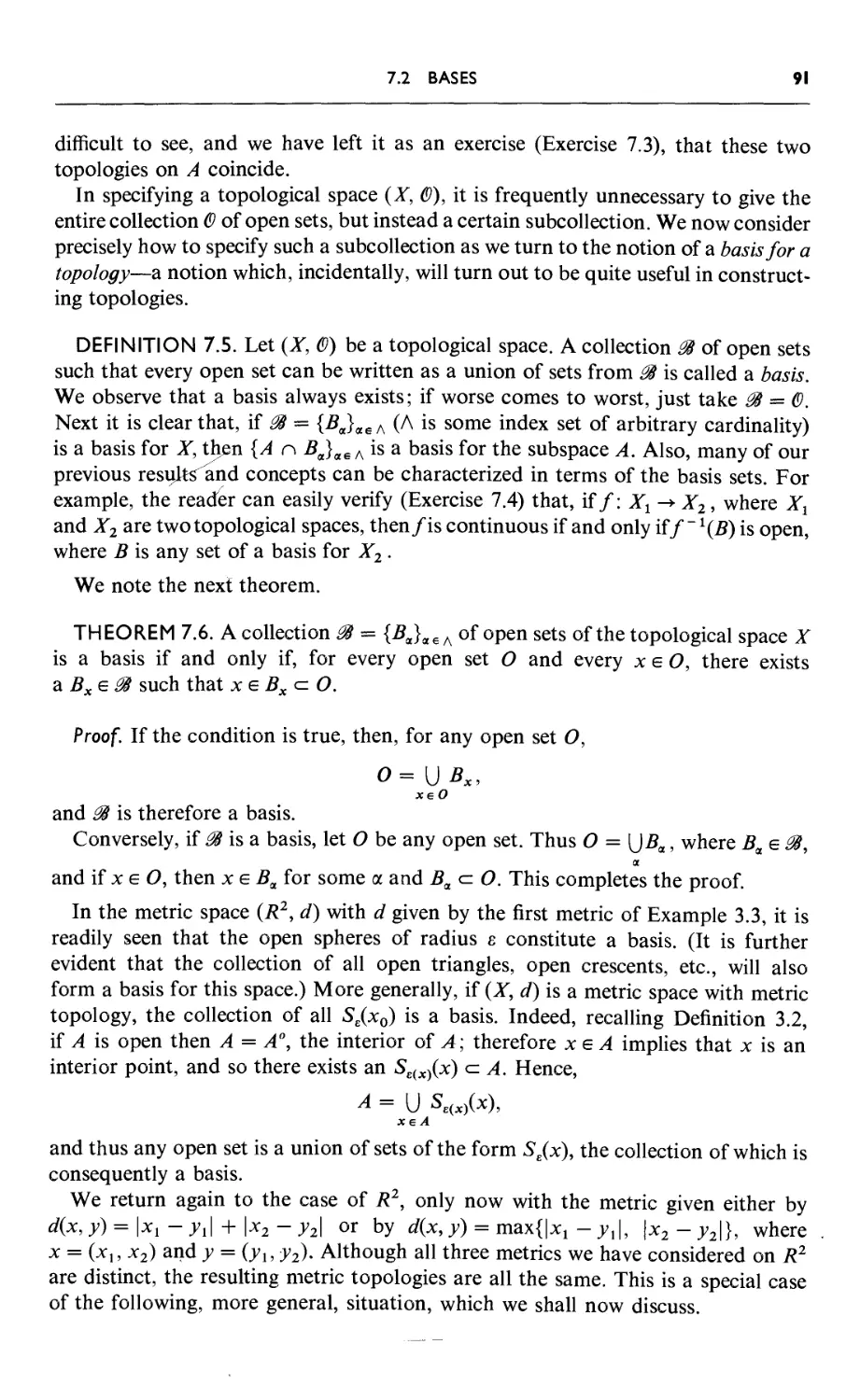
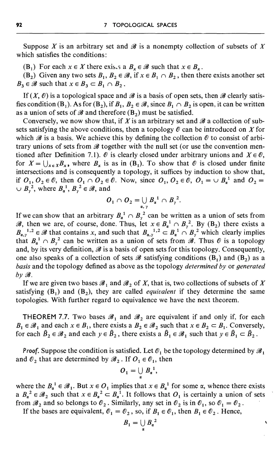
7.2 Bases 90
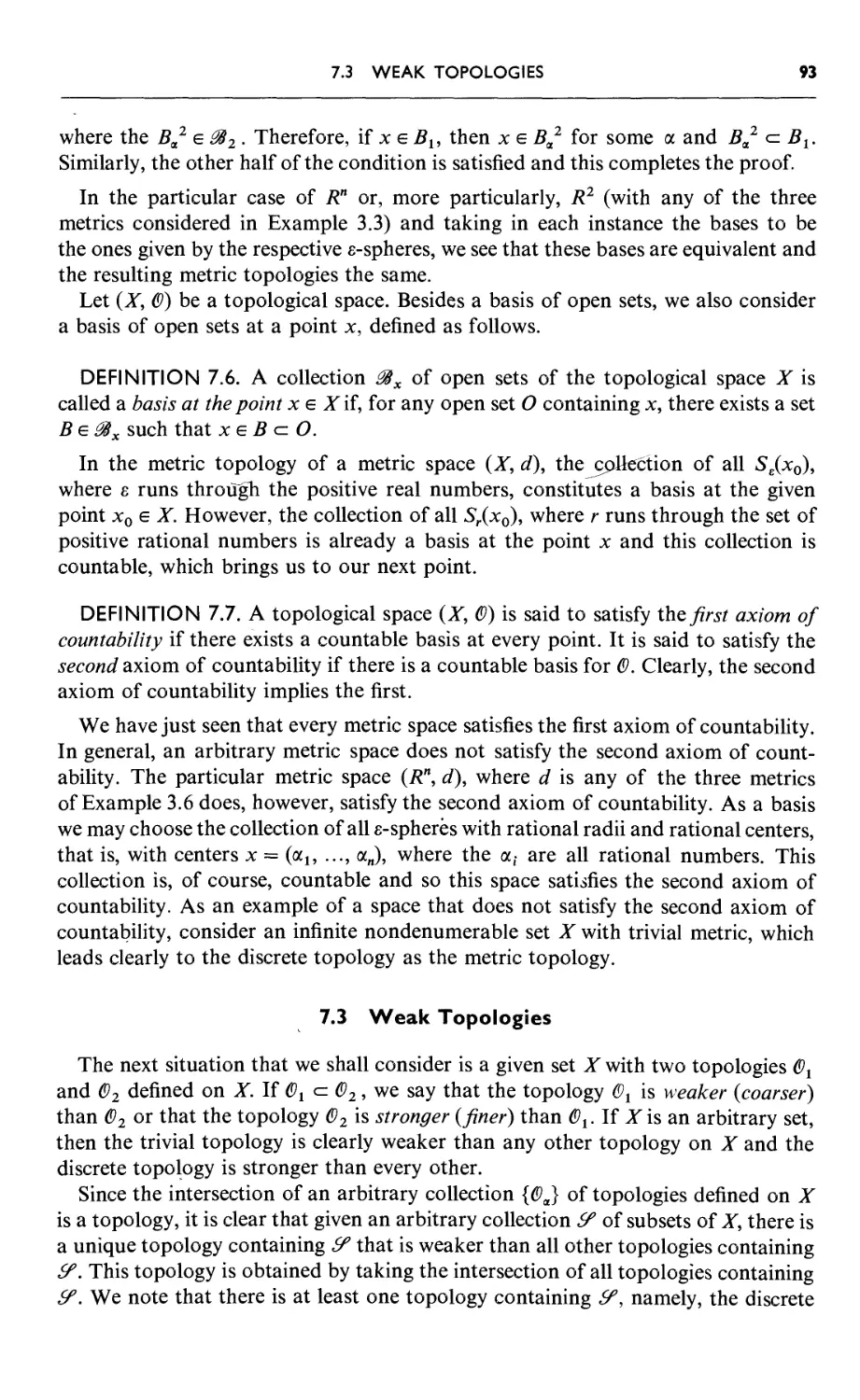
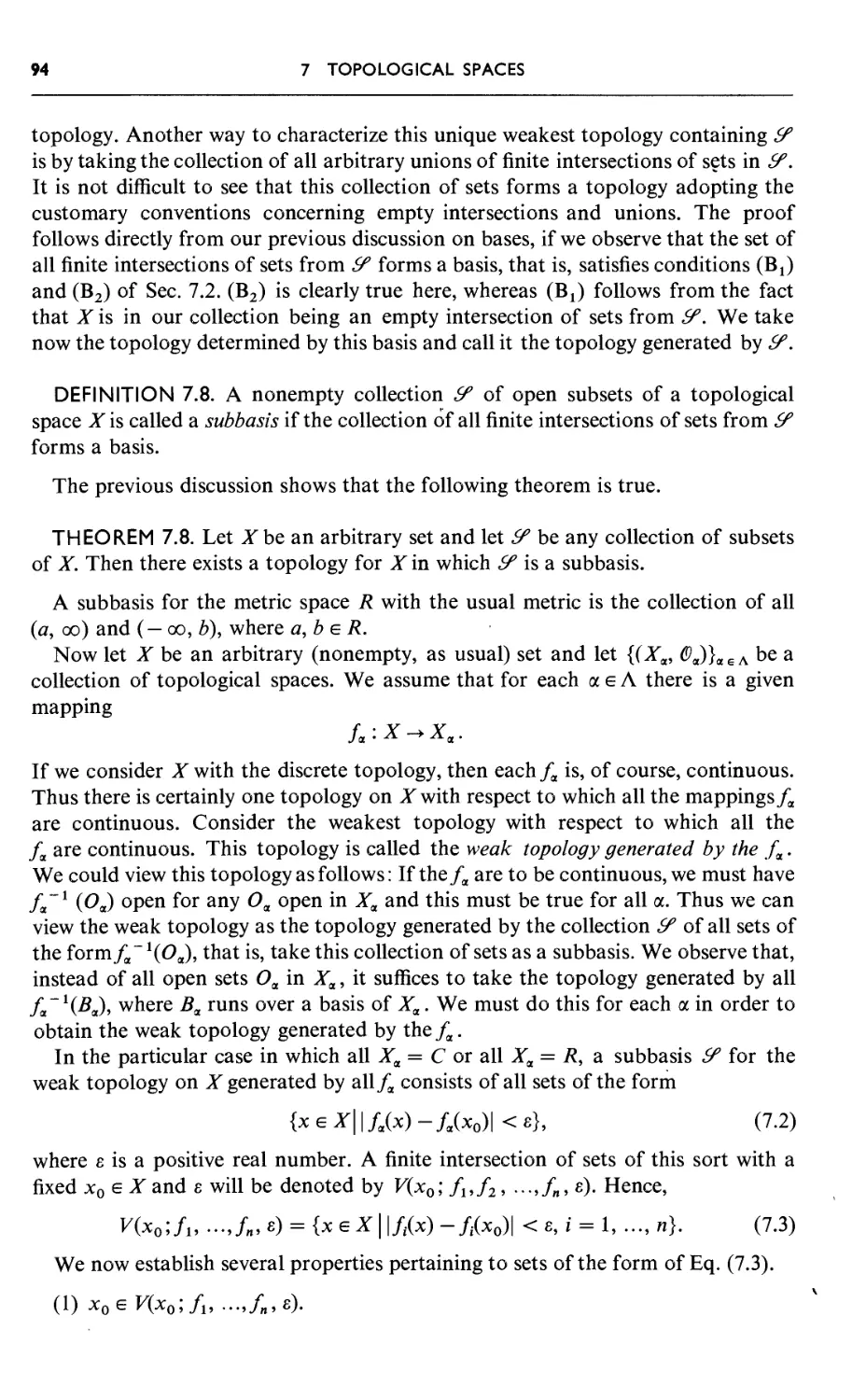
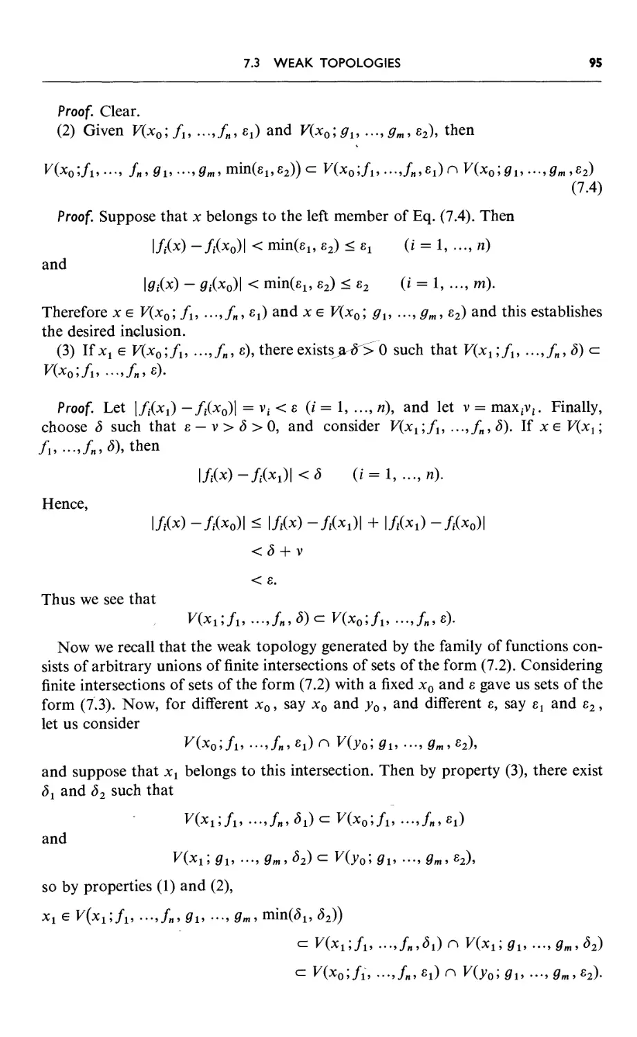
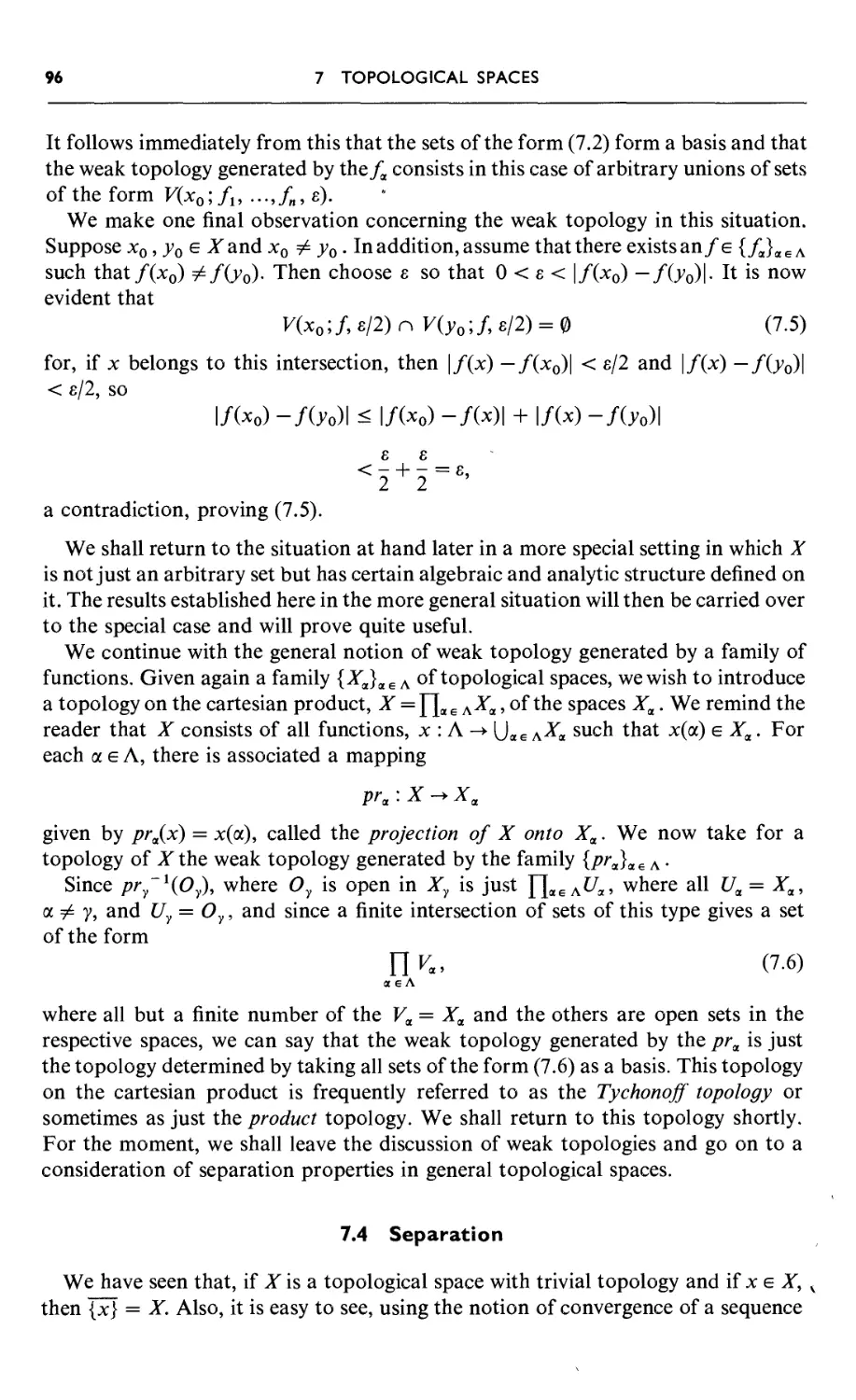
7.3 Weak Topologies 93
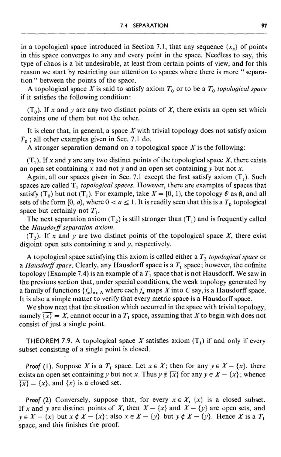
7.4 Separation 96
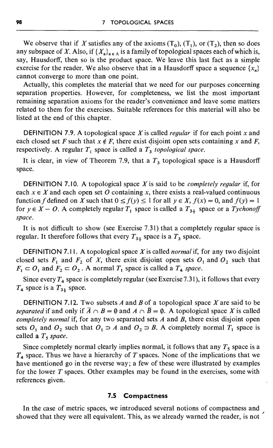
7.5 Compactness 98
Exercises 7 103
References 107
chapter 8. Banach Spaces, Equivalent Norms, and Factor Spaces 108
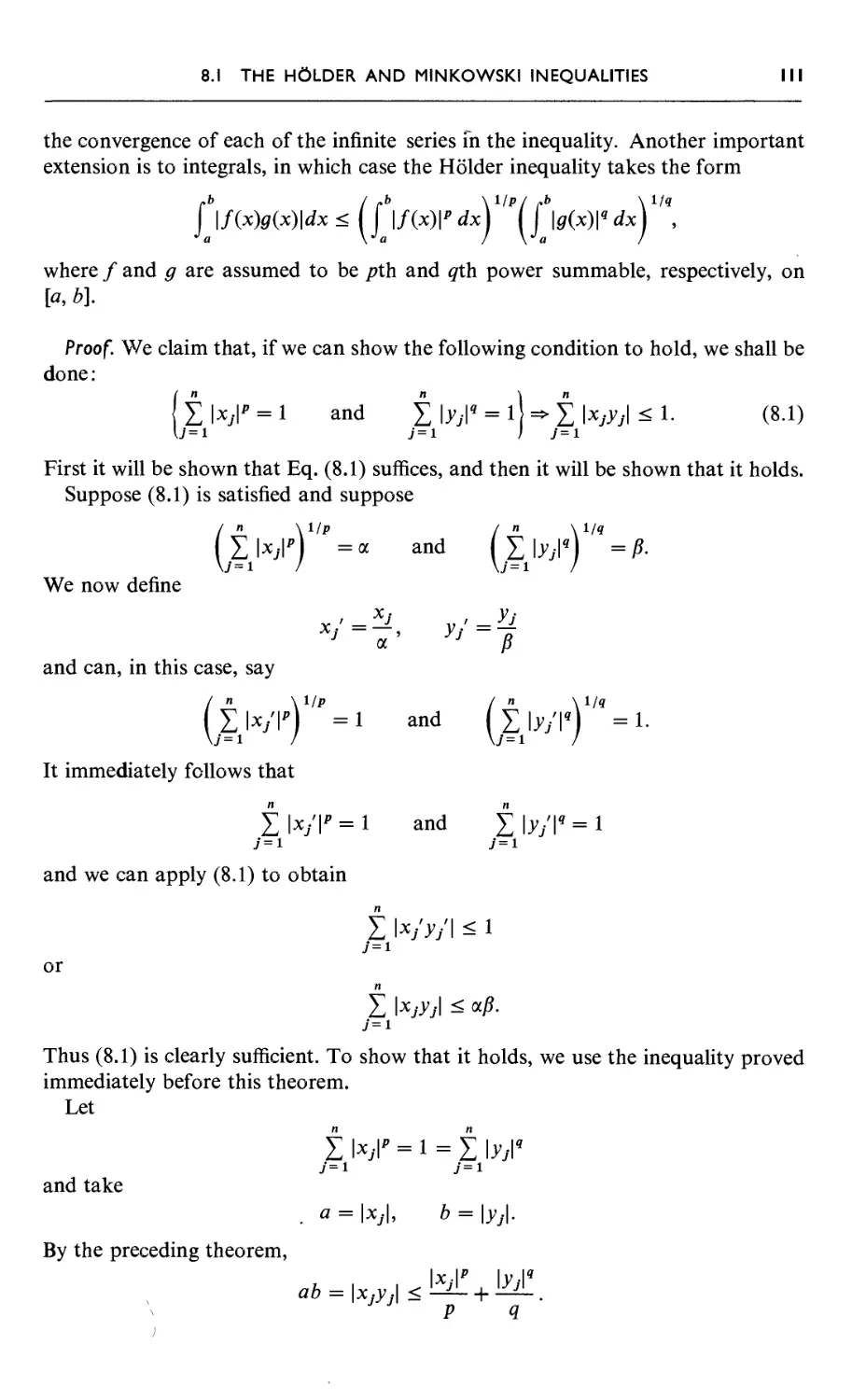
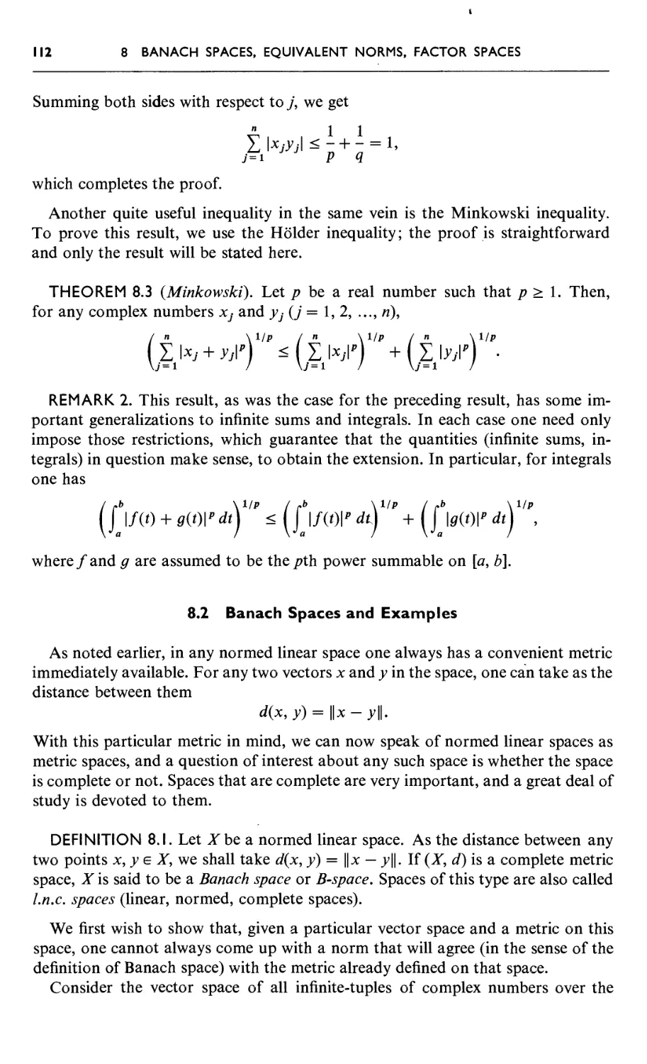
8.1 The Holder and Minkowski Inequalities 109
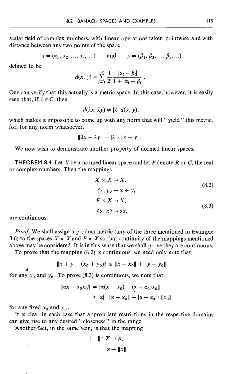
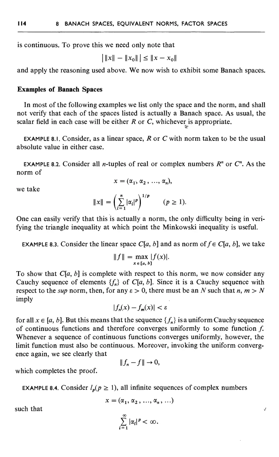
JL2 Banach Spaces and Examples . 112
8.3 The Completion of a Normed Linear Space 118
8.4 Generated Subspaces and Closed Subspaces 121
8.5 Equivalent Norms and a Theorem of Riesz 122
8.6 Factor Spaces 126
8.7 Completeness in the Factor Space 129
8.8 Convexity 131
Exercises 8 133
References 135
CONTENTS
ix
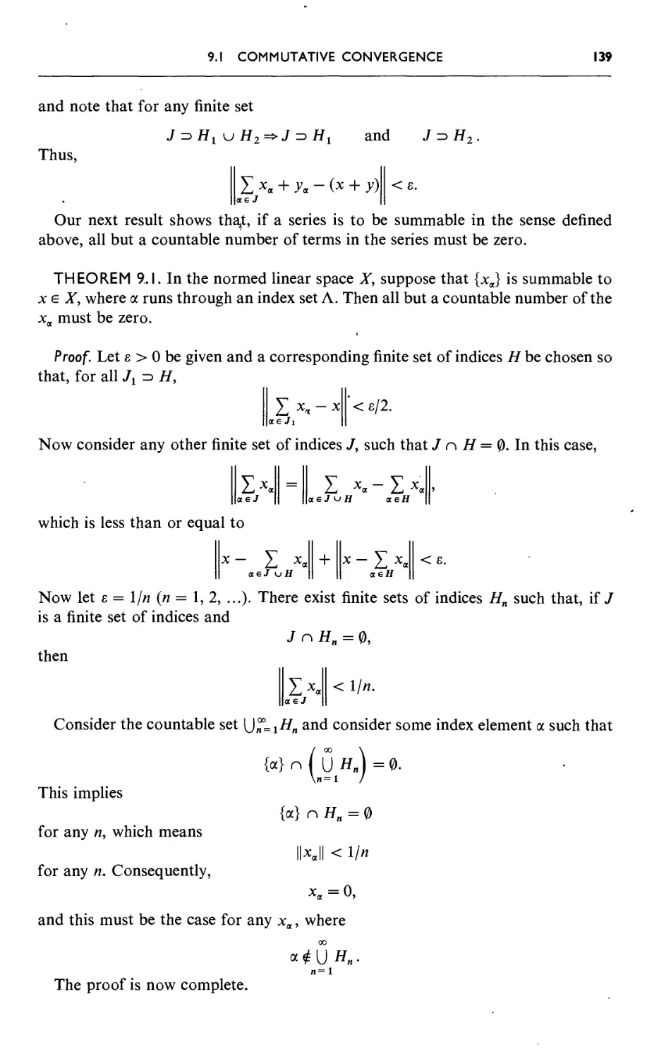
chapter 9. Commutative Convergence, Hilbert Spaces, and Bessel's
Inequality 136
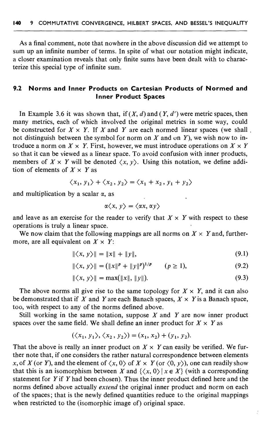
9.1 Commutative Convergence 138
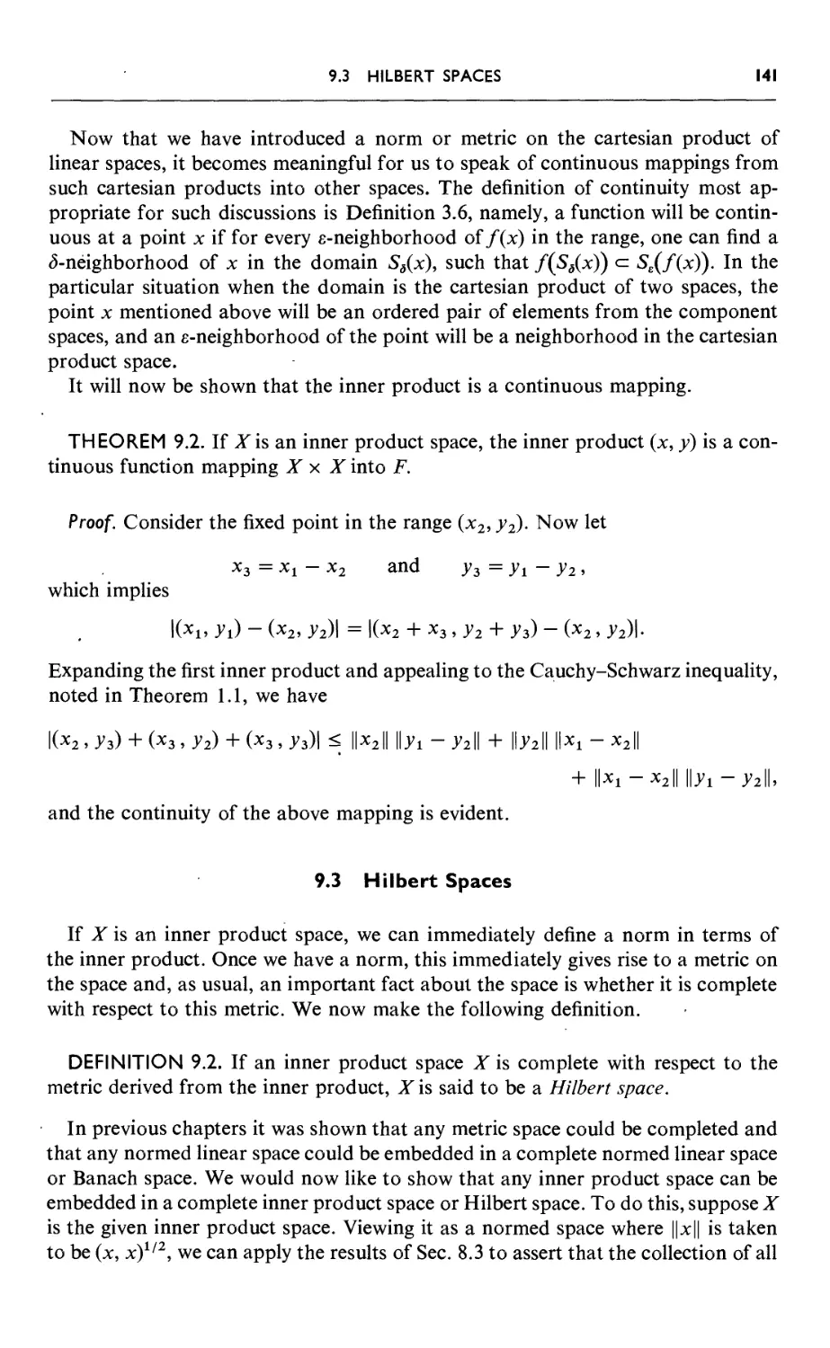
9.2 Norms and Inner Products on Cartesian Products of Normed
and Inner Product Spaces 140
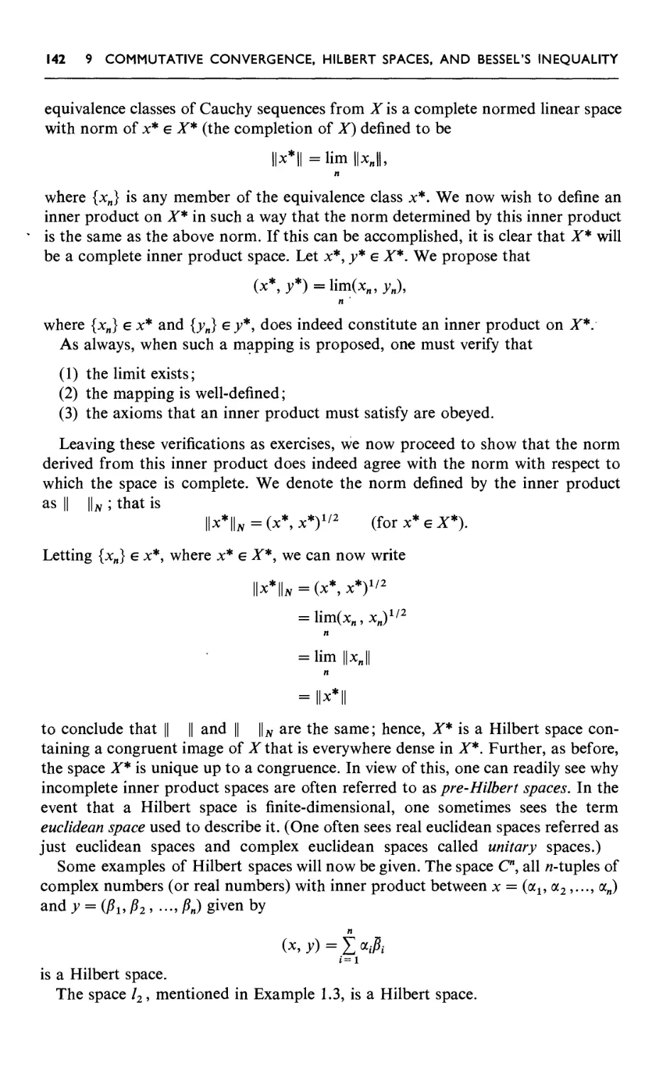
9.3 Hilbert Spaces 141
9.4 A Nonseparable Hilbert Space 143
9.5 Bessel's Inequality 144
9.6 Some Results from L2(0, 2tt) and the Riesz-Fischer Theorem 146
9.7 Complete Orthonormal Sets 149
9.8 Complete Orthonormal Sets and Parseval's Identity 153
9.9 A Complete Orthonormal Set for L2(0, 2tt) 155
Appendix 9 157
Exercises 9 160
References 161
chapter 10. Complete Orthonormal Sets 162
10.1 Complete Orthonormal Sets and Parseval's Identity 163
10.2 The Cardinality of Complete Orthonormal Sets 166
10.3 A Note on the Structure of Hilbert Spaces 167
10.4 Closed Subspaces and the Projection Theorem for Hilbert
Spaces 168
Exercises 10 172
References 174
chapter 11. The Hahn-Banach Theorem 175
11.1 The Hahn-Banach Theorem 176
11.2 Bounded Linear Functionals 182
11.3 The Conjugate Space 184
Exercises 11 187
Appendix 11. The Problem of Measure and the Hahn-Banach
Theorem 188
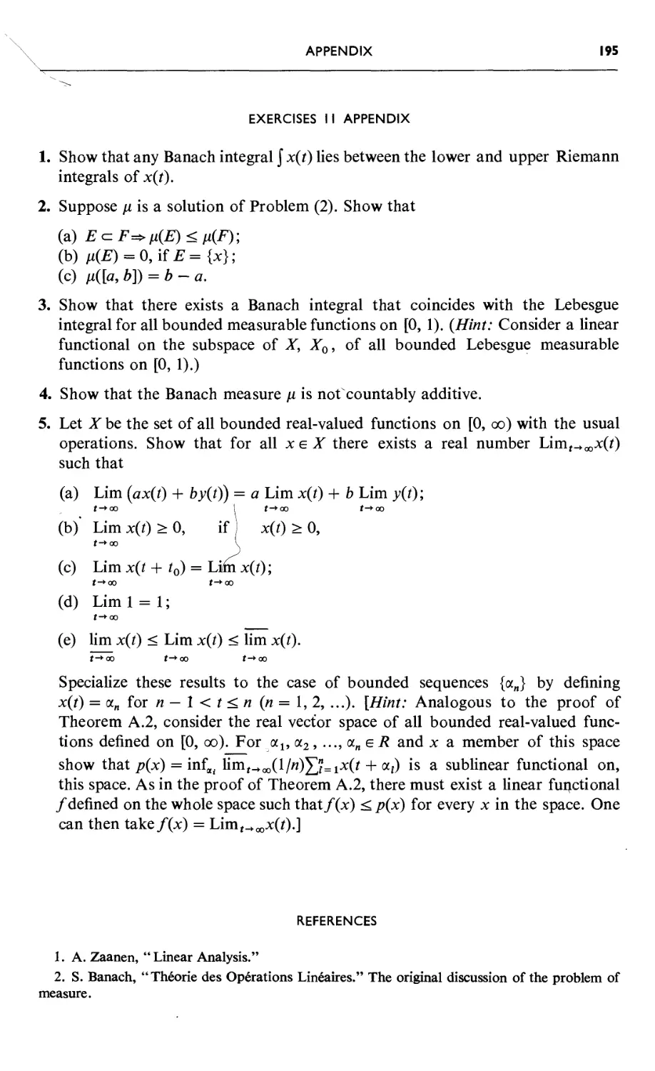
Exercises 11 Appendix 195
References 195
chapter 12. Consequences of the Hahn-Banach Theorem 196
12.1 Some Consequences of the Hahn-Banach Theorem 197
12.2 The Second Conjugate Space 203
X
CONTENTS
12.3 The Conjugate Space of lp 205
12.4 The Riesz Representation Theorem for Linear Functionals on
a Hilbert Space 209
12.5 Reflexivity of Hilbert Spaces 211
Exercises 12 214
References 215
chapter 13. The Conjugate Space of C[a, b] 216
13.1 A Representation Theorem for Bounded Linear Functionals
on C[a,b] 218
13.2 A List of Some Spaces and Their Conjugate Spaces 227
Exercises 13 , 227
References 229
chapter 14. Weak Convergence and Bounded Linear
Transformations 230
14.1 Weak Convergence 231
14.2 Bounded Linear Transformations 238
Exercises 14 243
References 244
chapter 15. Convergence in L (X, Y) and the Principle of Uniform
Boundedness 245
15.1 Convergence in L(X, Y) 246
15.2 The Principle of Uniform Boundedness 250
15.3 Some Consequences of the Principle of Uniform Boundedness 253
Exercises 15 257
References 258
chapter 16. Closed Transformations and the Closed Graph
Theorem 259
16.1 The Graph of a Mapping • 260
16.2 Closed Linear Transformations and the Bounded Inverse
Theorem 261
16.3 Some Consequences of the Bounded Inverse Theorem 271
Appendix 16. Supplement to Theorem 16.5 273
Exercises 16 274
References 275
CONTENTS
xi
chapter 17. Closures, Conjugate Transformations, and Complete
Continuity 276
17.1 The Closure of a Linear Transformation 277
17.2 A Class of Linear Transformations that Admit a Closure 279
17.3 The Conjugate Map of a Bounded Linear Transformation 281
17.4 Annihilators 283
17.5 Completely Continuous Operators; Finite-Dimensional
Operators 286
17.6 Further Properties of Completely Continuous Transformations 289
Exercises 17 294
References 295
chapter 18. Spectral Notions 296
18.1 Spectra and the Resolvent Set 297
18.2 The Spectra of Two Particular Transformations 300
18.3 Approximate Proper Values 304
Exercises 18 304
References 306
chapter 19. Introduction to Banach Algebras 307
19.1 Analytic Vector-Valued Functions 308
19.2 Normed and Banach Algebras 311
19.3 Banach Algebras with Identity 315
19.4 An Analytic Function — the Resolvent Operator 319
19.5 Spectral Radius and the Spectral Mapping Theorem for
Polynomials 322
19.6 The Gelfand Theory 327
19.7 Weak Topologies and the Gelfand Topology 336
19.8 Topological Vector Spaces and Operator Topologies 342
Exercises 19 348
References 350
chapter 20. Adjoints and Sesquilinear Functionals 351
20.1 The Adjoint Operator 352
20.2 Adjoints and Closures 355
20.3 Adjoints of Bounded Linear Transformations in Hilbert Spaces 362
xii
CONTENTS
20,4 Sesquilinear Functional 367
Exercises 20 373
References 374
chapter 21. Some Spectral Results for Normal and Completely
Continuous Operators 375
21.1 A New Expression for the Norm of A e L(X, X) 376
21.2 Normal Transformations 379
21.3 Some Spectral Results for Completely Continuous Operators 383
21.4 Numerical Range 386
Exercises 21 389
Appendix to Chapter 21. The Fredholm Alternative Theorem
and the Spectrum of a Completely Continuous Transformation 390
A.l Motivation 391
A.2 The Fredholm Alternative Theorem 393
References 405
chapter 22. Orthogonal Projections and Positive Definite
Operators 406
22.1 Properties of Orthogonal Projections 407
22.2 Products of Projections 409
22.3 Positive Operators 411
22.4 Sums and Differences of Orthogonal Projections 412
22.5 The Product of Positive Operators 415
Exercises 22 417
References 418
chapter 23. Square Roots and a Spectral Decomposition Theorem 419
23.1 Square Root of Positive Operators 420
23.2 Spectral Theorem for Bounded, Normal, Finite-Dimensional
Operators 426
Exercises 23 430
References 431
chapter 24. Spectral Theorem for Completely Continuous Normal
Operators 432
24.1 Infinite Orthogonal Direct Sums: Infinite Series of
Transformations 433
CONTENTS
xiii
24.2 Spectral Decomposition Theorem for Completely Continuous
Normal Operators 438
Exercises 24 442
References 443
chapter 25. Spectral Theorem for Bounded, Self-Adjoint
Operators 444
25.1 A Special Case — the Self-Adjoint, Completely Continuous
Operator 445
25.2 Further Properties of the Spectrum of Bounded, Self-Adjoint
Transformations 448
25.3 Spectral Theorem for Bounded, Self-Adjoint Operators 450
Exercises 25 458
References 459
chapter 26. A Second Approach to the Spectral Theorem for
Bounded, Self-Adjoint Operators 460
26.1 A Second Approach to the Spectral Theorem for Bounded,
Self-Adjoint Operators 461
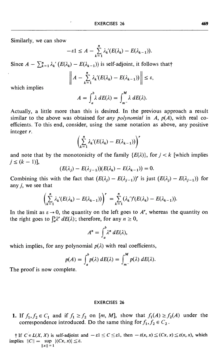
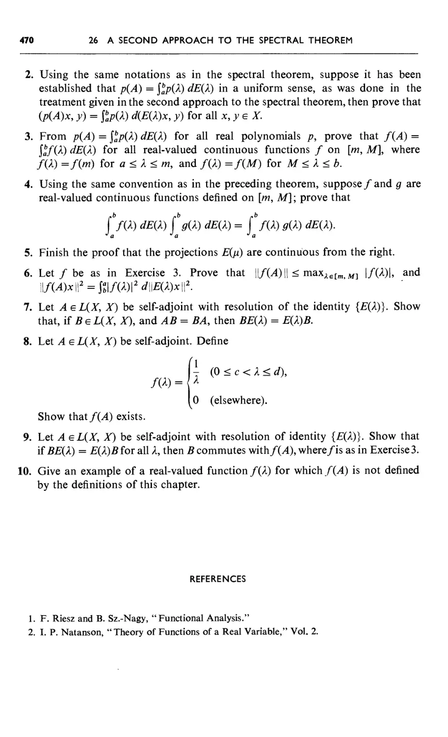
Exercises 26 469
References 470
chapter 27. A Third Approach to the Spectral Theorem for
Bounded, Self-Adjoint Operators and Some
Consequences 471
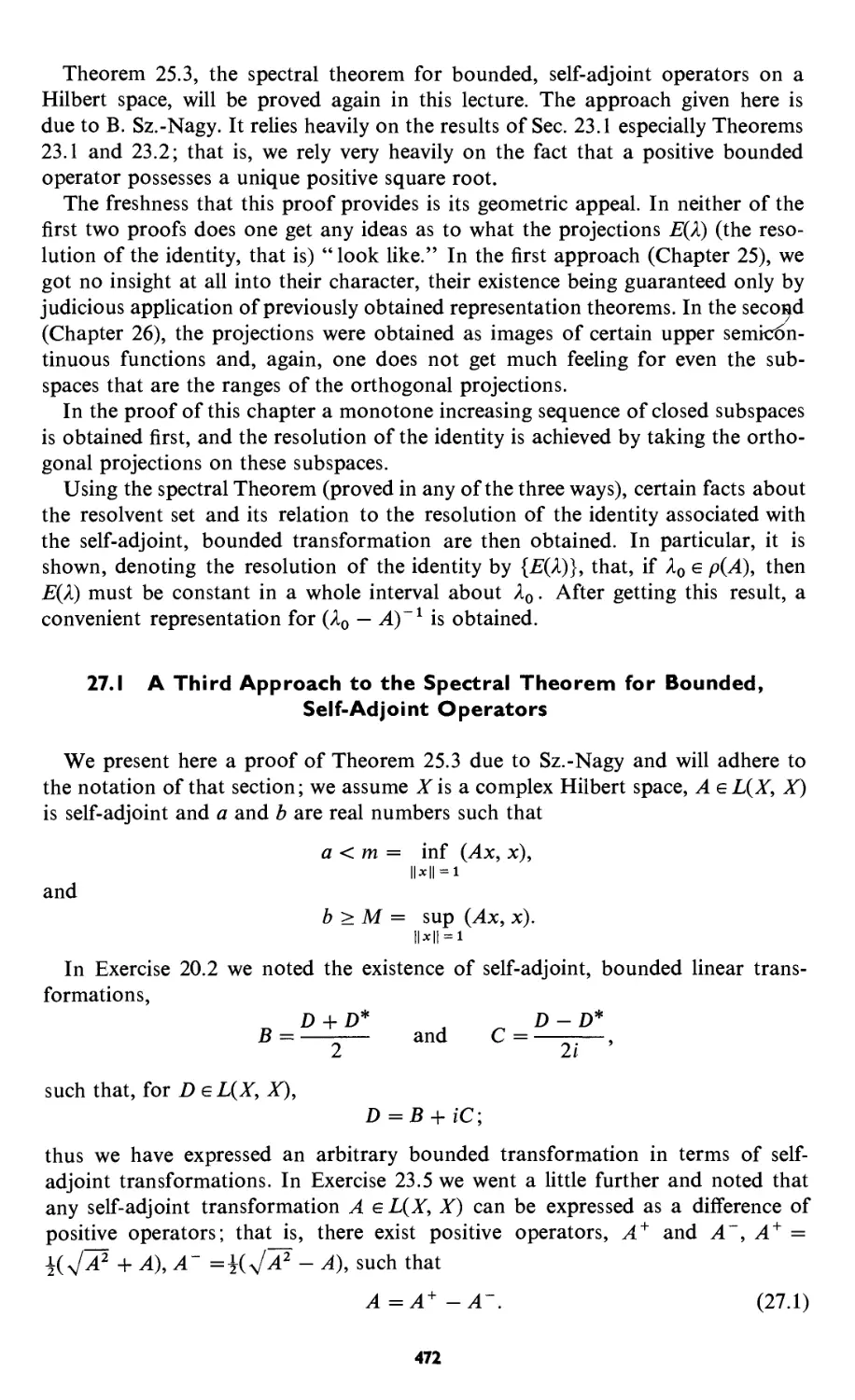
27.1 A Third Approach to the Spectral Theorem for Bounded,
Self-Adjoint Operators 472
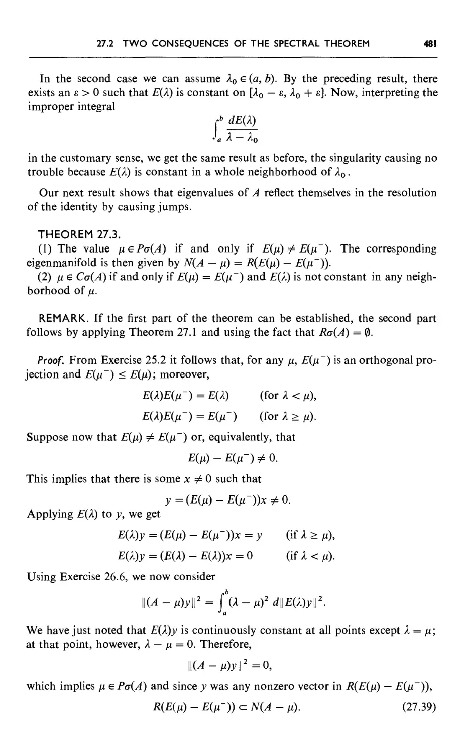
27.2 Two Consequences of the Spectral Theorem 478
Exercises 27 483
References 483
chapter 28. Spectral Theorem for Bounded, Normal Operators 484
28.1 The Spectral Theorem for Bounded, Normal Operators on
a Hilbert Space 485
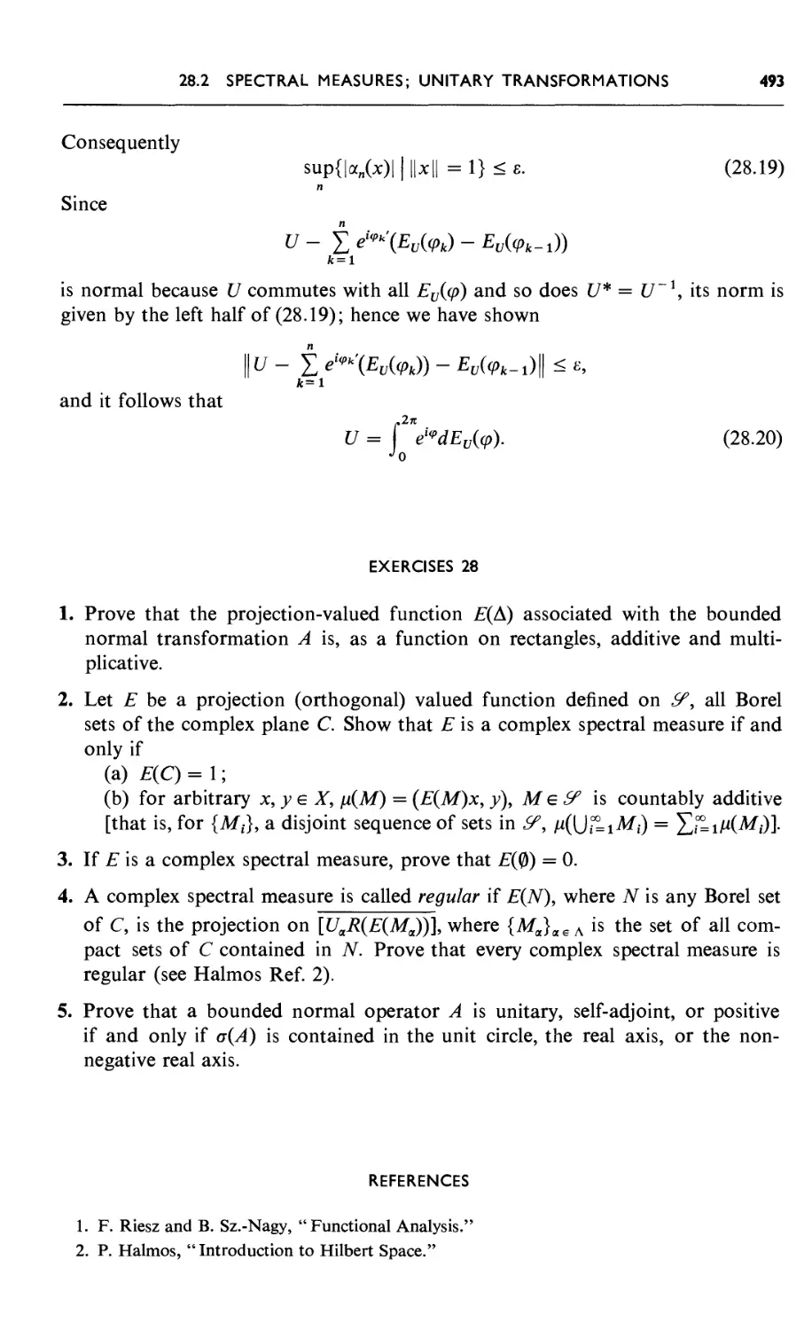
28.2 Spectral Measures; Unitary Transformations 488
Exercises 28 493
References 493
xiv
CONTENTS
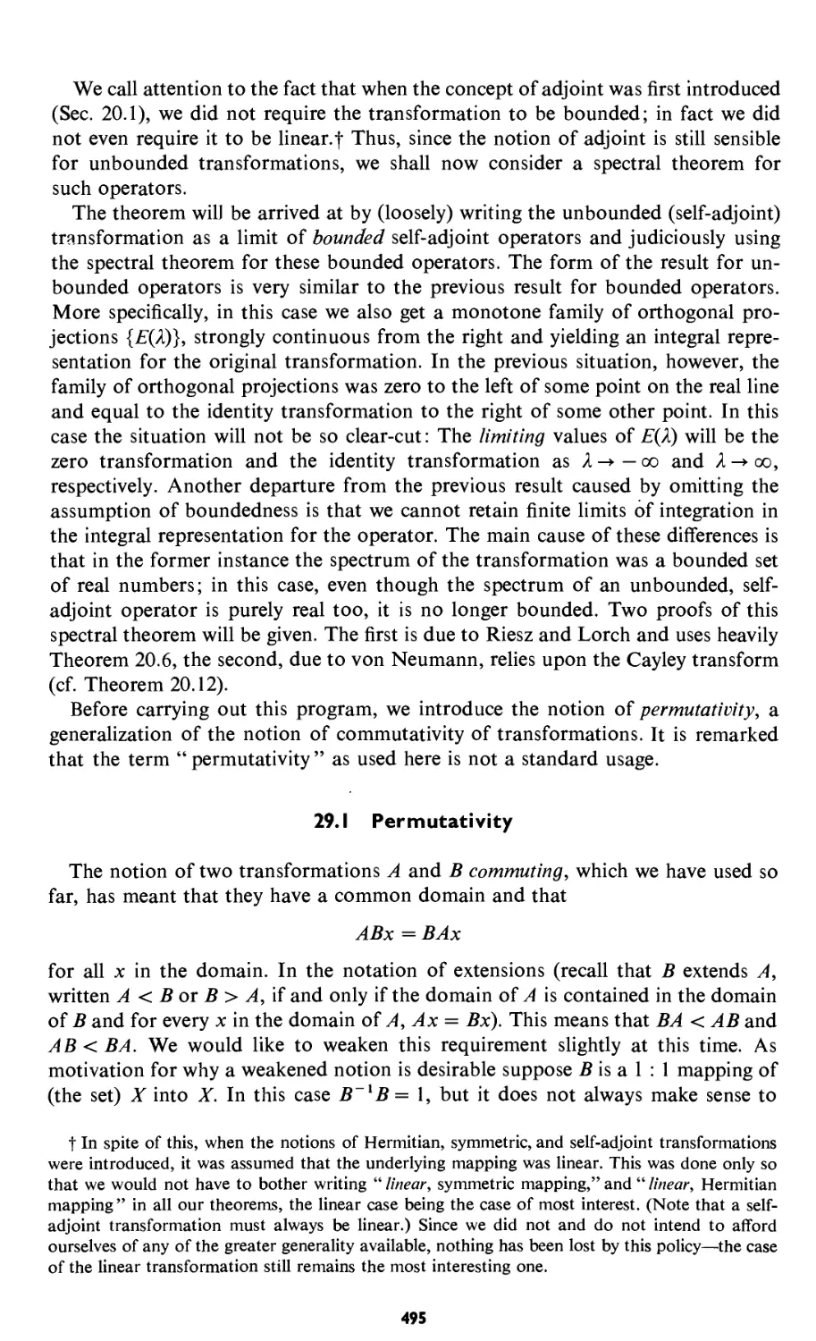
chapter 29. Spectral Theorem for Unbounded, Self-Adjoint
Operators 494
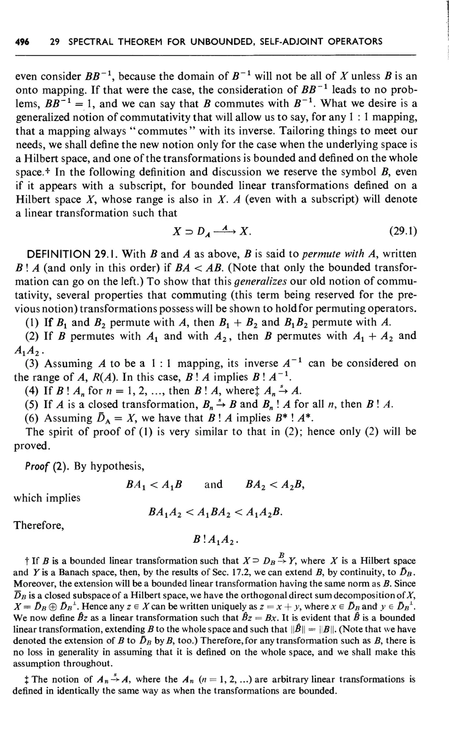
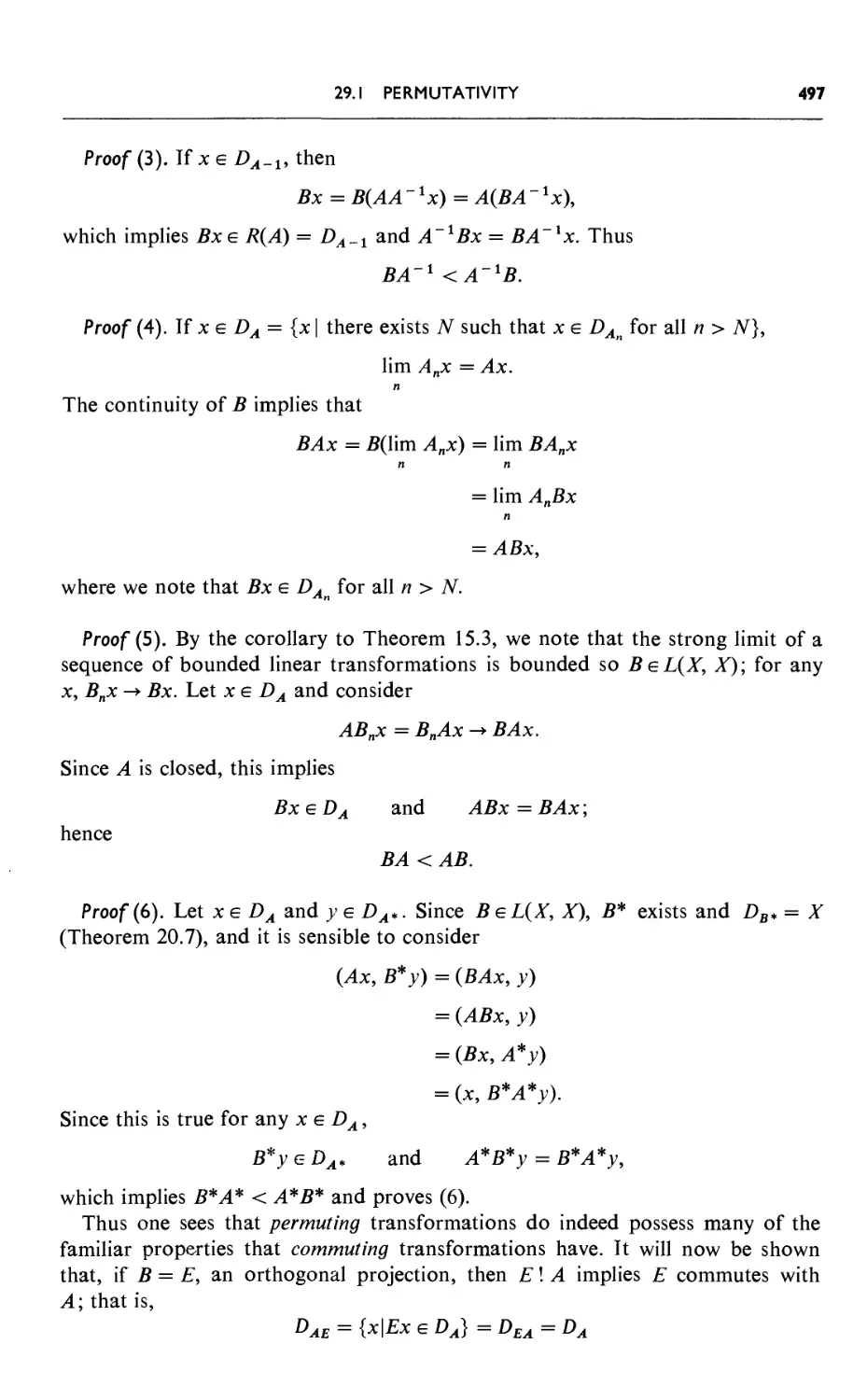
29.1 Permutativity 495
29."2 The Spectral Theorem for Unbounded, Self-Adjoint Operators 498
29.3 A Proof of the Spectral Theorem Using the Cayley Transform 516
29.4 A Note on the Spectral Theorem for Unbounded Normal
Operators 520
Exercises 29 521
References 522
Bibliography 523
Index of Symbols 525
Subject Index 527
Functional Analysis
CHAPTER I
Introduction to Inner Product Spaces
)¾¾ and terminology ^hat will be adhered to
throughout this book will be set dow*| They are listed only |b that there can be no
ambiguity when terms such as "veclbr space" or "Jmeai| transformation" are
used later, and are not intended as a brief course in linear jffgebra.
After establishing our rules, certain fe*|§ic notions pertaining to inner product
spaces will be touched upon. In particular, 6git®i»*mequalities and equalities will
be stated. Then a rather natural extension of the notion of orthogonality of vectors
from the euclidean plane is defined. Just as choosing a mutually orthogonal basis
system of vectors was advantageous in two- or three-dimensional euclidean space,
there are also certain advantages in dealing with orthogonal systems in higher
dimensional spaces. A result proved in this chapter, known as the Gram-Schmidt
process, shows that an orthogonal system of vectors can always be constructed
from any denumerable set of linearly independent vectors.
Focusing then more on the finite-dimensional situation, the notion of the adjoint
of a linear transformation is introduced and certain of its properties are
demonstrated.
I.I Some Prerequisite Material and Conventions
The most important structure in functional analysis is the vector space (linear
space)—a collection of objects, X, and a field F, called vectors and scalars,
respectively, such that, to each pair of vectors x and y, there corresponds a third vector
x + y, the sum of x and y in such a way that X constitutes an abelian group with
respect to this operation. Moreover, to each pair a and x, where a is a scalar and x
is a vector, there corresponds a vector ax, called the product of a and x, in such a
way that
a(fix) = (afi)x (a, /? scalars, x a vector), (1.1)
lx = x (x any vector, 1 the identity of F). (1.2)
For scalars a, /? and vectors x, y, we demand
(a + fi)x = ax + fix, (1.3)
cc(x + y) = ax + ay. (1.4)
We shall often describe the above situation by saying that X is a vector space
over F and shall rather strictly adhere to using lower-case italic letters (especially
x, y, z, ...) for vectors and lower-case Greek letters for scalars. The additive identity
element of the field will be denoted by 0, and we shall also denote the additive
identity element of the vector addition by 0. We feel that no confusion will arise
from this practice, however. A third connotation that the symbol 0 will carry will
be the transformation of one vector space into another and mapping every vector
of the first space into the zero vector of the second.
The multiplicative identity of the field will be denoted by 1 and so will that
transformation of a vector space into itself which maps every vector into itself.
A collection of vectors xt, x2, ..., x„ is said to be linearly independent if the
relation
a^i + a2x2 + ••• + anxn = 0 (1.5)
3
4 I INTRODUCTION TO INNER PRODUCT SPACES
implies that each oct = 0; in other words, no linear combination of linearly
independent vectors whatsoever (nontrivial, of course) can yield the zero vector. An
arbitrary collection of vectors is said to be linearly independent if every finite subset
is linearly independent.
A linearly independent set of vectors with the property that any vector can be
expressed as a linear combination of some subset is called a basis (for the vector
space) or sometimes a Hamel basis. Note that a linear combination is always a
finite sum, which means that, even though there may be an infinite number of
vectors in the basis, we shall never express a vector as an infinite sum—the fact of the
matter being that infinite sums are meaningless unless the notion of " limit of a
sequence of vectors " has somehow been introduced to the space. Thus if B is a
basis for X and if x and y are two distinct vectors, the typical situation would be the
existence of basis vectors zu z2, ■■■, zn and scalars al5 a2, ..., a„ such that
x = a^! + a2z2 H + a„z„
and basis vectors wu w2, ..., wm and scalars /?1} /?2, ..., /?,„ such that
y = £1^ + j52w2 + ••• + j5mwm.
A subset of a vector space that is also a vector space, with respect to the same
operations, is called a subspace. Given any collection U of vectors, there is always
a minimalf subspace containing them called the subspace spanned by U or the
subspace generated by U and denoted by placing square brackets about the set: [£/].
In general, if a collection of vectors, linearly independent or not, is such that any
vector in the space can be expressed as a linear combination of them, the collection
is said to span the space.
A collection of subspaces Mt, M2, ..., M„ is said to be linearly independent if,
for any i = 1,2, ..., n,
Mt n (Mi + M2 + ••• + M,_! + Mi+1 + ••• + M„) = {0},
where by Mt + M2 + ■■• + Mt_^ + M{+1 + ••• + Mn we mean all sums x1 + ■■• +
*,•_! + xi+l + ■■■ xn, where Xj e Mj. Assuming that things take place in the vector
space X if Mu M2, ..., Mn are linearly independent and
X = M1+M2 + - +Mn,
the subspaces {M,-} are said to form a direct sum decomposition for X, a situation
we shall denote by writing
X = Mi®M2®"<®Mn. (1.6)
Equation (1.6) is equivalent to requiring that every vector in X can be written
uniquely in the form xl + x2+ ••• + x„, where Xj e Mj.
One will sometimes see another adjective involved in the description of the above
situation—it is often called an internal direct sum decomposition. This is because a
new vector space V can be formed from two others X and Y (over the same field);
this new one is called the external direct sum of X and Y. What is done in this case
t By minimal we mean that any other subspace containing the vectors must also contain that
subspace.
I.I SOME PREREQUISITE MATERIAL AND CONVENTIONS 5
is to introduce vector operations to the cartesian product of X and Y, the set of all
ordered pairs <x, j>>, where x e X and y e Y. We define
ai<*i> J>i> + a2<*2' y*> = <ai*i + a2x2, a^t + a2y2>.
By identifying the vector <x, 0> in F with the vector x in X, we can indulge in a
common but logically inaccurate practice of viewing Jasa subspace of V
(similarly, Y can be viewed as a subspace of V) and throw this back into the case of the
internal direct sum. Adopting this convention then, given a direct sum
decomposition, we need not bother to enquire: Are the terms in the direct sum distinct vector
spaces or are they subspaces of the same vector space ?
Whenever the word " function," " mapping," ' or " transformation" is used,
it will be tacitly assumed that it is well-defined (single-valued); symbolically, if/is
a mapping defined on a set D (the domain of f), we require that x = y implies
/(*) =f(y)- If the converse is true, that is, if x # y implies f(x) #/00 (distinct
points have distinct images), we say that/is 1 : 1. In the case when/maps D into a
set Y (denoted by/: D^> Y) and the range off,f(D) = Y, we say that/is onto Y.
Given a mapping A which maps a vector space X into a vector space Y (over the
same field),
A : X -+ Y,
with the property that for any scalars a and /? and for any vectors x and y,
A(ax + 0y) = aA(x) + fiA(y),
A is called a linear transformation. Often when linear transformations are involved,
we shall omit the parenthesis and write Ax instead of A(x). In the special case when
Y = F, the underlying field, A is said to be a linear functional. If the linear
transformation is 1 : 1, it is called an isomorphism (of X'vnto Y). If A is 1 : 1 and onto, the
two spaces are said to be isomorphic. It can be shown that a linear transformation
is 1 : 1 if and only if Ax = 0 implies x = 0 (see, for example, Halmos [1]). Two
isomorphic spaces are completely indistinguishable as abstract vector spaces and in
some cases, isomorphic spaces are actually identified. An instance where such an
identification is convenient was mentioned in the preceding paragraph.
The collection of all linear transformations mapping X into Y can be viewed as a
vector space by defining addition of the linear transformations A and B to be that
transformation which takes x into Ax + Bx; symbolically, we have
(A + B)x= Ax + Bx.
As for scalar multiplication, let
(ccA)x = a Ax.
Having given meaning to the formation of linear combinations of linear transforma-*
tions, let us look at the special case of all linear transformations mapping a vector
space into itself. Denoting the identity transformation by 1 (that transformation
mapping x into x for all vectors x) and letting A be an arbitrary linear
transformation, we now form (A — XI), which we abbreviate simply A — X, where X is an
arbitrary scalar. As noted above, if this transformation fails to be 1 : 1, there must be
some nonzero vector x such that {A — X)x = 0. When this situation occurs, one says
6 I INTRODUCTION TO INNER PRODUCT SPACES
that x is an eigenvector of A with eigenvalue X. Equivalent terminology also used is
characteristic vector and proper vector instead of eigenvector, and characteristic
value and proper value for eigenvalue.
Still working in the linear space of all linear transformations mapping X into X,
suppose the linear transformation E has the property that E is idempotent; that is,
E2 = E, where by E2 we mean the transformation taking x into E(Ex); E2x =
E(Ex). Such a transformation is called a projection. As it happens, a projection
always determines a direct sum decomposition of X into (cf. Ref. 1):
M ={xe X\Ex = x} and N = {x e X\Ex = 0},
and one usually says that E is a projection on M along N. On the other hand, given
a direct sum decomposition of the space X = M® N, every z e X can be written
uniquely as z = x + y, where x e M and y e N. In this case the linear transformation
E, such that Ez = x, is a projection on M along N. One notes in this case that
E(M) = {Ex\xeM} = M;
that is, the subspace M is left fixed by E. This is a special case of a more general
property that certain pairs (A, L) possess, where A is a linear transformation and L
is a collection of vectors, namely, the property of L being invariant under A, which
means that A(L) <= L. We do not mean by this that every vector in L is left fixed by
A; it is just mapped into some vector in L.
Two other concepts that we shall make extensive use of are greatest lower bounds
and least upper bounds. A set U of real numbers is said to be bounded on the left
{bounded from below) if there exists some number al such that ax < x for all x e U.
Similarly, U is said to be bounded on the right (bounded from above) if there exists
some number ar such that x < ar for all x e U. The numbers ax and ar have the
properties that ax can be replaced by anything smaller, whereas ar can be replaced
by anything larger, and we shall still obtain lower and upper bounds, respectively,
for U. A fundamental property of the real numbers, however, is that among all the
lower bounds, there is a greatest one in the sense that at least one point of U lies
to the left of any number greater than the greatest lower bound. Symbolically, if we
denote the greatest lower bound by X and if we consider a number only slightly
larger than X, say X + s where s > 0, there must be some x e U such that x < X + e.
The number X that may or may not belong to U is called the infimum of U and
we denote the relationship of X to U by writing
X = inf U.
Similarly, of all the upper bounds there is a smallest, a number /i, such that a
member of U lies to the right of any smaller number; for any s > 0, there exists
x £ U such that x > pi — &. The number /i is called the least upper bound of U or
supremum of U and is denoted by
H = sup U:
Aside from this material pertaining to functions, there are many other notions
from set theory that are absolutely indispensable to the study of functional analysis.
We feel it is unnecessary to discuss any of the notions from set theory and consider
1.2 INNER PRODUCT SPACES
7
it sufficient to list the pertinent notation we shall use in the List of Symbols. No
doubt the reader has come in contact with them (for example, unions,
intersections, membership) before. We make one exception to this rule with regard to the
concept of an equivalence relation. Letting X be an arbitrary collection of elements,
we suppose that ~ is a relation between elements of X with the following three
properties. For any x, y, z e X,
(1) x ~ x (reflexive);
(2) x ~ y implies y ~ x (symmetric);
(3) x ~ y and y ~ z imply x ~ z (transitive).
In this case the relation is called an equivalence relation. As a mnemonic device
for recalling the three defining properties of an equivalence relation, one sometimes
sees it referred to as an RST relation. Examples of equivalence relations are equality
of real numbers, equality of sets (subsets of a given set, say), congruence among the
class of all triangles, and congruence of integers modulo a fixed integer. An
equivalence relation has a very important effect on the set: It partitions it into disjoint
equivalence classes of the form y = {z e X\ z ~ y}. (For a proof and further
discussion one might look at Ref. 3, pp. 11-13.)
I
1.2 Inner Product Spaces
Suppose X is a real or complex vector space; that is, suppose the underlying
scalar field is either the real or complex numbers R or C. We now make the
following definition.
DEFINITION I. I. An inner product on Zis a mapping from X x X, the cartesian
product space, into the scalar field, which we shall denote generically by F:
X x X -»• F,
<x, y} -*■ (x, y)
[that is, (x, y) denotes the inner product of the two vectors, whereas <x, y)
represents only the ordered pair inlxl] with the following properties:
(Ix) let x, y £ X; then (x, y) = (y, x), where the bar denotes complex conjugation;
(12) if a and /? are scalars and x, y, and z are vectors, then (ax + Py, z) =
a(x, z) + fi(yt z);
(13) (x, x) > 0 for all x e X and equal to zero if and only if x is the zero vector. It
is noted that by property (Ix) that (x, x) must always be real, so this requirement
always makes sense.
A real or complex vector space with an inner product defined on it will be called
an inner product space; one often sees this abbreviated as i.p.s. Inner product spaces
are also called pre-Hilbert spaces.
Some immediate consequences of the definition will now be noted, the first of
which is that if a vector y has the property that (x, y) = 0 for all x e X, then y
8 I INTRODUCTION TO INNER PRODUCT SPACES
must be the zero vector. To prove this, noting that this is true for every vector
in the space, take x equal to y and apply part (I3) of the definition.
If x, y, and z are vectors and a and /? are scalars, then
(z, ax + py) = a(z, x) + /?(z, y).
The mapping of X into F via (x, x)1/2 is a norm on X and will be denoted by
|| _xr|| _ The notion of a norm will be thoroughly elaborated upon later and, for the
sake of the present discussion, it suffices to regard ||x|| as merely a convenient
shorthand representation for (x, x)1/2.
Examples of Inner Product Spaces
In the following examples, the scalar field can be taken to be either the real
numbers or the complex numbers. The verification that the examples have the
properties claimed is left as an exercise for the reader.
EXAMPLE I.I. Let X= C"; that is all «-tuples of complex numbers. As the inner
product of the two vectors
x = (al5a2, ..., a„)
and
y = (^,^,...,^),
where the at and /?,• are complex .numbers, we shall take
n
(x, .y) = £ *$i •
i=l
C" with this inner product is referred to as complex euclidean n-space. With R in
place of C one speaks of real euclidean n-space.
, EXAMPLE 1.2. Let X= C[a, b] be complex-valued continuous functions on the
closed interval [a, b] with addition and scalar multiplication of such functions
defined as follows: For continuous functions f and g, (f + g)(x) = f(x) + g(x); for
a £ C and f continuous, (ocf)(x) = <xf(x). As the inner product of any two vectors
f(x) and g(x) in this space, we shall take
rb
(/, 9) = J f(x)g(x) dx.
a
We shall sometimes use the same notation to denote the real space of real-valued
continuous functions on [a, b]. We shall always specifically indicate which one is
meant however.
EXAMPLE 1.3. Let X = /2: all sequences of complex numbers (alf ..., an, ...) with
the property that
I k-l2 < oo. (1.7)
; = i
1.2 INNER PRODUCT SPACES 9
As the inner product of the vectors
x = (al5 ...)
and
we shall take
1 = 1
which converges by property (1.7) and the Holder inequality for infinite series (cf.
Theorem 8.2).
The following example is presented for those familiar with some measure theory.
Since it is not essential to the later development, the reader should not be disturbed
if he does not have this background.
EXAMPLE 1.4. Let 7 be a set and let S be a collection of subsets of 7 with the
following properties:
(1) ifE, FeS, then E-FeS;
(2) if Ei £ 5 (/ = i, 2, ...), then \)«LXEX e S;
(3) YeS.
In other words, we assume that S is a cr-algebra of subsets of 7 Let pi be a measure
on S and let E be some particular set in S. Analogous to the case of C[a, b]
(Example 1.2), one can introduce vector operations on the class of all functions
(complex-valued) which are measurable on E by defining
(f+ 9)(x) = f(x) + g(x) and (a/)(x) = a/(x).
Among the members of this collection, the relation "f~g if and only if f=g
almost everywhere on E (on all but a subset of E with measure zero)" is easily
demonstrated to be an equivalence relation (Sec. 1.1). As such, it partitions the set
into disjoint equivalence classes, where a typical class is given by
f = {g, measurable on £ | g ~/},
and any g e/would be called a representative of this class.
The vector operations can now be carried over to the classes by defining
■ f+§=f + 9 and a/=(a/).
It can easily be verified that these operations are well-defined—namely, that if h ~f
and k ~ g; then h + k =f+ g, and similarly for scalar multiplication.
Let us now restrict our attention to only those classes whbse representatives are
square-summable on E—those / such that,
f \f\2dpi< oo.
10
1 INTRODUCTION TO INNER PRODUCT SPACES
It is now easily demonstrated that
(J,g) = f fg d/n
JE
is an inner product on this space. The reason we went to the bother of dealing with
equivalence classes and not the functions themselves is so that (z, z) = 0 only when
z is the zero vector would not be violated. For if; a measurable function/is equal to
0 almost everywhere on E, then \E\f\2 dfi = 0. (Note that the zero vector of the set
of all square-summable functions on E is the function that is 0 everywhere on E.)
Since the only nonnegative measurable functions on E satisfying the above equality
are those that equal 0 almost everywhere on E, we see that this problem is
circumvented when one deals with classes.
In the following we shall omit the formality of writing /to represent the class td~
which/belongs and shall write only/, it being understood that we are dealing with
equivalence classes. This space of equivalence classes is denoted by L2(E, /i).
Sometimes we shall wish to deal with only real-valued functions and to view the
collection as a real vector space. When this is done, the space will still be referred
to as L2(E, /i), but we shall specifically indicate how we are viewing things.
As a special case of the above result, the following example is presented.
example 1.5. Let the set Y be the closed interval [a, b], let S be the Lebesgue
measurable sets in Y and let /i be Lebesgue measure. Then, for the equivalence
classes of square-integrable functions (complex-valued) on [a, b] we can take, as
inner product between two classes/and g,
cb
(/ 9) = ] f(x)g(x) dx,
a
where the integral is just the Lebesgue integral. This space is usually referred to as
L2{a, b).
The proof of the following, very important result can be found in the references
to this lecture and will only be stated here.
THEOREM I.I (Cauchy-Schwarz inequality). Let X be an inner product space
and let x, y e X. Then
|(x, y)\ < \\x\\ \\y\\
with equality holding if and only if x and y are linearly dependent.
The following three results represent straightforward, although somewhat
arduous, tasks to prove and will also only be stated.
THEOREM 1.2 {Polarization identity). Let Xbe a real inner product space and
let x, y £ X. Then
(x, y) = i\\x + y\\2 - i\\x - y\\2.
THEOREM 1.3 (Polarization identity). Let Jbea complex inner product space
and let x, y e X. Then
(x, y) = -\\x + y\\2 — -\\x — y\\2 + - \\x + iy\\2 — - ||x — iy\\2.
1.2 INNER PRODUCT SPACES
II
It should be noted from the above two results that if we know the norm in an
inner product space, the inner product can be recovered.
THEOREM 1.4 {Parallelogram law). Let X be an inner product space, and let
x, y £ X. Then
II* + y\\2 + \\x - y\\2 = 2\\x\\2 + 2\\y\\2.
This theorem derives its name from the analogous statement one has in plane
geometry about the opposite sides of a parallelogram.
Orthogonality and Orthogonal Sets of Vectors
If x and y represent two vectors from real euclidean 3-space, it is well known
that the angle between these two lines in space has its cosine given by
/X _ aifti + a2jg2 + ct3fi3 (x,y)
COS\ i, _ /% 2 , „ 2 , „ 2\l/2/o 2,02,0 2\l/2 n vm m ,,m '
v {al + a2 +a3)'{p1 + p2 + Pz ) 11*11 II .Hi
where x = (al5 a2, a3), y = (fiuPi-> &$)•> andtne ai and Pi are real numbers. Further,
the two vectors will be perpendicular if and only if (x, y) = 0. (x and y are, of course,
each assumed to be not the zero vector.) As a very natural generalization of this
familiar resttlt from the real vector space R3, we now wish to state a definition.
DEFINITION 1.2. Let X be an inner product space and let x, y e X. Then x is
said to be orthogonal to y, written x _L y, if (x, y) = 0. The next result follows
immediately from just expanding the quantities involved and using the hypothesis.
THEOREM 1.5 (Pythagorean theorem). If x _1_ y, then
II* + ^112 = M12 + IM12-
DEFINITION 1.3. Let Xbe an inner product space, let S be a subset of X, and
suppose, for.any two distinct vectors x and y in S, that (x, y) = 0. Then S is said to
be an orthogonal set of vectors. Suppose now that S is an orthogonal set of vectors
with the added property that, for all x e S, \\x\\ = 1. In this case S is said to be an
orthonormal set of vectors.
Some examples of orthonormal sets of vectors will now be given.
EXAMPLE 1.6. Let the vector space be /2 and consider the set of vectors from this
space
(1, 0, 0, ..., 0, ...), (0, 1, 0, ..., 0, ...), (0, 0, 1, ..., 0, ...), ...
This collection or any subset of this collection, according to the inner product
defined in Example 1.3, forms an orthonormal set in /2 .
12
I INTRODUCTION TO INNER PRODUCT SPACES
EXAMPLE 1.7. Consider the inner product space L2( — n, n) as defined in Example
1.5. The collection (or any subset thereof)
xn = -^=eint («=0, ±1, ...)
2;r
constitutes an orthonormal set of vectors in this space.
EXAMPLE 1.8. If we restrict our attention to only real-valued functions that are
square-integrable on the closed interval [ — n, n], then the collection (or any subset
thereof)
1 1 1
—1=- cos t, —j= cos It, ...
1 1
—=. sin t, —= sin It, ...
is an orthonormal set in this space.
We now wish to proceed to the intuitively plausible (from our geometric
experience in R3, real euclidean 3-space) result that a collection of mutually
orthogonal vectors is linearly independent.
THEOREM 1.6. Let Xbe an inner product space and let S be an orthogonal set
of nonzero vectors. Then S is a linearly independent set.
Proof. Before passing to the proof, the reader is asked to recall that an
arbitrary set of vectors is called linearly independent if and only if every finite subset
is linearly independent. In light of this, choose any finite collection of vectors,
xlf x2, ..., xn from S and suppose that
a^i + <x2x2 + •■■ + a„x„ = 0, (1.8)
where the a,- are scalars. Equation (1.8) now assures us that
(a^i + ••• + ocnxn, x{) = 0 (for any i = 1, 2, ..., n).
But, since S is an orthogonal set, the inner product on the left is just a,-(x,-, xf).
Hence, since S is a set of nonzero vectors, we can conclude that a; = 0, and this is
true for any i = 1, 2, ..., n. Thus the collection is linearly independent.
Knowing that there exists a basis for any finite-dimensional vector space, the
following result assures that among other things, in such a space, there is an
orthonormal basis.
THEOREM 1.7 {Gram-Schmidt process). Let X be an inner product space and
let {yu ..., yn, ...} be a linearly independent set of vectors. Then there exists an
orthonormal set of vectors {xl5 ..., xn, ...} such that, for any n,
*'
1.2 INNER PRODUCT SPACES 13
where the square brackets indicate the space spanned by the set of vectors enclosed;
for example, if x, y e X, then [{x, y}] = {ax + fly | a, /? e F}.
Proof. The proof will be by induction. First we verify that the theorem is true in
the case when n = 1. Since yt ^ 0, it makes sense to consider xt = j>i/||j>il|, which,
clearly, has norm 1. Further, the spaces that xt and yt span must be identical,
because the two vectors are linearly dependent. Now that this is done, assume
orthonormal vectors {xl,x2, ..., x„_ J have been constructed such that
[{*!, x2, ..., xj] = [{ylty2, —,.>>»}]
for any t between 1 and (n — 1) inclusive. Our job now is to construct the «th vector
with the same properties. To this end, consider the vector
»i-i
w = y„ - £ (y„, xdxi,
i=l
and take, for 1 <j < n — 1,
»i-i
(w, xj) = (yn, xj) - £ (y„, xt) (xt, Xj)
i=l
= (Jn » XJ) ~ (yn , Xj) = 0.
Hence w 1 xt for i = 1, 2, ...,«— 1. Suppose it were possible for w to be zero.
This would imply that
»i-i
i=l
or, in words, that yn could be written as a linear combination of xu x2, ..., xn_u
which, by the induction hypothesis, would imply that yn could be written as a linear
combination of yu y2, ...,y„-x, which is contrary to our assumption that the
{^i» yi > •••> ^n > •••} was a linearly independent set. Thus w cannot be zero. It now
remains only to choose xn = w/||w||, with the fact that the spaces spanned by
{xux2, ..., xn} and {y1,y2, ..-,^} are the same being left as a simple exercise
for the reader.
As applications of the above theorem the following examples are presented.
EXAMPLE 1.9. Consider the inner product space L2(a, b) mentioned in Example 1.5
and take the linearly independent set to be {1, t, t2, ..., t", ...}. (It is easily verified
that this is a linearly independent set by noting that any polynomial of degree n has
at most n zeros.) Applying the Gram-Schmidt process would then lead us to the
following orthonormal set in this space, where ak is a scalar:
xk = ak ^ (t - a)\t - bf (k = 0, 1, 2, ...). (1.9)
In particular if a = — 1 and b = \, then ak would be 1/2*/:! and the functions (1.9)
would be the Legendre polynomials.
In the next example, although the interval is changed, we shall consider
essentially the same linearly independent set but multiplied by the weighting factor
e~t2/2.
14
I INTRODUCTION TO INNER PRODUCT SPACES
EXAMPLE 1.10. Consider L2(— oo, oo) and take the linearly independent set of
vectors to be
e-t2'2,te-t2'2,...,fe-t2'2, ....
Applying the Gram-Schmidt process in this case we would obtain, as the
corresponding orthonormal set
akHk(t)e-t2'2 (k = 0, 1,2, ...),
where ak is a scalar and the Hk(t) are the Hermite polynomials.
DEFINITION 1.4. Let Xbe an inner product space and let S be a subset of X. The
collection of vectors
SL = {y £ X\y _L x for all xeS}
is called the orthogonal complement of S. It is to be noted that, even though S is only
a subset, S1 is a subspace of X.
Our next theorem yields an important result about the orthogonal complement
of a subspace that is finite-dimensional.
THEOREM 1.8. Let X be an inner product space and let M be a subspace of X
such that dim M < oo. Then we have the direct sum decomposition X = M © ML.
[The notation M ®N = X means that any vector z e X can be written uniquely as
z = x + y, where x e M and y eN, or, equivalently, that every z e Zcan be written
as z = x + y, where x eM and y eN and M n N = {0}.]
Proof. First it will be shown that any vector in the space can be written as the sum
of an element from M and an element from ML.
Since dim M < oo, we can choose an orthonormal basis for M : xt, x2, ..., xn.
Now it is clear that
tCz.x^eM (1.10)
for any vector z e X, because expression (1.10) is just a linear combination of the
basis vectors in M. Now consider the vector
n
Letting Xj be any one of the basis vectors in M, we have
(y, Xj) = (z, Xj) - (z, xj) = 0 (j = 1, 2, ..., n)
or that y is orthogonal to each of the basis vectors in M. Hence it is orthogonal to
every vector in M, which implies that;; e M1. Therefore, we have the representation,
for any vector z e X,
n
z=J^(z, xt)xt + y,
i=l
where the first term on the right is in M and the second is in ML, and have completed
the first part of the proof.
1.3 LINEAR FUNCTIONALS, THE RIESZ REPRESENTATION THEOREM IS
To prove the second part, suppose that x e M n ML. This immediately implies
that (x, x) = 0, which implies that x = 0 and completes the proof.
1.3 Linear Functionals, the Riesz Representation Theorem,
and Adjoints
Suppose X is an inner product space and that y is some fixed vector in X. From
property I2 of Definition 1.1, it is clear that the mapping
x -► (x, y)
represents a linear functional on X. Thus every inner product gives rise to a
collection of linear functionals on a space. The following representation theorem gives
some answer as to the validity of the converse of the above statement.
THEOREM 1.9 (Riesz). If X is a finite-dimensional inner product space and/is a
linear functional on X, f: X -► F, then there exists a unique vector y e X such that
f(x) = (x, y) for all x e X.
Proof. Since dim X< oo, we can choose an orthonormal basis for X:x1,x2,
..., xn. Consider now the vector
n
y = Jlf(Xi)Xi
;=i
and consider the mapping
fy:X^F
x -+fy(x) = (x, y).
We now let/,, operate on any of the basis vectors Xj(j = 1,2, ..., n) of X to get
fy(Xj) = (xj, y) = (Xj,f(Xj)Xj) =f(xj).
Thus the two linear functionals agree on each of the basis vectors, which implies
that they must agree on any vector in the space, or that the two linear functionals
are the same:
fy(x) = (x, y) = f(x) (for all x e X).
Having established this, we now wish to show that the vector y is unique. Suppose
there was a vector z such that
(x, y) = (x, z) (for all x e X).
This immediately implies (x, y — z) = 0 for every x which, in turn, implies that
y — z = 0 or that y = z, and completes the proof of the theorem.
We shall now turn our attention from linear functionals to linear
transformations. Suppose, again, that X is a finite-dimensional inner product space, and let A
be a linear transformation on X into X:
A:X^X.
16
I INTRODUCTION TO INNER PRODUCT SPACES
Letting y be some particular vector from X, it is clear that the mapping
P : X -+ F
x -► (Ax, y)
is a linear functional on X. Since dim X < oo and by the previous theorem, we can
represent the linear functional fy(x) as
f>(x) = (x, z)
for some unique z in X. Alternatively, we might say that there exists a unique z in
X such that
(Ax, y) = (x, z) (for all x e X).
In this manner then, for each y in X, a corresponding z in X is associated by
invoking the previous representation theorem; that is, we have the mapping
A*:X^X
y^z
or, writing z as A*y, we have
(Ax, y) = (x, A*y) (for all x, y e X) (1.11)
as the defining equation for the adjoint, A*, of A. It is to be emphasized that, since
we have relied upon the representation theorem so heavily, one can only speak of
adjoints in finite-dimensional inner product spaces for the sake of the present
discussion. Having defined the adjoint, we now show that it is also a linear
transformation. It will be shown that it preserves sums here, the proof that it also preserves
scalar multiples being left as an exercise for the reader.
Let A*yx = zx and A*y2 = z2, where A is a linear transformation on X and
consider
(x, A*(y1 + y2j) = (Ax, y1 + y2)
= (Ax, yt) + (Ax, y2)
= (x, A*yt) + (x, A*y2)
= (x, A*y, + A*y2).
Since this is true for every x e X, we can conclude that
A*(y1+y2) = A*y1+A*y2.
The proof that A*(ccx) = ocA*x, where a is a scalar, follows in a similar manner.
The following properties of adjoints may all be proved in a manner similar to the
above proof (namely, using defining Eq. (1.11) strongly) and will not be proved
here. With A and B as linear transformations and a a scalar, we have
(1) (aA)* = 6tA*;
(2) (A + B)* = A* + B*;
(3) (AB)* = B*A*;
(4) (A*)* = A** = A.
1.3 LINEAR FUNCTIONALS, THE RIESZ REPRESENTATION THEOREM 17
Before proceeding further, two new definitions are necessary and both should be
viewed in the framework of a finite-dimensional (so that it makes sense to talk
about adjoints) inner product space X.
DEFINITION 1.5. Let A be a linear transformation on X. If
(1) A = A*, then A is said to be self-adjoint;
(2) AA* = A*A, then A is said to be normal.
One notes immediately that every self-adjoint linear transformation must also be
normal. With these definitions in mind we can now proceed to the next theorem.
THEOREM 1. 10. (1) If A is self-adjoint and X is an eigenvalue of A, then X is real.
(2) Eigenvectors associated with distinct eigenvalues of a self-adjoint linear
transformation are orthogonal.
Proof (I). Suppose x is an associated (nonzero) eigenvector with the eigenvalue X;
that is, Ax = Xx, x ^ 0. We then have
X(x, x) = (Xx, x) = (Ax, x)
= (x, A*x)
= (x, Ax)
= (x, Xx)
= l(x, x).
Since x ^ 0, we can conclude that X = X.
Proof (2). Consider two distinct eigenvalues, X and pi and associated eigenvectors,
x and y and note immediately that, by part (1) of the theorem, both of the
eigenvalues must be real. Consider now
X(x, y) = (Xx, y) = (Ax, y) = (x, A*y) = (x, Ay)
= (x, piy) = pl(x, y) = pi(x, y).
Looking at the first and last terms, we now see that if (x, y) ^ 0, then X must equal
pi, which would contradict our original assumption that they were distinct. Hence
(x, y) = 0 and completes the proof.
THEOREM 1. 11. Let M be an invariant subspace of the finite-dimensional inner
product space under the linear transformation A. Then ML is invariant under A*.
Proof Let x e M and let y e M1. Consider now
(x, A*y) = (Ax, y),
which must be zero because Ax e M (by the invariance of M under A) and y e ML.
Since the above would be true for any x e M, we can conclude that A*y e ML for
any y e M1.
18 I INTRODUCTION TO INNER PRODUCT SPACES
THEOREM 1.12. Let Xbe an inner product space such that dim X < oo and let A
be a linear transformation on X:
A\X^X.
Then R(A)L = N(A*), where R(A) is the range of A, {Ax | x e X}, and N(A*) is the
null space of A*, {x \ A*x = 0}.
Proof. Let x e X and let y e RiA)1. We now have
{Ax, y) = 0 = {x, A*y) (for any x e X),
which implies that A*y = 0 or that y e N(A*). Noticing that only definitions have
been used in the proof, all the steps are seen to be reversible, or
R(A)L = N(A*).
EXERCISES I
1. Let X be a finite-dimensional inner product space and A : X^> X a linear
transformation. If A is self-adjoint and if A2x = 0, show that Ax = 0.
2. Let A : X -*■ X be a linear transformation, where J is a finite-dimensional
complex inner product space. Show that A is self-adjoint if and only if (Ax, x)
is real for all x e X.
3. Let A : X -*■ X be a linear transformation, where X is an inner product space.
Show, if \\Ax\\ = ||x|| for all x e X, that (Ax, Ay) = (x, y) for all x, y e X.
Show also that if A is an onto map with the property that (x, y) = (Ax, Ay)
for all x, y then for any subset U <=. X, A(UL) = A(U)1.
4. Let S be a subset of an inner product space X. Show that SL1=> [S], If X is
finite-dimensional, show that S11 = [S].
5. Show that on any real or complex vector space an inner product can be
introduced. (Hint: Use the fact that a basis exists for any vector space.)
6. Using the inner product of Example 1.1 in real euclidean 3-space, apply the
Gram-Schmidt process to the vectors Xj = (1, 0, 1), x2 = (0, 1, 1), and x3 =
(1, 1, 0) to obtain an orthonormal basis for this space.
7. Let jcl5 ..., xn be a set of mutually orthogonal nonzero vectors in the space
X. Suppose the only vector orthogonal to each of these vectors is the zero
vector. Then prove that xl5 ..., xn form a basis for X.
8. Consider the (real) space C(— 1, 1) of all real-valued continuous functions
on the closed interval [—1, 1]. Using the operations and inner product of
Example 1.2, determine the orthogonal complement of the subspace of all odd
functions. [By an odd function/, one means that/(/) = —/( —t); the function
/(/) = t is an example of an odd function.]
1.3 LINEAR FUNCTIONALS, THE RIESZ REPRESENTATION THEOREM 19
9. Let X be a complex three-dimensional inner product space with the ortho-
normal basis xu x2, x3. The linear transformation A : X^> X has the property
that
+ 2x2 + 3x3 ,
AX2 = X2 + ^3 ,
and
Express A*xx, A*x2, A*x3 in terms of this basis.
10. Suppose the linear transformation A : X^> X, where X is finite-dimensional,
has the property that An = 0 for some integer n. Determine the eigenvalues
of ,4.
11. Consider the (real) space C(—00,00) of real-valued functions continuous
on all of R, with respect to the operations and inner product of Example 1.2.
Show that the transformation A, where (Af)(t) = JV/T*) dx, has no eigenvalues.
REFERENCES!
References pertaining to linear algebra:
1. P. R. Halmos, "Finite-Dimensional Vector Spaces."
2. K. Hoffman and R. Kunze, "Linear Algebra."
The following references pertain more particularly to inner product spaces:
3. A. Kolmogorov and S. Fomin, "Elements of the Theory of Functions and Functional
Analysis," Vol. 1.
4. A. Taylor, " Introduction to Functional Analysis."
General:
5. N. Jacobson, " Lectures in Abstract Algebra," Vol. II. Linear algebra is discussed here but
from a somewhat more sophisticated viewpoint; for example, one should be familiar with some
modern algebra in order to profit most from the book.
6. P. R. Halmos, " Measure Theory." Some further discussion of Li(E, /a) for those familiar
with measure theory.
7. I. P. Natanson, "Theory of Functions of a Real Variable." Discussion of Li(a, b).
t Here, as will be our custom in listing references throughout the book, only the author and
title are listed. Other pertinent information about the reference appears in the Bibliography.
CHAPTER
2
Orthogonal Projections and the Spectral Theorem
for Normal Transformations
The first notion to be discussed in this chapter will be the complexification of a
real vector space: a process by which we can extend a real vector space to a complex
vector space. We shall be most interested in the case when the space to be extended
is a real inner product space. After having defined what is meant by the
complexification, the inner product on the original space will also be extended, as will linear
transformations. It is to be noted that a strong motivational factor for making this
extension is that the complex numbers constitute an algebraically closed field (that
is, all polynomials completely factor into linear factors), whereas the field of real
numbers does not have this property which is often so desirable when the eigenvalues
of linear transformations are being sought. Next it will be shown that orthonormal
bases for inner product spaces (finite-dimensional) can be constructed consisting
purely of eigenvectors of certain types of linear transformations. After having done
this, the notion of an orthogonal projection is introduced and certain properties
of orthogonal projections are then demonstrated, along with the related notion of an
orthogonal direct sum decomposition of the space.
In Sec. 2.2 it is shown that any normal transformation can be expressed in a
unique way as a linear combination of orthogonal projections—a desirable
representation, because orthogonal projections are comparatively simple to work with.
However, from the way "adjoint" was defined in Chapter 1 and also from the
nature of the proof, the result seems hopelessly tied to finite-dimensional spaces.
This is not the case at all though, and by introducing suitable machinery, one can go
far beyond this rather severe restriction. In particular, one might compare the
spectral theorem for normal operators proved in Theorem 2.6 with the spectral theorem
stated in Sec. 24.2 to see what sort of changes occur in the infinite-dimensional case.
Loosely, one refers to the whole business of expressing a linear transformation
somehow in terms of orthogonal projections as spectral theory. A nice application of
the spectral theorem is given in Theorem 2.8: A transformation A is normal if, and
only if, its adjoint A* can be expressed as a polynomial in A.
2.1 The Complexification
f
ISuppose Xis a real vector space. The complexification of X, described below, will
extend Xto X+, a complex vector space. It is now claimed that the set of elements
X+ = {<*, y>\x, yeX}
with addition defined as
<*i> J>i> + (x2,y2y = <xt + x2,y1 + y2y,
and multiplication by a complex number (scalar) as
(a + i(3)(x, y} = (.ocx - fiy, fix + ay}
constitutes a complex vector space. The verification of this fact is quite
straightforward and will not be performed here.
It was claimed above, though, that X+ was an "extension" of X; hence, one
expects to find X embedded in X+ somehow, and the embedding process consists of
noting the following mapping:
X^X +
x -*■ <x, 0>
21
22 2 ORTHOGONAL PROJECTIONS AND THE SPECTRAL THEOREM
that is, we shall "identify" every element x of X with the element <x, 0> of X+
and in this way can locate every element of Xin X+. This identification process will
be simplified even further. By our rules of addition and scalar multiplication, we
can write
<x, yy = <x, o> + <o, yy
= <x, 0> + i(y, 0>
" = " x + iy,
where the last equal sign is in quotation marks because we have made the
identification indicated above. It is to be noted, however, that the last representation is
unique.
When one extends anything, it is usually desirable that the main structural
properties of the original set be preserved in the larger one. Certainly, one will agree
that a rather fundamental relationship in a vector space is that of linear
independence, and it will be shown here that this relationship is invariant under the com-
plexification.
(1) Suppose xu ..., xn are linearly independent in X. Then, making the
identification mentioned above, they will be linearly independent in X+, too. To verify
this, suppose
f (a,- + ifyxj = 0 (= <0, 0> here)
n n
= Ii"jXj+iIiPjXj,
which immediately implies that
n n
X ccjXj = 0 and £ fijXj = 0.
To complete the proof, all we need do now is to note that the xl5 x2, ..., xn were
assumed to be linearly independent in X, which implies that all the a,- and /?,- must
be zero.
Our next result shows that a basis in Scarries over as a basis in A"1".
(2) Suppose B = {xl5 x2, ..., xn} is a basis for X. Then (again making the
required identification) B is a basis for X also. Since B is a basis for X, then, for any
two vectors x and y in X, we have real scalars such that
n n
x = !<%•> y = I,PjXj.
Thus we can write
n
x + iy = Z (a, + ipj)xj
j = i
and, in this manner, can express any vector in X+ as a linear combination of (using
complex scalars, though) these vectors. We can also note from this result that the
dimensions of X and X+ must be the same.
2.1 THE COMPLEXIFICATION
23
Another property that one would certainly like to extend if the original space were
an inner product space, is the inner product on that space, and the next result
indicates this extension.
(3) If X is an inner product space, then the inner product ( , ) is extended to
X+ by defining the following mapping as an inner product on X+:
(xt + iylt x2 + iy2)+ = (xl5 x2) +. (yu y2) - i((xu y2) - (yu x2)).
Two things should be verified now: (a) It should be verified that the mapping
defined above is really an inner product and (b) the mapping defined above extends
the original inner product. To verify the former, one need only perform the required
expansions and check the axioms listed in Chapter 1. To verify the latter one need
only set yl and y2 to zero to see that this truly provides an extension.
(4) Suppose now that A : X -*■ X is a linear transformation on X. We would like
to extend A now, in a natural way, to a linear transformation onI+, and this is
accomplished by the following definition of the mapping A +:
A+ : X+ ^X +
A+(x + iy) = Ax + iAy.
One notes immediately from this definition that A + is a linear transformation on
X+ with the following properties:
(a) (aA)+ = aA+;
(b) (A + B)+ =A + + B+;
(c) (AB) + = A+B+;
(d) (A*) + = (A+)*.
When one has linear transformations on a space, it becomes sensible to speak
of the eigenvalues of those transformations. We should now like to investigate what
relation, if any, exists between the eigenvalues of A+ and the eigenvalues of A.
To this end, suppose a + //? is an eigenvalue of A + with the associated eigenvector
x + iy. We note immediately, since x + iy is assumed to be eigenvector of A+,
that not both x and y can be zero. We now have
A +(x + iy) = (a + i/?)(x + iy) = txx — (ly + i(/?x + ay),
which implies, by the uniqueness of the representation of <x, y} as x + iy, that
Ax = ax — fly, Ay = fix + ccy,
in general. In the special case that /? = 0, though, we have
Ax = ax, Ay = ccy,
which in view of the fact that at least one of x, y must be nonzero, implies that a
is a real eigenvalue of A. Hence if A+ has a real eigenvalue a, then a is a real
eigenvalue of A as well.
/
24 2 ORTHOGONAL PROJECTIONS AND THE SPECTRAL THEOREM
THEOREM 2.1. Let Xbe a finite dimensional inner product space and let A be a
self-adjoint linear transformation on X: A : X-*■ X. Then there exists an orthonor-
mal basis for X consisting of eigenvectors of A.
Proof. First it will be shown that the above statement is not vacuous; i.e., it will
be shown that, since A is self-adjoint, it always possesses eigenvectors. There are
two cases to consider: Either Zis a complex space or it is a real space. In the former,
the characteristic equation factors completely, and A must have eigenvalues. In
the latter, however, it is not clear that A will always have eigenvalues and so we
turn our attention toward the complexification of X and to the corresponding
extension of A, A+, it being clear that A+ will have eigenvalues. Since A is self-
adjoint, we have, by property (d) above,
A+ =(A*)+ ={A+)*,
which shows that A being self-adjoint implies that A+ is self-adjoint too. As shown
at the end of the first chapter, however, the eigenvalues of a self-adjoint
transformation must be real; hence all the eigenvalues of A+ are real. Since they are all real
and by the observatioa immediately preceding Theorem 2.1, they must also be
eigenvalues of A. Thus we have shown that the consideration of the eigenvalues of a
self-adjoint transformation is nonvacuous in either case, and we shall now proceed
with the rest of the theorem.
Let X be an eigenvalue of A and suppose x is a corresponding eigenvector. Thus
we have Ax = Xx. Since x cannot be zero, we can choose x1 = x/\\x\\ and if, in
addition, dim X= 1, then we are done. If not, we shall proceed by induction;
i.e., we shall assume that the theorem is true for all spaces of dimension less than
Zand then show that it follows for X from this assumption. Letting M = [xj =
{ocq | a £ F}, the space spanned by xlf we have the following direct sum
decomposition of X:
X = M®ML,
and we can note immediately that we must have dim M1 < dim X. As shown in
Chapter 1, M being invariant under A implies that M1 is invariant under A*,
which, in this case since A is self-adjoint, is just A. Consider now the restriction of A
to ML denoted by A\M± where A\M±: ML -+ ML. It is clear that, if A is self-adjoint,
then so must be the restriction of A to M1. Now, since dim M < dim X, we can
apply the induction hypothesis to assert the existence of an orthonormal basis for
ML consisting of eigenvectors for A\M±, {x2,x3, ..., xn). Eigenvectors of A\M±,
however, must also be eigenvectors of A. Hence for the entire space we have
{xu x2, ..., xn} as orthonormal basis of eigenvectors of A.
Having made this statement for self-adjoint transformations, we now wish to
make a similar statement about normal transformations; that is, linear
transformations A : A -+ A that commute with their adjoints. Some preliminary results will
be necessary first, however, and will be stated in the following two lemmas.
LEMMA 2.1. Let A be a normal transformation on X (finite-dimensional), an
inner product space. Then \\Ax\\ = M*x|| for all x e X.
2.2 ORTHOGONAL PROJECTIONS AND ORTHOGONAL DIRECT SUMS 25
Proof. We note that Lemma 2.1 is certainly true in the event that A = A*. In any
case, though, we have
\\Ax\\2 = (Ax, Ax) = (.x, A*Ax) =(x, AA*x)
= (A*x, A*x)
= \\A*x\\2.
LEMMA 2.2. Let A be a normal transformation on a finite-dimensional inner
product space X. Then if X is an eigenvalue of A with eigenvector x, I is an
eigenvalue of A* with eigenvector x.
Proof. Suppose x is an eigenvector of A and X the corresponding eigenvalue
which implies (A — X)x = 0. By the results of Chapter 1 we have (A — X)* = A* — X,
which, clearly, must commute with (A — X). Thus if A is normal, then so must be
(A — X), which, by Lemma 2.1 implies that
||(/4 - A)x|| = \\(A - X)*x\\ = ||U* - X)x\\ = 0
=> (A* - l)x = 0 or A*x = Xx,
or that x is an eigenvector of A* with corresponding eigenvalue X.
THEOREM 2.2. Let Xbe a complex finite-dimensional inner product space and
let A be a normal transformation on X. Then there exists an orthonormal basis for
X consisting of eigenvectors of A.
Proof. Since we are working over the complex numbers, it is clear that A must have
eigenvalues. Since this is the case, let x be an eigenvector of A such that ||x|| = 1.
(This can always be accomplished because any scalar multiple of an eigenvector is
still an eigenvector.) If the dimension of X happens to be 1, we are done. If not, we
can proceed by induction as in the proof of Theorem 2.1. To this end, consider the
subspace M = [x], and the ensuing direct sum decomposition of X, X = M © M1.
Since x is an eigenvector of A, it is clear that M is invariant under A which, by the
result of Lemma 2.2, implies that M is invariant under A*, too, because eigenvectors
of A must also be eigenvectors of A*. We can now apply the results of chapter 1 to
assert that ML is invariant under A** = A. We now have two statements:
(1) M is invariant under A;
(2) ML is invariant under A.
A look at the proof of Theorem 2.1 shows that the proof of this theorem, from this
point on, can be carried out in exactly the same way.
2.2 Orthogonal Projections and Orthogonal Direct Sums
Before introducing the notion of an orthogonal projection, some basic ideas about
projections in general will be reviewed. A projection on a vector space is a linear
transformation of a special type. Suppose one has a direct sum decomposition
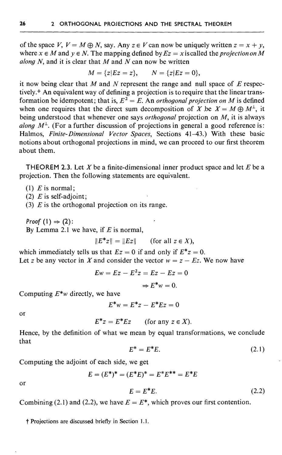
26 2 ORTHOGONAL PROJECTIONS AND THE SPECTRAL THEOREM
of the space V, V = M ® N, say. Any ze V can now be uniquely written z = x + y,
where x e M and y e N. The mapping defined by Ez = x is called the projection on M
along N, and it is clear that M and N can now be written
M = {z\Ez = z}, N = {z\Ez = 0},
it now being clear that M and N represent the range and null space of E
respectively.* An equivalent way of defining a projection is to require that the linear
transformation be idempotent; that is, E2 = E. An orthogonal projection on M is defined
when one requires that the direct sum decomposition of X ,be X = M © A/1, it
being understood that whenever one says orthogonal projection on M, it is always
along M1. (For a further discussion of projections in general a good reference is:
Halmos, Finite-Dimensional Vector Spaces, Sections 41-43.) With these basic
notions about orthogonal projections in mind, we can proceed to our first theorem
about them.
THEOREM 2.3. Let Xbe a finite-dimensional inner product space and let E be a
projection. Then the following statements are equivalent.
(1) i?is normal;
(2) E is self-adjoint;
(3) E is the orthogonal projection on its range.
Proof(\)=>(2):
By Lemma 2.1 we have, if E is normal,
||£*z|| = ||£z|| (for all ze*),
which immediately tells us that Ez = 0 if and only if E*z = 0.
Let z be any vector in X and consider the vector w = z — Ez. We now have
Ew = Ez- E2z = Ez- Ez = 0
=>E*w = 0.
Computing E*w directly, we have
E*w = E*z - E*Ez = 0
or
E*z = E*Ez (for any zeX).
Hence, by the definition of what we mean by equal transformations, we conclude
that
E* = E*E. (2.1)
Computing the adjoint of each side, we get
£ = (£*)* = (£*£)* = £*£** = e*E
or
£ = E*E. (2.2)
Combining (2.1) and (2.2), we have E = E*, which proves our first contention.
t Projections are discussed briefly in Section 1.1.
2.2 ORTHOGONAL PROJECTIONS AND ORTHOGONAL DIRECT SUMS 27
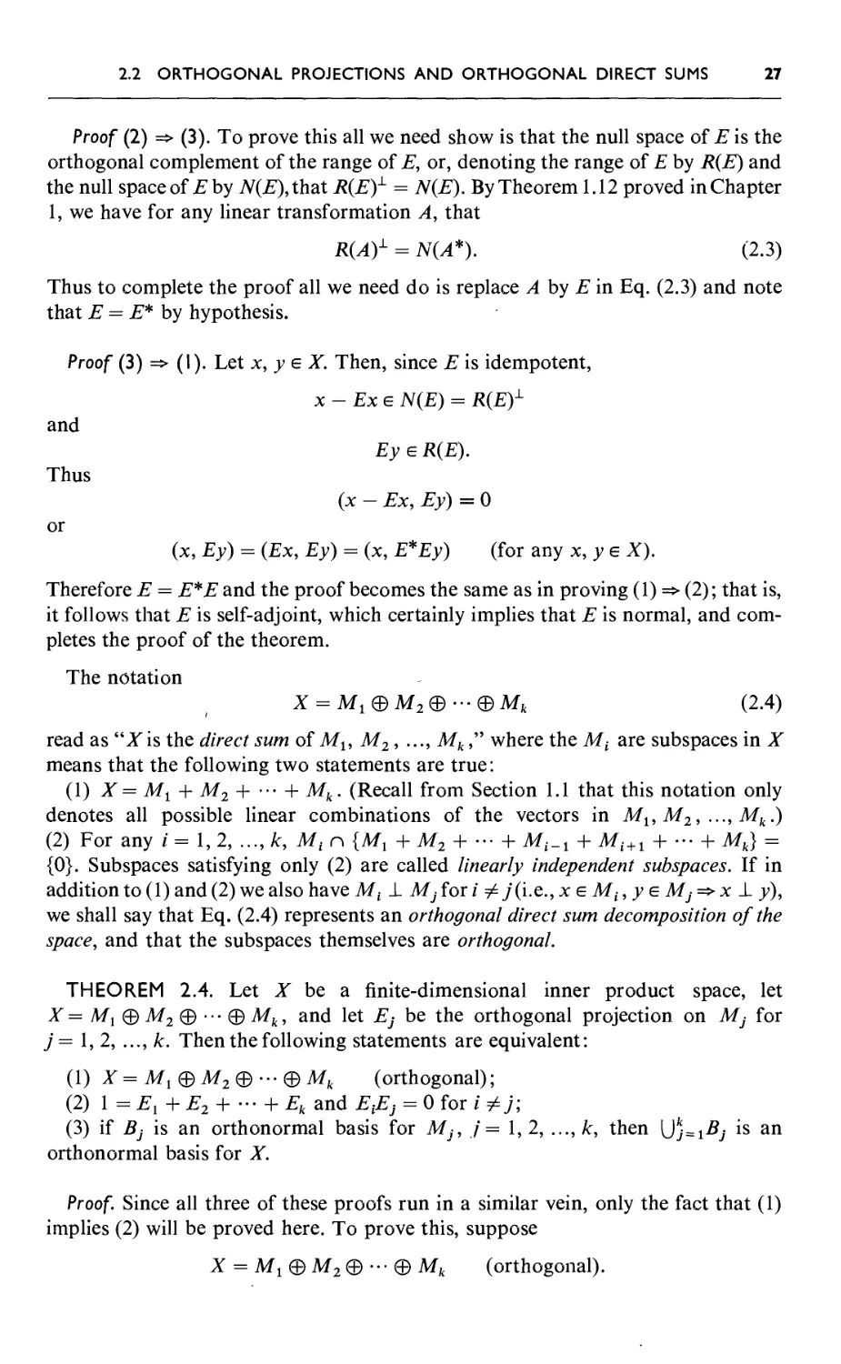
Proof (2) => (3). To prove this all we need show is that the null space of E is the
orthogonal complement of the range of E, or, denoting the range of E by R{E) and
the null space of E by N{E),XhsX R{E)L = N(E). By Theorem 1.12 proved in Chapter
1, we have for any linear transformation A, that
R(A)L = N(A*). (2.3)
Thus to complete the proof all we need do is replace A by E in Eq. (2.3) and note
that E = E* by hypothesis.
Proof (3) => (I). Let x, y e X. Then, since E is idempotent,
x - Ex £ N(E) = R(E)L
and
£y £ R(E).
Thus
(x — .Ex, Ey) = 0
or
(x, Ey) = (£jc, £/y) = (x, E*Ey) (for any x, y e X).
Therefore E = E*E and the proof becomes the same as in proving (1) => (2); that is,
it follows that E is self-adjoint, which certainly implies that E is normal, and
completes the proof of the theorem.
The notation
X = M1®M2®---®Mk (2.4)
read as "Xis the direct sum of Mu M2, ..., Mk," where the Mt are subspaces in X
means that the following two statements are true:
(1) X = M1 + M2 + ••• + Mk. (Recall from Section 1.1 that this notation only
denotes all possible linear combinations of the vectors in M1, M2, ..., Mk.)
(2) For any i = 1, 2, ..., k, Mt n {Mx + M2 + ■■■ + Mi_1 + Mi+1 + ■■■ + Mk) =
{0}. Subspaces satisfying only (2) are called linearly independent subspaces. If in
addition to (1) and (2) we also have Mi 1 Mj for i ^ j(i.e., x e Mt, y £ Mj => x 1 y),
we shall say that Eq. (2.4) represents an orthogonal direct sum decomposition of the
space, and that the subspaces themselves are orthogonal.
THEOREM 2.4. Let I be a finite-dimensional inner product space, let
X= Mx © M2 © ••• © Mk, and let Ej be the orthogonal projection on Mj for
j = 1, 2, ..., k. Then the following statements are equivalent:
(1) X = Mx © M2 © ••• © Mk (orthogonal);
(2) \=El+E2 + -~+ Ek and Efij = 0 for i ^j;
(3) if Bj is an orthonormal basis for Mj, /= 1,2, ..., k, then \Jkj=lBj is an
orthonormal basis for X.
Proof. Since all three of these proofs run in a similar vein, only the fact that (1)
implies (2) will be proved here. To prove this, suppose
X = Mi © M2 © • • • © Mk (orthogonal).
28 2 ORTHOGONAL PROJECTIONS AND THE SPECTRAL THEOREM
This implies the existence, for any x e X, of unique xt (i = 1, 2, ..., k) such that
X = X± i X2 1 ■" 1 Xk,
where xte Mt. Applying jE^ to both sides, we have
E-x = JS^ + Etx2 + ••• + £,x4 + ••• + Etxk
= 0 + 0 H + E^ H + 0 = xj (for any /)•
Hence we can write any x as
x = £xx + E2x + ••■ + Ekx,
and, by our rules for addition of linear transformations, we can paraphrase this
last result as
x = (Ex + E2 + ••• + Ek)x.
Since this is true for any x e X, we conclude that
1 =Et +E2 + -- +Ek,
where the symbol 1 represents the identity transformation—the transformation that
takes everything into itself. It is clear that Mj c MtL, since the subspaces are
orthogonal. Thus, since EjX e Mj, we have ExEpc = 0 for any x e X or EtEj is the
zero transformation for i ?= j.
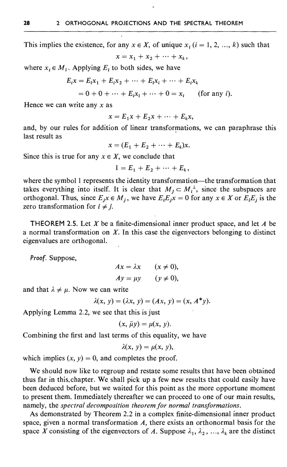
THEOREM 2.5. Let Xbe a finite-dimensional inner product space, and let A be
a normal transformation on X. In this case the eigenvectors belonging to distinct
eigenvalues are orthogonal.
Proof. Suppose,
Ax = Xx (x^ 0),
Ay = fiy (y^ 0),
and that X 7= /i. Now we can write
Kx, y) = (Xx, y) = (Ax, y) =
Applying Lemma 2.2, we see that this is just
(x, fly) = n(x, y).
Combining the first and last terms of this equality,
X(x, y) = n(x, y),
which implies (x, y) = 0, and completes the proof.
We should now like to regroup and restate some results that have been obtained
thus far in this.chapter. We shall pick up a few new results that could easily have
been deduced before, but we waited for this point as the more opportune moment
to present them. Immediately thereafter we can proceed to one of our main results,
namely, the spectral decomposition theorem for normal transformations.
As demonstrated by Theorem 2.2 in a complex finite-dimensional inner product
space, given a normal transformation A, there exists an orthonormal basis for the
space X consisting of the eigenvectors of A. Suppose Xu X2, ..., Xk are the distinct
(x, A*y).
we have
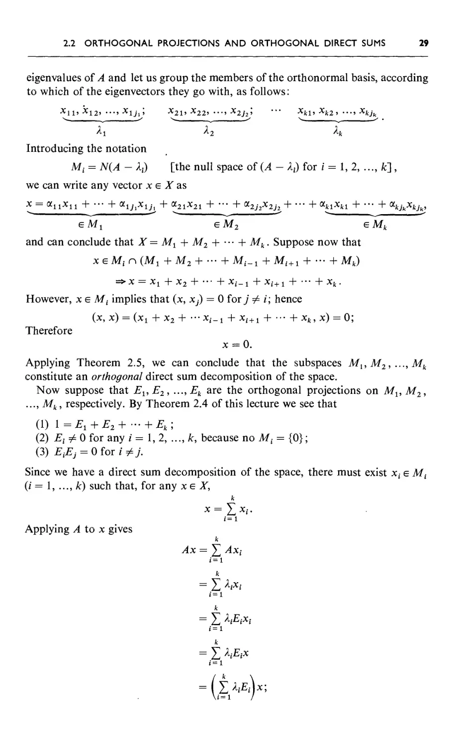
2.2 ORTHOGONAL PROJECTIONS AND ORTHOGONAL DIRECT SUMS 29
eigenvalues of A and let us group the members of the orthonormal basis, according
to which of the eigenvectors they go with, as follows:
XU> x12> •••■> xlji> x21i x22i •••■> x2j2> '" xkl> xk2 >•••■> xkj,
Jk
X1 A2 Xk
Introducing the notation
M( = N(A - Aj) [the null space of (A — A,) for i = 1, 2, ..., fc] ,
we can write any vector x e X as
x = anxn + ••• + a^x^, + a21x21 + ••• + a2j-2x2J2 + — + a*i**i + — + ajykx*A>
eMj eM2 e Mfc
and can conclude that X = M1 + M2 + ••• + Mk. Suppose now that
xeMin (Mi + M2 + ••• + M^ + Mi + 1 + ••• + Mk)
=^ X = Xj t X2 T "' + Xj_ j ~r Xi+ i + '" + Xk .
However, x e Mt implies that {x, Xj) = 0 for j ^ /; hence
(x, x) = (xt + x2 + •••Xj.i + xi+1 + ••• + xk, x) = 0;
Therefore
x = 0.
Applying Theorem 2.5, we can conclude that the subspaces Mx, M2, ..., Mk
constitute an orthogonal direct sum decomposition of the space.
Now suppose that EUE2, ..., Ek are the orthogonal projections on MUM2,
..., Mk, respectively. By Theorem 2.4 of this lecture we see that
(1) 1=^ + ^+- + ^
(2) £;^0 for any i = 1,2, ..., k, because no Mt = {0};
(3) EtEj = Q for i# 7-
Since we have a direct sum decomposition of the space, there must exist x( e Mt
(i = 1, ..., k) such that, for any x e X,
k
Applying A to x gives
i=l
k
Ax = Z ^4x(-
i=i
= Z ^
i=i
k
= X A^Xj
i=l
k
= Z A^*
i=l
= ( Z A,E,Jx;
30 2 ORTHOGONAL PROJECTIONS AND THE SPECTRAL THEOREM
therefore
^ = ZAf£lf (2.5)
£=1
and we have " decomposed " the normal transformation A into a linear combination
of orthogonal projections where the scalar multipliers are the distinct eigenvalues
of A. The representation (2.5) for A is called the spectral form of A. We summarize
these results by stating the next theorem.
THEOREM 2.6. To every normal transformation ^ ona complex
finite-dimensional inner product space there correspond scalars kuX2, ..., \, the distinct
eigenvalues of A, and orthogonal projections Eu E2, ■■■, Ek (where k is a positive
integer not greater than dim X) such that
(1) Et is the orthogonal projection on N(A — kt) (i = 1, ..., k);
(2) Et*0 (for i = 1, 2, ..., k) and Efij = 0 (for i^j);
(3)I}=i^=l;
This theorem is called the spectral decomposition theorem for normal transformations^
We note immediately that if the transformation was self-adjoint, we could even
weaken the hypothesis to include the case of a real inner product space, the complex
numbers being needed only to guarantee the existence of eigenvalues for normal
transformations. If this were done, we would rename the theorem and call it the
spectral decomposition theorem for self-adjoint transformations.
As a final word on the spectral form for any normal transformation, however,
one can say that it is unique.
Before proving the uniqueness of the representation for a normal transformation,
mentioned in the spectral decomposition, some facts about Lagrange polynomials
will be stated (the interested reader might also check Ref. 2).
Let Xu X2, ..., Xk be distinct complex numbers. We define the /th Lagrange
polynomial to be
vm = ri j^jf
j=l Ai Aj
and note immediately that
p{(lj) = dtj,
where <5l7 is the Kronecker delta. We now observe that if P(X) is any polynomial of
degree less than or equal to (k — 1), we have the following representation for P(l):
i=l
where the/^(/1) are just the Lagrange polynomials. With this in mind, we can now
state the next theorem.
2.2 ORTHOGONAL PROJECTIONS AND ORTHOGONAL DIRECT SUMS 31
THEOREM 2.7. Suppose there exist distinct complex numbers Xr,X2, ..., Xk,
and nonzero linear transformations Eu E2, ..., Ek such that the normal
transformation A can be written
(1) A-ZXjEj,
./= i
(2) £^,. = 0 (i*;),
and
(3) i = £^.
Then Xu ..., Xk are the distinct eigenvalues of A and E{ is the orthogonal projection
on N(A — Xt) for /= 1, ..., k.
Proof. To show that each E{ is a projection, one need only apply E{ to both sides of
(3) and apply (2). We now show that the Xu X2, ..., Xk are the distinct eigenvalues
of A. Denoting the range of Et by R(Et), let us consider some nonzero vector
x £ R(Ei). (Such a vector must exist because Ex is not identically zero.) Since
x £ R(Et) and Et is a projection, we have Etx = x. Applying A to both sides of this
last equality, we have
Ax = AEtx
and we also contend that
AEtx = EtAx,
that is, that A commutes with Et for i = 1,2, ..., k. To show that this last
contention is so we note that
A = i XjEj
./=1
and property (2) of the hypothesis imply that
A2 = ixj%. (2.6)
We can now apply A to both sides in (2.6) repeatedly and reapply (2) to conclude
that, for any positive integer n,
A"=ixj"Ej.
j'=i
Hence, for any polynomial f{X), we can say that
f(A)=£f(Xj)Ej,
./=1
and since it is true for any polynomial, it is certainly also true for the Lagrange
polynomials mentioned before. In view of this we have, for the /th Lagrange
polynomial pt(X),
k k
Pi(A) = £ Pi(Xj)Ej = £ StJEj
j=i ./= i
32 2 ORTHOGONAL PROJECTIONS AND THE SPECTRAL THEOREM
Thus Bt is a polynomial in A and must, therefore, commute with A, and we can now
write, using (1) again,
Ax = EtAx = EA Y, h^jx)
= X^E^X
= X{x
to conclude that each Xt is an eigenvalue of A. We now wish to prove that these are
the only eigenvalues that A has. To this end, suppose
Ax = fix (x ^ 0)
or
(A - pi)x = 0.
Using (1) and (3), we can rewrite this as
£ (Xj - n)EjX = 0.
Applying Ex to both sides, we obtain for any i = 1, 2, ..., k,
(X{ — fi)EiX = 0.
Hence if pi =£ Xt for any i, then (Xt — fi) ^ 0, and we can say that Etx = 0 for
i = 1,2, ..., k, which, using (3) again, implies that
x = E^x + •" + Ekx = 0,
which is a contradiction because we assumed x ^ 0. Therefore pi must equal one of
the Xi.
We now wish to show that the Et are orthogonal projections on the N(A — X{),
the null spaces of A — Xt; hence we must first show that
R(Ed = N(A - X{).
Suppose x £ N(A — Xt). This implies
(A - Xi)x = 0.
Using (1) and (3), this can be rewritten as
£ (Xj - Xt)EjX = 0.
./=1
Applying Em to both sides and using (2), we have
(A* - h)Emx = 0.
Thus m ^i implies that Emx = 0. Hence
x = E^x + E2x + -■■ + Ekx = E(X
or
x £ R(Et).
2.3 UNITARY AND ORTHOGONAL TRANSFORMATIONS
33
Since we have already shown that x e R(Ei) implies that x is an eigenvector of A,
we have demonstrated the equality of the two sets R(Ei) and N(A — /1,).
To complete the proof we must show that Ex is the orthogonal projection on
N(A — /I,). Since A is normal, Et = pt(A) is normal too. Thus Et is a projection and
Ei is normal. By Theorem 2.3, we can conclude that Et is the orthogonal projection
on its range.
The following theorem yields an alternative way of characterizing the adjoint of
a normal transformation and constitutes one nice application of the spectral
theorem.
THEOREM 2.8. Let Xbe a finite-dimensional inner product space and let A be a
linear transformation on X. Then A is normal if and only if A* can be expressed
as some polynomial in A.
Proof. If A* can be written as some polynomial in A, it must certainly commute
with A, which establishes the sufficiency of the condition. To show that it is also
necessary, suppose that A is normal. By the spectral decomposition theorem, then,
we can write A as
k
A = Z^A-'
J=l
where the Xj are the eigenvalues of A, and the Ej are orthogonal projections. It was
pointed out previously that an orthogonal projection must always be self-adjoint,
which allows us to write
A* = i (XjEj)*
= £ljEj.
But, as noted in Theorem 2.7, the Ej can be written as pj(A), where pj{X) is just the
y'th Lagrange polynomial. Hence,
A* = £ XjPj(A),
J=l
which completes the proof.
2.3 Unitary and Orthogonal Transformations
We now wish to consider linear transformations U:X^X where X is a finite-
dimensional inner product space X, with the property that
U*U = 1. (2.7)
If Xis a complex space, then U is called unitary; if X is real, then U will be called
orthogonal. Our first claim about transformations satisfying (2.7) is that they also
satisfy
UU* = 1.
34 2 ORTHOGONAL PROJECTIONS AND THE SPECTRAL THEOREM
To prove this, suppose Ux = Uy. Applying U* to both sides, we have
U*Ux = U*Uy,
which, by (2.7), implies that x = y. Hence if. U satisfies (2.7), it must be 1 : 1. On a
finite-dimensional space, however, if a linear transformation is 1 : 1 it must also be
onto, and we can conclude that U must have an inverse, which in this case must be
U*, to establish the contention. For most of our results about transformations which
satisfy (2.7), we shall assume that X is complex (that is, that U is unitary) with
appropriate modifications applying when one wishes to obtain analogous results
about orthogonal transformations.
THEOREM 2.9. Let C/be a linear transformation on the finite-dimensional inner
product space X. In this event, the following statements are equivalent:
(1) U*U= 1;
(2) (Ux, Uy) = (x, y);
(3) \\Ux\\ = \\x\\ for all x e X.
Proof (I) => (2). To prove this, all we need do is note that
(Ux,Uy) = (x,U*Uy) = (x,y)
when (1) is satisfied.
To prove that (2) implies (3), we need only consider
\\Ux\\2=(Ux, Ux) = (x,x) = \\x\\2.
Before establishing that (3) implies (1), however, we shall establish the following
result: if A is self-adjoint and (Ax, x) = Ofor all x, then A = 0. Since (Ax, x) = 0 for
any x, then for any x and y we also have
(A(x + y), x + y) = 0.
Expanding this, we get
0 = (Ax, x) + (Ax, y) + (Ay, x) + (Ay, y)
= (Ax, y) + (Ay, x)
= (Ax, y) + (y, A*x)
= (Ax, y) + (y, Ax)
= (Ax, y) + (Ax, y).
Since y is arbitrary, let y = Ax. We then have 2||^4x||2 = 0 for all x e X, which
implies Ax = 0 for all x; hence A = 0.
We now show that (3) implies (1). By (3) we can write
(Ux, Ux) = (x, x)
or
(U*Ux, x) = (x, x)
or
((U*U - l)x, x) = 0 (for any x).
2.3 UNITARY AND ORTHOGONAL TRANSFORMATIONS 35
All we need do now is note that U*U — 1 is self-adjoint and apply the result just
proved to complete the proof.
THEOREM 2.10. If U is a unitary transformation on the finite-dimensional
inner product space X, then each of the eigenvalues of U must have an absolute
value equal to 1.
Proof. Suppose Ux = kx, x ^ 0. By the preceding theorem, then,
||x|| = ||l/x|| = ||Ax||=|A|||x||f
which, since ||x|| ^ 0, implies that |A| = 1.
Suppose now that A is a normal transformation on a complex finite-dimensional,
inner product space. In view of the spectral decomposition theorem, we can write
A as
A = k1El + — +kkEkt
where the kt and Et are as in Theorem 2.6. We can also write
A* = 11E1 + ••• + lkEk.
If all lt = k{, then clearly A* = A. Next we note that
^ = 1^1^ + ... + 1^12¾.
Suppose now that each kt(i= 1, 2, ..., k) has absolute value equal to 1. In this
case then, clearly,
A* A = 1.
On the other hand, suppose A*A = 1. This implies that
1 = 1^1^ + ... + 1^12¾.
which, in turn, implies that
Et = 1^-12¾
or
(1 - 1^-12)¾ = 0.
Thus, since E{ cannot be zero for any i = 1,2, ..., k, we can conclude that \k{\2 = 1
for i = 1, 2, ..., k. We summarize these results in Theorem 2.11.
THEOREM 2.11. Let A be a normal transformation on a complex
finite-dimensional inner product space. Then
(1) A is self-adjoint if and only if each eigenvalue of A is real;
(2) A is unitary if and only if each eigenvalue of A has absolute value equal to 1.
We noted before for any normal transformation A and any polynomial p(k), that
p(A) = Yj=iP(^j)Ej> where, again, the kj and Ej are as in Theorem 2.6.
Suppose now that f(k) is any complex-valued function defined on the points
ku ..., kk, and consider the linear transformation one obtains by defining f {A) to be
f(A)=if(kj)Ej.
36 2 ORTHOGONAL PROJECTIONS AND THE SPECTRAL THEOREM
At first sight it seems reasonable to expect that the class of linear transformations
obtained in this manner would be a somewhat "larger" class than the one gotten
by considering just polynomials in A. This is not the case, however, and we shall
show that the classes obtained by the two different methods of generation are
identical. To this end, let f(X) be an arbitrary complex function defined on the
distinct points Xu ..., Xk and let a,- = f{Xj). Now consider the polynomial function
W) = £ «jPM),
where the Pj(X) are theyth Lagrange polynomials. In this case the linear
transformation corresponding to this polynomial is just
k k
P(A) = J ajPj(A) = £ f(Xj)Ej =f(A).
j=i . j=i
Hence for any such complex-valued function, there exists a polynomial that will
yield the same, linear transformation; for example, suppose f(X) = X, which
is not a polynomial. In this case we have f(A) = A* = l^E^ + ••• + lkEk, which,
after noting that Ej =pj(A), we see is a polynomial in A.
EXERCISES 2
1. Show that, if \\Ax\\ = \\A*x\\ for all x belonging to the finite-dimensional
inner product space X, the linear transformation A is normal.
2. Let Xbz a finite-dimensional complex inner product space. Prove that the linear
transformation A is normal if, and only if, A{M) a M implies A(ML) c ML,
where M is a subspace.
3. If A is a self-adjoint linear transformation on the finite-dimensional inner
product space X such that A" = 1 for some positive integer n, prove that
A2 = \.
4. If A and B are normal linear transformations on the finite-dimensional complex
inner product space X such that AB = 0, does it follow that BA = 0?
5. Let Xbe a complex three-dimensional vector space and let xt, x2, and x3 be a
basis for X. Let A be a linear transformation mapping X into X such that
/\.%"\ z=z *™"X| "T" X9 -^-¾ •
Determine the spectral decomposition of A.
EXERCISES
37
6. Let A be a normal transformation on the finite-dimensional vector space X.
If B is a transformation which commutes with A, show that B also commutes
with A*.
7. Let ^4 and B be normal transformations on the finite-dimensional complex inner
product space X such that A and B commute. Prove that there exists a normal
transformation C such that both A and B are polynomials in C. {Hint: Let
^4 = T,tAtEi, B = ZjUjFj be the spectral decompositions of A and 1?; let C =
IliJyijGij, where Gij = EiFj and {y^} are arbitrary complex numbers. Show
that Cis normal and then make use of the discussion after Theorem 2.11.)
8. Show that, if A commutes with AA*, then A is normal.
9. Let A be a linear transformation defined on the complex inner product space X
such that (Ax, x) > 0 for all x e X. A is then called a positive linear
transformation. Show that a positive linear transformation is self-adjoint and that a
normal transformation is positive if and only if each eigenvalue is nonnegative.
10. If A is a positive linear transformation (see Exercise 9), show that A possesses
a unique positive square root, that is, there exists a unique positive linear
transformation B such that A = B2.
REFERENCES
1. P. R. Halmos, "Finite-Dimensional Vector Spaces." A good discussion of projections and
direct sums can be found here as well as the complexification (p. 151) and a proof of the spectral
theorem (p. 156).
2. K. Hoffman and R. Kunze, " Linear Algebra." A discussion of Lagrange polynomials and
Lagrange's interpolation formula appears on pp. 114-115; the spectral theorem appears on p. 275.
3
CHAPTER
Normed Spaces and Metric Spaces
Probably the biggest difference between analysis and algebra is that in the former
one utilizes the concept of limits. With limiting notions, one can discuss such
things as differentiation and integration and can deal with infinite processes in
general; or, rather, one can avoid infinite processes by reducing them to a
consideration of some finite process. If one looks at anything pertaining to limits of real or
complex numbers one sees that they all rest on the fact that some measure of
"closeness" can be ascribed to any pair of points. In order to wrest linear spaces
from purely the realm of algebra, we now wish to introduce some sort of distance-
measuring device to those spaces and ultimately introduce limiting notions.
Specifically, the concept of a norm on a vector space will be defined, and indeed
almost all our subsequent results will involve normed spaces.
A more general notion than norm will also be dealt with in this chapter—that of
a metric, a distance-measuring device defined on an arbitrary set. After defining
these things, many familiar notions about real or complex numbers, such as limits
of sequences, continuous functions, and Cauchy sequences, will be generalized
to this new setting.
3.1 Norms and Normed Linear Spaces
In Chapter 1 we defined the notation ||x|| to mean (x, x)1/2 in an inner product
space, and we would now like to note some further properties of this mapping. It is
simple to verify that the following assertions about ||x|| are valid:
II l|:*-K,
x-||x||.
(1) ||x|| >0and = 0if and only ifx = 0;
(2) for a scalar a and a vector x, \\ax\\ = \a\\\x\\;
(3) ||a: + y\\ < \\x\\ + \\y\\ (triangle inequality).
We shall verify here that the third assertion is indeed correct. Consider
II*+ 3^ = (^ + 3^ + 30
= (x, x) + (x, y) + (y, x) + (y, y)
= \\x\\2 + 2Re(x,y)+\\y\\2.
But, since 2 Re(x, y) < 2|(x, y)\, we can say
^ ||x + y||2<IW|2+2|(x,y)| + |M|2.
Appealing to the Cauchy-Schwarz inequality, noted in Chapter 1, we can now say
||x + y\\2 < \\x\\2 + 2||x|| \\y\\ + \\y\\2 = (||x|| + \\y\\)2,
and it remains only to take the square root of both sides to complete the proof.
We now wish to view mappings of the above type abstractly; that is, we now
single out the three- properties cited above and define mappings of this type, on a
real or complex space, to be norms. Note that to have a norm it is not necessary to
have an inner product at all. Conversely, though, whenever one has an inner
product, one can always define a norm (that is, a mapping that will satisfy the above
three conditions) right from the inner product as we have already indicated. Real
39
40
3 NORMED SPACES AND METRIC SPACES
or complex spaces over which a norm is defined are called normed linear spaces
(n.l.s.), and we remark that there are normed linear spaces over which one cannot
define an inner product that will " generate " [that is, no inner product such that
(x, x)1/2 = \\x\\] the norm on the space. Thus the essential thing is to make the norm
and inner product generated norm agree. As one might expect, if further conditions
are imposed on the norm, one can guarantee the existence of an inner product that
will generate the norm. One such further condition is the parallelogram law
mentioned in Chapter 1. There are many other conditions that one might equally well
impose upon the norm to guarantee an inner product representation but other
interests prevent us from listing them all here. It is now necessary to leave normed
spaces temporarily for the sake of a more general structure—the metric space.
Normed spaces will be returned to and dwelt upon at great length from Sec. 8.2 on.
3.2 Metrics and Metric Spaces
If X is a normed linear space and x, y e X, it is easily verified that the function
d(x, y) = \\x — y\\ satisfies the following conditions:
(1) d(x, y) > 0 and is equal to zero if and only if x = y;
(2) d{x,y) = d(y, x);
(3) d(x, z) < d(x, y) + d(y, z) for any x, y, z e X (triangle inequality).
Again, in a manner analogous to the way the norm was defined abstractly, one
can now make the following definition.
DEFINITION 3.1. X, an arbitrary set, will be called a metric space if there is a
function d: X x X ^> R satisfying properties (1)-(3) above. The mapping d itself
will be called a metric.
One thing that should be pointed out immediately is that, when one refers to
metric spaces, it does not suffice to mention just the set X involved; indeed, one
must speak of the pair (X, d), for it is certainly possible that two different metrics
could be defined on the same set and would, thus, give rise to two different metric
spaces. To clarify these notions, several examples will now be given, noting that any
normed space is, of course, a metric space.
EXAMPLE 3.1. Although the metric we shall define now is not too interesting for
its own sake, it comes in quite handy in counterexamples. In addition, it illustrates
that one can define a metric over any set whatsoever.
Let X be an arbitrary set and consider the function
{,y) 10 (x = y),
where x and y are members of X. It is exceedingly simple to verify that properties
(1)-(3) are satisfied by this mapping. This particular metric is called the trivial
metric.
3.2 METRICS AND METRIC SPACES 41
EXAMPLE 3.2. Take the set X to be the real numbers R, and d{x, y) to be \x — y\,
the usual absolute value.
EXAMPLE 3.3. Take Zto be euclidean 2-space R2, and for any two members of
R2, x = (al5 a2) and y = (filt )S2), take
d(xiy) = l(al-pl)2+(a2-p2)2y'2.
Alternatively, one might choose d(x, y) to be
d{x,y) = \cc1-pi\ + |a2-)S2|
or
d(x, y) = maxdai - jSJ, |a2 - p2\)
with similar results holding for euclidean «-space. Although these metrics are quite
different, they do have a feature that unites them: They all lead to equivalent
topologies. This notion will be discussed in more detail later.
EXAMPLE 3.4. Let X = C[a, b] (continuous functions on the closed interval [a, b])
and let f, g e X. We can now take, as a metric on this set,
d(f, g) = max \f{x) - g{x)\.
x e [a,ft]
EXAMPLE 3.5. Let X = Q, the rational numbers, let c be some real number such
that 0 < c < 1, and let/? be any prime. It is clear that any x e Q can be written
a
x = pa - (where p X a and p )( b)
b
wherep\a means "p divides a" andp^a means "p does not divide a."
We can now define the p-adic valuation of any x e Q as
|x|p = C (x # 0),
101, = o,
where | \p has the foil owing properties:
(1) \x\p > 0 and equals zero if and only if x = 0.
(2) \xy\p = |x|p|j;|p. To prove this consider
x = p%alb), y = p\a'lb'),
where p X a, b, a', b'. Hence,
xy = f+fi w {p* aa''p x bb'x
and
\xy\ = ca+^ = c^ = \x\p\y\p.
(3) |x + y\p < max(|x|p, \y\p). Proving this directly is a bit of chore, but it turns
out that this condition is equivalent to the following condition [Eq. (3.1)], the
verification of which is not as difficult:
|x|p<l=>|l+x|p<l. (3.1)
42
3 NORMED SPACES AND METRIC SPACES
Let us prove that (3.1) is really equivalent to (3). Suppose (3) is true and suppose
|x|p< 1. By(3), then,
|1 + x\p < max(l, \x\p) = 1,
it being clear that |l|p = 1. Conversely, suppose now that (3.1) holds, and consider
any two x, y e Q. We may assume that x and y are not zero for the assertion is
clearly valid in that case. Further, let us suppose that
\x\p<\y\p.
This implies that
IyI V
< 1.
p
Using (3.1), we have
1*1,
\y\P
y
X
y
p
<1,
y p
which implies
\x + y\p < \y\p = max(|x|p, \y\p)
and establishes the equivalence of (3.1) and (3). We now show that (3.1) is satisfied.
It follows immediately that, for x ^ 0, if \x\p = ca < 1, then a > 0 and x can be
written in the form x = e/d, where (e, d)= I (e and d are relatively prime, in other
words the greatest common divisor of e and d is 1) and p X d. In this case, then
e e + d
l+x = l+-=——-,
a a
and 1 + x also has a denominator relatively prime to p, which implies |1 + x\p < 1
and completes the proof.
With these basic properties of the p-adic valuation established, consider the
function d(x, y) = \x — y\p. Clearly, d(x, y) > 0 and equals zero if and only if
x = y. Also
d(y, x) = \y - x\p = \-.l\p\x - y\p = \x - y\p = d(x, y)
so
Finally,
d(x, y) = d(y, x).
d(x, z) = \x - z\p = \(x - y) + (y - z)\p
< max(\x - y\p, \y - z\p) = max(d(x, y), d(y, z)).
Thus
d(x, z) < m2ix(d{x, y), d(y, z)),
from which it immediately follows that
d{x, z) < d(x, y) + d{y, z),
and we have established that d is a metric or that (Q, d) is a metric space. Inequality
(3.2) is often called the ultrametric inequality, it being clearly stronger than the
triangle inequality. We note that the trivial metric satisfies the ultrametric inequality
also.
3.3 TOPOLOGICAL NOTIONS IN METRIC SPACES
43
example 3.6.Given a finite collection of metric spaces (Xl, dx), (X2, d2), ...,
(Xn, dn), itjs possible to assign a distance function d to the set of all ordered n-
tuples (xx,x2,..., xn), where ^s Xt (i = 1, 2,..., n), that is,to the cartesian product
Xx x X2X '" x Xn. Certainly one possibility is to assign the trivial metric. Other
possibilities, each of which defines a metric of a less trivial nature are given below,
the verification that they are indeed bona fide distance functions being left to the
reader.
Let* = (xu x2, •.., xn) andy = (y1,y2, ..., y„) be points of X1 x X2 x ••• x Xn.
Each of the following defines a metric on Xl x X2 x ••• x Xn:
(1) dix, y) = dx(xu yj + d2(x2, y2) + — + dn(xn, yn);
(2) d(x, y) = max^f(xf, y{);
(3) d(x,y) = \]td{xttyds
1/2
Last, we remark that, if A is a subset of a metric space (X, d), A itself can be
viewed as a metric space by merely restricting d to A. A with this restricted metric is
called a subspace of the metric space.
3.3 Topological Notions in Metric Spaces
Suppose (X, d) is a metric space, x e X, and r is a positive real number. We now
define a spherical neighborhood of radius r about x (with center x) to be the set of
points
Sr(x) = {yeX\d(y,x)<r}.
For example, suppose X is a normed linear space. In this case we would have, as a
neighborhood about a point,
S,(x) = {j;sX|||j;-x||<r}.
If the metric space was (R, d) as in Example 3.2, then
Sr(x) = {yeR\\y-x\<r}. '
If we considered (X, dy, where X was any set and d was the trivial metric, then
br{X) -\X (r> 1).
DEFINITION 3.2. Suppose now that Aa X. Then x e A is called an interior
point of A if there exists an r > 0 such that Sr(x) a A, the collection of all interior
points of A being called the interior of A and denoted by A0. It is clear that A0 c A.
If every point of A is an interior point of A (that is, A0 = A), then A is called an
open set. We would now like to examine some properties that the class of all open
sets in a given metric space (X, d) have. Denoting the class of all open sets by O,
we have
(Oj) Arbitrary unions of open sets are also open. Symbolically, if Oa e O
(a £ A, A some index set), then U«6a Oa e O.
44
3 NORMED SPACES AND METRIC SPACES
(02) If Ol5 02, ..., 0„ e O for any finite n, then
C\OteO.
i=l
(03) X and 0 are each open sets.
DEFINITION 3.3. A point x is called an adherence point of the set A a X if, for
any Sr(x), Sr(x) n A ^ 0. The set of all adherence points of A is called the
closure of A and is denoted by A.
Three observations that follow immediately from the definition are the following:
(\)AczA;
(2) AaB=>AaB;
(3) Akj B =AkjB.
To illustrate how we prove observations such as these, we shall prove (3). It is
clear that B and A are each contained in A u B. Since this is true then (2) implies
that
A c A u B,
BcAuB,
which, together, imply that
A u B a A u B.
Conversely, suppose that x e A <j B and, in addition, suppose that x 4 A and x$B.
This assumption means that there exist neighborhoods of x, Sri(x) and Sr2(x), such
that Sri(x) n A = 0 and 5r2(x) n B = 0. Let r be the smaller of /^ and r2 . In
this case, we have
Sr(x) n(Av B) = 0,
which is contradictory. Therefore x e A or x e B, which implies that xelul. One
notes in passing here that the above argument cannot be extended to include the
case of infinitely many sets. An essential feature in the proof is our ability to select
the smaller of the two real numbers r1 and r2 . If there were an infinite number of
sets under consideration, no such selection would be possible. A concept closely
related to, but somewhat stronger than, an adherence point is given in Definition
3.4. The reader should have the distinction between the two clearly fixed in his
mind.
DEFINITION 3.4. The point x is said to be a limit point of A cz X if and only if,
for every r, Sr(x) n A contains infinitely many points of A, the collection of all
limit points of A being called the derived set of A and denoted by A'. One notes
immediately that no finite set can possess a limit point.
DEFINITION 3.5. Consider the sequence of points in X,xl,x2, ..., xn, ... --
{xn}. The sequence of points {xn} is said to converge to the point x, denoted by
3.4 CLOSED AND OPEN SETS, CONTINUITY, HOMEOMORPHISMS 45
xn -*■ x, if for any Sr(x) there exists an N (which will depend on r, in general) such
that
n > N => xne S£x).
Clearly, xn -> x is equivalent to requiring that the sequence of real numbers,
d{x, xn), converge to zero.
Now consider the pair (X, d), where d is the trivial metric. In this space xn -> x
implies that, for some N, for n> N, all xn must equal x.
As another example consider the pair (Q, d), where d(x, y) = \x — y\p, and the
sequence {p,p2, ...,p", ...}. Now,
<*(o, P") = \p\; = c\
and, since c < 1, we have p" -*■ 0, a result which rather confounds one's intuition.
3.4 Closed and Open Sets, Continuity, and Homeomorphisms
Let (X, d) be a metric space and let A be a subset of X It is clear that, if x is an
adherence point of A, every neighborhood of x, in particular each S1/n(x), where n
runs through the positive integers, must contain a point of A. Calling a point of A
selected from Sl/n(x), xn, it follows that the sequence of points {xn} must converge
to x : x„ -*■ x. In light of this we can say:
x £ A if and only if there exists a sequence {xn},
where xne A for every n, such that xn -*■ x.
It,is immaterial whether the points in the sequence are distinct or not; that is, the
sequence (x, x, x, ..., x, ...) is perfectly acceptable. We note that, if x is actually
a point of A, this sequence will always satisfy the conditions in the above assertion.
If, however, x is not a member of A but belongs to A (x must be a limit point of A
in this case), then a sequence of distinct points (see Exercise 3.1) can be selected.
We define a closed set to be one that contains all its limit points. It can be shown
that this is equivalent to defining a set A to be closed if and only if A = A (the reader
is asked to verify that A itself is a closed set in Exercise 3.3), and it is this definition
that we shall use in proving the following relationship between closed and open
sets.
THEOREM 3.1. In a metric space (X, <af),for a subset of X, A,
(1) A being open implies that CA, the complement of A, is closed;
(2) A closed implies that CA is open.
Proof. The reader, having seen the proof of assertion (1), can easily prove (2) by
little more than just interchanging the words open and closed; for this reason,
only (1) will be proved here.
Suppose A is open and x e A. Since A is open, there exists some neighborhood
of x, Sr(x), such that Sr(x) a A. This implies that Sr(x) n CA = 0 with analogous
46 3 NORMED SPACES AND METRIC SPACES
statements holding for every x e A. Thus, for any x e A, we can say that
x §§ CA (if it did, every neighborhood of x would have to contain a point of CA)
or
x §§ CA =>x$ CA.
Taking the contrapositive of this statement, we get
x £ CA =>x e CA
or
CAaCA.
But, since any set is contained in its closure, we also have
CAaCA-
Hence
CA = CA
and CA is closed.
The proof of Theorem 3.2 is straightforward and will be omitted.
THEOREM 3.2. In a metric space (X, d), if {AJ where a e A, A an index set, is a
collection of closed sets, then
(fo n a
<xe A
is closed too. (The intersection of closed sets is always a closed set.) Further, if
Bt (i = 1, 2, ..., n) are closed sets, then
(F2) U Bt
£=1
is also a closed set. (The union of a finite number of closed sets is a closed set.)
(F3) X and 0 are closed.
We would now like to extend the familiar concept of a function of a real (or
complex) variable being continuous to a more general setting.
DEFINITION 3.6. Let (X, d) and (7, d') be metric spaces and let/: X-+ Y. The
function / is said to be continuous at the point x0e X if, for any neighborhood
Se(f(x0)) there exists a d > 0 such that
f(SM) a S.(/(x0)).
The function/is said to be a continuous function if it is continuous at every point
of X.
It is easily verified that this definition matches up exactly with the usual notion
of continuity of a real-valued function of a real variable, when viewed in that
framework.
3.4 CLOSED AND OPEN SETS, CONTINUITY, HOMEOMORPHISMS 47
The following theorem gives us an equivalent way of defining continuity in a
metric space.
THEOREM 3.3. If (X, d) and (7, d') are metric spaces where/: X-+ 7, then/is
continuous at the point x if and only if for every sequence {xn} converging to x,
f{xn) -+f(x).
Proof {necessity). Suppose/is continuous and let xn-+x. For any e there exists
a 8 such that
/(S,(x)) c SE(f(x)).
For this d there exists an integer Nd, such that n > N8 implies that xn e Sd(x).
By virtue of the above inclusion, then
/(*„) e Se(f(x)) (for n > Nd).
Hence f(xn) -+ f(x).
Proof (sufficiency). Let e > 0 be given and suppose for any 5 there is an x' eS8 (x)
such that
d'(f(x'),f(x))>s. (3.3)
Consider now any sequence of real numbers {<5„} such that Sn -+ 0. For each n
select the x' that satisfies Eq. (3.3) and call this xn'. It is clear that x„' -+ x, but
f(xn')++f(x), because the distance between f(xn') and/(x) cannot be made smaller
than e for any n. Hence we have shown that, if/is not continuous, then not every
sequence {xn} converging to x will yield a sequence {f(xn)} that converges to/(x).
Taking the contrapositive of this statement demonstrates that the condition is
sufficient. b
Continuing on in the same vein, we now state another condition that is equivalent
to continuity.
THEOREM 3.4. If (X, d) and (7, d') are metric space and/: X-+ 7, then /is
continuous if and only if/_1(F), where Fis any closed set in 7, is a closed set in X.
Proof. First we shall show that the condition is necessary. To this end, suppose
that/is continuous, F is a closed set in 7, and let A =/_1(F). What we want to
show now is that every limit point of A must actually belong to A or that x e A'
implies that x e A. Thus, let us consider any limit point of A, x. Since x e A', there
must exist a sequence of points of A, {x„} such that xn -+ x. Since/is continuous,
though, this implies that
/(*„) -+f(x).
Each of the terms f(xn), however, must be in F, which implies that/(x) e F. Since
F is closed, though, F = F, and we can say that f(x) e F, which is equivalent to
saying that x e/_1(F) = A and completes this part of the proof.
Using the fact that the inverse mapping takes closed sets into closed sets, we
must now show that/is continuous. For any x e A^it is clear that SE(f(x)) is open,
48
3 NORM ED SPACES AND METRIC SPACES
which implies that CSe(f(x)) is closed. Since this is a closed set in Y, its pre-image,
f~1[CSe(f(x))], must be a closed set in X. We can rewrite the abovef
f-'iCSlfix))-] = Cf-'lS^fix))-]
is closed. Taking the appropriate complement, we can say that
/_1[S^/(x))]
is open. Since the set is open and x is a member of the set, there must exist some
neighborhood of x lying wholly within the set (x must be an interior point) or, there
must exist a 8 such that
S6(x)czf-l[SE(f(x))l
which implies
f(S6(x)) c S,(/(x))f
which is the statement of continuity at the point x and completes the proof.
COROLLARY. If (X, d) and (7, d') are metric spaces and/: X-+ Y, then/is
continuous if and only if/-1 (B), where B is any open set in Y, is an open set in X.
EXERCISES 3
The context for the following exercises is assumed to be a metric space (X, d).
1. Show that, if x is an adherence point of a set A but is not a member of A, a
sequence of distinct points xn (n = 1, 2, ...) can be selected from A such that
xn-+x.
2. Prove that S£(x) cz {y\d(x,y) < e}, and give an example for which the
inclusion is proper.
3. For an arbitrary subset A of X, show that A = A.
4. For an arbitrary subset A of X, prove that CA = (CA)° and C(A°) =~CA.
5. For any subsets A and B, prove that {A n I?)0 = A0 n B°.
6. Give examples for which (a) AnB ^ A n B; (b) (A u B)° ^ A0 u B°.
7. Give an example of a metric space and subsets At (i = 1, 2, ...) such that
(U£i^)*U£i*i.
t For any function f and any two sets X and Y, where/: A"-» F, we can say that f~x{CA) =
Cf~x{A) for any A <= y; a rather nice property of inverse functions for which there is no
corresponding statement about/itself.
EXERCISES
49
8. Let A be a subset of X. For x e X, the distance from x to A, denoted by d(x, A)
is defined as follows: d(x, A) = infy6 A d(x, y). Show thatd(x, A) = 0 if and only
if x £ X
9. Show that, if d satisfies the ultrametric inequality, then if d(x, y) ^ d(y, z),
d(x, y) = max(d(x, y), d(y, z)).
10. Show that, if d satisfies the ultrametric inequality, every point of the sphere
Se(x) is a center.
11. In the definition of | |p on Q, take c = I/p. Then show that, if x e Q and x ^ 0,
np|x|p = l/|;t|, where the product on the left is taken over all primes/?.
12. (a) Show that d(x, x0) is a continuous function of x. (b) Show that d(x, y) is a
continuous function of x and y.
13. Let/, g be two continuous mappings of (X, d) into (Y, d'). Show that the set
{x £ X\f{x) = g{x)} is a closed subset of X.
14. Let X = R and define d(x, y) = \x — y\*, where a £ i? (0 < a ^ 1). Show that
(R, d) is a metric space.
15. Let Dk(a, b) be the space of all complex-valued functions on [a, b] having
continuous derivatives up to order k. For fe Dk{a, b), define
ll/||=I - max{|/<f)(0l |/ £ La, &]}.
£ = 0 l-
One can easily show, with respect to the way linear operations were introduced
to the space C[a, b] of continuous^functions on [a, b] that Dk(a, b) is a linear
space. For the above operation, show that the norm axioms are satisfied.
REFERENCE
1. A. Komolgoroff and S. Fomin, "Elements of the Theory of Functions and Functional
Analysis," Vol. 1. Discussion and examples of metric spaces, as well as properties of metric spaces,
Sections 8-12.
CHAPTER
4
Isometries and the
Completion of a Metric Space
A vital concept for the consideration of metric spaces is that of an isometry—a
mapping between metric spaces which "preserves metric properties." After
introducing an isometry and another similar mapping, the homeomorphism, in Sec. 4.1,
we put it to almost immediate use in discussing the completion of a metric space. It
will be shown that any metric space can be embedded, in a certain sense, in a
complete metric space or, loosely speaking, that an arbitrary metric space can be
incorporated into a larger space that is complete. The rest of the chapter will be
devoted to the completion procedure which, aside from its usefulness in the sequel,
is an elegant mathematical construction.
4.1 Isometries and Homeomorphisms
Whenever certain specific properties of a set are being examined, one usually
wants to see what sort of mappings will preserve the properties under consideration.
For example, in considering vector spaces where the basic operation is that of
forming linear combinations, the isomorphism is of interest because it preserves
this basic property. Aside from placing two linear spaces in 1 : 1 correspondence,
it also sets up a correspondence of linear combinations in the domain with linear
combinations of corresponding vectors (that is, images under the isomorphism)
in the range. When an isomorphism exists between two linear spaces, there is no
harm done in adopting the logically inaccurate convention of actually identifying
the two spaces and calling them the same. Even though the two spaces may be very
different concretely (for example, one space may be a collection of polynomials,
whereas the other may be a set of «-tuples of numbers), there is no way of abstractly
telling them apart as vector spaces.
So much for vector spaces. Since our present interest is in metric spaces, we now
wish to define a mapping called an isometry that will preserve metric properties.
After this is done, we shall feel frefe to identify isometric spaces.
Apropos to this discussion and to the preceding paragraph we now wish to
make two definitions.
DEFINITION 4.1. Let (X, d) and (Y, d') be metric spaces and let/be a 1 : 1, onto
mapping such that/: X-+ Y. Iff and/-1 are each continuous functions (mapping
of this type are called bicontinuous), then/is said to be a homeomorphism. Further,
X is said to be homeomorphic to Y if such a mapping exists.
Homeomorphisms preserve all the essential topological properties; in particular,
open sets in X are mapped into open sets in Y, and, if x is a limit point of A a X,
then/(x) will be a limit point of /(./4). The next definition defines a mapping that
preserves metric properties.
DEFINITION 4.2. If/maps (X, d) in 1 : 1 onto fashion onto (Y,d') such that, for
any x, ye X, d(x, y) = d'(f(x),f(y)), then/is said to be an isometry and the two
spaces are said to be isometric.
It is clear that an isometry is also a homeomorphism. As an example of an
isometry, one might take the two metric spaces to be the real numbers with the usual
metric under the mapping x -> x + a, where a is a fixed real number. Another
mapping that is also an isometry in this context is the one that takes any real number
x into — x. As it happens, these are the only isometries of the real line onto itself.
51
52 4 ISOMETRIES AND COMPLETION OF A METRIC SPACE
4.2 Cauch/ Sequences and Complete Metric Spaces
DEFINITION 4.3. If, in a metric space (X, d), the sequence {xn} has the property
that, for any e > 0, there exists an integer N such that for all n and m greater than N,
d(xn, xm) < e, the sequence is said to be a Cauchy sequence. In the case of the
real line, every Cauchy sequence converges; that is, being a Cauchy sequence is
sufficient to guarantee the existence of a limit. In the general case, however, this is?
not so. If a metric space does have the property that every Cauchy sequence
converges, the space is called a complete metric space. Several examples will now be
considered.
EXAMPLE 4.1. Consider R", all «-tuples of real numbers. This collection, along with
any of the distance functions mentioned in Example 3.6, is complete.
EXAMPLE 4.2. Let Xbe any set with the trivial metric d assigned to it. The only way
{xn} can be a Cauchy sequence in this space is if there is some integer N such that
xN = xN+l = -•'. Hence (X, d) is complete.
EXAMPLE 4.3. Consider the space C[a, b] with the distance between any two
functions/, g £ C[a, b] defined to be
d(f,g)= max |/Oc)-0O)|,
x e [a, ft]
and suppose {/} is a Cauchy sequence. This implies that
max 1/0)-/,0)1 <s
x 6 [a, ft]
for n and m bigger than some N, say. Hence we can say by a theorem of advanced
calculus that the sequence must converge uniformly. We have a uniformly
convergent sequence of continuous functions and, by another well-known theorem from
advanced calculus, we can assert the continuity of the limit function. Thus this
space is complete.
EXAMPLE 4.4. Consider C[a, b] but with the metric
d(f, 9) = (JVO) - 0(x)|2 dx)1'2 (/, g £ C[a, &]).
We shall show, by a counterexample, that this space is not complete. Let a and b
be — 1, and 1, respectively and consider the Cauchy sequence (Fig. 4.1)
[0 (-l<x<0),
fn(x) = lnx (0<x<l/n),
[ 1 (1/n < x < 1).
It is clear that the limit function in this case is a discontinuous function and, hence,
the space is not complete.
4.2 CAUCHY SEQUENCES AND COMPLETE METRIC SPACES 53
n
FIG. 4.1.
EXAMPLE 4.5. Let X = (0, 1) and take the distance between any two numbers x
and y belonging to X to be
d{x, y) = \x - y\.
The sequence {1/«} is a Cauchy sequence in this space but converges to 0, which
is not in the space. Thus this space is not complete.
EXAMPLE 4.6. Let X = Q, the rational numbers with distance between any two
rational numbers x and y, be defined as
d(x, y) = \x-y\.
One can easily make up Cauchy sequences of rational numbers that converge to
irrational numbers. Hence this space is not complete.
EXAMPLE 4.7. Again let X= Q, but take the distance between any two rational
numbers to be |x — y\p ; that is, the/?-adic valuation of their difference as discussed
in Chapter 3. In the case when p = 5, it can be shown that the Cauchy sequence
converges to v — 1 which is not a rational number. Similar examples can be
constructed for each prime p. Thus Q with respect to any p-adic valuation is not
complete.
The property of completeness is very important when one wishes to make an
existence statement, and a fact of fundamental importance, which we shall prove
later, is that every metric space can be regarded as a subset of a complete metric
space. In a certain sense an incomplete metric space can be completed, the precise
meaning of being completed being given by the following definition.
DEFINITION 4.4. Let (X, d) be an arbitrary metric space. The complete metric
space (X*, d*) is said to be a completion of (X, d) if
(1) {X, d) is isometric to a subspace (X0, d*) of (X*, d*);
(2) the closure of X0, X0, is all of X* : X0 = X*.
An equivalent way of stating condition (2) is saying that X0 is everywhere dense,
or simply dense, in X*. It means that every point of X* is either a point or a limit
54 4 ISOMETRIES AND COMPLETION OF A METRIC SPACE
point of X0, which means that, given any point x of X*, there exists a sequence
of points in X0 that converge to x.
We are now in a position to demonstrate that every metric space has a
completion.
THEOREM 4.1. Every metric space (X, d) has a completion (X*, d*) and,
furthermore, if (X**, d**) is also a completion of (X, d), then (X*, d*) is isometric to
(X**, d**); that is, the completion of a space is unique to within an isometry.
Proof. Consider the collection of all equivalence classes of Cauchy sequences in
(X, d) under the following equivalence relation: If {xn} and {yn} are Cauchy
sequences in (X, d), then {xn} is said to be equivalent to {yn}, denoted by {xn} ~ {yn},
if and only if
lim d{xn, yn) = 0.
The collection of all these equivalence classes will be called X*. We now wish to
define a metric on X* with the properties stated in the theorem. To this end, consider
the following function: Let x* and >>* be equivalence classes in X*. We define
d*(x*, y*) = lim d(xn, yn), (4.1)
where {xn} e x* and {yn} e y*. Before showing that this is even a metric, we must
consider two other points. We must show that the limit [Eq. (4.1)] exists, and we
must also show that it does not depend on which particular member of the
equivalence class was chosen; that is, we must show that it is well-defined. First it will be
shown that the limit (4.1) exists.
Let {sn} denote the sequence of real numbers {d(x„, yn)}, where the xn and yn
are as in (4.1). Now we can say
W(xn, yn) - d(xm ,ym)\ = \d{xn, yn) - d{xn, yj + d{xn, yj - d{xm, ym)\
^ \d(xn, yn) - d(xn, ym)\ + \d(xn, yj - d(xm, yj\
^d(yn,ym) + d(xn,xm),
where the last inequality follows from the fact that, if d is any metric, then
\d(x, y) — d(x, z)\ <d(y,z). The last inequality, since {xn} and {yn} are Cauchy
sequences, implies that {sn} is a Cauchy sequence. Since the real numbers are
complete, the limit exists.
Now we show that d* is well-defined. To this end, suppose
{x„}, {*„'} e x* and {yn}, {yn'} e y*.
We must show that the limit (4.1) is the same regardless of which sequences were
chosen. Hence consider
< \d(xn, yn) - d(xn', yn)\ + \d(xn', yn) - d(xn', yn')\
<d(xn,xn') + d(yn,yn').
4.2 CAUCHY SEQUENCES AND COMPLETE METRIC SPACES
55
Since {xn} ~ {xn'} and {y„} ~ {y„'}, both terms on the right go to zero as n increases
and d* is, indeed, well-defined. We are now at least " in the ball park," for we have
shown that it makes sense to consider d* a function. We now show that it is a metric,
by verifying that the axioms are satisfied.
(1) It is clear that d*(x*, y*) > 0. We must also show that equality prevails
if and only if x* = y*. To this end suppose d*(x*, y*) = 0. This means that lim„ _ ^
d(x„,yn) = 0, which implies that {xn} ~ {yn} or x* = y*.
(2) Symmetry of d* is clear because d(xn, y„) = d{y„, xn) for every n.
(3) Last, we must show that the triangle inequality is satisfied. For this purpose
let x*, y*, z* £ X* and suppose that {xn}, {yn}, and {zn} are members of these
classes, respectively. For every n, we can make the statement:
d{xn, z„) < d{xn, yn) + d{yn, z„).
Since the statement holds for every n, it is also true in the limit, and we have
shown that (X*, d*) is a metric space.
We now wish to show that X* contains a subspace X0 that is isometric to X.
In light of this, consider the subset of X* consisting of those equivalence classes x',
which contain the sequences (x, x, ..., x, ...). Calling this collection X0, we now
contend that X is isometric to X0, where the isometry is
X —► A0,
Since it is clear that there cannot be two different Cauchy sequences, of the type
mentioned above, in the same equivalence class and that the mapping is onto by
virtue of the way it was defined, we need only verify that it preserves distances to
prove that it is isometry. For this purpose, let us compute the distance between any
two points in X0, x' and y :
d (x\ y') = lim d(x, y) = d(x, y).
With this done we shall now show that X0 = X*. To prove this, we show that,
for any point in X*, there is sequence of points in X0 converging to it. Let x* e X*
and let {xn} e x*. For any e > 0, there exists an N such that n, m> N implies that
d{xn, xm) < e. Now let us examine the distance [in (X*,d*)] between the two
points of X*, x* and xn'; select the representatives
^Xj, X2, .«., Xn , ...) £ X ,
\Xn , Xn , ..., Xn , ...) £ Xn ,
where n> N. Since d(xn, xm) < s for n, m> N, it follows that
d*(x*, xn') = lim d(xm, xn) < e.
m-Kx
Thus given any neighborhood of a point x* e X*, there is some member of X0 in
there and, by virtue of this, it is possible to construct a sequence of points from X0
converging to any desired point in X*. We have now shown that X0 = X*.
56
4 ISOMETRIES AND COMPLETION OF A METRIC SPACE
To show that X* is complete, we must demonstrate that any Cauchy sequence
of points in X* converges to a point in X*. Before doing this, however, we consider
a more special type of sequence in X* and show that it always converges to
something in X*: Consider the Cauchy sequence in X*,
xl » x2 ' •••■> Xn > ■■■> (4.Z)
where
(xt, x(, ..., x(, ...) ex/ (for i = 1, 2, ...).
Thus the distinguishing feature of this sequence is that the terms have been taken
from X0. We now claim that assuming (4.2) to be a Cauchy sequence in X* implies
that the sequence obtained by taking the isometric preimages of the entries in (4.2)
is a Cauchy sequence in Z(and, therefore, determines a point of X*) and is also the
limit that (4.2) approaches. Once again we are trying to show that the sequence
" of sequences" [(4.2)] has a limit in X*. Consider now the sequence obtained from
(4.2) by taking the isometric images of each of its entries in X: Consider
{x„} =(xltx2t ...)^(^/, x2\ ...) = {*„'}.
We wish to show first that {xn} is a Cauchy sequence in X. Since Eq. (4.2) is a Cauchy
sequence and the mapping X-*- X0 is an isometry, we have that
d*(xm', xn') = d{xm, xn)
is arbitrarily small for m and n bigger than some N. It is now seen that our original
assumption that (4.2) was a Cauchy sequence implies that the sequence {xn} is
a Cauchy sequence of points in X. Let us suppose that this Cauchy sequence
belongs to the equivalence class x*. We now show that the sequence (4.2) approaches
x* as a limit in X*. Thus consider
lim d*(xn', x*) = lim lim d(xn, xm) = 0,
n-Kx> m-> oo
because {xn} is a Cauchy sequence.
Now consider an arbitrary Cauchy sequence of points in X* :
^1 » x2 » • • •» Xn ,
Since X0 = X*, there exist points in X0
x± , x2 5 • • •, xn , ...
such that d*{x*, xn') < (l/«). Consider now the sequences
^1 J X2 5 •• •» Xn ,...,
it is easily seen that, for any e > 0,
d*(xn', xm') < d*(xn', x*) + d*(xn*, xm*) + d*(xm*, xm')
1 1
<- + s -\
n m
for n and m large enough. Therefore,
{xn'} is a Cauchy sequence.
4.2 CAUCHY SEQUENCES AND COMPLETE METRIC SPACES
57
As noted above, then, {xn'} must converge to some y* e X*; we now claim that
{x*} must converge to y*, too, and to prove it we only need note that
d*(y*, x*) < d*(y*, xn') + d*(xn', x*),
where, as previously noted, each of the terms on the right goes to zero as n increases.
Finally, we must show that we are justified in saying that (X*, d*) is the
completion; that any other completion must be isometric to (X*, d*). To do this we
must show that, for any other completion (X**, d**), there exists a 1 : 1 onto
mapping <p, taking X* onto X** with the property that if q>(x*) = x** and q>(y*) =
y**, then
d**(x**, y**) = d*(x*, y*).
In view of this, suppose there are two completions of X, X* and X**, with,
of course, corresponding metrics. We first note that X itself must appear (actually
an isometric image of X) in each of these spaces if each is to be a completion of X.
This means that there is already a certain isometry established between the subsets
of X* and X** that represents the image of X under that isometry. We shall call
the images of X in X* and X**, X0* and X0**, respectively. For any point x* of
X*, we can say that there must be a sequence of points in X0*, {xn*}, that must
converge to x*. Each of these points has an isometric image in X**, though; thus
the original (Cauchy) sequence in X* gives rise to another Cauchy sequence in X**,
{xn**}. Since X** is complete, this sequence must have a limit x** in X** and it is
x** that we shall take to be the image of x*. It is clear that this mapping is 1 : 1,
onto, and does not depend on which member of the equivalence class was chosen.
It only remains for us to show that distances are preserved under this mapping.
Pictorially, we have, reading the arrows outside parentheses as "gives rise to"
(x* £ X*) -»(x* £ X0*, xn* -»x*) -»({x*} a Cauchy sequence)
-*X{*n**}> where xn** is the isometric image of xn* in X0**)
-+(x**-+x**eX**)
as the mapping <p. We immediately note that, if one considers the isometric image
x' of any point x, from X, in J*, a sequence of points from X0* that converges to
x' is just
Thus cp(x') is just the isometric image of x itself in X0**. If we had adopted the
practice of just identifying an element x of a space X with its isometric image in the
completion of X, we would say that <p reduces to the identity mapping on X0* and
X0**, that is, takes an element into itself. Making this identification and also
identifying d with d* or d** (when it is sensible to do so), we let
Xn —► X £ Ji. ,
yn-+y*eX* (xn,yneX0*),
and
xn-+x**eX**,
yn-* y**6 x**-
58
4 ISOMETRIES AND COMPLETION OF A METRIC SPACE
We now have
d*(x*, y*) < d*(x*, xn') + d{xn,yn) + d*(yn', y*),
for every n, where xn' = (xn, xn, ...) and similarly for yn. Since it is true for every n,
it is true in the limit as n becomes infinite, which yields
d*(x*, y*) < lim d{xn, yn).
n-KX
But d(x„,y„) < d*(xn', x*) + d*(x*, y*) + d*(y*,yn') which yields the reverse
inequality. In a completely analogous manner, we can also show that
d**(x**,y**) = \imd(xH,yH).
Consequently,
d*(x*, y*) = d**(x**, y**),
which completes the proof.
EXERCISES 4
Unless otherwise indicated, operations are assumed to take place in a metric
space (X, d).
1. If xn -► x, show that {xn} is a Cauchy sequence; show also that every
subsequence of {xn} also converges to x.
2. Show that, if a Cauchy sequence {xn} has a convergent subsequence, it is
convergent.
3. Give an example of a homeomorphism which is not an isometry.
4. Give an example of two metric spaces which are homeomorphic and where one
is complete but the other is not.
5. Prove that the only isometries of R with the usual metric are f(x) = x + a and
f(x) = — x + a.
6. Assuming (X, d) to be a complete metric space, let A be a closed subset of X.
Show that A considered a metric space by itself is complete.
7. If (X, d) and (Y, d') are metric spaces and if/: X-+ Y, show that/is continuous
if and only if for every A cz X,f{A) cf(A), and construct an example to show
that the closure operation is not necessarily preserved by a continuous mapping.
Moreover, if/is 1 : 1 and onto, show that Zand Y are homeomorphic if and
only iff (A) =j\A) for all A a X.
EXERCISES
59
8. Let Qp be the completion of Q with respect to | |p (see Example 3.5); actually
Qp can be made into a field called the field of p-adic numbers). Defining
convergence in the natural fashion, show that if {an} is a sequence of elements of
Qp, then £*= Yan converges if and only if an -> 0.
9. Consider a mapping/: X-+ X.fis said to be a contraction mapping if there exists
a positive number a (a < 1), such that d(f(x),f(y)) < ad(x, y) for any x, y e X.
Show that every contraction mapping is continuous and that every contraction
mapping on a complete metric space has a unique fixed point, that is, a point y
such that/(j) = y. [Hint: Consider for arbitrary x0 e Zthe sequence x1 =f(x0),
X2 =J\Xl)> •••' Xn =J\Xn-l)> •• •]
10. A mapping/: X-> 7, where (X, d) and (7, d') are metric spaces, is said to be
uniformly continuous on X if for every e > 0 there exists a d > 0 such that
d(xlt x2) < $ implies that d'(f(x1),f(x2)) < s.
Prove (a) If (7, d') is complete and /: A -+ 7 is uniformly continuous on A
and A — X, then /has a unique continuous extension# : X-*- 7, and this
extension g is uniformly continuous on X. (b) Show that (a) is not true in general
if 7 is not complete.
11. Show that the cartesian product of a finite number of complete metric spaces,
with respect to any of the product distances mentioned in Example 3.6, is
complete.
REFERENCE
1. A. Komolgoroff and S. Fomin, "Elements of the Theory of Functions and Functional
Analysis," Vol. 1, pp. 39-43.
5
CHAPTER
Compactness in Metric Spaces
We shall begin to exploit the concept of completeness, introduced in the last
chapter, in this one. In many cases it will be possible to construct Cauchy sequences,
and completeness will be used when we wish to assert that those sequences have
limits. It will thus become quite evident why completeness is such a desirable
property. At the outset, an equivalent way of describing a complete space is given
in our first theorem. We shall then introduce the extremely important concept of
compactness and other notions bearing a close relation to compactness in metric
space such as e-nets and totally bounded sets. Other related notions will then be
introduced—namely, countable compactness and sequential compactness, and we
then show that the notions of compactness, countable compactness, and sequential
compactness are all equivalent in a metric space.
5.1 Nested Sequences and Complete Spaces
DEFINITION 5.1. By a nested sequence of sets {Ft} (i = 1, 2, ...), we shall mean
that
F1=>F2=>F3=> ■•-.
DEFINITION 5.2. The diameter of a set A a X where (X, d) is a metric space,
d(A), is defined to be supa>beA d(a, b).
Many important results can be derived, using the above notions, from the
following theorem.
THEOREM 5.1. A necessary and sufficient condition that the metric space (X, d)
be complete is that every nested sequence of nonempty closed sets {F-} (i = 1,2, ...),
with diameters tending to zero, have a nonempty intersection:
i=l
Proof. First suppose (X, d) is complete. We shall show that this implies that the
above condition is satisfied. Suppose that {FJ (i = 1,2, ...) is a nested sequence
of nonempty closed sets such that
«/(Fr) - 0.
By selecting a point xn e Fn for each n = 1,2, ..., we can generate the sequence {xn}.
This sequence must be a Cauchy sequence though, because, assuming m > n, we
have
d(xm,xn)<d{Fn),
which tends to zero. Since (X, d) is complete, {xn} must have a limit x. Now, for
any given m, we have the sequence of points {xm, xm+l, ...} a Fm. In view of this,
xe Fn = Fn (for every «).
Hence
oo
xe(]Fn,
and the intersection is seen to be nonempty.
61
62
5 COMPACTNESS IN METRIC SPACES
Conversely, suppose that the condition is satisfied, and let {xn} be a Cauchy
sequence. Letting H„ = {xn,xn+1, ...}, we can say that, since {xn} is a Cauchy
sequence, d(Hn) -> 0. It is a simple exercise to verify that this implies that d(H„) -> 0.
Further, since
we can say that {H„} constitutes a closed, nested sequence of nonempty sets in X
whose diameters tend to zero. By the hypothesis, then, we can assert the existence
of an x such that
n= 1
Therefore, since d(x, x„) < d(Hn) -> 0 •, we can say
xn^x
to complete the proof.
Bounded Sets and Compactness
DEFINITION 5.3. A subset A of the metric space (X, d) is said to be bounded if
there exists a real number M such that d(A) < M. We define the distance between
the point x and the set B of (X, d) to be d(x, B) = infy 6 B d(x, y) and, in an analogous
manner, define the distance between the two sets B and C of (X, d) to be
d(B, C) = inf d(x, y).
xe B
yeC
We now proceed to define the extremely important notion of compactness.
DEFINITION 5.4. Let A be an indexing set and further suppose that {GJ, where
a runs through A, has the property that A cUaeA^a. Then {GJ is said to be a
covering of the set A. If the set A is finite, it is said to be a finite covering of A.
If each Ga is open, the covering is said to be an open covering of A. If the set A has
the property that, from every open covering, one can select a finite subcovering,
A is said to be compact.
Since we must be able to select a finite subcovering from every open covering of
the set A, if A is to be compact, then it suffices to exhibit one open covering from
which no finite subcovering can be selected to prove that A is not compact. For
example, if we happen to be working on the real line with the usual metric and
consider the open interval (0, 1), it suffices to note that no finite subcovering can be
selected from the open covering {(l/«, 1)}, where n runs through the positive
integers, to prove that (0, 1) is not compact. Similarly, working in the same space,
if we consider the set {«}, where n runs through the integers, we can note that no
finite subcovering can be selected from the open covering {(« — ^, n + •£) | n = 0,
± 1, ±2, ...} to prove that this set is not compact. In retrospect, we note that the
first set was not closed and the second set was not bounded. Theorem 5.2 shows that
both of these conditions must be satisfied for a set to have a chance of being
compact, in a metric space.
5.1 NESTED SEQUENCES AND COMPLETE SPACES 63
THEOREM 5.2. Let (X, d) be a metric space. Then A is compact only if A is
closed and bounded.
Proof. In the proof that follows, it will first be shown that compactness of a set
implies that the set is closed. Then we shall show that compactness of a set implies
that the set is bounded. A feature to be noted is that, in proving the first contention,
we do not employ the metric directly; instead, we make use of the property of the
metric that, given any two distinct points, we can find disjoint open sets containing
each of the points. To prove the second contention, however, the metric itself
plays a vital role.
Compactness of a Set Implying the Set Be Closed
Suppose A is a compact subset of (X, d). Let x e A and let y e CA. For some
real number ex, there exist neighborhoods of x and y, SBx(x) and SeJy) such that
SJx) n Sex(y) = 0. (5.1)
In addition, it is clear that
A a U S Jx).
xe A
Since A is compact, though, there must exist xux2, ■■■, xn, such that
" A c (J S (x).
For each of the x-t (i = 1,2, ..., «), there is some neighborhood of the fixed point y,
S. (v), satisfying (5.1). Now we let
B=[] Sexi(y).
i=i
Suppose now that A n B was not null. This would mean that
B n Sex.(x) * 0
for some i. Therefore, SEx((x) n Se (y) ^ 0, and contradicts the way in which the
ex, were chosen. Hence A n B = 0, where B is an open set containing y, and we
have shown that no point in'the complement of A can be a limit point of A. Thus
all the limit points of A must belong to A or A' a A, which implies that A = A or
that A is closed.
Proof that Compactness Implies Boundedness
If A is not bounded, there must exist x, y e A such that, for any pre-assigned
number, the distance between x and y is greater than that number. With this in
mind, suppose that A is compact and consider an open covering of A consisting of
1-neighborhoods of each of its points:
A <= U Si(x).
xe A
64 5 COMPACTNESS IN METRIC SPACES
Since A is assumed compact, there must exist xu x2, ..., xn such that
A a U St(xd.
Now let a = max d(xt, X,), 1 < i < j < n and assume there exist x, y e A such that
d(x, y) > a + 2. Since x, y e A, there must exist elements xt and Xj from the above-
mentioned set such that x e S^Xi) and y e S^Xj). Applying the triangle inequality,
we can now say that
d(x, y) < d(x, xt) + d(Xi, Xj) + d(xj, y) < 1 + a + 1
and contradict the way in which the x and y were chosen. Hence the assumption
that they could be chosen in the first place must be wrong, and we have proved that
A must be bounded.
A pitfall to be avoided is assuming that the converse of the above theorem holds
in general, as is demonstrated by the following counterexample.
Suppose X is any infinite set and the trivial metric d has been assigned to it.
For e < ^, we can say that
Se(x) = {x} cz {x}
to conclude that even one-point sets are open sets in this space. Certainly, X itself is
a bounded set, because the distance between any two of its points is at most 1 and,
as noted in Chapter 4, this space is even complete. In addition, since Zis the whole
space, X is also closed. Now consider the following open covering of X:
Xcz[j {x}.
xeX
It is clear that no finite subcovering can be selected from this covering, and we
conclude that the closed and bounded set X is not compact.
There are certain special spaces however in which the converse does hold, a
notable example of which is Rn, all «-tuples of real numbers with any of the metrics
mentioned in Example 3.6, and one need only slightly modify the ordinary Heine-
Borel theorem to prove that this is so.
We now wish to proceed to some other, equivalent, ways of describing compact
sets in metric spaces.
5.2 Relative Compactness, e-Nets, and Totally Bounded Sets
DEFINITION 5.5. In the metric space (X, d) a subset A is said to be relatively
compact if A is compact.
It is immediately evident that, in the euclidean spaces Rn (or C"), relative
compactness is equivalent to boundedness by virtue of the paragraph immediately
preceding this section. In general, however, since compact sets must always be
closed by Theorem 5.2, we can say that compact sets are always relatively compact.
DEFINITION 5.6. The set of points TV of the metric space (x, d) is said to be an
e-net with respect to the set A if, for any xe A, there exists a ye N such that
d(x, y) < s.
5.2 RELATIVE COMPACTNESS, e-NETS, TOTALLY BOUNDED SETS 65
-2 -1.
FIG. 5.1. An e-net for R2 fore > V2/2-
For example, suppose A is R2. Then the set ^=((^,^)1^,^ = 0, +1,...}
constitutes an e-net for R2 (see Fig. 5.1), provided e is greater than ^/2/2.
DEFINITION 5.7. A set A of the metric space (x, d) is said to be totally bounded
if for any e > 0 there exists a finite e-net with respect to A.
We .shall now prove that total boundedness in the general metric space
immediately implies boundedness. To this end, let A be a totally bounded set, and
suppose e > 0 has been given. Since A is assumed to be totally bounded, there
exists a finite e-set for A, N. Since A' is a finite set of points, the diameter of A'
must be finite also: d{N) < oo. Now let ax and a2 be any two points of A. There
must be two corresponding points of N, yx and y2, such that d(ax,yx) < e and
d(a2, y2) < e. Applying the triangle inequality, we can now say that
d(ax, a2) < d(au yx) + d(yu y2) + d{y2,a2)
< 2e + d(N).
But, since ax and a2 were any two elements of A, this implies that
sup d(au a2) = d{A) < 2e + d(N),
fll, «2 G A
which proves that A must be bounded.
In the case of euclidean spaces, it can be shown that not only does total
boundedness imply boundedness, but that the implication also goes the other way around.
In the general case, however, the converse does not hold, as is evidenced by the
following counterexample.
Consider the metric space /2 (see Example 1.3), and let x = (ax, a2, ..., a„, ...)
and y = (fix, fi2, ..., j6„, ...) be two points of this space with distance between them
d(x, y) defined to be
r 6o -\ 1/2
d{x, y)= X \<*i ~ Pi\r
i=l
Consider the subset of /2 now,
A = {x £ l2\d(x, 0) = 1},
that is, the points on the surface of the unit sphere in /2. For any two points x and
y in A, we can say that
d(x, y) < d(x, 0) + d(0, y) = 2
66
5 COMPACTNESS IN METRIC SPACES
to conclude that A is indeed bounded. To prove that A is not totally bounded,
consider the following collection of points from A:
^=(1,0,0, ...)
e2 = (0, 1,0, ...)
e3=(0,0,l,...)
In this case, for n ^ m, we can say that d(en, em) = ^/2. We now contend that,
for e < ^/2/2, no finite e-net can exist. Suppose e < ^/2/2 and
d(et, yt)<s and d{e3, yj) < e.
Is it possible now for yt to equal y^l If yt = yj, then
d(et, ej) < d(et, yt) + d{y-t, es) < 2e < J 2,
which is impossible. Thus if we assume that a finite e-net existed, at least one point
in the net would have to be within ^/2/2 of infinitely many of the et, and the above
contradiction would prevail. Therefore, there can be no finite e-net for e < ^/2/2,
and A cannot be totally bounded.
The following theorem gives us an important criterion for determining when a
set is totally bounded. It is identical in form to the converse of the Bolzano-
Weierstrass theorem for real numbers. (See also Exercise 5.6.)
THEOREM 5.3. Let A be a subset of the metric space (X, d). If from every
sequence of points from A one can select a convergent subsequence, then A is totally
bounded.
Proof. We shall prove the contrapositive of the above statement. To this end,
suppose that A is not totally bounded. This means that, for some e, no finite e-net
exists for A. In particular, it also means that there can be no finite e-net in A itself.
Further if x1 is any point in A, there must be another point of A, x2, such that
d{xu x2) > e, for otherwise the set {jq} would constitute an e-net for A. Similarly,
there must exist a point x3 e A such that
d(xu x3) > e and d(x2, x3) > e,
otherwise the set {xu x2} would constitute an e-net for A. Proceeding in this fashion,
we generate the sequence of points
with the property that, for n ^ m, d(xn, xm) > e. In view of this, it is clearly
impossible to extract any convergent subsequence from this sequence of points. (A
necessary condition that a sequence be convergent is that the sequence be a Cauchy
sequence.) Thus we have proved a little more than we originally set out to prove;
indeed, we have shown that not only is it possible to assert that A is totally
bounded if a convergent subsequence can be selected from every sequence, but
also that the finite e-net is wholly contained in A. We shall have occasion to make
use of this fact very shortly.
5.3 COUNTABLE COMPACTNESS AND SEQUENTIAL COMPACTNESS 67
5.3 Countable Compactness and Sequential Compactness
DEFINITION 5.8. A set A is said to be countably compact if every infinite subset
of A has a limit point in A.
Our next theorem shows that a compact set must always be countably compact.
THEOREM 5.4. All compact sets are countably compact.
Proof. We shall, as in the previous theorem, prove the contrapositive; hence we
shall assume that A is not countably compact and prove that this implies A is not
compact. Since A is not countably compact, there must be some infinite subset of
A, B with no limit point in A. Since B is infinite, it must be possible to select a
denumerable set of distinct points from B. Let M = {x1,x2, ...} be such a set.
It is clear that the set M can have no limit point in A either. Let Eu E2, ...,£„, ■■■
be a sequence of e„-neighborhoods of xu x2, ..., xn, ..., respectively, where the e„
have been chosen to guarantee that
EnnM={xn} (« = 1,2, ...).
If it were not possible to construct such neighborhoods for every point, this would
mean that for some xn, every neighborhood of xn would contain some other point
of M distinct from xn. Thus xn would be a limit point of the set M and, hence, of B.
Now let x be a point of A — M. Since B can have no limit points in A, there
must exist some neighborhood of x, E{x), such that E(x) n M = 0. Letting
U = \)xeA-\tE(x), we see that we now have an open covering for A, for
A c ( 0 En\ u U.
Since U contains no points of M and each of the En contain only one point of M,
we see that it is impossible to select any finite subcovering of A from this covering.
Thus A is not compact, taking the contrapositive of this result yields the theorem.
DEFINITION 5.9. A set A is said to be sequentially compact if, from every
sequence in A, one can select a convergent subsequence with limit in A.
Our next theorem, in conjunction with some other results of this chapter, will
show that the notions of compactness, countable compactness and sequential
compactness are all equivalent in a metric space.
THEOREM 5.5. A subset A of a metric space (X, d) is sequentially compact if
and only if it is compact.
Proof {sufficiency). Suppose that A is compact. By Theorem 5.4, we note that
this implies A is countably compact. We shall now show, just using the fact that
A is countably compact, that A is sequentially compact. For this purpose let {xn}
68
5 COMPACTNESS IN METRIC SPACES
be a sequence of points in A. There are now two categories into which this
sequence might fall:
(1) It might be that, for n± < n2 < n3 •••,
that is, infinitely many terms of the sequence may be equal. In this case the theorem
immediately follows, because we can take the subsequence consisting of the
repeated point. Clearly, then
"m
(2) The other possibility is that infinitely many points of the sequence are
distinct. In this case the set consisting of the points in the sequence,
{Xy, x2, •••)
is an infinite set of points in A. Since A is countably compact, this set must have a
limit point in A, x, which implies that there is some subsequence of points {x„J
converging to x e A. Thus, in either case, from every sequence of points of A,
it is possible to extract a convergent subsequence which converges to something
in A, which is the statement of sequential compactness.
Before proceeding to the proof that the condition is also necessary, let us examine
more carefully what has already been done. We have not only shown that
compactness implies sequential compactness, but also that countable compactness implies
sequential compactness. In view of the fact that we have already shown that
compactness implies countable compactness, when, in the next part of this theorem,
we show that sequential compactness implies compactness, we shall have the
following statement:
(Compactness) o (countable compactness)
o (sequential compactness)
in a metric space.
Proof (necessity). Let A be sequentially compact and suppose {Ga} is an open
covering of A. For any point x e A we now define 8(x) to be
3(x) = sup{a | Sa(x) cz Ga for some Ga}.
Thus, loosely speaking, d(x) is just about the radius of the biggest spherical
neighborhood of x that can still be contained in some open set of the covering.
We first wish to show that, for any x, 8(x) is positive. Since x e A, there is some
Ga from the covering such that x e Ga. By the definition of an open set, we
can say that there must be some spherical neighborhood of x, Sp(x), such that
Sp(x) cz Ga. Now, since 8(x) is the supremum of all such numbers p, we can say
that8(x) >p>0.
Thus, for every x e A, we have assigned a real number S(x). We can now define
<50 = inf{<5(.x)|.x £ A}.
From the way <50 was defined (i.e., since it is a greatest lower bound), we can assert
5.3 COUNTABLE COMPACTNESS AND SEQUENTIAL COMPACTNESS 69
the existence of a sequence S(xn), where all xn e A, such that 8(xn) -> <50. Our next
goal is to show that the number <50 is strictly positive.
Since A is assumed to be a sequentially compact set, we can say that there must
exist a subsequence of the {*„}, {x„k}, such that
Since this is true, then, for all nk bigger than some N, say, we have
d(xnk, x0) < 8(x0)l4,
and we now claim that this implies
8(xJ > 8(x0)l4 (nk > N).
To prove this, suppose,
z £ Sd(xo)/4(xnk) (for any nk>N).
This implies that
d(x0, z) < d(x0, xj + d(xnk, z)
<K*o) ^(^o) = ^(x0)
4 4 2 *
Therefore,
z e ^5(^0)/2(-^0)-
Now, since <5(x0)/2 < 5(x0), there must exist an open set from the covering Gp such
that
Sd(x0)/2\xo) ^ Gp •
But, since
d(xnk, x0) < S(x0)i'4 => Sd{xo)/2(xo) => S5(JC0)/4(x„k) (for «fc > JV),
we can also say that
Sd(x0)/4-(Xnk) ^ ^ >
which implies that
*(x0)/4 < S(xnk) (nk > N)
by the definition of S(xnt). Since any subsequence of a convergent sequence must
have the same limit as the sequence, taking the limit of both sides of the last
inequality as k -> 00, we get
lim S(xnk) = S0> d(x0)/4.
k~*OD
Since 8(x0) is strictly greater than zero, there must exist some positive real number e
such that
8(x0)l4 > e > 0.
Therefore,
<50 > e > 0. (5.2)
Applying Theorem 5.3, we can say that A must be totally bounded and, by the
observation right after the proof of that theorem, can further say that the e-net
must wholly be contained in A. Let the e-net, where the e is as in (5.2), be given by
yi,y2,...,y„e A.
70
5 COMPACTNESS IN METRIC SPACES
Since <50 > e, we are assured of the existence of open sets Gr,G2, -,Gn from
the covering such that
%)cG| (i = 1,2, ..., n),
because certainly, for each i, ¢)(^-) > 80 > s > 0.
Now, for any x e A, there is some yt such that
d(x, yt) < s,
which implies that
x e Se(yt) c Gt.
Hence the family {(?;} (i = 1,2, ..., n) constitutes a finite subcovering of A, and we
conclude that A must be compact.
Our next theorem yields an equivalent way of describing a relatively compact set.
THEOREM 5.6. A set A is relatively compact if and only if a convergent
subsequence can be selected from every sequence of points in A. (Note that we do not
claim that the limit point is a member of A.)
Proof (necessity). Suppose A is relatively compact. By the definition of relative
compactness, A must be compact. Using Theorem 5.5, we can say that, since A is«
compact, it must also be sequentially compact. Hence, from every sequence of
points in A, we can select a convergent subsequence with limit in A. Since A a A,
every sequence of points of A is a sequence of points in A, as well, and we have just
noted that every such sequence does have a convergent subsequence.
Proof (sufficiency). Suppose every sequence in A has a convergent subsequence.
To show that this implies that A is compact, we shall prove the equivalent result
that A is sequentially compact. To this end, let {y„} be a sequence of points in A.
Since A is dense in A, there must exist a sequence of points from A, {xn}, such that,
for each n,
d(xn, yn)< 1/n.
Using the hypothesis, we can now assert that a convergent subsequence {x„k} can be
selected from {xn} such that
This implies that
ynk -► x £ A.
Therefore, A is sequentially compact which, by virtue of Theorem 5.5, implies
that A is compact.
THEOREM 5.7.
(1) If a set A is relatively compact, it is also totally bounded, in the metric space
(X, d).
(2) If (X, d) is complete and A is totally bounded, then A is relatively compact.
5.3 COUNTABLE COMPACTNESS AND SEQUENTIAL COMPACTNESS 71
Proof.
(1) Suppose A is relatively compact. We can apply the preceding theorem to
assert that, from any sequence in A, a convergent subsequence can be extracted.
We need only apply Theorem 5.3 now to conclude that A is totally bounded.
(2) Let (X, d) be a complete metric space and let A be a totally bounded subset
of X. By'Theorem 5.6 we must show that it is possible to extract a convergent
subsequence from every sequence of points in A. To this end, let {xn} be a sequence
of points from A. Since A is assumed to be totally bounded, for each ek = l/k,
where k is a positive integer, there must be a finite efc-net:
i/i > yi > ■■■■> JV /•
Considering the collection of spheres of radius 1 about each point in the k = 1
net, we see that this collection must cover all of A. In particular, the xn (n = 1, 2, ...)
must be contained in a finite number of these spheres. Further, one of these spheres
must contain an infinite number of the xn. Hence we have some sphere, S1 say,
containing the subsequence of {xn}:
Y (l) Y (l) v (l)
where
xi(1)e{x1,x2, ...} (for i = 1,2, ...).
Reasoning along the same lines for the collection of neighborhoods of radius \
about the points in the k = 2 net, we can get some sphere of radius \ from this
collection containing infinitely many of the x„(1). Thus, calling this sphere S2 and
denoting the points it contains by *i(2), x2(2\ ..., we have
o . (2) (2) (2)
02. A! , X2 , -*<3 , •••,
where
xi(2)e{x1, x2, ...} (/=1,2,...).
Proceeding in this fashion, we arrive at Fig. 5.2.
c • v (1) Y (1)
C - Y (2hjy (2)
: \
e . v (») Y (") •
r
FIG. 5.2.
It is now clear that selecting the "diagonal" terms (see arrows in Fig. 5.2, the
sequence {x/l)}) yields a Cauchy sequence which, since the space is complete,
must have a limit in X. Since each of the sequences {xn(i)} (n is the index here,
while i is fixed) is a subsequence of {xM(l-1)} it is clear that {x/l)} is a subsequence
of the original sequence {xn}. Hence we need only apply the preceding theorem to
complete the proof.
In conclusion it is noted that, in (X, d),
theorems 5.2, 5.7(1)
{A compact) => {A closed and totally bounded).
72
5 COMPACTNESS IN METRIC SPACES
Further, if (X, d) is complete, then A being closed and totally bounded implies
that A is compact by Theorem 5.7, part (2).
The next theorem shows that continuous mappings preserve the property of
compactness. It should be noted that the proof is not of a highly metric nature;
that is, we really need only the concept of open set in each space.
THEOREM 5.8. Let/be a continuous function such that/: X^> Y where Zand
Y ark metric spaces. In this case, if A is a compact set in X, then f(A) will be a
compact set in Y. (The continuous image of a compact set is compact.)
Proof. We consider an arbitrary open covering of f{A) and show that a finite
subcovering can be selected. To this end, let {GJ be a collection of open sets in Y
such that
f(A) cUGr
a
Now we can say that
ct, ct.
Since/is continuous, each of the/_1(Ga) are open sets (the inverse image of an
open set must, itself, be open by the corollary to Theorem 3.4, and thus the family
{/_1(Ga)} constitutes an open covering of A. Since A is assumed to be compact,
there must exist Gx, G2, ..., G„ such that
n
■- 1(
A^iJf'HGd,
i=i
which implies
i=i i=i
We have now succeeded in selecting a finite subcovering from the original open
covering for f(A), and therefore/(/4) is compact.
EXERCISES 5
1. Let (X, d) be a metric space and suppose A is a subset of X. Show that d(A) =
d(A).
2. In the metric space (X, d) show that, if {xn} is a Cauchy sequence, there must
be some positive number M such that d(xn, xm) < M for all n and m; that
is, the set {jq, x2, ••■, x„, ...} must be bounded.
3. Let A and B be compact and closed subsets, respectively, of the metric space
(X, d) such that A n B = 0. Prove that d(A, B) > 0. Construct an example to
show that this need not be true if A and B are only closed sets.
EXERCISES
73
4. Let A be a compact subset of a metric space. Show that A considered as a
metric space by itself is complete.
5. Show that a subset of R, with the usual metric, is relatively compact if and only
if it is bounded.
6. Show that in R" (with respect to any of the metrics listed in Example 3.6)
boundedness and total boundedness are equivalent.
7. Show that if (X, d) is complete, then A a X is relatively compact, if for every
e > 0 there exists a relatively compact e-net for A.
8. Show that the union of a finite number of relatively compact sets is relatively
compact.
9. Let A be a subspace of the metric space (X, d). Prove that the completion A*
of A is compact if and only if A is totally bounded.
10. Let (X, d) be an arbitrary metric space and (Y, d') a compact metric space.
Letting C(X, Y) denote the set of all continuous functions from X into Y,
we introduce the following metric p to this set: For/, g e C(X, Y), take
p(f, g) = sup d'(j\x), g(x)).
xeX
Show that (C(X, Y), p) is a complete metric space.
11. Let/be a continuous function mapping X'vaio Y, where (X, d) and (Y, d') are
arbitrary metric spaces. Show that/maps relatively compact sets into relatively
compact sets.
12. Let/be a continuous mapping of a compact subset A of the metric space Zinto
R. Show that/assumes its maximum and minimum on A; that is, there exist
points x0, y0 e A such that
f(x0) = inf/(x) and /(y0) = sup/(x).
xeA xe A
13. Show that Theorem 5.1 ceases to be true if the assumption that d(Fn) -+0 is
removed from the hypothesis.
14. Show that the Hilbert cube [the set of all x = (al5 a2, ..., a„, ...) e /2 such that
|a„| < !/«(«= 1,2, ...)] is a compact subspace of /2.
REFERENCES
1. A. Komolgoroff and S. Fomin, "Elements of the Theory of Functions and Functional
Analysis," Vol. 1, pp. 51-53. A rather short discussion covering relative compactness and total
boundedness. Note that the term " compact" as used there denotes what we have designated as
relative compactness.
2. J. Dieudonne, "Foundations of Modern Analysis," pp. 55-62. The word "precompact"
used there denotes what we have referred to as totally bounded.
6
CHAPTER
Category and Separable Spaces
Proofs in which the existence of some entity is to be shown are usually extremely
difficult no matter how they are approached, and of the possible approaches, the
constructive type of proof is usually the most difficult to achieve. But what about
other possibilities? Certainly one thought would be to assume that the entity in
question does not exist and arrive at a contradiction as is done, for example, in
Euclid's proof of the existence of an infinite number of primes.
In this section, another tool that will be useful in existence proofs will be
introduced. More specifically, it is the notion of category that we shall be concerned with.
We define what is meant by saying " a set is of category I" or " a setis of category II."
The notion is defined in such a way that a set must be of one of these two categories.
It will then be observed that any set of category II cannot be empty. Thus, if we can
show that a set is in category II, we can be assured that it is not empty, that is, we
shall have proved the existence of members of the set. As an illustration of the way
such arguments go, we shall prove the existence of functions continuous everywhere
but differentiable nowhere. Another useful item for existence proofs is introduced
in the Appendix to Chapter 9—Zorn's lemma.
The final object of our attention in this chapter is the separable metric space. The
notion is defined, and several examples are given.
6.1 Fa Sets and Gd Sets
In this discussion, the following notation will be used: (X, d) will be an underlying
metric space, & will designate the open sets of (X, d), and «F will be used to denote
the class of closed sets in (X, d).
DEFINITION 6.1 .We shall mean by G5 the class of all sets expressible as a
countable (denumerable or finite) intersection of open sets. Any member of this class will
be said to be of type Gd.
DEFINITION 6.2. Fa will denote the class of all sets that can be written as a
countable union of closed sets. A member of this family of sets is said to be of type Fa.
EXAMPLE 6.1. Consider the real numbers R, with the usual distance function, and
consider the subset Q of all rational numbers. Since the rational numbers are a
denumerable set, they can be enumerated, that is, set in 1 : 1 correspondence with
the positive integers. (It is noted that the set Q is neither open nor closed.) Thus we
can list all the rational numbers as follows:
Q'. %i, x2, ••■ •
We can now write Q as
Q = U {*,}.
i=l
Since each of the one-point sets {x£} is closed, it follows that Q is a set of type F„.
We note that, if
EeFa,
then, by using the definition of an Fa set and taking complements, we have
CEeG*.
75
76 6 CATEGORY AND SEPARABLE SPACES
Applying this result to the example, we can say that the irrational numbers, the
complement of Q, must be a set of type G5. Thus, we have proved that the irrational
numbers can be written as a countable intersection of open sets.
It is clear that any open set is of type G5, and any closed set is of type F„. We can
write this fact symbolically by saying
0 c G5 and ^ cFa.
We now contend that we can also say:
0<=F.t (6.1)
«T c Gd. (6.2)
It is clear, if we can show that (6.2) holds, that (6.1) will follow by taking
complements. Now it will be shown that (6.2) is valid.
Let F' e 3F. We shall show that Fe Gd. For each positive integer n, we define the
open set On to be
On = U S1/n(x),
xeF
it being clear that 0„ => F for any n. Since this is so,
oo *
()<>„=> F.
We now demonstrate that the inclusion can be reversed. Let
oo
yef)on.
n=i
This implies
xeF
for every n. By this result we can say that, for some xeF,
y e S1/n(x),
which means that d(y, x) < l/n. Let e be an arbitrary positive number. It is clear
that an n can be chosen so that l/n < e, which means, for any e, that there is some
xeF such that
x £ Se(y).
Therefore
yeF = F,
because every neighborhood of y has been shown to contain a point of F. This
completes the proof.
6.2 Nowhere-Dense Sets and Category
DEFINITION 6.3. A set A, a subset of the metric space (X, d), is said to be
nowhere dense if A = 0. It can be shown (see Exercise 1) that this is equivalent to
requiring that CA be dense in X or that CA = X.
6.2 NOWHERE-DENSE SETS AND CATEGORY
77
REMARK I. If d is the trivial metric, the only nowhere-dense set is the null set.
REMARK 2. The notion of being nowhere dense is not the opposite of being
everywhere dense; that is, not being nowhere dense does not imply that the set is
everywhere dense. As an example of a set which is neither, let R be the metric space with
the usual metric, and consider the subset consisting of the open interval (1, 2). The
interior of the closure of this set is nonempty, whereas the closure of (1, 2) is
certainly not all of R.
DEFINITION 6.4. A set is said to be of category Hi it can be written as a
countable union of nowhere-dense sets. Otherwise it is said to be of category II.
REMARK 3. The above relation is mutually exclusive; a set is either of category I
or category II.
It is clear that the null set is of category I. Another example of a set that is of
category I is the rational numbers Q for, as in Example 6.1, we can write
o
Q = U (*i>,
it being clear that, for every i,
PJ={X!> and {x,}° = 0.
Since a denumerable union of denumerable sets is also a denumerable set, it
follows that, if Au A2, ■■■, An, ... are each in category I, then so must be
oo
IMi-
i= 1
In view of this, if
where it is known that A is of category I and C is of category II, then B must be of
category II. To prove this, one need only make use of Remark 3 and consider the
two possibilities for B.
In light of this, denoting the irrational numbers by /, if it is known that R, the
real numbers, is of category II, where
R = QuI,
since Q is of category I, we can say that I is of category II. The following theorem
will allow us to confirm this conjecture.
THEOREM 6.1 {Baire). Any complete metric space is of category II.
Proof. Letting X denote a complete metric space, we shall now show that no set of
category I can possibly be all of X.
Suppose A is any set, in X, of category I. We can write A as
78
6 CATEGORY AND SEPARABLE SPACES
where each of the E„ is nowhere dense. Since this is so, CE„, for any n, is
everywhere dense, and we can assert the existence of points in each of these sets: they
cannot be empty. In the case of CE1 let x1 be a member of the open set CE1. Since
CE1 is open, there must be some neighborhood of xu S^x^, lying wholly within the
set. We now have
Sp(Xl) c CE,.
For e1 < p we can say
which implies
S.t(*t) n Ex = 0.
In view of this construction we now wish to make the following
Induction hypothesis. There exist spheres Sek(xk) for k = 1,2, ...,«— 1 such that
Sek(xfc) n £fe = 0 where xfe e C£fe
and
Sek(xk) c ^ek-iC^- l)'
where
Using this information, our wish now is to construct an «th sphere that also
has these properties and, for this purpose, we now claim that there must be an
element, xn, in Sen_l(xn_ !>-£„; that is,
Xn E Se„-i\Xn- l) — En .
If no such element exists, then
Se„- i(Xn- l) C En => Xn- 1 e E°n
and contradicts the fact that En is nowhere dense. Thus we have
XneS^fa-j) n CEn = B.
Since B is the intersection of two open sets, it must be open, as well, and there must
be an e such that
Se(x„) c B.
We now choose
en < min(e, en_ J2),
which implies
SJX) c Se(x„) c B
or
Sen(x„)n£„=0.
But, since we also have
SJxJcS^C*,,-!)
and
e„ <sn-J2,
6.2 NOWHERE-DENSE SETS AND CATEGORY
79
we have constructed the desired «th sphere. We now have a nested sequence of
nonempty closed spheres in a complete metric space with diameters tending to 0.
Applying Theorem 5.1, we can say there exists some x0 such that
oo
n= 1
oo
CA=()CEn,
n= 1
Xq £: O^T-5
A*X,
Further, since Sen(x„) n En = 0 for any n, we can say
x0 ¢ En (for any «),
or
x0 e CEn (for all «).
Thus, since
we have
which implies
and we conclude that any set of category I cannot be the whole space. This
completes the proof.
We note that, just because a set is of category I, the set itself need not be nowhere
dense. For example, the rational numbers Q were shown to be in category I, whereas
the closure of the rational numbers in R is all of R; that is, the set itself is
everywhere dense even though it can be written as a countable union of nowhere-dense
sets. —-"""""^
Our next theorem shows some connection between the notion of a set being of
type G5 and the category it is in.
THEOREM 6.2. Let A be an everywhere-dense subset of the complete metric
space (X, d). If A is of type G5, then A is of category II.
Proof. 'Since A is in Gd, there exist open sets On, such that
oo
A=f]On.
n= 1
Taking the complement of both sides and calling the closed set COn = Fn, we have
oo oo
CA={JCOn={JFn.
n= 1 n=1
It is clear that, for every n, CA r> Fn or A c: CFn. Now, since
X = AczCFn = CFn,
which yields
X = CF„,
80
6 CATEGORY AND SEPARABLE SPACES
we can say that each of the F„ is nowhere dense and can assert that CA is of category
I. Now, since
X = A u CA
and Zis of category II by virtue of Theorem 6.2, we can say that A is of category II,
by applying the results directly following Remark 3 of this Section.f The proof is
now complete.
6.3 The Existence of Functions Continuous Ever/where,
Differentiable Nowhere
As a nice application of category arguments, it will now be shown that on the
closed interval [0, 1] there are functions continuous throughout this interval, while
they possess a derivative at no point in this interval. The proof here will not be
letter perfect but it will be brought to a point where it is felt that the reader can
readily supply any further information that is needed.
It has been noted previously that the null set is in category I, which implies that
it cannot be of category II. Thus if it can be shown that a set is of category II, we
can be sure that it is nonempty. In the material that follows, it will be shown that a
subset of the functions that are continuous everywhere but possess a derivative
nowhere is of category II, and the existence of continuous functions, differentiable
nowhere (throughout [0, 1]) will have been proved.
Consider the complete metric space C[0, 1] with metric d given by
d(f, g) = max |/(x) - g(x)\ (f, g e C[0, 1]).
xe[0,l]
First consider the subset of this space
A :fe C[0, 1] such that, for some x e [0, l],/has a finite right-hand derivative.
Next, let n be a positive integer and consider
\f(x + h)-f(x)\
En= /eC[0,l]
< n, 0 < h < 1/n, for some x e [0, 1 — 1/n]
It is certainly true that A a \J„=lEn. If it can be shown that \J™= tEn is of category I,
it will immediately follow that A is of category I. If we can show this then, since
we can write
C[0, Y]=AkjCA
and it is known by Baire's theorem that (C[0, 1], d) is of category II, we can apply
the results after Remark 3 of the preceding section to assert that CA is of
category II. CA, however, consists of those functions that do not possess a finite
right-hand derivative and is certainly a subset of those/e C[0, 1] that do not possess
any derivatives. But, if it can be shown that this set is in category II, it cannot be
empty.
t In this case we have shown that A is of category II, whereas CA is of category I. Sets of this
general type are called residual sets.
6.3 FUNCTIONS CONTINUOUS EVERYWHERE, DIFFERENTIABLE NOWHERE 81
With this in mind let us proceed to showing that \J™= xEn is of category I. Certainly,
if we can show that each of the E„ is nowhere dense or that, for every n,
CEn = X,
we shall have shown that \J™=lEH is of category I. Our first contention is that
En = En or that g e En implies g e En.
Suppose that g e En. Since this is so, there must exist a sequence of functions from
En, {fj}, converging (with respect to d) to the continuous function g. Since each
of the/} is in En, there must be some point Xj associated with each of the/,- such that
lfj<Xj+^~fj(Xj)l<n (0<h<l/n, Xj e [0, 1 - 1/n]). (6.3)
The {x^ now constitutes a bounded sequence (they all come from the interval
[0, 1]) of real numbers and, by the Bolzano-Weierstrass theorem, we must be able
to extract a convergent subsequence from them, {xJk}; xJk -> x0. Since any
subsequence of a convergent sequence must converge to the same limit to which the
sequence converges, the limit in (6.3) can be passed to asy* runs through the values
jk to yieldt
\g(x0 + h) - g(x0)\
h -"'
which, since x0 must belong to [0, 1 — 1/n], implies g e Eh .
Having proved that the En are closed sets, we wish now to return to proving
that they are nowhere dense. As noted before, we must show
'n
G£„ — X.
First let us consider
|/(x + h) -f(x)\
=(
C£„ = /eC[0,l]
> n,
for some h e (0, 1/n) and all x e [0, 1 — 1/n] J.
To show that CEn = X, we must show that any neighborhood of any point of X
contains a point of CEn, or, for h e C[0, 1], we must show that there exists age CEn
such that
d(g, h) < e,
where e is any preassigned, positive number.
Suppose now that h e C[0, 1]. By the theorem due to Weierstrass,J there exists
some polynomial p(x) such that
max \h(x) — p(x)\ < e/4.
xe[0,l]
t The full justification lies in observing fjk(x) -»• g(x) uniformly, that g(x) is continuous so
that lim g(xjk) = g(\im Xjk) = g(xo) and applying the triangle inequality.
% Weierstrass1 theorem: Let The a. closed bounded set of real numbers. Then every function/(x),
continuous there, is the limit of a sequence of polynomials in x with real coefficients which is
uniformly convergent on that set. For a proof, see Naimark, Normed Rings, pp. 30-33, or Buck,
Advanced Calculus.
82 6 CATEGORY AND SEPARABLE SPACES
We now draw a saw-tooth function (Fig. 6.1) whose slope will be greater than
n + max{|/?'(x)||x £ [0, l]}and whose magnitude is less than e/4. Calling the
sawtooth function s(x), it is clear that adding p(x) to s(x) will yield a continuous
function that is in CE„ and that is within e of the given, continuous function.
e/4
0
h(x)
>(*)
s(x)
ywwsAft/wwwvwvwsi
1
FIG. 6.1. /)(x) is the given continuous function, p(x) is the polynomial, and s(x) is the saw-tooth
function.
Now, since we can write C[0, 1] = A u CA, as noted earlier, we can say that
CA must be of category II, because the complete space C[0, 1] is of category II.
Denoting the subset of C[0, 1] that is differentiable nowhere by N, it is clear that,
if a function has no finite right-hand derivative, it must also be in N or
CAcN.
CA being of category II implies that N must be of category II, which means that it is
a nonempty set; indeed one rather expects "more" elements in sets of category II
than in sets of category I. In view of this, it is almost surprising that we can find
continuous functions that are differentiable everywhere, the other variety being the
more common.
6.4 Separable Spaces
DEFINITION 6.5. Let (X, d) be a metric space. Xis said to be separable or to be a
separable space if it contains a denumerable dense subset. It is easy to see that
subsets of a separable space are separable.
To make the idea of a separable space a little clearer, we give several examples.
EXAMPLE 6.2. The real numbers, with the usual metric, constitute a separable space
because we can exhibit the rational numbers Q as a denumerable, dense subset.
EXAMPLE 6.3. Consider C[a, b] with distance between any two functions (points)
/ and g taken to be
d(f,g)= max \f(x)-g(x)\.
x e [a, 6]
6.4 SEPARABLE SPACES
83
We know, by virtue of the Weierstrass theorem cited on page 81 that a dense
subset of this space is given by the collection of all polynomials. This collection,
however, is not denumerable. The collection of all polynomials with rational
coefficients is a denumerable subset, however, that is also dense in C[a, b] and
therefore (C[a, b], d) is a separable space.
EXAMPLE 6.4. Let (X, d) be any trivial space (d is the trivial metric), and consider
any subset of this space
A = WaeA
It is easily seen that the closure of this set is just the set itself:
A = A.
Thus we can conclude that a trivial space will be separable if and only if X is a
denumerable set.
EXAMPLE 6.5. Consider /2, the collection of all infinite sequences with real entries
(al5a2, ..., a„, ...)
such that £i*Lila«l2 < oo with distance between x — (al5 a2, ..., a„, ...) and
y = {fi,J2, ..., pn, ...) taken to be Q£ il«i ~Pi\2f-
A denumerable dense subset for this space is the set of all sequences with rational
entries such that all butra finite number of the entries are zero. We can easily
extend this to the case of complex entries by an analogous procedure. In this case,
we would have, as a denumerable dense subset, entries whose real and imaginary
parts are rational and all but a finite number of the entries are zero.
Our next example is an example of a space that is not separable.
EXAMPLE 6.6. Consider the space Ix ; all bounded sequences (ccu oc2, a„, ...).
As distance between any two points of 1^, x = (al5 a2, ..., a„, ...) and y = (J}t,
p2, ..., j5„, ...), we take
d(x,y) = sup\ak-pk\.
k
Now consider a point x of this space such that all the entries are either 0 or 1. The
collection of all such points is not a countable set, because this set can be put in 1 : 1
correspondence with the real numbers between 0 and 1 [each member of this set
can be regarded as the image of the dyadic (base 2) expansion of a real number
between 0 and 1] and, as such, must have the power of the continuum. It is clear that
if any two members of this set are distinct, they must be of distance 1 apart.
Suppose now that we surrounded each member of this set by a sphere of radius \.
By virtue of the preceding paragraph, these spheres do not intersect. Now for any
dense subset in this space we can say that at least one member of the dense subset
must be in each of these nonintersecting spheres. Hence there can be no denumerable
dense subset in this space.
84
6 CATEGORY AND SEPARABLE SPACES
EXERCISES 6
1. Show that A is nowhere dense if and only if CA is dense in X; that is, CA — X.
2. Show that if O is any open set, O — O is nowhere dense.
3. Construct a function f(x) which is discontinuous at every rational point of
[0, 1] and continuous at every irrational point of [0, 1].
4. Prove the impossibility of constructing a function on [0, 1] which is continuous
at every rational point and is discontinuous at every irrational point.
5. Show the Cantor ternary set to be nowhere dense and perfect (where a set A is
perfect if and only if A' = A).
6. Let s be the set of all infinite sequences of real numbers. For any two points of
s,x = (plx,ol2, ...) and j = (Pitp2, ...), define
- 1 |qt - pt\
iti X 1 + | a, - PA
Show that (s, d) is a separable, complete metric space.
7. Show that a set A is nowhere dense if and only if any nonempty open set U
has a nonempty open subset V such that V n A = ¢.
REFERENCES
1. R. Boas, "A Primer of Real Functions." Further category arguments similar in spirit to the
one presented in Section 6.3.
2. A. Komolgoroff and S. Fomin, "Elements of the Theory of Functions and Functional
Analysis," Vol. 1, p. 25. A few more examples of separable spaces.
CHAPTER
7
Topological Spaces
In the last few chapters we have been considering properties of metric spaces.
Many of the concepts introduced there, such as adherence point, continuity, and
compactness, can be characterized purely in terms of open sets (see e.g., Theorem
3.1 and Corollary to Theorem 3.4). We shall now introduce a more general
structure than a metric space, namely, a topological space. Many of our previous results
for metric spaces will carry over to topological spaces, directly or with at most
minor modifications, whereas others (the equivalence of the various notions of
compactness, for example, discussed in Sec. 5.3) will completely fail to be true
in this more general setting.
We do not discuss topological spaces just for the sake of generalization, however.
Many of the results developed here will be vital for our subsequent development of
Banach algebras and operator topologies in Chapter 19. However, the reader
primarily interested in Banach spaces or Hilbert spaces, and the spectral theory, may
omit this chapter and go directly to the next chapter on Banach spaces.
7.1 Definitions and Examples
We observed after Definition 3.2 that the open sets as defined in a metric space
(X, d) satisfied the three basic properties Ol5 02, and 03. Those properties are
precisely what we shall single out and make axioms of in the foundation of a
topological space. There are other equivalent axiomatic characterizations of topological
spaces, some of which are referred to in the exercises, but we choose the one via
open sets for its simplicity and applicability to the structures that will be considered
later. We now proceed to the formal definition of a topological space.
DEFINITION 7.1. A topological space is a set X (assumed to be nonempty
throughout) together with a nonempty collection of subsets 0 of X called open sets
such that:
(OO The union {JaOa, of any number of sets of 0 is again a member of 0.
(02) The intersection of a finite number of sets of 0 is in 0.
(03) 0 and X are members of 0.
We observe that (03) could be omitted if we include in (OJ and (02) the
possibility of an empty union and empty intersection and agree that an empty union
designates the null set and an empty intersection, the whole set X.
The pair (X, 0) satisfying the conditions of the definition is called a topological
space, and the collection 0 is called a topology for X. Usually, we shall just refer to X
itself as a topological space—it being understood that we are considering a fixed
topology 0. But we warn the reader that, on a given set X, it is possible to have more
than one collection of subsets 0 satisfying the above conditions (see Examples
7.1 and 7.2) and constituting, therefore, a topology for X.
As mentioned in Definition 7.1, the members of 0 are referred to as open sets,
whereas the elements of X are frequently called points of the topological space.
We now consider a number of examples that will be useful for illustrative
purposes and for counterexamples later. They will also be useful in many of the
exercises.
86
7.1 DEFINITIONS AND EXAMPLES
87
EXAMPLE 7.1. Let X be an arbitrary set and take & = {X, 0}. It is evident that &
satisfies the conditions of Definition 7.1, and it is called the trivial topology.
example 7.2. Let X be an arbitrary set. We now go to the opposite extreme of
Example 7.1 and take 0 = P(X), the power set of X; that is, the collection of all
subsets of X. (9 is, of course, a topology for X and is called the discrete topology,
because every subset, even discrete points, are open sets in this topology.
EXAMPLE 7.3. Let {X, d) be a given metric space and define a set O <=: X to be open
according to Definition 3.2. The observations following Definition 3.2 show that
this collection of sets can still be called open sets in the new sense, that is, they do
indeed form a topology for X called the metric topology.
EXAMPLE 7.4. Let Xbe an arbitrary infinite set. We define a subset O to be open if
either O is equal to 0, X or if CO is finite. The reader may verify easily that this
collection of sets gives a topology for X called the cofinite topology.
DEFINITION 7.2. A subset Fof the topological space Zis called closed'xiCF, the
complement of^fs open.
\ *
Thus the notion of a closed set is thrown back to the basic collection of open sets
0. Similarly, we reduce the concept of an adherence point of an arbitrary subset E
of a topological space Xto one involving just the open sets, namely Definition 7.3.
DEFINITION 7.3. A point xe X is called an adherence point of the subset E
if every open set containing x contains a point of E.
It should be observed that every point of E is clearly an adherence point of E.
As in Definition 3.3, the set of all adherence points of Eis called the closure of E and
is designated, as in the metric space situation, by E. We have, by the preceding
observation, that E c: E.
Finally we characterize the notions of continuity and homeomorphisms in terms
of open sets. Recalling the Corollary to Theorem 3.4 we make the following
definition.
DEFINITION 7.4. Let (Xu Qx) and (X2,&2) be two topological spaces and let
/: X1 -> X2 be a mapping of Xx into X2 . The mapping /is called continuous if,
for every O e ®2,f~1(02) e 0l (we require that the inverse image of every open set
be an open set).
If/is 1 : 1, continuous, and such that/-1 is also continuous, then /is called a
homeomorphism. Finally, if/ is a homeomorphism mapping X1 onto X2, the
topological spaces Xx and X2 are said to homeomorphic.
If X1 and X2 are homeomorphic spaces, there exists a 1 : 1 correspondence /
between the elements of the two spaces which preserves open sets. Since topological
properties of a space can eventually be characterized solely in terms of open sets,
two homeomorphic spaces are indistinguishable from the topological point of view,
88
7 TOPOLOGICAL SPACES
although concretely they might consist of vastly different types of elements. For
this reason, considering them exclusively with regard to their topological properties,
we can frequently identify them (see the corresponding discusssion related to metric
spaces and isometries in Sec. 4.1).
We shall now establish a number of theorems, in the setting of the general
topological space, which were proved for the special case of the metric topology. In all
these cases, the modifications are minor, and because of this many proofs are
left as exercises for the reader. Before proceeding, we must once again warn the reader
that many results proved for the case of the metric topology simply do not remain
true in the more general setting. This will be especially apparent in Sec. 7.2 and, in
particular, in the exercises for that section. We can already point out one marked
contrast: It is clear that, if X is a metric space and x e X then {x} = {x]; whereas
{x} = Xin the topological space of Example 7.1! With this word of warning, we
proceed to the theorems.
THEOREM 7.1. Let (X, 0) be a topological space and let A and B be subsets of X.
Then
(1) A cB=>Ac:B;
(2) A~T7b = AkjB;
(3) A = A.
(Compare these results with those following Definition 3.3.)
Proof. The proof of (1) is clear. Using this result, it follows immediately that
iulc Akj B.
If, on the other hand, an element x e A v B, any open set O containing x has a
nonempty intersection with A u B. \f x $ A v B, there exists an open set 01
containing x such that Ox r\ A = 0 and an open set 02 containing x such that
02 n B = 0. Thus xe 01 n 02, which is an open set by the second axiom, and
01 n 02 n (A u B) = 0, a contradiction. Therefore, A u B c= A u B, and this
completes the proof of (2).
Finally, we prove (3). A c= A, as noted earlier. Thus, suppose that x e A and let
O be any open set containing x; then O n A ^ 0. Let y e O n A; hence y e A,
and therefore any open set containing y has a nonempty intersection with A, but
yeO, which is open. Thus, O n A ^ 0. Since O was any open set containing
x, we can conclude that x e A, so A <= A, which completes the proof of part (3).
The next theorem gives an alternate characterization of the closedness of a set
(cf. Theorem 3.1).
THEOREM 7.2. Let (X, 0) be a topological space. A subset F of Xis closed if and
only if F = F.
Proof (I). If F is closed, CF is open. Let x be any element of CF. Thus x e CF,
which is open, and of course F n CF = 0. Therefore, no element of CF is an
adherence point of F, so that we must have F a F. But we always have F <=: F;
hence, F = F.
7.1 DEFINITIONS AND EXAMPLES
89
Proof (2). Conversely, suppose that F = F. Then if x e CF, x is certainly not an
adherence point of F. Thus there exists an open set Ox which contains x and such
that Ox n F = 0. Let O = [)xe CfOx • O is open by the first axiom for a topological
space, and, moreover, it is clear that CF = O, since Oxr\ F = 0 for each x e CF. Thus
CF is open, and consequently F is closed. This completes the proof of the theorem.
We observe that, as in the case of the metric topology, we can define the notion
of a limit point of a set. Namely, if (X, G) is a topological space and A is a subset of
X, a point x e X is called a limit point of A if every open set containing x contains a
point of A distinct from x. This is not quite the definition that was taken in the
metric space situation; as the reader can readily show, however, they are equivalent
in the case of metric space (cf. Exercise 7.1). This, however, is no longer the case
for the general topological space as illustrated by Exercise 7.22.
Again, the set of all limit points of A is denoted by A' and is called the derived
set of A. Clearly, A = A u A' and, in view of Theorem 7.2, A is closed if and only if
A' a A.
If {xn} is a^equence of points in a topological space (X, 6) we can introduce the
notion oijewivergence as follows: The sequence {xn} is said to converge to the point
xe X, denoted by x„ -> x, if, for every open set O containing x, there exists an index
N (depending in general on O) such that xn e O for all n > N. Or, to paraphrase this
requirement, every open set containing x must contain almost all (all but a finite
number) of the xn.
The notion of convergence of a sequence of points of a general topological space
does not play as important a role in the general setting as it does in the special case
of a metric space, as will be apparent from many of the exercises. Actually to get
certain analogous theorems in the general case, one must introduce some sort of
notion of generalized sequence.
We shall now establish a few theorems related to continuous mappings.
THEOREM 7.3. Let Xu X2, and X3 be three topological spaces. Suppose that/
is a continuous mapping of X1 into X2 and g a continuous mapping of X2 into X3.
Then the composite mapping gf of Xx into X3 is continuous.
Proof. Pictorially, we have the following situation:
f 9
Xi —> X2 —*■ X$ .
Let 03 be any open set in X3 and let h = gfbe the composite map. Then
and, since g is continuous, #_1(03) is open in X2 ; since f is continuous,
f1 {91 (0,)) is open in X1. This completes the proof.
THEOREM 7.4. Let X1 and X2 be two topological spaces and/: Xx -*■ X2 be a
mapping of Xx into X2 . / is continuous if and only if for every subset A of X,
f(A) aJ{A).
90
7 TOPOLOGICAL SPACES
Proof (I). First assume that/is continuous and let A be an arbitrary subset of Xx.
Let x £ A and consider /(x). If 02 is any open set of X2 such that/(x) e 02, then
xe/"_1(02)> which is an open set of X, since/is assumed continuous. Therefore,
f~1(02)r\A^Q, since xeA. Consequently, 02 r^f{A) ^0, but 02 was any
open set containing/(x). Thus/(x) ef{A), or f(A) af(A).
Proof (2). Conversely, we now assume that f(A) <=f(A), where A is any subset of
X. Let 02 be an open set in X2 ; we must show that C/=/_1(^2) is open in A\.
It is easy to see that
f(CU)=f(X1)nC02.
Now, by hypothesis, f(CU) cf(CU); that is,
f(CU)af(Xx)nC02. (7.1)
Let xe CU. It is clear that x <£ U, for otherwise /(x) e 02 and by Eq. (7.1),
f(x)ef(Xx) n C02, which would imply, since 02 is open and f(x) e 02, that
02 n C02 ^ 0, which is clearly absurd. Thus, if x e CU, x $ U or CV c CU, so
CU is closed and U—f~ \02) is open, completing the proof.
Strengthening the inclusion of Theorem 7.4 to an equality, we have the following
result.
THEOREM 7.5. Let Xx and X2 be two topological spaces and f: Xx -*■ X2
be a 1 : 1, onto mapping. Then/ is a homeomorphism of Xx onto X2 if and only if,
for all subsets A of Xx,f(A) =/(7).
Proof. The proof follows readily from the definition of a homeomorphism and the
preceding theorem and is left as an exercise for the reader.
7.2 Bases
Again, let (X, 0) be a topological space and let A be a subset of X. We want to
make A into a topological space in a natural fashion; for this purpose we must
define the open sets of A. The collection of all sets of the form A r\ O, where O e 0,
is easily seen to form a topology for A and is called the topology induced by X or
the relative topology of A, and A together with this topology is called a subspace
of the given topological space (X, (9).
A word of caution is necessary in considering a subspace A of the topological
space X. It is entirely possible for a set to be open in A but not in X, for if E is open
in A, it simply means that E is of the form A r\ O, where O is open in X. Clearly,
A r\ O need not be open in X; it surely will be, however, if A itself is open in X.
We note that, if (X, d) is a metric space and if we consider the metric topology,
for any subset A of X, then (A, d) is a metric space (Sec. 3.2) and therefore A can be
considered a topological space with metric topology determined by the restriction
of d to A. In addition, however, A inherits the induced topology of X. It is not
7.2 BASES
91
difficult to see, and we have left it as an exercise (Exercise 7.3), that these two
topologies on A coincide.
In specifying a topological space (X, 0), it is frequently unnecessary to give the
entire collection 0 of open sets, but instead a certain subcollection. We now consider
precisely how to specify such a subcollection as we turn to the notion of a basis for a
topology—a notion which, incidentally, will turn out to be quite useful in
constructing topologies.
DEFINITION 7.5. Let (X, 0) be a topological space. A collection 0& of open sets
such that every open set can be written as a union of sets from $ is called a basis.
We observe that a basis always exists; if worse comes to worst, just take 0& = 0.
Next it is clear that, if J1 = {Ba}aeA (A is some index set of arbitrary cardinality)
is a basis for X, then {A n Ba}ae A is a basis for the subspace A. Also, many of our
previous resujtsand concepts can be characterized in terms of the basis sets. For
example, the reader can easily verify (Exercise 7.4) that, if f: X^-* X2, where X1
and X2 are two topological spaces, then/is continuous if and only if/" 1(B) is open,
where B is any set of a basis for X2 .
We note the next theorem.
THEOREM 7.6. A collection J1 = {#Ja6A of open sets of the topological space X
is a basis if and only if, for every open set O and every x e O, there exists
a Bx £ 0& such that x e Bx c: O.
Proof. If the condition is true, then, for any open set O,
0=\JBx,
xeO
and J1 is therefore a basis.
Conversely, if J1 is a basis, let O be any open set. Thus O = \JBa, where Ba e &,
and if x e O, then x e Ba for some a and Ba a O. This completes the proof.
In the metric space (R2, d) with d given by the first metric of Example 3.3, it is
readily seen that the open spheres of radius e constitute a basis. (It is further
evident that the collection of all open triangles, open crescents, etc., will also
form a basis for this space.) More generally, if (X, d) is a metric space with metric
topology, the collection of all SE{xQ) is a basis. Indeed, recalling Definition 3.2,
if A is open then A = A°, the interior of A; therefore x e A implies that x is an
interior point, and so there exists an SE{x)(x) ¢= A. Hence,
A = U Se(x)(x),
x e A
and thus any open set is a union of sets of the form SE(x), the collection of which is
consequently a basis.
We return again to the case of R2, only now with the metric given either by
d(x, y) = \xi - yx\ + \x2 - y2\ or by d(xty) = max{\x1-yl\, \x2-y2\}, where
x = (*,, x2) and y = {yx,y2). Although all three metrics we have considered on R2
are distinct, the resulting metric topologies are all the same. This is a special case
of the following, more general, situation, which we shall now discuss.
92
7 TOPOLOGICAL SPACES
Suppose X is an arbitrary set and J1 is a nonempty collection of subsets of X
which satisfies the conditions:
(B J For each x e X there exists a Bx e £8 such that x e Bx.
(B2) Given any two sets Bt, B2 £ &, if x e Bx r\ B2, then there exists another set
B3 £ $ such that x e B3 a Bt n B2 .
If (X, 61) is a topological space and J1 is a basis of open sets, then M clearly
satisfies condition (Bj). As for (B2), if Bu B2 £ &, since Bt n i?2 is open, it can be written
as a union of sets of J1 and therefore (B2) must be satisfied.
Conversely, we now show that, if Zis an arbitrary set and J1 a collection of
subsets satisfying the above conditions, then a topology 0 can be introduced on X for
which J1 is a basis. We achieve this by defining the collection & to consist of
arbitrary unions of sets from $ together with the null set (or use the convention
mentioned after Definition 7.1). & is clearly closed under arbitrary unions and Xe 0,
for X = {JxeXBx> where Bx is as in (BJ. To show that 0 is closed under finite
intersections and is consequently a topology, it suffices by induction to show that,
if Ou 02 £ 0, then Olr\02e &. Now, since Ou02e&, 01 = <j B^ and 02 =
u By2, where Ba\ By2 e 8, and
0,n02 = U Bal n By2.
a, y
If we can show that an arbitrary B^ n i?y2 can be written as a union of sets from
J1, then we are, of course, done. Thus, let x e B^ n i?y2. By (B2) there exists a
B^y1'2 £ J1 that contains x, and such that l?a>y1,2 <= B^ n i?y2 which clearly implies
that #/ n By2 can be written as a union of sets from J1. Thus 0 is a topology
and, by its very definition, J1 is a basis of open sets for this topology. Consequently,
one also speaks of a collection of sets M satisfying conditions (BJ and (B2) as a
basis and the topology defined as above as the topology determined by or generated
by M.
If we are given two bases $x and J>2 of X, that is, two collections of subsets of X
satisfying (BJ and (BJ, they are called equivalent if they determine the same
topologies. With further regard to equivalence we have the next theorem.
THEOREM 7.7. Two bases J\ and M2 are equivalent if and only if, for each
Bt £ J^ and each x e Bx, there exists afi2£l2 such that x e B2 c: Bt. Conversely,
for each B2 e £ft2 and each y e B2, there exists a^el, such that y e Bt c B2 .
Proof. Suppose the condition is satisfied. Let &x be the topology determined by ffl\
and &2 that are determined by 88 2 .lf01e&1, then
O, = U V,
a
where the B/ e 28 x. But x e Ot implies that x e B* for some a, whence there exists
a 5a2 £ 28 2 such that x £ B2 cz B^. It follows that Ot is certainly a union of sets
from 28 2 and so belongs to G>2 . Similarly, any set in (92 is in 01, so &t = (92 .
If the bases are equivalent, &t = &2, so, if Bt e<91, then B1e(92. Hence,
BX = \}B2
7.3 WEAK TOPOLOGIES
93
where the B2 e $2 . Therefore, if x e Bu then x e B2 for some a and B2 c Bx.
Similarly, the other half of the condition is satisfied and this completes the proof.
In the particular case of R" or, more particularly, R2 (with any of the three
metrics considered in Example 3.3) and taking in each instance the bases to be
the ones given by the respective e-spheres, we see that these bases are equivalent and
the resulting metric topologies the same.
Let (X, 0) be a topological space. Besides a basis of open sets, we also consider
a basis of open sets at a point x, defined as follows.
DEFINITION 7.6. A collection 88x of open sets of the topological space X is
called a basis at the point x e Zif, for any open set O containing x, there exists a set
BeMx such that xeB aO.
In the metric topology of a metric space (X, d), thej^pllection of all SE(x0),
where e runs through the positive real numbers, constitutes a basis at the given
point x0 £ X. However, the collection of all Sr(x0), where r runs through the set of
positive rational numbers is already a basis at the point x and this collection is
countable, which brings us to our next point.
DEFINITION 7.7. A topological space (X, 0) is said to satisfy the first axiom of
countability if there exists a countable basis at every point. It is said to satisfy the
second axiom of countability if there is a countable basis for 0. Clearly, the second
axiom of countability implies the first.
We have just seen that every metric space satisfies the first axiom of countability.
In general, an arbitrary metric space does not satisfy the second axiom of count-
ability. The particular metric space (Rn, d), where d is any of the three metrics
of Example 3.6 does, however, satisfy the second axiom of countability. As a basis
we may choose the collection of all e-spheres with rational radii and rational centers,
that is, with centers x = (al5 ..., a„), where the a,- are all rational numbers. This
collection is, of course, countable and so this space satisfies the second axiom of
countability. As an example of a space that does not satisfy the second axiom of
countability, consider an infinite nondenumerable set X with trivial metric, which
leads clearly to the discrete topology as the metric topology.
7.3 Weak Topologies
The next situation that we shall consider is a given set X with two topologies &t
and &2 defined on X. If 0^ c: &2, we say that the topology 0t is weaker (coarser)
than &2 or that the topology G>2 is stronger (finer) than 01. If Zis an arbitrary set,
then the trivial topology is clearly weaker than any other topology on X and the
discrete topology is stronger than every other.
Since the intersection of an arbitrary collection {&a} of topologies defined on X
is a topology, it is clear that given an arbitrary collection 9* of subsets of X, there is
a unique topology containing 9 that is weaker than all other topologies containing
9. This topology is obtained by taking the intersection of all topologies containing
Sf. We note that there is at least one topology containing y, namely, the discrete
94
7 TOPOLOGICAL SPACES
topology. Another way to characterize this unique weakest topology containing Sf
is by taking the collection of all arbitrary unions of finite intersections of sets in Sf.
It is not difficult to see that this collection of sets forms a topology adopting the
customary conventions concerning empty intersections and unions. The proof
follows directly from our previous discussion on bases, if we observe that the set of
all finite intersections of sets from y forms a basis, that is, satisfies conditions (Bx)
and (B2) of Sec. 7.2. (B2) is clearly true here, whereas (Bx) follows from the fact
that X is in our collection being an empty intersection of sets from Sf. We take
now the topology determined by this basis and call it the topology generated by £f.
DEFINITION 7.8. A nonempty collection y of open subsets of a topological
space X is called a subbasis if the collection of all finite intersections of sets from Sf
forms a basis.
The previous discussion shows that the following theorem is true.
THEOREM 7.8. Let Xbe an arbitrary set and let Sf be any collection of subsets
of X. Then there exists a topology for X in which y is a subbasis.
A subbasis for the metric space R with the usual metric is the collection of all
(a, oo) and (— oo, b), where a, b e R.
Now let X be an arbitrary (nonempty, as usual) set and let {(Xa, 0a)}a 6 A be a
collection of topological spaces. We assume that for each a e A there is a given
mapping
If we consider X with the discrete topology, then each /a is, of course, continuous.
Thus there is certainly one topology on X with respect to which all the mappings/a
are continuous. Consider the weakest topology with respect to which all the
fa are continuous. This topology is called the weak topology generated by the /a.
We could view this topology as follows: If the/a are to be continuous, we must have
/a_1 (0J open for any Oa open in Xa and this must be true for all a. Thus we can
view the weak topology as the topology generated by the collection Sf of all sets of
the form/a_1(0a), that is, take this collection of sets as a subbasis. We observe that,
instead of all open sets Oa in Xa, it suffices to take the topology generated by all
f<x~1(Ba), where Ba runs over a basis of Xa. We must do this for each a in order to
obtain the weak topology generated by the fa.
In the particular case in which all Xa = C or all Xa = R, a subbasis Sf for the
weak topology on X generated by all/a consists of all sets of the form
{x6*||/8(x)-/8(xo)|<e}, (7.2)
where e is a positive real number. A finite intersection of sets of this sort with a
fixed x0 £ Xand e will be denoted by V(x0; fuf2, ...,/„, e). Hence,
V(x0;fu ...,/„, s) = {xeX\\fi(x)-fi(x0)\ < e, i = 1, ..., n}. (7.3)
We now establish several properties pertaining to sets of the form of Eq. (7.3).
(1) x0e V(x0;fu ...,/„,£).
7.3 WEAK TOPOLOGIES
95
Proof. Clear.
(2) Given V(x0; fu ...,/„, e^ and V(x0;gu ...,gm,e2), then
V(x0;flt..., /„, flfi,...,flf*, min(e1,e2)) c V(x0;/i, —,/«,«1) n V(xo;0i>.•.,flfm ,fi2)
(7.4)
Proof. Suppose that x belongs to the left member of Eq. (7.4). Then
\fi(x) -fi(x0)\ < minCEi, e2) < ex (/ = 1, ..., n)
and
l0t(x) - 0t(*o)l < min(e1} e2) < 82 (/ = 1, ..., m).
Therefore x e F(x0; fu ...,/„, ^) and x e Hx0; #l5 ..., #m, e2) and this establishes
the desired inclusion.
(3) If xx £ F(x0;/i, ...,/„, e), there exists>#> 0 such that V(x^-,/^ ...,/„, 5) <=
K*o;/i, ...,/«,«).
Proof. Let l/Xxj) —/Xx0)| = v^ < e (/= 1, ..., «), and let v = max^Vj. Finally,
choose d such that e — v > 8 > 0, and consider V(xl;f1, ...,/„, 5). If x e F(xj;
/;, ...,/„, <5), then
l/«(x)-/f(*i)l<a (/ = 1, ..., n).
Hence,
\Mx) -Mx0)\ < \Mx) -MXl)\ + \f{Xl) -Mx0)\
< 8 + v
< s.
Thus we see that
V(xx\fu ...,/„, <5)c: V(x0;flt ...,/„,e).
Now we recall that the weak topology generated by the family of functions
consists of arbitrary unions of finite intersections of sets of the form (7.2). Considering
finite intersections of sets of the form (7.2) with a fixed x0 and e gave us sets of the
form (7.3). Now, for different x0, say x0 and y0, and different e, say sx and e2,
let us consider
V(x0;flt ...,/„, fii)n V(y0;glt ...,gm,e2),
and suppose that xx belongs to this intersection. Then by property (3), there exist
$! and 82 such that
P(*i;/i, •••,/„, <5i)c V(x0;flt ...,/„,80
and
V(Xi\ gu ..., gm,S2) c V(y0; glt ..., gm,s2),
so by properties (1) and (2),
Xi £ V(x1\f1,..., fn, gu -.., gm, nan(5lt d2))
<= P(*i;/i, •••,/,, A) n VCxiJflfi, ...,flf*,52)
c V(xQ\fi, ...,/„, £i)n V(y0;flfi, ..-,flf«,fi2).
96
7 TOPOLOGICAL SPACES
It follows immediately from this that the sets of the form (7.2) form a basis and that
the weak topology generated by the/a consists in this case of arbitrary unions of sets
of the form V(x0;fu ...,/„, e).
We make one final observation concerning the weak topology in this situation.
Suppose x0, y0e Zand x0 =£ y0. In addition, assume that there exists an/e {/Ja6A
such that/(x0) i^fiyo)- Then choose e so that 0 < e < \f(x0) —f(y0)\. It is now
evident that
V(x0; f, e/2) n V(y0; f, e/2) = 0 (7.5)
for, if x belongs to this intersection, then \f(x) —f(x0)\ < e/2 and \f(x) — f(y0)\
< e/2, so
l/(*o) -f(y0)\ * l/(*o) -f(x)\ + |/(x) -f(y0)\
e e
2 2
a contradiction, proving (7.5).
We shall return to the situation at hand later in a more special setting in which X
is not just an arbitrary set but has certain algebraic and analytic structure defined on
it. The results established here in the more general situation will then be carried over
to the special case and will prove quite useful.
We continue with the general notion of weak topology generated by a family of
functions. Given again a family {Xa}!zeA of topological spaces, we wish to introduce
a topology on the cartesian product, X = Y[ae \^<x»of the spaces Xa. We remind the
reader that X consists of all functions, x : A -> (Ja6 AXa such that x(a) e Xa. For
each a £ A, there is associated a mapping
pra:X-+Xa
given by pra(x) = x(a), called the projection of X onto Xa. We now take for a
topology of X the weak topology generated by the family {/?ra}a 6 A.
Since pry~l(OJ), where Oy is open in Xy is just n^A^*' wnere a^ U<* = X<*>
a ^ y, and Uy = Oy, and since a finite intersection of sets of this type gives a set
of the form
n^a, (7.6)
a 6 A
where all but a finite number of the Va = Xa and the others are open sets in the
respective spaces, we can say that the weak topology generated by the pra is just
the topology determined by taking all sets of the form (7.6) as a basis. This topology
on the cartesian product is frequently referred to as the Tychonoff topology or
sometimes as just the product topology. We shall return to this topology shortly.
For the moment, we shall leave the discussion of weak topologies and go on to a
consideration of separation properties in general topological spaces.
7.4 Separation
We have seen that, if X is a topological space with trivial topology and if x e X, v
then {3c| = X. Also, it is easy to see, using the notion of convergence of a sequence
7.4 SEPARATION
97
in a topological space introduced in Section 7.1, that any sequence {xn} of points
in this space converges to any and every point in the space. Needless to say, this
type of chaos is a bit undesirable, at least from certain points of view, and for this
reason we start by restricting our attention to spaces where there is more "
separation" between the points of the space.
A topological space X is said to satisfy axiom T0 or to be a T0 topological space
if it satisfies the following condition:
(T0). If x and y are any two distinct points of X, there exists an open set which
contains one of them but not the other.
It is clear that, in general, a space X with trivial topology does not satisfy axiom
T0 ; all other examples given in Sec. 7.1 do.
A stronger separation demand on a topological space Xis the following:
(TJ. If x and y are any two distinct points of the topological space X, there exists
an open set containing x and not y and an open set containing y but not x.
Again, all our spaces given in Sec. 7.1 except the first satisfy axiom (TJ. Such
spaces are called Tx topological spaces. However, there are examples of spaces that
satisfy (T0) but not (Tx). For example, take X = [0, 1), the topology & as 0, and all
sets of the form [0, a), where 0 < a < 1. It is readily seen that this is a T0 topological
space but certainly not Tx.
The next separation axiom (T2) is still stronger than (Tj) and is frequently called
the Hausdorff separation axiom.
(T2). If x and y are two distinct points of the topological space X, there exist
disjoint open sets containing x and y, respectively.
A topological space satisfying this axiom is called either a T2 topological space or
a Hausdorff space. Clearly, any Hausdorff space is a 7i space; however, the cofinite
topology (Example 7.4) is an example of a Tx space that is not Hausdorff. We saw in
the previous section that, under special conditions, the weak topology generated by
a family of functions {fa}aeA where each/a maps Zinto C say, is a Hausdorff space.
It is also a simple matter to verify that every metric space is a Hausdorff space.
We show next that the situation which occurred in the space with trivial topology,
namely [xj = X, cannot occur in a Tx space, assuming that Xto begin with does not
consist of just a single point.
THEOREM 7.9. A topological space X satisfies axiom (Tx) if and only if every
subset consisting of a single point is closed.
Proof (I). Suppose X is a 7i space. Let x e X; then for any ye X — {x}, there
exists an open set containing y but not x. Thus y $ {3c} for any y e X — {x}; whence
{x} = {x}, and {x} is a closed set.
Proof (2) Conversely, suppose that, for every x e X, {x} is a closed subset.
If x and y are distinct points of X, then X — {x} and X — {y} are open sets, and
y £ X — {x} but x$ X — {x}\ also x e X — {y} but y <£ X — {y}. Hence X is a Tt
space, and this finishes the proof.
98
7 TOPOLOGICAL SPACES
We observe thai if X satisfies any of the axioms (T0), (TJ, or (T2), then so does
any subspace of X. Also, if {JfJ. 6 A is a family of topological spaces each of which is,
say, Hausdorff, then so is the product space. We leave this last fact as a simple
exercise for the reader. We also observe that in a Hausdorff space a sequence {xn}
cannot converge to more than one point.
Actually, this completes the material that we need for our purposes concerning
separation properties. However, for completeness, we list the most important
remaining separation axioms for the reader's convenience and leave some matters
related to them for the exercises. Suitable references for this material will also be
listed at the end of this chapter.
DEFINITION 7.9. A topological space Zis called regular if for each point x and
each closed set F such that x$F, there exist disjoint open sets containing x and F,
respectively. A regular Tx space is called a T3 topological space.
It is clear, in view of Theorem 7.9, that a T3 topological space is a Hausdorff
space.
DEFINITION 7.10. A topological space Xis said to be completely regular if, for
each x e X and each open set O containing x, there exists a real-valued continuous
function/defined on Zsuch that 0 <f{y) < 1 for all y e X, f(x) = 0, and f(y) = 1
for y £ X — O. A completely regular Tx space is called a T3i space or a Tychonoff
space.
It is not difficult to show (see Exercise 7.31) that a completely regular space is
regular. It therefore follows that every T3i space is a T3 space.
DEFINITION 7.11. A topological space Xis called normal if, for any two disjoint
closed sets Ft and F2 of X, there exist disjoint open sets Ox and 02 such that
Ft c= Ot and F2 <= 02 . A normal Tx space is called a T4 space.
Since every T4 space is completely regular (see Exercise 7.31), it follows that every
T4 space is a T^ space.
DEFINITION 7.12. Two subsets A and B of a topological space X are said to be
separated if and only if A r\ B = 0 and A r\ B = 0. A topological space X is called
completely normal if, for any two separated sets A and B, there exist disjoint open
sets Ot and 02 such that 01=> A and 02 => B. A completely normal Tt space is
called a T5 space.
Since completely normal clearly implies normal, it follows that any T5 space is a
r4 space. Thus we have a hierarchy of T spaces. None of the implications that we
have mentioned go in the reverse way; a few of these were illustrated by examples
for the lower T spaces. Other examples may be found in the exercises, some with
references given.
7.5 Compactness
In the case of metric spaces, we introduced several notions of compactness and
showed that they were all equivalent. This, as we already warned the reader, is not
7.5 COMPACTNESS
99
the case in general topological spaces. We proceed now to discuss these concepts in
a general topological space. We leave, for the exercises, examples illustrating the
nonequivalence of these notions. The definition of covering and compactness, given
in Definition 5.4, can be carried over verbatim to general topological spaces and we
list it for convenience.
DEFINITION 7.13. Let A be an indexing set and further suppose that {(/J, where
a runs through A, has the property that X c {JaeAGa. Then {GJ is said to be a
covering of X. If the set A is finite, it is said to be a finite covering. If X is a
topological space and if each Ga is open, the covering is said to be an open covering of X.
Finally, if the space Zhas the property that from every open covering one can select
a finite subcovering, then X is said to be compact. A subspace A of X is compact if
it is compact in the induced topology.
In a metric space we saw (Theorem 5.2) that every compact set is closed. In
general, we can prove the next theorem.
THEOREM 7.10. A compact subspace of a Hausdorff space is closed.
Proof. Let X be a Hausdorff space and A a compact subspace. Let x e A and let
y be a fixed but arbitrary point of CA. Since X is Hausdorff, there exist disjoint
open sets Ox and Ox, depending on x, such that x e Ox and y e Ox. It is clear that
A = U (Ox n A)
x e A
and, since A is assumed compact,
A = U (0Xi n A).
i=l
Consider now the corresponding Oyx' (i = 1,2, ..., n). Each of these open sets
contains y; therefore,
V = fl OyXt * 0.
i=l
In addition V r\ A = 0, for, if V n A ^ 0, then V n Ox. ^ 0 for some /* (1 < i < n);
hence,
' Ox. n 0Xi ^ 0 (for some i, 1 < i < n),
a contradiction. Thus any point y e CA lies in an open set V having an empty
intersection with A so y ¢ A. Hence A a A and A is closed, which completes the
proof.
THEOREM 7.11. A closed subspace of a compact space is compact.
Proof. Let X be a compact topological space and F a closed subspace. Let {t/J
be an open covering of F in the relative topology on F. Then each Ua is of the form
Oa n F, where Oa is open in X. Clearly, the collection {OJ u {CF} of open sets
of X covers X and, since X is compact, a finite subcovering 01,02, ..., 0H, CF
100
7 TOPOLOGICAL SPACES
can be found. Then the collection {Ot n F}, (i = 1,..., n) a subcollection of the
original collection {t/J, yields a covering of the space F\ hence .Fis compact.
We recall that the proof of Theorem 5.8 made no use of the metric properties of
the spaces X and Y but only of the characterization of compactness in terms of
open sets, as well as the characterization of the continuity of/via open sets. Thus
the proof of that theorem can be carried over completely to the case of topological
spaces and we have:
THEOREM 7.12. Let/be a continuous mapping of the topological space Zinto
the topological space Y. If A is a compact subspace of X, then f(A) is a compact
subspace of Y.
A related result is the following theorem.
THEOREM 7.13. If/: X-+ Fis a continuous 1 : 1 mapping of a compact space
Xinto a Hausdorff space Y, then/is a homeomorphism.
Proof. Let F be an arbitrary closed subspace of X. Since X is compact, it follows
from Theorem 7.11 that F is compact and therefore, by Theorem 7.12, f(F) is
compact. However, Yis Hausdorff; hence by Theorem 7.10 f(F) is closed. Thus/
maps closed sets into closed sets, so/-1 is continuous, and since/is assumed 1 : 1
and continuous, the desired conclusion that/is a homeomorphism follows.
Earlier we introduced into a general topological space X the notion of limit
point of a set and convergence of a sequence of points. Thus, as in Sec. 5.3 for
metric spaces, we can introduce in an identical manner into topological spaces the
notions of countably compact and sequentially compact. We list them for reference
for the reader, with the word of warning that a number of authors take a different
definition for countably compact than we do; it is not equivalent to ours. The
relationship between these two definitions are given in the exercises (see especially
Exercise 7.19).
DEFINITION 7.14. A set A is said to be countably compact if every infinite subset
of A has a limit point in A.
DEFINITION 7.15. A set A is said to be sequentially compact if, from every
sequence in A, one can select a convergent subsequence with limit in A.
As noted earlier, these concepts of compactness are not equivalent in a general
topological space, as they are in metric spaces. The full interconnection can be
found in the exercises (see Exercises 7.14-7.21) and is not needed for our later
applications, where we shall be concerned exclusively with ordinary compactness as
given in Definition 7.13. Here we simply note and prove with minor modifications
of the proof of Theorem 5.4 that compactness implies countable compactness.
THEOREM 7.14. Every compact subspace A of a topological space Zis countably
compact.
7.5 COMPACTNESS
101
Proof. Let B be an infinite subset of A and suppose that B has no limit point in A.
Choose an infinite sequence of distinct points of B, jc1? x2, •■-, xn, ..., say, and
let F = {xux2, ..., xn, ...}. Clearly, F has no limit point in A. Hence no xn (n =
1, 2, ...) is a limit point of F. Thus, for each n, there exists an open set On such
that xn £ On and On n F = {xn}. Also, for each x e A — F, there exists an open set
Ox such that x e Ox and Ox n F= 0. Consider U = \JX€a-fOx', U is, of course,
an open set, and the collection {On\n = 1, 2, ...} u {U} is an open covering of A,
which clearly has no finite subcovering. This contradicts the hypothesis that A is
compact and completes the proof.
Whenever we work with sets, there is always a certain duality present stemming
from the fact that if two sets are equal, their complements must also be equal. One
manifestation of this duality in topological spaces is that, for every statement about
open sets, there is a corresponding statement about closed sets. Compactness is no
exception for, if X is compact,
n
\J Oa = JT=> there exists U Oa. = X.
a i=l
The corresponding dual statement is
n
f] Fa = 0 => there exists ft Fa. = 0,
a i=l
where the Fa are closed, which is equivalent to:
if no C]Fai=d>, then ft Fa # 0.
i=l a
We have thus obtained an equivalent characterization of compactness which we
summarize in the next theorem.
THEOREM 7.15. A topological space X is compact if and only if, for any
collection of closed sets {F^^ e A having the finite intersection property (that is, the
intersection of any finite number of sets from the collection is nonempty), then
COROLLARY. A topological space Zis compact if and only if every collection
{-ZiJa 6 A that has the finite intersection property has at least one common adherence
point: HA^ 0-
Proof. The proof follows by considering the family of closed sets {£a}a e A.
The final theorem we shall consider pertaining to the notion of compactness is the
important Tychonoff theorem. We shall only apply this result later in our discussion
of Banach algebras, but it has many other important applications in analysis and
topology.
THEOREM 7.16 (Tychonoff). The cartesian product X of an arbitrary collection
{Xa}!z 6 A of compact spaces is compact (with respect to the topology discussed in
Section 7.3 for cartesian products).
102
7 TOPOLOGICAL SPACES
Proof. Let {Ey}y e r be a collection of sets of X having the finite intersection
property. By the preceding Corollary, we shall be done if we can show that f]ye rEy^ 0.
The collection {Ey}y e r maybe assumed to be a maximal collection of sets having the
finite intersection property, for, if this is not the case, we observe that the totality
of all collections of sets of X containing the collection {Ey}y e r and having the finite
intersection property is inductively ordered by set inclusion (see Appendix to
Chapter 9). Consequently, by Zorn's lemma, it has a maximal element. If the intersection
of the closures of all sets from this maximal collection, which is contained in the
intersection of the closures of our original collection, is nonempty, then of course
the same is true for the original collection. Thus we assume henceforth that {Ey}ye r
is a maximal collection of sets having the finite intersection property.
Let Ey = pra(Ey). For fixed a and any finite collection yu ..., yke F, consider the
sets Eay\ Eay2, ..., Eayk in Xa. We contend that their intersection is nonempty, for,
suppose
k k
0 = fl E^ = fl pra(Ey%
i=l i=l
Then clearly, since 0u=1pra{Eyi)^ pra{(]ki=1En), we must have f]k=lEyi = 0—a
contradiction; therefore, O^iE^1^ ®, and we see that the family {Eay}yeT has
the finite intersection property but Xa is, by hypothesis, compact. Hence, by the
previous corollary, f]yerEayy^ 0. Let xa e C\yerEay. We now contend that the
element £ of X, where £(a) = xa, all a e A, is a common adherence point of the
collection {Ey}yer. To prove this, we must show that every basis open set at the
point £ has a nonempty intersection with each Ey.
Recall (see Section 7.3) that a typical basis set at the point £, V(x) of the product
topology consists of those x e X such that
x(cct) = xai e V($a) (i = l,2, ..., k),
where V($a.) is an open set in Xa. containing jca. (/ = 1, 2, ..., k). If we just consider,
for a fixed i,
V6X) = {XE 11^,.) = Xai £ V(*J},
then Vt(£) is a subbasis set (Section 7.3) of the product topology, and V(x) =
f)f=i^(^)- However, we know that jca. e C\yerEay, and therefore, V(xa.) n
EJ* 0 for all y e T and each i = 1, 2, ...,'k.
Thus
Vtf) n Ey* 0 (7.7)
for all y £ r and each i = 1, 2, ..., k.
Next, by the maximality of the collection {Ey}y e r with respect to the finite
intersection property, it follows that the intersection of any finite number of sets in this
collection is again in the collection (the adjunction of a finite intersection of sets
from {Ey}yer to the collection {Ey}y eT will again yield a collection satisfying the
finite intersection property). Equation (7.7) therefore implies that each V^S) has a
nonempty intersection with any finite intersection of sets from the collection
EXERCISES
103
{Ey}yeT. However, again by the maximality of the collection {Ey}yer, it follows
that each Vtft) e {Ey}yer, i =1,2, ..., k. Hence
V(x) = ()Vi(x)e{Ey}yer,
i=l
and since by assumption the collection possesses the finite intersection property,
we have, of course, that
V(&) n Ey ^ 0 (for all y e Y).
This is what we desired to show and completes the proof of Tychonoff's theorem.
We round out this section with two important notions, one of which we
considered in the special case of metric spaces. These concepts are added mainly for
completeness and will not play a role in our subsequent development. We shall,
however, refer to them in the exercises.
DEFINITION 7.16. A topological space X is called locally compact if for each
x £ X there exists an open set Ox containing x and such that Ox is compact.
The real axis' with the customary metric topology is an example of a locally
compact space that is not compact. It is clear that any compact space is certainly
locally compact.
DEFINITION 7.17. A topological space X is called separable if there exists a
countable dense subset A of X; that is, A = X.
THEOREM 7.17. Let Xbe a topological space that satisfies the second axiom of
countability; then Xis separable.
Proof. By hypothesis, X has a countable basis J1 of open sets. We form a set A
consisting of one element from each of the sets of the basis M. A is of course
countable and A = X, for if not, then X — A=£ 0, and since X — A is open, it must
contain some set O e gft. But by the construction of A, A r\ O ^ 0, which is clearly
a contradiction, and completes the proof.
We note that in general topological spaces the converse of this theorem is false.
It is even possible (see Exercise 7.29) for a space to satisfy the first axiom of count-
ability and be separable but still fail to satisfy the second axiom of countability.
However, in a metric space the converse is true (see Exercise 7.30), namely, every
separable metric space satisfies the second axiom of countability.
EXERCISES 7
1. Show that the general topological definition of limit point of a set given in this
chapter agrees with that given earlier (Definition 3.4) in the special case of metric
spaces.
104
7 TOPOLOGICAL SPACES
2. Prove Theorem 7.5.
3. Let (X, d) be a metric space. Show that the topology defined by the induced
metric on a subset A agrees with the induced topology on A from the metric
topology of X.
4. Let Xt and X2 be topological spaces and/: Xx -+ X2 . Show that/is continuous
if and only if/"- 1(B) is open, where B is any basis open set of X.
5. Let X and Y be topological spaces and/: X-+ Y. /is said to be continuous at
x e Xif, for each open set U of 7containing/(x), there exists an open set O of
X containing x such that/(C?) c: U. Show that/is continuous if and only if it is
continuous at every point x e X.
6. Let X be an arbitrary set and suppose that, to each subset E of X, there is
associated another subset E such that
(a) EaE,
(b) 0=0,
(c) EvF=Ev F,
(d) E = E.
Define Eto be closed if and only if E = E and E open if and only if CE is
closed. Show that the system of open sets defined in this way is a topology for
X and that the resulting closure E defined in terms of this topology agrees
with E, that is, E = E. [Axioms (a)-(d) are called the Kuratowski closure
axioms.]
7. The neighborhood topology. Let X be an arbitrary set and suppose that, to each
x £ X there corresponds a collection N{x) of subsets of X called the set of
neighborhoods of x, such that:
(a) if A £ N(x) and B is any subset of X such that A a B, then B e N(x);
that is, any superset of a set of N(x) belongs to N(x);
(b) the point x belongs to all sets of N(x);
(c) all finite intersections of sets of N(x) belong to N(x);
(d) if V £ N{x), there exists a U e N(x) such that, for all y e U, Ve N(y)—
in other words, a neighborhood of x is a neighborhood of all points y
" sufficiently close " to x.
Define a set O to be open if and only if for each x e O there exists a
neighborhood V(x) of x such that V(x) <=z O (that is, O is open if and only if O is a
neighborhood of each of its points). Show that the collection of open sets so
defined is a topology.
Conversely, if (X, &) is a topological space, define U to be a neighborhood
of x [Ue N(x)] if and only if there exists an O e(9 such that xeO <=: U. Show
that N(x) satisfies the neighborhood axioms (a)-(d) and that the resulting
collection of open sets defined in terms of neighborhoods, as given in the
previous paragraph, coincides with the given topology.
8. Construct an example to show that the closure operation is not necessarily
preserved by a continuous mapping.
EXERCISES
105
9. Let X = Z, the set of integers, and let p e Z be a fixed prime. Define U to be a
neighborhood of n if U contains all integers n + mpk for some k and all m = 0,
±1, ±2, Show that the neighborhood axioms given in Exercise 7 are
satisfied.
10. Let Xx and X2 be two topological spaces and/: Zj -^Z2. Show that f is
continuous at x e Xx (see Exercise 5) if and only if, to every neighborhood
(as in Exercise 7) V2 of f{x), there exists a neighborhood Vx of x such that
11. Show that the cartesian product of 7\ spaces is a T1 space; same problem for
T2 spaces. (It is assumed, of course, that the Tychonoff topology has been
assigned to the cartesian product, an assumption that will be made every time
cartesian products of topological spaces are mentioned.)
12. Prove that a compact Hausdorff space is normal.
13. Show that every metric space is a T5 space.
14. Take X = Z+, the positive integers, and let U„ = {In, 2n — 1}. Take, now,
the family {U„ \ n e Z+) as a subbasis (actually a basis in this instance) for a
topology on Z+. Show that Xh countably compact, but not compact.
15. Show that every sequentially compact space is countably compact.
16. Give an example of a topological space that is countably compact but not
sequentially compact. {Hint: Consider the space of Exercise 14.)
17. Give an example of a topological space that is sequentially compact but not
compact. {Hint: Let Q0 be the set of all ordinal numbers less than the first
uncountable ordinal with the order topology—see Ref. 4 with regard to this
exercise.)
18. Give an example of a topological space which is compact but not sequentially
compact. {Hint: Take X to be the set of all functions/: [0, 1] -> [0, 1], where
[0, 1 ] has the induced topology of the real axis. Note that this collection of
functions is nothing more than the cartesian product TiX^, where each Xa =
[0, 1] and a e [0, 1]. In this (compact) space consider the following sequence of
functions: Divide [0, 1] into intervals of length 1/10" (there is nothing special
about 10 here) and consider the sawtooth function of Fig. 7.1. Consider any
1 - • • • •
V \/ ]/_ kl I L
0 1/10» 2/10» • • • (A: - 1)/10» £/10» • • • 1
FIG. 7-1.
106
7 TOPOLOGICAL SPACES
subsequence {fnJ of {/„} now. Recalling that a typical basis set is of the form
V{g; xu ..., xn, e), show that no function g mapping [0, 1] into [0, 1] can exist
such that f„k -+g. Loosely speaking, the sequence {/„}, or any subsequence
thereof, is approaching something that is not single-valued, that is, not a
function.)
19. Some authors define a topological space X to be countably compact if, from
every countable covering of X by open sets, a finite subcovering can be obtained.
Show that this definition agrees with the one given in the text if X is a 7\
topological space, and in general (for arbitrary topological spaces) implies the
one in the text. Construct an example which is countably compact according
to the definition of the text but not countably compact according to the
definition given above. {Hint: See Exercise 14.)
20. Assuming that the topological spaces satisfies the first axiom of countability,
show that compactness implies sequential compactness.
21. Show that all the notions of compactness are equivalent in a space satisfying
the second axiom of countability and axiom (TO.
22. Give an example of a topological space and a limit point of a subset such that
any open set about the limit point does not contain infinitely many poults of the
set. {Hint: Consider any finite set with the trivial topology.) Show that this
cannot happen in a Hausdorff space.
23. Give an example of a topological space X and a limit point of a subset of X for
which no sequence of points of the set converges to the limit point. {Hint:
Consider X= [0, 1] with the cocountable topology and the subset [^, 1] and note
that the point £, for example, is a limit point of this subset. The cocountable
topology is defined such that a set O is open if O = 0 or if CO is countable.)
Show that this cannot occur if X satisfies the first axiom of countability.
24. Show that the continuous image of a countably compact set, as defined in the
text, need not be countably compact. [Hint: Consider the space of positive
integers with the topology defined in Exercise 14 as Xx and take as X2 the set
of positive integers only with the discrete topology. Let/: X1 -+ X2 be defined
by f{2n) =f{2n — 1) = «.] Show, however, that the continuous image of a 7\
countably compact space is countably compact.
25. Let Xt and X2 be two topological spaces and/: X1 -+ X2 . Show that, if/is
continuous, then xn -+ x implies f{xn) -+f{x). Construct an example to show that
the converse is false. [Hint: Let X1 be the space in Hint to Exercise 23 and
let X2 be the same set with the usual topology; let /: X1 -+ X2 be defined by
taking/(x) = x.]
26. Under the same assumptions as the preceding exercise plus the assumption that
X1 satisfies the first axiom of countability, show that/is continuous if and only
if xn -»• x implies/CO -+fix).
27. Let {X, &x) be a Hausdorff topological space and let {X, 02) be a compact
topological space. If ^t c G>2, show that 0l= &2.
EXERCISES
107
28. Let X be a topological space and let {Xa}ae A be a collection of topological
spaces. If/: X-> 11,^, show that/is continuous if and only if each pra(f) is
continuous.
29. Construct an example of a topological space X which does not satisfy the second
axiom of countability, but is separable and satisfies the first axiom of count-
ability. [Hint: Let X = {<*, y> e R x R j y > 0} and let E = {<*, .y> e X\ y =
0}. For p=(x,y}eX and e > 0, define £/,(/>) = SJip) n X if pe X- E and
UE(p) = SE(p) r\ (X — E) u {p} if p £ E and take the topology generated by the
UE(p).]
30. Show that every separable metric space satisfies the second axiom of count-
ability.
31. Prove that a completely regular space is regular. Prove that every T4 space is
completely regular. (Hint: Use Urysohn's lemma; see, for example, Ref. 3 or 4.)
32. Show that a T2 space is not necessarily T3. (Hint: Consider the example of
Exercise 29; for other examples showing the nonequivalence of the T spaces,
see Ref. 2 or 5.)
REFERENCES
1. D. Bushaw, " Elements of General Topology." An introductory treatment.
2. D. Hall and G. Spencer, " Elementary Topology." An elementary treatment with numerous
examples and counterexamples.
3. N. Bourbaki, "Topologie Generate," Chap. I. A more sophisticated approach.
4. J. Kelley, " General Topology."
5. R. Vaidyanathaswamy, " Set Topology."
CHAPTER
8
i
Banach Spaces, Equivalent Norms,
and Factor Spaces
In this chapter the emphasis will be on completeness. In Sec. 3.1 the concept of a
normed linear space was defined. In Sec. 3.2 we observed that any normed linear
space was certainly a metric space, and, as such, all the subsequent notions about
metric spaces can be applied to it. In particular, the concept of completeness is
applicable as is the notion of a completion. Since the general metric space need not
have any algebraic structure, merely completing a normed linear space is hardly
satisfactory. What is much more desirable is to be able to complete it (as a metric
space) and also extend the vector operations to the completion—which will be
demonstrated in Sec. 8.3. Calling a complete normed linear space a Banach
space, we shall show that any normed linear space can be embedded in a Banach
space. In addition, several examples pertaining to Banach spaces will be given.
Our main interest in norms is for their metric qualities, that is, when a norm is
present we can deal with such things as Cauchy sequences and open sets. Hence
it is desirable to investigate when two norms have similar or identical metric
qualities. More specifically, we wish to obtain a criterion for determining when a Cauchy
sequence with respect to a first norm will also be a Cauchy sequence with respect to
a second norm and when an open set with respect to a first norm will be an open set
with respect to a second norm. Naturally enough when this situation occurs we
shall call the two norms equivalent.
Indeed an old friend from linear algebra is that of the smallest subspace
containing a given set of vectors—the subspace spanned or generated by that set. Viewing
this process in the context of a normed space, we now wish to consider the smallest
closed subspace containing a given set of vectors. In a finite-dimensional space, this
subspace is always a closed set; in fact any subspace of a finite-dimensional space is
closed.
Last, we wish to consider the notion of a. factor space—another vector space that
is readily available once a vector subspace has been chosen. In the event that the
original space is a normed space, we shall be particularly concerned with the case
when a closed subspace has been chosen, because then a new normed space can be
formed.
8.1 The Holder and Minkowski Inequalities
Having a good supply of inequalities to draw from is a handy supplement to any
mathematical toolbox, and the ones that will be demonstrated here are particularly
useful in functional analysis. Knowing them is often vital when we encounter an
unfamiliar metric or normed linear space and are trying to verify the triangle
inequality. However, this is not their only use by far.
Although the first result that we wish to prove might be put in a more rigorous
setting, the proof offered here is retained because of its intuitive appeal.
THEOREM 8.1. Let a and b be nonnegative real numbers and let p and q be real
numbers, each of which is greater than 1 and with the added property that
1 1
- + - = 1.
P q
Then
, ap bq
ab < 1— .
p q
109
110 8 BANACH SPACES, EQUIVALENT NORMS, FACTOR SPACES
Proof. Clearly, three possibilities about the relative size of a and b exist: Either
a <b,b < a, or a = b. The function y = xp~1 is sketched in Fig. 8.1 for the cases of
the first two possibilities. Appealing to the diagram, we see that the area of the
rectangle, ab, will be less than At + A2. These two areas will now be computed by
integration:
At = x"'1 dx= —
J,. n
and, since (1/p) + (1/q) = 1 implies that l/(p — I) = q — 1, we can say that
Consequently,
Thus,
x = //(p-d =/-1.
-J.
yl'1 dy = — ,
o <l
a1
ab < At + A2= 1
P a
*-x
(«)
(b)
FIG. 8.1. The function x?-1. (a) The case a > b. (b) The case b > a. In each case Ai represents the
area between the curve and the x-axis and A2 represents the area between the curve and the y-axis.
We can now proceed to the more important inequality, namely, Holder's
inequality.
THEOREM 8.2 (Holder). Let p and# be real numbers greater than 1, with the
added property that
1 1
- + - = 1.
P q
Then for any complex numbers Xj and yj(j = 1,2, ..., «),
n I n \ l/p/ n \l/q
l\*jyj\*[I.M') (l\yj\q) •
REMARK I. There are some extensions of this inequality that are also of interest.
One extension is to infinite sums, in which case one must, of course, be assured of
8.1 THE HOLDER AND MINKOWSKI INEQUALITIES
the convergence of each of the infinite series in the inequality. Another important
extension is to integrals, in which case the Holder inequality takes the form
rb / rb \l/P/ rb \ if*
jJf(x)g(x)\dx<^Jf(x)\odxj [jjg(x)\*dx) ,
where f and g are assumed to be pih and gth power summable, respectively, on
[a, b].
Proof. We claim that, if we can show the following condition to hold, we shall be
done:
(£|xy|' = l and i\yj\q = l)=>i\xjyj\<L (8.1)
First it will be shown that Eq. (8.1) suffices, and then it will be shown that it holds.
Suppose (8.1) is satisfied and suppose
In \l/p in \i/q
(.IWP) =a and (|>/) = £
We now define
and can, in this case, say
J a' yj fi
In \l/p In \l/q
JZW') =1 and \Z\y/\q) =i.
It immediately follows that
£ \XJT = 1 and £ \yjT = 1
and we can apply (8.1) to obtain
£ \x/y/\ < l
or
n
£ \xjyj\ < ccp.
Thus (8.1) is clearly sufficient. To show that it holds, we use the inequality proved
immediately before this theorem.
Let
t \xj\P = 1 = 1 W
and take
a = \xj\, b = \yj\.
By the preceding theorem,
P q
I
112 8 BANACH SPACES, EQUIVALENT NORMS, FACTOR SPACES
Summing both sides with respect to j, we get
" 11
Z \xjyj\ < - + - = 1,
j=i p q
which completes the proof.
Another quite useful inequality in the same vein is the Minkowski inequality.
To prove this result, we use the Holder inequality; the proof is straightforward
and only the result will be stated here.
THEOREM 8.3 (Minkowski). Let p be a real number such that p > 1. Then,
for any complex numbers Xj and y>j(j = 1, 2, ..., «),
/ n \l/p / n \l/p I n \ 1/p
(X>y + *l') ^EW) + (.|>;IP) •
REMARK 2. This result, as was the case for the preceding result, has some
important generalizations to infinite sums and integrals. In each case one need only
impose those restrictions, which guarantee that the quantities (infinite sums,
integrals) in question make sense, to obtain the extension. In particular, for integrals
one has
ab \l/p I J> \ 1/p I J> \ 1/p
\f(t) + g(t)\pdtj < yja\f(t)\p dtj + {jjg(t)\p dtj ,
where/and g are assumed to be the/?th power summable on [a, b].
8.2 Banach Spaces and Examples
As noted earlier, in any normed linear space one always has a convenient metric
immediately available. For any two vectors x and y in the space, one can take as the
distance between them
d(x,y) = \\x-y\\.
With this particular metric in mind, we can now speak of normed linear spaces as
metric spaces, and a question of interest about any such space is whether the space
is complete or not. Spaces that are complete are very important, and a great deal of
study is devoted to them.
DEFINITION 8.1. Let Xbe a normed linear space. As the distance between any
two points x, y e X, we shall take d(x, y) = ||x — y\\. If (X, d) is a complete metric
space, X is said to be a Banach space or B-space. Spaces of this type are also called
l.n.c. spaces (linear, normed, complete spaces).
We first wish to show that, given a particular vector space and a metric on this
space, one cannot always come up with a norm that will agree (in the sense of the
definition of Banach space) with the metric already defined on that space.
Consider the vector space of all infinite-tuples of complex numbers over the
-&2 BANACH SPACES AND EXAMPLES
113
scalar field of complex numbers, with linear operations taken pointwise and with
distance between any two points of the space
x = (al5a2, ...,a„,...) and y = (Pi,P2>—>Pn>—)
defined to be
1 1¾ - pt\
d(
^"^2'1+k-V
One can verify that this actually is a metric space. In this case, however, it is easily
seen that, if X e C, then
d(Xx, Xy) # |A| d(x, y),
which makes it impossible to come up with any norm that will " yield" this metric,
for, for any norm whatsoever,
\\Xx-Xy\\=\X\-\\x-y\\.
We now wish to demonstrate another property of normed linear spaces.
THEOREM 8.4. Let Xbe a normed linear space and let Fdenote R or C, the real
or complex numbers. Then the mappings
X x X -+ X,
(8.2)
<x, y> -»• x + y,
F x X -+ X,
(8.3)
<a, x>->ax,
are continuous.
Proof. We shall assign a product metric (any of the three mentioned in Example
3.6) to the spaces X x X and F x X so that continuity of the mappings mentioned
above may be considered. It is in this sense that we shall prove they are continuous.
To prove that the mapping (8.2) is continuous, we need only note that
\\x + y - (x0 + y0)\\ < \\x - x0\\ + \\y - y0\\
for any x0 and y0. To prove (8.3) is continuous, we note that
|| ax — a0x0|| = ||a(x — x0) + (a — a0)x0||
< |a|-||x-x0|| + |a-a0|-||x0||
for any fixed a0 and x0.
It is clear in each case that appropriate restrictions in the respective domains
can give rise to any desired " closeness " in the range.
Another/fact, in the same vein, is that the mapping
II W'X^R,
x-||*||
114 8 BANACH SPACES, EQUIVALENT NORMS, FACTOR SPACES
is continuous. To prove this we need only note that
|NI - l|x0||| - H*-*oll
and apply the reasoning used above. We now wish to exhibit some Banach spaces.
Examples of Banach Spaces
In most of the following examples we list only the space and the norm, and shall
not verify that each of the spaces listed is actually a Banach space. As usual, the
scalar field in each case will be either R or C, whichever is appropriate.
EXAMPLE 8.1. Consider, as a linear space, R or C with norm taken to be the usual
absolute value in either case.
EXAMPLE 8.2. Consider all «-tuples of real or complex numbers R" or C". As the
norm of
x =(ar, a2, ..., a„),
we take
One can easily verify that this is actually a norm, the only difficulty being in
verifying the triangle inequality at which point the Minkowski inequality is useful.
EXAMPLE 8.3. Consider the linear space C[a, b] and as norm of/e C[a, b], we take
H/ll = max |/(x)|.
x e [a, ft]
To show that C[a, b] is complete with respect to this norm, we now consider any
Cauchy sequence of elements {/„} of C[a, b]. Since it is a Cauchy sequence with
respect to the sup norm, then, for any e > 0, there must be an N such that n, m> N
imply
l/X*)-/«(*)I <e
for all x £ [a, b]. But this means that the sequence {/„} is a uniform Cauchy sequence
of continuous functions and therefore converges uniformly to some function f.
Whenever a sequence of continuous functions converges uniformly, however, the
limit function must also be continuous. Moreover, invoking the uniform
convergence again, we see clearly that
11/,,-/11-0,
which completes the proof.
EXAMPLE 8.4. Consider lp{p > 1), all infinite sequences of complex numbers
x =(al5a2, ..., a„, ...)
such that j
j = l
8.2 BANACH SPACES AND EXAMPLES
115
As norm of x we take
Comparing this to Example 8.2, one might suspect that the Minkowski inequality
will come in handy when one is trying to verify that the triangle inequality holds
for the proposed norm. In this case, however, the Minkowski inequality for
infinite sums is needed. Completeness will follow as a special case of the space in
Example 8.6.
EXAMPLE 8.5. Consider the linear space 1^ mentioned in Example 6.6. As norm of
x =(al5a2, ..., a„, ...),
we take
II *ll =sup|ai|.
i
In this case, to verify the triangle inequality, one needs only the fact that the sup
of a sum is less than or equal to the sum of sups.
EXAMPLE 8.6. Suppose X is any set, S is a cr-algebra (Example 1.4) of subsets of
X, and /i is a measure on S. Let E be any fixed set in S. In this case we define the
linear space
Lp(E, /i) (1 < p < oo)
to be all equivalence classesf of functions that are measurable and /?th-power
summable on E. The Minkowski inequality for integrals is used here in verifying
that
11/11, = (\\f\P dpDj* [/6 Lp(E, M (8.4)
satisfies the triangle inequality. Here it is to be noted that we are identifying
functions that are equal almost everywhere on E. This is necessary to guarantee
that the first norm axiom will be satisfied. With these notions in mind it is easily
verified that || ||p is, indeed, a norm on Lp(E, /i).
We now prove that Lp(E, /i) is complete with respect to this norm. Let {f„} be a
Cauchy sequence in Lp(E, /i) so that ||/„ —fm\\p -> 0 as n, m -> oo; that is,
lim(f 1/,-
n, m V E
\1/P
fjpdfi) =0.
This, however, implies that {/„} is a Cauchy sequence in measure (cf. Ref. 1) in
regard to convergence in measure and other convergence relationships) which,
in turn, implies that there exists a subsequence {f„k} which converges almost
everywhere. Thus there exists a measurable function / such that
lim/,^ =/ (almost everywhere).
k
f See also Example 1.4 for a discussion of this space and mention of the need for considering
equivalence classes of functions instead of the functions themselves.
116 8 BANACH SPACES, EQUIVALENT NORMS, FACTOR SPACES
For a fixed j, we then have
lim \fnj -fjp = \fnj -f\p (almost everywhere),
k
and, consequently, by Fatou's lemma,
f totbAfnj -Lk\p dpi = f \fnj -f\pdpi < limk f \fnj -fnfdpi. (8.5)
JE JE JE
Let e > 0 now be given. Since {/„} is a Cauchy sequence in Lp(E, pi) to begin with,
there must exist an N such that, for j, k > N,
(\fnj-fnk\pdfi<(sl2y
so
ton* f \fnj ~fnk\Pdfi < (8/2)', (for7 > N)
JE
which, together with (8.5) implies that
jE\fnj-f\Pdfi<(el2y (for j>N). (8.6)
It follows from (8.6) that (fnj — f) eLp{E, pi) and, since fn. eLp(E, /t), we get that
feLp(E, fi). From the Minkowski inequality, we now observe that
(jj/„ ~f\P ^)1^ * (JJL -fn/ d^IP + (Jjf^. ~f\P ^)1/P.
This together with (8.6) and the fact that the given sequence is a Cauchy sequence
in Lp(E, pi) implies that, for n sufficiently large,
iy\\fn-f\Pd^'P <z
or that \fn —f\\p -> 0 as n -*■ oo; since we have already seen that fe Lp(E, /i), this
completes the proof that LP(E, /i) is complete.
Using this result, we now show that the space considered in Example 8.4, /p,
is complete. Consider the class of all positive integers Z+. Clearly P(Z*), the class of
all subsets of Z+ (the power set of Z+) is a cr-algebra of subsets of Z+. As a measure
pi, defined on this collection, we consider the following function: For E c Z+ (or,
equivalents, E e P(Z+)), take
fnumber of elements in E if E is a finite set,
(oo (otherwise).
with the usual conventions about oo prevailing.
It is easily verified that pi is a measure on P(Z+). For the set E, mentioned above in
the more general framework, we now take all of Z+; thus we consider the space
Lp(Z+, pi). Since all subsets of Z+ are in the tr-algebra of the power set, all functions
defined on E are measurable; note too that a complex-valued function defined on
the integers is nothing more than a sequence. By the definition of abstract integral,
8.2 BANACH SPACES AND EXAMPLES
117
the integral of such a function,/on Z+, is just (using the countable additivity of the
integral)
r r r °° °°
fdfi= /^= I /^ = E/(n)Ai({*}) = £/(»)•
JZ+ JU{n) neZ+ J {n} n= 1 n=l
neZ +
Hence, to say that the function / belongs to Lp(Z+, /j) is equivalent to saying that
the sequence {/(«)} is a member of lp ; lp, therefore, since we can view it in this
framework, is complete.
EXAMPLE 8.7. Again we consider a set X, a tr-algebra of subsets of X, S, and \i,
a measure on S. Now let E be some particular set from S. We define the space
L^E, n) to be all those functions (real- or complex-valued), / measurable on E
such that, for any given/, there is some real number M such that
|/(x)| < M (for almost all x e E).
(Note that we do not require the same M to work for all/) It is quite simple to
verify that L^E, /i) is indeed a linear space with respect to pointwise addition of
functions and pointwise multiplication by a scalar.
We now consider all equivalence classes of functions in this space defined by the
equivalence relation:
f ~ g if and only iff = g almost everywhere on E.
We let any member of a given class denote the whole class; that is,/will now denote
not only /itself, but all other functions that are equal to/almost everywhere on E.
Having adopted this convention, we now wish to consider the mapping from the
equivalence classes of L^E, /i) into the real numbers defined for any class /, as
follows:
ess sup/= inf {M||/(x)| < M almost everywhere on E}.
This is read as the essential sup off and, denoting ess sup / by a, it can be shown
thatf
l/(x)| < a (almost everywhere on E).
Furthermore, it is now easy to verify that ess sup/is actually a norm on the
equivalence classes .of L^E, /i). Once again, it is vital that we work with the equivalence
classes to guarantee that
H/ll = ess sup/= 0 (i/and only if / = 0).
It can also be shown that the above space is complete.
t To prove this, we note that a denumerable union of sets of measure zero is itself of measure
zero and observe that we can write
E(\f\>*)= Q ^|/|>a + ^,
where E(\f\ > a) denotes those points of E where \f\ > oc.
118 8 BANACH SPACES, EQUIVALENT NORMS, FACTOR SPACES
Thus, in the sequel, if we refer to L^E, p) as a Banach space, it is understood
that we are actually considering the equivalence classes of functions from LJJL, \i)
and not the functions themselves.
EXAMPLE 8.8. Consider the closed interval [a, b] and all functions (real- or
complex-valued) of bounded variation on [a, b]. This class will be denoted by BV[a, b].
With respect to the operations of ordinary addition of functions and multiplication
by a real or complex number, it can be shown that this space is a vector space, and
we wish to introduce the following norm on BV[a, b]:
\\f\\=\f(a)\ + V(f) (JeBVfabl),
where V(f) denotes the total variation of/on [a, b]. We state without proof that the
above is truly a norm and that, with respect to this norm, BV[a, b] is a Banach
space.
EXAMPLE 8.9. Let X, S, and E be as in Example 8.6. If we introduce the following
notation:
SE: all measurable subsets of E,
B: all finite signed measures (^-measures) on SE,
we can show that:
(1) B is a real linear space with respect to addition of the signed measures (set
functions) defined in the usual way and multiplication by a real number;
(2) B is a Banach space with respect to the norm
\\n\\=\li\(£) QieB),
where \fi\ denotes the total variation of/i on E.
8.3 The Completion of a Normed Linear Space
Let Jbea normed linear space and consider the distance function d defined by
taking
d{x,y) = \\x-y\\ (x,yeX).
For the sake of this proof, we shall refer to this distance function as the norm-
derived metric. Relying upon the results of Sec. 4.2 and treating (X, d) as just a
metric space, we know that there is a complete metric space (X*, d*) such that Zis
isometric to a dense subset of this space. We shall adopt the convention of
identifying the element, x of X with its isometric image in X* and shall also often not
distinguish between d and d*.
Our goal now is to show that, after defining vector addition and scala*
multiplication appropriately, X* will be a complete normed linear space with the
property that not only is X isometric to a dense subset of X* but is also isomorphic to
this dense subset. Further, we shall show that the norm on X* will actually extend
the norm on X, the extension being made with the above identification in mind.
Thus we wish to exhibit a subspace of X*, X0, such that
8.3 THE COMPLETION OF A NORMED LINEAR SPACE
119
(\) X0 = X*;
(2) X is isomorphic and isometric to X0.
Another way of stating (2) is to say that X and X0 are congruent: In general, a
mapping A : X -> Y, where X and Y are normed linear spaces, is said to be a
congruence if it is simultaneously an isometry and an isomorphism.
Using the notation and conventions mentioned above we now proceed to the
proof.
Let x* and y* be elements (equivalence classes of Cauchy sequences of X)
of X* and let
{x„} £ x*, {yn} £ y*. (8.7)
We now define x* + y* to be the equivalence class containing {xn + yn) and shall
refer to this class as z*. We must first show that {x„ + yn} is a Cauchy sequence, and
to prove this, we need only note that
II*« + yn - Um + ym)\\ ^ \\xH - xj + \\yn - yj.
Having noted this, we must now demonstrate that the mapping does not depend on
the particular representatives of the classes x* and y* that were chosen; that isa we
must show that the operation is well-defined. Suppose
{x„} ~ {xn} and {yn} ~ {yn}.
Recalling from Sec. 4.2 what is meant for two sequences to be equivalent, we can
now show that {xn + yn} ~ {xn + yn} by noting that
II*„ + yn - (xn + yn)\\ < \\xn - xj + \\yn - yn\\.
Now' let oce F, where F, as usual, denotes the real or complex numbers. With
{xn} £ x* as in (8.7) we now define ax* to be the class containing {occ„}. It is easily
verified that {ccx„} is a Cauchy sequence and that the operation of scalar
multiplication, as we have defined it, is well-defined. It is equally simple to verify that X*
with respect to these two operations is, indeed, a linear space. We now wish to
introduce a norm on X* that will have the properties claimed above. With {xn} e x*
as in (8.7) we now define
||x*||=lim||xj|. (8.8)
Strictly speaking, the norm on the left side of (8.8) might be better denoted by some
different symbol, || || + , say. In view of what will be shown below, however, we
shall dispense with this formality and shall use the same symbol for the norm on X*
as for the norm on X.
In order for (8.8) to be meaningful, it must first be shown that the limit in that
equation exists. But, since
|II*J| - ll*J|| ^ ll^-xj,
it is seen that the sequence of real numbers {||x„||} is a Cauchy sequence and, hence,
the limit exists.
Suppose now that {xn} ~ {x„}. Since
|ll*J-PJl|<ll*,,-xJ
120 8 BANACH SPACES, EQUIVALENT NORMS, FACTOR SPACES
and the term on the right must go to zero, the norm defined in (8.8) is well-defined.
Knowing that the mapping defined in (8.8) is meaningful, we now show that it
is truly a norm. In the following statements {x„} and {yn} are as in (8.7).
(1) The mapping is clearly nonnegative and equals zero if x* = 0*. Now suppose
11**11=0.
This implies
lim||xj| =0,
which, in turn, implies that
x„->0.
Thus,
{x„} ~ (0, 0, 0, ...) or {xn} £ 0* and x* = 0*.
(2) Consider -
||ax*|| = lim||ax„|| = |a| lim ||x„|| = |a|||x*||.
(3) Last, the triangle inequality must be verified. For this purpose we note that
||x* + y || = lim ||x„ + yn\\ < lim ||x„|| + lim \\yn\\
or
||x* + y||<||x*|| + ||y||.
Thus (8.8) determines a norm on X*. However, the fact that we now have a normed
linear space is still not enough. We want X* to be complete with respect to the
distance function determined by this norm, which we shall denote by dN. If we can
show that dN and d*, where d* is as in Sec. 4.2, agree, however, we shall have
achieved this result. With {x„} and {yn} as in (8.7), consider
dN(x*, y*) = ||x* - y*\\ = lim ||x„ - yj = lim d(xn,yn)
= d*(x*,y*);
hence we can conclude that X* is a complete normed linear space.
In Sec. 4.2 we had an isometric mapping A from the metric space X onto the
dense subset X0, of X* : The set of all equivalence classes of X* containing all
elements of the form
I -^5 *^*5 *^*5 • * •/ *~* "^ 5
where x e X.
We now show that the mapping A also establishes an isomorphism between Xand
X0. It is already known that the mapping is onto X0 and, since it is an isometry, it
must also be 1 : 1. Thus all we need show now is that it preserves linear
combinations. To this end, suppose x, y e X and let
Ax = x' and Ay = y'.
Now consider
Mx + y) = (x + y)'.
Since
(x + y, x + y, ...)e(x+y)'
and
(x + y, x+y, ...) = (x, x, ...) + 0,^, •••),
8.4 GENERATED SUBSPACES AND CLOSED SUBSPACES 121
we can say, by our rule for addition, that
(X + yy = X' +y'
and A thus preserves sums. Scalar multiplication follows in a similar fashion, and we
have proved Theorem 8.5.
THEOREM 8.5. For every normed linear space X, there is a complete normed
linear space X* such that Zis congruent to a dense subset of X*, X0, and the norm
on X* extends the norm on X.
8.4 Generated Subspaces and Closed Subspaces
Suppose X is a linear space and S is an arbitrary subset of X. Since the
intersection of any collection of subspaces is still a subspace and X itself is a subspace
containing S, we can define the subspace generated by S, or the subspace spanned by
S, to be the intersection of all subspaces containing S. One can easily show that the
subspace spanned by S is the same as the set of all linear combinations of elements
in S, [S].
Suppose now that X is a normed linear space. In this context it is meaningful
to ascertain whether a given subspace is closed or not. In any finite-dimensional
normed linear space, all subspaces are closed. In the infinite-dimensional case,
subspaces that are not closed can easily be exhibited and, for this reason, we now
wish to consider the smallest closed subspace containing an arbitrary subset of
the space. To aid this investigation we first prove the following, simple, theorem.
THEOREM 8.6. In a normed linear space X, if Mis a subspace, the closure of M,
M is a subspace too.
Proof. To prove this, we must show that any linear combination of elements in M
is also in M. For any element to be in M, however, it suffices to show that, for any e,
there is some element of M that is within e distance from it. Thus let e > 0 be given,
let x and y be elements of M, and consider ax + Py, where a and /? are scalars. Since
x and y are inM, there must exist elements xt and y^ in M such that
||x — xJI < e and \\y-yd<£,
which implies
||ooc+ ^-(00^ +fiy\)\\ < lalHx-XiH + 10111^-^11
< aflal + 1^1).
Noting that ocxl +Py1 e M, the proof is seen to be complete.
We can describe the smallest closed subspace containing a given subset of a
normed linear space as the intersection of all closed subspaces containing the given
set. If S is the subset and M denotes the smallest closed subspace containing S, we
can say that, since \S] is a closed subspace and
[S] => S,
122 8 BANACH SPACES, EQUIVALENT NORMS, FACTOR SPACES
then since M is the smallest closed subspace containing S
[5] c M,
[5] c: M = M.
M = [S].
Thus the smallest closed subspace containing a given set of vectors is just the closure
of the subspace generated by that set.
8.5 Equivalent Norms and a Theorem of Riesz
DEFINITION 8.2. Suppose Zis a vector space over Fand suppose that || ||x and
|| ||2 are each norms on X. || ||x is said to be equivalent to || ||2, || Hi ~ II II2 >
if there exist positive numbers a and b such that
a\\x\\, < ||x||2 < b\\xU (for all x £ X). (8.9)
It is not difficult to show that this relation is an equivalence relation on the set
of all norms over a given space.
If two norms are equivalent then certainly if {xn} is a Cauchy sequence with
respect to || ||l5 it must also be a Cauchy sequence with respect to || ||2 and vice
versa. Another fact that is evident about equivalent norms is that the class of open
sets defined by one is the same as the class defined by the other. To prove this one
need only note that in any e-neighborhood induced by || ||l5 a neighborhood
induced by || ||2 is wholly contained, and conversely.
Whenever one introduces an equivalence relation on ascertain set, the set
becomes partitioned into equivalence classes; something to look for anytime such a
relation has been introduced is what the classes look like. We shall provide a partial
answer to this question with the following theorem.
THEOREM 8.7. On a finite-dimensional space all norms are equivalent.
Proof. We shall show that all norms are equivalent by showing that any norm is
equivalent to the particular norm defined below and called the zeroth norm:
Let a basis for the finite-dimensional space X be given by
Xi ? x2 , ..., xn.
For any x e X, there exist unique scalars al5 a2, ..., a„ such that
n
x = £ aixi- (8.10)
i=l
One can easily show that
||x||0 = max \at\
i
is indeed a norm.
But
which implies
Therefore,
8.5 EQUIVALENT NORMS AND A THEOREM OF RIESZ 123
Now let || || be any norm on X. Our job now is to find real numbers a, b > 0
such that (8.8) is satisfied, where || ||2 is replaced by || || and || ||x is replaced by
11 \W-
The right side of (8.9) is easily seen to be satisfied by noting, for x as in (8.10)
11*11 = \\ioLixi\\<£\ai\\\xi\\<\\x\\0£\\xi\\
i=l i=l i=l
because, since the basis is fixed, we can take as the number b,
i=l
to get, for any x e X,
\\x\\<b\\x\\0.
The left side of (8.9) does not follow quite as simply. Consider the simple case of a
one-dimensional space with basis xt. Any vector in the space x can be written
uniquely as
x = cclxl
for some o^ e F. Hence,
IMIHaJII^UHMIollxill.
Thus, in this case, the number a on the left side of (8.9) can be taken to be just \\xl ||.
Having verified this, we shall now proceed by induction; suppose the theorem is
true for all spaces of dimension less than or equal to n — 1. We can now say that,
if dim X = n, with basis {xux2, ..., x„} and
M = [{xls x2, ..., x„_J],
the subspace spanned by the first n — 1 basis vectors, then
II 11-11 No
on M. Since this is so, if {yn} is a Cauchy sequence of elements from M with respect
to || ||, then {yH} is also a Cauchy sequence with respect to || || 0. Consider the rth
term of this sequence now:
yt =a1(0x1 +a2(0x2 + ••• +a.n_^i)xn-1.
By the above,
\\yn~ Jmllo^-0 (as n,m -► oo). (8.11)
But
\\y„-ym\\o=max\a/n)-oc/m\
j
which,, by (8.11) implies
|a/n) - a/m)| ->-0 (as n, m -+ oo) (8.12)
fory = 1, 2, ..., n—\. Since F= R or C and each is complete, and (8.12) states
that each of the {a/m)} is a Cauchy sequence, there must exist als a2, ...ia.n^ e F
such that
a/m)^a,. (; = 1,2, ..., n- 1).
124 8 BANACH SPACES, EQUIVALENT NORMS, FACTOR SPACES
In view of this, it is clear that
n-i
ym -+ y = Z atxi>
j = i
with respect to the zeroth norm. Further,
II Ho II II
ym ► y => ym > y-
Thus, under the induction hypothesis, we have shown that the subspace M is
complete with respect to an arbitrary norm which immediately implies that it is
closed. Furthermore, from the above we see that this statement will be true for any
finite-dimensional subspace of a normed space.
Consider the «th basis vector xn now, and form the set
xn + M = {xn + z | z £ M}.
Since, for any y, z e M,
\\xn + z - (xn + y)\\ =\\z-y\\
xn + M is seen to be isometric to M under the mapping z -> xn + z. Hence, since
M is closed, xn + M must be closed as well, which implies, denoting the
complement of xn + M by C(xn + M), that C(xn + M) is open.
We now contend that
0>£xn + M,
for, if it did, we would be able to write, for some /?l5 /?2 , ..., j5„_1 e F,
0=xn + P&! + p2x2 + ••• + /?„_!*„_!,
which is ridiculous. We now have that 0 is a point of the open set C(xn + M);
hence there must be a whole neighborhood of 0 lying entirely within C(xn + M). In
other words, there must exist cn > 0 such that, for any x e xn + M,
\\x\\ >cn.
(Note that all we are saying here is that the distance from any point in xn + M to 0
is positive.) Thus, for all a,- e F {i = 1, ..., n — 1),
Ha^i + a2x2 + ••• + a^jx^i + xj > cH,
which implies, for any a„ e F, that
Kx! + a2x2 + ••• + a„x„|| > |a„|c„
because we can write, for a„ ^ 0,
ai a«-i
— xt + •" H x„_i + xn
> cn.
Suppose now that we had not taken
M = [{xls x2, ..., x„_1}]
but had taken instead
Ll-^l? x2i •••> xi-li xi+li •••!> xn)J-
8.5 EQUIVALENT NORMS AND A THEOREM OF RIESZ 125
Since the only fact about M that was essential to our discussion was that its
dimension was n — 1, it is clear that, in an analogous fashion, we could have arrived at
some ct > 0 such that
KXi + ••• +<vc„|| > Ci|a,.|,
for any /' = 1, 2, ..., n. In view of this, we can say for any x = Yj = iaixi,
Ha^i + cc2x2 + ••• + a„x„|| > min c,- max \at\ = min Cil|x||0,
( i i
which completes the proof, since a = min,- ct is positive.
There are some immediate corollaries to this theorem; indeed, they are more than
corollaries for they have actually been proved in the course of proving the theorem.
COROLLARY I. If X is any finite-dimensional normed linear space, X is
complete.
COROLLARY 2. If X is a normed linear space and M is any finite-dimensional
subspace, M is closed.
We turn now to another interesting fact about closed subspaces.
THEOREM 8.8 {Riesz). Let Mbe a closed proper subspace of the normed linear
space X, and let a be a real number such that 0 < a < 1. Then there exists a vector
xa £ X such that
II* J = 1
and
||x — xa\\ > a (for all x e M).
Proof. Since M is a proper subspace, there must exist some vector xx such that
■i xle X — M.
Now let ' **
d = inf ||x — Xj || = d(xl5 M).
xeM
It is clear that d must be strictly greater than zero, for otherwise we would have
d = 0 => d(xu M) = 0 => Xl £ M = M,
which contradicts the way in which xt was chosen. Letting a be the a mentioned
in the hypothesis, it is obvious that
d A
- > d.
a
This now implies that there is some x0e M such that
ll*o-*ill <-,
a
126 8 BANACH SPACES, EQUIVALENT NORMS, FACTOR SPACES
because, if \\x0 — xj were greater than or equal to a~1d for all x0 e M, this wou^d
contradict the fact that d was the greatest lower bound of {d(x0, xt)\ x0 e M).
Consider now
*fl =
■*! xO
||Xi -x0|
It is clear that ||xj = 1. To complete the proof we now let x be any vector in M and
consider
|x-xj| =
Xi Xq
X-r. u +
l*i-Xoll ll^i-Xol
1
\xl ~ xo\
(\\xi -x0||)x + x0 -Xj
Since (||xx — x0||)x + x0e M, however, the above quantity must be greater than
or equal to
d
ll*i -*oll '
Now, noting that
d d
\\xi — xo\\ ~ a~1d
we see that the proof is complete.
We wish to turn to a new concept now—the notion of a factor space.
8.6 Factor Spaces
Let X be a vector space and let M be a subspace of X. We shall now define a new
vector space which will, in some sense, allow us to focus attention on the
complementary subspace of M; loosely speaking, the vectors in M will all correspond
to the zero vector in the space that we are about to define.
Consider the relation ~ now for any two vectors in X, x and y, defined by
x ~ y if and only if x — y e M. We now show that this is an equivalence relation
on X:
(1) Since 0 e M, it is clear that x ~ x for
x — x = 0 e M.
(2) If x ~ y, then x — y e M. Since M is a subspace, though,
— (x — y) = y — x £ M,
which means that y ~ x. Thus the relation ~ is symmetric.
(3) Suppose that x ~ y and y ~ z. This implies that
x — y £ M and y — z e M.
Since M is a subspace, the sum of any two of its members must also be in M; hence
x — y + y — z = x — z e M=> x ~ z,
and the relation is seen to be transitive. Therefore, ~ is an equivalence relation.
8.6 FACTOR SPACES
127
If two vectors x and y are equivalent under ~, this means that
xey + M = {y + z\zeM}, (8.13)
and any other vector equivalent to x under ~ must also belong toy + M. In view of
this, a typical equivalence class under ~ must have the same form as (8.13). Hence,
given any two equivalence classes
x + M and y + M,
either
x + M = y + M
or
(x + M) n(y + M)= 0.
The set of all such equivalence classes {x + M \ x e X) will be referred to as X/M,
and is read X modulo M or, more simply, X mod M. X/M is called the factor space
or quotient space of X with respect to M.
We now introduce operations of addition and scalar multiplication on the
elements of X/M and show that, under these operations, X/M is a vector space.
We define
(x + M) + (y + M) = (x + y) + M;
that is, we add the particular representative of the equivalence classes and take
the equivalence class to which their sum belongs. Similarly, if a e F, we define
a(x + M) = (ax) + M.
It must now be shown that the operations of addition and scalar multiplication do
not depend on the particular representatives chosen. To this end, let zl5 z2 e M.
(It is^easily demonstrated that y e M implies that y + M = M by just using the
definition of y + M; moreover, y + M = M if and only if y e M.) Noting now that
x + M = x + zl+M and y + M=y + z2 + M,
we consider the sum
(x + Zj + M) + (y + z2 + M) = x + y + (z1 + z2) + M.
Since zt + z2 e M, by virtue of the fact that M is a subspace, we can now write
x + y + (zl + z2) + M = x + y + M
to conclude that the operation of addition is well-defined. Scalar multiplication can
be shown to be well-defined in an exactly analogous manner. It can now easily be
verified that X/M is a vector space. In the event that X is finite-dimensional, it can
readily be shown (see Exercise 8.16) that, if dim X = n and dim M = m, then dim
(X/M) = n — m, by merely choosing an appropriate basis for X.
Example of a Factor Space
We now apply the notions introduced above to the particular setting of R2, all
ordered pairs of real numbers over R, so that the entire process can be viewed in the
128 8 BANACH SPACES, EQUIVALENT NORMS, FACTOR SPACES
euclidean plane. Any one-dimensional subspace of this space must be a straight line
passing through the origin. Denoting some particular subspace of R2 by M (see
Fig. 8.2), we now wish to see what the equivalence classes in this space look like.
Proceeding as in Fig. 8.2, we draw a vector z± from the origin. We now wish to
y
M
*~x
FIG. 8.2.
determine the set of all vectors in the plane that are equivalent to z^ under the
equivalence relation zx ~ z2 if and only if z^ — z2e M. We l^ave it as an exercise for
the reader to verify that this set consists of all vectors drawn from the origin such
that their terminal point intersects the line drawn parallel to M and passing through
the terminal point of z1 as shown in the figure; that is, a typical vector in z^ + Mis
w, as indicated in Fig. 8.2.
Having noted that X\M is a linear space with respect to the operations defined
above, we now wish to suppose that X is a normed linear space and exhibit a norm ,
for X\M. To do this, however, we must restrict ourselves to considering only closed
subspaces of X.
Using the same notation as above, we now define for any element of X/M, x + M,
\\x + M\\ = inf \\y\\ = inf ||x + y||-
y6 x+M v e M
Since this operation is clearly well-defined, it remains for us only to verify that the
norm axioms are satisfied; first scalar multiplication will be investigated. To this
end, let a e F and consider
||ax + M|| = inf ||ax + v\\
v e M
= inf || ax + ay ||,
v e M
provided a ^ 0, the desired result being trivially obtained when a = 0. The last term
is equal to
|a|inf ||x + y|| = |a| ||x + M||,
v e M
which is the desired result.
8.7 COMPLETENESS IN THE FACTOR SPACE 129
Next, we wish to show that the triangle inequality is satisfied for any two elements
of X/M, x + M, and y + M. By the definition of addition in XjM, we have
\\x + M + y + M\\ =\\x + y + M\\,
but since \\x + y + M\\ has been defined as a greatest lower bound, we can assert the
existence of sequences of points in M, {zn} and {wn}, such that
v lim||x+z„|| =||x + Af|| and lim \\y + wn\\ = \\y + M\\,
n n
which implies, for any n, that
\\x + y + M\\ < \\x + y + zn + wn\\
< \\x + zH\\ + \\y + wH\\.
Since the above statement is true for any n, it must also be true in the limit, which
yields
\\x + y + M\\ < \\x + M\\ + \\y + M\\
and, thus, the triangle inequality is seen to be satisfied.
Since 0 e M, it is clear that if x + M = M (the zero vector in XjM) that || x + M\\
= 0. We now wish to show that the converse of this statement also holds; hence
suppose
^ ||x + M||=0.
By the definition of the above norm as a greatest lower bound, we can assert the
existence of a sequence of points in M, {z„} such that
lim ||x + zj = ||x + M|| =0,
n
which implies
||x + zJ|->0 '
or
x + zn -*■ 0
or
z„ —> X.
Now, using for the first time the fact that M is closed, we can say that (— x) e M,
because it is the limit of a Cauchy sequence of points of M, which implies x + M =
M and completes the proof.
8.7 Completeness in the Factor Space
Suppose that X is a normed linear space and that M is a closed subspace of X.
We now wish to show that, if Xis a Banach space, then X/Mis a Banach space too;
or that completeness of X implies the completeness of X/M. To achieve our result,
we must show that any Cauchy sequence of points in X/M must converge to some
other point in XjM using, somewhere along the line, the fact that X was complete.
To this end suppose that {xn + M} is a Cauchy sequence of points of X/M. Since
this is assumed to be Cauchy sequence, if a convergent subsequence of the above
130 8 BANACH SPACES, EQUIVALENT NORMS, FACTOR SPACES
sequence can be extracted, it follows that the entire sequence must converge and,
furthermore, must converge to the same limit as the subsequence. With this in mind,
we shall now try to extract a convergent subsequence.
By the definition of a Cauchy sequence, there must exist some integer n± such that
the distance between any pair of terms whose indices exceed n^ will be less than \.
Thus we have
xHl + M, xni + l+M, .... (8.14)
We can now choose an n2 such that a subsequence of (8.14) can be extracted with the
property that the distance between any twp terms (with respect to the norm on
X\M) is less than |; thus we have
x„2 + M, x„2+1+M, .... (8.15)
Proceeding in the same way, we next extract a subsequence of (8.15) such that, for
all pairs of indices greater than n^, the distance between corresponding terms is less
than \: j
x„3 + M, xn3 + l+M, ..., (8.16)
and so on. We now consider the " diagonal" terms of the subsequences so obtained
and denote them by {yt + M}; that is,
We further note that
lltt+i +M- (y, + M)\\ = \\(yt+l - yt) + M\\ < 1/2'
and, by virtue of the definition of the above norm, assert the existence of
ute(yt+1 -yt) + M,
such that
lk-ll < i/2'.
Choose Zj ey^ + M now, and suppose zlt z2, ..., z„ have been chosen such that
zi+1eyt+1+M (8.17)
and
Zt+i-Zt=Ui (8.18)
for/ = 1, 2, 3, ..., n — 1. We wish to demonstrate that an (n + l)st vector can be
added to the list having the same properties. To this end, we write
u„ = y„+i- y„ + v,
where ve M, and also
z« = yn + w,
where w is some element of M. The first equation implies that
u„ + y„ = y„+i +v.
Adding w to both sides and letting v + w = w', we have
zn + un = yn+1 + w',
and we now define
z„+i =yn+i + w'
8.8 CONVEXITY 131
which completes the induction process concerning the existence of vectors
zx,z2, ..., having properties (8.17) and (8.18). It will now be shown that {z„} is a
Cauchy sequence. Suppose n> m, and consider
IIz« - zJI ^ IIz« - z«-ill + •" + l|z« + i - zj,
the terms on the right being just
1 1 1
K_J + ||w„_2|| + ••• + ||ttj| < —r + - + ^ <2^i-
It is now clear that {z„} is a Cauchy sequence of elements from X which, since X
is a Banach space, must converge to some point z of X. Next, we wish to show that
the sequence of elements from X/M, {yt + M}, approaches as a limit (z + M).
Noting, by the way the z„ were defined, that
yt + M =Zi + M,
we consider
\\z + M- (yt + M)|| = \\z + M - (z, + M)||.
- Btt
• Hz-Zi + Afll^llz-z.H
and
Hz-ZiH-O,
which implies
ji + M -*■ z + M.
We need only note now that, if a convergent subsequence can be extracted from a
Cauchy sequence, the sequence itself must converge to this limit, to complete the
proof.
8.8 Convexity
In this section we assume throughout that X is a real or complex vector space.
We want to introduce and discuss here a few results related to the notion of
convexity; some of these results will be used later in our discussion of linear
transformations on Hilbert spaces. However, we are essentially only introducing the
reader to a rather extensive body of results related to convexity. For further results,
the reader may consult some of the books listed in the references^—in particular
Ref. 4.
DEFINITION 8.3. The segment connecting the vectors x, y e X is the set of all
vectors z = (1 — <x)x + ay, where 0 ^ a ^ 1. Alternatively, we could write the
segment connecting x, y e X as the set of all vectors z = ax + (ly, where a + (1 = 1
(a > 0, fl > 0). A subset Kof Xis called convex if, whenever x, y e K, it follows that
the segment connecting them also belongs to K. (The concept of a segment in the
euclidean plane is actually a straight-line segment as is easily verified.)
We proceed at once to establish certain elementary properties pertaining to
convex sets.
132 8 BANACH SPACES, EQUIVALENT NORMS, FACTOR SPACES
THEOREM 8.9. Let K be a convex set and let xu x2, ..., xn e K. Then all
elements of the form oclxl + cc2x2 + ••• + oc„xn, where all at > 0 and ccl + a2 + ••• +
a„ = 1, belong to K too.
Proof. The proof will be by induction. The contention for n = 2 is satisfied by the
definition of a convex set. We therefore assume the result to be true for n — 1 and
proceed to n.
If ax + a2 + ••• + a„_i = 0, then each a,- (/ = 1, 2, ..., n — 1) is zero and a„ = 1,
which implies
a^i + a2x2 + ••• + cc„x„ e K.
Thus we assume that /? = ocl + oc2 + ••• + a„_i > 0, and o^ + a2 + ••• + a„ = 1.
Then,
al . a2 . . an-l ^
~o Xl + "o" ^2 + * * * ^ o- x«- 1 e A
by the induction assumption. Consequently,
n/al a2 an-i \
a^i +a2x2 + ••• +a„x„=j5l— xx +yx2 + — +-^-xB_1l + a„x„ e ^,
since A" is convex, which completes the proof.
THEOREM 8.10. Let Xbe a normed linear space and let Kbe a convex subset of
X; then K is convex.
Proof. Let x, y e K and let e be an arbitrary positive real number. There exist
elements x1,y1eK such that
llx-xJI <e and \\y - yt\\ < e.
Let a, p > 0 and a + /? = 1. Then
||ax + Py - (axi + ^i)ll ^allx-xJI +)511^-^11
< (a + j5)e = e.
But ccxi + jS^j £ K, since K is convex. Thus, since e > 0 is arbitrary, it follows that
ax + fly eK, so K is convex also.
THEOREM 8.11. The intersection of any number of convex subsets of the vector
space X is a convex subset.
Proof. Clear.
DEFINITION 8.4. Let S be a subset of the vector space X. The convex hull of S
is the intersection of all convex sets containing S.
We note that the definition makes sense; namely, there is a convex set containing
S : X itself. For that matter, it is clear that every subspace of X is a convex set. An
alternate characterization of convex hull is given in the next theorem.
EXERCISES
133
THEOREM 8.12. The convex hull of the subset S of the vector space X consists
of all vectors of the form cl1x1 + a2x2 + ••• + a„x„, where the xt e S, cct> 0, for
i = 1, 2, ..., n and X"=iai = 1-
Proof. Let K be the set of all vectors of the form given in the statement of the
theorem. K is clearly a convex set from its very definition. Moreover, K=> S.
It follows that K => Sc, the convex hull of S. However, it is clear by Theorem 8.9
that any convex set containing S must contain K; in particular, Sc => K. Therefore
Sc = K, and this completes the proof.
DEFINITION 8.5. Let Xbe a normed linear space and let S be any subset of X.
The closure of the convex hull of S is called the closed convex hull of S.
THEOREM 8.13. Let E = f) {K\ K => S, K convex and closed}, that is, E is the
intersection of all closed and convex sets containing S. Let Sc equal the convex hull
of S. Then E = Sc, the closed convex hull of S.
Proof. Since Sc is convex, Sc is convex by Theorem 8.10 and is, of course, closed
and Sc => S. Therefore E c= Sc. However, E=> Sc, since Sc is the intersection of all
convex sets containing S, whereas E is just the intersection of the closed and convex
sets containing S. But E => Sc implies that E = E => Sc. This, combined with the
preceding inclusion, gives E = Sc.
EXERCISES 8
1. Let X be a normed linear space. Show that
sjx) = {y\\\y-x\\<e}.
(See also Exercise 3.2.)
2. Let Jbea normed linear space, let x0 be a fixed vector in X, and let a ^ 0
be a fixed scalar. Show that the mappings x -> x0 + x and x -> ocx are home-
omorphisms of X onto itself.
3. Show that, if X is a normed linear space, then X is homeomorphic to 5r(0)
for any fixed r > 0. [Hint: Consider the mapping x -> rx/(l + ||x||).]
4. Let A and 5 be two subsets of a normed linear space X. Let
^ + B = {x + y\x £ A, y e B}.
Prove: (a) If A or B is open, then A + B is open.
(b) If A and 5 are compact, then A + B is compact.
\
134 8 BANACH SPACES, EQUIVALENT NORMS, FACTOR SPACES
(c) If A is compact and B is closed, then A + B is closed.
(d) Give an example where A and B are closed but A + Bis not closed.
5. Prove that lx is a complete space (cf. Example 6.6).
6. Show that lp (Example 8.4) is separable for 1 <p < oo.
7. Show that a set ^ in a normed linear space is bounded if and only if
supX6Jx|| < oo.
8. If feLp(E, n) (Example 8.6), show that
p = max
\ fgdfi =max f \fg\ dfi,
J E J E
where the max is taken over all g e Lq such that \\g\\q < 1 and (l/p) + (l/q) = 1.
9. If feLp(E, /i) and feLq{E, /i), where p < q, show that feLr{E, /i) for all r
satisfying p < r <q.
10. Denote by c the set of all convergent sequences of complex numbers. By
defining vector operations as in /2, it is easily verified that c is a linear space.
Letting x e c, where x = (al5 a2, ...), one can take supf|a£| = ||x|| as a norm on
c. Show that c is a Banach space.
11. Prove that an infinite-dimensional Banach space cannot have a countable basis.
(Hint: Use the Baire category theorem of Sec. 6.2.)
12. If X and Y are normed linear spaces over the same field F(=C or R), both
having the same finite dimension n, then prove that X and Y are topologically
isomorphic, where a topological isomorphism is defined to be a mapping that is
simultaneously an isomorphism and a homeomorphism.
13. Let Xbe a normed linear space. Letting S be a subset of X, give an example for
which [S] ^ \S\.
14. Let Xbe an ^-dimensional normed linear space. Let xt, x2, ..., xn e Zsuch that
[{*!, x2, ..., xn}] = X. Show that every x e X can be written uniquely in the
form x = ££=10^.
15. Let X be a normed linear space. Show that X is finite-dimensional if and only
if every closed and bounded set in X is compact.
16. If dim X = n and M is a subspace of X of dimension m, show that dim (X/M)
= n — m.
17. Show that if X is a normed linear space and if Xh separable, then so is X/M.
18. Let M be a finite-dimensional subspace of the normed space X. If x + Me X/M,
show that there exists an element y e x + M such that ||j>|| = \\x + M\\.
19. If X is a vector space and if X'= M © N, where M and N are subspaces,
prove that N is isomorphic to X/M.
EXERCISES
135
20. Let/be a continuous linear functional defined on the normed linear space X.
Show that M = {x e X\f{x) = 0} is a closed subspace of X.
REFERENCES
1. P. Halmos, "Measure Theory." A more analytic proof of the Holder and Minkowski
inequalities.
Material on Banach spaces
2. N. Dunford and J. Schwartz, "Linear Operators. Part I: General Theory."
3. A. Zaanen, " Linear Analysis."
4. F. Valentine, " Convex Sets."
CHAPTER
9
Commutative Convergence,
Hilbert Spaces, and BessePs Inequality
When one considers an infinite series or sum, the index of summation is only
allowed to range through the integers. It is clear that letting the index range through
any denumerable set will serve the purpose just as well. As a generalization of this,
we now wish to consider the case for which the index of summation ranges through
a nondenumerable set. We shall refer to this consideration as summability or
commutative convergence. Unfortunately, as will be seen, the generalization
provided by such considerations is not so grand as it seems.
When dealing with spaces of certain types, one is always interested in combining
them in various ways to generate new spaces. Thus, in this vein, given two normed
linear spaces X and Y, norms will be proposed for the cartesian product (external
direct sum) Jx7in such a way that the norm on the product space will, in some
sense, extend the norms on the original spaces. Similarly, if X and Y are inner
product spaces, an inner product will be suggested for X x Y.
Since an inner product space is a normed space and hence a metric space, it
makes sense to consider when an inner product space is complete. According to
the terminology of the last chapter, such a space, if complete, would be called a
Banach space. Since the norm is derived from an inner product, however, we wish
to give some special consideration to these spaces and, to facilitate referring to
them, we shall call them Hilbert spaces. Just as we were able to embed any metric
space in a complete metric space and any normed linear space in a complete
normed linear space, we shall be able to embed any inner product space in a
complete inner product space or Hilbert space.
Historically, when Hilbert spaces were first considered, an additional demand was
made upon them: It was required that, in addition to being complete, they also be
separable. In most modern treatments this requirement has been dropped, and in
Sec. 9.4 an example of a nonseparable Hilbert space is given.
A rather important Hilbert space is L2(Q, lit)—equivalence classes of square-
summable functions on [0, 2%\—and we shall devote some time to it in this chapter.
For example, it is observed that the collection
1 , cos tsint
is an orthonormal set in this space. Using this collection in the familiar context
of ordinary Fourier series, the well-known Riemann-Lebesgue lemma is deduced.
Another problem that will be answered by working in this space is the following:
Given a collection of real numbers, under what conditions will there exist a
function such that these numbers will be the Fourier coefficients of that function ? This
rather formidable sounding problem is completely answered in Sec. 9.6 by the
Riesz-Fischer theorem and in such a way that its simplicity is the most singular
feature.
When a basis for a vector space was defined, it was required that every vector
in the space be expressible as a. finite linear combination of basis elements; indeed,
it was not required that every vector in the space be expressible in terms of the same
finite collection of basis elements but just some finite collection of basis elements
(for example, x might be expressed in terms of the basis vectors xu x2, ..., xn,
whereas y is expressible in terms of the basis vectors yu y2, ..., ym). A new concept
will be introduced in this chapter somewhat akin to the notion of a basis, namely,
the notion of a complete orthonormal set in an inner product space. Instead of just
137
138 9 COMMUTATIVE CONVERGENCE, HILBERT SPACES, AND BESSEL'S INEQUALITY
forming linear combinations (that is, finite) of these vectors, we shall form com-
mutatively convergent sums as defined in Sec. 9.1. It will then be shown that
complete orthonormal sets exist in any inner product space, and also that such
a set, when it is infinite, is never a basis in a Hilbert space.
As a concrete illustration of these notions, it will be shown that
1
Jnt
yjln
n =0, ±1, ±2, ...
is a complete orthonormal set in L2(0, 2n).
An appendix to this chapter is included in which the notions of partially ordered
sets and Zorn's lemma are discussed.
9.1 Commutative Convergence
DEFINITION 9.1. Suppose {xa}, where a runs through an index set A, is a
collection of elements from the normed linear space X. {xa} is said to be summable
(commutatively convergent) to x e X, written
£ xa = x or sometimes just £ xa = x
a 6 A A
if, for all e > 0, there exists some finite set of indices H ¢= A, such that, for any
finite set of indices J => H,
ae J
< 8.
Before proving some immediate consequences of the definition, we note the
similarity of this notion to that of unconditional convergence of real numbers: a
convergence strong enough to guarantee that no regrouping of the terms will have
any effect. (The last observation rather suggests the term commutatively convergent.)
The first observation we wish to make is that, if £a6Axa = x and /? e F, then
I P*« = fix-
a 6 A
To prove this, let e be given. It is clear that a finite set of indices H can be chosen
so that, for all finite sets J => H,
IP*.
aeJ
-fix
= \P\
!>«"
aeJ
- X
<e.
Next we claim that if
then
][>a = x and £ ya = y,
IE A IE A
Z (*« + 30 = x + y-
a 6 A
To prove this we choose H1 and H2 such that, for all finite sets of indices J^ and J2,
where Jt => Ht and /2 => H2,
Z x«~x
aeJi
<e/2
and
aeJ2
<e/2
9.1 COMMUTATIVE CONVERGENCE 139
and note that for any finite set
J => Hl u H2=> J => Hi and
J=>H?.
Thus,
Z *« + y« - 0 + y)
IE J
<e.
Our next result shows tha,t, if a series is to be summable in the sense defined
above, all but a countable number of terms in the series must be zero.
THEOREM 9..1. In the normed linear space X, suppose that {xa} is summable to
xe X, where a runs through an index set A. Then all but a countable number of the
xa must be zero.
Proof. Let e > 0 be given and a corresponding finite set of indices H be chosen so
that, for all J1 => H,
Z x*~x
<e/2.
Now consider any other finite set of indices /, such that J n H = 0. In this case,
z*«
isJ
Z x* - z *«
aeJyjH aeH
which is less than or equal to
x- Z *«
aeJyjH
+
x- z *«
aeH
< 8.
Now let e = 1/« (« = 1, 2, ...). There exist finite sets of indices Hn such that, if/
is a finite set of indices and
J n H„ = 0,
then
z*«
xeJ
< 1/«.
Consider the countable set \Jn=\Hn and consider some index element a such that
{a} n (0^.) = 0-
This implies
{a} n H„ = 0
for any «, which means
ll*JI < 1/«
for any n. Consequently,
xa=0,
and this must be the case for any xa, where
The proof is now complete.
n=i
140 9 COMMUTATIVE CONVERGENCE, HILBERT SPACES, AND BESSEL'S INEQUALITY
As a final comment, note that nowhere in the above discussion did we attempt to
sum up an infinite number of terms. In spite of what our notation might indicate,
a closer examination reveals that only finite sums have been dealt with to
characterize this special type of infinite sum.
9.2 Norms and Inner Products on Cartesian Products of Normed and
Inner Product Spaces
In Example 3.6 it was shown that, if (A", d) and (Y, d') were metric spaces, then
many metrics, each of which involved the original metrics in some way, could
be constructed for X x Y. If A" and Y are each normed linear spaces (we shall
not distinguish between the symbol for norm on X and on Y), we wish now to
introduce a norm onlx Y. First, however, we must introduce operations on X x Y
so that it can be viewed as a linear space. To avoid confusion with inner products,
members of X x Y will be denoted <x, y). Using this notation, we define
addition of elements oflx 7 as
<*i, j>i> + <*2, yi> = <*i + ^2^1 + y2>
and multiplication by a scalar a, as
and leave as an exercise for the reader to verify that X x Y with respect to these
operations is truly a linear space.
We now claim that the following mappings are all norms on X x Y and,
furthermore, are all equivalent onlx 7:
\\<x,y>\\ = 11*11 + \\y\\, (9-1)
\\<x,y>\\=(\\x\\'+\\y\\pY* G>>1), (9-.2)
||<x,j>||=max(||x||, \\y\\). (9.3)
The above norms all give rise to the same topology for X x Y, and it can also
be demonstrated that if X and Y are each Banach spaces, X x 7 is a Banach space,
too, with respect to any of the norms defined above.
Still working in the same notation, suppose X and 7 are now inner product
spaces over the same field. We shall define an inner product for X x Y as
«*i, J>i>, <*2, yi» = Oi, x2) + (ylt y2).
That the above is really an inner product on X x 7 can easily be verified. We
further note that, if one considers the rather natural correspondence between elements
x, of X (or 7), and the element of <x, 0> of X x 7 (or <0, y}), one can readily show
that this is an isomorphism between X and {<x, 0> | x e X} (with a corresponding
statement for 7 if 7 had been chosen). Thus the inner product defined here and the
norms defined above actually extend the original inner product and norm on each
of the spaces; that is the newly defined quantities reduce to the original mappings
when restricted to the (isomorphic image of) original space.
9.3 HILBERT SPACES
141
Now that we have introduced a norm or metric on the cartesian product of
linear spaces, it becomes meaningful for us to speak of continuous mappings from
such cartesian products into other spaces. The definition of continuity most
appropriate for such discussions is Definition 3.6, namely, a function will be
continuous at a point x if for every e-neighborhood of f(x) in the range, one can find a
^-neighborhood of x in the domain Sd(x), such that f(Sd(x)) <= SE(f(x)). In the
particular situation when the domain is the cartesian product of two spaces, the
point x mentioned above will be an ordered pair of elements from the component
spaces, and an e-neighborhood of the point will be a neighborhood in the cartesian
product space.
It will now be shown that the inner product is a continuous mapping.
THEOREM 9.2. If Zis an inner product space, the inner product (x, y) is a
continuous function mapping X x X into F.
Proof. Consider the fixed point in the range (x2, y2). Now let
x3=xl- x2 and y3 = yx - y2,
which implies
l(*i> Ji) - (x2, y2)\ = \(x2 + x3 , y2 + y3) - (x2, y2)\.
Expanding the first inner product and appealing to the Cauchy-Schwarz inequality,
noted in Theorem 1.1, we have
IO2, y3) + (*3, y2) + (*3, y3)\ ^ ll*2ll ll^i - yi\\ + \\y2\\ ll*i - *2ll
+ ll^i -X2II \\yi - yih
and the continuity of the above mapping is evident.
9.3 Hilbert Spaces
If X is an inner product space, we can immediately define a norm in terms of
the inner product. Once we have a norm, this immediately gives rise to a metric on
the space and, as usual, an important fact about the space is whether it is complete
with respect to this metric. We now make the following definition.
DEFINITION 9.2. If an inner product space X is complete with respect to the
metric derived from the inner product, X is said to be a Hilbert space.
In previous chapters it was shown that any metric space could be completed and
that any normed linear space could be embedded in a complete normed linear space
or Banach space. We would now like to show that any inner product space can be
embedded in a complete inner product space or Hilbert space. To do this, suppose X
is the given inner product space. Viewing it as a normed space where \\x\\ is taken
to be (x, x)1/2, we can apply the results of Sec. 8.3 to assert that the collection of all
142 9 COMMUTATIVE CONVERGENCE, HILBERT SPACES, AND BESSEL'S INEQUALITY
equivalence classes of Cauchy sequences from X is a complete normed linear space
with norm of x* e X* (the completion of X) defined to be
||x*||=lim||x„||,
n
where {xn} is any member of the equivalence class x*. We now wish to define an
inner product on X* in such a way that the norm determined by this inner product
v is the same as the above norm. If this can be accomplished, it is clear that X* will
be a complete inner product space. Let x*, y* e X*. We propose that
(x*, y*)=lim(xn, yn),
n
where {xn} e x* and {yn} e y*, does indeed constitute an inner product on X*.
As always, when such a mapping is proposed, one must verify that
(1) the limit exists;
(2) the mapping is well-defined;
(3) the axioms that an inner product must satisfy are obeyed.
Leaving these verifications as exercises, we now proceed to show that the norm
derived from this inner product does indeed agree with the norm with respect to
which the space is complete. We denote the norm defined by the inner product
as || ||# ; that is
||x*||JV=(x*,x*)1/2 (forx*eZ*).
Letting {xn} e x*, where x* e X*, we can now write
||Y*|| _ (x* Y*W2
II-* IIjv — \x > ■* )
= lim(x„,x„)1/2
n
= lim ||x„||
to conclude that || || and || ||jy are the same; hence, X* is a Hilbert space
containing a congruent image of X that is everywhere dense in X*. Further, as before,
the space X* is unique up to a congruence. In view of this, one can readily see why
incomplete inner product spaces are often referred to as pre-Hilbert spaces. In the
event that a Hilbert space is finite-dimensional, one sometimes sees the term
euclidean space used to describe it. (One often sees real euclidean spaces referred as
just euclidean spaces and complex euclidean spaces called unitary spaces.)
Some examples of Hilbert spaces will now be given. The space C", all «-tuples of
complex numbers (or real numbers) with inner product between x = (al5 a2,..., a„)
and y = (0lt p2, ..., /?„) given by
n
(*, y) = Z <*iPi
i=i
is a Hilbert space.
The space /2, mentioned in Example 1.3, is a Hilbert space.
9.4 A NONSEPARABLE HILBERT SPACE
143
The space of equivalence classes L2(E, pi), discussed in Example 1.4, is another
example of a Hilbert space of which the Hilbert space L2 [a, b] discussed in Example
1.5 is a special case.
As an example of an inner product space that is not a. Hilbert spar.e1 consider the
linear space C\a, b\ (Example 1.2) with inner product of f g e C[a, b] defined to be
(/, g) = \ f(x)g(x) dx.
J a
If a sequence of functions from C[a, b], {/„} converges with respect to the norm
defined by this inner product, they will only converge " in the mean." Since mean
convergence does not necessarily imply uniform convergence, it is seen that this
spaces does not have to be complete and the counterexample (Example 4.4) shows
that this is actually so.
In Theorem 1.4 we noted that, if x and y are any two vectors in an inner product
space X, then
II* + y\\2 + II* - y\\2 = 2WI2 + 2llyll2-
This result is called the parallelogram law and is of interest to us now because
it provides a necessary condition that any inner-product-determined norm must
satisfy. Thus if we are given a normed linear space and are wondering whether an
inner product can be introduced which will determine a normthat will agree with the
norm already defined, we know that we need check no further if the norm already
defined does not satisfy the parallelogram law; any norm derivable from an inner
product must satisfy this equality. As an immediate application of this fact,
consider the linear space 1^ [0, 1] consisting of equivalence classes of functions sum-
mable on [0, 1] with respect to Lebesgue measure (see Example 8.6 for a discussion
of the 5-space, LP(E, /i)), with the norm of/eL^O, 1] taken as
ll/H = f |/(x)| dx.
It will now be shown that this norm does not satisfy the parallelogram law and
thus precludes the possibility of viewing this space as a Hilbert space (with respect
to this norm).
Consider the sets A = [0, •£], B = [%, 1] and the characteristic functions of these
sets, kA and kB. (The characteristic function of a set is that function which is one
everywhere on the set and zero elsewhere.) We now note that
\\kA + kB\\2 = l and \\kA— kB\\2 = 1,
whereas
OWL- II2 _u 9lit- II2 — 9.1.1-9.1- 1
-^11^ II ~r-^ 11½ II ~L 7 + z ~Z — l»
and, therefore, the parallelogram law is not satisfied.
9.4 A Nonseparable Hilbert Space
Recalling the notion of a separable metric space (see Sec. 6.4), we now wish to
exhibit a Hilbert space that is not separable. The reasoning will go in a fashion
similar to the way in which /«, was shown (Example 6.6) to be nonseparable.
144 9 COMMUTATIVE CONVERGENCE, HILBERT SPACES, AND BESSEL'S INEQUALITY
Let X be any nondenumerable set, and consider those functions /onl (real or
complex-valued) that are equal to zero on all but a countable subset of X and such
that
X |/(x)|2 < 00.
x e X
It can be shown that the collection of all such functions with respect to addition
of functions in the usual manner and multiplication by scalars is a linear space and
will be denoted by L2(X). Furthermore, the operation
(/, 0) = I f(x)g(x),
xeX
where f,ge L2(X) can be shown to be an inner product on L2{X). (The Holder
inequality for infinite sums mentioned in Remark 1 of Sec. 8.1 is useful in verifying
this claim.) To show that L2(X) is nonseparable, consider the subset of L2(X)
consisting of all characteristic functions defined for one-point sets in X; that is,
{k{x] | xe X). Suppose now that xt ^ x2 and consider the distance between k{Xl] and
k{X2] '•
ll*<*i> - W2 = 11w*) - W*)l2 = 2-
xeX
Thus _
We now surround each of these points k{x] (characteristic functions) by spheres
of radius ^/2/2, it being clear that none of the spheres so defined overlap (have a
nonempty intersection). For any dense subset, each sphere must contain at least
one distinct point of the dense subset. Since there are a nondenumerable number
of such spheres, because X was assumed to be nondenumerable, the subset itself
must also be nondenumerable and, hence, the space cannot be separable.
Actually the preceding example is a special case ofL2(E, /i) in which one takes E
to be X, S to be the collection of all subsets of X, and /i a discrete measure on S;
that is, n{A) is the number of elements in A if A is finite; otherwise, /i(A) = co,
for any subset A of X.
9.5 Bessel's Inequality
THEOREM 9.3. Let Xbe an inner product space, A an orthonormal set of vectors
in X, and y an arbitrary vector in X. Then:
(1) (Bessel's inequality) for all xt, x2, ..., xn e A,
tl(j,^)l2<lljll2;
i=l
(2) the set E = {x e A \ (y, x) ^ 0} is countable;
(3) if zeX, then %xeA\(y, x)(z, x)\ < \\y \\ \\z\\.
9.5 BESSEL'S INEQUALITY
145
Proof. Let a£ = (y, x(). It is clear that
0< [y-f^cCiX^y- YctjXj)
\ i=i y=i /
n n n n
2
- Z aj(y> xj) - Z xfai»y) + Z Z <W*»> */)
j=i i=i i=ij=i
n
2
= IMI2-ZN2-Zkl2 + ZW
j=i i=i i=i
= imi2-i>/
j=i
or
* lly||2>ZK^^)l2'
./ = 1
which proves (1).
To prove (2), consider the set
En = | x £ A
\{y,x)\>-\
n)
where n is some positive integer and suppose that xt, x2, ..., xk e En. In this case,
by Bessel's inequality and the definition of En,
k--2<j:\{y,x^<\\y\\2,
n i'=i
which implies
k<n2\\y\\2 < oo.
Thus the set
oo
E = {xeA\(y,x)^0} = [jEn
n=i
is a denumerable union of finite sets and is therefore countable.
Last, applying part (2) of the theorem to assert that (y, xt) = 0 and (z, Xj) = 0
for all but a countable number of x-t e A, and using the Holder inequality and
Bessel's inequality, we can say, for any n whatsoever, that
n In \ 1/2/ n \ 1/2
Z I0>, xd(z, x,)| < Z K* xd\2) Z l(*. **)l2
i=l \i=l I \i=l /
< \y\W\A-
The series Z*e JCy> xd(z> xd\ is now seen to converge absolutely and therefore,
unconditionally, which, for series of complex numbers, means commutative
convergence. Actually for series of complex numbers, commutative convergence
is equivalent to absolute convergence as one can readily see.
146 9 COMMUTATIVE CONVERGENCE, HILBERT SPACES, AND BESSEL'S INEQUALITY
9.6 Some Results from L2(0, 2n) and the Riesz-Fischer Theorem
Consider the real Hilbert space of real-valued square-summable functions
L2(0, 27t)f (Example 1.5) and the orthonormal set in this space
1 sin t cos t sin It cos 2t
A , ;=■ , ■?=■ , ;=", r=~ , T=- , . .. = Xq , Xj, X2 ,...,
that is, for n > 0,
y=cos(-n Oeven),
In + 1
x„ = <
IV7* \ 2
■)
(n odd).
We now define, for/e L2(0, 27i),
that is,
1 r2lt
cc0=—==j f(t) dt,
\j2n •'o
1 r2*
ccl = —= f{i) sin t dt,
V71 Jo
Consider now the ordinary Fourier series coefficients:
1 r2n
«0 = - f(t)-dt,
n J0
and, for n > 0,
and
1 r* In \
an = - /(Ocosl- n df (n even),
K = \ j /(Osin^^i t} dt (n odd),
We now have the relationships
n
a° = a°V2'
ai = blyfn,
a2 = a2\J'K->
t For a proof that this space is complete see Example 8.6.
9.6 RESULTS FROM L2(0, 2tt) AND RIESZ-FISCHER THEOREM 147
Appealing to Bessel's inequality [Theorem 9.3(1)], we have
I kl2 < ll/ll2
n = 0
and can substitute the preceding relationships to get
< 2 + \ I>.2 + bn2J < |o f\t) dt
which implies
lim an = 0 and lim bn = 0,
n n
an important result usually called the Riemann-Lebesgue lemma.
Returning to the general situation once again, we now wish to prove the following
theorem.
THEOREM 9.4. If Xis a separable inner product space and A is any orthonormal
set in X, then A is countable.
Proof. Let x and y be any two elements of A. We can say immediately
II* ~ yf = (x - y, x - y) = \\x\\2 - (x, y) - (y, x) + \\y\\2
ii n 0 ii ii "?
= 11*11 + \\y\\
= 2,
which implies
II* - y\\ = yfl-
Now consider the collection of (v/2/2)-neighborhoods about each point in A. It is
clear that no two of these neighborhoods can have a point in common which
implies that each such neighborhood must contain a distinct point of the countable
dense subset. Thus if A were not countable we would have to have a noncountable
dense subset contrary to our hypothesis.
Our next result yields an important fact about convergence (in the sense of sum- -.,
mability introduced in Sec. 9.1) in Hilbert space.
THEOREM 9.5. Let Xbe a Hilbert space and let
A\ Xj, x2 , ...
be an orthonormal set in X. Then, if <xneF («=1,2, ...), we have (1)
£„°°=1a„x„ converges if and only if £^=1 |a„|2 < oo, and (2) if ^Ll<tHxH converges
to x, then a„ = (x, x„).
Proof (I). Consider the partial sum
n
sn = Z aixi
148 9 COMMUTATIVE CONVERGENCE, HILBERT SPACES, AND BESSEL'S INEQUALITY
and suppose now that n> m; then
ic _ <: II2 —
n
i = m + 1
n
m + 1
= I W2. (9.4)
i = m + l
Clearly, if the series mentioned in (1) converges X?=m+ila;l2 must go to zero and
the series Z^°=ilanl2 must converge. Conversely suppose as n, m -> oo,
t W2-o.
i = m + 1
This implies that the sequence of partial sums Z"=ia;x; *s a Cauchy sequence
and, since X is a Hilbert space,
IX*«
/1=1
must converge to some x e X.
Proof (2). Consider
and the partial sum
For n > j, we define
x = £ a„x„
n=i
S„ = £ a;*; •
£=1
a,- = (S„, xy).
Since this relationship is true (that is, the value remains the same) for any n > j, it
must also be true in the limit, and we can write
lim(S„, xj) = ctj.
n
Appealing to Theorem 9.2, we can assert the continuity of the inner product
mapping which allows us to interchange the operations of limit and inner product
in the above equation, which yields
(X, Xj) = a/,
which is the desired result. Thus, knowing that the given series converges to some x,
we have a strong relationship between the coefficients in the series and x.
Let us now return to the special setting of L2(0, 2n) mentioned at the beginning
of this section with the same notation prevailing.
THEOREM 9.6 {Riesz-Fischer). Let c0, d1, c2 , ... be a collection of real numbers
such that
; U2 +1 cn2 + z dA < oo.
\ n even n odd /
9.7 COMPLETE ORTHONORMAL SETS
149
Then there exists a function feL2(0, In) such that the numbers ck and dk are the
Fourier coefficients of/.
Proof. To prove this we need only appeal to part (1) of Theorem 9.5, where the
orthonormal set is
1 sin t cos t
A.. ,—— , 7=-, /— , ...= Xq , Xj, X2 , ...
to assert that [with respect to the norm on L2(0, 2rc)]
~7== + —/= I X c„ cos nt + Y, dn sin «/ j
yj 271 yj 71 \n even n odd /
converges to some/eL2(0, In) and f/jn has c„ and dn {n = 0, 1, 2,...) as the
customary Fourier coefficients.
9.7 Complete Orthonormal Sets
DEFINITION 9.3. Let A be an orthonormal set in the inner product space X. A is
said to be complete if there exists no other orthonormal set containing A; that is, A
must be a maximal orthonormal set.
CRITERION. An orthonormal set A is complete if and only if, for any x such that
x -L A, x must be zero.
r
Proof. Suppose A is complete and x is a nonzero vector such that x _1_ A. Clearly,
this is contradictory because the orthonormal set
A J A)
\x\
contains A properly and contradicts the maximality of A.
Conversely, suppose the above condition is satisfied, that is, x _L A implies
x = 0. If A is not complete, there must exist some orthonormal set B such that
B^> A properly. In this case let x e B — A. Since ||x|| = 1 and x _1_ A, the
assumption that such an orthonormal set B exists must be false and A must be complete.
Our next theorem shows that there are complete orthonormal sets in any inner
product space.
THEOREM 9.7. Let Xbe an inner product space (not the trivial space consisting
of just the zero vector). Then:
(1) there exist complete orthonormal sets in X;
(2) any orthonormal set can be extended to a complete orthonormal set.
Proof. It is clear that if (2) can be proved, this will imply (1) by virtue of the fact
that, in any space, orthonormal sets must exist; for, for any nonzero vector x, the
set {x/||x||} is an orthonormal set. Hence we shall prove (2).
150 9 COMMUTATIVE CONVERGENCE, HILBERT SPACES, AND BESSEL'S INEQUALITY
Let E be a given orthonormal set and let S be the collection of all orthonormal
sets containing E. It is clear that the collection S is partially ordered by set inclusion
(see Appendix to Chapter 9). We wish to show now that every totally ordered
subset of S has an upper bound in S; that is, S is inductively ordered. We can then
apply Zorn's lemma (see Appendix to Chapter 9), which states that every inductively
ordered set must have a maximal element to obtain a maximal orthonormal set.
Let The any totally ordered subset of S; let
T = {AJ (a £ A).
It is clear that, for any a,
^a C U ^a J
a
furthermore,
Ed[jAa.
Hence to show that [jaAa e S it remains to show that it is an orthonormal set.
Let x and y be any two members of [jaAa. This implies there exist Aa and Ap such
that
x £ Aa and y e Ap.
Since T was totally ordered, however, either Aa c= Ap or Ap c= Aa ; supposing the
former inclusion to hold, we can say
x, yeApt
which implies
x _L y (\\x\\ = \\y\\ =1)
and, therefore,
[)AaeS.
Thus the set [jaAa is an upper bound for T in S and S is seen to be inductively
ordered. By Zorn's lemma there must exist a maximal element in S. It is clear that
no other orthonormal set in the space could contain this maximal element, because
this would contradict its maximality.
Recall now the definition of a basis for a vector space. This was a collection of
linearly independent elements such that any vector in the space could be expressed
as a. finite linear combination of them; indeed, the general vector space is an entity
without limiting notions attached to it, and, for this reason, consideration of
anything but finite linear combinations is out of the question. With these notions in
mind, we now wish to show that an infinite complete orthonormal set is never a
basis in a Hilbert space.
To this end suppose X is a Hilbert space and A is an infinite complete ortho-
normal set in this space. Since A is assumed to be infinite, we can certainly extract a
denumerable sequence of distinct points of A,
Consider now the series
^1 > ^2 > ^3 > ■ ■ ■ *
9.7 COMPLETE ORTHONORMAL SETS
151
Since Xfc°=i(l/^4) converges we can apply Theorem 9.5(1) to assert that
k=\ K
must converge to some xe X. Suppose now that A were a basis for X. If so, we
could write x as some finite linear combination of basis elements; that is, we could
write
* = ?«*« + ■•■ +yvxv,
where
xa,...,xveA and ya,...,yveF.
Now let j be any other index value different from a, ..., v and compute
T2 = \XJ > Z 72 *fc ) = (*/ ' ?«*« + ■•• + 7v*v) = 0,
7 \ fc=i /c /
which is ridiculous. Thus A cannot be a basis.
THEOREM 9.8. Let Xbe a Hilbert space, suppose that A = {xa}a6A, is an ortho-
normal set in X, and let x be an arbitrary vector in X. Then the following statements
are true.
(1) y = £a6A(x, xa)xa exists; that is, the series is summable;
(2) the vector y mentioned in (1) belongs to [A\;
(3) x £ [,4] if and only if x = y (it can be written as the above series);
(4) x-y±[A].
Proof (I). We note that £j(x, xa)xa||2 converges, since
Ill(x,xa)xa||2=£|(x,xa)|2<NI2
a a
by the Bessel inequality [Theorem 9.3(1)].
Since this is so, using the same argument used in proving Theorem 9.1, for any
e > 0 there must exist a finite set K ¢= A such that, for any finite subset J a A,
where J n K = (fr,
£ || (x, xa)xa||2<e.
<xe J
But, since
we can say
Z(x,
xe J
•O*.
2
= 1
a € J
2>
a e J
, xajxa
\X, xajxa
2
< 8.
Now by Exercise 9.1 we can say
Z (*' XaK
exists.
152 9 COMMUTATIVE CONVERGENCE, HILBERT SPACES, AND BESSEL'S INEQUALITY
Proof (2). It is clear that any partial sum of £a(x, xa)xa must belong to [A]. This
implies that the limit y must belong to [A\.
Proof (4). Let xpe A and consider
(x - y, x„) = (x, xp) - O, xp)
= (x, x„) - I £ (x, xa)xa, X, J .
= (x, Xp) — (x, Xp) (See Exercise 9.3)
= 0.
Thus
x — y _1_ A,
which implies
x-yl M.
For any z e [A], there must exist a sequence of elements of [A], {vn}, such that
z = lim vn,
n
which means
(x — y, vn) = 0 (for every n).
Since this statement is true for any n, it is also true in the limit; thus
lim(x - y, vn) = 0.
n
By the continuity of the inner product mapping (Theorem 9.2), the operations
of limit and inner product can be interchanged to yield
(X - y,z)= 0,
which is the statement of the fact that
x-yl[A],
which proves (4).
Proof (3). It is clear that if x = y, then x e [A] by virtue of (2). Conversely,
suppose that x e [A]. Since, by (2), y e [A\, we must have
x- ye[A\.
But, by (4), _
x-yl[4
which implies
x- y =0
and completes the proof.
Note that in our next theorem we do not need the more special framework of
a Hilbert space; an ordinary inner product space suffices. In words, the following
theorem says that, if the space spanned by an orthonormal set is dense in the whole
space, the orthonormal set must be complete.
9.8 COMPLETE ORTHONORMAL SETS, PARSEVAL'S IDENTITY 153
THEOREM 9.9. Let Xbe an inner product space, and suppose the orthonormal
set A has the property that [,4] = X. Then A is complete.
Proof. The proof of this result will be by contradiction. It will be shown that,
assuming the hypothesis to be true while assuming the conclusion to be false, leads
to incompatible results.
If A is not complete, there must be some nonzero vector x, such that x _L A. This
implies that
which, in turn, implies
x_L[3].
But, since [A] = X, this implies
x _1_ x.
Consequently, x must be zero, and we have arrived at the desired contradiction.
Our next theorem shows that, if we are working in a Hilbert space, the converse
of the above theorem holds.
THEOREM 9.10. Suppose A = {xa}a6A, is a complete orthonormal set in the
Hilbert space X. Then [Zj = X.
Proof. The contrapositive of this result will be proved here. We shall assume that
A is an orthonormal set in X and that
[A] * X,
which means there is some element x e X — [A]. Now, since X is a Hilbert space,
we can apply part (1) of Theorem 9.8 to guarantee the existence of
£ (x, xa)xa = y.
Appealing now to part (4) of that theorem, we can say that
ll*-y|| II* - y\
being assured, by part (3) of Theorem 9.8, that \\x — y\\ ^ 0. We have now found a
nonzero vector orthogonal to all of A. In view of this we can say that A is not
complete for
, _ f x~y'
u A.
\x - y\
9.8 Complete Orthonormal Sets and Parseval's Identity
Our next result gives us an equivalent description of a complete orthonormal
set in a Hilbert space. Note, however, that to prove part (1) of the following
theorem we need only an inner product space.
154 9 COMMUTATIVE CONVERGENCE, HILBERT SPACES, AND BESSEL'S INEQUALITY
THEOREM 9.11. Let X be an inner product space and let A = {xa}a6A, be an
orthonormal set in X. Then:
(1) If for any x e X,
IM|2=H(x,xa)|2, (9.5)
a
then A is complete.
(2) If X is a Hilbert space and A is a complete orthonormal set then Eq. (9.5)
holds for any x e X.
REMARK. The equality of Eq. (9.5) is called Parseval's identity.
Proof (I). If we assume A not to be complete, there must be some nonzero vector
x such that
x LA.
Substituting this x into Parseval's identity, we get
N|2=H(x,xa)|2=0,
a
which is a contradiction; consequently A must be complete.
Proof (2). By Theorem 9.10, the closure of the subspace generated by a complete
orthonormal set in a Hilbert space must be the whole space; hence
For any vector xelwe have that x £ [,4]. Applying Theorem 9.8(3), we can now
say that
X = Z (X> Xa)xa •
a
To show that Parseval's identity holds, we compute
||x||2 =(x, x)
= ( Z (X> Xa)*a > Z (X' */»)*/? )
= Z Z (x> *«)(*> x/»Xxa» x/j) (see Exercise 9.3)
a /J
= Z l(x, x*)l2-
a
Combining the first and last terms, we see that Parseval's identity is indeed satisfied.
We now wish to summarize all our results with the following theorem. Note
that even though the special setting of a Hilbert space is assumed, it is not essential
in every case. It is felt that, although some of the implications stated below have not
been proved so far, the reader can easily supply any missing details.
9.9 A COMPLETE ORTHONORMAL SET FOR L2(0, 2tt) 155
THEOREM 9.12. Let A = {xa}a6A be any orthonormal set in the Hilbert space
X. Then
(1) A is complete;
o (2) xLA=>x=0;
o (3) x £ X => x = £a(x, xa)xa;
o (4) {A] = X;
o (5) ' l|x||2=Ea|(x,xa)|2
o (6) for any x, y e X, (x, y) = £a(x, xa)(xa, y).
9.9 A Complete Orthonormal Set for L2(0, 2n)
Returning once more to the special setting of /the Hilbert space L2(0, 2n)
(complex-valued functions), we wish to demonstrate that
A={eint/yj2n\n=0, +1,+2, ...}
constitutes a complete orthonormal set in this space. To do this, we shall select a
function feL2(0, In), suppose that it is orthogonal to A, and show that this
implies that/must be zero almost everywhere on the closed interval [0, 2n];
remembering that we are identifying functions equal almost everywhere, we shall have
shown that/is the zero function.
To this end, let/eL2(0, 2n) and suppose/_L A. This means that
f nf(t)e-int dt=0 (for any n). (9.6)
•'o
Now define
G(t)= (f(x)dx-C,
0
1
where the constant C will be determined later. Since
\ fix) dx
is an absolutely continuous function of t, we can say that
G\t) =/(0 (almost everywhere),
which implies
f nG'{i)e-int dt=Q.
Integrating this last expression by parts, we have for n = +1, ±2,
0=<T"»G(0
U - f nG{i){-in)e-'int dt
o •'o
= G{2n) - G(0) - f nG(t)(-in)e-int dt.
(9.7)
156 9 COMMUTATIVE CONVERGENCE, HILBERT SPACES, AND BESSEL'S INEQUALITY
Now, since (9.6) holds for any n (in particular n = 0),
f /(*) dx = 0,
and we have
G(2n) = -C = G(0).
Thus, by (9.7), for all integers n =£ 0,
dr =0.
Letting
f G('K
•'o
(9.8)
we see that (9.8) is the same as
f *(F(t)-C)e-intdt=0
(9.9)
for«= ±1, ±2,
'0
Choose C now such that
,2jt
f F(0 dr = 2tiC,
•'o
that is, such that (9.9) holds for n = 0 too. Now by the theorem due to Weierstrass,f
we can uniformly approximate G(t) by the trigonometric polynomial
m
T{t)= £ akeikt;
k— —m
that is, we can now write, for any given e > 0,
\G{t) - T(t)\ < s
for all t £ [0, 2n] for an appropriate m. [Note also that since G(t) is absolutely
continuous, it is certainly continuous.] Now, by taking conjugates in (9.9) we can
write
* 2 ?t m * 2 it
G(t)T(t) dt= £ ak G(tykt dt = 0,
which implies
fc=-m •'O
.2jr
f |G(0|2 dr = f G(t)G(t) dt
-'o •'o
= f *G(0(G(0 - T(0) </*
•'o
< e f |G(0l • 1 dt
< 8y/2n( j U\G{i)\2 dt
1/2
t Weierstrass' Theorem. Let f(x) be a continuous periodic function of period 2ir. For every
e > 0, there exists a trigonometric polynomial T(x) such that \f(x) — T(x)| < e for all x.
APPENDIX
157
where the last inequality is obtained by applying the Holder inequality to the
previous term.
Suppose that
a2it \ 1/2
^ |G(0I2 dtj * 0,
If so, we can divide through by this term in the previous inequality to get
a 2* \l/2
\G{i)\2dt\ <&^2n
or
f *\G{t)\2 dt < e22n.
Since e is arbitrary, however, this implies
\2n\G{t)\2dt=Q,
which, since G(t) is continuous, implies
G(t) = 0
or
f f(x)dx=C.
Differentiating both sides, we get
f(t) = 0 (almost everywhere),
and, noting that we are identifying functions that are equal almost everywhere, the
proof is complete.
APPENDIX
In this appendix the notions of partially ordered set, upper bounds, and maximal
elements will be discussed. All these notions will then be lumped together to obtain
the notion of an inductively ordered set and, once this has been defined, Zorn's
lemma will be stated. For our purposes it suffices to consider Zorn's lemma an
axiom.
DEFINITION A. I. Let Xbe a set and let the relation 0t be defined between some
elements of this set. X is said to be partially ordered under 0t if the following
conditions are satisfied among the elements of X that are "comparable" with-
respect to 0t.
158 9 COMMUTATIVE CONVERGENCE, HILBERT SPACES, AND BESSEL'S INEQUALITY
(1) Let a e X. Then a0ta. (reflexive);
(2) Let a,b,ce X. Then a0tb and b0tc=>a0tc (transitive);
(3) For a,beX, if a0tb and b0ta, then a = b.
Furthermore if for any two elements of X one of the relations
a0tb or b0ta
holds, then X is said to be totally ordered under 01.
Some examples of partially ordered sets will now be considered.
EXAMPLE A.l. Let the set Xbe the real numbers, and let 0t be <. It is clear that,
for any real numbers a, b and c,
(1) a < a,
(2) a < b and b < c => a < c,
(3) a < b and b <a=>a = b.
Consequently, < is a partially ordering for the real numbers. In this case we note
that the real numbers are actually totally ordered.
EXAMPLE A.2. Let the set X consist of the points in Fig. 9.1. For any two elements
x and y, of X, we shall say x0ty if y can be reached from x by a strictly ascending
path or standing still. Thus, referring to Fig. 9.1, c0ta and c0td. It is easily verified
that the requirements (1)-(3) are met and it is further noted that the points b and e
are not "comparable" with respect to 01; that is, neither b0te nor e0tb holds.
Consequently, X is not totally ordered with respect to 01.
a d
v.
c
FIG. 9.1.
EXAMPLE A.3. Let X be any set and S be any collection of subsets of X. It is clear
that, taking set inclusion as 01,
(1) for any A e S, we have A c: A;
(2) if A, B, C £ S, A c B and B c C, then A c C;
(3) for A, B £ S, if A c B and B c A, then A = B. Indeed this is the definition
of set equality.
Having seen that set inclusion is a partial ordering on S, we note that, if two sets
are disjoint, they are not "comparable" with respect to 01; consequently S is not
totally ordered.
APPENDIX 159
If one takes as the prototype that partial ordering mentioned in Example A.l, it
seems natural to wonder about such notions as the " largest" member of a given set
and this motivates our next two definitions.
DEFINITION A.5. Let Xbe partially ordered under @ and let A be a subset of X.
The element a e X(but not necessarily to A) is said to be an upper bound for A if for
all y e A,
y0ta.
Note that we require an upper bound for a set to be "comparable" to every
member of the set.
DEFINITION A.6. Let X be as in the previous definition. The element a e Zis
said to be a maximal element of X if a0ty implies a must equal y.
Loosely speaking, we do not require a maximal element to be the biggest element
in a given set; we require only that nothing be bigger than it.
It is further noted that nothing unique about the maximal element or the upper
bound is required. In a given situation there may be many of each. For example, in
Example A.2 the elements a and d are each maximal elements of the set.
In Example A.3, if we extend the partial ordering to the collection of all subsets
of X, it is clear that the union of all the sets in S is an upper bound for S and that
any other set in X containing S is also an upper bound for S or any subset thereof.
This union may not be a maximal element for S though, because it may not be a
member of S.
DEFINITION A.7. The partially ordered set X, under 0t, is said to be inductively
ordered if any totally ordered subset of X has an upper bound in X.
With these notions in mind we can now state the following theorem, which is
equivalent to the axiom of choice.
ZORN'S LEMMA. Every nonempty inductively ordered set has a maximal
element.
Needless to say, this statement is extremely useful when one wishes to make
some statement about the existence of "maximal" elements in a given set. The
key feature in successfully utilizing Zorn's lemma is to define a partial ordering
in such a way as to fit the particular problem at hand. For example, suppose one
wishes to prove the existence of maximal ideals in a ring with identity. By considering
the set of all ideals of the ring and taking set inclusion to be the partial ordering,
one can show that this set is inductively ordered and can, thus, assert the existence
of maximal ideals without resorting to trying to construct one.
As another application of Zorn's lemma, suppose we wish to prove that every
vector space has a basis. In this case we would consider the set of all linearly
independent subsets of the vector space. By Example A.3, it is clear that set
inclusion induces a partial ordering on this collection, and it can be further verified that
any totally ordered subset has an upper bound in the collection. Zorn's lemma can
160 9 COMMUTATIVE CONVERGENCE, HILBERT SPACES, AND BESSEL'S INEQUALITY
now be applied to assert the existence of a maximal linearly independent subset of
the space. If this maximal element were not a basis for the space, there would
have to be some element x of the space that could not be expressed as a linear
combination of the members of the maximal linearly independent subset; the union
of x and this set would then constitute a "larger" (under set inclusion) linearly
independent subset and would contradict the maximality of that subset. Hence the
maximal element must be a basis for the space.
EXERCISES 9
1. Show that, if X is a Banach space and if for every e > 0, there exists a finite set
K of indices such that |XaejXa| < £ for any finite set of indices J such that
J n K = 0, then {xa}a6A is summable. (Note how very much this is like the
Cauchy criterion for convergence of a sequence in a complete space.)
2. Let Ibe a Banach space. Show that, if £^°= txn is absolutely convergent
(that is, X^°=iHxJ is convergent), then YJ?=ixn converges and ||X^°=i*/.| <
Z00 II -v- II
rt= 1 ll-^rtll-
3. Show that, if X is an inner product space and if £axa = x, then £a(xa, y) =
{x, y) and £a(y, xa) = (y, x) for every y e X.
4. If X is a real inner product space and if \\x + y\\2 = \\x\\2 + \\y\\2, show that
x _L y. Show that this is not necessarily true in a complex inner product space.
5. If X is a complex inner product space and if x, y e X, show that x _L y if and
only if ||ax + fly\\2 = \\ccx\\2 + \\py\\2 for all scalars a and /?.
6. Let x be an inner product space and {xn} a sequence of elements of X. If
II xnII ~* IMI and (¾) x) "*" (*> x), show that xn -*■ x.
7. Let X be an inner product space and A be an orthonormal set of vectors of X
such that (x, y) = (x, z) for all x e A implies y = z. Prove that A is complete
and conversely.
8. In the Hilbert space/2, prove that (1,0,0, ...),(0, 1,0,0,...),(0,0, 1,0,0,...),...,
is a complete orthonormal set.
9. Let Xbe a separable Hilbert space and M a closed subspace of X. Prove that M
is a separable Hilbert space.
10. Show that if^i,^2^ --^yn, ••• is a sequence of vectors in the Hilbert space X
such that every x e X is a linear combination of finitely many of the y-t then
X is finite-dimensional.
11. Give an example of a sequence {x„} such that X^°=iHxJ2< oo but S„ =
Yj=ixt is not a Cauchy sequence.
EXERCISES
161
12. Show that, if X is a Hilbert space and A is a countable complete orthonormal
set, then X is separable.
13. If Xis an inner product space which contains a finite complete orthonormal set
{;q, ..., xn}, show that lis finite-dimensional.
14. Let X be an inner product space and y a fixed vector of X. Prove that the
functional/(x) = (x, y) for all x e X is a continuous linear functional.
15. Prove that lp, p =£ 2, with usual norm, is not an inner product space.
16. Let Ibe a Hilbert space and let A = {xa \ a e A} be an orthogonal family
of vectors. Show that {xa} is summable if and only if {||xa||2} is summable and,
ifx=laxa,then||x||2=£jxj2.
17. Let Ibe a Hilbert space and let S be a convex set in X. Let d = inf^sHxH.
Prove that, if {xn} is a sequence of elements of S such that lim„||x„|| = d, then
{xn} is a Cauchy sequence.
18. Using Exercise 17, show that any closed convex subset S of a Hilbert space X
contains a unique element of minimal norm.
19. Let/ be a linear functional defined on a subspace M of the linear space X.
Prove that / can be extended to the whole space; that is, there exists a linear
functional/defined on all X which extends/:
f:X^F
I
f.M^F
(Hint: See Lemma and Theorem 11.1.)
20. Consider the class of continuous functions on the closed interval [a, b], C[a, b].
Show that the relation, for/, g e C[a, b],f<g if and only if/(0 < g(t) for all
t £ [a, b] is a partial ordering on C[a, b].
21. Prove that every vector space has a basis.
REFERENCES
1. P. Halmos, "Introduction to Hilbert Space."
2. A/Taylor, "Introduction to Functional Analysis."
3. A. Zaanen, "Linear Analysis."
Material on Zorn's lemma
4. H. Rubin and J. Rubin, "Equivalents of the Axiom of Choice."
5. J. Kelley, "General Topology."
10
CHAPTER
Complete Orthonormal Sets
The principal topics of discussion in this chapter will be complete orthonormal
sets and Hilbert spaces. A feature to note is that the special setting of a Hilbert
space is not necessary to all our theorems; in many the more general notion of
inner product space suffices. For example in Theorem 9.11(1) it was shown that,
in any inner product space, if Parseval's identity held for every vector in the space,
then the orthonormal set in question must be complete. This result will be extended
a little further in this chapter, where it will be shown that, with a particular ortho-
normal set in mind, if Parseval's identity is satisfied by every vector in a dense
subset of the space, then the orthonormal set is complete. Using this fact, we shall see
that an alternate proof that the functions
1 cos t sin t
constitute a complete orthonormal set for L2(0, In). If one compares this proof to
the one given in the preceding chapter, it seems that the newer proof is the simpler.
This is somewhat illusory, however, for this proof rests very heavily on the fact that
the trigonometric polynomials are dense in L2(0, 2n)—a somewhat deeper fact than
anything used in the previous proof.
A familiar result from linear algebra is that any finite-dimensional vector space,
of dimension n say, over a field F is isomorphic to F"—all n-tuples of entries from
that field. Here it will be shown that any complex ^-dimensional inner product
space is congruent to C"; that is, it is isometric as well as isomorphic.
Toward the end of the chapter, the special setting of a Hilbert space becomes
indispensable, and the last few theorems just could not be pushed through in the
general inner product space. One result about Hilbert spaces of particular interest is
the projection theorem for Hilbert spaces—the fact that if M is any closed subspace
of a Hilbert space X, then X can be decomposed into the direct sum decomposition
of M and its orthogonal complement M1.
10.1 Complete Orthonormal Sets and Parseval's Identity
THEOREM 10.1. Let S be a dense subset of the inner product space X, and let
A = {xj, where a runs through the index set A, be an orthonormal set in X. If,
for any y e S
2 _
A
(that is, Parseval's identity holds for every y e S), then A is complete.
Proof. By part (1) of Theorem 9.11, we know that, if we can show Parseval's
identity to hold for every vector in the space, we can conclude that A is complete,
andihis is what will be shown in this proof. To this end, let x be any vector in X.
Since S is a dense subset, for any preascribed e > 0, there is some y e S such that
\\y -x\\ <e.
Since y e S, we can apply the hypothesis to assert that
= 110^)12.
^= J II 1/ X II
(10.1)
163
164
10 COMPLETE ORTHONORMAL SETS
Now let us note that, for any finite subset of A, J,
y - E (y> xaK
-Il(y,Xa)|2-D(y,*a)|2 + Il(y,*a)|;
J J J
- E \(y, x*)l2
J
<llbll2-II(j,xa)|2|.
Since the series (10.1) is summable, the last term above can be made arbitrarily
small, and by taking a suitable finite subset K of A, we can say that, for any finite
subset J' z? K,
Now consider
y - E CK, xaK
< 8.
(10.2)
E (3>> Xa)Xa - E (X> XaK
E (j> - x, xa)xa
J
= l\(y- x, xj|2
< \\y-Xr<s\
the next to the last inequality being obtained by applying the Bessel inequality
(Theorem 9.3) to the vector x — y. Combining all the above results after adding and
subtracting some terms and applying the triangle inequality, we have
x - E (x> X*K
< \\x-y\\ +
+
y - E (3>» xaK
j
E (y - x> xaK
< 3e,
where 7 is as in (10.2). This implies now that {(x, xa)xa} is summable to x or that
x = E (X' XaK •
A
We can now apply Exercise 9.3 to assert that
(x,x) = ||x||2=El(x,Xa)|2.
A
Thus we have shown that Parseval's identity holds for every vector in the space;
A, therefore, is complete.
The beauty of the above result is that if we wish to check whether a given ortho-
normal set is complete, we need not check Parseval's identity for any vector in the
space, we need only check a dense subset. Not only has this cut down immensely
the number of things to check, but in many cases there will be a dense subset
available that lends itself very readily to the particular situation, as shown by the
following example.
10.1 COMPLETE ORTHONORMAL SETS, PARSEVAL'S IDENTITY 165
A Complete Orthonormal Set in L2(0, 2n)
It will be shown here that the set
1 cos t sin t _
j=-, ... — x0, Xi, x2,... (10.5)
is a complete orthonormal set in the real vector space L2(0, 2ri). To facilitate the
discussion we make the following definition.
DEFINITION 10.1. Any function of the form
n
T(t) = a + £ (cfc cos kt + dk sin kt)
fc=i
is said to be a trigonometric polynomial of degree n.
It can be shown that the class of all trigonometric polynomials S is dense in
L2(0, 27i)f; thus if we can show that Parseval's identity holds for every vector in S,
we can apply the preceding result to conclude that the proposed orthonormal set is
complete. For a typical vector in S,
\ y = T{i) = a + £ (ck cos kt + dk sin kt),
> fc=i
let us compute the square of the norm of y:
\\y ||2 = (y, y) = 2na2 + n £ (ck2 + dk2). (10.4)
fe=i
On the other hand, let us now compute
Since expressions (10.4) and (10.5) are the same, we conclude that the orthonormal
set is complete. Further, we can say that Parseval's identity holds for every vector
in the space or that
2jt
aS °° 1 rz*
-±-+Z(an2 + bn2)=- f |/(0|2 dt,
z „=i n Jq
where the a0, al, a2, ..., an, ... are the ordinary Fourier series coefficients
mentioned in Sec. 9.6.
Now, since the orthonormal set is complete and L2(0, 2%) is a Hilbert space, we
can appeal to Theorem 9.10 to say that the closure of the space spanned by the
orthonormal set must be the whole space. Then, by part (3) of Theorem 9.8 for
any fe L2(0, 2n),
f f = Z (/; x«)x«.
t For a proof see I. P. Natanson, Theory of Functions of a Real Variable, Vol. 1, Theorem 6,
p. 172. Actually it,follows directly from this that the set A given in (10.3) is complete for [A]
equals the set of all trigonometric polynomials; therefore by the denseness, \A] = X, whence A
is complete by Theorem 9.9. We proceed as we do in order to show how Theorem 10.1 is
frequently applied.
166
10 COMPLETE ORTHONORMAL SETS
where the xn are as in (10.3). In terms of the Fourier series coefficients, we can
write
/(0 —ir + alcos t + a2 cos 2t + •••
+ bx sin t + b2 sin 2t + •••
and note that every function in the space possesses such an expansion. A fact of
great importance is that the above series converges in the norm on L2(0, 2%); that is,
in the mean. This does not imply that the Fourier series actually converges to the
function point by point or even that it converges pointwise to the function almost
everywhere, the latter still being an open question. The only thing about pointwise
convergence that can be definitely inferred from the above is that there is a
subsequence (of the sequence of partial sums, that is) that converges to the function f,
pointwise almost everywhere. (See Exercise 10.7.)
10.2 The Cardinality of Complete Orthonormal Sets
In the following theorem the symbol a will denote the power of a denumerable
set and A will denote the power of the set A. In addition, if A and B are two sets, the
following two facts about the arithmetic of cardinal numbers will be used:
(1) Aa = A for any set A of infinite cardinality;
(2) If A < B and B < A, then A = B.
We now show that all complete orthonormal sets in an inner product space have
the same cardinality.
THEOREM 10.2. Let A = {xa}aeA, and_5 = {yp}per, be complete orthonormal
sets in the inner product space X. Then A = B.
Proof. For any xa e A the set
BXa = {ypeB\(xa,yp)^0}
must be countable [Theorem 9.3(2)]. We now claim that any ype B must belong
to some B,, for if it did not, this would mean that
(xa,yp) = 0 (for all a).
In other words, the vector j^ is orthogonal to all of A. Since A is complete, however,
this means that yp — 0, which is impossible because ||^|| = 1. Hence ype B must
belong to some BXa. In view of this, we can write B as
a 6 A
which implies that
B < Aa = A.
10.3 A NOTE ON THE STRUCTLIRE OF HILBERT SPACES 167
(Note that we are assuming both A and B to be infinite, the theorem being trivial
otherwise.) In an exactly analogous procedure, we arrive at
A< B
and conclude that
A=B,
^the desired result.
10.3 A Note on the Structure of Hilbert Spaces
THEOREM 10.3. Let X be a complex inner product space of dimensions. Then X
is congruent to C".
Proof. Let an orthonormal basis for Xbe given by xl, x2, x3, ..., xn. Any vector
x £ X can now be written as the linear combination
n
X=Yj <Xi*i (<*i 6 Q.
i=l
We now define the linear transformation A to be
A: X^Cn,
x^(ccu cc2, ..., a„).
It is easy to verify that A is an isomorphism. We wish to show that A is a norm-
preserving mapping as well (the norm on C" being that mentioned in Example 1.1),
and for this purpose we compute
(n n \ n
E^x,, Zapc£ =X|a{|2 = |Mbc|i2,
i=i t=i J i=i
which proves that the mapping is an isometry and establishes the theorem.
REMARK. If X is a separable inner product space, then X contains a countable
complete orthogonal set. To prove this we need only note that by virtue of Theorem
9.7 complete orthonormal sets must exist in X. But, by Theorem 9.4, an orthonormal
set in a separable space must be countable. With this in mind we now prove
Theorem 10.4.
THEOREM 10.4. Let Xbe a separable, complex Hilbert space of infinite
dimension. Then X is congruent to /2 .
Proof. Because of the Remark above, we can safely assume the existence of a
complete orthonormal set for X: xu x2, ..., xn, ... . For any xe Xwe now define
Since the orthogonal set is complete and X is a Hilbert space, Parseval's identity
must hold [Theorem 9.11(2)] for every x or
II* II2 = Z l(*» *«)l2 = Z la«l2 < °°-
/1=1 /1=1
168
10 COMPLETE ORTHONORMAL SETS
Consider now the mapping
A:X-+l2
x-»(a1} a2, ..., a„, ...).
Since the inner product is linear in the first argument, it is clear that A is a linear
transformation. Since it is linear, to prove that it is 1 : 1 we need only show that the
zero vector of X is the only thing that maps into the zero vector of /2. Hence,
suppose
Ax = (als a2, ..., a„, ...) =0,
which implies that
a„ = (x, xn) = 0
for every n. Since the orthonormal set is complete, this means that x must be zero
and proves that the mapping is 1 : 1.
To prove that the mapping is onto, consider an arbitrary element
(P1,P2,...,Pn,...)el2.
Since
I \Pn\2 < 00,
then £^= iP„xn converges to some x e X and furthermore
h = (x, xn)
by Exercise 9.3. Thus, since
Ax=(fiup23...3PH3...)3
we have established the ontoness of the mapping and shown that A is an
isomorphism. Lastly, by Parseval's identity, we note that
oo
M*ii2 = I>„|2 = IW|2,
/1=1
which proves that A is an isometry as well as an isomorphism and proves that the
two spaces are congruent.
Now, in view of Theorems 10.3 and 10.4, we have the option of viewing any
finite-dimensional inner product space (which is a separable Hilbert space) and any
separable Hilbert space in a different setting. Although we shall rarely have
occasion to do this, we note that when pondering whether some property holds for a
separable Hilbert space, it might turn out that the answer to the problem may turn
up in some already proved theorem about Cn or /2 (see Exercise 10.1 for the
extension of these results to inseparable Hilbert spaces).
10.4 Closed Subspaces and the Projection Theorem for
Hilbert Spaces
THEOREM 10.5. Let M be a closed subspace of the Hilbert space X, and let
x £ X. Then, denoting the distance between x and M by d = infy6M||x — y \ there
exists a vector y e M such that ||^ — x|| = d.
10.4 CLOSED SUBSPACES AND PROJECTION THEOREM 169
Proof. Since, by definition,
d{x, M) = d = inf \\z — x\\,
z e M
there must exist a sequence of points of M, {yn}, such that
\\yH-x\\->d.
Consider the two vectors yn — x and ym — x now. By the parallelogram law, we can
say
\\yn + ym- 2x\\2 + \\yH - ymf = 2\\yn - x\\2 + 2\\ym - x\\2
or
\\yn-yJ\2 = nyn-x\\2 + 2\{ym-xf-A\\y-^^-x\\2.
We now note that since
2
then
y„ + ym
y" + ymE M,
— x
> d,
2
which implies
\\yn - ym\\2 < 2\\yn - xf + 2\\ym - x\\2 - Ad2.
Taking the limit as n, m -> oo and noting that \\yn — *ll and \\ym — x\\ each approach
d, we conclude that
ILv,.-;kJI-o
or that {yn} is a Cauchy sequence. Since X is a Hilbert space, there must be some
y £ X such that yn -> y and, further, since M is a closed subspace, y must belong to
M. Since the norm is a continuous mapping, we can now say that
d = lim \\yn - x\\ = ||lim yH-x\\= \\y - x\\.
n n
The proof is now complete.
In the following theorems we shall have occasion to make use of the vector
whose existence was proved in the above theorem many times. In particular, note
the role it plays in our next theorem.
THEOREM 10.6. Let M be a closed subspace of the Hilbert space X, and let N be
a subspace that properly contains M. Then there exists a nonzero vector w e N
such that w _L M.
Proof.-f Since the inclusion M c Nis proper, there must exist an x e N — M. For
t Actually we could give a shorter, less constructive proof of this theorem using the results
of the preceding chapter; namely by. Theorem 9.7 there exists a complete orthonormal set A in
M and since Mis a closed subspace of the Hilbert space X, and therefore a Hilbert space, [A] = M
by Theorem 9.10. Now since N => M properly, by Theorem 9.7 we can extend A to a complete
orthonormal set B of N and B => A properly. Let yeB— A; then y± A and therefore
y J- \A\ — M,y being of course not 0. We choose the proof above because of its more elementary
nature.
170
10 COMPLETE ORTHONORMAL SETS
this x let d = d(x, M). Applying the preceding theorem, there must be some
y £ M such that d—\y — x\. Now we define
w = y — x.
Clearly, w ^ 0 for y e M and x e N — M, which precludes the possibility of y being
equal to x. We wish now to show that w is orthogonal to every vector in M. For
this purpose let z be any element of M, let a be a scalar, and consider
\\w + ccz\\ = \\y — x + azj| = \\y + ccz — x\\ > d = \\w\\,
the last inequality following from the definition of d = d{x, M) and the fact that
y + ccz £ M. Thus,
0 < \\w + ccz\\2 — ||wjj2 = (w + ccz, w + ccz) — (w, w)
= a(w, z) + a(z, w) + |a|2ijz||2 (10.6)
for any scalar a. Now let a assume the particular value /?(w, z), where /? is real. If we
substitute this for a, the last expression becomes
2/?|(w, z)|2 + jS2|(w, z)|2||z||2 = p\(w, z)|2(2 + jSIJzii2).
If (w, z) ^ 0, we can clearly choose /? so that
j5|(W,z)|2(2 + igi|z|i2)<0
and contradict (10.6). Hence (w, z) must be zero for any z £ M or w ± M.
We now wish to list some simple observations about Hilbert spaces.
(1) If X was any inner product space and S was an arbitrary subset, then SL was
a subspace. We now note that it is more: It is a closed subspace. To prove this, let
y be any member of the closure ofSL. This implies that there is a sequence of points
of SL, {yn}, such that
Thus, for any x e S and any n
0 = (x, yn).
Since this is true for any n, it must also be true in the limit and, since the inner
product is a continuous mapping (Theorem 9.2), we have
0 = lim(x, yn) = (x, lim yn) = (x, y)
n n
which proves assertion (1).
(2) For any inner product space X and any subset S,
SnSLa {0},
the inclusion going the other way as well if S is a subspace.
(3) For any inner product space X and any subset S, S a SLL.
(4) For any inner product space X and any subsets St and S2 such that Si a S2,
For our next result the framework of Hilbert space is needed.
10.4 CLOSED SUBSPACES AND PROJECTION THEOREM 171
(5) If M is a closed subspace of the Hilbert space X, then M = TV/11.
Proof. By (3) we know that M <=: TV/11. Suppose now that this inclusion were
proper; that is, TV/ ^ TV/11. Since TV/ is a closed subspace of a Hilbert space, we can
apply Theorem 10.6 to assert the existence of a nonzero vector w e TV/11 such that
w _L TV/ or w £ TV/1. But we now have
weML n M11,
and since
M1 n M11 = {0},
w must be zero—a contradiction. Thus the inclusion cannot be proper and we must
have M = TV/11.
A result that follows immediately from (5) is
(6) If X is a Hilbert space and S is any subset, then SL = 5111.
(7) If X is a Hilbert space and S is any subset, then S11 = \S\.
Proof. Clearly, by (3) and (1), S11 is a closed subspace containing S; hence it
must certainly contain the smallest closed subspace containing S, [S\.
It is clear that S c [S]. By (4) this implies that
and that
But, noting that \S] is a closed subspace of a Hilbert space, we can apply (5) to
assert that [S] = [S]11 or that S11 c= [S] which completes the proof.
THEOREM 10.7. Let M and N be closed subspaces of the Hilbert space X and
suppose that M 1. N (this immediately implies that M r\ N = {0}). Then M + N =
{x + y\x e M, y e N} is a closed subspace.
Proof It is clear that M + TV is a subspace; thus all we have to show is that it
closed. Let
w e M + N.
There must be a sequence of points of M + N, {wn}, such that wn -*■ w. Since each
wn £ M + N, we have the representation
w„ = xn + yn,
where xne M and j>„ £ TV. Using this representation, let us examine the norm of
w« - wm = (x„ - xj + 0„ - ym).
Since (xn — xm) _L (^„ — ^m), we can apply the Pythagorean theorem (see Theorem
1.5) to assert that
IIw„ - wm]|2 = jjx„ - xm\\2 + \\yn - ym\\2.
Since the term on the left must go to zero as n, m -> oo, so must each of the terms
172
10 COMPLETE ORTHONORMAL SETS
on the right; hence {xn} and {yn} are Cauchy sequences. Using simultaneously the
facts that X is a Hilbert space and that M and N are closed subspaces, we can
assert the existence of vectors x e M and y e N such that
xn -*■ x and yn -*■ y.
Now, since addition is a continuous operation, we can say that
x„ + yn -»• x + y.
Thus,
w = x + yeM + N.
THEOREM 10.8 (projection theorem). If M is a closed subspace of the Hilbert
space X, we have the direct sum decomposition of X, X = M © M1.
REMARK. Note that in Theorem 1.8 it was shown that if Mwas a finite-dimensional
subspace of any inner product space, such a decomposition of the space was
possible.
Proof. Since it is clear that M n ML = {0}, we need only check that X = M + ML.
To this end, consider
N =M + M1.
By Theorem 10.7, it is clear that N is a closed subspace; further, we have
M cN and M1 c N,
which, by (4), implies that
N1 c M1 and N1 c M11
or
N1 aM1 n M11 = {0}.
Therefore,
N1 = {0}
and, by (5),
N =NL1 = (0}1 =X.
The proof is now complete.
Vital to the truth of this result is the completeness of X; a counterexample is
offered in Exercise 10.8.
EXERCISES 10
1. Let Jbea Hilbert space and A = {xa}a6A a complete orthonormal set. If the
cardinality of A is y, and, if S is any set with cardinality y, show that X is
congruent to L2(S). (The space L2(S) is first discussed in Sec. 9.4.)
EXERCISES
173
2. Let Xbe an inner product space and S a subset of X. Show that [5']1= S1.
3. If M is a closed subspace of the Hilbert space X, prove that X\M is isomorphic
toM1.
4. If M is a complete subspace of the inner product space X, prove that X =
ML®M and that M11 = M.
5. Consider the real inner product space L2(— 1, 1). Show that in this space the set
of Legendre polynomials constitutes a complete orthonormal set.
6. Let M be a subspace of the Hilbert space X. Prove that M is dense in X if and
only ifyLM^y = 0 (that is, M1 = {0}).
7. As an example of a sequence of functions that converge in the mean to a
function but do not converge pointwise almost everywhere to that function,
consider the following: On the half-open interval [0, 1) define the k functions
/iW(x),A(fc)(x), ...,f«\x),
for every natural number k according to the following definition:
[i - 1 i\
1 for x £
fi{k\x) = {
0 for x $
i — 1 i^
k ' kj
[let/1(1)(x) = 1 on [0, 1)]. We now obtain
9i(x) =/!(1)(x), q>2(x) =h{2\x\ q>3(x) =/2(2)(x), <p4(x) =f^\x\ ....
The reader should verify that {(pn(x)} converges in the 2-norm on L2(0, 1)
to the zero function and also that {(p„(x)} does not converge to 0 pointwise
almost everywhere.
8. Let X be th£ following inner product space: The elements of X are all sequences
of complex numbers (al5 a2, ...) such that a„ = 0 for all n greater than some N.
(The number N is not assumed to be the same for each sequence.) The vector
operations are as in /2. For x = (al5 a2, ...) andy = (j5l5 /?2, .-•), one can show
that
OP
i=l
constitutes an inner product on X. Let M be the set of all x e X such that
££i(l/0ai = °- Show that M is a closed subspace of I but I^A/eM1
and M ^ MLL.
9. Show that the projection theorem ceases to be true if M is not closed.
10. Let Sx and S2 be arbitrary subspaces of the inner product space X. Prove that
V1 + s/1 <= (Si + s2)L\
174
10 COMPLETE ORTHONORMAL SETS
REFERENCES
1. S. Berberian, "Introduction to Hilbert Space."
2. P. Halmos, " Introduction to Hilbert Space."
3. A. Taylor, "Introduction to Functional Analysis."
II
CHAPTER
The Hahn-Banach Theorem
^
In this chapter a mapping similar to a norm is introduced and called a convex
functional. It is easily verified that every norm is a convex functional and, thus, any
results proved for convex functionals will also hold for norms. The first result, the
Hahn-Banach theorem, is exceedingly important in functional analysis and has
many striking consequences. The theorem is first proved for real linear spaces and
then, with a slight modification of the hypothesis, for complex spaces. It is
interesting to note that the complex version of the theorem was not proved until some eight
years after the version for real spaces.
When one studies finite-dimensional vector spaces, a considerable amount of
time is usually devoted to the.space of all linear functionals over a vector space. This
space, the conjugate or dual space, is a linear space having the same dimension as
the original space. In the infinite-dimensional case, however, there are just " too
many" linear functionals on which to focus attention. In our investigation, we
shall limit ourselves to the examination of only those linear functionals (over a
normed linear space) that are bounded—the next notion introduced in this chapter.
It is shown that the collection of all bounded linear functionals over a normed
linear space after introducing suitable operations, is, itself, a normed linear space.
Furthermore, it is shown that this space is a Banach space regardless of whetner
the original space is a Banach space.
I I.I The Hahn-Banach Theorem
DEFINITION I I. I. Let Jbea linear space and consider the mapping
p: X^R
with the properties
(1) p(x) > 0 for all x e X;
(2) for all x, y e X, p(x + y) < p(x) + p(y) (subadditive);
(3) for a £ Fandxe X,p(ocx) = ocp(x) provideda > 0 (positivehomogeneous).
A mapping satisfying all three conditions is said to be a convex functional. If only
the last two requirements are met (that is, the mapping is subadditive and positive
homogeneous), the mapping is called a sublinear functional.
One should note the similarity of a convex functional to a norm. It is evident that
every norm is a convex functional from the above definition.
Before proceeding to our main result, we first wish to prove the following lemma.
LEMMA. Let M be a proper subspace of the real vector space X and let
xqe X — M. Consider the subspace spanned by M and {x0}; that is, consider
N = [M u {x0}],
and suppose that f is a linear functional defined only on M, that p is a stiblinear
functional defined on all of X, and that
f(x) < p(x) (for x £ M). -
Then f can be extended to a linear functional F defined on N. with the property
that
F(x) < p(x) (for all x e N).
176
I I.I THE HAHN-BANACH THEOREM 177
REMARK. Pictorially we are trying to establish the following:
N >R LF(x) < p(xy],
M——>K U(x)<p(x)-].
Proof. Since/(x) <p(x) on M then, for arbitrary yu y2 e M, we can say
/Cki - yi) =f(yi) -f(yi) ^ p(yi - yi). = p(yi + x0 - y2 - *0)
< p(yt + x0) + p(-y2- x0).
Grouping the terms involving y2 on one side and those involving yt on the other,
we have
-pi-yi - x0) -f(y2) ^ p(yi + x0) -f(yi). (li.i)
Suppose now that yt is held fixed while y2 is allowed to vary through all of M.
From (11.1), it is clear that the set of real numbers
{-p(-yi - x0) -f(y2) I y2 e M}
has an upper bound—hence a least upper bound. In view of this we define
a = sup{-p(-y2 - x0) -f(y2)\y2 e M). f
In a similar fashion, we are also assured of the existence of
b = inf{/>(j>i + x0) -/Oi) I yi e M}.
By (11.1), we have r
a < b
and, hence, there must be a real number c0, such that
a < c0 < b.
In the event that a = b, c0 is just the common value.
We now have, for any y e M,
-Pi-y ~ x0) -f(y) <c0< p(y + x0) -f{y). (11.2)
Since x0 £ M, we can write any x e N as
x = y + ccx0,
where a is a uniquely determined scalar and y is a uniquely determined vector in
M. Because of this unique representation, the mapping
F:N^R
via
F(y + ax0) =f(y) + ac0
»
178 11 THE HAHN-BANACH THEOREM
is certainly well-defined and is, furthermore, clearly a linear functional on the sub-
space N. In addition, it is also evident that, if y e M, then
F(y)=f(y)
or that F extends/. To complete the proof it only remains to show that
F(x) < p(x)
for all xeN. To prove this, we now consider three cases: For any x e N, x =
y + <xx0, one of a = 0, a > 0, or a < 0 must hold; hence consider
(1) a = 0. In this case we need only note that F(y + ocx0) = F(y) =f(y) and apply
the hypothesis.
(2) a > 0. In this case we consider the right half of inequality (11.2) with y
replaced by y/cc. This yields
c0<pl- + x0\ -f(y/ct).
Multiplying through by a and using the fact that p is a sublinear functional, we
have
f(y) + occ0 < p(y + ax0)
or
F(x) < p(x).
(3) Last, suppose a < 0. We now appeal to the left half of (11.2) with y replaced
by yja. This yields *
- p( - yl<* ~ *o) - /0>/a) ^ co
or
-p(-y/oc - x0) < c0 +f(y/oc).
Multiplying through by a changes the sense of the inequality and gives
( - a)K - y/oc - x0) > ac0 + f(y)
or, since — a > 0,
p(y + ccx0)> occ0+f(y),
which completes the proof.
We can now proceed to the theorem.
THEOREM 11.1 (Hahn-Banach). Let M be a subspace of the real linear space X,
p a sublinear functional on X, and / a linear functional on M such that, for all
xeM,
f{x) < p(x).
Then there exists a linear functional Fdefined on all of Zand extending/such that
F(x) < p(x) (for all x e X).
I I.I THE HAHN-BANACH THEOREM 179
RErlARK. Pictorially this amounts to the following:
1 X —£-> R [F(x) < |<x)],
M ->K [/(x)<K*)].
Proof. To prove this result, a partial ordering will be introduced on a certain set.
The set will be shown to be inductively ordered, and then Zorn's lemma will be
applied. (Zorn's lemma is discussed in the Appendix to Chapter 9.)
Let S denote the class of all linear functionals {/}, extending/, and such that
f(x) < p(x),
when xe Df, where Df represents the doftiain of/. The set S must be nonempty,
for certainly f itself is a member of S and, furthermore, by virtue of the lemma
just proved, it is seen that there are other less trivial members of S. Being assured
that oiir results will not be vacuous, we define, for/l5/2 e S,
/ fi<fi
xiu extends / or, equivalently, if Df2 zd Dft and
fl\Dfi = /l
where the notation/2| Dfi is read "f2 restricted to £>/,-" Using an argument very
similar to that employed in Example A. 3 in the Appendix to Chapter 9, it is easily
verified that < induces a partial ordering on S. We now wish to show that S is
inductively ordered, namely, that every totally ordered subset of S has an upper
bound in S. T« this end let T = {/J be a totally ordered subset of S. We now wish to
demonstrate the existence of some/e S such that /is an upper bound for T. For
this purpose, consider the function / whose domain is Ua^/a • If
xe[JDfa,
a
X £ Dfx
Ax) =/8(x).
Before even showing that/is well-defined, we must verify that its domain is a sub-
space (remember that a linear functional can only be defined on a subspace). If
x £ {JaDfa, then, x e D}x, for some a, which since D}x must be a subspace, implies
that, for any scalar /?, fix e D}x. Now suppose
*> yE U D/„ ■
a
This implies, for some o^ and a2,
there must be some a such that
and we define
x £ Dfx and y e Df
180 11 THE HAHN-BANACH THEOREM
but since T is totally ordered, either D}x a D}x or Dfa a Dfa . Assuming, without
loss of generality, the former relationship to hold, we have
which implies, since D}x is a subspace, that
x + yE D/«2 ■
Thus the domain of/, {]*£>/„, is a subspace. Now we must show/is well-defined.
Suppose
x £ Dfx and x e Dfp .
By the definition of/, we have
/(*) =/.(*) and /(*) =fp(x).
But, by the total ordering of T, either/ extends/^ or vice versa. In either case,
and/is seen to be well-defined. It is clear that/is a linear mapping, that it extends/,
that
Ax) < P(x)
when x e Df and, also, that for any /a e T,
/</•
In summary/is an upper bound for Tin S and, hence, S is inductively ordered.
By Zorn's lemma there must be some Fe S such that Fis a maximal element for
S. Since Fe S, F must be a linear functional extending/ with the additional
property that
F(x) < p(x)
when x e DF. To complete the proof of the theorem, it only remains to show that
DF = X.
Suppose not; that is, suppose there exists x0 e X such that x0 £ DF. Applying
the preceding lemma, we see that F could be extended to another linear functional
F' extending /and such that
F'(x) < p(x)
when xe [DF u {x0}]. Thus F' would belong to S and, since F'also extends F,
would contradict the maximality of F Therefore no such x0 can exist and the
domain of F must be the whole space. The proof is now complete.
Having obtained this result for real linear spaces, we wish to obtain a similar
statement for complex spaces. In order to push it through some slight modification
of the hypothesis [and of the condition/(x) < p(x) which does not make sense if/is
complex-valued] is necessary. With this in mind, we make the following definition.
DEFINITION 11.2. The convex functionalp(x) is said to be symmetric if, for all
scalars a, p(ocx) = \a\p(x).
I I.I THE HAHN-BANACH THEOREM
181
THEOREM 11.2. Let M be a subspace of the complex linear space X, p a
symmetric convex functional defined on X, and/a linear functional defined on M with
the property that
l/(*).l ^ p(x)
for x £ M. In this case there exists a linear functional F defined on all of X,
extending f, and satisfying the condition
\F(x)\ < p(x)
for any x e X.
REMARK. In this case the pictorial representation becomes:
X_L->C [|F(x)| < p(x)-],
M \>C Uf(x)\<p(x)l
Proof. It is clear that the complex Vector space X can be viewed as a real vector
space. Adopting this viewpoint and letting f^x) denote the real part of/(x) and
/2(x) the imaginary part, we can write
f(x) =/i(x) + if2(x).
We now claim that f^x) and/2(x) are real-valued real linear functionals, where
by a real linear functional we mean the following: g is a real linear functional on the
complex space V if a e R implies g(ocx) = ocg(x) for any x e V. To prove that /x
and/2 have this property, let oce R and consider
af(x) = a/i(x) + ia/2(x).
Since/is a linear functional, this must equal
/(ax) =/i(ax) + i/2(ax).
Equating real and imaginary parts, we have
/i(ax) = a/i(x) and /2(ax) = a/2(x).
In a similar fashion we can show that sums are also preserved, and/j and/2 are
indeed seen to be real linear functionals. Now consider
i(fi(x) + if2(x)) = if(x) =f(ix) =/^) + if2(ix).
Equating real and imaginary parts allows us to make one of the key observations of
the proof; namely
fi(ix)=-f2(x). (11.3)
Clearly, by the hypothesis, the real-valued real linear functional ft satisfies
/i(x) < p(x)
182
11 THE HAHN-BANACH THEOREM
for any x e M. By Theorem 11.1 there exists a real-valued real linear functional
Ft defined on the whole space, extending ^ and satisfying
Fi(x) < p(x)
for every x e X. We now define
F{x) = F^x) — iF^ix).
[Note that, although we cannot immediately say F(ix) = iF(x), to consider F(ix) is
sensible.] We now assert that F extends/. To prove this let x e M and consider
F{x) = F^x) — iF^ix).
Ft extends/i, so
Fi(x)=f1(x) and F^ix) =/^) = -f2{x),
where the last equality is obtained by invoking Eq. (11.3). Thus
F(x)=fl(x) + if2(x)=f(x),
and F is seen to extend f. Since F is clearly a real linear functional, to\how that
it is a complex linear functional it only remains to show that F(ix) = iF(x). First
let us compute
F(ix) = F^ix) - iF^-x) = F^ix) + iF^x).
Comparing this to
iF(x) = iF^x) + Fi(/x),
we see that F is indeed a complex linear functional.
Last, we must show that \F(x)\ < p(x), and to do this we finally make use of the
fact that p(x) was assumed to be a symmetric convex functional.
Since the inequality is clearly satisfied if F(x) = 0, we assume that F(x) ^ 0.
In this case, let us write the complex number F(x) as
F(x) = reie.
Hence
F(e-iex) = r=\F(x)\.
Thus F(e~ iex) is a purely real quantity, which implies the imaginary part of F(e~wx),
— F^ie'^x), must be zero, or
F(e-iex) = F1(e-iex).
But, since IF^x)! < p{x) for all x, we can say
\F(x)\ = Fx{e-»x) < p(e-iex) = p(x).
The proof is now complete.
11.2 Bounded Linear Functionals
The first theorem demonstrates a rather remarkable way to ascertain whether a
linear functional is continuous. /
11.2 BOUNDED LINEAR FUNCTIONALS 183
THEOREM 11.3. Let/be a linear functional on the normed linear space X. Then
if/ is continuous at x0 e X, it must be continuous at every point of X.
Proof. By the hypothesis, if xn -*■ x0, then f(xn) -+f(x0). To prove continuity
everywhere, we must show, for any y e X, that if y„ -*■ y, then f(y„) -*■ f(y). To
this end suppose yn -*■ y e X and consider
f(yn) =f(y„ - y + x0 + y-x0)
=f(yn -y + x0) +/O0 -/(*<>)•
Since y„ - y + x0 -*■ x0,
and Jx
Before proceeding, a new definition is necessary.
DEFINITION 11.3. The linear functional/on the normed linear space Zis called
bounded if there exists a real constant k, such that, for all x e X,
\f(x)\<k\\x\\. (11.4)
It is immediately evident that there may be many such real numbers k satisfying
(11.4) for a particular/ For example, if /q works, certainly anything bigger than /q
will also work.
Our next theorem shows that the condition of boundedness is equivalent to
continuity.
THEOREM I 1.4. The linear functional/defined on the normed linear space Zis
bounded if and only if it is continuous.
Proof. First we shall show that continuity implies boundedness, and the proof will
be by contradiction; thus, suppose / is continuous but not bounded. The negation
of being bounded is that for any natural number n, however large, there is some
point, xn say, such that
l/tol>»ll*J.
Consider now the vectors
n\\xn\\
with norms
Wl=-.
n
Clearly, then the sequence
Since any linear functional maps the zero vector into the zero scalar and / is
continuous, this implies
f(yn) -/(0) = o.
184
11 THE HAHN-BANACH THEOREM
But
»11* J
and
f(xn) >n||xj,
which implies
I/OOI > i
and precludes the possibility of f(y„) approaching 0. Since we have^ arrived
at contradictory results, the assumption (the only one we made) that f was i|ot
bounded must be false when/is continuous.
To prove the converse, that boundedness implies continuity, we need only
note that boundedness certainly implies continuity at the origin and apply the
preceding theorem.
11.3 The Conjugate Space
Suppose/and g are bounded linear functionals over the normed linear space X.
Two such linear functionals / and g will be said to be equal, f=g, if and only if
f(x) = g{x) for all x e X. By defining/ + g to be the linear functional whose value,
at any point x, is/(x) + g(x) and, with a a scalar and /as above, a/to be ocf(x) at
any point x, it is easy to verify that the class of such linear functionals is a linear
space. Note that so far we have not availed ourselves of the fact that we are dealing
with only the bounded linear functionals. We make use of this now, in the
following definition.
DEFINITION I 1.4. If/is a bounded linear functional on the normed linear space
X, we define
ll/ll = sup ——-.
\\x\f*0 \\X\\
Let us first verify that the least upper behind mentioned in Definition 11.4 exists.
Since/was assumed to be bounded, there must be some k such that, for all x,
1/0)1 < fc||x||,
which implies, for x ^ 0,
1/0)1
II*
In view of this, the set of real numbers
(fix)
< k.
x
x^O
has an upper bound, hence a least upper bound. Further, denoting by K the set of
all real numbers k satisfying Eq. (11.4), we can say that ||/|| e K for, since, for all
x¥=0,
\\x\\
11.3 THE CONJUGATE SPACE 185
we have, for every x,
\m\<\\f\\-\\x\\.
The normed linear space consisting of all bounded linear functionals over X is
called the conjugate space and will be denoted by X, it being easily verified that
ll/H is .truly a norm.
We now wish to determine some equivalent ways of expressing ||/||.
(1) 11/11 = inffcsK^- First we note that, since ||/|| e K,
11/11^ infjc
Next consider x ^ 0 and k e K. In this case
!/(*)! < ,
IWI " "
Since this is true for any x ^0, however, we have
k> sup ---- = ll/ll
ll*||*0 ||x||
for any k e K; therefore
inf/c> ll/ll.
keK
Hence . ^
ll/ll =inf/c.
keK
We now claim that the following formulas for ||/|| also hold. The proof of (3)
involves only a modification of the proof of (2); hence only (2) will be proved here.
(2) H/ll = supn,||il|/(x)|.
(3) H/||=supl|x||=1|/(x)|. '
Proof (2). Consider an x e X such that \\x\\ < 1. In this case
|/(x)| < ll/ll ||x|| < ll/ll,
which implies
sup |/(x)| < ll/H. (11.5)
ll*ll<i
By the definition of ||/||, for any e > 0, there exists an x' ^ 0, such that
l/MI > (ll/ll-8)11^11.
We now define
x'
X llx'll
and note that ||x|| = 1, which implies
SUP |/(X)| > |/(X)| =^ |/(X')| > ll/ll -8
||*||<i II* II
or, for any e > 0, that
SUP |/(x)|>||/||-8.
11*11*1
186
11 THE HAHN-BANACH THEOREM
Therefore,
sup |/(x)| > 11/11.
Il*llsi
Combining this with (11.5) yields
ll/ll = sup |/(x)|.
In the study of finite-dimensional linear spaces, the conjugate space is usually
defined to be all linear functionals over the space and seems to conflict with the
definition we gave. The following theorem shows that no conflict arises.
THEOREM 11.5. If X is a finite-dimensional linear space, all linear functionals
are bounded.
Proof. Let/be a linear functional on X, and let xu x2, ..., xn be a basis for X.
There must exist scalars al5 a2, ..., ot„ associated with any vector xe X such that
we can write
x = Z a,x,. v
i=l
Since/is a linear functional, we have ^
n V
fix) = J aJXx,-),
i = l
i=l
^ Wo i\f(xdi
Letting the constant
we see that
i = l
^=11/(^)1,
; = i
/W < fc||x||o
or that /is bounded with respect to || ||0, hence with respect to any norm on X.
(See Chapter 8 for a discussion of || ||0 and the notion of equivalent norms.)
Having already noted that the conjugate space X of a normed linear space X is
itself a normed linear space, we wish to show, in addition, that I is a Banach ,
space regardless of whether X is a Banach space. '
THEOREM 11.6. Let X denote the normed linear space of all bounded linear
functionals over the normed linear space X. Then X is a Banach space.
Proof. We must show that any Cauchy sequence (in the norm on X) converges (in
the norm on X) to some element of X. To this end, let {/„} be a Cauchy sequence of
elements of X.
11.3 THE CONJUGATE SPACE
187
This means that for any e > 0, there exists an N such that n, m> N implies
11/- -/Jl< 8
or, for any x e X,
\fn{x)-Ux)\<\\fn-fm\\\\A\<4A\-
Thus for any particular x, {/„(*)} is a Cauchy sequence of scalars; since R and C
are complete, the limit
\imfn(x)=f(x) (11.6)
n
must exist. The function^denned in this way is clearly a linear functional. We wish
also to show that itHrbounded. For any j and an appropriate N, we can say
\\fn + j-fn\\<l (n>N),
which implies
\\fn + j\\ < 1 + ll/JI
or
l/B+/x)l<(ll/J+l)Hx||.
Since this must also be true asy'-» oo, we have
I/W1< (ll/JI + i)W,
and, therefore,/is a bounded linear functional.
Last, we wish to show that {/„} converges to/in the norm on X. For any e > 0,
there must be an N such that n, m > N implies
II/--/JK8.
So, for any x,
\Ux)-fm(x)\<s\\x\\;
hence
/ Hm|/„(x) -/m(x)| = \fJLx) - limfjx)\ < s\\x\\
6r
for every x, which implies
and completes the proof.
\fn(x)-f(x)\<8\\x\
11/, -/11 < 8,
EXERCISES II
1. Let p be a sublinear functional denned on X, a real linear space. Prove that
for x0 £ X, there exists a linear functional F defined on X such that F(x0) '=
p(x0), and F(x) < p(x) for all x e X.
2. If p(x) is a symmetric convex functional defined on the complex linear space X,
then prove, for arbitrary x0 e X, that there exists a linear functional F defined
on X such that F(x0) = p(x0) and \F(x)\ < p(x) for all x e X.
188
11 THE HAHN-BANACH THEOREM
f
3. Let Jbea normed linear space and let X > R. If/ is additive [f(x + y) =
f(x) + f(y)] and if/ is continuous, then show that/is homogeneous, that is,
/(ax) = ccf(x) for all cce R.
4. Let X be a finite-dimensional linear space; let xu ..., xn be a basis. If x =
Yj=^ixi define ||x|| = (£?=ilail2)*- If/is a bounded linear functional on X,
find ||/||. Do the same thing only now define ||x|| = max^o^l.
5. Let F be the linear functional defined on C[a, b] (with sup norm) by f(x) =
jbax(t) dt for x £ C[a, b]. Find ||/||.
6. Let/be a continuous linear functional defined on the normed linear space X.
Prove that, if the sequence {xn} is a Cauchy sequence in X, then {/(*„)} is a
Cauchy sequence of complex numbers.
7. If p is a convex functional on X, show that, for arbitrary x0e X and a > 0,
5 = {x £ A^/^x — x0) < a} is a convex set.
8. On the space /x (Example 8.4) for x = (al5 a2, •••) define/(x) =X^=ia/. and
introduce a new norm: ||x|| = supjaj. Prove that/is linear but not continuous
with respect to this norm. J
9. Let M be a subspace of the normed linear space X. Let
L = {feX\f(x)=0 forallx£M}.
Show that L is a closed subspace of X and that M is isometrically isomorphic
to X/L.
10. In real euclidean space construct two distinct linear functionals both extending
a linear functional / defined on a subspace and both having the same norm
as/
11. Consider the Banach space C[a, b] (sup norm). For any fixed x e C[a, b],
define/.(y) for any y £ C[a, b] as follows:
fx(y) = fyitXt) dt.
J a
Show that/, is a bounded linear functional and compute \\fx\\.
APPENDIX
A.I The Problem of Measure and the Hahn-Banach Theorem
In the development of Lebesgue measure on the real line R, one develops a set
function defined on a class of subsets of R known as the Lebesgue-measurable sets.
And indeed this is a "large" class of sets, for it can be shown to have cardinal
APPENDIX
189
number 2C, where c denotes the power of the continuum.f It is so large that one
wonders if the Lebesgue-measurable sets coincide with the class of all subsets of the
real line. The answer to this question, however, is in the negative; there are subsets
of R that are not Lebesgue-measurable| (that is, they do not belong to the class of
Lebesgue-measurable sets).
Thus, the following problem arises:
(1) Is impossible, for each bounded subset E of the real line, to assign a non-
negatiyereal number pi(E), so that the following three conditions are satisfied:
jk) M[0, i]) = i.
(b) Letting two subsets of R, A and B, be called isometric if there exists an
isometry of R mapping A onto B, we require that if A and B are isometric, /i(A) =
KB).
(c) If the sequence of subsets of R, Et, E2, ... is pairwise disjoint, then
(oo \ oo
i=l / £=1
(This last requirement will be referred to as countable additivity of pi.)
In answer to this question, one can exhibit a disjoint sequence of isometric sets§
Et, E2, ... such that
oo
[-±,±]<=U ££<=[-*,*]•
£ = 1
The first and third requirements imply that, if A c B a R, pi(A) < pi(B); therefore,
Since [ —-j, -½] is isometric (since pure translations are isometries) to [0, 1], we have,
i = K[o,i]) = K[-i,m
and the preceding equation becomes, using (c) again,
l < M£i) + KE2) + ••• < oo-
Since the Et are isometric, pi{Ex) = fi(E2) = •• •, and denoting theij: common value by
a, a must satisfy
1 < a + a + ••• < oo,
a condition no real number can satisfy. Hence we have Theorem A.l.
t To see that this is so, recall that every subset of a set of Lebesgue measure zero is measurable
and has measure zero. The Cantor set is then a set with power c, Lebesgue measure zero, and
having the property that every subset is measurable. The cardinality of the class of all subsets of a set
with power c is 2°.
X A rather lucid example of such a set is given in I. P. Natanson, Theory of Functions of a Real
Variable, Vol. 1, pp. 77-78.
§ Cf. Natanson, op. cit., pp. 76-79.
190 11 THE HAHN-BANACH THEOREM
THEOREM A.I. Problem (1) cannot be solved on R.
Knowing that the requirements of problem (1) are too stringent, let us weaken
it slightly and see if it can be solved then. We state the weakened problem:
(2) Everything in (1) remains the same except condition (c), which we replace
by (C).
(c') If Eu E2, ..., En is a finite, disjoint, sequence of sets in R,
(This property will be referred to as finite additivity of pi.)
As it happens, this problem can be solved on R and can also be solved in the
euclidean plane [requirement (a) being altered to involve the unit square instead of
the unit interval]. It cannot, however, be solved in euclidean n-space for n > 2, the
proof of this fact first being demonstrated by Hausdorff. Using a delightful
application of the Hahn-Banach theorem (Theorem 11.1), we now present Banach's proof
that (2) is solvable on R.
As will be clarified later, if the problem can be solved on just [0, 1), it is easy to
extend the solution to all subsets ofR. To solve it on [0, 1), we first get an " integral"
defined on the class of all bounded, periodic functions, with period 1 and from this
integral get the desired set function /i. Thus, we now wish to solve the following
problem which we again refer to as (2).
(2) To every subset E of [0, 1) we wish to assign a nonnegative number n(E)
such that 0 < fi{E) < 1 :
(a) ji([0, 1)) = 1;
(b) If A, B c: [0, 1) are isometric sets, then pi{A) = fi(B);
(c) If Ex, E2, ..., En is a finite, disjoint collection of subsets of [0, 1), then
/^(.0 £;) = !>(£;)•
Let X denote the class of all bounded, real-valued, periodic functions with
period 1. It is easy to see, with respect to the usual operations of addition [(x, + x2)(t)
= x^t) + x2(t)] and multiplication by a real scalar [(ctx)(t) = ax(i)], that X is a
real vector space. We now wish to exhibit a functional \x{t), defined for all x e X,
with the following properties:
(i) for a, /? g R, x, y e X,
J(ax(r) + i3y{i)) = ct\x{t) + [3jy(t);
(ii) for any fixed t0 e R, J x(t + t0) = J x(t);
(iii) if x g X is nonnegative for all t, j" x(t) > 0;
(iv) for x g X, Jx(l - t) = \x{t);
(v) letting 1 denote the function that is equal to 1 for every t,
ji-i.
The functional J x(t) is called a Banach integral on X.
APPENDIX
191
THEOREM A.2. There exists a (nonunique) Banach integral defined on X.
Proof. In this existence proof the Banach integral will actually be constructed. To
obtain it, we first obtain a sublinear functional p on X. Then, as a consequence of
Exercise 11.1, it follows that there exists a (nonunique) linear functional f defined
on the whole space such that/(x) < p(x) for all x e X. It will then be shown that
wnere x(t) = x(l — i), is a Banach integral on X.
Let al5 a2, ..., a„ e R and form, for any x e X,
\ i
p(x) = inf sup - YjX(t + 0Ci)\. (A.l)
<xt lo<:f<l » i=l j
(Note that n is not intended to be held fixed in computing the rnfimum.) We now
show p to be a sublinear functional on X.
Since x e X, there must be some M > 0 such that
|x(f)| < M
for all t. This implies that
1 "
-M <- Vx(l + a,) < M
for/any al5 a2, ..., a„ and every ?; hence,
1 "
-M < sup - Y x(t + <Xi) < M;
t rn = i
therefore,
\p(x)\ < M,
and p is seen to be real-valued.
If A is a subset of R, then, for any nonnegative cce R, sup ccA = cc sup A and
inf a/4 = a inf A. In view of this, it follows that p(ccx) = ccp(x) for a > 0; that is, it
follows that/? is positive homogeneous. To complete proving thatp is a sublinear
functional on X, it remains to show that it is subadditive. By the definition of p (as
an infimum), for any e > 0, and any x, ye X, there must exist al5 a2, ..., a„ e R and
Pufi2, ..., pmeR such that
1 " 1 m
-E^ + <*d < Pix) + s and - £ y(f + £,.) < p(j) + s
n i = i m j = i
for every ?. Let ytj = a,- + /?y (/ = 1,2, ..., n, j = 1,2, ..., aw) and consider
— I {^(^ + y{j) + y(t + ytj)}.
nmi,jti
Since only finite sums are involved, we can carry out the summation in any way we
please and, in particular, can write it as
1 m 11 n \ 1 " (1
m
-i?]X((+ai + Wj + .i?]|_^(( + a, + /;;)j
192
11 THE HAHN-BANACH THEOREM
which (letting t' = t + fij in the first expression and t" = tj+ a,- in the second, say)
is less than or equal to p(x) + p(y) + 2e; thus we have
1 n,m
— I {x(t + yiJ) + y(t + y{J)} < p(x) + p(y) + 2s
for any t—hence for the supremum over all t. Noting that
1 n,m
sup — X {x{t + ytJ) + y{t + ytJ)}
is a member of the set whose greater lower bound yields p(x + y), we see that we
have shown
p(x + y)< p(x) + p(y) + 2e,
where e is arbitrary. The subadditivity ofp is thus established. As noted previously,
as a consequence of Exercise 11.1, we can now assert the existence of a linear
functional/defined on Zsuch that/(x) <p(x) for all xe X. Since/(x) <p(x) for
every x, we also have
f(-x)<p(-x),
which implies
-f(-x)=f(x)> -p(-x);
therefore,
-p(-x)<f(x)<p(x). (A.2)
It will now be shown that the linear functional /satisfies conditions (i)-(iii) and (v)
of the requirements that a functional must satisfy to be a Banach integral on X. The
first requirement is clearly satisfied because/is linear. For any xe X, we wish to
show that/(x(r + t0j) =f(x(t)), where t0 e R. Let
y(t) = x(t + t0) - x(t).
In this notation, since/is linear, we must show that f{y) = 0. Let o^ = 0, a2 = t0,
a3 = 2t0, ..., a„ = {n — \)t0 and form
1 " 1
- E y(* + ai) = - (Wf + fo) - *(0] + Mt + 2t0) - x(t +10)-]
n i=i n
+ ... + [x(f + nt0) - x(t + (n - l)r0)]} (A.3)
= - {x(t + nt0) - x(t)}.
n
Since xe X, there must be some real number M such that \x{i)\ < M for all /;
using this in the last expression, we see that
1 "
- V y(t + a,) < 2Mjn.
n , = i
Hence, by choosing a huge n, Q/n) Yj=iy(t + af) can be made correspondingly
small, which implies for arbitrary e > 0, p(y) < s and therefore,
p(y) < o.
APPENDIX
193
If we had used — y instead of y, the only change that would occur is that where, in
(A.J), we had x(t + nt0) — x(t), we now get x(t) — x(t + nt0). Thus we also have
p(-ly) < 0, which implies
\ -p(-y)>0.
Using (A.2) we have
0< -p(-y)<f(y)<p(y)<0,
which implies/"(j) = 0—the desired result. As for (iii), suppose that x(t) > 0; this
implies — x(t) < 0 for every t. By the definition of p, we must have p( — x) < 0.
Therefore, using the left half of (A.2), we have
0< -p(-x)<f(x).
With regard to requirement (v) we see that if x(t) = 1, then, by the definition ofp,
p(x) = 1; similarly p( — x) = — 1. An application of (A.2) demonstrates that/(x) =
1. We now modify f slightly and get a functional that also satisfies (iv) as well as
(i)-(iii) and (v). We denote by \x(i):
where x(t) = x(\ — i). [The notation J x(i) will be justified by what is proved below.]
The linearity of/clearly implies (noting that x + y = x + y) the linearity of \x(t).
If t0 £ R,
jx(t + t0) = *[/(x(f + to)) +/(x(l - t - to))-].
Since f(x(t + to)) =f(x(t)), replacing t by (1 — t — t0) we can conclude that
f(x(l-t-t0))=f(x(l-t)).
Therefore,
lx(t + r0) = i[/(x) +/(x)] = J x(t).
Requirement (iii) is clearly satisfied. As for (iv), consider
Jx(l-0 = J*(0
= Kf(x)+f(x)-]
= Jx(0.
Last, requirement (v) is also clearly satisfied, and we have proved the existence of
a Banach integral on R. We remark once again that it is by no means unique.
Having done this, we can now show that Problem (2) is solvable on [0, 1) by
taking, for any E c: [0, 1), /.i(E) to be
ti(E) = \kE(t),
where kE(t) denotes the characteristic function of E. By (iii), p is clearly a non-
negative set function on the class of all subsets of [0, 1). As for the finite additivity
of p, it suffices to consider two subsets, and for this purpose we consider two
disjoint subsets of [0, 1), E and F. Since they are disjoint
k-E u f = k*e -\- kF,
194
11 THE HAHN-BANACH THEOREM
which implies
KE uF) = I \_kE{i) + kF(t)-]
= J kE(t) + J kF(t) = ii{E) + ti(F).
Before showing that isometric sets map into the same number under n, some facts
about the isometries of R will be recalled. Certainly the following three mappings
are isometries of R:
(1) \//(x) = x + d (translation);
(2) \\i(x) = —x (reflection in the origin);
(3) ij/(x) = -x + d.
It can be shownf that these exhaust all possible isometries of R. Similarly, one can
show that the only possible isometries of [0, 1) in [0, 1) are translations and
reflections about the point \ (or combinations thereof).
Suppose that E and F are isometric subsets of [0, 1). One possibility is that the
isometry is a translation—that there is some t0 e R such that
F = E + t0 = {x + t0\x £ E}.
In this case
li(F) = J kF(i) = J kE(t -t0) = \ kE(i) = fi(E).
On the other hand, suppose that the isometry was a reflection about \; that is,
suppose that
E={t\teE} and F = {1 - t \ t e E}.
Then
piF) = J kF(t) = J kE(\ - i) = J kE(i) = ME).
In view of property (v) of the Banach integral, it also follows that ju([0, 1)) = 1.
To extend n to any bounded subset of R, first consider a subset A of R contained
in [/, / + 1), where / is an integer. Any subset of [/, / + 1) is clearly isometric to some
subset B of [0, 1), and it is the value /j.(B) that we shall take as /x(A). For any
bounded subset of R, F there must exist an integer n such that
F a [ — n, ri).
Write F as
F = "U {F n [/, i + 1))
i= — n
and define
m = "e K? n [/, t +1)).
i= —n
We have now completely proved the next theorem.
THEOREM A.3 (Banach). Problem (2) is solvable on R (but not uniquely),
t Cf., for example, I. P. Natanson, Theory of Functions of a Real Variable, Vol. 1, p. 72.
*
APPENDIX
195
EXERCISES II APPENDIX
1. Show that any Banach integral j" x(t) lies between the lower and upper Riemann
integrals of x(t).
2. Suppose /a is a solution of Problem (2). Show that
(a) EaF=>n(E)<n(F);
(b) ai(£) = 0, if £={*};
(c) n([a, b]) = b- a.
3. Show that there exists a Banach integral that coincides with the Lebesgue
integral for all bounded measurable functions on [0, 1). (Hint: Consider a linear
functional on the subspace of X, X0, of all bounded Lebesgue measurable
functions on [0, 1).)
4. Show that the Banach measure /j. is not countably additive.
5. Let X be the set of all bounded real-valued functions on [0, oo) with the usual
operations. Show that for all x e X there exists a real number Lim^^x^)
such that
(a) Lim (ax(t) + by(tj) = a Lim x(t) + b Lim y(t);
(-•■oo I (-»-oo (-»-oo
(b)' Lim x(t) > 0, if x(t) > 0,
(-»oo V
(c) Lim x(t + t0) = Liin x(t);
(-»oo (-»oo
(d) Lim 1 = 1;
(-»oo
(e) lim x(t) < Lim x(t) < lim x(t).
(-»oo (-»oo (-»oo
Specialize these results to the case of bounded sequences {a„} by defining
x(t) = a„ for n — 1 < t <n (n = 1, 2, ...). [Hint: Analogous to the proof of
Theorem A.2, consider the real vector space of all bounded real-valued
functions defined on [0, oo). For al5 a2, ..., a„ e R and x a member of this space
show that p(x) = infa. lim,.,^(1/^)^=^(^ + af) is a sublinear functional on,
this space. As in the proof of Theorem A.2, there must exist a linear functional
/defined on the whole space such that/(x) <, p(x) for every x in the space. One
can then take/(x) = Lim^^x^).]
REFERENCES
1. A. Zaanen, "Linear Analysis."
2. S. Banach, " Theorie des Operations Lineaires." The original discussion of the problem of
measure.
12
CHAPTER
Consequences of the Hahn-Banach Theorem
Certain important direct consequences of the Hahn-Banach theorem will be
obtained in this chapter. For the most part, our concern will be with applications to
bounded linear functionals; in particular, it will be shown that, given an arbitrary
vector in the space x, there always exists a bounded linear functional which assumes
the value ||x|| when applied to x. This consequence is of such importance that often
this, and not the result proved in the last chapter, is referred to as the Hahn-
Banach theorem.
Having defined the conjugate or dual space of a normed linear space in Chapter
11, we wish to obtain some insight into the structure of this space. In particular, it is
shown that whenever the conjugate space is separable, so is the original space.
Proceeding in the same vein, our next concern is with what sort of functionals
(assuming of course that they are bounded) exist on the conjugate space; that is,
we wish to consider the dual space of the dual space. In many cases it turns out that
the dual of the dual space is, under a very specific mapping mentioned here,
essentially, just the original space. Such spaces are called reflexive spaces—a
category into which every finite-dimensional space and every Hilbert space fits.
Another structural consideration of interest is that of the dual space of /p.
An extremely interesting result emerges from this investigation; namely, that the
dual of /p is (in the sense of a congruence) just lq, where/? and q are related by
p q
In proving this we also obtain an expression for the norm of any linear functional in
the conjugate space of lp.
Finally, in the special setting of Hilbert space, we get a representation theorem
(in terms of a fixed ve€terrand the inner product) for any bounded linear functional
on the space. The expression obtained is very similar to the Riesz representation
theorem obtained for the finite-dimensional case, proved in Theorem 1.9
12.1 Some Consequences of the Hahn-Banach Theorem
In the last chapter it was shown that a linear functional, defined on a subspace,
could be extended in such a way as to preserve the property of being less than or
equal to some symmetric convex functional (or sublinear functional, as the case may
be). Using this fact, we are now able to prove, for bounded linear functionals, the
existence of a new linear functional, defined on the whole space, extending the
original one, and having the same norm as the original.
THEOREM 12.1. Suppose/is a bounded linear functional, defined on the sub-
space M of the complex normed linear space X. Then there exists a bounded linear
functional F, extending/, defined on the whole space, and having the same norm
as/. Pictorially we have >
F: X > C
and ||F|| = 11/11.
/: M >C
Proof. Since/is assumed to be a bounded linear functional, then, for all x e M,
\m\<\\f\\\\x\\-
197
198
12 CONSEQUENCES OF THE HAHN-BANACH THEOREM
For every xelwe now define
P(x)=\\f\\\\x\\
and claim the following assertions about p(x) are valid:
(1) p(x) > 0, for all x e X;
(2) for x, y e X, p{x + y) < p(x) + p(y);
(3) for x £ X and cc e C, p(ccx) = \cc\p(x).
Thus, after easily verifying the validity of these assertions, it is seen that p(x) is
a symmetric convex functional; furthermore, for every x e M,
\f(x)\ < p(x).
Therefore, by the Hahn-Banach theorem, (Theorem 11.2), we can extend/to a new
linear functional F, defined on all of X and such that
\F(x)\<p(x)=\\f\\\\x\\ (12.1)
for all x £ X. In view of this result it is clear that F is a bounded linear functional
and also that
\\F\\ < ll/H (12.2)
for, since ||/|| is a bound for F in the sense of the definition of a bounded linear
functional (see Sec. 11.2), it is certainly greater than or equal to the greatest lower
bound of the set of all such bounds. [It was shown in Sec. 11.3, Observation (1), that
\\F\\ can be written as inf{k \F{x)\ < £||x|| for all x e X}.] We wish to show now that
the norm of F is actually equal to the norm of/. To prove this, we note that,
if x £ M, then
|/(x)| = \F(x)\ < \\F\\ ||x||,
which, by the same reasoning as used in getting (12.2), implies
11/11 < HF||. (12.3)
Combining (12.2) and (12.3), we have the desired result and the proof is complete.
It is clear that, with only slight modification, the result also holds for real spaces.
Our next result also deals with the existence of a bounded linear functional having
certain properties. The essential feature in the proof, as in the preceding theorem,
is to fit the problem into a framework where the Hahn-Banach theorem may be
applied.
THEOREM 12.2. Let x0 be a nonzero vector in the normed linear space X. Then
there exists a bounded linear functional F, defined on the whole space, such that
\\F\\ = 1
and
F(x0)=\\x0\\.
Before proceeding to the proof we wish to note two immediate consequences of the
theorem.
12.1 SOME CONSEQUENCES OF THE HAHN-BANACH THEOREM 199
CONSEQUENCE I. If X is not the trivial space (the vector space consisting
solely of the zero vector), the conjugate space is not trivial either. In other words,
nonzero bounded linear functionals must exist on any nontrivial normed space.
CONSEQUENCE 2. If all bounded linear functionals vanish on a given vector,
the vector must be zero. This is certainly true, because one of the bounded linear
functionals, when applied to the vector, must assume the norm of the vector as its
value; hence the norm must be zero, which implies the vector is zero.
We now proceed to the proof.
Proof. Consider the subspace
M = [{x0}]
consisting of all scalar multiples of x0, and consider the functional / defined on
M as follows:
f:M^F
ccx0^cc\\x0\\,
where F, as usual, denotes either the real or complex numbers. Clearly,/is a linear
functional with the property that
/Oo)= ||x01|.
Further, since for any x e M,
|/(x)| = la| ll*oll = ll«*oll = 11*11, (12-4)
we see that/is a bounded linear functional. The last equation tells us that
11/11 < 1
but, if there were a real constant k such that
k<\ and |/(x)| < fc||x|| (for all xeM),
this would contradict the equality dictated by (12.4). Thus,
11/11 = 1-
We have now established that/is a bounded linear functional, defined on the sub-
space M with norm 1. It now remains only to apply Theorem 12.1 to assert the
existence of a bounded linear functional F, defined on the whole space, extending
/, and having the same norm as/, that is, ||jF|| = 1. The proof is, thus, seen to be
complete.
In the same spirit as the above two results, our next theorem is concerned with
the existence of a bounded linear functional, with still another property.
THEOREM 12.3. Let Mbe a subspace of the normed linear space Zand suppose
that x1 £ X has the property that the distance from x1 to M, d(xu M) = d, is
positive. Then there exists a bounded linear functional F, with norm 1, such that
F(x1) = d and, for any x e M, F(x) = 0.
200
12 CONSEQUENCES OF THE HAHN-BANACH THEOREM
REMARK. It is to be noted that if Mis a closed proper subspace of Xand xl $ M,
the conditions of the hypothesis are met. Usually, this will be the situation in which
we shall have occasion to apply the theorem.
Proof. Consider
N=[M[]{Xl}],
the subspace spanned by M and x^ Any y e N can be written
y = x + <xxu
where x e M and a is a scalar. Also, since x1 $ M, the representation is unique.
(Assuming y could be written in two different ways immediately implies that
jsq £ M.) Because of this uniqueness, we are assured that the functional/defined by
taking
/GO = <*<?>
where y is as above and d as in the hypothesis, is a well-defined mapping from TV
into the scalar field. In addition/is clearly linear and has the property that
x £ M =>f(x) = 0 and /GO = d.
If we can now show that/is bounded (a bounded linear functional, that is) and has
norm 1, we can apply Theorem 12.1 and complete the proof. To this end suppose a
is a nonzero scalar and consider, with y as above,
\y\\ = \\x + occj =
-aK-xi)
= a
x
x
a
Since —(x/a) e M and d = d(xu M) = infxeM||;c — xj, we have that
x
— x,
cc
> d;
hence
or
\y\\ ^ \<*\d,
\f(y)\ = Md<\\y\\
for all y e N. This implies that / is a bounded linear functional and that
ll/li<l. (12.5)
For arbitrary e > 0, by the definition of d, there must exist an x e M such that
||jc — jcj_ || < d + s. (12.6)
For such an x consider
z =
X Xi
\X Xi
12.1 SOME CONSEQUENCES OF THE HAHN-BANACH THEOREM 201
Clearly, ||z|| = 1 and, by the definition of/and (12.6),
d d
\f(z)\ = > —- . (12.7)
|| jc — jc! || d + e
Since, by Observation (3) of Sec. 11.3,
11/11= supl/OOl
11)-11 = 1
and the fact that ||z|| = 1, Eq. (12.7) implies that
ii/ii > "
d + e
Since e > 0 is arbitrary it follows that
II/II >1. (12.8)
Combining (12.5) and (12.8), we see that ||/|| = 1. By Theorem 12.1 it now follows
that there is a bounded linear functional F, extending/, defined on the whole space,
and such that
11*11 = 11/11=1.
Our next result, also a consequence of the Hahn-Banach theorem, relates the
separability of the dual space to the separability of the original space.
THEOREM 12:4. Denote the dual space of the normed linear space Zby X; then
if X is separable, so is X.
REMARK. That the converse of this theorem is false is easily verified by
considering the separable space X= l^.In this case X is congruent to /^—a nonseparable
space.
Proof. Consider the set
S= {/£X1||/|| = 1}.
Since any subset of a separable metric space must be separable, S must be separable.
In view of this, let
be a countable dense subset of S. Since each of the /„ e S, then
ll/J = 1
for all n. By Observation (3) of Section 11.3, it follows that, for each n, there must
exist some vector x„ with norm 1 such that
\fn(xn)\ > h
(If such xn did not exist, this would contradict the fact that ||/„|| = 1.) Now let
M = [{xux2, ..., xn, ...}]
and suppose that
M^X. (12.9)
202 12 CONSEQUENCES OF THE HAHN-BANACH THEOREM
By virtue of (12.9) there must exist some vector x0 e X — M. Consequently, the
distance d = d(x0, M) must be strictly positive and Theorem 12.3 is applicable.
On the basis of that theorem, there must exist some bounded linear functional F
such that
\\F\\ = 1,
F(x0) * 0,
and
x £ M => F(x) = 0.
Hence, since ||.F|| = 1, Fe S, and F(xn) = 0 (n = 1, 2, ...), because each xn e M.
Now consider
fn(x„) =fn(x„) - F(xn) + F(xn);
thus
\fn(Xn)\ < \fnM ~ F(xn)\ + \F(xn)\. (12.10)
But, since F(xn) = 0 and
fn(xn) - F(xn) = (fn - F)(xn),
we can rewrite (12.10) as
\fn(Xn)\<\(fn-F)(xn)\.
Hence
i <\fn(xn)\ < |(/» - F)M\ < 11/. - F\\ \\xn\\
or, since ||x„|| = 1,
i < 11/. - ^11
for every n. This last statement contradicts the fact that/l5/2, ...,/„, ... was a dense
subset of S, since, because they are dense in S and Fe S, there must be some/„e,
for any e > 0, such that ||/„e — jF|| < e. Hence our lone assumption (12.9) must be
incorrect and M must indeed be the whole space, so the set of all (finite) linear
combinations of the xt is dense in X. To verify that this truly implies that X is
separable we give the following "counting argument":
(1) By a gaussian rational number we mean a number of the form a + bi, where a
and b are rational.
(2) Since the cartesian product of a finite number of denumerable sets is, itself, a
denumerable set, the set of all gaussian rationals is a denumerable set, and we can
list them as follows:
(3) Since the rationals are dense in the real numbers, the gaussian rationals are
dense in the complex numbers.
(4) Since the set {ccmxn} with m fixed and n = 1, 2, ... is denumerable and the
fact that a denumerable union of denumerable sets is denumerable, the set
U \ccmxn\
n,m=l{. J
is denumerable.
(5) Now, since the set of all finite linear combinations of this set constitutes a
denumerable dense set, and since M = X, the separability of X follows.
12.2 THE SECOND CONJUGATE SPACE
203
12.2 The Second Conjugate Space
Having defined the conjugate space of a normed linear space to be the set
consisting of all bounded linear functionals on the space, we now wish to ascertain
some things about the conjugate space of this normed linear space. To avoid
excessive use of the awkward "conjugate space of the conjugate space," we shall
often refer to this as the second conjugate space. Before proceeding, we wish to
introduce a convenient notation concerning linear functionals on a vector space.
Let y be a linear functional on the vector space X. We shall denote y(x), where
x £ X, by [x, y]. Thus whenever such a bracket appears it is understood that the
vector appears in the first argument and the linear functional appears in the second.
An important property of the bracket is that it is bilinear—it is linear in both
arguments. To paraphrase this, if o^ and cc2 are scalars, and xl and x2 are vectors,
[a^i + cc2x2 , y~] = ail>i, y] + cc2[x2 , y~\
and, similarly, if y^ and y2 are linear functionals,
[x, a^! + a2y2] = a^x, yj + a2[x, y2~\.
Suppose now that we adopted a slightly different viewpoint from the one we
usually take; suppose instead of letting x vary and holding y fixed, we held x fixed
and let y vary throughout the vector space of linear functionals on X. In this case
[x, y] (x fixed, y varying)
constitutes, by virtue of the bilinearity, a linear functional on the space of linear
functionals. Further, if X is a normed space and y ranges through X, the bounded
linear functionals on X, the above process yields a bounded linear functional on X
(that is, a member of X). For consider the mapping
J:X^X
where the linear functional x" is defined as follows: Let x' eX; then
x"(x') = [x',x"] = [x, x'].
With every vector x e X, we are associating a linear functional, x" on X. The
only difficulty that might arise here is one of category; that is, it is somewhat
incorrect to say that x is the linear functional on X. Instead, one should say every
vector is associated (uniquely) with a linear functional onX Our next job is to
verify that x" is indeed a bounded linear functional on X. To do this consider,
for x' £ X,
|x"MI Hx'(x)| £ ||x'|| ||x||.
Thus the constant ||x|| is a bound (in the sense of a bounded linear functional) for
x"; furthermore, by a now standard argument,
l|x"|| < 11x11.
(12.11)
204 12 CONSEQUENCES OF THE HAHN-BANACH THEOREM
Since the identification between x and x" is so strong, it seems reasonable to
suspect that an even stronger statement can be made about the relationship between
\\x"\\ and ||a:||, namely, that \\x"\\ = \\x\\, and indeed this is so.
To verify this contention, first consider the case when x = 0; in this event
we have
0< ||x"|| <0
and, consequently,
If x is a nonzero vector then, by Theorem 12.2, there must be some bounded linear
functional x0' with norm 1, such that x0'(x) = \\x\\. But
||x"|| = sup |x"(x')l = sup |x'(x)|,
ll*'ll = l ll*'ll = l
which, since ||x|| = |x0'(x)| < supn^n = 1 |x'(x)|, implies,
||x"|| > ||x||. (12.12)
Combining this with (12.11), we see that the contention is verified.
Let us look at the mapping J in a little more detail now. Since, as noted previously,
the bracket is bilinear, it readily follows that J is a linear mapping between the
vector spaces X and X or, to paraphrase this, J is a linear transformation. We have
just noted that
which implies that J is an isometry. Since an isometry is always a 1 : 1 mapping,
it follows that J is an isomorphism. Note however that we are not saying the spaces
X and X are isomorphic; that is, J is also onto. To cover this special situation,
we make the following definition.
DEFINITION 12.1. If the mapping J is onto X, then X is called reflexive.
For linear transformations between finite-dimensional spaces of the same
dimension if such a linear transformation is 1 : 1, it immediately follows that it is onto.
We noted above that J is always 1:1; therefore, since it is simple to verify that the
conjugate space of a finite-dimensional space is also finite-dimensional and of the
same dimension, every finite-dimensional space is reflexive. To round out the
picture, we now wish to note the existence of nonreflexive spaces. In Theorem 11.6 it
was shown that the conjugate space of any space was a Banach space. Thus X must
always be a complete normed space. In view of this, no incomplete space has a chance
of being reflexive. (Note that for two metric spaces that are isometric, if one is
complete, so is the other.) It can also be shown that every Hilbert space possesses
the property of reflexivity, as will be shown in Sec. 12.5.
Looking back at the above discussion one might wonder why only bounded
linear functionals were considered: Why didn't we consider the vector space of all
linear functionals on the space ? The answer is, loosely speaking, that this class of
functionals is just too big to handle conveniently. Further, if we considered the
mapping J above as being into this class, it can be shown that, if X is not finite-
dimensional, J is never an onto map (onto the class of all linear functionals over the
12.3 THE CONJUGATE SPACE OF lp
205
space of all linear functional, that is) and in Exercise 12.10 the reader is asked to
verify this claim.
12.3 The Conjugate Space of/p
Thus far we have been discussing the conjugate space in the general case. We now
wish to ascertain some facts about the conjugate space of the specific normed space
lp, where 1 < p < oo. Letting lp denote the conjugate space of lp, it will be shown
here that lp is congruent to lq, where (l/p) + (\/q) = 1, but before doing this we
wish to note some facts about the " signum" function, sgn a.
For a complex number a we define
( 0 (a = 0),
sgn a = | a
n (a^0)-
a
The following two observations are immediately evident:
|sgn a| =
0
r0
a sgn a = aa
= a
a
(a = 0),
(a * 0),
(a = 0),
(a * 0).
Let x — \t,\, c,2 > ■■■■> £/i:
,.) be a generic element of lp ; this implies
00
n=\
Next consider the sequence of elements from lp
^=(1,0,0,...,0,..
<?2 = (0, 1,0, ...,0, ..
e3 = (0,0, 1,0, ...,0, ...)
(12.13)
(12.14)
(12.15)
Since
we see that
X ~ Z <^fc = (0,0, ..., £n+1, £n + 2, ■■),
k^l
* - Z &**
k=l
= [ I I&I"
Vfc=«+1
1/P
0,
since it is the "tail" of the convergent series (12.15). Equivalently, we have
oc
x = Z ^ek ■
k=l
206
12 CONSEQUENCES OF THE HAHN-BANACH THEOREM
Let/e?p and let
n
sn = Z &** •
fe=i
Since/is linear,
f(sn) = t 6/(¾).
fe=i
Since sn -*■ x and / must be continuous because it is a bounded linear
transformation,
f(Sn) -/(X)
or, equivalently, we arrive at the intuitively plausible result
oo
/(*) = I MM.
fe=l
We now proceed to our main result.
CONTENTION. Letting ak=f(ek) (k = 1, 2, ...), where felp, p > 1, and
(l/p) + (l/q) = 1, the mapping
/-►(ai,a2, ..., a„, ...)
constitutes a congruence between lp and /^.
REMARK. In considering finite-dimensional spaces, one notes that a linear
functional can be completely characterized by knowing only what it does to each vector
in some fixed set—the basis. The result here is quite analogous in that bounded
linear functionals will be characterized only by what values they assume on the
set ek (k= 1,2,...).
Proof of Contention. It will first be shown that the mapping does indeed take lp
into lq. Consider the vector from lp
* = (^1,^2,..-, A,, 0,0, ...),
where
(Kl""1 sgnafe, (1 <&<«),
h = \
1 0 (n > k),
and ock is as in the statement of the contention. We note for 1 < k < n, using
Eq. (12.13),
Now, since (l/p) + (l/q) = 1, p(q — 1) = q, and we have
\Pk\p=\ock\(q-1)p=K\q.
Thus, by (12.14),
«*Pu = \xk\q = \Pk\p, \ (12.16)
12.3 THE CONJUGATE SPACE OF lp
207
which implies
i/p
=It™)
i/p
Dividing through by the last term on the right, we now obtain
J>*l€l
Kk--
and the sequence of partial sums
s„ ' ^ '
n \l/q
fe=i /
*« = (J>*1*)
(12.17)
Now, since we can write
n
X= Z/Vfc,
fe=l
it follows that
fe=i fe=i
which, by (12.16), yields
fix) = t l«*l€- (12.18)
fe=i
But for every x e lp, we have
1/001 < 11/1111*11,
which, using (12.17) and (12.18), becomes
1/(*)1 = £ Kl* < ll/ll( t\«k\q)
is seen to be a bounded, monotone increasing, sequence which, therefore, converges.
Hence the image of/under T, the sequence {ock}, is indeed a member of lq.
Next we wish to show that Tis an isometry, or that \\Tf\\ = \\f\\. As an immediate
consequence of the above equation, we have
/ 00 \ l/q
(I>*1*) =117/11 < 11/11;
hence it only remains to get the inequality going the other way around to show that
T is an isometry. Suppose that x e lp and write
00
x = £ &ek.
fe=i
Hence
00 00
fix) = Z £Jiek) = Z Zk«k
k=l fe=l
208
12 CONSEQUENCES OF THE HAHN-BANACH THEOREM
and, by the triangle and Holder inequalities,!
oo / oo \ 1/q I oo \ 1/p
l/(*)l<H411afcl< (I|a*H Zl^lP •
fe=i \fe=i / \fe=i /
But since Qjt°=il£fclp)1/p *s Just 11*11» tne ^ast inequality is seen to be /
/ oo \l/q
\m\<[lWJ \\x\\ (for all x),
which implies
/ oo \ 1/q
therefore,
117/11 = 11/11,
and r is seen to be an isometry. Since T is clearly a linear transformation and
is also 1 : 1 because it is an isometry, it only remains to show that T is onto lq to
complete the proof. Hence for every point {/?fe} of lq, we must find a linear functional
g £ lp that maps into {fik}. Consider x e lp, where
oo
* = Ife)k. (12.19)
fe=i
We now claim that such a functional is given by
oo
g(x) = £ £A •
fe=i
To verify this, we first note that since representation (12.19) is unique, g is well-
defined. Clearly g is linear on lp and, to show that it is bounded, consider (using the
triangle and Holder inequalities)
oo I oo \ 1/p I oo \ 1/q
l<7(*)l < L itel < Ll<yp Elftl*)
fe=l \fe=l / U=l /
or, since M = (B°=il4lp)1/P,
/ 00 \l/«
ls(*)l < (D/y*) ll*ll;
therefore g is bounded. To find out what T maps g into, all we need know is what
g(ek) is for k = 1, 2, .... Since g(ek) = flk, for any k, we see that Tg = {/?fe} and 77 is
seen to be an onto map. The proof of the contention is now complete.
We now wish to draw four immediate consequences of the above result.
CONSEQUENCE I. With x an element of lp as above and/a bounded linear
functional on lp, we have the unique representation for /:
oo
f(x) = £ M(ek).
k=l
t Here, in applying the Holder inequality, we use the fact that p > 1.
12.4 THE RIESZ REPRESENTATION THEOREM
209
CONSEQUENCE 2. The norm of/is given by
= (ty^)
CONSEQUENCE 3. For the Hilbert space l2 (recall that /2 is a Hilbert space but
all the other lp, p > 2, are not) we can say it is, essentially, its own dual space;
more precisely, /2 is congruent to /2 .
1/2
CONSEQUENCE 4. In the special setting of /2 suppose x and/are as above. By
Consequences 1 and 2,
and
oo
fe=l
Alternatively, one might say, by defining y to be the sequence {afe}, that there
is a unique vector y e /2 such that/(x) = (x, ^) for all x e l2. Thus we have achieved
an inner product representation for bounded linear functionals on /2.
12.4 The Riesz Representation Theorem for Linear Functionals on a
Hilbert Space
Thus far we have already met representation theorems for linear functionals;
for example, in Chapter 1 (Theorem 1.9), we showed that any linear functional
over a finite-dimensional inner product space was representable by an inner
product with some unique vector y. Again, in the preceding section, Consequence
4 is a representation for a bounded linear functional on /2 . Theorems of this
type allow us, essentially, to devote our full efforts to only one specific type of
linear functional with no loss of generality, and it is for this reason that they are
so useful in functional analysis. In addition they also have wide application in
analysis since, there, they yield existence statements (about certain integrals, etc.)
but, for these applications, one clearly needs theorems about representations on
infinite-dimensional spaces. In this spirit we now present the following
representation theorem for linear functionals on a Hilbert space.
THEOREM 12.5 (Riesz). f is a bounded linear functional on the Hilbert space X
if and only if there exists a unique vector y e X such that/(x) = (x, y) for all x e X.
Alternatively, denoting the conjugate space of X by X, one might say that
X = {fy(x) = (x, y)\y e X}.
Proof. In any case, it is clear that such a y must be unique, for if yt and y2 each
had the above property, this would mean
(x, yj = (x, y2)
or
(x, j>! -y2)=0
210 12 CONSEQUENCES OF THE HAHN-BANACH THEOREM
for every x. It remains only to choose x = yt — y2 to prove that yt = y2. We now
show the condition to be sufficient. Suppose y e X and consider the functional f
defined by
fix) = (x, y).
Clearly, f is linear. To show it is bounded, consider (using the Cauchy-Schwarz
inequality)
|/(x)| = |(x, y)\< ||x|| \\y\\.
Thus /is bounded and
11/11 < \\y\l
But for x = y, we have
\f(y)\ = \\y\\ \\y\\;
hence nothing smaller than \\y\\ will work as a bound for/(x), and we have
11/11 = \\y\\.
Proof (necessity). Suppose / is a bounded linear functional on X and let M
denote the null space of/:
M= {xeX\f(x) = 0}.
By merely using the continuity of/, one can easily prove that M is a closed subspace
of X. In the case that M = A",/is trivial, and y = 0 will satisfy the conditions of the
theorem, that is,
0=/(x) = (x,0).
° On the other hand, suppose M ^ X. In this case there must be a nonzero vector w,
such that w e M1. To prove this we could simply apply Theorem 10.6 or note that,
if no such w existed, M1 = {0}, which, taking orthogonal complements, implies
M11 = M= {0}1 = X,
the relation M = M11 being true because M is a closed subspace of a Hilbert space
[Observation (5) of Sec. 10.4]. At any rate, such a w must exist. We now make
the following contention.
CONTENTION. There exists a scalar a such that y = ocw satisfies the conditions
of the theorem.
To prove this we shall look at, separately, different "types" of vectors. The first
type we wish to consider are those that are in M, the null space of/. Thus let x e M
and compute
/(x) = 0 = (x, aw) = a(x, w) = 0.
Thus, for vectors in M, any multiple of w works. Still having the choice of a
particular a at our disposal, we now consider, as the second type, those vectors that are
multiples of w or [{w>}]. In this case let x = /?w (it is assumed that /? ^ 0 for if it
were, x would belong to M) and consider
Pf(w) =/(j5w) and (/?w, y) = (/?w, aw) = /?a(w, w).
12.5 REFLEXIVITY OF HILBERT SPACES
211
Hence f(Pw) = (/?w, y) if and only if
f(w) = a(w, w)
or
f(w) f(w)
a =
(w, w) || w I
2
We now see that, with a as above, y = aw satisfies the conditions of the theorem
for all x £ M and all x e [{w}]. Last, let x be any vector in the space and form the
difference
x — /?w,
where
p /«'
it being clear that/(w) ^ 0 because w £ M. We now have
/(x-jM=/(x)-jS/(w) = 0
and conclude that x — fiw e M. Writing
x = x — /?w + /?w,
we see that
f(x)=f(x-M+f(P*\ (12.20)
But the argument of the first term on the right is in M, which implies
f(x - pw) = (x - jSw, aw), (12.21)
while the argument of the second term is a multiple of w, which implies
/CM = (jSw, aw) (12.22)
Combining (12.21) and (12.22) into (12.20), we have, letting y = aw
f(x) = (x - £w, 3;) + (£w, 30
= (x, y),
and the theorem is proved.
12.5 Reflexivity of Hilbert Spaces
In this section, we wish to show that every Hilbert space is reflexive. One recalls
(see Definition 12.1) that this means that a certain mapping, denoted by J, from
the space into the second conjugate space be onto. Before showing this, let us
examine the following mapping: Let Jbea Hilbert space, let X denote the
conjugate space of X, and consider the mapping T defined by
T:X^X' (12.23)
y^Ty=f,
212 12 CONSEQUENCES OF THE HAHN-BANACH THEOREM
where the bounded linear functional/is, for any x e X, given by
(Ty)(x)=f(x) = (x,y). (12.24)
Suppose now that, under T,
and
and let
Thus,
g{x) = (x, yi + y2)
= (*, yj + (x, y2)
= fi(xl + f2(x),
and we conclude that
T(yt + y2)= Tyt + Ty2;
hence, T is additive. Now suppose,
Tiy^f,
and, for a scalar a, let T(ccy) = h. In this case,
h(x) = (x, ay) = a(x, y) = afpc);
therefore,
T(ocy) = aTy,
and T is seen to be conjugate linear.
The Riesz representation theorem for bounded linear functionals on a Hilbert
space, proved in Sec. 12.4, states that, for every bounded linear functional on X, g,
there exists a unique y e X such that, for any x e X, g(x) = (x, y) and that \\g\\ =
\\y\\. In view of this, the mapping 77 is seen to be onto all of X, and, further, for y
and/as in the defining equation for T, Eq. (12.23),
\\y\\ = \\f\\ = \\Ty\\;
therefore, 77 is a norm-preserving mapping or isometry. Since an isometry is always
a 1 : 1 mapping, we can summarize as follows: The mapping T constitutes a 1 : 1
onto, isometric, conjugate linear mapping from a Hilbert space into its conjugate
space. Thus, we see that Hilbert spaces and their conjugate spaces are
indistinguishable metrically and "almost" indistinguishable algebraically. Were it not for the
fact that T was conjugate linear instead of linear, the spaces would be congruent
and we could remove the word " almost" from the preceding sentence.
To arrive at the above properties of T, one notes how strongly the fact that X was
a Hilbert space was used via the Riesz representation theorem. In the next result, we
shall again make strong use of the fact that the space is a Hilbert space by using
that same theorem.
THEOREM 12.6. If X is a Hilbert space, then Zis reflexive.
Proof. Let g be a bounded linear functional on X and x e X. We have, as the
definition of [x, g],
0(*) = [x,0]. (12.25)
12.5 REFLEXIVITY OF HILBERT SPACES
213
We note in this equation, if x is held fixed and g is allowed to range through the
conjugate space of X, X, that this defines a bounded linear functional on X. Thus,
to every element x of X, we associate some member of the conjugate space of X, X,
which we shall denote by Jx. Symbolically, we have
J:X^$,
(12.26)
where, for the defining equation for Jx we have, for any g e X,
(Jx)(g) = lg, Jx~] = [x, g] = g(x). (12.27)
We now proceed to show that, for Hilbert spaces, the mapping J is onto all of X.
To this end, let /be any element of X. We must find z e X such that Jz =/. For T
as defined in Eq. (12.24), consider the functional g defined below:
g-X^F,
x^f(Tx).
First, it is noted that the above operation is categorically sensible; namely, TxeX
and fe X. Let us investigate the mapping g a little further now. For xl5 x2e X
xonsrder
3(Xi + x2) =f(T(x1 + x2))
= f(TXl + Tx2) (12>2g)
= f(TXl)+f(Tx2)
= g(xl) + g(x2);
thus, g is seen to be additive. Now let x e X, a e F, and consider
g(ax) =f(Tax)
=f{*Tx) (12.29)
= a/(Tx)
= ag(x).
Combining (12.28) and (12.29), the linearity of g is proved. We now wish to show
that g is a bounded linear functional. To this end, recall that T is an isometry and
consider
\g(x)\ = |7(77)| = \f(Tx)\ < ll/H HTxIl = ||/|| • ||x||
or
\g(x)\<\\f\\-\\x\\;
hence, ||/|| is seen to serve as a bound for the linear functional g. To paraphrase
this, we can say g e X, and appealing to the Riesz representation theorem of
Sec. 12.4, we can assert the existence of z e X such that, for all x e X,
g(x) = (x, z).
214
12 CONSEQUENCES OF THE HAHN-BANACH THEOREM
Equivalently, we have
f(Tx) = (x, z)
or
f(Tx) = (z,x). (12.30)
By the definitions of J [Eq. (12.27)] and T [Eq. (12.24)], we see that
(Jz)(Tx) = (Tx)(z) = (z, x). (12.31)
[Note that the expression (Jz)(Tx) is categorically sensible because Tx e X and
Jz £ %.] Combining (12.30) and (12.31) and using the fact that any bounded linear
functional can be written in the form Tx (T was shown to be onto X), we have that
the bounded linear functionals f and Jz agree on every member of X; hence, the
linear functionals must be the same and the proof is complete, the vector z being the
desired vector.
EXERCISES 12
1. Let Jbea normed linear space. Show that if f(x) =f(y) for allfeX, then
x = y.
2. Let/be a linear functional on the Hilbert space X; let N be the null space of/
Show that, if/ is not continuous, then N = X.
3. Prove that if/is a linear functional on the Hilbert space X, with null space N,
then / is continuous if and only if N is a closed subspace.
4. Let / be a linear functional on the vector space X over F, /^ 0, and N the
null space of/. Show that there exists a vector y such that every x e X can be
written uniquely in the form: x = Xy + z, where z e N and X e F.
5. Let Jbea normed linear space and let xu x2, ..., xn, ... be a sequence of
elements of X. Show that y e [{xl5 ..., xn, ...}] if and only if f{y) = 0 for all
bounded linear functionals/which vanish on xt, x2,
6. Show that, if two linear functionals on a vector space X have the same null
space, they must be scalar multiples of each other.
7. Let x be an element of the normed linear space X. Prove that ||x|| = sup{|/(x)||
/£X,||/|| = 1}.
8. Prove that a closed subspace of a reflexive Banach space is reflexive.
9. Show that, if X is a Banach space, then Xis reflexive if and only if X is reflexive.
EXERCISES
215
10. Let X be the space of all linear functionals on the linear space X. Define
J : X-* X analogously to the mapping J, that is, for x e X:
[x', Jx~\ = [x, x'~]
for all x' £ X. Show that J is an onto mapping if and only if X is
finite-dimensional.
11. If X is an inner product space and if M11 = M for every closed subspace
M of X, show that X is a Hilbert space. [Hint: Use the mapping T mentioned
in Eq. (12.23).]
REFERENCES
1. A. Taylor, "'Introduction to Functional Analysis."
2. F. Riesz and B. Sz.-Nagy, " Functional Analysis."
3. A. Zaanen, " Linear Analysis."
13
CHAPTER
The Conjugate Space of C[a, b]
Results of extreme importance in functional analysis are representation theorems
such as the representation theorem obtained for bounded linear functionals on lp
in the last chapter. Here we shall obtain a similar result for the bounded linear
functionals on C[a, b]—complex-valued, continuous functions defined on the closed
interval [a, b]; addition of functions and multiplication by a scalar is defined in the
usual way (for function spaces) and the norm of x e C[a, b] is taken as
||x|| = max \x(t)\. (13.1)
tela, ft]
It will be shown here that, to every bounded linear functional / on this space,
there is some corresponding function of bounded variation g(t) defined on {a, b]
with the property that, for every x e C[a, b], the value of f(x) is given by the
Riemann-Stieltjes integral
f(x) = f x(r) dg{t). (13.2)
J a
In this way we shall have achieved a way to represent any bounded linear
functional on C[a, b]. Needless to say, armed with the information that any bounded
linear functional on C[a, b] can be dressed in the above guise, when further facts
about the conjugate space of C[a, b] are desired, we need only examine this very
particular type expression; thus we have discovered a great deal.
Just as in the preceding chapter, when we found that the conjugate space of lp
was congruent to lq, it will be shown here that the conjugate space of C[a, b] is
congruent to a subspace of the (normed linear space of) complex-valued functions of
finite variation on [a, b]. The whole chapter will be devoted to obtaining the
mapping that will establish this congruence. The first stage of the proof will be Theorem
13.1 to show that to every bounded linear functional/ on C[a, b] there is some
function of bounded variation g{t) on [a, b] satisfying (13.2). In view of this, one
might think that we might be able to take this as the desired mapping.
Unfortunately, however, the correspondence between bounded linear functionals/and
functions of bounded variation g{t) satisfying (13.2) is not 1 : 1, so this possibility is out.
What must be done to salvage it is to find some way of cutting down the number of
functions of bounded variation that can correspond to/by satisfying (13.2). To
further this end, we next introduce an equivalence relation between functions of
bounded variation. Once this is done, only equivalence classes remain. Whenever
an equivalence relation is introduced on a set it is always of interest to determine
what the classes " look like " or to find out what a representative of the class is, and
here is no exception. We show that every equivalence class can be represented by a
normalized function of bounded variation and at last we are in business. Our main
result of the chapter (Theorem 13.2) then shows that a congruence exists between
the conjugate space of C[a, b] and the normalized functions of bounded variation.
Some facts about functions of bounded variation will be needed throughout the
course of the chapter and they will be listed separately as they are needed. As noted
in Example 8.8, the space BV[a, b] is a Banach space with norm of the function of
bounded variation on [a, b], x(t), taken as
Hxll = v(x) + \x(a)\, (13.3)
where V(x) denotes the total variation of x(t) on [a, b]. The notation BV[a, b] will
be used throughout this chapter to denote this Banach space.
217
218
13 THE CONJUGATE SPACE OF C[a, b]
Another space that we shall have to consider is B[a, b]: all those complex-valued
functions defined on [a, b] such that, for some real number M,
(Note that we do not require the same M to work for every/.)
It is clear that this space, the space of all bounded functions on [a, b], is a linear
space (usual definition of addition and scalar multiplication). Further, it is a normed
space (in fact, a Banach space) with norm of x e B[a, b] taken as
||x|| = sup |x(0|. (13.4)
( 6 [fl, ft]
One can easily verify that C[a, b] is a subspace of the normed linear space B[a, b].
As a final word on notation, we shall denote the conjugate space of C[a, b] by
C[a, b]. We now proceed to establish the first link in the chain that will lead to the
congruence mapping mentioned before.
13.1 A Representation Theorem for Bounded Linear Functionals on C[a, b]
The following theorem, an existence statement, is one in which we shall actually
construct a function having the desired properties.
THEOREM 13.1. Let/e C[a, b]. Then there exists a function g{t) e BV[a, b] such
that, for all x e C[a, b],
rb
f(x) = x(t) dg{t)
J a
and such that
= V(g\
where V{g) denotes the total variation of g(i).
Proof. By virtue of Theorem 12.1, if we view C[a, b] as a subspace of B[a, b],
there exists a bounded linear functional F defined on all of B[a, b], extending/, and
such that ||F|| = ||/||. Now for a < s < b, consider the characteristic function of
[a, s], ki0t s](0:
Clearly, for every such s,
lc[o>s](0 6 5[a^].
With F, the extension of /, as above, we now define (omitting the argument of the
characteristic function)
g(s) = F(kla,sl) (a<s<b), (13.5)
and
g(a) = 0;
13.1 BOUNDED LINEAR FUNCTIONALS ON C[a, b]
219
also note that, categorically, this consideration is sensible since F is defined on
B[a, b]. Next we partition [a, b] as follows:
a = t0 < ti < t2 < ••• < tn= b,
and define, for i = 1,2, ..., n,
«i = sgn lg{td-g(U-J\, (13.6)
where the bar above " sgn " denotes, as usual, the complex conjugate. (The function
sgn a is discussed in Sec. 12.3.)
We now define
,,(a = /ai Co ^ t < t^,
yKl) \at (U^KtKU, i = 2,...,n) (13.7)
and claim that
y(t) e B[a, b~].
To verify this claim we need only note that
|a,|=0orl (i= 1,2, ..., n), (13.8)
which implies that not only is y(t) bounded but
\\y\\ < i. (13.9)
Our next contention is that
y(t) = t^i(yl<t)-yi-1(t)), (13.10)
i=i
where
yt=ha,t<\ 0 = 1,2, ..., n), (13.11)
and
y0 = 0.
We shall actually verify now that (13.10) is valid in the case when t0 < t < tu the
verification for other t following in an exactly analogous manner. The sum on the
right of (13.10) for t0 < t < tt yields
ai(yi(0 - J>o(0) + a2((y2(0 - yi(t)) + •" + ccn(yn(t) - y^^t))
= ai(l -0) + a2(l -1) + ••• + a„(l - 1)
= y(t).
We now apply F to y:
F(y) = t<Hyd-F(yt-i)),
i=l
which, since F(y;) = g{t?) [using (13.5) and (13.11)], yields
F(y) = t«i(9(h)-g(h-i))-
i=i
But since a sgn a = |a| [see Eq. (12.4)], then, by the definition of a,- [Eq. (13.6)], we
can write
F(y) = t\g(ti)-g(ti_l)\,
i=i
220 13 THE CONJUGATE SPACE OF C[a, b]
which implies, using (13.9) and the fact that Fis a bounded linear functional with
the same norm as/, that
t Wd ~ 9(ti-i)\ = \F(y)\ < \\F\\ \\y\\ < \\F\\ = H/ll (13.12)
i = i
for any n. Therefore the function g(t), defined by (13.5), is of bounded variation or
g(t) e BVla, b].
Inequality (13.12) further implies that
V(g)<\\fl (13.13)
Suppose now that x e C[a, b] and define
z(t) = £ xfo.iXttW " tt-i(O). (13.14)
i=i
In this case
F(z) = f x(*,_0(0(¾) - g{U_,)), (13.15)
i = l
where, as above, we have used the fact that F(y{) = g{t^). It is now evident that
z(0 _ x{t) = (*«o) - m (t0 < t < h\
Letting
f/ = max|t, - ff—il.
i
we note that, since x(f) e C[a, 6] is uniformly continuous (a continuous function
defined on a compact set is uniformly continuous there) if r\ -*■ 0, then
||z — x|| ->0.
But, since Fis a bounded linear functional and therefore continuous, this implies
lim F(z) = lim F(z) = F(x).
>/->0 z-*x
By the definition of the Riemann-Stieltjes integral, though,
lim F(z) = x(0 dg(t);
ri->0
hencef
F(x)= ( x(i)dg(i).
Now, since x was an arbitrary continuous function on [a, b] and F must agree with
/ on C[a, 6], we can write
/(x)= \bx(t)dg{i) (13.16)
t There is no problem about the existence of this integral for we have the following theorem
about the Riemann-Stieltjes integral:
(I) If x(t) is continuous on [a, b] and g(t) is of finite variation on [a, b], then $ba x(t) dg(t) exists.
13.1 BOUNDED LINEAR FUNCTIONALS ON C[a, b]
221
for any x e C[a, b], and the first part of the theorem is proved. We now wish to
prove that ||/|| = V{g). Since, by (13.13), we have already shown that V{g) < \\f\\,
if we can now show that ||/|| < V{g), we shall be done. We first state the following
fact:
(II) If cp{i) is continuous on [a, b] and \j/(t) is of finite variation on [a, b], then
J ¢)(0 #(0
< max \<p(t)\ • V{\j/).
t e [a, ft]
[To render this intuitively plausible consider the familiar result about the Riemann
integral:
dt
[<K0
< max \<p(t)\-(b - a).']
(6[fl,ft]
Applying (II) to (13.16) yields
\f(x)\<max\x(t)\-V(g)=\\x\\V(g)
tela, ft]
for all x £ C[a, b]. Thus
< V(g), (13.17)
and the result is proved; that is, (13.13) and (13.17) imply
= V(g).
An Equivalence Relation between Functions of Bounded Variation
Through the above theorem we have achieved a certain correspondence between
functionals from C[a, b] and functions of bounded variation. This correspondence
is by no means well-defined, however, for if g{t) satisfies (13.16), then, clearly,
g(t) + c, where c is any constant, will also satisfy (13.16). [One can easily
demonstrate this fact about the Riemann-Stieltjes integral by just examining the partial
sums induced by g{t) + c and comparing them to those induced by g(t).]
Further, if h(a) = g(a), h{b) = g{b), and h{t) = g{i) at all interior points of
[a, b], where g(t) is continuous, we claim that
rft rft
f(x)= x(t)dg(l)= x(t)dh(t) (13.18)
•'a •'a
regardless of how h{t) is defined at interior points of [a, b], where g(i) is
discontinuous (provided, of course, that h{t) is still of finite variation on [a, b]).
To prove the above equation's validity, we note that, since a function of bounded
variation must be continuous on all but a denumerable set of points, we can
partition the interval [a, b] in such a way as to let r\ shrink to zero while passing through
only the points of continuity of g{t). [Note here that, since we are assured of the
integral's existence for such an x{t) and g(t), we can pass to the limit in any way
whatsoever and still arrive at the same value.] Clearly, if this limiting process is
chosen, each and every partial sum will be identical; hence the integrals must be
equal and the validity of (13.18) is apparent.
222
13 THE CONJUGATE SPACE OF C[a, b]
In the hope of retaining something of the above correspondence, we introduce
now the following equivalence relation between elements of BV[a, b]: For
xu x2 £ BV[a, b], we define
Xi~x2 (13.19)
if and only if
| y(t) dXl(t) = | y(t) dx2(t)
(13.20)
for all y e C[a, b]. It is easily verified that ~ is an equivalence relation. Note also
how well-suited the above equivalence relation is to our needs; if we consider
only equivalence classes instead of functions themselves the correspondence
induced by (13.16) seems to have a much better chance of being 1 : 1.
Before proceeding further, we wish to establish some
CRITERIA FOR x ~ 0. We claim that, for x e BV[a, b], x ~ 0 if and only if, for
any c such that a < c < b,
x(a) = x(b) = x(c + 0) = x(c - 0), (13.21)
where by x(c + 0) and x(c — 0) we mean, respectively, \imt^0x(c + t), t > 0, and
lim,^0x(r — t), t > 0. Note that requirement (13.21) does not imply that *(*) be
continuous at each interior point, as is evidenced by the function shown in Fig'. 13.1.
x(t)
j_
t
a c b
FIG. 13.1. A function x(t) satisfying condition (13.20).
We now proceed to the proof of the above claim.
Proof {necessity). Suppose x ~ 0. Using (13.20) with y(t) = 1, we get
0 = J dx(t) = x(b) - x(a);
(13.22)
hence,
x(b) = x(a).
Before finishing the proof, the following two facts, which can easily be
demonstrated, are listed:
For a < c < b and h > 0,
\ »c + h
[ x(0 dt -> x(c + 0)
(13.23)
13.1 BOUNDED LINEAR FUNCTIONALS ON C[a, b]
223
as h -*■ 0; similarly, for a < c < b, h > 0,
1 rc
- J x(t) dt -»• x(c - 0)
(13.24)
c-h
as h -* 0.
We now show that x(a) = x(c + 0). The argument to show that this is also equal
to x(c — 0) is quite similar and will be omitted.
Consider the continuous function
/1
y(t) = 1 -
lo
t - c
illustrated in Fig. 13.2.
{a < t < c),
(c < t < c + h),
(c + h<t<b)
(13.25)
/(»
-»- /
,c + h
a c c + h b
FIG. 13.2. The function y{t) defined by Eq. (13.25).
Now, with x(t) as above, we consider
0 = y(t) dx(t) = dx(t) + y(t) dx(t) = x(c) ~ x(a) + y(t) dx(t).
(13.26)
The formula for integration by parts for the Riemann-Stieltjes integralf and Eq.
(13.25) imply
| y(t)dx(t)= -x(c) + - j x{t)dt. (13.27)
Thus (13.26) becomes
or
1 cc+h
0 = x(c) — x(a) — x(c) + - x(t)
1 rc + h
x(a) = - x(t) dt.
dt
(13.28)
t (HI) If the integral fba <p(t) dip(t) exists, then /£ 0(/) dcp(t) exists and fba cp(t) di/j(t) +
ft 4>(t) dcp(t) = <p(b)t(b) - 9>(fl)0(fl).
224
13 THE CONJUGATE SPACE OF C[a, b]
Letting h -*■ 0 and applying (13.23), we get
x(a) = x(c + 0). (13.29)
In a similar fashion, we can also show that x(b) = x(c — 0) and, in view of this,
the necessity of the condition has been established.
Proof (sufficiency). Suppose now that x(t) satisfies condition (13.21). In this case
if we define x(t) = x (a) for all t e [a, b], then x(b) = x(b), and x(t) = x(t) at all
points t interior to[a, b], where x(t) is continuous. Now, using the same argument
used in establishing (13.18), we can say, for all y e C[a, b],
rb rb
y(t)dx(t)= y(t)dx(t); (13.30)
•'a •'a
hence, for all y e C[a, b], since x(t) is constant and, as such, has total variation
equal to zero:
rb
y(t) dx(t) = 0,
•'a
which implies
x~0.
Normalized Functions of Bounded Variation
DEFINITION 13.1. The function g(t) e BV[a, b] is said to be normalized if g(a) = 0
and g is continuous from the right; that is, for all t e(a, b), g(t + 0) = g(i). The
collection of normalized functions of bounded variation will be denoted by
NBV[a, b] and it may readily be verified that NBV[a, b] is a subspace of BV[a, b].
We now wish to establish the following lemma.
LEMMA. Let xu x2 e BV[a, b], where jsq ~ x2 and xx and x2 are normalized.
In this case x1 = x2.
Proof. To prove this, we first note that xx — x2 ~ 0 and implies that the criteria
for (x1 — x2) ~ 0, previously established, has been satisfied. Thus,
(Xl - x2)(a) = (Xl - x2)(b). (13.31)
But, since x1 and x2 are normalized, x^a) = x2(ci) = 0 and (13.31) becomes
x,(b) = x2(b). (13.32)
Further, since (x1 — x2) ~ 0, for any c such that a < c < b,
(*i - x2)(a) = (x1- x2)(c + 0)
or
0 = x^c + 0)- x2(c + 0),
13.1 BOUNDED LINEAR FUNCTIONALS ON C[a, b]
225
and, since x1 and x2 must be continuous from the right,
0 = xx(c) - x2(c)
or
xi(c) = x2(c).
Since c was any interior point of [a, b], we have proved that
*i(0 = *2(0-
A Normalized Representative for Each Equivalence Class of BV[a, b]
We now wish to show that for each equivalence class of BV[a, b] under (13.19)
there is one normalized representative. Then, using the lemma just proved, we can
immediately say that this representative is unique for, if any other normalized
function were equivalent to it under (13.19) it would have to be equal to it. Thus,
given the function x(t) e BV[a, b], we now wish to define a function x e NBV[a, b]
such that (x — x) ~ 0.
Let x(t) £ BV[a, b]. Consider now the function x(t) defined as follows: at the left
endpoint of [a, b]
x(a) = 0,
whereas, for any interior point t,
x(t) = x(t + 0)- x(a)
and at the right endpoint
x(b) = x(b) - x(a).
We now claim that the following assertions are valid:
x(t) £ NBV[a, ft], (13.33)
V(x) < V(x), (13.34)
x~x. (13.35)
The proofs of statements (13.33) and (13.35) are straightforward and will be
omitted. [One need only use the definition of x(t) to get either of them.] We now
prove (13.34).
Let
a = t0 < t1< ■■• < tn = b
be a partition of [a, b]. By the definition of x(t + 0), there must exist
"to the right" of the tu t2, ..., r„_t, that is, tt < c{ (/= 1, ..., n - 1), such that,
for any preascribed e > 0,
x(tt + 0)- x(cj)\ < s/2n (13.36)
226
13 THE CONJUGATE SPACE OF C[a, b]
for i = 1, ..., n — 1. Now, using the definition of x(t), we can write for i = 2, ...,
n-l,
2(tt) - *(*i_ 0 = x(f, + 0)- x(a) - (x(*,_! + 0) - x(a))
= x(f, + 0)-x(ff_1+0)
= (xfo + 0)- x(q)) - (x(*,_! + 0) - x(c,_ J) + (xfo) - x(c,_ 0).
Taking c0 = a and c„ = b, we can now write
t Wd - aft-i)! < Z |x(q) - x^^)! + 6 < V(x) + 6. (13.37)
i=l £=1
Hence
V(x) < V(x) + 8,
and, since e was arbitrary,
V(x) <; F(x)
and (13.34) is established.
We are now in a position to get our main result.
The Conjugate Space of C[a, b]
THEOREM 13.2. The spaces C[a, b] and NBV[a, b] are congruent. In particular,
the congruence is given by the following mapping:
T : NBV[a, ft] -► C[a, ft],
<7(O^T<7=/(x),
where, for x e C[a, ft],
/(x) = x(0 dg{t). .
Proof. Clearly, T is a linear transformation and f is a linear functional. By
Eq. (II) of this lecture, we can also say
|/(x)| < V{g)\\x\\
for any x e C[a, ft], which implies f(x) is a bounded linear functional and that
\\f\\<V(g)=\\g\\. (13.38)
[Note that, since g e NBV[a, ft], \\g\\ = \g(a)\ + V(g) is just V(g\]
It will now be shown that Tis an onto mapping. Let/e C[a, ft]. By Theorem 13.1
there exists some function h{t) e BV[a, ft] such that
f(x) = f x(0 dh(t).
J a
By our previous results [Eqs. (13.33)-(13.35) and the lemma] we know there exists
some unique normalized function g e NBV[a, ft] such that
h ~ g.
13.2 LIST OF SOME SPACES AND THEIR CONJUGATE SPACES
227
Thus,
rb
f(x) = x(t) dg{t)
J a
and, clearly,
T:g^f,
which proves that T is an onto mapping.
Further, with/, g, and h as above, Theorem 13.1 also states that
11/11 = V(h).
Applying (13.34) and (13.38), we have
\\f\\<V(g)<V(h)=\\f\\,
\\f\\ = V(g)=\\g\\
\\Tg\\ = \\f\\ = \\g\\.
Hence T is an isometry, therefore 1:1, and the theorem is proved.
A feature to be noted about the above proof, and which can be said about
representation theorems in general, is that they usually entail quite a bit of work.
The above proof, for example, is quite simple compared to what one must go
through in order to obtain the conjugate space of Lp(E, ju). That they do demand a
great deal of effort is rather reasonable, however, when one takes into account the
tremendous amount of information and insight they provide, that is, a bit of work
should be expected. Since our function is primarily to survey, other such proofs
will not be done here, and below a number of results of this type are listed. For
proofs the reader is referred to, for example, Ref. 2.
13.2 A List of Some Spaces and Their Conjugate Spaces
In Table I, as usual, X denotes the conjugate space of the normed linear space X.
Instead of actually listing X, however, we list here a space to which X is congruent.
which implies
or
228
13 THE CONJUGATE SPACE OF C[a, b]
TABLE I
Spaces and Their Conjugate Spaces
X
2
1. C[a, b]
2. lp
3. /i
4. /oo
5. LP(E, /x)
6. Li(E, jx)
7. c: the space of all sequences of
complex numbers (£i, £2, ..., £n, ...)
such that thelimra £n exists. Addition
and scalar multiplication is the
same as for lv and as the norm of
x = (£i,$2, ..., ^n, ...) ec, we take
||x|| = sup„|£„|
8. co: the subspace of c with the property
that limra £ra = 0
NBV[a, b]
k U/P+ 1/4=1)
/co
ba(Z, P(Z), /j) : bounded, additive set
functions on all subsets of Z, where we
take as the norm of such a set function
/x, ||ju|| = |/x|(Z), the total variation of
[i onZ. Z, as usual, denotes the integers
Lq(E,n) (1/p+ l/q=l)
Lco(E, /x)
/1
EXERCISES 13
1. Prove that c is a Banach space.
*2. Prove that c = lv
3. Consider the complex euclidean «-space where, for x = (al5 ..., a„), we define
i/p
IWI^Zla^)1
Determine the conjugate space. (Hint: Consider first p > 1 and then /? = 1.)
4. Consider, as in Exercise 3, complex euclidean «-space but take
||x|| = SUp |<Xj|.
i
Determine the conjugate space.
5. For x £ Lp(a, b), p > 1, show that
rb
f(x) = y(t)x(t) dt [y £ Lq{a, b), 1/p + \\q = 1]
J a
exists and is a bounded linear functional on Lp(a, b).
EXERCISES
229
6. Show that the conjugate space of Lp(a, b), 1 < p < oo (see Ref. 3) is Lq(a, b).
7. Show that the spaces c and c0 are not reflexive.
8. Show the conjugate space of lx is /«,.
9. Without using the form of lx in Table I, show that the conjugate space of lx is
not /t. {Hint: See Theorem 12.4.)
IjO. Prove that the spaces lp (1 < p < oo) are not reflexive.
11. With respect to the norm for BV[a, b] given in Eq. (13.3), show that BV[a, b]
is a Banach space. Show that the subset of all absolutely continuous functions
on [a, b] is a closed subspace of BV[a, b].
REFERENCES
1. A. Taylor, "Introduction to Functional Analysis." Discussion of the conjugate space of
C[a, b].
2. N. Dunford and J. Schwartz, " Linear Operators. Part I. General Theory." A very extensive
table of spaces and their conjugate spaces.
3. L. Liusternik and W. Sobolev, "Elements of Functional Analysis."
CHAPTER
14
Weak Convergence and
Bounded Linear Transformations
/
We wish to introduce a new notion of convergence of a sequence of vectors in a
normed linear space, called weak convergence. To distinguish this type of
convergence from our old notion of convergence, we shall, when there is possible ambiguity,
refer to ordinary convergence as strong convergence. That the words " strong" and
"weak" are aptly chosen is illustrated by a theorem, which demonstrates that
strong convergence implies weak convergence, and a counterexample, which shows
that, in general, weak convergence does not imply strong convergence. Having
made this definition, we wish to see what weak convergence looks like in the
particular case of lp ; that is, in this space we obtain conditions that are both necessary
and sufficient for weak convergence. In general, however, such investigations are
quite involved and for this reason we limit ourselves to examining just this one
special case.
By viewing the underlying field of a vector space as a one-dimensional space, it is
clear that every linear functional can be viewed as a linear transformation between
the space and the underlying field. Thus, after observing so many properties of linear
functionals, especially bounded linear functionals, one might wonder about
generalizing these results to linear transformations. In a manner exactly analogous to
the way in which bounded linear functionals were defined and presented, we next
introduce the notion of a bounded linear transformation between two normed linear
spaces. The only thing which enables one to distinguish between one discussion and
the other is that wherever absolute values appeared in the discussion of bounded
linear functionals, norm symbols appear in the discussion of-bounded linear
transformations. All theorems and proofs that were valid for linear functionals also hold
for bounded linear transformations, after we have made the interchange of norm
and absolute value symbols mentioned earlier. One interesting fact that we shall
obtain about bounded linear transformations is that bounded sets are mapped into
bounded sets (and conversely) under such mappings.
Proceeding along in the same analogous spirit, just as we were able to view the
class of all bounded linear functionals on a given normed space as a normed
linear space, we can also view the class of all bounded linear transformations
between two normed spaces as a normed linear space after introducing
appropriate operations. After defining this space, certain facts about it will be deduced,
most of which are analogous to statements about the now familiar conjugate space.
14.1 Weak Convergence
In this section, we wish to introduce a new kind of convergence.
DEFINITION 14.1. The sequence {xn} from the normed linear space X is said to
converge weakly to x e X, written xn -*■ x, if for every fe X (X, as usual, denotes
the conjugate space of X),
f(xn)^f(x). (14.1)
To avoid any possible ambiguity, we shall often refer to our old notion of
convergence as strong convergence.
231
232 14 WEAK CONVERGENCE; BOUNDED LINEAR TRANSFORMATIONS
The first fact about weak convergence we wish to demonstrate is thatthe " weak "
limit is unique; more precisely, if
w w
x„^>x and x„-*y, (14.2)
which means, for anyfeX, that
/(*„) -/(x) and /(xj -/(j;),
then we wish to show that x must equal y. Since ordinary convergence always
leads to a unique limit, the above assumptions imply that
/(*) =/00-
By the linearity of f, this is equivalent to
f(x -y) = 0
for any/e X. Since/can be any bounded linear functional, we can apply Theorem
12.2 (especially Consequence 2 of that theorem) to assert that x — y = 0 or x = y;
hence, it is impossible,for a sequence to converge weakly to two different things.
Another property that is equally simple to demonstrate is that if
w w
xn -»• x and yn -► y,
then A,
x„ + yn^x + y.
Similarly, if a is a scalar and
w
Xn > X,
then
ax„ -> ax.
The definition of continuity of the function fix) requires that, if xn -*■ x, then
f(xn)^fix). Since (Theorem 11.4) every bounded linear functional is continuous,
it is clear that strong convergence implies weak convergence. That the converse of
this implication is not true in general is demonstrated by the following
counterexample.
Weak Convergence Does Not Imply Strong Convergence
In Table I at the end of Chapter 13, concerning some spaces and the space tfhat
their conjugate space is congruent to, it is noted that (for 1 < p < oo) the conjugate
space cfiLpiE, /.i) is congruent to LqiE, fx), where/? and q are related by the equation
1 1
- + -= 1.
p q
Thus, for the special case of real L2iO, 2n), we see that the conjugate space is
congruent to the original space. Denoting the Hilbert space real L2iO, 2n),
by X and its conjugate space by X, and applying the Riesz representation theorem
14.1 WEAK CONVERGENCE
233
of Sec. 12.4, we see that for any feX there exists some g e X such that, for any
xe X,
f(x) = (x, g) = \ nx(t)g(t) dt. (14.3)
Consider the sequence of vectors {xn} from X now, where
sin nt
xH(t) =
n
for n = 1, 2, .... We now claim that
x„-0, (14.4)
but
xn++0. (14.5)
First the validity of (14.4) will be shown. Let/e X and let g be as in (14.3); then
In
1 r
/(*„) = - (sin nt)g(t)dt.
n J0
In view of the Riemann-Lebesgue lemma (see discussion immediately preceding
Theorem 9.1), we have that
f(xn) - 0
for any/eX. Therefore,
With regard to showing (14.5), consider
1 r2n 1
|| xn - 0 ||2 = -5 (sin2 nt) dt = -
n J0 n
for every n; hence,
xn++0.
and the counterexample is complete. (See Exercise 14.1 for further
counterexamples.)
Thus far many notions which have given rise to genuinely different things in the
infinite-dimensional case have been seen to collapse altogether when viewed in a
finite-dimensional space. For example, when the notion of equivalent norms was
introduced (Sec. 8.5), it was seen that all norms on a finite-dimensional space were
equivalent. Similarly, when the concept of a bounded linear functional was defined,
it turned out that all linear functionals on a finite-dimensional space were bounded.
The concept of weak convergence (as opposed to strong convergence) provides no
exception to this trend, and our next theorem demonstrates the indistinguishability
of strong and weak convergence in finite-dimensional spaces.
THEOREM 14.1. If Xis a finite-dimensional normed space, strong convergence
is equivalent to weak convergence.
Proof. Since we have already shown that, in any space, strong convergence implies
weak convergence, we need only show that in this situation weak convergence
234 14 WEAK CONVERGENCE; BOUNDED LINEAR TRANSFORMATIONS
implies strong convergence. To this end, suppose eu e2, ..., ek is a basis for X
and that
w
x„ —> x,
where
^ = ^1 + -+¾¾.
for n= 1,2, ..., and
x = cc1e1 + ••• + cckek.
We now consider the linear functional ft eX (/ = 1, 2, ..., k) defined as follows:
ft(ej) = Stj
where <5^ is the Kronecker delta.f Since we are assuming that xn ■%■ x, it follows
that, for / = 1, 2, ..., k,
/iOO-/i(*).
Since, by the definition of/j,/£(x„) = a,-(n), whereas/;(x) = a,-, we have that
a,(,° -+ a,
for /= 1, 2, ..., k. Now let M = maxjej. For any preascribed e > 0, there must
exist some integer TV such that, for all n> N, and every i = I, 2, ..., k,
|| a,00 - a,|| < e/M/c;
hence,
i=i
k
< y ia.(") _ a.i ||e.|i
i=i
<e,
which is the statement that x„ -*■ x. Thus, it has been shown that weak convergence
implies strong convergence, and the proof is complete.
Suppose now that X is a normed linear space and that, for the sequence {xn},
xn -+ x. For any given e > 0, there is some integer N such that n> N implies
||x„ — x|| < 8.
But, since
II V || — IIyII <1 II X — "V" II
ll-^nll 11-^11 — ll-^/t -^IIj ,
this implies that
||xj < 8 + ||x||
for all n> N. Now let M = maxj^^Hx,-!!. It is now clear that
||xj < e + ||x|| + M
tThe linear functionals/1,/2, ...,/* actually form a basis for the (^-dimensional) conjugate
space as is easily verified. For a further discussion of this dual basis, see Halmos, Finite-Dimensional
Vector Spaces, pp. 23-24.
14.1 WEAK CONVERGENCE 235
for all n. Thus if {xn} is a convergent sequence, the terms of the sequence are
uniformly bounded. As it happens, we have the same statement for sequences that are
weakly convergent; that is, we have the next theorem.
THEOREM 14.2. If X is a normed linear space and xn —>x, then there exists
some positive constant M such that
ll*JI < M
for all n.
The proof of this fact will be postponed until Theorem 15.4 (Corollary), however.
One notes that, for a sequence to be weakly convergent to a given vector, any
bounded linear functional, when applied to the sequence, must converge to the
functional value that arises when applied to the proposed limit vector. Our next
result enables us to cut down the number of bounded linear functionals that must be
checked; in the situation suggested in the theorem, one need not check all bounded
linear functionals.
THEOREM 14.3. Let {xn} be a sequence of vectors from the normed linear space
X with the property that, for every n, there is a positive constant M such that
Wl < M.
Further, suppose that/(x„) ->f(x) for all bounded linear functionals/belonging to
the set A, where A has the property that [A] is dense in X, that is,
\A\ = X.
If this situation prevails, then xn -> x.
REMARK. By virtue of Theorem 14.2, we immediately note that the converse
of this statement also holds.
Proof. To prove this, we must show, for any h e X = [A], that h(xn) -> h{x) and
this will be done in two steps. First, it will be shown that this is true for all h e [A],
then for [,4]. To prove the first contention, let g e [A]. By the definition of [A] this
means that g must be expressible as a linear combination of elements of A or there
exists scalars al5 a2, ..., afe and members fuf2, -.-, ft, of A such that
k
9=Y,aifi-
Now consider
k
1=1
Since, by hypothesis, /j(x„) ->fi(x), we now have that
k k
Z *ifixn) -+ Z aifi(x) = 9(x)
;=i ;=i
236 14 WEAK CONVERGENCE; BOUNDED LINEAR TRANSFORMATIONS
or that
g(xn) -»• g(x),
and the first contention is established.
As for the second contention, suppose he [A]. For any given e > 0, there must
exist gi e [A] (j = 1,2, ...) and an integer N such that/ > N implies
\\h-gj\\ <e.
By hypothesis, there is some constant M such that
||xj < M (n = 1, 2, ...)
and
11*11 ^ M.
Since we wish to show h(xn) -*■ h(x) to complete the proof, consider now
\h(xn) - h(x)\ = \h(xn) - gj(xn) + gpc,) - gpn) + gpt) - h(x)\
< \Kxn) - 9j(xn)\ + \gj(xn) - gj(x)\ + \gj(x) - h(x)\
< \\h - gj\\ \\xj + \gj(xn) - g£x)\ + \\gj - h\\ \\x\\
<eM + \gj(xn) - gj(x)\ + sM,
provided/ > N. Since gi e [A] then, by the first part of the proof,
djM -»• gj(x),
and the middle term above can, therefore, also be made arbitrarily small, which
implies
h(xn) -»• h(x),
and it follows that (since h was any bounded linear functional)
w
Xn^X.
Our discussion so far has been quite general, and we now wish to examine what
weak convergence means in a very specific situation. In particular, we wish to
obtain necessary and sufficient conditions for a sequence to converge weakly in the
space lp (1 < p < oo). It so happens that this is not too difficult a task in this space;
in other spaces, however, it can be quite formidable.
Weak Convergence in /p(l <p < oo)
THEOREM 14.4. For 1 <p < oo, suppose
Xn = {CC1 , CC2 , ..., OCfc , ...) £ /p
and
x = (al5a2, ..., ak, ...)e/p.
Then xn -> x if and only if
(1) \\xn\\ < M (M a positive constant) for all n;
(2) for every /, <x£n) -> a£.
14.1 WEAK CONVERGENCE 237
Proof (sufficiency). In this proof, the reader will be asked to recall some facts
about lp that were proved in Sec. 12.3, where it was shown that the conjugate space
of lp was congruent to lq. Specifically, a set of bounded linear functional A on lp
will be exhibited with the property that [,4] = X. Applying Theorem 14.3 will then
enable us to confirm the theorem.
In Sec. 12.3, it was shown that any y = (£u £2, ..., £fc, ...) e lq could be written
y = Z ^
»1=1
where
^=(1,0,0, ...,0, ...)
e2 = (0, 1,0, ...,0, ...)
Since lp is congruent to lq, it follows that there is a corresponding set of bounded
linear functional
where/j corresponds to et under the congruence mapping mentioned in Sec. 12.3,
with the property that any/e lp can be written
/=EW,;
in fact ^ =f(et).
Denoting the set
by A, then, we see that
»i=i
\Ji i J2t •••tJni ••')
the property required by Theorem 14.3. By that theorem, if we can show that, for
every i,
fi(xn) ^Mx)
or, equivalently [since fi(x„) = <x£n) and/j(x) = cc{] that
a,(,° -»• a.,
1 i '
then we are done. Since, in part (2) of the hypothesis, we have assumed this last
condition to hold, Theorem 14.3 implies that
and the sufficiency of the conditions has been proved.
Proof (necessity). Suppose now that xn -*■ x. In this case, Theorem 14.2
guarantees that there is some constant M such that
ll*J ^ M
238 14 WEAK CONVERGENCE; BOUNDED LINEAR TRANSFORMATIONS
for every n; part (1) is therefore satisfied. Since weak convergence implies that
f(xn) ->f(x) for all/e lp, then certainly
where the/j are as mentioned in the first part of the proof. But, again, since fi(xn) =
a,(") andfi(x) = a,-, the above condition means that
and part (2) is seen to hold. The proof is now complete.
Loosely speaking, we now know what weak convergence "looks like" in lp.
We now turn to generalizing the concept of a bounded linear functional.
14.2 Bounded Linear Transformations
Clearly, every linear functional is also a linear transformation between the vector
space and the one-dimensional field underlying the vector space. (Any field can be
thought of as a one-dimensional vector space.) In view of this, since so many
interesting things have emerged from the consideration of bounded linear
functionals, it seems natural to conjecture about generalizing these results to linear
transformations. This brings us to our next definition.
DEFINITION 14.2. Let A be a linear transformation mapping the normed linear
space X into the normed linear space Y:
(We shall not distinguish between the symbol for norm on X and norm on 7.)
A is said to be a bounded linear transformation if there exists some positive constant
k such that, for all x e X,
\\Ax\\ < k\\x\\. (14.6)
A number of observations follow immediately from the definition, the proofs of
which exactly parallel the proofs of the analogous statements about bounded linear
functionals in Sees. 11.2 and 11.3, the only change which need be made in the
previous proofs to make them apply to this situation is to replace the absolute value
symbol by a norm symbol. In view of this similarity, only one result will be proved
to convince the reader of how strong an analogy prevails; the rest will only be
stated. Should the reader wish to consult the proof of the corresponding statement
about bounded functionals, the analogous theorem is listed, in parenthesis, after
each result.
THEOREM 14.5 (THEOREM 11.3). Let X and Y be normed linear spaces,
and let A be a linear transformation such that A : X -*■ Y. Then if A is continuous
at x0, it must be continuous everywhere.
THEOREM 14.6 (THEOREM 11.4). With A, X, and 7as above, A is a bounded
linear transformation if and only if it is continuous.
14.2 BOUNDED LINEAR TRANSFORMATIONS
239
In Sec. 11.3 the operations of addition and scalar multiplication were introduced
on the set of all bounded linear functional over a given normed linear space. Once
this was done, it was noted that the algebraic structure so defined was a linear space.
As one might expect when the analogous operations are introduced to the class of
all bounded linear transformations between two normed linear spaces, we again
obtain a new linear space. Again, just as we were able to introduce a norm on the
linear space of all bounded linear functional over a normed space, so can we
introduce a norm on the class of all bounded linear transformations between two normed
spaces; this we do as follows:
DEFINITION 14.3. Suppose A : X^> Y, where Zand 7are normed linear spaces
and A is a bounded linear transformation. We define
„ ,„ II-4* II
|| .41| = sup
x*0 11*11
The normed linear space consisting of all bounded linear transformations between
Zand 7 will be denoted by L(X, Y), it being easy to verify that \\A\\ does indeed
possess the desired properties.
We now list the following useful, alternative ways of computing \\A\\.
(1) [Sec. 11.3, (1)]: Denote by Kthe set of all real numbers k such that Mx|| <
k\\x\\ for all x e X. Then
Mil = inf k.
(2) [Sec. 11.3,(2)]:
(3) [Sec. 11.3,(3)]:
keK
\A\\ = sup Mx|
ll*ll*i
|./41| = sup Mx||
ll*ll = i
Since, by now, it seems rather routine for things to collapse in finite-dimensional
spaces,'the following theorem is not at all surprising. We prove it just to illustrate
the analogy between proofs about bounded linear transformations and bounded
linear functionals.
THEOREM 14.7 (THEOREM 11.5). Suppose A : X^ Y, where X and Y are
normed linear spaces and A is a linear transformation. If X is finite-dimensional,
then A is bounded.
Proof. Suppose dim X = n and that a basis for X is given by
In view of this, for any x e X, there exist scalars al5 a2, ..., a„ such that
x = £ CCtXi.
i=i
Since A is linear, we have
Ax = £ cciAxi.
i=i
240 14 WEAK CONVERGENCE; BOUNDED LINEAR TRANSFORMATIONS
Hence, letting k = £"=iMxj||, we have
I Ax II =
E aiAxi
i = l
< Z lail \\Axt\
i=l
< IMIo
k,
where it is recalled that max^o^l is the definition of ||x||0. Since all norms in a finite-
dimensional space are equivalent and A is bounded with respect to the zeroth
norm, it follows that A must be a bounded linear transformation no matter what
norm is chosen for X. (See Sec. 8.5 for a discussion of the notion of equivalent
norms and the zeroth norm.)
Our next result yields still another way of describing a bounded linear
transformation.
THEOREM 14.8. Let A be a linear transformation mapping the normed linear
space X into the normed linear space Y. Then A is bounded if and only if A maps
bounded sets in X into bounded sets in Y.
Proof. One recalls that a subset S of a normed space X is bounded if and only if
there exists some positive constant R, such that
11*11 ^R
for all x £ S. (In R2 this corresponds to being able to enclose S in some circle of
sufficiently large radius about the origin.)
Suppose first that S is a bounded subset of X, and A is a bounded linear
transformation. In this case there is some R such that
11*11 £R
for all x £ S. Thus for any x e S we have that
Mx|| < ||A|| ||x|| < M|| R,
which is the statement that the image of S under A, A(S), is bounded.
Conversely, suppose that A maps bounded sets in X into bounded sets in Y.
Consider the bounded set in X, 5^(0), the closed unit sphere about the origin of X.
By our assumption ,4(5^(0)) must also be bounded, which implies the existence of a
positive number k such that Mz|j < k for all z £ SX{G). Consider now any nonzero
vector x e X; clearly,
x
x
£ 5i(0).
Therefore,
x
\x\
<k
or
I Ax II < k\\x\
(14.7)
14.2 BOUNDED LINEAR TRANSFORMATIONS
241
Since (14.7) clearly holds for X = 0 as well, it follows that A is a bounded linear
transformation.
Having obtained this equivalent description of a bounded linear transformation,
we now wish to make some statement about the inverse of such a transformation.
Our next result provides criteria for when the inverse exists and when it, too, will
be a bounded linear transformation.
THEOREM 14.9. If A is a linear transformation, mapping the normed linear
space X into the normed linear space Y, the inverse function A-1 exists and is
bounded Qn the range of A, A(X), if and only if there exists some k > 0 such that
k\\x\\ < \\Ax\\ (for all x e X).
Proof (sufficiency). To show that A exists on A(X), all we need show is that A
is 1 : 1. But, to show that a linear transformation is a 1 : 1 mapping, it suffices to
show that the zero vector of the domain is the only thing mapped into the zero
vector of the range. Hence, for A as above, we shall now show that A is 1 : 1 by
showing that Ax = 0 implies x = 0.
Suppose Ax = 0. Then
fc||x|| < 0 => ||x|| = 0 => x = 0,
and we see that the condition insures the existence of A~l. We now show that it is
also a bounded linear transformation on A(X). Since it is quite straightforward to
demonstrate the linearity of A~l, we shall only verify that it is bounded here.
By hypothesis, for any x e X, we have
k\\x\\ < \\Ax\\.
Now, since any x e X can be written [for some y e A(X)]
x = A_1y,
the above condition becomes
kWA-'yW < WAiA-'yn = \\y\\,
and we see that, for all y e A(X),
1
M VII ^IMI-
Therefore A-1 is bounded on A(X).
Proof (necessity). Suppose now that A'1 exists and is a bounded linear
transformation on A(X). This implies the existence of some M > 0 such that, for any x e X,
WA-^Ax^l^MWAxW
or
1
— Ilxll < \\Ax\\,
M
and taking the k mentioned in the theorem to be l/M, we see that the theorem
is proved.
242 14 WEAK CONVERGENCE; BOUNDED LINEAR TRANSFORMATIONS
In Sec. 11.3 we saw that, regardless of the metric nature of X, the conjugate
space X was a Banach space. In proving this result, we relied most heavily upon the
fact that the underlying field F (either the real or the complex numbers) was a
complete metric space; that is, denoting X by L(X, F), we used the completeness of
Fto prove that L(X, F) was a complete normed linear space. We have an analogous
statement for the case when Fis replaced by the normed linear space Y. In this case,
however, we require that 7 be a Banach space, as is stated in our next theorem.
THEOREM 14.10. With X and Y assumed to be normed linear spaces, if 7 is a
Banach space, then L(X, Y) is a Banach space, too.
Proof. To prove this, we must show that every Cauchy sequence of elements of
L(X, Y) converges to some point in that space. To this end, suppose that {An}
is a Cauchy sequence from L(X, Y). This means that for any e > 0 there is some N
such that, for all n, m > N,
114 — 4JI < s.
This implies, for any fixed vector x e X, that
\\Anx - Amx\\ = 11(4, - Am)x\\ < \\An - Am\\ \\x\\ < e \\x\\
or that the sequence {A„x} is a Cauchy sequence in Y. Since Y is a Banach space;
this sequence must have a limit, and we shall call this limit Ax; we now have
Ax = lim Anx,
n
being assured that the function Ax is defined for every x e X. This transformation
is clearly linear; we now show that it is a bounded linear transformation and that
An -> A. As for the boundedness of A, since {An} is a Cauchy sequence, the terms
must be uniformly bounded; there must be some real number M such that, for
every n,
II4II < M. ■
This implies that, for all n and any xe X,
114*11 <II4IMMI<M||x||,
but, since this is true for every n, we must also have
lim 114,^11 ^ M\\x\\.
n
Since the norm is a continuous mapping, we can bring the limit inside to obtain
Mx||<M||x||,
which proves that A is a bounded linear transformation or that A eL(X, Y). We
now show that An -> A. With N and e as above, we have
||4x - 4,x|| < e||x||
EXERCISES 243
for all n, m > N and any vector x in X. Hence, taking the limit of this expression
as n -+ oo and using the continuity of the norm, we have
lim ^Anx — Amx\\ = \\Ax — Amx^ < e||x||,
n
which, for all m> N, implies that
\\A — Am\\ < s
and proves that An -+ A. We have now shown that any Cauchy sequence of elements
from L(X, Y) converges to some other element of this space and have proved that
this space is a Banach space.
EXERCISES 14
1. Prove the following:
(a) If X is an inner product space and if xn -+ x, then (x„, y) -+ (x, y) for
each y e X.
(b) If X is a Hilbert space, xn -+ x if and only if (xn, y) -+ (x, y) for each
ye X.
(c) If {xn} is an orthonormal sequence in a Hilbert space X, then xn -+ 0
but xn++0.
2. Let Xbe a normed linear space. Show that if xn -+ x, there exists a sequence
of linear combinations (X^i*/"^/"^ which converges to x where xftt) are
terms of the original sequence.
3. Let X be a normed linear space. If xn -+ x, then show that
||x|| < lim ||x„|| (lim ||xj = lim sup ||x„|| J.
n \ n k n>k /
4. If Xand Y are normed linear spaces and if A : X -+ Y is an isomorphism onto
Y such that both A and A~l are continuous, then show that M_1|| > Mil-1.
5. If X is a normed linear space, if 7 is a l?-space, and if A : X -+ Y is an onto
isomorphism such that both A and A~l are continuous, show that Zis also a
B- space.
6. Show that if X and Y are normed linear spaces such that X ^ {0}, then if
L(X, Y) is complete, Y must be complete.
7. Show that a mapping A : X-+ Y, where Zand Yare linear spaces, is a linear
transformation if and only if its graph G = «x, ^4x> | x e X}, is a subspace of
1x7,
244 14 WEAK CONVERGENCE; BOUNDED LINEAR TRANSFORMATIONS
8. Let X and 7 be normed linear spaces and let A : X -> Y be a bounded linear
transformation. Show that N(A), the null space of A, given by {x\Ax = 0}, is a
closed subspace of AT.
9. If X is a Hilbert space and xn -*■ x in Xand ||x„|| -> ||x||, then xn -> x.
10. Prove that the sequence {x„} in Lp(a, b), I <p < oo converges weakly to
x e Lp(a, b) if and only if (a) the sequence {||x„||} is bounded and (b)
,y ,y
xH(t) dt -*■ x(t) dt for all y e [a, b].
* st * rt
[Hint: Use the representation of bounded linear functionals on Lp(a, b) given
in Exercises 13.5 and 13.6.]
11. Let X and Y be normed linear spaces and A : X -*■ Y be a bounded linear
transformation. Show that A can be extended uniquely to B: X* -> 7*, where
1? is a bounded linear transformation such that \\A\\ = \\B\\ and where X* and
7* designate the completions of X and 7, respectively.
12. Show that in lt weak and strong convergence coincide.
13. Let Ibea normed linear space. Show that x„ -*■ x if Re(/(x„)) -> Re (/(*))
for all /el
14. Let Ibe a finite-dimensional space with basis xt, ..., x„. For xel, write
x = YA=iaixi and define ||x||0 = max^a^. Let A be the linear transformation
defined on the basis elements by
n
^ = X a^j (al7 e F).
Compute || A \\ with respect to the above norm.
15. Let Xbe a normed linear space and A : AT -> 7 be a bounded linear
transformation. Suppose there exists a vector x^O and a scalar X such that ^4x = Xx.
Prove that p|| > |A|.
16. Let X be a Hilbert space and let M be a closed subspace of X. For each ze X,
write z = x + y, where xeM and j> e Af1. Define ^E"z = x. Show that Is is a
bounded linear transformation such that \\E\\ = 1.
REFERENCES
1. A. Zaanen, "Linear Analysis."
2. N. Dunford and J. Schwartz, "Linear Operators, Part I: General Theory."
CHAPTER
15
Convergence in L(X, Y) and the Principle of
Uniform Boundedness
In Chapter 14 the notion of a sequence of vectors from a normed linear space
converging "weakly" to some other vector in the space was introduced. In making
this definition, there was a certain amount of interplay between the space and
its dual space. In this chapter, another kind of convergence will be introduced,
defined on the normed linear space that was first encountered in Sec. 14.2—the
normed linear space of all bounded linear transformations between two normed
linear spaces. The two new concepts we wish to introduce, namely, that of strong
and weak convergence of a sequence of bounded linear transformations, are quite
peculiar to this type of space; that is, it is quite meaningless to speak of strong
convergence as defined here of a sequence of vectors from an arbitrary normed
linear space and equally meaningless to apply the term weak convergence to the
general space.
As stated above, there are but two new concepts of convergence that will be
introduced here. There is, however, some additional new terminology. The
terminology is introduced only for convenience in distinguishing between the various types.
of convergence that are present in the space L(X, Y). [The space L{X, Y) is defined
and discussed in Sec. 14.2]. Alas, the new terminology does riot stop here though.
When one considers the special case of L(X, F)—F, as usual, denotes the underlying
scalar field of the real or complex numbers—some of the notions that are genuinely
different in the general case of L(X, Y) collapse to the same thing in this special
setting, and to avoid triviality we again do some relabeling. In the hope of bringing
all these things into their proper perspective, the various notions are summarized
in Table II with the feeling that, when viewed side by side, the true similarities and
differences will become apparent.
One of the more remarkable results proved in this lecture is the Banach-Steinhaus
theorem also referred to as the principle of uniform boundedness—a result which
allows statements to be made about when an arbitrary collection of bounded linear
transformations will have a finite least upper bound.
15.1 Convergence in L(X, Y)
Suppose that X and Y are each normed linear spaces and that L(X, Y) is the
normed linear space of all bounded linear transformations between X and Y as
described in Sec. 14.2. Since this is a normed linear space, it certainly is sensible to
say that the sequence {An}, of elements of L(X, Y) converges to A. By this, as usual,
we mean that for any e > 0 there is some integer N such that, for all n > N,
\\A„ — A\\ < e. *
Ordinarily, one would say only that the sequence {An} converges to A. In this special
vector space, though, if this situation prevails, we shall denote it by saying that the
sequence {An} converges uniformly to A. It is to be emphasized that only in this
special normed space I^{X, Y) will this terminology be used. The main reason for
introducing the term at all is because of the following definition in which a new kind
of convergence is defined and in light of Theorem 15.1.
DEFINITION 15.1. The sequence {An} from L(X, Y) is said to converge strongly
to A, denoted by
s
An —> A,
246
15.1 CONVERGENCE IN L(X, Y)
247
if for any x e X,
(This last convergence is, of course, with respect to the norm on Y.)
In Sec. 14.1 the notion of weak convergence was defined for the general normed
linear space. To review briefly, the sequence {xn} was said to converge weakly to x
if, for all bounded linear functionals/,/(x„) -+f(x). In the special case of L{X, Y)
the term weak convergence will carry the following connotation: The sequence of
bounded linear transformations {An} is said to converge weakly to A, denoted by
An -+ A, if for any xe X, the sequence of elements of Y, {Anx}, converges weakly
to Ax; in other words, we say that An -+ A if, for any xe Xand for/e Y, the dual
space of Y,
■ f(Anx) ^f(Ax).
As a final paraphrase, we say An-+ A if, for any xe X, Anx-+ Ax.
Even though the terms weak and strong convergence have been used previously
to mean other things (in a different setting), when either term is encountered it
should be clear from the context which notion is meant. In the following discussion
the symbols {An}, A, etc., are as above.
Thus we now have three kinds of convergence on L(X, Y)—uniform, strong, and
weak. We should like to see what relation, if any, exists between the three. If one
compares the definitions of strong and weak convergence, it is seen that each
entails^only the usual notions of strong and weak convergence of the vectors Anx,
a sequence of vectors from Y. Since this is so and we have already seen that strong
convergence of vectors always implies weak convergence (of these vectors), we see
that, in the newly defined sense of the terms, strong convergence implies weak
convergence. (The discussion about strong convergence implying weak
convergence in the general case is found in Sec. 14.1.) We shall now show that uniform
convergence implies strong convergence. To this end, suppose uniform convergence
prevails between the sequence {An} and A. This means that
MB-^|| ->o.
Therefore, for any xe X,
\\Anx — Ax\\ < \\A„ — A\\ \\x\\ -+ 0,
and the implication is proved. Hence, uniform => strong => weak.
We would now like to focus attention on an even more special situation, namely,
when the normed linear space Y is just the scalar field F. As above, then, we have
the three kinds of convergence defined on L{X, F), or at least there seem to be three.
As we shall see, there are really only two.
We show now that the notions of strong and weak convergence are equivalent
in L(X, F). If {/„} is a sequence of elements from L(X, F), we recall that {/„} will
converge to f strongly if, for any xe X,
/,,(x)-/(x).
(15.1)
248 15 CONVERGENCE IN L(X, Y); UNIFORM BOUNDEDNESS
Similarly, we say that {/„} converges weakly to f if for any x e X
w
Ux) -+fix). (15.2)
The strong and weak convergences, (15.1) and (15.2), take place in the
one-dimensional space F, however, and in the last chapter (Theorem 14.1) it was shown that
strong and weak convergence are equivalent in a finite-dimensional space. Thus we
cannot distinguish between the convergence (15.1) and (15.2) in this case, and the
desired equivalence has been demonstrated. In view of this we shall drop the term
" strong " convergence for this space, and shall refer to this type of convergence as
weak convergence.
Just as in the general case [the case of L(X, Y) where Y is any normed linear
space, that is] we still have our usual notion of what it means for the sequence {f„}
to converge to f with respect to the norm on L(X, F). To conform to the more
general situation, one would wish to call this " uniform " convergence.
Unfortunately, this is not standard practice, however, and this sort of convergence for linear
functionals is called strong convergence; we shall say that bounded linear
transformations converge uniformly and that bounded linear functionals converge
strongly if \\An - A\\ -► 0 or \\fn - f\\ ->0, where An, A e L(X, Y) and fn,feL
(X, F), respectively.
We beg the reader's indulgence as one last notion of convergence is defined.
Consider the normed linear space X and its conjugate space X = L(X, F).
Clearly, since X is a normed linear space, the usual notions of strong and weak
convergence apply. We wish now to modify the notion of weak convergence for
this special normed space. First, let us suppose that the sequence of elements from
X, {/„}, converge weakly to/. This means that, for every g e X,
giD^gif)- (15.3)
Since requiring all bounded linear functionals on X to have this property is such a
stringent requirement (this being such a large class of functionals, in general), we
shall not use this; we wish now to modify it by requiring only a subset of R to have
property (15.3).
Adhering to the notation of Sec. 12.2, suppose we required only all bounded
linear functionals of the form Jx, where xe X and J is as in Sec. 12.2, to have
property (15.3).f In this case the sequence {fn} is said to be w*-convergent
(weak-*) to/, written/, -+f Thus for w*-convergence of {/„} to/ we require, for
all xe X,
(Jx)(fn) - (Jx)(f)
or, equivalently, that
/„(*) -+fix).
To consolidate these notions, it is hoped that Table II will be helpful.
t The mapping J is as follows: Suppose y e X. Thus we have J: X->X; x-+Jx, where the
bounded linear functional Jx is defined by [y, Jx] = [x, y] = y(x).
15.1 CONVERGENCE IN L(X, Y)
249
TABLE
The Various Notions of Convergence
Type of
convergence
Uniform
Strong
Weak
*
Strong
Weak
UX, Y),
Notation
An -+A
An -+A
10
An -*■ A
X, {Xn}
Xn ~~*" X
X?i —> X
{An}
Definition
\\An — A\\-+0
Anx-+Ax
for all x e X
to
Anx-+Ax
for all x e X
llx«-x||->-0
/(*»)-/(*)
for all fe J?
Type of
convergence
Strong
Weak
Weak
w*
ux, n
Notation
fn-+f
fn-+f
w
/»-/
fn-+f
{/"»}
Definition
HA-/ll-o
Mx)-+m
for all x e X
V
tv
Mx)-+f(x)
for all x e X
V
(JxKfn)MJx)(f)
for all x e X
/„(*)-+/(*)
for all x e X
Our next theorem provides a strong motivation for using the word " uniform " in
the sense we did in L(X, Y).
THEOREM 15.1. The sequence {An} from L(X, Y) converges uniformly to A if
and only if Anx -+ Ax uniformly for all x e X such that ||x|| < 1.
Proof. First it will be shown An -+ A does indeed imply that the condition holds.
Hence, suppose for a given e > 0, there is some TV such that n> N implies
\\An — A\\ < s.
Thus, for x such that ||x|| < 1,
\\Anx — Ax\\ < \\An — A\\ \\x\\ < \\An — A\\ < e.
Clearly, the integer N mentioned above does not depend on any particular choice
of x in the closed unit sphere, and the uniform convergence mentioned in the
condition is/seen to be demonstrated.
Conversely, suppose that, with e as above, there is an integer N whose choice
depends only on e such that n> N implies
\A„x — Ax\\ < e
(15.4)
250 15 CONVERGENCE IN L(X, Y); UNIFORM BOUNDEDNESS
for all x such that ||x|| < 1. Now choose any nonzero vector xe Zand define ■
x
y =
\x\\
Clearly, (15.4) implies that, for n> N,
\\A„y-Ay\\ <s
or
\\Anx — Ax\\ < e||x||} (15.5)
for any nonzero x. Since it is obvious that (15.5) holds when x is zero, it follows that
(15.5) holds for every x and that
\\A„ — A\\ < s
for n > N. It is to be noted again how strongly we needed the fact that N depended
only on e and not on x, the proof now being complete.
In the special case of L(X, X) we would now like to introduce a new operation—
that of multiplication of bounded linear transformations. As one might expect for
any A, Be L(X, X), we define, for any xe X,
(AB)(x) = A(B(x)); (15.6)
that is, we shall take the composite of A and B as the product. One notes that this
could not be done in the more general situation of L(X, Y). We now wish to
demonstrate some of the algebraic properties of this new operation. We first wish to
demonstrate that the space L(X, X) is closed under multiplication, by virtue of the
following observation: With A, B, and x as above,
\\ABx\\ < \\A\\ \\Bx\\ < \\A\\ \\B\\ \\x\\
for any x, which implies that AB is bounded and that
\\AB\\ < M|| ||£|| (15.7)
or that the product of bounded linear transformations as defined above is also a
bounded linear transformation, it being simple to verify the linearity of AB. That
the operation is also associative follows directly, and as another note we see that
the product of the identity transformation with any other leaves it alone; thus the
identity transformation constitutes an identity element for this product. Last, it is
easily verified that
A(B + C) = AB + AC (15.8)
and that, for any scalar a,
a(AB) = (aA)B = A{<xB). (15.9)
We shall very shortly have occasion to return to this space, from a somewhat
enlightened viewpoint (see Chapter 19).
15.2 The Principle of Uniform Boundedness
The following theorem is the most important theorem of the chapter. It enables
us to determine whether the norms of a given collection of bounded linear
transformations [members of L(X, Y), that is] {AJ have a finite least upper bound or,
15.2 THE PRINCIPLE OF UNIFORM BOUNDEDNESS
251
equivalently, if there is some uniform bound for the set {MJ}. Clearly, since the
norm was defined to be a real-valued (not an extended real-valued) mapping, the
norm of each Aa must be finite, but there is no guarantee that they might not form an
increasing sequence. The following, pervasive, theorem provides a criterion for
determining when such an increasing sequence is not formed.
THEOREM 15.2 (BANACH-STEINHAUS) (principle of uniform boundedness).
Let A be an index set of arbitrary cardinality and suppose {AJ, where a runs
through A, is a collection of members of L(X, Y) [which has, as usual, the
connotation of Sec. 14.2] where X'\s a Banach space. Now if supj,4ax|| < oo for all x e X,
then supj,4a|| < oo.
REMARK. Clearly, if supJ,4J < oo, there exists some positive number M such
that || Aa || < M for all a, or the set of real numbers { Ma ||} has a uniform bound—M.
Proof. First we suppose that A is a denumerable set, that is, we suppose that
the denumerable set {Aa}, a £ A, satisfies the condition of the theorem. After proving
it for this case, we easily extend it to the'desired result encompassing sets of
arbitrary cardinality.
Hence suppose Ax, A2 , ..., An, ... satisfies the condition of the hypothesis.
We now claim that it suffices to prove that the following condition holds:
For some x0 e X and some positive number 8 there exists a k > 0 such that
\\Anx\\ < k (15.10)
for all n and all x e Ss(x0).
We will now show that (15.10) really does imply the theorem and then show that
(15.10) holds. Hence suppose it is satisfied and let x be a vector such that ||x|| < d.
In this case, we have
II Anx || — ||/i„(x + x0) — ^4„x0||
< Mn(x + x0)|| + M„x0||. (15.11)
But, since
||(x + x0) — x0|| = ||x|| < <5,
we see that
x + x0 e o5(x0),
which implies, by assumption (15.10),
\\An(x + x0)\\ < k
for every n. Since M„x0|| < k, too, (15.11) implies that, for all n,
\\Anx\\ < 2k
for all x such that ||x|| < 8. Now let x be any nonzero vector and consider
8x
Nl'
252 15 CONVERGENCE IN L(X, Y); UNIFORM BOUNDEDNESS
In this case,
\Ax\\ —
\/inX\\ —
\x\\ I bx \\
o \\\x\\n
^2k
for all n. Since the above statement must also hold for x = 0, we see that we must
have
\\AJ <2k\b
for all n; therefore,
2k
sup \\An\\ <—,
n 0
and we have indeed shown that (15.10) implies the uniform boundedness of
{MJ}. Now we shall show (15.10) holds. We do this by contradiction.
Suppose no such k > 0 as mentioned in (15.10) exists; that is, suppose for any
spherical neighborhood S of any point and any real number a, there exists an
integer «0 and an x0 e S such that
Mno*oll >a-
Since the function/"(x) = M„0x|| is a real-valued continuous function of x that is
greater than a at x0, it follows from the continuity that there must be a whole
neighborhood of x0 in which f(x) > a; furthermore, we can assume that this
neighborhood of x0 is wholly contained in S. Symbolically, we are asserting the
existence of a neighborhood of x0, Sa, such that Sa c= S and
M„oxll > a
for all x £ Sa. We are now in a position to pull the strings together and complete
the proof. In the above discussion S was any neighborhood and a was any (positive)
number. We continue to let S be any neighborhood, but we now take a = 1. By
virtue of the above discussion, we know there exists some closed set St such that
and an integer n^ such that
\\Anix\\ > 1
for all xeSv Further, we can also assume, without loss of generality, that the
diameter of St, d^Sj), is less than 1.
Now let us go through the above procedure again but with S replaced by St,
and a = 2. In this event, we get some closed set S2 <= St such that d(S2) < %, and
such that for some n2,
\\An2x\\ > 2
for all xe S2. Continuing on in this fashion, we generate a nested sequence of
closed sets with diameters shrinking to zero, which we denote by {Sk}. Since X is
a Banach space, we can appeal to Theorem 5.1 to assert the existence of some
ye()sk,
k
15.3 CONSEQUENCES OF UNIFORM BOUNDEDNESS 253
which implies
\\AnJ\\ > k (15.12)
for every k. But we were assuming
sup \\A„x\\ < 00,
n
for all x, which is incompatible with (15.12) and the assumption that (15.10) does
not hold has led to a contradiction. The proof of the theorem for the case when A is
denumerable is now seen to be complete. We -now proceed to the general case.
Suppose {Aa}, a £ A, A arbitrary, satisfies the hypothesis (certainly if this is so
then any denumerable subset must also satisfy the hypothesis) and suppose at the
same time, that
sup \\AJ\ = oo. (15.13)
Assumption (15.13) implies that there exist At, A2, ..., A„, ... such that
Mill>i ' -
M2|| > 2 (15.14)
But since the set {Au A2, ..., A„, ...} satisfies the hypothesis, by what we have
just proved,
sup ||./4J < oo,
n
a fact which is certainly discordant with (15.14). The theorem now follows.
15.3 Some Consequences of the Principle of Uniform Boundedness
As we already know, all the terms of an ordinary Cauchy sequence must be
bounded. We now obtain a somewhat similar result in the space L(X, Y).
THEOREM 15.3. Let {A„} be a sequence of terms from L(X, Y), where X is a
Banach space, converging strongly to A. Then there exists a positive constant M
such that ||./4 J < M for all n.
Proof. Since A„ ^ A, then
lim Anx = Ax
n
for all x £ X. This in turn, implies that
sup \\Anx\\ < oc
n
for all x and, now, by the principle of uniform boundedness, we see that we must
have
sup ||./4J < oo,
n
which is the desired result.
l
254 15 CONVERGENCE IN L(X, Y); UNIFORM BOUNDEDNESS
DEFINITION 15.2. The sequence {An} from L{X, Y) is said to be a strong Cauchy
sequence, if the sequence {Anx} is a Cauchy sequence for all x e X.
Having made this definition, it now becomes meaningful to consider a space
L{X, Y) to be complete in the strong sense; by this we shall mean that every strong
Cauchy sequence converges strongly to some member of the space. We now have
the following corollary to the above theorem.
COROLLARY. If the spaces X and Y are each Banach spaces, then L(X, Y) is
complete in the strong sense.
Proof. Let {An} be a strong Cauchy sequence in L(X, Y). We must show that there
is some element A of L(X, Y) to which {An} converges strongly. Since we have
assumed that {An} is a strong Cauchy sequence, it follows by definition that, for
any x e X, {A„x} is a Cauchy sequence of elements of Y. Since Y is a Banach space,
though, the limit of this sequence must exist in Y. Thus, for every x e X, the
function
Ax = lim Anx (15.15)
n
is defined. Clearly, A is a linear transformation and (15.15) is equivalent to saying
that
A A A.
We would now like to show that A is a bounded linear transformation. By Theorem
15.3, since Zis a Banach space,
\\An\\ <M
for all n and some positive constant M. Since, for any x e X, we can say
A V <!" A V
•rl.fA'll — || •*■*■/! | H-^ll?
this implies that
M„x|| < M||x||
for any x, and every n. Since it is true for every n, it must also be true in the limit or
limM„x|| <M||x||.
n
By the continuity of the norm, we can bring the limit inside the norm symbol to
assert that
\\Ax\\ < M||x||
for every x, which proves that A is bounded and the corollary follows.
In a way analogous to the way in which we just defined what was meant by a
strong Cauchy sequence of elements of L{X, Y), we now define what is meant by a
weak Cauchy sequence of elements of the normed linear space X.
DEFINITION 15.3. The sequence of elements {xn} of the normed linear space X
is said to be a weak Cauchy sequence if{f(xn)} is a Cauchy sequence of elements for
aWfeX, the conjugate space of X.
15.3 CONSEQUENCES OF UNIFORM BOUNDEDNESS 255
We now show that a weak Cauchy sequence must be bounded.
THEOREM 15.4. In the normed linear space X every weak Cauchy sequence is
bounded.
Proof. Let {xn} be a weak Cauchy sequence of elements of X; that is, {/(x„)} is
a Cauchy sequence for all feX. We recall the mapping J of Sec. 12.2 now:
J : X -»• X,
where the bounded linear functional Jx is defined for any y e X by
[y, Jx] = [x, y].
Clearly, an equivalent way of representing X is L(X, F); that is, we view J as
J : X -+ L(Z, F).
In addition, we recall, for any x, that \\Jx\\ = \\x\\.
Since {/(x„)} is a Cauchy sequence of complex numbers, we must have, for any
feX,
sup|Jx„(/)| = sup |/(x„)| < oo. (15.16)
n n
Recalling that X must be a Banach space (Theorem 11.6), we see that the
principle of uniform boundedness (Theorem 15.2) and Eq. (15.16) imply that
sup ||JxM|| < 00,
n
which, since \\Jxn\\ = ||x„||, yields
sup 11 xj < 00,
n
which is the desired result.
As a simple corollary we can now prove the one theorem that was not proved
in the preceding lecture—Theorem 14.2.
COROLLARY. In the normed linear space X, if the sequence {x„} converges
weakly to x, x„-^-x, there exists some positive constant M such that ||x„|| < M
for all n.
To prove this we need only note that, if
w
Xn > X,
certainly {x„} is a weak Cauchy sequence, and the theorem can be applied.
256 15 CONVERGENCE IN L(X, Y); UNIFORM BOUNDEDNESS
DEFINITION 15.4. A normed linear space Xis said to be weakly complete if every
weak Cauchy sequence of elements of X converges weakly to some other member of
X.
Our next theorem shows that any reflexive space has this property.
THEOREM 15.5. If the normed space Zis reflexive, it is also weakly complete.
REMARK. In Theorem 12.6 it was shown that all Hilbert spaces are reflexive.
This theorem then implies that every Hilbert space is weakly complete—an
intuitively plausible property one might tend to expect of a Hilbert space.
Proof. Suppose {xn} is a weak Cauchy sequence of elements of X. This means that
{/CO} is a Cauchy sequence for all/e X. Now, with J as in the preceding theorem,
we note that, since
Jx„(f =f(xn),
{Jxn(f)} is a Cauchy sequence of scalars for allfeX. Since the underlying scalar
field is either the real or complex numbers (each of which is a complete metric space)
this implies that the functional y defined (on X) by
y(f) = lim Jxn{f)
n
exists for every feX. That y is a linear functional is easily verified, and we shall
now show that y is a bounded linear functional.
Since \\Jxn\\ = \\xn\\ and {xn} is a weak Cauchy sequence, it follows, by the
preceding theorem, that there is some positive number M such that
H-xJI ^ M
for all n. This implies that
\Jxn(f)\<M\\f\\
for any fe X and all n; hence it is true in the limit. Since we can interchange the
operations of taking absolute value and limit by the continuity of the absolute
value operation, it follows that
|J</)I <M H/ll
for attfeX. This, however, implies that y is a bounded linear functional, or that
y e X. By the reflexivity of X, there must be some x e Zthat we can " identify " with
y; more precisely, there must exist some x e X such that
y = Jx.
Hence for any fe X we can say
lim/(x„) = lim Jxn(f) = y{f) = Jx(f) =/(x);
n n
therefore, since this is so for any fe X, we have
w
J* ft -^
and the theorem is proved.
EXERCISES
257
EXERCISES 15
1. Show that if An 4- A and Bn A B, then An + Bn i A + B. Show also that, if
An -*■ C, then A = C. Similarly, for weak convergence.
2. Let Jbea normed linear space and Y a Hilbert space, and let {An} be a se-
W
quence in L(X, Y). Show that An^> A, where AeL(X, Y) if and only if
(Anx, y) -> (Ax, y) for all x e X and all y e Y.
3. Let S be a subset of the. normed linear space X. Show that 51 is bounded if and
only if f(S) is bounded for each/6 X.
W
4. If {An} is a sequence in L(X, Y), where X is a Banach space such that An -*■ A,
then show that there exists an M such that \\An\\ < M for all n.
5. Prove that the strong limit of continuous linear transformations is continuous;
that is, if A„eL(X, Y), where J is a Banach space, and An^> A, then
AeL(X, Y).
6. Let X be a normed linear space and let {/„} be a sequence in X. If/„-►/"
[in the sense of L(X, F) of Table II] and if X is a Banach space, the sequence
{/„} is bounded.
7. Let X be a Banach space and {/„} be a sequence in X. Show that /„ ^>/ [in
the sense of L(X, F)as in Table II] where/e X if and only if the sequence {||/J}
is bounded and/„(x) ^f(x) for all x e A, where [A] = X.
8. Show that the Banach-Steinhaus theorem ceases to be true if X is not complete.
9. Show that, if X is a reflexive space, every bounded infinite set A cz X contains
a weak Cauchy sequence. (Hint: Use Exercise 12.8.)
10. Show that, if X is a separable space, an arbitrary bounded sequence of elements
of X contains a weakly convergent [in the sense of L(X, F)] subsequence.
11. Let {An} be a sequence in L(X, Y) where 7 is a Banach space such that \\An\\
< M for all n. Suppose that lim„ A„(x) exists for all x in a set W, dense in a sphere
S; then prove that lim„ An(x) exists for all x and that the limit is a bounded
linear transformation with norm less than or equal to lim„ MJI-
12. Show that, in a finite-dimensional vector space X, the three notions of
convergence for operators, introduced in this chapter (namely, uniform, strong, and
weak) coincide.
13. If S is a subset of the normed linear space X such that
sup |/(x)| < oo
xeS
for any /e X, prove that the set S is bounded.
258 15 CONVERGENCE IN L(X, Y); UNIFORM BOUNDEDNESS
REFERENCES
1. A. Zaanen, "Linear Analysis."
2. S. Banach, "Theorie des Operations Lineaires."
3. N. Dunford and J. Schwartz, "Linear Operators, Part I: General Theory."
4. A. Taylor, "Introduction to Functional Analysis."
CHAPTER
16
Closed Transformations and the
Closed Graph Theorem
By now, the notion of a bounded linear transformation is quite a familiar one.
In view of the large amount of machinery we have already developed about such
transformations, if one, in practice, could demonstrate a given operator to be a
bounded linear transformation, this would certainly be a step toward the solution
of whatever the problem at hand. As one's past experience in analysis might
indicate, other transformations which do not have all the desirable properties that
continuous transformations have might also arise quite frequently and, as it
happens, many operators defined in terms of differentiation (ordinary or partial)
are discontinuous; thus, the powerful theorems we have developed could not be
thrown at them. Many important operators do have another property, though,
which to somiAteot makes up for the fact that they are not continuous, and it is
to this type or^par transformation—the closed linear transformation—that we
devote this chapter; ^
After defining such tnRsformations, we are immediately concerned with what
linkage there may be b|tween closed linear transformations and bounded linear
transformations. Although it is shown that closed linear transformations are not
generally continuous, there are certain special settings when the property of
closure implies continuity and one such result along these lines is the closed-graph
theorem, Theorem 16.7.
This theorem however is but a consequence of the bounded inverse theorem,
Theorem 16.5. This theorem is of a stature in functional analysis commensurate
with the Hahn-Banach theorem and the principle of uniform boundedness. It
tells us that, under certain conditions, when the inverse of a closed transformation
exists, it is a bounded, linear transformation—a striking result. In addition to the
closed-graph theorem, another well-known result called the interior mapping
principle also follows as an immediate consequence of the bounded inverse
theorem.
>
16.1 The Graph of a Mapping
XTertainly the concept of the graph of a real-valued function of a single real
jjHrable is a familiar one; it is just the pictorial tabulation of the set of ordered
Pmrs <jc,/(jc)>, where x is allowed to assume all values in the domain of/. Indeed,
in modern terminology it is the collection of these ordered pairs that is referred to
as the function. At any rate, we now wish to generalize the notion of the " graph "
of a real-valued function of a real variable. To this end suppose X and Y are sets
and A is a mapping from some subset D of X, into Y. Then the collection of
ordered pairs
GA = «x, A(x)}\x e D}
is called the graph of A. [We use the notation <x, A(x)y to avoid any possible
confusion with inner products.] Our main concern will be with the case when X
and Y are normed linear spaces and A is a linear transformation; in this case the
subset D of X will have to be a subspace of X.
In Sec. 9.2 it was pointed out that the cartesian product of the vector spaces X
and Y could easily be viewed as a linear space by taking addition of elements of
Xx Fas
260
16.2 CLOSED LINEAR TRANSFORMATIONS; BOUNDED INVERSE THEOREM 261
and, for scalar multiplication,
Viewing X x Y in this way is sometimes denoted by X © Y, the resulting vector
space being called the external direct sum of X and Y. In this case it is easily
verified that A is indeed a linear transformation if and only if GA is a subspace of
XxY.
In Sec. 9.2 it was also pointed out that, if X and Y were each normed spaces,
a norm for X x Y was immediately available [Eqs. (9.1)-(9.3)]; namely, using the
same symbol for the norm on X and the norm on Y, one possibility was to take
IK*,)>>ll = IMI + lbll- (16.1)
Two other norms we might equally well have taken are
Kx,y>\\=(\\x\\p+\\y\\p)1/p, (p >l)
and
||<x,y>|| =max(||x||, ||y||),
it being noted that all three norms are equivalent on X x Y.
As a final observation, we note that if X and Y are Banach spaces, so is X x Y.
16.2 Closed Linear Transformations and the Bounded Inverse Theorem
DEFINITION 16.1. Let Zand Ybe normed linear spaces and let D be a subspace
of X. Then the linear transformation.
A'.D^Y m
is called closed if for every convergent sequence {xn} of points of D, where
x„ -+ x e X say, such that {Ax„} is a convergent sequence of points of Y, where
Axn -+y e Y say, the following two conditions are satisfied:
xe D and v = Ax.
As motiviation for the word " closed" in describing such transformations, we
now show that a linear transformation A is closed if and only if its graph GA is a
closedf subspace of X x Y.
A
First suppose that X 3 D -+ Y is a closed linear transformation. To show that
GA is closed, we must show that any limit point of GA is actually a member GA.
In view of this let <x, y> be a limit point of GA. Since this is so, there must be a
sequence of points of GA, <x„, Ax„), where x„ e D, converging to <x, y}. This is
equivalent to requiring that ||<x„ — x, Ax„ — y} \\ -+ 0 or \\x„ — x\\+ \\Ax„ — y || -+ 0,
which implies that
x„ -> x and Axn -+ y.
Since A is closed, we can say that this implies
xe D and y = Ax
f As norm onlx Y, we take that given in Eq. (16.1), namely, ||<x,yy\\ = \\x\\ + \\y\\.
(16.2)
(16.3)
262 16 CLOSED TRANSFORMATIONS; CLOSED GRAPH THEOREM
and, in view of this, we can write
<x,y} = (x,Ax}eGA;
therefore, GA is closed.
Conversely, suppose GA is closed and that
x„ -+ x, xn e D
for all n, and Axn -+ y. We must show x e D and y = Ax. The condition implies
that
(x„,Axny-+(x, y}eGA.
Since GA is closed, GA = GA, and we have that
<x, y>eGA.
By the definition of GA this means that
xe D and y = Ax;
A, therefore, is closed.
We have now proved the next theorem.
THEOREM 16.1. ^4 is a closed linear transformation if and only if its graph is a
closed subspace.
In view of the equivalence stated by the above theorem, it is now only a matter
of personal preference as to what to take for the defining property of a closed
linear transformation; in some cases using the closed graph requirement will yield
an answer much more quickly, while in others, the original definition will be the
judicious choice.
We now wish to exhibit another transformation.
Linear Transformation that is Closed But Not Bounded
Suppose
X => D -+ 7,
where X = Y= C[0, 1] with sup. norm (see Example 6.3 for a discussion of
C[0,1 ]) and D consists of all those functions that have a continuous derivative;
that is,
D = {xeX\x' e C[0, 1]}.
We take the linear transformation A to be differentiation, Ax = x', for any xe D.
We first note that A is clearly a linear transformation. To show that it is not
bounded, consider the sequence of points of D,
x„(0 = f
for n = 1,2, .... In this case Ax„ = ntn~x. We now observe that, with the sup norm,
||jc„|| = 1 and ||Ax„|| = n for all n; hence,
\\Ax„\\ = n = n||x„||.
16.2 CLOSED LINEAR TRANSFORMATIONS; BOUNDED INVERSE THEOREM 263
Since
sup —-—-— > sup ——j- = sup n = oo,
xeD
it follows that A is not a bounded linear transformation. To show that it is closed,
suppose {x„} is a sequence of points of D such that
x„ -> x and Axn -> y.
The second requirement means that
x»' -+ y-
Translating this last statement into function-theoretic language, we see that
the derived sequence of a given convergent sequence is also a uniformly
convergent sequence; consequently, the derivative of the original limit function must
exist and be equal to the limit function of the derived sequence. Restating this
once more in its original setting, we have
x e D and Ax = y,
the fact that x' is continuous/following because it is the limit of a uniformly
convergent sequence of continuous (functions. This, however, is just the statement of the
fact that A is closed.
We now wish to investigate when a bounded transformation is closed. Clearly,
if A is a bounded linear transformation such that
X 3 D 4 Y,
where D is a closed subspace of X, then if {x„} is a convergent sequence of points
of D such that
.*• Axn —> y,
the limit of the sequence, x say, must belong D while the continuity of A implies
that
Ax„ -> Ax.
Thus, under these conditions, A is easily seen to be closed and we have proved
Theorem 16.2.
THEOREM 16.2. Let A be a bounded linear transformation such that
X 3 D 4 7,
where D is a closed subspace of X. Then A is closed.
Since, in any case, the entire space is always a closed subspace, we have the
following corollary.
COROLLARY. Suppose A is a linear transformation such that
A-.X^Y.
Then if A is continuous, A is closed.
264 16 CLOSED TRANSFORMATIONS; CLOSED GRAPH THEOREM
In many situations one is much more concerned with the inverse of a given
operator than the operator itself [for example, suppose one is trying to solve the
differential equation y' + ay = f with y(0) = 0. The operator whose inverse we
wish is then A : y ->/.], and it is with the properties of the inverse operator that
our next theorem is concerned.
THEOREM 16.3. Suppose A is a closed linear transformation such that
A
Then if A-1 exists, it is also a closed linear transformation.
Proof. By Theorem 16.1, A being closed implies that
GA = {<jc, Ax}\x e D}
is closed. Consider now the range of A, A(D). Since A'1 exists, for any y eA{D),
there is a unique xe D such that y = Ax or x = A_1y. In view of this we can
describe the graph of A as
GA = {<A-ly,y>\yeA(D)}-
Consider now the mapping
X x Y^Y x X,
<*» y> -" <y> *>•
It is trivial to verify that this mapping is an isometry. Since isometries must send
closed sets into closed sets, we have that
{<A-1y,yy\yeA{D)}
being closed implies that
{<y,A~ly>\yeA(D)}
is also closed. This last set, however, is just the graph of A-1 and, since it is closed,
it being obvious that ^4-1 is linear if it exists, we see that A~l is a closed linear
transformation.
THEOREM 16,4. Suppose A is a linear transformation such that
X 3 D ^ Y,
where Y is a Banach space. If, in addition, A is closed and bounded, then D is a
closed subspace of X.
Proof To prove that D is closed, we must show that any limit point of D is also
a member of D. Hence suppose x is a limit point of D. This means that there must
be some sequence of points of D, {x„}, such that
x„ -> x
Consider now
\\Ax„ — Axm\\ < \\A\\\\x„ — xm\\.
/16.2 CLOSED LINEAR TRANSFORMATION*, OUNDED INVERSE THEOREM 265
Since \\x„ — xm\\ -> 0 as n, m -> oo, we see that the sequence of points {Ax„} of Y
is a Cauchy sequence. F-being a Banach space implies the existence of some
y e Y such that
Axn -> y.
Thus, having verified that the sequence {Ax„} is a convergent sequence, we
can now utilize the fact that A is closed to assert that xe D. Hence D contains
all its limit points, and the proof is, therefore, complete.
Our next result is an extremely important one. It ranks in importance with the
HahnrBanach theorem and the principle of uniform boundedness. The theorem's
essential concern is with the boundedness of the inverse transformation. The
theorem tells "us that, under the conditions of the theorem, when the inverse of
a closed transformation exists, it is a bounded, linear transformation—a
remarkable result. Some immediate consequences of this theorem are Theorems
16.6 and 16.7 {closed graph theorem) and the interior mapping principle (see
Exerciste 16.9). These consequences are so immediate that they might more
properly be ^called corollaries than separate theorems; the proof of each involves
nothing more than, fitting things into the setting of Theorem 16.5 and just applying
that theorem.
The proof of Theorem 16.5 involves several simple statements. In order not to
lose the flavor or over-all viewpoint of the proof, the key steps are numbered; in
the same spirit, not all the proofs of these simple statements are supplied in the
body of the proof—instead they are given in the appendix to this lecture. Those
that have been supplied in the body of the proof are those, it is felt, that
constitute the essence of the over-all demonstration, and it is in these that the entire
hypothesis is made use of. We now proceed to the theorem.
THEOREM 16.5 (bounded inverse theorem). Suppose between the normed linear
spaces, X and Y, we have
X 3 D 4. y,
where X is a Banach space, A is a closed linear transformation (which means
that D must be a subspace of X), and the range of A, A(D), is of category II. Then:
(a) /A is an onto mapping; that is, A(D) = Y.
(b/ There exists an m > 0 such that, for any y e Y, there is some x e D such
that Ax = y and ||x|| < m\\y\\.
(c) If A-1 exists, it is a bounded ljnear transformation.
REMARK. As a result of Theorem 14.9, we can make the following statement:
Let A be a linear transformation mapping the normed linear space D into the
normed linear space Y. Then, if there exists some k > 0 such that
fel|x||-^
M*|liter all x e D, then A'1 exists and is a bounded linear transformation on the range
of A, A(D). .
In view of this result we see that if (b) can be established, (c) follows.
266
16 CLOSED TRANSFORMATIONS; CLOSED GRAPH THEOREM
Proof. The proof proceeds by stages, the key steps being numbered 1, 2, etc.
Before proceeding, we wish to introduce the following notation:
For closures of neighborhoods of the origin of X, we shall use
Sa = Sa(0) = {xeX\\\x- 0|| < a}.
We now define
Da = Df]Sa
and note that, since A is defined on all of D, it is certainly defined on Da for any a.
We now proceed to the proof and remind the reader again that, if any step seems
troublesome, the proof can probably be found in the appendix.
In proving part (a) [that A(D) = Y], we first show that A(D) contains some
neighborhood of 0, and the first six steps in the proof are devoted to proving the
existence of such a neighborhood. Once we have done this, the fact that A(D) = Y
follows rather readily as is shown in Step 7.
Step 1.
oo
D=[)D„.
Applying A to both sides, we have
A(D) = U A{Dn). (16'5)
To avoid confusion, we shall denote a ^-neighborhood of the point z e Y by
B8(z).
Step 2. Using this notation, it then follows that, since A{D) is of category II
and has been written as a countable union of sets, not all of these sets A(D„) can
be nowhere dense. (See Sec. 6.2 for a discussion of nowhere dense sets and
category.) Hence suppose A(Dno) is not nowhere dense. Not being nowhere dense,
one recalls, means that the interior of A(Dno) is not empty; thus, there must exist
some
zeA(Dj (16.6)
and some 5 > 0 such that
B8(z) c A(DJ. (16.7)
Step 3 {scaling down). For a, j8, s > 0,
Be(w) c AjDJ<>BMa^j c A(PJ. (16.8)
Loosely speaking, the above equivalence shows that if one has an inclusion like
the one on the left of (16.8), one can "multiply through" by the scalar factor j8/a
without affecting the validity of the inclusion.
Step 4. Thus, in the inclusion (16.7), we can "multiply through" by the scalar
factor l/n0 to get
\»o/
B8/J-\ <= AiDJ. (16.9)
16.2 CLOSED LINEAR TRANSFORMATIONS; BOUNDED INVERSE THEOREM 267
Thus, so far, we have shown [using only the linearity of A and the fact that A(D)
is of category II] the existence of a point
zxeA{Dx)
such that a neighborhood of this point is wholly contained in A{DX). [We
are guaranteed such a zx exists because, since z/n0 e A{D^\ there must be
points zx from A{D^) as "close" to z/n0 as we wish.] In particular, we can now
say that there must be some zt e A{DX) such that for
we have
B8l(Zl) c^j. (16.10)
(
By the definition of A{D1)> since zx e AiDJ, it follows that there must be some
x e £>t such that
Consider now the set
N = {x - xlxeDJ.
For any x — x e N (since x, x e Dt c ^), we have
||x -x|| < ||x|| + ||x|| < 2,
which implies, since x — x e D,
x- xeS2c\D = D2
or
NcD2. (16.11)
Applying A to both sides of (16.11), we get
A(N) c A{D2),
which immediately implies
MN) c A(D2). (16.12)
But, for any x — x e N, we have
\ A(x — x) = Ax — Ax = Ax — Zi,
which implies
A(N) = A(Dt) - Zl = {Ay - zx \ y e DJ;
hence,
A(N) = A{DX) -zx= A(Dt) - zx. (16.13)
Using this, we are now able to establish the next step.
Step 5.
W0)c«- (16-14)
First, it is claimed that
Bdl(0) <= A(N),
268
16 CLOSED TRANSFORMATIONS; CLOSED GRAPH THEOREM
since, for any w e Bdl(0), we must have
|| w|| < dt,
which implies
||w + Zi — zj < Sii
therefore,
w + ZteB^c^)
or
w eA(D1) — zt.
Using (16.13) and (16.12) we see that
w e A(N) c A(D2).
Thus any element w of Bdl(0) is seen to also be a member of ^(D2)> and we have
5,,(0) c A(D2).
By virtue of Step 3 it now follows that
WO)c A&J- (16-15)
We now define
where a = 2~k (k = 0,1,2, ...). We now get to the meatiest part of the proof-
trie part where we shall use the facts that X is a Banach space and A is closed—
in establishing that A(D) contains some neighborhood of the origin. Symbolically,
we show the next step.
•
Step 6.
Pt c A(D2) c A(D).
Essentially, all we wish to do is to remove the bar over A(Da) in (16.14); yet, in
this seemingly simple maneuver, we shall need almost the entire strength of the
hypothesis.
We first note that, for any k = 0, 1, 2, ...,
P2-kcA(D2-k) (16.16)
and the radius of P2-k, rad P2-k, is just
8i
2k
rad P2 -, = -^ (16.17)
Suppose now that y e Pt (the case when k = 0); by (16.16) we have
Since this
such that
is so,
there must be
y e A{DX).
some
v e A{px)
ii ii ^ ^1
16.2 CLOSED LINEAR TRANSFORMATIONS; BOUNDED INVERSE THEOREM 269
But, since v e A{D]), there must be some jq e Dx such that Axx = v; consequently,
we can assert the existence of xt e Dt such that
Si
lly-^xill <22-
This now implies that
y - Axt eP2-ic A(D2-i).
Reasoning as above, we now assert the existence of x2 e D2 -1 such that
5X
\\{y - Axt) - Ax2\\ <^.
Proceeding in this fashion we obtain the sequence {xk}, where
Xfc G L)2-k+1
and
Si
\y-Ax1-Ax2 AxjK—pi (16.18)
Now we let
n
Sn = L Xk
fc=l
and note that
n
IM < Z Wl-
k=l
We can get a specific bound on \\s„\\, however, for, since xk e D2-k+i (k = 0,1,...),
it follows that
||xill < 1
Hy II < -i
llA2ll — 2
and this implies that
lis J =S 2.
This last statement is equivalent to saying
sn e S2 •
Since sn is a sum of terms from the subspace D, it follows that
s„eD;
therefore,
s„eS2nD = D2
for any n. Clearly, {s„} is a Cauchy sequence and, since X is a Banach space, there
must be some x e X such that
s„->x.
Since ||j„|| < 2 for every «, it follows, using the continuity of the norm, that
11*11 <2
and, therefore,
xeS2. (16.19)
270 16 CLOSED TRANSFORMATIONS; CLOSED GRAPH THEOREM
In view of the fact that [by Eq. (16.18)]
\\y ~As«\\ <^tt>
we see that
As„ -> y.
Using the closure of A, since we now have
s„ -> x and As„ -> y,
we can say
x e D and y = Ax.
Combining this with (16.19), we see that
x e D n S2 = D2.
Since y e Pu we have shown
Pt c 4(D2) c ^(D). (16.20)
Now that we have shown this neighborhood of 0 to be contained in A{D) it
remains only to turn the crank to prove the next step.
Step 7.
A{D) = Y.
Suppose y is any vector in Y. For a suitable real number j8 we can say
just take, for y # 0,
for example. In this case
and since, by (16.17),
we see that
P = 7T^> (16-21>
\\Py\\=^>
radP1=^,
PyePt.
But Pt a A(D), so there must be some x e D such that
fiy = Ax,
which implies
Hi)
Since y was any vector in Y (the result being trivially true if y = 0) the proof of
(a) is now complete.
16.3 SOME CONSEQUENCES OF THE BOUNDED INVERSE THEOREM 271
Proof (b). We now wish to show that, for any y e Y, there is some x e D such
that y = Ax and
||x|| <m\\y\\. (16.22)
Note that we do not exclude from consideration the possibility that many elements
x may map into y nor, if this is the case, do we say that every such x will satisfy
(16.22); we say only that there is some x satisfying (16.22) and such that y = Ax.
It is for this reason the expression, "If .4-1 exists" and not "A-1 must exist" is
used in part (c), for if (16.22) held for every such x, it would follow that
Ax = 0 <*■ x = 0
and A'1 would have to exist. Bearing this and the Remark after the statement
of the theorem in mind, we realize the validity of (c) once (b) has been shown.
We now proceed to the proof of (b).
Let y be any vector in Y. As noted in proving (a), there must be some scalar j8
and some vector x0 e D2 (see step 7) such that
-'(j)-
A direct computation yields, for j8 as in (16.21),
II O OII I
UN < __ \\J
P
P ~P 5,
thus, letting the x and m of the theorem be x0/P and S/du respectively, we see that
(b) is proved.
16.3 Some Consequences of the Bounded Inverse Theorem
THEOREM 16.6. Suppose A : X-> Y, where X and Y are Banach spaces, A
is a bounded linear transformation, and A(X) = Y (A is an onto map). Then if
A'1 exists, it is a bounded linear transformation.
Proof. To prove this result, all we do is show that everything fits into the setting
described in the hypothesis of the bounded inverse theorem. Hence we must show
that
(1) X is a Banach space;
(2) A is a closed linear transformation;
(3) the range of A, A{X), is of category II.
If we can do this it remains only to appeal to part (c) of the bounded inverse
theorem to complete the proof.
We see that (1) is satisfied by hypothesis and (2) is satisfied because A is bounded
and defined on the whole space. (3) is seen to be satisfied because we have assumed
that ^1(^) = Y and further assumed Y to be a Banach space. Since by the Baire
category theorem (Theorem 6.1), any complete metric space must be of category
II, we see that the hypothesis of Theorem 16.5 is completely satisfied and the desired
result now follows.
272 16 CLOSED TRANSFORMATIONS; CLOSED GRAPH THEOREM
THEOREM 16.7 (closed graph theorem). Suppose A is a linear transformation
such that A : X -> Y, where X and Y are Banach spaces. Then if A is closed, A is
bounded.
REMARK. Compare this result to the example given m the preceding section to
demonstrate that closed transformations need not be bounded. Since C[0, 1] with
sup norm is a Banach space and closed subspaces of a Banach space must also
be Banach spaces, we can conclude from the theorem and the example that the
subspace D mentioned in the example is not closed.
Proof. In this theorem, we shall just rearrange things so that the previous
theorem may be applied.
Since Xand Yare each Banach spaces, it follows that IxFisa Banach space.
A being a closed linear transformation implies that the graph of At GA is a closed
subspace of X x Y. Since closed subsets of complete metric spaces must also be
complete, it follows that GA is a Banach space, too. Now consider the mapping B:
B:GA >X,
<x, Axy -> x.
Clearly, B is a linear transformation, and we claim, in addition, that B is bounded.
To prove this, consider
||jB<x, Axy\\ = llxll < Hxll + ||^4x|| = ||<x, ^4x>||.
Thus, B is seen to be a bounded linear transformation. Clearly, B is onto, that is,
B(GA) = X, and we shall now show that B is 1:1. Since B is linear, all we need
do to prove this is show that <0, 0> is the only element B maps into 0. Hence,
suppose
B<x, Axy = x = 0.
But x = 0 implies Ax = 0, so
<x, Ax} = <0, 0>
and B is seen to be 1:1. We have now shown that B is a 1:1, onto mapping
between GA and X, which means that the inverse function B~x must exist between
X and GA. To summarize further, the situation we are now presented with is the
following:
(1) GA and Xare Banach spaces;
(2) B is a bounded linear transformation;
(3) B'1 exists.
It now follows by the preceding theorem that B'1 is a bounded linear
transformation. To complete the proof, we must show that
x„ -*■ x => Ax„ -*■ Ax.
Hence, suppose
xn -> x.
APPENDIX
273
Since B is continuous, we can say
or
or
therefore,
B~1x„^B~1x
<x„, Axny -> <x, Ax}
<x„ — x, Axn — Ax} -> <0, 0>;
Axn -> Ax,
and the continuity of A has been shown.
APPENDIX
Proof (I). Clearly,
A.I Supplement to Theorem 16.5
£>=> (J A,.
Since, for any x e D, there must be some n such that
IMI ^ »»
it follows that
oo
DcU D„,
n=l
Proof (»Ste/> 5). We wish to show that, if
A
x 3 d -> y,
where >1 is linear, then, for a, j8, s > 0,
B£(w) c i(Da)oBWa(^) c .4(/),).
(A.l)
We shall prove only that the implication from left to right holds, the other
way around following immediately from this; hence, suppose
and let
This implies
Be(w) c A(Da)
(A.2)
z —
jffw
a
a
274 16 CLOSED TRANSFORMATIONS; CLOSED GRAPH THEOREM
thus,
and we see that, using (A.2),
OL
-z-w
<£,
OL
J z e ADa).
Since this is so, there must be a sequence of points of A(Da), {zk}, such that
OL
or
Since, for any k,
we can write
where xke Da =
D
nSa.
Since
P
OL
z
k —*■ ttZ
p
p
-zk^z.
OL
zkeA(Da),
zk = Axk,
xk
<~-OL = P,
OL
it follows that
P
-xkeD n Sp = Dp;
OL
applying A to both sides of this last expression, we get
P
or
Thus,
- Axk e A{Df)
OL
^-zke A{Df).
OL P
P ~
-zk-+ze A(Df)
OL
and the inclusion is demonstrated,
EXERCISES 16
1. Let X be a normed linear space and A a linear transformation such that
Id/)->I. Show that, if A is closed, then A — X = A — XX is also closed.
EXERCISES
275
2. Let X be a normed linear space and let A and B be linear transformations such
that
IdD^I and X^DB^X.
If A and B are closed, does it necessarily follow that
A + B:DAnDB^X
is closed ?
3. Let X and Y be Banach spaces; then prove that X x Y is a Banach space with
respect to any of the norms in Sec. 16.1.
4. Let X and Y be normed linear spaces. Suppose A : X -> Y is closed. Let F be
a compact subset of X. Show that A(F) is a closed subset of Y.
5. Suppose >1 is a closed linear transformation defined on the normed linear space
X. Does it necessarily follow that A maps closed sets into closed sets ?
6. Let X be a Hilbert space and A : X^> X a. linear transformation such that
(Ax, y) = (x, Ay) for all x, y e X. Then prove that A is bounded.
7. Let X be a Banach space with respect to the norms || ||x and || ||2. Suppose
there exists a constant a such that Wx^ < a\\x\\2 for all xe X; then show that
the two norms are equivalent.
8. Let X be a Banach space and A a closed linear transformation such that
Id Z> -> X. Show that, if >1_1 exists and is continuous on A(D), then A(D)
is closed.
9. Under the same assumptions as Theorem 16.5, prove the interior mapping
principle: If E is a relatively open subset of D (that is, E = D n O, where
O is open in X), then A(E) is an open set in Y.
10. Let .4 be a closed linear transformation mapping the normed linear space
X into the normeyd linear space Y. If A' is a compact subset of Y, show that
^1-1^) (the inverse image) is a closed subset of X.
REFERENCES
1. M. Naimark, "Normed Rings."
2. A. Zaanen, " Linear Analysis."
3. A. Taylor, "Introduction to Functional Analysis."
CHAPTER
17
Closures, Conjugate Transformations,
and Complete Continuity
In this chapter the concept of a linear transformation permitting {admitting)
closure will be introduced. In a sense it is a linear transformation that can be
extended to a closed linear transformation. It is further shown that bounded linear
transformations, which map a subspace of a normed linear space into a Banach
space, are a class of linear transformations that always admit closure.
One of the most beautiful concepts one sees in linear algebra is that of the
adjoint of a linear transformation.! The subtle intertwining of linear functional
and linear transformation blended with the ever-present challenge of keeping the
categories straight makes it a most intriguing issue. Here, we shall look at the
adjoint in a slightly more special setting—the framework of normed linear spaces,
bounded linear functional, and bounded linear transformations. Later on, we shall
specialize even further, when we examine the adjoint in Hilbert space. In that
setting we shall even define it slightly differently, and in view of this latter interest
we shall reserve the term " adjoint" for what we shall later define for Hilbert spaces;
for the sake of what is meant in the present discussion, the term conjugate map will
be used.
Another old friend from linear algebra that shall be revisited in the special
setting of normed linear spaces is the annihilator of a subset of a linear space—all
bounded linear functional that vanish on that subset. Several facts about annihila-
tors will be listed here.
After defining bounded linear transformations, we went to a weaker type, the
closed linear transformation. We now wish to go to a type that is stronger than the
original, continuous, linear transformation—the completely continuous linear
transformation. To those interested in integral or integro-differential equations, this is a
frequently encountered operator, and in this chapter we begin to develop some
machinery about it.
17.1 The Closure of a Linear Transformation
Throughout the rest of the chapter, unless explicitly stated otherwise, X and Y
will denote normed linear spaces, D a subspace of X, and A a linear transformation.
With/this convention in mind, suppose the following situation prevails:
XzdD^Y. (17.1)
As noted in the last chapter the linear transformation A is closed if and only if
its graph GA is closed. Suppose in the above case that A is not closed—that GA is
not a closed subset of X x Y. Suppose, in addition, that there is some linear
transformation A such that the graph of A, GA is the closure of the graph of A, GA. If
so, one says that A permits {admits, has) a closure; furthermore one calls the linear
transformation A the closure of A.
The question that springs immediately to mind when one views this rather
unrestrictive definition is: Does the closure of A extend A! The answer to this
question is yes, as we shall now demonstrate.
Consider the sequence {x„} of points from D; suppose that
x„ -> x and Axn -> y. (17.2)
t For a supplementary discussion of the adjoint, one might refer to Halmos, Finite-Dimensional
Vector Spaces, pp. 78-80.
277
278 17 CLOSURES, CONJUGATES, COMPLETE CONTINUITY
Under these assumptions then, for the sequence of points from GA,(x„, Ax„), we
must have
<*„, Axny -> <x, y} e GA = GA,
where the same norm for X x Y as was used in the last lecture is assumed (namely,
||<x,^>||= ||x||+ b||). Since
<x, y) e Gj,
we must have, denoting the domain of A by DA,
x e Dj and y = Ax.
But since y = lim„ 4x„, this means that
Ax = lim Ax„ (17.3)
n
is a condition that >i must satisfy for all x satisfying (17.2). If we now consider the
special case when xe D, the domain of A, and the sequences
x, x, ..., x, ... = {x„} (17.4)
and
Ax, Ax, ..., Ax, ... = {Ax„}, (17.5)
then we see that condition (17.3) does indeed imply that A extends A. We might
now refer to A as the minimal closed extension of A. We now wish to formulate a
condition to assure the existence of a closure without referring to the graph.
(I) The linear transformation A, described in (17.1), admits a closure A, if and
only if the conditions
x„eD, x„'eD, x„^x, Axn->y, x„' -> x, Ax„' -> y'
imply that
y = y'-
The proof of this equivalence is straightforward, and in Exercise 17.1 the reader is
invited to demonstrate its validity.
It is clear that, if the above condition holds, the domain of A is as follows.
(II). Dj = {x e X | x„ e D, x„ -> x, lim Ax„ exists},
n
and from this it is clear that, in general,
The inclusion does not usually go the other way around, however. This is to be
expected though because, a priori, there is no reason to expect that, for every
convergent sequence of points of D, {x„}, the limit, lim„^4x„ will exist. In the class
of linear transformations that we discuss in the next section, a class that always
permits a closure, the inclusion does go the other way around as we shall presently
see.
17.2 LINEAR TRANSFORMATIONS THAT ADMIT A CLOSURE
279
17.2 A Class of Linear Transformations that Admit a Closure
Once again we suppose that
A
XzdD^Y (17.6)
with A, X, D, and Fas in (17.1). This time suppose also that A is a bounded linear
transformation and Y is a Banach space. In this case we shall show that A has a
closure, and we shall actually construct this new linear transformation. We obtain
it by a process known as extension by continuity, something of interest for its own
sake. Hence, we first establish the following contention.
CONTENTION. There exists a unique bounded linear transformation A defined
on all of D, extending A and such that ||^4|| = \\A\\.
Before proving that A possesses any of the properties we claim it has, we must
first prescribe how it operates on elements of D. To this end let x0 e D. There
must be a sequence of points of D, {x„} such that
xn -> x0. (17.7)
Consider now the sequence {Ax„}. We wish to show that this is a Cauchy sequence
in Y. Since A is a bounded linear transformation, it follows that
\\Ax„ — Axm\\ < \\A\\ ' \\x„ — xm\\,
and it is clear that {Ax„} is a Cauchy sequence. Since Y is a Banach space, the
sequence must have a limit, and we shall denote this limit in the following way:
Ax0 = lim Ax„.
n
The mapping A is now defined for every point in D. We now show that it is well-
defined.
uppose that, for x„, x„' e D,
x„ -> x0 and x„' -> x0. (17.8)
In this case it is clear that
which implies, by the continuity of A, that
A(x„ - x„') -> ,40 = 0
and, therefore,
lim Ax„ = lim Axn'. (17.9)
n n
Thus, A is seen to be well-defined. The linearity of A follows immediately from
the linearity of A and some elementary facts about limits. To show that
Ax = Ax
when x e D, all we need do is consider the sequence x, x, ..., x, ... and apply the
t
280
17 CLOSURES, CONJUGATES, COMPLETE CONTINUITY
\
definition of A. As for the boundedness of the linear transformation A we note
that [with xn and x0 as in (17.7)]
\\ A v <* AW v
"nl
holds for every n—hence in the limit. Since the norm is a continuous operation,
we are justified in interchanging the operations of limit and norm to get
\\ A v <** >d "V"
|| ^*1Aq II ^ || ./11| || Aq II 9
and the boundedness of A is evident; further,
II Z\\ < Mil
Since A extends A, however, we must havef \\A\\ < \\A\\, and we see that
11^11= ||^41|. We now show that this extension by continuity of A is unique.
Suppose that B is a bounded linear transformation defined on all of D, extending
A. Then, with x„ and x0 as in (17.7), since B is continuous, we must have
Bx0 = lim Bx„.
n
Since B extends A, we also have, for every n, the fact that
Bx„ = Ax„,
and therefore
Bx0 = lim Bx„ = lim Ax„ = Ax0;
n n
which proves the uniqueness of A. The contention has now been completely
established.
We next wish to show that A admits a closure A and that this closure is just A.
In Sec. 17.1 we stated a result [see (I), Sec. 17.1] which guaranteed that a linear
transformation would admit a closure. When we proved that A was well-defined
[Eqs. (17.8) and (17.9)], we showed that the conditions of that result were satisfied;
hence, by that result, A permits a closure. To show that the linear transformations
A and A are equal, we must show two things: that their domains are the same and
that they agree on every vector in the domain. First we show the domains to be
equal.
By the results of the last section we know that, in general,
Now let x be any element of D and let {x„} be a sequence of points of D converging
to x. Since Y is a Banach space and we showed before that {Axn} is a Cauchy
sequence, the limit lim„ Ax„ must exist. By (II) of the preceding section, we see that
xe Dx, and, therefore,
f To see the validity of the above reasoning, note that, if C and D are any two sets of real
numbers such that C <= D, we must have sup C < sup D; hence,
„ - \\Ax\\ \\Ax\\, \\Ax\\
D <= D => sup = sup < sup
xeD "*" xeD "*" xe3 "*'
a?t0 a?t0 a?t0
* /
17.3 CONJUGATE MAP OF BOUNDED LINEAR TRANSFORMATION 281
and the domains are seen to be equal. Since we must also have
Ax = lim Axn = Ax,
n
we see that A = A. In summary we have established:
If A is a bounded linear transformation into a Banach space, then A permits
a closure; furthermore, the closure of A is just the extension of A by continuity
to the closure of the domain of A.
17.3 The Conjugate Map of a Bounded Linear Transformation
Let X and Y be normed linear spaces, denote the conjugate spaces of X and
7 by X and Y, respectively, and let L(X, Y) denote the class of all bounded linear
transformations mapping X into Y, Now let / e Y and consider, for x e X, and
AeL(X, Y),
y\Ax) = [Ax, y"\. (17.10)
If in (17.10) we let x range through all of X, it is clear that we would generate a
set of scalar values; thus, a functional on the normed linear space X is defined.
We denote this functional by x' [that is, for any xe X, x'(x) = y'(Ax)], and we
now contend that (1) x' is a linear functional and further (2) that x' is a bounded
linear functional.
The proof of (1) follows immediately from the linearity of A and the linearity
of/. We now prove (2). To this end consider
|x'(x)| = |/(Ax)| < 11/11 • Mx|| < ll/H • \\A\\ • ||x||,
which proves not only that x' is a bounded linear functional but also that
llx'll ^ 11/11 Mil- (17.11)
Let us look at what we have done: we started with a member of Yand then,
using A, we obtained a member of X. Thus we have some kind of a mapping which,
since it depends on A, we shall denote by A' such that
A': Y^X, (17.12)
y'^A'y' = x';
that is, for any xe X,
(A'y')(x) = x'(x), (17.13)
or
[x, A'/"] = [x, x'] = [Ax, /].
DEFINITION 17.1. The mapping A' is called the conjugate map (or adjoint) of
the bounded linear transformation A. Most often we shall use the term conjugate
map, because we wish to reserve the term "adjoint" for something to be
introduced later.
We now have a mapping between two normed linear spaces and the fact that
this mapping A' is a linear transformation follows directly from the definitions of
282
17 CLOSURES, CONJUGATES, COMPLETE CONTINUITY
the quantities involved. We claim more, though: We claim that A' is actually a
bounded linear transformation. From (17.11) and (17.12) it follows that
II A 'v' II < 11/411 II v'll
which implies that A' is bounded and that
M'll ^ Mil- (17.14)
We now wish to make a slightly stronger statement and prove that equality prevails
in (17.14). Before doing this, however, we shall prove another fact (which, in itself,
is quite interesting) that will greatly facilitate the proof that ||^4' || = \\A ||. It is by now
very familiar that, for a bounded linear functional x', we can compute the norm of
x' by taking
||x'|| = sup {|x'(x)| \x e X and ||x|| = 1}.
We now wish to prove that a dual statement of the above also prevails—that we
can compute the norm of a vector x via
||x|| = sup{|x'(x)| I x' e X and ||x'|| = 1). (17.15)
For any x'el such that ||x'|| = 1, we see that
|x'(x)| < ||x'|| ||x|| = ||x||,
which implies
sup |x'(x)| < ||x||. (17.16)
||x'|| = l
On the other hand, by a consequence of the Hahn-Banach theorem (Theorem
12.2), there must be some x' e X such that
11*1 = 1
and
x'(x) = ||x||,
which implies
||x|| < sup |x'(x)|. (17.17)
||x'|| = l
Combining (17.16) and (17.17), Eq. (17.15) now follows.
In view of (17.15) we can write
Mx|| = sup{|/(^4x)| |/e fand ||/|| = 1}.
But for any y' e Y such that ||/1| = 1, we have
\y'(Ax)\ = |x'(x)| < ||x'|| ||x|| = M'/H ||x|| < \\A'\\ \\y'\\ \\x\\ = \\A'\\ ||x||,
which implies
M^ll = SUP 1/(^^)1 ^ M'll IMI-
ib-n = i
Therefore,
Mil < M'll, (17.18)
and combining this with (17.14), we see that
Mil = M'll- (17.19)
17.4 ANNIHILATORS
283
Thus if A is a bounded linear transformation mapping X into Y, the conjugate
map of A, A' is also a bounded linear transformation mapping Y into X and has
the same norm as A.
The following facts about the congujate map are straightforward to demonstrate
(the proofs involve only using definitions) and, for this reason, will only be listed
here; the only one that might present any difficulty at all is (17.23).
Suppose A, BeL{X, Y), Then
{A + B)' = A' + B', (17.20)
For a a scalar and A e L(X, Y),
(olA) =olA'. (17.21)
If
B A
X-» Y^Z
and B e L(X, Y),AeL{ Y, Z), then
(AB)' = B'A'.
\iAe L(X, Y),A~l exists and A~1 e L( Y, X) then (A')"1 exists,
(A'YxeL(X, Y) and (Ay1 = (A-1)',
17.4 Annihilators
DEFINITION 17.2. Suppose S is an arbitrary nonempty subset of the normed
linear space X. We define the annihilator of S, Sa to be those bounded linear
functional on X that take every vector in S into zero: symbolically,
— Sa = {x'eX\ x'(x) = 0 for all xeS}.
lfS = 0, we define Sa = X.
DEFINITION 17.3. Suppose, with X as above, that E is an arbitrary nonempty
subset of X. We define the annihilator of E, denoted by aE, as follows:
fl£ = {xel| x'(x) = 0 for all x' e E}.
We take aE = X if E is empty.
The sets Sa and "E can easily be shown to be subspaces regardless of whether
the subsets S and E were subspaces of X and X, respectively.
Let us look at the annihilator of a subset in a more special situation. In Theorem
12.5 it was shown that, if X was a Hilbert space, every bounded linear functional
on X could be represented by an inner product. Thus, in view of the
correspondence between bounded linear functionals and vectors of the Hilbert space [see
the mapping T mentioned in Eq. (12.23)], we see that, if S is a subset of a Hilbert
space, then, identifying vectors and corresponding linear functionals, we have
(17.22)
(17.23)
Sa = {yeX\(x,y) = 0 for all xeS}
284 17 CLOSURES, CONJUGATES, COMPLETE CONTINUITY
or, to paraphrase this result, we see that the annihilator of a subset and the
orthogonal complement of a subset coincide in a Hilbert space.
Properties of Annihilators
In the following discussion all symbols will have the same connotation as in the
two definitions just given.
(1) The subspaces Sa and aE are closed subspaces.
We noted above that S" and "E were subspaces; thus, it remains only to
demonstrate the proposed closure. We shall prove it here only for Sa, the proof that aE
is closed following in an exactly analogous manner.
Let
x'eS*
and let {x„'} be a sequence of points of Sa such that
x„' -> x'.
This implies that, for any x e X,
x„'(x) -> x'(x).
Since this is true for all vectors in X, it is certainly true for just those vectors in S,
but, for x e S,
x„Xx) = 0
for every n. This implies that
x'(x) = 0
if x e S and, therefore,
x' e Sa,
and Sa is seen to be closed.
(2) For S c X form
jT| = M.
Then
a(Sa) = M.
REMARK. If S is a closed subspace of X, then
\Sa) = S.
Proof (2). Clearly,
and it is easy to verify that this implies
Sa 3 Ma.
Now suppose that x' is an arbitrary element of Sa. This implies that x'(x) = 0 for
all x e S. Clearly, we also have
x'(x) = 0
17.4 ANNIHILATORS
285
for all xe[5]. By the continuity of x', the last statement can be strengthened to
include any xe [S] = M; therefore
x' e Ma,
and we have the fact that
Ma = Sa.
Thus for any x' e Sa = Ma, we must have
x'(x) = 0
for all xe M. For a vector to be in \Sa), all linear functional in Sa must vanish
on it, and in view of the preceding statement, we see that
M c %Sa).
Suppose this inclusion were proper; that is, suppose there exists
xt e \Sa) - M. (17.24)
Since M is a closed subspace and xt e M, it follows the distance d(xu M) is positive.
Now, by a consequence of the Hahn-Banach theorem (Theorem 12.3), it follows
that there exists some bounded linear functional x' such that
x'{xx) = d{xu M) > 0
and which vanishes on every vector in M. But since x' takes every vector in M
inlcrzero, it follows that
x' e Ma = S\
which implies x'(^i) = 0—a contradiction. Therefore assumption (17.24) must be
wrong, and we have proved that
M = a(Sa).
A reflection of this fact in the dual space is mentioned in Exercise 17.5.
The following facts are very straightforward things to prove; one uses only
definitions to prove any of them. To illustrate how these proofs go, the first will
be proved here; the rest will only be stated. In these statements R(A) will denote
the range of A, A(X) if you wish, and N(A) will denote the null space of A: those
xe X such that Ax = 0. A' denotes the adjoint of A.
(3) (R(A)y = ^)- __
We have just seen that, for an arbitrary set S, ([S]) = Sa. In particular, if S is a
subspace we have Sa = S". Thus the bar over R(A) in statement (3) is completely
optional. To prove the statement, consider:
/ e R(A)a
o 0 = [Ax, y'~\ = [x, Ay] (for any xe X)
oA'y' = 0
oy'eN(A').
(4) R(A) = aN(A').
286
17 CLOSURES, CONJUGATES, COMPLETE CONTINUITY
(5) \R(A')) = N(A).
(6) ^(I7) c N(A)a.
For a case when equality holds in statement (6), see Exercise 17.6.
17.5 Completely Continuous Operators; Finite-Dimensional Operators
For the following discussion, a handy reference is Chapter 5, where all the
topological notions used in this section are introduced and many theorems about them
are proved, the first such notion we wish to recall being the definition of a relatively
compact set, a set whose closure is compact.
DEFINITION 17.4. The linear transformation A mapping the normed linear
space X into the normed linear space Y is called completely continuous if it maps
bounded sets (of X) into relatively compact sets (of Y).
In Theorem 14.8, we showed that a bounded linear transformation mapped
bounded sets into bounded sets and conversely. Using this we now prove
Theorem 17.1.
THEOREM 17.1. Every completely continuous linear transformation is a
continuous linear transformation.
Proof. Let A be a completely continuous linear transformation. We shall show
that A maps bounded sets into bounded sets. To this end, let S be a bounded set
in the domain. Since A is completely continuous, the image of S under A, A(S)
must be relatively compact set. Therefore A(S) is compact which, by Theorem 5.2,
implies that it is bounded. Hence A is continuous.
We shall presently show that the converse of this theorem is false. We now wish
to consider completely continuous transformations on a finite-dimensional space.
As one might suspect, the usual collapse takes place: Every linear transformation
is completely continuous on a finite-dimensional space.
THEOREM 17.2. Let A be a linear transformation on the finite-dimensional
space X. Then A is completely continuous.
Proof. We first note that the image of the entire space A(X) must also be a finite-
dimensional vector space by virtue of the linearity of A. By Theorem 14.7, we
know that all linear transformations on a finite-dimensional space are bounded.
Since A must, therefore, be bounded, it follows, for any bounded set S in X, that
A(S) must be bounded, too. We now have
A(S)cA(X);
that is, we now have a bounded set in a finite-dimensional space. One can easily
verify that in a finite-dimensional space, (using Exercise 8.15) that a set is compact
o
17.5 COMPLETELY CONTINUOUS OPERATORS; FINITE-DIMENSIONAL OPERATORS 287
if and only if it is closed and bounded. Thus if K is bounded, its closure K is also
bounded; that is, K is closed and bounded, therefore compact. We have now shown
K, any bounded set, to be relatively compact which, implies that the totally bounded
set A(S) must be relatively compact, and the complete continuity of A is established.
We now wish to show that not every continuous linear transformation is
completely continuous and, thus, justify our use of a different term to describe such
linear transformations. Our example of a transformation that is bounded but not
completely continuous is a quite well-known transformation—the identity
transformation.
A Transformation That Is Bounded But Not Completely Continuous
In view of Theorem 17.2, to find a linear transformation that is not completely
continuous, it is futile to look at finite-dimensional spaces. Hence, suppose X is
an infinite-dimensional normed space and consider the identity mapping:
1 :X^X.
That this is a bounded linear transformation is indeed clear. We now show that
it is not completely continuous.
Since X was assumed to be infinite-dimensional, it follows that an infinite
number of linearly independent vectors xu x2,..., xn,... can be selected from X.
We now claim that there exist y„ (n = 1, 2, ...) such that
\\y„\\ = 1 (for all n),
yneMn = [{xux2, ..., x„}],
\\y„+1 - x\\ > i (for all x e M„).
To prove this claim, we start by exhibiting the first such vector:
yi =7.—ieMi-
ll*lll
We now note that since M„ is a finite-dimensional subspace it must be closed
(see Theorem 8.7, Corollary 2). Since the vectors xt and x2 are assumed to be
linearly independent, it follows that the inclusion
is proper. Now we can apply the theorem due to Riesz (Theorem 8.8), which asserts
the existence of a vector y2 e M2 with norm one and such that
II.K2-XII ^i
for all x g Af!. When we now consider M2 c= M3, we see that precisely the same
situation has occurred again, and the way to obtain the yu y2, ..-, y„, ... satisfying
the conditions specified before is apparent. Now consider the set
S = {.y,,.y2> •••>)>„, •••}•
288
17 CLOSURES, CONJUGATES, COMPLETE CONTINUITY
It is clear that S is a bounded set. Now consider the image of S under the identity
transformation which is just S again. To prove that the transformation 1 is not
completely continuous, all we need do now is to show that S is not relatively
compact.
Theorem 5.6 states that a set A is relatively compact if and only if a convergent
subsequence can be selected from every sequence of points in A. Since, for any
n and m, n =£ m,
ll.Vi.-jdl ^i
it is clear that one cannot extract a convergent subsequence from the sequence
{yn}, and it follows that S is not relatively compact.
(A, Type of Transformation That Is Always Completely Continuous
Let X be a normed linear space, z a fixed vector in X, and f a bounded linear
functional on X. We now define
A.X^X
by the following prescription: Let x e X. Then
Ax = f(x)z.
The linearity of the above transformation follows directly from the linearity of/.
We now show that A is completely continuous. To do this we must show that A
maps bounded sets into relatively compact sets; hence, let S be a bounded set in
X. To show that A(S) is relatively compact we will show (Theorem 5.6) that, from
every sequence of points in A(S), a convergent subsequence can be selected. Let
{Ax„} be a sequence of points from A(S). Since S was assumed to be bounded,
there must be some M > 0 such that
||xj < M (for every «),
which implies, since /is bounded, that
l/WI < 11/11 • llx.ll < H/ll M (for every n),
and we see that {/(*„)} is a (uniformly) bounded sequence of complex numbers.
By the Bolzano-Weierstrass theorem for the plane, it is clear that a convergent
subsequence of {/(x„)}, {f(xni)} can be selected, and we assume that the complex
number X is the limit of this convergent subsequence.
We now have
{Axnk} = {f(xjz};
consequently,
Axnu -> Xz,
and the desired convergent subsequence has been exhibited.
In retrospect, one might enquire as to whether something of a more general
nature about the structure of completely continuous operators might be gleaned
from the above construction. And, as it happens, there is. One notes that the range
of A, A(X), where A is as above, is one-dimensional. One further notes that A is
17.6 FURTHER PROPERTIES 289
a bounded linear transformation. It seems reasonable to suspect that, if some
additional conditions are imposed upon a bounded linear transformation, one can
guarantee that it is completely continuous, and in view of the above discussion, it
seems likely that requiring the range of the transformation to be finite-dimensional
might do the trick. Indeed this is the case and will be proved in Theorem 17.3.
DEFINITION 17.5. The linear transformation A : X-> Y is called
finite-dimensional if A(X) is finite-dimensional.
THEOREM 17.3. Let A be a linear transformation mapping the normed linear
space X into the normed linear space Y. Then, if A is continuous and finite-
dimensional, it is completely continuous.
Proof. We must show that such an A maps bounded sets into relatively compact
sets. Thus, let S be a bounded set in X. Since A is a bounded linear-transformation,
A(S) must be a bounded set; further A(S) is a bounded subset of the
finite-dimensional space A(X), due to the finite dimensionality of A. In finite-dimensional
spaces, however, as noted in the proof of Theorem 17.2, bounded sets must be
relatively compact which completes the proof.
17.6 Further Properties of Completely Continuous Transformations
Some additional facts about completely continuous operators will be
demonstrated here, among which will be the fact that the set of completely continuous
operators comprises a two-sided ideal in the ring L(X, X).
We first show a linear combination of completely continuous operators to be
a completely continuous operator. Throughout this section, it will be assumed that
X and Y are normed linear spaces.
THEOREM 17.4. Suppose A and B are completely continuous operators mapping
X into Y. Then A ± B is a completely continuous. Further, if a is a scalar, then
olA is completely continuous.
Proof. We first show that A ± B is completely continuous. Hence suppose
S a Zis a bounded set and that {xn} is a sequence of points of S. Since S is bounded,
there must be some M > 0 such that
||xj| < M (for all n).
Since A is completely continuous, then from the sequence {Axn}, we must be
able to select a convergent subsequence {Axnj}, and suppose
Ax„. -> y.
Consider now the sequence {Bxnj}. Since B is completely continuous, we must be
able to select a convergent subsequence from the above sequence, which we shall
denote by Bx„. . Since {Ax„ } is a subsequence of the original convergent sequence,
290
17 CLOSURES, CONJUGATES, COMPLETE CONTINUITY
it follows that this, too, is a convergent sequence and, moreover, must converge to
the same limit as the original sequence y. Thus, if
Bxnjk - z,
we must have
(A ± B)xnjk ^y±z,
which, since we have been able to select a convergent subsequence from any
sequence of points in (A ± B) (S), implies that (A ± B) (S) is relatively compact.
The proof that olA, where a e F, is completely continuous if A is completely
continuous, is quite straightforward and will be omitted.
A familiar result from analysis is that the limit of a sequence of continuous
functions is also continuous if the original sequence converges uniformly to the
limit function. We have a similar result for uniformly convergent sequences of
completely continuous linear transformations, Which we state in the next theorem.
THEOREM 17.5. Let {A„} be a sequence of completely continuous operators
mapping X into Y, where Y is a Banach space, such that
lim \An — A|| = 0.
n
Then A is a completely continuous operator.
Proof. We shall show that, whenever S is a bounded subset of X, A(S) is totally
bounded. After doing this it will follow that A(S) is relatively compact because Y
is a complete metric space [Theorem 5.7(2)].
Let S <=■ X be bounded and let s > 0 be given. Since the transformations {A„}
are completely continuous, An(S) is relatively compact—hence totally bounded
[Theorem 5.7(1)] for every n. Moreover (Theorem 5.6; proof of Theorem 5.3), a
finite e-net which is wholly contained in A„(S), {Anxt} can be selected in each case.
Since S is bounded, there exists an M > 0 such that ||x|| < M for all x e S, and
we can choose n so large that \\A — A„\\ < e/3M. For this n let {A„Xi}, i = 1, ..., k
be an (e/3)-net for A„(S). Let z e A(S); as such there exists yeS such that
z = Ay. By appropriately choosing xt and considering
\\z - Axt || = \\Ay - 4xf|| < \\Ay - Any\\
+ \\Any - Anxt\\
+ ||>lnXf — Axi ||,
the total boundedness of A(S) is seen to be established. This, in conjunction with
our initial remarks, proves the relative compactness of A(S). Since the linearity
of A is evident, it follows that A is a completely continuous operator.
THEOREM 17.6. If A and B are linear transformations mapping the normed
linear space X into X, where A is completely continuous and B is bounded, then
AB and BA are completely continuous operators.
17.6 FURTHER PROPERTIES 291
REMARK. Combining this result with Theorem 17.4, we see that the class of all
completely continuous operators is a two-sided ideal in the ring L{X, X).
Proof. Suppose S is a bounded set in X and consider
(AB)(S) = A(B(S)).
Since B is bounded, it follows that B(S) is a bounded set. A being completely
continuous implies that A(B(S)) is relatively compact. Therefore AB is a completely
continuous operator.
Consider now (BA) (S) = B(A(S)). By the complete continuity of A, A(S) is
relatively compact. Since the continuous image of a relatively compact set is,
";again, a relatively compact set and B is continuous, it follows that B(A(S)) is
relatively compact. The complete continuity of BA now follows.
COROLLARY. Suppose X is an infinite-dimensional space and that A is a
completely continuous operator mapping X into X. Then A'1, if it exists, is not a
bounded linear transformation, that is, A'1 4L(X, X). (It is possible that A-1
could be bounded but it cannot be defined on all of X.)
Proof. Suppose A'1 eL(X, X). Then, since A is completely continuous, we can
apply the theorem to assert the complete continuity of 1 = AA~X, which is false
as was shown in the preceding section. (The identity transformation, on an infinite-
dimensional spa&e, is not completely continuous.) In view of this contradiction,
the corollary is proved.
THEOREM 17.7. Suppose A : X-> Y. If A is completely continuous, the range
of A, R(A) is separable.
Proof. Before proving this result, it will be shown that a totally bounded metric
space X is separable.
Under these conditions we have, for each positive integer j, a finite (l//)-net Nj.
, We now claim that the countable set
N = \JNj
j
is dense in X. To prove this, let s > 0 and y s X be given. An integer k exists such
that (l/k) < s and an element x e Nk therefore exists whose distance from y is less
than l/k which is less than s.
We now suppose that A is a completely continuous transformation mapping
the normed linear space X into the normed linear space Y. Letting n run through
the positive integers, we can write X as the union of all ^-neighborhoods of 0:
X = U SJLO),
n
because the norm of any vector in X must be less than some n. Since the direct
image of a union is the union of the direct images (this is not so for intersections),
it follows that
A{X) = U A(Sn(0)).
n
292
17 CLOSURES, CONJUGATES, COMPLETE CONTINUITY
The complete continuity of A implies that A(Sn(Oj) is relatively compact for each n.
By Theorem 5.7(1), relatively compact sets are totally bounded; by what w'as
mentioned at the beginning of the proof, total boundedness implies separability.
In summary we have written A(X), the range of A, as a countable union of separable
spaces. A(X), therefore, is separable.
THEOREM 17.8. If A is completely continuous, its conjugate map A' is
completely continuous.
Proof. We suppose that X and Y are normed linear spaces and that A : X -> Y
is completely continuous. Recalling that its conjugate map A' maps Y into X,
to show that A' is completely continuous, therefore, we must show that, if./1,/2, •••,
/„, ... is a uniformly bounded sequence from Y, \\f„\\ < M for all n say, then we
can extract a convergent subsequence from A'fu A'f2, ..., A'f„, ....
Since A is completely continuous its range R(A) must be separable (Theorem
17.7); let wu w2, ..., w„, ... be a dense subset of R(A). Consider now the sequence
of complex numbers /
/i(*fi),/2(wi), ..-,/n(wi), ••••
Since
l/„(wi)|< ll/JIK||<M|K||,
{fn(wi)} is a bounded sequence of complex numbers and, by the Bolzano-Weier-
strass theorem, therefore must have a convergent subsequence, /ii(vfi),/i2(wi), ...,
/ln(vt>i), ..., say. (This notation is used instead of the more standard {/„ (vt^)}
because so many more subsequences will be selected.) We now consider the values
of the functional {/ln} at the vector w2 to get a new bounded sequence of complex
numbers
/11(^2),/12(^2), -,/1.(^2), ••••
By the same reasoning, {/i„(w2)} has a convergent subsequence which we shall
denote by {f2n(w2)}. Similarly, we apply the sequence {/2„} to w3 and get the
convergent subsequence {/3„(w3)}, and so on. Let the diagonal sequence {fkk} be
denoted by {gk}. It is clear that, for any/ the limit
lim gk(Wj)
k
exists, because for k > j, {gk(wj)} is a subsequence of the convergent sequence
fjl(Wj),fj2(Wj), ...,fJn(Wj), ••••
We now claim that
lim gk(y) (17.25)
k
<
exists for all y e R(A). To prove this, consider
, \9k(y) - 9j{y)\ ^ \9k(y) - 9kM\ + \gk(wn) - g/w„)| + \gj{wn) - gs{y)\
< \\9k\\ \\y - wj| + \gk(wn) - gj(wn)\ + \\gj\\ \\wn - y\\
< 2M\\y - w„\\ + \gk(w„) - gfavj\.
17.6 FURTHER PROPERTIES
293
Since wu w2, ..., w„, ... is a dense subset of R(A), hence of R(A), the term \\y — w„\\
can be made arbitrarily small by appropriate choice of w„; since limfc gk(w„) exists
by the preceding argument, {gk(wn)} is a Cauchy sequence, and therefore
\9k(wn) — 9j(wn)\ can be made arbitrarily small by choosing k and y large enough.
It now follows that {gk(y)} is a Cauchy sequence of complex numbers and,
therefore, must converge. Consider now
A'gk = vkeX.
Since
[*, fJ = [*, A'gk~\ = [Ax, gk~] = gk{Ax)
and Ax e R(A), then, by (17.25),
\ lim vk(x) = lim gk{Ax) = v(x) (for any xeX)
\ k k
exists. Clearly, y is a linear functional on X; in addition, since
\v(x)\ = lim \vk(x)\ = lim |g*C4x)|
ft k
< M\\A\\ \\x\\,
v is a bounded linear functional. To paraphrase these results, we can say
we contend that more is true, though; we contend that
vk -*■ v.
This is the same as
A'gk^v. (17.26)
Since {gk} is a subsequence of {/„}, the theorem follows if (17.26) can be shown.
To prove (17.26) we shall assume it to be false and get a contradiction; hence
suppose there is s > 0 such that there exists a subsequence of {gk}, {gkj} for which
\\A'gkj - v\\ > s > 0 (for ally). (17.27)
Let
hj = dkj •
One way of computing the norm of (A'hj — v) is via
M'fc,-i;||=sup||U'fcy-fO(x)||.
Il*ll = i
Thus there must exist vectors Xj(j = 1,2, ...) with norm one such that
\A'hj(Xj) - v(Xj)\ > MA'hj - v || > | (for each j). (17.28)
The vectors {xj} are clearly uniformly bounded so, since A is completely continuous,
one must be able to extract a convergent subsequence {AxJh} from {Axj). Let
X;k = zk (k = 1, 2, ...),
294
17 CLOSURES, CONJUGATES, COMPLETE CONTINUITY
and realize that to each zk there corresponds hJk; hJk will be denoted by {\l/k}. (The
important thing to remember about {\f/k} is that it is a subsequence of {gk}.) Let
the limit of Azk be denoted by z; that is, suppose
lim Azk = z. (1? 29)
Since z e i?04), the limit
lim gk{z) = a (17.30)
k
exists by (17.25). The subsequence of {gk(z)}, {\j/k(z)} must therefore be convergent
and converge to a, too. Next, note that
v{zk) = lim vj(zk)
j
= lim gj{Azk) = lim \l/}{Azk).
j j —-
Now we can write
Wjiz) -MAzd\*WA\\z-Azk\\
< M\\z - Azk\\
for every j, which implies
lim \\l/j(z) - \l/j(Azk)\ = | lim ^/z) - lim il/j(Azk) \
j j j
< M\\z - Azk\\
or
\ot-v(zk)\ <M\\z-Azk\\.
This implies that
\\}/k{Azk) - v{zk)\ < | \j/k(Azk) - if/k(z) | + \\j/k(z) - a| + |a - v(zk)\
< M\\Azk - z\\ + Wk(z) - a| + M\\z - Azk\\
= 2M\\Azk — z\\ + \\j/k{z) — a|.
It remains now only to utilize (17.29) and (17.30) to see that
\\l/k(Azk) - v(zk)\ ^> 0,
which contradicts our lone assumption—namely (17.27). In spite of all the
subscripts, this completes the proof
EXERCISES 17
1. Show that a linear transformation A defined on D <=. X, a normed linear
space, admits closure if and only if all sequences {x„} from D such that xn -+ 0
and Axn -* y imply that j> = 0.
EXERCISES
295
2. Consider the following diagram:
X — + Y Prove that the diagram is commutative—that A"J = J A
so that, under the natural identification, A" can be
considered an extension of A. Show also that \\A"\\ = \\A\\
and, if X is relexive, A" = A. The mapping /, referred to
+ Y in the diagram, is first discussed in Sec. 12.2.
3. If the linear transformation A has a closed extension B, prove that A permits
a closure.
4. Prove that the mapping of L(Z, Y) into L(Y, X) given by A -+ A' is a bounded
linear transformation.
5. Show that if X is reflexive and N is a closed subspace of X, then (aN)a = N.
6. Show that if A is a bounded operator on a 5-space, and if R(A) is a 5-space,
then 7?C4') = N(A)a.
7. Suppose >1: X -+ X is bounded and X is a 5-space. Show that, if R{A') = X,
then >1 has a bounded inverse.
8. Show that a completely continuous transformation maps a weakly convergent
sequence into a strongly convergent one.
9. Let X and F be normed linear spaces and A : X -+ F be a linear
transformation where X is reflexive and such that A maps every weak Cauchy sequence
(in particular every weakly converging sequence) into a strongly converging
sequence. Then prove that A is completely continuous.
10. Show that Exercise 9 is no longer true if X is not reflexive, that is, A : X -+ Y
such that A maps weakly convergent sequences into strongly convergent
sequences does not imply that A is completely continuous. {Hint: Take X = F
= lt and A = 1; see also Exercise 14.12.)
11. Let A : X-> F If Fis a Banach space and 4' is completely continuous, show
that A is completely continuous.
12. Let X and F be normed linear spaces and A : X-> F be a continuous linear
transformation. Show that if x„-^ x in X, then >lx„^ >lx in F
13. If Z is infinite-dimensional and if A is an isometric linear transformation
defined on X, prove that A is not completely continuous.
REFERENCES
1. M. Naimark, "Normed Rings." Further discussion of the closure.
For further properties of completely continuous transformations, see the following references.
2. A. Zaanen, " Linear Analysis."
3. A. Taylor, "Introduction to Functional Analysis."
4. F. Riesz and B. Sz.-Nagy, " Functional Analysis."
18
CHAPTER
Spectral Notions
Very often when an operator is encountered its inverse is of more interest than
the operator itself, and it is the inverses of certain operators that are the chief
concern in this chapter. In particular, if A e L(X, X), where X is, of course, a
formed linear space, and A is a scalar, we shall be concerned with the inverse of
the operator (A — A).\ When such considerations are made in finite-dimensional
spaces, the situation is exceedingly clear-cut: either (X — A)'1 exists or it does not.
If, for some given X,(X — A)'1 did not exist, then A was called an eigenvalue of A,
and it was easily shown that if dim X = n, there were at most n (distinct)
eigenvalues. Things are not so simple if X is infinite-dimensional. Aside from the fact
that there may be infinitely many, indeed even a whole continuum, of scalars A,
such that (X — A)'1 does not exist, the fundamental issue of the existence of this
inverse operator needs more qualification. Certainly a point of interest, assuming
(A — A)'1 exists, is whether (A — A)'1 is a bounded linear transformation. (It will
always be linear if it exists.) Another point, for reasons that will become apparent
later, is whether the range of (A — A), R(X — A), is dense in X; that is, does
R(X — A) = X? None of these issues had to be dealt with'if X was finite-dimensional.
The treatment of the above questions leads us into what is known as spectral
theory or spectral analysis of linear transformations. As to what direction such
investigations will ultimately take, let us return to the finite-dimensional case
once again. Knowing the eigenvalues of A, when A was a normal transformation
on an inner product space, for example, enabled us to write A as a linear
combination of projections and, further, to decompose X into an orthogonal direct sum
decomposition (see Theorem 2.6, the spectral decomposition theorem for normal
transformations). Things will usually be much more complicated in the infinite-
dimensional case but,, nevertheless, the trend is indicated by the above result.
18.1 Spectra and the Resolvent Set
Throughout this section, X will be assumed to be a complex normed linear space
and A a linear transformation on X such that
A
X^D^X. (18.1)
Our concern will be with introducing several notions pertaining to the inverse
operator of (A — A), where A e F (F, as usual, denotes the scalar field which, in
this case, is the complex numbers). In addition, we shall also prove a theorem
concerning the character of the point spectrum of completely continuous
transformations. Since we shall be so concerned with inverses, before proceeding any
further, we state precisely what we mean by the inverse of the operator A above
(there is no special fact about A used in the definition below, and it applies to
any function mapping a given set into another).
DEFINITION 18.1. Let A be as in (18.1). The inverse of A, A~\ is said to exist
if there exists a function A~x such that for any xe D, A~1(Ax) = x. The domain
of A'1 is just the range of A, R(A), and its range is D. Thus we have the
following picture:
A-1 : R(A) -+X. (18.2)
, t The notation (A — A) is just a shorthand notation for the operator Al — A, where 1 denotes
\ the identity transformation.
297
298 18 SPECTRAL NOTIONS
In addition, we note that A must be 1 : 1 and
A~1(R(A)) = D. (18.3)
We note that the inverse of A'1 is just A.
With A assumed to be only a linear transformation as in (18.1) and using the
abbreviation X — A, X a. scalar, to denote XI — A where 1 represents the identity
transformation, we now make the following definitions.
DEFINITION 18.2. If the range of X — A is dense in Zand if X — A has abounded
inverse on R(X — A), then X is said to belong to the resolvent set of A, p(A).
DEFINITION 18.3. If the range of X - A, R(X - A), is dense in X and if X - A
has an unbounded inverse (that is, we assume (X — A)'1 exists but is not bounded),
then X is said to belong to the continuous spectrum of A, C<r(A).
DEFINITION 18.4. If the range of X — A is not dense in X but X — A has an
inverse, bounded or unbounded, then X is said to belong to the residual spectrum
of A, Ra(A).
DEFINITION 18.5. If (X - A)'1 does not exist, then X is said to belong to the
point (discrete) spectrum of A, Pa(A). Note that this set consists of just the
eigenvalues of A.
TABLE III
A Summary of Definitions 18.2 through 18.5
(A — A)-1 Boundedness of (A — A)-1 R(X — A) Set to which A belongs
18.2. exists bounded dense in X resolvent set, p(A)
18.3. exists unbounded dense in X continuous spectrum,
Ca(A)
18.4. exists bounded or unbounded not dense in X residual spectrum,
Ra(A)
18.5. does not dense or not dense point spectrum,
exist in X Pcr(A)
The above definitions are restated in Table III. We note immediately that the
sets in Table III are disjoint and that an element Xe F belongs to one and only
one of the abovementioned sets. Thus we have the following disjoint union for F:
F = p(A) u Ca(A) u Ra(A) u Pa(A).
DEFINITION 18.6. The set
Ca(A) u Ra(A) kj P<t(A),
18.1 SPECTRA AND THE RESOLVENT SET
299
denoted by a(A), is called the spectrum of A. Thus the union of the continuous,
the residual, and the point spectra of A comprise the spectrum of A.
Suppose that X is finite-dimensional now and that A is defined on all of X.
Then, if (X — A)'1 exists, it must be bounded, because all linear transformations
on a finite-dimensional space are bounded (Theorem 14.7). Further, since (X — A)'1
exists, X — A must be 1:1, which, since (X — A) is a linear transformation from a
finite-dimensional space into itself, implies that X — A is onto X or that R(X — A)
= X. Hence if the inverse exists at all, it must be bounded and the range of (A — A)
must be dense in Zand Definitions 18.2-18.4 all collapse into the situation covered
by Definition 18.2. We have now established the next theorem.
THEOREM 18.1. In a finite-dimensional space X, with A defined on all of X,
Ra{A) = 0 and Co(A) = 0.
A collection of linear transformations whose behavior is very similar to linear
transformations from a finite-dimensional space into itself is the set of completely
continuous operators introduced in the last chapter. In their case it turns out that
0 is the only possible member of the residual or continuous spectra. In addition,
there are at most a countable number of elements in their point spectra, and we
shall prove this in our next theorem.
THEOREM 18.2. Suppose A is a completely continuous linear transformation
such that X ■=> D -> X. Then Po(A) is at most countable (it could be empty), and 0
is its only possible limit point.
Proof. We contend that, for any s > 0, there are at most finitely many points in
Pe={XePa(A)\\X\>e}.
Since, with the exception of 0, any X e Pa(A) can be found in \J™= t (P1/n), if
the contention can be established, the theorem will follow. The contention will be
proved by contradiction. Thus we now suppose the contention to be false, which
means that, for some s > 0, there are infinitely many XePs. Since there are infinitely
many we now can select.
XuX2,...,Xn,...ePs, , (18.4)
where the Xt are all distinct. We now select corresponding eigenvectors
and note that, since eigenvectors corresponding to distinct eigenvalues must be
linearly independent, the above vectors constitute a linearly independent set. Form
W)w the sets
^ M„ = [{*i, ...,*„}].
For any n, M„^t is finite-dimensional and therefore closed (Theorem 8.7, Corollary
2). By virtue of the linear independence of xu x2, ..., the inclusion-
M„_i cM„
300 18 SPECTRAL NOTIONS
must be proper. We are now in a position to bring the Riesz theorem, Theorem
8.8, to bear against the situation and assert the existence of a yn e M„ such that
||yj = 1 and \\yn - x\\ > \ for all x e Mn_t. (18.5)
Consider now the vector from Mn
n
»=1
where the af are scalars, and compute
n
Ax = Yj oii^Xi.
Consequently,
n-l
Xnx - Ax = (A„ - A)x = £ af(A„ - A^,
and we see that
In view of this, for any m such that 1 < m < n, we can say
w = (A„ - .%„ + Aym € M„_!. (18.6)
Since Af,,^ is a subspace, it is clear that A„_1w e -^„-i, too. We now form
Ayn - Aym = X„y„ - (X„y„ - Ay„ + Aym)
= ^(^-^-1^).
Using (18.4)-(18.6), we have
11^- - ^mll = \K\ \\y„ - V'wll > ^ > |. (18.7)
Now we shall make use of our assumption that >1 is completely continuous. In
view of (18.5), it is clear that the sequence y„ is a (uniformly) bounded sequence
which, since A is completely continuous, implies that it should be possible to
extract a convergent subsequence from {Ayn}. In view of (18.7), we see that such a
convergent subsequence cannot exist, and our lone assumption about the falsehood
of the contention has led to a contradiction, thus proving the validity of the
contention, from which the theorem immediately follows.
We now apply the definitions stated above to some concrete examples.
18.2 The Spectra of Two Particular Transformations
In this first example the results of Chapter 9 will be relied upon extensively.
EXAMPLE 18.1. Suppose Zis a separable, infinite-dimensional, Hilbert space. For
such a space (which happens to be congruent to /2), there must be a countable,
complete orthonormal set
■^1 > -^2> ••■> ^n > •• •
18.2 THE SPECTRA OF TWO PARTICULAR TRANSFORMATIONS 301
by virtue of Theorems 9.4 and 9.7. It further follows that any xe X has the
representation
oo
*=£an*n> (18.8)
n=l
where a„ = (x, x„). Consider a sequence of scalars {A„}, now such that
A„ -> 1 with no X„ = 1.
We are now going to show that the linear transformation mapping X into X
denned byf [with x as in (18.8)]
oo
Ax=Y. aA*„ (18.9)
has the following properties:
XnePa(A) (« = 1,2, ...), (18.10)
1 e Ca(A), (18.11)
A # A„ for any n and A # 1 => A e pG4), (18.12)
ItoGO = 0- (18.13)
Since >lx„ = X„x„ for any «, (18.10) follows immediately. We now show
(18.11). To do so, we must show that the transformation 1 — A has an unbounded
inverse and that the range of (1 — A) is dense in X. Denoting (1 — A) by Au we
first show that At_1 exists [on RiA^, the range of At] by showing that At is 1 : 1.
Hence, suppose
Atx = 0.
This implies that
x = Ax
or that
oo
Z a«(1 - A«)*«= °>
which by the orthonormality of the x„ implies
oo
Z|a„|2H-A„|2=0.
Since 1 — A„ # 0 for every n, we must have
a„ = 0 (for all ri);
therefore x = 0, and we have shown Ax to be 1 : 1. It now follows that Ax -1 exists.
Consider now
^!X„ = (1 - i4)x„ = x„ - i4x„ = (1 - A„)x„;
consequently,
Mi^JI = 11-^.1—0. (18.14)
f Clearly, Ax & X because, since {An } is convergent and therefore bounded by M say, we can
write IHxll2 = £"_x |an|2|An|2<MX£Li |a»|2 = M-||x||2. Thus not only do we see that the
coefficients in the series (18.9) are square summable [see Theorem 9.5(1)] but also that A is a
bounded linear transformation.
302
18 SPECTRAL NOTIONS
A necessary condition for Ax 1 to be bounded, however, is the existence of some.
k > 0 such that
fc||x|| < \\Atx\\ (for all x e X).
In view of (18.14), no such k could exist, and it follows that A^1 is not bounded.
To show that RiAi) is dense in X we note, for any n, that
therefore xn e RiA^. This implies that
, X2 , • • •, xn, .
and since we already know that theorem 9.12 (1), (4)]
\_\Xi, x2, ••-, xn, ...}J = X
it follows that RiAj) = X, and we have proved that
1 e C<r(A).
Now suppose that A is a scalar such that A # A„ for any n and that A # 1. For
any such A there must be a real number ax > 0 such that
|A — A„| > ax > 0 (for all «),
for if such an ak did not exist, this would contradict the fact that 1 is the only
limit point of the set {XUX2, ...}.f Our goal now is to show that for such A,
A e p{A); hence we must show that the transformation Ax = X — A has a bounded
inverse and that the range of Ax, R(AX), is dense in X. With x as in (18.8), we now
consider
00
AXX = Xx — Ax = Yj an(^- ~~ K)xn
which, by the Pythagorean theorem (see Exercise 9.16), implies
00
ll^ll2 = EKI2|A-^l2^^2ll^ll2.
Therefore,
\\Axx\\ > ax\\x\\ (for all x e X),
and it follows by Theorem 14.9 that Ax has a bounded inverse. We now show Ax is
onto X and, thus, certainly has a range that is dense in X. To show that it is onto,
consider any y e X, where
00
y = Z P«x» •
We wish to find anxel such that Axx = y or, equivalently, to find an x = Z^°= i«„xn
such that
00 00
Z a"(^ _ *-n)xn = Z PnXn •
t Note that A £ {Ai, A2,...} implies that the distance between A and the closure of {Ai, A2, ...}
must be positive.
18.2 THE SPECTRA OF TWO PARTICULAR TRANSFORMATIONS 303
Taking
a„ =
A An
certainly seems to do the trick, but we must verify for such a„ that ^^°=1a„x„
is indeed a member of the space; that is, we must show that ££°=i|a„|2 < oo. The
nod in the affirmative about the above issues is given by noting that
oo oo IR |2 1 oo
ew2=e;iBiU<Aeiai2<»
«=i „=i \A — A„\ ax „=l
and, therefore, R(AX) = X. Consequently, for all scalars X, such that X ^ X„ for
any n and X ^ 1, X e p(A). In view of what we have shown it also follows, now,
that Ra{A) = 0.
EXAMPLE 18.2. Again, we suppose X to be an infinite-dimensional, separable
Hilbert space and that
^1 » ^2 > • • •> ^n » •• •
is a complete orthonormal set in X. For
oo
x = £ a„x„,
as in (18.8), we now define a so-called destruction operator (mapping X into X) A
by taking
00 a
Ax = 2_j ; r xn +1 •
,,= 1/1+1
Thus,
. _ *2 . _ *3
AX1—-—, AX2— — ,
Suppose that, with x as above,
4x = 0.
This implies
00 a
n=i n + 1
consequently, (by Exercise 9.16, for example) a„ = 0 (n = 1, 2, ...), which means
x = 0,
and >1_1 is seen to exist [on R(A)]. Clearly, xt $ R(A) and, further, it is easy to
show that
R{A) = [x2,x3, ...]#X;
that is, the range of A is not dense in X. Thus it follows that
0 e Ra{A),
the residual spectrum of A. Last, although we shall not do so here, it can be shown
that X e p(A) for any X # 0.
304
18 SPECTRAL NOTIONS
18.3 Approximate Proper Values
As in (18.1), suppose that Z=> Z)4 X.
DEFINITION 18.7. The scalar X is called an approximate proper value of A if,
for any s > 0, there exists an xe D such that ||x|| = 1 and
||(A - A)x\\ < s.
Clearly we can modify the norm requirement on x and restate the last part of
the above definition to be: For any e > 0 there exists a nonzero vector xe D such
that
||(A — A)x\\ < e\\x\\.
We denote by n{A) the set of all approximate proper values and call this set the
approximate spectrum of A.
THEOREM 18.3. X is an approximate proper value of A if and only if A — A does
not have a bounded inverse.
Proof. Suppose X e n(A). If so, there must exist x„ e D, \\xn\\ = 1, such that
\\(X-A)x„\\<-
n
for n = 1, 2 .... This clearly precludes the possibility of finding a k > 0 such that
k\\x\\ <, \\{k - A)x\\ (18.15)
for all x e D and, thus, implies that X — A does not have a bounded inverse.
Conversely, if X — A does not have a bounded inverse, a k > 0 satisfying (18.15)
for all xe D cannot exist. Such a k not existing, however, means that for any
e > 0, an x e D with norm one can be found such that
||(A-i4)x||<e,
which proves that X is an approximate proper value of A.
COROLLARY. The above theorem immediately implies
n{A) c <r(A).
EXERCISES 18
1. Let Ibea Banach space and let A eL(X, X). Show that:
(a) If X e p(A), then X e p(A').
(b) If X e Ra{A), then X e Pa(A').
(c) If X e Pa{A), then either X e Pa(A') or X e Ra(A').
EXERCISES
305
(d) If A e C<r(A'\ then A e C<r(A).
(e) If X e p(A'\ then X e p(A).
2. Show that Pa{A) (J Ca(A) c n(A).
3. Supposed : Z-+ Z is bounded linear and Z is a Banach space. Show that, if
X e p(A), then R(X - A) = X.
4. Show that, if X e n(A), where A is a bounded linear transformation, then
W < ||A||.
5. Show that the transformation defined in Example 18.2 is completely continuous.
6. Let X be a Hilbert space and let >1 e L(Z, Z). Show that the following
statements are equivalent:
(a) X en(A).
(b) There exists a sequence {Bn} in L(Z, Z) such that ||2?„ || = 1 for all n
and ||(/l — 4)i?„ || -+ 0 as n -+ oo.
7. Let Z be an infinite-dimensional separable Hilbert space and let {x„}
be a complete orthonormal set. For x = ]£*=i ««*„, define >lx = £^°=1 ahx„+1.
(a) Prove that A is bounded with ||^4|| = 1,
(b) Show also that Po(A) = 0;
8. If A : Z -+ Z is completely continuous and Z is infinite-dimensional, prove
that 0 i p(A).
9. Let A : Z-+ Z be completely continuous. Show that if X ^ 0, either A e p(,4)
or A e P<7(yl).
10. Let Z= C[0, 1] (with sup norm) and define A : Z-+ Zby
(A/Xx) = f*/(*) <fc,
•'o
where/e Z and 0 < x < 1. Show that {0} = Ra{A) and {X e C\X # 0} = p(4).
11. Let Z = /j and define for x = (o^, <x2, ..-, a„, ...) e lu
Ax — \ot1,^a2> •••» — a«> ••• )•
V n J
Show that >1 is completely continuous and 0 e Ca(>l).
12. Let Zbe a separable infinite-dimensional Hilbert space with xux2, ..., x„,
as a complete orthonormal set. For x = £*= 1ci„x„, define
00 a
4*= £ — *„-i (X0=0).
n = 1 "
Show that P<7(4) = {0}.
306
18 SPECTRAL NOTIONS
13. In the separable Hilbert space X, let {xux2, ..., x„, ...} be a complete ortho-
normal set and let the linear transformation A behave as follows on these
elements:
Ax„ = Xxn — xn+1 (A e F,n = 1,2, ...).
Compute a{A).
14. The following is an example of an unbounded operator with a bounded spectrum.
(In this particular case the spectrum is empty, so is it certainly bounded.)
Consider the linear space of complex-valued functions defined on [0, 1 ], that
are infinitely differentiate on [0, 1], and such that all derivatives vanish at
the origin, that is,/(0) = 0,/'(0) = 0,/"(0) = 0, .... (Note that this class does
not consist solely of the zero function; for example, the function defined to be
exp — {lit2) for t #= 0 and taken to be 0 when t = 0 is a nonzero member of
this collection.) Calling this linear space wi\h supremum norm X, we now
consider
A : X -► X, /'
f -*r-
This operator is linear and not bounded (verify); moreover, for any scalar
a, A — al is onto all of X, for consider any g e X and consider
(1) f(t) = eat fe-*sg(s) ds.
The reader should verify that/e X. Further
/'(0 = ^e'^git) + aeat ! e~asg(s) ds,
J o
so that Af—ocf=g and proves the ontoness of A — al. It is also 1:1 for, if
(A — al)/= 0, then f'(t) — af(t) = 0 and this differential equation with
boundary condition /(0) = 0 can only be satisfied by the zero function. By
making some estimates in (1), it follows that there is some constant K such that
[for 04-0^)-^=/]
||U -al)"^11 = 11/11 <K\\g||.
REFERENCES
1. A. Zaanen, "Linear Analysis."
2. A. Taylor, "Introduction to Functional Analysis."
3. P. Halmos, "Introduction to Hilbert Space."
4. E. Lorch, " Spectral Theory.1'
19
CHAPTER
Introduction to Banach Algebras
Among the most important results in analytic function theory one must certainly
include Liouville's theorem, Cauchy's integral theorem, and Cauchy's integral
formula. Indeed, these results constitute the core of the richness of analytic
function theory.
In this chapter the concept of a vector-valued analytic function is defined, and
it is with surprising ease that the theorems mentioned above can be extended to
this new category of analytic function. The astounding pervasiveness of the Hahn-
Banach theorem asserts itself once again, as one of its consequences brings the
proofs of Liouville's theorem and Cauchy's integral theorem to swift and graceful
endings. Although we shall not have immediate occasion to use these results, they
will be called upon heavily to establish some results h>trie ensuing chapters.
Regardless of this consideration, however, their beautjf "alone justifies their inclusion.
We next introduce a new algebraic structure-—an algebra. This is a vector space
with a multiplication defined between vectors in such a way that the set of vectors,
together with the operations of vector addition and this multiplication, constitutes
a ring, and such that scalar multiplication and vector multiplication are linked in a
certain prescribed way. The notion of an algebra is then extended to the concepts
of normed algebra and Banach algebra.
After obtaining some results about Banach algebras, we then apply these results
to the special Banach algebra L(X, X), where X is a Banach space, and in so
doing we shall realize many pertinent facts about the bounded linear
transformations defined on X.
19.1 Analytic Vector-Valued Functions
In this section the notion of an analytic vector-valued function will be introduced.
It will then be shown that a theorem, identical in form to the ordinary Liouville
theorem of analytic function theory, holds for such functions. Another extension
of a familiar result that will be proved here is an extended version of Cauchy's
integral theorem for such functions. Our strongest tool in proving each of these
results is a consequence of the Hahn-Banach theorem.
Suppose D is a region in the complex plane C, suppose X is a normed
linear space and x is a function such that
x : D -> X,
A -> x{X).
In this context we now make the following definition.
DEFINITION 19.1. The function x(X) is said to be analytic in D if for all A0 e D
the limit
,,. x r x(A)-x(A0)
x'(A0) = lim —-
X-*A0 A — A0
exists. This limit, when it exists, will be referred to as the derivative of x(A) at A0.
Note, finally, that the above limit is taken in the sense of the norm of X.
Suppose now that x{X) is analytic in D and let /el. In this case we see that
the composite function fx is just a complex-valued function of a complex variable.
308
19.1 ANALYTIC VECTOR-VALUED FUNCTIONS
309
We shall show now that if x(A) is analytic in D, then/(x(A)) is an analytic function
in D as well. To show this, we must show that/possesses a derivative at each point
of D. Consider now
lim/(.(A))-/(*W) /lim *^-^n =/(xW)>
this manipulation being justified by the linearity and continuity of/. The analyticity
of/ is now evident.
Using mainly just a consequence of the Hahn-Banach theorem, we now state and
prove Liouville's theorem for analytic vector-valued functions.
THEOREM 19.1. Suppose X is a complex normed space and let x(A) be as
follows:
x: C-+X,
A -> x(X).
If x (A) is analytic throughout C (that is, entire) and there is some M > 0 such that
\\x(X) || < M for all A e C, then x{X) must be constant.
Proof. If/is any bounded linear functional on X, then, by the previous discussion,
it follows that/(x(A)) is an entire function. It also follows that
l/(*W)|< H/ll -||x(A)||^ H/ll -M,
which means that/is a bounded, entire function. By the ordinary Liouville theorem,
it follows that /(x(A)) must be constant. Thus, for any two complex numbers, a
and P, we must have
/(x(a)) =/(*(/?))
or, by linearity,
/(x(a) - x(P)) = 0.
Since/was any bounded linear functional, we see that all bounded linear functional
must vanish on the vector x(a) — x(fl) and it follows (see Consequence 2, Theorem
12.2) that the vector must be zero; hence
x(oc) = x(fl)
for any a, j8. This is equivalent to saying
x(X) = constant
and the theorem is proved.
Before proceeding to our next result, we wish to define a notion of integrating
vector-valued functions along a contour in the complex plane. Let X be a Banach
space and let x(X) be a continuous function whose domain is a region of C, D say,
and whose range is in X. Let T be some rectifiable Jordan arc in D connecting the
points z, w e D and consider a partition of T : z = At, A2, ..., A„ = w; that is,
A1} A2, ..., A„ e T. Now let A(* be a point on T "between" A£ and Xi+1. (What is
310 19 INTRODUCTION TO BANACH ALGEBRAS
meant by "between" here is, aside from its clear intuitive connotation, easily
realized by considering a parametrization of r.) Now, letting rj = max|A£+1 — kt\,
we define
lim Yj *(V)' (A-+i — h) = \ x(fy dk.
n-»oo i= 1 •'r
»j-»0
We point out that:
(1) the limit here is a limit in the norm on X;
(2) the limit must exist by virtue of the continuity,
(actually uniform continuity) of x(k) on r and the completeness of the space.
[The uniform continuity of x(k) on T follows because T can be regarded as the
continuous image of the compact set, the closed interval [0,1 ], which means that
x(k) is a continuous function on a compact set and must, therefore, be uniformly
continuous there.]
*~x
FIG. 19.1. A typical curve T and a partition of T for n = 7.
We now proceed to Cauchy's integral theorem for vector-valued functions.
THEOREM 19.2. Let Xbe a Banach space. If x(k) is analytic in a region bounded
by a rectifiable Jordan arc T and continuous on T, then
f x(A) dk = 0.
•'r
Proof. Let/be any bounded linear functional on X and let
y = x(k) dk.
J r
From the continuity and linearity of/, it follows that
/GO = j /(*W) dk.
19.2 NORMED AND BANACH ALGEBRAS
311
Since /(x(A)) is a complex-valued analytic function in the region bounded by T
and continuous on T, then, by the ordinary Cauchy integral theorem,
/GO = o.
Now, as in the preceding theorem, since every bounded linear functional vanishes
on y, y must be zero or
J,'
x(A) dX = 0.
In analytic function theory, a result which follows immediately from Cauchy's
integral theorem is Cauchy's integral formula, and in an identical manner we can
establish, for x(A) as in the above theorem, the following formula for nth
derivatives of x(A):
where A0 is any interior point of the region bounded by T.
Here, as in the more familiar situation, the existence of the nth derivative for
any n is implied by the existence of the first derivative. An immediate consequence
of the Cauchy integral formula is the Taylor series expansion of x(A) with (positive)
radius of convergence given by only slightly modifying the usual Cauchy-Hada-
mard formula; that is, we have for R, the radius of convergence of the power
series for x(A) about A0,
* = „- '..I ......1/,.. (19-2)
where
lim.supllxj1'"'
*(n)(A0)
x„= — and x(A) = £ x„(A - A0)n.
n\ „=o
19.2 Normed and Banach Algebras
A set X admitting three operations, scalar multiplication, vector addition, and
vector multiplication, is called a complex normed algebra if (denoting scalar and
vector multiplication by juxtaposition):
(1) X is a complex normed linear space with respect to scalar multiplication
and vector addition;
(2) X is a ring with respect to vector addition and vector multiplication;
(3) for a scalar a and any two vectors x and y,
<x(xy) = (otx)y = x(ay);
(4) for any two vectors x and y,
l|xy||^l|x||-||y||.
Note that in (3) the operations of internal (vector) and external (scalar)
multiplication have been linked. Also note how very similar (4) is, formally, to the triangle
312 19 INTRODUCTION TO BANACH ALGEBRAS
inequality. If, in addition, X is a Banach space, then X is called a Banach algebra.
Several examples of Banach algebras will now be presented.
EXAMPLE 19.1. In Theorem 14.10 we showed that, if Fwas complete, X\vQnL{X, Y)
was complete too. In Eq. (15.6) we showed that a multiplication could be defined
for members of L(X, X). Thus, in view of Eqs. (15.7)-(15.9), L{X, X) is seen to
be a Banach algebra if X is a Banach space—a fact we.shall have occasion to use
many times.
EXAMPLE 19.2. Let X be the linear space C[a, b] with sup norm. We define the
product off(x), g{x) e C[a, b] as follows:
(/flX*) =/(*)*(*)•
EXAMPLE 19.3. Let W be the set of all absolutely convergent trigonometric series,
E cnein\
n= — oo
and take, as the norm of any x(t) in W,
00
11*0)11= E kJ-
n= — oo
As the product of two such series, we shall take the Cauchy product, being assured
that this multiplication is a closed operation by the fact that the Cauchy product of
absolutely convergent series is, again, an absolutely convergent series. The
completeness of this space is evident once one realizes that, as a normed linear space,
it is congruent to lt.
EXAMPLE 19.4 Let A consist of all functions analytic in the open unit disc in the
complex plane and continuous in the closed unit disc. We shall take as the norm
of a function fe A,
11/11 = SUP |/(Z)| = SUp |/(Z)|,
|Z|*1 1*1 = 1
and as the product of f, g e A, we define
(/flfXz)=/(z)flf(z).
EXAMPLE 19.5. Let P„+1 denote the vector space of all polynomials (with complex
coefficients) of degree less than or equal to n. Since this is a finite-dimensional
space it must be complete (Theorem 8.7, Corollary 1). As the norm of
x{t) = a0 + a ^ + •■• + a„t",
we shall take
11*0)11 = E kl>
i=0
19.2 NORMED AND BANACH ALGEBRAS
313
and as the product of x(t) = a0 + att + ••• + a„t" and y(t) = b0 + btt + ••• + b„t",
we define
n
(xy)(t) = £ ckt\
k=0
where , *
ckT £ aJbi-
j + l = k
example 19.6. Suppose Lt(— oo, oo) is the normed linear space and the product of
f, g eLt(— oo, oo) is defined as the convolution offandg,
00
(f*g)(t) = j f(t—x)g(x) dx.
example 19.7. Suppose G = {au a2, ••■> c„} is a finite group. Consider the class
of all complex-valued functions defined on G; that is, all f such that f:G-+C.
Clearly, this collection of functions constitutes a linear space with scalar
multiplication and vector addition defined in the same way as for C[a, b]. We now
introduce the following norm on this space: Let/: G -+ C. We define
ii/ii = i 1/(^)1.
i=i
As the product of two functions/ and g mapping G into C, we take
n
(f*g)M = £/(^;~ ^0(^,),
j=i
and we now verify that ||/*flf|| < 11/11 llflf II:
ll/*flf|| = I K/*0)K)l
k=:
n
-I
fc=l
n n
j = i
<E Ei/c^r1)!-!^-)!.
fc=lj=l
Interchanging the order of summation in the last term, we see that it becomes
EkME I/C^OIHWI ii/H;
j=i ^=1
thus,
ll/*0ll< II/II llflfii.
example 19.8. Let Z denote the set of all integers, and take Lt(Z) to be all complex-
valued functions / on Z such that
00
E !/(»)!< ».
314 19 INTRODUCTION TO BANACH ALGEBRAS
We define the product of two functions/and g, from Lt(Z),f* g, as
oo
(/*#)(") = E /(" - "OflCm),
m= —oo
and take as the norm of feL^Z),
oo
11/11= E i/ooi.
n= — oo
Many similarities between Examples 19.6, 19.7, and 19.8 are apparent: In each
case multiplication was a "convolution-type" multiplication and the norms in
each case were also very similar. Actually, through the use of an abstract integral,
we could also have defined multiplication in 19.7 and 19.8 as convolution by
appropriately assigning a measure to the set of all subsets of the space. The
following example subsumes all three.
example 19.9. Let G be a locally compact topological group and let pi be a right
Haar measure defined on G. (It can be shown, although it is by no means easy,
that a right Haar measure can be defined on any locally compact topological
group.) Denote by L^G): all equivalence classes of complex-valued Borel
measurable functions,/, such that JG|/| dp < oo, and let scalar multiplication and addition
of such classes be defined in formally the same way as it was for Lt(a, b). As
norm offeLt(G), we take
11/11 = f l/l dp
J G
and as the product of two functions/and g, from L^G),/*^, we define
(J*0Xx)=( f(xy-1)g(y)d/^).
J G
In this case, aside from verifying that \\f*g\\ < H/HII0II, we must also verify that
the definition of multiplication is a sensible one; that is, it is necessary to show that
the integrand above is measurable and that the integral exists for almost every x.
The reader is referred to other sources (cf. Ref. 8) for the verification of these
facts, however.
We now wish to show that in any normed algebra, ring multiplication is a
continuous operation; that is, we wish to prove that the mapping
f:X xX-+X,
<x, y> -> xy,
is continuous. To do this we must show that, if N(xy) is a neighborhood of xy in
X (the range), there is a neighborhood of the pair <x, y) in X x X (the domain),
W say, such that
f{W) c N(xy).
A suitable choice for W might be of the form SBl(x) x SB2(y), where st and s2 are
chosen to satisfy the following requirement:
f(W) =f{SEl(x) x SE2(y)) = Sei(x)SE2(y) c N(xy),
X"
19.3 BANACH ALGEBRAS WITH IDENTITY 315
where
Sei(x)Se2(y) = {zw | z e Stl(x), w e SS2(y)}.
With these notions in mind we now proceed to the theorem.
THEOREM 19.3. In any normed algebra X, ring multiplication is continuous.
Proof. Let x0 and y0 be fixed points in X. Consider now
\\xy - x0y0\\ = || (x - x0)Cv - yo) + xo(y - yo) + (* - *o)j>o II
< II* - x0|| \\y - y0\\ + \\x0\\.\\y - y0\\ + \\y0\\ \\x - x0||.
The continuity of multiplication is now evident.
19.3 Banach Algebras with Identity
In this section we shall obtain a few facts about Banach algebras X with an
identity element, that is, an element e e X such that ex = xe — x for all xe X.
Once an identity is present, it makes sense to consider whether certain elements
have inverses (multiplicative), and so on. Among other things, it will be shown
here that the subset of elements with inverses (the units) is an open subset of X;
we also apply some of our results to the special Banach algebra L(X, X), where
X is a Banach space.
It has been our algebraic experience that, in any structure, the identity element
has an inverse, and our first theorem shows that in Banach algebras even things
close to the identity have inverses.
THEOREM 19.4. Let X be a Banach algebra with identity. Then if \\e -x || < 1,
x~1 exists and is given by the formula
00
x'1 =e + £(£?-*)".
REMARK. The above series is seen to be absolutely convergent by virtue of our
assumption that \\e — x\\ < 1. By Exercise 9.2, we see that, since we are in a Banach
space, the series must converge.
Proof. Write
x = e — (e — x),
and consider the product
{e - (e - x))(e + {e - x) + {e - xf + •••)
= e + (e - x) + (e - x)2 + (e - x) - (e - x)2 .
Since the series is absolutely convergent, if follows that the terms can be grouped
in any way whatsoever, and the same sum will still be arrived at. Thus the above
series is seen to converge to the identity element e, which proves the theorem.
316
19 INTRODUCTION TO BANACH ALGEBRAS
COROLLARY- Let x e Zand let A be a scalar. Then if \X\ > ||x||, Xe — x is a unit
(any element z e Z such that z'1 e X will be called a m/m* o/ Z) and (Xe — x)'1 =
Proof. We first note that, if w is a unit of Z and a is any scalar not zero, then aw
is a unit too, and (aw)-1 = ol~1w~1. In view of this, since
Xe-x = x(e-fj,
we lose nothing by showing that [e — (x/A)] is a unit. Taking the norm of e -
[e — (x/A)], we have
llxll
-(-3
|A| '
which is less than 1 by hypothesis. Using the theorem, it follows that [e — (x/A)]
is a unit. Using the formula given in the theorem, we have
Xe — x = X(e — X~ xx)
and
(Xe-x)'1 =X-\e~X-1xy1
= X-1(e + f[e-(e-X-1x)]n))
= 1-^ + 1a-1*)")
or, defining x° = e,
oo
(Xe-x)'1 = xrv-1.
The proof is now complete.
Let Z be a Banach space and consider the special Banach algebra L(Z, Z)
mentioned in the preceding section. As a direct application of the corollary to this
special setting, we see that, if A eL(Z, Z) and A is a scalar such that \X\ > \\A\\,
then (A — A)'1 exists and is given by
^ °°
(X-A)~1 = XA-M"-1. (19.3)
Further, since (A — A)'1 gL(X, Z), we see that (X — A)'1 is defined on all of
Z which implies the range of (A — A) is all of Z, hence, certainly dense in Z, and
we conclude that A belongs to the resolvent set of A, p(A). It is to be emphasized
that when we just say (A — A)'1 exists, we are saying it in the sense of Definition
18.1 and not in the sense that the inverse of (Xe — x) existed in the corollary to
Theorem 19.4; that is, the assertion that the inverse function exists is much weaker
than saying that the algebraic inverse element in L(X, Z) exists.
We now show that the units of a Banach algebra Z, with identity, form an
open set. To do this we must show that, for any unit x, there is some e-neighbor-
hood of x containing only units.
19.3 BANACH ALGEBRAS WITH IDENTITY
317
Let U denote the units of X:
U = {xeX\x~1eX}.
Clearly, e e U and, by virtue of Theorem 19.4, we see that
StO?) & U.
If x is any unit, then
xx'1 = e e S^e).
Since ring multiplication is continuous (Theorem 19.3), there must be an s > 0
such that
S£(x)x_1 c%)c £/,
where
SE(x)x-1 = {yx-1\yGSE(x)}.
For any y e S£x), we have yx'1 e £/, which implies joe-1 is a unit. Thus there
must be some z e X such that
(yx~1)z = z(yx~1) = e,
which implies that y is a unit whose inverse is given by x~xz.
This implies that yeU. But >> was any point in S£x), and x was any element of
£/, so that every point of U is contained in a neighborhood that lies within £/;
therefore £/ is an open set. Thus the set of units U is an open subset of the Banach
algebra X.
Two new definitions are now necessary. In each it is assumed that X is a normed
algebra with identity and U is the set of units of X.
DEFINITION 19.2. Let A be a scalar. If x — Xe is a unit, then A is called a regular
point of x.
DEFINITION 19.3. The set of nonregular points of x is called the spectrum of x
and will be denoted by o(x). Thus if A e o(x), then (x — Xe) 4 U.
Suppose X is a Banach space and consider the element A from the Banach
algebra L(X, X). We wish to show now that no ambiguity arises when one considers
the spectrum of A using Definition 19.3 or Definition 18.6. To prove this, we show
that the complements of these two sets are equal; that is, we show that the set of
regular points of A is just the resolvent set of A.
First, suppose that A is a regular point of A. This is equivalent to saying (A — A)'1
g L(X, X) which, in turn, means that (1) (A — A)'1 exists, and (2) (A — A)'1 is a
bounded linear transformation, and last, since (A — A) ~J is defined on all of X,
(3) 7?(A -A) = X. Thus A e p{A).
Conversely, suppose A e p{A). Then (A — A)'1 must be bounded, and the range
of A — At R(X — A), must be dense in X. To conclude that A is a regular point,
however, we must show that (A — A)'1 eL(X, X), or equivalently that 7?(A — A)
= X. Since we already know R(X — A) to be dense in X, it suffices now to prove
that the range of A — A is closed. Clearly, A — A is a bounded linear transformation
and, since it is defined on all of X, is therefore closed (Corollary to Theorem 16.2).
318
19 INTRODUCTION TO BANACH ALGEBRAS
Since it is closed, its inverse must also be closed (Theorem 16.3). Since, by
hypothesis, (2.- A)'1 is bounded we now have
(X-A)~1:R(k-A)^X,
where (X — A)'1 is a closed and bounded linear transformation. Using the fact
that X is a Banach space and Theorem 16.4, we conclude that R(X — A)Tis closed
or that
R(X - A) = R(X - A) = X.
Therefore, A is a regular point of A, and it follows that the set of regular points of A
coincides with the resolvent set of A. Moreover, it is now evident, by taking
complements, that the spectrum of A in the sense of Definition 19.3 agrees with
the notion of spectrum defined in Definition 18.6.
Compactness of the Spectrum
Suppose now that X is a Banach algebra with identity, and denote the units of
X by U. For any given element x e X, we shall now show that the spectrum of x
is a compact set. First, it will be shown that the regular points of x are an open set.
Let X0 be a regular point of x. This means that
xXo = x - X0e e U.
Since U is an open set, there exists a neighborhood of xXo, SB(xXo), such that
SE(xXo) cz U.
Consider the function xx = x — Xe; that is,
XX l Ks ► JL ,
X -> x — Xe.
This function is continuous for certainly X -*■ X0 implies x — Xe -> x — X0e. Since it
is continuous, given a neighborhood of xXo,
there must exist a neighborhood of X0, Sd(X0) c C such that
xx g S£xXo) c U for all X e SS(X0).
Thus, for all such X, xx e U. In view of this, all points in Sd(X0) are regular points;
hence the set of regular points is an open set, because every point is contained in
a neighborhood lying wholly within the set of regular points. Summarizing, we
have:
The regular points of x e X, where X is a Banach algebra with identity, are an
open set in the complex plane.
This implies that the a(x) is a closed set. We know by Theorem 19.4 [see also
Eq. (19.3)] that if \X\ > \\x\\, then (x - Xe)'1 e X (that is, X is regular) which
19.4 AN ANALYTIC FUNCTION—THE RESOLVENT OPERATOR 319
implies that a(x) must be wholly contained in the closed disk of radius ||x|| or,
symbolically, that
a(x) c S„x„(0).
We have now established that a(x) is a closed and bounded set in the complex plane;
it follows by the Heine-Borel theorem that a(x) is compact.
19.4 An Analytic Function—the Resolvent Operator
As in the preceding section, X will denote a Banach algebra with identity and
we shall denote the (open) set of regular points of a given element xg X by CR.
In this case the mapping
x t t^u —^ -A ,
A->(x — Xe)'1
clearly makes sense, and the vector-valued function x{X) = {x — Xe)'1 is called
the resolvent function associated with x, or, more simply, the resolvent of x. It is
our goal in this section to show that this function is an analytic function of X
(with domain CR) in the sense of analyticity defined in Definition 19.1.
First we show that taking inverses is a continuous operation.
THEOREM 19.5. With U denoting the units of X, the mapping
x-> x 1
is continuous.
Proof. It suffices to show that x„ -> x implies xn 1 -> x 1. To this end let {x„} be
a sequence of points from U converging to x e U. Thus,
x„->x,
which implies
x~1x„^e,
so that for any s > 0 there must be an N such that
\\x~1x„ —e\\ < e (for n > N).
Choose Nt now such that \\x~1x„ — e\\ < 1 for n > Nt and consider the series
oo
e+ £(£?-*" ^/ (forn>N1).
k=l
By Theorem 19.4, since \\e — x~1x„\\ < 1, the series must converge absolutely to
(x~1x„)~1 = x„~1x. We now have
oo
\e - xn 'xW < £ ||0? - x ^/H = £ ||x k(x - xn)k\\
k=l k=l
oo
< y iix-111*11* — x ii* = (*}
*=1
320 19 INTRODUCTION TO BANACH ALGEBRAS
Since x„ -> x, we can choose N2 such that n> N2 will make (*) as small as desired;
hence
\\e — x„~1x\\ ->0
or
x„_1x-> e
or
xn —> X ,
and the continuity, of taking inverses has been proved.
We now establish a certain equality and then, using the equality and the above
theorem, will prove the analyticity of the resolvent operator.
Suppose x(X) is the resolvent of the element x e X. If At and A2 are any two
regular points, then
x(A2) - x(At) = (A2 - aMa.MaJ. (19.4)
To prove this, consider
x(a1)~1x(a2) = (x — Xle)x{X2)
= (O - k2e) + (A2e - Ate))x(A2)
= e + (a2- At)x(A2).
This implies
x(a2) = x(Ai) + (A2 - aMaMa^,
and (19.4) follows.
We now proceed to the theorem.
THEOREM 19.6. The resolvent of xe Xt x(A), is analytic in the set of regular
points.
Proof. Let A and A0 be regular points. By the preceding equality [(19.4)], it
follows that
\[m — —<L _ \[m x(a0)x(a) = x(a0) lim x(a). (19.5)
A-+Ao A A0 A~*A0 X-*X0
Since, as A —> Aq , x — Ae -+ x — A0e then, using the continuity mentioned in Theorem
19.5, it follows that
lim (x — Xe)~1 = (x — A0e)~1 = x(a0);
x-+x0
therefore the limit in (19.5) exists and
x'(A0) = x(A0)2;
the analyticity of x(X) now follows.
We now show that the spectrum of any element in X is nonempty; thus, for
some A, the element x can be " translated " to the nonunit x — Ae.
THEOREM 19.7. For any xe X, a(x) # 0.
19.4 AN ANALYTIC FUNCTION—THE RESOLVENT OPERATOR 321
Proof. We will show that the assumption a(x) = 0 leads to contradictory results.
By Theorem 19.6, we know that the function x(A) = (x — Xe)'1 is an analytic
function over the set of regular points of X. If a(x) = 0, then x(A) is analytic
everywhere, hence entire. Clearly,
x
e — --*■ e
X
as | A| -^ oo, which implies, by Theorem 19.5 that
Consequently,
||(x - Xe)~' || = |A"J | || (e - ^ || -> l|j! -, 0 (19.6)
as |A| -> oo. Therefore, for any given Mt > 0, there is some R > 0 such that
||(x- Xe)'1]] <MX
for |A| > R. Letting
M2 = max ||x(A)||,
we see that x(A) = (x — Ae)-1 is bounded everywhere by the larger of Aft and M2.
By Liouville's theorem (Theorem 19.1), we see that x(A), since it is a bounded,
entire function, must be a constant, and Eq. (19.6) implies that this constant must
be zero. This is absurd, however, for if (x — Ae)-1 = 0, how can
(x- Ae)(x- ley1 = el
Thus our assumption that a(x) = 0 has led to contradictory results, and it now
follows that, for any xe X, a(x) ^ 0.
As a special case, if A e L(X, X), where X is a complex Banach space, we see
that a(A) # 0.
Our next theorem gives us some insight into the structure of certain types of
Banach algebras. It asserts that if X is a complex Banach algebra with identity such
that an inverse exists for every nonzero element, then X is isomorphic to the
complex numbers C. Such algebras (that is, algebras such that the nonzero elements
form a group with respect to vector multiplication) are called division algebras.
THEOREM 19.8. (Gelfand). Let X be a complex Banach algebra with identity.
If X is a division algebra, then X is isomorphic to the complex numbers.
Proof. Let x e X. The preceding theorem states that ct(x) #= 0, or that there
must be some Xe C such that x — Xe is not invertible. But we are in a division
algebra. This means that all elements except zero have inverses; hence,
x — Xe = 0 or x = Xe.
We see now that every xel can be written as a unique scalar multiple of the
322
19 INTRODUCTION TO BANACH ALGEBRAS
identity. The following mapping now suggests itself as the isomorphism mentioned
in the theorem:
x = ke -*■ k.
The mapping is easily seen to be 1 : 1,'linear, and multiplicative .For any scalar k,
the vector ke maps into k, which proves the ontoness off and, therefore,
establishes the desired isomorphism.
We state without proof that if a X is a real Banach algebra that is also a division
algebra then X is isomorphic either to the real numbers, to the complex numbers, or
to the quaternions. Thus, the real case is much more complicated indeed.
19.5 Spectral Radius and the Spectral Mapping Theorem for
Polynomials
Suppose X is a complex Banach algebra with identity. In Sec. 19.3 we saw that
the spectrum of x e X was wholly contained in the closed sphere Su^O). It is
possible that a(x) might be contained in some smaller circle about the origin,
however, and the radius of the "smallest" circle containing a(x) is referred to
as the spectral radius of x. More precisely, the spectral radius of x, denoted by
ra(x), is defined to be
rjix) = sap \X\. (19.7)
Presently, we shall show that an alternate way of computing ra(x) is given by
ra(x) = lim\\xn\\1/n. (19.8)
n
An important result that will aid us in proving (19.8) is the following theorem,
known as the spectral mapping theorem for polynomials.
THEOREM 19.9. Let X be a complex normed algebra with identity, let xe X,
and let p(t) be a polynomial with complex coefficients. Then a(p(x)) = p(a(x)).
Proof. The proof will proceed by stages. First we shall treat constant polynomials.
To this end let p(t) = a0 = a0f °, and compute
a(p(x)) = CT(ao^) = UI (aoe - te)~1 $ X}
= K}.
Now consider
p(a(x)) = {p{k) | k e o(x)}
= {oL0k°\kea(x)}
= {ao>-
Therefore, in this case,
o(p(xj) = p(<j(x)).
19.5 SPECTRAL MAPPING THEOREM FOR POLYNOMIALS 323
Before proceeding to the case of nonconstant polynomials, we wish to show that
for any vector z and any scalar a,
ff(az)-= <xo{z). - (19.9)
The result is clear when a = 0. Suppose now that a #= 0. Then
A g o-(az)
<*■ ocz — Xe is not invertible,
A
<*■ z e is not invertible,
a
<*■ - G ct(z),
a
<*■ Xe ao-(z).
Seeing that (19.9) holds, we now need only consider polynomials with leading
coefficient equal to 1. Suppose that
p(t) = t" + 0^-^-1 + — +att + a0,
where n > 1, and consider, /?(0 — ^ f°r anv ^C. Since C is an algebraically
closed field, p(t) — X must factor completely into linear terms:
p{t) -X = {t- /Wf - j82) - (f - j8„). (19.10)
Substituting x for t we getf
X*) - Xe = (x - pteXx - P2e) ... (x - j8„e). (19.11)
If A g ct(/?(x)), then one of the x — fij-e must be noninvertible or, equivalently,
there must be some j such that
Pj e o(x\
which implies
p(Pj) g p(<j(x)) = {p(X) | A g o(x)}. (19.12)
Substituting /?,- for t in (19.10), we see the/</*,•) = A and (19.12) becomes
A g j?(ct(x)),
and we have shown that
a(p{x)) c j?(ct(x)).
t The reason for the preservation of form between Eqs. (19.10) and (19.11) lies in observing
that the substitution mapping
C[t]^C[x],
p(t)^p(x),
is a ring homomorphism, where
C[t]
= {/>(') = Z out* | an eC, n = 0,1, 2,...}
and C[x] = |/>(x) = a0e + £ a«x* | a* e C, n = 1, 2,... 1
324 19 INTRODUCTION TO BANACH ALGEBRAS
To complete the proof, we must get the above inclusion going the other way
around. To this end, suppose A ep(a(x)). By the definition ofp(a(x)) [Eq. (19.12)],
there must be some ys e a{x) such that A = p{yj). Now form
p{i) - A = (t - yt) - (f - y,-) ••• {t - y„),
it being clear that ys is a root of p{t) — A. Substituting x for t, we get
p(x) - Xe = (x - yxe) • • • (x - yse) --{x- yne). (19.13)
Note now that in any complex normed algebra, commutative or not, elements of
the form x — oce, x — fie, where a and j8 are scalars, must always commute. In
view of this, if A $ g(j>(x)), that is, if p{x) — Xe were invertible, we could multiply
both sides of (19.13) on the left by (p(x) — Ae)_1 and, by the commutativity just
mentioned, move (x — yp) all the way to the right to get
e = (p(x) - Xe)-\{x - y,e) ••• (x - y„e)](x - yje) (19.14)
to conclude that (x — yje) has a left inverse. Similarly, we could show that (x — yf)
has right inverse (hence an inverse) which contradicts the fact that ys e a{x). We
therefore conclude that A e g(p(x)), which implies that
p(<j(x)) c a(p(x)),
and completes the proof.
COROLLARY. Let X be a complex normed linear space and consider the
complex normed algebra with identity L(X, X). If A e L(X, X) then, letting p(t) be any
polynomial with complex coefficients,
o{p{A)) = p{o(A)).
Suppose now that X is a complex Banach algebra with identity and that x e X.
Clearly, by the above theorem, a(x") = a(x)n. Using this, we now show that
ra(x") = ra{x)n- Consider
ra(x") = sup \X\ = sup \X\
Xe a(xn) Xe e(x)n
= sup \n\n
ft e e(x)
= ( sup \n\\
\H e a(x) /
= ra(xf. (19,15)
By the corollary to Theorem 19.4, it follows that
ra{xn) < \\xn\\.
Now we can write
ra(x)n < \\xn\\
or
ra(x) < \\xn\\1/n (for any «).
Since this is true for any n, taking the inferior limit of both sides yields
ra(x)<ljmn\\xn\\1/n. (19.16)
19.5 SPECTRAL MAPPING THEOREM FOR POLYNOMIALS 325
At present we must content ourselves with this statement, that is, taking the
inferior limit instead of the limit, because we have no assurance that the limit,
lim„ ||x" ||1/n exists, whereas the inferior limit always exists. Since, in general, the
inferior limit of a sequence is always less than or equal to the superior limit, if we
can show that
rff(x) = imT||xn||1/n (19.17)
n
we shall have that
iim||xn||1/n<lim„||xn||1/n,
n
which implies that lim„||x„||1/n exists and ra(x) = lim\\x„\\1/n. Our next theorem,
among other things; shows Eq. (19.17) to. hold.
THEOREM 19.10. Let X be a complex Banach algebra with identity and let
x g X. Then
(1) for \X\ > ra(x\ (Xe — x)'1 exists and is given by
oo
XA-v1; (19.18)
(2) if the series (19.18) converges for \X\ = ra(x), then it represents (Xe — x)'1;
(3) the series (19.18) diverges for \X\ < ra(x).
Proof. A well-known result from analytic function theory is the following: If
both power series
oo oo
£ an(z - z0)n and £ bn(z - z0)n
n=0 n=0
have a positive radius of convergence, and if their sums coincide for all points of a
neighborhood of z0, or only for an infinite number of such points (distinct from
one another and from z0) with the limit point z0, then they are identical. This
result is known as the identity theorem for power series,^ and it is a simple matter
to extend it to the case of power series with vector-valued coefficients such as the
series of (19.18). With this result in mind, we observe that if A is such that
| A| > rjx), then A must be a regular point of x [if not, if there was some A outside
the closed circle of radius ra(x) that was a spectral point of x, this would contradict
the way in which ra(x) was obtained]. Thus, by Theorem 19.6, the function
{Xe — x)'1 is analytic everywhere outside the closed disk of radius ra(x), and as
such can be expanded in a Taylor series, X!^°=o yn^~"> m powers of 1/A about the
point oo. On the other hand, by the corollary to Theorem 19.4, (Xe — x)'1 is given
by (19.18) for \X\ > \\x\\. By the identity theorem mentioned above, it follows that
the Taylor expansion of (Xe — x)'1 is identical with (19.18); moreover, since the
radius of convergence can be characterized as the distance to the nearest singular
point, this series in 1/A must converge at least for all \X\ > ra(x). This proves
part (1).
t See, for example, Knopp, Theory of Functions, Part 1. The above theorem is given as
Theorem 2, p. 81.
326
19 INTRODUCTION TO BANACH ALGEBRAS
Proof (2). Suppose the series (19.18) converges to y. We will now show that
{Xe — x)y = e. To this end, we compute
oo oo
(Ae -x)y = Yu *~"+ V"1 ~ E r"x"
oo oo
n=2 n=l
oo oo
= e + £ A~ V - J] A" V
n=l n=l
= e.
It is equally simple to verify that y(Xe — x) = e. Therefore part (2) is proved.
Proof (3). Compare the statement of part (2) to the proof of part (2). Note that
nowhere in the proof of part (2) did we make use of the fact that | A| = ra(x). What
we have really obtained in the above proof is the fact that anywhere the series
(19.18) converges, it represents the inverse of (Ae — x). Now if there were a A0,
|A0| < ra(x), such that (19.18) converged, it follows that it converges for all A, such
that |A| > |A0|, by virtue of the fact that (19.18) is a. power series. (Note that, if the
power series, £^= 0 anz" converges for z = z0, it must converge for all z such that
\z\ < \z0\.) Using the proof of part (2), this means that all points outside the circle
of radius |A0| are regular and contradicts the way in which ra(x) was chosen.
Therefore, the series diverges for all A whose absolute value is less than ra(x).
The proof of part (3) is now complete.
Combining parts (1) and (3) of this theorem, we see that ra(x) is the radius of
convergence of the series (19.18). We can compute the radius of convergence of
any power series, however, by the Cauchy-Hadamard formula. This yields
rad. of conv. of (19.18) = llm ||x"-Y/n = lim ||xT/n.
n n
Hence,
ra(x) = ^m\\xn\\1/n. (19.19)
n
Combining this with (19.16), we see that
lim ||xn||1/n (19.20)
n
exists (we have shown lim„||x"||1/n = lim„ [|x"||1/n) and
ra(x) = lim\\xn\\1/n- (19.21)
n
We now observe that, if X is a Banach space and A e L(X, X), then
^(^) = 1^11^111^. (19.22)
i9.6 THE GELFAND THEORY 327
19.6 The Gelfand Theory
We assume throughout this entire section,! unless otherwise stated, that X is a
complex commutative Banach algebra with an identity e such that ||e|| = 1.
DEFINITION 19.4. A nonempty subset I of X is called an ideal if
(a) I is a subspace of X;
(b) for any xe X and y e I, xy e I.
We observe that, in defining an ideal, it would suffice to demand that for x, y e I,
x + ye I and for x e X, y e I, xy e /. It then follows that, for Xe C and xel,
Xe • x = Xx e I and so / must indeed be a subspace.
Any algebra X certainly contains the two ideals {0} and X itself. An ideal I # X
is called a proper ideal.
THEOREM 19.11. Let I be a proper ideal of X; then 7 is also a proper ideal.
Proof. We first show that I is an ideal. Let x, ye I. Then there exist sequences
{x„} and {y„} such that
x„->x and .y„-».y (x„, ynel).
By the continuity of vector addition, x„ + y„ -> x + >>, which implies that x+^e/.
Similarly, one sees that xe I and zg! implies that zx e I, so I is an ideal.
Next we show that 7 is a proper ideal. If x e I, certainly x is not a unit, for
otherwise x'1 e X; whence e = x"'xe/, which clearly implies that the ideal
I = X—a contradiction. Thus xe I implies that x is singular, so I c CU = S, the
set of singular elements of X, but this is a closed proper subset of X (Sec. 19.3).
Hence I c= S and I is also a proper ideal.
We now wish to consider certain special ideals which will play a fundamental
role in what is to follow.
DEFINITION 19.5. A proper ideal M of X is called maximal if it is not properly
contained in any proper ideal of X.
It is clear that any maximal ideal is closed, for, if M is maximal, it is, in particular,
proper and therefore, by Theorem 19.11 M is a proper ideal. If M cM properly,
this would contradict the fact that M is a maximal ideal; hence, M = M, so M is
closed.
THEOREM 19.12. Let /be a proper ideal of X (a commutative, complex, Banach
algebra, as usual, with identity). Then there exists a maximal ideal M such that
/c M.
f The results of this section may be omitted on a first reading.
328
19 INTRODUCTION TO BANACH ALGEBRAS
Proof. Let S be the set of all proper ideals of X which contain I. S is, of course,
partially ordered with respect to set inclusion. It is, moreover, inductively ordered,
for if T = {Ia}aeA is any totally ordered subset of S, then UJa => I is an upper"
bound for T; it also is in S, since it is an ideal by the total ordering and is proper,
for, if UaIa = X, then e e Ia for some a which contradicts the fact that Ia is proper.
Thus S is inductively ordered and by Zorn's lemma (Appendix to Chapter 9) has
a maximal element M => I and M is clearly a maximal ideal.
COROLLARY. If x is a singular element of X, there exists a maximal ideal that
contains x.
Proof. We apply the preceding theorem to the proper ideal I = (x) = {yx\y e X).
We note that this is clearly an ideal and is proper, for if (x) = X for some y e X,
e = yx, contradicting the fact that x is singular.
In Sees. 8.6 and 8.7 we showed that, if X was a normed linear space and M was
a closed subspace of X, then X/M could also be viewed as a normed linear space,
by defining addition and scalar multiplication in X/M as:
(x + M) + (y + M) = (x + y) + M; a(x + M) = ax + M.
In the event that X is an algebra and M is an ideal in X, a further operation can
be introduced—that of multiplication:
(x + M){y + M) = xy + M.
The above operation is well-defined (independent of -the particular choice of
representatives x and y), because M is an ideal and X/M with respect to the three
operations noted above is actually an algebra (indeed, a normed algebra with
respect to the norm mentioned in Sec. 8.6)—a fact we leave for the reader to verify.
Moreover, as shown in Sec. 8.7, X/M is complete when Zis.
Suppose for the moment we forget about scalar multiplication in X/M and just
view it as a ring. In this case we claim that if M is a maximal ideal, then X/M is a
field.
Proof. Assuming the reader has already verified that X/M is a ring, it only remains
to verify that the nonzero elements of X/M form a multiplicative group, that is,
for x + M ^ 0 + M (equivalently, x $ M)viq must show that x + M has a
multiplicative inverse. To this end, let I be the ideal generated by M u {x} (the smallest
ideal containing M and x, that is). Since e e X, it is clear that
I = {y + zx | y g M, z e X}.
Now I contains M properly (equivalently: x 4 M):, since xe I but x 4 M. Therefore,
since M is maximal, I = X and, since e e X, there must exist elements y0 e M and
z0g X such that
e = y0 + z0x,
19.6 THE GELFAND THEORY 329
which implies that
e + M = {y0 + z0x) + M
= (y0 + M) + (z0x + M) = M + {z0x + M)
= z0x + M = (z0 + M)(x + M),
and z0 + M is the inverse of x + M, which completes the proof.
We must now pause to prove the following elementary fact: Let/: X-> Y be
a homomorphism of the complex algebra X onto the complex algebra Y. Then Y is
isomorphic to X/K, denoted by 7~ X/K, where K is the kernel of the
homomorphism f More precisely, we can decompose the homomorphism f into the
product of two mappings f = gh, where h: X-> X/K is a homomorphism onto and
g : X/K^> Y is an isomorphism onto.
Proof. Consider the kernel of f K:
K = {xeX\f(x) = 0}.
K is clearly an ideal, and X/K is therefore an algebra. Consider the mapping
X X X/K ^ Y,
x -+x + K^f(x).
The mapping h is clearly a well-defined homomorphism of the algebra X onto
the algebra X/K The map g is well-defined, for, if z e K, then
g{x + z + K) = f(x + z)= /(*) + /(z) = f{x).
Moreover, g is clearly a homomorphism onto Y. We contend that it is an
isomorphism, for suppose g(x + K) = 0, that is, f(x) = 0, which implies x e K and
therefore x + K = 0 + K; it follows that g is indeed an isomorphism, so Y ~ X/K.
Finally, it is observed that
g(h(x)) = g(x + K)=f(x),
so that/= gh.
Returning once more to consideration of X/M as an algebra instead of just a
ring, we see that X/M is certainly a division algebra if M is a maximal ideal, and
so by the Gelfand theorem (Theorem 19.8), it must differ from the complex numbers
in name only; more precisely, we have the following isomorphism \x{M) is
described below]:
X -+ X/M >C,
x -> x + M = x(M)(e + M) -> x(M). (19.23)
As for x(M), it was shown in the Gelfand theorem that in such a division algebra
every element was a scalar multiple of the identity. In our case the identity element
is (e + M) and the scalar multiple X of e + M such that x + M = X{e -f M) we
denote by x{M); we shall continue to use this notation throughout the rest of the
discussion.
330 19 INTRODUCTION TO BANACH ALGEBRAS
In addition to being an isomorphism, the mapping (19.23) is also an isometry.
To see this, we first prove that
|[e + M||=l. (19.24)
Clearly, by the definition of the norm in X/M,
\\e + M|| <|k||=l. (19.25)
Now let y e e + M, so y = e + x, where xe M, or y = e — (—x). If ||}>|| < 1, we
have
||e-(-x)||<l,
which implies, using Theorem 19.4 that — x and, consequently, x is invertible;
but this is impossible since xe M and M is a proper ideal because it was assumed
to be maximal. In summary, yee + M implies \\y\\ > 1, so \\e + M\\ > 1 and,
combining this with (19.25), Eq. (19.24) is established.
With regard to isometry, we now note that
x + M = x{M){e + M)
so
||x + M|| = \\x{M){e + M)\\ = |x(M)| \\e + M\\ = \x(M)\.
The set of all maximal ideals of X will henceforth be denoted by Jt. The above
considerations show that each Me Jt determines a homomorphism of X onto C.
Conversely, each nontrivial homomorphism of X onto C (nontrivial meaning not
identically equal to 0) determines a maximal ideal M, namely, its kernel: the set
of elements mapped into zero by the homomorphism. Moreover, X/M is
isomorphic to C. (This is a special case of the fundamental theorem of homomorphisms
for groups with operators, usually considered in an algebra course, but again not
difficult to prove.) Under the isomorphism between X/M and C, we have e + M
corresponding to 1 so that x{M){e + M) «-► x(M), which shows, together with our
previous considerations that there is a 1 : 1 correspondence between mappings of
the type (19.23) and homomorphisms of X onto C.
Consider now an arbitrary, but fixed, element of X, x. The element x determines
a complex-valued function x on Jt given by
x : Jt -> C, (19.26)
M^x(M).
Thus we obtain a mapping x -> x of X into F{Jt), the set of all complex-valued
functions defined on Jt. We list several properties of this mapping, many of which
we have already established, in the following theorem.
THEOREM 19.13. The mapping x->x given by (19.26) has the following
properties:
(a) if x = xt + x2, then x = xt + x2, that is, x{M) = x^M) + x2{M) for all
Me Jt\
(b) if x = ocx1, then x = axt, that is, x(M) = ccx^M) for all Me Jt;
(c) if x = xtx2, then x = x^, that is, x{M) = Xi(M)x2(M) for all M e Jt';
19.6 THE GELFAND THEORY 331
(d) 2 = 1, that is, e{M) = 1 for all Me Ji\
(e) x(M) = 0 if and only if x e M, that is, x{M) = 0 if and only if x e M;
(f) if Mu M2 e JI and Mx ^ M2, there exists anxe Zsuch that x(Mt) ^ x(M2),
that is, x{Mx) ^ x(M2);
(g) |x(M)| = \x(M)\ < \\x\\ for all Me Ji.
Proof. Properties (a) to (d) follow immediately from the fact that the mapping
(19.23): X-> X/M^-C given by x -> x + M = x(M)e + M^x{M) is a homo-
morphism of X onto C. Thus, for example,
xt + x2 -> (xi + x2)(M) = Xj(M) + x2(M)
directly because the mapping (19.23) is a homomorphism.
Property (e) follows from the fact that the mapping X/M <-> C given by x + M
= x{M)e + M <-+x(M) is an isomorphism, so x{M) = 0 if and only if x + M = 0,
that is, if and only if xe M.
(J) follows now directly from (e). For if Mx ^ M2, there exists an element
xe X such that x e Mt but x$ M2 so x{M{) = 0 but x{M2) ^ 0; hence, x(Mt)
* x(M2).
Finally, we prove (g). Write
x + M = x{M)e + M = x(M){e + M),
so
||x + M|| = \x(M)\ \\e +M\\ = \x(M)\,
recalling Eq. (19.24) of this section. However, ||x + M\\ < \\x\\ so \x(M)\ < \\x\\
and this completes the proof of the theorem.
In terms of notations we have introduced in this section, we shall next
characterize some of the concepts introduced earlier in this chapter.
THEOREM 19.14. o(x) = {x(M)\Me J?}, where xe X and where Ji is the set
of maximal ideals of X.
Proof. Let x{M) = X. Then
(jc - Xe){M) = x(M) - Xe(M) = X - X = 0.
Hence, x — Xe e M, which implies (as we know) that x — Xe is not a unit or,
equivalently, X e a(x).,
Conversely, if X e a(x), then x — Xe is not invertible. By the Corollary to
Theorem 19.12 then,
^ x — XeeM
for some maximal ideal M. Hence,
0 = (x - Xe){M) = x{M) - Xe{M) = x(M) - X,
which completes the proof.
Next we give an alternate characterization of the spectral radius.
332
19 INTRODUCTION TO BANACH ALGEBRAS
(19.27)
THEOREM 19.15. If x e X, the spectral radius,
ra(x) = sup \x(M)\
where X, as usual, denotes a commutative Banach algebra with identity.
Proof. To prove this it suffices to apply the previous theorem:
ra(x) = sup |A| = sup |x(M)|.
A e <x(x) Af e M
DEFINITION 19.6. The radical of Xis the intersection C\MeM M of all the
maximal ideals in X.
Clearly the radical always contains the 0 vector, since each ideal does. If,
however, the radical consists of only the 0 vector, then X is called semisimple.
We return now to the set F(J£) of all complex-valued functions on the set Ji.
F(Ji) is an algebra if we define operations in the pointwise fashion, that is,
(/ + g)(M) = f(M) + g(M); (a/)(M) = a/(M); (fg)(M) = f(M)g(M),
where/, g e F(Ji), a e C and M e Ji. Consider again the mapping
X-
x -*■ x
By Theorem 19.13, we know that
X^ t X2 ^ X^ t X2 » &X ^ OCX, X1X2 ^ -^1^2»
so that the mapping (19.27) is an algebra homomorphism. The kernel of
this homomorphism (the elements mapped into the zero element of F(Jt), that is)
is precisely the radical of X, for if x = 0, then x(M) = x(M) = 0 for all M, which
is equivalent toxeM for all Me Ji. If, conversely, x e f)M e M M, then clearly
x = 0. Hence we have proved the next theorem.
THEOREM 19.16. The mapping (19.27), x -> x, of X into F{M\ the algebra of all
complex-valued functions defined on Jt, is a homomorphism. It is an isomorphism
into F(J£) if and only if X is semisimple.
A particular example of a semisimple Banach algebra is the algebra ^considered
in Example 19.3. We shall see this by actually determining the set Ji of all maximal
ideals of W. Let t e [0, 2n) and consider the mapping W ^ C given by x -+ x(t0)—
a substitution mapping. This is clearly a homomorphism of W onto C and
therefore determines a maximal ideal
Mto = {xeW\x(to) = 0}.
We now desire to show that every maximal ideal is of this form. We must show that,
given a maximal ideal M of W, there exists a t0 e [0, 2n) such that M = Mto. For
19.6 THE GELFAND THEORY
333
this purpose let M be an arbitrary maximal ideal of W. M, as we know, determines
a homomorphism of W\
W^W/M^C. (19.28)
Under this homomorphism, let the element x0 = elt e W map into the complex
number a = x0{M) as follows:
x0-kx [under (19.28)].
Then
Xq'1 =e-'t->a~1 [under (19.28)].
Recalling the norm on W, it is clear that ||x0|| = 1; therefore,
H = \x0{M)\ < ||x0|| = 1.
Similarly,
la"1! ^11^^11 = 1.
Combining these two results, it is evident that |a| = 1, so there exists a t0 e [0, 2n)
such that a = eito and under the homomorphism (19.28),
eint _^ einto
which implies that
SN= t ^^ 1 Cne1*0
n=-N n=-N
under (19.28). But property (g) of Theorem 19.13 shows that the mapping (19.26),
x -> x, is norm-decreasing, so if {xn} converges to x, then {xn(M)} converges
to x(M). In our case, supposing that SN converges to £*=-oo c„eint, SN(M)
converges tO Y,n=-ao Cneint°\ tnat IS,
00 00
S cneint^ X cneint°
n= — oo n= — oo
under (19.28). In view of this, (19.28) is seen to be just a substitution mapping too
and M = Mt0. From this, in turn, it is clear that if x e 0MeJ(M, where Jt is the
set of all maximal ideals of W, then x = 0.
To rephrase this a little, we have seen that the set Jt of maximal ideals of W
can be identified with the interval [0, In). Furthermore, if x{t) = £*= _o0 c„eint e W
and x{t) does not vanish at any t, then
0 $ a{x) = {x(M) \MeJt},
whidh means that x(t) is invertible, that is, l/x(t) e W, a rather short proof of a
fact once proved using classical methods by Wiener (next theorem).
THEOREM 19.17. (Wiener). If the absolutely convergent trigonometric series
x{t) = Yjn= - oo cr£mt vanishes for no value of t, the function
1 00
— = 1/ £ cneint
X\l) n= — oo
can be expanded in an absolutely convergent trigonometric series.
334
19 INTRODUCTION TO BANACH ALGEBRAS
Before going on to some topological considerations, we want to consider
one more application of the general theory. Before doing this, however, we must
establish a few preliminary results, among which is the following remarkable
theorem. It states: If a homomorphism is nontrivial (an algebraic fact), it must
be continuous (an analytic fact). This is something like saying:/is a
homomorphism, therefore/is green.
THEOREM 19.18. Let Zbe a complex Banach algebra with identity (not
necessarily commutative) and/: X-> C a nontrivial homomorphism. Then/is
continuous; in fact ll/H = 1.
Proof. Let xe X and suppose/(x) = X. Since/is a homomorphism
f{x - Xe) =f{x) - Xf{e) = X - X = 0.
The element x — Xe is thus seen to be a member of the kernel of/, a maximal ideal,
and is therefore not invertible [X e a(x)]. By the Corollary to Theorem 19.4 then
|A| < 11*11; in other words,
1/001 * ll*||
for any x, which means that/is bounded and that ||/|| < 1. However,
i = \m\ < n/ii ihi = n/ii,
so 11/11 = 1, which completes the proof.
We now present a mapping with properties very similar to those of the ordinary
derivative.
DEFINITION 19.7. Letting X be an arbitrary complex Banach algebra (not
necessarily commutative), a mapping D : X -> X is called a derivation if (a) D
is a linear transformation; (b) D(xy) = Dxy + xDy, for all x, y e X (note that
the order here is important).
The following result about derivations was first established by Singer and
Wermer [Ref. 6].
THEOREM 19.19. Let X be a commutative complex Banach algebra with an
identity and let D : X -> X be a bounded (in the sense of bounded linear
transformation) derivation; then D must map Zinto its radical.
Proof. With D as above, let a e C and consider the series
This converges absolutely in L(X, X) and, therefore, converges to some operator
in L{X, X) which will be denoted by eaD. Next let/be an arbitrary homomorphism
of X into C and let
ga(x)=f(e*D(x)).
19.6 THE GELFAND THEORY
335
First, it is clear that ga is a linear functional. We now contend that it is also
multiplicative and is consequently a homomorphism. To see this, we observe that since
D is a derivation,
Thus
£^o_ 2!W£jw (1929)
n! i+%„ i\ j\
ga{xy)=f{f\xy))
=f(t ^)
= f a"^D ,^ [by Theorem (19.18)] (19.30)
«=o n!
« = 0 i + j=n i!j!
by (19.29) and since/is a homomorphism. Also
9,(^.[|«i][|^))]. (1,31)
But the infinite series of complex numbers occurring in (19.31) converges absolutely
and so we can, in multiplying the two sums, form the Cauchy product. Comparing
(19.30) and (19.31) under these circumstances, we see that
9a(xy) = ga{x)ga{y).
Thus ga is a homomorphism and, as such, Theorem 19.18 implies that
Il0«(*)ll < IWI (for all x). (19.32)
However, since
\9a(x)\ < 2, M — < X j
ga{x) is seen to be an entire function of a, holding x fixed but arbitrary. (Note that
at this point it is vital that D be a bounded derivation.) By (19.32), this entire
function is bounded in the entire complex plane; by the ordinary Liouville
theoremfor complex-valued analytic functions proved in Theorem 19.1, it must
therefore be constant. The only way for ga(x) to be constant for every a, however,
is for
f(D\x)) = 0 (n=l,2, ...)
and, in particular,
f(D(x)) = 0.
But / was any homomorphism! Thus by the general correspondence between
maximal ideals and homomorphisms, D(x) belongs to every maximal ideal; that
is, D(x) belongs to the radical, which is what we wanted to prove.
The theorem shows, in particular, that if D is a bounded derivation and X is a
semisimple, commutative, complex Banach algebra with identity, then D must be
336
19 INTRODUCTION TO BANACH ALGEBRAS
zero. It has been conjectured that this last result is true even when D is not bounded
(that is, the only derivation on a semisimple, commutative, complex Banach
algebra is the trivial one), but it has only been proved for certain special types of
Banach algebras.
As another application of Theorem 19.18 we have the following corollary.
COROLLARY. Let A,BeL(X, X), where X is a Banach space. Suppose AB
— BA belongs to the closed algebra generated by 1 (the identity transformation)
and A; then a{AB - BA) = {0}. In particular, AB - BA # 1.
Proof. We let Y designate the closed subalgebra generated by 1 and A. [Note that
this is a commutative subalgebra of L(X, X).] Define
D(C) = CB- BC.
It is readily verified that D is a derivation on L(X, X). Moreover, D is bounded
since
\\D(C)\\ = \\CB - BC\\
< ||CB|| + ||5C||
^||C||||B|| + ||B||||C||=(2||5||)||C||.
We contend finally that D maps the subalgebra Y, which is a commutative Banach
algebra with identity, into itself. For if p(A) is a polynomial in A, then (denoting
the formal derivative ofp(A) by p'(A)),
D(p(A)) = p'(A)D(A),
since D is a derivation; also p'{A)D{A) e Y, for D(A) = AB — BAeY, by
hypothesis. Now the general element C of Y is a limit of polynomials in A and, since
D is bounded, it follows immediately that D(C) e 7 for C e Y. Applying Theorem
19.19 to the algebra Y, we conclude that D maps Y into its radical. Thus D(A)
= AB — BA belongs to the radical of Y. By Theorem 19.14, however, any element
in the radical must have a spectrum consisting of just 0, so that a(AB — BA) = {0}.
Hence certainly AB —BA # 1, which completes the proof.
The fact that AB — BA # 1 for linear transformations on a finite-dimensional
space X can be established simply by considering the associated matrices in a
fixed basis and then by computing traces. The above corollary extends this result
to bounded operators on a Banach space. The result is no longer valid if the
operators are unbounded (counterexample?). AB — BA is frequently called the
commutator of the operators A and B, and commutators are of particular importance
in mathematics and certain areas of physics, but we shall not pursue these
matters any further, since it would take us too far afield.
19.7 Weak Topologies and the Gelfand Topologyf
In Sec. 7.3 we discussed what is meant by putting the weak topology on an
arbitrary set X associated with a family {fa}aeA of mappings, fa: X-> Xa, where each
f The results of this section will not be used again in this volume, and may therefore be omitted
on a first reading.
19.7 WEAK TOPOLOGIES AND THE GELFAND TOPOLOGY 337
Xa was a topological space. We then specialized a bit when we considered the
particular situation where all the Xa were the same, either C or R. (Throughout the
following discussion, we assume that all Xa = C.) We then saw that a basis for the
weak topology on X consisted of all sets of the form
V(x0;fuf2 , ...,/„,£) = {x | |/,(x) -/,(x0)| <s,i= 1, ..., n} (19.33)
where x0 e X, s > 0, and the/; e {fa}aeA •
Suppose now that Xis a complex normed space and {/a}aeA = X, the set of all
bounded linear functionals on X. The collection of open sets of the resulting weak
topology on X, generated by the family {/a}aeA = X will be denoted by &w to
distinguish it from the family 6 of open sets of the metric topology (with respect
to the norm) of X. From our general considerations of weak topologies (see, in
particular, Sec. 7.3), the topological space (X, &w) is a Hausdorff space—if x0 # y0,
that is, x0 — y0 # 0, there exists an fe X (Theorem 12.2) such that/(x0 — y0) # 0
or/(x0)#/G>o)-
Since each/a is continuous in the metric topology 0, each
V(x0;fu ...,fn,s)eO;
hence 0W <= (9; that is, the metric topology is stronger than the weak topology.
All notions of a topological nature pertaining to the topological space (X, &w)
will be preceded by the word "weak" to distinguish it from the corresponding
situation in the space (X, 0); for example, we speak of weak compactness, weak
convergence, weak closure, etc. We must be careful, however, in just one case of this
terminology: namely, we have already introduced (see Definition 14.1) a notion
of weak convergence: xn -> x0, in a normed linear space X. Let us show now that
this coincides with the notion of weak convergence just introduced with respect
to the topology (X, &w). To this end, suppose that xn -> x0 in the topology &w,
which means that every O e &w and containing x0 contains almost all (all but a
finite number, that is) of the xn. Thus almost all xn e V(x0 :f, s) or
\f(xn)-f(x0)\<E (feX,s>0),
for all n sufficiently large. This, however, just means that xn -+ x0 in our old sense.
On the other hand, suppose that xn —* x0 and let O e (9w be an arbitrary weakly
open set containing x0. Since the sets of the form (19.33) constitute a basis for
0W, there exist/1}/2 , ...,fmeX such that
V(x0;fu ...,/m,e)c= O.
But xn -*■ x0 implies that
\fi(xn) -fi(x0) \<s (i = 1, 2, ..., m),
for n sufficiently large, that is,
xne V(x0;fu ...,/m,s)
for all n sufficiently large; whence the sequence {xn} converges to x0 with respect to
the topology &w and shows consistent usage of the word " weak" with regard to
convergence in X.
338 19 INTRODUCTION TO BANACH ALGEBRAS
To emphasize at times that we are dealing with the metric topology 0 of X,
we shall sometimes preface topological properties here with the word "strong"; for
example, we say strong closure, strongly convergent sequence, etc.
If E is a subset of X, we denote by Es its strong closure and by Ew its weak
closure. Clearly, Es cz Ew, since, as we have already noted, 0W c 0. Thus if Ew = E,
then Es = E—every weakly closed subset is strongly closed. The converse is in
general not true; it is, however, true in the case of subspaces as the following
theorem shows.
THEOREM 19.20. A subspace M of a normed linear space X (over C or R) is
weakly closed if and only if it is strongly closed.
Proof. We have already noted, in general, that every weakly closed subset is
strongly closed, so it remains only to show that, if M is strongly closed, it is also
weakly closed. Hence suppose Ms = M, M is strongly closed. If we can show that
Mw czMs = M, we are done. Equivalent to this statement is
CM c CMW,
so suppose that x $ M = Ms. For such an x, d(x, M) = d > 0 [d(x, M) as usual
denotes the distance from x to M with respect to the norm-generated metric];
hence by Theorem 12.3 there exists an/el such that/(M) = 0,f(x) ^ 0. The set
Ow={yeX \f(y) * 0}
must be a member of 0W, because it is the inverse image of the open set C — {0}
in the complex plane and 0W was taken as the weakest topology with respect to
which all functional of X are continuous. We now have Ow e 0W and xe Ow.
But M fj Ow = 0, since / vanishes on M\ therefore, x $ Mw, which proves that
CM cz CMW and completes the proof.
Let us now return to the general situation of weak topologies generated by a
family of functions mapping a given set into C; only now instead of taking the
underlying set X to be an arbitrary normed linear space over C, let us take it to be
X; as family of functions {fa}aeA, mapping Zinto C, take X, the second conjugate
space of Z (discussed in Sec. 12.2). The resulting weak topology for X will not
interest us as much as something else known as the weak-* topology, which will
be discussed now.
Instead of taking {fa}aeA to be all of X we shall consider only the subset J(X),
where J: X-+X is the natural correspondence first mentioned in Sec. 12.2. If the
normed linear space Z happens to be reflexive, then J{X) =X and the weak
topology for X and the weak-* topology for X will, of course, coincide. Generally,
however, the weak-* topology is weaker than the weak topology, a fact which is
easy to see and is left as an exercise for the reader.
We observe that a typical basis set for the weak-* topology is of the form
V{f0\ Jxt, ..., Jxn, s) = {fe X | \Jxt(f) - JXi(f0)\ < s, i = 1, ..., n}
= {fe X\ \f(xt) -f0(Xi) | < 8, i = 1, ..., «}, (19.34)
19.7 WEAK TOPOLOGIES AND THE GELFAND TOPOLOGY 339
since Jx^f) =f{x^ by the definition of/. It is customary to abbreviate and to
write, instead of V(f0;Jx1, ..., Jx„, e),
fi), (19.35)
and we shall adhere to this convention.
The set X now has three topologies associated with it: 0, the-norm-metric topology;
&w, the weak topology; and 0W*, the weak-* topology. As before, to emphasize
which topology we are dealing with, we shall preface topological notions with the
words strong, weak, and weak-*. At first sight there seems to be a danger here
because we have already introduced weak-* convergence in Sec. 15.1, but just as
in the case of weak convergence, discussed previously, it is easily demonstrated
that we are employing a consistent usage of weak-* convergence.
We next note that all three topological spaces are Hausdorff. For example,
(X, 0W*) is Hausdorff for if/i,/2 e X and if/i #/2, there exists anxel such that
/i(x) 7^/2(^) or «fa(/i) ^ Jx{f2), and we now appeal to the general considerations of
Sec. 7.3 and 7.4 to see that (X, 0W*) is Hausdorff.
The following important result pertaining to weak-* topologies will subsequently
be applied to the set of maximal ideals of a Banach algebra.
THEOREM 19.21. The solid unit sphere,
S = {feX\ 11/11 <1}
of X is compact in the weak-* topology.
Proof. For any/e S,
l/(*)| * 11/11 ll*|| * IMI.
If the underlying space X is a real normed linear space, take Ix = [— \\x\\, \\x\\]
with the induced topology of the real axis, while if it is a complex space take
Ix = {a e C I |a| < ||x||} with the induced topology of the complex plane. In either
case, Ix is compact by the Heine-Borel theorem so, by Tychonoff's Theorem
(Theorem 7.16) E = \\xeXh ls compact (with respect to the Tychonoff topology).
E, we recall, consists of all functions g : X-> \JxeXIx sucn that g(x) e Ix; but we
have just observed that \f(x)\ < \\x\\ for feS so f(x)elx. Thus S c= E.
Recalling the initial discussion (Sec. 7.3) of the product (Tychonoff) topology,
it is remembered that this topology for E was the weakest topology for which all
the projection mappings were continuous, and a typical basis set in this particular
situation is of the form
V(g0; xu ..., x„, s) = {g e £| \g(x^ - g0(x^)\ < s, I = 1, ..., «},
where g0 e E, s > 0, for here prx{g) = g{x).
S as a subset of E has an induced topology, namely, that induced by the product
topology of E, and a typical basis set in this topology is
V(g0; xu ..., x„, s) n S = {g e S \ Igfa) - g0(xd\ <s,i= 1, ...,«}. (19.36)
However, S as a subset of X inherits a topology, namely, the one induced on S by
340
19 INTRODUCTION TO BANACH ALGEBRAS
the weak-* topology of X. Examining the basis open sets of the weak-* topology
given by (19.34) or (19.35) and comparing these with (19.36), it is apparent that
these two topologies for S coincide.
Since E is compact in the product topology it will follow (Theorem 17.11) that,
if S is a closed subspace of E, then £ is also compact. This, coupled with our
previous observation concerning the coincidence of the weak-* topology for S and
the induced product topology for S, will complete the proof. We proceed therefore
to show that S is closed. Let g0 e S. In this case every open set containing g0
contains elements of S. In particular, the basis open set V(g0; x, y, x + y, s),
s > 0, x, y e X, must contain points of S. Suppose that
fe V(g0; x, y, x + y, s) n S.
Since feScX, f is linear; in particular, f(x + y) =f(x) +f(y). Also since
fe V(g0 ;x,y,x + y, e), we have
\9o(x) -f(x)\ < e, \g0(y) -f(y)\ < s,
and
\9o(x + y)-f(x + y)\ < s.
Thus,
\g0(x + y) -(g0(x) + g0(y))\ < \g0(x + y) -f{x + y)\ + \f(x + y)- (g0(x) + g0(y))\
= \9o(x + y) "/(* + 301 + \f(x) +f(y) - (g0(x) + g0(y))\
< |0O(* + y) -A* + y)\+ \f(x) - 9o(x)\ + \f(y) - 9o(y)\
<3e,
and since s is an arbitrary positive real number, it follows that g0{x + y) = g0(x)
+ g0(y). Similarly,
g0(ax) = ag0(x) (a e C or R, as the case may be).
For any xe X, there exists an/x e V(g0; x, s) n S so
l0o(*)-/*(*)I <e»
and
l^oWl ^ \Ux)\ + 8
< ll/xll IMI + 6
< I|X» + £,
which implies that
l0o(*)l ^ ll^ll-
Thus g0 is a bounded linear functional such that ||g01| < 1; in other words, g0e S
and S is therefore closed. The proof is now complete.
Some of the results we have just established will now be applied to the Banach
algebra situation.
19.7 WEAK TOPOLOGIES AND THE GELFAND TOPOLOGY 341
The Gelfand Topology
Let X be a complex commutative Banach algebra with an identity, and let Ji be
the set of maximal ideals of X. Each xe X determines a function x on Ji with
the defining property
x(M) = x(M) (for all M e Ji),
where x(M) is as in Eq. (19.23). We now topologize Ji by taking the weak topology
determined by the family {x}xeX, that is, the weakest topology with respect to
which all x are continuous. We know by the general considerations of Sec. 7.3
that a typical basis open set in Ji is of the form
V(M0;xu ...,x„,s) = {MeJi\\xXM) - xJ(M0)\ < s, i = 1, ..., n}
(19.37)
= {MeJi\ |xj(M) - *i(M0)| < £, i = 1, ..., n).
Rather than write V(M0; xlt ..., xn, s) for a typical basis set, it is customary to
write instead just
V(M0;xu...,xn,s), (19.38)
and we shall do so.
The topology just introduced on Ji is sometimes called the Gelfand topology.
We note that Ji with respect to this topology is a Hausdorff space, for, if Mu
M2 e Ji and Mt ^ M2, then, by Theorem 19.13, there exists anxel such that
x(Mt) #: x(M2), which implies by the considerations of Sec. 7.3 and 7.4 that the
space is Hausdorff.
We observed in Sec. 19.6 that there is a 1 : 1 correspondence between maximal
ideals (elements of Ji) and nontrivial homomorphisms of X onto C. In Theorem
19.18, we noted that every nontrivial homomorphism of X onto C is bounded and
has norm equal to one. Thus we can view Ji as a subset of S, the solid unit sphere
of X, by simply identifying M (a fixed maximal ideal) and the homomorphism f,
where f(x) = x{M) for all xe X. Ji so viewed, as a subset of X, has a topology
induced by the weak-* topology of X, the basis sets being of the type given by
(19.34) or (19.35); comparing this with the basis sets (19.37) or (19.38) of the
Gelfand topology for Ji, we see easily that the two coincide.
THEOREM 19.22. The space Ji is compact with respect to the Gelfand topology.
Proof. Since, as just noted above, the Gelfand topology coincides with the
topology induced by the weak-* topology of X and since Ji is actually a subset of
S, the solid unit sphere of X which is compact in the weak-* topology by Theorem
19.21, it suffices to show that Ji is a closed subspace of S. To this end, let
g0e Ji n S. Then g0 e S, so g0 is a bounded linear functional such that ||g01| < 1.
But g0 e Ji, so that
V(g0; x, y, xy, s) n Ji ¥=0,
where s is an arbitrary positive number and x and y are arbitrary elements of X.
342
19 INTRODUCTION TO BANACH ALGEBRAS
Since the intersection is not empty, we have an fe V(g0; x,y, xy, e)r\M. Since
/e M,f(xy) =/0)/0), and since fe V(g0; x, y, xy, s),
I/O) - 0oO)l < s, I/O) - 0oOOI < e, \f(xy) - g0(xy)\ < s. (19.39)
Now,
9o(xy) - g0(x)g0(y) = (g0(xy) -f(xyj) + (f(xy) -f(x)f(y))
+ /0)(/0) - g0(x)) + g0(x)(f(y) - g0(y)).
Taking absolute values, using (19.39), noting that f(xy) =/0)/0) and that
H/ll < land ||0oll<l,weget
l0o(*>O - 0oO)0oO)l < e(l + \\y\\ + ||x||),
which implies that ^0(^) = 9o(x)g0(y) and shows that g0 is a homomorphism,
so g0 e Jt. Therefore, Jt is a closed subspace of S which, as we have observed,
completes the proof.
19.8 Topological Vector Spaces and Operator Topologies
In this final section,! we wish to introduce the concepts of a topological vector
space and a topological algebra, and also to give a variety of operator topologies.
The discussion will be just introductory and is given only to expose the reader
rather early to these notions. Considerable attention will be given to these matters
in the second volume. Relevant references are also given at the end of this chapter.
First, a particular example will be considered. Let X be just a real or complex
linear space, say complex for definiteness, and let #" be a subset of the set of all
linear functionals on X. We consider the weak topology on X generated by !F.
A typical basis open set is, as we know, of the form
V(x0;fu ...,/„, e) = {xeX\ I/O) -/O0)| < s, i = 1, ..., «}, (19.40)
where s > 0, x0 e X, and the /{e J5".
Consider the mapping
\J/:X x X^X,
where ij/(x, y} = x + y. Clearly, i^<0, 0> = 0. It is now contended that \j/ is
continuous at <0,0> (see Exercise 7.5). Let V(0;fu ...,/„, e) be an arbitrary basis
open set containing the vector 0. Let
<x, y> e V(0;fu ...,/„, e/2) x V(0;fu ...,/„, e/2)
be a basis open set in the product topology. Then
I/O + y)\ = \fi(x) +/0)1
< 1/0)1 + 1/0)1
g g
<- + - = £ (for i = l,2,...,«);
t This section will not be relied upon throughout the rest of this volume, and may be omitted
on a first reading.
19.8 TOPOLOGICAL VECTOR SPACES AND OPERATOR TOPOLOGIES 343
that is, we have shown that
ij/(V(0;fu ...,/„, 8) x V(0;fu ...,/„, e/2)) c V(0;fu ...,/„, e) (19.41)
which proves that ij/ is continuous at <0,0>.
Since the functions involved are all linear, it follows immediately that (see
Exercise 19.24)
V(x0;fu ...,/„, 8) = V(0;fu ...,/„, s) + x0. (19.42)
From this and the fact that ij/ is continuous at <0, 0>, it follows that \j/ is continuous
on all of X x X. To elaborate on this briefly, let <x0, y0} be an arbitrary point
of X x X and let V(x0 + y0',fi, ...,/„, e) be an arbitrary basis open set containing
x0 + yo- Using (19.42), it follows that
V(0;fu ...,/„, e) + (x0 + y0) = V(x0 + y0;fu ...,/„, e).
Using (19.41) and (19.42) together with this result, we now have
Hv(xo'Ju ••-,/„,£) x V(y0;fu ...,/„, e)
= <A(nO;/!, -.,/„, 8/2) + x0 x V(0;fu ...,/„, 8/2) + y0)
c 7(0;/!, ...,/„, e) + x0 + jo
= ^o + Jo;/^ •••>/„>£)•
Since <x0, j0> was an arbitrary point of X x X and we have shown \j/ to be
continuous at <x0, y0y, it follows that i/f is continuous everywhere on X x X.
Next consider the mapping
q>: C x X -> X,
<a, x> -> ax.
In similar fashion it can be shown that q> is continuous on C x X.
By the considerations of Sec. 7.5, we know that the weak topology on X
generated by J5" will be Hausdorff if 2F contains enough functionals to separate points
of X; that is, if for xu x2e X, xt ^ x2, there exists an/e #" such that/(:^) ¥zf{x2).
This is certainly the case if 2F consists of the set of all linear functionals on X.
DEFINITION 19.8. A topological vector space is a real or complex vector space
X plus a topology for X such that the mappings
(a) \J/ : X x X -> X,
<x, y} -> x + y,
(b) <p : C x X -> X,
<<x, x> -> ax
are continuous.
Note in (b) that we have assumed a complex vector space. If X is real, we must
replace C by R in (b). It is possible in certain cases to extend this definition to a
vector space over an arbitrary field, but we shall not deal with this here.
A topological vector space is called locally convex if there exists a basis of open
sets all of which are convex sets.
344
19 INTRODUCTION TO BANACH ALGEBRAS
We note that the above example of a topological vector space is an example of a
locally convex space, for consider the basis-open sets V(x0;fu ...,/„, e). Suppose
that x,ye V(x0;flt ...,/„, s); then [see (19.40)]
\fi(x)-fi(x0)\<s (i= 1, ..., n)
and
l/iO0-/i(*o)l<e (/=1,..., «).
Let a, fi be nonnegative real numbers such that a + fi = 1. Then for any /(1 < / < «),
/,(ox + jSy) -/,(x0) = a fix) + fif{y) -/,(x0)
= aftx) + £/Xj/) - (a + ft/fa)
= af{x) - a/,(x0) + fifty) - fifixo).
Therefore,
\fi*x + fiy) -fix0)\ < a\f{x) -f{x0)\ + fi\f(y) -f{x0)\
< (a + fi)s = s (i = 1, ..., n).
Hence, ax + fiy e V(x0;fu ...,/„, s) and this set is, consequently, a convex set.
Clearly, another example of a locally convex topological vector space is given
by a complex (or real) normed linear space with its norm-metric topology.
We now wish to discuss briefly the issue of various operator topologies. This
will enable us to put the discussion of Chapter 15 in a more appropriate framework
and also affords us an opportunity to introduce the reader to these topologies.
Let X be a complex (or real) normed linear space and consider L(X, X), the
algebra of all bounded linear transformations on X. The uniform topology for
L(X, X) is just the metric topology, that is, L{X, X) is a normed linear space, too,
and we take as a basis all sets of the form
SE{A0) = {Ae L{X, X)\\\A-A0\\< 8} IA0 e L{X, X)l
There is nothing particularly new that happens when L(X, X) is considered with
this topology, even though we indicate its consideration by prefacing all
topological notions about L(X, X) pertaining to this topology by the word uniform. In
particular, the notion of convergence in this topology, uniform convergence,
coincides with the notion of uniform convergence introduced in Chapter 15—a
fact which, because of its simplicity, is left for the reader to verify. The open sets
of the uniform topology will be denoted by 0U and the closure of a set S a L(X, X)
in the uniform topology is denoted by Su.
With X as above, let X designate the conjugate space of X and let y' e X.
Consider the mapping
fxy,:L(X,X)^C,
A >y'(Ax).
The weakest topology for L(X, X) such that each member of the family
{fxy-\x e X, y' el} is continuous is called the weak topology for L(X, X). In the
special case when I is a Hilbert space by the Riesz representation theorem
19.8 TOPOLOGICAL VECTOR SPACES AND OPERATOR TOPOLOGIES 345
(Theorem 12.5), we can consider the family {fxy\x, y e X} which has as a typical
member fxy eL(X, X),
fxy(A) = (Ax, y).
Returning once more to the general case, a typical basis set in the weak topology
is of the form
V(A0;fx.yi., i= 1, ...,«,£),
which we write simply as
V(A0;xu ...,xn,y^, ..., y„,e)
= {Ae L{X, X) | \yt'(Axd - 3V(4>*«)I <«.**= U •••> »} (19-43)
whereas in the Hilbert space situation, we write
V(A0;xu ...,x„,yu ..., y„,s)
= {Ae L(X, X)\ \((A - A0)xt, yt)\ < s, i = 1, ..., «}. (19.44)
We adopt the convention of prefacing all topological notions about L{X, X) with
respect to the weak topology with the word "weak," it being easy to verify that
in the special case of "weak convergence" there is no ambiguity with regard to
weak convergence in the sense of the weak topology or as introduced in Chapter
15. The class of weakly open sets will be denoted by 0W and the closure of a set
S c= L{X, X) with respect to the weak topology will be denoted by Sw. Clearly,
0W <= 0«, which implies Su c Sw.
Both of the preceding examples are special cases of a more general structure
known as a topological algebra, defined below.
DEFINITION 19.9. A complex (or real) algebra X which is also a locally convex
topological vector space (with respect to the same additive operation and scalar
multiplication) is called a topological algebra if, in addition, the mapping
<p : X x X -> X,
<x, y} -> xy,
is a continuous function of each argument separately.
It is possible to give a more general definition of a topological algebra, but this
will suffice for our short introductory purposes. At any rate, it is not difficult to
see that L(X, X) with both the uniform and weak topologies is a topological
algebra.
Next consider the mapping
fx : L(X, X) - X,
A -*■ Ax.
The strong topology for L(X, X) is the topology generated by the family {fx}xeX.
(Note that X here is taken with its metric topology, where the metric is that
generated by the norm on X.) The basis open sets are all sets of the form V(A0;fXl, ...,
fXn, e), which we write simply as
V(A0; xu ..., x„,s) = {Ae L(X, X) \ \\fXi(A) -fX((A0)\\ < e, i = 1, ..., n}
= {Ae L(X, X) | \\Axt - AoXi\\ < s, i = 1, ..., «}. (19.45)
346
19 INTRODUCTION TO BANACH ALGEBRAS
In this situation we preface topological notions about L(Z, Z) with respect to
the strong topology with the word " strong"; the topology for L(Z, Z) is denoted
by 0S and closures of subsets S of L(Z, Z) by Ss. The notion of strong convergence
in this latter sense is identical to that defined in Chapter 15, and we also have
&s c &u and 0W cz 0S. This last fact will be verified.
Let
V(A0;xu ..., x„, yx't ...,yn',s)
given by (19.43) be an arbitrary weak basis set. We contend that it contains the
strong basis set
V(A0;xu ..., x„, <5),
where 5 = e/max \\yj ||, given by (19.45). To see this, let A e V(A0; xu x2, ..., xn, e).
Then
||04 - A0)xt\\ < d (i= 1,2, ..., n).
Thus
\yi\AXi - A0Xi) | < ||y/W \\Axt - A0xt\\
< 5 max \\y\W = s,
i
that is, A0 e V(A0; xu ..., x„,y1', ..., y„',s). It follows at once from this that
<Pwc<Ps.
We wish to introduce one further topology on L(Z, Z), but before doing so, it
is necessary to introduce certain concepts closely related to those of Sec. 24.1.
Let Z1} Z2, ..., Z„, ... be normed linear spaces all over C or R. The (external)
direct sum Y = Xx © Z2 © ... of these spaces is defined to be the set of all vectors
^ = ^,^2,...) (xjel;),
such that Yj=i II xi II2 < °°- Y can be made into a vector space by defining addition
and scalar multiplication component-wise and can be made into a normed linear
space by defining
(oo \ 1/2
.Elk-ll2) • (19.46)
If each Z is also a Hilbert space, Y can be made into a Hilbert space by defining
the inner product for y and z, where
Z = \Xi, x2, .../
by
oo
(y> z) = z (¾ xi)-
It is quite straightforward to verify that all the necessary axioms are satisfied, and
thus it will not be done here.
Now, again, let Z be a normed linear space and consider the mapping, for
j = <x1(x2,...>eieie-,
fy:L(X,X)^X®X®-->,
A -*■ (Axu Ax2, •••>.
»
19.8 TOPOLOGICAL VECTOR SPACES AND OPERATOR TOPOLOGIES 347
It is noted that
oo oo
£ WAx^2 < \\A\\2 £ HxjII2 < oo,
so that, indeed, fy(A) e X® X® •••. We define the strongest topology for L(X, X)
to be the weak topology on L(X, X) generated by the family {fy}yeY> where Y is
taken with respect to its norm-derived metric topology, the norm being as in
(19.46). A typical subbasis set in this topology is of the form V(A0;fy, s), where
y = (xu x2, ...>, which we write as
V(A0 ; xux2, --.,8) = [A
YJ\\(A-A0)xi\\2<82\. (19.47)
i=i
A typical basis set is thus seen to be of the form
k
()V(A0;x«\x«\...,e),
i=i
where the (x^, x2(i\ ...> e Y.
However, considering the sequences
Y (1) Y (1)
Y (2) Y (2)
■*1 » 2 »
Y <*) Y <*)
-^1 > -^2 >
we can, by the usual method, write all these terms in a single sequence, zt, z2, ...,
z„, ..., which will be square summable, and clearly
it
0 P04o ; *i(i), x2(0, ..., e) 3 F04o; zt, z2, ..., e).
i=i
Thus the sets of the form (19.47) actually constitute a basis for the strongest
topology. As with the preceding notions, we prefix considerations in L(X, X)
pertaining to the strongest topology with " strongest," write Ost for the topology
and Sst for the closure of a subset S of L(X, X). If {A„} converges to /L0 in this
st
topology, we write An -> A0, which means that k
oo
»=i
for n sufficiently large and YT=i Italt2 < °°- ^n particular, taking all xt = 0 but
Xj, we get
\\AnXj- A0Xj\\2 <s2,
st
for n sufficiently large and Xje X. Thus A„->/10 implies An^> A0. We also have
0S c= 0st as can be seen by letting V(A0;xu ..., x„,s), given by (19.45), be an
arbitrary strong basis set. Then, clearly,
V(A0; xlt ..., x„, 0,0, ...,£)<= V(A0 ; xu ..., x„,s)
for, if A belongs to the set on the left side of this inclusion, then £»*! HC<4 — A^x^2
348
19 INTRODUCTION TO BANACH ALGEBRAS
< e2, and it follows that \\(A — ^40)x£|| < s (i = 1, 2, ..., n). It is now clear that
Last, it is noted that Gst c 0U, for if \\A - A0 \\ < 3, then for ££ t \\xt f = M < oo,
oo oo
= |M-^oll2M
<52M,
which can be made less than any prescribed s2 by taking 5 sufficiently small, that
is, for 5 sufficiently small,
S5(A) <= V(A0; xlt ..., x„, ..., s).
We note that L(X, X) with either the strong or strongest topologies is also a
topological algebra. In summary, we have that
Ow cz (9S c (9st c (9U ;
hence,
S" <= Sst cSscSw
for an arbitrary subset S of L{X, X). It is remarked too that, in general, the
inclusions cannot be replaced by equalities.
EXERCISES 19
1. Let Jbea Banach algebra and u a unit of X. Show that if x e X is such that
||x — u\\ < l/||w-1||, then x is also a unit.
2. Suppose that X is just a normed linear space and that A e L(X, X). Then
show that for \X\ > \\A ||, (A — A)-1 exists and is bounded and that
oo
(A - A)~xy = Yd^~nAn~1y for each yeR(X - A),
l
3. Let A e L(X, X), where X is a complex 5-space. Show that, for A e p04),
^K, = (-1)"«!K/+1,
where 7?A is the resolvent operator of A, that is, Rx = (A — ^4)-1.
4. Let Z be a Banach algebra and let xe X. x is called a topological divisor of
zero if there exists a sequence {x„} in X such that ||x„ |l = 1 and either xx„ -> 0
or x„x -> 0. If x is a topological divisor of zero, show that x is not a unit.
Show also that the boundary of the set of nonunits is a subset of the set of
topological divisors of zero. (Note: the boundary of a set S is S n CS.)
EXERCISES
349
5. Let Y be a closed subalgebra of the Banach algebra Z Let xe Y, and denote
by 0x(x) and 0y(x) the spectrum of x in Z and Y, respectively. Show that
(a) (TX(X) c (TY(X).
(b) Each boundary point of (TY(x) is also a boundary point of ax(x)-
6. Let Z be a complex normed algebra which is also a division algebra. Prove
that Z is isomorphic to C.
7. Let Z be a complex Banach algebra such that 0 is the only topological divisor
of zero in Z; then show that Z is isomorphic to C.
8. Let Z be a complex Banach algebra. If there exists a constant m > 0 such that
\\xy\\ > rallxllHyll for all x, y e Z, show that Z is isomorphic to C.
9. If Z is a commutative Banach algebra and if x, y e X, show that ra(xy) <
ra(x)rM-
10. Show that Theorem 19.4 is false if Z is just a normed algebra with an identity*
that is, not necessarily a Banach algebra.
The following exercises pertain to Sees. 19.6-19.8.
11. Let h be a nontrivial homomorphism of the commutative Banach algebra with
identity Z onto C. If x e Z, show that h(x) e a(x).
12. Let Z be a vector space and / a nontrivial linear functional defined on Z
Show that f maps Z o«to the underlying scalar field.
13. Let Z be a Banach space and let A, B e L(X, X). Suppose that C = AB — BA
and that AC = CA and BC = CB. Then prove that a{C) = {0}.
14. Let Z be a commutative Banach algebra with identity and let 01 be the radical
of x. Show that X\0t is semisimple.
15. Determine M for the Banach algebra A of all functions analytic in \z\ < 1
and continuous in \z\ < 1.
16. Same as Exercise 15, only consider the algebra C{X) of all continuous complex-
valued functions on a compact Hausdorff space Z with the usual point-wise
operations and sup norm.
17. Let Z be a commutative Banach algebra with identity. Show that xe X
belongs to the radical if and only if for every A e C, the sequence {(Ax)"}
converges to 0.
18. Let Z be an algebra with an identity e and h a nontrivial linear functional
on Z Show that h is multiplicative [h(xy) = h(x)h(y) for all x, y e X] if and
only if its kernel is a subalgebra of Z and h(e) = 1.
19. Let Z be a reflexive space. Show that the solid unit sphere is closed in the
weak topology.
20. Let Z be a normed linear space. Show that the only linear functionals on Z
which are continuous in the weak topology are the functionals of X.
350 19 INTRODUCTION TO BANACH ALGEBRAS
21. Let Xand Fbe Banach spaces and A : X-> Fa linear transformation. Show
that A is continuous with respect to the norm-metric topologies in X and F
if only if it is continuous with respect to the weak topologies.
22. Prove that the weak-* topology for X is weaker than the weak topology.
23. Consider X and the topologies 0W and (9W*, respectively. Show that convergence
with respect to these topologies coincides with weak convergence and weak-*
convergence, respectively, as introduced in Chapter 15 for normed linear spaces.
24. Verify Eq. (19.42).
25. Show that there exist complex algebras which cannot be normed (in the sense
of a normed algebra).
REFERENCES
1. M. Naimark, "Normed Rings."
2. E. Lorch, " Spectral Theory."
3. C. Rickart, "The General Theory of Banach Algebras."
4. E. Hille and R. Phillips, " Functional Analysis and Semigroups."
5. K. Knopp, "Theory of Functions of a Complex Variable," Vol. 1.
6. I. Singer and J. Wermer, "Derivations on Commutative Normed Algebras," Math. Ann.
129, 260-264 (1955).
7. C. Putnam, "On the Spectra of Commutators," Proc. Am. Math. Soc., 5(6), 929-931 (1954).
Another approach to Exercise 19.13 is given here.
8. G. Bachman, " Elements of Abstract Harmonic Analysis."
CHAPTER JA3
Adjoints and Sesquilinear Functionals
In the previous chapters we have noted some of the conveniences available in
Hilbert spaces. For example we noted such properties as being able to identify the
annihilator-*>f a subset with its orthogonal complement (Sec. 17.4) and being able
to identify vectors of the space with bounded linear functionals (Sec. 12.5). Both
these qualities are consequences of the Riesz representation theorem (Sec. 12.4),
which enabled us to make a certain identification between brackets (bounded
linear functionals) and parentheses (inner products). In view of this identification
it seems reasonable that a restatement or paraphrasing of the notion of conjugate
map, defined in terms "of brackets (Sec. 17.3), in terms of parentheses might be
possible in such spaces. Since the identification between space and dual space for
Hilbert spaces is a conjugate isometry (Sec. 12.5) and not a full-fledged congruence,
we might suspect that the analog might also invlove such complex conjugate
differences, and indeed this happens.
What we shall actually do is abandon the conjugate map in Hilbert space setting
and use the notion of adjoint. Where we had
A : X -> Y
and
A':Y^X
via
[Ax, y] = [x, A'y]
for normed spaces, we shall now use A*, the adjoint of AeL{X, Y), defined as
follows for the case when X and Y are Hilbert spaces:
A*: Y^X,
via
(Ax, y) = (x, A*y).
Needless to say, certain differences arise; for example, where we had, for a a scalar,
(ocA)' = ocA', we now get (<xA)* = ocA* (that is, a complex conjugate pops up).
Along with some other things, we now proceed to carry out the above program.
20.1 The Adjoint Operator
In Chapter 1 a representation theorem for linear functionals on finite-dimensional,
inner product spaces was proved. Using this theorem, the concept of the adjoint
of a linear transformation mapping such a space into itself was defined [see Eq.
(1.11)]. We now wish to extend this notion to the infinite-dimensional case. For
the sake of the present discussion, we assume that X and Y are inner product
spaces and that A is an arbitrary function (A does not have to be linear or
continuous or anything else) defined as follows:
IdV7; (20.1)
it is further assumed (and this is a vital assumption) that
DA = X. (20.2)
Suppose that y is some vector in Y. It is possible that there is some vector z e X
such that
(Ax, y) = (x, z) (20.3)
352
20.1 THE ADJOINT OPERATOR
353
for all xe DA. Denote by D* the set of all y e Y for which such a. z e X exists;
that is,
there exists zeX such that )
D* = {yeY
We now define
(Ax, y) = (x, z) for all x e DA ]'
Y=>D* = DA^X, (20.5)
y->z,
the mapping A* being called the adjoint of A. In summary if, for y e Y, there exists
z e Y such that
(Ax, y) = (x, z) (20.6)
for all xe DA, we say that
yeDA* and A*y = z. (20.7)
Once any mapping has been proposed, one must immediately ascertain whether
it is a bona fide function, that is, whether it is well-defined. We now show A* to be
well-defined, and it is in this endeavor that the assumption that DA = X is used.
Suppose y and z are as in (20.6) and suppose also that
(Ax, y) = (x, w)
for all x e DA. If so,
(x, z) = (x, w)
for all x e DA, which implies (x, z — w) = 0 for all x e DA. Equivalently, one
might say
z — w LDA.
From this it readily follows that
z - w 1DA = X,
which implies that z — w is orthogonal to itself, and it follows that z — w = 0.
Therefore A* is well-defined.
Note that no special assumptions about A were made; A is just an arbitrary
mapping from DA into Y. In spite of this weak hypothesis about A, we shall show
A* to be a linear transformation. To prove this conjecture, we must show that
DA* is a subspace and that A* preserves linear combinations. Hence suppose
yteDA., y2eDx„
and
A*yi = zlt A*y2 = z2.
Now, for scalars a and /3, consider the sum of
(Ax, ocy^ = a(Ax, yt) = a(x, A*yt) = (x, azt)
and
(Ax, Py2) = p(Ax, y2) = p(x, A*y2) = (x, /3z2);
this yields
(Ax, 0Lyt + Py2) = (x, txzl + /?z2) (for all x e DA).
Therefore,
ocyt + Py2 e DA.
354 20 ADJOINTS AND SESQUILINEAR FUNCTIONALS
and
A*(ay1 + fiy2) = oczt + £z2 = ctA*y1 + /3A*y2,
and the linearity of A* is apparent.
In Theorem 9.2, it was shown that the inner product was a continuous mapping.
Using this, we now wish to show that A* is a closed linear transformation. Let
{y„} be a sequence of vectors from DA* such that
y„ -> y and z„ = A*yn -> z.
We must show that y e DA* and A*y = z. For every n we have
(Ax, y„) = (x, ^*j„) = (x, z„).
Hence,
lim (Ax, y„) = lim (x, z„).
n n
Using the continuity of the inner product, we have
(Ax, y) = (x, z) (for all x e DA).
Consequently,
y e DA* and A*y = z,
which proves A* is closed. We have now established the following theorem.
THEOREM 20.1. The adjoint A* of an arbitrary function, A,X=>DA^>Y,
where X and Y are inner product spaces and DA is dense in X, is a closed linear
transformation.
Our next theorem appeals to one's love of symmetry.
THEOREM 20.2. Let A, X, and Fbe as in the preceding theorem. In addition,
suppose A-1 exists and that DA.± is dense in Y. Then
(A~1)* = (A*y1.
Proof. To show the equality of these two functions, we must show that their
domains are the same and that they agree on every vector in the domain. First,
suppose x e DA and that y e D(A.i)t. We have
(x, y) = (A-'Ax, y) = (Ax, (A^fy).
Therefore [see Eqs. (20.6) and (20.7)], since x is any vector in DA,
(A-'fyeD^ (20.8)
and
A*(A-1)*y = y. (20.9)
On the other hand, suppose x e DA.i and y e DA*. In this case we have
(x,y) = (AA-1x,y)=(A-1x,A*y),
which implies
A*yeD(A-1)* (20.10)
and
(A~1)*A*y = y. (20.11)
20.2 ADJOINTS AND CLOSURES
355
Equation (20.11) shows (4*) * ^o exist and that the restriction of (A *)* to R(A*)
is just (A*)-1, that is,
^(a*)-i c ^(A-i)*-
Since, if ye D(A_i)*, j; admits the representation (20.9), that is, ye R(A*) = D{A*.i)y
we also have
and the theorem now follows.
We now list several additional properties of adjoints. In the statements below it
is assumed that A and B are mappings from X into Y and that A and B, as well as
any other transformation occurring below, have domains which are dense in X.
The only difficult feature in proving any of the statements is in showing the equality
of the domains of the operators.
(1) For a e C, (olA)* = olA*.
(2) If A< B [read "5 extends A ", that is, DA c DB and B\DjL = A], then B* < A*.
(3) A* +B* <(A+ B)*. (Recall that DA+B = DAr\ DB.)
(4) B*A* < (AB)*.
(5) For oceC,(A + a)* = A* + a.
To illustrate how proving such statements goes, we prove (3) here.
Proof (3). Suppose xe DA+B = DAr\ DB, and suppose y e DA*+B* = DA* c\DB + .
Now consider
((A + B)x, y) = (Ax, y) + (Bx, y)
= (x, A*y) + (x, B*y)
= (x, (A* + B*)y).
Thus
y e D(A+B)*
and
(A + B)*y = (A* + B*)y.
(3) now follows.
20.2 Adjoints and Closures
In the discussion below we assume X and Y to be complex Hilbert spaces. We
shall consider certain effects of assuming a linear transformation A from X into
Fto admit a closure. Whenever adjoints are spoken of in this section, it is assumed
of course that the necessary domains are dense. We then consider the very special
types of operators known as Hermitian, symmetric, and self-adjoint operators.
If X and Y are Hilbert spaces, an inner product on the cartesian product 1x7
is defined by taking
K*i> *2>> <yu y2» = (*i> Ji) + (*2 > yi)>
where <xt, x2>, 0^, y2} e X x Y (see Sec. 9.2). In an identical fashion we can also
356
20 ADJOINTS AND SESQUILINEAR FUNCTIONALS
introduce an inner product on Y x X. With this inner product in mind, it is easy
to establish that the mappings U1 and U2
Ut:X x Y^Y x X,
U2 : Y x X -> X x 7,
(y, x> -><ix, -i»
establish congruences between X x Y and 7x1. Moreover, it is easy to verify
that
U1U2 = U2U1 = 1
and, using Exercise 1.3, for B a X x Y or Cc7x X,
U^B1) = U^B)1 and U2(CX) = U2(C)X. (20.12)
Suppose that A is an arbitrary mapping such that
X => DA A y
and i)A = X. Consider the graph of A:
GA = {<x,Ax}\xeDA}
and apply Ut to this subset of X x Y. We have
U1{GA) = {(iAx, -ix}\xeDA}
and claim that
^1(6^ = ^., (20.13)
where A* denotes the adjoint of A. The proof is as follows:
0>, z> e t/^GJ1
■^((y, z>> <i>lx, — **» = 0 (for all x e DA),
o (y, iAx) + (z, — ix) = 0 (for all x e DA)
o i(Ax, y) — i(x, z) = 0 (for all x e DA)
o(Ax, y) = (x, z) (for all x e DA)
oyeDA* and A*y = z
o(y,z}eGA*.
In the event that A is a linear transformation admitting a closure, we can show
the domain of A* to be dense in Y; then, similar to the way (20.13) was
demonstrated, it can be shown that
U2(GA*)X=GA„. (20.14)
To prove that the domain of A* is dense in Y (as we must in order to consider
A**), we suppose to the contrary and arrive at a contradiction. Hence suppose
DA* # Y. Since Y is a Hilbert space, by the projection theorem, Theorem 10.8,
Y = DA,®(DA.)\
20.2 ADJOINTS AND CLOSURES 357
Consequently there must be some nonzero vector w such that w_L DA*, that is,
w _L y for all y e DA+. This implies
<0, w> 1 (iA*y, - iy} (for all y e DA*\
or, equivalently,
<0,w}eU2(GA,)\ (20.15)
But Eq. (20.13) implies that
GA.X = U^G^ = U,{GA\
where the right equality holds by observing that X x Y is a Hilbert space and
invoking (7) of Sec. 10.4. Recalling that isometries must preserve closure, we now
apply the isometry U2 to the above equation to get
U2(GA.X) = U2(U1(GA)) = U^U^GJ),
which, since U2UX = 1, implies
U2(GAS) = GA = GA. (20.16)
Therefore, using (20.15), and (20.12), we have
<0,w}eGA,
which means that there must be some x e DA such that
<0, w> = <x, Ax}.
Hence x = 0 and w = Ax = 0—a contradiction. The denseness of the domain of
A* is now proved.
Another result which follows immediately from (20.13) is the fact that A* is a
closed transformation (a fact we have already noted in Theorem 20.1). To prove
this from (20.13), we need only recall that the orthogonal complement of a set
is always closed, which implies that the graph of A* is closed.
In Sec. 17.1 we first discussed the notion of a linear transformation A admitting
a closure A. In our next theorem we suppose A to be a linear transformation
admitting a closure, and investigate the relationships that ensue between A, A, A ,
A*, and A**.
THEOREM 20.3. Let X and Y be complex Hilbert spaces, DA a subspace of X
which is also dense in X, and A a linear transformation
X^DA^Y.
Suppose that A permits the closure A. Then
(1) A* =A*;
(2) A = A**;
(3) if A is a closed transformation, then A = A**.
REMARK. Part (2) implies that A** is an extension of A, since A is an extension
of A
358
20 ADJOINTS AND SESQUILINEAR FUNCTIONALS
Proof. We first prove part (1), but before doing this note that if the graphs of
any two mappings are equal, the mappings must be identical. With this in mind
we will now show that GA* = GA* to prove the equality of A and A*. Since
A is the closure of A, we must have
GA=GA,
which implies
U1(GA)=U1(GA). (20.17)
From Eq. (20.13), we see that
£/^-)1 = Gr- v (20.18)
Since Ut is an isometry, we have
U,{Ga) = Ut(GA),
and it follows, using (20.13) again, that
u,{GAy = ujgj1 = Ut(GA)^ = GA.i
hence,
GA*=GA.,
which implies
A* = A*
and proves part (1).
To prove (2) we note that since U2 maps Y x X isometrically onto 1x7 (see
Exercise 1.3),
U2(GAS) = U2(GA.)\ (20.19)
Using (20.14), (20.16), and (20.19), we now have
ga = U2(GA*)X = GA„,
which implies A = A** and proves (2). Part (3) now follows as a consequence of
(2).
We now wish to consider linear transformations of the following type: With
X a complex inner product space,
XdD^I. (20.20)
In the event that
(Ax, y) = (x, Ay) for all x, y e DA, (20.21)
then A is said to be Hermitian. Examples of such transformations are 1 and 0.
If, in addition, DA = X, then A is said to be symmetric.
If A is symmetric, then
(Ax, y) = (x, Ay) (for all x, y e DA)
oy eDA*,A*y = Ay (for all y e DA)
oA<A*. (20.22)
In view of this we could have used the requirement that A* extend A to define a
symmetric operator. If instead of requiring that A* extend A, we make the stronger
20.2 ADJOINTS AND CLOSURES 359
requirement that A* = A, then A is called self-adjoint. Since A* is always a closed
transformation, we see that all self-adjoint transformations are closed.
Note that these three definitions have been presented in order of increasing
strength: that is
self-adjoint => symmetric => Hermitian.
If DA = X and A is Hermitian, however, everything collapses—A must also be
symmetric and self-adjoint.
Using the definition of a self-adjoint operator and results (1) and (4) of the
preceding section, it is easy to establish the following result.
THEOREM 20.4. Suppose A = A*. Then for any real numbers a and j8, where
a # 0, the operator olA + ft is self-adjoint.
Our next theorem provides a criterion for determining when a symmetric
operator is self-adjoint.
THEOREM 20.5. Suppose A is a symmetric operator and suppose that R(A) = X,
that is, A is an onto mapping, then A is self-adjoint.
Proof. In view of (20.22), we know that A < A*. If we can show that DA* c DA,
the theorem will follow. We now proceed to establish this.
Let yeDA* and suppose A*y = ze X. Since R(A) = X, there must be some
we DA such that •
z = Aw.
For any x e DA, we now have
(Ax, y) = (x, A*y)
= (x, Aw).
Since we DA and A < A*, we must have
Aw = A*w;
therefore,
(Ax, y — w) = 0 (for all x e DA).
Since A is an onto mapping, it follows that y — w = 0 or
y = weDA,
consequently,
which establishes the theorem.
The following important theorem will be used when the spectral theorem for
unbounded, self-adjoint operators is discussed in Chapter 29.
THEOREM 20.6. Let X be a complex Hilbert space and suppose Id Da -> X,
where DA = X and A is a closed linear transformation. Then the linear
transformation (1 + A*A)'1 = B exists; so does C = A(l + A*A)'1. Moreover, B and C
360 20 ADJOINTS AND SESQUILINEAR FUNCTIONALS
are each defined on the whole space, each is bounded and such that ||1?|| < 1 and
||C|| < 1, and B is such thatf (Bx, x)>0 for all xe X.
Proof. Since A is closed then, by definition, its graph GA, is a closed subspace of
the Hilbert space X x X. Thus, by the projection theorem (Theorem 10.8), we
can write
X x X = GA e GA\
Another property that A possesses because it is closed is that
A** = A,
which implies that
GA = GA**.
Letting U2 be the mapping mentioned earlier in this section, Eqs. (20.14), (20.16),
and (20.19) state that
U2(GA.Y- = GA = GA...
Since U2 is an onto isometry, the fact that GA* is closed implies that U2(GA*) is
closed too. Therefore
U2(GA.Y-X = U2(GA.).
Substituting this in the previous equation yields U2(GA*) = GAX, and it now
follows that the above orthogonal direct sum decomposition of X x X can be
rewritten as
X x X = GA 0 U2(GA.). (20.23)
We now have the following unique representation of any <z, 0} e X x X: There
exist unique x and w belonging to X such that
<z, 0> = <x, Ax} + <L4*w, —iw},
or, letting y = iw,
<z, 0> = <x, Ax} + <A*y, -y}. (20.24)
To paraphrase this, we have found unique x and y belonging to X satisfying the
two equations
z = x + A*y and 0 = Ax — y.
Hence to each ze X there corresponds a unique x and a unique y, and we shall
denote this correspondence by the mappings B and C; that is,
Bz = x and Cz = y.
It will now be shown that these two mappings can be taken as the B and C
mentioned in the statement of the theorem.
Since all the equations were linear, the mappings B and C are linear. In this
notation, we have
z = Bz + A*Cz and 0 = ABz - Cz.
f Transformations with this property are called positive (see Sec. 22.3).
20.2 ADJOINTS AND CLOSURES
361
Since the above relations are satisfied by every z e X, it follows that
1 = B + A*C and AB - C = 0. (20.25)
Substituting C = AB in the former equation yields
1 = (1 + A*A)B. (20.26)
For any zelwe clearly have ||z||2 = ||<z, 0>||2 and since the decomposition in
(20.23) is orthogonal, we can write, using (20.24) and the Pythagorean theorem,
||z||2 = ||<z, 0>||2 = ||<x, ^x>||2 + KA*y, -y>\\2
= \\x\\z + \\Ax\\2 + \\A*y\\2 + \\y\\2,
which implies that
Ml2 + \\y\\2 = \\Bz\\2 + \\Cz\\2 < \\z\\2, (20.27)
which, in turn, implies
||Bz|| < ||z|| and ||Cz|| < ||z||
for all z. Therefore B and C are bounded and
||B||<1 and ||C||<1.
To complete the proof it only remains to show that (1 + A*A)_1 exists, that it
is defined on the whole space, that B = (1 + A*A)-1, and that (Bx, x) > 0 for all
x. We shall show that (1 + A*A)'1 exists and is defined on the whole space by
showing that (1 + A*A) is a 1:1 mapping of X onto X. First the 1:1-ness is
considered. Let w be any vector in DA such that Aw e DA*, and consider
((1 + A*A)w, w) = (w, w) + (A*Aw, w).
Since A** = A, this is equal to
(w, w) + (Aw, Aw) > (w, w).
So, if (1 + A*A)w = 0, we have
0 > (w, w) > 0,
which implies that w = 0. Combining this with the linearity of A, the 1:1-ness
follows.
By virtue of Eq. (20.26), any z e X can be written
z = (1 + A*A)(Bz);
that is, any vector ze.Iis the image of another vector Bz under (1 + A*A), and
(1 + A*A) is seen to be onto X.
Since (1 + A*A) is 1 : 1 and onto, its inverse exists and must, by virtue of
(20.26), be given by B. Last, for any xe X, consider
(Bx, x) = (Bx, (1 + A*A)Bx) = (Bx, Bx) + (ABx, ABx) > 0.
The proof is now complete.
362 20 ADJOINTS AND SESQUILINEAR FUNCTIONALS
20.3 Adjoints of Bounded Linear Transformations
in Hilbert Spaces
Suppose that X and Y are Hilbert spaces (complex) and that A is a bounded
linear transformation such that
Xz>DA^+Y (20.28)
and whose domain DA is dense in X. We now wish to establish that, when this
situation prevails, there is no loss in generality in assuming A to be defined on
the whole space.
In Sec. 17.2 it was noted that transformations such as A, bounded linear
transformations whose range is in a Banach space, always permit a closure A, actually
bounded with the same norm as A, defined on DA, which, in this case, is all of X.
In Theorem 20.3 it was shown that A = A*. Hence, every result valid for the
adjoint of A will also hold for A*. In view of this, any time a transformation such
as A is encountered, it can always be extended to its closure, A, which is defined
on the whole space; for this reason nothing is lost by assuming such
transformations to be defined on the whole space initially. We shall make this assumption
throughout the ensuing discussion, except in the last theorem.
With X and Y as above, we now suppose A e L(X, Y). Letting y be an arbitrary
fixed element of Y, we define
f,:X-+C,'
x -> (Ax, y).
fy is clearly a linear functional and the fact that it is bounded follows from the
Cauchy-Schwarz inequality (Sec. 1.2); applying this inequality also yields
11/,11 < M|| ||y||. (20.29)
Appealing to the Riesz representation theorem of Sec. 12.4, we now assert the
existence of a unique vector z e X such that
fy(x) = (x, z) (for all x) (20.30)
and
11/,11 = 11*11. (20.31)
Rewriting Eq. (20.30) as (Ax, y) = (x, z), we see that
y e DA* and A*y = z.
Since y was any vector in Y, we see that DA, = Y; moreover,
\\A*y\\ = \\z\\ = 11/,11 <: M|| \\y\\
for any y e DA, = Y, which implies A* is a bounded linear transformation and that
M*|| < M||. (20.32)
By exactly the same reasoning, it can also be shown that A** is a bounded linear
transformation and that
M**|| <; M*||. (20.33)
20.3 ADJOINTS OF BOUNDED LINEAR TRANSFORMATIONS
363
Since A e L(X, Y), A is closed (Corollary to Theorem 16.2); therefore, by Theorem
20.3 (3), A = A**. Substituting A for A** in (20.33) and comparing the resulting
inequality to (20.32), we conclude that
M|| = M*ll- (20.34)
We have now proved the next theorem.
THEOREM 20.7. If A is a bounded linear transformation mapping the complex
Hilbert space X into the complex Hilbert space Y, the adjoint of A, A*, always
exists and is a bounded linear transformation defined everywhere on Y; moreover,
\\A\\= \\A*\\.
For the case when A, BeL(X, Y), since DA* = DB*= Y, results (3) and (4) of
Sec. 20.1 can be strengthened to equalities; that is,
(A + B)* = A* + B* (20.35)
and
(AEf = B*A*. (20.36)
A number of results obtained for the conjugate map of a bounded linear
transformation in Sec. 17.4 still look just about the same for the adjoint of A. In
particular, with A, X, and Y as in Theorem 20.7, results (3)-(6) of Section 17.4 become
R(A) = R(A)X = N(A*); (20.37)
R(A) = R(A) = N(A*)X; (20.38)
R(A*)X = N(A); (20.39)
R(A*) = N(A)X. (20.40)
With A as in Theorem 20.7, we now establish a new theorem.
THEOREM 20.8. \\A*A\\= \\A\\2.
Proof. We note that
\\a*a\\<\\a*\\\\a\\ = \\a\\\\a\\ = \\a\\2,
while on the other hand,
Mil2 = ( sup \\Ax\\Y = sup \\Ax\\2
\||*ll = l I 11*11 = 1
= sup (Ax, Ax)
11*11 = 1
= sup (A*Ax, x)
ll*ll = i
< sup M*^c||-||x|| = M*A||.
11*11 = 1
The theorem now follows.
One recalls that, in the general setting of an arbitrary metric space, an isometric
mapping is one that preserves distances. Viewing this in the more special setting of
364
20 ADJOINTS AND SESQUILINEAR FUNCTIONALS
normed space, we saw that being an isometry was equivalent to preserving norms.
Specifically if X and Y are inner product spaces, and
X^DA^Y,
we required that
Mx|| = ||x|| (for all x e DA).
Using the following polarization identity for the case when X and Y are inner
product spaces,
(x, y) = i[||x + y\\2 - \\x - y\\2 + i\\x + iy\\2 - i\\x - iy||2]. (20.41)
it is easily verified that the linear transformation A is an isometry if, and only if,
(Ax, Ay) = (x, y) (20.42)
for all x, y e DA (see also Exercise 1.3). From now on when we are working with
inner product spaces we shall use (20.42) as the defining property of an isometry.
If A is a linear transformation, X is a normed space, and
A : X -> X,
that is also an isometry onto X then A is called unitary. In simpler spaces (for
example, euclidean spaces) the unitary transformations correspond to rotations
and reflections about the origin. We now wish to link the notions of isometric
transformations and unitary transformations. To this end let X and Y be complex
Hilbert spaces and let U be a linear transformation such that
U : X -> 7. (20.43)
THEOREM 20.9. U is an isometry if and only if U*U = 1.
Proof. If U is an isometry, then
(C/x, Uy) = (x, y) (for all x, y e X)
oUye Dv*, U*(Uy) = y (for all y e X)
oU*U = l.
Suppose now that
17*17= 1 (20.44)
and
1717* = 1. (20.45)
By Theorem 20.9, Eq. (20.44) implies that U is an isometry, whereas (20.45)
implies that every y e Y admits of the representation
y = U(U*y),
which means that the mapping U is onto. Noting that isometries are always 1 : 1
mappings, this argument can easily be reversed to yield a theorem.
20.3 ADJOINTS OF BOUNDED LINEAR TRANSFORMATIONS
365
THEOREM 20.10. U is an isometry onto Y if and only if
1717* = 1 and 17*17 = 1.
Combining the above results we now obtain the desired linkage between unitary
transformations and isometries.
THEOREM 20.11. If Y = X, U is unitary if and only if 17*U = UU* = 1.
(Compare this to the discussion of unitary transformations on finite-dimensional spaces
in Sec. 2.3: in particular, compare these results to Theorem 2.9.)
In an exactly analogous fashion to the way normal transformations were defined
over finite-dimensional spaces in Sec. 1.3, we now let A e L(X, X), where X is a
Hilbert space, and call A normal if AA* = A*A.
The Cayley Transform
The theorem below (which will be instrumental in proving the spectral theorem
for unbounded, self-adjoint operators in Chapter 29) and many others to follow
indicate a strong analogy between linear transformations and complex numbers.
As one will see, in this analogy, self-adjoint transformations play the role of real
numbers, positive transformations (cf. Sec. 22.3) correspond to the nonnegative
real numbers, and unitary operators play the role of complex numbers on the unit
circle. One recalls that the Moebius transformation
z — i
w =
z + i
maps the real axis R into the unit circle (strictly into, because no real number
maps into 1). Thus, when z is real, |w| = 1. Keeping the analogy mentioned above
in mind, the following theorem seems rather to be expected.
THEOREM 20.12. Let Xbe a Hilbert space. If A is a self-adjoint transformation
(not necessarily bounded) such that
Xz>DA±*X,
where DA = X, then the transformation
17 = 04-004+ 0"1
is defined on all of X and is unitary. U is called the Cayley transform of A.
Proof. First it will be shown that the mappings (A + /) are 1:1; the inverse
functions therefore exist on R(A + i). We note that since A is self-adjoint,
||^4x + ix\\2 = (Ax + ix, Ax + ix)
= \\Ax\\2 + 04x, ix) + (ix, .4*) + ||x||2
~ , (20.46)
= \\Ax\\2 + 04x, ix) + (Ax, ix) + ||x||2
= Mx||2+ ||x||2.
366
20 ADJOINTS AND SESQUILINEAR FUNCTIONALS
If (A ± i)x = 0, ||;4:>c||2 + ||x||2 = 0 which implies ||x|| =0 and the 1 : 1-ness has
been demonstrated.
Next it is shown that R(A + i) = X. To this end, suppose
z 1 R(A + i) and xeDA.
In this case
(Ax + ix, z) = (Ax, z) + i(x, z) = 0,
which implies
(Ax, z) = (x, iz)
for all xe DA. Therefore,
z e DAm and A*z = iz.
Since A is self-adjoint, this is the same as
z e DA and Az = iz.
But, since (A — i) is 1 : 1, (A — i)z = 0 implies that z = 0. In summary, then,
z 1 R(A + i) => z = 0,
and by Theorem 10.6 it follows that R(A + /) = X.
We now show that R(A + i) = R(A + i). By the denseness proved above, for
any y e X there exists a sequence of vectors {y„} from R(A + i) such that y„ -> y.
Clearly {y„} is a Cauchy sequence and each yn must be of the form
y„ = Ax„ + ix„
where x„ e Da ; hence, since
\\yn - ym\\2 = \\A(x„ - xm) + i(x„ - xm)\\2
which by (20.46) is equal to
M(*n-Xm)l|2+ ll*n-*ml|2>
the sequences {Ax„} and {x„} must be Cauchy sequences. Since X is a Hilbert
space, there must exist vectors x and z belonging to X such that
x„ -*■ x and Ax„ -*■ z.
The fact that A = A* is closed implies that
xe DA and Ax = z.
Collecting these results, we have shown that
Ax„ + ix„ -*■ Ax + ix = y e R(A + i)
and proved that R(A + i) is closed. In view of this and the fact that R(A + i) is
dense in X, (A + /)-1 exists on the whole space. By interchanging a few minus and
plus signs, one can easily see that a similar result holds for A — i; that is, (A -/)-1
is defined on all of X. We can now apply (A + /)-1 to any xe X, and this operation
must yield a vector in
DA+i = DA_i = DA.
20.4 SESQUIUNEAR FUNCTIONALS
367
Since (A + i) ~1 can be applied to any x and since R(A — i) = X, any x g X is the
image of some vector under U—the mapping U is onto all of X.
So far we have shown U to be defined on the whole space, linear (this property is
clear), and onto; hence, it only remains to show that it is an isometry to complete
the proof. To show that it is an isometry, consider any y g Zand write y as (A + i)x,
where x g DA. In this case
Uy = (A- i)(A + iy1 (A + i)x = (A - i)x.
Using (20.46) again,
\\Uy\\2=KA-i)x\\2=\\Ax\\2+\\x\\2
= \\Ax + ix\\2 = \\y\\2.
This completes the proof.
To make the analogy of the Cayley transform with the Moebius transformation
more complete, we now show that, knowing U, we can recover A analogous to the
way z can be recovered if w is known; that is, it is analogous to
1 w + 1 . w + 1
For any y g X, there exists xg Da such that
y = (A + Ox-
Applying U to y, we have
Uy = (A — Ox-
Adding and subtracting these two equations yields
(1 + u)y = 2Ax and (1 - U)y = 2ix.
This implies that if (1 — U)y = 0, x = 0; thus (1 — 17) is 1:1 and its inverse
exists on R{\ — U). For x g R(l — U), then,
(1 + £/)(1- Uy12ix = 2Ax,
which implies
A = i(i + u)(i-uy\
it being simple to verify that DA = R{\ — 17); in particular, any y g X has the
property that (\ — U) y = 2ix g Da and, conversely, for any x g DA, consider
y = (A + i)x. In this case 2ix = (1 — U)y so that x g R(l — U).
20.4 Sesquilinear Functionals
In this section a new kind of functional will be introduced—a sesquilinear
functional. Then, in a fashion similar to the case of linear functionals, the notion
of a bounded sesquilinear functional is defined. The analogy continues as we note
that the class of bounded sesquilinear functionals forms a normed linear space,
where the norm introduced is defined in pretty much the same way as it was for
the conjugate space.
368
20 ADJOINTS AND SESQUILINEAR FUNCTIONALS
As will be immediately seen from our first definition, the prototype sesquilinear
functional is an inner product.
DEFINITION 20.1. Let Xbe a complex linear space. A mapping,
f-.XxX^C,
<*» y> -»/<*, y>
with the following properties is called a sesquilinear functional:
(l)/<*i + x2 , y> = f<xu y} + f(x2 , y};
(2)/<ax, y> = a/<x, y};
[Conditions (1) and (2) mean that/is linear in the first argument.]
(3) /<x, yt + y2y =/<x, yt} + /<x, y2> (additivity in the second argument);
(4) fix, ay} = a/<x, y>.
As noted above, an inner product is an example of a sesquilinear functional.
Also, if X is an inner product space and
A:X^X
is linear, then
<x, y} -> (Ax, y)
is a sesquilinear functional.
If/ is a sesquilinear functional, then
9<x,y>=f<y,x>
is a sesquilinear functional. If it happens that g = f that is, if
f<x,y>=f<y,xy
for all x,yeX, then / is called a symmetric sesquilinear functional.
If, for an arbitrary sesquilinear functional f
Kx, x> > 0, (20.47)
then f is called positive; if the strict inequality prevails whenever x # 0, then f is
called strictly positive or positive definite. An inner product is of course strietly
positive and symmetric. If in (20.47) /was an inner product, the quantity
designated there leads to a norm—something of strong interest. /<x, x} is still a
quantity of interest in the case when /is an arbitrary sesquilinear functional, and is
called the quadratic form associated with the sesquilinear functional f When inner
products are present, it is possible to recover the inner product, just knowing the
norm, as is illustrated by the polarization identity, Eq. (20.41). A very similar
result prevails for arbitrary sesquilinear functional; specifically, letting f(x)
=/<x, x>,
/<*, y> =/(K* + y)) - /(Kx - y)) + f/(Kx + iy)) - i/(Kx - <»)• (20.48)
This is a straightforward computation and will not be verified here.
20.4 SESQUILINEAR FUNCTIONALS
369
As one might suspect from the above formula, knowledge of the associated
quadratic form uniquely determines the sesquilinear functional. In other words,
if /i and f2 are sesquilinear functional with associated quadratic forms ft and f2
and/i = f2, then/ must equal f2. To verify this, one need only apply Eq. (20.48).
(W next theorem shows that a sesquilinear functional is symmetric when, and
only when, the associated quadratic form takes on only real values.
THEOREM 20.13. Let/be a sesquilinear functional and let/be the associated
quadratic form. Then f is symmetric if, and only if, f is real-valued.
Proof. Suppose first that/is symmetric, that is,
Kx,ys)=fiy,xs).
Hence
which proves the necessity of the condition. On the other hand, suppose fix) is
real. Define
9<x,y>=f<y,x>.
Then
g(x) = g(x, x} =/<*, x} = fix)
= fix),
which implies, by the discussion preceding this theorem, that
0=/
Suppose A is a Hermitian linear transformation on an inner product space with
domain DA and consider the sesquilinear functional
fix, y} = iAx, y) = (x, Ay)
= (Ay, x)
=f<y>x}.
Therefore / is a symmetric, sesquilinear functional on DA x DA. By Theorem
20.13, this means that (Ax, x) is real. We now show that the converse of this
statement is also true—namely, if iAx, x) is real, then A is Hermitian. So suppose
iAx, x) is real for all xe DA and consider the sesquilinear functional
f<x, y} = iAx, y).
Applying Theorem 20.13, we see that/must be symmetric, since its associated
quadratic form is real-valued. The symmetry of/is equivalent to A being Hermitian
and we have proved the next theorem.
A
THEOREM 20.14. Consider the linear transformation Xz=,DA -> X, where X is
an inner product space. Then A is Hermitian if, and only if, iAx, x) is real for all
xgDa.
370
20 ADJOINTS AND SESQUILINEAR FUNCTIONALS
Bounded Sesquilinear Functional
In the subsequent discussion we assume X to be a Hilbert space.
DEFINITION 20.2. The sesquilinear functional f is called bounded if there is
some positive constant k such that
|/<x, y>\ < k\\x\\ \\y\\ (for all x, y e X). (20.49)
For sesquilinear functional fx and/2, and a e C, if we define fx +f2 and a/,
point-wise as
(/i +f2)<x, y> =/i<x, y> + /2<x, y> and (a/)<x, y> = a/<x, y>,
the class of bounded sesquilinear functionals over the space X forms a linear space.
Letting K denote the set of all positive constants k satisfying (20.49), the following
norm can be introduced on this space: Fofa bounded sesquilinear functional/
over X,
||/|| = inffc. (20.50)
keK
Consider the set of all quadratic forms associated with sesquilinear functionals
over X. Letting / be a particular associated quadratic form, we define / to be a
bounded associated quadratic form if there is some positive k such that
|/(x)| < fc||x||2 (for all x e X). (20.51)
Letting K denote the set of all k satisfying (20.51), the following "norm" can be
introduced on this set:
||/|| = inffc. (20.52)
keK
We can now establish the following analogs of familiar results about bounded
linear functionals and bounded linear transformations.
For a bounded sesquilinear functional/,
||/||= sup |/<x,y>|. (20.53)
11*11 = IIj»II = i
For a bounded associated quadratic form /,
||/||= sup |/(x)|. (20.54)
11*11 *=i
The proofs of these statements are quite similar and for this reason only (20.53)
will be proved here.
Proof. It is easy to verify that ||/|| itself is a bound for/in the sense of (20.49),
just using (20.50). So, for ||x|| = |b|| = 1,
1/^)1 ^11/1111*11 IMI = 11/11,
which implies
sup |/<x,3>>|<ll/||: (20.55)
11*11 = lbll = i
20.4 SESQUILINEAR FUNCTIONALS
371
We now show that (20.55) also goes the other way around. Consider, for any
nonzero x and y,
\f<x, y>\ =
= \f
f(~\\x\U^\\y\
\\\x\\ \\y\\
x y
\x\\-\\y\
_\x\\ \\y\\
<( sup |/<x,y>|)||x|
\||*ll = l|y|| = i /
\y\\
therefore, with K as in (20.50),
II
so certainly
sup \f(x,y}\eK,
*ll = lly|| = i
sup \Kx,y}\ > infk= ||/||.
I|x|| = lly|| = l keK
Combining this with (20.55), Eq. (20.53) follows.
(20.56)
Our next result links the boundedness of the sesquilinear functional f with the
boundedness of its associated quadratic form /. One may have suspected that the
two conditions were not independent and, indeed, they are equivalent.
THEOREM 20.15. /is bounded if and only if/is bounded; further, if/(and/)
are bounded, then
ll/ll < ll/ll < 2II/H. (20.57)
Proof. If/is bounded, then
|/(x)| = |/<*, *>l < ll/ll ||x||||x||,
which implies that not only is / bounded but also that
ll/ll < ll/ll- (20.58)
Suppose that/is bounded now. By Eq. (20.48),
/<*, y> =/( K* + y)) -/(Kx - y)) + if (Kx + ty)) - if fax - iy)).
Applying the triangle inequality for absolute values and using the fact that / is
bounded, we find
|/<x, y}\ < i||/|| (||x + y\\2 + ||x - y\\2 + ||x + *>||2 + j|x - iy\\2).
Using the Parallelogram law (Theorem 1.4), the term on the right reduces to
il|/||(2||x||2 + 2||j||2 + 2||x||2 + 2||*>||2) = ll/ll (||x||2 + HjII2),
which enables us to conclude, for ||x|| = ||j>|| = 1, that
sup |/<x,j>|<2||/||. (20.59)
11*11 = lbll = i
The fact that
sup |/<x, y}\
l*ll = lly|| = i
372
20 ADJOINTS AND SESQUILINEAR FUNCTIONALS
is finite implies that/is bounded, and (20.59) implies
11/11 < 2||/||.
Combining this with (20.58), the theorem is proved.
Some strength can be added to (20.57) if/is symmetric; in particular, we now
prove the next theorem.
THEOREM 20.16. If/is a bounded, symmetric, sesquilinear functional, then
11/11= 11/11.
Proof. By Eq. (20.48) and Theorem 20.13, we see that
|Re/<x, y>\ < |/(K* + 30)1 + I /(K* - y))\,
which, since / must be bounded, is less than or equal to
ill/ll(ll* + y\\2 + II* - y\\2) = ill/11 (2II* II2 + 2||y||2).
Hence, if ||x||= \\y\\ = l,
\ReKx,y}\< 11/11. (20.60)
Write/(x, y} in polar form now:
/<x, y> = reie.
Letting a = e '", we have
*f<x,y> = r = |/<x, y}\.
Now, invoking (20.60), it follows that v
11/11 > |Re/<ax, y>\ = | Re a/<x, y>\}= |/<x, y}\
for all x, y such that ||x|| = \\y\\ = 1; consequently,
||/||= sup \Kx,y}\< 11/11. (20.61)
llx|| = lly|| = i
This result in conjunction with (20.57) yields the theorem.
We now present a result for sesquilinear functional generalizing the Cauchy-
Schwarz inequality for inner products.
THEOREM 20.17. Let / be a positive sesquilinear functional on the complex
vector space X. Then
|/<x, y>\2 < f(x)f(y) (for all x, y e X).
Proof. The inequality is of course satisfied if/<x, y) = 0; therefore, assume that
f(x> yy 7^ 0. Then for arbitrary complex numbers a, j8, we have
0 </(ox + 0y) =Kclx + 0y, ocx + 0y}
= aa/(x) + ocpf{x, y} + oL^fiy, x} + pp (y)
= aa/(x) + apf{x, y> + aj8/<x, y> + ppf(y),
EXERCISES 20
373
since/is positive. Now let a = t be real and take j8 = f(x, y}/\f(x, y~)\. Then
/*/<*, y> = |/<x, y>\ and fifi = 1.
Hence,
0<t2f(x) + 2t\Kx,yy\+f(y)
for arbitrary real t. Thus the discriminant,
4\Kx,yy\2-4f(x)f(y)<0,
which completes the proof.
EXERCISES 20
1. Let A, B e L(X, X), where Z is a Hilbert space. Show that, if A and B are
Hermitian, then AB is Hermitian if and only if A and 5 commute.
2. Let >1 g L(X, X), where Zis a Hilbert space. Show that there exist two uniquely
determined Hermitian transformations B and C such that A = B + iC. Show,
in addition, that A is normal if and only if B and C commute.
3. Let X and Fbe Hilbert spaces and A : X^> Y, where AeL(X, Y). Show that
A is completely continuous if and only if A*A is completely continuous.
4. Let Zand Fbe Hilbert spaces. If A g L{X, Y) and if A is completely continuous,
show that A* is also completely continuous.
5. Let X be a Hilbert space. If A is a symmetric operator, show that A exists and
is also symmetric.
6. A symmetric transformation is said to be maximal if it has no proper symmetric
extensions. Show that a self adjoint transformation is a maximal symmetric
transformation.
7. (a) If A is a maximal symmetric transformation, then A = A**, (b) Every
maximal symmetric extension of a symmetric transformation A is also an
extension of A**, (c) If A is a symmetric transformation such that A* = A**
(a symmetric transformation with this property is called essentially self-adjoint),
then A* is the only maximal symmetric extension of A.
8. Show that A* cannot be defined uniquely if DA ^ X.
9. Let A be a linear transformation such that A* and A** exist. Show that
(A**}* = A*
10. Show that, if A is a symmetric transformation, then >!** exists.
374 20 ADJOINTS AND SESQUILINEAR FUNCTIONALS
11. Let/be a positive sesquilinear functional on X and let N = {xe X\f(x) = 0}.
Show that N= {xe X\f(x, y} = 0 all y e X}. [Hint: use the fact that for such
an/ |/<x, y>\2 < f(x)f(y) for all x, y e X.]
12. Give an example of a sesquilinear functional that is not symmetric.
13. Let X be a Hilbert space. Suppose A, B : X^ X and are such that (Ax,y)
= (x, By) for all x,yeX. Then show that A e L(Z, X)andB = A*.
14. If t/is a unitary transformation, prove that \\U\\ = 1.
15. Let X be a Banach space and let /<x, y> be a complex-valued sesquilinear
functional that is continuous in x for every fixed y and vice versa. Prove that
/<x, y) is continuous on I x I
REFERENCES
J
1. S. Berberian, "Introduction to Hilbert Space."
2. M. Naimark, "Normed Rings."
3. M. Stone, "Linear Transformations in Hilbert Space."
CHAPTER
21
Some Spectral Results for Normal and
Completely Continuous Operators
The concept of a sesquilinear functional, introduced in the last chapter, will
prove to be an extremely useful tool here. Needless to say, there may be other ways
of establishing some of the results we will obtain, but the treatment using
sesquilinear functionals, aside from its expediency, has a certain crisp quality to it that
makes it, esthetically, quite pleasant.
In this chapter, as in the last, the setting of Hilbert spaces will be the most usual
one. In some instances it might be possible to weaken this requirement and work
in only an inner product space, however. Even at this stage of the game it is
difficult to start tracing back to see what results apply only in Hilbert spaces, and, for
this reason, we shall rarely try to avail ourselves of the greater generality some of
our results have. Our main interest as well as the truth and proof of most of our
theorems from now on will be in Hilbert spaces.
Our long-range goal is to obtain decomposition theorems in infinite-dimensional
Hilbert spaces, such as the spectral decomposition theorem for normal
transformations, proved in Sec. 2.2. To further this end, certain vital results about the
spectra of normal, self-adjoint, and completely continuous transformations will be
proved. In particular, it will be shown that the spectrum of a normal
transformation (mapping a Hilbert space into itself) coincides with the approximate spectrum
—an extremely useful result, because the approximate spectrum can be described
by (seemingly) less stringent requirements. Further, it will be shown that the
spectrum of a self-adjoint transformation is purely real. We then devote our attention to
completely continuous operators. The results obtained for these transformations/are
quite similar to results we obtained for linear transformations on finite-dimensional
spaces.
21.1 A New Expression for the Norm of A £ L(X, X)
We have already obtained several convenient expressions for computing the
norm of a bounded linear transformation. Since working in the structurally
powerful setting of Hilbert spaces usually makes life a little easier, it is hardly surprising
that we can obtain still another expression for the norm of a bounded linear
transformation in such a situation.
Before doing this we shall establish a one-to-one correspondence (actually an
isometry) between the space of bounded sesquilinear functionals on a complex
Hilbert space X, and L(X, X).
THEOREM 21.1. Let X be a complex Hilbert space, and let A eL(X, X). If ,
/<*, y> = (Ax, y),
then /is a bounded sesquilinear functional and ||/|| = ||v4||. Conversely, if/is a
bounded sesquilinear functional, there exists a unique A e L{X, X) such that
f<x, y> = (Ax, y).
Proof. For arbitrary linear transformations At and A2, each mapping X into
itself, if
(A1x,y) = (A2x,y) (21.1)
for all x, y e X then, clearly,
Ax = A2.
376
21.1 A NEW EXPRESSION FOR THE NORM OF A e L(X, X) 377
Suppose that Ax and A2 satisfy the weaker condition that
(Atx, x) = (A2x, x) (for all x). (21.2)
Even this condition implies that At = A2, for consider the sesquilinear functional,
/<*, y> = (Aix> y) and 9<x, y> = (A2x, y).
Equation (21.2) implies that the associated quadratic forms of/and g are equal;
therefore [see Sec. 20.4, especially Eq. (20.48)], f and g must be equal or, for all
x,yeX,
(Atx, y) = (A2x, y).
As we have already noted, this means that At = A2. We now prove the first part
of the theorem. Let A e L(X, X) and consider /<x, y} = (Ax, y). The Cauchy-
Schwarz inequality implies that, for all x,yeX,
|/<xf3;>| = |(^,y)|^M||||x||||3;||,
which means that/is a bounded sesquilinear functional and that
11/11 < Mil. (21.3)
Since, for every x,
\\Ax\\2 = (Ax, Ax) =Kx, Ax} = \f{x, Ax>\ < ||/|| ||x|| \\Ax\\,
we see that
IM*II< 11/11 ll*||,
which implies
Mil < 11/11 (21.4)
and proves that ||/|| = ||^4I,|.
Conversely, suppose / is a bounded sesquilinear functional and consider the
functional
0x(y)=f<x,y>.
Clearly, gx is a linear functional and, to see that it is also bounded, consider
\gx(y)\ = \Kx,yy\<\\f\\\\x\\\\y\\;
hence gx is bounded and
110,11 £11/11 11*11. (21.5)
Since gx is a bounded linear functional then, by the Riesz representation theorem
(Sec. 12.4), there must be some unique vector z such that
9x(y)=f<x,y} = (y,z)
and
\\gj = \\z\\. (21.6)
Denote the vector z by Ax now. In this notation we have
/<*» y> = (Ax> y),
378 21 NORMAL AND COMPLETELY CONTINUOUs'OPERATORS
and to complete the proof it only remains to show that A is a bounded linear
transformation. As for the linearity of A, consider
^,+^00 = 0^01 + *2))-
Since
9xl+x2(y)=f<xi +x2,y>
= f<xi,y>+f<x2,y>
= gXl(y) + 9X2(y)
= (y, Axx) + (y, Ax2)
= (y, Axt + Ax2), —-v
for all y e X, we see that
A(xt + x2) = Axt + Ax2 .
The homogeneity of A follows similarly; thus A is linear. As for the boundedness
of A we see that (21.5) and (21.6) imply
||0X|| = Ml = M*II< 11/1111*11.
Having established this isometry between the space of bounded sesquilinear
functional over a Hilbert space X and L(X, X), then given any A e L(X\ X), we
can speak of its associated bounded sesquilinear functional, this functional being
obtained by the procedure given in Theorem 21.1. Thus with A and/as bounded
linear transformation and associated bounded sesquilinear functional, we see that
we can now write a new expression for the norm of A [see Eq. (20.53)]:
M||= sup \Kx,y}\= sup \(Ax,y)\. ' (21.7)
11*11 = 11)-11 = 1 11*11 = 11*11 = 1
Suppose that A is a bounded, self-adjoint transformation now, and consider
the bounded sesquilinear functional associated with it, / Since A is self-adjoint,
/must be symmetric (Theorems 20.13 and 20.14; see also the remarks preceding
Theorem 20.4). Since/is symmetric, then, by Theorem 20.16, denoting its
associated quadratic form by /, we have
11/11 = 11/11.
We can compute ||/||, however, as follows [Eq. (20.54)]:
||/||= sup |/(x)|.
11*11 = 1
Hence, for a bounded^ self-adjoint transformation A,
\\A\\= sup \(Ax,x)\. (21.8)
ll*ll = i
In the next section it will be shown that (21.8) holds even for normal
transformations.
21.2 NORMAL TRANSFORMATIONS
379
21.2 Normal Transformations
Throughout this section, we assume that X is a complex Hilbert space and that
A eL(X, X). The first result is an extension of a familiar result that was obtained
in Lemma 2.1 for the case when X was finite-dimensional. The proof here, as in
Chapter 2, relies on the Riesz representation theorem, which allows us to
guarantee the existence of A*.
THEOREM 21.2. A is normal if and only if ||>1*jc|| = \\Ax\\.
Proof. Consider
\\Ax\\2 = (Ax,Ax) = (A*Ax,x) (21.9)
and —-
\\A*x\\2 = (A*x, A*x) = (A**A*x, x) = (AA*x, x), (21.10)
the fact that A** = A following from Theorem 20.3 (3). Necessity is obvious; the
sufficiency of the conditions follows from the observations concerning Eq. (21.2).
As can be seen from Sec. 19.5 [especially Eq. (19.21)], the spectral radius of
A, ra(A), is always less than or equal to \\A \\. We now show that equality prevails
if A is normal.
THEOREM 21.3. If A is normal, ra{A) = \\A\\; moreover, there is some A eo(A)
such that |A| = \\A\\.
Proof. First replace x by Ax in the preceding theorem. The result of that theorem
implies
M2x|| = M*^||;
so M2|| = \\A*A\\.
This in turn implies, using Theorem 20.8,
\\A2\\ = \\A*A\\ = \\A\\2.
Hence,
M2II = M||2. (21.11)
Since (A1)* = {A*)} [see Eq. (20.36)], if A is normal then so is A". Hence it follows
by induction that
mi = Mir (21.12)
for all integers m of the form 2k. Now, using Eq. (19.22), we can write
7-,04) = lim M" ||1/B
n
= limM2"||1/2"
n
= Hm M||
n
= Mil-
380
21 NORMAL AND COMPLETELY CONTINUOUS OPERATORS
Since |A| is a continuous function of A and a{A) is a compact set (Sec. 19.3), |A|
must attain a maximum value on a(A); in other words,
MI| = r„U)= sup |A|= max|A|,
X e a(A) X e a(A)
and we see that there must be some A e a{A) such that |A| = ||^4||. The proof is
now complete.
In Sec. 18.3 the notion of the approximate spectrum of A, n{A), was introduced.
It was noted there that
n{A) c a(A), (21.13)
in general. For normal trancformations, the inclusion can be reversed, which
enables us to conclude that the spectrum and approximate spectrum coincide in
this case. We now prove this result.
THEOREM 21.4. If A is normal, then n{A) = o{A).
Proof. By virtue of the preceding discussion, it only remains to show that a{A)
c= n(A). To prove this, it suffices to show that the complement of n{A) is
contained in the complement of a(A), p(A). To this end, suppose that A £ n(A). This
means that, for some e > 0,
\\Ay - ky\\ > s\\y\\ (21.14)
for all y e X. Equation (21.14) implies that A — A has a bounded inverse (Theorem
14.9). If we can now show that the range of A — A is dense in X, we can conclude
that A g p(A)—the desired result. That is, we wish to show that
' R(A - A) = X. (21.15)
One can easily demonstrate that (21.15) is equivalent to the following condition:
R(A - A)1 = {0}. (21.16)
[To prove the equivalence of (2L15) and (21.16), one need only take orthogonal
complements and use observation (7) of Sec. 10.4.]
Clearly if A is normal then so is A — A. In view of the normality of A — A,
Eq. (21.14) coupled with Theorem 21.2 imply that
\\A*y-Iy\\ >s\\y\\. (21.17)
Suppose now that
yeR(A- A)1 = N(A* - A)
[Eq. (20.37)]. This implies that
A*y -Xy = 0
which, together with (21.17), implies that y = 0. Thus (21.16) has been established.
It now follows that A e p(A), which in turn implies
Cn(A) c p(A)
and establishes the theorem.
21.2 NORMAL TRANSFORMATIONS
381
The importance of this result will be realized in the proof of the next theorem,
for we now have a more convenient way of characterizing the spectral values of
a normal transformation. The main thing that our next theorem does is allow us
to use Eq. (21.8) for normal transformations.
THEOREM 21.5. For a bounded linear transformation A, A eL(X, X), the
following statements are equivalent:
(1) There exists A e n(A) such that |A| = ||^4||;.
(2) \\A\\= sup |(/x,x)|.
Proof (I) => (2). Let A be as in (1). If we can show that
|A| e {|C4x,x)||||x|| = l},
it will follow that
H|| = |A| < sup \(Ax, x)\ < sup \(Ax, y)\ = \\A\\,
11*11 = 1 l|x|| = l|y|| = i
and the result will be proved. Since A e n{A), there must exist x„ e X, \\xn\\ = 1,
such that
\\Axn — AxJ ->0.
Since ||x„|| = 1, we can write
\{Axn, x„) - k\ = \{Axn, x„) - A(x„, x„)\ = \(Ax„ - Xxn, xn)\
< \\Axn-2.xn\\^0,
which implies
\(Axn,x„)\^\X\
and, by the preceding remarks, the proof that (1) => (2) is complete.
Proof (2) => (I). If (2) holds, there must be vectors xn, \\x„\\ = 1, such that
\(Axn,xn)\^\\A\\. (21.18)
The sequence {(Ax„, x„)} is therefore a bounded sequence of complex numbers
and as such must have a convergent subsequence:
(Ax„k,x„k)^L (21.19)
Equation (21.18) implies that
|A| = M||;
hence to complete the proof, it suffices to show
Mx^ - AxJ - 0.
To prove this, consider (noting that ||j4x|| < ||i4||||x|| = |A| ||x||)
\\Ax„k - Ax„J|2 = \\AxJ\2 - (Ax„k, Ax„k) - (Ax„k, Ax„k) + |A|2
< |A|2||x„J|2 - X(Axnk,xnk) - X{xnk,Axnk) + |A|2.
382 21 NORMAL AND COMPLETELY CONTINUOUS OPERATORS
Equation (21.19) implies that the term on the right goes to
|A|2-|A|2-|A|2 + |A|2 = 0;
the proof is now complete.
Theorem 21.3 implies, for a normal transformation A, that there is always some
A g a(A) such that |A| = ||^4||. Theorem 21.4, however, states that the approximate
spectrum and the spectrum coincide for normal transformations; therefore
condition (1) of Theorem 21.5 is always satisfied for normal transformations. So, by
Theorem 21.5, the norm of a normal, bounded linear transformation can be
computed via
M||= sup \(Ax,x)\. (21.20)
ll*ll = i
Certainly (2) holds for self-adjoint transformations, by Eq. (21.8). If one
considers (21.19) in the case when A is self-adjoint, it is evident that A = A or that A
is real. Thus, if A is self-adjoint, then either \\A\\ or — \\A\\ belongs to n(A).
In Theorem 1.10 we showed that if X was finite-dimensional and A was self-
adjoint, all eigenvalues of A were real. We shall now extend this result and show,
for any Hilbert space that, if A is self-adjoint, its entire spectrum is real.
THEOREM 21.6. If A is self-adjoint, a(A) = n(A) c R.
REMARK. This means that the entire spectrum of a self-adjoint transformation
A lies within the closed interval [— \\A\\, ||^4||].
Proof. For any complex number A with nonzero imaginary part and any x ^ 0,
0 < |A - A| ||x||2 = |((yl - X)x, x) - ((A - A>, x)\
= |(C4 - X)x, x) - (x, (A* - X)x)\
= |(04 - A)x, x) - (x, (A - A)x)|
< 2||04-A)x||||x||.
If A g a(A) = n(A), there must exist x„, ||x„ || = 1, such that
H04-A)x„ || ^0.
Since 2||04 — A)x„|| must be greater than or equal to |A — 1\ > 0, if A has a nonzero
imaginary part, we conclude that if A g a(A), then A = A. This proves the theorem.
As a rule it is difficult to get one's hands on the residual spectrum of a
transformation. If the transformation is normal, such difficulties are done away with
because the residual spectrum is empty, a property which makes normal
transformations very desirable to work with. We now prove this result.
THEOREM 21.7. If A is normal, Ra(A) = 0.
21.3 SOME SPECTRAL RESULTS
383
Proof. For any scalar A, if R(A — A) is not dense in X, either A e Rg(A) or
A gPct(/0. In this proof we show that anytime the range of A — A is not dense in
X, then A must belong to the point spectrum. Let A be such that
R(A - A) # X.
Hence
l
K(A-A) #{0}.
But [Eq. (20.37)]
l
R(X-A) = N(A*-X).
Since >1 is normal, Theorem 21.2 implies that (noting that A — A is normal too)
N(A* -1) = N(A - A) # {0},
so that there must be some nonzero vector x, such that
(A -X)x = 0
which implies that A e Pct(>1). The theorem now follows.
Using this result and the fact that Po(A)vCo(A) c= n{A) (see Exercise 18.2), an
alternate proof of Theorem 21.4, namely, a(A) = n(A) for normal transformations,
is available.
21.3 Some Spectral Results for Completely Continuous Operators
Many of the results that held for linear transformations on finite-dimensional
spaces get through unscathed in the infinite-dimensional case, provided the
additional hypothesis of complete continuity is imposed. Some results in this spirit will
be proved in this section. As for notation, X will denote a complex Hilbert space
and A a member of L{X, X), throughout this section, with additional assumptions
about A applying where indicated.
THEOREM 21.8. If A is completely continuous and A is a nonzero scalar, then
N(A — A) is finite-dimensional.
Proof. We shall prove the contrapositive of this result. Suppose, for A #= 0,
N(A — A) is infinite-dimensional. If so, we can select an infinite collection of
linearly independent vectors,
■^l> -^2 » •••> ■*•« » •••
from N(A — A); moreover, in view of the Gram-Schmidt process (Theorem 1.7), this
set of vectors can be assumed to be an orthonormal set. For any n #= m,
\\Axn - AxJ2 = \\Xxn - XxJ2 = |A|2||x„ - xm||2 = 2|A|2,
which means that no subsequence of {Ax„} can possibly be a Cauchy sequence.
This precludes the possibility of A being completely continuous and proves the
theorem.
384
21 NORMAL AND COMPLETELY CONTINUOUS OPERATORS
In the preceding section, we showed that the spectrum and the approximate
spectrum of a normal transformation coincide. For completely continuous
transformations, a somewhat similar result prevails. In this case one can almost say
that the approximate spectrum coincides with the point spectrum.
THEOREM 21.9. If ^4 is completely continuous and A #= 0, then
ken(A)=>kePa(A).
REMARK. Since Po(A) c n(A), in general, this implies that n(A) - {0} =
Pa{A)- {0}.
Proof. Let 2 be a nonzero member of n(A) and choose a sequence of vectors
{xn}, each with norm one such that
\\Ax„-Xx„\\ ->0.
The complete continuity of A implies that {Ax„} contains a convergent subsequence;
Ax„k -> y.
Since any subsequence of a convergent sequence must converge to the same thing
that the sequence converges to,
\\Ax„k - Xx„k\\ ->0,
too. Thus, since
IIy - XxnJ <\\y - Ax„J + \\Ax„k - Xx„k\\,
we see that
lim Xx„k = y.
k
Applying A to both sides of this expression and using the continuity of A, we have
Ay = A lim Xx„k = X lim Ax„k = Xy.
k k
In view of this, if we can show that y is not zero, it will follow that X e Pa{A).
Since, by the continuity of the norm,
||y||=lim||AjfJ = |A|>0,
k
we see that y is, indeed, not zero; hence X e Pa(A) and the theorem is proved.
In general,
Po{A) u Co{A) c n(A). (21.21)
Just taking part of this result, we have, in general, that
Pg(A) c n(A).
If A is completely continuous, however, we have just shown that
n{A) - {0} c Pa(A) - {0}.
Consequently, if A is completely continuous,
n(A) - {0} = Po(A) - {0}. (21.22)
I
21.3 SOME SPECTRAL RESULTS
385
Also, using (21.21), we see that for completely continuous transformations A, only
0 could belong to the continuous spectrum Ca{A).
One says that the subspace M is invariant under A if A{M) c M. Also the pair
of subspaces M and N is said to reduce A if
(1) M and N are complementary subspaces, that is, X = M® N;
(2) M and N are each invariant under A.
Note that even though a subspace M has many complementary subspaces, in
general, it may not be possible to find one that is also invariant under A. These
two definitions are rather familiar ones and have been previously encountered in
linear algebra. For our purposes it is advantageous to redefine the second slightly
in the special case when Zis a Hilbert space. In this connection we state a definition.
DEFINITION 21.1. The subspace M reduces Aif M and M1 are each invariant
under A. We remark that in most of the results to follow, we shall assume that M
is a closed subspace, the main reason for this being that for such subspaces, M =
M11 (in a Hilbert space).
A convenient, equivalent description of invariance of closed subspaces is
provided by the following result:
(A) The closed subspace M is invariant under A if and only if M1 is invariant
under A*.
Proof. Suppose M1 is invariant under A*. Then for xe M and y e M1:
(x, A*y) = 0 = (Ax, y).
This implies that
Ax g M11 = M.
Hence M is invariant under A. The converse follows similarly.
Our next result provides an equivalent description of when M reduces A.
(B) The closed subspace M reduces A if and only if M is invariant under A
and A*.
Proof. Suppose that M reduces A; that is, that M is invariant under A and that
M1 is invariant under A. The last statement means, using result (A) above, that
M11 = M is invariant under A*. On the other hand, suppose that M is invariant
under A and A*. Since M is invariant under A*, M1 is invariant under A** = A,
and M is seen to reduce A.
By the results of Theorem 19.7, we know that the spectrum of A is never empty.
For completely continuous, normal transformations one can go a step further and
say that the point spectrum is never empty—completely continuous, normal
transformations always possess eigenvalues. Also for normal transformations A,
we know by Theorem 21.3 that there is some A e a(A) such that |A| = ||^4||. If A
is completely continuous as well as normal, we can strengthen this result to assert
the existence of A e Pa(A) such that |A| = ||^4||.
386 21 NORMAL AND COMPLETELY CONTINUOUS OPERATORS
THEOREM 21.10. If A is completely continuous and normal, then Pa{A) ^ 0,
and there is some A gPg(A) such that |A| = \\A\\.
Proof. Since A is normal we know thatf
7i(A) = o(A),
so that certainly
a(A) - {0} = n(A) - {0}.
By Theorem 21.9, however,
n(A) - {0} = Pa(a) - {0}. (21.23)
Since one must always have Pa(A) — {0} c= o(A) — {0}, it follows that
Pa(A) - {0} = a(A) - {0}.
Clearly if A = 0, we are done. On the other hand, if A is not zero, \\A\\ > 0, and
since A is normal£ rJA) = \\A\\, which implies a(A) — {0} #= 0- Also| there must
be some A e a(A) such that |A| = ||^4||. Since A #= 0, A g Pct(>1), and the theorem is
proved.
21.4 Numerical Range
Let A eL(X, X), where X is a Hilbert space; also let
W(A) = {(Ax, x) | || x || = 1}.
The set W(A) of complex numbers is called the numerical range of A, and in this
section we shall investigate a few properties of the numerical range of a bounded
linear transformation.
THEOREM2l.il. Let AeL(X, X), where lis a Hilbert space. Then a(A)
c W(A) and, if d=d(X, W(A))> 0 (d, as usual, denotes the distance function
derived from the norm), then ||(A — ^1)-11| < \\d.
Proof. If A $ W(A), then of course d = d(X, W(A)) > 0. Thus, recalling the
definition of W(A), we must have
d < \(Ax, x) — A|
for all x such that ||x|| = 1; that is,
d < \(Ax, x) — X(x, x)\ = \(Ax — 2.x, x)\,
for all x such that ||x|| = 1. But this implies clearly that
d\\x\\2 <, \(Ax - Ax, x)\ (for all x e X).
Thus, applying the Cauchy-Schwarz inequality, we get
d\\x\\2< Mx-Ax|| 1*11,
t Theorem 21.4. If A is normal, then it(A) =a(A).
t Theorem 21.3. If A is normal, ra(A) = \\A\\ and there exists A e o(A) such that |A| = \\A\\.
21.4 NUMERICAL RANGE
387
so d\\x\\ < \\Ax — Xx\\. This implies (see Theorem 14.9) that (A — A) 1 exists and is
continuous; moreover,
KA-Xy'yW^d-'WyW (21.24)
for all y g R(X — A). There are, therefore, only two possibilities: Either A g p(A)
or X g Rg(A). Suppose X e Ra(A). We recall that R(A - X)1 = N(A* - X). Thus if
X g Ro(A), then R(A - X)1 # {0}, so N(A* - X) # {0}, and A is an eigenvalue of
A*. Thus let xel, ||x|| = 1, such that A*x = Xx. Then
(Ax, x) = (x, A*x) — (x, Xx) = X,
which implies that X e W(A)—a contradiction. Hence if X $ W(A), then X e pC4),
or, equivalently, A eo(A) implies that A e W(A). This together with (21.24)
completes the proof of the theorem.
Now let us assume that X is just a complex vector space. We wish to prove a
rather general theorem concerning convexity due to Stone (see Ref. 4 or Ref. 5),
which will have, as a particular consequence, that the numerical range is a convex
set.
THEOREM 21.12. Let/i be a sesquilinear functional on X and let/2 #0bea
positive, and consequently symmetric (Theorem (20.13)), sesquilinear functional on
X. If V= (x|/2(x) = 1}, then W = fx{V) is convex.
Proof. Wis not empty, for let/2(x) = a #= 0. Then/2(x/a1/2) = 1. If Wcontains
just a single point, we are then done. Thus let o^ and a2 be distinct complex numbers
belonging to the set W. Then there exist vectors xt and x2 in X such that/^jq) = a1}
/i(x2) = a2, and.¾^) = l,/2(x2) = 1.
We now consider the functions
0i<«» J8) = /i(a*i + 0x2) =/i<a*i + 0x2 , a*i + fe>
= aa^ + a.fij\(xu x2} + a.Phix2 , xt> + Pftct2
and
02<a, j8> =f2(ax1 + fix2) =f2(otx1 + fix2, axt + px2>
= aa + otpf2(xu x2y + a/?/2<x2 , xt> + /?/?.
We shall now show that, when we make the restriction #2<a, j8> = 1, gt assumes
all values in the line segment connecting o^ and a2, that is, we restrict
02<a> P> = 1 =/2(0*1 + fe)
and consider
0i<a,j8>=/i(a*i + fe)-
If we can establish the above contention, then clearly the line segment connecting
<*! and a2 belongs to W; hence W is convex. Thus we just prove the above
contention. For gi to assume all values on the segment connecting o^ and a2, it
suffices to show (assuming g2 = 1) that
#<a, P/ = = aa + a12aj8 + a21ap
at — a,
388
21 NORMAL AND COMPLETELY CONTINUOUS OPERATORS
assumes all real values between 0 and 1. Now let
±1 (if «12 = «2l),
+ ,"12""21, (ifSia#«ai),
kl2~ «211
and where the plus or minus sign is chosen in either case so that c = Re(yf2(x2 > *i»
is not negative.
Substituting oc = a and j8 = yb (where a and b are real) in g(a, j8> and #2^ j8>,
it is easily checked that
g(a, yb} = a2 + dab
where
A A.( , ^ ~- ^ , («12«12-«21«2l)
^=±(«12 + «2l) 0r d=± — ; ,
1*12- «2ll
depending on whether al2 = a21 or not. In either case, d is clearly real. Also,
g2(a, b} = a2 + 2cab + b2.
Now, by the choice of y, c > 0; whereas
\c\ = |Re(y/2<x2,x1»| < \y\\f2<x2,x1y\,
but |y| = 1, and by Theorem 20.17,
1/2^2^1)1^/2(^)^/2(^2)^ = 1.
Thus 0 < c < 1. Hence to satisfy the equation g2(a> by = 1, we can take
b= -ca + (l-(l-c2)a2)1/2,
which we note is real for 0 < a < 1. Substituting this value of b into g(a, by yields
g(a, by = (1 - dc)a2 + da(l -(1- c2)a2)1/2.
When a = 0, #<a, 6> = 0, and when a = 1, #<a, ^> = 1- Moreover, for 0 < a < 1,
we see that g(a, by is a real-valued continuous function; hence as a varies between
0 and 1, g(a, by assumes all values between 0 and 1, which, as observed earlier,
completes the proof.
As a special case, let X be a Hilbert space and let A e L(X, X). Consider
/i<*» y> = 04*> y) and /2<*> y> = (*» y).
Then ff= {(>lx, x)| i|x|| = 1} = W(A), the numerical range of A. Hence by the
theorem W{A) is convex, as is stated in the following corollary.
COROLLARY. Let AeL(X, X), where X is a Hilbert space; then W(A), the
numerical range of A, is a convex set.
Since W(A) is convex, it follows that W(A) is convex, too by Theorem 8.10.
Moreover since W(A) 3 a(A) by Theorem 21.11, it follows that W(A) contains the
y =
EXERCISES 21
389
closed convex hull of o(A). In conclusion it is noted that if A is normal, it can be
shown that W(A) coincides with the closed convex hull of a{A). We refer the
reader to Ref. 4 for a proof or to Ref. 6 for a more recent proof.
EXERCISES 21
In all the exercises, X denotes a complex Hilbert space and A e L(X, X).
1. Show that if A'1 eL(X, X), then ct(^_1) = o{A)-\
2. Show that a(A*) = ^4) = {A|A e g(A)}.
3. If A is normal, prove that X = R(A) © N(A).
4. If A is unitary, show that A e a(A) =>|A| = 1.
5. Let AeL(X, X). Prove that there exists a XePo(A) such that |A| = |L4||, if
and only if there exists a vector xe X such that ||x|| = 1 and \(Ax, x)\ = \\A\\.
6. Show that, if A e L(X, X) is a completely continuous normal operator, there
exists a vector x with ||x|| = 1 and such that \(Ax, x)\ = \\A\\.
7. Let A e L(X, X) be normal and such that o(A) = {0}; then show that A = 0.
8. Show that there exist Hilbert spaces X and normal transformations A on X
such that Po(A) = 0. [Hint: Consider a separable Hilbert space X with the
complete orthonormal set xu x2, ..., xn, .... Let z„ = x2n+1 (n = 0, 1, 2, ...,
and z_„ = x2„ (/1=1,2, ...). Then for any xel, ^ = Z7= -<»a/z/• ^efine
now Ax = ^7=-oo <Xjzj+v]
9. Let A e L(X, X) be a normal transformation. Show that 7?(.4) = R(A*).
10. Let Z be a separable Hilbert space with the complete orthonormal set
xlt x2, ..-, x„, .... For each x = Yj%i ^^i m % define Ax = J^fLi a^i+i- Is
the transformation >1 normal ?
11. Let A e L(X, X), where X is a Hilbert space and let U be a unitary
transformation of X. Show that W(A) = W{UAU~l).
12. Using the same notation as in 11, determine the relationship between W(aA + j8)
and W{A), where a ^ 0 and j8 are complex numbers.
13. Using the same notation as Exercise 11 and assuming that W(A) contains
more than a single point, show that the derived set W(A)' of W(A) is a perfect
set (coincides with its derived set) which is convex and contains W(A).
APPENDIX TO CHAPTER 21
The Fredholm Alternative Theorem and the Spectrum of
a Completely Continuous Transformation
In this appendix we wish to consider the case of an arbitrary completely
continuous transformation defined on just a normed linear space. We wish to obtain
facts concerning certain null spaces and ranges and facts concerning the spectrum
of the transformation. Some of these facts will be generalizations of those already
proved (see, for example, Sec. 21.3) in the special case of a normal completely
continuous transformation on a Hilbert space. This section will not be used in the
sequel, and the reader interested primarily in the spectral theory in Hilbert space
may omit this appendix and go directly to the next chapter.
A.I Motivation
To motivate some of the ensuing discussion, we begin by considering the
following system of inhomogeneous linear equations:
*ii«i + «i2«2 + ••• +-tfi„a„ = Pi
a21oct + a22oc2 + ••• + a2noc„ = j82
fl»i«i + "n2«2 + ••• + annoc„ = 0„
The corresponding system of homogeneous equations is, of course, just
«llal + «12a2 + '•• + aln<*n = °
a2locl + a22cc2 + ••• + a2ncc„ = 0
*»iai + «„2a2 + ••• + a„„oc„ = 0
(A.l)
(A. 2)
By working in the ^-dimensional vector space X of «-tuples written as column
vectors, we can write these equations in vector form, namely, if we let
*1 =
f1!
0
0
A
» x2 ~
(0)
1
0
A
, ..., xn
(0)
0
•
6
v =
A>
then, defining the linear transformation A by its effect on the basis vectors Xj as:
Axj = Y,1=i auxi U = 1> 2, ..., n) we have for the vector
that
W = CLtXi + 0L2X2 + '•• + OC„X„
Aw = v.
This is the vector form of (A.l), and the vector form of (A.2) is just
Aw = 0.
(A.3)
(A.4)
If (A.2) or (A.4) has only the trivial solution w = 0, then A is 1:1 and
consequently onto, since the space is finite-dimensional and therefore (A.3) [or (A.l)]
has a unique solution for any vector v. Conversely, if (A.3) has a solution for
arbitrary v, then A is onto and therefore 1:1, so (A.4) has only the trivial solution.
391
392 APPENDIX TO CHAPTER 21
Now let us investigate the case where (A.4) does not have just the trivial solution;
in other words, we assume [denoting the null space of A by N(A)] N(A) ^ {0}.
Let dim N(A) = v(A) = nullity of A. But [denoting the rank of A by p(A)],
p(A) = dim R(A),
where R(A) denotes the range of A so thatf
v(A) + p(A) = n,
which implies that (A.4) has n — p(A) linearly independent solutions. Next, by
Sec. 17.4, Result (3), we see that
N(A') = R(A)a = R(A)a (X finite-dimensional)
so that
dim N(A') = n- p(A) = v(A).
Thus the equation
A'z = 0
has also n — p(A) linearly independent solutions.
Let us choose yt', ..., y„' to be the dual basis in the conjugate space of Zto the
basis xu ..., x„ [that is, y{(xj) = <5l7, where <5,7 is the Kronecker delta]. The matrix
of A' with respect to this basis is (<Xj/), where af/ = a,,- and letting z = X"=i<x,-#,
(A.5) becomes
a12oc1 + a22ot2 + ••• + an2oc„ = 0 (A.5)
«in«i +a2„oc2 + ■•■ + annotn =0
Finally, we wish to show that the original equation [(A.l) or (A.3)] possesses
solutions for just those vectors v that are annihilated by z/, ..., zv', where v = v(A)
and the z/ are linearly independent vectors of N{A'). In other words we contend
that (A.3) possesses solutions just for those v e aN(A'). Suppose first that there
exists some w such that Aw = v; since A'z/ = 0 (i = 1, 2, ..., v), then (using the
bracket notation below as in Sec. 12.2)
[>, A'zfl = 0 (i = 1, 2, ..., v and all x e X).
In particular,
[_w,A'zn=0 (i=l,2, ..., v)
that is,
\_Aw, z/] = [>, z/] = 0 (i = 1,2, ..., v);
therefore, v e aN(A'). Conversely, suppose v e aN(A'). Then, since
aN(A') = R(A) = R(A),
it follows that there exists a vector w e X such that Aw = v.
In summary we have the following theorem.
f A standard fact from linear algebra. Cf. Halmos (Ref. 7), for example. One might also note
that p(A) is also the rank of the matrix (ay).
A.2 THE FREDHOLM ALTERNATIVE THEOREM 393
THEOREM A.I (alternative theorem). Either the homogeneous system (A.2)
(or (A.4)) has only the trivial solution in which case the inhomogenous system
(A.l) [or (A.3)] has a unique solution for arbitrary f}u ..., j8„ (arbitrary v), or the
homogeneous system has v = n — p(A) = n — rank (atJ) linearly independent
solutions in which case the adjoint system of A, (A.5), has v linearly independent
solutions z/, ..., zv', and then the original inhomogeneous system has solutions
for just those v such that v e a[{z/, ..., zv'}] = aN(A').
A.2 The Fredholm Alternative Theorem
Our aim is first to extend this theorem in a natural fashion to certain special
operators in an infinite-dimensional normed linear space X. In particular, we
consider linear operators of the form A — A, where A : X-+ X is completely
continuous. After having done this, we shall investigate certain further properties of the
spectrum of A. Thus we assume throughout the rest of the appendix that A :X-+ X,
where A is completely continuous and X is a normed linear space. We noted earlier
that (A.3) has a unique solution for arbitrary v e X, if and only if (A.4) has only
the trivial solution. We generalize part of this, at first, to the operators under
consideration.
THEOREM A.2. If y = 2.x — Ax has a solution for A #= 0 where A is completely
continuous and arbitrary y e X, the equation 2.x — Ax = 0 has only the trivial
solution x = 0 (in other words, if A — A is onto, it is also 1 : 1).
Proof. We assume that the contention of the theorem is false and let xt # 0 be a
vector of X such that
AX\ — AX-^ ^ U
or, letting B = A — A,
BXl = 0.
Clearly,
N(B) c N(B2) c ••■• c N(BT) c -,
and all these null spaces are closed. We contend, moreover, that all these inclusions
are proper. To prove this, we note that by hypothesis, the equation y = Bx has
a solution for arbitrary yeX. Thus, there exists an x2 e X such that. xt = Bx2;
similarly, there exists an x3 e X such that Bx3 = x2. Continuing in this fashion,
we obtain a sequence xux2, ••-, x„, ..., no element of which is equal to zero, since
xt ^ 0, such that
Bx2 = X\, Bx^ = x2,..., Bxn = x„-.l, ....
Now x„ e N(B"), since
but x^JV(fi"~l), since
Bn~1xn=*,Bn~2xn-1 = — =Bx2 = xl #0.
Since N(Bn) properly contains NiB"'1), it follows from Riesz's Theorem (Theorem
8.8) that there exists a vector j>„+1 e N(Bn+1) such that
lly»+;ll=l and \\x-yn+1\\>±
394
APPENDIX TO CHAPTER 21
for all xe N(B"). Thus, we obtain another sequence of vectors {yn}. Finally, we
consider the sequence {Ay„}. For n> m,
Uyn ~ Aym\\ = \\Xyn - (Xym + Byn - Bym)\\
= \X\
*n-(ym + \
l
+ jBy„--Byn
>l-§, (A.6)
since
for
Hence
Xym + Byn-BymeN(Bn-1)
B"~ \Xym + Byn - ByJ = XBn~ xym + Bnyn - Bnym = 0.
- (Xym + Byn - ByJ = ym + -Byn-j Bym e N(B"" *).
It follows immediately from (A.6) that the sequence {Ay„} does not contain a
convergent subsequence. This, of course, contradicts the hypothesis that A is
completely continuous, and completes the proof of the theorem.
It follows immediately from the theorem that the solution of the equation
y = Ax — Xx (X #: 0) must be unique since, as we saw, X — A is 1:1, assuming it is
onto.
We know, if A is completely continuous, that A' is also completely continuous
(Theorem 17.8). Thus, applying the theorem to X — A' (X #=0), we find that, if
X — A' is onto, it is also 1:1; that is, if y' = Xx' — Ax' (X ^ 0) is solvable for all
y', then Xx' — Ax' = 0 has only the trivial solution.
If X is finite-dimensional, all subspaces are closed as we know; in particular,
R(X — A) is a closed subspace. We next show that this is true even if X is not
finite-dimensional, provided X ^ 0.
THEOREM A.3. If A is completely continuous, mapping the normed linear
space X into itself, and A is a nonzero scalar, then R(X — A) is a closed subspace
of X.
Proof. We argue again by contradiction. If R(X — A) is not closed, there exists
a sequence of vectors of the form (X — A)x„ (n = 1, 2, ...) such that (X — A)xn -> y,
but y 4 R(X — A). Since y $ R{X — A), it follows that y cannot be the zero vector
and consequently, x„ $ N( X — A) for all n sufficiently large. We may, therefore,
without loss of generality, assume that x„ $ N(X — A) for any n, but N(X — A) is a
closed subspace so the distances
dn = d(xn, N(X — A))
are all strictly positive. Let z„ e N(X — A) be such that \\x„ — z„\\ < 2d„. We contend
that a„ = \\x„ — z„|| -> oo. If a„++ oo, the sequence {x„ — z„} must contain a bounded
subsequence, which in turn implies by the complete continuity of A that the
sequence {A(x„ — z„)} has a convergent subsequence. However, we can write
xn~ z„ = X~1[_(X- A)(x„ - z„) + A(x„ - z„)];
moreover,
(A - A)(x„ - z„) = {X- A)x„ -► y.
A.2 THE FREDHOLM ALTERNATIVE THEOREM
395
This, together with the fact that {A(x„ — z„)} has a convergent subsequence implies
that the sequence {x„ — z„} itself has a convergent subsequence. Designating the
limit of this subsequence by x, we see that the sequence {(A — A)(x„ — z„)} would
have a subsequence converging to both y and (A — A)x. Thus, y = (A — A)x, but
this contradicts the assumption that y $ R(X — A). Therefore we must have that
an-+ oo. Then for
we see that ||w„|| = 1 for every n and
(A - A)wn = — (A - A)xn -+ 0, (A.7)
since an -> oo and since the sequence {(A — A)x„) converges.
We can write
wn = A" *((A - ^)w„ + Awn\ (A.8)
but the sequence {w„} is bounded, as we noted, and A is completely continuous;
using these facts in conjunction with (A.7), we see from (A.8) that {w„} has a
convergent subsequence with limit w, say. Since
(A - A)w„ -+ 0
we must have (A — A)w = 0. Finally, let y„ = z„ + a„w {n = 1, 2, ...). Since both
z„ and w belong to N(2, — A), we have that y„ e N(X — A) for all n; consequently,
dn< \\xn-yn\\. But
^-^ = ^-^- ««w
= a„(w„-w);
hence
d„< IK-yJ <2dJwB- w||,
so
1 < 2||w„ - w|| (for any n). (A.9)
However, we saw previously that {w„} has a subsequence converging to w.
This clearly is at variance with (A.9), and so we have that the assumption that
7?(A — A) is not closed has given rise to a contradiction; therefore, 7?(A — A)
must be closed.
REMARK. It is a simple matter to show, under the same hypothesis as Theorem
A.3, that all 7?((A - A)n) (« = 1, 2, ...) are closed. Since (A - Af = A" - nXn~^A +
••• +(-l)M" = Xn - AB, where fi is bounded [that is, B = -rd"'1 + — +
(— 1)M"-1], >15 must be completely continuous (Theorem 17.6), and we can
apply the result of the theorem to AB and conclude that R(X — AB) = 7?((A — A)")
is closed.
In Theorem 21.8, it was shown that if A is completely continuous and X is a
Hilbert space, for A #= 0, N(X — A) is finite-dimensional. We now generalize this
result to the case when X is only a normed space.
396
APPENDIX TO CHAPTER 21
THEOREM A.4. Let X be a normed linear space and let A : X-+ X be a
completely continuous transformation. Then, for A 7^ 0,7V(A — >1) is finite-dimensional.
Proof. Recalling Exercise 8.15, we see that it suffices to show that every closed
and bounded set in N(X — A) is compact. Thus let F a N{X — A) be closed and
bounded. Since compactness and sequential compactness are equivalent in a metric
space (Theorem 5.5), all we need show is that from every sequence {x„} in F we can
extract a convergent subsequence (the limit is of course in F because F is closed).
Since F is bounded, there must be some M > 0 such that ||x„|| < M for all n.
Since x„e F for all n, it follows that all x„ e N(X — A). Thus
Xx„ — Ax„ = 0 ^
or
but A is completely continuous and, therefore, it follows from this relation that
{x„} contains a convergent subsequence.
REMARK. As in the remark after Theorem A.3, it follows, under the same
hypothesis as Theorem A.4, that N((X — A)n) is finite-dimensional for n = 1, 2, ..., by
just writing (A — A)" = A" — AB, where AB is completely continuous.
We now return to the problem of generalizing the alternative theorem of the
finite-dimensional case to the case of operators of the form A — A, where A ^ 0
and where A is completely continuous, and defined on an arbitrary normed linear
space X.
THEOREM A.5. Let A : X-> X be a completely continuous transformation {X
an arbitrary normed linear space), and let A be a nonzero scalar. Then one can find
an x to solve y = Ax — 2.x if and only if z'{y) = [y, z'\ = 0 for all bounded linear
functional z' satisfying Xz' — A'z' = 0. In other words y = Xx — Ax is solvable
for those and only those y belonging to *W(A — A').
Proof. Clearly, y = Xx — Ax if and only if y e R(X — A). But by Theorem A.3,
R(X -A) = R(X - A), and by Sec. 17.4, Result (4),
R(X - A) = aN(X - A').
Consequently, y e R(X — A) if and only if y e aN(X — A'), that is, if and only if
z'(y) = 0 for all z' such that Xz' — A'z' = 0, which completes the proof of the
theorem.
REMARK. Tf N(X - A') = {0}, clearly R(X - A) = X under the hypothesis of
the theorem, and so the equation y = Xx — Ax has a solution for all y e X.
To proceed further, we must improve upon the relation R(X — A') c N(X — A)a
for the operators at hand. [Note that this result is generally true by virtue of
Sec. 1.74. Result (6).] Ultimately, for completely continuous operators, we shall
show that R(X — A') = N(X — A)a, and, to aid us in this endeavor, we first prove
the following lemma.
A.2 THE FREDHOLM ALTERNATIVE THEOREM 397
LEMMA. Let A : X-> X be a completely continuous transformation, let X be
a normed linear space, and let A be a nonzero scalar. If, for xel,we let d(x) =
d(x, N(X — A)), there exists a constant M > 0 such that d(x) < M ||(A — A)x\\.
Proof. Suppose that no such constant M exists; then there must exist a sequence
of points {x„} of X such that
d(x„)
||(A - A)xn\\ "* °°'
where we may assume that no xn e N(X — A). Now N(X — A) is finite-dimensional
by Theorem A.4 and, consequently, a closed subspace of X; therefore there
existsf w„ e N(X — A) such that ||x„ — w„|| = d(x„). Next, we let
Clearly, \\vn\\ = 1, and
(A
But vn = A_1((A — A)v„ + Av„) and, therefore, by the complete continuity of A
and the fact that (A — A)v„ -> 0, it follows that {v„} has a convergent-subsequence
with limit v, say. Again, using the fact that (A — A)v„ -► 0, we must have that
(A — A)v = 0. Hence, w„ + d(x„)v e JV(A — A); therefore, we must have, for any n,
„ „ ll^n-(w„ + 4^»ll ^ 1
K ~ V\\ = -T—T > 1,
d(xn)
which means that the sequence {v„} cannot contain a subsequence which converges
to v. Thus we have arrived at a contradiction, and this completes the proof of the
lemma.
As our first application of the lemma, we have the next theorem.
THEOREM A.6. Let A : X-> X be a completely continuous transformation on
the normed linear space X and let A be a nonzero scalar. Then if y e R(X — A),
there exists an x such that (A — A)x = y and ||x|| < M|lj>||, where M is the constant
of the lemma.
REMARK. One might think that, from this theorem, an appeal could be made
to Theorem 14.9 to assert the existence of (A — A)~l. This cannot be done,
however, because the present theorem only yields the existence of some x such that
||x[| < M||(A — A)x\\; it is quite possible that there beazel such that ||z|| >
M\\(X-A)z\\.
Proof. Since y e R{k — A), there exists anjc0el such that y = (A - A)x0. The
subspace N(X — A) is finite-dimensional and therefore closed, so there exists an
element w e N(X — A) such that
d(x0) = d(x0, N(X - A)) = \\x0 -w\\.
f It is generally true that if M is a finite-dimensional subspace of the normed space X then,
for any xeX, there exists a yeM such that d(x,M) =d(x,y). This follows from Ex.8.15
and Theorem 5.5.
v„ =
x„-w„
d(x„)
(A - A)xn
A)v„ = > 0.
d(x.\
398 APPENDIX TO CHAPTER 21
Now let x = x0 — w. We have, since w e N(X — A), that (A — A)x = (/1- A)x0 = y
and, by the lemma,
IMI = ll*o - HI
= d(x0)
<M||(A-^)x0||
= M\\y\\.
We can now realize the goal announced prior to the lemma by proving the
following theorem.
}
THEOREM A.7. Let Zbe a normed linear space, let A : X-> Zbe a completely
continuous linear transformation, and suppose that A is a nonzero scalar. Then
R(X-A') = N(X-A)a.
Proof. We have already noted that R(X — A') a N{X — A)a; so we must just show
that N(X - A)a c R(X - A'). Thus let g be any element of N(k - A)a. For
y e R(X — A), we define
/00 = 9(x),
where x is any element of X such that (A — A)x = y. Clearly, there is some doubt
as to whether the functional/is well-defined, and we shall deal with this issue first.
Suppose that xt e X is such that (A — A)xt = y. Then x — xte N(X — A); hence,
g(x — xt) = 0, since g e N(2. — A)a, which implies g{x) = gOq). Thus, f is well-
defined and is clearly a linear functional defined on R{X — A). By Theorem A.6,
there exists anxelsuch that (A — A)x = y and ||x|| < M||>>||; therefore,
1/001 H0(*)l<ll0llNI<M||0||||j/||,
so f is a bounded linear functional on 7?(A — A). By the Hahn-Banach theorem
(Theorem 11.2),/can be extended to a bounded linear functional F defined on
all of X. Then
F((A - A)x) = g(x)
for all xe X, or, in bracket notation,
[>, 9l = [(/ - A)x, F] = [>, (A - A'Wl;
so g = (A — A')F, that is, g e 7?(A — A'), and this completes the proof.
It is now a simple matter, using Theorem A.7, to establish the corresponding
result of Theorem A.5.for the adjoint equation.
THEOREM A.8. Let Zbe a normed linear space, let A : X^ Zbe a completely
continuous linear transformation, and let A be a nonzero scalar. There exists a
bounded linear functional x' satisfying/ = Xx' — A'x' if and only if y' e N{X — A)a;
that is, y'(x) = 0 for all x satisfying Ax — Ax = 0.
A.2 THE FREDHOLM ALTERNATIVE THEOREM 399
Proof, y' = Xx' — A'x' is solvable if and only if y' e R(X — A'), but this is
equivalent to, by Theorem A.7, y' e N(X - A)a; that is
/(*) = LX /] = 0
for all x g N(X — A) or, in other words, for all x such that Xx — Ax = 0, which
completes the proof.
REMARK. If N(X - A) = {0}, then R(X - A') = X, the conjugate space, and so
the equation y' = Xx' — A'x' is solvable for all y' e X.
At long last we establish the converse of Theorem A.2.
THEOREM A.9. Let Ibea normed linear space, let A : X^ X be completely
continuous, and let A be a nonzero scalar. If the equation Xx — Ax = 0 has only the
trivial solution, the equation Xx — Ax = y is solvable for arbitrary y e X (or, in
other words, if X — A is 1 : 1, it is onto).
Proof. By hypothesis, N(X — A) = {0}; therefore by the Remark to Theorem
A.8, R(X — A') = X, the conjugate space of X. It follows immediately now by the
comment following Theorem A.2 that N(X — A') = {0} and finally, by the Remark
following Theorem A.5, we have that R(X — A) = X, which is what we wanted to
prove.
The final fact, concerning the finite-dimensional situation, we want to generalize
to get the complete analog of the alternative theorem for the operators we have
been considering is the equality of the dimension of the null space of the operator
and of its adjoint. That is, suppose as usual that A : X -> X is completely continuous
(linear of course) on the normed linear space X and that X ^ 0. We know, by
Theorem A.4, that both N{X — A) and N(X — A') are finite-dimensional. We
contend that the dimensions are the same. Before formally stating and proving this,
we shall establish two preparatory results.
Recall (cf. Theorem 12.3) that, if X is a normed linear space and M is a closed
subspace of X, for any xe X such that d = d(x, M) > 0, there exists an /eX
such that/(x) = d, \\f\\ = 1, and f(y) = 0 for all y s M. Suppose now that xlt x2,
..., xm are linearly independent vectors of X. Let M = [{x1} ..., Xy-i, xJ+i, ..., xm}].
Then M is a closed subspace of X and Xj $ M. Hence there exists an /} e X such
that fj(xj) = d= d(xj, M) and fpc^) = 0 for i ^j. Letting g} = (l/d)fj, we have
established the lemma.
LEMMA I. If xt, ..., xm are linearly independent vectors of the normed linear
space X, there exist elements gu ...,gm \nX such that g^xj) = 3^ (i,j = 1, 2, ..., m).
The second preparatory result we need is just a dual type statement of Lemma 1.
First, suppose that fu ...,/„ are linearly independent elements of X and that
g g X. Assume in addition that
°[{/i, -,/„}] <=a[flf].
Then we claim that g is a linear combination of fu ...,/„. This is most readily
established by induction. Let n = 1 and write
x = Xy + z (for x e X),
400
APPENDIX TO CHAPTER 21
where z belongs to the null space of /j (see Exercise 12.4), the fixed vector y does not
belong to this null space and j\{y) =/? ^ 0. Then, since
°[/i] <= a[flf],
we have, letting g(y) = a,
g(x) = Xg(y) = Xccp~ ^(x),
which implies that g = a/?~Vi.
Now suppose the statement is true for n — 1 linearly independent elements of X.
Then there exists an Xj e X such that fjixj) = a,- ^ 0, but fj(xt) = 0 for i ^j, for
otherwise a[ft, ...,fj-ufj+u ..-,/„]«="[/)], which implies by the induction
hypothesis that/,- is a linear combination of/i, ■ ■■tfj-ufj + u •••»fn» and this contradicts
the linear independence of these functionals; therefore, such Xj exist. Replacing
the Xj by (l/a^x,-, we see that there exist vectors Xj(j = 1, ..., n) in X such that
fi(Xj) = dij(i,j= 1,2, ..., n).
Let
n
where x is any vector in X. Then
/<(>o =/,<*) - ifj(xM*j) =m -m = o,
which implies that g(j') = 0; hence,
n
g(x)= T,fj(x^(Xj),
that is,
n
9 = Z 0(*/)/.j»
which finishes the proof. We see immediately from this discussion that the following
lemma is valid.
LEMMA 2. Let fu ...,/„ be linearly independent elements of X, the conjugate
space of the normed linear space X. Then there exist vectors xlt ..., xn of X such
that f^xj) = 5U (ij =1,..., n).
We are now ready to prove the theorem referred to prior to proving Lemma 1.
THEOREM A. 10. Let Ibea normed linear space, let A : X^> X be completely
continuous, and let A be a nonzero scalar. Then
dim N(X - A) = dim N(A - A').
Proof. Let dim N{X - A) = m and dim N(X - A') = n. If m = 0, then N{X - A)
= {0} and, therefore by Theorem A.9, R(X - A) = X, so N(X - A') = R(X - A) =
Xa = {0} or n = 0. Similarly, n = 0 implies m = 0. Thus we assume now that
m and n are each greater than or equal to 1.
Next choose a basis xu ..., xm of N(X — A) and a basis fu ...,/„ of N(X — A').
Using Lemmas 1 and 2, we know that there exist elements yuy2, ---,^ in X and
9\>02>—>0minX such that
flyj) = &ij (A. 10)
A.2 THE FREDHOLM ALTERNATIVE THEOREM
401
and
0^) = 6^. (A. 11)
Suppose now that m < n. Let
m
Cx = Ax + £ g^x)yt.
C is the sum of the two completely continuous operators A and B, where Bx =
Ym-i 9i(x)yi- (Note that B is bounded and finite-dimensional and therefore
completely continuous.) Hence C is completely continuous (cf. Theorem 17.4). Also
since A ^ 0, Theorem A.3 and Result (3) of Sec. 17.4 imply that
#(A - A)a = R(X - A) = N(X - A').
But (A - A)x g 7?(A - A). Thus,
//(A - A)x) = 0 (for all x<=X) (A. 12)
since each /} e 7V(A — 4'). Recalling the definition of C, we have
m
(A - Qx = (a-A)x-Y flfitott • (A-13)
; = i
Hence (A — C)x = 0 implies that
m
(A-.4)X= J> ;(*)}>;;
so, by (A. 12),
m
0 =/X(A - A)x) = Y 9&)f{yd = 9j{x) U = 1, 2, ..., a),
where the last equality results from (A. 10). However, substituting the result that
each gjix) = 0(/= 1, ..., n) into (A.13), yields
(A - A)x = 0
soxg 7V(A — A) and, therefore, x = Y?=i ^^i• Consequently,
m
0 = 0/*) = X ajflf/xj),
and it follows from (A.11) that a,. = 0 (/ = 1, ..., m) so x = 0. Thus (A — C) is
1 : 1 and, since C is completely continuous, Theorem A.9 implies that 7?(A — C) = X.
Hence, there exists an element w e X such that
(A- C)w = ym+i
(recall that we are assuming n> m). Then
1 =Jm + V,ym+l)
= /m+l((A-C»
m
= /m+l((^ - ^)W) - X 0i(w)/m+l(Vf)
= 0 [by(A.12)and(A.10)].
Hence we conclude that n <m.
402
APPENDIX TO CHAPTER 21
To show that m > n is impossible, we argue quite similarly (or perhaps dually
is the better word). Namely, suppose m> n. Let
Tf=A'f+ tfiydot-
Since A' is completely continuous (cf. Theorem 17.8) and T — A' is continuous
and finite-dimensional, hence completely continuous by Theorem 17.3, it follows
that T is completely continuous. Using the complete continuity of A' and the
fact that A is not 0, we see that
aR(X - A') = °R(2. - A') = N(A - A).
But this implies that xn+l e a7?(A — A'), since xn+l e N(2. — A). Suppose (A — T)f
= 0. Then
m
(A -A')f= Ytfiydoi,
so
0 = ((A - A')f)(Xj) =f(yj) (j = 1, 2, ..., n)
using (A.11). Thus (A -0/=0, so feN(X-A'). Therefore, f=YiUiPtfi-
From this it follows that 0 = f(yj) = Pj(j = 1» ••-,") by (A. 10), but this means
that/= 0. Thus (A - T) is 1 : 1, and so R(X - T) = X by Theorem A.9. Choose h
such that (A — T)/* = gn+i (recall that we are assuming m > ri). Then,
1 = 9n+\\Xn+l)
= ((X-T)h)(xn+i)
= {X-A')h{xn+1)- tHyddi(xn+i)
= 0,
since xn+l e aR(X — A') and since fif;(x„+1) = 0 (i = 1, ..., ri). Since w > n has led
to a contradiction, we must finally conclude that m = n, which completes the proof
of the theorem.
In a form of partial summary, we have from Theorems A.9, A.4, A.10, and A.5
the following Fredholm Alternative Theorem analogous to the finite-dimensional
situation which motivated this entire discussion.
THEOREM A.I I (Fredholm alternative theorem). Let A be a nonzero scalar, let
X be a normed linear space, and let A be a completely continuous transformation
mapping X into X. Then either the homogeneous equation
2.x — Ax = 0
has only the trivial solution, in which case the inhomogeneous equation
2.x — Ax = y
has a unique solution for arbitrary y g X, or the homogeneous system has a finite
A.2 THE FREDHOLM ALTERNATIVE THEOREM
403
number v = dim N(X — A) of linearly independent solutions, in which case the
adjoint homogeneous equation
Xx — A'x = 0
has v linearly independent solutions, too; then the inhomogeneous equation has
solutions for just those y e aN(X — A').
As an application, we consider the Fredholm integral equation of the second
kind; namely,
0(0 = /(0 - A f "k(s, t)f(s) ds, (A. 14)
J a
where in this example X = L2{a, b), k(s, t), the kernel, is given such that
f f k\s, t) ds dt < oo (A.15)
and g e L2(a, b) is also given; a solution/e L2(a, b) is sought.
Equation (A. 14) can be written in the form
g=f-XAf,
where
(4/)(0 = f /C(5, 0/(5) ds
is a completely continuous transformation in view of the conditions imposed on
k(s, t). [The reader should attempt to prove this by first proving it for continuous
kernels and then for kernels of the type stated, by using the denseness (in the mean)
of the continuous functions in the square {(x, y)\a < x < b, a < y < b in the space
of square integrable functions on that square, and finally recalling (cf. Theorem
17.5) that the uniform limit of a sequence of completely continuous
transformations is completely continuous).]
We can write our equation in the standard form
rig = rif-Af
(clearly we may assume A 7^ 0).
Applying the alternative theorem, we know that either (A. 14) has a unique
solution for arbitrary g e L2(a, b) or the homogeneous equation
0=f(t)-2.fbk(s,t)f(s)ds
J a
has v linearly independent solutions. In this case, the adjoint equation
0 =/(0 - A f k(t, s)f(s) ds (A.16)
^ a
[Note: The reader should prove that the adjoint A' is indeed given by (A'f)(t)
= §ba k(t, s)f(s) ds] has v linearly independent solutions, and then the original
inhomogeneous equation (A.14) has solutions for just those g such that
geaN(l/X- A').
Before concluding the appendix, we want to give a more heavily spectral
interpretation to some of our results. We see directly from Theorem A.6 that, if A is
404
APPENDIX TO CHAPTER 21
completely continuous and A 7^ 0, then if (A — A) ~1 exists, it is bounded. We also
know by Theorem A.9 that, if (A — ^4)-1 exists, then 7?(A - A) = X. Thus, for A ^ 0,
there are just two possibilities: Either A e Pa(A) or (2, — A)"1 exists, in which case,
as we have just seen, (A — ^4)-1 is bounded and 7?(A — A) = X, which implies that
A e p(A).
Now let us investigate the value A = 0, where Z is infinite-dimensional. If
0 e p(A), then 7?(^4) = Z and A has a bounded inverse defined on R(A). We already
noted in Sec. 17.5 that the identity transformation on an infinite-dimensional
normed space is not completely continuous; in Theorem 17.6, however, it is shown
that if A is completely continuous and B g L(X, X), then AB and BA are also
completely continuous. In view of these two results, if A"1 were defined on all of
X instead of just R(A), it would follow that the identity is completely continuous—
a contradiction.
One's first thought now is to extend A'1 to all of X using, somehow, the fact
that R(A) is dense in X. To carry out this program, first consider the completion
of X, X. By a simple application of the triangle inequality one sees that R(A) is
dense in X, too. Using the results of Sec. 17.2, we can now extend the bounded
transformation A"1 to the bounded transformation A'1 defined on all of X
(extension by continuity). Similarly, one can extend the completely continuous
transformation A to the bounded transformation A, defined on X. There is some
doubt as to whether A is completely continuous, though, and we shall verify that
it is now.
Let {x„} be a bounded sequence of vectors from X. Since X is dense in X, there
exists a sequence of vectors {yn} from X such that
11*11 - yn\\ < i/«.
The boundedness of the sequence {xn} clearly implies the boundedness of the
sequence {yn} by the triangle inequality. Since A is completely continuous on X,
there must be some subsequence {y„k} such that {Ay„k} converges to some y g X.
But since
||Ax„k - y\\< \\Axnk - Aynk\\ + \\Aynk - y\\,
it follows that
Axnk -> y
and proves the complete continuity of A. ^^
By the previously quoted theorems, it now follows that A-1 A is completely
continuous. Showing that A-1 A — 1 will therefore complete the proof. To show this, let
xg! and consider a sequence of vectors {xn} from X such that xn ->x. We now
have ^-^.
A~1Axn = xn (for every n),
and, using the continuity of A~ 1A,
x = lim x„ = lim A~1Ax„ = A~1A(limx„) = A-1 Ax.
This completes the argument and we now summarize our results in the following
theorem.
A.2 THE FREDHOLM ALTERNATIVE THEOREM
405
THEOREM A. 12. Let X be a normed linear space and let A be a completely
continuous transformation mapping Xinto X. If A 7^ 0, either A g Po-(^4) or A g p(A).
If ^ is infinite-dimensional, then A = 0 g a(A).
We note in conclusion that it is possible for a completely continuous
transformation A that 0-(4) = {0} and that Po(A) = 0 (see Exercise 18.5). Also any of
the three possibilities 0 g Pa(A), 0 e Ca(A), or 0 g Ra(A) can occur (see, for
example, Exercises 18.12, 18.11, and 18.5, respectively).
REFERENCES
1. S. Berberian, "Introduction to Hilbert Space."
2. A. Taylor, " Introduction to Functional Analysis."
3. P. Halmos, "Introduction to Hilbert Space."
4. M. Stone, "Linear Transformations in Hilbert Space."
5. M. Stone, "Hausdorff's Theorem Concerning Hermitian Forms," Bull. A.M.S., 36 (4),
April, 1930.
6. S. Berberian, "The Numerical Range of a Normal Operator," Duke Math. J., 31 No.3,
September, 1964.
7. P. Halmos, "Finite-Dimensional Vector Spaces."
CHAPTER
22
Orthogonal Projections
and Positive Operators
In the setting of Hilbert space, we now return to the study of orthogonal
projections, introduced in Sec. 2.2, redefining the notion slightly for the infinite-
dimensional case. Since these mappings are so simple, it is desirable to be able to
express other mappings in terms of them, and this is our ultimate goal for certain
transformations.
In this chapter we investigate the properties of orthogonal
projections—properties they possess and equivalent ways of describing them—and also what happens
when orthogonal projections are combined; that is, we investigate products and
linear combinations of orthogonal projections. By requiring, for example, that two
orthogonal projections commute, we show that their product is also an orthogonal
projection. Differences and sums of orthogonal projections are a little more
difficult to treat and are best handled after the notion of a positive operator has been
introduced. Using this notion, it becomes easier to describe the conditions under
which differences and sums of projections will also be projections.
22.1 Properties of Orthogonal Projections
In this section the notion of an orthogonal projection on a Hilbert space is
introduced, and some properties of orthogonal projections that follow quickly from
the definition are obtained. In particular, in Theorem 22.1 we get an equivalent
way of describing an orthogonal projection. We assume throughout that X is a
complex Hilbert space and that M is a closed subspace of X.
Consider the direct sum decomposition of X, X = M® M1. It follows that
any vector z e X can be written uniquely as
z = x + y, (22.1)
where x e M and y e M1.
DEFINITION 22.1. The mapping E: X^ X, defined by taking Ez = x is called
the orthogonal projection on M.
It immediately follows that
(1) E is linear;
(2) E is idempotent (E2 = E);
(3) the range of E, R(E), is given by
M = {z | Ez = z}
whereas the null space of E, N(E), is just
M1 = {z\Ez = 0}.
Throughout the rest of the section we exclude from consideration the trivial
projection defined on the subspace consisting only of the zero vector. For any non-
trivial projection E, we now show that E is bounded and that the norm of E is 1.
To show E is bounded consider, with z as in (22.1),
Ez = x;
hence,
HFzll2 — llxrll2 < IIyII2 4- llvll2 — llzll2
ii-^ ii — ii^ii — 11*^11 * iiyii — ii^ii >
407
408 22 ORTHOGONAL PROJECTIONS AND POSITIVE OPERATORS
which implies E is bounded and that
\\E\\ < 1. (22.2)
Clearly the strict inequality cannot prevail in (22.2), because for any nonzero
x g M, we must have Ex = x; thus we have
(4) \\E\\ = 1.
Now consider any two vectors zx and z2 in X. From the decomposition, we can
write
z1=x1+ ylt z2=x2 + y2,
where Xj, x2 e M and yu y2 e M1. Since
(£z1} z2) = (xu z2) = (xt, x2)
and
(zu Ez2) = (zu x2) = (xu x2),
we see that
(5) E is self-adjoint.
We now wish to reverse the above trend and prove that if a linear transformation
E is idempotent and self-adjoint, it must be an orthogonal projection on
M = {z | Ez = z).
First we show that M is closed, it being clear that M is a subspace. For z g M, we
consider the sequence of points in M, {z„}, such that z„ -+ z. Since E = E*, it
follows that E must be a bounded linear transformation. (Proof: Any adjoint is a
closed transformation; then apply Theorem 16.7). Since E is continuous,
Ezn = zn -+ Ez,
which proves that Ez = z and therefore ze M.
Any z g X can be written
z = Ez + (1 - E)z.
Since is is idempotent,
E(Ez) = Ez;
therefore, Ez g M. On the other hand, for any w g M,
(w, (1 - £)z) = ((1 - E)w, z) = (0, z) = 0,
which implies
(1 - E)z g M1,
and we have proved that E is the orthogonal projection on M. In summary, we have
established a theorem.
THEOREM 22.1. A linear transformation E is an orthogonal projection if and
only if it is idempotent and self-adjoint.
Again letting E be a projection on M, we show
22.2 PRODUCTS OF PROJECTIONS
409
(6) If ||£z|| = \\z||, then Ez = z.
Proof. Noting that
z = Ez + (1 — E)z,
where Ez e M and (1 — E)z e N(E) = M1, the Pythagorean theorem implies that
||z||2 = ||£z||2 + \\z - Ez\\2.
Since ||z||2 = ||£z||2, we have ||z — £z|j = 0 and the result follows.
Since
(Ez, z) = (E2z, z) = (Ez, Ez) = \\ Ez\\2,
we see that, for orthogonal projections,
(7) ||£z||2 = (£z, z).
In our next two results we assume that A e L(X, X) and investigate the questions:
Is the closed subspace M invariant under A ? Does M reduce A ? As we shall see, this
investigation will be greatly facilitated by introducing the orthogonal projection E
on M.
(8) M is invariant under A if and only if AE = EAE.
We shall first prove sufficiency; hence suppose AE = EAE and that x is any
vector in M. In this case x = Ex and
Ax = AEx = E(AEx) = E(Ax),
which implies that Ax e M. Conversely, suppose that M is invariant under A. For
any xe X, Exe M. By the invariance of M under A, AEx e M as well. Hence
E(AEx) = AEx.
Since x was any vector in the space, the fact that EAE = AE now follows. Although
we shall not have occasion to use it, we note that this result is valid for any linear
transformation A mapping X into X. In our next result the continuity of A is
needed, because we wish to be guaranteed of the existence of A*.
(9) M reduces A if and only if A commutes with E.
If AE = EA, then EAE = E2A = EA = AE, which, by the preceding result,
implies that M is invariant under A. From the hypothesis it also follows that
EA* = A*E; hence A*E = EA*E, and we see that M is also invariant under A*.
By Result (B) of Sec. 21.3 we see that M reduces A. The proof of the converse
follows in a similar fashion and will be omitted.
22.2 Products of Projections
In this section our main result shows that the product of projections is also a
projection, provided the projections commute. As in the preceding section, we
assume the underlying space to be a complex Hilbert space.
410
22 ORTHOGONAL PROJECTIONS AND POSITIVE OPERATORS
THEOREM 22.2. Let Et and E2 be the orthogonal projections on the closed
subspaces Mt and M2, respectively. Then EXE2 is an orthogonal projection if
and only if EtE2 = E2Et. In this case E = EtE2 is the orthogonal projection on
Mx n M2.
Proof. If EtE2 is an orthogonal projection, it must be self-adjoint; therefore,
(£^2) = (£1^2) = E2 Et = E2EU
and the necessity of the condition is established. On the other hand, suppose that
Ei and E2 commute. To show that E = EtE2 is a projection, we must show that it
is idempotent and self-adjoint; Eqs. (22.3) and (22.4), show both of these
requirements to be satisfied.
(£^2)* = E2*Et* = E2EX = EJL2. (22.3)
(£^2)2 =E1E2E1E2=E12E22 =E,E2. (22.4)
We now show that, if £ is a projection, its range is Mt n M2. If x e M = Mx n M2.
£^ = x and E2x=x;
therefore,
E±E2x = x;
consequently, M c R(E). If x e R(E),
Ex = x = E1(E2x), (22.5)
and
x = E2(Exx). (22.6)
Equation (22.5) implies that xeR(E1) = Ml, whereas (22.6) implies xeR(E2)
= M2; thus xg M, and the proof is complete.
DEFINITION 22.2. Two orthogonal projections, Et and £2, will be called
orthogonal to each other, written Et _L £2, if £i£2 = 0- (Taking adjoints we see
that this equivalent to £2£i = 0.)
The following theorem provides us with some ways of restating this definition.
In particular, it implies that Et and £2 will be orthogonal if and only if the range
of Ex is orthogonal to the range of £2.
THEOREM 22.3. Let Et and £2 be the orthogonal projections on the closed
subspaces Mx and M2. Then the following statements are equivalent:
(1) M,1M2;
(2) £^=0;
(3) £2£!=0;
(4) ^(^) = (0};
(5) £2(M0 = {0}.
22.3 POSITIVE OPERATORS
411
Proof (I) => (2). If Mx _L M2, then M2 <= M^ = A^Ei)- Hence, since for any
x g X, E2x g M2, we see that
Et(E2x) = 0.
Consequently, EtE2 = 0.
The equivalence of (2) and (3) is easily demonstrated by taking adjoints. We
now prove that (2) implies (4). Suppose (2) holds and let x g M2. In this case we
can write x as E2x, and it follows that Etx = 0. Result (4) now follows.
Proof (4) => (5). If (4) holds, M2 a M/, which implies Mx c M 2L = N(E2);
therefore, E2(M]) = 0. To prove (5) => (4), we merely interchange subscripts in the
above argument. Last, we prove that (4) => (1).
Proof (4) => (I). If ^(M2) = {0}, M2 c M/ = N{E^). This implies that M2 1
Mt. The proof of the theorem is now complete.
We now have, in particular, that
E1±E2oM1±M2oE1(M2) = {0}. (22.7)
22.3 Positive Operators
In Sec. 22.4 we shall wish to consider sums and differences of orthogonal
projections and see under what conditions these quantities are also orthogonal
projections. It will be most convenient to state the requirements that are needed using
the terminology we introduce in this section—that of positive operators.
Let A be a linear transformation mapping the complex Hilbert space X into
itself. A is called positive if
(Ax, x)>0 (22.8)
for all x g X. If (Ax, x) > 0 for all x^0, then A is called positive definite. One
immediately sees that the only way a linear transformation A has a chance of
satisfying (22.8) is if the quantity (Ax, x) is always real; that is, a necessary
condition that A be positive is that (Ax, x) is always real. Hence, by Theorem 20.14,
A must necessarily be self-adjoint. In view of this, nothing is lost by restating the
definition as follows:
DEFINITION 22.3. If A is self-adjoint and (22.8) is satisfied for every x e X, then
A is called positive, denoted by A > 0.
For self-adjoint transformations A and B, we now define A > B, B < A, if and
only ifA-B>0.
THEOREM 22.4. Let Et and E2 be the orthogonal projections on the closed
subspaces Mt and M2, respectively. The following conditions are then equivalent.
(1) E,<E2;
(2) WE^xW < \\E2x\\ (for all x e X);
(3) M^M2;
(4) E2E, = E,;
(5) EXE2 = EX.
412 22 ORTHOGONAL PROJECTIONS AND POSITIVE OPERATORS
Proof (I) => (2). By (7) of Sec. 22.1, assuming (1) to hold, we have
WE.xW2 = (ElX, x) < (E2x, x) = \\E2x\\2.
Proof (2) => (3). Let x e Mt and suppose (2) holds. In this case, using (4) of Sec.
22.1,
\\x\\ = H-E^ll < ||-E2*II ^ ||jc||;
therefore,
11*11 =
Utility (6) of Sec. 22.1, this implies and (3) is established.
Proof (3) => (4). Suppose (3) holds and consider
z = x + y, xeMt, yeM^,
where z is arbitrary.
Etz = x e Mt c= M2.
Therefore,
E2E1z = E2x = x = Etz,
and it follows that
E2E^ = Et.
Taking adjoints in this expression we see that (4) o (5).
Proof (5) =^ (I). If EtE2 = E2E± = Eu then, for any x,
(E2x, x) — (Etx, x) = (E2x, x) — {E2Exx, x)
= (E2(l - Et)x, x).
Since Ex and E2 commute, so does E2 and (1 — E^); therefore, by Theorem 22.2
£"2(1 — Et) is an orthogonal projection. Letting E2(l — Et) = E, we have
(£2(1 - Et)x, x) = (Ex, x) = \\Ex\\2 > 0.
This completes the proof.
22.4 Sums and Differences of Orthogonal Projections
Having treated products of orthogonal projections and introduced positive
operators, we are now in the best position to handle sums and differences of
orthogonal projections. We shall show in this section that the sum or difference
of orthogonal projections E1 and E2 is also an orthogonal projection if and only
if Et is orthogonal to E2; also it is demonstrated that Et — E2 is an orthogonal
projection if and only if Et> E2.
We assume throughout the section that Et and E2 are the orthogonal projections
on Mj and M2, respectively, and that the underlying space is a complex Hilbert
space.
The difference of orthogonal projections is treated first.
22.4 SUMS AND DIFFERENCES OF ORTHOGONAL PROJECTIONS 413
THEOREM 22.5. E = Ex — E2 is an orthogonal projection if and only if Ex > E2.
In this case the range of E is given by Mx n M2L.
Proof. Suppose Et — E2 is an orthogonal projection. Then, by (7) of Sec. 22.1,
we must have
((E1-E2)x,x) = \\(E1-E2)x\\2>0,
which proves that the condition is necessary. To prove its sufficiency we must
show Ex — E2 to be idempotent and self-adjoint. Noting that, by the theorem of
the preceding section, E±E2 = E2 = E2EU we see that Et — E2 is idempotent;
namely,
(£i - E2f = Et2- EtE2 - E2Et + E22 =E1-E2. (22.9)
That it is also self-adjoint is demonstrated by Eq. (22.10):
(Et - E2)* =Et*-E2* = E1-E2. (22.10)
We now show that in the event that E is a projection, the range of E is given by
Mx c\ M2L. Since Et and E2 commute, so do Ex and (1 — E2); hence, Et(l — E2)
is an orthogonal projection with range given by
R(Et) n R(l - E2) = R(Et) n £(£2)1.
Noting that, by Theorem 22.4,
El-E2=E1(1-E2),
the proof is seen to be complete.
THEOREM 22.6. E = Et + E2 is an orthogonal projection if and only if Ex 1 E2.
In this case the range of E is given by [Mt u M2] = Mt + M2 .
Proof. We suppose Et 1 E2 and show Ex + E2 to be idempotent and self-adjoint.
idempotent: (Ex + E2f = Et2 + E22 = Et + E2.
self-adjoint: (Et + E2)* = Et* + E2* =Et+E2.
Conversely, suppose E = Et + E2 is an orthogonal projection. Since this implies
\\E|| = 1, we can write, for any x e Mu
||x||2 > ||-Ex||2 = (Ex, x) = (Etx, x) + (E2x, x)
= 11^1^+ || £2x ||2 (22.11)
= ||x||2+ ||£2^ll2 ^ ll^ll2-
Therefore, E2x = 0 which, since x was any vector in Mu implies
E2(Mt) = {0}.
Applying Theorem 22.3, we see that this implies
EtlE2.
414 22 ORTHOGONAL PROJECTIONS AND POSITIVE OPERATORS
Equation (22.11) also implies that, for x e Mt,
II T~" II II II
which in turn implies that x = Ex or
x e R(E).
Hence,
Mt c R(E).
Since the argument is completely symmetric, we also must have
M2 c £(£),
which implies
Mt u M2 c #(£).
It follows that
[Mt u M2] c #(£).
For any x e 7?(£), we can write
x = isx = E^x + £2x.
Since ^xe ^(£i) and £2;c e R(E2), we see that
x e Mt + M2 = {y + z | y e Mt, z e M2}.
Therefore,
R{E) cMt+ M2c [Mj u M2],
and the proof is seen to be complete.
Having treated sums, differences, and products of orthogonal projections, we
now form a slightly more complicated combination.
THEOREM 22.7. If Ex and E2 commute, then E = Et + E2 - E±E2 is an
orthogonal projection on [Mt u M2].
Proof. Write E as
E=E1+(l-El)E2.
Since 1 — Et and E2 must commute, (1 — E{)E2 is the orthogonal projection on
MXL r\ M2. Since
£i(l - E,)E2 = (Et - E,2)E2 = 0,
we see that
E1L{\-E1)E2,
and the preceding theorem can be applied, which enables us to assert that E is a
projection on
R{E) = [Mj u (M/ n M2)] <= [Mt u M2]. (22.12)
Since we can write
E=E2 + E1(1-E2),
we must also have
R{E) = [M2 u (M2X n MJ]. (22.13)
22.5 THE PRODUCT OF POSITIVE OPERATORS
415
Equations (22.12) and (22.13) imply that R(E) contains Mt and M2 and, therefore,
Mx u M2 ■ Since R(E) is a closed subspace, we have
R(E) => [Mi u M2],
and the proof is complete.
22.5 The Product of Positive Operators
In this section we show the product of positive operators to be positive, provided
the operators commute. The underlying space is assumed to be a complex Hilbert
space.
THEOREM 22.8. Suppose A,BeL(X, X) and that A and B commute. Then
A > 0 and B > 0 implies that AB > 0.
Proof. We first note that, since A is self-adjoint, A2 > 0 for
(A2x, x) = (Ax, Ax)>0.
Assuming that A is not the zero linear transformation, we form the operators
A
A2 = Ai — Ai
VT.-3 -^T-9 -^T-
2
An +1 — An — A„
and note that each is self-adjoint. In addition we now make the following statement.
CONTENTION. 0 < An < 1 for every n.
The contention will now be proved by induction. For n = 1, we clearly have
At >0.
To show 1 — At > 0, consider
((1 — At)x, x) = (x, x) — (Atx, x) = (x, x) —■—- (Ax, x)
Mil
1
> (x, x) - -—- ||j4|| \\x\\z = 0.
Mil
Assume the contention to be true for n now. We must show that
A„+i = A„ — A„
satisfies the contention. To this end, consider
(A„2(l - A„)x, x) = ((1 - A„)Anx, A„x).
416 22 ORTHOGONAL PROJECTIONS AND POSITIVE OPERATORS
This quantity must always be nonnegative by the induction assumption; therefore,
An2(l - An) > 0.
In similar fashion we can also show
An{\ - A„)2 > 0.
Since the sum of positive operators must also be positive, we have
An\l - An) + An(l - An)2 > 0.
Multiplying out, we see that this is just
An +1 = A„ — A„ > 0.
We now show An+1 < 1 by noting that, since 1 — A„ and A„2 are positive
l-An+1=l-An + An2>0.
The contention is now established.
From the definition of A2 it follows that
Ax = A12 + A2.
Similarly,
At =At2 + A22 + A3
and
Al=A12 + A22 + -+An2 + An+1
or
fdAi2=A1-An+1*A1. (22.14)
i=l
Thus, since each Ai is self-adjoint,
(n \ n n
X A2x, x I = X (A2x, x) = X (A(x, Atx) < (Atx, x),
i=l / i=l i=l
for every n. This implies that the monotone sequence {£"=i ll^i^ll2} is bounded
above; therefore its limit exists. The limit existing, however, implies that
||-4„x|| -> 0.
Consequently, using (22.14),
n
YJA-2x=Axx — An + lx^A1x. (22.15)
i=i
Note that so far we have made no use of the fact that B commutes with A. We
do so now and complete the proof. Since B commutes with A, it must commute
with every An; this enables us to write
(ABx, x) = \\A\KBAiX, x)
= M||(i?lim f^x)
= M||lim Y,(BAi2xtx)
n i=l
n
= \\A\\ lim Yj (BAiX, Atx).
n i=l
EXERCISES 22
417
Since B > 0 implies that
(BAtx, Atx) > 0 (for every i),
the last equation implies that
(ABx, x) > 0
and the proof is seen to be complete.
EXERCISES 22
In the following exercises, X will designate a Hilbert space.
1. Let A, Be L(X, X). Show that, if A < B and B < A, then A = B. If C e L(X, X),
show that A < B and B < C implies A < C.
2. Let ,4, BeL(X, X). If 0 < ,4 and 0 < B and A + 5 = 0, show that ,4 = 5 = 0.
3. Let A, Be L(X, X) be such that A > 0, 5 > 0, and AB > 0; show that ^ and
B commute.
4. Let ^, BeL(X, X) and suppose 5 > 0; show that A*BA > 0.
5. Let ^4 e L(Z, X). Show that ^4 is a projection (orthogonal, of course) if and only
if A = A*A.
6. If Et and E2 are nonzero orthogonal projections and EtE2 = 0, show that
111"» , T~» I I 111""» II i 1177 11
11 J?! + E2\\ < Pill + l|£2ll-
7. Let ^4eL(Z, Z). ^4 is called hyponormal if ||^4*x|| < \\Ax\\ for all xel.
Prove (a) A is hyponormal if and only if ,4,4* < ^4*^4. (b) if A e ^(^4), then
A e n(A*), when ,4 is hyponormal.
8. Give an example of a hyponormal operator that is not normal.
9. Let E be an orthogonal projection. Determine a{E).
10. Given two orthogonal projections, Et and E2, on X, under what conditions
does the relation a{E{) u a{E2) = a(Et + E2) hold?
11. Suppose that A < B and C is positive such that C commutes with both A and
5. Then show that AC < BC.
12. Let A be a closed operator with domain Z)^ , where DA is assumed to be dense
in the Hilbert space X. Show that ^4*^4 is a positive operator.
418 22 ORTHOGONAL PROJECTIONS AND POSITIVE OPERATORS
REFERENCES
1. F. Riesz and B. Sz.-Nagy, "Functional Analysis."
2. P. Halmos, "Introduction to Hilbert Space."
3. L. Liusternik and W. Sobolev, "Elements of Functional Analysis."
CHAPTER
23
Square Roots and a Spectral
Decomposition Theorem
In certain respects self-adjoint transformations behave very much like real
numbers. The reader has probably observed this in some of the earlier theorems.
Further evidence of this fact will be displayed in the first theorem of this chapter.
We shall also show that, if the squares of two positive, self-adjoint transformations
are equal, the transformations themselves are equal.
To show the last property, we shall make use of the notion of the square root
of a positive operator. This is defined exactly as one might suspect: For A > 0
and B such that B2 = A, B is called a square root of A. When square roots of real
numbers are spoken of, there is usually some ambiguity about the square root.
This is eliminated if one agrees to always take the positive square root, however.
Similarly one can show (Theorem 23.2) that for each positive operator, there is a
unique positive square root.
The existence and uniqueness of a positive square root for each positive operator
will enable us to prove a very important theorem later on (a spectral
decomposition theorem for bounded, self-adjoint operators) and, indeed, this is the main
reason for introducing the notion.
In this chapter we shall obtain a spectral decomposition theorem for bounded,
normal, finite-dimensional operators, which will be generalized in the next chapter
to the case of normal, completely continuous operators.
23.1 Square Root of Positive Operators
We assume throughout this section that J is a complex Hilbert space. In this
setting, then, our first result provides an analog for self-adjoint transformations
from L(X, X) to the following well-known result: A bounded, monotone sequence
of real numbers has a limit.
THEOREM 23.1. Let {A„} be a sequence of self-adjoint, commuting
transformations from L(X, X). Let BeL(X, X) be a self-adjoint transformation such that
AjB = BAj, for all j, and further suppose that
A1<A2<..-<A„<.-<B,
Then there exists a self-adjoint, bounded linear transformation A such that An -> A,
(see Sec. 15.1, Table II) and A < B.
REMARK. It is easy to formulate a corresponding statement about monotone
decreasing sequences.
Proof. Consider the sequence of linear transformations {C„} formed by taking
C„ = B - An > 0.
We now show that, for any x, the sequence {C„x} converges. Then, since
Cnx = {B-AJ)x (23.1)
we shall be able to conclude that lim„ A„x exists for every x. Taking Ax = lim„ A„x
will then yield the theorem.
420
23.1 SQUARE ROOT OF POSITIVE OPERATORS
421
Clearly, the C„ commute with each other. Further, they are seen to be a monotone
decreasing sequence, viz., for n > m, A„ — Am> 0, which implies
Cm=B-Am>B-An = Cn.
Hence, since Cm and Cm — C„ are each positive and commute with each other,
their product is positive :
(Cm - Cn)Cm > 0.
Similarly,
Cn(Cm - C„) > 0.
Combining these two statements, we have, for any x,
(Cm2x, x) > (CnCmx, x) > (Cn2x, x) > 0, (23.2)
which implies that {(C„2,x x)} is a monotone decreasing sequence of real numbers
bounded below by zero; therefore the limit
lim (C„2x, x)=(x (23.3)
exists. Since the C„ are self-adjoint and commute, we can now write, using (23.2)
and (23.3),
||(C„ - CJx||2 = ((C„ - CJx, (C„ - CJx)
= ((Q - CJ(C„ - CJx, x))
= (C2x, x) - 2(CnCmx, x) + (Cm2x, x)
-+ a — 2a + a = 0.
We have now proved that {C„x} is a Cauchy sequence. Since Zis a Hilbert space,
lim„ C„x exists, which implies by (23.1) that lim„ A„x exists for all x. Clearly, the
transformation A defined by
Ax = lim Anx
n
has the property that An ^+ A, while the linearity of A is obvious. To show that A
is bounded consider
Mx||=lim|^„x«. (23.4)
n
Since lim„ Anx exists for every x, sup„ \\Anx\\ must be finite for every x. By the
principle of uniform boundedness (Sec. 15.2) then, sup„ ||^4„||<oo, and there
must be some M such that \\An || < M for all n. Hence for any n,
\\Anx\\ < M\\x\\,
which implies
lim \\A„x\\ < M\\x\\
n
and proves that A is bounded. (Note that we actually proved this in Theorem 15.3.)
It remains to prove that A is self-adjoint and that A < B. As for the former,
consider, using the continuity of the inner product,
(Ax, y) = lim (A„x, y) = lim (x, A„y) = (x, Ay).
n n
422 23 SQUARE ROOTS AND SPECTRAL DECOMPOSITION THEOREM
Last, since
(A„x, x) < (Bx, x)
for all n, it follows that A < B, and the proof is complete.
DEFINITION 23.1. The self-adjoint operator B is called a square rbot of the
positive operator A if B2 = A. When, in addition, B > 0, we often denote this
relationship by writing B = yjA or B = A1/2.
Using Theorem 23.1, we can now prove a theorem about the existence and
uniqueness of square roots.
THEOREM 23.2 Suppose AeL(X, X) is positive. If jso, there exists a unique
B>0, BeL(X, X), such that B2 = A; B commutes with any CeL(X, X) that
commutes with A.
Proof. Our approach in this theorem is similar to the outlook one takes when
trying to compute the square root of a real number by using the binomial expansion
—similar in that we too shall obtain the square root as the limit of a sequence.
We shall be sure that the limit of the sequence defined exists by virtue of the
preceding theorem; that is, we shall construct a monotone sequence of self-adjoint,
commuting transformations, "bounded" above by the identity transformation.
If A = 0, then clearly B = 0 works. With this trivial case out of the way, we now
claim that there is no loss of generality in assuming A < 1. To show that we lose
nothing, consider, for any positive A,
(Ax, x) < \\A\\ \\x\\ \\x\\ = \\A\\(x, x),
which implies
/A \ ,
x, x I < (lx, x),
VM.-
and we see that
A
< 1.
Ml.
Assuming we had already proved the theorem for this case, we could assert the
existence of a positive operator C such that
c- A
Mil'
and we see that taking B = ||^4||1/2C would provide a positive square root of A.
Consider now the sequence of transformations B0, Bt, ..., B„, ..., where B0 = 0
and
Bn + 1=Bn + i(A-Bn2) (n = 1,2,...).
Since each B„ is a polynomial in A we see that
each B„ is self-adjoint; (23.5)
B„ commutes with anything that A commutes with; in particular, n
the Bn all commute with each other. ' '
23.1 SQUARE ROOT OF POSITIVE OPERATORS 423
We next show that {Bn} is a monotone increasing sequence, bounded above by 1.
To show that B„ < 1 for all n, first note it to be true for n = 0. Assume it is true for
B„ now. Since A < 1 and 1 — B„ is positive, hence, self-adjoint, it follows that
l-Bn+l=$(l-Bn)2 + i(l-A)
is positive therefore,
Bn < 1 (for all n). (23.7)
As for the monotonicity, we first observe that B0 < Bv Assuming 5„_! < Bn,
this implies that
Bn + 1-B= i((l - BH.t) + (1- Bn))(Bn - B.-J
is also positive; hence,
0 = Bo<Bt< B2< ■■■ <1. (23.8)
We note that (23.8) also implies that each B„ is positive. By the preceding theorem,
there exists a self-adjoint transformation B such that B„ -> B. Since, for every n,
and every x, (B„x, x) > 0, it follows that for every x,
lim (B„x, x) > 0
n
and proves that B > 0. To show that B2 = A, consider
B„+1x = B„x + \(Ax - Bn2x).
Noting that lim„ Bnx = Bx and letting n -> go in the above expression, we have
A = B2. So much for the existence of the square root. We now prove that the
positive square root is unique. First, we show that B commutes with anything that
commutes with A. Let C e L(X, X) be any transformation that commutes with A.
By (23.6),
CB„ = B„C (for every n).
Since B„ -^ B,
B„Cx -> BCx.
Using the continuity of C, we now have
lim CB„x = C lim B„x = CBx = lim B„Cx = BCx.
n n n
To prove the uniqueness of B, consider any positive C now such that C2 = A.
In this case
CA = CC2 = C2C = AC,
and we see that C commutes with A—hence with B. Let x be any vector in I'and
call (B — C)x = y. In this case
{By, y) + (Cy, y) = {(B + C)y, y)
= ((B + C){B - Ox, y).
Since B and C commute, (B + C)(B - C) = B2 - C2 = 0, and the last term on
the right is zero. Since (By, y) and (Cy, y) are each nonnegative, each of these
terms must be zero:
{By, y) = (Cy, y) = 0. (23.9)
424 23 SQUARE ROOTS AND SPECTRAL DECOMPOSITION THEOREM
By the first part of the proof, since B > 0, there must be some D > 0 such that
D2 = B. With y as above then, using (23.9), we have
\\Dy\\2 = (Dy, Dy) = (D2y, y) = (By, y) = 0,
which implies Dy = 0; hence,
D2y=By=0. (23.10)
Similarly,
Cy=0. (23.11)
In view of (23.10) and (23.11) we have, for any vector x,
\\Bx - Cx\\2 = ((B - C)(B - C)x, x)
= ((B - C)y, x)
= 0;
therefore B = C, and we have proved that B is unique.
The squares of two real numbers may easily be equal without the numbers
themselves being equal; the closest statement to equality we can make about the
numbers themselves is to within a minus sign. A similar situation prevails here.
For example, suppose A e L(X, X) is self-adjoint but not positive. Since it is self-
adjoint, its square A2 will be positive and, as such, will have a positive square
root, B. Thus, in this situation, we shall have A2 = B2 but shall definitely not
have A = B, because B is positive and A is not. The following corollary is now
apparent.
COROLLARY. Let A,BeL(X,X). Then if A > 0, B > 0, and A2 = B2, it
follows that A = B.
We treat the issue of, " what can we say about A and B if A2 = B2 ? " further in
our next theorem.
THEOREM 23.3. Suppose A, BeL(X, X) are self-adjoint, commute with each
other, and A2 = B2. Then there exists an orthogonal projection E such that:
(1) E commutes with any transformation that commutes with A — B;
(2) Ax = 0 implies that Ex = x; equivalently, N(A) c R(E);
(3) ,4 = (2£- \)B.
We can also prove the following result with the same hypothesis: There exists
an orthogonal projection F such that
(1') i7 commutes with any transformation that commutes with A + B;
(2') Ax = 0 implies that Fx = x; equivalently, N(A) c R(F);
(3') A = (1 - 2F)B.
Proof. Consider the closed subspace M = N(A — B) and let E be the orthogonal
projection on M. [To prove the alternate statement we would let F be the
orthogonal projection on ^(^4 + B).] Suppose that C commutes with A — B. This implies
that M is invariant under C:
C(M) a M.
23.1 SQUARE ROOT OF POSITIVE OPERATORS
425
Similarly, since
C(A -B) = (A- B)C => 04 - B)C* = C*(A - B),
we see that C* commutes with A — B, which implies
C*(M) c M;
therefore M reduces C. By Result (9) of Sec. 22.1, it follows that
CE = EC,
and proves part (1).
Proof (2). If Ax = 0, then
\\Bx\\2 = (Bx, Bx) = (B2x, x) = (A2x, x) = \\Ax\\2 = 0,
that is, Bx = 0, so certainly (A — E)x = 0. This, however, is the statement that
x e N(A -B) = M = R(E).
Proof (3). Since, for any x,
(A - B)(A + B)x = {A2 - B2)x = 0,
it follows that
04 + B)x e N(A - E) = R(E);
consequently,
E(A + B)x = 04 + B)x-
Since this is so for every x, we must have
E(A + B) = A + B. (23.12)
Let z be any vector in X and write it as z = x + y, where xe M any y e M1. In
this case
E(A - B)z = E{A - B)x + E(A - B)y.
The first term on the right is zero, because xe M = N(A — B), and the second is
zero because E commutes with A — B and y is in the null space of E, M1, so
E(A — E)z = 0 for all z e X, which implies
E(A-B)=0. (23.13)
Using (23.12) and (23.13), we have -
E(A + E) - E{A - B) = A + B,
EA + EB - EA + EB = A + B
or
A = 2EB -B = (2E- 1)B.
426 23 SQUARE ROOTS AND SPECTRAL DECOMPOSITION THEOREM
23.2 Spectral Theorem for Bounded, Normal,
Finite-Dimensional Operators
Since we shall be dealing mainly with completely continuous, normal transforc
mations in this section, we ask the reader to recall the following facts about them:
if A is completely continuous and A is a nonzero scalar, then N(A — A) is finite-
dimensional (Theorem 21.8); (23.14)
if A is completely continuous, then Pa{A) is at most countable and zero is its
only possible limit point (Theorem 18.2). (23.15)
Establishing our first theorem really allows the second—the decomposition
theorem—to be brought to a swift ending.
THEOREM 23.4. Let A eL(X, X), X a complex Hilbert space, be a completely
continuous normal transformation. Then if x-_L N{A — A) for every A, x = 0;
that is, f]X6CN(A-1)^ = {0}.
REMARK. By virtue of (23.15), we note that N(A - A) # {0} for at most a
countable number of A.
Proof. Let
Since
L = (J N(A - A).
XeC
Lx = (u N(A-X)Y
UsC I
U N(A - A)
XeC
= 0 N(A- A)1,
XeC
if we can show that L1 = {0}, we shall be done. We now proceed to show this.
For any A, A and A* commute with A — A, so
A(N(A - A)) c N{A - A)
and
A*(N(A - A)) c N(A - A).
This implies that
A(L)cL and /(L)cL. (23.16)
Let z be any vector in L and let y be any vector in L1. By virtue of (23.16),
(z,Ay)=(A*z,y)=0;
hence,
A(V-) c L1. (23.17)
23.2 BOUNDED, NORMAL, FINITE-DIMENSIONAL OPERATORS 427
Similarly (z, A*y) = (Az, y) = 0, which proves
A*(LL) c L1. (23.18)
Since L1 is a closed subspace, (23.17) and (23.18) imply that L1 reduces A. We
now make one assumption [Eq. (23.19)] that will lead to a contradiction: Suppose
Lx^{0}. (23.19)
Consider the restriction of A to L1; that is, let B = A\Ll. Since L1 reduces A,
A.L1^ L1 and A* : L1 -> L1,
and it makes sense to talk about the normality of A\L±. In view of this and the fact
that A is normal, we conclude that B is normal. Consider a sequence of vectors
{x„} from L1 such that ||xj| < M for all «. Since Bx„ = Ax„ for all n and ^4 is
completely continuous, the sequence {Bx„} = {Ax„} must have a convergent
subsequence
Bx„k = Ax„k -> j.
Since L1 is closed, y e L1. Therefore B is completely continuous. Collecting these
last few facts, we have shown B to be a completely continuous, normal
transformation on the nontrivial space L1. Since L1 # {0}, it is possible for B to possess
eigenvectors and, indeed, by Theorem 21.10, B must possess an eigenvector.
Hence there must be a nonzero vector x eL1 and associated eigenvalue A such that
Bx = Ax = Xx => x e N(A - A) c L. (23.20)
Consequently, x e L n L1 = {0}, contrary to the way in which x was chosen. The
theorem is now proved.
Before proceeding to the spectral decomposition theorem for bounded, normal,
finite-dimensional operators, we wish to note how very similar this consideration is
to the finite-dimensional case. When dim X < oo and A is a linear transformation
mapping X into X, A has only a point spectrum consisting of a finite number of
eigenvalues. The same thing happens when X is an infinite-dimensional Hilbert space
and A is bounded, normal and finite-dimensional. Since A is normal, its residual
spectrum is empty (Theorem 21.7); since it is bounded and finite-dimensional,
therefore completely continuous, only zero can belong to its continuous spectrum.f
For zero to belong to Ca{A), however, A(X) must be dense in X. Since A(X) is
finite-dimensional, therefore closed, and X is infinite-dimensional, we see that this
cannot happen. Therefore the continuous spectrum of A is empty. Knowing that
the spectrum of A reduces to just the point spectrum, we now prove that the point
spectrum can have only a finite number of elements. The second part of the theorem
below yields the desired decomposition theorem.
THEOREM 23.5. Let AeL(X, X), X a complex Hilbert space, be a normal
transformation.
(1) If ^4 is finite-dimensional, its point spectrum is a finite set.
(2) If A is completely continuous and has a finite point spectrum, then A is
finite-dimensional. In this case, letting Po(A) = {Xu ..., Xk):
f Section 21.3, especially Eq. (21.22).
428 23 SQUARE ROOTS AND SPECTRAL DECOMPOSITION THEOREM
(a) A = Y!t=i ^-1^1, where Et is the orthogonal projection on N{A — A,);
(b) Et 1 Ej for i^j;
(c) H=1Et=l.
Proof. We first assume A to be bounded, normal, and finite-dimensional and
prove that it has a finite point spectrum. The proof will be by contradiction.
Suppose
A1, /2 , ..., A„, ...
are all distinct eigenvalues of A with associated eigenvectors
Since eigenvectors associated with distinct eigenvalues of a normal transformation
are orthogonal—therefore linearly independent—and we can write,
for all but at most one A„ (the A„ were assumed to be distinct), it follows that
A(X) is infinite-dimensional, thus contradicting the finite-dimensionality of A.
Now, suppose Po{A) = {Al5 ...,'Afc}, where A is normal and completely
continuous. We now show that this implies A is finite-dimensional. Since A is normal,
eigenvectors associated with distinct eigenvalues are orthogonal, which implies
that the subspaces N(A — ^,)(/ = 1,2, ..., k) are mutually orthogonal. The space
spanned by the union of these subspaces
U N{A - Xd
M =
is just
i=l
N(A - kx) + N(A-X2) + -- + N(A - Xk) = (^,-1 x; e N(A - aA
and since the subspaces are mutually orthogonal, we can write
M = N(A - Aj) 0 N(A - X2) 0 ••• ®N(A - Xk).
We now wish to show that X = M. Since Ml _L M2 (Mx and M2 closed subspaces)
implies that Mx + M2 is a closed subspace (Theorem 10.7) it follows by induction
that M is a closed subspace. In view of this, if we can show that ML = {0}, we
shall have X= M. Let
L=\JN(A- A;)
i=i
and note that LL = ML; therefore we have further reduced the problem to showing
that LL = {0}. For any A $ Pa(A), we have N(A - A) = {0}; therefore,
L = U N(A - A,-) = [j N(A- A)
and Theorem 23.4 implies that the orthogonal complement of this set is the set
consisting of just the zero vector. Hence X = M and any x e X can be written uniquely
as
k
*=!*;, lxteN(A-Xt)-]. (23.21)
23.2 BOUNDED, NORMAL, FINITE-DIMENSIONAL OPERATORS 429
For i^j,
xt g N(A - A<) c N(A - Xj)\
which implies
EjXi = 0,
for i 7^ j. Therefore, Ev _L E} and we can write
k
Ejx = ^L Ejxi = EjXj = Xj.
i=l
Substituting E^ for Xi in (23.21), we have
x = £ £|X = ( j^x, (23.22)
which implies
and proves part (c).
Applying A to both sides of (23.21), and using (23.22), we have
k k
Ax = £ Axj = £ A4x,
i=l i=l
A:
i=i
= (lA,E,)x;
hence,
i=i
and part (a) is proved.
Suppose A1} A2, ..., Afc to be distinct and delete zero, if it occurs. Clearly nothing
is lost by writing
k
Ax = £ AjEjX, (A; ^ 0).
;=i
This means that
Ax e WC4 - At) 0 W(A - A2) 0 ••• 0 N(A - Afc), (A; ^ 0).
By (23.14), each of the spaces N(A — A;) is finite-dimensional for Xt ^ 0 (therefore
their sum is too) and we have proved A(X) to be finite-dimensional or, equivalently,
have proved A to be a finite-dimensional operator. The proof of the theorem is
now complete.
Let us summarize what we have done. If we start with A e L{X, X), X as in the
theorem, A normal and finite-dimensional, we observe the following:
(i) A is completely continuous because it is bounded and finite-dimensional;
(ii) A has a finite-point spectrum because it is finite-dimensional.
Parts (2,a,b,c) are now applicable to A, and we have indeed achieved a spectral
decomposition for A just like the one in Sec. 2.2 for normal transformations on
430 23 SQUARE ROOTS AND SPECTRAL DECOMPOSITION THEOREM
finite-dimensional spaces. After proving that theorem, we noted that there was a
uniqueness statement going along with it which we proved as Theorem 2.7. In
proving the uniqueness statement, however, nothing about the
finite-dimensionality was needed—only the finiteness of the spectrum was used; therefore the same
uniqueness statement applies in the general, infinite-dimensional case. For future
reference we now state a theorem.
THEOREM 23.6.
(1) Let Ibea complex Hilbert space and let A e L(X, X). If A is normal and
finite-dimensional, then
(a) A has a finite point spectrum: kuk2, ••-, Afc.
(b) A = Y!t=i. ^i, where Et is the orthogonal projection on N{A — A£);
(c) Et±Ej(foTi*j);
(d) 51f=i^i=l-
(2) If A is a normal linear transformation mapping X into X, A1} A2, ..., Afc are
distinct complex numbers, and Eu E2, ..., Ek are nonzero linear transformations
such that
(a) a = yjU^e1\
(b) EtlEj(i¥:jyt
(c) £?=!*,£, = 1;
then A1} ..., Afc are the distinct eigenvalues of A, and Ex is the orthogonal projection
on N(A — Aj), for i = 1, 2, ..., k.
EXERCISES 23
1. If {»Sa}aeA is a collection of subsets of the inner product space X, prove that
[U« sjt = f]asa\
2. Let Ibea Hilbert space and A e L(X, X) be a normal completely continuous
transformation; also, let BeL(X, X). Show that all N{A — A) are invariant
under B if and only if BA* = A*B. Show that this is also equivalent to the fact
that all N(A - A) reduce B.
3. Let X be a Hilbert space, and A e L(X, X) be such that 0 < A < 1. Prove that
0 <A2 <A.
4. Let X be a Hilbert space and let A, B e L(Z, Z) be such that ^ > 0 and B > 0;
also, suppose that ^5 = 5^. Then prove that yJAB = yj'AyjB.
5. Let Ibea Hilbert space and let A e L(X, X) be self-adjoint. Prove that there
exist positive operators A+ and A' such that A = A+ — A~ and A+ A' = 0.
[J/i/i/: let .4+ = KV^1 + ^) and A~ = hW~A2 - A).]
EXERCISES 23
431
6. Suppose A is a normal completely continuous transformation defined on the
Hilbert space X. If A has only finitely many eigenvalues and if A is 1 : 1, prove
that X is finite-dimensional.
7. Give an example of an operator that does not possess a square root.
8. Let Ibea Hilbert space and let A e L(X, X) be a positive operator. What can
be said about a{ *JA) ?
9. Using the functional calculus as in the case of finite-dimensional spaces (Sec.
2.3), show that if X is a Hilbert space and U is a unitary operator belonging
to L{X, X) such that U is also a finite-dimensional operator, there exists a
self-adjoint transformation A such that U = eiA.
10. Let A be a finite-dimensional operator belonging to L(X, X), where J is a
Hilbert space. Show that there exists a sequence {An} of invertible linear
transformations such that A„^> A.
REFERENCES
1. F. Riesz and B. Sz.-Nagy, "Functional Analysis."
2. L. Liusternik and W. Sobolev, " Elements of Functional Analysis."
3. S. Berberian, "Introduction to Hilbert Space."
CHAPTER
24
Spectral Theorem for Completely
Continuous Normal Operators
Having obtained a spectral decomposition theorem for bounded, normal, finite-
dimensional operators in the preceding chapter, we now wish to generalize this
result to the case of completely continuous, normal operators. The main
weakening of the previous hypothesis lies in dropping the assumption of a finite-point
spectrum. The omission of this assumption shows itself in the result in that, where
finite sums appeared, "infinite series" replace them. This is a reflection of the fact
that completely continuous operators possess point spectra consisting of, at most,
a denumerable set of eigenvalues. As the chain of generalizations increases to the
consideration of operators whose point spectra do not obey this cardinality
requirement, one might wonder what will replace the "infinite series" in the spectral
theorem. Indeed, a reasonable guess would be some sort of integral, and this is
precisely what happens.
Our first results provide the necessary framework to treat the spectral theorem.
For example, if {Aa\a. eA} is a collection of linear transformations, the notion
of {Aa} being summable to the transformation A is formulated precisely. After
introducing this and related concepts and proving certain results about them,
proving the spectral decomposition theorem for completely continuous, normal
operators is a relatively simple task.
24.1 Infinite Orthogonal Direct Sums; Infinite Series of
Transformations
Let X be a complex Hilbert space and let {Ma\oc eA} be a collection of closed
subspaces of X. We define £a Ma to be all commutatively convergent (Sec. 9.1) sums
Y,a xa, where xa e Ma. We remark that £a Ma is a subspace and further note
that it need not be closed.^ Our first two theorems deal with alternate ways of
expressing [\Ja Ma], the smallest closed subspace containing \JaMa. Note that
in our first theorem (and only in the first theorem) the assumptions that X is a
Hilbert space, and each Ma is a closed subspace can be done without—the result is
true in any inner product space for any collection of subspaces, closed or not.
THEOREM 24.1. Letting M= £aA/«,
[u MJ = £ Ma = M.
a
REMARK. For the case of two subspaces Mt and M2, we have already noted
that
[Mx u M2] =Mt + M2.
The theorem is just a generalization of this fact.
Proof. Certainly, since M is a closed subspace containing (Ja Ma,
a
Conversely, let
S = {£ xa | xa e Ma, almost all xa = 01.
f For a counterexample see Halmos, Introduction to Hilbert Space, pp. 28-29.
433
434 24 COMPLETELY CONTINUOUS NORMAL OPERATORS
We have
[)Ma
which implies
[)Ma
Since the terms in M are all limits of members of S,
M <=S,
which implies
and the theorem is proved.
McS
The added hypothesis of the next theorem allows the bar over £aAfa in the
preceding result to be removed.
THEOREM 24.2. If {Ma} is a pair-wise orthogonal, family of closed subspaces,
then
UMa
= £Ma.
Since the family {Ma} is an orthogonal family, we shall denote £aAfa by £a©A/"a,
In this notation the conclusion of the theorem can be written
UMa
= E©Ma,
Proof. By the preceding theorem,
UMa
= £0Ma3£0Ma.
To get the inclusion going the other way, we must make full use of the closedness
and pair-wise orthogonality of the Ma. Let
Since each Ma is closed,
and we can write x as
xe[{JMa
X=Ma@MaL,
x=xa + ya,
where xa g Ma and ya g M/; thus we have a myriad of representations for x.
Consider those indices A' such that xa ^ 0. For any of those
*'^r =\x* + y*>ir~?>) = I, I, = 11**11-
\ \\xu\\/ \ \\xa\\ \\xa\\
24.1 INFINITE SERIES OF TRANSFORMATIONS
435
Therefore, by the Bessel inequality (since the collection {xj\\xa\\ \xa #= 0} is an
orthonormal set),
Ill*J2=Il(*,*a/ll*all)|2<IM|2,
and we see that
Zll*J2<co-
By the proof of Theorem 9.1, for any s > 0, there must exist a finite set K c A
such that, for any finite set J c= A, J n K = 0,
Zll*al|2<£-
By the Pythagorean theorem,
a e J
which implies that
Zx«
a e J
= Z H*J2<£,
a e J
Z X« = Z *a
a e A' a e A
converges (Exercise 9.1) to some w e Za © -^a c [Ua^J; consequently,
x — w G
UMa
(24.1)
Let >> g Af^, where /? is an arbitrary element of A. In this case
(x - w, y) = lxp + y„ - Z xa, y I
\ aeA /
= (^»y)- Z^,y
Wa /
= (xp,y)- Z(*a,}0
aeA
hence,
This implies
= (xp, y) - (xp, y)
= 0;
x — w _L Ma (for every a g A).
x — w _L
Combining (24.1) and (24.2), we have
[)Ma
(24.2)
or
x — w = 0
x=w = Z*aeZ©M«-
Q.E.D.
aeA' a
In the event that X = Za © -^a > this means that any x e X can be written
uniquely as
* = Z *«»
436
24 COMPLETELY CONTINUOUS NORMAL OPERATORS
where xa e Ma. Demonstrating that this representation is unique is equivalent to
showing that
£ xa = 0 => xa = 0 (for all a).
a
But if £axa = 0, then
0 =
Zx«
Ell ii 2
llAall >
which does indeed imply that each xa must be zero.
In our next theorem we continue to be concerned with orthogonal families
of closed subspaces. Before proceeding to it, we wish to recall some facts from
Chapter 9, where the notion of a complete orthonormal set, {xa} = A, was
defined by requiring that
x _L A =>x = 0.
We saw that, in a Hilbert space X, this was equivalent to requiring that [A] = X.
These results have an obvious analog in the following theorem.
THEOREM 24.3. Suppose {Ma} is an orthogonal family of closed subspaces. Tf
x± \JMa =>x=0,
then X = [(JaMJ = £a © Ma and conversely.
Proof. Suppose the condition holds. Clearly we can always write
1
X =
UMa
©
UMa
If x g [(JaMJ , then certainly
xl[]Ma,
which, by the condition, implies x = 0; hence
1
UMa
= {0}
and sufficiency is established.
Conversely if x = £a © Ma, any x e X can be written
x = 2^ "*■«'
a
where xa e Ma. If x 1 Ma for every a, then
(x,x) = \Yxu,x) = £(xa,x)=0;
therefore x = 0 and the theorem is proved.
We now wish to demonstrate the validity of the interchange of arbitrary
convergent summation and continuous linear operation. To this end let A gL(X, X)
and suppose
E x« = x
24.1 INFINITE SERIES OF TRANSFORMATIONS 437
We claim that
/ix — / J yixa,
Since {xa} is assumed to be summable to x, for any s > 0, there must exist a
finite set of indices H such that if J is any finite set containing H,
- EX«
ate J
< S.
To finish the proof of the above contention, we merely observe that
7 j s*^oc
a e J
(x -.?/«)
< Mile.
DEFINITION 24.1. The collection {Aa} from L(X, X) is said to be summable to
v4if
£ /lax = Ax
a
for all x e X. We denote this relation by writing
A=^Aa.
a
Note how similar this is to strong convergence of a sequence of bounded linear
transformations as defined in Chapter 15. We are now in a position to generalize
the following result: If Ex and E2 are orthogonal projections, then Et + E2 is an
orthogonal projection if, and only if, Et _L E2; moreover, in this case the range
of Et + E2 is given by [R^Ej) u R(E2)] = R(Et) 0 R{E2).
THEOREM 24.4. If {£"a|aeA} is a pair-wise orthogonal family of orthogonal
projections, then
is the orthogonal projection on
where Ma = R(Ea).
[)Ma
= l0Ma,
REMARK. The converse of this theorem is also true in this, the infinite case.
The reader is asked to prove it in Exercise 24.1.
Proof. Let E be the orthogonal projection on M = £a © Ma. For any zelwe
can write
z = x + y,
where x e M and y e A/1. In this case x = Y.axa and, for any fi,
and
EpX — Xp
Epy=0.
438
24 COMPLETELY CONTINUOUS NORMAL OPERATORS
(Note that y e M1 c= MpL.) Thus Epz = xp and
Ez = x = £ xa = £ £az,
a a
which implies
24.2 Spectral Decomposition Theorem for Completely Continuous
Normal Operators
Having introduced the necessary framework in the preceding section, it is a
relatively simple matter to get the spectral theorem. Note how very similar it is
to the spectral theorem obtained in the last chapter. After proving the spectral
theorem some alternate ways of expressing Ax, where A is completely continuous
and normal, and x is any vector, are obtained. These alternate forms are often
quite useful.
THEOREM 24.5. (Spectral theorem for completely continuous, normal
operators). Let A e L(X, X), X a complex Hilbert space, be completely continuous
and normal. Then
(1) X=N(A)@ £ ®N(A-A)=N(A)@ £ ®N(A-X)
XePa(A) XeC
X*0 X*0
= £ ®N(A-X),
XeC
or X=^®N(A*-Z);
XeC
(2) R(A) = R(A*) = £ 0 N(A - X) = £ 0 N{A* - I);
A#0 A#0
(3) A =EA£,= £ XEX and 1= £ Ex,
XeC Xe Pe(A) XeC
where Ex is the orthogonal projection on N(A — X).
REMARK. Since A is completely continuous, all but a countable number of
N(A — X) will consist solely of the zero vector.
Proof. Since A is normal the family {N(A — X)\X e C} is an orthogonal family of
closed subspaces. By Theorem 23.4, since A is completely continuous and normal,
x±N(A - X) for all A => x = 0.
Applying Theorem 24.3, this implies that
X = \ (J N(A - A)] = £ 0 NU - A), (24.3)
L^eC J AeC
and proves (1).
24.2 COMPLETELY CONTINUOUS NORMAL OPERATORS
439
Using the fact that, for normal transformations, N{A) = N(A*), we see that
[Eq. (20.38)]
R(A)=N(A*)1=N(A)1.
Thus we have the orthogonal direct sum decomposition
X = N(A) 0 R(A),
whereas rewriting (24.3) yields the orthogonal direct sum
x = n(a) ej;e(v(i- a).
x*o
Since the orthogonal complement of a subspace is unique, it follows that
R(A) =l0iVU- A),
which implies (since A* is also completely continuous and normal)
R(A*) = £ 0 N(A* - I)
x*o
and proves (2), because, since A — A is normal, N{A — A) = N((A — A)*) =
N(A* - A).
Since the family {N(A — A)|Ae C} is an orthogonal family, the collection
{EX\X g C} must be an orthogonal family of orthogonal projections. Since they are
an orthogonal family, by Theorem 24.4, they must be summable to the orthogonal
projection on
U NU - A)
XeC
= £ ®N(A-X)=X.
XeC
The orthogonal projection on the whole space, however, is just the identity
transformation; hence,
1^ = 1.
XeC
Using (24.3), we can write any x g X
x = 2^ xx»
XeC
where xx g N(A — A), and, since A is continuous, it follows that
Ax = Yj Axx = Yj Xxx .
XeC XeC
For any v g C, we can write
hvx = 2^ Evxx = xv.
XeC
Therefore,
Ax = Yj A.Exx,
XeC
which implies
A= Y*EX.
XeC
This completes the proof.
440
24 COMPLETELY CONTINUOUS NORMAL OPERATORS
By the results of the preceding chapter, if A is completely continuous and normal
but not finite-dimensional, it must have an infinite point spectrum. Since Po(A)
c= ff(A) and a(A) is a bounded set (it lies within the circle bounded by \\A ||) it
follows by the Bolzano-Weierstrass theorem that Pa(A) must have a limit point.
We noted in Theorem 18.2 that zero is the only possible limit point of the point
spectrum of a completely continuous transformation; in this case, therefore,
zero must be a limit point of Pa(A). Suppose we ordered the points of Pa(A)
according to diminishing absolute value; that is, we write
where
|At| > |A2| > - > |A„| > -.
The sequence {A„} will converge to zero. In any event, since we can write
oo oo n
A = E XtEXtoAx = E XtEXlx = lim £ ^Ex.x (for all x),
i=l i=l n i= I
then, letting
n
An = E A4£x<,
i=i
we see that
More than strong convergence is true, though: In fact we have uniform convergence,
An-*A,
and we shall prove this now.
Using (24.3), we can write any x e X
oo
*=*o+ Ett» (24.4)
i=i
where x0 e N(A) and yt g AX^ — Af). Since, for / = 1, 2, ..., each N(A — Aj) is
finite-dimensional, let us choose an orthonormal basis for each:
xil> -*12 » ■■■» -^ifii •
We can now choose scalars ocy such that
yt = E ayxo-» (24-5)
thus
oo «(
* = *0 + E E ai/xv»
£=1 j = l
and by the orthogonality,
oo «j
l|x||2 = ||x0||2+ E EM2- (24.6)
1=1 j = l
24.2 COMPLETELY CONTINUOUS NORMAL OPERATORS
441
We now compute Ax and A„x:
oo «i
Ax = 0 + £ £ atJAxtJ
£=1 /=1
oo n,-
= 1 E<VW- (24.7)
i=i /= i
oo oo
A„x=0 + A„YJyi = S^„ji,
i=l 1=1
whereas
Therefore,
A V 1 IT /0 0' > »)»
n n
It follows that
A„x = £ Any{ = £ toi
i=l i=l
n n;
= I L haijxij •
t=i /= l
oo ni
\Ax-A„x\\2= £ II^XI2- (24-8)
i = n+l /=1
Since {|A;|} converges monotonically to zero we can choose an N such that i > N
implies |A,-| < e for a prescribed s > 0. By taking n bigger than N in (24.8), we can
thus guarantee
oo ni
\\Ax - A„x\\2 < s2 £ £|ay|2,
i=n+l/=1
2 ii ii 2
•A' •
which by (24.6), is less than or equal to
Since, for n> JV, we have made
II A A || < p
it follows that
A„^A.
Having noted this, we now wish to note the following alternate ways of expressing
Ax when A e L(X, X) is completely continuous and normal. In the same notation
as before, using (24.7), we can write
oo ni
(Ax, xst) =J J ayAj(x0., xst).
i=l /=i
This expression evaluates only when i = s and j = t; hence,
(Ax, xst) = as,As.
Using this fact in (24.7), we get
00 «(
Ax =^ Y (Ax, x^j. (24.9)
»=i /=i
442 24 COMPLETELY CONTINUOUS NORMAL OPERATORS
Since (Ax, x^) = (x, 1^-) = X{(x, xy), Eq. (24.9) can be rewritten as
oo n,-
Ax =^ l^x^.. (24.10)
»=i /=i
EXERCISES 24
1. Let A gL(X, X), where X is a Hilbert space. Suppose that {Ea}aeA is a family
of projections such that A = YjaEa. Prove that A is a projection if and only if
the family {Ea} is orthogonal. Show in this case that, if R(Ea) = Ma, then
R(A) = [[)aMa].
2. Let A g L(X, X), where X is a Hilbert space. Show that A is completely
continuous if, and only if, there exists a sequence {A„} in L(X, X) of
finite-dimensional transformations such that An -> A
3. Let {Ma}aeA be a family of closed subspaces of the Hilbert space X. If each
Ma is invariant under A (or reduces A), then show that [(Ja^d and Pl<r^a are
both invariant under A (or reduce A), where >1 e L(Z, X).
4. Suppose >1 is a completely continuous normal transformation defined on the
Hilbert space X. Show that A is self-adjoint if all eigenvalues of A are real.
Show that A is positive if all eigenvalues are nonnegative.
5. Let A be a completely continuous normal transformation defined on the
Hilbert space X. Then Ax = ££1^=1^(½ x^x^, using the notation of the
spectral theorem. Show that R(A) consists of those elements y e^A#0©
N(A - A) such that £." i£}=i[0% Xy)/AJ xy converges.
6. Let >1 g L(X, X), where X is a Hilbert space be self-adjoint and completely
continuous with eigenvalues A1}..., A„,... such that |At| > |A2| .... Prove that
|Ak| = ± sup \(Ax, x)\,
where the sup is taken over all x with \\x\\ = 1 and x _L N(>1 — A;), (/= 1, ..., k).
7. Suppose >1 is a bounded normal operator such that A = ]£,* iA^,, where the
£^. are mutually orthogonal projections on finite-dimensional subspaces Mx
and where the A; are distinct, no A(- = 0, and A; -> 0. Then prove that A is
completely continuous, A; are the distinct nonzero eigenvalues of A, and Mv =
N(A - A;).
8. Using the notation of Eq. (24.10), give a necessary and sufficient condition
for the set {xy} to be a complete orthonormal set.
EXERCISES 24 443
9. Given a family {Xa}aeA of Hilbert spaces, try to define an "external" direct
sum X, of the Xa, in such a way that X = £a © Afa, where each Ma is congruent
to*..
10. Using the notation of the spectral theorem, show that, if A = Yjiec^Ex > then
p(A) = Yj^ecPi^x > where p(X) is any polynomial.
REFERENCES
1. P. Halmos, "Introduction to Hilbert Space."
2. S. Berberian, " Introduction to Hilbert Space."
CHAPTER
25
Spectral Theorem for Bounded,
Self-Adjoint Operators
In this chapter we shall obtain a spectral decomposition theorem for bounded,
self-adjoint operators on a Hilbert space. Although we have dropped the weaker
requirement of normality for the stronger self-adjoint, we compensate for this by
doing away with the need for a countable point spectrum, as the assumption of
complete continuity dictated in Chapter 24. Doing away with this is bound to
make some changes in the results, however. We have already noticed how finite
sums have given way to infinite series. We now make the final transition from
infinite series to integrals. Something like this must be expected, though, because
it is possible that there be a whole continuum of eigenvalues. For motivation, we
first rephrase the results of the last chapter—the infinite series—in terms of a
Riemann-Stieltjes integral. Specifically, where we had (for a completely continuous,
normal transformation A)
Ax= £ ;HEXlx,
X'iePa(A)
we shall get for completely continuous, self-adjoint transformations, an F(X) such
that
Ax=\ X dF(X)x,
^ a
where a and b are two real numbers such that a(A) <= {a, b). If we wished, we could
also have dealt with A instead of Ax and gotten an F(X) such that
A = \ X dF(X).
This will not be done, however.
We have noted before that the entire spectrum of a self-adjoint transformation
A must be wholly contained in [— \\A ||, \\A ||]. We wish to do away with the symmetry
imposed by this observation and obtain a tighter bound on the spectrum. We shall
show that it is contained in [m, M], where
m = inf (Ax, x) and M = sup (Ax, x).
Il*ll = i ll*ll = i
Then, relying heavily on the results of Chapter 13, we establish the spectral theorem
for self-adjoint, bounded operators. To provide further insight into this theorem,
two alternate proofs will be given.
25.1 A Special Case—the Self-Adjoint,
Completely Continuous Operator
In this section we adhere to the notation of Theorem 24.5, and obtain a
restatement of one of the results of that theorem for the case when A is self-adjoint. In
that section we noted that, if A is not finite-dimensional, it must have an infinite
point spectrum and zero must be a limit point of Pa(A). We then arranged the
eigenvalues of A according to decreasing absolute value to get a sequence of scalars
converging to zero. With the added assumption that A is self-adjoint thrown in,
we see that all these scalars must be real (Theorem 21.6), which enables us to
define
I EXt (X < 0),
1-1¾. (*>0),
Xi>X
F(X) =
445
446 25 BOUNDED, SELF-ADJOINT OPERATORS
where we take Yj^<^h anc* Y^h>^h t0 ^e ^ ^ there are no Xt < X or Xt > X,
respectively. For any X, F(X) will be an orthogonal projection [Theorems 24.4,
22.5, and 24.5(3)]. Loosely speaking, F(X) is like a step function. In addition it
also has the following properties:
(1) Xa<Xb=>F(Xa)<F(Xb);
(2) strong continuity from the right;
(3) for any X0, the limit from the left
lim F(X)x = F(X0~)x
x-*
Coexists;
(4) for kt g Pa(A),
F(Xi)-F(Xi-) = EXi;
and, as we shall clarify later,
b
X dF{X)x
a
for x g X and a{A) <= {a, b).
We now set about proving these facts. To do a complete job, we should actually
verify each assertion in the separate cases when X < 0 or X > 0. This, however,
constitutes more of a bothersome prospect than an enlightening one, and in most
instances we shall verify it in only one case. Suppose Xa < Xb < 0. This implies
F(Xb)-F(Xa)= £ EXi>0,
and verifies (1). It says more though; indeed, by Theorem 22.4, it also implies that
F(Xa)F(Xh) = F(Xb)F(Xa) = F(Xa). (25.1)
We now wish to show that F{X) is strongly continuous from the right; that is,
for any X0 and any x e X,
lim F(X)x = F(X0+)x = F(X0)x.
First, using the completeness of X, it will be shown that F(X0+)x exists for every x.
Let {n„} be a monotone sequence converging to X0 from the right. From (1) it
follows that, as jjl„ decreases toward X0, (F(n„)x, x) decreases monotonically and
is bounded below by (F(X0)x, x); therefore l\mn(F(nn)x, x) exists. In view of this,
since (assuming n > m)
\\F{nn)x - F(nm)x\\2 = ((F(n„) - F(nJ)x, x)
= (F(Vn)x, *) ~ (FiUm)*, X),
we see that
lim \\F(nJx-F(nJx\\ =0;
that is, {F(n„)x} is a Cauchy sequence. The completeness of X now yields the
(5) Ax = J
25.1 SELF-ADJOINT, COMPLETELY CONTINUOUS OPERATOR
447
existence of the limit F(X0+)x. We now wish to show F(X0+) = F(X0). Suppose
that A0 < 0, choose s so that A0 + s < 0, and consider
Wo +e)= E EXl.
Xi<Xo+£<0
Since zero is the only accumulation point of Pa{A), there must be some £ > 0 such
that
PffC4)n(Ao,Ao+8)=0;
for such £,
*U> + s) = £ EM = F(X0).
Xt<Xo
Assertion (2) now follows for A0 < 0 and similarly for A0 > 0. The case A0 = 0
requires special consideration, because the above argument cannot be applied.
IfAo = 0,
F(0)x = x - £ Ehx
and, for A > 0,
Xi>0
\\F{X)x - F(Q)x\\ =
<
Since, for any x,
E Ehx
0<Xi<X
E Ehx
0<Xi<X
E EMX
+
E E*ix
X<Xi<0
converges to x, and |At| converges monotonically to zero, there exists for arbitrary
A > 0 an JV such that for i > N, A£ e [ — A, A], and
£ >
E^*
i>N
= E ll^*n2 + E ll£^ii2,
Xt<0 Xi>0
where £ > 0 is arbitrary. Thus, as A -> 0 + ,
||F(A)x-F(0)x||->0.
Assertion (3) is easily established using an argument analogous to the proof of
the existence of the strong limit from the right. We proceed to establish (4) now.
For a nonzero A0 £ Po{A), there must exist e such that
(A0-e, A0 +e) n P(j(/0 = 0
which implies
f(io)-f(Ao1=0.
If A0 g PcrC4), A0 # 0, we choose e such that
(A0 - e, A0] n Pcr(/4) = {A0};
hence,
Fa0) - Fa0~) = E,0
in this case. Last, let A0 = 0. If we can show that
F(O-) = lim E ^
(25.2)
448
25 BOUNDED, SELF-ADJOINT OPERATORS
is just X!a(<o^p it wiH follow that
F(0)-F(0-)=Eo,
where we note that E0 = 0 if 0 £ Pa(A). To show (25.2), consider
E E*ix ~ E ExF
Xi<0 Xt<X
E EMX
X<Xt<0
which must go to zero because it is part of the " tail" of a convergent series.
We can now write
Ax= £ X{EXlx
Xi e Po(A)
as
Ax= £ X^XJ - F(Xr))x
Xi e Pa(A)
= £ X(F(X) - F{X~))x
XeC
or as the following Riemann-Stieltjes integral:
Ax = \ X dF(X)x,
(25.3)
where a and b are chosen so that o(A) a [a, b] and the limit in (25.3) is defined as
the natural extension of Riemann-Stieltjes integrals. Bear in mind that the implied
limit in (25.3) is taken with respect to the norm on X. In addition, we remark that,
using the uniform convergence of A„ = Yj=i^iExt, to A, we could also have shown
that
rb
A= XdF(X);
that is, a uniform-type convergence instead of the strong-type convergence asserted
by (25.3).
25.2 Further Properties of the Spectrum of Bounded,
Self-Adjoint Transformations
We assume that X is a complex Hilbert space and that A is a self-adjoint
transformation belonging to L(X, X). In this case [Eq. (21.8)]
We define
Clearly,
||A|| = sup \{Ax, x)\.
Ilx||=i
m = inf (Ax, x) and M = sup (Ax, x).
11*11 = 1 ' H*ll = i
||^4|| = max (|ra|, |M|).
(25.4)
We know from previous investigations that the purely real spectrum of A will be
contained in the closed interval [— \\A\\, \\A\\]. Our next result strengthens this.
25.2 SPECTRUM OF BOUNDED, SELF-ADJOINT TRANSFORMATIONS 449
THEOREM 25.1. a{A) c [m, M].
Proof. For any x ^ 0,
A~ —) <M,
11*11 11*11/
which implies, for every x,
(Ax, x) < M(x, x).
Suppose A & [m, M]. This can only mean A < m or X> M. We assume the latter
to hold and show A & a(A). To show that the same conclusion follows from the
former is a simple matter and will be omitted. If A > M, then
A = M + s (e > 0).
Thus,
(04 — X)x, x) = (Ax, x) — X(x, x)
< M(x, x) — X(x, x) = — s(x, x) < 0,
or, taking absolute values,
|(C4 - X)x,x)\ > s\\x\\2.
Since
\((A- A)x,x)\ < \\(A-A)x\\ \\x\\,
it follows that
HC4 - X)x\\ > s\\x\\
for every x, so, certainly,
Hn(A),
where n(A) is the approximate spectrum of A. For self-adjoint transformations,
n(A) = a(A); a similar argument is applicable when A < m, and the theorem
follows.
The following result shows that the bound on a(A) cannot be tightened.
THEOREM 25.2. Both m and M belong to a(A).
Proof. There must be some real number v such that
M — v > m — v >0.
In this case, using (25.4),
sup (04 — v)x, x) = M — v = \\A — v\\.
Il*ll = i
If we could show that, under these conditions,f
M-vea(A-v) = {A-v\Ae(T(A)}, (25.5)
it will follow that
Meo(A).
f The full justification for the equality in (25.5) follows from the spectral mapping theorem for
polynomials, Theorem 19.9.
450
25 BOUNDED, SELF-ADJOINT OPERATORS
Consequently there is no loss in generality in assuming M > m > 0 and showing
Meo(A). There must exist a sequence of vectors xn, \\xn\\ = 1 for every n, such
that
(Axn, x„) -► M.
By the definition of M, {(Axn, x„)} must approach M from below, or
(Ax„ ,x„)=M-s„,
where s„ -> 0 and s„ > 0 for all «. Consider
\\Ax„ - Mx„\\2 = \\Ax„\\2 - 2M(Ax„, xn) + M2||x„||2
< \\A\\2 - 2M(Ax„, x„) + M2
= 2M2 - 2M(M - e„)
= 2Me„^0;
therefore M e n(A) = o(A). An analogous argument shows m e <r{A) and proves the
theorem.
25.3 Spectral Theorem for Bounded, Self-Adjoint Operators
Now, for the first time, we obtain a spectral theorem for an operator which
need not have a countable point spectrum. We assume that A is a self-adjoint
transformation belonging to L{X, X), where X is a complex Hilbert space, and let
m and M carry the same meaning as in the preceding section. We shall be very
concerned with the real Banach space, the real-valued, continuous functions with
sup norm on [m, M], C[m, M], and the representation of bounded linear
functional on this space gotten in Chapter 13. Owing to the very different nature of the
operator discussed here, the methods used in treating it will also be quite different
from those used in obtaining the previous spectral theorems.
THEOREM 25.3. There exists a family of orthogonal projections {E(X)} defined
for each real A such that:
(1) for X,<X2, E{X1)E{X2) = EiXJEiXJ = E^);
[Note that this is equivalent to £^Xt) < ^2).]
(2) lim E(X)x = £(A0+)x = E(X0)x;
(3) E{X) = 0 for A < m and £(A) = 1 for A > M;
(4) AE{X) = E(X)A [R{E{Xj) reduces A];
(5) for any x, y e X and any polynomial in the real variable A with real
coefficients, p(X), (£(A)x, y) is of bounded variation (as a function of A on [a, b]) and
(p(A)x, y) = p(A) d(E(X)x, y)
\
for a < m and b > M; in particular,
M
(Ax, y)= \ A d(E(X)x, y).
25.3 SPECTRAL THEOREM FOR BOUNDED, SELF-ADJOINT OPERATORS 451
DEFINITION 25.1. The family {E(X)} is called the resolution of the identity
associated with A.
Proof. With p{X) as in (5), since A is self-adjoint, p(A) must be self-adjoint. Since
it-is self-adjoint its spectral radius must be equal to its norm (Theorem 21.3);
symbolically,
\\PU)\\ = ra(p(A))
= sup |A|
Xeo(p(A))
= sup |p(A)|.
Xea(A)
Viewing/)(/1) as an element of C[m, M], we see that its norm is given by
||p|| = sup |p(A)|.
Ae[m,Af]
Since, by the results of the preceding section, a{A) a [m, M],
\\p(A)\\ = sup |p(A)| < sup |p(A)| = ||p||. (25.6)
The space P of all such polynomials p is clearly a subspace of C[m, M]; moreover,
by virtue of the Weierstrass theoremf it is a dense subspace. Consider the linear
functional F, now. With x and y fixed vectors,
F.P^C,
P -> (p(A)x, y).
In this case, using (25.6),
|F(p)|=|(P(yl)x,3;)|^||p(yl)||||x||||3;||
^llplllNIHyll; (25.7)
therefore, FeL(P, C) and \\F\\ < \\x\\l\y\\. By the results of Sec. 17.2, we can
extend F uniquely to a new bounded linear functional with the same norm
defined on P = C[m, M]. We shall denote the extension of F by F, too. We now
write F as a sum of its real and imaginary parts:
F=F1 + iF2;
clearly, the real-valued Ft and F2 are bounded linear functional on C[m, M\.
As such, by Theorem 13.2, there must exist real-valued nofmalized functions of
bounded variation Gt and G2» such that, letting G = Gt+ iG2 we have
M
F{p) = J Ptt) dG{X; x, y) and \\FJ = WGJ = V{GX\ \\F2\\ = \\G2\\ = V(G2\
m
[Since G depends on A, x and y, albeit in different ways, we indicate its functional
dependence by writing G(X; x, y).]
f See footnote, p. 81.
452
25 BOUNDED, SELF-ADJOINT OPERATORS
For an arbitrary interval [a, b], if g e NBV[a, b] and
tndg(t)=0 (forn=0, 1,2, ...,),
then g{t) must be identically zero. For if the above integral vanishes for all t", it
must also vanish for all polynomials. If it vanishes for all polynomials then, using
the Weierstrass theorem again, it must vanish for any continuous function x(t).
Using the equivalence relation introduced in Chapter 13, it follows that g is
equivalent to the zero function. Since g(t) is normalized and the zero function is manifestly
normalized and there is only one normalized function of bounded variation in
each equivalence class, it follows that g = 0.
CLAIM. G(X; x, y) is a symmetric bounded sesquilinear functional on X for
any A.
We now prove this. It will be shown that G(X; x, y), viewed on the pair <x, y},
is additive in the first argument. To this end consider the polynomial p{X) = A".
In this case
M
(A"(Xl + x2), y) = f A" dG(X; xt+x2, y), (25.8)
which is equal to
M M
(Anxu y) + U"x2, y) = f A" dG(X; xu y) + A" dG(X; x2, y)
m m
= \ Xnd [G(k; xu y) + G(A; x2, y)]. (25.9)
Subtracting (25.9) from ,(25.8) and noting that the resulting expression vanishes
for all A", then by the remarks in the preceding paragraph, it follows that
G(a; xt + x2 , y) = G(X; xu y) + G(a; x2 , y).
In identical fashion the homogeneity in the first argument, additivity, and
conjugate homogeneity in the second argument follow. The symmetry of G(A; x, y) will
now be demonstrated. Since A is real and A is self-adjoint.
j A" dG(X; x,y) = j A" dG{X\ x, y)
= (Anx, y)
= (x, Any)
= (Any, x)
M
= j XndG(X;y,x)
25.3 SPECTRAL THEOREM FOR BOUNDED,SELF-ADJOINT OPERATORS 453
for every n. Subtracting the last expression from $ X" dG(X; y, x) and noting that
the resulting quantity is zero, for all X", it follows that
G(a; x, >) = G(a; y, x),
which proves that G(X; x, y) is a symmetric sesquiHnear functional on X. From
the definition of total variation, it follows that
V(G) < V(Gt) + V(G2) = ||/i|| + ||F2||,
which, by (25.7), is less than or equal to 2||x||||_yj|. Since, recalling that G is
normalized,
V(G) > |G(A; x, y) - G(m; x, y)\ = \G(X; x, y)\,
#
the boundedness of the sesquilinear functional G{X; x, y) is proved.
To every bounded sesquilinear functional on a Hilbert space there is a unique,
corresponding bounded linear transformation (Theorem 21.1.) so that in our
case we can assert the existence of B(X) eL(X, X) such that
G(X;x,y) = (B(X)x,y).
Moreover, since G(X; x, y) is symmetric, B{X) must be self-adjoint. Since G{X; x, y)
is a normalized function of X,
0 = G(m; x, y) = (B(m)x, y)
for all x, y e X. This implies that
B(m)=0.' (25.10)
Similarly, letting p(X) = 1, for any x, y e X,
fM
(x, y) = J dG(X; x, y) = G(M; x, y) - G(m; x, y) = (B(M)x, y),
m
which implies that'
B(M) = 1. (25.11)
Thus B{m) < B{M). A much stronger condition prevails, however: if Xa < Xb, then
B(Xa) < B(Xb). It is this fact—the monotonicity of the family {B(X)}—that will be
proved next. A result that will aid us in this endeavor is needed first.|
Let/, g e C[a, b], let h e BV[a, b], and form the function
w(0 = d(x) dh{x).
a
Then w(t) is of bounded variation and
f/(/) dw(t) = ff(t)g(t) dh{t).
There is no doubt that w(a) = 0. Hence w(t) has a chance of being normalized.
Indeed, if h{t) is normalized then so is w(t), for consider
w(t+) - w(t) = g(t)(h(t+) - h(t)).
f For a proof see Widder, The Laplace Transform.
454
25 BOUNDED, SELF-ADJOINT OPERATORS
If h(t) is normalized, then h(t+) — h(t) = 0 for any t e (a, b) and the normality of
w(t) is evident.
Consider the function
C{X; x,y)=\ // dG(n; x, y). (25.12)
Identifying C{X; x, y) with w(t) in the previous result, we see that, since G{X; x, y) is
normalized, C(X; x, y) is normalized; in addition the previous result also implies
X" dC(X; x,y)=\ Xn+k dG(X; x, y)
= (An+kx,y)=(Anx,Aky)
= X" dG{X; x, Aky).
Since this is valid for every n, it follows by a now standard argument that (since
C and G are each normalized)
C{X; x, y) = G{X; x, Aky); (25.13)
in effect we have carried out the integration in (25.12). We are now in a position
to show, for Xa < Xb, that *
B(Xa)B(Xb) = B{Xb)B{Xa) = B(Xa). (25.14)
Since
G(X; x, Aky) = (B(X)x, Aky) = (AkB(X)x, y)
= // dG(n; B(X)x, y)
J m
= nk d(B(n)B(X)x, y),
J m
we have, using (25.13) and (25.12),
C(X; x,y)= nk d{B(fi)x, y) = / d(B(n)B(X)x, y). (25.15)
J m J m
We now introduce a normalized function W(jx; x, y) with the property that /
I nk d(B(n)x, y) = nkdW^;x,y).
In this case, (25.15) implies that W(ji; x, y) = (B(jj)B(X)x, y). Clearly, a suitable
W(n; x, y) is obtained by taking
((B(ji)x, y) (m < n< X),
W(ji;x,y)= (25.16)
\(B(X)x,y) (X<n<M);
that is, Win; x-> y) is constant from X on. If (Bin)x, y) happened to be real-valued,
things might be as in Fig. 25.1. Note that, for Win; x, v) as in (25.16),
ff dWiji; x,y)=0 and also that
Hk dWin; x,y)= iik d(Bin)BiX)x, y).
25.3 SPECTRAL THEOREM FOR BOUNDED, SELF-ADJOINT OPERATORS 455
(B(X)x,y)
(B(n)x,yl
_L
M
m X M
FIG. 25.1. A typical function W(/x;x,y) for the case where (B(/x)x,y) is real-valued.
As noted before, since W{p.; x, y) is clearly normalized, we conclude that
(B(jji)B(X)x, y) = W{n ;x,y)= (B(ji)x, y) or (B(X)x, y)
as
jj. < X or X < \x.
Consequently, letting v = min(2, /j), we have
BQi)B(X) = B(y).
Taking adjoints, this is the same as
W)B(ji) = B(v).
If we let X = ji, we have
B{X)2=B{X)-
or each B(X) is idempotent. Hence, since we have already noted that each B{X) is
self-adjoint, {B(X)} is a family of orthogonal projections. Moreover, for X =£ m,
lim flQO* = B(X+ )x = B(X)x;
H-+X +
that is, continuity from the right prevails everywhere except possibly at X = m. To
prove this, consider \i > X > m\ B{pi) — B(X) is an orthogonal projection because
B(pi) > B(X) and, therefore,
\\B(n)x - B(X)x\\2 = &B{n) - B(X)-]x, x)
= (B(n)x, x) - (B(X)x, x)
= G(/u; x, x) — G(X; x, x).
As ji -> X+,
G{ii; x, x) -> G{X+; x, x),
which must equal G(X; x, x) at each interior point of [m, M], because G(X; x, y) is
normalized. This proves the asserted continuity from the right. We now proceed
to obtain the family {E(X)} mentioned in the statement of the theorem, by defining
E{X) = \B(X+)
(X < m),
(m < X < M),
(X > M).
456
25 BOUNDED, SELF-ADJOINT OPERATORS
Properties (1), (2), and (3) are clearly satisfied for this family of orthogonal
projections. To verify that
(E(X)x, y) e BV[m, M],
we note that (E(X)x, x) is a monotone nondecreasing function; since (E(X)x, y) is a
sesquilinear functional on X, we can write| it in terms of (E(X)[x + y], [x + y]),
(E(X)[x — y], [x — y]), etc., which implies that its real and imaginary parts can be
written as differences of monotone functions. This assures us that (E(X)x, y) is of
bounded variation. The integral representation of (p(A)x, y) asserted in (5) will be
verified now. We wish to show
(p(A)x, y) = f bp(X) d(E(X)x, y). (25.17)
J a
Since E{X) is constant from M on,
f p(X) d(E(X)x, y) = 0. (25.18)
J M
Allowing a possible jump in E(X) at X = m, we have
I pa) d(E(X)x, y) + I p(X) d[(E(X)x, y) - B(X)x, j)]
J a J m - *
= p{m)[(E(m)x, y) - (£(m")x, j)]
+ p(m)[(E(m + )x, y) - (B(m + )x, y)
- (E(m)x, y) + (B(m)x, y)].
Noting that E(m) = E(m+) = B(m+) and E{m~) = B{m) = 0, the above quantity
is seen to be zero. Therefore,
M
f p{X) d{E{X)x, y) = f p{X) d{B{X)x, y)
= (p(A)x, y),
and (5) is proved. Last, (4) is proved by a direct computation; consider
(E(n)Ax, y) = (Ax, E(jx)y) \
= j X d(E(X)x, E(M)y),
a
and compare this to
(AE(m)x, y) = )l d(E(X)E(n)x, y)
a
b
= f X d(E(n)E(X)x, y)
J a
= f X d(E(X)x, E(ji)y).
f Equation (20.48), the polarization identity.
25.3 SPECTRAL THEOREM FOR BOUNDED, SELF-ADJOINT OPERATORS 457
Since x and y are arbitrary,
AE{pi) = E(ji)A,
and the theorem is proved.
The family of projections {E(X)} is uniquely determined by A. If {F(X)} is a
family of orthogonal projections also satisfying parts (1), (2), and (3) of the
theorem such that, for all p e P,
(p(A)x, x) = j p(X) d(F(X)x, x), (25.19)
a
then F{X) must equal E(X). Clearly, the function (F(X)x,y)e NBV[a, b] by virtue
of (1), (2), and (3). In view of (25.19),
b b
(p{A)x, x) = j p(X) d(E(X)x, x) = j p{X) d(F(X)x, x) (for all p e P).
a a
Since (E(X)x, x) and (F(X)x, x) are each normalized, it follows that
(E(X)x, x) = (F(X)x, x) (for every x),
which implies
W) = FU).
A stronger result than (5) of Theorem 25.3 prevails, however, and this constitutes
our next theorem. Some notation pertaining to it is introduced first.
Let
a = X0 < X-l < ■ ■ ■ < Xn = b
be a partition of [a, b], let
let
5k = max \p(X) - p(£)|,
let e = ma.xk5k, and let
In our next theorem we shall show that, as max(2fc — kk-i) ->0, independently of
the method of subdivision and the choice of £k,
\\p(A)-B\\^0,
denoting the limit of B so obtained by
f p(2) dE{X).
Ja
THEOREM 25.4. In the same notation as the preceding theorem and the above,
p{A) = J p(X) dE(X).
458 25 BOUNDED, SELF-ADJOINT OPERATORS
Proof. With B as above and any x,
(Bx, x) = £ f ptf*) d(E(X)x, x).
[Note that
ptf*) J " d(£(A)x, x) = p(^)([£(4) - £(Vi)>, *)]■
Since
ft
(pG4)x, x) = J p(2) d(E(X)x, x)
= E fk pw<w>x,x),
*=1 ■'Ak-l
we can write
{(p(A) - B)x, x) = f f " (pU) - ptf*)) «W)x, x),
which, since (is(A)x, x) is monotonic, is less than or equal to|
n
e Z ([£(4) - ^(4- i)]x, x) = s(E(X„)x, x) - e(£(A0)x, x)
= e(x, x),
the last equality following because E(Xn) = 1 and E{X0) = 0. We have established,
for any x, that
(CpC4-) - B]x, x) < e(x, x),
which implies that
([_p(A) - B~\x, x) < £,
for all x with norm one; this implies
inf ([_p(A) - B~\x, x) < sup {\_p(A) - B~\x, x) < s.
\\x\\=l \\x\\ = l
In similar fashion, since (E(X)x, x) is nondecreasing, we can show
-e< inf (lp(A) - B~\x, x).
Il*ll = i
In light of the self-adjointness of p(A) — B, these last results imply, by (25.4), that
\\p(A) - B\\ < s.
By the continuity of p(X), ecan be made arbitrarily small and the theorem follows.
EXERCISES 25
X denotes a Hilbert space in all exercises.
1. Let AeL(X, X) be self-adjoint and let m = inf^x^ = 1(Ax, x). Show that
m e o{A).
t See (II), Chapter 13. It is easy to verify that the analogous result holds here.
EXERCISES 25
459
2. Let {F(X)}Xeiab-i be a family of projections such that F{X) < F{v) for X < v.
Let F{X+)x = \imv^x+F(v)x, where a < X <b. Prove that F(X+) is a projection
and that F(X+) < F(v) for v > X. Show also that limv_x.F(y)x exists for
a < X < b and defines a projection, denoted by £U~); also show F(X~) > F(y)
for v < X.
3. Let Sf be a collection of subsets of 7?, the real axis, such that (a) Re£f\
(b) if A e £f, then CA e Sf\ (c) if {A„} is a countable sequence of sets of Sf,
then [)nAn e £f. Let E be a set function defined on «9^ whose values are
projections on X such that E{R) = 1 and E([)nA„) = £„£G4„), where {An} is a
countable disjoint collection of sets of Sf. Prove the following:
(a) A, B e ST and A c 5, then £(,4) < £(5) and £(5 - A) = E{B) - E(A).
(b) A, Be^, then £U u E) + E(A n B) = E(A) + E(B) and E(A n B) =
E{A)E{B).
4. If B e L(X, X) and BE(X) = E(X)B for all X, where {£(/1)} is the resolution of
identity of the self-adjoint operator A, show that AB — BA.
5. Consider ft X dE{X) and assume that it exists in the uniform sense on L(X, X).
Show that it represents a self-adjoint transformation.
6. Show that, if A e L(X, X) is self-adjoint, then A = B — C, where B and C are
bounded and positive.
7. Consider the operator ^defined on L2[— 1,1] by (Ax)(t) = tx(t) for xeL2[— 1,1].
(a) Show that yl is bounded and self-adjoint.
(b) Find m and M.
(c) Show that (£(2)x)(?) = 0 (for t > X) or x(0 (for f < X) is a resolution of
identity associated with A.
8. Let X be finite-dimensional and A self-adjoint with Xt, ..., 2fcas distinct
eigenvalues. Starting with Theorem 25.3, show that, if E(X), for Xt< X < Xi+1 is
the projection on X}=i^(^ " A/) tnen ^W ^s a resolution of identity for A
and obtain the spectral theorem of Chapter 2 for self-adjoint transformations
as a special case of Theorem 25.3.
9. Let A e L(X, X) be self-adjoint. Show that, if a(A) is nonnegative, then A is
positive.
10. Using the notation of Theorem 25.3, show that if f(X) is continuous then
\baf(X) d(E(X)x, y) exists. Denote its value by g(x, y). Prove that g(x, y) is a
bounded sesquilinear functional.
REFERENCES
1. A. Taylor, "Introduction to Functional Analysis."
2. P. Halmos, "Introduction to Hilbert Space."
3. D. V. Widder, "The Laplace Transform."
CHAPTER
26
A Second Approach to the
Spectral Theorem for Bounded,
Self-Adjoint Operators
In this chapter a completely different proof of the spectral theorem for bounded,
self-adjoint operators on a Hilbert space X will be given. In developing the proof
a mapping from the class C2 of differences of nonnegative, upper semicontinuous
functions into L{X, X) will be defined. In this proof it is this mapping and its
properties that constitute the core of the approach. We make no reference to
knowledge of the dual space of C[a, b] nor to the correspondence between bounded
sesquilinear functionals on X and L(X, X) anywhere in this presentation, despite
the fact that acquaintance with these notions was vital to the other proof (given in
Chapter 25).
Using the mapping mentioned above, we shall be able to get a resolution of the
identity and to obtain a spectral theorem. The mapping is of interest for its own
sake, however. Specifically, the mapping will be an algebraic homomorphism from
(the algebra) C2 into L(X, X)—it preserves sums, products, and scalar multiples.
One often refers to the homomorphism taking feC2 into f(A) e L(X, X), where
A eL(X, X) is some particular self-adjoint operator, and its ramifications as an
operational calculus for A. A use for the operational calculus, for example, is that
it allows computation of inverse operators in certain cases.
The mapping will be built up in steps: First a rather natural correspondence
between polynomials (real coefficients) and operators will be defined; this mapping
will then have its domain extended to Q, the class of nonnegative, upper semi-
continuous functions on a certain interval. This extension will be effected by
noting that a sequence of polynomials exists, for each upper semicontinuous
function, converging to it monotonically from above, taking the image of each
polynomial in L{X, X), and then taking the strong limit of these images in L(X, X).
Of course there are problems: The strong limit must exist and, even more
fundamentally, we must be assured that we get the same strong limit even if a different
sequence of polynomials is chosen that also converges to the upper semicontinuous
function. After doing this, it is then an easy matter to extend the domain of
definition a little further to C2—differences of elements of Q. Under this correspondence,
we find that the functions
k»{A) ~ \0 (a > /i),
have as their corresponding images in L(X, X) the family of orthogonal projections
E{jj) which, as it happens, is a resolution of the identity for A.
26.1 A Second Approach to the Spectral Theorem for Bounded,
Self-Adjoint Operators
A second proof of the theorem of Sec. 25.3, due to F. Riesz, is given here. The
notation of that section will be adhered to throughout: X is a complex Hilbert
space, AeL(X, X) is self-adjoint, m = inf||JcH = 1(^4^:, x) and M = supl]xll = l(Ax, x).
The first link in the chain to be established is forged by defining a mapping from
P, the class of polynomials with real coefficients, into L(X, X) as follows:
(p.-.P^UX/X),
P(a) -> p(A).
461
462 26 A SECOND APPROACH TO THE SPECTRAL THEOREM
Noting that we define the product of two polynomials, pt(X) and p2{X), (PiP2)(X),
as Pi{X)p2{X), the following facts about the mapping <pt are evident:
0) <Pi(Pi +Pi)=PiU) +P2U);
(2) <Pi(Pi p2) = Pi(A)p2(A);
(3) for real scalars a, (p^ap) = ocp(A).
In addition it also possesses the following property of monotonicity:
(4) If p{k) > 0 on [m, M], then p{A) > 0.
Clearly this last requirement implies that, if p^X) > p2(X) on [m, M], then P\(A)
>P2(A).
Viewing L(X, X) as a real space (which we can always do), properties (1)-(3) are
seen to constitute an algebraic homomorphism between the algebras P and L{X, X).
The first three properties all follow directly from the definition of the mapping; the
last property, the property of monotonicity, will be demonstrated now.
Denote the real roots ofp{k) that are less than or equal tombya1( ..., a,-; denote
those that are greater than or equal to M by /?1} ..., /?,; last, denote all the rest,
real or complex, by vt + //i1} ..., vk + i^xk. Thus if ^ = 0, we require vr e (m, M).
The assumption that p(X) > 0 in [m, M] implies that any real root of p{X) in
(m, M) must be of even multiplicity. Since the complex roots must occur in
conjugate pairs, the following representation for p(X) is assured:
p(A) = ari(A - ar)ri(ft - A)lia - v,)2 + Hi2, (26.1)
i=i i=i ;=i
where a > 0.
We wish to show
A-<xt>0, \w
that is,
(04 - aj)x, x) > 0
or
(^4x, x) > (a^x, x) = a^(x, x)
for all x. Since a{<m = inf^y = 1(Ax, x), the last requirement is indeed seen to be
satisfied; this implies that A — oci > 0. In similar fashion,
Pj-A> 0.
Since A — vk is self-adjoint, its square is positive, and since the sum of positive
operators is positive,
(A - vk)2 + ^2 > 0.
Thus each factor in (26.1) is positive, and since all the factors commute, it follows
by Theorem 22.8 that their product is positive. Property (4) has now been verified.
It is our wish now to greatly expand the domain of definition of q>t to a much
larger class. Before doing this a new definition is necessary, however.
DEFINITION 26.1. Let S be a subset of the real numbers R and denote its derived
set by 5". Consider the function
f.S^R
26.1 BOUNDED, SELF-ADJOINT OPERATORS
463
and let x0 e S n S'./is said to be upper semicontinuous at x0 if
lim sup/(x) = lim/(x) </(x0),
x-*xo x-*xo
where, it is recalled,
lim/(x0) = inf sup {/(5£(x0) o. S - {x0})}.
£>0
It can be shown that upper semicontinuity at x0 e S n 5" is equivalent to being
able to find a real number 3(e) = 5, such that, for each e > 0,
/(x) </(x0) + s
for all x e Sd(x0) n S. Iff is upper semicontinuous at every point of S n 5", then
/ is said to be upper semicontinuous on S. We denote by Q the class of all real-
valued, nonnegative upper semicontinuous functions on [m, M], and it is to this
classt that we wish to extend the domain of definition of q>v To facilitate this, the
following fact about upper semicontinuous functions is needed^:
(A) If/e C1} there exists a family of continuous functions gn such that, point-
wise, gn(X) converges monotonically to /(/) from above; that is, for i>j,
gm>gj(k)>f(X).
The convergence mentioned in (A) will be denoted symbolically by writing
gna)lf(V-
In view of the Weierstrass theorem, since the functions g„ e C[m, M], we can
find polynomials p„e P such that
d(gt + 1, Pi) < \
d(g2 + j,P2)^i
the distance function d, here being the sup norm distance function of C[m, M].
Having taken this care to preserve the monotonicity of the sequence, we have now
achieved a sequence of polynomials that converge monotonically to the upper
semicontinuous function/from above; symbolically, pn(X) [f(X).
Although every continuous function is upper semicontinuous, it is quite easy
to show that the converse is not true. For example, the function defined on [0, 1]
to be 0 at every point except x = % and defined to be \ there is upper
semicontinuous at \ but not continuous there. In view of this, the convergence of the above-
mentioned polynomials to the upper semicontinuous function/cannot be uniform
in most cases, for if it were it would imply that the limit function is continuous.
Since plX) if(X) > 0,
PiU) > p2{A) > ■■■ > p„(A) > Pn + M) > ••• > 0
t Note that if/i ,/2 e Ci and a is a nonnegative scalar, then/i +/2,/1/2, and a/i are all upper
semicontinuous. As an example of an upper semicontinuous function, consider the intersection of
the interval [a, b] with any closed set. Denoting this intersection by E, the characteristic function
of E is semicontinuous.
% A slight rewording of Theorem 10 on p. 152 of Natanson, Theory of Functions of a Real
Variable, Vol. 2, yields this result.
464 26 A SECOND APPROACH TO THE SPECTRAL THEOREM
by (4). Since each p„(A) is self-adjoint and since, for any j and k, pj{A)pk{A) =
Pk(A)Pj(A), by Theorem 23.1 the strong limit of {p„(A)} exists. We denote this
limit, naturally enough, by f(A); that is,
Pn(A)^f(A)>0.
Also, by the theorem just mentioned, f(A) is self-adjoint, f(A) e L(X, X), and any
transformation that commutes with A will also commute with f(A). In this way we
have achieved a correspondence between members of Q and members of L(X, X);
whether this correspondence is well-defined or not is something else, and we shall
verify this vital consideration now.
Clearly it is possible that two different sequences of polynomials, {p„(X)} and
{q„(X)}, converge to f{X) monotonically from above. And by the same reasoning
as used above, the strong limits of {pn(A)} and {q„(A)} must exist. It will now be
demonstrated that these two strong limits are the same. Before doing this the reader
is asked to recall Dini's theorem:
If the sequence of continuous functions {gn(X)} defined on a compact set S
converges monotonically to the continuous function g{X) on S, then the
convergence is uniform.
Having recalled this fact, denote the maximum (point-wise) of the polynomials
pn{X) and qk{X) on [m, M] by p„(X) vqk(X):
max (pn(X), qk{X)) = p„(X) v qk{X).
x
Sincepn{X) and qn{X) are each continuous then, clearly,/?„(2) v qk{X) is continuous.
In view of this, the sequence sf
K(X) = pk(X) v q„(X) (/c = l,2, ...)
is a sequence of continuous functions. From the monotone character of the
sequence (p„(X)} and {q„(X)}, it is evident that
By Dini's theorem, therefore, the convergence must be uniform, and it follows that
for all sufficiently large k and every X e [m, M],
h&) ~ qn(X) = pk(X) v qn(X) - qn(X) < -.
n
Since
PfcU) - 4„U) ^ h(X) - q„(X),
it follows that, for all sufficiently large k, and all X e [m, M],
P&) ~ qM * - ■ (26.2)
n
Similarly, interchanging the roles of the polynomials, we can also show that, for
all sufficiently large k,
«kW - P»U) ^ " (for a11 ^ e Cm» M])- (26.3)
n
26.1 BOUNDED, SELF-ADJOINT OPERATORS
465
By the monotonicity mentioned in (4), (26.2) implies that (for the strong limit)
lim pk(A) < qn(A) + ~ ■ (26.4)
k n
Since the self-adjoint transformation q„(A) + }/n commutes with limkpk(A) for
every n, then, by the remark following Theorem 23.1, it follows that
lim pk(A) < limtq„(A) + -) = lim qn{A).
In an exactly analogous fashion, Eq. (26.3) implies that
lim qk(A) < lim pn(A),
k n
and we conclude that the two strong limits must be the same. The following
extension of q>i to q>2 has now been established:
cp2:C1^L(X,X),
/(A) ->/U),
with the properties that, for /1}/2 e Q,
(1') <p2(fi+f2)=fi(4)+f2(A);
(2') <p2(fif2)=MA)f2(A);
(3') for a nonnegative scalar a, <p(a/i) = ocf(A);
(4') if/i(A) >/2U) on [m, M], then/iU) >/2(//).
It is now a simple matter to extend the domain of the mapping even a little
further to
C2={f-g\f,geC1}
by taking the image of a typical element of C2, h =f—g, to be
h(A)=f{A)-g{A).
To show that this mapping is well-defined, suppose that we can write he C2 in
two different ways as differences of elements of C\; that is, suppose/, g,e Cx
(/'= 1, 2) and that
h =/i -0i =/2 -02-
In this case/i + 02 =f2 + gx e C\, so, since q>2 is well-defined,
flU) + 02(A)=f2(A) + gl(A),
which implies
fl(A)-gl(A)=f2(A)-g2(A).
This extension of q>2 will be denoted by <p3,
(p3:C2^L(X,X),
h=f-g^h(A)=f(A)-g(A).
This mapping clearly preserves sums and products just as q>2 does. In addition, it
466
26 A SECOND APPROACH TO THE SPECTRAL THEOREM
also preserves any scalar multiple; this being demonstrated by noting that, for
a<0,
a(f-g) =(-<*)0 -(-«)/; -<*9, -a/e Cx.
Thus, by allowing differences of elements of C\, any scalar multiple is preserved;
in addition it is a simple matter to verify that (p3 also has the property of
monotonicity. Now that this mapping has been established, we are in a position to get
the spectral theorem. It will be shown that the images of the upper semicontinuous
functions
under <p3, letting cp$(kJJC)) = kJ^A) = £00, are a resolution of the identity.
Certain properties that the family {£00} possesses are already clear. Certainly
each E(fi) is self-adjoint; each commutes with A, hence with any polynomial in
A, and therefore with each other. To show that each E(ji) is an orthogonal
projection, since we have already noted that each is self-adjoint, it only remains to
demonstrate their idempotency. Since, by the definition of the functions kjik),
k^kjik) = kM(X)
for any /.<, it follows that
£002 = E(ji)
and proves that the family {E(ja)} is a family of orthogonal projections. Another
direct consequence of the definition of the functions kJiX) is the monotonicity of
the family {£00} ; for certainly, if v > ^, then
kva)k„(X) = kM(X)kM) = *„U),
which, since <p3 preserves products, implies
E(v)E(fi) = E(fi)E(v) = E(n) (for fi < v).
If // < m, kft(X) = 0 on [m, M] and a sequence of polynomials converging mono-
tonically to kj^l) from above is 0, 0, ..., 0, ...; this implies by Theorem 23.1 that
£00 = 0 (for fi < m).
Similarly, if /i > M, k^k) = 1 on [m, M] and the sequence 1, 1, ..., 1, ... j kj^l)
on [m, M].
Therefore,
£00 = 1 (for n > M).
Next it is shown that the family {£00} is strongly continuous from the right. To
this end we first establish the existence of a sequence of polynomials {/>„(/)}
satisfying simultaneously the conditions
PnW 1 *„(/) (26.5)
and
P„W>(Vl/„a). (26.6)
26.1 BOUNDED, SELF-ADJOINT OPERATORS
467
For any fixed n, there exists a sequence of polynomials {p/n)(X)} such that
Py(n)a)l^+1/„(A).
Thus we have
Pi(1)a),p2(1)U),... u,+iU)
Pi(2)a),p2(2)a),... iwa)
Pi(3)tf),P2(3)U),- |/c,+i(A)
Consider the monotone sequence
0„(A)=inf{ps('>(A)|r,s = 1,2, ...,«}.
It is evident that
gn(V>K + 1/n(2,). (26.7)
We also have gn(X) [kJ^X) by virtue of the following: Because of (26.7), we have
lim gn(X) > lim kM + 1/fl(A) = fc„(A). (26.8)
n n
By the way g„(A) was defined,
gn(X) < p„('>(A) (r = 1,2, ..., ii),
which implies
lim 0„(A) < lim p„<'>(A),
n n
for any r. Taking the limit as r -> oo,
lim lim p„<'>(A) = *„(A),
r n
we see that
lim 0„(A) = fc„(A).
n
The functions gn(X) need not be polynomials, however. To get polynomials
satisfying (26.5) and (26.6), we shall "stretch" the continuous functions gn{X) apart
[that is, consider {gn{X) + (1/«)}] and then " approximate " each term in the stretched
sequence uniformly by a polynomial /?„(A) (/?„(A) is chosen so that \gn{X) + (l/«)
— Pn(fy\ < l/2"+1 for all Ae [m, M]). The sequence of polynomials so obtained
satisfies (26.5) and (26.6).
We now have
pn(A) -> E(jl)
and
pH(A) > K + 1/n(A) = e(h + *) > E(M). (26.9)
The sequence {E[fi + (1/«)]} must converge strongly to some self-adjoint
transformation, F say, by Theorem 23.1. Using this and (26.9), we have, in the limit as
n -*■ oo,
(E(ji)x, x) > (Fx, x) > (E(n)x, x)
for any x; hence,
(E(ji)x, x) = (Fx, x)
468 26 A SECOND APPROACH TO THE SPECTRAL THEOREM
for every x, which implies
E(]i) = F,
and we have shown
eU + A-^EQi).
Since the family {E(/j)} is monotone, this implies that, for any sequence of positive
terms {e„} converging to zero,
£(/i + £„)—^+£0),
which, in turn, implies strong continuity from the right.
To complete the proof it only remains to show that we have the desired integral
representation of A in terms of the family {E(X)}. We show now that the integral
representation of Theorem 25.4 prevails here.
For [i < v,
KKW - *„(A)) < A(/cv(A) - *„(A)) < v(/cv(A) - *„(A)). (26.10)
To verify this, it is noted that, if A is strictly less than fx or strictly greater than v,
everything equals zero. If fx < A < v, then kv(X) — kJ^X) = 1 and, again, the
inequality is verified. The monotonicity of the mapping 4>3 then implies
/i(£(v) - EQi)) < A(E(y) - E(rf) < v(E(v) - £(/.)). (26.11)
Choosing real numbers a and b such that a <m and b > M, we partition [a ,b] as
follows:
a = A0 < Xt < ••• < A„ = b.
Using the same reasoning as in showing that (26.10) implies (26.11), we see that,
for any k = 1,2, ..., n,
A*-i(£(A*) - %_!)) < A(E(Xk) - E{Xk_,)) * Afc(£(Afc) - £(Afc_0).
Summing with respect to k and noting that Y,k=i(E(K) ~ ^(A^-i)) = 1, we have
f Afc_ ,(£(2.,) - E(Xk. ,))<A<t K{E{Xk) ~ E{Xk. ,))■ (26.12)
Let Xk be any point in [Afc_l5 Xk] and form
A- t h'(E(Xk) - E(Xk^)).
By (26.12) and noting that Xk — Xk < Xk — Afc_l5 we have
A-t K{E(Xk) - Eak-i) < t (A* - K-i)(E(Xk) - £(Afc_0).
Letting e = max \Xk — Afc_ 11, we halve
A:
A - £ Afc'(£(Afc) - £(Afc_ 0) < s I (E(Xk) - E(Xk_t)) = sL
k=l fc=l
EXERCISES 26
469
Similarly, we can show
-sl<A- t^'(E(Xk)- £(4-0)-
Since A ~ £2=1 Ak' (£(4) ~ £(4-0)is self-adjoint, it follows that|
which implies
a- j;vTO-%-i))
^=1
<e.
A = \ X dE(X) = X dE(X)
Actually, a little more than this is desired. In the previous approach a result
similar to the above was obtained for any polynomial in A, p(A), with real
coefficients. To this end, consider, using the same notation as above, any positive
integer r.
^VTO-^-i)))'
and note that by the monotonicity of the family {E(X)}, for/ < k [which implies
J<(k- 1)],
(EUj) - £(/,-_ 0)(£(4) - £(4-0) = 0.
Combining this with the fact that (£(4) — £(4_0)r is just (£(4) — £(4-0) for
any/, we see that
( £ 4W4) - £(4-0)V = t (47(£(4) - £(4-0)-
U=l / fc=l
In the limit as e -> 0, the quantity on the left goes to Ar, whereas the quantity on
the right goes to §baXr dE{X); therefore, for any n > 0,
rb
A" = \ X" dE(X),
which implies, for any polynomial p(X) with real coefficients,
p(A) = p(X) dE(X) = p{X) dE{X).
The proof is now complete.
EXERCISES 26
1. If f1,f2eCl and if/i >f2 on [m, M], show that A(A)>f2(A) under the
correspondence introduced. Do the same thing for ft,f2 e C2 .
f If C e L(X, X) is self-adjoint and — fil < C <&\, then — s(x, x) < (Cx, x)<s(x, x), which
implies ||C|| = sup \(Cx, x)| <£.
11x11 = 1
470
26 A SECOND APPROACH TO THE SPECTRAL THEOREM
2. Using the same notations as in the spectral theorem, suppose it has been
established that p(A) = lbap(X) dE(X) in a uniform sense, as was done in the
treatment given in the second approach to the spectral theorem, then prove that
(p(A)x, y) = \bap{X) d(E(X)x, y) for all x, y e X.
3. From p(A) = \bap{X) dE{X) for all real polynomials p, prove that f(A) =
Jfl/W dE(X) for all real-valued continuous functions f on [m, M], where
f(X) =/(m) for a < X < m, and f(X) =f(M) for M < X < b.
4. Using the same convention as in the preceding theorem, suppose/and g are
real-valued continuous functions defined on [m, M]; prove that
f/(A) dE{X) (g{X) dE{X) = f f(X) g{X) dE{X).
">a Ja Ja
5. Finish the proof that the projections E{fx) are continuous from the right.
6. Let / be as in Exercise 3. Prove that ||/C4)|| < maxAe[m M] |/(A)|, and
\\f{A)x\\2 = \l\f{X)\2 d\\E(X)x\\2.
7. Let AeL(X, X) be self-adjoint with resolution of the identity {E(X)}. Show
that, if B g L(X, X), and AB = BA, then BE(A) = E(X)B.
8. Let A g L(X, X) be self-adjoint. Define
- (0 < c < X < d),
Show that/(>l) exists.
0 (elsewhere).
9. Let A gL(X, X) be self-adjoint with resolution of identity {E{X)}. Show that
if BE{A) = E(X)B for all A, then B commutes with f (A), where/is as in Exercise 3.
10. Give an example of a real-valued function /(A) for which f(A) is not defined
by the definitions of this chapter.
REFERENCES
1. F. Riesz and B. Sz.-Nagy, "Functional Analysis."
2. I. P. Natanson, "Theory of Functions of a Real Variable," Vol. 2.
CHAPTER
27
A Third Approach to the
Spectral Theorem for Bounded,
Self-Adjoint Operators
and Some Consequences
Theorem 25.3, the spectral theorem for bounded, self-adjoint operators on a
Hilbert space, will be proved again in this lecture. The approach given here is
due to B. Sz.-Nagy. It relies heavily on the results of Sec. 23.1 especially Theorems
23.1 and 23.2; that is, we rely very heavily on the fact that a positive bounded
operator possesses a unique positive square root.
The freshness that this proof provides is its geometric appeal. In neither of the
first two proofs does one get any ideas as to what the projections E(X) (the
resolution of the identity, that is) " look like." In the first approach (Chapter 25), we
got no insight at all into their character, their existence being guaranteed only by
judicious application of previously obtained representation theorems. In the secoad
(Chapter 26), the projections were obtained as images of certain upper semicon-
tinuous functions and, again, one does not get much feeling for even the sub-
spaces that are the ranges of the orthogonal projections.
In the proof of this chapter a monotone increasing sequence of closed subspaces
is obtained first, and the resolution of the identity is achieved by taking the
orthogonal projections on these subspaces.
Using the spectral Theorem (proved in any of the three ways), certain facts about
the resolvent set and its relation to the resolution of the identity associated with
the self-adjoint, bounded transformation are then obtained. In particular, it is
shown, denoting the resolution of the identity by {E(X)}, that, if A0 e p(A), then
E(X) must be constant in a whole interval about X0. After getting this result, a
convenient representation for (X0 — ^1)-1 is obtained.
27.1 A Third Approach to the Spectral Theorem for Bounded,
Self-Adjoint Operators
We present here a proof of Theorem 25.3 due to Sz.-Nagy and will adhere to
the notation of that section; we assume .^ is a complex Hilbert space, A eL(X, X)
is self-adjoint and a and b are real numbers such that
a < m = inf (Ax, x),
ll*ll = i
and
b > M = sup (Ax, x).
Il*ll = i
In Exercise 20.2 we noted the existence of self-adjoint, bounded linear
transformations,
D + D* D-D*
B = —-— and C = — ,
2 2/
such that, for D e L(X, X),
D =B + iC;
thus we have expressed an arbitrary bounded transformation in terms of self-
adjoint transformations. In Exercise 23.5 we went a little further and noted that
any self-adjoint transformation A e L(X, X) can be expressed as a difference of
positive operators; that is, there exist positive operators, A+ and A", A+ =
K V^5 +A),A~ =KV^ - A), such that
A=A+-A~. (27.1)
472
27.1 BOUNDED, SELF-ADJOINT OPERATORS
473
The operators A+ and A have the additional properties that A+A = 0 and each
commutes with anything that commutes with A. If it happens that A is positive,
then A = yj A2 and A+ and A~ reduce to
A+=A, A~ = 0. (27.2)
If A < 0 (that is, -A > 0), then
A+ = 0 and -A~=A (27.3)
In this notation, then, let Ndenote the null space of A+ and let is be the orthogonal
projection on this closed subspace. For any x e X, Ex e N and A+Ex = 0;
therefore,
A+E = 0, (27.4)
which, taking adjoints, implies
EA+ = 0. (27.5)
Since A+A" = 0, >l+(>l-;c) = 0 for any x, which implies A'x e AX4+) = -ftCE);
hence EA"x = A~x for every x, which implies
EA' = A' and (taking adjoints) A~~E=A~~. (27.6)
Since A+ and A ~ each commute with E, A+ + A ~ commutes with E; therefore,
in view of (27.1) and
JA~2=A++A~, (27.7)
it follows that
A and ^Ja2 commute with E. (27.8)
Thus, using (27.5) and (27.6),
AE = EA = E(A+ - A~) = EA+ - A' = 0 - A~ = -A~ ;
so
AE = EA= -A". (27.9)
Equation (27.9) in turn implies that
A{\ - E) = (1 - E)A = A - EA = A + A ~ = A+;
hence,
A(1-E)=(1-E)A=A + . (27.10)
Since A+ and A~ are each positive it follows that
J~A* =A+ +A~>A+-A'=A
Similarly,
^A2 =A+ +A~ >A~ -A+ = -A;
hence,
^/A2 > ±A. (27.11)
Also we clearly have
A+>A+-A~=A (27.12)
and similarly,
A' > -A. (27.13)
We now wish to demonstrate a contention.
474 27 A THIRD APPROACH TO THE SPECTRAL THEOREM
CONTENTION I. If the self-adjoint transformation B e L{X, X) commutes with
A, then B commutes with E.
Proof. If B commutes with A, B certainly commutes with A2, hence with
yj A2 and therefore with A +. This implies that N{A+) is invariant under B which is
equivalent to|
BE = EBE.
Taking adjoints, we see that we also have
EB = EBE,
which proves that B commutes with E.
CONTENTION 2. Suppose BeL{X, X) is self-adjoint; B commutes with A;
B > A (that is, B has all the properties, essentially, of yj A2). Then B > yj A2
(that is, yj'A2 is the " smallest" transformation having the above properties).
Proof. By the preceding result, B commutes with E; by hypothesis B commutes
with A; therefore the positive operators {B — A) and (1 — is) commute. This
implies that
(B - A)(l - £) > 0,
or, using (27.10),
B(l -E)> A(l -E)=A+. (27.14)
Since (B + A)E = E(B + A), E > 0, and (B + A) > 0,
BE + AE > 0
or, using (27.9),
BE> -AE=A~. (27.15)
Adding (27.14) and (27.15), we get
B>A+ +A~ =yJ~A2,
which proves Contention 2.
CONTENTION 3. Suppose BeL(X, X) is positive; B > A; B commutes with
A. Then B > A +.
Proof. Clearly Eq. (27.14) also holds here:
B-BE>A + .
Since B and E are each positive and commute,
BE > 0.
It is now evident that B > A + .
In a similar fashion one can also establish another contention.
f See Result (8), Sec. 22.1.
27.1 BOUNDED, SELF-ADJOINT OPERATORS
475
CONTENTION 4. Suppose BeL{X, X), B > 0, B commutes with A and B >
-A. Then B > A~
We now introduce the following abbreviation:
A(k) = A-k.
In this notation, if kt < k2, then, clearly,
A(kt) > A(k2). (27.16)
By (27.12)
A(kt) + > A(k,) > A{X2).
Since A(kt)+ eL(X, X), A(kt)+ >0 and A(k1)+ commutes with anything that
commutes with A(kt), in particular A{X2), then by Contention 3,
A(kxY>A{k2y. (27.17)
For X < m = infy^n = t(Ax, x) and any x,
k(x, x) < m(x, x) < (Ax, x)
which implies
((A — X)x, x) = (A(k)x, x) > 0 (for any x);
consequently,
A(k) > 0 (for X < m). (27.18)
By (27.2) then, for X < m,
A(k)+ =A(X). (27.19)
For k > M,
(Ax, x) < M(x, x) < k(x, x),
which implies
(A(X)x, x) < 0 (for k > M) (27.20)
for any x; therefore A(X) < 0, which [by (27.3)] implies
A(X)+ = 0 (for X > M). (27.21)
For kt <k2, A(kty > A(k2)+ by (27.17); since they commute and each is
positive,
A(k2)+(A(kty -A(k2)+)>0
or
A(k2yA(k,y > (A(k2yy.
So, for any x,
(A(k2yA(ktyx, x) > (A(k2yx, A(k2yx) = \\A(k2yx\\2. (27.22)
If x e N(A(kt)+),
A(kt) + x = 0,
which, by (27.22) implies
A(k2)+x=0;
therefore,
N(A(kt)+) c N(A(k2)+) (for kt < k2). (27.23)
476
27 A THIRD APPROACH TO THE SPECTRAL THEOREM
In set-theoretic language one says that the family of closed subspaces {N(A(X)+)}
forms a monotone increasing sequence of sets. This immediately implies that the
orthogonal projections defined on this family will be a monotone family. Letting
E(X) denote the orthogonal projection on N(A(X)+), we now show that E(X) = 0
for A < m and E{X) = 1 for A > M. For A < m, by the definition of m,
(U - A)x, x) > 0 (for x # 0). (27.24)
Using (27.19) this implies
((A(X)+)x, x) > 0 (x # 0, A < m). (27.25)
Therefore, for X < m, N{A{X)+) = {0}, which implies
£(A) = 0. (27.26)
Similarly, for A > M we can show
.4(A)+=0,
which implies
N(.4(A)+) = X
and, consequently,
£(A) = 1. (27.27)
To complete the proof it only remains to show that E{X) is strongly continuous
from the right and that we have an integral representation for A like the one in
Theorem 25.4. As for the integral representation, consider Xt < A2 and define
F(Alf A2) = £(A2) - £(A0 > 0.
In this notation!
E{X2)F{XU A2) = £(A2) - £(AX) = F{X„ A2) (27.28)
and
£(A1)F(A1,A2)=0. (27.29)
In view of this we can write
(A2 - A)F(au A2) = -A(X2)E(X2)F(XU A2). (27.30)
Using (27.9) and the fact that A{X2)~ commutes with anything that A{X2) commutes
with, we have that the last term in the preceding equation is just
A{X2YF{XU A2) > 0. (27.31)
Similarly, using (27.10)
{A - a,)F{Xu A2) = AiXJFtti, X2) =A(a1)(1 - E^F^, A2)
= ^(AO+^Aj, A2) > 0. (27.32)
The last three results (27.30)-(27.32), imply that
XXF{XU X2) < AF(XU X2) < X2F(XU X2) (27.33)
or
X^EiXJ - E{X,)) < A(E(X2) - EiX,)) < X2(E(X2) - E^)). (27.34)
f Section 22.3, Theorem 22.4, parts 1, 4 and 5.
27.1 BOUNDED, SELF-ADJOINT OPERATORS
477
In the previous chapter we had arrived at precisely the same condition [Eq.
(26.11)]. Once it was seen that the family {E(X)} gotten in the previous proof
satisfied this condition, it followed that
rb
A = A dE(X)
and also, for any polynomial with real coefficients p(X),
p{A) = fp(X) dE(X).
Ja
In showing this in the preceding chapter, no use was made from this point on
of how the E{X) were obtained; thus exactly the same procedure could be gone
through here to verify that we do, indeed, have the desired integral representation.
Last, strong continuity from the right will be investigated.
In the same notation as before, consider
lim F(Xl, X2)x = GiX^x,
it being clear from the monotonicity of the family {E{X)} that the strong limit
G(Ai) exists; it will be shown that G(AX) = 0. Using (27.33) and letting X2^Xl + ,
we have
(A1G(A1)x, x) < (AG(X{)x, x) < {X^^X^x, x),
which implies
AG(XX) = XXG(XX)
or
AiXJGiXy) = 0. (27.35)
Now consider, using (27.10) and (27.35),
AiX.yCiX,) = (1 - EiX^AiX^GiX,) = 0;
thus, for any x, G(Xt)x e ^04(^)+). This implies
EiXJGiXJx = GU0*
or
EiXJGiXJ = G(AX). (27.36)
Since, by (27.29), E(XX) F(Xlt X2) = 0,
(1 - E{Xi))n^, *2)x = F(XU X2)x, (27.37)
for any x. Letting X2 -*■ Xt+ in (27.37), we get
(1 - EiX^GiXJx = G(Xt)x,
which, since x is arbitrary, implies
(1 - £(A1))C(A1) = GUt),
or
EiXMXJ = 0.
In view of (27.36) the proof is seen to be complete.
478
27 A THIRD APPROACH TO THE SPECTRAL THEOREM
27.2 Two Consequences of the Spectral Theorem
In this section we shall adhere to the notation of the preceding section.
Under the correspondence used in the proof of the spectral theorem given in
Chapter 26, if/ is a real-valued, continuous function defined on [m, M], there is
an associated transformation f{A) e L(X, X) obtained by taking the strong limit
of a certain sequence of polynomials in A. It is exceedingly simple to verify that we
also have|
/04) = f/(A) dE{X) (27.38)
Ja
(the reader was asked to verify this in Exercise 26.3); that is, the Stieltjes integral
(27.38) exists and is equal to the same quantity as obtained by taking the strong
limit of the abovementioned sequence of polynomials.
In Sec. 25.1 the infinite series respresentation of completely continuous, self-
adjoint operators was rephrased as an integral. The resolution of the identity used
there, {E(X}}, was a continuous function everywhere except at eigenvalues [or
possibly 0 if 0 e Ca{A)]. E{X) was in fact constant at all other points. Using the
results of the preceding paragraph, we shall examine the jumps of E{X) when E(X)
is the resolution of the identity of a bounded, self-adjoint operator A.
THEOREM 27.1. Let A eL(X, X) be self-adjoint and let {E(X}} be the resolution
of the identity associated with A. In this case the point A0 e p(A), the resolvent set
of A, if and only if there exists e > 0 such that E(X) is constant in the interval
[A0 — s, A0 + ej.
Proof. Suppose the condition is satisfied and consider the functions:
/(A) = A0- A (- 00 < A < 00),
g(X) = -. r (A $ [A0 - «, A0 + £]).
Aq — A
We now wish to define g{X) within the interval [A0 — s, A0 + e] and in such a way
as to make it continuous everywhere. One such acceptable extension is obtained by
defining
g(X) =-—(A- A0) (A g [A0 - s, A0 + ej)
as shown by the dotted line in Fig. 27.1. At any rate, we now assume that g(X) has
been defined for every A as a continuous function. By virtue of Exercises 26.3 and
26.4, we have
f /(A)fif(A) dE{X) = (ftt)dE(A) f'W) dE(X) = f(A)g(A).
Ja Ja Ja
f We take /(A) =f(m), a<X<m, and /(A) =/(M), M < A < b for this consideration.
27.2 TWO CONSEQUENCES OF THE SPECTRAL THEOREM 479
\
\
\
\
-*-x
Xo — €
\
\
Xo + «
\
\
\
\
\
FIG. 27.1. A continuous extension of g(A).
Since a{A) a [m, M] if A0 $ [m, M], A0 g p(A); thus we assume A0 g [m, M], and
note that, by hypothesis,
,Ao + e
f /(A)flf(A) d£(A) = 0.
For A $ [A0 — e, A0 + s], f(X)g(X) = 1; therefore
f /(A)flf(A) dE{X) = \° \ dE(X) + 0 + f 1 dE(X)
= £(A0 - fi) + £(2>) - £(A0 + £).
Since E(a0 — e) = E(a0 + s) and E(b) = 1, we see that
0U)/G4) =/(^)fifU) = (Aq - A)g{A) = 1;
so (A0 — A) is 1 : 1 and onto.
Also, by the way g(A) was obtained, g{A) e £(^, ^), and we have shown that
(A0 — A) has a bounded inverse [namely, #04)]. In view of this
A0 g p{A).
Conversely, suppose that no s satisfying the condition of the theorem exists;
that is, for every s > 0, we assume existence of /i1} /½ e [A0 — e, A0 + s] such that
E(jix) # E(n2).
Since the family {^A)} is a monotone family then, assuming /it < /z2, we must
have
£(/*!> < £(/½).
This implies
£(¾)) c R(E(n2)l
and this inclusion must be proper. By Theorem 10.6, there must be some nonzero
vector weR(E(ji2)) such that ^1^(¾)) (that is, wg ^(£(^))1 = NiEfjiJ);
thus
480
27 A THIRD APPROACH TO THE SPECTRAL THEOREM
For A < (xx, using the monotonicity of E(X) again, we have
E(X)w = E(X)E(fil)w = 0.
Consequently,
E(X)w = 0 (for A < aO,
whereas for A > jx2 ,
E(X)w = E(X)E(n2)w = £(/½) w = w.
By Exercise 26.6 with/(A) = X — X0 and x = w, we then have
||C4-A0)w||2= (\X - X0\\d\\E{X)w
Ja
= f)x - X0\2 d\\E{X)
wii2
Hi
< (2e)\\\E{ii2)w\\2 -\\E(^)w\\2)
= (2£)2||w||2;
hence, since e is arbitrary and such a w must exist for every s, we see that A0 e n(A),
the approximate spectrum which for the self-adjoint transformation A coincides
with g(A) by Theorem 21.6. The theorem is now proved.
For A e p(A) we define the resolvent operator associated with A as
RX={X-A)-K
Most often we shall refer to Rx as simply the resolvent operator. A convenient
representation for Rx in terms of an integral and the resolution of the identity
associated with A is obtained in the next theorem.
THEOREM 27.2. If A0 e p(A), then RXo = $ [dE(X)/(X0 - A)].
Proof. We must consider two cases: the case when A0 $ [a, b] and the case when
A0 e [a, b]. In the first case
e C[a, fc]
X0 — X
and, as in the preceding theorem,
•" d£(A) -6
J rz4 J (A° - ^dE^ = $dE{X) =L
a Aq — A Ja
Noting that
we conclude
•* dE{X)
I^-".-^1-*.-
'a Aq — A
27.2 TWO CONSEQUENCES OF THE SPECTRAL THEOREM
481
In the second case we can assume X0 e (a, b). By the preceding result, there
exists an e > 0 such that E{X) is constant on [X0 — e, X0 + e]. Now, interpreting the
improper integral
rb dE(X)
J a X — ^0
in the customary sense, we get the same result as before, the singularity causing no
trouble because E{X) is constant in a whole neighborhood of X0.
Our next result shows that eigenvalues of A reflect themselves in the resolution
of the identity by causing jumps.
THEOREM 27.3.
(1) The value /j.ePa(A) if and only if £(/t) # £(/0- The corresponding
eigenmanifold is then given by N(A — ft) = R(E(ji) — £(/t-))-
(2) jx e Ca(A) if and only if £(/t) = £(/t~) and E(X) is not constant in any
neighborhood of jl.
REMARK. If the first part of the theorem can be established, the second part
follows by applying Theorem 27.1 and using the fact that Ra{A) = 0.
Proof. From Exercise 25.2 it follows that, for any ft, E(ji~) is an orthogonal
projection and E(n~) < E(ji); moreover,
E{k)E(jT) = £(/) (for X < ft),
E(k)E{pT) = £(/T) (for X > /*).
Suppose now that E(ji) # £(/0 or, equivalently, that
E(ji) - £(/0 # 0.
This implies that there is some x # 0 such that
y = {E(ji) - E{fi-))x # 0.
Applying E(X) to y, we get
E{X)y = (E(n) - E(ji-))x = y (if X > ft),
E(X)y = (E(X) - E{X))x = 0 (if X < //).
Using Exercise 26.6, we now consider
\\(A-n)y\\2= f(X-n)2d\\E(X)y\\2.
We have just noted that E{X)y is continuously constant at all points except X = /x;
at that point, however, X — /j. = 0. Therefore,
IM-/^||2=o,
which implies \i ePa{A) and since y was any nonzero vector in R(E(fi) — E(ji~)),
R(E(n) - £(/.-)) c N(A - ii). (27.39)
482
27 A THIRD APPROACH TO THE SPECTRAL THEOREM
Conversely if fi e Pa(A), there is a nonzero vector y such that {A — (x)y = 0:
0 = ||U " tiyf = fa - n)2 d\\E(X)y\\2. (27.40)
Also n e Po(A) implies /j. e [m, M], which assures us that (by choosing b strictly
greater than M)
a < jx<b.
Hence there must exist a 3 > 0 such that
a < n — 3 and /j. + 3 < b,
which implies that, for a < X < \i — 3,
(A - ft)2 > 32.
Since ||£"(/l)j>||2 is a monotone function and since (A — ft)2 > 0, it follows that
(27.40) implies
0 = f" \k - ft)2 d\\E(X)y\\2 > 32(\\E(n - 3)y\\2 - \\E(a)y\\2).
Ja
Since E(a) = 0, the above result implies that E(ji — 3)y = 0. Since 3 can be made
arbitrarily small, it follows that
E(n~)y=0.
In similar fashion we have
0 = ( (A - n)2 d\\E{X)yf > 32(\\E(b)y\\2 - \\E(fi + 3)y\\2).
J n+d
Noting that E(b) = 1, this implies that
\\y\\2 = \\E(n + 3)y\\2
which, since E(/j. + 3) is an orthogonal projection, implies [Sec. 22.1, property (6)]
y = E(ji + 3)y.
Letting <5 -> 0 and using the continuity from the right of E(X), we have
y=E(ji)y;
therefore,
E(ji) # E(jT)
and
y = (E(n) - EQi-))y
or
y e R(E(n) - £(/.-)).
Combining this with (27.39), the theorem is completely proved.
EXERCISES 27
483
EXERCISES 27
1. Let B e L(X, X) and suppose BA = AB, where A is a bounded self-adjoint
transformation. Using the customary notations, show that iff is continuous on
R, then f(A)B = Bf(A).
2. Establish the existence of \JA2, A + , A~ on the basis of the correspondence
set up between C2 and functions of A.
3. Using the same notation as in the development of the spectral theorem for a
completely continuous normal transformation A, show that if A is self-adjoint
and A0 e p{A), then, if x = Rx0y,
1 1 » £ Uy,xu)
4. Recall that E{X) is the projection on N(A(X)+), where {£"(/1)} is the resolution of
the identity for the self-adjoint operator A eL(X, X). Let lim E(v)x = E(n~)x.
What is the range of E(ji~)l v"*""
5. Give an alternate proof that Po(A) = {/j.\E(n) # E{n~)} and that N(A — ft) =
R(E(n) - E(ji~)) using the fact that R{E(X)) = N(A(X)+).
6. From the spectral decomposition for a bounded self-adjoint transformation A,
obtain the spectral decomposition for a self-adjoint completely continuous
transformation as a special case.
7. Although we have seen earlier (Sec. 19.3) that a(A) is a closed set for A e L{X, X),
prove this fact again for A bounded and self-adjoint just on the basis of the results
of this chapter.
REFERENCES
1. F. Riesz and B. Sz.-Nagy, "Functional Analysis."
2. L. Liusternik and W. Sobolev, " Elements of Functional Analysis."
3. A. Taylor, "Introduction to Functional Analysis."
CHAPTER
28
Spectral Theorem
for Bounded, Normal Operators
In this brief chapter we wish to obtain a spectral decomposition theorem for
bounded, normal transformations on a Hilbert space. The result obtained here
follows rather directly from the theorem for bounded, self-adjoint operators,
proved previously, after one realizes that any bounded transformation can be
expressed as a linear combination of self-adjoint transformations (Exercise 20.2).
It is desirable to note any significant changes from the theorem for self-adjoint
operators. One recalls that in the case of a self-adjoint transformation, the entire
spectrum is real. This is not so for normal transformations. A reflection of this
property is found in that in the theorem of the chapter, we can no longer represent
the transformation as a single integral—a double integral is necessary; we have been
forced to extend our thinking and our result from the line to the plane.
For the reader familiar with measure theory, the result is then modified slightly
after the notion of a complex spectral measure (a countably additive set function
defined on the Borel sets of the plane that assumes orthogonal projections as values)
is briefly introduced. Much, indeed most, of the material presented about this
function is so analogous to standard results from measure theory that only a sketch
is given. (For example, one of the things that is sketched is the process of extending
a set function defined only on half-open rectangles to the Borel sets of the plane.)
Only very limited use will be made of this highly useful tool, however. |
The special case of a unitary transformation is treated next. In this case it turns
out that, once again, the transformation can be represented as a single integral.
28.1 The Spectral Theorem for Bounded, Normal
Operators on a Hilbert Space
First the spectral theorem for bounded, normal operators on a Hilbert space
will be presented. The theorem itself follows quite readily from the theorem for
bounded self-adjoint operators.
THEOREM 28.1. Let Xbe a complex Hilbert space and let A be a normal
transformation belonging to L(X, X). Let B = \(A + A*) and C = l/2i(A - A*).
Then B and C are self-adjoint operators such that A = B + iC and, denoting the
resolutions of the identity associated with B and C, respectively, by EB(X) and Ec(/j),
~O0 -CO
A= (A + in) dEB(X) dEc(n).
^— 00 ^ -00
Proof. It is obvious that the transformations B and C are self-adjoint and that
A = B + iC; moreover, each of these transformations is clearly bounded. (In fact
||-S|| < \\A\\ and ||C|| < \\A\\.) Thus, each is a self-adjoint transformation belonging
to L(X, X) and Theorem 25.3, the spectral theorem for bounded self-adjoint
operators on Hilbert space, is applicable. We denote the resolutions of the identity
associated with B and C by EB(X) and Ec{fx) and can write
~ CO -CO
B= XdEB(X) and C= ndEc(n),
^ -00 ^— 00
the limits on the integrals being written this way just for symmetry. Since A is
f For a further discussion see Halmos, "Introduction to Hilbert Space".
485
486 28 SPECTRAL THEOREM FOR BOUNDED, NORMAL OPERATORS
assumed to be normal, B and C must commute with each other. Since B and C
commute, certainly any polynomials in B and C must also commute. By the
proof of the spectral theorem for bounded self-adjoint operators given in Sec. 26.1
for any given fixed A and /j., there exist monotonic sequences of polynomials in B
and C, {pn{E)} and {qn(C)} such that pn(B) and qn(C) converge from above to
EB(X) and Ec(/j) strongly. Since all the terms in the above sequences commute, the
strong limits [namely, EB(X) and Ec(fi)] must commute, too.
Bearing these facts in mind, we now write
A = B + iC
.CO .CO
= A dEB(X) + i \ H dEc{fx).
^ -00 ^-00
Since j^^dE^X) = j-^dEciji) = 1, we can rewrite the preceding equation as
»00 .00 .CO .00
A = \ XdEB(X) dEc(n) + i\ fidEc(fi) dEB(X). (28.1)
^-00 ^-00 ^-00 ^-00
We now claim that the interated integrals can be merged into a double integral;
that is,
• 00 .00
A= (Z + in)dEB(X)dEc(n),
J — m J — m
■CO — CO
where the double integral denotes
lim I ti/EMd ~ EM-ME&ij) - £cOiy-1)),
(28.2)
(28.3)
l,J-*CO I, J
area of max Aij-*0
in the uniform sense on L(X, X), AtJ is the half-open rectangle shown in Fig. 28.1
and £tj is an arbitrary point in AtJ.
Mi-2
{«
*-\
A = Ai_i A = A|
FIG. 28.1. The rectangle Ay; Ay = {(A, /a)|Aj-i < A < Ay /xy-i < /x < /*■_,•}.
The validity of this last assertion will be verified now.
We write
Hi = EB(X^ — Eg^i-i),
Kj = Ec(Hj)- Ec(fij_1),
28.1 BOUNDED, NORMAL OPERATORS ON A HUBERT SPACE 487
In this notation, a typical term in (28.3) becomes
E tijHtKj = £ hjH^j + i £ HjHtKj.
i, J i, J i, J
Suppose that |A£ — A^J = s. Then, for every j (see Fig. 28.1),
\au - Aj| < £
Xi — s < Ay < A; + s.
£ (A, - e)HtKj < £ AyH,^ < £ (A, + 8)tf ,K,
or
This implies
(28.4)
i,j i,j i,j
Since these are finite sums, the mode of summation is irrelevant; in particular,
we can write
But
£ (A, + 8)HtKj = £ HA + a) £ Xy.
(28.5)
[We assume, of course, that the spectrum of C, a{C), is contained in the grid
imposed by {/^} in the finite sum above.]
A similar result holds for the left inequality in (28.4); therefore, (28.4) becomes
£ XtHt - fil < £ *ijHtKj < £ AiHi + el.
(28.6)
i.j
According to our previous remarks about commutativity, it follows that for any
i and /, H{ commutes with Kj. Since each Hi and Kj is an orthogonal projection, it
now follows that the product H{Kj is an orthogonal projection (Theorem 22.2).
The orthogonal projections HiKi are clearly an orthogonal family because the
families {EB{X)} and {Ec(/j)} are monotonic families that commute with each other.
Hence (Theorem 24.4) the middle term in (28.6) is an orthogonal projection;
consequently the middle term in (28.6) is certainly self-adjoint. Hence, (28.6)
implies that
E hjHiKj ~ E hHi
i,j
< s.
(28.7)
[The positive definite statement such as (28.6) always implies the norm statement
(28.7), for self-adjoint transformations; its validity is verified in the discussion
following Eq. (26.12).] In (28.7) we may now let i,j-> oo and let e -> 0; since
,00 - 00
and
lim £ XtjHtKj = A dEB{X) dEc(n)
i,j i,j J — oo J — oo
,,00
lim£A^ = j_ XdEB(X),
i,j i
we have shown that
,,00 -CO ,,00 -00 -00
AdEB(X)dEc(n)= \ XdEB(X)=\ XdEB(X) dEc(n).
J—nn J—nn •'—on •'—on ^ — OO
■00 — 00
488 28 SPECTRAL THEOREM FOR BOUNDED, NORMAL OPERATORS
A corresponding statement immediately follows for the imaginary part of (28.2),
and we have demonstrated the validity of that representation for A. The theorem
is now proved.
Note, however, that integrating over the whole plane is somewhat superfluous;
that is, the double integral of the theorem is not really improper, because each of
the functions EB(X) and Ec(p) are constant outside the spectra of B and C,
respectively. For this reason one need actually integrate only over a sufficiently large
rectangle and, thus, one's fears about convergence can be allayed. In the next
section we shall show that we have only to integrate over the closed circle of
radius \\A\\.
28.2 Spectral Measures; Unitary Transformations
In this section we shall adhere precisely to the notation of the preceding section.
We wish to introduce the concept of a spectral measure and, briefly, apply it to
the theorem of the preceding section. In addition we shall also treat the special case
of a unitary transformation; more precisely, we shall get a spectral theorem for
unitary transformations.
Consider the family of half-open rectangles A^- described in Fig. 28.1 and the
set function E defined on these rectangles by taking
£(Ay) = (EB(Ad - EB{Xt_ ,WM) ~ EM- !»• (28.8)
Let us note some properties of E now|:
(1) E(Aij) is an orthogonal projection;
(2) for k # i or m#y, E(Akm)E(Aij) = 0; that is, the family {E(Aij)} is an
orthogonal family of orthogonal projections.
In view of these observations, Theorem 24.4 enables us to assert that {E(Aij}}
is summable to an orthogonal projection whose range is given by
£ 0 R(E(AU)).
Since the number of distinct terms involved in the family {£"(Afj-)} is finite, the
summation can be carried out in an iterated fashion; doing this we note [as in
Eq. (28.5)] that
Z E(AU) = 1,
which implies
£ e k(£(a0-)) = x. (28 9)
Although the union of two half-open rectangles At and A2 is rarely a half-open
rectangle, it is possible; moreover, it is possible that At and A2 could be disjoint
and still have as their union a half-open rectangle. If the latter occurs, then
£(At u A2) = £(At) + £(A2). (28.10)
Adopting the convention that
£(0)=0, (28.11)
f These results are discussed in more detail in the preceding section; see especially the discussion
following inequality (28.6).
28.2 SPECTRAL MEASURES; UNITARY TRANSFORMATIONS
489
then we can say [see Exercise 28.1] that, for any two half-open rectangles At and A2,
E(A, n A2) = E(A1)E(A2). (28.12)
Suppose now that 5 is the closed rectangle given by
{(X, jx) | mB < X < MB ,mc<n< Mc},
mB = inf (Bx, x), mc = inf (Cx, x),
\\x\\=l \\x\\ = l
MB = sup (Bx, x) and Mc = sup (Cx, x).
Il*ll = i ll*ll=i
Clearly for any half-open rectangle A 3 5, we have
E(A) = 1, (28.13)
whereas if A is a half-open rectangle such that 5 n A = 0,
£(A)=0. (28.14)
Note how very similar this entire development has been to the case of developing
Lebesgue-Stieltjes measure on the real line. In that case it is customary to define a
set function P on the intervals as follows: If F is a monotone nondecreasing
function, continuous from the right, we take
P(a, ft] = F(b) - F(a),
P[«, b) = F(b~) - F(a~),
Pla,^ =F(b)-F(a~)
P(a,b)=F(b-)-F(a);
in the special case when b — a, we take
Pla,^ =F(a)-F(a~).
If we adopt the convention
[a, b) =(a~, &"],
[a, fc] =(a~, ft],
(a, b) = (a, b"],
we need only consider entities of the form (u, v] and take
P(u, v\ = F(v) - F(u).
In the case of the function E we have been working with, we assume an analogous
convention has been adopted concerning the representation of half-open rectangles.
In this way we now have a function defined on the class I of all rectangles. In the
event that A = U*°=iAfc e I, Ak e I for all k, Ak n A,- = 0 for k # j, then
GO
E(A) = £ E(Akl
fc=i
Now consider the class I2 of all countable, disjoint unions of rectangles (note that
490 28 SPECTRAL THEOREM FOR BOUNDED, NORMAL OPERATORS
this class is the same as all countable unions of rectangles, disjoint or not) and
define, for Ur=i4e 4,4 e/,
(CO \ 00
U h ) = E E(Ik).
k=l J k=l
By defining, for an arbitrary collection of orthogonal projection {Ea},
inf Ea = orthogonal projection on (~]R(Ea)
and a
sup Ea = orthogonal projection on [{JR(Ea)]
a a
we can define the function E* for any plane set S as follows:
E*(S) = inf {£(/) | Sc I e I J.
And so on, in this fashion, we obtain a set function E defined on all Borel sets in
the complex plane C (the smallest a-algebra containing all rectangles) S such that
(a) E(C) = 1;
(b) for a disjoint union of Borel sets, \J™=lS„,
(CO \ 00
U Sn ) = £ E(Sn).
n=l / n=l
(The notion of summability of {E(Sn)} here is intended in the sense of
Definition 24.1.)
The function E constitutes what is called a complex spectral measure. This is a
special instance of a general spectral measure—an orthogonal projection-valued,
set function E defined on a o--algebra of subsets of an abstract set X such that
E{X) = 1 and E is countably additive. The integral representation obtained for A
in the previous section can now be rewritten in terms of the spectral measure we
have obtained: Letting ^ = A + iji, we have
A= U dE(0- (28.15)
Jc
Equation (28.15) implies that, for any x, y e X,
(Ax,y)= Ud(E(0x,y). (28.16)
Jc
It is to be noted here that the set function fi(S) = (E(S)x, y) is a complex Borel
measure and (E(S)x, x) is actually a Borel measure. We now wish to show that it
suffices in (28.15), to integrate just over the set G = {£| |£| < \\A\\}\ that is,
A= UdE(t)= f QdE(0- (28.17)
[Although we shall not prove it here, one need actually only integrate over the set
of points, <j(A).]
Since
f £ dE{Q = f £ dE(0 + f i dE(0
JC JG JCG
28.2 SPECTRAL MEASURES; UNITARY TRANSFORMATIONS
491
(where CG denotes complement of G) if we can show E vanishes on every closed
rectangle A outside G—hence on every Borel set outside G—we shall have
established (28.17). To show this, let y = E(A)x, where x is arbitrary; in this case
\\A\\2\\y\\2>\\Ay\\2=(Ay,Ay)
= (A*Ay, y)
= f £Z d(E(£)y, y) [Similar to Exercise 26.4]
Jc
= f ^ d(E(£)y, 30 + f tf d(E(Oy, y).
JA JCA
> f tf d(Etf)y, y). (28.18)
J A
We now contend that
f tfd(E(Oy,y)=0.
CA
To prove it, we show that, for any A such that A n A = 0, E(A)y = 0. Consider
E(K)y = E(K)E(A)x
=E(2L n A)x
= E(fi)x
= 0.
This establishes the contention.
Since A and G are compact sets and A n G = 0, it follows that
infflz — w\ | z e A, w e G} = s > 0.
Therefore, continuing (28.18),
\\A\\2\\y\\2>(\\A\\+s)2 f d(E(Oy,y)
JA
= (M||+8)2 f d(E(t)y,y)
J c
= (\\A\\+s)2(E(C)y,y)
= (\\A\\+s)2\\y\\2,
which implies
which in turn implies
0 = y = E(A)x,
£(A) = 0.
This proves the validity of (28.17).
In the above discussion we have shown that E(A) vanishes whenever A is outside
G and has nothing in common with G. In quite similar fashion one can show that
if there exists an a > 0 such that
\\Ay\\ > a||}>||
492 28 SPECTRAL THEOREM FOR BOUNDED, NORMAL OPERATORS
for all y, then E(A) = 0 for all rectangles A lying wholly within the closed circle
of radius a. Consider the special kind of normal transformation now—the unitary
transformation. Denoting such a transformation by U, we have \\Ux\\ = \\x\\ for
every x e X. Thus, for unitary transformations, an a such as was mentioned above
exists, and it follows that the associated spectral measure will vanish on every
closed rectangle—hence on every Borel set—within the closed circle of radius 1.
(Note that every unitary transformation has norm one.) Loosely speaking, the
entire spectral measure associated with U is concentrated on the rim of the unit
circle. In this case we need not integrate over the whole circle but only over the
circumference. Let C^ denote the segment of arc on the unit circle: 0 < 6 < cp.
Denoting the spectral measure generated by U as E, we-:now define the function
(0 {cp < 0),
Eu(<p) = \£(C„) = f dE(0 0<cp< 2n),
JC<p
Kl (cp > 2n).
It will now be verified that Ev(<p) is continuous from the right. With n a positive
integer, we clearly have
lim C(p + 1/n= f] C9 + 1/fl = Ccp,
n n
which, using the countable additivity of E, implies [in the strong sense]
lim Ev[q> + -)= lim £^C, + 1/^ = £(C„).
From the monotonicity of E, it now follows that Ev{(p) is continuous from the right.
We now claim that
U = f t dE(0 = f 2> dEv(cp).
JC2n J0
To prove this, consider a partition of [0, 2n],
0 = cp0 <q>x < ■■■ < cpn = 27i,
let cpk' e [(pk-i, (Pk\, let e = maxk\(pk — <pk-i\, and form the difference
U- t^k\Ev^k)-Ev{cpk^))
k=l JC
{t-J"')dE(t).
'C<pk-C<pk_l
Thus, letting Tk = C^ - CVk_li for any x,
an(x) =
U- T.^XEvM-E^cp,^))
k=l
x,x)
which implies
fc=i Jrk
in(x)\<s£ f d||£(0x||2=a f ^||£(^ll2-
= s\\x\\2
28.2 SPECTRAL MEASURES; UNITARY TRANSFORMATIONS
493
Consequently
sup{|a„(x)||||x|| =1} <£. (28.19)
n
Since
k=l
is normal because U commutes with all Ev{(p) and so does U* = U~\ its norm is
given by the left half of (28.19); hence we have shown
\\U-t ^\Ev{cpk)) - £„(<?*_01 < e,
and it follows that
U = f nei<pdEv((p). (28.20)
EXERCISES 28
1. Prove that the projection-valued function E(A) associated with the bounded
normal transformation A is, as a function on rectangles, additive and
multiplicative.
2. Let £ be a projection (orthogonal) valued function defined on £f, all Borel
sets of the complex plane C. Show that E is a complex spectral measure if and
only if
(a) E(C) = 1;
(b) for arbitrary x, y e X, fi(M) = (E(M)x, y), M' e Sf is countably additive
[that is, for {Mf}, a disjoint sequence of sets in =9^, n(\J™= jM;) = X^iA^-^Q]-
3. If E is a complex spectral measure, prove that £"(0) = 0.
4. A complex spectral measure is called regular if E(N), where Af is any Borel set
of C, is the projection on [UaR(E(Ma))], where {Ma}aeA is the set of all
compact sets of C contained in N. Prove that every complex spectral measure is
regular (see Halmos Ref. 2).
5. Prove that a bounded normal operator A is unitary, self-adjoint, or positive
if and only if a{A) is contained in the unit circle, the real axis, or the non-
negative real axis.
REFERENCES
1. F. Riesz and B. Sz.-Nagy, "Functional Analysis."
2. P. Halmos, "Introduction to Hilbert Space."
CHAPTER
29
Spectral Theorem for Unbounded,
Self-Adjoint Operators
We call attention to the fact that when the concept of adjoint was first introduced
(Sec. 20.1), we did not require the transformation to be bounded; in fact we did
not even require it to be linear, j Thus, since the notion of adjoint is still sensible
for unbounded transformations, we shall now consider a spectral theorem for
such operators.
The theorem will be arrived at by (loosely) writing the unbounded (self-adjoint)
transformation as a limit of bounded self-adjoint operators and judiciously using
the spectral theorem for these bounded operators. The form of the result for
unbounded operators is very similar to the previous result for bounded operators.
More specifically, in this case we also get a monotone family of orthogonal
projections {E(X)}, strongly continuous from the right and yielding an integral
representation for the original transformation. In the previous situation, however, the
family of orthogonal projections was zero to the left of some point on the real line
and equal to the identity transformation to the right of some other point. In this
case the situation will not be so clear-cut: The limiting values of E(X) will be the
zero transformation and the identity transformation as A -> — oo and A -> oo,
respectively. Another departure from the previous result caused by omitting the
assumption of boundedness is that we cannot retain finite limits of integration in
the integral representation for the operator. The main cause of these differences is
that in the former instance the spectrum of the transformation was a bounded set
of real numbers; in this case, even though the spectrum of an unbounded, self-
adjoint operator is purely real too, it is no longer bounded. Two proofs of this
spectral theorem will be given. The first is due to Riesz and Lorch and uses heavily
Theorem 20.6, the second, due to von Neumann, relies upon the Cayley transform
(cf. Theorem 20.12).
Before carrying out this program, we introduce the notion of permutativity, a
generalization of the notion of commutativity of transformations. It is remarked
that the term "permutativity" as used here is not a standard usage.
29.1 Permutativity
The notion of two transformations A and B commuting, which we have used so
far, has meant that they have a common domain and that
ABx = BAx
for all x in the domain. In the notation of extensions (recall that B extends A,
written A < B or B > A, if and only if the domain of A is contained in the domain
of B and for every x in the domain of A, Ax = Bx). This means that BA < AB and
AB < BA. We would like to weaken this requirement slightly at this time. As
motivation for why a weakened notion is desirable suppose B is a 1 : 1 mapping of
(the set) X into X. In this case B~lB = 1, but it does not always make sense to
t In spite of this, when the notions of Hermitian, symmetric, and self-adjoint transformations
were introduced, it was assumed that the underlying mapping was linear. This was done only so
that we would not have to bother writing " linear, symmetric mapping," and " linear, Hermitian
mapping" in all our theorems, the linear case being the case of most interest. (Note that a self-
adjoint transformation must always be linear.) Since we did not and do not intend to afford
ourselves of any of the greater generality available, nothing has been lost by this policy—the case
of the linear transformation still remains the most interesting one.
495
496 29 SPECTRAL THEOREM FOR UNBOUNDED, SELF-ADJOINT OPERATORS
even consider BB-1, because the domain of B'1 will not be all of Sunless B is an
onto mapping. If that were the case, the consideration of BB'1 leads to no
problems, BB'1 = 1, and we can say that B commutes with B'1. What we desire is a
generalized notion of commutativity that will allow us to say, for any 1 : 1 mapping,
that a mapping always " commutes" with its inverse. Tailoring things to meet our
needs, we shall define the new notion only for the case when the underlying space is
a Hilbert space, and one of the transformations is bounded and defined on the whole
space.* In the following definition and discussion we reserve the symbol B, even
if it appears with a subscript, for bounded linear transformations defined on a
Hilbert space X, whose range is also in X. A (even with a subscript) will denote
a linear transformation such that
Xz>DA-^-+X. (29.1)
DEFINITION 29.1. With B and A as above, B is said to permute with A, written
B ! A (and only in this order) if BA < AB. (Note that only the bounded
transformation can go on the left.) To show that this generalizes our old notion of
commutativity, several properties that commuting (this term being reserved for the
previous notion) transformations possess will be shown to hold for permuting operators.
(1) If Bt and B2 permute with A, then Bt + B2 and BXB2 permute with A.
(2) If B permutes with Ax and with A2, then B permutes with Ax + A2 and
AtA2.
(3) Assuming A to be a 1:1 mapping, its inverse A'1 can be considered on
the range of A, R(A). In this case, B ! A implies B ! A'1.
(4) If B ! An for « = 1,2, ..., then B ! A, where! An U A.
(5) If A is a closed transformation, 5„ A B and Bn! A for all n, then B ! A.
(6) Assuming DA = X, we have that B ! A implies B* ! A*.
The spirit of proof of (1) is very similar to that in (2); hence only (2) will be
proved.
Proof (2). By hypothesis,
BA^<AXB and BA2 < A2B,
which implies
BAXA2 < A1BA2 < AXA2B.
Therefore,
B\AtA2.
t If B is a bounded linear transformation such that X => DB->Y, where X is a Hilbert space
and Yis a Banach space, then, by the results of Sec. 17.2, we can extend B, by continuity, to DB.
Moreover, the extension will be a bounded linear transformation having the same norm as B. Since
Db is a closed subspace of a Hilbert space, we have the orthogonal direct sum decomposition of X,
X' — DB® Db1- Hence any z e Xcan be written uniquely as z = x + y, where x e DB and y e DBL.
We now define &z as a linear transformation such that £z = Bx. It is evident that £ is a bounded
linear transformation, extending B to the whole space and such that ||^|| = iLB||. (Note that we have
denoted the extension of B to DB byB, too.) Therefore, for any transformation such as B, there is
no loss in generality in assuming that it is defined on the whole space, and we shall make this
assumption throughout.
% The notion of An-> A, where the An in = 1, 2, ...) are arbitrary linear transformations is
defined in identically the same way as when the transformations are bounded.
29.1 PERMUTATIVITY
497
Proof (3). If xe DA_U then
Bx = B(AA ~1x)= A(BA ~ 1x),
which implies Bx g R(A) = DA„t and A'^Bx = BA~lx. Thus
5^4-1 <A~XB.
Proof (4). If x e DA = {x | there exists A7" such that x e DAn for all « > A7"},
lim Anx = Ax.
n
The continuity of B implies that
BAx = 5(lim Anx) = lim BAnx
n n
= lim AnBx
n
= ABx,
where we note that Bx g Da for all n > N.
Proof (5). By the corollary to Theorem 15.3, we note that the strong limit of a
sequence of bounded linear transformations is bounded so B gL(X, X); for any
x, Bnx -*■ Bx. Let x g Da and consider
ABnx = BnAx -*■ BAx.
Since A is closed, this implies
Bx g DA and ABx = BAx;
hence
BA < AB.
Proof (6). Let xe DA and ye DA*. Since BeL(X, X), B* exists and DB* = X
(Theorem 20.7), and it is sensible to consider
{Ax, B*y) = (BAx, y)
= (ABx, y)
= (Bx, A*y)
= (x, B*A*y).
Since this is true for any x e DA,
B*y g DA* and A*B*y = B*A*y,
which implies B*A* < A*B* and proves (6).
Thus one sees that permuting transformations do indeed possess many of the
familiar properties that commuting transformations have. It will now be shown
that, if B = E, an orthogonal projection, then E! A implies E commutes with
A; that is,
DAE = {x\Ex g DA} = DEA = DA
498 29 SPECTRAL THEOREM FOR UNBOUNDED, SELF-ADJOINT OPERATORS
and AEx = EAx for all x e DA. To prove this, suppose E ! A, or
EA < AE.
EAE < AE2 = AE.
DEae = R(E) <^DA = DAE
it follows that EAE = AE. This [Sec. 22.1(8)] implies that R(E) is invariant under
A. Since E! A, it follows that (1 — E)! A; hence, using the same argument on
(1 — E), we conclude that R(E)X is also invariant under A. It now follows [Sec.
22.1(9)] that AE = AE. We have now established our next theorem.
THEOREM 29.1. If E is an orthogonal projection on the Hilbert space Zand
A is as in (29.1), E! A implies EA = AE.
29.2 The Spectral Theorem for Unbounded, Self-Adjoint Operators
Letting X denote a complex Hilbert space and A a linear transformation such
that
Xz> DA^X (29.2)
where DA = X, we obtain a spectral theorem for the case when A is self-adjoint.
Before doing this, two facts which were proved for bounded, self-adjoint
transformations will be shown to hold for arbitrary self-adjoint transformations. The first
such consideration is to show that the spectrum of a self-adjoint transformation
is real (proved for the bounded case in Theorem 21.6).
THEOREM 29.2. If A, as in (29.2), is self-adjoint, the spectrum of A, a(A), is
real; symbolically, o{A) a R.
Proof. The following statement is equivalent to the theorem: If A = a + /j8 (fl # 0),
then A e p(A), the resolvent set of A, and this is what will be proved here. If
A g Pa(A), there exists x # 0 such that Ax = Ax and, thus,
A(x, x) = (Ax, x) = (Ax, x) = (x, Ax)
= (x, Ax) = I(x, x),
which implies A = I—an impossibility if j8 # 0; hence A <£Po(A). In view of this,
the inverse of (A — A) must exist on the range of A — A, R(A — A). To complete
showing the Ae p(A) we must show that R(A — A) = X and that (A — A)-1 is
continuous. With respect to the latter, consider
s
y = (A - A)x;
|| y ||2 = (04 — a)x — fjSx, (A — a)x — /j8x)
= || 04 - a)x||2 - /j8(x, (A - a)x) + i/}((A - a)x, x) + |j8|2||x||
= ||04-a)x||2 + |j8|2||x||2.
This implies
Noting that
29.2 UNBOUNDED, SELF-ADJOINT OPERATORS
499
This implies |j8|2!|;c||2 < ||.y||2 or
■■ ■■ !
\\x\\ < — II Vll
or
for any y g R(A — X); therefore, {A — X) l is continuous. With regard to showing
R(A — X) = X, consider, denoting the null space of A — X as usual by N(A — X),
R(A-X) = N((A-X)*)
(cf. Eq. (20.37), the proof for A unbounded being almost identical to the bounded
case). This implies R(A - X) = N((A - X)*)x
= N{A* - X)1
= N(A - a)x.
Since Im I = — j8 ^ 0, it follows from first observation that (A — I)-1 exists,
which implies
N(A -1) = {0};
hence
R(A - X) = X,
and the proof is complete.
For bounded self-adjoint operators, we showed that the spectrum was closed,
bounded, and real. For unbounded self-adjoint operators, the spectrum is closed
(see Exercise 29.3), and real but not necessarily bounded.
Previously (Theorem 21.7), it was shown that the residual spectrum of a
bounded normal transformation was empty, which implied that the residual spectrum
of any bounded self-adjoint transformation was empty. (The use of boundedness
in that theorem lay in being able to make the assumption that the transformation
was defined on the whole space.) We now prove that the residual spectrum of any
self-adjoint transformation is empty.
THEOREM 29.3. With A as in (29.2) assumed to be self-adjoint, the residual
spectrum of ^4 is empty.
Proof. Suppose
a g Rg(A) c g(A) c R.
Since X = I, and X g Ro(A) implies R(A - X) # X,
N(A* -1) = N(A* - X)
= N(A - X)
= R(A - X)X =£ Xx = {0}.
500 29 SPECTRAL THEOREM FOR UNBOUNDED, SELF-ADJOINT OPERATORS
The fact that N(A — A) # {0} is equivalent to
A e Pa{A).
Since Ra(A) n Pa(A) = 0, the assumption that A g 7?ct(>1) must be false; hence
#ctC4) = 0-
In our next theorem we show that, given an orthogonal family of closed sub-
spaces and a sequence of self-adjoint transformations defined on those subspaces,
there exists a self-adjoint transformation that reduces to these transformations on
each of the given closed subspaces. In Theorem 29.5 it is shown that the converse
holds; actually a little more than the converse holds, for it is shown that, given a
self-adjoint transformation, there exists a complete orthogonal family of subspaces
and a sequence of bounded, self-adjoint transformations defined on each of the
subspaces that the original reduces to on those subspaces. Once these two results
have been obtained, we obtain the spectral theorem.
THEOREM 29.4. Let Mt, M2, ... be a-complete orthogonal family of (closed)
subspaces of the Hilbert space X; that is,
00
UM,
= Z0M;=I.
Suppose, in addition, that Au A2, ... is a sequence of linear transformations such
that the restriction of At to M-x, A^M{, is a self-adjoint transformation mapping
Mi into Mt. Then there exists a unique, self-adjoint transformation A such that
A\ — A I
Proof. Since X = £,- © M{, then for any x e X there exist unique xt g Mt such
that
x = E xi
i
In this notation then, it will be shown that the transformation A, whose domain
A* is
I*
defined by|
£M,x,||2<oo
Ax = 2_j A-iXi,
satisfies the conditions of the theorem.
Consider the set,
S = [u,MJ
consisting of all finite sums of vectors chosen from the Mt. Since S is clearly
contained in DA,
S^DA.
f Recall that, in a Hilbert space, Yityt converges if and only if Si||.y«||2 < oo; see Theorem 9.5.
29.2 UNBOUNDED, SELF-ADJOINT OPERATORS
501
But S must also contain £f @Mt = X, so it follows that
DA = X. (29.3)
It is clear that A is linear and also, if Xj e Mj, that AXj = AjXj. In view of (29.3),
to show that A is a symmetric transformation, it suffices to show that A is Hermitian.
To this end let x and y belong to DA. As noted before there exist x( and yt
belonging to Mt such that x = Y,ixt and y = £^,- • We now have
(Ax, y) = (£Atxt>y) = HAtxi> y)
i i
i J
Since (Ap^y^ = 0 if /V j because Mt is invariant under At and the family {MJ
is orthogonal, the last term can be replaced by
E (Aixt' yd = E (**»^.-) = (*» ^j0,
i i
which proves, by using (29.3), that A is symmetric; that is, A < A*. We wish to
show that A is self-adjoint, so it remains to prove that A* < A, which means that
y in DA* is also in DA and A*y = Ay. For this purpose, let y = £,-^ g Da* and
* = YjixiG A* and consider
(Ax, y) = (x, A*y)
or
i i i
Writing A*>- as £,-(.4 *v)i, the last term becomes £,(^,04¾). Taking x = xJt
we get
(AjXj,yj) = (Xj,(A*y)j),
and, since ^. is self-adjoint on Mj,
Ajyj = (A*y)j.
Now we have
A*y=Yj(A*y)j=YjAjyj = Ay.
j j
Note that this tacitly implies y e DA because £,-11^-112 = £;l!U*y)/ll2 < oo and
we have proved A* < A; hence A is self-adjoint.
It will now be shown that the transformation A is the only such transformation
with these properties. Suppose there exists some self-adjoint transformation B such
that B is defined on each Mt and that
B\Mi — Ai\Mi'
We contend that
I x — £jXi
EII^||2<CX)
is contained in the domain of B, D
502 29 SPECTRAL THEOREM FOR UNBOUNDED, SELF-ADJOINT OPERATORS
To prove this contention consider a vector, x = £^,-, from this set. In this
case we have
xt + x2 + ■•• + x„-> x
and
Bxt + Bx2 + ■•■ + Bxn -> y.
Since each x( e DB and the domain of B is a subspace, £^=^,-g DB, and the
latter convergence can be written
B(xt + x2 + ••• + xn)-*y.
Since B = B* is closed, we must have
x g DB and y = Bx;
hence
i
and we have proved the contention. Since, for xtG Mit Bx( = AiX^
I x ~ 2~iXi
Z\\AiXi\\2 < oo\ =D,
Y}BXi\\ <ooJ = jx=^Xj
Consequently DA <=. DB; moreover, for any x = Y,ixiG A*>
Ax = Yj^iXi = YJ*xt = ^x>
i i
which implies
A < B.
Taking adjoints, we have B* = B < A = A*, which proves A = B. The theorem is
now proved.
In the notation of the above theorem, note that if each At is bounded and there
is some real number M such that H^H < M for every i, then for any x = ^,-6¾.
\\Ax\\2 = VMjjc.-ll2 < IMII2M2 ^ M2||x||2,
M ii / jii i in / jii in ii in — ii ii '
i i
which implies that A is bounded and ||^4|| < M. In view of the footnote at the
beginning of Sec. 29.1, it follows that we can view A as being defined on the whole
space in this case.
We now prove a result slightly stronger than the converse of Theorem 29.4.
THEOREM 29.5. If A, as in (29.2), is self-adjoint, there exists an orthogonal family
of closed subspaces {MJ (/= 1,2, ...) such that
X=%®Mt (29.4)
i
and a family of linear transformations
At: Mi -> Mt,
where each A{ is a bounded, self-adjoint operator on M{ such that A\M. = A{.
Proof. It has been shown (Theorem 20.6) that for a self-adjoint operator such as
A, the transformations B = (1 + A2)~x and C = AB exist and are defined on all
29.2 UNBOUNDED, SELF-ADJOINT OPERATORS
503
of X; B is positive (therefore self-adjoint, since it is defined on the whole space),
and B and C are continuous with norm less than or equal to one. For a
bounded self-adjoint operator such as B,
a{B) c [m, M],
where m = inf^x^ = 1(Bx, x) and M = sup^x^ = 1(Bx, x) (Theorem 25.1). Since B is
positive and continuous with norm less than or equal to one,
ra > 0 and M < 1.
By the spectral theorem for bounded self-adjoint operators (Theorem 25.3), we
have a resolution of the identity {F(A)} associated with B. From the estimates on
m and M above, it follows that
F(X) = 0 (for A < 0) and F(X) = 1 (for A > 1).
Since {F(A)} is a resolution of the identity, it must be strongly continuous from
the right everywhere, and the only places it will not also be continuous from the
left [that is, where F{X~) # F(A)] are at points A belonging to Pa(B), the point
spectrum of B (Theorem 27.3(1)). Since B'1 exists, 0 £Pa(B\ and we must have
F(0-) = F(0).
We shall use this fact shortly. To prove the theorem we must get an orthogonal
family of closed subspaces satisfying (29.4). To this end, consider
"■-'GHkri)1
since \/n > \/(n + 1) and the family {F(A)} is a monotone family of orthogonal
projections, it follows that Hn is an orthogonal projection. Consider now the
closed subspace R(H„), the range of H„, and let M„ = R(H„). We claim that
{M„} is the required family of subspaces. Since, using the monotonicity of the
family {F(A)}, it is easily verified that {Hn} is an orthogonal family of orthogonal
projections, it follows that {M„} is an orthogonal family of closed subspaces.
This latter fact implies (Theorem 24.4) that {Hn} is summable to the orthogonal
projection on [u„M„]. Letting "lims" denote the strong limit of a sequence of
bounded linear transformations, knowing that £„//„ exists, we write
!"» = !
'GHfcrr)]
-'T&Hil-iirnJ.
- i^hl
= f (1) - F(0+) = f (1) - F(0).
As noted previously F(0~) = 0 = F(0); therefore,
!#„ = !.
= lims
F(l)
504 29 SPECTRAL THEOREM FOR UNBOUNDED, SELF-ADJOINT OPERATORS
This implies that any x e X can be written
X = E HnX-
n
Since Hnx e Mn, then, letting Hnx = xn, we have shown that any x e X can be
written as x = £„x„, where xn e Mn, and we have thus shown that ]£„ © M„ = X.
With this out of the way, we now show that:
(1) Mn is invariant under A for every n;
(2) A\Mn is a bounded, self-adjoint transformation.
Thus, we shall be able to take the transformations An mentioned in the statement
of the theorem to be A\Mn. Furthermore, if the following two conditions can be
shown, (1) and (2) will follow!:
(1') Hn\Aiox allw;
(2') AH„ is defined on all of X and is bounded.
Using Theorem 29.1, the equivalence of (1) and (1') is clear. To see that (2')
implies (2), note first that A\Mn is trivially self-adjoint on M„ once we have shown
(1), because A is self-adjoint; on the other hand, since for x e M„, x = Hnx,
Ax = AHnx. Therefore, A\Mn will certainly be bounded on M„ if AH„ is bounded
on all of X. We now demonstrate the validity of (1') and (2').
Clearly,
A{\ + A1) =(1+ A2)A,
which implies
But
5,4(1 + A2)B = 5(1 + A2)AB.
(1 + A2)B = 1 and 5(1 + A2) < 1,
so the previous relation implies
BA<AB
or B ! A. Now consider
BC = BAB < ABB = CB;
hence B ! C. Since B and C are each defined on all of X, this implies BC = CB,
so we also have C ! B. Since B ! C, any polynomial in B permutes with C and any
strong limit of polynomials in B will therefore! permute with C. According to the
proof of the spectral theorem for bounded self-adjoint operators given in
Chapter 26, there exists a sequence of polynomials in B that converge strongly to F(X).
By virtue of the preceding remarks, then, F(X)! C, which implies Hn! C.
Consider the function (see Fig. 29.1)
/1
,0 (elsewhere).
In Chapter 26 a mapping taking fe C2, differences of upper semicontinuous
f The meaning of HI A is defined and discussed in Sec. 29.1.
X Section 29.1, (5); note that C is closed because it is bounded and defined on the whole space.
29.2 UNBOUNDED, SELF-ADJOINT OPERATORS
505
n+ 1
n+ 1
1
n
FIG. 29.1.
-»~A
functions, into f(A) e L(Z, Z), where >£ g L(X, X) is a fixed, self-adjoint
transformation is defined. Thus if we can show that \j/n can be written as the difference of
upper semicontinuous functions, we can consider the image of \j/n under the above
map with A = B. Letting
and
M = h [n + l-*- n)'
V0 (elsewhere),
i0
(elsewhere),
it is clear that w„ and vt>„ are each upper semicontinuous and that \j/„ = wn — w„.
We obtain the image of \j/n{X) under the above map, \j/n{E), as the strong limit of a
certain sequence of polynomials in B. Since this is the case \j/n{B)! B and ij/n(B)! C.
By direct computation, we have
1
\« + 1 n/,
#„(A) = \l/n{X)X =
\fi (elsewhere).
Letting kJ^X) denote the same function it did in Chapter 26, we can write
#„(/) = k1/n(X) - fc 1/(ll+1)(/),
which implies
Hence
Bij/n(B) = xj,n(B)B = kl/n(B) - kl/(n+l)(B)
= \n) ~ F\n + lj
= Hn.
AHn = ABxjj^B) = Cxj/n{B).
Since C and \}/n{E) are each defined everywhere and are bounded, (2') is established.
To show (T), we note that
HnA = ^n{B)BA < il/n(B)AB = ^„(B)C,
506 29 SPECTRAL THEOREM FOR UNBOUNDED, SELF-ADJOINT OPERATORS
which implies
HnA < x{/n(B)C = Ol/n(B) = ABxj/n(B) = AHn
and proves that H„! A. The proof is now complete.
By virtue of this result, with any self-adjoint transformation A, as in (29.2),
we associate an orthogonal family of closed subspaces {M„} and a sequence of
bounded, self-adjoint transformations An: Mn^Mn, where An = A\M„. Since, for
any n, An is a bounded self-adjoint transformation on M„, there exists an
associated resolution of the identity {En(X)}, by virtue of the spectral theorem for
bounded self-adjoint operators. For each fixed value of A, the sequence Et(X),
£"2(A), ... satisfies the conditions of Theorem 29.4; therefore, by that theorem,
there exists a self-adjoint transformation E{X) such that
£„(A)=£(A)|Mn,
the domain of E{X) being given by
DEW = \x = E xt E ll£iU)*tll 2 < °° ;
E(A)x=£££(AK..
i
Since, for any i and any A, 11^,-(A) || < 1, we have for any x
Eii^k-ii^EM'hw
|2
which implies that DEW = X and that E{X) is continuous with norm less than or
equal to one. For any A we claim that E(X) is idempotent; this, coupled with the
fact that E(X) is self-adjoint, implies that {E{X)} is a family of orthogonal
projections. We now prove its idempotency: For x = Y,ixi consider
E(X)E(X)x = E(A)£ Eik)xt.
i
Since E(X) is continuous, and E£X)xt e M{, this is equal to
£ E{X)Elk)Xl = £ E? (X)xt
i i
= E(k)x
and proves the idempotency of E{X). Things are beginning to take shape now in
that, associated with A, we have shown the existence of a certain family of
orthogonal projections. Three additional properties that the family {E(X}} possesses are:
(1) for Ai < A2, E(2.t) < E(X2) (monotonicity);
(2) for e > 0, E(X + s)-^> E(X) as s -> 0 (strong continuity from the right);
(3) E{X) -*■ 0 as A -> — oo; E{X) -4 1 as A -> oo.
Properties (1) and (2) are identical to (1) and (2) of Theorem 25.3, whereas (3)
is only similar. It is in (3) that the fact A need not be a bounded linear
transformation manifests itself.
DEFINITION 29.2. A family of orthogonal projections {F{X)} satisfying (1)(-3)
is called a generalized resolution of the identity.
29.2 UNBOUNDED, SELF-ADJOINT OPERATORS
507
Proof that {E(X)} satisfies (I): Suppose At < A2 and consider, using the mono-
tonicity of each of the families {En(X)} and the continuity of the inner product,
{E{X^)x, x)=Yj (E&i)xt, xd
i
< £ (E£X2)xt, xt) = (£(A2)x, x).
i
Proof that {E(X)} satisfies (2): The convergence of ^^(A + £)xf is equivalent
to the convergence of the series of real numbers, £f ||£"f(A + e)xf ||2. Since
||E,(A + e)x,||2 < ||xj||2
for every i, and £,- ||xj||2 < oo, it follows by the Weierstrass M-test that
Y,i\\Ei(X + s)xi\\2 converges uniformly, that is, in a manner independent of s.
Hence £,•£",•( A + e)xf converges uniformly too.
For sequences of real-valued functions the following result is valid (Ref. 4,
pp. 119-120).
THEOREM. Suppose /„ ->/ uniformly on E. Let x be a limit point of E and
suppose that
Yxmfn(t)=An (n = l,2, ...).
t-*x
Then {An} converges and limt_x/(0 = \\mnAn. In other words,
lim lim/„(f) = lim lim/„(f).
t-*x n n t-*x
By merely replacing absolute values by norms, it is straightforward to extend this
result to the case of vector-valued functions—in particular to the sequence of
partial sums of ^^(A + e)x{. For s > 0, we now have, since each £",-(A) is strongly
continuous from the right,
lim £(A + s)x = lim ]£ £,(A + s)xi
£-+0 £~>0 I
= ]£ lim £f(A + s)xt
i £-+0
= £ Eta)xt = E(X)x.
i
Proof that {E(X)} satisfies (3): Let x = Y,ixi be an arbitrary vector and consider,
interchanging limit and summation as above,
lim E(X)x = lim £ E£X)xt
X-+ — oo X-* — oo £
= £ lim Ei{X)xi=0.
i X-* — oo
Similar reasoning proves the second statement in (3).
To finish off the spectral theorem for unbounded self-adjoint operators, we would
like to show that E{X) permutes (instead of commutes) with A and get an integral
representation for A in terms of E{X). Since A need not be bounded, we cannot
508 29 SPECTRAL THEOREM FOR UNBOUNDED, SELF-ADJOINT OPERATORS
2<oo
say that its spectrum is wholly contained in some closed interval on the real axis
and, as a result, shall not be able to put finite limits on the integral for A. What
we shall do is get the following representation for A:
»00 I .00
Ax = A dE{X)x DA = Ix \ A2 d\\E(X)x\
J - 00 { J - 00
but first we must give meaning to J*^ A dE{X).
The Meaning of {*«, A dE(X).
Let {£(A)} be an arbitrary generalized resolution of the identity, and consider
the orthogonal family of orthogonal projections
Hn = E(n) - E{n - 1) (w = 0, + 1, + 2, ...).
Let the range of Hn, R(Hn), be denoted by Mn. Since {Hn} is an orthogonal family,
{M„} is an orthogonal family of closed subspaces. If it can be shown that any
x g X can be written as x = Y,txt» where xt e Mt, it will follow that X = £f ©M,-.
Since
(£(0 - E{i - \))x g M{
and
n
lim £ (£(0 - E(i - l))x = lim(£(n)x - E( - n - l)x)
n i= — n
= X,
we do indeed have this representation for any x e X; therefore X = ^,-©Mf. Let
f be a real-valued, continuous function, defined on the closed interval [a, b] and
let x and y be arbitrary vectors. Using the polarization identity for sesquilinear
functionals [Eq. (20.48)] and the monotonicity of {£(A)}, it is easily verified that
the real and imaginary parts of (E(X)x, y) can be written as differences of monotone
functions (of A), which implies that (E(X)x, y) is of bounded variation on {a, b].-\
In view of this there is no problem about the existence of the Riemann-Stieltjes
integral
Lf<x,y>= f /(A) d(E(X)x, y).
Moreover, since £(A) is self-adjoint, (E(X)x, y) is a symmetric sesquilinear
functional; hence, since/is real-valued, it can readily be verified that Lf(x, y} is a
symmetric sesquilinear functional on X.
There must be some real number M such that 1/(01 ^ M for all t e [a, b],
because/is a continuous function defined on a compact set. Hence
\Lf(x, jc> I = I /(A) d||£(A);c||2| < M(\\E(b)x\\2 - ||£(a)x||2)
< M\\x\\2.
f An almost identical thing was done in the proof of Theorem 25.3.
29.2 UNBOUNDED, SELF-ADJOINT OPERATORS
509
Thus the quadratic form associated with Lf(x, y} is bounded which implies
(Theorem 20.15) that Lf(x, y} is a bounded, symmetric sesquilinear functional. As
such there must be some AeL(X, X) such that (Theorem 21.1)
Lf(x, y> = (Ax, y). (29.5)
Since Lf(x, y} is symmetric, A must be self-adjoint (Theorems 20.13, 20.14).
Now, exactly as in the proof of Theorem 25.4, it can be shown that (29.5) implies
A = f/(A) dE(X).
[The only modification that needs to be made is that where, at the end of that proof,
we wrote E(X$ = 1, we have here E(Xn) < 1; similarly, instead of having E(a0) = 0
we have E(a0) > 0.]
By these remarks we have established the existence of the self-adjoint operator
/„ g L(X, X) defined by
/„ = f A dE(A).
Jn-1
CONTENTION I. M„ is invariant under /„.
Proof. Letting n — 1 = A0 < Xt < ■■■ < Xk = n be a partition of [n — 1, n], it
follows from the existence of the integral /„ that
/„ = lim t XiEiXi) - E(X{_ 0)
fc -+ oo i ~ 1
max,|A; — Xi-i | -+0
(the convergence here is meant to be in the uniform sense). From the monotonicity
of {E(a)} we have that each [E(Xt) — £(/1,-^)] is an orthogonal projection and
E(At) - EiA;^) < E(n) - E(n - 1),
which implies
R(lEikt) - Ea^M) c R(lE(n) - E(n - 1)]) = M„.
Hence, for every k,
^AlEiAd-EiA^MxeM,,.
Recalling that Mn is a closed subspace, it follows that InxeMn, for any x and
establishes the contention.
The sequence of transformations {/„}, and family of subspaces {M„}, therefore,
satisfies the hypothesis of Theorem 29.4, and it follows, by that theorem, that there
exists a self-adjoint transformation I such that
It is this transformation I that we shall take as J*^ A dE{X); that is, we define
I = \ a dE{X).
510 29 SPECTRAL THEOREM FOR UNBOUNDED, SELF-ADJOINT OPERATORS
Letting x„ = [E(n) — E(n — \)]x and appealing to Theorem 29.4 again, it follows
that the domain of I, Dt, is given by
Di = \x =Z*«
E ll^*J2 < °° •
Recalling that improper Riemann-Stieltjes integrals involving real-valued
functions have a customary interpretation, we now state and prove contention 2.
CONTENTION 2. Dt = {xl^^dWE^xf < oo}.
Proof. In Chapter 26, when A was a bounded, self-adjoint operator, we obtained
the relation
rb
A= XdE(X).
Using the monotonicity of the family {£(/1)} obtained there, it was a simple, indeed
trivial, matter to show that the above relation implied the validity of
Ak = \ Xk dE(X).
•'a
Hence, in exactly the same fashion, since {E(X)} is a monotone family in this
situation too,
/„ = f A dE{X)
implies
Ink = f Xk dE(X)
•'n- 1
for any k; in particular, it is true for k = 2 and, hence, for any y:
On2y, y) = f A2 d(E{X)y, y).
Letting x„ = [E(n) — E(n — \)]x, then, we have
11/ x \\2 =(T x I x }
= f X2 d\\E(X)xn\\2.
•>n-l
Since, for any A e [n — 1, n],
E(X)xn = £(A)[£(/i) - E{n - 1)]jc
= E(X)x - E(n - l)x, (29.6)
it follows that
\\EU)xn\\2 = \\E(X)x\\2 - \\E(n - l)x\\2
29.2 UNBOUNDED, SELF-ADJOINT OPERATORS
511
(i.e. we can use x instead of xn); therefore,
l|/„*J2= f X2 d\\E(X)x\\2, (29.7)
which establishes the contention.
By Theorem 29.4, for x e Dj,
00
n= — oo
oo »n
= £ f XdE(X)xn.
n= - oo Jn- 1
Using (29.6) [noting that E{n — Y)x is constant], x„ can be replaced by x to yield
oo »n
Ix = £ /I dE(X)x
n= — oo ^n — 1
or
»oo oo »n
/I d£(A);c = £ A d£(A);c. (29.8)
^-oo n=-oo^n-l
CONTENTION 3. If x e D,, then £(/*)* e D, for any /z.
Proof. To show that £"(//);*: e57,we must show that
»00
X2 d\\E{X)E{n)x\\2 < oo.
^ -00
Since x e Dx, it follows that
»00 »jU »00
X2 d\\E(X)x\\2 = X2 d\\E(X)x\\2 + X2 d\\E(k)x\\2 (29.9)
^- 00 ^ -00 ^jU
is finite. For all X > n,E(X)E(n)x = E(fi)x is constant; for all X < \i, E(X)E(p) = E(X);
hence, using (29.9)
»00 »#
X2 d\\E(X)E(n)x\\2 = X2 d\\E(X)x\\2 < oo.
* -00 ^ - 00
Contention 3 has now been established.
CONTENTION 4. For any n, E(n)! I. (Note that I need not be defined on the
whole space.)
Proof. In the same notation as before, for any x such that E(fi)x e Dj,
00
IE(fi)x= £ /„[£(/-)*]„. (29.10)
n= — oo
We claim that
[E(n)x-]n = E(n)xn, (29.11)
where, as usual, xn = [E(n) — E(n — \)]x. This is shown by observing that if
x = E xi (xiG Mt),
512 29 SPECTRAL THEOREM FOR UNBOUNDED, SELF-ADJOINT OPERATORS
then, by the continuity of E{p),
EU)x=ZEQi)xt. (29.12)
i
Since E(/j.) must commute with E(X) for any \i and A (by the monotonicity of
{£"(A)}), it follows that E{\jl) commutes with the orthogonal projection on M,-,
£"(A,) — E(A, — 1). Therefore, Mt is invariant under £"00, and, in the above expression,
£(/i)Xi 6 Mr; that is, in (29.12) we have succeeded in writing E(/j)x as an infinite
series of terms, from {M,}. Since any y e X can be written uniquely as y = £,-^,-,
where yt is a (unique) vector in Mf, it follows that (29.11) is correct.
Since /„ is defined as the uniform limit of a sequence of linear combinations of
[E(X;) — E{1; — 1)] and E{jjl) commutes with each term in the sequence, it follows
that E{jS) commutes with /„.
By the preceding contention then, this and Eq. (29.11) in (29.10), imply (for
xgDj)
00
IE(n)x = £ I„E(iA)xn
n— — oc
oo
= £00 E InXn
n= — oo
= E(n)Ix,
which implies
£(/0 ! I,
and proves Contention 4.
We note that any sequence {A„} (n = 0,+ 1, ±2, ...) such that A+„->oo and
A_„ -> — oo would serve just as well as the sequence {«}; that is, it would yield the
same value for I.
At this point we conclude our discussion of an arbitrary generalized resolution
of the identity and return to the case at hand—namely, the generalized resolution
of the identity associated with the self-adjoint operator A.
THEOREM 29.6. Consider the linear transformation A : Xz* DA^> X, where X
is a complex Hilbert space and DA = X. If A is self-adjoint, there exists a family
of orthogonal projections {E(X)} such that:
(1) Aj < A2 implies E^) < £"(A2). Note that this is equivalent to E^X^E^)
= E{X2)E{X1) = E(kx), for lx<X2;
(2) for e > 0, E{X + £)^ E{X) as £ -> 0;
(3) E(k) A 0 as A -> - oo; E(X) A 1 as A -> + oo;
(4) £-(A) ! ,4; if TgL{X, X) and r! A, then r! E(X) and £(A) ! T;
(5) interpreting the improper integral below in terms of the previous discussion,
^.00
A = A d£(A),
^-00
and we can write the domain of A as
DA = L J°° A2 d||£(A);c||2 < oo);
29.2 UNBOUNDED, SELF-ADJOINT OPERATORS
513
(6) if {F(X)} is a generalized resolution of the identity [properties (1)-(3)] such
that
» 00
A = A dF(X),
^ - 00
then
£(A) = F(A) for all A.
Proof. In the discussion following Theorem 29.5, we exhibited a family of
orthogonal projections {E(X)} associated with A satisfying conditions (1)-(3). We now
show that {E(X)} satisfies the last three requirements. To show (4) it must be shown
that, if T is any bounded linear transformation that permutes with A, then T! E(X).
Just as we used Theorem 29.5 and certain facts from its proof to obtain the family
{£(A)}, we return to that setting and notation to prove T\ E(X). Since T\A,
T\ (1 + A2)'1 = B (Sec. 29.1, (3)). Since T\ B, T must also permute with any
polynomial in B. The transformation i/'Xfi), as introduced in Theorem 29.5, is
a strong limit of polynomials in B; hence it follows that| T\ ij/n(B); consequently,
T! B\j/n(B) = Hn. Since H„ is the orthogonal projection on M„, we have proved
that Mn is invariant under T (note, too, that if two permuting transformations are
defined on the whole space, they commute).
Viewing things on the space Mn now, we certainly have that T permutes with
the bounded self-adjoint operator A\Mn\
T I /41
Since the resolution of the identity associated with A\Mn, {£"„(A)}, is a strong limit
of polynomials in A\M ,
r\En{X).
But E(X)x = Y,nEnU)xn, where x„ = Hnx [that is, E(X) = ^^(A)//,,], so
T\E(X). (29.13)
Since T and E(X) are each bounded and defined on the whole space, this implies
that
E(X)'\T. (29.14)
This proves half of (4); the fact that E{X)! A will follow once (5) has been
established by invoking Contention 4 of the preceding discussion.
In the sense of the discussion preceding this theorem, we consider the self-adjoint
transformation
»00
I = A dE{X).
J — rr
We would now like to show that I = A. To do this, it suffices to show that
because, by Theorem 29.4, there can be only one self-adjoint transformation with
this property.
f Sec. 29.1, (4).
514 29 SPECTRAL THEOREM FOR UNBOUNDED, SELF-ADJOINT OPERATORS
Consider a particular subspace Mt and the resolution of the identity {£,-(/1)}
associated with A\M.. There must be real numbers a and b such that Et(X) = 0 for
A < a and Et(X) = 1 for A > b. Recalling that
we can now say, for x e Mt
E(X)\m, = Elk),
E(a)x =
(0 (A < a),
\x (A > ft).
Consequently, for such x,
»00 »ft
A2 d||£(A);c||2 = A2 d\\E(X)x\\2 < oo.
*^ -oo "* a
Since (Contention 2)
Dj = lx j X2 d\\E{X)x\\2 <oo ,
this implies that
and, as usual,
Thus
and it follows that
»00
lx = A dE(X)x
•* -00
»00
= A dEi(/)x
J -00
r"
= A dEi(X)x
= <A\M)x =Ax.
»00
^ = / = J A d£(A),
(29.15)
which proves (5).
One notes that the only differences between the family obtained here and the
family of orthogonal projections {£(A)} obtained in the bounded case is that in
the latter case there exist real numbers a and b such that E(X) = 0 for A < a and
E(X) = 1 for A > b; in the former instance we have only the limiting statements.
We show now, before proving uniqueness, that if A is bounded, the family
obtained by this theorem also has this property; that is, the generalized resolution
of the identity reduces to a resolution of the identity if A is bounded. To this end
suppose A g L(X, X) is self-adjoint and consider
m = inf (Ax, x) and
11x11=1
M = sup (Ax, x).
Il*ll = i
Let x be an arbitrary vector. Consider a <m, and let {F(X)} be the associated
generalized resolution of the identity and consider
y = F(a)x.
29.2 UNBOUNDED, SELF-ADJOINT OPERATORS
515
In this case
rF(X)x (A < a),
F{X)y = {y (A = a),
^(ajx (A > a),
and|
»00
(Ay,y) = ld\\F{X)y\\2 (29.16)
J -00
= (/X d\\F{X)y\\2
< a\\F(a)y\\2 = a(y, y).
But, since (for y ^ 0)
04j, y) > m(y, y) > a(y, y),
y must be zero; that is,
F(a)x = 0
for any x, which implies
F(a) = 0.
That F(X) = 1 for A > M follows similarly, and we have shown that nothing new
or different is obtained if ^4 gL(X, X).
Having proved this, we are now in a better position to deal with the uniqueness
mentioned in part (6). Once again let A be the transformation of the theorem, let
{£"(A)} be as above, and let {F(X)} be as in (6). We first observe that since {F(X)}
is a generalized resolution of the identity, as we have defined it,
IF = A dF(A) = A
^ -OO
makes sense; moreover, from the way in which IF was defined, F(A) must permute
with IF = A. Since
F(X)\A
we have, by part (4),
F(A)!£(A),
which implies Mn = R(E(n) — F(n -1)) is invariant under F(X) as well as E{X).
Define
Fn{X)=F{k)\ttn and En(X) = E(A)\Mn.
Since
»00 »00
A = A dE{X) = A dF(X),
^ -oo ^-oo
then certainly
»00 »00
A\xn = A dEn{X) = A dFB(A).
J -oo J -oo
f Equality (29.16) follows readily from A = Jf A dF(X). See also Exercise 26.2.
516 29 SPECTRAL THEOREM FOR UNBOUNDED, SELF-ADJOINT OPERATORS
For xg M„, however,
(0 (A < n - 1),
EH(k)x = En(X)[_E(n) - E(n - l)]x = | [£(A) - E(n - 1)] jc (« - 1 < A < «),
XE(n) - E(n - l)]x (A > «),
which implies
A\an =C X dFn{X) = f A <*£„(A).
In discussing the meaning of J*^ XdE(X), terms such as JjJ-iA dEn(X) appeared
[Eq. (29.5)ff], and it was noted at that point that they were bounded self-adjoint
operators [specifically, self-adjoint transformations belonging to L{Mn, M„) in
this case], it being clear that {E„(X)} is a generalized resolution of the identity.
Thus {£„(A)} and {F„(X)} are generalized resolutions of the identity for the bounded
self-adjoint operator A\!iin. Since A\gtn is bounded then, by what we have just shown,
{£"„(A)} and {Fn(X)} reduce to just resolutions of the identity. By the theorem for
bounded self-adjoint operators, however, we know there is only one such associated
resolution of the identity; hence
En{X) = Fn(X) or £(A)U = F(A)| *„.
Finally, since F(A) and E(X) are self-adjoint and A?„ is invariant under each of them,
we can apply Theorem 29.4 to assert that
£(A) = F(A).
This (at last!) completes the proof.
29.3 A Proof of the Spectral Theorem Using the Cayley Transform
Once again we assume that X is a complex Hilbert space, that A is defined on a
dense subspace of X and that A is self-adjoint. For such transformations, it has
been shown| that {A ±i) is onto X and that
V ={A -i)(A + 1)-1 (29.17)
exists (on all of X) and is unitary; furthermore (on the domain of A),
A = i{\ + 1/)(1- I/)"1. (29.18)
The operator U is referred to as the Cayley transform of A. Using the already
proven spectral theorem for unitary operators!, we shall give an alternate proof
of Theorem 29.6—the spectral theorem for unbounded self-adjoint operators. We
adhere to the notation of the spectral theorem for unitary operators throughout
(Sec. 28.2). In this notation, then, the unitary operator U can be written as
U= f nei(pdF{cp), (29.19)
J n
f Sec. 20.3, Theorem 20.12.
t Eq. (28.20).
29.3 A PROOF USING THE CAYLEY TRANSFORM
517
where, among other things, {F(cp)} is a monotone family of orthogonal projections,
strongly continuous from the right such that
F(„) = (° <* * °>' (29.20)
[l O > 2n).
Since F{cp) = 0 for q> < 0 and F(0) = F(0+),
^-(0+)=0=^(0-), (29.21)
which proves
F(cp) is continuous at 0.
We now contend that
F(cp) is continuous at cp = 2n.
Proof. Since F(2n) = F(2n+), we need only show F(2n~) = F(2n). Suppose
F(2n) - F(2ti-) ^ 0.
If so, there must be some x such that
[^(271)-^(270^ = )^0.
From the monotonicity of {F(cp)}, it follows that
F(cp)y = [° {<P<2nX (29.22)
[y {(p > 2n).
It is next observed that
■ U - l = f \ef<" - l) dF(cp)
•>o
and
U* -I = f \e'i(p - I) dF(cp).
[This latter fact follows from consideration of the limiting sums leading to U in
(29.19).] From the monotonicity of {F((p)} and resulting pairwise orthogonality of
the family {F((pn) — ^(¢),,^)), where {<p„} is any partition of [0, 27r], it can be
shown (Exercise 26.4) that
(U* - 1)(U - 1) = f \e~tv - l)(el,p- 1) dF(cp)
Jo
= f n\eUp- \\2dF{cp),
which implies,! for any z e X,
({U* - l)(U- l)z, z) = fn k'> - 1|2 d\\F(cp)z\\2.
t The proof for Exercise 26.2 will work here, too.
518 29 SPECTRAL THEOREM FOR UNBOUNDED, SELF-ADJOINT OPERATORS
Thus, with y as before,
||((/ -1)>12 =((17- 1)^,(1/- 1)>0
= ((17 - 1)*(£/ - 1)3,, y)
= fn\ei<p-i\2d\\F(cp)y\\2
= 0,
the last equality following from (29.22). Since y¥=0, this states that 1 ePa(U),
which is contradictory because (1 — C/)"-1 exists. Therefore F(cp) is continuous at
cp = 2n.
Choose a sequence of real numbers cpn e (0, 2n) (n = 0, +1, ±2, ...) such that
(see Figs. 29.2 and 29.3)
cot
(t)-
•~9
— 0
FIG. 29.2.
FIG. 29.3.
and let the orthogonal projection F(<pn) — F((pn_1) = T„. Since U commutes with
F(cp), U commutes with Tn\ since A = /(1 + £/)(1 - J/)"1, this implies that T„! A.
Therefore the range of Tn is invariant under U and under A.
The family of orthogonal projections {Tn} is summable to the orthogonal
projection on £„ © R(Tn); moreover, using the continuity of F{cp) at cp = 0 and <p = 2n,
Hence,
= lim F(<p) — lim F(<p)
= 1-0 = 1.
X © i?(T„) = X.
29.3 A PROOF USING THE CAYLEY TRANSFORM
519
Before continuing the proof per se, a slight digression is necessary. For an
arbitrary unitary transformation U to each trigonometric polynomial with complex
coefficients
P(elv) = t ckeik\
fc=-n
we assign the transformation
p(U) = t ckU\
k=-n
We state without proof that the correspondence so obtained is linear, multiplicative
and such that the transformation corresponding to
k=-n
hp(U)*, the adjoint of p(U). If p(ei(p) is real-valued, p(U) is self-adjoint, and if
pit*) > 0 then p{U) > 0.
Note how very similar this situation is to the one that prevailed in Chapter 26,
where a similar mapping was discussed. A significant difference is that the role
played by polynomials p(X) is now played by p(el<p), this is significant because, in
the previous situation, we were able to extend the mapping to continuous functions
by using the fact that the polynomials were dense in the class of continuous
functions (dense with respect to the supremum norm, that is). It can also be shown
(Ref. 3, p. Ill) that the class of trigonometric polynomials is dense (supremum
norm) in the class of continuous functions on [0, 2n]. Following in strict analogy
with Chapter 26, we can give meaning to f(U), where/is a continuous function on
[0, 2tt] and prove that (Ref. 1, p. 283)
f(V) = f2 /(**) dF((p) (29.23)
(f(U)x, y) = fnf(n d(F(cp)x, y). (29.24)
and the corresponding weak result,
,2rt
'0
Returning to the proof again, let x = Tnx belong to the range of T„. In this case
(0 (<P<<Pn-l),
F(cp)Tnx = | (F(cp) - F(q>n_x))x (<p„_! < <p < (pn),
XF((pn) - F{q>n-X))x ((p > (pn).
Hence,
,2rt
(1 - U)x = f (1 - et(p) dF((p)x
= f" (1 - ^) dF(cp)x.
<Pn-\
520 29 SPECTRAL THEOREM FOR UNBOUNDED, SELF-ADJOINT OPERATORS
By Exercise 26.4, then
f " (1 - e^)-1 dF{cp) f " (1 - ei(p) dF{cp)x
= f " (1 - <&Y\\ - O dF(q>)x
J<Pn-l
= dF(cp)x = dF(<p)x = x.
>„ _ i ^ o
Since J^_t(l - e1*)'1 dF(q>) commutes with J^_t(l - eiq>) dF(cp), it follows that
f" (1 - ^)-1 dF(cp) = ((1 - 1/)1^^,)-1
*>n-l
= (1-^1^).
With a: as above, then,
Ax = f" /(1 + ^)(1-^)-1^^.
*>„-i
Letting
A = - cot - and £(/1) = F( - 2 cot"* A),
we have
Ax = f A d£(A)x, (29.25)
and it is simple to verify that E{X) is a generalized resolution of the identity such
that
R(E(n) - E{n - 1)) = R{F{cpn) - F{cpn^)).
Since this is so, the discussion of the preceding section [concerning the meaning
of J*^ XdE{X)} is applicable the expression in (29.25) being called Inx in the notation
of that section. Therefore, taking the improper integral in the same sense as in the
preceding section,
«00
Ax = A dE(X)x.
J -00
29.4 A Note on the Spectral Theorem for Unbounded
Normal Operators
Let X be a Hilbert space and A a closed linear transformation such that
where DA = X. A is called normal if AA* = A*A. It can be shown that if A is a
normal operator, there exists a complex spectral measure! E such that
DA = lx
lim £ dE{£)x exists
\4\<r
f See Sec. 28.2 for the definition of complex spectral measure.
EXERCISES 29
521
and, for x e DA,
Ax = lim f f dE(f )jc.
This can be shown by first proving that an operator A is normal if and only if
A = Ax+ iA2, where Ax and A2 are self-adjoint with generalized resolutions of the
identity {^(A)} and {E2(X)}, where E^SJE^SJ = £2(^2)^1(^1) for arbitrary
Borel sets of 7?, where the generalized resolution of identity has been defined on
Borel subsets of R analogous to the construction carried out in Sec. 28.1. One then
defines a complex spectral measure E such that E(S) = E^S^E^S^ for all
rectangles S = Sx x S2, where Sx and S2 are Borel sets of R. This can be achieved by
defining a finite complex measure \i on the a-algebra of all finite, disjoint unions of
rectangles by taking \i{Sx x S2) = (E^S^E^S^x, y) and extending \x to all Borel
sets of C in the usual measure-theoretic fashion. This complex measure is written
n(S; x, y); it is a symmetric sesquilinear functional to which corresponds a bounded
operator E(S). One then shows that E has the desired properties. We leave the
details to the reader.
We shall return to spectral considerations in Volume 2 from a different point of
view and will there go into the concept of spectral measures in much greater detail.
An analogous construction for bounded normal operators is carried out in Halnios,
Ref. 9. See also Sz.-Nagy, Ref. 8, for some other related considerations.
EXERCISES 29
1. Let X be a Hilbert space and X r> DA^> X be such that DA = X. Show that, if
A is self-adjoint, then:
(a) If X g p(A), then R(A - X) = X.
(b) Co(A) c {X\R(A - X) # R(A - A)}; this latter set is called the essential
spectrum of A and is denoted by Ea{A). Show that Ea{A) a a{A).
(c) Pa(A) => {X\R(A - X) # X).
2. Under the same hypothesis as 1, the transformation Rx = (A — A)'1 is called the
resolvent operator of A and is defined for all A for which (A — A)"1 exists and
for which R(A — A) = X. Prove, assuming A is self-adjoint, the following:
(a) H-R^xll < — ||x||, where/? = ImA ^ 0.
(b) RX2 - RXl = (Ax - X2)RXiRX2, where Alf A2 e p(A).
(c) RX* = R%.
3. Under the same hypothesis as 1, show that if A is self-adjoint, then a(A) is a
closed set.
522 29 SPECTRAL THEOREM FOR UNBOUNDED, SELF-ADJOINT OPERATORS
4. Suppose that X is a Hilbert space, let X=> DA^> X and let A be unbounded.
A is called normal if A is closed, and DA — X, and AA* = A*A. Show that if A
is normal, then A* is normal.
5. Suppose that Zis a Hilbert space, let X => Z>A-> X, DA = X; also let U = (A — i)
(A + i)"1 if it exists and call it the Cayley transform of A. Show that if U is
unitary and A is symmetric, then A is self-adjoint. Show that if A is symmetric,
U is isometric.
6. Using the same hypothesis and notation as in 5, let A be a closed symmetric
operator. Show that
DVL = {x\A*x = ix}
and
R(U)L = {x\A*x = - ix}.
These subspaces are called the deficiency subspaces of A, and their dimensions,
the deficiency indices of A. Show that A is self-adjoint if and only if its deficiency
indices are both zero.
7. The integral of Theorem 29.6 can be put in a different form using some
techniques from measure theory. In particular if, for A as in Theorem 29.6, a{A)
c= [a,b], we can write A = J£ XdE(X). Using this, show that if A (self-adjoint)
has a bounded spectrum, then A is bounded.
REFERENCES
1. F. Riesz and B. Sz.-Nagy, "Functional Analysis."
2. E. Lorch, " Spectral Theory."
3. I. P. Natanson, "Theory of Functions of a Real Variable," Vol. 1.
4. W. Rudin, " Mathematical Analysis."
5. N. Dunford and J. Schwartz, "Linear Operators. Part 2: Spectral Theory."
6. M. Naimark, "Nonned Rings."
7. M. Stone, "Linear Transformations in Hilbert Space."
In these references some alternate approaches to the material of this chapter are available.
8. B. Sz.-Nagy, " Spektraldarstellungen Linearer Transformationen des Hilbertschen
Raumes."
9. P. Halmos " Introduction to Hilbert Space."
Bibliography
G. Bachman, "Elements of Abstract Harmonic Analysis," Academic Press, New York, 1964.
G. Bachman, "Introduction to p-adic Numbers and Valuation Theory," Academic Press,
New York, 1964.
S. Banach, "Operations Lineaires," Hafner, New York, 1932.
S. Berberian, "Introduction to Hilbert Space," Oxford Univ. Press, London and New York,
1961.
S. Berberian, "The Numerical Range of a Normal Operator," Duke Math J., 31(3), 479-85,
September (1964).
R. Boas, "A Primer of Real Functions," Wiley, New York, 1961.
N. Bourbaki, "Topologie Generale," Hermann, Paris, 1951.
R. Buck, "Advanced Calculus," McGraw-Hill, New York, 1956.
D. Bushaw, "Elements of General Topology," Wiley, New York, 1963.
J. Dieudonne, "Foundations of Modern Analysis," Academic Press, New York, 1960.
N. Dunford and J. Schwartz, "Linear Operators. Part I: General Theory," Wiley (Inter-
science), New York, 1958.
D. Hall and G. Spencer, "Elementary Topology," Wiley, New York, 1955.
P. Halmos, "Finite-Dimensional Vector Spaces," Van Nostrand, Princeton, N.J., 1958.
, "Introduction to Hilbert Space," Chelsea, New York, 1951.
, "Measure Theory," Van Nostrand, Princeton, N.J., 1950.
E. Hille and R. Philips, "Functional Analysis and Semigroups," Am. Math. Soc, Providence,
R.I., 1957.
K. Hoffman and R. Kunze, "Linear Algebra," Prentice-Hall, Englewood Cliffs, N.J., 1961.
N. Jacobson, "Lectures in Abstract Algebra," Vol. II, Van Nostrand, Princeton, N.J., 1953.
J. Kelley, "General Topology," Van Nostrand, Princeton, N.J., 1955.
K. Knopp, "Theory of Functions," Vol. I, Dover, New York, 1945.
A. Kolmogoroff and S. Fomin, "Elements of the Theory of Functions and Functional
Analysis," Vol. I, Graylock Press, Rochester, N.Y., 1957.
L. Liusternik and W. Sobolev, "Elemente Der Funktionalanalysis," Akademie-Verlag, Berlin,
1955.
E. Lorch, "Spectral Theory," Oxford Univ. Press, London and New York, 1962.
M. Naimark, "Normed Rings," Noordhoff, Groningen, 1959.
I. P. Natanson, "Theory of Functions of a Real Variable," Ungar, New York, 1955.
C. Putnam, "On the Spectra of Commutators," Proc. Am. Math. Soc, 5(6), 929-931 (1954).
C. Rickart, "General Theory of Banach Algebras," Van Nostrand, Princeton, N.J., 1960.
F. Riesz and B. Sz.-Nagy, "Functional Analysis," Ungar, New York, 1955.
H. Rubin and J. Rubin, "Equivalents of the Axiom of Choice," North Holland, Amsterdam,
1963.
W. Rudin, "Principles of Mathematical Analysis," McGraw-Hill, New York, 1953.
I. Singer and J. Wermer, "Derivation on Commutative Normed Algebras," Math. Ann., 129,
260-264 (1955).
M. Stone, "Hausdorff's Theorem Concerning Hermitian Forms," Bull. Am. Math. Soc, 36(4),
259-262 (1930).
M. Stone, "Linear Transformations in Hilbert Space," Am. Math. Soc, Providence, R.I., 1932.
B. v. Sz.-Nagy, "Spektraldarstellungen Linearer Transformationen des Hilbertschen Raumes,"
Ungar, New York, 1955.
A. Taylor, "Introduction to Functional Analysis," Wiley, New York, 1958.
F. Valentine, "Convex Sets," McGraw-Hill, New York, 1964.
R. Vaidyanathaswamy, "Set Topology," Chelsea, New York, 1960.
D. V. Widder, "The Laplace Transform," Princeton Univ. Press, Princeton, N.J., 1946.
A. Zaanen, "Linear Analysis," Wiley (Interscience), New York, 1952.
, "An Introduction to the Theory of Integration," Interscience, New York, 1958.
523
Index of Symbols
A°
A*
A
A
A'
A'
interior of the set A, 43
adjoint of the mapping A, 16,
352
restriction of the mapping A to
M\ 24
closure of the set A, 44, 87
closure of the mapping A, 277
derived set of A, 44
conjugate mapping of the
mapping /4, 281
cardinal number of the set A,
166
A„ converges strongly to A, 246
An converges weakly to A, 247
norm of the mapping A, 239
inverse function of the mapping
/1,297
collection of functions, 312
square root of the mapping
A, 422
functions associated with A, 472
mapping A greater than or
equal to 0, 411
A permutes with B, 496
members of the underlying
scalar field, 3
BV[a, b] functions of bounded variation
on [a, b], 118
B[a, b] bounded functions on [a, b],
218
C complex numbers, 7
C" space of n-tuples of complex
numbers, 8
C[a, b] continuous functions on [a, b],
8, 41, 312
Co(A) continuous spectrum of A, 298
© direct sum decomposition, 4, 27
d(x, y) distance (metric) from x to y, 40
d(x, A) distance from the point x to the
set A, 62
d(A) diameter of the set A, 61
d{B, C) distance between set B and set
C, 62
e identity element of a normed
algebra, 315
An
A„
A*
A
a,
-JUA
•", A
\\A\\
A~l
A
,A~
> o
AlB
fry
Ew weak closure of E, 338
Es strong closure of E, 338
Est strongest closure of E, 347
E" uniform closure of E, 344
F underlying scalar field (R or
C), 3, 7
f(A) image of set A under function
/,35
ll/ll norm of the bounded, linear
functional/, 184
fn^Lf weak-* convergence of /„ to /
248
F(Jt) complex-valued functions on
Jt, 330
GA graph of the mapping A, 260
inf infimum (greatest lower
bound), 6
(x, y) inner product of x and y, 1
j" A dE(X) integral in spectral theorem, 450
]""„ A ^(A) integral in spectral theorem,
508
/2 square-summable sequences, 8,
83
L2{E,\i) square-integrable functions on
E, 10
lx bounded sequences, 83
/p pth power summable
sequences, 114
LP{E, /a) pth power integrable functions
onE, 115
Lx(E,/ji,) essentially bounded functions
on £,117
L{X, Y) bounded, linear
transformations mapping normed space
X into normed space Y, 239
Lx(— oo, oo) functions integrable everywhere
on R, 313
LX(Z) functions summable on the
integers, 313
LX{G) functions integrable on the
group G, 314
M © N direct sum of M and N, 4, 27
M maximal ideals of a Banach
algebra, 330
526
INDEX OF SYMBOLS
N(A) null space of the mapping A, 27
II II norm, 39
||jc + M|| norm of a coset, 128
NB V[a, b] normalized functions of
bounded variation on the closed
interval [a, b], 224
II Ho zeroth norm, 122
Il/lI norm of a bounded, linear
functional, 184
l!/4|! norm of a bounded, linear
transformation, 239
& open sets of a topological
space, 86
(9W weak topology, 337, 345
<9s strong topology, 346
(9st strongest topology, 347
&w* weak-* topology, 339
0U uniform topology, 344
<jc, y} ordered pair, 5
pra projection function (Cartesian
product), 96
n„eA^a Cartesian product, 96
77-(/4) approximate spectrum of A,
304
P„ +1 space of polynomials, 312
R
R"
R{A)
lo(A)
p{A)
r„{x)
sup
S1
Sr(x)
real numbers, 7
«-tuples of real numbers, 8,
52
range of the mapping A, 27
residual spectrum of A, 298
resolvent set of A, 298
spectral radius of x, 322
supremum (least upper bound),
6
orthogonal complement of S,
14
metric neighborhood of x of
radius r, 43
[S] closed subspace spanned by S,
121
sgn a signum a (function), 205
S" annihilator of a set of vectors
5,283
"S annihilator of set of
functional S, 283
o{A) spectrum of operator A, 299
a{x) spectrum of algebra element x,
317
U units of a Banach algebra, 317
V(f) variation of/, 118
V{fo\ xi, x2, ..., x„, e) neighborhood
(weak-*), 339
V(x0;fi, ...,/,,«) neighborhood, 94, 337
V{M0\ xu ..., x„,e) Gelfand neighborhood,
341
V(A0; xi, ..., x„, yu ..., y„, e)
neighborhood, 345
V(A0; xt, ..., x„,e) neighborhood, 345
V{A0; xi, x2, ..., e) neighborhood, 347
W absolutely convergent
trigonometric series, 312
x, y, z, ... vectors, 3
<x, y> ordered pair, 140
x A_ y x orthogonal to y, 11
[{x, y, ...}] space spanned by x,y,z,...,
13
x ~ y x equivalent to y, 7
X+ complexification of A', 21
X* metric completion of A', 53
XIM quotient space, 127
X conjugate space of X, 185
x„ _jx. x x„ converges weakly to x, 231
x Gelfand mapping, 330
x(M) Gelfand theory notation, 329
Z integers, 313
Z+ positive integers, 116
Index
A
Adherence point, 44, 87
Adjoint, 16, 281, 352ff.
Admits a closure, 277
Algebra homomorphism, 334
Alternative theorem, 393
Fredholm, 402
Analytic vector-valued function, 308
Annihilator, 283
properties, 284
Approximate proper value, 304
Approximate spectrum, 304
B
B -space, 112
Baire category theorem, 77
Banach algebra, 312
with identity, 315
Banach integral, 190
Banach space, 112
Banach-Steinhaus theorem, 251
consequences of, 253
Basis, 4
at a point, 93
for a topology, 91
for a vector space, 4
Hamel, 4
Bessel's inequality, 144
Boundary of a set, 348
Bounded inverse theorem, 265
consequences of, 271
Bounded linear functional, 183
Bounded linear transformation, 238
Bounded set, 62
Bounded, totally, 65
C
Category, 77
Cauchy integral formula, 311
Cauchy integral theorem, 310
Cauchy-Schwarz inequality, 10
Cauchy sequence, 52
strong, 254
weak, 254
Cayley transform, 365
Characteristic function, 143
Closed graph theorem, 272
Closed linear transformation, 261
Closed set, 45, 87
Closure, 44, 87
of a mapping, 277
Compact, 62, 99
countably, 67, 100
locally, 103
relatively, 64
sequentially, 67, 100
Compactness of unit sphere in weak-*
topology, 339
Complete continuity, 286, 289
Complete metric space, 52
(weak, strong, 256)
Complete orthonormal set, 149, 155, 166
Completely normal, 98
Completely regular, 98
Completion of a metric space, 53
Complex euclidean n-space, 8
Complexification, 20ff.
Congruence, 119
Conjugate linear, 212
Conjugate mapping, 281
Conjugate space, 185, 217ff.
second, 203
table of, 228
Continuity,
complete, 286
extension by, 279
Continuous,
at a point, 46
not differentiable, 80
uniformly, 59
Continuous function, 46, 87
Contraction mapping, 59
Convergence, 44, 89
commutative, 138
strong, for vectors, 231
strong, for bounded linear
transformations, 246
table about, 249
uniform, 247
weak, 231, 236, 247
weak-*, 248
Convex, 131 '
hull, 133
functional, 176
Countable additivity, 189
Countable compactness, 67, 100
Countability, first and second axioms of, 93
Covering,
finite, 62, 99
of a set, 62, 99
open, 62, 99
527
528
INDEX
D
Deficiency indices, 522
Dense, 53
Derivation, 334
Derivative of a vector-valued function, 308
Derived set, 44, 89
Destruction operator, 303
Diameter of a set, 61
Direct sum decomposition, 4
orthogonal, 27
Distance, 40
between a point and a set, 62
between two sets, 62
Division algebra, 321
Domain of a function, 5
E
£-net, 64
Eigenvalue, 6, 298
approximate, 304
Eigenvector, 6
Equivalence relation, 7
Equivalent bases, 92
Essentially self-ad joint, 373
Euclidean space, 8
Everywhere dense, 53
Extension by continuity, 279
F
Fa set, 75
Factor space, 126, 127
Finite additivity, 189
Finite dimensional transformation, 289
Finite intersection property, 101
Fredholm alternative theorem, 402
Function of a transformation, 35
G
Gg set, 75
Gaussian rational number, 202
Gelfand theorem, 321
Gelfand theory, 327
Gelf and topology, 341
Gram-Schmidt process, 12
Graph, 260
H
Hahn-Banach theorem, 178
consequences, 197-199
Hausdorff space, 97
Hermite polynomials, 14
Hermitian transformation, 358
Hilbert cube, 73
Hilbert space, 141, 211
Holder inequality, 110, 111
Homeomorphism, 51, 87
Hyponormal, 417 *
I
Ideal, 327
maximal, 327
proper, 327
Idempotent, 6
Induced topology, 90
Inductively ordered, 159
Inner product, 7
space, 7
Interior mapping principle, 275
Interior point, 43
Invariant subspace, 6, 385
Inverse of a transformation, 297
Isometric, 51
Isometry, 51, 364
Isomorphic, 5
topolosjcally, 134
Isomorphism, 5
K
Kuratowski closure axioms, 104
L
Lagrange polynomials, 30
Legendre polynomials, 13
Limit point, 44, 89
Linear functional, 5
Linear independence,
of subspaces, 4
of vectors, 3
Linear space, 3
Linear transformation, 5
Liouville's theorem, 309
Locally compact, 103
M
Maximal element, 159
Maximal ideal, 327
Maximal symmetric transformation, 373
Measure, problem of, 188ff.
Metric, 40
norm-derived, 118
INDEX
529
Metric space, 40
trivial, 40
Minimal closed extension, 278
Minkowski inequality, 112
Multiplication of linear transformations,
250
N
Neighborhood, 43, 104
Nested sequence, 61
Nonseparable Hilbert space, 143
Norm, 39
-derived metric, 118
for a cartesian product, 140
Normal space, 98
completely, 98
Normal transformation, 17, 365
Normed space, 40
Normed algebra, 311
Nowhere dense, 76
Null space, 27
Numerical range, 386
O
One-one (1:1),5
Onto, 5
Open set, 43, 86
Operator topology, 341
Orthogonal complement, 14
Orthogonal direct sum, 27
Orthogonal projection, 26, 407
Orthogonal sets of vector, 11
Orthogonality, 11
between projections, 410
P
Parallelogram law, 11
Parseval's identity, 154
Partial ordering, 157
Perfect set, 84
Permits a closure, 277
Permutativity, 496
Polarization identity, 10
Positive homogeneous, 176
Positive operator, 411
products of, 415
Pre-Hilbert space, 7
Principle of uniform boundedness, 251, 253
Projection, 6, 96
infinite series of, 437
orthogonal; 26, 407
products of, 410
sums and differences of, 413
theorem, 172
Pythagorean theorem, 11
Q
Quotient space, 127
R
Radical, 332
Range of a function, 5, 27
Real euclidean n -space, 8
Real linear functional, 181
Reduce, 385
Reflexive space, 204, 211
Regular point, 313
Regular space, 98
Regular spectral measure, 493
Relative compactness, 64
Relative topology, 90
Resolution of the identity, 451
generalized, 506
Resolvent of x, 319
Resolvent operator, 480
Resolvent set, 298
Restriction of a mapping, 24
Riemann-Lebesgue lemma, 147
Riesz, 125
-Fischer theorem, 148
representation theorem, 15, 209
S
Scalar, 3
Segment, 131
Self-adjoint, 17, 359, see also Spectral
decomposition theorem
Semisimple, 332
Separated sets, 98
Sesquilinear functional, 368
bounded, 370
positive, 368
quadratic form, 368
symmetric, 368
sgn (signum), 205
Singular elements, 327
Space,
Banach, 112
complete, 52
conjugate, 185, 205ff.
euclidean, 142
Hilbert, 141
530
linear, 40
metric, 40
normal, 98
normed, 40
pre-Hilbert, 142
reflexive, 204
second conjugate, 203
separable, 82, 103
To, TU... 97, 98
topological, 86
Tychonoff, 98
unitary, 142
Spectral decomposition theorem(s):
bounded normal, 485ff.
bounded, normal, finite-dimensional, 430
bounded self-adjoint, 450, 46 Iff., 472ff.
normal (finite-dimensional space), 30
completely continuous, 438
unbounded normal, 520
unbounded self-adjoint, 512, 516
unitary, 493
Spectral form, 30
Spectral mapping theorem for polynomials,
322
Spectral measure, 490, 493
Spectral radius, 322
Spectrum, 299, 317
approximate, 304
continuous, 298
discrete, 298
essential, 521
point, 298
residual, 298
table about, 298
Square root, 422
Subadditive, 176
Subbasis, 94
Sublinear functional, 176
Subspace, 4, 90
generated, 4, 121
spanned, 4, 121
Summable, 138, 437
Symmetric convex functional, 180
Symmetric sesquilinear functional, 368
Symmetric transformation, 358
gical vector space, 343
lly convex, 343
logy, 86
cocountable, 106
cofinite, 87
discrete, 87
Gelfand, 341
generated by a basis, 92
generated by a family of functions, 94
induced, 90
metric, 87
neighborhood, 104
operator, 34Iff.
relative, 90
strong ( forL(X,X) ),345
stronger, 93
strongest ( for L{X,X) ), 347
subspace, 90
Tychonoff, 96
uniform, 344
weak, 336ff., 344
weak-*, 338
Totally bounded, 65
Totally ordered, 158
Transformation, 5
Trigonometric polynomial, 165
Trivial metric, 40
Tychonoff space, 98
Tychonoff theorem, 101
U
Ultrametric inequality, 42
Unit, 315
Unitary transformation, 33, 364
Upper bound, 159
Upper semicontinuous, 463
Valuation (p-adic),
Vector space, 3
41
W
Weierstrass (theorems), 81, 156
Wiener (theorem), 333 .
T-axioms, 97, 98
Topological algebra, 345
Topological divisor of zero, 348
Zorn's lemma, 159