FUNCTIONAL
ANALYSIS
Second Edition
Walter Rudin
Professor of Mathematics
University of Wisconsin
McGraw-Hill, Inc.
New York St. Louis San Francisco Auckland Bogota Caracas
Hamburg Lisbon London Madrid Mexico Milan Montreal New Delhi
Paris San Juan Sao Paulo Singapore Sydney Tokyo Toronto

FUNCTIONAL ANALYSIS
International Editions 1991
Exclusive rights by McGraw-Hill Book Co - Singapore for manufacture and export. This book
caimot be re-exported from the country to which it is consigned by McGraw-Hill.
Copyright © 1991, 1973 by McGraw-Hill, Inc. All rights reserved. Except as permitted under the
United States Copyright Act of 1976, no part of this publication may be reproduced or distributed
in any form or by any means, or stored in a data base or retrieval system, without the prior written
permission of the publisher.
1234567890 BIEFC 987
This book was set in Times Roman.
The editors were Laura Gurley, Richard Wallis, and Margery Luhrs;
the production supervisor was Leroy A. Young.
The cover was designed by Hermarm Strohbach.
Library of Congress Cataloging-in-Publication Data
Rudin, Walter, (date).
Functional analysisAValter Rudin.-2nd ed.
p. cm. - (international series in pure and applied mathematics)
Includes bibliographical references (p. ).
ISBN 0-07-054236-8
1. Functional analysis. I. Title. H. Series.
QA320.R83 1991
515'.7-dc20 90-5677
When ordering this title, use ISBN 0-07-100944-2
Printed in Singapore

ABOUT THE AUTHOR
In addition to Functional Analysis, Second Edition, Walter Rudin is the
author of two other books: Principles of Mathematical Analysis and Real
and Complex Analysis, whose widespread use is illustrated by the fact that
they have been translated into a total of 13 languages. He wrote Principles
of Mathematical Analysis while he was a C.L.E. Moore Instructor at the
Massachusetts Institute of Technology—just two years after receiving his
Ph.D. at Duke University. Later, he taught at the University of Rochester,
and is now a Vilas Research Professor at the University of Wisconsin-
Madison. In the past, he has spent leaves at Yale University, the University
of California in La JoUa, and the University of Hawaii.
Dr. Rudin's research has dealt mainly with harmonic analysis and
with complex variables. He has written three research monographs on these
topics: Fourier Analysis on Groups, Function Theory in Polydiscs, and
Function Theory in the Unit Ball ofC.
VII

CONTENTS
Preface
Part I General Theory
1 Topological Vector Spaces 3
Introduction 3
Separation properties 10
Linear mappings 14
Finite-dimensional spaces 16
Metrization 18
Boundedness and continuity 23
Seminorms and local convexity 25
Quotient spaces 30
Examples 33
Exercises 38
2 Completeness 42
Baire category 42
The Banach-Steinhaus theorem 43
The open mapping theorem 47
The closed graph theorem 50
Bilinear mappings 52
Exercises 53
3 Convexity 56
The Hahn-Banach theorems 56
Weak topologies 62
Compact convex sets 68
Vector-valued integration 77
Holomorphic functions 82
Exercises 85
ix

CONTENTS
Duality in Banach Spaces 92
The normed dual of a normed space 92
Adjoints 97
Compact operators 103
Exercises 111
Some Applications 116
A continuity theorem 116
Closed subspaces of L''-spaces 117
The range of a vector-valued measure 120
A generalized Stone-Weierstrass theorem 121
Two interpolation theorems 124
Kakutani's fixed point theorem 126
Haar measure on compact groups 128
Uncomplemented subspaces 132
Sums of Poisson kernels 138
Two more fixed point theorems 139
Exercises 144
Part II Distributions and Fourier Transforms
6 Test Functions and Distributions 149
Introduction 149
Test function spaces 151
Calculus with distributions 157
Localization 162
Supports of distributions 164
Distributions as derivatives 167
Convolutions 170
Exercises 177
Fourier Transforms 182
Basic properties 182
Tempered distributions 189
Paley-Wiener theorems 196
Sobolev's lemma 202
Exercises 204
Applications to Differential Equations 210
Fundamental solutions 210
Elliptic equations 215
Exercises 222

CONTENTS XI
Tauberian Theory 226
Wiener's theorem 226
The prime number theorem 230
The renewal equation 236
Exercises 239
Part III Banach Algebras and Spectral Theory
10 Banach Algebras 245
Introduction 245
Complex homomorphisms 249
Basic properties of spectra 252
Symbolic calculus 258
The group of invertible elements 267
Lomonosov's invariant subspace theorem 269
Exercises 271
11 Commutative Banach Algebras 275
Ideals and homomorphisms 275
Gelfand transforms 280
Involutions 287
Applications to noncommutative algebras 292
Positive functionals 296
Exercises 301
12 Bounded Operators on a Hilbert Space 306
Basic facts 306
Bounded operators 309
A commutativity theorem 315
Resolutions of the identity 316
The spectral theorem 321
Eigenvalues of normal operators 327
Positive operators and square roots 330
The group of invertible operators 333
A characterization of B*-algebras 336
An ergodic theorem 339
Exercises 341
13 Unbounded Operators 347
Introduction 347
Graphs and symmetric operators 351
The Cay ley transform 356
Resolutions of the identity 360
The spectral theorem 368
Semigroups of operators 375
Exercises 385

XII CONTENTS
Appendix A Compactness and Continuity 391
Appendix B Notes and Comments 397
Bibliography 412
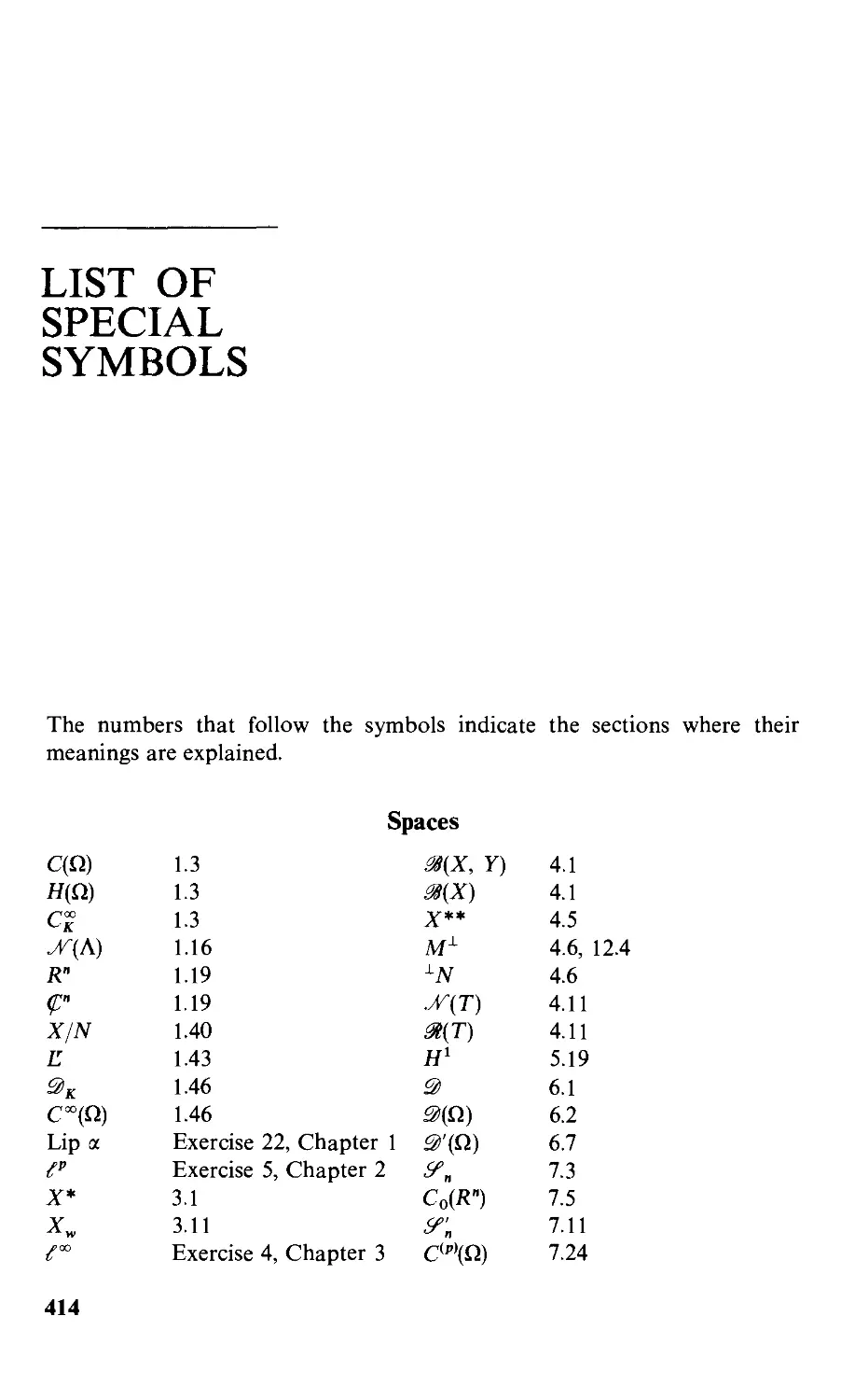
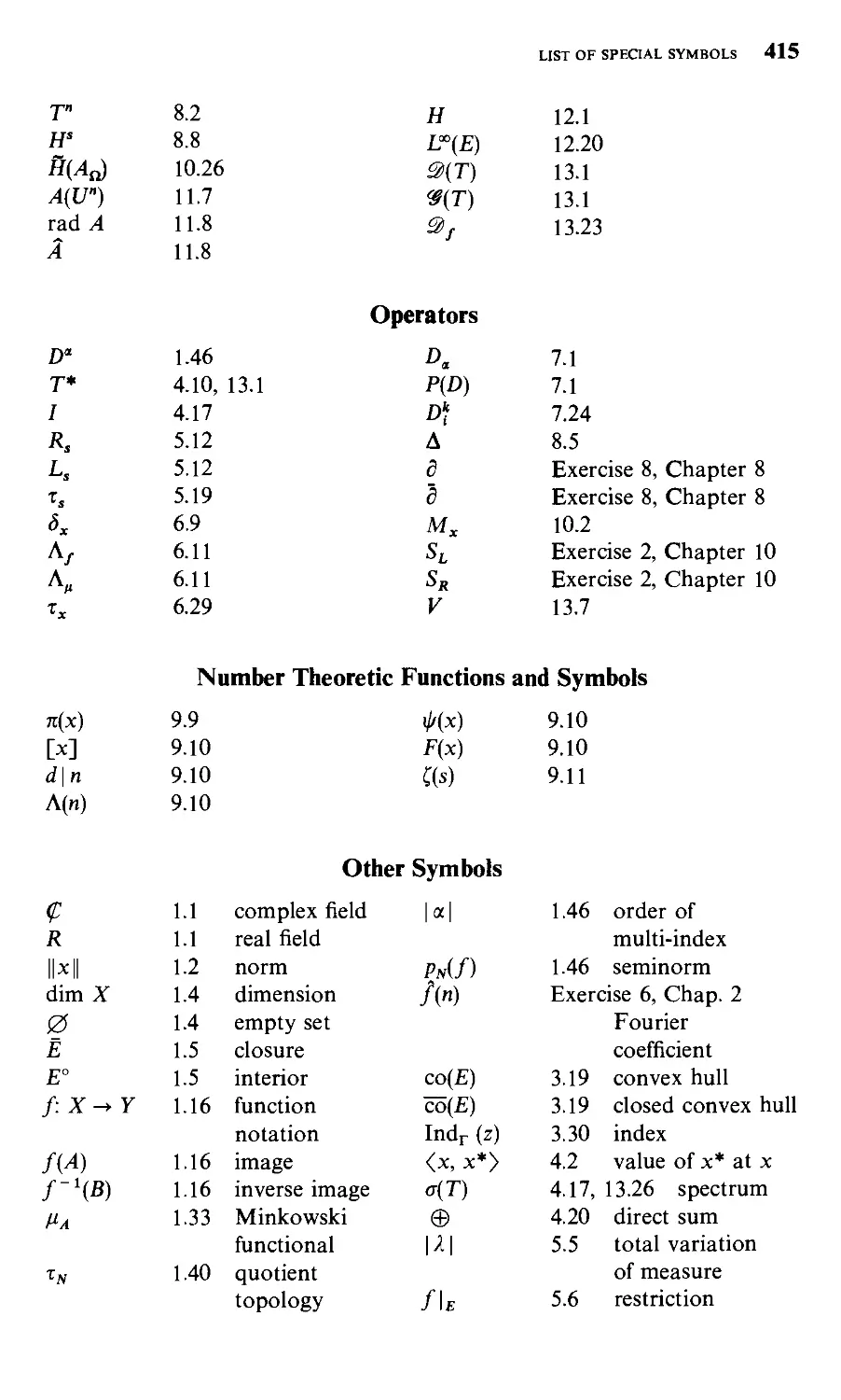
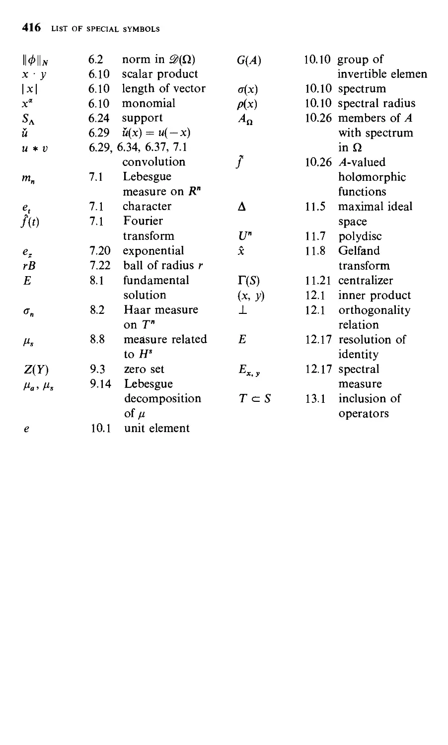
List of Special Symbols 414
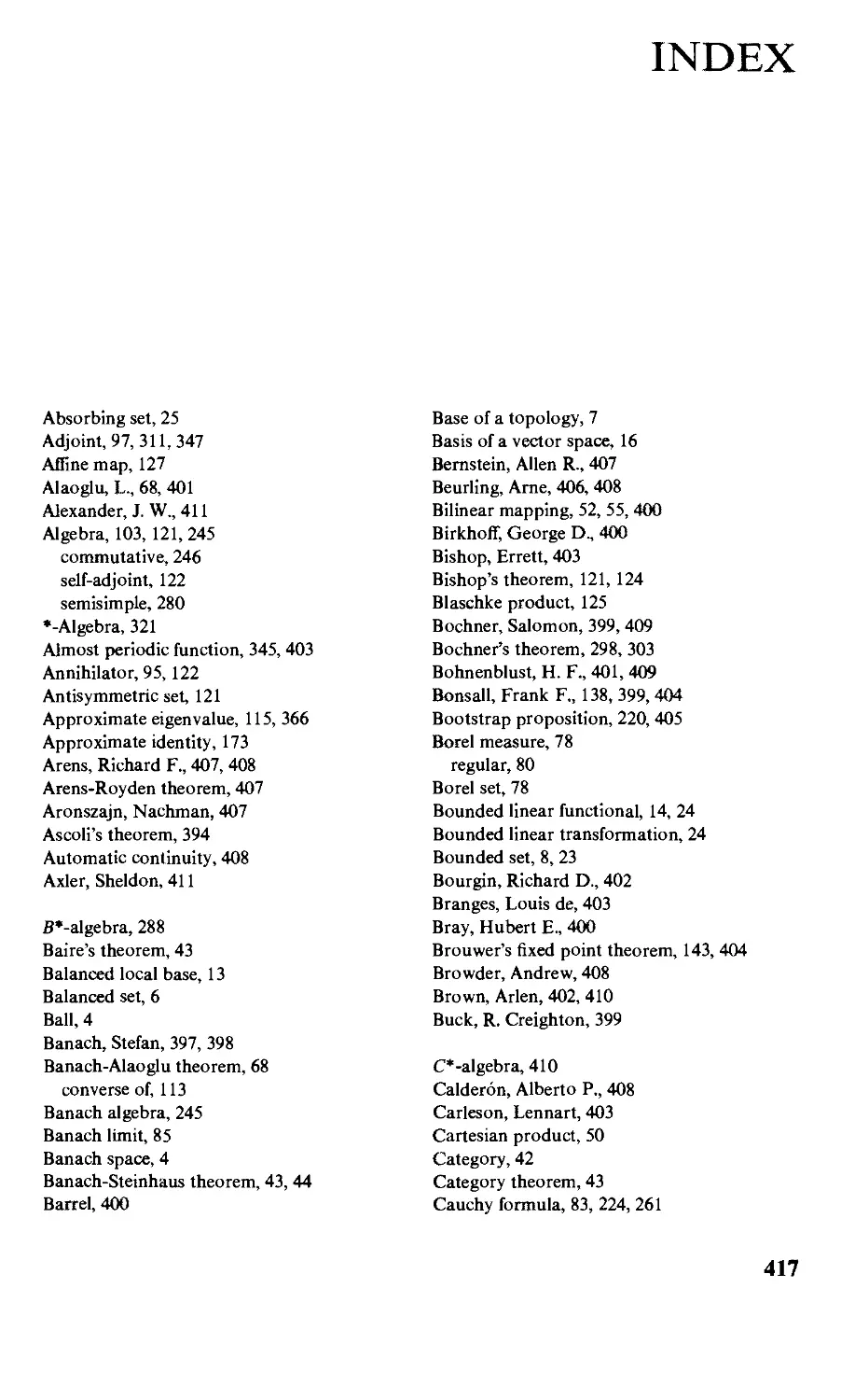
Index 417

PREFACE
Functional analysis is the study of certain topological-algebraic structures
and of the methods by which knowledge of these structures can be applied
to analytic problems.
A good introductory text on this subject should include a presentation
of its axiomatics (i.e., of the general theory of topological vector spaces), it
should treat at least a few topics in some depth, and it should contain some
interesting applications to other branches of mathematics. I hope that the
present book meets these criteria.
The subject is huge and is growing rapidly. (The bibliography in
volume I of [4] contains 96 pages and goes only to 1957.) In order to write
a book of moderate size, it was therefore necessary to select certain areas
and to ignore others. I fully realize that almost any expert who looks at the
table of contents will find that some of his or her (and my) favorite topics
are missing, but this seems unavoidable. It was not my intention to write an
encyclopedic treatise. I wanted to write a book that would open the way to
further exploration.
This is the reason for omitting many of the more esoteric topics that
might have been included in the presentation of the general theory of
topological vector spaces. For instance, there is no discussion of uniform spaces,
of Moore-Smith convergence, of nets, or of filters. The notion of
completeness occurs only in the context of metric spaces. Bornological spaces are
not mentioned, nor are barreled ones. Duality is of course presented, but
not in its utmost generality. Integration of vector-valued functions is treated
strictly as a tool; attention is confined to continuous integrands, with values
in a Frechet space.
Nevertheless, the material of Part I is fully adequate for almost all
applications to concrete problems. And this is what ought to be stressed in
such a course: The close interplay between the abstract and the concrete is
xiii

XIV PREFACE
not only the most useful aspect of the whole subject but also the most
fascinating one.
Here are some further features of the selected material. A fairly large
part of the general theory is presented without the assumption of local
convexity. The basic properties of compact operators are derived from the
duality theory in Banach spaces. The Krein-Milman theorem on the
existence of extreme points is used in several ways in Chapter 5. The theory of
distributions and Fourier transforms is worked out in fair detail and is
applied (in two very brief chapters) to two problems in partial differential
equations, as well as to Wiener's tauberian theorem and two of its
applications. The spectral theorem is derived from the theory of Banach algebras
(specifically, from the Gelfand-Naimark characterization of commutative
B*-algebras); this is perhaps not the shortest way, but it is an easy one. The
symbolic calculus in Banach algebras is discussed in considerable detail; so
are involutions and positive functional.
I assume familiarity with the theory of measure and Lebesgue
integration (including such facts as the completeness of the /f-spaces), with some
basic properties of holomorphic functions (such as the general form of
Cauchy's theorem, and Runge's theorem), and with the elementary
topological background that goes with these two analytic topics. Some other
topological facts are briefly presented in Appendix A. Almost no algebraic
background is needed, beyond the knowledge of what a homomorphism is.
Historical references are gathered in Appendix B. Some of these refer
to the original sources, and some to more recent books, papers, or
expository articles in which further references can be found. There are, of course,
many items that are not documented at all. In no case does the absence of a
specific reference imply any claim to originality on my part.
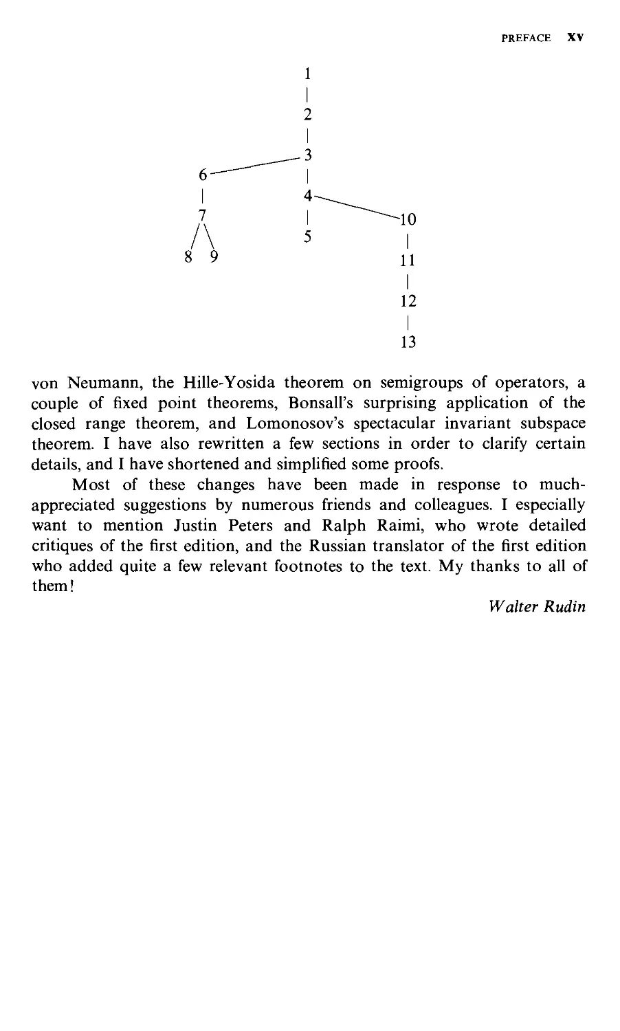
Most of the applications are in Chapters 5, 8, and 9. Some are in
Chapter 11 and in the more than 250 exercises; many of these are supplied
with hints. The interdependence of the chapters is indicated in the diagram
on the following page.
Most of the applications contained in Chapter 5 can be taken up well
before the first four chapters are completed. It has therefore been suggested
that it might be good pedagogy to insert them into the text earlier, as soon
as the required theoretical background is established. However, in order
not to interrupt the presentation of the theory in this way, I have instead
started Chapter 5 with a short indication of the background that is needed
for each item. This should make it easy to study the applications as early as
possible, if so desired.
In the first edition, a fairly large part of Chapter 10 dealt with diff"er-
entiation in Banach algebras. Twenty years ago this (then recent) material
looked interesting and promising, but it does not seem to have led
anywhere, and I have deleted it. On the other hand, I have added a few items
which were easy to fit into the existing text: the mean ergodic theorem of

PREFACE XV
von Neumann, the Hille-Yosida theorem on semigroups of operators, a
couple of fixed point theorems, Bonsall's surprising application of the
closed range theorem, and Lomonosov's spectacular invariant subspace
theorem. I have also rewritten a few sections in order to clarify certain
details, and I have shortened and simplified some proofs.
Most of these changes have been made in response to much-
appreciated suggestions by numerous friends and colleagues. I especially
want to mention Justin Peters and Ralph Raimi, who wrote detailed
critiques of the first edition, and the Russian translator of the first edition
who added quite a few relevant footnotes to the text. My thanks to all of
them!
Walter Rudin

FUNCTIONAL ANALYSIS

PART
I
GENERAL
THEORY

CHAPTER
1
TOPOLOGICAL
VECTOR
SPACES
Introduction
1.1 Many problems that analysts study are not primarily concerned with
a single object such as a function, a measure, or an operator, but they deal
instead with large classes of such objects. Most of the interesting classes
that occur in this way turn out to be vector spaces, either with real scalars
or with complex ones. Since limit processes play a role in every analytic
problem (explicitly or imphcitly), it should be no surprise that these vector
spaces are supplied with metrics, or at least with topologies, that bear some
natural relation to the objects of which the spaces are made up. The
simplest and most important way of doing this is to introduce a norm. The
resulting structure (defined below) is called a normed vector space, or a
normed linear space, or simply a normed space.
Throughout this book, the term vector space will refer to a vector
space over the complex field (^ or over the real field R. For the sake of
completeness, detailed definitions are given in Section 1.4.
1.2 Normed spaces A vector space X is said to be a normed space if to
every x e X there is associated a nonnegative real number ||x||, called the
norm of x, in such a way that

4 PART 1: GENERAL THEORY
(a) ||x + y\\ < \\x\\ + \\y\\ for all x and y in X,
(b) ||ax|l = I a| ||x|| if x e X and a is a scalar,
(c) ||x|| >Oifx #0.
The word " norm" is also used to denote the function that maps x
to ||x||.
Every normed space may be regarded as a metric space, in which the
distance d{x, y) between x and y is ||x — y||. The relevant properties of d are
(i) 0 < d{x, y) < CO for all x and y,
(ii) d{x, y) = 0 if and only if x = y,
(hi) d{x, y) = d{y, x) for all x and y,
(iv) d{x, z) < d{x, y) + d{y, z) for all x, y, z.
In any metric space, the open ball with center at x and radius r is
the set
BXx) = {y: d{x, y)<r}.
In particular, if X is a normed space, the sets
Bi(0) = {x: ||x|l < 1} and Bi(0) = {x: ||xl| < 1}
are the open unit ball and the closed unit ball of X, respectively.
By declaring a subset of a metric space to be open if and only if it is a
(possibly empty) union of open balls, a topology is obtained. (See Section
1.5.) It is quite easy to verify that the vector space operations (addition and
scalar multiplication) are continuous in this topology, if the metric is
derived from a norm, as above.
A Banach space is a normed space which is complete in the metric
defined by its norm; this means that every Cauchy sequence is required to
converge.
1.3 Many of the best-known function spaces are Banach spaces. Let us
mention just a few types: spaces of continuous functions on compact
spaces; the familiar L''-spaces that occur in integration theory; Hilbert
spaces — the closest relatives of euclidean spaces; certain spaces of differen-
tiable functions; spaces of continuous linear mappings from one Banach
space into another; Banach algebras. All of these will occur later on in the
text.
But there are also many important spaces that do not fit into this
framework. Here are some examples:
(a) C(Q), the space of all continuous complex functions oft some open set
n in a euclidean space R".

CHAPTER 1: TOPOLOGICAL VECTOR SPACES ^
(b) H{Q), the space of all holomorphic functions in some open set Q in the
complex plane.
(c) Ck , the space of all infinitely differentiable complex functions on R"
that vanish outside some fixed compact set K with nonempty interior.
(d) The test function spaces used in the theory of distributions, and the
distributions themselves.
These spaces carry natural topologies that cannot be induced by
norms, as we shall see later. They, as well as the normed spaces, are
examples of topological vector spaces, a concept that pervades all of functional
analysis.
After this brief attempt at motivation, here are the detailed definitions,
followed (in Section 1.9) by a preview of some of the results of Chapter 1.
1.4 Vector spaces The letters R and <p will always denote the field of
real numbers and the field of complex numbers, respectively. For the
moment, let O stand for either i? or (T. A scalar is a member of the scalar
field O. A vector space over O is a set X, whose elements are called vectors,
and in which two operations, addition and scalar multiplication, are defined,
with the following familiar algebraic properties:
(a) To every pair of vectors x and y corresponds a vector x + y, in such a
way that
X + y = y + X and x + {y + z) = {x + y) + z;
X contains a unique vector 0 (the zero vector or origin of X) such that
X + 0 = X for every x e X; and to each x e X corresponds a unique
vector — X such that x + (— x) = 0.
(b) To every pair (a, x) with a e O and x e X corresponds a vector ax, in
such a way that
Ix = X, o^iPx) = {a.p)x,
and such that the two distributive laws
a(x + y) = ax + ay, (a + P)x = ax + ^x
hold.
The symbol 0 will of course also be used for the zero element of the
scalar field.
A real vector space is one for which O = i?; a complex vector space is
one for which O = (T. Any statement about vector spaces in which the
scalar field is not explicitly mentioned is to be understood to apply to both
of these cases.

O PART I: GENERAL THEORY
If X is a vector space, A cz X, B cz X, x e X, and A e O, the following
notations will be used;
X + A = {x + a: a e A},
X — A = {x — a: a e A},
A + B = {a + b: a e A, b e B},
XA = [ka: a e A}.
In particular (taking A = — 1), —A denotes the set of all additive inverses of
members of A.
A word of warning: With these conventions, it may happen that 2A #
A + A (Exercise 1).
A set y cz X is called a subspace of X if 7 is itself a vector space (with
respect to the same operations, of course). One checks easily that this
happens if and only if 0 e 7 and
xY + PY czY
for all scalars a and p.
A set C c X is said to be convex if
fC + (1 - f)C cz C (0 < f < 1).
In other words, it is required that C should contain fx + (1 — t)y if x e C,
y e C, and 0 < f < 1.
A set B cz X is said to be balanced if aB cz B for every a e O with
|a|<l.
A vector space X has dimension n (dim X = n) if X has a basis
{mi, ..., M„}. This means that every x e X has a unique representation of the
form
X = ajMi + ■ • • + a„M„ (a; e O).
If dim X = n for some n, X is said to have^nife dimension. If X = {0}, then
dim X = 0.
Example. If X = (T (a one-dimensional vector space over the scalar
field <^, the balanced sets are (T, the empty set 0, and every circular
disc (open or closed) centered at 0. If X = i?-^ (a two-dimensional
vector space over the scalar field R), there are many more balanced
sets; any line segment with midpoint at (0, 0) will do. The point is
that, in spite of the well-known and obvious identification of <P with
R^, these two are entirely different as far as their vector space
structure is concerned.
1.5 Topological spaces A topological space is a set S in which a
collection T of subsets (called open sets) has been specified, with the following

CHAPTER 1: TOPOLOGICAL VECTOR SPACES /
properties: S is open, 0 is open, the intersection of any two open sets is
open, and the union of every collection of open sets is open. Such a
collection T is called a topology on S. When clarity seems to demand it, the
topological space corresponding to the topology t will be written (S, t) rather
than S.
Here is some of the standard vocabulary that will be used, if S and t
are as above.
A set £ c S is closed if and only if its complement is open. The closure
£ of £ is the intersection of all closed sets that contain £. The interior E° of
£ is the union of all open sets that are subsets of £. A neighborhood of a
point p e S is any open set that contains p. {S, t) is a Hausdorff space, and t
is a Hausdorff topology, if distinct points of S have disjoint neighborhoods.
A set X cz S is compact if every open cover of K has a finite subcover. A
collection t' c t is a base for t if every member of t (that is, every open set)
is a union of members of t'. A collection y of neighborhoods of a point
p e S is a local base at p if every neighborhood of p contains a member of y.
If £ c: S and if a is the collection of all intersections E n V, with
Vet, then cr is a topology on £, as is easily verified; we call this the
topology that £ inherits from S.
If a topology T is induced by a metric d (see Section 1.2) we say that d
and T are compatible with each other.
A sequence {x„} in a Hausdorff space X converges to a point x e X
(or lim„^^ x„ = x) if every neighborhood of x contains all but finitely many
of the points x„.
1.6 Topological vector spaces Suppose t is a topology on a vector
space X such that
(a) every point of X is a closed set, and
(b) the vector space operations are continuous with respect to t.
Under these conditions, t is said to be a vector topology on X, and X
is a topological vector space.
Here is a more precise way of stating (a): For every x e X, the set {x}
which has x as its only member is a closed set.
In many texts, (a) is omitted from the definition of a topological
vector space. Since (a) is satisfied in almost every application, and since
most theorems of interest require (a) in their hypotheses, it seems best to
include it in the axioms. [Theorem 1.12 will show that (a) and (b) together
imply that t is a Hausdorff topology.]
To say that addition is continuous means, by definition, that the
mapping
{x,y)^x + y

8 PART I: GENERAL THEORY
of the cartesian product X x X into X is continuous: If X; e X for i = 1,2,
and if F is a neighborhood of Xj + Xj, there should exist neighborhoods V^
of Xj such that
V. + V^ci V.
Similarly, the assumption that scalar multiplication is continuous means
that the mapping
(a, x) -► ax
of O X X into X is continuous: If x e X, a is a scalar, and F is a
neighborhood of ax, then for some r > 0 and some neighborhood H^ of x we have
PW <= V whenever | ^ — a | < r.
A subset £ of a topological vector space is said to be bounded if to
every neighborhood F of 0 in X corresponds a number s > 0 such that
E <= tV for every t > s.
1.7 Invariance Let X be a topological vector space. Associate to each
a e X and to each scalar A # 0 the translation operator T^ and the
multiplication operator M^, by the formulas
r„(x) = a + X, M;i(x) = Ax (x e X).
The following simple proposition is very important:
Proposition. T„ and M^ are homeomorphisms ofX onto X.
PROOF. The vector space axioms alone imply that 7^ and M^ are
one-to-one, that they map X onto X, and that their inverses are T_„
and Mii^, respectively. The assumed continuity of the vector space
operations implies that these four mappings are continuous. Hence
each of them is a homeomorphism (a continuous mapping whose
inverse is also continuous). ////
One consequence of this proposition is that every vector topology t is
translation-invariant (or simply invariant, for brevity): A set £ c: X is open if
and only if each of its translates a -I- £ is open. Thus t is completely
determined by any local base.
In the vector space context, the term local base will always mean a
local base at 0. A local base of a topological vector space X is thus a
collection ^ of neighborhoods of 0 such that every neighborhood of 0
contains a member of ^. The open sets of X are then precisely those that are
unions of translates of members of ^.

CHAPTER 1: TOPOLOGICAL VECTOR SPACES 9
A metric d on a vector space X will be called invariant if
d(x + z, y + z) = d{x, y)
for all X, y, z in X.
1.8 Types of topological vector spaces In the following definitions, X
always denotes a topological vector space, with topology t.
(fl) X is locally convex if there is a local base ^ whose members are
convex.
(b) X is locally bounded if 0 has a bounded neighborhood.
(c) X is locally compact if 0 has a neighborhood whose closure is compact.
(d) X is metrizable if t is compatible with some metric d.
(e) X is an f-space if its topology t is induced by a complete invariant
metric d. (Compare Section 1.25.)
(/) X is a Frechet space if X is a locally convex f-space.
(g) X is normable if a norm exists on X such that the metric induced by
the norm is compatible with t.
(H) Normed spaces and Banach spaces have already been defined (Section
1.2).
(i) X has the Heine-Borel property if every closed and bounded subset of
X is compact.
The terminology of (e) and (/) is not universally agreed upon: In
some texts, local convexity is omitted from the definition of a Frechet space,
whereas others use f-space to describe what we have called Frechet space.
1.9 Here is a list of some relations between these properties of a
topological vector space X.
(a) If X is locally bounded, then X has a countable local base [part (c) of
Theorem 1.15].
(b) X is metrizable if and only if X has a countable local base (Theorem
1.24).
(c) X is normable if and only if X is locally convex and locally bounded
(Theorem 1.39).
(d) X has finite dimension if and only if X is locally compact (Theorems
1.21, 1.22).
(e) If a locally bounded space X has the Heine-Borel property, then X has
finite dimension (Theorem 1.23).

10 PART 1; GENERAL THEORY
The spaces H{ii) and C^ mentioned in Section 1.3 are infinite-
dimensional Frechet spaces with the Heine-Borel property (Sections 1.45,
1.46). They are therefore not locally bounded, hence not normable; they
also show that the converse of (a) is false.
On the other hand, there exist locally bounded f-spaces that are not
locally convex (Section 1.47).
Separation Properties
1.10 Theorem Suppose K and C are subsets of a topological vector space
X, K is compact, C is closed, and K n C = 0. Then 0 has a neighborhood V
such that
{K+V)n{C+V) = 0.
Note that K + V is a union of translates x + V of V {x e K). Thus
X + F is an open set that contains K. The theorem thus implies the
existence of disjoint open sets that contain K and C, respectively.
PROOF. We begin with the following proposition, which will be useful
in other contexts as well:
If W is a neighborhood of 0 in X, then there is a neighborhood U
of 0 which is symmetric {in the sense that U = ~U) and which satisfies
U +U czW.
To see this, note that 0-1-0 = 0, that addition is continuous, and
that 0 therefore has neighborhoods V^, Vj such that V^ + Vjci W. If
then U has the required properties.
The proposition can now be applied to JJ in place of W and
yields a new symmetric neighborhood t/ of 0 such that
JJ + IJ + IJ +V czW.
It is clear how this can be continued.
If X = 0, then K + V = 0, and the conclusion of the theorem
is obvious. We therefore assume that X # 0, and consider a point
X e K. Since C is closed, since x is not in C, and since the topology of
X is invariant under translations, the preceding proposition shows
that 0 has a symmetric neighborhood K, such that x + V^ + V^ + V^
does not intersect C; the symmetry of K, shows then that
(1) ix+V,+ VJ n{C+ VJ = 0.

CHAPTER 1: TOPOLOGICAL VECTOR SPACES 11
Since K is compact, there are finitely many points x^,..., x„m K such
that
Xcz(xj + V;,)u---u(x„+FJ.
Put F = V^i n ■ ■ ■ n V^^. Then
X + F cz 0 (x, + V;^ + F) cz U (x, + K, + V,),
1=1 1=1
and no term in this last union intersects C + F, by (1). This completes
the proof ////
Since C + F is open, it is even true that the closure of X + F does not
intersect C + F; in particular, the closure of X + F does not intersect C.
The following special case of this, obtained by taking K = {0}, is of
considerable interest.
1.11 Theorem If^ is a local base for a topological vector space X, then
every member of 0S contains the closure of some member of 3S.
So far we have not used the assumption that every point of X is a
closed set. We now use it and apply Theorem 1.10 to a pair of distinct
points in place of K and C. The conclusion is that these points have disjoint
neighborhoods. In other words, the Hausdorff separation axiom holds:
1.12 Theorem Every topological vector space is a Hausdorff space.
We now derive some simple properties of closures and interiors in a
topological vector space. See Section 1.5 for the notations E and E°.
Observe that a point p belongs to E if and only if every neighborhood of p
intersects E.
1'13 Theorem Let X be a topological vector space.
{a) IfAcX then A = f] {A + V), where V runs through all neighborhoods
ofO.
(b) If A cz X and B cz X, then A + B cz A + B.
(c) // Y is a subspace ofX, so is Y.
id) IfC is a convex subset ofX, so are C and C°.
(e) IfB is a balanced subset ofX, so is B; if also 0 e B° then B° is balanced.
if) IfE is a bounded subset ofX, so is E.

12 PART I: GENERAL THEORY
PROOF, (a) X e A if and only if (x + F) n A # 0 for every
neighborhood V of 0, and this happens if and only if x e A — F for every such
V. Since — F is a neighborhood of 0 if and only if V is one, the proof
is complete.
(b) Take a e A, b e B; let W be a neighborhood of a + b. There
are neighborhoods W^ and W2 of a and b such that Wi + W2C: W.
There exist x e A n W^ and y e B n Wj, since a e A and b e B. Then
X + y lies in {A + B) n W, so that this intersection is not empty.
Consequently, a + b e A + B.
(c) Suppose a and P are scalars. By the proposition in Section
1.7, aY= aY if a # 0; if a = 0, these two sets are obviously equal.
Hence it follows from (b) that
(iY+ PY= xY + PY ciaY + PY cz Y;
the assumption that 7 is a subspace was used in the last inclusion.
The proofs that convex sets have convex closures and that
balanced sets have balanced closures are so similar to this proof of (c)
that we shall omit them from (d) and (e).
(d) Since C° <= C and C is convex, we have
tC° +{l - t)C° cz C
if 0 < f < 1. The two sets on the left are open; hence so is their sum.
Since every open subset of C is a subset of C°, it follows that C° is
convex.
(e) If 0 < I a I < 1, then aB° = (aB)°, since x-<■ ax is a homeo-
morphism. Hence aB° c xB c B, since B is balanced. But aB° is open.
So aB° cz B°. If B° contains the origin, then a.B° cz B° even for a = 0;
(/) Let F be a neighborhood of 0. By Theorem 1.11, Wcz V for
some neighborhood W of 0. Since E is bounded, E cz tW iox all
sufficiently large t. For these t, we have E cz tWcz tV. ///
1.14 Theorem In a topological vector space X,
(a) every neighborhood ofO contains a balanced neighborhood ofO, and
(b) every convex neighborhood of 0 contains a balanced convex
neighborhood 0/0.
PROOF, (a) Suppose t/ is a neighborhood of 0 in X. Since scalar
multiplication is continuous, there is a <5 > 0 and there is a neighborhood
F of 0 in X such that aV cz U whenever | a | < <5. Let W be the union
of all these sets xV. Then H^ is a neighborhood of 0, W is balanced,
and W czU.

CHAPTER 1: TOPOLOGICAL VECTOR SPACES 13
(b) Suppose t/ is a convex neighborhood of 0 in X. Let
/4 = n at/, where a ranges over the scalars of absolute value 1.
Choose W as in part (a). Since W is balanced, a~'H^= W when
I a I = 1; hence W a at/. Thus ]V a A, which implies that the interior
A° of /4 is a neighborhood of 0. Clearly A° a JJ. Being an intersection
of convex sets, A is convex; hence so is A°. To prove that A° is a
neighborhood with the desired properties, we have to show that A° is
balanced; for this it suffices to prove that A is balanced. Choose r and
P so that 0 < r < 1,1 i? I = 1. Then
rfiA = f) rfia.V = f) rat/.
Since at/ is a convex set that contains 0, we have rat/ c at/. Thus
r^A a A, which completes the proof. ////
Theorem 1.14 can be restated in terms of local bases. Let us say that a
local base 0S is balanced if its members are balanced sets, and let us call ^
convex if its members are convex sets.
Corollary
(a) Every topological vector space has a balanced local base.
(b) Every locally convex space has a balanced convex local base.
Recall also that Theorem 1.11 holds for each of these local bases.
1.15 Theorem Suppose V is a neighborhood ofO in a topological vector
space X.
{a) IfO < ri < rj < ■ ■ ■ and r„ -> oo as n -► oo, then
X= 0 r„V.
(b) Every compact subset KofX is bounded.
(c) //<5i >,52 > ■■■ and <5„->0 as n -> 00, and if V is bounded, then the
collection
{<5„F:n = l,2, 3, ...}
is a local base for X.
PROOF, (a) Fix X e X. Since a -► ax is a continuous mapping of the
scalar field into X, the set of all a with ax e F is open, contains 0,
hence contains l/r„ for all large n. Thus (l/r„)x e F, or x e r„ V, for
large n.

14 PART I: GENERAL THEORY
(b) Let H^ be a balanced neighborhood of 0 such that W cz V.
By (a),
00
X cz [j nW.
n=l
Since K is compact, there are integers nj < • • • < n^ such that
K c n^W ^ ■ ■ ■ ^ n,W = n,W.
The equality holds because W is balanced. If f > n^, it follows that
KctWc tV.
(c) Let t/ be a neighborhood of 0 in X. If V is bounded, there
exists s > 0 such that V a tU for all f > s. If n is so large that s6„ < 1,
it follows that V a (l/<5„)t/. Hence U actually contains all but finitely
many of the sets <5„ V. ////
Linear Mappings
1.16 Definitions When X and Y are sets, the symbol
f:X^Y
will mean that / is a mapping of X into Y. If A cz X and B cz Y, the image
f{A) of A and the inverse image or preimage f ~ '(B) of B are defined by
f(A) = {/(x): X e A}, f-\B) = {x:f{x) e B}.
Suppose now that X and Y are vector spaces over the same scalar
field. A mapping A: X -► 7 is said to be linear if
A(ax + Py) = ocAx + fiAy
for all X and y in X and all scalars a and p. Note that one often writes Ax,
rather than A(x), when A is linear.
Linear mappings of X into its scalar field are called linear functionals.
For example, the multiplication operators M^ of Section 1.7 are linear,
but the translation operators 7^ are not, except when a = 0.
Here are some properties of linear mappings A: X -<-Y whose proofs
are so easy that we omit them; it is assumed that A cz X and B cz Y:
(a) A0 = 0.
(b) If A is a subspace (or a convex set, or a balanced set) the same is true
ofA(A).
(c) If B is a subspace (or a convex set, or a balanced set) the same is true
of A"'(B).

CHAPTER 1: TOPOLOGICAL VECTOR SPACES 15
(d) In particular, the set
A-i({0}) = {xeX:Ax = 0} = A^{A)
is a subspace of X, called the null space of A.
We now turn to continuity properties of linear mappings.
1.17 Theorem Let X and Y be topological vector spaces. If A: X ^ Y is
linear and continuous at 0, then A is continuous. In fact, A is uniformly
continuous, in the following sense: To each neighborhood WofO in Y corresponds a
neighborhood VofO in X such that
y — X e V implies Ay — Ax e W.
PROOF. Once W is chosen, the continuity of A at 0 shows that
AV cz W foT some neighborhood V of 0. If now y — x e F, the
linearity of A shows that Ay — Ax = A(y — x) e W. Thus A maps the
neighborhood x + F of x into the preassigned neighborhood Ax + H^
of Ax, which says that A is continuous at x. ////
1.18 Theorem Let A be a linear functional on a topological vector space
X. Assume Ax # Ofor some x e X. Then each of the following four properties
implies the other three:
(a) A is continuous.
{b) The null space ^'^{A) is closed.
(c) .tXA) is not dense in X.
(d) A is bounded in some neighborhood V ofO.
PROOF. Since J^{A) = A" '({0}) and {0} is a closed subset of the scalar
field <1>, (a) implies (b). By hypothesis, yt^^A) # X. Hence (b) implies (c).
Assume (c) holds; i.e., assume that the complement of .yV{A) has
nonempty interior. By Theorem 1.14,
(1) {x+V)n J^\A) = 0
for some x e X and some balanced neighborhood F of 0. Then A F is
a balanced subset of the field <1>. Thus either A F is bounded, in which
case (d) holds, ot AV = (t>. In the latter case, there exists y 6 F such
that Ay = —Ax, and so x + y e J^{A), in contradiction to (1). Thus
(c) implies (d).
Finally, if (d) holds then | Ax | < M for all x in F and for some
M < 00. If r > 0 and if H^ = {r/M)V, then | Ax | < r for every x in W.
Hence A is continuous at the origin. By Theorem 1.17, this implies (a).
nil

16 PART I: GENERAL THEORY
Finite-Dimensional Spaces
1.19 Among the simplest Banach spaces are R" and (^", the standarr
n-dimensional vector spaces over R and (T, respectively, normed by mean
of the usual euclidean metric: If, for example,
z = (zi, ..., z„) (Zje^Z:)
is a vector in <P", then
\\z\\={\z,\' + --- + \z„\y.
Other norms can be defined on <P". For example,
||z|| =|zj+ --- + |z„| or ||z|| =max(|zi|: 1 <f <n).
These norms correspond, of course, to different metrics on ^" (when n > 1)
but one can see very easily that they all induce the same topology on (P".
Actually, more is true.
If X is a topological vector space over <p, and dim X = n, then every
basis of X induces an isomorphism of X onto (P". Theorem 1.21 will prove
that this isomorphism must be a homeomorphism. In other words, this says
that the topology of (P" is the only vector topology that an n-dimensional
complex topological vector space can have.
We shall also see that finite-dimensional subspaces are always closed
and that no infinite-dimensional topological vector space is locally
compact.
Everything in the preceding discussion remains true with real scalars
in place of complex ones.
1.20 Lemma If X is a complex topological vector space andf: (P" —■> X is
linear, then f is continuous.
PROOF. Let {e^, ..., e„} be the standard basis of (P": The fcth
coordinate of e,, is 1, the others are 0. Put u^ =/(e/c)> for ^ = !> ..., n. Then
/(z) = z^u^ + ••• + z„M„ for every z = (zj, ..., z„) in f". Every z^ is a
continuous function of z. The continuity of/is therefore an immediate
consequence of the fact that addition and scalar multiplication are
continuous in X. ////
1.21 Theorem // n is a positive integer and Y is an n-dimensional sub-
space of a complex topological vector space X, then
(a) every isomorphism of<P'' onto Y is a homeomorphism, and
(b) Y is closed.

CHAPTER 1: TOPOLOGICAL VECTOR SPACES 17
PROOF. Let S be the sphere which bounds the open unit ball B of
^". Thus z e S if and only if E|z;|^ = 1, and z e B if and only if
E|z,|'<l.
Suppose f:f"-^Y is an isomorphism. This means that / is
linear, one-to-one, and/(^") = Y. Put K =/(5). Since/is continuous
(Lemma 1.20), K is compact. Since/(0) = 0 and/is one-to-one, 0 ^ K,
and therefore there is a balanced neighborhood F of 0 in X which
does not intersect K. The set
E=f-'{V)=f-'{V n Y)
is therefore disjoint from S. Since/is linear, E is balanced, and hence
connected. Thus E <^ B, because 0 e £, and this implies that the linear
map / ~' takes V n Y into B. Since / ~' is an n-tuple of linear
functional on Y, the implication (d) -^ (a) in Theorem 1.18 shows that/ ~'
is continuous. Thus/is a homeomorphism.
To prove (b), choose p e Y, and let / and F be as above. For
some t > 0,p e tV,so that p lies in the closure of
Y n{tV) ^f(tB) ^f(tB).
Being compact, f{tB) is closed in X. Hence p ef(tB) <= Y, and this
proves that Y=Y. ////
1.22 Theorem Every locally compact topological vector space X has
finite dimension.
PROOF. The origin of X has a neighborhood F whose closure is
compact. By Theorem 1.15, F is bounded, and the sets 2"F (n = 1, 2,
3,...) form a local base for X.
The compactness of F shows that there exist x^, ..., x^ in X
such that
Fc(xj+iF)u •■■u(.x„ + iF).
Let Y be the vector space spanned by x^, ..., x„. Then dim Y <m.
By Theorem 1.21, 7 is a closed subspace of X.
Since F <= Y + ^V and since 17 = 7 for every scalar A # 0, it
follows that
iV ^Y + iV
so that
F<=y + iF<=y+y + iF = 7 + i:F.

18 PART I: GENERAL THEORY
If we continue in this way, we see that
CO
Fc n {Y + 2-"V).
n= 1
Since {2 "F} is a local base, it now follows from (a) of Theorem 1.13
that F <= K But y= y. Thus F <= 7, which implies that fcF <= 7 for
k = 1, 2, 3, Hence Y = X,hy (a) of Theorem 1.15, and
consequently dim X <m. ////
1.23 Theorem If X is a locally bounded topological vector space with the
Heine-Borel property, then X has finite dimension.
PROOF. By assumption, the origin of X has a bounded neighborhood
F. Statement (/) of Theorem 1.13 shows that Fis also bounded. Thus
Fis compact, by the Heine-Borel property. This says that X is locally
compact, hence finite-dimensional, by Theorem 1.22.
Metrization
We recall that a topology t on a set X is said to be metrizable if there is a
metric d on X which is compatible with t. In that case, the balls with radius
1/n centered at x form a local base at x. This gives a necessary condition
for metrizability which, for topological vector spaces, turns out to be also
sufficient.
1.24 Theorem If X is a topological vector space with a countable local
base, then there is a metric d on X such that
(a) d is compatible with the topology ofX,
(b) the open balls centered at 0 are balanced, and
(c) d is invariant: d{x -\- z,y -\- z) = d(x, y)for x, y, z e X.
If, in addition, X is locally convex, then d can be chosen so as to satisfy
(a), (b), (c), and also
(d) all open balls are convex.
PROOF. By Theorem 1.14, X has a balanced local base {F„} such that
(1) V„^, + V„^, + V„^, + V„^,^K (n + 1.2, 3,...);
when X is locally convex, this local base can be chosen so that each V„
is also convex.

CHAPTER 1. TOPOLOGICAL VECTOR SPACES 19
Let D be the set of all rational numbers r of the form
CO
(2) r= Sc„(r)2-",
n= 1
where each of the "digits" c,(r) is 0 or 1 and only finitely many are 1.
Thus each r e D satisfies the inequalities 0 < r < 1.
Put A{r) = X \ir > 1; for any r e D, define
(3) A{r) = c,{r)V, + c,(r)F, + c,{r)V, + • • •.
Note that each of these sums is actually finite. Define
(4) f{x) = M{r:xeA(r)} {x e X)
and
(5) d{x, y) =f{x - y) {x e X, y e X).
The proof that this d has the desired properties depends on the
inclusions
(6) A{r) + A{s) <= A{r + s) {r e D, s e D).
Before proving (6), let us see how the theorem follows from it.
Since every A{s) contains 0, (6) imples
(7) A{r) <= A{r) + A{t - r) <= A{t) if r < t.
Thus {A{r)} is totally ordered by set inclusion. We claim that
(8) /(x + y) < f(x) + /(y) (xeX,ye X).
In the proof of (8) we may, of course, assume that the right side is < 1.
Fix £ > 0. There exist r and s in D such that
f{x) < r, f{y) <s, r + s <f{x) +/(y) + e.
Thus X e A{r), y e A{s), and (6) implies x + y e A{r + s). Now (8)
follows, because
f{x + y)<r + s <f{x) +/(y) + e,
and e was arbitrary.
Since each A{r) is balanced, f{x) =/( —x). It is obvious that
/(0) = 0. If x#0, then x ^ F„ =/4(2'") for some n, and so
fix) > 2-" > 0.
These properties of/show that (5) defines a translation-invariant
metric d on X. The open balls centered at 0 are the open sets
(9) BlO) = {x:f{x)<5}=\jA{r).
If <5 < 2"", then 5^(0) <= F„. Hence {£^(0)} is a local base for the
topology of X. This proves (a). Since each A{r) is balanced, so is each B^{0).

20 PART I: GENERAL THEORY
If each F„ is convex, so is each A{r), and (9) implies that the same is
true of each 8^(0), hence also of each translate of 8^(0).
We turn to the proof of (6). If r + s > 1, then A{r + s) = X and
(6) is obvious. We may therefore assume that r + s < 1, and we will
use the following simple proposition about addition in the binary
system of notation:
// r, s, and r + s are in D and c„{r) + c„{s) # c„{r + s) for some n,
then at the smallest n where this happens we have c„(r) = cj^s) = 0,
c„(r + s) = 1.
Put a„ = c„(r), p„ = c„(s), y„ = c„(r + s). If a„ + ^„ = y„ for all n
then (3) shows that A{r) + A{s) = A{r + s). In the other case, let N be
the smallest integer for which o^n + Pn ^Jn- Then, as mentioned
above, a^ = ^^ = 0, y^ = 1. Hence
A{r)^cc,V, +--- + a^_iF^_i + F^+i + K^ + 2 + ---
caiFi + ••• +a^_iF^_i + F^+i + F^+i.
Likewise
A{s) ^ P,V, + ■■■ + P„^,V^., + V^^, + V^^,.
Since a„ + ^„ = y„ for all n < N, (1) now leads to
A{r) + A{s)^y,V, + • • • + y^v-i K.-i + Vn ^ A{r + s)
because y^ = 1. ////
1.25 Cauchy sequences (a) Suppose d is a metric on a set X. A
sequence {x„} in X is a Cauchy sequence if to every £ > 0 there corresponds
an integer N such that d{x^, x„) < e whenever m > N and n > N. If every
Cauchy sequence in X converges to a point of X, then d is said to be a
complete metric on X.
(b) Let T be the topology of a topological vector space X. The notion
of Cauchy sequence can be defined in this setting without reference to any
metric: Fix a local base ^ for t. A sequence {x„} in X is then said to be a
Cauchy sequence if to every V e 3S corresponds an N such that x„ — x„ e F
if n > N and m > N.
It is clear that different local bases for the same t give rise to the same
class of Cauchy sequences.
(c) Suppose now that A' is a topological vector space whose topology
T is compatible with an invariant metric d. Let us temporarily use the terms
d-Cauchy sequence and t-Cauchy sequence for the concepts defined in (a)
and {b\ respectively. Since
d{Xn,xJ = d{x„-x„,0),

CHAPTER 1: TOPOLOGICAL VECTOR SPACES 21
and since the d-balls centered at the origin form a local base for t, we
conclude:
A sequence {x„} in X is a d-Cauchy sequence if and only if it is a
x-Cauchy sequence.
Consequently, any two invariant metrics on X that are compatible
with T have the same Cauchy sequences. They clearly also have the same
convergent sequences (namely, the r-convergent ones). These remarks prove
the following fact:
If d^ and ^2 a^^ invariant metrics on a vector space X which induce the
same topology on X, then
(a) di and dj ^ove the same Cauchy sequences, and
(b) di is complete if and only if d2 is complete.
Invariance is needed in the hypothesis (Exercise 12).
The following " dilation principle " will be used several times.
T.26 Theorem Suppose that {X, d^) and {Y, dj) ore metric spaces, and
{X, di) is complete. If E is a closed set in X, f:E-^Y is continuous, and
d2{f{x'),f{x"))>d,{x',x")
for all x', x" e E, thenf(E} is closed.
PROOF. Pick y ef{E). There exist points x„ e £ so that y = lim /(x„).
Thus {/(x„)} is Cauchy in Y. Our hypothesis implies therefore that
{x„} is Cauchy in X. Being a closed subset of a complete metric space,
E is complete; hence there exists x — lim x„ in E. Since/is
continuous,
/(x) = lim /(x„) = y.
Thus y ef{E). ////
1.27 Theorem Suppose Y is a subspace of a topological vector space X,
and Y is an F-space (in the topology inherited from X). Then Y is a closed
subspace ofX.
PROOF. Choose an invariant metric d on Y, compatible with its
topology. Let
Bi/„ = |ye Y:d{y,0)<^,

22 PART I: GENERAL THEORY
let U„ be a neighborhood of 0 in X such that Y n U„ = B^/^, and
choose symmetric neighborhoods F„ of 0 in X such that F„ + F„ <= [/
and F„+icF„.
Suppose X e Y, and define
E„=Yn{x+K) (n = l, 2, 3,...).
If yi e £„ and yj ^ ^n. then yj — yj lies in 7 and also in V„+ V„cz
U„, hence in B^^. The diameters of the sets £„ therefore tend to O.
Since each £„ is nonempty and since Y is complete, it follows that the
y-closures of the sets £„ have exactly one point yo in common.
Let H^ be a neighborhood of 0 in X, and define
F„=Y n{x + W n F„).
The preceding argument shows that the y-closures of the sets f „ have
one common point y^,. But F^ (^ E^. Hence yw = Vo- Since f„ cr:
X + H^, it follows that yo lies in the X-closure of x + W, for every W.
This implies yo = x. Thus x e Y. This proves that Y= Y. ////
The following simple facts are sometimes useful.
1.28 Theorem
(fl) Ifd is a translation-invariant metric on a vector space X then
d(nx, 0) < nd{x, 0)
for every x e X and for n = 1, 2, 3,
(b) If {x„} is a sequence in a metrizable topological vector space X and if
x„~>-0 as n —>■ CO, then there are positive scalars y„ such that y^-^ co and
PROOF. Statement (a) follows from
n
d{nx, 0) < X d{kx, {k - l)x) = nd{x, 0).
k= 1
To prove (b), let d be a metric as in (a), compatible with the
topology of X. Since d{x„, 0) -^ 0, there is an increasing sequence of
positive integers n,, such that d{x„ ,0)<k~^ if n>n^. Put y„= l if
n < n^; put y„ = kit n,,< n < n,,+ i. For such n,
d{y„x„, 0) = d{kx„, 0) < kd{x„, 0) < k~\
Hence )»„ x„ -^ 0 as n -^ oo. ////

CHAPTER 1: TOPOLOGICAL VECTOR SPACES 23
Boundedness and Continuity
1.29 Bounded sets The notion of a bounded subset of a topological
vector space X was defined in Section 1.6 and has been encountered several
times since then. When X is metrizable, there is a possibility of
misunderstanding, since another very familiar notion of boundedness exists in metric
spaces.
If d is a metric on a set X, a set £ <= X is said to be d-bounded if there
s a number M < go such that d{z, y) < M for all x and y in E.
If X iis a topological vector space with a compatible metric d, the
bounded sets and the d-bounded ones need not be the same, even if d is
invariant. For instance, if d is a metric such as the one constructed in
Theorem 1.24, then X itself is d-bounded (with M = 1) but, as we shall see
presently, X cannot be bounded, unless X = {0}. If X is a normed space
and d is the metric induced by the norm, then the two notions of
boundedness coincide; but if d is replaced by d^ = d/{l + d) (an invariant
metric which induces the same topology) they do not.
Whenever bounded subsets of a topological vector space are
discussed, it will be understood that the definition is as in Section 1.6: A set E is
bounded if, for every neighborhood V of 0, we have E (^ tV for all
sufficiently large t.
We already saw (Theorem 1.15) that compact sets are bounded. To see
another type of example, let us prove that Cauchy sequences are bounded
(hence convergent sequences are bounded): If {x„} is a Cauchy sequence in X,
and V and W are balanced neighborhoods of 0 with V + V (^ W, then
[part {b) of Section 1.25] there exists N such that x„ e x^ + F for all n> N.
Take s > I so that x^, e sV. Then
x„esV + V'^sV+ sV'^sW {n > N).
Hence x„ s tH/ for all n > 1, if t is sufficiently large.
Also, closures of bounded sets are bounded (Theorem 1.13).
On the other hand, if x # 0 and E = {nx: n = 1, 2, 3, ...}, then E is
not bounded, because there is a neighborhood F of 0 that does not contain
x; hence nx is not in nF; it follows that no nF contains E.
Consequently, no subspace ofX {other than {0}) can be bounded.
The next theorem characterizes boundedness in terms of sequences.
'•30 Theorem The following two properties of a set E in a topological
vector space are equivalent:
(") E is bounded.
^"1 If {x„} is a sequence in E and {a„} is a sequence of scalars such that
("n -*• 0 fls n -^ 00, then a„ x„ -^ 0 as n -^ oo.

24 PART I: GENERAL THEORY
PROOF. Suppose E is bounded. Let F be a balanced neighborhood
of 0 in X. Then £ <= tF fbr some t. If x„ e £ and a„ ->■ 0, there exists
N such that | a„11 < 1 if n > N. Since r^E ^ V and F is balanced,
a„ x„ e F for all n > N. Thus a„ x„ -^ 0.
Conversely, if £ is not bounded, there is a neighborhood F of 0
and a sequence r„ -^ oo such that no r„ F contains £. Choose x„ e £
such that x„ ^ r„ F. Then no r~'x„ is in F, so that {r~'x„} does not
converge to 0. ////
1.31 Bounded linear transformations Suppose X and Y are
topological vector spaces and A: X -^ 7 is linear. A is said to be bounded if A maps
bounded sets into bounded sets, i.e., if A(£) is a bounded subset of Y for
every bounded set £ <= X.
This definition conflicts with the usual notion of a bounded function
as being one whose range is a bounded set. In that sense, no linear function
(other than 0) could ever be bounded. Thus when bounded linear mappings
(or transformations) are discussed, it is to be understood that the definition
is in terms of bounded sets, as above.
1.32 Theorem Suppose X and Y are topological vector spaces and
A: X ~>^ Y is linear. Among the following four properties of A, the implications
{a)-^{b)-^{c)
hold. IfX is metrizable, then also
(c)-^(^-^(fl),
so that all four properties are equivalent.
(a) A is continuous.
(b) A is bounded.
(c) //x„ —>■ 0 then {Ax„: n = 1, 2, 3,...} is bounded.
(d) If x„-^0 then Ax„-^0.
Exercise 13 contains an example in which (b) holds but (a) does not.
PROOF. Assume (a), let £ be a bounded set in X, and let H^ be a
neighborhood of 0 in Y. Since A is continuous (and AO = 0) there is a
neighborhood F of 0 in X such that A(F) <= W. Since £ is bounded,

CHAPTER 1: TOPOLOGICAL VECTOR SPACES 25
£ <= tF for all large t, so that
A(£) <= A{tV) = tA{V) <= tW.
This shows that A(£) is a bounded set in Y.
Thus (a) -^ (b). Since convergent sequences are bounded,
Assume now that X is metrizable, that A satisfies (c), and that
x„ -^ 0. By Theorem 1.28, there are positive scalars y„ -^ oo such that
y„ x„ -^ 0. Hence {A(y„ x„)} is a bounded set in Y, and now Theorem
1.30 implies that
Ax„ =y„"''A(y„x„)-^0 as n~>-co.
Finally, assume that (a) fails. Then there is a neighborhood W of
0 in y such that A~'(H^) contains no neighborhood of 0 in X. If X
has a countable local base, there is therefore a sequence {x„} in X so
that x„ -^ 0 but Ax„ ^ W. Thus (d) fails. ////
Seminorms and Local Convexity
1.33 Definitions A seminorm on a vector space X is a real-valued
function p on X such that
(a) p{x + y)< p{x) + piy) and
(b) piax) = I a I p{x)
for all X and y in X and all scalars a.
Property (a) is called subadditivity. Theorem 1.34 will show that a semi-
norm p is a norm if it satisfies
(c) p{x) # 0 if X # 0.
A family 0' of seminorms on X is said to be separating if to each x # 0
corresponds at least one p e ^ with p(x) # 0.
Next, consider a convex set A <= X which is absorbing, in the sense
that every x e X lies in tA for some f = t(x) > 0. [For example, (a) of
Theorem 1.15 implies that every neighborhood of 0 in a topological vector
space is absorbing. Every absorbing set obviously contains 0.] The
Minkowski functional ^^ of A is defined by
^^(x) = inf {t > 0: r 'x e A} (x e X).
Note that ^^(x) < oo for all x e X, since A is absorbing. The seminorms on
■^ will turn out to be precisely the Minkowski functional of balanced
convex absorbing sets.

26 PART I: GENERAL THEORY
Seminorms are closely related to local convexity, in two ways: In
every locally convex space there exists a separating family of continuous
seminorms. Conversely, if ^ is a separating family of seminorms on a vector
space X, then 0* can be used to define a locally convex topology on X with
the property that every p e ^ is continuous. This is a frequently used
method of introducing a topology. The details are contained in Theorems
1.36 and 1.37.
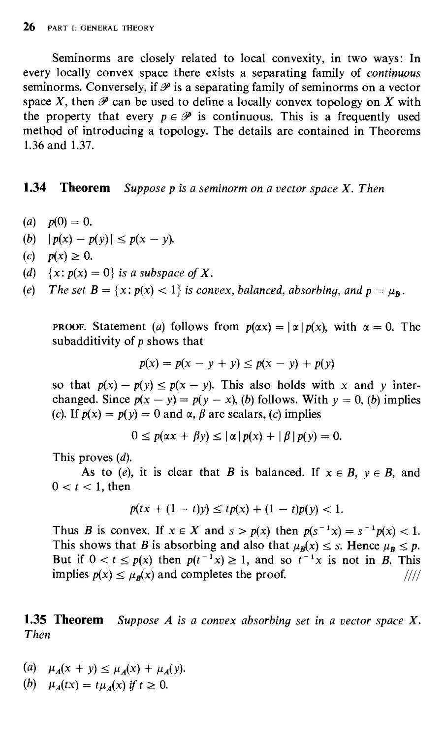
1.34 Theorem Suppose p is a seminorm on a vector space X. Then
(a) p(0) = 0.
(b) \p{x)-p{y)\<p{x-y).
(c) p{x)>0.
(d) {x: p{x) = 0} is a subspace ofX.
(e) The set B = {x: p{x) < 1} is convex, balanced, absorbing, and p == Hg-
PROOF. Statement (a) follows from p(ax) = | a | p{x), with a = 0. The
subadditivity of p shows that
p(x) = p(x - y + y) < p(x - y) + p(y)
so that p{x) — p(y) < p{x — y). This also holds with x and y
interchanged. Since p{x — y) = p(y — x), (b) follows. With y = 0, (b) implies
(c). If p{x) — p(y) = 0 and a, ^ are scalars, (c) implies
0 < p(ax + ^y) < |a|p(x) + |^|p(y) = 0.
This proves {d).
As to {e), it is clear that B is balanced. If x e B, y e B, and
0 < t < 1, then
p{tx + (1 - i)y) < tp{x) + (1 - t)p{y) < 1.
Thus B is convex. If x e X and s > p{x) then p(s~ 'x) = s'^p{x) < 1.
This shows that B is absorbing and also that ^^x) < s. Hence Hg < p.
But if 0 < t < p{x) then p(t"'x) > 1, and so t~'x is not in B. This
implies p{x) < fx^x) and completes the proof ////
1.35 Theorem Suppose A is a convex absorbing set in a vector space X.
Then
(a) t^Aix + y)< HAix) + tiAiy)-
if>) HAitx) = tn^ix) if t > 0.

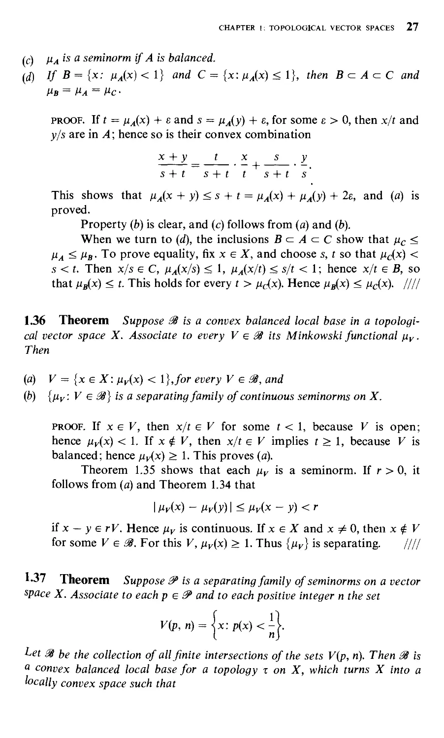
CHAPTER 1: TOPOLOGICAL VECTOR SPACES 27
(c) liji isaseminorm if A is balanced.
{dj If B = {x: ^^(x) < 1} and C = {x: n^{x) < 1}, then B <= A <= C and
PROOF. If t = ^x(x) + £ and s = ^^(y) + e, for some £ > 0, then x/t and
y,'s are in A; hence so is their convex combination
x + y t
X S
t s + t
y
s
s + t s + t
This shows that fi^{x + y) < s + t = //^(x) + //^(y) + 2e, and (a) is
proved.
Property (b) is clear, and (c) follows from (a) and (b).
When we turn to (d), the inclusions B <= A <= C show that //^ <
/"^ < //j. To prove equality, fix x e X, and choose s, t so that //c(^) <
s < t. Then x/s e C, //^(x/s) < 1, //^(x/t) < s/f < 1; hence x/t e B, so
that //j(x) < t. This holds for every t > fidx). Hence ^fl(x) < Hci^). IIII
1.36 Theorem Suppose ^ is a convex balanced local base in a
topological vector space X. Associate to every V e 3S its Minkowski functional Hy.
Then
(a) V = {xeX: Hy{x) < I}, for every V e 38, and
(b) {fly-. V e ^} is a separating family of continuous seminorms on X.
PROOF. If X e F, then x/t e V for some t < 1, because V is open;
hence iiy{x) < 1. If x ^ F, then x/t e F implies t > 1, because F is
balanced; hence fiy{x) > 1. This proves (a).
Theorem 1.35 shows that each Hy is a seminorm. If r > 0, it
follows from (a) and Theorem 1.34 that
I t^vix) - My) I ^ Mx -y)<r
if X - }• e rV. Hence Hy is continuous. If x e X and x # 0, then x ^ F
for some F e ^. For this F, Hy{x) > 1. Thus {ny} is separating. ////
io7 Theorem Suppose SP is a separating family of seminorms on a vector
''Pace X. Associate to each p e 0' and to each positive integer n the set
Vip, n) = jx:p(x) <-
^et ^ bg (/,g collection of all finite intersections of the sets V(p, n). Then ^ is
^ convex balanced local base for a topology t on X, which turns X into a
ocally convex space such that

26 PART I: GENERAL THEORY
Seminorms are closely related to local convexity, in two ways: In
every locally convex space there exists a separating family of continuous
seminorms. Conversely, if ^ is a separating family of seminorms on a vector
space X, then 0' can be used to define a locally convex topology on X with
the property that every p e 0* is continuous. This is a frequently used
method of introducing a topology. The details are contained in Theorems
1.36 and 1.37.
1.34 Theorem Suppose p is a seminorm on a vector space X. Then
(a) p(0) = 0.
{b) \p(x)-p{y)\<p(x-y).
(c) p(x)>0.
(d) {x\ p{x) = 0} is a subspace ofX.
(e) The set B == {x: p{x) < 1} is convex, balanced, absorbing, and p = iib-
PROOF. Statement (a) follows from p{ax) = | a | p{x), with a = 0. The
subadditivity of p shows that
pix) = p{x-y + y)<p{x- y)+ p{y)
so that p{x) — p{y) < p{x — y). This also holds with x and y
interchanged. Since p{x — y) = p{y — x), (b) follows. With y = 0, (b) implies
(c). If p(x) = p{y) = 0 and a, ^ are scalars, (c) implies
0 < piocx + fiy) < |a|p(x) + \P\p{y) = 0.
This proves (d).
As to (e), it is clear that B is balanced, li x e B, y e B, and
0 < t < 1, then
p(tx + (1 - t)y) < tp{x) + (1 - t)p{y) < 1.
Thus B is convex. If x e X and s > p{x) then p(s~ 'x) = s~ 'p(x) < 1.
This shows that B is absorbing and also that ^^x) < s. Hence fig < p.
But if 0 < t < p{x) then p(t~'x) > 1, and so t~'x is not in B. This
implies p{x) < n^x) and completes the proof ////
1.35 Theorem Suppose A is a convex absorbing set in a vector space X.
Then
(a) n^{x + y)< fi^{x) + n^iy)-
(b) nAtx) = tnJ,x)ift^O.

CHAPTER 1: TOPOLOGICAL VECTOR SPACES 27
(c) t^A '•s ^ seminorm if A is balanced.
((f) IfB= {x: Ha{x) < 1} ^>^d C = {x: Ha{x) < 1}, then B <= A <= C and
t^B = t^A == t^C ■
PROOF. If t = Ha{x) + £ and s = ^^(y) + e, for some e > 0, then x/t and
y/s are in A; hence so is their convex combination
X + y t X s y
s + t s + t t s + t s
This shows that ^^(x + y) < s + t = HAi^) + t^Aiv) + 2£, and (a) is
proved.
Property (fe) is clear, and (c) follows from (a) and (fe).
When we turn to (d), the inclusions B <= A <= C show that ^^ ^
Ha'^ t^B- To prove equality, fix x e X, and choose s, t so that ^cW <
s < t. Then x/s e C, Ha{^Is) < 1, HAi^/f) < s/t < \; hence x/t e B, so
that n^x) < t. This holds for every t > Hcix). Hence n^x) < Hci^). ////
1.36 Theorem Suppose 3S is a convex balanced local base in a
topological vector space X. Associate to every V e 3S its Minkowski functional Hy ■
Then
(fl) F = {x e X: iiv{x) < I},for every V e 3S, and
(b) {^y-. V e ^} is a separating family of continuous seminorms on X.
PROOF. If X e F, then x/t e F for some t < 1, because F is open;
hence iiy{x) < 1. If x ^ F, then x/t e F implies t > 1, because F is
balanced; hence Hv{x) > 1. This proves (a).
Theorem 1.35 shows that each Hy is a seminorm. If r > 0, it
follows from (a) and Theorem 1.34 that
I AivW - i^viy) I < i^v^x. - y)<r
if X — y e rF. Hence Hy is continuous. If x e X and x # 0, then x ^ F
for some V e 3S. For this F, Hy(x) > 1. Thus {iiy} is separating. ////
1'37 Theorem Suppose ^ is a separating family of seminorms on a vector
space X. Associate to each p e ^ and to each positive integer n the set
F(p, ri) = \x: p{x) <-
Let ^ be the collection of all finite intersections of the sets V{p, n). Then 3S is
0 convex balanced local base for a topology x on X, which turns X into a
locally convex space such that

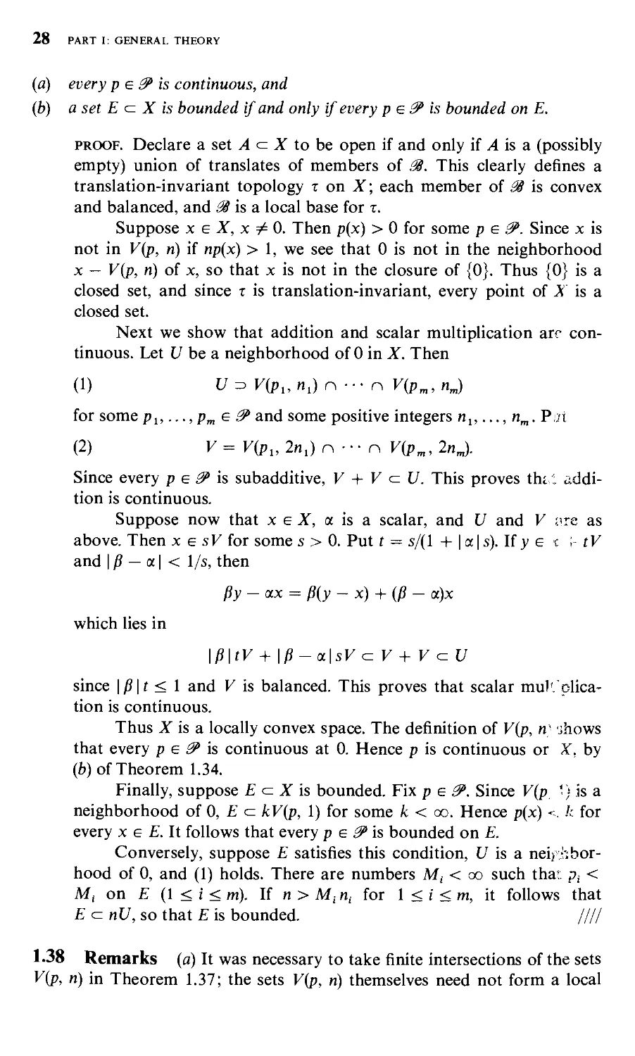
28 PART I: GENERAL THEORY
(a) every p e ^ is continuous, and
(b) a set E <^ X is bounded if and only if every p e ^ is bounded on E.
PROOF. Declare a set A <= X to be open if and only if A is a (possibly
empty) union of translates of members of 3S. This clearly defines a
translation-invariant topology t on X; each member of 3S is convex
and balanced, and ^ is a local base for t.
Suppose X e X, X # 0. Then p{x) > 0 for some p e ^. Since x is
not in V(p, n) if np(x) > 1, we see that 0 is not in the neighborhood
X — V{p, n) of X, so that x is not in the closure of {0}. Thus {0} is a
closed set, and since t is translation-invariant, every point of X is a
closed set.
Next we show that addition and scalar multiplication are
continuous. Let t/ be a neighborhood of 0 in X. Then
(1) U^V{p„n,)r^■■^ r^V(p„,n„)
for some p^, ...,p„e ^ and some positive integers nj,..., n„. Pji
(2) V=V{p„2n,)r^■^^ r^V(p„,2nJ.
Since every p e 0' is subadditive, F + F <= t/. This proves thi'.
addition is continuous.
Suppose now that x e X, a is a scalar, and U and F ;sre as
above. Then x e sF for some s > 0. Put t = s/{l + | a | s). If y e c r tV
and I ^ — a I < 1/s, then
^y - ax = P{y - x) + (^ - a)x
which lies in
\P\tV + |^-a|sF<= F + F <= t/
since \[i\t < 1 and F is balanced. This proves that scalar mul'.
plication is continuous.
Thus X is a locally convex space. The definition of V(p, n} jhows
that every p e 0* is continuous at 0. Hence p is continuous or X, by
(b) of Theorem 1.34.
Finally, suppose £ <= X is bounded. Fix p e 0'. Since V(p ') is a
neighborhood of 0, £ <= kV{p, 1) for some k < co. Hence p{x) <. k for
every x e £. It follows that every p e ^ is bounded on £.
Conversely, suppose £ satisfies this condition, t/ is a neij hbor-
hood of 0, and (1) holds. There are numbers M, < oo such thar. p, <
Mj on £ (1 < i < m). If n > M^n^ for \ <i <m, it follows that
£ <= nt/, so that £ is bounded. ////
1.38 Remarks (a) It was necessary to take finite intersections of the sets
V{p, n) in Theorem 1.37; the sets V{p, ri) themselves need not form a local

CHAPTER 1: TOPOLOGICAL VECTOR SPACES 29
base. (They do form what is usually called a subbase for the constructed
topology.) To see an example of this, take X = R^, and let ^ consist of the
seminorms p^ and pj defined by p,-(x) = |Xj|; here x = (Xj, Xj). Exercise 8
develops this comment further.
{b) Theorems 1.36 and 1.37 raise a natural problem: If ^ is a convex
balanced local base for the topology t of a locally convex space X, then 3S
generates a separating family ^ of continuous seminorms on X, as in
Theorem 1.36. This ^ in turn induces a topology Tj on X, by the process
described in Theorem 1.37. Is t = Tj ?
The answer is affirmative. To see this, note that every p e 0' is t-
continuous, so that the sets V{p, ri) of Theorem 1.37 are in t. Hence Tj <= t.
Conversely, liWeSS and p = Hw, then
W = {x: n^{x) < 1} ^ V{p, 1).
Thus H^ e Ti for every W e ^i this implies that t <= Tj.
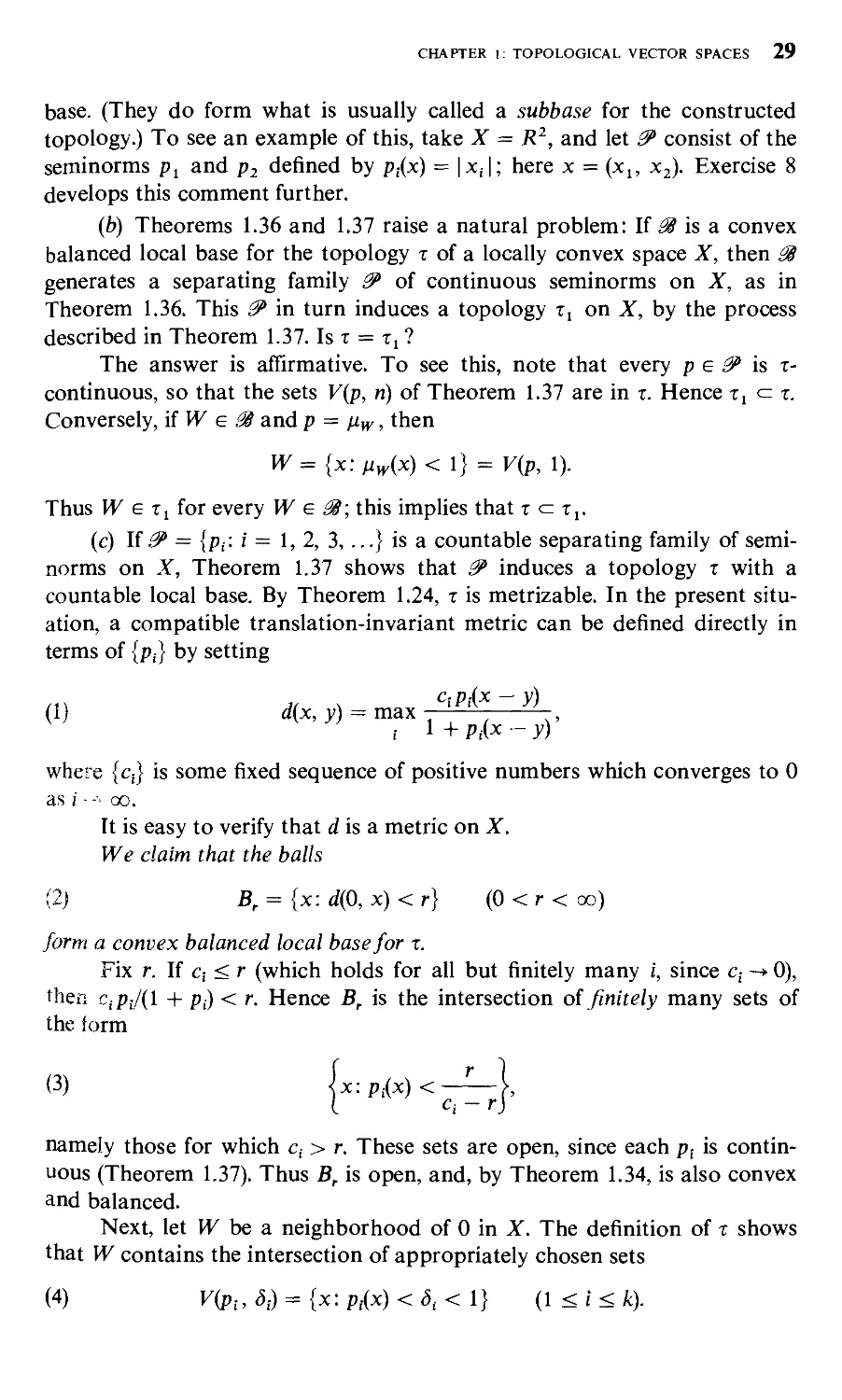
(c) If ^ = {p,: i = 1, 2, 3,...} is a countable separating family of semi-
norms on X, Theorem 1.37 shows that 0* induces a topology t with a
countable local base. By Theorem 1.24, t is metrizable. In the present
situation, a compatible translation-invariant metric can be defined directly in
terms of {pj by setting
(1) dix,y) = m..;f^-'\,
I 1 + Piix - y)
where {c,} is some fixed sequence of positive numbers which converges to 0
as i ^ -■■ 00.
It is easy to verify that d is a metric on X.
We claim that the balls
(2) B, == {x: d{0, X) < r} (0 < r < oo)
form a convex balanced local base for x.
Fix r. If c; < r (which holds for all but finitely many i, since c,- -<• 0),
then CjP,-/(l + p;) < r. Hence B^ is the intersection oi finitely many sets of
the form
(3) |^:p_.(^)<_^
namely those for which Cj > r. These sets are open, since each p, is
continuous (Theorem 1.37). Thus B^ is open, and, by Theorem 1.34, is also convex
and balanced.
Next, let H^ be a neighborhood of 0 in X. The definition of t shows
that W contains the intersection of appropriately chosen sets
(4) K(p,-, <5,.) = {x: p,(x) < <5, < 1} (1 < i < /c).

30 PART I: GENERAL THEORY
If 2r < min {c^di,..., c,,3,,} and x e B^, then
CiPi(x) C:8:
(5) TtH\ < '• < -T^ {^<i<k),
1 + P;(X) 2
which implies p,-(x) < 8^. Thus B, <= W.
This proves our claim and also shows that d is compatible with t.
1.39 Theorem A topological vector space X is normable if and only if its
origin has a convex bounded neighborhood.
PROOF. If X is normable, and if || • || is a norm that is compatible with
the topology of X, then the open unit ball {x\ \\x\\ < 1} is convex and
bounded.
For the converse, assume F is a convex bounded neighborhood
of 0. By Theorem 1.14, V contains a convex balanced neighborhood
t/ of 0; of course, t/ is also bounded. Define
(1) l|x||=M^) (xeX)
where ^ is the Minkowski functional of t/.
By (c) of Theorem 1.15, the sets rU {r > Q) form a local base for
the topology of X. If x # 0, then x ^ rU for some r > 0; hence
llx|| > r. It now follows from Theorem 1.35 that (1) defines a norm.
The defliiition of the Minkowski functional, together with the fact that
U is open, implies that
(2) {x: \\x\\ <r} =rt/
for every r > 0. The norm topology coincides therefore with the given
one. ////
Quotient Spaces
1.40 Definitions Let N be a subspace of a vector space X. For every
X e X, let n{x) be the coset of N that contains x; thus
n{x) = X + N.
These cosets are the elements of a vector space X/N, called the quotient
space of X modulo N, in which addition and scalar multiplication are
defined by
(1) n{x) + n{y) = n{x + y), xk{x) = ;c(ax).
[Note that now an{x) = N when a = 0. This differs from the usual notation,
as introduced in Section 1.4.] Since N is a vector space, the operations (1)
are well defined. This means that if n{x) = n{x') (that is, x' - x e N) and

CHAPTER 1: TOPOLOGICAL VECTOR SPACES 31
n{y) = n{y') then
(2) 7r(x) + K{y) = k{x') + K{y'), aK{x') = xn{x).
The origin of X/N is 7r(0) = N. By (1), tt is a linear mapping of X onto
X/N with N as its null space; k is often called the quotient map of X onto
X/N.
Suppose now that t is a vector topology on X and that N is a closed
subspace of X. Let t^ be the collection of all sets E <= X/N for which
n~\E} e T. Then t^ turns out to be a topology on X/N, called the quotient
topology. Some of its properties are listed in the next theorem. Recall that
an open mapping is one that maps open sets to open sets.
1.41 Theorem Let N be a closed subspace of a topological vector space
X. Let T be the topology ofX and define t^ as above.
(a) T^ is a vector topology on X/N; the quotient map n: X -* X/N is linear,
continuous, and open.
(b) If 3S is a local base for r, then the collection of all sets n{V) with V e ^
is a local base for t^.
(c) Each of the following properties of X is inherited by X/N: local
convexity, local boundedness, metrizability, normability.
(d) IfX is an F-space, or a Frechet space, or a Banach space, so is X/N.
PROOF. Since 7r^'(A n fi) = tt '(A) n n~'^(B) and
n~\\jE,)^\Jn-\E,),
T^ is a topology. A set f <= X/N is t^-closed if and only if n~^(F) is
T-closed. In particular, every point of X/N is closed, since
7r"'(7r(x)) = N + X
and N was assumed to be closed.
The continuity of n follows directly from the definition of t^.
Next, suppose Vex. Since
7r-'(7r(F)) = N +V
and N + V e x,\i follows that n(V) e t^ . Thus n is an open mapping.
If now H^ is a neighborhood of 0 in X/N, there is a
neighborhood F of 0 in X such that
V + V ^n~'{W).
Hence n{V) + 7r(F) <= W. Since n is open, n{V) is a neighborhood of 0
in X/N. Addition is therefore continuous in X/N.

32
PART I: GENERAL THEORY
The continuity of scalar multiplication in XjN is proved in the
same manner. This establishes (a).
It is clear that (a) implies (b). With the aid of Theorems 1.32,
1.24, and 1.39, it is just as easy to see that (b) implies (c).
Suppose next that d is an invariant metric on X, compatible
with T. Define p by
p{n{x), n{y)) = inf {d{x - y, z): z e N}.
This may be interpreted as the distance from x — y to N. We omit the
verifications that are now needed to show that p is well defined and
that it is an invariant metric on X/N. Since
n{{x:d{x,0)<r})^{u:p(u,Q)<r},
it follows from (b) that p is compatible with t^ .
If X is normed, this definition of p specializes to yield what is
usually called the quotient norm of X/N:
||7r(x)||=inf{||x-z||:zeN}.
To prove (d) we have to show that p is a complete metric
whenever d is complete.
Suppose {m„} is a Cauchy sequence in X/N, relative to p. There
is a subsequence {m„J with p{u„., u„.^^)< 2 '. One can then
inductively choose X;e X such that n{xi) = m„, and d{x;, Xj+1) < 2~'. If d is
complete, the Cauchy sequence {xj converges to some x e X. The
continuity of n implies that m„. -^ n{x) as i ->■ oo. But if a Cauchy
sequence has a convergent subsequence then the full sequence must
converge. Hence p is complete, and so is the proof of Theorem 1.41.
////
Here is an easy application of these concepts:
1.42 Theorem Suppose N and F are subspaces of a topological vector
space X, N is closed, and F has finite dimension. Then N + F' is closed.
PROOF. Let n be the quotient map of X onto X/N, and give X/N its
quotient topology. Then n{F) is a finite-dimensional subspace of X/N;
since X/N is a topological vector space. Theorem 1.21 implies that
7r(f) is closed in X/N. Since N + F = n~\n:{F)) and n is continuous,
we conclude that N + F is closed. (Compare Exercise 20.) ////
1.43 Seminorms and quotient spaces Suppose p is a seminorm on a
vector space X and
N= {x: p(x) = 0}.

CHAPTER 1: TOPOLOGICAL VECTOR SPACES 33
Then N is a subspace of X (Theorem 1.34). Let n be the quotient map of X
onto X/N, and define
p(7r(x)) = p(x).
If n(x) = n(y), then p(x — y) = 0, and since
I p('^) - p(y) I < p(^ - y)
it follows that p(7i(x)) = {>(n{y)). Thus p is well defined on X/N, and it is now
easy to verify that p is a norm on X/N.
Here is a familiar example of this. Fix r, 1 < r < oo; let E be the space
of all Lebesgue measurable functions on [0, 1] for which
p(/)=iI/L =
l/r
f{t)\'dt\ < 00.
This defines a seminorm on E, not a norm, since ||/||r = 0 whenever/= 0
almost everywhere. Let N be the set of these " null functions." Then E/N is
the Banach space that is usually called E. The norm of E is obtained by the
above passage from p to p.
Examples
L44 The spaces C(f2) If Q is a nonempty open set in some euclidean
space, then Q is the union of countably many compact sets K„ # 0 which
can be chosen so that K„ lies in the interior of K„+1 (n = 1, 2, 3, ...). C(Q) is
the vector space of all complex-valued continuous functions on Q, topol-
ogized by the separating family of semi norms
(1) p„(/) = sup{|/(x)|:xeK„},
in accordance with Theorem 1.37. Since p^ <P2<-' -, the sets
(2) K„ = |/e C(Q): p„(/) < ^j (n = 1, 2, 3, ...)
form a convex local base for C(Q). According to remark (c) of Section 1.38,
the topology of C(Q) is compatible with the metric
(3) .(/.) = max fp^.
If {/(} is a Cauchy sequence relative to this metric, then p„(/; —/j)-^0 for
every n, as i, j -^ oo, so that {/,} converges uniformly on K„, to a function
/e C(Q). An easy computation then shows d{f,f,) ->■ 0. Thus d is a complete
metric. We have now proved that C(Q) is a Frechet space.
By {b) of Theorem 1.37, a set £ <= C(Q) is bounded if and only if there
are numbers M„< co such that p„(/) < M„ for all/e E; explicitly,
(4) I fix) I < M„ iff e E and x e K„.

34 PART I: GENERAL THEORY
Since every F„ contains an/for which p„+i{f) is as large as we please, it
follows that no F„ is bounded. Thus C(Q) is not locally bounded, hence is not
normable.
1.45 The spaces H{il) Let Q now be a nonempty open subset of the
complex plane, define C(Q) as in Section 1.44, and let H{Q) be the subspace
of C(Q) that consists of the holomorphic functions in Q. Since sequences of
holomorphic functions that converge uniformly on compact sets have
holomorphic limits, H{H) is a closed subspace of. C(Q). Hence H{Q.) is a Frechet
space.
We shall now prove that H(Q) has the Heine-Borel property. It will
then follow from Theorem 1.23 that H{Q) is not locally hounded, hence is not
normable.
Let £ be a closed and bounded subset of H{Ql). Then £ satisfies
inequalities such as (4) of Section 1.44. Montel's classical theorem about
normal families (Th. 14.6 of [23]') implies therefore that every sequence
{/J <= £ has a subsequence that converges uniformly on compact subsets of
Q [hence in the topology of H(Q)] to some/e H(Ql). Since £ is closed,/e £.
This proves that £ is compact.
1.46 The spaces C°°(f2) and ®k We begin this section by introducing
some terminology that will be used in our later work with distributions.
In any discussion of functions of n variables, the term multi-index
denotes an ordered n-tuple
(1) a = (ai, ..., a„)
of nonnegative integers a,-. With each multi-index a is associated the
differential operator
\dxj \dx,
whose order is
(3) |a| = a, -h----ha„.
If|a| = 0,Dy = /
A complex function / defined in some nonempty open set Q c: i?" is
said to belong to C°°(Q) if DJ e C(Q) for every multi-index a.
' Numbers in brackets refer to sources listed in the bibliography.

CHAPTER 1: TOPOLOGICAL VECTOR SPACES 35
The support of a complex function / (on any topological space) is the
closure of {x; f{x) # 0}.
If K is a compact set in R", then ^j^ denotes the space of all
fe C^iR") whose support lies in K. (The letter ^ has been used for these
spaces ever since Schwartz published his work on distributions.) If K c: Q,
then ^ic niay be identified with a subspace of C°°(Q).
We now define a topology on C°°(Q) which makes C°°(Q) into a Frechet
space with the Heine-Borel property, such that 3)f^ is a closed subspace of
C°°(i2) whenever K c: Q.
To do this, choose compact sets K, {i = 1, 2, 3,...) such that K,- lies in
the interior of K,+1 and Q = |J K,-. Define seminorms p^ on C°°(Q), N = I,
2, 3,..., by setting
(4) p^if) = max{\Df{x)\:x e K^, |a| < N}.
They define a metrizable locally convex topology on C°°(Q); see Theorem
1.37 and remark (c) of Section 1.38. For each x e O, the functional/-^/(x)
is continuous in this topology. Since S^g; is the intersection of the null spaces
of these functional, as x ranges over the complement of K, it follows that
^jf is closed in C°°(Q).
A local base is given by the sets
(5) K^ = |/e C°°(Q): p^f) < ^| {N = 1, 2, 3, ...).
If {fi} is a Cauchy sequence in C°°(Q) (see Section 1.25) and if N is fixed,
then /;. -fj e V„ if i and; are sufficiently large. Thus 10% - D%-\ < l/N on
Kf^, if \a\ < N. It follows that each D% converges (uniformly on compact
subsets of Q) to a function g^. In particular,/(x) -->^o(x). It is now evident
that 00 e C°°(Q), that g^ = D^go, and that/ -^ ^ in the topology of C°°(Q).
Thus C°°(Q) is a Frechet space. The same is true of each of its closed
subspaces S>^.
Suppose next that E a C°°(Q) is closed and bounded. By Theorem
1-37, the boundedness of E is equivalent to the existence of numbers
M;v < 00 such that p^(/) < M^ for N = 1, 2, 3, ... and for all /e E. The
inequalities |DJ \ < M^, valid on K^ when \a.\ <N, imply the equicon-
tinuity of {D^f:feE} on K^y-i, if \l^\<N-l. It now follows from
Ascoli's theorem (proved in Appendix A) and Cantor's diagonal process
that every sequence in E contains a subsequence {f} for which {D^f}
converges, uniformly on compact subsets of Q, for each multi-index y3. Hence
{f} converges in the topology of C^IQ). This proves that E is compact.
Hence C°°(Q) has the Heine-Borel property. It follows from Theorem
i-23 that C°°(Q) is not locally bounded, hence not normable. The same
conclusion holds for ^jf whenever K has nonempty interior (otherwise 3)^ =
iO)), because dim ^j^ = oo in that case. This last statement is a consequence
01 the following proposition:

36 PART 1: GENERAL THEORY
If Bi and Bj are concentric closed balls in R", with Bj in the interior of
Bj, then there exists 4> e C°°{R") such that 4>ix) = 1 for every x e B^,
4>{x) = Ofor every x outside Bj , and 0 ^ 4> < I on R".
To find such a 4>, we construct g e C^iR^) such that g{x) = 0 for
X < a, g{x) = I for X > b (where 0 < a < fe < oc are preassigned) and put
(6) <^(Xi, ...,x„)= 1 - gix] + ■ ■ ■ + x^„).
The following construction of g has the advantage that suitable choices of
{3i} can lead to functions with other desired properties.
Suppose 0 < fl < fe < 00. Choose positive numbers 3q, 3^, 32, ■■■,
with Z5, = b — a; put
(7) m„=- (n=l, 2, 3, ...);
let/o be a continuous monotonic function such that/Q(x) = 0 when x < a,
fo(x) = 1 when x > a + 3q; and define
(8) /"W = r I fn~iit)dt (n=l, 2, 3, ...).
Differentiation of this integral shows, by induction, that/„ has n continuous
derivatives and that | D"f„ | < m„. If n > r, then
(9) D%{x) = ^\\D%_,){x-t)dt,
On Jo
SO that
(10) \DJ„\<m,. {n>r),
again by induction on n. The mean value theorem, applied to (9), shows
that
(11) \mn-D%^i\<'n,^,3„ (n>r + 2).
Since Z5„ < oo, each {D^} converges, uniformly on ( —oo, oo), as n-^ co.
Hence {/„} converges to a function g, with \D''g\ < m^ for r = 1, 2, 3, ...,
such that g(x) = 0 for x < a and g{x) = 1 for x > fe.
1.47 The spaces f with 0 < /> < 1 Consider a fixed p in this range.
The elements of U are those Lebesgue measurable functions / on [0, 1] for
which
(i) ^{f)=\\f{t)\''dt<a,,

CHAPTER 1: TOPOLOGICAI, VECTOR SPACES 37
with the usual identification of functions that coincide almost everywhere.
Since 0 < p < 1, the inequality
(2) {a + h)" < fl" + fe"
holds when a > 0 and fe :> 0. This gives
(3) A{f+g)<A{f) + A{g),
so that
(4) ' d{f,g) = Aif-^g)
defines an invariant metric on H. That this d is complete is proved in the
same way as in the familiar case p > 1. The balls
(5) B, = {/6L'';A(/)<r}
form a local base for the topology of LF. Since Bj = r'^'''B^, for all r > 0,
jBj is bounded.
Thus LP is a locally bounded F-space.
We claim that /f contains no convex open sets, other than 0 and II.
To prove this, suppose F # 0 is open and convex in II. Assume
0 e V, without loss of generality. Then F =3 B^, for some r > 0. Pick/e W.
Since p < 1, there is a positive integer n such that n**"^ A(/) < r. By the
continuity of the indefinite integral of | /1*", there are points
0 — Xq < x^ < ■ ■ ■ < x„ = 1
such that
(6) I \f{t)\^dt = n~' Aif) {l<i<n).
J XI- 1
Define g^t) = nf(t) if Xj_j <t< x,, git) — 0 otherwise. Then 0, e F, since
(6) shows
(7) A(0,.) = n''-' A(f) <r (I < i < n)
and V => B^. Since F is convex and
(8) /=^(0, +■■■+<?„),
it follows that/ e F. Hence V = L".
This lack of convex open sets has a curious consequence.
Suppose A: L*"-^ y is a continuous linear mapping of U into some
locally convex space Y. Let ^ be a convex local base for 7. If H^ e ^, then
^ '(H^) is convex, open, not empty. Hence A''\W) = H. Consequently,
MB) <= W for every W e ^.We conclude that A/= 0 for every/e L".
Thus 0 is the only continuous linear mapping of II into any locally
convex space Y, if 0 < p < I. In particular, 0 is the only continuous linear
Junctional on these E-spaces.
This is, of course, in violent contrast to the familiar case p ^ 1.

38 PART I: GENERAL THEORY
Exercises
1. Suppose Z is a vector space. All sets mentioned below are understood to be
subsets of X. Prove the following statements from the axioms as given in
Section 1.4. (Some of these are tacitly used in the text.)
(a) If X e X and y e X there is a unique z e X such that x + z = y.
(h) Ox = 0 = aO if X 6 Z and a is a scalar.
(c) 2AczA + A;\t may happen that 2A ^ A + A.
(d) A is convex if and only if (s + t)A = sA + tA for all positive scalars s and t.
(e) Every union (and intersection) of balanced sets is balanced.
(/') Every intersection of convex sets is convex.
(g) If r is a collection of convex sets that is totally ordered by set inclusion,
ihen the union of all members of F is convex.
(h) If A and B are convex, so is A + B.
(i) If A and B are balanced, so is A + B.
(j) Show that parts (/), (g), and (h) hold with subspaces in place of convex sets.
2. The convex hull of a set A in a vector space Z is the set of all convex
combinations of members of A, that is, the set of all sums
hxi + ■■■ + t„x„
in which x, e A, I, > 0, ^ I, = 1; « is arbitrary. Prove that the convex hull of A
is convex and that it is the intersection of all convex sets that contain A.
3. Let Z be a topological vector space. All sets mentioned below are understood to
be the subsets of Z. Prove the following statements.
(a) The convex hull of every open set is open.
{b) If Z is locally convex then the convex hull of every bounded set is bounded.
(This is false without local convexity; see Section L47.)
(c) If A and B are bounded, so is A + B.
(d) If A and B are compact, so is A -h B.
(e) If A is compact and B is closed, then A + B is closed.
(/) The sum of two closed sets may fail to be closed. [The inclusion in (b) of
Theorem 1.13 may therefore be strict.]
4. Let B = {{z^, z^) e ^^; |Zi | < Izil}- Show that B is balanced but that its
interior is not. [Compare with (e) of Theorem 1.13.]
5. Consider the definition of "bounded set" given in Section 1.6. Would the
content of this definition be altered if it were required merely that to every
neighborhood F of 0 corresponds some t > 0 such that E cz tVl
6. Prove that a set £ in a topological vector space is bounded if and only if every
countable subset of E is bounded.
7. Let Z be the vector space of all complex functions on the unit interval [0, 1],
topologized by the family of seminorms
P.(/) = I/WI (0<x<l).
This topology is called the topology of pointwise convergence. Justify this
terminology.
Show that there is a sequence {/„} in Z such that (a) {/„} converges to 0
as « -» 00, but {b) if {y„} is any sequence of scalars such that y„ -> co then {?„/„}

CHAPTER 1: TOPOLOGICAL VECTOR SPACES 39
does not converge to 0. (Use the fact that the collection of all complex sequences
converging to 0 has the same cardinality as [0, 1].)
This shows that metrizability cannot be omitted in (b) of Theorem 1.28.
8. (a) Suppose ^ is a separating family of seminorms on a vector space X. Let J
be the smallest family of seminorms on X that contains ^ and is closed
under max. [This means: If p^ e 2., P2&2., and p = max (p,, pj)' then
p 6 J.] If the construction of Theorem L37 is applied to 0' and to J, show
that the two resulting topologies coincide. The main difference is that 2.
leads directly to a base, rather than to a subbase, [See Remark (a) of Section
L38.]
(b) Suppose 2 is as in part {a) and A is a linear functional on X. Show that A is
continuous if and only if there exists a p e 2 such that | Ax | < Mp{x) for all
X e X and some constant M < oo.
9. Suppose
{a) X and Y are topological vector spaces,
(b) A: Z -» y is linear,
(c) iV is a closed subspace of X,
(d) 71: Z -> X/N is the quotient map, and
(e) Ax = 0 for every x e N.
Prove that there is a unique /; X/N -» Y which satisfies A =/ = n, that is.
Ax =/(n(x)) for all x e Z. Prove that this/is linear and that A is continuous if
and only if/is continuous. Also, A is open if and only if/is open.
10. Suppose Z and Y are topological vector spaces, dim 7 < oo, A:Z-» 7 is
linear, and A(Z) = Y.
{a) Prove that A is an open mapping.
(b) Assume, in addition, that the null space of A is closed, and prove that A is
then continuous.
11. If iV is a subspace of a vector space Z, the codimension of A^ in Z is, by
definition, the dimension of the quotient space X/N.
Suppose 0 < p < 1 and prove that every subspace of finite codimension is
dense in U. (See Section L47.)
12. Suppose diix, y) = | x — y |, djix, y) = | <p{x) — <p{y) I, where (p{x) = x/(l + | x |).
Prove that d^ and (ij ^re metrics on R which induce the same topology,
although d^ is complete and dj is not.
13. Let C be the vector space of all complex continuous functions on [0, 1]. Define
d{f,g)
\f(x)-~g{x)\ ^^
1 +|/(x)-g(x)|
Let (C, cr) be C with the topology induced by this metric. Let (C, t) be the
topological vector space defined by the seminorms
P.{f) = \f{x)l (0<x<l),
in accordance with Theorem L37.
(a) Prove that every t-bounded set in C is also cr-bounded and that the identity
map id: (C, t) -»(C, cr) therefore carries bounded sets into bounded sets.
(b) Prove that id: (C, t)-»(C, cr) is nevertheless not continuous, although it is
sequentially continuous (by Lebesgue's dominated convergence theorem).

40 PART I: GENERAL THEORY
Hence (C, t) is not metrizable. (See Appendix A6, or Theorem 1.32.) Show
also directly that (C, t) has no countable local base.
(c) Prove that every continuous linear functional on (C, t) is of the form
i= 1
for some choice of x,,,.,, x„ in [0, 1] and some Cj e ^.
(d) Prove that (C, cr) contains no convex open sets other than 0 and C.
(e) Prove that id: (C, cr) -»(C, t) is not continuous.
14. Put K = [0, 1] and define @j. as in Section 1.46. Show that the following three
families of seminorms (where n = 0, 1, 2,...) define the same topology on ®j., if
D = d/dx:
(a) \\D"f\\ „ = sup {I D"f{x)\ : - CO < X < cx)}.
1/2
ib) ||D"/||,= \D''f{x)\dx.
0
(c) IID"/II2= \D"f{x)\Ux
15. Prove that the spaces C(fi) (Section 1.44) do not have the Heine-Borel property.
16. Prove that the topology of C{il) does not depend on the particular choice of
{K„}, as long as this sequence satisfies the conditions specified in Section 1,44.
Do the same for C"(fi) (Section 1,46),
17. In the setting of Section 1,46, prove that /-» D"/ is a continuous mapping of
C"(fi) into C"(fi) and also of ©j. into ©j., for every multi-index a.
18. Prove the proposition concerning addition in the binary system which was used
at the end of the proof of Theorem 1.24.
19. Suppose M is a dense subspace of a topological vector space X, Y is an f-space,
and A: M -> 7 is continuous (relative to the topology that M inherits from X)
and linear. Prove that A has a continuous linear extension A; Z -> 7.
Suggestion: Let F„ be balanced neighborhoods of 0 in Z such that
V„+ V„<= V„^, and such that d{0. Ax) <2'" if x e M n F„. If x e A' and x„ e
(x -I- F„) n M, show that {Ax„} is a Cauchy sequence in Y, and define Ax to be
its limit. Show that A is well defined, that Ax = Ax if x e M, and that A is linear
and continuous.
20. For each real number t and each integer n, define e„{t) = e'"', and define
fn = e^„ + ne„ (« = 1, 2, 3, ...),
Regard these functions as members of l}[~n, n). Let Z, be the smallest closed
subspace of 1} that contains e^, e,, Bj, ■■■, and let Xj be the smallest closed
subspace of 1} that contains/,,/2 ,f^, Show that Z, -I- Zj is dense in L^ but
not closed. For instance, the vector
CO
x= Y.n~^e^„
is in IJ but not m X^ + Xj. (Compare with Theorem 1,42,)

CHAPTER 1; TOPOLOGICAL VECTOR SPACES 41
21. Let F be a neighborhood of 0 in a topological vector space X. Prove that there
is a real continuous function / on Z such that /(O) = 0 and /(.x) = 1 outside F.
(Thus X is a completely regular topological space.) Suggestion: Let V„ be
balanced neighborhoods of 0 such that F, + F, cr F and I^+, + I^ + , c F„.
Construct/as in the proof of Theorem 1.24. Show that/is continuous at 0 and that
l/W-/(y)l</(^--y).
22. If/is a complex function defined on the compact interval / = [0, 1] c= R, define
w,{f) = sup {\ fix) ~f{y)\: \x-^ y\ < S, x e I, y e I}.
If 0 < a < 1, the corresponding Lipschitz space Lip a consists of all/for which
11/11 = 1/(0) I + sup {^-«,(/): ^>0}
is finite. Define
lip a = {/e Lip a: lim S^'co^if) = 0}.
5-0
Prove that Lip a is a Banach space and that lip a is a closed subspace of Lip a.
23. Let X be the vector space of all continuous functions on the open segment (0, 1).
For/6 X and r > 0, let F(/ r) consist of all g e Z such that | g{x) -/(x) | < r
for all X e (0, 1). Let t be the topology on X that these sets F(/ r) generate.
Show that addition is t-continuous but scalar multiplication is not.
24. Show that the set W that occurs in the proof of Theorem 1.14 need not be
convex, and that A need not be balanced unless U is convex.

CHAPTER
2
COMPLETENESS
The validity of many important theorems of analysis depends on the
completeness of the systems with which they deal. This accounts for the
inadequacy of the rational number system and of the Riemann integral (to
mention just the two best-known examples) and for the success encountered
by their replacements, the real numbers and the Lebesgue integral. Baire's
theorem about complete metric spaces (often called the category theorem) is
the basic tool in this area. In order to emphasize the role played by the
concept of category, some theorems of this chapter (for instance. Theorems
2.7 and 2.11) are stated in a little more generality than is usually needed.
When this is done, simpler versions (more easily remembered but sufficient
for most applications) are also given.
Baire Category
2.1 Definition Let S be a topological space. A set £ c S is said to be
nowhere dense if its closure E has an empty interior. The sets of the first
category in S are those that are countable unions of nowhere dense sets. Any
subset of S that is not of the first category is said to be of the second
category in S.
This terminology (due to Baire) is admittedly rather bland and unsug-
gestive. Meager and nonmeager have been used instead in some texts. But
"category arguments" are so entrenched in the mathematical literature and
are so well known that it seems pointless to insist on a change.
Here are some obvious properties of category that will be freely used
in the sequel:
42

CHAPTER 2: COMPLETENESS 43
(a) If A c: B and B is of the first category in S, so is A.
(b) Any countable union of sets of the first category is of the first category.
(c) Any closed set £ c: S whose interior is empty is of the first category
in S.
(d) If /i is a homeomorphism of S onto S and if £ c S, then E and h{E)
have the same category in S.
2.2 Baire's theorem If Sis either
(a) a complete metric space, or
(b) a locally compact Hausdorff space,
then the intersection of every countable collection of dense open subsets of S is
dense in S.
This is often called the category theorem, for the following reason.
If {£,} is a countable collection of nowhere dense subsets of S, and if
Vi is the complement of £;, then each Vi is dense, and the conclusion of
Baire's theorem is that f] F; # 0. Hence S ¥=■{] Ef.
Therefore, complete metric spaces, as well as locally compact
Hausdorff spaces, are of the second category in themselves.
PROOF. Suppose Fj, V2, V3,... are dense open subsets of S. Let Bq be
an arbitrary nonempty open set in S. If n ^ 1 and an open B„ _ j #0
has been chosen, then (because F„ is dense) there exists an open
B„ # 0 with
B„c:F„nB„_,.
In case (a), B„ may be taken to be a ball of radius < 1/n; in case (b) the
choice can be made so that B„ is compact. Put
n= 1
In case (a), the centers of the nested balls B„ form a Cauchy sequence
which converges to some point of K, and so K # 0. In case (b),
^ # 0 by compactness. Our construction shows that K c: Bq and
K c F„ for each n. Hence Bq intersects f] V„. ////
The Banach-Steinhaus Theorem
2.3 Equicontinuity Suppose X and Y are topological vector spaces and
r is a collection of linear mappings from X into Y. We say that F is
^<}uicontinuous if to every neighborhood I^ of 0 in Y there corresponds a
neighborhood F of 0 in X such that A{V) c: W for all A e P.

44 PART 1: GENERAL THEORY
If r contains only one A, equicontinuity is. of course, the same as
continuity (Theorem 1.17). We already saw (Theorem 1.32) that continuous
linear mappings are bounded. Equicontinuous collections have this
boundedness property in a uniform manner (Theorem 2.4). It is for this
reason that the Banach-Steinhaus theorem (2.5) is often referred to as the
uniform boundedness principle.
2.4 Theorem Suppose X and Y are topological vector spaces, F is an
equicontinuous collection of linear mappings from X into Y, and E is a
bounded subset of X. Then Y has a bounded subset F such that A(£) cz F for
every A e F.
PROOF. Let F be the union of the sets A(£), for A e F. Let H^ be a
neighborhood of 0 in Y. Since F is equicontinuous, there is a
neighborhood F of 0 in X such that A{V) cz W for all A e F. Since E is
bounded, £ cz t F for all sufficiently large t. For these t,
A(£) cz A(tF) = tA(F) cz tW,
so that F cz tW. Hence F is bounded. ////
2.5 Theorem (Banach-Steinhaus) Suppose X and Y are topological
vector spaces, F is a collection of continuous linear mappings from X into Y,
and B is the set of all x e X whose orbits
F(x) = {Ax: AeF}
are bounded in Y.
If B is of the second category in X, then B = X and F is
equicontinuous.
PROOF. Pick balanced neighborhoods W anc t/ of 0 in 7 such that
t7 -I- t7 cz H/. Put
£= n A-'(t7).
If X e B, then F(x) cz nU for some n, so that x e nE. Consequently,
00
B cz \J nE.
n= 1
At least one nE is of the second category in X, since this is true of B-
Since x^ nx is a homeomorphism of X onto X, E is itself of the
second category in X. But £ is closed because each A is continuous.
Therefore £ has an interior point x. Then x — E contains a neighbor-

CHAPTER 2: COMPLETENESS 45
hood F of 0 in X, and
A{V) c Ax - A(£) czU -U czW
for every A e F.
This proves that F is equicontinuous. By Theorem 2.4, F is
uniformly bounded; in particular, each F(x) is bounded in Y. Hence
B = X. nil
In many applications, the hypothesis that B is of the second category
is a consequence of Baire's theorem. For example, F-spaces are of the
second category. This gives the following corollary of the Banach-Steinhaus
theorem:
2.6 Theorem //F is a collection of continuous linear mappings from an
¥-space X into a topological vector space Y, and if the sets
F(x)= {Ax: AeF}
are hounded in Y,for every x e X, then F is equicontinuous.
Briefly, pointwise boundedness implies uniform boundedness
(Theorem 2.4).
As a special case of Theorem 2.6, let X and Y be Banach spaces, and
suppose that
(1) sup !IAx|| < 00 for every x e X.
The conclusion is that there exists M < oo such that
(2) ||Ax||<M if ||x|| < 1 and A eF.
Hence
(3) ||Ax|| <M||x|| ifxeXandAeF.
The following theorem establishes the continuity of limits of sequences
of continuous linear mappings:
2.7 Theorem Suppose X and Y are topological vector spaces, and {A„} is
a sequence of continuous linear mappings ofX into Y.
(a) If C is the set of all x e X for which {A„x} is a Cauchy sequence in Y,
and ifC is of the second category in X, then C = X.
(b) IfL is the set of all x e X at which
Ax = lim A„ X

46 PART I: GENERAL THEORY
exists, if L is of the second category in X, and if Y is an F-space, then
L = X and A: X ->^ Y is continuous.
PROOF, (a) Since Cauchy sequences are bounded (Section 1.29), the
Banach-Steinhaus theorem asserts that {A„} is equicontinuous.
One checks easily that C is a subspace of X. Hence C is dense.
(Otherwise, C is a proper subspace of X; proper subspaces have
empty interior; thus C would be of the first category.)
Fix X e X; let H^ be a neighborhood of 0 in Y. Since {A„} is
equicontinuous, there is a neighborhood F of 0 in X such that
A„{V) cz W for n = 1, 2, 3, .... Since C is dense, there exists
x' e C n (x + V). If n and m are so large that
A„x' - A„x' e W,
the identity
(A„ - A Jx = A„(x - x') + (A„ - A Jx' + A Jx' - x)
shows that A„x — A„x e W + W + W. Consequently, {A„x} is a
Cauchy sequence in Y, and x e C.
(b) The completeness of Y implies that L = C. Hence L = X, by
(a). If V and W are as above, the inclusion A„(F) c W, valid for all n,
implies now that A( F) c W. Thus A is continuous. ////
The hypotheses of (b) of Theorem 2.7 can be modified in various ways.
Here is an easily remembered version:
2.8 Theorem //{A„} is a sequence of continuous linear mappings from an
F-space X into a topological vector space Y, and if
Ax = lim A„ X
exists for every x e X, then A is continuous.
PROOF. Theorem 2.6 implies that {A„} is equicontinuous. Therefore if
H^ is a neighborhood of 0 in Y, we have A„(F) c W for all n and for
some neighborhood F of 0 in X. It follows that A(F) ci W; hence
(being obviously linear) A is continuous. ////
In the following variant of the Banach-Steinhaus theorem the
category argument is applied to a compact set, rather than to a complete metric
one. Convexity also enters here in an essential way (Exercise 8).
2 9 Theorem Suppose X and Y are topological vector spaces, K is a
compact convex set in X, F is a collection of continuous linear mappings of X

CHAPTER 2: COMPLETENESS 47
into Y, and the orbits
r(x) = {Ax: A er}
are bounded subsets of Y,for every x e K.
Then there is a bounded set B a Y such that A{K) cz Bfor every A e F.
PROOF. Let B be the union of all sets r(x), for x e X. Pick balanced
neighborhoods W and t/ of 0 in 7 such that U + U czW.Put
(1) £= Ha-'(17).
AsT
If X e X, then r(x) cz nt/ for some n, so that x e nE. Consequently,
(2) X = U (^ n nE).
n=l
Since E is closed, Baire's theorem shows that K n nE has nonempty
interior (relative to K) for at least one n.
We fix such an n, we fix an interior point Xq of X n nE, we fix a
balanced neighborhood F of 0 in X such that
(3) X n (Xo + F) c nE,
and we fix a p > 1 such that
(4) X c xo + pV.
Such a p exists since X is compact.
If now X is any point of X and
(5) z=(l-p-')Xo + p"'x,
then z e X, since X is convex. Also,
(6) z-Xo = p'\x - Xo) e V,
by (4). Hence z e nE, by (3). Since A(n£) cz nt7 for every A e F and
since x = pz — (p — l)xo, we have
Ax e pnU -{p- l)nU cz pn{U + U) cz pnW.
Thus B cz pnW, which proves that B is bounded. ////
The Open Mapping Theorem
2.10 Open mappings Suppose / maps S into T, where S and T are
topological spaces. We say that/is open at a point p e S if/(F) contains a
neighborhood offip) whenever F is a neighborhood of p. We say that/is
open if/(C/) is open in T whenever U is open in S.

48 PART I: GENERAL THEORY
It is clear that/is open if and only if/is open at every point of S.
Because of the invariance of vector topologies, it follows that a linear
mapping of one topological vector space into another is open if and only if
it is open at the origin.
Let us also note that a one-to-one continuous mapping/of S onto T
is a homeomorphism precisely when/is open.
2.11 The open mapping theorem Suppose
(a) X is an F-space,
(b) Y is a topological vector space,
(c) A: X -y Y is continuous and linear, and
(d) A{X) is of the second category in Y.
Then
(0 A(X) = y,
{ii) A is an open mapping, and
{Hi) Y is an F-space.
PROOF. Note that {ii) implies (i), since Y is the only open subspace of
Y. To prove {ii), let F be a neighborhood of 0 in X. We have to show
that A{V) contains a neighborhood of 0 in Y.
Let d be an invariant metric on X that is compatible with the
topology of X. Define
(1) V„ = {x:d{x,0)<2-'r} (n = 0, 1, 2, ...),
where r > 0 is so small that Vq c V. We will prove that some
neighborhood H^ of 0 in Y satisfies
(2) W cz A(Fi) c A(F).
Since Vi ^ Vj — Vj, statement {b) of Theorem 1.13 implies
(3) A(F.) ^ A( V2) - A{V2) ^ A{V2) - A{V^).
The first part of (2) will therefore be proved if we can show that A(F2)
has nonempty interior. But
(4) A{X) = 0 fcACF^),
/c=l
because V-i is a neighborhood of 0. At least one kA{ V2) is therefore of
the second category in Y. Since y ^ ky is a homeomorphism of Y
onto Y, A(F2) is of the second category in Y. Its closure therefore has
nonempty interior.

CHAPTER 2: COMPLETENESS 49
To prove the second inclusion in (2), fix yj e A(Fi). Assume
n > 1 and y„ has been chosen in A{V„). What was just proved for Fj
holds equally well for J^ + i, so that A(F„ + i) contains a neighborhood
of 0. Hence
(5) (y„-A(K, + i))n A(F„)#0.
This says that there exists x„e V„ such that
(6) Ax„ey„-A(F„^i)-
Put y„ + i = y, — Ax„. Then y„ + i e A(F„ + i), and the construction
proceeds.
Since d{x„, 0) < 2~"r, for n = 1, 2, 3, ..., the sums Xj + ■ ■ • + x„
form a Cauchy sequence which converges (by the completeness of X)
to some X e X, with d{x, 0) < r. Hence x e V. Since
m m
(7) Z Ax„ = X (y»-y»+i) = yi-ym+i>
n=1 n=1
and since y^^.j—>0 as m—>cx) (by the continuity of A), we conclude
that yi = Ax e A(F). This gives the second part of (2), and (ii) is
proved.
Theorem 1.41 shows that X/N is an F-space, if N is the null
space of A. Hence (Hi) will follow as soon as we exhibit an
isomorphism/of X/N onto Y which is also a homeomorphism. This can
be done by defining
(8) fix + N) = Ax (xe X).
It is trivial that this / is an isomorphism and that Ax = f{n{x)), where
71 is the quotient map described in Section 1.40. If F is open in Y, then
(9) f-\v) = niA'\V))
is open, since A is continuous and n is open. Hence / is continuous. If
E is open in X/N, then
(10) /(£) = A(7r-'(£))
is open, since n is continuous and A is open. Consequently, / is a
homeomorphism. ////
2.12 Corollaries
(a) // A is a continuous linear mapping of an F-space X onto an F-space Y,
then A is open.
(b) If A satisfies (a) and is one-to-one, then A ~ ': Y ^ X is continuous.

50
PART I: GENERAL THEORY
(c) // X and Y are Banach spaces, and if A: X ->^ Y is continuous, linear,
one-to-one, and onto, then there exist positive real numbers a and b such
that
a\\x\\ < \\Ax\\ < b\\x\\
for every x e X.
(d) Ifti cz T2 are vector topologies on a vector space X and if both {X, Tj)
and {X, T2) are F-spaces, then Tj =12-
PROOF. Statement (a) follows from Theorem 2.11 and Baire's theorem,
since Y is now of the second category in itself. Statement (b) is an
immediate consequence of (a), and (c) follows from (b). The two
inequalities in (c) simply express the continuity of A'' and of A.
Statement (d) is obtained by applying (b) to the identity mapping of
(X,T2)onto(X,Ti). ////
The Closed Graph Theorem
2.13 Graphs If X and Y are sets and/maps X into Y, the graph of/is
the set of all points (x,/(x)) in the cartesian product X x Y.U X and Y are
topological spaces, if X x 7 is given the usual product topology (the
smallest topology that contains all sets U x V with U and V open in X and Y,
respectively), and if/: X -► 7 is continuous, one would expect the graph of/
to be closed in X x 7 (Proposition 2.14). For linear mappings between
F-spaces this trivial necessary condition is also sufficient to assure
continuity. This important fact is proved in Theorem 2.15.
2.14 Proposition If X is a topological space, Y is a Hausdorff space, and
f: X ->■ Y is continuous, then the graph G off is closed.
PROOF. Let Q be the complement of G in X x 7; fix (xq , yo) e Q.
Then y^ #/(xo). Thus yo and /(xq) have disjoint neighborhoods V
and W in 7. Since/is continuous, x^ has a neighborhood U such that
f{U) c W. The neighborhood U x V of (Xq, yo) lies therefore in Q.
This proves that Q is open. ////
Note: One cannot omit the hypothesis that 7 is a Hausdorff space.
To see this, consider an arbitrary topological space X, and let/: X ^X be
the identity. Its graph is the diagonal
D = {{x, x): X e X} cz X X X.
The statement " D is closed in X x X " is just a rewording of the Hausdorff
separation axiom.

CHAPTER 2: COMPLETENESS 51
2.15 The closed graph theorem Suppose
(a) X and Y are F-spaces,
(b) A: X -^ Y is linear,
(c) G = {{x. Ax): X e X} is closed in X x Y.
Then A is continuous.
PROOF. X X y is a vector space if addition and scalar multiplication
are defined componentwise :
a(^i> Vi) + P{^2, Vi) = (a^i + P^2, ayi + fiVi)-
There are complete invariant metrics d^ and dy on X and Y,
respectively, which induce their topologies. If
d{{xi, yi), (X2, Vi)) = dx{x^, Xj) + dy{y^, y2),
then d is an invariant metric on X x 7 which is compatible with its
product topology and which makes X x Y into an F-space. (The easy
but tedious verifications that are needed here are left as an exercise.)
Since A is linear, G is a subspace of X x Y. Closed subsets of
complete metric spaces are complete. Therefore G is an F-space.
Define ttj : G ->• X and ttj: X x 7 -► 7 by
n^{x. Ax) = X, n2{x, y) = y.
Now 711 is a continuous hnear one-to-one mapping of the F-space G
onto the F-space X. It follows from the open mapping theorem that
7rf':X-^G
is continuous. But A = n^ ° ni^ and ttj is continuous. Hence A is
continuous. ////
Remark. The crucial hypothesis (c), that G is closed, is often verified
in applications by showing that A satisfies property (c') below:
(c') // {x„} is a sequence in X such that the limits
X = lim x„ and y = lim Ax„
n-* IX} n-» 00
exist, then y = Ax.
Let us prove that (c') implies (c). Pick a limit point (x, y) of G.
Since X x 7 is metrizable,
(X, y) = lim (x„, Ax„)

52 PART I: GENERAL THEORY
for some sequence {x„}. It follows from the definition of the product
topology that x„^ x and Ax„ -^ y. Hence y = Ax, by (c'), and so
{x, y) e G, and G is closed.
It is just as easy to prove that (c) implies (c').
Bilinear Mappings
2.16 Definitions Suppose X, Y, Z are vector spaces and B maps
X X Y into Z. Associate to each x e X and to each y e Y the mappings
B^.Y^Z and B^: X ^ Z
by defining
B,{y) = B{x, y) = B^{x).
B is said to be bilinear if every B^ and every B" are linear.
If X, Y, Z are topological vector spaces and if every B^ and every B" is
continuous, then B is said to be separately continuous. If B is continuous
(relative to the product topology of X x Y) then B is obviously separately
continuous. In certain situations, the converse can be proved with the aid of
the Banach-Steinhaus theorem.
2.17 Theorem Suppose B: X x Y ^ Z is bilinear and separately
continuous, X is an F-space, and Y and Z are topological vector spaces. Then
(1) B{x„,y„)^B{x^,y^)inZ
whenever x„ -^ x^ in X and y„ -^ y^ in Y. If Y is metrizable, it follows that B
is continuous.
PROOF. Let U and W be neighborhoods of 0 in Z such that
U +U czW. Define
b„{x) = B{x, y„) (xeX,n=l, 2, 3, ...).
Since B is continuous as a function of y,
lim b„ix) = Bix, yo) {x e X).
Thus {b„{x)} is a bounded subset of Z, for each x e X. Since each b„ is
a continuous linear mapping of the F-space X, the Banach-Steinhaus
theorem 2.6 implies that {b„} is equicontinuous. Hence there is a
neighborhood F of 0 in X such that
b„{V)czU (n= 1, 2, 3, ...).

CHAPTER 2: COMPLETENESS 53
Note that
B{x„, y„) - B(xo, yo) = b„{x„ - Xq) + B{Xo, y„ - yo)-
If n is sufficiently large, then (i) x„e Xq + V, so that fc„(x„ — Xq) e V,
and (n) B(xo, y„ — yo) ^ V, since B is continuous in y and B(xo, 0) =
0. Hence
B{x„,y„)-B{Xo,yo)^V +V^W
for all large n. This gives (1).
If Y is metrizable, so is X x Y, and the continuity of B then
follows from (1). (See Appendix A6.) ////
Exercises
1. If X is an infinite-dimensional topological vector space which is the union of
countably many finite-dimensional subspaces, prove that X is of the first
category in itself. Prove that therefore no infinite-dimensional f-space has a
countable Hamel basis.
(A set /? is a Hamel basis for a vector space Z if /? is a maximal linearly
independent subset of X. Alternatively, /? is a Hamel basis if every x e X has a
unique representation as Si finite linear combination of elements of /?.)
2. Sets of first and second category are " small" and " large " in a topological sense.
These notions are different when " small" and " large" are understood in the
sense of measure, even when the measure is intimately related to the topology.
To see this, construct a subset of the unit interval which is of the first category
but whose Lebesgue measure is 1.
3. Put K = [~ 1, 1]; define Si^ as in Section 1.46 (with R in place of R"). Suppose
{/„} is a sequence of Lebesgue integrable functions such that
\4> = lim
mm dt
exists for every <p e 2^. Show that A is a continuous linear functional on
Show that there is a positive integer p and a number M < oo such that
fMm dt
<M\\D''<P\\,
for all n. For example, i(f„{t) = n^t on [—1/n, !/«] and 0 elsewhere, show that
this can be done with p = 1. Construct an example where it can be done with
p = 2 but not with p = 1.
4. Let 1} and l3 be the usual Lebesgue spaces on the unit interval. Prove that l3 is
of the first category in l), in three ways:
(a) Show that {/: j | / |^ < n} is closed in 1} but has empty interior.
(b) Put g„ = non [0, «"^], and show that
fg n-*o
for every/6 l3 but not for every/e 1).

54 PART 1. GENERAL THEORY
(c) Note that the inclusion map of l3 into I) is continuous but not onto.
Do the same for IF and B if p < q.
5. Prove results analogous to those of Exercise 4 for the spaces /', where /' is the
Banach space of all complex functions x on {0, 1,2,...} whose norm
iixii, = |iix(«)r|
is finite.
6. Define the Fourier coefficients/(«) of a function/e l3{T) (T is the unit circle) by
/» = i-
in
/(e'>-''"« id
for all « 6 Z (the integers). Put
A„/= i m.
Prove that {/e l3(T): lim„^„ A„/exists} is a dense subspace of l3(T) of the
first category.
7. Let C(T) be the set of all continuous complex functions on the unit circle T.
Suppose {)'„} (n e Z) is a complex sequence that associates to each/e C(T) a
function A/e C(T) whose Fourier coefficients are
(A/)-(«) = y„/» (neZ).
(The notation is as in Exercise 6.) Prove that {)'„} has this multiplier property if
and only if there is a complex Borel measure fionT such that
?„
dn(e) (n e Z).
Suggestion: With the supremum norm, C(T) is a Banach space. Apply the
closed graph theorem. Then consider the functional
oo
/-»(A/X1)= ^yj(n)
— CO
and apply the Riesz representation theorem ([23], Th. 6.19). (The above series
may not converge; use it only for trigonometric polynomials.)
8. Define functional A^ on / ■^ (see Exercise 5) by
A„x= f;«^x(«) (m=l. 2, 3....).
(1=1
Define x„ e /^ by x„(«) = l/n, x„(i) = 0 if i # «. Let X c: /^ consist of 0, Xj, Xj,
X3, — Prove that K is compact. Compute A„ x„. Show that {A„ x} is bounded
for each x e K but {A„ x„} is not. Convexity can therefore not be omitted from
the hypotheses of Theorem 2.9.

CHAPTER 2: COMPLETENESS 55
Choose c„ > 0 so that X <^ii = 1> Z "c„ = oo. Take x = ^ c„ x„. Show that
X lies in the closed convex hull of K (by definition, this is the closure of the
convex hull) and that {A„ x} is not bounded.
Show that the convex hull of K is not closed.
9. Suppose X, Y, Z are Banach spaces and
fl: Z X r -> Z
is bilinear and continuous. Prove that there exists M < oo such that
||fl(x,y)||<M||x||||y|| {x e X, y e Y).
Is completeness needed here?
10. Prove that a bilinear mapping is continuous if it is continuous at the origin
(0, 0).
11. Define fl(Xi, Xj; y) = (Xj y, Xj y). Show that fl is a bilinear continuous mapping
of R^ X R onto R^ which is not open at (1, 1; 0). Find all points where this fl is
open.
12. Let X be the normed space of all real polynomials in one variable, with
11/11
\m\dt.
Put fl(/, g) = jo f(t)g(t) dt, and show that fl is a bilinear functional on Z x Z
which is separately continuous but is not continuous.
13. Suppose Z is a topological vector space which is of the second category in itself
Let K be a closed, convex, absorbing subset of Z. Prove that K contains a
neighborhood of 0.
Suggestion: Show first that H = K n ( — K) is absorbing. By a category
argument, H has interior. Then use
2H = H + H = H~H.
Show that the result is false without convexity of K, even if Z = R^. Show that
the result is false if Z is l3 topologized by the L'-norm (as in Exercise 4).
14. (a) Suppose Z and Y are topological vector spaces, {A„} is an equicontinuous
sequence of linear mappings of Z into Y, and C is the set of all x at which
{A„(x)} is a Cauchy sequence in Y. Prove that C is a closed subspace of Z.
(b) Assume, in addition to the hypotheses of (a\ that Y is an f-space and that
{A„(x)} converges in some dense subset of Z. Prove that then
A(x) = lim A„(x)
n-»oo
exists for every x e Z and that A is continuous.
15. Suppose Z is an f-space and K is a subspace of Z whose complement is of the
first category. Prove that Y = X. Hint: Y must intersect x + K for every x e Z.
16. Suppose that Z and K are metric spaces, that K is compact, and that the graph
of/: Z -♦ K is a closed subset of Z x K. Prove that/is continuous. (This is an
analogue of Theorem 2.15 but is much easier.) Show that compactness of K
cannot be omitted from the hypotheses, even when Z is compact.

CHAPTER
3
CONVEXITY
This chapter deals primarily (though not exclusively) with the most
important class of topological vector spaces, namely, the locally convex ones. The
highlights, from the theoretical as well as the applied standpoints, are
(a) the Hahn-Banach theorems (assuring a supply of continuous linear func-
tionals that is adequate for a highly developed duality theory), (b) the
Banach-Alaoglu compactness theorem in dual spaces, and (c) the Krein-
Milman theorem about extreme points. Applications to various problems in
analysis are postponed to Chapter 5.
The Hahn-Banach Theorems
The plural is used here because the term "Hahn-Banach theorem" is
customarily applied to several closely related results. Among these are the
dominated extension theorems 3.2 and 3.3 (in which no topology is involved),
the separation theorem 3.4, and the continuous extension theorem 3.6.
Another separation theorem (which implies 3.4) is stated as Exercise 3.
3.1 Definitions The dual space of a topological vector space X is the
vector space X* whose elements are the continuous linear functionals on X.
Note that addition and scalar multiplication are defined in X* by
(Ai -I- A2):>c = AjX -I- AjX, (aA)x = a ■ Ax.
It is clear that these operations do indeed make X* into a vector space.
56

CHAPTER 3: CONVEXITY 57
It will be necessary to use the obvious fact that every complex vector
space is also a real vector space, and it will be convenient to use the
following (temporary) terminology: An additive functional A on a complex vector
space X is called real-linear (complex-linear) if A(ax) = aAx for every x e X
and for every real (complex) scalar a. Our standing rule that any statement
about vector spaces in which no scalar field is mentioned applies to both
cases is unaffected by this temporary terminology and is still in force.
If M is the real part of a complex-linear functional / on X, then u is
real-linear and
(1) f(x) = u(x) - iu(ix) (x e X)
because z = Re z — i Re (iz) for every z e <p.
Conversely, if u: X ^ R is real-linear on a complex vector space X
and if/is defined by (1), a straightforward computation shows that / is
complex-linear.
Suppose now that X is a complex topological vector space. The above
facts imply that a complex-linear functional on X is in X* if and only if its
real part is continuous, and that every continuous real-linear u: X ^ R is
the real part of a unique/ e X*.
3.2 Theorem Suppose
(a) M is a subspace of a real vector space X,
(b) p: X ^ R satisfies
Pix + y) < p(x) -\- p(y) and p(tx) = p(x)
ifxeX,yeX,t>0,
(c) f-.M^R is linear andf(x) < p(x) on M.
Then there exists a linear A: X ^ R such that
Ax =f(x) (x e M)
and
-p{-x) < Ax < p{x) (xeX).
PROOF. If M # X, choose Xj e X, Xi $ M, and define
MI = {x + tx■^■. X e M, t e R}.
It is clear that Mj is a vector space. Since
f(x) +/(y) =/(^ + y) < p(x + y)<p{x- X,) + p(xi -\- y).

58 PART 1: GENERAL THEORY
we have
(1) f{x)-p{x-x,)<piy + x,)-fiy) {x, y e M).
Let a be the least upper bound of the left side of (1), as x ranges over
M. Then
(2) fix) - a < p(x - X,) (xe M)
and
(3) f{y) + oc<p{y + x,) {y e M).
Define/i on Mj by
(4) /i(x + txi) =/(x) + ta {x e M,t e R).
Then/i =/on M, and/i is linear on Mj.
Take t > 0, replace x by t"'x in (2), replace y by t'^y in (3), and
multiply the resulting inequalities by t. In combination with (4), this
proves that/i < p on M,.
The second part of the proof can be done by whatever one's
favorite method of transfinite induction is; one can use well-ordering,
or Zorn's lemma, or Hausdorff's maximality theorem.
Let ^ be the collection of all ordered pairs {M',f'), where M' is
a subspace of X that contains M and /' is a linear functional on M'
that extends/and satisfies/' < p on M'. Partially order ^ by
declaring (M',/') < {M",f") to mean that M' c M" and/" =/' on M'. By
Hausdorff's maximality theorem there exists a maximal totally
ordered subcoUection Q of ^.
Let O be the collection of all M' such that (M',/') e Q. Then O is
totally ordered by set inclusion, and the union M of all members of O
is therefore a subspace of X. If x e M then x e M' for some M' e O;
define Ax =/'(x), where/' is the function which occurs in the pair
(M',/') e Q.
It is now easy to check that A is well defined on M, that A is
linear, and that A < p. If M were a proper subspace of X, the first
part of the proof would give a further extension of A, and this would
contradict the maximality of Q. Thus M = X.
Finally, the inequality A < p implies that
-p(-x) < -A(-x) = Ax
for all X e X. This completes the proof. ////
3.3 Theorem Suppose M is a subspace of a vector space X, p is a semi-
norm on X, and f is a linear functional on M such that
|/(x)|<p(x) (xeM).

CHAPTER 3: CONVEXITY 59
Then/extends to a linear functional A on X that satisfies
\Ax\< pix) {x e X).
PROOF. If the scalar field is R, this is contained in Theorem 3.2, since p
now satisfies p{ — x) = p{x).
Assume that the scalar field is <p. Put u = Re/. By Theorem 3.2
there is a real-linear U on X such that U = u on M and U < p on X.
Let A be the complex-linear functional on X whose real part is U. The
discussion in Section 3.1 implies that A =/on M.
Finally, to every x e X corresponds an a e (T, | a | = 1, such that
aAx = I Ax I. Hence
I Ax I = A(ax) = t/(ax) < p(ax) = p(x). ////
Corollary. If X is a normed space and Xq e X, there exists A e X* such
that
Axq = ||X(,|| and | Ax | < ||x|| for all x e X.
PROOF. If Xq = 0, take A = 0. If Xq / 0, apply Theorem 3.3, with
p(x) = ||x||, M the one-dimensional space generated by Xq, and
/(axo) = a||Xo|| on M. ////
3.4 Theorem Suppose A and B are disjoint, nonempty, convex sets in a
topological vector space X.
(a) If A is open there exist A e X* and y e R such that
Re Ax < y < Re Ay
for every x e A and for every y e B.
(b) If A is compact, B is closed, and X is locally convex, then there exist
A e X*, yi e R,y2 e R, such that
Re Ax < yi < 72 < ^^ ^V
for every x e A and for every y e B.
Note that this is stated without sf^ecifyiiig the scalar field; if it is R,
then Re A = A, of course.
PROOF. It is enough to prove this for real scalars. For if the scalar field
is <p and the real case has been proved, then there is a continuous
real-linear A, on X that gives the required separation; if A is the

60 PART I: GENERAL THEORY
unique complex-linear functional on X whose real part is Aj, then
A e X*. (See Section 3.1.) Assume real scalars.
(a) Fix Aq e A,boe B. Put x^ = b^ — a^; put C = A — B + x^.
Then C is a convex neighborhood of 0 in X. Let p be the Minkowski
functional of C. By Theorem 1.35, p satisfies hypothesis {b) of
Theorem 3.2. Since A n B = 0, Xq ^ C, and so p(xo) > 1.
Define fitx^) = t on the subspace M of X generated by Xq . If
t > 0 then
fitxo) = t < tp(xo) = pitxo);
if t < 0 then/(tXo) < 0 < p{tXo). Thus/< p on M. By Theorem 3.2,/
extends to a linear functional A on X that also satisfies A < p. In
particular, A < 1 on C, hence A > — 1 on — C, so that | A | < 1 on the
neighborhood C n (-C) of 0. By Theorem 1.18, A e X*.
If now X e A and b e B,we have
Aa - Ab + I = A{a - b + Xq) < pia - b + Xg) < I
since Axq = l,a — b + x^e C, and C is open. Thus Aa < Ab.
It follows that A{A) and A(B) are disjoint convex subsets of R,
with A{A) to the left of A{B). Also, A{A) is an open set since A is open
and since every nonconstant linear functional on X is an open
mapping. Let y be the right end point of A{A) to get the conclusion of
part (a).
(b) By Theorem 1.10 there is a convex neighborhood F of 0 in
X such that {A + V) r> B = 0. Part (a), with A + V in place of A,
shows that there exists A e X* such that A{A + V) and A(B) are
disjoint convex subsets of R, with A{A + V) open and to the left of A(B).
Since A{A) is a compact subset of A{A + V), we obtain the conclusion
of(fe). ////
Corollary. // X is a locally convex space then X* separates points on
X.
PROOF. If Xj e X, Xj e X, and Xj # Xj, apply (b) of Theorem 3.4 with
A = {xj, B = {x,}. ////
3.5 Theorem Suppose M is a subspace of a locally convex space X, and
Xq e X. // Xq is not in the closure of M, then there exists A e X* such that
Axq = 1 but Ax = Ofor every x e M.
PROOF. By (b) of Theorem 3.4, with A = {xq} and B = M, there exists
A e X* such that Axq and A(M) are disjoint. Thus A(M) is a proper

CHAPTER 3: CONVEXITY 61
subspace of the scalar field. This forces A(M) = {0} and Axq # 0. The
desired functional is obtained by dividing A by Axq . ////
Remark. This theorem is the basis of a standard method of treating
certain approximation problems: In order to prove that an Xq e X lies
in the closure of some subspace M of X it suffices (if X is locally
convex) to show that Ax^ = 0 for every continuous linear functional
A on X that vanishes on M.
3.6 Theorem /// is a continuous linear functional on a subspace M of a
locally convex space X, then there exists A e X* such that A =fonM.
Remark. For normed spaces this is an immediate corollary of
Theorem 3.3. The general case could also be obtained from 3.3, by
relating the continuity of linear functionals to seminorms (see Exercise
8, Chapter 1). The proof given below shows that Theorem 3.6 depends
only on the separation property of Theorem 3.5.
PROOF. Assume, without loss of generality, that / is not identically 0
on M. Put
Mo = {x e M: f{x) = 0}
and pick Xq e M such that/(xo) = 1. Since/is continuous, x^ is not in
the M-closure of Mq , and since M inherits its topology from X, it
follows that Xq is not in the X-closure of Mq .
Theorem 3.5 therefore assures the existence of a A e X* such
that Axq = 1 and A = 0 on Mq .
If X e M, then x —/(x)xo e Mq, since/(Xq) = 1. Hence
Ax -fix) = Ax -/(x)Axo = A(x -/(x)Xo) = 0.
Thus A =/on M. ////
We conclude this discussion with another useful corollary of the
separation theorem.
3.7 Theorem Suppose B is a convex, balanced, closed set in a locally
convex space X, Xq e X, but Xq ^ B. Then there exists A e X* such that
I Ax I < 1 /or all x e B,but Axq > 1.
PROOF. Since B is closed and convex, we can apply (b) of Theorem 3.4,
with A = {xq}, to obtain Aj e X* such that AjXq = re'® lies outside

62 PART I: GENERAL THEORY
the closure K of Ai(B). Since B is balanced, so is K. Hence there
exists s, 0 < s <r, so that | z | < s for all z e K. The functional
A = s^'e^'^Ai has the desired properties. ////
Weak Topologies
3.8 Topological preliminaries The purpose of this section is to explain
and illustrate some of the phenomena that occur when a set is topologized
in several ways.
Let Ti and Tj be two topologies on a set X, and assume Tj cz Tj; that
is, every tj-open set is also tj-open. Then we say that Tj is weaker than Tj,
or that T2 is stronger than x^. [Note that (in accordance with the meaning of
the inclusion symbol cz)- the terms "weaker" and "stronger" do not
exclude equality.] In this situation, the identity mapping on X is continuous
from {X, Tj) to {X, Tj) and is an open mapping from {X, Tj) to {X, Tj).
As a first illustration, let us prove that the topology of a compact
Hausdorff space has a certain rigidity, in the sense that it cannot be
weakened without losing the Hausdorff separation axiom and cannot be
strengthened without losing compactness:
(a) //ti cz t2 are topologies on a set X, if x^ is a Hausdorff topology, and if
Tj is compact, then Tj = Tj .
To see this, let F cz X be tj-closed. Since X is tj-compact, so is F.
Since Tj cz Tj, it follows that F is Tj-compact. (Every tj-open cover of F is
also a Tj-open cover.) Since Tj is a Hausdorff topology, it follows that F is
Ti-closed.
As another illustration, consider the quotient topology t^^ of X/N, as
defined in Section 1.40, and the quotient map n: X ^X/N. By its very
definition, t^^ is the strongest topology on X/N that makes n continuous,
and it is the weakest one that makes n an open mapping. Explicitly, if t'
and t" are topologies on X/N, and if n is continuous relative to t' and open
relative to t", then t' cz t^^ cz t".
Suppose next that X is a set and #" is a nonempty family of mappings
/: X ^ Yf, where each Y^ is a topological space. (In many important cases,
Yf is the same for all / e ^.) Let t be the collection of all unions of finite
intersections of sets/"'(F), with/e ^ and V open in Yj. Then t is a
topology on X, and it is in fact the weakest topology on X that makes every
/ e #" continuous: If t' is any other topology with that property, then
T cz t'. This T is called the weak topology on X induced by ^, or, more
succinctly, the S'-topology ofX.
The best-known example of this situation is undoubtedly the usual
way in which one topologizes the cartesian product X of a collection of
topological spaces X^. If 7i^{x) denotes the ath coordinate of a point x e X,

CHAPTER 3. CONVEXITY 63
then TTj, maps X onto X^, and the product topology t of X is, by definition,
its {tt^}-topology, the weakest one that makes every n^ continuous. Assume
now that every X^ is a compact Hausdorff space. Then t is a compact
topology on X (by Tychonoff's theorem), and proposition (a) implies that t
cannot be strengthened without spoiling Tychonoff's theorem.
In the last sentence a special case of the following proposition was
tacitly used:
(b) If S' is a family of mappings f: X ^ Y^, where X is a set and each Yj is
a Hausdorff space, and if ^ separates points on X, then the ^-topology
ofX is a Hausdorff topology.
For if p # 5 are points of X, then f{p) ^f{q) for some fe^; the
points/(p) and f{q) have disjoint neighborhoods in Yj whose inverse images
under/are open (by definition) and disjoint.
Here is an application of these ideas to a metrization theorem.
(c) IfX is a compact topological space and if some sequence {/„} of
continuous real-valued functions separates points on X, then X is metrizable.
Let T be the given topology of X. Suppose, without loss of generality,
that I /„ I < 1 for all n, and let Tj be the topology induced on X by the
metric
d{p,q)= t 2"\f„ip)-f„iq)\-
n=l
This is indeed a metric, since {/„} separates points. Since each /„ is
T-continuous and the series converges uniformly on X x X, d is a
T-continuous function on X x X. The balls
B^(p) = {qeX:d{p,q)<r}
are therefore t-open. Thus Tj c t. Since Tj is induced by a metric, tj is a
Hausdorff topology, and now (a) implies that t = tj .
The following lemma has applications in the study of vector
topologies. In fact, the case n = 1 was needed (and proved) at the end of
Theorem 3.6.
3.9 Lemma Suppose Aj, ..., A„ and A are linearfunctionals on a vector
space X. Let
N = {x: AiX = ■•• =A„x = 0}.
The following three properties are then equivalent:
(a) There are scalars a.^, ...,a„ such that
A = aiAi -I- ■•• +a„A„.

64 PART I. GENERAL THEORY
(b) There exists y < co such that
I Ax I ^ y max | Aj x | (x e X).
1 SiSn
(c) Ax = Ofor every x e N.
Proof. It is clear that (a) implies (b) and that (b) implies (c). Assume (c)
holds. Let O be the scalar field. Define tt : X ^ O" by
^(x) = (AiX, ..., A„x).
If 7i{x) = 7i{x'), then (c) implies Ax = Ax'. Hence /(7r(x)) = Ax defines a
linear functional / on n{X). Extend / to a linear functional F on O".
This means that there exist a,- e O such that
F{ui, ..., M„) = cCiUi + ■■■ + a„u„.
Thus
Ax = F(7r(x)) = F(AiX, ..., A„x) = ^ ajAjX,
i=l
which is (a). ////
3.10 Theorem Suppose X is a vector space and X' is a separating vector
space of linear functional on X. Then the \X'-topology x' makes X into a
locally convex space whose dual space is X'.
The assumptions on X' are, more explicitly, that X' is closed under
addition and scalar multiplication and that Axj # Axj for some A e X'
whenever Xj and Xj are distinct points of X.
PROOF. Since R and (^ are Hausdorff spaces, (b) of Section 3.8 shows
that x' is a Hausdorff topology. The linearity of the members of X'
shows that x' is translation-invariant. If Aj, ..., A„ e X', if r, > 0, and
if
(1) F = {x: I A,x I < r,. for 1 < i < n},
then V is convex, balanced, and V e x'. In fact, the collection of all V
of the form (1) is a local base for x'. Thus x' is a locally convex
topology on X.
If (1) holds, then \V + \V = V. This proves that addition is
continuous. Suppose x e X and a is a scalar. Then x e sV for some
s>0. If|^ — a|<r and y — x e rV then
Py - XX = iP - cc)y + cc{y - x)

CHAPTER 3: CONVEXITY 65
lies in V, provided that r is so small that
r{s + r) + \a\r <\.
Hence scalar multiplication is continuous.
We have now proved that t' is a locally convex vector topology.
Every A e X' is t'-continuous. Conversely, suppose A is a t'-con-
tinuous linear functional on X. Then | Ax | < 1 for all x in some set V
of the form (1). Condition (b) of Lemma 3.9 therefore holds; hence so
does (a): A = Y, °^i^i- Since A, e X' and X' is a vector space, A e X'.
This completes the proof ////
Note: The first part of this proof could have been based on Theorem
1.37 and the separating family of seminorms p^(A e X') given by PaW =
lAxl.
3.11 The weak topology of a topological vector space Suppose X is
a topological vector space (with topology t) whose dual X* separates points
on X. (We know that this happens in every locally convex X. It also
happens in some others; see Exercise 5.) The X*-topology of X is called the
weak topology of X.
We shall let X^ denote X topologized by this weak topology t^.
Theorem 3.10 implies that X^ is a locally convex space whose dual is
also X*.
Since every A e X* is t-continuous and since t^ is the weakest
topology on X with that property, we have t^ c t. In this context, the given
topology T will often be called the original topology of X.
Self-explanatory expressions such as original neighborhood, weak
neighborhood, original closure, weak closure, originally bounded, weakly
bounded, etc., will be used to make it clear with respect to which topology
these terms are to be understood.'
For instance, let {x„} be a sequence in X. To say that x„^0 originally
means that every original neighborhood of 0 contains all x„ with sufficiently
large n. To say that x„ ^ 0 weakly means that every weak neighborhood of
0 contains all x„ with sufficiently large n. Since every weak neighborhood of
' When X is a Frechet space (hence, in particular, when X is a Banach space) the original
topology of X is usually called its strong topology. In that context, the terms "strong" and
" strongly " will be used in place of " original" and " originally." For locally convex spaces in
general, the term "strong topology" has been given a specific technical meaning. See [15], pp.
255-258; also [14], p. 169. It seems therefore advisable to use "original" in the present general
discussion.

66 PART I; GENERAL THEORY
0 contains a neighborhood of the form
(1) V = {x:\Aix\<ri for 1 < i < n},
where A,- e X* and r, > 0, it is easy to see that x„ ^ 0 weakly if and only if
Ax„ -^ Ofor every A e X*.
Hence every originally convergent sequence converges weakly. (The
converse is usually false; see Exercises 5 and 6.)
Similarly, a set £ c X is weakly bounded (that is, £ is a bounded
subset of XJ if and only if every V as in (1) contains t£ for some
t = t{V) > 0. This happens if and only if there corresponds to each A e X*
a number y(A) < oo such that | Ax | < y(A) for every x e £. In other words,
a set E cz X is weakly bounded if and only if every A e X* is a bounded
function on E.
Let V again be as in (1), and put
N = {x: A,x = --- = A„x = 0}.
Since x^(A,x, ..., A„x) maps X into (^ with null space N, we see
that dim X < n + dim N. Since N cz V, this leads to the following
conclusion.
// X is infinite-dimensional then every weak neighborhood of 0 contains
an infinite-dimensional subspace; hence X^ is not locally bounded.
This implies in many cases that the weak topology is strictly weaker
than the original one. Of course, the two may coincide: Theorem 3.10
implies that {XJ^ = X^.
We now come to a more interesting result.
3.12 Theorem Suppose E is a convex subset of a locally convex space X.
Then the weak closure E^ of E is equal to its original closure E.
PROOF. £^ is weakly closed, hence originally closed, so that E cz E^.
To obtain the opposite inclusion, choose Xq e X, Xq ^ £. Part {b) of
the separation theorem 3.4 shows that there exist A e X* and y e R
such that, for every x e £,
Re Axq < y < Re Ax.
The set {x: Re Ax < y) is therefore a weak neighborhood of Xq that
does not intersect £. Thus Xq is not in £^. This proves £^ cz E. ////
Corollaries. For convex subsets of a locally convex space,
(a) originally closed equals weakly closed, and
(b) originally dense equals weakly dense.

CHAPTER 3: CONVEXITY 67
The proofs are obvious. Here is another noteworthy consequence of
Theorem 3.12.
3.13 Theorem Suppose X is a metrizable locally convex space. If {x„} is
a sequence in X that converges weakly to some x e X, then there is a
sequence {yi} in X such that
(a) each y; is a convex combination of finitely many x„, and
(b) yi^ X originally.
Conclusion (a) says, more explicitly, that there exist numbers a,, > 0,
such that
00 00
n=I n=I
and, for each i, only finitely many a,, are #0.
PROOF. Let H be the convex hull of the set of all x„; let K be the weak
closure of H. Then x e X. By Theorem 3.12, x is also in the original
closure of H. Since the original topology of X is assumed to be
metrizable, it follows that there is a sequence {yj in H that converges
originally to x. ////
To get a feeling for what is involved here, consider the following
example.
Let X be a compact Hausdorff space (the unit interval on the real line
is a sufficiently interesting one), and assume that/and/„ (n = 1, 2, 3,...) are
continuous complex functions on K such that/„(x) -^f{x) for every x e K,
as n ^ 00, and such that | /„(x) | < 1 for all n and all x e K. Theorem 3.13
asserts that there are convex combinations of the/„ that converge uniformly
to/.
To see this, let C{K) be the Banach space of all complex continuous
functions on K, normed by the supremum. Then strong convergence is the
same as uniform convergence on K. If fx is any complex Borel measure
on K, Lebesgue's dominated convergence theorem implies that ^ f„ d^^
J / d^. Hence /„ -^f weakly, by the Riesz representation theorem which
identifies the dual of C{K) with the space of all regular complex Borel
measures on K. Now Theorem 3.13 can be applied.
After this short detour we now return to our main hne of
development.
3.14 The weak*-topology of a dual space Let X again be a
topological vector space whose dual is X*. For the definitions that follow, it is

68 PART I: GENERAL THEORY
irrelevant whether X* separates points on X or not. The important
observation to make is that every x e X induces a linear functional f^ on X*,
defined by
/, A = Ax,
and that {f^: x e X} separates points on X*.
The linearity of each/^ is obvious; if/^A =/xA' for all x e X, then
Ax = A'x for all x, and so A = A' by the very definition of what it means
for two functions to be equal.
We are now in the situation described by Theorem 3.10, with X* in
place of X and with X in place of X'.
The X-topology of X* is called the weak*-topology of X*
(pronunciation: weak star topology).
Theorem 3.10 imphes that this is a locally convex vector topology on
X* and that every linear functional on X* that is weak*-continuous has the
form A -^ Ax for some x e X.
The weak*-topologies have a very important compactness property to
which we now turn our attention. Various pathological features of the
weak- and weak*-topologies are described in Exercises 9 and 10.
Compact Convex Sets
3.15 The Banach-Alaoglu theorem // V is a neighborhood of 0 in a
topological vector space X and if
X = {A e X*: I Ax I < 1 for every x e V}
then K is weak*-compact.
Note: K is sometimes called the polar of V. It is clear that K is
convex and balanced, because this is true of the unit disc in (p (and of the
interval [—1, 1] in R). There is some redundancy in the definition of K,
since every linear functional on X that is bounded on V is continuous,
hence is in X*.
PROOF. Since neighborhoods of 0 are absorbing, there corresponds to
each X e X a number y(x) < oo such that x e y{x)V. Hence
(1) I Ax I < y(x) (x e X, A e K).
Let D^ be the set of all scalars a such that | a | < y(x). Let t be the
product topology on P, the cartesian product of all D^, one for each
X e X. Since each D^ is compact, so is P, by Tychonoff's theorem. The
elements of P are the functions/on X (linear or not) that satisfy
(2) |/(x)l<y(x) (xeX).

CHAPTER 3. CONVEXITY 69
Thus K <= X* n p. It follows that K inherits two topologies:
one from X* (its weak*-topology, to which the conclusion of the
theorem refers) and the other, t, from P. We will see that
(a) these two topologies coincide on K, and
(b) X is a closed subset of P.
Since P is compact, (b) implies that K is t-compact, and then (a)
implies that K is weak*-compact.
Fix some Aq e K. Choose x, e X, for 1 < i < n; choose <5 > 0.
Put
(3) H^i = {A e X*: I Ax, - AqX,. | < <5 for \ ^ i < n}
and
(4) W'2 = {/eP:|/(x,)-AoX, |<<5 for 1 < f < n}.
Let n, Xf, and <5 range over all admissible values. The resulting sets W^
then form a local base for the weak*-topology of X* at Aq and the
sets W2 form a local base for the product topology t of P at Aq . Since
K cz P n X*, we have
Wi n K = W2 n K.
This proves (a).
Next, suppose /o is in the t-closure of K. Choose x e X, y e X,
scalars a and P, and e > 0. The set of all/e P such that I/-/0 | < £
at X, at y, and at ax + ^y is a t-neighborhood of /o. Therefore K
contains such an/. Since this/is linear, we have
/o(ax+^y)-a/o(x)-^/o(y)
= (/o -fXocx + Py) + a{f-htx) + P(f-f^\y),
so that
I /o(ax + py) - a/o(x) - pUy) | < (1 + | a | + | i? | )£.
Since e was arbitrary, we see that /q is linear. Finally, if x e F and
£ > 0, the same argument shows that there is an / e X such that
l/W -/oWI < £■ Since |/(x)| < 1, by the definition of K, it follows
that I /o(x) I < 1. We conclude that /q e K. This proves {b) and hence
the theorem. ////
When X is separable (i.e., when there is a countable (dense set in X),
then the conclusion of the Banach-Alaoglu theorem can be strengthened by
combining it with the following fact;

70 PART I: GENERAL THEORY
3.16 Theorem // X is a separable topological vector space, if K c X*,
and ifK is weak*-compact, then K is metrizable, in the weak*-topology.
Warning: It does not follow that X* itself is metrizable in its weak*-
topology. In fact, this is false whenever X is an infinite-dimensional Banach
space. See Exercise 15.
PROOF. Let {x„} be a countable dense set in X. Put /„(A) = Ax„, for
A e X*. Each/„ is weak*-continuous, by the definition of the weak*-
topology. If /„(A) = /„(A') for all n, then Ax„ = A'x„ for all n, which
implies that A = A', since both are continuous on X and coincide on
a dense set.
Thus {/„} is a countable family of continuous functions that
separates points on X*. The metrizability of K now follows from (c) of
Section 3.8. ////
3.17 Theorem // V is a neighborhood of 0 in a separable topological
vector space X, and if {A„} is a sequence in X* such that
|A„x|<l (x e F, n= 1, 2, 3, ...),
then there is a subsequence {A„.} and there is a A e X* such that
Ax = lim A„. X {x e X).
t-* 00
In other words, the polar of V is sequentially compact in the weak*-
topology.
PROOF. Combine Theorems 3.15 and 3.16. ////
The next application of the Banach-Alaoglu theorem involves the
Hahn-Banach theorem and a category argument.
3.18 Theorem In a locally convex space X, every weakly bounded set is
originally bounded, and vice versa.
Part (d) of Exercise 5 shows that the local convexity of X cannot be
omitted from the hypotheses.
PROOF. Since every weak neighborhood of 0 in X is an original
neighborhood of 0, it is obvious from the definition of " bounded" that
every originally bounded subset of X is weakly bounded. The
converse is the nontrivial part of the theorem.

CHAPTER 3: CONVEXITY 71
Suppose £ c: X is weakly bounded and U is an original
neighborhood of 0 in X.
Since X is locally convex, there is a convex, balanced, original
neighborhood F of 0 in X such that Vc: U. Let X c: X* be the polar
of F:
(1) X= {A eX*: |Ax| < 1 for all x e V}.
We claim that
(2) F= {x e X: I Ax I < 1 for all A e K}.
It is clear that F is a subset of the right side of (2) and hence so is V,
since the right side of (2) is closed. Suppose Xq e X but Xq ^ F
Theorem 3.7 (with Fin place of B) then shows that Axq > 1 for some
A e X. This proves (2).
Since E is weakly bounded, there corresponds to each A e X* a
number y(A) < oo such that
(3) |Ax|<y(A) (xe£).
Since K is convex and weak*-compact (Theorem 3.15) and since the
functions A -^ Ax are weak*-continuous, we can apply Theorem 2.9
(with X* in place of X and the scalar field in place of Y) to conclude
from (3) that there is a constant y < oo such that
(4) I Ax I < y (x e £, A e K).
Now (2) and (4) show that y~^x e Vcz U for all x e £. Since F is
balanced,
(5) £ cz tVci tU (t > y).
Thus £ is originally bounded. ////
Corollary. IfX is a normed space, ifEczX, and if
(6) sup|Ax|<oo (AeX*)
X e E
then there exists y < oo such that
(7) ||x||<y (xe£).
PROOF. Normed spaces are locally convex; (6) says that E is weakly
bounded, and (7) says that £ is originally bounded. ////
We now turn to the question: What can one say about the convex
hull H of a compact set K ? Even in a Hilbert space, H need not be closed,
and there are situations in which H is not compact (Exercises 20, 22). In

72 PART I: GENERAL THEORY
Frechet spaces the latter pathology does not occur (Theorem 3.20). The
proof of this will depend on the fact that a subset of a complete metric
space is compact if and only if it is closed and totally bounded (Appendix
A4).
3.19 Definitions (a) If X is a vector space and E cz X, the convex hull
of E will be denoted by co{E). Recall that co{E) is the intersection of all
convex subsets of X which contain E. Equivalently, co{E) is the set of all
finite convex combinations of members of E.
(b) If X is a topological vector space and E cz X, the closed convex
hull of E, written cd{E), is the closure of co{E).
(c) A subset £ of a metric space X is said to be totally bounded if E
lies in the union of finitely many open balls of radius e, for every e > 0.
The same concept can be defined in any topological vector space,
metrizable or not:
{d} A set £ in a topological vector space X is said to be totally
bounded if to every neighborhood F of 0 in X corresponds a finite set F
such that £ cz £ + F.
If X happens to be a metrizable topological vector space, then these
two notions of total boundedness coincide, provided we restrict ourselves to
invariant metrics that are compatible with the topology of X. (The proof of
this is as in Section 1.25.)
3.20 Theorem
(a) If Ai, ..., A„ are compact convex sets in a topological vector space X,
then co{A i u ■ ■ • u A„) is compact.
(b) If X is a locally convex topological vector space and E a X is totally
bounded, then co{E) is totally bounded.
(c) IfX is a Frechet space and K cz X is compact, then cd{K) is compact.
(d) If K is a compact set in R", then co{K) is compact.
PROOF, (a) Let S be the simplex in R" consisting of all s = (sj, ..., s„)
with s, > 0, Si + • ■ • + s„ = 1. Put A = Ai x • ■ ■ x A„. Define
f:S X A-^X by
(1) f{s,a) = siai+-+s„a„
and put K=f{S X A).
It is clear that K is compact and that K cz co{Ai u • ■ ■ u A„).
We will see that this inclusion is actually an equality.

CHAPTER 3. CONVEXITY 73
If (s, a) and (t, b) are in S x A and if a > 0, i? > 0, a + P = I,
then
(2) oif{s,a) + mt,b)=f{u,c),
where u = txs + fit e S and c e A, because
(3) c, = -——- e Ai (1 < ! < n).
This shows that K is convex. Since A, c: X for each i [take s, = 1 in
(1), Sj = 0 for j # f], the convexity of X implies that coiA^ u • • ■ u
/!„) cz K. This proves (a).
(b) Let t/ be a neighborhood of 0 in X. Choose a convex
neighborhood F of 0 in X such that V +V cU. Then E c F + V for
some finite set F cz X. Hence E cz co{F) + V. The latter set is convex.
It follows that
(4) co{E) cz co{F) + V.
But co{F) is compact [a special case of (a)], and therefore co{F) cz
Fi + V for some finite set Fj cz X. Thus
(5) co{E) czFi + V + V czFi + U.
Since U was arbitrary, co{E) is totally bounded.
(c) Closures of totally bounded sets are totally bounded in every
metric space, and hence are compact in every complete metric space
(Appendix A4). So if K is compact in a Frechet space, then K is
obviously totally bounded; hence co{K) is totally bounded, by (b), and
therefore cd{K) is compact.
(d) Let S be the simplex in R"^^ consisting of all t = (ti, ...,
fn+i) with t, > 0 and ^ t, = 1. Let X be compact, K cz R". By the
proposition that follows, x e co{K) if and only if
(6) x = tiXi + ■•■ + t„+ix„+i
for some t e S and x, e X (1 < i < n + 1). In other words, co{K) is the
image of S x X""^' under the continuous mapping
(7) (t, Xi, ..., x„+i)-^tiXi + ••• + t„+ix„+i.
Hence co{K) is compact. ////
Proposition. IfEczR" and x e co{E), then x lies in the convex hull of
some subset of E which contains at most n + I points.
PROOF. It is enough to show that if fc > n and x = Ya^^ U^i is a
convex combination of some k + I vectors x,- e R", then x is actually a
convex combination of some k of these vectors.

74 PART I: GENERAL THEORY
Assume, with no loss of generality, that t,- > 0 for 1 < f < fc + 1.
The null space of the linear map
(k+l k + l \
which sends i?*"^' into R" x R, has positive dimension, since k > n.
Hence there exists (aj,..., % + !), with some a,- # 0, so that ^ a.Xj = 0
and Y, ^i — 0- Since tj > 0 for all i, there is a constant 1 such that
I /ia, I < tf for all i and ia^ = t^ for at least one j. Setting Ci = t^ — ia,,
we conclude that x = Y, CfX,- and that at least one Cj is 0; note also
that X <^.- = Z fi = 1 and that C; > 0 for all i. ////
The following analogue of part (b) of the separation theorem 3.4 will
be used in the proof of the Krein-Milman theorem.
3.21 Theorem Suppose X is a topological vector space on which X*
separates points. Suppose A and B are disjoint, nonempty, compact, convex
sets in X. Then there exists A e X* such that
(1) sup Re Ax < inf Re Ay.
X e A y E B
Note that part of the hypothesis is weaker than in {b) of Theorem 3.4
(since local convexity of X implies that X* separates points on X); to make
up for this, it is now assumed that both A and B are compact.
PROOF. Let X^ be X with its weak topology. The sets A and B are
evidently compact in X^. They are also closed in X^ (because X^ is a
Hausdorff space). Since X^ is locally convex, (b) of Theorem 3.4 can
be applied to X^ in place of X; it gives us a A e (X^)* that satisfies
(1). But we saw in Section 3.11 (as a consequence of Theorem 3.10)
that (X J* = X*. ////
3.22 Extreme points Let X be a subset of a vector space X. A
nonempty set S c X is called an extreme set of K if no point of S is an internal
point of any line interval whose end points are in K, except when both end
points are in S. Analytically, the condition can be expressed as follows: If
X e X, y e X, 0 < t < 1, and
(1 - t)x + ty e S,
then X e S and y e S.
The extreme points of X are the extreme sets that consist of just one
point.
The set of all extreme points of X will be denoted by E{K).

CHAPTER 3: CONVEXITY 75
The following two theorems show that under certain conditions E{K)
is quite a large set.
3.23 The Krein-Milman theorem Suppose X is a topological vector
space on which X* separates points. If K is a nonempty compact convex set in
X, then K is the closed convex hull of the set of its extreme points.
In symbols, K = cd{E{K)).
PROOF. Let ^ be the collection of all compact extreme sets of K. Since
X e ^, ^ # 0. We shall use the following two properties of ^:
(a) The intersection S of any nonempty subcollection of ^ is a member
of0>, unless S = 0.
(b) IfS e ^, A e X*, n is the maximum of Re A on S, and
S^ = {x e S: Re Ax = fx},
then Sf, e ^.
The proof of (a) is immediate. To prove (b), suppose tx +
{\ - t)y = z e S^, X e K, y e K, 0 < t < \. Since z e S and S e ^, we
have X e S and y e S. Hence Re Ax < fi. Re Ay < fi. Since Re Az = //
and A is linear, we conclude: Re Ax = // = Re Ay. Hence x e S^ and
y 6 Sf^. This proves (b).
Choose some S e ^. Let ^' be the collection of all members of
^ that are subsets of S. Since S e ^', ^' is not empty. Partially order
0*' by set inclusion, let Q be a maximal totally ordered subcollection
of ^', and let M be the intersection of all members of Q. Since Q is
a collection of compact sets with the finite intersection property,
M # 0. By (a), M e 0>'. The maximality of Q implies that no proper
subset of M belongs to 0^. It now follows from (fe) that every A e X*
is constant on M. Since X* separates points on X, M has only one
point. Therefore M is an extreme point of K.
We have now proved that
(1) E{K) n S^0
for every S e 0. In other words, every compact extreme set of K
contains on extreme point of K.
Since K is compact and convex (the assumed convexity of K will
now be used for the first time), we have
(2) co{E{K)) cz K
and this shows that co{E{K)) is compact.
Assume, to reach a contradiction, that some Xq e X is not
in cd{E{K)). Theorem 3.21 furnishes then a A e X* such that

76 PART I: GENERAL THEORY
Re Ax < Re Axq for every x e cd{E{K)). If X^ is defined as in (b), then
K^ e ^. Our choice of A shows that K^ is disjoint from co{E{K)), and
this contradicts (1). ////
Remark. The convexity of K was used only to show that cd{E{K)) is
compact. If X were assumed to be locally convex, the compactness of
cd{E{K)) would not be needed, since one could use (b) of Theorem 3.4
in place of Theorem 3.21. The above argument proves then that K a
cd{E{K)). The following version of the Krein-Milman theorem is thus
obtained:
3.24 Theorem // K is a compact subset of a locally convex space then
K cz co(£(X)).
Equivalent^, cd{K) = cd{E{K)).
It may happen in this situation that co{K) has extreme points which
are not in K. (See Exercise 33.) The next theorem shows that this pathology
cannot occur if co{K) is compact. Therefore it occurs in no Frechet space,
by (c) of Theorem 3.20.
3.25 Milman's theorem // K is a compact set in a locally convex space
X, and ifcd{K) is also compact, then every extreme point ofcd{K) lies in K.
PROOF. Assume that some extreme point p of WiK) is not in K. Then
there is a convex balanced neighborhood F of 0 in X such that
(1) (p + V)nK = 0.
Choose Xi,..., x„in X so that K c [J" (x; + V). Each set
(2) A, = cd{K n (x; + V)) (1 < i < n)
is convex and also compact, since A( cz co{K). Also, X c: Aj u • ■ ■ u
A„. Part (a) of Theorem 3.20 shows therefore that
(3) ^{K) cz ~co{Ai u ■ ■ ■ u A„) = co{Ai u ■ ■ ■ u A„).
But the opposite inclusion holds also, because Ai cz ^{K) for each i.
Thus
(4) cd{K) = co{Ai u ■■■ u A„).
In particular, p = tiyi + ■ ■ ■ + tjvyiv. where each yj lies in some
Ai, each tj is positive, and Yj h— ^- ^^^ grouping
(5) P = tiyi+(1 - ti)—— ——
'2 + ' ' ' + tjv

CHAPTER 3: CONVEXITY 77
exhibits p as a convex combination of two points of 1^{K), by (4).
Since p is an extreme point of co(X), we conclude from (5) that y^ = p.
Thus, for some i,
(6) pe A1CZX1+ VciK+V,
which contradicts (1). [Note that A; c X; + K by (2), because V is
convex.] ////
Vector-Valued Integration
Sometimes it is desirable to be able to integrate functions / that are defined
on some measure space Q (with a real or complex measure ^) and whose
values lie in some topological vector space X. The first problem is to
associate with these data a vector in X that deserves to be called
fdn,
Q
i.e., which has at least some of the properties that integrals usually have.
For instance, the equation
\JQ / JQ
ought to hold for every A e X*, because it does hold for sums, and because
integrals are (or ought to be) limits of sums in some sense or other. In fact,
our definition will be based on this single requirement.
Many other approaches to vector-valued integration have been
studied in great detail; in some of these, the integrals are defined more
directly as limits of sums (see Exercise 23).
3.26 Definition Suppose /i is a measure on a measure space Q, X is a
topological vector space on which X* separates points, and/is a function
from Q into X such that the scalar functions A/ are integrable with respect
to ^, for every A e X*; note that A/is defined by
(1) (A/)(5) = A{f(q)) {q e Q).
If there exists a vector y e X such that
(2) Ay= \{Af)dn
for every A e X*, then we define
(3) \fdn = y.
JQ

78 PART I: GENERAL THEORY
Remarks. It is clear that there is at most one such y, because X*
separates points on X. Thus there is no uniqueness problem.
Existence will be proved only in the rather special case (sufficient
for many applications) in which Q is compact and / is continuous. In
that case,/(g) is compact, and the only other requirement that will be
imposed is that the closed convex hull of/(g) should be compact. By
Theorem 3.20, this additional requirement is automatically satisfied
when X is a Frechet space.
Recall that a Borel measure on a compact (or locally compact) Haus-
dorff space g is a measure defined on the cr-algebra of all Borel sets in Q;
this is the smallest cr-algebra that contains all open subsets of Q. A
probability measure is a positive measure of total mass 1.
3.27 Theorem Suppose
(a) X is a topological vector space on which X* separates points, and
(b) n is a Borel probability measure on a compact Hausdorff space Q.
lff:Q-^X is continuous and if~cd{f{Q)) is compact in X, then the
integral
(1) y= fdn
exists, in the sense of Definition 3.26.
Moreover, y e cd{f{Q))-
Remark. If v is any positive Borel measure on Q, then some scalar
multiple of V is a probability measure. The theorem therefore holds
(except for its last sentence) with v in place of ^. It can then be
extended to real-valued Borel measures (by the Jordan decomposition
theorem) and (if the scalar field of X is (T) to complex ones.
Exercise 24 gives another generalization.
PROOF. Regard X as a real vector space. Put H = co{f{Q)). We have
to prove that there exists y e H such that
(2) Ay = (A/) dn
JQ
for every A e X*.
Let L = {Ai, ..., A„} be a finite subset of X*. Let £^ be the set
of all y e H that satisfy (2) for every A e L. Each £^ is closed (by the
continuity of A) and is therefore compact, since H is compact. If no E^

CHAPTER 3: CONVEXITY 79
is empty, the collection of all E^ has the finite intersection property.
The intersection of all E^ is therefore not empty, and any y in it
satisfies (2) for every A e X*. It is therefore enough to prove £^ # 0.
Regard L = (Aj, ..., A„) as a mapping from X into R", and put
K = L{f{Q)). Define
(3) m, =
(A J) dn {\<i< n).
Q
We claim that the point m = (mj,..., m„) hes in the convex hull of K.
If t = (ti, ..., t„) e i?" is not in this hull, then [by Theorem 3.20
and (b) of Theorem 3.4 and the known form of the linear functionals
on R"'] there are real numbers Cj,..., c„ such that
n n
(4) Zc,M,< Xc.t,-
i=l 1 = 1
if M = (mi, ..., M„) e X. Hence
(5) ic,A,/(5)< ic,t,. (5 6 0.
i=i i=i
Since ^ is a probabihty measure, integration of the left side of (5) gives
^ Cj rrii < Yj Ci tj. Thus t # m.
This shows that m lies in the convex hull of K. Since
K = L(f{Q)) and L is linear, it follows that m = Ly for some y in the
convex hull H of/(0. For this y we have
{AJ)dn (l<i<n).
G
(6) \.y = m,=
Hence y e E^. This completes the proof ////
3.28 Theorem Suppose
(a) X is a topological vector space on which X* separates points,
(b) Q is a compact subset ofX, and
(c) the closed convex hull HofQ is compact.
Then y e H if and only if there is a regular Borel probability measure ^
on Q such that
(1) y=\xdn{x).
JQ
Remarks. The integral is to be understood as in Definition 3.26, with
fix) = X.

80 PART 1: GENERAL THEORY
Recall that a positive Borel measure on Q is said to be regular if
(2) fi{E) = sup {niK): K cz E} = inf {^(G): E cz G}
for every Borel set E cz Q, where K ranges over the compact subsets
of E and G ranges over the open supersets of E.
The integral (1) represents every y e H as a "weighted average"
of Q, or as the " center of mass" of a certain unit mass distributed
over Q.
We stress once more that (c) follows from (b) if X is a Frechet
space.
PROOF. Regard X again as a real vector space. Let C{Q) be the Banach
space of all real continuous functions on Q, with the supremum norm.
The Riesz representation theorem identifies the dual space C{Q)* with
the space of all real Borel measures on Q that are differences of
regular positive ones. With this identification in mind, we define a
mapping
(3) <P:C{Qr-^X
by
(4) <P{n) = X dnix).
•JQ
Let P be the set of all regular Borel probability measures on Q.
The theorem asserts that (p{P) = H.
For each x e Q, the unit mass <5^ concentrated at x belongs to P.
Since (p{S^) = x, we see that Q cz (p{P). Since (p is linear and P is
convex, it follows that H cz (p{P), where H is the convex hull of Q. By
Theorem 3.27, (p{P) cz H. Therefore all that remains to be done is to
show that (p{P) is closed in X.
This is a consequence of the following two facts :
(i) P is weak*-compact in C{Q)*.
(ii) The mapping (p defined by (4) is continuous if C{Q)* is given its
weak*-topology and ifX is given its weak topology.
Once we have (i) and (ii), it follows that (p{P) is weakly compact,
hence weakly closed, and since weakly closed sets are strongly closed,
we have the desired conclusion.
To prove (i), note that
(5) P^<n:
h d^i
Q
< 1 if i|/ill < 1
and that this larger set is weak*-compact, by the Banach-Alaoglu
theorem. It is therefore enough to show that P is weak*-closed.

CHAPTER 3; CONVEXITY 81
If he C{Q) and /z > 0, put
(6)
E, = ifx: \ hdn>Q\.
Since fi-^^hdfx is continuous, by the definition of the weak*
topology, each E,, is weak*-closed. So is the set
(7)
E = ^H: I dn=l}.
Since P is the intersection of E and the sets E^, P is weak*-closcd.
To prove (ii) it is enough to prove that (p is continuous at iue
origin, since (p is hnear. Every weak neighborhood of 0 in X contains
a set of the form
(8)
W={yeX:\Aiy\<ri for 1 < i < n}.
where A,- e X* and r,- > 0. The restrictions of the Aj to Q lie in C{Q).
Hence
(9)
V=<neC{Qr:
Aidn
< r, for 1 < i" < n
is a weak*-neighborhood of 0 in C{Q)*. But
(10)
A, dfi = A.-l
xdn{x)\ = Ai(P{n),
by Definition 3.26. It follows from (8), (9), and (10) that 0(F) cz W.
Hence (p is continuous. ////
The following simple inequality sharpens the last assertion in the
statement of Theorem 3.27.
3.29 Theorem Suppose Q is a compact Hausdorff space, Y is a Banach
space,/: Q-^ X is continuous, and ^ is a positive Borel measure o,i Q. Then
fdn
<
11/11 dn.
PROOF. Put y = ^fdfi. By the corollary to Theorem 3.3, there is a
A e X* such that Ay = ||y|| and | Ax | < |!x|| for all jc e X. In
particular,
\Af{s)\<lf(s)l
for all s e g. By Theorem 3.27, it follows that
■|y|| = Ay = I i\f)dfi <
11/11 dn.
nil

82 PART 1: GENERAL THEORY
Holomorphic Functions
In the study of Banach algebras, as well as in some other contexts, it is
useful to enlarge the concept of holomorphic function from complex-valued
ones to vector-valued ones. (Of course, one can also generalize the domains,
by going from (^ to cp' and even beyond. But this is another story.) There
are at least two very natural definitions of " holomorphic " available in this
general setting, a " weak " one and a " strong " one. They turn out to define
the same class of functions if the values are assumed to lie in a Frechet
space.
3.30 Definition Let Q be an open set in (T and let X be a complex
topological vector space.
(a) A function /: Q -^ X is said to be weakly holomorphic in CI if A/ is
holomorphic in the ordinary sense for every A e X*.
(b) A function/: Q -^ X is said to be strongly holomorphic in Q if
exists (in the topology of X) for every z e Q.
Note that the above quotient is the product of the scalar {w — z)~'^
and the vector/(w) —f{z) in X.
The continuity of the functional A that occur in (a) makes it obvious
that every strongly holomorphic function is weakly holomorphic. The
converse is true when X is a Frechet space, but it is far from obvious. (Recall
that weakly convergent sequences may very well fail to converge originally.)
The Cauchy theorem will play an important role in this proof, as will
Theorem 3.18.
The index of a point z e <p with respect to a closed path F that does
not pass through z will be denoted by Indp (z). We recall that
All paths considered here and later are assumed to be piecewise
continuously differentiable, or at least rectifiable.
3.31 Theorem Let Q. be open in <p, let X be a complex Frechet space,
and assume that
is weakly holomorphic. The following conclusions hold:
(a) f is strongly continuous in CI.

CHAPTER 3. CONVEXITY 83
(b) The Cauchy theorem and the Cauchy formula hold: IfT is a closed path
in Q such that Indp (w) = Ofor every w ^ CI, then
(1)
and
(2)
/(C) dC = 0,
/(z) = ^|(C-z)-V(OrfC
ifz e Q and Indp (z) = 1. //Fj and Fj are closed paths in Q such that
Indpi (w) = Indpj (w)
/or ef ery w ^ CI, then
(3)
/(O rfC =
Fi
/(O rfC
(c) / is strongly holomorphic in CI.
The integrals in (b) are to be understood in the sense of Theorem 3.27.
Either one can regard dC as a complex measure on the range of F (a
compact subset of (p), or one can parametrize F and integrate with respect
to Lebesgue measure on a compact interval in R.
PROOF, (a) Assume 0 e Q. We shall prove that / is strongly
continuous at 0. Define
(4)
A,= {ze(^:\z\<r}
Then Aj^ c CI for some r > 0. Let F be the positively oriented
boundary of Aj,.
Fix A 6 X*. Since A/is holomorphic,
(5)
(A/)(z) - (A/)(0) _ 1
z 2ni
' (A/XC)
r (C - z)C
dC
if 0 < I z I < 2r. Let M(A) be the maximum of | A/ | on Aj
0 < i z I < r, it follows that
(6) |z~U[/(z)-/(0)]|<r~iM(A).
The set of all quotients
/(z) -/(O).
If
(7)
0< Izl <r

84 PART I: GENERAL THEORY
is therefore weakly bounded in X. By Theorem 3.18, this set is also
strongly bounded. Thus if V is any (strong) neighborhood of 0 in X,
there exists t < oo such that
(8) /(z)-/(0)eztF (0<|z|<r).
Consequently,/(z) -^/(O) strongly, as z -^ 0. [It may be of some
interest to observe that the proof of (a) used only the local convexity of X.
Neither metrizability nor completeness has played a role so far.]
This was the crux of the matter. The rest is now almost
automatic.
(b) By (a) and Theorem 3.27, the integrals in (1) to (3) exist.
These three formulas are correct (by the theory of ordinary
holomorphic functions) if / is replaced in them by A/, where A is any
member of X*. The formulas are therefore correct as stated, by
Definition 3.26.
(c) Assume, as in the proof of (a), that Aj^ c Q, and choose F
as in (a). Define
(9) ^ = 2^ j/"'^^^^'^^-
The Cauchy formula (2) shows, after a small computation, that
(10) -= ^ -r yc'sZ)
z
ifO< !r; -. T. wher,:
1 f"
(11) g{z) - -r;^ \ \_2re^\2re"> - z)]-'f{2re^') dd.
Let F be a convex balanced neighborhood of 0 in X. Put
K = {/(C): ICI = 2r}. Then K is compact, so that X c: tF for some
t < CO. If s = tr~^ and | z | < r, it follows that the integrand (11) lies in
sV for every 6. Thus g{z) e sFif | z | < r The left side of (10) therefore
converges strongly to y, as z -^ 0. ////
The following extension of Liouville's theorem concerning bounded
entire functions does not even depend on Theorem 3.31. It can be used in
the study of spectra in Banach algebras. (See Exercise 10, Chapter 10.)
3.32 Theorem Suppose X is a complex topological vector space on which
X* separates points. Suppose f: (^ -^ X is weakly holomorphic and f{(p) is a
weakly bounded subset of X. Then f is constant.

CHAPTER 3: CONVEXITY 85
PROOF. For every A e X*, A/ is a bounded (complex-valued) entire
function. If z e (T, it follows from Liouville's theorem that
A/(z) = A/(0).
Since X* separates points on X, this imphes /(z) =/(0), for every
z e (p. ' ////
Part {d) of Exercise 5 describes a weakly bounded set which is not
originally bounded, in an F-space X on which X* separates points.
Compare with Theorem 3.18.
Exercises
1. Call a set H <= /?" a hyperplane if there exist real numbers a^, ..., a„, c (with
flj ^ 0 for at least one i) such that H consists of all points x = {x^, ..., x„) that
satisfy Y^^t^i^ '^•
Suppose £ is a convex set in R", with nonempty interior, and y is a
boundary point of E. Prove that there is a hyperplane H such that y e H and E
lies entirely on one side of H. (State the conclusion more precisely.) Suggestion:
Suppose 0 is an interior point of E, let M be the one-dimensional subspace that
contains y, and apply Theorem 3.2.
2. Suppose l3 = £^([— 1, 1]), with respect to Lebesgue measure. For each scalar a,
let £„ be the set of all continuous functions / on [ — 1, 1] such that/(O) = a.
Show that each £„ is convex and that each is dense in I}. Thus £, and £^ are
disjoint convex sets (if ȴ" fi) which cannot be separated by any continuous
linear functional A on l3. Hint: What is A(£J?
3. Suppose Z is a real vector space (without topology). Call a point Xp e A <= Z an
internal point o{ A'\{ A — x^ is an absorbing set.
(a) Suppose A and B are disjoint convex sets in Z, and A has an internal point.
Prove that there is a nonconstant linear functional A on Z such that
A(/4) n A(S) contains at most one point. (The proof is similar to that of
Theorem 3.4.)
[b] Show (with Z = R^, for example) that it may not be possible to have \[A)
and A(S) disjoint, under the hypotheses of (a).
4. Let /" be the space of all real bounded functions x on the positive integers. Let
T be the translation operator defined on /°^ by the equation
{TX){n) = x{n + \) (« = 1, 2, 3,...).
Prove that there exists a linear functional A on /°° (called a Banach limit) such
that
[a] Atx = Ax, and
(b) lim inf x(n) < Ax <, lim sup x(n)
for every x e /".

86 PART I: GENERAL THEORY
Suggestion: Define
x{l) + ■ ■ ■ + x{n)
A.x =
M = {x 6 /": lim A„x = Ax exists}
n-*ao
p(x) = lim sup A„ X
and apply Theorem 3.2.
5. For 0 < p < 00, let if be the space of all functions x (real or complex, as the
case may be) on the positive integers, such that
00
X |x(«)|''<oo.
n-l
For 1 <p< 00, define IIX lip = {^ I x(«) I"}"", and define ||x||„ =sup„|x(«)|.
{a) Assume 1 < p < oo. Prove that ||x||p and ||x||„ make if and /" into Banach
spaces. If p~' + q~' = 1, prove that ((f)* = /', in the following sense: There
is a one-to-one correspondence A <-> y between ((f)* and /', given by
Ax = X x{n}y{n) (x e /").
{b) Assume 1 < p < oo and prove that /'' contains sequences that converge
weakly but not strongly.
(c) On the other hand, prove that every weakly convergent sequence in /'
converges strongly, in spite of the fact that the weak topology of /' is different
from its strong topology (which is induced by the norm).
(d) If 0 < p < 1, prove that if, metrized by
00
d{x,y)= Y^\x{n)-y{n)\^
is a locally bounded f-space which is not locally convex but that {if)*
nevertheless separates points on /''. (Thus there are many convex open sets
in if but not enough to form a base for its topology.) Show that ((f)* = /",
in the same sense as in {a). Show also that the set of all x with Z | x{n) | < 1 is
weakly bounded but not originally bounded.
(e) For 0 < p < 1, let t^ be the weak*-topology induced on /" by /''; see (a) and
(d). If 0 < p < r < 1, show that t^ and t, are different topologies (is one
weaker than the other?) but that they induce the same topology on each
norm-bounded subset of /". Hint: The norm-closed unit ball of if-"' is
weak*-compact.
6. Put f„{t) = e'"' {-n < t <n); let B = !!{-%, %\ with respect to Lebesgue
measure. If 1 < p < oo, prove that/„ -» 0 weakly in Zf, but not strongly.
7. L"([0, 1]) has its norm topology (||/||„ is the essential supremum of |/1) and its
weak*-topology as the dual of L'. Show that C, the space of all continuous
functions on [0, 1], is dense in U' in one of these topologies but not in the
other. (Compare with the corollaries to Theorem 3.12.) Show the same with
" closed " in place of " dense."

CHAPTER 3: CONVEXITY 87
8. Let C be the Banach space of all complex continuous functions on [0, 1], with
the supremum norm. Let B be the closed unit ball of C. Show that there exist
continuous linear functionals A on C for which A(S) is an open subset of the
complex plane; in particular, | A | attains no maximum on B.
9. Let E <^ l3{ — n, n) be the set of all functions
L.„{t) = e""' + me''",
where m, n are integers and 0 < m < «. Let Ej be the set of all g e l3 such that
some sequence in E converges weakly to g. (£j is called the weak sequential
closure of £.)
(a) Find all g e Ej.
(b) Find all g in the weak closure £„ of E.
(c) Show that 0 e £„ but 0 is not in £j, although 0 lies in the weak sequential
closure of Ej.
This example shows that a weak sequential closure need not be weakly
sequentially closed. The passage from a set to its weak sequential closure is
therefore not a closure operation, in the sense in which that term is usually used
in topology. (See also Exercise 28.)
10. Represent /' as the space of all real functions x on S = {(m, «): m ^ 1, « > 1},
such that
||x||i =X |x(m, «)| < CO.
Let Cq be the space of all real functions y on S such that y(m, «) -> 0 as
m + « -» 00, with norm Hyll^ = sup \y(m, n)\.
Let M be the subspace of /' consisting of all x e /' that satisfy the
equations
00
mx{m, 1) = X ^('"> ") ("* = 1' 2, 3, ...).
n = 2
{a) Prove that /' = {Cq)*. (See also Exercise 24, Chapter 4.)
(b) Prove that M is a norm-closed subspace of/'.
(c) Prove that M is weak*-dense in /' [relative to the weak*-topology given
by {a)-].
(d) Let B be the norm-closed unit ball of /'. In spite of (c), prove that the
weak*-closure of M n S contains no ball. Suggestion: If <5 > 0 and m > 2/<5,
then
|x(m, 1)1 < <-
m 2
if X 6 M n S, although x(m, 1) = <5 for some x e SB. Thus SB is not in the
weak*-closure of M n S. Extend this to balls with other centers.
(e) Put Xg{m, 1) = m~^, Xg{m, «) = 0 when n> 2. Prove that no sequence in M is
weak*-convergent to Xg, in spite of (c). Hint: Weak*-convergence of {xj} to
Xg implies that Xj{m, n)-> Xg{m, n) for all m, n, as/-» oo, and that {||Xj||i} is
bounded.
11. Let X be an infinite-dimensional Frechet space. Prove that X*, with its weak*-
topology, is of the first category in itself

88 PART I: GENERAL THEORY
12. Show that the norm-closed unit ball of Cg is not weakly compact; recall that
(Co)* = /' (Exercise 10).
13. Put/^(0 = Af ~' XJ'= 1 «'"'■ Prove that/^ ->■ 0 weakly in l3{-n, n).
By Theorem 3.13, some sequence of convex combinations of the/^
converges to 0 in the L^-norm. Find such a sequence. Show that g^ = N~^(f^ + ■■■
+fn) will not do.
14. (a) Suppose O is a locally compact Hausdorff space. For each compact K <= O
define a seminorm p^ on C(0), the space of all complex continuous functions
on O, by
Pk(/) = sup{|/(x)|:x6K}.
Give C(0) the topology induced by this collection of seminorms. Prove that
to every A e C(0)* correspond a compact K <= O and a complex Borel
measure /i on K such that
A/= fdfi [/6C(n])].
JK
(b) Suppose il is an open set in <p. Find a countable collection F of measures
with compact support in CI such that H{C1) (the space of all holomorphic
functions in il) consists of exactly those/e C(0) which satisfy j /d/i = 0 for
every /i e V.
15. Let Z be a topological vector space on which X* separates points. Prove that
the weak*-topology of X* is metrizable if and only if Z has a finite or countable
Hamel basis. (See Exercise 1, Chapter 2 for the definition.)
16. Prove that the closed unit ball of I? (relative to Lebesgue measure on the unit
interval) has no extreme points but that every point on the " surface " of the unit
ball in Z? (1 < p < 00) is an extreme point of the ball.
17. Determine the extreme points of the closed unit ball of C, the space of all
continuous functions on the unit interval, with the supremum norm. (The answer
depends on the choice of the scalar field.)
18. Let K be the smallest convex set in R^ that contains the points (1, 0, 1), (1, 0,
— 1), and (cos 9, sin 6, 0), for 0 < 0 < 2n. Show that K is compact but that the
set of all extreme points of K is not compact. Does such an example exist in R^l
19. Suppose K is a compact convex set in R". Prove that every x e K is a convex
combination of at most n + I extreme points of K. Suggestion: Use induction
on n. Draw a line from some extreme point of K through x to where it leaves K.
Use Exercise 1.
20. Let {ui,U2,u^,...} be a sequence of pairwise orthogonal unit vectors in a
Hilbert space. Let K consist of the vectors 0 and «"'«„ {n :> 1). Show that (a) K
is compact; {b) co{K) is bounded; (c) co{K) is not closed. Find all extreme points
of co(K).
21. If 0 < p < 1, every / 6 Zf (except/= 0) is the arithmetic mean of two functions
whose distance from 0 is less than that of/. (See Section 1.47.) Use this to
construct an explicit example of a countable compact set K in I! (with 0 as its
only limit point) which has no extreme point.
22. If 0 < p < 1, show that if contains a compact set K whose convex hull is
unbounded. This happens in spite of the fact that {if)* separates points on if;

CHAPTER 3: CONVEXITY 89
see Exercise 5. Suggestion: Definex„ e (f by
x„{n} = «"-', x„(m) = 0 if m ^ «.
Let K consist of 0, Xj, Xj, X3, If
show that {y^} is unbounded in if.
23. Suppose fi is a Borel probability measure on a compact Hausdorff space Q, X is
a Frechet space, and/: Q -» Z is continuous. A partition of Q is, by definition, a
finite collection of disjoint Borel subsets of Q whose union is Q. Prove that to
every neighborhood F of 0 in Z there corresponds a partition {Ej such that the
difference
z= fdf,-Y^ti{Edf{s,)
JQ i
lies in V for every choice of Sj e £,. (This exhibits the integral as a strong limit
of "Riemann sums.") Suggestion: Take V convex and balanced. If A e X* and if
I Ax I < 1 for every x e V, then | Az | < 1, provided that the sets £, are chosen so
that/(.?) — f{t) e V whenever s and t lie in the same Et.
24. In addition to the hypotheses of Theorem 3.27, assume that T is a continuous
linear mapping of X into a topological vector space Y on which Y* separates
points, and prove that
T
fdn =
Q JQ
(Tf) dn.
Hint: AT e X* for every A e Y*.
25. Let E be the set of all extreme points of a compact set K in a topological vector
space X on which X* separates points. Prove that to every y e K corresponds a
regular Borel probability measure /i on Q = E such that
y= X dfi{x).
JQ
26. Suppose O is a region in <?, Z is a Frechet space, and/; O -» Z is holomorphic.
(a) State and prove a theorem concerning the power series representation of/
that is, concerning the formula/(z) = ^ (z — a)"c„, where c„ e Z.
{b) Generalize Morera's theorem to Z-valued holomorphic functions.
(c) For a sequence of complex holomorphic functions in O, uniform
convergence on compact subsets of il implies that the limit is holomorphic.
Does this generalize to Z-valued holomorphic functions?
27. Suppose {aj is a bounded set of distinct complex numbers,/(z) = ^J" c^z" is an
entire function with every c„ ^ 0, and
Prove that the vector space generated by the functions g^ is dense in the Frechet
space H{(^) defined in Section 1.45.

90 PART I: GENERAL THEORY
Suggestion: Assume ^ is il measure with compact support such that
j gi dn = 0 for all i. Put
<PM
f{wz) dn{z) (w 6 (T).
Prove that (j){w) = 0 for all w. Deduce that j z" dfi{z) = 0 for « = 1, 2, 3, Use
Exercise 14.
Describe the closed subspace of H{<P) generated by the functions g, if some
of the c„ are 0.
28. Suppose Z is a Frechet space (or, more generally, a metrizable locally convex
space). Prove the following statements:
(a) X* is the union of countably many weak*-compact sets £„.
(b) If X is separable, each E„ is metrizable. The weak*-topology of X* is
therefore separable, and some countable subset of X* separates points on X.
(Compare with Exercise 15.)
(c) If K is a weakly compact subset of X and if Xp e K is a weak limit point of
some countable set E <^ K, then there is a sequence {x„} in E which
converges weakly to Xg. Hint: Let Y be the smallest closed subspace of X that
contains E. Apply (b) to Y to conclude that the weak topology of K n 7 is
metrizable.
Remark: The point of (c) is the existence of convergent subsequences
rather than subnets. Note that there exist compact Hausdorff spaces in
which no sequence of distinct points converges. For an example, see Exercise
18, Chapter 11.
29. Let C{K) be the Banach space of all continuous complex functions on the
compact Hausdorff space K, with the supremum norm. For p e K, define A^ e
C{K)* by Apf = f{p). Show that p -»A^ is a homeomorphism of K into C{K}*,
equipped with its weak*-topology. Part (c) of Exercise 28 can therefore not be
extended to weak*-compact sets.
30. Suppose that p is an extreme point of some convex set K, and that p =
t^x^ + • ■ • + t„x„, where Y,h= 1, 'i > 0 and X; e K for all i. Prove that x,- = p
for all i".
31. Suppose that A^, ..., A^ are convex sets in a vector space X. Prove that every
X 6 co(Ai u • ■• \j A^ can be represented in the form
X = t^a^ + ■•• + t„a„,
with a; e A^ and I, > 0 for all i", ^ I, = 1.
32. Let X be an infinite-dimensional Banach space and let S = {x e Z: ||x|| = 1} be
the unit sphere of X. We want to cover S with finitely many closed balls, none
of which contains the origin of X. Can this be done in (a) every X, (b) some X,
(c) no Z?
33. Let C{I) be the Banach space of all continuous complex functions on the closed
unit interval /, with the supremum norm. Let M = C(/)*, the space of all
complex Borel measures on /. Give M the weak*-topology induced by C{I).
For each t e I, let e, e M be the "evaluation functional" defined by e,/=
f{t), and define A e M by A/= j^ f{s) ds.

CHAPTER 3: CONVEXITY 91
{a) Show that I — e, is a continuous map from / into M and that K = {e,: t e 1}
is a compact set in M.
{b) Show that A e cd{K).
(c) Find all fi e co{K).
{d) Let X be the subspace of M consisting of all finite linear combinations
Co A + Cie„ + ••• + c„e,,
with complex coefficients Cj. Note that co{K) a X and that X n cd{K) is
the closed convex hull of K within X. Prove that A is an extreme point of
X n cd{K), even though A is not in K.

CHAPTER
4
DUALITY IN
BANACH
SPACES
The Normed Dual of a Normed Space
Introduction If X and Y are topological vector spaces, 3S(X, Y) will
denote the collection of all bounded linear mappings (or operators) of X
into y. For simplicity, 3S{X, X) will be abbreviated to SS{X). Each ^{X, Y)
is itself a vector space, with respect to the usual definitions of addition and
scalar multiplication of functions. (This depends only on the vector space
structure of Y, not on that of X) In general, there are many ways in which
3S(X, Y) can be made into a topological vector space.
In the present chapter, we shall deal only with normed spaces X and
y. In that case, 3S{X, Y) can itself be normed in a very natural way. When
y is specialized to be the scalar field, so that 3S{X, Y) is the dual space X*
of X, the above-mentioned norm on 3S{X, Y) defines a topology on X*
which turns out to be stronger than its weak*-topology. The relations
between a Banach space X and its normed dual X* form the main topic of
this chapter.
4.1 Theorem Suppose X and Y are normed spaces. Associate to each
A e ^{X, Y) the number
(1) ||A||=sup{||Ax||:xeX, ||x|| < 1}.
92

CHAPTER 4: DUALITY IN BANACH SPACES 93
This definition of || A || makes ^{X, Y) into a normed space. If Y is a Banach
space, so is 3S{X, Y).
PR(X)F. Since subsets of normed spaces are bounded if and only if they
i\r in some multiple of the unit ball, ||A|| < oo for every A e 3S{X, Y).
If a is a scalar, then (aAX^) = « ■ Ax, so that
(2) ||aA||=|a|||A||.
The triangle inequality in Y shows that
||(A, + A2)x|| = ||A,x + A^xll < ||A,x|| + HA^xH
<(l|Ai|| + ||A2l|)||x|| <||Ai|| + ||A2||
for every x e X with ||x|| < 1. Hence
(3) IIA1+A2II <||Ai|| + ||A2||.
If A / 0, then Ax # 0 for some x e X; hence ||A|| > 0. Thus 3S(X, Y)
is a normed space.
Assume now that Y is complete and that {A„} is a Cauchy
sequence in 3S{X, Y). Since
(4) l|A„^-A«^ll<l|A„-A.III|x||
and since it is assumed that ||A„ — A„|| -^0 as n and m tend to 00,
{A„x} is a Cauchy sequence in Y for every x e X. Hence
(5) Ax = lim A„ x
exists. It is clear that A: X -^ 7 is linear. If £ > 0, the right side of (4)
does not exceed £||x||, provided that m and n are sufficiently large. It
follows that
(6) ||Ax-A„x||<£||x||
for all large m. Hence ||Ax|| < (||A„|| + £)||x||, so that A e 3S{X, Y),
and IIA — A„ II < e. Thus A„ -^ A in the norm of 3S{X, Y). This
establishes the completeness of 3S(X, Y). I HI
4.2 Duality It will be convenient to designate elements of the dual
space X* of X by x* and to write
(1) <x, x*>
in place of x*(x). This notation is well adapted to the symmetry (or duality)
that exists between the action of X* on X on the one hand and the action
of X on X* on the other. The following theorem states some basic
properties of this duality.

94 PART I: GENERAL THEORY
4.3 Theorem Suppose B is the closed unit ball of a normed space X.
Define
||x*||=sup{|<x,x*>|:xeB}
for every x* e X*.
(a) This norm makes X* into a Banach space.
(b) Let B* be the closed unit ball ofX*. For every x e X,
||x||=sup{|<x,x*>|:x*eB*}.
Consequently, x* -^ <x, x*> is a bounded linear functional on X*, of
norm \\x\\.
(c) B* is weak*-compact.
PROOF. Since 3S(X, Y) = X*, when Y is the scalar field, (a) is a
corollary of Theorem 4.1.
Fix X e X. The corollary to Theorem 3.3 shows that there exists
y* e B* such that
(1) <x,y*>=||x||.
On the other hand,
(2) |<x,x*>|< ||x||||x*|| < ||x||
for every x* e B*. Part (b) follows from (1) and (2).
Since the open unit ball U of X is dense in B, the definition of
||x*|| shows that x* e B* if and only if | <x, x*> | < 1 for every x e U.
Part (c) now follows directly from Theorem 3.15. ////
Remark. The weak*-topology of X* is, by definition, the weakest one
that makes all functionals
X* -^ <X, X*>
continuous. Part (b) shows therefore that the norm topology of X* is
stronger than its weak*-topology; in fact, it is strictly stronger, unless
dim X < 00, since the proposition stated at the end of Section 3.11
holds for the weak*-topology as well.
Unless the contrary is explicitly stated, X* will from now on
denote the normed dual of X (whenever X is normed), and all
topological concepts relating to X* will refer to its norm topology. This
implies in no way that the weak*-topology will not play an important
role.
We now give an alternative description of the operator norm defined
in Theorem 4.1.

CHAPTER 4: DUALITY IN BANACH SPACES 95
4.4 Theorem IfX and Y are normed spaces and ifAe 3S{X, Y), then
IIMI = sup { I <Ax, >.*>!: ||x||<l, ||>'*|| <1}.
PROOF. Apply {b) of Theorem 4.3 with Y in place of X. This gives
IIAxll =sup{|<Ax,>'*>|: ||>'*||<1}
for every x € X.To complete the proof, recall that
||A||=sup{||Ax||: ||x|| <1}. ////
4.5 The secQOd dual of a Banach space The normed dual X* of a
Banach space X is itself a Banach space and hence has a normed dual of its
own, denoted by X**. Statement {b) of Theorem 4.3 shows that every x e X
defines a unique (^x e X**, by the equation
(1) <x,oc*> = <x*, 4>xy (x* 6 X*),
and that
(2) II <^^ II = II ^11 {xeX).
It follows from (1) that <{>: X->-X** is linear; by (2), <}> is an isometry. Since
X is now assumed to be complete, (f>{X) is closed in X**.
Thus (f) is an isometric isomorphism ofX onto a closed subspace ofX**.
Frequently, X is identified with <}>{X); then X is regarded as a sub-
space of X**.
The members of <}>(X) are exactly those linear functionals on X* that
are continuous relative to its weak*-topology. (See Section 3.14.) Since the
norm topology of X* is stronger, it may happen that (j){X) is a proper
subspace of X**. But there are many important spaces X (for example, all
If-spaces with 1 < p < oo) for which (j){X) = X**; these are called reflexive.
Some of their properties are given in Exercise 1.
It should be stressed that, in order for X to be reflexive, the existence
of some isometric isomorphism (p of X onto X** is not enough; it is crucial
that the identity (1) be satisfied by cj).
4.6 Annihilators Suppose X is a Banach space, M is a subspace of X,
and iV is a subspace of X*; neither M nor N is assumed to be closed. Their
annihilators M-^ and ^N are defined as follows:
JVfJ- = {x* e X*: <x, x*y = 0 for all x e M],
^N = {xe X: <x, x*} = 0 for all x* e N}.
Thus M-^ consists of all bounded linear functionals on X that vanish
on M, and ^N is the subset of X on which every member of N vanishes. It

96 PART 1: GENERAL THEORY
is clear that M-^ and ^N are vector spaces. Since M-^ is the intersection of
the null spaces of the functional (j)x, where x ranges over M (see Section
4.5), M^ is a weak*-closed subspace of X*. The proof that ^N is a norm-
closed subspace of X is even more direct. The following theorem describes
the duality between these two types of annihilators.
4,7 Theorem Under the preceding hypotheses,
(a) \M-^) is the norm-closure ofM in X, and
(b) (-^N)-^ is the weak*-closure ofN in X*.
As regards (a), recall that the norm-closure of M equals its weak
closure, by Theorem 3.12.
PROOF. If X € M, then <x, x*> = 0 for every x* e M-^, so that
X 6 ^(M-^). Since ^{M-^) is norm-closed, it contains the norm-closure
M of M. On the other hand, if x $ M the Hahn-Banach theorem
yields an x* e M-^ such that <x, x*} ^ 0. Thus x ^ ^{M-^), and (a) is
proved.
Similarly^ if x* e N, then <x, x*} = 0 for every x e ^N, so that
X* e i'^N)^. This weak*-closed subspace of X* contains the weak*-
closure N of N. If x* $ i^, the Hahn-Banach theorem (applied to the
locally convex space X* with its weak*-topology) implies the
existence of an X 6 ^N such that <x, x*} ^ 0; thus x* ^ {^'MY, which
proves (b). ////
Observe, as a corollary, that every norm-closed subspace of X is the
annihilator of its annihilator and that the same is true of every weak*-
closed subspace of X*.
4.8 Duals of subspaces and of quotient spaces If M is a closed sub-
space of a Banach space X, then XjM is also a Banach space, with respect
to the quotient norm. This was defined in the proof of (d) of Theorem 1.41.
The duals of M and of XjM can be described with the aid of the annihilator
M^ of M. Somewhat imprecisely, the result is that
M* = X*IM^ and (X/M)* = M^.
This is imprecise because the equalities should be replaced by isometric
isomorphisms. The following theorem describes these explicitly.

CHAPTER 4: DUALITY IN BANACH SPACES
97
4.9 Theorem Let M be a closed subspace of a Banach space X.
(a) The Hahn-Banach theorem extends each m* e M* to a functional
X* 6 X*. Define
am* = X* + M-^.
Then a is an isometric isomorphism ofM* onto X*/M-^.
(b) Let Tt: X ->■ X/M be the quotient map. Put Y = X/M. For each y* e Y*,
define
Ty* = y*n.
Then t is an isometric isomorphism of Y* onto M-^.
PROOF, (a) If X* and xf are extensions of m*, then x* — x* is in M-^;
hence x* + M-^ = x* + M-^. Thus a is well defined. A trivial
verification shows that a is linear. Since the restriction of every x* e X* to M
is a member of M*, the range of a is all of X*/M-^.
Fix m* 6 M*. If X* 6 X* extends m*, it is obvious that
||w*|| < \\x*\\. The greatest lower bound of the numbers \\x*\\ so
obtained is \\x* + M-^\\, by the definition of the quotient norm. Hence
||w*|| < ||o-w*|| < \\x*\\.
But Theorem 3.3 furnishes an extension x* of m* with \\x*\\ = ||w*||.
It follows that ||o-w*|| = ||w*||. This completes (a).
(b) If X 6 X and y* e Y*, then nx e Y; hence x ->■ y*nx is a
continuous linear functional on X which vanishes for x e M. Thus
■zy* e M-^. The linearity of t is obvious. Fix x* e M-^. Let N be the
null space of x*. Since M a N, there is a linear functional A on 7
such that An = x*. The null space of A is Tt{N), a closed subspace of
y, by the definition of the quotient topology in 7 = X/M. By
Theorem 1.18, A is continuous, that is, A e Y*. Hence tA = Ajr = x*.
The range of t is therefore all of M-^.
It remains to be shown that t is an isometry.
Let B be the open unit ball in X. Then nB is the open unit ball
of y = nX. Since ry* = y*Tt, we have
||T_y*|| = ||_y*7r|| = sup {I <7rx, >'*>|: x e B]
= sup { I <>;, >'*> I: >' 6 TzB} = \\y*\\
for every y* e Y*. ////
Adjoints
We shall now associate with each T e ^{X, Y) its adjoint, an operator
T* 6 ^{Y*, X*), and will see how certain properties of T are reflected in
the behavior of T*. If X and Y are finite-dimensional, every T e ^{X, Y)

98 PART 1: GENERAL THEORY
can be represented by a matrix [T]; in that case, [T*] is the transpose of
[T], provided that the various vector space bases are properly chosen. No
particular attention will be paid to the finite-dimensional case in what
follows, but historically linear algebra did provide the background and
much of the motivation that went into the construction of what is now
known as operator theory.
Many of the nontrivial properties of adjoints depend on the
completeness of X and Y (the open mapping theorem will play an important role).
For this reason, it will be assumed throughout that X and Y are Banach
spaces, except in Theorem 4.10, which furnishes the definition of T*.
4.10 Theorem Suppose X and Y are normed spaces. To each
T e ^{X, Y) corresponds a unique T* e ^{Y*, X*) that satisfies
(1) iTx, y*y = ix, T*y*y
for all X e X and all y* e Y*. Moreover, T* satisfies
(2) ||T*|| = ||T||.
PROOF. If >;* 6 y* and T e ^{X, Y), define
(3) T*y* =y* '^ T.
Being the composition of two continuous linear mappings,
T*y* € X*. Also,
ix, T*y*y = iT*y*)ix) = y*{Tx) = <Tx, >'*>,
which is (1). The fact that (1) holds for every x e X obviously
determines T*y* uniquely.
If yf 6 y* and y^ e Y*, then
ix, T*iyf + y^)y = iTx, yf + yt}
= <Tx, >'*> + iTx, yty
= <x, T*y*y + ix, T*yty
= ix, T*yf + T*yty
for every x e X, so that
(4) T*iyr + yt) = T*yf+T*y*2.
Similarly, T*{(xy*) = (xT*y*. Thus T*: Y* ^ X* is linear. Finally, (b)
of Theorem 4.3 leads to
||T||=sup{|<Tx,>'*>|: ||x|| < 1, ||>'*|| < 1}
= sup{|<jc, T*y*y\: \\x\\ < 1, \\y*\\ ^1}
= sup{||T*>'*||: ||>;*||<1} = ||T*||. ////

CHAPTER 4; DUALITY IN BANACH SPACES 99
4.11 Notation If T maps X into Y, the null space and the range of T
will be denoted by J^(T) and .^(T), respectively.
j^{T) = {xe X: Tx = 0],
^(T) = {yeY:Tx = y for some x e X].
The next theorem concerns annihilators; see Section 4.6 for the notation.
4.12 Theorem Suppose X and Y are Banach spaces, and T e ^{X, Y).
Then
J/-{T*) = 0i{T)^ and J/-{T) = ^0i{T*).
PROOF. In each of the following two columns, each statement is
obviously equivalent to the one that immediately follows and/or precedes
it.
y* 6 J/-{T*). X e J^(T).
T*y* = 0. Tx = 0.
ix, T*y*y = 0 for all x. (Tx, y*} = 0 for all y*.
{Tx, y*y = 0 for all x. {x, T*y*} = 0 for all y*.
y* e ^(T)^. X e ^^(T*). ////
Corollaries
(a) >"(T*) is weak'-closed in T*.
(b) M{T) is dense in Y if and only if T* is one-to-one.
(c) T is one-to-one if and only if lM{T*) is weak*-dense in X*.
Recall that M^ is weak*-closed in Y* for every subspace M of
Y. In particular, this is true of ^(T)-^. Thus (a) follows from the
theorem.
As to (b), ^{T) is dense in Y if and only if .^(T)^ = {0}; in that
case, j^{T*) = {0}.
Likewise, ^^(T*) = {0} if and only if ^(T*) is annihilated by no
X e X other than x = 0; this says that ^(T*) is weak*-dense in X*.
Note that the Hahn-Banach theorem 3.5 was tacitly used in the
proofs of (b) and (c).
There is a useful analogue of {b), namely, that ^{T) is all of Y if
and only if T* is one-to-one and its inverse [mapping M{T*) onto 7*]

100 PART 1: GENERAL THEORY
is bounded. The equivalence of (a) and {d) in the following theorem
expresses this in slightly diiferent terms. Theorem 4.15 is closely
related. The union of the following three theorems is sometimes called
the closed range theorem.
4.13 Theorem Let U and V be the open unit balls in the Banach spaces
X and Y, respectively. IfTe ^{X, Y) and ^ > 0, then the implications
{a)^{b)^{c)^{d)
hold among the following statements:
(a) IITVII ^ S\\y*\\for every y* e Y*.
(b) T(U) ^SV.
(c) T([/) ^dV.
id) T{X)=Y.
Moreover, if{d) holds, then (a) holds for some S > 0.
PROOF. Assume (a), and pick _Vo ^ T{U). Since T{U) is convex, closed,
and balanced. Theorem 3.7 shows that there is a y* such that
I <>', >'*> I < 1 for every y e T{U), but | <>'o, >'*> I > 1- If x e U, it
follows that
\(x,T*y*y\ = \(Tx,y*y\<l.
Thus II T*y* II < 1, and now (a) gives
^ < ^1 <>'o, >'*>l < ^ll>'oll \\y*\\ < Iboll \\T*y*\\ < Wyol
It follows that y e T{U) if ||>'|| < S. Thus (a) ^ (b).
Next, assume (b). Take ^ = 1, without loss of generality. Then
T{U) => K To every y e Y and every e > 0 corresponds therefore an
X e X with ||x|| < ||3'|| and \\y - Tx\\ < e.
Pick yi e V. Pick e„ > 0 so that
00
Ie„<l-Il>'ill-
n=l
Assume n > 1 and y„ is picked. There exists x„ such that ||x„|| < ||>'„||
and ||>'„- TxJ <e„.Put
>'. + ! =>'„ - Tx„.
By induction, this process defines two sequences {x„] and {_y„}. Note
that
ll^„ + ill<ll>'„+ill=JI>'„-T'x„||<e„.

CHAPTER 4: DUALITY IN BANACH SPACES 101
Hence
00 00 00
Il|x„ll<l|xi||+ Ie„<||>'ill+ Ie„<l.
It follows that X = ^ x„ is in [/ (see Exercise 23) and that
N N
since >';v +1 -> 0 as N ^ cx). Thus y^ = Tx e T(U), which proves (c).
Note that the preceding argument is just a specialized version of
part of the proof of the open mapping theorem 2.11.
That (c) implies {d) is obvious.
Assume (d). By the open mapping theorem, there is a ^ > 0 such
that T{U)^SV. Hence
II T*>'*|| = sup {I <x, T*y*y \: xeU]
= sup {I <Tx, _v*> \: X e U}
> sup {\(y,y*y\: ye SV}=S\\y*\\
for every y* e Y*. This is (a). ////
4.14 Theorem // X and Y are Banach spaces and if T e ^{X, Y), then
each of the following three conditions implies the other two:
(a) gi{T) is closed in Y.
{b) ^{T*) is weak*-closed in X*.
(c) ^(T*) is norm-closed in X*.
Remark. Theorem 3.12 implies that (a) holds if and only if ^{T) is
weakly closed. However, norm-closed subspaces of X* are not always
weak*-closed (Exercise 7, Chapter 3).
PROOF. It is obvious that {b) implies (c). We will prove that (a) implies
(b) and that (c) implies (a).
Suppose (a) holds. By Theorem 4.12 and (b) of Theorem 4.7,
J^{T)-^ is the weak*-closure of ^(T*). To prove (b) it is therefore
enough to show that A"{T)^ c ^(T*).
Pick X* 6 A"{T)^. Define a linear functional A on .^(T) by
ATx = <x, x*y (x 6 X).
Note that A is well defined, for if Tx = Tx', then x — x' e >"(T);
hence
<x — x', x*y = 0.

102 PART 1: GENERAL THEORY
The open mapping theorem applies to
T:X^^(T)
since .^(T) is assumed to be a closed subspace of the complete space Y
and is therefore complete. It follows that there exists K < ao such that
to each y e 0i{T) corresponds an x e X with Tx = y, \\x\\ <, K\\y\\,
and
\Ay\ =\ATx\ =\(x, x*y\ < K\\y\\\\x*\\.
Thus A is continuous. By the Hahn-Banach theorem, some y* e Y*
extends A. Hence
iTx, y*y = ATx = ix, x*y {x e X).
This implies x* = T*y*. Since x* was an arbitrary element of A^(T)^,
we have shown that J^{T)^ c ^(T*). Thus {b) follows from (a).
Suppose next that (c) holds. Let Z be the closure of .^(T) in Y.
Define S e ^{X, Z) by setting Sx = Tx. Since ^(S) is dense in Z,
Corollary {b) to Theorem 4.12 implies that
is one-to-one.
If z* 6 Z*, the Hahn-Banach theorem furnishes an extension y*
of z*; for every x e X,
ix, T*y*y = iTx, y*y = (Sx, z*> = <x, S*z*y.
Hence S*z* = T*y*. It follows that S* and T* have identical ranges.
Since (c) is assumed to hold, ^(S*) is closed, hence complete.
Apply the open mapping theorem to
S*: Z*^^(S*).
Since S* is one-to-one, the conclusion is that there is a constant c > 0
which satisfies
c||z*|| < ||S*z*||
for every z* e Z*. Hence S: X ^ Z is an open mapping, by Theorem
4.13. In particular, S(X) = Z. But .^(T) = ^(S), by the definition of S.
Thus ^(T) = Z, a closed subspace of Y.
This completes the proof that (c) implies (a). ////
The following consequence is useful in applications.
4,15 Theorem Suppose X and Y are Banach spaces, and T e 3S{X, Y).
Then

CHAPTER 4: DUALITY IN BANACH SPACES 103
(a) .^(T) = y if and only if
(b) T* is one-to-one and M{T*) is norm-closed.
PROOF. If (a) holds then T* is one-to-one, by Theorem 4.12. The
implication {d) -^ (a) of Theorem 4.13 shows that T* is (a multiple of)
a dilation; hence lM{T*) is closed, by Theorem 1.26.
If (b) holds, then ^(T) is dense in Y, again by Theorem 4.12, and
gi{T) is closed by Theorem 4.14.
Compact Operators
4.16 Definition Suppose X and Y are Banach spaces and U is the open
unit ball in X. A linear map T: X ^Y is said to be compact if the closure of
T{U) is compact in Y. It is clear that T is then bounded. Thus T e ^{X, Y).
Since 7 is a complete metric space, the subsets of Y whose closure is
compact are precisely the totally bounded ones. Thus T e ^{X, Y) is
compact if and only if T{U) is totally bounded. Also, T is compact if and
only if every bounded sequence {x„} in X contains a subsequence {x„.} such
that {Tx„^] converges to a point of Y.
Many of the operators that arise in the study of integral equations are
compact. This accounts for their importance from the standpoint of
applications. They are in some respects as similar to linear operators on finite-
dimensional spaces as one has any right to expect from operators on
infinite-dimensional spaces. As we shall see, these similarities show up
particularly strongly in their spectral properties.
4.17 Definitions (a) Suppose X is a Banach space. Then ^(X) [which is
an abbreviation for ^{X, 7)] is not merely a Banach space (see Theorem
4.1) but also an algebra: If S e ^(X) and T e ^{X), one defines ST e ^{X)
by
{ST){x) = S(T{x)) (x 6 X).
The inequality
l\ST\\ < \\S\\ \\Tl\
is trivial to verify.
In particular, powers of T e ^(X) can be defined: T° = /, the identity
mapping on X, given by Ix = x, and T" = TT''~\ for n = 1, 2, 3, ... .
{b) An operator T e ^{X) is said to be invertible if there exists
S e ^{X) such that
ST = I = TS.

104 PART 1: GENERAL THEORY
In this case, we write S = T" ^ By the open mapping theorem, this happens
if and only if J^{T) = {0} and .^(T) = X.
(c) The spectrum a(T) of an operator T e ^(X) is the set of all scalars
X such that T — XI is not invertible. Thus X e a{T) if and only if at least one
of the following two statements is true:
(i) The range of T — XI is not all of X.
(U) T — XI is not one-to-one.
If {a) holds, / is said to be an eigenvalue of T; the corresponding
eigenspace is J^{T — XI); each x e J^{T — XI) (except x = 0) is an
eigenvector of T; it satisfies the equation
Tx = Xx.
Here are some very easy facts which will illustrate these concepts.
4.18 Theorem Let X and Y be Banach spaces.
(a) IfTe ^(X, Y) and dim ^{T) < ao, then T is compact.
(b) IfTe ^{X, Y), T is compact, and ^(T) is closed, then dim ^{T) < oo.
(c) The compact operators form a closed subspace of ^{X, Y) in its norm-
topology.
{d) IfTe ^{X), T is compact, and X ^ 0, then dim A^{T - XI) < ao.
(e) //dim X = ao,T e ^{X), and T is compact, then 0 e (t(T).
if) IfS e ^{X), T 6 ^{X), and T is compact, so are ST and TS.
PROOF. Statement (a) is obvious. If ^{T) is closed, then .^{T) is
complete (since Y is complete), so that T is an open mapping of X onto
^(T); if T is compact, it follows that ^{T) is locally compact; thus {b)
is a consequence of Theorem 1.22.
Put y = J^(T - XI) in (d). The restriction of T to 7 is a
compact operator whose range is Y. Thus {d) follows from {b), and so
does (e), for if 0 is not in (7(7), then .^(T) = X. The proof of (/) is
trivial.
If S and T are compact operators from X into Y, so is S -I- T,
because the sum of any two compact subsets of Y is compact. It
follows that the compact operators form a subspace T of ^{X, Y).
To complete the proof of (c), we now show that Z is closed. Let T e
^{X, Y) be the closure of Z, choose r > 0, and let U be the open unit
ball in X. There exists S e Z with ||S - T|| < r. Since S(U) is totally
bounded, there are points x^, ..., x„ in U such that S(U) is covered
by the balls of radius r with centers at the points Sx^. Since

CHAPTER 4: DUALITY IN BANACH SPACES 105
IISx — Tx\\ <r for every x e U,it follows that T(U) is covered by the
balls of radius 3r with centers at the points Txf Thus T(U) is totally
bounded, which proves that Tel,. ////
The main objective of the rest of this chapter is to analyze the
spectrum of a compact T e ^{X). Theorem 4.25 contains the principal results.
Adjoints will play an important role in this investigation.
4.19 Theorem Suppose X and Y are Banach spaces and T e 3S{X, Y).
Then T is compact if and only ifT* is compact.
PROOF. Suppose T is compact. Let {y*} be a sequence in the unit ball
of y*. Define
fniy) = <>', >'„*> iy 6 Y).
Since !/„(>')-/„(/)! < lb-/II, {/„} is equicontinuous. Since T(U)
has compact closure in Y (as before, U is the unit ball of X), Ascoli's
theorem implies that {/„} has a subsequence {/„,} that converges
uniformly on T{U). Since
II T*y* - T*y*\\ = sup | <Tx, y* - y*} \
= snp\UTx)^UTx)\,
the supremum being taken over x e U, the completeness of X*
implies that {T*y*^] converges. Hence T* is compact.
The second half can be proved by the same method, but it may
be more instructive to deduce it from the first half
Let (f>: X -^ X** and ij/: Y ->■ Y** be the isometric embeddings
given by the formulas
<x, x*y = <x*, (f)xy and <>', y*} = iy*, ij/y},
as in Section 4.5. Then
<>'*, ij/Txy = iTx, y*y = ix, T*y*y = iT*y*, (px} = iy*, T**<}>xy
for all X 6 X and y* e Y*, so that
\j/T = T**(j).
If X 6 V, then (j)x lies in the unit ball [/** oiX**. Thus
^T{U) c T**(U**).
Now assume that T* is compact. The first half of the theorem
shows that T**: X** ^ Y** is compact. Hence T**{1}**) is totally

106
PART 1: GENERAL THEORY
bounded, and so is its subset ij/T{U). Since ij/ is an isometry, T{U) is
also totally bounded. Hence T is compact. ////
4.20 Deflnition Suppose M is a closed subspace of a topological vector
space X. If there exists a closed subspace N of X such that
X = M + N and M n N = {0},
then M is said to be complemented in X. In this case, X is said to be the
direct sum of M and N, and the notation
is sometimes used.
We shall see examples of uncomplemented subspaces in Chapter 5, At
present we need only the following simple facts.
4.21 Lemma Let M be a closed subspace of a topological vector space X.
(a) IfX is locally convex and dim M < oo, then M is complemented in X.
(b) //dim (X/M) < oo, then M is complemented in X.
The dimension of X/M is also called the codimension of M in X.
PRCK)F. (a) Let {ei, ..., e„} be a basis for M. Every x e M has then a
unique representation
X = aiWei + • • • + a„We„.
Each a, is a continuous linear functional on M (Theorem 1.21 and
Lemma 1.20) which extends to a member of X*, by the Hahn-Banach
theorem. Let N be the intersection of the null spaces of these
extensions. Then X = M@N.
(b) Let Tt: X ->■ X/M be the quotient map, let {ci, ..., e„} be a
basis for X/M, pick x,- e X so that ttx, = g; (1 < i :S n), and let N be
the vector space spanned by {xj,..., x„}. Then X = M ® iV. ////
4.22 Lemma // M is a subspace of a normed space X, if M is not dense
in X, and ifr>\, then there exists x e X such that
\\x\\ < r but \\x - >'|| ^ 1 for all y e M.
PROOF. There exists x^ e X whose distance from M is 1, that is,
M{\\x,^y\\:yeM] = \.
Choose _Vi 6 M such that \\xy — yy\\ < r, and put x = x^ — yi- ////

CHAPTER 4: DUALITY IN BANACH SPACES 107
4,23 Theorem // X is a Banach space, T e 3S{X), T is compact, and
/19^ 0, then T — U has closed range.
PROOF. By {d) of Theorem 4.18, dim jViT - U) < ao. By (a) of
Lemma 4.21, X is the direct sum of jV{T — XI) and a closed subspace
M. Define an operator S e ^{M, X) by
(1) Sx = Tx - Xx.
Then S is one-to-one on M. Also, ^(S) = 0i{T - XI). To show that
^(S) is closed, it suffices to show the existence of an r > 0 such that
(2) r||x|| < \\Sx\\ for all x e M,
by Theorem 1.26.
If (2) fails for every r > 0, there exists {x„] in M such that
||x„|| = 1, Sx„-^0, and (after passage to a subsequence) Tx„^Xo for
some Xq e X. (flii^ is where compactness of T is used.) It follows that
Xx„ -^ Xg. Thus Xg 6 M, and
Sxq = lim {XSx„) = 0.
Since S is one-to-one, Xq = 0. But \\xj = 1 for all n, and Xo =
lim/lx„, and so ||xo|| = |/l| > 0. This contradiction proves (2) for
some r > 0. ////
4.24 Theorem Suppose X is a Banach space, T e ^{X), T is compact,
r > 0, and E is a set of eigenvalues XofT such that \X\ > r. Then
(a) for each X e E, ^{T -- XI) ^ X, and
(b) E is a finite set.
PROOF. We shall first show that if either (a) or (b) is false then there
exist closed subspaces M„ of X and scalars X„ e E such that
(1) MicM^cMaC:---, M„^M„^„
(2) T{M„) ciM„ for n > 1,
and
(3) (T - X„ /)(MJ c M„ _ 1 for n > 2.
The proof will be completed by showing that this contradicts the
compactness of T.

108 PART 1: GENERAL THEORY
Suppose (a) 's false. Then ^{T — A^I) = X for some Ag e E. Put
S = T — A^!, and define M„ to be the null space of S". (See Section
4.17.) Since Xq is an eigenvalue of T, there exists x^ e M^, x^ ^ 0.
Since J?(S) = X, there is a sequence {x„] in X such that Sx„ + i = x„,
n= 1,2,3,... .Then
(4) S"x„ + i= Xi=AO but S" + 'x„ + i =Sxi =0.
Hence M„ is a proper closed subspace of M^^^. It follows that (1) to
(3) hold, with /l„ = /Iq • [Note that (2) holds because ST = TS.^
Suppose {b) is false. Then E contains a sequence {/l„} of distinct
eigenvalues of T. Choose corresponding eigenvectors e„, and let M„
be the (finite-dimensional, hence closed) subspace of X spanned by
{ei, ..., e„}. Since the A„ are distinct, {e^,..., e„} is a linearly
independent set, so that M„_i is a proper subspace of M„. This gives (1). If
X e M„, then
x = cciei +■■■ + cc„e„,
which shows that Tx e M„ and
(T - A„I)x = ai(/l, -/l„)ei -I- ■ ■ ■ -I- a„_i(/l„_i -/l„)e„-i 6 M„_i.
Thus (2) and (3) hold.
Once we have closed subspaces M„ satisfying (1) to (3), Lemma
4.22 gives us vectors y„ e M„, for n = 2, 3, 4,..., such that
(5) ||>'„||<2 and \\y„ - x\\ > I if xeM„_,.
If 2 < w < n, define
(6) z=Ty„^{T-XJ)y„.
By (2) and (3), z e M„_ j. Hence (5) shows that
\\Ty„ - TyJ = U„y„ - z\\ = U„ | lb„ - K'zW > |/„| > r.
The sequence {T_y„} has therefore no convergent subsequences,
although {_v„} is bounded. This is impossible if T is compact. ////
4.25 Theorem Suppose X is a Banach space, T e 3S{X), and T is
compact.
(a) IfX^O, then the four numbers
a = dim A^{T - U)
P = dim XI0i(T - U)
a* = dim J/-{T* - U)
P* = dim X*/^iT* - AI)

CHAPTER 4: DUALITY IN BANACH SPACES 109
are equal and finite,
{b) IfX^O and X e (t(T) then X is an eigenvalue of T and of T*.
(c) (t(T) is compact, at most countable, and has at most one limit point,
namely, 0.
Note: The dimension of a vector space is here understood to be either
a nonnegative integer or the symbol cx). The letter / is used for the identity
operators on both X and X*; thus
(T - XI)* = T* - XI* = T* - XI,
since the adjoint of the identity on X is the identity on X*.
The spectrum a(T) of T was defined in Section 4.17. Theorem 4.24
contains a special case of (a); ^ = 0 implies a = 0. This will be used in the
proof of the inequality (4) below.
It should be noted that a{T) is compact even if T is not (Theorem
10.13). The compactness of T is needed for the other assertions in (c).
PROOF. Put S = T — XI, to simplify the writing.
We begin with an elementary observation about quotient spaces.
Suppose Mq is a closed subspace of a locally convex space Y, and k is
a positive integer such that k < dim Y/Mg. Then there are vectors
_Vi, ..., j'„. in Y such that the vector space M, generated by Mq and
_Vi,..., _Vi contains Mj^i as a proper subspace. By Theorem 1.42, each
Ml is closed. By Theorem 3.5, there are continuous linear functional
Ai, ..., Aj on Y such that Ai_y,. = 1 but Ai_v = 0 for all y e M,_i.
These functionals are linearly independent. The following conclusion
is therefore reached: If Z denotes the space of all continuous linear
functionals on Y that annihilate Mq , then
(1) dim y/Mo < dim Z.
Apply this with Y = X, Mg = ^{S). By Theorem 4.23, ^(S) is
closed. Also, Z = ^(S)^ = A^{S*), by Theorem 4.12, so that (1)
becomes
(2) p < a*.
Next, take Y = X* with its weak*-topology; take Mq = ^(S*).
By Theorem 4.14, ^{S*) is weak*-closed. Since Z now consists of all
weak*-continuous linear functionals on X* that annihilate .^(S*), Z is
isomorphic to ^^(S*) = >"(S) (Theorem 4.12), and (1) becomes
(3) p* < a.
Our next objective is to prove that
(4) (x<p.

110 PART 1: GENERAL THEORY
Once we have (4), the inequality
(5) a* < P*
is also true, since T* is a compact operator (Theorem 4.19). Since
a < 00 by (t/) of Theorem 4.18, (a) is an obvious consequence of the
inequalities (2) to (5).
Assume that (4) is false. Then a> p. Since a < oo, Lemma 4.21
shows that X contains closed subspaces E and F such that dim F = p
and
(6) X = yf^(S) ®E = 0i{S) ® F.
Every x e X has a unique representation x = x^ + X2, with Xy e
>"(S), Xj 6 E. Define n: X ^ -^{S) by setting nx = x^. It is easy to see
(by the closed graph theorem, for instance) that n is continuous.
Since we assume that dim J^(S) > dim F, there is a linear
mapping (j) of >"(S) onto F such that (J)Xq = 0 for some Xq ^ 0. Define
(7) Ox = Tx + (j)nx {x 6 X).
Then O e ^{X). Since dim ^{(f)) < oo, (pn is a compact operator;
hence so is <I> (Theorem 4.18).
Observe that
(8) <D - /I/ = S + 4>Tt.
If X e E, then nx = 0, (<I> — ^I)x — Sx; hence
(9) (<D - AIXE) = ^(S).
If X 6 J^{S), then nx = x,
(10) (<D - n)x = (px,
and therefore
(11) i<S> - AI)iA^iS)) = cpiA^iS)) = F.
It follows from (9) and (11) that
(12) ^(<D - AI) =. ^(S) + F = X.
But if (10) is used with x = Xq, we see that X is an eigenvalue of
<I>, ahd since <I> is compact, Theorem 4.24 shows that the range of
(^ — AI cannot be all of X. This contradicts (12); hence (4) is true and
(a) is proved.
Part (b) follows from (a), for if A is not an eigenvalue of T, then
a(T) = 0, and (a) implies that P(T) = 0, that is, that .^(T - AI) = X.
Thus T — AI is invertible, so that A ^ (t(T).
It now follows from (b) of Theorem 4.24 that 0 is the only
possible limit point of (t(T), that a(T) is at most countable, and that

CHAPTER 4: DUALITY IN BANACH SPACES 111
a(T) u {0} is compact. If dim X < ao, then (t{T) is finite; if
dim X = cx), then 0 e a(T), by (e) of Theorem 4.18. Thus (7(7) is
compact. This gives (c) and completes the proof of the theorem. ////
Exercises
Throughout this set of exercises, X and Y denote Banach spaces, unless the contrary
is explicitly stated.
1. Let (p be the embedding of X into X** described in Section 4.5. Let t be the
weak topology of X, and let c be the weak*-topology of X**—the one induced
byX*.
(a) Prove that 4> is a homeomorphism of {X, t) onto a dense subspace of
{X**, a).
(b) If B is the closed unit ball of X, prove that (f>{B) is cr-dense in the closed unit
ball o{ X**. (Use the Hahn-Banach separation theorem.)
(c) Use (a), (b), and the Banach-Alaoglu theorem to prove that X is reflexive if
and only if B is weakly compact.
{d) Deduce from (c) that every norm-closed subspace of a reflexive space X is
reflexive.
(e) If X is reflexive and 7 is a closed subspace of X, prove that X/Y is reflexive.
(/) Prove that X is reflexive if and only if X* is reflexive.
Suggestion: One half follows from (c); for the other half, apply (d) to the sub-
space (^(X) of X**.
2. Which of the spaces Cg, /', f, if^ are reflexive? Prove that every finite-
dimensional normed space is reflexive. Prove that C, the supremum-normed
space of all complex continuous functions, on the unit interval, is not reflexive.
3. Prove that a subset E of ^{X, Y) is equicontinuous if and only if there exists
M < 00 such that ||A|| < M for every A 6 £.
4. Recall that X* = 3S(X, (P), if f is the scalar field. Hence A* 6 ^(f, X*) for every
A 6 X*. Identify the range of A*.
5. Prove that T e ^(X, Y) is an isometry of X onto Y if and only if T* is an
isometry of Y* onto X*.
6. Let a and t be the weak*-topologies of X* and Y*, respectively, and prove that
S is a continuous linear mapping of (V*, t) into {X*, c) if and only if S = T* for
some T e ^{X, Y).
7. Let 1} be the usual space of integrable functions on the closed unit interval J,
relative to Lebesgue measure. Suppose T e gS(I}, Y), so that T* e SS(Y*, L°°).
Suppose X(T*) contains every continuous function on J. What can you deduce
about r?
8. Prove that (ST)* = T*S*. Supply the hypotheses under which this makes sense.
9. Suppose S 6 ^(X), T e 3S(X).
(a) Show, by an example, that ST = / does not imply TS = /.
(b) However, assume T is compact, show that
S(l - T) = / if and only if (/ - T)S = /,
and show that either of these equalities implies that / —(/—T)"' is
compact.

112 PART I: GENERAL THEORY
10. Assume T e SS{X) is compact, and assume either that dim X = oo or that the
scalar field is <p. Prove that cr(T) is not empty. However, c{T) may be empty if
dim X < (X> and the scalar field is R.
11. Suppose dim X < oo and show that the equality ^* = P of Theorem 4.25
reduces to the statement that the row rank of a square matrix is equal to its
column rank.
12. Suppose T 6 Sg{X, Y) and ^(T) is closed in Y. Prove that
dim jV{T) = dim X*/3i{T*),
dim ^{T*) = dim Y/3i{T).
This generalizes the assertions a = P* and a* = ^ of Theorem 4.25.
13. (a) Suppose T e 3S(X, Y), T„ 6 3S(X, Y) for «= 1, 2, 3, ..., each T„ has finite-
dimensional range, and lim ||T — 7^|| = 0. Prove that T is compact.
(b) Assume 7 is a Hilbert space, and prove the converse of (a): Every compact
T 6 ^(X, Y) can be approximated in the operator norm by operators with
finite-dimensional ranges. Hint: In a Hilbert space there are hnear
projections of norm 1 onto any closed subspace. (See Theorems 5.16, 12.4.)
14. Define a shift operator S and a multiplication operator M on f^ by
fO if « = 0,
<^^^"'i.(„-l) ifn^l,
(Mx)(n) = («-(- 1)" 'x(«) if « > 0.
Put T = MS. Show that T is a compact operator which has no eigenvalue and
whose spectrum consists of exactly one point. Compute || T"||, for « = 1, 2, 3,...,
and compute lim„_„ l|T"||i'".
15. Suppose /i is a finite (or cr-finite) positive measure on a measure space Q, /i x /i
is the corresponding product measure on Q x Q, and K e l}(ij. x fi). Define
(Tf)(s) = K{s, t)f(t) dii(t) [/6 I}(ii)-].
Jii
(a) Prove that T e 3S(l3(n)) and that
\K(s,t)\-'dii(s)dii(t).
(b) Suppose flj, b; are members of I}(ii), for 1 < i < «, put Ki(s,t) = Y^ als)bi{t),
and define Ti in terms of K i as T was defined in terms of K. Prove that
dim ^(Ti) < n.
(c). Deduce that T is a compact operator on i?(;i). Hint: Use Exercise 13.
(d) Suppose X e <p, X ^ 0. Prove: Either the equation
Tf- Xf= g
has a unique solution fe l}{fi) for every g e l}{fi) or there are infinitely
many solutions for some g and none for others. (This is known as the Fred-
holm alternative.)
(e) Describe the adjoint of T.

CHAPTER 4: DUALITY IN BANACH SPACES
113
16. Define
K{s, t)
and define T e 3S(l3(Q, 1)) by
(Tfts) =
(\-s)t ifO<t<5
(1 - t).s if 5 < t < 1
K(s, t)f(t) dt (0 < s < 1).
(a) Show that the eigenvalues of T are (nn)~^, « = 1, 2, 3, ..., that the
corresponding eigenfunctions are sin nnx, and that each eigenspace is one-
dimensional. Hint: \{ X^O, the equation Tf= A/implies that/is infinitely
diflferentiable, that Xf" +/= 0, and that/(0) =/(l) = 0. The case A = 0 can
be treated separately.
(b) Show that the above eigenfunctions form an orthogonal basis for l3(Q, 1).
(c) Suppose g(t) = Yj^n ^^^ ^^t- Discuss the equation Tf— Xf= g.
(d) Show that T is also a compact operator on C, the space of all continuous
functions on [0, 1]. Hint: If {/■} is uniformly bounded, then {T/} is equi-
continuous.
17. If l3 = i?(0, oo) relative to Lebesgue measure, and if
{Tf)is) = -
s
fit) dt (0 < 5 < 00),
prove that T e SS(I}) and that T is not compact. (The fact that jjT|| < 2 is a
special case of Hardy's inequality. See p. 72 of [23].)
18. Prove the following statements:
(a) If {x„} is a weakly convergent sequence in X, then {l|x„||} is bounded.
(b) If T 6 3S(X, Y) and x„-^x weakly, then Tx„ ->■ Tx weakly.
(c) If T 6 3S{X, Y), i{x„->-x weakly, and if T is compact, then || Tx„ - Tx\\->■ 0.
{d) Conversely, if X is reflexive, if T 6 ^{X, Y), and if \\Tx„ - Tx|j -*0
whenever x„-* X weakly, then T is compact. Hint: Use (c) of Exercise 1, and part
(c) of Exercise 28 in Chapter 3.
(e) If X is reflexive and T e gS(X, e\ then T is compact. Hence ^(T) ?tif'.
Hint: Use (c) of Exercise 5 of Chapter 3.
(/) If Y is reflexive and T 6 ^(cq , Y), then T is compact.
19. Suppose y is a closed subspace of X, and x% 6 X*. Put
;. = sup{|<x, x*>|:x6 Y, \\x\\<\},
b = m{ {\\x* - xl\\: X* ^ y-^}.
In other words, jx is the norm of the restriction of x% to Y, and b is the distance
from x% to the annihilator of Y. Prove that n~b. Prove also that b =
\\x* — xjll for at least one x* e Y^.
20. Extend Sections 4.6 to 4.9 to locally convex spaces. (The word " isometric " must
of course be deleted from the statement of Theorem 4.9.)
21. Let B and B* be the closed unit balls in X and X*, respectively. The following is
a converse of the Banach-Alaoglu theorem: If E is a convex set in X* such that

114 PART I: GENERAL THEORY
E n (rB*) is weak*-compact for every r > 0, then E is weak*-closed. (Corollary:
A subspace of X* is weak*-closed if and only if its intersection with B* is
weak*-compact.)
Complete the following outline of the proof
(0 E is norm-closed,
(i'i) Associated to each F <= X its polar
P{F) = {x*:\ <x, x*> I < 1 for all x e F}.
The intersection of all sets P{F), as F ranges over the collection of all finite
subsets of r" 'B, is exactly rB*.
{Hi) The theorem is a consequence of the following proposition: //, in addition
to the stated hypotheses, E n B* = 0, then there exists x e X such that
Re ^x, X*} > I for every x* e E.
(iv) Proof of the proposition: Put F^ = {0}. Assume finite sets Fg, ..., F^_^
have been chosen so that iF^ <= B and so that
(1) P(Fo) n ■ • ■ n P{F,_ i) n £ n feB* = 0.
Note that (1) is true for fe = 1. Put
Q = P(Fo) n ■ ■ ■ n P{F,^,) n £ n (fe + 1)B*.
If P{F) n Q jt 0 (or every finite set F <= /c^'B, the weak*-compactness of
Q, together with (h), implies that (feB*) (^ Q ^ 0, which contradicts (1).
Hence there is a finite set F^i^k'^B such that (1) holds with fe + 1 in place
of k. The construction can thus proceed. It yields
(2) £ n n PiF,) = 0.
k= 1
Arrange the members of (J F^ in a sequence {x„]. Then jjx„|| -* 0. Define
T:X*-^Cohy
Tx* == {ix„, x*y].
Then T(E) is a convex subset of Cq . By (2),
\\Tx*\\ =sup|<x„,x*>|> 1
n
for every x* e E. Hence there is a scalar sequence {a„}, with ^ |a„| < oo,
such that
Re Ia„<^„,x*>< 1
n=l
for every x* e E. To complete the proof, put x = ^ a„ x„.
22. Suppose T e 3S(X), T is compact, A ^^ 0, and S = T - XL
(a) If jr(S") =jr(S"*^) for some nonnegative integer n, prove that jr(S") =
^'(S"^'') for fe = 1,2, 3,... .
(b) Prove that (a) must happen for some n. (Hint: Consider the proof of
Theorem 4.24.)

CHAPTER 4: DUALITY IN BANACH SPACES 115
(c) Let n be the smallest nonnegative integer for which (a) holds. Prove that
dim J^(S") is finite, that
X = ^{S") e 3i{S"),
and that the restriction of S to ^{S") is a one-to-one mapping of ^{S") onto
3i{S").
23. Suppose {x„} is a sequence in a Banach space X, and
X ||x„|| = M < cx).
n=l
Prove that the series ^ jc„ converges to some x e X. Explicitly, prove that
lim ||x-(xi +---+x„)\\ =0.
Prove also that ||x|| < M. (These facts were used in the proof of Theorem 4.13.)
24. Let c be the space of all complex sequences
for which x„ = lim x„ exists (in <P). Put ||x|| = sup \x„\. Let Cq be the subspace
of c that consists of all x with x„ = 0.
(a) Describe explicitly two isometric isomorphisms u and v, such that u maps c*
onto (f' and u maps cj onto if',
(fc) Define S: c,, -* c by Sf =f. Describe the operator vS*u~^ that maps if' to if',
(c) Define T: c -* c,, by setting
J'i=^oo. 3'„+i=^„-^oo if">l.
Prove that T is one-to-one and that Tc = Co- Find ||T|| and ||T"'||.
Describe the operator uT*v~ ' that maps if' to if'.
25. If T 6 3S(X, Y) and 3i{T*) = ^{T^, prove that 3i{T) is closed.
26. Assume T 6 ^(X, Y) and T(X) = 7. Show that there exists <5 > 0 such that
S{X) = y for all S e 3S{X, Y) with ||S - T|| < .5.
27. Suppose T e dS(X). Prove that X e a(T) if and only if there is a sequence {x„} in
X, \\x„\\ = 1, for which
lim||Tx„-/lx„||=0.
n~* 00
[Thus every X e ct(T) which is not an eigenvalue of T is an "approximate"
eigenvalue.]

CHAPTER
5
SOME
APPLICATIONS
This chapter contains some applications of the preceding abstract material
to more concrete problems in analysis. Most of these applications depend
only on a small part of the contents of Chapters 1 through 4. Here is a
partial list of the theorems, ordered more or less according to prerequisites.
Theorems Prerequisites
5.23 Vector topologies
5.27 Minkowski functionals (and Brouwer's fixed point theorem)
5.1, 5.2 Closed graph theorem
5.4 Hahn-Banach theorem
5.5, 5.7, 5.10, 5.11 Banach-Alaoglu and Krein-Milman theorems
5.18 Banach-Steinhaus theorem and vector-valued integrals
5.9, 5.21 Closed range theorem
A Continuity Theorem
One of the very early theorems in functional analysis (Hellinger and
Toeplitz, 1910) states that if T is a linear operator on a Hilbert space H
which is symmetric in the sense that
{Tx, y) = (x, Ty)
116

CHAPTER 5: SOME APPLICATIONS 117
for all X e H and y e H, then T is continuous. Here (x, y) denotes the usual
Hilbert space inner product. (See Section 12.1.)
If {x„} is a sequence in H such that \\x„\\ -»0, the symmetry of T
implies that Tx„ -»0 weakly. (This depends on knowing that all continuous
linear functionals on H are given by inner products.) The Hellinger-Toeplitz
theorem is therefore a consequence of the following one.
5.1 Theorem Suppose X and Y are F-spaces, Y* separates points on Y,
T: X ^ Y is linear, and ATx„ -+ 0/or every A e Y* whenever x„ -» 0. Then
T is continuous.
PROOF. Suppose x„^ X and Tx„ -»y. If A e Y*, then
AT(x„ -x)->'0
so that
A_v = lim ATx„ = ATx.
Consequently, y — Tx, and the closed graph theorem can be applied.
////
In the context of Banach spaces, Theorem 5.1 can be stated as
follows: IfT:X-^Yis linear, if \\xj ->■ 0 implies that Tx„ -» 0 weakly, then
\\x„\\ -» 0 actually implies that \\ Tx„\\ -* 0.
To see that completeness is important here, let X be the vector space
of all complex infinitely differentiable functions on (— oo, oo) which vanish
outside the unit interval, put
/; 0) = fg.
if,9)^jj9, \\f\\=w,fr',
and define T:X^Xhy {Tf)(x) = if'{x). Then (T/, g) = {f Tg), but T is
not continuous.
Closed Subspaces of ^''-Spaces
The proof of the following theorem of Grothendieck also involves the
closed graph theorem.
5.2 Theorem Suppose 0 < p < oo, and
(a) nis a probability measure on a measure space il.
{b) S is a closed subspace oflFin).
(c) Sczn^ii,).
Then S is finite-dimensional.

118 PART I: GENERAL THEORY
PROOF. Let j be the identity map that takes S into L°, where S is given
the if-topology, so that S is complete. If {/„} is a sequence in S such
that /„ -►/ in S and /„ -» g in L°, it is obvious that /= g a.e. Hence j
satisfies the hypotheses of the closed graph theorem, and we conclude
that there is a constant K < ao such that
(1) ll/IL<-K||/||,
for all/eS. As usual, ||/||p means (^ \ f]" dfiY'", and ||/|L is the
essential supremum of | /|. If p < 2 then ||/||p < ||/||2- If 2 < p < cx),
integration of the inequality
i/r<ii/r«,-'i/i'
leads to \\f\\^ < K"'^||/1|2. In either case, we have a constant M < co
such that
(2) ll/IL<M||/||2 (/eS).
In the rest of the proof we shall deal with individual functions,
not with equivalence classes modulo null sets.
Let {(^1, ..., (^„} be an orthonormal set in S, regarded as a sub-
space of l}. Let 2 be a countable dense subset of the euclidean unit
ballBof rifc = (ci, ..., c„) 6 B, define/, = Xc,(^,. Then II/JI2 < 1,
and so || /1| „, ^ ^- Since Q is countable, there is a set Q' >= Q, with
li{€i) = 1, such that | f^{x) | < M for every c e Q and for every x e Q.'.
If X is fixed, c -> | f{x) \ is a continuous function on B. Hence
I fix) I < M whenever ce B and x e Q'. It follows that ^ | (f);{x) \^ <
M^ for every x e Q'. Integration of this inequality gives n < M^. We
conclude that dim S < M^. This proves the theorem. ////
It is crucial in this theorem that L°° occurs in the hypothesis (c). To
illustrate this we will now construct an infinite-dimensional closed subspace
of L' which lies in I^. For our probability measure we take Lebesgue
measure on the circle, divided by In.
5.3 Theorem Let E be an infinite set of integers such that no integer has
more than one representation as a sum of two members of E. Let P^ be the
vector space of all finite sums f of the form
(1) /(e-'')= I c(n)e'"''
n— - 00
in which c{ri) = 0 whenever n is not in E. Let S^ be the L^-closure ofPs- Then
Se is a closed subspace ofl^.

CHAPTER 5: SOME APPLICATIONS 119
Much
An example of such a set is furnished by 2*, A: = 1, 2, 3,
slower growth can also be achieved.
PROOF. If/is as in (1), then
/2(e'-e) = Y c{nfe^'"' + X c(n)c(w)e'<"-^'""'.
Our combinatorial hypothesis about E implies that
/r =
|/^|^ = Xlc(n)r + 4 I I c(m) 1^1 c(n) I
so that
(2)
I/r<2(X|c(n) 1^)^ = 21
I/I
Holder's inequality, with 3 and | as conjugate exponents, gives
(3)
\f?<
\f\
1/3
/
2/3
It follows from (2) and (3) that
(4) II/II4<2''^||/||2 and II/II2 < 2'/^||/IU
for every/6 P^. Every L'-Cauchy sequence in P^ is therefore also a
Cauchy sequence in I^. Hence S^ >= I^. The obvious inequality
II4 then shows that S^ is closed in I^. I HI
An interesting result can be obtained by applying a duality argument
to the second inequality (4). Recall that the Fourier coefficients g{n) of every
g e I^ satisfy ^ |0(«)|^ < 00. The next theorem shows that nothing more
can be said about the restriction of g to E.
5.4 Theorem IfE is as in Theorem 5.3 and if
00
— 00
then there exists g e L° such that g{n) — a{n)for every n e E.
PROOF. If/ 6 Pg, the preceding proof shows that
lZ/(n)a(n)| < A{Y,\ f{n)\'y/' = A\\f\\, < 2^/^11/11,.
Hence/-* Yjfi'^)'^{f') is a linear functional on P^ which is continuous
relative to the if-norm. By the Hahn-Banach theorem, this functional
has a continuous linear extension to Lf. Hence there exists g e U"

120
PART I: GENERAL THEORY
(with II0IL < 2^1^A) such that
I fin)ain) = -
f{e-'')g{e'')de {feP,).
With/(e''*) = e'"* (« e E), this shows that g{n) = a{n).
nil
The Range of a Vector-Valued Measure
We now give a rather striking application of the theorems of Krein-Milman
and Banach-Alaoglu.
Let 2W be a ff-algebra. A real-valued measure /I on 2W is said to be
nonatomic if every set £ 6 2W with | /I | (£) > 0 contains a set /I e 2W with
0 < I /I I (.4) < I /I I (£). Here | X \ denotes the total variation measure of /I; the
terminology is as in [23].
5.5 Theorem Suppose n^, ... , ij.„ are real-valued nonatomic measures on
a a-algebra 2W. Define
M£) = (A^i(£), ...,A^„(£)) (£6aW).
Then /j. is a function with domain 2W whose range is a compact convex subset
ofR".
PROOF. Associate to each bounded measurable real function g the
vector
Ag =
g dfii.
g dn„
in R". Put (7 = l^ij -I- ■ ■ ■ -I- |;i„|. If 01 = 02 a.e. [ff], then Ag^ = Ag^.
Hence A may be regarded as a linear mapping of Lf{a) into R".
Each li; is absolutely continuous with respect to a. The Radon-
Nikodym theorem [23] shows therefore that there are functions
hi 6 l}{a) such that d^i = hi da (1 < i < ri). Hence A is a weak*-
continuous linear mapping of L°°(it) into R"; recall that L"'((t) = L^{a)*.
Put
K = {geL^(a):0<g<l}.
It is obvious that K is convex. Since g e Kif and only if
0<
fgda<
fda
for every nonnegative/e L'((t), K is weak*-closed. And since K lies in
the closed unit ball of Lf{a), the Banach-Alaoglu theorem shows that
K is weak*-compact. Hence A(K) is a compact convex set in R".

CHAPTER 5: SOME APPLICATIONS 121
We shall prove that fi^) = A{K).
If Xe is the characteristic function of a set £ e 2W, then Xe ^ ^
and fi{E) = Ag. Thus ;i(2W) cz A{K). To obtain the opposite inclusion,
pick a point p e A{K) and define
K^ = {geK:Ag = p}.
We have to show that K^ contains some Xe ^ for then p = n{E).
Note that K^ is convex; since A is continuous, Kp is weak*-
compact. By the Krein-Milman theorem, K^ has an extreme point.
Suppose 00 6 ^p and g^ is not a characteristic function in U'ia).
Then there is a set £ e 2W and an r > 0 such that a{E) > 0 and r <
00 < 1 - '■ on £. Put Y = Xe ' I^i^^)- Since o-(£) > 0 and o- is non-
atomic, dim Y > n. Hence there exists g e Y, not the zero element of
L"'((t), such that Ag = 0, and such that —r<g<r. It follows that
go + g and go — g are in K^. Thus go is not an extreme point of K^.
Every extreme point of Kp is therefore a characteristic function.
This completes the proof. ////
A Generalized Stone-Weierstrass Theorem
The theorems of Krein-Milman, Hahn-Banach, and Banach-Alaoglu will
now be applied to an approximation problem.
5.6 Definitions Let C{S) be the familiar sup-normed Banach space of
all continuous complex functions on the compact Hausdorff space S. A
subspace A of C{S) is an algebra iffg e A whenever/e A and g e A. A set
£ 1= S is said to be A-antisymmetric if every/e A which is real on £ is
constant on £; in other words, the algebra A^ which consists of the
restrictions/I£ of the functions / e .4 to £ contains no nonconstant real
functions.
For example, if S is a compact set in ^ and if A consists of all/e C(S)
that are holomorphic in the interior of S, then every component of the
interior of S is A-antisymmetric.
Suppose A cz C{S), p e S,q e S, and write p '^ q provided that there is
an .4-antisymmetric set £ which contains both p and q. It is easily verified
that this defines an equivalence relation in S and that each equivalence class
is a closed set. These equivalence classes are the maximal /4-antisymmetric
sets.
5.7 Bishop's theorem Let A be a closed subalgebra of C{S). Suppose
g e C{S) and g\g e A^for every maximal A-antisymmetric set E. Then g e A.
Stated differently, the hypothesis on g is that to every maximal A-
antisymmetric set £ corresponds a function/e A which coincides with g on

122 PART I: GENERAL THEORY
E; the conclusion is that one/exists which does this for every £, namely,
f=g-
A special case of Bishop's theorem is the Stone-Weierstrass theorem;
Suppose that
(a) A is a closed subalgebra of C{S),
{b) A is self-adjoint {i.e.,fe A for allfe A),
(c) A separates points on S, and
(d) at every p e S,f(p) / Ofor somefe A. Then A = C(S).
For in this case the real-valued members/ + /of A separate points on
S. Therefore no .4-antisymmetric set contains more than one point. It
follows that every g e C{S) satisfies the hypothesis of Bishop's theorem.
PROOF. The annihilator A-^ of A consists of all regular complex Borel
measures n onS such that J/rf^i = 0 for every/e A. Define
K = {i,€A^: ||Ai||<l},
where ||;i|| = \n\(S). Then K is convex, balanced, and weak*-compact,
by (c) of Theorem 4.3. If K = {0}, then A^ = {0}; hence A = €(8), and
there is nothing to prove.
Assume K / {0}, and let fi be an extreme point of K. Clearly,
ll^ill = 1. Let E be the support of fi; this means that E is compact, that
\ H\{E) = II;i||, and that E is the smallest set with these two properties.
We claim: E is antisymmetric.
Consider an fe A with /l^ real; without loss of generality,
— 1 </< 1 on £. Define measures a and t by
d(T = Ui+f)di^, dt = Ui-f)dii.
Since A is an algebra, a e A-^ and t e A-^. Since 1 +/and 1 —/are
positive on E, \\a\\ > 0, ||t|| > 0, and
(l-/)rf|;i| = |;i|(£)=l.
Ikll + I|T||=^
ii+f)d\i^\ + \
E ^
This shows that /j. is a convex combination of the measures (t^ =
a/\\(T\\ and t^ = t/||t||. Both of these are in K. Since n is extreme in K,
H = a^An other words,
i(l +/) rf/i = Ikll rf/i.
Therefore/= 2\\a\\ — 1 on £, i.e.,/1^ is constant.
This proves our claim.
If g satisfies the hypothesis of the theorem, it follows that
^ g dfi = 0 for every fi that is extreme in K, hence for every fi in the
convex hull of these extreme points. Since ^-^ ^ g dfi is a weak*-

CHAPTER 5: SOME APPLICATIONS
123
continuous function on K, the Krein-Milman theorem implies that
J 0 rf^i = 0 for every n e K, hence for every fi e A-^.
Every continuous linear functional on C{S) that annihilates A
thus also annihilates g. Hence geA,by the Hahn-Banach separation
theorem. ////
Note: If {d) is dropped from the hypotheses of the Stone-Weierstrass
theorem, then (c) implies that there is at most one po £ S, where f{po) = 0
for every/6 A. If this is the case, then the proof shows that A = {fe C{S):
fiPo) = 0}.
Here is an example that illustrates Bishop's theorem:
5.8 Theorem Suppose
(a) K is a compact subset of R" x ^ and
(b) ift = {t„...,t„)eR",theset
K, = {z6 (j::{t,z)eK}
does not separate ^. Ifg e C{K), define g, on K, by g,{z) = g{t, z).
Assume that g e C{K), that each g, is holomorphic in the interior ofK,
and that e > 0. Then there is a polynomial P in the variables t^, ..., t„, z such
that
I P{t, z) - git, z) I < £
for every (t, z) e K.
PROOF. Let A be the closure in C{K) of the set of all polynomials
P{t, z). Since the real polynomials on R" separate points, every
/4-antisymmetric set lies in some K,. By Theorem 5.7 it is therefore
enough to show that to every t e R" corresponds anfeA such that
ft = g,-
Fix t 6 R". By Mergelyan's theorem [23] there are polynomials
P,(z) such that
GO
and \Pi\ < 2 ' if 1 > 1. There is a polynomial Q on R" that peaks at t,
in the sense that Q{t) = 1 but | Q{s) | < 1 if s / t and K^ / 0. Consider
a fixed 1 > 1. The functions (j)„ defined on K by
4>Js,z) = \Q"'is)P^z)\

124
PART I: GENERAL THEORY
form a monotonically decreasing sequence of continuous functions
whose limit is <2~' at every point of K. Since K is compact, it follows
that there is a positive integer w,- such that <}>„,(s, z) < 2~' at every
point of K. The series
00
/(s, z) = X Q""is)P,{z)
converges uniformly on K. Hence/e A, and obviously/, = g,. ////
Two Interpolation Theorems
The proof of the first of these theorems involves the adjoint of an operator.
The second furnishes another application of the Krein-Milman theorem.
The first one (due to Bishop) again concerns C{S). Our notation is as
in Theorem 5.7.
5.9 Theorem Suppose Y is a closed subspace of C{S), K is a compact
subset of S, and \n\{K) = 0 for every n e Y-^. If g e C{K) and \g\ <l, it
follows that there exists fe Y such thatf\i^ = g and \ f \ < I on S.
Thus every continuous function on K extends to a member of Y. In
other words, the restriction map/->/lx maps Y onto C{K).
This theorem generalizes the following special case.
Let A be the disc algebra, i.e., the set of all continuous functions on
the closure of the unit disc [/ in ^ which are holomorphic in U. Take
S = T, the unit circle. Let Y consist of the restrictions to T of the members
of A. By the maximum modulus theorem, 7 is a closed subspace of C{T). If
K <^ T is compact and has Lebesgue measure 0, the theorem of F. and M.
Riesz [23] states precisly that K satisfies the hypothesis of Theorem 5.9.
Consequently, to every g e C{K) corresponds anfe A such thatf= g on K.
PROOF. Let p: y-> C{K) be the restriction map defined by pf = f\K-
We have to prove that p maps the open unit ball of Y onto the open
unit ball of C(K).
Consider the adjoint p*: M{K)->-Y*, where M(K) = C(K)* is
the Banach space of all regular complex Borel measures on K, with
the total variation norm ||;i|| = \n\{K). For each n e M(K), p*fi is a
bounded linear functional on 7; by the Hahn-Banach theorem, p*n
extends to a linear functional on C{S), of the same norm. In other
words, there exists a e M{S), with \\(t\\ = \\p*n\\, such that
fda = ifp*ny = ipf^y =
K

CHAPTER 5: SOME APPLICATIONS 125
for every/6 Y. Regard fi as a member of M{S), with support in K.
Then a — fi e Y-^, and our hypothesis about K implies that
(7(£) = fi(E) for every Borel set E ^ K. Hence ||;i|| < \\a\\. We
conclude that II ;i|| < II p*n\\. By (b) of Theorem 4.13, this inequality proves
the theorem. ////
Note: Since ||p*|| = ||p|| < 1, we also have \\a\\ < \\n\\ in the preceding
proof It follows that a = n. Hence p*n has a unique norm-preserving
extension to C{S).
Our second interpolation theorem concerns finite Blaschke products,
i.e., functions B of the form
B{z) = c n 7
z — a.
KiZ
where | c | = 1 and | a^ | < 1 for 1 < A: < iV. It is easy to see that the finite
Blaschke products are precisely those members of the disc algebra whose
absolute value is 1 at every point of the unit circle.
The data of the Pick-Nevanlinna interpolation problem are two finite
sets of complex numbers, {zq ,..., z„} and {wq , ..., w„}, all of absolute value
less than 1, with Z; / Zj if i / j. The problem is to find a holomorphic
function / in the open unit disc U, such that | /(z) | < 1 for all z e U, and such
that
/(Zi) = w, (0 < i < n).
The data may very well admit no solution. For example, if {zq, z^} =
{0, j] and {wq, w^] = {0, f}, the Schwarz lemma shows this. But if the
problem has solutions, then among them there must be some very nice
ones. The next theorem shows this.
5.10 Theorem Let {zq ,..., z„}, {wq , .. ■, w„} be Pick-Nevanlinna data.
Let E be the set of all holomorphic functions f in U such that | /1 < 1 and
f{Zj) = W; for 0 <i < n. If E is not empty, then E contains a finite Blaschke
product.
PROOF. Without loss of generality, assume Zq = Wq = 0. We will show
that there is a holomorphic function F in U which satisfies
(1) Re Fiz) > 0 for z 6 [/, F(0) = 1,
1 -I- w-
(2) F{zd = p, = '- for \<i<n,
1 — w.

126
PART I: GENERAL THEORY
and which has the form
a^ + z
(3) F(z)= X c, ,
where c^ > 0, ^ c^ = 1, and la^l = 1. Once such an F is found, put
B = (F - 1)/(F + 1). This is a finite Blaschke product that
satisfies B(z;) = w,- for 0 < i < n.
Let K be the set of all holomorphic functions F in U that
satisfy (1).
Associate to each fi e M{T) = C{T)* the function
(4) FJz) =
e" + z
dnie'') (z 6 U).
If P is the set of all Borel probability measures on T, then ;/ <-> F^ is a
one-to-one correspondence between P and K (Theorems 11.9 and
11.30 of [23]). Define A: M(T) -^ ^" by
(5) A;i = (F,(zi),...,F,(z„)).
Since E is assumed to be nonempty, there exists fio ^ ^ such that
(6) \^i^^p = {p„...,p„).
Since P is convex and weak*-compact, and since A is linear and
weak*-continuous, \{P) is a convex compact set in ^ = R^". Since
P 6 \.{P), P is a convex combination of iV < 2n -|- 1 extreme points of
K{P) (Exercise 19, Chapter 3). If y is an extreme point of h.{P), then
A ~ ^{y) is an extreme set of K, and every extreme point of A " ^{y) (their
existence follows from the Krein-Milman theorem) is an extreme point
of P. It follows that there are extreme points fi^, ..., fif^ of P and
positive numbers c^ with Yj^k= 1. such that
(7) A(ciHi + ■■■ +CffHff) = p.
Being an extreme point of P, each ^/^ that occurs in (7) has a
single point a^ e T for its support; hence
(8) FJz) = .
a^- z
If F is now defined by (3), it follows from (7) and (8) that F satisfies (1)
and (2). ////
Kakutani's Fixed Point Theorem
Fixed point theorems play an important role in many parts of analysis and
topology. The one we shall now prove will be used to establish the existence
of a Haar measure on every compact group. Rather than state it for linear

CHAPTER 5: SOME APPLICATIONS 127
maps, we shall state it in terms of affine maps. These are essentially linear
maps followed by a translation (Exercise 17), but in the present context they
need not be defined globally. The following definition makes this precise:
If K is a convex set, 7 is a vector space, and T: K -* Y satisfies
T((l - A)x + ^y) = (1 - A)Tx + ATy
whenever x e K, y e K, 0 < A < I, then T is said to be affine.
5.11 Theorem Suppose that
(a) K is a nonempty compact convex set in a locally convex space X, and
(b) G is an equicontinuous group of affine maps taking K into K.
Then G has a common fixed point in K.
More explicitly, the conclusion is that there exists p e K such that
Tp = p for very T e G.
Part (b) of the hypothesis may need some explanation. To say that G
is a group means that every T e G is a one-to-one map of K into K whose
inverse T~^ also belongs to G (so T maps K onto K!) and that T^TjS G
whenever 7] e G for i = 1, 2. Here (TiTj)^ = Ti{T2x), of course; note that
the composition of two affine maps is affine.
To say that G is equicontinuous (compare with Section 2.3) means
now that to every neighborhood W of 0 in A' corresponds a neighborhood
K of 0 in Z such that Tx — Ty e W whenever x e K, y e K, x — y e V,
and T 6 G.
Hypothesis {b) is satisfied, for instance, when G is a group of linear
isometrics on a normed space X.
PROOF. Let Q. be the collection of all nonempty compact convex sets
H ^ K such that T{H) c H for every T e G. Partially order Q by set
inclusion. Note that Q / 0, since K e Q. By Hausdorff's maximality
theorem, Q contains a maximal totally ordered subcollection Hq . The
intersection Q of all members of Qq is a minimal member of Q. The
theorem will be proved by showing that Q contains only one point.
Assume, to the contrary, that there exist x e Q, y e Q, x ^ y.
Then there is a neighborhood W of 0 in A' such that x — y ^ W. Let
V be associated to W as in the preceding definition of equicontinuity.
If Tx — Ty were in V, for some T e G, then
x-y= T-\Tx)- T-\Ty)
would be in W, a contradiction. We conclude:
For no T e G is Tx — Ty in V.

128 PART I: GENERAL THEORY
Put z = i(x + y). Then z e Q. Define Giz) = {Tz: T e G}. This
" G-orbit of z" is G-invariant (i.e., every T e G maps it into itself),
hence so is its closure Kg = G{z), and therefore co{Kg) is a nonempty
G-invariant compact convex subset of Q. The minimality of Q implies
thatco(Ko) = Q.
Let p be an extreme point of Q. (It exists, by the Krein-Milman
theorem.) Since Q is compact and Q = co(Ko), Theorem 3.25 shows
that p lies in the closure Kq ofG{z).
Define a set
E = {{Tz, Tx, Ty): TeG]ciQxQxQ.
Since p e G(z) and Q x Q is compact, the lemma that is stated below
shows that there exists a point (x*, y*) e Q x Q so that {p, x*, y*) lies
in the closure of E. Since 2Tz = Tx + Ty for every T e G, it follows
that 2p = X* + y*, and this implies that x* = y* because p is an
extreme point of Q.
But Tx — Ty ^ V, for every T e G; hence x* — y* i V; hence
X* / y*, and we have our contradiction. ////
Lemma Suppose that A and B are topological spaces, B is compact, n is
the natural projection of A x B onto A, and E <^ A x B.
IfpeA lies in the closure ofn{E), then {p, q) lies in the closure of E for
some q e B.
PROOF. If the conclusion fails, then every q e B has a neighborhood
W^<^ B so that (V^ X W^) n £ = 0 for some neighborhood l^ of p in
A. The compactness of B implies that B cz W^^ u ■ ■ ■ u W^^ for some
finite set {q^, ..., q„]. Then V^^ r\ ■ ■ ■ n V^^ is a neighborhood of p
which does not intersect n{E), contrary to the assumption that p lies in
the closure of 7t{E). ////
Haar Measure on Compact Groups
5.12 Definitions A topological group is a group G in which a topology
is defined that makes the group operations continuous. The most concise
way to express this requirement is to postulate the continuity of the
mapping (f>: G x G ^ G defined by
(j){x,y) = xy~\
For each a e G, the mappings x-*ax and x-* xa are homeomor-
phisms of G onto G; so is x-*x~^. The topology of G is therefore
completely determined by any local base at the identity element e.
If we require (as we shall from now on) that every point of G is a closed
set, then the analogues of Theorems 1.10 to 1.12 hold (with exactly the same

CHAPTER 5: SOME APPLICATIONS 129
proofs, except for changes in notation); in particular, the Hausdorff
separation axiom holds.
If/is any function with domain G, its left translates L^/and its right
translates R^/are defined, for every s e G, by
(L, f)ix) = fisx), (R, fXx) = fixs) (xeG).
A complex function / on G is said to be uniformly continuous if to
every e > 0 corresponds a neighborhood K of e in G such that
|/(t)-/(s)|<£
whenever s e G,t e G, and s" 't e V.
A topological group G whose topology is compact is called a compact
group; in this case, C{G) is, as usual, the Banach space of all complex
continuous functions on G, with the supremum norm.
5.13 Theorem Let G be a compact group, suppose fe C{G), and define
tihif) ^o be the convex hull of the set of all left translates off. Then
(a) s^ L^fis a continuous map from G into C{G), and
{b) the closure ofHj^f) is compact in C{G).
PROOF. Fix £ > 0. Since / is continuous, there corresponds to each
a 6 G a neighborhood W^ of e such that | f{x) — f(a) \ < e if xa~^ e
W„. The continuity of the group operations gives neighborhoods V„ of
e which satisfy V^^V^ cz W^. Since G is compact, there is a finite set
A <^ G such that
(1) G= [j V,- a.
ae A
Put
(2) v=f]K.
ae A
Choose X, y e G so that yx^^ e V, and choose a e .4 so that ya"^ e
V^. Then \f{y) - f{a)\ < e, and since xa'' = ixy'^Xya'') e V~'V^^
W^, we also have | f{x) —f(a) \ < e.
Thus I f(x) —f(y) I < 2£ whenever yx~^ e V.
For any s e G, {ys){xsy^ = yx^^. Hence yx~^ e V implies that
I f{xs) — f{ys) I < 2e. This is just another way of saying that
(3) \\L^f-LJ\\ <2e
whenever y lies in the neighborhood Vx of x. This proves (a).

130
PART I: GENERAL THEORY
As a consequence of (a), {L^ f.xeG} is compact in the Banach
space C{G). Hence (b) follows from part (c) of Theorem 3.20. ////
5.14 Theorem On every compact group G exists a unique regular Borel
probability measure m which is left-invariant, in the sense that
(1)
fdm =
{LJ)dm [S6G,/6C(G)].
This m is also right-invariant:
(2)
fdm =
{RJ)dm [s6G,/6C(G)]
and it satisfies the relation
(3)
fix) dnix)
= \ f{x-')dm{x
Jg
) [/6 C(G)].
This m is called the Haar measure of G.
PROOF. The operators L^ satisfy L^ L, = L„, because
iL,LJ)ix) = iL,f){sx) =f(tsx) = {L,J)ix).
Since each L^ is an isometry of C{G) onto itself, {L^: s e G} is an equi-
continuous group of linear operators on C(G). If fe C{G), let Kj be
the closure of Hjj^f). By Theorem 5.13, Kj^ is compact. It is obvious
that LJ^Kj) = Kf for every s e G. The fixed point theorem 5.11 now
implies that K^ contains a function (j) such that L^<}> = <}> for every
s 6 G. In particular, (f>{s) = <}>{e), so that (f> is constant. By the
definition of Kf, this constant can" be uniformly approximated by functions
in H J/).
So far we have proved that to each/e C(G) corresponds at least
one constant c which can be uniformly approximated on G by convex
combinations of left translates of f. Likewise, there is a constant c'
which bears the same relation to the right translates of f. We claim
that c' = c.
To prove this, pick e > 0. There exist finite sets {a,} and {bj} in
G, and there exist numbers «; > 0, ^j > 0, with X "^ = 1 = Z i^j > ^"'^^
that
(4)
c-Z«i/(«i^)
< £
(xe G)

CHAPTER 5: SOME APPLICATIONS 131
and
(5)
C - I Pjfi^bj)
< £
(x 6 G).
Put X = bj in (4); multiply (4) by Pj, and add with respect to j.
The result is
(6)
c- T,<^iPjfiaibj)
< £.
Put X = 0; in (5), multiply (5) by «;, and add with respect to i, to
obtain
(7)
c' -T,<XiPjfiaibj)
< £.
Now (6) and (7) imply that c = c'.
It follows that to each/6 C{G) corresponds a unique number,
which we shall write Mf, which can be uniformly approximated by
convex combinations of left translates of /; the same Mf is also the
unique number that can be uniformly approximated by convex
combinations of right translates of f The following properties of M are
obvious:
(8) M/> 0 if/> 0.
(9) Ml = 1.
(10) M{af) = (xMf if a is a scalar.
(11) M(L, f) = Mf= M(R, f) for every s 6 G.
We now prove that
(12) M(/+ g) = Mf+ Mg.
Pick £ > 0. Then
(13)
W- Z ai/(«i^)
< £
{xeG)
for some finite set {aj ^ G and for some numbers «; > 0 with
Z o^i = 1- Define
(14) ;i(x) = Za,-0(ai^)-
I
Then h e K^, hence K^<^ K^, and since each of these sets contains a
unique constant function, we have Mh = Mg. Hence there is a finite
set {bj} cz G, and there are numbers (ij > 0 with Z i^j = !> such that
(15)
Mg-Y.Pjh{bjX)
< £
{x 6 G);

132
PART I: GENERAL THEORY
by (14), this gives
(16)
Mg-Y.cCiPjgiaibjx)
< £
(x 6 G).
Replace x by bjx in (13), multiply (13) by Pj, and add with respect to;',
to obtain
(17)
Thus
(18)
Mf-Y.a,pjf{a,bjx)
< £ (x e G).
Mf + Mg -Y^a.p^if + gta.b^x)
<2e {xe G).
Since ^ <^iPj = 1, (18) implies (12).
The Riesz representation theorem, combined with (8), (9), (10),
and (12), yields a regular Borel probability measure m that satisfies
(19)
Mf =
fdm (fe C(G)y,
properties (1) and (2) follow now from (11).
To prove uniqueness, let fi be a regular Borel probability
measure on G which is left-invariant. Since m is right-invariant, we
have, for every/e C(G),
fdti =
dm{y)
dijix)
f{yx) dfiix)
f{yx) dm{y) =
fdm.
Hence fi = m.
The proof of (3) is similar. Put g{x) =f{x~^). Then
dmiy)
g{xy ') dm{x) =
dm{x)
f{yx-')dm{y).
The two inner integrals are independent of y and x, respectively.
Hence ^ g dm = ^ f dm. ////
Uncomplemented Subspaces
Complemented subspaces of a topological vector space were defined in
Section 4.20; Lemma 4.21 furnished some examples. It is also very easy to
see that every closed subspace of a Hilbert space is complemented
(Theorem 12.4). We will now show that some very familiar closed subspaces

CHAPTER 5: SOME APPLICATIONS 133
of certain other Banach spaces are, in fact, not complemented. These
examples will be derived from a rather general theorem about compact groups of
operators that have an invariant subspace; its proof uses vector-valued
integration with respect to Haar measure.
We begin by looking at some relations that exist between
complemented subspaces on the one hand and projections on the other.
5.15 Projections Let AT be a vector space. A linear mapping P: X -* X
is called a projection in X if
P^ = P,
i.e., if P{Px) = Px for every x e X.
Suppose P is a projection in X, with null space ^(P) and range .^(P).
The following facts are almost obvious:
(a) ^{P)==J^{I-P)={xeX:Px = x].
(b) jV{P) = ^{I-P).
(c) 0i{P) n J/-{P) = {0} and X = 0i{P) + J/-{P).
(d) If A and B are subspaces of X such that A n B = {0} and X = A + B,
then there is a unique projection P in X with A = .^(P) and B = ^(P).
Since (/ - P)P = 0, ^{P) c j^{I - P). If x e j^{I - P), then
X — Px = 0, and so x = Px e 0i{P). This gives (a); {b) follows by applying
(a) to I -P. If X 6 3i{P) n J^{P), then x = Px = Q; if x e X, then
X = Px + {x — Px), and x — Px € jV{P). This proves (c). If A and B satisfy
{d), every x e X has a unique decomposition x = x' -\- x", with x' e A,
x" 6 B. Define Px = x'. Trivial verifications then prove (d\
5.16 Theorem
(a) IfP is a continuous projection in a topological vector space X, then
X = ^{P) ® A^iP).
(b) Conversely, if X is an F-space and if X = A @ B, then the projection P
with range A and null space B is continuous.
Recall that we use the notation X = A@ B only when A and B are
closed subspaces of X such that A r\ B = [Q] and A + B = X.
PROOF. Statement (a) is contained in (c) of Section 5.15, except for the
assertion that ^{P) is closed. To see the latter, note that
^{P) = jr{I - P) and that I - Pis continuous.

134 PART I: GENERAL THEORY
Next, suppose P is the projection with range A and null space B,
as in {b). To prove that P is continuous we verify that P satisfies the
hypotheses of the closed graph theorem: Suppose x„^x and Px„ -»y.
Since Px„ e A and A is closed, we have y e A, hence y = Py. Since
x„ — Px„ 6 B and B is closed, we have x — y e B, hence Py = Px. It
follows that y = Px. Hence P is continuous. ////
Corollary. A closed subspace of an F-space X is complemented in X if
and only if it is the range of some continuous projection in X.
5.17 Groups of linear operators Suppose that a topological vector
space X and a topological group G are related in the following manner: To
every s e G corresponds a continuous linear operator 7^: AT -» AT such that
7, = /, T,,= T,T, {seG,teGy,
also, the mapping (s, x) ^ T^x oi G x X into X is continuous.
Under these conditions, G is said to act as a group of continuous
linear operators on X.
5.18 Theorem Suppose
(a) X is a Frechet space,
{b) Y is a complemented subspace ofX,
(c) G is a compact group which acts as a group of continuous linear
operators on X, and
{d) TXY) cz Y for every s e G.
Then there is a continuous projection Q of X onto Y which commutes
with every 7^.
PROOF. For simplicity, write sx in place of T^x. By {b) and Theorem
5.16, there is a continuous projection P of X onto Y. The desired
projection Q is to satisfy s~^Qs = Q for all s e G. The idea of the
proof is to obtain Q by averaging the operators s~^Ps with respect to
the Haar measure w of G: define
(1) Qx =
s ^Psx dm(s) (x e X).
To show that this integral exists, in accordance with Definition
3.26, put
(2) f,{s) = s-'Psx (seG).

CHAPTER 5: SOME APPLICATIONS 135
By Theorem 3.27, it suffices to show that/^: G -► AT is continuous. Fix
So 6 G; let [/ be a neighborhood of/^(so) in X. Put y = Psq x, so that
(3) So"V=/x(so)-
Since (s, z) -^ sz is assumed to be continuous, Sq has a neighborhood
Vi and y has a neighborhood W such that
(4) s-'(W')^l/ ifseKi.
Also, So has a neighborhood V2 such that
(5) Psxe W if s 6 K2.
The continuity of P was used here. If s e V^ n VjA^ follows from (2),
(4), and (5) that/,(s) e U. Thus/, is continuous.
Since G is compact, each /^ has compact range in X. The
Banach-Steinhaus theorem 2.6 implies therefore that {s~^Ps: s e G} is
an equicontinuous collection of linear operators on X. To every
convex neighborhood 11^ of 0 in A' corresponds therefore a
neighborhood U2 of 0 such that s~^Ps{U2) <^ U^. It now follows from (1) and
the convexity of 11^ that QiUj) ■= U^. (See Theorem 3.27.) Hence Q is
continuous. The linearity of Q is obvious.
If X e X, then Psx e Y, hence s~ ^Psx e 7 by (d), for every s e G.
Since Y is closed, Qx e Y.
If X e Y, then sx e Y, Psx = sx, and so s ^Psx = x, for every
s 6 G. Hence Qx = x.
These two statements prove that 2 is a projection of X onto Y.
To complete the proof, we have to show that
(6) gso = So g for every So e G.
Note that s~^Pssq = So{sso)^^P{ssq). It now follows from (1) and
(2) that
QsqX = s ^' Pssq X dm{s)
Sofxisso) dmis)
So/,(s) dmis)
f^(s) dmis) = So Qx.
The third equality is due to the translation-invariance of m; for
the fourth (moving So across the integral sign), see Exercise 24 of
Chapter 3. ////

136
PART I: GENERAL THEORY
5.19 Examples In our first example, we take X = I}, Y = H^. Here L'
is the space of all integrable functions on the unit circle, and H^ consists of
those / 6 L' that satisfy f{n) = 0 for all n < 0. Recall that /(n) denotes the
nth Fourier coefficient of/:
(1) /W = ^
f(e)e-'"^ de (n = 0, +1, +2, ...).
Note that we write/(0) in place of/(e'*), for simplicity.
For G we take the unit circle, i.e., the multiplicative group of all
complex numbers of absolute value 1, and we associate to each e" e G the
translation operators t^ defined by
(2) {rjm =/(s + 6).
It is a simple matter to verify that G then acts on 1} as described in Section
5.17 and that
(3) {Tjr{n) = e'-f{n).
Hence t^H^) = H^ for every real s. (See Exercise 12.)
If H^ were complemented in I}, Theorem 5.18 would imply that there
is a continuous projection Q of l) onto H^ such that
(4) r,Q = QT, for alls.
Let us see what such a Q would have to be.
Put e„(e) = e'"*. Then T,e„ = e'"'e„, and
(5) T.ee„ = eT,e„ = e'"'ee„,
since Q is linear. The first equality in
(6) e"\Qe„) ^ (k) = (t, Qe„) ^ (k) = e'"%Qe„) ^ (k)
follows from (3), the second from (5). Hence (QeJ ^(k) = 0 when k ^ n. Since
if-functions are determined by their Fourier coefficients, it follows that
there are constants c„ such that
(7) Qen = c„e„ (n = 0, +1, +2, ...).
So far we have just used (4). Since Qe„ e H^ for all n, c„ = 0 when
n < 0. Since Qf = f for every/e H^, c„= 1 when n > 0. Thus Q (if it exists
at all) is the "natural" projection of l} onto H^, the one that replaces/(n)
by 0 when n < 0. In terms of Fourier series.
(8) Q{la„e"-'\ = Ya„e'"'-
\-co / 0
To get our contradiction, consider the functions
00
(9) fxe) = X '•'"'e'"* (0 < r < 1).

CHAPTER 5; SOME APPLICATIONS 137
These are the well-known Poisson kernels. Explicit summation of the series
(9) shows that/r > 0. Hence
(10) WW-i
for all r. But
\fxe)\de = ~
2n
m de = 1
oo J
(11) (e/rX^) = I rV"" = J-^.
0 1 ~ re
Fatou's lemma implies that ||2/rlli -> oo as r-> 1, since J 11 — e'*|~' dO
= 00. By (10), this contradicts the continuity ofQ.
Hence H^ is not complemented in I}.
The same analysis can be applied to A and C, where C is the space of
all continuous functions on the unit circle, and A consists of those feC
that have/(n) = 0 for all n <0. If A were complemented in C, the operator
Q described by (8) would be a continuous projection from C onto A.
Application of Q to real-valued feC shows that there is a constant M < oo that
satisfies
(12) sup 1/(0)1 <M-sup I Re/(0) I
e e
for every/6 A. To see that no such M can exist, consider conformal
mappings of the closed unit disc onto tall thin ellipses.
Hence A is not complemented in C.
However, the projection (8) is continuous as an operator in H, if
1 < p < 00. Hence H" is then a complemented subspace of H. This is a
theorem of M. Riesz (Th. 17.26 of [23]).
We conclude with an analogue of (b) of Theorem 5.16; it will be used
in the proof of Theorem 11.31.
5.20 Theorem Suppose X is a Banach space, A and B are closed sub-
spaces of X, and X = A + B. Then there exists a constant y < oo such that
every x e X has a representation x = a + b, where a e A, b e B, and
\\a\\ + \\b\\<y\\x\\.
This differs from (b) of Theorem 5.16 inasmuch as it is not assumed
that A n B = {0}.
PROOF. Let Y be the vector space of all ordered pairs (a, b), with
a e A, b e B, and componentwise addition and scalar multiplication,
normed by
|i(a, b)|| = |ia|i + ||b||.

138
PART I: GENERAL THEORY
Since A and B are complete, 7 is a Banach space. The mapping
A: y-► X defined by
A(a, b) = a + b
is continuous, since |la + b|| < \\{a, b)\\, and maps Y onto X. By the
open mapping theorem, there exists y < oo such that each x e X is
A(a, b) for some (a, b) with \\{a, b)\\ <y\\x\\. ////
Sums of Poisson Kernels
Let U and T be the open unit disc and the unit circle in ^. Let 1} = 1}{T)
be as in Theorem 5.19, with norm
\fL-i
\fie")\de.
Associate to each z e U the Poisson kernel P^ e l}(T):
It is easy to check that \\P^\\i = 1 for every z e U.
Call a set £ c [/ nontangentially dense on T if to every e'* e T and to
every e > 0 there is a point z e £ such that
\z~e"\ <min(e,2(l -|z|)).
There are such sets which have no limit point in U. To construct one, let
0 < Ti < Tj < • • •, lim r„ = 1, and place w„ equally spaced points on the
circle r„ T, taking w„ > 2/(1 - r„).
It is a rather surprising fact that every/e L'(T) can be represented as
the sum of a convergent series of multiples of Poisson kernels. This was
proved by F. F. Bonsall as an application of the closed range theorem. Here
is his more precise statement:
5.21 Theorem If {z^, Z2, z^, ...} a U is nontangentially dense on T,
then to every fe l}(T) and every e > 0 correspond scalars c„ such that
ZlcJ ^ 11/111 +eand
1
This turns out to be a special case of the following abstract result:
5.22 Theorem Let {x„} be a sequence in a Banach space X, with ||x„|| <
1 for all n, and suppose that there is ad > 0 such that
sup |<x„, x*>| > 6\\x*\\

CHAPTER 5; SOME APPLiCATlONS 139
for every x* e X*. //e > 0, every x e X can then be represented in the form
GO
with6YT\c„\<\\x\\+E.
<X1
PROOF. Define T: /' -i-X by Tc =^c„x„, for c ={ci, Cj, C3, ...je /\
1
Then, for every x* e X*,
<c, T*x*y = iTc, x*y = f c„<x„, x*y
1
so that
Zc„<x„,x*>
< \\T*x*
if ||c||i < 1. The supremum of the left side, over all such c, is
sup„ |<x„, x*y\, which is >^||x*|| by assumption. Theorem 4.13
asserts therefore that T maps the set of all c with ^ | c„| < 1/^ onto a
set that contains the open unit ball of X.
This proves Theorem 5.22. Let us apply it with X = L}{T),
x„ = P^^, where {z„] is nontangentially dense on T. Every
g 6 n'{T) = l}{T)* has a harmonic extension
G(z) = i^
/',(eXe''')rf0 = </',,0>.
Since {z„} is nontangentially dense on T, Fatou's theorem concerning
nontangential limits of bounded harmonic functions implies that
sup I </>,,, 0> I = sup I G(z„)I = II0IL.
n n
Therefore Theorem 5.21 is a consequence of Theorem 5.22, with ^ = 1.
////
Two More Fixed Point Theorems
It is a well-known consequence of the axiom of choice that there is no
measure on the real line R which is finite on compact sets, not identically
zero, translation-invariant, and defined on the ff-algebra of all subsets of R.
The usual proof that nonmeasurable sets exist shows this. However, if
countable additivity—a property that, by definition, measures have—is
weakened to finite additivity, i.e., to the requirement that
M£i u • ■ • u £„) = tiE,) + ■■■ + M£„)

140 PART I: GENERAL THEORY
for all finite unions of pairwise disjoint sets E,, then there do exist such
"finitely additive" measures fi which have all the other above-mentioned
properties. Moreover, one can have 0 < ;/(£) < 1 for every E a R.
Theorem 5.25 will prove this, with any abelian group G in place of R,
as an application of an " invariant" version of the Hahn-Banach theorem.
The latter will be derived from the surprisingly elementary fixed point
theorem 5.23, due to Markov and Kakutani:
5.23 Theorem // K is a nonempty compact convex set in a topological
vector space X and ^ is a commuting family of continuous affine maps taking
K into K, then there exists a point p e K such that Tp = pfor every T e ^.
PROOF. For T e ^, put T' = T, 7"+' = T o T", for n = 1, 2, 3,....
The fact that the averages
(1) T„^^{I +T+T^ + --- + T"-')
are also affine maps of K into K leads to the conclusion that any two
of them (with possibly different T's and different n's) commute with
each other.
Let ^* be the semigroup generated by the maps (1). Thus J^* is
the collection of all compositions of finitely many averages (1). If f,
ge S^*, and h=fo g = g of then h e J^*. Since f{g{K)) cf{K) and
g{f{K)) c g{K), we see that
(2) fiK) n giK) ^ h{K).
Induction shows therefore that the collection {f{K):fe J^*} has the
finite intersection property. Since each f(K) is compact, there is a
point p e K which lies in f{K) for every/e ^*.
Now fix T 6 J»^ and let F be a neighborhood of 0 in X. For
every n > 1, p e T„{K), since T„ e J^*. This means that there exist
points x„€ K such that
(3) p = i(x„+Tx„ + -- + T"-ix„).
n
But then
(4) P-Tp = - {x„ - T"x„) e-{K~ K),
n n
and K ~ K <^ nV for all sufficiently large n, because K ~ K is
compact and therefore bounded. Thus p ~ Tp e V, for every
neighborhood V of 0. This forces p - Tp to be 0. ////

CHAPTER 5: SOME APPLICATIONS 141
5.24 An invariant Hahn-Banach theorem Suppose that Y is a sub-
space of a normed linear space X,fe Y*, F c ^{X), and that
(a) T{Y) c Yand ST = TSfor all S, T e T,
{b) f°T=f for every T eF.
Then there exists F e X* such that F =f on Y, \\F\\ = ||/||, and
F ° T = Ffor every T e F.
Briefly, the given r-invariant/has a r-invariant Hahn-Banach
extension F.
PROOF. Assume that ||/|| = 1, without loss of generality. Define
(1) A: = {A eX*: ||A|| < 1, A =/on y}.
It is clear that K is convex. The Hahn-Banach theorem implies that K
is not empty. Since K is weak*-closed, the Banach-Alaoglu theorem
shows that K is a. weak*-compact subset of X*. For every T eF, the
map
(2) A ^ A ° T
is an affine map of K into K which is weak*-continuous (as we will
see in a moment). Theorem 5.23 shows therefore that some F e K
satisfies F o r = F for every T eF.
To finish, we show that (2) is a weak*-continuous map of X* into
X*Jor every T e ^{X). Fix Aj 6 X*, let
(3) V = {LeX*:\ Lx^ - (Aj T)x^\ <s,l:^i<,n}
be a typical weak*-neighborhood of AjT, determined by x^,...,
x„ e X and e > 0. Then
(4) Jf = {A 6 X*: I A{TXi) - Ai(Tx,.) | < e, 1 < i < n}
is a weak*-neighborhood of Aj, and if A e W, it is clear that AT e V.
nil
5.25 Theorem // G is an abelian group {with + as group operation) and
Ji is the collection of all subsets of G {the "power set " of G), then there is a
function fi: JI -► [0, 1] such that
(a) M^i u £2) = M£i) + A^i) ifE, n £2 = 0.
{b) fi{E + a) = n{E)for allEe Ji,ae G, and
(c) MG)=1.

142 PART I. GENERAL THEORY
PROOF. This is trivial if G is finite. So assume G is infinite, and let
/°°(G) be the Banach space of all bounded complex functions on G,
with the supremum norm.
Let Y be the space of all/e /°°(G) which have a limit, call it A/,
at cx). This means that, if fe Y and e > 0, then there is a finite set
£ c G so that I Af~f(x)\ < e for all x outside E. Note that Ae Y*
and that ||A|| = 1.
Let r be the set of all translation operators t^ , for a e G, defined
by
(1) (T,/)(x)=/(x-a).
Since G is abelian, any two members of F commute; each t^ is a linear
isometry of /°°(G); and it is clear that tJ^Y) c Y and that At„ = A
on y.
The hypotheses of Theorem 5.24 are thus satisfied, with
X = /°°(G). We conclude that there exists an extension L of A, a linear
functional of norm 1 on /°°(G), which satisfies
(2) Lf=Af for every/ey
and
(3) LxJ=Lf for every/6 HG).
If we now define ii{E) — Lxe (where Xe is the characteristic
function of £ c G), then (a) holds because Xei + Xe2 = XeiuE2 if
£i n £2 = 0, and L is linear, and (b) holds because
(4) XE+aix) = XeIx - a) = T^ XeIx).
It remains to be shown that 0 < ^(E) < 1 for every E c G. This
is done by the following lemma, since A (hence also L) preserves
constants: If fix) = c for all xe G, then/e Y and A/= c. ////
5.26 Lemma Suppose that X is a normed linear space of bounded
functions, with the supremum norm, and that L is a linear functional on X, such
that
\\L\\ = L(l) = 1.
Then 0 < L/< 1 iffe X and 0 </< 1.
PROOF. Put Lf= a + ifi. For every real t.
Since ||/- ill < i, it follows that

CHAPTER 5: SOME APPLICATIONS
143
so that a^ - a + p^ + 2pt <0 for every real t. This forces P = 0,
hence a^ < a, hence 0 < a < 1. ////
5.27 Example Commutativity cannot be dropped from the hypotheses
of the preceding three theorems. To see this, let G be the free group on two
generators, a and b. Except for the identity element, G is the union of four
4isjoint sets, say I, II, III, IV, consisting of those reduced words that start
with a, a \ b, b~^, respectively. If fi is a finitely additive measure on the
power set of G,~with 0 < ;/ ^ 1 and ;i(a£) = ti(E) = iJ(bE) for all E a G,
then we see that ^{1 u III u IV) = ;i(I) and ;i(I u II u III) = ;i(III). The
first of these shows that ;i(III) = ;i(IV) = 0, the second that ;i(I) = ;i(II) = 0.
Since singletons must have measure 0, fi = 0. Thus Theorem 5.25 fails for
this group.
We conclude this chapter with the Schauder-Tychonoff fixed point
theorem. This is an infinite-dimensional version of Brouwer's theorem
concerning the fixed point property of closed balls in R'. It is nonlinear, and its
proof is therefore not really an application of any of the preceding material,
except that it will involve a Minkowski functional.
5.28 Theorem If K is a nonempty compact convex set in a locally convex
space X, andf. K -* K is continuous, thenf(p) = pfor some p e K.
PROOF. Assume/fixes no point of K. Its graph
(1) G= {(x,f(x))e X X X:xe K}
is then disjoint from the diagonal A of X x X and is compact. Hence
there is a convex balanced neighborhood F of 0 in X such that
G + (V X V) misses A. In particular,
(2) fix) ix+V (xe K).
Let fi be the Minkowski functional of V. Theorem 1.36 shows
that fi is continuous on X and that n{x) < 1 if and only if x e V.
Define
(3) o[(x) = max {0, 1 - n(x)} (x e X).
Choose Xi, ..., x„e K so that the sets Xf + V {I < i < ri) cover K, put
iXiix) = ix{x — Xj), and define
(4) H^) = , , ^'^"^y , , {xeKA<i^n),
noting that the denominator in (4) is positive for every x e K.

144 PART I: GENERAL THEORY
Let H = co{xi, ..., x„}. Then g, defined by
(5) gix) = t H^)^i (^ 6 ^),
1
is a continuous map from K into the compact finite-dimensional
simplex H a K. The same is true of g °f. Brouwer's fixed point
theorem asserts therefore that there is an x* e H such that
(6) gifix*)) = X*.
Since Piix) = 0 outside X; + V, we see that
(7) X - gix) = t P.M^ - ^i) (^6 ^)
is a convex combination of vectors x — x, e F. Thus x — g(x) e V, for
every x e K.ln particular, this is true for x =f{x*). We conclude that
(8) fix*) 6 gifix*)) +V = x*+V,
contrary to (2). ////
Exercises
1. Define measures n^, H2 on the unit circle by
dni = cos 6 d6, dn2 = sin 6 dd
and find the range of the measure fi = {fi^, /ij)-
2. Construct two functions/and g on [0, 1] with the following property: If
dfii=f{x)dx, dy.2 = g(x)dx, fi = (n^, ^2),
then the range of fi is the square with vertices at (1, 0), (0, 1), (—1, 0), (0, — 1).
3. Suppose that the hypotheses of Theorem 5.9 are satisfied, that (p e C{S), <l> > 0,
g 6 C{K), and \g\ < <^ j^. Prove that there exists f e Y such that f\^ = g and
\ f \ < 4> on S. Hint: Apply Theorem 5.9 to the space of all functions//<^, with
feY.
4. Supply the details of the proof that every extreme point of P has its support at a
single point. (This refers to the end of proof of Theorem 5.10.)
5. Prove the analogues of Theorems 1.10 to 1.12 that are alluded to in Section
5.12. (Do not assume that G is commutative.)
6. Suppose G is a topological group and H is the largest connected subset of G
that contains the identity element e. Prove that H is a normal subgroup of G,
that is, a subgroup that satisfies x'^Hx = H for every x e G. Hint: If A and B
are connected subsets of G, so are AB and A~^.
7. Prove that every open subgroup of a topological group is closed. (The converse
is obviously false.)
8. Suppose m is the Haar measure of a compact group G, and F is a nonempty
open set in G. Prove that m(V) > 0.

CHAPTER 5: SOME APPLICATIONS 145
9. Put e„(d) = e'"*. Let i? refer to the Haar measure of the unit circle. Let A be the
smallest closed subspace of l3 that contains e„ for « = 0, 1, 2, ..., let B be the
smallest closed subspace of L^ that contains e^„ + ne„ for «= 1, 2, 3, Prove
the following:
(a) A r, B= {0}.
(b) KX = A + B then X is dense in l3, but X yt I}.
(c) Although X = A © B, the projection in X with range A and null space B is
not continuous. (The topology of X is, of course, the one that X inherits
from I}. Compare with Theorem 5.16.)
10. Suppose X is a Banach space, P e 3S(X), Q e 3S(X), and P and Q are
projections.
(a) Show that the adjoint P* of P is a projection in X*.
(b) Show that ||P - fill > 1 if PQ = QP and P yt Q.
11. Suppose P and Q are projections in a vector space X.
(a) Prove that P + g is a projection if and only if PQ = QP = 0. In that case,
J^(P + Q) = ^(P) n jr(Q),
3i(P + 2) = 3i(P) + 3i{Q),
gi(P) n gi(Q) = {0}.
(b) If PQ = QP, prove that PQ is a projection and that
^(PQ) = .^(P) + ^(Q),
3i(PQ) = 3i(P) n gi(Q).
(c) What do the matrices
' °) and (' -'
0 0/ \0 0
show about part (b)?
12. Prove that the translation operators x^ used in Example 5.19 satisfy the
continuity property described in Section 5.17. Explicitly, prove that
N,9-T,/jj,^0
if r -* 5 and g -*/in l}.
13. Use the following example to show that the compactness of G cannot be
omitted from the hypotheses of Theorem 5.18. Take X = L' on the real line R,
relative to Lebesgue measure;/6 Y if and only if 1^/= 0; G = i? with the usual
topology; G acts on 1} by translation: (Ts/)(x) = f(s + x). The joint continuity
property is satisfied (see Exercise 12), x^Y = Y for every s, and Y is
complemented in X. Yet there is no projection of X onto Y (continuous or not) that
commutes with every t, .
14. Suppose S and T are continuous linear operators in a topological vector space,
and
T = TST.
Prove that T has closed range. (See Theorem 5.16 for the case S = I.)

146 PART I: GENERAL THEORY
15. Suppose A is a closed subspace of C{S), where S is a compact HausdorfT space;
suppose fi is an extreme point of the unit ball of A-'-; and suppose/6 C{S) is a
real function such that
gfdfi = 0
for every g e A. Prove that / is then constant on the support of fi. (Compare
with Theorem 5.7.) Show, by an example, that the conclusion is false if the word
" real" is omitted from the hypotheses.
16. Suppose X is a vector space, £ c X, T:co(E)-^X is afTme, and T{E) i^ E.
Prove that T{co{E)) c co{E). (This was tacitly used in the proof of Theorem
5.11.)
17. If X and Y are vector spaces and T: X -> Y is affine, prove that T — T(0) is
linear.
18. Suppose K is a compact set in a Frechet space X and f: X -* K is continuous.
Prove that/fixes some point of K.
Do the same if fl is a convex open set in X, fl => K, and f: il-* K is
continuous.
19. Prove the existence of a continuous function/on / = [0, 1] which satisfies the
equation
/w =
sin {x +f\t)) dt
for all X e I. Hint: Denoting the right side by (T/Xx), show that the set
[Tf:fe C(/)} is uniformly bounded and equicontinuous and that its closure is
therefore compact in C(I). Apply Schauder's fixed point theorem (via Exercise
18).

Jl/vJlvX
n
DISTRIBUTIONS
AND FOURIER
TRANSFORMS

CHAPTER
6
TEST
FUNCTIONS
AND
DISTRIBUTIONS
Introduction
6.1 The theory of distributions frees differential calculus from certain
difficulties that arise because nondifferentiable functions exist. This is done
by extending it to a class of objects (called distributions or generalized
functions) which is much larger than the class of differentiable functions to
which calculus applies in its original form.
Here are some features that any such extension ought to have in order
to be useful; our setting is some open subset of R":
(a) Every continuous function should be a distribution.
(b) Every distribution should have partial derivatives which are again
distributions. For differentiable functions, the new motion of derivative
should coincide with the old one. (Every distribution should therefore
be infinitely differentiable.)
(c) The usual formal rules of calculus should hold.
149

150 PART 11; DISTRIBUTIONS AND FOURIER TRANSFORMS
(d) There should be a supply of convergence theorems that is adequate for
handling the usual limit processes.
To motivate the definitions to come, let us temporarily restrict our
attention to the case n = 1. The integrals that follow are taken with respect
to Lebesgue measure, and they extend over the whole line R, unless the
contrary is indicated.
A complex function/is said to be locally integrable if/is measurable
and Jjj I/I < cx) for every compact K cz R. The idea is to reinterpret / as
being something that assigns the number J /<}) to every suitably chosen
" test function " (f>, rather than as being something that assigns the number
f(x) to each x e R. (This point of view is particularly appropriate for
functions that arise in physics, since measured quantities are almost always
averages. In fact, distributions were used by physicists long before their
mathematical theory was constructed.) Of course, a well-chosen class of test
functions must be specified.
We let 2i = &{R) be the vector space of all cj) e C°°(R) whose support
is compact. Then J f(j) exists for every locally integrable / and for every
4) € 3i. Moreover, 3i is sufficiently large to assure that/is determined (a.e.)
by the integrals J f(j). (To see this, note that the uniform closure of Qi
contains every continuous function with compact support.) If/happens to be
continuously differentiable, then
(1)
If/6 C=°(R), then
f'<i> =
f4>' {<i> 6 m-
(2)
/> = (-!)"
/(^"" {(j)e2!,k = l,2,3,...).
The compactness of the support of (p was used in these integrations by
parts.
Observe that the integrals on the right sides o/(l) and (2) make sense
whetherf is differentiable or not and that they define linearfunctionals on 3i.
We can therefore assign a "A:th derivative" to every/that is locally
integrable:/*** is the linear functional on ® that sends (j) to (—1)* J /<^*''*-
Note that/itself corresponds to the functional (^ -► J f(j).
The distributions will be those linear functionals on ^ that are
continuous with respect to a certain topology. (See Definition 6.7.) The preceding
discussion suggests that we associate to each distribution A its "derivative"
A' by the formula
(3) A'(,^)= -A(,^') (,^6^).
It turns out that this definition (when extended to n variables) has all
the desirable properties that were listed earlier. One of the most important

CHAPTER 6: TEST FUNCTIONS AND DISTRIBUTIONS 151
features of the resulting theory is that it makes it possible to apply Fourier
transform techniques to many problems in partial differential equations
where this cannot be done by more classical methods.
Test Function Spaces
6.2 The space ®(Q) Consider a nonempty open set il c R". For each
compact K ci Q, the Frechet space ^j^ was described in Section 1.46. The
union of the spaces ^j^, as K ranges over all compact subsets of Q, is the
test function space S>{0.). It is clear that S>{Q) is a vector space, with respect
to the usual definitions of addition and scalar multiplication of complex
functions. Explicitly, cj) e 2{Q) if and only if cj) e C*(Q) and the support of
(j)isa compact subset of Q.
Let us introduce the norms
(1) ||(^IU = max {\D''4>{x)\:xeil, |a| <iV},
for <}> 6 S>{0.) and N = 0, 1, 2, ...; see Section 1.46 for the notations D"
and I a I.
The restrictions of these norms to any fixed 2i,^ c Q[Q) induce the same
topology on Sif^ as do the seminorms Pf^ of Section 1.46. To see this, note that
to each K corresponds an integer Nq such that K c Kf, for all N > Nq.
For these N, \\<}>\\n = PiA<P) if <^ e ^k- Since
(2) ll<^IU< ll<^lliv+i and p,^<l>)<PN^ii4>),
the topologies induced by either sequence of seminorms are unchanged if
we let N start at Nq rather than at 1. These two topologies of ^j^ coincide
therefore; a local base is formed by the sets
(3) V^ = }^4>e&^:Uh<^^ (N =1,2,3,...).
The same norms (1) can be used to define a locally convex metrizable
topology on S>{Q); see Theorem 1.37 and (b) of Section 1.38. However, this
topology has the disadvantage of not being complete. For example, take
n = 1, n = R, pick (j) e S!{R) with support in [0, 1], cj) > 0 in (0, 1), and
define
ij/^ix) = <j){x - I) + -<j){x - 2) + ■ ■ ■ + -(f){x - m).
Then {\j/^} is a Cauchy sequence in the suggested topology of Si(R), but
lim \j/^ does not have compact support, hence is not in ^(R).
We shall now define another locally convex topology t on ^(Q) in
which Cauchy sequences do converge. The fact that this t is not metrizable
is only a minor inconvenience, as we shall see.

152 PART II: DISTRIBUTIONS AND FOURIER TRANSFORMS
6.3 Definitions Let Q be a nonempty open set in R".
(a) For every compact K a il, x^^ denotes the Frechet space topology of
^K, as described in Sections 1.46 and 6.2.
(b) p is the collection of all convex balanced sets W c ^(Q) such that
S>g^ n W e Xg^ for every compact K a Q.
(c) T is the collection of all unions of sets of the form (p + W, with
4> 6 S>iil) and W e p.
Throughout this chapter, K will aways denote a compact subset of Q.
The following two theorems establish the basic properties of the
topology T, which is quite different from the one discussed in Section 6.2.
For example, if {x„] is a sequence in Q, without limit point in Q, and if {c„}
is a sequence of positive numbers, then the set
{(pe^iQ): I cpixj] < c„ for w = 1, 2, 3, ...}
belongs to fi, i.e., is a t-neighborhood of 0 in ^(Q). It is this fact (see
Theorem 6.5) which forces t-bounded sets (and hence t-Cauchy sequences)
to be concentrated on a common compact set K a Q, and therefore
T-Cauchy sequences converge.
6.4 Theorem
(a) T IS a topology in 2i{Q), and fi is a local base for x.
(b) X makes Si{Q) into a locally convex topological vector space.
PROOF. Suppose Vj e X, Vj e X, (j) e Vi n V2. To prove (a), it is clearly
enough to show that
(1) 4>+W ciVi nV2
for some W e p.
The definition of x shows that there exist <}>{ e ^(il) and W;e p
such that
(2) cl>ecl>:+Wic:V, (i = 1,2).
Choose K so that S>g contains (p^, (f>2, and <}>. Since 2^ n W; is open
in Sifr, we have
(3) ^ _ ^. 6 (1 - S,)W;
for some Sf > 0. The convexity of W^ implies therefore that
(4) 4>-4>! + S, Wic:{l~ Si)W, + 6; W; = Wi,

CHAPTER 6; TEST FUNCTIONS AND DISTRIBUTIONS 153
SO that
(5) <{> + S;W, ci 4>, + W, ci V: (1=1,2).
Hence (1) holds with W = (SjWi) n (^2 ^2). ^^^ W i^ proved.
Suppose next that <}>i and <}>2 are distinct elements of Si{Q), and
put
(6) W = {4>€2iQ): ||<^|lo<ll<^i-<^2llo},
where \\(f>\\o is as in (1) in Section 6.2. Then W e p and (f>j is not in
(f>2 + W- It follows that the singleton {(^,} is a closed set, relative to t.
Addition is t-continuous, since the convexity of every W e p
implies that
(7) iiki+iW) + i^2 + iW) = {il,, + ilj2)+W
for any i/r, 6 ^(Q), i/r^ e ^(Q).
To deal with scalar multiplication, pick a scalar ocq and a (j)o ^
^(Q). Then
(8) cc(f) - cCo(j)o = cc{(f) - (f)o) + {cc- ao)<^o •
If W e p, there exists ^ > 0 such that Scj),, e jW. Choose c so that
2c( I Kq I + ^) = 1 • Since W is convex and balanced, it follows that
(9) oi4,-oio4>oeW
whenever | a — Kq I < ^ and <}> ~ (f>o e cW.
This completes the proof. ////
Note: From now on, the symbol 2{Q) will denote the topological
vector space (^(fi), t) that has just been described. All topological concepts
related to ^{Q) will refer to this topology t.
6.5 Theorem
(a) A convex balanced subset V ofSi(Q) is open if and only ifVep.
(b) The topology Tj^ of any 3ig^ a ^(Q) coincides with the subspace topology
that ^K inherits from ^(Q).
(c) // E is a bounded subset of ^(Q), then E a ^j^ for some K ciQ, and
there are numbers Mjy < 00 such that every cf) e E satisfies the
inequalities
||<^IU<M^ (iV = 0, 1,2, ...).
(d) 2i{Q) has the Heine-Borel property.

154 PART II: DISTRIBUTIONS AND FOURIER TRANSFORMS
(e) If {(pi) is a Cauchy sequence in Si(Q), then {(^J c Sif^ for some compact
K ci Q, and
lim \\4,,-4,j\\^ = 0 (iV = 0, 1, 2, ...).
i. J-"x>
if) If4>i ~* 0 '" the topology of Si(Q), then there is a compact K a Q which
contains the support of every cj),, and D'cpi-^^O uniformly, as i-> co,/or
every multi-index a.
(g) In Si{Q), every Cauchy sequence converges.
Remark. In view of (b), the necessary conditions expressed by (c), (e),
and (/) are also sufficient. For example, if £ c Sg^ and ||(^||jv :S A^jv <
cx) for every (f> e E, then £ is a bounded subset of ^j^ (Section 1.46),
and now (b) implies that £ is also bounded in Si{Q).
PROOF. Suppose first that Vet. Pick cf) e Sg^ n V. By Theorem 6.4,
(j) + W <= V foT some W e p. Hence
(p + iSgn W)ciSgn V.
Since Sg n W is open in S>g,-we have proved that
(1) Sgn V eTg if F 6 T and K aQ.
Statement (a) is an immediate consequence of (1), since it is
obvious that fi a x.
One half of {b) is proved by (1). For the other half, suppose
E e Tfr. We have to show that £ = Sg n V for some Vex. The
definition of Xg implies that to every (j) e E correspond N and ^ > 0
such that
(2) {il,eSg:\\il,~4>\\N<^}^E.
Put W^ = {il,e S(ny. ||./r|U < S]. Then W^ e p, and
(3) Sgn{4>+W^) = 4> + i^K n W^) c £.
If V is the union of these sets (j) + W^, one for each (j) e E, then V has
the desired property.
For (c), consider a set £ c S>{Q) which lies in no Sg. Then there
are functions (j)„,e E and there are distinct points x^ e Q, without
limit point in Q, such that <^m(^J 9^ 0 (w = 1, 2, 3, ...). Let W be the
set of all <}> 6 S>{0.) that satisfy
(4) \4>ixJ\<m-'\4>^ixJ\ (m=l,2, 3, ...).
Since each K contains only finitely many x„, it is easy to see that
Sg n W e Xg. Thus W e p. Since (f>„ i mW, no multiple of W
contains £. This shows that £ is not bounded.

CHAPTER 6: TEST FUNCTIONS AND DISTRIBUTIONS 155
It follows that every bounded subset E of Si{Q) lies in some ^j^.
By (b), E is then a bounded subset of S>g^. Consequently (see Section
1.46)
(5) sup{||,^IU:,^6£}<oo (iV=0, 1, 2, ...).
This completes the proof of (c).
Statement (d) follows from (c), since ^j^ has the Heine-Borel
property.
Since Cauchy sequences are bounded (Section 1.29), (c) implies
that every Cauchy sequence {(^J in ^(Q) lies in some Sif^. By (b), {(^J
is then also a Cauchy sequence relative to Tj^ . This proves (e).
Statement (/) is just a restatement of (e).
Finally, (g) follows from (b), (e), and the completeness of ^^.
(Recall that Sifr is a Frechet space.) ////
6.6 Theorem Suppose A is a linear mapping of 2{Q) into a locally
convex space Y. Then each of the following four properties implies the others:
(a) A is continuous.
(b) A is bounded.
(c) If (!>!->■ 0 in 2i{n) then Acj); ->-OinY.
{d} The restrictions of A to every Sif^ c Si(Q) are continuous.
PROOF. The implication (a) -► (b) is contained in Theorem 1.32.
Assume A is bounded and (^i -► 0 in S>{0.). By Theorem 6.5,
(pi^O in some ^j^, and the restriction of A to this ^j^ is bounded.
Theorem 1.32, applied to A: S>g^ ->■ Y, shows that A(f>i -► 0 in Y. Thus
(b) implies (c).
Assume (c) holds, {(p;} <= S>g^, and (^.-►O in S>g^. By (b) of
Theorem 6.5, (^; -► 0 in ^(Q). Hence (c) implies that A(j); -► 0 in Y, as
i->- CO. Since S>g^ is metrizable, (d) follows.
To prove that (d) implies (a), let U be a convex balanced
neighborhood of 0 in y, and put V = A"'([/). Then V is convex and
balanced. By (a) of Theorem 6.5, V is open in ^(Q) if and only if ^j^ n V
is open in Sifr, for every ^j^ c ^(Q). This proves the equivalence of (a)
and (d). nil
Corollary. Every differential operator D" is a continuous mapping of
^(Q) into ^(Q).
PROOF. Since \\D''<p\\,^ < iJc^lU+ki for iV = 0, 1, 2, ..., D" is continuous
on each ® j^. ////

156 PART 11: DISTRIBUTIONS AND FOURIER TRANSFORMS
6.7 Definition A linear functional on ^(Q) which is continuous (with
respect to the topology t described in Definition 6.3) is called a distribution
in Q.
The space of all distributions in Q is denoted by ^'(Q).
Note that Theorem 6.6 applies to linear functional on ^(Q). It leads
to the following useful characterization of distributions.
6.8 Theorem If A is a linear functional on Si(Q), the following two
conditions are equivalent:
(a) A6^'(i^).
(b) To every compact K a Q corresponds a nonnegative integer N and a
constant C < oo such that the inequality
\Acl>\<C\\4>h
holds for every (j) e Sif^.
PROOF. This is precisely the equivalence of (a) and {d} in Theorem 6.6,
combined with the description of the topology of Sifr by means of the
seminorms ||(^||jv given in Section 6.2. ////
Note: If A is such that one N will do for all K (but not necessarily
with the same C), then the smallest such N is called the order of A. If no N
will do for all K, then A is said to have infinite order.
6.9 Remark Each x e Q determines a linear functional 6^ on S>{Q), by
the formula
^M) = <^(^)-
Theorem 6.8 shows that 6^ is a distribution, of order 0.
If X = 0, the origin of R", the functional 6 = SqIs frequently called the
Dirac measure on R".
Since ^^ ,foTKc Q, is the intersection of the null spaces of these 6^,
as X ranges over the complement of K, it follows that each ^j^ is a closed
subspace of £^{€i). [This follows also from Theorem 1.27 and part {b) of
Theorem 6.5, since each ^j^ is complete.] It is obvious that each ^j^ has
empty interior, relative to 3i{Q). Since there is a countable collection of sets
K, c fi such that 3i{€i) = (J 2ig_., ®(fi) is of the first category in itself Since
Cauchy sequences converge in ^(fi) (Theorem 6.5), Baire's theorem implies
that ®(fi) is not metrizable.

CHAPTER 6: TEST FUNCTIONS AND DISTRIBUTIONS 157
Calculus with Distributions
6.10 Notations As before, Q will denote a nonempty open set in R". If
« = («,,...,«„) and ^ = (^,,..., ^„) are multi-indices (see Section 1.46) then
(1) |a| =«! + ••• + «„,
d
(2) D" = D", ■ ■ ■ D:\ where Dj = —,
(3) jS < a means jSj < a, for 1 < i < n,
(4) a + i3 = (a, +i3„...,«„ +W.
If X 6 R" and y e R", then
(5) ^ • >' = ^i>'i + •••+ ^„>'„,
(6) \x\ = ix-xy^' = ixi + --- + x'„y^\
The fact that the absolute value sign has different meanings in (1) and
in (6) should cause no confusion.
If X e R" and a is a multi-index, the monomial x" is defined by
(7) y^ = x'\' ■■■ xl\
6.11 Functions and measures as distributions Suppose/is a locally
Integra ble complex function in Q. This means that/is Lebesgue measurable
and lg^\f{x)\ dx < CO for every compact KaCl; dx denotes Lebesgue
measure. Define
(1) \^{<i>) =
Since
<f>{x)f{x) dx 14> 6 ^(Q)].
(2) |A/,^)|<(|^|/|j- ||,^|io {<l>€2^),
Theorem 6.8 shows that Ay e Si'{Q).
It is customary to identify the distribution Ay with the function/and
to say that such distributions " are " functions.
Similarly, if ;/ is a complex Borel measure on Q, or if;/ is a positive
measure on Q with fi{K) < cx) for every compact K a il, the equation
(3) A,(<^) =
(j)dn l(j)e ^(Q)]
defines a distribution A^ in Q, which is usually identified with n.

158 PART II: DISTRIBUTIONS AND FOURIER TRANSFORMS
6.12 Differentiation of distributions If a is a multi-index and
A 6 S>'{0.), the formula
(1) (/)"A)(<^) = (- 1)I"IA(DV) [<^ 6 ^(")]
(motivated in Section 6.1) defines a linear functional D^A on Si(Q). If
(2) |A,^|<C||,^|1^
for all (j) 6 S>g^, then
(3) \{D^Am\<C\\D'HN<CUh^^^^.
Theorem 6.8 shows therefore that D^A e S>'{il)-
Note that the formula
(4) D''D^A = D''^^A = D^D''A
holds for every distribution A and for all multi-indices a and p, simply
because the operators D" and D^ commute on C°°(Q):
{D''Dl>A){4>) = (- 1)I°'I(D^A)(DV)
= {D^^fAX4>).
6.13 Distribution derivatives of functions The ath distribution
derivative of a locally integrable function/in Q is, by definition, the distribution
D''Aj-.
If D"/ also exists in the classical sense and is locally integrable, then
D"/is also a distribution in the sense of Section 6.11. The obvious
consistency problem is whether the equation
(1) D^Af - A„.f
always holds under these conditions.
More explicitly, the question is whether
(2) (-1)
-ni""!
f{xXD'4>Xx) dx =
{DJ){x)<i>{x) dx
for every (^ e 2!{Q).
If/has continuous partial derivatives of all orders up to N,
integrations by part give (2) without difficulty, if | a | < iV.
In general, (1) may be false. The following example illustrates this, in
the case n = 1.
6.14 Example Suppose Q is a segment in R, and / is a left-continuous
function of bounded variation in Q. If D = dldx, it is well known that

CHAPTER 6: TEST FUNCTIONS AND DISTRIBUTIONS 159
(D/)(x) exists a.e. and that Dfe I}. We claim that
(1) DAf = A,
where n is the measure defined in Q by
(2) Kla, b)) =f{b) -/(a).
Thus DA J- = Apj- if and only iff is absolutely continuous.
To prove (1), we have to show that
(A,)(,^) = (DA^X,^) = ~Aj{D4>)
for every (j) e ^i^), that is, that
(3)
(j) dn= ~
(i>'{x)f{x) dx.
But (3) is a simple consequence of Fubini's theorem, since each side of (3) is
equal to the integral of (j)\x) over the set
(4) {{x, y): x€n,yen,x<y}
with respect to the product measure of dx and dfi. The fact that (j) has
compact support in Q. is used in this computation.
6.15 Multiplication by functions Suppose A e 3i\€l) and fe C=°(fi).
The right side of the equation
(1) (/A)(,^) = A(f<j>) l<j> e ^(Q)^
makes sense because /(^ e Si(Q) when (j) 6 ^(fi). Thus (1) defines a linear
functional/A on S!(Q). We shall see that/A is, in fact, a distribution in Q.
Observe that the notation must be handled with care: If/e S>{il), then
A/is a number, whereas/A is a distribution.
The proof that/A e S!'(Q) depends on the Leibniz formula
(2) D^ifg) = X c^i,{D^-^fXDfg),
valid for all/and g in C°°(Q) and all multi-indices a, which is obtained by
iteration of the familiar formula
(3) {uv)' = u'v + uv'.
The numbers c^^ are positive integers whose exact value is easily computed
but is irrelevant to our present needs.
To each compact K aO. correspond C and N such that | A(j) \ <
C\\(j)\\f^ for all (j) 6 ^jf. By (2), there is a constant C, depending on/ K, and
N, such that UMn ^ C'||(^|j^for (j)€3ig,. Hence
(4) I (/A)(,^) I <CC'II ,^IU {<i>B2^).
By Theorem 6.8,/A e 2i'{£l).

160 PART II: DISTRIBUTIONS AND FOURIER TRANSFORMS
Now we want to show that the Leibniz formula (2) holds with A in
place of g, so that
(5) D^{fA)=j:c^i,{D'-ffXD^A).
The proof is a purely formal calculation. Associate to each u e R" the
function h^ defined by
hj(x) = exp (u ■ x).
Then D'h^ = u''h^. If (2) is applied to h^ and h^ in place of / and g, the
identity
(6) (u + uf = X c^fi t*"'""" (u eR",ve R")
fi<aL
is obtained. In particular,
«"= Iv + {-v + u)Y
y<(z y <P<<i
Hence
[(-ly""' ify = a,
Apply (2) to D\(j)D'''^f), and use (7), to obtain the identity
fi<OL
The point of all this is that (8) gives (5). For if (^ e ^(Q), then
D\fKm = (- 1)I"I(/A)(DV) = (- l)'"'A(yDV)
= I(-l)l''lc,,A(D''(,^D"-''/))
fi<OL
= Xc,,(D''A)(,^D"-''/)
= I c,,[(D"-''/)(D''A)](#
6.16 Sequences of distributions Since 3i'{£l) is the space of all
continuous linear functions on 2i{Q), the general considerations made in Section
3.14 provide a topology for 2i'{Q)—its weak*-topology induced by 2i{Q)—
which makes 3i'{Q) into a locally convex space. If {A,} is a sequence of
distributions in Q, the statement
(1) A,.^Ain^'(")

CHAPTER 6: TEST FUNCTIONS AND DISTRIBUTIONS 161
refers to this weak*-topology and means, explicitly, that
(2) limA;(^ = A(^ l<}>eS>iO.)l
In particular, if {fi} is a sequence of locally integrable functions in Q,
the statements "/■ ^ A in Si'(Q)" or "{/J converges to A in the distribution
sense " mean that
(3) lim
i-»oo
(l){x)fi{x) dx = Acj)
for every cf) e 2i{Q).
The simplicity of the next theorem, concerning termwise
differentiation of a sequence, is rather striking.
6.17 Theorem Suppose Aj e ^'(Q)for i = 1, 2, 3,..., and
(1) A(^=limA;(^
i-*co
exists {as a complex number) for every <j) e 2i{Q). Then A e 2i'{Q), and
(2) D-'Ai ^ D''A in ^'(Q),
for every multi-index a.
PROOF. Let K be an arbitrary compact subset of il. Since (1) holds for
every (p e 3i^, and since 3ig^ is a Frechet space, the Banach-Steinhaus
theorem 2.8 implies that the restriction of A to ^j^ is continuous. It
follows from Theorem 6.6 that A is continuous on 3i{Q); in other
words, A 6 £^'{Q). Consequently (1) implies that
(D"A)(,^)=(-1)WA(DV)
= (- 1)1^1 lim A,.(DV) = lim (Z)"A,.)(<^). ////
6.18 Theorem //A; ^ A in £^'{Q) and g^ ->■ g in C^iQ), then g; A; ->■ gA in
S>'{Q).
Note: The statement "gi^g in C°°(Q)" refers to the Frechet space
topology of C°°(Q) described in Section 1.46.
PROOF. Fix (j) 6 2i{Q). Define a bilinear functional B on C°°(fi) x 2i'{€i)
by
B{g, A) = {gA){4>) = A{g<i>).

162 PART II: DISTRIBUTIONS AND FOURIER TRANSFORMS
Then B is separately continuous, and Theorem 2.17 implies that
BiGi, A;) -^ B{g, A) as i -^- oo.
Hence
ig,AM)^{gm<t>)- nil
Localization
6.19 Local equality Suppose A, e 3i(€l) (i = 1, 2) and a> is an open
subset of Q. The statement
(1) Ai = Aj in w
means, by definition, that Ajc^ = Aj (^ for every (j) e 2i{ai).
For example, if / is a locally integrable function and ;/ is a measure,
then Ay = 0 in w if and only if/(x) = 0 for almost every x e oi, and A^ = 0
in (X) if and only if )u(£) = 0 for every Borel set E a co.
This definition makes it possible to discuss distributions locally. On
the other hand, it is also possible to describe a distribution globally if its
local behavior is known. This is stated precisely in Theorem 6.21. The proof
uses partitions of unity, which we now construct.
6.20 Theorem If r is a collection of open sets in R" whose union is Q,
then there exists a sequence {i/rj c Si{Q), with i^; > 0, such that
(a) each ij/; has its support in some member ofT,
{b) ^ i/'j(x) = 1 for every x e Q,
1 = 1
(c) to every compact K c: Q correspond an integer m and an open set
W ^ K such that
(1) •/'iW + ■ ■ ■ + •/'.W = 1
for all X e W.
Such a collection {i/rj is called a locally finite partition of unity in €1,
subordinate to the open cover F of Q. Note that it follows from {b) and (c)
that every point of Q. has a neighborhood which intersects the supports of
only finitely many i/*;. This is the reason for calling {i/rj locally finite.
PROOF. Let S be a countable dense subset of Q. Let {B^, B2, B^, ...]
be a sequence that contains every closed ball B,- whose center p,- lies in
S, whose radius r,- is rational, and which lies in some member of F. Let

CHAPTER 6: TEST FUNCTIONS AND DISTRIBUTIONS 163
Vi be the open ball with center p, and radius r,/2. It is easy to see that
The construction described in Section 1.46 shows that there are
functions (^; e ^(Q) such that 0 < (^ < 1, (^j = 1 in Vi, (pi = 0 off B;.
Define ij/^ = (j)i, and, inductively,
(2) >/'i + i=(l-<^i)---(l-<^,-)<^.>i (i>l).
Obviously, i/*, = 0 outside B,-. This gives (a). The relation
(3) ./^i + ■ ■ ■ + ./r, = 1 ~ (1 - ,^i) ■ ■ ■ (1 - 4>d
is trivial when i = 1. If (3) holds for some i, addition of (2) and (3)
yields (3) with i + 1 in place of i. Hence (3) holds for every i. Since
(^i = 1 in I^, it follows that
(4) il,,{x) + ■ ■ ■ + ./r„(x) =1 ifxeV,u-uV^.
This gives {b). Moreover, if K is compact, then K a V^ u ■ ■ ■ u ^^ for
some w, and (c) follows. ////
6.21 Theorem Suppose F is an open cover of an open set Q c R", and
suppose that to each co e F corresponds a distribution A^ e 2i'{a}) such that
(1) A„. = A„» in co' n co"
whenever co' n co" ^ 0.
Then there exists a unique A e 2'{Q) such that
(2) A = A^ in CO
for every co e F.
PROOF. Let {i/'J be a locally finite partition of unity, subordinate to F,
as in Theorem 6.20, and associate to each i a set co^e F such that coi
contains the support of i/r,..
If (^ 6 ^(Q), then cp = Y,^i4'- Only finitely many terms in this
sum are different from 0, since <}> has compact support. Define
00
(3) A,^=XA„,#,#
i= 1
It is clear that A is a linear functional on ^(Q).
To show that A is continuous, suppose cpj ^ 0 in ^(Q). There is
a compact K a Q which contains the support of every <}>j. If m is
chosen as in part (c) of Theorem 6.20, then
m
(4) A4>j=i:^Mi<t>j) 0=1,2, 3,...).

164 PART 11: DISTRIBUTIONS AND FOURIER TRANSFORMS
Since i/t; (pj ^ 0 in S>{a>i), as j ^ cx), it follows from (4) that A(f>j ->■ 0. By
Theorem 6.6, A e ^'{il).
To prove (2), pick (j) e ^(<u). Then
(5) il,,4,e2{co,nco) {i = I, 2, 3, ...)
so that (1) implies A^.{ij/i<}>) = A^{ij/i<}>). Hence
(6) A<f> = Y. Ki^i <!>) = AJX ^i <t>) = A„ ,i>,
which proves (2).
This gives the existence of A. The uniqueness is trivial since (2)
(with W; in place of oi) implies that A must satisfy (3). ////
Supports of Distributions
6.22 Definition Suppose A e £^'{Cl). If m is an open subset of Q and if
A(j) = 0 for every (^ e 2i{a)), we say that A vanishes in a>. Let W be the union
of all open w c Q in which A vanishes. The complement of W (relative to
Q) is the support of A.
6.23 Theorem // W is as above, then A vanishes in W.
PROOF. W is the union of open sets co in which A vanishes. Let F be
the collection of these w's, and let {i/rj be a locally finite partition of
unity in W, subordinate to F, as in Theorem 6.20. If (p e S>{W), then
(j) = Y,^i4'- Only finitely many terms of this sum are different from 0.
Hence
A<^ = IA(^,,^) = 0
since each i/r,. has its support in some co e F. ////
The most significant part of the next theorem is (d). Exercise 20
complements it.
6.24 Theorem Suppose A e Si'(Q) and S^ is the support of A.
(a) If the support of some (j) 6 ^(Cl) does not intersect S^, then Acf) = 0.
{b) IfSx is empty, then A = 0.
(c) If ij/ e C°°(Q) and ij/ = I in some open set V containing S^, then
i/rA = A.
(d) If Sx is a compact subset of€l, then A has finite order; in fact, there is a
constant C < oo and a nonnegative integer N such that
\A4,\<cmN

CHAPTER 6: TEST FUNCTIONS AND DISTRIBUTIONS 165
for every (j) e 2i{Q). Furthermore, A extends in a unique way to a
continuous linear functional on C°°(Q).
PROOF. Parts (a) and (b) are obvious. If ij/ is as in (c) and if (f> e S>{Q),
then the support of (j) — ij/cj) does not intersect S^. Thus A(j) =
AiU) = i^^X4>),byH
If S^ is compact, it follows from Theorem 6.20 that there exists
ijj 6 S>{il) that satisfies (c). Fix such a ij/; call its support K. By
Theorem 6.8, there exist c^ and N such that \A(f>\ < Ci||(^||jv for all
<}> 6 S>g^. The Leibniz formula shows that there is a constant Cj such
that \\^(f>\\N ^ C2ll<^lljv for every (j) e ^(Q). Hence
|A,^|= lAiM)] <cM4,\\N<CiC2mN
for every (f> e S>{0.).
Since Acj) = A{\l/(j)) for all (j) e 2{Q), the formula
(1) A/= Aiikf) [/6 C-(n)]
defines an extension of A. This extension is continuous, for iff ^ 0 in
C°°(Q), then each derivative of f tends to 0, uniformly on compact
subsets of Q; the Leibniz formula shows therefore that ij/fi^O in
^(Q); since A e ^'(Q), it follows that Af ->■ 0.
If/e C°°(Q) and if Kq is any compact subset of Q, there exists
(f> e 2{Q) such that (f> =f on Kg. It follows that ^(fi) is dense in
C°°(Q). Each A e ^'(^) has therefore at most one continuous
extension to C-^iQ). nil
Note: In (a) it is assumed that 4) vanishes in some open set
containing S^, not merely that (j) vanishes on S^.
In view of {b), the next simplest case is the one in which S^ consists of
a single point. These distributions will now be completely described.
6.25 Theorem Suppose A e ^'{O.), p e Q, {p] is the support of A, and A
has order N. Then there are constants c^ such that
(1) A = X c^D^S^,
where 6^ is the evaluation functional defined by
(2) dj(<j>) = <i>ipy
Conversely, every distribution of the form (1) has {p] for its support
(unless c^ = Ofor all a).
PROOF. It is clear that the support of D'S^ is {p}, for every multi-index
a. This proves the converse.

166 PART 11: DISTRIBUTIONS AND FOURIER TRANSFORMS
To prove the nontrivial half of the theorem, assume that p = 0
(the origin of R"), and consider a (p e ^(Q) that satisfies
(3) (£>»(0) = 0 for all a with \(x\<N.
Our first objective is to prove that (3) implies A(j) = 0.
If >7 > 0, there is a compact ball K a Q, with center at 0, such
that
(4) I Z)°'(^ I < >7 in K, if | a | = N.
We claim that
(5) \D''(j)(x)\<t]n'^-^''^\x\'^-~^''^ (xe K,\a\<N).
When I a I = iV, this is (4). Suppose 1 < i < iV, assume (5) is
proved for all a with | a | = i, and suppose | ^ | = i — 1. The gradient of
D^(f> is the vector
(6) grad D^ = (£> i £>V, • ■ ■, £>n £>V)-
Our induction hypothesis implies that
(7) I (grad DVX^) I < « ' m""' I ^ T"' (x e K),
and since (D^(^)(0) = 0 the mean value theorem now shows that (5)
holds with p in place of a. Thus (5) is proved.
Choose an auxiliary function ij/ e S>{R"), which is 1 in some
neighborhood of 0 and whose support is in the unit ball B of R".
Define
(8) il^Xx) = Jfj {r>0,xe R").
If r is small enough, the support of ij/^ lies in rB c K. By Leibniz'
formula
(9) D^iij,, cl^Xx) = I c,^(D"-V)f-V'''^X^)'-"""'"'■
It now follows from (5) that
(10) ll'/'r<^lliV<'?C||^IU
as soon as r is small enough; here C depends on n and N.
Since A has order N, there is a constant C^ such that \A\j/\ <
Ci\\ij/\\ff for all ijj 6 S>g^. Since i/r^ = 1 in a neighborhood of the support
of A, it now follows from (10) and (c) of Theorem 6.24 that
|A,^| = |A(^,,^)|<Ci||^,,^||^<^CCi||./r|U.
Since t] was arbitrary, we have proved that A<}> = 0 whenever (3)
holds.

CHAPTER 6: TEST FUNCTIONS AND DISTRIBUTIONS 167
In other words, A vanishes on the intersection of the cull spaces
of the functional D'Sq ( | a | < iV), since
(11) (D"^o)<^ = (- lpSoiD^4>) = (- 1)I"I(DV)(0).
The representation (1) follows now from Lemma 3.9. ////
Distributions as Derivatives
It was pointed out in the introduction to this chapter that one of the aims
of the theory of distributions is to enlarge the concept of function in such a
way that partial differentiations can be carried out unrestrictedly. The
distributions do satisfy this requirement. Conversely—as we shall now see—
every distribution is (at least locally) Dyfor some continuous function/and
some multi-index a. If every continuous function is to have partial
derivatives of all orders, no proper subclass of the distributions can therefore be
adequate. In this sense, the distribution extension of the function concept is
as economical as it possibly can be.
6.26 Theorem Suppose A e ^'(O), and K is a compact subset ofQ. Then
there is a continuous function f in Q and there is a multi-index a such that
(1) A,^ = (-1)W
for every (p e Sifr.
/(x)(DVX^) dx
n
PROOF. Assume, without loss of generality, that K a Q, where Q is the
unit cube in R", consisting of all x = (x^, ..., x„) with 0 < X; < 1 for
1 = 1,..., n. The mean value theorem shows that
(2) \il,\<max\{D:il,)ix)\ (ij, e ^q)
xeQ
for 1 = 1, ..., n. Put T = D1D2 ■ ■ ■ D„. For y e Q, let Q(y) denote the
subset of Q in which x^ < yi (l < i < ri). Then
(3) Hy) =
(T^x) dx (ij, e ^q).
Q(y)
If iV is a nonnegative integer and if (2) is applied to successive
derivatives of ij/, (3) leads to the inequality
(4) ||./'|U<max|(TVX^)|<
xeQ
for every \j/ e SIq .
|(T^+V)W|rf^,
Q

168 PART 11: DISTRIBUTIONS AND FOURIER TRANSFORMS
Since A e ^'(Q), there exist N and C such that
(5) |A,^|<C||,^|U i4>e2^).
Hence (4) shows that
(6)
|A,^|<
(T™ + »(x)|rfx {4>e^^).
By (3), T is one-to-one on SIq, hence on ^j^. Consequently,
-j-iv+i. Q^-^Q^ is one-to-one. A functional A^ can therefore be
defined on the range y of T*^^' by setting
(7) AiT^+V = A,^ i4>e2^),
and (6) shows that
(8)
\A,il,\<C
\il,{x)\dx (ikeY).
The Hahn-Banach theorem therefore extends A^ to a bounded linear
functional on I}(K). In other words, there is a bounded Borel function
g on K such that
(9)
(10)
A4> = AiT'''^'4> =
gixXT''^'4>)(x)dx (<^6^j,).
Define g{x) = 0 outside K and put
fiy)
g{x) dx„-- dxi (ye R").
Then/is continuous, and n integrations by parts show that (9) gives
(11)
A<^ = (-ir
fixXT^^'tPXx) dx {<i> 6 2^).
This is (1), with a = {N + 2, ..., N + 2), except for a possible change
in sign. ////
When A has compact support, the local result just proved can be
turned into a global one :
6.27 Theorem Suppose K is compact, V and Q are open in R", and
K ci V ci Q. Suppose also that A e Si'(Q), that K is the support of A, and that
A has order N. Then there exist finitely many continuous functions f^ in Q
{onefor each multi-index fi with Pi < N + 2 for i = I,..., n) with supports in
V, such that
(1)
A = !/)%.

CHAPTER 6: TEST FUNCTIONS AND DISTRIBUTIONS 169
These derivatives are, of course, to be understood in the distribution
sense: (1) means that
(2) A,^ = X(-1)I''I /^(x)(DV)W rfx l<f>€2{Q)l
PROOF. Choose an open set W with compact closure W, such that
K a W and Wa V. Apply Theorem 6.26 with Win place of K. Put
a = (iV + 2, ..., iV + 2). The proof of Theorem 6.26 shows that there
is a continuous function/in Q such that
(3) A4> = i-ir
f{x){D^<f>Xx) dx l<i, e 2{W)l
We may multiply / by a continuous function which is 1 on f^ and
whose support lies in V, without disturbing (3).
Fix \j/ 6 ^(Q), with support in W, such that \j/ = I on some open
set containing K. Then (3) implies, for every (p e ^(il), that
A(j) = A{il/(f)) = {-Ip
fD\xl><i>)
fT^c^l,D^-^il,Dl>4>.
a fi<oL
This is (2), with
fl> = {-lr-l'^c^l,f■D--l'^iJ {ii<a). nil
Our next theorem describes the global structure of distributions.
6.28 Theorem Suppose A e Si'{Q). There exist continuous functions g^ in
Q, one for each multi-index a, such that
(a) each compact K c Q intersects the supports of only finitely many g^, and
(b) A = Y.D^g.-
a
If A has finite order, then the functions g^ can be chosen so that only
finitely many are different from 0.
PROOF. There are compact cubes Qi and open sets Vi (i = I, 2, 3, ...)
such that QiC Vi cQ, Q is the union of the Q^, and no compact
subset of Q intersects infinitely many Vf. There exist <}>i e 3i{V^ such
that (^j = 1 on gj. Use this sequence {(^J to construct a partition of
unity {i/rj, as in Theorem 6.20; each i/r,- has its support in V^.

170 PART II: DISTRIBUTIONS AND FOURIER TRANSFORMS
Theorem 6.27 applies to each i/^jA. It shows that there are
finitely many continuous functions ^^ with supports in Vj, such that
(1) il,,A = Y.D%^.
Define
GO
(2) 0.= IA.-
i=l
These sums are locally finite, in the sense that each compact
K c fi intersects the supports of only finitely many/; ^. It follows that
each g^ is continuous in Q. and that (a) holds.
Since (f> =Y,^i<f>, for every (f> e S>{0.), we have A = ^ i/r,- A, and
therefore (1) and (2) give (b).
The final assertion follows from Theorem 6.27. ////
Convolutions
Starting from convolutions of two functions, we shall now define the
convolution of a distribution and a test function and then (under certain
conditions) the convolution of two distributions. These are important in the
applications of Fourier transforms to differential equations. A characteristic
property of convolutions is that they commute with translations and with
differentiations (Theorems 6.30, 6.33, 6.37). Also, differentiations may be
regarded as convolutions with derivatives of the Dirac measure (Theorem
6.37).
It will be convenient to make a small change in notation and to use
the letters u,v,... for distributions as well as for functions.
6.29 Definitions In the rest of this chapter, we shall write ^ and 2' in
place of ^(R") and ^'{R"). If « is a function in R", and x e R", x^ u and u are
the functions defined by
(1) {T,uty) = u{y-xl h(y) = u{-y) (y e R").
Note that
(2) (t^ iiXy) = iiiy - x) = «(x - y).
If u and V are complex functions in R", their convolution u * v is
defined by
(3) (u * v){x) =
u{y)v{x - y) dy,

CHAPTER 6: TEST FUNCTIONS AND DISTRIBUTIONS 171
provided that the integral exists for all (or at least for almost all) x e R", in
the Lebesgue sense. Because of (2),
(4) {u * v){x) =
This makes it natural to define
(5) {u * (f>Xx) = u{t^ ^) {ue 2',(f>e 2,xe R"),
for if M is a locally integrable function, (5) agrees with (4). Note that u * (j) is
a function.
The relation J (t^m) ■ f = J u ■ (t_^u), valid for functions u and v,
makes it natural to define the translate T^uofu e ^' by
(6) (T, um = uit.,4>) {<!> 6 &, X 6 R").
Then, for each x e R",t^u e S>'; we leave the verification of the appropriate
continuity requirement as an exercise.
6.30 Theorem Suppose u e 2', cj) e 2,il/ e 2. Then
(a) t^(m * (f>) = (t^u) * (f> = u * (t^ <{>)for all x e R";
(b) u* (f) eC-=^ and
for every multi-index a;
(c) U * ((j) * \j/) = {U * (j)) * \j/.
PROOF. For any y e R",
(t^(« * (f>)){y) = (« * (pXy -x) = «(t^_^ ^),
(« * (Tx 4>)ty) = uixyix^ 4>Y) = «(t^_^ ^),
which gives (a); the relations
■^yT:-x = h-x and {x^<}>y = x_^^
were used. In the sequel, purely formal calculations such as the
preceding ones will sometimes be omitted.
If u is applied to both sides of the identity
(1) TMD^<f>r) = {-i)^^^D^{Tj)
one obtains part of {b), namely,
(u * (D^mx) = iiD%) * 4>)ix).

172
PART II: DISTRIBUTIONS AND FOURIER TRANSFORMS
To prove the rest of {b), let e be a unit vector in R", and put
(2) r,^ = r-'ito-rre) (r > 0).
Then (a) gives
(3) t]Xu * (j))=u* (ri^4>).
As r -^0,ri^(f) -^D^(f>m Qi, where D^ denotes the directional derivative
in the direction e. Hence
for each x e R", so that
(4) lim (u * (r,, 4>))ix) = (u * (D, 4>))ix).
r-'O
By (3) and (4) we have
(5) DXu*cf)) = u*iD,cl>),
and iteration of (5) gives (b).
To prove (c), we begin with the identity
(6)
{<f> * rm =
UsXrJm ds.
Let Ki and Kj be the supports of ^ and i[/. Put K = K^ + K2. Then
is a continuous mapping of R" into S>g^, which is 0 outside Kj.
Therefore (6) may be written as a ^jf-valued integral, namely,
K2
(7) (4> * ^r =
and now Theorem 3.27 shows that
{u*{<i>* m^) = «((<^ * ^Y)
^{s)u{x, ^) ds =
^(s)t^ ^ ds.
Ki
\l/{ — s){u * (^)(s) ds,
or
(8)
(« * ((^ * i/r)xo) = ((« * 4>)* i/r(0).
To obtain (8) with x in place of 0, apply (8) to t_^i/' in place of
ij/, and appeal to (a). This proves (c). ////

CHAPTER 6: TEST FUNCTIONS AND DISTRIBUTIONS 173
6.31 Definition The term approximate identity on R" will denote a
sequence of functions hj of the form
hfx)=j''h{ix) (7=1, 2, 3,...),
where h e 2{R"), h>0, and J^,, h{x) dx = I.
6.32 Theorem Suppose {hj} is an approximate identity on R", (j) e Si, and
u 6 S'. Then
(a) lim (f> * hj = (f> in S>,
j->oo
(b) lim u * hj = uin S'.
j->oo
Note that {b) implies that every distribution is a limit, in the topology
of S', of a sequence of infinitely differentiable functions.
PROOF. It is a trivial exercise to check that/* hj^f uniformly on
compact sets, if/is any continuous function on R". Applying this to
D^cj) in place of / we see that D\(i> * hj) ->■ D''<}> uniformly. Also, the
supports of all (j) * hj lie in some compact set, since the supports of
the hj shrink to {0}. This gives (a).
Next, (a) and statement (c) of Theorem 6.30 give {b), because
„(^) = („ * ,^X0) = lim {u * {hj * (f))XO)
= lim ((« * hj) * cl>m = lim (u * hjU). nil
6.33 Theorem
(a) IfueS' and
(1) L(f, = u* 4> i4>e S>),
then L is a continuous linear mapping of Si into C°° which satisfies
(2) t,L = Lt, (xeR").
(b) Conversely, if L is a continuous linear mapping of S into C{R"), and if L
satisfies (2), then there is a unique u e S' such that (1) holds
Note that (b) implies that the range of L actually lies in C°°.
PROOF, (a) Since t^(m * (j)) = u * {t^ (j)), (1) implies (2). To prove that L
is continuous, we have to show that the restriction of L to each Sfr is
a continuous mapping into C°°. Since these are Frechet spaces, the
closed graph theorem can be applied. Suppose that (f>i-Kf> in Si^ and
that u * (f)i ^/in C°°; we have to prove that/= u * <}>.

174 PART II: DISTRIBUTIONS AND FOURIER TRANSFORMS
Fix X 6 R". Then t^^^^t^^ in Qi, so that
f{x) = lim (« * (^;)(x) = lim «(t^ ^;) = «(t^ ^)={u* 4>\x).
(b) Define u(<}>) = {Lc[>){0). Since <}> -^ ^ is a continuous operator
on Si, and since evaluation at 0 is a continuous linear functional on C,
u is continuous on S. Thus u e &'. Since L satisfies (2),
(L,^X^) = (t_,L,^)(0) = (Lt_,,^XO)
The uniqueness of u is obvious, for if « e ®' and « * (^ = 0 for
every <})€&, then
«(^) = (« * (^)(0) = 0
for every <}> e &; hence « = 0. ////
6.34 Definition Suppose now that u e Sf' and that u has compact
support. By Theorem 6.24, u extends then in a unique fashion to a
continuous linear functional on C°°. One can therefore define the convolution of u
and any (p e C°° by the same formula as before, namely,
{u * (^X^) = m(t^ ^) {x e R").
6.35 Theorem Suppose u e S'has compact support, and cf) e C". Then
(a) T^u * (l)) = {z^u) * (f) = u* (t^ (f)) ifx e R",
(b) u* (l)e C-^ and
D%u * (^) = (D-'u) * <}>^u* iD''(f,).
If, in addition, \j/ e S, then
(c) u * ij/ e &, and
(d) u * {(j) * ij/) — {u * (j)) * \j/ = (u * \j/) * (j).
PROOF. The proofs of (a) and (b) are so similar to those given in
Theorem 6.30 that they need not be repeated. To prove (<:), let K and
H be the supports of u and ij/, respectively. The support of t^ij/ is
X — H. Therefore
(u*nx) = iirj) = 0
unless K intersects x — H, that is, unless x e K + H. The support of
u * ij/ thus lies in the compact set K + H.
To prove (d), let W be a bounded open set that contains K, and
choose (f>g e & so that ^q = <^ in W + H. Then ((p * ij/Y = {(J)q * ij/)
in W, so that
(1) iu*i4>* mo) = (u * (<^o * mo).

CHAPTER 6: TEST FUNCTIONS AND DISTRIBUTIONS 175
If ~s 6 H, then t^^ = t^^q in W; hence u * (f> = u * (f>o in —H.
This gives
(2) ((« * 4>) * xl>){Q)) = ((« * ,^o) * •Z'XO).
Since the support of u * ij/ lies in K + H,
(3) ((« * ./r) * ,^)(0) = ((« * ./r) * ,^o(0).
The right sides of (1) to (3) are equal, by Theorem 6.30; hence so
are their left sides. This proves that the three convolutions in (d) are
equal at the origin. The general case follows by translation, as at the
end of the proof of Theorem 6.30. ////
6.36 Definition If u e Si', v e 2', and at least one of these two
distributions has compact support, define
(1) L(f) = u * {v * (f)) {(f) e S).
Note that this is well defined. For if v has compact support, then
V * (j) € S, and L(j) e C°°; if « has compact support, then again L(j) e C°°,
since v * (f> e C°°. Also, t^L = Lx^, for all x e R". These assertions follow
from Theorems 6.30 and 6.35.
The functional (p -^ {L([>)(0) is in fact a distribution. To see this,
suppose (pi ^ 0 in ^. By (a) of Theorem 6.33, v * ^j ^ 0 in C°°; if, in
addition, V has compact support then v * c[>i -^ 0 in S>. It follows, in either case,
that (L^iXO) ->■ 0.
The proof of {b) of Theorem 6.33 now shows that this distribution,
which we shall denote by u * v, is related to L by the formula
(2) L(j) = (u * v) * (j) ((j)e S).
In other words, u * v e S' is characterized by
(3) {u * v) * (}) = U * {v * (j)) {(j) € S).
6.37 Theorem Suppose u e 2i',v e Si',w e 3)'.
(a) If at least one ofu, v has compact support, then u * v = v * u.
{b) If S„ and S„ are the supports of u and v, and if at least one of these is
compact, then
(c) // at least two of the supports S„, S„, S„ are compact, then
(u * v) * w = u * {v * w).
(d) If 6 is the Dirac measure and a is a multi-index, then
D^u = (D''6) * u.
In particular, u = S * u.

176 PART II: DISTRIBUTIONS AND FOURIER TRANSFORMS
(e) If at least one of the sets S„, S„ is compact, then
£)"(« * v) = (D''u) * V = u * iD''v)
for every multi-index a.
Note: The associative law (c) depends strongly on the stated
hypotheses; see Exercise 24.
PROOF, (a) Pick (j)eSi,\j/eSi. Since convolution of functions is
commutative, (c) of Theorem 6.30 implies that
(U * v) * {(f> * ijj) = U * (v * {(f) * \j/))
= U * ({v * 4)) * \j/) = U * {\j/ * {v * (j))).
If S„ is compact, apply (c) of Theorem 6.30 once more; if S„ is
compact, apply (d) of Theorem 6.35; in either case
(1) {u * v) * {(j) * ij/) — {u * ij/) * {v * (j)).
Since (j) * \j/ = \j/ * (j), the same computation gives
(2) {v * u) * {(j) * ij/) = {v * (f)) * {u * ij/).
The two right members of (1) and (2) are convolutions of
functions (one in ^, one in C°°); hence they are equal. Thus
(3) {(u * v) * (f)) * ij/ = {(v * u) * (j)) * \j/.
Two applications of the uniqueness argument used at the end of the
proof of Theorem 6.33 now give u * v = v * u.
(b) If (j) e Si,a simple computation gives
(4) (u * vm - uiiv * ^n
By (a) we may assume, without loss of generality, that S„ is compact.
The proof of (c) of Theorem 6.35 shows that the support of u * ^ lies
in S^ - S^. By (4), (u * u)((^) = 0 unbess S„ intersects S^- S^, that is,
unless S^ intersects S^ + S^.
(c) We conclude from (b) that both
{u * v) * w and u * (v * w)
are defined if at most one of the sets S^, S^, S„ fails to be compact. If
(j) e 3i,it follows directly from Definition 6.36 that
(5) {u * {v * w)) * (j) = u * {{v * w) * (}))= u * {v * {w * 4>)).
If S^ is compact, then
(6) {{u * v) * w) * <j) = {u * v) * {w * (j)) = u * {v * {w * (j)))

CHAPTER 6: TEST FUNCTIONS AND DISTRIBUTIONS 177
because w * (j) e ^,by (c) of Theorem 6.35. Comparison of (5) and (6)
gives (c) whenever S„ is compact.
If S^ is not compact, then S„ is compact, and the preceding case,
combined with the commutative law (a), gives
u * (v * w) = u * (w * v) = {w * v) * u
= w * {v * u) = w * {u * v) = (u * v) * w.
(d) If (^ 6 S>, then 6 * cj) = (f>, because
(6 * ,^x^) = %.<?) = i^Jm = k-x) = <^w.
Hence (c) above and (b) of Theorem 6.30 give
(D-'u) *(j) = u*D''(j) = u* D\6 * (j))=u* {D^d) * cj).
Finally, (e) follows from {d), (c), and (a):
D^u *v) = (D-'S) *{u*v) = iiD''6) * u)*v = {D''u) * v
and
{{D^S) * u)* v = {u* D''S) *v = u* ((D-'S) * v) = u * O'v. ////
Exercises
1. Suppose/is a complex continuous function in R", with compact support. Prove
that ij/Pj -*f uniformly on R", for some \ji e 3! and for some sequence [Pj] of
polynomials.
2. Show that the metrizable topology for 3i{il) that was rejected in Section 6.2 is
not complete for any Q.
3. If E is an arbitrary closed subset of R", show that there is an / 6 C"(K") such
that/(x) = 0 for every x e E and/(x) > 0 for every other x e R".
4. Suppose A 6 &'(Q) and A</> > 0 whenever </> 6 ®(Q) and </> > 0. Prove that A is
then a positive measure in Q (which is finite on compact sets).
5. Prove that the numbers c^^ in the Leibniz formula are
6. (a) Suppose c„ = exp {—(m!)!}, m = 0, 1, 2,... . Does the series
X cJD-c/.XO)
m = 0
converge for every (j> e C°°(/?)?
(b) Let Q be open in R', suppose A, 6 3'(Q), and suppose that all A,- have their
supports in some fixed compact K czQ. Prove that the sequence {A,} cannot
converge in &'(Q:) unless the orders of the A^ are bounded. Hint: Use the
Banach-Steinhaus theorem.
(c) Can the assumption about the supports be dropped in (b)?

178 PART II; DISTRIBUTIONS AND FOURIER TRANSFORMS
7. Let n = (0, 00). Define
\4,= £(£)'"4-) i4>e2(iiy].
m=i \mj
Prove that A is a distribution of infinite order in Q. Prove that A cannot be
extended to a distribution in R; that is, there exists no A,, e 3i'{R) such that
Aq = A in (0, oo).
8. Characterize all distributions whose supports are finite sets.
9. (a) Prove that a set £ cz 3>(il) is bounded if and only if
sup { I A</> I: </> 6 £} < 00
for every A 6 3i'{il).
(b) Suppose {(pjl is a sequence in ®(Q) such that {A<t)j} is a bounded sequence
of numbers, for every A 6 ®'(Q). Prove that some subsequence of {</>j}
converges, in the topology of ®(Q).
(c) Suppose {Aj} is a sequence in &'(Q) such that {Aj</>} is bounded, for every
(p 6 ®(Q). Prove that some subsequence of {Aj} converges in &'(Q) and that
the convergence is uniform on every bounded subset of ®(Q). Hint: By the
Banach-Steinhaus theorem, the restrictions of the Aj to 3!^ are equi-
continuous. Apply Ascoli's theorem.
10. Suppose {f;} is a sequence of locally integrable functions in Q (an open set in
R")and
lim
mx)\dx^o
for every compact K czQ. Prove that then £)"/( -* 0 in 3'(Q), as i -* oo, for every
multi-index a.
11. Suppose Q is open in R^, and {/J is a sequence of harmonic functions in Q that
converges in the distribution sense to some A e &'(Q); explicitly, the assumption
is that
A</> = lim
Mx)4>(x) dx i4> 6 ®(n)].
{-♦oo Jfl
Prove then that {/J converges uniformly on every compact subset of Q and that
A is a harmonic function. Hint: If/is harmonic,/(x) is the average of/over
small circles centered at x.
12. Recall that d (the Dirac measure) is the distribution defined by 5{4>) = 4>(0}, for
4> 6 &(R). For which/6 C"(/?) is it true that/i5' = 0? Answer the same question
for fS". Conclude that a function / 6 C"(/?) may vanish on the support of a
distribution A e &'(R) although/A ^ 0.
13. 1( (j> e ®(Q) and A 6 &(Q), does either of the statements
(j>A = 0, A(j) = 0
imply the other?

CHAPTER 6: TEST FUNCTIONS AND DISTRIBUTIONS 179
14. Suppose K is the closed unit ball in R", A 6 &'(R") has its support in K, and
fe C"(/?") vanishes on K. Prove that/A = 0. Find other sets K for which this is
true. (Compare with Exercise 12.)
15. Suppose K cz K cz Q, K is compact, V and Q are open in R", A 6 ®'(Q) has its
support in K, and {</>;} cz &(Q) satisfies
(a) lim
,X^)lJ^
sup|(£)>,X^)| =0
{-♦00 L^e V
for every multi-index a. Prove that then
lim A((j>,) = 0.
f-*ao
16. The preceding statement becomes false if V is replaced by K in the hypothesis
(a). Show this by means of the following example, in which Q = R. Choose
Ci > Cj > ■ ■ ■ > 0, such that ^ c^ < oo; define
A4> = Y^{4>(cj) - <l>{0)) {(l>e&(R));
j=i
and consider functions 4>i e &(R) such that 4>,{x) = 0 if x < C(^.i, 4>i(x) = 1/i if
C; < X < Cj. Show also that this A is a distribution of order 1.
However, for certain K, V can be replaced by K in the hypothesis (a) of
Exercise 15. Show that this is so when K is the closed unit ball of R". Find other
sets K for which this is true.
17. If A e Si'(R) has order N, show that A = D'^^^f, for some continuous function/
If A = i5, what are the possibilities for/?.
18. Express 5 e 3i'{R^) in the form given by Theorem 6.27, as explicitly as you can.
19. Suppose A e ®'(Q), </> 6 ®(Q), and (£>''</>Xx) = 0 for every x in the support of A
and for every multi-index a. Prove that \4> = 0. Suggestion: Do it first for
distributions with compact support, by the method used in Theorem 6.25.
20. Prove that every continuous linear functional on C^Cfi) is of the form /-* A/
where A is a distribution with compact support in Q; this is a converse to {d) of
Theorem 6.24.
21. Let C^iT) be the space of all infinitely differentiable complex functions on the
unit circle T in <p. One may regard C^iT) as the subspace of C"(/?) consisting of
those functions that have period 2%. Suppose
00
/(z)= Y^a„7-
n = 0
converges in the open unit disc U in <p. Prove that each of the following three
properties of/implies the other two:
(a) There exist p < oo and y < oo such that
\a„\<yn'' («=1,2,3, ...).
(b) There exist p < od and y < oo such that
|/(r)|<7-(l-|z|)-'' (zeU).
(c) lim^_i Jl^ f(re'^(j>(e'^) dd exists (as a complex number) for every 4> e C^iT).

180 PART U: DISTRIBUTIONS AND FOURIER TRANSFORMS
22. For u e &'(R), show that
^ ->■ Du in &(R),
X
as X -* 0. (The derivative of u may thus still be regarded as a limit of quotients.)
23. Suppose {/i} is a sequence of locally integrable functions in R", such that
lim (/i * (j>)(x)
exists, for each 4> e ®(/?") and each x e R". Prove that then {£>"(/; * 4>)}
converges uniformly on compact sets, for each multi-index a.
24. Let H be the Heaviside function on R, defined by
fl i( x> 0,
H(x) = {
^ ' |0 if X < 0,
and let 3 be the Dirac measure.
(a) Show that (H * (j))(x) = f_ „ (j>(s) ds, if (j> e ®(R).
(b) Show that 3' * H = 3.
(c) Show that 1 * 5' = 0. (Here 1 denotes the locally integrable function whose
value is 1 at every point and which is thought of as a distribution.)
(d) It follows that the associative law fails:
1 * (<5' * H) = 1 * <5 = 1,
but
(1 * <5') * W = 0 * H = 0.
25. Here is another characterization of convolutions analogous to Theorem 6.33.
Suppose L is a continuous linear mapping of 3i into C" which commutes with
every D", that is,
(a) LD'cf) = D'L4> (</> 6 ®).
Then there is a u e &' such that
Lcf) = u * 4>.
Suggestion: Fix 4> e 3!, put
h(x) = (x_,Lx,4))(Q) = (Lt, 4))(x) (x e R%
let D,, be the directional derivative used in the proof of Theorem 6.30, and show
that
(D, h)(x) = (D, Lt, 4>)(x) - (Lt, D, 4>)(x),
which is 0 if (a) holds. Thus h(x) = h(0), which implies that t^ L = Lt^ .
Can the assumption that the range of L is in C°° be weakened?
26. If/6 L'((— 00, —3)'u (6, 00)) for every i5 > 0, define its principal value integral to
be
PV
f(x) dx = lim
o S-*0 \J
3
+
m dx,

CHAPTER 6: TEST FUNCTIONS AND DISTRIBUTIONS 181
if the limit exists. For 4> e &(R), put
A<f) = <t>(x) log \x\ dx.
Show that
A'<t> = PV
A"(f, = -PV
dx
'(X)—,
X
4>(x)-<K0)
dx.
27. Find all distributions u e &'(R") that satisfy at least one of the following two
conditions:
(a) T^u = u for every x e R",
(b) D'u = 0 for every a with | a | = 1.

CHAPTER
7
FOURIER
TRANSFORMS
Basic Properties
7.1 Notations (a) The normalized Lebesgue measure on R" is the
measure m„ defined by
rfw„(x) = (27r)-"/^ dx.
The factor (Iny"'^ simplifies the appearance of the inversion theorem 7.7
and the Plancherel theorem 7.9. The usual Lebesgue spaces H, or L''(R"),
will be normed by means of w„:
\\f\\p = \\ Ifl'dmy" (l<p<cx)).
It is also convenient to redefine the convolution of two functions on R" by
(/*0)W =
fix - y)giy) dm„{y)
whenever the integral exists.
{b) For each t e R", the character e, is the function defined by
e,{x) = e"•" = exp {iit^x^ + ■■■ + t„x„)} (x e R").
182

CHAPTER 7: FOURIER TRANSFORMS 183
Each e, satisfies the functional equation
e,ix + y) = e,ix)e,(y).
Thus e, is a homomorphism of the additive group R" into the multiplicative
group of the complex numbers of absolute value 1.
(c) The Fourier transform of a function fel}(R") is the function/
defined by
/(0 =
/e_, dm„ (t e R").
The term " Fourier transform " is often also used for the mapping that takes
/to/ Note that
m = if*e,m.
(d) If a is a multi-index, then
•-i-l=t| A d Y' /I dV"
\i dxj \i dxj
The use of D^ in place of D" simplifies some of the formalism. Note that
D,e, = t\
where, as before, t" = t1^ ■ ■ ■ Q. If P is a polynomial of n variables, with
complex coefficients, say
the differential operators P{D) and P{ — D) are defined by
P(D) = Y^c^D^, P{-D) = Y^(-\pc^D^.
It follows that
P{D)e, = P{t)e, (t 6 R").
(e) The translation operators t^ are defined, as before, by
i^.f)(y)=f{y-x) (x,>'6R").
7.2 Theorem Suppose/, g e L^R"), x e R". Then
(«) ir.fr = e. J;
ib) ie.fr = r J;
ic) if*gr=fg.
id) If I > 0 and h{x) =fix/X), then /j(t) = rf{Xt).

184 PART 11: DISTRIBUTIONS AND FOURIER TRANSFORMS
PROOF. It follows from the definitions that
i^.fnt) =
and
(Tx/) ■ e-,
ie.fnt) =
/■ t:-x
e-t =
e>
fe-t =
fe-it-
fe.,{x)e^, = e.J,t)f{t)
An application of Fubini's theorem gives (c); {d) is obtained by a
linear change of variables in the definition of/ ////
7.3 Rapidly decreasing functions This name is sometimes given to
those/6 C^iR") for which
(1)
sup sup (l + |x|Tl(^./)WI<oo
lnlsJV xei?"
for iV = 0, 1, 2, (Recall that | x p = ^ xf.) In other words, the
requirement is that P ■ D^f is z. bounded function on R", for every polynomial P
and for every multi-index a. Since this is true with (1 + |xp)'^/'(x) in place
oiP{x), it follows that every P ■ D^ flies in L\R").
These functions form a vector space, denoted by £^„, in which the
countable collection of norms (1) defines a locally convex topology, as
described in Theorem 1.37.
It is clear that ^{R") c 5^„.
7.4 Theorem
(a) £^„ is a Frechet space.
(b) If P is a polynomial, g e £^„, and a is a multi-index, then each of the
three mappings
f^Pf f^sf, f^DJ
is a continuous linear mapping of ^„ into ^^.
(c) /// 6 y„ and P is a polynomial, then
{P{D)fr=Pf and iPfr = Pi-D)f
{d) The Fourier transform is a continuous linear mapping of£^„ into £^„.
[Part (d) will be strengthened in Theorem 7.7.]
PROOF, (a) Suppose {/} is a Cauchy sequence in £/'„. For every pair of
multi-indices a and p the functions x^D''f{x) converge then (uniformly

CHAPTER 7: FOURIER TRANSFORMS 185
on R") to a bounded function 3^^, as i ->■ ao.lt follows that
d,z^x) = x''D''goo{x)
and hence that/; -^ ^qo in ^„. Thus £^„ is complete.
(b) If fe^„, it is obvious that D^fe^„, and the Leibniz
formula implies that Pf and gf are also in ^„. The continuity of the
three mappings is now an easy consequence of the closed graph
theorem.
(c) If/6 6^„, so is P(D)f, by (b), and
iPiD)f) *e,=f* PiD)e, =f* Pit)e, = Pit)U* ej.
Evaluation of these functions at the origin of R„ gives the first
part of (c), namely,
iPiD)mt) = Pit) fit).
If t = (ti,..., tJ and t' = (ti + £, fj, ■.., f„), £^0, then
fit')-fit)
1£
g-'^ic _ 1
^i/W—: e'^'dmix).
The dominated convergence theorem can be applied, since x^fe I},
and yields
1 Oti
xJix)e-'^'dmix).
This is the case Pix) = x^ oi the second part of (c); the general case
follows by iteration.
id) Suppose /6 ^„^and g(x) = (- ly'^'xYW- Then g e y„; now
(c) implies that ^ = D^/ and P- D^f= P ■ g = iPiD)g)\ which is a
bounded function, since PiD)g e L^R"). This proves that fe ^„. If
/. -♦/ in £^„, then / -♦/ in L\R'). Therefore l{t) -»/({) for all t e R".
That/^/is a continuous mapping of £^„ into 5^„ follows now from
the closed graph theorem. ////
7.5 Theorem Iffe L\R"), thenfe Co(R"), and ||/|L < Wfh-
Here Co(R") is the supremum-normed Banach space of all complex
continuous functions on R" that vanish at infinity.
PROOF. Since | e,ix) | = 1, it is clear that
(1) !/>)!< II/111 (/eLSteR").
Since ^(R") c 5^„, ^„ is dense in L^R"). To each/eL^R")
correspond functions /; 6 ^„ such that \\f-fi\\i-*0. Since /■ e 5^„ c

186 PART II: DISTRIBUTIONS AND FOURIER TRANSFORMS
Cq{R") and since (1) implies that/ -♦/uniformly on R", the proof is
complete. ////
The following lemma will be used in the proof of the inversion
theorem. It depends on the particular normalization that was chosen
for m„.
7,6 Lemma If (f>„ is defined on R" by
(1) ,^„(x) = exp{-i|xp}
then (f)„e £^„,^„ = (j)„, and
(2)
4>n{0) =
0„ dm„.
PROOF. It is clear that (j)„ e ^„. Since (f)^ satisfies the differential
equation
(3)
y' + xy = 0,
a short computation, or an appeal to (c) of Theorem 7.4, shows that
$1 also satisfies (3). Hence $i/(f>i is a constant. Since (f>i{0) = 1 and
0i(O) =
<}>i dmi ={2n)-^'^
sxp { — jx^} dx = 1,
we conclude that ^i = (py Next,
(4) <^„W = <^i(^i)---<^iW (xeR")
so that
(5) 0„(f) = 0i(fi)--<^i(y iteR").
It follows that 0„ = (f>„ for all n. Since 0„(O) = j <^„ dm„, by definition,
and since $„ = (f>„, we obtain (2). ////
7.7 The inversion theorem
(a) If g 6 ^„, then
(1) 0W =
^e^ rfw„ (x 6 R").
(b) The Fourier transform is a continuous, linear, one-to-one mapping of£^„
onto Sf„, of period 4, \Mhose inverse is also continuous.

CHAPTER 7: FOURIER TRANSFORMS 187
(c) IffeL\R")JeL\R"),and
(2)
/o(^) =
fe, dm„ {X 6 R"),
thenf{x) =fo{x)for almost every x e R".
PROOF. If/ and g are in l}{R"), Fubini's theorem can be applied to the
double integral
f{x)g(y)e-'^-''dm„(x)dm„{y)
to yield the identity
(3)
fg dm„ =
fg dm„.
To prove part (a), take g e £^„, <j) e £^„, f{x) = <}>{x/A), where
;i > 0. By (d) of Theorem 7.2, (3) becomes
or
(4)
g{t)mm dm„{t) =
g(j)m dm„{t) =
<l>[jjgiy)dm„iy).
<l>ij]giy)dm„iy).
As ;i -♦ cx), g(t/A) -* g(0) and (^(>'//l) -♦ (j)(0), boundedly, so that the
dominated convergence theorem can be applied to the two integrals in
(4). The result is
(5)
g{0)
4> dm„ = ,^(0)
g dm„ {g, (f) e ^„).
If we specialize cf) to be the function (^„ of Lemma 7.6, (5) gives the
case X = 0 of the inversion formula (1). The general case follows from
this, since (a) of Theorem 7.2 yields
0(x) = (t_,0XO)
(t.^gy dm„ =
ge^ dm„.
This completes part (a).
To prove part (b), we introduce the temporary notation Og = g.
The inversion formula (1) shows that O is one-to-one on >5^„, since
^ = 0 obviously implies g = 0.1t also shows that
(6)
^'g = g

188 PART 11: DISTRIBUTIONS AND FOURIER TRANSFORMS
where, we recall, g(x) = g( — x), and hence that O'^g = g. It follows that
0 maps £/'„ onto £/'„. The continuity of O has already been proved in
Theorem 7.4. To prove the continuity of O" \ one can now either refer
to the open mapping theorem or to the fact that O^ = O^.
To prove (c), we return to the identity (3), with g e 5^„. Insert
the inversion formula (1) into (3) and use Fubini's theorem, to obtain
(7)
/o S dm„ =
fg dm„ {g 6 ^„).
By (b), the functions g cover all of ^„. Since ^(R") c 5^„, (7) implies
that
(8)
if,-f)4>dm„ = 0
for every (f> e S>{R"), hence (by a uniform approximation described in
Exercise 1 of Chapter 6) for every continuous <}> with compact
support. It follows that/o —/= 0 a.e. ////
7.8 Theorem /// e ^„ and g e ^„, then
(a) f*ge^„, and
ib) {fgr=f*g.
PROOF. By (c) of Theorem 7.2, (/ * g^ =fg, or
(1) (tif * g) = Q>f ■ Q>g,
in the notation used in the proof of (b) of Theorem 7.7. With/and g in
place of/and g,{l) becomes
(2) dK/ * g) = Oy ■ 0^0 = fg = ifgr = ^'ifg).
Now apply O"^ to both sides of (2) to obtain (b). Note that fg e ^„;
hence (b) implies that f * g e £/'„, and this gives (a), since the Fourier
transform maps >5^„ onto Sf„. ////
7.9 The Plancherel theorem There is a linear isometry W ofli^R") onto
l}{R") which is uniquely determined by the requirement that
Wf = f for every fe^„.
Observe that the equality 4*/ =/extends from 5^„ to 1} n l3, since £^„
is dense in ll as well as in l). This gives consistency; The domain of W is I},
/was defined in Section 7.1 for all/e l}, and 4/ =/whenever both
definitions are applicable. Thus W extends the Fourier transform from 1} n I^ to

CHAPTER 7: FOURIER TRANSFORMS 189
I}. This extension W is still called the Fourier transform (sometimes the
Fourier-Plancherel transform), and the notation/will continue to be used in
place ofWf, for any/e l}(R").
PROOF. If/and g are in 5^„, the inversion theorem yields
fg dm„ =
g{x) dm„{x)
fit) dm„{t)
f{t)e'^ 'dmit)
gixy" ■' dm„{x).
The last inner integral is the complex conjugate of g{t). We thus get
the Parseval formula
(1)
fs dm„ =
f^dm„ if, ge </'„).
If 0 =/ (1) specializes to
(2) Il/ll2=ll/ll2 (/e^J-
Note that 5^„ is dense in L^(R"), for the same reason that 5^„ is
dense in 1}{R"). Thus (2) shows that /-♦/ is an isometry (relative to
the L^-metric) of the dense subspace £^„ of l}{R") onto £/'„. (The
mapping is onto by the inversion theorem.) It follows, by elementary
metric space arguments, that/-♦/has a unique continuous extension
W: L\R")-* I}{R") and that this 4* is a linear isometry onto l}(R").
Some details of this are given in Exercise 13. ////
It should be noted that the Parseval formula (1) remains true for
arbitrary/and g in l}{R").
That the Fourier transform is an L^-isometry is one of the most
important features of the whole subject.
Tempered Distributions
Before we define these, we establish the following relation between 5^„ and
S>iR").
7.10 Theorem
(a) 2(R") is dense in ^„.
(b) The identity mapping of2{R") into £^„ is continuous.
These statements refer, of course, to the usual topologies of 2i{R") and
£^„, as defined in Sections 6.3 and 7.3.

190 PART II: DISTRIBUTIONS AND FOURIER TRANSFORMS
PROOF, (a) Choose/6 ^„,ij/ e ^(R") so that i/r = 1 on the unit ball of
R", and put
(1) XW =/W«/'M (x eR\r> 0).
Then/ e 2{R"). If P is a polynomial and a is a multi-index, then
P{x)D'if~f,){x) = P{x) X c^^D'-'^nxy^Dl'll - ./r](rx).
Our choice of ^ shows that D^[l — i/'](rx) = 0 for every multi-index p
when \x\-^ 1/r. Since /e 5^„, we have P ■ D''~'''fe Co(R") for all
^ < a. It follows that the above sum tends to 0, uniformly on R", when
r-*0. Thus/ -*f'm £^„, and (a) is proved.
(b) If K is a compact set in R", the topology induced on S>g^ by
£^„ is clearly the same as its usual one (as defined in Section 1.46),
since each (1 + | x^)*^ is bounded on K. The identity mapping of ^^
into >5^„ is therefore continuous (actually, a homeomorphism), and
now {b) follows from Theorem 6.6. ////
7.11 Definition If i: ^(R")-»5^„ is the identity mapping, if L is a
continuous linear functional on 5^„, and if
(1) M^ = L o ,■
then the continuity of i (Theorem 7.10) shows that m^ e ^'{R"); the dense-
ness of ^(R") in 5^„ shows that two distinct L's cannot give rise to the same
u. Thus (1) describes a vector space isomorphism between the dual space £/"„
of >5^„, on the one hand, and a certain space of distribution on the other.
The distributions that arise in this way are called tempered:
The tempered distributions are precisely those u e ^'(R") that have
continuous extensions to £^„.
In view of the preceding remarks, it is customary and natural to
identify M^ with L. The tempered distributions on R" are then precisely the
members of £^'„.
The following examples will explain the use of the word " tempered "
in this connection; it indicates a growth restriction at infinity. (See also
Exercise 3.)
7.12 Examples (a) Every distribution with compact support is tempered.
Suppose K is the compact support of some u e ^'{R"), fix \j/ e S>{R") so that
i/r = 1 in some open set containing K, and define
(1) «(/) = «(•/'/) (/6^„).
If/ -♦ 0 in 5^„, then all DJt -* 0 uniformly on R", hence all £>"(!/'/) -♦ 0
uniformly on R", so that i/r/ -♦ 0 in 2{R"). It follows that u is continuous on
5^„. Since u{<}>) = u{(j)) for <}> e ^IR"), m is an extension of u.

CHAPTER 7: FOURIER TRANSFORMS 191
(2)
{b) Suppose n is a positive Borel measure on R" such that
(1 + \x\^)-'' dn{x)< OD
for some positive integer k. Then (i is a tempered distribution. The assertion
is, more explicitly, that the formula
(3)
A/ =
fdti
defines a continuous linear functional on ^„.
To see this, supposeyj -♦ 0 in 5^„. Then
(4) £,.= sup (l+|xp)*|/,(x)|-0.
Since | hf \ is at most e, times the integral in (2), A/J -♦ 0. This proves the
continuity of A.
(c) Suppose I ^ p < ao, N > 0, and g is a measurable function on R"
such that
(5)
\{l + IxlY^gix)]' dm„{x) = C < oo.
Then g is a tempered distribution.
As in (b), define
(6)
A/ =
fg dm„.
Assume first that p > 1; let 5 be the conjugate exponent. Then Holder's
inequality gives
(7)
\\f\ <€'!''
|(l+|x|Y/(x)|«rfm„(x)
1/4
< C'-l''B'-li sup 1(1 + \x\^ff{x)\,
xuRo
where M is taken so large that
(1 + |x|^)<'^-^»' dm„(x) ==B<oo.
The inequality (7) proves that A is continuous on £^„. The case p = 1 is
even easier.
(d) It follows from (c) that every g e n{R") (1 < p < 00) is a tempered
distribution. So is every polynomial and, more generally, every measurable
function whose absolute value is majorized by some polynomial.

192 PART 11: DISTRIBUTIONS AND FOURIER TRANSFORMS
7.13 Theorem If a is a multi-index, P is a polynomial, g e ^„, and u is a
tempered distribution, then the distributions D'u, Pu, and gu are also
tempered.
PROOF. This follows directly from {b) of Theorem 7.4 and the
definitions
(D"«)(/) = (-l)W«(Dy),
{Pu\f) = u{Pf),
{gutf) = u{gf). nil
7.14 Definition For « e 5^;,, define
(1) U(<i>) = U{4>) {<f> 6 ^„).
Since (j) -* cf) is a continuous linear mapping of >5^„ into ^„ [(t/) of Theorem
7.4], and since u is continuous on £^„, it follows that u e £/"„.
We have thus associated with each tempered distribution u its Fourier
transform u, which is again a tempered distribution. Our next theorem will
show that the formal properties of Fourier transforms of rapidly decreasing
functions are preserved in the larger setting of tempered distributions.
But first there arises a consistency question that ought to be settled. If
fe L'(R"), then/may also be regarded as a tempered distribution, say Uf, so
that two definitions of the Fourier transform are available, namely, (c) of
Section 7.1 and Definition 7.14. The question is whether they agree, i.e.,
whether the distribution {Uf)" corresponds to the function/ The answer is
affirmative, because
{Ufr(4>) = «/0) =
f4> =
/> = {UfU)
for every <}> e Sf „. The third of these equalities is the identity (3) of Section
7.7; the others are definitions.
Since L^(R") c ^'^, the ■ same question arises for the Fourier-
Plancherel transform. The answer is again affirmative, by the same proof,
since the identity \ f^ = \ f(\> persists for/e L^(R") and cj) e y„.
7.15 Theorem
(a) The Fourier transform is a continuous, linear, one-to-one mapping of ^'„
onto S/"„, of period 4, whose inverse is also continuous.
(b) Ifue S/"„ and P is a polynomial, then
{P{V)uf = Pu and {Puf = P{-D)u.

CHAPTER 7: FOURIER TRANSFORMS 193
Note that these are the analogues of (b) of Theorem 7.7 and (c) of
Theorem 7.4. The topology to which (a) refers is the weak*-topology that
£^„ induces on ^'„. Note also that the differential operators P(D) and
P{ — D) are defined in terms of D^,, not D"; see {d) of Section 7.1.
PROOF. Let W be a neighborhood of 0 in 5^^. Then there exist
functions (pi,..., (j)^ e Sf „ such that
(1) {u 6 ^'„: I «((^i)| < 1 for \<i<k]<:zW.
Define
(2) V = {uB ^'„: I«(0,.)I < 1 for \<i<k].
Then K is a neighborhood of 0 in 5^^, and since
(3) u{<\>) = u{^) i4>e^„,ue ^'„),
we see that u e W whenever u e V. This proves the continuity of O,
where we write Om = u. Since O has period 4 on 5^„, (3) shows that O
has period 4 on 5^^, that is, that <^*u = u for every u e £^'„. Hence O is
one-to-one and onto, and since O^ = O^, O'Ms continuous.
Statement (b) follows from (c) of Theorem 7.4 and from Theorem
7.13, by the computations
{P{D)un4>) = iPiD)u)i,p) = u{P{-D)$)
= u{{P4>T) = u(P4>) = (/'")(<^)
and
(/'(-D)u)(,^) = u(P{D)4>) = «((/'(/?)<^)^)
= u{P4>) = (/'"X.^) = (/'«)^(<^),
where 4) is an arbitrary function in >5^„. ////
7.16 Examples We saw in {d) of Section 7.12 that polynomials are
tempered distributions. Their Fourier transforms are easily computed. We
begin with the polynomial 1; regarded as a distribution on R", 1 acts on test
functions (j) by the formula
(1) 1(,^) =
Hence
\<i) dm„ =
4> dm„.
R"
(2) 1(<^) = 1(<^) =
<t> dm„ = ,^(0) = S{4>),
R"

194 PART 11: DISTRIBUTIONS AND FOURIER TRANSFORMS
where S is the Dirac measure on R". Likewise,
(3) di4>) = S{<t>) = <^(0) =
<f> dm„ = 1((^).
Thus (2) and (3) give the results
(4) 1 = ^ and ^ = 1.
If P is now an arbitrary polynomial on R", and if we apply (b) of
Theorem 7.15 with u = S and with « = 1, the results in (4) show that
(5) iPiD)Sf = P and P = Pi-D)S.
The two formulas in (4) [as well as those in (5)] can also be derived
from each other by the inversion theorem, which may be stated for
tempered distributions in the following way:
Ifue£^'„, then {u)" = ii, where u is defined by
(6) u(<j>) = u(^) (<j> 6 y„).
The proof is trivial, since {4>T = <^> by (a) of Theorem 7.7;
{un4>) = u{4>) = ui{4>r) = «(<^) = u{4>).
Note that 1 = 6.
If we combine (5) with Theorem 6.25, we find that a distribution is the
Fourier transform of a polynomial if and only if its support is the origin (or
the empty set).
The following lemma will be used in the proof of Theorem 7.19. Its
analogue, with ^(R") in place of 5^„, is much easier and was used without
comment in the proof of Theorem 6.30.
7,17 Lemma Ifw = (1, 0,..., 0) e R", if(f)e6^„, and if
<Mx + £w) — <t>(x)
(1) <^.(X) = ^^ ' ^^ ' {X 6 R", £ > 0),
£
then (f>^ -* d(f>/dxi in the topology of£^„ ,as£-*0.
PROOF. The conclusion can be obtained by showing that the Fourier
transform of <}>^ — d(f>/dxi tends to 0 in 5^„, that is, by showing that
(2) il/^$-*Oin^„, as£-»0,
where
(3) ^^(^),exp(.-£,J-l_^.^^ (,eR",£>0).

CHAPTER 7: FOURIER TRANSFORMS 195
If P is a polynomial and a is a multi-index, then
(4) P ■ D'iij,,0) = I c,^ P ■ (/)""0) ■ (DVJ.
A simple computation shows that
Uyi if|i3| = 0,
(^) i/)''«/'.(>')i<]£i>'ii inp\ = u
[fil^l-i if|^|>l.
The left side of (4) tends therefore to 0, uniformly on R", as e -♦ 0. The
definition of the topology of £^„ (Section 7.3) shows now that (2)
holds. ////
7.18 Definition \iue£/"„ and (j)e£/'„, then
{u*4>tx) = u{xj) {xeR").
Note that this is well defined, since t^ ^ e 5^„ for every x e R".
7.19 Theorem Suppose (j) e ^„ and u is a tempered distribution. Then
(a) u* (f>e C=°(R"), and
£)"■(„ * (f)) = (D^u) * (j) = u* (D^cj))
for every multi-index a,
(b) u * (j) has polynomial growth, hence is a tempered distribution,
(c) {u * (f>y = 0u,
(d) (u *<}>)* ijj = u * {(j) * \l/),for every \j/ e ^„,
(e) u * 0 = {(jfuy.
PROOF. The second equality in (a) is proved exactly as in Theorem
6.30, since convolution obviously still commutes with translations.
This also shows that
(1) (^""i^)" * '^)=" * (c'^y
Lemma 7.17 now gives D^iu * cf)) = u * (D^cj)) if a = (1, 0, ..., 0).
Iteration of this special case gives (a).
Let pf^f) denote the norm (1) of Section 7.3, for/e 5^„. The
inequality
(2) i+\x + y\^<2{l+\x\^)(l+\y\^) ix,yeR")

196 PART II: DISTRIBUTIONS AND FOURIER TRANSFORMS
shows that
(3) Piv(T./) < 2^(1 + I Xl'fp^f) {X 6 R",/6 ^„).
Since « is a continuous linear functional on y„ and since the norms
Pjy determine the topology of 5^„, there is an N and a C < co such
that
(4) \uif)\<Cp^f) {fe<^„y,
see Chapter 1, Exercise 8. By (3) and (4),
(5) I (u * 4>)ix) I = I «(T, <^) I < i^cp^m +1X \'r,
which proves {b).
Thus u * <}> has a Fourier transform, in £^'„. If ij/ e 2{R"), with
support K, then
{u * 4>r{^) = {u * <i>\h =
{u * <i)Xx)\li{-x)dm„{x)
«['/'(- x)x^ ^] dm„{x) = u i/r( - x)t^ ^ dm„(x)
-K J-K
= uii4> * ikY) = uu * ikT) = uiU)
so that
(6) (u * 4>m) = iUw.
In the preceding calculation. Theorem 3.27 was applied to an
5^„-valued integral, when u was moved across the integral sign. So far,
(6) has been proved for \jj e 2i{R"). Since 2i{R") is dense in ^„, the
Fourier transforms of members of ^(R") are also dense in 5^„, by {b)
of Theorem 7.7. Hence (6) holds for every ij/ e £^„. The distributions
(u * (^)^ and 0u are therefore equal. This proves (c).
In the computation that precedes (6), the two end terms are now
seen to be equal for any ij/ e £^„. Hence
(7) (u * <{>){iif) = uii<{> * ii,n
which is the same as
(8) ((«* 4>) * ii^xo) = iu *{<{>* mo)-
If we replace ij/by x^ij/ in (8), we obtain (d).
Finally, (u * 0)^ = ^m = {(puY, by (c) above and (6) of Section
7.16; this gives (e), since (4>uy = ((4>u)'')\ ////
Paley-Wiener Theorems
One of the classical theorems of Paley and Wiener characterizes the entire
functions of exponential type (of one complex variable), whose restriction to

CHAPTER 7: FOURIER TRANSFORMS
197
the real axis is in IJ, as being exactly the Fourier transforms of L^-functions
with compact support; see, for instance, Theorem 19.3 of [23]. We shall
give two analogues of this (in several variables), one for C°°-functions with
compact support and one for distributions with compact support.
7.20 Definitions If fi is an open set in (p", and if / is a continuous
complex function in Q, then / is said to be holomorphic in Q if it is holo-
morphic in each variable separately. This means that if (a^, ..., a„) e Q and
if
gi{^)=fiai, ...,ai-i, «( + /1, Oi+i, ...,a„),
each of the functions g^,..., 0„ is to be holomorphic in some neighborhood
of 0 in ^. A function that is holomorphic in all of ^" is said to be entire.
Points of ^" will be denoted by z = (zj, ..., z„), where z^ e ^. If z^ =
Xk + iyk» ^ = i^i, ■■■, x„), y = (yi,..., y„), then we write z = x + iy. The
vectors
X = Re z and _y = Im z
are the real and imaginary parts of z, respectively; R" will be thought of as
the set of all z € (p" with Im z = 0. The notations
\\mz\={y\ + ---+ylfl^
z" = zl' ■ ■ ■ z-
z ■ t = zit^ + ■■■ + z„t„
e^t) = exp {iz • t)
will be used for any multi-index a and any t e R".
7.21 Lemma /// is an entire function in ^" that vanishes on R", then
/=o.
PROOF. We consider the case n = 1 as known. Let P^ be the following
property of/: If z e ^" has at least k real coordinates, then/(z) = 0.
P„ is given; Pq is to be proved. Assume I < i <, n and Pi is true. Take
ai, ..., a; real. The function g,- considered in Section 7.20 is then 0 on
the real axis, hence is 0 for all ;i e ^. It follows that P.-.i is true. ////
In the following two theorems,
rB = {xe R":\x\< r].

198 PART II: DISTRIBUTIONS AND FOURIER TRANSFORMS
7.22 Theorem
(a) If(f>e 2{R") has its support in rB, and if
(1) /W =
me-''-'dm„{t) (zerX
Rn
then f is entire, and there are constants yjy < co such that
(2) |/(z)|<y^l+|z|)-V""^l (z 6^,^ = 0,1,2,...).
(b) Conversely, if an entire function f satisfies the conditions (2), then there
exists (j) e ^(R"), with support in rB, such that (1) holds.
PROOF, (a) If t 6 rB then
The integrand in (1) is therefore in L^(R"), for every z e ^", and / is
well defined on ^". The continuity of/is trivial, and an application of
Morera's theorem, to each variable separately, shows that/is entire.
Integrations by part give
zj{z) =
{D,m)e-''"dm„it).
R"
Hence
(3) |z"ll/(z)|<||Z),,^IUe^l""^
and (2) follows from the inequalities (3).
(b) Suppose/is an entire function that satisfies (2), and define
(4) 4>{t) =
f{x)e"-''dm„{x) itsR").
R'
Note first that (1 +\x\)'^f{x) is in L^R") for every N, by (2). Hence
(j) 6 C°°(R"), by the argument that proved (c) of Theorem 7.4.
Next, we claim that the integral
(5)
fii + ir],z2,..., z„) exp {ilti(i + ijy) + tj Zj + ■ • ■ + t„ z„]} di
is independent of rj, for arbitrary real t^,..., t„ and complex Zj,..., z„.
To see this, let F be a rectangular path in the (<^ + i>7)-plane, with one
edge on the real axis, one on the line rj = rji, whose vertical edges
move off to infinity. By Cauchy's theorem, the integral of the
integrand (5) over T is 0. By (2), the contribution of the vertical edges to
this integral tend to 0. It follows that (5) is the same for >; = 0 as for
>7 = >7i. This establishes our claim.

CHAPTER 7: FOURIER TRANSFORMS 199
The same can be done for the other coordinates. Hence we
conclude from (4) that
(6) m =
for every y e R".
Given t e R", t / 0, choose y = Xt/\t\, where X > 0. Then
t- y = A\t\,\y\ = A,
\f{x + i»e"-<^ + '>»| < v^(l + |jc|)-Vl'l^
and therefore
(7) l<^(OI<rive
{r-\t\)X
{l+\x\)-''dm„{x),
where N is chosen so large that the last integral is finite. Now let
/ -♦ cx). If 111 > r, (7) shows that (j){t) = 0. Thus (j) has its support in rB.
Now (1) follows, for real z, from (4) and the inversion theorem.
Since both sides of (1) are entire functions, they coincide on ^", by
Lemma 7.21. This completes the proof ////
The following remarks will motivate the next theorem.
Let M be a distribution in R", with compact support. Then u is defined,
as a tempered distribution, by u{<}>) = m(0). However, the definition f{x) =
I fe-^dm„, made for/e L'(R"), suggests that u ought to be a function,
namely,
u{x) = «(e_ J {x e R"),
because e ^ e C°°(R") and u((j)) makes sense for every (p e C°°(R"), as shown
by {d) of Theorem 6.24. Moreover, e-^ e C°°(R") for every z e (p", and M(e_ J
therefore looks like an entire function, whose restriction to R" is u.
That all this is correct is part of the content of the next theorem,
which also characterizes the resulting entire functions by certain growth
conditions.
7.23 Theorem
(a) Ifue Si'iR") has its support in rB, ifu has order N, and if
(1) /(z) = «(e_J (zen,
then f is entire, the restriction off to R" is the Fourier transform ofu, and
there is a constant y < cx) such that
(2) |/(z)|^V(l + |z|)V""^l (zen-

200 PART II: DISTRIBUTIONS AND FOURIER TRANSFORMS
(b) Conversely, iff is an entire function in (p" which satisfies (2) for some N
and some y, then there exists u e ^'(R"), with support in rB, such that (1)
holds.
Note: The notation u will sometimes be used to denote the extension
to ^" given by (1). Thus
u{z) = M(e_J
for z 6 ^". This extension is sometimes called the Fourier-Laplace
transform of u.
PROOF, (a) Suppose u e Si'iR") has its support in rB. Pick ij/ e 2i{R")
so that i/r = 1 on (r + 1)B. Then u = ij/u, and (e) of Theorem 7.19
shows that
(3) u = {xj/u)" = u * {jj.
Thus u 6 C=°(R"). Pick (^ e 5^„ so that $ = ij/. Then
(u * ij^Xx) = (u * ^)(x) = u(t^ <}>) = m((t^ (^)'^)
= u(e-^$) = «(i/'e_J = «(e_J,
so that (3) gives
(4) u(x) = «(e_J (xeR").
Our next aim is to show that the function / defined by (1) is
entire. Choose a e ^", b e ^", and put
(5) giA)=fia + Xb) = uie.,.J (X e (j:).
The continuity of/poses no problem: If w -♦ z in ^", then e-„-* e-^
in C°°(R"), and u is continuous on C°°(R"). To prove that/is entire it is
therefore enough to show that each of the functions g defined by (5) is
entire.
Let r be a rectangular path in ^. Since A-*e-a-xb is
continuous, from ^ to C=°(R"), the C=°(R")-valued integral
(6) F =
e_„_,h dA
a-Xb
r
is well defined. Evaluation at any t e R" is a continuous linear
functional on C°°(R"). It therefore commutes with the integral sign. Hence
F(t) =
e-a-xbit)d:i =
r
g-ia-,g-i(6.,)A^^^0.
r

CHAPTER 7: FOURIER TRANSFORMS 201
Thus F = 0, and (6) gives
0 = u{F) =
uie-a-xb)d:>.=
g{X) dX.
r
By Morera's theorem, g is entire.
The proof of part (a) will be completed by proving (2). Choose
an auxiliary function h on the real line, infinitely differentiable, such
that h{s) = 1 when s < 1 and h{s) = 0 when s > 2, and associate with
each z 6 ^" (z ^ 0) the function
(7) <j>Xt) = e-'^-'h(\t\\z\-r\z\) (t s R").
Then cj)^ e ^(R"). Since the support of u is in rB and
h{\t\\z\- r\z\)= I if \t\<\z\~^ +r, comparison of (1) and (7)
shows that
(8) /(z) = «(<^J.
Since u has order N, there is a Vq < oo such that | u{<}>) | < Voll'^IU
for all <}> 6 S>iR"), where ||(^|U is as in (1) of Section 6.2; see (d) of
Theorem 6.24. Hence (8) gives
(9) l/(z)l<roll<^zlliv
On the support of (^^, 111 < r + 2/| z |, so that
(10) |e-''^-'| =e>'-'<e2 + r|imz|^
If we now apply the Leibniz formula to the product (7) and use
(10), (9) implies (2).
This completes the proof of part (a).
{b) Since/now satisfies (2), we have
(11) \f{x)\<y{l+\x\f (xbR").
The restriction of/to R" is therefore in £^'„ and is the Fourier
transform of some tempered distribution u.
Pick a function h e 2i{R"), with support in B, such that J ^ = 1,
define h^{t) = e^"h{t/e), for e > 0, and put
(12) /(z) =/(z)/?,(z) (z 6 rX
where fi^ now denotes the entire function whose restriction to R" is the
Fourier transform of h^. Statement (a) of Theorem 7.22, applied to h,.,
leads to the conclusion that / satisfies (2) of Theorem 7.22 with r + e
in place of r. Therefore (b) of Theorem 7.22 implies that / = 0^ for
some (^j 6 S>{R") whose support lies in (r + ejB.
Consider some ij/ e £/'„ such that the support of ij/ does not
intersect rB. Then ij/(f>^ = 0 for all sufficiently small e > 0. Since

202 PART II: DISTRIBUTIONS AND FOURIER TRANSFORMS
f\j/ e L^(R") and fi^ix) = fi(ex) -* 1 boundedly on R", we conclude that
u(\l>) = u(ij/) =
fij/ dm„ = lim
c->0 J
= lim
c->0 J
0j i/r (iw„ = lim
'^4>c dm„ = 0.
Hence u has its support in rB.
Now we see that z-»M(e_J is an entire function, and since (1)
holds for z e R" (by the choice of u). Lemma 7.21 completes the proof
of(b). ////
Sobolev's Lemma
If Q is a proper open subset of R", no Fourier transform has been defined
for functions whose domain is Q or for distributions in fi. Nevertheless,
Fourier transform techniques can sometimes be used to attack local
problems. Theorem 7.25, known as Sobolev's lemma, is an example of this.
7.24 Definitions A complex measurable function/, defined in an open
set Q c R", is said to be locally 1} in Q if Jk l/P dm„ < oo for every
compact K c Q.
Similarly, a distribution u e S>'{Q) is locally 1} if there is a function g,
locally 1} in Q, such that u{(j)) = J^ gcj) dm„ for every (j) e ^(Q). To say that
a function/has a distribution derivative D"/which is locally l3 refers to the
distribution Dy and means, explicitly, that there is a function g, locally l3,
such that
0,^rfm„ = (-l)W
PV dm.
for every 4) e ^(Q). A priori, this says nothing about the existence of D"/ in
the classical sense, in terms of limits of quotients.
On the other hand, the class C*''*(Q) consists, for each nonnegative
integer p, of those complex functions / in Q whose derivatives Dy exist in
the classical sense, for each multi-index a with \a\ < p, and are continuous
functions in Q.
We shall write D\ for the differential operator (d/dx;f.
7.25 Theorem Suppose n, p, r are integers, n > 0, p > 0, and
n
(1)
r>p +

CHAPTER 7: FOURIER TRANSFORMS 203
Suppose f is a function in an open set Q a R" whose distribution derivatives
off are locally 1} in Q, for I <i <n,0 < k <r.
Then there is a function fg e C<''*(Q) such that /o(x) = f(x) for almost
every x e Q.
Note that the hypothesis involves no mixed derivatives, i.e., no terms
like D^Djf The conclusion is that / can be "corrected" so as to be in
C*''*(n), by redefining it on a set of measure 0.
Note also, as a corollary, that if all distribution derivatives of / are
locally 1} in Q, then/o e C=°(n).
PROOF. By hypothesis, there are functions Qi^, locally 1} in Q, that
satisfy
(2)
gik<i>dm„ = {-\f
fJ)U dm„ l<f> 6 ^(Q)],
foT I ^ i < n, 0 ^ k < r.
Let a> be an open set whose closure K is a compact subset of Q.
Choose ijj 6 S>{Q.) so that ij/ = I on K, and define F on R" by
\\l/{x)f{x) if xeil,
F{x)
Then F e{l} n I}W).
In Q, the Leibniz formula gives
D]F=t (''Vr>x^/)= Z \\Dr'^)gu
(3)
In the complement €Iq of the support of \jj, D'^F = 0. These two
distributions coincide in Q n Qq • Hence D] F, originally defined as a
distribution in R", is actually in l3iR"), for I <i <, n, because the
functions (DJ~'i/r)g[;j are in l3{Q.). [Having compact support, D;F is
therefore also in L\R").']
The Plancherel theorem, applied to F and to ly^F, ..., D^„F,
shows now that
(4)
and
(5)
Since
(6)
|f P dm„ < cx)
R"
yr\Fiy)\'dm„iy)<c^
(1
+ l>'l)''<
{In + 2/(1 + yf
(1 < i < n).

204 PART II: DISTRIBUTIONS AND FOURIER TRANSFORMS
where \y\ = (yl + --- + y^)^'^, (4) and (5) imply
(7)
{l+\y\r\F{y)\'dm„{y)<^.
If J denotes the integral (7), and if a„ is the (n — l)-dimensional
volume of the unit sphere in R", the Schwarz inequality gives
(l+lylf-'^dm^iy)
(1 + tfP-^'t"-^ dt< CO,
{\+\y\Y\F(y)\dmJ,y)\ <J
= J(T.
since 2p — 2r + n—1<—1. We have thus proved that
(8)
(9)
{l+\y\r\F{y)\dm„{y)<^.
Define
F^x) =
F{y)e''' ■" dm„{y) (x e R").
By (c) of the inversion theorem 7.7, F^ = F a.e. on R". Moreover, (8)
implies that y''F(y) is in I) whenever | a | < p. Iteration of the proof of
(c) of Theorem 7.4 leads therefore to the conclusion
(10) F„ 6 C^'XR").
Our given function / coincides with F in co. Hence f=F^ a.e.
in CO.
If co' is another set like co, the preceding proof gives a function
F„. 6 C*''*(R"), which coincides with / a.e. in co'. Hence F„. = F„ in
co' n CO. The desired function /q can therefore be defined in Q by
setting/o(x) = FJx) if x e w. ////
Exercises
1. Suppose A is an invertible linear operator on R'',fe l^iR"), and g(x) =f(Ax).
Express g in terms off. This generalizes (d) of Theorem 7.2.
2. Is the topology of ^„ induced by some invariant metric which turns the Fourier
transform into an isometry of ^„ onto ^„?
3. Suppose f(x) = e^, g(x) = e^ cos (e^, on the real line. Show that 3 is a tempered
distribution but that/is not.
4. By Exercise 3 there exist distributions in R" which are not tempered. Such
distributions are continuous linear functional on 3i{R") which have no continuous

CHAPTER 7: FOURIER TRANSFORMS 205
linear extension to Sf „. Explain why this does not contradict the Hahn-Banach
theorem.
5. (a) Construct a sequence in ^(/?") which converges to 0 in the topology of Sf^
but not in that of Qt^R").
(b) Construct a sequence of polynomials which converges in the topology of
2'(R^) but not in that of ^[.
6. Prove that the operations listed in Theorem 7.13 are continuous mappings of ^^
into ^'„.
7. If u e £^'„, prove that
(T^uy=e_^u and (e^u)^ = x^u
for every x e R".
8. Suppose/e l}{R%f¥= 0, A is a complex number, and/= kf. What can you say
about XI
9. Prove (a) of Theorem 7.8 directly (without using Fourier transforms).
10. The Fourier transform of a complex Borel measure fi on R" is customarily
defined to be the function jl given by
(i(x)= e-""-' d/j.(t) (xeR").
Jr'
Of course, fi is also a tempered distribution, and as such its Fourier transform
was defined in Section 7.14. Show that these two definitions are consistent.
Prove that each p. is bounded and uniformly continuous.
11. Suppose A; £^„ -» C(R") is continuous, linear, and t^A = At^ for every x e R".
Does it follow that there exists u e £^'„ such that
A</> — u * 4>
for every cf) e £^„1
12. If {hj} is an approximate identity, as in Definition 6.31, and u e £^'„, does it
follow that u * hj -* u as j -* oo, in the weak*-topology of £^'„1
13. Suppose X and Y are complete metric spaces, A is dense in X, f: A-* Y is
uniformly continuous.
(a) Prove that/has a unjque continuous extension F: X -^ Y.
(b) If/is an isometry, prove that the same is true of F, and prove that F(X) is
closed in Y.
(This was used in the proof of the Plancherel theorem; see also Exercise 19,
Chapter 1.)
14. Suppose F is an entire function in (p", and suppose that to each s > 0 there
correspond an integer N(e) and a constant y(e) < oo such that
I F(z) I < 7(£X1 + I z f «e'l'"" ^1 (X 6 (P").
Prove that F is a polynomial.
15. Suppose/is an entire function in (P", N is a. positive integer, r ^ 0, and
I /(z) I < (1 + I z I )Vl'"" "I for all z e T.
\f(x)\^l forallxeR".

206 PART 11: DISTRIBUTIONS AND FOURIER TRANSFORMS
Prove that then
I/(z) I <£'!'"■'I for all z € (C".
Suggestion: Fixz = x + iy e (P"; define
g,{X) = (1 - isXy-'e'^^'^^nx + Xy)
(oT X e (p, s > 0, and apply the maximum modulus theorem to a large
semicircular region in the upper half-plane to deduce that | g^ii) I < 1- Let s ->-0.
16. In (b) of Theorem 7.23 it is not asserted that u has order N. The following
example shows that this is not always true.
Let /i be the Borel probability measure on R' which is concentrated on
the unit sphere S^ and which is invariant under all rotations of S^. Compute (by
Using spherical coordinates) that
sin IXI ,
fl{x) = —^ {X e R%
\x\
Put u = Di/i. Then
\u(x)\ = \x,ii(x)\<l {x€R%
Deduce from Exercise 15 that
|u(e_,)|<yel''"'l {z e <p^)
although u is not a distribution of order 0. (Its order is 1.) Find an explicit
formula for the entire function u{e_J, z e ^'.
17. Suppose u is a distribution in R", with compact support K, whose Fourier
transform u is a bounded function on R".
(a) Assume « = 1 or « = 2, and prove that i/^u = 0 for every i/( € C"(R") that
vanishes on K.
{b) Assume « = 2, and assume that there is a real polynomial P, in two
variables, that vanishes on K. Prove that Pu = 0 and that u therefore satisfies
the partial differential equation P( — D)u = 0. For example, when K is the
unit circle, then
u + Au = 0,
where A = d^/dxj + 8^/dxj is the Laplacian.
(c) Show, with the aid of Exercise 16 and the polynomial 1 — x\ — x\ — xl,
that (b), hence also (a), becomes false with « = 3 in place of « = 2.
(d) Assume n = \,fe l}(R),f= 0 on K, and / satisfies a Lipschitz condition of
order {, that is, | f(t) -f(s) | < C11 - 51 "^ Prove that, then
f(x)u(x) dx = 0.
Suggestion: For any n, let H^ be the set of all points outside K whose
distance from K is less than £ > 0. Let [h^] be an approximate identity, as in the
proof of (b) of Theorem 7.23, use the Plancherel theorem to obtain
K\\i<\m^'^'"^\\h
111 2'

CHAPTER 7: FOURIER TRANSFORMS 207
and show that therefore
l«(</')l<PILII''ill2liminfi£
)l/2
|2
\4>\'dm„
H,
for any (f> e &{R") that vanishes on K.
This yields (a). A slight modification yields {d); {b) follows from (a).
18. Was it necessary to introduce the function i/* into the proof of Theorem 7.25?
Could the proof have been simplified by setting F{x) =f{x) on K, F{x) = 0 off
K?
19. Show that the hypotheses of Theorem 7.25 imply that D^is locally l3 for every
multi-index a with | a | < r.
20. Let/€ I}(R^) be the continuous function whose Fourier transform is
f(y) = (1 + bD-^Oog (2 + 1^1)}-' {ye R'y
Since \y\^f{y) is in l3(R\ Theorem 7.25 implies that/e 0^\R^). Show that the
stronger conclusion/€ 0^\R^) is false, by proving that
/(;i,o)+/(-;i,o)-2/(0,0)
5 ► — 00 as n -► 0.
This shows that > cannot be replaced by > in (1) of Theorem 7.25.
21. Suppose u is a distribution in R" whose first derivatives D^u, ..., D„u are
functions in i?(R"). Prove that u is also a function and that u is locally l3. (Show that
" locally " cannot be omitted in the conclusion.) Hint: u is in fact the sum of an
L^-function and an entire function.
When « = 1, show that u is actually a continuous function. Show that this
stronger conclusion is false when n = 2. For example, the gradient of the
function
u(re'") = log log I 2 -I- -
is in I3{R^). See Exercise 11, Chapter 8, for the same result under weaker
hypotheses.
22. Periodic distributions, or distributions on a torus T", have Fourier series whose
theory is somewhat simpler than that of Fourier transforms. This is mainly due
to the compactness of T": Every distribution on T" has compact support. In
particular, tempered distributions are nothing special.
Prove the various assertions made in the following basic outline:
T"= {(e'*', ...,e''"): x^ real}.
Functions 4> on T" can be identified with functions 4> on R" that are 27t-periodic
in each variable, by setting
Z" is the set (or additive group) of «-tuples k = (ki, .■■, k„) of integers kj. For
k e Z", the function e^ is defined on T" by
e,(e-', .... e'^') = e'"- = exp {i(fc,x, -^ • • + k„x„)}.

208 PART II: DISTRIBUTIONS AND FOURIER TRANSFORMS
(T„ is the Haar measure of T". If (p e L'((t„), the Fourier coefficients of (f) are
m-
e.,ct>d<7„ {keZ").
®(T") is the space of all functions ct> on T" such that ^ e C"(R"). I( 4) e ®(T")
then
I (i + /c-/cn#)i4"'<oo
keZ' J
for N = 0, 1, 2, These norms define a Frechet space topology on 3(T"\
which coincides with the one given by the norms
max sup |(D"(^Xx)l (N = 0, 1, 2, ...).
|a|:£N xsR'
3i'(T") is the space of all continuous linear functional on 3i(T"); its members
are the distributions on T". The Fourier coefficients of any u e 3i'(T") are defined
by
u(k) = u(e.,) (keZ").
To each u e 3'(T") correspond an N and a C such that
|u(/c)|<C(H-|/c|f (keZ").
Conversely, if g is a complex function on Z" that satisfies \g(k)\ < C(\ -\- \k\y
for some C and N, then g = u for some u e ®'(T").
There is thus a linear one-to-one correspondence between distributions
on T", on one hand, and functions of polynomial growth on Z", on the other.
If £i c £2 <= £3 <= ■ ■ ■ are finite sets whose union is Z", and if u € &'{T"),
the " partial sums "
keEj
converge to ua.sj->- 00, in the weak*-topology of ®'(T").
The convolution u * v o( u e 3>'(T") and v e 3i\T") is most easily defined
as having Fourier coefficients u(k)v(k). The analogues of Theorems 6.30 and 6.37
are true; the proofs are much simpler.
23. Modify the proof of Theorem 7.25 so that Fourier series are used in place of
Fourier transforms, by replacing f by a suitable periodic function.
24. Put c = (2/7t)''^. For 7 = 1, 2, 3,..., define g^ on the real line by
.^.{clt ii\li<\t\<i
[0 otherwise.
Prove that {qj) is a uniformly bounded sequence of functions which converges
pointwise, as 7-► 00. If/€ l3(R% it follows that /* g^ converges, in the 13-
metric, to a function Hfe li. This is the Hilbert transform of/; formally.
(H/Xx) = -
7t
I^dt.

CHAPTER 7: FOURIER TRANSFORMS 209
(The integral exists, in the principal value sense, for almost every x, but this is
not so easy to prove; if/satisfies a Lipschitz condition of order 1, for instance,
the proof is trivial.) Prove that
I|H/||, = ||/||2 and H(Hf)=-f,
for every/€ l3(R^). Thus H is an L^-isometry, of period 4.
Is it true that Hfe Sf ^ if/e 5^i?

CHAPTER
8
APPLICATIONS TO
DIFFERENTIAL
EQUATIONS
Fundamental Solutions
8.1 Introduction We shall be concerned with linear partial differential
equations with constant coefficients. These are equations of the form
(1) P(D)u = V
where P is a nonconstant polynomial in n variables (with complex
coefficients), P{D) is the corresponding differential operator (see Section 7.1),
i; is a given function or distribution, and the function (or distribution) m is a
solution of (1).
A distribution E e &'{R") is said to be a fundamental solution of the
operator P{D) if it satisfies (1) with.i; = 5, the Dirac measure:
(2) P{D)E = S.
The basic result (Theorem 8.5, due to Malgrange and Ehrenpreis) that will
be proved here is that such fundamental solutions always exist.
Suppose we have an E that satisfies (2), suppose v has compact
support, and put
(3) u = E * V.
210

CHAPTER 8: APPLICATIONS TO DIFFERENTIAL EQUATIONS 211
Then u is a solution of (1), because
(4) P{I>iE *v) = {P{D)E) *v = d*v = v,
by Theorems 6.35 and 6.37.
The existence of a fundamental solution thus leads to a general
existence theorem for the equation (1); note also that every solution of (1)
differs from £ * i; by a solution of the homogeneous equation P{D)u = 0.
Moreover, (3) gives some additional information about u. For instance, if
V e &iR"l then m e C"(/?").
It may of course happen that the convolution £ * i; exists for certain v
whose support is not compact. This raises the problem of finding £ so that
its behavior at infinity is well under control. The best possible result would
of course be to find an £ with compact support. But this can never be done.
If it could, £ would be an entire function, and (2) would imply PE = 1. But
the product of an entire function and a polynomial cannot be 1 unless both
are constant.
However, the equation PE = 1 can sometimes be used to find £,
namely, when 1/P is a tempered distribution; in this case, the Fourier
transform of 1/P furnishes a fundamental solution which is a tempered
distribution. For examples of this, see Exercises 5 to 9.
Another related question concerns the existence of solutions of (1)
with compact support if the support of v is compact. The answer (given in
Theorem 8.4) shows very clearly that it is not enough to study P on R" in
problems of this sort but that the behavior of P in the complex space CP" is
highly significant.
8.2 Notations T" is the torus that consists of all points
(1) w = (e'*S...,e'*")
in (P", where Oi, ..., 9„ are real; <7„ is the Haar measure of T", that is,
Lebesgue measure divided by (27r)".
A polynomial in (p", of degree N, is a function
(2) P{z) = X c(a)z"" (z e ^"),
|a|<W'
where a ranges over multi-indices and c(a) e ^. If (2) holds and if c(a) # 0
for at least one a with (a | = N, P is said to have exact degree N.
8.3 Lemma // P is a polynomial in (P", of exact degree N, then there is a
constant A < cc, depending only on P, such that
(1) \fiz)\<Ar-
|(/P)(z + rw)Mff„(w)
for every entire function fin (P",for every z e (P", and for every r > 0.

212 PART II: DISTRIBUTIONS AND FOURIER TRANSFORMS
PROOF. Assume first that F is an entire function of one complex
variable and that
(2) QiX) = c n (^ + «■•) (^ e <P).
i = 1
Put eo(^) = c n (1 + ^i ^)- Then cf (0) = (FCo)(0). Since | Co I = IGI
on the unit circle, it follows that
(3) l^^^°^l-2^J K^eXOM^.
The given polynomial P can be written in the form P =
Pq + Pi + " ' + Pn' where each Pj is a homogeneous polynomial of
degree 7. Define A by
J = I."'«'
(4) -=||P„M»..
This integral is positive, since P has exact degree N. [See part (b) of
Exercise 1.] If z e ^" and w e T", define
(5) f(A) =/(z + rAw), Q{X) = P{z + r?iw) (A e ^).
The leading coefficient of Q is r'^'P^w). Hence (3) implies
(6) r" I P^w) 11 /(z) I < ^ I " I (/^)(z + '•^''''w) I de.
If we integrate (6) with respect to a„, we get
(7) I /(z) I < Ar -^ • ^ r rf0 I I (/P)(z + re'"w) | da„{w).
The measure (7„ is invariant under the change of variables
w -^ e'*w. The inner integral in (7) is therefore independent of 0. This
gives (1). ////
8.4 Theorem Suppose P is a polynomial in n variables, v e &'{R"), and v
has compact support. Then the equation
(1) P{D)u = V
has a solution with compact support if and only if there is an entire function g
in <P" such that
(2) Pg = V.
When this condition is satisfied, (1) has a unique solution u with compact
support: the support of this u lies in the convex hull of the support of v.

CHAPTER 8; APPLICATIONS TO DIFFERENTIAL EQUATIONS 213
PROOF. If (1) has a solution u with compact support, (a) of Theorem
7.23 shows that (2) holds with g = ii.
Conversely, suppose (2) holds for some entire g. Choose r > 0 so
that V has its support in rB = {x e /?": |x| < r}. By Lemma 8.3, (2)
implies
A I \vi
(3) \g{z)\<A \v{z + w)\ dcj„{w) (zen-
By (a) of Theorem 7.23, there exist N and y such that
(4) \v{z + w)\<y{l + \z + w\ f exp {r| Im (z + w)|}.
There are constants Cj and Cj that satisfy
(5) 1+|z + w| <Ci(l+|z|)
and
(6) I Im (z + w) I < Cj + I Im z I
for all z e <P" and all w e T". It follows from these inequalities that
(7) |0(z)|<B(l+|z|f exp{r|Imz|} (z e D,
where B is another constant (depending on y. A, N, Ci, Cj, and r). By
(7) and (b) of Theorem 7.23, g = u for some distribution u with
support in rB. Hence (2) becomes Pit = v, which is equivalent to (1).
The uniqueness of u is obvious, since there is at most one entire
function ft that satisfies Pit = t).
The preceding argument showed that the support S„ of u lies in
every closed ball centered at the origin that contains the support S„ of
V. Since (1) implies
(8) P(D)(t,m) = t,i; {xeR"),
the same statement is true of x + S„ and x + S„. Consequently, S„ lies
in the intersection of all closed balls (centered anywhere in R") that
contain S„. Since this intersection is the convex hull of S„, the proof is
complete. ////
8.5 Theorem IfP is a polynomial in (P, of exact degree N, and ifr>0,
then the differential operator P{D) has a fundamental solution E that satisfies
(1) \E{iP)\<Ar-'' \ da„{w) | | iA(t + rw) \ dm„{t)
JT" JRo
for every i/' e &{R").

214 PART II: DISTRIBUTIONS AND FOURIER TRANSFORMS
Here A is the constant that appears in Lemma 8.3. The main point of
the theorem is the existence of a fundamental solution, rather than the
estimate (1) which arises from the proof.
PROOF. Fix r > 0, and define
(2) \m={ da„iw) I \i{t + rw)\ dm„it)-
In preparation for the main part of the proof, let us first show that
(3) lim \\}Pj\\ =0 if^j->-0 in &iR").
J->CO
Note that i^(t + w) = {e^^^)\t) ifteR" and w e (T". Hence
= [ da„{w) [ I
JT'' JR"
(4) \m= da„{w) \{e.,^ipr\dm„.
JT- JR"
If i/'y ^ 0 in &{R"), all tj/j have their supports in some compact set K.
The functions e,^ (w e T") are uniformly bounded on K. It follows
from the Leibniz formula that
(5) \\D%e_,^il,j)\\^ < C{K, a) max HCVjIL■
The right side of (5) tends to 0, for every a. Hence, given e > 0, there
exists 7"o such that
(6) ||(/ - A)V-,.ikj)\\2 < e (7 >7o, w e T"),
where A = Dj + ■■ ■ + D^ is the Laplacian. By the Plancherel
theorem, (6) is the same as
(7) I |(l + |t|^)>/t + /•w)|^rfm„(t)<e^
jRo
from which it follows, by the Schwarz inequality and (2), that
III/'J-II < Ce for all7 >7"o, where
=L
(8) C^= \ (1 +|t|2)-2"dm„(t)<oo.
This proves (3).
Suppose now that (f> e &{R") and that
(9) lA = P{D)(f,.
Then nj/ = P^, 4> and i^ are entire, hence \j/ determines (f>. In particular,
(/)(0) is a linear functional of i/', defined on the range of P(D). The crux

CHAPTER 8: APPLICATIONS TO DIFFERENTIAL EQUATIONS 215
of the proof consists in showing that this functional is continuous, i.e.,
that there is a distribution m e &'{R") that satisfies
(10) u{P{D)<f,) = <^(0) i<f, e mR%
because then the distribution E = u satisfies
(P(D)£)(<^) = EiP{-D)<f,) = um-DW)
= u(pm^) = <^(o) = <^(o) = ^(<^),
so that P{D)E = S, as desired.
Lemma 8.3, applied to P(p = \j/, yields
JT"
(11) I <^(t)| < Ar-^ I i/,(t + rw) I da„{w) (t e R").
JT"
By the inversion theorem, (^(0) = \r„ <p dm„. Thus (11), (2), and (9) give
(12) I <^(0) I < Ar-''\\P{D)<f,\\ i<f, e &{R%
Let Y be the subspace of &{R") that consists of the functions
P(D)(^, (p e ^iR"). By (12), the Hahn-Banach theorem 3.3 shows that
the linear functional that is defined on Y by P(D)(^ ->■ (^(0) extends to a
linear functional u on &{R") that satisfies (10) as well as
(13) \u{il,)\<Ar-''\m {ike&iR")).
By (3), u e 2>'{R"). This completes the proof ////
Elliptic Equations
8,6 Introduction If m is a twice continuously differentiable function in
some open set Q c R^ that satisfies the Laplace equation
(1) -— + —- = 0,
then it is very well known that u is actually in C"(Q), simply because every
real harmonic function in Q is (locally) the real part of a holomorphic
function. Any theorem of this type—one which asserts that every solution of a
certain differential equation has stronger smoothness properties than is a
priori evident—is called a regularity theorem.
We shall give a proof of a rather general regularity theorem for elliptic
partial differential equations. The term " elliptic " will be defined presently.
It may be of interest to see, first of all, that the equation
dx dy
behaves quite differently from (1), since it is satisfied by every function u of

216 PART II; DISTRIBUTIONS AND FOURIER TRANSFORMS
the form u{x, y) =f{y), where/is any diiferentiable function. In fact, if (2) is
interpreted to mean
then/can be a perfectly arbitrary function.
8.7 Definitions Suppose Q is open in R", N is a positive integer,
/, e C"(Q) for every multi-index a with |a| < N, and at least one/, with
I a I = N is not identically 0. These data determine a linear differential
operator
(1) L= Y. faD^
which acts on distributions u e &'{Q) by
(2) L«= I faD^u.
The order of L is N. The operator
(3) I LD^
is the principal part of L. The characteristic polynomial of L is
(4) Pix, y) = I Ux)y^ {xeQ,ye R").
This is a homogeneous polynomial of degree N in the variables y =
(^i' ■ ■ ■' yn\ with coefficients in C"(Q).
The operator L is said to be elliptic if p(x, y) # 0 for every x e Q and
for every y e R", except, of course, for y = 0. Note that ellipticity is defined
in terms of the principal part of L; the lower-order terms that appear in (1)
play no role.
For example, the characteristic polynomial of the Laplacian
h ■ ■ ■ H
dxj dxl
is p(x, y) = — (yi + ■ ■ ■ + yl), so that A is elliptic.
On the other hand, if L = d'^/dxi dxj, then p(x, y) = —yiyj, and L is
not elliptic.
The main result that we are aiming at (Theorem 8.12) involves some
special spaces of tempered distributions, which we now describe.
8.8 Sobolev spaces Associate to each real number s a positive measure
Us on R" by setting
(1) dnAy) = {i + \y\'Ydm„{y).
(5) A = -^+---+_

CHAPTER 8: APPLICATIONS TO DIFFERENTIAL EQUATIONS 217
If/e I^inJ, that is, if J l/l^ rf/ij < 00, then / is a tempered distribution
[Example (c) of Section 7.12]; hence/is the Fourier transform of a
tempered distribution u. The vector space of all u so obtained will be denoted
by H^; equipped with the norm
(2) \\ul = (^^Ju\'dn^"'
H^ is clearly isometrically isomorphic to L^(/iJ.
These spaces H^ are called Sobolev spaces. The dimension n will be
fixed throughout, and no reference to it will be made in the notation.
By the Plancherel theorem, H° = I}.
It is obvious that H" <^ H' if t < s. The union X of all spaces H" is
therefore a vector space. A linear operator A: X ^ X is said to have order t
if the restriction of A to each H" is a continuous mapping of H" into H^'';
note that t need not be an integer and that every operator of order t also
has order t' if f > t.
Here are the properties of the Sobolev spaces that will be needed.
8.9 Theorem
(a) Every distribution with compact support lies in some W.
(b) If — 00 < t < 00, the mapping u —>-v given by
v{y) = ii + \y\'y"u{y) iyeR")
is a linear isometry of H" onto H" ' and is therefore an operator of order
t whose inverse has order — t.
(c) If b e I^{R"), the mapping m -> i; given by v = bu is an operator of
order 0.
(d) For every multi-index a, D^ is an operator of order | a |.
(^) Vf e ^„, then u -^fu is an operator of order 0.
PROOF. If M e &'{R") has compact support, (a) of Theorem 7.23 shows
that
(1) \uiy)\<C{l+\y\f (ye/?"),
for some constants C and N. Hence u e W ifs< —N — n/2. This
proves part (a); (b) and (c) are obvious. The relation
\iD,uny)\ = \y^\\u{y)\<{l+\y\'r''\u{y)\
implies
(2) l|0,«|L_|a| < ll"IL,
SO that (d) holds.

218
PART II: DISTRIBUTIONS AND FOURIER TRANSFORMS
The proof of (e) depends on the inequality
(3) {l + \x + y \^Y < 2'^'(1 + I X l^ni + I y \^tK
valid for x e R", y e R", — oo < s < oo. The case s = 1 of (3) is
obvious. From it the case s = — 1 is obtained by replacing x by x — y
and then y by —y. The general case of (3) is obtained from these two
by raising everything to the power | s |. It follows from (3) that
f \K
(4) \hix-y)\^dnXx)<2^'Kl + \y\T
\h\'dn.
R"
for every measurable function h on R".
Now suppose u e H\ /e ^„, t > \s\ + n/2. Since fe6^„,
11/11, < 00. Put y = /i,,|_,(/?"). Then y < oo. Define F = JMJ * ]/|. By
Theorem 7.19,
(5) |(/„)^| = |ii*/|<jfl|*|/|=f.
By the Schwarz inequality,
(6) |f(x)p<
\fiy}\'dn,iy)
j«(x - y)\^ dfi_,{y)
for every x e R". Integrate (6) over R", with respect to fi^. By (4), the
result is
(7)
\F\'dn,<2^Mf\\f\\u\
2
It follows from (5) and (7) that
(8) \\fuL<i2^'h)"'\\
This proves (e). ////
8.10 Definition Let Q be open in R". A distribution u e &'{Q) is said to
be locally H" if there corresponds to each point x e Q a distribution v e H^
such that M = i; in some neighborhood co of x. (See Section 6.19.)
8.11 Theorem If u e &'{Q) and — oo < s < oo, the following two
statements are equivalent:
(a) u is locally H\
(b) \l/u e H'for every ij/ e &{Q).
Moreover, ifs is a nonnegative integer, (a) and (b) are equivalent to
(c) D^u is locally 13 for every a. with | a | < s.

CHAPTER 8: APPLICATIONS TO DIFFERENTIAL EQUATIONS 219
Statement (b) may need some clarification, since u acts only on test
functions whose supports lie in fl. However, ij/u is the functional that
assigns to each (f) e &{R") the number
Note that ij/cj) e ^(fi), so that m(i/'(^) is defined.
PROOF. Assume u is locally H^. Let K be the support of some
ip e &{Q). Since K is compact, there are finitely many open sets cDj c
Q, whose union covers K, and in which u coincides with some i;,- e H^.
There exist functions i/',- e ^(cd,) such that X '/'i = ^ °" ^- ^^
(^ e ^(R") it follows that
«(»/'^) = Z "('/'.■ "A^) = Z f.#i^<^)'
since i/'j i/*^ e ^(cd,). Thus i/'w = Z '/'i '/'I'i • By (e) of Theorem 8.9,
i^fi/'Ui e H^ for each i. Thus t/^w e W, and (a) implies (b).
If (b) holds, if X e fi, and if i/* e @(Q) is 1 in a neighborhood cd of
X, then M = i/'M in cd, and }pu e H^ by assumption. Thus (b) implies (a).
Assume again that (b) holds. If ip e ®(0), then ij/u e H\ hence
D^(i/^m) € H^~ I"I, by (d) of Theorem 8.9. If | a) < s, then
Thus Dj^il/u) e l3{R"). Taking i/^ = 1 in some neighborhood of a point
X e Q shows that D^ u is locally 1} in Q. Thus {b) implies (c).
Finally, assume D^ u is locally 1} for every a with | a j < s. Fix
i/' e ®(Q). The Leibniz formula shows that DJ^ij/u) e I^iR") if | a | < s.
Hence
b
(1) \y^\'\i^uriy)\'dm„{y)<cx> (|al<s).
If s is a nonnegative integer, (1) holds with the monomials y\, ..., y^in
place of y". It follows, as in the proof of Theorem 7.25, that
(2) I (1 + I y \'Y I i^uYiy) P dm,{y) < oo.
JR-
Thus ij/u e H", (c) implies (b), and the proof is complete. ////
8.12 Theorem Assume Q is an open set in R", and
(a) L = Y, fa^a 'S ^ linear elliptic differential operator in Q., of order N > \,
with coefficients f^ e C"{Q),
(b) for each a. with \a.\ = N,f^isa constant.

220 PART II: DISTRIBUTIONS AND FOURIER TRANSFORMS
(c) u and v are distributions in Q that satisfy
(1) Lu = V,
and V is locally H^.
Thenu is locally H''^'^.
Corollary. IfL satisfies (a) and (b) and ifve C"(Q), then every solution
u o/(l) belongs to C"'(Q). In particular, every solution of the
homogeneous equation Lu = 0 is in C"'(Q).
For if i; e C"(Q), then tpv e ^(/?") for every \j/ e ^(Q); hence v is
locally H^ for every s, and the theorem implies that u is locally H" for every
s; it follows from Theorems 8.11 and 7.25 that u e C"(n).
Assumption (b) can be dropped from the theorem, but its presence
makes the proof considerably easier.
PROOF. Fix a point x e Q, let Bq (^ Q be a closed ball with center at x,
and let (p^ e &{Q) be 1 on some open set containing Bq . By (a) of
Theorem 8.9, <J)qu e H' for some t. Since H' becomes larger as t
decreases, we may assume that t = s + N — k, where fc is a positive
integer. Choose closed balls
Bo^ Bi^ •■• ^ B
t'
each centered at x, and each properly contained in the preceding one.
Choose (^1,..., (^t e &{Q) so that (^; = 1 on some open set containing
Bi, and (^i = 0 off Bi_i. Since (poU e H', the following "bootstrap"
proposition implies that
(f>iueH'^\...,(f>,ueH'^\
It therefore leads to the conclusion that u is locally H"^'^, because
t + k = s + N and (^^ = 1 on B^. ////
Proposition. If in addition to the hypotheses of Theorem 8.12, ij/u e H'
for some t < s + N — 1 and for some ip e &{Q) which is 1 on an open
set containing the support of a function (p e &{Q), then (pu e H'"^'.
PROOF. We begin by showing that
(2) L((f>u)eH'-''^K
Consider the distribution
(3) A = L{(^m) - (PLu = L{(Pu) - 4>v.

CHAPTER 8: APPLICATIONS TO DIFFERENTIAL EQUATIONS 221
Since its support lies in the support of (j), u can be replaced by i/'w in
(3), without changing A:
(4) A = U<f>il,u) - <^L{iA«) = I /, • Wai4>^u) - (l>DJ,^uJ].
If the Leibniz formula is applied to DJ^cj) ■ \j/u), one sees that the
derivatives of order N of \j/u cancel in (4). Therefore A is a linear
combination [with coefficients in ^(/?")] of derivatives of \j/u, of orders at
most N — \. Since \j/u e H', parts {d) and (e) of Theorem 8.9 imply that
A e H'~'^^K By Theorem 8.11, (pv e H\ and since t - N + 1 < s, we
have (f>veH'-'^^\ Now (2) follows from (3).
Since L is elliptic, its characteristic polynomial
(5) p{y) = 1 Ly' {ye R")
has no zero in R", except at y = 0. Define functions
(6) qiy) = \y\- "piy), r(y) = i\ + \y ^qiy),
for y e R", y ^ 0, and define operators Q, R, S on the union of the
Sobolev spaces by
(7) (QwY = qw, (RwY = rw
and
(8) S= X #,D,.
\a\<N
Since p is a homogeneous polynomial of degree N, q{^y) = q{y) if
/I > 0, and since p vanishes only at the origin, the compactness of the
unit sphere in R" implies that both q and 1/q are bounded functions.
It follows from (c) of Theorem 8.9 that both Q and Q ~' are operators
of order 0.
Since both (1 + |>'|^)^'^'^(1 + ly^) and its reciprocal are
bounded functions on R", it follows from the preceding paragraph,
combined with (b) and (c) of Theorem 8.9, that R is an operator of
order N whose inverse R ~' has order — N.
Since i/^/^ e &iR") it follows from (d) and (e) of Theorem 8.9 that
S is an operator of order N — 1.
Since p = r — q, and since p is assumed to have constant
coefficients/,, we have
(9) ( I /a Oa w )^ =pw = {r- q)w = (Rw - QwY
if w lies in some Sobolev space. Hence
(10) iR-Q + S){(t)u) = L{4>u).

222
PART II: DISTRIBUTIONS AND FOURIER TRANSFORMS
By{2lL{(f>u)eH'-''^K
Since }pu e H' and (ptp = (p, (e) of Theorem 8.9 implies that
(j)u = (^i/'M e H'. Hence
(11) {Q-S){<t>u)eH'-''^\
because Q has order 0 and S has order N — 1 > 0. It now follows
from (10) that
(12) R{(f>u)eH'-''^\
and since /?"' has order —N, we finally conclude that <j)u e H'""^. ////
8.13 Example Suppose L is an elliptic differential operator in R", with
constant coefficients, and £ is a fundamental solution of L. In the
complement of the origin, the equation LE = 6 reduces to LE = 0. Theorem
8.12 implies therefore that, except at the origin, E is an infinitely differentia-
ble function. The nature of the singularity of E at the origin depends, of
course, on L.
8.14 Example The origin in R^ is the only zero of the polynomial
p{y) = ^1 + (>'2- If ^ is open in R^, and if m e 2i'{Qi) is a distribution
solution of the Cauchy-Riemann equation
dxi dxj)
Theorem 8.12 implies that u e C"(Q). It follows that m is a holomorphic
function of z = Xj + (Xj in Q. In other words, every holomorphic distribution
is a holomorphic function.
Exercises
1. The following simple properties of holomorphic functions of several variables
were tacitly used in this chapter. Prove them.
(a) If/is entire in ^, if w € f", and if (t>{X) =f{Xw), then (p is an entire function
of one complex variable.
{b) If P is a polynomial in <P" and if
\P\da„ = 0
then P is identically 0. Hint: Compute Jp, \P\^ da„.
(c) If P is a polynomial (not identically 0) and g is an entire function in ^", then
there is at most one entire function/that satisfies P/= g.
Find generalizations of these three properties.
2. Prove the statement about convex hulls made in the last sentence of the proof of
Theorem 8.4.

CHAPTER 8: APPLICATIONS TO DIFFERENTIAL EQUATIONS 223
3. Find a fundamental solution for the operator d^/dx^ 8x2 in R^. (There is one
that is the characteristic function of a certain subset of R^.)
4. Show that the equation
dx\ 8x1
is satisfied (in the distribution sense) by every locally integrable function u of the
form
u(xi, X2) =/(xi + X2) or "(^1, X2) =f{xi — X2)
and that even classical solutions (i.e., twice continuously differentiable functions)
need not be in C". Note the contrast between this and the Laplace equation.
5. For X e R', define/(x) = (1 + \x\^)~\ Show that/e I}(R^) and that/is a
fundamental solution of the operator / — A in R'. Find/, by direct computation
and also by the following reasoning:
(a) Since / is a radial function (i.e., one that depends only on the distance from
the origin) the same is true of/; see Exercise 1 of Chapter 7.
{b) Away from the origin, (/ — A)/= 0, and/e C".
(c) If fdyl) =f{y% (b) implies that F satisfies an ordinary differential equation
in (0, 00) that can easily be solved explicitly.
Ans.f{y) = {n/2r/'\y\-Uxp{-\y\).
Do the same with R" in place of R'; you will meet Bessel functions.
6. For 0 < X< n and x € R", define
K,{x)=\x\-\
Show that
(a) KAy) = c{r:,X)K„_,(y) {y e R"),
where
2"/^-^r[(»-A)/2]
c(n. A) = .
^ ' r(/i/2)
Suggestion: If n <2X < 2n, K^ is the sum of an i?-function and an
L^-function. For these X, Equation (a) can be deduced from the homogeneity
condition
K^{tx) = t~^K^{x) (x e R",t> 0).
The case 0 < 2X < n follows from the inversion theorem (for tempered
distributions). A passage to the limit gives the case 2X = n. The constants c(n, /)
can be computed from ^ f^ = ^ f(f), with <^x) = exp ( —| x |^/2).
7. Take n > 3 and A = 2 in Exercise 6, and deduce that —c{n, 2)K„_2 is a
fundamental solution of the Laplacian A in R". For example, if v has compact support
in R', show that a solution of Au = u is given by
u(x) = - ^ \x-y\-^v(y)dy.

224 PART II: DISTRIBUTIONS AND FOURIER TRANSFORMS
8. Identify R^ and ^ (so that z = x^ + iXj); put
d d - d 8
Show that the Fourier transform of 1/z (regarded as a tempered distribution) is
— i/z. Show that this result is equivalent to the Cauchy formula
w — z
4>(z)-
Since 8 log \w\ = 1/w and A = 88, deduce that
4)(z) = (A(^)(w) log I w - z I dm2{w) 14> e ®(R^)].
Thus log I z I is a fundamental solution of the Laplacian in R^.
9. Use Exercise 6 to compute that
lim le-'-b- K^-^iy)-] = log lyl {ye R'),
E->0
where fc is a certain constant. Show that this leads to another proof of the last
statement in Exercise 8.
10. Suppose P{D) = D^ + aD + hi. (We are now in the case n = 1.) Let / and g be
solutions of P(D)u = 0 which satisfy
Define
and put
/(O) = 9(0) and /'(O) - g'(0) = 1.
\f(x) if X < 0,
K(j>
G(x) ■■ ,
^ lg{x) if X > 0,
(t>(x)G{x) dx [(^ € ®(R)].
Prove that A is a fundamental solution of P(D).
11. Suppose u is a distribution in R" whose first derivatives DjU, ...,D„u are locally
I}. Prove that u is then locally l3. Hint: If >j/ e 3>{R") is 1 in a neighborhood of
the origin and if A£ = S, then A(i/(£) - S e ®(R"). Hence
u- f (D,«)*D,#£)
1=1
is in C"(R"). Each Dl^E) is an L'-function with compact support.
12. Suppose u is a distribution in R" whose Laplacian Au is a continuous function.
Prove that u is then a continuous function. Hint: As in Exercise 11,
u - (^E) * (Au) € C"(R").
13. Prove analogues of Exercises 11 and 12, with R" replaced by an arbitrary open
setn.

CHAPTER 8: APPLICATIONS TO DIFFERENTIAL EQUATIONS 225
14. Show, under the hypotheses of Exercise 12, that
(a) 8^u/8xl is locally I}, but
{b) 8^u/8xj need not be a continuous function.
Outline of {b) for periodic distributions in R^ (Exercise 22, Chapter 7): If
g e C(T^) has Fourier coefficients g(m, n) and if/is defined by
/(m, n) = (1 + m^ + n^y^g{m, n),
then/€ C{T^) and A/ = /- g € C{T^), since ^ |/(m, n)| < oo. The Fourier
coefficients of 8^fl8x\ are —m^f(m, n). If 8^fl8x\ were continuous for every
g € C(T^), then (SY/SxjXO, 0) would be a continuous linear functional of g.
Hence there would be a complex Borel measure /x on T^, with Fourier
coefficients
aim, n) = = r.
The next exercise shows that no such measure exists.
15. If /i is a complex Borel measure on T^, and if
y(A, B) =
(2/l + l)(2B+l)„il^„
A
I
-B
prove that
lim
lim 7(4, B)
lim
B-*OD
lim 7(4, B)
Suggestion: If D^(0 = (24 + 1)"' ^1^ e'"', then D^(x) = 1 if x = 0,
D^(x) -► 0 otherwise, and
7(4, B):
D^{x)D^y) diix, y).
Conclude that each of the two iterated limits exists and that both are equal to
M{0, 0}).
If /i were as in Exercise 14, one of the iterated limits would be 1, the
other 0.
16. Suppose L is an elliptic linear operator in some open set fl a R", and suppose
that the order of L is odd.
(a) Prove that then n = 1 or n = 2.
{b) If n = 2, prove that the coefficients of the characteristic polynomial of L
cannot all be real.
In view of (a), the Cauchy-Riemann operator is not a very typical example
of an elliptic operator.

CHAPTER
9
TAUBERIAN
THEORY
Wiener's Theorem
9.1 Introduction A tauberian theorem is one in which the asymptotic
behavior of a sequence or of a function is deduced from the behavior of
some of its averages. Tauberian theorems are often converses of fairly
obvious results, but usually these converses depend on some additional
assumption, called a tauberian condition. To see an example of this, consider
the following three properties of a sequence of complex numbers
s„ = ao + ■ ■ ■ + a„.
(a) lim s„ = s.
(b) If/(r) = X; «„ r", 0 < r < 1, then lim /(r) = s.
(c) lim na„ = 0.
Since/(r) = (1 -r)Y,s„r" and {1 - r) ^ r" = l,/(r) is, for each r e (0, 1), an
average of the sequence {s„}. It is extremely easy to prove that (a) implies
(b). The converse is not true, but (b) and (c) together imply (a); this is also
quite easy and was proved by Tauber. The tauberian condition (c) can be
226

CHAPTER 9. TAUBERIAN THEORY 227
replaced by the weaker assumption that {na„} is bounded (Littlewood). It is
remarkable how much more difficult this weakening of (c) makes the proof.
Wiener's tauberian theorem deals with bounded measurable functions,
originally on the real line. If (p e [^{R) and if (^(x) -> 0 as x -> + oo, then it
is almost trivial that {K * <^)(x) -> 0 as x -> + oo for every K e I}{R). The
convolutions K * (f> may be regarded as averages of 4>, at least when
f X = 1- Wiener's converse [(a) of Theorem 9.7] states that if (X * 4>^x) -> 0
for one K e I}{R) and if the Fourier transform of this K vanishes at no
point of R, then (/* (^)(x)->0 for every fe I}{R); the stronger conclusion
that (f){x).-*0 need not hold under these hypotheses, but it does hold if a
slight additional condition (slow oscillation) is imposed on (f) [_{b) of
Theorem 9.7].
The unexpected tauberian condition—the nonvanishing of K—enters
the proof in the following manner: If (X * (^)(x) -> 0, the same is true if K is
replaced by any of its translates, hence also if K is replaced by any finite
linear combination g of translates of K. When K has no zero, it turns out
that the set of these functions g is dense in I) (Theorem 9.5). One is thus led
to the study of translation-invariant subspaces of L*.
9,2 Lemma Suppose f e I)(R"), t e R", and s > 0. Then there exists
h e L'(/?"), with \\h\\i < e, such that
(1) %) =/(f) -f{s)
for all s in some neighborhood of t.
The lemma states that/is approximated, in the L'-norm, by a function
f+h whose Fourier transform is constant in a neighborhood of the point t.
PROOF. Choose g e I}{R") so that g = 1 in some neighborhood of the
origin. For A > 0, put
(2) g,{x) = e"T"g{x/X) {x e R")
and define
(3) h,ix)=fit)g,ix)-{f*g,)ix).
Since g){s) = 1 in some neighborhood F^ of t, (3) shows that (1) holds
for s e F;i, with h,^ in place of h. Next,
(x) = [
(4) Kix) = fiy)le -" ■ "g.ix) - g,(x - y)2 dm„iy).
The absolute value of the expression in brackets is
(5) \X-'g{X-'x)-r"gi^-\x-y))\.

228 PART II: DISTRIBUTIONS AND FOURIER TRANSFORMS
It follows that
(6) \\hh<i I f{y) I dm„{y) [ | gi^) - gii - T V) I dmM
by the change of variables x = ^. The inner integral in (6) is at most
2IIall 1, and it tends to 0 for every y e R", as X-> co. Hence \\h^\\ ^ -> 0,
as A -> 00, by the dominated convergence theorem. ////
9.3 Theorem If(f>e n^{R"), Y is a subspace ofL\R"), and
(1) f * 4> = Ofor every fe Y,
then the set
(2) ZiY)= n {s 6/?":/(s) = 0}
feY
contains the support of the tempered distribution 4>-
PROOF. Fix a point t in the complement of Z(Y). Then/(t) = 1 for a
certain/e Y. Lemma 9.2 furnishes h e I}{R"), with ||/i||i < 1, such that
fi(s) = 1 —/(s) in some neighborhood V of t.
To prove the theorem, it suffices to show that (^ = 0 in V, or,
equivalently, that ${ip) = 0 for every ij/ e £^„ whose Fourier transform
xj/ has its support in V. Since
(3) 4i^) = <i>(^) = {<f> * lAXO),
it suffices to show that (j) * tj/ = 0.
Fix such a ij/. Put Qq = \j/, gm = ^ * Qm-i for m > 1. Then
llgmlli ^ ll''lli'll'/'lli> and since ||/i||i < 1, the function G = ^ g^ is in
I}{R"). Since fi{s) = 1 -/(s) on the support of i^, we have
(4) (1 - /J(s))^(s) = ^(s)f(s) (s e R"),
or
(5) ^= t^'"^f=Gl
m=0
Thus ij/ = G * f and (1) implies
(6) ,j,*4, = G*f*(j> = o. nil
9.4 Wiener's theorem // Y is a closed translation-invariant subspace of
L\R") and ifZ{Y) is empty, then Y = H^iR").
PROOF. To say that Y is translation-invariant means that t^/e Y if
/e y and X e /?". If (^ e L=°(/?") is such that J /<^ = 0 for every/e Y,

CHAPTER 9: TAUBERIAN THEORY 229
the translation-invariance of Y implies that f * (f> = 0 for every feY.
By Theorem 9.3, the support of the distribution ^ is therefore empty,
hence <p = 0 (Theorem 6.24), and since the Fourier transform maps
6^'„ to £^'„ in a one-to-one fashion (Theorem 7.15), it follows that (j) = 0
as a distribution. Hence (j) is the zero element of L'°(/?").
Thus y-*- = {0}. By the Hahn-Banach theorem, this implies that
Y = L\R"). nil
9.5 Theorem Suppose K e I}{R") and Y is the smallest closed
translation-invariant subspace of I}{R") that contains K. Then Y = I}{R") if and
only ifk{t) # 0/or every t e R".
PROOF. Note that Z{Y) = {t e R": K{t) = 0}. The theorem thus asserts
that Y = L\R") if and only if ZiY) is empty. One-half of this is
Theorem 9.4; the other half is trivial. ////
9.6 Definition A function (p e L'°(/?") is said to be slowly oscillating if to
every e > 0 correspond an A < oo and a ^ > 0 such that
(1) \(l>ix)-(l>iy)\<B if\x\>A,\y\>A,\x-y\<5.
If n = 1, one can also define what it means for (p to be slowly
oscillating at + oo: the requirement (1) is replaced by
(2) \(l>ix)-(l>iy)\<B ifx>A,y>A,\x-y\<5.
The same definition can of course be made at — oo.
Note that every uniformly continuous bounded function is slowly
oscillating but that some slowly oscillating functions are not continuous.
We now come to Wiener's tauberian theorem; part (b) was added by
Pitt.
9.7 Theorem
(a) Suppose (j) e U'iR"), K e L\R"), K{t) # Ofor every t e R", and
(1) lim (X * (^)(x) = aK{0).
Then
(2) lim(/*<^)(x) = a/(0),
Ixl-oo
for every f e L\R").
(b) If in addition, (f> is slowly oscillating, then
(3) lim (f>{x) = a.
W-oo

230 PART II: DISTRIBUTIONS AND FOURIER TRANSFORMS
PROOF. Put \j/{x) = <i){x) - a. Let Y be the set of all fe L\R") for
which
(4) lim (/*i/')(x) = 0.
It is clear that F is a vector space. Also, Y is closed. To see this,
suppose/- e Y, ||/—/;||i -> 0. Since
(5) ll/*i/'-/i*i/'IL<ll/-/;llill"/'IL,
fi * \j/ ->/ * \j/ uniformly on R"; hence (4) holds. Since
(6) ((t, /) * iA)(x) = (t,(/ * iA))(x) = (/ * ikXx - y),
Y is translation-invariant. Finally, K e 7, by (1), since K * a = aK{0).
Theorem 9.5 now applies and shows that Y = l}{R"). Thus every
/ e L}{R") satisfies (4), which is the same as (2). This proves part (a).
If (f) is slowly oscillating and if e > 0, choose A and 5 as in
Definition 9.6, and choose f e L\R") so that/> 0,/(0) = 1, and/(x) = 0 if
|x|>^.By(2),
(7) lim(/*c6)(x) = a.
IxHoo
Also,
(8) <^(x) - (/ * 4,)ix) = f [<^(x) - 4>{x - y)my) dm„{y).
J\y\<d
If I XI > A + ^, our choice of A, 3, and/shows that
(9) |<^(x)-(/*<^Xx)l<e.
Now (3) follows from (7) and (9).
This completes the proof ////
9.8 Remark If n == 1, Theorem 9.7 can be modified in an obvious
fashion, by writing x -> + oo in place of | x | -> oo wherever the latter occurs
and by assuming in (b) that (^ is slowly oscillating at + oo. The proof
remains unchanged.
The Prime Number Theorem
9.9 Introduction For any positive number x, n{x) denotes the number
of primes p that satisfy p < x. The prime number theorem is the statement
that
,,, ,. n{x) log X
(1) lim = 1.

CHAPTER 9: TAUBERIAN THEORY 231
We shall prove this by means of a tauberian theorem due to Ingham, based
on that of Wiener. The idea is to replace the rather irregular function jr by a
function F whose asymptotic behavior is very easily established and to use
the tauberian theorem to draw a conclusion about n from knowledge of F.
9.10 Preparation The letter p will now always denote a prime; m and n
will be positive integers; x will be a positive number; [x] is the integer that
satisfies x — 1 < [x] < x; the symbol d\n means that d and n/d are positive
integers. Define
(1) ^^"^ = lo otherwise,
(2) iPix) = Z A(n),
n<x
(3) Fix) = f J-\
The following properties of ip and F will be used:
^ < ^(^) log ^ ^ 1 Hx) log X
X "" X log X X log (x/log^ x)
if X > e, and
(5) F{x) = X log X — X + b{x) log X,
where fc(x) remains bounded as x -> oo.
By (4), the prime number theorem is a consequence of the relation
(6) lim ^ = 1,
x-*oo ^
which will be proved from (3) and (5) by a tauberian theorem.
PROOF OF (4). [log x/log p] is the number of powers of p that do not
exceed x. Hence
•/'W= I
log X
log p < ^ log X = n{x) log X.
PSX
log p
This gives the first inequality in (4). If 1 < _v < x, then
n{x) - n{y) = L 1< X ] ^] •
y<P<x y<p<x log y log J'
Hence n{x) < y + \j/{x)/\og y. With y = x/log^ x, this gives the second
half of (4). ////

232 PART II: DISTRIBUTIONS AND FOURIER TRANSFORMS
PROOF OF (5). If n > 1, then
The mth summand is 0 except when n/m is an integer, in which case it
is A(n/m). Hence
F{n) - Fin - 1) = Xa(-) = I A(d) = log n.
m\n \"I/ d\n
The last equality depends on the factorization of n into a product of
powers of distinct primes. Since F(l) = 0, we have computed that
(7) Fin) = i log m = log (n!) (n = 1, 2, 3, ...),
m=l
which suggests comparison of F(x) with the integral
(8) J(x) = log t rft = X log X - X + 1.
If n < X < n + 1 then
(9) Jin) < Fin) < Fix) < F(n + 1) < J(n + 2)
so that
(10) I F(x) - J(x) I < 2 log (x + 2).
Now (5) follows from (8) and (10). ////
9,11 The Riemann zeta function As is the custom in analytic number
theory, complex variables will now be written in the form s = a + it. In the
half-plane ct > 1, the zeta function is defined by the series
(1) cis)= i"-^
n= 1
Since | n"^^! = n'", the series converges uniformly on every compact subset
of this half-plane, and C is holomorphic there.
A simple computation gives
s\ [x]x-i-^rfx = s X« X-'-'dx= Y^n-'-NiN+ !)-'.
Jl n= 1 Jn n= 1
When (7 > 1, NiN + \)~' -+ 0 as N -+ oo. Hence
'oo
(2) Cis) = s Mx-'-'dx (ff>l).

CHAPTER 9: TAUBERIAN THEORY 233
(3)
If b{x) = [x] — X, it follows from (2) that
s
as)
1
+ s
b{x)x"
dx
{a > 1).
Since b is bounded, the last integral defines a holomorphic function in the
half-plane a >0. Thus (3) furnishes an analytic continuation of C to ct > 0,
which is holomorphic except for a simple pole at s = 1, with residue 1. The
most important property we shall need is that ( has no zeros on the line
(7= 1:
(4) C(l+(t)#0 (-oo<t<oo).
The proof of (4) depends on the identity
(5) c(s)=n(i-p"^)"' (^>i)-
Since (1 - p"')'' = 1 + p"' + p"^' + • • •, the fact that the product (5)
equals the series (1) is an immediate consequence of the fact that every
positive integer has a unique factorization into a product of powers of
primes. Since ^ p"" < oo if ct > 1, (5) shows that ((s) # 0 if ct > 1 and that
(6) logC(s) = X £ m-'p-'"^ (a>l).
p m= 1
Fix a real t # 0. If ct > 1, (6) implies that
(7) \og\C\a)C\a + it)Cia + 2it)\
= X m" V""*" Re {3 + 4p-'"" + p"^™'} > 0,
p, m
because Re (6 + 8e'* + 2e"^ = {e'^'^ + e-'^'^f > 0 for all real 0. Hence
C(ff + it)
(8)
l(^-i)CWI
1
|C(a + 2(t)|> —
1
If C(l + it) were 0, the left side of (8) would converge to a limit,
namely, | ('(1 + (t)l*l C(l + 2it)\, as ct decreases to 1. Since the right side of
(8) tends to infinity, this is impossible, and (4) is proved.
9.12 Ingham's tauberian theorem Suppose g is a real nondecreasing
function on (0, oo), g{x) = Oifx < 1,
(1)
and
(2)
G(x)= Y.9[
(0 < X < oo).
G(x) = ax log X + bx + X8(x),

234 PART II: DISTRIBUTIONS AND FOURIER TRANSFORMS
where a, b are constants and e(x) -> 0 as x -> oo. Then
(3) limx^'g(x) = a.
x~* oo
If g is the function xji defined in Section 9.10, Ingham's theorem
implies, in view of Equations (3) and (5) of Section 9.10, that (6) of Section
9.10 holds, and this, as we saw there, gives the prime number theorem.
PROOF. We first show that x"'g(x) is bounded. Since g is nonde-
creasing,
.w-<-(f)^|(->r*'.©-«(«)-2G@
= x< a log 2 + e(x) ~ fi( :^ I f < ^^>
where A is some constant. Since
g{x) = gix) - g(~\ + gi^j - g(^] + ■■■,
it follows that
(4) g{x)<A(x + ^ + ^ + ---] = 2Ax.
We now make a change of variables that will enable us to use
Fourier transforms in a familiar setting. For — oo < x < oo, define
(5) hix) = 0(e^), H(x) = thix- log n).
n= I
Then h{x) = 0 if x < 0, H{x) = G(e*); hence (2) becomes
(6) H{x) = e^(ax + fe + ei(x))
where £i(x) -> 0 as x -> oo. If
(7) (^(x) = e~''h(x) (—CO < X < oo),
then (j) is bounded, by (4). We have to prove that
(8) lim <^(x) = a.
x~* oo
Put k{x) = [e'']e"% let A be a positive irrational number, and
define
9) K(x) = 2/c(x) -k{x- 1)- k{x- X) (- oo < x < oo).

CHAPTER 9; TAUBERIAN THEORY 235
Then K e l}{-ao, oo); in fact, e''X(x) is bounded. (See Exercise 8.) If
s = (T + it,(7>0, then formula (2) of Section 9.11 shows that
I
/c(x)e-"rfx= [e^e-^<^+»>rfx
lyly-'-'dy
2-s... «l+5)
1+s
Repeat this with k(x — 1) and /c(x — 1) in place of ^x), use (9), and
then let ct -> 0. The result is
r K{x}
J — OO
(10) I K{x)e-'" dx = {2- e"" - e"''') ^ ^."^-
Since C(l + >t) # 0 and since k is irrational, K{i) / 0 if f 5^ 0. Since C
has a pole with residue 1 at s = 1, the right side of (10) tends to 1 + /I
as t - 0. Thus X(0) # 0.
To apply Wiener's theorem, we have to estimate K * (f>. To
do this, put m(x) = [e''], let v be the characteristic function of [0, 00),
and let /i be the measure that assigns mass 1 to each point of the set
{logn: n = 1, 2, 3, ...} and whose support is this set. By (5),
H = h * fi. Also, u = V * fi. Hence
Jo
(11) (h * u){x) = {h*v* /i)(x) = {H * uXx) = H{y) dy.
Jo
(Note that we now take convolutions with respect to Lebesgue
measure, not with respect to the normalized measure mj.) Since
((^ * kM = e'-'^hix - >')[e^e"'' dy = e'^ih * u){xl
J — 00
(6) and (11) imply that
(12) {(f> * kXx) = e'"' Hiy) dy = ax + b - a + e^ix),
Jo
where £2(x) -> 0 as x -> 00. By (12) and (9),
(13) lim {K * <pXx) = {\ + ^a = a K{y} dy.
x~* 00 J - 00
Therefore Wiener's theorem 9.7 (see also Remark 9.8) implies that
(14) lim(/*<^X^) = a I f{y)dy
for every fe I}{—cc, 00).
Let/i and/2 be nonnegative functions whose integral is 1 and
whose supports lie in [0, e] and [ —e, 0], respectively. By (7), e^cpix) is

236 PART II: DISTRIBUTIONS AND FOURIER TRANSFORMS
nondecreasing. Thus (f){y) < e'(t){x) if x — e < _y < x, and (f>{y) >
e^^(^(x) if X < J' < X + e. Consequently,
(15) e-%f, * <^)(x) < <f>ix) < e\f2 * <^)(x).
It follows from (14) and (15) that the upper and lower limits of (t>{x), as
X -> 00, lie between ae~' and ae'. Since e > 0 was arbitrary, (8) holds,
and the proof is complete. ////
The Renewal Equation
As another application of Wiener's tauberian theorem we shall now give a
brief discussion of the behavior of bounded solutions (f) of the integral
equation
(x)-j_
(pix) - (Pix- t) dn{t) =/(x)
J — oo
which occurs in probability theory. Here /i is a given Borel probability
measure, / is a given function, and (j) is assumed to be a bounded Borel
function, so that the integral exists for every x e R. The equation can be
written in the form
(f) - (f) * H=f,
for brevity.
We begin with a uniqueness theorem.
9.13 Theorem If fi is a Borel probability measure on R whose support
does not lie in any cyclic subgroup of R, and if <j) is a bounded Borel function
that satisfies the homogeneous equation
(1) <^(x) - (<^ * fi)ix) = 0
for every x e R, then there is a constant A such that (^(x) = A except possibly
in a set of Lebesgue measure 0.
PROOF. Since /i is a probability measure, /j(0) = 1. Suppose that p.{t) =
1 for some t # 0. Since
r
(2) /x(t) = e—' dn{x),
J — oo
it follows that /i must be concentrated on the set of all x at which
e~"" = 1, that is, on the set of all integral multiples of Init- But this is
ruled out by the hypothesis of the theorem.
If a = 5 — n, where 5 is the Dirac measure, then a = \ — fi-
Hence d{t) = 0 if and only if t = 0, and (1) can be written in the form
(3) (j)* a = 0.

CHAPTER 9: TAUBERIAN THEORY 237
Put g{x) = exp (-x^); put K = g * a. Then K e L\ K{t) = 0
only if t = 0, and (3) shows that K * (p = 0. By Theorem 9.3 (with the
one-dimensional space generated by K in place of Y) the distribution
(^ has its support in {0}. Hence (^ is a finite linear combination of 6
and its derivatives (Theorem 6.25), so that (j) is a polynomial, in the
distribution sense. Since nonconstant polynomials are not bounded
on R, and since (f) is assumed to be bounded, we have reached the
desired conclusion. ////
9.14 Convolutions of measures If/i and A are complex Borel measures
on R", then
(1) /- I \ f{x + y) dn{x) d^y)
is a bounded linear functional on Co{R"), the space of all continuous
functions on R" that vanish at infinity. By the Riesz representation theorem,
there is a unique Borel measure li * X on R" that satisfies
(2)
f /% * A) = I I /(x + y) dnix) dX{y) [/e Co(/?")].
A standard approximation argument shows that (2) then holds also for
every bounded Borel function/ In particular, we see that
(3) in * xy = fi^-
Two other consequences of (2) will be used in the next theorem. One
is the almost obvious inequality
(4) \\^l * M\ < M Ul
where the norm denotes total variation. The other is the fact that /i * /I is
absolutely continuous (relative to Lebesgue measure m„) if this is true of /i;
for in that case.
Jr"
(5) fix + y)dnix) = 0
Jr"
for every y e R", if / is the characteristic function of a Borel set E with
m„{E) = 0, and (2) shows that (fi * X^E) = 0.
Recall that every complex Borel measure ji has a unique Lebesgue
decomposition
(6) n = n^ + n^,
where /i„ is absolutely continuous relative to m„ and n^ is singular.
The next theorem is due to Karlin.

238 PART II: DISTRIBUTIONS AND FOURIER TRANSFORMS
9.15 Theorem Suppose n is a Borel probability measure on R, such that
(1) Ha # 0,
(2) \x\dn{x)<co,
-\:
(3) M = X dn{x) # 0.
J ~ oo
Suppose that f e l}{R), that f{x)^0 as x-> +oo, and that <j) is a
bounded function that satisfies
(4) (^(x) -{(f> * /i)(x) =/(x) (- CO < X < CO).
Then the limits
(5) (f>{oo) = \im (f>{x), (f>{ — oo)= lim (^(x)
x~* oo X-* — oo
exist, and
(6) ^(^)_^(_^) = _Lp/(3,)rf3,.
PROOF. Put (7 = 5 — li, as in the proof of Theorem 9.13. Define
li{{— 00, x)) ifx < 0,
(7) X(x) = a((-co,x)) =
[/i([x, 00)) if X > 0.
The assumption (2) guarantees that K e 1}{R). A straightforward
computation, whose details we omit, shows that
K{x)e'''" dx = y
I '^('.«--={r v.t:
and that
(9) /(x) dx = {K * (f>^s) -{K * (f>Xr) (- oo < r < s < oo),
since/+ 4> * a.
By (1), /I is not singular. The argument used at the beginning of
the proof of Theorem 9.13 shows therefore that d{t) #0 if t # 0.
Hence (8) and (3) imply that K has no zero in R.
Since/e l}{R), (9) implies that X * (^ has limits at +oo, whose
difference is j!?^ /
We shall show that <^ is slowly oscillating. Once this is done, (5)
and (6) follow from the properties of K and K * (f> that we just
proved, by Pitt's theorem (b) of 9.7.

CHAPTER 9. TAUBERIAN THEORY 239
Repeated substitution of (p =f+ (p * fi into its right-hand side
gives
(10) (^ =/ + /*/I+ •••+/*/i"^'+ (^ */i"
=fn + gn + K (n = 2, 3, 4, ...),
where/i' = li, n" = H * fi'''\f„ =f+ •• +/* /^""', and
(11) gn = <t>*(M")a, h„ = <t>*in%.
For each n, f„{x) -> 0 as x -> + oo, and g„ is uniformly
continuous. Hence /„ + g„ is slowly oscillating. Since the total variations
satisfy
(12) WiMlsW < ll(/^,)"lf < ll/^JI",
we have
(13) IM^)I<II<MI • ll/^Ji" (-OT<x<co),
where \\(f>\\ is the supremum of \(f)\ on R. By (1), \\nj\ < 1. Hence
h„ -> 0, uniformly on R. Consequently, (p is the uniform limit of the
slowly oscillating functions/„ + g„. This implies that (p is slowly
oscillating, and completes the proof. ////
Exercises
1. Prove the theorem of Tauber stated in Section 9.1.
2. Suppose (p e L"(R") and the support of the distribution 4> consists of k distinct
points 5i,..., 5j. Construct suitable functions i/(,,..., i/^^ such that ((p * i/'y)* has
the singleton (sj) as support, and conclude that (^ is a trigonometric polynomial,
namely,
(p(x) = a^e"' ■ ^ + • • • + a^ e"' ■ ^ (a.e.).
(The case /c = 1 is done in the proof of Theorem 9.13.)
3. Suppose y is a closed translation-invariant subspace of l}{R") such that Z(Y)
consists of k distinct points. (The notation is as in Theorem 9.3.) Use Exercise 2
to prove that Y has codimension k in L'(R"), and conclude from this that Y
consists of exactly those/e L'(R") whose Fourier transforms are 0 at every point
of Z(y).
4. Prove the following analogue of (a) of Theorem 9.7: l( 4> e n°{R"), and if
to every t e R" corresponds a function K, e L'(R") such that K,{t) # 0 and
(K, * (p){x) -> 0 as IX I -> 00, then (/♦ 4>)(x) -> 0 as | x | -> oo, for every/e I}{R").
5. Assume K e L'(R") and K has at least one zero in R". Show that then there
exists 4> e L"(R") such that {K * 4>){x) --= 0 for every x e R", although cp does not
satisfy the conclusion of (a) of Theorem 9.7.
6. If (p(x) = sin (x^), — 00 < X < 00, show that
lim (/ ♦ cp){x) = 0

240 PART 11. DISTRIBUTIONS AND FOURIER TRANSFORMS
for every/e I}(R), although the conclusion of (fc) of Theorem 9.7 does not hold.
7. For a > 0, let/, be the characteristic function of the interval [0, a]. Define/^ in
the same way; put 3 = / + /^. Prove that the set of all finite linear
combinations of translates of g is dense in l}{R) if and only if ^/a is irrational.
8. If a > 0 and ax = 1, prove that
1 — a < a[x] < 1,
and deduce from this that e^K(x) is bounded, as asserted in the proof of
Theorem 9.12.
9. Let Q denote the set of all rational numbers. Let /x be a probability measure on
R that is concentrated on Q, and let (f> be the characteristic function of Q. Show
that (l>(x) = ((^ ♦ /i)(x) for every x e R, although (f) is not constant. (Compare
with Theorem 9.13.) What other sets could be used in place of Q to achieve the
same effect?
10. Special cases of the following facts were used in Theorem 9.15. Prove them.
(a) If (^ e L'"(R") and k e L'(R"), then k * 4) is uniformly continuous.
(b) If {(t>j} is a sequence of slowly oscillating functions on R" that converges
uniformly to a function (f), then (p is slowly oscillating.
(c) If /i and X are complex Borel measures on R", then
WiM * 411 ^ \M Usl
11. Put il/{x) = COS (IX1''^) and define
1
fix) = il/{x) - ■
il/{x — y) dy (— 00 < X < 00).
Prove that/e {1} n CqXR) but that no bounded solution of the equation
4>(x)-
ct>{x- y)dy=f{x)
has limits at + 00 or at — 00. (This illustrates the relevance of the condition
M # 0 in Theorem 9.15.)
12. Let /i be a probability measure concentrated on the integers. Prove that every
function 4) on R which is periodic with period 1 satisfies <j> — <j> * ^ = Q. (This is
relevant to Theorems 9.13 and 9.15.)
13. Assume (j> e L"(0, 00),
° , dx
|K(x)| —< 00,
dx
|H(x)| —<oo,
.,dx
K(x)x " —#0
for — 00 < t < 00,
and
lim
Ki
</,(«) ^ = 0.

CHAPTER 9: TAUBERIAN THEORY 241
Prove that
lim
' x\ du
m - U(u) — = 0.
This is an analogue of (a) of Theorem 9.7. How would "slowly
oscillating" have to be defined to obtain the corresponding analog of (b) of
Theorem 9.7?
14. Complete the details in the following outline of Wiener's proof of Littlewood's
theorem. Assume \na„\^l, f{r) = YjO ^n^^ and /(r)-> 0 as r->l. If
■Sn = ^0 + ■ ■ ■ + ^n. it is to be proved that 5„ -> 0 as n -> oo.
(a) |5„ —/(I — l/n)| < 2. Hence {5„} is bounded.
{b) If <j>{x) = 5„ on [n, n + \) and 0 < x < y, then
\<i>{y)-<i>{x)\^
y+1
ic)
xe "(pit) dt = f{e ") -> 0 as X -> 0. Hence
lim
K(^V(„)^ = 0
K{x) =
exp
id)
dx
K(x)x"" — = r(l + it) # 0 if t is real.
(e) Put H(x) = l/(£x) if (1 + £) ' < X < 1, H(x) = 0 otherwise. Conclude that
lim
(/) By {b) and (e), lim (^(x) = 0.
1
f(l+E)j£
(/>(y) dy = 0.
Note: If na„ -> 0 is assumed to hold, then a modification of step (a) is all that is
needed for the proof
15. Let y be a closed subspace of I}(R"). Prove that Y is translation-invariant if and
only if/* g e Y whenever/e Y and g e I}{R").
The closed translation invariant subspaces of I}(R") are thus exactly the
same as the closed ideals in the convolution algebra I}(R").

PART
ITT
BANACH
ALGEBRAS AND
SPECTRAL
THEORY

CHAPTER
10
BANACH
ALGEBRAS
Introduction
10.1 Definition A complex algebra is a vector space A over the complex
field (p in which a multiplication is defined that satisfies
(1) x{yz) = {xy)z,
(2) (x + y)z = xz + yz, x{y + z) = xy + xz,
and
(3) a.{xy) = {a.x)y = x{cty)
for all X, y, and z in A and for all scalars a.
If, in addition, A is a Banach space with respect to a norm that
satisfies the multiplicative inequality
(4) llxj'll <||x||||j;|| {xeA,yeA)
and if A contains a unit element e such that
(5) xe = ex = X {x e A)
and
(6) Ikii = 1,
then A is called a Banach algebra.
Note that we have not required that A be commutative, i.e., that
245

246 PART TIT: BANACH ALGEBRAS AND SPECTRAL THEORY
xy = yx for all x and y in A, and we shall not do so except when explicitly
stated.
It is clear that there is at most one e e A that satisfies (5), for if e' also
satisfies (5), then e' = e'e = e.
The presence of a unit is very often omitted from the definition of a
Banach algebra. However, when there is a unit it makes sense to talk about
inverses, so that the spectrum of an element of A can be defined in a more
natural way than is otherwise possible. This leads to a more intuitive
development of the basic theory. Moreover, the resulting loss of generality is
small, because many naturally occurring Banach algebras have a unit, and
because the others can be supplied with one in the following canonical
fashion.
Suppose A satisfies conditions (1) to (4), but A has no unit element.
Let A1 consist of all ordered pairs (x, a), where x e A and a e (p. Define the
vector space operations in A^ componentwise, define multiplication in A^
by
(7) (x, <x)iy, P) = {xy + ay + fix, ajS),
and define
(8) ||(x, a)|| = ||x|| + |a|, e = (0, 1).
Then A^ satisfies properties (1) to (6), and the mapping x->(x, 0) is an
isometric isomorphism of A onto a subspace of A ^ (in fact, onto a closed
two-sided ideal of A^) whose codimension is 1. If x is identified with (x, 0),
then A^ is simply A plus the one-dimensional vector space generated by e.
See Examples 10.3(d) and 11.13(4
The inequality (4) makes multiplication a continuous operation in A.
This means that if x„ -> x and y„^ y then x„ y„ -> xy, which follows from
the identity
(9) x„ y„-xy = (x„ - x)y„ + x{y„ - y).
In particular, multiplication is left-continuous and right-continuous:
(10) x„y-*xy and xy„-»xy
\ix„^x and y„^y.
It is interesting that (4) can be replaced by the (apparently) weaker
requirement (10) and that (6) can be dropped without enlarging the class of
algebras under consideration.
10.2 Theorem Assume that A is a Banach space as well as a complex
algebra with unit element e # 0, in which multiplication is left-continuous and
right-continuous. Then there is a norm on A which induces the same topology
as the given one and which makes A into a Banach algebra.
(The assumption e # 0 rules out the uninteresting case A = {0}.)

CHAPTER 10: BANACH ALGEBRAS 247
PROOF. Assign to each x e A the left-multiplication operator M^
defined by
(1) MJ^z) = xz (z e A).
Let A be the set of all M^. Since right multiplication is assumed to be
continuous, A c ^(A), the Banach space of all bounded linear
operators on A.
It is clear that x -^ M^ is linear. The associative law implies that
M^y = M^My. If X e A, then
(2) llxll = llxell = ||M,e|| < ||M,|| ||e||.
These facts can be summarized by saying that x -^ M^ is an
isomorphism of A onto the algebra A, whose inverse is continuous. Since
(3) \\M,My\\ < \\MJ IJM.II and ||MJ| = ||/|| = 1,
^ is a Banach algebra, provided it is complete, i.e., provided it is a
dosed subspace of ^(A), relative to the topology given by the operator
norm. (See Theorem 4.1.) Once this is done, the open mapping
theorem implies that x -> M^ is also continuous. Hence ||x|| and ||M^||
are equivalent norms on A.
Suppose T e ^(A), T,e X, and T,-*T in the topology of ^(A).
If 7] is left multiplication by x, e A, then
(4) TJiy) = xiy = ixie)y = T^e)y.
As (' ->■ 00, the first term in (4) tends to T{y), and 7^(e) -^ T{e). Since
multiplication is assumed to be left-continuous in A, it follows that
the last term of (4) tends to T{e)y. Put x = T{e). Then
(5) Tiy) = Tie)y = xy = M^iy) {y e A),
so that T = M^ e A, and A is closed. ////
The theorem says, in particular, that, in the presence of completeness,
left continuity plus right continuity implies "joint" continuity. Exercise 6
shows that this may fail in normed linear algebras that are not complete.
10.3 Examples (a) Let C{K) be the Banach space of all complex
continuous functions on a nonempty compact Hausdorff space K, with the
supremum norm. Define multiplication in the usual way: ifg){p) =f{p)g{p)-
This makes C{K) into a commutative Banach algebra; the constant function
1 is the unit element.
If X is a finite set, consisting of, say, n points, then C{K) is simply (p",
with coordinatewise multiphcation.

248 PART III: BANACH ALGEBRAS AND SPECTRAL THEORY
In particular, when n = 1, we obtain the simplest Banach algebra,
namely ^, with the absolute value as norm.
(b) Let X be a Banach space. Then ^(X), the algebra of all bounded
linear operators on X, is a Banach algebra, with respect to the usual
operator norm. The identity operator / is its unit element. If dim X = n < ao,
then ^(X) is (isomorphic to) the algebra of all complex n-by-n matrices. If
dim X > 1, then ^(X) is not commutative. (The trivial space X = {0} must
be excluded.)
Every closed subalgebra of ^(X) that contains / is also a Banach
algebra. The proof of Theorem 10.2 shows, in fact, that every Banach
algebra is isomorphic to one of these.
(c) If X is a nonempty compact subset of (p, or of (p", and if A is the
subalgebra of C(K) that consists of those / e C{K) that are holomorphic in
the interior of K, then A is complete (relative to the supremum norm) and is
therefore a Banach algebra.
When K is the closed unit disc in (p, then A is called the disc algebra.
(d) I}{R"), with convolution as multiplication, satisfies all requirements
of Definition 10.1, except that it lacks a unit. One can adjoin one by the
abstract procedure outlined in Section 10.1 or one can do it more
concretely by enlarging L'(/?") to the algebra of all complex Borel measures /i
on R" of the form
dfi =fdm„ + ^ dS
where/e L'(/?"), 5 is the Dirac measure on R", and i is a scalar.
(e) Let M(/?") be the algebra of all complex Borel measures on R", with
convolution as multiplication, normed by the total variation. This is a
commutative Banach algebra, with unit S, which contains (d) as a closed
subalgebra.
10.4 Remarks There are several reasons for restricting our attention to
Banach algebras over the complex field, although real Banach algebras
(whose definition should be obvious) have also been studied.
One reason is that certain elementary facts about holomorphir
unctions play an important role in the foundations of the subject. This ,riay be
observed in Theorems 10.9 and 10.13 and becomes even more obvious in
the symbolic calculus.
Another reason—one whose implications are not quite so obvious—is
that (p has a natural nontrivial involution (see Definition 11.14), namely,
conjugation, and that many of the deeper properties of certain types of
Banach algebras depend on the presence of an involution. (For the same
reason, the theory of complex Hilbert spaces is richer than that of real
ones.)

CHAPTER 10: BANACH ALGEBRAS 249
At one point (Theorem 10.34) a topological difference between (p. and
J? will even play a role.
Among the important mappings from one Banach algebra into
another are the homomorphisms. These are linear mappings h that are also
multiplicative:
h{xy) = hix)hiy).
Of particular interest is the case in which the range is the simplest of all
Banach algebras, namely, (p itself. Many of the significant features of the
commutative theory depend crucially on a sufficient supply of
homomorphisms onto (p.
Complex Homomorphisms
10.5 Definition Suppose A is a complex algebra and (^ is a linear
functional on A which is not identically 0. If
(1) <f>{xy) = <f>{x)<f>{y)
for all X e A and y e A, then (p is called a complex homomorphism on A.
(The exclusion of (^ = 0 is, of course, just a matter of convenience.)
An element x e Ais said to be invertible if it has an inverse in A, that
is, if there exists an element x"'^ e A such that
(2) x'^x = xx'^ = e,
where e is the unit element of A.
Note that no x e A has more than one inverse, for if yx = e = xz then
y = ye = y{xz) = {yx)z = ez = z.
10.6 Proposition If (p is a complex homomorphism on a complex algebra
A with unit e, then (f>{e) = 1, and (^(x) # Ofor every invertible x e A.
PROOF. For some y e A, (^(_y) # 0. Since
(piy) = (t>iye) = <^(j')<^(e),
it follows that (^(e) = 1. If x is invertible, then
(f){x)(f){x''') = (^(xx-') = (f){e) = 1,
so that (j){x) # 0. ////
Parts (a) and (c) of the following theorem are perhaps the most widely
used facts in the theory of Banach algebras; in particular, (c) implies that all
complex homomorphisms of Banach algebras are continuous.
10.7 Theorem Suppose A is a Banach algebra, x e A, ||x|| < 1. Then

250 PART 111. BANACH ALGEBRAS AND SPECTRAL THEORY
(a) e — X is invertible,
IIyI|2
(b) \\{e-xy^ -e-x\\ <■
l-||x||'
(c) I (f>{x)\ < \for every complex homomorphism (p on A.
PROOF. Since ||x"|| < ||x||" and ||x|| < 1, the elements
(1) s„ = e + X + x^ + ■■■ + x"
form a Cauchy sequence in A. Since A is complete, there exists s e A
such that s„ -> s. Since x" -> 0 and
(2) s„-{e-x) = e-x''^'={e-x)-s„,
the continuity of multiplication implies that s is the inverse of e — x.
Next, (1) shows that
lis — e — xll = ||x^ + x^ +
*-^ 1 V
B= ■) 1 X
Finally, suppose i e ^, | i | > 1. By (a), e — 1 'x is invertible. By
Proposition 10.6,
1 - r^(f>ix) = (f>{e - il^'x) ^0.
Hence (^(x) # i. This completes the proof. ////
We now interrupt the main line of development and insert a theorem
which shows, for Banach algebras, that Proposition 10.6 actually
characterizes the complex homomorphisms among the linear functionals. This
striking result has apparently found no interesting applications as yet.
10.8 Lemma Suppose f is an entire function of one complex variable,
/(O) = l,/'(0) = 0, and
(1) 0<|/(i)|<el^l {le(p).
Thenf{X)= IforallXe (p.
PROOF. Since / has no zero, there is an entire function g such that
/= exp {g}, g(0) = g'{Qi) = 0, and Re [g(i)] < | i |. This inequality
implies
(2) \g(X)\<\2r-g{X)\ {\X\<r).
The function
r'g{X)
(3) hXX)
X\lr - g(X)-]

CHAPTER 10: BANACH ALGEBRAS 251
is holomorphic in {i: |i| <2r}, and I^X-^)! < 1 if |i| = r. By the
maximum modulus theorem,
(4) \K{^)\<i i\M<r).
Fix i and let r ^ oo. Then (3) and (4) imply that g{l) = 0. ////
10.9 Theorem (Gleason, Kahane, Zelazko) If (j) is a linear functional
on a Banach algebra A, such that 4>{e) = 1 and (f>{x) # 0/or every invertible
X e A, then
(1) <f>ixy) = (t){x)(f>iy) ixeA,ye A).
Note that the continuity of (f> is not part of the hypothesis.
PROOF. Let N be the null space of (p. If x e A and y e A, the
assumption (f){e) = 1 shows that
(2) x = a + (f){x)e, y + b + (f){y)e,
where aeN,beN. If (j) is applied to the product of the equations (2),
one obtains
(3) (Pixy) - (Piab) + (l>ix)(l,iy).
The desired conclusion (1) is therefore equivalent to the assertion that
(4) ab e N if a e N and b e N.
Suppose we had proved a special case of (4), namely,
(5) a^ e N ifaeN.
Then (3), with x = y, implies
(6) <f,{x') = l<f>{x)y (X e A).
Replacement of x by x + j' in (6) results in
(7) <f>{xy + yx) = 2(f>{x)(f>{y) {x e A, y e A).
Hence
(8) xy + yx e N if x e N, y e A.
Consider the identity
(9) (xy - yxf + {xy + yxf = 2lx{yxy) + iyxy)xl
If X e N, the right side of (9) is in N, by (8), and so is {xy + yx)^, by (8)
and (6). Hence {xy — _vx)^ is in N, and another application of (6) yields
(10) xy - yz e N if x e N, y e A.
Addition of (8) and (10) gives (4), hence (1).

252 PART TIT: BANACH ALGEBRAS AND SPECTRAL THEORY
Thus (5) implies (1), for purely algebraic reasons. The proof of (5)
uses analytic methods.
By hypothesis, N contains no invertible element of A. Thus
||e — x|| > 1 for every x e N, by (a) of Theorem 10.7. Hence
(11) llie-xll > |i| = |(^(ie-x)| {xeN,le(p).
We conclude that (^ is a continuous linear functional on A, of norm 1.
To prove (5), fix a e N, assume ||a|| = 1 without loss of
generality, and define
(12) /(i) = Z ^ i" (i 6 (p).
Since |(^(a")| < ||a"|| < ||a||" = 1, / is entire and satisfies |/(i)| <
exp I i I for all Xe(p. Also,/(0) = (f>{e) = 1, and/'(0) = (^(a) = 0.
If we can prove that/(i) # 0 for every X e (p. Lemma 10.8 will
imply that/"(0) = 0; hence (^(a^) = 0, which proves (5).
The series
(13) £(i) = Z ^ a"
converges in the norm of A, for every 1 e (p. The continuity of (p
shows that
(14) fil) = <t>{E{l)) {len
The functional equation E{1 + n) = E{X)E{^) follows from (13) exactly
as in the scalar case. In particular,
(15) E{X)E{ - i) = £(0) = e (i e (p).
Hence £(i) is an invertible element of A, for every Xe (p. This implies,
by hypothesis, that (j){E{X)) # 0, and therefore f{X) # 0, by (14). This
completes the proof ////
Basic Properties of Spectra
10.10 Definitions Let A be a Banach algebra; let G = G{A) be the set
of all invertible elements of A. If x e G and y e G, then y~^x is the inverse
of x'''_v; thus x'^y e G, and G is a group.
\i X e A, the spectrum a{x) of x is the set of all complex numbers X
such that ie — X is not invertible. The complement of a{x) is the resolvent
set of x; it consists of all i e ^ for which {Xe — x)~' exists.
The spectral radius of x is the number
(1) p(x) = sup{|i|:iea(x)}.

CHAPTER 10: BANACH ALGEBRAS 253
jt is the radius of the smallest closed circular disc in (p, with center at 0,
which contains a{x). Of course, (1) makes no sense if a{x) is empty. But this
never happens, as we shall see.
10.11 Theorem Suppose A is a Banach algebra, x e G{A), h e A, and
\\h\\ < illx^Ml"'- Then x + h e G{A), and
(1) ||(x + h)'^ - x'^ + x''^hx''^\\ < 2\\x
■1||3||
PROOF. Since x + h = x{e + x'^h) and llx^'/iH <^, Theorem 10.7
implies that x + h e G{A) and that the norm of the right member of
the identity
{x + hy' -X'' +x'^hx'' =l{e + x'^hy^ -e + x''h-]x'^
isatmost2||x^';i||^||x~i||. ////
10.12 Theorem If A is a Banach algebra, then G{A) is an open subset of
A, and the mapping x —^ x^^ is a homeomorphism ofG{A) onto G{A).
PROOF. That G{A) is open and that x^x"' is continuous follows
from Theorem 10.11. Since x ^ x"' maps G{A) onto G{A) and since it
is its own inverse, it is a homeomorphism. ////
10.13 Theorem If A is a Banach algebra and x e A, then
(a) the spectrum (7{x) ofx is compact and nonempty, and
(b) the spectral radius p{x) ofx satisfies
(1) p(x) = lim \\x"fi" = inf ||x"||i'".
n-*oo n> 1
Note that the existence of the limit in (1) is part of the conclusion and
that the inequality
(2) P(x)<||x||
is contained in the spectral radius formula (1).
PROOF. If |i| > ||x|| then e-l'^x lies in G{A), by Theorem 10.7, and
so does le — x. Thus i ^ (t{x). This proves (2). In particular, (t(x) is a
bounded set.
To prove that (7{x) is closed, define g: (p^ A by g{l) = Xe — x.
Then g is continuous, and the complement Q. of c{x) is g'^(C^Af),
which is open, by Theorem 10.12. Thus c(x) is compact.
Now define/: Q ^ G{A) by
(3) /(i) = (ie-x)-i (ieQ).

254 PART III. BANACH ALGEBRAS AND SPECTRAL THEORY
Replace x by ie — x and hhy (fi — l)e in Theorem 10.11. If i e Q and
/I is sufficiently close to i, the result of this substitution is
(4) wfin) -m + {n- i)/'(i)ii < 2ii/(i)i|3 i/i - i|^
so that
(5) Hm M^ = _^2(^) (^ ^ j2)
Thus/is a strongly holomorphic A-valued function in Q.
If I i I > ||x||, the argument used in Theorem 10.7 shows that
oo
(6) f{X)= J^X-"-''?^ = X-''e + X-''x + ---.
n = 0
This series converges uniformly on every circle F, with center at 0 and
radius r > ||x||. By Theorem 3.29, term-by-term integration is
therefore legitimate. Hence
X" = r^ I X-j
2ni Jr,
(7) ^" = ^ ^"/W dX (r > llxll, n = 0, 1, 2,...).
2ni Jr,
If (t{x) were empty, Q would be (p, and the Cauchy theorem 3.31
would imply that all integrals in (7) are 0. But when n = 0, the left-
hand side of (7) is e # 0. This contradiction shows that (7{x) is not
empty.
Since Q contains all X with | i | > p(x), an application of (3) of
the Cauchy theorem 3.31 shows that the condition r> \\x\\ can be
replaced in (7) by r > p(x). If
(8) M{r) = max \\f{re")\\ (r > p(x)),
e
the continuity of/implies that M{r) < oo. Since (7) now gives
(9) ||x"|| <r" + iM(r),
we obtain
(10) lim sup ||x"||''" <r (r > p(x))
n-* oo
SO that
(11) lim sup ||x"||''" <p(x).
n-* oo
On the other hand, if i e (t{x), the factorization
(12) X"e-x" = {Xe-x){X"''e + ■■■ + x"'')

CHAPTER 10: BANACH ALGEBRAS 255
shows that i"e - x" is not invertible. Thus i" e (j{x"). By (2),
|i"| < ||x"|| forn = 1,2, 3,... . Hence
(13) p(x) < inf ||x"r/",
and (1) is an immediate consequence of (11) and (13). ////
The nonemptiness of (t{x) leads to an easy characterization of those
Banach algebras that are division algebras.
10.14 Theorem (Gelfand-Mazur) // A is a Banach algebra in which
every nonzero element is invertible, then A is {isometrically isomorphic to) the
complex field.
PROOF. If X e A and ij #i2> then at most one of the elements
ijC — X and ij^ ~ ^ is 0; hence at least one of them is invertible.
Since (t{x) is not empty, it follows that (t{x) consists of exactly one
point, say i(x), for each x e A. Since i(x)e — x is not invertible, it is 0.
Hence x = i(x)e. The mapping x -^ i(x) is therefore an isomorphism
of A onto (p, which is also an isometry, since ji(x)| = ||i(x)e|| = ||x||
for every x e A. ////
Theorems 10.13 and 10.14 are among the key results of this chapter.
Much of the content of Chapters 11 to 13 is independent of the remainder
of Chapter 10.
10.15 Remarks (a) Whether an element of A is or is not invertible in A
is a purely algebraic property. The spectrum and the spectral radius of an
X e A are thus defined in terms of the algebraic structure of A, regardless of
any metric (or topological) considerations. On the other hand, lim ||x"p'"
depends obviously on metric properties of A. This is one of the remarkable
features of the spectral radius formula: It asserts the equality of certain
quantities which arise in entirely different ways.
(b) Our algebra A may be a subalgebra of a larger Banach algebra B,
and it may then very well happen that some x e A is not invertible in A but
is invertible in B. The spectrum of x depends therefore on the algebra. The
inclusion (7^(x) 3 o^x) holds (the notation is self-explanatory); the two
spectra can be different. The spectral radius is, however, unaffected by the
passage from A to B, since the spectral radius formula expresses it in terms
of metric properties of powers of x, and these are independent of anything
that happens outside A.
Theorem 10.18 will describe the relation between ct^(x) and ^^(x) in
greater detail.

256 PART III: BANACH ALGEBRAS AND SPECTRAL THEORY
10.16 Lemma Suppose V and W are open sets in some topological space
X, V '^ W, and W contains no boundary point of V. Then V is a union of
components of W.
Recall that a component of W is, by definition, a maximal connected
subset of W.
PROOF. Let Q be a component of W that intersects V. Let U be the
complement of V. Since W contains no boundary point of V, Q is the
union of the two disjoint open sets Q n F and Q n I/. Since Q is
connected, Q n V is empty. Thus Q <^ V. ////
10.17 Lemma Suppose A is a Banach algebra, x„ e G{A)for n = 1,2, 3,
...,x is a boundary point ofG{A), and x„^ x as n-^ oo.
Then ||x"'|| —>■ oo as n—^ oo.
PROOF. If the conclusion is false, there exists M < oo such that
llx^'ll < M for infinitely many n. For one of these, ||x„ — x|| < 1/M.
For this n,
Ik - x;^x\\ = ||x~'(x„ - x)|| < 1,
so that x"'x e G{A). Since x = x„(x„'' 'x) and G{A) is a group, it follows
that X e G{A). This contradicts the hypothesis, since G{A) is open. ////
10.18 Theorem
(a) If A is a closed subalgebra of a Banach algebra B, and if A contains the
unit element of B, then G{A) is a union of components of A n G{B).
(b) Under these conditions, if x e A, then o'^(x) is the union of o^x) and a
{possibly empty) collection of bounded components of the complement of
o^x). In particular, the boundary ofaj^x) lies in a^x).
PROOF, (a) Every member of A that has an inverse in A has the same
inverse in B. Thus G{A) c G{B). Both G{A) and A n G{B) are open
subsets of A. By Lemma 10.16, it is sufficient to prove that G{B)
contains no boundary point y of G{A).
Any such y is the limit of a sequence {x„} in G{A). By Lemma
10.17, llx^'ll ^00. If y were in G{B), the continuity of inversion in
G{B) (Theorem 10.12) would force x~^ to converge to y'^. In
particular {IIx"' II} would be bounded. Hence y $ G{B), and (a) is proved.
(b) Let Q^ and Qg be the complements of ct^(x) and of <7^x),
relative to (p. The inclusion Q^ c Qg is obvious, since i e Q^ if and
only if Xe — X e G{A). Let Xq be a boundary point of Q^. Then

CHAPTER 10: BANACH ALGEBRAS 257
igs — ^ is a boundary point of G{A). By (a), l^e — x ^ G{B). Hence
Iq ^Qb- Lemma 10.16 implies now that Q^ is the union of certain
components of Qg. The other components of Qg ^re therefore subsets
of CTx(x). This proves (b). ////
Corollaries. Suppose x e A <^ B.
(a) If a^x) does not separate (p, i.e., if its complement Q.^ is connected,
then ffx(x) = CTb(x).
(b) If ffx(x) is larger than (Jgix), then ^^(x) is obtained from ff^x) by
"filling in some holes " in a^x).
(c) Iff^di^) ^^^ empty interior, then ^^(x) = ff^x).
The most important application of this corollary occurs when
(7g(x) contains only real numbers.
As another application of Lemma 10.17 we now prove a theorem
whose conclusion is the same as that of the Gelfand-Mazur theorem,
although its consequences are not nearly so important.
10.19 Theorem If A is a Banach algebra and if there exists M < ao such
that
(1) l|x|| Ibll < M||xj;|| {xeA,yeA),
then A is {isometrically isomorphic to) <p.
PROOF. Let _v be a boundary point of G{A). Then y = lim y„ for some
sequence {y„} in G{A). By Lemma 10.17, Ib^Ml -* oo. By hypothesis,
(2) \\y„\\\\y;^'\\<M\\e\\ (n = l, 2, 3, ...).
Hence ||_v„|| ->■ 0 and therefore _v = 0.
If X e A, each boundary point i of (t{x) gives rise to a boundary
point ie — X of G{A). Thus x = Xe. In other words, A = {le: 1 e (p).
nil
It is natural to ask whether the spectra of two elements x and y oi A
are close together, in some suitably defined sense, if x and y are close to
each other. The next theorem gives a very simple answer.
10.20 Theorem Suppose A is a Banach algebra, x e A,Q. is an open set
in (p, and a{x) c Q. Then there exists <5 > 0 such that a{x + }')<= Q.for every
ye A with \\y\\ < 6.

258
PART TIT: BANACH ALGEBRAS AND SPECTRAL THEORY
PROOF. Since \\{le — xy^W is a continuous function of i in the
complement of (7{x), and since this norm tends to 0 as i ^ oo, there is a
number M < oo such that
||(ie-x)-i|| <M
for all i outside Q.lfye A, \\y\\ < 1/M, and i ^ Q, it follows that
Ae- {x + y) = (le - x)[e - (le - x)' V]
is invertible in A, since ||(ie — x)"';?!! < 1; hence i ^ (7{x + y). This
gives the desired conclusion, with S = 1/M. ////
Symbolic Calculus
10.21 Introduction If x is an element of a Banach algebra A and if
/(i) = ag + • • • + a„ i" is a polynomial with complex coefficients a,, there
can be no doubt about the meaning of the symbol/(x); it obviously denotes
the element of A defined by
/(x) = aoe + ajX -I- • • • + a„x".
The question arises whether /(x) can be defined in a meaningful way for
other functions /. We have already encountered some examples of this. For
instance, during the proof of Theorem 10.9 we came very close to defining
the exponential function in A. In fact, if/(i) = ^ a^ i* is any entire function
in (p, it is natural to define /(x) e A by /(x) = ^ a^ x*; this series always
converges. Another example is given by the meromorphic functions
-1'
In this case, the natural definition of/(x) is
f{x) = {cte- x)'^
which makes sense for all x whose spectrum does not contain a.
One is thus led to the conjecture that/(x) should be definable, within
A, whenever/is holomorphic in an open set that contains (7{x). This turns
out to be correct and can be accomplished by a version of the Cauchy
formula that converts complex functions defined in open subsets of (p to
A-valued ones defined in certain open subsets of A. (Just as in classical
analysis, the Cauchy formula is a much more adaptable tool than the power
series representation.) Moreover, the entities /(x) so defined (see Definition
10.26) turn out to have interesting properties. The most important of these
are summarized in Theorems 10.27 to 10.29.
In certain algebras one can go further. For instance, if x is a bounded
normal operator on a Hilbert space H, the symbol /(x) can be interpreted
as a bounded normal operator on H when / is any continuous complex

CHAPTER 10: BANACH ALGEBRAS 259
function on (t{x), and even when/is any complex bounded Borel function
on ct(x). In Chapter 12 we shall see how this leads to an efficient proof of a
very general form of the spectral theorem.
10.22 Integration of A-\a.lued functions If A is a Banach algebra and
/is a continuous A-valued function on some compact Hausdorff space Q on
which a complex Borel measure /i is defined, then j fdfi exists and has all
the properties that were discussed in Chapter 3, simply because A is a
Banach space. However, an additional property can be added to these and
will be used in the sequel, namely: IfxeA, then
(1) X /d/i = xfip) dnip)
JQ JQ
and
(2) (\fdnjx=\f{p)xdn{p)
To prove (1), let M^ be left multiplication by x, as in the proof of
Theorem 10.2, and let A be a bounded linear functional on A. Then AM^ is
a bounded linear functional. Definition 3.26 implies therefore that
AM, \fdn= \iAM,f)dn = A \iMJ)dn,
JQ JQ JQ
for every A, so that
M. \ fdn= \iMJ)dn,
JQ JQ
which is just another way of writing (1). To prove (2), interpret M^ to be
right multiplication by x.
10.23 Contours Suppose X is a compact subset of an open Q c ^, and
r is a collection of finitely many oriented line intervals y^, ■..,y„ in Q, none
of which intersects K. In this situation, integration over T is defined by
(1) \4>{X)dX= t \ (t>Wdl.
Jr J= 1 Jyj
It is well known that F can be so chosen that
(2) lnd.(0 = ^
dl fl ifCeX
r/l-C (.0 ifC^n

260 PART III: BANACH ALGEBRAS AND SPECTRAL THEORY
and that the Cauchy formula
(3) m = :^.{{X-0''fWdX
then holds for every holomorphic function/in Q and for every C e K. See,
for instance. Theorem 13.5 of [23].
We shall describe the situation (2) briefly by saying that the contour F
surrounds K in Q.
Note that neither K nor Q nor the union of the intervals fi has been
assumed to be connected.
10.24 Lemma Suppose A is a Banach algebra, x e A, a.e (p, a. $ a{x), Q.
is the complement of<x in <p, and F surrounds cf{x) in Q. Then
(1) -^ (a-/l)"(/le-x)-id/l = (ae-x)" (n = 0, + 1, +2, ...).
2m Jr
PROOF. Denote the integral by y„. When i ^ (t{x), then
(le — x)'^ = {a.e — x)'^ + (a — i)(ae — x)^'(ie — x)'^.
By Section 10.22, y„ is therefore the sum of
(2) {ae
since Indp (a) = 0, and
(3)
-x)-i • -^ (a-i)"rfi = 0,
27r(Jr
(ae - x)-i • -— (a - Xf^^Xe - x)"' dX.
2ni Jr
Hence
(4) (ae - x)y„ = y„^, {n = 0, + 1, ±2, ...).
This recursion formula shows that (1) follows from the case
n = 0. We thus have to prove that
(5) -^ (ie-x)-i dX = e.
2ni Jr
Let r, be a positively oriented circle, centered at 0, with radius
r > \\x\\. On r, ,(ie — x)"' = ^ X''"''^x". Termwise integration of this
series gives (5), with F, in place of F. Since the integrand in (5) is a
holomorphic A-valued function in the complement of (7{x) (see the
proof of Theorem 10.13), and since
(6) Indr, (0=1= Indr (C)

CHAPTER 10: BANACH ALGEBRAS 261
for every C e (7{x), the Cauchy theorem 3.31 shows that the integral (5)
is unaffected if F is replaced by F,. This completes the proof. ////
10.25 Theorem Suppose
(1) /?(i) = P(i)+ Xc^,,(i-aJ"''
m, k
is a rational function with poles at the points a^. [P is a polynomial, and the
sunt in (1) has only finitely many terms.^ If x e A and ifcF{x) contains no pole
ofR, define
(2) Rix) = P(x) + I c,, ,(x - a, e)"".
m, k
IfQ is an open set in (p. that contains a{x) and in which R is holomorphic, and
ifY surrounds a{x) in Q., then
(3) R(x) = -— R(X){Xe - x)"' dL
2ni Jr
PROOF. Apply Lemma 10.24. ////
Note that (2) is certainly the most natural definition of a rational
function of X e A. The conclusion (3) shows that the Cauchy formula achieves
the same result. This motivates the following definition.
10.26 Definition Suppose A is a Banach algebra, Q is an open set in (p,
and H{Q) is the algebra of all complex holomorphic functions in Q. By
Theorem 10.20,
(1) An = {xe A:(j{x)cn}
is an open subset of A.
We define H(An) to be the set of all A-valued functions^ with domain
Ajj, that arise from an/e H{Q) by the formula
^^=ii^
(2) /(x) = — |/(i)(ie-x)-idA,
where F is any contour that surrounds (t{x) in Q.
This definition calls for some comments.
(a) Since F stays away from (t(x) and since inversion is continuous in
A, the integrand is continuous in (2), so that the integral exists and defines
fix) as an element of A.
(b) The integrand is actually a holomorphic X-valued function in the
complement of (j{x). (This was observed in the proof of Theorem 10.13. See

262 PART Til: BANACH ALGEBRAS AND SPECTRAL THEORY
Exercise 3.) The Cauchy theorem 3.31 implies therefore that/(x) is
independent of the choice ofT, provided only that T surrounds a{x) in Q..
(c) If X = ae and a. e Q., (2) becomes
(3) f{ae) =me.
Note that ae e A^ if and only if a e Q. If we identity i e ^ with ie e A,
every/e H{Q) may be regarded as mapping a certain subset of A^ (namely,
the intersection of A^ with the one-dimensional subspace of A generated by
e) into A, and then (3) shows that/may be regarded as an extension off.
In most treatments of this topic, /(x) is written in place of our /(x).
The notation/is used here because it avoids certain ambiguities that might
cause misunderstandings.
(d) If S is any set and A is any algebra, the collection of all A-valued
functions on S is an algebra, if scalar multiplication, addition, and
multiplication are defined pointwise. For instance, if u and v map S into A, then
(m^Xs) = u{s)v{s) (s e S).
This will be applied to ^-valued functions defined in A^.
10.27 Theorem Suppose A, H{Q), and S{Aq) are as in Definition 10.26.
Then R(A^ is a complex algebra. The mapping f^f is an algebra
isomorphism ofH{Q) onto fi{Ai^ which is continuous in the following sense:
Iff e H{Q) {n = 1, 2, 3, ...) andf„ -^f uniformly on compact subsets of
Q, then
(1) fix) = lim /„(x) (X e An).
If u{X) = 1 and v{l) = 1 in Q, then u{x) = x and v{x) = e for every
X e Afj.
PROOF. The last sentence follows from Theorem 10.25. The integral
representation (2) in Section 10.26 makes it obvious that/^/is linear.
If/= 0, then
(2) fioc)e =fioce) = 0 (a e Q),
so that/= 0. Thus/^/is one-to-one.
The asserted continuity follows directly from the integral (2) in
Section 10.26, since \\{le — x)"'!! is bounded on F. (Use the same F
for all/„, and apply Theorem 3.29.)
It remains to be proved that/^/is multiplicative. Explicitly, if
fe H{n), g e H{n), and /i(i) =/(%(i) for all i e Q, it has to be shown
that
(3) h{x) =/(x)0(x) (X e An).

CHAPTER 10: BANACH ALGEBRAS 263
If/and g are rational functions without poles in Q, and if h=fg,
then h{x) =f{x)g{x), and since Theorein 10.25 asserts that R{x) = R{x),
(3) holds. In the general case, Runge's theorem (Th. 13.9 of [23])
allows us to approximate / and g by rational functions /„ and g„,
uniformly on compact subsets of Q. Then /„ g„ converges to h in the
same manner, and (3) follows from the continuity of the mapping
/-/■ ////
Since H{Q) is obviously a commutative algebra. Theorem 10.27
implies that H{A[^ is also commutative. This may be surprising, because
f{x) and/(>') need not commute. However,/(x) and g{x) do commute in A,
for every x e A^^. Hencefg = gf, by Definition 10.26 (d).
10.28 Theorem Suppose x e A^ and f e H{Q).
(a) f{x) is invertible in A if and only iff(X) # 0/or every X e (7{x).
(b) aifix))=fia{x)).
Part (b) is called the spectral mapping theorem.
PROOF, (a) If/ has no zero on (t{x), then g = 1// is holomorphic in an
open set Q^ such that (t{x) c Q^ <z Q. Since fg=\ in Q.^, Theorem
10.27 (with Qi in place of Q) shows that/(x)3(x) = e, and thus/(x) is
invertible. Conversely, if /(a) = 0 for some a e a{x) then there exists
h e H{n) such that
(1) (i - oc)h{X) =f{X) (X e Q),
which implies
(2) (x — ixe)h{x) =/(x) = h{x){x — ae),
by Theorem 10.27. Since x — ae is not invertible in A, neither is/(x),
by (2).
(b) Fix i3 e ^. By definition, p e aifix)) if and only if/(x) - ^e is
not invertible in A. By (a), applied to/— j3 is place of/ this happens if
and only if/ — fi has a zero in (t{x), that is, if and only if j3 e /(ct(x)).
////
The spectral mapping theorem makes it possible to include
composition of functions among the operations of the symbolic calculus.
10.29 Theorem Suppose x e A^./e H{Q), Q^ is an open set containing
/((7(x)), geH{Qi), and h{X) = g{f{X)) in Qq. the set of all XeQ with
fiX) e Q,.

264 PART III: BANACH ALGEBRAS AND SPECTRAL THEORY
Thenf(x) e A^ and h{x) = g{f{x)).
Briefly, h = g °f\ih = g of.
PROOF. By (b) of Theorem 10.28, ct(/(x)) c Q^, and therefore gifix)) is
defined.
Fix a contour F^ that surrounds/((7(x)) in Qj. There is an open
set W, with (7{x) c W^ c Qq , so small that
(1) Indr. (/(i)) =1 (i e W).
Fix a contour Fg that surrounds (t{x) in W^. If C e Fj, then 1/(C —/) e
H{W). Hence Theorem 10.27, with W in place of Q, shows that
(2) ICe -fix)]-1 = -^ f [C -/(i)]-i(ie - X)-1 rfi (C e F^).
27t> Jro
Since Fj surrounds ct(/(x)) in Qj, (1) and (2) imply
3(/(x)) = ^il diOLCe -fix)] -1 dC
= :r{ ^l 3(^)K -/(i)]-' rfC(ie - x)-i rfi
27r( Jr„ 2ni j^,
= :^ [ gifim^e - x)-i rfi = -^ f ;i(i)(ie - x)-i rfi = Mx).
27t> Jro 27r( Jr„
////
We shall now give some applications of this symbolic calculus. The
first one deals with the existence of roots and logarithms. To say that an
element x e A has an nth root in A means that x = y" for some y e A. If
X = exp (y) for some y e A, then y is a logarithm of x.
Note that exp (y) = Y^o y"/" •' but that the exponential function can
also be defined by contour integration, as in Definition 10.26. The
continuity assertion of Theorem 10.27 shows that these definitions coincide (as
they do for every entire function).
10.30 Theorem Suppose A is a Banach algebra, x e A, and the spectrum
(7(x) ofx does not separate Ofrom oo. Then
(a) X has roots of all orders in A,
ib) X has a logarithm in A, and
(c) ife>0, there is a polynomial P such that \\x'^ — P(x)|| < e.

CHAPTER 10. BANACH ALGEBRAS 265
Moreover, if (t{x) lies in the positive real axis, the roots in (a) can be
chosen so as to satisfy the same condition.
PROOF. By hypothesis, 0 lies in the unbounded component of the
complement of (7{x). Hence there is a function /, holomorphic in a simply
connected open set Q :=> (t{x), which satisfies
exp (/(i)) = X.
It follows from Theorem 10.29 that
exp (fix)) = X,
so that y =f{x) is a logarithm of x. If 0 < i < oo for every i e a{x),f
can be chosen so as to be real on a{x), so that a{y) lies in the real axis,
by the spectral mapping theorem. If z = exp (y/n), then z" = x, and
another application of the spectral mapping theorem shows that
a{z) c (0, oo) if a{y) cz (— oo, oo). This proves (a) and (b); of course (a)
could have been proved directly, without passing through (b).
To prove (c), note that 1/i can be approximated by polynomials,
uniformly on some open set containing (t{x) (Runge's theorem), and
use the continuity assertion of Theorem 10.27. ////
These results are not quite trivial even when ^ is a finite-dimensional
algebra. For example, it is a special case of (b) that a complex n-by-n matrix
M is the exponential of some matrix if and only if 0 is not an eigenvalue of
M, that is, if and only if M is invertible. To deduce this from (b), let A be the
algebra of all complex n-hy-n matrices (or the algebra of all bounded linear
operators on <p").
If some X e A satisfies a polynomial identity, i.e., if P(x) = 0 for some
polynomial P, then /(x) can always be calculated as a polynomial in x,
without using the Cauchy integral as in Definition 10.26. If A is finite-
dimensional, then this remark applies to every x e A. Here are the details:
10.31 Theorem Let P(i) = (i - ai)"" ■ ■ ■ (i - a.,)"" be a polynomial of
degree n = mj + • ■ • + m^ and let Q be an open set in (p which contains the
zeros (Xi,..., 01^ of P.
If A is a Banach algebra, x e A, and P(x) = 0, then
(a) (j{x) cz {ai,...,(x^} and
(b) to every fe H{Q) corresponds a polynomial Q, of degree < n, and a
function g e H{Q), so that
(1) fiX) - G(^) = PWgiX) (i e Q)

266 PART III; BANACH ALGEBRAS AND SPECTRAL THEORY
and
(2) fix) = Q{x).
PROOF. By the spectral mapping theorem,
(3) P(a(x)) = a{P{x)) = a{0) = {0}.
This proves (a).
If all multiplicities m; are I, Q can be obtained with the aid of
the Lagrange interpolation formula
This gives Q{oii) =/(«,-) (1 < i < n); hence (/— Q)/P is holomorphic
inn.
In the general case, the Laurent series of f/P about the points
ai,..., a^ give constants c^ so that
is holomorphic in Q.
This proves (1), and now (2) is a consequence of Theorem 10.27,
because (1) imphes
(6) fix) = Q{x) + P{x)g{x),
and P{x) = 0. ////
10.32 Definition Let ^(X) be the Banach algebra of all bounded linear
operators on the Banach space X. The point spectrum a^T) of an operator
T e 3S{X) is the set of all eigenvalues of T. Thus i e ap{T) if and only if the
null space jV{T — XI) of T — XI has positive dimension.
When A = ^(X), the spectral mapping theorem can be refined in the
following way.
1033 Theorem Suppose T e 3S{X), Q. is open in (p, a{T) a Q., and
fe HiQ).
(a) IfxeX,aeQ, and Tx = ax, thenf{T)x =f{oi)x.
(b) f(aJ,T)) c^a,(f{T)).
(c) If a. 6 (Jp{f{T)) andf— a. does not vanish identically in any component of
n, then oi€fidpiT)).
(d) Iff is not constant in any component ofQ, thenf{aJ(T)) = aJ(f{T)).

CHAPTER 10. BANACH ALGEBRAS 267
Part (a) states that every eigenvector of T, with eigenvalue a, is also
an eigenvector of f{T), with eigenvalue/(a).
PROOF, (a) If X = 0 there is nothing to be proved. Assume x # 0 and
Tx = ax. Then a e (t(T), and there exists g e H(Q} such that
(1) /(i)-/(a)=0(i)(i-a).
By Theorem 10.27, (1) implies
(2) /(D -/(a)/ = g{T)iT - a/).
Since (T — a/)x = 0, (2) proves (a).
Thus/(a) is an eigenvalue of/(r) whenever a is an eigenvalue of
T. It follows that (a) implies (fc).
Under the hypotheses of (c),
(3) a e a,(/(r)) c <T(/(r)) =fHT)),
so that
(4) /-'(a)na(r)#0.
Moreover, the set (4) is finite, because (t{T) is a compact subset of Q
and/— a does not vanish identically in any component of Q. Let
Ci, ..., C„ be the zeros of/— a in ct(T), counted according to their
multiplicities. Then
(5) m - a = 0(iXi - Ci) ■ • • (i - C„),
where g e H{Q) and g has no zero on (t{T), so that
(6) /(D - a/ = ~g{nT - C,/) • • • (T - C„ /).
By (a) of Theorem 10.28, g{T) is invertible in ^(X). Since a is an
eigenvalue off{T),f{T) — a/ is not one-to-one on X. Hence (6) implies that
at least one of the operators T — dl must fail to be one-to-one. The
corresponding d is in (Jp(T), and since /((,) = a the proof of (c) is
complete.
Finally, (d) is an immediate consequence of (b) and (c). ////
The Group of Invertible Elements
We shall now take a closer look at the structure of G = G{A), the
multiplicative group of all invertible elements of a Banach algebra A.
Gi will denote the component of G that contains e, the identity
element of G. Sometimes Gj is called the principal component of G. By the
definition of component, Gj is the union of all connected subsets of G that
contain e.

268 PART III. BANACH ALGEBRAS AND SPECTRAL THEORY
The group G contains the set
exp (A) = {exp (x): x e A},
the range of the exponential function in A, simply because exp ( —x) is the
inverse of exp (x). In fact, the power series definition of exp (x) yields the
functional equation
exp (x + y) = exp (x) exp (y),
provided that xy = yx; also, exp (0) = e.
Note also that G is a topological group (see Section 5.12) since
multiplication and inversion are continuous in G.
10.34 Theorem
(a) Gi is an open normal subgroup of G.
(b) Gi is the group generated by exp (A).
(c) If A is commutative, then Gj = exp (A).
(d) If A is commutative, the quotient group G/Gi contains no element of
finite order (except for the identity).
PROOF, (a) Theorem 10.11 shows that every x e Gj is the center of an
open ball U <^ G. Since U intersects Gj and V is connected, 1/ c Gj.
Therefore Gj is open.
If X e Gi then x~'Gi is a connected subset of G which contains
x~'x = e. Hence x~'Gi c Gj, for every x e G^ This proves that Gj is
a subgroup of G. Also, y^^Giy is homeomorphic to Gj, hence
connected, for every y e G, and contains e. Thus y^^G^y c Gj. By
definition, this says that Gj is a normal subgroup of G.
{b) Let r be the group generated by exp {A). For n = 1, 2, 3,...,
let E„ be the set of all products of n members of exp {A). Since
_V^' e exp [A) whenever y e exp {A), T is the union of the sets £„.
Since the product of any two connected sets is connected, induction
shows that each £„ is connected. Each £„ contains e, and so £„ c Gj.
Hence F is a subgroup of Gp
Next, exp {A) has nonempty interior, relative to G (see Theorem
10.30); hence so has F. Since F is a group and since multiplication by
any x e G is a homeomorphism of G onto G, F is open.
Each coset of F in Gj is therefore open, and so is any union of
these cosets. Since F is the complement of a union of its cosets, F is
closed, relative to Gj.
Thus F is an open and closed subset of Gj. Since Gi is
connected, F = Gj.

CHAPTER 10: BANACH ALGEBRAS 269
(c) If A is commutative, the functional equation satisfied by exp
shows that exp (A) is a group. Hence (b) implies (c).
(d) We have to prove the following proposition:
If A is commutative, if x e G, and if x" e Gj for some positive integer n,
then X e Gi.
Under these conditions, x" = exp (a) for some a e A,hy (c). Put
y = exp (n~'a) and z = xy~^. Since _v e Gj, it suffices to prove that
z e Gj.
The commutativity of A shows that
z" = x"_v~" = exp (a) exp ( —a) = e.
Therefore (t{z) does not separate 0 from oo (it consists of at most n
points, lying on the unit circle), and this implies, by Theorem 10.30,
that z = exp (w) for some w e A. Put
/(i) = exp (iw).
Then/: <p-* G is continuous,/(O) = e e Gi, hence f{<p) c Gj. In
particular, z =/(l) e Gj. ////
Theorem 12.38 will show that exp (A) is not always a group.
Lomonosov's Invariant Subspace Theorem
An invariant subspace of an operator T e 3S{X) is, by definition, a closed
subspace M of X such that M # {0}, M # X, and Tx e M for every x e M;
or, briefly, T{M) c M.
The question arises (and was asked more than half a century ago)
whether it is true, for every complex Banach space X, that every T e 0S{X)
has an invariant subspace. In recent years some counterexamples have been
constructed in some nonreflexive spaces, and even in /'. (References are
given in Appendix B.) Positive results have been found for certain classes of
operators on a Hilbert space (in particular, for normal operators; see
Chapter 12), but even there the general question is still open.
Lomonosov's proof of the following striking theorem used Schauder's
fixed point theorem to produce an eigenvalue (namely, 1). T. M. Hilden
observed that this could also be done by an appeal to the spectral radius
formula; the resulting proof is a slight simplification of the original one.
10.35 Theorem Suppose that X is an infinite-dimensional complex
Banach space and that T e ^(X) is compact, T # 0.

270 PART III; BANACH ALGEBRAS AND SPECTRAL THEORY
Then there is a closed subspace M of X such that M # {0}, M ^ X,
and
(1) S(M) c M
for every S e 3S{X) that commutes with T.
Observe, as a corollary, that every S e 3S{X) which commutes with
some nonzero compact operator has an invariant subspace!
PROOF. Let us introduce the notations
(2) T = {S e ^{Xy. ST = TS)
and, for each y e X,
(3) Tiy) = {Sy: S e F}.
It is easy to see that F is a closed subalgebra of ^(X) and that r{y) is
therefore a closed subspace of X which contains y. Thus r{y) # {0} if
J' # 0. Moreover,
(4) Siny)) c r{y)
for a\\ y e X and S e F, simply because F is closed under
multiplication. Thus (1) holds for every F(_v).
If the conclusion of the theorem is false, it follows that F(_v) = X
for every y ^ 0.
Let us assume this.
Pick Xq 6 X so that Txq # 0. Then Xq # 0, and the continuity of
T shows that there is an open ball B, centered at Xg, so small that
(5) lirx||>i||rxoll and ||x|| > i||xo||
for every x e B. Our assumption about F(_v) implies that every j' # 0
has a neighborhood W which is mapped into the open set B by some
S e F. Since T is a compact operator, K = T{B) is a compact set. By
(5), 0 ^ K. Therefore there are open sets Wi, ..., W„, whose union
covers K, such that S,{W^ c B for some S; e F, 1 < ( < n. Put
(6) /i = max{||Si||,...,||S„||}.
Starting with Xq, Txq lies in K, hence in some W^^, and SjjTxq 6
B. Therefore TSi^Txq lies in K, hence in some Wi^, and Si^TSi^TXo is
back in B. Continuing this ping-pong game, we obtain vectors
(7) xjv = S;, r • • • S,.rxo = S,, • • • S.J^Xo
in B. Hence
(8) illxoll <||xjvl|</i^||r^||||xoll (iV= 1,2,3,...),

CHAPTER 10 BANACH ALGEBRAS 271
and this gives information about the spectral radius of T, namely,
(9) p{T)= lim||r'^||'/'^>i>0.
We now invoke Theorem 4.25. Since p{T) > 0, T has an
eigenvalue i # 0. The corresponding eigenspace
(10) M^= {xeX:Tx = ;t.x}
is finite-dimensional; hence M,^ # X. If S e F and x e M^, then
(11) T{Sx) = S{Tx) = S{lx) = iSx,
so that Sx e Mj^. This says that S{Mj) a M,^.
Thus M^ satisfies the conclusion of the theorem, even though we
assumed that this conclusion failed. ////
Exercises
Throughout this set of exercises, A denotes a Banach algebra and x, y, ... denote
elements of A, unless the contrary is stated.
1. Use the identity {xyf = x{yx)''~^y to prove that xy and yx always have the same
spectral radius.
2. (a) If X and xy are invertible in A, prove that y is invertible.
(fe) If xy and yx are invertible in A, prove that x and y are invertible. (The
commutative case of this was tacitly used in the proofs of Theorems 10.13
and 10.28.)
(c) Show that it is possible to have xy = e but yx # e. For example, consider the
right and left shifts Sg and S^^, defined on some Banach space of functions/
on the nonnegative integers by
(S«/)(«)=/(«-!) if«>l,
(S«/XO) = 0,
(Si./)(n)=/(n+ 1) foralln>0.
{d) K xy = e and jx = z # e, show that z is a nontrivial idempotent. (This
means that z^ = z, z # 0, z # e.)
3. Prove that every finite-dimensional A is isomorphic to an algebra of matrices.
Hint: The proof of Theorem 10.2 shows that every A is isomorphic to a sub-
algebra of ^(A). Conclude that xy = e implies yx = e if dim A < oo.
4. (a) Prove that e — yx is invertible in A if e — xy is invertible. Suggestion: Put
z = (e — xy)~', write z as a geometric series (assume llx|| < 1, \\y\\ < 1), and
use the identity stated in Exercise 1 to obtain a finite formula for (e — yx)~'
in terms of x, y, z. Then show that this formula works without any
restrictions on \\x\\ or \\y\\.
{b) If X e f, A ^ 0, and X e (T{xy), prove that X e a{yx). Thus (7{xy) w {0} =
<y{yx) w {0}. Show, however, that a(xy) is not always equal to (T{yx).

272 PART III. BANACH ALGEBRAS AND SPECTRAL THEORY
5. Let Aq and Ai be the algebras of all complex 2-by-2 matrices of the form
^a 0\ /a ^^
Prove that every two-dimensional complex algebra A with unit e is isomorphic
to one of these and that Aq is not isomorphic to Ai. Hint: Show that A has a
basis {e, a} in which a^ = Xe for some X e ^. Distinguish between the cases
X = 0, X ^ 0. Show that there exists a three-dimensional noncommutative
Banach algebra.
6. Let A be the algebra of all complex functions / on {1, 2, 3, ...} which are 0
except at finitely many points, with pointwise addition and multiplication and
norm
11/11= lk-'\f(k)\.
k= 1
Show that multiplication is left-continuous (hence also right-continuous, since A
is commutative) but not jointly continuous. (Adjunction of a unit element, as
suggested in Section 10.1, would make no difference.) Show, in fact, that there is
a sequence {/„} in A so that ]]/„]] -► 0 but ]]/^]] -► oo, as n -► oo.
7. Let C^ = C^([0, 1]) be the space of all complex functions on [0, 1] whose
second derivative is continuous. Choose a > 0, fc > 0, and define
11/11 = ll/IU + a||/'IL + fc||/"IL.
Show that this makes C^ into a Banach space, for every choice of a, b, but that
the Banach algebra axioms hold if and only if 2b < a^. (For necessity, consider x
and x^.)
8. What happens if the process of adjoining a unit (described in Section 10.1) is
applied to an algebra A which already has a unit? Clearly, the result cannot be
an algebra A^ with two units. Explain.
9. Suppose that CI is open in ^ and that/: Cl-> A and cp: fl -► ^ are holomorphic.
Prove that cpf: Cl^ A is holomorphic. [This was used in the proof of Theorem
10.13, with (p(/l) = A".]
10. Another proof that (t(x) # 0 can be based on Liouville's theorem 3.32 and the
fact that (Ae — x)"' -► 0 as A -► 00. Complete the details.
11. Call X e A a. topological divisor of zero if there is a sequence {y„] in A, with
\\yj = 1, such that
lim xy„ = 0 = lim y„ x.
n-* CO n-» CO
(a) Prove that every boundary point x of the set of all invertible elements of A is
a topological divisor of zero. Hint: Take y„ = x~^/\\x~'-\\, where x„ -► x.
(fe) In which Banach algebras is 0 the only topological divisor of 0?
12. Find the spectrum of the operator T e ^{/^) given by
i (X J, X2 , X3 , X4 , ...) = ( X2 , X1, X4 , X3 , .. .}.
13. Suppose K = {/I e (C: 1 < ]/l] < 2}. Put/(A) = X. Let A be the smallest closed
subalgebra of C{K) that contains 1 and / Let B be the smallest closed sub-
algebra of C{K) that contains/and 1// Describe the spectra (t^(/) and (Tb(/)-

CHAPTER 10; BANACH ALGEBRAS 273
14. (a) Fubini's theorem was applied to vector-valued integrals in the proof of
Theorem 10.29. Justify this,
(fe) Construct a proof of Theorem 10.29 that uses no contour integrals, as
follows: Prove the theorem first for polynomials g, then for rational
functions g with no poles in flj, and obtain the general case from Runge's
theorem.
15. Suppose Z is a Banach space, T e SS(X) is compact, and 1]T"|| > 1 for all n > 1.
Prove that the point spectrum of T is not empty.
16. Let X = C([0, 1]) and define T e dS(X) by
(Txts) ■■
x(u) du (0 < s < 1).
Show that (Tp(T) = 0. Hence/((Tp(T)) = 0 for every/, but if/= 0, then/(T) =
0; hence
<Tp(/(T)) = aJS>) = {0} # 0.
The extra hypotheses in (c) and (d) of Theorem 10.33 are thus needed.
17. Suppose that the spectrum of some x e A is not connected. Prove that A
contains a nontrivial idempotent z. (This is defined in Exercise 2.)
Prove also that A = Aq® Ai, where
Aq = {x\ zx = 0}, Ai = {x: zx = x).
18. Suppose n is open in ^, a is an isolated boundary point of fl, /: fl -► Z is a
holomorphic Z-valued function (where X is some complex Banach space), and
there is a smallest nonnegative integer n such that
l^-aril/(^)ll
is bounded as A -► a. If n > 0, then/is said to have a pole of order n at a.
(a) Suppose x e A and (Ae — x)~^ has a pole at every point of a(x). [Note that
this can happen only when a(x) is a finite set.] Prove that there is a non-
trivial polynomial P such that P(x) = 0.
(fe) As a special case of (a), assume a{x) = {0} and (Ae — xY^ has a pole of order
n at 0. Prove that x" = 0.
19. Let Sg be the right shift, acting on {'^, as in Exercise 2. Let {c„} be a sequence of
complex numbers such that c„ # 0 but c„ -► 0 as n -► oo. Define M e SS(f'^) by
(M/X«) = c„/(«) («>0),
and define T e ^(/^) by T = MSr .
(a) Compute HT"!!, for m = 1, 2, 3,... .
(fe) Show that (t(T) = {0}.
(c) Show that T has no eigenvalue. (Its point spectrum is therefore empty,
although its spectrum consists of a single point!)
{d) Show that {kl — T)"' does not have a pole at 0.
(e) Show that T is a compact operator.
20. Suppose X E A, x„ e A, and lim x„ = x. Suppose fl is an open set in f that
contains a component of (t(x). Prove that (t(x„) intersects H for all sufficiently

274 PART III: BANACH ALGEBRAS AND SPECTRAL THEORY
large n. (This strengthens Theorem 10.20.) Hint: If (t(x) c= H w Hq, where Hq is
an open set disjoint from CI, consider the function/that is 1 in fl, 0 in CIq .
21. Let Cg be the algebra of all real continuous functions on [0, 1], with the
supremum norm. This satisfies all requirements of a Banach algebra, except that
the scalars are now real.
(a) If (^(/) = Ji f{t) dt, then (^(1) = 1, and (t>{f) # 0 if/is invertible in Q, but 0
is not multiplicative.
(b) If G and G 1 are defined in Cg as^ in Theorem 10.34, show that G/Gi is a
group of order 2.
The analogues of Theorem 10.9 and {d) of Theorem 10.34 are thus false
for real scalars. Exactly where would the proof of {d) of Theorem 10.34 break
down?
22. Suppose A = C{T), the algebra of all continuous complex functions on the unit
circle T, with the supremum norm. Show that two invertible members of C{T)
are in the same coset of Gi if and only if they are homotopic mappings of T into
the set of all nonzero complex numbers. Deduce from this that G/Gi is
isomorphic to the additive group of the integers. (The notation is as in Theorem
10.34.)
23. Suppose A = M(R), the convolution algebra of all complex Borel measures on
the real line; see (e) of Example 10.3. Supply the details in the following proof
that G/Gi is uncountable: If a e R, let 5^ be the unit mass concentrated at a.
Assume S, e G^ Then S, = exp {/xj for some ^, e M(R); hence, for
— 00 < t < 00,
— rat = fij(t) + Ikni,
where k is an integer. Since ji^ is a bounded function, a = 0. Thus Sq is the only
(5, in Gi. No coset of G^ in G contains therefore more than one S^.
24. (a) Prove that A is commutative if there is a constant M < oo such that
\\xy\\ < M\\yx\\ for all x and y in A. Hint: \\w~ ^yw\\ < M\\y\\ if w is invertible
in A. Replace w by exp (Xx), where x e A and X e <p. Continue as in
Theorem 12.16.
(b) Prove that A is commutative if ||x^|| = \\x\\^ for every x e A. Hint: Show
that ||x]| = p{x). Use Exercise 1 to deduce that ||w '>w|| = \\y\\. Continue as in
(a).
25. As regards the invariant subspace problem, described in the introduction to
Theorem 10.35, explain why the problem is
(a) trivial in <P",
(b) different in R",
(c) uninteresting if X is not separable.
How should Lomonosov's theorem be reformulated when X = (p'l
26. Let Sg be the right shift on f^, as in Exercise 2. Prove that 0 is the only compact
T e a{/f^) that commutes with Sg. Hint: If T 5^ 0 then
||T(S^x)-T(S«x)||
does not tend to 0 when N — M -<■ 00.

CHAPTER
11
COMMUTATIVE
BANACH
ALGEBRAS
This chapter deals primarily with the Gelfand theory of commutative
Banach algebras, although some of the results of this theory will be applied
to noncommutative situations. The terminology of the preceding chapter
will be used without change. In particular, Banach algebras will not be
assumed to be commutative unless this is explicitly stated, but the presence
of a unit will be assumed without special mention, as will the fact that the
scalar field is (p.
Ideals and Homomorphisms
11.1 Definition A subset J of a commutative complex algebra A is said
to be an ideal if
(a) J is a subspace of A (in the vector space sense), and
{b) xy e J whenever x e A and y e J.
If J # A, J is a proper ideal. Maximal ideals are proper ideals which
are not contained in any larger proper ideal.
11.2 Proposition
(a) No proper ideal of A contains any invertible element of A.
(b) If J is an ideal in a commutative Banach algebra A, then its closure J is
also an ideal.
The proofs are so simple that they are left as an exercise.
275

276 PART III: BANACH ALGEBRAS AND SPECTRAL THEORY
11.3 Theorem
(a) If A is a commutative complex algebra with unit, then every proper ideal
of A is contained in a maximal ideal of A.
(b) If A is a commutative Banach algebra, then every maximal idea of A is
closed.
PROOF, (a) Let J be a proper ideal of A. Let ^ be the collection of all
proper ideals of A that contain J. Partially order ^ by set inclusion,
let J be a maximal totally ordered subcoUection of ^ (the existence of
M is assured by Hausdorff's maximality theorem), and let M be the
union of all members of 1. Being the union of a totally ordered
collection of ideals, M is an ideal. Obviously J (^ M, and M # A since no
member of ^ contains the unit of A. The maximality of M implies that
M is a maximal ideal of A.
(b) Suppose M is a maximal ideal in A. Since M contains no
invertible element of A and since the set of all invertible elements is
open, M contains no invertible element either. Thus M is a proper
ideal of A, and the maximality of M shows therefore that M = M. ////
11.4 Homomorphisms and quotient algebras If A and B are
commutative Banach algebras and (j) is a homomorphism of A into B (see Section
10.4) then the null space or kernel of (j) is obviously an ideal in A, which is
closed if (j) is continuous.
Conversely, suppose J is a proper closed ideal in A and n: A-> A/J is
the quotient map, as in Definition 1.40. Then A/J is a Banach space, with
respect to the quotient norm (Theorem 1.41). We will show that A/J is
actually a Banach algebra and that n is a homomorphism.
If x' — X e J and y' — y e J, the identity
(1) x'y' -xy = (x' - x);;' + x{y' - y)
shows that x'y' — xy e J; hence n{x'y') = n{xy). Multiplication can therefore
be unambiguously defined in A/J by
(2) n{x)n{y) = n{xy) (x e A, y e A).
It is then easily verified that A/J is a complex algebra and that jr is a
homomorphism. Since ||7r(x)|| < ||x||, by the definition of the quotient norm,
n is continuous.
Suppose Xj e A ((■ = 1, 2) and <5 > 0. Then
(3) \\x, + yA<\\n{xd\\+S (i = 1, 2)
for some y, e J, by the definition of the quotient norm. Since

CHAPTER 11: COMMUTATIVE BANACH ALGEBRAS 277
(^1 + J'lXXj + J'2) e X1X2 + J,
we have
(4) MxiX2)\\ < ||(xi +yitxj + yj)\\ < ||xi ^yAW^i + yil
so that (3) implies the multiplicative inequality
(5) ll^(xiMx2)|| < ||7r(xi)|| ||7r(x2)||.
Finally, if e is the unit element of A, then (2) shows that n{e) is the
unit of AjJ, and since 7r(e) # 0, (5) shows that ||7r(e)|| > 1 = ||e||. Since
||7r(x)|| < ||x|| for every x eA, \\n{e)\\ = 1. This completes the proof
Part (a) of the next theorem is one of the key facts of the whole theory.
The set A that appears in it will later be given a compact Hausdorff
topology (Theorem 11.9). The study of commutative Banach algebras will then to
a large extent be reduced to the study of more familiar (and more special)
objects, namely, algebras of continuous complex functions on A, with point-
wise addition and multiplication. However, Theorem 11.5 has interesting
concrete consequences even without the introduction of this topology.
Sections 11.6 and 11.7 illustrate this point.
11.5 Theorem Let A be a commutative Banach algebra, and let A be the
set of all complex homomorphisms of A.
(a) Every maximal ideal of A is the kernel of some h e A.
(b) Ifhe A, the kernel ofh is a maximal ideal of A.
(c) An element x e A is invertible in A if and only ifh{x) # 0/or every he A.
(d) An element x e A is invertible in A if and only ifx lies in no proper ideal
of A.
(e) X e (t{x) if and only ifh{x) = Xfor some h e A.
PROOF, (a) Let M be a maximal ideal of A. Then M is closed
(Theorem 11.3) and AjM is therefore a Banach algebra. Choose x e A,
X $ M, and put
(1) J = [ax + y: ae A, y e M).
Then J is an ideal in A which is larger than M, since x e J. (Take
a = e, _y = 0.) Thus J = A, and ax + y = e iov some a e A, y e M.\i
n: A -* A/M is the quotient map, it follows that 7r(a)7r(x) = n{e). Every
nonzero element n{x) of the Banach algebra A/M is therefore
invertible in A/M. By the Gelfand-Mazur theorem, there is an isomorphism
7 of A/M onto (p. Put h =J o n. Then h e A, and M is the null space
ofh.

278 PART III: BANACH ALGEBRAS AND SPECTRAL THEORY
(b) If h e A, then /i '(0) is an ideal in A which is maximal
because it has codimension 1.
(c) If X is invertible in A and h e A, then
h{x)h{x-^) = h{xx-^) = h{e) = I,
so that h(x) #0. If x is not invertible, then the set {ax: a e A} does
not contain e, hence is a proper ideal which lies in a maximal one
(Theorem 11.3) and which is therefore annihilated by some h e A,
because of (a).
(d) No invertible element lies in any proper ideal. The converse
was proved in the proof of (c).
(e) Apply (c) to ie — X in place of x. ////
Our first application concerns functions on R" that are sums of
absolutely convergent trigonometric series. The notation is as in Exercise 22 of
Chapter 7.
11.6 Wiener's lemma Supposef is a function on R", and
(1) /(x) = Xa^e""-, Xl«J<°o.
where both sums are extended over all m e Z". Iff(x) # 0 for every x e R",
then
(2) -^^ = lb^e"-^ with X|fcJ<^.
PROOF. Let A be the set of functions of the form (1), normed by
11/11 =X l^ml- On^ checks easily that A is a commutative Banach
algebra, with respect to pointwise multiplication. Its unit is the
constant function 1. For each x, the evaluation /->/(x) is a complex
homomorphism of A. The assumption about the given function / is
that no evaluation annihilates it. If we can prove that A has no other
complex homomorphisms, (c) of Theorem 11.5 will imply that / is
invertible in A, which is exactly the desired conclusion.
For r = 1, ..., n, put g^x) = exp (jxj, where x, is the rth
coordinate of X. Then g^ and 1/g, are in A and have norm 1. If h e A, it
follows from (c) of Theorem 10.7 that
%,)|<1 and
1
.9r
h{gr)
Hence there are real numbers y, such that
(3) %.) = exp ((>,) = gXy) {\<r<n)..
< 1.

CHAPTER 11: COMMUTATIVE BANACH ALGEBRAS 279
where y = (yi, ■■■, y„)- If P is a trigonometric polynomial (which
means, by definition, that P is a finite linear combination of products
of integral powers of the functions g^ and 1/g,), then (3) implies
(4) hiP) = P{y),
because h is linear and multiplicative. Since h is continuous on A
(Theorem 10.7) and since the set of all trigonometric polynomials is
dense in A (as is obvious from the definition of the norm), (4) implies
that h{f) =f{y) for every/e A. Thus h is evaluation at y, and the
proof is complete. ////
This lemma was used (with n = 1) in the original proof of the tau-
berian theorem 9.7. To see the connection, let us reinterpret the lemma.
Regard Z" as being embedded in R" in the obvious way. The given
coefficients a^ define then a measure /i on R", concentrated on Z", which assigns
mass a„ to each m e Z". Consider the problem of finding a complex
measure a, concentrated on Z", such that the convolution fi * a is the Dirac
measure 5. Wiener's lemma states that this problem can be solved if (and
trivially only if) the Fourier transform of fi has no zero on R"; this is
precisely the tauberian hypothesis in Theorem 9.7.
For our next application, let U" be the set of all points z = (zj, ..., z„)
in (p" such that | z,-1 < 1 for 1 :S j < n. In other words, this polydisc U" is the
cartesian product of n copies of the open unit disc U in (p. We define A(l/")
to be the set of all functions / that are holomorphic in V" (see Definition
7.20) and that are continuous on its closure U".
11.7 Theorem Suppose fi, ..., f^ e A{U"), and suppose that to each
z e U" there corresponds at least one i such that f^z) # 0. Then there exist
functions (^i,..., (^t e A(l/") such that
(1) /i(z)<^ i(z) + ■ • ■ +W)U^) = 1 (z e 17").
PROOF. A = A(l/") is a commutative Banach algebra, with pointwise
multiplication and the supremum norm. Let J be the set of all sums
Z fi4>i> with (j)i e A. Then J is an ideal. If the conclusion is false, then
J # A; hence J lies in some maximal ideal of A (Theorem 11.3), and
some /i e A annihilates J, by (a) of Theorem 11.5.
For 1 < r < n, put g^z) = z,. Then ||gj| = 1; hence Hg^) = w,,
with I wj < 1. Put w = (wi,..., w„). Then w e £/", and h{g^) = g,(w). It
follows that h{P) = P{w) for every polynomial P, since /i is a homo-
morphism. The polynomials are dense in A(l/") (Exercise 4). Hence
h{f) =/(w) for every/e A, by essentially the same argument that was
used in the proof of Theorem 11.6.
Since h annihilates J,fi{w) = 0 for 1 < ( < fc. This contradicts the
hypothesis. ////

280 PART III: BANACH ALGEBRAS AND SPECTRAL THEORY
Gelfand Transforms
11.8 Definitions Let A be the set of all complex homomorphisms of a
commutative Banach algebra A. The formula
(1) x{h) = h{x) (h e A)
assigns to each x e A a function x: A-> (p; we call x the Gelfand transform
of X.
Let A be the set of all x, for x e A. The Gelfand topology of A is the
weak topology induced by A, that is, the weakest topology that makes
every x continuous. Then obviously A c C(A), the algebra of all complex
continuous functions on A.
Since there is a one-to-one correspondence between the maximal
ideals of A and the members of A (Theorem 11.5), A, equipped with its
Gelfand topology, is usually called the maximal ideal space of A.
The term " Gelfand transform " is also applied to the mapping x -> x of
A onto A.
The radical of A, denoted by rad A, is the intersection of all maximal
ideals of A. If rad A = {0}, A is called semisimple.
11.9 Theorem Let A be the maximal ideal space of a commutative
Banach algebra A.
(a) A is a compact Hausdorff space.
(b) The Gelfand transform is a homomorphism of A onto a subalgebra A of
C(A), whose kernel is rad A. The Gelfand transform is therefore on
isomorphism if and only if A is semisimple.
(c) For each x e A, the range ofx is the spectrum (t(x). Hence
I|x|L = pW<I|x||,
where ||x||^ is the maximum of\ x{h)\ on A, and x e rad A if and only if
p(x) = 0.
PROOF. We first prove (b) and (c). Suppose x e A, y e A, a e (p, h e A.
Then
(ax)^(/i) = h{ixx) = ixh{x) = (ax)(/i),
(x + yrih) = h{x + y) = h{x) + h{y) = x{h) + y{h) = (x + ym
and
{xyYih) = h{xy) = h{x)h{y) = x{h)y(h) = {xy){h).
Thus X -> X is a homomorphism. Its kernel consists of those x e A
which satisfy h{x) = 0 for every h e A; by Theorem 11.5, this is the
intersection of all maximal ideals of A, that is, rad A.

CHAPTER 11: COMMUTATIVE BANACH ALGEBRAS 281
To say that i is in the range of x means that i = x{h) = h(x) for
some h e A. By (e) of Theorem 11.5, this happens if and only if
X e (t{x). This proves (b) and (c).
To prove (a), let A* he the dual space of A (regarded as a
Banach space), and let K be the norm-closed unit ball of A*. By the
Banach-Alaoglu theorem, K is weak*-compact. By (c) of Theorem
10.7, A c X. The Gelfand topology of A is evidently the restriction to
A of the weak*-topology of A*. It is therefore enough to show that A
is a weak*-closed subset of A*.
Let Aq be in the weak*-closure of A. We have to show that
(1) Ao(xj') = Aq xAq y {xe A, ye A)
and
(2) Aoe=l.
[Note that (2) is necessary; otherwise Aq would be the zero homo-
morphism, which is not in A.]
Fix X e A, y e A,B > 0. Put
(3) W = {Ae A*:\ Az, - AqZ,-! < e for 1 < ( < 4},
where Zj = e, Zj = x, z^ = y, z^ = xy. Then W^ is a weak*-
neighborhood of Aq which therefore contains an /i e A. For this h,
(4) |1-Aoe| = IMe)-Aoe| <e,
which gives (2), and
Ao(xj') - Aq xAq y = [Ao(xj') - Hxy)\ + \Hx)Ky) - Aq xAq yl
= [Ao(xj') - ^xy)^ + vKy) - Ao y^^x)
+ \Hx) - Aq x]Ao y,
which gives
(5) |Ao(xj;)-AoxAoJ'| <(1 + ||x|| +|Aoj'|)e.
Since (5) implies (1), the proof is complete. ////
Semisimple algebras have an important property which was earlier
proved for ^:
11.10 Theorem If>j/:A-*B is a homomorphism of a Banach algebra A
Wo a semisimple commutative Banach algebra B, then ij/ is continuous.
PROOF. Suppose x„-*x in A and i/'(x„) ->■ y in B. By the closed graph
theorem, it is enough to show that y = \j/{x).

282
PART III: BANACH ALGEBRAS AND SPECTRAL THEORY
Pick some homomorphism h:B->C- Then (p = h o ij/ is a
homomorphism of A into C- Theorem 10.7 shows that h and (p are
continuous. Hence
h{y) = lim h{ij/{x„)) = lim (p{x„) = (p{x) = h{il/{x)),
for every h e Ag. Thus y — >j/{x) e rad B. Since rad B = {0}, y = <l/{x).
nil
Corollary. Every isomorphism between two semisimple commutative
Banach algebras is a homeomorphism.
In particular, this is true of every automorphism of a semisimple
commutative Banach algebra. The topology of such an algebra is therefore
completely determined by its algebraic structure.
In Theorem 11.9, the algebra A may or may not be closed in C(A),
with respect to the supremum norm. Which of these cases occurs can
be decided by comparing ||x^|j with ||x||^, for all x e A. Recall that
llx^ll < IIX11^ is always true.
11.11 Lemma If A is a commutative Banach algebra and
(1) r = mf -—3, s = mf —-— (x e A, x # 0),
ll^ll ll^ll
then s^ <r < s.
PROOF. Since ||x|L > s||x||,
(2) 11x^11 >||x^lL = Plli>s'll^ll'
for every x e A. Thus s^ < r.
Since ||x^|| > rHxp for every x e A, induction on n shows that
(3) ||x"'||>r"'^'||x|r (m = 2", n=l,2, 3, ...).
Take mth roots in (3) and let m -> 00. By the spectral radius formula
and (c) of Theorem 11.9,
(4) ||x|L=p(x)>r||x|| (xeA).
Hence r < s. Illl
11.12 Theorem Suppose A is a commutative Banach algebra.
(a) The Gelfand transform is an isometry (that is, \\x\\ = \\x\\^ for every
X e A) if and only »/||x^|| = ||xp/or every x e A.
(b) A is semisimple and A is closed in C(A) if and only if there exists K < cc
such that IIxp < K\\x^\\for every x e A.

CHAPTER 11: COMMUTATIVE BANACH ALGEBRAS 283
PROOF, (a) In the terminology of Lemma 11.11, the Gelfand transform
is an isometry if and only if s = 1, which happens (by the lemma) if
and only if r = 1.
(b) The existence of K is equivalent to r > 0, hence to s > 0, by
the lemma. If s > 0, then x -> x is one-to-one and has a continuous
inverse, so that A is complete (hence closed) in C(A). Conversely, if
X -> X is one-to-one and if A is closed in C(A), the open mapping
theorem implies that s > 0. ////
11.13 Examples In some cases, the maximal ideal space of a given
commutative Banach algebra can easily be described explicitly. In others,
extreme pathologies occur. We shall now give some examples to illustrate
this.
(a) Let X be a compact Hausdorff space, put A = C{X), with the
supremum norm. For each x e X,f-*f{x) is a complex homomorphism h^.
Since C{X) separates points on X (Urysohn's lemma), x # _v implies
h^^hy. Thus x-*h^ embeds X in A.
We claim that each /i e A is an /i^. If this is false, there is a maximal
ideal M in C{X) which contains, for each p e X, ?l function/with/(p) # 0.
The compactness of X implies then that M contains finitely many functions
/i,... ,/„ such that at least one of them is #0 at each point of X. Put
0=/l/l +■■■ +fnfn-
Then g e M, since M is an ideal; g > 0 at every point of X; hence g is
invertible in C{X). But proper ideals contain no invertible elements.
Thus x<->/i^ is one-to-one correspondence between X and A and can
be used to identify A with X. This identification is also correct in terms of
the two topologies that are involved: The Gelfand topology y of X is the
weak topology induced by C{X) and is therefore weaker than t, the original
one, but y is a Hausdorff topology; hence y = t. [See (a) of Section 3.8.]
Summing up, X "is" the maximal ideal space of C{X), and the
Gelfand transform is the identity mapping on C{X).
(b) Let A be the algebra of all absolutely convergent trigonometric
series, as in Section 11.6. We found there that the complex homomorphisms
are the evaluations at points of R". Since the members of A are 27r-periodic
in each variable, A is the torus T" obtained from R" by the mapping
(x„...,x„)-*(e'^', ...,e'^").
This is an example in which A is dense in C(A), although A # C(A).
(c) In the same way, the proof of Theorem 11.7 contains the result
that V" is the maximal ideal space of A{U"). The argument used at the end
of (a) shows that the natural topology of U" is the same as the Gelfand
topology induced by A(t7"); the same remark applies to (b).

284 PART III. BANACH ALGEBRAS AND SPECTRAL THEORY
(d) The preceding example has interesting generalizations. Let A now
be a commutative Banach algebra with a finite set of generators, say Xj,...,
x„. This means that x,- e A (1 < i < n) and that the set of all polynomials in
Xi,..., x„ is dense in A. Define
(1) <^(;i) = (xi(;i),...,x„(;i)) (heA).
Then (p is a homeomorphism of A onto a compact set K c (p". Indeed, (j) is
continuous since A c C(A). If (^(/ii) = (^(^2)' then /ii(x;) = ^2(^i) for ^H '';
hence hi{x) = hjix) whenever x is a polynomial in Xj, ..., x„, and since
these polynomials are dense in A, hi — hj. Thus (j) is one-to-one.
We can now transfer A from A to X and may thus regard K as the
maximal ideal space of A. To make this precise, define
(2) >j/{x) = X o (^"' (x e A).
Then >j/ is a homomorphism (an isomorphism if A is semisimple) of A onto
a subalgebra ij/{A) of C{K). One verifies easily that
if z = (zi, ...,z„) e X,
(3)
and therefore
(4)
iA(x,.)(z) = Zi
•/'(P(Xi, ...,
x„))(z) = P{z) (z e X)
for every polynomial P in n variables.
It follows that every member of >j/{A) is a uniform limit of polynomials,
onK.
The sets X c ^" which arise in this fashion as maximal ideal spaces
have a property known as polynomial convexity:
If w e (p." and w ^ K, there exists a polynomial P such that \ P{z) \ < 1
for every z e K, but \ P{w) | > 1.
To prove this, assume there is no such polynomial. The norm-
decreasing property of the Gelfand transform implies then that
(5) |P(w)|<||P(xi,...,x„)||
for every polynomial P; the norm is that of A. Since {xj, ..., x„} is a set of
generators of A, it follows from (5) that there is an /i e A such that (^(/i) = w.
But then w e X, and we have a contradiction.
The compact polynomially convex subsets of (p are simply those
whose complement is connected; this is an easy consequence of Runge's
theorem. In (p", the structure of the polynomially convex sets is by no
means fully understood.
(e) Our next example shows that the Gelfand transform is a
generalization of the Fourier transform, at least in the L'-context.

CHAPTER 11: COMMUTATIVE BANACH ALGEBRAS 285
Let A be l}{R") with a unit attached, as described in (d) of Section
10.3. The members of A are of the form/+ a<5, where/e l}{R"), a e (p, and
S is the Dirac measure on R"; multiplication in A is convolution:
(/+ a<5) *{g + pS) = {f*g + ff + ag) + afid.
For each t e R", the formula
(6) /!,(/+a<5)=/(t) +a
deiines a complex homomorphism of A; here/is the Fourier transform off.
In addition,
(7) hJf+oid) = oi
also defines a complex homomorphism. There are no others. (A proof will
be sketched presently.) Thus A, as a set, is R" u {oo}. Give A the topology
of the one-point compactification of R". Since f{t) -> 0 as 111 -> oo, for every
fe I}{R"), it follows from (6) and (7) that A cz C(A). Since A separates points
on A, the weak topology induced on A by A is the same as the one that we
just chose.
It remains to be proved that every /i e A is of the form (6) or (7). If
/i(/) = 0 for every fe L}{R"), then h = h^. Assume h{f) # 0 for some
feL\R"). Then h{f) = ] ffi dm„, for some p e n^{R"). Since
Hf * g) = KDKd)' on^ can prove that fi coincides almost everywhere with
a continuous function b which satisfies
(8) b(x + y)= b(x)b{y) (x, y e R").
Finally, every bounded solution of (8) is of the form
(9) fc(x) = e-''^-' {xeR")
for some t e R". Thus h{f) =f{t), and h has the form (6).
For n = 1, the details that complete the preceding sketch may be
found in Sec. 9.22 of [23]. The case n > 1 is quite similar.
(/) Our final example is n'{m). Here m is Lebesgue measure on the
unit interval [0, 1], and I^{m) is the usual Banach space of equivalence
classes (modulo sets of measure 0) of complex bounded measurable
functions on [0, 1], normed by the essential supremum. Under pointwise
multiplication, this is obviously a commutative Banach algebra.
If /e n'{m) and Gj is the union of all open sets G c ^ with
'"(/^ '(G)) = 0, then the complement of G^ (called the essential range off) is
easily seen to coincide with the spectrum a{f) off hence with the range of
its Gelfand transform/ It follows that/is real if/is real. Hence n'{mY is
closed under complex conjugation. By the Stone-Weierstrass theorem,
I^{m)'' is therefore dense in C(A), where A is the maximal ideal space of
I^{m). It also follows that/->/is an isometry, so that IJ'{mY is closed in
C(A).

286 PART III: BANACH ALGEBRAS AND SPECTRAL THEORY
We conclude thatf->fis an isometry of IT{m) onto C(A).
Next, /-> J / rfm is a bounded linear functional on C(A). By the Riesz
representation theorem, there is therefore a regular Borel probability
measure /i on A that satisfies
Ja Jo
(")
(10) \ fdn=\ fdm
Ja Jo
for every / e I^{m). This measure is related to the topology of A in the
following way:
(0 /i( F) > 0 (/ F is open and nonempty.
To every bounded Borel function q) on A corresponds anfe C(A) such
thatf= (p a.e. [ji].
(Hi) If V is open, so is V.
(iv) If E is a Borel set in A, then
(11) M£°) = M£) = M£)-
If V is as in (i), Urysohn's lemma implies that there is an / e C(A),
/> 0, such that/= 0 outside V and f{p) = 1 at some p e V. Hence/is not
the zero element of I^{m\ and the integrals (10) are positive. This gives (().
In (('(■), assume \(p\ < I. Since C(A) is dense in I}{fi) (recall that /i is a
regular Borel probability measure), there are functions/, e C(A) such that
J iff," V\^ dfi-*0, and which can be so adjusted that |/„| < 1. Then
||/„|loo ^ 1. and (10) implies that {/„} is a Cauchy sequence in I}{m). Hence
there is an/ e I^{m) such that
(12) {\L-f\'dn=[\f„-f\'dm-.0
Ja Jo
as n -> 00. Thus (p =/a.e. [/i].
Next, let V be open and let W be the complement of V. By (it) there is
an/e C(A) such that/= 1 a.e. [/i] off V. The set on which/is neither 1 nor
0 is open and has /i-measure 0, hence is empty, by (i). The same reasoning
shows that the sets F n {/# 1} and W^ n {/# 0} are empty. Hence/= 1
on K/=Oon W.
This proves (Hi), and shows also that /i(F) = niV). Taking
complements, we see that n{K°) = ^(K) for every compact K a A.
If £ is a Borel set in A, and e > 0, then there is a compact K and an
open V such that X c £ c F and /i(F) < /i(X) + e. Hence
M£) < MP) = KV) < KK) + s = niK°) + B < M£0) + e,
and this proves (iv).
It is an easy consequence of (Hi) that disjoint open sets have disjoint
closures.

CHAPTER 11. COMMUTATIVE BANACH ALGEBRAS 287
If we define two bounded Borel functions (p and ip to be equivalent,
provided fi{(p # i/'} = 0, then (») asserts that every equivalence class
contains one continuous function—and only one, by ((')• Hence (with an
obvious interpretation) I^{fi) = C(A).
Property (iv) asserts, among other things, that of two disjoint Borel
sets in A, at most one can be dense in A, even though no point of A is
isolated (Exercise 18).
We conclude with an application to measure theory. If E and F are
measurable sets, let us say that F almost contains E if F contains E except
for a set of measure 0, that is, if m(£ — F) = 0.
The union of an uncountable collection of measurable sets is not
always measurable. However, the following is true:
If {E^} is an arbitrary collection of measurable sets in [0, 1], there is a
measurable set E c [0, 1] with the following two properties:
(() E almost contains every E^.
(») If F is measurable and F almost contains every E^, then F almost
contains E.
Thus E is the least upper bound of {£^}. The existence of £ implies
that the Boolean algebra of measurable sets (modulo sets of measure 0) is
complete.
With the machinery now at our disposal, the proof is very simple.
Let /, be the characteristic function of E^. Its Gelfand transform f^ is
then the characteristic function of an open (and closed) set Q^ c A. Let Q be
the union of all these Q^. Then Q is open, so is its closure fi, and there
exists / e U'im) such that / is the characteristic function of fi. The desired
set £ is the set of all x e [0, 1] at which/(x) = 1.
Involutions
11.14 Definition A mapping x-> x* of a complex (not necessarily
commutative) algebra A into A is called an involution on A if it has the
following four properties, for a\\ x e A, y e A, and ^ e (p:
(1) (x + y)* = X* + y*.
(2) (/Ix)* = Ix*.
(3) (xy)* = y*x*.
(4) X** = X.
In other words, an involution is a conjugate-linear antiautomorphism
of period 2.

288 PART III: BANACH ALGEBRAS AND SPECTRAL THEORY
Any X e A for which x* = x is called hermitian, or self-adjoint.
For example,/^/is an involution on C{X). The one that we will be
most concerned with later is the passage from an operator on a Hilbert
space to its adjoint.
11.15 Theorem If A is a Banach algebra with an involution, and ifx e A,
then
(a) X + X*, ('(x — X*), and xx* are hermitian,
(b) X has a unique representation x = u + iv, with u e A, v e A, and both u
and V hermitian,
(c) the unit e is hermitian,
(d) X is invertible in A if and only if x* is invertible, in which case
(x*)-i =ix-')*,and
(e) k e (t{x) if and only ifl e (7{x*).
PROOF. Statement (a) is obvious. If 2m = x + x*, 2v = j(x* — x), then
X = u + iv is a representation as in (b). Suppose x = u' + iv' is another
one. Put w = v' — V. Then both w and iw are hermitian, so that
iw = (iw)* = — iw* = — iw.
Hence w = 0, and the uniqueness follows.
Since e* = ee*, (a) implies (c); {d) follows from (c) and (xy)* =
y*x*. Finally, (e) follows if {d) is applied to ie — x in place of x. ////
11.16 Theorem If the Banach algebra A is commutative and semisimple,
then every involution on A is continuous.
PROOF. Let /i be a complex homomorphism of A, and define (j){x) =
h{x*). Properties (1) to (3) of Definition 11.14 show that (^ is a complex
homomorphism. Hence (f> is continuous. Suppose x„ -> x and x* -* y
in A. Then
h{x*) = ,^(x) = lim <f>{x„) = lim /i(x*) = h{y).
Since A is semisimple, y = x*. Hence x -> x* is continuous, by the
closed graph theorem. ////
11.17 Definition A Banach algebra A with an involution x-> x* that
satisfies
(1) ||xx*|| = ||xp
for every x e A'ls called a B*-algebra.

CHAPTER 11: COMMUTATIVE BANACH ALGEBRAS 289
Note that \\x\\^ = \\xx*\\ < ||x|t||x*|| implies ||x|t < |tx*t|, hence also
ltx*|t < |tx**|t = llxlt.
Thus
(2) l|x*|| = llxlt
in every B*-algebra. It also follows that
(3) ||xx*|t = |tx||||x*|t.
Conversely, (2) and (3) obviously imply (1).
The following theorem is the key to the proof of the spectral theorem
that will be given in Chapter 12.
11.18 Theorem (Gelfand-Naimark) Suppose A is a commutative B*-
algebra, with maximal ideal space A. The Gelfand transform is then an
isometric isomorphism of A onto C(A), which has the additional property that
(1) h(x*) = 'h(x) {xeA,he A),
or, equivalently, that
(2) (x*)^ = ^ (x e A).
In particular, x is hermitian if and only ifx is a real-valued function.
The interpretation of (2) is that the Gelfand transform carries the
given involution on A to the natural involution on C(A), which is
conjugation. Isomorphisms that preserve involutions in this manner are often called
*-isomorphisms.
PROOF, Assume first that u e A, u = u*, h e A. We have to prove that
h{u) is real. Put z = m + ite, for real t. If h{u) = a + iji, with a and P
real, then
h{z) = a + J(i3 + t), zz* = M^ + t^e,
so that
a^ + (i3 + tf = |/i(z)l' < ItzP = ltzz*ll < lt"ll' + t\
or
(3) a^ + P^ + 2pt < \\uf (-oo<t<oo).
By (3), P = 0; hence h(u) is real.
If X e A, then x = m + Ju, with u = u*, v = v*. Hence x* =
u — iv. Since u and v are real, (2) is proved.
Thus A is closed under complex conjugation. By the Stone-
Weierstrass theorem, A is therefore dense in C(A).

290 PART III: BANACH ALGEBRAS AND SPECTRAL THEORY
If X e A and y = xx*, then y = y* so that Ib^H = Hj'p. It
follows, by induction on n, that |t_v"'|| = ||j'ir for m = 2". Hence
IIJ'lloo = \\y\\^ by the spectral radius formula and (c) of Theorem 11.9.
Since y = xx*, (2) implies that y = \x\^. Hence
llx|li=llj)|L = llyll = llxx*|| = iixp,
or PIloo = II^11- Thus X -> X is an isometry. Hence A is closed in C(A).
Since A is also dense in C{A), we conclude that A = C(A). This
completes the proof. ////
The next theorem is a special case of the one just proved. We shall
state it in a form that involves the inverse of the Gelfand transform, in order
to make contact with the symbolic calculus.
11.19 Theorem If A is a commutative B*-algebra which contains an
element x such that the polynomials in x and x* are dense in A, then the
formula
(1) (•P/r^/ox
defines an isometric isomorphism W of C((t(x)) onto A which satisfies
(2) 4'/= (T/)*
for every fe C{(t{x)). Moreover, iff{X) = X on a{x), then ^f= x.
PROOF. Let A be the maximal ideal space of A. Then x is a continuous
function on A whose range is (t{x). Suppose h^ e A, /ij e A, and
x{hi) = x(/j2), that is, /ii(x) = /i2(x). Theorem 11.18 implies then that
hi(x*) = h2{x*). If P is any polynomial in two variables, it follows that
h,{P{x, X*)) = h,{P{x, X*)),
since h^ and hj are homomorphisms. By hypothesis, elements of the
form P(x, X*) are dense in A. The continuity of h^ and hj implies
therefore that hi{y) = h2iy) for every y e A. Hence /ii = /ij. We have
proved that x is one-to-one. Since A is compact, it follows that x is a
homeomorphism of A onto a{x).
The mapping/-*/° x is therefore an isometric isomorphism of
C{a{x)) onto C(A) which also preserves complex conjugation.
Each/° X is thus (by Theorem 11.18) the Gelfand transform of a
unique element of A which we denote by ^f and which satisfies
WfW = ll/lloo- Assertion (2) comes from (2) of Theorem 11.18. If
f{k) = X, then/ o X = X, so that (1) gives 4'/= x. ////
Remark. In the situation described by Theorem 11.19, it makes
perfectly good sense to write /(x) for the element of A whose Gelfand

CHAPTER 11: COMMUTATIVE BANACH ALGEBRAS 291
transform is / ° x. This notation is indeed frequently used. It extends
the symbolic calculus (for these particular algebras) to arbitrary
continuous functions on the spectrum of x, whether they are holomorphic
or not.
The existence of square roots is often of special interest, and in
algebras with involution one may ask under what conditions hermitian
elements have hermitian square roots.
11.20 Theorem Suppose A is a commutative Banach algebra with an
involution, x e A, x = x*, and (t{x) contains no real X with k <Q. Then there
exists y e A with y = y* and y^ = x.
Note that the given involution is not assumed to be continuous. This
will give us an opportunity to use the radical of A. We shall see later, in
Theorem 11.26, that commutativity can be dropped from the hypotheses.
This will be used in the proof of Theorem 11.31.
PROOF. Let Q. be the complement (in (p) of the set of all nonpositive
real numbers. There exists/e H(Q) such that/^(/l) = k, and/(I) = 1.
Since a{x) c Q, we can define y e Ahy
(1) y =/>),
as in Definition 10.26. Then y^ = x, by Theorem 10.27. We will prove
that y* = y.
Since Q. is simply connected, Runge's theorem furnishes
polynomials P„ that converge to /, uniformly on compact subsets of Q.
Define Q„ by
(2) 2Q„{k) = P„{k) + P„{k).
Since f{k) = f{k), the polynomials g„ converge to / in the same
manner. Define
(3) J'„ = G„W (n= 1,2,3,...).
By (2), the polynomials Q„ have real coefficients. Since x = x*, it
follows that y„ = y*. By Theorem 10.27,
(4) y= \\my„,
n-* oo
since Q„ ->/, so that Q„(x) ->/(x). If the involution were assumed to be
continuous, the set of hermitian elements would be closed, and y* = y
would follow directly from (4).
Let R be the radical of A. het n: A -* A/R be the quotient map.

292 PART III: BANACH ALGEBRAS AND SPECTRAL THEORY
If n{x) = n{y) and z = x — y, then z e R; hence z* e R because
p(z*) = p(z) = 0 (see Theorem 11.15), and therefore n{x*) = n{y*). This
shows that the formula
(5) ln{a)]* = n{a*) (a e A)
defines an involution in A/R. If a e A is hermitian, so is n{a). Since n is
continuous, Tt(y„) -> n{y). Since A/R is isomorphic to A (Theorem
11.9), A/R is semisimple, and therefore every involution in A/R is
continuous (Theorem 11.16). It follows that n{y) is hermitian. Hence
n{y) = n{y*).
We conclude that y* — y lies in the radical of A.
By Theorem 11.15, _v = m + iv, where u = u* and v = v*. We just
proved that v e R. Since x = _v^, we have
(6) X = M^ — u^ + 2iuv.
Let h be any complex homomorphism of A. Since v e R, h(v) = 0.
Hence h{x) = [/i(m)]^. By hypothesis, 0 ^ (7(x). Thus h{x) / 0; hence
/i(m) / 0. By Theorem 11.5, u is invertible in A. Since x = x*, (6)
implies that uv = 0. Since i; = u'^{uv), we conclude that i; = 0. This
completes the proof ////
Remark. If (t{x) c (0, oo), then also (T{y) a (0, oo). This follows from
(1) (the definition of _v) and the spectral mapping theorem.
Applications to Noncommutative Algebras
Noncommutative algebras always contain commutative ones. Their
presence can sometimes be exploited to extend certain theorems from the
commutative situation to the noncommutative one. On a trivial level, we have
already done this: In the elementary discussion of spectra, our attention
was usually fixed on one element x e A; the (closed) subalgebra Aq of A
that X generates is commutative, and much of the discussion took place
within Aq . One possible difficulty was that x might have different spectra
with respect to A and Aq. There is a simple construction (Theorem 11.22)
that circumvents this. Another device (Theorem 11.25) can be used when A
has an involution.
11.21 Centralizers If S is a subset of a Banach algebra A, the central-
izer of S is the set
r(5) = {x e A: xs = sx for every s e S}.
We say that S commutes if any two elements of S commute with each other.
We shall use the following simple properties of centralizers.

CHAPTER 11: COMMUTATIVE BANACH ALGEBRAS 293
(a) r{S) is a closed subalgebra of A.
(b) Sc:r(r(S)).
(c) IfS commutes, then r(r(S)) commutes.
Indeed, if x and y commute with every s e S, so do Ax, x + y, and xy;
since multiplication is continuous in A, r(S) is closed. This proves (a). Since
every s e S commutes with every x e r(S), (b) holds. If S commutes, then
S c r(5), hence r(S) ^ r(r(S)), which proves (c), since r(£) obviously
commutes whenever r(£) c E.
11.22 Theorem Suppose A is a Banach algebra, S c A, S commutes, and
B = r(r(5)). Then B is a commutative Banach algebra, S a B, and a^x) =
aJx)for every x e B.
PROOF. Since e e B, Section 11.21 shows that B is a commutative
Banach algebra that contains S. Suppose x e B and x is invertible
in A. We have to show that x ^' e B. Since x e B, xy = yx for
every _y e r(S); hence y = x~^yx, yx~^ = x~^y. This says that
x-'er(r(S)) = B. ////
11.23 Theorem Suppose A is a Banach algebra, x e A, y e A, and
xy = yx. Then
(t{x + y) <= <y{x) + (7{y) and <yixy) c (7{x)(7{y).
PROOF. Put S = {x, y}; put B = r(r(S)). Then x + y e B, xy e B, and
Theorem 11.22 shows that we have to prove that
(^aix + y)^ (^aix) + (^aiy) and (yaixy) ■= ffB(x)(7B(j').
Since B is commutative, (7^(2) is the range of the Gelfand
transform z, for every z e B. (The Gelfand transforms are now functions on
the maximal ideal space of B.) Since
(x + y)'' = X + y and (x_v)^ = xy,
we have the desired conclusion. ////
11.24 Definition Let A be an algebra with an involution. If x e A and
XX* = x*x, then x is said to be normal. A set S c A is said to be normal if S
commutes and if x* e S whenever x e S.
11.25 Theorem Suppose A is a Banach algebra with an involution, and B
is a normal subset of A that is maximal with respect to being normal. Then

294 PART III: BANACH ALGEBRAS AND SPECTRAL THEORY
(a) B is a closed commutative subalgebra of A, and
(b) CTb(x) = (T^{x)for every x e B.
Note that the involution is not assumed to be continuous but that B
nevertheless turns out to be closed.
PROOF. We begin with a simple criterion for membership in B: If
X e A, if XX* = x*x, and ifxy = yxfor every y e B, then x e B.
For if X satisfies these conditions, we also have xy* = y*x for all
y e B, since B is normal, and therefore x*y = yx*. It follows that
B u {x, X*} is normal. Hence x e B, since B is maximal.
This criterion makes it clear that sums and products of members
of B are in B. Thus B is a commutative algebra.
Suppose x„ e B and x„ -^ x. Since x„y = yx„ for all y e B, and
multiplication is continuous, we have xy = yx and therefore also
x*y = {y*x)* = (xy*)* = yx*.
In particular, x*x„ = x„x* for all n, which leads to x*x = xx*. Hence
X e B, by the above criterion. This proves that B is closed and
completes (a).
Note also that e e B.To prove (b), assume x e B, x~' e A. Since
X is normal, so is x~ S and since x commutes with every _y e B, so does
x" ^ Hence X"' eB. ////
Our first application of this is a generalization of Theorem 11.20:
11.26 Theorem The word "commutative" may be dropped from the
hypothesis of Theorem 11.20.
PROOF. By Hausdorff's maximality theorem, the given hermitian
(hence normal) x e A lies in some maximal normal set B. By Theorem
11.25 we can apply Theorem 11.20 with B in place of A. ////
Our next application of Theorem 11.25 will extend some
consequences of Theorem 11.18 to arbitrary (not necessarily commutative) B*-
algebras.
11.27 Definition In a Banach algebra with involution, the statement
"x > 0" means that x = x* and that (t{x) a [0, oo).
11.28 Theorem Every B*-algebra A has the following properties:

CHAPTER 11: COMMUTATIVE BANACH ALGEBRAS 295
(a) Hermitian elements have real spectra.
(b) Ifx e A is normal, then p{x) = \\x\\.
(c) IfyeA,thenpiyy*)=\\yf.
(d) Ifu e A, V e A, u > 0, and v > 0, then u + v > 0.
(e) IfyeA, then yy* > 0.
(/) Ify s ^> then e + yy* is invertible in A.
PROOF. Every normal x e A lies in a maximal normal set B a A. By
Theorems 11.18 and 11.25, B is a commutative B*-algebra which is
isometrically isomorphic to its Gelfand transform B = C(A) and which
has the property that
(1) ^(z) = z(A) (z 6 B).
Here (t{z) is the spectrum of z relative to A, A is the maximal ideal
space of B, and z(A) is the range of the Gelfand transform of z,
regarded as an element of B.
If X = X*, Theorem 11.18 shows that x is a real-valued function
on A. Hence (1) implies (a).
For any normal x, (1) implies p(x) = ||x||„. Also, ||x||^ = |tx||,
since B and B are isometric. This proves (b).
If y e A, then yy* is hermitian. Hence (c) follows from (b), since
Piyy*)=\\yy*\\ = \\yf.
Suppose now that u and v are as in (d). Put a. = \\u\\, P = \\v\\,
w = u + v, y = ix + li. Then (t(u) c [0, a], so that
(2) (7(ae — m) c [0, a]
and (b) implies therefore that |tae — «[! < a. For the same reason,
||i3e-i;|t <i3. Hence
(3) Wye - w\\ < y.
Since w = w*, (a) implies that (T{ye — w) is real. Thus
(4) ff(ye-w)c [-y, y],
because of (3). But (4) implies that (t{w) c [0, 2y]. Thus w > 0, and (d)
is proved.
We turn to the proof of (e). Put x — yy*. Then x is hermitian,
and if B is chosen as in the first paragraph of this proof, then x is a
real-valued function on A. By (1), we have to show that x > 0 on A.
Since B = C(A), there exists z e B such that
(5) z = IXI — X on A.

296 PART III: BANACH ALGEBRAS AND SPECTRAL THEORY
Then z = z*, because z is real (Theorem 11.18). Put
(6) zy = w = u + iv,
where u and v are hermitian elements of A. Then
(7) WW* = zyy*z* = zxz = z'^x
and therefore
(8) w*w = 2u^ + 2v^ - WW* = 2u^ + 2v^ - z^x.
Since u = u*, (t{u) is real, by (a), hence u^ > 0, by the spectral mapping
theorem. Likewise v^ > 0. By (5), z^x < 0 on A. Since z^x e B, it
follows from (1) that —z^x > 0. Now (8) and (d) imply that w*w > 0.
But (7{ww*) c (7{w*w) u {0} (Exercise 4, Chapter 10). Hence
WW* > 0. By (7), this means that z^x > 0 on A. By (5), this last
inequality holds only when x = | x |. Thus x > 0, and (e) is proved.
Finally, (/) is a corollary of (e). ////
Equality of spectra can now be proved in yet another situation, in
which commutativity plays no role.
11.29 Theorem Suppose A is a B*-algebra, B is a closed subalgebra of
A, e e B, and x* e Bfor every x e B. Then ^^(x) = a^x)for every x e B.
PROOF. Suppose X e B and x has an inverse in A. We have to show
that x~' e B. Since x is invertible in A, so is x*, hence also xx*, and
therefore 0 ^ (7^{xx*). By (a) of Theorem 11.28, aj^xx*) c ( —oo, oo),
so that (T^{xx*) has a connected complement in (p. Theorem 10.18
shows now that (7g(xx*) = (t^{xx*). Hence (xx*)"' e B, and finally
x-i =x*(xx*)-'eB. ////
Positive Functional
11.30 Definition A positive functional is a linear functional F on a
Banach algebra A with an involution, that satisfies
F(xx*) > 0
for every x e A. Note that A is not assumed to be commutative and that
continuity of F is not postulated. (The meaning of the term "positive"
depends of course on the particular involution that is under consideration.)
11.31 Theorem Every positive functional F on a Banach algebra A with
involution has the following properties:

CHAPTER 11: COMMUTATIVE BANACH ALGEBRAS 297
(a) F{x*)=W)-
(b) \ Fixy*)\^ < F{xx*)Fiyy*).
(c) I F{x) |2 < F{e)F{xx*) < F{efp{xx*).
(d) I F{x) I < F{e)p{x)for every normal x e A.
(e) F is a bounded linear functional on A. Moreover, \\F\\ = F{e) if A is
commutative, and \\F\\ < P^^'^F{e) if the involution satisfies \\x*\\ < P\\x\\
for every x e A.
PROOF. IfxeA and y e A, put
(1) p = F{xx*), q = F{yy*), r = F{xy*), s = F{yx*).
Since F\_{x + a_v)(x* + aj'*)] > 0 for every ae (p,
(2) p + ar + as + |a|^^ > 0.
With a = 1 and a = J, (2) shows that s = r and i{s — r) are real. Hence
s = r. With y = e, this gives (a).
If r = 0, {b) is obvious. If r / 0, take a = tr/1 r | in (2), where t is
real. Then (2) becomes
(3) p + 2\r\t + qt^ >Q (-oo<t<oo),
so that \r\'^ <pq. This proves {b).
Since ee* = e, the first half of (c) is a special case of {b). For the
second half, pick t > p{xx*). Then (T(te — xx*) lies in the open right
half-plane. By Theorem 11.26, there exists u e A, with u = u*, such
that u^ = te — XX*. Hence
(4) tF{e) - F(xx*) = F(m^) > 0.
It follows that
(5) F(xx*) < F(e)p(xx*).
This completes part (c).
.If X is normal, i.e., if xx* = x*x. Theorem 11.23 implies that
f7(xx*) c (j(x)(t(x*), so that
(6) p(xx*) < p(x)p(x*) = pixf.
Clearly, (d) follows from (6) and (c).
If A is commutative, then (d) holds for every x e A, so that
\\F\\=F{e). If |tx*|| <i3||x||, (c) implies \F{x)\ < FieW"^\\x\\, since
p(xx*) < ||x II ||x* It. This disposes of the special cases of part (e).
Before turning to the general case, we observe that F{e) > 0 and
that F(x) = 0 for every x e A if F{e) = 0; this follows from (c). In the

298 PART III: BANACH ALGEBRAS AND SPECTRAL THEORY
remainder of this proof we shall therefore assume, without loss of
generality, that
(7) F{e) = 1.
Let H be the closure of H, the set of all hermitian elements of A.
Note that H and iH are real vector spaces and that A = H + iH, by
Theorem 11.15. By (d), the restriction of F to H is a real-linear
functional of norm 1, which therefore extends to a real-linear functional $
on H, also of norm 1. We claim that
(8) ^y) = 0 if ye H n iH,
for if y = lim m„ = lim (ji;„), where u„e H and u„ e H, then ul -> _v^,
vl-* — y^, so that (c) and {d) imply
(9) I F{u„) I^ < F{ul) < F{ul + vl) < II ul + t;„2 It -. 0.
Since <^{y) = lim F(m„), (8) is proved.
By Theorem 5.20, there is a constant y < ao such that every
X e A has a representation
(10) x~xi+ix2, x^eH, Xj e H, It^^ill + ItxjH < yllxH.
If X = M -I- iv, with u e H, v e H, then Xj — m and Xj — u lie in
H n iH. Hence (8) yields
(11) F{x) = F{u) + iF{v) = a)(x i) + iOixj),
so that
(12) |F(x)| <|a)(xi)| + |a)(x2)| < llxilt + Itx^ll <y|tx||.
This completes the proof ////
Exercise 13 contains further information about part (e).
Examples of positive functional—and a relation between them and
positive measures—are furnished by the next theorem. It contains
Bochner's classical theorem about positive-definite functions as a very
special case. The identifications that lead from one to the other are
indicated in Exercise 14.
11.32 Theorem Suppose A is a commutative Banach algebra, with
maximal ideal space A, and with an involution that is symmetric in the sense
that
(1) h{x*) = hix) {xeA,heA).
Let K be the set of all positive functionals F on A that satisfy F{e) < 1.

CHAPTER 11; COMMUTATIVE BANACH ALGEBRAS 299
Let M be the set of all positive regular Borel measures fi on A that satisfy
fi{A) < 1. Then the formula
^l
(2) F{x) = \xdn (x e A)
establishes a one-to-one correspondence between the convex sets K and M,
which carries extreme points to extreme points.
Consequently, the multiplicative linear functional on A are precisely the
extreme points of K.
PROOF, li fie M and F is defined by (2), then F is obviously linear,
and F{xx*) = J |x|^ rf/i > 0, because (1) implies that {xx*Y = |x|^.
Since F{e) = n{A), F e K.
If F e K, then F vanishes on the radical of A, by (d) of Theorem
11.31. Hence there is a functional F on A that satisfies F{x) — F(x) for
all xeA.ln fact,
(3) I fix) I = I F{x) I < F{e)pix) = F(e) || x |L (x e A).
by (d) of Theorem 11.31. It follows that f is a linear functional of
norm F{e) on the subspace A of C(A). This extends to a functional on
C(A), with the same norm, and now the Riesz representation theorem
furnishes a regular Borel measure ji, with \\ji\\ = F{e), that satisfies (2).
Since
^b
(4) MA) = \edn^ F{e) = M,
we see that /i > 0. Thus ^ e M.
By (1), A satisfies the hypotheses of the Stone-Weierstrass
theorem and is therefore dense in C(A). This implies that /i is uniquely
determined by F.
One extreme point of M is 0; the others are unit masses
concentrated at points h e A. Since every complex homomorphism of A has
the form x -> x{h), for some h e A, the proof is complete. ////
We conclude by showing that the extreme points of K are
multiplicative even if (1) is not satisfied.
11.33 Theorem Let K be the set of all positive functional F on a
commutative Banach algebra A with an involution that satisfy F{e) < I. If F e K,
then each of the following three properties implies the other two:
(a) F{xy) = F{x)F{y)for all x and y e A.

300 PART III: BANACH ALGEBRAS AND SPECTRAL THEORY
(b) F{xx*) = F{x)F{x*)for every x e A.
(c) F is an extreme point of K.
PROOF. It is trivial that (a) implies (b). Suppose (b) holds. With x = e,
(b) shows that F{e) = F(e)^ and so F{e) = 0 or F{e) = 1. When
F{e) = 0, then F = 0, by (c) of Theorem 11.31, and so F is an extreme
point of K. Assume F{e) = 1, and 2F = Fj + Fj, Fj e K, Fj e K. We
have to show that F^ = F. Clearly, Fi(e) = I = F{e). If x e A is such
that F(x) = 0, then
(1) I Fi(x) P < Fi(xx*) < 2F(xx*) = 2F(x)F(x*) = 0,
by (b) and Theorem 11.31. Thus F^ coincides with F on the null space
of F and at e. It follows that F^ = F. Hence {b) implies (c).
To show that (c) implies (a), let F be an extreme point of K.
Either F{e) = 0, in which case there is nothing to prove, or F{e) = 1.
We shall first prove a special case of (a), namely,
(2) F{xx*y) = F{xx*)F{y) {x e A, y e A).
Choose X so that ||xx*|| < 1. By Theorem 11.20, there exists z e A,
z = z*, such that z^ — e — xx*. Define
(3) ^{y) = F{xx*y) {y e A).
Then
(4) ^yy*) = Fixx*yy*) = F[ixy)(xy)*:\ > 0,
and also
(5) (F - ^)iyy*) = F[(e - xx*)yy*^ = F{z^yy*) = Fl{yz)(yz)*^ > 0.
Since
(6) 0 < a)(e) = F(xx*) < F(e)|txx*|| < 1,
(4) and (5) show that both 0) and F - 0) are in K. If ^(e) = 0, then
0) = 0. If a)(e) > 0, (6) shows that
0) F-O)
<D{e) F{e) — <D{e)
a convex combination of members of K. Since F is extreme, we
conclude that
(8) 0) = a)(e)F.
Now (2) follows from (8) and (3).
Finally, the passage from (2) to (a) is accomplished by any of the
following identities, which are satisfied by every involution:

CHAPTER 11: COMMUTATIVE BANACH ALGEBRAS 301
// n = 3, 4, 5, ..., if CO = exp {2ni/n), if x e A, and if z^, =
e + a)~''x, then
(9) ^ = -1 «%z*.
The proof of (9) is a straightforward computation which uses the
fact that
(10) t^'^ i co^" = 0. ////
p=i p=i
Exercises
1. Prove Proposition 11.2.
2. State and prove an analogue of Wiener's lemma 11.6 for power series that
converge absolutely on the closed unit disc.
3. If Z is a compact Hausdorff space, show that there is a natural one-to-one
correspondence between closed subsets of X and closed ideals of C{X).
4. Prove that the polynomials are dense in the poly disc algebra A{U"). (See
Theorem 11.7.) Suggestion: If/e A{U"), 0 < r < 1, and/, is defined by/,(z) =
f{rz), then / is the sum of an absolutely (hence uniformly) convergent multiple
power series on U".
5. Suppose 4 is a commutative Banach algebra, x e A, and / is holomorphic in
some open set fl c ^ that contains the range of x. Prove that there exists y e A
such that y =f° X, that is, such that h(y) =f(h{x)) for every complex homo-
morphism h of A. Prove that y is uniquely determined by x and fit A is semi-
simple.
6. Suppose A and B are commutative Banach algebras, B is semisimple, ij/: A->- B
is a homomorphism whose range is dense in B, and a; Ag -► A^ is defined by
(a/iXx) = h(il/(x)) {xeA,he Ag).
Prove that a is a homeomorphism of Ag onto a compact subset of A^. [The fact
that il/{A) is dense in B implies that a is one-to-one and that the topology of Ag
is the weak topology induced by the Gelfand transforms of the elements ij/{x),
for X e 4.]
Let A be the disc algebra, let B = C{K), where K is an arc in the unit disc,
and let ij/ be the restriction mapping of A into B. This example shows that a(Ag)
may be a proper subset of A^, even if ip is one-to-one.
Find an example in which il/{A) = B but a(Ag) # A^.
7. In Example 11.13(fc) it was asserted that A # C(A). Find several proofs of this.
8. Which properties of Lebesgue measure are used in Example 11.13(/)? Can
Lebesgue measure be replaced by any positive measure, without changing any
of the results?
Supply the details for the last paragraph in Example 11.13(/).
9. Let C be the algebra of all continuously differentiable complex functions on the
unit interval [0, 1], with pointwise multiplication, normed by

302 PART III: BANACH ALGEBRAS AND SPECTRAL THEORY
11/11 = ll/lL+ll/'lloo-
(a) Show that C is a semisimple commutative Banach algebra. Find its
maximal ideal space.
(b) Fix p, 0 < p < 1; let J be the set of all/e C for which/(p) =/'{p) = 0. Show
that J is a closed ideal in C and that C'/J is a two-dimensional algebra
which has a one-dimensional radical. (This gives an example of a semisimple
algebra with a quotient algebra that is not semisimple.) To which of the two
algebras described in Exercise 5 of Chapter 10 is C'/J isomorphic?
10. Let A be the disc algebra. Associate to each fe A a. function f*eA by the
formula
f*{z) =7(1).
Then/->/* is an involution on A.
(a) Does this involution turn A into a B*-algebra?
(b) Does a(jf*) always lie in the real axis?
(c) Which complex homomorphisms of A are positive functionals, with respect
to this involution?
(d) If /I is a positive finite Borel measure on [ — 1, 1], then
/-
m dn(t)
is a positive functional on A. Are there any others?
11. Show that commuting idempotents have distance > 1. Explicitly, if x^ = x,
y^ = y, xy = yx for some x and j in a Banach algebra, then either x = j or
||x — jll > 1. Show that this may fail if xy # yx.
12. If xy = yx for some x and j in a Banach algebra, prove that
p{xy) < p{x)p{y) and p(x 4- j) < p(x) 4- p{y\
13. Let t be a large positive number, and define a norm on ^^ by
llwll = |Wi| 4-tlwj if w = (wi, Wj).
Let A be the algebra of all complex 2-by-2 matrices, with the corresponding
operator norm:
l|j||=max{||j(w)||-. ||w|| = l} (yeA\
For y e A, let y* be the conjugate transpose of y. Consider a fixed x e A,
namely,
^0 "
.1 0,
Prove the following statements.
(a) llx(w)||=t||w||; hence 11x11 =t.
(b) <j{x) = {t,-t}=c{x*).
(c) (T(xx*) = (l,t*} =a{x*x).
{d} (t(x4-x*)= {1 4-t^ -1 -t^}

CHAPTER 11: COMMUTATIVE BANACH ALGEBRAS 303
(e) Therefore commutativity is required in Theorem 11.23 and in Exercise 12.
(/) If F(y) is the sum of the four entries in y, for y e A, then f is a positive
functional on A.
{g) The equality \\F\\ = F{e) [see (e) of Theorem 11.31] does not hold, because
F(e) = 2 and F{x) = 1 4- t^ so that \\F\\ > t.
(h) If K is the set of all positive functionals f on A that satisfy /(e) < 1 (as in
Theorem 11.33), then K has many extreme points, although 0 is the only
multiplicative linear functional on A. Commutativity is therefore required in
the implication (c) -► (a) of Theorem 11.33.
14. A complex function (f>, defined on R", is said to be positive-definite if
r
i. j= 1
for every choice of Xj, ..., x,, in R" and for every choice of complex numbers
Ci,...,C,.
(a) Show that | (j)(x) \ < (^(0) for every x e R".
(b) Show that the Fourier transform of every finite positive Borel measure on R"
is positive-definite.
(c) Complete the following outline of the converse of (b) (Bochner's theorem): //
4> is continuous and positive-definite, then (f> is the Fourier transform of a finite
positive Borel measure.
Let A be the convolution algebra L'(R"), with a unit attached, as
described in (d) of Section 10.3 and (e) of Section 11.13. Define/(x) =/(—x).
Show that
/+ a(5->/4- ad
is an involution on A and that
/+a<5-
f4> dm„ + cut>{0)
is a positive functional on A. By Theorem 11.32 and (e) of Section 11.13,
there is a positive measure /x on the one-point compactification A of R", such
that
f(t> dm„ + a(t>{0)
(/+ a) dn.
If (T is the restriction of /x to R", it follows that
f4> dm„ =
fda
for every/e I}{R"). Hence 4> = a. (Actually, ^ is already concentrated on R",
so that a = fx.)
(d) Let P be the set of all continuous positive-definite functions (^ on R" that
satisfy (^(0) < 1. Find all extreme points of this convex set.
15. Let A be the maximal ideal space of a commutative Banach algebra A. Call a

304 PART III: BANACH ALGEBRAS AND SPECTRAL THEORY
closed set )S c A an A-boundary if the maximum of | ic | on A equals its
maximum on fi, for every x e A. (Trivially, A is an ^-boundary.)
Prove that the intersection 5^ of all ^-boundaries is an ^-boundary.
^J^ is called the Shilov boundary of A. The terminology is suggested by the
maximum modulus property of holomorphic functions. For instance, when A is
the disc algebra, then 5^ is the unit circle, which is the topological boundary of
A, the closed unit disc.
Outline of proof: Show first that there is an ^-boundary Pq which is
minimal in the sense that no proper subset of Po is an ^-boundary. (Partially
order the collection of ^-boundaries by set inclusion, etc.) Then pick h^ e Pg,
pick Xi,..., x„e A with x^(hg) = 0, and put
F = {;i e A: Ixih)| < 1 for 1 < i < n).
Since fig is minimal, there exists x e A with l|jc||^ = 1 and |x(^)| < \ on fif,— V.
If J = x™ and m is sufficiently large, then |ic; j| < 1 on fig, for all i. Hence
ll-*i>'ll<» < 1- Conclude from this first that |>'(^)| = \\y\\^ only in F, hence that
F intersects every ^-boundary fi, and finally that hf, e p. Thus Pq c fi, and
16. Suppose y4 is a Banach algebra, m is an integer, m > 2, K < oo, and
\\x\r<K\\x'"\\
for every x e A. Show that there exist constants K„ < oo, for n = 1, 2, 3, ...,
such that
11x11" < KJx"\\ {X e A).
(This extends Theorem 11.12.)
17. Suppose {a)„} (— oo < n < oo) are positive numbers such that coq = 1 ^nd
for all integers m and n. Let A = A{a)„} be the set of all complex functions/on
the integers for which the norm
GO
11/11= X \f{n)\w„
— GO
is finite. Define multiplication in A by
GO
(/*9X«)= I f(n-k)g{k).
k= — oo
(a) Show that each A{(o„] is a commutative Banach algebra.
(b) Show that R+ = lim„^^ (<»„)''" exists and is finite, by showing that R+ =
inf„^o('»„)""-
(c) Show similarly that R_ = lim„^„ (co_„)"''" exists and that R_ < R+.
(d) Put A = {/I e (C: R_ < |/l| < R + }. Show that A can be identified with the
maximal ideal space of A{oj„} and that the Gelfand transforms are
absolutely convergent Laurent series on A.

CHAPTER 11. COMMUTATIVE BANACH ALGEBRAS 305
(e) Consider the following choices for {a)„}:
(0 £"„ = 1-
("■) c"„ = 2".
{Hi) co„ = 2" if n > 0, co„ = 1 if n < 0.
(iu) co„ = 1 4- 2n^
(u) co„ = 1 4- 2nMf n > 0, co„ = 1 if n < 0.
For which of these is A a circle? For which choices is A{a)„} self-adjoint, in
the sense that A is closed under complex conjugation?
(/) Is A{a)„} always semisimple?
(g) Is there an A{a)„}, with A the unit circle, such that A consists entirely of
infinitely differentiable functions ?
18. Let A be the maximal ideal space of L°'(m), as in Section 11.13. Show that
(a) A has no isolated point, and
(b) A contains no convergent sequence of distinct points. Hint: If pi, pj > Pa > ■ • ■ >
are distinct points in A, none of which is a limit point of the others, and if
{w,} is any bounded sequence of numbers, then there exist pairwise disjoint
open sets F, in A such that Pi e I^, and there exists a function cp e C(A) such
that (p = w, on V^.
19. Let U'im) be as above and prove: If/„ e L^{m) and/„ -► 0 in the weak topology
of L^{m), then jj | /„ I'' dm -► 0 for every p e (0, oo). Show, by constructing an
example, that the converse is false.
20. Prove the following partial converse of Theorem 11.31: If f is a bounded hnear
functional on a B*-algebra A, and ||f || = F(0) = 1, then F is positive.
Suggestion: Choose x e A, \\x\\ < 1, put F{xx*) = a 4- fii,
y, = XX* - (^ 4- it)e,
for — 00 < t < 00. Use Theorem 11.28 to show that a{xx*) <= [0, 1] and that
therefore
\F{y,)\<\\y,\\=p{y,)<\i + it\-
Proceed as in Lemma 5.26.
In ^^, let Ki consist of all points (e", e '*), and let Kj consist of the points
21.
(e'*, e'*), 0 < 9 < 271. Of these circles, show that K^ is polynomially convex but
Kj is not. How about K^ = {(cos e,sin e):0<e <n}l
22. Show that a 3-by-3 matrix M commutes with
0 0 1
0 0 0
0 0 0
if and only if M =
a X y
0 z w
0 0a
Deduce from this that centralizers (see Section 11.21) need not be commutative.

CHAPTER
12
BOUNDED
OPERATORS ON
A HILBERT
SPACE
Basic Facts
12.1 Definitions A complex vector space H is called an inner product
space (or unitary space) if to each ordered pair of vectors x and j' in H is
associated a complex number (x, y), called the inner product or scalar
product of X and y, such that the following rules hold:
(a) (y, x) = (x, y). (The bar denotes complex conjugation.)
(b) (x + y,z) = (x, z) + (y, z).
(c) (ax, y) = a(x, _v) if x e H, _v e H, a e ^.
{d) (x, x) > 0 for all x e H.
(e) (x, x) = 0 only if x = 0.
For fixed y, (x, y) is therefore a linear function of x. For fixed x, it is a
conjugate-linear function of y. Such functions of two variables are
sometimes called sesquilinear.
If (x, _v) = 0, X is said to be orthogonal to y, and the notation x -L y is
sometimes used. Since (x, y) = 0 implies {y, x) = 0, the relation ± is
symmetric. If £ c H and F a H, the notation ELF means that x L y when-
306

CHAPTER 12: BOUNDED OPERATORS ON A HILBERT SPACE 307
ever x e E and y e F. Also, £-"■ is the set of a\\ y e H that are orthogonal to
every x e E.
Every inner product space can be normed by defining
\\x\\=ix,xY'\
Theorem 12.2 implies this. If the resulting normed space is complete, it is
called a Hilbert space.
12.2 Theorem If x e H and y e H, where H is an inner product space,
then
(1) l(x,J')|<||x|||tj;||
and
(2) l|x + j'||<||x|| + ||j;||.
Moreover
(3) \\y\\<Ux + y\\ for every Xe<p
if and only ifx J. y.
PROOF. Put a = (x, y). A simple computation gives
(4) 0 < Ux + yf = Ul^ltxlP + 2 Re (ocX) + \\yf.
Hence (3) holds if a = 0. If x = 0, (1) and (3) are obvious. Ifx #0, take
A = -a/||xp. With this A, (4) becomes
(5) 0<Ux + yf^\\yf~\^,.
This proves (1) and shows that (3) is false when a / 0. By squaring
both sides of (2), one sees that (2) is a consequence of (1). ////
Note: Unless the contrary is explicitly stated, the letter H will from
now on denote a Hilbert space.
12.3 Theorem Every nonempty closed convex set E c H contains a
unique x of minimal norm.
PROOF. The parallelogram law
(1) \\x + yf+\\x-yf^2\\xf + 2\\yf {x e H, y e H)
follows directly from the definition \\x\\^ = (x, x). Put
(2) rf-inf {||x||:x6£}.

308 PART III: BANACH ALGEBRAS AND SPECTRAL THEORY
Choose x„ e £ so that ||x„|| -> d. Since j{x„ + xj s E, ||x„ + x„\\^ >
4d^. If X and y are replaced by x„ and x„ in (1), the right side of (1)
tends to 4d^. Hence (1) implies that {x„} is a Cauchy sequence in if,
which therefore converges to some x e E, with ||x|| = d.
If y E E and ||j'|| = d, the sequence {x, y, x, y, ■■■} must converge,
as we just saw. Hence _v = X. ////
12.4 Theorem If M is a closed subspace of H, then
H = M®M^.
The conclusion is, more explicitly, that M and M^ are closed subspaces of
H whose intersection is {0} and whose sum is H. The space M-"■ is called the
orthogonal complement of M.
PROOF. If £ c H, the linearity of (x, y) as a function of x shows that
£-"■ is a subspace of H, and the Schwarz inequality (1) of Theorem 12.2
implies then that £-"■ is closed.
If X e M and x e M-"-, then (x, x) = 0; hence x = 0. Thus
M n M^ = {0}.
If X e H, apply Theorem 12.3 to the set x — M to conclude that
there exists x^ e M that minimizes ||x — x^\\. Put Xj = x — x^. Then
11^211 ^ 11^2 + y\\ for ^11 y E M. Hence Xj e M^, by Theorem 12.2.
Since x = Xj + Xj, we have shown that M + M-"■ = H. ////
Corollary. If M is a closed subspace of H, then
[M^Y = M.
PROOF. The inclusion M <= (M-'-)-'- is obvious. Since
M@M^ = H = M"-® (M'-)'-,
M cannot be a proper subspace of (M-'■)-'-. ////
We now describe the dual space H* of H.
12.5 Theorem There is a conjugate-linear isometry y-> A of H onto H*,
given by
(1) Ax = (x, y) (x e H).
PROOF. If _v e H and A is defined by (1), the Schwarz inequality (1) of
Theorem 12.2 shows that A e H* and that ||A|| < \\y\\. Since
(2) \\yf = {y,y) = Ay<\\A\\\\y\\,
it follows that ||A|| = ||_v||.

CHAPTER 12: BOUNDED OPERATORS ON A HILBERT SPACE 309
It remains to be shown that every A e H* has the form (1).
If A = 0, take y = 0.lfA¥^0, let J/'(A) be the null space of A.
By Theorem 12.4 there exists z e J^{A)^, z # 0. Since
(3) (Ax)z - (Az)x e J^{A) (x e H),
it follows that (Ax)(z, z) — (Az)(x, z) = 0. Hence (1) holds with y =
(z,z)~HA"z)z. ////
12.6 Theorem // {x„} is a sequence of pairwise orthogonal vectors in H,
then each of the following three statements implies the other two.
00
(a) X ^n converges, in the norm topology of H.
n = l
(b) £||x„p<co.
n=l
00
(c) ^ (x„, y) converges, for every y e H.
n= 1
Thus strong convergence (a) and weak convergence (c) are equivalent
for series of orthogonal vectors.
PROOF. Since (x,-, Xj) = 0 if ( # j, the equality
(1) l|x„ + ---+xj|^=||x„p + --- + ||xj|^
holds whenever n <m. Hence (b) implies that the partial sums of ^ x„
form a Cauchy sequence in H. Since H is complete, {b) implies (a). The
Schwarz inequality shows that (a) implies (c). Finally, assume that (c)
holds. Define A„ e H* by
(2) A„J'= i(j',x..) {yeH,n=\,2,X..).
1 = 1
By (c), {A„_v} converges for every y e H; hence {||A„||} is bounded, by
the Banach-Steinhaus theorem. But
(3) II A„|| = llxi + • • • + x„|| = {llxip + • • • + \\x„fy"-
Hence (c) implies (b). ////
Bounded Operators
In conformity with notations used earlier, ^(H) will now denote the Banach
algebra of all bounded linear operators T on a Hilbert space H # {0},

310 PART III: BANACH ALGEBRAS AND SPECTRAL THEORY
normed by
liril =sup{||rx||:xeH, ||x|| < 1}.
We shall see that J'(H) has an involution which makes it into a B*-algebra.
We begin with a simple but useful uniqueness theorem.
12.7 Theorem If T e 3S(H) and if (Tx, x) = 0 for every x e H, then
T = 0.
PROOF. Since (r(x + y),x + y) ^ 0, we see that
(1) (Tx, y) + (Ty, x) = 0 (x e H, y e H).
If y is replaced by iy in (1), the result is
(2) - i{Tx, y) + i{Ty, x) = 0 {x e H, y e H).
Multiply (2) by i and add to (1), to obtain
(3) {Tx, y) = 0 {xeH,ye H).
With y = Tx, (3) gives ||Tx\\^ = 0. Hence Tx = 0. ////
Corollary. IfSe 3S{H), T e 3S{H), and
{Sx, x) = (Tx, x)
for every x e H, then S = T.
PROOF. Apply the theorem to S — T. ////
Note that Theorem 12.7 would fail if the scalar field were R. To see
this, consider rotations in R^.
12.8 Theorem ///: H x H -* <p is sesquilinear and bounded, in the sense
that
(1) M = sup{|/(x, J')!: ||x|| = |b|| = l}<oo,
then there exists a unique S e ^(H) that satisfies
(2) fix, y) = (X, Sy) (x e H, y e H).
Moreover, \\S\\ = M.
PROOF. Since |/(x, j')| < M||x|| ||_v||, the mapping
X -'fix, y)
is, for each y e H, a bounded linear functional on H, of norm at most
M ||_v||. It now follows from Theorem 12.5 that to each y e H corre-

CHAPTER 12: BOUNDED OPERATORS ON A HILBERT SPACE 311
sponds a unique element Sy e H such that (2) holds; also,
\\Sy\\ < M IIj'II. It is clear that S: H-* His additive. If a e ^, then
(x, Siccy)) =/(x, ccy) = a/(x, y) = a(x, Sy) = (x, ccSy)
for all X and y in H. It follows that S is linear. Hence S e ^(H), and
||S|| < M.
But we also have
|/(x,j;)| = |(x, Sj;)|<||x||||Sj;|| <||x||||S|||b||,
which gives the opposite inequality M < ||S||. ////
12.9 Adjoints If T e ^(H), then (Tx, y) is linear in x, conjugate-linear
in y, and bounded. Theorem 12.8 shows therefore that there exists a unique
T* e 3S{H) for which
(1) (Tx, y) = (x, T*y) (x e H, y e H)
and also that
(2) lir*|| = iini.
We claim that T -* T* is an involution on ^(H), that is, that the
following four properties hold:
(3) (T + S)* =T* + S*.
(4) (aT)* = aT*.
(5) (ST)* = T*S*.
(6) r** = T.
Of these, (3) is obvious. The computations
(ccTx, y) = aiTx, y) = a(x, T*y) = (x, ocT*y),
{STx, y) = {Tx, S*y) = (x, T*S*y),
(Tx, y) = {T*y, x) = (y, T**x) = {T**x, y)
give (4), (5), and (6). Since
\\Txf = {Tx, Tx) = (T*Tx,x)< ||r*r||||xp
for every x e H, we have || Tp < || r*r||. On the other hand, (2) gives
\\T*T\\ < ||r*||||r|| = \\Tf.
Hence the equality
(7) lir*r|| = ||rp
holds for every T e 3S(H).
We have thus proved that ^(H) is a B*-algebra, relative to the
involution T -> T* defined by{\).

312 PART III: BANACH ALGEBRAS AND SPECTRAL THEORY
Note: In the preceding setting, T* is sometimes called the Hilbert
space adjoint of T, to distinguish it from the Banach space adjoint that was
discussed in Chapter 4. The only difference between the two is that in the
Hilbert space setting T -> T* is conjugate-linear instead of linear. This is
due to the conjugate-linear nature of the isometry described in Theorem
12.5. If T* were regarded as an operator on H* rather than on H, we would
be exactly in the situation of Chapter 4.
12.10 Theorem If T e 3S(H), then
jV(T*) = ^(TY and J/'(T) = ^(r*f.
We recall that jV(T) and ^(T) denote the null space and range of T,
respectively.
PROOF. Each of the following four statements is clearly equivalent to
the one that follows and/or precedes it.
(1) T*y = 0.
(2) (x, T*y) = 0 for every x e H.
(3) (Tx, y) = 0 for every x e H.
(4) y e ^(TY.
Thus J^(T*) = 3i(TY. Since T** = T, the second assertion
follows from the first if T is replaced by T*. ////
12.11 Definition An operator T e J'(H) is said to be
(a) normal if TT* = T*T,
(b) self-adjoint (or hermitian) if T* = T,
(c) unitary if T*T = I = TT*, where / is the identity operator on H,
(d) a projection if T'^ = T.
It is clear that self-adjoint operators and unitary operators are
normal. Most of the theorems obtained in this chapter will be about normal
operators.
This algebraic requirement, namely, that T should commute with its
adjoint, has remarkably strong analytic and geometric consequences.
12.12 Theorem An operator T e ^(H) is normal if and only if
(1) IITxii = ||r*x||
for every x e H. Normal operators T have the following properties:

CHAPTER 12: BOUNDED OPERATORS ON A HILBERT SPACE 313
(a) ^(r) = ^(r*).
(^7) ^(T) is dense in H if and only if T is one-to-one.
(c) T is invertible if and only if there exists ^ >0 such that \\Tx\\ > S\\x\\
for every x e H.
(d) IfTx = ax for some x e H,(x e (p, then T*x = ax.
(e) If a and fi are distinct eigenvalues of T, then the corresponding eigen-
spaces are orthogonal to each other.
PROOF. The equalities
\\Txf = {Tx, Tx) = (T*Tx,x\
\\T*xf = (T*x, T*x) = {TT*x, x),
combined with the corollary to Theorem 12.7, prove the first
statement, and (a) is an immediate consequence. Since ^(T)-"- = J^{T*), (a)
implies (b). If there is a ^ > 0 as in (c), then ^(T) is closed, by
Theorem 1.26, and is dense, by (b); hence ^(T) = H and T is
invertible. The converse follows from the open mapping theorem. To obtain
(d), apply (a) to T — al in place of T. Finally, if Tx = ax and
Ty = Py, then (d) shows that
a(x, y) = (ax, y) = {Tx, y) = (x, T*y) = (x, fiy) = P(x, y).
Since a # j3, we conclude that x L y. ////
12.13 Theorem IfUe ^(H), the following three statements are
equivalent.
(a) U is unitary.
(b) ^(U) = H and (Ux, Uy) = {x, y)for all x e H, y e H.
(c) ^{U)= H and \\ Ux\\ = \\x\\for every x e H.
PROOF. If U is unitary, then ^(t/) = H because UU* = I. Also,
U*U = /, so that
{Ux, Uy) = (x, U*Uy) = (x, y).
Thus (a) implies (b). It is obvious that (b) implies (c). If (c) holds, then
{U*Ux,x) = {Ux, Ux)= \\Uxf = ||xp = (x, x)
for every x e H, so that U*U = I. But (c) implies also that U is a
linear isometry of H onto H, so that U is invertible in ^(H). Since
U*U = I,U~^ = U*, and therefore U is unitary. ////

314 PART III: BANACH ALGEBRAS AND SPECTRAL THEORY
Note: The equivalence of (a) and (b) shows that the unitary operators
are precisely those linear isomorphisms of H that also preserve the inner
product. They are therefore the Hilbert space automorphisms.
The equivalence of (b) and (c) is also a corollary of Exercise 2.
The preceding proof shows that an operator T e ^(H) is an isometry
(i.e., satisfies IITxH = ||x|| for every x e H) if and only if T*T = /. This is
one half of what is needed to be unitary, but it is not enough. For example,
let T be the right shift Sr on /^ (see Exercise 2, Chapter 10) whose adjoint is
easily seen to be S^.
12.14 Theorem Each of the following four properties of a projection
P e ^(H) implies the other three:
(a) P is self-adjoint.
(b) P is normal.
(c) ^(P) = J/-(P)-L.
(d) (Px, x) = II Px 11^/or every x e H.
Moreover, two self-adjoint projections P and Q have ^(P) J. ^(0 (/
and only if PQ = 0.
Property (c) is usually expressed by saying that P is an orthogonal
projection.
PROOF. It is trivial that (a) implies (b). Statement (a) of Theorem 12.12
shows that ^(P) = ^(P)-"- if P is normal; since P is a projection,
^(P) = jr(i - pl so that ^(P) is closed. It now follows from the
corollary to Theorem 12.4 that (b) implies (c).
If (c) holds, every x e H has the form x = y + z, with y ± z,
Py = 0, Pz = z. Hence Px = z, and (Px, x) = (z, z). This proves {d).
Finally, assume {d) holds. Then
IIPxp = (Px, x) = (x, P*x) = (P*x, x).
The last equality holds because ||Pxp is real and (x, P*x) = ||Pxp.
Thus (Px, x) = (P*x, x), for every x e H, so that P = P*, by Theorem
12.7. Hence {d) implies (a).
The identity (Px, Qy) = (x, PQy) proves the last assertion. ////
12.15 Theorem
(a) //U is unitary and k e c{fJ\ then \k\ = 1.
(fc) //S is self-adjoint and k e a{S\ then k is a real number.

CHAPTER 12: BOUNDED OPERATORS ON A HILBERT SPACE 315
PROOF, (a) Theorem 12.13 shows that \\U\\ = 1, and therefore m < 1
if A e aiU). On the other hand, if Ul < 1, then ||/tt/* || < 1; hence
AI -U = -U{I - AU*)
is invertible in ^(H) (Theorem 10.7), and therefore A ^ (j{U).
(b) Suppose S = S*, A = (x + iP e (j{S). Put S;, = S- AI. A
simple calculation gives
||S^xp= WSx-axf + i3^||xl|^
so that ||S^x|| > |j3|||x||. If i3 # 0, it follows that S^ is invertible [by (c)
of Theorem 12.12], and thus A i a(S). HI I
A Commutativity Theorem
Let X and y be commuting elements in some Banach algebra with an
involution. It is then obvious that x* and y* commute, simply because
x*y* = (yx)*. Does it follow that x commutes with y*l Of course, the
answer is negative whenever x is not normal and y = x. But it can be
negative even when both x and y are normal (Exercise 28). It is therefore an
interesting fact that the answer is affirmative (if x is normal) in ^(H),
relative to the involution furnished by the Hilbert space adjoint:
If N e 3S{H) is normal, if T e ^(H), and if NT = TN, then
N*T = TN*.
In fact, a more general result is true:
12.16 Theorem (Fuglede-Putnam-Rosenblum) Assume that M, N,
T e ^(H), M and N are normal, and
(1) MT = TN.
ThenM*T = TN*.
PROOF. Suppose first that S e J'(H). Put F = S - S*, and define
(2) e = exp(F)= Z^(;)i)^"-
Then V* = —V, and therefore
(3) Q* = expiV*) = expi-V) = Q^\
Hence Q is unitary. The consequence we need is that
(4) llexp (S - S*)|| = 1 for every S e ^(H).

316
PART III: BANACH ALGEBRAS AND SPECTRAL THEORY
Hence
(5)
or
(6)
If (1) holds, then M'^T = TN* for fc = 1, 2, 3, ..., by induction,
exp {M)T = T exp (N),
T = exp { — M)T exp (N).
N*). Since M and N are
Put t/i = exp (M* - M), Uj = exp {N
normal, it follows from (6) that
(7) exp(M*)rexp(-N*)= t/iTl/j.
By (4), \\UJ = llt/jll = 1, so that (7) implies
(8) llexp {M*)T exp (-N*)|| < ||r||.
We now define
(9) f{X) = exp (/IM*)r exp (- AN*)
(A e n
The hypotheses of the theorem hold with IM and IN in place of M
and N. Therefore (8) implies that \\f(k)\\ < \\ T\\ for every k e (p. Thus/
is a bounded entire ^(H)-valued function. By Liouville's theorem 3.32,
f(k) =fiO) = T, for every k e (p. Hence (9) becomes
(10) exp ikM*)T = T exp (/IN*) (k e ^).
If we equate the coefficients of k in (10), we obtain M*T
TN*
nil
Remark. Inspection of this proof shows that it used no properties of
3S(H) which are not shared by every B*-algebra. This observation
does not lead to a generalization of the theorem, however, because of
Theorem 12.41.
Note that the hypotheses of Theorem 12.16 do not imply that
MT* = T*N, even when M and N are self-adjoint and T is normal: If
M
N
0 1
1 0
T
then MT = TN but MT* # T*N.
Resolutions of the Identity
12.17 Definition Let 9JJ be a a-algebra in a set Q, and let H be a
Hilbert space. In this setting, a resolution of the identity (on 9JJ) is a mapping
£:a«-+^(H)
with the following properties:

CHAPTER 12: BOUNDED OPERATORS ON A HILBERT SPACE 317
(a) £(0) = 0, £(Q) =/.
(b) Each E{w) is a self-adjoint projection.
(c) £((u' n oj") = £((u')£(<u").
(d) If w' n oj" = 0, then £((u' u oj") = E{co') + E{co").
(e) For every x e H and y e H, the set function £^ ,, defined by
£x, :,(<«) = {E{a})x, y)
is a complex measure on J^.
When 9Jl is the cr-algebra of all Borel sets on a compact or locally
compact Hausdorff space, it is customary to add another requirement to
(e): Each E^ ^ should be a regular Borel measure. (This is automatically
satisfied on compact metric spaces, for instance. See [23].)
Here are some immediate consequences of these properties.
Since each £(a)) is a self-adjoint projection, we have
(1) £,,» = {E{co)x, x) = II E{co)x II ^ (x e H)
so that each £^ x is a positive measure on 9Jl whose total variation is
(2) ||£,,J|=£,,,(Q)=||x||^
By (c), any two of the projections E{co) commute with each other.
If co' n co" = 0, (a) and (c) show that the ranges of E{co') and E{co")
are orthogonal to each other (Theorem 12.14).
By (d), E is finitely additive. The question arises whether £ is count-
ably additive, i.e., whether the series
00
(3) Z Eiw„)
n — 1
converges, in the norm topology of SS{H), to E((o), whenever co is the union of
the disjoint sets a„ e 9Jl. Since the norm of any projection is either 0 or at
least 1, the partial sums of the series (3) cannot form a Cauchy sequence,
unless all but finitely many of the £((u„) are 0. Thus £ is not countably
additive, except in some trivial situations.
However, let {a„] be as above, and fix x e H. Since E(a^E(a^ = 0
when n ^ m, the vectors E{co„)x and E{co^)x are orthogonal to each other
(Theorem 12.14). By (e),
00
(4) X (£(«-.)^' y) = iE{(o)^^ y)
n= 1
for every y e H.lt now follows from Theorem 12.6 that
00
(5) X E{o}„)x = E{(o)x.

318 PART III; BANACH ALGEBRAS AND SPECTRAL THEORY
The series (5) converges in the norm topology of H. We summarize the
result just proved."
12.18 Proposition IfE is a resolution of the identity, and ifx e H, then
CO —>■ E{a)x
is a countably additive H-valued measure on 931.
Moreover, sets of measure zero can be handled in the usual way:
12.19 Proposition Suppose E is a resolution of the identity. If co^ eTl
and E{(ji}„) = Ofor n = 1, 2, 3,..., and if a) = (J *= i a)„, then E(a) = 0.
PROOF. Since £((u„) = 0, E^ J(a^ = 0 for every x e H. Since £^ ^ is
countably additive, it follows that E^ J^co) = 0. But \\E(co)x\\^ =
£,,». Hence £(aj)=0. ' ////
12.20 The algebra Z,°°(£) Let £ be a resolution of the identity on SR,
as above. Let / be a complex 9Jl-measurable function on Q. There is a
countable collection {D-\ of open discs which forms a base for the topology
of (p. Let V be the union of those D, for which E(f~^(D>i) = 0. By
Proposition 12.19, £(/ '(F)) = 0. Also, V is the largest open subset of (p with this
property.
The essential range of/is, by definition, the complement of V. It is the
smallest closed subset of ^ that contains f{p) for almost all p e Q, that is,
for all p e Q except those that lie in some set oj e 931 with E{a) = 0.
We say that / is essentially bounded if its essential range is bounded,
hence compact. In that case, the largest value of m, as >i runs through the
essential range of/, is called the essential supremum \\f\\^ of/
Let B be the algebra of all bounded complex 931-measurable functions
on Q; with the norm
11/11= sup {|/(p)|:peQ},
one sees easily that B is a Banach algebra and that
N={feB:\\f\\^=0}
is an ideal of B which is closed, by Proposition 12.19. Hence B/N is a
Banach algebra, which we denote (in the usual manner) by If{E).
The norm of any coset [/] =f+N of L*(£) is then equal to ||/IL'
and its spectrum <t([/]) is the essential range of/ As is usually done in
measure theory, the distinction between/and its equivalence class [/] will
be ignored.

CHAPTER 12: BOUNDED OPERATORS ON A HILBERT SPACE 319
Our next concern will be the integration of functions with respect to
the projection-valued measures described above. The resulting integrals
^ fdE turn out to be not only linear (as all good integrals ought to be) but
also multiplicative!
12.21 Theorem // E is a resolution of the identity, as above, then there
exists an isometric*-isomorphism *P of the Banach algebra L°°(£) onto a closed
normal subalgebra A of 3S(H), which is related to E by the formula.
(1) m/)x, y) =
This justifies the notation
(2) "fif) =
Moreover,
fdE,_^ {x,yeH,femE)).
fdE.
n
(3) \mf)x\\' =
\f\'dE^^^ {xEH,feL^{E)),
and an operator Q e ^(H) commutes with every E{<x)) if and only if Q
commutes with every *P(/).
Recall that a normal subalgebra A of ^{H) is a commutative one
which contains T* for every T e A. To say that *P is a *-isomorphism
means that *P is one-to-one, linear, and multiplicative and that
(4) 4'(/) = 4'(/)* (/eL»(£)).
PROOF. To begin with, let {coi, ..., a„] be a partition of Q, with
ojj e 931, and let s be a simple function, such that s = a; on oJj .
Define W{s) e m{H) by
(5) ^(s)=Y.a,E(cD^.
1 = 1
Since each £(a),) is self-adjoint,
(6) 4'(s)*= Xai£K) = *P©.
I = 1
If {oj'i,..., a'^] is another partition of this kind, and if t = Pj on
co'j, then
W{sfV{t) = X <x.JjE{(O:)E{0}j) = Z oc.PjEiw, n w)).

320 PART III: BANACH ALGEBRAS AND SPECTRAL THEORY
Since st is the simple function that equals a; Pj on cOi n co'j, it follows
that
(7) W{s)W{t) = W{st).
An entirely analogous argument shows that
(8) '¥{as + pt) = a'¥is) + P'i'it).
If X e H and y e H, (5) leads to
(9) ms)x, y) = X o^mcodx, y) = Z a.. £,, ,(a;..) =
I — 1 1=1
By (6) and (7),
(10) *P(s)**P(s) = »P(s)*P(s) = ^{ss) = *P( I s 1^).
Hence (9) yields
|sr^£x,x,
(11) ||*P(s)x||' = (4'(s)*4'(s)x, x) = {"¥{Is\^)x, x) =
so that
(12) ll»P(s)x||<||s|L||x||,
by formula (2) of Section 12.17. On the other hand, if x e ^{E(a>i),
then
(13) W{s)x = ajE{co^x = cCjX,
since the projections £((U() have mutually orthogonal ranges. If j is
chosen so that | a^ | = ||s|| ^, it follows from (12) and (13) that
(14) ||4'(s)|| = ||s|L.
Now suppose / e If{E). There is a sequence of simple
measurable functions s^^ that converges to/in the norm of If{E). By (14), the
corresponding operators ^{Si^) form a Cauchy sequence in ^{H) which
is therefore norm-convergent to an operator that we call *P(/); it is
easy to see that *P(/) does not depend on the particular choice of {s,,}.
Obviously (14) leads to
(15) ii*p(/)ii = ii/iL ifemm
Now (1) follows from (9) (with s,^ in place of s), since each £^_ y is
a finite measure; (2) and (3) follow from (6) and (11); and if bounded
measurable functions / and g are approximated, in the norm of L°°(£),
by simple measurable functions s and t, we see that (7) and (8) hold
with/and g in place of s and t.

CHAPTER 12: BOUNDED OPERATORS ON A HILBERT SPACE 321
Thus *P is an isometric isomorphism of If{E) into ^(H). Since
L*(£) is complete, its image A = *P(L*(£)) is closed in ^{H), because of
(15).
Finally, if Q commutes with every E{co), then Q commutes with
*P(s) whenever s is simple, and therefore the approximation process
used above shows that Q commutes with every member of ^. ////
It is perhaps worth mentioning that the equality
(16) ll/ll« = sup
|/|^d£,,,: 11x11 <1
holds for every/e L*(£), because of (3) and (15).
The Spectral Theorem
The principal assertion of the spectral theorem is that every bounded
normal operator T on a Hilbert space induces (in a canonical way) a
resolution £ of the identity on the Borel subsets of its spectrum <t(T) and
that T can be reconstructed from £ by an integral of the type discussed in
Theorem 12.21. A large part of the theory of normal operators depends on
this fact.
It should perhaps be stated explicitly that the spectrum <t(T) of an
operator T e ^{H) will always refer to the full algebra ^{H). In other
words, X e (t{T) if and only if T — XI has no inverse in ^(H). Sometimes we
shall also be concerned with closed subalgebras A of ^{H) which have the
additional property that I e A and T* e A whenever T e A. (Such algebras
are sometimes called *-algebras.)
Let A be such an algebra, and suppose that T e A and T ~' e ^{H).
Since TT* is self-adjoint, <t(TT*) is a compact subset of the real line
(Theorem 12.15), hence does not separate ^, and therefore <t^(TT*) =
<t(TT*), by the corollary to Theorem 10.18. Since TT* is invertible in ^(H),
this equality shows that (TT*)'^ e A, and therefore T ' = T*{TT*)~'^ is
also in A.
Thus T has the same spectrum relative to all closed *-algebras in ^(H)
that contain T.
Theorem 12.23 will be obtained as a special case of the following
result, which deals with normal algebras of operators rather than with
individual ones.
12.22 Theorem If A is a closed normal subalgebra of 3S(H) which
contains the identity operator I and if A is the maximal ideal space of A, then the
following assertions are true:

322 PART III: BANACH ALGEBRAS AND SPECTRAL THEORY
(a) There exists a unique resolution E of the identity on the Borel subsets of
A which satisfies
(1) T= TdE
Ja
for every T e A, where Tis the Gelfand transform of T.
(b) The inverse of the Gelfand transform (i.e., the map that takes f back to
T) extends to an isometric *-isomorphism 4> of the algebra If{E) onto a
closed subalgebra B of 3S(H\ B :^ A, given by
(2) <^f=\fdE (/eL»(£)).
Ja
Explicitly, 4> is linear and multiplicative and satisfies
(3) <!>/= mr, WW = 11/11^ (/e L»(£)).
(c) B is the closure [in the norm topology of ^(H)] of the set of all finite
linear combinations of the projections E(a).
(d) Ifa<^A is open and nonempty, then E{a) # 0.
(e) An operator S e ^{H) commutes with every T e A if and only if S
commutes with every projection E{w).
PROOF. Recall that (1) is an abbreviation for
(4) (Tx, y) =
TdE^^^ {x,yeH,TeA).
A
Since ^(H) is a B*-algebra (Section 12.9), our given algebra A is
a commutative B*-algebra. The Gelfand-Naimark theorem 11.18
asserts therefore that T ^ T is an isometric *-isomorphism of A onto
C(A).
This leads to an easy proof of the uniqueness of E. Suppose E
satisfies (4). Since T ranges over all of C(A), the assumed regularity of
the complex Borel measures E^ ^ shows that each E^ ^ is uniquely
determined by (4); this follows from the uniqueness assertion that is
part of the Riesz representation theorem ([23], Th. 6.19). Since, by
definition, {E{co)x, y) = E^ y{(o), each projection E{m) is also uniquely
determined by (4).
This uniqueness proof motivates the following proof of the
existence of £. If X e H and y e H, Theorem 11.18 shows that f^ {Tx, y)
is a bounded linear functional on C(A), of norm <||x|| ||y||, since
ll^l<r, = II7"II- The Riesz representation theorem supplies us therefore
with unique regular complex Borel measures /i^ ,, on A such that
(5) (Tx, y) =
fd^^y {x, y e H, T E A).

CHAPTER 12: BOUNDED OPERATORS ON A HILBERT SPACE 323
For fixed T, the left side of (5) is a bounded sesquilinear functional on
H, hence so is the right side, and it remains so if the continuous
function Tis replaced by an arbitrary bounded Borel function/. To each
such / corresponds therefore an operator 4>/e ^{H) (see Theorem
12.8) such that
(6)
m)x, y) =
/^/^X.J
(x, y e H).
Comparison of (5) and (6) shows that <^T= T. Thus 4> is an
extension of the inverse of the Gelfand transform.
It is clear that 4> is linear.
Part of the Gelfand-Naimark theorem states that T is self-
adjoint if and only if Tis real-valued. For such T,
Tdfi^y = {Tx, y) = {x, Ty) = {Ty, x) =
and this implies that /i^, :^ = ^i^^y Hence
fdfi^.y =
Tdn
{{^f)x, y) =
/d/i,,, = ((<I>/)y,x) = (x,(<I>/)y)
for all X, y e H, so that
(7) <!>/= (O/)*.
Our next objective is the equality
(8) ^ifg) = (<I>/X4>0)
for bounded Borel functions /, gi on A. If S e ^ and T e A, then
{ST)'' = Sf; hence
STdfi,_^ = {STx,y) =
S dflTx. y ■
This holds for every S e C(A); hence the two integrals are equal if S is
replaced by any bounded Borel function/ Thus
ffdn^_^ =
fd^irx_^ = {{^f)Tx,y)={Tx,z) =
Tdn^^,,
where we put z = {(^f)*y. Again, the first and last integrals remain
equal if Tis replaced by g. This gives
mfg)x, y) =
fg ^/^x, V =
g ^/^x, z
= ((<D0)x, z) = {{^g)x, (<D/)*y) = mfmg)x, y).
and (8) is proved.

324 PART III: BANACH ALGEBRAS AND SPECTRAL THEORY
We are finally ready to define £: If oj is a Borel subset of A, let
Xoi be its characteristic function, and put
(9) E(co) = <I>(z„).
By (8), E((o n co') = E((o)E((o'). With co' = co, this shows that
each E{(ji}) is a projection. Since 4>/is self-adjoint when/is real, by (7),
each E{co) is self-adjoint. It is clear that E{0) = 4>(0) = 0. That
£(A) = / follows from (5) and (6). The finite additivity of £ is a
consequence of (6), and, for all x, y e H,
£x, :,(<«) = {E{co)x, y) = Xc dfi^. y = /^x, y((o).
Thus (6) becomes (2). That \\^f\\ = \\f\\^ follows now from Theorem
12.21.
This completes the proof of (a) and (b).
Part (c) is now clear because every/e L°°(£) is a uniform limit of
simple functions (i.e., of functions with only finitely many values).
Suppose next that co is open and E{co) = 0. If T e ^ and f has
its support in oj, (1) implies that T = 0; hence 7= 0. Since A = C(A).
Urysohn's lemma implies now that co = 0. This proves (d).
To prove (e), choose S e ^(H), x e H, y e H, and put z = S*y.
For any T e A and any Borel set co c A we then have
(10) {STx, y) = {Tx, z) =
TdE,_^,
A
(11) iTSx,y) =
TdEs^_,,
(12) {SE{co)x, y) = {E{co)x, z) = £,,,(«),
(13) {E{(o)Sx,y) = Es,,,{(o).
If ST = TS for every T e A, the measures in (10) and (11) are
equal, so that SE{w) = E{w)S. The same argument establishes the
converse. This completes the proof ////
We now specialize this theorem to a single operator.
12.23 Theorem IfTe 3S(H) and T is normal, then there exists a unique
resolution of the identity E on the Borel subsets ofa(T) which satisfies
(1) T =
X dE{X).

CHAPTER 12: BOUNDED OPERATORS ON A HILBERT SPACE 325
Furthermore, every projection E{w) commutes with every S e ^(H)
which commutes with T.
We shall refer to this E as the spectral decomposition of T.
Sometimes it is convenient to think of E as being defined for all Borel
sets in ^; to achieve this put E{co) = 0 if oj n <t(T) = 0.
PROOF. Let A be the smallest closed subalgebra of ^{H) that contains
/, T, and T*. Since T is normal. Theorem 12.22 applies to A. By
Theorem 11.19, the maximal ideal space of A can be identified with
<t(T) in such a way that %).) = X for every X e <t(T). The existence of E
follows now from Theorem 12.22.
On the other hand, if E exists so that (1) holds. Theorem 12.21
shows that
(2) p(T, T*) =
p{X, X) dE{X),
where p is any polynomial in two variables (with complex coefficients).
By the Stone-Weierstrass theorem, these polynomials are dense in
C(<t(T)). The projections £(a)) are therefore uniquely determined by
the integrals (2), hence by T, just as in the uniqueness proof in
Theorem 12.22.
If ST = TS, then also ST* = T*S, by Theorem 12.16; hence S
commutes with every member of A. By (e) of Theorem 12.22,
SE{co) = E{(o)S for every Borel set co c (t(T). ////
12.24 The symbolic calculus for normal operators If E is the spectral
decomposition of a normal operator T e ^(H), and if/ is a bounded Borel
function on (t(T), it is customary to denote the operator
(1) *P(/)
fdE
by/(T).
Using this notation, part of the content of Theorems 12.21 to 12.23
can be summarized as follows;
The mapping f^f{T) is a homomorphism of the algebra of all bounded
Borel functions on a{T) into ^(H), which carries the function 1 to I,
which carries the identity function on a(T) to T, and which satisfies
(2) /(T) =/(T)*
and
(3) ||/(T)||<sup{|/W|:^e<T(T)}.

326 PART III: BANACH ALGEBRAS AND SPECTRAL THEORY
If f e C(a(T)), then equality holds in (3), and therefore f^f(T) is an
isomorphism on C((t(T)) which satisfies
\fiT)xf =
\f\' dE,
Iffn -^f uniformly, then ||/„(T) -/(T)|| ^ 0, as n ^ oo.
IfSe m{H) and ST = TS, then Sf{T) =f(T)Sfor every bounded
Borel function f
Since the identity function can be uniformly approximated, on
<t(T), by simple Borel functions, it follows that T is a limit, in the norm
topology of ^(H), of finite linear combinations of projections E(a).
The following proof contains our first application of this symbolic
calculus.
12.25 Theorem IfTe 3S(H) is normal, then
\\T\\ =sup{\{Tx,x)\:xeH, \\x\\ < 1}.
PROOF. Choose e > 0. It is clearly enough to show that
(1) |(Txo,Xo)|>||T|| -e
for some Xq e H with ||xoll = 1.
Since ||T|| = ||f ||^ =/7(T) (Theorem 11.18), there exists ^e
(t(T) such that ^^ | = || T\\. Let a be the set of all A e (t{T) for which
[X — Xq\ < e. If E is the spectral decomposition of T, then (d) of
Theorem 12.22 implies that E{a) # 0. Therefore there exists Xq e H
with IIxqII = 1 and £((u)xo = Xq.
Define f{A) = A — Aq for X e co; put f{X) = 0 for all other
X e <t(T). Then
so that
fiT)=iT-XoI)E{a}),
f{T)xo = Txq — AqXq.
Hence
|(Txo, xo) - ^ol = \(f(T)x^, Xo)| < il/(T)|| < e,
since | f{X) | < e for all X e (t(T). This implies (1), because Uo I = II 7^11-
////
To see that normality is needed here, let T be the linear operator on
^^ (with basis [e^, Cj]) given by Te^ = 0, Tcj = e^- It has ||T|| = 1, but
|(Tx,x)|<iif||x|| <1.
Our next result contains a converse to Theorem 12.15.

CHAPTER 12: BOUNDED OPERATORS ON A HILBERT SPACE 327
12.26 Theorem A normal T e m{H) is
(a) self-adjoint if and only if (y(T) lies in the real axis,
(b) unitary if and only if (y(T) lies on the unit circle.
PROOF. Choose A as in the proof of Theorem 12.23. Then f(l) = I
and {T*)\X) = I on (t(T). Hence T = T* if and only if /I = I on (t(T),
and TT* = / if and only if /ll = 1 on a{T). HI I
12.27 Invariant subspaces As in Theorem 10.35, a closed subspace M
of H is an invariant subspace of a set ^ c gB{H) if every T e ^ maps M into
M. For example, every eigenspace of T is an invariant subspace of T. When
dim H < 00, the spectral theorem implies that the eigenspaces of every
normal operator T span H. [Sketch of proof: The characteristic function of
each point in <t(T) corresponds to a projection in H. The sum of these
projections is E(a(T)) = /.] If dim H = co, it can happen that T has no
eigenvalues (Exercise 20). But normal operators still have invariant sub-
spaces that are nontrivial (that is, # {0} and #H).
In fact, let ^ be a normal algebra, as in Theorem 12.22, and let E be
its resolution of the identity, on the Borel subsets of A. If A consists of a
single point, then A consists of the scalar multiples of /, and every subspace
of H is invariant under A. Suppose that A = co u co', where co and w' are
nonempty disjoint Borel sets. Let M and M' be the ranges of £(0;) and
E{(o'). Then TE((o) = E((o)T for every T e ^. If x e M, it follows that
Tx = TE{co)x = E{co)Tx,
so that Tx e M. The same holds for M'.
Hence M and M' are invariant subspaces of A.
Moreover, M' = M^, and H = M ® M'.
Decompositions of A into finitely many (or even countably many)
disjoint Borel sets induce, in the same manner, decompositions of H into pair-
wise orthogonal invariant subspaces of A.
It is an open problem whether every (nonnormal) T e ^(H) has a
nontrivial invariant subspace if H is an infinite-dimensional separable
Hilbert space.
Eigenvalues of Normal Operators
If T e ^{H) is normal, its eigenvalues bear a simple relation to its spectral
decomposition (Theorem 12.29). This will be derived from the following
application of the symbolic calculus:

328 PART III: BANACH ALGEBRAS AND SPECTRAL THEORY
12.28 Theorem Suppose T e ^(H) is normal and E is its spectral
decomposition. Iffe C((t(T)) and ifcoo =/~'(0), then
(1) ^(/(T)) = mEiwo)).
PROOF. Put g{X) = 1 on (Uq , g{X) = 0 at all other points of a{T). Then
fg = 0, so that f{T)g{T) = 0. Since g{T) = £((Uo), it follows that
(2) mE{cOo)) ^ ^(/(T)).
For each positive integer n, let co„ be the set of all X e (t(T) where
1/n < \f(X)\ < l/(n — 1). The complement a of (Uq, relative to <t(T), is
then the union of the disjoint Borel sets a„. Define
^ ' ■'"^ ' [O elsewhere on (t(T).
Each/„ is a bounded Borel function on <t(T), and
(4) UT)f(T) = E(co„) (n= 1,2,3,...).
If/(T)x = 0, it follows that E{co„)x = 0. The countable additivity
of the mapping w^E{w)x (Proposition 12.18) shows therefore that
E{cb)x = 0. But £(g)) + E{coq) = I. Hence E{coq)x = x. We have now
proved that
(5) ^(/(T)) c mE{cOo)),
and (1) follows from (2) and (5). ////
12.29 Theorem Suppose E is the spectral decomposition of a normal
T E m{H\ /lo e (t(T), and E^ = £({/lo}). Then
(a) .^{T-XoI) = mEo),
{b) Xq is an eigenvalue of T if and only if Eq # 0, and
(c) every isolated point of a(T) is an eigenvalue of T.
(d) Moreover, if a(T) = [X^, Xj, X^,, ■■■} is a countable set, then every x e H
has a unique expansion of the form
00
^ = Z ^i'
i= 1
where Tx,- = XiX;. Also, x,- 1 Xj whenever i #y.
Statements (b) and (c) explain the term point spectrum of T for the set
of all eigenvalues of T.
PROOF. Part (a) is an immediate corollary of Theorem 12.28, with
f[X) = X — Xq. It is clear that (b) follows from (a). If Xq is an isolated

CHAPTER 12: BOUNDED OPERATORS ON A HILBERT SPACE 329
point of <t(T), then {Xq} is a nonempty open subset of (t{T); hence
Eq # 0, by (d) of Theorem 12.22. Therefore (c) follows from (b).
To prove (d), put £, = £({>i,}), i = 1, 2, 3, At limit points Ai of
<t(T), £,- may or may not be 0. In any case, the projections £, have
pairwise orthogonal ranges. The countable additivity of oj ^ £(a))x
(Proposition 12.18) shows that
00
X £;X = £((t(T))x = x {x e H).
1= 1
The series converges, in the norm of H. This gives the desired
representation of X, if X; = £; X. The uniqueness follows from the
orthogonality of the vectors x,-, and Tx,- = Xi x, follows from (a). ////
12.30 Theorem A normal operator T e ^{H) is compact if and only if it
satisfies the following two conditions:
(a) <t(T) has no limit point except possibly 0.
(b) IfX # 0, then dim jV(T - XI) < oo.
PROOF. For the necessity, see {d) of Theorem 4.18, and Theorem 4.25.
To prove the sufficiency, assume (a) and (b) hold, let {Xij be
an enumeration of the nonzero points of a(T) such that UJ >
^21 S: • • •, define f„(X) = Xii X = X-, and i < n, and put f„(X) = 0 at the
other points of (t(T). If £, = E{{X-^), as in Theorem 12.29, then
/„(T) = ^,£,+ --- + ^„£„.
Since dim ^(£;) = dim .yr(T - >i;/) < oo, each /„(T) is a compact
operator. Since | X —f„(X)\ <\X„\ for all X e (t(T), we have
||T-/„(T)||<U„|^0 as n^cx).
It now follows from (c) of Theorem 4.18 that T is compact. ////
We have tacitly assumed that (t(T) is infinite. If a{T) contains only n
points different from 0, then/„(T) = T in the preceding proof, and Theorem
4.18 is not needed.
12.31 Theorem Suppose T e ^(H) is normal and compact. Then
(a) T has an eigenvalue X with \X\ = || T||,
(b) f(T) is compact iff e C((t(T)) andf(0) = 0, but
(c) f(T) is not compact iffe C((t(T)),/(0) # 0, and dim H = oo.

330
PART III: BANACH ALGEBRAS AND SPECTRAL THEORY
PROOF. Since T is normal. Theorem 11.18 shows that there exists
A e (t(T) with m = ||T||. If ||T|| > 0, this X is an isolated point of (t(T)
(Theorem 12.30), hence an eigenvalue of T (Theorem 12.29). If
||T|| = 0, (a) is obvious.
To prove (b), choose e > 0, then S >0 so that | f{X)| < e if
|A| <d; let Ai, ..., X^ be the points in (t(T) for which \Xi\ > 5; find
polynomials Q,,(\ <k<N) so that Q^(k^ = 1, Q^iXj) = 0 for j # k,
1 <j<N; and define
(1=1
where M is a positive integer, so large that |P{X)\ < e U \X\ < S. The
polynomial P has >i as a factor. Hence P{T) is a compact operator, by
(/) of Theorem 4.18. Also, P{Xj) =f{Xj) for 1 < j < AT. It follows that
I P{X) -f{X)\ < 2e for all X e (t(T). Hence \\P{T) -f{T)\\ < 2e, and (c)
of Theorem 4.18 implies that/(T) is compact.
In the proof of (c), assume /(O) = 1, without loss of generality.
Then (b), applied to 1 —/, shows that the operator S = I — f{T) is
compact. Let B be the unit ball of H. Then
B<^S{B)+f{TXB).
If/(T) were compact, it would follow that B lies in the sum of two
compact sets; hence H would be locally compact, hence finite-
dimensional, contrary to our hypothesis. ////
Positive Operators and Square Roots
12.32 Theorem Suppose T e ^(H), Then
(a) {Tx, x) > Ofor every x e H if and only if
(b) T =T* and a{T) a [0, oo).
If T e ^(H) satisfies (a), we call T a positive operator and write T > 0.
The theorem asserts that this terminology agrees with Definition 11.27.
PROOF. In general, (Tx, x) and (x, Tx) are complex conjugates of each
other. But if (a) holds, then (Tx, x) is real, so that
(x, T*x) = (Tx, x) = (x, Tx)
for every x e H. By Theorem 12,7, T = T*, and thus (t(T) lies in the
real axis (Theorem 12,15). If X > 0, (a) implies that
X\\xf = (Xx, x) < ((T + XI)x, x) < \\(T + XI)x\\\\x\\,

CHAPTER 12: BOUNDED OPERATORS ON A HILBERT SPACE 331
SO that
||(T + ^/)x||>^||x||.
By Theorem 12.12(c), T + XI is invertible in ^(H), and -.1 is not in
(t(T). It follows that (a) implies (b).
Assume now that (b) holds, and let E be the spectral
decomposition of T, so that
{Tx, x) =
X dE^_ J^X) (x e H).
Since each E^^ is a positive measure, and since X>Q on (t(T\
we have (Tx, x) > 0. Thus {b) implies (a). ////
12.33 Theorem Every positive T e ^{H) has a unique positive square
root S e ^(H). // T is invertible, so is S.
PROOF. Let A be any closed normal subalgebra of ^{H) that contains
/ and T, and let A be the maximal ideal space of A. By Theorem
11.18, A = C(A). Since T satisfies condition (b) of Theorem 12.32, and
since (t(T) = T^A), we see that t^O. Since every nonnegative
continuous function has a unique nonnegative continuous square root, it
follows that there is a unique S e A that satisfies S^ = T and S > 0;
by Theorem 12.32, S > 0 is equivalent to S > 0.
In particular, let Aq be the smallest of these algebras A. Then
there exists Sq e Aq such that S^ = T and Sq > 0. If S 6 ^(H) is any
positive square root of T, let A be the smallest closed subalgebra of
^{H) that contains / and S. Then T e A, since T = S^. Hence Aq c A,
so that So 6 A. The conclusion of the preceding paragraph shows now
that S = So.
Finally, if T is invertible, then S~' = T~^S, since S commutes
with S' = T, ////
12.34 Theorem IfTe ^(H), then the positive square root of T*T is the
only positive operator P e ^{H) that satisfies \\Px\\ = \\ Tx\\ for every x e H.
PROOF. Note first that
(1) (T*Tx, x) = (Tx, Tx)= II Txp >0 (x e H),
so that T*T >0. (In the more abstract setting of Theorem 11.28 this
was much harder to prove!)
Next, if P e ^(H) and P = P*, then
(2) (P^x, x) = {Px, Px)=\\ Px f (x e H).

332 PART III: BANACH ALGEBRAS AND SPECTRAL THEORY
By Theorem 12.7, it follows that ||Px|| = ||Tx|| for every x e H if and
only if P^ = T*T.
This completes the proof ////
The fact that every complex number X can be factored in the form
X = a\A\, where | a| = 1, suggests the problem of trying to factor T e ^{H)
in the form T = UP, with U unitary and P > 0. When this is possible, we
call UP a polar decomposition of T.
Note that U, being unitary, is an isometry. Theorem 12.34 shows
therefore that P is uniquely determined by T.
12.35 Theorem
(a) If T e ^(H) is invertible, then T has a unique polar decomposition
T = UP.
(b) If T e ^(H) is normal, then T has a polar decomposition T = UP in
which U and P commute with each other and with T.
PROOF, (a) If T is invertible, so are T* and T*T, and Theorem 12.33
shows that the positive square root P of T*T is also invertible. Put
U = TP~^. Then U is invertible, and
U*U = p-iT*TP^ = P 'P^P"' = /,
so that U is unitary. Since P is invertible, it is obvious that TP~^ is
the only possible choice for U.
(b) Put p{X) = m, u(/l) = /l/UI if /I # 0, u(0) = 1. Then p and u
are bounded Borel functions on (t{T). Put P = p{T), U = u{T). Since
p > 0, Theorem 12.32 shows that P > 0. Since uu = 1, UU* =
U*U = I. Since A = u{A)p{A), the relation T = UP follows from the
symbolic calculus. ////
Remark. It is not true that every T e ^{H) has a polar
decomposition. (See Exercise 19.) However, if P is the positive square root of
T*T, then ||Px|| = || Tx\\ for every xe H; hence Tx = Ty if Px = Py,
by linearity. The formula
VPx = Tx
defines a linear isometry V of ^(P) onto ^(T), which has a
continuous extension to a linear isometry of the closure of ^(P) onto the
closure of i^(T).
If there is a linear isometry of ^{P)^ onto ^{T)^, then V can be
extended to a unitary operator on H, and then T has a polar
decomposition. This always happens when dim H < co, since ^(P) and ^{T)
have then the same codimension.

CHAPTER 12: BOUNDED OPERATORS ON A HILBERT SPACE 333
If V is extended to a member of ^{H) by defining Vy = 0 for all
y e ^(PY, then V is called a partial isometry.
Every T e ^{H) thus has a factorization T = VP in which P is
positive and V is a partial isometry.
In (a), no two of T, U, P need to commute. For example,
0 i\_/o 1Y2 0
2 0;~1,1 oAo 1
In combination with Theorem 12.16, the polar decomposition
leads to an interesting result concerning similarity of normal
operators.
12.36 Theorem Suppose M, N, T e 3S(H), M and N are normal, T is
invertible, and
(1) M=TNT'\
IfT= UP is the polar decomposition of T, then
(2) M=UNU'\
Two operators M and N that satisfy (1) are usually called similar. If U
is unitary and (2) holds, M and N are said to be unitarily equivalent. The
theorem thus asserts that similar normal operators are actually unitarily
equivalent.
PROOF. By (1), MT = TN. Hence M*T = TN*, by Theorem 12.16.
Consequently,
T*M = {M*T)* = (TN*)* = NT*,
so that
NP^ = NT*T = T*MT = T*TN = P^N,
since P^ = T*T. Hence N commutes with/(P^), for every/e C((t(P^)).
(See Section 12.24.) Since P > 0, (t{P^) c [0, oo). If/(/I) = /l"^ > 0 on
<t(P^), it follows that NP = PN. Hence (1) yields
M = {UP)N{UPy^ = UPNP-^U^ = UNU'K ////
The Group of Invertible Operators
Some features of the group of all invertible elements in a Banach algebra A
were described at the end of Chapter 10. The following two theorems
contain further information about this group, in the special case A = ^(H).
12.37 Theorem The group G of all invertible operators T e ^(H) is
connected, and every T e G is the product of two exponentials.

334 PART III: BANACH ALGEBRAS AND SPECTRAL THEORY
Here an exponential is, of course, any operator of the form exp (S)
with S e ^{H).
PROOF. Let T = UP be the polar decomposition of some T e G.
Recall that U is unitary and that P is positive and invertible. Since
(t(P) cz (0, 00), log is a continuous real function on <t(P). It follows
from the symbolic calculus that there is a self-adjoint S e ^(H) such
that P = exp (S). Since U is unitary, <t(C/) lies on the unit circle, so
that there is a real bounded Borel function/on <t(C/) that satisfies
exp {ifiX)} =X iXe <t(C/)].
(Note that there may not exist any continuous f with this property!)
Put g =f{U). Then Q e ^{H) is self-adjoint, and U = exp (ig). Thus
T = UP = exp (iQ) exp (S).
From this it follows easily that G is connected, for if T^ is defined, for
0 < r < 1, by
T, = exp (irQ) exp (rS)
then r ^ T^ is a continuous mapping of the unit interval [0, 1] into G,
Tq = I, and Ti = T. This completes the proof ////
It is now natural to ask whether every T e G is an exponential, rather
than merely the product of two exponentials. In other words, is every
product of two exponentials an exponential? The answer is affirmative if
dim H < CO, in fact, it is affirmative in every finite-dimensional Banach
algebra, as a consequence of Theorem 10.30. But in general the answer is
negative, as we shall now see.
12.38 Theorem Let D be a bounded open set in ^ such that the set
(1) Q = {ae(p:<x^eD}
is connected and such that 0 is not in the closure of D. Let H be the space of
all holomorphic functions f in D that satisfy
(2)
l/l^ dm2 < 00
{where nij is Lebesgue measure in the plane), with inner product
(3) (/, g) =
fg dm^.
D
Then H is a Hilbert space. Define the multiplication operator M e ^(H) by
(4) {Mf){z) = zf{z) {fEH,zeD).
Then M is invertible, but M has no square root in 3S{H).

CHAPTER 12: BOUNDED OPERATORS ON A HILBERT SPACE 335
Since every exponential has roots of all orders, it follows that M is not
an exponential.
PROOF. It is clear that (3) defines an inner product that makes H a
unitary space. We show now that H is complete. Let K be a compact
subset of D, whose distance from the complement of D if S. If z e K,
if A is the open circular disc with radius S and center z, and if/(Q =
Y, a„(C — z)" for f e A, a simple computation shows that
CO J
(5) X(«+1)"'I«J'^'"''=-
\f\'dm.
Since/(z) = Aq > it follows that
(6) \f{z)\<n-'"d-'\\f\\ {zeKJeH),
where ||/|| = {f,fy^. Every Cauchy sequence in H converges
therefore uniformly on compact subsets of D. From this it follows easily
that H is complete. Hence H is a Hilbert space.
Since D is bounded, M e ^(H). Since 1/z is bounded in D,
M-' em{H).
Assume now, to reach a contradiction, that M = Q^ for some
Q e ^{H). Fix a e Q. Put ^ = al Then X e D. Define
(7)
so that
(8)
M;,= M -
-XI, S = Q- a/.
ST = M;^ = TS.
T=Q + ocI,
Since we are dealing with holomorphic functions, the formula
(9) (M, g\z) = (z - X)g{z) {z e D, g e H)
shows that M^ is one-to-one and that its range ^(M^) consists of
exactly those/e H that satisfy/(>i) = 0. Hence (6) shows that ^(MJ is
a closed subspace of H, of codimension 1.
Since M^ is one-to-one, the first equation (8) shows that T is
one-to-one; the second shows that S is one-to-one. Since ^(MJ # H,
M^ is not invertible in ^(H). Hence at least one of S and T is not
invertible. Suppose S is not invertible. Since M^ = ST, ^(M^) a ^(S),
so that ^(S) is either ^(MJ or H. In the latter case, the open mapping
theorem would imply that S is invertible. Hence S is a one-to-one
mapping of H onto ^(MJ. But the equation M;^ = ST shows that S
maps ^(T) onto ^(MJ. Hence ^(T) = H, and another application of
the open mapping theorem shows that T ^' e ^(H).
We have now proved that one and only one of the operators S
and T is invertible in ^{H). Therefore exactly one of the numbers a
and — a lies in (t{Q), if a e Q. It follows that Q is the union of two

336 PART III; BANACH ALGEBRAS AND SPECTRAL THEORY
disjoint congruent sets, (t{Q) n Q and — <T(g) n Q, both of which are
closed (relative to Q) since (t{Q) is compact. The assumption that
M = Q^ leads thus to the conclusion that Q is not connected, which
contradicts the hypothesis.
This completes the proof ////
The simplest example of a region D that satisfies the hypothesis of
Theorem 12.38 is a circular annulus with center at 0. In that case, a more
conceptual proof can be given. See Exercise 40.
A Characterization of fi*-algebras
The fact that every ^(H) is a B*-algebra has been exploited throughout this
chapter. We shall now establish a converse (Theorem 12.41) which asserts
that every B*-algebra (commutative or not) is isometrically *-isomorphic to
some closed subalgebra of some ^{H). The proof depends on the existence
of a sufficiently large supply of positive functionals.
12.39 Theorem // A is a B*-algebra and if z e A, then there exists a
positive functional F on A such that
(1) F{e)=l and F{zz*)=\\zf.
PROOF. Set zz* = Xq. By (e) of Theorem 11.28, (t{xq) a [0, oo). Let Aq
be the maximal ideal space of the closed algebra Aq <^ A generated by
e and Xq. Then Aq = C{Aq) and (by Theorem 11.19) Xq is a non-
negative real continuous function on Aq. It attains its maximum at
some point ^ e Aq . Thus
(2) Xo(/i)=||xolL=||xol| = ||zp.
Define a linear functional/on Aq hyf{x) = x{h). Then
(3) fie)=\, fizz*)=\\z\\\
and 11/11 = 1, because |/(x)| < ||x||^ = ||x|| for all x e Aq.
The Hahn-Banach theorem extends/to a linear functional F on
A, with ||F|| = 1. We have to prove that F{yy*) > 0 for every y e A.
Fix y E A and let A, be the maximal ideal space of the closed
algebra Ai <^ A generated by e and yy*. Then Ai = C(Ai). Use F to
define a linear functional (p on C(AJ by setting
(4) <p{x) = F{x) {X E A^).
Then (p{\) = F{e) =f(e) = 1, \(p{x)\ < \\x\\ = ||x|L, hence ||<?>|| = 1,
and now Lemma 5.26 shows that (p{x) > 0 for all x e A for which
X > 0 on Aj. If Xi = yy*, we see, as at the start of this proof, that
ici > 0 on Aj. Thus F{yy*) = F{xi) = <p(xi) > 0, as needed. ////

CHAPTER 12: BOUNDED OPERATORS ON A HILBERT SPACE 337
12.40 Theorem // A is a B*-algebra and if u e A, u ^ 0, there exists a
Hubert space H„ and there exists a homomorphism T^ of A into ^{HJ that
satisfies Tj^e) = I,
(1)
(2)
and||T»|| = ||u||.
T„(x*) = T„(x)*
Ii7;(x)ii<iix|i
(x e A),
{x e A),
PROOF. We regard u as fixed and omit the subscripts u. Fix a positive
functional F on A that satisfies
(3) F{e)=l and F{u*u)=\\uf.
Such an F exists, by Theorem 12.39. Define
(4) Y = {y e A: F{xy) = 0 for every x e A}.
Since F is continuous (Theorem 11.31), Y is a closed subspace of A.
Denote cosets of Y, that is, elements of A/Y, by x':
(5)
(6)
We claim that
x' = X + Y {x e
{a', b') = F{b*a)
defines an inner product on A/Y.
To see that {a', b') is well defined by (6), i.e., that it is independent
of the choice of representatives a and b, it is enough to show that
F{b*a) = 0 if at least one of a or b lies in 7. If a e Y, F{b*a) = 0
follows from (4). If b e Y, then
(7) F{b*a) = F{a*b) = 0,
by (a) of Theorem 11.31 and another application of (4). Thus (a', b') is
well defined, it is linear in a', and conjugate-linear in b', and
(8) (a', a') = F{a*a) ^ 0,
since F is a positive functional. If (a', a') = 0, then F{a*a) = 0; hence
F{xa) = 0 for every x e ^, by (b) of Theorem 11.31, so that a e Y and
a' = 0.
A/Y is thus an inner product space, with norm ||a'|| = F{a*ay^.
Its completion H is the Hilbert space that we are looking for. We
define linear operators T{x) on A/Y by
(9) T{x)a' = (xa)'.

338 PART III: BANACH ALGEBRAS AND SPECTRAL THEORY
Again, one checks easily that this definition is independent of the
choice of a e a', for if y e Y, (4) implies that xy e Y. {Y is a left ideal
in A.) It is obvious that x -^ T{x) is linear and that
(10) T{xi)T{x2) = T{xiX2) (xi E A,X2e A);
in particular, (9) shows that T{e) is the identity operator on A/Y. We
now claim that
(11) ||T(x)|| <||x|| (xeA).
Once this is shown, the uniform continuity of the operators T{x)
enables us to extend them to bounded linear operators on H. Note
that
(12) II T{x)a'f = {{xa)', (xa)') = F{a*x*xa).
For fixed a e A, define G{x) = F{a*xa). Then G is a positive functional
on A, so that
(13) G{x*x) < G{e)\\x\\\
by (d) of Theorem 11.31. Thus
(14) ||T(x)a'p = Gix*x) < Fia*a)\\x\\' = \\a'f\\xf,
which proves (11).
Next, the computation
{T{x*)a', b') = ((x*a)', b') = F{b*x*a) = F{{xb)*a)
= {a', (xb)') = {a', Tix)b') = {T{x)*a', b')
shows that T(x*)a' = T{x)*a', for all a' e AjY. Since A/Y is dense in
H, this proves (1).
Finally, (3) and (12) show that
(15) \\u\\^=F(u*u)=\\T(u)e'\\^<\\T(u)f
since \\e'\\^ = F(e*e) = F(e) = 1. In conjunction with (11), (15) gives
II T(u) II = ||u||, and the proof is complete. ////
12.41 Theorem If A is a B*-algebra, there exists an isometric *-isomor-
phism of A onto a closed subalgebra of ^(H), where H is a suitably chosen
Hilbert space.
PROOF. Let H be the "direct sum" of the Hilbert spaces H„
constructed in Theorem 12.40. Here is a precise description of H: Let
7c„(i;) be the H„-coordinate of an element v of the cartesian product of
the spaces H„. Then, by definition, i; e H if and only if
(1) Z 11^1^)11' < ex..

CHAPTER 12: BOUNDED OPERATORS ON A HILBERT SPACE 339
where ||7c„(i;)|| denotes the H„-norm of nj^v). The convergence of (1)
implies that at most countably many nj^v) are different from 0. The
inner product in H is given by
(2) (v\ V") = X (nj,v'), nj,v")) (v', v" e H),
u
so that ||i;p = {v, v) is the left side of (1). We leave it as an exercise to
verify that all Hilbert space axioms are now satisfied by H.
If S„ e ^(H„), if ||S„|| < M for all u, and if Sv is defined to be the
vector whose coordinate in H„ is
(3) nJ,Sv) = S„ njv),
one verifies easily that Sv e H iiv e H, that S e ^(H), and that
(4) IISII = sup ||S„||.
u
We now associate with each x e ^ an operator T{x) e 3S(H), by
requiring that
(5) nJJ(x)v) = TJxtnM),
where T„ is as in Theorem 12.40. Since
(6) l|T„(x)||<||x|| = ||T,(x)||,
by Theorem 12.40, it follows from (4) that
(7) ||T(x)||=sup||T„(x)|| = ||x||.
u
That the mapping x ->■ T{x) of A into ^(H) has the other
required properties follows from a coordinatewise application of
Theorem 12.40. ////
An Ergodic Theorem
12.42 Definitions The term "ergodic" comes from statistical
mechanics, where it is applied to systems in which " time average = space average "
holds for certain quantities. To see a simple mathematical example, let /i be
a probability measure on some cr-algebra ^ in a set Q, let i// map Q into Q,
and define its iterates by i//' = i//, i//" = i/^ o i/^""' (n = 2, 3, 4,...). If we think
of time as discrete, the " time average " of a function / on Q, relative to the
transformation i//, is
(1) lim -(/ + /o^+-+/o^"-')
when this limit exists in some sense.
The "space average" of an/e L'(/i) is simply jn/d/i.

340 PART III: BANACH ALGEBRAS AND SPECTRAL THEORY
We will be concerned with measure-preserving one-to-one maps i/' of Q
onto Q. This means that i//(£) and !//"'(£) are in J^ for every E e Jt and
that their measure is /i(£). It is then clear that
{f^il^)dfi= fd^i
n
(2)
Ja
for every/e L'(/i).
If, moreover, i//(£) = E e Ji occurs only when /i(£) = 0 or /i(£) = 1^
then i// is said to be ergodic. In that case it is clear that every measurable
function g for which g o ^ — g a.e. [/i] is constant a.e. [/i].
We can now state von Neumann's mean ergodic theorem; it is so
named because L^-convergence used to be called "convergence in the
mean."
12.43 Theorem Let (Q, Ji, y) be as above. If xj): Q. ^ Q. is one-to-one and
measure-preserving, andf e L^(/i), then the averages
n
converge, in the l3-metric, to some g e L^(/i), as n^ co.
Moreover, g ° ij/ = g. Thus g is the constant ^nfdfi if^j) is ergodic.
It is clear that the second assertion follows from the first. The first one
says, explicitly, that
lim
\g-AJ\'d^i = 0.
The key to the proof is the observation that the map f^f o i// is an
isometry of l}{n) onto I}(ix). It is thus a unitary operator on the Hilbert
space l}(n). The following abstract reformulation of Theorem 12.43 is then
an easy consequence of the spectral theorem.
12.44 Theorem If U e 3B{H) is unitary and x e H, then the averages
(1) A„x=-(x+Ux + --- + U''-^x)
n
converge, in the norm topology of H, to some y e H.
PROOF. Let £ be the spectral decomposition of U. Define functions a„
and b on the unit circle by
(2) a„iX)=^{\ + X+--- + X"-'),
b{\)= l,b(/l) = Ofor/l# 1.

CHAPTER 12: BOUNDED OPERATORS ON A HILBERT SPACE 341
Then A„x = a„{U)x. Set y = b{U)x. This gives
(3) \\y - A„xf = \\b{U)x - a„{U)xf = \ \b - a„\'dE,_,.
Since | b — a„ | < 1 on the unit circle, and {b — a^{X) ->■ 0 pointwise, the
dominated convergence theorem shows that
(4) lim||y-^„x||=0. ////
Exercises
Throughout these exercises, the letter H denotes a Hilbert space.
1. The completion of an inner product space is a Hilbert space. Make this
statement more precise, and prove it. (See the proof of Theorem 12.40 for an
application.)
2. Suppose N is a. positive integer, a e ^, a" = 1, and a^ # 1. Prove that every
Hilbert space inner product satisfies the identities
1 "
(^'3') = };^ I ttx + a"y||V
and
2n
\\x + e'^yfe'^ de.
Generalize this: Which functions / and measures fi on a. set Q give rise to the
identity
ix, y) =
\\x +myV dtiip)^
3. (a) Assume x„ and y„ are in the closed unit ball of H, and (x„, y„) -► 1 as n -► oo.
Prove that then ||x„ - y„|| ->■ 0.
(b) Assume x„eH, x^-> x weakly, and ||x„tt-► ||xtt. Prove that then
\\x„-x\\^0.
4. Let H* be the dual space of H; define i^: H* -► H by
y*(x) = {x, lAy*) {x eH,y*e H*).
(See Theorem 12.5.) Prove that H* is a Hilbert space, relative to the inner
product
[x*, y*] = {ipy*, ipx*).
If (/>: H** ->■ H* satisfies z**(y*) = [y*, (/)z**] for all y* e H* and z** e H**,
prove that i/'</> is an isomorphism of H** onto H whose existence implies that H
is reflexive.

342 PART III; BANACH ALGEBRAS AND SPECTRAL THEORY
5. Suppose {u„} is a sequence of unit vectors in H (that is ||u„|| = 1), and assume
that
If {a,} is any sequence of scalars, prove that
(i-r)Sia,-l'<
Z a.".-
<(l+r)S ia,|^
and deduce that the following three properties of {a,} are equivalent to each
other:
00
(a) X laj' < 00.
i=l
00
(b) Yj '^i "i converges, in the norm of H.
i= 1
00
(c) Y, °'i("i' y) converges, for every y e H.
i= 1
This generalizes Theorem 12.6.
6. Suppose £ is a resolution of the identity, as in Section 12.17, and prove that
I £,.,(£0)1^ <£,,,(«)£,,,(CO)
for ail X e H, y e H, and co e W.
7. Suppose U e ^{H) is unitary, and £ > 0. Prove that scalars af,, ..., a„ can be
chosen so that
||(7-'-ao/-a,(7-----a„(7"||<£,
if a(U) is a proper subset of the unit circle, but that this norm is never less than
1 if a{U) covers the whole circle.
8. Prove Theorem 12.35 with PU in place of UP.
9. Suppose T = f7P is the polar decomposition of an invertible T e ^{H). Prove
that T is normal if and only if UP = PU.
10. Prove that every normal invertible T e ^{H) is the exponential of some normal
S e ^(H).
11. Suppose Af e ^{H) is normal, and T e ^{H) is invertible. Prove that TNT'' is
normal if and only if N commutes with T*T.
12. (a) Suppose S e ^{H), T e ^(H), S and T are normal, and ST = TS. Prove that
S + T and ST are normal.
(b) If, in addition, S > 0 and T > 0 (see Theorem 12.32), pnove that S + T >0
and ST > 0.
(c) Show, however, that there exist S > 0 and T > 0 such that ST is not even
normal (of course, then ST # TS). In fact, such examples exist if dim H = 2.
13. If T e ^(H) is normal, show that T* = UT, for some unitary U. When is U
unique?
14. Assume T e ^(H) and T*T is a compact operator. Show that T is then
compact.

CHAPTER 12: BOUNDED OPERATORS ON A HILBERT SPACE 343
15. Find a noncompact T e 3i{H) such that T^ = 0. Can such an operator be
normal?
16. Suppose T e 3^(H) is normal, and a{T) is a finite set. Deduce as much
information about T from this as you can.
17. Show, under the hypotheses of {d) of Theorem 12.29, that the equation Ty = x
has a solution y e H \i and only if
00
Xii,-r'iix,p<oo.
i=l
(If ii = 0 for one i, then x, must be 0, for this i.)
18. The spectrum a{T) of T e ^{H) can be divided into three disjoint pieces:
The point spectrum ffpiT) consists of all i e ^ for which T — II is not
one-to-one.
The continuous spectrum ff^CT) consists of all i e ^ such that T — i/ is a
one-to-one mapping of H onto a dense proper subspace of H.
The residual spectrum (T,(r) consists of all other X e a{T).
(a) Prove that every normal T e ^{H) has empty residual spectrum.
{b) Prove that the point spectrum of a normal T e 3i{H) is at most countable, if
H is separable,
(c) Let S^ and S^ be the right and left shifts (as defined in Exercise 2 of Chapter
10), acting on the Hilbert space Z^.
Prove that (Sg)* = S^ and that
a,{S^) = aXSg)={l:\l\<\},
(T,(SJ = ff,(SJ={i:U| = l},
ff,(SJ = ff,(SJ = 0.
19. Let Sg and S^ be as above. Prove that neither S^ nor S^ has polar
decompositions UP, with U unitary and P > 0.
20. Let /i be a positive measure on a measure space fi, let H = ]3{fi), with the usual
inner product
(/, 9)
fgdfi.
n
For (p e I^ifi), define the multiplication operator M^ by M^(/) = cj)/. Then
M^ e 3S(H).
Under what conditions on (j) does M^ have eigenvalues? Give an example
in which a(M^ = a^{M^). Show that every M^ is normal. What is the relation
between a(M^) and the essential range of cj) 7 Show that (p -► M^ is an isometric
♦-isomorphism of L^ip.) onto a closed subalgebra A of ^{H). (Certain
pathological measures fi have to be excluded in order to make this last statement correct.)
Is A a maximal commutative sub-algebra of ^(H)l Hint: If T e SS{H) and
TM^ = M^ T for all 4> e L"(/^), and if /i(fi) < oo, show that T is a multiplication
by r(l) and hence that T e A.
21. Suppose T e ^(H) is normal, A is the closed subalgebra of 3S(H) generated by /,
T, and T*, and T can be approximated, in the norm topology of SS{H), by finite
linear combinations of projections that belong to A.

344
PART III: BANACH ALGEBRAS AND SPECTRAL THEORY
Under what (necessary and sufficient) conditions on a(T) does this
happen?
22. Does every normal T e ^{H) have a square root in ^{H)l What can you say
about the cardinality of the set of all square roots of T? Can it happen that two
square roots of the same T do not commute? Can this happen when T = 11
Show that the Fourier transform/-►/is a unitary operator on I}{R"). What is
its spectrum? Suggestion: When n = 1, compute the Fourier transforms of
23,
exp
exp(
-x')
(m = 0,1,2,...).
24.
Show that any two infinite-dimensional separable Hilbert spaces are isometri-
cally isomorphic (via countable orthonormal bases; see [23]). Show that the
space H in Theorem 12.38 is separable. Show that the answer to the question
that precedes Theorem 12.38 is therefore negative for every infinite-dimensional
H, separable or not.
25. Suppose T e ^(H) is normal, / is a bounded Borel function on a(T\ and
S =f{T). If Ej. and Eg are the spectral decompositions of T and S, respectively,
prove that
for every Borel set co >= a{S).
26. If S e ^{H) and T e ^{H), the notation S>T means that S
that
{Sx, x) > {Tx, x)
T > 0, that is.
for all X e H. Prove the equivalence of the following four properties of a pair of
self-adjoint projections P and Q:
(a) P>Q.
(b) 3t(P) 3 gt(Q).
(c) PQ = Q.
id) QP = Q.
If £ is a resolution of the identity, it follows that £(«') > E{w") if co' 3 ca".
27. Suppose * is an involution in a complex algebra A, q is an invertible element of
A such that q* = q and x* is defined by
q 'x*q
28.
for every x e A. Show that * is an involution in A.
Let A be the algebra of all complex 4-by-4 matrices. If M
the conjugate transpose of M: mf, = m„. Put
(my) e A, let M* be
0
0
\l
1
0
\o
0
0
0
0
0
\o
0
0
1
As in Exercise 27, define
M*
Q-'M*Q {Me A).

CHAPTER 12: BOUNDED OPERATORS ON A HILBERT SPACE 345
(a) Show that S and T are normal, with respect to the involution *, that
ST = TS, but that ST* ^T*S.
{b) Show that S + T is not *-normal.
(c) Compare \\SS*\\ with t|S||^
(d) Compute the spectral radius fy{S + S*)\ show that it is different from
l|S + S*ll.
(e) Define V = (t),j) e A so that Dij = 1)24 = 1, fsi = ^43 = —', fy = 0 otherwise.
Compute a{VV*);iX does not lie in [0, 00).
Part (a) shows that Theorem 12.16 fails for some involutions. Part {b)
does the same for part (a) of Exercise 12; (c), (d), and (e) show that various parts
of Theorem 11.28 fail for the involution *.
29. Let X be the vector space of all trigonometric polynomials on the real line:
these are functions of the form
where s^e R and Ct e ^, for 1 < /c < n. Show that
1
mg(t) dt
(f,g)= lim
exists and defines an inner product on X, that
11/11'= (/,/) = |cJ^ + ■■■ + lc„|^
and that the completion of A" is a nonseparable Hilbert space H. Show that H
contains all uniform limits of trigonometric polynomials; these are the so-called
" almost-periodic " functions on R.
30. Let H„ be an infinite-dimensional Hilbert space, with its weak topology. Prove
that the inner product is a separately continuous function on H„ x H„ which is
not jointly continuous.
31. Assume T„ e 3S(H) for n = 1, 2, 3,..., and
lim||r„x||=0
n-* 00
for every x e H. Does it follow that
lim||r„*x|| = 0
n-*oo
for every x e HI
32. Let A" be a uniformly convex Banach space. This means, by definition, that the
assumptions
tUJI^l, ||y„||<l, ||x„ + y„||-»2
imply that ||x„-y„||-0.
For example, every Hilbert space is uniformly convex.
(a) Prove that Theorem 12.3 holds in X.
(b) Assume ||x„|| = 1, A eX*, ||A|| = 1, and Ax„->• 1. Prove that {x„} is a
Cauchy sequence (in the norm-topology of X). Hint: Consider A(x„ + xj.
(c) Prove that every K e X* attains its maximum on the closed unit ball of X.

346 PART III: BANACH ALGEBRAS AND SPECTRAL THEORY
(d) Assume that x„-* x weakly and ||x„|| -» ||x||. Prove that \\x„ — x\\ -* 0. Hint:
Reduce to the case ||x„|| = 1. Consider A(x„ + x), for a suitable A.
(c) Show that the preceding four properties fail in certain Banach spaces (for
instance, in D, or in C). These are therefore not uniformly convex.
33. Prove the assertion about the case dim H < co made in the remark that follows
Theorem 12.35.
34. Find an operator T e 3S(H), with a(T) = {1}, which is neither unitary nor self-
adjoint.
35. If S is self-adjoint and U = exp {iS\ show that U is unitary. Deduce from this,
and from the fact that a{U) lies on the unit circle, that a{S) lies on the real axis.
36. Show that 3i{T*) = 3i{T) if T e SS(H) is normal. Hint: Using Theorem 12.35,
T = T*U^.
37. Define T on H = l3(0, 1) by (r/)(x) = xf(x). Show that T is self-adjoint and
that ^(T) is a dense proper subspace of H.
38. Find a nonnormal T e ^(H) such that
||r||=sup{|(rx,x)|:xeH, ||x|| < 1}.
(This shows that Theorem 12.25 has no converse.)
39. Show that T and T* can have the same null space without being normal.
40. Let D be a circular annulus in (p with center at 0. Define H and M e SS(H) as in
Theorem 12.38. Prove that M has no square root in ^(H) by completing the
following outline: Assume Q e ^(H), Q^ = M. Put u{z) = 1, v{z) = z, h = Qu.
Since QM = MQ, induction shows that Qv" — hv" for all integers n. It follows
from the Laurent series expansion that Qf=hf for every f e H. This leads to
h^ = V, i.e., h\z) = z for all z e D, an impossibility.
Find the adjoint M* of M. (Use Laurent series.)

CHAPTER
13
UNBOUNDED
OPERATORS
Introduction
13.1 Definitions Let H be a Hilbert space. By an operator in H we shall
now mean a linear mapping T whose domain 3>{T) is a subspace of H and
whose range ^(T) lies in H.
It is not assumed that T is bounded or continuous. Of course, if T is
continuous [relative to the norm topology that &{T) inherits from H] then
T has a continuous extension to the closure of 3>{T), hence to H, since
S>{T) is complemented in H. In that case, T is the restriction to 3>{T) of
some member of ^{H).
The graph 'S(T) of an operator T in H is the subspace of H x H that
consists of the ordered pairs {x, Tx}, where x ranges over ®(T). Obviously,
S is an extension of T [that is, ®(T) cz S>{S) and Sx = Tx for x e ®(T)] if
and only if '^(T) c '^(S). This inclusion will often be written in the simpler
form
(1) TczS.
A closed operator in H is one whose graph is a closed subspace of
H X H. By the closed graph theorem, T e m{H) if and only if S>{T) = H
and T is closed.
We wish to associate a Hilbert space adjoint T* to T. Its domain
®(T*) is to consist of all y e H for which the linear functional
(2) x^{Tx,y)
347

348 PART III: BANACH ALGEBRAS AND SPECTRAL THEORY
is continuous on 2{T). If y e S>{T*), then the Hahn-Banach theorem
extends the functional (2) to a continuous linear functional on H, and
therefore there exists an element T*y e H that satisfies
(3) {Tx, y) = {X, T*y) [x e ®(T)].
Obviously, T*y will be uniquely determined by (3) if and only if 3>{T) is
dense in H, that is, if and only if T is densely defined. The only operators T
that will be given an adjoint T* are therefore the densely defined ones.
Routine verifications show then that T* is also an operator in H, that is,
that S>{T*) is a subspace of H and that T* is linear.
Note that if T e ^(H), then the definition of T* given here coincides
with that given in Section 12.9. In particular, ®(T*) = H and T* e ^(H).
Ordinary algebraic operations with unbounded operators must be
handled with care; the domains have to be watched. Here are the natural
definitions for the domains of sums and products:
(4) S>{S +T) = S>{S) n S>{T),
(5) S>{ST) = {xe S>{T): Tx e S>{S)}.
The usual associative laws
(6) {R + S)+T = R + {S + T), {RS)T = R{ST)
then hold. As regards the distributive laws, one of them, namely,
(R + S)T = RT + ST, holds in its usual form, but the other one may only
hold in the form
(7) T{R + S):dTR + TS,
since it can happen that {R + S)x e ®(T), even though one of Rx or Sx is
not in S>{T). Scalar multiplication is defined as follows: If a = 0, then
®(aT) = H and aT = 0. If a # 0, then ®(aT) = S>{T) and {aT)x = a{Tx) for
X e S>{T).
13.2 Theorem Suppose S, T, and ST are densely defined operators in H.
Then
(1) T*S* cz (ST)*.
If, in addition, S e ^{H), then
(2) T*S* = (ST)*.
Note that (1) asserts that (ST)* is an extension of T*S*. The equality
(2) implies that T*S* and (ST)* actually have the same domains.
PROOF. Suppose X E S>{ST) and y e &{T*S*). Then
(3) {Tx, S*y) = {X, T*S*y),

CHAPTER 13: UNBOUNDED OPERATORS 349
because x e ®(T) and S*y e ®(T*), and
(4) {STx, y) = (Tx, S*y),
because Tx e 3i(S) and y e 3i(S*). Hence
(5) (STx, y) = (X, T*S*y).
This proves (1).
Assume now that S e m{H) and y e S>{{ST)*). Then S* e ^(H),
so that ®(S*) = H, and
(6) (Tx, S*y) = (STx, y) = {x, {STry)
for every x e S>{ST). Hence S*y e S>{T*), and therefore y e &{T*S*).
Now (2) follows from (1). ////
13.3 Definition An operator T in H is said to be symmetric if
(1) {Tx, y) = {X, Ty)
whenever x e 2{T) and y e 2{T). The densely defined symmetric operators
are thus exactly those that satisfy
(2) T cz T*.
If T = T*, then T is said to be self-adjoint.
These two pr.operties evidently coincide when T e 3S(H). In general,
they do not.
Moreover, if 3i(T) is dense and (Tx, y) = (x, Sy) for all x e S^(T) and
y e S>{S), then S cz T*.
13.4 Example Let H = 1} = L^([0, 1]), relative to Lebesgue measure.
We define operators Tj, Tj, and T3 in I}. Their domains are as follows:
®(Ti) consists of all absolutely continuous functions/on [0, 1] with
derivative/' e I}.
®(T,) = ®(T.)n{//(0)=/(l)}.
2(T,) = 2(T,)n{f:f(Q)=f(\) = 0].
These are dense in I}. Define
(1) TJ= if for/e 2(T,), k = \, 2, 3.
We claim that
(2) T^ = T^, Tf-Tj, Tf = Ti.

350 PART III: BANACH ALGEBRAS AND SPECTRAL THEORY
Since T3 cz Tj cz T^, it follows that Tj is a self-adjoint extension of the
symmetric (but not self-adjoint) operator T3 and that the extension T^ of Tj is
not symmetric.
Let us prove (2). Note that
n
(3) [TJ, g) =
iif')9 =
f{i9')={f,T^9)
when/e ®(Tfc), g e 3>{TJ, and m + fe = 4, since then/(l)0'(l) =/(0)^(0). It
follows that T^ c Tf, or
(4) Ti cz Tf, T^^cT^, Ta cz Tf.
Suppose now that g e ®(r?) and (p = T^g. Put 0(x) = jg (p. Then, for
(5)
1
if'd = iTJ,g) = if(t>)=fil)m)-
/'^.
When fe = 1 or 2, then 3>{Ti,) contains nonzero constants, so that (5) implies
<D(1) = 0. When fe = 3, then/(l) = 0. It follows, in all cases, that
(6) ig-<l>e 3i{T,)\
Since 3i{Ti) = I}, ig = O if k = 1, and since 4>(1) = 0 in that case,
g E ^(Ta). Thus Tf cz T3 .
If fe = 2 or 3, then ^(T^) consists of all u e ll such that jj u = 0. Thus
(7) ^{T,) = ^{T,) = Y\
where Y is the one-dimensional subspace of l3 that contains the constants.
Hence (6) implies that igi — 4> is constant. Thus g is absolutely continuous
and g! e I3, that is, g e ®(Ti). Thus Tf cz Tj.
If fe = 2, then 0(1) = 0, hence g{0) = g{l), and g e ^(Tj). Thus
HczT^.
This completes the proof
Before we turn to a more detailed study of the relations between
symmetric operators and self-adjoint ones, we insert another example.
13.5 Example Let H = 13, as in Example 13.4, define Df = f' for
/e ^(Tj), say (the exact domain is now not very important), and define
{Mf){t) = tf(t). Then (DM - MD)f = f or
(1) DM - MD = I,
where / denotes the identity operator on the domain of D.
The identity operator appears thus as a commutator of two operators,
of which only one is bounded. The question whether the identity is the

CHAPTER 13: UNBOUNDED OPERATORS
351
commutator of two bounded operators on H arose in quantum mechanics.
The answer is negative, not just in ^{H), but in every Banach algebra.
13.6 Theorem If A is a Banach algebra with unit element e,ifxeA and
y e A, then
xy — yx ^ e.
The following proof, due to Wielandt, does not even use the
completeness of A.
PROOF. Assume xy — yx = e. Make the induction hypothesis
(1) x"y - yx" = nx""^ / 0,
which is assumed to hold for n = 1. If (1) holds for some positive
integer n, then x" / 0 and
x"'^^y - yx"'^'^ = x"{xy — yx) + [x'y - yx")x
= x"e + nx""^x = (n + l)x",
so that (1) holds with n + 1 in place of n. It follows that
n||x""^|| = Wx'y -yx"|| < 2||x"||||y|| < 2||x""^||||x||||y||,
or n < 2||x||||y||, for every positive integer n. This is obviously
impossible. ////
Graphs and Symmetric Operators
13.7 Graphs If H is a Hilbert space, then H x H can be made into a
Hilbert space by defining the inner product of two elements {a, b} and
{c, d} of H X H to be
(1) {{a, b}, {c, d}) = {a, c) + (b, d),
where (a, c) denotes the inner product in H. We leave it as an exercise to
verify that this satisfies all the properties listed in Section 12.1. In particular,
the norm in H x H is given by
(2) \\{a, b}f = \\a\\'+ \\b\\\
Define
(3) V{a, b} = {-b,a} {a e H, b e H).
Then F is a unitary operator on H x H, which satisfies V^ = —I. Thus
V^M = M if M is any subspace of H x H.
This operator yields a remarkable description of T* in terms of T:

352 PART III: BANACH ALGEBRAS AND SPECTRAL THEORY
13.8 Theorem If T is a densely defined operator in H, then
(1) ^(T*) = IV^iTJ]^,
the orthogonal complement ofV'S(T) in H x H.
Note that once '^(T*) is known, so are S>{T*) and T*.
PROOF. Each of the following four statements is clearly equivalent to
the one that follows and/or precedes it.
(2) {y, z] e ^(T*).
(3) {Tx, y) = {x, z) for every x e 2{T).
(4) ({- Tx, x}, {y, z}) = 0 for every x e ®(T).
(5) {y, z} e ivnT)r. nil
13.9 Theorem If T is a densely defined operator in H, then T* is a
closed operator. In particular, self-adjoint operators are closed.
PROOF. M-"- is closed, for every M c H x H. Hence ^(T*) is closed in
H X H,by Theorem 13.8. ////
13.10 Theorem If T is a densely defined closed operator in H, then
(1) H X H = V^iT) ® ^(T*),
a direct sum of two orthogonal subspaces.
PROOF. If '^(T) is closed, so is V'S(T), since V is unitary, and therefore
Theorem 13.8 implies that VSiT) = \J^{T*)']^; see Theorem 12.4. ////
Corollary. IfaeH and b e H, the system of equations
— Tx + y = a
X + T*y = b
has a unique solution with x e ®(T) and y e 2(T*).
Our next theorem states some conditions under which a symmetric
operator is self-joint.

CHAPTER 13: UNBOUNDED OPERATORS 353
13.11 Theorem Suppose T is a densely defined operator in H, and T is
symmetric.
(a) lf3i(T) = H, then T is self-adjoint and T e ^(H).
(b) If T is self-adjoint and one-to-one, then &t{T) is dense in H, and T~^ is
self-adjoint.
(c) lf&t{T) is dense in H, then T is one-to-one.
(d) lfSt(T) = H, then T is self-adjoint, andT'^ e 3S(H).
PROOF, (a) By assumption, T c T*. If 3>{T) = H, it is thus obvious
that T = T*. Hence T is closed (Theorem 13.9) and therefore
continuous, by the closed graph theorem. (We could also refer to Theorem
5.1.)
(b) Suppose y i. ^(T). Then x -^ (Tx, y) = 0 is continuous in
S>{T), hence y e ®(T*) = S>{T), and {x, Ty) = {Tx, y) = 0 for all
X e 3>{T). Thus Ty = 0. Since T is assumed to be one-to-one, it
follows that y = 0. This proves that ^(T) is dense in H.
T '^ is therefore densely defined, with S>{T' ^) = ^{T), and
(T " ')* exists. The relations
(1) ^(T-')= F^(-T) and 7^(7"') = ^(-T)
are easily verified:
{a,b} E'i0{T-^)o{b,a} e'^{T)o{b, -a} e^(-T)
o{a,b} e Vi^i-T).
Being self-adjoint, T is closed (Theorem 13.9); hence — T is
closed, and hence T"' is closed, by (1). Theorem 13.10 can now be
applied to T " ^ and to — T and yields the orthogonal decompositions
(2) H X H= F^(T-i)®^((T-i)*)
and
(3) H X H = F^(-T)®^(-T) = ^(T-')® F^(T-').
Consequently,
(4) ^((T-')*) = [F^(T-')]-^ = ^(T-'),
which shows that (T ')* = T \
(c) Suppose Tx = 0. Then (x, Ty) = (Tx, y) = 0 for every
y e S>{T). Thus x 1 ^(T), and therefore x = 0.
(d) Since ^(T) = H, (c) implies that T is one-to-one, and
3>{T " ^) = H. If X e H and y e H, then x = Tz and y = Tw, for some

354 PART III: BANACH ALGEBRAS AND SPECTRAL THEORY
z E &{T) and w e ®(T), so that
(T'^x, y) = (z, Tw) = (Tz, w) = (x, T'^y).
Hence T'^ is symmetric, (a) implies that T~^ is self-adjoint (and
bounded), and now it follows from {b) that T = (T'^Y^ is also self-
adjoint. ////
13.12 Theorem If T is a densely defined closed operator in H, then
S>{T*) is dense and T** = T.
PROOF. Since V is unitary, and F^ = —/, Theorem 13.10 gives the
orthogonal decomposition
(1) H X H = ^(T) ® VSiT*).
Suppose z i. S>{T*). Then (z, y) = 0 and therefore
(2) i{0,z},{-T*y,y}) = 0
for all y e ®(T*). Thus {0, z} e [F^(T*)]-^ = ^(T), which implies that
z = T(0) = 0. Consequently, 3>{T*) is dense in H, and T** is defined.
Another application of Theorem 13.10 gives therefore
(3) H X H = VSiT*) ® ^(T**).
By (1) and (3),
(4) ^(T**) = [y'S(T*)Y = ^(T),
so that T** = T. nil
We shall now see that operators of the form T*T have interesting
properties. In particular, 3>{T*T) cannot be very small.
13.13 Theorem Suppose T is a densely defined closed operator in H, and
Q = I + T*T.
(a) Under these assumptions, Qis a one-to-one mapping of
S>{Q) = &{T*T) = {xe S>{T): Tx e S>{T*)}
onto H, and there are operators B e 3S(H), C e 3S(H) that satisfy
\\B\\ < 1, ||C|| < 1, C= TB,and
(1) B(l + T*T) c{I + T*T)B = I.
Also, B >0, and T*T is self-adjoint.
(b) If T is the restriction of T to 2{T*T), then '^{T') is dense in 'S(T).

CHAPTER 13: UNBOUNDED OPERATORS 355
Here, and in the sequel, the letter / denotes the identity operator with
domain H.
PROOF. If X e 2(0.) then Tx e S>{T*), so that
(2) (x, x) + {Tx, Tx) = (x, x) + {x, T*Tx) = {x, Qx).
Therefore ||x||^ < ||x|| ||gx||, which shows that Q is one-to-one.
By Theorem 13.10 there corresponds to every h e H a unique
vector Bh e S>{T) and a unique Ch e S>{T*) such that
(3) {0, h} = {-TBh, Bh} + {Ch, T*Ch}.
It is clear that B and C are linear operators in H, with domain H. The
two vectors on the right of (3) are orthogonal to each other (Theorem
13.10). The definition of the norm in H x H implies therefore that
(4) ||/i||'> ||B/i||'-H ||C/i||^ (heH),
so that ||B|| < 1 and ||C|| < 1.
Consideration of the components in (3) shows that C = TB and
that
(5) h = Bh + T*Ch = Bh + T*TBh = QBh
for every h e H. Hence QB = I. In particular, B is a one-to-one
mapping of H onto S>{Q,). If y e S^(Q), then y = Bh for some h e H,
hence Qy = QBh = h, and BQy = Bh = y. Thus BQ cz I, and (1) is
proved.
If h e H, then h e Qx for some x e 2{Q), so that
(6) (Bh, h) = [BQx, Qx) = [x, Qx) > 0,
by (2). Thus B > 0, B is self-adjoint (Theorem 12.32), and now (b) of
Theorem 13.11 shows that Q is self-adjoint, hence so is T*T = Q — I.
This completes the proof of part (a).
Since T is a closed operator, '^(T) is a closed subspace of
H X H; hence '^(T) is a Hilbert space. Assume {z, Tz} e '^(T) is
orthogonal to '^(T'). Then, for every x e 3i(T*T) = S>{Q),
0 = ({z, Tz}, {x, Tx}) = (z, x) + (Tz, Tx) = (z, x) + (z, T*Tx)
= (z, Qx).
But ^(g) = H. Hence z = 0. This proves [b). ////
13.14 Definition A symmetric operator T in H is said to be maximally
symmetric if T has no proper symmetric extension, i.e., if the assumptions
(1) T c S, S symmetric
imply that S = T.

356 PART III: BANACH ALGEBRAS AND SPECTRAL THEORY
13.15 Theorem Self-adjoint operators are maximally symmetric.
PROOF. Suppose T is self-adjoint, S is symmetric (that is, S c S*), and
T c S. This inclusion implies obviously (by the very definition of the
adjoint) that S* cz T*. Hence
S c S* c T* = T c S,
which proves that S=T. nil
It should be noted that maximally symmetric operators need not be
self-adjoint; see Example 13.21 and Exercise 10.
13.16 Theorem If T is a symmetric operator in H {not necessarily
densely defined), the following statements are true:
(a) \\Tx + ixf = \\xf + \\Txf [x e ®(T)].
(b) T is a closed operator if and only if &t{T -I- i7) is closed.
(c) T + il is one-to-one.
(d) if ^(T -I- (/) = H, then T is maximally symmetric.
(e) The preceding statements are also true ifi is replaced by —i.
PROOF. Statement (a) follows from the identity
\\Tx + ix\\^ = ||xp -I- ||Tx||^ -I- {ix, Tx) + {Tx, ix),
combined with the symmetry of T. By (a),
(T -I- il)x <-* {x, Tx}
is an isometric one-to-one correspondence between the range of
T + il and the graph of T. This proves (b). Next, (c) is also an
immediate consequence of (a). If ^{T + il) = H and Tj is a proper
extension of T [that is, &{T) is a proper subset of ^(TJ], then Tj -|- (/ is a
proper extension of T -|- (/ which cannot be one-to-one. By (c), Tj is
not symmetric. This proves (d).
It is clear that this proof is equally valid with — (in place of (.
////
The Cayley Transform
13.17 Definition The mapping
(1) r^^
t + 1
sets up a one-to-one correspondence between the real line and the unit
circle (minus the point 1). The symbolic calculus studied in Chapter 12
shows therefore that every self-adjoint T e ^(H) gives rise to a unitary

CHAPTER 13: UNBOUNDED OPERATORS 357
operator
(2) C/ = (T-i/)(T + i7)-'
and that every unitary U whose spectrum does not contain the point 1 is
obtained in this way.
This relation T <^U will now be extended to a one-to-one
correspondence between symmetric operators, on the one hand, and isometries, on
the other.
Let T be a symmetric operator in H. Theorem 13.16 shows that
(3) \\Tx + ixf = \\xf + \\Txf = \\Tx - ix\\^ {x e 2{T)).
Hence there is an isometry U, with
(4) 3>{U) = ^{T + il), ^(U) = ^{T - il),
defined by
(5) U{Tx + ix) = Tx-ix {x e 3>{T)).
Since {T + il)~'^ maps S>{U) onto S>{T), U can also be written in the
form
(6) U = iT -iIXT + iI)-K
This operator U is called the Cayley transform of T. Its main features
are sumnlarized in Theorem 13.19. It will lead to an easy proof of the
spectral theorem for self-adjoint (not necessarily bounded) operators.
13,18 Lemma Suppose U is an operator in H which is an isometry:
\\Ux\\ = \\x\\ for every xeS>{U).
(a) Ifx e 3>{U) and y e 3>{U), then {Ux, Uy) = {x, y).
(b) lf0t{l — U) is dense in H, then I — U is one-to-one.
(c) If any one of the three spaces S^{U), &t(U), and 'S{U) is closed, so are the
other two.
PROOF. Any of the identities listed in Exercise 2 of Chapter 12 proves
(a). To prove {b), suppose x e S^{U) and (/ — U)x = 0, that is, x = Ux.
Then
{X, (I - U)y) = (x, y) - (x, Uy) = {Ux, Uy) - {x, Uy) = 0
for every y e S>{U). Thus x 1 ^{I - U), so that x = 0 if ^(/ - U) is
dense in H. The proof of (c) is a consequence of the relations
\Ux- Uy\\ = \\x-y\\ =-^ \\{x, Ux} - {y, Uy}\\,
which hold for all x,y e 3>(U). IIII

358 PART III: BANACH ALGEBRAS AND SPECTRAL THEORY
13.19 Theorem Suppose U is the Cayley transform of a symmetric
operator T in H. Then the following statements are true:
(a) U is closed if and only if T is closed.
(b) ^{I — U) = S^(T), I — U is one-to-one, and T can be reconstructed from
U by the formula
T = i{I +U){I -U)-K
{The Cayley transforms of distinct symmetric operators are therefore
distinct.)
(c) U is unitary if and only ifT is self-adjoint.
Conversely, if V is an operator in H which is an isometry, and if I — V
is one-to-one, then V is the Cayley transform of a symmetric operator in H.
PROOF. By Theorem 13.16, T is closed if and only if ^{T + il) is
closed. By Lemma 13.18, U is closed if and only if S>{U) is closed.
Since 3>{U) = ^{T + il), by the definition of the Cayley transform, (a)
is proved.
The one-to-one correspondence x<-*z between S>{T) and
S>{U) = ^{T + il), given by
(1) z = Tx + ix, Uz = Tx — ix
can be rewritten in the form
(2) (/ - U)z = 2ix, {I + U)z = 2Tx.
This shows that I - U is one-to-one, that ^{I - U) = 3>{T), so that
(/ - C/)"' maps ®(T) onto &{U), and that
(3) 2Tx = {I + U)z = {I + U){I - U)-\2ix) [x e ®(T)].
This proves (b).
Assume now that T is self-adjoint. Then
(4) ^{I +T^) = H
by Theorem 13.13. Since
(5) (T + iI)iT - i/) = / + T^ = (T - iI){T + il)
[the three operators (5) have domain ®(T^)], it follows from (4) that
(6) &{U) = ^{T + il) = H
and
(7) ^(U) = ^(T - il) = H.

CHAPTER 13: UNBOUNDED OPERATORS 359
Since U is an isometry, (6) and (7) imply that U is unitary (Theorem
12.13).
To complete the proof of (c), assume that U is unitary. Then
(8) mi - U)y = ^{I - C/) = {0},
by (b) and the normality of I - U (Theorem 12.12), so that ®(T) =
^{I - U) dense in H. Thus T* is defined, and T c T*.
Fix y E S>{T*). Since ^{T + il) = 3i{U) = H, there exists y^ e
3i{T) such that
(9) (T* + il)y = (T + il)y^ = (T* + i^o ■
The last equality holds because T c T*. If yi = y — yo> then yi e
S>{T*) and, for every x e S>{T),
(10) ((T - i7)x, y,) = (X, (T* + ,7)3;,) = (x, 0) = 0.
Thus yi 1 St(T - il) = St(U) = H, and so yj = 0, and y = yo e ®(T).
Hence T* cz T, and (c) is proved.
Finally, let V be as in the statement of the converse. Then there
is a one-to-one correspondence z<-*x between ®(F) and ^{I — F),
given by
(11) x = z-Vz.
Define S on 3>{S) = ^(/ - F) by
(12) Sx = i(z + Vz) if X = z - Vz.
If X e ®(S) and y e ®(S), then x = z — Vz and y = u — Fu for some
z e S>{V) and u e S>{V). Since F is an isometry, it now follows from (a)
of Lemma 13.18 that
(13) (Sx, y) = i{z + Vz,u- Vu) = i{Vz, u) - i{z, Vu)
= (z — Vz, iu + iVu) = (x, Sy).
Hence S is symmetric. Since (12) can be written in the form
(14) 2iFz = Sx- ix, 2iz = Sx + ix [z e ®(F)],
we see that
(15) ViSx + ix) = Sx-ix [x e ^(S)]
and that ®(F) = ^{S + il). Therefore F is the Cayley transform of S.
////

360 PART III: BANACH ALGEBRAS AND SPECTRAL THEORY
13.20 The deficiency indices If C/j and C/j are Cayley transforms of
symmetric operators T^ and Tj, it is clear that Tj c Tj if and only if C/j cz
C/j. Problems about symmetric extensions of symmetric operators reduce
therefore to (usually easier) problems about extensions of isometries.
Let us now consider a closed and densely defined symmetric operator
T in H, with Cayley transform U. Then ^{T + il) and ^{T - il) are closed
(see Theorem 13.16), and U is an isometry carrying the first onto the
second. The dimensions of the orthogonal complements of these two spaces
are called the deficiency indices of T. (The dimension of a Hilbert space Js, by
definition, the cardinality of any one of its orthonormal bases.)
Since ^{I — C/) = ®(T) is now assumed to be dense in H, every
isometric extension Ui of U has ^{I — Uj) dense in H, so that 1 — U ^ is
one-to-one (Lemma 13.18) and C/j is the Cayley transform of a symmetric
extension Tj of T.
The following three statements are easy consequences of Theorem
13.19 and the preceding discussion; we still assume that T is closed,
symmetric, and densely defined.
(a) T is self-adjoint if and only if both its deficiency indices are 0.
(b) T is maximally symmetric if and only if at least one of its deficiency
indices is 0.
(c) T has a self-adjoint extension if and only if its two deficiency indices are
equal.
The proofs of (a) and (b) are obvious. To see (c), use (c) of Theorem
13.19 and note that every unitary extension of U must be an isometry of
[^(T -I- i/)]-^ onto [^(T - il)y.
13.21 Example Let V be the right shift on <f^. Then V is an isometry
and / — F is one-to-one (Chapter 12, Exercise 18), and so V is the Cayley
transform of a symmetric operator T. Since S>{V) = <f^ and ^{V) has co-
dimension 1, the deficiency indices of T are 0 and 1.
This provides us with an example of a densely defined, maximally
symmetric, closed operator T which is not self-adjoint.
Resolution of the Identity
13.22 Notation 931 will now be a <T-algebra in a set Q, H will be a
Hilbert space, and £: 9JJ ^ ^(H) will be a resolution of the identity, with all
the properties listed in Definition 12.17. Theorem 12.21 describes a
symbolic calculus which associates to every/e L*(£) an operator *P(/) e ^(H),

by the formula
(1) m/)x, y) =
fdE^^
CHAPTER 13: UNBOUNDED OPERATORS 361
{xeH,ye H).
This will now be extended to unbounded measurable functions / (Theorem
13.24). We shall use the same notations as in Definition 12.17.
13.23 Lemma Letf: Q^ (p be measurable. Put
(1)
3ij- = UeH:
\f\'dE^^^<^y
Then 3>j- is a dense subspace ofH. Ifx e H and y e H, then
(2) [l/|rf|£x,.l<llyll|[l/l'^£x,.j'''.
Iff is bounded and v = *P(/)z, then
(3) dE^^^^fdE,^, {xeH,zeH).
PROOF. If z = X + y, and co e 9Jl, then
\\E{co)z\\' < {\\E{(o)x\\ + \\E{(o)y\\)' < 2\\E{a})x\\' + 2||£(aj)yp
or
(4) £„,(aj)<2£,,,(aj) + 2£^,^(aj).
It follows that &J- is closed under addition. Scalar multiplication is
even easier. Thus 3>j- is a subspace of H.
For n = 1, 2, 3, ..., let a)„ be the subset of Q in which | /1 < n. If
X E ^{E{coJ} then
(5)
so that
(6)
and therefore
(7)
£(a))x = E{(o)E{(o„)x = E{co n a„)x
£x. x(<w) = £x. x(<w n co„) {(o e 9W),
l/l'd£x.x =
|/|^d£,,,<n^||xp<cx..
Thus ^(£((u„)) cz &J.. Since Q=[j^^i a}„, the countable additivity of
CO ->■ E{(o)y implies that y = lim E{co„)y for every y e H, so that y lies
in the closure of &j-. Hence &j- is dense.

362 PART III: BANACH ALGEBRAS AND SPECTRAL THEORY
If X e H, y e H, and / is a bounded measurable function on Q,
the Radon-Nikodym theorem [23] shows that there is a measurable
function u on Q, with \u\ = 1, such that
(8)
Hence
(9)
ufdE,^^ = \f\d\E,^
I/I d\E,^^\={^'{uf)x,y)<muf)x\\\\y\\.
By Theorem 12.21,
(10) |14'(u/)xp =
l"/l'rf£x,x =
l/l'rf£x,.-
Now (9) and (10) give (2) for bounded/ The general case follows from
this.
Finally (3) holds because
g dE,^, = mg)x, v) = mg)x, 4'(/)z)
= mf)W{g)x, z) = iW{fg)x, z) =
for every bounded measurable g, by Theorem 12.21.
afdE^^
nil
13.24 Theorem Let E be a resolution of the identity, on a set Q..
(a) To every measurable f.Q^f corresponds a densely defined closed
operator *P(/) in H, with domain ®(*P(/)) = 3>j-, which is characterized
by
(1) (4'(/)x, y) =
and which satisfies
(2) mf)x\\' =
fdE^,
ixe3>j-,ye H)
\f\'dE^^, (xe^^).
(b) The multiplication theorem holds in the following form: If f and g are
measurable, then
(3) W{fmg)c^W{fg) and ®(4'(/)4'(0)) = ®^ n ®^,.
Hence "ViffVig) = *P(/g() if and only ifS>j-g e 3)^.
(c) For every measurablef: Q—>'(p,
(4) 4'(/)* = 4'(/)

CHAPTER 13: UNBOUNDED OPERATORS 363
and
(5)
*p(/m/)* = *p(i/i') = *?(/)**?(/).
PROOF. If X e 3>j- then y ^ jn/d£^ j, is a bounded conjugate-linear
functional on H, whose norm is at most (j |/|^ dE^^Y'^, by (2) of
Lemma 13.23. It follows that there is a unique element *P(/)x eH
that satisfies (1) for every y e H and that
(6)
mf)x\\'<
\f\'dE,_, [xe^f).
The linearity of *P(/) on Sij- follows from (1), since E^ ^ is linear in x.
Associate with each/its truncations f„ =/(^„, where (pjj>) = 1 if
l/(p)l<n,<^„(p) = Oif|/(p)|>n,
Then S'j-^j-^ = S>j-, since each/, is bounded, and therefore (6)
shows, by the dominated convergence theorem, that
(7) mf)x-^'{f„)xr<
|/-/„|^d£,,,^0 asn
00,
for every x e Sij-. Since/, is bounded, (2) holds with/„ in place of/
(Theorem 12.21). Hence (7) implies that (2) holds as stated.
This proves (a), except for the assertion that *P(/) is closed. The
latter follows from Theorem 13.9 if (4) (to be proved presently) is
applied to/in place of/
We turn to the proof of {b).
Assume first that / is bounded. Then Sij-^ ^ 3)^. If z e H and
i; = *P(/)z, Equation (3) of Lemma 13.23 and Theorem 12.21 show
that
mfmg)x, z) = {^'ig)x, 4'(/)z) = {W{g)x, v)
9 dE^^, =
fgE,^^ = (W(fg)x,z).
Hence
(8) 'V(fmg)x = Wifg)x (xe2^,fe L»).
If y = ^(g)x, it follows from (8) and (2) that
(9)
l/l'rf£y,.=
\fg\^dE,^, (xe^^JeL^).
Now let / be arbitrary (possibly unbounded). Since (9) holds for
all/e L*, it holds for all measurable/ Since 3{W{f)W{g)) consists of
aH X e 3>g such that y e S>j-, and since (9) shows that y e ®y if and

364 PART III: BANACH ALGEBRAS AND SPECTRAL THEORY
only if X e Qif^, we see that
(10) 2{Wifmg)) = 2^r^2^^.
If X E Sig r\ Sij-g, if y = *P(g()z, and if the truncations /„ are
defined as above, then /„ ->■/ in I^{Ey y), f„ g -^fg in l}(E^ J, and now
(8) (with/„ in place of/) and (2) imply
'V(fmg)x = 4'(/)y = lim 4'(/„)y = lim Wif„g)x = Wifg)x.
n-* 00 n-* 00
This proves (3) and hence (b).
Suppose now that x e 3>j- and y e 3>j = S>j-. It follows from (7)
and Theorem 12.21 that
(4'(/)x, y) = lim (4'(/„)x, y) = lim (x, W{f„)y) = (x, 4'(/)y).
n-* 00 n-* 00
Thus y e ®(*P(/)*), and
(11) 4'(/) cz 4'(/)*.
To pass from (11) to (4) we have to show that every
z e ®(4'(/)*) lies in ^j-. Fix z; put i; = *P(/)*z. Since/„ =#„, the
multiplication theorem gives
(12) 4'(/„) = ^{fm<p„).
Since *P((^„) is self-adjoint, we conclude from Theorems 13.2 and 12.21
that
*P(-^J*P(/)* ^ [*P(/m-^„)]* = *?(/„)* = *?(/„).
Hence
(13) 4'((^„)i; = 4'(/„)z (n= 1,2,3, ...).
Since | (^„ | < 1, (13) and (2) imply
(14)
l/J'rf£z
|2 „,
" '-'z, z
|(^„|^d£,.,^£,.,(Q)
n
for n = 1, 2, 3, Hence z e 3>j-, and (4) is proved.
Finally, (5) follows from (4) by another application of the
multiplication theorem, because ^j-j^ cz ^j.. ////
Remark. If g is bounded, then ^j-^ cz S>g (simply because S>g = H) so
that *P(/)4'(g() = *P(/g(). This was used in (12). It also shows, for
bounded g, that
(15) "Vigmn cz ^'(fmg).

CHAPTER 13: UNBOUNDED OPERATORS 365
because *P(g()*P(/) cz *P(g/') = *P(/g(). If g is the characteristic function
of a measurable set oj cz Q, (15) becomes
(16) E{comf) cz 4'(/)£(a;).
If X e ®y n St(E((o)), it follows that
(17) £(co)4'(/)x = 4'(/)£(aj)x = 4'(/)x.
Thus *P(/) maps 3ij- n ^(£(aj)) into St(E(co)).
This should be compared with the discussion of invariant sub-
spaces in Section 12.27.
Note also that, by analogy with (3),
(18) W(f) + W(g)<^W(f+g).
Equality holds if and only iiS>j-+g = S'j-r\S>g, which is true
whenever at least one off g is bounded.
13.25 Theorem In the situation of Theorem 13.24, 3) f = H if and only if
fe L^(E).
PROOF. Assume Qij- = H. Since *P(/) is a closed operator, the closed
graph theorem implies that *P(/) e 3S(H). If/„ = /(^„ is a truncation of
/, it follows from the multiplication theorem, combined with Theorem
12.21, that
II/JL - ii*p(/jii = ii*p(/m-^jii < ii^(/)L
since \m4>„)\\ - ||,^„|L ^ 1. Thus ||/IL < ||4'(/)||, and/e L»(£). The
converse is contained in Theorem 12.21. ////
13,26 Definition The resolvent set of a linear operator T in H is the set
of a\\ X e (p such that T — XI is a one-to-one mapping of S^(T) onto H
whose inverse belongs to 3B(H).
In other words, T — XI should have an inverse S e 3B{H), which
satisfies
S(T - XI) cz (T - XI)S = I.
For instance, Theorem 13.13 states that — 1 lies in the resolvent set of
T*T if T is densely defined and closed.
The spectrum <t(T) of T is the complement of the resolvent set of T,
just as for bounded operators.
Some properties of <t(T), for unbounded T, are described in Exercises
17 to 20.

366 PART III: BANACH ALGEBRAS AND SPECTRAL THEORY
For the next theorem, we refer to Section 12.20 for the definition of
the essential range of a function, with respect to a given resolution of the
identity.
13.27 Theorem Suppose E is a resolution of the identity on a set Q,
f: Q ^ f^ IS measurable, and
co,= {pEQ:f{p) = a} (a e ^).
(a) If a is in the essential range off and E{wJ # 0, then *P(/) — a/ is not
one-to-one.
(b) If a IS in the essential range of f but E{wJ — 0, then *P(/) — a/ is a
one-to-one mapping of S^^ onto a dense proper subspace of H, and there
exist vectors x„ e H, with \\x„\ = 1, such that
lim VV(f)x„ - ax„] = 0.
n-* 00
(c) <t(*P(/)) is the essential range off.
In the terminology used earlier for bounded operators, we may say
that a lies in the point spectrum of *P(/) in case (a) and in the continuous
spectrum of *P(/) in case (b). The conclusion of (b) is sometimes stated by
saying that a is an approximate eigenvalue ofW{f).
PROOF. We shall assume, without loss of generality, that a = 0.
(a) If E(coq) # 0, there exists Xq e ^(£(a)o)) with ||xoll = 1. Let
(f>Q be the characteristic function of coq . Then f4>Q = 0, hence
*P(/)»P((^o) = 0, by the multiplication theorem. Since ^{(po) = E{coo), it
follows that
*P(/)^o = »P(/)£(a;o)xo = 4'(/)4'(,^o)^o = 0.
(b) The hypothesis is now that E{coq) = 0 but E{a„) # 0 for
n = 1, 2, 3,..., where
(o„ = lpeQ:\f{p)\ <-
Choose x„ e ^{E{(o„)), \\x„\\ = 1; let (^„ be the characteristic functions
of co„. The argument used in (a) leads to
mf)xj = mf<t>jx„\\ < mf<t>„)\\ = ii#„il < J.
Thus *P(/)x„ ^ 0 although ||x„|| = 1.

CHAPTER 13: UNBOUNDED OPERATORS 367
If *P(/)x = 0 for some x&a>f, then
a
Since | /1 > 0 a.e. \_E^^ J, we must have E^ ^(Q) - 0. But E^ ^(Q) =
||x|| ^. Hence *P(/) is one-to-one.
Likewise *P(/)* = ^{f) is one-to-one. If y 1 ^i*!'!/)), then
X ->■ (*P(/)x, y) = 0 is continuous in S>j-, hence y e ®(*P(/)*), and
(X, 4'(/)y) = (4'(/)x, y) = 0 (x e ®^).
Therefore, *P(/)3; = 0, and y = 0. This proves that ^(*P(/)) is dense
inH.
Since "Vif) is closed, so is *P(/)-'. If ^(^Pi/)) filled H, the closed
graph theorem would imply that *P(/)"' e ^(H). But this is
impossible, in view of the sequence {x„} constructed above.
Hence (b) is proved.
(c) It follows from (a) and (b) that the essential range of/is a
subset of <t(*P(/)). To obtain the opposite inclusion, assume 0 is not
in the essential range of /. Then g = l//e L*(£), fg = 1, hence
»P(/)»P(0) = »P(l) = /, which proves that ^(^PC/)) = H. Since |/| > 0,
^PC/) is one-to-one, as in the proof of (b). Therefore *P(/)-' e ^(H), by
the closed graph theorem.
This completes the proof ////
The following theorem is sometimes called the change of measure
principle.
13,28 Theorem Suppose
(a) 9Jl and 931' are a-algebras in sets Q and Q',
{b) £: 9Jl ^ 3S(H) is a resolution of the identity, and
(c) (^: Q ^ Q' has the property that <p~^{co') e SSI for every m' e 931'.
// £'(a)') = E{(t)~ \co')), then £': 931' ^ ^(H) is a/so a resolution of the
identity, and
(1)
fdE',^ =
(f°4>)dE^_
for every SSI-measurable f: Q' -^ ^for which either of these integrals exists.
PROOF. For characteristic functions/, (1) is just the definition of £'.
Hence (1) holds for simple functions/ The general case follows from

368 PART III; BANACH ALGEBRAS AND SPECTRAL THEORY
this. The proof that £' is a resolution of the identity is a matter of
straightforward verifications and is omitted. ////
The Spectral Theorem
13.29 Normal operators A (not necessarily bounded) linear operator
T in H is said to be normal if T is closed and densely defined and if
'j'*'Y' = fT*
Every *P(/) that arises in Theorem 13.24 is normal; this is part of the
statement of the theorem. We shall now see, just as in the bounded case
discussed in Chapter 12, that all normal operators can be represented in
this way, by means of resolutions of the identity on their spectra (Definition
13.26). For self-adjoint operators, this can be deduced very quickly from the
unitary case, via the Cayley transform (Theorem 13.30). For normal
operators in general, a different proof will be given in Theorem 13.33.
13.30 Theorem To every self-adjoint operator A in H corresponds a
unique resolution E of the identity, on the Borel subsets of the real line, such
that
(1) {Ax, y) =
tdE^Jt) (x e ai(A), y e H).
Moreover, E is concentrated on <t(^) cz (—go, oo), in the sense that
E(a(A)) = I.
As before, this E will be called the spectral decomposition of A.
PROOF. Let U be the Cayley transform of A, let Q be the unit circle
with the point 1 removed, and let E' be the spectral decomposition of
U (see Theorems 12.23 and 12.26). Since I — U is one-to-one
(Theorem 13.19), £'({1}) = 0, by (b) of Theorem 12.29, and therefore
(2) {Ux, y) =
Define
/I d£;, y(/l) {xeH,y e H).
n
(3) fW = ^ {X e Q),
and define *P(/) as in Theorem 13.24 with £' in place of £:
(4) mf)x, y) =
/d£;., (xe®^,yeH).
n

CHAPTER 13: UNBOUNDED OPERATORS 369
Since/is real-valued, *P(/) is self-adjoint (Theorem 13.24), and
since/(>i)(l — X) = i{l + X), the multiplication theorem gives
(5) W{f){I -U) = i{I + U).
In particular, (5) implies that ^{I - U) c ®(*P(/)). By Theorem 13.19,
(6) A{I -U) = i{I + U),
and &{A) = ^{I - U) c ®(*P(/)). Comparison of (5) and (6) shows
now that *P(/) is a self-adjoint extension of the self-adjoint operator
A. By Theorem 13.15, .4 = *P(/). Thus
(7) {Ax,y)= fdE',_, [X e ®(^), y e H].
Ja
By (c) of Theorem 13.27, a{A) is the essential range of/. Thus
a{A) cz (— 00, Qo). Note that/is one-to-one in Q. If we define
(8) E{f{cD)) = E'{CD)
for every Borel set oj cz Q, we obtain the desired resolution E which
converts (7) to (1).
Just as (1) was derived from (2) by means of the Cay ley
transform, (2) can be derived from (1) by using the inverse of the Cayley
transform. The uniqueness of the representation (2) (Theorem 12.23)
leads therefore to the uniqueness of the resolution E that satisfies (1).
This completes the proof. ////
The machinery developed in Theorem 13.24 can now be applied to
self-adjoint operators. The following theorem furnishes an example of this.
13,31 Theorem Let Abe a self-adjoint operator in H.
{a) {Ax, x) > 0 for every x e Si{A) {briefly: ^ > 0) if and only if (t{A) cz
[0, 00).
{b) If A > 0, there exists a unique self-adjoint B >0 such that B^ = A.
PROOF. The proof of (a) is so similar to that of Theorem 12.32 that we
omit it.
Assume ^ > 0, so that (t{A) cz [0, oo), and
(1) {Ax, y)
t dE^^ y(t) [x e &{A), y e H],
where 2{A) = {x e H: j t^ dE^ y{t) < oo}; the domain of integration
is [0, oo). Let s{t) be the nonnegative square root of t > 0, and put

370 PART HI: BANACH ALGEBRAS AND SPECTRAL THEORY
B = »P(s); explicitly.
(2) {Bx, y)
s{t)dE,M {xeS>,,yeH).
The multiplication theorem (b) of Theorem 13.24, with/= gi = s,
shows that B^ = A. Since s is real, B is self-adjoint [(c) of Theorem
13.24], and since s{t) > 0, (2) with x = y, shows that B>0.
To prove uniqueness, suppose C is self-adjoint, C > 0, C^ = A,
and £'' is its spectral decomposition:
(3) {Cx, y) =
sdE';,{s) {x e 3!iQ, y e H).
Apply Theorem 13.28 with Q = [0, oo), (p{s) = s^,f{t) = t, and
(4) E'{(l>{w)) = E'={co) for co cz [0, oo),
to obtain
(5) {Ax, y) = {C'x, y) =
s'dEi^is)
tdE',„{t).
By (1) and (5), the uniqueness statement in Theorem 13.30 shows that
£' = E. By (4), E determines Ef, and hence C. ////
The following properties of normal operators will be used in the proof
of the spectral theorem 13.33.
13.32 Theorem IfN is a normal operator in H, then
(a) 3>{N) = 3>{N*),
{b) II Nx II = II N*x II for every x e 2{N), and
(c) N is maximally normal.
PROOF. If y e S>{N*N) = S>{NN*), then {Ny, Ny) = {y, N*Ny) because
Ny e S>{N*), and {N*y, N*y) = {y, NN*y) because N*y e S>{N) and
N - AT** (Theorem 13.12). Since N*N = NN*, it follows that
(1) IJATyll = ||Ar*3;|| if y e S>{N*N).
Now pick X e 2{N). Let N' be the restriction of N to S>{N*N).
By Theorem 13.13, {x, Nx} lies in the closure of the graph of N'.
Hence there are vectors y,- e 3>{N*N) such that
(2) lly,- — x|| ^ 0 as ( ^ 00

CHAPTER 13: UNBOUNDED OPERATORS 371
and
(3) llATy,. - ATxIl ^Oas (^00.
By (1), \\N*y, - N*yj\\ = \\Nyi - Nyj\\, so that (3) implies that {N*y,}
is a Cauchy sequence in H. Hence there exists z e H such that
(4) HAT*;;,-z|| ^Oas (^00.
Since N* is a closed operator, (2) and (4) imply that {x, z} e 'S{N*).
From this we conclude first that x e S>{N*), so that S>{N) a
S>{N*), and secondly that
(5) ||Ar*x|| = llzll - lim ||Ar*3;,.|| = lim \\Ny,\\ = \\Nx\\.
This proves {b) and half of (a). For the other half, note that N* is also
normal (since AT** = N), so that
(6) 3>{N*) cz 3>{N**) = 3>{N).
Finally, suppose M is normal and AT cz M. Then M* cz N*, so
that
(7) 3>{M) = 3>{M*) cz 3>{N*) = 3i(N) a 3i(M),
which gives ®(M) = S^(N)\ hence M = N. ////
13.33 Theorem Every normal operator N in H has a unique spectral
decomposition E, which satisfies
(1) (Nx, y) =
X dE^_ y(/l) {x E 3i(N), y e H).
Moreover, E{w)S = SE{w)for every Borel set to co cz (t{N) and for every
S E 3B{H) that commutes with N, in the sense that SN cz NS.
It also follows from (1) and Theorem 13.24 that E{q})N cz NE{a).
PROOF. Our first objective is to find self-adjoint projections P,-, with
pairwise orthogonal ranges, such that P^N cz ATP, e ^(H), ATP, is
normal, and x = ^ P; x for every x e H. The spectral theorem for
bounded normal operators will then be applied to the operators ATP,,
and this will lead to the desired result.
By Theorem 13.13, there exist B e SS(H) and C e SS(H) such that
B>Q, \\B\\ < 1, C = ATB, and
(2) B(I + AT*AT) cz / = (/ + N*N)B.

372 PART III: BANACH ALGEBRAS AND SPECTRAL THEORY
Since N*N = NN*, (2) implies
(3) BN = BN{I + N*N)B = B(I + N*N)NB c NB = C.
Consequently, BC = B{NB) = {BN)B c CB. Since B and C are
bounded, it follows that BC = CB and therefore .that C commutes
with every bounded Borel function of B. (See Section 12.24.)
Choose {t,} so that 1 = to > ti > tj > • • ■, lim t,- = 0. Let p, be
the characteristic function of (t,, t.-J, for i = 1, 2, 3, ..., and put
f.{t) = Pi{t)/t. Each/- is bounded on (t{B) c [0, 1]. Let £* be the
spectral decomposition of B. The equality (2) shows that B is one-to-one,
that is, 0 is not in the point spectrum of B. Hence £*({0}) = 0, and £*
is concentrated on (0, 1].
Define
(4) Pi^Pm 0=1,2,3,...).
Since PtPj = 0 if i #7, the projections P, have mutually orthogonal
ranges. Since ^ Pi is the characteristic function of (0, 1], we have
00
(5) E ^.-^ = ^*((0> 1])^ = x {x E H).
i= 1
Since pit) = tfit),
(6) ATP, = NBflB) = cm) e 3S(H),
and P; N = fiB)BN c f.(B) C, by (3), so that
(7) PtN c NP^.
By (6), 3>{NP,) = H, so that
(8) ^(P..)cz®(AO (1=1,2,3,...).
Hence, if P,- x = x, (7) implies P,- Nx = ATPj x = Nx. Thus N carries
^(P,) into ^(P,), or: ^(Pj) is an invariant subspace ofN.
Next, we wish to prove that each ATP, is normal. By (7) and
Theorem 13.2,
(9) (ATP,)* cz (p. N)* = N*Pi.
But ATPi e m{H), so that (ATP,.)* has domain H. Hence
(10) {NP,)* = N*P„
and now Theorem 13.32 shows, by (8) and (10), that
(11) ||ArP,x|l = ||Ar*P,x|| = |l(ArP,)*x|| {x e H).
By Theorem 12.12, (11) implies that ATP, is normal.
Hence (5), (6), and (7) show that our first objective has now been
reached.

CHAPTER 13: UNBOUNDED OPERATORS 373
By Theorem 12.23, each ATP, has a spectral decomposition £'',
defined on the Borel subsets of ^.
Since N carries ^{P,) into ^(P,), P; commutes with ATP,.
Therefore P; commutes with E'{co), for every Borel set co c (p, so that
(12) E'{(o)Pi X = P, E'{(o)x e ^(P,) (x e H, i = 1, 2, 3, ...).
Since these ranges are pairwise orthogonal, and since (5) implies
(13)
Xll£'HP,xp< X ||P.-^I1'=IUII',
the series ^ E\a)Pi x converges, in the norm of H, and it makes sense
to define
(14)
E{co)= Y^E'HP,
for all Borel sets w c (p.
It is easy to check that £ is a resolution of the identity. Hence
there is a normal operator M, defined by
(15)
{Mx, y) =
X dE^_ i/l) (x e ®(M), y e H),
where the domain of integration is (p, and
(16)
®(M) = \x^U:
U|^d£,,,(^)<coS.
Our assertion (1) will not be proved by showing that M = N.
For any x e H, (14) shows that
00 00
(17) £,,M = IIEia})xP = Z IIE\a})P,x\\'= Y. K,x,(to),
i"= 1 i=l
where x, = P.x. If x e 2{N), then P.ATx = ATP.-x, so that
CO (* CO CO
(18) X Ul' rf£kx,W = Z llA^/'.-^ill' = Z ll/'iA^^ll' = IIA^^II'.
i= 1 J 1=1 i= 1
It follows from (17) and (18) that the integral in (16) is finite for every
X e 2{N). Hence
(19) 3>{N) cz 3>{M).
If X e ^{Pi), then x = P,-x, and so E{a)x = £'((u)x; thus £^_j, =
£^_ for every y e H. Hence
(ATx, y) = (ArP,x,y) =
^rf4,.W =
Ad£.,i^) = (Mx,y).

374 PART III; BANACH ALGEBRAS AND SPECTRAL THEORY
Consequently
(20) P,Nx = NPiX = MPiX [x e®(AO, I = 1, 2, 3,...].
If 6, = -Pi + ■ ■ • + ^i, it follows that QiNx = MQ^x. Thus
(21) {Q,x,Q,Nx}EnM) [xe®(AO,i= 1,2,3,...].
Since '^(M) is closed, it follows from (5) and (21) that {x, Nx} e 'S(M),
that is, that Nx = Mx for every x e S>(N). Thus AT cz M, by (19), and
now the maximality of AT (Theorem 13.32) implies N = M.
This gives the representation (1), with ^ in place of (y(N). That E
is actually concentrated on <t(AO follows from (c) of Theorem 13.27.
To prove the uniqueness of E, consider the operator
-1
(22) T = N{1 + ^N*N)
where ^N*N is the unique positive square root of N*N. If (1) holds,
it follows from Theorem 13.24 that
(23) T = (p dE,
where (j){X) = X/{1 + \X\),so that T e ^{H), and since (j) is one-to-one
on (p, Theorem 13.28 implies that the spectral decomposition E^ of T
satisfies
(24) Eico) = E^{(t>{(o))
for every Bor-el set w c (p. The uniqueness of E follows now from that
of £^ (Theorem 12.23).
Finally, assume S e 3S(H} and SN cz NS. Put g = g„ = E(&),
where w = {l:\X\ <n}, and n is some positive integer. Then
NQ e 3S(H) is normal and is given by
(25) Are =
fdE,
where/(>i) = >i on (b,f(X) = 0 outside m. Theorem 13.28 implies that
the spectral decomposition £' of NQ satisfies E'((o) = £(/ " '(oj)), or
1f({0}) = £({0} u (^ - &)) = £({0}) + / - e-
Hence
(27) E((o) = QE(a>) = QE'((o) if oj cz &.
By Theorem 13.24, QN c NQ = QNQ, so that
(28) (QSQ)(NQ) = QSNQ cz QNSQ cz (NQ)(QSQ).

CHAPTER 13: UNBOUNDED OPERATORS 375
Since {QSQ,){NQ) e 3S{H), the inclusions in (28) are actually equalities.
Now Theorem 12.23 implies that QSQ commutes with every E'{a).
Consider a bounded co, and take n so large that oj cz cb. By (27)
QSE(co) = QSQE'(co) = E{a)QSQ = E((o)SQ
so that
(29) e„ SE(co) = E(CD)SQ„ (n = 1, 2, 3, ,..).
It now follows from Proposition 12.18 that
(30) SE((o) = E{(o)S
if a is bounded [let n ^ oo in (29)], and hence also if co is any Borel
set in (p. nil
Semigroups of Operators
13.34 Definitions Let X be a Banach space, and suppose that to every
t e [0, Qo) is associated an operator Q{t) e 3B{X), in such a way that
(a) Q{0) = I,
(b) Q{s + t) = Q{s)Q{t) for all s > 0 and t > 0, and
(c) lim ||2(t)x — x|| = 0 for every x e X.
r-*0
If (a) and (b) hold, {Q{t)} is called a semigroup (or, more precisely, a
one-parameter semigroup). Such semigroups have exponential
representations, provided that the mapping t -^ Q{t) satisfies some continuity
assumption. The one that is chosen here, namely (c), is easy to work with.
Motivated by the fact that every continuous complex function that
satisfies/(s -I- t) =f{s)f{t) has the form/(t) = exp (At), and that/is
determined by the number A =/'(0), we associate with {Q{t)} the operators A^,
by
(1)
and define
(2)
A,x
= - [.Q{£)x - x] {xE X,e> 0),
e
Ax = MmA^x
for all X E 3>{A), that is, for all x for which the limit (2) exists in the norm
topology of X.
It is clear that 2{A) is a subspace of X and that A is thus a linear
operator in X.

376 PART III: BANACH ALGEBRAS AND SPECTRAL THEORY
This operator, which is essentially Q'{0), is called the infinitesimal
generator of the semigroup {Q{t)}.
13.35 Theorem // the semigroup {Q{t)} satisfies the preceding
hypotheses, then
(a) there are constants C, y such that
|ie(t)ll<Ce" (0<t<Qo);
(b) t -^ Q{t)x is a continuous map of[0, oo) into X,for every x e X;
(c) 3>{A) is dense in X and A is closed;
(d) the differential equation
d
- Q{t)x = AQ{t)x = Q{t)Ax
dt
holds for every x e 3>{A);
(e) for every x e X,
Q{t)x = lim (exp {tA^))x,
£->0
the convergence being uniform on every compact subset o/[0, oo); and
(/) if X e (p and Re >i > y, the integral
R(X)x= e''-'Q(t)x dt
defines an operator R(X) e 3S(X) {the so-called resolvent o/{g(t)}] whose
range is 3!(A) and which inverts XI — A.
It is remarkable that (e) holds for every x e X, not just for x e S!(A).
The limit in (e), as well as the one that is implicit in the derivative used in
(d), is understood to refer to the norm topology of X. It follows from (/)
that (7(A) lies in the half plane {X:9.s X < y}.
PROOF, (a) If there were a sequence t„^0 with ||6(t„)ll ^ °o, the
Banach-Steinhaus theorem would imply the existence of an x e X for
which {||6(t„)x||} is unbounded, contrary to our assumption that
(1) |ie(t)x-x|| ^0 ast^O.
Hence there is a 5 > 0 and a C < oo such that ||g(t)ll < C on [0, 5']. If
now 0 < t < 00 and n is the positive integer satisfying (n — \)d <
t < nd, then ||g(t/n)|| < C, and the functional equation
(2) Q(s + t) = Q(s)Q(t)

CHAPTER 13: UNBOUNDED OPERATORS 377
leads to
(3) new II = II e(t/n)" II <c"<cl+'/^
which proves (a), with e' = C*.
(b) If 0 < s < t < T, then (a) and (2) imply that
iie(t)x-e(s)xii <iie(s)ii ■ woxt - s)x - x\\
<Ce'^|ie(t-s)x-x||,
which tends to 0 as t — s ^ 0.
(c) Because of (b), the X-valued integrals
(4) M,x = -\Q{s)^is (xeX, t>0)
f Jo
can be defined. In fact, M, e M{X) and ||M,|| < Ce", by (a). We claim
that
(5) A^M,x = A^M.x (e > 0, t > 0, X e X).
To prove (5), insert the integrand Q{s)x is into
By (2), the left side becomes
'[6(6 + S) - e(s)]x ds - [6(6) - /] I 6(5)5 ds
)
= eA^ tM, X.
In the same way, the right side becomes tA, sM^ x. This gives (5).
As 6^0, the right side of (5) converges to A, x. Thus M,x e
&(A), which proves that &(A) is dense in X, because M,x^x as
t -^ 0. Moreover,
(6) AM,x = A,x (xeX).
To show that A is closed, suppose x„ e Si{A\ x„ -^ x, and
Ax„ ->■ y. Since Q{s) commutes with Q{t), A^ commutes with M,, and
therefore A commutes with M, on &{A). Thus (6) gives
A,x„ = AM,x„ = M,Ax„.
Letting n ^ oo, we get
(7) A,x = M,y.
As t ^ 0, the right side of (7) converges, to y; hence the same is true of
A,x. This says that x e &(A) and that Ax = y. The graph of A is
therefore closed.

378 PART III: BANACH ALGEBRAS AND SPECTRAL THEORY
(d) Multiplying (6) by t gives
(8) A Q{s)x ds = Q{t)x - x.
Jo
The integrand is continuous. Differentiation of the integral therefore
proves (d), since Q{t)Ax = AQ{t)x for x e &{A). [Note that Q{t)A^ =
(e) We need an estimate for the norm of
exp{tA,) = e'"'expr~Q{e)
= ,-./. y !::e(ne)
Replace the norm of this sum by the sum of the norms, apply the
estimate (a), and sum the resulting series, to obtain
(9) llexp {tA,)\\ < C exp \~ {e"'' - 1)> < C exp (te")
for 0 < e < 1. Now define, for fixed x e X,
(10) q>{s) = {exp ((t - s)AMis)x (0 < s < t).
If X e &{A), it follows from (d) that
(11) cp'is) = {exp ((t - s)A,)}Qis){Ax - A, x).
Thus (a) and (9) show that there is a K{t) < oo such that
(12) \\(p'{s)\\ < K{t)\\Ax - A,x\\
whenever 0<s<t, 0<e<l, and x e &(A).
Since (p{t) = Q{t)x and (p(0) = {exp (t^j)}x, (12) implies
(13) ||g(t)x - {exp (tA^)}x\\ < tK(t)\\Ax - A,x\\,
for X e Si(A\ 0 < e < 1. This gives (e) for x e ^(^).
However, ||g(t) - exp (tA^)\\ is bounded on 0 < t < T, 0 < e < 1,
by (a) and (9). These operators form therefore an equicontinuous
family (Chapter 4, Exercise 3); it follows that their convergence on the
dense set Si{A) forces their convergence on all of X (Chapter 2,
Exercise 14). This proves (e).
(/) It follows from (a) that
(14) ||i?(^)|| < C
g(y-Re Dt ^f ^ ^ < 00
Re (X — y)

CHAPTER 13: UNBOUNDED OPERATORS 379
if Re /I > y. Thus R(X) e 3S(X). The definition of i?(/l) shows that
eA,R(X)x=\ e~^'Q(t + e)xdt-\ e~^'Q{t)x dt.
Jo Jo
If we replace t by t — e in the first integral, we are led to
(15) A,R{X)x = R{X)x ~-e^ e~'-'Q(t)x dt.
e e Jo
As e^O, the right side of (15) converges to XR(X)x — x. This shows
that R{X)x e Si{A) and that
(16) {XI - A)R{X)x = x (x e X).
On the other hand, if x e iS>(A), we can apply (d) to
(17) R(X)A,x^ e~'-'Q{t)A^x dt
Jo
and see that
(18) i?(/l).4x = e~^' — e(t)x dt = -X + XR{X)x
Jo flf
by an integration by parts. Thus
(19) R{X){XI - A)x = x {xe S)(A)).
In particular, Si(A) hes in the range of R{X). This completes the proof
////
It is now natural to ask whether the limit can be removed from the
conclusion (e), that is, under what conditions the exponential representation
g(t) = exp (tA) is vahd. Theorems 13.36 and 13.38 give answers to these
questions.
13.36 Theorem //{6(t)} 's as in Theorem 13.35, then any of the
following three conditions implies the other two:
(a) Sj{A) = X.
(b) lim |ie(e)-/|| =0.
£-.0
(c) A e ^(X) and Q{t) = e"^ (0 < t < oo).
PROOF. We shall use the same notations as in the proof of Theorem
13.35.

380 PART III: BANACH ALGEBRAS AND SPECTRAL THEORY
If (a) holds, the Banach-Steinhaus theorem implies that the
norms of the operators A^ are bounded, for all sufficiently small e > 0.
Since g(e) — / = sA^, (b) follows from (a).
If (b) holds, then also ||M, — /|| ^ 0 as t ^ 0. Fix t > 0, so small
that M, is invertible in ^{X). Since M, A^ = A,M^, we have
(1) A^ = {Mr'A,M,.
As e^O, (1) shows first of all that A^x converges, for every x eX
[since M,x->^x and {M,y^A, e ^{X)], second that /4 = (M,)"M,,
and third that
(2) ||^^_^||<||(M,)-M,||||M,-/||^0 ase^O.
The formula Q{t) = exp (tA) follows now from (e) of Theorem 13.35,
since (2) implies that
(3) lim II exp {tAJ - exp (t^)|| =0 (0 < t < oo).
£->0
Thus (c) follows from (b).
The implication (c) -^ (a) is trivial. ////
Infinitesimal generators have the following characterization.
13.37 The Hille-Yosida theorem A densely defined operator A in a
Banach space X is the infinitesimal generator of a semigroup {Q{t)} as in
Definition 13.34 if and only if there are constants C, y so that
(1) ||(^/_^)-'n||<C(^_y)-'n
for all X> y and all positive integers m.
PROOF. If A is related to {Q(t)} as in Theorem 13.35, we saw there that
(XI - Ay"^ = R(X), for X>y, where
(2) R(X)x = e~^'Q(t)x dt
is the Laplace transform of Q{t)x. Hence R{Xf'x is the transform of the
convolution
(3) Q(t - s)Q(s)x ds = tQ(t)x.
Jo
(The formalism is the same as for Fourier transforms.) Continuing in
this way, we find that
(4) RiXfx =
(m-1)!
f~ie~'-'Q(t)xdt

CHAPTER 13: UNBOUNDED OPERATORS 381
for m = 1, 2, 3, Therefore, with C and y as in (a) of Theorem 13.35,
c r*
(5) ||i?(;i)"'|| <; — r-v~<'-'" dt = c(X - yy".
(m- 1)! Jo
This proves the necessity of (1).
For the converse, set S(e) = (/ — eA)~^, so that (1) becomes
(6) ll^)"-!! <C(l-e7)-"' (0<e<eo,m=l,2, 3, ...),
and the relations
(7) (/ - eA)S(e)x = x = S(e)(/ - eA)x
hold, the first for all x e X, the second for all x e S/!(A).
If X e &(A), then x — S(e)x = — eS{e)x, so that
(8) lim S{e)x = x.
£->0
But since ||S(e)|| < C(l — eo7)~\ {S{s): 0 < e < eo} is equicontinuous,
and hence (8) holds for all x e X-
Next we set
(9) T{t, e) = exp {tAS{£))
and claim that
(10) \\T{t, e)\\ < C exp \ ^^ i (0 < e < eo, t > 0).
(.1 -eyj
Indeed, the relation eAS{e) = S(e) — / [see (7)] shows that
00 *m
t
(11) T(t,e) = e-'/^ Z -n;,m'"-
Now (10) follows from (6) and (11).
For X e S!{A), (7) and (9) show that
- {T{t, e)T{t, Sy'x} = T(t, e)T{t, d)~\S{e) - S{d))Ax.
dt
If we integrate this and apply T{t, S) to the result, we obtain
(12) T{t, s)x - T(t, d)x = T(u, e)T{t - u, d){S{s) - S{d))Ax du.
If we use (8) with Ax in place of x, and refer to (10), we see that
the right side of (12) converges to 0 when e ^ 0 and S ->^0. The limit
(13) Q{t)x = lim T{t, s)x
£-.0

382 PART III: BANACH ALGEBRAS AND SPECTRAL THEORY
exists therefore for every x e S!{A), uniformly on every bounded
subset of [0, Qo). Moreover, (10) shows that ||g(t)|| < Ce". By equi-
continuity, and the assumption that S!{A) is dense, we see now that
(13) holds for all x e X. Since T{t, e) is defined by (9), it follows that
{Q{t)} is a semigroup, as in Definition 13.34.
Let A be the infinitesimal generator of {Q{t)}. Then, by (/) of
Theorem 13.35,
(14) {XI-A)~'x=\ e~'-'Q{t)xdt {). > y).
Jo
On the other hand, AS{e) is the infinitesimal generator of
{exp (tASie))} = {T{t, e)}. Thus
(15) {n - AS{e))~'x= e-'-'T{t,e)xdt.
By (13) this becomes
(16) {n-A)~'x=\ e~^'Q{t)xdt.
Comparison of (14) and (16) shows now that XI — A and XI — A have
the same inverse for all sufficiently large X, and this implies that
A^A. ///I
For our final theorem, we return to the Hilbert space setting.
13.38 Theorem Assume that {Q(t): Q <t < co} is a semigroup of normal
operators Q(t) e 3S{H), which satisfies the continuity condition
(1) lim ||g(t)x-x|| =0 (xe H).
r->0
The infinitesimal generator A of {Q(t)} is then a normal operator in H,
there is ay < co such that Re X < yfor every X e a{A), and
(2) e(t) = 6'" (0 < t < 00).
// each g(t) is unitary, then there is a self-adjoint operator S in H such
that
(3) Q{t) = e'« (0 < t < 00).
This representation of unitary semigroups is a classical theorem of
M. H. Stone.
Note: Although &{A) may be a proper subspace of H, the operators
e'"* are defined in all of H and are bounded. To see this, let £"* be the
spectral decomposition of A (Theorem 13.33). Since \e"'\<e''' for all

CHAPTER 13: UNBOUNDED OPERATORS 383
X e (y{A), the symbolic calculus described in Theorem 12.21 allows us to
define bounded operators e'"* by
(4) e'-* = e"- dE\X) (0 < t < oo).
Ja(A)
The theorem has an easy converse: If ^ is as in the conclusion, then
(2) obviously defines a semigroup of normal operators, and (1) holds
because
(5) \\Q(t)x - xp = I I e'^ - 1 P dEi,{X)^0
Ja{A)
as t ^ 0, by the dominated convergence theorem.
PROOF. Since each Q(s) commutes with each Q(t). Theorem 12.16
implies that Q{s) and 6(0* commute. The smallest closed subalgebra
of 3S(H) that contains all Q(t) and all Q(t)* is therefore normal. Let A
be its maximal ideal space, and let E be the corresponding resolution
of the identity, as in Theorem 12.22.
Let fi and a^ be the Gelfand transforms of Q(t) and A^,
respectively. Then
(6) a, = ^^^ (£ > 0),
e
and a simple computation gives
(7) ^2^ - "^ = 2 ("^)^'
since/j, = {f,f. Define
(8) b(p) = lim a^-„(p)
n-* 00
for those p e A at which this limit exists (as a complex number), and
define b(p) = 0 at all other p e A. Then b is a complex Borel function
on A. Put B = *P(b), as in Theorem 13.24, with domain
(9) Si{B)=\xeH:\\b\'dE,,<oo
Then B is a normal operator in H.
We will show that A = B.
If X e Si{A) then MjXll is bounded, as e^O. Hence there exists
C-. < 00 such that
(10)
2
" ' X, X
A
a,\^ dE,_,= \\A,xf<C, (0<e<l)

384 PART III: BANACH ALGEBRAS AND SPECTRAL THEORY
and therefore
(11) JJa2,-aJd£,,,<Jc, (0<5<1),
"X, X —= /^
by (7). Take e = 2~" (n = 1, 2, 3, ...) in (11) and add the resulting
inequalities. It follows that
00
(12) ^ |a2.„+,-flj.^l < GO a.e. [£^ J.
The limit (8) exists therefore a.e. [£^ ^], and now Fatou's lemma and
(10) imply that
(13) |jb|^d£,,,<C,.
Consequently, S!{A) c &{B).
Part (a) of Theorem 13.35 shows that || exp (^J|| < 7i < oo for
0 < e < 1, where y^ depends on {Q{t)}. Hence |exp a^(p)\ < y^ for
every p e A, since the Gelfand transform is an isometry on B*-
algebras. It now follows from (8) that | exp b{p) | < 7i for every p e A.
Hence there exists y < oo such that
(14) Re b(p) <y (p e A).
For every x e S!{A) and every t > 0,
(15) IIexp {tA,)x - exp {tB)x p = | exp (taj - exp (tb) \ ^ dE,_,
tends to 0 as e ^0 through the sequence {2~"}, because the integrand
is bounded by Ayf and its limit is 0 a.e. [£^ J. Hence (e) of Theorem
13.35 implies that
(16) Q{t)x = e'^x [x e Sj(A)\.
However, e" is a bounded function on A, e'* e SS(H), and since
(16) shows that the continuous operators Q{t) and e'* coincide on the
dense set Si(A), we conclude that
(17)
It
(18)
so that
(19)
Q(t) = e'*
(0 < t < QC
))■
follows from (17) that
• A^x- Bx = \ B k
\\A,x-Bxf =
A
— b
e
2
a
cLE,

CHAPTER 13: UNBOUNDED OPERATORS 385
As e^O, the integrand (19) tends to 0, at every point of A. Since
|(e^ — l)/z| is bounded on every half-plane {z: Re z < c}, and since
the integrand (19) can be written in the form
1
eb
it follows from (14) and the dominated convergence theorem that
(20) lim \\A^x- Bxf = 0 if x e &{B).
£->0
This proves that &{B) c S!{A) and that A == B.
That the real part of (t{A) is bounded above follows now from
(14) and (c) of Theorem 13.27.
This completes the proof, except for the final statement about
unitary semigroups. If each Q{t) is unitary, then |/J = 1, (6) shows
that lim a^ is pure imaginary at every point at which it exists, as e ^ 0,
hence b{p) is pure imaginary at every p e A, and if S = —iB then (17)
gives (3), and (c) of Theorem 13.24 shows that S is self-adjoint. ////
Exercises
Throughout this set of exercises, the letter H denotes a Hilbert space, unless the
contrary is stated.
1. The associative law (Tj 72)73 = Ti{T2 T^) has been used freely throughout this
chapter. Prove it. Prove also that T^ cz Tj implies ST^ a ST2 and T^S a Tj S.
2. Let T be a densely defined operator in H. Prove that T has a closed extension if
and only if &{T*) is dense in H. In that case, prove that T** is an extension
of T.
3. By Theorem 13.8, &{T*) = {0} for a densely defined operator T in H if and only
if ^(T) is dense in H x H. Show that this can actually happen.
Suggestion: Let {e„: n = 1, 2, 3, ...} be an orthonormal basis of H; let
{x„} be a dense subset of H; define Te„ = x„; and extend T linearly to &{T), the
set of all finite linear combinations of the basis vectors e„. Show that the graph
of this T is dense in H x H.
4. Suppose T is a densely defined, closed operator in H, and T*T a TT*. Does it
follow that T is normal?
5. Suppose T is a densely defined operator in H, and {Tx, x) = 0 for every
X e &(T). Does it follow that Tx = Q for every x e &(T)'!
6. If T is an operator in H, define
jr(T) = {x e3i(T): Tx =0}.
If 2(T) is dense, prove that
jr(T*) = 3t(T)^ n &{T*).

386 PART III: BANACH ALGEBRAS AND SPECTRAL THEORY
If T is also closed, prove that
jr(T) = 3i{T*y n 3i(T).
This generalizes Theorem 12.10.
7. Consider the following three boundary value problems. The differential
equation is
where g e ]3{[0, 1]) is given. The choices of boundary conditions are
(0 /(0)=/(i) = o.
(H) /'(O) =/'(!) = 0.
{Hi) /(0)=/(l)and/'(0) =/'(!).
Show that each of these problems has a unique solution/such that/' is
absolutely continuous and /" e l3{[0, 1]). Hint: Combine Example 13.4 with
Theorem 13.13.
Do this also by solving the problems explicitly.
8. (a) Prove the self-adjointness of the operator T in ]3{R), defined by Tf=if',
with &{T) consisting of all absolutely continuous/e l3 such that/' e 13.
Hint: You may need to know that /(t)-> 0 as t-» +oo for every
fe3i(T). Prove this. Or prove more, namely, that every fe&CT) is the
Fourier transform of an L'-function.
(b) Fix g e l3(R). Use Theorem 13.13 to prove that the equation
/" -/= 9
has a unique absolutely continuous solution /e Z?, which has /'e Z?,
/" e l3, and/' absolutely continuous.
Prove also, by direct calculation, that
m--\
e'--g(t)dt-\
'g(t) dt.
This solution can also be found by means of Fourier transforms.
9. Let H^ be the space of all holomorphic functions/(z) = X "^n^" '" ^^^ open unit
disc that satisfy
00
\\ff= I|CJ^<C».
n = 0
Show that H^ is a Hilbert space which is isomorphic to f^ via the one-to-one
correspondence/<-» {cj.
Define V e ^(H^) by (K/Xz) = zf(z). Show that V is the Cayley transform
of the symmetric operator T in H^, given by
(Tf\z) = .■ |i^ /(z).
Find the ranges of T + il and of T - i7; show that one is H^ and one has
codimension 1. (Compare with Example 13.21.)

CHAPTER 13: UNBOUNDED OPERATORS 387
10. With H^ as in Exercise 9, define V now by
(K/)(z) = z/(z^).
Show that V is an isometry which is the Cayley transform of a closed symmetric
operator T in H^, whose deficiency indices are 0 and oo.
11. Prove part (c) of Lemma 13.18.
12. (a) In the context of Theorem 13.24, how are the operators *?(/+ g) and
'i'if) + 'i'ig) related?
(b) If / and g are measurable and g is bounded, prove that ^{g) maps 2^
into &f.
(c) Prove that *P(/) = *P(3) if and only if/= g a.e. [£], that is, if and only if
£({p:/(p)^3(p)}) = 0.
13. Is the operator C that occurs in the proof of Theorem 13.33 normal?
14. Prove that every normal operator N in H, bounded or not, has a polar
decomposition
N =UP = PU,
where U is unitary, P is self-adjoint, P > 0. Moreover, &{P) = &{N).
15. Prove the following extension of Theorem 12.16: If T e 3^(H), if M and A^ are
normal operators in H, and if TM a NT, then also TM* cz N*T.
16. Suppose T is a closed operator in H, 3i(T) = 3i(T*), and |irx|| = ||r*x|| for
every x e &(T). Prove that T is normal. Hint: Begin by proving that
(Tx, Ty) = (T*x, T*y) (x e 9(T), y e 3i(T)).
17. Prove that the spectrum (;(T) of any operator T in H is a closed subset of (p.
(See Definition 13.26.) Hint: If ST c TS = /, and S e ^(H), then S(/ - AS)"' is
a bounded inverse of T — M, for small \X\.
18. Put (i>(t) = exp (-t^). Define S e ^(l3), where li = l3(R), by
(S/XO = #)/(f - 1) (/eL^),
so that (SyXO = (f){t)(f){t - l)/(t - 2), etc. (Note that S is presented in its polar
decomposition S = PU.)
Find S*. Compute that
||S"||=exp< ~ > (n= 1, 2, 3, ...).
Conclude that S is one-to-one, that ^(S) is dense in l3, and that (t(S) = {0}.
Define T, with domain ®(r) = if(S), by
rS/ = / (/eL^).
Prove that a{T) is empty.
19. Let Ti, Tj, Tj be as in Example 13.4, put
mTd = {/e .@(r,); /(O) = 0},
and define T^f=: if for all/e ^(7^).

388 PART III: BANACH ALGEBRAS AND SPECTRAL THEORY
Prove the following assertions:
(a) Every A e ^ is in the point spectrum of T^.
(b) (tCTj) consists of the numbers 2nn, where n runs through the integers; each of
these is in the point spectrum of Tj .
(c) ^(Tj — XI) has codimension 1 for every X e (p. Hence <y(T^) = (p. The point
spectrum of T^ is empty.
(d) (T(7i) is empty.
Hint: Study the differential equation if — Xf= g.
This illustrates how sensitive the spectrum of a differential operator is to
its domain (in this case, to the boundary conditions that are imposed).
20. Show that every nonempty closed subset of ^ is the spectrum of some normal
operator in H (if dim H = oo).
21. Define Q(t) e 3S(li), where 1} = l}(R), by
(Qmm =f{s +1).
(a) Prove that each Q{t) is unitary.
(b) Prove that {Q{t)} satisfies the conditions stated in Definition 13.34.
(c) If A is the infinitesimal generator of {Q{t)}, prove that/e &{A) if and only if
j ly/(y)P dy < CO (where/is the Fourier transform of/) and that Af=f'
for all/s &{A).
(d) Prove that r7{A) is the imaginary axis. More precisely, show that A — U is
one-to-one for every 2. e <p, that X lies in the resolvent set of A if and only if
X is not pure imaginary, and that the range of A ~ II is a proper dense
subspace of l3 if 1 is pure imaginary.
Hint: g e St(A — XI) if and only if g e l3 and also g{y)/{iy — X) is in l3.
22. If/e H^ (see Exercise 9) and/(z) = Y. c„z", define
00
[e(0/](z) = I (n + l)-'c„z" (0 < f < «).
n = 0
Show that each Q{t) is self-adjoint (and positive). Find the infinitesimal
generator A of the semigroup {Q{t)}. Is A self-adjoint? Show that A has pure point
spectrum, at the points log 1, log j, log 5,
23. For/e li(R), x e R, 0 < y < 00, define
[e(y)/]W = -
71
{X - 0' + y
^^—-I M) di.
and put Q{0)f=f. Show that {Q(y): 0 < y < 00} satisfies the conditions imposed
in Definition 13.34 and that |12(y)|| = 1 for all y.
[The integral represents a harmonic function in the upper half-plane, with
boundary values/ The semigroup property of {Q(y)} can be deduced from this,
as well as from a look at the Fourier transforms of the functions Q{y)f-~\
Find the domain of the infinitesimal generator A of {Q(y)}, and prove that
Af= -Hf,
where H is the Hilbert transform (Chapter 7, Exercise 24).
Prove that —A is positive and self-adjoint.

CHAPTER 13: UNBOUNDED OPERATORS 389
24. Show that every isometric operator in H has a closed isometric extension.
25. On the other hand, show that some symmetric operators in H have no closed
symmetric extension by completing the following outline.
Let {gi, 62, e^, ...} be an orthonormal basis of H. Let X be the set of all
finite sums ^ aj gj, subject to the condition Yj °'-i ~^- Prove that Z is a dense
subspace of H. Define U e 3S(H) by
and let V be the restriction of U to X. Then V is an isometry, with 3i(V) = X,
and / — K is one-to-one on X. Hence V is the Cayley transform of a symmetric
operator T. Any closed symmetric extension of T would correspond to a closed
isometric extension V^ of V, with I — V^ one-to-one. But &(V) is dense in H;
hence V has only one closed isometric extension, namely U, and / — f7 is not
one-to-one.

APPENDIX
A
COMPACTNESS
AND CONTINUITY
Al Partially ordered sets A set 0 is said to be partially ordered by a
binary relation < if:
(i) a <b and b < c implies a < c.
(ii) a < afoT every a e 0,
(Hi) a < b and b < a implies a = b.
A subset J of a partially ordered set ^ is said to be totally ordered if
every pair a,b e 3. satisfies either a <b or b < a.
HausdorfTs maximality theorem states:
Every nonempty partially ordered set 0 contains a totally ordered
subset 3. which is maximal with respect to the property of being totally
ordered.
A proof (using the axiom of choice) may be found in [23]. Explicit
applications of the theorem occur in the proofs of the Hahn-Banach
theorem, of the Krein-Milman theorem, and of the theorem that every
proper ideal in a commutative ring with unit lies in a maximal ideal. It will
now be applied once more (A2) to prepare the way to an easy proof of the
Tychonoff theorem.
391

392
APPENDIX A
A2 Subbases A collection ^ of open subsets of a topological space X is
said to be a subbase for the topology t of X if the collection of all finite
intersections of members of 9' forms a base for t. (See Section 1.5.) Any
subcollection of 9' whose union is X will be called an ^-cover of X. By
definition, X is compact provided that every open cover of X has a finite
subcover. It is enough to verify this property for .^^-covers:
Alexander's subbase theorem. // 9 is a subbase for the topology of a
space X, and if every 9-cover of X has a finite subcover, then X is
compact.
PROOF. Assume X is not compact. We will deduce from this that X
has an .^^-cover T without finite subcover.
Let ^ be the collection of all open covers of X that have no
finite subcover. By assumption, ^ t^ 0. Partially order ^ by
inclusion, let Q be a maximal totally ordered subcollection of ^, and let Y
be the union of all members of fi. Then
(a) r is an open cover of X,
(b) r has no finite subcover, but
(c) r u {V} has a finite subcover, for every open V $ T.
Of these, (a) is obvious. Since Q is totally ordered, any finite
subfamily of F lies in some member of Q, hence cannot cover X; this
gives (b), and (c) follows from the maximality of CI.
Put r = r n 9. Since T c F, (b) implies that T has no finite
subcover. To complete the proof, we show that T covers X.
If not, some x e X is not covered by T. By (a), x e W^ for some
W eV. Since ^ is a subbase, there are sets Vi, ..., V„e 9 such that
X e P) Vi<^ W. Since x is not covered by T, no Vj belongs to F. Hence
(c) implies that there are sets Yi, ..., Y„, each a finite union of
members of F, such that X = VJ u Y|- for 1 < i < n. Hence
n
X = Yi u • • • u y„ u (^Vi<^YiKj ■■■ Kj Y„KJ W,
which contradicts (b). ////
A3 Tychonoff's theorem If X is the cartesian product of any nonempty
collection of compact spaces X^, then X is compact.
PROOF. If n^{x) denotes the X^-coordinate of a point x e X, then, by
definition, the topology of X is the weakest one that makes each
7c^: X ^ X^ continuous; see Section 3.8. Let 9^ be the collection of all

COMPACTNESS AND CONTINUITY 393
sets n~ ^{VJ, where V^ is any open subset of X^. If ^ is the union of all
^^, it follows that ^ is a subbase for the topology of X.
Suppose r is an .S^-cover of X. Put F^ = F n ^^. Assume (to
get a contradiction) that no F^ covers X. Then there corresponds to
each a a point x^ e X^ such that F^ covers no point of the set tc" \xJ,
and if X e X is chosen so that n^{x) = x^, then x is not covered by F.
But F is a cover of X.
Hence at least one F^ covers X. Since X^ is compact, some finite
subcollection of F^ covers X. Since F^ c F, F has a finite subcover,
and now Alexander's theorem implies that X is compact. ////
A4 Theorem // K is a closed subset of a complete metric space X, then
the following three properties are equivalent:
(a) K is compact.
(b) Every infinite subset of K has a limit point in K.
(c) K is totally bounded.
Recall that (c) means that K can be covered by finitely many balls of
radius e, for every e > 0.
PROOF. Assume (a). If £ c /C is infinite and no point of /C is a limit
point of E, there is an open cover {V^ of K such that each V^ contains
at most one point of E. Therefore {Vj has no finite subcover, a
contradiction. Thus (a) implies {b).
Assume {b), fix e > 0, and let d be the metric of X. Pick Xi e K.
Suppose Xi, ..., x„ are chosen in K so that d(x,, Xj) > e if i #/ If
possible, choose x„ + i e K so that d{Xi, x„+i) > e for 1 < i < n. This
process must stop after a finite number of steps, because of (b). The
e-balls centered atXi,...,x„ then cover K. Thus (b) implies (c).
Assume (c), let F be an open cover of K, and suppose (to reach a
contradiction) that no finite subcollection of F covers K. By (c), K is a
union of finitely many closed sets of diameter < 1. One of these, say
K^, cannot be covered by finitely many members of F. Do the same
with Ki in place of K, and continue. The result is a sequence of closed
sets Kf such that
(0 K^K,z,K2^---,
(ii) diam K„ < 1/n, and
(ill) no K„ can be covered by finitely many members of F.
Choose x„ e K„. By (i) and (ii), {x„} is a Cauchy sequence which
(since X is complete and each K„ is closed) converges to a point

394 APPENDIX A
X e (^ K„. Hence x e F for some F e P. By {ii), K„<^ V when n is
sufficiently large. This contradicts {Hi). Thus (c) implies (a). ////
Note that the completeness of X was used only in going from (c) to (a). In
fact, (a) and (b) are equivalent in any metric space.
A5 AscoH's theorem Suppose X is a compact space, C{X) is the sup-
normed Banach space of all continuous complex functions on X, and
4> cz C{X) is pointwise bounded and equicontinuous. More explicitly,
(a) sup { I f{x) I: / e 4>} < oo for every x e X, and
(b) if e>0, every x e X has a neighborhood V such that \f{y) ~f{x)\ < e
for all y e V and for allfe 4>.
Then 4> is totally bounded in C{X).
Corollary. Since C{X) is complete, the closure of 4> is compact, and
every sequence in 4> contains a uniformly convergent subsequence.
PROOF. Fix e > 0. Since X is compact, (b) shows that there are points
Xi, ..., x„ E X, with neighborhoods Fj, ..., F„, such that X = [j V^
and such that
(1) |/(x)-/(x,)|<e {fe^,xeV,,\<i<n).
If (a) is applied to Xj, ..., x„ in place of x, it follows from (1) that 4> is
uniformly bounded:
(2) sup{|/(x)|:xeX,/e<D}=M<cx).
Put D = {X E f:-. \X\ < M}, and associate to each/e 4> a point p(f) e
D" cz ^, by setting
(3) Pif ) = [fix,),..., f{x„)).
Since D" is a finite union of sets of diameter <e. there exist/i, ...,
/„ e 4> such that every p(f) lies within e of some p(fu).
Iff e 4>, there exists k, \ < k <m, such that
(4) |/(x,.)-/,(x,)|<e (l<i<n).
Every x e X lies in some V^, and for this i
(5) |/(x)-/(x..)|<e and I/,(x) -/,(x,) |< e.
Thus I f{x) —fu{x) I < 3e for every x e X.
The 3e-balls centered at/i, ■■■,fk therefore cover 4>. Since e was
arbitrary, 4> is totally bounded. ////

COMPACTNESS AND CONTINUITY 395
A6 Sequential continuity If X and Y are Hausdorff spaces and if
/ maps X into Y, then / is said to be sequentially continuous provided
that liin„^^/(x„) =/(x) for every sequence {x„} in X that satisfies
lim„^^ x„ = x.
Theorem
(a) Iff: X ^ Y is continuous, thenf is sequentially continuous.
(b) Iff. X ^ Y is sequentially continuous, and if every point ofX has a
countable local base {in particular, if X is metrizable), then f is
continuous.
PROOF, (a) Suppose x„ ^ x in X, F is a neighborhood of f{x) in Y,
and U =f'^{V). Since/is continuous, U is a neighborhood of x, and
therefore x„ e C/ for all but finitely many n. For these n, f{x„) e V.
Thus/(x„) -^f{x) as n ^ 00.
(b) Fix X e X, let {U„} be a countable local base for the
topology of X at X, and assume that/is not continuous at x. Then there is
a neighborhood V of/(x) in Y such that/"'(F) is not a
neighborhood of X. Hence there is a sequence x„, such that x„ e U„, x„^x as
n->- CO, and x„ ^f~^{V). Thus/(x„) ^ V, so that/is not sequentially
continuous. ////
A7 Totally disconnected compact spaces A topological space X is
said to be totally disconnected if none of its connected subsets contains
more than one point.
A set £ c X is said to be connected if there exists no pair of open sets
Vi, V2 such that
£ c Fi u F2, £ n Fi # 0, E r, V2 ¥= 0,
but £ n Fi n F2 = 0.
Theorem. Suppose K <^ V <^ X, where X is a compact Hausdorff
space, V is open, and K is a component of X. Then there is a compact
open set A such that K <^ A <^ V.
Corollary. IfX is a totally disconnected compact Hausdorff space, then
the compact open subsets of X form a base for its topology.
PROOF. Let r be the collection of all compact open subsets of X that
contain K. Since X eF, F # 0. Let H be the intersection of all
members of F.
Suppose H <= W, where W is open. The complements of the
members of F form an open cover of the compact complement of W.

396 APPENDIX A
Since F is closed under finite intersections, it follows that A <^ W for
some ^ e r.
We claim that H is connected. To see this, assume H = Hq u
Hi, where Hq and Hi are disjoint compact sets. Since K <^ H and K is
connected, K lies in one of these. Say K <^ Hq. By Urysohn's lemma,
there are disjoint open sets Wq, Wi such that Hq <^ Wq, Hi a Wi, and
the preceding paragraph shows that some A eT satisfies A <^Wq \j
Wi. Put Aq^Ac^Wq. Then K<^Aq, Aq is open, and A^ is
compact, because A i^ Wq = A r\ Wq. Thus Aq e T. Since H c ^^, it
follows that Hi = 0.
Thus H is connected. Since K <^ H and K is a component, we
see that K = H. The preceding argument, with K and V in place of H
and W, shows that ^ c F for some A e F. ////

APPENDIX
B
NOTES AND
COMMENTS
The abstract tendency in analysis which developed into what is now known
as functional analysis began at the turn of the century with the work of
Volterra, Fredholm, Hilbert, Frechet, and F. Riesz, to mention only some of
the principal figures. They studied integral equations, eigenvalue problems,
orthogonal expansions, and linear operations in general. It is of course no
accident that the Lebesgue integral was born in the same period.
The normed space axioms appear in F. Riesz' work on compact
operators in C{la, b]) {Acta Math., vol. 41, pp. 71-98, 1918), but the first abstract
treatment of the subject is in Banach's 1920 thesis {Fundam. Math., vol. 3,
pp. 133-181, 1922). His book [2], published in 1932, was tremendously
influential. It contains what is still the basic theory of Banach spaces, but
with some omissions which, from our vantage point, seem curious.
One of these is the complete absence of complex scalars, in spite of
Wiener's observation (Fundam. Math., vol. 4, pp. 136-143, 1923) that the
axioms can be formulated just as well over <p, and, more importantly, that a
theory of Banach-space-valued holomorphic functions can then be
developed whose basic features are very similar to the classical complex-valued
case. Very little (if anything) was done with this until 1938. (See the notes
for Chapter 3 in this appendix.)
Even more puzzling, in retrospect, is Banach's treatment of weak
convergence—surely one of his most important contributions to the subject.
397

398
APPENDIX B
In spite of the vigorous development of topology in the twenties, and in
spite of von Neumann's explicit description of weak neighborhoods in a
Hilbert space and in operator algebras [Math. Ann., vol. 102, pp. 370-427,
1930; see p. 379), Banach deals only with weakly convergent sequences.
Since the adjunction of all limits of weakly convergent subsequences of a set
need not lead to a weakly sequentially closed set (see Exercise 9, Chapter 3),
he is forced into complicated notations such as transfinite closures, but he
never uses the much simpler and more satisfactory concept of weak
topologies.^
Occasionally, unnecessary separability assumptions are made in [2].
This is also true of von Neumann's axiomatization of Hilbert space [Math.
Ann., vol. 102, pp. 49-131, 1930), where separability is included among the
defining properties. In this fundamental paper on unbounded operators, he
establishes the spectral theorem for them, thus generalizing what Hilbert
had done for the bounded ones more than 20 years earlier. Another basic
contribution to operator theory was M. H. Stone's 1932 book [28].
Although continuous functions obviously play an important role in
Banach's book, he considers only their vector space structure. They are
never multiplied. But multiplication was not neglected for very long. In his
work on the tauberian theorem {Ann. Math., vol. 33, pp. 1-100, 1932)
Wiener stated and used the fact that the Banach space of absolutely
convergent Fourier series satisfies the multiplicative inequality ||xy|| < ||x||||y||.
M. H. Stone's generalization of the Weierstrass approximation theorem
{Trans. Amer. Math. Soc, vol. 41, pp. 375-481, 1937; especially pp. 453-481)
is undoubtedly the best-known instance of the explicit use of the ring
structure of spaces of continuous functions. Von Neumann's interest in operator
theory, which stemmed from quantum mechanics, led him to a systematic
study of operator algebras. M. Nagumo {Jap. J. Math., vol. 13, pp. 61-80,
1936) initiated the abstract study of normed rings. But what really got this
subject off the ground was Gelfand's discovery of the important role played
by the maximal ideals of a commutative algebra {Mat. Sbornik N. S., vol. 9,
pp. 3-24, 1941) and his construction of what is now known as the Gelfand
transform.
Before the middle forties, the interest of functional analysts was
focused almost exclusively on normed spaces. The first major paper on the
general theory of locally convex spaces is that of J. Dieudonne and L.
Schwartz in Ann. Inst. Fourier {Grenoble), vol. 1, pp. 61-101, 1949. One of
' Banach is obviously one of the major heroes of this story. The preceding remarks are not
intended to be in any way derogatory (as some readers of the first edition thought) or to
belittle the importance and originality of his work. Their intent is merely to contrast our
present mathematical environment with what it was then.

NOTES AND COMMENTS 399
its principal motivations was Schwartz' construction of the theory of
distributions [26]. (The first version of this book appeared in 1950.) Just as
Banach and Gelfand had predecessors, so did Schwartz. As Bochner points
out in his review of Schwartz' book {Bull. Amer. Math. Soc, vol. 58, pp.
78-85, 1952), the idea of "generalized functions" goes back at least as far as
Riemann. It was applied in Bochner's Vorlesungen uber Fouriersche Inte-
grale (Leipzig, 1932), a book that played a very important role in the
development of harmonic analysis. Sobolev's work also predates Schwartz. But it
was Schwartz who built all this into a smoothly operating very general
structure that turned out to have many applications, especially to partial
differential equations.
The following expository articles describe some of the history of our
subject in greater detail.
Bonsall, F. F.: "A Survey of Banach Algebra Theory," Bull. London Math.
Soc, vol. 2, pp. 257-274, 1970.
Hildebrandt, T. H.: "Integration in Abstract Spaces," Bull. Amer. Math.
Soc, vol. 59, pp. 111-139, 1953.
Horvath, J.: "An Introduction to Distributions," Amer. Math. Monthly, vol.
77, pp. 227-240, 1970.
Lorch, E. R.: " The Structure of Normed Abelian Rings," Bull. Amer. Math.
Soc, vol. 50, pp. 447^63, 1944.
Taylor, A. E.: "Notes on the History and Uses of Analyticity in Operator
Theory," Amer. Math. Monthly, vol. 78, pp. 331-342, 1971.
Treves, F.: "Applications of Distributions to PDE Theory," Amer. Math.
Monthly, vol. 77, pp. 241-248, 1970.
Volume 1 of the series Studies in Mathematics (published by the
Mathematical Association of America, 1962, edited by R. C. Buck) contains
articles by
Goffman, C.: " Preliminaries to Functional Analysis "
Lorch, E. R.: "The Spectral Theorem"
McShane, E. J.: "A Theory of Limits "
Stone, M. H.: "A Generalized Weierstrass Approximation Theorem "
There are two special issues of Bull. Amer. Math. Soc: One (May
1958) is devoted to the work of John von Neumann; the other (January
1966) to that of Norbert Wiener.
The origins of functional analysis are well described in Dieudonne's
book [36].
We now give detailed references to some items in the text.

400
APPENDIX B
Chapter 1
For the general theory of topological vector spaces, see [5], [14], [15],
[31], [32].
Section 1.8 (e). In Banach's definition of an F-space, he postulated
only the separate continuity of scalar multiplicatioti and proved that joint
continuity was a consequence. See [4], pp. 51-53, for a proof based on
Baire's theorem. Another proof (due to S. Kakutani) does not require
completeness of X but uses Lebesgue measure in the scalar field; see [33],
pp. 31-32.
Theorem 1.24. This metrization theorem was first proved (in the more
general context of topological groups) by G. Birkhoff {Compositio Math.,
vol. 3, pp. 427^30, 1936) and by S. Kakutani {Proc. Imp. Acad. Tokyo, vol.
12, pp. 128-142, 1936). Part (d) of the theorem is perhaps new.
Section 1.33. The Minkowski functional of a convex set is sometimes
called its support function.
Theorem 1.39 is due to A. Kolmogorov (Studia Math., vol. 5, pp.
29-33, 1934). It may well be the first theorem about locally convex spaces.
Section 1.46. The construction of the function g by repeated
averaging may be found on pp. 80-84 of S. Mandelbrojt's 1942 Rice Institute
Pamphlet "Analytic Functions and Classes of Infinitely Differentiable
Functions," where it is credited to H. E. Bray.
Section 1.47. Of particular interest among the F-spaces that are not
locally convex but have enough continuous linear functionals to separate
points are certain subspaces of H, the //''-spaces (with 0 < p < 1). For a
detailed study of these, see the paper by P. L. Duren, B. W. Romberg, and
A. L. Shields in J. Reine Angew. Math., vol. 238, pp. 32-60, 1969, and those
by Duren and Shields in Trans. Amer. Math. Soc, vol. 141, pp. 255-262,
1969, and in Pac. J. Math., vol. 32, pp. 69-78, 1970, as well as [40].
Chapter 2
Basically, all results of this chapter are in [2].
Exercise 11. Charles Horowitz constructed a bilinear map from
R^ X R^ onto R^ which is not open at (0, 0), in Proc. Amer. Math. Soc, vol.
53, pp. 293-294, 1975. P. J. Cohen (J. Func. Anal., vol. 16, pp. 235-239,
1974) had earlier constructed a much more complicated example, mapping
/I X (fi ontO(f\
Exercise 13. A barrel is a closed, convex, balanced, absorbing set. A
space is barreled if every barrel contains a neighborhood of 0. Exercise 13
asserts: Topological vector spaces of the second category are barreled.
There exist barreled spaces of the first category, and certain versions of the
Banach-Steinhaus theorem are valid for them. See [14], p. 104; also [15].

NOTES AND COMMENTS 401
Barreled spaces with the Heine-Borel property are often called Montel
spaces; see Sec. 1.45.
Chapter 3
Theorem 3.2 is in [2]. Its complex version, Theorem 3.3, was proved by
H. F. Bohnenblust and A. Sobczyk, Bull. Amer. Math. Soc, vol. 44, pp.
91-93, 1938, and by G. A. Soukhomlinoff, Mat. Sbornik, vol. 3, pp. 353-358,
1938. The latter also considered quaternion scalars. In Proc. Amer. Math.
Soc, vol. 50, pp. 322-327, 1975, J. A. R. Holbrook presents a proof in which
real scalars are not treated separately, and he includes a simplified version
of Nachbin's work on Hahn-Banach extensions of linear transformations
(in place of linear functional); see Trans. Amer. Math. Soc, vol. 68, pp.
28^6, 1950.
Theorem 3.6. For a partial converse, see J. H. Shapiro, Duke Math. J.,
vol. 37, pp. 639-645, 1970.
Theorem 3.15. See L. Alaoglu, Ann. Math., vol. 41, pp. 252-267, 1940.
For separable Banach spaces, the theorem is in [2], p. 123.
Theorem 3.18. A shorter proof, based on seminorms, may be found
on p. 223 of [32].
Section 3.22. Compact convex sets with no extreme point exist in
some F-spaces. See [40].
Theorem 3.23 was proved, for weak*-compact convex subsets of the
dual of a Banach space, by M. Krein and D. Milman, in Studia Math., vol.
9, pp. 133-1940.
Theorem 3.25 appeared in Dokl. Akad. Nauk SSSR, vol. 57, pp. 119-
122, 1947.
The history of vector-valued integration is described by T. H. Hilde-
brandt in Bull. Amer. Math. Soc, vol. 59, pp. 111-139, 1953. The "weak"
integral of Definition 3.26 was developed by B. J. Pettis, Trans. Amer. Math.
Soc, vol. 44, pp. 277-304, 1938.
The history of vector-valued holomorphic functions is described by
A. E. Taylor in Amer. Math. Monthly, vol. 78, pp. 331-342, 1971.
Theorem 3.31. That weakly holomorphic functions (with values in
a complex Banach space) are strongly holomorphic was proved by
N. Dunford in Trans. Amer. Math. Soc, vol. 44, pp. 304^356, 1938.
Theorem 3.32 was used by A. E. Taylor to prove that the spectrum of
every bounded linear operator on a complex Banach space is nonempty
{Bull. Amer. Math. Soc, vol. 44, pp. 70-74, 1938). Since every Banach
algebra A is isomorphic to a subalgebra of ^{A) (see the proof of Theorem
10.2), Taylor's result contains (a) of Theorem 10.13.
Exercise 9 is due to von Neumann, Math. Ann., vol. 102, pp. 370-427,
1930; see p. 380.

402
APPENDIX B
Exercise 10 is patterned after a construction in the appendix of [2].
Exercise 25. If K is also separable and metric, then such a /i exists
even on E, rather than on E. This is Choquet's theorem. See [20]. For a
recent paper on this, see R. D. Bourgin, Trans. Amer. Math. Soc, vol. 154,
pp. 323-340, 1971.
Exercise 28 (c). This is the easy part of the Eberlein-Smulian theorem.
See [4], pp. 430-433 and p. 466. Another characterization of weak
compactness has been given by R. C. James, Trans. Amer. Math. Soc, vol. 113,
pp. 129-140, 1964: A weakly closed set S in a Banach space X is weakly
compact if and only if every x* e X* attains its supremum on S.
Exercise 33. See [14], p. 133.
Chapter 4
A large part of this chapter is in [2].
Compact operators used to be called completely continuous. As defined
by Hilbert (in /^) this means that weakly convergent sequences are mapped
to strongly convergent ones. The presently used definition was given by
F. Riesz (Acta Math., vol. 41, pp. 71-98, 1918). In reflexive spaces, the two
definitions coincide (Exercise 18).
Section 4.5. R. C. James has constructed a nonreflexive Banach space
X which is isometrically isomorphic with X** (Proc. Natl. Acad. Sci. USA,
vol. 37, pp. 174^177, 1951).
Theorems 4.19 and 4.25 were proved by J. Schauder (Studia Math.,
vol. 2, pp. 183-196, 1930). For generalizations to arbitrary topological
vector spaces, see J. H. Williamson, J. London Math. Soc, vol. 29, pp. 149-
156, 1954;also[5], chap. 9.
Exercise 13. It was a problem of long-standing whether every
compact operator in every separable Banach space can be approximated (in
the operator norm) by operators with finite-dimensional ranges. The first
counterexample was constructed by P. Enflo, in Acta Math., vol. 130, pp.
309-317, 1973. (This also gave a negative solution to the so-called basis
problem.) Ramifications of this approximation problem are discussed in
[41].
Exercise 15. These operators are usually called Hilbert-Schmidt
operators. See [4], chap. XI.
Exercise 17. Operators of this type are discussed by A. Brown, P. R.
Halmos, and A. L. Shields in Acta Sci. Math. Szeged., vol. 26, pp. 125-137,
1965.
Exercise 19. This "max-min duality" was exploited by W. W. Rogo-
sinski and H. S. Shapiro to obtain very detailed information about certain
extremum problems for holomorphic functions. See Acta Math., vol. 90, pp.
287-318, 1953.

NOTES AND COMMENTS 403
Exercise 21. This was proved by M. Krein and V. Smulian in Ann.
Math., vol. 41, pp. 556-583, 1940. See also [4], pp. 427^29.
Chapter 5
Theorem 5.1. For a more general version, see R. E. Edwards, J. London
Math. Soc, vol. 32, pp. 499-501, 1957.
Theorem 5.2 is due to A. Grothendieck, Can. J. Math., vol. 6, pp.
158-160, 1954. His proof is less elementary than the one given here.
Theorem 5.3. For more on trigonometric series with gaps, see J.
Math. Mech., vol. 9, pp. 203-228, 1960; also, sec. 5.7 of [24], J. P. Kahane's
article in Bull. Amer. Math. Soc, vol. 70, pp. 199-213, 1964, and [42].
Theorem 5.5 was first proved by A. Liapounoff, Bull. Acad. Sci. USSR,
vol. 4, pp. 465—478, 1940. The proof of the text is due to J. Lindenstrauss, J.
Math. Mech., vol. 15, pp. 971-972, 1966. J. J. Uhl {Proc. Amer. Math. Soc,
vol. 23, pp. 158-163, 1969) generalized the theorem to measures whose
values lie in a reflexive Banach space or in a separable dual space.
Theorem 5.7. The idea to use Krein-Milman to prove Stone-
Weierstrass is due to L. de Branges, Proc. Amer. Math. Soc, vol. 10, pp.
822-824, 1959. E. Bishop's generalization is in Pac J. Math., vol. 11, pp.
777-783, 1961. The proof given here is that of I. Glicksberg, Trans. Amer.
Math. Soc, vol. 105, pp. 415-435, 1962. C. Hamburger pointed out to me
that one does not need to assume that A contains the constants. A very
elementary approach to Bishop's theorem was found by Mao Chao-Lin, C.
R. Acad. Sci. Paris, vol. 301, pp. 349-350, 1985.
Theorem 5.9. Bishop proved this in Proc. Amer. Math. Soc, vol. 13,
pp. 140-143, 1962. For the special case of the disc algebra, see Proc. Amer.
Math. Soc, vol. 7, pp. 808-811, 1956, and L. Carleson's paper in Math Z.,
vol. 66, pp. 447-451, 1957. Other applications occur in Chapter 6 of [25]
and in Chapter 10 of [45]. See also [29].
Theorem 5.10. The proof follows that of M. Heins, Ann. Math., vol.
52, pp. 568-573, 1950, where the same method is applied to a large class of
interpolation problems.
Theorem 5.11 was proved by S. Kakutani in Proc. Imp. Acad. Tokyo,
vol. 14, pp. 242-245, 1938. The proof given here was communicated to me
by Isaac Namioka and is due to F. Hahn, Math. Systems Theory, vol. 1, pp.
55-57, 1968. The lemma avoids the use of nets and subnets at the end of the
proof
Theorem 5.14. This simple construction of the Haar measure of a
compact group is essentially that of von Neumann {Compositio Math., vol.
1, pp. 106-114, 1934). His is even more elementary and self-contained,
though a little longer, since he uses no fixed point theorem. (In Trans.
Amer. Math. Soc, vol. 36, pp. 445-492, 1934, he uses the same method to
construct mean values of almost periodic functions.) If compactness is

404
APPENDIX B
replaced by local compactness, the construction of Haar measure becomes
more difficult. See [18], [11], [16].
Theorem 5.18 was proved (for Banach spaces) in Proc. Amer. Math.
Soc, vol. 13, pp. 429-432, 1962. For further results on uncomplemented
subspaces, see H. P. Rosenthal's 1966 AMS Memoir Projections onto
Translation-Invariant Subspaces of II{G) and his paper in Acta Math., vol.
124, pp. 205-248, 1970. There are also positive results. For example Cq is
complemented in any separable Banach space which contains it
(isomorphically) as a closed subspace. A very short proof of this theorem of
A. Sobczyk was obtained by W. A. Veech in Proc. Amer. Math. Soc, vol. 28,
pp. 627-628, 1971.
Section 5.19. That H^ is uncomplemented in 1} was first proved by
D. J. Newman, Proc. Amer. Math. Soc, vol. 12, pp. 98-99, 1961. The proof
given here is in Proc. Amer. Math. Soc, vol. 13, pp. 429—432, 1962.
Theorem 5.21. F. F. Bonsall's paper in Quart. J. Math. Oxford, vol.
37, pp. 129-136, 1986, contains this and further applications of Theorem
5.22.
Theorems 5.23, 5.28. The history of these fixed point theorems is
described on pp. 470-471 of [4]. A proof of Brouwer's theorem that is both
elementary and simple may be found on pp. 38—40 of Dimension Theory by
Hurewicz and Wallman, Princeton University Press, Princeton, N.J., 1948.
Chapter 6
The standard reference is, of course, [26]. See also [5], [8], [27], [31]. [13]
contains a very concise introduction to the subject.
Definition 6.3. 3>{Q) is here topologized as the inductive limit of the
Frechet spaces ^^(Q). See [15], pp. 217-225, for a systematic discussion of
this notion in an abstract setting.
Chapter 7
For those aspects of Fourier analysis that are related to distributions, we
refer to [26] and [13]. The group-theoretic aspects of the subject are
discussed in [11] and [24]. The standard work on Fourier series is [34].
Theorem 7.4. The intimate relation between Fourier transforms and
differentiation is no accident; Fourier series were invented, in the eighteenth
century, as tools to solve differential equations.
Theorem 7.5 is sometimes called the Riemann-Lebesgue lemma.
Theorem 7.9 was originally proved by M. Plancherel in Rend.
Palermo., vol. 30, pp. 289-335, 1910.

NOTES AND COMMENTS 405
Theorems 7.22 and 7.23. These proofs are as in [13] but contain more
details.
Theorem 7.25 is due to S. L. Sobolev, Mat. Sbornik, vol. 4, pp. 471-
497, 1938.
Exercise 16. This is taken from L. Schwartz' first counterexample to
the spectral synthesis problem (C. R. Acad. Sci. Paris, vol. 227, pp. 424-426,
1948). For further information on this problem, see C. S. Herz {Trans.
Amer. Math. Soc, vol. 94, pp. 181-232, 1960) and chap. 7 of [24].
Exercise 17. See C. S. Herz, Ann. Math., vol. 68, pp. 709-712, 1958.
Chapter 8
General references: [1], [13], [27], [30].
The existence of fundamental solutions (Theorem 8.5) was established
independently by L. Ehrenpreis {Amer. J. Math., vol. 76, pp. 883-903, 1954)
and by B. Malgrange in his thesis {Ann. Inst. Fourier, vol. 6, pp. 271-355,
1955-1956). Lemma 8.3 is Malgrange's. He proves it for Fourier transforms
/ of test functions. He integrates over a ball where we have used a torus. As
far as applications are concerned, this makes hardly any difference. The
point is to get some useful majorization of f by fP, that is, to have division
by P under control. Ehrenpreis solved this division problem in a different
way and went on to solve more general division problems of this type. See
[13] and [30] for further references and more detailed results.
It is essential in Theorem 8.5 that the coefficients of the differential
operator under consideration be constant. This follows from an equation
constructed by H. Lewy {Ann. Math., vol. 66, pp. 155-158, 1957), which has
C coefficients but no solution. Hormander ([13], chap. VI) has investigated
this nonexistence phenomenon very completely.
Section 8.8. Many other types of Sobolev spaces have been studied.
See[13], chap. II.
Theorem 8.12. See K. O. Friedrichs, Comm. Pure Appl. Math., vol. 6,
pp. 299-325, 1953, and P. D. Lax, Comm. Pure Appl. Math., vol. 8, pp.
615-633, 1955. Lax treats the periodic case first, via Fourier series, and then
uses the bootstrap proposition to obtain the general case. He does not
assume that the highest-order terms are constant. See also [4], pp. 1703-
1708.
Exercise 10. G is the so-called "Green's function" of P{D).
Exercise 16. This is a theorem about zero sets of homogeneous
polynomials (with complex coefficients) in R". See [1], p. 46.
Chapter 9
Section 9.1. See A. Tauber, Monatsh. Math., vol. 8, pp. 273-277, 1897, and
J. E. Littlewood, Proc. London Math. Soc, vol. 9, pp. 434-448, 1910.

406
APPENDIX B
Theorem 9.3. The use of distributions in this proof is as in J.
Korevaar's paper in Proc. Amer. Math. Soc, vol. 16, pp. 353-355, 1965.
Theorem 9.4 to Theorem 9.7. N. Wiener, Ann. Math., vol. 33, pp.
1-100, 1932, and H. R. Pitt, Proc. London Math. Soc, vol. 44, pp. 243-288,
1938. Later proofs gave various generalizations; see [24], p. 159, for further
references. See also A. Beurling, Acta Math., vol. 77, pp..127-136, 1945.
Section 9.9. The prime number theorem was first proved,
independently, by J. Hadamard {Bull. Soc. Math. France, vol. 24, pp. 199-220, 1896)
and by Ch. J. de la Vallee-Poussin {Ann. Soc. Sci. Bruxelles, vol. 20, pp.
183-256, 1896). Both used complex variable methods. Wiener gave the first
tauberian proof, as an application of his general theorem. "Elementary"
proofs were found in 1949 by A. Selberg and by P. Erdos. For a simpler
elementary proof, see N. Levinson, Amer. Math. Monthly, vol. 76, pp. 225-
245, 1969. The complex variable proofs still give the best error estimates;
see W. J. Le Veque, Topics in Number Theory, vol. II, p. 251, Addison-
Wesley Publishing Company, Reading, Mass., 1956.
Theorem 9.12. A. E. Ingham, J. London Math. Soc, vol. 20, pp. 171-
180, 1945.
The material on the renewal equation is from S. Karlin, Pac J. Math.,
vol. 5, pp. 229-257, 1955, where references to earlier work may be found.
Nonlinear versions of the renewal equation are discussed by J. Chover and
P. Ney in J. d'Analyse Math., vol. 21, pp. 381^13, 1968; see also B. Henry,
Duke Math. J., vol. 36, pp. 547-558, 1969.
Exercise 7. This approximation problem is much less delicate in t}.
See[23], sec. 9.16.
Chapter 10
General references: [7], [12], [16], [19], [21]. In [16] and [21], a great
deal of basic theory is developed without assuming the presence of a unit.
[21] contains some material about real algebras.
Gelfand's paper {Mat. Sbornik, vol. 9, pp. 3-24, 1941) contains
Theorems 10.2, 10.13, and 10.14, some symbolic calculus, and Theorem 11.9. For
Fourier transforms of measures, the spectral radius formula {b) of Theorem
10.13 had been obtained earlier by A. Beurling {Proc IX Congres de Math.
Scandinaves, Helsingfors, pp. 345-366, 1938). See also the note to Theorem
3.32.
Theorem 10.9. The commutative case was obtained independently by
A. M. Gleason (J. Anal. Math., vol. 19, pp. 171-172, 1967) and by J. P.
Kahane and W. Zelazko {Studia Math., vol. 29, pp. 339-343, 1968). W.
Zelazko {Studia Math., vol. 30, pp. 83-85, 1968) removed the commutativity
hypothesis. The proof given in the text contains some simplifications. See
also Theorem 1.4.4 of [3], and J. A. Siddiqi, Can. Math. Bull., vol. 13, pp.

NOTES AND COMMENTS 407
219-220, 1970. M. Roitman and Y. Sternfeld {Trans. Amer. Math. Soc, vol.
267, pp. 111-124, 1981) found a more algebraic proof, which uses no
function theory. Related results concerning ideals of finite codimension were
found by N. V. Rao (J. Func. Anal., vol. 82, pp. 237-258, 1989).
Theorem 10.19. H. A. Seid {Amer. Math. Monthly, vol. 77, pp. 282-
283, 1970) obtains the same conclusions, without assuming that A has a
unit, if M = 1.
Theorem 10.20 says that <t(x) is an upper semicontinuous function of
X. An example of Kakutani ([21], p. 282) shows that <t(z) is not, in general, a
continuous function of x. See also Exercise 20.
Section 10.21. The terms operational calculus or functional calculus are
also frequently used. [12] contains a very thorough treatment of the
symbolic calculus in Banach algebras.
Theorem 10.34 {d) is due to E. R. Lorch {Trans. Amer. Math. Soc, vol.
52, pp. 238-248, 1942).
Theorem 10.35. Lomonosov's proof was published in Func. Anal, and
AppL, vol. 7, pp. 55-56, 1973. Even for a single operator it is much simpler
and more far-reaching than anything that was known before. A. J. Michaels
gave an account of Hilden's contribution in Adv. in Math., vol. 25, pp.
56-58, 1977.
As regards earlier work, N. Aronszajn and K. T. Smith {Ann. Math.,
vol. 60, pp. 345-350, 1954) proved that every compact operator on a
Banach space has a proper invariant subspace. A. R. Bernstein and A.
Robinson {Fac. J. Math., vol. 16, pp. 421-431, 1966) obtained the same
conclusion for bounded operators T on a Hilbert space that have p{T)
compact for some polynomial p. Their proof uses nonstandard analysis;
P. R. Halmos converted it into one that uses only classical concepts {Pac. J.
Math., vol. 16, pp. 433^37, 1966).
Since some operators, even on a Hilbert space, commute with no
compact one (Exercise 26), Lomonosov's theorem does not settle the
invariant subspace problem. In fact, operators without invariant subspaces have
been found in certain nonreflexive Banach spaces (P. Enflo, Acta Math., vol.
158, pp. 213-313, 1987), and even in /^ and Cq (C. J. Read, Proc. London
Math. Soc, vol. 53, pp. 583-607, 1989). See also Section 12.27.
Exercise 22. This is one of the simplest cases of the Arens-Royden
theorem for commutative Banach algebras. It relates the group G/Gi to the
topological structure of the maximal ideal space of A. See H. L. Royden's
article in Bull. Amer. Math. Soc, vol. 69, pp. 281-298, 1963, that by R.
Arens in F. T. Birtel, ed.. Function Algebras, pp. 164—168, Scott, Foresman
and Company, Glenview, 111., 1966, and [6] and [29].
Exercise 23. For the precise structure of G/Gi in this case, see J. L.
Taylor, Acta Math., vol. 126, pp. 195-225, 1971.
Exercise 24. See C. Le Page, C. R. Acad. Sci. Paris, vol. 265, pp.
A235-A237, 1967.

408 APPENDIX B
Exercise 26. The invariant subspaces of this shift operator are
completely known. This is Beurling's theorem {Acta Math., vol. 81, pp. 239-255,
1949). Helson and Lowdenslager {Acta Math., vol. 99, pp. 165-202, 1958)
used different methods and extended Beurling's theorem to other settings.
Chapter 11
Theorem 11.7. The case n = 1 was proved in elementary fashion by P. J.
Cohen in Proc. Amer. Math. Soc, vol. 12, pp. 159-163, 1961. For n > 1, the
proof of the text seems to be the only one that is known.
Theorem 11.9. When A has no unit, then A is locally compact (but
not compact) and A a Co(A); the origin of ^* is then in the closure of A.
See [16], pp. 52-53.
Theorem 11.10 is what has been called an "automatic continuity"
theorem. (Theorems 10.7 and 11.31 are other examples.) This is a concept
which brings classical analysis into contact with axiomatic set theory. For
example, "Kaplansky's problem" is the following: Is it true, for every
compact Hausdorff space X and every Banach algebra A, that every homo-
morphism from C{X) into A is continuous? The work of Dales, Esterle,
Solovay, and Woodin has shown that this question is undecidable in ZFC
(Zermelo-Frankel set theory plus the axiom of choice). See [38] for details.
Example 11.13 {d) shows why there are very close relations between
commutative Banach algebras, on the one hand, and holomorphic functions
of several complex variables on the other. This topic is not at all pursued in
the present book. Very good, up-to-date accounts of it may be found in the
books by Browder [3]. Gamelin [6], Stout [29], and Wermer [47]. A
symbolic calculus for functions of several Banach algebra elements can be
developed. See R. Arens and A. P. Calderon, Ann. Math., vol. 62, pp. 204-
216, 1955, and J. L. Taylor, Acta Math., vol. 125, pp. 1-38, 1970.
Example 11.13 (e) shows why certain parts of Fourier analysis may be
derived ea.sily from the theory of Banach algebras. This is done in [16] and
[24].
Theorem 11.18 was proved by Gelfand and Naimark in Mat. Sbornik,
vol. 12, pp. 197-213, 1943. In the same paper they also proved that every
B*-algebra A (commutative or not) is isometrically *-isomorphic to an
algebra of bounded operators on some Hilbert space (Theorem 12.41), if
e + x*x is invertible for every x e A. That this additional hypothesis is
redundant was proved 15 years later by I. Kaplansky [(/) of Theorem
11.28]. See [21], p. 248, for references to the rather tangled history of this
theorem. B. J. Glickfeld (///. J. Math., vol. 10, pp. 547-556, 1966) has shown
that ^ is a B*-algebra if ||exp (ix)|| = 1 for every hermitian x e A.
Theorem 11.20. The idea to pass from A to A/R, in order to prove the
theorem without assuming the involution to be continuous, is due to J. W.
M. Ford (J. London Math. Soc, vol. 42, pp. 521-522, 1967).

NOTES AND COMMENTS 409
Theorem 11.23. See R. S. Foguel, Ark. Mat., vol. 3, pp. 449-461, I957
Theorem 11.25. See P. Civin and B. Yood, Pac. J. Math., vol. 9, np
415^36, 1959; especially p. 420. Also [21], p. 182.
Theorem 11.28. A recent treatment of these matters was given by V.
Ptak, Bull. London Math. Soc, vol. 2, pp. 327-334, 1970. Also, see the note
to Theorem 11.18.
Theorem 11.31. See [19], [21]. H. F. Bohnenblust and S. Karlin {Ann.
Math., vol. 62, pp. 217-229, 1955) have found relations between positive
functionals, on the one hand, and the geometry of the unit ball of a Banach
algebra on the other.
Theorem 11.32. See [7]. Also [16], p. 97, and [21], p. 230.
Theorem 11.33 is in [20], for continuous involutions.
Exercise 13. Part (g) contradicts the second half of corollary (4.5.3) in
[21], It also affects Theorem (4.8.16) of [21],
Exercise 14. This was first proved by S. Bochner {Math. Ann., vol.
108, pp. 378-410, 1933; especially p. 407), using essentially the same
machinery that we used in Theorem 7.7. See [24] for a somewhat different
proof The proof that is suggested here shows that the presence or absence
of a unit element makes a difference in studying positive functionals. See
[16], p. 96, and [21], p. 219.
Chapter 12
General references: [4], [9], [10], [17], [22],
Theorem 12.16. B. Fuglede proved the case M = AT in Proc. Natl.
Acad. Sci. USA, vol. 36, pp. 35-40, 1950, including the unbounded case
(Chapter 13, Exercise 15). His proof used the spectral theorem and was
extended to the case M # iV by C. R. Putnam (Amer. J. Math., vol. 73, pp.
357-362, 1951), who also obtained Theorem 12.36. The short proof of the
text is due to M. Rosenblum, J. London Math. Soc, vol. 33, pp. 376-377,
1958.
Theorem 12.22. The extension process that is used here to go from
continuous functions to bounded ones is as in [16], pp. 93-94.
Theorem 12.23. See [4], pp. 926-936, for historical remarks about the
spectral theorem. See also P. R. Halmos' article in Amer. Math. Monthly,
vol. 70, pp. 241-247, 1963, for a different description of the spectral
theorem.
Theorem 12.38 was proved by P. R. Halmos, G. Lumer, and J.
Schaffer, in Proc. Amer. Math. Soc, vol. 4, pp. 142-149, 1953. D. Deckard
and C. Pearcy {Acta Sci., Math. Szeged., vol. 28, pp. 1-7, 1967) went further
and proved that the range of the exponential function is neither open nor
closed in the group of invertible operators. Their paper contains several
references to intermediate results.
Theorem 12.39. See [21], p. 227.

410
APPENDIX B
Theorem 12.41. Closed *-subalgebras oi ^(H) are called C*-algebras.
Before Theorem 12.41 was known (see the note to Theorem 11.18),
B*-algebras were studied separately, but now the term B*-algebra is no
longer used much.
Theorems 12.43, 12.44. Several types of ergodic theorems are
discussed in [4] and [43].
Exercise 2 is very familiar if AT = 4.
Exercise 18. The relation between shift operators and the invariant
subspace problem is discussed by P. R. Halmos in J. Reine Angew. Math.,
vol. 208, pp. 102-112, 1961.
Exercise 27. See P. Civin and B. Yood, Pac. J. Math., vol. 9, pp. 415-
436, 1959, for many results about involutions.
Exercise 32. Part (c) implies that every uniformly convex Banach
space is reflexive. See Exercise 1 of Chapter 4 and the note to Exercise 28 of
Chapter 3. All L''-spaces (with 1 < p < oo) are uniformly convex. See J. A.
Clarkson, Trans. Amer. Math. Soc, vol. 40, pp. 396—414, 1936, or [15], pp.
355-359.
Chapter 13
General references: [4], [12], [22].
Theorem 13.6 was first proved by A. Wintner, Phys. Rev., vol. 71, pp.
738-739, 1947. The more algebraic proof of the text is H. Wielandt's, Math.
Ann., vol. 121, p. 21, 1949. It was generalized by D. C. Kleinecke {Proc.
Amer. Math. Soc, vol. 8, pp. 535-536, 1957), to yield the following theorem
about derivations: If D is a continuous linear operator in a Banach algebra
A such that D{xy) = xDy + {Dx)y for all x, y e A, then the spectral radius of
Dx is 0 for every x that commutes with Dx. This was also proved by Shiro-
kov (Uspehi, vol. 11, no. 4, pp. 167-168, 1956) and, in commutative Banach
algebras, by Singer and Wermer (Math. Ann., vol. 129, pp. 260-264, 1955).
See p. 20 of I. Kaplansky's article " Functional Analysis " in Some Aspects of
Analysis and Probability, John Wiley & Sons, New York, 1958.
A. Brown and C. Pearcy {Ann. Math., vol. 82, pp. 112-127, 1965) have
proved, for separable H, that an operator T e ^(H) is a commutator if and
only if T is not of the form M + C, where A ¥=0 and C is compact. See also
C. Schneeberger, Proc. Amer. Math. Soc, vol. 28, pp. 464-472, 1971.
The Cayley transform, its relation to deficiency indices, and the proof
of Theorem 13.30 are in von Neumann's paper in Math. Ann., vol. 102, pp.
49-131, 1929-1930, and so is the spectral theorem for normal unbounded
operators. The material on graphs is in his paper in Ann. Math., vol. 33, pp.
294-310, 1932. Our proof of Theorem 13.33 is like that of F. Riesz and E. R.
Lorch, Trans. Amer. Math. Soc, vol. 39, pp. 331-340, 1936. See also [4],
chap. XII.

NOTES AND COMMENTS 411
Definition 13.34. The continuity condition we impose can be
weakened: if (a) and (b) hold, and if Q{t)x->'X weakly, as t-^O, for every
X e X, then (c) holds. See [33], pp. 233-234. The proof uses more from the
theory of vector-valued integration than the present book contains.
Theorems 13.35-13.37 are proved in [4], [12], [22], [33], and [46].
Theorem 13.38. This is due to M. H. Stone, Ann. Math., vol. 33, pp.
643-648, 1932; see also B. Sz. Nagy, Math. Ann. vol. 112, pp. 286-296, 1936.
Exercise 25 was pointed out to me by Sheldon Axler. It corrects an
error made on p. 341 of the first edition of this book.
Appendix A
Section A2. J. W. Alexander, Proc. Natl. Acad. Sci. USA, vol. 25, pp. 296-
298, 1939.
Section A3. A. Tychonoff proved this for cartesian products of
intervals (Math. Ann., vol. 102, pp. 544—561, 1930) and used it to construct what
is now known as the Cech (or Stone-Cech) compactification of a completely
regular space. E. Cech {Ann. Math., vol. 38, pp. 823-844, 1937; especially
p. 830) proved the general case of the theorem and studied properties of the
compactification. Thus it appears that Cech proved the Tychonoff theorem,
whereas Tychonoff found the Cech compactification—a good illustration of
the historical reliability of mathematical nomenclature.

BIBLIOGRAPHY
1. AGMON, s.: Lectures on Elliptic Boundary Value Problems, D. Van Nostrand Company,
Princeton, N.J., 1965.
2. BANACH, s.: Th'eorie des Operations lin'eaires, Monografje Matematyczne, vol. 1, Warsaw,
1932.
3. BROWDER, A.: Introduction to Function Algebras, W. A. Benjamin, New York, 1969.
4. DUNFORD, N., and J. T. SCHWARTZ! Linear Operators, Interscience Publishers, a division of
John Wiley & Sons, New York, pt. I, 1958; pt. II, 1963; pt. Ill, 1971.
5. EDWARDS, R. E.: Functional Analysis, Holt, Rinehart and Winston, New York, 1965.
6. GAMELIN, T. w.: Uniform Algebras, Prentice-Hall, Englewood Cliffs, N.J., 1969.
7. GELFAND, I. M., D. RAIKOV, and G. E. sHiLOv: Commutative Normed Rings, Chelsea
Publishing Company, New York, 1964. (Russian original, 1960.)
8. GELFAND, I. M., and G. E. sHiLOv: Generalized Functions, Academic Press, New York, 1964.
(Russian original, 1958.)
9. HALMOs, P. R.: Introduction to Hilbert Space and the Theory of Spectral Multiplicity,
Chelsea Publishing Company, New York, 1951.
10. HALMOS, P. R.: A Hilbert Space Problem Book, D. Van Nostrand Company, Princeton, N.J.,
1967.
11. HEWITT, E., and K. A. ROSS: Abstract Harmonic Analysis, Springer-Verlag OHG, Berlin, vol.
1, 1963; vol. 2, 1970.
12. HILLE, E., and R. s. PHILLIPS, Functional Analysis and Semigroups, Amer. Math. Soc.
Colloquium Publ. 31, Providence, R.I., 1957.
13. h6rmander, l.: Linear Partial Differential Operators, Springer-Verlag OHG, Berlin, 1963.
14. KELLEY, J. L., and I. namioka: Linear Topological Spaces, D. Van Nostrand Company,
Princeton, N.J., 1963.
15. KOTHE, G.: Topological Vector Spaces, Springer-Verlag, New York, vol. 1, 1969; vol. 2,
1979.
16. LOOMIS, L. H.: An Introduction to Abstract Harmonic Analysis, D. Van Nostrand Company,
Princeton, N.J., 1953.
412

BIBLIOGRAPHY 413
17. LORCH, E. R.: Spectral Theory, Oxford University Press, New York, 1962.
18. NACHBiN, L.: The Haar Integral, D. Van Nostrand Company, Princeton, N.J., 1965.
19. NAiMARK, M. A.: Normed Rings, Erven P. Noordhoff, Groningen, Netherlands, 1960.
(Original Russian edition, 1955.)
20. PHELPS, R. R.: Lectures on Choquet's Theorem, D. Van Nostrand Company, Princeton, N.J.,
1966.
21. RICKART, c. E.: General Theory of Banach Algebras, D. Van Nostrand Company, Princeton,
N.J., 1960.
22. RIESZ, F., and b. sz.-nagy; Functional Analysis, Frederick Ungar Publishing Company,
New York, 1955.
23. RUDIN, w.: Real and Complex Analysis, 3d ed., McGraw-Hill Book Company, New York,
1987.
24. RUDiN, w.: Fourier Analysis on Groups, Interscience Publishers, a division of John Wiley &
Sons, New York, 1962.
25. RUDIN, w.: Function Theory in Polydiscs, W. A. Benjamin, New York, 1969.
26. SCHWARTZ, L.: Theorie des distributions, Hermann & Cie, Paris, 1966.
27. SHILOV, G. E.: Generalized Functions and Partial Differential Equations, Gordon and Breach,
Science Publishers, New York, 1968. (Russian original, 1965.)
28. STONE, M. H.: Linear Transformations in Hilbert Space and Their Applications to Analysis,
Amer. Math. Soc. Colloquium Publ. 15, New York, 1932.
29. STOUT, E. L.: The Theory of Uniform Algebras, Bogden and Quigley, Tarrytown, N.Y., 1971.
30. TREVES, F.: Linear Partial Differential Equations with Constant Coefficients, Gordon and
Breach, Science Publishers, New York, 1966.
31. TREVES, F.: Topological Vector Spaces, Distributions, and Kernels, Academic Press, New
York, 1967.
32. wiLANSKY, A.: Functional Analysis, Blaisdell, New York, 1964.
33. YOsiDA, K.: Functional Analysis, Springer-Verlag, New York, 1968.
34. ZYGMUND, A.: Trigonometric Series, 2d ed., Cambridge University Press, New York, 1959.
Supplementary Bibliography
35. DALES, H. G., and w. H. woodin: An Introduction to Independence for Analysts, London
Math. Soc. Lecture Notes, vol. 115, Cambridge University Press, Cambridge, 1987.
36. DiEUDONNt, J. A.: History of Functional Analysis, North Holland, Amsterdam, 1981.
37. DiXMiER, J.: C*-algebras, North Holland, Amsterdam, 1977.
38. DOUGLAS, R. G.: Banach Algebra Techniques in Operator Theory, Academic Press, New
York, 1972.
39. KELSON, H.: Lectures on Invariant Subspaces, Academic Press, New York, 1964.
40. KALTON, N. J., N. T. PECK, and J. w. ROBERTS; An F-space Sampler, London Math. Soc.
Lecture Notes, vol. 89, Cambridge University Press, Cambridge, 1984.
41. LINDENSTRAUSS, J., and L. TZAFRiRi: Classical Banach Spaces, Springer-Verlag, Berlin, vol. 1,
1977, vol. 2, 1979.
42. LOP^z, J. M., and K. A. ross: Sidon Sets, Marcel Dekker, New York, 1975.
43. PETERSEN, K.; Ergodic Theory, Cambridge University Press, Cambridge, 1983.
44. RADJAVi, H., and p. Rosenthal: Invariant Subspaces, Springer-Verlag, New York, 1973.
45. RUDIN, w.: Function Theory in the Unit Ball of<P", Springer-Verlag, New York, 1980.
46. TREVES, F.: Basic Linear Partial Differential Equations, Academic Press, New York, 1975.
47. WERMER, J.: Banach Algebras and Several Complex Variables, 2d ed., Springer-Verlag, New
York, 1976.

LIST OF
SPECIAL
SYMBOLS
The numbers that follow the symbols indicate the sections where their
meanings are explained.
Spaces
C(Q)
H(Q)
•^(A)
R"
(P"
X/N
E
^K
C*(Q)
Lip a
/"
X*
X^
^=0
1.3
1.3
1.3
1.16
1.19
1.19
1.40
1.43
1.46
1.46
Exercise 22, Chapter 1
Exercise 5,
3.1
3.11
Exercise 4,
Chapter 2
Chapter 3
^{X, Y)
m{X)
X**
M"-
^N
^(T)
&t(T)
H'
3)
®(Q)
a>\Wi
^n
CoiR")
^'n
C""(Q)
4.1
4.1
4.5
4.6, 12.4
4.6
4.11
4.11
5.19
6.1
6.2
6.7
7.3
7.5
7.11
7.24
414

LIST OF SPECIAL SYMBOLS 415
yn
H'
fiiAn)
A{U")
rad A
A
8.2
8.8
10.26
11.7
11.8
11.8
H
L'"(£)
3>{T)
^(T)
®r
12.1
12.20
13.1
13.1
13.23
Operators
D"
T*
I
Rs
Ls
^s
K
A/
A.
■^x
1.46
4.10, 13.1
4.17
5.12
5.12
5.19
6.9
6.11
6.11
6.29
K
P(D)
D)
A
d
d
M,
Sl
Sr
V
7.1
7.1
7.24
8.5
Exercise 8, Chapter 8
Exercise 8, Chapter 8
10.2
Exercise 2, Chapter 10
Exercise 2, Chapter 10
13.7
Number Theoretic Functions and Symbols
n{x)
[x]
d\n
A(n)
^
R
ll^ll
dimX
0
E
E°
f-X^Y
f(A)
f-\B)
f^A
Tn
9.9
9.10
9.10
9.10
1.1
1.1
1.2
1.4
1.4
1.5
1.5
1.16
1.16
1.16
1.33
1.40
^(x)
F{x)
as)
Other Symbols
complex field
real field
norm
dimension
empty set
closure
interior
function
notation
image
inverse image
Minkowski
functional
quotient
topology
|a|
PNif)
f{n)
co(£)
co(£)
Indr (z)
<x, x*>
<T(T)
®
Ul
f\E
9.10
9.10
9.11
1.46
1.46
order of
multi-index
seminorm
Exercise 6, Chap. 2
3.19
3.19
3.30
4.2
4.17,
4.20
5.5
5.6
Fourier
coefficient
convex hull
closed convex hull
index
value of X* at x
13.26 spectrum
direct sum
total variation
of measure
restriction

416 LIST OF SPECIAL SYMBOLS
ll<^IU
X ■ y
\x\
x"
Sa
u
u * V
'"n
e,
fit)
ez
rB
E
<^n
fJ-s
ZiY)
f^a'f^s
e
6.2
6.10
6.10
6.10
6.24
6.29
6.29,
7.1
7.1
7.1
7.20
7.22
8.1
8.2
8.8
9.3
9.14
10.1
norm in S>{Q)
scalar product
length of vector
monomial
support
u{x) = u{ — x)
6.34, 6.37, 7.1
convolution
Lebesgue
measure on R"
character
Fourier
transform
exponential
ball of radius r
fundamental
solution
Haar measure
on T"
measure related
toH'
zero set
Lebesgue
decomposition
of fi
unit element
G{A)
(t{x)
p{x)
^n
/
A
17"
X
T(S)
(^, y)
1
E
'^x.y
T cS
10.10
10.10
10.10
10.26
10.26
11.5
11.7
11.8
11.21
12.1
12.1
12.17
12.17
13.1
group of
invertible elemen
spectrum
spectral radius
members of A
with spectrum
in Q
^-valued
holomorphic
functions
maximal ideal
space
polydisc
Gelfand
transform
centralizer
inner product
orthogonality
relation
resolution of
identity
spectral
measure
inclusion of
operators

INDEX
Absorbing set, 25
Adjoint, 97, 311,347
Afline map, 127
Alaoglu, L., 68, 401
Alexander, J. W., 411
Algebra, 103, 121, 245
commutative, 246
self-adjoint, 122
semisimple, 280
•-Algebra, 321
Almost periodic function, 345, 403
Annihilator, 95, 122
Antisymmetric set, 121
Approximate eigenvalue, 115, 366
Approximate identity, 173
Arens, Richard F., 407, 408
Arens-Royden theorem, 407
Aronszajn, Nachman, 407
Ascoli's theorem, 394
Automatic continuity, 408
Axler, Sheldon, 411
B*-algebra, 288
Baire's theorem, 43
Balanced local base, 13
Balanced set, 6
Ball, 4
Banach, Stefan, 397, 398
Banach-Alaoglu theorem, 68
converse of, 113
Banach algebra, 245
Banach limit, 85
Banach space, 4
Banach-Steinhaus theorem, 43, 44
Barrel, 400
Base of a topology, 7
Basis of a vector space, 16
Bernstein, Allen R., 407
Beurling, Ame, 406, 408
Bilinear mapping, 52, 55,400
Birkhofr, George D, 400
Bishop, Errett, 403
Bishop's theorem, 121, 124
Blaschke product, 125
Bochner, Salomon, 399, 409
Bochner's theorem, 298, 303
Bohnenblust, H. F., 401, 409
Bonsall, Frank F., 138, 399, 404
Bootstrap proposition, 220, 405
Borel measure, 78
regular, 80
Borel set, 78
Bounded linear functional, 14, 24
Bounded linear transformation, 24
Bounded set, 8, 23
Bourgin, Richard D., 402
Branges, Louis de, 403
Bray, Hubert E., 400
Brouwer's fixed point theorem, 143, 404
Browder, Andrew, 408
Brown, Arlen, 402, 410
Buck, R. Creighton, 399
C*-algebra, 410
Calderon, Alberto P., 408
Carleson, Lennart, 403
Cartesian product, 50
Category, 42
Category theorem, 43
Cauchy formula, 83, 224, 261
417

418 INDEX
Cauchy-Riemann equation, 222
Cauchy sequence, 20
Cauchy's theorem, 83
Cayley transform, 356
Cech, Eduard,411
Centralizer, 292
Change of measure, 367
Character, 182
Characteristic polynomial, 216
Choquet's theorem, 402
Chover, Joshua, 406
Civin, Paul, 409, 410
Clarkson, James A., 410
Qosed convex hull, 72
Closed graph theorem, 51
Closed operator, 347
Closed range theorem, 100, 138
Closed set, 7
Closure, 7
Codimension, 39
Cohen, Paul J., 400, 408
Commutator, 351, 410
Compact operator, 103
Compact set, 7
Complete metric, 20
Completely continuous operator, 402
Complex algebra, 245
Complex homomorphism, 249
Complex-linear functional, 57
Complex vector space, 5
Component, 256
principal, 267
Conjugate-linear function, 306
Continuity, 7
of scalar multiplication, 41
Continuous spectrum, 343, 366
Contour, 259
Convergent sequence, 7
of distributions, 161
Convex base, 13
Convex combination, 38
Convex hull, 38, 72
Convex set, 6
Convolution, 170, 182
of distributions, 171, 174, 180, 195
of measures, 237
of rapidly decreasing functions, 188
Convolution algebra, 244, 248, 285
Dales, H. Garth, 408
Deckard, Don, 409
Deficiency index, 360
Degree of polynomial, 211
Dense set, 15
Densely defined operator, 348
Derivation, 410
Diagonal, 50
Dieudonne, Jean, 398, 399
Differential operator, 34, 202, 216
elliptic, 216
order of, 34, 216
Differentiation:
of distributions, 150, 158
Dilation, 21
Dimension, 6, 360
Dirac measure, 156, 165, 194
Direct sum, 106
of Hilbert spaces, 338
Disc algebra, 124, 248
Distance, 4
Distribution, 149, 156
on a circle, 179
locally//', 218
periodic, 207, 225
tempered, 189
on a torus, 207
Distribution derivative, 158
Domain, 347
Dual space, 56
ofc,Co,87, 115
of C(K), 67, 80
of qn), 88
of a Hilbert space, 308, 341
of /', 86
ofL", 36
of a quotient space, 97
of a reflexive space. 111
second, 95, 111
of a subspace, 97
Dunford, Nelson, 401
Duren, Peter L., 400
Eberlein-Smulian theorem, 402
Edwards, Robert E., 403
Ehrenpreis, Leon, 210, 405
Eigenfunction, 113
Eigenvalue, 104, 328
Eigenvector, 104
Elliptic operator, 216
Enflo, P., 402,407
Entire function, 197
Equicontinuity, 43, 394
Equicontinuous group, 127
Erdos, Paul, 406

INDEX 419
Ergodic theorem, 339
Essential range, 285, 318
Essential supremum, 86, 318
Essentially bounded function, 285, 318
Esterle, Jean, 408
Evaluation functional, 90,165
Exact degree, 211
Exponential function, 264, 267, 315, 334
Extension of holomorphic function, 262
Extension theorem, 57, 58, 61
Extreme point, 74, 299
Extreme set, 74
f-space, 9
Finite additivity, 139, 317
First category, 42
Foguel, Shaul R., 409
Ford, J. W. M., 408
Fourier coefficient, 54
of a distribution, 191
Fourier-Plancherel transform, 189
Fourier transform, 183
of convolutions, 183
of derivatives, 184
of LMunctions, 188
of polynomials, 194
of rapidly decreasing functions, 184
of tempered distributions, 192
Frechet, Maurice, 397
Frechet space, 9
Fredholm, Ivar, 397
Fredholm alternative, 112
Free group, 143
Friedrichs, Kurt O., 405
Fuglede, Bent, 315, 409
Function:
almost periodic, 327, 377
entire, 180
essentially bounded, 285, 303
exponential, 264, 267, 315, 317, 334
harmonic, 178, 388
Heaviside, 180
holomorphic, 34, 82
infinitely differentiable, 34
locally integrable, 150
locally L^, 202
positive-definite, 303
rapidly decreasing, 184
slowly oscillating, 229
strongly holomorphic, 82
weakly holomorphic, 82
{See also Functional; Operator)
Functional, 14
bounded, 24
complex-linear, 57
continuous, 15, 56
linear, 14
multiplicative, 249
positive, 296, 336
on quotient space, 96
real-linear, 57
sesquilinear, 292
on subspace, 96
(See also Dual space)
Functional calculus, 407
Fundamental solution, 210
Gamelin, Theodore W., 408
Gelfand, Izrail M., 255, 398, 406, 408
Gelfand-Mazur theorem, 255
Gelfand-Naimark theorem, 289, 380
Gelfand topology, 280
Gelfand transform, 280
Gleason, Andrew M., 251, 406
Glickfeld, Bamett W., 408
Glicksberg, Irving, 403
Goffman, Casper, 399
Graph, 50, 347
Green's function, 405
Grothendieck, Alexandre, 117, 403
Group:
compact, 129
of invertible elements, 252, 267
of operators, 127, 134, 333
topological, 128
Haar measure, 130, 144, 403
of a torus, 211
Hadamard, Jacques, 406
Hahn, Frank, 403
Hahn-Banach theorems, 56-61, 141
Halmos, Paul R., 402, 407, 409, 410
Hamburger, C, 403
Hamel basis, 53
Harmonic function, 178, 388
Hausdorff separation axiom, 11, 50
Hausdorff space, 7
Hausdorff topology, 7, 62
Hausdorff's maximality theorem, 391
Heaviside function, 180
Heine-Borel property, 9, 153
Heins, Maurice, 403
Hellinger-Toeplitz theorem, 117
Helson, Henry, 408

420
Henry, Bruce, 406
Hermitian element, 288
Hermitian operator, 312
Herz, Carl S., 405
Hilbert, David, 397, 398
Hilbert-Schmidt operator, 402
Hilbert space, 307
adjoint, 312, 347
automorphism, 314
Hilbert transform, 208, 388
Hildebrandt, T. H., 399, 401
Hilden, Hugh M., 269, 407
Hille-Yosida theorem, 380
Holbrook, J. A. R., 401
Holder's inequality, 119
Holomorphic distribution, 222
Holomorphic function, 34
of several variables, 197
vector-valued, 82
Homomorphism, 183, 249, 276
Hormander, Lars, 405
Horowitz, Charles, 400
Horvath, John M., 399
Hurewicz, Witold, 404
Hyperplane, 85
Ideal, 275
maximal, 275
proper, 275
Idempotent element, 302
Image, 14
Index, 82
Inductive limit, 404
Infinitesimal generator, 376
Ingham, Albert E., 406
Ingham's theorem, 233
Inherited topology, 7
Inner product, 306
Integral of vector function, 77, 81, 89, 196,
254, 259
Integration by parts, 136
Interior, 7
Internal point, 85
Invariant measure, 130
Invariant metric, 18
Invariant subspace, 269, 327, 410
Invariant topology, 8
Inverse, 249, 365
Inverse image, 14
Inversion theorem, 186
Invertible element, 249
Invertible operator, 104
Involution, 287
•-Isomorphism, 289
James, Robert C, 402
Kahane, Jean-Pierre, 251, 403, 406
Kakutani, Shizuo, 400, 403, 407
Kakutani's fixed point theorem, 127, 140
Kaplansky, Irving, 408, 410
Kaplansky's problem, 404
Karlin, Samuel, 237,406, 409
Kleinecke, David C, 410
Kolmogorov, A., 400
Korevaar, Jacob, 406
Krein, M.,401, 403
Krein-Milman theorem, 75, 403
Laplace equation, 215
Laplace transform, 200, 380
Laplacian, 206
La Vallee-Poussin, Ch.-J. de, 406
Lax, Peter D., 405
Lebesgue decomposition, 237
Lebesgue integral, 397
Lebesgue spaces, 33, 36, 117
Left continuity, 246
Left multiplication, 247
Left shift, 271
Left translate, 129
Leibniz formula, 159 160
Le Page, Claude, 407
Le Veque, William J., 406
Levinson, Norman, 406
Lewy, Hans, 405
Liapounoff, A., 403
Limit, 7
Lindenstrauss, Joram, 403
Linear functional (see Functional)
Linear mapping, 14
Liouville's theorem, 84
Lipschitz space, 41
Littlewood, John E., 227,405
Littlewood's tauberian theorem, 227, 241
Local base, 8,122
balanced, 13
convex, 13
Local compactness, 9
Local convexity, 9, 24
Local diffeomorphism, 253
Local equality of distributions, 162
Local finiteness, 162
Locally bounded space, 9

INDEX 421
Locally convex space, 9
Locally integrable function, 150
Locally L^ function, 202
Logarithm, 264
Lomonosov, Victor J., 407
Lomonosov's theorem, 269
Lorch, Edgar R., 399, 407, 410
Lowdenslager, David, 408
Lumer, Gunter, 409
McShane, Edward J., 399
Malgrange, Bernard, 210, 405
Mandelbrojt, Szolem, 400
Mao, Chao-Lin, 403
Mapping;
bilinear, 52, 55, 400
open, 31, 48
{See also Operator)
Markov, A., 140
Max-min duality, 402
Maximal ideal space, 280
Maximally normal operator, 370
Maximally symmetric operator, 355
Mean ergodic theorem, 340
Measure:
Borel, 78
//-valued, 318
Haar, 130
nonatomic, 120
normalized Lebesgue, 182
probability, 78
projection-valued, 317
regular, 80
Mergelyan's theorem, 123
Metric, 4
compatible, 7
complete, 20
euclidean, 16
invariant, 18
Metric space, 4
Metrization theorem, 18, 63, 400
in locally convex spaces, 29
Milman, D., 76, 401
Minkowski functional, 25, 143
Monomial, 157
Montel space, 401
Multi-index, 34
Multiplication operator, 8, 112, 334
Multiplication theorem, 362
Multiplicative functional, 249
Multiplicative inequality, 245
Nachbin, Leopoldo, 401
Nagumo, M., 398
Naimark, M. A., 408
Namioka, Isaac, 403
Neighborhood, 7
Neumann, John von, 340, 398, 401, 403, 410
Newman, Donald J., 404
Ney, Peter, 406
Nonatomic measure, 120
Nontangentially dense, 138
Norm, 3
in dual space, 89
Norm topology, 4
Normable space, 9
Normal element, 294
Normal operator, 312, 368
Normal subset, 294
Normalized Lebesgue measure, 182
Normed dual, 92
Normed space, 3
Nowhere dense set, 42
Null space, 15, 99
Open mapping, 31
Open mapping theorem, 48
Open set, 6
Operational calculus, 407
Operator:
bounded, 24
closed, 347
compact, 103
completely continuous, 376
densely defined, 348
differential, 34, 202, 216
elliptic, 216
hermitian, 312
invertible, 103
linear, 14
locally H', 218
maximally normal, 370
maximally symmetric, 355
normal, 312, 368
positive, 330, 369
self-adjoint, 312, 349
symmetric, 116, 349
unitary, 312
Order:
of a differential operator, 34, 216
of a distribution, 156
of an operator on Sobolev spaces, 217
partial, 391
total, 391

422
Origin, 5
Original topology, 65
Orthogonal complement, 308
Orthogonal projection, 314
Orthogonal vector, 306
Paley-Wiener theorems, 198, 199
Parallelogram law, 307
Parseval formula, 189
Partial isometry, 333
Partially ordered set, 391
Partition, 89
of unity, 162
Pearcy, Carl M., 409, 410
Pettis, Billy J., 401
Pick-Nevanlinna problem, 125
Pitt, Harry R., 229, 406
Pitt's theorem, 229, 238
Plancherel, M., 404
Plancherel theorem, 188
Point spectrum, 266, 273, 328, 343
Poisson kernel, 138
Polar of a set, 68
Polar decomposition, 332, 387
Pole, 273
Polydisc, 279
Polydisc algebra, 301
Polynomial convexity, 284
Positive-definite function, 303
Positive functional, 296, 336
Positive operator, 330, 369
Power set, 141
Preimage, 14
Prime number theorem, 230
Principal component, 267
Principal part of operator, 216
Principal value integral, 180
Probability measure, 78
Product topology, 50
Projection, 133, 312, 314
Ptak, Vlastimil, 409
Putnam, Calvin R., 315, 409
Quotient algebra, 276
Quotient map, 31
Quotient norm, 32
Quotient space, 30
Quotient topology, 31
Radical, 280
Range, 99
Rao, Nagisetty, V., 407
Rapidly decreasing function, 184
Read, C.J., 407
Real vector space, 5
Reflexive space, 95, 111, 410
Regularity theorem, 215, 220
Renewal equation, 236
Residual spectrum, 343
Resolution of identity, 316, 360, 368
Resolvent, 376
Resolvent set, 252, 365
Riemann, Bernhard, 399
Riemann-Lebesgue lemma, 404
Riemann sums, 89
Riemann zeta function, 232
Riesz, Frederic, 124, 397, 402,410
Riesz, Marcel, 124, 137
Riesz representation theorem, 54, 67
Right continuity, 246
Right multiplication, 247
Right shift, 271
Right translate, 129
Robinson, Abraham, 407
Rogosinski, Werner W., 402
Roitman, Moshe, 407
Romberg, Bernard W., 400
Root, 264
Rosenblum, Marvin, 315, 409
Rosenthal, Haskell, P., 404
Royden, Halsey L., 407
Runge's theorem, 263
Scalar, 5
Scalar field, 5
Scalar multiplication, 5
Scalar product, 306
Schaffer, Juan J., 409
Schauder, J., 402
Schauder-Tychonoff theorem, 143, 269
Schneeberger, Charles M., 410
Schwartz, Laurent, 398, 405
Schwarz inequality, 307
Second category, 42
Second dual, 95, 111
Seid, Howard A., 407
Selberg, Atle, 406
Self-adjoint algebra, 122
Self-adjoint element, 288
Self-adjoint operator, 312, 349
Semigroup, 375
of normal operators, 382
unitary, 382

423
Seminorm, 25
Semisimple algebra, 280
Separable space, 69
Separate continuity, 52
Separating family, 25
Separation theorems, 10, 59, 74
Sequential continuity, 395
Sesquilinear functional, 306
Set:
absorbing, 25
antisymmetric, 121
balanced, 6
Borel, 78
bounded, 8, 23
closed, 7
compact, 7
connected, 395
convex, 6
dense, 15
extreme, 74
of first category, 42
normal, 294
nowhere dense, 42
open, 6
partially ordered, 391
of second category, 42
totally ordered, 391
weakly bounded, 66
Shapiro, Harold S., 402
Shapiro, Joel H., 401
Shields, Allen L., 400, 402
Shift operator, 112
Shilov boundary, 304
Shirokov, F. V., 410
Siddiqui, Jamil A., 406
Similar operators, 333
Singer, Isadore M., 410
Slowly oscillating function, 229
Smith, Kennan T., 407
Smulian, V., 402, 403
Sobczyk, Andrew, 401, 404
Sobolev, S. L., 399, 405
Sobolev spaces, 216, 405
Sobolev's lemma, 202
Solovay, Robert M., 408
Soukhomlinofr, G. A., 401
Space:
Banach, 4
barreled, 400
complete metric, 20
Frechet, 9
with Heine-Borel property, 9
Hilbert, 307
Lipschitz, 41
locally bounded, 9
locally compact, 9
locally convex, 9
metric, 4
Montel, 401
normable, 9
normed, 3
quotient, 30
reflexive, 95, 111,410
separable, 69
topological, 6
totally disconnected, 395
uniformly convex, 345,410
unitary, 306
vector, 5
Spectral decomposition, 325, 368, 371
Spectral mapping theorem, 263, 266
Spectral radius, 252
formula, 253
Spectral theorem, 321, 324, 368, 371
Spectrum, 104, 252, 365
of compact operator, 109
continuous, 343, 366
of differential operator, 388
point, 266, 273, 328, 343, 366
residual, 343
of self-adjoint operator, 314, 368
of unitary operator, 314
Squareroot, 291, 331,369
Sternfeld, Y., 407
Stone, Marshall H., 382, 398, 399, 411
Stone-Weierstrass theorem, 122,403
Stout, Edgar Lee, 408
Strong topology, 65n.
Strongly holomorphic function, 82
Subadditivity, 25
Subbase, 29, 392
Subbase theorem, 392
Subspace, 6
complemented, 106
translation-invariant, 228
uncomplemented, 132, 136
Support, 35
of a distribution, 164
Support function, 400
Surrounding contour, 260
Symbolic calculus, 258, 290, 325
Symmetric involution, 298
Symmetric neighborhood, 10
Symmetric operator, 116, 349

424 INDEX
Tauber, A., 226, 405
Tauberian condition, 226
Tauberian theorem, 226
Ingham's, 233
Littlewood's, 241
Pitt's, 229
Wiener's, 228, 229
Taylor, Angus E., 399,401
Taylor, Joseph L., 407,408
Tempered distribution, 189
Test function space, 151
topology of, 152
Topological divisor of zero, 272
Topological group, 128
Topological space, 6
Topology, 7
compact, 63, 392
compatible, 7
Hausdorfr, 7, 61
inherited, 7
invariant, 8
metrizable, 18
norm, 4
original, 65
strong, 65n.
stronger, 62
weak, 62, 65
weak*, 67
weaker, 62
Torus, 211
Totally bounded set, 72, 393
Totally disconnected space, 395
Totally ordered set, 391
Transformation (see Mapping; Operator)
Translate, 8, 129, 170
of a distribution, 156
Translation-invariant subspace, 228
Translation-invarient topology, 8
Translation operator, 8
Treves, Franfois, 399
Truncation, 363
Tychonoff, A., 411
Tychonoff's theorem, 63, 391
Uniform continuity, 15
Uniformly convex space, 345, 410
Unit ball, 4
Unit element, 245, 246
Unitarily equivalent, 333
Unitary operator, 312
Unitary space, 306
Vector space, 5
complex, 5
real, 5
topological, 7
locally bounded, 9
locally compact, 9
locally convex, 9
metrizable, 9
normable, 9
Vector topology, 7
Veech, William A., 404
Volterra, Vito, 397
Wallman, Henry, 404
Weak closure, 65
Weak neighborhood, 65
Weak sequential closure, 87
Weak topology, 62, 65
Weak*-topology, 67
Weakly bounded set, 66
Weakly convergent sequence, 66
Weakly holomorphic function, 82
Wermer, John, 408, 410
Wielandt, Helmut W., 351, 410
Wiener, Norbert, 397-399, 406
Wiener's lemma, 278
Wiener's theorem, 228, 229
Williamson, John H., 402
Wintner, Aurel, 410
Woodin, W. H., 408
Yood, Bertram, 409,410
Uhl, J. Jerry, 403
Uniform boundedness principle, 44
Zelazko,W., 251,406
ZFC, 408