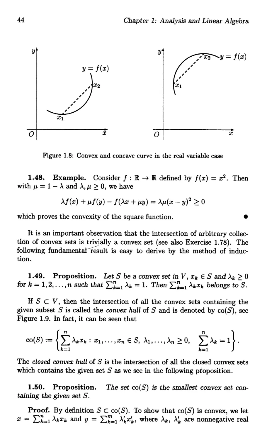
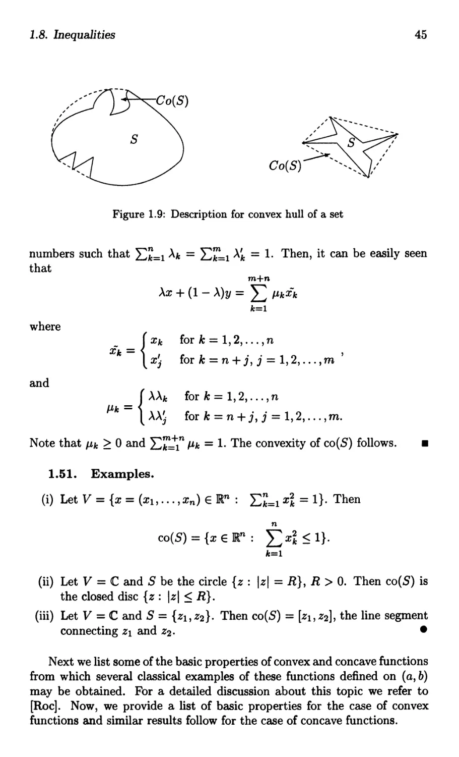
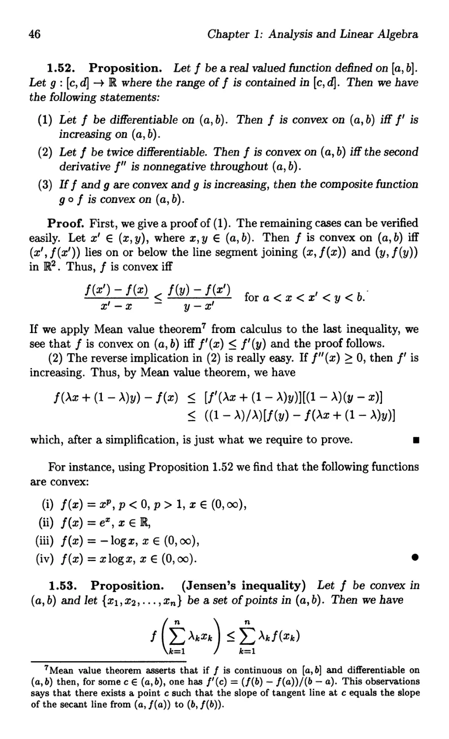
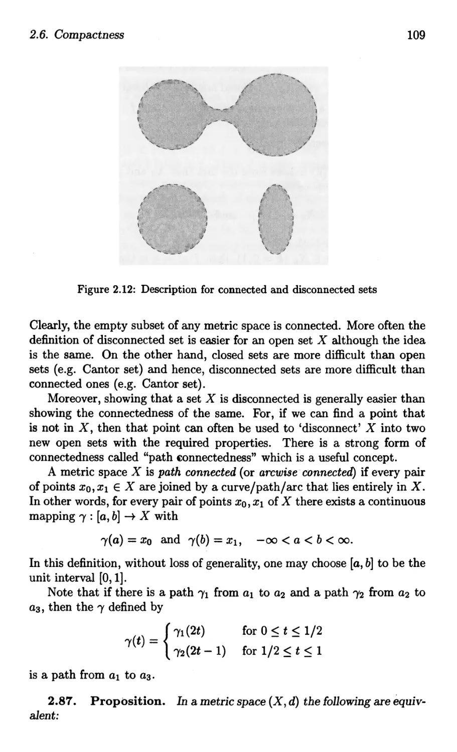
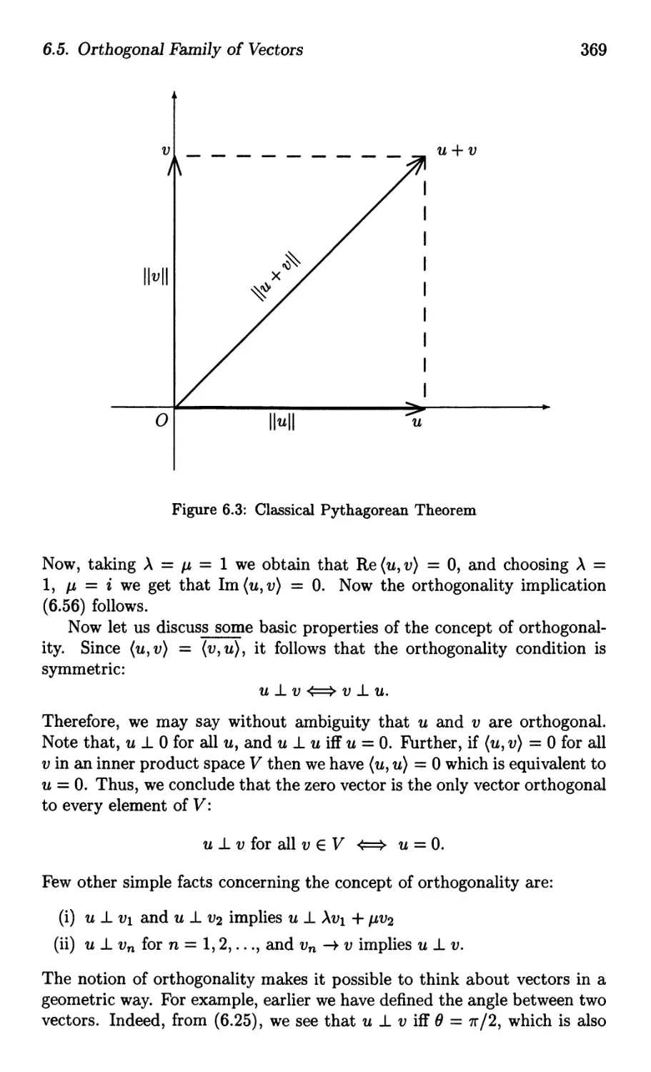
/


Text
ou nations
Function I
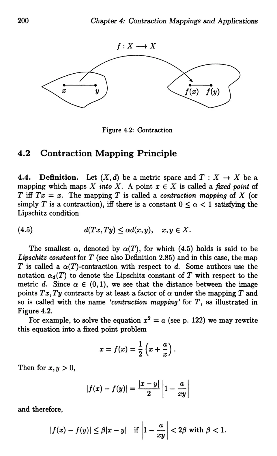
na Sl
S PONNUSAMY
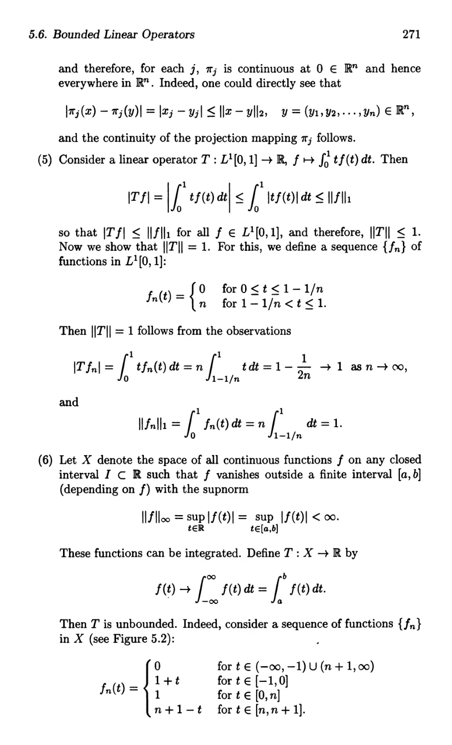
\,/
Alpha Science
Foundations of
FUNCTIONAL ANALYSIS
Otlaer Books of Interest
Advanced Engineering Mathematics (1-84265-086-6)
R.K. Jain and S.R.K. Iyengar
Calculus for Scientists and Engineers (1-84265-048-3)
KD. Joshi
Complex Analysis (1-84265-030-0)
v: Karunakaran
A Course in Ordinary Differential Equations (1-84265-068-8)
B. Rai et al
An Elementary Course in Partial Differential Equations
(81-7319-170-0)
T. Amarnath
A First Course in Mathematical Analysis (81-7319-064-X)
D. Somasundaram and B. Choudhary
Foundations of Complex Analysis (81-7319-040-2)
S. Ponnusamy
Function Spaces and Applications (1-84265-002-5)
D.E. Edmunds
Functional Analysis (1-84265-109-9)
Chandrasekhara Rao
Functional Analysis (81-7319-199-9)
Pawan K. Jain
An Introduction'to Measure and Integration (81-7319-120-4)
Inder K. Rana
Mathematical Analysis and Applications (81-7319-306-1)
A.R Dwivedi
Mathematical Appli tions in Social and Industrial Sectors
(81-7319-357-6)
NC. Mahanti
Foundations of
FUNCTIONAL ANALYSIS
s. Ponnusam.y
a
Alpha Science International Ltd.
Pangbourne England
s. Ponnusamy
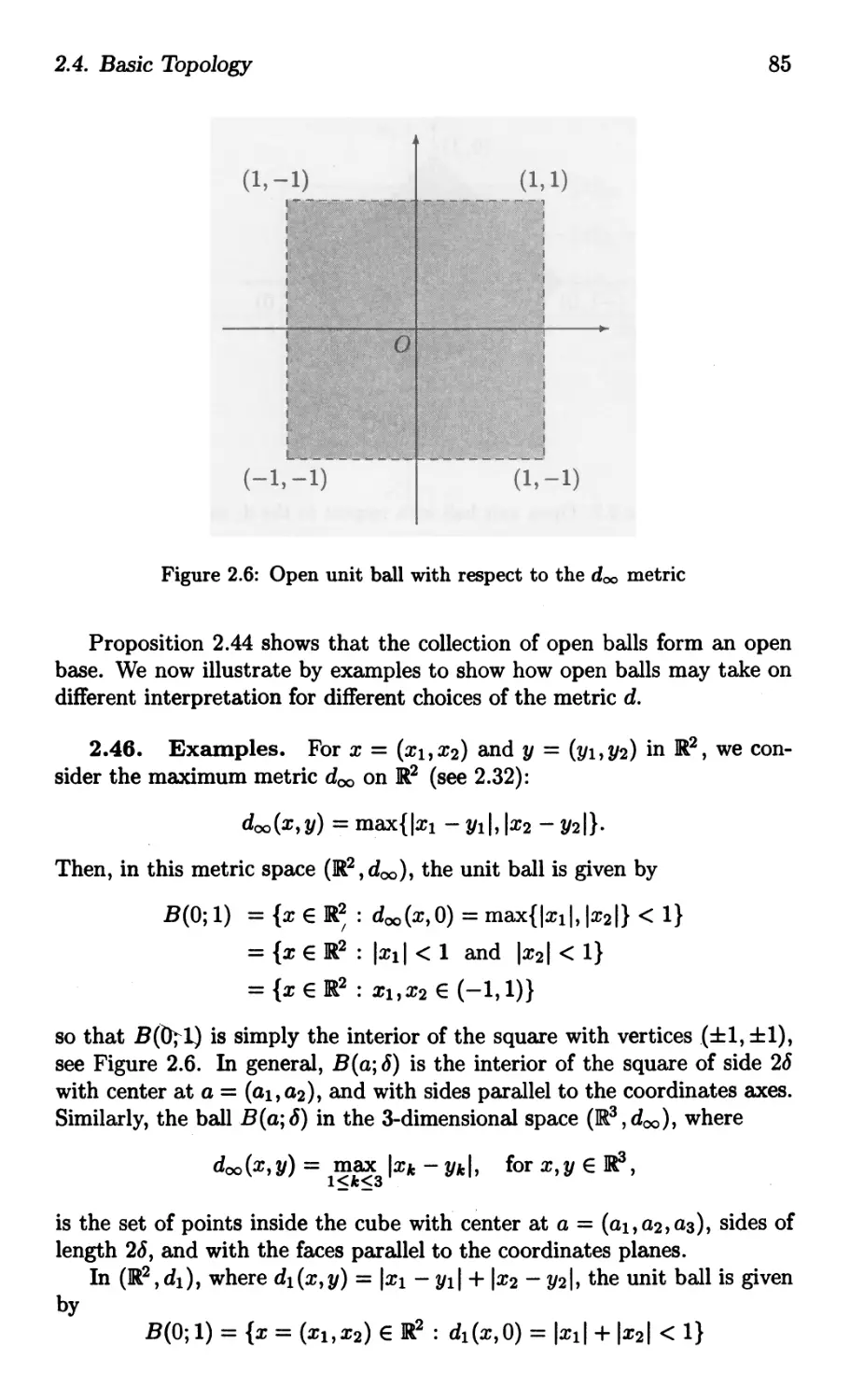
Associate Professor
Department of Mathematics
Indian Institute of Technology, Madras
Chennai-600 036, India
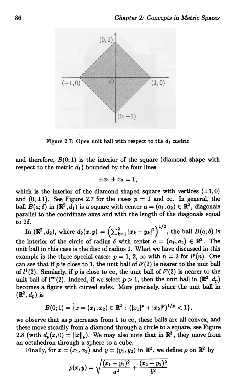
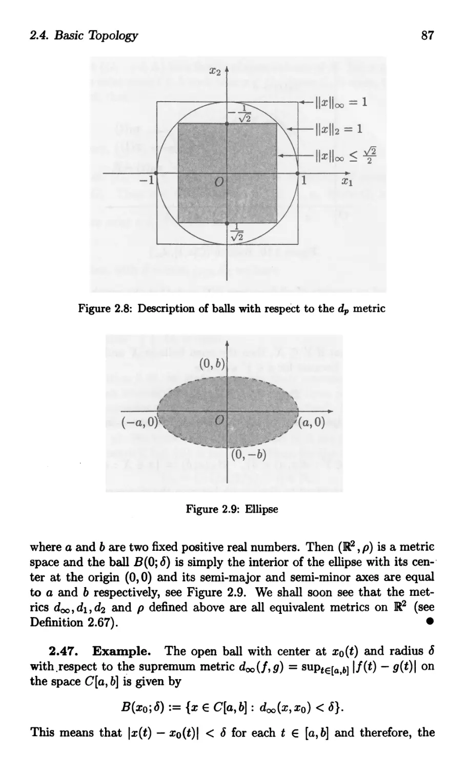
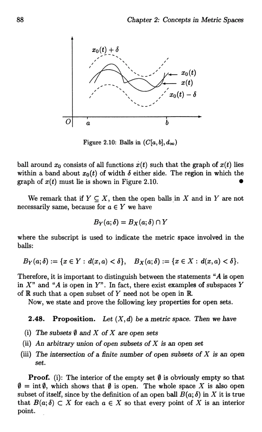
Copyright @ 2002
Alpha Science International Ltd.
P.o. Box 4067, Pangbourne RG8 BUT, UK
All rights reserved. No part of this publication may be reproduced, stored in a
retrieval system or transmitted in any form or by any means, electronic,
mechanical, photocopying, recording or otherwise, without the prior written
permission of the publishers.
ISBN 1-84265-079-3
Printed in India.
TO
BOOMA
Preface
This book is a first course on functional analysis and therefore not much
of prerequisite is assumed here. In fact, only some knowledge of elementary
linear algebra, real and complex analysis is essential. However, I have tried
my best to include, in Part I, the necessary basic results and the ideas of
the aforesaid topics. From some point of view, the reader will find that
they are the essential beginning for the course on functional analysis.
Part I of this text concerns with two fundamental chapters. Chapter 1 is
preliminary i nature and deals with elements of basic concepts in calculus,
lgebra, real and complex analysis. One of the interesting parts in the sub-
ject of analysis is the concept of metric spaces and Chapter 2 concentrates
more on this topic.
Besides metric spaces, the most important parts in functional analysis
are Banach spaces, Hilbert spaces and linear functionals on these spaces.
Thus, the main goal of this book is to give a rigorous analysis of the ba-
sics of functional analysis and therefore, the material found in Parts II
and III forms the core of the book. Part II is devoted to the theory of
normed space.s, Banach spaces, principle of contraction mappings and lin-
ear operators in normed spaces, while Part III is focused more on inner
product spaces, Hilbert spaces and the representation of linear functionals
with some applications.
Examples, remarks, observations and figures of this book are used to
illustrate the important points, the concepts and the motivation at every
suitable opportunity. Each chapter is provided with a fairly extensive set of
useful exercises. In general, these exercises are not difficult and should be
worked out to master the subject. Some of the problems are challenging,
but they should not be beyond the range of the talented students.
The numbering system followed in the text is self-evident and needs no
elucidation here. Now, I have one last comment on the notation. For the
sake of convenience, the sign _ signals the end of the proofs of Theorem,
Corollary, Lemma and Proposition whereas the sign. indicates the end of
Remark, Observation and Example.
In summary, I have endeavoured to produce a text which is useful for
the class room, as well as for self-study. In addition, I hope that through
this book the reader will gain sufficient mathematical maturity to be able
to pursue any advanced course in Functional Analysis with greater ease and
understanding. I believe that the text can be comfortably used by the en-
gineering students because of the inclusion of a large number of motivating
examples and exercises. Certainly there will be much room for improve-
. . .
Vlll
Preface
ments, and I welcome comments and suggestions from anyone who reads
the book.
In writing this book, I received lot of encouragement from several of my
teachers, friends and collaborators with whom I learnt lot of mathemat-
ics. I am particularly grateful to Professors R.Balasubramanian (Chen-
nai), O.P.Juneja (Kanpur), R.Ramachandran, R.K.S.Rathore (Kanpur),
M.S.Rangachari (Chennai), F.Ronning (Norway), St.Ruscheweyh (Germany),
C.S.Seshadri (Chennai), and V.Singh (Kanpur) who have been the source of
inspiration. Also, I take this opportunity to thank Professor Matti Vuori-
nen (Finland) for the hospitality during several of my visits to the Uni-
versity of Helsinki, Finland, resulting in many improvements at various
stages of the book manuscript. I also thank Prof. Hans-Olav J.Tylli and
Prof. G.P.Youvaraj for providing many useful suggestions.
My special thanks to Dr. Susma N.Agrawal, who spared her invaluable
time in reading the entire manuscript and made many criticisms. It is
my duty to thank Dr. Manju Rani Agrawal and Mrs. P.Vasundhra for
their careful reading of the entire manuscript, Mr. V.Ashok Kumar and
Ms. V.Sunitha for preparing the figures. I enjoyed the company of all
my colleagues in the Mathematics Department at lIT Madras, especially,.
Professors A.Avudainayagam, S.Sundar, P.Veeramani and V.Vetrivel for
their encouragement and I thank all of them.
I started this project while I was at the Indian Institute of Technol-
ogy, Guwahati and I thank the institute for its support. I wish to express
my thanks to the Centre for Continuing Education at the Indian Institute
of Technology, Madras, India, for its support in the preparation of the
manuscript. Finally, it has been a pleasure in working with the Narosa
Publishing House and I am indebted to Shri N.K. Mehra for his confidence
and continued enthusiasm during all stages of the writing process.
I must also record my appreciation due to my daughter Abirami and
son Ashwin for their understanding and love during the long period that
I have taken to complete this book. Above all, my deepest gratitude goes
to my wife Booma (alias Geetha), to whom the book is dedicated, for her
infinite patience, continued support, and the loving encouragement in all
walks of my life.
S. Ponnusamy
Symbol
o
aES
aftS
{a}
{x:...}
XuY
XnY
XCY
X C Y or X S; Y
XxY
X \Y or X - Y
XC
=>
<==}
or
-/-t or -It
N
No
z+
z-
z
Q
I
R
Index of Special Notation
Meaning for
empty set
a is an element of the set S
a is not an element of S
set having a as unique element
set of all elements with the property
set of all elements in X or Y;
Le., union of the sets X and Y
set of all elements in X as well as in Y;
Le., intersection of the sets X and Y
set X is contained in the set Y; Le X is a subset of Y
X C Y and X :F Y;
Le., set X is a proper subset of Y
Cartesian product of sets X and Y, {(x,y): x EX, Y E Y}
set of all elements that live in X but not in Y
complement of X
implies (gives)
if and only if, or briefly 'iff'
converges (approaches) to; into
does not converge
does not imply
set of all natural numbers, {I, 2, · . .}
N U {OJ = {O, 1,2, · . .}
set of positive integers, {1,2,...}
set of all negative integers, {..., -2, -I}
set of all integers (positive, negative and zero)
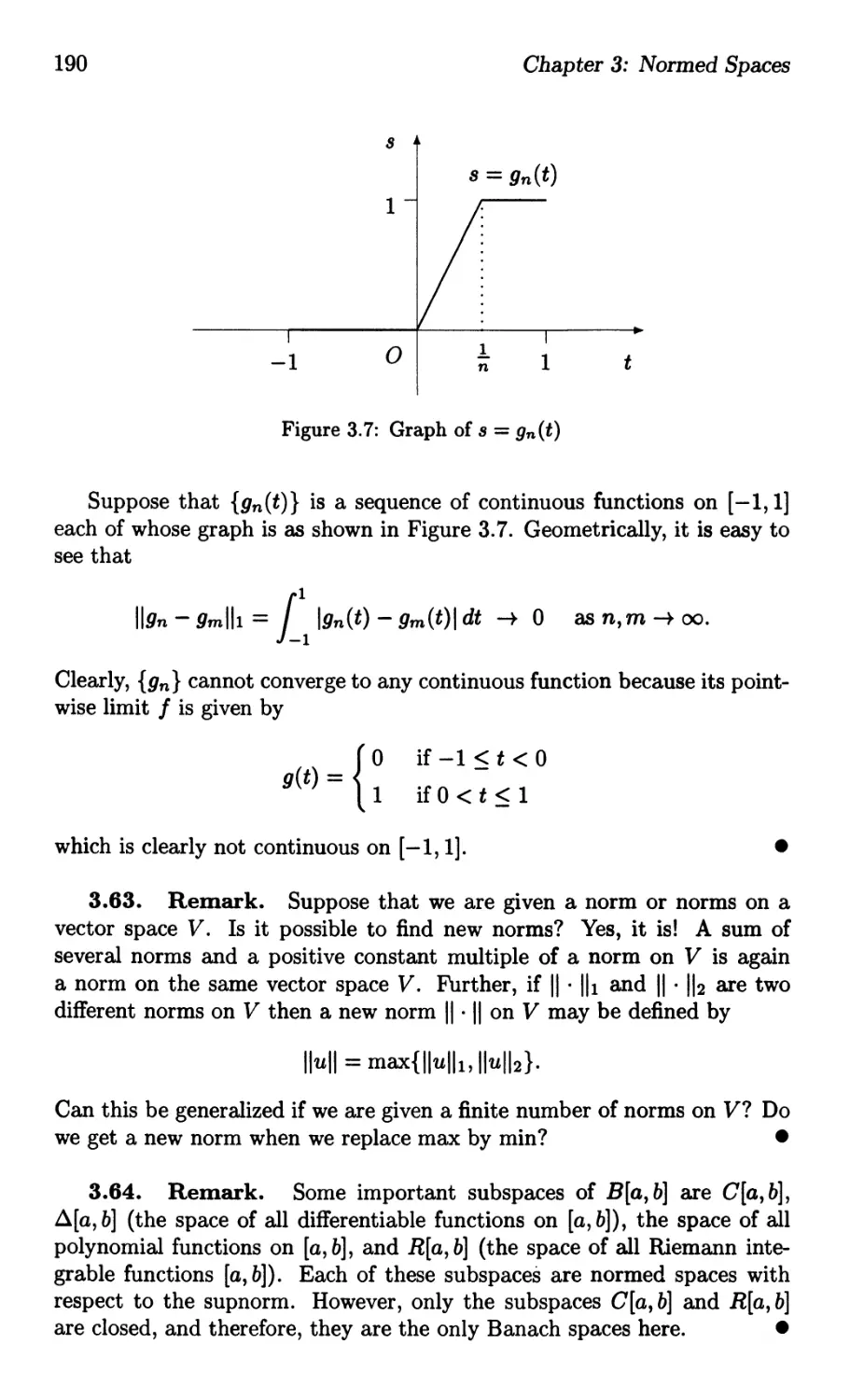
set of all rational numbers, {p/q: p, q E Z, q :F O}
set of all irrational number
set of all real numbers
x
1R
c
C
IRQ
IR-
IRt
IR+
IRoo
Coo
IRn
en
i]R
1F
Z
Izi
Rez
Imz
argz
Argz
limsup IZnl
lim inf IZnl
lim IZnl
supS
f : D Dl
f(x)
f(D)
f-l (D)
f-l(y)
fog
SUPxED f(x)
Index of Special Notations
IR U {-oo, oo}, extended real line
set of all complex numbers, complex plane
extended complex plane, C U {oo}
set of all nonpositive real numbers, {x E IR : x < O}
set of all negative real numbers, {x E ]R : x < O}
set of all nonnegative real numbers, {x E ]R: x > O}
set of all positive real numbers, {x E ]R: x > O}
set of all infinite sequence of real numbers
set of all infinite sequence of complex numbers
n-dimensional real Euclidean space,
the set of all n-tuples x = (Xl, X2, · · · , x n ),
Xj E IR, j = 1,2, . . . , n
n-dimensional complex Euclidean space,
the set of all complex n-tuples z = (Zl, Z2, . . . , zn)
set of all purely imaginary numbers, imaginary axis
field C or IR
z := x - i y, complex conjugate of z = x + iy
V X2 + y2, modulus of z = x + iy, x, y E ]R
real part x of z = x + iy
imaginary part y of z = x + iy
set of real values of () such that z = Izle iB
argument () E arg z such that -1r < () < 1r
upper limit of the real sequence {Iznl}
lower limit of the real sequence {Iznl}
limit of the real sequence {Iznl}
least upper bound, or the supremum, of the set S C IR
f is a function from D into Dl
the value of the function at x
set of all values f(x) with xED;
Le., y E f(D) <==} 3 xED such that f(x) = y
{x : f(x) ED}, the preimage of D w.r.t f
the preimage of one element {y}
composition mapping of f and g
supremum of f in D
Index of Special Notation
inf S
infzED f(x)
maxS
minS
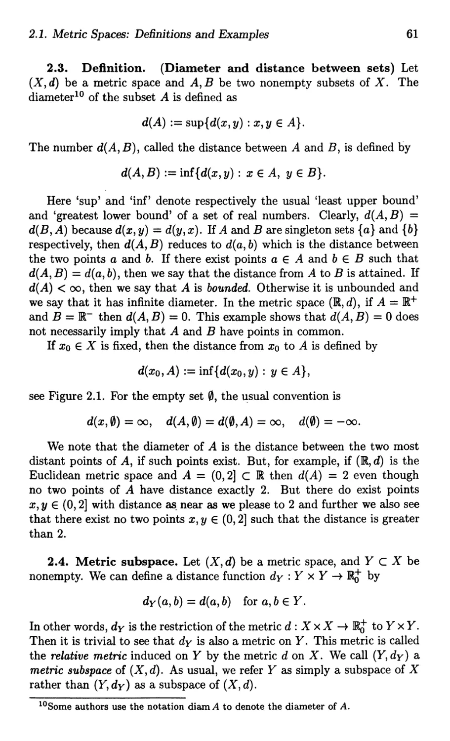
dist (A, B)
d(A)
[Xl, X2]
(Xl, X2)
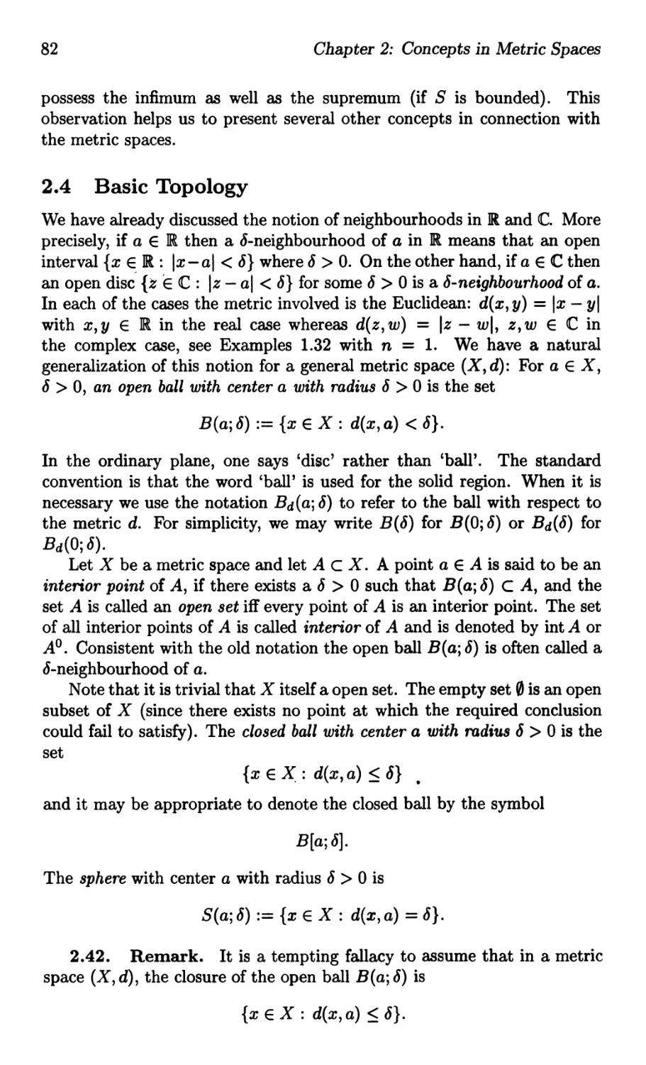
(a; r)
(a; r)
o (a; r)
r
ad
e Z
Logz
logz
o
oz
o
{)z
fz
fz:
1'1 + 1'2
£(1')
f(n) (a)
1l(D)
f(x) = O(g(x)) }
asx-+a
Xl
greatest lower bound, or the infimum, of the set S C ]R
infimum of f in D
the maximum of the set S C JR;
the largest element in S
the minimum of the set S C JR;
the smallest element in S
distance from A to B
diameter of A
{x = (1- t)X1 + tX2 : 0 < t < I}
{x = (1 - t)X1 + tX2 : 0 < t < I}
open disc {z E C: Iz - al < r} (a E C, r > 0)
closed disc {ZEC: Iz-al < r}(aEC, r>O)
the circle {z E C: Iz - al = r}
d(O; r)
d (0; 1), unit disc {z E C: I z I < I}
unit circle {z E C: Izl = I}
exp(z) = En o , exponential function
In Izl + iArgz, -1r < Argz < 1r
In Izi + i argz := Logz + 2k1ri, k E Z
1 ( 0 .0 ) .
- - - - z = x + y
2 ox oy'
1 ( +i )
2 ox oy
of
oz
of
{)z
sum of the curves 1'1, 1'2
length of the curve l'
n-th derivative of f evaluated at a
family of analytic (holomorphic) functions on D.
If(x)1 < Klg(x)1 for all x in a neighbourhood of a
. .
Xll
f(x) = o(g(x)) }
asx-+a
lim X n = X, }
n-+oo
or X n -+ x, or
d(xn, x) -+ 0
C(X)
I" (n ) }
(l < p<oo)
1 00 (n)
I" (1 < p < 00)
1 00
c
Co
Coo
A = (aij)
A-l
At
r n (IF)
Mmxn (IF)
6 ij
det (A)
trace (A)
Cc[a, b]
C[a, b]
[ ']B : V -+ r
Iv := I
Bv := (}, 0
L(V, W)
B(V, W)
Ker (T) or NT
1m (T) or RT
Sl.
Index of Special Notations
Hm f(x) = 0
z-+a g(x)
sequence {xn} converges to x with a metric d
set of all continuous scalar valued functions on X
{Z = (Zl, Z2, . · · , zn) E r : L 1 I Z k I" < oo}
{z = (Zl, Z2,..., zn) E r : maxl<k<n IZkl < oo}
{z = {Zn}n l : L llzkl" < oo}
{z = {Zn}n l : SUPl k<oo IZkl < oo}
{z = {Zn}n l E 1 00 : lim n -+ oo Zn exists and is finite}
{z = {Zn}n l E c: lim n -+ oo Zn = O}
{z = {Zn}n l E 1 00 : support [{Zn}n l] = {n : Zn O}
is finite}
matrix A whose (i,j)-th entry is aij
inverse of a non-singular matrix A
transpose of a matrix A
set of all polynomials of degree at most n
with coefficients over the field IF
set of all m x n matrices with entries in IF
Kronecker delta function
determinant of a matrix A = (aij)nxn
L au, trace of A
set of all continuous complex valued functions on [a, b]
set of all continuous real valued functions on [a, b]
coordinate map v I-t [V]B w.r.t the basis B
identity map on the set V
zero element on the vector space V
set of all linear transformations T : V -+ W
set of all bounded linear transformations T : V W
kernel of T or the nullspace of T
image of T or range space of T
orthogonal complement of S
Index of Special Notation
Xl,ll,
d( ., .)
d x (.,.)
IIxll
IIxlix
II/lip
(., .)
distance function in a metric space
distance function in a metric space X
norm or length of a vector x
norm of a vector x E X
LP-norm of /
inner product
Contents
Preface ...........
Index of Special Notations.
I BASIC ANALYSIS . . . . . . . .
1 Analysis and Linear Algebra. .
1.1 Review of Complex Numbers
1.2 Functions and Countability. ....
1.3 Review of Differentiability in Real Line
1.4 Concept of Derivative in Complex Plane.
1.5 Concept of Riemann and Riemann Stieltjes Integrals
1.6 Vector Spaces . . . . . . . . . . . . . . . . . . . .
1.7 Linear Transformations between Vector Spaces
1.8 Inequalities.....
1.9 Exercises..................
Concepts in Metric Spaces . . . . . . . . . . . . .
2.1 Metric Spaces: Definitions and Examples
2.2 Holder and Minkowski Inequalities . . . .
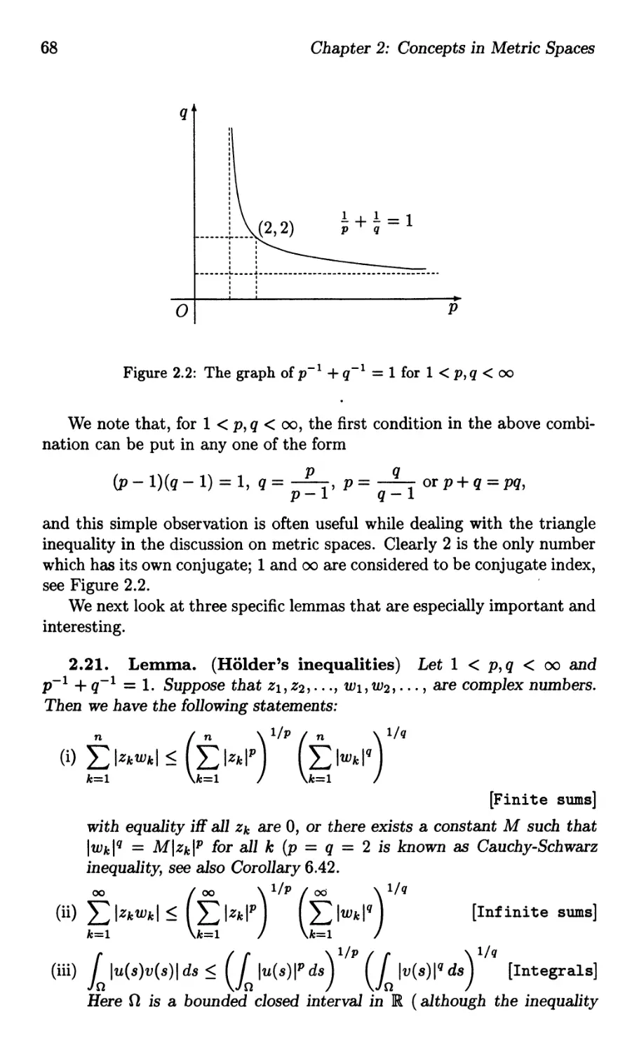
2.3 Metric spaces IP(n), IP and C[a, b]
2.4 Basic Topology . . . . . . . . . . . . . .
2.5 Continuity and Equivalent Metrics
2.6 Compactness.............
2.7 Cauchy Sequences and Completeness . .
2.8 Completion of Metric Spaces . . . .
2.9 Exercises
II BANACH SPACES . . . . . . .
3 Normed Spaces . . . . . . .
3.1 Properties of Norm.
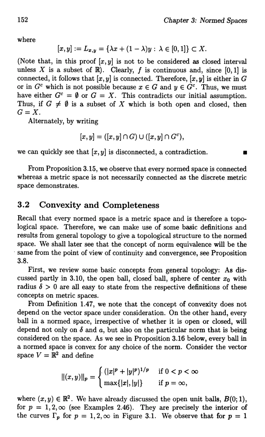
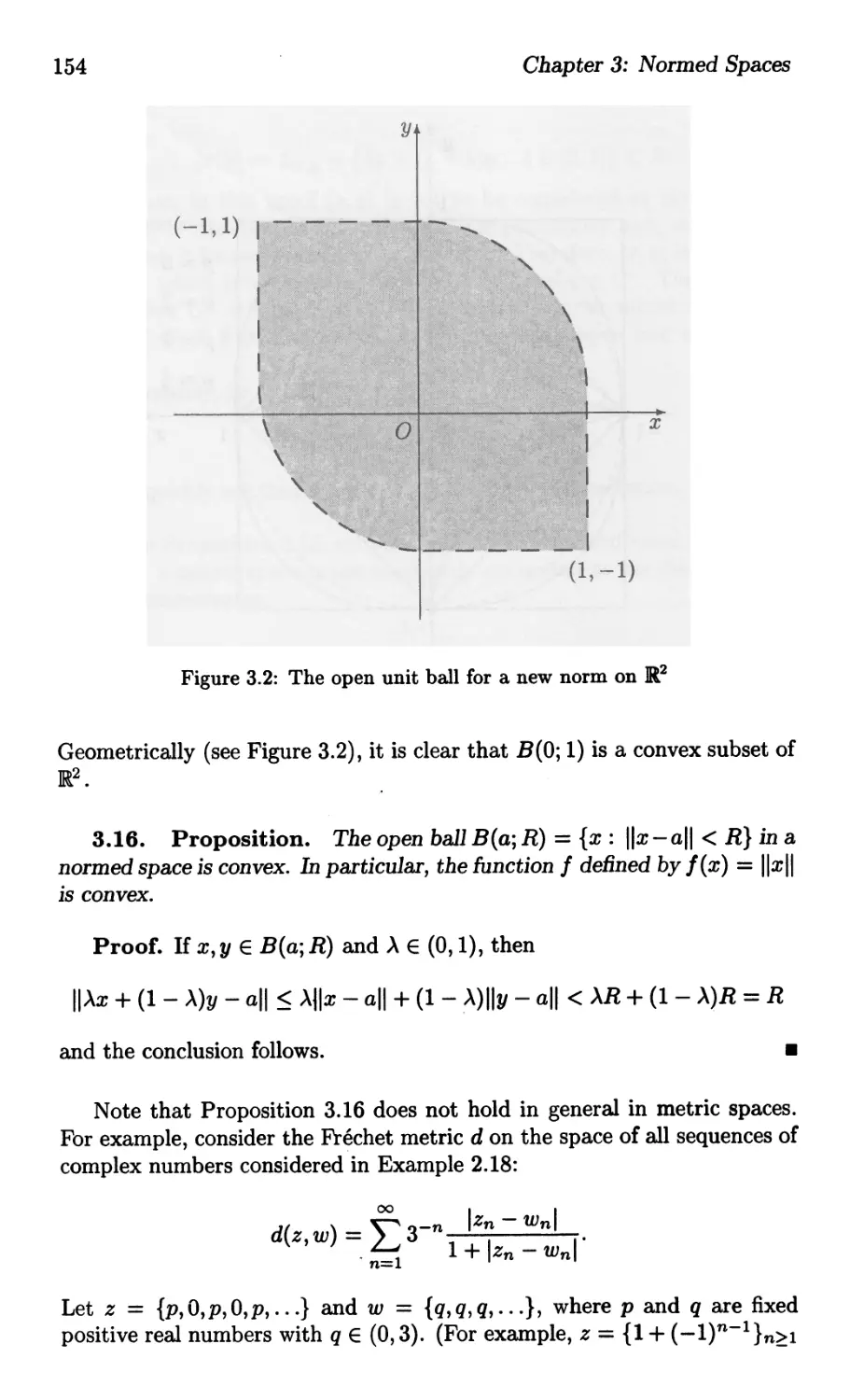
3.2 Convexity and Completeness
3.3 The Banach Spaces IP(n) (1 < p < 00)
3.4 The Sequence Spaces lP (1 < p < 00) .
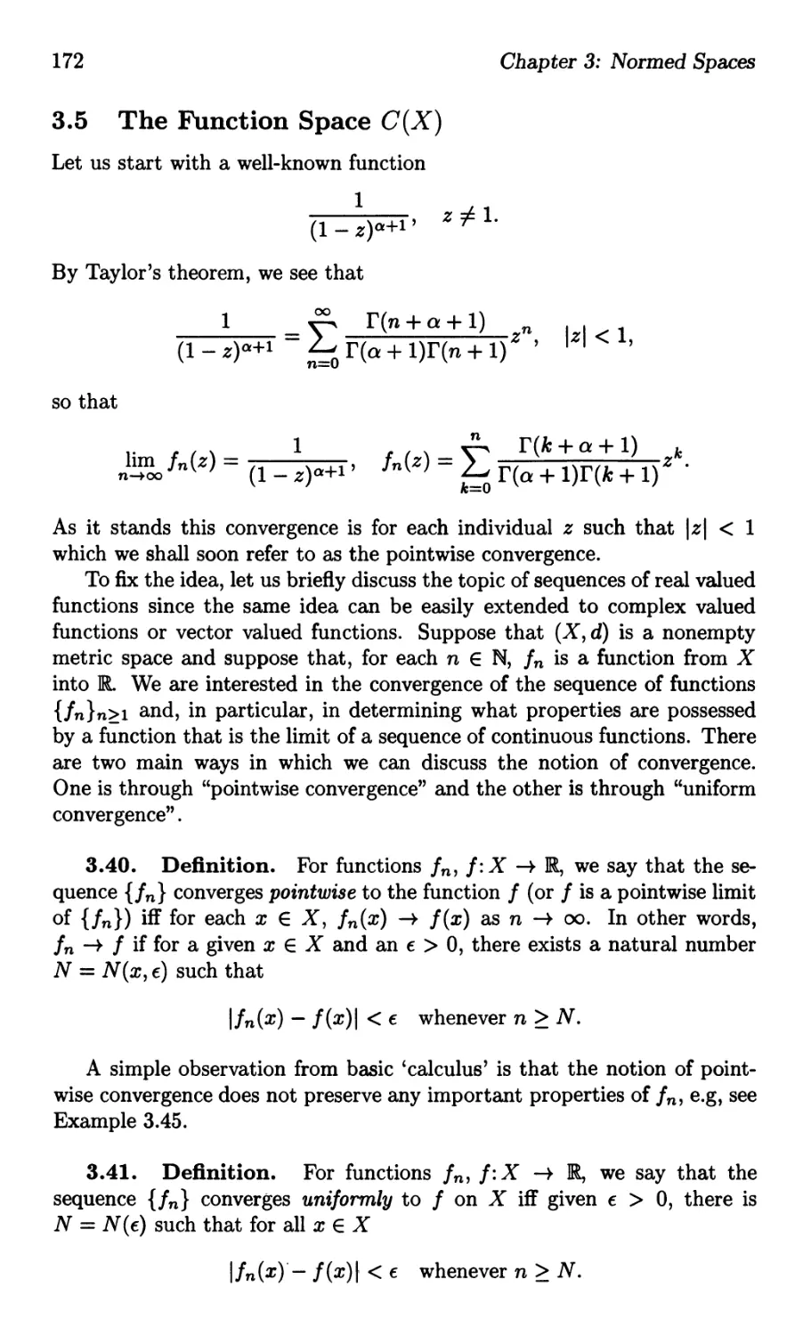
3.5 The Function Space C(X) . .
3.6 Basic Results on LP-Spaces
3.7 Norms on C[a, b]
3.8 Exercises...........
2
iii
v
1
3
3
10
15
19
22
27
35
42
53
59
59
67
75
82
94
103
120
.. 127
132
141
143
143
152
162
164
172
179
185
191
XVl
CONTENTS
Contraction Mappings and Applications . . .
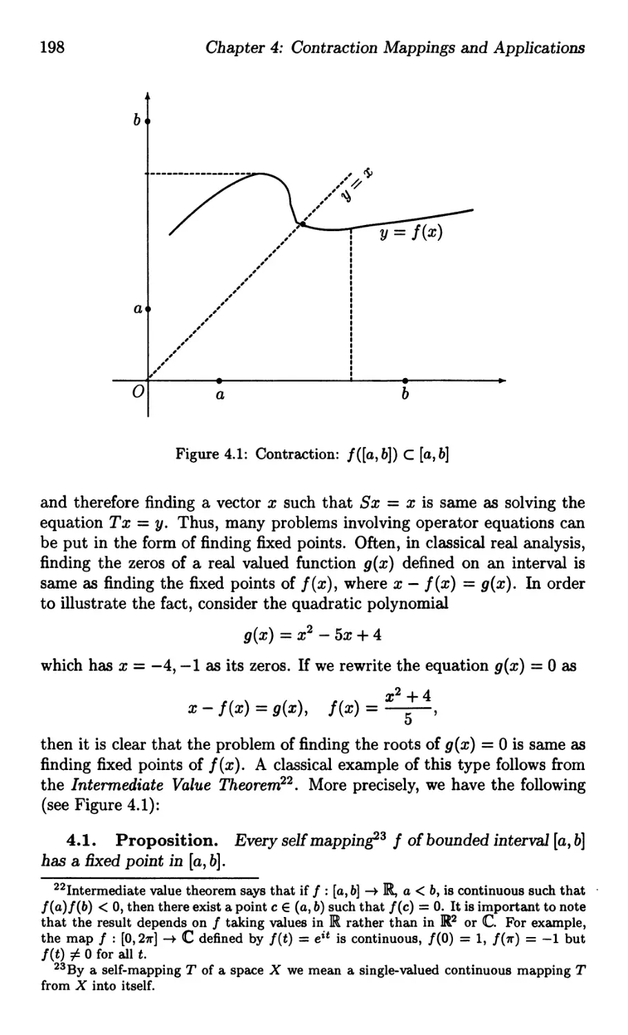
4.1 Discussion on Fixed Point Problems
4.2 Contraction Mapping Principle . . .
4.3 Applications to Differential Equations
4.4 Exercises...............
Linear Operators on Normed Spaces . . . . . .
5.1 Finite Dimensional Normed Space . . .
5.2 Direct Sums and Complementary Subspaces .
5.3 Riesz Theorems. . . . . . . . . . . . . . . .
5.4 Approximation in Function Spaces
5.5 Schauder Basis . . . . . . . . . . . . . .
5.6 Bounded Linear Operators ........
5.7 Inverse Operators. . . . . . . . .
5.8 Completion of Normed Spaces ......
5.9 Quotient Spaces ...... . . . . .
5.10 Baire Category Theorem. .
5.11 Open Mapping Theorem. . . . . . . . . . .
5.12 Closed Graph Theorem ... .....
5.13 Uniform Boundedness Principle. . . . . .
5.14 Extension of Continuous Functionals . . .
5.15 Embedding of Normed Spaces. .
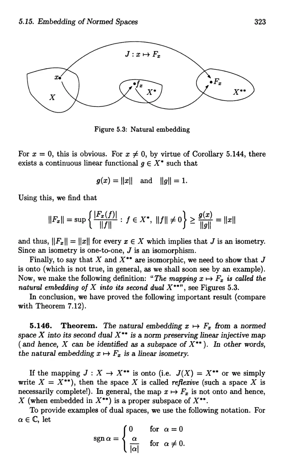
5.16 Exercises .... . . . . .
III HILBERT SPACES. . . . . . . . .
6 Inner Product Spaces. . . . . .
6.1 Inner Product. . . . . . . .
6.2 Examples of Hilbert Spaces . . . . .
6.3 Applications of Polarization Identity
6.4 Completion of Inner Product Spaces
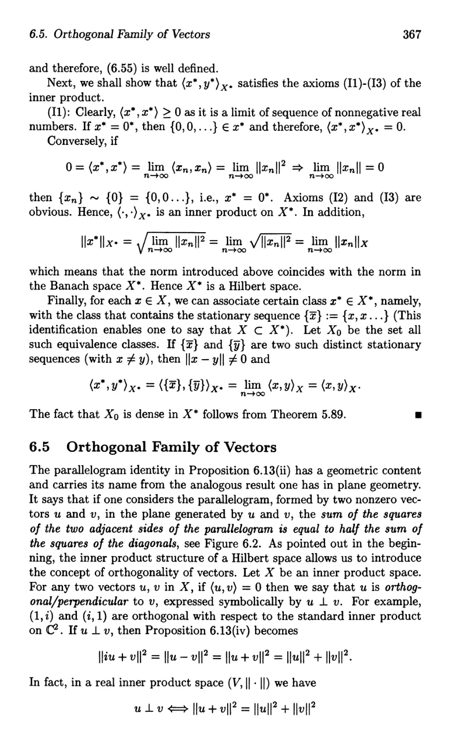
6.5 Orthogonal Family of Vectors . . . . . .
6.6 Projections on Finite Dimensional Spaces
6.7 Orthogonal Projections on Hilbert Spaces
6.8 Orthonormal Basis and Bessel Inequality
6.9 Cardinality Theorems for Orthonormal Bases
6.10 Applications of Uniform Boundedness Principle.
6.11 Exercises.............
Representation of Linear Functionals . . . .
7.1 Riesz Representation Theorem . ...
7.2 Adjoint Operators on Hilbert Spaces . .
7.3 Exercises...............
4
5
7
Bibliography
Index .............
197
197
200
212
217
221
222
231
234
247
253
255
274
277
285
290
294
299
305
307
321
332
339
343
343
353
361
365
367
377
382
399
413
416
422
429
429
436
448
449
451
Part I
BASIC ANALYSIS
In this part we shall first review in Chapter 1 some basic facts from real
and complex analysis and linear algebra. Apart from certain additional
materials for the foundation of functional analysis, Chapter 1 also contains
the mathematical background for most of the chapters and it is expected
that they will really be useful for the understanding of the rest of the book.
The material is grouped under several sections, each of which contains a set
of theorems, lemmas, propositions, basic mathematical examples, remarks
and certain interesting observations.
Inequalities play an important role in several branches of science and
technology, and therefore for an easy access to the reader, we provide a
separate section on Inequalities particularly to represent several standard
inequalities associated with sums and integrals of real/ complex valued func-
tions. Some of these inequalities are important in other branches of math-
ematics as well and, in fact, most of the students might have learnt the
preliminary part of the material of this chapter in the usual analysis course.
Chapter 2 reviews the concept of metric spaces, certain function spaces
and develops point-set topology of metric spaces. These are done through
concepts such as neighbourhoods, open sets, closed sets, sequences, etc.
In Section 2.4, we introduce the concept of topology. These topological
concepts are used to define the concept of continuity on metric spaces. In-
deed, in Section 2.5, we investigate some topological properties of continuity
which, in fact, can be applied in a more general setting.
The concept of completeness plays a central role in the theory of metric
spaces and is discussed in Sections 2.7 and 2.8. In particular, prior to the
discussion on the completeness property, we analyze some basic examples
of function spaces that appear frequently in Analysis. For example, the
space CF[a, b] of all F(C or IR)-valued continuous functions on the closed
interval [a, b] and the space BV[a, b] of all functions of bounded variation
on the closed interval [a, b]. The sequence spaces lP(n) and IP, 1 < p < 00,
and the properties such as inequalities between them are also discussed in
Section 2.3. In particular, we shall see in the subsequent chapters that how
the completeness property is important in the study of Banach spaces and
Hilbert spaces. Completeness of some other spaces will be considered in
Part II as well.
Chapter 1
Analysis and Linear Algebra
The purpose of this chapter is to give a brief review of the basic concepts
from the theory of real and complex analysis which will be needed in what
follows. In Section 1.2, we introduce the basic definitions such as one-to-
oneness and ontoness. In Section 1.6, we deal with vector spaces, subspaces,
linear transformations, and some of the basic properties of certain spaces
such as IP(n) and IP, 1 < p < 00. Several basic inequalities will be proved in
Section 1.8. These inequalities are required to show that certain spaces are
metric spaces and they are also important in the other branches of analysis.
1.1 Review of Complex Numbers
We briefly recall some notation and a few facts from the algebra of sets.
If A is a set of objects (Le. numbers, vectors, or functions), and x is an
element (or member) of A, we write x E A. Likewise, the expression x A
refers to "x is not a member of A". IT B is another set and each element
of B is also an element of A, then we say that B is a subset of A, and we
write B C A. Equivalently,
B C A {:::::} x E B implies that x E A.
For instance, if A and B are two sets then
A = B {:::::} B C A and A C B.
We use the symbol '0' to denote the empty set, the set with no elements.
Clearly, each set is a subset of itself, and therefore to distinguish the subsets
that do not coincide with the set in question, we say that A is a proper subset
of B if A C B and in addition, B also contains at least one element that
does not belong to A. We denote by the symbol A S; B, a proper subset A
of B. However, if one wishes to indicate that A is a subset of B which is
4
Chapter 1: Analysis and Linear Algebra
possibly the set A itself, then we write
A C B.
When A is not a subset of B, then we can indicate this by the notation
Acj.B
meaning that there is at least one element x E A but not in B.
1.1. Relation. A relation < on a set F is a strict total order whenever
a f:. a, a < b and b < c =} a < c, a < b or a = b or b > a for all a, b and
c in F. We write a < b for a < b or a = b, and note that in a total order
a < b {:} b f:. a.
Familiar ordered fields are Q and III In an ordered field we define the
absolute value lal of a as:
lal = { a
-a
for a > 0
for a < O.
1.2. Concept of equivalence relation. Now, we consider a useful
class of mappings called equivalence relation. Later we shall discus a variety
of classes of mappings such as one-to-one, onto, and continuous. We use
the notation "a f'J b" to indicate the relationship between two elements a, b
of a set X rather than the ordered pair notation (a, b).
Given a non empty subset X, an equivalence relation on X is a relation
between the elements of X, denoted by the symbol f'J (or R), which satisfies
the following three rules for all x, y, z EX:
(El) x f'J x, Le. every element 01 X has a relation with itself [Reflexivity]
(E2) x f'J y => y f'J x, Le. if x is related to y, then y is related to x
[Symmetry]
(E3) x f'J y, Y f'J Z => X f'J z, Le. if x is related to y and y is related to
z, then x is related to z. [Transitivity]
A relation f'J on a set X is called a partial ordering if it is reflexive, an-
tisymmetric (Le. for x, y EX, X f'J Y and y f'J X imply that x = y), and
transitive. A partially ordered set is a pair (X, ""), where X is a set and f'J
is a partial ordering on that set. Clearly, the standard operation " < " on IR
defines a partial ordering on III In consistent with this fact, it is a standard
practice to denote the partial ordering by the more suggestive symbol " < "
rather than the symbol "f'J".
A partially ordered set (X, < ) is called linearly/totally ordered if < sat-
isfies the condition
x < y or y < x for every x, y EX.
1.1. Review of Complex Numbers
5
In this case, < is called a linear ordering. If Y e x, then an element m E X
is an upper bound for Y (with respect to the ordering < ) if Y < m for all
Y E Y. An element m E X is called the maximal provided
m < x, x E X implies m = x.
1.3. Examples.
(1) Ordinary equality '=' is a trivial example of an equivalence relation
on IR whereas each of ' < ' and ' > ' is not an equivalence relation. Note
that, each of ' < ' and ' > ' is a partial ordering on III Moreover, the
relation "<" does not satisfy the reflexivity condition since x < x
is not true for any x E III It is also not symmetric, although it is
transitive.
(2) Assume that x = y iff x - y is even, where x, y E III Then ' = ' is an
equivalence relation on the set III In particular, IR is not a partially
ordered set with respect to this relation (eg. choose x = 3 and y = 5).
(3) Let X = Z, the set of all integers. On X, define x f"oJ y iff y - x
is divisible by 2. Then, it can be checked that Z is an equivalence
relation with respect to the defined relation.
(4) Let Y be the family of all subsets of a set X, and assume that A < B
iff A C B, for A, BEY. Then Y is a partially ordered set with respect
to the set inclusion C as our partial ordering on Y. In particular, for
each A, BEY, it follows that A C Band B C A imply that A = B.
If S C Y, then UA S A is an upper bound for S.
We shall now state without proof the axiom of choice in one of its
equivalent form, namely the Zorn's lemma:
1.4. Lemma. Let E be a nonempty partially ordered set. If every
totally ordered subset of E has an upper bound, then E has a maximal
element.
Now, we start with the discussion on the set of complex numbers. The
starting point for the introduction of the complex numbers, which all al-
ready familiar to us from high schools, arises when we need to solve certain
equations such as
x 2 + 1 = o.
Complex numbers may be introduced in the following way. A complex
number is an ordered pair of real numbers:
Z = (x, y).
The word 'ordered' means that (x, y), (y, x) are distinct unless x = y. If
Zl = (Xl,Yl) and Z2 = (X2,Y2) then we say that
Zl = Z2 <==> Xl = X2 and Yl = Y2.
6
Chapter 1: Analysis and Linear Algebra
In particular,
Z = (x, y) = (0,0) <==} x = 0 and y = o.
In C, the set of all ordered pairs of real numbers, we define the arithmetic
operations for Zl = (Xl, Yl) and Z2 = (X2, Y2) E C:
Zl Z2 - (Xl, Yl) (X2, Y2)
- (Xl X2,Yl Y2)
ZlZ2 - (Xl, Yl)(X2, Y2)
(XlX2 - YlY2, XlY2 + YlX2)
AZ - (AX, AY), A E IR
Zl ( X1 X 2 + 1}11}2 X2Y1 - X1Y2 ) if Z2 (0,0).
- 2 2 ' 2 1A '
Z2 x 2 + Y2 x2 + 2
The notation commonly used for a complex number is not (x,y) but x+iy,
x, y real. Following Euler, we define i in the complex number system C of
ordered pairs: i := (0, 1). From here it follows that complex numbers (x, 0)
may be identified with real numbers x. From the multiplication rule we can
write (in an informal way)
i 2 = i x i = (-1,0) = -1 + iO
which makes it possible to express a complex number Z - (x, y) in the
following useful algebraic form:
Z = (x, y) = (x, 0) + (0, y) = (x, 0) + (0, l)(y, 0).
Thus, the set C of complex numbers is defined to be the set of numbers of
the form Z = x + iy, where i = A and x, yare real numbers.
1.5. Elementary properties of complex numbers. Complex num-
bers of the form (x, 0) are said to be purely real or just real. Those of the
form (0, y) are said to be purely imaginary. 'Zero' viz. (0,0) = 0 + iO is
the only complex number at once real and purely imaginary. The complex
conjugate of Z = x + iy is the complex number Z := x - iy. Note that
Z = Z iff l x + iy = x - iy, i.e. Z is purely real. Geometrically, the complex
conjugate of Z is obtained by reflecting Z in the real axis. For any two
complex numbers Zl and Z2, the following simple properties of the complex
conjugate are easy to verify by a straightforward calculation:
· Z'1:EZ2 = Z l Z2
· ZlZ2 = Z l Z2
1 The shorter form 'iff' is to be read as 'if and only if'.
1.1. Review of Complex Numbers
7
· Zl = Zl
. Zl/Z2 = Z l/ Z2 for Z2 O.
We also define Izi := vx 2 + y2 which is called the modulus of the complex
number z. We observe that
Izl 2 = z z = x 2 + y2 = (Rez)2 + (Imz)2.
With the standard notation, it follows that
z+ z z- z
Re z = x = and 1m z = Y = .
2 2i
For any pair Zl, Z2 E C, the following properties are easy to verify:
. Re (Zl :i: Z2) = Re Zl :i: Re Z2
. 1m (Zl :i: Z2) = 1m Zl :i: 1m Z2
· I Z IZ21 = I Z lllz21
· IZ1/ z21 = I Z ll/l z 21 for Z2 :F O.
We know that the ordered pairs of real numbers represent points in the
geometric plane with respect to a pair of rectangular axes. We then call
the collection of ordered pairs as the Cartesian product }R x ]R = ]R2 and
the two axes as x-axis, y-axis. Because (x,O) E }R2 corresponds to real
numbers, x-axis is called the real axis and since iy = (0, y) E ]R2 is purely
imaginary for y real, y-axis is called the imaginary axis.
Now, we can conveniently visualize C as a plane with x + iy as points
in }R2 and we simply refer to it as the complex plane. Depending on the
problems on hand, we use x + iy, or (x, y), to represent a complex number.
Thus, we see that a complex number Z = x+iy can be viewed geometrically
as the point (x, y) in a coordinate plane (complex plane C): x+iy I-t (x, y).
The distance from the origin to a complex number Z = x + iy is then
V X 2 + y2 = Izi.
For Z = x + iy, it is appropriate to include some useful elementary inequal-
ities:
. IRezl < Izl
. IImzl < Izl
· ( )(Ixl + Iyl) < Izl < Ixl + Iyl
. Iz:i: wi < Izi + Iwl, for z, w E C
. Ilzl - Iwll < Iz - wi.
8
Chapter 1: Analysis and Linear Algebra
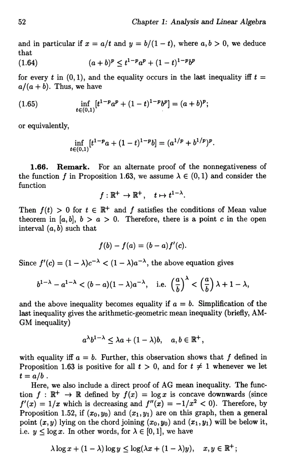
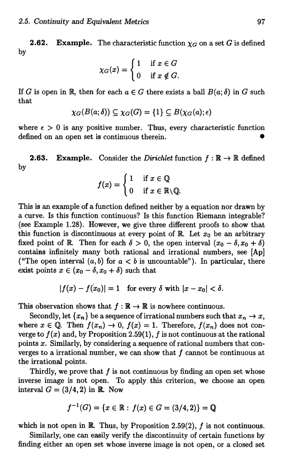
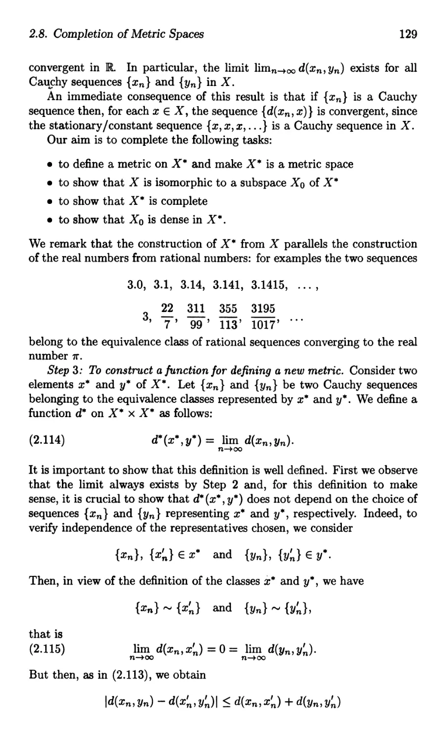
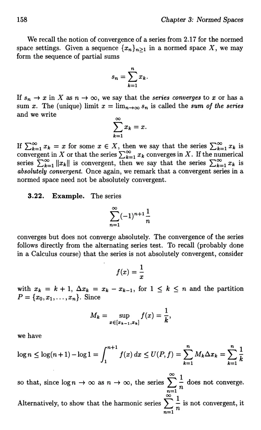
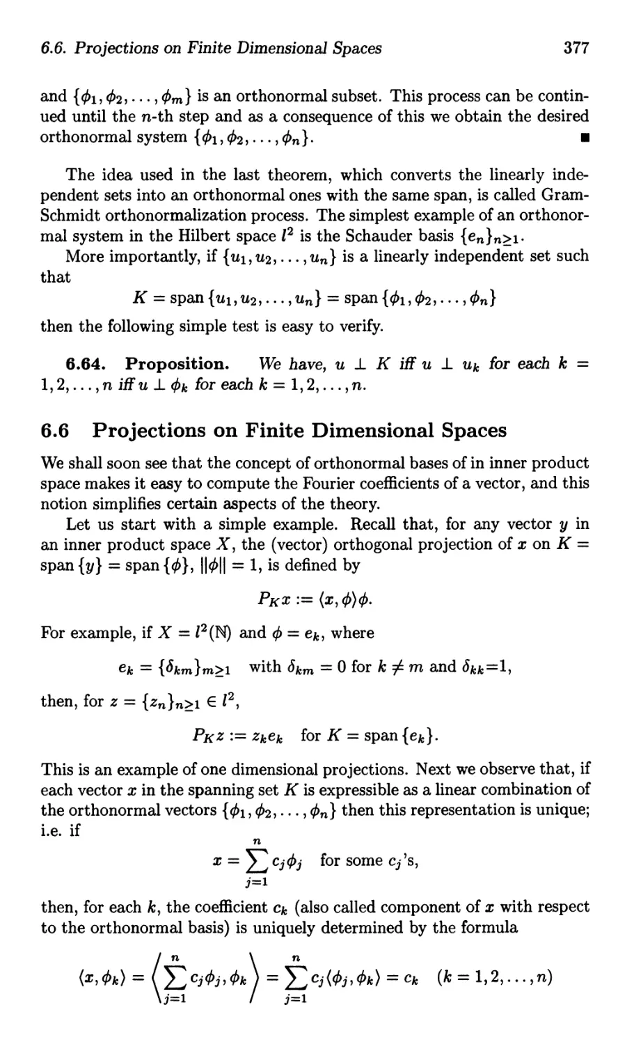
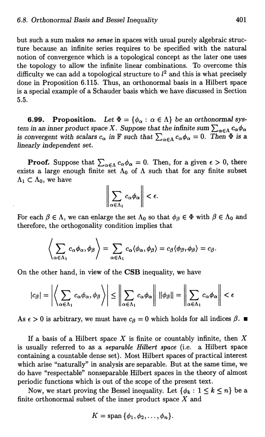
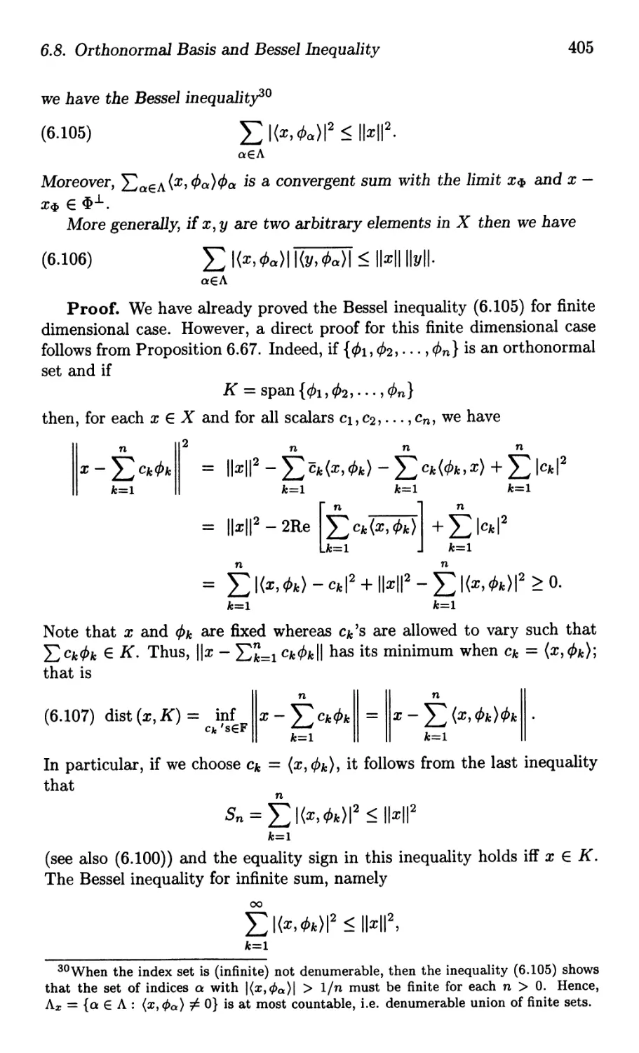
y
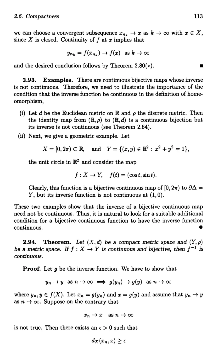
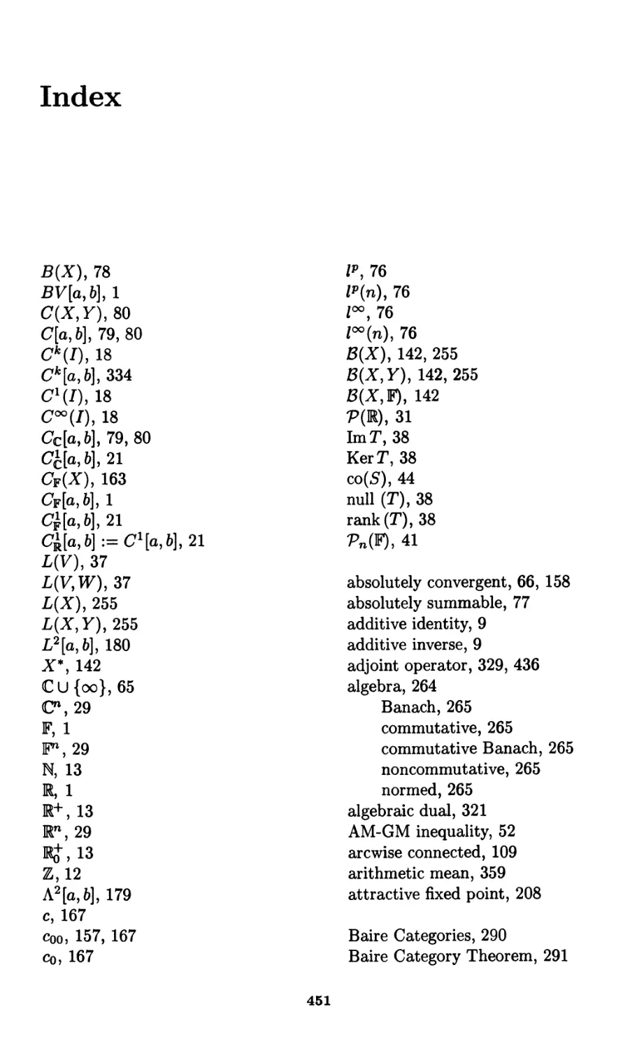
y = r sin 8
z = re i9 = x + iy
o
x = r cos 8
x
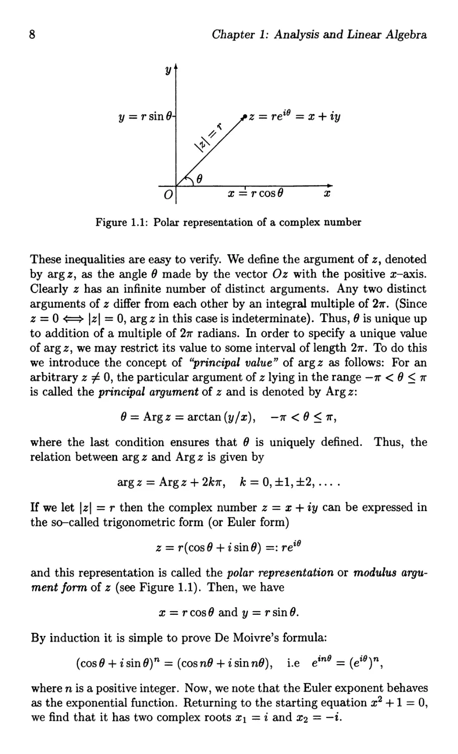
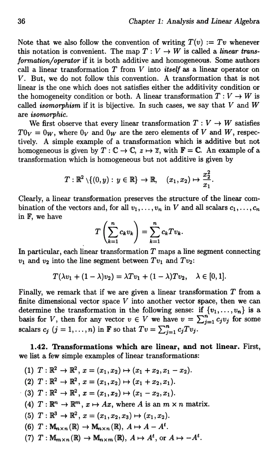
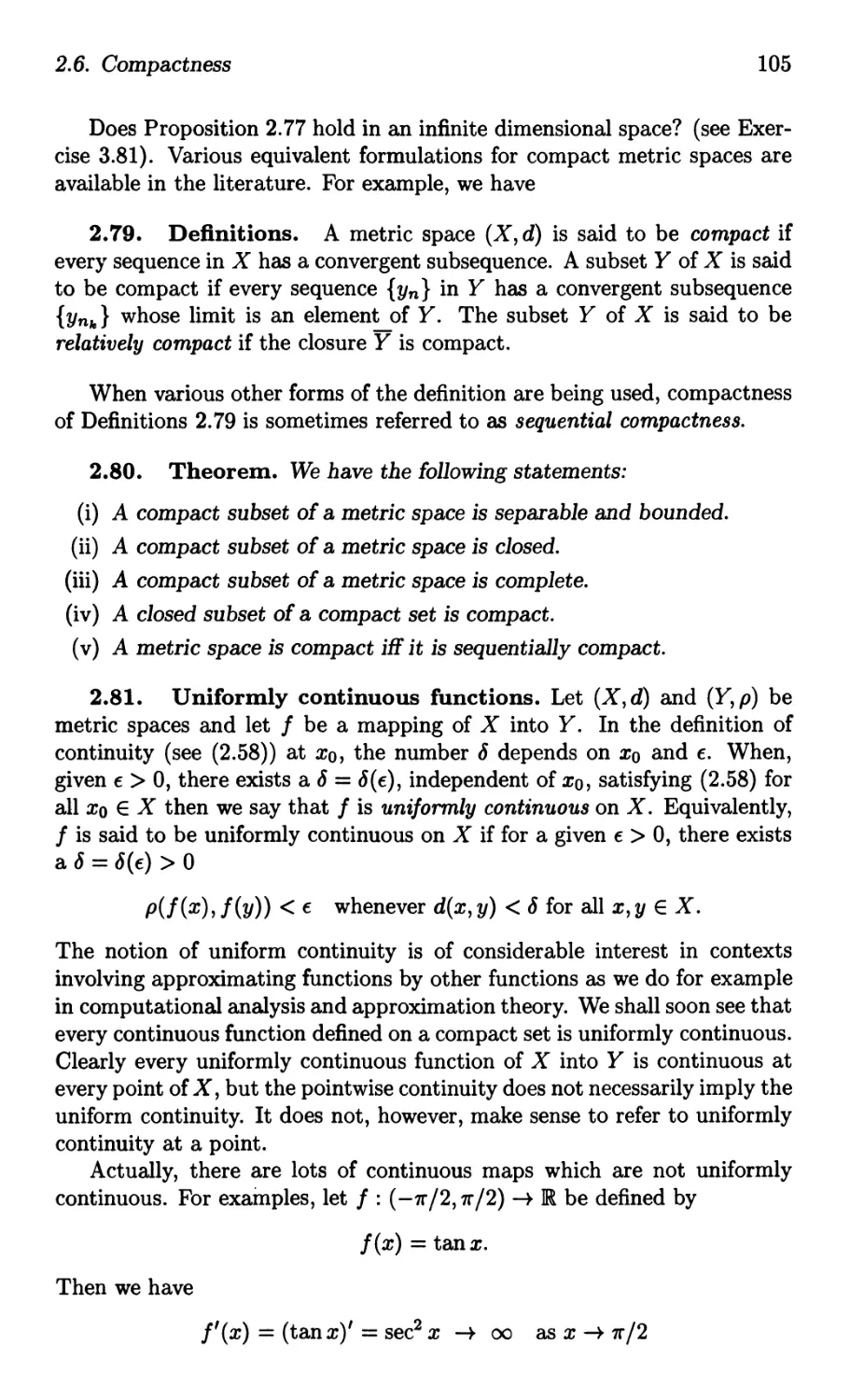
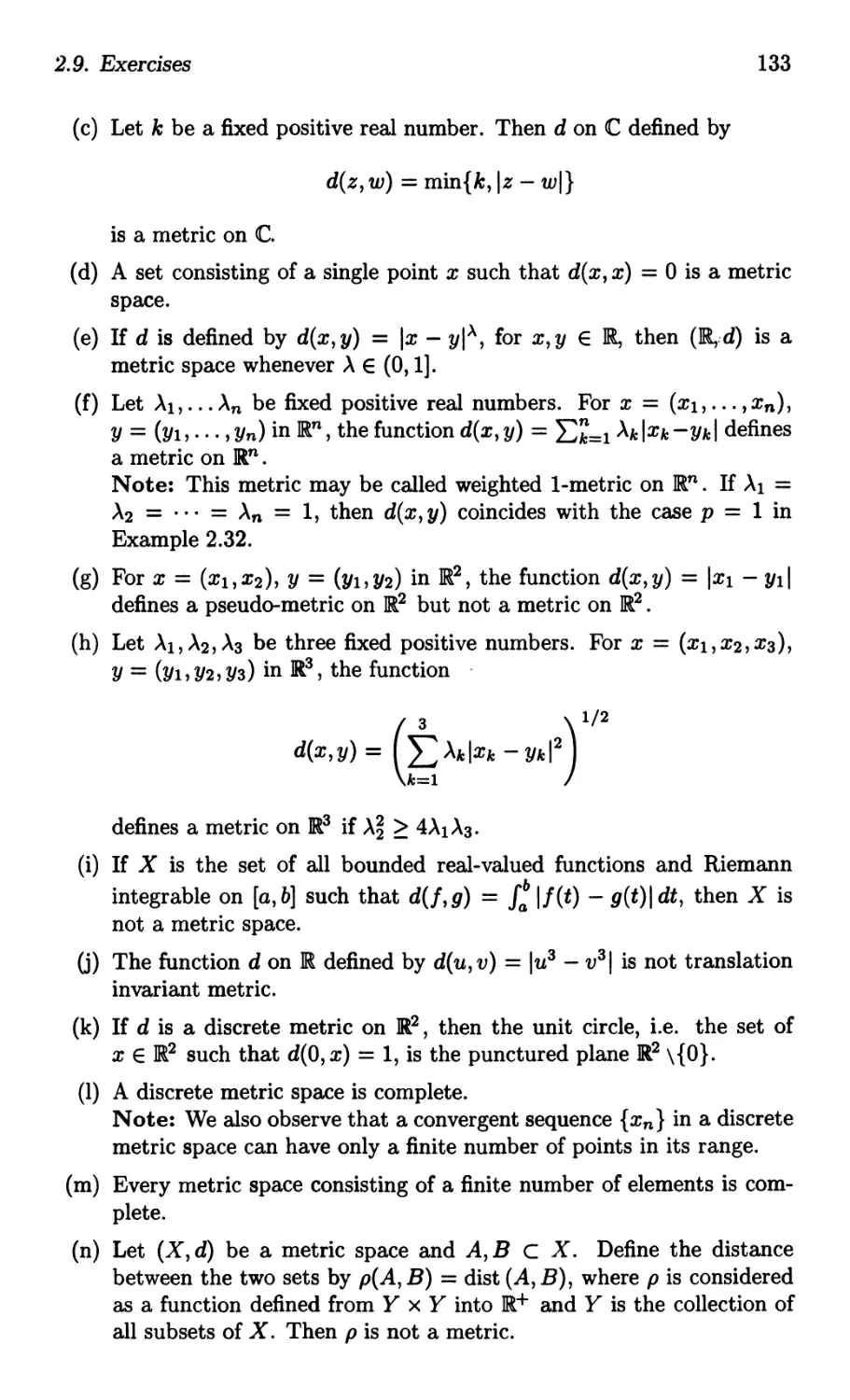
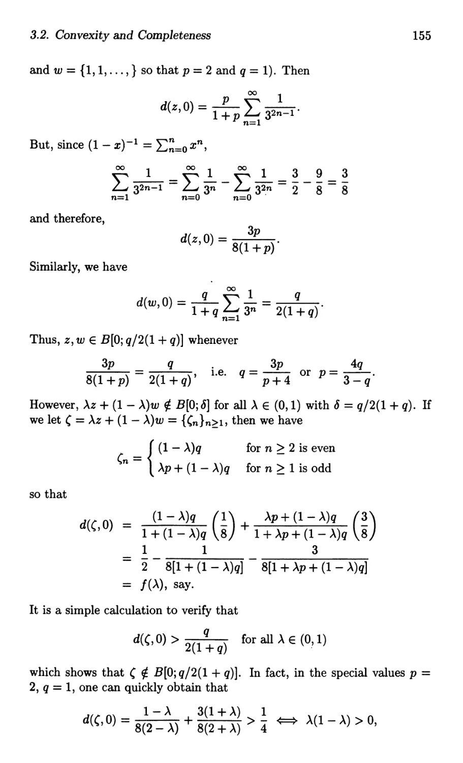
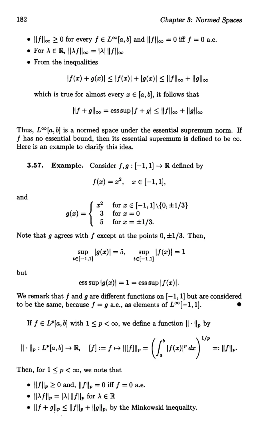
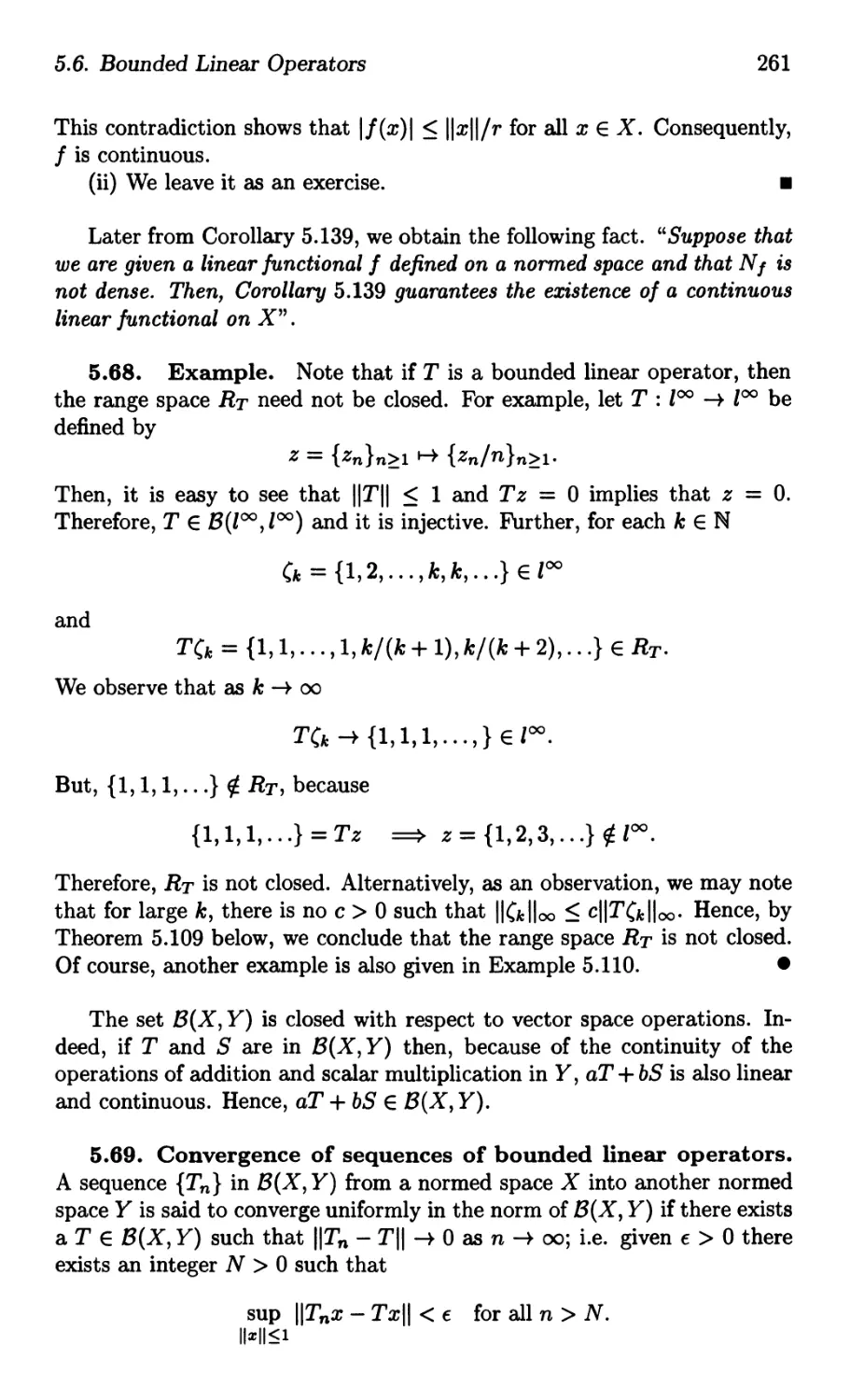
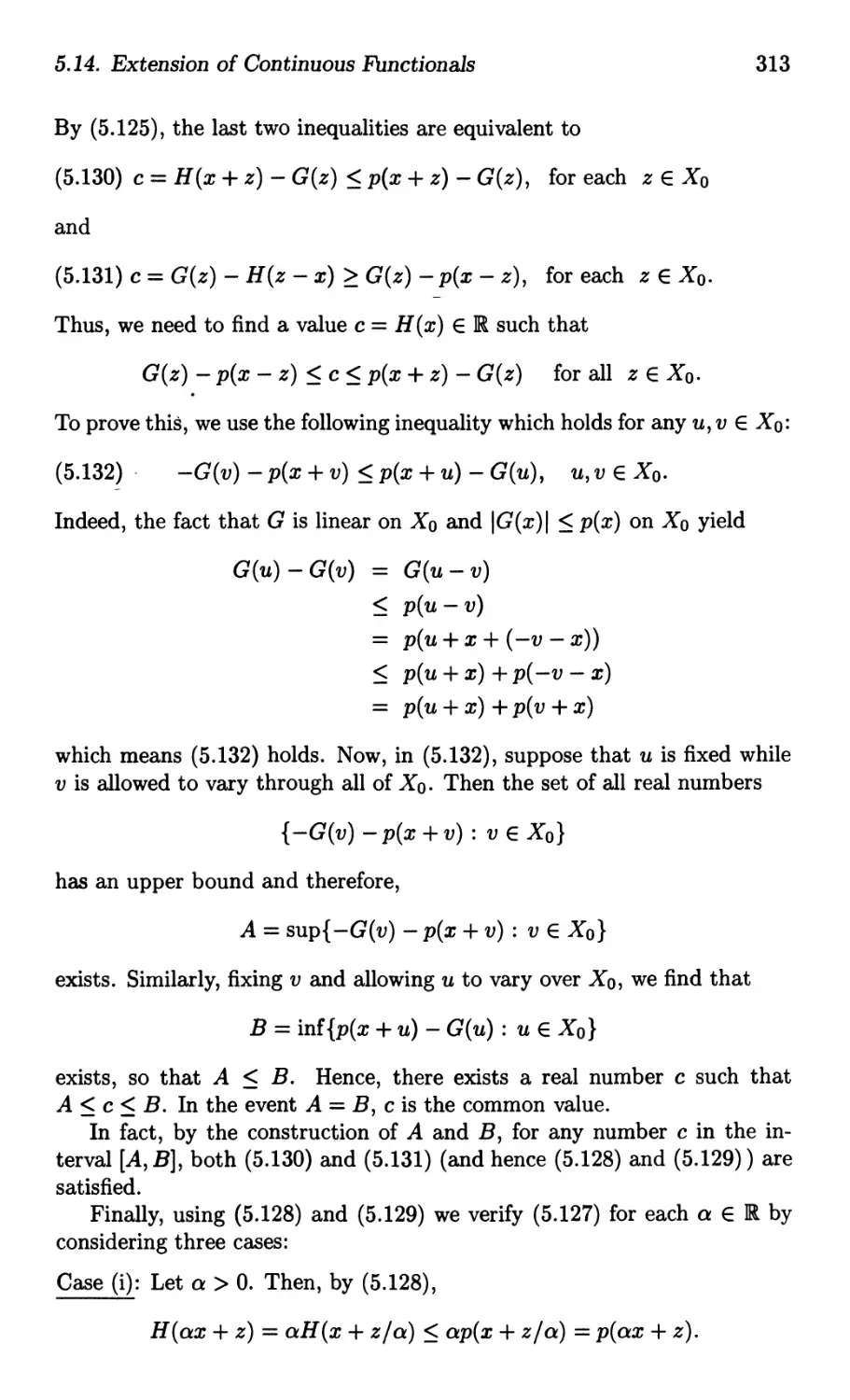
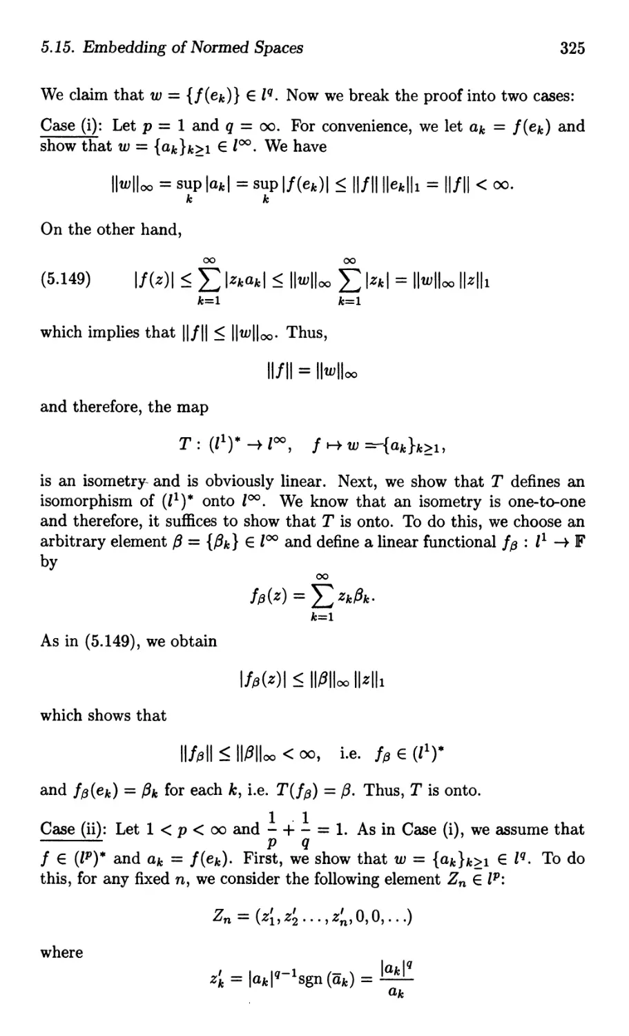
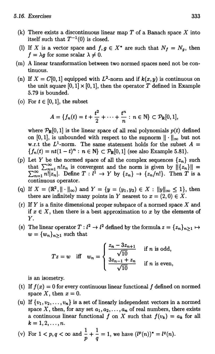
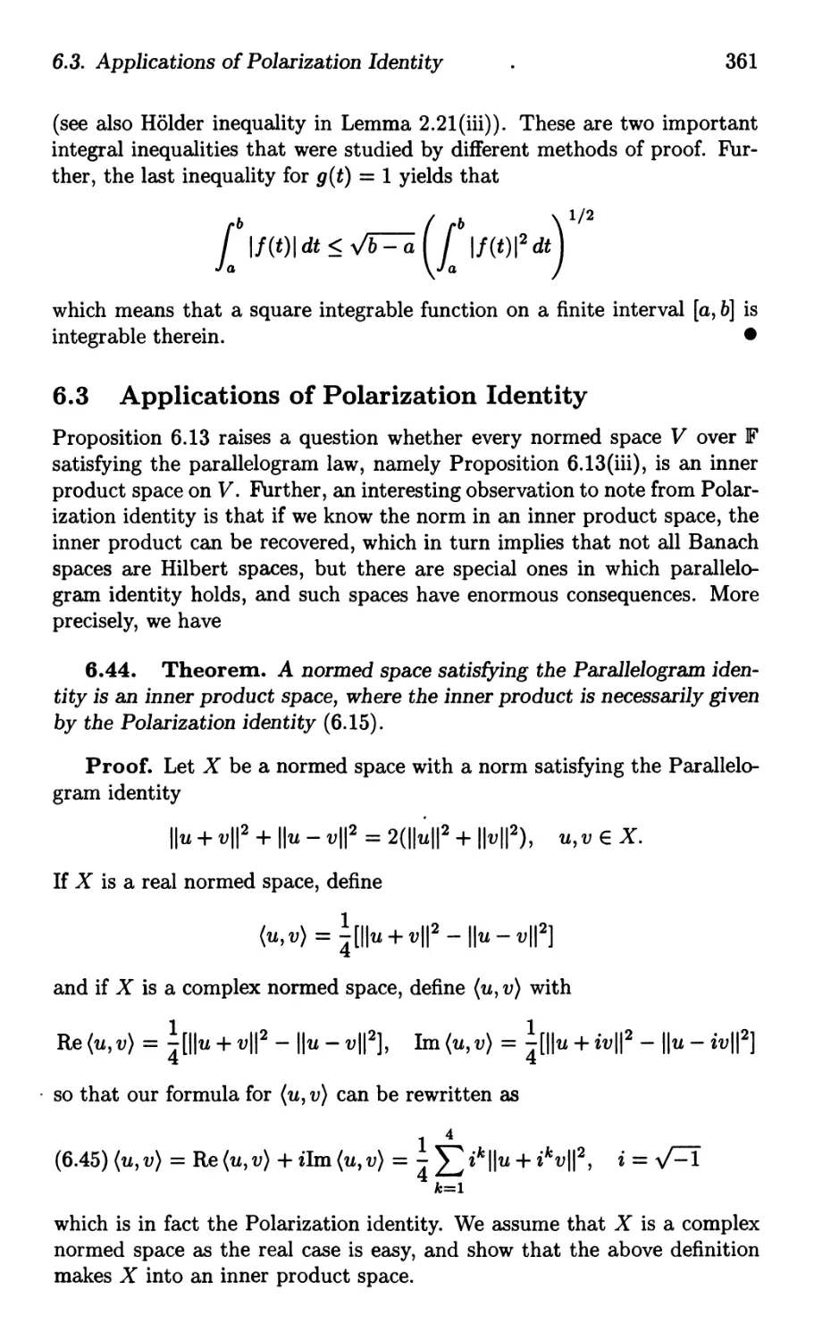
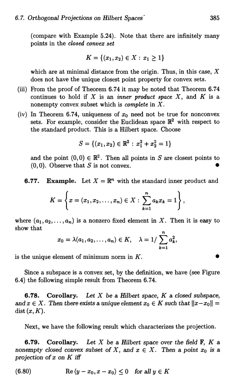
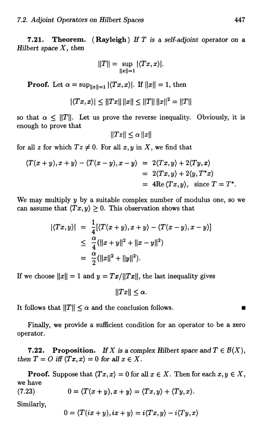
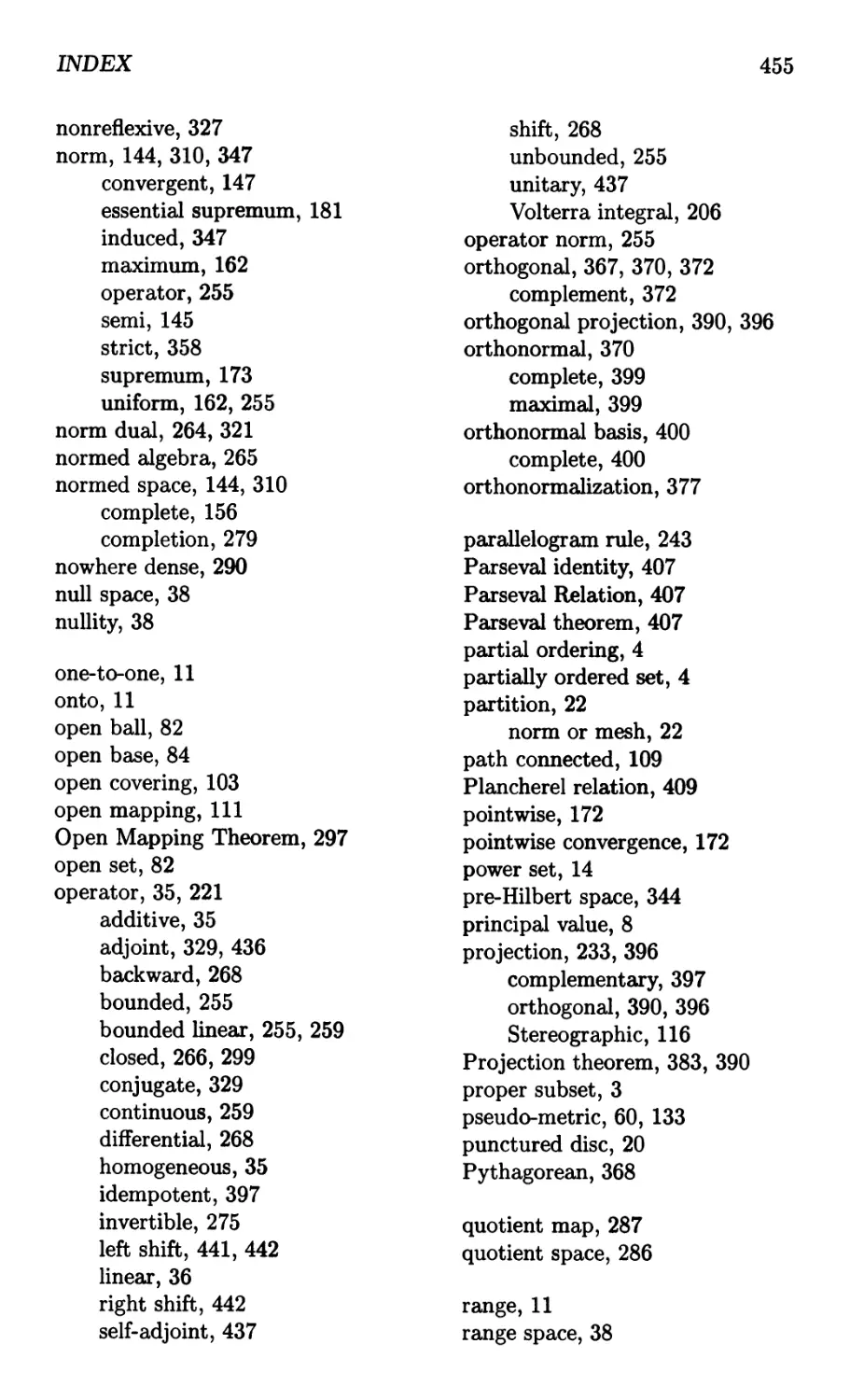
Figure 1.1: Polar representation of a complex number
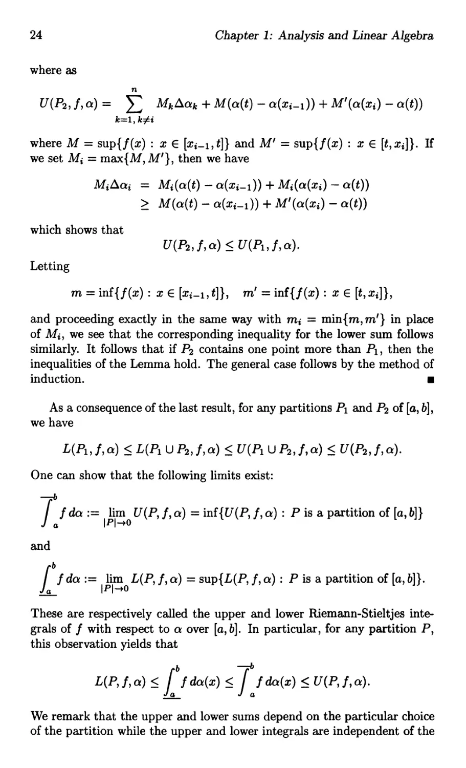
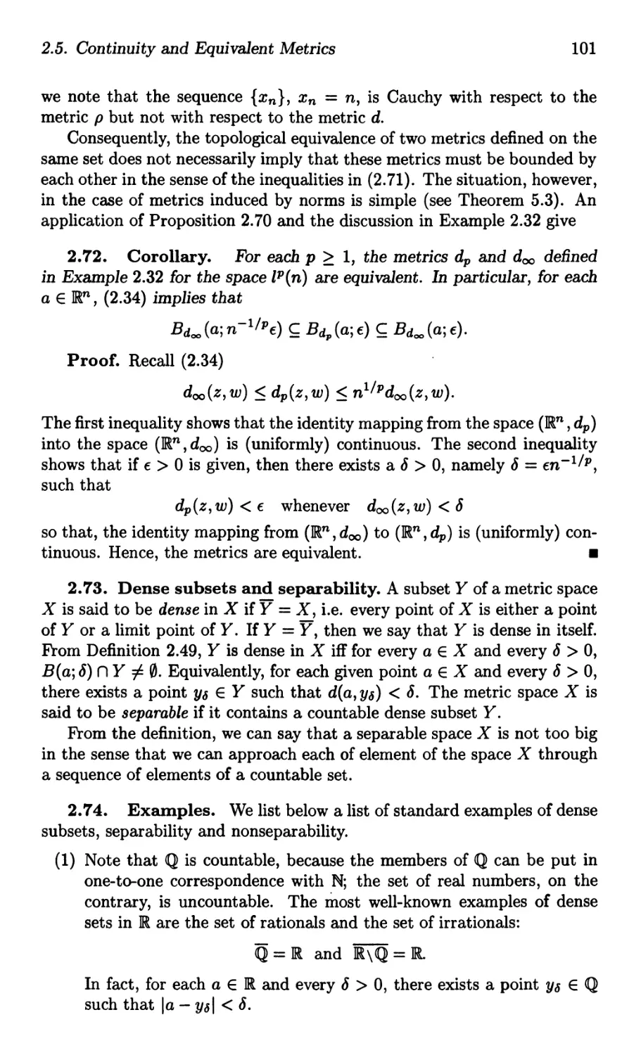
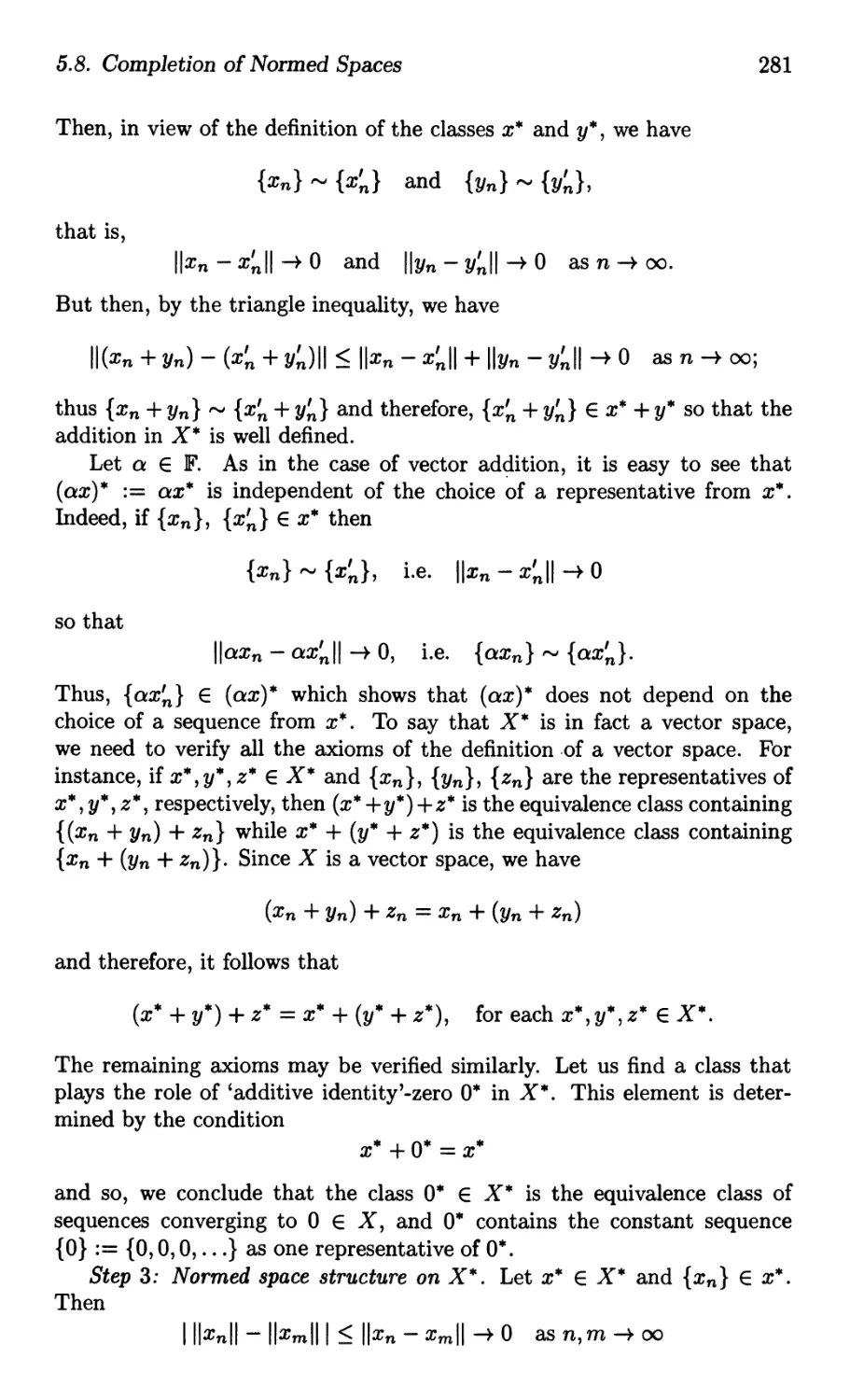
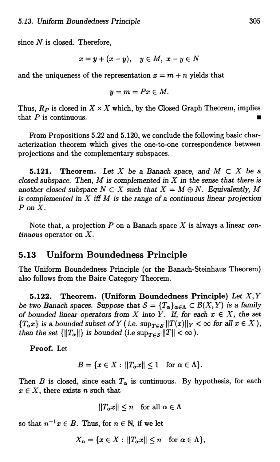
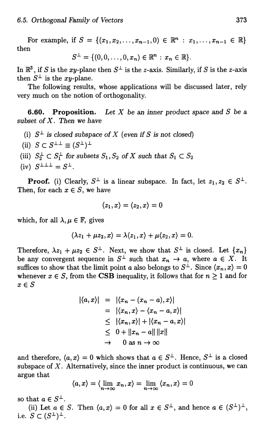
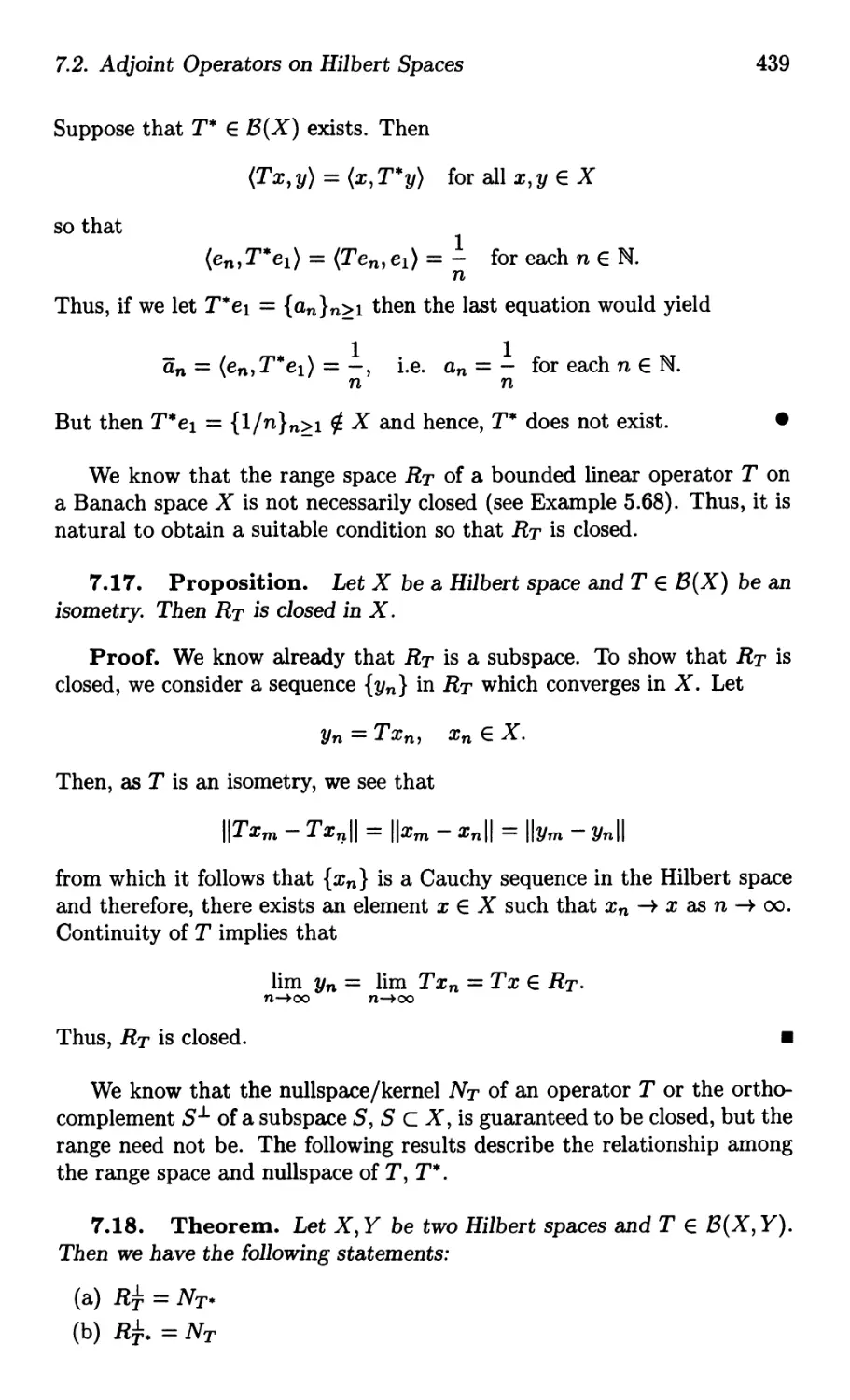
These inequalities are easy to verify. We define the argument of z, denoted
by arg z, as the angle 8 made by the vector 0 z with the positive x-axis.
Clearly z has an infinite number of distinct arguments. Any two distinct
arguments of z differ from each other by an integral multiple of 21r. (Since
z = 0 <==} Izl = 0, argz in this case is indeterminate). Thus, 8 is unique up
to addition of a multiple of 21r radians. In order to specify a unique value
of arg z, we may restrict its value to some interval of length 21r. To do this
we introduce the concept of "principal value" of arg z as follows: For an
arbitrary z :j:. 0, the particular argument of z lying in the range -1r < 8 < 1r
is called the principal argument of z and is denoted by Arg z:
8 = Argz = arctan (y/x), -1r < 8 < 1r,
where the last condition ensures that 8 is uniquely defined. Thus, the
relation between arg z and Arg z is given by
argz = Argz + 2k1r, k = 0, :i:1, :i:2, ... .
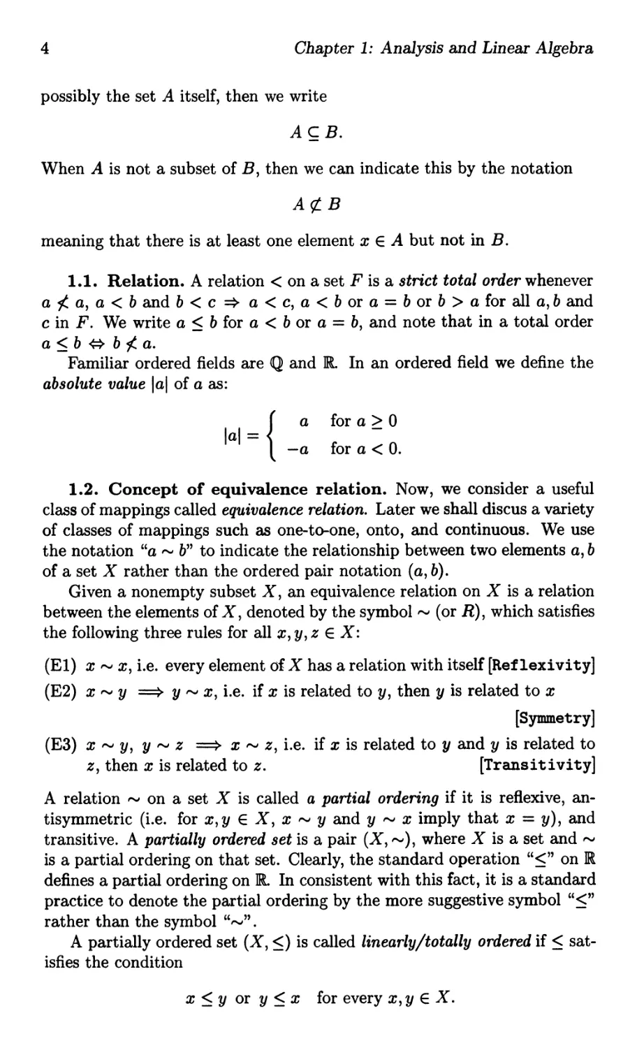
If we let Izl = r then the complex number z = x + iy can be expressed in
the so-called trigonometric form (or Euler form)
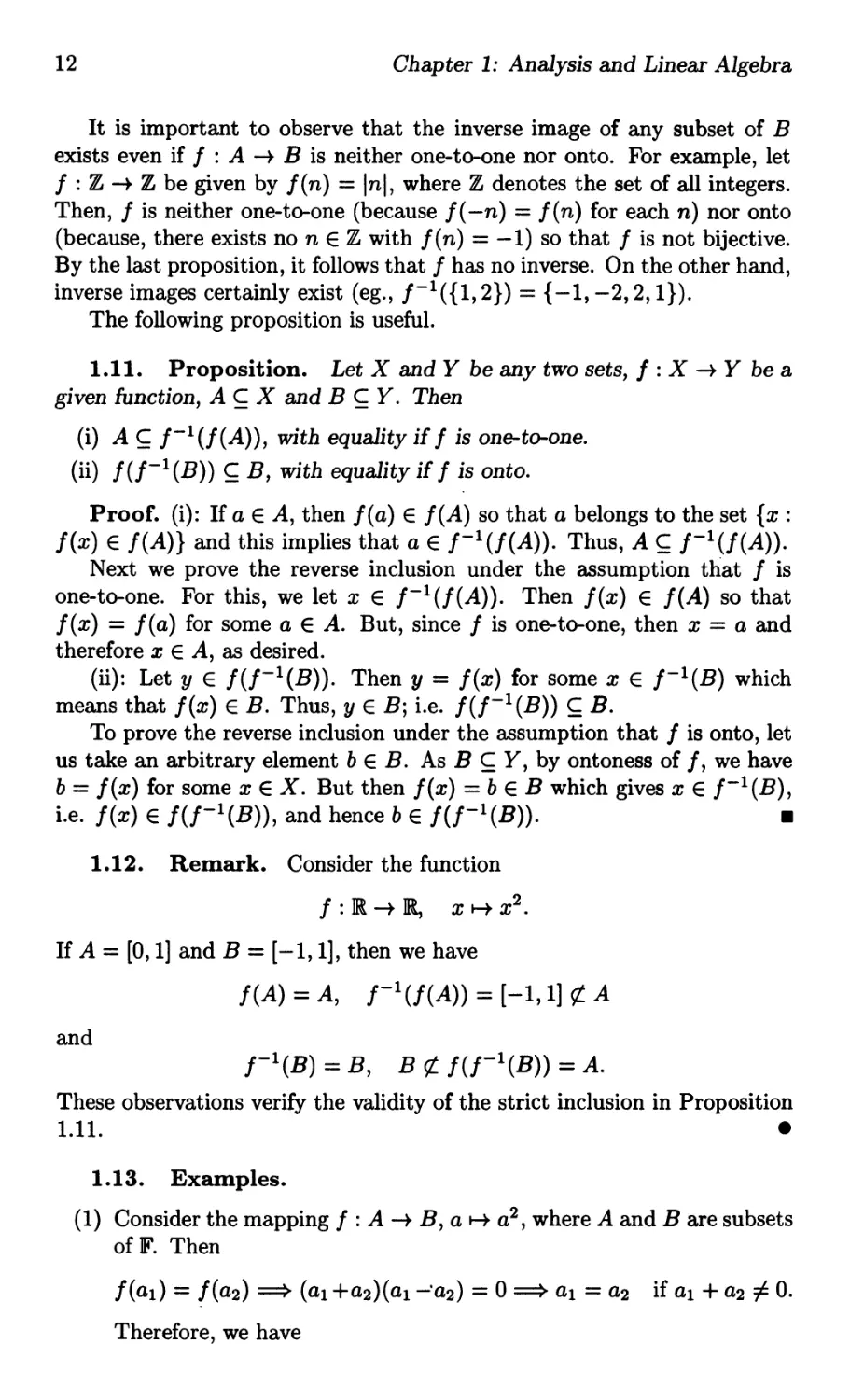
z = r( cos 8 + i sin 8) =: re i9
and this representation is called the polar representation or modulus argu-
ment form of z (see Figure 1.1). Then, we have
x = rcos8 and y = r sin 8.
By induction it is simple to prove De Moivre's formula:
(cos 8 + i sin 8)n = (cos n8 + i sin n8), i.e e in9 = (e i9 )n,
where n is a positive integer. Now, we note that the Euler exponent behaves
as the exponential function. Returning to the starting equation x 2 + 1 = 0,
we find that it has two complex roots Xl = i and X2 = -i.
1.1. Review of Complex Numbers
9
1.6. Field. A field is a set F which possesses two binary operations
namely, addition (+) and multiplication (.) such that F is closed with
respect to these two operations (meaning that a, b E F implies a + b E F
and a · b E F) and satisfies the familiar rules of rational arithmetic:
. addition is associative, i.e. (a + b) + c = a + (b + c) for each a, b, c E F
. addition is commutative, Le. a + b = b + a for each a, b E F
. there exists an element 0 E F such that 0 + a = a for all a E F (0 is
called additive identity)
. to every a E F, there corresponds an additive inverse -a E F such
that a + (-a = 0 for all a E F
. multiplication is associative, Le. (a · b) · c = a. (b. c) for each a, b, c E F
. multiplication is commutative, Le. a. b = b · a for each a, b E F.
. there exists an element 1 E F, 1 :j:. 0, such that 1 . a = a for all a E F
(1 is called multiplicative identity)
. to every 0 :j:. a E F, there corresponds a multiplicative inverse a -1 E
F such that a . a -1 = 1 for all a E F
. multiplication distributes over addition, i.e. a. 0 = 0 and
a · (b + c) = a · b + a · c
The most familiar examples of fields are the set of rational numbers
and the set of real numbers, for which the notation Q and IR are used,
respecti vely.
1.7. The field C. First we show that C is a field. For this it suffices
to prove the existence of the multiplicative inverse of each nonzero complex
number Zl :j:. 0, as the remaining axioms are easy to verify. Thus, for Zl :j:. 0,
we need to solve for Z2 the equation
ZlZ2 = 1.
By the multiplication rule, namely
Zl Z 2 = (Xl, Y1)(X2, Y2) = (X1 X 2 - Y1Y2, X1Y2 + Y1 X 2),
it follows that
Zl Z 2 = (1,0) <==> { X1X2 - Y1Y2 = 1
X1Y2 + Y1 X 2 = 0
10
Chapter 1: Analysis and Linear Algebra
<==} ( Xl l ) (::) = ( )
Yl
<==} ( X2 ) 1 (Xl YI) ( )
Y2 - x + X -Yl Xl
<==} ( X2 ) (Xl YI)
Y2 = X + X ' - X + X .
Therefore, the multiplicative inverse (or simply the inverse or reciprocal)
Z-l of a complex number z = X + iy :j:. 0 is then given by
1 x - iy ( x ) . ( y )
z = x 2 + y2 = x 2 + y2 - x2 + y2 .
In particular, in view of the fact that IR is field, the above discussion shows
that C is a field too. Further, writing a real number x as (x, 0), as pointed
out earlier, and noting that
(Xl,O) + (X2,0) = (Xl + X2,0)
and
(Xl, 0)(X2, 0) = (XlX2, 0),
IR turns out to be a subfield of C. If z = x + iy, then we use the notation
x = Re z for the real part of z, and y = 1m z for the imaginary part of z.
It is important to note that C is not an ordered field.
1.2 Functions and Countability
Let X and Y be two nonempty subsets of C or III A function/mappinrr I
from X to Y is a rule, which associates with each x E X a unique element
y E Y. We write
(1.8) I : X -+ Y
to denote the mapping of X into Y. We call the sets X and Y the domain
and codomain of the function I, respectively. When we describe a mapping
by describing its effect on the individual elements, we use the symbolt-t;
thus "the mapping x t-t I(x) of X into Y" means that I is a mapping of X
into Y taking each element x of X into the element I(x) of Y. IT y = I(x),
we say that y is the image of x. If S e x, we can have I : S Y and
we call this new function the restriction of I in (1.8) to S and denote it by
lis'
If I is defined on X and S e x, then
1(8) = {/(s) : s E S}
2The terms mapping, function and transformation are used synonymously.
1.2. Functions and Countability
11
is called the image of the set S under I. In particular, I(X) C Y is called
the range of I. In other words, the subset {/(x) E Y : x E X} C Y is
called the range of I. If Y 1 C Y, then the inverse image of Y 1 under I,
denoted by 1- 1 (y 1 ), is the subset of X defined by
1- 1 (y 1 ) = {x EX: I(x) E Y 1 }.
If Y 1 = {y} C Y, then we write 1-1(y) instead of 1-1({y}). Note that
1- 1 (Y 1 ) is a well defined set irrespective of whether I has any inverse or
not. The following result is trivial.
1.9. Proposition. Let X and Y be any two sets, I : X Y be a
given function, A C X and B C Y. Then I(A) S; B iff A S; 1- 1 (B).
There are several similar properties of images and inverse images (preim-
ages) but these will be discussed in Chapter 2 in a more general setting.
However we shall recall some more elementary background material as we
proceed.
For two mappings I : A Band g : B C, we can define the
composite mapping g 0 I : A C by
(g 0 I)(x) = g(/(x)).
The mapping I : A B is said to map A onto B iff the codomain and
the range set are equal, Le. I(A) = B. Therefore, to prove that I is onto,
one must start with an arbitrary b E B and then find at least one a E A
such that I(a) = b. The mapping is said to be 1-1 (one-to-one) iff it maps
distinct elements into distinct elements, Le. I (a1) :j:. I (a2) for all a1, a2 E A
with a1 :j:. a2. More formally, I is one-to-one iff for a1, a2 E A,
l(a1) = l(a2) => a1 = a2.
A mapping which is both one-to-one and onto is called bijective. 3 The map
I : A B is said to have an inverse if there exists a function 9 : B A
such that
g(/(a)) = a for all a E A
and
I(g(b)) = b for all b E B.
Here 9 is called the inverse of I. We have a simple and useful result which
we state without proof.
1.10. Proposition. Let A and B be two sets and I : A B. Then
I has a unique inverse 9 iff I is bijective.
3The term 'one-to-one', 'onto', and 'one-to-one correspondence' are sometimes re-
ferred as 'injective', 'surjective', and 'bijective' mappings, respectively.
12
Chapter 1: Analysis and Linear Algebra
It is important to observe that the inverse image of any subset of B
exists even if f : A B is neither one-to-one nor onto. For example, let
f : Z -+ Z be given by f(n) = Inl, where Z denotes the set of all integers.
Then, f is neither one-to-one (because f( -n) = f(n) for each n) nor onto
(because, there exists no n E Z with f (n) = -1) so that f is not bijective.
By the last proposition, it follows that f has no inverse. On the other hand,
inverse images certainly exist (eg., f-1 ({I, 2}) = { -1, -2,2, I}).
The following proposition is useful.
1.11. Proposition. Let X and Y be any two sets, f : X Y be a
given function, A C X and B C Y. Then
(i) A C f-1(f(A)), with equality if f is one-to-one.
(ii) f(f-1(B)) C B, with equality if f is onto.
Proof. (i): If a E A, then f(a) E f(A) so that a belongs to the set {x :
f(x) E f(A)} and this implies that a E f-1(f(A)). Thus, A C f-1(f(A)).
Next we prove the reverse inclusion under the assumption that f is
one-to-one. For this, we let x E f-1(f(A)). Then f(x) E f(A) so that
f(x) = f(a) for some a E A. But, since f is one-to-one, then x = a and
therefore x E A, as desired.
(ii): Let y E f(f-1(B)). Then y = f(x) for some x E f-1(B) which
means that f(x) E B. Thus, y E B; Le. f(f-1(B)) C B.
To prove the reverse inclusion under the assumption that f is onto, let
us take an arbitrary element b E B. As B C Y, by ontoness of f, we have
b = f(x) for some x E X. But then f(x) = b E B which gives x E f-1(B),
Le. f(x) E f(f-1(B)), and hence b E f(f-1(B)). .
1.12. Remark. Consider the function
f : IR IR, x I-t x 2 .
If A = [0,1] and B = [-1,1], then we have
f(A) = A, f-1(f(A)) = [-1,1] ct A
and
f-1(B) = B, B ct f(f-1(B)) = A.
These observations verify the validity of the strict inclusion in Proposition
1.11. .
1.13. Examples.
(1) Consider the mapping f : A B, a I-t a 2 , where A and B are subsets
of IF. Then
f(a1) = f(a2) ==> (a1 +a2)(a1 -'a2) = 0 ==> a1 = a2 if a1 + a2 :F o.
Therefore, we have
1.2. Functions and Countability
13
(i) Let A = R and B = IRt , the set of all nonnegative real numbers.
Since there exist a1, a2 E A such that a1 + a2 = 0, f is not
one-to-one in this case. Similarly, if A = B = Z, then f is not
one-to-one because of similar reasoning.
(ii) Let A = B = B+, the set of all positive real numbers. Then,
for each a1, a2 E A, we have a1 + a2 :j:. 0 and therefore, f is
one-to-one in this case. Similarly, we see that if A = B = N,. the
set of natural numbers, then f is one-to-one.
(iii) If A = B = JR, then f is not onto because the set of all real
numbers is not the image of IR under our mapping. Also, if
A = B = N then f is not onto. However, if A = IR and B = IRt
then f is onto. In fact, when A = B = R+ , f is bijective.
(iv) If A = B = C, then f is not one-to-one but onto.
(2) The mapping f : Z N U {OJ = No by x I-t Ixl is onto.
(3) The mapping f : Z Z described by x I-t x + 1 is onto whereas
f : N N defined by x I-t x + 1 is not onto because there is no
element a E N with the property that f (a) = a + 1 = 1. On the other
hand f : No N, x I-t x + 1, is onto.
(4) The mapping f : Z Z by x I-t 2x is not onto. For, let b E Z. Then
we have to solve the equation
f(a) = b = 2a, Le. a = b/2.
But b/2 is not necessarily an integer when b E Z. However, if B
denotes the set of even integers then f : Z B by x I-t 2x is onto.
(5) The mapping f : IR [-1,1], x I-t sin x, is onto whereas f : R JR,
x I-t sin x, is not onto. .
A sequence Z1, Z2, . .. of points in IF (where 1F denotes either the field
C of complex numbers or the field IR of real numbers) is really a mapping
f : N IF. If f is a sequence, we write, in keeping with the tradition, Zn
instead of f(n), so that the points f(n) = Zn are called the (n-th) terms
of the sequence. The other common notation to denote the sequence is by
either {zn} or {Zn}n 1' or {Zn} l' for the sequence f, where Zn = f(n) E
IF. It is purely a notational reason to let the sequence to begin with Z1. For
Z E IF, the sequence given by Zn = Z for all n E N is called the constant
sequence with value z.
Let 9 : N N be an increasing sequence of natural numbers. Then the
sequence {Zg(n)} is called a subsequence of the sequence {zn}. We often
write g(k) = nk so that 1 < n1 < n2 < ..., and thus, the sequence {Wk}
defined by
Wk = Zn",
14
Chapter 1: Analysis and Linear Algebra
is the subsequence of {zn}. Intuitively, a subsequence is obtained by 'throw-
ing away' some terms of the original sequence. subsequences 'are used ex-
tensively in analysis. For example, the concepts such as compactness can
be handled nicely with the help of subsequences.
Often we talk of an indexed family of objects: Notation like {Za}aEA is
commonly used for indexed families, where A is the indexing set. The point
here is that for each a E A, there is an object Zao For instance, the infinite
sequence {Zn} 1 is a family indexed by N, the set of natural numbers.
Further, the concept of the sequences of points defined on an arbitrary set
is similar.
A set S is said to be countable if it is either finite or there exists a
one-to-one correspondence between N and the set S. A set is said to be
uncountable if it is not countable. For example, N, Z and Q are all countable
sets. On the other hand, we know from real analysis that IR is uncountable
and hence, the set of all rational numbers is uncountable. In particular,
any interval which contains more than one point is uncountable. Indeed,
the fact that there are uncountably many real numbers in (0, 1) follows
from constructing, for example, a set of all infinite sequences of O's and
l's which is uncountable. Therefore, we have a natural question to look
at: How about other familiar sets that are uncountable? We note that,
according to the definition, the counting convention is via bijections, and
the set of real numbers actually have a lot more numbers than the set of
rational numbers. In general, given a set X, does there exist a method of
constructing another set from X that will contain more elements than X?
If X is countable (finite or infinite), then the answer is trivial, because if
X is finite then one can simply obtain a new set just by adding one more
element that does not belong to X. If X is count ably infinite, then the
new set obtained by adding a finite number of elements or even countably
infinite number of elements to X would again be countable. Hence, we
have to think of some other method. Indeed, a method of getting a bigger
and bigger set follows from the definition of power set: "The power set of
a given set X is the set of all subsets of X, denoted by P(X)". Thus, the
notion of cardinality of a set X comes in to play a role.
If a set X is finite, then the number of elements of X is defined to be
the cardinality of X, denoted by IX I or card X. Thus, two finite sets A and
B have same size, Le. card A = card B, if they contain the same number of
elements. An important question is how to carry the notion of equal size
over to infinite sets such as Nand Z? Now, we have the definition. Given
two arbitrary sets A and B (finite or infinite), cardA = cardB iff there
exists a bijection between them. In particular, the notion of equal size is
an equivalence relation, and we then associate a number called cardinal
number to every class of equal sized sets. At this point, it is important to
note that it is often difficult to find the cardinal number as it requires th3:t
the function is both one-to-one and onto. But it is usually easy to find
one-to-one functions than onto functions. Now, we state without proof the
1.3. Review of Differentiability in Real Line
15
following theorem due to Cantor-Bernstein.
1.14. Theorem. (Cantor-Bernstein) Let A and B be two sets.
If there exists a one-to-one function f : A B and another one-to-one
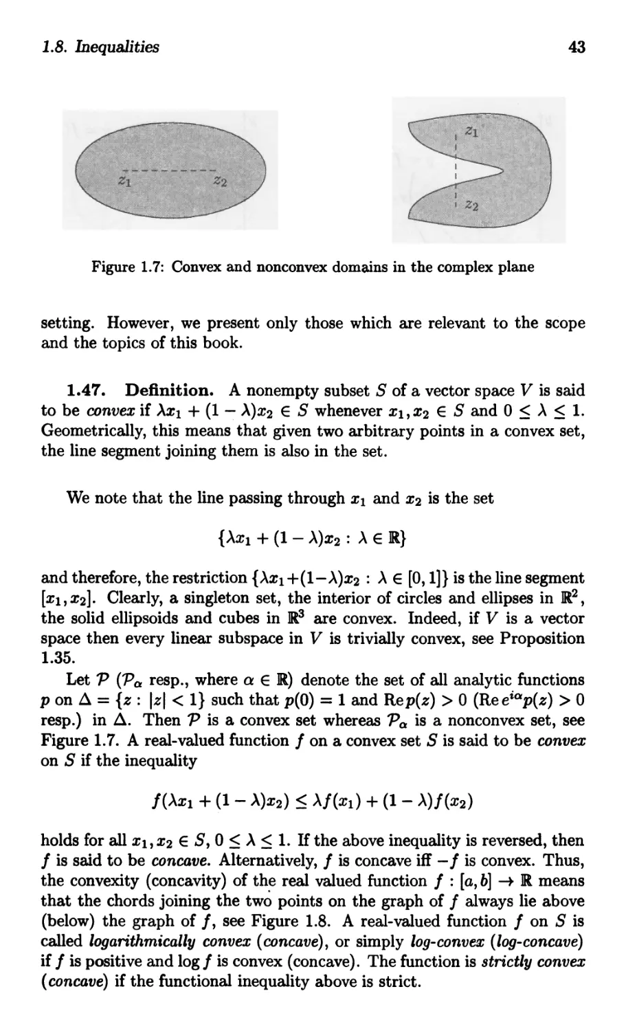
function 9 : B A, then card A = card B.
This theorem can be used to show, for example, that
card (IR x IR) = card III
Moreover, the fact that Q is countable can also be obtained by showing
that Q and Z x Z have the same cardinality (prove this!).
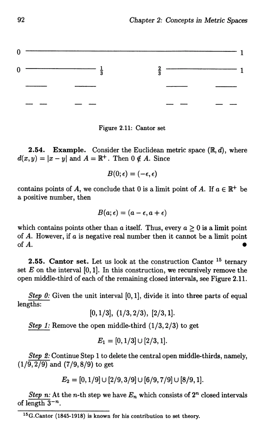
1.3 Review of Differentiability in Real Line
In this section, we show how the idea of the derivative of a function at a
point in IR, as a linear approximation, is fundamental to the understanding
of the derivative in the real case. We are assuming the concepts of limit,
continuity, and uniform continuity for functions defined on subsets of III
One of the important concepts in real and complex analysis is the notion
of neighbourhoods. Given a point a E IR and a positive number €, the open
interval
(a-€,a+€)={xEIR: a-€<x<a+€}
is called a neighbourhood of the point a. Likewise, if.a = al + ia2 is a given
complex number and r is a positive number, then the open disc
(a;r) := {ZEC: Iz-al <r}
: = { (x, y) E ]R2 : (x - a) 2 + (y - b) 2 < r 2 }
is called a neighbourhood of a E C. If G C IR, then G is called open iff for
every a E G there exists an € > 0 such that (a - €, a + €) C G. Similarly,
D C C is said to be open iff for every a ED, there exists a r > 0 such that
(a; r) C D. We shall also name the complements of open sets. They will
be called closed sets but we shall discuss them in detail later.
Let G be an open subset of IR containing a point a. We say that a
function f : G IR is differentiable at a if the limit
(1.15)
I . f(x) - f(a)
1m
x-+a X - a
exists and is finite. Then we say that f has a derivative at a and this limit
is denoted by f'(a). IT f has a finite derivative for every point of G, then
f is differentiable on G and, in that case, f'(x) is a function of x and the
following notation may be used instead of f'(x):
D f(x), :x f(x), , y', f(1) (x).
16
Chapter 1: Analysis and Linear Algebra
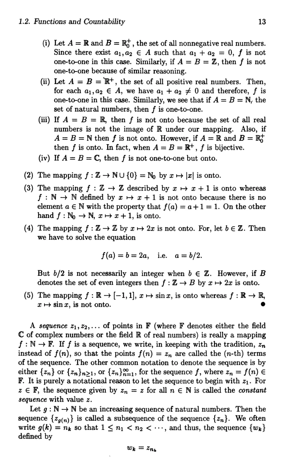
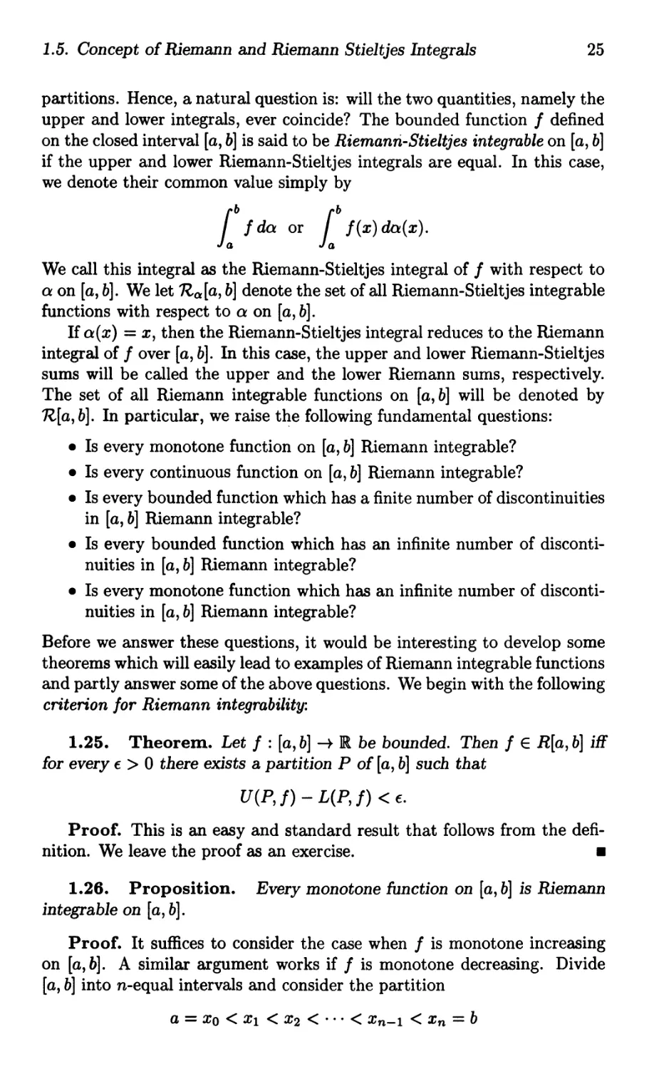
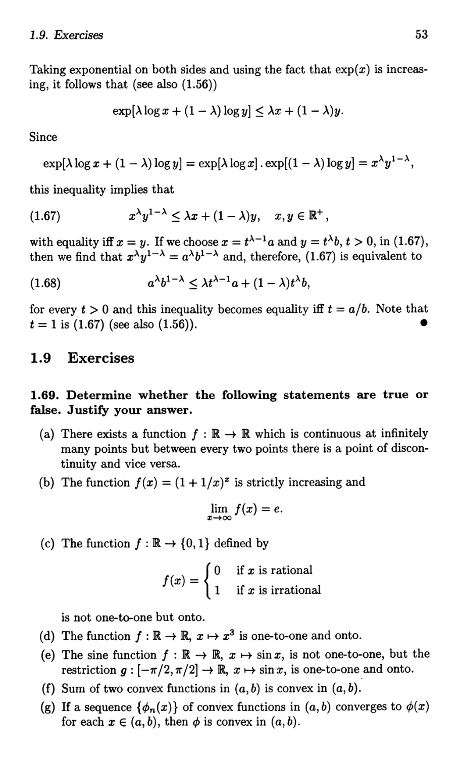
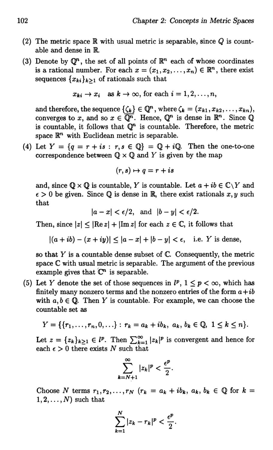
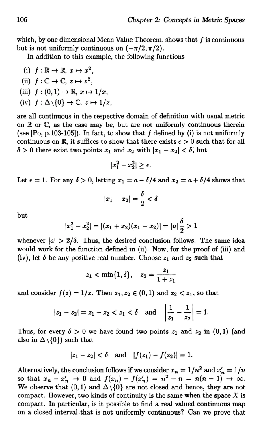
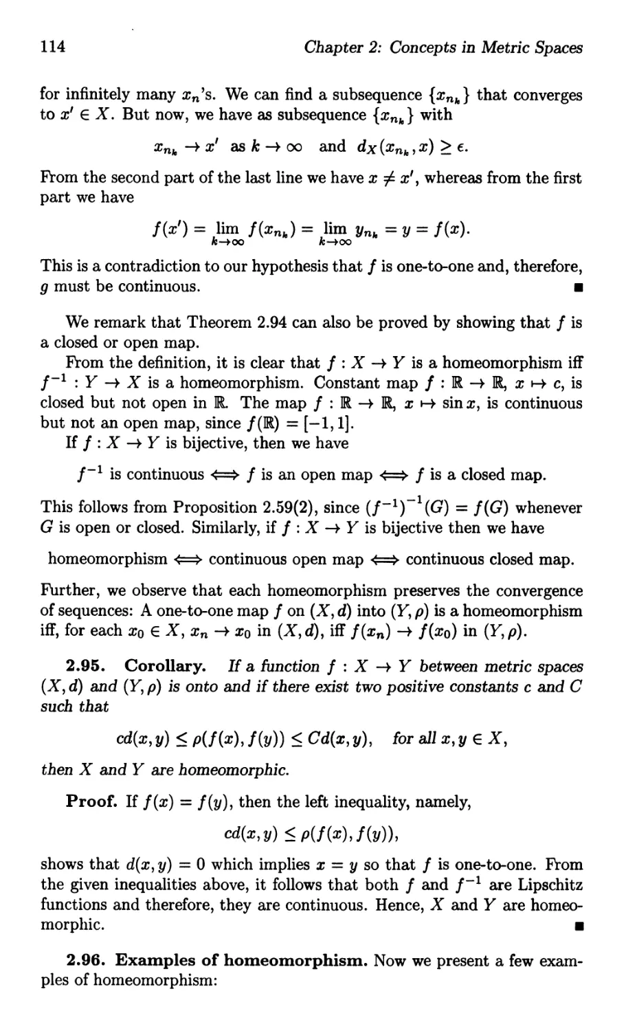
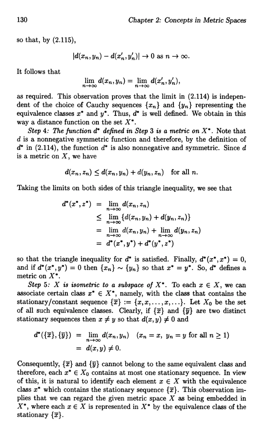
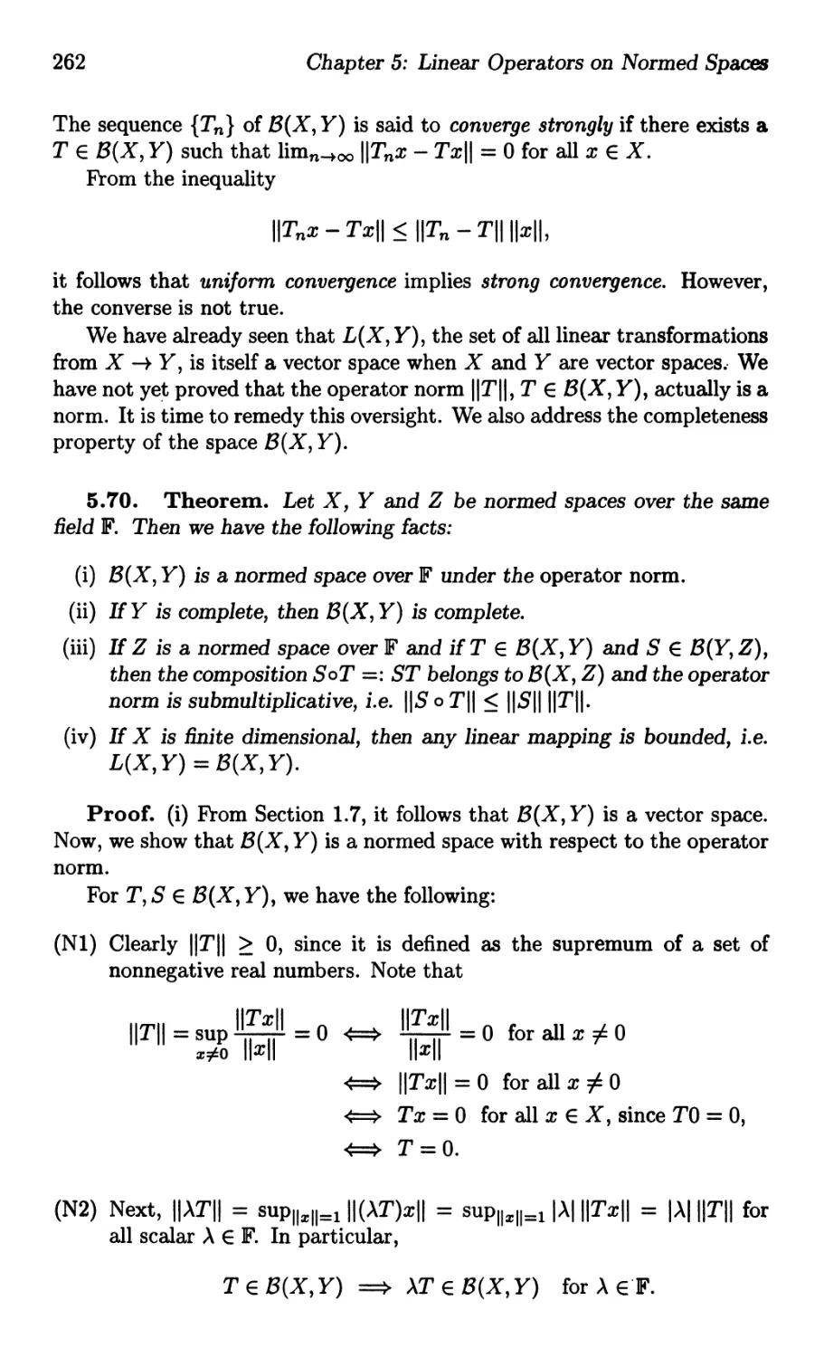
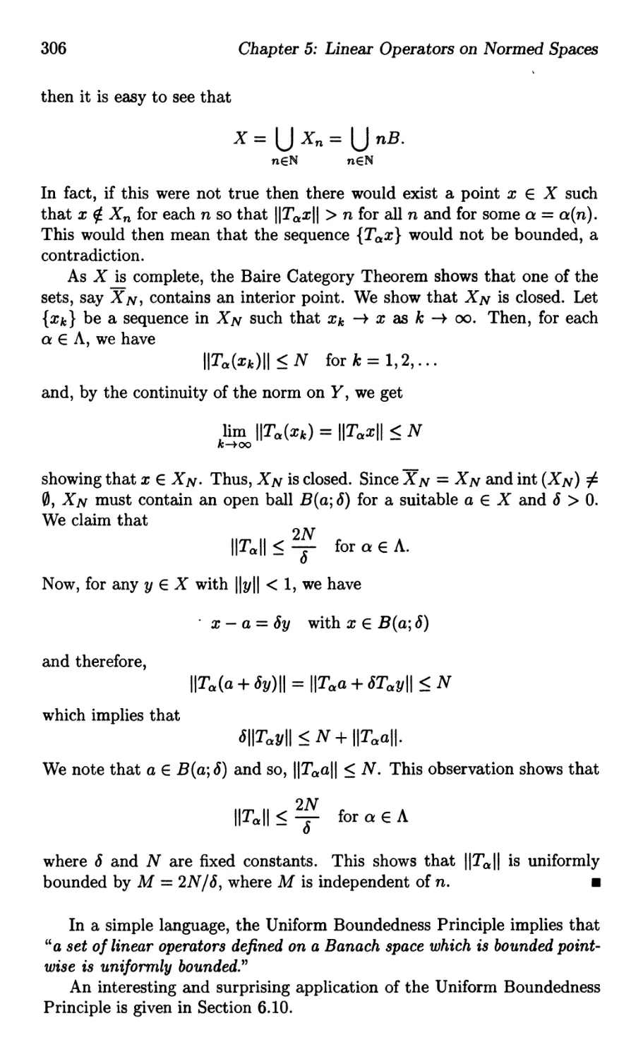
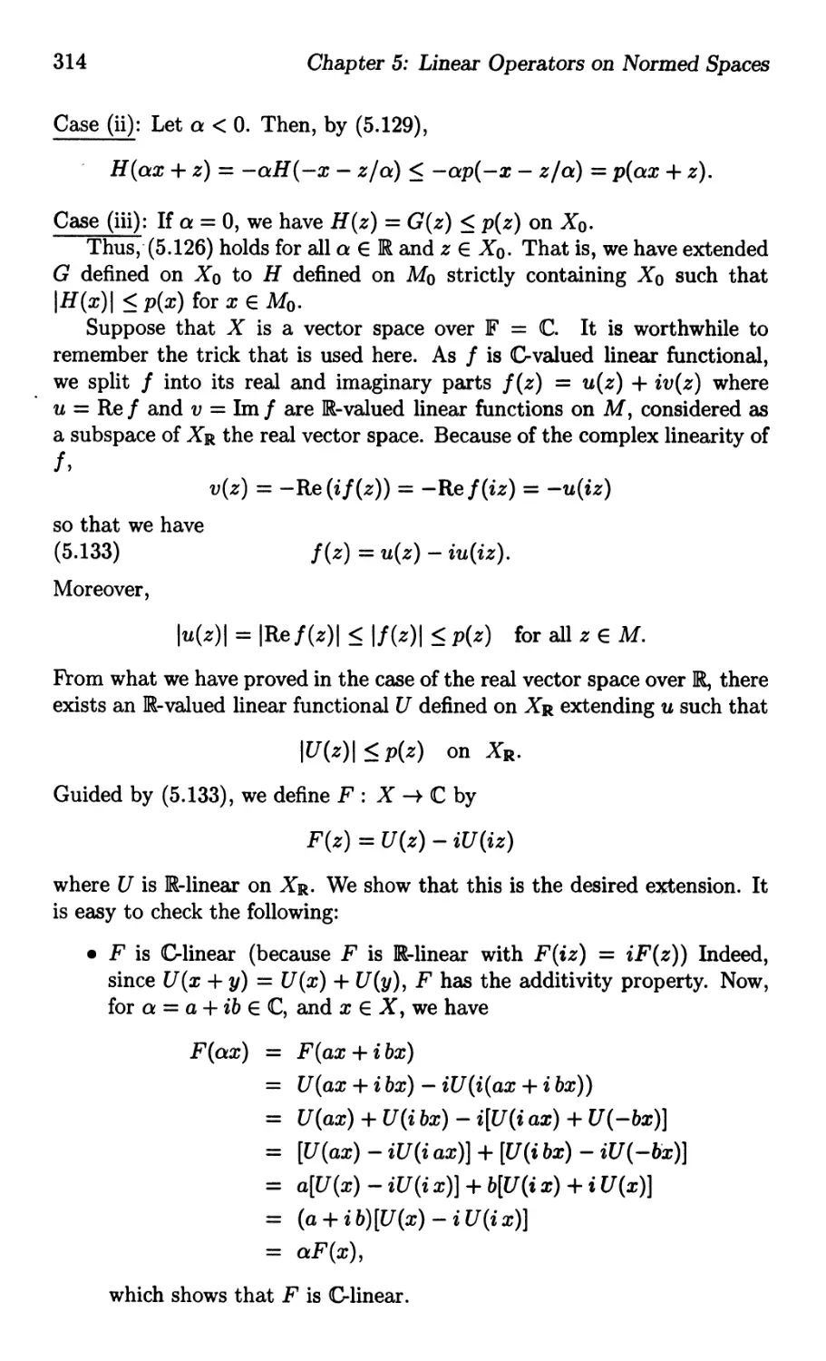
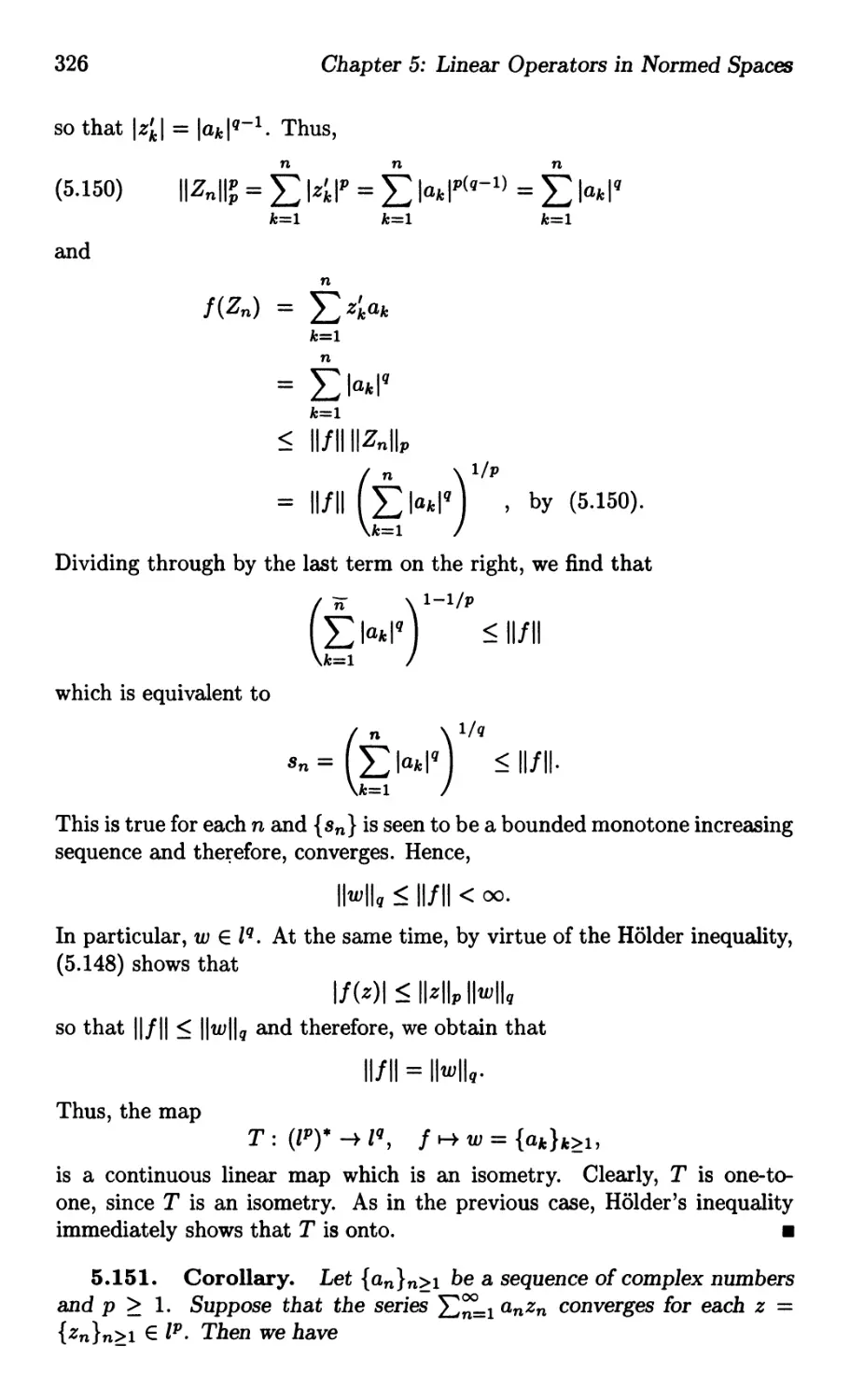
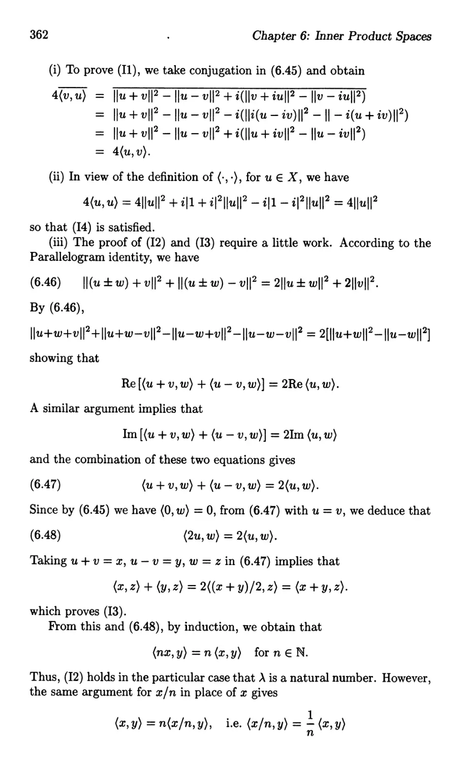
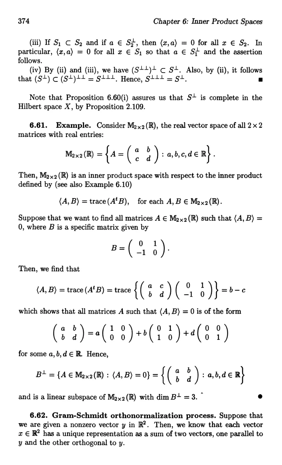
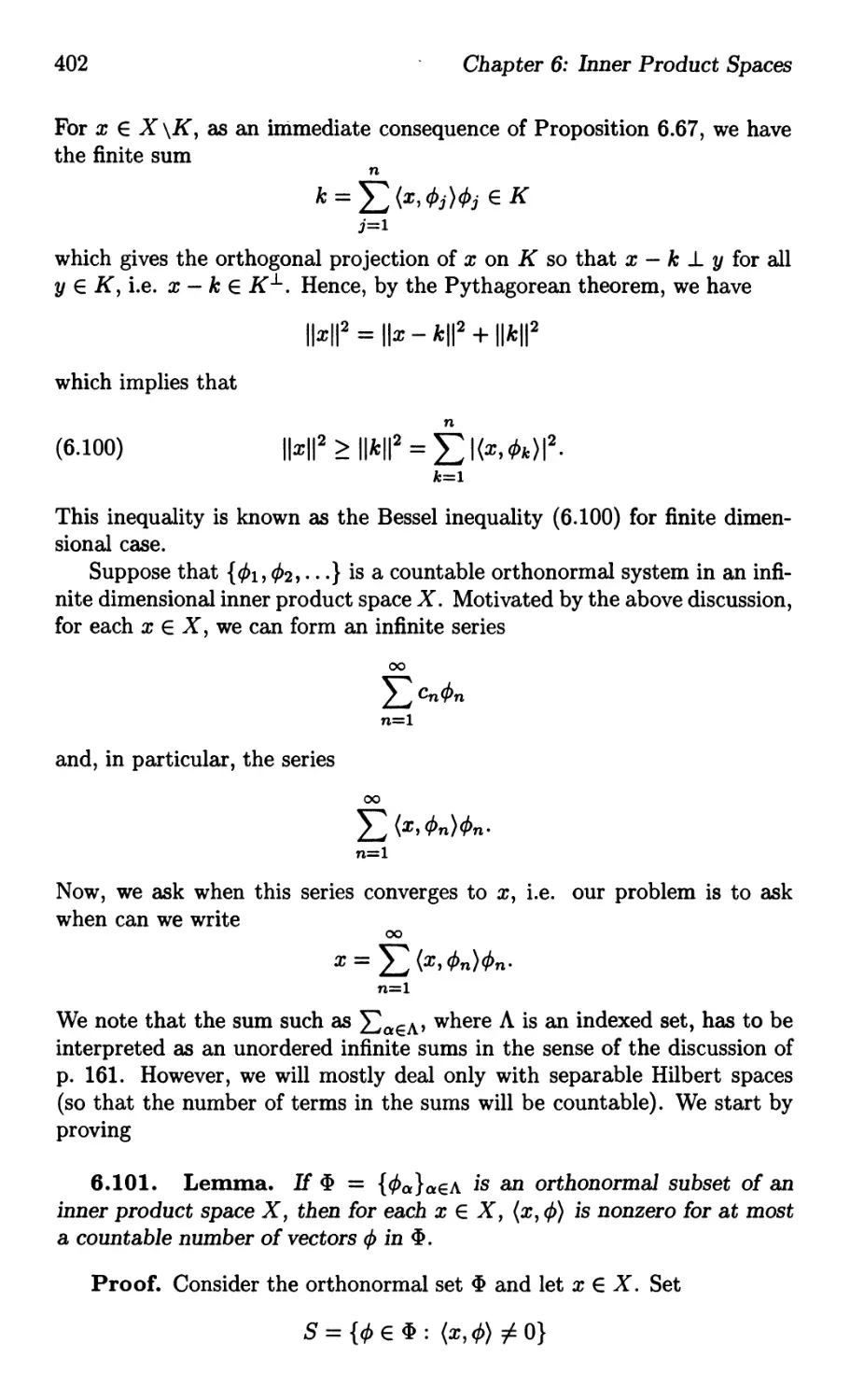
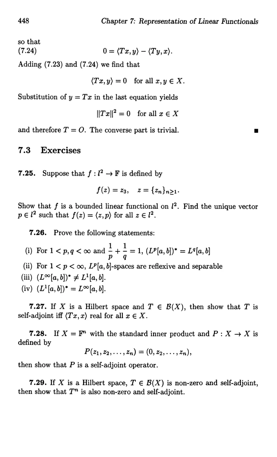
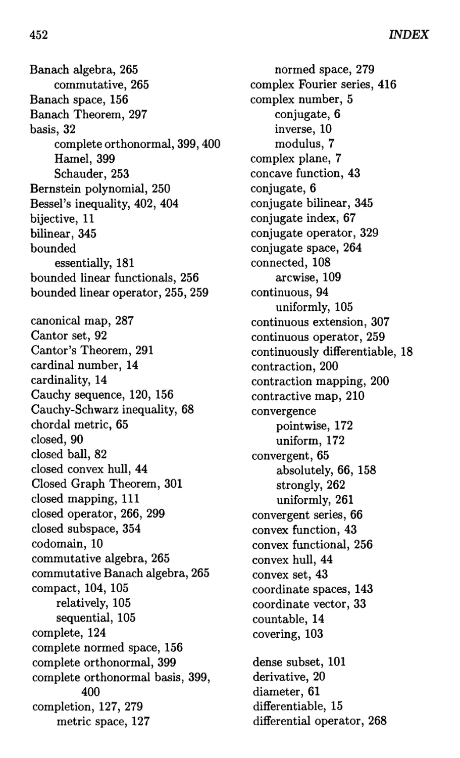
y
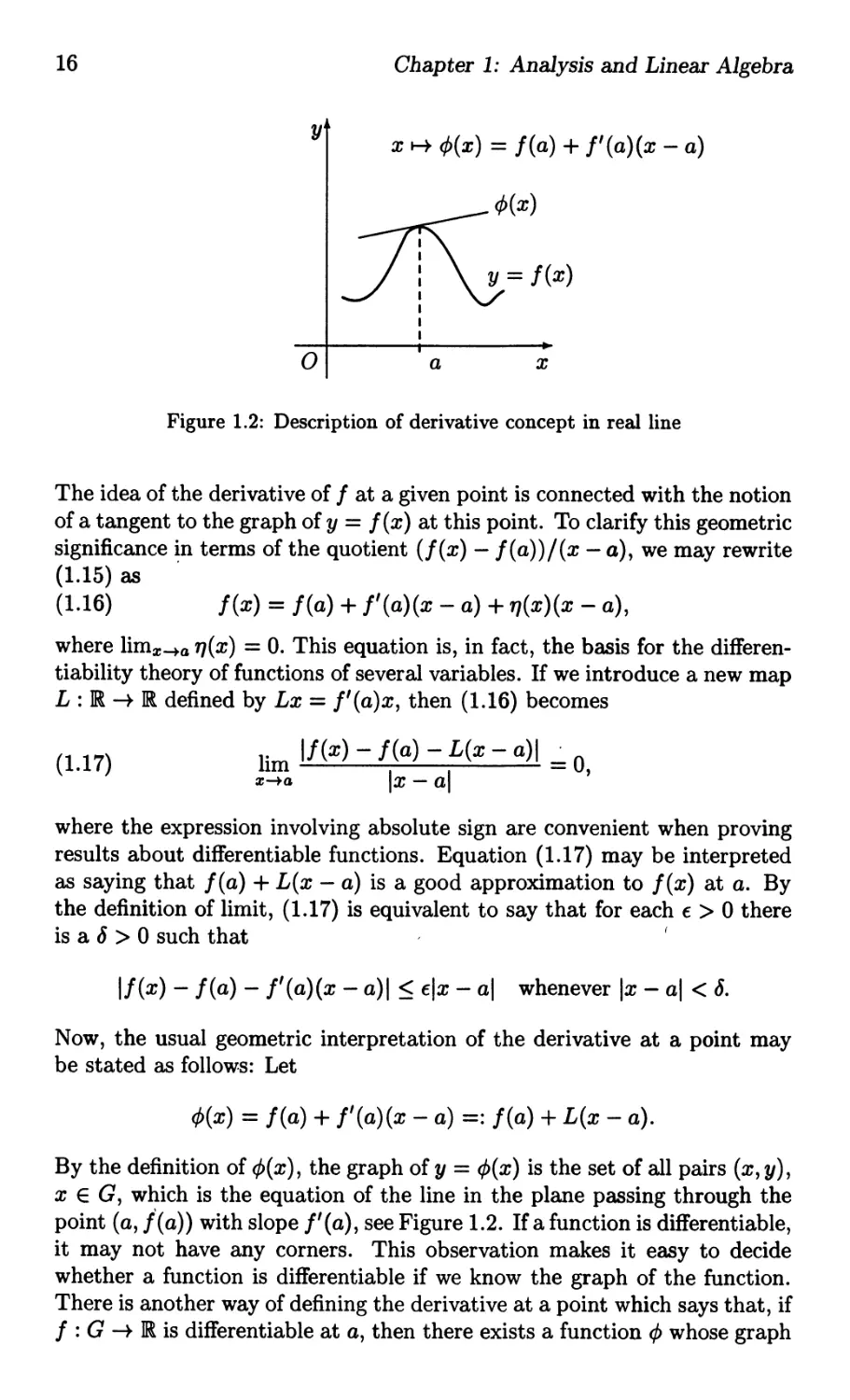
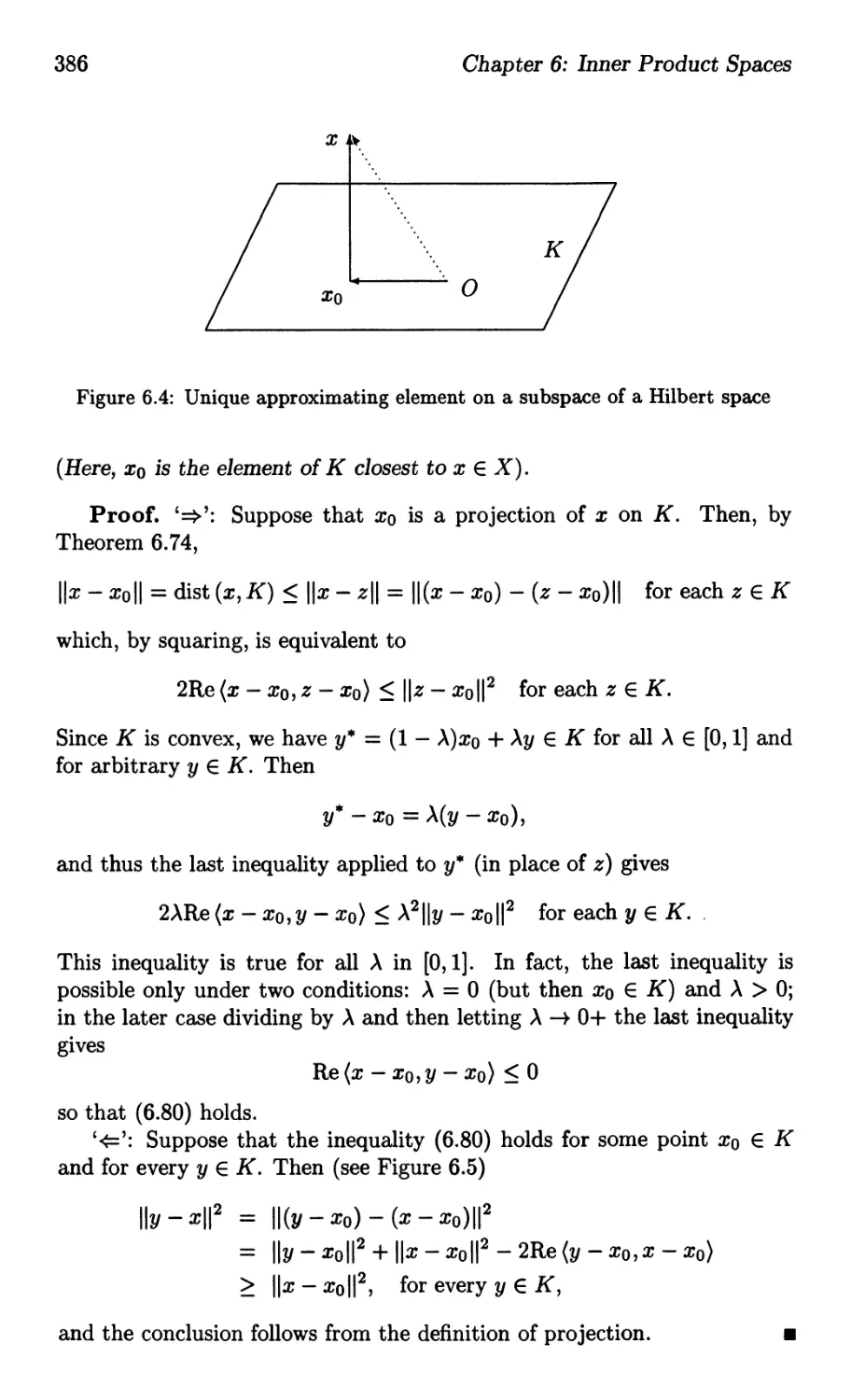
x </J(x) = f(a) + f'(a)(x - a)
o
a
x
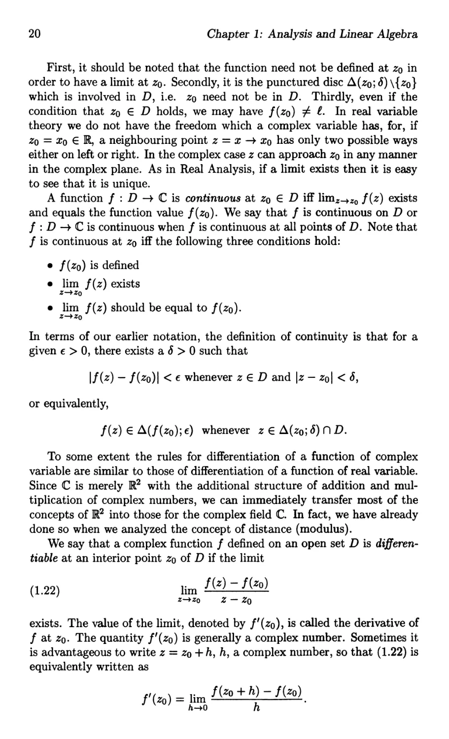
Figure 1.2: Description of derivative concept in real line
The idea of the derivative of f at a given point is connected with the notion
of a tangent to the graph of y = f(x) at this point. To clarify this geometric
significance n terms of the quotient (f(x) - f(a))/(x - a), we may rewrite
(1.15) as
(1.16) f(x) = f(a) + f'(a)(x - a) + 7J(x)(x - a),
where lim x -+ a 1J(x) = O. This equation is, in fact, the basis for the differen-
tiability theory of functions of several variables. If we introduce a new map
L : IR IR defined by Lx = f'(a)x, then (1.16) becomes
(1.1 7)
Urn If(x) - f(a) - L(x - a)1 . 0,
x-+a Ix - al
where the expression involving absolute sign are convenient when proving
results about differentiable functions. Equation (1.17) may be interpreted
as saying that f(a) + L(x - a) is a good approximation to f(x) at a. By
the definition of limit, (1.17) is equivalent to say that for each € > 0 there
is a 6 > 0 such that (
If (x) - f(a) - f'(a)(x - a) I < €Ix - al whenever Ix - al < 6.
Now, the usual geometric interpretation of the derivative at a point may
be stated as follows: Let
</J(x) = f(a) + f'(a)(x - a) =: f(a) + L(x - a).
By the definition of </J(x), the graph of y = </J(x) is the set of all pairs (x, y),
x E G, which is the equation of the line in the plane passing through the
point (a, f'(a)) with slope f'(a), see Figure 1.2. If a function is differentiable,
it may not have any corners. This observation makes it easy to decide
whether a function is differentiable if we know the graph of the function.
There is another way of defining the derivative at a point which says that, if
f : G IR is differentiable at a, then there exists a function </J whose graph
1.3. Review of Differentiability in Real Line
17
is a straight line and this function provides the best linear approximation
to f at a. In fact, (1.15) means that f'(a) can be approximated by
f(a + h) - f(a)
h
for sufficiently small h, which is same as to say that y = f(a + h) - f(a)
can be approximated by f'(a)h. If we write h = dx, we find that
y f'(a)dx
where the symbol denotes the "approximately equal to". From this, one
gets the differential dy at a point a by
dy = f'(a)dx,
d
or dx f(x)
= f'(a).
x=a
Are f1 (x) = x 2 , f2(X) = -IX and f3(X) = Ixl differentiable at O? One
can draw the graphs of these functions to analyze the geometric significance
of the quotient (fj(x) - fj(a))/(x - a) for j = 1,2,3. If f is defined by
{ X for x > 0
f(x) = _2X2 for x < 0
then we have f'(x) = 21xl which is not differentiable at O.
By writing
f(x) - f(a) = ( f(X) - f(a) ) (x - a),
x-a
it is seen immediately that every function which is differentiable at a point
is continuous thereat. The converse is not true. For example, the function
f(x) = Ixl is continuous on IR but is not differentiable at the origin.
We summarize the discussion of this section and reformulate the defini-
tion of the differentiability as follows:
1.18. Theorem. Let G be an open subset of IR and a E G. We say
that a function f : G ]R is differentiable at a iff there exists a linear map
L : IR -+ ]R such that
f(x) = f(a) + L(x - a) + R(x),
where the remainder function R(x) satisfies the condition
lim IR(x)1 = O.
x-+a Ix - al
It is this theorem which provides a method of generalizing the concept
of derivative of f defined from a subset of n-dimensional Euclidean space
18
Chapter 1: Analysis and Linear Algebra
an into IRm in which case the corresponding L in the last theorem becomes
an m x n-matrix, which we denote by D f(a) and is called the derivative
of f at a. The generalization of this idea is studied in advanced calculus
as well as in advanced analysis courses. Since we require the concept of
norm on n-dimensional Euclidean space IRn to give the precise definition
of the differentiability in the higher dimension, we do not wish to include
this definition at this stage. However, the following result is important to
remember and we shall make a general statement later in Chapter 2 (see
Corollary 2.83).
1.19. Proposition. Every continuous function on the closed interval
[a, b] is uniformly continuous therein.
1.20. Continuously differentiable functions on IR. Recall that if f
is differentiable at every point on I = (a, b) c IR, then f'(x) not only exists
as a function on I but also that f is continuous on I. Hence, it makes
sense to ask two natural questions that are considered to be important: Is
f' continuous on I? Is f' differentiable on I? and so on. In general, the
answer is no for both the questions as we see from the examples below.
A function f : I = ( a, b) IR is said to be continuously differentiable
on I, or of class C 1 on I, if f' exists on I and the function f' : I IR
is continuous. The class of all one time continuously differentiable on I is
denoted by C 1 (I). If f' is differentiable on I, then f is twice differentiable
on I. If the second derivative f" is continuous, then f is of class C 2 on I.
More generally, one can define k-times continuously differentiable func-
tions on I for any positive integer k, and we denote the class of all such
functions by Ck(I), see Exercise 5.162. Thus, COO (I) denotes the class of
all infinitely differentiable functions on the open interval I.
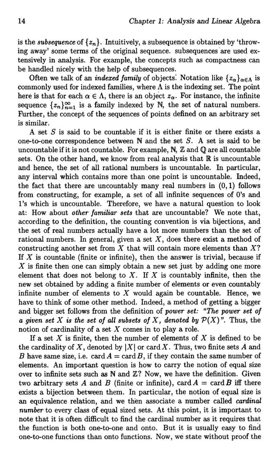
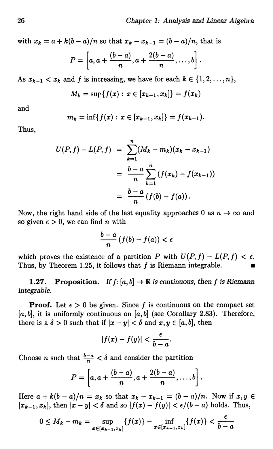
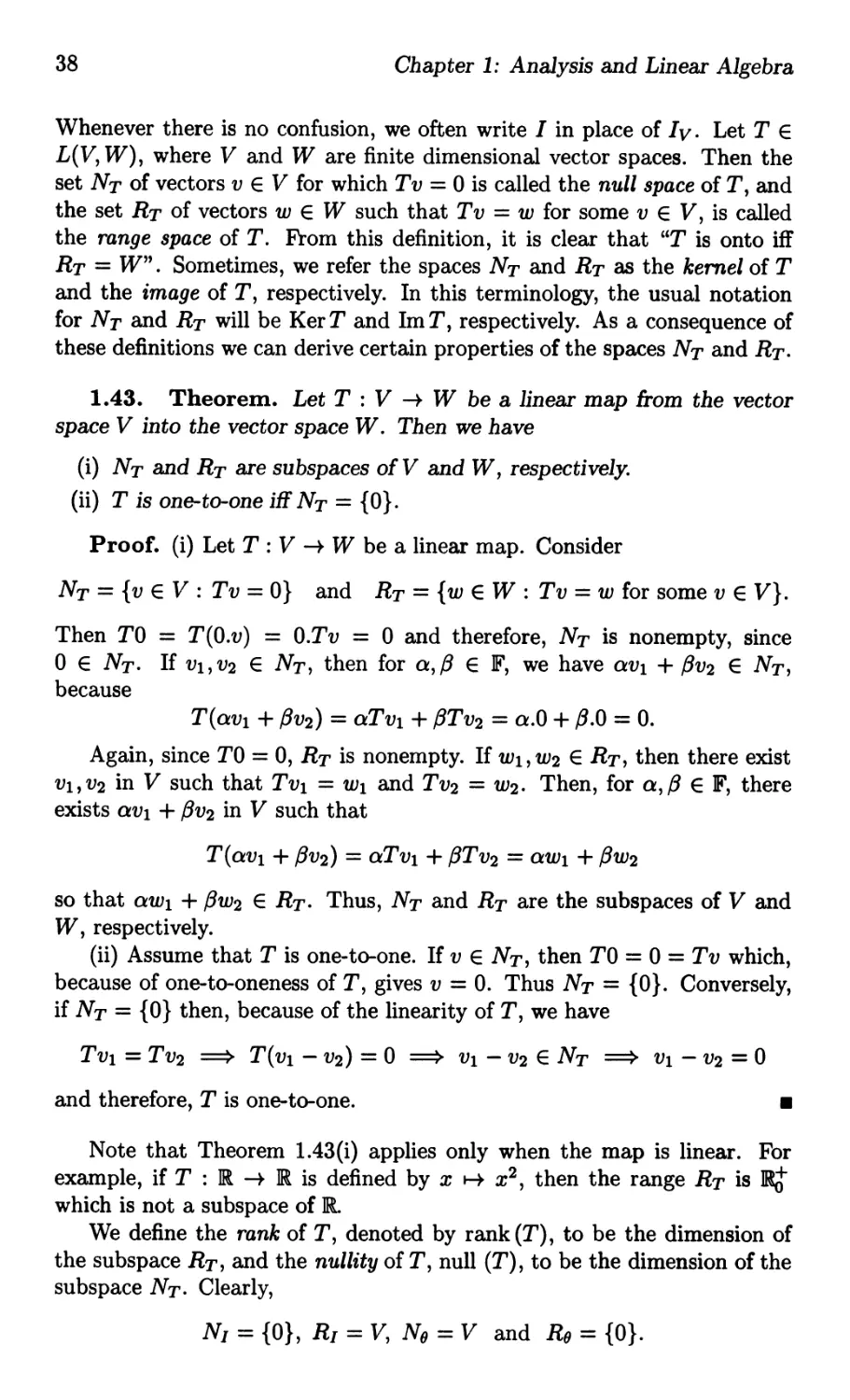
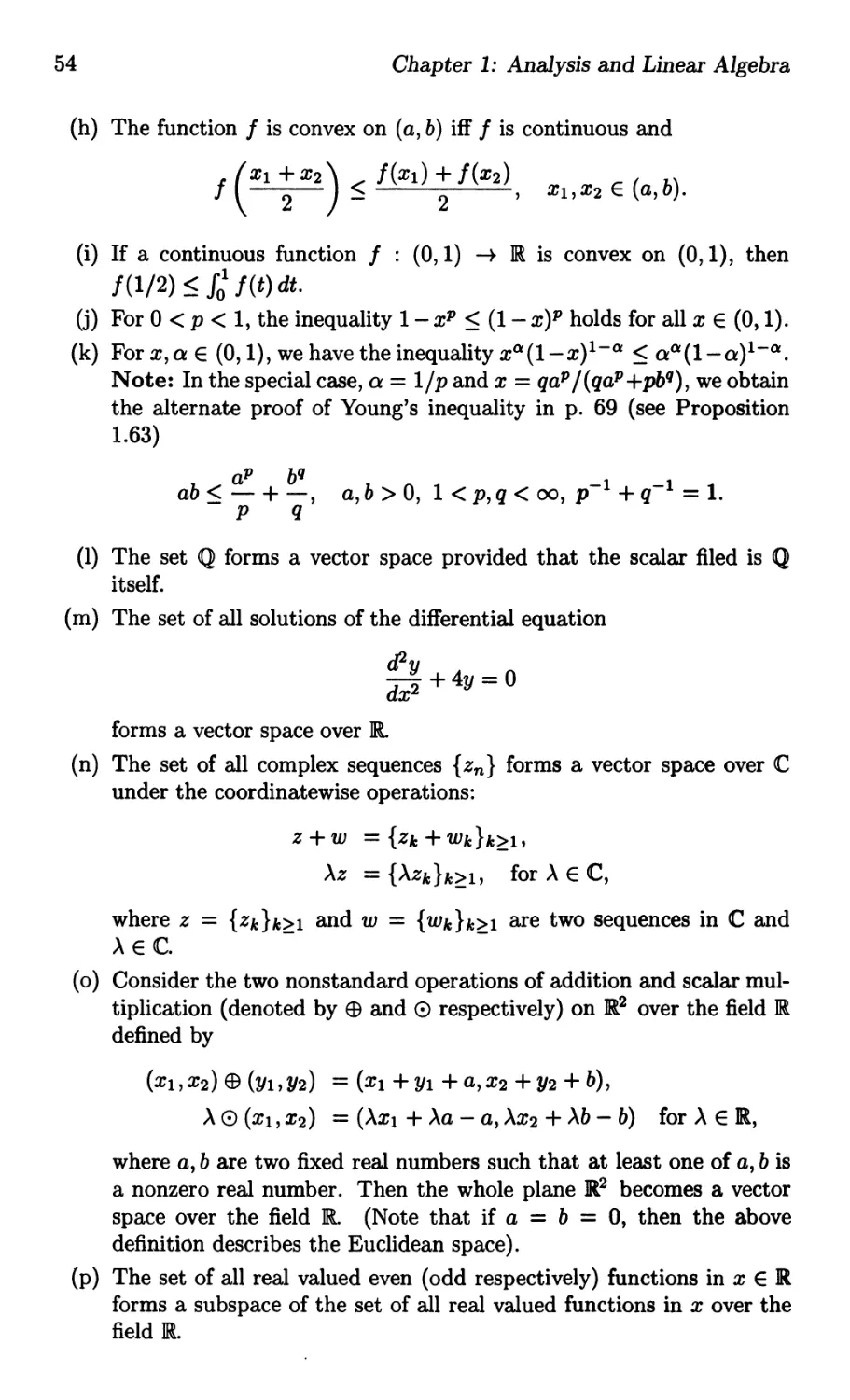
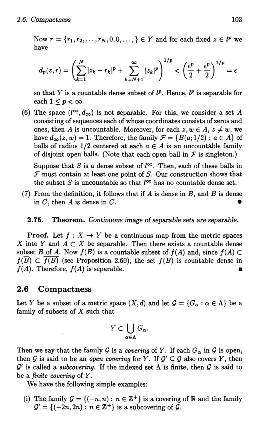
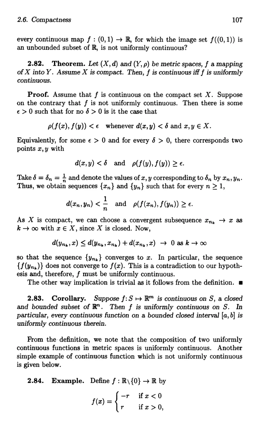
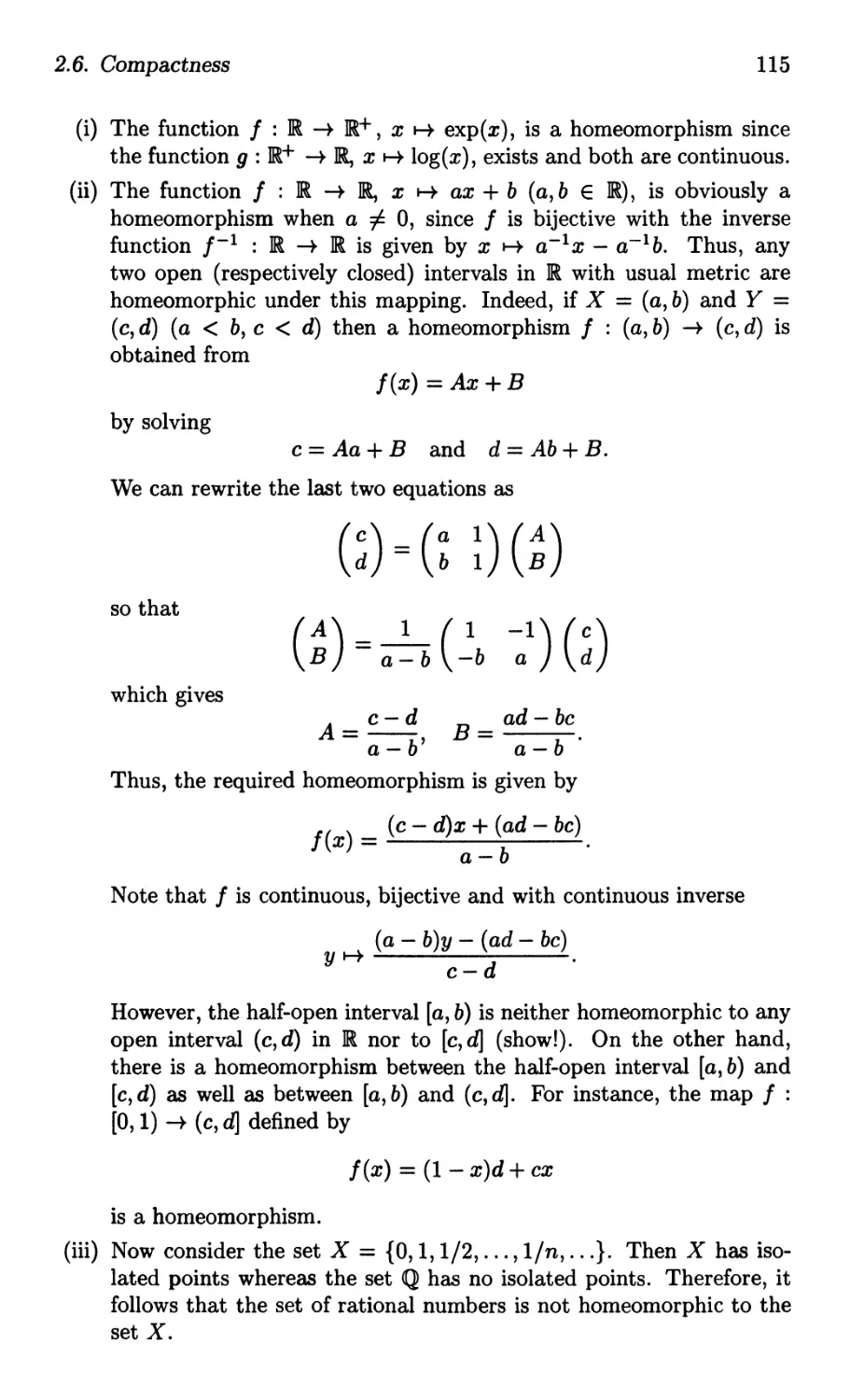
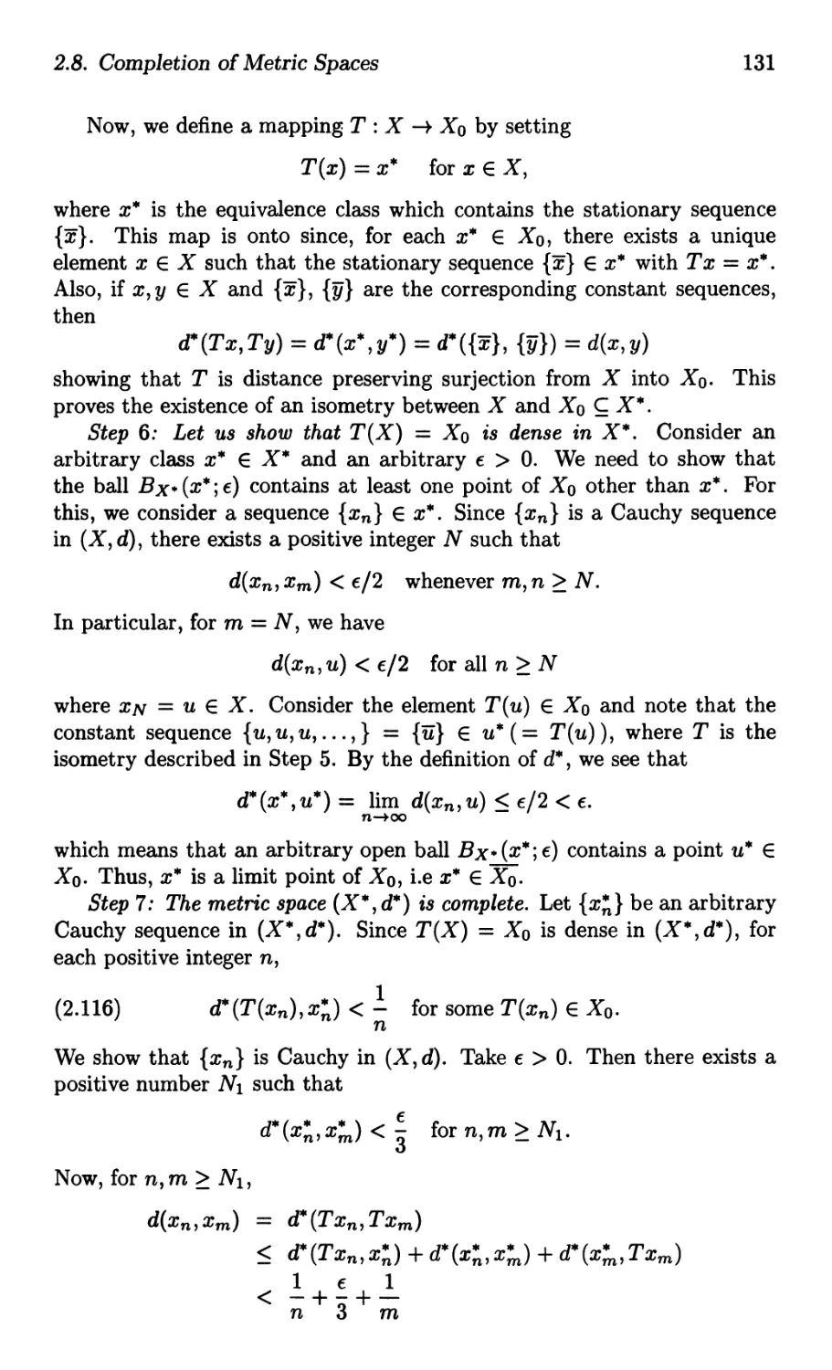
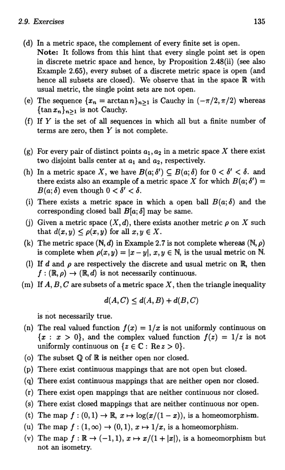
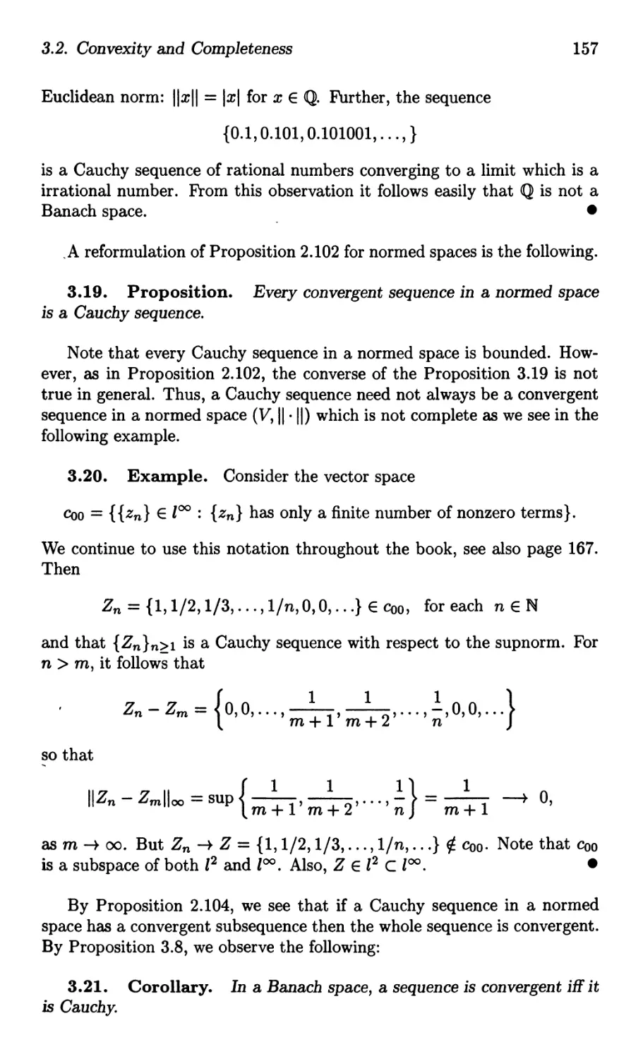
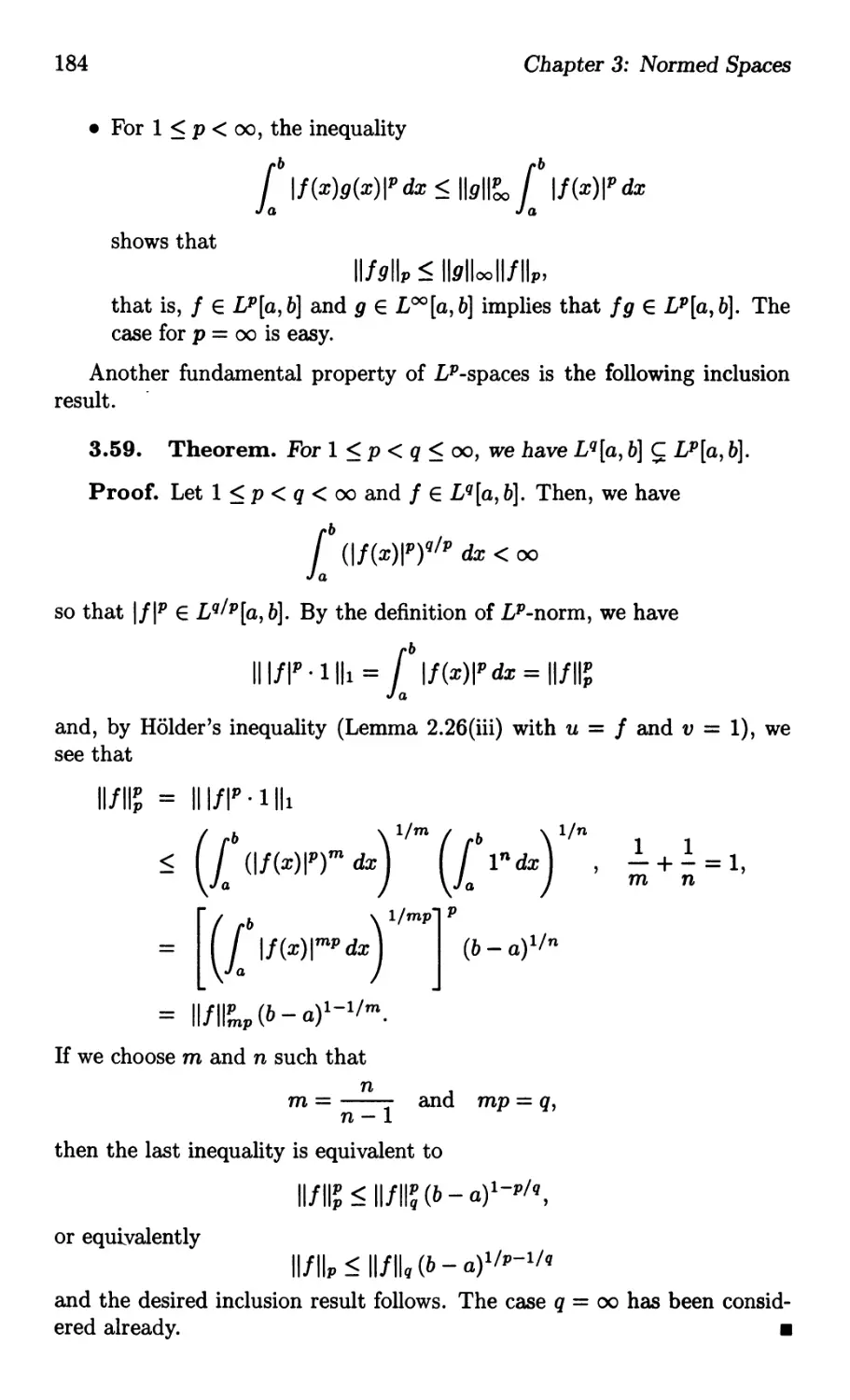
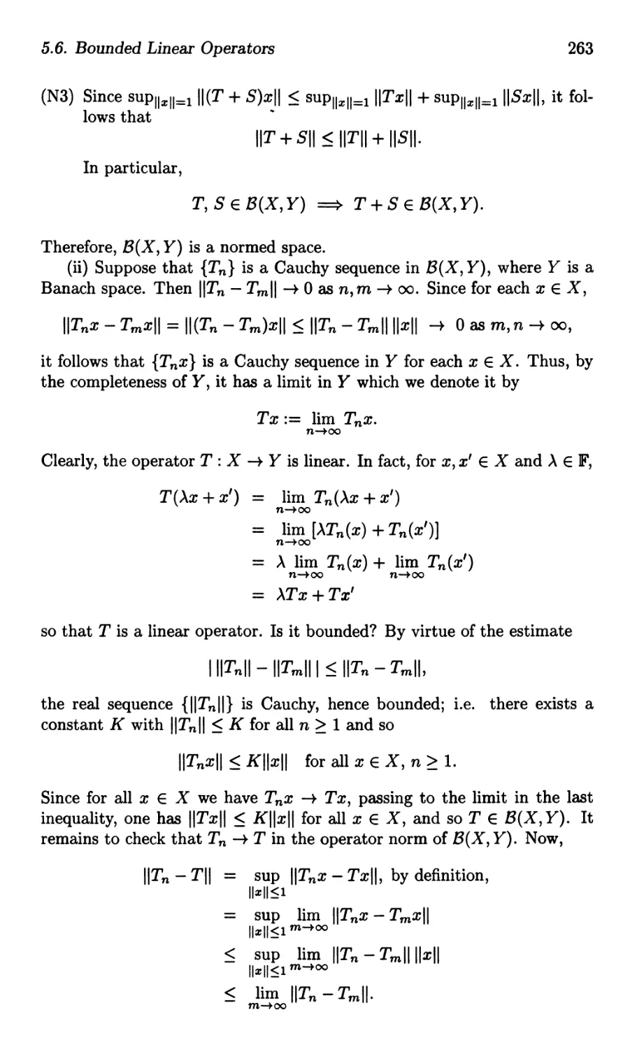
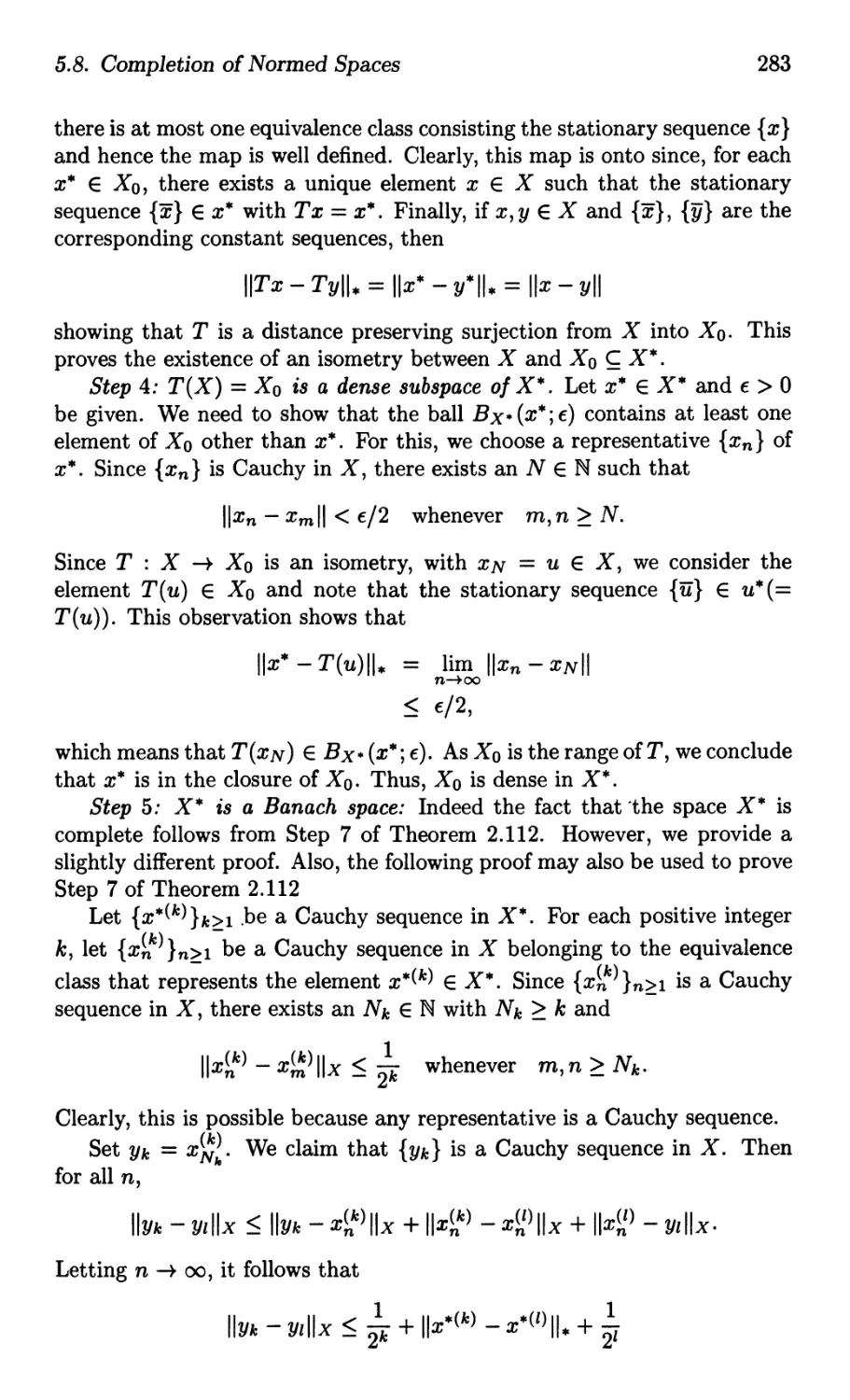
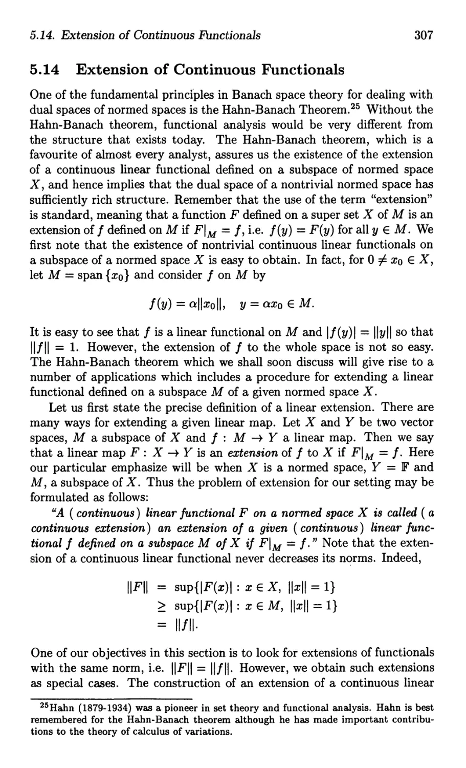
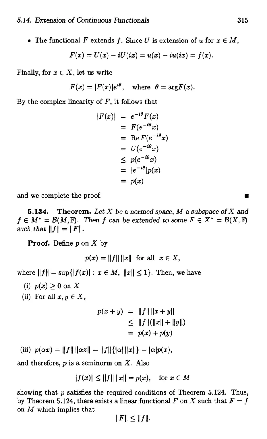
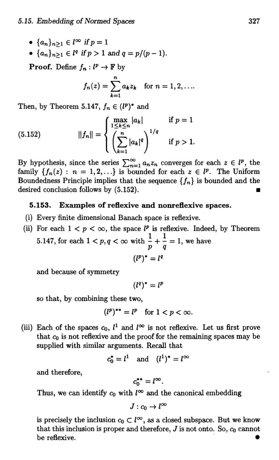
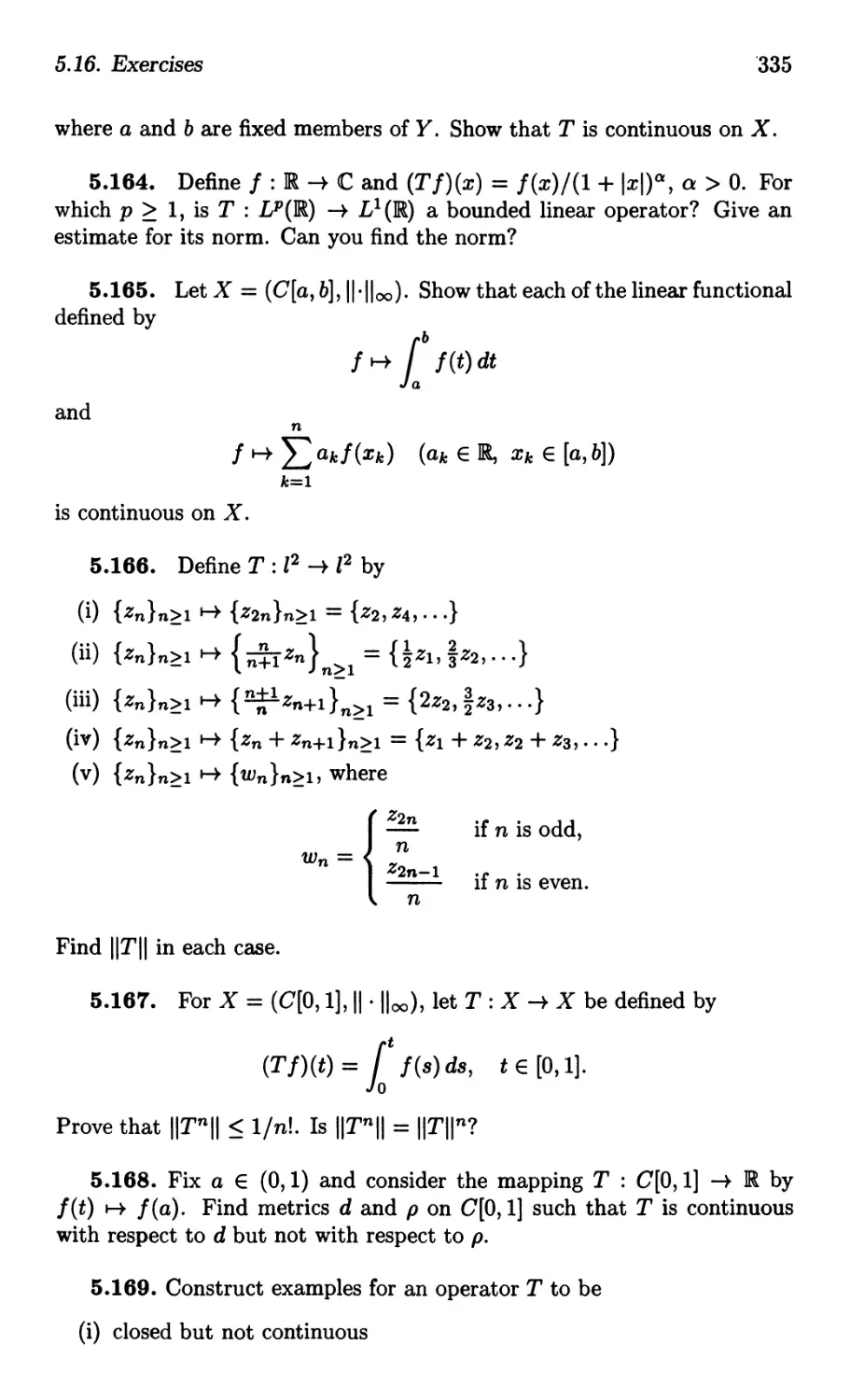
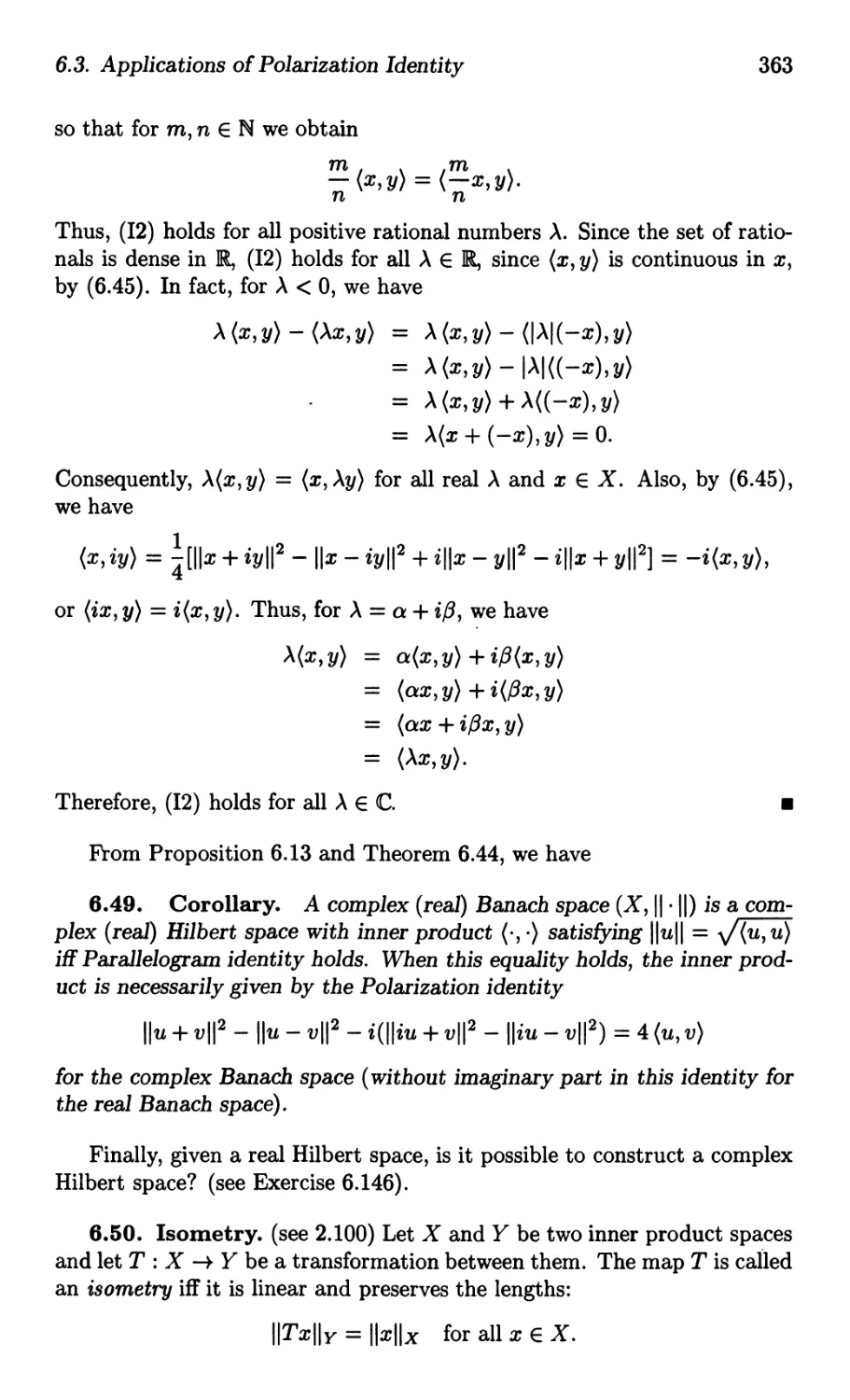
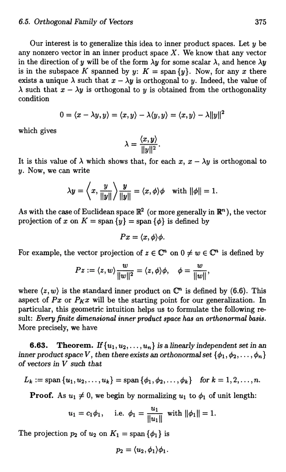
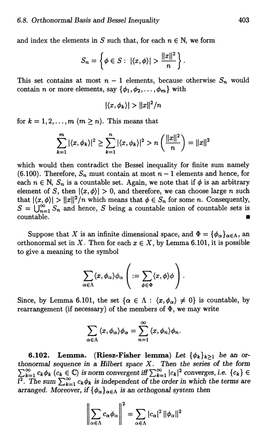
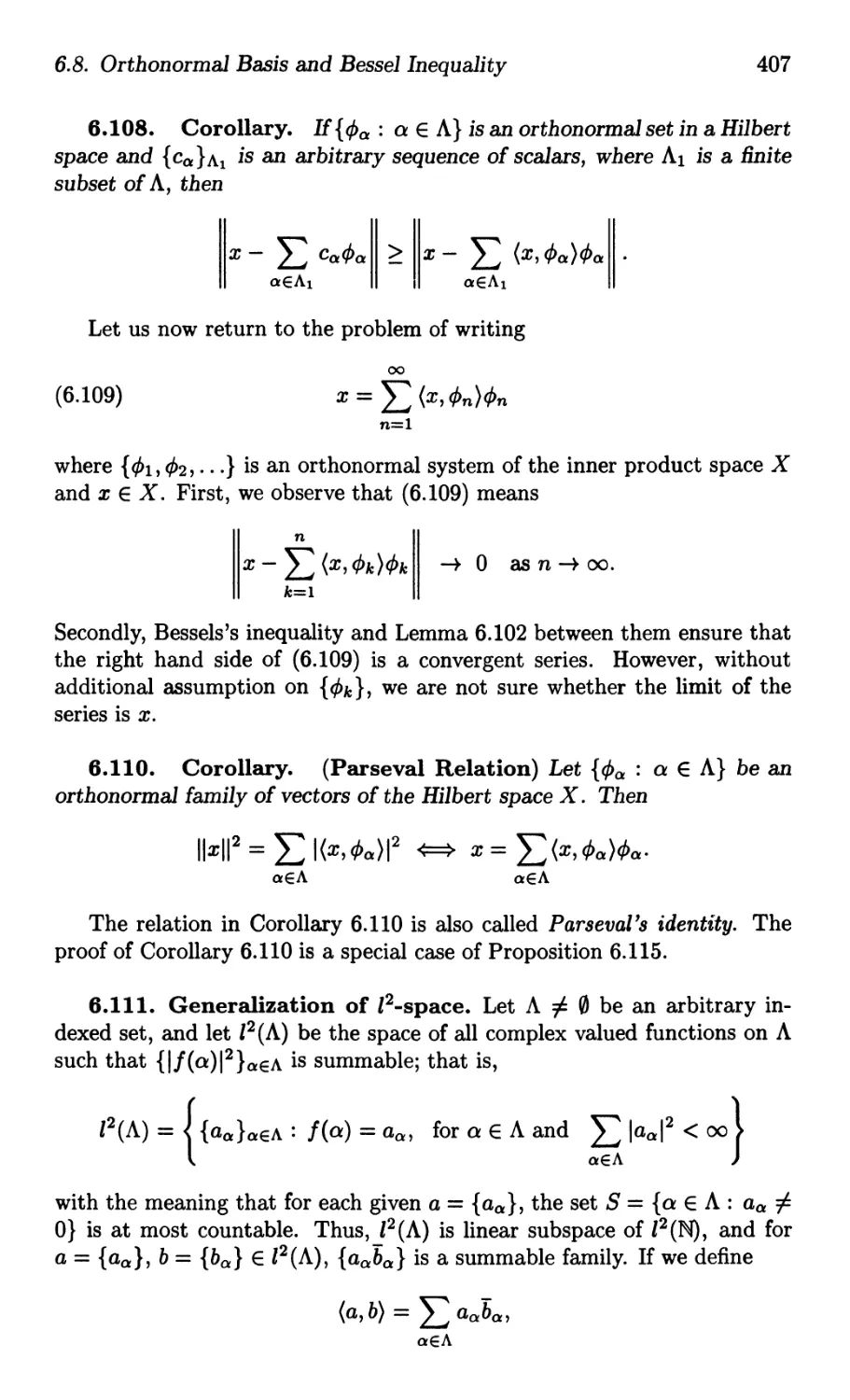
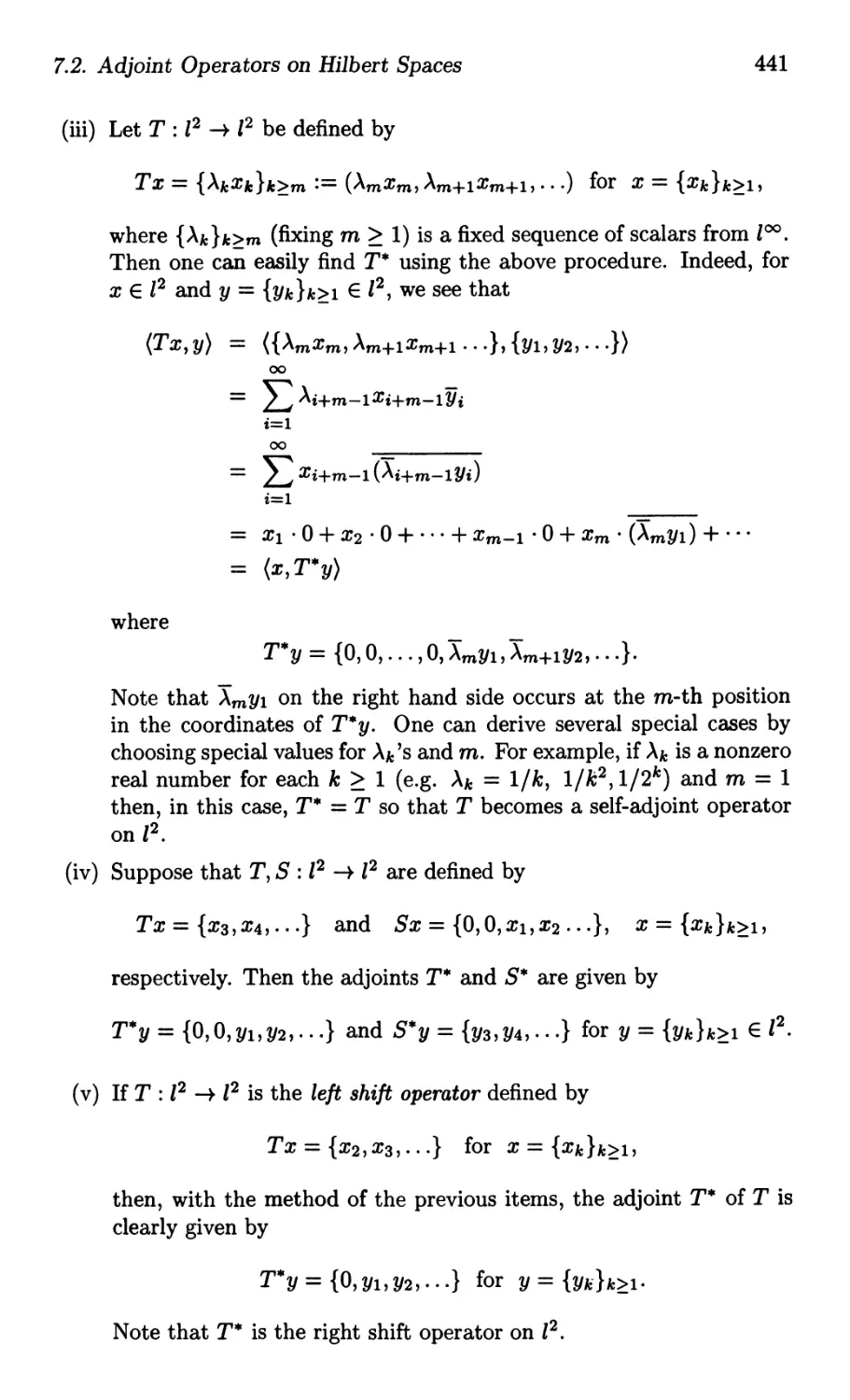
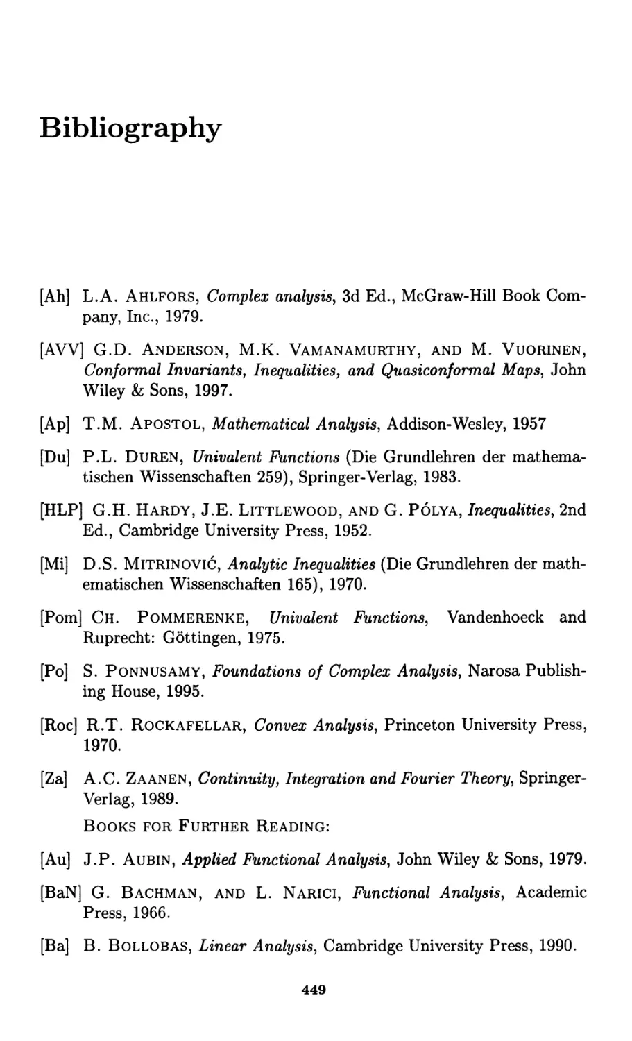
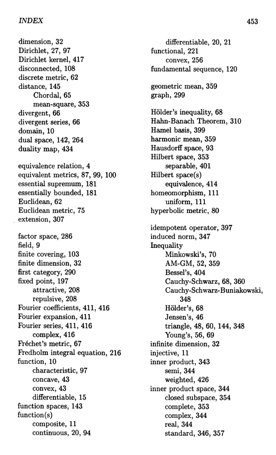
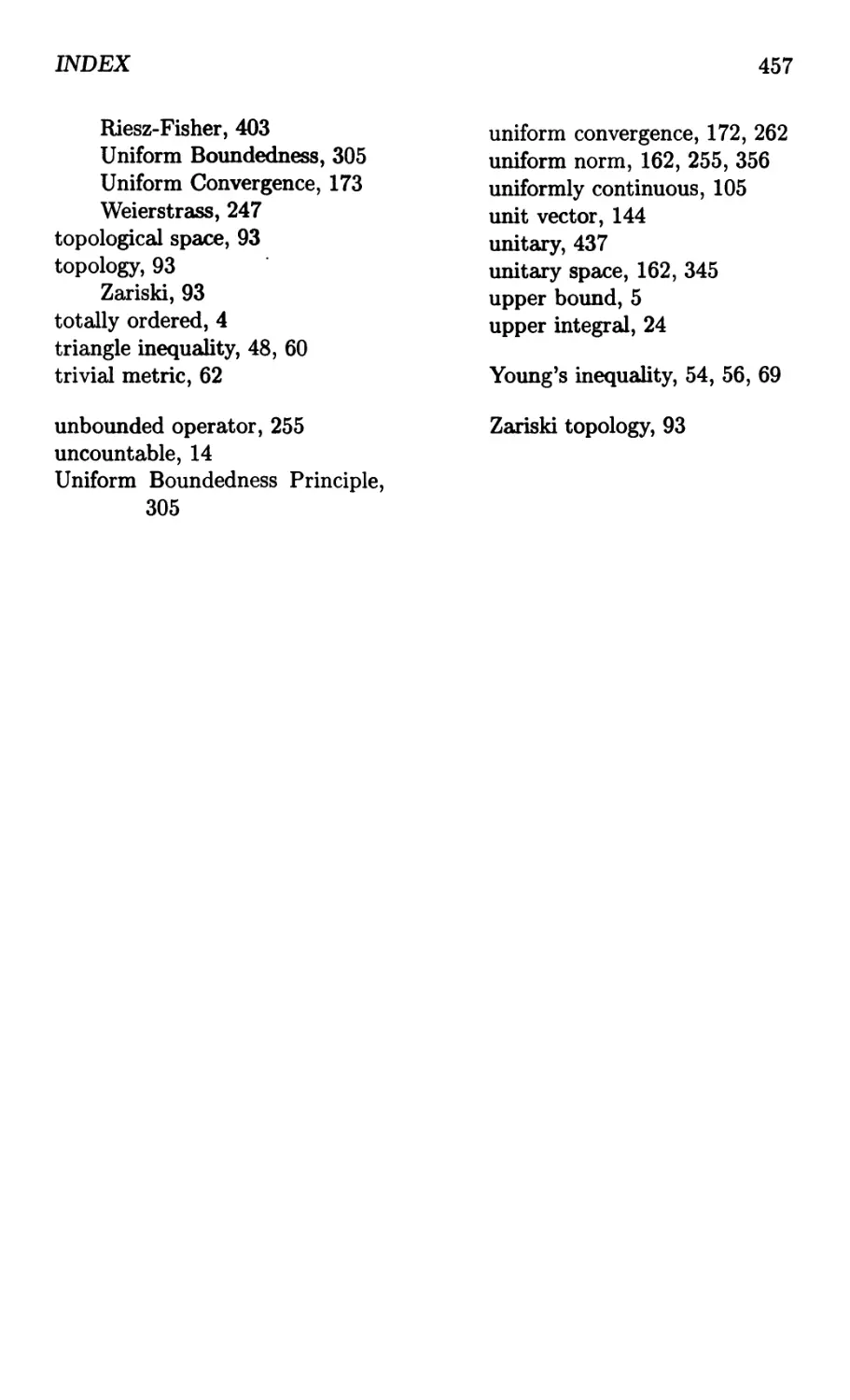
1.21. Example. The function f defined by
f(x) = { 0
x n
for x < 0
for x > 0
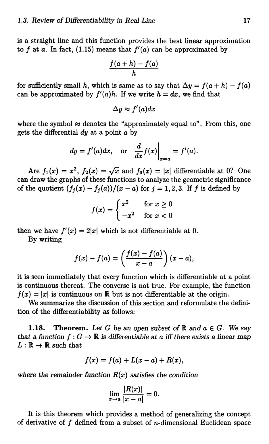
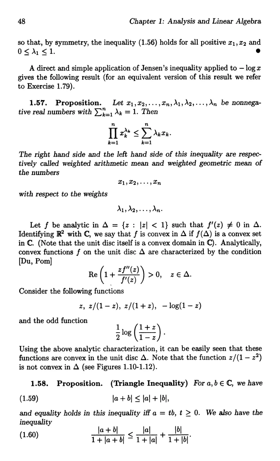
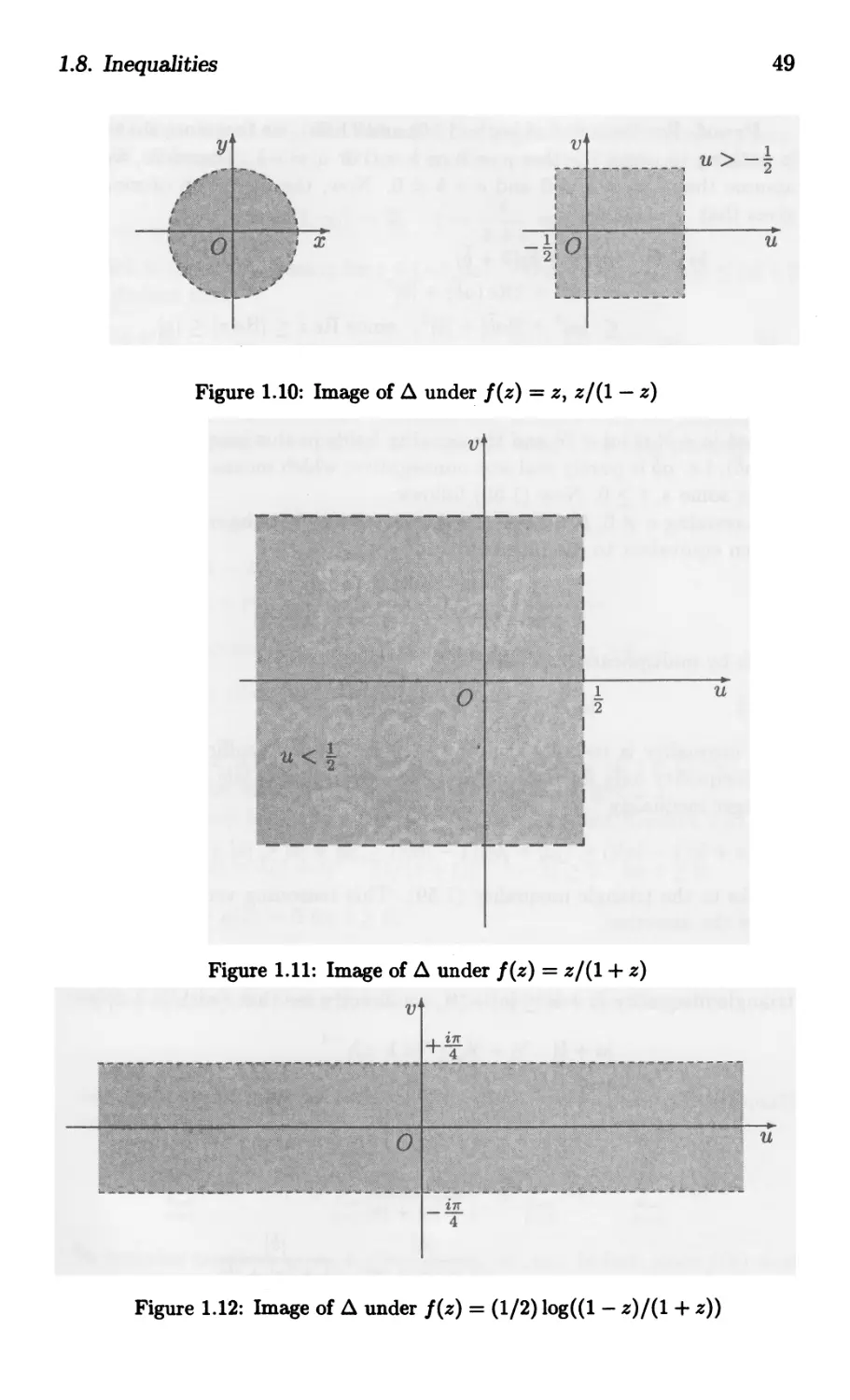
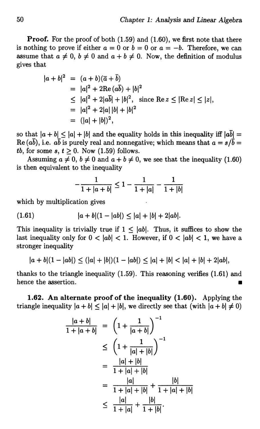
belongs to cn-1(IR), but does not belong to Cn(IR). See Figure 1.3 for the
case n = 2, where
g(x) = { :2
for x E [-1,0)
for x E [0,1].
It is easy to see that 9 and g' are both continuous, but g"(x) is discontinuous
at the origin and hence, 9 C 2 [-1, 1]. Indeed,
, (0) 1 . x2 - 0 0
9 =lm 0 =,
x-+o x-
and g'(x) = { 0
2x
for x E [-1, 0)
for x E [0, 1]
1.4. Concept of Derivative in Complex Plane
19
y
(0,1)--------- (1,1)
y = f(x) I
I
I
I
I
I
I
(-1,0)
o
(1,0)
x
Figure 1.3: 9 E C 1 [-I, 1] but not in C 2 [-I, 1]
whereas
I . g' (x) - 0 _ I " 2x - 2
1m -lm--,
x-+o+ X - 0 x-+O+ X
which shows that g' is not differentiable at the origin.
Another simple example is given by
{ xn1x 1
f(x) =
o
for x :j:. 0
for x = O.
It can be easily seen that this function belongs to en (IR), but does not
belong to e n + 1 (IR) since fen) is not continuous at the origin.
Another simple example of function f such that fen) exists at the origin
but the function fen) is not continuous at the origin may be given by f(x) =
x2n sin (l/x) for x :j:. 0 and f(O) = o. .
1.4 Concept of Derivative in Complex Plane
The definitions of limit, continuity, differentiability and uniform continuity
are some what analogous to those in Real Analysis. In this section, we
briefly discuss about the concept of differentiability in the complex plane.
Suppose that a complex-valued function f is defined on D C C and Zo
is either in D or on the boundary of D. We say that the function f has a
limit l as z Zo and write
lim f(z) = l or f(z) l as z Zo
Z-+ZO
iff for any given € > 0, there exists a 6 = 6(€, zo) > 0 such that
If(z) -ll < € whenever zED and 0 < Iz - zol < 6.
i.e. iff for each € > 0 there exists a 6 > 0 such that
f(z) E (l; €) whenever z E [ (zo; 6) \{zo}] n D.
20
Chapter 1: Analysis and Linear Algebra
First, it should be noted that the function need not be defined at Zo in
order to have a limit at ZOo Secondly, it is the punctured disc (zo; 6) \{zo}
which is involved in D, Le. Zo need not be in D. Thirdly, even if the
condition that Zo E D holds, we may have j(zo) :j:. t. In real variable
theory we do not have the freedom which a complex variable has, for, if
Zo = Xo E ]R, a neighbouring point z = x Xo has only two possible ways
either on left or right. In the complex case z can approach Zo in any manner
in the complex plane. As in Real Analysis, if a limit exists then it is easy
to see that it is unique.
A function j : D C is continuous at Zo E D iff limz-+zo j(z) exists
and equals the function value j(zo). We say that j is continuous on D or
j : D C is continuous when j is continuous at all points of D. Note that
j is continuous at Zo iff the following three conditions hold:
. j(zo) is defined
. lim j(z) exists
z -+ Zo
. lim j(z) should be equal to j(zo).
z -+ Zo
In terms of our earlier notation, the definition of continuity is that for a
given € > 0, there exists a 6 > 0 such that
Ij(z) - j(zo)1 < € whenever zED and Iz - zol < 6,
or equivalently,
j(z) E (j(zo); €) whenever z E (zo; 6) n D.
To some extent the rules for differentiation of a function of complex
variable are similar to those of differentiation of a function of real variable.
Since C is merely }R2 with the additional structure of addition and mul-
tiplication of complex numbers, we can immediately transfer most of the
concepts of}R2 into those for the complex field C. In fact, we have already
done so when we analyzed the concept of distance (modulus).
We say that a complex function j defined on an open set D is differen-
tiable at an interior point Zo of D if the limit
(1.22)
I . j(z) - j(zo)
1m
z-+zo Z - Zo
exists. The value of the limit, denoted by j'(zo), is called the derivative of
j at Z00 The quantity j'(zo) is generally a complex number. Sometimes it
is advantageous to write z = Zo + h, h, a complex number, so that (1.22) is
equivalently written as
j ' ( ) _ I . j(zo + h) - j(zo)
ZO-lffi h .
h-+O
1.4. Concept of Derivative in Complex Plane
21
Again we note that the limit exists irrespective of the path along which
h O.
In terms of '€ - 6' notation, the limit in (1.22) exists iff given any € > 0,
there exists a 6 = 6 ( €, zo) > 0 such that
j(z) - j(zo) _ j'(zo) < € whenever 0 < Iz - zol < 8.
Z - Zo
For a given Zo, one can also consider the function 1J : D C defined by
{ I(z)-/(zo) - f'(zo)
1J(z) = z-zo
o
for z :j:. Zo
for z = Zo.
Then (1.22) is equivalent to limz-+zo 1J(z) = 0 so that 1J is continuous at
Zo. This observation shows that f (z) is differentiable at Zo iff there exists a
number f'(zo) and a function 1J, continuous at Zo, satisfying the condition
1J(zo) = 0 such that
(1.23) f(z) = f(zo) + (z - zo)f'(zo) + (z - zO)1J(z).
Note that, as in the real case, the explicit expression in the form (1.23) has
the advantage of containing no limit since this is replaced by the continuity
of 1J(z).
The function f is said to be differentiable on (in) the open set D if it is
differentiable at every point of D. A function f is said to be analytic at a
point a ED, where D is some open set in C, if there exists an open disc
(a; 6) in D such that f is differentiable at all points of (a; 6). Thus, f
is analytic in an open set D is equivalent to say that f is differentiable on
D.
A function f : [a, b] C is said to be continuously differentiable on [a, b],
or a map of class C1 (denoted by C [a, b]) if the function f(t) = u(t) +iV(t)1
t E [a, b], is continuously differentiable on [a, b], Le. u' (t) and v' (t) exist. for
each t in [a, b] and are continuous functions of t on [a, b]. Note that f(t) is
differentiable on [a, b] means that f'(t) exists on (a, b), and
I . f(a + h) - f(a)
lIll ,
h-+O+ h
I . f(b + h) - f(b)
1m
h-+O- h
both exist. We denote these limits by f'(a+) and f'(b-:-), respectively.
The space of all scalar-valued and continuously differentiable functions f
on [a, b]" is usually denoted by Ci[a, b]. If the map f is from [a, b] into IR
(instead of IIlapping into C) then it is denoted by
C 1 [a, b] := C [a, b].
22 Chapter 1: Analysis and Linear Algebra
1.5 Concept of Riemann and Riemann Stieltjes
Integrals
One of the useful concepts is integration and is introduced in a calculus
course especially for 'finding the area under a curve'. Is it possible to think
of 'integration' in the form of summation? The summation interpretation
of integration will make many of its properties easier to remember and
also to get more information without much hardship. First, we recall how
to construct the Riemann-Stieltjes integrals (in particular, the Riemann
integrals). We will briefly discuss the Lebesgue integrals later, in Section
3.6.
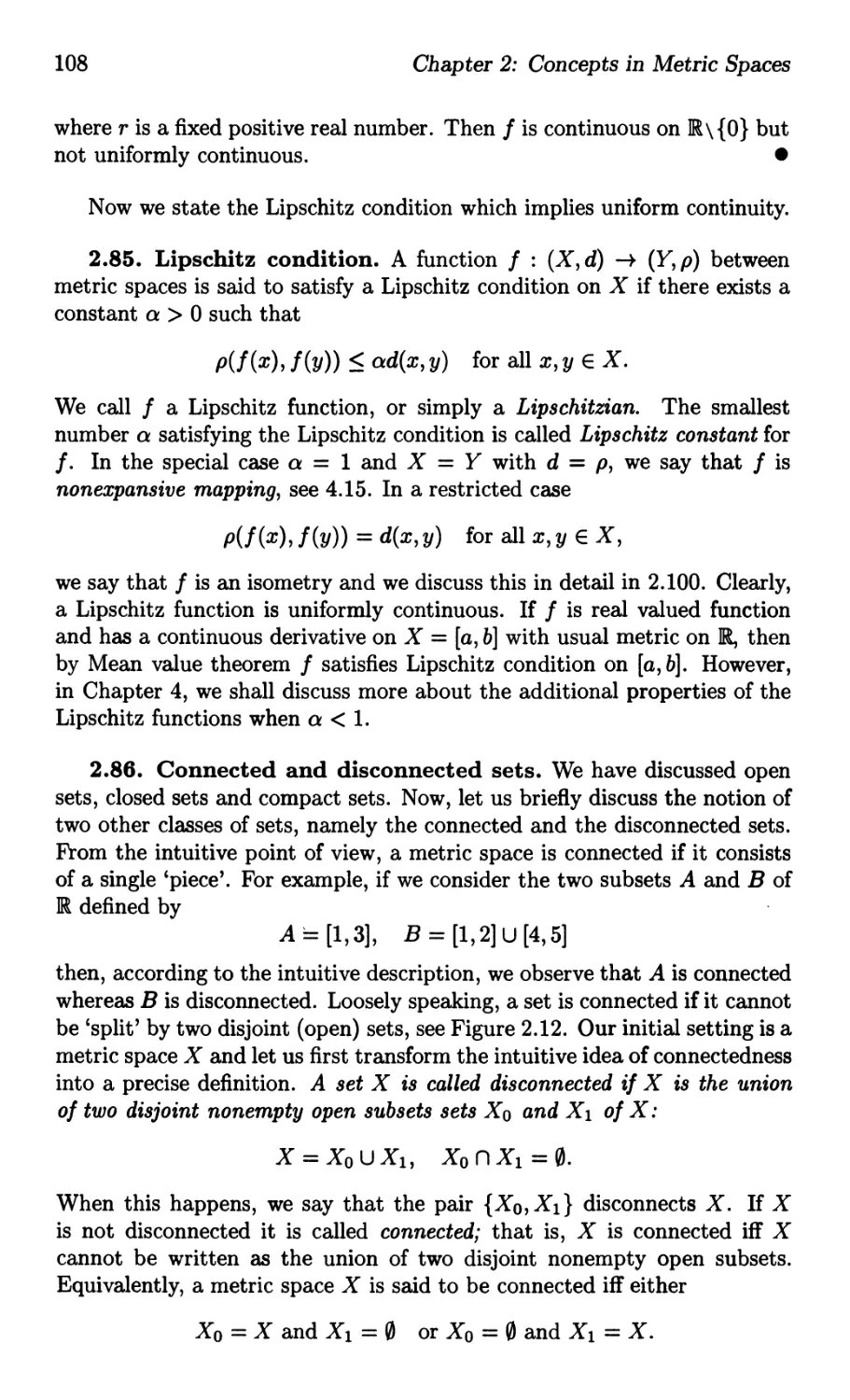
Let a < b. A partition P of the closed interval [a, b] is a finite set of
points {XO, Xl, . . . , xn} satisfying
a = Xo < Xl < X2 < ... < Xn-l < X n = b.
We denote the set of all partitions of [a, b] by II[a, b]. If
P = {Xk}k=O E II[a, b],
then
Xk = Xk - Xk-l
defines the length of the k-th subinterval [Xk-l, Xk]. In this case, we define
the norm or mesh of the partition by
IPI=max{ Xk: k=l,...,n}.
If PI and P 2 are any two partitions of [a, b], then we say that the partition
P 2 is a refinement of the partition PI, written PI C P 2 , if P 2 contains all
the points from PI and some additional points, again sorted in order of
magnitude as defined for any partition P. Since each of the subintervals
formed by the partition P 2 is contained in a subinterval which arises from
the partition PI, it follows that IP 2 1 < IPll whenever PI C P 2 .
Let f: [a,b] IR be a bounded function. Let P = {XO,Xl,...,Xn} be
a given partition of [a, b]. For each k, 1 < k < n, we let
M k = sup{f(x) : X E [Xk-l,Xk]} and mk = inf{f(x) : X E [Xk-l,Xk]}.
For a nondecreasing function a on [a, b], define
ak := a(xk) - a(xk-l).
We define the 'Upper and lower Riemann-Stieltjes sums for f, defined on
[a, b], with respect to a by
n n
U(P,f,a) = LMk ak and L(P,f,a) = Lmk ak'
k=l k=l
1.5. Concept of Riemann and Riemann Stieltjes Integrals
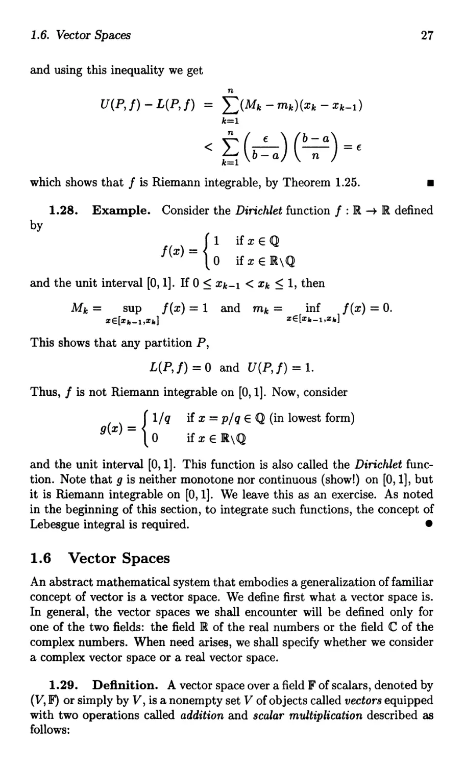
23
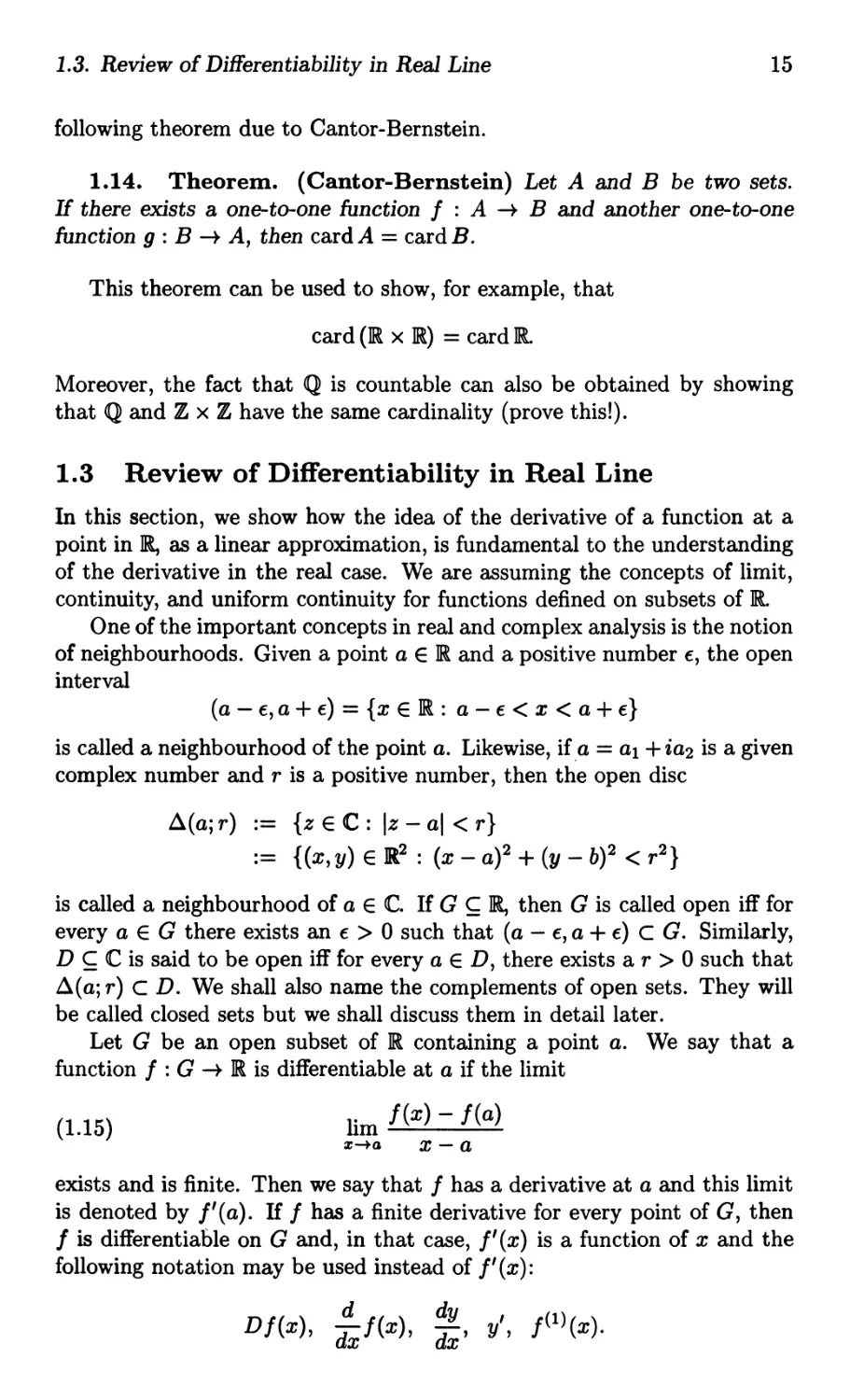
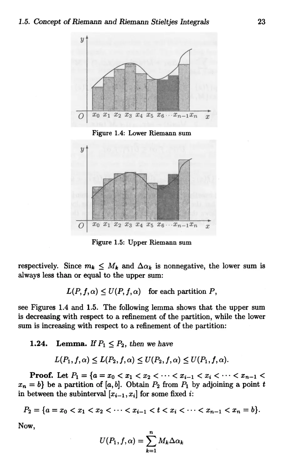
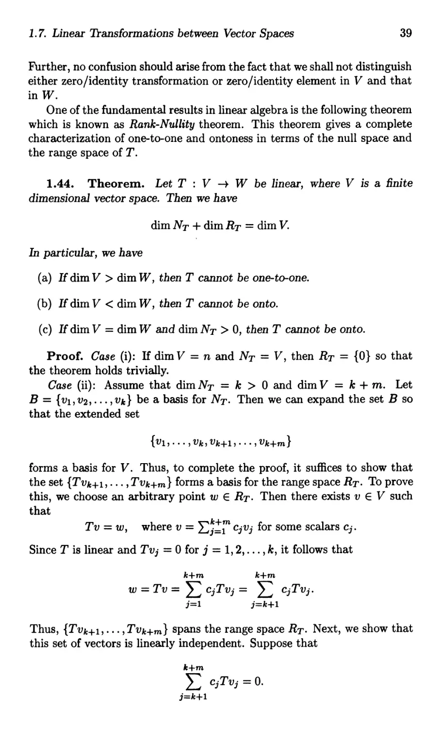
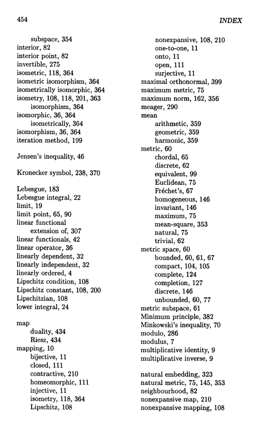
y
.
I
i
o Xo Xl X2 X3 X4 X5 X6.. .Xn-lX n X
Figure 1.4: Lower Riemann sum
y
.. . '..", ' :.:
." ..... fj
.
'">, ": ". . I
Xo Xl X2 X3 X4 X5 X6.. .Xn-IX n X
o
Figure 1.5: Upper Riemann sum
respectively. Since mk < Mk and ak is nonnegative, the lower sum is
always less than or equal to the upper sum:
L{P,f,a) < U{P,f,a) for each partition P,
see Figures 1.4 and 1.5. The following lemma shows that the upper sum
is decreasing with respect to a refinement of the partition, while the lower
sum is increasing with respect to a refinement of the partition:
1.24. Lemma. H P l < P 2 , then we have
L{Pl,f,a) < L{P 2 ,f,a) < U{P 2 ,f,a) < U{Pl,f,a).
Proof. Let P l = {a = Xo < Xl < X2 < ... < Xi-l < Xi < ... < Xn-l <
X n = b} be a partition of [a, b]. Obtain P 2 from P l by adjoining a point t
in between the subinterval [Xi-l, Xi] for some fixed i:
P 2 = {a = Xo < Xl < X2 < ... < Xi-l < t < Xi < ... < Xn-l < X n = b}.
Now,
n
U{Pl,f,a) = LMk ak
k=l
24
Chapter 1: Analysis and Linear Algebra
where as
n
U(P 2 , 1,0:) = E Mk O:k + M(o:(t) - O:(Xi-l)) + M'(O:(Xi) - o:(t))
k=l, k;f:.i
where M = sup{/(x) : x E [Xi-I, t]} and M' = sup{/(x) : x E [t, Xi]}. If
we set M i = max{M, M'}, then we have
Mi O:i - Mi(o:(t) - O:(Xi-l)) + Mi(O:(Xi) - o:(t))
> M(o:(t) - O:(Xi-l)) + M'(O:(Xi) - o:(t))
which shows that
U ( P 2 , I, 0:) < U (PI, I, 0: ).
Letting
m = inf{/(x) : x E [Xi-I, t]}, m' = inf{/(x) : x E [t, Xi]},
and proceeding exactly in the same way with mi = min {m, m'} in place
of M i , we see that the corresponding inequality for the lower sum follows
similarly. It follows that if P 2 contains one point more than PI, then the
inequalities of the Lemma hold. The general case follows by the method of
induction. _
As a consequence of the last result, for any partitions PI and P 2 of [a, b],
we have
L(Pl, 1,0:) < L(PI U P 2 , 1,0:) < U(P 1 U P 2 , 1,0:) < U(P 2 , I, 0:).
One can show that the following limits exist:
--=b
! 1 do::= lim U(P, 1,0:) = inf{U(P, 1,0:) : P is a partition of [a, b]}
a IPI-+O
and
(b Ida:= lirn L(P, I, a) = sup{L(P, I, a) : P is a partition of [a, b]}.
IPI-+O
These are respectively called the upper and lower Riemann-Stieltjes inte-
grals of 1 with respect to 0: over [a, b]. In particular, for any partition P,
this observation yields that
b --=b
L(P, I, a) < i lda(x) < !/da(x) < U(P,I,a).
We remark that the upper and lower sums depend on the particular choice
of the partition while the upper and lower integrals are independent of the
1.5. Concept of Riemann and Riemann Stieltjes Integrals
25
partitions. Hence, a natural question is: will the two quantities, namely the
upper and lower integrals, ever coincide? The bounded function f defined
on the closed interval [a, b] is said to be Riemanri-Stieltjes integrable on [a, b]
if the upper and lower Riemann-Stieltjes integrals are equal. In this case,
we denote their common value simply by
lab f do: or lab f(x) do:(x).
We call this integral as the Riemann-Stieltjes integral of f with respect to
a on [a, b]. We let ROl[a, b] denote the set of all Riemann-Stieltjes integrable
functions with respect to a on [a, b].
If a(x) = x, then the Riemann-Stieltjes integral reduces to the Riemann
integral of f over [a, b]. In this case, the upper and lower Riemann-Stieltjes
sums will be called the upper and the lower Riemann sums, respectively.
The set of all Riemann integrable functions on [a, b] will be denoted by
R[a, b]. In particular, we raise t e following fundamental questions:
. Is every monotone function on [a, b] Riemann integrable?
. Is every continuous function on [a, b] Riemann integrable?
. Is every bounded function which has a finite number of discontinuities
in [a, b] Riemann integrable?
. Is every bounded function which has an infinite number of disconti-
nuities in [a, b] Riemann integrable?
. Is every monotone function which has an infinite number of disconti-
nuities in [a, b] Riemann integrable?
Before we answer these questions, it would be interesting to develop some
theorems which will easily lead to examples of Riemann integrable functions
and partly answer some of the above questions. We begin with the following
criterion for Riemann integrability:
1.25. Theorem. Let f : [a, b] IR be bounded. Then f E R[a, b] iff
for every € > 0 there exists a partition P of [a, b] such that
U(P, f) - L(P, f) < €.
Proof. This is an easy and standard result that follows from the defi-
nition. We leave the proof as an exercise. -
1.26. Proposition. Every monotone function on [a, b] is Riemann
integrable on [a, b].
Proof. It suffices to consider the case when f is monotone increasing
on [a, b]. A similar argument works if f is monotone decreasing. Divide
[a, b] into n-equal intervals and consider the partition
a = Xo < Xl < X2 < ... < Xn-l < X n = b
26
Chapter 1: Analysis and Linear Algebra
with Xk = a + k(b - a)/n so that Xk - Xk-1 = (b - a)/n, that is
[ (b - a) 2(b - a) ]
P = a, a + n ' a + n ' . · · , b ·
As Xk-1 < Xk and f is increasing, we have for each k E {I, 2, . . . , n},
M k = sur{f(x) : x E [Xk-1, Xk]} = f(Xk)
and
mk = inf {f (x) : x E [x k -1 , X k]} = f (x 1e-1 ).
Thus,
n
U(P, f) - L(P, f) - L(Mk - mk)(XIe - Xk-1)
k=1
n
b-a
- L...J (f(Xk) - f(Xk-1))
n
k=1
_ b - a (f(b) - f(a)) .
n
Now, the right hand side of the last equality approaches 0 as n 00 and
so given € > 0, we can find n with
b-a
(f(b) - f(a)) < €
n
which proves the existence of a partition P with U(P, f) - L(P, f) < €.
Thus, by Theorem 1.25, it follows that f is Riemann integrable. -
1.27. Proposition. If f: [a, b] IR is continuous, then f is Riemann
integrable.
Proof. Let € > 0 be given. Since f is continuous on the compact set
[a, b], it is uniformly continuous on [a, b] (see Corollary 2.83). Therefore,
there is a 6 > 0 such that if Ix - yl < 6 and x, y E [a, b], then
€
If ( x) - f (y ) I < b _ a .
Choose n such that b a < 6 and consider the partition
[ (b-a) 2(b-a) ]
P = a, a + n ' a + n ' . · · , b ·
Here a + k(b - a)/n = Xk so that Xk - Xk-1 = (b - a)/n. Now if x,y E
[Xk-1,Xk], then Ix - yl < 6 and so If(x) - f(y)1 < €/(b- a) holds. Thus,
o < M k - mk = sup {f(x)} - inf {f(x)} < b €
xE[xle-t,xle) xE[xle-t,xle) - a
1.6. Vector Spaces
27
and using this inequality we get
n
U(P, f) - L(P, f) = E(M k - mk)(xk - Xk-l)
k=l
< ( b a ) C:a ) =€
which shows that f is Riemann integrable, by Theorem 1.25.
.
1.28. Example. Consider the Dirichlet function f : IR IR defined
by
{ I ifxEQ
f(x)= 0 ifxEIR\Q
and the unit interval [0, 1]. If 0 < Xk-l < Xk < 1, then
M k = sup f(x) = 1 and mk = inf f(x) = o.
XE[XIe-bXIe] XE[XIe-bXIe]
This shows that any partition P,
L(P, f) = 0 and U(P, f) = 1.
Thus, f is not Riemann integrable on [0,1]. Now, consider
{ l/q
g(x) = 0
if x = p/q E Q (in lowest form)
if x E R\Q
and the unit interval [0, 1]. This function is also called the Dirichlet func-
tion. Note that 9 is neither monotone nor continuous (show!) on [0, 1], but
it is Riemann integrable on [0, 1]. We leave this as an exercise. As noted
in the beginning of this section, to integrate such functions, the concept of
Lebesgue integral is required. .
1.6 Vector Spaces
An abstract mathematical system that embodies a generalization of familiar
concept of vector is a vector space. We define first what a vector space is.
In general, the vector spaces we shall encounter will be defined only for
one of the two fields: the field IR of the real numbers or the field C of the
complex numbers. When need arises, we shall specify whether we consider
a complex vector space or a real vector space.
1.29. Definition. A vector space over a field IF of scalars, denoted by
(V, IF) or simply by V, is a nonempty set V of objects called vectors equipped
with two operations called addition and scalar multiplication described as
follows:
28
Chapter 1: Analysis and Linear Algebra
(1) For u,v E V, we have u + v E V [Closed under addition]
(2) For A E IF and u E V, we have AU E V.
[Closed under scalar multiplication]
These two operations must satisfy the following conditions for all u, v, w E
V and all scalars A, J.t E 1F:
(AI) u + v = v + u [Commutative with respect to addition]
(A2) (u+v)+w=u+(v+w)
[Associative with respect to addition]
(A3) There is a vector in V, denoted by () (or ()v or 0 or Ov), called zero
vector, such that
u + () = u for all u E V. [Zero element]
(A4) For e ch u E V, there is a vector, denoted usually by -u, in V called
additive inverse such that
u + ( -u) = () for all u E V.
(-u is called additive inverse of u E V).
(SI) (AJ.t). u = A · (J.tu)
[Associative with respect to scalar multiplication]
(S2) A' (u + v) = A · u + A · v
[Distributive with respect to addition]
(S3) (A + J.t) · u = A · u + J.t · u
[Additive inverse]
[Distributive with respect to scalar multiplication]
(S4) 1. u = u for all u E V . [Identity for scalar multiplication]
Note that it does not matter how the operations of addition u+v and the
scalar multiplication AU are defined. All we require is that these operation
must satisfy all the above axioms. We shall first present a set of important
examples of vector spaces.
1.30. Examples of vector spaces. Two simple examples are as fol-
lows.
(1) The field IF itself is a vector space over IF with respect to the usual
addition and scalar multiplication.
(2) The set Mmxn (IF) of all m x n matrices over the field IF forms a
vector space with respect to the usual matrix addition and scalar
multiplication. .
1.31. Examples of sets which are not vector spaces. We have
1.6. Vector Spaces
29
(1) The set Mnxn (]F) of all n x n matrices A over the field IF with the
determinant of A being zero is not a vector space because it is not
closed with respect to the matrix addition.
(2) If S = {A E Mnxn(JF) : detA:j:. OJ, then S is not closed with respect
to the matrix addition.
(3) The set of all solutions X of a nonhomogeneous system of equations
described by a matrix system AX = B, where B :j:. 0, does not form
a vector space. .
1.32. Space r (}Rn or CR). The space en is the higher dimensional
analog of C and this space is called the n-dimensional (complex) space.
Thus, the space en of all n-tuples 4 of complex numbers is defined by the
Cartesian product of n-copies of C:
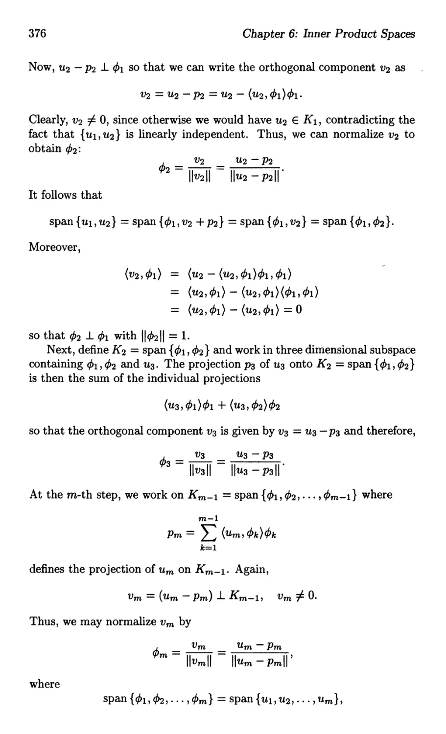
en = {z = (Zl,Z2",.,Zn): Zk E C, k = 1,2,...,n}.
The elements of en are called points or vectors, and the rules for addition
and scalar multiplication, in strict analogy with the corresponding opera-
tions in C, are defined in a natural way:
Z+W =(Zl+Wl,Z2+W2,...,Zn+wn),
AZ = (AZl, AZ2, . . . , AZ n ),
where Z = (Zl, Z2,"', zn), W = (Wl, W2,..., w n ) belong to en and A E C.
Thus, Z + W and AZ belong to en. Recall that Z = W iff Zj = Wj, for all
j = 1,2,. . ., n. It is easy to verify that all the axioms of the vector space are
satisfied. Thus, (en, C) forms a vector space. If each Zj (j = 1,2, . . . , n) is
real then in this case the space is called n-dimensional real space, denoted
by }Rn: .
]Rn = {x = (x 1 , X2, . . . , X n) : x k E IR, k = 1, 2, . . . , n } .
Similarly, (IRn, IR) is a vector space. Unless otherwise stated explicitly
we shall assume the standard operations, see Figure 1.6.
According to the convenience, we can consider the element in r (en or
}Rn) either as column vector:
Zl
Z=
Zn
(thought of as a n x 1 column matrix) or as a row vector:
Z = (Zl,Z2,... ,zn).
4The n-tuples are regarded as vectors and are also considered as points or elements
orO.
30
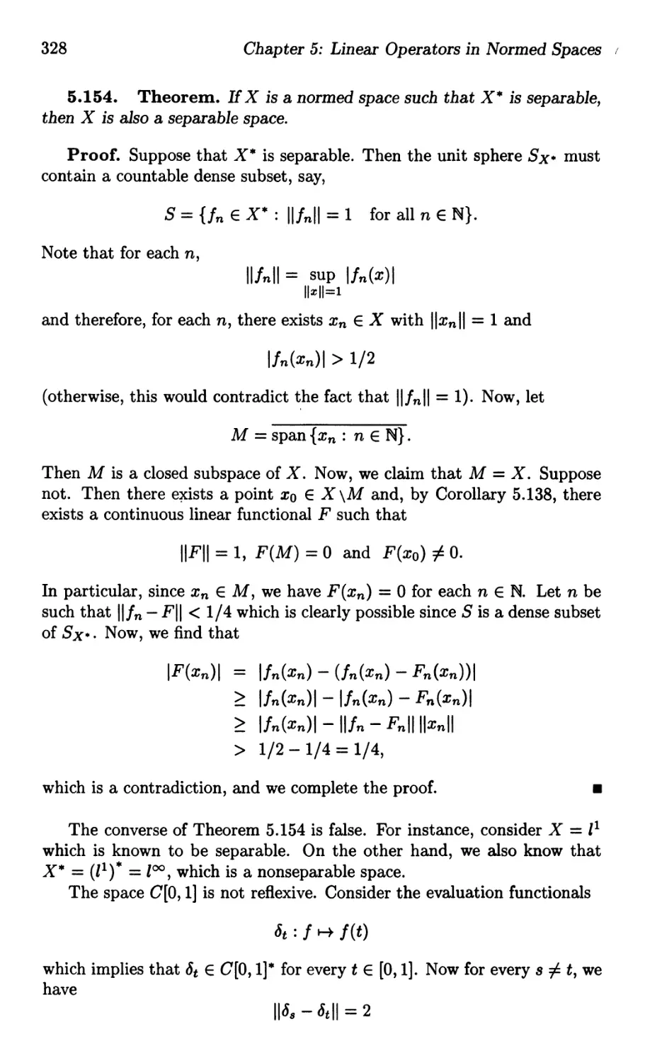
Chapter 1: Analysis and Linear Algebra
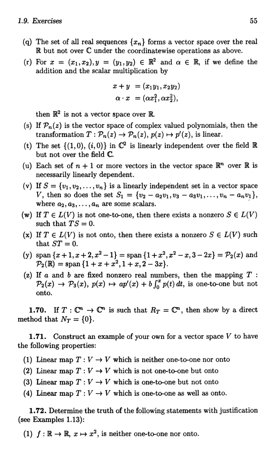
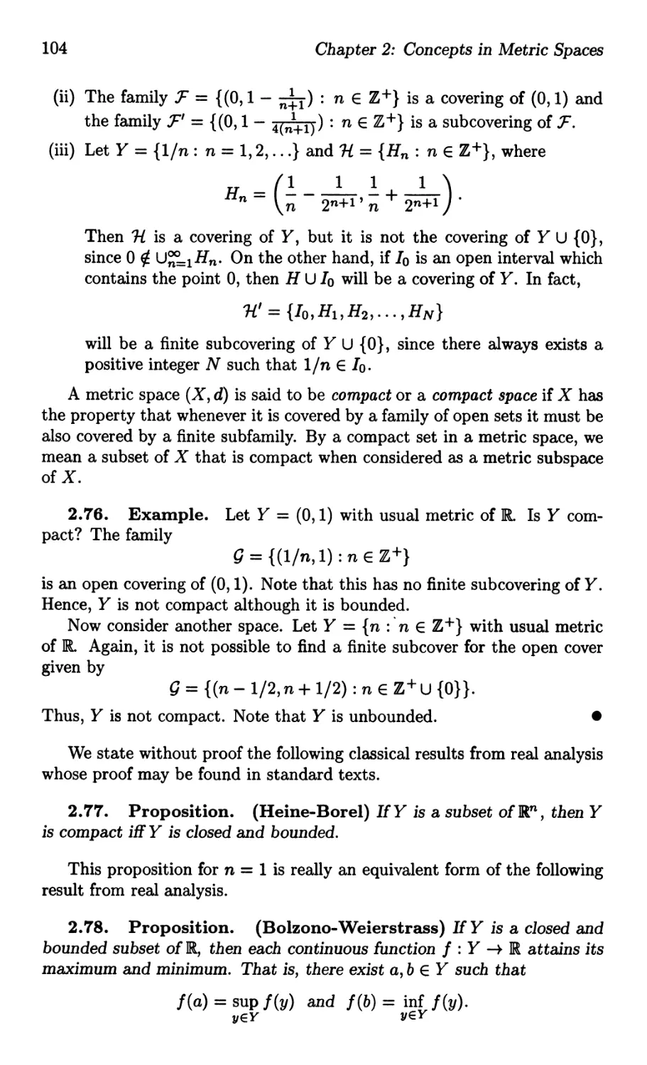
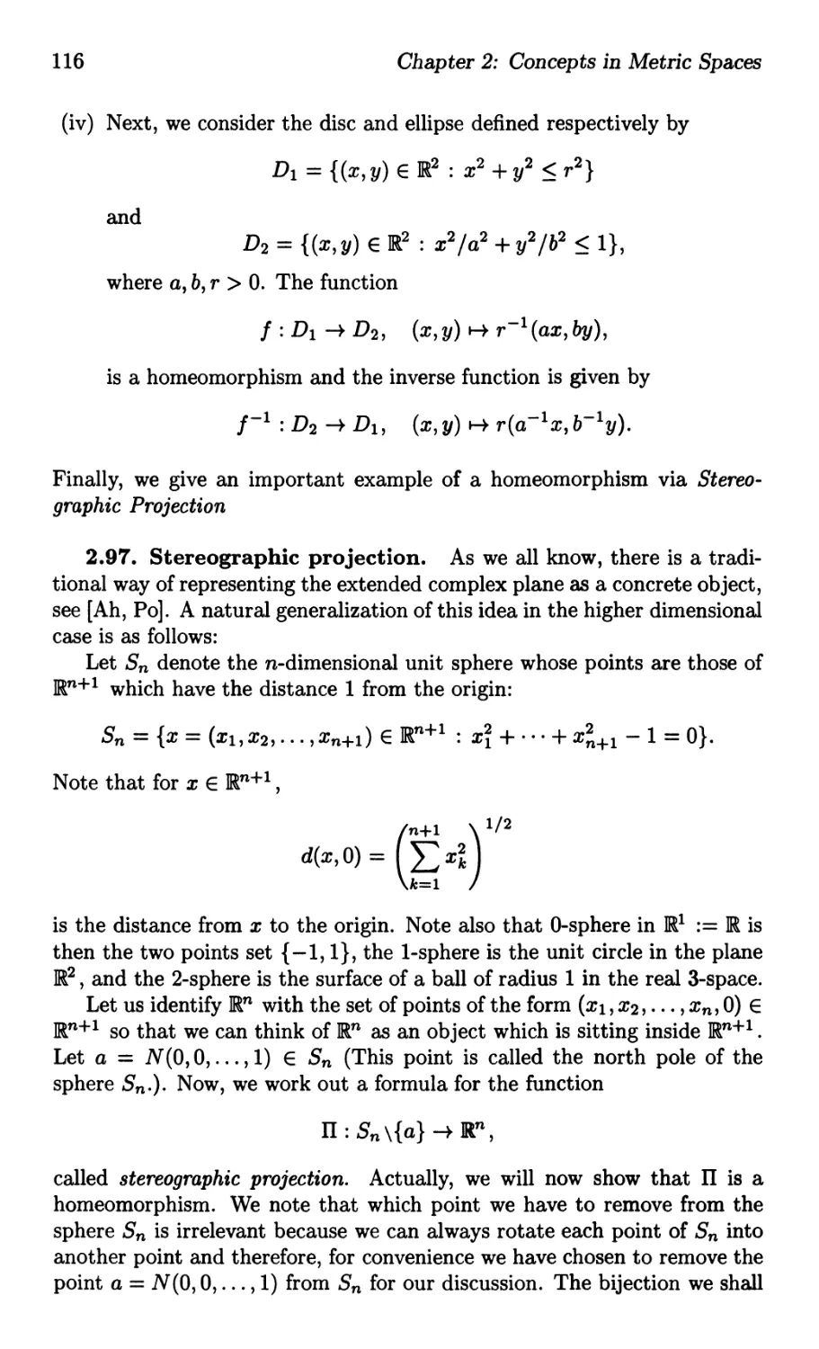
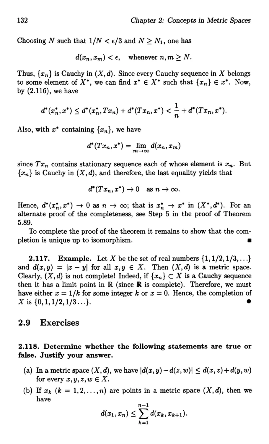
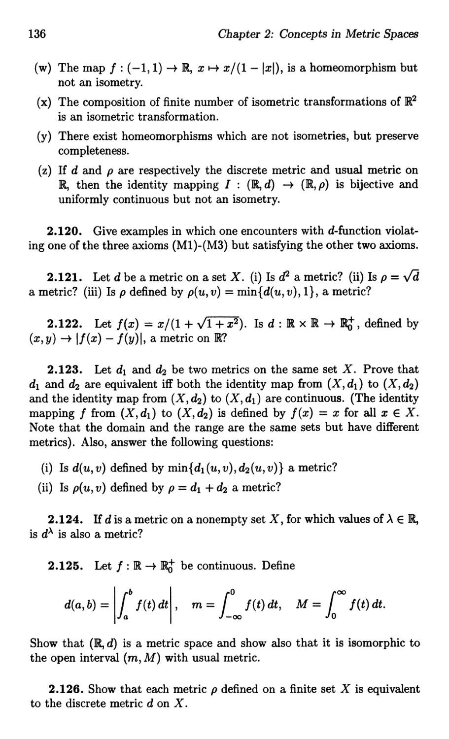
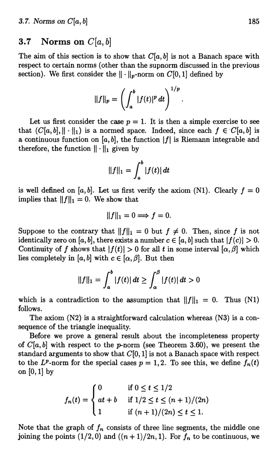
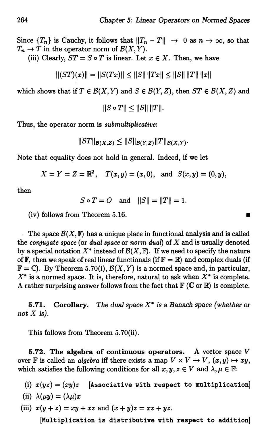
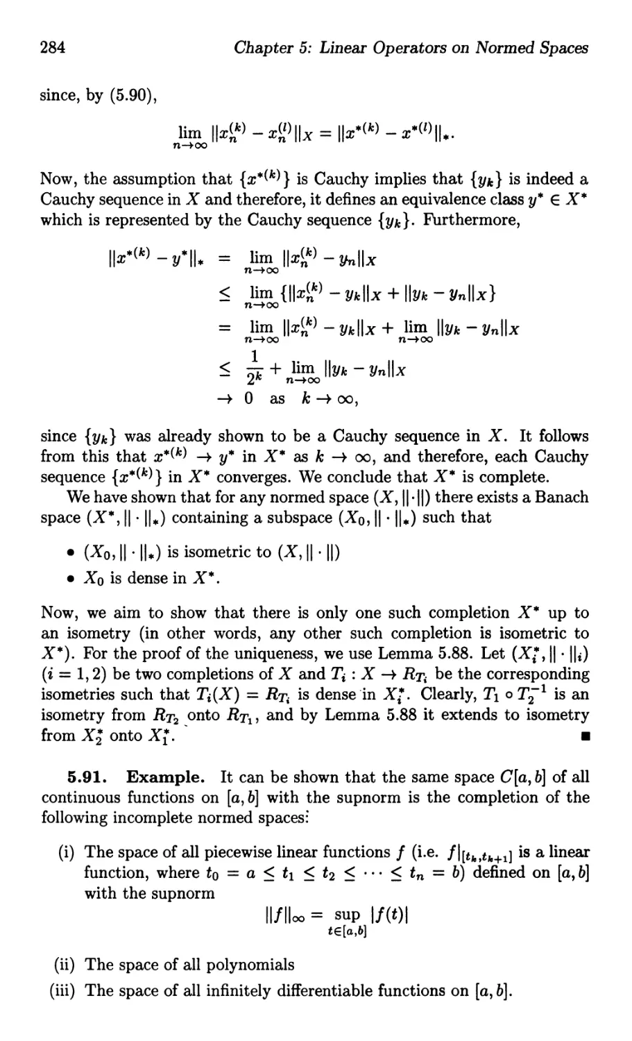
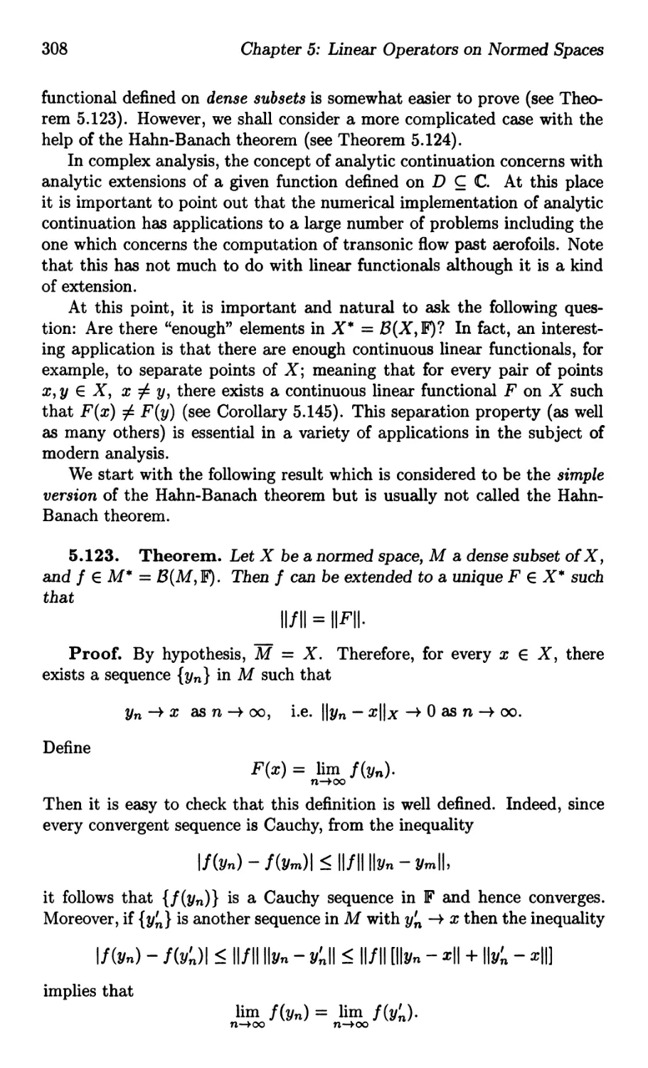
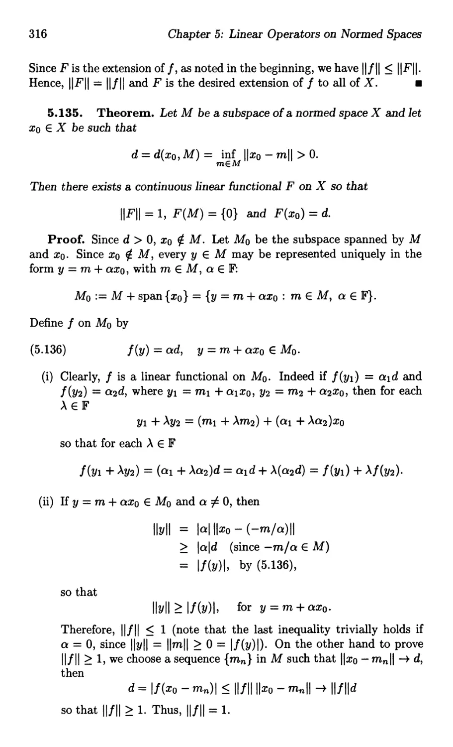
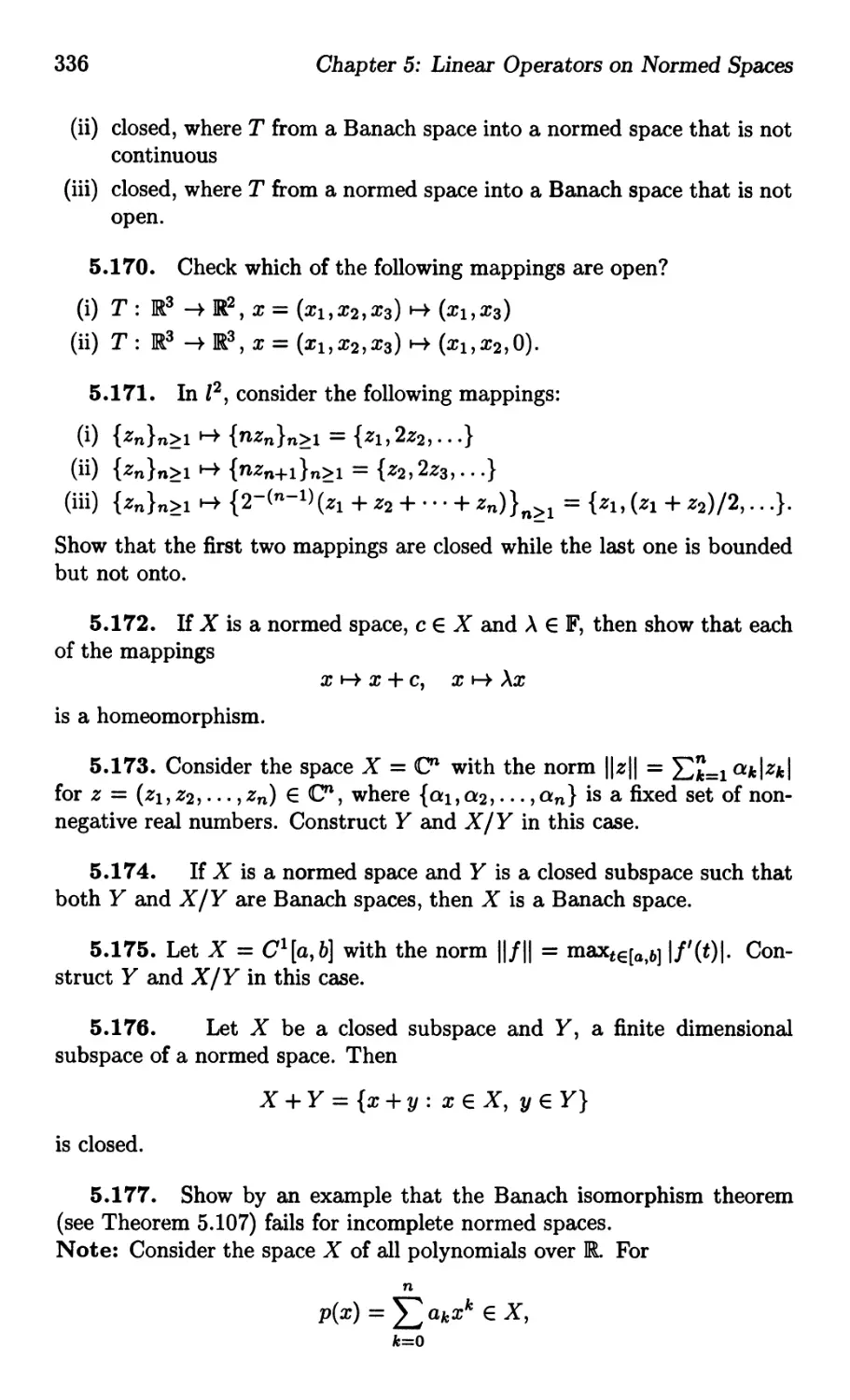
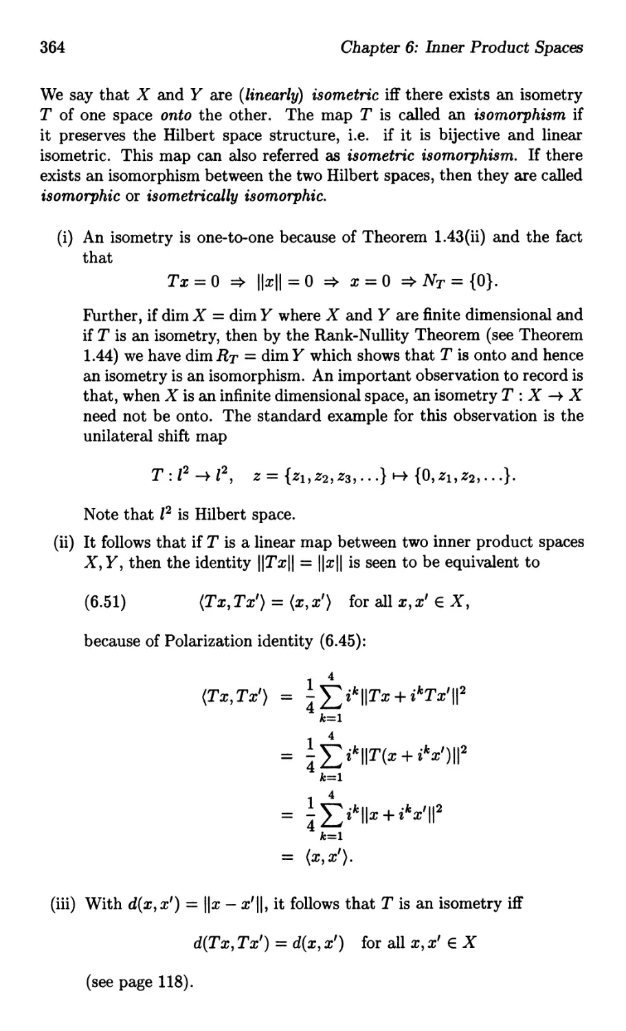
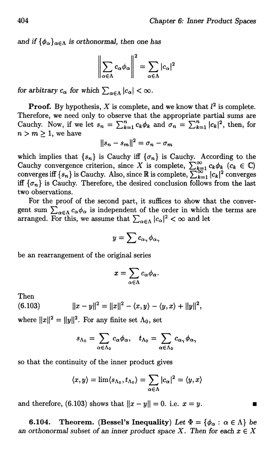
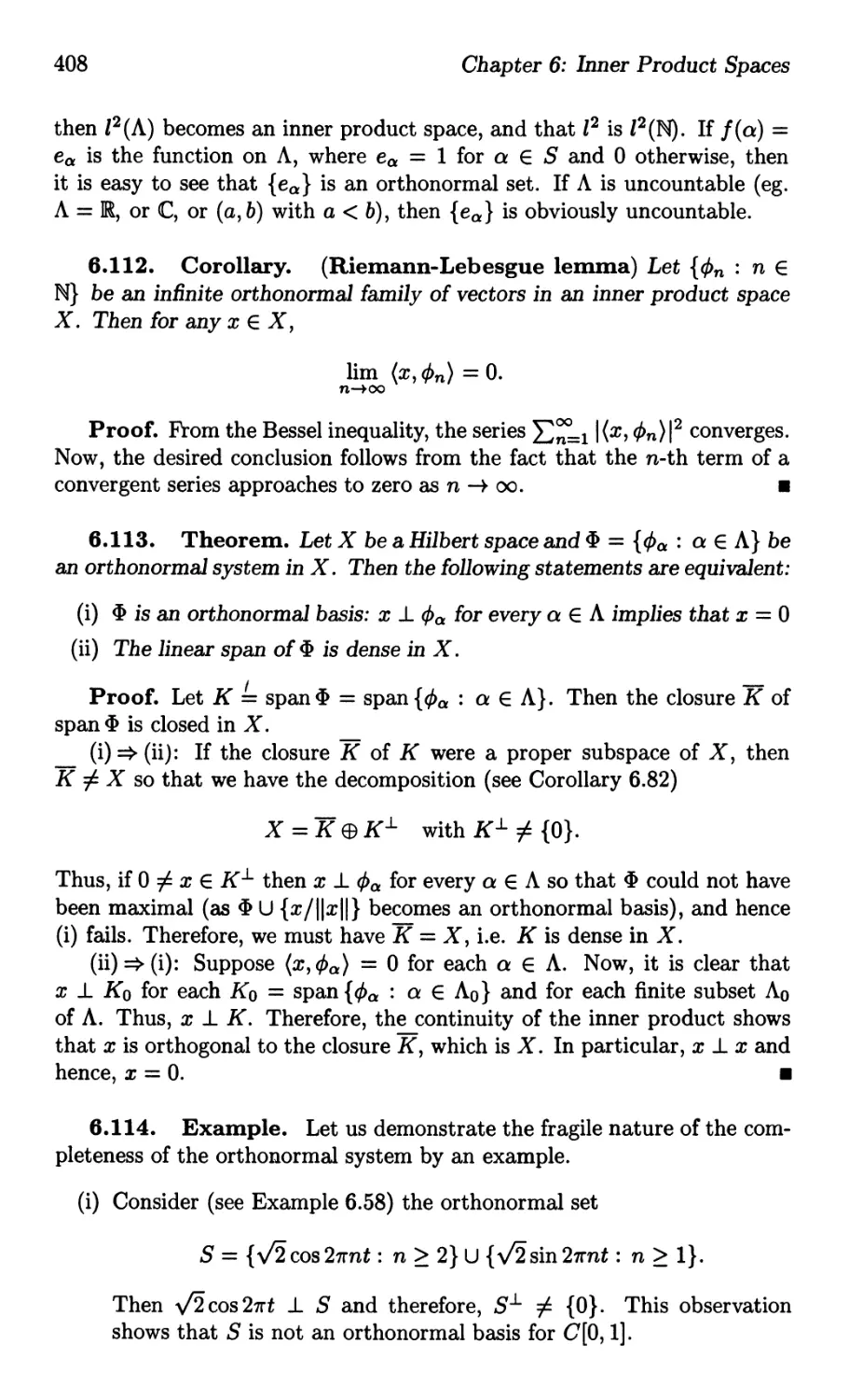
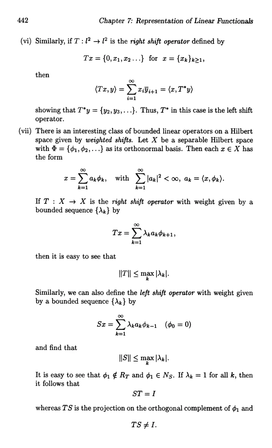
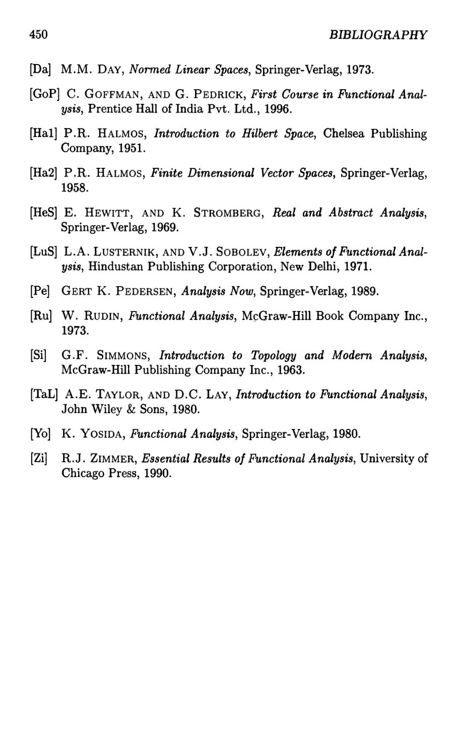
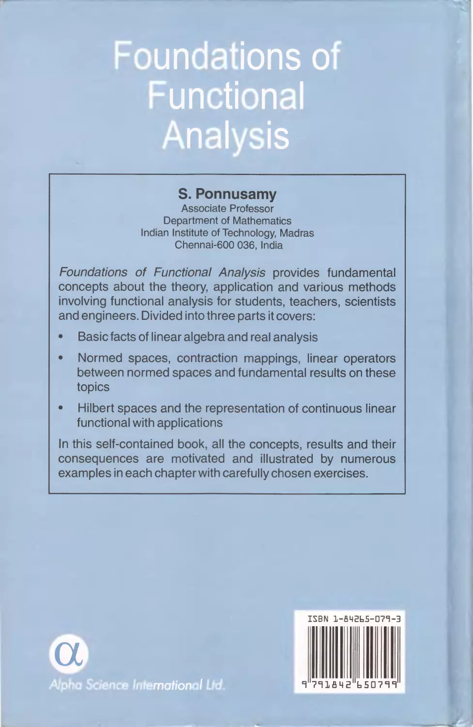
Y
N
x + Y = (Xl + Yl, X2 + Y2)
...
..-4
'-'"
I
I
I
I
I
I
I
I
o
x
Figure 1.6: Addition of vectors in }R2
The idea of interchanging row vector and column vector notation will be
helpful while using the Matrix theory.
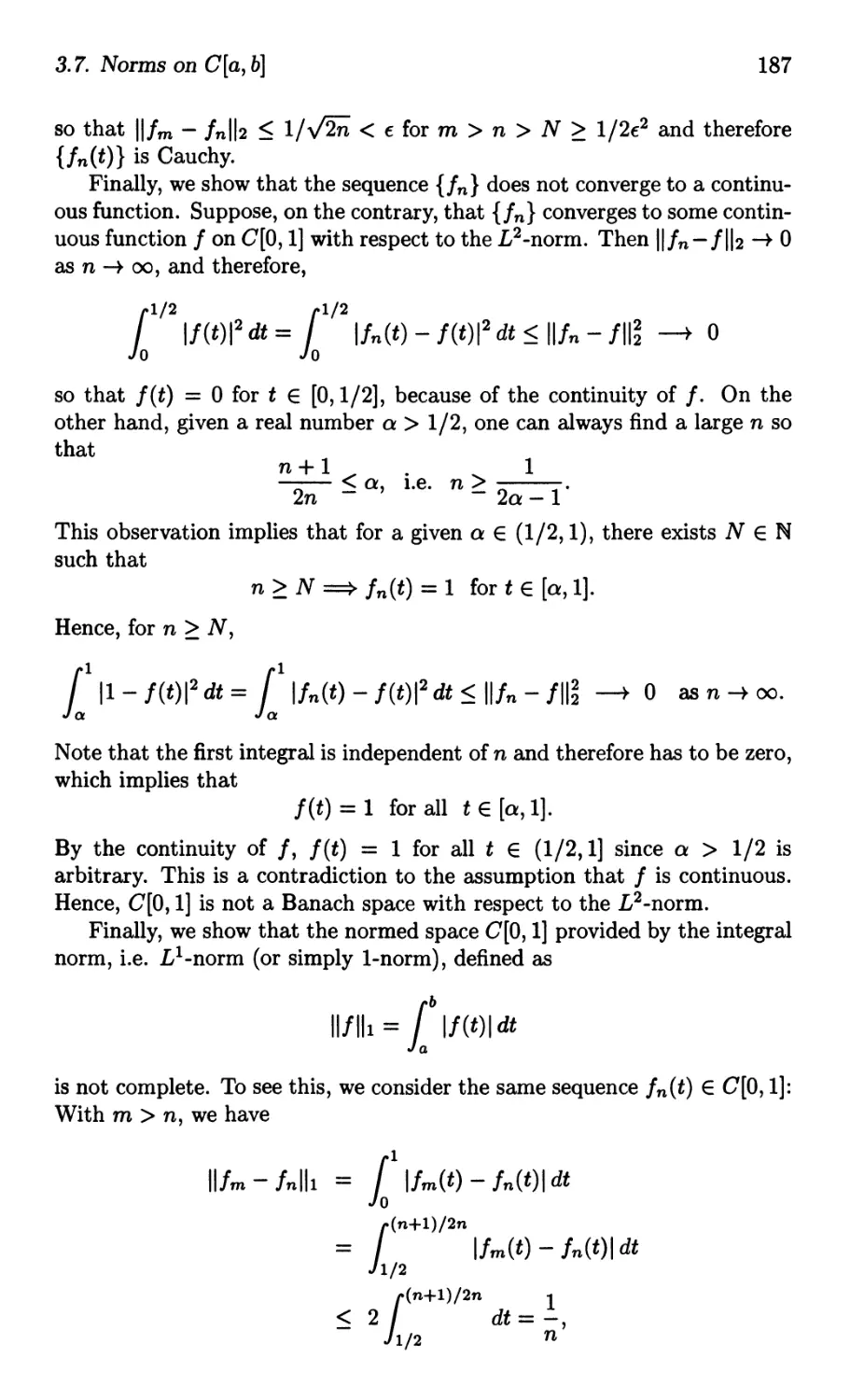
1.33. Space of continuous functions CF[a, b]. Denote by C(X)5
the set of all continuous complex valued functions on a compact set X
(usually X will be a compact Hausdorff space). This is a simple example
of a function space, Le. the space whose elements are themselves functions
defined on a space. In particular, we are mainly concerned in the case
X = [a, b]:6
CF[a, b] = {I : [a, b] 1F1 I is continuous from [a, b] into F}
where 1F may be C or IR, and [a, b], a < b, is the bounded closed interval in
III When 1F = C, the members of CF[a, b] may be regarded as a parametric
representation of continuous curves in C. We remind the reader that every
continuous function from [a, b] into}R has a maximum and a minimum. For
I, 9 E CF[a, b] and A E C, the addition I + 9 and the scalar multiplication
AI are defined in a natural way by the rules:
(I + g)(t) = I(t) + g(t)
(A/)(t) = A/(t)
t E [a, b].
It is not hard to show that the vector space axioms are satisfied for the
space CF[a, b].
5The letter C suggests "continuous", and the definition of compactness and Hausdorff
space will be discussed later, as we will not really use these concepts until we define metric
spaces.
6Most of the authors use the notation C[a, b], instead of CF[a, b], but often with a
word stating that whether they are dealing with complex valued or real valued functions.
By continuous we mean the unbroken graph, or else one could use "E - 6" definition of
continuous functions.
1.6. Vector Spaces
31
1.34. Subspaces. Let V be a vector space (over]F). A subset 8 of V
is said to be a subspace of V if 8 is itself a vector space when the addition
and scalar multiplication of V are used.
Some straightforward examples of subsets which are not subspaces are
(1) The subset 8 = {(a, a 2 ) E IR2 : a E IR} is not a subspace of IR 2
because it is neither closed with respect to the scalar multiplication
(eg. 2(1, 1) 8) nor with respect to the addition.
(2) The subset S = {(a, b) E IR2 : b > O} is not a subspace of IR 2 , because
(0,-1) = -1(0,1) 8.
(3) The subset 8 = {(a, b, c) E IR3 : lal = Ibl = Icl} is not a subspace of
IR3 because (-1,1,1) + (1,1,1) = (0,2, 2) 8.
(4) Each of the subsets 8 1 = {(a,O) E IR2 : a E IR} and 8 2 = {(O,b) E
]R2 : b E IR} is a subspace of IR2 whereas the union 8 = 8 1 U 8 2
does not form a subspace of jR2, because 8 is not closed with respect
to vector addition (Note that el = (1,0), e2 = (0,1) are in 8 but
el + e2 = (1, 1) is not in 8). .
We have the following simple characterization of a subspace whose proof
is routine and hence we leave it as an exercise.
1.35. Proposition. A nonempty subset 8 of a vector space V over
the field IF is a subspace of V iff AU + J.tV E 8 whenever u, v E S, A, J.t E F.
We note that a subset 8, which does not contain the zero vector 8, of a
vector space V cannot be a subspace. Now we present simple examples of
subspaces.
(1) The set of all polynomials defined on IR, denoted by P(IR) is a subspace
of the vector space V of the set of all functions defined from IR into
]R over the field III
(2) The set 8 = {p E P(IR) : p(O) = O} is a subspace of P(IR). .
On the other hand, if we define
8 1 - {p E P(IR) : p(O) = I}
8 2 - {p E P(IR) : p(x) < O}
8 3 - {p E P(IR) : p(x) > O}
then we see that none of 8 1 , 8 2 and 8 3 forms a subspace of P(IR).
1.36. Linearly independent sets and bases. Let V be a vector
space over a field IF. A linear combination of a set of vectors {VI, V2, . . . , v m }
in V is an element of V and is of the form
m
L CkVk, where Ck'S are in F.
k=1
32
Chapter 1: Analysis and Linear Algebra
A set of vectors {Vl, V2, . . . , v n } in a vector space V over a field ]F is called
linearly independent if there exist no scalars Cl, C2, . . . , C n E ]F such that
n
ECkVk = 0 and
k=l
n
E I C kl 2 > O.
k=l
If there exist scalars Cl, C2, . . . , C n E 1F which satisfy the above condition,
then we say that the set of vectors {Vl, V2, . . . , v n } is linearly dependent. In
the later case, anyone of the Vk'S, with Ck :j:. 0, will be a linear combination
of the others:
Vk = t ( Cj ) Vj.
i=l Ck
i 1e
A set of vectors {Vl, V2, . . . , v m } in a vector space V is called a spanning
set for V iff every vector v E V can be written as a linear combination of
Vl, V2, . . . , V m . We denote the so spanned set simply by span { Vl , V2, . . . , v m }
and therefore,
span {Vl, V2,. · · , v m } = { f CkVk: Ck E F, k = 1,2,..., m } .
k=l
We now come to the important concept of basis of a vector space. A set
B = {Vl, V2, . . . , v n } of vectors in a vector space V forms a basis for V iff
(i) B is linearly independent
(ii) V = span { Vl , V2, . . . , v n }, Le. every vector in V is a linear combina-
tion of the elements of B.
If {Vl, V2,.. . . , v n } is a linearly independent set, then we have
n n n
E akVk = E bk V k ==> E(ak - bk)Vk = 0
k=l k=l k=l
==> ak - b k = 0 for k = 1,2, . . . , n,
and in view of this, we note that (i) and (ii) together is equivalent to
the statement that every vector in V is uniquely expressible as a linear
combination of the vectors Vl, V2, . . . , V n . The vector space V is said be
finite dimensional if there exists a finite set of vectors that spans V, Le.
the number of basis elements is finite. Otherwise, we say that V is an
infinite dimensional vector space. If a vector space V has a basis consisting
of n vectors, then we say that V has a dimension n and we write dim V = n.
The subs pace containing only the zero vector, namely {OJ (zero space) of
V, is said to have finite dimension. Naturally, we define dim {OJ = O.
We use ek to denote the n-tuple (Xl, X2, . . . , x n ) where Xk = 1 and
x j = 0 for 1 < j :j:. k < n, Le. ek is the element in }Rn with 1 in the k-th
1.6. Vector Spaces
33
place and zero elsewhere. Then En = {el, e2, . . . , en} becomes a basis for
]in and is called the standard basis for }Rn.
Let B = {VI, V2, . . . , v n } be a basis of V. Then for every vector V E V,
we have the unique representation
V = ClVl + C2 V 2 +... + CnV n
in scalar unknowns Cl, C2, . . . , Cn. The column/row vector
Cl
[V]B :=
C n
or in consistence with our earlier discussion
[V] B : = (Cl, C2, . · · , c n ) ,
is called the coordinate vector of V with respect to the basis B. Conversely,
given [V]B = (Cl, C2,. .. , cn), we can recover the vector by writing v =
EZ=l CkVk. If V = }Rn and if En = {el, e2,. . . , en}, then for v E }Rn, we
have [V]En = v.
1.37. Proposition. The dimension of en over C is n.
Proof. We need to show that there exists a set of n linearly indepen-
dent vectors in en over C but every set of n + 1 or more vectors in en is
linearly dependent. Clearly, {el, e2, . . . , en} is linearly independent since
each (Zl, Z2, . . . , zn) E en can be written as E j 1 zjej and this is a zero
vector iff all the Zj'S are zero. On the other hand, suppose that we are
given (n + 1 )-vectors VI, V2, . . . , Vn+l, where
Vj = (alj, a2j, . . . , anj), j = 1, 2, . . . , n + 1.
Form the matrix system AZ = 0, where A is a matrix of order n x (n + 1)
with Vj as the j-th column of A and Z = (Zl, Z2,. . . Zn, Zn+l)(n+l) xl, or
with
Zl
Z=
Zn+l
i.e. the homogeneous system of equations are determined by
(1.38 )
n+l
L ZjVj = O.
j=l
34
Chapter 1: Analysis and Linear Algebra
Since this is a system of n equations with n+ 1 unknowns Z1, . . . , Zn+1, there
exists a nontrivial solution C = (C1, C2, . . . , C n + 1) (n+ 1) x 1 where at least one
of the Cj'S is nonzero, satisfying (1.38), that is
n+1
AC = 0 = E CjVj = O.
j=1
Thus, V1, V2, . . . , V n +1 are linearly dependent over C.
.
1.39. Remark. Is the dimension of en over IR 2n?
.
1.40. Proposition. Let {V1, V2, . . . , v m } span a finite dimensional
vector space V. If S = {W1, W2, . . . , w n } is any set of vectors in V, then
S is linearly dependent whenever n > m. Alternatively, if S is linearly
independent then n < m.
Proof. Let n > m. By the definition of spanning set, we can write
m
Wj = E aijVi, for each j = 1, 2, . . . , n,
i=1
so that
tCjWj = ( ta1jCj ) V1 +... + ( tamjCj ) vm.
3=1 3=1 3=1
Consider the system of equations
n
E aij Cj = 0, for each i = 1, 2, . . . , m,
j=1
or equivalently, the matrix equation AC = 0, where A is an m x n matrix
with n > m. Note that we have more unknowns than the number of equa-
tions in this linear system of equations and therefore, we have a nontrivial
solution c = (ci, . . . , c )n x 1. Thus, for this nontrivial solution c, we have .
n
EcjWj = 0
j=1
so that the set S is linearly dependent.
.
1.41. Corollary. Let V be a finite dimensional vector space with
dim V = n. Then we have the following statements:
(1) Every set of linearly independent vectors ofn elements is a basis for
V. In particular, the number of elements in any two bases of V is
same.
1.7. Linear Transformations between Vector Spaces
35
(2) Any spanning set for V must contain at least n elements.
Proof. (1) Let S = {V1, V2, . . . , v n } be a linearly independent set of vec-
tors in V. We show that this set spans the space V. Let v E V be arbitrary.
Then, the set {V1, V2, . . . , V n , v} is linearly dependent (since dim V = n) and
therefore there exist scalars c, C1, . . . , c n , not all of them being zero, such
that
n
cv + ECjVj = O.
j=1
As S is a linearly independent set, we have c :j:. 0 so that
n
V = E(-Cj/C)Vj.
;=1
Thus, v E span (S) and hence S is a basis for V. The next part follows
from Proposition 1.40.
(2) Let the set B = {V1, V2, . . . , v m } span V. If B is linearly independent,
then, by definition, this would be a basis for V and therefore, by part (1), we
have m = n. If B is linearly dependent, then at least one of the vectors, say
Vk, is a linear combination of the remaining vectors in B. Thus, Vk can be
removed from B so that the resulting subset of B forms a spanning set for
V. This process may be continued (if necessary) until we obtain a linearly
independent spanning set containing less than m vecto)"s and consequently,
by part (1), we have m > n. _
The space CF[a, b], where IF = C or JR, is an infinite dimensional vector
space. In fact, the subset {t n }n O C CF[a, b] is linearly independent, since
n
f(t) = E akt k = 0 => ao = a1 = . · . = an = 0 for each n > 0,
k=O
so that the space CF[a, b] cannot be finite dimensional.
1.7 Linear Transformations between Vector Spaces
Let V, W be two vector spaces, both over the same field IF. Now, we shall
briefly look at the mappings from V into Wand such mappings are also
called operators or transformations. Our particular interest is when the
operator maintains a special "structure" in the following sense: An operator
T : V W is said to be additive if it preserves the addition:
T(V1 + V2) = T(V1) + T(V2), for V1, V2 E V,
and is said to be homogeneous if it preserves the scalar multiplication:
T(av) = aT (v), for a E IF, v E V.
36
Chapter 1: Analysis and Linear Algebra
Note that we also follow the convention of writing T(v) := Tv whenever
this notation is convenient. The map T : V W is called a linear trans-
formation/operator if it is both additive and homogeneous. Some authors
call a linear transformation T from V into itself as a linear operator on
V. But, we do not follow this convention. A transformation that is not
linear is the one which does not satisfies either the additivity condition or
the homogeneity condition or both. A linear transformation T : V W is
called isomorphism if it is bijective. In such cases, we say that V and W
are isomorphic.
We first observe that every linear transformation T : V W satisfies
TOv = Ow, where Ov and Ow are the zero elements of V and W, respec-
tively. A simple example of a transformation which is additive but not
homogeneous is given by T : C C, z I-t z , with IF = C. An example of a
transformation which is homogeneous but not additive is given by
T : }R2 \ { (0, y) : y E }R} IR,
X
(Xl, X2) I-t -.
Xl
Clearly, a linear transformation preserves the structure of the linear com-
bination of the vectors and, for all Vl, . . . , V n in V and all scalars Cl, . . . , C n
in F, we have
T ( tCkVk ) = tCkTvk'
k=l k=l
In particular, each linear transformation T maps a line segment connecting
Vl and V2 into the line segment between TVl and TV2:
T(AVl + (1 - A)V2) = ATvl + (1 - A)Tv2, A E [0, 1].
Finally, we remark that if we are given a linear transformation T from a
finite dimensional vector space V into another vector space, then we can
determine the transformation in the following sense: if {Vl,.", v n } is a
basis for V, then for any vector v E V we have v = E 7 1 CjVj for some
scalars Cj (j = 1,. . . , n) in IF so that Tv = E 7 1 cjTvj.
1.42. Transformations which are linear, and not linear. First,
we list a few simple examples of linear transformations:
(1) T:}R2 }R2, X = (Xl, X2) I-t (Xl + X2, Xl - X2).
(2) T:}R2 }R2, X = (Xl,X2) I-t (Xl +X2,Xl).
. (3) T:}R2 }R2 , X = (x 1 , X2) I-t (Xl - X2, Xl)'
(4) T: IRn }Rm, X I-t Ax, where A is an m x n matrix.
(5) T:}R3 -+ IR 2 , X = (Xl, X2, X3) I-t (Xl, X2).
(6) T: Mnxn (}R) Mnxn (IR), A I-t A - At.
(7) T: Mmxn (IR) Mnxm (IR), A I-t At, or A I-t _At.
1.7. Linear Transformations between Vector Spaces
37
(8) T: Mnxn (JR) Mnxn (IR), A I-t AB - BA, where B is a fixed n x n
matrix.
(9) T: Mnxn (IR) IR, A = (aij) I-t El i n au.
(10) T: CR[a, b] IR, f I-t J: f(t) dt.
Next, we list below some simple examples of transformations which are not
linear:
(1) T: Mnxn (JR) JR, A I-t det A.
(2) T: IR2 IR 2 , X = (Xl, X2) I-t (Xl + k l , X2 + k 2 ), where at least one of
k l , k 2 is a fixed nonzero real number.
(3) T: IR IR, X I-t x2 .
(4) T: IR 2 JR2 , X = (Xl, X2) I-t (lxll, 2Xl - X2).
(5) T: IR 2 JR2 , X = (Xl, X2) I-t (Xl + X2, Xl + 1).
(6) T: IR2 ]R2, X = (Xl,X2) I-t (XlX2,Xl).
(7) T:]R2 ]R2, X = (Xl, X2) I-t (Xl + 1, XlX2).
Let L(V, W) denote the space of all linear mappings from a vector space
V into another vector space W. -In fact, if Tl : V Wand T 2 : V W
are two linear transformations and A is a scalar in IF then the sum Tl + T 2
and the scalar product ATl are defined by
{ (Tl + T 2 )v = Tlv + T 2 v
(AT1)V =A(TIV) , forallvEV,AEF.
Then, for linear operators T l , T 2 E L(V, W) and for c E IF, v, v' E V, we
have
(T l + T )(cv + v') - Tl(CV + v') + T 2 (cv + v')
- [CTl v + Tl v'] + [cT 2 v + T 2 v']
- C(Tl + T 2 )v + (T l + T 2 )v',
and similar identity holds for ATl' Thus, Tl + T 2 and ATl are also linear
transformations so that the set L(V, W) is easily seen to be a vector space
under the pointwise operations of addition and scalar multiplication defined
above. The zero vector in L(V, W) is the zero transformation
8 : V W, v I-t Ow,
where Ow represents the zero vector in tv; and 8 or 0 are also used in place
of Ow. The additive inverse of T E L(V, W) is - T defined by - T = (-l)T.
IT W = V, then we often use the notation L(V) instead of L(V, V). The
identity transformation on V is defined by
Iv : V -+ V, v I-t v, for all v E V.
38
Chapter 1: Analysis and Linear Algebra
Whenever there is no confusion, we often write I in place of Iv. Let T E
L(V, W), where V and Ware finite dimensional vector spaces. Then the
set NT of vectors v E V for which Tv = 0 is called the null space of T, and
the set RT of vectors W E W such that Tv = W for some v E V, is called
the range space of T. From this definition, it is clear that "T is onto iff
RT = W". Sometimes, we refer the spaces NT and RT as the kernel of T
and the image of T, respectively. In this terminology, the usual notation
for NT and RT will be KerT and ImT, respectively. As a consequence of
these definitions we can derive certain properties of the spaces NT and RT.
1.43. Theorem. Let T : V -t W be a linear map from the vector
space V into the vector space W. Then we have
(i) NT and RT are subspaces of V and W, respectively.
(ii) T is one-to-one iff NT = {OJ.
Proof. (i) Let T : V W be a linear map. Consider
NT = {v E V : Tv = O} and R T = {w E W : Tv = w for some v E V}.
Then TO = T(O.v) = O.Tv = 0 and therefore, NT is nonempty, since
o E NT. If Vl,V2 E NT, then for a,{3 E F, we have aVl + {3v2 E NT,
because
T(avl + {3v2) = aTvl + {3 Tv 2 = 0..0 + ,8.0 = O.
Again, since TO = 0, RT is nonempty. If Wl , W2 E RT, then there exist
Vl, V2 in V such that TVl = Wl and TV2 = W2. Then, for a, {3 E F, there
exists aVl + {3v2 in V such that
T(avl + {3v2) = aTvl + {3 Tv 2 = aWl + {3w2
so that aWl + {3w2 E RT. Thus, NT and R T are the subspaces of V and
W, respectively.
(ii) Assume that T is one-to-one. If v E NT, then TO = 0 = Tv which,
because of one-to-oneness of T, gives v = o. Thus NT = {OJ. Conversely,
if NT = {OJ then, because of the linearity of T, we have
TVl = TV2 ==> T(Vl - V2) = 0 ==> Vl - V2 E NT ==> Vl - V2 = 0
and therefore, T is one-to-one.
.
Note that Theorem 1.43(i) applies only when the map is linear. For
example, if T : IR IR is defined by x I-t x 2 , then the range RT is IRt
which is not a subspace of IR.
We define the rank of T, denoted by rank (T), to be the dimension of
the subspace RT, and the nullity ofT, null (T), to be the dimension of the
subspace NT. Clearly,
N] = {OJ, R[ = V, No = V and Ro = {OJ.
1.7. Linear Transformations between Vector Spaces
39
Further, no confusion should arise from the fact that we shall not distinguish
either zero/identity transformation or zero/identity element in V and that
in W.
One of the fundamental results in linear algebra is the following theorem
which is known as Rank-Nullity theorem. This theorem gives a complete
characterization of one-to-one and ontoness in terms of the null space and
the range space of T.
1.44. Theorem. Let T : V W be linear, where V is a finite
dimensional vector space. Then we have
dim NT + dim RT = dim V.
In particular, we have
( a) If dim V > dim W, then T cannot be one-to-one.
(b) If dim V < dim W, then T cannot be onto.
(c) If dim V = dim W and dim NT > 0, then T cannot be onto.
Proof. Case (i): IT dim V = n and NT = V, then RT = {OJ so that
the theorem holds trivially.
Case (ii): Assume that dim NT = k > 0 and dim V = k + m. Let
B = {V1, V2, . . . , Vk} be a basis for NT. Then we can expand the set B so
that the extended set
{ V1 , . · · , Vk, Vk+1 , · · · , Vk+m}
forms a basis for V. Thus, to complete the proof, it suffices to show that
the set {TVk+1, . . . , TVk+m} forms a basis for the range space RT. To prove
this, we choose an arbitrary point wERT. Then there exists v E V such
that
Tv = w, where v = E ;+ CjVj for some scalars Cj.
Since T is linear and TVj = 0 for j = 1,2,. . . , k, it follows that
k+m k+m
W = Tv = L cjTvj = L cjTvj.
j=1 j=k+1
Thus, {TVk+1,. . . , TVk+m} spans the range space R T . Next, we show that
this set of vectors is linearly independent. Suppose that
k+m
L cjTvj = O.
j=k+1
40
Chapter 1: Analysis and Linear Algebra
Since T is linear, this can be written as
( k+m )
T E CjVj
j=k+1
=0
so that
k+m
u:= E CjVj E NT,
j=k+1
and since {V1, V2,. . . , Vk} is a basis set for NT, we must have
k
U = ECjVj
j=l
for some scalars Cj, 1 < j < k. From the last two equations, it follows that
k k+m
E CjVj + E (-Cj)Vj = O.
j=l j=k+ 1
As {V1, . · . , Vk, Vk+1, . . . , Vk+m} is linearly independent, it follows that Cj =
o for j = 1,2,..., k + m which shows that the set {TVk+1,..., TVk+m} is
linearly independent.
Case (iii): IT dim NT = 0, Le. NT = {OJ, and if {V1, V2,. . . , Vk+m} is
a basis for V, then it follows that the set {TV1, TV2, . . . , TVk+m} forms a
basis for the range space RT, and once again the theorem follows. .
The following examples help us to understand the ideas behind Theo-
rems 1.43 and 1.44.
(1) Any linear map T : ]R4 IR3 cannot be one-to-one.
(2) Any linear map T : M 2X2 (IR) IRs cannot be onto.
(3) The linear map T : IR 2 IR2, (Xl, X2) I-t (-Xl + 2X2, 0) is neither
one-to-one nor onto, since NT = {(X1,X2) : Xl = 2X2, X2 E JR.} so
that dim NT = 1.
(4) The linear map T : P2(IR) P 2 (1R), p(x) = ax2 + bx + C I-t ax2 +
(b - 2c)x + a - b + 2c is neither one-to-one nor onto, since
NT - {p(x): a = 0, b = 2c, C E IR}
- {p(x): p(x) = c(2x + 1), C E IR}
so that dim NT = 1.
(5) The linear map T : P3(IR) P 3 (IR), p(x) I-t p'(x) is neither one-to-
one nor onto.
1.7. Linear Transformations between Vector Spaces
41
(6) The linear map T : Pn{Ii) JRn+1, E =o akx k I-t (ao, a1, . . . , an), is
one-to-one and onto.
If dim V = dim W, then, from Theorem 1.44, it follows that
T is one-to-one <==} T is onto.
Here P n (F) denotes the set of all polynomials of degree less than or equal to
n in z (if IF = C) (and respectively in x if 1F = JR) with complex coefficients
over the field C (with real coefficients if 1F = JR).
The linearity of T in Theorems 1.43 and 1.44 is essential, for it is a
simple exercise to construct examples of functions from JR into JR that are
not one-to-one but are onto, and vice versa. Now we have the following
1.45. Corollary. Let V and W be two finite dimensional vector
spaces over the same field IF. Then we have
(i) If T : V W is bijective, then dim V = dim W
(ii) If dim V = dim W, then there exists a bijective linear transformation
from V into W.
Proof. If T is one-to-one and onto, then dim NT = 0 and RT = W
so that by Theorem 1.44, we have dim W = dim V. To prove the second
part, we assume that dim W = dim V. Let B = {V1, V2, . . . , v n } and B' =
{ W1, W2, . . . , w n } be any two bases of V and W, respectively. Then, we
see that there exists a unique linear transformation T : V W such that
TVj = Wj for j = 1,2,. . . , n (how?). If W E W is an arbitrary vector, then
we have the unique representation
n
W = L CjWj for some scalars Cj.
j=1
Now, for v = E j 1 CjVj E V we have
n n
Tv = LCjTvj = LCjWj = W
j=1 j=1
which implies that T is onto and therefore, dim RT = dim W = dim V.
Again, by Theorem 1.44, we have dim NT = 0, i.e. T is one-to-one. -
From Corollary 1.45, we observe that if dim W = dim V, then T : V
W is one-to-one iff T is onto.
1.46. Example. Consider the linear map T : Mnxn (lR) Mnxn (IR),
A I-t A - At. Now, to find the null space NT, we need to solve
T A = A - At = 0
42
Chapter 1: Analysis and Linear Algebra
for A. If A = (aij)nxn, then A - At = (aij - aji) = (bij), so that
0 b I2 bIn
-b 12 0 b 2n
A - At = , where b ij = aij - aji,
-bIn -b 2n 0
which shows that A - At = 0 yields the condition aij = aji for each i and
j. Thus, NT is the set of all n x n symmetric matrices and therefore
n 2 -n
dimNT=n+ 2
n(n + 1)
2
Since
RT = {B E Mnxn(IR) : A - At = B, for A E Mnxn(IR)},
we obtain
0 b I2 bIn
-b 21 0 b 2n
RT= b ij E JR .
-b nl -b n2 0
and therefore, we find that R T is the set of all skew-symmetric matrices.
Thus,
n 2 -n
dimRT = 2
n(n - 1)
2
Note that T is neither one-to-one nor onto.
.
Recall that the dimension of IF (where IF is either C or JR) over itself is
one. Linear maps from a vector space V into IF, T : V IF, play a special
role in the theory of vector spaces, and therefore they have a special name
"linear functionals" , see Chapter 5. The definite integrals of continuous
function is one of the most important examples of linear functionals in
mathematics.
1.8 Inequalities
Geometric and integral inequalities have a prominent place particularly in
real, complex and functional analysis. Among the tools used in establishing
these inequalities, convex and concave functions are especially important.
In this section, it is shown that these tools yield several important inequal-
ities. There are some standard reference books on inequalities, for example
[HLP, Mi]. Most of the inequalities in this section are valid in more general
1.8. Inequalities
43
Figure 1.7: Convex and non convex domains in the complex plane
setting. However, we present only those which are relevant to the scope
and the topics of this book.
1.47. Definition. A nonempty subset S of a vector space V is said
to be convex ifAxl + {I - A)X2 E S whenever Xl, X2 E S and 0 < A < 1.
Geometrically, this means that given two arbitrary points in a convex set,
the line segment joining them is also in the set.
We note that the line passing through Xl and X2 is the set
{AXI + {I - A)X2 : A E JR}
and therefore, the restriction {AXI +{1-A)x2 : A E [0, I]} is the line segment
[Xl, X2]. Clearly, a singleton set, the interior of circles and ellipses in JR2,
the solid ellipsoids and cubes in JR3 are convex. Indeed, if V is a vector
space then every linear subspace in V is trivially convex, see Proposition
1.35.
Let P (POl resp., where a E JR) denote the set of all analytic functions
p on = {z: Izl < I} such that p{O) = 1 and Rep{z) > 0 (Reeiap{z) > 0
resp.) in . Then P is a convex set whereas P a is a nonconvex set, see
Figure 1.7. A real-valued function f on a convex set S is said to be convex
on S if the inequality
f{AXI + (1- A)X2) < Af{XI) + (1- A)f{X2)
holds for all Xl,X2 E S, 0 < A < 1. Hthe above inequality is reversed, then
f is said to be concave. Alternatively, f is concave iff - f is convex. Thus,
the convexity (concavity) of the real valued function f : [a, b] JR means
that the chords joining the two points on the graph of f always lie above
(below) the graph of f, see Figure 1.8. A real-valued function f on S is
called logarithmically convex (concave), or simply log-convex (log-concave)
if f is positive and log f is convex (concave). The function is strictly convex
(concave) if the functional inequality above is strict.
44
Chapter 1: Analysis and Linear Algebra
y
y
y= f(x)
y = f(x)
Xl
o
X
o
X
Figure 1.8: Convex and concave curve in the real variable case
1.48. Example. Consider f : IR IR defined by f(x) = z2. Then
with J.t = 1 - A and A, J.t > 0, we have
Af(x) + J.tf(y) - f(AX + J.ty) = AJ.t(X - y)2 > 0
which proves the convexity of the square function.
.
It is an important observation that the intersection of arbitrary collec-
tion of convex sets is trivially a convex set (see also Exercise 1.78). The
following fundamentalf;;ult is easy to derive by the method of induc-
tion.
1.49. Proposition. Let S be a convex set in V, Xk E S and Ak > 0
for k = 1,2, . . . , n such that E =l Ak = 1. Then E 1 AkXk belongs to S.
IT S c V, then the intersection of all the convex sets containing the
given subset S is called the convex hull of S and is denoted by co(S), see
Figure 1.9. In fact, it can be seen that
co(S) := { t AkXk : Xl,..., X n E S, A1'...' An > 0,
k=l
t Ak = I } ·
k=l
The closed convex hull of S is the intersection of all the closed convex sets
which contains the given set S as we see in the foll.owing proposition.
1.50. Proposition. The set co(S) is the smallest convex set con-
taining the given set S.
Proof. By definition S c co(S). To show that co(S) is convex, we let
X = E 1 AkXk and y = E 1 A X , where Ak, A are nonnegative real
1.8. Inequalities
45
.,
,
,
,
,
,
,
I
I
t.
Figure 1.9: Description for convex hull of a set
numbers such that E =l Ak = E ;; 1 A = 1. Then, it can be easily seen
that
m+n
AX + (1 - A)Y = E J.tkX-k
k=l
where
{ X k
Xk =
x'.
,
for k = 1, 2, . . . , n
for k = n + j, j = 1, 2, . . . , m
and
{ AAk for k = 1, 2, . . . , n
J.t k = , ' , '. £ k .. 1 2
1\1\ lor = n + J, J = , ,..., m.
Note that J.tk > 0 and E n /.-Lk = 1. The convexity of co(S) follows. .
1.51. Examples.
(i) Let V = {x = (Xl,...,Xn) E}Rn: E lX = I}. Then
n
co(S) = {x E}Rn: Ex < I}.
k=l
(ii) Let V = C and S be the circle {z: Izi = R}, R > o. Then co(S) is
the closed disc {z: Izl < R}.
(iii) Let V = C and S = {Zl, Z2}. Then co( S) = [Zl, Z2], the line segment
connecting Zl and Z2. .
Next we list some of the basic properties of convex and concave functions
from which several classical examples of these functions defined on (a, b)
may be obtained. For a detailed discussion about this topic we refer to
[Roc]. Now, we provide a list of basic properties for the case of convex
functions and similar results follow for the case of concave functions.
46
Chapter 1: Analysis and Linear Algebra
1.52. Proposition. Let I be a real valued function defined on [a, b].
Let g: [c,dj IR where the range of I is contained in [c,dj. Then we have
the following statements:
(I) Let I be differentiable on (a, b). Then I is convex on (a, b) iff I' is
increasing on (a, b).
(2) Let! be twice differentiable. Then I is convex on (a, b) iff the second
derivative I" is nonnegative throughout (a, b).
(3) If I and 9 are convex and 9 is increasing, then the composite function
9 0 I is convex on (a, b).
Proof. First, we give a proof of (1). The remaining cases can be verified
easily. Let x' E (x, y), where x, y E (a, b). Then I is convex on (a, b) iff
(x',/(x')) lies on or below the line segment joining (x,/{x)) and (y,/(y))
in IR 2 . Thus, I is convex iff
f(x') - f(x) < f(y) - f(x') for a < x < x' < y < b.
x' - x y - x'
If we apply Mean value theorem 7 from calculus to the last inequality, we
see that I is convex on (a, b) iff I' (x) < I' (y) and the proof follows.
(2) The reverse implication in (2) is really easy. If I"(x) > 0, then I' is
increasing. Thus, by Mean value theorem, we have
I(AX + (1 - A)Y) - I(x) < [/'(AX + (1- A)y)][(1 - A)(Y - x)]
< ((1- A)/A)[/(y) - I{AX + (1- A)Y)]
which, after a simplification, is just what we require to prove.
.
For instance, using Proposition 1.52 we find that the following functions
are convex:
(i) I (x) = x P , P < 0, p > 1, x E (0, 00 ) ,
(ii) I{x) = eX, x E IR,
(Hi) I{x) = -log x, x E (0,00),
(iv) I(x) = x log x, x E (0,00).
.
1.53. Proposition. (Jensen's inequality) Let I be convex in
(a, b) and let {Xl, X2,. . . , x n } be a set of points in (a, b). Then we have
f ( AkXk) < Akf(Xk)
7Mean value theorem asserts that if I is continuous on [a, b] and differentiable on
(a, b) then, for some c E (a, b), one has I' (c) = (f(b) - f(a»/(b - a). This observations
says that there exists a point c such that the slope of tangent line at c equals the slope
of the secant line from (a,/(a» to (b, f(b».
1.8. Inequalities
47
for Ak > 0, E 1 Ak = 1.
Proof. From the definition of convexity of ! on (a, b), we see that f is
convex on (a, b) iff
(1.54 )
! (A1 X 1 + A2 X 2) < A1!(X1) + A2!(X2)
for A1, A2 > 0 and A2 = 1 - A1. Now we show the Jensen's inequality by
the method of induction. Assume that it is true for n - 1, Le.
f ( A Xk) < A f(Xk)
for A > 0, E - : Ak = 1. Assume E Z- : Ak = 1 - An. Then there exists
at least one p, p E {I, 2, . . . , n}, such that Ap is strictly less than 1, and
without loss of generality, we can assume that An < 1 and therefore, we
can write
n ( n-1 Ak )
L AkXk = AnXn + (1 - An) L 1 _ A Xk =: AnXn + (1 - An)Y'
k=l k=l n
If we let A = Ak / (1 - An), then
n-1
'" A' = A1 + A2 + · · · + A n -1 = 1 - An = 1
L...J k I-A I-A.
k=l n n
Thus, y E (a, b) and, therefore, we have
( AkXk) < Anf(xn) + (1 - An)f(y)
n-1 A
< Anf(xn) + (1 - An) L 1 _ \ f(Xk)
k=l n
n
- L Ak!(Xk)
k=l
and the Jensen's inequality follows.
.
1.55. Remark. Let 0 < Xl < X < X2 with
\ _ X2 - X d \ _ X - Xl
1\1 - an 1\2 - .
X2 - Xl X2 - Xl
Then, the convexity condition (1.54) for !(x) = -logx. becomes (see also
(1.67) )
(1.56) X lX -'\l < A1X1 + (1- A1)X2
48
Chapter 1: Analysis and Linear Algebra
so that, by symmetry, the inequality (1.56) holds for all positive Xl, X2 and
o < Al < 1. .
A direct and simple application of Jensen's inequality applied to -log X
gives the following result (for an equivalent version of this result we refer
to Exercise 1.79).
1.57. Proposition. Let Xl, X2,. . . , X n , Al, A2,. . . , An be nonnega-
tive real numbers with E Z- l Ak = 1. Then
n n
II X 1c < E Akxk.
k=l k=l
The right hand side and the left hand side of this inequality are respec-
tively called weighted arithmetic mean and weighted geometric mean of
the numbers
Xl, X2, . . · , X n
with respect to the weights
Al, A2, · · · , An.
Let f be analytic in = {z : Izl < I} such that f'(z) 0 in .
Identifying ]R2 with C, we say that f is convex in if f( ) is a convex set
in C. (Note that the unit disc itself is a convex domain in C). Analytically,
convex functions f on the unit disc are characterized by the condition
[Du, Porn]
( Zf"(Z) )
Re 1 + j'(z) > 0, z E .
Consider the following functions
z, z/(1 - z), z/(1 + z), -log(1 - z)
and the odd function
1 ( 1 + Z )
2 log 1 - z ·
Using the above analytic characterization, it can be easily seen that these
functions are convex in the unit disc . Note that the function z/(1 - z2)
is not convex in (see Figures 1.10-1.12).
1.58. Proposition. (Triangle Inequality) For a, b E C, we have
(1.59)
la + bl < lal + Ibl,
and equality holds in this inequality iff a = tb, t > O. We also have the
inequality
(1.60 )
la + bl < lal Ibl
1 + la + hi - 1 + lal + 1 + Ibl'
1.8. Inequalities
49
y
v
1
u> --
2
,.... -':..
"..
,
'-.
iJ..., .
,..;.
#
'::'-"...,.
..".
.:-,
. .:- ,-,
,
\
1
-1:0
21
I
t
I:
L___
u
, - 0
\."
\:..
\ .::
.
,- .-
.,.....:- --
'-' X
:-- ,
)
i
..>-'
Figure 1.10: Image of 6. under j(z) = z, z/(1 - z)
v
'>.:
J
1
1
1
1
.1
o
1 1
_ 2
1
1
J
1
1
___.J
u
u<!
2
Figure 1.11: Image of 6. under j(z) = z/(l + z)
v
+ i1r
4
. : ........?"'...... . ..... .-r:. . ......-: .- _ " :_: .' "-.. :' ..."''' -"!'"!' - - _.- _.- -...-:--.. ..- _.- - -. -- - - _.- -- - - ""!"':.. -- _. ..
o
i u
"_' .;_ _ _"-Mo.-_.- ._... _ _.,.. ..-.w-.................j;._ _ . ;.w M/-'._"Mr _.:....,-.;_ ._*.;4JM. _ Mill _ MIl _ ".;.,.".;:..::"_....... _ _-......:...... ._-_..._ _ _....- -..ii..-._ - - ... ..:...
i1r
4
Figure 1.12: Image of 6. under j(z) = (1/2) log«l - z)/(1 + z»
50
Chapter 1: Analysis and Linear Algebra
Proof. For the proof of both (1.59) and (1.60), we first note that there
is nothing to prove if either a = 0 or b = 0 or a = -b. Therefore, we can
assume that a -# 0, b :j:. 0 and a + b :j:. O. Now, the definition of modulus
gives that
la + bl 2 - (a + b)( a + b)
- lal 2 + 2Re (ab) + Ibl 2
< lal 2 + 21abl + Ih1 2 , since Re z < IRe zl < Izl,
_ lal 2 + 21allbl + Ibl 2
_ (Ial + Ib!)2,
so that la + bl < lal + Ibl and the equality holds in this inequality iff labl =
Re (ab), i.e. ab is purely real and nonnegative; which means that a = sib =
tb, for some s, t > O. Now (1.59) follows.
Assuming a :j:. 0, b :j:. 0 and a + b :j:. 0, we see that the inequality (1.60)
is then equivalent to the inequality
1 <1- 1 _ 1
1 + la + bl - 1 + lal 1 + Ibl
which by multiplication gives
(1.61 )
la + hl(1 -lab!) < lal + Ibl + 2la b l.
This inequality is trivially true if 1 < labl. Thus, it suffices to show the
last inequality only for 0 < labl < 1. However, if 0 < labl < 1, we have a
stronger inequality
la + bl(1 -lab!) < (Ial + Ib!)(1 -lab!) < lal + Ihl < lal + Ibl + 2labl,
thanks to the triangle inequality (1.59). This reasoning verifies (1.61) and
hence the assertion. _
1.62. An alternate proof of the inequality (1.60). Applying the
triangle inequality la + bl < lal + Ihl, we directly see that (with la + bl 0)
la+bl
1 + la + bJ
( 1 ) -1
- 1 + la + bl
( 1 ) -1
< 1 + lal + Ibl
lal + Ibl
1 + lal + Ibl
lal Ibl
- 1 + lal + Ibl + 1 + lal + Ibl
lal Ibl
< 1 + lal + 1 + IhI'
1.8. Inequalities
51
The inequality (1.60) also follows from a general result that appears in
[AVV, Remark 2.116(e)]. To give another proof of (1.60) we consider the
function
t 1
f:(-l,oo) IR, tt-t l+t =l- l+t '
which is clearly increasing for t E (-1,00). Further, since la + bl < lal + Ibl,
we deduce that
la + bl tal + Ibl tal Ibl
1 + la + bl = f(la + bl) < f(lal + Ibl) = 1 + lal + Ibl < 1 + lal + 1 + IbI"
There is a general procedure to obtain new metrics from old metrics which
yields this triangle inequality as a special case. For this procedure, see
Remark 2.41. .
1.63. Proposition. For A E (0, 1], we define
(i) I(t) = 1 - A + At - t'x
(ii) g(t) = 1 + t'x - (1 + t)'x.
Then the functions I and 9 are nonnegative for all t > o.
Proof. (i) Clearly
I' (t) = A(1 - t'x-l)
so that I'(t) < 0 for all t E (0,1), and f'(t) > 0 for all t E (1,00). Thus,
for all t > 0, we have I(t) > f(l) = 0 with equality iff t = 1.
(ii) It is easy to see that (see also Lemma 2.29 and Remark 2.31)
g' (t) = A(1 + t)'x-l [(tj (1 + t))'x-l - 1] > 0 for t > 0
so that g(t) > g(O) = 0 for t > O.
.
IT we substitute t = ajb, and A = p in the function 9 defined in Propo-
sition 1.63, then for 0 < p < 1 and a, b > 0 we have the inequality
(a + b)P < a P + if
and there is nothing here to prove if a = 0 or b = O. Using this inequality
we find that
n n n n
L IZk + wkl P < L(lzkl + IWkl)P < L IZkl P + L IWkl P
k=1 k=1 k=1 k=1
for complex numbers ZI,Z2,... ,Zn, Wl,W2,... ,W n . In fact, since I(x) = x P ,
P > 1, is convex on [0,00), we see that
I(tx + (1- t)y) < tf(x) + (1 - t)f(y)
52
Chapter 1: Analysis and Linear Algebra
and in particular if x = aft and Y = b/(1 - t), where a, b > 0, we deduce
that
(1.64) (a + b)P < tl-Pa P + (1 - t)l-PlJP
for every t in (0,1), and the equality occurs in the last inequality iff t =
a/(a + b). Thus, we have
(1.65)
inf [tl-Pa P + (1 - t)l-plJP] = (a + b)P;
tE(O,I) .
or equivalently,
inf [tl-Pa + (1 - t)l-Pb] = (a l / P + bl/P)P.
tE(O,I)
1.66. Remark. For an alternate proof of the nonnegativeness of
the function f in Proposition 1.63, we assume A E (0, 1) and consider the
function
f : IR+ IR+ , t t--+ t l - A .
Then f(t) > 0 for t E IR+ and f satisfies the conditions of Mean value
theorem in [a, b], b > a > O. Therefore, there is a point c in the open
interval (a, b) such that
f(b) - f(a) = (b - a)f'(c).
Since f'(c) = (1- A)C- A < (1 - A)a- A , the above equation gives
bl- - al- < (b - a)(1- A)a-\ i.e. G f < G ) A + 1- A,
and the above inequality becomes equality if a = b. Simplification of the
last inequality gives the arithmetic-geometric mean inequality (briefly, AM-
GM inequality)
aAb l - A < Aa + (1 - A)b, a, b E IR+ ,
with equality iff a = b. Further, this observation shows that f defined in
Proposition 1.63 is positive for all t > 0, and for t :j:. 1 whenever we let
t = a/b.
Here, we also include a direct proof of AG mean inequality. The func-
tion f : IR+ IR defined by f(x) = log x is concave downwards (since
f'(x) = l/x which is decreasing and f"(x) = -1/x2 < 0). Therefore, by
Proposition 1.52, if (xo, Yo) and (Xl, YI) are on this graph, then a general
point (x, y) lying on the chord joining (xo, Yo) and (Xl, YI) will be below it,
Le. y < log x. In other words, for A E [0,1], we have
Alogx + (1 - A) logy < 10g(Ax + (1 - A)Y), x, Y E IR+;
1.9. Exercises
53
Taking exponential on both sides and using the fact that exp(x) is increas-
ing, it follows that (see also (1.56))
exp[Alogx + (1 - A) logy] < AX + (1 - A)Y.
Since
exp[A log x + (1 - A) log y] = exp[A log x] . exp[(1 - A) log y] = x A yl-A,
this inequality implies that
(1.67)
x A yl-A < AX + (1 - A)y, X, Y E IR+ ,
with equality iff x = y. If we choose x = t A - 1 a and y = tAb, t > 0, in (1.67),
then we find that x A yl-A = a A b 1 - A and, therefore, (1.67) is equivalent to
(1.68 )
a A b 1 - A < At A - 1 a + (1 - A)tAb,
for every t > 0 and this inequality becomes equality iff t = a/b. Note that
t = 1 is (1.67) (see also (1.56)). .
1.9 Exercises
1.69. Determine whether the following statement are true or
false. Justify your answer.
(a) There exists a function f : IR IR which is continuous at infinitely
many points but between every two points there is a point of discon-
tinuity and vice versa.
(b) The function f(x) = (1 + l/x)X is strictly increasing and
lim f(x) = e.
x-+oo
(c) The function f : IR {O, I} defined by
f(x) = {
if x is rational
if x is irrational
is not one-to-one but onto.
(d) The function f : IR IR, x I-t x 3 is one-to-one and onto.
(e) The sine function f : IR IR, x I-t sin x, is not one-to-one, but the
restriction 9 : [-1r/2, 1r/2] IR, x I-t sinx, is one-to-one and onto.
(f) Sum of two convex functions in (a, b) is convex in (a, b).
(g) If a sequence {l/Jn (x)} of convex functions in (a, b) converges to l/J( x)
for each x E (a, b), then l/J is convex in (a, b).
54
Chapter 1: Analysis and Linear Algebra
(h) The function 1 is convex on (a, b) iff 1 is continuous and
1 ( Xl + X 2 ) < I(X1) + I(X2) ( )
2 - 2 ' Xl, X2 E a, b ·
(i) If a continuous function 1 : (0, 1) IR is convex on (0,1), then
1(1/2) < fo1 I(t) dt.
(j) For 0 < p < 1, the inequality 1- xP < (1- x)P holds for all X E (0, 1).
(k) For x, a E (0,1), we have the inequality x Q (I-x)l-Q < a Q (I-a)l-Q.
Note: In the special case, a = l/p and x = qa P /(qaP+pb q ), we obtain
the alternate proof of Young's inequality in p. 69 (see Proposition
1.63 )
a P b q
ab < - + -, a, b > 0, 1 < p, q < 00, p-1 + q-l = 1.
p q
(I) The set Q forms a vector space provided that the scalar filed is Q
itself.
(m) The set of all solutions of the differential equation
tFy
dx 2 + 4y = 0
forms a vector space over III
(n) The set of all complex sequences {zn} forms a vector space over C
under the coordinatewise operations:
Z + W = {Zk + Wk}k l,
AZ = {AZk}k l, for A E C,
where Z = {Zk}k l and W = {Wk}k l are two sequences in C and
A E C.
( 0) Consider the two nonstandard operations of addition and scalar mul-
tiplication (denoted by EB and 0 respectively) on JR2 over the field IR
defined by
(X1,X2) EB (Y1,Y2) = (Xl + Y1 + a,X2 + Y2 + b),
A 0 (X1,X2) = (AX1 + Aa - a, AX2 + Ab - b) for A E JR,
where a, b are two fixed real numbers such that at least one of a, b is
a nonzero real number. Then the whole plane ]R2 becomes a vector
space over the field III (Note that if a = b = 0, then the above
definition describes the Euclidean space).
(p) The set of all real valued even (odd respectively) functions in x E ]R
forms a subs pace of the set of all real valued functions in x over the
field IR.
1.9. Exercises
55
(q) The set of all real sequences {x n } forms a vector space over the real
IR but not over C under the coordinatewise operations as above.
(r) For x = (Xl, X2), Y = (Y1, Y2) E IR 2 and a E IR, if we define the
addition and the scalar multiplication by
x+y = (X1Y1,X2Y2)
a · x = (ax , ax ),
then IR2 is not a vector pace over IR.
(s) If Pn(z) is the vector space of complex valued polynomials, then the
transformation T : Pn(z) Pn(z), p(z) t--+ p'(z), is linear.
(t) The set {(I, 0), (i, O)} in C2 is linearly independent over the field IR
but not over the field C.
(u) Each set of n + 1 or more vectors in the vector space IRn over IR is
necessarily linearly dependent.
( v) IT S = {V1, V2, . . . , v n } is a linearly independent set in a vector space
V, then so does the set Sl = {V2 - a2V1,V3 - a3V1,..' ,V n - a n V 1},
where a2, a3, . . . , an are some scalars. .
(w) If T E L(V) is not one-to-one, then there exists a nonzero S E L(V)
such that T S = O.
(x) If T E L(V) is not onto, then there exists a nonzero S E L(V) such
that ST = O.
(y) span {x + 1,x + 2,x 2 -I} = span {I +x 2 ,x 2 - x, 3 - 2x} = P2(X) and
P2(IR) = span {I + x + x 2 , 1 + x, 2 - 3x}.
(z) If a and b are fixed nonzero real numbers, then the mapping T :
P2(X) P3(X), p(x) t--+ ap'(x) + b fox p(t) dt, is one-to-one but not
onto.
1.70. If T : en en is such that R T = en, then show by a direct
method that NT = {OJ.
1. 71. Construct an example of your own for a vector space V to have
the following properties:
(1) Linear map T : V V which is neither one-to-one nor onto
(2) Linear map T : V -+ V which is not one-to-one but onto
(3) Linear map T : V V which is one-to-one but not onto
(4) Linear map T : V V which is one-to-one as well as onto.
1.72. Determine the truth of the following statements with justification
(see Examples 1.13):
(1) f: IR IR, x t--+ x 2 , is neither one-to-one nor onto.
56
Chapter 1: Analysis and Linear Algebra
(2) f: IR IR+ , x I-t x 2 , is not one-to-one but onto.
(3) I: IR+ IR, x I-t z2, is one-to-one but not onto.
( 4) I: IR+ IR+ , x I-t z2, is one-to-one and onto.
1.73. Construct an example of your own for a function 1 on ]R to have
the following properties:
(1) 1 is continuous at the irrational points but discontinuous at the ra-
tional points
(2) 1 is differentiable, but the derivative is not continuous
(3) 1 is n-times differentiable, but not (n + I)-times
(4) 1 is everywhere continuous and nowhere differentiable on III
1.74. Let V be the set of all polynomials in x E IR with real coefficients,
and let T, S be two mappings in L(V) defined by
T(P(x)) = p'(x) and S(P(x)) = 1 111 p(t) dt.
Prove that both T and S are linear on V, dim NT > 0 and T S = Iv but
ST:/;Iv.
Note: The space V is not a finite dimensional vector space.
1.75. Is the map T: Mnxn(IR) Mnxn(IR), A I-t -(A - At), linear?
H so find the null space and the range space of T and their respective
dimensions.
1.76. Show that the product Ig of two positive real valued functions
I, 9 defined on an open interval (a, b) is decreasing (increasing, convex re-
spectively) whenever I, 9 are both decreasing (increasing, convex respec-
tively) .
1.77. Give a geometric proof of the Young's inequality (see also p. 69):
Let y = I(x) be a real-valued continuous, unbounded, and strictly increas-
ing function on [0,00) with 1 (0) = O. If x = g(y) is the inverse of I, then
for a, b > 0,
ab < 1 B f(x) dx + 1 b g(y) dy.
Equality holds iff 1 (a) = b.
1.78. Show that the intersection of an arbitrary family of convex,sets
in IRn is convex.
1.9. Exercises
57
1.79. If Xl,X2,... ,X n > 0 and Pl,P2,... ,Pn > 1 with EZ=l p;l = 1,
then show that
n n Pk
II Xk < L
k=l k=l Pk
I
with equality iff xii = X 2 = · · · = x n .
Chapter 2
Concepts in Metric Spaces
The plane has both algebraic(vector space) and geometric(distance) prop-
erties. In the earlier chapter we have discussed some of the algebraic and
geometric properties of the complex field or plane as the case may be. In
this chapter, first we discuss the notion of metric spaces with several ex-
amples of metric spaces and study some of the topological properties of
metric spaces as these spaces are important in both theoretical and applied
fields like functional analysis, numerical analysis, physics, economics and
engineering.
2.1 Metric Spaces: Definitions and Examples
We will realize that some of the results and their proofs on metric spaces
are mainly the translation of the proof from the Euclidean setting to the
new setting of metric spaces. For example, as we have studied in the first
course on real and complex analysis, the functionS
x x X JR, (z, w) I-t Iz - wi, X = IR or C
has the following properties:
(i) Iz - wi = 0 <==> z = w, Le. the distance between the two points is
zero iff the two points coincide;
(ii) Iz - wi = Iw - zl, i.e. the distance from the point z to the point w is
same as the distance from the point w to the point z;
(ill) Iz-(I < Iz-wl+lw-(I, where z, w, ( E X, Le. in Euclidean geometry
it says that the length of one side of a triangle (with vertices z, w, ()
cannot exceed the sum of lengths of the other two sides.
8The symbol 'x' denotes the Cartesian product of two sets.
60
Chapter 2: Concepts in Metric Spaces
Based on these three properties, we study more general spaces and functions
defined on them. In particular, these observations motivate us to introduce
the following:
2.1. Definition. Let X be a nonempty set and let d(.,.) be a map-
ping/function from X x X to IR, d : X x X IR, satisfying the following
conditions for all x, y and z in X:
(Ml) d(x, y) = 0 {::::::} x = y [Identity]
(M2) d(x,y) = d(y,x) [Symmetry]
(M3) d(x,y) < d(x,z) +d(z,y). [Triangle inequality]
Then d is called a metric or a distance function 9 on X. The set X together
with a metric, denoted by (X, d), is called a metric space. The conditions
(Ml)-(M3) are usually called the metric axioms.
By a pseudo-metric d on X we mean that the function d that satisfies
the axioms (Ml)-(M3) except that d(x, y) = 0 does not imply x = y. In
this case, the space (X, d) will be called pseudo-metric space.
As we shall see in several examples below, it is always possible to have
different metrics defined on the same set X. Thus, it should be noted that
when one refers to metric spaces, it is always the pair (X, d). However,
we are usually concerned only with one metric at a time, and so we often
talk of "the metric space X" especially when the specific metric d on the
underlying set X is clearly indicated. It is customary to refer the members
of a metric space as 'points'.
By setting y = x in (M3) gives
o = d(x, x) < 2 d(x, z), Le. d(x, z) > 0 for each x, z E X
which shows that d is always nonnegative. In other words,. the distance
between two points is nonnegative and the distance between a point and
itself vanishes. Conversely, the only point at distance. 0 from x is x itself.
From now onwards, we can consider the distance function as a mapping
from X x X into IRt. By the triangle inequality (M3), we note that every
metric space (X, d) satisfies the inequality
(2.2) Id(x, y) - d(x, z)1 < d(y, z) for each x, y, z E X.
Most often to verify whether a given function satisfies all the axioms of a
metric, it is nontrivial to check the triangle inequality as we do for instance
in Examples 2.5-2.38, because the other two axioms can be easily verified.
We say that the metric space (X, d) is a bounded metric space if there
exists M > 0 such that d(x,y) < M for all x,y E X. Otherwise (X,d) is
said to be unbounded.
9The real number d( x, y) is called the distance between the two points x E X and
y E x.
2.1. Metric Spaces: Definitions and Examples
61
2.3. Definition. (Diameter and distance between sets) Let
(X, d) be a metric space and A, B be two nonempty subsets of X. The
diameter 10 of the subset A is defined as
d(A) := sup{d(x, y) : x, YEA}.
The number d(A,B), called the distance between A and B, is defined by
d(A, B) := inf{ d(x, y) : x E A, y E B}.
Here 'sup' and 'inf' denote respectively the usual 'least upper bound'
and 'greatest lower bound' of a set of real numbers. Clearly, d(A, B) =
d(B, A) because d(x, y) = d(y, x). If A and B are singleton sets {a} and {b}
respectively, then d(A, B) reduces to d(a, b) which is the distance between
the two points a and b. If there exist points a E A and b E B such that
d(A, B) = d(a, b), then we say that the distance from A to B is attained. If
d(A) < 00, then we say that A is bounded. Otherwise it is unbounded and
we say that it has infinite diameter. In the metric space (IR, d), if A = IR+
and B = IR- then d(A, B) = O. This example shows that d(A, B) = 0 does
not necessarily imply that A and B have points in common.
If Xo E X is fixed, then the distance from Xo to A is defined by
d(xo, A) := inf{d(xo, y) : yEA},
see Figure 2.1. For the empty set 0, the usual convention is
d(x,0) = 00, d(A,0) = d(0, A) = 00, d(0) = -00.
We note that the diameter of A is the distance between the two most
distant points of A, if such points exist. But, for example, if (IR, d) is the
Euclidean metric space and A = (0,2] C IR then d(A) = 2 even though
no two points of A have distance exactly 2. But there do exist points
x, y E (0,2] with distance as, near as we please to 2 and further we also see
that there exist no two points x, y E (0,2] such that the distance is greater
than 2.
2.4. Metric subspace. Let (X, d) be a metric space, and Y C X be
nonempty. We can define a distance function dy : Y x Y -+ IRt by
dy(a, b) = d(a, b) for a, bEY.
In other words, dy is the restriction of the metric d : X x X IRt to Y x Y.
Then it is trivial to see that dy is also a metric on Y. This metric is called
the relative metric induced on Y by the metric d on X. We call (Y, dy) a
metric subspace of (X, d). As usual, we refer Y as simply a subspace of X
rather than (Y, dy) as a subspace of (X, d).
lOSome authors use the notation diam A to denote the diameter of A.
62
Chapter 2: Concepts in Metric Spaces
,... -
.......
",
./ A
/ '\
/ \
I \
I xo I
\ ./
\ I
./ "\
\ / /
./ /
't
, /
" ",
........ .""
- --
Figure 2.1: Description for the distance from a point to a set
2.5. Euclidean metric on C and IR. If X = C or IR, define d :
, X X X IRt by the usual Euclidean distance
d(z,w) = Iz - wi, z,w E X.
Then (X, d) is a metric space. We note that (X, d) is unbounded, while
the space (X, p), where p(z, w) = min{ d(z, w), 2}, is seen to be a bounded
metric space.
2.6. Discrete metric. The discrete metric (or trivial metric) on any
nonempty set X is defined by
d(x,y) = {
ifx=y
if x :F y
x, Y E X.
Note that we do not assume X to be finite. Clearly eacl\ of the following
inequalities hold:
O=d(x,x) < d(x,z)+d(z,x)=2d(x,z) withy=x,
d(x,y) < d(x,y)+d(y,y)=d(x,y) withz=y,
d(x,y) < d(x,x)+d(x,y)=d(x,y) withz=x.
Further, for different values of x, y, z, the above inequalities give the tri-
angle inequality (M3). Thus, every nonempty set X can be made into a
2.1. Metric Spaces: Definitions and Examples
63
bounded metric space in a trivial way as above. Even though the discrete
metric space is not too interesting it stands, most often it is helpful in
constructing counterexamples.
The set of all rationals Q is a subspace of IR with respect to the Euclidean
metric. But, if we treat Q as a discrete metric space then Q would not be
a subspace of (IR, d), where d is the Euclidean metric. This is because the
metric used on Q is different from Euclidean metric.
If (R, d) is the discrete metric space and A = {4, 100} C IR, then
d(A) = sup{d(4, 100),d(4, 4), d(100, 100)} = sup{l,O,O} = 1.
\J
2. 'T. Metric on the extended set of N. For X N := N U {oo} and
f(x) = 1/x, we define
d(x, y) =
If(x) - f(y)1
f(x)
f(y)
o
if x, yEN
if x E N, y = 00
if x = 00, yEN
if x = 00, y = 00.
OJ
Then (N, d) is a metric space which is clearly bounded.
\J
2.8. Chordal metric on C. We recall a basic result from complex
analysis, see [Po]. Stereographic projection determines a one-to-one corre-
spondence between the unit sphere S of radius 1/2 with center at (0,0, 1/2)
in 1R3 minus the north pole N = (0,0, 1), and the complex plane via the
correspondence
+ i1]
z+-+ 1-(
where ({, 1], () E S\{(O, 0, I)}, z E C with
Rez Imz Izl 2
= (1 + I z I 2 ) ' 17 = (1 + IzI 2 ) ' (= 1 + Izl 2 ·
\J
IT we define C = C U {60}, then we have the one-to-one correspondence
\J
between Sand C by mapping the point at infinity with the north pole
(0,0, 1) and the points in the complex plane C with that of the points
on the sphere S ininus the north pole (0,0,1), respectively. This idea of
\J
Riemann allows us to define a new function on C: for z, wEe we define
(see ExampleS 2.8 and 2.96)
Iz-wl
(2.9) x(z, w) = V(l + Izl2)(l + Iw1 2 )
and
x(z,oo) = lim X(z,w) = VI ,
w-+oo (1 + Iz12)
64
Chapter 2: Concepts in Metric Spaces
see [Ah, Po]. Clearly, X(z, w) < 1. Indeed,
X(Z,w) < 1 <==} 1+lzI 2 1IwI 2 +2Re(z w ) > 0
<==} 11 + z w l 2 > O.
Geometrically X( z, w) represents the Euclidean distance of the preimages of
Z and w under the stereographic projection of the sphere of radius 1/2 with
center at (0,0, 1/2) onto the complex plane, thought of as the xy-plane,
from the point (0,0, 1). Observe that
X ( , :, ) = X(z,z'), z,z' E t = c u {co}.
A higher dimensional analog of this notion will be explained in detail later
in this chapter, see pages 65 and 116.
2.10. Proposition. For a, b, c E C, we have the triangle inequality
(2.11) x(a, c) < x(a, b) + X(b, c).
Proof. Let a, b, c E C and let X be defined by (2.9). Clearly la - bl > 0
which is equivalent to
11 + a bl 2 < (1 + laI 2 )(1 + IbI 2 ).
If we apply this inequality to the identity
(a - c)(l + bb) = (a - b)(l + be) + (b - c)(l + ab),
then we find that
la - cl(l + Ib1 2 ) < la - bill + bcl + Ib - cl11 + abl
< la - bl v 1 + Ibl 2 V 1 + Icl 2 + Ib - cl V 1 + lal 2 v 1 + Ibl 2
from which we immediat ely get t h e inequa lity (2.11), if we divide the last
inequality by (1 + Ib1 2 ) V I + lal 2 V I + Ic1 2 . .
Now, for X = C, let X(z,w) be defined by (2.9). Clearly
(i) X(Zl, Z2) > 0;
(ii) X(Zl, Z2) = 0 <==} Zl = Z2;
(iii) X(Zl, Z2) = X(Z2, Zl);
(iv) X(Zl, Z3) < X(Zl, Z2)+X(Z2, Z3); (In fact, the triangle inequality follows
from Proposition 2.10.)
(v) X(O, Zl) < X(O, Z2) provided IZll < IZ21 < 00;
(vi) X(Zl,Z2) < IZl - z21 = d(Zl,Z2).
2.1. Metric Spaces: Definitions and Examples
65
v
In particular, we call X defined on C, the extended complex plane C U
v
{oo}, the chordal metric on C and X(z, w) is called the Chordal distance
of z from w, see [Ah, Po]. This allows us to treat the point at 00 like any
other point.
2.12. Convergence of sequences. Let us briefly discuss the familiar
concepts of convergence of sequences and series in IR or C. In the real or
complex number system, when we have a sequence {zn} in C or IR con-
verging to a limit z, we write IZn - zl 0 as n 00. Here IZn - zl is the
Euclidean distance between Zn and z. Now, we generalize this notion to the
analysis of metric spaces. A sequence {xn} of elements of a metric space X
is said to be convergent if there exists a point x E X such that d( X n , x) 0
as n 00, and the point x (such point should be unique as we see below)
is called the limit point of the sequence {x n }. Common notation expressing
that the sequence {xn} converges to x are:
x = lim X n , X n x.
n-+oo
If a confusion arises, we shall usually say 'xn x in the metric d of X'
rather than just 'xn x'. In terms of €-N notation, we say X n x if for
a given € > 0 there exists a positive integer N = N(€) such that
d(xn, x) < € for all n > N.
Geometrically, this means that X n E Bd(X; €) for all n > N, where
Bd(X; 6) := {y EX: d(y, x) < 6}.
Thus, an equivalent definitions of convergence of a sequence may be formu-
lated as
2.13. Proposition. Let {xn} be a sequence in a metric space (X, d).
Then X n x in (X, d) iff d(xn, x) 0 in the Euclidean space IR.
In addition to the above Proposition, the following will be useful
2.14. Proposition. If €n are nonnegative real numbers such that
€n 0 as n 00 in the Euclidean space IR and d(xn,x) < €n for all
(sufliciently large) n, then X n x in (X,d).
Proof. By definition, €n 0 in IR iff for arbitrary € > 0, there exists a
positive integer N = N(€) such that
€n < € for all n > N.
But then, d(xn,x) < €n < € for all (sufficiently large) n, which means that
X n x in (X,d). .
66
Chapter 2: Concepts in Metric Spaces
2.15. Uniqueness of the limit. H {x n} is a sequence in (X, d) such
that d(xn,x) 0 and d(xn,Y) 0 for some x and Y in X, then from (M3)
we see that
d(x,y) < d(x,x n ) + d(xn,y) 0
so that d(x, y) = 0, which gives x = y. Thus, the limit is unique.
Here is an important result about subsequences and is left as an exercise
for the readers.
2.16. Proposition. If {xn} is a sequence in a metric space (X, d)
that converges to x in (X, d), then each subsequence {x n ,.} also converges
to x in (X, d).
One way of proving that a sequence fail to converge is to find two con-
vergent subsequences but with different limits. For example, the sequence
{ III' 1 I }
1, 1 - 2' 3 ' 1 - 4 '.." 2k _ 1 ' 1 - 2k "'.
in IR (with usual metric) does not converge, since it contains two subse-
quences {xn} with X n = 1/(2n -1), and {x } with x = l-l/(2n), which
converge to 0 and I, respectively.
2.17. Convergence of series. Let {zn} be a sequence of complex
numbers. Then, the sequence {Sn}n l of partial sums of {zn} is defined by
n
Sn = LZk.
k=l
H Sn Z as n 00, then the original sequence is said to constitute the
terms of the convergent series. In other words, if Sn Z then we say that
the series E 1 Zk converges to Z or has a sum Z; that is,
00
Z = lim Sn = Zn
n-+oo
n=l
where the limit Z is called the sum of the series, and can be easily seen to
be unique. H the sequence {sn} does not converge, then we say that the
series is divergent.
By the triangle inequality
ISnl < IZll + I Z 21 + · · · + IZnl := Un.
If {Un} converges, Le. if E llzkl < 00, then the series E 1 Zk is said
to be absolutely convergent. Absolute con'vergence implies convergence, but
not the converse as the example E 1 (-I)n /n points out.'
2.2. Holder and Minkowski Inequalities
67
We shall present some further important examples of metric spaces that
arise naturally.
2.18. The metric space of all sequences of complex numbers.
Let X be the set of all infinite sequences of complex numbers not necessarily
convergent, not even bounded. Let {k n } be an arbitrary fixed sequence of
positive real numbers such that the sum E 1 k n converges (For instance,
k n = 2- n , 3- n or I/n! etc.). For z = {Zn}n>l and w = {W n }n>l in X,
- -
define d by
( IZn -wnl
d z, w) = L..- k n 1 I _ I'
n=l + Zn W n
First, we note that the series defining d(z, w) converges, since
k n IZn - W n I < k n
1+l z n- w nl
and that E 1 k n converges. Secondly, the triangle inequality (M3) IS
immediate from the inequality (1.60). Further, since
00
d(z,w) < E k n < 00,
n=l
the space (X, d) is bounded. This metric is called Frechet metric for X.
2.19. Product metric spaces. Given a set of metric spaces (Xk, dk),
k = 1, 2, . . . , n, we define the Cartesian product (or simply product) X of
the metric spaces Xk, k = 1,2,. . . , n, by
X = {(X1,X2,...,X n ): Xk E Xk, k = 1,2,...,n}.
If we define the function d oo by the formula
doo(x,y) = max dk(Xk,Yk)
l k n
then (X, d oo ) becomes a metric space and this space is usually denoted by
Xl X X 2 x... X Xn. Can you define some other metric d on X x X?
2.2 Holder and Minkowski Inequalities
In this section, we discuss several important inequalities and their conse-
quences.
2.20. Definition. If p > 1, then we say that a number q is said to
be conjugate index of p if
p-1 + q-1 = 1,
q = 00,
q = 1,
for 1 < p < 00
for p = 1
for p = 00.
68
Chapter 2: Concepts in Metric Spaces
q
!.+!.=1
_ __ __ _po __ __ (2, 2) p q
I I
I I
I I
I I
I I
I I
------ ---- -------------------------------------
I I
I I
I I
I I
o
p
Figure 2.2: The graph of p-l + q-l = 1 for 1 < p, q < 00
We note that, for 1 < p, q < 00, the first condition in the above combi-
nation can be put in anyone of the form
p q
(p - 1) (q - 1) = 1, q = l ' P = 1 or p + q = pq,
p- q-
and this simple observation is often useful while dealing with the triangle
inequality in the discussion on metric spaces. Clearly 2 is the only number
which has its own conjugate; 1 and 00 are considered to be conjugate index,
see Figure 2.2. '
We next look at three specific lemmas that are especially important and
interesting.
2.21. Lemma. (Holder's inequalities) Let 1 < p, q < 00 and
p-l + q-l = 1. Suppose that Zl, Z2, . . ., Wl, W2, . . . , are complex numbers.
Then we have the following statements:
n ( n ) l/p ( n ) l/q
(i) IZkWkl < IZkl P IWklq
[Finite sums]
with equality iff all Zk are 0, or there exists a constant M such that
IWklq = MlzklP for all k (p = q = 2 is known as Cauchy-Schwarz
inequality, see also Corollary 6.42.
00 ( 00 ) l/P ( 00 ) l/q
(ii) IZkWkl < IZklP IWklq [Infinite sums]
(Hi) L lu(s)v(s)1 ds < (L lu(s)IP dS) lip (L Iv(sW dS) l/q [Integrals]
Here {} is a bounded closed interval in IR (although the inequality
2.2. Holder and Minkowski Inequalities
69
continues to hold in a general setting) and u(s) and v(s) are Lebesgue
measurable functions defined on n.
Proof. (i) Let a, b > 0 and consider f (t) = 1 - A + At - t A . Then, from
Proposition 1.63 with A = 1 I p and t = a P Ib q , it follows immediately that
a P b q
(2.22) ab < - + -
- P q
with equality iff a P = b q , see also Remark 1.66. Inequality (2.22) is known as
Young's inequality and for a simple extension of (2.22), we refer to Exercise
1.79. Now we consider
( n ) l/p
0: = IZklP ,
( n ) l/q
/3 = IWkl q ·
If a{3 = 0, then either a = 0 or {3 = 0 or both. In either case the result is
trivial as both sides of (i) equal to zero. If a{3 > 0, we let
IZkl b = IWkl (k )
a= , /3 =1,2,...,n
so that the inequality (2.22) becomes
IZkllwkl < IZklP + IWklq
{3 /3 (k = 1,2,...,n)
a - paP q q
with equality iff {3qlzkl P = aPlwk Iq, for each k = 1,2, . . . , n. From the last
inequality we see that
n { 1 n 1 n } ( 1 1 )
E IZkWkl < 0:/3 o:P E IZkl P + {3 q E IWkl q = a{3 - + - = a{3
k=l p k=l q k=l P q
with equality iff {3qlzkl P = aPlwklq, i.e IWklq = MlzklP, for each k =
1,2,...,n, where M = {3qla P . The conclusion of part (i) of the lemma
follows at once.
(ii) Follows from (i). Without loss of generality we assume that
00 00
E IZkl P < 00 and E IWkl q < 00.
k=l k=l
Note that by (i) every partial sum EZ=l IZkWkl is bounded so that the
series E 1 IZkWkl converges and the conclusion follows from (i) if we let
n 00.
,(iii) Again, without loss of generality, we assume that In lul P ds < 00
and In Ivl q ds < 00. Since p-l + q-l = 1, the inequality (1.68) (with a P for
a, bP for b and A = lip) may be rewritten as
(2.23) ab < 1 r 1 / q a P + t 1 / P b Q
-p q
70
Chapter 2: Concepts in Metric Spaces
so that
(2.24 )
inf[! rl/qa P + ! tl/Pb q ] = ab.
t>O p q
Therefore, if we choose a = lu(s)1 and b = Iv(s)1 in (2.23), then we get
lu(s)v(s)1 < !rl/qlu(s)IP + !tl/Plv(sW
p q
which, by integrating both sides, yields
k1u(s)v(s)1 ds < r l/q (k'u(s)IP dS) + t l/p (k'V(SW dS) ·
Now, taking infimum over all t > 0 and using (2.24) with
a P = k1u(s)IP ds, b q = L Iv(sW ds,
we find that
k1u(s)v(s)' ds < (k'U(s)IP ds riP (k'v(SW ds r lq
which proves (iii).
.
2.25. Remark. The inequality (2.22) follows from Exercise 1.79 if
we assume n = 2, al = a, a2 = b, Pl = P, P2 = q in Exercise 1.79. .
2.26. Lemma. (Minkowski's inequalities) Let 1 < p < 00. Sup-
pose that Zl, Z2, . . ., Wl, W2, . . . , are complex numbers. Then we have the
following statements:
( n ) IIp ( n ) IIp ( n ) IIp
(i) IZk ::I: wkl P < IZkl P + IWklP
[Finite sums]
with equality iff either all Zk are 0, or IWkl = Mlzkl for all k and for
some M > 0 or else P = 1 and, for each k, either Zk = 0 or Wk = MkZk
for some M k > O.
( 00 ) IIp ( 00 ) IIp ( 00 ) IIp
(ii) IZk ::I: wkl P < IZkl P + IWkl P
[Inf ini te sums]
(Hi) (L I(u::l: v)(s)IP ds riP < (L lu(s)IP ds riP + (L Iv(s)IP ds riP
[Integrals]
2.2. Holder and Minkowski Inequalities
71
Hereu and v are Lebesgue measurable functions denned on n. lEO < p < 1,
then the inequality signs in (i), (ii) and (iii) are reversed.
Proof. (i) Applying Holder's inequality (Lemma 2.21(i)) for p > 1, we
have
n ( n ) IIp ( n ) l/q
IZkl{(lzkl + IWkDP-1} < IZklP (IZkl + IWkD(p-l)q
( n ) IIp ( n ) l/q
= IZkl P (IZkl + IWkDP ,
since (p - l)q = p. From the equality part of Lemma 2.21(i), we note that
we have the equality in the above inequality if
{(IZkl + IWkDP-l}q = (IZkl + IWkDP = MPlzkl P
for some M, Le. there exists M l = M - 1 > 0 such that IWkl = Mllzkl.
Similar inequality holds for Wk:
n ( n ) IIp ( n ) l/q
IWklHlzkl + IWkD P - 1 } < IWkl P (IZkl + IWkD P ·
Therefore, writing
(IZkl + IWkD P = IZkl(lzkl + IWkDp-l + IWkl(lzkl + IWkD p - l
and then applying the last two inequalities we obtain that
( n ) l-l/q ( n ) IIp ( n ) IIp
(IZkl + IWkDP < IZkl P + IWkl P ·
Since 1 - l/q = l/p, the desired inequality is immediate from the last
inequality if we use the triangle inequality Iz + wi < Izi + Iwi. Thus we
complete the proof of (i).
(ii) Without loss of generality, we assume that E 1 IZklP < 00 and
E llwkl P < 00. By (i), we see that
( n ) IIp ( 00 ) IIp ( 00 ) IIp
IZk ::I: wkl P < IZkl P + IWklP
for every n, and since the two series on the right converge we obtain that
the series on the left converges. Therefore (ii) follows.
72
Chapter 2: Concepts in Metric Spaces
(Hi) Again, without loss of generality, we assume that In lu(s)IP ds < 00
and In Iv(s)IP ds < 00. From (1.64), we see that for all t E (0,1),
L lu + viP ds < L (Iul + Ivl)P ds < t l - p L lul P ds + (1 - t)l-p L Ivl P ds.
Taking infimum over all t E (0,1) and then using (1.65), we get
L I(u + v)(s)lP ds < [ (L lu(s)IP ds rIP + (L Iv(s)IP ds r/Pr
which proves (Hi).
.
2.27. Corollary. Let 1 < p, q < 00 and p-l + q-l = 1. Then all
the zeros of the polynomial P(z) = EZ=o akzk (ak E C, an :j:. 0) lie in
the closed disc R = {z E C: Izi < R}, where
{ ( a a n k P ) q/P } l/q .
R := 1 + I:
k=O
Proof. For Izl > 1, we have
n-l k Izqln - 1 Izqln
t; Iz I q = Izlq - 1 < Izlq - 1 ·
Using this and the Holder inequality (see Lemma 2.21(1)) we find that
n-l ( n-l ) l/p ( n-l ) l/q ( n-l ) l/p
lakzkl < lakl P Izklq < lakl P (IZlql n1)l/q '
Now for Izl > R > 1, the last inequality gives
n-l
IP(z)1 > lanznl - E lakllzl k , by the triangle inequality (1.59),
k=O
> lanllzl n [1 - la 1 ( laklP) IIp CIZlq 1)l/q ) ]
in which the square bracketed term in the last inequality is nonnegative
provided
{ a a n k P ) q/P } l/q .
Izi > R = 1 + (
k=O
2.2. Holder and Minkowski Inequalities
73
Thus all the zeros of P(z) lie in, the closed disc R = {z E C: Izi < R}. .
The next lemma is straightforward consequence of the triangle inequal-
ity (1.59).
2.28. Lemma. (i) If ZI, Z2,..., WI, W2,..., (1, (2,... are complex
numbers, then 11 .
sup IZk - wkl < sup IZk - (kl + sup I(k - wkl,
k 1 k 1 k 1
and
max IZk - wkl < max IZk - (kl + max I(k - wkl.
l:Sk:Sn l:Sk:Sn l:Sk:Sn
(ii) If f{t), g{t), h{t) are either arbitrary continuous complex valued func-
tions on a closed interval [a, b], or arbitrary bounded functions on [a, b],
then
sup If(t) - g(t)1 < sup If(t) - h(t)1 + sup Ih(t) - g(t)l.
tE[a,b] tE[a,b] tE[a,b]
(Note that this inequality continues to hold if we replace the closed interval
by an arbitrary compact set X.)
(iii) If ZI, Z2 are any two complex numbers, then for a fixed real number p,
1 < p < 00, we have
I Z I :f: z21 P < 2Pmax{lzIIP, IZ2IP} < 2 P (l z II P + IZ2IP).
Proof. (i) We prove the first part and the second part follows by similar
procedure. For each k > 1, we have
IZk - wkl < IZk - (kl + I(k - wkl, by the triangle inequality,
< sup IZk - (kl + sup I(k - wkl
k 1 k 1
and since this holds for every k, the conclusion follows.
(ii) For the proof of the first part, as in Case (i), we have
If{t) - g(t)1 < If(t) - h(t)1 + Ih(t) - g(t)1
< sup If{x) - h(x)1 + sup Ih(x) - g(x)1
xE[a,b] xE[a,b]
which shows that f(t) - g(t) is bounded on [a, b]. Therefore, taking the
supremum on the left we obtain the required inequality. The second part
follows similarly.
11 The least upper bound of a nonempty set S of real numbers is denoted by sup S.
74
Chapter 2: Concepts in Metric Spaces
(iii) Without loss of generality we can assume that IZll < IZ21. Then,
the triangle inequality (1.59) gives
I Z I ::I: z21 < I Z ll + I Z 21 < 21 z 21
and the required inequality follows by raising to pth power.
-
A more refined form of Lemma 2.28(iii) is contained in the following
(2.30)
2.29. Lemma. For a, b > 0, we have
{ 2p-l(aP + bP)
(a + b)P <
- a P + 1JP
ifl < p<oo
if 0 < p < 1.
Proof. Without loss of generality, we can assume 0 < a < b so that if
we divide the inequality (2.30) by a P , we find that (2.30) is equivalent to
show that
(1 + x)P { 2P-l
g(x) := <
1 + x P - 1
ifl < p<oo
if 0 < p < 1
for x > 1.
Since
, _ p(l + x)p-l (1 - x P - 1 )
9 (x) - (1 + X p )2 < 0, for x > 1,
the function 9 is decreasing for x E (1, 00) if p > 1, and it is increasing if
o < p < 1. Thus g(x) < g(l) = 2 P - 1 if p > 1 and since g(x) 1 as x 00,
g(x) < 1 for 0 < p < 1. This reasoning completes the proof. _
2.31. Remark. From the proof of Lemma 2.29, we also see that if
o < p < 1 then
(a + b)P > 2P-l(a P + 11')
for a, b > o. Indeed, for an alternate proof of Lemma 2.29 for p > 1, we
consider the function f(x) = Ixl P for x E III Then
{ pl x l p-l X > 0 }
f ' ( x ) = ' - = X l x l p - 2 > 1
I IP -l 0 P , p-
-p x , x <
(meaning 0 when x = 0). Clearly, f'(x) is strictly increasing on III In
particular f is convex on (0,00) and therefore, for x, y E (0,00) we must
have
f((x + y)/2) < (f(x) + f(y))/2
which gives the desired inequality. Letting y = 1 in the last inequality we
deduce that
((1 + x)/2)P < (1 + x P )/2, Le. (1 + x)P < 2 P - 1 (1 + x P ), p > 1
and the conclusion follows.
.
2.3. Metric Spaces IP(n), IP and C[a, b]
75
2.3 Metric spaces lP(n), lP and C[a, b]
2.32. The metric spaces lP(n) and lP. If X = (IF = C or IR) and
if 1 < p < 00 is fixed, then (X, d p ) is a metric space with the metric d p
defined by
(2.33 )
dp(z, w) =
( n ) l/p
IZk - wkl P
max IZk - wkl
l k n
ifl < p<oo
if p = 00,
wherez = (Zl,Z2,...,Zn), W = (W1,W2,...,W n ) E JF'1. The space X defined
with this metric is usually denoted by lP(n) and is actually the space r with
the metric d p (.,.) defined by (2.33). We note that the triangle inequality
for 1 < p < 00 follows from Minkowski inequality (see Lemma 2.26(i)) and
for p = 00, this is immediate from Lemma 2.28(i). Even though Minkowski
inequality fails when p < 1, lP(n) is still a vector space for 0 < p < 1 because
z + w, AZ E lP(n) whenever z, w E lP(n) and A is a constant. We remark
that the natural metric produced by the case p = 00 is known as maximum
metric on X. When p = 2 and X = IRn , the corresponding metric
( n ) 1/2
d 2 (x,y) = IXk - Ykl 2
is called Euclidean metric on IRn. Here
x = (Xl, X2, · · . , x n ) and Y = (Y1, Y2, . . . , Yn) E IR n .
It is important to find relationship between the metrics dp(z, w) on
x=r:
doo(z,w) < dp(z,w) < n 1 / p d oo (z,w) for p > 1.
First, we shall prove the following inequalities:
doo(z,w) < d 2 (z,w) < y'ndoo(z,w)
doo(z,w) < d 1 (z,w) < ndoo(z,w)
d2(Z,W) < d 1 (z,w) < y'nd 2 (z,w)
for n > 1 and for z, w E IP(n). First we note that
n
max IZk - wkl < IZk - wkl := d 1 (z,w) < n max IZk - wkl
l<k<n - - l<k<n
- - k=l - -
which is equivalent to
doo(z,w) < d 1 (z,w) < ndoo(z,w)
76
Chapter 2: Concepts in Metric Spaces
and other two inequalities may be proved similarly. In fact, since
d p (z , w) > I Zk - W k I for each k = 1, 2, . . . , n,
we have
dp(z,w) > max IZk - wkl = doo(z,w).
- l k n
On the other hand, for p > 1, we have
n
[dp(z,w)]P = E IZk - wkl P < n[ max IZk - wkl]P = n[doo(z,w)]P
l<k<n .
k=l - -
so that dp(z,w) < n 1 / p d oo (z,w). Thus, we have
(2.34 )
doo(z,w) < dp(z,w) < n 1 / p d oo (z,w) for p > 1.
Now, since lim p -+ oo n 1 / p = 1, passing the limit p 00 in the last inequality,
we see that
doo(z,w) = lim dp(z,w), z,w E r,
p-+oo
and because of this reasoning, we use the index 00 for denoting the space
defined in (2.33) by loo(n). In fact the last equality (2.34) also follows from
a simple observation that for a > b > 0 and p > 1
a < (a P + lJP)l/P = a[1 + (b/a)P]l/P < a2 1 / p a as p 00.
In particular, we have
( n ) l/p
max IZkl = lim IZklP ,
1 <k<n p-+oo L....J
- - k=l
Z E lP(n)
and we remark that the relationship between different metrics plays a very
important role in numerical analysis.
The spaces lP and 1 00 , for infinite sequences are analogous to lP(n)
and loo(n), respectively. In fact, this is a natural analog of the forego-
ing Example 1.32 for a set of oo-tuples {Zk}k>l that are pth summable:
E 11 z kl P < 00 (IT p = 2 this condition is called square summable). Let
Z = {Zk}k>l and w = {Wk}k>l be two sequences in IF. For 1 < p < 00, we
define the sequence space lP (pronounced "little ell p") by12
{z: Iz"IP < 00 } if 1 < p < 00,
{ z: sup IZkl < oo } if p = 00.
l k<oo
lP =
121f we consider real sequences we get real space lP, otherwise the complex space lP,
1 < p < 00. However, we do use the same notation irrespective of whether we deal with
complex space or real space.
2.3. Metric Spaces lP(n), lP and C[a, b]
77
(1 2 is called the space of square summable sequences whereas II is called
the space of absolutely summable sequences.) In the sequence spaces oper-
ations for addition and scalar multiplication are defined, in a natural way,
coordinatewise (as in Examples 1.32):
Z + W = {Zk + Wk}k l,
AZ = {AZk}k>l, for A E IF.
By Lemma 2.28(iii), we note that
00 00
L IZk :f: wkl P < 2 P L(lzkl P + IWkI P ), for 1 < p < 00
k=l k=l
and therefore for 1 < p < 00 we have
Z, W E lP => Z + W E lP.
For p = 00, by Lemma 2.28(i),
Z, W E ' 00 => Z + W E ' 00 and AZ E ' 00 for A E 1F.
Thus lP, 1 < p < 00, becomes a vector space with respect to the above
rules for addition and scalar multiplication. Obviously, one cannot find a
finite number of elements in lP which can span the space lP, and therefore
lP is an infinite dimensional vector space for each 1 < p < 00.
We shall meet this example on and often. Let X = lP, 1 < p < 00,
where lP is defined as above. For Z = {Zk}k>l and W = {Wk}k>l in X,
- -
define d p (z , w) by
dp(z,w) =
( 00 ) IIp
IZA: - wkl P
sup IZk - wkl
l k<oo
if1 < p<00
if p = 00.
Then (X, d) is an unbounded metric space because
d(nz, nw) = nd(z, w) for every n > o.
We observe that the triangle inequality (M3) for 1 < p < 00 and p = 00
follows from Lemmas 2.28(i) and 2.28(iii), respectively.
2.35. Remark. For X = rand 0 < p < 1, let d p be defined by
(2.33). That is
( n ) IIp
dp(z,w) = IZk - wkl P
78
Chapter 2: Concepts in Metric Spaces
where Z = (Zl, Z2,..., zn), W = (WI, W2,..., w n ) E r. Then d p does not
define a metric on X. In fact, for
z=(I,I,O,...,O)j (=(0,1,0,...,0) and w={O,O,O,...,O)
we have
dp(z, w) = 21/p, dp(z, () = 1 = d p ((, w)
so that
2 1 / P =d p (z,w) >dp(z,()+dp{(,w) =2
which shows that the triangle inequality is not satisfied.
.
2.36. Remark. Since this definition of d p for 0 < p < 1 does not
satisfy the triangle inequality for the space IP, it follows that this definition
does not define a metric on IP for 0 < p < 1. However, in this case, if we
define a map d : lP x IP IRt by a new formula
00
d(z,w) = E IZk - wkl P , 0 < p < 1,
k=l
then (IP, d) becomes a metric space (show!). .
2.37. The metric space of bounded functions. For a nonempty
set X, the space B(X) of bounded, but not necessarily continuous, scalar-
valued functions on X is defined by
B(X) = {f : there exists K > 0 such that If(t)1 < K for t EX}.
This is another example of function spaces. First we note that B{X) is a
real (or complex) vector space under pointwise addition and multiplication
by a scalar:
(f + g).(t) = f(t) + g(t) and ()..f)(t) = )..f{t),
for t E X. IT f,g E B{X), we can introduce a metric on the space B{X)
by the formula 13
doo{f, g) = sup If(t) - g(t)l,
tEX
for each pair f, 9 E B{X). Lemma 2.28(ii) is precisely the triangle inequal-
ity (M3) for B{X) and the verification for the other axioms of the metric
space is trivial. The space B(X) is then a metric space.
2.38. The metric space of continuous functions. The concept of
continuous functions defined on an arbitrary metric space will be introduced
13We use the term "max" only when the supremum is actually attained. This is in
fact the case in Example 2.38 but not necessarily in Example 2.37.
2.3. Metric Spaces IP(n), lP and C[a, b]
79
s
doc (f, g)
s = g(t)
s = f(t)
/
o
a
b t
Figure 2.3: Greatest width d oo (I, g)
later in Section 2.5. Let [a, b] c IR be a (nonempty) closed and bounded
interval. Now we introduce a metric on the function space Cc[a, b]. Let
the distance between two members of f, 9 E Cc[a, b] be maximal distance
between their values. Note that in this definition If(t) - g(t)1 is continuous
on the closed interval [a, b] and as a consequence of this If(t) - g(t)1 attains
its maximum value (and hence it is finite for every pair of functions f,g),
which we take it as doo(f,g)). Thus, we have
doo(f,g) = sup If(t) - g(t)l, f,g E Cc[a,b],
tE[a,b]
see Figure 2.3. Now (Ml) and (M2) trivially holds while the triangle
inequality follows from Lemma 2.28(ii). In this way we make the space
Cc[a, b] into a metric space and the metric is called supremum/maximum
metric on Cc[a, b]. Note that a continuous real/complex valued function
on an arbitrary metric space X may fail to be bounded as the example
f(t) = t on IR points out.
For f, 9 E C[a, b] := CR[a, b], we define another metric (a special case of
LP-space which we shall discuss separately)
dd!,g) = l b I!(t) - g(t)1 dt.
This is explained in Figure 2.4 by the area between the two curves. Also,
Figure 2.3 illustrates the meaning of the distance function doo(f,g) when
f, 9 E C[a, b]. The vertical line drawn at the place where the width is
largest apart, the length of this arrow is doo(f,g) and this gives the distance
between f and 9 in C[a, b].
80
Chapter 2: Concepts in Metric Spaces
s
d 1 (f,g)
s = g(t)
s = f(t)
I
o
a
b t
Figure 2.4: d 1 (I, g) = area of the shaded portion
More generally, we let C(X, Y) to denote the set of all continuous func-
tion 1 from" a metric space (X, d) into a metric space (Y, p) such that the
quantity sUPzEX p(/(x), f(a)) is finite, where a E X is a fixed point. Then
as above, it may be easily shown that C(X, Y) is a metric space with the
metric given by the formula
doo(f, g) = sup p(f(x), g(x)).
xEX
The finiteness condition on d oo (f (x), f ( a )) ensures that d oo (I, g) is finite.
Now, if Y := IF where IF = C or IR, then we write C(X) := C(X, y).14 In
the special case X = [a, b], we use the notation Cc[a, b] if IF = C, and C[a, b]
if IF = III
2.39. Hyperbolic metric. For IZII < 1 and IZ21 < 1, define
1 ( 1 + 4>(Zl, Z2) ) Zl - Z2
d(Zl, Z2) = 2 log 1 t/J( ) ' t/J(Zl, Z2) = 1 - ·
- Zl,Z2 -ZlZ2
Then the function d defines a metric and is called hyperbolic metric on the
unit disc . This metric is important in the study of Hyperbolic geometry.
2.40. Example. Suppose that we are given a metric space (X, d),
bounded or not. Then we can always find metrics d* and d' on X defined
by
d*(x, ) = d(x, y)
Y l+d(x,y)
and d'(x,y) = min{l,d(x,y)}
14This notation is particularly used when X is a compact space (note that every
continuous function on a compact set is bounded). One could also use the same notation
C{X) = C{X,IP) to denote the space of bounded continuous functions from the metric"
space X to IF with the sup metric.
2.3. Metric Spaces IP(n), IP and C[a, b]
81
such that (X, d*) and (X, d') are bounded. To show that d* is a metric we
first verify the triangle inequality (M3) for d*:
d*(x, y)
1- 1
1 + d(x,y)
< 1- 1
1 + d(x, z) + d(z, y)'
d(x, z) + d(z, y)
1 + d(x, z) + d(z, y)
< d(x,z) d(z,y)
l+d(x,z) + l+d(z,y)'
- d*(x, z) + d*(z, y).
by (M3)
by (1.60)
Alternately, to verify the triangle inequality (M3), we only need to observe
that the function f(x) = x/(1 + x) is an increasing function for x > o. The
other two axioms follow from the fact that d is a metric. Similarly d' can
be shown to be a metric. Note that all distances, d* as well as in d', are
less than 1. .
2.41. Remark. We have already met several metric spaces. Now,
we indicate how certain modifications of a metric space yield other metric
spaces.
Let h : [0, 00) [0, 00) be a strictly increasing function such that h(O) =
o and h(t)/t is decreasing. Then it is easy to see that h is subadditive, Le.
h(x + y) < h(x) + h(y) for all x, y E (0,00).
Furthermore, if d is a metric on a set X, then so is the composition hod,
see [AVV, Remark 7.42 (1)]. Moreover, if h(t)/t is strictly decreasing, then
the metric hod satisfies a strict triangle inequality for any three distinct
points in X. In particular, if d is a metric and a E (0, 1], then also dO: is
a metric and setting h(t) = t/(1 + t) we get a quick proof of the triangle
inequality for d* in 2.40.
Another example in .this respect is that if (X, d) is a metric space for
which there exist distinct points x, y, z E X such that
d(x, z) = d(x, y) + d(y, z),
then it can be easily seen that
d(x, z)P = (d(x, y) + d(y, z))P > d(x, y)P + d(y, z)P.
Therefore, d P cannot be a metric on X for any p > 1.
.
By the completeness property of JR, it follows that if A e x, B c X
then the set
S={d(x,y): xEA, YEB}cIRt
82
Chapter 2: Concepts in Metric Spaces
possess the infimum as well as the supremum (if S is bounded). This
observation helps us to present several other concepts in connection with
the metric spaces.
2.4 Basic Topology
We have already discussed the notion of neighbourhoods in ]R and C. More
precisely, if a E IR then a 6-neighbourhood of a in IR means that an open
interval {x E IR: Ix-al < 6} where 6 > O. On the other hand, if a E C then
an open disc' {z E C: Iz - al < 6} for some 6 > 0 is a 6-neighbourhood of a.
In each of the cases the metric involved is the Euclidean: d(x, y) = Ix - yl
with x, y E IR in the real case whereas d(z, w) = Iz - wi, z, w E C in
the complex case, see Examples 1.32 with n = 1. We have a natural
generalization of this notion for a general metric space (X, d): For a EX,
6 > 0, an open ball with center a with radius 6 > 0 is the set
B(a;6) := {x EX: d(x,a) < 6}.
In the ordinary plane, one says 'disc' rather than 'ball'. The standard
convention is that the word 'ball' is used for the solid region. When it is
necessary we use the notation Bd(a; 6) to refer to the ball with respect to
the metric d. For simplicity, we may write B(6) for B(O; 6) or Bd(6) for
Bd(O; 6).
Let X be a metric space and let A eX. A point a E A is said to be an
interior point of A, if there exists a 6 > 0 such that B(a; 6) C A, and the
set A is called an open set iff every point of A is an interior point. The set
of all interior points of A is called interior of A and is denoted by int A or
AD. Consistent with the old notation the open ball B(a; 6) is often called a
6-neighbourhood of a.
Note that it is trivial that X itself a open set. The empty set 0 is an open
subset of X (since there exists no point at which the required conclusion
could fail to satisfy). The closed ball with center a with radius 6 > 0 is the
set
{x EX:: d(x, a) < 6} .
and it may be appropriate to denote the closed ball by the symbol
B[a; 6].
The sphere with center a with radius 6 > 0 is
S(a;6):= {x EX: d(x,a) = 6}.
2.42. Remark. It is a tempting fallacy to assume that in a metric
space (X, d), the closure of the open ball B(a; 6) is
{x EX: d(x,a) < 6}.
2.4. Basic Topology
83
However, we can easily verify that if x is in the closure of B(a; 6) then
d(x, a) < 6 holds. In the discrete metric space (X, d) the closure of B(a; 1)
is {a} while
{x EX: d(x,a) < 1}=X.
In normed spaces, the set {x EX: d(x,a) < 6} is denoted by B(a;6), the
closure of the open ball B(a; 6), where d(x, a) = IIx - all, see Example 3.10.
Similarly, S(a; 6) can be denoted by 8B(a; 6) in normed spaces. .
Note that if X = JR, then
S(a; 6) := {a - 6, a + 6}.
For example, the line segment
{(x,Y)EIR 2 : -1<x<l, y=l}
is not an open set in IR 2 since every 6-ball contains points with y 1. But
{(x, y) E IR 2 : -1 < x, y < I} and {(x, y) E IR 2 : (x - 1)2 + y2 :F I}
are both examples of open sets in }R2.
In situation when there exist several metrics under consideration on
the same space X, then the symbol such as B (a; 6) may be modified by
indicating the metric involved in X by a subscript, as Bd(a; 6).
We shall soon see that the concept of "open set" defined above will
be used often. As a simple justification of the terminology that we have
introduced, let us prove that every open ball is an open set.
2.43. Proposition. An open ball B(a; R) = {x EX: d(x, a) < R}
in a metric space X is an open set.
Proof. We show that around each point ( such that d( ( , a) < R there
is a small 6-ball around ( which is entirely lying in the R-ball around
a. Let ( be an arbitrary point of B(a; R). Then d((, a) < R, so that
6 = R - d((, a) > O. Now, B((; 6) = {x EX: d(x, () < 6} and therefore,
if x is such that x E B((; 6) then by triangle inequality we have
d(x, a) < d(x, () + d((, a) < 6 + d((, a) = R
which shows that if x E B((;6), then one has x E B(a;R), Le. B((;6) C
B(a; R). As ( E B(a; R) being arbitrary, we obtain that B(a; R) is open. -
We note that int (A) could be empty. For example, let X = C, d is the
usual metric for C and
A={zEC: Izl=I}, or {z=x+i: XEIR}.
84
Chapter 2: Concepts in Metric Spaces
." .",.-..-. ..1:-' ..... ....... ....--....
- '"-' ....
,
/' " , ,
" , ,
/ , / ,
l , I \
I \ I \
f , I \
t ] ( r \ , ,
,: . I C -a =:;J
\ a ,
a-d a a+d \ j \ I
\ I \ I
, \ I
" , /
'-. , ,
'-., " ,
.... ,
." ",-- _ .. ...;J. .; ... -
.... - ---
Figure 2.5: Description of open ball in Euclidean spaces (n = 1,2,3)
Then int (A) = 0. We note that int (A) is an open set and if A is open,
then int (A) = A. In particular,
int (int (A)) = int A.
In fact, int (A) is the largest open subset of A. IT A, B are two subsets of a
metric space (X, d), then it can be easily shown that
A c B => int (A) C int (B).
Indeed, a E int (A) implies that there is a ball B(a; d) in A and hence in B,
since A C B. Thus, a becomes an interior point of B.
As a converse of the Proposition 2.43, we can characterize open sets in
a different way by means of open balls.
2.44. Proposition. Let G be a subset of a metric space (X,d).
Then G is open ill G is a union of a family of open balls.
Proof. Let G be open. IT G = 0, there is nothing to prove. IT G 0,
then for each a E G there exists a 6a > 0 such that B(a; 6a) C G. Since
this inclusion holds for each a E G, it follows that
G C U{B(a;d a ) : a E G} c G.
(The use of notation 6a is to remind the reader that it depends on the point
a E G.)
Conversely, let G = U{ B : B E .r}, where .r is a family of open balls.
IT the family .r is empty, then G = 0 and so G is open. IT .r is nonempty,
then for each point a E G there exists a ball B in .r such that a E B.
Thus, by Proposition 2.43, B is open; so there exists ad> 0 such that
B(a; 6) C BeG. Therefore, G is open. -
2.45. Definition. A collection B = {G i : i E A} of non empty open
sets in a metric space (X, d) is called an open base for (X, d) if every open
set in X is a union of sets from B.
2.4. Basic Topology
(1,-1)
l.-:'- -:<.-.-.'.,- -".--
...
1
1
f
...
t.
t.
1
I
t 0
. . . .
1/
t-
t
(:
::
t
L _. _.'....., _'_ .......... _ '_
(-1,-1)
85
(1,1)
:""" - - _. - .......,... - - 1
I
t
1
I
1
'1
.J
I
1
1
1
I
1
I
1
1
1
.................. - - ,_,...._1
(1, -1)
Figure 2.6: Open unit ball with respect to the d oo metric
Proposition 2.44 shows that the collection of open balls form an open
base. We now illustrate by examples to show how open balls may take on
different interpretation for different choices of the metric d.
2.46. Examples. For x = (Xl, X2) and Y = (YI, Y2) in ]R2, we con-
sider the maximum metric doo on ]R2 (see 2.32):
doo(x, y) = max{lxl - YII, I X 2 - Y21}.
Then, in this metric space (]R2, doo), the unit ball is given by
B(O; 1) = {x E]R : doo(x,O) = max{lxII, IX21} < I}
= {x E ]R2 : IXll < 1 and )x21 < I}
= {x E JR2 : Xl, X2 E (-1, 1) }
so that B( 1) is simply the interior of the square with vertices .(:1:1, :1:1),
see Figure 2.6. In general, B(a; 6) is the interior of the square of side 26
with center at a = (al, a2), and with sides parallel to the coordinates axes.
Similarly, the ball B (a; <5) in the 3-dimensional space (IR 3 , d oo ), where
doo(x,y) = max IXk - Ykl, for X,Y E]R3,
t k 3
is the set of points inside the cube with center at a = (at, a2, a3), sides of
length 26, and with the faces parallel to the coordinates planes.
In (]R2, d t ), where d l (x, y) = IXI - YII + IX2 - Y21, the unit ball is given
by
B(O; 1) = {x = (Xl,X2) E ]R2 : dl(x,O) = IXII + IX21 < I}
86
Chapter 2: Concepts in Metric Spaces
(0,1);,
;'
,
"'
,
.,
,
"'
,
,
,
,
"'.
,.,
;'
;'
;'
,
;'
(-1,0)", 0
,
,
".y
"
,
\.
,
,
, /
,.
./
./
./
./
/
(1,0)
(0, -1)
Figure 2.7: Open unit ball with respect to the dl metric
and therefore, B(O; 1) is the interior of the square (diamond shape with
respect to the metric d 1 ) bounded by the four lines
X1 X2 = 1,
which is the interior of the diamond shaped square with vertices ( 1, 0)
and (0, 1). See Figure 2.7 for the cases p = 1 and 00. In general, the
ball B(a; ) in (]R2, d 1 ) is a square with center a = (a1, a2) E ]R2, diagonals
parallel to the coordinate axes and with the length of the diagonals equal
to 2 .
In (1R2,d 2 ), where d (x,y) = (E =llxk -Y k I 2 f/2, the ball B(aj6) is
the interior of the circle of radius with center a = (a1, a2) E ]R2. The
unit ball in this case is the disc of radius 1. What we have discussed in this
example is the three special cases: p = 1, 2, 00 with n = 2 for IP(n). One
can see that if p is close to 1, the' unit ball of lP(2) is nearer to the unit ball
of 1 1 (2). Similarly, if p is close to 00, the unit ball of lP(2) is nearer to the
unit ball of 1 00 (2). Indeed, if we select p > 1, then the unit ball in (1R2, d,)
becomes a figure with curved sides. More precisely, since the unit ball in
(]R2 , d p ) is
B(O; 1) = {x = (Xl, X2) E ]R2 : (IX1IP + IX2IP)1/p < I},
we observe that as p increases from 1 to 00, these balls are all convex, and
these move steadily from a diamond through a circle to a square, see Figure
2.8 (with dp(x,O) = IIxllp). We may also note that in ]R3, they move from
an octahedron through a sphere to a cube.
Finally, for x = (Xl, X2) and Y = (Y1, Y2) in ]R2 , we define p on ]R2 by
(Xl - Y1)2 (X2 - Y2)2
a 2 + .b 2
p(X, Y) =
2.4. Basic Topology
87
X2
..-lIxlioo = 1
IIxll2 = 1
IIxll oo < 4-
-1 0 1 Xl
Figure 2.8: Description of balls with respect to the d p metric
(0, b)
---
- -,,
-,-
"
...."
.....
',..,.
,:.-.,
\
I
I
\
( -a, O)(,, :. 0 .
.,,<: :, ..
....... ::......."""-..--..:-
.))( a, 0)
jI
....#.::.)
.....
(()": -=b)
Figure 2.9: Ellipse
where a and b are two fixed positive real numbers. Then (]R2, p) is a metric
space and the ball B(O; <5) is simply the interior of the ellipse with its cen-
ter at the origin (0,0) and its semi-major and semi-minor axes are equal
to a and b respectively, see Figure 2.9. We shall soon see that the met-
rics d oo , d 1 , d 2 and p defined above are all equivalent metrics on ]R2 (see
Definition 2.67). .
2.47. Example. The open ball with center at xo(t) and radius <5
with.respect to t e supremum metric doo(f,g) = SUPtE[a,b] If(t) - g(t)1 on
the space C[a, b] is given by
B(xo; <5) := {x E C[a, b] : doo(x, xo) < 6}.
This means that Ix(t) - xo(t)1 < 6 for each t E [a, b] and therefore, the
88
Chapter 2: Concepts in Metric Spaces
xo(t) + 8
--....
;,'" ....,
,
/ ,
I ,
"
....
;'
/
/
I
/
/
/
/
;'
"
"
,
,
"
....
'----'
;'
o
a
b
Figure 2.10: Balls in (C[a, b], d oo )
ball around Xo consists of all functions x(t) such that the graph of x(t) lies
within a band about xo(t) of width 8 either side. The region in which the
graph of x(t) must lie is shown in Figure 2.10. .
We remark that if Y e x, then the open balls, in X and in Y are not
necessarily same, because for a E Y we have
By(a; 8) = Bx(a; 8) n Y
where the subscript is used to indicate the metric space involved in the
balls:
By(a;8) := {x E Y: d(x,a) < 8}, Bx(a;8):= {x EX: d(x,a) < 8}.
Therefore, it is important to distinguish between the statements "A is open
in X" and "A is open in Y". In fact, there exist examples of subspaces Y
of 1R such that a open subset of Y need not be open in III
Now, we state and prove the following key properties for open sets.
2.48. Proposition. Let (X, d) be a metric space. Then we have
(i) The subsets 0 and X of X are open sets
(ii) An arbitrary union of open subsets of X is an open set
(Hi) The intersection of a finite number of open subsets of X is an open
set.
Proof. (i): The interior of the empty set 0 is obviously empty so that
o = int 0, which shows that 0 is open. The whole space X is also open
subset of itself, since by the definition of an open ball B(a; 8) in X it is true
that B(a; 8) C X for each a E X so that every point of X is an interior
point.
2.4. Basic Topology
89
(ii): Let {G i : i E A} be a family of open subsets of X. Let x E UiEA G i .
Then there exist some i E A such that x E G i . Since G i is open, there exist
a 6 > 0 such that
B(x;6) C G i C U G i
iEA
and therefore, U G i is open.
iEA
(iii): Let {Gi : 1 < i < n} be a finite collection of open sets and
x E n G i . Then x E G i for each i = 1,2,..., n. Since G i is open for
1 <i<n
each i there exist a 6 i > 0 such that
B ( x' 6. ) C G.
, t _ t
and therefore, with 6 = minl i n 6 i , we have
B(x; 6) c n B(x; 6 i ) C n G i
l i n l i n
which shows that n G i is open.
l i n
.
In Proposition 2.48, we state that only finite intersections of open sets
are open. Is an intersection of infinite number of open sets is again open?
We provide examples to show that the answer is "no". For example, con-
sider (X, d) where X = [-1,1] C IR and d is the usual metric given by
d(x, y) = Ix - yl. We know that open intervals in IR are open sets (relative
to the usual metric), but {OJ is not open. Thus, for the open intervals,
Dn=(-I/n,}/n), nEN,
. we see that
00
n Dn = {OJ.
n=l
Indeed for each n E N, 0 E Dn so that
00
o E n Dn.
n=l
To show that n 1 Dn contains no element other than 0, we assume that
a E n 1 Dn and a :j:. o. Then lal > 0 so that there is a kEN such that
I/k < lal which shows that a Dk = (-I/k, I/k). This is a contradiction
to our assumption that a E n 1 Dn. Hence, 0 is the one and only member
of n : 1 Dn showing that n 1 Dn = {OJ. On the other hand, we have
00
n En = (-1/2,1/2),
n=l
E _ ( _ n n )
n- n+I'n+I
90
Chapter 2: Concepts in Metric Spaces
and
00
n D = [0, 1], D = (-l/n, 1 + 1/n).
n=l
2.49. Definition. (Limit point and Closed set) A point a in a
metric space X is a limit point of A C X iff, for every € > 0, the open ball
B(a; €) contains a point of A other than a itself (if a happens to be the
point of A) Le. if for every € > 0
(B(a; €) \{a}) n A :F 0.
The point a mayor may not be in the set A. A set A C X is said to be
closed if it contains all its limit points.
Alternatively, we have the following equivalent characterization for closed
sets.
2.50. Proposition. In a metric space X, A C X is closed iff its
complement X \A is open.
Proof. Follows from the following sequence of equivalence:
A is closed <==} A contains all its limit points
<==} A C contains no limit points of A
<==} for every a E A c, there exists 6 > 0 such that
(B(a;6)\{a})nA=0, Le. B(a;6)nA=0
<==} for every a E AC, there exists 6 > 0 s.t B(a; 6) C AC
<==} A C is open.
This completes the proof.
.
2.51. Corollary. A closed ball {x EX: d(x,a) < R} is a closed
set.
We have an equivalent form of Proposition 2.48 for closed sets:
2.52. Proposition. Let (X, d) be a metric space. Then we have
(i) The subsets 0 and X of X are closed sets
(ii) An arbitrary intersection of closed subsets of X is a closed set
(iii) The union of a finite number of closed subsets of X is a closed set.
2.4. Basic Topology
91
Proof. (i) Since Xc = 0 and 0 c = X, the proof of this part follows from
Propositions 2.50 and 2.48(i). For the proof of the second and the third
part, it suffices to note the identities:
Ca Gi) C = i Gi, ( Gi) C = i G
and apply Proposition 2.50. .
2.53. Proposition. Let Y be a nonempty subset of a metric space
(X,d) and a E X. Then a E Y iff there exists a sequence {Yn} in Y such
that Yn a.
Proof. Let a E Y . Then for each n E N, there exists Yn in YnB(a; 1/n).
Since
1
d(Yn, a) < N whenever n > N,
the sequence {Yn} converges to a.
Conversely, let {Yn} be a sequence in Y converging to a. Then, for
€ > 0, there exists a positive integer N such that
d(Yn, a) < € whenever n > N.
Since {Yn : n > N} is infinite, it contains a point of Y different from a.
Hence, a is a limit point of Y. .
For example, we have
(i) In a metric space X, every singleton set {x} is closed. To see this, it
suffices to observe that a sequence in a singleton set is necessarily a
constant sequence and hence, converges to its constant value. Further,
since finite union of closed sets is closed, it follows that, in a metric
space, every finite subset is closed.
(ii) The intervals [a, b], [a, 00) and (-00, b] are closed subsets of IR.
(iii) The set Z of all integers is a closed subset of IR, since
00
ZC= U (n,n+1)
n=-oo
is open.
(iv) The set Q of rational numbers is neither a open nor a closed subset
R .
92
Chapter 2: Concepts in Metric Spaces
o
1
o
!
3
3
1
Figure 2.11: Cantor set
2.54. Example. Consider the Euclidean metric space (]R, d), where
d(x, y) = Ix - yl and A = IR+. Then 0 A. Since
B(O; €) = (-€, €)
contains points of A, we conclude that 0 is a limit point of A. If a E IR+ be
a positive number, then
B(a; €) = (a - €, a + €)
which contains points other than a itself. Thus, every a > 0 is a limit point
of A. However, if a is negative real number then it cannot be a limit point
of A. .
2.55. Cantor set. Let us look at the construction Cantor 15 ternary
set E on the interval [0, 1]. In this construction, we recursively remove the
open middle-third of each of the remaining closed intervals, see Figure 2.11.
Step 0: Given the unit interval [0, 1], divide it into three parts of equal
lengths:
[0, 1/3], (1/3,2/3), [2/3,1].
Step 1: Remove the open middle-third (1/3,2/3) to get
E 1 = [0, 1/3] U [2/3, 1].
Step 2: Continue Step 1 to delete the central open middle-thirds, namely,
(1/9,2/9) and (7/9,8/9) to get
E 2 = [0, 1/9] U [2/9,3/9] U [6/9, 7/9] U [8/9, 1].
Step n: At the n-th step we have En which consists of 2 n closed intervals
of length 3- n .
15G.Cantor (1845-1918) is known for his contribution to set theory.
2.4. Basic Topology
93
The set E of all points from [0, 1] which remain after infinite steps of
the process is called the Cantor set. Thus, the Cantor set E is defined as
the infinite intersections
E = n 1 En
which is a subset of III The set E is closed by Proposition 2.52.
2.56. Topological spaces. A topology 7 on a nonempty set X is a
family of subsets of X (called open sets) satisfying the conditions (i)-(iii) of
Proposition 2.48. A set X together with a topology 7, Le. the pair (X,7),
is called a topological space. One says that 7 defines a topology of the set
X.
For example, from Proposition 2.48, every metric space is automatically
a topological space. A topological space need not be a metric space in
general. However, there are very important topologies which are not of this
kind. One such topology is the so called Zariski topology which plays a key
role in the subject of algebraic geometry. Since this is beyond the scope of
this book, we do not get in to explain examples of Zariski topology.
It is interesting to point out that a metric space has special properties
which some topological spaces do not posses.
Recall that a subset G of a metric space (X, d) is called open if for every
a E G there exists a 6 > 0 such that a ball B(a; 6) is completely contained
in G. A topological space X is called H ausdorfJ if, for each pair of distinct
points Xl, X2 in X, there exist two open sets G l and G 2 such that Xl E G l ,
X2 E G 2 and G l n G 2 = 0. In other words, every two distinct points can
be separated by disjoint open sets. It is obvious that every metric space is
a Hausdorff space.
Motivated by Proposition 2.48 we make the following definition.
2.57. Definition. (Topology of metric space) Given a metric
space (X, d), the set O(d) of all open sets of X is called the topology of the
metric space (X, d).
Many subsets of X are neither open nor closed. On the other hand, it
is possible (see Theorem 2.64) for a set to be both open and closed: for
example, X and 0 are both open and closed. However, for most common
spaces, the whole space and the 0 are the only sets that are both open
and closed. In any case, since open subsets of a topology are just the
complements of the closed sets, a topology can be equally defined in terms
of closed sets. We have the following definition in terms of closed sets:
"A topology 7 on a set X is a family of subsets of X (called closed sets)
satisfying the conditions (i)-(iii) of Proposition 2.52.
94 Chapter 2: Concepts in Metric Spaces
2.5 Continuity and Equivalent Metrics
The study of continuity for real (complex) valued functions relies on the
presence of Euclidean distance on IR (C). Therefore, it is natural to gen-
eralize the idea of the continuity of a function on metric spaces and our
formal definition of continuity in the context of metric spaces is a straight-
forward translation of the real or complex definition with the Euclidean
metric replaced by the general metric function.
Let (X, d) and (Y, p) be metric spaces and let f be a mapping of X into
Y. We say that f is continuous at Xo E X iff, for every € > 0, there exists
a 8 = 8(€,xo) > 0 such that
(2.58 )
p(f(x), f(xo)) < € whenever x E X and d(x, xo) < 8.
The condition (2.58) is equivalently written as
f(x) E Bp(f(xo); €) whenever x E X n Bd(XO; 8),
or simply by
f(X n Bd(XO; 8)) = f(Bd(XO; 8)) C Bp(f(xo); f).
Thus, f : X Y is continuous at a E X iff for every open ball B' with
center at f (a) there is an open ball B with center a such that f (B) c B'.
The function f : X Y is said to be continuous 16 on X iff it satis-
fies this condition at every point of X. This is a good old classical "€-8"
definition of continuity characterization. In fact, "€-8" parts of the elemen-
tary analysis makes extensive use of the topological ideas and techniques.
Clearly, if X and Y are the subset of IR, and both d and p are the usual
metric for IR, then this definition is exactly the usual definition of the conti-
nuity of f. It is trivial that every function on a discrete metric is continuous,
see Theorem 2.64. Another trivial example is that every constant function
from a metric space into another metric space is continuous. It is easy to
rephrase the above definition of continuity in terms of open sets and limit
points which is useful in characterizing continuous functions.
2.59. Proposition. Let (X, d) and (Y, p) be two metric spaces.
(1) The function f : X Y is continuous at Xo E X iff
f(xo) = lim f(x n )
n-+oo
for every sequence {xn} such that X n E X for n = 1,2, . .. and
X n Xo as n 00; that is every continuous function in metric spaces
preserve the convergence. This equivalence is called the sequential
characterization of continuity.
16Many authors call a function simply a map.
2.5. Continuity and Equivalent Metrics
95
(2) The function f : X Y is continuous on X iff for every open set
G c Y, the inverse-image of G, denoted by
f-l(G) = {x EX: f(x) E G},
is open in X (This part remains valid if the open set G in Y is
replaced by a closed set in Y. This property is called the inverse
image characterization of continuity).
Proof. (1) (=> ): Consider a sequence {xn} in (X, d) such that X n Xo
and assume that f is continuous at Xo. Continuity of f at Xo implies that,
. for a given € > 0 there exists a 6 such that
p(f(x), f(xo)) < € whenever d(x, xo) < 6.
For this 6, since X n Xo, there exists an N such that for all n > N,
d(xn,xo) < 6. Thus
p(f(xn), f(xo)) < € for all n > N,
Le. the sequence {f(xn)} in (Y, p) converges to f(xo).
( {::: ): Suppose that f is not continuous at Xo. Then there exists an
€ > 0 such that for every 6 > 0 and x E X, d(x,xo) < 6 but
p(f(x), f(xo)) > €.
For each n E N, we choose 6 = 1/n. We find that there exist X n in X with
1
d(xn,xo) < - and p(f(xn),f(xo)) > €.
n
But now, the sequence {xn} converges to xo in X while the sequence
{f(xn)} does not converge to f(xo) in Y which is a contradiction. Thus,
we complete the proof of (1).
(2) (=»: We prove the second part using the standard metric space
arguments. First, let f be continuous on X and let G.be an open set in Y.
If f-l (G) = 0, then it is open. Otherwise, let Xo be an arbitrary point of
f-l(G) so that f(xo) E G. As G is open containing f(xo), there exists an
€ > 0 such that By(f(xo); €) C G. Continuity of f at Xo then implies that
there exists a 6 > 0 such that
f(Bx(xo;6)) C By(f(xo);€) c G Le. Bx(xo;6) c f-l(G).
Hence, Xo is an interior point of f-l (G). Since Xo is arbitrary, it follows
that f-l(G) is open in X.
({:::): Suppose that for each open set G in Y, f-l(G) is open in X. Let
Xo E X and € > 0 be given. Then A = By(f(xo); €) is an open ball which
is an open set in Y, and so, by assumption, f-l (A) is open in X. Since
96
Chapter 2: Concepts in Metric Spaces
f-l(A) is open in X and Xo E f-l(A), there exists an open ball Bx(xo;c5)
such that
Bx(xo; c5) C f-l (A).
Hence
f(Bx(xo; c5)) c A = By(f(xo); f).
Continuity of f at Xo is thus established. Since Xo is an arbitrary point of
X, this proves that f is continuous on X.
Part (2) continues to hold if the open set in Y is replaced by a closed
set in Y. This equivalence follows from the fact that f-l(G) is open for
every open set G iff f-l (F) is closed in X for every closed F in Y, because
f-l(Y\G) = X\f- 1 (G). .
Another useful characterization for continuous function may be stated
without proof.
2.60. Proposition. For two metric spac es (X , d) and (Y, p), the
function f : X -t Y is continuous in X iff f( A ) c f(A) for all A c x.
Note that Proposition 2.59 does not say whether f(G) is open whenever
G is open in X. In fact, the map f : IR -t JR, x I-t x 2 , clarify this fact.
For example, if G = (-1, 1) then f (G) = [0, 1) which is not open in IR.
Similarly, the image of a closed set is not necessarily closed for continuous
functions. Further, this proposition can be used to verify whether a function
is continuous, and is particularly easy when the domain G is either a open
set or a closed set as we do for several examples below. From Proposition
2.59, we can also conclude that, in the study of continuity of functions
in the metric spaces, it is the family of open sets in each space which is
important rather than the actual metric itself.
2.61. Remark. According to Proposition 2.59, to check the discon-
tinuity of the real function 1 : (IR 2 , d) -t (IR, d) at (0,0) defined by
{ XY
f(x,y}= ;2+ y 2
if (x, y) (0,0)
ifx=y=O
it is enough to consider the sequence X n = ( , ) E ]R2. Here d is the usual
metric on IR 2 and JR, respectively. Note that X n -t (0,0) as n -t 00, and
f(x n ) = 1/2 for all n > 1 so that f(x n ) -t 1/2 1(0,0). Therefore, f is
not continuous at (0,0). .
In the following example, we demonstrate the continuity concept in
various equivalent ways.
2.5v Continuity and Equivalent Metrics
97
2.62. Example. The characteristic function Xa on a set G is defined
by
Xa{x) = {
ifxEG
if x G.
If G is open in ]R, then for each a E G there exists a ball B(a; 6) in G such
that
xa(B(a;6)) C Xa(G) = {I} C B(Xa(a);€)
where € > 0 is any positive number. Thus, every characteristic function
defined on an open set is continuous therein. .
2-.63. Example. Consider the Dirichlet function f : IR IR defined
by
f{x) = {
ifxEQ
if x E IR \ Q.
This is an example of a function defined neither by a equation nor drawn by
a curve. Is this function continuous? Is this function Riemann integrable?
(see Example 1.28). However, we give three different proofs to show that
this function is discontinuous at every point of III Let Xo be an arbitrary
fixed point of III Then for each 6 > 0, the open interval (xo - 6, Xo + 6)
contains infinitely many both rational and irrational numbers, see [Ap]
("The open interval (a, b) for a < b is uncountable"). In particular, there
exist points x E (xo - 6, Xo + 6) such that
If(x) - f(xo)1 = 1 for every 6 with Ix - xol < 6.
This observation shows that f : ]R IR is nowhere continuous.
Secondly, let {x n } be a sequence of irrational numbers such that X n x,
where x E Q. Then f(x n ) 0, f(x) = 1. Therefore, f(x n ) does not con-
verge to f(x) and, by Proposition 2.59(1), f is not continuous at the rational
points x. Similarly, by considering a sequence of rational numbers that con-
verges to a irrational number, we can show that f cannot be continuous at
the irrational points.
Thirdly, we prove that f is not continuous by finding an open set whose
inverse image is not open. To apply this criterion, we choose an open
interval G = (3/4,2) in III Now
f-l(G) = {x E IR : f(x) E G = (3/4, 2)} = Q
which is not open in III Thus, by Proposition 2.59(2), f is not continuous.
Similarly, one can easily verify the discontinuity of certain functions by
finding either an open set whose inverse image is not open, or a closed set
98
Chapter 2: Concepts in Metric Spaces
whose inverse image is not closed. For example, applying this criterion, we
see that 1 : IR IR defined by
f(x) = { :
ifx=O
if x :F 0
is not continuous. Indeed, 1- 1 (1/2,5/2) = (1/2,5/2) U {OJ and 0 does not
belong to the interior of (1/2,5/2) U {OJ. .
In the discrete metric space (X, d), we have
(i) Sd(XO; 1) = {x EX: d(xo,x) = I} = X\{xo}
(ii) Sd(xo;6) = {x EX: d(xo,x) = 6} = 0 for 0 <.6:F 1
(iii) Bd[XO; 6] = Bd(XO; 6) = Bd[XO; 1] = X for 6 > 1
(iv) Bd[XO; 6] = Bd(XO; 6) = Bd(XO; 1) = {xo} for 0 < 6 < 1
(v) Bd[XO; 1] = X and Bd(XO; 1) = {xo}.
2.64. Theorem. Every subset of discrete metric space (X, d) is open
as well as closed. Every function 1 from a discrete metric space (X, d) into
a metric space (Y, p) is continuous.
Proof. Let a E X be arbitrary. Then we see that the ball Bd(a; 6) in
the discrete metric space (X, d) is described by
Bd(ajc5) = { }
if 6>1
if 6 < 1.
Clearly, each singleton set {a} in the discrete metric space (X, d) is open,
because {a} = B (a; 1) C {a}. Further, each G c X is a union of singletons
and is therefore open. Also, for each G eX, the complement GC is open
and hence, G is closed.
Now, given € > 0 there exists a 6, e.g. 6 = 1 (with Bd(a; 1) = {a}), such
that
I(Bd(a; 1)) = {/(a)} C Bp(/(a); f).
We remark that if we consider X = IR with discrete metric d and Y = IR
with usual metric p, then Bd(O; 1) = IR and
{OJ = Bd(O; 1) C Bp(O; 1) = (-1, 1).
.
2.65. Example. Consider 1 : (IR, d) (IR, p), x I-t x, where d is the
discrete metric whereas p is the usual metric on III By Theorem 2.64, 1 is
continuous. In fact, every subset of the discrete metric space (IR, d) is open.
Hence, for each open set Gin (IR, p), 1-1(G) is open in (IR, d) and therefore,
1 is continuous. On the other hand, even though S = {x} is open in (IR, d),
2.5. Continuity and Equivalent Metrics
99
1 (S) = {x} is not open in (IR, p). Also, this example shows that even if 1
is a continuous mapping from a metric space X into another metric space
Y and if S is open in X, then it is not necessary that I(S) is open in Y. .
2.66. Example. Consider the usual metric space (IR, d) and define
1 : (IR, d) (IR, d), x I-t 3. Then for every open set G in IR, we have
f-l(G) = {:
if3EG
otherwise
and, since 1-1(G) is open, 1 is continuous on III However, since 1((0,1») =
{3}, {3} is not an open subset of (IR, d). Thus, 1 need not take an open set
onto an open set. .
2.67. Definition. (Equivalent metrics) Two metrics d and p on
the same set X are said to be equivalent if the two topologies induced by
the two metrics are the same: O(d) = O(p), Le. if every open set in (X,d)
is open in (X, p) and vice versa. In other words, if for each E > 0 and a E X
there are 6 1 , 6 2 > 0 such that
Bp(a; 6 1 ) C Bd(a; E) and Bd(a; 6 2 ) C Bp(a; E).
2.68. Example. Given a metric space (X, d), we can construct a
bounded metric p on the space X by defining (see Example 2.40)
p( x, y) = min {I, d( x, y) } .
Then, for every E and every Xo EX, we find that
{x EX: d(x,xo) < E} C {x EX: p(x,xo) < E}
because p( x, y) < d( x, y) for all x, y EX. Therefore, every p-open set is
d-open. Conversely, if E > 0 be given then with E' = min{l, E} it follows
that
{x EX: p(x,xo) < E'} C {x EX: d(x,xo) < E}
for every Xo EX. Thus, every d-open set is p-open.
Similarly, if d 1 is another metric on X defined by
d(x,y)
d 1 (x,y) = l+d(x,y)
then it is easy to see that d and d 1 are equivalent. Hence, d, p and d 1 are
equivalent on X.
Now we give an alternate proof for the equivalence of these metrics.
Since
d 1 (x, y) < p(x, y) < d(x, y) for all x, y E X,
100
Chapter 2: Concepts in Metric Spaces
the identity mapping from (X, d) to (X, p) and the identity mapping from
(X, p) to (X, d 1 ) both are (uniformly) continuous. To complete the proof
it suffices to show that the identity mapping from (X, d 1 ) to (X, d) is con-
tinuous. For € > 0, there exists a 6 = €/(1 + €) > 0 such that
d(x,y) < € whenever d1(x,y) < 6,
since d1(x,y) < €/(1+€) is equivalent to d(x,y) < €. It follows that all the
identity mappings between (X, d), (X, p) and (X, d 1 ) are continuous and
hence, d, p and d 1 are all equivalent metrics on X. .
2.69. Remark. For a given metric space (X, d), we recall that there
are several new metrics on the same space X which give rise to the same
topology for X as d does. Thus, the metric of the given metric space X is
not uniquely determined by its topology. For example, consider the metrics
doo and d 2 on the same space JR2. Then to say that the metrics d oo and d 2
on JR2 are equivalent, it suffices to note geometrically that inside any disc
in }R2 we can find a square, and conversely, inside a square we can find a
disc. Similarly, it follows that doo and d 1 on }R2 are equivalent, since inside
a square we can find a diamond shaped square and conversely. Therefore,
geometrically it is clear that d oo , d 1 and d 2 generate the same topologies
on }R2. .
The following characterization which gives a sufficient condition for the
equivalent metrics is often useful. We omit the proof as it follows easily.
2.70. Proposition. Given a nonempty set X, two metrics d and p
on X are equivalent if there exist two positive constants c and C such that
(2.71)
cp(x, y) < d(x, y) < C p(x, y), for all x, y EX.
The converse of this proposition is not true as Example 2.68 points out.
Indeed, Example 2.68 shows that
cp(x, y) < d(x, y), for c = 1
but the second inequality d(x,y) < Cp(x,y) does not hold, since d(x,y)
,may be arbitrarily large while p(x,y) < 1. Similarly, if X = [1,00) with
respect to the usual metric d and p is another metric on X defined by
1 1
p(x,y) = ---,
x y
then it can be shown that d and p are equivalent metrics. However, it is
important to point out that the Cauchy sequence (see Section 2.7) may be
used to show that the converse of Proposition 2.70 fails. For this example,
2.5. Continuity and Equivalent Metrics
101
we note that the sequence {x n }, x n = n, is Cauchy with respect to the
metric p but not with respect to the metric d.
Consequently, the topological equivalence of two metrics defined on the
same set does not necessarily imply that these metrics must be bounded by
each other in the sense of the inequalities in (2.71). The situation, however,
in the case of metrics induced by norms is simple (see Theorem 5.3). An
application of Proposition 2.70 and the discussion in Example 2.32 give
2.72. Corollary. For each p > 1, the metrics d p and d oo defined
in Example 2.32 for the space IP(n) are equivalent. In particular, for each
a E IRn, (2.34) implies that
Bd oo (a; n- 1 / P €) C Bd" (a; €) C Bd oo (a; f).
Proof. Recall (2.34)
doo(z, w) < dp(z, w) < n 1 / p d oo (z, w).
The first inequality shows that the identity mapping from the space (IRn, d p )
into the space (IRn, doo) is (uniformly) continuous. The second inequality
shows that if € > 0 is given, then there exists a 6 > 0, namely 6 = €n- 1 / p ,
such that
dp(z,w)<€ whenever d oo (z,w)<6
so that, the identity mapping from (IRn, d oo ) to (IRn, d p ) is (uniformly) con-
tinuous. Hence, the metrics are equivalent. _
2.73. Dense subsets and separability. A subset Y of a metric space
X is said to be dense in X if Y = X, Le. every point of X is either a point
of Y or a limit point of Y. If Y = Y , then we say that Y is dense in itself.
From Definition 2.49, Y is dense in X iff for every a E X and every 6 > 0,
B(a; 6) n Y :j:. 0. Equivalently, for each given point a E X and every 6 > 0,
there exists a point Yd E Y such that d(a, Yd) < 6. The metric space X is
said to be separable if it contains a countable dense subset Y.
From the definition, we can say that a separable space X is not too big
in the sense that we can approach each of element of the space X through
a sequence of elements of a countable set.
2.74. Examples. We list below a list of standard examples of dense
subsets, separability and nonseparability.
(1) Note that Q is countable, because the members of Q can be put in
one-to-one correspondence with N; the set of real numbers, on the
contrary, is uncountable. The most well-known examples of dense
sets in IR are the set of rationals an d the set of irrationals:
Q = IR and IR\Q = III
In fact, for each a E IR and every 6 > 0, there exists a point Yd E Q
such that la - Ydl < 6.
102
Chapter 2: Concepts in Metric Spaces
(2) The metric space }R with usual metric is separable, since Q is count-
able and dense in III
(3) Denote by ((r, the set of all points of}Rn each of whose coordinates
is a rational number. For each x = (Xl, X2, . . . , X n ) E }Rn, there exist
sequences {Xki}k l of rationals such that
Xki Xi as k 00, for each i = 1,2,...,n,
and therefore, the sequence {(k} E «r, where (k = (Xkl, Xk2, · · · , Xkn),
converges to x, and so X E Qn . Hence, «r is dense in }Rn. Since Q
is countable, it follows that Q1 is countable. Therefore, the metric
space }Rn with Euclidean metric is separable.
(4) Let Y = {q = r + is : r,s E Q} = Q + iQ. Then the one-to-one
correspondence between Q x Q and Y is given by the map
(r,s) t--+ q = r + is
and, since Q x Q is countable, Y is countable. Let a + ib E C \ Y and
€ > 0 be given. Since Q is dense in IR, there exist rationals x, y such
that
la - xl < €/2, and Ib - yl < €/2.
Then, since Izi < IRe zl + 11m zl for each z E C, it follows that
I(a + ib) - (x + iy)1 < la - xl + Ib - yl < €, Le. Y is dense,
so that Y is a countable dense subset of C. Consequently, the metric
space C with usual metric is separable. The argument of the previous
example gives that en is separable.
(5) Let Y denote the set of those sequences in IP, 1 < p < 00, which has
finitely many nonzero terms and the nonzero entries of the form a + ib
with a, b E Q. Then Y is countable. For example, we can choose the
countable set as
Y = {{rl,...,rn,O,...}: rk = ak +ibk, ak, bk E Q, 1 < k < n}.
Let z = {Zk}k l E IP. Then E 1 IZklP is convergent and hence for
each € > 0 there exists N such that
00 P
L IZk IP < €2 ·
k=N+l
Choose N terms rl,r2,...,rN (rk = ak +ibk, ak, bk E Q for k =
1, 2, . . . , N) such that
N P
L IZk - Tk IP < €2 ·
k=l
2.6. Compactness
103
Now r = {rl, r2, . . . , r N , 0, 0, . . . ,} E Y and for each fixed z E lP we
have
( N 00 ) IIp IIp
dp(z,r) = L IZk - rkl P + L IZkl P < ( €; + €; ) = €
k=l k=N+l
so that Y is a countable dense subset of lP. Hence, lP is separable for
each 1 < p < 00.
(6) The space (1 00 , d oo ) is not separable. For this, we consider a set A
consisting of sequences each of whose coordinates consists of zeros and
ones, then A is uncountable. Moreover, for each z, w E A, z :j:. w, we
have doo(z,w) = 1. Therefore, the family F = {B(a; 1/2) : a E A} of
balls of radius 1/2 centered at each a E A is an uncountable family
of disjoint open balls. (Note that each open ball in F is singleton.)
Suppose that S is a dense subset of 1 00 . Then, each of these balls in
F must contain at least one point of S. Our construction shows that
the subset S is uncountable so that 1 00 has no countable dense set.
(7) From the definition, it follows that if A is dense in B, and B is dense
in C, then A is dense in C. .
2.75. Theorem. Continuous image of separable sets are separable.
Proof. Let f : X Y be a continuous map from the metric spaces
X into Y and A c X be separable. Then there exists a countable dense
subset B of A . Now f(B) is a countable subset of f(A) and, since f(A) c
f( B ) c f(B) (see Proposition 2.60), the set f(B) is countable dense in
f(A). Therefore, f{A) is separable. _
2.6 Compactness
Let Y be a subset of a metric space (X,d) and let Q = {G a : a E A} be a
family of subsets of X such that
Y c U Ga.
aEA
Then we say that the family Q is a covering of Y. If each G a in Q is open,
then Q is said to be an open covering for Y. If Q' c Q also covers Y, then
Q' is called a s'Ubcovering. H the indexed set A is finite, then Q is said to
be a finite covering of Y.
We. have the following simple examples:
(i) The family Q = {( -n, n) : n E Z+} is a covering of IR and the family
Q' = {( -2n, 2n) : n E Z+} is a subcovering of Q.
104
Chapter 2: Concepts in Metric Spaces
(ii) The family :F = {(0,1 - n l ) : n E Z+} is a covering of (0,1) and
the family :F' = {(O, 1 - 4(n l» ) : n E Z +} is a sub covering of :F.
(Hi) Let Y = {l/n : n = 1,2,...} and 1-/, = {Hn : n E Z+}, where
( 1 1 1 1 )
Hn = n - 2 n + 1 ' n + 2n+l ·
Then 1-/, is a covering of Y, but it is not the covering of Y U {OJ,
since 0 U 1 Hn. On the other hand, if 10 is an open interval which
contains the point 0, then H U 10 will be a covering of Y. In fact,
1-/,' = {10,Hl,H2,...,HN}
will be a finite sub covering of Y U {OJ, since there always exists a
positive integer N such that 11n E 10.
A metric space (X, d) is said to be compact or a compact space if X has
the property that whenever it is covered by a family of open sets it must be
also covered by a finite subfamily. By a compact set in a metric space, we
mean a subset of X that is compact when considered as a metric subspace
of X.
2.76. Example. Let Y = (0,1) with usual metric of III Is Y com-
pact? The family
9 = {(l/n,l): n E Z+}
is an open covering of (0,1). Note that this has no finite sub covering of Y.
Hence, Y is not compact although it is bounded.
N ow consider another space. Let Y = {n : . n E Z +} with usual metric
of III Again, it is not possible to find a finite subcover for the open cover
given by
9 = {(n-1/2,n+ 1/ 2 ): n E Z+U {OJ}.
Thus, Y is not compact. Note that Y is unbounded.
.
We state without proof the following classical results from real analysis
whose proof may be found in standard texts.
2.77. Proposition. (Heine-Borel) IfY is a subset ofJRn, then Y
is compact iff Y is closed and bounded.
This proposition for n = 1 is really an equivalent form of the following
result from real analysis.
2.78. Proposition. (Bolzono- Weierstrass) If Y is a closed and
bounded subset of IR, then each continuous function f : Y IR attains its
maximum and minimum. That is, there exist a, bEY such that
f(a) = sup f(y) and f(b) = inf f(y).
yEY yEY
2.6. Compactness
105
Does Proposition 2.77 hold in an infinite dimensional space? (see Exer-
cise 3.81). Various equivalent formulations for compact metric spaces are
available in the literature. For example, we have
2.79. Definitions. A metric space (X, d) is said to be compact if
every sequence in X has a convergent subsequence. A subset Y of X is said
to be compact if every sequence {Yn} in Y has a convergent subsequence
{Ynle} whose limit is an element of Y. The subset Y of X is said to be
relatively compact if the closure Y is compact.
When various other forms of the definition are being used, compactness
of Definitions 2.79 is sometimes referred to as sequential compactness.
2.80. Theorem. We have the following statements:
(i) A compact subset of a metric space is separable and bounded.
(ii) A compact subset of a metric space is closed.
(iii) A compact subset of a metric space is complete.
(iv) A closed subset of a compact set is compact.
(v) A metric space is compact iff it is sequentially compact.
2.81. Uniformly continuous functions. Let (X, d) and (Y, p) be
metric spaces and let f be a mapping of X into Y. In the definition of
continuity (see (2.58)) at xo, the number 6 depends on Xo and f. When,
given f > 0, there exists a 6 = 6(f), independent of XO, satisfying (2.58) for
all Xo E X then we say that f is uniformly continuous on X. Equivalently,
f is said to be uniformly continuous on X if for a given f > 0, there exists
a 6 = 6(f) > 0
p(f(x),f(y)) < f whenever d(x,y) < 6 for all x,y EX.
The notion of uniform continuity is of considerable interest in contexts
involving approximating functions by other functions as we do for example
in computational analysis and approximation theory. We shall soon see that
every continuous function defined on a compact set is uniformly continuous.
Clearly every uniformly continuous function of X into Y is continuous at
every point of X, but the pointwise continuity does not necessarily imply the
uniform continuity. It does not, however, make sense to refer to uniformly
continuity at a point.
Actually, there are lots of continuous maps which are not uniformly
continuous. For examples, let f : (-1r /2, 1r /2) IR be defined by
f(x) = tanx.
Then we have
f'(x) = (tan x)' = sec 2 x 00 as x 1r/2
106
Chapter 2: Concepts in Metric Spaces
which, by one dimensional Mean Value Theorem, shows that f is continuous
but is not uniformly continuous on (-1r /2, 1r /2).
In addition to this example, the following functions
(i) f: IR IR, x r-+ x 2 ,
(ii) f: C C, Z r-+ Z2,
(iii) f: (0, 1) IR, x r-+ 1/ x,
(iv) f: \{O} C, Z r-+ l/z,
are all continuous in the respective domain of definition with usual metric
on IR or C, as the case may be, but are not uniformly continuous therein
(see [Po, p.103-105]). In fact, to show that f defined by (i) is not uniformly
continuous on IR, it suffices to show that there exists € > 0 such that for all
6 > 0 there exist two. points Xl and X2 with IXI - x21 < 6; but
Ix - x I > €.
Let € = 1. For any 6 > 0, letting Xl = a - 6/4 and X2 = a + 6/4 shows that
6
IXI - x21 = 2 < 6
but
2 2 6
IXI - x21 = I(XI + X2)(XI - x2)1 = lal 2 > 1
whenever lal > 2/6. Thus, the desired conclusion follows. The same idea
would work for the function defined in (ii). Now, for the proof of (iii) and
(iv), let 6 be any positive real number. Choose Zl and Z2 such that
Zl
Z2 =
1 + Zl
and consider f(z) = 1/ z. Then Zl, Z2 E (0, 1) and Z2 < Zl, so that
Zl < min{l, 6},
IZI - z21 = Zl - Z2 < Zl < 6 and
1 1
--- _ 1
- .
Zl Z2
Thus, for every 6 > 0 we have found two points Zl and Z2 in (0,1) (and
also in \ {O}) such that
IZI - z21 < 6 and If(ZI) - f(Z2)1 = 1.
Alternatively, the conclusion follows if we consider X n = 1/n2 and x = l/n
so that X n - x 0 and f(xn) - f(x ) = n 2 - n = n(n - 1) 00.
We observe that (0,1) and \{O} are not closed and hence, they are not
compact. However, two kinds of continuity is the same when the space X is
compact. In particular, is it possible to find a real valued continuous map
on a closed interval. that is not uniformly continuous? Can we prove that
2.6. Compactness
107
every continuous map 1 : (0, 1) JR, for which the image set 1((0,1)) is
an unbounded subset of JR, is not uniformly continuous?
2.82. Theorem. Let (X, d) and (Y, p) be metric spaces, 1 a mapping
of X into Y. Assume X is compact. Then, 1 is continuous iff 1 is uniformly
continuous.
Proof. Assume that 1 is continuous on the compact set X. Suppose
on the contrary that 1 is not uniformly continuous. Then there is some
€ > 0 such that for no 6 > 0 is it the case that
p(/(x),/(y)) < € whenever d(x,y) < 6 and X,Y EX.
Equivalently, for some € > 0 and for every 6 > 0, there corresponds two
points x, y with
d(x, y) < 6 and p(/(y),/(y)) > €.
Take 6 = 6n = and denote the values of x, y corresponding to 6n by x n , Yn'
Thus, we obtain sequences {x n } and {Yn} such that for every n > 1,
d(xn, Yn) <.!. and p(f(x n ), f(Yn)) > f.
n
As X is compact, we can choose a convergent subsequence X n1c x as
k 00 with x E X, since X is closed. Now,
d(Yn1e' x) < d(Yn1e' x n1e ) + d(xn1c' x) 0 as k 00
so that the sequence {Yn1e} converges to x. In particular, the sequence
{/(Y n 1e)} does not converge to I(x). This is a contradiction to our hypoth-
esis and, therefore, 1 must be uniformly continuous.
The other way implication is trivial as it follows from the definition. _
2.83. Corollary. Suppose I: S I-t IRm is continuous on S, a closed
and bounded subset of ]in. Then 1 is uniformly continuous on S. In
particular, every continuous function on a bounded closed interval [a, b] is
uniformly continuous therein.
From the. definition, we note that the composition of two uniformly
continuous functions in metric spaces is uniformly continuous. Another
simple example of continuous function which is not uniformly continuous
is given below.
2.84. Example. Define 1 : IR\ {OJ IR by
f(x) = { r
ifx<O
if x > 0,
108
Chapter 2: Concepts in Metric Spaces
where r is a fixed positive real number. Then f is continuous on IR\ {OJ but
not uniformly continuous. .
Now we state the Lipschitz condition which implies uniform continuity.
2.85. Lipschitz condition. A function f : (X, d) (Y, p) between
metric spaces is said to satisfy a Lipschitz condition on X if there exists a
constant a > 0 such that
p(f(x), f(y)) < ad(x, y) for all x, y E X.
We call f a Lipschitz function, or simply a Lipschitzian. The smallest
number a satisfying the Lipschitz condition is called Lipschitz constant for
f. In the special case a = 1 and X = Y with d = p, we say that f is
nonexpansive mapping, see 4.15. In a restricted case
p(f(x), f(y)) = d(x, y) for all x, y EX,
we say that f is an isometry and we discuss this in detail in 2.100. Clearly,
a Lipschitz function is uniformly continuous. If f is real valued function
and has a continuous derivative on X = [a, b] with usual metric on IR, then
by Mean value theorem f satisfies Lipschitz condition on [a, b]. However,
in Chapter 4, we shall discuss more about the additional properties of the
Lipschitz functions when a < 1.
2.86. Connected and disconnected sets. We have discussed open
sets, closed sets and compact sets. Now, let us briefly discuss the notion of
two other classes of sets, namely the connected and the disconnected sets.
From the intuitive point of view, a metric space is connected if it consists
of a single 'piece'. For example, if we consider the two subsets A and B of
IR defined by
A [1,3], B = [1,2] U [4,5]
then, according to the intuitive description, we observe that A is connected
whereas B is disconnected. Loosely speaking, a set is connected if it cannot
be 'split' by two disjoint (open) sets, see Figure 2.12. Our initial setting is a
metric space X and let us first transform the intuitive idea of connectedness
into a precise definition. A set X is called disconnected if X is the union
of two disjoint nonempty open subsets sets Xo and Xl of X:
X=XOUX l , x o nx l =0.
When this happens, we say that the pair {Xo,X l } disconnects X. If X
is not disconnected it is called connected; that is, X is connected iff X
cannot be written as the union of two disjoint nonempty open subsets.
Equivalently, a metric space X is said to be connected iff either
Xo = X and Xl = 0 or Xo = 0 and Xl = X.
2.6. Compactness
109
; ...... .......
/:11:. ",,:,.'- .... ".. "'. ,:.:( .:, "-
,." . £ "
.f':- ':"::\ [' :\
1\ ::::=>.:........_ _<:1:: ,
r 1
t.
t : .': .t::)' ,....:.:«:\. i!
":: .j" \..:- . :"
'.,.j,-::.;..."".:::;;.:.:::,;,:,?, '- . '.1
. ":::::";;':::;""'i"",: .. ...... . :.:/
""'-
1';...:
(::.
l :
f
ti
V
\.
""'"
,:'
.'
..:........:"'"
....:::::,
:'::::,
?\
:::.:\
')
.)
{i
.:: .:./)9
':':::":;,;.0'
11" ':' ::".
l:: A
C ..
1\ :;j
\.:: ...J
\. j
\.V
.....:.""".
'.:: '::'-; \: .::'
Figure 2.12: Description for connected and disconnected sets
Clearly, the empty subset of any metric space is connected. More often the
definition of disconnected set is easier for an open set X although the idea
is the same. On the other hand, closed sets are more difficult than open
sets (e.g. Cantor set) and hence, disconnected sets are more difficult than
connected ones (e.g. Cantor set).
Moreover, showing that a set X is disconnected is generally easier than
showing the connectedness of the same. For, if we can find a point that
is not in X, then that point can often be used to 'disconnect' X into two
new open sets with the required properties. There is a strong form of
connectedness called "path eonnectedness" which is a useful concept.
A metric space X is path connected (or arcwise' connected) if every pair
of points xo, Xl E X are joined by a curve/path/arc that lies entirely in X.
In other words, for every pair of points Xo, Xl of X there exists a continuous
mapping 7 : [a, b] X with
7{a) = Xo and 7{b) = Xl, -00 < a < b < 00.
In this definition, without loss of generality, one may choose [a, b] to be the
unit interval [0, 1].
Note that if there is a path 71 from a1 to a2 and a path 72 from a2 to
a3, then the 7 defined by
{ 71 (2t)
'Y(t) = 'Y2(2t - 1)
for 0 < t < 1/2
for 1/2 < t < 1
is a path from a1 to a3.
2.87. Proposition. In a metric space (X, d) the following are equiv-
alent:
110 Chapter 2: Concepts in Metric Spaces
(i) X = Xo U Xl with XO, Xl open nonempty subsets and Xo n Xl = 0.
(ii) X = XOUX l with Xo, Xl closed nonempty subsets and XOnXl = 0.
(iii) There exists a nonconstant continuous function f : X Y where Y
has the discrete metric.
(iv) X is disconnected.
Proof. (i){:::::}(ii) follows from the fact that Xo and Xl are both open
(or both closed) implies that
Xo = X\X l and Xl = X,X o
are both closed (or both open).
(i)==>(iii): If x E X k (k = 0, 1), then f(x) = k is the required map in
(iii) .
(iii) ==> (i): Define Xk = f-l(k) (k = 0,1), where the two points of Y
are 0, 1.
(i){:::::}(iv) is clear. _
2.88. Proposition. A path connected set is connected.
Proof. Suppose that X is path connected but not connected. By
the definition of path connectedness it follows that for any pair of points
xo, Xl E X, there exists a continuous map 7 : [0, 1] X with 7(0) = Xo,
7(1) = Xl. By Proposition (2.87)(iii), there exists a continuous map
f : X Y where Y is a discrete metric space. Now, we define a map
4> : IR [0, 1] by .
o ifx<O
4>( x) = X if x E [0, 1]
1 if x > 1.
Note that 4> is a continuous function. Now, f 07 0 4> : IR Y is a noncon-
stant continuous function which means IR is disconnected and we obtain a
contradiction. _
From Proposition 2.88, it is trivial to observe that discs in C are con-
nected sets. For instance, if z E D(a; 6) then the path 7 : [0, 1] D(a; 6)
given by
7(t) = (1 - t)a + tz
is a path in the disc joining a to z.
2.89. Example. We list down the following simple examples. We
provide the proof for (1) and we leave the rest as an exercise.
2.6. Compactness
111
(1) Every interval (open, closed, half-open) in }R is connected. Indeed this
statement is a consequence of Proposition 2.88. Let I be an interval
with a, bEl and a < b. Then [a, b] C I. Consider
1'(t) = (1 - t)a + tb, t E [0, 1].
Clearly, 1'(t) E [a, b] for all t E [0, 1] showing that 1'(t) is a path
between a and b lying in I. Thus, I is path connected.
Conversely, every nonempty connected subset Y of }R is an interval
(possibly degenerate). Indeed, if this is not then there would exist
points Y1, Y2 in Y such that Y1 < a < Y2 with a Y. But then
Xo = (-00, a) n Y and Xl = (a, 00) n Y form a disconnection of Y.
(2) Every disjoint union of nonempty open subsets of}Rn is disconnected.
(3) Any finite or countable set in }Rn (eg. the set of all rationals in JR)
disconnected.
(4) The Cantor middle third set is disconnected.
(5) If X = C and D(a;r) = {z E C: Iz - al < r}, then D(O; 1) U D(2; 1)
is disconnected whereas D(O; 1) U D(2; 1) U {I} is connected. .
2.90. Homeomorphism. It is important to know under what condi-
tions one can say that two structures are equivalent. As far as set theory is
concerned, two sets A and B are equivalent (eg. cardinality) if there exists
bijective map which maps A onto B. Now, we shall see when two metric
spaces are equivalent.
Let (X, d) and (Y, p) be two metric spaces. A function f : X Y is
called a homeomorphism if it is bijective and bicontinuous, i.e both f and
its inverse f-1 are continuous. If such a homeomorphism exists, then the
two metric spaces are called homeomorphic spaces. In other words, we say
that X is homeomorphic to Y, and we may write X = Y. Clearly, the
relation "being homeomorphic to" (i.e. = ) is an equivalence relation on
the family of metric spaces. A property is called a topological property iff
it is preserved by a homeomorphism. Properties of this type are important
in topology. A function f : X Y is called uniformly homeomorphic
or uniform homeomorphism if it is bijective and if f and its inverse are
uniformly continuous.
We have shown that for continuous functions, the inverse images of
open sets are open, and the inverse images of closed sets are closed. It
is also easy to see that the image of a open (closed) set is not necessarily
open (closed). It is then natural to investigate the images of sets under
continuous functions.
We say that the map f : X Y is an open mapping if f (G) is open for
every open set G in X; it is said to be closed mapping if f(n) is closed for
every closed set n in X. Continuous maps need not be open. For example,
define f : JR2 IR by f(x) = c for all x E }R2 and for some constant c.
112
Chapter 2: Concepts in Metric Spaces
Then, j, being a constant function, is continuous but for any nonempty
open set {} C }R2, we have j ({}) = {c} which is not open in III Similarly, if
9 (x) = x 2 , x E IR,
then g((-l,l)) = [0,1) is not open. Consider h defined by
1
h(x) = -, x E [1,00).
x
Then h([l,oo)) = (0,1] is " not closed in }R although [1,00) is closed in III
Another example may be given by the following mapping
cP : }R2 IR, ( x, Y) I-t y.
Note that cP maps the hyperbola
{} = {(x, y) : xy = I}
(which is a closed subset of }R2) into the open set ]R \ {OJ.
One can see that the image of a bounded set under a continuous function
need not be bounded. However, the image of bounded and closed sets under
a continuous function is again bounded and closed whenever the function
j is defined from }Rn into }Rm (m, n > 1).
2.91. Proposition. (Images of connected sets) The continuous
image of a connected set is connected.
Proof. Let j be a continuous function from X to Y and X be connected.
Clearly, j is continuous from X to j(X), and so without loss of generality,
we may assume that Y = j(X). If Y is disconnected, then
Y=Y l UY 2
for some disjoint nonempty open subsets Y l and Y2. Therefore,
X = j-l(y l ) U j-l(y 2 ) = Xl U X 2
where Xl = j-l(y l ) and X 2 = j-l(y l ) are both nonempty open and
disjoint subsets of X. This observation shows that X is disconnected, a
contradiction. Hence, Y must be connected. _
2.92. Proposition. (Images of compact sets) The continuous
image of a compact set is compact.
Proof. Let (X; d) and (Y, p) be metric spaces, j a continuous mapping
of X into Y and let X be compact. Let {Yn} be a sequence in j(X). Then
for each n there exists a point X n such that j(x n ) = Yn' As X is compact,
2.6. Compactness
113
we can choose a convergent subsequence x n " x as k 00 with x EX,
since X is closed. Continuity of I at x implies that
Yn" = I(x n ,,) I(x) as k 00
and the desired conclusion follows by Theorem 2.80(v).
.
2.93. Examples. There are continuous bijective maps whose inverse
is not continuous. Therefore, we need to illustrate the importance of the
condition that the inverse function be continuous in the definition of home-
omorphism,
(i) Let d be the Euclidean metric on IR and p the discrete metric. Then
the identity map from (IR, p) to (IR, d) is a continuous bijection but
its inverse is not continuous (see Theorem 2.64).
(ii) Next, we give a geometric example. Let
X = [0,271") C IR, and Y = {(x,y) E IR 2 : x2 +y 2 = I},
the unit circle in IR 2 and consider the map
I : X Y, I(t) = (cos t, sin t).
Clearly, this function is a bijective continuous map of [0,271") to 8 =
Y, but its inverse function is not continuous at (1,0).
These two examples show that the inverse of a bijective continuous map
need not be continuous. Thus, it is natural to look for a suitable additional
condition for a bijective continuous function to have the inverse function
continuous. .
2.94. Theorem. Let (X, d) be a compact metric space and (Y, p)
be a metric space. If f : X Y is continuous and bijective, then 1-1 is
continuous.
Proof. Let 9 be the inverse function. We have to show that
Yn y as n 00 => g(Yn) g(y) as n 00
where Yn, Y E I(X). Let X n = g(Yn) and x = g(y) and assume that Yn Y
as n 00. Suppose on the contrary that
x n x as n 00
is not true. Then there exists an € > 0 such that
dx(xn,x) > €
114
Chapter 2: Concepts in Metric Spaces
for infinitely many xn's. We can find a subsequence {x n ,,} that converges
to x' EX. But now, we have as subsequence {x n ,,} with
x n " x' as k 00 and dx (x n1c , x) > €.
From the second part of the last line we have x :j:. x', whereas from the first
part we have
f(x') = lim f(x n ,,) = lim Yn" = Y = f(x).
k--+oo k--+oo
This is a contradiction to our hypothesis that f is one-to-one and, therefore,
9 must be continuous. _
We remark that Theorem 2.94 can also be proved by showing that f is
a closed or open map.
From the definition, it is clear that f : X Y is a homeomorphism iff
f-l : Y X is a homeomorphism. Constant map f : IR IR, x I-t c, is
closed but not open in III The map f : IR IR, x I-t sin x, is continuous
but not an open map, since f(IR) = [-1,1].
If f : X Y is bijective, then we have
f-l is continuous <==> f is an open map <==> f is a closed map.
This follows from Proposition 2.59(2), since (f-l)-l(G) = f(G) whenever
G is open or closed. Similarly, if f : X Y is bijective then we have
homeomorphism <==> continuous open map <==> continuous closed map.
Further, we observe that each homeomorphism preserves the convergence
of sequences: A one-to-one map f on (X, d) into (Y, p) is a homeomorphism
iff, for each Xo EX, X n Xo in (X, d), iff f(xn) f(xo) in (Y, p).
2.95. Corollary. If a function f : X Y between metric spaces
(X, d) and (Y, p) is onto and if there exist two positive constants c and C
such that
cd(x, y) < p(f(x), f(y)) < Cd(x, y), for all x, y EX,
then X and Y are homeomorphic.
Proof. If f(x) = f(y), then the left inequality, namely,
cd(x, y) < p(f(x), f(y)),
shows that d(x, y) = 0 which implies x = y so that f is one-to-one. From
the given inequalities above, it follows that both f and f-l are Lipschitz
functions and therefore, they are continuous. Hence, X and Yare homeo-
morphic. _
2.96. Examples of homeomorphism. Now we present a few exam-
ples of homeomorphism:
2.6. Compactness
115
(i) The function I : IR IR+ , x I-t exp(x), is a homeomorphism since
the function 9 : IR+ IR, x I-t log(x), exists and both are continuous.
(ii) The function I : IR IR, x I-t ax + b (a, b E IR), is obviously a
homeomorphism when a :j:. 0, since I is bijective with the inverse
function 1-1 : IR IR is given by x I-t a-Ix - a-lb. Thus, any
two open (respectively closed) intervals in IR with usual metric are
homeomorphic under this mapping. Indeed, if X = (a, b) and Y =
(c, d) (a < b, c < d) then a homeomorphism I : (a, b) (e, d) is
obtained from
I(x) = Ax + B
by solving
c = Aa + Band d = Ab + B.
We can rewrite the last two equations as
( )=( )( )
so that
( ) = a b ( b 1) ( )
which gives
c-d ad-be
A= , B= .
a-b a-b
Thus, the required homeomorphism is given by
f(x) = (e - d)x + (ad - be) .
a-b
Note that I is continuous, bijective and with continuous inverse
(a - b)y - (ad - be)
yl-t d .
c-
However, the half-open interval [a, b) is neither homeomorphic to any
open interval (c, d) in IR nor to [c, dJ (show!). On the other hand,
there is a homeomorphism between the half-open interval [a, b) and
[e, d) as well as between [a, b) and (c, dJ. For instance, the map I :
[0, 1) (e, dJ defined by
I(x) = (1 - x)d + ex
is a homeomorphism.
(iii) Now consider the set X = {O, 1, 1/2, . . ., 11n, . . .}. Then X has iso-
lated points whereas the set Q has no isolated points. Therefore, it
follows that the set of rational numbers is not homeomorphic to the
set X.
116
Chapter 2: Concepts in Metric Spaces
(iv) Next, we consider the disc and ellipse defined respectively by
D 1 = {(x,y) E JR2 : X2 +y2 < r 2 }
and
D 2 = {(x,y) E JR2 : x 2 ja 2 +y2jb 2 < I},
where a, b, r > o. The function
I : D 1 D 2 , (x, y) I-t r- 1 (ax, by),
is a homeomorphism and the inverse function is given by
1- 1 : D 2 D 1 , (x, y) I-t r(a- 1 x, b- 1 y).
Finally, we give an important example of a homeomorphism via Stereo-
graphic Projection
2.97. Stereographic projection. As we all know, there is a tradi-
tional way of representing the extended complex plane as a concrete object,
see [Ah, Po]. A natural generalization of this idea in the higher dimensional
case is as follows:
Let Sn denote the n-dimensional unit sphere whose points are those of
JRn+1 which have the distance 1 from the origin:
Sn = {x = (Xl, X2, . . . , X n +1) E JRn+1 : X + · · · + X +l - 1 = OJ.
Note that for x E JRn+1,
( n+1 ) 1/2
d(x,O) = x
is the distance from x to the origin. Note also that O-sphere in JR1 := JR is
then the two points set {-I, I}, the I-sphere is the unit circle in the plane
JR2, and the 2-sphere is the surface of a ball of radius 1 in the real 3-space.
Let us identify JRn with the set of points of the form (Xl, X2, . . . , X n , 0) E
JRn+1 so that we can think of JRn as an object which is sitting inside JRn+1.
Let a = N(O, 0,. . .,1) E Sn (This point is called the north pole of the
sphere Sn.). Now, we work out a formula for the function
II : Sn \ { a} ]in ,
called stereographic projection. Actually, we will now show that II is a
homeomorphism. We note that which point we have to remove from the
sphere Sn is irrelevant because we can always rotate each point of Sn into
another point and therefore, for convenience we have chosen to remove the
point a = N (0, 0, . . . , 1) from Sn for our discussion. The bijection we shall
2.6. Compactness
117
produce from Sn \{a} to }Rn is the projection that maps each point P of
Sn \ {a} to that point Q of an so that N PQ is a line L in a n + l . Let
x = P(XI' X2, . . . , Xn+l) E Sn \ {a}. The line L in }Rn+l that starts from a
and passes through x is the set of points of the form
Aa + (1 - A)X = ((1 - A)XI, (1 - A)X2,.", A + (1 - A)Xn+I), A E III
This line meets an at the point Q provide4 we have zero in their last
coordinates. This corresponds to the parameter value,
A = - Xn+l (Xn+l # 1 since x # a).
1 - Xn+l
Consequently, if x E Sn \ { a }, then L n }Rn , which is the point of intersection
of}Rn and the straight line determined by x and a, reduces to the point
I1(x) where the coordinates of I1(x) in }Rn may be obtained from the above
set of points by substituting
\ _ _ Xn+l
1\- ,
1 - Xn+l
Le.
l-A= 1
1 - Xn+l
This gives I1(x) = (YI, Y2, . . . , Yn, 0), where
(2.98 )
{ Xk
Yk = - XnH
if k = 1, 2, . . . , n,
if k = n + 1.
So our projection map II : Sn \ {a} }Rn is defined by
( Xl X2 xn )
I1(XI,X2,...,X n +l) = 1 ' ,..., 1 ,0 .
- Xn+l 1 - Xn+l - Xn+l
On any subset of Sn which does not contain point with Xn+l = 1, the
projection II defined by this formula is continuous. Indeed, the continuity
of II follows from the fact that the component maps
IIi : Sn \{a} a, (Xl, X2,..., Xn+l) t--+ Xi,
are continuous, since by the basic properties of the continuity sum, differ-
ence, product and reciprocal (where it is defined) of continuous real valued
functions are continuous.
Conversely, given a point Y = (YI, Y2, . . . , Yn) E }Rn we can always find
one and only point x = (Xl, X2, . . . , Xn+l) E Sn \ {a} such that I1(x) = y
and arrive at the fact that II has an inverse function II-I : }Rn Sn \ {a}
having the rule for correspondence as .
I1-I(y) = (XI,X2,...,X n +I),
118
Chapter 2: Concepts in Metric Spaces
where
2Yk
2 2 2 if k = 1, 2, . · · , n
Yl + Y2 + . · . + Y n + 1
2 2 2 1
Yl + Y2 + . . · + Y n -
2 2 if k = n + 1.
Yl + Y2 + . . . + Y + 1
The above correspondence is easy to obtain because points on the line
joining Q(Yl, Y2, . . . , Yn, 0) and N(O, 0, . . . , 1) are given parametrically by
(2.99 )
Xk =
{x = Aa + (1 - A)Y = ((1 - A)Yl, (1 - A)Y2,..., (1 - A)Yn, A) : A E IR}
and for this point to meet the sphere Sn \ { a }, we must have
(1 - A)2y + . . . + (1 - A)2y + A 2 - 1 = O.
We note that the term 1 - A (A :j:. 1 because x :j:. a) is a factor of the L.H.S
of the last equation and therefore deleting the common factor 1 - A and
then simplifying the resulting equation we obtain the solution
\ _ EZ=l Y - 1
1\- n 2 '
Ek=l Yk + 1
i.e. 1 - A = En 2 2 l '
k=l Yk +
Using this we get the required representation for x = (Xl"", Xn+l) E
Sn \ {a} given by (2.99). Thus, we have established the one-to-one corre-
spondence between Sn \ { a} and }Rn, Le. II is bijective. Evidently, II-I
defined through (2.99) is continuous for reasons similar to those applicable
to the function II defined by the formula (2.98). Further, the construction
makes it clear that II and II-I are inverses to each other, but one can also
directly substitute into the corresponding formula to verify this fact (For
a graph when n = 2, see Figure 2.13). From the examples and the defini-
tion, we infer that the intuitive meaning of a homeomorphism is that it is
a "rubber-sheet transformation".
2.100. Isometry. Let (X,d) and (Y,p) be metric spaces. A function
f : X Y is an isometry iff it preserves the distances:
p(f(x), f(x')) = d(x, x') for all x, x' E X.
Two metric spaces are said to be isometric iff there exists an isometry of
one space onto the other. A property is said to be a metric property iff it
is preserved by an isometry, Le. a bijection f : X Y which preserves
distances. More precisely, if X and Yare isometric and if one has the
property, then so does the other. In other words, we say that the two metric
spaces are "essentially" the same. Note that the algebraic properties of
these spaces may differ from each other. It is clear that the relation "being
isometric to" is an equivalence relation on the family of metric space.
2.6. Compactness
119
,
,
,
,
,
,
,
,
,
,
.
1J = X2
((, 1J) = ( + i1J
Figure 2.13: Stereographic projection when n = 2
Simple examples of isometries of the Euclidean plane }R2 into }R2 are
translation map (T : }R2 }R2, (x, y) I-t (x + a, y + b), where (a, b) is an
arbitrary given point of ]R2), reflection map of]R2 in the x-axis (T : }R2
}R2, (x, y) I-t (x, -y)), rotation map (see below) and the glide-reflection
map. Further, the metric spaces (}R2, d) and (C, d), where d is the usual
metric, are isometric and the isometry is given by
f(x,y) =x+iy=z.
An easy example from elementary geometry is that every isometry f : }Rn
}Rn (n = 2,3) between two Euclidean spaces (n = 2,3) is a composition of
a translation and a rotation about a point.
Clearly, since an isometry f : X Y preserves distances, isometry is
injective:
f(x) = f(x') => d(x, x') = 0 => x = x'.
Therefore, the inverse mapping f-l exists. In fact,
d(f-l (x), 1-1 (y)) = d(f f-l(x), f f-l (y)) = d(x, y)
so that f-l is also an isometry. Thus, an isometry is clearly uniformly
bicontinuous and is always relative to the specified metrics in the two spaces.
120
Chapter 2: Concepts in Metric Spaces
This observation shows that an isometry is a homeomorphism, but not the
converse. For example, let 8 E IR. Then the formula
To : IR 2 IR 2 , (Xl, X2) (Xl cos 8 - X2 sin 8, Xl sin 8 + X2 cos 8),
or equivalently in matrix form (where 8 is an arbitrarily given angle)
T9(Xl,X2) = ( :: ()) ( )
represents a counterclockwise rotation of the point (Xl, X2) E IR 2 about the
origin (0,0) through an angle 8 with the origin and the coordinate axes
remaining unchanged. The relative positions of (Xl, X2) and To (Xl , X2) can
easily be indicated pictorially. Note that rotation preserves the distances
and hence To is an isometry. Note that To is bijective and bicontinuous.
This is an example of a homeomorphism which is an isometry (see also
Example 4.6(iv)). On the other hand, the mapping
(d - c)x + bc - ad
f : [a, b] [c, d], x b _ a '
with usual metric both for the domain and codomain spaces, is a homeo-
morphism but it is not an isometry unless b - a = d - c. Similarly, the
mapping f : IR IR+, X eX, is a homeomorphism but not a distance
preserving map whenever the metrics involved are the usual metrics. Thus,
we have the one way implication:
Isometry => homeomorphism => continuity.
Our last example of an isometry is the following: Let
X n = {z = {Zk}k l E 1 2 : Zk E C, Zk = 0 for k > n}.
Define T from the Euclidean space en into X n by
(Zl Z2,". ,zn) {Zl,Z2,... ,zn,O,O,.. .}.
Then with Z = (Zl,Z2,... ,zn) and W = (Wl,W2,... ,w n ), we have
00 n
d 2 (Tz, Tw) = E I(Tz)k - (TW)kI 2 = E IZk - wkl 2 = d 2 (z, w)
k=l k=l
and therefore, T is an isometry between en and Xn.
2.7 Cauchy Sequences and Completeness
2.101. Definition. A sequence {xn} in a metric space (X,d) is called
Cauchy or fundamental if
d(xn, x m ) 0 as n, m 00.
2. 7. Cauchy Sequences and Completeness
121
Equivalently {xn} is Cauchy in (X, d) if for every € > 0 there exists an
N = N(€) such that
d(xn, x m ) < € for all n, m > N.
This is one of the important definitions in Euclidean space (IR, d). For
example, a sequence in (IR, d) is convergent iff it is Cauchy. However, as
we see below, for a general metric space only one way implication remains
valid in general: Suppose that a sequence {xn} in a metric space (X, d)
converges to a limit x in X. Then for every € > 0 there exists an N = N(€)
such that
d(xn, x) < €/2 for all n > N
so that
€ €
d(xn, x m ) < d(xn, x) + d(xm, x) < 2 + 2 = € for all n, m > N.
Therefore, {xn} is Cauchy and thus we have the following.
2.102. Proposition. Every convergent sequence in a metric space
is a Cauchy sequence.
Homeomorphism does not preserve Cauchy sequences. See for example,
Exercise 2.119:
f:IR (-l,l),
x
x r-+ 1 + Ix!'
Does a homeomorphism between semi-metric spaces preserve Cauchy se-
quences? Now, we have the following simple and important result.
2.103. Proposition. Every Cauchy sequence (and hence every con-
vergent sequence) in a metric space X is bounded.
Proof. Let {Xn}n l be a Cauchy sequence in the metric space (X,d).
Then for € = 1, there exists an N E N such that
d(xn,xm) < 1 for all n,m > N.
Then for all n > 1, we have
d(Xn,XN) < l+d(Xl,XN)+...+d(XN-l,XN)
and the boundedness follows easily.
.
Consider the sequence {en}n l, en = {O, 0,...,1,0,0,.. .}, of elements
from 1 2 . Then for i :j:. j,
!!ei - ejll2 = V2
122
Chapter 2: Concepts in Metric Spaces
and, therefore the sequence {en}n l is not Cauchy and hence, it is not
convergent.
Proposition 2.102 shows that, a necessary condition for a sequence in
any metric space (X, d) to converge is that it is Cauchy. A natural question
now is whether the converse of Proposition 2.102 is also true: Does every
Cauchy sequence converge to a limit? For real or complex sequences in
the Euclidean space the answer is yes, b t this is not so in general, as the
metric space (Q, d), where d(p, q) = Ip - ql for p, q E Q, shows. Let X n
denote the first n decimal approximation of V2. Then
d ( x x ) < 10- min{n,m}
n, m _
so that X n is Cauchy. But X n V2, where V2 is not a rational number.
Similar reasoning may be applied by taking X n to be the first n terms from
the series representation of e:
1 1
X n = 1 + 2! + · · · + (n - 1)! ·
The Cauchy sequence {1/2n} converges to 0 E Q while the Cauchy sequence
{(1 + 1/n)n} converges to the limit e, where e ft Q as e is irrational.
In (IR, d) with usual metric, the sequence {1 / n} is Cauchy, because for
any € > 0 there exists N > 1/ € so that
1 1 { 11 }
--- < max -,- < € forn,m > N.
n m n m
Thus, {1 / n} is convergent to 0 E IR. On the other hand, if X = (0, 1)
or IR \ {O} then the sequence {1 / n} in X with usual metric is Cauchy but
does not converge to a point of X as 0 ft X. Another simple example is
the sequence of rational numbers X n , where Xl = 2 and X n for n > 2 are
obtained inductively from
Xn+l = (xn + :n ) ·
The first few terms are 2, 1.5, 1.416, : 1.4142, . . . and it is easy to
see that this is a Cauchy sequence which does not converge to a rational
number(show!). Now, we discuss the method of iteration for computing
va, where a > O. Define f : (0,00) (0,00) by
f(x)= (x+ : )
where a > 0 is the number to which we want to compute the square root.
Clearly va is a fixed point of f, Le f(va) = va. Suppose we have some
'initial guess' Xl for the value of va. Then, a/xl is also a good guess for
2. 7. Cauchy Sequences and Completeness
123
the value of va. If the guess Xl is too big, then a/xl is necessarily too
small, and vice versa. Consequently, their average
X2 = ! ( Xl + .!!:... )
2 Xl
will be even a better guess than either one. Thus, f(x) provides the average
of two approximations of va, one that is too big and the other one that
is too small. The same reasoning help us to form a sequence of numbers
obtained recursively by iterating the process
f(xn) = Xn+l = (xn + xa n ), for n > 1,
where Xl is any reasonable first guess (rational number) at the value of va.
Before we start using this process, we must make sure that
f(xn) := fn(XI) = fn-l(f(XI))
converges to some point. In fact, we can easily show that if the sequence
X n converges then it must converge to the point va because the limit is the
solution of the equation
X= (X+ : ),
Is {xn} a Cauchy sequence? To check this out, we suppose X n x. Then
we also .have Xn+l X so that
· 2
I.e. X = a.
2
I . I . xn + a
X = 1m Xn+l = 1m -
n-+oo n-+oo 2x n
X2 +a
2x .
Solving this for x, we find that X = :i:va. Now, we observe the following:
. For all n > 1, we have
2X n (X n +1 - va) - (x + a - 2vax n )
- ( - va)2 > 0
so that
Xn+l > va for n > 1.
. We have Xn+l - X n = -(x - a)/2x n < 0 so that {xn} is decreasing
for n > 1 and X n > va for n > 1.
· IXn+1 - val = (vx;, - ...[a) 2 /2x n < (vx;, - va)/2a for all n > 1.
Thus, we conclude that X n converges and hence, it is Cauchy. Thus, we
have a natural question: Under what condition does a Cauchy sequence
become a convergent sequence?
124
Chapter 2: Concepts in Metric Spaces
2.104. Proposition. If a Cauchy sequence in a metric space has a
convergent subsequence, then the whole sequence is convergent.
Proof. Let {xn1e} be a subsequence of a Cauchy sequence {xn} and
X n1e x as k 00. Since
d(xn, x) < d(xn, x n1e ) + d(xn1e' x),
the convergence of {xn} follows if we use the standard arguments. _
We shall single out particularly those interesting class of metric spaces
in which every Cauchy sequence is convergent:
2.105. Complete metric space. A metric space is called a complete
space iff every Cauchy sequence of points in it converges to a point in the
space.
In particular, one dimensional Euclidean space (]R, d) is complete and
we do not give the details of the proof. Using the completeness of (IR, d),
one can easily prove the completeness of n-dimensional Euclidean space
(IRn, d). We shall discuss the notion of completeness of more general spaces
and its application in Chapter 3. However, now we shall discuss some basic
properties concerning the completeness.
If p and d satisfy the condition (2.71), each sequence which is Cauchy
with respect to p is also Cauchy with respect to d" and conversely. Hence
we have
2.106. Proposition. Suppose that R and d are two metrics on
X satisfying the condition (2.71). Then (X,d) is complete iff (X,p) is
complete.
The definition of convergence implies that the continuous image of a
convergent sequence is a convergent sequence (see Proposition 2.59(1)).
From the definition of uniformly continuous, we also have the following
2.107. Proposition. Every uniformly continuous map f from a
metric space X into another metric space Y maps a Cauchy sequence in X
into a Cauchy sequence in Y.
Proof. Let f: (X, dx) (Y, dy) be uniformly continuous. Suppose
that {xn} is a Cauchy sequence in X and that € > 0 is given. By uniform
continuity of f, there exists a 6 > 0 such that
dy(f(x),f(x')) < € whenever dx(x,x') < 6 and x,x' EX.
As {x n } is a Cauchy sequence in X, for 6 > 0, there exists an N E N such
that
dx(xn,x m ) < 6 for all n,m > N.
2. 7. Cauchy Sequences and Completeness
125
But then, dy(f(xn),f(xm)) < € for all m,n > N. Since € > 0 arbitrary, it
follows that {f(xn)} is Cauchy in Y. .
On the other hand, the uniformly continuous image of a complete metric
space need not be complete. For example, the map
f:]R (-1,1),
x
x r-+ 1 + lxi'
with usual metrics is a homeomorphism as well as uniformly continuous
(show!). However, the image f(IR) = (-1,1) is evidently not complete!
2.108. Example. Suppose that there is a sequence {Zn}n l of com-
plex numbers (or real numbers) such that
IZn+l - znl < alz n - zn-ll for all n > 2,
where a E (0, 1) is fixed. Then, by iteration, we find that
IZn+l - znl < a n - l lz2 - zll
so that for m > n we have
IZm - znl - I(zn - Zn+l) + (Zn+l - Zn+2) + ... + (Zm-l - zm)1
m-n
< L IZn+k-l - zn+kl
k=l
m-n
< I Z 2 - zll L a n + k - 2
k=l
m-n
- IZ2 - zlla n - l L a k - l
k=l
n-l
< IZ2-Z11 0 asn oo(sinceo:<l).
-a
Thus, the sequence {zn} is Cauchy in the complete metric space C (or IR)
and hence converges.
For example, consider a sequence of real numbers defined recursively
as follows: Xl > 0 is chosen, and for n > 1, Xn+l is' defined through the
equation
Xn+l = (a + xn)-l, n > 1,
where a > 1 is fixed real quantity. Then, {xn} converges. Indeed, for n > 2,
I I IXn - xn-ll 1
xnH - X n = ( )( ) < 2"lx n - xn-d
a+x n a+xn-l a
(a=1/a<1)
126
Chapter 2: Concepts in Metric Spaces
which shows that {x n } converges to some x > 0, where
I . 1
x = 1m Xn+l = .
n-+oo a + hm n -+ oo X n
1
- ,
a+x
Le. x 2 + ax - 1 = o.
Hence, the given sequence converges to x = (-a + v a 2 + 4) 12. .
2.109. Proposition. Let (X, d) be a metric space and S e x.
(i) If X is complete and S is closed in (X,d), then (S,ds) is complete.
(ii) If (S, ds) is complete, then S is closed in (X, d).
Proof. (i) Let S be a closed subset of the complete metric space (X, d).
Consider a Cauchy sequence {xn} in (S, ds). Then {xn} is Cauchy in (X, d).
But, since X is complete, {xn} converges to some x E X. We have either
XES or x is a limit point of S. Since S is closed in (X, d), XES. As {xn}
is an arbitrary Cauchy sequence, we conclude that S is complete.
(ii) Let S be a complete subspace of a metric space (X, d), and let x
be a limit point 0f S in (X, d). By Proposition 2.53, there is a sequence
{xn} in S\{x} such that X n x. By Proposition 2.102, {xn} is Cauchy in
(S, ds), and since S is complete, we conclude that {xn} converges to some
point x' E S. Uniqueness of the limit gives x = x', so that xES and hence
S is closed. -
We shall see several important applications of completeness property in
Chapter 3.
2.110. Theorem. Completeness is preserved under isometry.
Proof. Let (X, d) and (Y, p) be two metric spaces and let f : (X, d)
(Y, p) be an isometry. First we assume that X is complete and {Yn} a
Cauchy sequence in Y. Then, given € > 0 there exists N such that
d(f-l(Yn),f-l(Ym)) = P(Yn,Ym) < € whenever n,m > N
so that {f-l(Yn)} is a Cauchy sequence in X and therefore, possesses a
limit x E X, since X is complete. Thus, we have f(x) = lim n -+ oo Yn and
hence, Y is complete. Similarly, if Y is complete then X is also complete.
Hence, X is complete iff Y is complete. -
We note that, completeness is not preserved under homeomorphisms,
Le. completeness is not a topological property. Indeed, homeomorphisms
preserve convergence because of bicontinuity, but they do not necessar-
ily preserve Cauchy sequences. For example, consider the usual metric
spaces X = (0,1] and Y = [1, (0). Then f : X Y, x I-t 1/x, is a
homeomorphism. We observe that {xn} = {l/n} is Cauchy in X whereas
{f(xn)} = {n} is not Cauchy in Y.
2.8. Completion of Metric Spaces
127
2.8 Completion of Metric Spaces
We have already discussed several examples of complete and incomplete
metric spaces. A typical way of solving a system of equations is to construct
a sequence of approximations to a solution, and then prove that it is a
Cauchy sequence. If the space under consideration is complete, then we
know that such a sequence of approximations converges to a member of the
space. Thus, in this setup, complete metric spaces are more useful than
incomplete ones as the incomplete ones are inadequate for many purposes.
An intuitive meaning of an incomplete metric space X is that it is, in some
sense, a space with hole(s) at "point(s)" where Cauchy sequence(s) should
converge there is(are) nothing (For example, we can think of passing from
Q to IR by working with Cauchy sequences of rationals as Q with usual
metric is not a complete metric space and we also note that Q = IR). From
the known examples of incomplete metric spaces, this intuition suggests the
possibility of embedding each 'incomplete metric space' as a dense subspace
of a larger metric space that is complete. To put it another way, to make
any incomplete metric space into a complete metric space, we should be
able to "fill the hole(s)-the missing element(s)" by adding to X the new
point(s) that serves as the limit of the Cauchy sequences. The resulting
space that we end up after filling the hole(s) for all the non convergent
Cauchy sequences is called the completion of the given incomplete metric
space. Now, our aim in this section is to consider a device by which one
can obtain a completion and show that any such completion is unique up
to isometry. We remark that the completeness of IR(and hence of C) is
assumed throughout the book.
2.111. Definition. A metric space X* = (X*, d*) is called the com-
pletion of a metric space X = (X, d) (the completion rather than a comple-
tion in contrast to Theorem 2.112) if the following conditions are satisfied:
(i) X* is complete
(ii) X* contains a dense subspace that is isometric with X.
It is easy to list down some simple and well-known examples. With
respect to the usual metric of IR, we have
(i) The completion of IR is IR itself,
(ii) The completion of Q is IR,
(iii) The completion of (a, 00) is [a, 00),
(iv) The completion of (-00, b) is (-00, b],
(v) The completion of each of (a, b), [a, b) and (a, b], -00 < a < b < 00,
is [a, b].
128
Chapter 2: Concepts in Metric Spaces
We shall now discuss the process of completion of a metric space. The
completion of a normed space will be dealt in Section 5.8 while the com-
pletion of inner product space will be done in Section 6.4.
2.112. heorem. Every metric space has a completion and the com-
pletion is unique up to an isometry.
Proof. Let X = (X, d) be a given metric space. Let S denote the set
of all Cauchy sequences in X. An element of S is then a Cauchy sequence
{x n }. Two sequences a = {xn} and {3 = {Yn} in X are called equivalent,
written a f"oJ (3, iff lim n -+ oo d(xn, Yn) = O.
Step 1: The relation f"oJ is an equivalence relation on S. Indeed, if
a = {xn}, (3 = {Yn} and 'Y = {zn} are any three Cauchy sequences in X
then we have
(i) f"oJ is reflexive, since d(xn, x n ) = 0 for each n so that a f"oJ a
(ii) f"oJ is symmetry, since d(xn, Yn) = d(Yn, x n ) for all n so that
a f"oJ {3 => (3 f"oJ a
(iii) f"oJ is transitive, since d(xn, zn) < d(xn, Yn) + d(Yn, zn) for all n so that
a f"oJ {3, {3 f"oJ 'Y => a f"oJ 'Y.
Thus, the relation f"oJ decomposes the set S of all Cauchy sequences into
equivalence classes, where two Cauchy sequences belong to the same equiv-
alence class x. iff they are equivalent. Let X. denote the collection of
all these equivalence classes of Cauchy sequences in X with respect to the
equivalence relation f"oJ, Le. X. = S / f"oJ.
Step 2: If {xn} and {Yn} are two Cauchy sequences in the metric space
(X, d), then {d(xn, Yn)} is a convergent sequence of real numbers. Indeed,
by virtue of the triangle inequality, we see that
d(xn, Yn) < d(xn, x m ) + d(xm, Ym) + d(Ym, Yn)
and thus, for all m and n,
d(xn,Yn) - d(xm,Ym) < d(xn,xm) + d(Ym,Yn)'
Interchanging the role of m and n, it follows that
(2.113)
Id(xn,Yn) - d(xm,Ym)1 < d(xn,xm) + d(Ym,Yn),
for all m, n E N. This observation shows that, if {xn} and {Yn} are Cauchy
sequences, then {d(xn, Yn)} is a Cauchy sequence of positive numbers in
the complete metric space IR and therefore, the sequence {d(xn, Yn)} is
2.8. Completion of Metric Spaces
129
convergent in III In particular, the limit lim n -+ oo d(xn, Yn) exists for all
CauShy sequences {xn} and {Yn} in X.
An immediate consequence of this result is that if {xn} is a Cauchy
sequence then, for each x EX, the sequence {d(xn, x)} is convergent, since
the stationary/constant sequence {x, X, x, . . .} is a Cauchy sequence in X.
Our aim is to complete the following tasks:
. to define a metric on X* and make X* is a metric space
. to show that X is isomorphic to a subspace Xo of X*
. to show that X* is complete
. to show that Xo is dense in X*.
We remark that the construction of X* from X parallels the construction
of the real numbers from rational numbers: for examples the two sequences
3.0, 3.1, 3.14, 3.141, 3.1415,
. .. ,
22 311 355 3195
3, , 99 ' 113 ' 1017'
belong to the equivalence class of rational sequences converging to the real
number 1r.
Step 3: To construct a function for defining a new metric. Consider two
elements x* and y* of X*. Let {xn} and {Yn} be two Cauchy sequences
belonging to the equivalence classes represented by x* and y*. We define a
function d* on X* x X* as follows:
(2.114)
d*(x*, y*) = lim d(xn, Yn).
n-+oo
It is important to show that this definition is well defined. First we observe
that the limit always exists by Step 2 and, for this definition to make
sense, it is crucial to show that d* (x* , y*) does not depend on the choice of
sequences {xn} and {Yn} representing x* and y*, respectively. Indeed, to
verify independence of the representatives chosen, we consider
{Xn}, {x } E x* and {Yn}, {y } E y*.
Then, in view of the definition of the classes x* and y*, we have
{Xn} {x } and {Yn} {y },
that is
(2.115)
lim d(xn, x ) = 0 = lim d(Yn, Y ).
n-+oo n-+oo
But then, as in (2.113), we obtain
Id(xn,Yn) - d(x ,y )1 < d(xn'x ) + d(Yn,Y )
130
Chapter 2: Concepts in Metric Spaces
so that, by (2.115),
Id(xn,Yn) - d(x ,y )1 0 as n 00.
It follows that
lim d(xn,Yn) = lim d(x ,y ),
n-+oo n-+oo
as required. This observation proves that the limit in (2.114) is indepen-
dent of the choice of Cauchy sequences {xn} and {Yn} representing the
equivalence classes x* and y*. Thus, d* is well defined. We obtain in this
way a distance function on the set X*.
Step 4: The function d* defined in Step 3 is a metric on X*. Note that
d is a nonnegative symmetric function and therefore, by the definition of
d* in (2.114), the function d* is also nonnegative and symmetric. Since d
is a metric on X, we have
d(x n , zn) < d(xn, Yn) + d(Yn, zn) for all n.
Taking the limits on both sides of this triangle inequality, we see that
d*(x*,z*) -
lim d(xn, zn)
n-+oo
< lim {d(xn,Yn)+d(Yn,zn)}
n-+oo
- lim d(xn, Yn) + lim d(Yn, zn)
n-+oo n-+oo
- d*(x*, y*) + d*(y., z*)
so that the triangle inequality for d* is satisfied. Finally, d* (x*, x*) = 0,
and if d*(x*, y*) = 0 then {xn} f"oJ {Yn} so that x* = y*. So, d* defines a
metric on X*.
Step 5: X is isometric to a subspace of X*. To each x EX, we can
associate certain class x* E X*, namely, with the class that contains the
stationary / constant sequence { x } := {x, X, . . . , X, . . .}. Let Xo be the set
of all such equivalence classes. Clearly, if { x } and { y } are two distinct
stationary sequences then x # Y so that d(x, y) 0 and
d*({ x },{ y }) -
lim d(xn, Yn)
n-+oo
- d(x,y) # O.
(X n = x, Yn = Y for all n > 1)
Consequently, { x } and { y } cannot belong to the same equivalent class and
therefore, each x* E Xo contains at most one stationary sequence. In view
of this, it is natural to identify each element x E X with the equivalence
class x* which contains the stationary sequence { x }. This observation im-
plies that we can regard the given metric space X as being embedded in
X*, where each x E X is represented in X* by the equivalence class of the
stationary { x }.
2.8. Completion of Metric Spaces
131
Now, we define a mapping T : X Xo by setting
T(x) = x* for x E X,
where x* is the equivalence class which contains the stationary sequence
{ x }. This map is onto since, for each x* E X 0, there exists a unique
element x E X such that the stationary sequence { x } E x* with Tx = x*.
Also, if x,y E X and { x }, { y } are the corresponding constant sequences,
then
d* (T x, Ty) = d* (x* , y *) = d* ( { x }, { y }) = d (x, y)
showing that T is distance preserving surjection from X into Xo. This
proves the existence of an isometry between X and Xo C X*.
Step 6: Let 'Us show that T(X) = Xo is dense in X*. Consider an
arbitrary class x* E X* and an arbitrary € > o. We need to show that
the ball Bx. (x*; €) contains at least one point of Xo other than x*. For
this, we consider a sequence {x n } E x*. Since {x n } is a Cauchy sequence
in (X, d), there exists a positive integer N such that
d(x n , x m ) < €/2 whenever m, n > N.
In particular, for m = N, we have
d(x n , u) < €/2 for all n > N
where XN = u E X. Consider the element T(u) E Xo and note that the
constant sequence {u,u,u,...,} = { u } E u*(= T(u)), where T is the
isometry described in Step 5. By the definition of d*, we see that
d* (x*, u*) = lim d(x n , u) < €/2 < €.
n-+oo
which means that an arbitrary open ball Bx.(x*;€) contains a point u* E
Xo. Thus, x* is a limit point of Xo, i.e x* E Xo .
Step 7: The metric space (X*, d*) is complete. Let {x } be an arbitrary
Cauchy sequence in (X*, d*). Since T(X) = Xo is dense in (X*, d*), for
each positive integer n,
(2.116) d"(T(xn),x ) <.! for some T(xn) E Xo.
n
We show that {x n } is Cauchy in (X,d). Take € > o. Then there exists a
positive number N 1 such that
d * ( * * ) € £ N
xn,x m < 3 or n,m > 1.
Now, for n,m > N 1 ,
d(xn,x m ) - d*(Txn,Tx m )
< d*(Txn'x ) + d*(x ,x:n) + d*(x:n,Tx m )
1 € 1
< -+-+-
n 3 m
132
Chapter 2: Concepts in Metric Spaces
Choosing N such that I/N < €/3 and N > N 1 , one has
d(xn, x m ) < €, whenever n, m > N.
Thus, {xn} is Cauchy in (X,d). Since every Cauchy sequence in X belongs
to some element of X*, we can find x* E X* such that {xn} E x*. Now,
by (2.116), we have
d" (x , x") < d" (x , Tx n ) + d" (Txn, x.) < + d" (Txn. x").
Also, with x* containing {x n }, we have
d*(Txn,x*) = lim d(xn,xm)
m-+oo
since TX n contains stationary sequence each of whose element is Xn. But
{xn} is Cauchy in (X,d), and therefore, the last equality yields that
d*(Txn,x*) 0 as n 00.
Hence, d*(x ,x*) 0 as n 00; that is x x* in (X*,d*). For an
alternate proof of the completeness, see Step 5 in the proof of Theorem
5.89.
To complete the proof of the theorem it remains to show that the com-
pletion is unique up to isomorphism. _
2.117. Example. Let X be the set of real numbers {I, 1/2, 1/3,...}
and d(x,y) = Ix - yl for all x,y E X. Then (X,d) is a metric space.
Clearly, (X,d) is not complete! Indeed, if {xn} C X is a Cauchy sequence
then it has a limit point in IR (since ]R is complete). Therefore, we must
have either x = l/k for some integer k or x = O. Hence, the completion of
X is {O, 1, 1/2, 1/3. . .}. .
2.9 Exercises
2.118. Determine whether the following statements are true or
false. Justify your answer.
(a) In a metric space (X, d), we have Id(x, y) - d(z, w)1 < d(x, z) + d(y, w)
for every x, y, z, w E X.
(b) IT Xk (k = 1,2,..., n) are points in a metric space (X, d), then we
have
n-l
d(Xl,Xn) < L d(Xk,Xk+l).
k=l
2.9. Exercises
133
( c) Let k be a fixed positive real number. Then d on C defined by
d(z, w) = min{k, Iz - wi}
is a metric on C.
(d) A set consisting of a single point x such that d(x,x) = 0 is a metric
space.
(e) IT d is defined by d(x, y) = Ix - ylA, for x, y E JR, then (JR,:d) is a
metric space whenever A E (0, 1].
(f) Let A1,... An be fixed positive real numbers. For x = (Xl,.'" X n ),
y = (Y1, · · · , Yn) in }Rn, the function d(x, y) = E =l Ak IXk -Ykl defines
a metric on ]Rn .
Note: This metric may be called weighted I-metric on }Rn. If A1 =
A2 = ... = An = 1, then d(x, y) coincides with the case p = 1 in
Example 2.32.
(g) For x = (X1,X2), Y = (Y1,Y2) in }R2, the function d(x,y) = I X 1 - Y11
defines a pseudo-metric on }R2 but not a metric on }R2 .
(h) Let AI, A2, A3 be three fixed positive numbers. For x = (Xl, X2 , X3),
Y = (Y1, Y2, Y3) in ]R3 , the function .
( 3 ) 1/2
d(x,y) = AklXk - Ykl 2
defines a metric on JR3 if A > 4A1 A3.
(i) If X is the set of all bounded real-valued functions and Riemann
integrable on [a, b] such that d(f, g) = J: If(t) - g(t)1 dt, then X is
not a metric space.
(j) The function d on }R defined by d( u, v) = lu 3 - v 3 1 is not translation
invariant metric.
(k) If d is a discrete metric on ]R2, then the unit circle, i.e. the set of
x E }R2 such that d(O, x) = 1, is the punctured plane ]R2 \ {OJ.
(I) A discrete metric space is complete.
Note: We also observe that a convergent sequence {x n } in a discrete
metric space can have only a finite number of points in its range.
(m) Every metric space consisting of a finite number of elements is com-
plete.
(n) Let (X,d) be a metric space and A,B c X. Define the distance
between the two sets by p(A, B) = dist (A, B), where p is considered
as a function defined from Y x Y into }R+ and Y is the collection of
all subsets of X. Then p is not a metric.
134
Chapter 2: Concepts in Metric Spaces
( 0) In the Euclidean metric space (IRn , d 2 ), the convergence is equivalent
to the coordinate wise convergence: The sequence {xk}k>l in IRn
converges to x E IRn, where xk = (x ,... , x ) and x = (Xl "" x n ),
iff {X;}k l converges to x p , for p = 1,2,..., n.
(p) If p,q > 1, Z = {zn} E lP and W = {w n } E lq, then zw = {znwn} E lr
with r = pq/(P + q).
(q) In the Euclidean metric space (IR, d), the set Q is not open whereas
in the metric space (Q,d), where d(r,s) = Ir - sl, r,s E Q, the set Q
IS open.
(r) In the Euclidean metric space (IR, d), the set of all irrational numbers
is not open.
(s) The function d : N x N IR, d(x, y) = Ix - yl, defines a metric and
the ball B(O; 6) is given by N n (-6,6).
(t) Let (X, d) be a metric space, A C X and a be a limit point of A.
Then for any 6 > 0, the ball B(a; 6) contains infinitely many points
of A. In particular, arbitrary finite subset of a metric space is closed.
Note: If the intersection B(a; 6) n A were infinite, then the set of
all distances d(a, Xi) might not have a minimum in this case. Thus,
finiteness is essential to define 6'.
(u) Any finite subset A, say A = {Xl, . . . , x n }, of IRn cannot be open.
(v) If S is a nonempty subset of a metric space (X, d), then S consists of
single point iff d(S) = O.
(w) In the Euclidean metric d on C, if A and B are defined by
A = {z E C: Izi < R}, and B = {z E C: Iz-2RI < R}, R > 0,
then An B = 0 and dist (A, B) = O.
(x) If A is closed, B is compact and AnB = 0, then dist (A, B) is positive.
In particular, x E A <==> d(x, A) = o.
(y) In a metric space (X, d), it is not always true that if A ex, then
there exist points x and y in A such that d(A) = d(x, Y)L
(z) Let A be a nonempty subset of a metric space (X, d). IT x E A, then
d(x, A) = 0 but not conversely.
2.119. Determine whether the following statements are true
or false. Justify your answer.
(a) Every subset of a metric space is open iff every singleton set is open.
(b) In a metric space (X, d), every singleton set is closed.
( c) The convex hull of a closed set in IR is not closed.
2.9. Exercises
135
(d) In a metric space, the complement of every finite set is open.
Note: It follows from this hint that every single point set is open
in discrete metric space and hence, by Proposition 2.48(ii) (see also
Example 2.65), every subset of a discrete metric space is open (and
hence all subsets are closed). We observe that in the space IR with
usual metric, the single point sets are not open.
(e) The sequence {x n = arctann}n l is Cauchy in (-1r/2,1r/2) whereas
{tanxn}n l is not Cauchy.
(f) If Y is the set of all sequences in which all but a finite number of
terms are zero, then Y is not complete.
(g) For every pair of distinct points al, a2 in a metric space X there exist
two disjoint balls center at al and a2, respectively.
(h) In a metric space X, we have B(a; 6') C B(a; 6) for 0 < 6' < 6. and
there exists also an example of a metric space X for which B(a; 6') =
B(a; 6) even though 0 < 6' < 6.
(i) There exists a metric space in which a open ball B(a; 6) and the
corresponding closed ball B[a; 6] may be same.
(j) Given a metric space (X,d), there exists another metric p on X such
that d(x, y) < p(x, y) for all x, y EX.
(k) The metric space (N, d) in Example 2.7 is not complete whereas (N, p)
is complete when p(x,y) = Ix-yl, x,y E N, is the usual metric on N.
(1) If d and p are respectively the discrete and usual metric on IR, then
f : (IR, p) (IR, d) is not necessarily continuous.
(m) If A, B, C are subsets of a metric space X, then the triangle inequality
d(A, C) < d(A, B) + d(B, C)
is not necessarily true.
(n) The real valued function f(x) = l/x is not uniformly continuous on
{x : x > O}, and the complex valued function f (z) = 1/ z is not
uniformly continuous on {z E C : Rez > OJ.
(0) The subset Q of IR is neither open nor closed.
(p) There exist continuous mappings that are not open but closed.
(q) There exist continuous mappings that are neither open nor closed.
(r) There exist open mappings that are neither continuous nor closed.
(s) There exist closed mappings that are neither continuous nor open.
(t) The map f : (0, 1) IR, x I-t 10g(x/(1- x)), is a homeomorphism.
(u) The map f : (1, 00) (0,1), x I-t l/x, is a homeomorphism.
(v) The map f : IR (-1,1), x I-t x/(l + lxI), is a homeomorphism but
not an isometry.
136
Chapter 2: Concepts in Metric Spaces
(w) The map f : (-1, 1) IR, x I-t x/(1 - lxI), is a homeomorphism but
not an isometry.
(x) The composition of finite number of isometric transformations of IR 2
is an isometric transformation.
(y) There exist homeomorphisms which are not isometries, but preserve
completeness.
(z) If d and p are respectively the discrete metric and usual metric on
IR, then the identity mapping I : (IR, d) (IR, p) is bijective and
uniformly continuous but not an isometry.
2.120. Give examples in which one encounters with d-function violat-
ing one of the three axioms (Ml)-(M3) but satisfying the other two axioms.
2.121. Let d be a metric on a set X. (i) Is lfJ a metric? (ii) Is p = Jd
a metric? (iii) Is p defined by p(u, v) = min{d(u, v), I}, a metric?
2.122. Let f(x) = x/(1 + v' 1 + z2). Is d : IR x IR JRt, defined by
(x,y) If(x) - f(y)l, a metric on IR?
2.123. Let d l and d 2 be two metrics on the same set X. Prove that
d l and d 2 are equivalent iff both the identity map from (X, d l ) to (X, d 2 )
and the identity map from (X,d 2 ) to (X,d l ) are continuous. (The identity
mapping f from (X, d l ) to (X, d 2 ) is defined by f(x) = x for all x E X.
Note that the domain and the range are the same sets but have different
metrics). Also, answer the following questions:
(i) Is d(u,v) defined by min{d l (u,v),d 2 (u,v)} a metric?
(ii) Is p( u, v) defined by p = d l + d 2 a metric?
2.124. IT d is a metric on a non empty set X, for which values of A E IR,
is d A is also a metric?
2.125. Let f : IR JRt be continuous. Define
d(a, b) = l b f(t) dt, m = [°00 f(t) dt, M = 1 00 f(t) dt.
Show that (IR, d) is a metric space and show also that it is isomorphic to
the open interval (m, M) with usual metric.
2.126. Show that each metric p defined on a finite set X is equivalent
to the discrete metric d on X.
2.9. Exercises
137
1
,
, ,
" ,
" "
" ,
, ,
" '
" "
" ,
" ,
" "
1
\
\
\
\
\
\
\
\
o
x
y
y
o x
Figure 2.14:
v
2.127. For X = IR := IR U {oo}, the extended set of real numbers, let
Ij(x) (j = 1,2) be given by
x/(l+lxl) ifxEIR
11(X)= 1 ifx=+oo,
-1 ifx=-oo
and
arctan (x) if x E IR
12(X) = 1r/2 if x = +00 .
-1r/2 if x = -00
If d is defined by d(x,y) = I/j(x) - Ij(y)1 (j = 1,2), then show that
v
(IR, d) becomes a bounded metric space. Are 11 and 12 one-to-one? If
\J
Y = [-1, 1] with Euclidean metric, is IR isometric to Y for the first function?
\J
If Y = [-1r /2, 1r /2] with Euclidean metric, is IR isometric to Y with respect
to the metric of second function? Is IR homeomorphic to (-1r /2, 1r /2) under
the map I(x) = arctanx?
Note: For x, y E IR, d(x, y) = I arctan(x) - arctan(y)I represents the angle
shown in Figure 2.14. Note that d(x,y) < 1r for all x,y E III
2.128. For X = IR, define d(x,y) = arctan(x - y) for x,y E III Check
whether d is a metric on IR?
Note: We need some work to establish the triangle inequality.
2.129. Let X be a nonempty set and let d : X x X IRt satisfy the
following conditions
(i) d(x, y) = 0 {:::::} x = Y
(ii) d(x, y) < d(x, z) + d(y, z).
Show that d is metric.
138
Chapter 2: Concepts in Metric Spaces
2.130. Let X denote the space of all convergent sequences of complex
numbers. For u = {Un}n l' and v = {Vn}n l' define the function d by
d(u,v) = l lim (un - vn) l .
n-+oo
Prove that (X, d) is not a metric space.
2.131. Use €-6 notation to show that the function J.t : (C[a, b], d oo )
(C[a, b], d oo ), x(t) I-t x2(t), is continuous, where d oo is the supremum metric
defined in Example 2.38.
I
2.132. Let f be a real valued continuous function on [0,00). Suppose
that either the restriction of f on [b, 00) is uniformly continuous for some b >
o or lim x -+ oo f(x) exists. Show that f is uniformly continuous throughout
[0,00).
2.133. Given two metric spaces (X, d) and (Y, p), check whether the
following statements are equivalent or not:
(i) f: X Y is not uniformly continuous on X.
(ii) There exists an € > 0 such that for every 6 > 0 there are points X6
and x:S in X such that
d(X6, X:S) < 6 and p(f(X6), f(x:S)) > €.
(iii) There exists an € > 0, and two sequences {xn} and {x } in X such
that for every n
d(xn, x ) < 6 and p(f(xn), f(x )) > €.
Note: For example, eX is not uniformly continuous on IR with usual metric
because for X n = log n and x = log( n + 1), we have
IXn -x 1 = Ilog(n/(n+1))1 0 as n 00, If(xn)- f(x )1 = 1 for all n.
2.134. Prove that the function f : (0, 1) IR defined by f(x) = sin(l/x)
is not uniformly continuous on (0,1). Is g(x) = cos(l/x) is uniformly
continuous on (0, I)?
2.135. Prove that if the sequences {x n } and {Yn} in a metric space
(X, d) converge to x and Y respectively, then the sequence {d(xn, Yn)} con-
verges to d( x, y) in IR with usual metric.
2.136. Let (X, d) be a metric space. Define (X x X, p) by
p( (Xl, X2), (x , X )) = d(Xl, X ) + d(X2, x ).
2.9. Exercises
139
Prove that a sequence {(xf,x )} converge to (xi, x;) iff both {xl} and
{x 2 } converge to xi and x; in (X,d), respectively.
2.137. Let I be a continuous map of a metric space (X, d) into itself.
Prove that the map T : X JR, x I-t d(x, I(x)), is continuous, where ]R is
equipped with the usual metric obtained from the absolute value.
2.138. If a mapping I : X Y of metric spaces is continuous and
bijective, is 1- 1 necessarily continuous? Justify your answer.
2.139. Find the interior and closure of the subset G of}R2 defined by
G = {(x,sin(l/x)) : x E (0, I)} when}R2 is equipped with the usual metric
d 2 on }R2 .
2.140. Prove that [0,3] is not homeomorphic to [-1,1) U (2,3]. Show
also that there is no continuous onto map from [0,3] to (0,3).
2.141. Assuming}R is complete with respect to the Euclidean metric
on JR, show that C is complete with respect to the Euclidean metric on C.
2.142. Let X be a metric space and Y C X. Show that Y is dense in
X iff X \ Y has no interior point. (In particular, Q is dense in lll)
2.143. For Zk E C (k = 1,2, . . . , n) and p > 1, prove the inequality
( n ) p n
IZkl < n P - 1 IZkl P ,
2.144. If {an} is a sequence of nonnegative real numbers such that
E 1 a < 00, then show that
( 00 ) IIp
La
n=l
is a decreasing function of p for p > o.
Part II
BANACH SPACES
Banach space theory plays a special role in functional analysis and more
interestingly in the infinite dimensional spaces. In Section 3.1, introduce
the concept of normed spaces which is fundamental to the development of
the theory of Banach spaces. Therefore, the material presented in Section
3.1 is essentially a foundation on this topic.
The notion of normed spaces can be thought of as a generalization of
the n-dimensional unitary space en with the Euclidean length given by
( n ) 1/2
IZk 1 2
The norm lIull, which is assigned to each element u in a normed linear space
V, will then be used to define a metric and hence the convergence Un u
as n 00 in V, by means of the equivalent condition lIu n - ull 0 as
n 00. An important observation that we shall see in Section 3.1 is that
every normed space is a metric space and therefore a topological space; thus
it is natural that the topological concepts such as open subset, closed subset,
limit, closure, denseness, compactness, relative compactness, separability,
connectivity etc., make sense on a normed space. Further, among the class
of normed spaces, the most important ones are the complete normed spaces
which are universally known as Banach spaces. We develop these concepts
in Chapter 3. Section 3.2 discusses the notion of convexity and complete-
ness. Section 3.3 and 3.5 include important examples of Banach spaces.
Further, we also illustrate the fact that the same vector space can generate
different normed spaces, see Sections 3.3 and 3.4. We also examine several
standard examples of Banach spaces in Sections 3.3-3.5.
Chapter 4 is devoted fully to the fixed point theory. First, we briefly
review some basic facts in fixed point theory. Then, we start with the notion
of contraction mappings defined on a metric space (and also on some of its
subsets), Le. those mappings such that the distance between the images of
any two points is less than the distance between these points. We prove
some basic results such as the Banach contraction principle which becomes
a useful tool for the proof of various existence and uniqueness theorems, for
example in the theory of differential and integral equations. Further, we
142
also discuss several simple examples in order to understand the application
part of fixed point theory.
In Section 5.1, we first prove an important result stating that all norms
in a finite dimensional vector space are equivalent (whereas this is not
the case in infinite dimensional spaces). In Section 5.4, we include the
Bernstein proof of the Weierstrass approximation theorem (see Theorem
5.47), and we observe that Bernstein's proof actually displays a sequence
of polynomials that approximate a given continuous function in C[a, b].
Moreover, Bernstein proof leads to a powerful Bohman-Korovkin theorem
(see Theorem 5.57). In Section 5.6, we study certain linear operators and
functionals. An important result about the linear operators is that a linear
operator between normed spaces is bounded iff it is bounded on every ball,
iff it is bounded on some ball, iff it is continuous at some point, iff it is
uniformly continuous, see Theorem 5.66. The set of all bounded linear
operators between normed spaces X and Y is denoted by B(X, Y). When
Y = F, then the members of B(X,]F) are called functionals on the normed
space X. The set of all bounded linear functionals on X is called the
dual space of X and this is denoted by X., instead of B(X,]F). We show
in Theorem 5.70 that B(X, Y) is a normed space if the addition and the
scalar multiplication are defined pointwise. In fact, B(X, Y) becomes a
Banach space if Y is Banach (whether X is Banach or not). In particular,
the operator norm T I-t IITII makes B(X) = B(X, X) a Banach algebra,
Le. a complete normed algebra (A normed algebra is an algebra A together
with a norm a I-t lIall satisfying the submultiplicativity: lIabll < lIalillbll for
a, b E A). In Chapter 5, we also establish an important result known as
the "Open Mapping Theorem" which asserts that an onto bounded linear
operator between two normed spaces is an open mapping, Le. it carries
open sets onto open sets.
Chapter 3
Normed Spaces
In this chapter we shall first discuss the notion of a norm on a vector space
and give several examples of normed vector spaces. These are the linear
vector spaces with a length factor or norm defined on them. Throughout
Chapter 3 we shall consider real or complex vector spaces only. The study
of normed vector spaces requires a vector space together with a "measure of
length" called "norm" which is in fact an analogous concept to the length
of a vectors in }R3 .
Our early examples of normed vector spaces may be divided into three
kinds; namely those which are subspaces of}Rn or en (eg. IP(n), 1 < p <
00), those which are subspaces of sequence spaces (eg. IP-spaces, 1 < p <
00), and those which are subs paces of functions spaces (eg. CF[a, b]). We
will refer to spaces of the first kind as coordinate spaces, the second kind as
sequence spaces, and the third kind as function spaces. Since a coordinate
spaces consists of functions on a finite subset of N and the elements of the
sequence spaces are functions on N, these two spaces may also be considered
as functions spaces. Next, we proceed to the topic of Banach spaces. A
Banach space is simply a complete normed space. Thus it contains the
limit of all its Cauchy sequences.
3.1 Properties of Norm
The concept of norm was introduced in order to give a method for measuring
the magnitude of a vector. For example, if x = (-1,2,-3,-7,-11) is in
]R5, then Ilxll = 11 is the vector norm 17 which is the length of the largest
17The number IIull will be read as "norm of u" and will be used throughout this book
as various generalizations of the elementary Euclidean distance.
144
Chapter 3: Normed Spaces
coordinate. The Euclidean norm in en will be defined by
( n ) 1/2
IIzII2 = I Z kl 2 , Z = (Zl, Z2,..., Zn) E en,
which is the same as the Euclidean distance of the point z E en from the
origin. For example if n = 1 we have IR 1 = IR and C 1 = C so that
x E IR => IIxll = Ixl
which is the absolute value of the real number x, and that
x + iy = z E C => IIzll = Izl = V x 2 + y2
which is the modulus of the complex number z, Le. the length of the vector
emanating from (0,0) to (x,y) E IR 2 :: C. This observation shows that
the concept of norm which we are going to define explicitly is actually a
generalization of the concept of (Euclidean) length that is familiar for the
set of real or complex numbers. The set of vector norms on en known as
the p-norms is defined by
( n ) IIp
IIzllp = IZk IP
For p = 2 this corresponds to the Euclidean norm in en. The norm based
on the length of the largest coordinate corresponds to p = 00, which is
given by
(3.1)
if 1 < p < 00.
Ilzlloo = max IZkl,
l k n
see Section 3.3. To obtain a relationship between the algebraic structure
and the metric properties of a vector space V, we study a metric on V
obtained by means of a norm. The resulting space will be called a normed
space. As a first step towards achieving this relation, we introduce the
following terminology in which the three axioms (N1)-(N3) are the extension
of the familiar properties of the Euclidean length in the plane:
3.2. Definition. Let V be a linear/vector space over the field IF (=
C or IR). A norm on V is a mapping/function II · II from V to IRt ,
11.11 :V IRt,
satisfying the following three axioms 18 :
(N1) lIuli = 0 => u = 0
(N2) IIAul1 = IAIliuli for all u E V and all A E IF
(N3) lIu + vii < lIuli + Ilvll for all u, v E V.
We call the pair (V, II · II), a n ormed space. 19
18Note that 111.£11 is to be thought of as the distance from the zero element Ov to u. A
vector of norm 1 is called. a unit vector.
19 Also called a normed vector/linear space.
[Positivity]
[Homogenei ty]
[Triangle inequality]
3.1. Properties of Norm
145
There are two definitions: the real norm that is applicable to a real
vector space and the complex norm that is applicable to a complex vector
space. The condition (N2) for A = 0 gives that 11011 = 0, which means that
u = 0 => Ilull = o.
When we refer to Vasa normed space, it is always assumed that there
is a norm II . II defined on the vector space V. A seminorm is one which
satisfies the axioms (N2) and (N3), but not necessarily (N1). The seminorm
is usually denoted by 1.1, when there is no confusion with the absolute value
of a complex number. When the seminorm is given on V, we say that V is
a semi normed vector space. A seminorm generalizes the notion of a norm
in the sense that vectors other than the zero vector are also allowed to have
zero length.
Let (V, 11.11) be a normed space and S be a (linear) subs pace of V. Then
it is clear that S is also a normed space with respect to the norm II . II, Le.
the restriction of the norm II · II to S is also a norm on S. We may denote
this restriction by II . lis and call (S, II . lis) a normed linear subspace of
(V, II · 11). As usual, when there is no danger of confusion, we refer to S as
a normed subspace of V, rather than the more accurate usage (S, II. lis) as
a subspace of (V, II . ID.
3.3. Example. The proof that the p-norm on en defined by (3.1) is
a norm may be done using the Minkowski inequality (see Lemma 2.26(i)).
So, we leave this as an exercise. .
For a given normed space V, we can always define a function d : V x V
IRt , called the distance from u to v, by (u, v) t--+ Ilu - vii so that d becomes
a metric on V; Le. d defined in this fashion satisfies all the axioms of the
metric, see Definition 2.1:
(i) II u - v II = 0 iff u = v,
(ii) lIu vII = IIv - ull,
(iii) lIu - wll < lIu - vii + IIv - wll,
for all u, v, w E V. The metric defined in this way is often referred to as the
natural metric induced by the norm. Thus, a normed space is automatically
a metric space and, hence a topological space. We shall always assume that
a normed space carries this metric and its associated topology, which we
call the norm topology. Thus, a normed vector space combines the algebraic
structure of a vector space with the topological structure of a metric space.
In conclusion, we have
3.4. Proposition. Every normed space (V, II . ID is a metric space
with respect to the distance function d(u, v) = Ilu - vII, for u, v E V.
146 Chapter 3: Normed Spaces
3.5. Simple norms on }R2. On V = }R2, we have a I-norm on }R2
defined by
Ilxlh = IXll + I X 21, x = (Xl,X2) E]R2.
Still another norm on }R2, known as the elliptical norm II. lie, is given by
Ilxll e =
X X 2
a 2 + b 2 ' x = (Xl, X2) E JR: ,
for some fixed a, b > O. The unit ball on the normed space (}R2, II · lie) is
then given by
{ 2 2 }
2 2 Xl X2
{x E IR : Ilx II e < I} = (Xl, X2) E IR : a 2 + b 2 < 1 ·
If we define IlxliM = max{lIxll e , IIxlh} and IIxli m = min{llxll e , IIxlh} then
(1R2, II · 11M) becomes a normed space whereas (}R2, II · 11m) is not (verify!).
These examples clearly indicate that a given vector space may have several
norms leading to the existence of different normed spaces.
3.6. Converse of Proposition 3.4. While normed spaces give inter-
esting examples of metric spaces, there are many interesting examples of
metric spaces that do not come from norms. This means that the converse
of Proposition 3.4 does nbt hold in general. Indeed, one can give several
examples of metric spaces which are not normed spaces, i.e. each of whose
metric is not given by any norm in the sense of Proposition 3.4. For ex-
ample, consider the discrete metric space defined in Example 2.6. Another
simple example is to consider the bounded metric space (X, d) of Example
2.18. This metric space cannot be a normed space because if there exists a
norm such that d(u,v) = lIu - vii, then it should satisfy (N2). But it is a
simple exercise to see that the condition (N2) is not satisfied for the metric
space of Example 2.18. We note that the Chordal metric X(z, w) on C (see
Example 2.8) is another example of a metric which is not induced by the
norm, as the Chordal metric X(z, w) defined by
Iz-wl
X(z, w) = J(l + Iz1 2 )(1 + Iw1 2 )
does not satisfy the property (N2) because X(AZ, AW) IAI X(z, w).
Moreover, the natural metric induced by the norm is translation invari-
ant, i.e.
d(u + W,'V + w) = d(u, v), for all u, v, w E V,
and it is also a homogeneous metric because
d(AU, AV) = IAld(u, v).
3.1. Properties of Norm
147
This observation shows that
d(u, v) = Ilu - vii = d(u - v, 0)
so that the translation invariance property helps in answering many ques-
tions by transforming them to the corresponding questions about conver-
gence to the zero vector.
3.7. Convergence. We now extend the definition of convergence of
sequences in a set of points to functions in the normed space (V, II.ID which
may be classified into two categories: those normed spaces in which every
convergent sequence in V has a limit in a subspace Y of V and those in
which not every convergent sequence in V has a limit in Y.
Let 11.11 be a norm on a vector space V over F. We say that a sequence
{un} of vectors in V converges to a vector u E V with respect to the norm
II .11, written as
lim Un = U
n-+oo
or simply as
Un u,
if the norm Ilu n - ull converges to 0 as n 00. The element u is called the
limit of the sequence {un} in V. Remember that the limit u must also be
an element of V. Thus, from the definition of the normed space, we have
lim Un = U <==} lim lIun - ull = 0
n-+oo n-+oo
which is equivalent to say that for each f > 0 there exists a natural number
N = N(f) such that lIun - ull < f whenever n > N.
Note that the convergence depends on the choice of the norms: A given
sequence of vectors in V may converge with respect to one norm but not
with respect to another norm. Such a situation can happen in an infinite
dimensional vector space. Is this possible in the finite dimensional cases?
For a detailed discussion on this topic we refer to Section 5.1. The following
results are easy to prove.
3.8. Proposition. Let V be a normed space over F. Let Un, v n , U, v E
V and An, A E F for n = 1,2, . ... Suppose that
lim Un = u, lim V n = v and lim An = A.
n-+oo n-+oo n-+oo
Then we have
(i) u is unique,
(ii) {un} is bounded,
(iii) lIunll lIuli as n 00,
148
Chapter 3: Normed Spaces
(iv) AnUn AU as n 00,
(v) Un + V n u + V as n 00.
Proof. (i) If Un U and Un u', then the uniqueness part follows
from
lIu - u'li = lI(u - un) - (u' - un)1I < lIun - ull + lIun - u'li.
(ii) As Un U implies lIun - ull 0, there exists an M > 0 such that
lIun - ull < M for all n so that
lIunll = lIun - u + ull < lIun - ull + lIuli
and hence (ii) follows.
(iii) By the triangle inequality (N3), we note that every normed space
V satisfies the inequality
Iliull - IIvlll < lIu - vii for each u, v E V
(This inequality also follows from (2.2) with u = x - y and v = z - y). H
{un} is a sequence in V such that Un u, then from the above inequality
we have
IlIunll - lIulll < lIun - ull
and the desired conclusion follows from this inequality.
(iv) This part follows from
IIAnUn - Aull < II(An - A)U n + A(U n - u)1I < IAn - Aillunil + IAIliu n - ull.
(v) Here the conclusion follows from
lI(u n + v n ) - (u + v) II < lIun - ull + IIV n - vII.
.
3.9. Corollary. Let V be a normed space and Y C V, a linear
subspace. Then the closure Y is a closed linear subspace of V.
Proof. Let Y be a subspace of V. We show that Y is a (linear) subspace.
For this, we let x, y E Y and A E F. Then, by Proposition 2.53, there
are sequences {xn} and {Yn} in Y such that X n x and Yn y. By
Proposition 3.8, it follows that
AX n ...+ Yn AX + y.
Since Y is a linear subspace, we have AX n + Yn E Y for all n. Therefore,
letting n 00, we note that AX+Y E Y (see Proposition 2.53) and therefore,
Y is a subspace of V. .
3.10. Geometry of norms. As with metric spaces, it is possible to
understand the concept of norms from a geometrical point of view. For
3.1. Properties of Norm
149
instance, the open and closed balls (with center a and radius 6 > 0) in a
normed space (V, II · II) are defined by the sets
B(a;6) = {x E V : IIx - all < oJ, B[a;6] = {x E V: IIx - all < 6}.
In particular, the open and the closed unit balls in V are then defined by
B := B(O; 1) = {x E V: Ilxll < 1}, B := B[O; 1] = {x E V: Ilxll < 1},
respectively. It is important to note that in a normed space,
B[a; 6] = B(a; 6),
where B(a; 6) denotes the closure of the open ball B(a; 6). It can be easily
shown that
B(a; 6) C B[a; 6]
since B(a; 6) C B[a; 6] and B[a; 6] is a closed set. Indeed, since B(a; 6)' is the
union of B(a; 6) and its limit points and since B(a; 6) C B[a; 6], it suffices
to prove that all the limit points of B(a; 6) belong to B[a; 6]. Assume that
x is a limit point of B(a;6). Then there exists a sequence {x n } in B(a;6)
such that X n x. Thus,
IIx - all < IIx - xnll + IIxn - all < Ilx - xnll + 6.
As IIxn - xII 0, this implies that IIx - all < 6, i.e. x E B[a; 6] which
proves that
B(a; 6) c B[a; 6].
To prove the reverse inclusion, we choose x E B[a; 6]. Then, IIx - all < 6.
If Ilx - all < 6, then x E B(a; 6) C B(a; 6). Thus, it suffices to consider the
points x E B[a; 6] with IIx - all = 6. Define
X n = (1 - ) x + : .
Then, for all n, we see that
IIxn - all = (1 - ) (x - a) = (1 - ) 8 < 8.
Therefore, X n E B(a; 6) for all n, and
1 6
IIxn - xII = -lix - all = - 0 ' as n 00
n n
so that X n x as n 00. Thus, each x E B[a; 6] is a limit point of a
sequence in the open ball B(a; 6) which shows that B[a; 6] is contained in
the closure of B (a; 6).
150
Chapter 3: Normed Spaces
3.11. Proposition. A normed space X is homeomorphic to the
open unit disc B = {y EX: lIyll < I}.
Proof. For x EX, Y E B, we consider
x y
f(x) ::: 1 + IIxll and g(y) = 1 -llyll '
Then, we have
1 1
· IIf(x)1I < 1, 1 -lIf(x)1I = 1 + IIxll ' 1 + IIg(y)1I = 1 -llyll
I(x) g(y)
· g(f(x)) = 1 -lIf(x)1I = x, f(g(y)) = 1 + IIg(y)1I = y.
Thus, I : X B is bijective with 9 = 1-1. Since the norm II · II is
a continuous function, X n x implies that IIxnll IIxli. In particular,
I(x n ) I(x) so that I is continuous. Similarly, we see that 9 is continuous.
Thus, I is a homeomorphism. -
3.12. Observations. In a normed space it is important to note the
following observations:
(a) If V :F {OJ and if II · II is a norm on V, then all · II is also a norm for
each a > O.
(b) When we work on more than one norm on the space V (see 3.5) that
is under consideration, then we may write these norms by 11,111, 11.112,
etc. Similarly when discussing more than one space with respect to
the same norm, the associated norm with respect to the spaces V, W
may sometimes be denoted by 11.llv, 11.llw respectively, if necessary.
(c) From Proposition 3.8(iii), it follows t"hat the norm
II · II : V IRt , u lIull,
is a uniformly continuous function. .
It is also important to observe that the interior of a set depends on the
choice of the metric. For example, consider the closed interval J = [0, 1].
Then we have the following simple observation:
(a) Int J = (0, 1), when J is considered as a subset of IR with usual metric.
(b) Int J = J, when J is considered as a subset of IR with discrete metric.
(c) Int J = 0, when J is considered as a subset of (IR2, 11.112).
For normed spaces, we have the following important result concerning
the interior of subspaces.
3.1. Properties of Norm 151
3.13. Proposition. Every proper subspace of a normed space has
empty interior.
Proof. Let Y be a proper subspace of a normed space (X, 11.11). Assume
on the contrary that, int Y # 0. Then there exists an element a E Y and
an open ball B(a;6) c Y for some 6 > O. Then, for each 0 # x E X, we
have
6 x
y = a + 211xll E B(aj 6), i.e. lIy - all = 6/2 < 6,
which shows that y E Y, and therefore,
2
6 (y - a)lIxll = x E Y.
Thus, every x E X is a point of Y, contradicting the assumption that Y is
proper subspace of X. .
From the idea of the proof of Proposition 3.13, we can obtain the fol-
lowing general property for normed spaces.
3.14. Corollary. A subspace Y of a normed space X is either dense
(i.e. Y = X) or nowhere dense (i.e. Y does not contain an open ball which
is equivalent to say that int Y = 0 ).
Proof. Suppose Y # X. Then we must show that Y does not contain
an open ball. Assume on the contrary that, B(a; 6) c Y for some 6 > 0
and for some point a E Y . Then, as in the proof of Proposition 3.13, it
follows that every x E X is also in Y , contradicting the assumption that
Y # X. .
For a metric space (X, d), we have already shown that 0 and X are both
open and closed. Further, every subset of a discrete metric space is both
open and closed. However, for normed spaces we have the following precise
information.
3.15. Proposition. In a normed space (X, II · II), the only subsets
which are both open and closed are the empty set 0 and the whole space
X.
Proof. Suppose not. Then there exists a proper nonempty subset G of
X which is both open and closed. Therefore, GC is also both open, closed
and nonempty. Further, X = GuGc is a disjoint union of nonempty proper
open subsets of X and so, X is disconnected. Let us take x E G and y E GC.
Consider the map
f : [0, 1] [x, y], A r-+ AX + (1 - A) y ,
152
Chapter 3: Normed Spaces
where
[x, y] : = Lx,y = {Ax + (1 - A) Y : A E [0, I]} eX.
(N ote that, in this proof [x, y] is not to be considered as closed interval
unless X is a subset of IR). Clearly, f is continuous and, since [0, 1] is
connected, it follows that [x, y] is connected. Therefore, [x, y] is either in G
or in GC which is not possible because x E G and y E GC. Thus, we must
have either GC = 0 or G = X. This contradicts our initial assumption.
Thus, if G # 0 is a subset of X which is both open and closed, then
G=X.
Alternately, by writing
[x, y] = ([x, y] n G) U ([x, y] n G C ),
we can quickly see that [x, y] is disconnected, a contradiction.
.
From Proposition 3.15, we observe that every normed space is connected
whereas a metric space is not necessarily connected as the discrete metric
space demonstrates.
3.2 Convexity and Completeness
Recall that every normed space is a metric space and is therefore a topo-
logical space. Therefore, we can make use of some basic definitions and
results from general topology to give a topological structure to the normed
space. We shall later see that the concept of norm equivalence will be the
. same from the point of view of continuity and convergence, see Proposition
3.8.
First, we review some basic concepts from general topology: As dis-
cussed partly in 3.10, the open ball, closed ball, sphere of center Xo with
radius 6 > 0 are all easy to state from the respective definitions of these
concepts on metric spaces.
From Definition 1.47, we note that the concept of convexity does not
depend on the vector space under consideration. On the other hand, every
ball in a normed space, irrespective of whether it is open or closed, will
depend not only on 6 and a, but also on the particular norm that is being
considered on the space. As we see in Proposition 3.16 below, every ball in
a normed space is convex for any choice of the norm. Consider the vector
space V = IR2 and define
{ (lxlP + lyIP)l/p
II (x, y)lIp = max{lxl,lyl}
ifO<p<oo
if p = 00,
where (x, y) E IR2. We have already discussed the open unit balls, B(O; 1),
for p = 1,2,00 (see Examples 2.46). They are precisely the interior of
the curves r P for p = 1,2,00 in Figure 3.1. We observe that for p = 1
3.2. Convexity and Completeness
y
1
-1
-1
153
p= 00
p=3
p=2
p=l
P -!
-2
1
x
Figure 3.1: Description of r p = 8(0; 1) for p = 1,2,00,1/2
and p = 00, the boundary of the unit ball in each case is a square, while
for p = 2 it is a circle; in each of these three cases the interior of r p is
convex. It is easily seen that, as p increases from 1 to 00, the open unit
ball grows steadily as a convex domain. However, we note that if p E (0,1),
the convexity conclusion fails. See Figure 3.1, for the case p = 1/2, where
the region bounded by the curve rl/2 is obviously not convex. Note that
the function 11(., .)llp for 1 < p < 00 defines a norm on }R2. What about for
o < p < I?
Finally, on }R2 , define a new function
x _ { (lxl2 + lyI2)1/2
II( · y}1I - max{lxl.lyl}
if xy > 0
if xy < O.
Clearly, this function II · II defines a new norm on }R2 and, with respect to
this norm, }R2 becomes a normed space. Now, the open unit ball B(O; 1) in
this normed space is described as follows: (x, y) E B(O; 1) if (x, y) satisfies
x 2 + y2 < 1
max{-x,y}<l
max{x, -y} < 1
ifxy > O
if x < 0, y > 0
if x > 0, y < o.
154
Chapter 3: Normed Spaces
y
(-1,1) 1- - -- -
""
"
1 "
I '\
1 \
\
I
\
,
\ 0 x
1
\
" I
" I
"'"
"- _--_ - I
- --.-
(1, -1)
Figure 3.2: The open unit ball for a new norm on ]R2
Geometrically (see Figure 3.2), it is clear that B(O; 1) is a convex subset of
]R2 .
3.16. Proposition. The open ball B(a; R) = {x: IIx-all < R} in a
normed space is convex. In particular, the function f defined by f(x) = IIxll
1S convex.
Proof. If x, y E B(a; R) and A E (0, 1), then
IIAX + (1 - A)Y - all < A lx - all + (1 - A)lIy - all < AR + (1 - A)R = R
and the conclusion follows.
.
Note that Proposition 3.16 does not hold in general in metric spaces.
For example, consider the Frechet metric d on the space of all sequences of
complex numbers considered in Example 2.18:
d(z, w) = f 3- n IZn - wnl .
- n=l 1 + IZn - wnl
Let Z = {p,O,p,O,p,...} and w = {q,q,q,.. .}, where p and q are fixed
positive real numbers with q E (0,3). (For example, z = {I + (_I)n-l }n l
3.2. Convexity and Completeness
155
and W = {I, 1, . . . , } so that p = 2 and q = 1). Then
pool
d ( z , O ) = .
1 + p 3 2n - 1
n==l
But, since (1 - x)-l = E:=o x n ,
00 1 00 1 00 1 3 9 3
L 3 2n - 1 = L 3 n - L 3 2n = 2 - 8 = 8
n=l n=O n=O
and therefore,
3p
d(z,O) = 8(1 + p) '
Similarly, we have
q 1 q
d(w,O) = 1 + q 3 n = 2(1 + q)'
Thus, z, W E B[O; q/2(1 + q)] whenever
3p q . 3p 4q
8(1 + p) = 2(1 + q) , I.e. q = p + 4 or p = 3 _ q.
However, AZ + (1 - A)W ft B[0;6] for all A E (0,1) with 6 = q/2(1 + q). If
we let ( = AZ + (1 - A)W = {(n}n l, then we have
{ (I - A)q
(n =
AP+ (1- A)q
for n > 2 is even
for n > 1 is odd
so that
(l-A)q ( 1 ) Ap+(l-A)q ( 3 )
d((,O) - 1+(1-.\)q 8 + 1+.\p+(1-.\)q 8
1 1 3
-
2 8[1 + (1 - A)q] 8[1 + AP + (1 - A)q]
- f(A), say.
It is a simple calculation to verify that
q
d((,O) > 2(1 + q) for all .\ E (0,1)
which shows that ( ft B[O; q/2(1 + q)]. In fact, in the special values p =
2, q = 1, one can quickly obtain that
1 - A 3(1 + A) 1
d((,O) = 8(2 _ .\) + 8(2 + .\) > 4 {=::} .\(1-.\) > 0,
156
Chapter 3: Normed Spaces
which shows that AZ + (1- A)W ft B[O; 1/4] whenever Z,W E B(O; 1/4). To
complete the proof for other values of p > 0 and q E (0,3), we must verify
that 1(>") > 1(0) for all >.. E (0,1). Since p = 3 4q > 0, we have
-q
134
1(>") > 1(0) {=::} 1 + (1 - >..)q + 1 + >"[4q/(3 - q)] + (1 - >..)q < 1 + q
l+q 3 4
{=::} 1 + (1 - >..)q + 1 + (>..q/(3 - q)) <
{=::} { l+q I } 3 { 3-q I } 0
1 + (1 - >..)q - + 3 - q + >..q - <
{=::}A { 1 3 } 0
q 1 + (1 - A)q - 3 - q + Aq <
qA(l - A) > 0
{=::} [1 + (1 - A)q][3 - q + Aq]
{=::} A(l - A) > 0, since A > 0 and q E (0,3).
A similar conclusion may be drawn with 2- n in place of 3- n in the metric
expression of d(z, w).
3.17. Notion of Banach spaces. The sequence {un} in a normed
space (V, II · II) is called a Cauchy sequence if for every € > 0 there exists a
positive integer N = N(€) such that
lIu m - Un II < € whenever m,n > N.
We note that Cauchy sequences play a vital role in the theory of normed
spaces. The normed space (V, II . II) is said to be complete if V is complete
as a metric space with the metric d(u,v) = lIu - vII for u,v E V. In other
words, (V, 11.11) is called a complete normed space if for every sequence {un}
in V such that
d(un,u m ) = lIu n - umll 0 as n,m 00,
there exists an element u E V such that
d(un,u) = lIun - ull 0 as n 00.
A Banach space is a complete normed space. 20 Note that a given sequence
{un} in V may be a Cauchy sequence with respect to one norm but not
necessarily with respect to another norm.
3.18. Example. Recall that Q is a vector space over the field Q
itself and one can easily see that Q is a normed subspace of IR with the
20The name Banach is referred to the famous Polish mathematician S. Banach who
extensively investigated the properties of these spaces from the year 1922 onwards.
3.2. Convexity and Completeness
157
Euclidean norm: IIxll = Ixl for x E Q. Further, the sequence
{ 0.1 , 0.101, 0.101001, . . . , }
is a Cauchy sequence of rational numbers converging to a limit which is a
irrational number. From this observation it follows easily that Q is not a
Banach space. .
.A reformulation of Proposition 2.102 for normed spaces is the following.
3.19. Proposition. Every convergent sequence in a normed space
is a Cauchy sequence.
Note that every Cauchy sequence in a normed space is bounded. How-
ever, as in Proposition 2.102, the converse of the Proposition 3.19 is not
true in general. Thus, a Cauchy sequence need not always be a convergent
sequence in a normed space (V, 11.11) which is not complete as we see in the
following example.
3.20. Example. Consider the vector space
Coo = {{zn} E 1 00 : {zn} has only a finite number of nonzero terms}.
We continue to use this notation throughout the book, see also page 167.
Then
Zn = {1, 1/2, 1/3, . . ., 1/n, 0, 0, . . .} E Coo, for each n E N
and that {Zn}n l is a Cauchy sequence with respect to the supnorm. For
n > m, it follows that
Zn - Zm = { o, 0, .. . , 1 l ' 1 2 '''''.!.' 0, 0, .. . }
m+ m+ n
so that
{ 1 1 1 } 1
IIZn - Zmlloo = sup 1 ' 2 " . . , - = 1 0,
m+ m+ n m+
as m 00. But Zn Z = {1, 1/2, 1/3,..., 1/n,...} ft Coo. Note that Coo
is a subspace of both 1 2 and 1 00 . Also, Z E 1 2 C 1 00 . .
By Proposition 2.104, we see that if a Cauchy sequence in a normed
space has a convergent subsequence then the whole sequence is convergent.
By Proposition 3.8, we observe the following:
3.21. Corollary. In a Banach space, a sequence is convergent iff it
is Cauchy.
158
Chapter 3: Normed Spaces
We recall the notion of convergence of a series from 2.17 for the normed
space settings. Given a sequence {Xn}n l in a normed space X, ",.e may
form the sequence of partial sums
n
Sn = LXk.
k=l
If Sn x in X as n 00, we say that the series converges to x or has a
sum x. The (unique) limit x = lim n -+ oo Sn is called the sum of the series
and we write
00
LXk = x.
k=l
If E %" 1 Xk = x for some x EX, then we say that the series E %" 1 Xk is
convergent in X or that the series E 1 Xk converges in X. If the numerical
series E 1 Ilxkll is convergent, then we say that the series E 1 Xk is
absolutely convergent. Once again, we remark that a convergent series in a
normed space need not be absolutely convergent.
3.22. Example. The series
00
L(-1)n+1.!
n
n=l
converges but does not converge absolutely. The convergence of the series
follows directly from the alternating series test. To recall (probably done
in a Calculus course) that the series is not absolutely convergent, consider
1
f(x) = -
x
with Xk = k + 1, Xk = Xk - Xk-l, for 1 < k < n and the partition
p = {XO, Xl, . . . , x n }. Since
1
M k = sup f(x) = k '
XE[Xk-t,XIc]
we have
(n+l n n 1
logn < log(n+ 1) -log1 = 11 f(x) dx < U(P, f) = L Mk Xk = L k
1 k=l k=l
00 1
so that, since logn 00 as n 00, the series L n does not converge.
n=l
00
Alternatively, to show that the harmonic series L is not convergent, it
n=l
3.2. Convexity and Completeness
159
suffices to show that the sequence of partial sums is not Cauchy. For this,
we notice that
1 1 1 n 1
S2n - Sn = n + 1 + n + 2 + · . . + 2n > 2n = 2
and therefore, {sn} does not converge.
00
Moreover, for p > 1, the series '" -.!:.. is convergent because
L....J n P
. n=l
{n. dx _ 1 [ 1 _ 1 ] 1 as n 00.
J 1 x P - 1 - p n P - 1 p - 1
How about 0 < p < I? .
3.23. Example. We provide some simple examples to demonstrate
the facts described above for the convergence of 'series.
(i) Consider the Banach space X = IR with the Euclidean norm. If we
set Xk = (k 2 + k)-l, then
n n ( 1 1 ) 1
Sn = Xk = L - - = 1 - - 1
k=l k k + 1 n
asn oo
so that
00 1 .
L k 2 k =1.
k=l +
(ii) Consider the Banach space X = C with the Euclidean norm and let
Zk = a k - 1 , where a is some fixed complex number with lal < 1. Then
n I n
L n 1 -a
Sn = Zk = 1 + a + · · · + a - =
I-a
k=l
which shows that
1
. Sn - 1
-a
= lain 0 as n 00 for lal < 1.
11- al
Therefore,
00 1
a k - 1 = (Ial < 1).
I-a
k=l
160
Chapter 3: Normed Spaces
(Hi) If we consider the space X = C[0,3/4] with respect to the supnorm
and fk(X) = xk, kEN, then we have the estimate
n
L k X
X -
I-x
k=l
( 1 - x n ) X
- x I-x -1-x
Ixln+l
I-x
(3/4)n+l
<
1/4
and therefore, E 1 fk(X) converges to the function x/(1 - x). .
Note that, an absolutely convergent series need not be convergent in
normed spaces, in general. For example, consider the space of all polynomi-
als p defined on [0, 1] with respect to the supnorm IIplioo = sUPxe[O,l] Ip(x)l.
The series E ° is absolutely convergent, but not convergent in the
space of all polynomials with respect to the supnorm since eX is not an ele-
ment of this space. Also, we can construct examples by choosing a sequence
{fn(X)}n l of functions in C[O, 1] such that IIfnll = for each n > 1 and
that E 1 fn is not continuous. However, from our next result, we see that
every absolutely convergent series in a Banach space is convergent.
3.24. Proposition. A normed space X is Banach iff every abso-
lutely convergent series in X is convergent.
Proof. Assume first that X is a Banach space. If the absolute conver-
gence of a series E 1 x n is assumed for some (countable) sequence {x n },
then E lllxnll < 00. Let Sn = EZ=l Xk. Now, since
n n
IIsn - smll = L Xk < L Ilxkll ---+ 0 as n > m 00,
k=m+l k=m+l
it follows that the sequence {Sn} of partial sums is a Cauchy sequence in
X. As X is Banach, the sequence {sn} has a limit in X and hence the
series E 1 xk is convergent.
Conversely, suppose that X is a normed space and every absolutely
convergent series in X is convergent. Given a Cauchy sequence {x n }, we
can choose an increasing subsequence {nk} keN of positive integers such that
Ilxn - xmll < 2- k as n,m > nk.
Thus, the series
X nl + (x n2 - x n1 ) + (x n3 - x n2 ) + · · ·
3.2. Convexity and Completeness
161
converges to some x (Note that the k th partial sum of this series is x n ",).
Indeed,
00
IIx n1 + (x n2 - x n1 ) + (x n3 - x n2 ) + ...11 < IIxn11l + L 2- k < 00
k=l
so that the series
00
X n1 + L(Xn"'+l - x n ",)
k=l
is summable absolutely, and therefore converges (by hypothesis). As the
k th partial sum of this series is X n "', we have x n1c x. Since {xn} is
Cauchy and has a convergent subsequence {x n1c } which converges to x, by
Proposition 2.104, X n x and the space is complete. _
3.25. Definition. A family {Xa}aEA of elements in a normed space
is called s'Ummable to x, written EaEA Xa = x, if for each f > 0 there exists
a finite subset J(f) of A such that if J is a finite subset of A containing
J(f) then one has
L Xa - x < f.
aEJ
The family {Xa}aEA is said to be absolutely summable if {lixall}aEA is
summable in III Note that if :F denotes the collection of all finite subsets
of A, then EaEA Xa is nothing but
LX a = sup LXa.
aEA JEF aEJ
In the case A = N, this is equivalent to the convergence of the series.
We state the following results without proof as it is routine.
3.26. Proposition. If {Xa}aEA and {Ya}aEA are two summable
families in a normed space X with sums x and y respectively, then {xa +
Ya}aEA is a summable family with sum x + y.
3.27. P oposition. In a Banach space (X, 11,11), the family {Xa}aEA
is summable to x iff for each f > 0, there xists a finite subset J(f) of A
such that, for every finite subset J of A distinct from J(f), one has
L Xa - x < f.
aEJ
162 Chapter 3: Normed Spaces
3.3 The Banach Spaces lP(n) (1 < p < 00)
The norms of the spaces lP(n) and lOO(n) (these norms are usually called
lP-norm and loo-norm, respectively) are given by
Ilzllp =
( n ) lip
IZkIP
max IZk I
l k n
if 1 < p < 00,
if p = 00,
where Z = (Zl, Z2, . . . , zn) E en. The triangle inequality (N3) is a con-
sequence of the Minkowski inequality (see Lemma 2.26). Note that (see
2.32)
max IZkl = lim Ilzllp.
l k n p-+oo
The loo-norm II . 1100 on the space lOO(n) is called the supnorm or the max-
imum norm or uniform norm. We note that 1 2 (n) is the n-dimensional
unitary space (also called complex n-space) and, when we deal with IRn
instead of en, this is simply the n-dimensional Euclidean space (also called
real n-space) (see 2.32). The fact that Ilzlloo, Z = (Zl, Z2,... , zn), is a norm
follows easily. Indeed,
(i) We note that
Ilzlloo = 0 <==} IZkl = 0 for all kEN
<==} Zk = 0 for all kEN
<==} Z = o.
(ii) IIAZlloo = max IAZkl = IAI max IZkl = IAlllzlloo.
l k n l k n
(iii) The triangle inequality (N3) follows from Lemma 2.28(i).
Now, to show that it is a Banach space, we assume that {(k} is a Cauchy
sequence in lOO(n), where (i = (Zl (i), . . . , zn(i)). Then for all i, j > 1, we
have the inequality
IZk(i) - zk(j)1 < lI(i - (jlloo = max IZk(i) - zk(j)l, 1 < k < n,
- l k n
so that {zk(i)}i l is a Cauchy sequence in F (IR or C) for each k with
1 < k < n. Since 1F (C or IR) is complete, the classical Cauchy convergence
theorem implies that {zk(i)}i l is convergent and hence zk(i) Zk for
each fixed k = 1,2,..., n, as i 00. If ( = (Zl,.'., zn), then
lI(i - (1100 = sup IZk(i) - zkl 0 as n 00
l k n
3.3. The Banach Spaces IP(n) (1 < p < 00)
163
and therefore, we obtain that (i ( as i 00. Hence lOO(n) is complete.
More precisely, we can write
Jim lI(i-.(lloo = Jim { max IZk(i) - Zkl } = max { .lim IZk(i) - zkl } = 0
-+oo ---too l:5k:5n l:5k:5n -+oo
and conclude that lOO(n) is complete.
Let CF(X) denote the space of all continuous functions on an arbitrary
compact set X over the field F. Then, we see that the space lOO(n) is
a special case of the CF(X) space, where X = {I, 2, . . . , n} is a discrete
compact space.
In the above discussion, we have defined II . lip under the assumption
that 1 < p < 00. Suppose that 0 < p < 1 and use the same definition
of II · lip on en. Then, we see that II . lip, 0 < p < 1, does not satisfy the
triangle inequality (N3) and is therefore not a norm on en for 0 < p < 1,
unless n = 1. This observation is easy to verify, for example if
n = 2, u = (1,0) and v = (0, 1)
then
lIuli p = 1 = Ilvll p , Ilu + vll p = 11(1, 1)llp = 2 l/p > 2, as p < 1,
and therefore (N3) cannot hold for 0 < p < 1.
We now show that the space IP(n) = (en, II · lip) for 1 < p < 00 is
complete and hence a Banach space. This is in fact equivalent to show the
completeness of this space with respect to the metric dp(z, w) of Examples
2.32 defined by
( n ) IIp
dp(Z, w) = dp(z - w, 0) = Ilz - wll p = E IZk - wkl P ·
k=l
To see this, we suppose that 1 < p < 00. Let {(i}, (i = (zl(i),...,zn(i)),
be a Cauchy sequence in IP(n) with respect to the norm (called IP-norm or
p-norm on en)
( n ) IIp
IIzllp = IZkl P ·
Then for each 1 < k < n and for all i,j > 1, we have
IZk(i) - zk(j)1 < dp((i, (j) := II(i - (jllp 0 as i,j 00
so that {zk(i)}i l is a Cauchy sequence in F (C or IR) with the usual
metric, for every 1 < k < n. Since F (C or IR) is complete, {zk(i)}i l is
convergent and thus it has a limit Zk, where Zk = limi-+oo zk(i). Therefore,
if ( = (Zl, . . . , zn) then using the inequality in 2.32 we deduce that
lI(i - (lip < n 1 / P d oo ((i. () = n 1 / p l n IZk(i) - zkl.
which shows that (i ( as i 00. Hence lP(n) is complete.
164 Chapter 3: Normed Spaces
3.4 The Sequence Spaces lP (1 < p < 00)
For sequences Z = {Zn}n l and w = {Wn}n l belonging to the space X of
the space of all sequences of complex numbers, we consider the associated
metric d p (., .), 1 < p < 00, defined in 2.32 so that the corresponding norm
is given by
dp(z,O) := IIzlIp, 1 < p < 00.
The III-norm (or simply p-norm) and loo-norm (or simply supnorm) are
given by
IIzllp =
( 00 ) l/p
IZkIP
sup IZk I
l k<oo
ifl < p<oo
if p = 00
Now, we define
IP = {z = {Zn}n l : IIzllp < oo}.
where Z = {Zn}n>l E lP. Now it should be pointed out that, in general,
(E 1 IZkIP)l/P n;ed not always be finite for 1 < p < 00. However, in the
definition of lP-spaces, we have restricted ourselves to the case for which
this sum is finite.
The norm properties are left to the reader for verification. We now show
that the space lP for 1 < p < 00 is complete and hence a Banach space.
Let {(i}, (i = {zk(i)}k l E lP for i = 1,2,..., be a Cauchy sequence in the
normed space (lP, II. lip). Then for each kEN and for all i,j > 1, we have
(3.28) IZk(i) - zk(j)1 < dp((i,(j) = dp((i - (j,O) = lI(i - (jllp ---+ 0
as i, j 00. Set Zk = limj-+oo Zk(j) for each k > 1. This provides a sequence
( = {Zk}k l' To complete the proof, we need to answer the following two
questions:
. Is ( E lP for 1 < p < oo?
. Is lI(i - (lip 0 for 1 < p < oo?
We first consider the case p = 00. Since {(i} is Cauchy in 1 00 , inequality
(3.28) gives the following: Given € > 0 there exists a natural number N =
N(k) such that
(3.29) IZk(i) - zk(j)1 < doo((i,(j):= lI(i - (jlloo < €
whenever i,j > N. Now fixing i and letting j 00, in (3.29), we see that
IZkl < IZk(i) - zkl + IZk(i)1 < € + IZk(i)1 < € + lI(ilioo for i > N(k).
Note that {(i}, being a Cauchy sequence, is bounded (see Proposition
2.103). Thus, ( E 1 00 . Further, by (3.29), we have
lI(i - (1100 = sup IZk(i) - zkl 0 as i 00.
k
3.4. The Sequence Spaces lP (1 < p < 00)
165
Next, we consider the case 1 < p < 00. We shall first show that ( E lP and
then lI(i - (lip 0 as i 00. We note that if M is a positive integer, then
M M
E IZkl P = .lim E IZk(j)IP and
J-+OO
k=l k=l
M
E IZk(j)IP < II(jll .
k=l
Thus, since {(i} is a Cauchy sequence in lP, given f > 0 there exists an N
such that
M
E IZk(i) - zk(j)IP < lI(i - (jll < f whenever i,j > N.
k=l
Now, fixing i and letting j 00, we obtain
M
E IZk(i) - zkl P < f whenever i > N.
k=l
Since this is true for every M, on letting M 00, we get
lI(i - (II < f for i > N
or equivalently,
lI(i - (lip 0 as i 00.
Now, by the triangle inequality in lP (see Lemma 2.26),
1I(lIp =
( 00 ) IIp
IZkIP
( 00 ) IIp ( 00 ) IIp
< h IZk - zk{i}IP + h IZk(i}IP ,
- II( - (illp + lI(illp
< flIp + lI(ilip
for i > N,
shows that ( E lP. Hence, lP is a Banach space for 1 < p < 00.
Thus, we arrived at the following result.
3.30. Theorem. The space lP is a Banach space for 1 < p < 00.
We note that the elements of the Banach space 1 00 are called bounded
sequences in the field IF whereas the elements of the Banach space 1 1 are
called absolutely summable sequences in IF. Similarly, the elements of the
Banach space 1 2 are called absolutely square summable sequence whereas
the elements of the Banach spaces lP for each p in (1,00) are called p-th
summable sequences in IF.
166 Chapter 3: Normed Spaces
3.31. Theorem. For 1 < p < q < 00, we have the strict inclusion
IP C lq.
....
Proof. Let z E IP (z :j:. 0), where 1 < p < q < 00. If we define
z
e = II z II p = {a 1 , a2, · · .},
then lIeli p = 1, by (N2); that is E 1 lanl P = 1 and therefore, we have
lanl < 1 for each n > 1. If q < 00, then -Ianl < 1 implies that
lanl' > lanl q , Le. 1 = Ilell > lIell ,
which gives
Ilell q < 1, i.e. Ilzllq < Ilzllp.
Moreover, equality can occur in the last inequality only if z is a multiple of
en for some n; that is, z can have at most one nonzero term. Here en E 1 00
where only the n-th coordinate is 1 and others are zero. If q = 00, then the
desired inclusion is clear. Indeed, as
Ian I < 1 => sup Ian I < 1,
n l
by (N2), it follows that
IIz II 00
IIzllp = II ell 00 < 1, i.e. IIzlloo < IIzllp.
Thus, for 1 < p < q < 00, we have shown that IIzllq < IIzllp and hence the
inclusion
lP C lq.
Finally, in order to prove that the inclusion is proper, we choose a point s
in the open interval (p, q), q < 00. Then the element Zo given by
Zo = {n-l/S}n l
belongs to ,q because
00
IIzoll = E n- q / s < 00.
n=l
On the other hand,
00
IIzolI = E n- p / s
n=l
which is divergent. Note that
Zo = {(I/k 2 10g 2 k)l/ q }
3.4. The Sequence Spaces lP (1 < P < 00)
167
also serves our purpose if q < 00. If q = 00, then in this case we see that
the constant sequence {Zk}, Zk = C :j:. 0, belongs to 1 00 but not to lP for
each P < 00. The same holds for the sequence {Zk}, where Zk = 1/ log k for
k > 2, whose term approaches zero as k 00. Hence, the spaces lP and ,q
for p :j:. q are not equal. _
3.32. Corollary. If Z = {Zk}k l belongs to lP for some p < 00, then
Ilzlloo = lim p .-+ oo Ilzllp.
Proof. If Z E lPo, then Z E lP for Po < P < 00. Since IZkJ 0, there
exists a largest IZkl, say IZNI, so that Ilzlloo = IZNI. Note that if ZN = 0,
then Z = 0 and therefore, the result follows. So, we may assume that
ZN :j:. O. Further, since IZk/ZNI < 1 and Ek IZklP < 00, it follows that the
series E IZk/ zNIP converges. Hence there exists c > 0, independent of p, as
II. lip < II. II Po for Po < p < 00, such that E IZk/ZNIP < c. Therefore, we
have
IZNIP < IIzlI = IZNIP E IZk/ zNI P < CIZNIP
and the conclusion follows if we take p-th root on both side of the last
inequality (note that c is independent of p) and allow p 00. _
3.33. Remark. For 0 < p < 1, define (IP, d) as in Remark 2.36.
Then (IP, d) is a metric space but not a normed space. .
There are a few important subs paces of 1 00 , namely c, Co and Coo, where
c - {z = {Zn}n l E 1 00 : lim n -+ oo Zn exists and is finite} ,
Co { z = {Zn}n>l E c: lim Zn = O }
- n.-+oo
and Coo C ' 00 is the vector space of all finitely supported sequences {Zn}n l,
Le. "support [{ Zn}n l] = {n : Zn :j:. O}" is finite. The supnorm on Coo is
(then
Ilzlloo = maxlznl, for Z = {Zn}n l E Coo.
nEN
With the notation lP = lP(N) and ' 00 = lOO(N) in mind, we can introduce
more general Banach spaces lP(A) and Co(A) for an abstract set A, where
lP(A) = { f : A F: E If(a)IP < oo }
aEA
with the norm (EaEA If(o:)IP)l/ P . Note that
E If(a)IP = sup { E If(a)IP : J a finite subset of A } .
aEA aEJ
168
Chapter 3: Normed Spaces
In view of this definition, it can be shown that Co(r) and lP(r), p E [1,00],
are nonseparable for r uncountable (see Examples 2.74).
3.34. Example. Let X = lP (1 < p < (0) or Co. Given a sequence
{Zn}n l in the normed space X, we have the representation
00
{Zn}n l = L Znen
n=l
where {en}n>l is the usual sequence of standard unit vectors in X. Note
that the abo;e representation cannot be extended to 1 00 , for if {zn} E 1 00
is such that Zn does not tend to zero, then the corresponding sequence of
partial sums given by
n
Sn = LZkek
k=l
is not Cauchy and therefore, cannot converge.
.
3.35. Corollary. The subspaces c and Co are closed subspaces of 1 00
(hence are Banach spaces), but Coo is not complete.
Proof. First, we want to prove that the space c is a closed subspace
of 1 00 . This follows from the fact that the uniform limit of convergent
sequences is a convergent sequence. Indeed, in order to prove that the
uniform limit of a convergent sequences in c is convergent, we consider a
sequence {(i}, where (i = {zk(i)}k l E c, that converges to ( = {Zk}k l E
1 00 . This means that for every € > 0 there exists an JV E N such that
lI(i - (1100 < €/3 for all i > N.
In particular, this in turn implies that for each kEN and for each given
€ > 0 and for all i > N,
(3.36)
IZA,(i) - zkl < lI(i - (1100 := s p IZk(i) - zA,1 < ;
and then, fix an i satisfying the last inequality. For such a fixed i, since
{Zk (i)} k l E c is a convergent sequence, there exists an N 1 such that
IZp(i) - zq(i)1 < ; for all p, q > N 1 .
Also, for p, q > N 1 ,
Izp - zql - Izp - zp(i) + zp(i) - zq(i) + zq(i) - zql
< Izp - zp(i)1 + IZp(i) - zq(i)1 + IZq(i) - zql
< 211(i - (1100 + IZp(i) - zq(i)1
€ €
< 2 3 + 3 = €, by (3.36),
3.4. The Sequence Spaces lP (1 < p < 00)
169
showing that {Zk} is a convergent (scalar) sequence (since every Cauchy
sequence in C is convergent). The closedness property of c follows. Propo-
sition 2.109 immediately yields the fact that "a closed subspace of a Banach
space is Banach". This observation shows that c (with X = 1 00 and S = c
in Proposition 2.109) is a Banach space under the supnorm. The same
reasoning gives that the space Co is Banach with respect to the supnorm.
Finally, we recall from Example 3.20 that Coo is not complete. For
this, it suffices to show that Coo is not closed in Co. Consider the sequence
{Zn}n l in Coo, where
Zn = {1,1j2,1j3,...,1jn,0,0,...} E Coo for each n = 1,2,....
Then, it is Cauchy (see Example 3.20) with respect to the supnorm and,
therefore {Zn} converges to
Z = {1, 1 j 2, 1 j 3, . . . , 1 j n, . . .} E Co \ Coo.
The fact that Z E Co follows from the completeness of the space Co and
IIZn-Zlloo= { o,o,..., 11 ' 1 2 ,... }
n+ n+ 00
1
1 0 as n 00.
n+
Hence, we conclude that Coo is not complete. Also, we observe that Zn Z
in 1 00 and, since
'00
1
IIZn - ZII = I: k 2 ° as n 00,
k=n+l
Zn Z in 1 2 . This observation shows that Coo is not a closed subspace of
1 2 and ' 00 although Coo is a subs pace of both 1 2 and 1 00 . .
3.37. Example. We provide one more example of an incomplete
space, this time as a subspace of 1 2 . We consider Coo as a subspace of 1 2 .
Now, with the understanding that Coo = (Coo, II · 112), Coo is again a vector
space consisting of all finitely supported sequences from 1 2 . Clearly, with
the norm inherited from 1 2 , Coo is in fact a normed space. However, Coo is
not complete. For this, it suffices to consider the sequence {Zn}n l in Coo,
where .
Zn = {1,1j2,1j2 2 ,...,1j2 n ,0,0,...} E Coo for each n = 1,2,....
However, we remark that the sequence considered in Corollary 3.35 can also
be used to show that Coo is not complete. Now, for n > m,
Zn - Zm = { 0,0, .. · , 2 ' 2 H ' · .. , 2n1_1 ,0,0, .. .}
170
Chapter 3: Normed Spaces
so that
00 1 1 1
IIZn - Zmll < L 2 2k = 34 m - 1 ---+ 0 as m 00
k=m
so that {Zn} is a Cauchy sequence with respect to 2-norm in the Banach
space 1 2 and therefore, {Zn} converges in 1 2 to
Z = {1, 1/2, 1/2 2 , . . . , 1/ 2 n , . . .} E 1 2 \ Coo.
Consequently, Coo is not complete. Is Zn Z in lOO?
.
3.38. Remark. By Theorem 3.31, we have the strict inclusion
lP S; 1 00 for 1 < p < 00.
By the definition of Co, we get c C 1 00 as the convergent sequences are
bounded. Is it true that Co C lP for 1 < p < oo? Observe that, as n- 1 / p 0
as n 00,
Z = {n-l/P}n l E Co.
But
00 1
IIzllP = -
P n
n=l
which is divergent and therefore, z lP. This observation shows that the
inclusion Co C IP fails to hold for 1 < p < 00. However, if z = {Zn}n>l E Coo
then Zn = 0 for large n so that E 1 IZn 1 P < 00 which shows that Z E lP
for 1 < p < 00. Thus, the inclusion Coo C lP holds for all 1 < p < 00. By
definition, Coo C 1 00 . .
We end this section with the following theorem which gives a necessary
and sufficient condition for a normed space to be complete.
3.39. Theorem. Let X be a normed space. Then X is a Banach
space iff the unit sphere S(O; 1).= {x EX: Ilxll = 1} is a complete metric
space (under the induced metric d(x, y) = IIx - ylI).
Proof. (=»: Let {Yn} be a sequence in S(O; 1) such that Yn y. Then,
since the norm is a continuous function, Yn y implies that IIYnll Ilyli.
Further, as IIYnll = 1 for each n, it follows that
lIylI = lim llYn II = 1, Le. y E S(O; 1).
n-+oo
Therefore, S(O; 1) is a closed subset of the complete space X and hence,
S(O; 1) is complete.
3.4. The Sequence Spaces IP (1 < p < 00)
171
( {::): Let the unit sphere S(O; 1) be complete, and let {xn} be a Cauchy
sequence in X. Then IIxm - X n II 0 as n, m 00. If it has a subse-
quence {x nk } converging to 0, then it is easy to see that the sequence {xn}
converges to 0 because {xn} is a Cauchy sequence. So, without loss of
generality, we assume that no subsequence of {xn} converges to o. Thus,
there exists a N E Nand 6 > 0 such that Ilxnll > 6 for all n > N. This
observation suggests that it suffices to consider {xn} for which X n :j:. 0 for
each n and does not have any subsequence converging to O. Now, define a
sequence {Yn} in S(O; 1) by
X n
Yn = IIxn II ' X n =I- O.
Then
IIYm-Ynll -
xmllxnll - xnllxmll
IIxn IIlIxm II
(xm - xn)lIxnll + xn(llxnll-lIxmID
Ilxnllllxmll
< IIxm - xnll + IlIxnll-lIxmlll
IIxm II IIxm II
< IIxm - xnll + IIxm - xnll
IIxm II IIxm II
211 x m - X n II
IIxm II
Since a Cauchy sequence of nonzero elements in a normed space is bounded,
we can find a 6 > 0 and an M > 0 such that
6 < Ilxl: II < M
for all k = 1,2, . ... Thus,
IIYm - Ynll < 211 x m {}- xnll 0 as m,n 00
so that {Yn} is a Cauchy sequence in the complete space S(O; 1) and hence,
there exists Y E S(O; 1) such that
X n
IIxnll = Yn y.
Recall that if {xn} is Cauchy, then so is the sequence {lIxnll} of positive
real numbers, since IlIxm II - IIxn III < IIxm - X n II. Since IR is complete,
IIxnll a for some a E IRt and consequently, X n ay E X. Hence, X is
conaplete. _
172 Chapter 3: Normed Spaces
3.5 The Function Space C(X)
Let us start with a well-known function
1
(1 - Z)Q+l '
By Taylor's theorem, we see that
Z # 1.
1 r(n + a + 1) n
(1 - z)aH = r(o: + l)r(n + 1) z, Izi < 1,
so that
lirn fn(z) = (1 1) H '
n-+oo - Z Q
r(k + a + 1) k
fn(z) = t:o r(o: + l)r(k + 1) z ·
As it stands this convergence is for each individual z such that Izl < 1
which we shall soon refer to as the pointwise convergence.
To fix the idea, let us briefly discuss the topic of sequences of real valued
functions since the same idea can be easily extended to complex valued
functions or vector valued functions. Suppose that (X, d) is a nonempty
metric space and suppose that, for each n E N, In is a function from X
into III We are interested in the convergence of the sequence of functions
{In}n l and, in particular, in determining what properties are possessed
by a function that is the limit of a sequence of continuous functions. There
are two main ways in which we can discuss the notion of convergence.
One is through "pointwise convergence" and the other is through "uniform
convergence" .
3.40. Definition. For functions In' I: X ]R, we say that the se-
quence {In} converges pointwise to the function I (or I is a pointwise limit
of {In}) iff for each x EX, In(x) I(x) as n 00. In other words,
In I if for a given x E X and an € > 0, there exists a natural number
N = N(x, €) such that
I/n(x) - l(x)1 < € whenever n > N.
A simple observation from basic 'calculus' is that the notion of point-
wise convergence does not preserve any important properties of In' e.g, see
Example 3.45.
3.41. Definition. For functions In' I: X ]R, we say that the
sequence {In} converges 'Uniformly to I on X iff given € > 0, there is
N = N(€) such that for all x E X
I/n(x)'- l(x)I' < € whenever n > N.
3.5. The Function Space C(X)
173
",---....
"
"
,
\
\
,
"
/
I(x)
In (X)
,
€ ! ,'..../ ./
€ ! '''''--''''''''
/ ,
I \
,
"
'...._",
/
,
'...._-'
Figure 3.3: Description for uniform convergence
The difference between these two definitions is that, in the uniform
convergence, N depends only on €, meaning that the same N works for
each x EX, whereas in the pointwise convergence, x E X is given and N
can depend on x as well as €. Clearly, the definition of uniform convergence
is equivalent to "A sequence of functions {In} defined on X converges
uniformly to a function I on X iff In I in the sup-metric/supnorm; that
is
sup I/n(x) - l(x)1 = II/n - 11100 0 as n 00,
xEX
see Figure 3.3."
From the two definitions, it is clear that the uniform convergence is a
stronger property than the pointwise convergence, as the following results
and the examples show.
3.42. Proposition. The uniform convergence implies the pointwise
convergence but not conversely.
Recall that if X is a compact set and C(X) denotes the space of all
continuous IF-valued functions on the compact space, then for each I E
C(X), we define the norm, called uniform norm or supremum norm or
simply supnorm, by
11/1100 = sup I/(t) I.
tEX
Now, for the convenience of the reader, we state and prove the following
important result, known as the Uniform Convergence Theorem.
3.43. Proposition. The limit of a uniformly convergent sequence
{In} of continuous functions on X is also continuous therein.
Proof. Let {In} converge uniformly to I on X. We need to show that
f is continuous at every point of X. Let a E X be arbitrary and € > 0 be
given. Since In I uniformly on X, there exists an N = N(€) such that
for all x EX,
I/n(x) - l(x)1 < €/3 for n > N(€).
174
Chapter 3: Normed Spaces
Continuity of In at a shows that there exists a 6 > 0 such that
In(Bx(a; 6)) c By(ln(a); f/3).
Then for x E Bx{a; 6) and all n > N{f), we have
I/(x) - l{a)1 < I/(x) - In(x)1 + I/n(x) - In(a)1 + I/n(a) - l(a)1
showing that
I{Bx{a; 6)) C By(/(a); f).
The desired conclusion follows.
.
3.44. Corollary. Suppose that a sequence of functions {In} con-
verges pointwise on a X to I and that each In is continuous at a point
a E X. If I is not continuous at a, then the sequence {In} does not con-
verge uniformly on X to I.
Most often this corollary is useful in a way to prove that the convergence
of a given sequence is not uniform.
3.45. Example. Let X = [0,1] and In{t) = tn. Then X is compact
and each In is continuous on X for n > 1. Clearly, {In} converges pointwise
on X to the function
f(t) = {
ifO < t<1
if t = 1,
since, for t E (0, 1), In(t) = t n 0 as n 00 and In(l) = 1. Clearly, I is
not a continuous function, so the convergence is not uniform by Corollary
3.44. Thus, point-wise convergence of a sequence cannot guarantee the
continuity of the limit function. One can easily verify this fact by a direct
method. Indeed, we first observe that
I/n(t) - l(t)1 = t n for t E (0, 1)
so that
n log{l/t)
Ifn(t) - f(t)1 < € <==} t < € <==} n > log(l/€) = N(t,€).
But the quantity N(t, f) depends on t as well as f and hence, {In} may not
converge uniformly on [0, 1]. Alternately, we may simply consider
sup I/n(t) - l(t)1 = 1
tE[O,l]
and it suffices to observe that this does not approach to O.
.
3.5. The Function Space C(X)
175
3.46. Example. Let n = {x = (Xl, X2, . . . , X n ) E }Rn : IIxll < 1} and
a = (a1, a2,.. '.' an) E }Rn be a fixed element such that lIall < 1 (example
lIall = 1/2, 1/3 etc). Here II · II denotes the Euclidean norm II · 112 on an
(see Section 3.4) defined by
( n ) 1/2
nXll2 = I X kl 2 ·
Define In: n c an }R2 by
In(x) = (lIxll n , (x · a)n) =: (g(x), h(x))
where x · a denotes the usual dot product on }Rn defined by
n
x.a=Lxkak.
k=l
Then the component functions 9 and h satisfy
{ 0 1
g(x) = IIxlin
for IIxll < 1
for Ilxll = 1
and, by Cauchy inequality,
h(x) = (x.. a)n < Ilxllnllali n < lIalin 0 as n 00
for all x E n, respectively. Therefore, {In (x)} converges pointwise to the
function
{ (0, 0)
f(x) = (1,0)
for IIxll < 1
for IIxll = 1,
which is equivalent to writing
f(x) = (cjJ(x), 0), cjJ(x) = {
for IIxll < 1 };
for IIxll = 1.
Note that cP : n ]R is not continuous on n and therefore, f is not
continuous on n.
By Corollary 3.44, a sequence of continuous functions cannot converge
uniformly to a discontinuous function. In view of this, we conclude that
{In} does not converge to I uniformly on n. Alternatively, as
{ (lIxlln, (x. a)n)
fn(x) - f(x) = (IIxlln _ 1, (x . a)n)
for IIxll < 1
for IIxll = 1,
176
Chapter 3: Normed Spaces
it is simply sufficient to observe that
sup II/n(x) - I(x) II > sup II/n(x) - l(x)11 > sup Ilxlin = 1 +0
IIxll::;l IIxll<l IIxll<l
and the conclusion readily follows.
.
3.47. Example. Define In : I = [0, 1] }R by
{ 1-nx
fn(x) = 0
for 0 < x < 1/ n
for 1/ n < x < 1.
Clearly, In E C[O,I] and In(x) converges pointwise on [0, 1] to the function
f(x) = {
for 0 < x < 1
for x = 0,
which is not continuous on [0,1].
.
3.48. Example. Define In : [0, 1] }R by
nx x
fn(x) = n+x = l+x/n '
Then In(x) x as n 00 and so {In} converges pointwise on [0, 1] to
I(x) = x. Now, to verify the uniform convergence, we compute
-x -
n+x
x 2
= cP(x),
n+x
say.
I/n(x) - xl =
nx
Note that
,p'(x) = x(2n + x)
(n + x)2
so that cP is increasing on [0, 1] and therefore,
1
,p(x) < ,p(l) = n + 1 0 as n 00.
Hence, we concltIde that the convergence is uniform on [0, 1].
.
3.49. Example. Let {} = {(x, y) E }R2 : 0 < x, y < I} and define
In: {} }R2 by
In(x, ) = ( l+n y , l +nx ) = ( l/n+ y , x+l/n ) .
y n + x n + y 1 + x/n 1 + y/n
Clearly, {In} converges pointwise on {} to the function I(x,y) = (y,x).
Moreover,
( 1 - xy 1 - x Y ) ( 1 1 )
In (x, y) - I (x, y) = , = (1 - xy) ,
n+x n+y n+x n+y
3.5. The Function Space C(X)
177
and therefore, with respect to the Euclidean norm II . 112 on }R2, it follows
that
II/n(x, y) - I(x, y)ll
- (l-xy)2 Cn:x)2 + (n:y)2 )
< (l-xy)2 ( 2 + 2 )
2(1 - xy)2
n 2
So,
sup IIfn(x,y) - f(x,y)1I2 < V2 0 as n 00
(x,y)EO n
showing that {In} converges uniformly to I on n. .
3.50. Supnorm on continuous functions. The space CF[a, b], a
distinguished member of the class of infinite dimensional spaces, is a well-
known example of a function space. For each I E Cera, b], we consider the
function II · 1100 defined by
11/1100 = sup I/(t)l.
tE[a,b]
It can be easily shown that II . 1100 defines a norm on Cera, b]. Indeed, the
null vector (J := 0 is the function identically zero on [a, b]. It is obvious that
11/1100 > 0 and 11/1100 = 0 iff I(t) = 0 for all t E [a, b]. The axiom (N2)
follows from the relation
sup IA/(t)1 = sup IAII/(t)1 = IAI sup I/(t)l.
Finally, we see that the triangle inequality (N3) follows from Lemma 2.28(ii).
Thus, (Ce[a, b], II · 1100) is a normed space and it becomes a metric space
with respect to the metric induced by the norm II · 1100.:
doo(/, g) = III - glloo = sup I/(t) - g(t)l, for I, 9 E Cera, b],
tE[a, .
see Example 2.38. Further, Figure 3.4 shows that the graph of a function
1 E C[a, b] rises to a height h l and sinks to a distance h 2 so that the norm
11/1100 is defined by the larger of these two numbers. The height to which the
graph rises and the depth to which it falls are both 0 whenever 11/1100 = 0,
thus (N1) holds. If 11/1100 = Cl and IIglioo = C2, then from the definition
of norms on 1 and 9 it follows that for all t E [a,b], I(t) E [-Cl,Cl] and
g(t) E [-C2, C2] which give f(t) + g(t) E [-Cl - C2, Cl +C2]' This proves (N3).
Finally, we show that the space (Ce[a, b], II · 11(0) is complete and hence a
Banach space. Let {In} be an arbitrary Cauchy sequence in (Ce[a, b]., 11.11(0).
178
Chapter 3: Normed Spaces
s
-
II
I f""'4
I
, I
I I
, I
I
0 a
b t
Figure 3.4: Description for 11/1100
Thus, for each € > 0 there exists an N = N(€) such that for n,m > Nand
all t E [a, b], we have
f
IIfm - fnlloo = sup Ifm(t) - fn(t)1 < 3
tE[ a,b]
so that
(3.51 )
€
Ifm(t) - fn(t)1 < IIfm - fnlloo < 3 for all n,m > N.
In particular, for each fixed t E [a, b], the inequality (3.51) shows that
{fn(t)} is a Cauchy sequence in C. Since C is complete under the usual
metric topology, there exists a function f : [a, b] C such that fn(t)
f(t), for each fixed t E [a, b]. Letting m 00 in (3.51) shows that for each
fixed -t- E [a, b]
(3.52)
€
If(t) - fn(t)1 < 3 ' for all n > N.
But N is independent of t and, as t is arbitrary, we may take the supremum
in (3.52) to obtain
(3.53)
€
Ilfn - flloo < 3 ' for all n > N.
Thus, {fn} becomes a sequence of uniformly convergent (continuous) func-
tions on the compact set [a, b] with limit f(t). Hence, fn -+ f uniformly,
Le. IIfn - flloo 0 as n 00. It remains to show that f is a continuous
function of t on [a, b]. Proposition 3.43 implies that the limit function J
is continuous in [a, b]. Hence, (Cc[a, b], II · 11(0) is a Banach space Indeed,
for the proof of the continuity of f, we must show that t n t implies that
f(t n ) f(t). By (3.53), given € > 0, there exists an N E N such that
€
IIf - fNlloo < 3
3.6. Basic Results on LP-Spaces
179
and therefore, for n sufficiently large,
I/(t n ) - l(t)1 < I/(t n ) - IN(tn)1 + I/N(t n ) - IN(t)1 + I/N(t) - l(t)1
< €/3 + I/N(t n ) - IN(t)1 + €/3
< €.
So, I is continuous.
3.54. Proposition. Let Y = {I I I : [a, b] [c, d] is continuous}.
Then the subspace (Y, II .11(0) c (C[a, b], 11.1100) is complete.
Proof. Since (C[a, b], 11.11(0) is complete, by Proposition 2.109, it suffices
to show that Y is closed. If {In} is a sequence in Y such that In I for
some I E C[a, b], then for each fixed t E [a, b],
I/n(t) - l(t)1 < II/n - 11100 0 as n 00.
Further, since In(t) E [c, d] for each fixed t E [a, b], we must have I(t) E [c, d]
as [c, d] is a closed subspace of the complete metric space III Thus, lEY
so that Y is closed. _
Analogously, we can prove the following result. So, we omit the details.
3.55. Theorem. The supnorm makes the space CF(X) into a Banach
space, where X is a compact space.
3.6 Basic Results on V-Spaces
Let a and b satisfy -00 < a < b < 00. We denote by A2[a, b] the set of all
real valued functions I on [a, b] that satisfy the condition
lab If(xW dx < 00,
where the above integral is in the sense of Lebesgue. We call A2[a, b], the
space of all real valued square integrable functions on [a, b].
3.56. Example. If I is bounded on [a, b], then there exists an M > 0
such that I/(x)1 < M for all x E [a, b] and therefore
lab If(x)1 2 dx < M 2 (b - a) < 00.
Thus, A2[a, b] contains all bounded functions on [a, b]. Consider the function
9 : [-1, 1] IR defined by
g(x) = { Ixl-l/ 0 2 for x E [-1,1] \{O}
for x = o.
180
Chapter 3: Normed Spaces
Note that the corresponding integral is an improper integral. In fact if
€ > 0 is small, then we have
r- f dx + 1 1 dx = 2 1 1 dx = 2 log ( ! )
J -1 Ixl f Ixl f x €
which approaches 00 as € O. Thus, 9 is not a square integrable function
on [-1,1]. Hence, 9 A2[-I, 1]. However, it can be easily seen that the
function cP defined by cP(x) = Ixl- 1 / 3 belongs to A 2 [-I, 1] although x = 0
is a singular point. .
Let II. U2 be a function from A2[a, b] into IR defined by
( b ) 1/2
11/112 = 1 1/ (x W dx ·
It is easy to see that the space A2[a, b] forms a vector space with respect
to the usual addition and scalar multiplication, but the function II · 112 does
not define a norm on it because there exist functions 9 :j:. 0 in A2[a, b] such
that IIgl12 = O. For example, if
g(x) = {
for x E (a, b]
for x = a
then IIgl12 = 0, but 9 :j:. O. Observe that 9 is not continuous on [a, b] and
9 = 0 almost everywhere. 21 However, the Minkowski inequality enables us
to show that 11.112 is a semi-norme<;l space and it does become a norm if we
identify functions which differ only on a set of measure zero on [a, b], Le.
two such functions are equal almost everywhere. Thus, by defining
11/112 = IIgll2
whenever I = 9 a.e., we can partition the space A2[a, b] into equivalence
classes based on equality almost everywhere. Let L2[a, b] denote the re-
sulting space of equivalence classes [I] of A 2 [a, b] (also called functions by
convention). Thus, L2[a, b] is the set of all equivalence classes of functions
[I] such that if 11, 12 E [I], then 11 = 12 a.e. With the addition and scalar
multiplication defined as
[I] + [g] = [I + g] and [0:/] = 0:[/],
respectively, the set L2[a, b] forms a vector space. With the norm of the
equivalence class [I] defined as
( b ) 1/2
11[/]112 := 11/112 = 1 1/ (X)1 2 dx ,
21 We use the phrase "almost everywhere", abbreviated a.e., to mean "except on a set
of measure zero". Hence " f g a.e." means that {x : f(x) #- g(x)} has a measure zero.
3.6. Basic Results on LP-Spaces
181
(L2[a, b], II .112) is a normed space and is in fact a Banach space. However,
we do not discuss the completeness of L2[a, b]-space in detail. Now, we
proceed to discuss the LP[a, b]-spaces and some of their properties.
We consider a measure space (X, S, J.t)-that is, a triplet consisting of a
set X, au-algebra S and a measure J.t on S. For 1 < p < 00, we define
LP(X, J.t) to be the set of all measurable functions I : X IR such that I/IP
is integrable with respect to p" Le.
!If(x)IP dx < 00.
Remember that elements of LP(X, J.t) are equivalence classes of measurable
functions which are equal 'almost everywhere. The LP(X, J.t) spaces are
usually studied in the theory of measure and integration and is therefore
beyond the scope of this book. However, when X = [a, b] and J.t is the
Lebesgue measure, we write LP[a, b] for the corresponding space. Thus, the
space LP[a, b] is the vector space of equivalence classes of functions such
that in each class two functions are equal almost everywhere. Indeed, by
Lemma 2.28(iii), it follows that
II ::l: glP < 2 P (I/IP ::l: IgJP)
so that
. I, 9 E LP[a, b] => I::l: 9 E LP[a, b]
. I E LP[a, b] => Ag E LP[a, b] for A E IR.
The Holder inequality helps us to show that
1 1
- + - = 1.
p q
We may also define LOO[a, b] which is a generalization of the space of all
bounded functions I on [a, b]. A real valued measurable functions defined
on [a, b] is said to be essentially bounded, or simply bounded, on [a, b] if
I E LP[a, b], 9 E Lq[a, b] => Ig E L 1 [a, b],
I/(x)1 < m a.e. on [a, b]
where m > 0 is finite and is called an essential upper bound for III. IT
III has an essential upper bound, then there is a least upper bound. The
least such bound is denoted by ess sup III. We define LOO[a, b] to be the
space of all (essentially) bounded functions from [a, b] into IR. As with the
LP-spaces, we are considering the equivalence classes of I as elements of
LOO[a, b]. On LOO[a, b], we define the essential supremum
11/1100 := esssup[a,b]I/(x)1 = inf{m > 0: I/(x)1 < m a.e. on [a, b] }.
We show that essential supremum is actually a norm on LOO[a, b]. For this
we simply observe the following facts:
182
Chapter 3: Normed Spaces
· 11/1100 > 0 for every I E Loo[a, b] and 11/1100 = 0 iff I = 0 a.e.
· For A E JR, IIA/lioo = IAlll/lioo
. From the inequalities
II (x) + g(x)1 < I/(x)1 + Ig(x)1 < 11/1100 + Ilglioo
which is true for almost every x E [a, b], it follows that
III + glloo = ess sup II + gl < 11/1100 + IIglioo
Thus, LOO [a, b] is a normed space under the essential supremum norm. H
I has no essential bound, then its essential supremum is defined to be 00.
Here is an example to clarify this idea.
3.57. ExampleCi Consider I,g : [-1, 1] ]R defined by
I (x) = x 2 , x E [-1, 1],
and
{ x2
g(x) =
for x \E [-1, 1] \ { 0, :i: 1/3 }
for x = 0
for x = :i:1/3.
Note that 9 agrees with I except at the points 0, :i:1/3. Then,
sup Ig(x)1 = 5, sup I/(x)1 = 1
tE[-l,l] tE[-l,l]
but
esssuplg(x)1 = 1 =esssupl/(x)l.
We remark that I and 9 are different functions on [-1,1] but are considered
to be the same, because I = 9 a.e., as elements of L oo [-1, 1]. .
HIE LP[a, b] with 1 < p < 00, we define a function II · lip by
II · lip : P[a, b] IR, [/]:= 1 t-+ 11[1] lip = (l b I/(x)IP dx ) IIp =: III lip.
Then, for 1 < p < 00, we note that
· II I lip > 0 and, II I lip = 0 iff I = 0 a.e.
· IIA/lip = IAlll/lip for A E IR
· III + g!lp < III lip + IIgllp, by the Minkowski inequality.
3.6. Basic Results on LP-Spaces
183
This observation shows that, for 1 < p < 00, the function II · lip defines a
norm on LP[a, b], called LP-norm, which makes the space LP[a, b] a normed
space. It is an infinite dimensional Banach space. In fact, with the help
of the Holder and the Minkowski inequalities, it can be shown that LP[a, b]
forms a Banach space. However, we shall prove a weaker form of this
result in the next section. Moreover, the proof for the case 1 < p < 00 is
similar to that for the case p = 1. Note also that space LOO[a, b] becomes
Banach space under the essential supremum norm defined above. Also, the
following result gives a motivation for the use of the notation II · 1100. We
leave the proof as an exercise.
3.58. Proposition. 11/1100 = lim p -+ oo II/lIp.
Complex LP-spaces are defined in the following way. Let I : [a, b] C
be a complex valued function defined on [a, b]. Then we have the decom-
position
I(x) = Re I(x) + iIm I(x)
where Re I and 1m I are real valued functions defined on [a, b]. For each
complex number z = x + iy, we have the following well-known inequalities
Ixl
Iyl
} < Izl,
Izi < Ixl + Iyl
which shows that I/IP is integrable iff IRe liP and 11m liP are both inte-
grable. Thus, a complex valued function I defined on [a, b] is said to belong
to LP[a, b] iff Re I and 1m I are both belong to LP[ a, b]. As with the spaces
Cera, b], the complex LP[a, b] space may be denoted by Lt[a, b], if necessary.
The complex Banach spaces Lt[a, b] and the real Banach spaces LP[a, b] are
collectively referred to as the Lebesgue or LP spaces.
We obtain the following simple properties of LP[a, b]:
. We have
( b ) IIp ( b ) IIp
l lf (X)IP dx < ll1fll dx < IIflloo (b - a)l/P
which gives the inequality
l b If(x)IP dx < IIfll (b - a).
. From the above inequality, we have
LOO[a, b] S; LP[a, b] for 1 < p < 00.
By Proposition 3.58, we observe that if I E LOO [a, b] then
11/1100 = lim III lip.
P-+OO
184
Chapter 3: Normed Spaces
. For 1 < p < 00, the inequality
i b I/(x)g(x)IP dx < IIgll i b I/(x)IP dx
shows that
II 19 lip < IIg II 00 II/lIp,
that is, I E LP[a, b] and 9 E Loo[a, b] implies that Ig E LP[a, b]. The
case for p = 00 is easy.
Another fundamental property of LP-spaces is the following inclusion
result. .
3.59. Theorem. For 1 < p < q < 00, we have Lq[a, b] LP[a, b].
Proof. Let 1 < p < q < 00 and I E Lq[a, b]. Then, we have
i b (1/(x)IP)qlp dx < 00
so that I/IP E Lq/P[a, b]. By the definition of LP-norm, we have
III/I P · 1111 = i b I/(x)IP dx = 11/11:
and, by Holder's inequality (Lemma 2.26(iii) with u = I and v = 1), we
see that
II/II - 111/1" 1111
< (i b (1/(x)IP)m dx ) 11 m (i b In dx ) 11n
[ (i b I/(x)lmp dx ) lImp] P (b _ a)l / n
11/11 p (b - a)l-l/m.
If we choose m and n such that
n
m = and mp = q,
n-1
then the last inequality is equivalent to
II/II < II/II (b - a)l-P/q,
or equivalently
1 1
- + - = 1,
m n
II/lIp < 1I/IIq (b - a)l/P-l/q
and the desired inclusion result follows. The case q = 00 has been consid-
ered already. _
3.7. Norms on C[a, b]
185
3.7 Norms on C[a, b]
The aim of this section is to show that C[a, b] is not a Banach space with
respect to certain norms (other than the supnorm discussed in the previous
section). We first consider the II · lip-norm on C[O, 1] defined by
( b ) IIp
II/lip = 1 1 /(t)IP dt ·
Let us first consider the case p = 1. It is then a simple exercise to see
that (C[a, b], II · 111) is a normed space. Indeed, since each I E .C[a, b] is
a continuous function on [a, b], the function III is Riemann integrable and
therefore, the function II .111 given by
II/Ill = l b 1/(t)1 dt
is well defined on [a, b]. Let us first verify the axiom (Nl). Clearly I = 0
implies that 11/111 = O. We show that
111111 = 0 => I = O.
Suppose to the contrary that 11/111 = 0 but I :j:. o. Then, since I is not
identically zero on [a, b], there exists a number c E [a, b] such that I/(c)1 > O.
Continuity of I shows that I/(t)1 > 0 for all t in some interval [0:,.8] which
lies completely in [a, b] with c E [0:, .8]. But then
II/Ill = l b 1/(t)1 dt > I: 1/(t)1 dt > 0
which is a contradiction to the assumption that 11/111 = o. Thus (Nl)
follows.
The axiom (N2) is a straightforward calculation whereas (N3) is a con-
sequence of the triangle inequality.
Before we prove a general result about the incompleteness property
of C[a, b] with respect to the p-norm (see Theorem 3.60), we present the
standard arguments to show that C[O, 1] is not a Banach space with respect
to the LP-norm for the special cases p = 1,2. To see this, we define In(t)
on [0, 1] by
o if 0 < t < 1/2
In(t) = at + b if 1/2 < t < (n + 1)/(2n)
1 if (n + 1) / (2n) < t < 1.
Note that the graph of In consists of three line segments, the middle one
joining the points (1/2,0) and ((n + 1)/2n, 1). For In to be continuous, we
186
Chapter 3: Normed Spaces
s
,
II
OJ
: \
:
o
1
2
1+1m
2 2
1 + 1n
2 2
t
Figure 3.5: A Cauchy sequence in C[O, 1] without limit
must have
a a(n+ 1)
fn(1/2) = b + 2 = 0, fn((n + 1)j(2n)) = 2n + b = 1
which, by solving for a and b, give a = 2n and b = -n so that
at + b = n(2t - 1) for 1/2 < t < (n + 1)j(2n).
With these values of a and b, each element of the sequence {fn(t)} is a con-
tinuous function and hence belongs to C[0,1]. Now, we show that {fn(t)}
is a Cauchy sequence in C[O, 1] but does not converge to a limit in C[0,1],
see Figure 3.5. With m > n, we have
IIfm - fnll = ( r(nH)/2n + r 1 ) Ifm(t) - fn(t)1 2 dt
11/2 1(n+l)/2n
< ( r(nH)/2n + r 1 ) (1 _ fn(t))2 dt,
11/2 1(n+l)/2n
since 0 < fm(t) - fn(t) < 1 - fn(t),
j (n+l)/2n
- (1 - fn(t))2 dt,
1/2
since 1 - fn(t) = 0 for (n + 1)/(2n) < t < 1,
j (n+l)/2n
- (1 - n(2t - 1))2 dt
1/2
j (n+l)/2n
< dt = 1j2n
1/2
3.7. Norms on C[a, b]
187
so that 111m - Inl12 < 1/V2ii < t: for m > n > N > 1/2t: 2 and therefore
{In(t)} is Cauchy.
Finally, we show that the sequence {In} does not converge to a continu-
ous function. Suppose, on the contrary, that {In} converges to some contin-
uous function I on C[O, 1] with respect to the L2- norm . Then Il/n - 1112 0
as n 00, and therefore,
r 1 / 2 r 1 / 2
10 If(tW dt = 10 Ifn(t) - f(t)12 dt < IIfn - fll -t 0
so that I(t) = 0 for t E [0,1/2], because of the continuity of I. On the
other hand, given a real number a > 1/2, one can always find a large n so
that
n+l < . > 1
2n - a, I.e. n - 2a _ 1 ·
This observation implies that for a given a E (1/2, 1), there exists N E N
such that
n > N => In(t) = 1 for t E [a, 1].
Hence, for n > N,
i 1 11 - f(tW dt = i 1 Ifn(t) - f(tW dt < IIfn - fll -t 0 as n 00.
Note that the first integral is independent of n and therefore has to be zero,
which implies that
I(t) = 1 for all t E [a, 1].
By the continuity of I, I(t) = 1 for all t E (1/2,1] since a > 1/2 is
arbitrary. This is a contradiction to the assumption that I is continuous.
Hence, C[O,I] is not a Banach space with respect to the L2- norm .
Finally, we show that the normed space C[O, 1] provided by the integral
norm, Le. Ll- norm (or simply I-norm), defined as
IIfll1 = l b If(t)1 dt
is not complete. To see this, we consider the same sequence In(t) E C[O,I]:
With m > n, we have
IIfm - fnll1 - 1 1 Ifm(t) - fn(t)1 dt
j (n+l)/2n
I/m(t) - In(t)1 dt
1/2
j (n+l)/2n 1
< 2 dt = -,
1/2 n
188
Chapter 3: Normed Spaces
since I/m(t) - In(t)1 < I/m(t)1 + I/n(t)1 < 2, so that the sequence {/n(t)} is
Cauchy. Next, we show that there is no continuous function to which the
sequence {In} converges with respect to Ll-norm. Suppose on the contrary
that In converges to a limit I E C[O,l] in Ll-norm. As before, it can be
shown that
1 1/2+1/2n
lim I/n(t) - l(t)1 dt = 0,
n-+oo 0
and
Le. I(t) = 0 for t E [0,1/2)
lim (l 11 - f(t)1 dt = 0, i.e. f(t) = 1 for all t E (1/2, 1].
n-+oo J 1/2+1/2n
These observations show that I cannot be continuous at t = 1/2. Hence,
C[O,l] is not a Banach space with respect to the L1-norm.
More generally, we have
3.60. Theorem. The space C[a, b] with respect to the LP-norm is
not complete for every p with 1 < p < 00.
Proof. Let {In(t)} be a sequence of continuous functions taking values
between 0 and 1 with the following two properties:
(i) In 0 on every interval [a, c - €]
(ii) In 1 on every interval [c + €, b],
where c is a fixed point in (a, b) (For instance, the sequence of continuous
functions {/n(t)} on [a, b] defined by
{ 0 for a < t < c - l/n
In(t) = n 1 (t - c + l/n) for c - l/n < t < c , c E (a, b),
for c < t < b
satisfies the conditions (i) and (ii) with € = l/n and c = (a + b)/2). Note
that I/n(t)1 = In(t) for each n. Then, for any given € > 0 and with m > n,
we have
(l C - f l c+f l b )
II/n - Imll = + + I/n(t) - Im(t)IP dt < € + 26 + € = 4€
a C-f C+f
which converges to 0 as n, m 00. Therefore, {In} is a Cauchy sequence.
Suppose on the contrary that In converges in p-norm to a limit I, where
I E C[a, b]. We may first note that if a sequence {In} converges in p-norm
to a function I E C[a, b] and also converges uniformly to a function 9 on
the subinterval [c, dJ C [a, b], then I(t) = g(t) on [c, dJ. Indeed, if we restrict
functions in C[a, b] to the interval [c, dJ then we have
. IIfn - fll = l d Ifn(t) - f(t)IP dt < i b Ifn(t) - f(t)IP dt ---+ 0 as n 00,
3.7. Norms on C[a, b]
189
s
s = In(t)
/
-1
_1 0
n
1
n
1
t
Figure 3.6: Graph of s = fn(t)
and
d
IIfn - gll = r Ifn(t) - g(t)IP dt < (d - c) max Ifn(t) - g(t)IP -t 0,
lc tE[c,d]
as n 00, so that I(t) = g(t) on [c, d], since the limit is unique. Thus, in
particular, if the sequence {/n(t)}, which we have assumed at the beginning,
converges to I with LP-norm, then we must have
f(t) = {
for a < t < c
for c < t < b ' c E (a , b).
But I is not continuous and hence we arrive at a contradiction. -
3.61. Remark. In the space CF[a, b], we note that In I in sup-
norm iff In(t) I(t) uniformly on [a, b]; Le. for a given € > 0 there exists
a natural number N, independent of t, such that for every t E [a, b]
I/n(t) - l(t)1 < € for n > N.
.
3.62. Example. Consider the sequence {In(t)} of continuous func-
tions on [-1,1] each of whose graph is given as in Figure 3.6. Note that
{ 0 for t fj; [-1 In, 1 In]
In ( t) = 1 + nt for -1 In < t < 0 , t E [-1, 1].
1 - nt for 0 < t < 1 In
Let X = (C[-I, 1], II . 111) and Y = (C[-I, 1], II · 11(0)' Then for all n > 1,
we have
11/111 = / 1 Ifn(t)1 dt = .!.
-1 n
which is the area of the isosceles triangle with vertices at (-l/n,O), (0,1)
and (1/n,O). Also, II/nlloo = 1. Then In 0 in X but {In} does not
converge to 0 in Y.
190
Chapter 3: Normed Spaces
s
s = gn(t)
1
-1
o
1.
n
1
t
Figure 3.7: Graph of s = 9n(t)
Suppose that {gn(t)} is a sequence of continuous functions on [-1,1]
each of whose graph is as shown in Figure 3.7. Geometrically, it is easy to
see that
119n - 9mlh = ill 19n(t) - 9m(t)1 dt 0 as n,m 00.
Clearly, {gn} cannot converge to any continuous function because its point-
wise limit f is given by
9(t) = {
if-1 < t<0
ifO<t < l
which is clearly not continuous on [-1, 1].
.
3.63. Remark. Suppose that we are given a norm or norms on a
vector space V. Is it possible to find new norms? Yes, it is! A sum of
several norms and a positive constant multiple of a norm on V is again
a norm on the same vector space V. Further, if II · 111 and II · 112 are two
different norms on V then a new norm 11.11 on V may be defined by
lIuli = max{ lIull1' lIuI12}'
Can this be generalized if we are given a finite number of norms on V? Do
we get a new norm when we replace max by min? .
3.64. Remark. Some important subspaces of B[a, b] are C[a, b],
[a, b] (the space of all differentiable functions on [a, b]), the space of all
polynomial functions on [a, b], and R[a, b] (the space of all Riemann inte-
grable functions [a, b]). Each of these subspaces are normed spaces with
respect to the supnorm. However, only the subspaces C[a, b] and R[a, b]
are closed, and therefore, they are the only Banach spaces here. .
3.8. Exercises
191
3.8 Exercises
3.65. Determine whether the following statements are true or
false. Justify your answer.
(a) It is always possible to define a norm on each vector space.
(b) The set {x: IIx - all < R} on IRn is convex where
( n ) 1/2
II x - a II = E (x k - a k ) 2 , X = (Xl, · · · , X n ) , a = (a 1 , · · · , an).
k=l
(c) If {x n } is a sequence in a normed space X, then X n a implies that
Yn -+ a, where Yn = (Xl + X2 + · · · + xn)/n.
(d) If II .1 h and II .112 are. two norms on a vector space X, then II .11 defined
by IIxll = IIxlh + IIxll2 for x E X is also a norm.
(e) If X is any nontrivial vector space, then there is no norm which
induces the discrete metric.
(f) The metric space (C,d), where d(z,w) = Iz - wl/(l + Iz - wI), does
not define a norm on C.
(g) The metric space (C[O, 1], d), d(f, g) = max x E[O,l] arctan I!(x) - g(x)l,
does not define a norm. .
(h) Let (IR, d) be a metric space. Define d* by
1 + d(x, y) if one and only one of x, y,
d* (x, y) = is strictly positive,
d( x, y) otherwise.
Then d* defines a metric on IR and there is no norm which induces
the metric d*.
(i) Any metric induced by a norm is always unbounded.
(j) The set of all convergent sequences in a normed space (V, 11.11) forms
a vector space as well as a normed space.
(k) The space of polynomials p(z) on [a, b] with the supnorm is a normed
space but not a Banach space.
Note: The space of polynomials p(z) on [a, b] with the supnorm is
a subspace of (CF[a, b], II . 11(0) with respect to the supnorm IIplloo =
SUPtE[a,b] Ip(t)l. Any conti uous function can be uniformly approxi-
mated by polynomials on [a, b], by the Weierstrass theorem.
(1) If X = R[a, b], the space of all functions f : [a, b] IR such that If I
is Riemann integrable, then the function II . 111 defined by
II/Ill = lab 1/(t)1 dt
192
Chapter 3: Normed spaces
is not a norm on R[a, b].
(m) The space Pn[a, b] of polynomials p(t) on [a, b] is a normed space but
not a Banach space with respect to the Ll-norm
IIpll1 = lab Ip(t) I dt.
(n) If X = C1[a,b], then the formula
11/111 = lab 1!,(t)1 dt, I E C 1 [a, b],
defines a seminorm on X but not a norm whereas the modified formula
11/111 = 1/(0) I + lab II' (t) 1 dt
defines a norm on X.
(0) In a normed space (X, 11,11), we have S(xo; 6) = Xo + 6B(O; 1), where
Xo E X, 6 > O.
(p) For ReA> lip, the sequence {n-A}n>l belongs to lP. In particular,
{n-A}n l E 1 2 for A E IR with A E (1/2,00).
(q) The p-norm II · lip on r satisfies the inequalities
IIzllq < IIzllp and IIzllp < n (q-p)/pq IIzllq for p < q.
(r) The subset 8 = {f E C[O,l] : f(x) > 0 for all x E [0,1]} is open in
(C[O, 1], II. 11(0)' '
(s) The subset S = {f E C[O,l] : f(O) = O} is a closed linear subspace
of (C[O, 1], II .11(0)'
(t) For the subset 8 = {f E 0[0, 1] : f(O) = 0, If(t)1 < 6}, the element
g(t) = 6 E (C[O, 1], 11.11(0) is not a limit point of S.
(u) If X = (C[a, b], 11.11(0), then the subset
y = {I EX: lab I(t) dt < 1 }
is open in X.
(v) In any nontrivial normed space, there exist subsets that are not open.
(w) The sequence {fn(t)} of functions in C[a, b], where
o
fn(t) = n(t - c + 1/n)
1
for a < t < c - 11n
for c - 1 I n < t < c C E (a b)
, , ,
for c < t < b
3.8. Exercises
193
is Cauchy with respect to the L1 and L2-norms but does not converge
to a limit in C[a, b] with respect to these norms.
Note: See Theorem 3.60.
(x) The sequence {fn(t)} of functions in C[O, 1], where
{ 2ntn+1
In(t} = 1 - 2 n (1 - t}n+1
for 0 < t < 1/2
for 1/2 < t < 1 '
C E (a, b),
is Cauchy with. respect to the L1 and L 2 -norms but converges to a
discontinuous function f with respect to these norms, where
o forO < t<I/2
f(t) = 1/2 for t = 1/2
1 for 1/2 < t < 1.
(y) If n = {(x, y) E IR 2 : 0 < x, y < I}, then the function fn : n JR2
defined by
( ny nx )
In(x,y}= n+x ' n+y
is uniformly convergent on n to g(x,y) = (y,x).
(z) The map T : LP(IR) LP(IR) defined by f(t) I-t t- 2 / p f(l/t), t E IR,
is an isometry.
3.66. If a E C with 0 < lal < 1 and Zk = {ank}n o. Then prove or
disprove that {Zk} E 1 2 for each kEN and Y = {Zk : kEN} is dense in 1 2 .
3.67. Define G = {{X n }n>l E , 1 : IXkl < l/k2, for k = 1,2,. . .}.
Verify whether G is an open subset of 1 1 or not.
3.68. Let
n = {x = (Xl, X2, . . . Xn): 0 < Xi < 1 for 1 < i < n}
and let cPn : n JRn be defined by
A,. ( ) _ ( nXn nXn-1. . . nX1 )
'Pn X - n , n " n ·
n + E "'=1 Xk n + E "'=1 Xk n + E "'=1, Xk
"' n k n-l "' 1
Is cPn convergent uniformly to cP(x) = (X n ,X n -1,...,X1) on n?
3.69. Let
n = {x = (Xl, X2, . . . Xn): 0 < Xi < 1 for 1 < i < n}
194
Chapter 3: Normed spaces
and let cPk : {} }Rn be defined by
cPk(X) = (x ,x ,... ,x ).
Does cPk converge pointwise to a function cP on {} as k oo? If so, find the
limit function cPo Is the convergence uniform?
3.70. Determine which of the following defines a norm on X:
(i) IIxll = 2 [x] , X = }R (Here [x] denotes the largest integer < x).
(ii) IIxll = log lxi, X = IR.
(iii) Ilxll = exp x, X = IR.
(iv) lI(x1,x2)1I = IX11, X =}R2 and (X1,X2) E }R2.
(v) II(X1,X2)1I = max{21x11 +3Ix21,3Ix11 +2Ix21}, X =}R2 and (X1,X2) E
}R2.
(vi) II(X1,X2)1I = IX1 +x21, X = }R2.
(vii) II(Zl,Z2"..,zn)1I = IZ11, X =en.
(viii) II(Zl, Z2,..., zn)1I = EZ=l I Z kI 2 , X = en.
(ix) IIfll = U:U' (t))2 dt) 1/2, X = {J E C1 [a, b] : f(a) = f(b) = O}.
3.71. Let A1,. . . An be fixed positive real numbers. Define
(i) II(Zl,...,zn)lh = EZ=l Ak l zk l,
(ii) lI(zl"",zn)112 = (E Z- 1 Akl z kI 2 )1/2,
(iii) II ( Z 1, . . . , Zn) 112 = (E Z= 1 Ak I Z k 1 1 /2) 2 ,
(iv) II(Zl,.", zn)lIoo = max1 k n AklZkl.
Determine which of the above defines a norm on en .
3.72. If x = (1, -1,2) E }R3, then find IIxli p when p = 1,3,5,7,00..
3.73. Let V denote the set of all complex-valued functions I(z(t)) =
u(t) + iv(t), t E [a, b], which are continuously differentiable on [a, b]. For
I E V, define
(i) II/lh = maxxE[a,b] I/(x)l,
(ii) 11/112 = maxxE[a,b] {1/(x) I + II' (x)I},
(iii) 11/113 = maxxE[a,b] II' (x) I,
(iv) 11/114 = maxxE[a,b] I/(x)12.
3.8. Exercises
195
Determine which of the above defines a norm on V. Verify also the com-
pleteness property for those which are normed spaces.
3.74. If X = LP[O, 1], I(t) = t and g(t) = t 3 , then find III lip and IIglip
for 1 < p < 00. Verify lim p -+ oo II/lIp = Ilglloo and lim p -+ oo IIglip = IIglioo.
3.75. Show that the functions II · 111,00 and II .111,1 on en [a, b] defined
by
11/111,00 = sup I/(t)1 + sup 1/'(t)l,
tE[a,b] tE[a,b]
and
IIflh.1 = i b {If(t)1 + If'(t)l} dt,
are norms on en [a, b].
3.76. Show that the normed spaces LP[a, b], 1 < p < 00, are complete.
Note: We have already observed this result in Section 3.6 but without a
detailed proof.
3.77. Let V = A, the space of all analytic functions I in the unit disc
= {z E C: Izl < I} and continuous on the closure = {z E C: Izl < I}.
Show that (V, 11.11) is a normed space with the norm 11/11 = maxlzl=1 I/(z)l.
3.78. In a normed space (V, 11,11), show that the mapping cP : V x V
V, (u,v) I-t u+v, as well as the mapping 1/J: C x V V, (A,u) I-t AU, are
continuous. --
3.79. Let I : C IRt be defined by the formula
f(z) = 14Rez + iImzl 2 ,
Does this define a norm on C? Draw the picture of the unit ball B(O; 1).
3.80. Let (X, d) be a metric space, a E X and r > O. Prove that the
subset S(a;r) = {x EX: d(x,a) = r} is closed. Give an example of a
situation where X is not bounded with respect to d but S(a; r) = 0. Show
that if X {OJ is a real vector space and d is determined by a norm 11,11,
then S(a; r) :j:. 0 for all a E X and r > o.
3.81. Show by an example that the Heine-Borel Theorem (see Propo-
sition 2.77) does not extend to infinite dimensional normed spaces.
Chapter 4
Contraction Mappings and
Applications
In this chapter, we present several classical theorems on fixed point prop-
erties and in particular, Banach fixed point theorem, Peano's theorem on
differential equations. We include a large number of examples for motivat-
ing the fixed point theory.
4.1 Discussion on Fixed Point Problems
Given a nonempty set X and an operator T on X into itself, the problem
of finding a vector jpoint x E X such that Tx = x is called a fixed point
problem and the solution x is called fixed point (or invariant point) of the
operator T. The space X is said to have a fixed point property if each
continuous operator T : X X has a fixed point. A natural question is
under what conditions on X and T, a fixed point exists? Theorems which
establish the existence (and uniqueness) of such points are called fixed point
theorems. There are a number of versions of these theorems and especially,
when X is a complete metric space. These have several simple and fun-
damental results which receive far reaching applications. In this section,
we present the simplest and more widely used version of the fixed point
theorem and some of its consequences via completeness. The theorems of
this type often enable us to solve the existence of the solutions of operator
equation satisfying certain conditions. For example, Fredh<;>lm and Volterra
integral equation, two point boundary value problems in differential equa-
tions as well as in eigenvalue problems including approximation theory and
variational inequality.
Indeed, an operator equation Tx = y may be equivalently transformed
to fixed point formulation:
Sx = x, with Sx = x + Tx - y
198
Chapter 4: Contraction Mappings and Applications
b
,
,,' //
, "'\
" ''0
,
"
,
,
a
,
"
,
,
,
,
,
,
,
,
,
,
,
,
,
,
,
"
,
"
,
,
,
,
,,'
,
"
,
,
,
,
y = f(x)
o
a
b
Figure 4.1: Contraction: f([a, b]) C [a, b]
and therefore finding a vector x such that Sx = x is same as solving the
equation Tx = y. Thus, many problems involving operator equations can
be put in the form of finding fixed points. Often, in classical real analysis,
finding the zeros of a real valued function g(x) defined on an interval is
same as finding the fixed points of f(x), where x - f(x) = g(x). In order
to illustrate the fact, consider the quadratic polynomial
g(x) = x 2 - 5x + 4
which has x = -4, -1 as its zeros. If we rewrite the equation g(x) = 0 as
x - f(x) = g(x), f(x) = x 2 + 4 ,
5
then it is clear that the problem of finding the roots of g(x) = 0 is same as
finding fixed points of f(x). A classical example of this type follows from
the Intermediate Value Theorem 22 . More precisely, we have the following
(see Figure 4.1):
4.1. Proposition. Every selfmapping23 f of bounded interval [a, b]
has a fixed point in [a, b].
22Intermediate value theorem says that if 1 : [a, b] IR, a < b, is continuous such that
l(a)/(b) < 0, then there exist a point c E (a, b) such that I(c) = o. It is important to note
that the result depends on 1 taking values in IR rather than in ]R2 or C. For example,
the map 1 : [0, 211"] C defined by I(t) = e it is continuous, 1(0) = 1, 1(11") = -1 but
I(t) f:. 0 for all t.
23By a self-mapping T of a space X we mean a single-valued continuous mapping T
from X into itself.
4.1. Fixed Point Problems
199
Proof. Consider the metric space X = [a, b] with the usual/Euclidean
metric, and assume that f : [a, b] [a, b] is continuous, so that
4>(t) = f(t) - t
is continuous. Since f([a, b]) C [a, b], we have f(a) > a and f(b) < b so that
4>(a) = f(a) - a > 0 and 4>(b) = f(b) - b < O.
If 4>(a) = 0 or 4>(b) = 0, then it is clear that either a or b is a fixed point
of f. If this is not the case, then we must have 4>(b) < 0 < 4>(a). Since
4> is continuous, Intermediate value theorem guarantees that there exists a
number c in (a, b) such that 4>(c) = 0, Le. f(c) = c. Hence, f has a fixed
point on [a, b]. .
The proof of Proposition 4.1 shows that "every continuous and bounded
map f from the unbounded interval [0, 00) into itself has a fixed point in
[0,00)". This fact follows easily if we define 4>(t) = f(t) - t, where f(t) < k
for all t > 0, and observe that 4>(0) > 0, 4>(k + 1) = f(k + 1) - k - 1 < -1.
We see that the boundedness condition in this example is essential for the
existence of a fixed point. For example, there exists a continuous map f
from [0,00) into itself without having a fixed point in [0,00). In fact, the
mapping f(t) = t 2 + a, where a > 1/4 is an arbitrary fixed real number,
does this job, as the inequality f(t) - t = (t - 1/2)2 + a - 1/4 > 0 holds for
all t and hence has no fixed point.
Next, we state (without proof) a result which extends Proposition 4.1
for higher dimensional Euclidean spaces proved by Brouwer in 1912:
4.2. Proposition. Every self mapping f of a closed unit ball B[O; 1]
in }Rn has a fixed point in B[O; 1].
It is natural to ask whether there exists a larger class of other mappings
in metric spaces which have fiXed points. Now, we consider the fixed point
problem
(4.3) x=Tx, T:X X,
for a metric space X. A close examination of (4.3) suggests a method of
constructing a sequence of approximations to the exact solution x: let Xl
be the first approximation to x. If Xl were the exact solution of (4.3),
then TXl = Xl; otherwise Xl ':j:. X so that TXl will not equal either Xl or
4
x. Therefore, we may set X2 = TXl is the second approximation for x.
Repeating the arguments,...we end up with a sequence
Xn+l = TXn, n E N.
Then we say that the map T assigns on X a method of successive approxi-
mations or the iteration method. The sequence {xn} so obtained is referred
to as an iterative sequence. Now the problem is to ask whether {xn} con-
verges to x. This question led to the introduction of contraction mapping
in metric spaces.
200
Chapter 4: Contraction Mappings and Applications
f:X--tX
Figure 4.2: Contraction
4.2 Contraction Mapping Principle
4.4. Definition. Let (X, d) be a metric space and T : X X be a
mapping which maps X into X. A point x E X is called a fixed point of
T iff Tx = x. The mapping T is called a contraction mapping of X (or
simply T is a contraction), iff there is a constant 0 < a < 1 satisfying the
Lipschitz condition
(4.5)
d(Tx,Ty) < ad(x,y), x,y E X.
The smallest a, denoted by a(T), for which (4.5) holds is said to be
Lipschitz constant for T (see also Definition 2.85) and in this case, the map
T is called a a(T)-contraction with respect to d. Some authors use the
notation ad(T) to denote the Lipschitz constant of T with respect to the
metric d. Since a E (0, 1), we see that the distance between the image
points Tx, Ty contracts by at least a factor of a under the mapping T and
so is called with the name 'contraction mapping' for T, as illustrated in
Figure 4.2.
For example, to solve the equation x 2 = a (see p. 122) we may rewrite
this equation into a fixed point problem
x = f(x) = (x + : ).
Then for x, y > 0,
If(x) - f(y)1 = Ix - yl 1 -
2 xy
and therefore,
If(x) - f(y)1 < ,8lx - yl if 1 _.!:. < 2,8 with ,8 < 1.
xy
4.2. Contraction Mapping Principle
201
Thus, f is a contraction mapping if one necessarily has a < (2{3 + l)xy
which means that we have to exclude y that are too small. This observation
suggests that we must try a metric space of the form ( [a, 00 ) , d), a > O.
Note that ( [a, 00 ) , d) is a closed su bspace of the complete metric space
(JR, d) and hence complete. (For example, let a = 2. As discussed in p. 122,
the sequence Xn+l = f(x n ), n E N, converges to a solution of x 2 = 2, where
Xl = 2 can be chosen as the first approximation to x.) However, to make a
good choice of a and apply fixed point theorem, we may write that
1 ( a ) (x-va>2
f(x) = 2 x + x = va + 2x > va for each x > o.
Moreover, for x,y > va, we have 11- (a/xy) I < 1 with Lipschitz constant
1/2 and hence, f is a contraction.
4.6. Examples. We shall now present a list of simple examples,
comments and remarks: First we recall that a map T : X Y between
two normed spaces is called an isometry (into) if IITx - Tx'ily = Ilx - x'lIx
for all x, x' EX. If, in addition, the map T is linear, then it suffices to
check that IITxlly = IIxlix for every x E X.
(i) Clearly, since a is independent of x, y EX, a contraction mapping
is uniformly continuous. However, it is interesting to oote that the
converse is not true. For example, if k > 1 is fixed then f(x) = kx is
uniformly continuous on IR but not a contraction map. Here f'(x) = k
so that f has a bounded derivative on III
Let us look another example. Consider
f : (IR+ , d) (IR+ , d), x 1-t..[X, d-usual metric.
Then for all x, y E R+ , we have
{ x-y
I..[X - v'Y12 = x + Y - 2VXY <
y-x
ifx > y
ifx<y
= Ix - yl
so that T is uniformly continuous (with 6 = €2). On the other hand,
for instance
d(O, 1/3) = 1/3, d(f(O), f(1/3)) = 1/v?' = v?'d(0,1/3)
and therefore, T is not a contraction. Note that T'(x) = 1/(2..fi)
and therefore, this function has unbounded derivative in R+ .
(ii) Let a < 1 be fixed. Then the mapping T : lP IP, Z I-t {aZn}n l,
is clearly a contraction. Similarly, each mapping T defined on the
n-dimensional Euclidean space (IRn, d), x I-t ax, is a contraction.
202
Chapter 4: Contraction Mappings and Applications
(Hi) The translation mapping T on the Euclidean space (IRn, d), x I-t a+x
(a :j:. 0), has no fixed points. Note that d(Tx, Ty) = d(x, y) and
]in is convex but not compact (compare with Exercise 4.29). But
T: (IRn,d) (IRn,d), x I-t a+x/4 (a 0), has a fixed point
x = 4a/3 on an.
(iv) The mapping T on the Euclidean space (IR 2 , d) such that
_ ( Xl ) ( a -e )
x - I-t X,
X2 e a
a,e E IR, (a - 1)2 + e 2 :j:. 0,
has only one fixed point (0,0) E IR 2 . In fact, this is a linear map and
hence, (0, 0) is always a fixed point. Also, as (a - 1)2 + c2 :j:. 0, it is
unique. If x = (Xl, X2) and y = (Yl, Y2), then we have
TX-Ty= ( a c -e ) ( X l - Yl ) .
a X2 - Y2
It is easy to show that
IITx - TylI = IIx - yll (a 2 + e 2 ).
In fact, because of the linearity of T, it suffices to show that
IITxll = IIxll (a 2 + c 2 ).
Notice that
IITxll - lI(axl - CX2, eXl + x2)11
- (axl - CX2)2 + (CXl + aX2)2
_ IIxll (a 2 + e 2 ).
This observation shows that, if a 2 + c2 = 1 then IITxl12 = IIxll2 and
therefore, T is an isometry.
(v) Consider the space X := R = {z E C: Izl < R} with respect to the
Euclidean metric. Then T : R R, Z I-t zn (n > 2), where R =
(a/n)l/(n-l) with a < 1 being fixed, is a contraction. In particular,
the following special cases are interesting to state separately.
(a) T: l/4 l/4' Z I-t Z2, is a contraction with a = 1/2.
(b) T: l/6 l/6' Z I-t Z2, is a contraction with a = 1/3.
(c) T: l/V6 l/V6' z I-t Z3, is a contraction with a = 1/2.
(vi) Define T : [0, 1] [0, 1], X I-t x 2 - x + 1. Then x = 1 is the unique
fixed point but T is not a contraction mapping on [0, 1]. Since
Tx - Ty = (x - y)(x + y - 1)
4.2. Contraction Mapping Principle
203
and since sUPO x,y l (x + Y - 1) = 1, we have a = 1 which shows that
T is not a contraction. Alternatively, this fact can also be proved as
follows: Suppose on the contrary that T is a contraction mapping.
Then there is a constant a < 1 satisfying the Lipschitz condition
ITx - Tyl < alx - yl for all x, y E [0, 1].
Thus, for x = y + h, where h, y > 0 are small enough, we have
T(y + ) - Ty < a with a < 1
which, by taking h -+ 0, gives IT'(y)1 < a < 1, for all y E [0,1). But
T' (0) = -1 and this contradiction proves our assertion.
(vii) The mapping T : ]R2 }R2, (x, y) I-t (0, y), has all points of the y-axis
as fixed points and hence, has infinitely many fixed points. Similarly,
the map T : }R2 }R2, (x, y) I-t (x,O), has infinitely many fixed
points. .
Recall that, since all distances under contraction mapping" are reduced
by at least a factor of a, repeated application of T in (4.5) will shrink
distances drastically so that the existence of unique fixed point becomes
plausible. Thus, we have the following simple version of "Banach con-
traction principle" which is perhaps the most frequently cited fixed point
theorem in many branches of mathematical analysis:
4.7. Theorem. (Contraction Mapping theorem) Every contrac-
tion mapping on a complete metric space has a unique fixed point.
. Proof. Let Xo be arbitrary. Form a sequence of points {Xn}n l recur-
sively by Xn+l = TXn, Le.
Xl = Txo, X2 = TXl = T(Txo) = T2xo, ..., Xn+l = Tn+lxo
(This procedure of constructing a sequence of elements starting from a point
Xo is called the method of iteration). Since T is a contraction mapping, the
definition of X n gives
d(Xn+l,Xn) = d(Txn,Txn-l) < ad(Xn,Xn-l) for all n > 1,
and therefore, by induction, it follows that
d(Xn+l' x n ) < and(xl' xo) for all n > 1.
Hence, for n > m, we have from the Triangle inequality
d(xm,xn) < d(Xm,Xm+l) + d(X m +l,X m +2) +... + d(Xn-l,Xn)
< d(Xl, xo)[a m + a m + l + . . . + a n - l ]
am
< d(xl,xo) l_a 0 as m 00, since a < 1.
204
Chapter 4: Contraction Mappings and Applications
Note that if € > 0 is arbitrary, then we have
am 1 ( (1 - a)f )
d(Xl, xo) 1 < € {::::::} m > I log d( ) .
- a oga Xl,XO
Therefore, there exists an N such that
d(xm,xn)<€ forn,m>N
which shows that {xn} is a Cauchy sequence in X and, since X is complete,
{xn} converges to a point x in X. We now claim that x is a fixed point of
T. Clearly, T is continuous and since every continuous function in a metric
space preserve the convergence (see Proposition 2.59), we have
Xn+l = TX n Tx,
but Xn+l x, which implies Tx = x. As for the uniqueness, suppose that
x, x' are fixed points of T. Then
d(x', x) = d(Tx', Tx) < ad(x', x)
and since a E (0, 1), the last inequality is possible only when d(x', x) = 0,
· h '
I.e. w en x = x. .
The proof of the preceding theorem contains a result which is interesting
enough to be stated separately. This form of Theorem 4.7 is often more
convenient.
4.8. Corollary. Let 8 be a closed subset of a complete metric space
in (X, d) and T : 8 8 be a contraction mapping. If Xo be any point of
8, and Xn+l = TX n for every n > 0, then the sequence {x n } converges to
the fixed point of T.
Proof. From the proof of Theorem 4.7 and hypothesis, it follows that
{xn} is a Cauchy sequence in 8. But, since every closed subset of a complete
metric space is complete, the sequence {xn} converges to a limit point
x E 8, as in Theorem 4.7, we have T(x) = x. .
In applying this corollary one has to keep in mind the two importC¥lt
facts: T is not only mapping closed subset 8 into itself but is also a con-
traction on 8. For example, if X = IR is a Banach space with usual metric,
if 8 is an open unit ball B = {x E IR: Ixl < I} and if p E IR is such that
Ipl = 1, then contraction map
T: B B,
x+p
Xl-t 2 '
4.2. Contraction Mapping Principle
205
has no fixed point in B. This example shows that the condition that S
is closed in Corollary 4.8 is necessary. Further, under the hypothesis of
Corollary 4.8, we also see that
d( ) < d(xo, Txo)
Xo,x - 1- a(T)
holds. Here a(T) denotes the Lipschitz constant. For,
d(xo, x) -
lim d(xo, Tnxo)
n-+oo
n-l
< lim d(Tkxo, Tk+lxO)
n-+oo
k=O
00
- Ld(Tkxo,Tk+lxO)
k=O
00
< Lakd(xo,Txo)
k=O
1
1 _ a d(xo, Txo).
4.9. An application. H T is contraction with Lipschitz constant a,
then Tn, where n is a positive integer, is clearly a contraction mapping with
Lipschitz constant an. However, the converse is not true as the following
example points out. Define
T: (C[O, 1], 11.11(0) (C[O, 1],11,11(0), f Tf,
where
(T f)(x) = 1 z f(t) dt (x E (0,1)).
Note the variable limit of integration in contrast to the Fredholm operator,
see p. 216. Then
(T2f)(X) = (T(Tf)(x) = 1 z {I t f(U)dU} dt,
where 0 < u < t and t < x. Interchanging the order of integration gives
(T 2 f)(x) = 1:1: lZ f(u) dtdu = 1 z f(u) (lZ dt) du = 1 z (x - u)f(u) du
from which, by induction, we deduce that
(Tn f)(x) = (n 1)! 1 z (x - ut- 1 f(u) duo
206
Chapter 4: Contraction Mappings and Applications
In fact, if this formula holds for n = 1,2,..., m, then for n = m + 1, we
have
(T m +1 f)(x) - T ( m I)! 1 t (t - u)m-l f(u) du ) (x)
- 1 x [ (m I)! LX (t - u)m-l dt] f(u) du
1 1 x
- -, (x - u)m f(u) duo
m. 0
If we choose f1 = 1 and f2 = 0 on C[O, 1], then we have
d oo (f1,f2) = 1 = d oo (Tf1,Tf2)
which shows that T is not a contraction on C[O, 1]. On the other hand, for
f, 9 E C[O, 1], we have
d oo (T2 f, T2g) - sup 1 x (x - u)(f(u) - g(u» du
xe[O,1] 0
1
< 2 sup If(x) - g(x)1
xe[O,1]
1
- 2 d oo (f,g)
and therefore, T2 is a contraction.
A more general integral operator which we encounter often is the follow-
ing type which is called Volterra Integral Operator T with k as its kernel:
T : (C[a, b], II .11(0) (C[a, b], II · 1100)
where
f(x) t-t (Tf)(x) = 1 x k(x,t)f(t)dt, a < t < x < b,
and k : [a, b] x [a, b] IR is continuous on the triangular region {(x, t) : a <
t < x < b} and zero for t > X. As above, it is easy to see that
1 {X
(Tn f)(x) = (n _ I)! lr. k(x, t)(x - u)n-l f(u) duo
Therefore, technically speaking, the following version is a slightly general-
ized form of Theorem 4.7.
4.10. Corollary. Let (X, d) be a complete metric space. 1fT: X
X is such that Tn is a contraction map for some integer n > 1, then Tx = x
has a unique solution.
4.2. Contraction Mapping Principle
207
Proof. Assume that 8 = Tn is a contraction for some n. By Theorem
4.7, 8 has a unique fixed point Xo, say; that is 8xo = Xo so that T8 x o =
Txo. Now, since
T(8x) = 8(Tx) (= Tn+1x), for all x E X,
we have
8Txo = T8xo = Txo
which shows that Txo is a also a fixed point of 8. But by uniqueness of the
fixed point of 8, we have Txo = Xo. In other words, we say that T has a
fixed point Xo. It remains to show that Xo is unique. Since
Tnxo = Tn-1(Txo) = Tn- 1x o = ... = Txo = Xo,
it follows that a fixed point of T is also a fixed point of 8 = Tn which must
be unique as 8 is a contraction on the complete metric space X. Thus, the
map T has a unique fixed point. -
4.11. Example. Consider the usual metric d(x,y) = Ix - yl on III
Define T : (]R, d) (]R, d) by x I-t 1 + x/4. Then T has a fixed point at
4/3.
IT we let 8 = [0,2], then 8 is a closed subset of the complete metric
space (]R, d) and
1
d(Tx, Ty) = ITx - Tyl = 4 1x - yl for x, y E 8.
Note that T(8) = [1,3/2] C 8 and thus, T maps 8 into 8. Therefore, T
must have a fixed point in 8. On the other hand, for the closed subset
8 1 = [0, 1] of (JR, d), we have T(8 1 ) = [1,5/4] which is not a subset of 8 1
and therefore, in this case, T is not a mapping of 8 1 into 8 1 , Note that
T has no fixed point in 8 1 . Finally, T : (0, 1/2] (0, 1/2], x I-t x 2 , is
a contraction map with a = 1/2 but has no fixed point in (0, 1/2]. This
is because of the fact that (0, 1/2] is not a complete metric space. Note
that Tx = x 2 = x gives x is either 0 or 1 but neither of them belongs
to (0, 1/2]. This example establishes the fact that the Banach contraction
principle (Theorem 4.7) does not hold for incomplete metric space. .
Next, we examine a classical applications of calculus for giving informa-
tion about the iteration using the concept of derivative. Let f be differen-
tiable at a point a E IR such that f(a) = a. Then with x = a + h, Ihl < 6,
we have
f(a + h) - f(a) = f(x) - a hf'(a).
Thus if If'(a)1 < 1, where h is small enough, then it seems plausible that
f(x) approaches a than x was, and if If'(a)1 > 1, then f(x) should be
208
Chapter 4: Contraction Mappings and Applications
further away. This observation shows that the quantity If' (a) I is helpful
in classifying the fixed points into two categories, namely attractive and
repulsive. For example, the real root of x 3 + x-I can be regarded as a
fixed point of the maps f(x) = 1 - x 3 or g(x) = (-2x 3 + 3x + 2)/5. In the
first map, the fixed point turns out to be repulsive whereas in the second
map it is attractive.
4.12. Example. Let 8 be either a closed interval in ]R (not neces-
sarily bounded) or 8 = III Assume f : 8 8 is a differentiable function
on 8, If'(x)1 < a < 1 on 8. Then by Mean value theorem, for x,y E 8,
there is a c in the open interval (x, y) such that
If(x) - f(y)1 = If'(c)llx - yl < alx - yl, for all x,y E 8,
which is the desired Lipschitz condition. Thus f is a contraction. Further,
8 is a closed subspace of the complete metric space ]R with usual metric,
and so 8 itself is a complete metric space. According to Theorem 4.7, f
has a unique fixed point x E 8, and is given by
x = lim x n ,
n-+oo
where Xo is any point of 8 and X n = f(Xn-l) for every n > 1.
.
This example motivates us to have the following simple result.
4.13. Proposition. A differentiable map f : [a, b] [c, d] is a
contraction on [a,b] iff there exists an a < 1 such that If'(x)1 < a on [a,b].
Proof. First, we assume that f is a contraction on [a, b]. Then
If (x + h) - f(x)1 < al(x + h) - xl for x, x + h E [a, b]
so that, for h 0, we have
f(x + h) - f(x)
h
< a.
As h 0, we have If'(x)1 < a.
The converse part follows from Example 4.12.
.
4.14. Example. In this example, we show that every differentiable
function f on [a,b] with f(a) < 0 < f(b) and f'(x) E [r,R] C (0,00) for all
x E [a, b], has a solution c such that f(c) = O. Note that, by Intermediate
value theorem, f(x) = 0 has solution in [a, b] whenever f is continuous
and f(a)f(b) < O. Our objective here is to find iteration converging to
4.2. Contraction Mapping Principle
209
the solution. Thus, in order to find c such that f(c) = 0, we convert the
problem to a fixed point problem by setting
g(x) = x - af(x)
where a > 0 will be chosen in such a way that 9 is a contraction mapping
of [a, b] into itself. Note that, a point y is zero of f iff y is fixed point of g.
Since f(a) < 0 < f(b), we have
g(a) = a - af(a) > a, g(b) = b - af(b) < b
and therefore 9 is a differentiable map from [a, b] into [a, b]. Further, since
f'(x) E [r, R],
1 - aR < g' (x) = 1 - af' (x) < 1 - ar < 1
and so if we choose a in (0,2/ R), we have
-1 < g'(x) < 1 for all x E [a, b].
This shows that Ig'(x)1 < 1 on [a, b], and, in particular, there exists a
A E (0,1) such that Ig'(x)1 < A for all x E [a, b]. Therefore, by Example
4.12, it follows that 9 has a unique fixed point c in [a, b] which means that
f(c) = O. For such A, the solution c can be obtained by iteration. More
precisely, this can be achieved by choosing an arbitrary point Xo E [a, b]
and then forming the sequence of iterations
{x n }, X n = 1- af(xn-l) = g(Xn-l),
converging to the unique fixed point c.
Finally, we discuss the example of solving the following equation for 8:
8 - e sin 8 = 4>,
where 4> is a fixed real number in the interval (0, 21r). We encounter this
equation in orbital mechanics, where e is the eccentricity of an orbit of some
satellite and 8 is the central angle from pregee. Also, we may note that if
P and t the period and the time for pregee respectively, then 4> = 21rt/ P.
If we define
f(8) = 8 - e sin 8 - 4>,
then f(O) = -4> < 0 < 21r - 4> = f(21r) and f'(8) = 1 - ecos8 so that
f'(9) lies in the closed interval [1 - e,l + e]. Therefore, from the above
discussion, we conclude that there is a unique fixed point in [0,21r] provided
a E (0,2/(1 + e)). Indeed, with r = 1 - e and R = 1 + e, we have
g(9) = 8 - af(8) = 9 - 0.[8 - e sin 8 - 4>] = (1 - 0.)9 + a(e sin 8 - 4»
210
Chapter 4: Contraction Mappings and Applications
y
d(z, s)
o
x
o
u
z-plane
w-plane
Figure 4.3: Rotation about Zo in X = {z : r < Iz - zol < R}
so that if we choose for example a = 1/(1 + e), then it follows that
(8) = ( e ) 8 + e sin 8 - cP .
9 1+e 1+e
This observations shows that g'(8) E "[0, A] with A = 2e/(1 + e). Hence, for
e < 1, we can solve the given equation by successive approximations. .
What happens if a = 1 in the definition contraction? (see Examples
4.6(iii)). Note that the function f(x) = Ixl satisfies Lipschitz condition with
a = 1 but not differentiable at x = O. As another example., we consider a
closed annulus
x = {z E C : r < Iz - zol < R}.
Let T be a rotation about the center zoo Then,
d(Tz,T() = d(z,() for z,( E X, z # (,
so that the contraction condition (4.5) holds with a = 1 (see Figure 4.3).
Note that T is continuous on X, where X is compact but not convex. On the
other hand, such rotations in general have no fixed points. Thus, a < 1 in
Definition 4.4 is essential. What happens to Banach contraction principle if
ad(T) = 1? We begin our discussion of this case with the following definition
and several simple examples.
4.15. Definition. A mapping T : (X, d). (X, d) is called contrac-
tive (or strictly contractive) if
(4.16)
d(Tx,Ty) < d(x,y), x,y E X, x y,
and T is called nonexpansive if (4.5) holds with a = 1, i.e. if
d(Tx,Ty) < d(x,y), for all x,y E X.
4.2. Contraction Mapping Principle
211
The translation map f : IR IR, x I-t x + a with a > 0, is nonexpansive,
but f has no fixed point. The case a = 0 shows that the identity map is a
nonexpansive map and each point of the domain is a fixed point. Clearly,
the basic properties of contraction mappings do not extend to nonexpansive
mappings. Thus, it is natural to look for
nonexpansive mappings having fixed points (see Exercise 4.30).
First, we recall the one way implication:
contraction => contractive => nonexpansive.
We remark that the weaker property (4.16) does not guarantee the existence.
of a fixed point as the example T : IR IR, x I-t 10g(1 + eX), with usual
metric, shows. Thus, Theorem 4.7 fails to hold under this weaker condition.
In this example, we note that T'(x) = eX /(1 + eX) < 1 for all x E IR and
therefore, by Mean value theorem, T satisfies the weaker inequality
d(Tx, Ty) = ITx - Tyl < d(x, y) = Ix - yl, for x, y E IR, x :F y.
But T has no fixed point in IR, because
ITx - xl = Ilog(l + eX) - xl > 0, for all x E IR.
Similar reasoning shows that the function T defined by
T:IR IR,
eX
xl-tx+ 1 '
+e x
has no fixed point in IR, where T'(x) = 1- eX /(1 + e X )2 < 1 for x E IR, and
ITx - Tyl < Ix - yl for x, y E IR, x :F y.
Finally, it is easy to see that the function T defined by
T:IR IR,
1
x I--t Ixl + 1 + lxi '
is strictly contractive and has no fixed points. How about the example
T : [1, 00) [1,00), x I-t x + l/x, with usual metric? Can we say that this
map has no fixed point? Can we say that this map is not a contraction
whereas T : [1,00) [1,00), with x I-t (75/76)(x + l/x), a contraction
map? All of the above examples show that 'A contractive self mapping of
a complete metric space need not have a fixed point. '
If Tx = sin x or cosx, then T'(x) exists and IT'(x)1 < 1 for all x E III
Therefore, by Mean value theorem, T satisfies the Lipschitz condition so
that T is uniformly continuous on III In fact, a direct calculation gives that
I sinx-sinyl = 21 sin((x-y)/2) cos((x+y)/2)1 < 21 sin((x-y)/2)1 < Ix-yl
212
Chapter 4: Contraction Mappings and Applications
(Also, we remark that this inequality is a simple consequence of the Mean
Value Theorem). Therefore, we obtain that
T : IR [-1, 1], x I-t sin x,
is a nonexpansive map, and hence uniformly continuous on ]R (Recall that
j(z) = sin z is not uniformly continuous on C). Clearly, this function is not
distance preserving and so not an isometry. However, Tx = sinx 2 is not
uniformly continuous on IR, because for
x n = V2n1r and Yn = y 2n1r + 1r /2
we have
IX n - Ynl 0, and ITx n - TYnl = 1 for n > 1.
This observation shows that the function Tx = sin x 2 cannot be a contrac-
tion on IR. Note that
T : IR IR, x I-t cos x or SIn x,
is not a contraction, but the map
T : IR IR, x I-t 0.999 cos x or 0.999 sin x,
is a contraction.
We remark that in the above examples satisfying the weaker property
(4.16), the corresponding metric space is not compact. Further, T satisfying
the property (4.16) need not have a fixed point. However, if X is compact
then T has a unique fixed point (see Exercise 4.29).
4.3 Applications to Differential Equations
The most important applications of the contraction mapping theorem are to
function spaces. Consider the ordinary differential equation for the Cauchy
problem:
(4.17) = f(x,y) subject to y(xo) = Yo.
Let j be a continuous function in a neighbourhood G of U o = (xo, Yo) in
]R2, say G = [a,b] x IR. Then we say that Y = cP(x) is a solution of (4.17) if
following conditions are satisfied.
. cP is differentiable on [a, b]
. cP'(x) = j(x, cP(x)) for x E [a, b]
· cP(xo) = Yo.
4.3. Applications to Differential Equations
213
Thus, the Fundamental Theorem of Calculus is equivalent to the following:
4.18. Proposition. The function 4> : [a, b]. IR is a solution of
(4.17) iff 4> satisfies the integral equation
,p(x) = Yo + (Z f(t, ,p(t» dt, x E [a, b).
lzo
4.19. Theorem. Suppose that f is a continuous function on the
neighbourhood G = [a, b] x IR C IR 2 and satisfies ( the Lipschitz condition
in yon G)
If(x, y) - f(x, y')1 < a:ly - y'l fo all (x, y), (x, y') E G.
Assume that Xo E ( a, b) and Yo E III Then the ordinary differential equation
4>' (x) = f(x, 4>(x))
with initial condition 4>(xo) = 4>0, has a unique solution 4>(x) in the function
space ( C [a, b], II · II 00 ) ·
Proof. Let X = (C[a, b], II · 11(0)' Then the differential equation with
the given initial condition is equivalent to the integral equation described
by the map T : X X such that
Tg(x) = ,po + (Z f(t, g(t» dt.
lzo
H we let Sg(x) = J: o f(t,g(t)) dt, then the discussion in 4.9 clearly implies
that
sng = (n 1)! 1: (x - t)n-l f(t, g(t» dt
and hence, we have
Tng(x) = Tn-lr/Jo + (n 1)! 1: (x - t)n-l f(t, g(t» dt.
Now, it can be easily shown that for all n E N and for g,h EX,
ITng(x) - Tnh(x)1 < o:lx -,x o1n doo(g, h).
n.
Indeed
ITng(x) - Tnh(x)1 - 1: ( n- ) ) l [f(t, g(t» - f(t, h(t») dt
{Z Ix - tl n - 1
< 1zo (n _ 1)! o:lg(t) - h(t)1 dt
< d ( h) Ix - xoln
a: 00 g, ,
n.
< a:lb - al n d ( h)
, 00 g, .
n.
214
Chapter 4: Contraction Mappings and Applications
But, for sufficiently large value of n,
alb - al n 1
, <,
n.
and so Tn is a contraction on C[a, b]. Thus, T has a unique fixed point
in C[a, b], which is the unique solution to the differential equation and the
proof is complete. _
4.20. Example. Note that the solution of the differential equation
in Theorem 4.19 is the limit function in the iteration defined by
</>n+l (x) = </>0 + 1 x f{t, ,pn{t)) dt, for n = 1,2, . . ..
XQ
For example, consider the simple initial value problem
dy 2
- = m x + my subject to y(O) = 0,
dx
where m is a nonzero real number. Here Xo = 0 and f(x, y) = m 2 x+my and
it is easy to see that Theorem 4.19 is applicable on any closed interval [a, b]
which contains the origin. Hence, this differential equation has a unique
solution in IR. Indeed the above iteration formula (with </>0 = 0) yields that
{X {X (mt)2
,pl - 10 f{t, r/Jo) dt = 10 m 2 t dt = 2 '
{X {X . (mt)2 (mt)3
,p2 - 10 f{t,,pl (t)) dt = 10 [m 2 t + m,pI(t)] dt = 2 + 3!
and so on. In this case, we obtain a series for exp(mt) - 1 - mt which
converges uniformly on bounded closed intervals. .
As another example of the applications of the contraction mapping the-
orem to differential equations, we state and prove Peano's (also Picard's)
theorem which asserts the basic existence and uniqueness of the solution
of ordinary differential equations under appropriate hypotheses. This the-
orem is a generalization of the Theorem 4.19. We use a slightly different
argument to complete the proof of this theorem.
4.21. Theorem. (Peano-Picard's heorem) If f is a continuous
function in a neighbourhood G of U o = (xo, Yo) in IR 2 satisfying (the Lips-
chitz condition in y on the neighbourhood G)
If(x, y) - f(x, y')1 < aly - y'l for all (x, y), (x, y') E G,
4.3. Applications to Differential Equations
215
then, on some neighbourhood I = [xo - 6, Xo + 6], there exists a unique
solution cP(x) of the ordinary differential equation for the Cauchy problem:
cP' (x) = f(x, cP(x)), x E I with cP(xo) = cPo.
Proof. Let 6 > 0 be such that 0 < 6 < 1 and B[U o ; 6] c G. Choose
6 > 0 such that 0.6 < 1 and
{(x,y) : Ix - xol < 6, Iy - Yol < a6} = I x J c B[U o ;6],
where J = [Yo - 0.6, Yo + 0.6]. Now, since f is ,continuous on the compact
set B[U o ; 6], f is bounded on B[U o ; 6]; that is, there exists a number M >
o such that If(x,y)1 < M for all (x,y) E B[U o ;6]. We show that the
differential equation has a solution on I. Let X be the set of continuous
function 9 : I J (Le whose graph is contained in the rectangle I x J)
satisfying the initial condition g(xo) = cPo:
X = {g : 9 is continuous on I, Ig(x) - g(xo)1 < M6 for x E I, g(xo) = cPo}.
Then, by Proposition 3.54, X becomes a complete metric space under the
supremum metric
doo(g, h) = sup Ig(x) - h(x)l, g, hEX.
xEI
For 9 EX, we consider the map T : X X defined by
Tg(x) = ,po + r f(t,g(t)) dt
1xo
and seek a function cP that satisfies the integral equation
,p(x) = ,po + r: f(t, ,p(t)) dt, 'i.e. T,p = ,p.
1xo
We first check that if 9 E X, then so does Tg (so that T has the stated
range). Clearly, T is continuous and
ITg(x) - ,pol < r If(t, g(t))l dt < (Z Mdt < Mix - xol < M
1 x o 1xo
so that Tg E X. Thus, T is a mapping from X into itself. Next we show
that T is contraction mapping with k < 0.6 < 1. Indeed, for g, hEX, we
have
doo(Tg, Th) sup (Z [j(t, g(t)) - f(t, h(t))] dt
xEI 1xo
< sup (Z If(t, g(t)) - f(t, h(t)) I dt
xEI 1 Xo
216
Chapter 4: Contraction Mappings and Applications
< o:sup r Ig(t) - h(t)1 dt, by Lipschitz condition,
xEI J Xo
< 0.6 sup Ig(x) - h(x)1
xEI
- a6d oo (g,h)
so that, since 0.6 < 1, T is a contraction mapping. By contraction mapping
theorem, there exists a unique function 4> in X such that T 4> = 4>, or
,p(x) = ,po + r f(t, ,p(t)) dt
Jxo
which is exactly equivalent to a solution of the given initial value problem,
namely,
4>'(x) = f(x, 4>(x)) on I with 4>(xo) = 4>0,
and the proof is complete.
.
4.22. Example. Consider the Fredholm Integral Equation for an
unknown function f : [0, 1] JR:
(4.23) f(x) = ,p(x) + 1 1 k(x, y)f(y) dy,
where 4> E C[O, 1] and k : [0,1] x [0, 1] IR are given functions. Let C[O,I]
be equipped with the maximum metric d oo (see also Example 5.79).
Let an operator T be defined by
T : C[O, 1] C[O, 1], g(x) t-+ ,p(x) + 1 1 k(x, y)g(y) dy.
Then the integral equation (4.23) is a fixed point equation in the form
Tf = f.
If M = sUPO<x<1 f01 Ik(x, y)1 dy < a, then for each g, h E C[O,I], we find
that - -
doo(Tg, Th) < sup (1 k(x, y)(g(y) - h(y)) dy
xE[0,1] Jo
< sup (1 Ik(x, y)llg(y) - h(y)1 dy
xE[0,1] J o
< M sup Ig(y) - h(y)1
0 y 1
- Mdood(g,h).
This observation shows that if there exists an a < 1 with M < a, then
the method of successive approximation will produce the solution to the
Fredholm Integral Equation since the map T in this case is contraction
on the complete metric space (C[O, 1], II · 11(0)' Hence there is a unique
continuous function f satisfying (4.23) whenever M < a < 1. .
4.4. Exercises
217
4.4 Exercises
4.24. Determine whether the following statements are true or
false. Justify your answer.
(a) The function f(x) = x n for x E (0, 1) and n E N is a contraction.
(b) The function f(x) = cosx has a unique fixed point in [0,1r/2].
(c) The mapping T: [a,b] [a,b], x I-t log x, has a unique fixed point.
(d) Let f be an analytic function in a domain D C C. Let S C D be
a connected compact subset of D and f maps S into itself such that
If' (z) I <.1 for all z E S. Then there exists a unique fixed point in S.
(e) The function f : [0, 1] [0, 1], x I-t 1/(2 + x), is a contraction with
the corresponding Lipschitz constant a = 0.25.
(f) IT T l , T 2 : (X, d) (X, d), then we have the inequality
a(Tl 0 T 2 ) < a(T l )a(T 2 ),
where a(T) is the Lipschitz constant of a mapping T.
(g) Let Tl and T 2 be two a-contraction mapping of a metric space (X, d)
such that d(Tlx, T 2 x) < /3 for all x E X and for some /3. IT Xl and
X2 are two fixed points of Tl and T 2 respectively, then we have the
inequality
(3
d(Xl,X2) < 1 ·
-a
(h) Let d and p be two metrics on X and suppose that there exist two
positive constants c and C such that
cp(x,y) < d(x,y) < Cp(x,y), for all x,y E X.
IT T : (X, d) (X, p), then
Hm [ad(Tn)]l/n = lim [a (Tn)]l/n,
n-+oo n-+oo P
where ad(S) stands for the Lipschitz constant of S with respect to
the metric d.
(i) The mapping T : (0, 00) (0,00), x I-t e- x + x, with usual metric is
not a contraction.
(j) IT a > 0 and X = [y'a/2,00), then he map x I-t (1/2)(x + a/x) is a
contraction.
(k) The map Tl : ]R -+ JR, x I-t cos( cos x), is a contraction but not the
map Tl : IR JR, X I-t sin (sin x).
218
Chapter 4: Contraction Mappings and Applications
(I) If a E IR with lal < 1, then the continuous map
T: IR 2 IR 2 , X = (Xl,X2) I-t X = (2 + asinxl,acosx2),
is a contraction with usual metric.
(m) The mapping T : IR IR, X I-t X - arctan( x) + 1r /2, has no fixed point
in III
(n) The map 1 : IRt IRt , x I-t y a + x2, has no fixed point. Here a is
a fixed positive real number.
(0) If Xo > 0, then the sequence {xn} defined by
1
Xn+l = 1 + X n
converges.
(p) A nonexpansive map may not have a fixed point, or it may have more
than one fixed point.
(q) If B = {z E 1 2 : IIzll2 < I} is the closed unit ball on , 2 and T : B B
is defined_by
z ' {Zn}n l t-+ h/ l-lIzlI ,Zl,Z2,...,Zn'."}'
then T has no fixed point.
(r) If X = {z E 1 2 : IIzl12 < I}, then the continuous map
( 1 - IIzll )
T : X X, {zn} I-t 2 ' Zl , Z2, · .. ,
has no fixed point.
(s) If X = {/(t) E C[O,l] : 0 = 1(0) < I(t) < 1(1) = I} and if
T : X X is defined by I(t) I-t tl(t), then T is a nonexpansive
map.
(t) There exists a nonexpansive map T : X X which has a fixed point
in X.
(u) There exists a nonexpansive map T : X X having more than two
fixed points in X.
(v) If a space X has a fixed point property, then so does the -space Y
which is homeomorphic to X.
(w) If 1 : IR IR is a contraction map, then there exists a closed interval
[a, b] in IR such that 1 maps [a, b] into itself.
(x) If a E IR is a fixed real number such that lal > 1, then the mapping
1 ; IR IR, x I-t 1/(x 2 + a 2 ), is a contraction.
4.4. Exercises
219
(y) Let T be a self map of a complete metric space X. If S : X X
and if STS-1 is a contraction map, then T must have a unique fixed
point.
(z) If T is a self map of a = {z E C: Izi = I} defined by
T:a a , zt--+z n , nEZ,
then, for n 1, T has In - 11 distinct fixed points given by
{e 21rki /(n-1): k= 1,...,ln-ll}.
4.25. Use the Banach contraction principle to solve the equation g(x) =
0, where g(x) = x 2 - 4x + 1.
4.26. Let I(x) = x 3 + x 2 - 1. Using the fixed point theory idea, find
the solution of the equation I(x) = 0 in the interval (0,1).
4.27. Let a, b be fixed positive real numbers with b < a + 1 < 2 and
X = [1, 00 ). Does the mapping 1 from the usual metric space (X, d) into
itself with x t--+ ax + (b/x) satisfy the hypothesis of contraction mapping
principle on X? What is the fixed point of I?
4.28. Define T : }Rn }Rn be defined by
x t--+ Ax + b
where T is an n x n matrix and b E }Rn is a given n x 1 matrix. Consider
the following metrics
(i) doo(x,y) = max1 k n IXk - Ykl,
( n ) 1/2
(ii) d 2 (x, y) = E(Xk - Yk)2 ,
k=l
(iii) d 1 (x, Y) = EZ=l IXk - Ykl,
where x = (Xl, X2, . . . , x n ), Y = (Y1, Y2, . . . , Yn) E }Rn. In each case, find a
condition on the matrix A which ensures that the corresponding operator
T is a contraction.
4.29. Let (X, d) be a compact metric space. If T : X X is strictly
contractive, then T has a unique fixed point.
4.30. Find a condition under which nonexpansive mappings have
fixed points.
Chapter 5
Linear Operators on N ormed Spaces
As we see in Section 5.1, the finite dimensional normed spaces are much
simpler than the infinite dimensional normed spaces. Indeed, the complete-
ness property is inherent in all finite dimensional spaces, see Theorem 5.18.
However, in the subject of analysis, infinite dimensional spaces are more
important and therefore, special attention must be paid to the norms in
question. We start with the properties of finite dimensional spaces in Sec-
tion 5.1 in which we also discuss characterization theorems for equivalent
norms. In Section 5.2 we introduce the notion of direct sums, complemen-
tary subspaces and projections on to subspaces. In Section 5.3, we prove
Riesz Theorem and its consequences. In Section 5.4, we briefly discuss the
Weierstrass approximation theorem whereas in Section 5.5, we introduce
the notion of Schauder basis.
Recall that a mapping from a normed space X into a normed space Y
is called an operator. A mapping from X into the scalar field IF is called
a junctional. In Section 5.6, we study certain bounded linear operators
and in particular bounded linear functionals. These are in fact continuous
maps and therefore the collection of all bounded linear operators possess the
structure of a vector space, see Theorem 5.70. There are various types of
special operators which are not linear (eg. 'sub linear' operators) although
we do not discuss them in this book.
We consider the completion of normed spaces and the quotient spaces
in Sections 5.8 and 5.9, respectively.
The Open Mapping Theorem (or equivalently, the Banach theorem on
the continuity of the inverse operator), the Uniform Boundedness Principle
(which is also called Banach-Steinhaus theorem) together with the Hahn-
Banach Theorem are considered as the "three pillars of junctional analysis" .
The first two of these are fairly easy consequence of the Baire Category
Theorem which is indispensable. We discuss the Baire Category Theorem
(see Theorem 5.96) in Section 5.10. Recall that an operator T E L(X, Y),
222
Chapter 5: Linear Operators on Normed Spaces
where X and Yare Banach spaces, is invertible if it maps X bijectively
to Y = RT, the range space of T. We consider the Open Mapphlg The-
orem in Section 5.11 which insures that the inverse of such an operator is
automqtically continuous-this result is known as the Banach theorem on
the continuity of the inverse, see Theorem 5.107. In Section 5.12, we es-
tablish the Closed Graph Theorem via the Open Mapping Theorem. In
Section 5.13, we state and prove the Uniform Boundedness Principle which
was obtained by S. Banach and H. Steinhaus in 1927 and therefore, this re-
sult is also known as the Banach-Steinhaus Theorem. Section 5.14 gives the
classical proof of Hahn-Banach Theorem and derive a number of corollaries.
5.1 Finite Dimensional Normed Space
Most engineering analysis deals with the solution of certain equations on
finite dimensional space. It is therefore interesting to study the properties
such as continuity and boundedness of certain linear transformations be-
tween finite dimensional spaces. If X is a finite dimensional normed space
over the field F and if B = {V1, V2, . . . , v n } is a basis for X, then for each
x E X we have
n
X = E ajvj for some scalars aj E F.
j=1
If we define
n
IIxll(a) - aElajl (a > 0)
j=1
( ) IIp
IIxll p i ; laj I P , P > 1,
IIx II 00 - max la.1
1 < .<n 3'
_3_
then each of the above defines a norm on X. These examples show that
there are infinitely many norms on the same vector space.
We remark that any two open balls in a normed vector space V (finite
or infinite) are homeomorphic. Indeed,
{x E V : IIx-xoll < 6} = {xo+y E V : lIyll < 6} = {xo+6z E V : IIzll < I}
so that
B(xo; 6) = Xo + 6B(0; 1).
Thus, x t--+ xo+6x is a homeomorphism from B(O; 1) onto B(xo; 8). Because
of this reasoning, open unit balls and unit spheres play a significant role
in the study of normed spaces as we see in many theorems in this chapter.
5.1. Finite Dimensional Normed Space
223
First we discuss the notion of equivalent norms and important basic results
associated with this topic. In particular, these results show that changing
from one norm to an equivalent norm does not alter the convergence and
completeness, see Corollaries 5.7 and 5.8.
5.1. Equivalent norms (see Definition 2.67). Two norms 11.111 and
II · 112 on a normed space X are said to be equivalent iff the corresponding
metrics are equivalent, Le. iff they generate the same topologies.
Let B1 (a; f) and B 2 (a; f) denote respectively the balls of radius f and
center at a in (X, II · Ih) and (X, II. 112)'
5.2. Lemma. Let II .Ih and 11.112 be two norms on a vector space X.
Then B 1 (0; 1) C B 2 (0; 6) for some 6 > 0 iff IIxll2 < 611xlh for all x EX.
Proof. Suppose that B 1 (0; 1) C B2 (0; 6) for some 6 > o. Assume the
contrary that there exists a point Xo E X such that IIxoll2 _ > 611xolh for
some d > O. Set y = xo/llxolh. Then, by the homogeneity condition of the
normed space namely (N2), we have
1111112 = ::::::: = cb > 6 for some c > 1, and lIylclll = lie < 1,
so that the point y/c is in B 1 (0; 1) but not in B 2 (0; 6), since Ily/cll2 = 6.
This is a contradiction. However, the converse part is trivial. -
Note that the two way implication '<==}' in Lemma 5.2 is not true, in
general, if we replace norms by metrics. For example, we consider two
metric spaces (JR, d) and (IR, p) where d and p are the discrete and the
Euclidean metrics, respectively. Then for all x, y "E JR, we have
{OJ = Bd(O; 1) C Bp(O; 6) = (-6,6) for each 6 > O.
However, since d( x, y) < 1 for all x, y E JR, there exists no 6 > 0 such that
the inequality
d(x, y) < 6p(x, y) = 61x - yl
holds for all x, y E III
5.3. Theorem. (see Proposition 2.70) Two norms 1I.lh and 11.112 on
a normed space X are equivalent iff there exist two positive numbers c and
C, independent of x EX, such that
(5.4)
cllxl11 < IIxll2 < Cllxlh for each x E X.
(This is equivalent to the fact that the identity operator I : (X, II · 111)
(X, II · 112) is an homeomorphism.)
224
Chapter 5: Linear Operators on Normed Spaces
Proof. Suppose that (5.4) holds for some c, C > O. Let a E X and
f > o. Then, by Lemma 5.2, it follows that
IIxll2 < Cllxlh <==} B 1 (0; 1) C B 2 (0; C)
<==} a + (C /f)B1 (0; f/C) C a + (C /f)B 2 (0; f)
<==} B 1 (a;f/C) C B 2 (a;f)
and similarly, we have
B 2 (a; Cf) C B 1 (a; f) <==} IIxlh < c- 1 I1xIl2'
Thus, the topologies induced by the norms 1I.lh and II .112 are the same. -
The size of the constants of equivalence c, C in (5.4) is often useful in the
study of fixed point theory. For example, in order to apply the contraction
mapping theory to the map T : (X, II . II) (X, II. II), we must have
IITx - Tyll < allx - yll for some 0 < a < 1.
On the other hand, if we know that II · 111 and II · 112 are two equivalent
norms on X satisfying (5.4), then the contraction condition IITx - TyJh <
allx - ylh implies that
IITx - Tyll2 < CIITx - Tyll1 < Calix - ylh < Cc- 1 allx - y112'
This observation shows that the map T may be a contraction with respect
to II · Ih but need not be with respe.ct to II .112 unless Cc- 1 a < 1. Let us
give a precise example to demonstrate the last fact.
5.5. Example. Consider T : }R2 ]R2 defined by
( X + Y x - Y )
T(x, y) = 2 ' 2 ·
It is easy to check that T is a contraction with a = 1/V2 and with respect
to the Euclidean norm. However, if we consider T as a mapping from }R2
to }R2 with respect to I-norm, we find that T is not a contraction. Indeed,
by the definition of the map T, we have
T(2,0) - T(3, 0) = (1, 1) - (3/2,3/2) = -(1/2, 1/2)
so that
IIT(2,0) - T(3, O)lh = 1
and
11(2,0) - (3,0)111 :;: II( -1, O)lh = 1.
.
5.1. Finite Dimensional Normed Space
225
Obviously, if the inequalities (5.4) are satisfied, then the inequalities
(5.6)
C- 1 11x1l2 < IIxlh < c- 1 11x1l2
are also true for each x E X. It follows from the inequalities (5.4) and (5.6)
that if X n x in some norm, then so does in an equivalent norm. Thus,
we have
5.7. Corollary. Two norms 11.111 and 11.112 on a normed space X are
eqwvalent iff any sequence in X converges with respect to II · 111 converges
with respect to II · 112 and conversely.
We observe that if II · Ih is equivalent to II · 112 and II · 112 is equivalent
to II · 113, then it is trivial to see that II · 111 is equivalent to II · 113. Thus,
equivalent of norms is an equivalence relation. Also, we note that Theorem
5.3 and Corollary 5.7 do not extend to nonempty metric spaces with equiv-
alent metrics since the property of Cauchy sequences is not invariant under
equivalent metrics. In view of Theorem 5.3, we easily have the following
corollary which requires no proof.
5.8. Corollary. Let the two norms 11.111 and 11.112 on a normed space
X be equivalent. Then we have
(a) (X, II. 111) is a Banach space iff (X, II. 112) is a Banach space.
(b) A set is bounded in (X, II · Ih) iff it is bounded in (X,II'112).
5.9. Example. Let k(x) be a function such that 0 < c < k(x) < C
for all x E [0,1], where c and C are some positive number independent of
x. On C[O, 1], consider the L2- norm and the norm 11.11 defined by
[ 1 ] 1/2
11/112 = 1 1/ (t W dt ,
[ 1 ] 1/2
11/11 = 1 k(t)l/(tW dt ,
respectively. Then, these two norms are equivalent.
5.10. Example. Now, we give an example of two norms in C[a, b]
which are not equivalent. For f, 9 E C[a, b], we know that
(5.11) III - gll1 = l b I/(t) - g(t)1 dt < (b - a)1I1 - glloo
and
(5.12) III - gll2 = (l b I/(t) - g(tW dt) 1/2 < Vb - a III - glloo.
In particular, this observation shows that if a sequence of functions in C[a, b]
converges with respect to the supnorm, then it converges with respect to
226
Chapter 5: Linear Operators on Normed Spaces
s
1
1
t
o
Figure 5.1: The graph of In (t)
the L1 and L2_ norms. In terms of € - 6 concept, for every € and for ever y
10 E C[a, b], there exist 6 1 (with 6 1 = €/(b-a)) and 6 2 (with 6 2 = €/ v b - a)
such that
Boo (/0; 6 1 ) C B 1 (/o;€) and Boo (/0; 6 2 ) C B 2 (/0;€),
respectively. Thus, every open sets in C[a, b] with the L1- norm and respec-
tively with the L2- norm is open in C[a, b] with the supnorm.
However, the converse part is not true. It suffices to show for a = 0 and
b = 1. Define a sequence {In(t)} of functions in C[O, 1] (see Figure 5.1):
in(t) = { - nt
if 0 < t < l/n
if l/n < t < 1.
Then, we compute
1 1
lIinlll = 2n 0 and II in 112 = V3Ti 0 as n 00
(Note that II/nlh is simply the area of the triangle with vertices (0,0),
(l/n,O) and (0, 1)). On the other hand, for n = 1,2, . . ., we have II/nlloo = 1
so that the {In} does not converge to lo(t) = O. In terms of €-6 notation,
we have
In E B 1 [0; 1/2n] and In E B2[0; l/J3n]
but In is neither in Boo [0; 1/2] nor in Boo [0; 1/v'3]. Thus, for each n =
1,2, . . ., it follows that
B 1 (0; 1/2n) ct Boo (0; 1/2) and B 2 (0; 1/v'3?) rt. Boo(O; 1/V3).
This means that there exists no 6 > 0 such that
B 1 (0;6) C Boo (0; 1/2) and B 2 (0;6) C Boo(O;l/V3).
Hence, the two norms 11.1100 and 1I.lh on C[a, b] are not equivalent. Similarly,
II . 1100 and II · 112 on C[a, b] are not equivalent norms. -
5.1. Finite Dimensional Normed Space
227
Finite dimensional real or complex vector spaces posses a simple struc-
ture. In fact, if X is a finite dimensional vector space then
. there exists a norm on X
. all norms on X are equivalent
. all norms on X are complete
. every linear self map of X is continuous.
We begi? with the following theorem which in particular yields the last
consequence (see Proposition 5.16) as a corollary to this theorem. Moreover,
this theorem shows that although one can define many different norms
on finite dimensional linear spaces such as an and en, there is only one
topology derived from these norms. However, we have already shown in
Chapter 2 that for 1 < p < 00 the p-norms on ]in are all equivalent.
5.13. Theorem. Any two norms on a finite dimensional normed
space X are equivalent. Equivalently, the inequalities of the type (5.4) in
Theorem 5.3 holds for any two norms on X.
Proof. Let X be a finite dimensional vector space, where dim X = n,
B = {V1, V2, . . . , v n } is a basis for X, and that II · II is a norm on X. For
each x EX, we have the unique representation
n
X = L ajvj for some scalars aj E IF,
j=1
which gives an element x = (a1, a2, . . . , an) E r. Consequently, we have an
one-to-one correspondence between the elements of X and r. Specifically,
the map x = (a1, a2, . · · , an) E r I-t x = E j 1 ajvj is obviously linear and
bijective. Now,
( ) 1/2
II x lb = lajl2
and for each x = E j 1 ajVj EX, we can define
( ) 1/2
IIxll2 = laj 1 2
which means that
II x l12 = Ilxll2.
Let us show that
cllxl12 < Ilxll < Mllxll2.
228
Chapter 5: Linear Operators on Normed Spaces
Now, for each x E X
n
IIxll = L ajVj
j=1
n
< L lajlllvjll
j=1
< ( IIVjIl2) 1/2 ( la jl2 ) 1/2
( ) 1/2
= Mllxl12' where M = E j 111 v jl12 .
Therefore, there exists a positive constant M such that
(5.14)
Ilxll < Mllxl12' for each x E X,
which establishes the one half of the desired inequality.
Now, we work in establishing the other inequality. Define
s = { x = (a 1 , a2, . . . , an) E ]Ffl : II x 112 = I},
the 'unit sphere' for the Euclidean norm on r. Then S is closed and
bounded, and hence is compact (by Heine-Borel t eorem) with respect to
the Euclidean norm. Define f : S IR by
n
f( x) = f(a1, a2, · · · , an) = L ajvj = Ilxli.
j=1
Since B is a linearly independent set and since x ES, Le. x :j:. 0, all aj
cannot vanish simultaneously on S so that f( x ) > 0 on S. Moreover,
If( x) - f( y )1 = IlIxll - lIylll < IIx - yll < Mllx - yll2
where the last inequality is a consequence of (5.14) and the fact that the
norm is linear. This observation shows that f is continuous on S. Thus, f is
a positive valued continuous function on the compact set S and therefore, f
attains its minimum m at some point on the compact set S. Consequently,
whenever X ES, we have
f( x ) = IIxll > m.
Note that m > O. Thus, for each 0 :j:. U = (C1, C2,. . . , cn) E r,
(5.15) lIuli = CjVj = lI u ll2f ( II IJ > mll u ll2 = mllull2
which establishes the second half of the desired inequality. From (5.14)
and (5.15), any given norm II · II is equivalent to the 2-norm II . 112. Since
5.1. Finite Dimensional Normed Space
229
equivalence of norms is an equivalence relation, it follows that any two
norms on X are equivalent. _
Theorem 5.13 does not hold for metric spaces. For example, the se-
quence {l/n} in IR with usual metric converges to 0, but does not converge
with respect to the discrete metric. So, IR with usual metric and IR with
discrete metric are not equivalent.
Also, as we have seen in Example 5.10, Theorem 5.13 does not hold for
infinite dimensional normed spaces.
5.16. Proposition. Each linear map T from a finite dimensional
normed space X into a normed space Y is continuous.
Proof. Let X be finite dimensional normed space, and {V1, V2, . . . , v n }
be a basis for X. Then for each x E X we have
n
X = Eajvj
j=l
n
and Tx = E ajTvj,
j=l
for some scalars aj E IF,
so that
n n
IITxll < E lajlllTvjl1 < M 1 E lajl,
j=l j=l
where M 1 = max1 j n IITvjll. Since X is a finite dimensional normed
space, all norms on X are equivalent. Since II · 111 defined by
n
IIxIl1:= Elajl
j=l
is a norm, there exists a constant M 2 > 0 such that IlxllI < M211xll. Thus,
we have
IITxll < M1M211xll
from which the continuity of T follows.
-
5.17. Corollary. Let X be a finite dimensional normed space and
let r > O. Then, the closed unit ball B[O; r] = {x EX: IIxll < r} is
compact.
Proof. With the notation of the proof of Theorem 5.13 (see Equation
(5.15)), we see that there exists a constant m > 0 such that
m ( f; laj 1 2 ) 1/2 < f ; ajVj
230
Chapter 5: Linear Operators on Normed Spaces
for all x = 2:, ; 1 ajVj EX, where {V1, V2, . . . , v n } is a basis for X. In
particular,
x E B[O;r] =>
n
'" a.v.
L.J J J
j=1
2
< r 2
n
=> m 2 2: lajl2 < r 2
j=1
=> m 2 lajl2 < r 2 foreachj=1,2,...,n
=> lajl < r/m foreachj=1,2,...,n.
Hence, B[O; r] is a closed subset of the compact set
n
S={x=2:ajVj: lajl < r/m, j=1,2,...,n}
j=1
and this completes the proof.
-
5.18. Theorem. Every finite dimensional normed space is Banach.
In particular, each finite dimensional subspace of a normed space is closed.
Proof. Suppose that Y is a finite dimensional subspace of a normed
space X, where dim Y = m and m < n = dim X. Then Y is isomorphic
with . Therefore, by Theorem 5.13, the given norm of X restricted to Y
is equivalent to the Euclidean norm of . Thus, every Cauchy sequence for
the given norm of X restricted to Y is a Cauchy sequence for the Euclidean
norm and hence has a limit, since is complete. In particular, Y is a
complete metric space, and hence by Proposition 2.109(ii), Y is closed. _
Theorem 5.18 does not hold for an infinite dimensional subspace of a
normed space. For example, if X = C[O, 1] and if Y c X is the set of all
polynomials in IR with real coefficients then
Y = span {1, t,..., t n ,...} and Y = C[O, 1] :j:. Y
and hence Y is not closed.
We have already seen in Chapter 2 that (C[a, b], II · 11(0) is separable
while (100, doc) is not, see Examples 2.74. However, there are many infinite
dimensional normed spaces which are separable. We first show the result
for finite dimensional spaces.
5.19. Proposition. Each finite dimensional normed space over the
field 1F is separable. In particular, lP(n) is separable for 1 < p < 00.
5.2. Direct Sums and Complementary Subspaces
231
Proof. The statement is trivial if X = {OJ. Now, let dim X = n with
n > 1, and {V1, V2, . . . , v n } be a basis for X. Then for each x E X we have
n
X = Lajvj,
j=1
,
for some scalars aj E IF.
If IF = ]R, then the set XQ defined by
XQ = { t aivj EX: ai E Q }
J=1
is countable and is dense in X, see Example 2.74. Since Q is dense in ]R,
given € > 0, we have
laj - ail < nil:; II '
Thus, for each x E X and x' = E j 1 ajvj E XQ, we obtain
n
Ilx - x'il < L laj - ajlllvjll < €.
j ":" 1
The case when IF = C follows in a similar fashion as discussed in Example
2.74. .
5.20. Corollary. The Banach space (eo, 11.11(0) is separable.
We leave this corollary as an exercise. Is c a separable Banach space?
Is eo a closed subspace of c?
5.2 Direct Sums and Complementary Subspaces
We will introduce some notation that will be used in the sequel. Given two
subspaces M and N of a vector space X, and x EX, we define
x+N={x+n: nEN}, M+N={m+n: mEM,nEN},
and for each A E IF,
AM = {Am: m EM}.
The space X is said to be (algebraic) direct sum of M and N if
X = M +N, and MnN = {OJ;
or equivalently, we write X = M fBN meaning that each x E X is expressible
uniquely (in the sense that there exist unique elements m E M and n E N)
in the form x = m + n. In this case, the two subspaces M and N are called
232
Chapter 5: Linear Operators on Normed Spaces
(algebraic) complementary su.bspaces of (in) X. In other words, we say that
M is called an algebraic complement (or just complement) of N. Given a
single subspace M of X, we say that M is complemented in X if there exists
a complementary subspace N, meaning that we can write X = M E9 N for
some N. It is easy to see that the complementary subspaces need not be
unique. For example, if
M -
N 1 -
N 2 -
{ (x, 0) E IR 2 : x E }R}
{(O,y) E]R2 : y E IR}
{ (y , y) E IR 2 : y E JR}
then, we see that each (x, y) E IR can be written as
(x,y) = (x,O) + (O,y) = (x - y,O) + (y,y) = (O,y - x) + (x,x)
and hence, we have the decomposition
}R2 = M E9 N 1 = M E9 N 2 = N 1 E9 N2.
In fact, there are uncountably many subspaces M, N in }R2 such that IR 2 =
M E9 N. Also, in this example, we observe that
M n N 1 = M n N 2 = N 1 n N 2 = {OJ
and
M + N 2 = JR2 .
Suppose that X = M E9 N, where M and N are two subspaces of X.
Then we may define a map
P : X X, x I-t m, where x = m + n,
so that
Px = P(m + n) = m.
Unique representation of x E X by x = m + n makes the map P well-
defined. It is linear, since, for each a, 13 E IF and for all x = m + n E X and
all y = m' + n' EX,
P(ax + 13y) - P(a(m + n) + 13(m' + n'))
- P(am + 13m' + an + 13n')
- am + 13m'
- aPx + 13Py.
When necessary, we write PM (instead of P) to indicate the dependence of
P on M and PM is called the projection onto the subspace M.
5.2. Direct Sums and Complementary Subspaces
233
Clearly, the range of P is M. As Px EM, it follows that
P(Px) = P(m) = m = Px, p2 = P,
and therefore, the restriction PIM is then the identity map on M. Further,
N is clearly the null space of P, and we have the following result.
5.21. Proposition. H X = M E9 N, then there is a linear map P
on X with range M and kernel N and such that p2 = P.
Thus, one can make the following definition. "Let X be a vector space
over the field IF. A linear map P : X X is called projection in (on) X if
p2 = P, i.e P{Px) = Px for each x EX".
Note that if P is a projection on X, then so is the map Q = 1 - P, since
Q2 = (I - p)2 = 1 - 2P + p2 = 1 - 2P + P = 1 - P = Q.
Now, we prove the converse of Proposition 5.21 .
5.22. Proposition. Given a projection P : X X, we have X =
M E9 N with M = Rp and N = Np.
Proof. Let P be a projection on X and Q = 1 - P. Then, we have
PQ = P(1 - P) = P - p2 = 0 = (1 - P)P = QP.
Thus, Q(x) E N p for each x E X and x = Px + (1 - P)x for each x E X
so that X = Rp + Np. Suppose y E Rp n Np. Since y E Rp, y = Px for
some x E X. Now, y E Np implies that
0= Py = p2x = Px = Y E Np.
Consequently, y = 0 and hence, X = Rp E9 N p.
.
5.23. Example. Consider X = Coo c 1 00 , the vector space of all
finitely supported sequences {zn} n 1. Let {An} n 1 be a sequence of scalars.
Define T : X X by the formula
PZ = z'
where Z == {Zn}n>1 and z' = {Z }n>1 with
- -
{ o
z' =
n Zn + A(n+1)/2Zn+1
if n = 2k
, kEN.
if n :;: 2k - 1
Thus,
P{ {zn}) = {Z1 + A1 Z 2, 0, Z3 + A2 Z 4, 0, Z5 + A3 Z a,. · .}
234
Chapter 5: Linear Operators on Normed Spaces
so that
Rp = { { Zk} EX: Z2k = 0 for each kEN}
and
Np = {{Zk} EX:" Z2k-l + AkZ2k = 0 for each kEN}.
We observe that
P(PZ) = P(z') = z' = Pz, Le. p2 = P,
and therefore, P is a projection. Finally, it is easy to show that P is
bounded iff {An} is a bounded sequence. Moreover, if the sequence {An} of
scalars is bounded then it can be easily verified that
IIPII = 1 + II {An} 1100.
.
5.3 Riesz Theorems
Let Y be a proper subspace of the Euclidean space }Rn. Suppose x E }Rn is
a unit vector orthogonal to Y, Le. IIxII2 = 1 and the dot product x.y = 0
for all 0 :j:. y E Y. Then the application of Pythagorean theorem to Y gives
that the distance from x to the subs pace Y is 1, Le. dist (x, Y) = 1. This
result holds for arbitrary finite dimensional spaces, see Theorem 5.33 (The
use of the term 'orthogonal' will be discussed in Chapter 6). However, this
property does not hold for general normed space, see Theorem 5.25. Now,
we shall discuss the issue of nearest points in detail. If Y is a nonempty
subset of a normed space X and Xo EX, then we say that the point y* E Y
is nearest to Xo if
lIy* - xoll = dist (xo, Y) = inf lIy - xoll.
yEY
In other words, the element y* is called the best approximation in Y to
Xo. We observe that if Xo E Y, then Xo itself is the (unique) nearest point
to Xo in Y. On the other hand, if Y is closed then this infimum exists
and is positive which happens when Xo ft Y, but such an element (best
approximation) does not exist, in general. Moreover, even if nearest points
exist, they need not be unique, as the following Example 5.24 shows.
5.24. Example. Let X = }R2 with the supnorm
lI(xl, x2)1I00 = max{lxll, I X 21}
and Y = {(Xl,O) E }R2 : Xl E }R}. Observe that in the subspace Y, the
subspace topology on Y is same as the Euclidean topology. Then Y is a
closed subspace of X and the point a = (0,1) E X has infinitely many
nearest points in Y; in fact, for y = (Xl,O) E Y with IXll < 1,
lIa - ylloo = II( -Xl, 1)1100 = max{lxll, I} = 1
5.3. Riesz Theorems
235
and hence, every point in Y with Xl E [-1,1] is nearest to (0,1). Similarly,
every point (Xl, 0) E Y with Xl E [0,2] is nearest to (1,1). However,
for example, if the maximum norm considered above is replaced by the
Euclidean norm then the nearest point is unique (why?), see also Theorem
6.74. In fact, if a = (0,1) and y = (Xl, 0) then
lIa - yll2 = 1I(-Xl,l)lb = VX + 1
so that with respect to the Euclidean norm
dist (a, Y) = inf V x + 1 = 1 {::::::} Xl = O.
xlER
Hence, (0,0) is the unique best approximation in Y to a = (0, 1). Similarly,
if b = (1, 1), and y = (Xl, 0) then, with respect to the Euclidean norm, we
have
dist (b, Y) = inf v' (1 - Xl)2 + 1 = 1 {::::::} Xl = 1
(Xt,O)EY
so that (1,0) is the unique best approximation in Y to b = (1, 1). We also
observe that one can construct examples of this type with X = an with
respect to the maximum metric and the Euclidean metric, respectively.
Consider the subspace
Y = {(Xl, Xl) E }R2 : Xl E IR} C X = IR 2
with I-norm, and an element e = (1, -1) E X\Y. Then, for all y -
(Xl, Xl) E Y, we have
lie - ylh = 11(1 - Xl, -1 - xl)lh = 11 - xII + 11 + xII > 2
so that with respect to I-norm
dist (c, Y) = inf {II - xII + 11 + xII} = 2 {::::::} IXll < 1
xlER
and hence, every point (Xl, Xl) E Y, with Xl E [-1,1], is nearest to the
point c = (1, -1). .
It is therefore natural to ask: Under what conditions on Y will nearest
points always exist? When is it unique? These are two important questions
which have practical importance too.
In fact, the following remarkable result due to Riesz is often helpful
in providing proofs of several results in the study of normed spaces. The
normalized element X A (unit vector) such that dist (x A , Y) = 1 in some sense
is perpendicular to Y and is, therefore, called ort ogonal to Y, and (The
use of the term 'orthogonal' will be discussed in Chapter 6.) It is because
of this reasoning, the following theorem due to Riesz is called "result about
almost orthogonal element" or "almost perpendicularity."
236
Chapter 5: Linear Operators on Normed Spaces
5.25. Theorem. (Riesz) Let Y be a proper closed subspace of a
normed space X over IF. Then, for each A E (0,1), there exists a point
x).. E X \Y (not necessarily unique) such that IIx)..1I = 1 and
dist (x).., Y) = inf IIx).. - yll > A.
yEY
Proof. Choose an arbitrary element x E X \Y, and let d = inf yEY IIx-
yll. Since Y is closed, it follows that d > 0; otherwise, x would be a limit
point of Y so that x E Y, a contradiction. Since d > 0 and d/ A > d, by the
definition of infimum, there exists a Yo E Y with
(5.26)
d < II x - Yo II < d / A.
Define
x-Yo
x).. = .
IIx-yoll
Then IIx)..1I = 1 (Again, we observe that x).. Y; otherwise, the point
x = Yo + IIx - Yo II x).. would belong to Y, a contradiction). Further, for an
arbitrary y E Y we have
Ilx).. - yll -
IIx - {Yo + yllx - yoll} II
IIx-yoll
IIx-y'li
- IIx - Yo II , where y' = Yo + yllx - yoll E Y,
d
> IIx _ Yo II ' by the definition of d and (5.26),
d
> dj A = A, by (5.26),
and the proof is complete.
.
5.27. Corollary. (Compare with Corollary 5.17) Let X be a normed
space such that the closed ball B[xo; r] = {x EX: IIx-xoll < r} is compact
for some Xo E X and r > o. Then X is finite dimensional.
Proof. Note that B[xo; r] = Xo +rB[O; 1] and, since the translation and
homogeneity are norm continuous, therefore the compactness of B[xo; r]
impli s that the closed unit ball B[O; 1] = {x EX: IIxll < I} is compact.
Thus, it suffices to prove the corollary for the closed unit ball.
Suppose on the contrary that the normed space X is infinit,e dimen-
sional. Let Xl E X be an arbitrary element with IIX111 = 1. Then we
have a one dimensional subspace Y 1 = span {Xl} of X, which is proper and
closed (see Theorem 5.18). By virtue of Theorem 5.25, there exists a point
X2 E X\Y 1 such that IIX211 = 1 and
IIX2 - yll > 2- 1 for all y E Y 1 .
5.3. Riesz Theorems
237
In particular,
IIX2 - xlii > 2- 1 .
Then, Y2 = span {Xl, X2} is proper closed subspace of X so that there exist
a point X3 E X\Y 2 such that IIx311 = 1 and
IIX3 - yll > 2- 1 for all y E Y2.
In particular, we have
IIX3 - xlii > 2- 1 and IIX3 - x211 > 2- 1 .
Continuing inductively, we see that there exists Xk E X, IIxkll = 1 with
IIXk - yll > 2- 1 , for each y E Yk-1 = span {Xl, X2, · · · , Xk-1}'
.
In particular,
II X k - X j II > 2 -1 , for each j = 1, 2, . . . , k - 1
which holds for each int ger value of k as X is infinite dimensional. Thus,
we obtain a sequence {xn} of elements on the unit sphere S(O; 1) which has
no convergent subsequence (In fact, if there exists a subsequence X n "', then
X n '" is Cauchy so that there exists an integer p such that
IIx ni - x nj II < 3- 1 ' for all i, j > p.
But, 2- 1 < IIx np - x np + 1 11 < 3- 1 contradicts the fact that B[O; 1] is com-
pact). Hence, X must be finite dimensional. -
.--
From Corollaries 5.17 and 5.27, we conclude that "a normed space X
is finite dimensional iff the closed unit ball B[O; 1] = {x EX: IIxll < I} is
com pact."
5.28. Corollary. A compact set K in an infinite dimensional space
X is nowhere dense.
Proof. Recall that if K is compact, then it is closed. IT it has an interior
point, then it contains a closed ball B[xo; r] for some Xo E K and for some
radius r > 0 which is compact (since a closed subset of a compact set is
compact). By Corollary 5.27, X is a finite dimensional space which is a
contradiction. -
We can formulate the above discussion as follows:
5.29. Theorem. Let X be a normed space. Then the following
statements are equivalent:
238
Chapter 5: Linear Operators on Normed Spaces
(a) X is finite dimensional.
(b) The closed ball B[O; 1] = {x EX: Ilxll < I} is compact.
( c) Every bounded sequence has a convergent subsequence.
(d) The unit sphere S(O; 1) = {x EX: Ilxll = I} is compact.
Proof. (a) (b) is Corollary 5.17.
(b) => (c) is trivial, because if {xn} is a bounded sequence in X then
there exists an M such that IIxnll < M for all n so that, by (b), the set
{x EX: IIxll < M} is compact, since x I-t Mx is continuous and hence
{xn} has a convergent subsequence.
(c) => (d) If {x n } is a sequence in the unit sphere S(O; 1), then it is
bounded and hence has a convergent subsequence in S(O; 1), say x n1e a
as k 00. Since a norm is a continuous function, we have
IIxn1e II lIall as k 00
which implies that lIall = 1, as IIxn1e II = 1 for each k. This means that
a E S(O; 1) and hence, S(O; 1) is compact.
(d) => (a) follows from the proof of Corollary 5.27. .
It is important to note that Theorem 5.29 (known as local compactness
theorem) has various applications. Further, from Corollary 5.27 we see
that for any infinite dimensional normed space the closed unit ball is not
compact.
5.30. Example. We know that (eo, 11.1100) is an infinite dimensional
normed space (see Corollary 3.35). Then the closed unit ball B[O; 1] = {x E
eo : IIxll < I} is not compact.
On the other hand, we can directly prove that the unit sphere S(O; 1) =
{x E eo : IIxll = I} is not compact which would then imply that eo is
infinite dimensional. Let us show that unit sphere S(O; 1) is not compact.
For this, we recall the definition of Kronecker 'delta' symbol defined on an
indexed set A:
{ 0,
6o.{3 =
1,
For each j > 1, we consider
0: /3
, 0:, /3 E A.
0:={3
ej := {6ij}i 1 = {O,O,..., 1,0,...}
where 1 appears in the j-th place. Clearly, ej E S(O; 1) for each j > 1 and,
for each m n, we have
Ile m - enll oo = 1.
Therefore, distinct terms of the sequence {en}n l are at a distance 1 from
each other and hence, the sequence {en}n l has no convergent subsequence.
5.3. Riesz Theorems
239
Similarly, from Tn orem 5.29, it can be easily checked that the closed
unit ball B[O; 1] is not compact in C[a, b] and also in lP for 1 < p < 00. In
this way, we can conclude that the spaces C[a, b] and lP (1 $ p < 00) are
infinite dimensional. .
The Riesz Theorem states that for any closed proper subspace Y of a
normed space X, there exist points in the unit sphere S(O; 1) = {x EX:
IIxll = I} whose distance from Y is as near as we please to 1 (but not 1).
On the other hand, there exists a point x E X on the unit sphere whose
distance from Y is exactly one if Y is finite dimensional (see Theorem 5.33).
However, this is not necessarily be true, in general, for infinite dimensional
subspaces; Le. there does not exist a point on the unit sphere whose distance
from an infinite dimensional subspace Y is ex ctly equal to one, as the
following example proves:
5.31. Example. Consider two proper closed subspaces X and Y of
(C[O, 1], 11.11(0) defined by
X - {f E (C[O, 1],11,11(0) : f(O) = OJ,
Y - {J EX: L 1 f(t) dt = O}.
Clearly, Y is a closed subspace of X. Indeed; if we let
G{f) = L 1 f(t) dt
then G is a linear functional on X and
IG{f)1 < L 1 If(t)1 dt < IIflloo.
Therefore, G is continuous and Y = {f EX: G(f) = O} is a closed
subspace of X. Moreover, Y is proper, because, for example f(t) = t,
t E [0, 1], belongs to X \ Y. Now, we show that there does not exist f E X \ Y
with IIflloo = 1 and d(f, Y) = 1. - Suppose on the contrary, there exists such
a fun tion fl',E X with IIf11100 = 1 and
(5.32)
IIf1 - glloo > 1 for each 9 E Y.
Now, for F E X \Y, we let
1 1 h(t) dt
C - 0
- 1
L F(t) dt
240
Chapter 5: Linear Operators on Normed Spaces
Then 11 - cF E Y and, by (5.32),
1 < 11/1 - (11 - cF)lloo = IclllFlloo
which, by substituting the value of c, gives
1 1 F(t) dt < 1 1 h (t) dt 1IFll00o
We can allow 1 1 F(t) dt as close to 1 as we please, and still have I IF II 00 = 1
(For example, Fn(t) = t 1 / n as n 00 does the job!). Thus,
1 1 h(t) dt > 1.
But, since 11 is continuous with 11/11100 = 1 (Le. If1 (t)1 < 1) and 11 (0) = 0,
it can be geometrically seen that
1 1h (t)dt <1.
This inequality is a contradiction and therefore, the assumption in (5.32)
is not possible, and we complete the proof. .
Consider the space X = (C[O, 1], 11.11(0) and, a subspace Y = Pn{lR), the
set of all polynomials of degree not exceeding n in III Then Y is a closed
subspace of X with dim Y = n + 1. Our aim is to look for a polynomial
y* (t) = E =l ak t k E Y satisfying the following condition: For each x EX,
IIx - y*Jloo = dist (x(t), Y) < sup Ix(t) - y(t)1 for all y E Y,
tE[O,l]
that is y* yields the best approximation to x(t) E C[O,I] among all poly-
nomials of degree at most n. The existence of such a best approxima ing
element is guaranteed by the following result.
5.33. Theorem. Let Y be a finite dimensional, proper subspace of a
normed space X over IF. Then we have the following facts:
(i) there exists y* E Y such that IIx - y* II = dist (x, Y)
(ii) there exists a point Xl E X such that IIx111 = 1 and dist (Xl, Y) = 1.
Proof. Let Y be finite dimensional. Then, by Theorem 5.18, Y is
closed. Choose an arbitrary element x E X \Y. Then d = dist (x, Y) > o.
Suppose that y* is a best approximation' . Since 0 E Y, it follows that
the best approximation point y* must satisfy the inequality
Ilx - y*11 < IIxll = IIx - 011.
5.3. Riesz Theorems
241
Therefore, it suffices to look for y* among the elements y E Y satisfying
the inequality IIx - yll < Ilxli. Moreover,
Ilx - yll < IIxll ==} lIyll = II (x - y) - xII < Ilx - yll + IIxll < 211xll.
This observations helps us to consider slightly a larger set of vectors, namely
the ball in Y,
K = {y E Y : Ilyll < 211xll}
and try to prove the existence of y* E Y.
(i) Clearly, K is a closed ball in Y (and a bounded subset of the finite
dimensional subspace Y) and therefore, Theorem 5.29 assures that K is a
compact subset of Y. First, we note that the map
cP : K --+ IRt , Y t-t IIx - yll
is continuous on the compact set K:
IcP(Y) - cP(y')1 = Ilix - yll -llx - y'lil < lIy - y'lI,
and hence, in particular, cP(y) = Ilx - yll attains a minimum value at some
point y* E K.
Secondly, if y E Y \K, then lIyll > 211xll and therefore, again by triangle
inequality, we have
IIx - yll > Illyll - IIxlll > IIxll = IIx - 011 > Ilx - y* II = dist (x, K).
Here strict inequality in the above inequalities indicates that dist (x, Y)
cannot be attained for y E Y \K. So, for all y E Y \K,
IIx - yll > IIx - y*1I = dist (x, K)
and hence
IIx - y*1I = dist (x, K) = dist (x, Y);
Le. y* is, by definition, a best 24 approximation to x in Y.
(ii) First we observe that
IIx - y*1I < II (x - y*) - (y - y*)11 = IIx - yll
so that
dist (x, Y) = dist (x - y*, Y).
Now, as in Theorem 5.25, define
x-y*
Xl = IIx _ y* II.
24Notice that we say "a best" rather than "the best", see Example 5.24.
242
Chapter 5: Linear Operators on Normed Spaces
Then Ilxlll = 1,
d . ( Y) - dist (x - y., Y) _ Ilx - y*1I - 1
1St Xl, - IIx - Y.II - IIx _ y"l1 -
and the proof is complete.
.
5.34. Definition. A norm II . lion a vector space X is said to be
strictly convex or rotund if
(5.35)
x,y E X, X:F y, Ilxll = Ilyll = 1 =>
X+y
2 < 1,
or equivalently,
x+y
x,y E X, Ilxll = Ilyll = 2 => x = y.
We often say that the normed space X is strictly convex, with the
understanding that the corresponding norm is strictly convex in the sense
of the above definition.
We have the following result.
5.36. Proposition. A normed space X- is strictly convex iff for each
x,y E X, X:F y, Ilxll = Ilyll = 1, we have
IIAX + (1 - A)yll < 1 for A E (0,1).
In other words, in a strictly convex space X, the open line segment between
any pairs of points on the unit sphere in X lies entirely inside the unit ball.
Proof. Let x, y E X and x :F y with Ilxll = lIyll = 1. Suppose that
(5.37)
IIAoX + (1 - Ao)yll < 1
holds for some AO E (0,1). If A E (0, AO), then set J.t = AI AO and Zo =
AOX + (1 - AO)y so that J.t E (0,1), Ilzll < 1 and
/-LZ + (1 - /-L)Y = (AOX + (1 - AO)Y) + (1 - :J Y = AX + (1 - A)Y.
Therefore, by the triangle inequality, we have
II AX + (1- A)yll = IIJ.tz + (1- J.t)yll < J.tllzll + (1- J.t)lIyll < 1 for A E (0, AO).
If A E (AO, 1), then set J.t = (1 - A)/(1 - AO) so that J.t E (0,1) and
/-LZ + (1 - /-L)x = 11 (AOX + (1 - AO)Y) + ( = : ) X = AX + (1 - A)Y.
5.3. Riesz Theorems
243
Again,
IIAX + (1 - A)yll < 1 for A E (Ao, 1).
Thus, if X is strictly convex then (5.37) holds for Ao = 1/2, and hence,
IIAx + (1 - A)yll < 1 holds for all A E (0, 1). The reverse part is trivial. _
5.38. Definition. A norm 11.11 on a vector space X is said to satisfy
the parallelogram rule/identity if
IIx + yl12 + IIx - yll2 = 2(llxlI2 + Ilyll2) for x, y EX.
In Chapter 6, we shall see that this identity holds only in real normed
spaces in which the norm is generated by an inner product. Each of the
IP-space and the LP[a, b]-space fails to satisfy the parallelogram identity if
p :j:. 2, see 6.33 and 6.38.
5.39. Example. Let X be the space of all sequences of complex
numbers Z = {Zk}k l such that
00
E I Z 2k IP < 00 and
k=l
00
E I Z 2k+11 q < 00,
k=O
where p and q are fixed positive real numbers with p > 1 and q > 1. For
Z E X, define
( 00 ) l/p ( 00 ) 1/ q
IIZII= IZ2kIP + IZ2k+1lq ·
Then it can be easily verified that this defines a norm on X. Moreover, we
see that
Z = {Zk}k l E X iff Z(p) = {Z2k}k 1 E lP and Z(q) = {Z2k+1}k 1 E lq.
Because of this observation, it follows that {Zn} is Cauchy sequence in X
iff the corresponding subsequences {Z!r)} and {Z q)} are Cauchy in IP and
lq, respectively. Since IP is complete for each p > 1, it follows that X is
a Banach space. However, the parallelogram identity is not satisfied in X.
Indeed, if Z = {I, 0, 0, . . .} and W = {O, 1,0,0,. . .}, then
Z + W = {I, 1,0,0,.. .}, Z - W = {I, -1,0,0,...}
and hence, IIZ + WI1 2 + IIZ - WII 2 = 8 4 = 2(IIZ1I 2 + IIWI1 2 ). .
5.40. Proposition. A normed space X which satisfies the parallel-
ogram identity is strictly convex.
244
Chapter 5: Linear Operators on Normed Spaces
Proof. If X,Y E X, x :F Y, Ilxll = 1 = IIYII, IIx - yll > € > 0, and if
parallelogram rule holds, then
IIx + yll2 = 2(lI x 1l 2 + lIyll2) - IIx - yll2 < 4 - £2 < 4, I.e. x ; y < 1.
and therefore, the mid point (x + y)/2 lies strictly inside the unit ball. .
Next, we observe that the set of best approximation possesses a reason-
able geometric property.
5.41. Theorem. Let Y be a subspace of a normed space X, and let
x EX. Then the set Y x consisting of all best approximation to x out of Y
is a convex set.
Proof. Let d = dist (x, Y). If Y x = 0 or Y x contains only one element,
then there is nothing to prove. Therefore, we assume that Y x contains more
than one element. Let Yl, Y2 E Y x . Then
IIx -Ylil = IIX-Y211 = d.
Next, given 0 < A < 1, let y* = AYl + (1 - A)Y2' We want to show that
y* E Y x . Clearly, y* E Y and so, we find that
IIx - y*11 > d
and
IIx - y*11 - IIx - (AYl + (1 - A)Y2)1I
- IIA(X - Yl) + (1 - A)(X - Y2)11
< Allx - Ylil + (1 - A)lIx - Y211
- Ad + (1 - A)d = d.
Hence, Ilx - y*11 = d so that y* E Y x .
.
If Y x consists of more than one point, then it must contain an entire
line segment joining any two points in Y x . This observation shows that Y x
is either empty, or contains exactly one point, or contains infinitely many
points. Thus, we have
5.42. Theorem. H a normed space X contains no line segments on
any sphere 8(0;6) = {x EX: IIxll = 6}, then each best approximation
( out of any subspace) is unique.
For practical purposes, one would like uniqueness and not just the exis-
tence of a best approximation. Here we have two simple geometric condi-
tions that permit us to claim the uniqueness of best approximation on
5.3. Riesz Theorems
245
convex sets, see Theorem 6.74 and Corollary 6.78. Indeed, in normed
spaces, the strict form convexity condition guarantees the uniqueness of
best approximation on convex sets. The following result is a consequence
of Theorems 5.41 and 5.121 (below). However, for a clear understanding of
this, we include the proof here.
5.43. Corollary. If X has a strictly convex norm, then, for each
convex subset Y of X and for each x EX, there exists at most one best
approximating element to x out of Y; i.e. the set Y x , consisting of all best
approximation to x out ofY, is either empty or consists of a single element.
Proof. Suppose that d = dist (x, Y), and that there exist two best
approximations Yl, Y2 to x. Then
IIx - Ylil = IIx - Y211 = d, Yl, Y2 E Y x .
Since Y is convex, (Yl + Y2)/2 belongs to Y. Further,
d -
IIx - Ylil IIx - Y211
2 + 2
x - Yl X - Y2
2 + 2
I Yl + Y2
- I X - 2
> d
>
so that
x - Yl X - Y2 Yl + Y2
2 + 2 = x- 2 .
It is easy to see that the last equality implies Yl = Y2. Indeed, if Yl :j:. Y2
then
x - Yl X - Y2
2 :j:. 2
so that, by Definition 5.34, it follows that
_ Yl + Y2 _ X - Yl X - Y2 d
x 2 - 2 + 2 <
which is a contradiction to the last identity. This observation proves the
uniqueness of the best approximating element. _
5.44. Theorem. The following statements are equivalent:
(i) (X, II · II) is strictly convex
(ii) If x, Y E X and Ilx + yll = IIxll + lIylI, then x = AY for some A > O.
246
Chapter 5: Linear Operators on Normed Spaces
Proof. (i) => (ii): Assume that (X, II · II) is strictly convex. Suppose
that x,y E X and
(5.45) IIx + yll = IIxll + lIyll.
Without loss of generality, we may assume that x # 0 and lIyll > IIxll. Then
2 > x y
n;rr+TIYTI
- ( 11: 11 + 11: 11 ) - ( 11: 11 - 11:11 )
> Ilx + yll ( II II - II II ) y
IIxll
IIxll + Ilyll Ilyll (llyll - Ilxll) by (5.45) and lIyll > IIxll,
- Ilxll Ilxlillyll
- 2
which shows that
x' + y'
2
, x , y
= 1, with x = IIxll ' y = TIYTI'
Because of (5.35), it follows that x' = y'. Therefore, (ii) holds.
(ii) => (i): Assume that (ii) holds. To show that X is strictly convex, we
let x, y E X, x # y, IIxll = Ilyll = 1 and
Ilx + yll = 2 = IIxll + lIyll, Le.
x+y
= Ilxll = lIyll = 1.
2
Then, by (ii), we get that x = AY for some A > O. It follows that
A= =1
lIyll
which means that x = y. Therefore, X is strictly convex
.
5.46. Example.
(i) Consider the scalar field F, viewed as a normed space over F. Then
it can be easily seen that this is strictly convex.
(ii) Let X = Co or 1 00 ,
x = el + e2, Y = el - e2
where el = {I, 0, 0,. . .} and e2 = {O, 1,0, . . .}. Then
IIxli oo = lIylloo = II (x + y) /21100 = 1 but x # AY.
Thus, neither Co nor 1 00 is strictly convex.
(iii) In}Rn, the norms II . 111 and II · 1100 are not strictly convex. .
5.4. Approximation in Function Spaces
247
5.4 Approximation in Function Spaces
Our goal in this section is to state and prove an important result due to
Weierstrass which in a simple form states that the set of all polynomial
functions is dense in C[a, b]. This result can be formulated in the following
precise form.
5.47. Theorem. (Weierstrass Approximation Theorem, 1885)
Let f E C[0,1]. Then, for every € > 0, there exists a polynomial p such
that SUPtE[O,l] If(t) - p(t)1 < €.
Before we present the proof of Theorem 5.47, it is essential to make few
remarks and illustrations. A direct extension of Theorem 5.47 is "Every
continuous function on a nonempty compact subset D of C can be approx-
imated by complex polynomials in z and z". Note that the polynomial in
this case will be of the form
n
p(z, z ) = E al,m zlzm , where n E N, al,m E C.
l, m=O
Since z = II z iff Izl = 1, from the above observation, it follows that "Every
continuous function on a unit circle all = {z E C : Izi = 1} in C can be
uniformly approximated by the functions in the space
{P: p z) = k ) n ak zk , where n E NU {O}, a- n ,... ,an E C} ".
Various other extensions of Theorem 5.47 is available in the literature which
can be found in advanced texts on this topic.
For the proof of the Weierstrass approximation theorem we need to show
that for each f E C[O, 1] there exists a sequence of polynomials Pn such that
lim n -+ oo Ilf - Pn II 00 = O. Also, we remark that the underlying interval [0, 1]
in Theorem 5.47 is of no consequence here. The intervals [0,1] and [-1,1]
are popular choices, but it hardly matters which interval we choose. In
fact, given F E C[a, b] (-00 < a < b < 00) the function f defined by
f(t) = F((b - a)t + a), t E [0,1],
is an element of C[O,I]. By Theorem 5.47, given € > 0 there exists a
polynomial p in [0, 1] such that
sup If(t) - p(t)1 < €
tE[O,l]
which is equivalent to
sup IF(t) - P(t)1 < €, where P(t) = p((t - a)/(b - a)).
tE[a,b]
248
Chapter 5: Linear Operators on Normed Spaces
Note that the space P[a, b] of all real polynomials,
P(x) = ao + alt + . . · + ant n , n = 0, 1,2, . . . ,
on [a, b] is invariant under translation and is an infinite dimensional sub-
space of C[a, b]. Thus, by Theorem 5.47, we can approximate a real valued
continuous function on [a, b] arbitrarily closely in modulus by a real valued
polynomial in [a, b]. Since classical approximation theorems are often for-
mulated in terms of dense sets in metric spaces, we can extend the above
idea to a general metric space defined in terms of closure. Thus, one of
the easy ways to explore the structure of a metric space is to look for sets
whose closure is the whole space.
Using Theorem 5.47 we see that the set Y = PQ[a, b] of all polynomials
with rational coefficients is dense in C[a, b] with uniform metric. In fact,
for each ak E IR and for every € > 0, there exists a point Tk E Q such that
lak - Tk I < €.
Form
q(t) = "0 + Tl t + · · · + Tnt n , n = 0, 1,2, . . .
which is in PQ[a, b]. By Theorem 5.47, for f E C[a, b] and for each € > 0
there is a polynomial p with real coefficients ak such that
doo(f,p) = sup If(t) - p(t)1 < €.
tE[a,b]
Therefore,
doo(f, q) < doo(f,p) + doo(P, q) < f + t laic - Tic I ( max It l ) Ic < Cf
tE[a,b]
k=O
for some constant c. This shows that, Y is dense in C[a, b]. But, Y is
countable, since Q and the union of a countable number of countable sets
is again countable. Consequently, we have
5.48. Corollary. The space C[a, b] is separable.
Also, it follows from Theorem 5.47 that each f E C[O, 1] has a distance 0
from P[O, 1]. Further, since not every member of C[O, 1] is a polynomial, we
cannot expect a best approximating polynomial to exist for each f E C[O,l].
For example, the function f defined by
{ t sin(ljt)
f(t) =
o
if t :F 0
ift=O
is in C[O, 1] but cannot possibly agree with any polynomial in [0,1] because
f has infinite number of zeros in [0, 1].
5.4. Approximation in Function Spaces
249
5.49. Example. Consider the function f : [a, b] IR defined by
f(x) = Ix - cl, c E [a, b].
We provide a direct method of getting a polynomial approximation for f
on [a, b]. Without loss of generality we can assume a = 0 and b = 1 so that
C E [0, 1]. First we let C E (0, 1/2] and write
Ix ci = {c 2 - [c 2 - (x - c)2]} 1/2 = c(l- y)1/2, with y = 1- ((x - c)/c)2
so that the resulting series expansion for Ix - cl is given by the series
(-1/2,k) k
c ( 1 k ) y.
k=O '
Here (a,O) = 1 for a :j:. 0 and (a, k) is the ascending factorial notation
defined by
(a, k) = a( a + 1) · · · (a + k - 1).
Therefore, we can rewrite the series expansion as
c [ I - f: Ckyk ] ,
k=1
where C1 = 1/2 and for k > 2
(-1/2,k) 1 1 3 2k-3
-Ck = (1, k) = - 2 · 4 · 6 ' 2k ·
Note that Ck > 0 for all k > 1 and
Ck = ak-1 - ak
where ao = 1 and
1 · 3 . 5 · · · (2k - 1)
ak =
2.4.6...(2k)
so that
n
L Ck = ao - an = 1 - an < 1.
k=1
Thus, E 1 Ck < 00 and, therefore, the series
00
1- Lckyk
k=1
converges absolutely and uniformly for Iyl < 1. Equivalently, we say that
the series
C[I- Cdl-((X-C)/C)2)k],
250
Chapter 5: Linear Operators on Normed Spaces
converges uniformly to Ix - cl whenever
1-( x:c r <1
and hence, for Ix - cl < c, or equivalently, x E [0,2c]. Thus, the polynomial
of partial sums converges uniformly to Ix-cion the interval [0, 2c], a fortiori
in [0, 1].
The conclusion for c E (1/2,1) is similar if we replace c 2 by 1- c 2 . .
The proof of Theorem 5.47 that we present here is due to the Rus-
sian mathematician S.N.Bernstein in 1912, who constructed, for every I E
C[O, 1], an explicit formula for a sequence of polynomials converging to I.
These are called the Bernstein polynomials.
5.50. Definition. Let I be a function defined on the closed interval
[0,1]. The polynomial (Bn(/))(x) defined by
(Bn(f))(X):=Bn(X)= /( ) ( )xk(1_X)n-k, XE[O,1]
is called the Bernstein polynomial (associated to I) of degree at most n.
Here ( ) denotes the usual Binomial coefficient defined by
( n ) n!
k - k!(n - k)!.
We remark that
Bn(1 + g) = Bn(/) + Bn(g) and Bn(A/) = ABn(/) (A E IR).
Moreover, Bn(/) > 0 whenever I > 0 and therefore, the map I I-t Bn(/)
is linear, and positive.
Now we are in a position to prove Theorem 5.47.
Proof. We need some preparation. Let us start with the well-known
Binomial formula
(x + y)n = t ( ) xkyn-k.
k=O
Define
10 = 1, 11 = x, 12 = x 2 .
We first show that
(5.51) Bn/o = 10, Bnl1 = 11, Bnh - h = 11 - h = x(1 - x) .
n n
5.4. Approximation in Function Spaces
251
The Binomial formula for y = 1 - x gives
(5.52)
t ( ) Xk(l- x)n-k = 1
k=O
so that Bnfo = fOe Differentiation of the Binomial formula with respect to
x and then multiplication of the resulting equation by x gives
i k( )xkyn-k =nx(x+y)n-l
and a similar operation on this equation yields
t k 2 ( ) xkyn-k = n[(n - l)x(x + y)n-2 + (x + y)n-l ]x.
k=O
Substitution of y = 1 - x in the last two identities and the division by n
and n 2 respectively give
(5.53) [ ] ( )Xk(l- x)n-k = x, i.e. Bnlt = It,
and,
(5.54) [ f ( )Xk(l- x)n-k = (1- ) x 2 + x
so that
Bn h = (1 - ) h + It, i.e. Bn h - h = (It - h).
Thus, (5.51) follows. Finally, by (5.52)-(5.54), it follows that
i [ -xf ( )Xk(l-xt-k = (1- ) x 2 + X-2x2+X2 = x(\:-x)
so that
(5.55) [ - xf ( )Xk(l- x)n-k < 4
because x(l - x) has the maximum value 1/4 in [0,1]. Then, because of
(5.52), we have
IBn(f) - l(x)1 - [I ( ) - I(X)] ( )Xk(l- x)n-k
< 1 ( ) - I(x) ( )Xk(l- x)n-k.
252
Chapter 5: Linear Operators on Normed Spaces
Let f E C[O,l], M = SUPtE[O,l] If(t)l, and let € > O. By the uniform
continuity of f on [0, 1], there exists a 6 > 0 such that
If(y) - f(x)1 < € whenever y,x E [0,1] and Iy - xl < 6.
Next, we observe that
(5.56)
2M k 2 ( k ) 2M k 2
-€ - - - - x < f - - f( x ) < € + - - - X
6 2 n - n - 6 2 n
holds for all x, kin E [0,1]. Indeed, if I(kln) - xl < 6 then (5.56) trivially
follows from
-€ < f( ) -f(x) < f.
On the other hand, if I(kln)-xl > 6 then (5.56) follows from the inequalities
2M k 2 ( k ) 2M k 2
-- - - x < -2M < f - - f( x ) < 2M < - - - x .
6 2 n - - n - -6 2 n
Thus, for a given € > 0 and given x, we can split the sum into two parts:
(i) those k's in the set K = {O, 1, 2, . . . , n} for which
I(kln) - xl < 6
and name the subset of K which satisfies the last inequality as Kl
(ii) those k's in K for which
I(kln) - xl > 6
and name this subset as K 2 .
Now, K = Kl U K 2 and obtain
IBn(f)(x) - f(x)1 < f ( ) - f(x) ( )xA:(1- x)n-k
< € L ( )xk(1- x)n-k
kEKl
+ 2:: L [ - xf ( )XA:(1 - x)n-A:
kE K 2
< €.1 + 2:: ( 4 )' by (5.52) and (5.55),
M M
- € + 2n6 2 < 2€, whenever n > 2€6 2 '
5.5. Schauder Basis
253
Thus, for f E C[O, 1],
sup IBnf(t) - f(t)1 < 2€
tE[O,1]
must hold for all sufficiently large n. Hence,
lim Bnf(t) = f(t)
n-+oo
uniformly in [0, 1], and the proof is complete.
.
This theorem, in particular, implies that Bernstein polynomials are
dense in C[O,l]. There are several other proofs and extension (in various
forms) of this theorem in the literature. However, an interesting gener-
alization of this theorem is the following classical result due to Bohman-
Korovkin whose proof is essentially identical to the above proof due to
Bernstein, see [Za, Chapter 2].
5.57. Theorem. (Bohman-Korovkin) Let {Tn} be a sequence of
positive linear operators from C[O,l] into itself. H lim n -+ oo Tn(f) = f for
all f in the test set
8 =: {I, x, x2},
then lim n -+ oo Tn(f) = f holds for every f E C[O, 1].
5.5 Schauder Basis
Let {tPn}n 1 be a nonzero sequence of elements in.'an infinite dimensional
normed space X over the field IF. The sequence {tPn} is called a Schauder
basis for X if each element x E X admits a unique sequence of scalars {an}
in IF such that
00
x = L antPn
n=1
with the series converging in norm to x; Le. II EZ=1 aktPk - xII 0 as
n 00 (IT X is a finite dimensional normed space and dim X = n, then a
Schauder basis in X is just any (vector space) basis and the above represen:"
tation is to be understood as x = EZ=1 aktPk ). Clearly, a Schauder basis for
X is linearly independent. Moreover, any Schauder basis has dense linear
span, Le. the subspace
span {tPk : kEN} = { t ak rPk : al,"., an E F, n E N } ,
k=1
containing a countable dense subset of X, namely the set
{ takrPk: k=1,2,...,n, nEN } ,
k=1
254
Chapter 5: Linear Operators on Normed Spaces
where the coefficients ak must be chosen in the following way: If IF = C,
then
a k = 0: k + i {3 k, 0: k , {3 k E Q,
and if 1F = JR., then we assume {3k = O. Thus, we have
5.58. Theorem. A normed space X that is equipped with a Schauder
basis is separable.
For example, 1 00 cannot have a Schauder basis since 1 00 is not sepa-
rable. During Banach's time, Schauder bases were constructed for all the
familiar separable Banach spaces such as LP[a, b], lP (1 < p < 00), and
C[a, b]. On the other hand, the converse statement of Theorem .5.58 is not
true. In fact, in 1927, Schauder asked the following well-known "problem
of a Schauder basis": Does a separable Banach space necessarily have a
Schauder basis? The answer is no and in 1972, Per Enflo settled this long-
standing open question by proving that there exist separable Banach spaces
without Schauder bases. We now give some examples of Schauder basis.
5.59. Example. The sequence {en}n>l helps us to write each ele-
ment Z = {Zn}n l in lP (1 < p < 00) as the sum Z = E I Znen. To prove
this fact, we set
n
Sn = LZkek = {ZI,Z2)... ,zn,O,.. .}.
k=l
We show that the sequence {sn} converges to z, where Z = {Zn}n l' In
fact,
n
IIz - snllp = Z - L Zkek
k=l
( 00 ) IIp
P - k 1 IZkl P
0 as n 00;
Consequently,
00
Z = lim sn = Znen
n-+ 00 L....J
n=l
in lP norm. Hence, {en}n l is a Schauder basis for lP (Note that {en} is not
a Hamel basis because every Z = {zn} E lP cannot be written as a linear
combination of a finite number of ej's).
A similar argument can be applied to (eo, II · 11(0) and to conclude that
{ en} n I is a Schauder basis for eo.
We have already seen that 1 00 cannot have a Schauder basis. How-
ever, the fact that {en}n l cannot be a Schauder basis for 1 00 is seen very
concretely, because otherwise
n
Z - LZkek
k=l
0 asn oo
==>
sup IZkl 0
k n+l
00
5.6. Bounded Linear Operators
255
which is not true for all Z E loo (as the elen1ent {I, 1, 1,. ..} shows!). We
note that the limit transition is not possible for loo in the last one way
implication. .
5.6 Bounded Linear Operators
We shall study linear mappings T : X Y, where X and Yare two normed
spaces over the same field]F. For the sake of simplicity, we use the same
symbol 11.11 for both the norms in X and Y especially when we study linear
operators from X into Y. Then the operator norm or uniform norm of a
linear transformation T in L(X, Y) is defined by
IITII = sup{IITxll : Ilxll = I}
(if it exists). We note that, we have written IITxl1 and IIxll in place of
IITxlly and IIxllx, respectively. Recall that, L(X) := L(X, X). The linear
operator T E L(X, Y) is called bounded if there exists an M > 0 such that
( 5.60)
IITxll < Mllxll for all x E X.
The set of all bounded linear transformations from the normed space X into
the normed space Y will be denoted by B(X Y). If X = Y, we often write
B(X) := B(X, X). The identity mapping, denoted by I, belongs to B(X).
In (5.60), if IIxll = 1 then IITxll < M, and IITII is then the infimum of all
such M satisfying (5.60). In other words, T is called a bounded operator if
IITII is finite; otherwise called unbounded operator.
Now, we state a simple criterion for the evaluation of the operator norm
IITII for a bounded linear operator T. If there exists a 0 :j:. Xo E X such
that equality holds in the inequality (5.60), then we have
IITxoll = Mllxoll < IIT1l1lxo11 for some 0 :j:. Xo E X
so that M < IITII. But, by the definition, IITII < M. Combining the last
two inequalities, we obtain that M = IITII.
As an immediate consequence of (5.60), we have
5.61. Proposition. T E B(X, Y) iffT maps Cauchy sequences into
Cauchy sequences.
Proof. The direct implication part follows trivially from (5.60). For the
proof of reverse part, let T map Cauchy sequences into Cauchy sequences.
Suppose to the contrary that T is unbounded. Then, there exists a sequence
{ x n } such that
IITxnll > n 2 11x n ll for ea h n
and therefore, for those X n :j:. 0, we can form a subsequence {Yn}, where
x n
Yn = nllxnU'
256
Chapter 5: Linear Operators on Normed Spaces
Then llYn II = 1/n 0 so that {Yn} converges and hence, is a Cauchy
sequence. On the other hand,
liT II - IITxnll n 2 l1x n ll_
Yn - > - n
nllxnll nllxnll
so that {TYn} is unbounded and hence, {TYn} is not a Cauchy sequence,
which is a contradiction. Hence, T must be bounded. -
Later, in Theorem 5.66, we present several equivalent characterization
for boundedness of the linear operator T.
If Y = F, then the operators in B(X, IF) are called bounded linear func-
tionals. Also, note that a bounded functional f on X satisfies the condition
If(x)1 < Mllxll for all x EX,
and for f E B(X,IF),
II f II = sup { If ( x ) I : II x II = I}.
Further, from (5.60), we see that a bounded linear operator maps bounded
sets in X onto bounded sets in Y. This suggests the term "bounded op-
erator", see also the equivalence in Theorem 5.66. Thus, the present use
of the word "bounded" is different from the notion of boundedness for an
ordinary complex function f on a set X in which f is. bounded would mean
If(x)1 < M as x runs over the whole space X. Since f(AX) = Af(x),
for all scalar values of A, we observe that no nonzero linear operator can
satisfy the last condition. It is a simple exercise to show that only the
zero-transformation has this extreme form of boundedness. We mention
here that the linear functional is the special case of the so called convex
functional: the mappings f from a normed space X into IR such that
f(AX + (1 - A)Y) < Af(x) + (1 - A)f(y), x, Y E X, A E (0,1).
If T : X Y is linear, then, for any x :F 0, Y = x/llxli satisfies IlylI = 1,
and therefore
II Tx II ( X )
IIxll = T jj;jj = IITyll < IITII,
which shows that
(5.62)
IITxll < IITII Uxll for all x EX.
For x = 0, the last inequality is clear, since
T(O) = T(O + 0) = T(O) + T(O), Le. T(O)=O.
5.6. Bounded Linear Operators
257
Thus, if T is a bounded linear operator then (5.60) holds for any choice of
the real number M with M > IITII. In particular, it follows from the last
inequality that
11TII = sup{IITxll : IIxll < I}.
Finally, assume that T is bounded, i.e. T satisfies (5.62). Let
IITxll
M = IIxll ·
If we choose IIxll = 1, then from the definition we must have IITII < M.
Further, if we let x 0, then by (5.62)
IITxll < IITII
IIxll -
which gives M < IITII. Therefore, M = IITII. Hence, there is a number of
alternate expressions for IITII = IITIIB(x,y) in the classical setting and in
conclusion, we have
5.63. Theorem. If T : X Y is a bounded linear transformation
between two normed spaces and X :j:. {OJ, then
liT II - inf{M: IITxll < Mllxll for all x E X}
- sup IITxl1
IIx 11=1
- sup IITxll
IIxll 1
II Tx II
- : IIxll ·
In the degenerate case X = {OJ, two out of these expressions in Theorem
5.63 are meaningless. However, the last equality is meaningful which gives
IITII = O. Unless otherwise stated specifically, we always assume that the
bounded linear operators are equipped with the operator norm defined in
Theorem 5.63. We shall write IITII = 00 if T E L(X, Y) is not bounded.
5.64. Example. Consider X = (C[O, 1], II · 11(0) and define a func-
tional T q, on X by
T,p : X Ii, f(t) t-t 1 1 rjJ(t)f(t) dt,
where cp is a given function in X such that 4>(t) 0 on [0, 1]. We call Tq, a
multiplication operator. Obviously, Tq, is linear and
IT,pfl < Mllflloo. where M = 1 1 IrjJ(t) I dt, i.e. IIT,p1l < M,
258
Chapter 5: Linear Operators on Normed Spaces
so that Tq, is a continuous linear functional for each 4> EX. On the other
hand, for each positive integer n, we have
M = {1 IcjJ(t) I dt = {1 ( 14>(t)1 + n l 4>(t)1 2 ) dt
10 10 1 + nl4>(t)1
{1 IcjJ(t) I d T: ( n4>(t) )
- 10 1 + nlcjJ(t) I t + ., 1 + nlcjJ(t) I
(I dt n4>(t)
< 10 ;- + IIT.,II 1 + nlcjJ(t) I 00
< .!. + IIT.,II.
n
Letting n 00, we obtain the reverse inequality
M = 1 1 IcjJ(t) I dt < IIT.,II.
Hence, we must have
IIT.,II = 1 1 IcjJ(t) I dt
which shows that the minimum of all the values of M satisfying (5.60) is
attained and the minimum is given by
1 1 IcjJ(t)1 dt.
In particular, choose 4>(t) = 1 for all t E [0,1]. Then it follows that
IT<t>4>1 = 1
since 114>1100 = 1. Hence, in this special case, we obtain IITq,11 = 1. In the
equivalent characterizations in Theorem 5.63, we cannot expect that the ex-
istence of such a minimum for every linear operator between normed spaces.
This reasoning indicates why infimum is used rather than a minimum in
the first equality in Theorem 5.63. .
From the second equality in Theorem 5.63, we note that IITII is the least
upper bound of the range of the map T
( 5.65)
x IITxlI
on the unit sphere. In this connection, recall that, in the finite dimensional
space X, the unit sphere is compact. Therefore, according to Theorem 5.33
and the Weierstrass theorem, namely "the continuous image of a compact
set is compact" , there exists Xl E X with
IIXlllx = 1 and IITxllly = liT II ,
5.6. Bounded Linear Operators
259
Le. the maximum is attained. On the other hand, in an infinite dimensional
space, the sphere is not compact and hence, the map in (5.65), in general,
does not attain its maximum on this set.
Our next theorem shows that any linear transformation T between two
normed spaces is either uniformly continuous or else everywhere discontin-
uous. It is important to know that the linearity of T forces the continuity
of T at one point to imply the continuity of T everywhere in the domain
of T. Further, we also see in the next theorem that the bounded opera-
tors are precisely the continuous linear operators and hence the people who
work in this context refer to "continuous" by the name "bounded" for lin-
ear operators. Again, we remark that the interchangeable use of the words
"continuous" and "bounded" is justified from the fact that T : X Y is
continuous (in the topological sense) iff it is bounded in the sense of the
definition (5.60).
5.66. Theorem. Let T : X Y be a linear transformation be-
tween the two normed spaces X and Y. Then the following statements are
equivalent:
(i) T is continuous at 0 (or at any point of X)
(ii) T is continuous on X
(iii) T is uniformly continuous on X
(iv) T is bounded (Equivalently, T(Bx[O; 1]) is a bounded subset of Y,
where Bx[O; 1] = {x EX: IIxll < I}).
Proof. Without loss of generality we may assume that T :j:. o. The
implications "(Hi) ==> (ii) ==> (i)" are clear. Therefore, it suffices to
prove the implications "(i) ==> (iv)" and "(iv) ==> (iii) " .
Assume (i) holds. Therefore the continuity of T at 0 implies that there
exists a 6 such that
IITxll < 1 whenever x E X and IIxll < 6.
Therefore, for x = 6x' with IIx'll < 1, the last implication becomes
IIT(6x'll < 1 whenever x' E X with IIx'll < 1,
or equivalently, IITx'll < 1/6, Le. IITII < 1/6 and (iv) holds.
Assume (iv) holds, Le. IITII is finite. Let x, y E X and € > O. Set
6 = €/IITII so that for x, y E X we have
IIT(x - y)1I = IITx - Tyll < IITllllx - yll < € whenever IIx - yll < 6,
arid therefore, (iii) holds.
.
We note that the linearity of T in the hypothesis of Theorem 5.66 cannot
be dropped, in general, to get the same conclusion as the example T : IR
260
Chapter 5: Linear Operators on Normed Spaces
JR, x I-t x 2 , clarifies (with the Euclidean norm on IR). Here T is continuous
on IR but not uniformly continuous on III As a consequence of the continuity,
the nulls pace NT of T : X Y forms a closed subspace of X.
5.67. Corollary. If a linear operator T between two normed spaces
X and Y is continuous, then the nullspace NT is a closed subspace of X.
Moreover, for linear functionals, we have the following facts:
(i) A linear functional I on a normed space X is continuous iff the
nullspace N/ is a closed subspace of X.
(ii) H a nonzero linear functional I on a Banach space X is discontinuous,
then the nullspace N/ is dense in X.
Proof. Let T : X -+ Y be continuous. By Proposition 2.59, the inverse
image of any closed set is closed. Since {OJ is closed and since
T-I({O}) = {x EX: Tx = O} = NT,
it follows that NT is closed.
Alternatively, assume that T : X Y is continuous and x E NT is
arbitrary. Then there exists a sequence {x n } in NT such that X n x.
Continuity of T gives TX n -+ Tx. But TX n = 0 for each n so that Tx = 0
which implies that x E NT so that NT is closed.
(i) We need only to prove that if the nulls pace N/ is closed, then I is
continuous. Suppose that N / is closed. There is nothing to prove if I is a
zero functional. IT I is not a zero functional, then there is a point a E X such
that I(a) = 1. Then, a must belong to the open set X\I-l({O}). Thus,
there exists an r > 0 such that the ball B(a; r) is" contained in X \1- 1 ({O}).
We show that
If(x)1 < IIxll for l x EX.
r
Suppose on the contrary that there exists an 0 Xl E X such that
If(Xl)1 > IIXlll .
r
Define y = -xl/I(XI). Then
Ilyll = Ilxlll
I I/(Xl)1 < r,
so that a + y E B(a; r). Therefore, a + y 1-1 ({O}), Le. I(a + y) O.
However, because of the linearity of I,
Le. Y E B(O; r),
f(a + y) = f(a) + f(y) = 1 + f ( - f l) ) = 1 - 1 = O.
5.6. Bounded Linear Operators
261
This contradiction shows that If(x)1 < Ilxli/r for all x E X. Consequently,
f is continuous.
(ii) We leave it as an exercise. _
Later from Corollary 5.139, we obtain the following fact. "Suppose that
we are given a linear functional f defined on a normed space and that N f is
not dense. Then, Corollary 5.139 guarantees the existence of a continuous
linear functional on X" .
5.68. Example. Note that if T is a bounded linear operator, then
the range space RT need not be closed. For example, let T : 1 00 1 00 be
defined by
z = {Zn}n>l I-t {zn/n }n>l.
- -
Then, it is easy to see that IITII < 1 and Tz = 0 implies that z = o.
Therefore, T E B(IOO, 1(0) and it is injective. Further, for each kEN
(k = {I,2,...,k,k,...} E 1 00
and
T (k = {I, 1, . . . , 1, k / (k + 1), k / (k + 2), . . .} E RT.
We observe that as k 00
T(k {I,I,I,...,} E 1 00 .
But, {I, 1, 1, . . .} RT, because
{I,I,I,...}=Tz ==> z={1,2,3,...} 100.
Therefore, RT is not closed. Alternatively, as an observation, we may note
that for large k, there is no c > 0 such that lI(klloo < cIlT(klloo. Hence, by
Theorem 5.109 below, we conclude that the range space RT is not closed.
Of course, another example is also given in Example 5.110. .
The set B(X, Y) is closed with respect to vector space operations. In-
deed, if T and S are in B(X, Y) then, because of the continuity of the
operations of addition and scalar multiplication in Y, aT + bS is also linear
and continuous. Hence, aT + bS E B(X, Y).
5.69. Convergence of sequences of bounded linear operators.
A sequence {Tn} in B(X, Y) from a normed space X into another normed
space Y is said to converge uniformly in the norm of B(X, Y) if there exists
aTE B(X, Y) such that IITn - TII 0 as n 00; Le. given € > 0 there
exists an integer N > 0 such that
sup IITnx - Txll < € for all n > N.
IIx" l
262
Chapter 5: Linear Operators on Normed Spaces
The sequence {Tn} of B(X, Y) is said to converge strongly if there exists a
T E B(X, Y) such that lim n -+ oo IITnx - Txll = 0 for all x E X.
From the inequality
IITn x - Txll < IITn - Tllllxll,
it follows that uniform convergence implies strong convergence. However,
the converse is not true.
We have already seen that L(X, Y), the set of all linear transformations
from X Y, is itself a vector space when X and Y are vector spaces.. We
have not ye proved that the operator norm IITII, T E B(X, Y), actually is a
norm. It is time to remedy this oversight. We also address the completeness
property of the space B ( X, Y).
5.70. Theorem. Let X, Y and Z be normed spaces over the same
field IF. Then we have the following facts:
(i) B(X, Y) is a normed space over 1F under the operator norm.
(ii) IfY is complete, then B(X, Y) is complete.
(iii) H Z is a normed space over IF and if T E B(X, Y) and S E B(Y, Z),
then the composition SoT =: ST belongs to B(X, Z) and the operator
norm is submultiplicative, i.e. liS 0 TII < IISIlIiTIi.
(iv) If X is finite dimensional, then any linear mapping is bounded, i.e.
L(X, Y) = B(X, Y).
Proof. (i) From Section 1.7, it follows that B(X, Y) is a vector space.
Now, we show that B(X, Y) is a normed space with respect to the operator
norm.
For T, S E B(X, Y), we have the following:
(N1) Clearly IITII > 0, since it is defined as the supremum of a set of
nonnegative real numbers. Note that
IITII = sup IITxll = 0 <=>
x#O IIxll
<=>
<=>
<=>
IITxll = 0 for all x =I- 0
II xII
IITxll = 0 for all x 0
Tx = 0 for all x EX, since TO = 0,
T =0.
(N2) Next, IIATII = sUPllxll=l II (AT)xll = sUPllxll=l IAllITxll = IAIIiTIl for
all scalar A E IF. In particular,
T E B(X, Y) => AT E B(X, Y) for A EOIF.
5.6. Bounded Linear Operators
263
(N3) Since sUPllxll=l II (T + S)xll < sUPllxll=l IITxll + sUPllxll=l II Sx II , it fol-
lows that ...
liT + SII < IITII + IISII.
In particular,
T, S E B(X, Y) => T + S E B(X, Y).
Therefore, B(X, Y) is a normed space.
(ii) Suppose that {Tn} is a Cauchy sequence in B(X, Y), where Y is a
Banach space. Then IITn - Tmll 0 as n,m 00. Since for each x E X,
IITn x - T mxll = II (Tn - T m)xll < IITn - T m IIlIxll 0 as m, n 00,
it follows that {Tnx} is a Cauchy sequence in Y for each x EX. Thus, by
the completeness of Y, it has a limit in Y which we denote it by
Tx:= lim Tnx.
n-+oo
Clearly, the operator T : X Y is linear. In fact, for x, x' E X and A E IF,
T(AX + x')
lim Tn(AX + x')
n-+oo
- lim [ATn(X) + Tn(x')]
n-+oo
A lim Tn(x) + lim Tn(x')
n-+oo n-+oo
- ATx + Tx'
so that T is a linear operator. Is it bounded? By virtue of the estimate
IIITnll-IITmlll < IITn - Tmll,
the real sequence {IITnll} is Cauchy, hence bounded; Le. there exists a
constant K with IITnl1 < K for all n > 1 and so
IITnxll < Kllxll for all x EX, n > 1.
Since for all x E X we have Tnx Tx, passing to the limit in the last
inequality, one has IITxll < Kllxll for all x EX, and so T E B(X, Y). It
remains to check that Tn T in the operator norm of B(X, Y). Now,
IITn - TII - sup IITnx - Txll, by definition,
IIxll l
- sup lim IITnx - T mxll
IIxll l m-+oo
< sup lim IITn - Tmllllxll
IIxll l m-+oo
< lim IITn - Tmll.
m-+oo
264
Chapter 5: Linear Operators on Normed Spaces
Since {Tn} is Cauchy, it follows that IITn - TII 0 as n 00, so that
Tn T in the operator norm of B(X, Y).
(iii) Clearly, ST = SoT is linear. Let x EX. Then, we have
II (ST) (x ) II = IIS(Tx) II < IISlIlITxll < IISlllITllllxll
which shows that if T E B(X, Y) and S E B(Y, Z), then ST E B(X, Z) and
liS 0 TII < IISIlIiTIi.
Thus, the operator norm is submultiplicative:
IISTIIB(X,Z) < IISIIB(Y,z) IITIIB(X,y).
Note that equality does not hold in general. Indeed, if we let
x = y = Z = JR2, T(x,y) = (x,O), and S(x,y) = (O,y),
then
SoT = 0 and IISII = IITJI = 1.
(iv) follows from Theorem 5.16. .
The space B(X, 1F) has a unique place in functional analysis and is called
the conjugate space (or dual space or norm dua of X and is usually denoted
by a special notation X. instead of B (X, 1F). IT we need to specify the nature
of IF, then we speak of real linear functionals (if IF = JR) and complex duals (if
IF = C). By Theorem 5.70(i), B(X, Y) is a normed space and, in particular,
X. is a normed space. It is, therefore, natur to ask when X. is complete.
A rather surprising answer follows from the fact that IF (C or JR) is complete.
5.71. Corollary. The dual space X. is a Banach space (whether or
not X is).
This follows from Theorem 5.70(ii).
5.72. The algebra of continuous operators. A vector space V
over IF is called an algebra iff there exists a map V x V V, (x, y) I-t xy,
which satisfies the following conditions for all x, y, z E V and A, JJ E IF:
(i) x(yz) = (xy)z [Associative with respect to multiplication]
(ii) A(J.tY) = (AJ.t)X
(iii) x(y + z) = xy + xz and (x + y)z = xz + yz.
[Multiplication is distributive with respect to addition]
5.6. Bounded Linear Operators
265
An algebra V is said to be commutative iff xy = yx for all x, y E V. An
algebra is said to have an identity element if there exists an e E V (called
identity/unit element) such that ex = xe = x for all x E V. For example,
since "T, S E L(X) implies that T 0 S E L(X)", L(X) is in a natural
way an algebra over the field IF with unit element Ix, the identity operator.
Moreover, II Ix II = 1. In many situations it makes sense to multiply elements
of a normed space together. Not all algebras posses identity elements, as
Remark 5.74 below shows.
A normed algebra X is a normed space (X, 11.11) which is also an algebra
(over the same field) together with a submultiplicativity of the norm:
Ilxyll < IIxlillyll for all x, y EX.
A complete normed algebra is called a Banach algebra. If a Banach algebra
B has an unit element, namely the identity element of B written as e (or
simply by 1 or I), then we also require that Ilell = 1. For example, the set
C[O,I] of all continuous functions on [0,1] with the supnorm II · 1100 forms
a Banach algebra with the multiplication given by
(fg)(x) = f(x)g(x).
A constant function with value 1 is the multiplicative unit element. A
Banach algebra which is commutative is said to be commutative Banach
algebra .
Theorem 5.70(iii), in particular, shows that B(X) := B(X,X) with the
operator norm is a normed algebra with unity (namely Ix = x), i.e. it has
an additional "multiplication operation" which makes it a noncommutative
algebra (see the example below). For example, with X = }Rn and taking a
basis for }Rn , we may identify B (}Rn) with the space of n x n real matrices
which is known to be a noncommutative Banach algebra for n > 2.
Further, if T E B(X) then we define the power Tn of T by Tl = T and
Tn+l = To Tn := T(Tn) for each n E N.
5.73. Example. Let X = (C[O, 1], II . 11(0)' Consider T, S E B(X)
defined by
(Tf)(y) = y 1 1 xf(x) dx and (Sf)(y) = yf(y),
respectively. Then
T(Sf)(y) = T(yf(y)) = Y 1 1 x 2 f(x) dx
and
S(Tf)(y) = yTf(y) = y211 xf(x) dx
266
Chapter 5: Linear Operators on Normed Spaces
which give TS :j:. ST, Le. B(X) is noncommutative algebra.
.
5.74. Remark. In many parts of mathematics, an 'algebra' is un-
derstood to have an identity element in it. However, this is not the case in
functional analysis as we see below:
(i) The space C with usual norm IIzll2 = Izl is the simplest Banach
algebra which has unit element in it.
(ii) The spaces of continuou.s functions which vanishes at infinity such
as Co(lR) with pointwise multiplication and group algebras such as
£1 (JR) with convolution as multiplication, are standard examples of
an algebra. On can show that £1 (IR) does not have multiplication
identi ty.
(Hi) The space Loo, Co, C, 1 00 and Hoo (the bounded analytic functions on
the unit disc with supremum norm) are example of algebras (Here
the multiplication is defined in the pointwise manner).
(iv) Let X = en. Then B(X) can be identified with the algebra Mnxn (C)
of all n x n matrices with entries from C. Under this identification,
the operator multiplication corresponds to matrix multiplication. .
Suppose that X is a Banach space. Then, by Theorem 5. 70(ii), it follows
that the norm T I-t IITII actually makes B(X) a Banach algebra. It is
usual to refer to B(X) as the algebra of bounded operators in X. Another
property of B(X) is that it has a unique identity junit element I such that
TI = IT = T for all T E B(X). In fact,
IIIIIB(x) = sup IIIxll = sup IIxll = 1.
IIx 11=1 IIx 11=1
5.75. Definition. (Closed opera or) Let X, Y be normed spaces
and D T e x, a linear subspace. Then the operator T : D T Y is closed
if X n E DT for all n and
X n x E X, and TX n Y E Y,
then following hold
x E DT and y = Tx.
A motivation of the word "closed" in describing such operators follow
from Proposition 5.114 where we proved that an operator T between two
normed spaces is closed iff its graph is closed.
5.76. Examples of bounded linear operators. Boundedness of a
linear transformation is often easy to check as we see in the following ex-
amples:
5.6. Bounded Linear Operators
267
(1) Let X = C[O, 1] with the supnorm and T : X X, I(x) I-t xk I(x),
where k is a fixed positive integer. Then T is linear and liT 11100 <
11/1100 for each I EX, which shows that IITII < 1. Thus, T is bounded.
In fact, by cho.osing I(x) = x, we can obtain that IITII = 1 (since
IIxll oo = 1 and liT 11100 = Ilx k + 1 1100 = 1 for x E [0, 1]). Does the
same conclusion hold if X = Cc[O, 1] with I(x) I-t xk I(x)? Using the
LP-norm with p > 1, we have
IITfll = 1 1 !X k1P If(x)IP dx < IIfll
so that IITlllp < II/lIp for all I E (C[O, 1], 1I.lIp)' What is IITII?
(2) Let X = (C1[0, 1], II . 11(0)' the linear subspace of C[O, 1] consisting
of all real valued functions on [0,1] that have continuous derivatives
with the supnorm, and let Y = C[O, 1] with supnorm. Note that Y is
a Banach space whereas X is an incomplete normed space. Indeed,
consider the sequence of functions {/n(x)} in C 1 [0, 1] defined by
In(x) = V (2x - 1)2 + (l/n 2 ).
Then {/n(x)} is Cauchy and converges pointwise to the function
I(x) = 12x - 11 which is in C[O,I]. On the other hand,
II/n - 11100 = sup ( V (2x - 1)2 + (l/n2) - 1 2 x - 11) =.!:. 0
xe[O,1] n
which shows that the convergence is uniform. But I is not dif-
ferentiable at t = 1/2 and therefore, I cannot be in X. Thus,
(C1[0, 1], II · 11(0) is not closed in (C[O, 1], II · 11(0) and by Proposi-
tion 2.109(ii), (C1 [0, 1], II · 11(0) is not complete. Define T : X Y,
I I-t I'. Then T is clearly linear but not continuous. In fact, if
In(x) = cos(n1rx) then I (x) = -n1rsin(n1rx) so that for each n > 1,
we have
II/nlloo = sup I/n(x)1 = 1, liT In 1100 = sup 1/ (x)1 = n1r
xe[O,1] xe[O,1]
and
liT In 1100
II/nlloo = n1r.
For a similar example, we can consider the polynomial functions on
[0, 1] with the supnorm: for example, let gn(x) = x n . Then, for each
n E N, we have
IIYniloo = 1 and IITgnlloo = sup {nxn-1} = n,
xe[O,1]
268
Chapter 5: Linear Operators on Normed Spaces
so that
IITgnlloo
= n.
IIgnlloo
Since Il/nlloo = IIgnlloo = 1, both liT Inlloo and IITgnlloo increase in-
definitely for n 00, there is no constant M such that
liT 11100 < Mll/lioo for all I EX.
Finally, for each I E X, consider the sequence {In (x)} defined by
e- nx
In (x) - I(x) =
n
so that I (x) - I'(x) = _e- nx . Then with respect to the supnorm
In I uniformly in X but I (x) + I'(x) in supnorm. Indeed,
I (O) + 1'(0) - 1
so that T is not continuous.
Therefore, in all the three illustrating examples, T is unbounded and
hence not continuous. This operator T used in this example is often
referred as differential operator. Also, note that T is closed because
the dimension of the nullspace of T is one. Indeed, if
In I and Tin = I 9
then, since the derived sequence is uniformly convergent, I' exists and
I I'. Therefore, we have I' = 9 and hence I E X with T I = g,
which shows that T is closed. But T is neither one-to-one (since
the dim NT = 1) nor continuous. From this example we see that
unbounded linear operators do occur in the applications. However,
for each A E C, the operator T : X Y, I(x) e-'xx J: I(t)e'xt dt,
is continuous.
(3) Define a shift operator T : 1 2 1 2 ,
Z = {Zl, Z2, . . . , Zk, . . .} ...-t w = {O, Zl, Z2, · · · , ZIe, · · .}.
Clearly, T is an isometry, since IITzII2 = IIzI12 for all Z E 1 2 . Therefore,
T is a continuous operator with IITII = 1. Suppose, we consider a
simple backward shift operator S : 1 2 1 2 ,
Z = {z 1 , Z2, . . . Z k, . . .} ...-t w = {Z2, Z 3, · · · , Z Ie, · · · } ·
Then, S is clearly not an isometry. Observe that
00 00
IISzlI = E I Z kl 2 < E I Z kl 2 = IIzlI
k=2 k=l
5.6. Bounded Linear Operators
269
and equality holds in this inequality for Z = {O, Z2, Z3, . . .}. Thus, the
operator S is continuous with IISII = 1. For Z = {Zl, Z2,..., Zk,.. .},
we have
STz = S({0,Zl,Z2,'" ,Zk,.. .}) = {Zl,Z2,... ,Zk,"'} = Z
and
T S Z = T( {Z2, Z3, . . . , Zk, . . .}) = {O, Z2, Z3 . . . , Zk, . . .} z.
Thus, ST = I and TS :j:. I, Le. neither T nor S is. invertible. On
the other hand, T has a left inverse (and is one-to-one), while S has
a right inverse (and is onto).
(4) The linear operator T : 1 00 1 00 , {zn} {zn/nQ} (where a > 1 is
fixed), is continuous.
(5) Let PF denote the set of all polynomials with coefficients in the field
IF (IR or C). Define T : PF PF by p(z) I-t np(z) with respect to the
supnorm, where n is the degree of the polynomial. Then T is neither
linear nor bounded: IITplioo = nllplloo, where
Ilplloo = sup Ip(t)l.
tE[O,l]
(6) Define T : IR n ]Rn, X = (Xl, X2,. . . , X n ) I-t (X2, X3, . . . , x n , 0), with
the Euclidean norm. Then for each 0 :j:. x E IRn we have
IITxlI = IIxlI - I X ll2 < 1 Le. IITxII2 < IIx1I2'
Ilxll Ilxll -,
and therefore, IITII < 1. Since
IIT(O,X2,X3,...,x n )1I2 = 1,
11(0, X2, X3,..., X n )1I2
we get IITII > 1. Hence, we must have IITII = 1.
.
5.77. Remark. Let X and Y be normed space and T E L(X, Y).
Then, with respect to the metric induced by the norm, we have
T is an isometry {:::::} d(Tx,Ty) = d(x,y) for each x,y E X
{:::::} II-T(x - y)1I = IITx - Tyll = IIx - yll
{:::::} IITxl1 = IIxli for each x EX.
This observation shows that if X :j:. {OJ and if T is an isometry, then IITII =
1. However, the converse is not true; Le. IITII = 1 does not necessarily imply
270
Chapter 5: Linear Operators on Normed Spaces
that T is an isometry. Indeed, for I E X = (C[O, 1], 11.11(0) and T : X }R
defined by
T(f) == 1 1 f(t) dt,
we have IITII = 1 but for I(t) = t, IT(/)I = 1/2 :F 11/1100' This example
shows that IITII = 1 does not guarantee that T is an isometry. .
5.78. Examples of bounded linear functionals. We gather to-
gether a set of examples concerning the bounded linear functionals on
normed spaces.
(1) Let X = C[O,l] with the supnorm and Y = }R with the Euclidean
norm. Define T : X Y, I I-t 1(0). Then T is linear. Moreover,
since ITII = 1/(0)1 < 11/1100 for each I E X, T is continuous.
(2) Consider X = C[O,l] with L 2 -norm and Y = }R with the Euclidean
norm. Then T : X Y, I I-t 1(0), is linear and discontinuous.
Consider In(t) = (1- t)n from C[O, 1] so that Tin = In(O) = 1 for all
1fl, E N and Tin 1 as n 00. Then
[ 1 ] 1/2 1
IIfnll2 = 1 (1 - t)2n dt - (2n + 1)1/2 0 as n 00
and therefore, In I(t) = 0 as n 00. But TI = 1(0) = O:F 1 and
hence, the operator T in this case is neither bounded nor closed.
Similarly, for the sequence 9n(t) = n1/8e-nt2, we have
IIgnll2 = [1 1 (n1/8e-nt2)2 dt] 1/2 = n1/8 [1 1 e-2nt2 dt] 1/2 0
as n 00. But T maps 9n into 9n(0) = n 1 / 8 which is a divergent
sequence of numbers.
(3) The operator T : }R2 }R2 , i.e. T : C C, defined by anyone of the
following way
(a) (x, y) I-t (-y, -x), Le. z t-+ -i z ,
(b) (x,y) t-+ (x - y,x + y), Le. z I-t (1 + i)z,
(c) (x, y) I-t (x + y, 0), Le. z I-t [(1 - i)z + (1 + i) z] /2,
is continuous. We note that the possible difference between the two
operators, T : }R2 }R2 and T : C C, is that the former is real
linear while the later is complex linear.
(4) For each j = 1,2,..., n, consider t4e projection mapping defined by
1rj : }Rn IR, X = (Xl, X2, . . . , x n ) I-t Xj, with the Euclidean norm.
Then 1r j is a linear functional on }Rn such that
l1rj(x)1 = IXjl < IIxII2
5.6. Bounded Linear Operators
271
and therefore, for each j, 1rj is continuous at 0 E }Rn and hence
everywhere in }Rn. Indeed, one could directly see that
l1rj(x) -1rj{Y)1 = IXj - Yjl < IIx - y1I2, Y = (Y1,Y2,... ,Yn) E }Rn,
and the continuity of the projection mapping 1rj follows.
(5) Consider a linear operator T : £1[0, 1] IR, I t--+ f01 tl(t) dt. Then
IT II = 1 1 tl(t) dt < 1 1 Itl(t)1 dt < 111111
so that IT II < 11/111 for all I E £1 [0,1], and therefore, IITII < 1.
Now we show that IITII = 1. For this, we define a sequence {In} of
functions in £1 [0, 1]:
In(t) = {
for 0 < t < 1 - 1/ n
for 1 - 1/ n < t < 1.
Then IITII = 1 follows from the observations
IT In I = {1 tln(t)dt = n {1 tdt = 1- 2 1 1 as n 00,
10 11-1/n n
and
IIInll1 = (1 In(t) dt = n (1 dt = 1.
10 1 1 - 1 /n
(6) Let X denote the space of all continuous functions I on any closed
interval I C IR such that I vanishes outside a finite interval [a, b]
(depending on I) with the supnorm
11/1100 = sup I/(t)1 = sup I/(t)1 < 00.
tER tE[atb]
These functions can be integrated. Define T : X }R by
I(t) i: I(t) dt = lb I(t) dt.
Then T is unbounded. Indeed, consider a sequence of functions {In}
in X (see Figure 5.2):
In(t) =
o
l+t
1
n+l-t
for t E (- 00, -1) U (n + 1, 00 )
for t E [-1, 0]
for t E [0, n]
for t E [n, n + 1].
272
Chapter 5: Linear Operators on Normed Spaces
-1 0
n n+I
Figure 5.2: The graph of fn(t)
Clearly, In(t) E X, II/nlloo = SUPtER I/n(t)1 = 1 and
1 1 0 i n I n+l
Tln= I(t)dt= (I+t)dt+ dt+ (n+I-t)dt=n+l.
R -IOn
Therefore, T is unbounded in the unit. ball of X. It is important to
note that if the interval [a, b] is fixed, then the operator T becomes
bounded.
(7) Let a = (ai, a2, . . . , an) E 1 2 (n) be a fixed nonzero element. Define
n
I: l2(n) IF, Z = (Zl,Z2,...,Zn) t--+ LZk a k.
k=l
Then I is clearly linear. By the Schwarz inequality, we have
n n
I/(z)1 = LZk a k < L IZk a kl < IIzII211all2
k=l k=l
and therefore, I is a bounded linear functional. Indeed, for Z 0, we
find that
I/(z)1 .
IIzll2 < lIall2. I.e. 11/11 < lIall2.
The choice Z = a gives I/(a)1 = EZ=11ak12 = lIall so that 11/11 =
Ila112' Note that if a is a zero vector in 12(n), then I becomes a zero
functional and therefore, 11/11 = lIall2 is trivial.
Similarly, for a fixed nonzero vector a = {an}n l E 1 2 , I : 1 2 IF
define by I(z) = E 1 Zk a k for Z = {zn}, is a linear functional with
11/11 = lIall2.
(8) If I : 11 IF is defined by Z = {Zk}k l t--+ E 1 Zk, then we have
00
I/(z)1 < L IZkl = IIzlh
k=l
so that 11/11 = 1. Hence, I is a bounded linear functional on 11.
5.6. Bounded Linear Operators
273
(9) Let X = Coo c 1 00 , the vector space of all finitely supported sequences
{Zn}n 1. Define T : X ]F by the formula
00
T( {zn}) = L Zn.
n=1
For each n E N, let
n
Zn = Lej.
j=1
Then, we have that Zn E X for each n E N. Moreover, for each
n EN,
IIZnlloo = 1 Le. Zn E Bx[O; 1] and T(Zn) = n.
It follows that T(Bx[O; 1]) is not bounded and therefore, T is not a
bounded operator.
(10) Suppose that 9 E (CF[a, b], II . 112) is fixed. Define
b
T : (CF[a, b], 11.112) IF, I t-t 1 I(t) g(t) dt.
Then, as in the previous example, T is linear and the inequality
IT II = l b I(t) g(t) dt < l b I/(t) g(t) 1 dt < 11/1I211g112
(see Holder inequality) shows that T is bounded with IITII < IIg112.
Further, Tg = IlglI and therefore, we obtain that IITII = IIg112. .
5.79. Example. If X = C[O,I] is equipped with the supnorm and
if k(x, y) is continuous on the unit square [0,1] x [0,1], then the operator
T defined by
(5.80) T: X X, I t-t TI, i.e. (Tf)(x) = 1 1 k(x,y)/(y)dy
is bounded (The function k(x, y) is usually referred to as the kernel of the
operator T). In particular for k(x, y) = x, the functional
T : X X, (Tf)(x) = x 1 1 I(y) dy,
is bounded with IITII = 1. Here, the linearity ofT is easy to verify. Further,
if M = sUPO x,y 1 Ik(x, y)1 then for each f E C[O, 1], we find that
IITfiloo = sup IT(f(x))1
0 x 1
- sup (1 k(x, y)/(y) dy
0 x 1 10
< M sup If(y)1 = Mllflloo.
0 y 1
274
Chapter 5: Linear Operators on Normed Spaces
Therefore, T is a bounded (continuous) linear operator. In this example,
continuity of T may be verified directly. Indeed, if In I in C[O,I] then
(since the convergence in C[O, 1] is uniform, the limit operation can be taken
inside the integral),
lim (Tfn)(x) = (l k(x,y){ lim fn(y)}dy = {l k(x,y)f(y)dy = (Tf)(x)
n-+oo J 0 n-+oo J 0
and the continuity of T follows.
Also, we note that the integral expression in (5.80) may be used to
define various integral operators T : X X with X = L 2 [0, 1], etc. .
5.81. Example. We give an example showing that a bounded set
in (C[a, b], 11.11(0) is bounded in (C[a, b], 11.111) but not conversely (see also
Exercise 5.159).
Suppose that A C C[a, b] is bounded with respect to the supnorm. Then
for each I E A, we have
11/111 < (b - a)lI/lIoo,
and therefore, the first part is clear. For the converse part, we assume a = 0
and b = 1 for the sake of convenience, and consider
{ I - nt
fn(t) = 0
if 0 < t < I/n
, n > 1,
if I/n < t < 1
and the subset A = {In E C[O, 1] : n > I}. Then
II/nlloo = max I/n(t)1 = n
tE[O,l]
and
1 1 1 1/n nP-1
Il/nll = I/n(t)I P dt = n P (1 - nt)P dt = l '
o 0 p+
Therefore, A is unbounded with respect to the supnorm as well as with
respect to the LP-norm for p > 1. But II/nlll = 1/2. .
5.7 Inverse Operators
Recall that if I : X Y is a map with I(X) C Y, then a necessary and
sufficient condition for the existence of an inverse map,
1-1 : I(X) X,
is that I is injective. Thus, if T : X Y is linear operator then the
condition that the nullspace NT = {OJ is necessary and sufficient for the
existence of the inverse map T-1 : RT = T(X) X. Clearly, T-1 is linear.
5. 7. Inverse Operators
275
Indeed, let Y1, Y2 E RT and, Xi = T-1Yi (i = 1,2) be their preimages. Since
T is linear, we have
T(>"X'l + J.t X 2) = >"TX1 + J.tTX2 = >"Y1 + J.tY2 for >.., J.t E F,
which implies that there exists an element >"X1 + J.tX2 such that
T-1(>"Y1 + J.tY2) = >"X1 + J.tX2 = >..T-1Y1 + J.tT- 1 Y2'
Thus, T-1 is linear. Now, we introduce the formal definition:
Let T : X Y be a given linear operator. We say that T has an
(algebraic) inverse or is (algebraically) invertible if there exists a linear
operator S : RT X defined on RT and assuming values in the domain of
T with the property that
ST = Ix, Le. STx = X for every x E Domain (T)
and
TS = IRT' Le. TSy = Y for every Y E RT.
Here Ix and IRT are the identityjselfmappings on X and RT, respectively.
The operator S is said to be the inverse of T and is denoted by T-1. The
operator T and T-1 are termed mutual inverses and from this definition it
follows that
(T-1)-1 =T.
In the space L(X), the operator T and T-1 E L(X) are characterized by
T-1T = I = TT- 1 .
Further, if T, S E L(X) then we can easily see that
(TS)-l = S-lT- 1 .
5.82. Example. Consider the differential equation given by
(5.83) au" (t) + bu' (t) + cu(t) = v(t)
with some initial conditions u(O) = 0 = u'(O). Using standard results from
ordinary differential equations, it is easy to solve this differential equation.
Indeed, the auxiliary equation is
a>..2 + b>" + c = O.
If the discriminant b 2 - 4ac is positive, then the above quadratic equation
has two distinct real roots >"1, >"2 .( say). Thus the two linear independent
solutions of homogeneous differential equation
Su = au" + bu' + cu = 0
276
Chapter 5: Linear Operators on Normed Spaces
is {e-Xl t , e-X 2 t}. U sing standard method, one can show that the solution of
the nonhomogeneous differential equation Su = v is
i t e-Xl t - e-X2 t
(5.84) u(t) = 0 k(t - s)v(s) ds, k(t) = a(Al _ A2) ·
This problem may be translated to the framework of linear operators. H
v E X, X = C([O,oo)), then so does u and in this case, (5.84) can be
written in the form Tv = u, where
T : X X, (Tv)(t) = l t k(t - s)v(s) ds.
This operator is clearly linear and continuous. We note that (5.83) is equiv-
alent to
Su = v,
where S is again a linear operator. Moreover, S is not defined on all of
X, but is only defined on the dense linear subspace of twice differentiable
functions. Furthermore, S is not continuous. However, T = S-1 is bounded
when restricted to any compact interval [0, e] for any e > 0, since
IITvll = sup i t k(t - s)v(s) ds
tE [O,c] 0
< sup i t Ik(t - s)llv(s)1 ds
tE[O,c] 0
< Mllvll oo
alA1 - A21
for some constant M > O. We know that a necessary and sufficient condition
for S to be invertible is that S is bijective. So, in this example, S : Y X
is (algebraically) invertible if Y = C2[0, c] and X = C[O, e]. Thus, the
solution for the operator equation Su = v exists. .
Finally, since the inverse of the linear transformation is again a linear
transformation, Theorem 5.66 is particularly useful to have the following
characterization of linear homeomorphism.
5.85. Theorem. Let T : X Y be a linear operator between two
normed spaces and T(X) = Y. Then T is a homeomorphism iff there exist
c > 0 and C > 0 such that
(5.86)
ellxll < IITxll < Cllxll for each x E X.
Proof. Suppose that T is a homeomorphism, Le. T is both bijective
and bicontinuous. By Theorem 5.66, the continuity of T implies that there
exists a constant C > 0 such that
IITxll < Cllxll for each x EX.
5.8. Completion of Normed Spaces
277
Similarly, continuity of T-l implies that there exists a c > 0 such that
IIT-lyll < c- 1 l1yll for each y E T(X) = Y.
Since for each y E Y, y = Tx for some x E X so that
IIT- 1 (Tx) II < c- 1 I1Txll, Le. cllxll < IITxll, for each x EX.
Conversely, suppose that the inequality (5.86) holds. Then, by Theorem
5.66, T is continuous. If we put Tx = 0 in
cllxll < II Tx II ,
then it follows that NT = {OJ so that T is one-to-one. But, by hypothesis,
T is onto. Therefore, T is bijective. In particular, T- 1 exists on Y = T(X)
and is linear. To show that T-l is continuous on T(X), we let y E Y =
T(X) and write x = T-ly. Then Tx = y so that
cllxll < IITxl1 => IIT-lyll < c- 1 I1yll, for each y E T(X).
By Theorem 5.66, T- 1 is continuous on T(X) = Y.
.
It is interesting to draw the following criterion for the inverse operator
to be bounded.
5.87. Corollary. Let T : X Y be a linear operator between two
normed spaces X, Y, and let T be onto. Then T-l exists and is continuous
iff there exists c > 0 such that cllxll < IITxll for each x EX.
For example, let X = {z = {Zk}k l} equipped with the norm
IIzll = IIzll2 + IIzlloo (lIzll < 00),
where II · 112 and II · 1100 are 12-norm and loo-norm, respectively. Then it is
trivial to see that
IIzll2 < IIzll < 211z112
and therefore, X is homeomorphic to 1 2 .
5.8 Completion of Normed Spaces
The completion of a metric space has been discussed in Section 2.8. In this
section we address the following question: Given an incomplete normed
space X, is it possible to enlarge X so that the new space is Banach? As
with the metric spaces if a normed space X is not complete, then it is
possible to expand X by adding new elements and suitably redefining the
norm to cope with the new elements so that the resulting space is complete.
278
Chapter 5: Linear Operators on Normed Spaces
Again, the completion of the set of rational numbers Q serves as a model
for the general completion process.
What do we mean by a completion of a normed space X? This is simply
a Banach space X. which contains a dense subspace which is isometric to
X.
First we prove the following lemma which is essential in the proof of our
next theorem.
5.88. Lemma. Let Xl and X 2 be two normed spaces and X2 be a
Banach space. Suppose that Y is a dense subspace of Xl. 1fT E B(Y, X 2 ),
then there exists a unique extension ofT to S E B(X 1 , X2), with Sly = T,
i.e. T(y) = S(y) for all y E Y.
Proof. Let x E Xl' Since Y is dense in Xl, for each x E Xl, there
exists a sequence {Yn} in Y converging to x. The boundedness of T shows
that
IITYn - TYmll < IITllllYn - Ymll for each m, n E N.
Now, {Yn} is a Cauchy sequence in Y (since every convergent sequence is
Cauchy) and therefore, the last inequality implies that {TYn} is a Cauchy
sequence in X 2 . Since X 2 is complete, the sequence {TYn} converges to
some element x' E X 2:
lim TYn = x'.
n-+oo
This limit depends only on x and not on the sequence {Yn}. To prove this
claim, let us assume that both {Yn} and {y } converge to x. Then, {Ty }
must converge to some element z' E X2. We need to show that x' = z'.
Now we have
IITYn - Ty 1I < IITllllYn - y 1I < IITII {llYn - xII + lIy - xII}.
and the desired claim follows as n 00.
Alternatively, this can be seen in the following way. Combine the two
sequences as follows:
" { Yn
Yk =
Y
if k = 2n - 1, n > 1,
if k = 2n, n > 1,
so that
{Y }k l = {Y1, Y , Y2, y ,.. .}.
The mixed sequence {y } converges to x and so, the sequence {Ty } is
convergent in X 2 . But, since {Ty } has one subsequence converging to x'
and another subsequence converging to z', it follows that
x' = z'
5.8. Completion of Normed Spaces
279
as claimed. We then define an operator S : Xl -+ X 2 as follows:
Sx = lim TYn (:= x').
n-.+oo
It is easy to check that S is a linear extension. Indeed, if x E Y then we
can take Yn = x for all n so that
Sx = Tx for all x E Y.
Moreover, the continuity of the norm II. II and the boundedness of T show
that
IISxll = lim IITYnl1 < IITII lim IIYnll = IITllllxl1
n-+oo n-.+oo
and therefore, IISII < IITII. Also,
1f311 = sup IISxll > sup IITxll = IITII
XEX1,X:;CO Ilxll xEY,x,eO Ilxll
and therefore,
IISII = IITII.
The final step of the proof is to show that S is unique. If S' were another
extension of T, then for each x E Xl there exists {Yn} such that Yn -+ x
and, by the continuity of S',
S'x = lim S'Yn = lim TYn = Sx
n-+oo n-+oo
which proves the uniqueness.
.
5.89. Theorem. For every normed space X = (X, 11,11), there exists
a Banach space X. = (X., II . II.) such that
(i) X C X. in the sense that X can be identified via an isomorphism
with a subset of X. .
(ii) Ilxli = Ilxll. for all x E X
(iii) X. contains a dense subspace that is isometric with X
( The space X. is called a completion of the normed space X ). The com-
pletion is unique up to an isometry.
Proof. The proof of this theorem is divided into several steps.
Let X = (X, II · IIx) be a given normed space. Let S denote the set of
all Cauchy sequences in X. Two Cauchy sequences {x n } and {Yn} in S are
said to be equivalent, written {x n } f"oJ {Yn}, iff
IIxn - Ynllx -+ 0 as n -+ 00.
For simplicity, we shall write II · II rather than II. Ilx.
280
Chapter 5: Linear Operators on Normed Spaces
Step 1: The relation "-J is an equivalence relation on S. As in the proof of
Theorem 2.112, it is easy to check that the relation "-J is reflexive, symmetric
and transitive. These properties are easy to derive as every normed space is
a metric space with respect to the metric d(x, y) = Ilx - yll. Therefore, the
set of all Cauchy sequences of X is decomposed into equivalence classes,
where two Cauchy sequences belong to the same equivalence class x* iff
they are equivalent.
Let X. = S / "-J be the collection of all these equivalence classes x*.
If {xn} E x*, we will say that the Cauchy sequence {xn} is a representa-
tive/ element of x*. Our aim is to show that X* is just the required Banach
space, and for this we need to complete the following tasks:
. define a vector addition and scalar multiplication on X*
. show that X. is a vector space
. define a norm on X* and make X* a normed space
. show that X is isomorphic to a subspace Xo of X*
. show that X. is complete
. show that Xo is dense in X*.
Step 2: Vector space structure on X*. Consider two elements/classes
x*,y* E X. and choose two representatives {xn} and {Yn} of x* and y*,
respectively. Our aim is to make X* into a vector space. Now, for all
n,m > 1, we have
lI(xn + Yn) - (xm + Ym)11 < IIxn - xmll + llYn - Ymll.
Since {xn} and {Yn} are Cauchy sequences, the sequence {x n +Yn} is also a
Cauchy sequence and therefore, it belongs to some equivalence class, which
may be symbolically denoted by x. + y*. Thus, we define the sum of two
elements x* and y* of X* with representatives {xn} and {Yn} respectively,
to be the class of all Cauchy sequences equivalent to {x n + Yn}'
Moreover, for each a E IF, we have
lIaxn - aX m II = lalllxn - X m II
so that {axn} is also a Cauchy sequence. Therefore, {axn} belongs to some
equivalence class which may be symbolically denoted by ax*. Thus, for each
a E F, we define the scalar multiplication of an element x* E X* with the
representative {xn} to be the class of all Cauchy sequences equivalent to
{ax n }.
We prove that the above definition is indeed well defined by showing that
the operations of addition and scalar multiplication in X* do not depend on
the choice of the representatives representing the classes x* and y*. Indeed,
suppose
{X n }, {x } E x. and {Yn}, {y } E y*.
5.8. Completion of Normed Spaces
281
Then, in view of the definition of the classes x* and y*, we have
{Xn} {x } and {Yn} {y },
that is,
Ilxn - x 1I 0 and llYn - y 11 0 as n 00.
But then, by the triangle inequality, we have
II(xn + Yn) - (x + y )11 < Ilxn - x 1I + llYn - y 1I 0 as n 00;
thus {x n + Yn} {x + Y } and therefore, {x + Y } E x* + y* so that the
addition in X* is well defined.
Let a E F. As in the case of vector ad ition, it is easy to see that
(ax)* := ax* is independent of the choice of a representative from x*.
Indeed, if {x n }, {x } E x* then
{Xn} {x }, Le. IIx n - x 11 0
so that
Ilaxn - ax 11 0, Le. {axn} {ax }.
Thus, {ax } E (ax)* which shows that (ax)* does not depend on the
choice of a sequence from x*. To say that X* is in fact a vector space,
we need to verify all the axioms of the definition .of a vector space. For
instance, if x*, y*, z* E X* and {x n }, {Yn}, {zn} are the representatives of
x*, y*, z*, respectively, then (x* +y*) +z* is the equivalence class containing
{(x n + Yn) + zn} while x* + (y* + z*) is the equivalence class containing
{x n + (Yn + zn) }. Since X is a vector space, we have
(x n + Yn) + Zn = X n + (Yn + zn)
and therefore, it follows that
(x* + y*) + z* = x* + (y* + z*), for each x*, y*, z* E X*.
The remaining axioms may be verified similarly. Let us find a class that
plays the role of 'additive identity'-zero 0* in X*. This element is deter-
mined by the condition
x* + 0* = x*
and so, we conclude that the class 0* E X* is the equivalence class of
sequences converging to 0 EX, and 0* contains the constant sequence
{OJ := {O, 0, 0, . . .} as one representative of 0*.
Step 3: Normed space structure on X*. Let x* E X* and {x n } E x*.
Then
Illxnll -lIxmlll < Ilx n - xmll 0 as n, m 00
282
Chapter 5: Linear O.perators on Normed Spaces
and thus, {llxnll} is a Cauchy sequence in the Banach space III This obser-
vation shows that the limit lim n -+ oo IIxn II exists. Hence, we may introduce
the function II · IIx. on X. as follows:
( 5.90)
IIx. II. = lim IIxn II
n-+oo
where {xn} is a Cauchy sequence in the class x.. Again, for simplicity
purpose, we shall write II · II. rather than II . IIx.. For the limit (5.90) to
make sense, it is crucial to show that this limit is independent of the chosen
representatives representing x.. This can be checked as follows: Suppose
{Xn} and {x } are two representatives of the same equivalence class X..
Then, by the triangle inequality,
IlIxnll-llx 1I1 < IIxn - x 1I 0 as n 00
which implies that the limit in (5.90) is indeed independent of the choice
of a representative from x.. It is now straightforward to verify that the
function II · II. satisfies all the axioms (Nl)-(N3) of Definition 3.2 on the
space X..
(i) Obviously Ilx.1I > 0, since IIxnll > o. Assume IIx.1I = o. By (5.90),
o = lim IIxnll = lim IIx n - 011
n-+oo n-+oo
so that {x n } f"oJ {O}:= {O,O,O,...}. In particular, the class x. con-
tains the constant sequence {O, 0, 0, . . .}, Le. x. = O. and the positiv-
ity condition (Nl) holds.
(H) The homogeneity condition, namely, lIax. II = lallix. II, follows from
the fact that
lIax n II = lalllxn II.
(Hi) Finally, since IIx n + Ynll < IIxnll + llYn II, we have
IIx. + y. II.
lim IIxn + Ynll
n-+oo
< lim [llx n II + llYn II]
n-+oo
- lim IIx n II + lim IIYnti
n-+oo n-+oo
- IIx. II. + IIY. II.
so that the triangle inequality (N3) follows.
Consider a mapping T : X Xo defined by
T (x) = x. for x EX,
where x. is the equivalence class which contains the stationary sequence
{ x }. For x :j:. Y, Tx :j:. Ty and this map is well defined. Indeed, if x E X then
5.8. Completion of Normed Spaces
283
there is at most one equivalence class consisting the stationary sequence {x}
and hence the map is well defined. Clearly, this map is onto since, for each
x* E Xo, there exists a unique element x E X such that the stationary
sequence { x } E x. with Tx = x*. Finally, if x, Y E X and { x }, { y } are the
corresponding constant sequences, then
IITx - Tyli. = IIx. - y.lI. = Ilx - yll
showing that T is a distance preserving surjection from X into Xo. This
proves the existence of an isometry between X and Xo C X..
Step 4: T(X) = Xo is a dense subspace of X.. Let x* E X* and € > 0
be given. We need to show that the ball Bx. (x.; €) contains at least one
element of Xo other than x.. For this, we choose a representative {x n } of
x*. Since {x n } is Cauchy in X, there exists an N E N such that
Ilx n - X m II < €/2 whenever m, n > N.
Since T : X Xo is an isometry, with XN = u E X, we consider the
element T(u) E Xo and note that the stationary sequence { u } E u*(=
T(u)). This observation shows that
Ilx* - T(u)ll.
- lim Ilx n - xN11
n-.+oo
< €/2,
which means that T(XN) E Bx. (x*; f). As Xo is the range ofT, we conclude
that x. is in the closure of Xo. Thus, Xo is dense in X..
Step 5: X. is a Banach space: Indeed the fact that the space X. is
complete follows from Step 7 of Theorem 2.112. However, we provide a
slightly different proof. Also, the following proof may also be used to prove
Step 7 of Theorem 2.112
Let {x.(k)} k>l .be a Cauchy sequence in X.. For each positive integer
k, let {x k)}n>l-be a Cauchy sequence in X belonging to the equivalence
class that rep esents the element x.(k) E X*. Since {x k) }n l is a Cauchy
sequence in X, there exists an N k E N with N k > k and
1
Il x(k) - x(k) Ilx < - whenever m n > N k .
n m - 2 k ' -
Clearly, this is possible because any representative is a Cauchy sequence.
Set Yk = x . We claim that {Yk} is a Cauchy sequence in X. Then
for all n,
IIYk - Yllix < IIYk - x k) IIx + Ilx k) - x ) Ilx + IIx ) - Yllix.
Letting n 00, it follows that
1 1
IIYk - Yllix < 2 k + IIx.(k) - x.(l) II. + 2 '
284
Chapter 5: Linear Operators on Normed Spaces
since, by (5.90),
lim Ilx k) - x ) Ilx = Ilx.(k) - x.(l) II..
n-.+oo
Now, the assumption that {x.(k)} is Cauchy implies that {Yk} is indeed a
Cauchy sequence in X and therefore, it defines an equivalence class y. E X.
which is represented by the Cauchy sequence {Yk}. Furthermore,
Ilx.(k) - y. II. - lim Ilx(k) - Ynllx
n-.+oo n
< lim {lIx k) - Ykllx + IIYk - Ynllx}
n-+oo
lim IIx k) - Yk Ilx + lim IIYk - Ynllx
n-.+oo n-+oo
< 2 1 k + Hrn IIYk - Ynllx
n-+oo
0 as k 00,
since {Yk} was already shown to be a Cauchy sequence in X. It follows
from this that x.(k) y. in X. as k 00, and therefore, each Cauchy
sequence {x.(k)} in X. converges. We conclude that X. is complete.
We have shown that for any normed space (X, 11.11) there exists a Banach
space (X., II. II.) containing a subspace (X o , II .11.) such that
. (X o , II . II.) is isometric to (X, II · II)
. Xo is dense in X..
Now, we aim to show that there is only one such completion X. up to
an isometry (in other words, any other such completion is isometric to
X.). For the proof of the uniqueness, we use Lemma 5.88. Let (Xi, II · IIi)
(i = 1,2) be two completions of X and T i : X RTi be the corresponding
isometries such that Ti(X) = RTi is dense 'in Xi. Clearly, Tl 0 T 2 - 1 is an
isometry from RT2 onto RT 1 , and by Lemma 5.88 it extends to isometry
from X; onto Xi. .
5.91. Example. It can be shown that the same space C[a, b] of all
continuous functions on [a, b] with the supnorm is the completion of the
following incomplete normed spaces:
(i) The space of all piecewise linear functions 1 (i.e. Iht""t"'+l] is a linear
function, where to = a < tl < t 2 < ... < t n = b) defined on [a, b]
with the supnorm
11/1100 = sup I/(t)1
tE[a,b]
(H) The space of all polynomials
(Hi) The space of all infinitely differentiable functions on [a, b].
5.9. Quotient Spaces
285
Similarly, for p E [1, 00 ), LP [a, b] is the completion of the space of all
[ b ] lip
polynomials with p-norm II/lip = fa 1/(t)IP dt and also of the space of
all piecewise linear functions with the same norm. We leave the proof of
the above items as exercise problems.
5.9 Quotient Spaces
Before we proceed to state the precise definition of a quotient space, let us
start with a simple example: consider a 3-dimensional Euclidean space
IR 3 = {x = (x I , X 2 , X 3) : x I , X2 , X3 E IR}.
Clearly,
Yo = {(Xl, X2, X3) E IR 3 : x3 = O} = span {el, e2}
i a subspace of IR3 which is in fact the Xlx2-plane. Then all the planes
parallel to Yo may be denoted by Yo:, where
Yo: = {x = (Xl, X2 , X3) E IR 3 : X3 = a}, a E III
Suppose that the planes are added and multiplied by a scalar in a natural
way:
Yo: + Y,a = Yo:+,a, AYo: = YAo: (A E IR).
These operations give rise to a vector space whose elements are planes
parallel to Yo, where Yo acts as the zero element. The vector space so
obtained is called the quotient space ofIR3 with respect to Yo, and is denoted
by IR3/Y O . We note that there is a one-to-one correspondence "a Yo:"
between IR and IR3/Y O preserving the linear structure:
a + {3 Yo: + Y,a, Aa YAo:.
Now, if X is a vector space and Y a subspace of X then for X E X we
may define the coset [x] relative to Y by
[x] := {x' EX: x' - x E Y} = {x + z : Z E Y} = x + Y.
Define x' "-J x iff x' - x E Y. Then '''-J' defines an equivalence relation on
X. Indeed,
(i) since 0 E Y, it is clear that x "-J x for x - x = 0 E Y
(ii) if x' "-J x,. then x' - x E Y and, since Y is a subspace, x - x'
-(x' - x) E Y, we have x "-J x'
(iii) if x' "-J x and x "-J x", then x' - x E Y, x - x" E Y and, since Y is a
subspace,
x' - x" = (x' - x) + (x - x") E Y
so that x' "-J x".
286
Chapter 5: Linear Operators on Normed Spaces
This proves the equivalence relation on X. Further, if x' f".J x, this means
that
x' E x + Y
and any other vector x" is equivalent to x' under f".J must also belong to
x + Y. Hence any two equivalence classes [x] = x + Y and [y] = y + Y
is either identical or disjoint: Le. either [x] = [y] or [x] n [y] = 0. Let us
denote the set of all cosets, or equivalence classes by X/Y:
X/Y := {[x] : x E X} = {x + Y : x EX}.
We read X/Y as 'X modulo Y' or, more simply, X mod Y and is called the
quotient space or factor space of X with respect to Y. Let us now introduce
the operations of addition and scalar multiplication on the elements of X/Y
so as to make X/Y a vector space. First, we note that
[x] = [y] whenever x - y E Y
so that we can identify the elements of X/Yo For A E IF, [x], [y] E X/Y,
the operations of addition and scalar multiplication can be introduced in
X/Y in a natural way:
[x] + [y]
A [x]
- [x+y], Le.
- [Ax], Le.
(x + Y) + (y + Y) = (x + y) + Y
A(x + Y) = AX + Y.
One can easily see from the linearity of the subspace Y that this definition
of linear operations is well defined. First we note that
x+Y=Y<==}xEY
so that two cosets Xl + Y and X2 + Yare equal, as sets Xl + Y = X2 + Y,
which is true iff Xl - X2 E Y, Le. Xl - X2 = Yl for some Yl E Y. Thus, with
these operations, it is easy to verify that the space X/Y becomes a vector
space over the field F. First, we consider [x], [x'], [z], [z'] E X / Y such that
[x] = [x'] and [z] = [z']
which is equivalent to x - x' , z - z' E Y and so
, , £ E Y
x = x + Yl, Z = z + Y2 or some Yl, Y2 ·
We want to show that [x] + [z] = [x'] + [z']. To do this, we note that
[x] + [z] = (x + z) + Y = x' + Yl + z' + Y2 + Y = x' + z' + Y
because Yl + Y2 + Y = Y. Hence, the operation of addition is well defined.
Similarly, we see that the scalar multiplication is well defined. The map
q : X X/Y, x I-t [x] := x + Y,
5.9. Quotient Spaces
287
is called the quotient map of X into X/Yo This map is clearly linear and
q(x) = q(x - y) for each y E Y. It is also called natural homomorphism or
canonical homomorphism of X onto the quotient space X / Y.
5.92. Example. Let X = }R3 and Y = span {(I, 1,0)}, a closed
subspace of }R3. Then X/Y is a two dimensional real vector space,
(1,0,1) + Y and (0,0,1) + Y
form one among the many pairs of elements that generate X/Yo .
5.93. Example. Let X = II and
Y = {{Zk}k l E II : Zl = Z2 = . · · = Zn = OJ.
Then, Y is a closed subspace of II and that X/Y is isomorphic to }Rn. .
Notice that in the first two examples, Y is a closed subspace. Thus, our
real interest on quotient spaces lies in the case where X is a normed space.
In this case, the question remains to see is how one can define a norm on
X/Y in a natural way. First, we note that such a norm should make the
quotient map q continuous and hence, the norm on X/Y should satisfy a
condition like
IIq(x)llx/y := Il[x]lIx/y < Ilxlix.
Since [x] = [x - y] for each y E Y, the norm condition on X/Y must also
satisfy
II [x] II < Ilx - yll for each y E Y.
This idea leads us to define a norm on X/Y
Il[x]1I = inf Ilx - yll = inf Ilx + yll = dist (x, Y),
yEY yEY
that is,
Il[x]llx/y = inf 1I(llx.
. <Eq-l([x])
It is easy to see that this definition is well defined and is a semi-norm. Note
that
Il[x]llx/y = O.<==} x E Y .
This observation shows that the above semi-norm on X/Y becomes a norm
precisely when Y is a closed subspace of X. Hereafter we shall refer to the
normed space X/Y with the above norm as the quotient space. We now
verify if the above definition satisfies the axioms of a normed space.
I
(1) 0 E Y gives Il[x]llx/y < Ilxllx.
288
Chapter 5: Linear Operators on Normed Spaces
(2) Clearly, lI[x]llx/y > o. Suppose that lI[x]llx/y = O. Then, in view of
the definition, this means that there exists a sequence {Yn} E Y with
llYn - xlix 0, Le. Yn X as n 00. Since Y is closed, x E Y.
Since x E Y, we get
x+Y=Y.
(3) For 0 # A E F,
II[AX]lIx/y = inf IIAX - yllx = inf IIA(X - Y)lIx = IAlll[x]lIx/y.
yEY yEY
Clearly, II[AX]llx/y = IAlll[x]lIx/y for A = 0 as 0 E Y, and therefore,
inf yEY Ilyllx = O.
(4) Finally, given x,x' E X, and € > 0, choose Y,Y' E Y such that
Ilx - yllx < Il[x]llx/y + € and IIx' - y'llx < Il[x']llx/y + €.
Then we have
Il[x] + [x']lIx/y - Il[x + x']lIx/y
< lI(x+x') - (y+y')lIx, y+y' E Y,
- II (x - y) + (x' - y')lIx
< IIx - yllx + IIx' - y'lIx, by triangle inequality,
< Il[x]llx/y + Il[x'Jllx/y + 2€.
Since € > 0 is arbitrary, the triangle inequality (N3)
Il[x] + [x']lIx/y < Il[x]lIx/y + Il[x']llx/y
follows.
(5) Since
. IIq(x)lIx/y
IIq(x)lIx/y := II[x]lIx/y < IIxllx, I.e. sup II II < 1,
x#O x x
the quotient map q is continuous and it maps the unit ball Bx (0; 1)
into the unit ball Bx/y(O; 1). In fact, the quotient map q is onto so
that q becomes an open map. .
If T : X Y is a linear map between two vector spaces X and Y, then
X jker T is one of the most commonly occurring quotient space, so that the
induced map
T' : XjkerT Y, T'[x] = Tx,
is one-to-one on XjkerT.
We have now shown that XjY is a normed space. Let us now addr s
the question of when the quotient space XjY is Banach.
5.9. Quotient Spaces
289
5.94. Theorem. If X is Banach space, and if Y is a closed (hence
complete) subspace of X, then X/Y is also a Banach space.
Proof. It suffices to show that X/Y is complete. To prove this, we make
use of Proposition 3.24. Let {xn} be a sequence in X for which E 1 q(xn)
is an absolutely convergent series in X/Y, Le. E lllq(xn)llx/y < 00. For
each n, choose Yn E Y such that
IIxn + Ynllx < IIq(xn)lIx/y + 2- n .
Then, E 1 IIxn + Ynllx < 00 and therefore, the series E 1 (xn + Yn)
converges to some x in X, since X is complete. Finally, since the quotient
map is continuous, E 1 (xn + Yn) = x implies that
00 00
L q(xn + Yn) = L q(xn) = q(x) E X/Y
n=l n=l
and hence, X/Y is complete.
.
The converse of Theorem 5.94 is true as we see in Exercise 5.174.
In general, the sum of two closed subspaces of a Banach space need not
be closed, unless one of the subspaces. is finite dimensional (see Exercise
5.176).
For a counterexample in 1 2 , let Xl be the vector space of all real se-
quences {Yn} 1 for which Yn = 0 if n is odd, and X 2 be the sequences
{zn} 1 for whicb Z2n = nZ2n-l, n = 1,2,.... Then, the spaces Y l and Y 2
defined by
Y l = , 2 n Xl and Y 2 = , 2 n X 2
are closed subspaces of 1 2 . Clearly, every sequence {Xn}n l in 1 2 can be
written uniquely as a sum of elements of Xl and X 2 . Indeed, if we write
{Xl, X2, · · .} - {O, Y2, 0, Y4, 0, . . .} + {Zl, Zl, Z3, 2z 3 , ZS, 3z s , · · .}
- {Zl, Y2 + Zl, Z3, Y4 + 2z 3 , ZS, Ya + 3z s ,.. .},
then we have
Zl = Xl, Y2 = X2 - Xl, Z3 = X3, Y4 = X4 - 2X3, and so on,
which implies the unique representation
{Xl, X2, . · .} = {O, X2 - Xl, 0, X4 - 2X3, 0, xa - 3xs, . . .}
+ {Xl, Xl, X3, 2X3, xs, 3xs, . . .}.
If a sequence has all but finitely many terms zero, so do the two summands.
Thus, all such sequences belong to Y l + Y 2 , showing that Y 1 + Y 2 is dense in
290
Chapter 5: Linear Operators on Normed Spaces
l2, Le. Y l + Y 2 = l2. If we consider the sequence {I, 0, 1/2,0, 1/3, . . .} E l2,
then we note that its only representation as elements of Xl and X 2 is
{I, 0,1/2,0,1/3,0,...} = {O, -1,0, -1,0, -I,...} + {I, 1, 1/2, 1, 1/3, 1,.. .},
and so it does not belong to Y l + Y 2 . (We note that {O, -1,0, -I,...} Y l
and {I, 1, 1/2, 1, 1/3, . . .} Y 2 .) Thus, Y l + Y 2 is not closed in 1 2 .
5.10 Baire Category Theorem
Let us recall some basic and standard terminology. Most of the results
and examples which we assemble here for the understanding of the Baire
Category Theorem are really for metric spaces since every normed space is
a metric space.
Let Y be a subset of a topological space X. 'rhen the subset Y is said to
be nowhere dense if the interior of the closure of Y is empty, Le. int ( Y ) = 0.
Clearly, this is equivalent of saying that Y contains no nonempty open
set. Thus, Y is nowhere dense iff for every x E Y , and for every € > 0,
B(x; €) n (X \ Y) # 0. The subset Y is said to be of first category if Y can be
expressed as a countable union of nowhere dense sets; otherwise it is said
to be of second category. These are called the Baire Categories. Clearly
the empty set 0 is of first category. In particular, this implies that any
second category set is nonempty. This observation forms a basis for many
existence proofs of second category sets. In a complete metric space, a first
category set is called meager while the complement of a first category set is
called residual set. Clearly, every nowhere dense subset is of first category.
The following simple examples are useful:
(i) In IR with usual metric, the subset
y = { 1, ' .. . , ' .. . }
is nowhere dense since Y = Y U {OJ and int Y = 0.
(H) Recall that every nonempty subset Y in a discrete metric space X
is both open and closed. Therefore, Y = Y and int Y = Y so that
int Y # 0. This observation implies that every non empty subset in a
discrete metric space is not nowhere dense.
(Hi) Every finite subset Y in IR with usual metric is nowhere dense because
Y = Y and int Y = 0 as any open subset in IR is an interval which
cannot be contained in Y as Y is a finite set.
(iv) The union AU B of two first category sets A and B in a metric space
X is also of first category because
A = U An, B = U Bn implies AU B = U An U Bn,
nEN nEN nEN
5.10. Baire Category Theorem
291
where An's and Bn's are nowhere dense subsets (and hence An U Bn
is nowhere dense for each n).
(v) A countable union of first category sets in a metric space X is also of
first category. .
5.95. emma. (Cantor Intersection Theorem) Suppose that X
be nonempty complete metric space and that {X n } is a decreasing nested
sequence of nonempty closed sets in X, i.e Xn+1 C X n , n E N. If the
sequence of diameters diam (X n ) converges to zero, then there exists exactly
one point x in the intersection nnEN Xn.
Proof. For each n E N, let X n be a point of Xn. Our strategy is to
show that the sequence {xn} is Cauchy. Since X n is decreasing, the points
x n , X n +1, .. . all will be in X n ; Le. for m > n, X m E Xn. By the definition
of the diameter,
d(xn, x m ) < diam (X n ) for all m > n
from which it follows that
d(xn, x m ) < diam (X n ) 0 as n 00
and so {xm} is a Cauchy sequence. As (X, d) is complete, X m x E X.
We claim that the limit point x is the point that appears in the statement
of the theorem, and that x is unique. For each m, X m E X n for m > nand,
X n being closed, we see that the limit point x E X n for each n. It follows
that x EnnEN Xn. The uniqueness of such x is clear. Indeed, if x, yare
points in the intersection then, by the definition of the diameter, we have
d(x, y) < diam (X n ) for all n
which, as n 00, implies that d(x, y) = 0 and so x = y.
.
5.96. Theorem. (Baire Category Theorem) A nonempty com-
plete metric space cannot be written as a countable union of nowhere dense
sets.
Proof. Suppose the statement were false. Then we could write
X = U X n ( = U Xn )
nEN nEN
where each X n is nowhere dense (Le none of X n contains any open set).
Fix an open ball B in X. Then, X 1 cannot contain the ball B. So there
exists a point Xl in B \ X 1. Clearly, this set is open and hence, it contains
292
Chapter 5: Linear Operators on Normed Spaces
an open ball B(Xl; €l) of radius €l < 1 such that its closure B(Xl; €l) is
contained in B \ X 1 :
B(Xl;€1)n X 1 =0.
Similarly, there exists a point X2 ft X 2 and a ball B(X2; €2) of radius €2 <
€1/2 such that
B(X2; €2) C B(Xl; €l), B(X2; €2) n X2 = 0.
Clearly, B(X2; €2) n X l = 0. Applying this a rgument i nductively we get
a nested decreasing sequence of closed balls B(x n ; €n) disjoint from Xk
(1 < k < n), since
B(x n ; €n) n X k = 0 for each k = 1,2,. . . , n,
and where the radius of the n-th ball B(x n ; €n) is at most 2- n , since
€n-l €n-2 €l 1
€n < 2 < 22 < . . · < 2 n - 1 < 2 n - 1 ·
For m > n we have
d(xm,xn) < d(Xn,Xn+l) +... + d(Xm-l,Xm)
< €n + €n+l + · · . + €m-l
1 1 1
< 2 n - 1 + 2 n + · · · + 2 m - 2
1 ( 1 + ! + . . . + 1 )
2 n - 1 2 2 m - n - 1
< 2n1_1 ( 1-\/2 ) = 2 n1 _ 2 '
and therefore, diam (B(x n ; €n)) O. So, by the Cantor Int ersection The-
orem, there exists a unique x E X such that x EnnEN B(x n ; €n). As
B(x n ; €n) n X n = 0, we have x ft X n for each n. But this would mean
x ft Un EN X n = X, a contradiction. -
In the language of metric spaces, a reformulation of the Baire Category
Theorem is that "A nonempty complete metric space is of second categorY';
Le. if X is a complete metric space and X = U X n , then int ( X n ) :j:. 0 for
some n. This equivalent statement implies that the sets of first category in
a complete metric space is small in some "topological sense" than that of
second category sets.
5.97. Corollary. No closed interval I = [a, b], a < b, in IR is of first
category.
Proof. This result follows from the Baire Category Theorem as I =
[a, b] is a complete metric space. We provide a direct proof of this corollary.
5.10. Baire Category Theorem
293
If the statement were false, then we could write I = UnEN In where each
In is nowhere dense. Let J 1 = [a1, b 1 ] be a subinterval of I with
1 1 n J 1 = 0 and b 1 - a1 < !.
In this way, by induction, we get a nested decreasing sequence of closed
intervals such that the n-th interval I n = [an, b n ] has a length at most
2- n and is disjoint from 1k for each k. Hence, by the Cantor Intersection
Theorem, the set nJ n contains a unique point common to each of the
intervals I n . This point can't belong to any 1k which is a contradiction,
since every point has to be in 1k for some k. .
The following result is a consequence of Corollary 5.97.
5.98. Corollary. Every open interval (a, b) in IR is of second cate-
gory.
Proof. If (a, b) were of first category, then [a, b], being the union of
( a, b), {a} and {b}, would have been of first category. This is a contradiction
to Corollary 5.97. .
5.99. Example. We know that IR with usual metric is a complete
metric space and therefore, Theorem 5.96 implies that "the set of real
numbers IR is of second category. Further, each single element set {q}
in IR has the property that
{q}= {q} , int{q}=0 intQ=0.
Since Q can be written as a countable union- of singleton sets, Q = UqEQ { q},
the above observation implies that Q is of first category (and so is the set
of real algebraic numbers, while the set of real transcendental numbers is of
the second category). As a simple consequence of Baire Category Theorem,
it follows that ((f is nonempty and therefore, the set of irrational numbers
is of second category. .
5.100. Example. Consider the subset Z (of integers) oflR with usual
metric. Then, Z is of first category. Indeed, Z has no limit point since for
each n E Z the neighbourhood Ix-nl < 1 contains no points of Z other than
n itself which shows that Z = Z , since int Z = 0 = int ( Z ), which implies
that Z is nowhere dense in IR. (Alternately, since ZC = U _oo(n,n + 1),
the countable union of open intervals, ZC is open in IR; Le. Z is closed as
well as Z is nowhere dense in IR). .
5.101. Remark. A set not being nowhere dense does not mean that
the set is dense. For example, consider the subset I = (1,2) (or (a, b)
with a < b) of the real line IR with usual metric. Then, the closure of I is
I = [1, 2] and int I :j:. 0. But the closure of I is clearly not all of IR.
294
Chapter 5: Linear Operators on Normed Spaces
We also observe that, if we have X = A U B where A is known to be
of first category and X to be of second category then it can be easily seen
that B must be of second category. In particular, since IR = QU]I , it follows
that IR \ Q = ]I, the set f all irrationals, is of second category. .
More generally, we have
5.102. Corollary. Nonempty open sets of complete metric spaces
are always of second category. In particular, the complete metric space }Rn
is of second category.
This corollary is known before Baire itself. Finally, we state and prove
an interesting application of the Baire Category Theorem.
5.103. Theorem. A Banach space cannot have a countably infinite
Hamel basis.
Proof. Suppose that {cPn} is a countably infinite Hamel basis for a Ba-
nach space X. Then each of the finite dimensional spaces Y n = span {cPk :
1 < k < n} is closed. Clearly X = U 1 Y n . But if X is infinite dimen-
sional, then each finite dimensional space must have empty interior; that
is, finite dimensional subspaces are nowhere dense since Y n = Y n :j:. X for
each n. Indeed, since Y n :j:. X for each n, Proposition 3.14 shows that Y n
is nowhere dense. This observations proves that X is a countable union
of nowhere dense sets, a contradiction to the Baire Category Theorem.
Thus, either {cPn} is finite (Le. X is finite dimensional) or {cPn} must be
uncountable. _
5.11 Open Mapping Theorem
Our main objective in this section is to establish the Open Mapping The-
orem which follows from the Baire Category Theorem and the following
lemma.
5.104. Lemma. Let T : X Y be a boun ded linear operator be-
tween Banach spaces. If By(O; €) c T(Bx(O; 1)) for some € > 0, then
By(O; €) C T(Bx(O; 2)).
Proof. Recall that if Bx(O; €) denotes the open ball centered at the
origin in a normed space X and having radius €, then Bx(O; €) = €Bx(O; 1)
so that, by the linearity of T, we must have
T(Bx(O;€)) = T(€Bx(O; 1)) = €T(Bx(O; 1)).
We define U 1 / E = T(Bx(O;€)) so that U 1 = T(Bx(O; 1)). Let y E Y be an
arbitrary point in By (0; €) for some € > O. By hypothesis, By (0; €) C U 1
5.11. Open Mapping Theorem
295
and so there exists YI E U I such that
lIy - YIII < €/2, Le. Y - YI E By(O; €/2).
Further, YI E U 1 gives that YI = TXI for some Xl with IIXIII < 1. We may
recall that
By(O;€) C U I <==> By(O;€/2)cT(Bx(O;I/2)= U 2,
since by hypothesis By(O; €) C T(Bx(O; 1)). Now, since
Y - YI E By(O;€/2) C U 2 ,
there exists Y2 E U2 such that
Ily - YI - Y211 < €/4.
Further, Y2 E U2 implies that Y2 = TX2 for some X2 E Bx(O; 1/2). There-
fore, by induction, we obtain a sequence {xn} in X such that
X n E Bx(O; 1/2n-I), TX n = Yn
and
IIY-(Yl+".+Yn)lI= Y- TXk - Y-T( Xk)
€
<-
2 n
so that
n
E Yk Y as n 00.
k=l
Now, for each n, we define Sn = L: =l Xk, and note that
n+p
Ilsn+p - snll < E IIXkl1
k=n+l
n+p 1
< E 2 k - 1
k=n+l
- ( 1 + ! + · · · + )
2 n 2 2p-1
_ 2-n+I(1 - 2- P )
which shows that {sn} is a Cauchy sequence in the complete space X and
hence converges in X. Let X = lim n -+ oo Sn = L: I x n in X. Note that
00 00 1
IIxll < E IIxnll < E 2 n - 1 = 2
n=l n=l
296
Chapter 5: Linear Operators on Normed Spaces
and therefore, x E Bx(O; 2). By the continuity and linearity of T, we see
that
n n
Tx = lim T(sn) = lim TXk = lim Yk = Y,
n oo n oo n oo
k=1 k=1
which gives that y E T(Bx(O; 2)) and hence, By(O; €) C T(Bx{O; 2)). .
We observe that the same method of proof of Lemma 5.104 works to
prove the statement with 2 replaced by any number greater than 1. How-
ever, the statement in Lemma 5.104 above suffices for the proof of the open
mapping theorem.
5.105. Lemma. Let T : X Y be a surjective bounded linear
operator between Banach spaces X and Y. If zero is an interior point of a
subset S of X, then zero is also an interior point ofT(S).
Proof. If zero is an interior point of a subset S, then there exists an
€ > 0 such that €Bx{O; 1) C S. Then, by the linearity of T, we must have
T(€Bx{O; 1)) = €T{Bx(O; 1)) c T{S).
Therefore, to establish the result, it suffices to show that zero is an interior
point of T(Bx(O; 1)). We note that for each x E X we can choose n E N
such that x E B x (O; n), since
00 00
X = U Bx{O; n) = U nBx(O; 1).
n=1 n=1
Further, since T is onto, {T(Bx(O;n))}nEN covers Y so that
00 00
Y = U T(Bx(O;n)) = U nT(B}((O; 1)).
n=1 n=1
Since Y is complete, by Baire's Category Theorem, the closure of one of
them (say T(Bx(O; no))) has a nonempty interior and hence must contain
an open ball in Y. Again
T(Bx(O;no)) = noT{Bx(O; 1))
and note that the map y I-t noY being a homeomorphism of Y, T (B x (0; 1))
must contain an open ball in Y. Therefore, there exists Yo E T(Bx{O; 1))
and € > 0 such that
By{yo; €) = Yo + €By{O; 1) c T{Bx{O; 1)).
Since T(Bx(O; 1)) and By(O; €) are symmetric, we have
-Yo + €By(O; 1) c T(Bx(O; 1))
5.11. Open Mapping Theorem
297
(we recall that a set A is symmetr ic iff x E A implies that -x E A). IT
Y E By(O; f), then the convexity of T(Bx(O ; 1)) gives th at
Y = Yo : Y + -Y0 2 + Y E T(Bx(Oj 1».
Consequently, By(O; €) C T(Bx(O; 1)). By Lemma 5.104, we have
By(O; €) c T(Bx(O; 2)), Le. By(O; €/2) C T(Bx(O; 1)),
which shows that zero is an interior point of T(Bx(O; 1)).
-
5.106. Theorem. (Open Mapping Theorem) A surjective bounded
linear operator T : X Y between two Banach spaces is an open mapping.
Proof. Let G be open subset of Y. If G = 0, then T(G) = T(0) = 0 so
that T(G) is open in this trivial case. Next, we assume that G # 0. Since
G is open, for each Xo E G, we have
Xo + €Bx(O; 1) = Bx(xo; €) C G for some € > 0, Le. Bx(O; €) C G - Xo
so that 0 is an interior point of G - Xo.
Suppose that y E T(G). Then, there exists an x E G such that y = Tx,
and note that
T(G) - y = T(G) - Tx = T(G - x)
By Lemma 5.105, zero is also an interior point of T(G - x) = T(G) - y
which is same as to say that y is interior point of T(G). _
An immediate consequence is the following
5.107. Theorem. (Banach Isomorphism Theorem) Let T be
one-to-one bounded linear operator T from a Banach space X onto a Banach
space Y. Then it has a bounded linear inverse. In particular, it is a
homeomorphism (so is an isomorphism).
Proof. We already know that the inverse map T-l is linear. Since
T is one-to-one with RT = Y (since T is onto), it remains to show that
T-l : Y X is continuous. Suppose G is an open set in X. Then, as T is
bijective, the inverse image of Gunder T- 1 is
(T-l)-l(G) = T(G).
But by the Open mapping theorem, it follows that T(G) is open and hence
T-l is continuous. _
This theorem is also called bounded inverse theorem. The following
example illustrates the necessity of the underlying space to be complete.
298
Chapter 5: Linear Operators on Normed Spaces
5.108. Example. Let X = (Coo, 11.11(0). We have already seen that
X is not complete. Define two operators T and S as follows:
T : X X, {Zn}n>l t--+ { Zn }
- n n l
and
S : X X, {Zn}n l t--+ {nZn}n l .
Clearly, both T and S are linear and inverse of each other. Moreover, T is
bounded with IITI! < 1 because
IIT( {zn} )1100 = sup I Zn I < sup IZnl = lI{zn}lIoo.
nEN n nEN
Define Zn = {I, 1, . . . , 1,0,0, . . .} where 1 appears in the first n places of
Zn. Note that IIZnlloo = 1 for each Zn E X, n E N. But
S(Zn) = {I, 2, 3, . . ., n, 0, 0,. ..} and IIS(Zn)lIoo = n
showing that S = T- 1 is unbounded.
.
As an example of one of the many applications of the Banach theorem we
prove the following useful characterization of closed embedding of Banach
spaces.
5.109. Theorem. .Let X and Y be Banach spaces and T E B(X, Y).
Then T is injective and R T is closed in Y iff there exists a G > 0 such that
IIxll < GIITxll for all x EX.
Proof. (=»: Since closed subspace of a complete space is complete, RT
is a Banach space. Suppose that T is one-to-one with closed range. Consider
the map T- 1 : R T X. It is the inverse of a bounded isomorphism
between X and RT, by Theorem 5.107. Therefore, there is a positive real
number G > 0 such that
IIT-lyll < Gllyl! for all y E RT;
Le. T-l : RT X is bounded. Replacing y by Tx we obtain the required
inequali ty.
( {=): If the inequality holds, then T is clearly one-to-one, and if {Txn}
is a Cauchy sequence in R T then {x n } is Cauchy by hypothesis. Hence, {xn}
converges to some x E X and because T is continuous, {Tx n } converges to
Tx. Therefore, RT is complete and hence, RT is closed. -
Our next example illustrates the application of Theorem 5.109 (see also
Example 5.68).
5.12. Closed Graph Theorem
299
5.110. Example. For X = (C[O, 1], 11.1100)' consider the linear op-
erator T E L(X) defined by f(t) I-t J f(s) ds (t E [0,1]). Clearly, T is
bounded. If we write 9 = Tf, then g(O) = 0, g'(t) = f(t) and, Tf = 0
implies that f(t) = 0 in [0,1]. Therefore, we conclude that T is injective
and, the range space is given by
RT = {g E C 1 [0, 1] : g(O) = OJ.
Now, by Theorem 5.109, RT is not closed. Indeed, the sequence {fn}
defined by fn(t) = nt n - 1 shows that fn E X, Ilf lloo = nand IITfnlloo = 1
for each n E N. Thus, there exists no C > 0 such that Ilfnlloo < CllTfnlloo
for large value n. Hence, by Theorem 5.109, RT is not closed. .
5.12 Closed Graph Theorem
Before we establish the Closed Graph Theorem with the help of the Open
Mapping Theorem, we need some preparations.
Let T : D C X Y be an operator between the two sets X and Y.
Then the subset
GT={(x,Tx): XED}cXxY
is called the graph of T. Logically a graph of T is really the same as the
mapping T itself, regarded as a set of ordered pairs.
Suppose that X and Yare two normed spaces and T : D C X Y is a
linear operator. We recall that X x Y is a vector space with the following
operations
(Xl, Yl) + (X2, Y2) = (Xl + X2, Y1 + Y2)
A(xl, Yl) = (AXl, AYl).
Further, we see that it is a normed space with the norm
II (x, y)lIxxY = max{lIxllx, Ilylly}.
Because of the linearity of T it follows that its graph G T is a linear subset
of X x Y. The linear operator T : D C X Y is called a closed operator if
G T is a closed subspace of X x Y: Le. GT is closed iff X n E D c X (domain
of T) for all nand
X n x E X, and TX n Y E Y => xED and y = Tx.
If T is a bounded operator, then it is easy to verify that G T is a closed
subspace of X x Y. Even an unbounded linear operator may have closed
graph, see Example 5.119.
5 111. Proposition. Suppose that X and Y are Banach spaces.
Then X x Y with respect to the supnorm II (x, y)llxxY = max{llxllx, lIylly}
is also a Banach space.
300
Chapter 5: Linear Operators on Normed Spaces
Proof. If {( X n , Yn)} is a Cauchy. sequence in X x Y, then the equation
max{lIxm - xnll, IIYm - YnJ!} = II(xm,Ym) - (xn,Yn)1I
shows that {xn} and {Yn} are Cauchy sequences in X and Y, respectively.
As X and Yare Banach spaces, the sequences {xn} and {Yn} must converge
to some points x E X and Y E Y, respectively. Again, the equation
lI(xn, Yn) - (x, y)1I = max{lIxm - xII, llYn - ylI}
implies that the sequence {( X n , Yn)} converges to (x, y) E X x Y as n 00.
Thus, X x Y is complete. _
5.112. Proposition. Suppose that X and Y are Banach spaces.
Then X x Y is also a Banach space with respect to norm lI(x,y)llxxY =
vl llxlI + lIyJI}.
Proof. Observe the inequalities
IIxm - xnllx < II (xm, Ym} - (xn, Yn}IIXxY = Vllxm - xnlli + IIYm - Ynll ,
IIYm - Ynliy < lI(xm,Ym) - (xn,Yn}IIXxy = V llx m - xnlli + IIYm - Ynll
and the equation
lI(xn, Yn) - (x, y}1I = lI(xn - x, Yn - y}lIxxY = V llx n - xIIi + llYn - ylI .
Use the idea of the last proposition to obtain the desired conclusion. _
More generally we have following result which can be readily checked.
5.113. Proposition. H X and Y are Banach spaces, then also is
X x Y with respect to norm lI(x,y)lIxxY = (lIxll + Ilyll )l/p for each
p > 1.
We remark that all these norms in the last three propositions are equiva-
lent. Now, we state and prove the following simple test for closed operators.
5.114. Proposition. Let X and Y be normed spaces and T : D C
X Y be linear. Then T is closed iff the following condition holds:
X n E D, X n x E X, and TX n Y E Y => xED and Y = Tx.
Proof. =>: Let T be closed and let GT = {(x,Tx) : x E X} be its
graph. To show that G T is closed, we must show that a limit of GT is
5.12. Closed Graph Theorem
301
actually a member of G T . Let (x, y) be a limit point of G T . Then there
exists a sequence of points, (x n , Tx n ) of GT, where X n ED, such that
lI(x n - x, TX n - y)lIxxY = lI(x n , Tx n ) - (x, y)llxxY 0 as n 00.
Taking the norm on X x Y (for instance, p = 1 of Proposition 5.113), we
have
IIxn - xlix + IITx n - ylly 0 as n 00
which implies that
X n x and TX n y as n 00.
Since T is closed, this gives xED and y = Tx, and so
(x,y) = (x,Tx) E G T .
Thus, G T is closed.
{=:: Conversely, let G T be closed. To show that T is closed, we let X n E D
for all n,
X n x and TX n y as n 00.
We must show xED and y = Tx. Our assumption implies that every
neighbourhood of (x,y) contains a point of G T so that
(x n , Tx n ) (x, y) E G T .
Since GT is closed, G T = G T , and so we obtain that (x, y) E G T . By the
definition of G T , this gives xED and y = Tx. .
The next result is important. It will be used often to prove the continuity
of a linear operator.
5.115. Theorem. (Closed Graph Theorem) A linear operator
between two Banach spaces is bounded iff its graph is a closed subset of
X x Y.
Proof. (=»: Let T : X Y be a linear operator. Suppose that T is
continuous. Then X n -+ x implies that TX n Tx showing that T is closed
and therefore, its graph is a closed subset of X x Y.
({=:): Let G T = {(x,Tx) : x E X} C X x Y denote the graph of T.
Since G T is a closed subspace of the Banach space X x Y (being a product
of two Banach spaces with respect to the above supnorm), G T itself is a
Banach space. Consider the operators defined by
IIx : GT X, (x, Tx) I-t x,
and
IIy : G T Y, (x, Tx) I-t Tx.
302
Chapter 5: Linear Operators on Normed Spaces
Clearly, IIx is a linear bijection. It is easy to see that both IIx and IIy are
bounded linear operators. Indeed, the boundedness follows from the fact
that
IIIIx(x, Tx)llx = Ilxllx < max{llxllx, IITxlly} = lI(x, Tx)lIxxY
and similarly,
IIIIy(x, Tx)lly = IITxlly < max{llxllx, IITxlly} = lI(x, Tx)lIxxy.
Further, the inverse maps IIx l is bounded by the Open Mapping Theo-
rem. Note that To IIx = IIy and the composition X G T C X X Y Y
is simply T = IIy 0 II:x 1 , which is a composition of two continuous oper-
ators, so T is continuous. Alternately, the boundedness of II:x 1 and the
inequality
IITxlly < II(x,Tx)lIxxY = IIII:x 1 (x)lIxxy < IIII:x 1 1111 x llx
can be used to obtain that T is bounded.
.
5.116. Example.. Let {Ak}k 1 be a sequence of scalars such that
00
E IAkZkl < 00 for all Z = {Zk}k 1 Ell.
k=1
Consider the mapping T : II II via the form
T(Z) = T( {Zk}k l) = {AkZk}k l.
J
Clearly, T is linear. Is it bounded? For the boundedness of T, by the
Closed Graph Theorem, it suffices to show that G T is closed. Let (Z, W) E
GT , where W = {Wk}k l. Then there exists a sequence {Zn}n l, Zn =
{zn(k) }k l, such that
Zn Z and T(Zn) W in ll.
Hence, for each kEN, we have
zn(k) Zk and AkZn(k) Wk as n 00.
Consequently, for each kEN,
Wk = lim AkZn(k) = AkZk
n-+oo
which implies that
T(Z) = W
so that (Z, W) E GT. Therefore, GT is closed and hence, T is continuous
on ll. .
5.12. Closed Graph Theorem
303
In order to prove that T is bounded, the Closed Graph Theorem is often
used in the following form:
5.117. Corollary. Let T : X Y be a linear operator between the
Banach spaces X and Y such that
x n 0 and TX n y as n 00 :::} y = o.
Then T is bounded.
Proof. Since X n x and TX n y implies that Tx = y, the graph of
T is closed. Hence, T must be bounded by the Closed Graph Theorem. _
5.118. Example. From 5.76, it follows that a closed linear operator
T may fail to be continuous unless both X and Yare Banach spaces.
Further, in the statement of the Closed Graph Theorem, it is also essential
that the operator T whose graph is considered is linear. For example,
let X = Y = IR with absolute function I · I as norm. Consider the map
I : IR IR defined by
{ l/x
f(x) = 0
if x :F 0
if x = o.
Clearly, I is not continuous on IR. However, the graph of I is given by
Gj = {(x, I(x)) : x E IR} = {(O,O)} U {(x, l/x) : x E IR\ {a} }
which is a closed subset of IR 2 = IR x IR with respect to the I-norm
1I(.,.)IIRxR = I.IR + I.IR.
.
5.119. Example. From Example 5.76(2), we see that there exists
an unbounded linear operator having a closed graph. Indeed, for D -
(C 1 [0,1], 11.11(0), X = Y = (C[O, 1],11.11(0)' the operator
T : D c X X, I t--+ I'
is clearly linear but not continuous. To show that the graph of T is closed,
let In E D for all n E Nand
In I E X and T In 9 in X.
Note that the convergence with respect to the supnorm is uniform so that
I = Tin converges to 9 uniformly in X. Since In converges I, we have
that I is differentiable and I' = g. Thus, the graph of T is closed. Does
this example contradict the closed graph theorem? .
304
Chapter 5: Linear Operators on Normed Spaces
Our main interest in the remaining part of this section lies in Banach
spaces and continuous projections. In particular, if X is a normed space and
M is a subspace of X, does there always exist a continuous linear projection
map such that M = Rp? Of course, the following simple arguments confirm
that the range of continuous linear projection must be closed: if PX n x,
then, by the continuity of P,
PXn = p2xn = P(Pxn) Px
and hence, we must have Px = x, Le. x E Rp so that M = Rp is closed.
Moreover, N = Np is closed if P is continuous and since, for each x,
x = x - Px + Px
where x - Px E N p and Px E Rp, we have
X = M fB N.
Now, we discuss the converse part.
5.120. Proposition. H X is a Banach space, M c X is closed and
X = M fB N for some closed subspace N of X, then the corresponding
projection P with N = N p is necessarily continuous.
Proof. Let X = M fB N. Then every x E X has a unique representation
x = m + n, m E M, n E N.
Define P : X X by Px = m, x EX. We have already proved that such
a map is linear, p2 = P, Rp = M and N p = N. It remains to show that
P is continuous which is, in fact, an easy consequence of the Closed Graph
Theorem. To apply the Closed Graph Theorem, it suffices to show that P
is closed. To do this, we suppose {x j} eX,
Xj = mj + nj E M fB N (j = 1,2,.. .),
where
Xj x and PXj y as j 00.
Then for each j, PXj E M and, because M is closed, we must have y E M.
We need to show that y = Px, and for this we observe that
Xj = mj + nj x = m + n E M fB N as j 00,
which implies that
nj = Xj - mj = Xj - PXj x - yEN as j 00,
5.13. Uniform Boundedness Principle
305
since N is closed. Therefore,
x=y+(x-y), YEM, x-yEN
and the uniqueness of the representation x = m + n yields that
y = m = Px E M.
Thus, Rp is closed in X x X which, by the Closed Graph Theorem, implies
that P is continuous. -
From Propositions 5.22 and 5.120, we conclude the following basic char-
acterization theorem which gives the one-to-one correspondence between
projections and the complementary subspaces.
5.121. Theorem. Let X be a Banach space, and M c X be a
closed subspace. Then, M is complemented in X in the sense that there is
another closed subspace N c X such that X = M E9 N. Equivalently, M
is complemented in X iff M is the range of a continuous linear projection
P on X.
Note that, a projection P on a Banach space X is -always a linear con-
tinuous operator on X.
5.13 Uniform Boundedness Principle
The Uniform Boundedness Principle (or the Banach-Steinhaus Theorem)
also follows from the Baire Category Theorem.
5.122. Theorem. (Uniform Boundedness Principle) Let X, Y
be two Banach spaces. Suppose that S = {Ta}aEA c B(X, Y) is a family
of bounded linear operators from X into Y. If, for each x EX, the set
{Tax} is a bounded subset ofY (i.e. SUPTES IIT(x)lIy < 00 for all x EX),
then the set {IiTall} is bounded (i.e sUPTES IITII < 00 ).
Proof. Let
B = {x EX: II Tax II < 1 for a: E A}.
Then B is closed, since each Ta is continuous. By hypothesis, for each
x EX, there exists n such that
liT axil < n for all a: E A
so that n-1x E B. Thus, for n E N, if we let
X n = {x EX: IITaxll < n for a: E A},
306
Chapter 5: Linear Operators on Normed Spaces
then it is easy to see that
x = U X n = U nB.
nEN nEN
In fact, if this were not true then there would exist a point x E X such
that x X n for each n so that IITax11 > n for all n and for some a = a(n).
This would then mean that the sequence {Tax} would not be bounded, a
contradiction.
As X is complete, the Baire Category Theorem shows that one of the
sets, say X N, contains an interior point. We show that XN is closed. Let
{Xk} be a sequence in XN such that Xk x as k 00. Then, for each
a E A, we have
IITa(Xk)11 < N for k = 1,2, . . .
and, by the continuity of the norm on Y, we get
lim IITa(Xk) = IITax11 < N
k-+oo
showing that x E XN. Thus, XN is closed. Since X N = XN and int (XN)
0, XN must contain an open ball B(a; c5) for a suitable a E X and c5 > o.
We claim that
2N
liT a II < T for a E A.
Now, for any y E X with lIyll < 1, we have
. x - a = c5y with x E B(a;c5)
and therefore,
IITa(a + c5y)1I = IITaa + c5Tayll < N
which implies that
c5I1 T ayll < N + IITaali.
We note that a E B(a; c5) and so, IITaall < N. This observation shows that
2N
IITal1 < T for a E A
where c5 and N are fixed constants. This shows that IITall is uniformly
bounded by M = 2N / c5, where M is independent of n. -
In a simple language, the Uniform Boundedness Principle implies that
"a set of linear operators defined on a Banach space which is bounded point-
wise is unifonnly bounded."
An interesting and surprising application of the Uniform Boundedness
Principle is given in Section 6.10.
5.14. Extension of Continuous Functionals
307
5.14 Extension of Continuous Functionals
One of the fundamental principles in Banach space theory for dealing with
dual spaces of normed spaces is the Hahn-Banach Theorem. 25 Without the
Hahn-Banach theorem, functional analysis would be very different from
the structure that exists today. The Hahn-Banach theorem, which is a
favourite of almost every analyst, assures us the existence of the extension
of a continuous linear functional defined on a subspace of normed space
X, and hence implies that the dual space of a nontrivial normed space has
sufficiently rich structure. Remember that the use of the term "extension"
is standard, meaning that a function F defined on a super set X of M is an
extension of f defined on M if FIM = f, Le. f(y) = F(y) for all y E M. We
first note that the existence of nontrivial continuous linear functionals on
a subspace of a normed space X is easy to obtain. In fact, for 0 :j:. Xo EX,
let M = span { xo} and consider f on M by
f(y) = a:llxoll, y = a:xo E M.
It is easy to see that f is a linear functional on M and If(y)1 = Ilyll so that
IIfll = 1. However, the extension of f to the whole space is not so easy.
The Hahn-Banach theorem which we shall soon discuss will give rise to a
number of applications which includes a procedure for extending a linear
functional defined on a subspace M of a given normed space X.
Let us first state the precise definition of a linear extension. There are
many ways for extending a given linear map. Let X and Y be two vector
spaces, M a subspace of X and f : M Y a linear map. Then we say
that a linear map F : X Y is an extension of f to X if FIM = f. Here
our particular emphasize will be when X is a normed space, Y = 1F and
M, a subspace of X. Thus the problem of extension for our setting may be
formulated as follows:
"A (continuous) linear functional F on a normed space X is called ( a
continuous extension) an extension of a given (continuous) linear func-
tional f defined on a subspace M of X if FIM = f." Note that the exten-
sion of a continuous linear functional never decreases its n rms. Indeed,
IIFII - sup{IF(x)l: x E X, Ilxll = I}
> sup{IF(x)l: x E M, Ilxll = I}
- Ilfll.
One of our objectives in this section is to look for extensions of functionals
with the same norm, Le. IIFII = Ilfll. However, we obtain such extensions
as special cases. The construction of an extension of a continuous linear
25Hahn (1879-1934) was a pioneer in set theory and functional analysis. Hahn is best
remembered for the Hahn-Banach theorem although he has made important contribu-
tions to the theory of calculus of variations.
308
Chapter 5: Linear Operators on Normed Spaces
functional defined on dense subsets is somewhat easier to prove (see Theo-
rem 5.123). However, we shall consider a more complicated case with the
help of the Hahn-Banach theorem (see Theorem 5.124).
In complex analysis, the concept of analytic continuation concerns with
analytic extensions of a given function defined on D C C. At this place
it is important to point out that the numerical implementation of analytic
continuation has applications to a large number of problems including the
one which concerns the computation of transonic flow past aerofoils. Note
that this has not much to do with linear functionals although it is a kind
of extension.
At this point, it is important and natural to ask the following ques-
tion: Are there "enough" elements in X* = B{X,]F)? In fact, an interest-
ing application is that there are enough continuous linear functionals, for
example, to separate points of X; meaning that for every pair of points
x, Y E X, x # Y, there exists a continuous linear functional F on X such
that F(x) # F(y) (see Corollary 5.145). This separation property (as well
as many others) is essential in a variety of applications in the subject of
modern analysis.
We start with the following result which is considered to be the simple
version of the Hahn-Banach theorem but is usually not called the Hahn-
Banach theorem.
5.123. Theorem. Let X be a normed space, M a dense subset of X,
and f E M* = B(M,]F). Then f can be extended to a unique F E X* such
that
IIfll = IIFII.
Proof. By hypothesis, M = X. Therefore, for every x EX, there
exists a sequence {Yn} in M such that
Yn x as n 00, Le. llYn - xlix 0 as n 00.
Define
F(x) = lim f(Yn).
n-+oo
Then it is easy to check that this definition is well defined. Indeed, since
every convergent sequence is Cauchy, from the inequality
If{Yn) - f(Ym)1 < IIflillYn - Ymll,
it follows that {f(Yn)} is a Cauchy sequence in IF and hence converges.
Moreover, if {y } is another sequence in M with Y x then the inequality
If(Yn) - f{y )1 < IIflillYn - y 1I < IIfll [llYn - xII + lIy - xiI]
implies that
Urn f{Yn) = lim f(y ).
n-+oo n-+oo
5.14. Extension of Continuous Functionals
309
These two observations show that the definition of F(x) is well defined.
For each Y EM, let c(y) denote the corresponding stationary/constant
sequence, all of whose terms are Y, Le. c(y) = {Yn} with Yn = Y for all n.
Clearly, this sequences is convergent with the limit y. In particular,
F(y) = I(Y) for all y E M, Le. FIM = I.
The linearity of F follows from the fact that I is linear and the addition
and the scalar multiplication are continuous on a normed space . Thus, to
complete the proof, we need to show that IIFII = 11/11 and that F is unique.
Allowing n 00 in the inequality
I/(Yn)1 < 11/111IYnll,
we obtain that
IF(x)1 < 1I/IIIIxii
which holds for each x EX, and therefore
IIFII < 11/11.
We know that the extension of a functional never decreases its norm so that
11/11 < IIFII.
Combining the last two inequalities, we find that IIFII = 11/11. It remains to
show that F is unique. Suppose that F and G are two continuous linear
extensions of I, and {Yn} is a sequence in M with Yn x, where x E X.
By virtue of the continuity of the functionals, we see that
F(x) = lim F(Yn) = lim I(Yn) = lim G(Yn) = G(x)
n-+oo n-+oo n-+oo
and therefore, F = G.
.
Let X be a vector space over 1F (1F = IR or C) and p, a real valued
function defined on X such that
(i) p(x + y) < p(x) + p(y) for all x, Y E X.
(ii) p(a:x) = Ia:lp(x) for all x E X and a: E F.
Here p is called a seminorm and the pair (X,p) is called a seminormed
space. We have
p(x) = p(x - Y + y) < p(x - y) + p(y), Le. p(x) - p(y) < p(x - y)
and, similarly
p(y) - p(x) < p(y - x) = p( -(x - y)) = p(x - y)
310
Chapter 5: Linear Operators on Normed Spaces
so that
Ip(x) - p(y)1 < p(x - y) for all x,y E X.
Putting y = 0 in the last inequality and noting that p(O) = 0 (take a = 0
in (ii) above), we obtain
p( x) > 0 for all x EX.
When p is a seminorm such that p(x) > 0 for each x # 0, we call it a norm
and the corresponding pair (X,p) is called a normed space. This notion is
a generalization of the normed space which we have studied under a special
case p(x) = IIxU.
There are two main versions of the Hahn-Banach theorem. Of course the
first version of the Hahn-Banach theorem follows from the second version.
For reasons of convenience, we do not always specify which of the two we
have in mind when we refer to the Hahn-Banach theorem. Also, there
are many equally elegant proofs available. Now we proceed to prove the
Hahn-Banach theorem.
5.124. Theorem. (Main versions) Let X be a vector space over
1F (1F = IR or C) and p, a seminorm defined on X as above. Let M be a
subspace of X, and let f be a linear functional on M with
If(z)1 < p(z) for all z E M.
Then f can be extended to a linear functional F defined on all of X such
that
IF(x)1 < p(x) for all x E X.
First, we remark that Theorem 5.124 has two main parts, one for real
vector spaces (called the first version of the Hahn-Banach Theorem) and
the other for complex vector spaces (called the second version of the Hahn-
Banach Theorem). By a real linear functional on a complex vector space
X, we mean the following: If we restrict ourselves to the multiplication by
real numbers only on X, then we regard X as a real vector space and may
be denoted by XR. Thus, we say that 9 is a real linear functional on the
complex vector space X if
g(ax) = ag(x), for a E IR and for any x E X.
Moreover, if 9 = U + iV is a complex valued linear functional on X then
both U = Re 9 and V = 1m 9 are real linear . Indeed, for a E IR,
U(ax + y) + iV(ax + y) - g(ax + y)
- ag(x) + g(y) (since 9 is linear ),
- a[U(x) + iV(x)] + [U(y) + iV(y)]
- [aU(x) + U(y)] + i[aV(x) + V(y)]
5.14. Extension of Continuous Functionals
311
and the linearity of U and V follows if we equate the real and the imaginary
parts on both sides.
It is interesting to observe that the Hahn-Banach theorem for complex
vector spaces was proved only after eight years of the appearance of the
version for real vector spaces. Later in this section we state a number
of results which are consequences of Theorem 5.124. The first result (see
Theorem 5.134) tells us that any continuous linear functional defined on
a subspace can be extended to continuous linear functional on the whole
space with the preservation of its original norm.
Proof. The idea of the proof is to use Zorn's lemma (see Lemma 1.4).
To do this, we let E be the collection of all ordered pairs (Yo:, 90:) such that
(i) Yo: is a subspace of X containing M
(ii) 90: is a linear functional on Yo: satisfying
. 90:(Z) = I(z) for all z E M
· lyo:(y)1 < p(y) for all y E Yo:.
Obviously the collection E is nonempty, since (I, M) E E. We can make E
into a partially ordered set by defining an order relation on E as follows:
(Yo:, 90:) (Y,a, y,a) <==} 9,a is an extension of 90:
Le Yo: c Y,a and 9,a Iyo = 90:.
A straightforward verification shows that the above defined relation is a
partial order. Now, we consider the totally ordered set (chain)
J = {(Y A ,9A) : A E A}
of E, Le. for every pair of elements a, (3 E A either
(Yo:, 90:) (Y,a,9,a) or (Y,a,9,a) (Yo:, 90:)'
Define
Y = U Y A .
AEA
It follows that Y is a subspace of X (in general, of course, the union of a
family of subspaces need not be a subspace, but these are nested). Next,
we define 9 on Y by letting
9(x) . 9A(X) if x E Y A .
Clearly, 9 is a linear functional. Moreover,
9(x) = I(x) for all x E M
and
ly(x)1 < p(x) for each x E Y.
312
Chapter 5: Linear Operators on Normed Spaces
Thus, we have (Y,g) E E. In addition, (Y,g) is an upper bound for J.
Hence, every chain of E has an upper bound in E and so, by Zorn's lemma
(see Lemma 1.4), it has a maximal element, say (X o , G). The theorem is
proved once we show that Xo = X (so, in that case, we may take F to be
G). Suppose that Xo :j:. X. Then there exists an x E X which is not in Xo.
Let Mo be the subspace spanned by x and Xo:
Mo = span {x} +Xo.
We claim that there exists a linear functional H on Mo such that
. H(x) = G(x) on Xo
. IH(y)1 < p(y) on Mo.
But then, (Mo, H) E E and (X o , G) (Mo, H) with Xo :j:. Mo, thereby
contradicting the maximality of (Xo, G). Let us give a proof of this claim.
To do this, since each element y E Mo may be expressed uniquely in the
form
y = ax + z,
we define a functional H on Mo by
(5.125)
H(ax + z) = ac + G(z), z E Xo,
where c = H(x) is a real number that is to be chosen such that
(5.126)
IH(ax + z)1 < p(ax + z), z E Xo,
(Observe that if y E Xo, then a = 0 so that H = G on X o ). Clearly, it is
easy to verify that H is linear on Mo for any constant c. However, the issue
is to choose a proper constant c = H(x) which can guarantee the validity
of inequality (5.126). In order to choose such a constant, let us assume that
X is a vector space over III
For the proof of (5.126), it suffices to show that
(5.127)
H(ax + z) < p(ax + z), z E Xo,
because (5.127) implies that
-H(ax + z) = H( -ax - z) < p( -ax - z) = p(ax + z).
We shall soon verify that, for the proof of (5.127), it suffices to restrict
a = :i:1; that is,
(5.128)
H(x + z) < p(x + z), for z E Xo
and
(5.129)
H( -x + z) < p( -x + z) = p(x - z), for z E Xo.
5.14. Extension of Continuous Functionals
313
By (5.125), the last two inequalities are equivalent to
(5.130) c = H(x + z) - G(z) < p(x + z) - G(z), for each z E Xo
and
(5.131) c = G(z) - H(z - x) > G(z) - p(x - z), for each z E Xo.
Thus, we need to find a value c = H(x) E IR such that
G(z) - p(x - z) < c < p(x + z) - G(z) for all z E Xo.
To prove this, we use the following inequality which holds for any u, v E Xo:
(5.132) - -G(v) - p(x + v) < p(x + u) - G(u), u, v E Xo.
Indeed, the fact that G is linear on Xo and IG(x)1 < p(x) on Xo yield
G(u) - G(v) - G(u - v)
< p(u-v)
- p(u + x + (-v - x))
< p(u+x)+p(-v-x)
- p(u + x) + p(v + x)
which means (5.132) holds. Now, in (5.132), suppose that u is fixed while
v is allowed to vary through all of Xo. Then the set of all real numbers
{-G(v) -p(x+v): v E Xo}
has an upper bound and therefore,
A = sup{ -G(v) - p(x + v) : v E Xo}
exists. Similarly, fixing v and allowing u to vary over Xo, we find that
B = inf{p(x + u) - G(u) : u E Xo}
exists, so that A < B. Hence, there exists a real number c such that
A < c < B. In the event A = B, c is the common value.
In fact, by the construction of A and B, for any number c in the in-
terval [A, B], both (5.130) and (5.131) (and hence (5.128) and (5.129) ) are
satisfied.
Finally, using (5.128) and (5.129) we verify (5.127) for each a E IR by
considering three cases:
Case (i) : Let a > o. Then, by (5.128),
H(ax + z) = aH(x + zla) < ap(x + zla) = p(ax + z).
314
Chapter 5: Linear Operators on Normed Spaces
Case (ii) : Let a: < O. Then, by (5.129),
, H(a:x + z) = -a:H( -x - z/a:) < -a:p( -x - z/a:) = p(a:x + z).
Case (iii) : If a: = 0, we have H(z) = G(z) < p(z) on Xo.
Thus, (5.126) holds for all a: E IR and z E Xo. That is, we have extended
G defined on Xo to H defined on Mo strictly containing Xo such that
IH(x)1 < p(x) for x E Mo.
Suppose that X is a vector space over ]F = C. It is worthwhile to
remember the trick that is used here. As f is C-valued linear functional,
we split f into its real and imaginary parts f(z) = u(z) + iv(z) where
u = Re f and v = 1m fare IR-valued linear functions on M, considered as
a subspace of XR the real vector space. Because of the complex linearity of
f,
v(z) = -Re (if(z)) = -Ref(iz) = -u(iz)
so that we have
( 5.133)
f(z) = u(z) - iu(iz).
Moreover,
lu(z)1 = IRef(z)1 < If(z)1 < p(z) for all z E M.
From what we have proved in the case of the real vector space over IR, there
exists an IR-valued linear functional U defined on XR extending u such that
IU(z)1 < p(z) on XR.
Guided by (5.133), we define F : X C by
F(z) = U(z) - iU(iz)
where U is IR-linear on XR. We show that this is the desired e ension. It
is easy to check the following:
. F is C-linear (because F is IR-linear with F(iz) = iF(z)) Indeed,
since U(x + y) = U(x) + U(y), F has the additivity property. Now,
for a: = a + ib E C, and x EX, we have
F(a:x) - F(ax + i bx)
- U(ax + i bx) - iU(i(ax + i bx))
- U(ax) + U(i bx) - i[U(i ax) + U( -bx)]
- [U(ax) - iU(i ax)] + [U(i bx) - iU( -bx)]
- a[U(x) - iU(i x)] + b[U(i x) + i U(x)]
- (a + i b) [U(x) - i U(i x)]
- a:F(x),
which shows that F is C-linear.
5.14. Extension of Continuous Functionals
315
. The functional F extends I. Since U is extension of u for x EM,
F(x) = U(x) - iU(ix) = u(x) - iu(ix) = I(x).
Finally, for x EX, let us write
F(x) = IF(x)le i9 , where () = argF(x).
By the complex linearity of F, it follows that
IF(x)1 - e- i9 F(x)
_ F(e- i9 x)
_ ReF(e- i9 x)
_ U(e- i9 x)
< p(e- i9 x)
= le- i9 Ip(x)
= p(x)
and we complete the proof. _
5.134. Theorem. Let X be a normed space, M a subspace of X and
I E M* = B(M,]F). Then I can be extended to some F E X. = B(X,]F)
such that 11/11 = IIFII.
Proof. Define p on X by
p(x) = 1I/IIIIxil for all x E X,
where 11/11 = sup{l/(x)1 : x E M, IIxll < 1}. Then, we have
(i) p(x) > 0 on X
(ii) For all x,y EX,
p(x + y) = 1I/IIIIx + yll
< 11/11 (lIxll + IlylD
= p(x) + p(y)
(iii) p(ax) = 1I/IIIIaxii = 1I/1I{lalllxll} = lalp(x),
and therefore, p is a seminorm on X. Also
I/(x)1 < 1I/IIIIxil = p(x), for x E M
showing that p satisfies the required conditions of Theorem 5.124. Thus,
by Theorem 5.124, there exists a linear functional F on X such that F = I
on M which implies that
IIFII < 11/11.
316
Chapter 5: Linear Operators on Normed Spaces
Since F is the extension of I, as noted in the beginning, we have 11/11 < IIFII.
Hence, IIFII = 11/11 and F is the desired extension of I to all of X. .
5.135. Theorem. Let M be a subspace of a normed space X and let
Xo E X be such that
d = d(xo, M) = inf Ilxo - mil > o.
mEM
Then there exists a continuous linear functional F on X so that
IIFII = 1, F(M) = {OJ and F(xo) = d.
Proof. Since d > 0, Xo ft M. Let Mo be the subspace spanned by M
and Xo. Since Xo ft M, every y E M may be represented uniquely in the
form y = m + axo, with m E M, a E 1F:
Mo:= M + span {xo} = {y = m+axo: mE M, a E 1F}.
Define I on Mo by
(5.136)
I(y) = ad, y = m + axo E Mo.
(i) Clearly, I is a linear functional on Mo. Indeed if I(Yl) = ald and
I(Y2) = a2 d , where Yl = ml + alXO, Y2 = m2 + a2 X O, then for each
AE1F
Yl + AY2 = (ml + Am2) + (al + A(2)XO
so that for each A E 1F
I(Yl + AY2) = (al + A(2)d = ald + A(a2 d ) = I(Yl) + A/(Y2)'
(ii) If Y = m + axo E Mo and a # 0, then
lIylI - lallixo - (-m/a)1I
> laid (since -m/a E M)
- I/(Y)I, by (5.136),
so that
Ilyll > I/(Y)I, for Y = m + axo.
Therefore, IIIII < 1 (note that the last inequality trivially holds if
a = 0, since Ilyll = IImll > 0 = If(y)l). On the other hand to prove
IIIII > 1, we choose a sequence {m n } in M such that Ilxo - mnll d,
then
d = I/(xo - mn)1 < 1I/IIIIxo - mnll 1I/IId
so that IIIII > 1. Thus, IIIII = 1.
5.14. Extension of Continuous Functionals
317
(iii) If y = Xo (m = 0, a = 1), then I(xo) = 1. d = d. If y = m E M (a =
0), then I(y) = O. d = 0 for each y E M and therefore, I vanishes on
M. Finally, the theorem now follows by extending I on Mo to F on
X such that IIFII = 11/11 = 1. .
Theorem 5.135 is equivalent to
5.137. Theorem. Assume the hypotheses of Theorem 5.135. Then
there exists a continuous linear functional F on X such that
IIFI! = lid, F(M) = {OJ and F(xo) = 1.
Proof. In the proof of Theorem 5.135, consider I(y) = a (instead of
I(y) = ad) and proceed exactly as in the proof of Theorem 5.135. .
Usually, there exist situations in which we shall have the occasion to
apply the above results in the following form.
5.138. 'Corollary. Let M be a closed subspace of a normed space X
and let Xo ft M. Then the conclusions of Theorems 5.135 and 5.137 hold.
Proof. By hypothesis d = d(xo, M) > 0 and the hypotheses of Theorem
5.135 are met; and hence the conclusions follow. .
5.139. Corollary. Let M be a closed subspace of a normed space
X and that M eX. Then there exists a nontrivial continuous linear
.....
functional F such that F(M) = O.
Proof. By hypothesis, M = M and M :j:. X. Therefore, there exists
a point Xo E X\ M such that d(xo,M) > d(xo, M ) > o. The desired
conclusion follows from Theorem 5.135. .
For instance, let VI and V2 be two linearly independent vectors in a
normed space X. Choose M = span {VI} and Xo = V2 in Corollary 5.138.
Then we have the following simple consequence: there exists a continuous
linear functional I such that I(VI) = 0 and I(V2) = 1. More generally, we
have
5.140. Corollary. Let {VI, V2,.'., v n } be a set of linearly indepen-
dent vectors in a normed space X. Then there exists a set {II, 12,.'.' In}
of continuous linear functionals on X such that Ii (Vj) = 6 ij . In particular,
each V E span {Vj : 1 < j < n} has the form
n
V = L Ij(v)vj.
j=l
318
Chapter 5: Linear Operators on Normed Spaces
Proof. For each fixed i (i = 1,2,. . . , n), let
M i = span {Vj': 1 < j < n, j i}.
Then, M i is finite dimensional with Vi ft M i and dim M i = n - 1 and
therefore, M i is a closed subspace of X. By Corollary 5.138, there exists
fi E X. such that
fi(M i ) = 0, fi(Vi) = 1.
and the first assertion follows as this is true for each such fixed i. Since
each V in span {Vj : 1 < j < n} can be written as
n
V = E CtjVj for some Ctj E IF,
j=1
it follows that
n
fi(V) = ECtjfi(Vj) = Cti
j=1
which proves the second assertion.
.
5.141. Corollary. If X is a finite dimensional normed space over
F, then dim X = dim X. .
Proof. Suppose that dim X = n and B = {V1, V2, . . . , v n } is a basis for
X. Then, X = span{vj : 1 < j < n} and therefore, by Corollary 5.140, we
have the following:
(i) there exists a set B' = {f1, f2'...' fn} in X. such that fi(Vj) = 6 ij
(ii) for each v E X, v = E j 1 fj(v)Vj.
We claim that B' is a basis for the dual space X.. Now
n n
E!3jfj = 0 => E!3jfj(v) = O(v) = 0 for each v E X
j=1 j=1
n
=> E/3jfj(Vi) = 0 for each Vi, 1 < i < n,
j=1
n
=> E /3j6ji = 0 for each i, 1 < i < n (by (ii) ),
j=1
=> /3i = 0 for each i, 1 < i < n,
so that B' is linearly independent set. Next, we show that B' spans X..
Let f E X. be arbitrary element. By (i), we have
f(v) = f ( h(v)Vj )
5.14. Extension of Continuous Functionals
319
n
- E/j(v)/(vj), since I is linear,
j=l
- ( f(Vj)/j) (v)
which is true for each v E X and hence, it follows that
n
I = E/3jlj with /3j = I(vj).
j=l
Thus, each I E X. can be expressed as a linear combination of the elements
of B'. Hence, B' is a basis for X.. .
Corollary 5.141 apparently implies that every linear functional on the
finite dimensional normed space X is bounded (see also Proposition 5.16).
We recall that a closed subspace of a normed space need not be com-
plemented (unless it is finite dimensional, see Corollary 5.142 ). However,
it will be shown (see Corollary 6.82 and Theorem 6.95) that every closed
subs pace M of a Hilbert space X is complemented by M.L: X = M EB M.L .
5.142. Corollary. Every finite dimensional subspace M of a normed
space X is complemented in X.
Proof. Suppose that dim M = nand B = {VI, V2, . . . , v n } is a basis for
M. By Corollary 5.141, we have the following:
(i) there exists a set {II, 12, . . . , In} in X. such that li( Vj) = 6 ij
(ii) for each V E M, v = E j I/j(v)vj.
Define N = n IN!" where N/i = {x EX: Ii (X) = OJ. Then N is a
closed subspace of X. We claim that
. M n N = {OJ
. X = M + N.
Suppose that Z E M n N, i.e Z E M and zEN. Then zEN implies that
z E N/, for each 1 < i < n, so that
li(Z) = 0 for each 1 < i < n
and z E M implies that
n
Z = E Ij(z)vj = O.
j=l
320
Chapter 5: Linear Operators on Normed Spaces
Thus, M n N = {O}. Finally, for each x EX, we let
n
y=Efj(x)Vj andz=x-y.
j=1
Clearly, y E M and x = y + z. We note that ZEN, since for each i
fi(Z) fi(X - y)
- fi(X) - fi(Y)
- fi(X) - fi ( t h(X)Vj )
J=1
n
- fi(X) - E fj(x)fi(Vj)
j=1
n
- fi(X) - E 6jifj(x)
j=1
- fi(X) - fi(X) = 0
so that Z E N/i and hence zEN.
.
Alternately, if we define P : X X by
n
Pv = Efj(v)vj for each v EX,
j=1
then, by using (i) and (ii) of the proof of the last corollary, we can show
that P is bounded, linear, Pv E M for each v E X, PVi = Vi, and Rp = M.
Thus, M is the range of the continuous linear projection P on X. Hence,
M is complemented in X (see Theorem 5.121).
Our next result is to demonstrate how a linear functional allows us to
decompose a given normed space.
5.143. Corollary. Let f : X 1F be a continuous linear functional
on a normed space X. Then X = N/ E9 M, where M is a one dimensional
subspace.
Proof. Now N/ = {x EX: f(x) = OJ. As f is continuous, N/ is
closed subspace of X. Assume that f # O. Then, by homogeneity of f, we
may choose a point Xo # 0 such that f(xo) = 1. Now for each x E X,
f(x - axo) - f(x) - af(xo)
- f(x)(1 - f(xo)], if a = f(x),
- O.
5.15. Embedding of Normed Spaces
321
That is, z = x - axo E N/ whenever a = f(x). Thus, each x E X has a
unique representation
x=z+axo withzEN/anda=f(x)
showing that X = N / €a span {xo}.
.
This corollary for Hilbert space setting is given in Corollary 7.7.
Our final result shows that nonzero continuous linear functional always
exists on every nontrivial normed space.
5.144. Corollary. Given a nonzero vector Xo in a normed space X,
there exists a continuous linear functional F such that
)
(5.145)
F(xo) = IIxoll 'and IIFII = 1.
In other words, if f(x) = 0 for all f E X* then x = O. In particular, X*,
the set of all continuous linear functionals, separates the points of X.
Proof. Choose M = {OJ, the trivial zero subspace of X and apply
Theorem 5.135. To show that X* separates the points of X, let x,y E X
with x :j:. y. Then Xo = x - y :j:. 0 so that Ilx - yll :j:. O. Therefore, by
(5.145), there exists F such that
F(x) - F(y) = F(x - y) = IIx - yll 0
and the conclusion follows.
.
5.15 Embedding of Normed Spaces
It is important to understand the notion of duality. First we recall that, if X
is a normed space then, by Theorem 5.70(ii), the norm dual X* = B(X, F) of
X is always a Banach space. Note that the algebraic dual of a vector space
V is L(V, F), Le. the set consisting of all linear (need not be continuous)
functionals on V.
We wish to ascertain something about the dual space X* of a given
normed space X. In this connection, it is therefore, natural to discuss the
duals with the properties and structure of the successive spaces
(X*)* := X**, (X**)*:= X***, and so on.
In particular, the norm dual X** of X* is a Banach space and our special
emphasis in the remaining part of this section is to look at the connection
between the given space X and its second dual X**. Note that X** consists
of all continuous linear functionals defined on X*. Let us start with certain
preliminaries and try to describe the notion of duality in a simple way. For
322
Chapter 5: Linear Operators in Normed Spaces
the sake of convenience, let the elements of X, X* and X** be x, y, . . ., be
f, g, · · ., and be F, G, . . ., respectively.
Consider the following bilinear mapping (often referred as a pairing
between X and its dual X*) via the formula
X* x X IF, (f, x) I-t f(x).
This mapping formula illustrates also that, just as a linear functional f
determines a map f : X F, each vector x E X determines a functional
X* IF which is an element of X**. To see this, fix x E X and let f to
vary over X*. Then for different f E X*, we obtain various values for f(x)
and thus, every vector x E X gives rise to certain functionals Fx on X* via
the formula
Fx(f) = f(x) for every f E X*.
At this place, it is appropriate to remember one of the basic results in linear
algebra which says that "X is isomorphic to X** if X is finite dimensional".
We shall soon see by examples that this result does not necessarily hold in a
general normed space. However, as we shall see in Chapter 7, the situation
is much better if X is a Hilbert space, instead of a normed space.
We now show that Fx is a bounded linear functional on X*, where X
is a normed space. Indeed, for f, 9 E X* and a E IF,
Fx(af + g) = (af + g)(x) = af(x) + g(x) = aFx(f) + Fx(g),
Le. the functional Fx is linear. Further, for every x EX, the inequality
IFx(f)1 = If(x)1 < Ilfllllxll
implies that
IIFx II < lIxll and Fx E X**.
This clearly defines a mapping
J : X X** , x I-t Fx.
We show that J is a linear mapping. Now, for x, y E X and a E IF, we have
Fax+y(f) = f(ax + y) = af(x) + f(y) = (aFx + Fy)(f)
for every f E X*, so that
F ax + y = aFx + Fy.
That is,
J(ax + y) = F ax + y = aFx + Fy = aJ(x) + J(y)
and therefore, J is linear. We have already shown that IIFxll < IIxli. Next,
we aim to prove the reverse inequality
IIFx II > IIxll.
5.15. Embedding of Normed Spaces
323
Figure 5.3: Natural embedding
For x = 0, this is obvious. For x :j:. 0, by virtue of Corollary 5.144, there
exists a continuous linear functional g E X* such that
g(x) = IIxll and lIyll = 1.
Using this, we find that
{ IFx(f)1 * } g(x)
IlFz II = sup 11/11 : I EX, 11/11 =I- 0 > li9iI = IIxll
and thus, IIFxll = Ilxll for every x E X which implies that J is an isometry.
Since an isometry is one-to-one, J is an isomorphism.
Finally, to say that X and X** are isomorphic, we need to show that J
is onto (which is not true, in general, as we shall soon see by an example).
Now, we make the following definition: "The mapping x I-t Fx is called the
natural embedding of X into its second dual x**" , see Figures 5.3.
In conclusion, we have proved the following important result (compare
with Theorem 7.12).
5.146. Theorem. The natural embedding x I-t Fx from a normed
space X into its second dual X** is a norm preserving linear injective map
(and hence, X can be identified as a subspace of X**). In other words,
the natural embedding x I-t Fx is a linear isometry.
If the mapping J : X X** is onto (i.e. J(X) = X** or we simply
write X = X**), then the space X is called reflexive (such a space X is
necessarily complete!). In general, the map x I-t Fx is not onto and hence,
X (when embedded in X**) is a proper subspace of X**.
To provide examples of dual spaces, we use the following notation. For
a E C, let
sgna = { :I
for a = 0
for a:j:. O.
324
Chapter 5: Linear Operators in Normed Spaces
Clearly,
Isgnal = {
for a = 0
for a:j:. 0
{ o
s n a =
g e-iArg 0:
for a = 0
for a:j:. 0
and
{ 0 for a = 0
a sgn a = I AI I
for a:j:. o.
Our first result concerns the spaces dual to lP for 1 < p < 00.
5.147.
1 1
Theorem. For 1 < p < 00 and - + - = 1 (q = 00 when
p q
p = 1 ), we have
(lP)* = ,q
in the sense that there exists a linear isometry (i.e. isometric isomorphism)
T which maps (IP)* onto lq. In particular, 1 2 is self-dual.
Proof. Using Schauder basis {ek}k l, each element Z = {Zk}k l E lP
has a unique representation
00
Z = LZkek,
k=l
since, if Sn = E =l Zkek = (Zl, Z2, . . . , Zn, 0, 0, . . .), we have
IIz-snllp = 1I(0,0,...,Zn+l,Zn+2,...)lIp
( 00 ) IIp
k l1ZklP
0 as n 00.
Now, let f E (IP)* = B(lP, IF) be arbitrary. Then, since f is linear, we have
n
f(sn) = L zkf(ek).
k=l
Moreover, since Sn Z as n 00 and f is continuous,
f(sn) f(z) as n 00
so that each f E (IP)* is represented in the form
(5.148)
00
f(z) = L zkf(ek), for each Z = {Zk}k l E lP.
k=l
5.15. Embedding of Normed Spaces
325
We claim that w = {/(ek)} E lq. Now we break the proof into two cases:
Case (i) : Let p = 1 and q = 00. For convenience, we let ak = I(ek) and
show that w = {ak}k l E 1 00 . We have
IIwll oo = sup lakl = sup I/(ek)1 < 1I/IIII e kill = I1III < 00.
k k
On the other hand,
(5.149)
00 00
I/(z)1 < E IZkakl < IIwll oo E IZkl = IIwll oo Ilzlll
k=l k=l
which implies that 11/11 < IIwll oo . Thus,
11/11 = Ilwll oo
and therefore, the map
T: (1 1 )* 1 00 , I t--+ W =-{ ak}k l,
is an isometry- and is obviously linear. Next, we show that T defines an
isomorphism of (1 1 )* onto 1 00 . We know that an isometry is one-to-one
and therefore, it suffices to show that T is onto. To do this, we choose an
arbitrary element /3 = {/3k} E 1 00 and define a linear functional 1/3 : 11 IF
by
00
1/3(Z) = E zk/3k o
k=l
As in (5.149), we obtain
1//3(z)1 < 11/31100 IIzlll
which shows that
11//311 < 11/31100 < 00, Le. 1/3 E (1 1 )*
and 1/3(ek) = /3k for each k, Le. T(I/3) = (3. Thus, T is onto.
Case (ii) : Let 1 < p < 00 and ! + ! = 1. As in Case (i), we assume that
p q
I E (IP)* and ak = I(ek). First, we show that w = {ak}k l E lq. To do
this, for any fixed n, we consider the following element Zn E lP:
Zn = (z ,z ... ,z ,O,O,...)
where
lakl q
z = laklq-1sgn ( a k) = -
ak
326
Chapter 5: Linear Operators in Normed Spaces
so that Iz 1 = lakl q - l . Thus,
(5.150)
n n n
IIZnll = E Iz IP = E laklp(q-l) = E lakl q
k=l k=l k=l
and
n
I(Zn) - E z ak
k=l
n
- E lakl q
k=l
< 1I/IIIIZnllp
( n ) l/p
- IIfll lakl q , by (5.150).
Dividing through by the last term on the right, we find that
( la k1q ) l-l/p < IIfll
which is equivalent to
( n ) l/q
Sn = lakl q < IIfll.
This is true for each n and {8n} is seen to be a bounded monotone increasing
sequence and the efore, converges. Hence,
IIwll q < 11/11 < 00.
In particular, w E lq. At the same time, by virtue of the Holder inequality,
(5.148) shows that
I/(z)1 < IIzllp IIwll q
so that 11/11 < IIwll q and therefore, we obtain that
11/11 = IIwll q .
Thus, the map
T: (lP)* lq, I I-t w = {ak}k l'
is a continuous linear map which is an isometry. Clearly, T is one-to-
one, since T is an isometry. As in the previous case, Holder's inequality
immediately shows that T is onto. _
5.151. Corollary. Let {an}n>l be a sequence of complex numbers
and p > 1. Suppose that the series E 1 anZ n converges for each z =
{Zn}n l E lP. Then we have
5.15. Embedding of Normed Spaces
327
. {an}n l E 1 00 ifp = 1
. {an}n l E Iq ifp > 1 and q = p/(p - 1).
Proof. Define In : lP IF by
n
In(z) = E akZk for n = 1,2, · . ..
k=l
Then, by Theorem 5.147, In E (IP)* and
maxlakl ifp=l
(5.152) IIfnll = l ( $;k n $;n ) l/q
lakl q if p > 1.
By hypothesis, since the series E 1 anZ n converges for each Z E lP, the
family {/n(z) : n = 1,2,...} is bounded for each Z E lP. The Uniform
Boundedness Principle implies that the sequence {In} is bounded and the
desired conclusion follows by (5.152). .
5.153. Examples of reflexive and nonreflexive spaces.
(i) Every finite dimensional Banach space is reflexive.
(ii) For each 1 < p < 00, the space lP is reflexive. Indeed, by Theorem
5.147, for each 1 < p, q < 00 with 1 + 1 = 1, we have
p q
(IP)* = ,q
and because of symmetry
(lq)* = lP
so that, by combining these two,
(IP)** = lP for 1 < p < 00.
(iii) Each of the spaces Co, 11 and 1 00 is not reflexive. Let us first prove
that Co is not reflexive and the proof for the remaining spaces may be
supplied with similar arguments. Recall that
= 11 and (1 1 )* = 1 00
and therefore,
C ** _ ' 00
0-'
Thus, we can identify Co with 1 00 and the canonical embedding
J : Co ' 00
is precisely the inclusion Co C 1 00 , as a closed subspace. But we know
that this inclusion is proper and therefore, J is not onto. So, Co cannot
be- reflexive. '.
328
Chapter 5: Linear Operators in Normed Spaces
5.154. Theorem. If X is a normed space such that X* is separable,
then X is also a separable space.
Proof. Suppose that X* is separable. Then the unit sphere Sx. must
contain a countable dense subset, say,
S = {fn E X* : IIfnll = 1 for all n EN}.
Note that for each n,
IIfnll = sup Ifn(x)1
IIx 11=1
and therefore, for each n, there exists X n E X with IIxn II = 1 and
Ifn(xn)1 > 1/2
(otherwise, this would contrad ict the fact that Il fnll = 1). Now, let
M = span {x n : n E N}.
Then M is a closed subspace of X. Now, we claim that M = X. Suppose
not. Then there e:?Cists a point Xo E X \M and, by Corollary 5.138, there
exists a continuous linear functional F such that
IIFII = 1, F(M) = 0 and F(xo) # O.
In particular, since X n E M, we have F(xn) = 0 for each n E N. Let n be
such that IIfn - FII < 1/4 which is clearly possible since S is a dense subset
of Sx.. Now, we find that
IF(xn)1 -
>
>
>
Ifn(x n ) - (fn(xn) - Fn(xn))1
Ifn(xn)1 - Ifn(x n ) - Fn(xn)1
Ifn(xn)1 - Ilfn - Fnllllxnll
1/2 - 1/4 = 1/4,
which is a contradiction, and we complete the proof.
.
The converse of Theorem 5.154 is false. For instance, consider X = 11
which is known to be separable. On the other hand, we also know that
X* = (11) * = 1 00 , which is a nonseparable space.
The space C[O, 1] is not reflexive. Consider the evaluation functionals
6t : f I-t f(t)
which implies that 6t E C[O, 1]* for every t E [0, 1]. Now for every s # t, we
have
116 8 - 6tll = 2
5.15. Embedding of Normed Spaces
329
T
1F
I f
Y
f f* f
f 0 -.-.
x
Figure 5.4: Adjoint of an operator
which shows that C[O, 1]* is nonseparable. Thus, if C[O, 1] = C[O, 1]** were
true, then, by Theorem 5.154, C[O, 1]* would be separable and we arrive at
a contradiction. Hence, the space C[O, 1] is not reflexive.
5.155. Adjoint of bounded linear operators. Let X and Y be two
normed spaces and T : X Y be an operator. Then we have a natural
map
T* : Y* X*
defined by
T* f = f 0 T or T* f(x) = f(Tx) for all f E Y* and x E X.
The mapping T* : Y* X* so defined is called the adjoint (or conjugate)
of T, see Figure 5.4. We have the following simple properties.
5.156. Proposition. Let X, Y and Z be three normed spaces and
T E B(X, Y). Then we have
(i) T* E B(Y*, X*) and IIT*IIB(Y*,X*} = IITIIB(X,y)
(ii) The mapping T I-t T* (via B(X, Y) I-t B(Y*, X*) ) is linear, injective
and an isometry.
(Hi) 1fT E B(X, Y) and U E B(Y, Z), then (UT)* = T*U..
Proof. To prove the linearity of T, consider f, 9 E Y* and a, {3 E IF.
Since
T*(af+{3g)(x) = (af+{3g)(Tx) = af(Tx) + {3g(Tx) = aT* f(x) + {3T*g(x)
for all x EX, we see that
T*(af + {3g) = aT* f + {3T*g.
So, T* is linear. Now,
IT* f(x)1 = If(Tx)1 < IIflillTllllxll
330
Chapter 5: Linear Operators in Normed Spaces
and therefore,
IT* fl < IIflillTl1
which shows that the operator T* is bounded and has a norm at most IITII.
Also, by an application of the Hahn-Banach theorem (see Corollary 5.144),
given a nonzero vector y E Y, there exists a continuous linear functional
9 E Y* such that
Ig(y)1 = lIyll and IIgll = 1.
Applying this with y = Tx (where x E X is arbitrary) gives
IITxll = Ig(Tx)1 = IT*g(x)1 < IIT*lIlIgllllxll = IIT*lIlIxll
which implies that IITII < IIT*II. Hence, IITII = IIT*II.
(ii) For all x EX, we have
(aT + (3S)* f(x) - f((aT + (3S)(x))
- f((aTx + /3Sx))
- af(Tx) + /3f(Sx)
- aT* f(x) + /3S* f(x)
- (aT* + (3S*)f(x)
which proves the linearity of the mapping * : T I-t T*. We have shown in
(i) that * is indeed an isometry and * is an injective map because
T* = S* :::} IIT* - S*II = 0
=> II(T - S)*II = 0
:::} liT - SII = 0
:::} T = S.
(iii) The last part is easy to verify. Indeed,
(UT)* f(x) - f((UT)(x))
- f(U(Tx))
- (U* f)(Tx)
- (T*(U* f))(x)
- (T*U*)f(x)
so that (UT)* = T*U*. .
Recall that to each x EX, we can correspond to a functional Fx E X**
via the formula
Fx(f) = f(x) for every f E X*.
Write Fx = J(x) and call J : x I-t Fx the natural embedding of X into
X**.
5.15. Embedding of Normed Spaces
331
We recall the definition of an extension of an operator. Let T : DT C
X Y be a operator between the two vector spaces X and Y with D T as
its domain. An operator S : X Y is an extension of T if D T c Ds and
Tx = Sx for all x EDT.
If we let XE and YE are the images under the natural embedding of
X, Y into X** and Y** respectively, and if T E B(X, Y), then we define
TE E B(XE, YE) by the relation
TEx e = Ye (xe E XE, Ye EYE)
where Y = Tx. If S : Ds C X** Y** such that XE C Ds and SX e =
TEx e for all Xe E X E , then we call S (which is an extension of TE) an
extension of T. If Ds = XE, then we write S = T.
5.157. Theorem. Let X, Y be two normed spaces and T E B(X, Y).
Then the second adjoint T** := (T*)* : X** Y** is an extension ofT. If
X is reflexive, then T** = T.
Proof. By Proposition 5.156(i),
IITIIB(X,y) = IIT*IIB(Y.,X.) = IIT**IIB(X..,y..).
Let J : x I-t Fx be a natural embedding of X into X** so that
Fx(f) = f(x) and Fx = J(x).
For x E X and 9 E Y*, we have
T** Fx(g) - Fx(T*g), by the definition of adjoint,
- (T*g)(x), by the definition of embedding,
- g(Tx), by the definition of adjoint,
- FTx(g)
which shows that
T** Fx = F Tx , or T** J(x) = J(Tx), Le. T** 0 J = JoT
and therefore, T** is a norm preserving extension of T. If X is reflexive,
then X = X** and so T = T**. .
5.158. Theorem. Let X be a Banach space, Y, a normed space and
T E B (X, Y). 1fT has a bounded inverse T-l (with domain Y), then T* has
a bounded inverse (T*)-l (with domain X*). Moreover, (T*)-l = (T- 1 )*.
Proof. Suppose that T- 1 exists. Then, by Proposition 5.156(iii),
Iy. = (TT- 1 )* = (T-1)*T* and Ix. = (T-1T)* = T*(T- 1 )*
332
Chapter,5: Linear Operators on Normed Spaces
where Ix. and Iy. are the identity operators in B(X*) and B(Y*), re-
spectively. This proves that the inverse (T*)-l exists and it is given by
(T*)-l = (T-l)*. .
The converse of Theorem 5.158 also holds but we leave it as an exercise.
It is indeed easier to prove the converse part in the case Y = X and it is a
Banach space.
5.16 Exercises
5.159. Determine whether the following statements are true or
false. Justify your answer.
(a) Let 11.111 and 11.112 be two norms on X such that Ilxlli < Cllxll2 for
each x E X. If a set A is dense in B with respect to 11.112, then it is
dense with respect to II · 111.
(b) The map T : C[O, 1] JR, I(t) I-t 1(1), is continuous for just one of
the metrics d l and doo on C[O, 1].
(c) Let X denote the set of all functions I in C[O,I] such that I'(x)
exists and continuous on [0,1] with the supnorm. Then T : X JR,
I(x) I-t 1'(0) is linear but not continuous.
(d) IfT:}R2 }R2 is defined by (x,y) (xcos8-ysin8,xsin8+ycos8)
with the Euclidean norm, then T is a bounded linear transformation
with IITII = 1.
(e) Let X = R[a, b] be the set of all Riemann integrable functions on
[a, b] with the supnorm and Y = }R with the Euclidean norm. Then
T : X Y, I I-t J: I(t) dt, is continuous on X.
(f) Let X be the vector space of all real valued functions on [0, 1] that have
continuous first derivatives with the supnorm and Y = ]R with the
Euclidean norm. Then T : X Y, I(x) I-t 1'(0), is an unbounded
operator.
(g) Let X be the vector space of all real valued functions on [0, 1] that
have continuous first derivatives with L 2 -norm and Y = C[O, 1] with
L 2 -norm. Then T : X Y, I I-t I', is an unbounded operator.
(h) Let T : X Y be a bijective linear operator between the Banach
spaces X and Y. Then T-l is continuous iff m = inf{llTyll : Ilyll =
I} > O.
(i) If Y is a closed convex subset of a Banach space X, and if T : Y Y
is a nonexpansive map, then inf xEY IIx - Txll = o.
(j) Every infinite dimensional Banach space X admits a discontinuous
linear functional on X.
5.16. Exercises
333
(k) There exists a discontinuous linear map T of a Banach space X into
itself such that T-1 (0) is closed.
(I) If X is a vector space and I,g E X* are such that N/ = N g , then
1 = Ag for some scalar A :j:. o.
(m) A linear transformation between two normed spaces need not be con-
tinuous.
(n) If X = C[O, 1] equipped with L 2 -norm and if k(x, y) is continuous on
the unit square [0, 1] x [0, 1], then the operator T defined in Example
5.79 is bounded.
(0) For t E [0,1], the subset
t 2 t n
A = {In(t) = t + 2 + · · · + n : n E N} C PR[O, 1],
where PR[O, 1] is the linear space of all real polynomials p(t) defined
on [0, 1], is unbounded with respect to the supnorm II · 1100 but not
w.r.t the L1- norm . The same statement holds for the subset A =
{In(t) = nt(l - t)n : n E N} C PR[O, 1] (see also Example 5.81).
(p) Let Y be the normed space of all the complex sequences {zn} such
that L: 1 n!zn is convergent and the norm is given by II{zn}1I =
L: 1 n!lznl. Define T .: , 1 Y by {zn} {znjn!}. Then T is a
continuous operator.
(q) If X = (IR2,1I'1I00) and Y = {y = (Y1,Y2) EX: lIylloo < I}, then
there are infinitely many points in Y nearest to x = (2,0) E X.
(r) If Y is a finite dimensional proper subspace of a normed space X and
if x EX, then there is a best approximation to x by the elements of
Y.
(s) The linear operator T : 1 2 1 2 defined by the formula Z = {zn} n 1 I-t
W = {Wn}n 1 such that
Tz = w iff W n =
Zn - 3z n + 1
v'iO
3z n - 1 + Zn
v'iO
if n is odd,
if n is even,
is an isometry.
(t) If I(x) = 0 for every continuous linear functional 1 defined on normed
space X, then x = O.
(u) If {V1, V2, . . . , v n } is a set of linearly independent vectors in a normed
space X, then, for any set a1, a2, . . . , an of real numbers, there exists
a continuous linear functional 1 on X such that I(Vk) = ak for all
k=1,2,...,n.
1 1
(v) For 1 < p,q < 00 and - + - = 1, we have (IP(n))* = lQ(n).
p q
334
Chapter 5: Linear Operators on Normed Spaces
(w) (l1(n))* = loo(n) and (loo(n))* = 11(n).
(x) (l1)* = 1 00 , but (1 00 )* :F l1.
(y) The strict inclusions Coo S; lP S; Co S; c holds for all 0 < p < 00, where
c, Co and Coo are the usual subs paces of lOO .
(z) If X is a Banach space and Y, Z are two closed subspaces of X such
that Y n Z = {OJ, then Y + Z is closed iff there exists a positive real
number M > 0 such that Ilyll < Mlly + zll for all y E Y and z E Z.
5.160. Prove or disprov the following statements:
(a) For 1 < p < 00, the spaces lP(n) and lP are strictly convex.
(b) The spaces 11(n), 1 1 , loo(n), lOO and (C[a,b], 11.11(0) are not strictly
convex.
5.161. If X = (]R2, 11.112) and Y = {(x,y) EX: x = 3y}, then find the
norm of a general element x + Y in the quotient space X/Yo
5.162. Let Ck[a, b], k > 1, denote the space of all k-times continuously
differentiable functions f(t) defined on the interval [a, b]. (Then Ck[a, b] is
an incomplete normed space under the supnorm, see Exercise 3.73(ii) for
k = 1.) Show that Ck[a, b] is a Banach space under the norm
k
IIfll = L IIf(m)lloo, where IIf(m) 1100 = max If(m)(t)l, f(O)(t) = f(t).
m=O tE[a,b]
Is the map T : (Ck[a, b], 11.11(0) (Ck[a, b], 11.11) continuous?
Note: Notice that the CO-norm is the supnorm and that then CO [a, b] is
what we would have written as C[a, b] earlier. Recall that, f E C1[a, b] iff
f is differentiable on (a, b), differentiable from the right at a and the left at
b, and the derivative f' is continuously differentiable. Here f'(a) and f'(b)
are the right hand and the left hand derivatives at a and b, respectively.
Let us now answer the question for the case k = 1.
Consider a sequence {fn(t)} of functions, where fn(t) = (l/n) sin n1rt.
Then (with k = 1)
sin n 1rt 1 1 1
IIfnlloo = sup = - and IIfnll = - + sup I cosn1rtl = 1 + -.
tE[O,1] n n n tE[O,1] n
This shows that {fn} converges to the limit f(t) = 0 in (C1 [0, 1], II · 11(0)
but not in (C1[0,1],II'II). Thus, T: (C1[0,1],II'1I00) (C1[0,1],II'11) is
not continuous.
5.163. Let X = (C1[0, 1], II · II), where IIfll = IIflloo + IIf'lIoo, and
Y = (C[O, 1], 11.11(0)' Define T : X Y by
(Tf)(t) = a(t)f'(t) + b(t)f(t),
5.16. Exercises
'335
where a and b are fixed members of Y. Show that T is continuous on X.
5.164. Define f : IR C and (Tf)(x) = f(x)f(1 + IxDQ, a: > O. For
which p > 1, is T : LP{IR) L1 (IR) a bounded linear operator? Give an
estimate for its norm. Can you find the norm?
5.165. Let X = (C[a, b], 11.11(0)' Show that each of the linear functional
defined by
1 t-+ i b I(t) dt
and
n
f I-t E akf(xk) (ak E IR, Xk E [a, b])
k=1
is continuous on X.
5.166. Define T : , 2 , 2 by
(i) {Zn}n 1 I-t {Z2n}n 1 = {Z2, Z4, . . .}
(ii) {Zn}n l t-+ { n l Zn L l = Hz!' i Z 2'...}
(Hi) {Zn}n 1 I-t { n 1 Zn+1} n 1 = {2z 2 , Z3' . . .}
(iv) {Zn}n 1 I-t {zn + Zn+1}n 1 = {Z1 + Z2, Z2 + Z3,...}
(v) {Zn}n 1 I-t {Wn}n 1' where
Z2n if n is odd,
W n = n
Z2n-1
if n is even.
n
Find IITII in each case.
5.167. For X = (C[O, 1], 11.11(0), let T : X X be defined by
(Tf)(t) = I t I(s) ds, t E [0,1].
Prove that IITnll < Ifn!. Is IITnll = IITlln?
5.168. Fix a E (0, 1) and consider the mapping T : C[O, 1] IR by
f(t) I-t f(a). Find metrics d and p on C[O,I] such that T is continuous
with respect to d but not with respect to p.
5.169. Construct examples for an operator T to be
(i) closed but not continuous
336
Chapter 5: Linear Operators on Normed Spaces
(ii) closed, where T from a Banach space into a normed space that is not
continuous
(iii) closed, where T from a normed space into a Banach space that is not
open.
5.170. Check which of the following mappings are open?
(i) T: }R3 ]R2, X = (Xl, X2, X3) I-t (Xl, X3)
(ii) T: }R3 JR3 , X = (Xl, X2, X3) I-t (Xl, X2, 0).
5.171. In 1 2 , consider the following mappings:
(i) {Zn}n l I-t {nZn}n l = {Zl, 2z 2 ,...}
(ii) {Zn}n l I-t {nZn+l}n l = {Z2, 2Z3,...}
(iii) {Zn}n l I-t {2-(n-l)(Zl + Z2 +... + Zn)} n l = {Zl, (Zl + z2)/2,.. .}.
Show that the first two mappings are closed while the last one is bounded
but not onto.
5.172. IT X is a normed space, c E X and A E IF, then show that each
of the mappings
X I-t X + c, X I-t AX
is a homeomorphism.
5.173. Consider the space X = en with the norm IIzll = E 1 aklzAd
for Z = (Zl, Z2, . . . , zn) E en, where {al, a2, . . . , an} is a fixed set of non-
negative real numbers. Construct Y and X/Y in this case.
5.174. If X is a normed space and Y is a closed subspace such that
both Y and X/Yare Banach spaces, then X is a Banach space.
5.175. Let X = Cl[a,b] with the norm 11/11 = maxtE[a,b] 1/'(t)l. Con-
struct Y and X/Y in this case.
5.176. Let X be a closed subspace and Y, a finite dimensional
subspace of a normed space. Then
X + Y = {x + y : X E X, Y E Y}
is closed.
5.177. Show by an example that the Banach isomorphism theorem
(see Theorem 5.107) fails for incomplete normed spaces.
Note: Consider the space X of all polynomials over III For
n
p(x) = L ak xk E X,
k=O
5.16. Exercises
337
let IIpll = maxo k n lakl. Define T : X X by
n
Tp(x) = ao+ L o; x k .
k=l
Show that X is an incomplete normed space, T E B(X), T-l exists but
T-l is not bounded.
5.178. Show by an example that the completeness assumption of the
domain of {Ta} in the Uniform Boundedness Principle (see Theorem 5.122)
cannot be dropped.
5.179. Discuss the conjugates of LP-spaces and the space C[O, 1].
Part III
HILBERT SPACES
In the earlier parts, we have considered different kinds of topological spaces,
namely metric spaces, normed spaces and Banach spaces. In this part,
we shall first present the elementary properties from the theory of Hilbert
spaces 26 , a well-developed area in the theory of inner product spaces. In the
real case, an inner product is a symmetric bilinear form and positive definite
on V x V III In the complex case, it is a Hermitian symmetric, conjugate
bilinear and positive definite on V x V C. A (semi) inner product gives
rise to a (semi) norm. Thus, an inner product space is a particular case of a
normed space. Our particular emphasis in Chapter 6 will be on orthogonal
projections and orthonormal bases. Unless otherwise is stated explicitly,
all the Hilbert spaces mentioned are assumed to be complex Hilbert spaces
whose definition is simple to state: a complete inner product space with a
norm that is derived from the inner product; Le. Hilbert spaces are special
Banach spaces. Further, because of the inner product structure, Hilbert
spaces have extra features than Banach spaces, which make them more
special and hence lead to several interesting properties. For example, some
ideas for use in differential equations like Fourier Analysis do not fit well in
Banach space setting but fits very well in Hilbert space setting.
Chapter 6 begins with the definition of inner product and discusses sev-
eral properties and applications of Hilbert spaces since the Hilbert space
theory is very important in applied mathematics and, in particular in the
study of quantum mechanics. In Proposition 6.13, we show how an inner
product space on a real or a complex vector space can be made into a
normed space with the help of a very important inequality (6.14) due to
Cauchy-Schwarz-Buniakowski (briefly we use the notation CSB27 to refer
this inequality), and probably, many others. Then we proceed to give ex-
amples showing that a normed space need not be an inner product space,
see for instance 6.33. The concepts such as continuity, convergence and
completeness presented in Chapter 2 are valid in the inner product spaces
26Hilbert spaces were developed by the German mathematician David Hilbert (1862-
1943) and his school but not in an abstract fashion. In 1927, Yon Neuman gave the
axioms for a Hilbert space which is named after David Hilbert.
27The CSB inequality was first proved for finite dimensional sums by Cauchy in 1821
(see Corollary 6.42), for integrals by Buniakowski (see Example 6.43) and rediscovered
by Schwarz in 1885.
340
because the family of all inner product spaces forms a proper subset of the
family of all normed spaces. The polarization identity derived in Proposi-
tion 6.13 expresses the norm of an inner product space in terms of the inner
product. Indeed for the real inner product spaces (see Theorem 6.44), we
have
1
(u, v) = 4 [IIu + vll 2 - lIu - v1l 2 ]
and for complex inner product spaces one has
(u, v) = [(lIu + vll 2 - lIu - v1l 2 ) + i(lIu + ivll 2 - lIu - i v Il 2 )].
Among the standard examples of Hilbert spaces, there is the Euclidean
space en with an inner product
n
(z,w) = LZk W k (z = (Zl,Z2"."Zn), W = (Wl,W2,...,W n )),
k=l
the space 1 2 of square-summable sequences indexed by N with an inner
product
00
({Zk}, {Wk}} = L Zn W n,
n=l
and the space L2[a, b] of all square-summable functions f : [a, b] IF with
an inner product
(f, g) = i b f(t) g(t) dt.
The most important among the features of Hilbert spaces is its underlying
concept of orthogonality which is useful to introduce the notion of orthonor-
mal basis (= maximal orthonormal set) (see Sections 6.5,6.7 and 6.6). We
warn the readers that an orthonormal basis is not a Hamel basis in the
usual sense, unless the underlying space is finite dimensional.
Section 6.7 covers an important result-called the "projection theorem"
(see Theorem 6.74); thus, in a Hilbert space X, it makes sense to talk about
a point Xo in a closed convex set K of X that is closest to a given point x E
X. In this section, we also use the orthogonality concept to split a Hilbert
space up into a 'sum' of subs paces and indeed, we show that every closed
subspace K of a Hilbert space X is complemented by Kl., Le. X = K E9K .1..
(see Corollary 6.82). However, in Examples 6.90 and 6.91, we point out that
a closed subspace of a Banach space is not necessarily complemented unless
the subspace is finite dimensional (see Corollary 5.142). In Section 6.8, we
prove an interesting result (see Theorem 6.121) stating that "every separable
Hilbert space X is isomorphic either to the 'Unitary space en for some n
or to the space l2". In Section 6.10, we discuss certain basic concepts from
Fourier Analysis and give an application of uniform boundedness principle.
341
In Chapter 7, we discuss an important result known as the Riesz repre-
sentation theorem which shows that there is a one-to-one correspondence
between the elements of a Hilbert space X and the members of its dual
X. (see Theorem 7.12). An important corollary to this fact is that each
Hilbert space X and its dual X. are isometrically isomorphic to each other.
More precisely, this result implies that the examples of bounded linear func-
tionals f on a Hilbert space X determined by a vector p E X such that
f(x) = (x,p) for each x E X, are indeed all bounded linear functionals on
X. Finally, we discuss the notion of adjoint operator as a consequence of
the Riesz representation theorem. A.t the end, we present several examples
of adjoint operator along with some applications.
Chapter 6
Inner Product Spaces
In this chapter, we first introduce the basic concept of an inner product
space and then proceed to discuss certain properties and examples of inner
product spaces. In Section 6.1, we also consider Hilbert spaces and exam-
ples of spaces that are not Hilbert spaces. Thanks to the inner product
structure of a Hilbert space, we discuss the concept of orthogonality in Sec-
tion 6.5. In Section 6.7, we present the deep property called the Projection
theorems on Hilbert spaces that follows from the concept of orthogonal
projections in Hilbert spaces.
6.1 Inner Product
We begin with
6.1.. Definition. Let V be a linear/vector space over a field IF (where
IF is either C or IR). By an inner product on V, we mean a mapping 28
f := (.,.) : V X V F, (u, v) I-t (u, v) = f(u, v),
that assigns for each (u,v) E V x V a value in F, denoted by (u,v), called
a scalar valued expression (or simply the inner product of u and v), such
that for each u, v, w E V and A E F we have
[Hermitian/Conjugate symmetric]
[Homogeneous]
[Additivity]
[Positivity]
(11) (u, v) = (v, u)
(12) (Au, v) = A(u, v)
(13) (u, v + w) = (u, v) + (u, w)
(14) (u, u) > 0, and (u, u) = 0 => u = o.
In (11), the bar denotes the complex conjugation.
28S ome authors use the notation (.,.) or (.1.) to denote the inner product (., .).
344
Chapter 6: Inner Product Spaces
There are number of observations that can be made about these axioms.
The fact that (u, u) must be real follows from (11) on taking v = u n (11).
Further, (12) for A = 0 shows that (0, v) = 0 for every v E V, and in
particular, we have u = 0 => u) O. We shall see in details how the
function II . II defined by lIull = (u, u) makes V into a normed space.
A vector space V together with its inner product (.,.), Le. the pair
(V, (., .) ),29 is said to be an inner product space. An inner product space is
also called a pre-Hilbert space. As in the case of normed spaces, there are
really two definitions here and these depend on V over the real field and V
over complex field, respectively. Thus, when the underlying field is JR, then
V is called a real inner product space; otherwise it is called a complex inner
product space. In the real case the axioms are the same, except that, (11)
will be written without the bar over (v, u) since complex conjugation has
no effect:
(u, v) = (v, u).
With this understanding, Definition 6.1 covers both real and complex cases.
When (11) is combined with (13) and (12), we have
(u + v, w) = (u, w) + (v, w), (u, AV) = A (U, v).
Thus, the inner product is linear in the first variable, and conjugate linear
in the second variable. As a consequence of this, we easily get that
(6.2)
(AU, J.tv) = A J.t (U, v) for A, J.t E F
and in the sequel, we shall use this formula often. In fact, we deduce the fol-
lowing general properties of the inner product which are indeed immediate
consequences of the axioms (11)-(14) of Definition 6.1, and can be verified
easily. If Ov denotes the zero vector in V and 0 denotes the scalar zero in
F, then, for any vector v E V, we have 0 · v = Ov so that by the linearity
property of the inner product
(Ov, v) = (0 · v, v) = O(v, v) = O.
Given a vector space V over F, a semi-inner product for V is a function
on V x V which satisfies all the axioms of the inner product except (14)
and instead of (14), satisfies just the condition
(u, u) > O.
Thus, a semi-inner product allows the possibility that for some u 0,
(u, u) = O. For example, let V be the set of all sequences u = {Un}n l
29When there is no confusion, very often we refer the inner product space (V, (., .) )
simply by V itself with an understanding that there is an associated inner product (.,.)
with respect to the vector space V.
6.1. Inner Product
345
such that Un = 0 for all, but a finite number of values of, n. For U and
v = {Vn}n l in this space V, define
00
(u,v) = LU2k V 2k.
k=l
Then, (.,.) defines a semi-inner product but is not an inner product.
6.3. Proposition. In an inner product space (V, (., .)), we have for
each u,v,w E V and Al,A2 E]F
(i) (0, u) = (u,O) = 0
(H) (Al U + A2V, w) = Al (u, w) + A2 (v, w) [Linearity]
(iii) (U,AlV+A2W) = A l(U,V)+ A 2(U,W) [Conjugate linearity]
(By (H) and (Hi), (.,.) is a conjugate bilinear function.)
(iv) More generally, for all Uj, Vk E V and Aj, J.tk E ]F (j = 1,2, . . . , n; k =
1, 2, . . . , m), we have
(6.4) ( )..jUj, J.tkVk) = )..j J.tk (Uj'Vk}'
The bar over Al, A2 in (Hi) and also the bar over J.tk in (6.4) are to be
omitted in the case of a real space as it has no effect.
From Definition 6.1 and Proposition 6.3, we say that the key properties
that characterize the inner product are 'Hermitian symmetric, conjugate
bilinear and positive definite '. Clearly, for every w E V,
(U, w) = (v, w)
holds iff (u - v, w) = 0, which for the choice w = u - v E V gives
(u - v, U - v) = 0, Le. U = v.
The simplest example of an inner product space is C itself, with (u, v) = u v .
Let us look at a simple generalization of this inner product space.
6.5. Standard inner product on r. Consider the unitary space
en, i.e. the set of all n-tuples of complex numbers, see Example 2.32. For
U = (Ul,U2,... ,un) and v = (Vl,V2,... ,v n ) in en, where the Uk and Vk are
complex numbers, we define the complex valued function (.,.) on the space
en x en by
(6.6)
n
(u,v) = LUk Vk = (Ul U2 ... un)
k=l
V l
V 2
V n
346
Chapter 6: Inner Product Spaces
(for vectors in }Rn the bar over Vk, denoting the complex conjugate, has
no effect). Then it is easy to verify that the space (en, (', .)) is an inner
product space and is often called standard inner product space on en. For
an example of nonstandard inner product, see Exercises 6.135(c). We re-
mark that in the real Euclidean space }Rn, the inner product defined above
becomes
(6.7)
n
(u, v) = U · v = E UkVk := (Ul U2 · .. un)
k=l
Vl
V2
V n
where the Uk and Vk in (6.7) are in }R and U · v denotes the familiar dot
product in several variables. Note that the complex vector spaces behave
very much like real vector spaces. But, in the complex case, one requires
some extra care while defining the inner product. For example in }R2, we
get
(u,u) = u +U for U = (Ul,U2) E}R2
which fails to satisfy (14) if U = (Ul, U2) is considered as a vector in C2. In
fact, if Ul and U2 are in C then u + u may be negative or complex.
6.8. Other inner products on r. One can define a general inner
product on }Rn in the following manner: let U = (Ul, U2, . . . , un), v =
( Vl , V2, . . . , v n ) E }Rn and
(u,v) = Ui ( aijVj) -
E aijUiVj
l i,j n
where A = (aij) is a real positive definite n x n matrix. Here positive
definiteness is to mean the following:
. A is a symmetric matrix
. L: j=l aijUiUj > 0 for each (Ul, U2, . . . , un) E }Rn and equality holds
in this inequality only when Ul = U2 = · · · = Un = O.
Analogously, one can define a general inner product on en by refining the
above inner product by
n
(u, v) = E aijUi Vj
i,j=l
where A = (aij) is a complex positive definite matrix, Le. A is a Hermitian
matrix, L: j=l aijUi Uj > 0 for each (Ul, U2,. . . , un) E en and that the
equality holds in this inequality only when Ul = U2 = . · · = Un = O.
6.1. Inner Product
347
6.9. Example. Let X and Y be two inner product spaces with
the corresponding inner products (.,.) x and (., .) y, respectively. Then the
Cartesian product X x Y defined by
X x Y = {(x, y) : x E X, Y E Y}
has a natural inner product on X x Y and is defined by
((XI,YI), (X2,Y2))XXY = (XI,X2)X + (YI,Y2)y
which in turn gives us a natural norm on the inner product space X x Y:
lI(x, y)llxxY = IIxll + lIylI}.
Unless otherwise is stated explicitly, this will be the norm considered as
the Cartesian product of two inner product spaces. The same idea can be
considered for Cartesian product Xl x X 2 x.. . X n of finite number of inner
product spaces Xl, X 2 ,. . · , Xn. .
6.10. Example. Consider Mnxn (C), the complex vector space of all
n x n matrices with complex entries. For A, B E Mnxn(C), define
(A, B) = trace (A* B),
where trace of a matrix is the sum of its diagonal entries and ,*, is the Her-
mitian conjugation (= conjugate transpose) of matrices. It is easy to verify
that this is the standard inner product obtained by identifying Mnxn (C)
with cn 2 .
In particular, in the real vector space Mnxn(IR), (A, B) = trace (At B)
defines an inner product on Mnxn(IR), where At stands for the transpose
of the matrix A. .
6.11. Definition. (see Corollary 6.21) If V is an inner product space
equipped with an inner product (., .), the norm 11.11 on V associated with
the inner product is the nonnegative real number defined by the formula
(6.12)
lIuli = v (u, u) for u E V.
In (6.12), we take the nonnegative square root. It is not immediately
clear whether the definition (6.12) satisfies the triangle inequality. We shall
soon check that (6.12) defines a norm which we say 'the norm induced by
the given inner product' or an induced norm of the given inner product.
Indeed, it is evident that for every u E V and A E C, by (6.2), we have the
homogenei ty condition
(AU, AU) = IAI2 lIull 2 , Le. IIAul1 = IAllluli.
348
Chapter 6: Inner Product Spaces
Also, from Definition 6.1, it follows that lIuli > 0 with equality iff u = o.
This property is called positivity condition for the norm. We remark
that the norm of a vector u E V, where V = en or }Rn , with respect to the
standard inner product defined in 6.5 is the familiar Euclidean length: for
z = (z 1 , Z2, . . . , Zn) E en,
n
Ilzll = v (z,z) = E I Z kl 2
k=l
which we have already noticed as the Euclidean distance from the origin to
the point z E en. This observation shows that the definition of inner prod-
uct space arise naturally as a generalization from the concept of (Euclidean)
length that is familiar for tne set of real or complex numbers.
Next we derive an important inequality which has many interesting
applications in the theory of inner product spaces, and as a consequence
we obtain that each inner product space is a normed vector space with the
norm II., II = V(0; Le. inner product generates this norm. In other words,
the set of inner product spaces is a proper subset of the set of normed
spaces. Moreover, there are several essential algebraic identities, variously
and ambiguously called Polarization identities. We shall state and prove
these identities in the following Proposition. These and other closely related
identities are of constant use. Now we are in a position to state and prove
the above mentioned important inequality known as the Cauchy-Schwarz-
Buniakowski inequality (briefly, we say CSB inequality), and we shall also
use this to define the concept of angle by means of a formula (6.25).
6.13. Proposition. (Cauchy-Schwarz-Buniakowski inequal-
ity) Every complex inner product space (V, (', .)) equipped with the norm
(6.12) satisfies the CSB inequality: for each u, v E V
(6.14)
l(u,v)1 < lIullllvll,
and the equality holds iff u, v are linearly dependent, where 11.11 is as defined
by (6.12).
In particular, for every u, v E V, we have
(i) lIu + vII < Ilull + IIvll [Triangle inequality]
and the equality holds iff either u = 0 or u = AV, A > o.
(ii) Ilu + vl1 2 + lIu - vl1 2 = 2(lIu1l 2 + Ilvll 2 ) [Parallelogram identity]
(Hi) When 1F = C, i.e. for complex inner product space, we have
(6.15) Ilu + vl1 2 - tlu - vl1 2 + i(lIu + ivl1 2 - Ilu - ivll 2 ) = 4 (u, v);
or equivalently,
6.1. Inner Product
349
4
E ikllu + i k vl1 2 = 4 (u,v). [Polarization identity]
k=l
(iv) When F = JR., i.e. for real inner product space, we have
Ilu + vl1 2 - Ilu - vl1 2 = 4 (u, v). [Polarization identity]
Proof. Clearly, if one of u and v equal to zero then (6.14) holds. There-
fore, we can assume that neither of u, v is zero so that Ilull and IIvll both
become nonzero. This means that (6.14) is equivalent to
I(U, V)I < 1
where U = u/liull and V = v/llvll. For every complex quantity A, by (6.4)
and by the fact that IIUII = IIVII = 1, we have
o < IIU + AVI1 2 = 1 + IAI2 + A (U, V) + A(U, V)
which, in particular for A = - (U, V), is equivalent to
(6.16)
o < 1 -I(U, V)1 2
and (6.14) follows from this.
Let I (u, v) I = lIullllvll and let both u and v be different from zero (oth-
erwise, u and v are trivially linearly dependent). Then, (6.16) implies that
U + A V = o. Thus, U, V, and hence u, v are linearly dependent if equality
in (6.14) holds. Conversely, if u # 0, v # 0 are linearly dependent then
there exist A E F, such that u = AV. From this, we deduce that
I (u, v) 1 2 = I (AV, v) 1 2 = IAI2 (v, v)2 = (AV, AV) (v, v) = (u, u) (v, v).
(i) By (6.4) we easily get
(6.17) (u + v, u + v) = Ilu + vll 2 = IIull 2 + 2 Re (u, v) + IIvll 2
so that using the CSB inequality (6.14), the above equality yields
Ilu + vll 2 < lIul1 2 + 21(u, v)1 + IIvl1 2 < (Ilull + IIvl1)2
and the triangle inequality follows. Next, we consider the equality case of
the last inequality. Assume that
Ilu + vII = lIuli + Ilvll
and v # o. Then, squaring the last inequality gives
Ilull · Ilvll = Re (u, v) = I (u, v) I
which means that
lIull.llvll = (u, v) = I(u, v)l.
350
Chapter 6: Inner Product Spaces
Thus, from the equality case of (6.14), we see that there exists a nonzero A
in 1F such that u = AV. Since
I (u, v) I = (u, v) = A(V, v),
we conclude that A > o. Conversely, if u = AV for A > 0 then
Ilu + vII = 11(1 + A)vll = (1 + A)llvll = IIvll + IIAVIl = IIvll + lIuli.
(ii) Recall the equation (6.17)
Ilu + vl1 2 = IIul1 2 + 2 Re (u, v) + IIv11 2 .
Similarly, we have
(6.18)
Ilu - vll 2 = lIull 2 - 2 Re (u, v) + IIvll 2
and therefore the parallelogram law follows just by adding the last two
equations.
(iii) In a similar vein, subtracting (6.18) from (6.17), we obtain
lIu + vll 2 - Ilu - vll 2 = 4 Re (u, v).
From replacing v by iv in the above equation and then using the formula
(6.2) with A = 1 and J.t = i, we directly see that
Ilu + ivl1 2 - Ilu - ivl1 2 = 4 Re (u, iv) = 4 Re {-i(u, v)} = 4Im (u, v).
Now the polarization identity (Hi) follows from the last two equalities, since
( u, v) = Re (u, v) + i 1m (u, v) . .
6.19. Remark. As an alternate proof of the CSB inequality (6.14)
where u and v are nonzero members of a real inner product spaces V, one
can consider the linear combinations
u v u V
Wl = + , W2 = -
so that the positivity condition of the inner product gives
(W j , W j) > 0 (j = 1, 2),
which for j = 1,2 is easily seen to be equivalent to
-lIullllvll < (u, v) and (u, v) < lIullllvll,
respectively. From this, it follows that I(u, v)1 < lIullllvll.
.
6.20. Corollary. IEV:F {OJ, then lIuli = sup I(u, v)l.
111111=1
6.1. Inner Product
351
Proof. There is nothing to prove if lIuli = o. Therefore, we assume
that U :j:. 0 so that by the definition
lIuli = / u, - II U II ) < sup I (u, v) I
\ U IIvll=1
and by the CSB inequality, we have
lIull = sup lIull'lIvll > sup l(u,v)l.
IIvll=1 IIvll=1
The conclusion follows by combining the last two inequalities.
.
6.21. Corollary. If (.,.) is an inner product on a vector sp ace V ,
then V is a normed space, where the norm on V is defined by lIull = V (u, u).
Proof. The axioms (N1) and (N2) are clear from the definition of lIuli
while (N3) follows from the triangle inequality in Proposition 6.13(i). .
6.22. Observations.
(i) In general, a norm in a normed space need not be induced by an inner
product (see Example 6.33). However, the existence of a norm in an
inner product space follows from Corollary 6.21 in a natural way.
(ii) Let (V, (., .)) be an inner product space, considered as a normed space
with 'induced norm'. Then the inner product (.,.) is a continuous
function from V x V into the scalar field IF; for, if we let Un u and
V n v in V, then, with the help of the CSB inequality, we have
I(un,v n ) - (u,v)1 = I(un,v n - v) + (un - u,v)1
< I(un,v n - v)1 + I(u n - u,v)1
< lIunllllv n - vII + Ilu n - ullllvil
so that the continuity of the inner product (.,.) follows from the
fact that every convergent sequence in 1F is bounded, i.e. {liu n II}
is bounded. In particular, for each point y E V, the map x I-t (x, y),
i.e. fy(x) = (x,y), is continuous linear functional on V. However,
several interesting properties of continuous linear functionals will be
discussed in detail in Chapter 7.
(Hi) We have observed that }Rn is an inner product space with the standard
inner product (see 6.5). In }R3 , we can calculate the angle between two
nonzero vectors 71 and 11 using the law of cosine from trigonometry
(see Figure 6.1):
( 6.23)
1171 - 11 11 2 = 117111 2 + 1111 11 2 - 211lt 111111 II cos (} ,
352
Chapter 6: Inner Product Spaces
B
o
Figure 6.1: Law of cosine
where () is the acute angle between 7t and 1. It is then natural to
raise the following question: "Is it possible to generalize the concept
of angle between vectors in an inner product space (V, (', .) ) ?". For
two nonzero vectors u and v in V, we have (see (6.18))
(6.24) lIu - vll 2 = lIull 2 - 2 Re (u, v) + IIvl1 2
and by the CSB inequality
IRe (u, v) I < I (u, v) I < lIullllvll,
so that
Re (u, v)
-1 < lIullllvll < 1.
Therefore, if we define
Re (u, v)
cos,p = lIullllvll
then (6.24) becomes
lIu - vll 2 = lIull 2 - 211ullllvil cos cP + IIvll 2
which agrees with (6.23) when V = ]R3. Now it makes sense to define
the angle between u and v by
(6.25)
( Re (u, v) )
,p = Arccos lIullllvll '
where Arccos denotes the principal value so that cP E [0,1r]. Thus,
the CSB inequality is helpful in extending the concept of angle be-
tween two vectors in plane geometry to inner product spaces. We also
mention that such representation given by (6.25) is consistent with
what we know about cosine in the context of real Euclidean space, in
particular: for every u, v E }Rn , the dot product u . v given by
u · v = Ilullllvll cos().
.
6.2. Examples of Hilbert Spaces
353
6.26. Example. In}R2 equipped with an inner product (see Exercise
6.135( d))
(u, v) = U1 V1 + (U2V1 + U1 V2) + 2U2V2,
the angle between (1,0) and (0, 1) is calculated as
() ((1,0), (0,1)) 1
cos = II (1, 0) 1111 (0, 1) II = V2
and therefore, () = 1r /4. Note that the angle between (1,0) and (0, 1) with
respect to the standard inner product on }R2 is 1r /2. This example shows
that the angle between the two vectors in a given inner product space
depends on the choice of the inner product of that space. .
6.27 . Natural metric. The "mean-square distance" d( u, v) between
two elements u and v in an inner product space is defined by
d(u,v) = lIu - vII = y (u - v,u - v).
Recall that the reflexivity, symmetry, and the positivity conditions of
this distance function are clear from the definition of inner product (.,.)
while the triangle inequality
d(x, z) < d(x, y) + d(y, z)
is equivalent to lIu + vII < Ilull + IIvll (see Proposition 6.13(i) with u = x - y
and v = y - z). This metric d defined by the 'induced norm', is called
"mean-square metric", or "natural metric", see page 145. Note that if
(u, v) = 0, then the mean-square distance gives
d(u, v) = (11u1l 2 + IIvIl 2 )1/2.
6.2 Examples of Hilbert Spaces
An inner product space V is called a Hilbert space if it is complete with
respect to the mean-square metric (Le. with respect to the induced norm
11.llv). In other words, a vector space V over the field 1F is a Hilbert space
iff the following two conditions hold:
(i) there is an inner product on V
(ii) every Cauchy sequence with respect to the induced norm is conver-
gent.
Most often we prefer to work with Hilbert spaces, since it is handy to
have the limits of Cauchy sequences available. Further, it is clear that
every Hilbert space is a Banach space whose norm is generated by its inner
product. However, the converse is not true in general, as we see from
Example 6.33 and also from several other examples.
354
Chapter 6: Inner Product Spaces
6.28. Subspaces and closed subspaces. Among all the subsets of
an inner product space (and Hilbert space), the only subsets which playa
distinguished role are those which have certain special properties (eg. linear
structure) on them. Now we consider these subset which we use quite often.
Let X = (X, (., .)) be an inner product space and Y be a nonempty
subset of X. Then
(i) Y is said to be a subspace of X if Y is a linear subspace of X, equipped
with the inner product reduced by X, Le.
(x, y)y = (x, y) for all x, y E Y
Evidently, Y is, likewise, an inner product space.
(ii) A subspace Y of X is said to be a closed subspace of X if Y is closed
in X considered as normed space under the induced norm !!'lIx.
(iii) If X is a Hilbert space, then a subspace (closed subspace) Y of X
regarded as an inner product space is said to be a subspace (closed
subspace) of the Hilbert space X.
It is important to emphasize that a subspace Y of Hilbert space X,
according to our definition, need not be a Hilbert space, because Y mayor
may not be complete as a normed space.
6.29. Examples. Every finite dimensional inner product space is a
Hilbert space, since every finite dimensional normed space is complete (see
Theorem 5.18). In particular, the Euclidean space en (JRn, respectively)
is a Hilbert space. Recall that en is a Banach space with respect to the
Euclidean norm (see 3.3)
( n ) 1/2
II ( Z 1 , Z2, · · · , Zn) 112 = E ! Z k 1 2
k=1
and we observe that this norm is derived from the inner product defined
by (6.6).
The space X of all real polynomials p(x) of degree less than or equal to
rt defined over a closed interval [a, b] with the inner product
{P, q} = lb p(t)q(t) dt
is finite dimensional inner product space, and hence a Hilbert space. .
Now we have the following simple result:
6.30. Proposition. Let X be a Hilbert space (resp. Banach space)
over the field F. Let K be a subspace of X and K be its closure. Then K
6.2. Examples of Hilbert Spaces
355
is also a Hilbert space (resp. Banach space) equipped with the same inner
product (resp. norm) as X.
Proof. From Corollary 3.9, we see that K is a subspace of X and it is
clear that K , as a restriction of the inner product (resp. norm) of X, is an
inner product space (resp. normed space). Since K is a closed subspace of
the complete space X, it follows that K is complete. _
Moreover, the following result is easy to prove!
6.31. Proposition. Let X be a Hilbert space and Y, a subspace of
X. Then Y is closed in X iff Y is complete.
6.32. Example. On }R2, consider the norm lI(x,y)lIl -
This norm does not satisfies the parallelogram identity.
Ixl + Iyl.
.
The parallelogram identity gives a criterion for a normed space to be-
come an inner product space. This is an important property which we use
below to obtain examples of Banach spaces which are not inner product
spaces.
6.33. Is lP a Hilbert space? For 1 < p < 00, consider the IP-space
defined in Example 2.32:
00
lP = {z = {Zn}n l : IIzlI = E IZkl P < oo}.
k=l
Suppose that 1 < p :j:. 2 < 00. Then, it is easy to see that there exists no
inner product (IP, II · lip) such that its induced norm is II · lip. In fact, for
Z = {-1,-1,0,0,...} and w = {-1,1,0,0,...} in lP, we have
IIzllp = Ilwll p = 21/p
and because of the coordinate-wise addition as a rule, we compute
IIz + wll p = IIz - wll p = 2.
Clearly, the parallelogram identity (see Proposition 6.13(ii)) is not satisfied
for p :j:. 2, 1 < p < 00. Therefore, IP for 1 < p :j:. 2 < 00 cannot be an inner
product space. However, we have seen in Example 2.40 that IP is Banach
space for all p such that 1 < p < 00.
Now, for p = 2, we define
00
(z, w) = E Zk W k,
k=l
z = {Zk}k>l and w = {Wk}k>l in 1 2 .
- -
356
Chapter 6: Inner Product Spaces
Since E llzkl 2 < 00 and E llwkl 2 < 00 so that the product series
E 1 Zk W k converges by the CSB inequality (6.14) for series, this definition
is well defined. It clearly satisfies all the conditions of the inner product.
Hence, 1 2 becomes an inner product space. Again for 1 2 , using the mean
square distance, namely
00
d(z,O) = IIzll2 = v (z,z) = E I Z kI 2 ,
k=l
the completeness property has already been proved in Section 3.4.
We recall that the space 1 2 is a particular Li(X, p,) space, with X = N
and p, is the counting measure. Even though every Hilbert space is a Banach
space, but there exist plenty of Banach spaces which are not Hilbert spaces.
Again, in the case of loo-space, the failure of parallelogram law in 1 00 may
be used to show that 1 00 is not an inner product space in such a way that
its induced norm is 11.1100; Le., it is impossible to define an inner product on
1 00 such that (z, z) = IIzll for all z E 1 00 . Thus, the only lP space which is
a Hilbert space is 1 2 , an infinite dimensional space with the inner product
defined above.
6.34. Is (CJF[a, b], II · 11(0) a Hilbert space? We show that it is im-
possible to construct an inner product on the infinite dimensional space
CF[a, b] such that the corresponding norm it induces is defined by the uni-
form/maximum norm :
IIflloo = max If(t)l.
tE[a,b]
To prove this, we consider
t- a
f(t) = 1 and g(t) = b _ a ' t E [a, b].
Then we have
1 = IIflloo = IIglioo = IIf - glloo = Ilf + glloo - 1
which shows that
IIf + gll + IIf - gll = 5, 2(lIfll + IIgll ') = 4,
and therefore, the parallelogram identity is not satisfied.
6.35. Is (CF[a, b], 11.112) a Hilbert space? For any pair of functions
f, 9 on the infinite dimensional space CF[a, b] (see Examples 1.33), define
(6.36)
(f, g) = lab f(t) g(t) dt,
6.2. Examples of Hilbert Spaces
357
We recall that this inner product induces the norm 11.112. Also, we note that
[a, b] is a bounded interval and therefore the continuous functions f and 9
are bounded. Then the product f(t) g(t) is also continuous (bounded) and
therefore, integrable. The formula (6.36) assigns to every pair of functions
a complex number and further, it is easy to verify that it possesses three
properties, namely, 'Hermitian symmetric, conjugate bilinear and positive
definiteness'. Therefore (CF[a, b], (., )) is an inner product space and the
inner product defined above is often referred as standard inner product on
CF[a, b]. Hence, (CF[a, b], (.,.)) is called the standard inner product space.
It is shown in Section 3.7 that CF[a, b] in not complete with respect to 11.112
and hence, it is not a Hilbert space.
Throughout, in the space C[a, b] (Le. the case 1F = IR), the bar over g(t)
in (6.36), denoting the complex conjugate, has no effect. Thus, for functions
in the infinite dimensional space C[a, b] the above formula becomes
(6.37)
(f, g) = l b f(t)g(t) dt.
However, we note that the formula (6.37) no longer defines an inner product
if we allow complex valued functions into the formula (6.37). In the complex
case, one can directly see that (6.37) is neither Hermitian symmetric nor
conjugate (linear in second variables); Le. Proposition 6.3 does not hold in
the complex case if we use (6.37).
6.38. Is (LP[a, b], II · lip) a Hilbert space? We show that for 1 <
p < 00, the only LP[a, b]-space which is a Hilbert space is L2[a, b]. The
L2-space has several other special properties that are not shared by other
LP-spaces. For simplicity, we let a = -1 and b = 1. Suppose that 1 < p
2 < 00. Then, it is not difficult to show that there exists no inner product
on LP[ -1, 1] which induces the norm II . lip, see Section 3.6. For this, we
consider
f(x) = 1 + x and g(x) = 1 - x.
Then f and 9 are (in equivalence classes) in LP[-I, 1] for all p > 1. More-
over,
/ 1 / 1 2P+1
Ilfll = If(x)IP dx = (1 + x)P dx =
-1 -1 P + 1
and
/ 1 2P+1
. IlglI = (1 - x)P dx = 1 ·
-1 p+
Because of the coordinatewise addition as a rule we find that
IIf + gll = ill 1(1 + x) + (1 - x)IP dx = ill 2 P dx = 2 P + l
358
Chapter 6: Inner Product Spaces
and
1 1 1 1 1 1 2P+1
Ilf - gll = 2 P Ixl P dx = 2 P + 1 Ixl P dx = 2 P + 1 x P dx = .
-1 0 0 P + 1
An elementary calculation shows that the parallelogram identity (see Propo-
sition 6.13(ii)) is equivalent to the equation
(p + 1)2/p - 3 = O.
Clearly, p = 2 is a solution and it is a simple exercise to see that p = 2 is the
only solution of this equation. Thus, we conclude that the parallelogram
identity is not satisfied for p :j:. 2, 1 < p < 00. Therefore, LP[-l,l] (and
hence, LP[a, b]) for 1 < p :j:. 2 < 00 cannot be an inner product space.
However, we have observed in Section 3.6 that LP[a, b] is Banach space
for all p such that 1 < p < 00. If f, 9 E L2[a, b], then from the Holder
inequality, it follows immediately that
lab I/(t)g(t)1 dt < 11/1I211g112
so that the integral J: f(t) g(t) dt exists as a finite number. Also, we observe
that.
(f,g) = lab f(t) g(t) dt
defines an inner product on L [a, b] (Note that the bar over g(t) has no
effect for the real space). Thus, L2[a, b] is an inner product space. As
(f, f) = IIfll ,
the Hilbert space norm V (f, f) and the already existing Banach norm IIfl12
are therefore identical. Hence, L2[a, b] is a Hilbert space.
6.39. Strict norm. Recall that a norm is said to be strict if for x :j:. 0,
y :j:. 0, IIx + yll = IIxll + lIyll implies that y = AX for some scalars A > O.
Proposition 6.13(i) shows that the norm induced by an inner product is
always strict. Note that the supnorm on 1 00 is not strict, because
sup IZn + wnl = sup IZnl + sup Iwnl
n n n
does not imply that Zk = AWk for all k with A > O. For example, choose
Z = {I, 0, 0, 1, 0, 0, 0, . . .} and W = {O, 1, 0, 1, 0, 0, 0, . . .}
so that IIzlloo = 1 = IIwlloo and Ilz + wl loo - 2 but Z :j:. . AW.
6.2. Examples of Hilbert Spaces
359
Similarly, the supnorm on C[O, 1] is not strict. In fact, the choice f(x) =
x and g(x) = 1 in C[O, 1] imply that
1 = IIflloo = IIglloo, Ilf + glloo = 2
although there exists no A > 0 such that f(x) = Ag(X).
The reason in both cases is that it is impossible to construct an inner
product on these spaces so that the corresponding norm is an induced one
(see 6.33 and 6.34).
6.40. Arithmetic-geometric-harmonic means. For Uk E IR+ (k = .
1, 2, . . . , n), let
A ( u) : = A ( U 1 , U2, . . . , un)
1 n
- - E Uk
n
k=l
G ( u) : = G ( U 1 , U2, . . . , Un)
_ ( iI Uk ) l/n
k=l
n
- n 1
L.Jk=l Uk
H ( U) : = H ( U 1 , U2, . . . , Un)
denote the arithmetic mean, the geometric mean and the harmonic mean,
respectively. Then, from Jensen's inequality (see Proposition 1.53) we ob-
tain the Arithmetic mean and the Geometric mean (or briefly AM-GM)
inequality:
(6.41 )
( n ) l/n n
g Uk < Uk,
Le. G(u) < A(u).
Indeed if we put Pk = n for every k = 1, 2, . . . , nand Xk = u /n = U /Pk in
Exercise 1.79, we get (6.41). If we replace Uk by l/uk in (6.41), then we
see that
( n ) l/n
n n 1 < II Uk ,
Ek=l Uk k=l
The last two inequalities show that the harmonic mean is less than or equal
to the geometric mean, which itself is less than or equal to the arithmetic
mean. Thus, we see that the Jensen's inequality (p. 46), which has a large
number of many other applications, is actually an extension of the basic
iI;lequality (6.41). Equality in the three means inequalities,
Le. H(u) < G(u).
H(u) < G(u) < A(u),
holds if, and only if, Ul = U2 = · · · = Un.
360
Chapter 6: Inner Product Spaces
6.42. Corollary. (CSB Inequality) For a given set of complex
numbers U1, U2, . . . , Un and V1, V2, . . . , V n , we have
Uk V k < ( I Uk I 2 ) ( I Vk I 2 ).
Equality holds iff there exists a A E C such that either Uk = AVk or VA: = AUk
holds for each k. In particular for Uk E IR+ for each k = 1,2, . . . , n, we have
n n 2
n < .!. U < Lik=1 Uk
E n 1 - L....J k - ,
- n n
k=1 Uk k=1
i.e. the harmonic mean of U1, U2, . . . , Un E IRt is less than or equal to
the arithmetic mean of these numbers which is less than or equal to the
root-mean square of these numbers.
Proof. Recall that (en, (., .)) is an inner product space, where the inner
product and the norm are defined by (6.6) and (6.12), respectively. Now
setting U = (U1'...' un), V = (V1, . . . , V n ) as points in en, we observe that
the CSB inequality, namely
I(U, v)1 < lIulillvlI,
is equivalent to the Cauchy inequality in Corollary 6.42. Equality case holds
iff U and V are linearly dependent, Le. either U = AV or v = AU which is
equivalent to either Uk = AVk or Vk = AUk for each k and for some A E C.
The left hand side inequality follows just by taking Vk = l/uk for every
k = 1,2,..., n while the right hand side inequality follows from choosing
v k = 1/ n for each k = 1, 2, . . . , n. .
Recall that a generalization of the Cauchy-Schwarz inequality of Corol-
lary 6.42 is the Holder inequality (see Lemma 2.21).
6.43. Example. If we apply the CSB inequality for each pair of
functions f, 9 on CF[a, b], then, according to the inner product defined by
(6.36), we find that
b ( b ) 1/2 ( b ) 1/2
fa f(t) g(t) dt < fa If(t)1 2 dt fa Ig(t)1 2 dt ·
If we apply this to the functions If I and Igl in places of f and g, we get
b ( b ) 1/2 ( b ) 1/2
fa If(t)g(t)1 dt < fa If(tW dt fa Ig(tW dt
6.3. Applications of Polarization Identity
361
(see also Holder inequality in Lemma 2.21(iii)). These are two important
integral inequalities that were studied by different methods of proof. Fur-
ther, the last inequality for g(t) = 1 yields that
b ( b ) 1/2
llf(t)1 dt < v b - a llf(t)1 2 dt
which means that a square integrable function on a finite interval [a, b] is
integrable therein. .
6.3 Applications of Polarization Identity
Proposition 6.13 raises a question whether every normed space V over 1F
satisfying the parallelogram law, namely Proposition 6.13(iii), is an inner
product space on V. Further, an interesting observation to note from Polar-
ization identity is that if we know the norm in an inner product space, the
inner product can be recovered, which in turn implies that not all Banach
spaces are Hilbert spaces, but there are special ones in which parallelo-
gram identity holds, and such spaces have enormous consequences. More
precisely, we have
6.44. Theorem. A normed space satisfying the Parallelogram iden-
tity is an inner product space, where the inner product is necessarily given
by the Polarization identity (6.15).
Proof. Let X be a normed space with a norm satisfying the Parallelo-
gram identity
lIu + vll 2 + lIu - vll 2 = 2(llull 2 + IIvI1 2 ), u, vEX.
If X is a real normed space, define
1
(u, v) = 4 [IIu + vll 2 - lIu - v1l 2 ]
and if X is a complex normed space, define (u, v) with
Re (u, v) = [IIu + vll 2 - lIu - vIl 2 ], 1m (u, v) = [IIu + ivll 2 - lIu - ivll 2 ]
. so that our formula for (u, v) can be rewritten as
4
(6.45) (u, v) = Re (u, v) + iIm (u, v) = I: i k lIu + i k vll 2 , i = yCi
k=1
which is in fact the Polarization identity. We assume that X is a complex
normed space as the real case is easy, and show that the above definition
makes X into an inner product space.
362
Chapter 6: Inner Product Spaces
(i ) To p rove (11), we take conjugation in (6.45) and obtain
4(v, u) - Ilu + vl1 2 - Ilu - vll 2 + i(lIv + iull 2 - Ilv - iull 2 )
- Ilu + vll 2 -Ilu - vl1 2 - i(lli(u - iv)1I2 -11- i(u + iv)1I 2 )
- Ilu + vll 2 - lIu - vl1 2 + i(lIu + ivll 2 - lIu - ivll 2 )
- 4(u,v).
(ii) In view of the definition of (., .), for u EX, we have
4(u, u) = 411ul1 2 + ill + il 2 11ull 2 - ill - il 2 11ull 2 = 411ull 2
so that (14) is satisfied.
(Hi) The proof of (12) and (13) require a little work. According to the
Parallelogram identity, we have
( 6.46) II (u ::l: w) + v 11 2 + II (u ::l: w) - V 11 2 = 211 u ::l: w 11 2 + 211 v 11 2 .
By (6.46),
Ilu+w+vI1 2 + Ilu+w-vI1 2 -llu-w+vI1 2 -llu-w-vI1 2 = 2[llu+wI1 2 -llu-wI1 2 ]
showing that
Re [(u + v, w) + (u - v, w)] = 2Re (u, w).
A similar argument implies that
1m [(u + v, w) + (u - v, w)] = 21m (u, w)
and the combination of these two equations gives
(6.47)
(u + v,w) + (u - v,w) = 2(u,w).
Since by (6.45) we have (0, w) = 0, from (6.47) with u = v, we deduce that
( 6.48)
(2u, w) = 2(u, w).
Taking u + v = x, u - v = y, w = z in (6.47) implies that
(x, z) + (y, z) = 2((x + y)/2, z) = (x + y, z).
which proves (13).
From this and (6.48), by induction, we obtain that
(nx, y) = n (x, y) for n E N.
Thus, (12) holds in the particular case that A is a natural number. However,
the same argument for x/n in place of x gives
(x, y) = n(x/n, y}, i.e. (x/n, y) = .! (x, y)
n
6.3. Applications of Polarization Identity
363
so that for m, n E N we obtain
m m
- (x, y) = (-x, y).
n n
Thus, (12) holds for all positive rational numbers A. Since the set of ratio-
nals is dense in ]R, (12) holds for all A E ]R, since (x, y) is continuous in x,
by (6.45). In fact, for A < 0, we have
A (x, y) - (AX, y) - A (x, y) - (IAI( -x), y)
- A (x, y) -IAI(( -x), y)
- A (x, y) + A(( -x), y)
- A(X + (-x),y) = o.
Consequently, A(X,y) = (X,AY) for all real A and x E X. Also, by (6.45),
we have
(x, iy) = [!Ix + iyll2 - IIx - iyll2 + illx - yll2 - illx + y1l2] = -i(x, y},
or (ix, y) = i(x, y). Thus, for A = a + i{3, we have
A(X, y) - a(x, y) + i{3(x, y)
- (ax, y) + i({3x, y)
- (ax + i{3x, y)
- (AX, y).
Therefore, (12) holds for all A E C.
.
From Proposition 6.13 and Theorem 6.44, we have
6.49. Corollary. A complex (real) Banach space (X, II.ID is a com-
plex (real) Hilbert space with inner product (.,.) satisfying Ilull = y (u,u)
iff Parallelogram identity holds. When this equality holds, the inner prod-
uct is necessarily given by the Polarization identity
Ilu + vll 2 - lIu - vl1 2 - i(lliu + vl1 2 -lliu - v1l 2 ) = 4 (u, v)
for the complex Banach space (without imaginary part in this identity for
the real Banach space).
Finally, given a real Hilbert space, is it possible to construct a complex
Hilbert space? (see Exercise 6.146).
6.50. Isometry. (see 2.100) Let X and Y be two inner product spaces
and let T : X Y be a transformation between them. The map T is cailed
an isometry iff it is linear and preserves the lengths:
IITxlly = IIxlix for all x E X.
364
Chapter 6: Inner Product Spaces
We say that X and Yare (linearly) isometric iff there exists an isometry
T of one space onto the other. The map T is called an isomorphism if
it preserves the Hilbert space structure, Le. if it is bijective and linear
isometric. This map can also referred as isometric isomorphism. If there
exists an isomorphism between the two Hilbert spaces, then they are called
isomorphic or isometrically isomorphic.
(i) An isometry is one-to-one because of Theorem 1.43(H) and the fact
that
Tx = 0 :::} IIxll = 0 :::} x = 0 :::} NT = {OJ.
Further, if dim X = dim Y where X and Yare finite dimensional and
if T is an isometry, then by the Rank-Nullity Theorem (see Theorem
1.44) we have dim RT = dim Y which shows that T is onto and hence
an isometry is an isomorphism. An important observation to record is
that, when X is an infinite dimensional space, an isometry T : X X
need not be onto. The standard example for this observation is the
unilateral shift map
T: 1 2 1 2 , Z = {Zl,Z2,Z3,...} I-t {O,Zl,Z2,.. .}.
Note that 1 2 is Hilbert space.
(H) It follows that if T is a linear map between two inner product spaces
X, Y, then the identity IITxl1 = IIxll is seen to be equivalent to
(6.51)
(Tx, TX/) = (x, x') for all x, x' EX,
because of Polarization identity (6.45):
4
(Tx, Tx') = ::>k IITx + i k Tx'1I 2
k=l
4
_ I>kIlT(x + i k x'}112
k=l
4
- L ikllx + i k x'1I 2
k=l
- (x, x').
(Hi) With d(x, x') = Ilx - x'II, it follows that T is an isometry iff
d(Tx, TX') = d(x, x') for all x, x' E X
(see page 118).
6.4. Completion of Inner Product Spaces
365
(iv) If (J is the angle between any two nonzero vectors x and x' in the inner
product space X and if T is an isometry, then, by (ii), we have
(x, x') (Tx, TX/)
cos (} = IIxllllx'll = IITxIlIlTx'll
and hence an isometry preserves angle but the converse is not true.
6.52. Example. Let Y be the normed space of all the complex
sequences {zn} such that E 1 n!Zn is convergent and the norm is given
by II{zn}11 = E 1 n!lznl. Define T : l1 Y by {zn} {zn/n!}. Then
00
IIT( {zn})11 = lI{zn/n!}1I = L IZnl = II{ Zn}1I1
n=1
and therefore, T is a continuous operator with IITII = 1. Further, T is
bijective and hence T is an isometric isomorphism. .
6.4 Completion of Inner Product Spaces
We have discussed the completion of metric spaces and normed spaces in
Sections 2.8 and 5.8, respectively. Further, we have already proved that
every inner product space is a normed space with respect to the induced
norm
IIxll = V (x, x) for each x.
Thus, it is natural to enquire whether a given incomplete inner product
space can be made complete by means of introducing the notion of com-
pleteness with the induced norm. We start with a basic result about the
convergence of certain scalar sequence.
6.53. Lemma. If {xn} and {Yn} are two Cauchy sequences in an
inner product space (X, (., .)), then the scalar sequence {zn}, Zn = (xn,Yn),
is convergent.
Proof. Let us show that {zn} forms a Cauchy sequence in IF, where IF
is either C or III Now, we can write
Zm - Zn - (xm, Ym) - (xn, Yn)
- (xm,Ym) - (xm,Yn) + (xm,Yn) - (xn,Yn)
- (xm,Ym - Yn) + (xm - xn,Yn).
Therefore, by virtue of triangle inequality, we have
IZm - znl < l(xm,Ym - Yn)1 + I(xm - xn,Yn)1
< IIxm IIIIYm - Yn II + IIxm - X n II llYn II
366
Chapter 6: Inner Product Spaces
where we have used CSB in the last step. Since every Cauchy sequence in
a metric space is bounded, there exist two constants Cl, C2 > 0 such that
Ilxnll < Cl and llYn II < C2 for all n. Therefore, with C = max{cl, C2} > 0,
we have
IZm - znl < c(IIYm - Ynll + IIxm - xnll).
In view of the assumption that {xn} and {Yn} are Cauchy, we conclude
that {zn} is a Cauchy sequence in the complete space IF. So, the sequence
{zn} is convergent, Le. lim n -+ oo (xn, Yn) exists. -
Now we state and prove the main theorem about the completion of an
inner product space.
6.54. Theorem. Given an inner product space X, there exists a
Hilbert space X. containing a subspace Xo with the following property:
(i) Xo is everywhere dense in X.
(ii) Xo is isometric with X:
(X,Y)x.=(X,Y)x for all x,yEX.
Proof. By Corollary 6.21, X is a normed space with respect to the
norm
IIxlix = V (x,xh.
Therefore, by Theorem 5.89, there exists a Banach space X* and an isom-
etry T : X Xo where Xo C X* and X 0 = X*. We need to equip X.
with an inner product and show that it is just the required Hilbert space.
Let {xn} and {Yn} be two representatives (Cauchy sequences in X) of their
equivalence classes x* and y* in X., respectively. In view of Lemma 6.53,
lim n -+ oo (xn, Yn) x exists and therefore, we can set
(6.55)
(X*, y*) x. = lim (xn, Yn) x'
n-+oo
To prove that this definition is well defined, we need to show that the limit
depends only on x. and y* and not on the chosen representatives {xn} and
{Yn} that represent the classes x* and y*, respectively. Indeed, if
{x n }, {x } E x* and {Yn}, {y } E y*,
then, by the method used in Lemma 6.53, we see that there exists C > 0
such that
I(xn, Yn) - (x , y )1 < C[IIYn - y 1I + IIxn - x 11] 0 as n 00
(since X n f"oJ x and Yn f"oJ Y ). That is,
lim (xn, Yn) = lim (x , Y )
n-+oo n-+oo
6.5. Orthogonal Family of Vectors
367
and therefore, (6.55) is well defined.
Next, we shall show that (x*, y*) x. satisfies the axioms (11)-(13) of the
inner product.
(11): Clearly, (x*, x*) > 0 as it is a limit of sequence of nonnegative real
numbers. If x* = 0*, then {O, 0, . . .} E x* and therefore, (x*, x*) x. = O.
Conversely, if
o = (x*, x*) = lim (xn, x n ) = lim IIx n l1 2 => lim Ilxnll = 0
n-+oo n-+oo n-+oo
then {x n } ,....., {OJ = {O,O...}, Le., x* = 0*. Axioms (12) and (13) are
obvious. Hence, (.,.) x. is an inner product on X*. In addition,
Ilx* IIx. =
lim IIx n l1 2 = lim V llx n l1 2 = lim IIxnllx
n-+oo n-+oo n-+oo
which means that the norm introduced above coincides with the norm in
the Banach space X*. Hence X* is a Hilbert space.
Finally, for each x EX, we can associate certain class x* E X* , namely,
with the class that contains the stationary sequence { x } := {x, x . . .} (This
identification enables one to say that X c X*). Let Xo be the set all
such equivalence classes. H { x } and { y } are two such distinct stationary
sequences (with x :F y), then Ilx - yll :F 0 and
(x* , y*) x. = ({ x }, { y } ) x. = lim (x, y) x = (x, y) x ·
n-+oo
The fact that Xo is dense in X* follows from Theorem 5.89.
.
6.5 Orthogonal Family of Vectors
The parallelogram identity in Proposition 6.13(ii) has a geometric content
and carries its name from the analogous result one has in plane geometry.
It says that if one considers the parallelogram, formed by two nonzero vec-
tors u and v, in the plane generated by u and v, the sum of the squares
of the two adjacent sides of the parallelogram is equal to half the sum of
the squares of the diagonals, see Figure 6.2. As pointed out in the begin-
ning, the inner product structure of a Hilbert space allows us to introduce
the concept of orthogonality of vectors. Let X be an inner product space.
For any two vectors u, v in X, if (u, v) = 0 then we say that u is orthog-
onal/perpendicular to v, expressed symbolically by u ..L v. For example,
(1, i) and (i,l) are orthogonal with respect to the standard inner product
on C2. H u ..L v, then Proposition 6.13(iv) becomes
Iliu + vll 2 = Ilu - vll 2 = lIu + vl1 2 = IIull 2 + IIv11 2 .
In fact, in a real inner product space (V, II · II) we have
u ..L v <==} Ilu + vll 2 = IIul1 2 + IIvl1 2
368
Chapter 6: Inner Product Spaces
- - - - _ _ _ _ _ +v
' /' 1
/' I
/'
lIull '\. /'
' I
/'
/' I
X
/' , I
/'
, I
X /
/' , I
,
/'
0 IIvll v
Figure 6.2: Illustration for parallelogram identity
which is the Pythagorean theorem in the classical case: The square of
the hypotenuse of a right angle triangle in the plane equals the sum of
the squares of the adjacent sides, see Figure 6.3. This simple result is
useful for certain calculations. However, the converse of the above result
is not necessarily true for complex inner product spaces. For example, for
u = (0, i) and v = (0, 1) in C2 we have
u+v=(O,l+i), u-v=(O,-l+i), iu+v'=(O,O),
which give
lIuli = Ilvll = 1, lIu + vll 2 = 2, lIiu + vII = 0
so that in this example,
lIull 2 + IIvll 2 = Ilu + vll 2
holds even though u is not orthogonal to v because (u, v) = i :j:. O. However,
if V is a complex inner product space and if u, v E V, then it is easy to
show that (see also Exercise 6.135)
( 6.56)
u ..L v {:::::} IIAu + J-tv1l 2 = IIAull 2 + lIJ-tvll 2
for all pairs of scalars A and J-t in C. For the proof of this simple two way
implications, it suffices to note that
II AU + J-tv 11 2 = II AU 11 2 + II J-tv 11 2 {:::::} Re { A J-t ( u, v)} = 0 for all A, J-t E C.
6.5. Orthogonal Family of Vectors
369
v_________
u+v
Ilvll
o
lIuli
u
Figure 6.3: Classical Pythagorean Theorem
Now, taking A = J.t = 1 we obtain that Re (u, v) = 0, and choosing A =
1, J.t = i we get that 1m (u, v) = O. Now the orthogonality implication
(6.56) follows.
Now let us discus s som e basic properties of the concept of orthogonal-
ity. Since (u, v) - (v, u), it follows that the orthogonality condition is
symmetric:
u ..L v <=> v ..L u.
Therefore, we may say without ambiguity that u and v are orthogonal.
Note that, u ..L 0 for all u, and u ..L u iff u = O. Further, if (u, v) = 0 for all
v in an inner product space V then we have (u, u) = 0 which is equivalent to
u = o. Thus, we conclude that the zero vector is the only vector orthogonal
to every element of V:
u ..L v for all v E V <=> u = o.
Few other simple facts concerning the concept of orthogonality are:
(i) u..L Vl and u ..L V2 implies u ..L AVl + J.tV2
(ii) u..L V n for n = 1, 2, . . ., and V n v implies u ..L v.
The notion of orthogonality makes it possible to think about vectors in a
geometric way. For example, earlier we have defined the angle between two
vectors. Indeed, from (6.25), we see that u ..L v iff () = 1r/2, which is also
370
Chapter 6: Inner Product Spaces
clear from the geometric interpretation because cos () = 0 iff () represents
the right angle. This fact explain the consistency in the terminology in
the plane case: Two nonzero vectors in}R2 are orthogonal precisely when
the angle between them is 1r/2. Also, in the formula (6.7) for n = 3 with
u = (Ul, U2, U3) and v = (Vl, V2, V3), the orthogonality condition is (u, v) =
u · v = 0 which agrees with the elementary concept of orthogonality in the
space }R3 .
In an inner product space (V, (., .) ), we write {u}..L for the set of vectors
which is orthogonal to u E V:
{u}..L:={vEV: (u,v)=O}={v: u..Lv}.
6.57. Proposition. The set {u}..L is a closed subspace of the inner
product space (V, (., .) ) .
Proof. Consider the linear functional f : V C, v I-t (v, u). Clearly,
{u}..L = N/ and the conclusion is immediate in view of the fact that N/ is
always a closed subspace. In fact, by the CSB inequality,
If(v)1 < Ilullllvll
which implies that f is bounded. Thus, for each u E V, the set {u}..L
is the inverse image of the closed set {OJ of C under the continuous map
v I-t (v, u) and hence, the set {u}..L is closed by Corollary 5.67. .
The vector u is orthogonal to a set S C V if u ..L y for all yES. We
write, u ..L S.
A finite or infinite (countable) set of vectors = {cPOl : a E A} in an
inner product space (V, (., .)) is said to be orthogonal iff
cPOl -L cP/3 whenever a, /3 E A, a :j:. /3.
The set is called orthonormal iff, in addition to being orthogonal, each
vector in is a unit vector, Le.
(cPOl, cP/3) := 60l/3
where 60l/3 denotes the Kronecker symbol. The standard basis vectors
{ej }l j n
is the simplest example of an orthonormal set of vectors for the real inner
product space (}Rn, (., .)) with standard inner product.
6.58. Example. Consider the space C[O, 1 with the standard inner
product defined by (6.37) and norm by 11.11 = (', .). Assume that
fn(t) = v'2cos27rnt and gn(t) = v'2sin21rnt, n E N.
6.5. Orthogonal Family of Vectors
371
First we note that sinn1r = 0 and cosn1r = (-1)n for all n E N. Now for
n,m E N we have
f ( t) 2 cos 2 27rnt = 1 + : (sin 47rnt),
1rn t
g ( t ) - 2 sin 2 27rnt = 1 - : (sin 47rnt),
· 1rn t
fn(t)fm(t) - cos 21r(n - m)t + cos 21r(n + m)t, m :j:. n
"!! [sin 27r(n - m)t + sin 27r(n + m)t] m :j:. n,
dt 21r(n - m) 21r(n + m) ,
gn(t)gm(t) - cos 21r(n - m)t - cos 21r(n + m)t, m :j:. n
- !! [sin27r(n-m)t _ Sin27r(n+m)t] m :j:. n,
dt 21r(n - m) 21r(n + m) ,
fm(t)gn(t) - sin 21r(n + m)t - sin 21r(n - m)t, m 1= n
- !! [COS27r(n - m)t _ cos27r(n + m)t] m :j:. n.
dt 21r(n - m) 21r(n + m) ,
Using these equalities, we easily obtain that Ilfnll = IIgnll = 1, (1, fn) =
(1, gn) = 0 for each n E N. Further, for each n, mEN with n :j:. m, it
follows that
(fn, fm) = (Yn, gm) = (fm, Yn) = O.
Therefore, we obtain that the set {I, V2 cos 21rnt, V2 sin 21rnt}n 1 forms an
orthonormal subset of C[O, 1] with respect to the inner product (6.37).
More generally, one can easily see that the set
{ 1 f2 ( 21rnt ) f2. ( 21rnt ) }
vb - a ' V cos b - a ' V SIn b - a
n l
forms an orthonormal set in C[a, b] with the standard inner product defined
by (6.37) and the norm by 11.11 = . Note that these are orthonormal
unit vectors. .
From the definition of the inner product space it is clear that every
countable orthogonal set {cPOl : a E A} of nonzero vectors in an inner
product space can be orthonormalized by replacing each vector cPOl with
cPOl/llcPOlII; Le. the collection
{ II::II : a E A} ·
Now we state a simple criterion for orthogonality, which is popularly
known as the generalized Pythagorean theorem in abstract form.
372
Chapter 6: Inner Product Spaces
6.59. Corollary. (Pythagorean theorem) Let V be an inner
product space over F. If { 4Jl , . . . , 4Jn} E V is an orthogonal set, then
n
L Ak4Jk
k=1
2
n
= L IAk 1 2 II4Jk 11 2 ,
k=1
where AI, . . . , An are scalars.
Proof. The proof follows easily from the orthogonality condition, and
(6.4) with m = nand Aj = J.tj = 1 for j = 1,2, . . . , n. T!le conclusion also
follows by induction. -
Does the converse of Corollary 6.59 hold? An important consequence
of Corollary 6.59 is that every orthogonal set {4Jk : 1 < k < n} of nonzero'
vectors in an inner product space is linearly independent. How about the
orthonormal family = {4Jo: : a E A} of vector in an infinite dimensional
inner product space? More generally, can we show that an orthonormal
family {4JO:}O:EA of vectors in V is summable iff the family {114Jo:I1 2 }O:EA is
summable? We shall answer these questions in an appropriate place at a
later stage. .
Two subsets SI, S2 C V are said to be orthogonal, denoted by SI 1.. S2,
iff (u, v) = 0 for all u E SI and all v E S2. From the definition, it follows at
once that two orthogonal subsets have the unique common element which
is indeed the null element. This null element is orthogonal to every subset.
Thus, if SI and S2 are orthogonal subspaces of an inner product space V
then SI n S2 = {OJ, and hence, in this case, we have
SI E9 S2 := SI + S2 c V
as the orthogonal direct sum of SI and S2.
If S is a nonempty subset of V, then the subspace
{v E V : (u, v) = 0 for all u E S} C V
is called the orthogonal complement of S, and is denoted by S.l.. Obviously,
if S = 0 (empty set) then S.l. = V. Clearly, 0 E S.l. for any subset S.
Moreover, the orthogonal complement of S is simply the intersection of the
family of closed sets, namely, the collection of all vectors orthogonal to S:
S.l. = n {u}.l..
uES
Recall from Proposition 6.57 that for each u, {u}.l. is a closed subs pace of
V and therefore, "S.l. itself is a closed subspace even if S is not closed".
An alternate proof of this result is provided in the next proposition.
6.5. Orthogonal Family of Vectors
373
For example, if S = {(Xl,X2,... ,Xn-l,O) E IRn : Xl,... ,Xn-l E IR}
then
SJ.. = {( 0, 0, . . . , 0, X n) E IR n : X n E IR}.
In IR3 , if S is the xy-plane then SJ.. is the z-axis. Similarly, if S is the z-axis
then SJ.. is the xy-plane.
The following results, whose applications will be discussed later, rely
very much on the notion of orthogonality.
6.60. Proposition. Let X be an inner product space and S be a
subset of X. Then we have
(i) SJ.. is closed subspace of X (even if S is not closed)
(ii) S C SJ.. .1.. = (S .1.. ) .1..
(Hi) st c Sf- for subsets Sl, S2 of X such that Sl c S2
( i v) SJ.. .1.. .1.. = SJ...
Proof. (i) Clearly, SJ.. is a linear subspace. In fact, let Zl, Z2 E SJ...
Then, for each XES, we have
(Zl, x) = (Z2, x) = 0
which, for all A, J.t E IF, gives
(AZI + J.t Z 2, x) = A(Zl, x) + J.t(Z2, x) = O.
Therefore, AZI + J.tZ2 E SJ... Next, we show that SJ.. is closed. Let {xn}
be any convergent sequence in SJ.. such that X n a, where a EX. It
suffices to show that the limit point a also belongs to SJ... Since (xn, x) = 0
whenever XES, from the CSB inequality, it follows that for n > 1 and for
xES
I(a, x)1 - I(xn - (xn - a),x)1
I(xn, x) - (xn - a, x)1
< l(xn,x)1 + I(xn - a,x)1
< o + Ilxn - alllixil
Oasn oo
and therefore, (a, x) = 0 which shows that a E SJ... Hence, SJ.. is a closed
subspace of X. Alternatively, since the inner product is continuous, we can
argue that
(a, x) = ( lim X n , x) = lim (xn, x) = 0
n-.+oo n-.+oo
so that a E SJ...
(H) Let a E S. Then (a, x) = 0 for all x E SJ.., and hence a E (SJ..)J..,
Le. S C (SJ..) .1.. .
374
Chapter 6: Inner Product Spaces
(iii) If S1 c S2 and if a E st, then (x, a) = 0 for all x E 82. In
particular, (x, a) = 0 for all x E 8 1 so that a E sf- and the assertion
follows.
(iv) By (ii) and (iii), we have (S.L.L).L C S.L. Also, by (ii), it follows
that (S.L) C (S.L ).L.L = S.L.L.L. Hence, S.L.L.L = S.L. .
Note that Proposition 6.60(i) assures us that 8.L is complete in the
Hilbert space X, by Proposition 2.109.
6.61. Example. Consider M 2X2 (IR), the real vector space of all 2 x 2
matrices with real entries:
M 2X2 (1R) = {A = ( :): a,b,c,d E IR} .
Then, M 2X2 (IR) is an inner product space with respect to the inner product
defined by (see also Example 6.10)
(A, B) = trace (At B), for each A,B E M 2x2 (IR).
Suppose that we want to find all matrices A E M 2X2 (IR) such that (A, B) =
0, where B is a specific matrix given by
B = ( 1 ).
Then, we find that
(A, B) = trace (At B) = trace { ( ) ( 1 )} = b - c
which shows that all matrices A such that (A, B) = 0 is of the form
( :)=a( )+b( )+d( )
for some a, b, d E III Hence,
B-1 = {A E M 2X2 (1R) : (A,B) = O} = { (: :): a,b,d E JR}
and is a linear subs pace of M 2X2 (IR) with dim B.L = 3.
.
6.62. Gram-Schmidt orthonormalization process. Suppose that
we are given a nonzero vector y in IR2. Then, we know that each vector
x E ]R2 has a unique representation as a sum of two vectors, one parallel to
y and the other orthogonal to y.
6.5. Orthogonal Family of Vectors
375
Our interest is to generalize this idea to inner product spaces. Let y be
any nonzero vector in an inner product space X. We know that any vector
in the direction of y will be of the form AY for some scalar A, and hence AY
is in the subspace K spanned by y: K = span {y}. Now, for any x there
exists a unique A such that x - AY is orthogonal to y. Indeed, the value of
A such that x - AY is orthogonal to y is obtained from the orthogonality
condition
o = (x - AY, y) = (x, y) - A(Y, y) = (x, y) - Allyll2
which gives
(x, y)
A = lIylI 2 .
It is this value of A which shows that, for each x, x - AY is orthogonal to
y. Now, we can write
AY = (x, 11:11 ) 11:11 = (x, ,p},p with 1I,p1l = 1.
As with the case of Euclidean space}R2 (or more generally in ]in ), the vector
projection of x on K = span {y} = span { cP} is defined by
Px = (x, cP)cP.
For example, the vector projection of z E en on 0 :j:. wEen is defined by
w
pz := (z, w) IIwll 2 = (z, ,p},p,
w
,p = M'
where (z, w) is the standard inner product on en is defined by (6.6). This
aspect of Px or PKX will be the starting point for our generalization. In
particular, this geometric intuition helps us to formulate the following re-
sult: Every finite dimensional inner product space has an orthonormal basis.
More precisely, we have
6.63. Theorem. H {U1, U2, . . . , un} is a linearly independent set in an
inner product space V, then there exists an orthonormal set { cP1 , cP2, . . · , cPn}
of vectors in V such that
Lk := span {U1, U2, · · · , Uk} = span { cP1, cP2, . . . , cPk} for k = 1, 2, . . . , n.
Proof. As U1 :j:. 0, we begin by normalizing U1 to cP1 of unit length:
Ul = Cl,pl, i.e.,pl = II: II with lI,plll = 1.
The projection P2 of U2 on K 1 = span {cP1} is
P2 = (U2, cP1)cP1.
376
Chapter 6: Inner Product Spaces
Now, U2 - P2 1. 4>1 so that we can write the orthogonal component V2 as
V2 = U2 - P2 = U2 - (U2, 4>1)4>1.
Clearly, V2 :j:. 0, since otherwise we would have U2 E K 1, contradicting the
fact that {U1, U2} is linearly independent. Thus, we can normalize V2 to
obtain 4>2:
4>2 = = U2 - P2 .
II v 211 II u 2 - P211
It follows that
span {U1, U2} = span {4>1, V2 + P2} = span {4>1, V2} = span {4>1, 4>2}.
Moreover,
( V2 , 4>1) - (U2 - (U2, 4>1 ) 4>1 , 4>1)
- ( U2, 4>1) - (U2, 4>1) ( 4>1 , 4>1 )
( U2, 4>1) - (U2, 4>1) = 0
so that 4>2 1. 4>1 with 114>211 = 1.
Next, define K 2 = span {4>1, 4>2} and work in three dimensional subspace
containing 4>1,4>2 and U3. The projection P3 of U3 onto K 2 = span {4>1, 4>2}
is then the sum of the individual projections
( U3 , 4>1) 4>1 + (U3, 4>2) 4>2
so that the orthogonal component V3 is given by V3 = U3 - P3 and therefore,
4>3 = = U3 - P3 .
II V 311 II u 3 - P311
At the m-th step, we work on Km-1 = span {4>1, 4>2, · · · , 4>m-1} where
m-1
Pm = E (U m ,4>k)4>k
k=l
defines the projection of U m on K m - 1 . Again,
V m = (u m - Pm) 1. K m - 1 , V m o.
Thus, we may normalize V m by
A,. _ V m U m - Pm
'Pm - - ,
IIvmll lIu m - Pm II
where
span { 4>1, 4>2, . . . , 4>m} = span { U1 , U2, · · · , U m },
6.6. Projections on Finite Dimensional Spaces
377
and {cPl, cP2, . . . , cPm} is an orthonormal subset. This process can be contin-
ued until the n-th step and as a consequence of this we obtain the desired
orthonormal system {cPl, cP2, · . · , cPn}. .
The idea used in the last theorem, which converts the linearly inde-
pendent sets into an orthonormal ones with the same span, is called Gram-
Schmidt orthonormalization process. The simplest example of an orthonor-
mal system in the Hilbert space 1 2 is the Schauder basis {en} n 1.
More importantly, if {Ul, U2, . . . , Un} is a linearly independent set such
that
K = span { Ul , U2, · . · , un} = span { cPl , cP2, . . . , cPn}
then the following simple test is easy to verify.
6.64. Proposition. We have, U ..L K iff U ..L Uk for each k -
1, 2, . . . , n iff U ..L cP k for each k = 1, 2, . . . , n.
6.6 Projections on Finite Dimensional Spaces
We shall soon see that the concept of orthonormal bases of in inner product
space makes it easy to compute the Fourier coefficients of a vector, and this
notion simplifies certain aspects of the theory.
Let us start with a simple example. Recall that, for any vector y in
an inner product space X, the (vector) orthogonal projection of x on K =
span {y} = span {cP}, IIcPll = 1, is defined by
PKx := (x, cP)cP.
For example, if X = 12(N) and cP = ek, where
ek = {6km}m 1 with 6 km = 0 for k:j:. m and 6kk=1,
then, for Z = {Zn}n 1 E 1 2 ,
PKZ:= Zkek for K = span {ek}.
This is an example of one dimensional projections. Next we observe that, if
each vector x in the spanning set K is expressible as a linear combination of
the orthonormal vectors {cPl, cP2, . . . , cPn} then this representation is unique;
Le. if
n
X = E CjcPj for some Cj'S,
j=1
then, for each k, the coefficient Ck (also called component of x with respect
to the orthonormal basis) is uniquely determined by the formula
(X,,pk) = ( Cj,pj,,pk) = Cj(,pj,,pk} = Ck (k = 1,2,... ,n)
378
Chapter 6: Inner Product Spaces
so that each x in its span has the unique representation
( 6.65)
n
X = L (x, cPj)cPj.
j=1
Now, the following proposition is trivial.
6.66. Proposition. Let {cP1, cP2, . . . , cPn} be an orthonormal basis
for a subspace K of an inner product space X. Then for any two sequences
{ak}k 1 and {bk}k 1 of scalars, we have
( aj j, bi i) = ajbj,
Equivalently for x, y E span { cP1 , cP2, . . . , cPn}, we have
n
(x, y) = L (x, cPj) (y, cPj).
j=1
Equation 6.65 actually infers that the best approximation of x by a
linear combination of the cPj'S (j = 1, 2, . . . , n) is the one having for com-
ponents the scalars (x, cPj). More precisely, we have
6.67. Proposition. Let { cP1 , cP2, . . . , cPn} be an orthonormal basis for
the subspace K of an inner product space X, i.e. K = span { cP1 , cP2, · · · , cPn}.
If x E X \K, then the (orthogonal) projection of x on K is given by
n
k = L (x, cPj)cPj.
j=1
(Again, remember that k is indeed the closest point of K to x).
Equivalent formulation of Proposition 6.67 may be stated as follows.
6.68. Proposition. Let K be an n-dimensional subspace of an inner
product space X. Then it has the orthogonal decomposition X = K E9 K.L .
Proof. Clearly k E K and (k, cPj) = (x, cPj) so that, for each j -
1, 2, . . . , n, we have
(x - k, cPj) = 0, Le. x:..... k ..L y for all y E K.
This observation shows that x - k E K.L and therefore, we have the unique
representation
x = k + (x - k) with k E K and x - k = k.L E K.L.
6.6. Projections on Finite Dimensional Spaces
379
Hence, k is the projection of x on K and X = K + K..L. Moreover, y E
K n K..L implies that (y,y) = 0, Le. y = 0 and hence, X = K E9 K..L. .
In particular, if X is finite dimensional, we have K = K..L..L and hence, in
this case, K is the orthogonal complement of K..L. However (see Examples
6.90 and 6.91), this fact fails to hold if X is an infinite dimensional space.
Let x and k be as in Proposition 6.67. Then for each y E K, we have
k - y E K. Since k - y E K, we note that
x - k E K..L => X - k .1.. k - y for each y E K.
Thus,
IIx - yl12 = Ilx - k + k - yl12 = Ilx - kl1 2 + Ilk _ yl12
so that
Ilx - yll > Ilx - kll for all y E K.
This is the meaning of the expression "closest vector to x from K". If
IIx - yll = IIx - kll for some y, then, by the above equality, we have k = y.
This confirms the uniqueness of k as the closest vector.
6.69. Example. Let X = IR3 and K = span {VI, V2}, where VI =
(1,0,2) and V2 = (1, -1,0). It is easy to verify that K = span {<PI, <P2},
where
1 1
<P1 = . R (1, 0, 2), <P2 = . R (4, -5, -2),
v 5 3v 5
and { <P1 , <P2} is the orthonormal basis for the subspace K. A typical element
(a, b, c) E K can be obtained from solving the equation
(a, b, c) = a(1, 0, 2) + ,8(1, -1,0).
From the last equation we see that (see also Example 6.96)
K = {(a, b, 2a + 2b) E IR 3 : a, b E IR}.
According to Proposition 6.67, the projection k of x on K is given by
k = (x, <PI )<P1 + (x, <P2)<P2.
Again, we note that k E span {<P1, <P2} which is nearest to x. Now if we
choose, for instance, x = (1,1, 1) E X \K, then the closest vector to (1,1,1)
IS
k - ((1,1,1), (I,O, 2) )cPl + ((1,1,1), 3 (4, -5, -2) )cP2
1 1
- y'5 (1 + 0 + 2)cPl + 3y'5 (4 - 5 - 2)cP2
1
- 3 (1,1,4).
380
Chapter 6: Inner Product Spaces
Finally, we remark that the method of Example 6.81 would yield the same
answer. .
6.70. Example. Let X = }R3 and K = {V1}, where V1 is a given
nonzero single vector in }R3. Then, the orthogonal complement K.L of K
is the plane through the origin perpendicular to the given vector V1. Note
that the orthogonal complement of {OJ is the whole space, and vice versa.
Here 0 means (0,0,0). If M = {V1, V2}, where V1 and V2 are two distinct
nonzero nonparallel vectors. Then M.l is the intersection {V1}.L n {V2}.L
and hence is a line through origin and perpendicular to the plane containing
V1,V2. .
6.71. Example. Consider the space C[O, 1] with the standard inner
product defined by (6.37) and the subs paces
K 1 = span {1 } and K 2 = span {1, t}.
Choose x = t 3 E C[O, 1] and Xo = a E K 1 . Then x - Xo E Kt if
1 1 1
o = (t 3 - a, I) = 0 (t 3 - a) · 1 dt = 4 - a,
. 1
I.e. a = 4 .
Thus, the projection of t 3 onto K 1 is 1/4.
Now, we work on the subspace K 2 . For a general element a + bt E K 2 ,
the condition on a and b such that t 3 - (a + bt) E Kt is determined from
the orthogonality conditions:
( 3 ) 1 1 3 1 b
o = t - a - bt, 1 = 0 (t - a - bt) · 1 dt = 4 - a - 2 '
and
Le. 4a + 2b = 1,
3 1 1 3 1 a b
O=(t -a-bt,t) = (t -a-bt).tdt=-----,
o S 2 3
Solving the last two equations for a and b, we find a = -l/S and b = 9/10
and therefore, the projection of t 3 onto K 2 is the function
I.e. lSa + lOb = 6.
1 9
- S + lO t.
Hence, we can write the decomposition of t 3 onto K 1 and K 2 respectively
as
t 3 = ! + ( t 3 - ! )
4 4 '
13 1 .1
where 4 E K 1 , t - 4 E K 1 ,
and
3 9 1 ( 31 9 )
t = 10 t - S + t + S - lO t
where
9 1 3 1 9 .L
10 t - S EK 2 , t + S - 10 tEK2.
6.6. Projections on Finite Dimensional Spaces
381
Finally, it is easy to verify that x = t 2 can be decomposed into the sum
2 1 ( 2 1 )
t = 3 + t - 3 '
1 2 1
where 3 E K 1 , t - 3 E K 1 ,
and
2 1 ( 2 1 )
t =t--+ t +--t
6 6'
1 2 ( 1 )
where t - 6 E K 2 , t - t - 6 E K 2 ·
Since {I, t} is a linearly independent set, by Gram-Schmidt orthonor-
malization process, we can orthonormalize this set to obtain
K =. span { tPl , tP2 } , tPl = 1, tP2 = Vi2 (t - 1/2).
Thus, the projection operator P on C[O, 1] is defined by
Px = P(k + k ) = Pk, for k E K 1 ,
Pk = 0 for k E Kt,
and similarly for K 2 . Now we can compute IIt 3 - kll for k E K 1 (resp. for
K 2 ). For example, for k = 1/4 E K 1 , we have
1 2 1 1 ( 1 ) 2 1 2 1 9
t 3 - 4 2 = 0 t 3 - 4 dt = 7 - 16 + 16 = 112 '
and, for a E K 1 , we have
II 3 11 2 1 1 ( 3 ) 2 1 a a 2 ( 1 ) 2 9
t - a = t - a dt = - - - + - = a - - + -.
2 0 7 2 4 4 112
We observe that for each a E K 1 , we have
IIt 3 - al12 > IIt 3 - 1/4112' Le. IIt 3 - 1/4112 = dist (t 3 , K 1 ).
Similar conclusions can be drawn for the subspace K 2 (see Theorem 6.74).
Once again, we recall that the problem of finding the closest element
Xo = xo(t) = a* + b*t to x = x(t) E C[O, 1] on the subspace K = span {I, t}
is obtained by determining a* and b* for which
IIx - XOll2 < IIx - (a + bt)1I2 for all a, b E IR.
Since K = span {tPl, tP2}, tPl = 1, tP2 = Vi2(t - 1/2), this problem is
equivalent of finding two scalars c* and d* such that
Ilx - (C*tPl + d*tP2)112 < IIx - (CtPl + dtP2)112, for all c, d E IR,
where c* = (x, tPl), and d* = (x, tP2). Notice that {tPl, tP2} is the orthonor-
mal basis for K, .
382 Chapter 6: Inner Product Spaces
6.72. Example. Consider the real Hilbert space L2[-1, 1] and
K = span {t k : k = 0, 1, 2, 3, 4}.
Then K is the space of all polynomials of degree at most 4, and therefore,
K is a 5-dimensional Hilbert subspace of L2[-1, 1]. Choose
x = x ( t) = cos tEL 2 [ -1, 1].
Then we know that the orthogonal projection xo = Px on K is the best
approximation of x by a polynomial of degree 4. Thus,
IIx(t) - xo(t)112 < Ilx(t) - y(t)1I2 for all y E K
or equivalently,
4 2
ill I cost - xo(tW dt < ill cost - I>kt k dt
k=O
for all ak E IR, 0 < k < 4. The procedure of finding xo is exactly same as
in the previous example. Using Gram-Schmidt orthonormalization process,
convert the basis
B = {t k : k = 0, 1, 2, 3, 4 }
into an orthonormal basis
= {tPk : k = 0, 1,2,3, 4}
for K with respect to the L2-inner product. Then, we get
4
xo(t) = EaktPk(t)
k=O
where a k = (x, tPk) = J l tPk(t) cos t dt.
.
6.7 Orthogonal Projections on Hilbert Spaces
We start with a general remark that one way in which Banach spaces differ
from Hilbert spaces is that there are, in general, not enough continuous
projections. One of the important basic properties of Hilbert spaces asserts
that the distance from a point to a nonempty closed convex set in a Hilbert
space is always attained, and this result is not valid for arbitrary Banach
spaces. This fundamental result is called the 'Minimum principle' (also
known as the 'Projection Theorem': "Every Hilbert space has the unique
closest point property for convex sets", see Theorem 6.74. Beware of the
fact that there is no analogous theorem for arbitrary Banach spaces. Recall
6.7. Orthogonal Projections on Hilbert Spaces
383
that, for a subset K of a metric space X, a point Xo E K is said to be the
closest point to x E X from K if
d(x, xo) = inf d(x, y).
yEK
We also say that Xo minimizes the distance from x to K or Xo is the pro-
jection of x on K.
First we start with a result which characterizes the closest vector in
terms of an orthogonality condition as given below.
6.73. Theorem. Let K be a subspace of an inner product space X.
Suppose Xo E K and x EX. Then
Ilx - xoll = dist (x, K) <==} x - Xo E KJ...
Proof. '=>': Fix x EX, and suppose that Ilx - Xo II = dist (x, K). We
claim that
x. - xo..Ly for all y E K.
Suppose on the contrary that there exists an y E K such that
A = (x - Xo, y) # O.
Without loss of generality we may assume that Ilyll = 1 since otherwise we
can divide y by its norm. Since K is a subspace, z = Xo + AY E K. But
then
IIx - Zll2 - (x - z, x - z)
- (x - Xo - AY, x - Xo - AY)
2 - 2 2
- IIx - xoll - A(Y, x - XO) - A(X - Xo, y) + IAI Ilyll
- IIx - xol1 2 - IAI2, since Ilyll = 1 and A = (y, x - xo),
< IIx - xoll 2 = (dist (x, K))2
which is a contradiction. Consequently,
(x - xo,y) = 0 for all y E K, Le. x - Xo E KJ...
'{::': Let x-xo E KJ... Then, for each y E K, the Pythagorean theorem
yields
IIx - (xo + y)1I2 = IIx - Xo - yl12 = IIx - xol1 2 + lIyll2 > IIx - xol1 2
which gives IIx - xoll = dist (x, K).
.
6.74. Theorem. (Projection Theorem) Let X be a Hilbert space,
K a nonempty closed convex subset of X and x EX. Then there exists a
unique element Xo E K that minimizes the distance from x to K:
IIx - Xo II = dist (x, K) = inf Ilx - yll.
yEK
384
Chapter 6: Inner Product Spaces
Proof. We start with a small remark. Note that d = dist (x, K) > 0
for if d = 0, then x would be a limit point of K and therefore must belong
to K, since K is closed. Moreover, the geometric intuition is not very much
reliable in the case of infinite dimensional space. However, according to
Theorem 6.73, there exists a point Xo E K closest to x such that minimum
is attained iff the vector x - Xo is perpendicular to K.
Now, we start proving the theorem. Note that K -x = {y -x : Y E K}.
Since
inf Ilx - yll = inf IIx - yll = inf lIy'li
yEK y-xEK-x y'EK-x
and
dist (x, K) = dist (0, K - x),
translating K to K - x if necessary, we may assume that x = O. So we
must show that there is a unique element of K of minimal norm. Put
d = dist (0, K) = inf IIYtI.
yEK
Since d > 0, it follows that there exists a sequence Yn E K with IIYnll d.
Let us show that {Yn} is Cauchy in K. For this, we first note that for any
u, v E K, the parallelogram law gives
2
lIull 2 + IIvll 2
2
u + v 2 lIull 2 + IIvll 2 _ d 2
2 < 2 '
(6.75)
u-v
2
because (u + v) /2 belongs to the convex set K, and II (u + v) /211 > d.
Replacement of'U and v by Ym and Yn respectively in (6.75) shows that
IIYm - Ynll 2 < 2(IIYm1l 2 + IIYnI1 2 ) - 4d 2 0 as m, n 00
and therefore, {Yn} is a Cauchy sequence. Consequently, the sequence {Yn}
has a limit Xo (as X is complete) and Xo must belong to K, since K is closed.
Since the norm is continuous, IIxoll = lim n -+ oo llYn II = d. This proves the
existence of Xo E K.
Again, the inequality (6.75) shows that any two Cauchy sequences con-
verging to the point minimizing the norm on K must have the same limit.
Indeed, if Xo,.Yo E K are such that IIxoll = IIYoll = d then (6.75) for Xo, Yo
gives that IIxo - Yo II < 0, Le. Xo = Yo as required. -
6.76. Observations. We have the following:
(i) We observe that Theorem 6.74 as such may fail if X is not complete.
(ii) The existence conclusion of Theorem 6.74 is not true in some normed
spaces. Finally, we also note that the uniqueness conclusion of The-
orem 6.74 is not valid in normed spaces. For example, consider the
Banach space }R2 with supnorm:
X = (}R2, II .11(0), where II (Xl , x2)1I00 = max{lxll, I X 21}
6.7. Orthogonal Projections on Hilbert Spaces.
385
(compare with Example 5.24). Note that there are infinitely many
points in the closed convex set
K = { (Xl, X2) EX: Xl > I}
which are at minimal distance from the origin. Thus, in this case, X
does not have the unique closest point property for convex sets.
(Hi) From the proof of Theorem 6.74 it may be noted that Theorem 6.74
continues to hold if X is an inner product space X, and K is a
nonempty convex subset which is complete in X.
(iv) In Theorem 6.74, uniqueness of Xo need not be true for nonconvex
sets. For example, consider the Euclidean space }R2 with respect to
the standard product. This is a Hilbert space. Choose
S = {(Xl,X2) E}R2 : x + x = I}
and the point (0, 0) E }R2. Then all points in S are closest points to
(0,0). Observe that S is not convex. .
6.77. Example. Let X = }Rn with the standard inner product and
K = { X= (Xl,X2,,,,,Xn) EX: takxk = I } ,
k=l
where (al, a2, . . . , an) is a nonzero fixed element in X. Then it is easy to
show that
n
xo=A(al,a2,...,a n )EK, A=l/Ea ,
k=l
is the unique element of minimum norm in K.
.
Since a subs pace is a convex set, by the definition, we have (see Figure
6.4) the following simple result from Theorem 6.74.
6.78. Corollary. Let X be a Hilbert space, K a closed subspace,
and x EX. Then there exists a unique element Xo E K such that IIx-xoll =
dist (x, K).
Next, we have the following result which characterizes the projection.
6.79. Corollary. Let X be a Hilbert space over the field IF, K a
nonempty closed convex subset of X, and x EX. Then a point Xo is a
projection of x on K iff
( 6.80)
Re (y - Xo, x - xo) < 0 for all y E K
386
Chapter 6: Inner Product Spaces
x .
..
Xo
o
..
Figure 6.4: Unique approximating element on a subspace of a Hilbert space
(Here, Xo is the element of K closest to x EX).
Proof. '=>': Suppose that Xo is a projection of x on K. Then, by
Theorem 6.74,
Ilx - xoll = dist (x, K) < IIx - zll = II (x - xo) - (z - xo)11 for each z E K
which, by squaring, is equivalent to
2Re (x - Xo, z - xo) < Ilz - xoll 2 for each z E K.
Since K is convex, we have y. = (1 - A)Xo + AY E K for all A E [0, 1] and
for arbitrary y E K. Then
y. - Xo = A(Y - xo),
and thus the last inequality applied to y. (in place of z) gives
2ARe (x - Xo, Y - xo) < A 2 11y - xol1 2 for each y E K. ,
This inequality is true for all A in [0, 1]. In fact, the last inequality is
possible only under two conditions: A = 0 (but then Xo E K) and A > 0;
in the later case dividing by A and then letting A 0+ the last inequality
gives
Re (x - Xo, Y - xo) < 0
so that (6.80) holds.
'{::': Suppose that the inequality (6.80) holds for some point Xo E K
and for every y E K. Then (see Figure 6.5)
lIy - xll 2 - lI(y - xo) - (x - xo)1I 2
- lIy - xoll 2 + IIx - xoll 2 - 2Re (y - Xo, x - xo)
> IIx - xoll 2 , for every y E K,
and the conclusion follows from the definition of projection.
.
6. 7. Orthogonal Projections on Hilbert Spaces
387
y
o
H
I
z
Figure 6.5: Best approximating element on a convex set in a real Hilbert space
6.81. Example. Let X =}R3 and K = span {Vl,V2}, where
VI = (1, 1,0) and V2 = (0, -1,2).
Then the set {VI, V2} is linearly independent. A typical element (a, b, c) in
K can be obtained from solving
(a, b, c) = a(l, 1,0) + (3(0, -1,2)
which gives a = a, b = a - /3, c = 2{3 = 2(a - b). Therefore, we can write
K = {(a, a - b, 2b) E }R3 : a, b E }R}.
Choose, for example, x = (1, 1, 1) E }R3 \K. Then, the condition for the
vector x - xo = (1 - a, 1 - a - b, 1 - 2b) to belong to K J.. is given by
(i) (x - XO,Vl) = 0
(ii) (x - Xo, V2) = 0
(Note that (i) and (ii) imply that (x - Xo, aVl + (3v2) = 0 for a, (3 E ]F).
The conditions (i) and (ii) are equivalent to
(1 - a) · 1 + (1 - a - b) · 1 + (1 - 2b) .0 = 0, Le. 2a + b = 2,
and
(1 - a) · 0 + (1 - a - b) · (-1) + (1 - 2b) · 2 = 0, Le. a - 3b = -1,
respectively. Solving these two equations, we get a = 5/7 and b = 4/7.
Hence, the projection of x = (1, 1, 1) E }R3 \K on K is given by
Xo = (a, a - b, 2b)
with a = 5/7, b = 4/7; that is Xo = (5/7,1/7,8/7).
.
388
Chapter 6: Inner Product Spaces
K
x = k + kJ..
....
k
o
Figure 6.6: Orthogonal decomposition of x E IR2: x = k + k.L
z
.......
.............1 ( x, y, z)
y
(x,y,O)
x
Figure 6.7: Orthogonal projection of (x, y, z) E IR 3 in the XY-plane
6.7. Orthogonal Projections on Hilbert Spaces
389
One of the important consequences of Theorem 6.73 is that a closed
subspace K of a Hilbert space X and its orthogonal complement K.L de-
compose the Hilbert space X in the following sense: K together with K.L
span the whole space X (see Figure 6.6 and 6.7).
6.82. Corollary. Let K be a closed subspace of a Hilbert space X.
Then X = K E9 K.L; that is each x E X admits a unique representation
(6.83)
x = k + k.L with k E K and k.L E K.L.
Proof. Let x E X be arbitrary. Clearly K ..L K.L. Since KnK.L = {O},
it suffices to show that X = K + K.L. By Theorem 6.74, there exists a
unique element k E K of minimal norm in K and, by Theorem 6.73, we
then have x - k E K.L. Thus
x = k + k.L with k E K and k.L = x - k E K.L
is a decomposition of the required form (if x E K, then k = 0). Further-
more, k and k.L are determined uniquely by x. Indeed, if there was a second
such decomposition,
x = m + m.L with m E K and m.L E K.L
then, by equating the two representations, we would have
m - k = k.L - m.L E K n K.L = {O}
which would then imply that m - k = 0 = k.L - m.L and hence, the decom-
position is unique. -
6.84. Example. Consider the Hilbert space 1 2 with respect to the
inner product defined in 6.33. Let
K = span {e2} := {a{O, 1,0,0,...} : a E IF}
and
M = {z = {Zn}n l : Z2 = OJ.
It follows that M = K.L and X = K E9 K.L, since each {zn} n 1 E 1 2 admits
a unique representation
{0,Z2'0,0,...} + {Zl,0,Z3,Z4,.. .}.
.
We have the following important points to remember.
. If X is a Hilbert space and K is a closed subspace, then K is auto-
matically a complete space.
. Corollary 6.79 continues to hold if X is an inner product space and
K is a complete subspace of X.
390
Chapter 6: Inner Product Spaces
. If X is an inner product space and K is not complete, then Corollary
6.79 may fail to hold even when K is a closed subspace of X, see 6.92.
. If K is a closed subspace of an inner product space X, K :j:. K..L..L
and x E K..L..L \K, then there exists no best approximation to x from
K. Indeed, if there exists a best approximating element Xo E K to x
then, from Theorems 6.73 and 6.74, Xo must satisfy the condition
x - Xo E K..L.
Now X-Xo E K..L..L as x, Xo E K..L..L. Thus, we arrive at a contradiction
that x - Xo = 0 (Specific example of a closed subspace K such that
K :j:. K..L1. is given in 6.92). .
6.85. Remark. Corollary 6.79 may also be used directly to obtain
that x - k E K..L. Indeed, for each x EX, Corollary 6.79 gives that
Re (w, x - k) < 0 for every w E K,
where k E K is a projection of x on K. Because K is a subspace, the same
is true when w is replaced by -k, ik, -ik. This observation yields that
(k,x-k)=O, Le.x-kEK..L. .
The equation (6.83) is known as the orthogonal decomposition of the
Hilbert space X. The element kin (6.83) is called the orthogonal projection
of x onto K, and the map T :)( E9 K..L X defined by T(k, k..L) = k + k..L
is an isomorphism of K E9 K..L onto X. Corollary 6.82, which establishes an
essential geometric fact about Hilbert spaces, is also called the Projection
theorem.
We know that for a subspace K of a Hilbert space X (see Proposition
6.60(ii) )
K c K..L..L := (K..L)..L.
However, as an immediate consequence of Corollary 6.82, we have
K..L..L C K
whenever K is closed. Indeed to show that this direction of containment
result holds, we consider an arbitrary element x in (K..L)..L. Then, Corollary
6.82 guarantees the existence of k E K and k..L E K..L such that x = k + k..L .
Since x is orthogonal to every vector in K..L, we have
(x,k1.) = o.
Therefore,
o = (k + k..L, k..L) = (k, k..L) + (k..L, k..L) = IIk..L112.
6.7. Orthogonal Projections on Hilbert Spaces
391
Hence, kJ.. = 0 which gives x = k E K; that is K J..J.. C K and hence,
K J..J.. = K for the closed subspace K of the Hilbert space X.
More precisely, the above discussion yields the following property of
orthogonal complements in Hilbert spaces.
6.86. Corollary. Let K be a subspace of a Hilbert space X. Then
K is closed iff K J..J.. = K. In particular, K = K J..J.. and K J.. = ( K ) J.. (see
Proposition 6.60( iv) ).
The projection theorem provides the following simple characterization
for dense subspaces of a Hilbert space in terms of the orthogonality condi-
tion.
6.87. Corollary. Let K be a subspace of a Hilbert space X. Then
KJ.. = {OJ iff K is dense in X.
Proof. '=>': Assume that the zero vector is the only vector orthogonal
to K. Since ( K )J.. = K J.., Corollary 6.82 implies that
K = K E9 {OJ = K E9 ( K )J..
which equals X, since K is closed subspace of X. Hence, K is dense in X.
'{::': To prove the converse part, we assume that K = X and let kJ.. E
K J... Then kJ.. ..L k for all k E K, and because ( K ) J.. = K J.., it follows that
kJ.. ..L k for all k E K . But, by assumption, K = X and consequently,
kJ.. ..L k for all k E X which gives k ..L k. This means that (k, k) = IIkl1 2 = 0
so that k = O. Hence, KJ.. = {OJ. .
6.88. Example. We see that C[a, b] is dense in £2[a, b] with £2_
norm. By Corollary 6.87, it follows that if f E £2[a, b] such that
o = (f, g) = l b f(t)g(t) dt for all 9 E C[a, b],
then f E C[a, b]J.. = {OJ so that f(t) = 0 in [a, b].
.
6.89. Corollary. If K is a proper closed subspace of a Hilbert space
X, then K J.. contains a nonzero element.
Proof. Let x E X\K. Suppose on the contrary that KJ.. = {OJ. Then,
by Corollary 6.82,
x = k + 0 with k E K and 0 E K J..
which is a contradiction.
.
In .our next example, we show that Corollary 6.82 is not valid when K
is not a closed subspace of a Hilbert space.
392
Chapter 6: Inner Product Spaces
6.90. Example. We show that there exists a subset K of 12-space
such that K + K..L 1 2 . For this, we consider a subset K which consists
of all sequences Z = {zn} E 1 2 with Zn = 0 for all but a finite number of n.
Then, K is a subspace of 1 2 . With the inner product inherited from 1 2 , K
is an inner product space. Consider the sequence {Zl, Z2, . . .} c K where
Zn is itself a sequence, say
{ II 1 }
Zn = 1, 2 ' 2 2 ' · · · , 2 n ' 0, 0, · · · E K
for each n = 1,2, . ... Then it is a Cauchy sequence, since for n > m
IIZn - Zmll =
{ II 1 } 2
0,0, · · · , 2m+l ' 2m+2 ' · · · , 2 n ' 0, 0, · · .
2
n 1
L 2 2 11:
k=m+l
00 1
L 2 2 11:
k=m+l
1 1
- 0 as m 00.
2 2 (m+l) 1 - 1/4
<
The sequence {Zn} converges to {I, 1/2, 1/2 2 , . . .} E 1 2 \K and, therefore,
K is not a closed subspace of 1 2 (Alternatively, for each n E N we can
consider
W n = { 1, , ' . . . , ' 0,0, . . .} E K.
Then, the sequence {Wn}n>l of elements in 1 2 converges to W = {1/k }k>l E
12\K as n 00, since - -
2 { II }
IIW n - WII2 = 0,0, . · . ,0, 1 ' 1 ' · · ·
- n+ n+
00 1
-" 0
m 2
m=n+l
and hence K is not closed). Next, we claim that K..L = {OJ. We know that
for each k,
ek = {0,0,...,1,0,0,...} E K,
where ek is the element in the sequence with 1 in the k-th place and zero
elsewhere. Suppose that there exists a vector Z = {Zn}n l E K..L. Then,
Z ..L ek for each k, and therefore for each k
o = (Z, e k) = ({ Z 1 , Z2, . . . , Z k, . . . }, {O, 0, . . . , 1, 0, 0, · · .}) = Z k
so that Z = {O, 0, 0, . . .}. Thus, K 1. = {OJ and hence, 1 2 K + K..L so
that 1 2 :j:. K E9 K..L (see Corollary 6.82). Also, we observe that, K is a
6.7. Orthogonal Projections on Hilbert Spaces
393
dense subspace of 1 2 , see Corollary 6.87. Hence, Corollary 6.82 fails to hold
if K is not a closed subspace of a Hilbert space X. Since every vector is
orthogonal to zero vector, it follows that
(K1-)1- = 1 2 :F K.
This observation shows that the equality (K 1-)1- = K fails to hold if K
is not a closed subspace. However, this equality always holds whenever
K is a subspace of finite dimensional space X (because in this case K is
automatically a closed subspace). .
6.91. Example. Consider the space C[O, 1] with the standard inner
product defined by (6.37), Le.
U, g) = 1 1 J(t)g(t) dt, J, 9 E C[O, 1].
Let K be the subspace of C[O, 1] consisting of all differentiable functions
on [0, 1]. Then K is a subspace of C[O, 1], but not a closed subspace. First
we show that K1- = {OJ. Suppose 4> E K1-. If 4>(c) > 0 for some point c
in [0, 1], then because 4> is continuous, 4>(t) > 0 for every t in some interval
( a, b) c [0, 1]. Choose any function 'ljJ E K which is positive in ( a, b) and
zero elsewhere. For instance,
{ sin 2 ( 1r (t - a) / (b - a))
1jJ(t) =
o
if t E (a, b)
if t E [0, 1] \ ( a, b)
will serve our purpose. Then,
(,p,1jJ) = 1 1 ,p(t)1jJ(t)dt > 0 with 1jJ E K and,p E KJ..
This contradiction shows that 4> cannot be positive anywhere in [0, 1]. Sim-
ilarly, 4> E K1- cannot be negative in [0,1]. This means that
K1- = {OJ and C[O, 1] K E9 K1-.
Hence, Corollary 6.82 fails to hold, and since every vector is orthogonal to
zero vector, we obtain that
(K1-)1- = C[O, 1] :F K.
This observation also shows that Proposition 6.68 fails for infinite dimen-
sional spaces. .
6.92. No best approximation. Now, we give an example to demon-
strate that the completeness of the subspace K plays a crucial role in Corol-
lary 6.82 in the sense that Corollary 6.82 is not valid for inner product space
394
Chapter 6: Inner Product Spaces
X unless K C X is a complete subspace. Thus, our aim is to define an inner
product space X and construct a closed subspace K (which is not complete)
with a property that X :j:. K E9 K.L. This can be achieved by constructing
a proper closed subspace K of X with the property that K.L = {OJ.
Take X to be the subspace K of 1 2 defined in Example 6.90. Then this
X is an incomplete inner product space. With the help of the standard
inner product on l2, namely,
00
(Z, W) = L Zk W k,
k=1
we choose a special element W = {Ilk} E 1 2 and define
M = { z = {ZA:h l EX: (Z, ) = f: = O } ·
k=1
Obviously, M is a nonempty subspace of X. Next, we prove the closedness
of M. Let {Zn} be a sequence in M such that {Zn} converges in X where
each Zn is itself a sequence. For the sake of convenience we write
Zn = {Zn(k)}k 1'
We need to show that {Zn} converges in M. For this, we use the standard
procedure:
(i) Find a candidate limit Z;
(ii) Show that Z E M and that Zn Z.
Let Zn Z in X and let N 1 E N be such that Zk = 0 for k > N 1 . Then,
for m > N 1 , we have
f z; = f ZA: - Zn( + zn(k)
k=1 k=1
Zk - zn(k) zn(k)
< Li k + Li k
k=1 k=1
( m ) 1/2 ( m ) 1/2
< :2 IZA: - Zn(kW +
( 00 ) 1/2 m
< :2 IIZ - Znll + Zn k)
111
- IIZ - Znll + L Znt) ·
v6 k=1
f Zn k)
k=1
6.7. Orthogonal Projections on Hilbert Spaces
395
Since Zn Z in X, for a given € > 0, there exists an N E N such that
IIZn - ZII < € whenever n > N.
Since ZN = {zN(k)}k l E M has the property
f: ZN k) = 0,
k=l
there exists an N 2 E N such that
zN(k)
L....J k < € whenever m > N 2 .
k=l
It follows that for m > max{N 1 ,N 2 }
00 m
Z k k _ _ Z k k 1r
L....J L....J < v'6 € + €
k=l k=l
which implies that
00
L = O.
k=l
Therefore, the candidate limit Z = {Zk}k>l belongs to M and hence, M is
closed. ,-
As in Example 6.90, we show that M.L = {OJ. Suppose that there
exists a vector Z = {Zn}n l E M.L. For each n, define En = {En(k)}k l
as follows:
0 if k :F nand k :F n + 1
En(k) = n ifk=n
-n-l ifk=n+l
that is
El - {El(k)}k l = {1,-2,0,0,0,...}
E 2 - {E 2 (k) }k l = {O, 2, -3,0,0, . . .}
E3 - {E 3 (k) }k l = {0,0,3, -4,0,...}
En - {En(k)}k l = {O,...,n,-n-l,O,...}
Clearly, En belongs to M. As Z ..L En for each n, we must have
0= (Z,E n ) = ({Zl,Z2," .}, {O,... ,n, -n -1,0,.. .}) = znn - Zn+l(n + 1)
396
Chapter 6: Inner Product Spaces
so that
n
Zn+l = 1 Zn for each n.
n+
This equation, in particular, implies that Zn :j:. 0 for each n even if Zj :j:. 0 for
one j. In this case, this contradicts the fact that Z ..L M c X and therefore,
we must have Z = {O, 0, 0,.. .}. Thus, MJ.. = {OJ, Le. M €a MJ.. = M :j:. X.
Hence, if M is a closed subspace of an inner product space X then it is not
necessarily true that X = M E9 M J.. .
From Theorems 6.74 and 6.73, we recall that if K is a closed subspace
of a Hilbert space X, then, for each x EX, there exists a unique Xo E K
such that
x - Xo E K J.. ,
or equivalently
IIx - xoll = dist (x, K).
The unique nearest element Xo appearing in Theorem 6.74 is the best ap-
proximation to x on K, and is called the projection of the element x E X \K
on K. We often write Xo = Px or simply by PKX.
When K is a closed subspace of Hilbert space X, the corresponding
operator defined by
PK : X K, x I-t k,
is a linear projection map/operator from X into K:
PK(ax + (3y) = aPKx + /3PKY
for every a, (3 E 1F and for each x, Y EX. With this, k = PKx is called the
orthogonal projection of x on K, since
x=k+(x-k) withkEKandx-kEKJ...
The map PK : X K, x I-t k, is called the orthogonal projection of X onto
K, in short, the orthoprojectorof X on K (Remember that x = k+kJ.. with
k E K and kJ.. E K J.. is the unique representation of x E X = K E9 K J.. ).
Such an operator is continuous, since by the Pythagorean theorem,
IIxll 2 = IIkll 2 + IlkJ..1I 2 > IIkll 2 = IIP K xIl 2 , i.e. IIPKII < 1
where equality is attained for K :j:. {OJ. In fact, if there exists a k' :j:. 0
with k' E K, then
IIPKllllk'll > IIPKk'll = Ilk' II, i.e. IIPKII > 1,
so that IIPKII = 1. Also, as PKX E K, it follows that
Pkx = PK(PKX) = PK(k) = k = PKX
6.7. Orthogonal Projections on Hilbert Spaces
397
and therefore, the projection operator satisfies
P K 0 P K = P K , Le. Pi< = PK
so that P K is an idempotent operator. Hence, we have the following re-
sult.
6.93. Proposition. If K is a closed subspace of a Hilbert space X,
then the projection operator P K defined by
P K : X K, x t--+ k,
is continuous, idempotent and has the operator norm 1.
From the definition, we find that
PK.LX = k.l. = X - k = (I - PK)X, Le. PK.L = 1- PK,
where I denotes the identity operator. Here PK.L = I - PK is called the
complementary projection to P K , and this formula leads to an easy proof
of the relation K = K.l..l.. Thus, for each x EX, the elements PKX and
(I - PK)x are orthogonal. Further, the decomposition
x = PKX + (I - PK)X, Le. 1= PK + (I - P K ),
is the unique representation of x into elements of K.l. and K.l..l.. In con-
clusion, we have
6.94. Theorem. If K is a closed subspace of a Hilbert space X, then
for each x E X
x = PKX + PK.LX, i.e. I = PK E9 PK.L,
where P K and PK.L are the projection map on K and K.l., respectively.
The direct decomposition of this theorem may be expanded to a finite
number of mutually orthogonal closed subspaces K i (i = 1,2, . . . , n).
Now, we consider the converse part of Theorem 6.94. Suppose P : X
X is a projection. Then the range and the null spaces defined respectively
by
Rp = {x: Px = x} and N p = {x: Px = O} = {x: (I - P)x = x}
are clearly closed subspaces of X. Further, if x is an arbitrary element of
X then
x = Px + (I - P)x,
398
Chapter 6: Inner Product Spaces
where Px E Rp because
P(Px) = p2x = Px,
and (1 - P)x E Np, because
P((1 - P)x) = (P - p2)x = O.
This observation shows that if P : X X is a projection, then
x = Rp E9 N p
and hence, N p and Rp are algebraically complementary subspaces of X.
Moreover,
(1 - p)2 = 1 - 2P + p2 = 1 - P
so that Q = 1 - P is also a projection. Note that RQ = N p and NO = Rp.
The above discussion gives the following basic characterization theorem.
6.95. Theorem. Each closed subspace K of a Hilbert space X is
complemented in X iff there is a projection P of X onto K.
6.96. Example. Let X =}R3 and K = span {Vl,V2}, where
VI = (0, 1, 1) and V2 = (1,0,2).
It is easy to see that the set {VI, V2} is linearly independent. Then a typical
element (a, b, c) E K can be expressed as
(a, b, c) = a(O, 1, 1) + ,8(1,0,2)
which gives a = ,8, b = a, c = a + 2,8 = 2a + b. Therefore, we obtain
K = {(a,b,2a+ b) E}R3 : a,b E JR}.
H k.l = (a', b', c') E K.l, then for (a, b, 2a + b) E K we must have
o = aa' + bb' + (2a + b)c' = a(a' + 2c') + b(b' + c').
As a and b are not related to each other, the last equation implies
o = a' + 2c' = b' + c', i.e. a' = -2d, b' = -c',
so that K J.. = {( - 2d, -d, c') E JR3 : c' E IR} = span { (2, 1, -I)}. .
6.97. Example. Let X = C3 with the standard inner product and
K = {( ,1],') : = OJ. Define P: X K by
P( , 1], () = (0,1], () for all ( , 1], () EX.
6.8. Orthonormal Basis and Bessel Inequality
399
Note that
p2( , 1J, () = P(O, 1J, () = (0, 1J, () = P( , 1J, ()
showing that p2 = P. Also, we observe that ( , 1J, () = (0, 1J, () + ( , 0, 0)
where (0, 1J, () E K and ( , 0, 0) E K.1. Further, the operator 1 - P is given
by
(1 - P)( , 1J, () = ( , 0, 0)
and is an orthogonal projection onto the space {( , 0, 0) : E C}. .
6.8 Orthonormal Basis and Bessel Inequality
Our main aim in this section is to describe an orthonormal basis in a Hilbert
space. To start with, we recall finite dimensional Hilbert spaces such as the
Euclidean space }Rn and the unitary space en. For such finite dimensional
Hilbert spaces, we have the notion of orthonormal basis; for example, the
standard orthonormal basis {el, . . . , en} for }Rn. Indeed, if we define
k = {el, e2, · · . , ek}
then, for each k (1 < k < n), k is an orthonormal set. Note that l can
be extended to 2, 2 to 3, and finally n-l to n' However, it is not
possible to extend n by adjoining to it any other unit vector, say {e}, so
that the resulting set
= {el,e2,...,e n ,e}
becomes an orthonormal basis for the space }Rn. In this sense, the set n
is called a complete orthonormal basis for }Rn. Thus, for any finite dimen-
sional inner product space, the idea of complete orthonormal basis is clear.
However, the concept of a basis for an infinite dimensional space is a little
problematic one since any orthonormal basis of this space will contain an in-
finite set of vectors which may be countably infinite or uncountable. Hence,
our goal is to find a way to generalize the notion of complete orthonormal
basis to arbitrary Hilbert spaces. We recall that to distinguish the ordinary
bases from such notions, an ordinary basis (for a finite dimensional space)
is called a Hamel basis. Again, a set B of elements is a Hamel basis for
a vector space V if these elements are linearly independent and span the
whole space V. In Section 6.5, we had defined the meaning of orthonormal
basis. More important than orthonormal bases are the complete orthonor-
mal bases which are infinite dimensional analogous of the finite dimensional
bases.
Now, let us first state the precise meaning of the maximal orthonormal
set/system in an inner product space where dirnX = 00.
6.98. Definition. Let = {tPO:}O:EA be an orthonormal set/system
in an infinite dimensional inner product space X. We say that the system
is maximal (or complete) orthonormal in X if there is no unit vector tP
400
Chapter 6: Inner Product Spaces
in X that is orthogonal to each cPo:; Le. is maximal for X if the only
member of X which is orthogonal to every cPo:, a E A, is the zero vector:
(cP, cPo:) = 0 for all a E A implies cP = O.
This notion of complete orthonormality is different from the complete-
ness concept in a general metric space. Most of the text books on this
topic refer a complete orthonormal set in a pre-Hilbert space X simply as
orthonormal basis, and we also adopt the same convention in this text.
Again, we note that the notion of orthonormal basis of an inner prod-
uct space X is not to be confused with that of a Hamel basis of a finite
dimensional vector (sub )space. A Hamel basis {cPo:} is maximal with respect
to linear independence because each x E X is uniquely representable as a
finite linear combination of the cPo:'s whereas an orthonormal basis is max-
imal with respect to being orthonormal (of course, complete orthonormal
basis is also a linearly independent set, see Proposition 6.99). Clearly, an
orthonormal basis need not be a Hamel basis and this can happen only
if is infinite. For example, consider subset
£00 = {ek E , 2 : kEN}
where ek = {O, 0, . . . , 1, 0, . . .} in which 1 appears only at the kth-slot. We
may write this
ek = {ekm}m l with ekm = 0 for k m and ekk=l.
Clearly, these vectors are linearly independent. Moreover, £00 is an or-
thonormal basis for 1 2 . Indeed, for each Z = {Zn}n l E 1 2 and for all k, we
calculate
00
(z, ek) = E Zmekm = Zk.
m=l
Thus, (z, ek) = 0 for all k iff Zk = 0 for all k, Le. when Z = 0 which shows
that £00 is a complete orthonormal set for 1 2 . In particular, using the fact
that (z, ek) = Zk, we see that
00 00
IIzlI = E I Z nl 2 = E l(z,e n )1 2 .
n=l n=l
On the other hand, £00 is not a Hamel basis for 1 2 since, for example,
the sequence {l/n}n>l cannot be written as a finite linear combination of
the ek's. Nevertheless each element of x E 1 2 can be written in the form
00
x = EXkek
k=l
6.8. Orthonormal Basis and Bessel Inequality
401
but such a sum makes no sense in spaces with usual purely algebraic struc-
ture because an infinite series requires to be specified with the natural
notion of convergence which is a topological concept as the later one uses
the topology to allow the infinite linear combinations. To overcome this
difficulty we can add a topological structure to [2 and this is what precisely
done in Proposition 6.115. Thus, an orthonormal basis in a Hilbert space
is a special example of a Schauder basis which we have discussed in Section
5.5.
6.99. Proposition. Let = {<Po: : a E A} be an orthonormal sys-
tem in an inner product space X. Suppose that the infinite sum EaEA cacPa
is convergent with scalars Co: in 1F such that EO:EA Co: cPo: = O. Then is a
linearly independent set.
Proof. Suppose that EO:EA co:cPa = o. Then, for a given € > 0, there
exists a large enough finite set Ao of A such that for any finite subset
Al c Ao, we have
L co:cPa < €.
o:EAl
For each {3 E A, we can --e!llarge the set Ao so that <P13 E <I> with {3 E Ao and
therefore, the orthogonality condition implies that
( L co:cPo:, cPl3 ) = L ca(cPa, cPl3) = c{3 ) = c/3.
o:EAl o:EAl
On the other hand, in view of the CSB inequality, we have
IC{31 = ( L Co: cPo: , cP(3 ) < L co:cPa IlcP{311 = L co:cPa < €
o:EAl o:EAl o:EAl
As € > 0 is arbitrary, we must have c{3 = 0 which holds for all indices {3. .
If a basis of a Hilbert space X is finite or countably infinite, then X
is usually referred to as a separable Hilbert space (Le. a Hilbert space
containing a countable dense set). Most Hilbert spaces of practical interest
which arise "naturally" in analysis are separable. But at the same time, we
do have "respectable" nonseparable Hilbert spaces in the theory of almost
periodic functions which is out of the scope of the present text.
Now, we start proving the Bessel inequality. Let {cPk : 1 < k < n} be a
finite orthonormal subset of the inner product space X and
K = span { <PI , <P2, . . . , <Pn}.
402
Chapter 6: Inner Product Spaces
For x E X \K, as an immediate consequence of Proposition 6.67, we have
the finite sum
n
k = L(x,cPj)cPj E K
j=1
which gives the orthogonal projection of x on K so that x - k ..L Y for all
y E K, i.e. x - k E K.L. Hence, by the Pythagorean theorem, we have
IIxl1 2 = IIx - kll 2 + IIkll 2
which implies that
(6.100)
n
IIxll 2 > IIkl1 2 = L I(x, cPk)1 2 .
k=1
This inequality is known as the Bessel inequality (6.100) for finite dimen-
sional case.
Suppose that {cP1, cP2, . . .} is a countable orthonormal system in an infi-
nite dimensional inner product space X. Motivated by the above discussion,
for each x EX, we can form an infinite series
00
L cncPn
n=1
and, in particular, the series
00
L (x, cPn)cPn.
n=1
Now, we ask when this series converges to x, Le. our problem is to ask
when can we write
00
x = L (x, cPn)cPn.
n=1
We note that the sum such as EaEA' where A is an indexed set, has to be
interpreted as an unordered infinite sums in the sense of the discussion of
p. 161. However, we will mostly deal only with separable Hilbert spaces
(so that the number of terms in the sums will be countable). We start by
proving
6.101. Lemma. H = {cPa}aEA is an orthonormal subset of an
inner product space X, then for each x EX, (x, cP) is nonzero for at most
a countable number of vectors cP in .
Proof. Consider the orthonormal set and let x EX. Set
s = {cP E : (x, </J) # O}
6.8. Orthonormal Basis and Bessel Inequality
403
and index the elements in S such that, for each n E N, we form
Sn = {cP E S: l{x,cP}l> 1I 12 }.
This set contains at most n - 1 elements, because otherwise Sn would
contain n or more elements, say {cPl, cP2, . . . , cPm } with
I(x, cPk)1 > IIxl1 2 In
for k = 1,2,..., m (m > n). This means that
f I{X,cPkW > f I{X,cPk}1 2 > n C' 12 ) = IIxll 2
k=1 k=1
which would then contradict the Bessel inequality for finite sum namely
(6.100). Therefore, Sn must contain at most n - 1 elements and hence, for
each n E N, Sn is a countable set. Again, we note that if cP is an arbitrary
element of S, then I(x, cP)1 > 0, and therefore, we can choose large n such
that I(x, cP)1 > IIxll 2 In which means that cP E Sn for some n. Consequently,
S = U 1 Sn and hence, S being a countable union of countable sets is
countable. -
Suppose that X is an infinite dimensional space, and = {cPo:} o:EA, an
orthonormal set in X. Then for each x E X, by Lemma 6.101, it is possible
to give a meaning to the symbol
E(x,cPo:)cPo: ( := E (x,cP)cP ) .
o:EA E
Since, by Lemma 6.101, the set {a E A : (x, cPo:) :j:. O} is countable, by
rearrangement (if necessary) of the members of , we may write
00
E (x, cPo:)cPo: = E (x, cPn)cPn.
o:EA n=1
6.102. Lemma. (Riesz-Fisher lemma) Let {cPk}k 1 be an or-
thonormal sequence in a Hilbert space X. Then the series of the form
L: 1 CkcPk (Ck E C) is norm convergent iffL: l1 c kl 2 converges, i.e. {Ck} E
l2. The sum L: 1 CkcPk is independent of the order in which the terms are
arranged. Moreover, if {cPO:}O:EA is an orthogonal system then
2
E co:cPo:
o:EA
= E I c o:I211cPo:I12
o:EA
404
Chapter 6: Inner Product Spaces
and if { cPa} aEA is orthonormal, then one has
2
L CacPa
aEA
= E Ic a l 2
aEA
for arbitrary C a for which EaEA ICal < 00.
Proof. By hypothesis, X is complete, and we know that l2 is complete.
Therefore, we need only to observe that the appropriate partial sums are
Cauchy. Now, if we let Sn = E Z 1 CkcPk and an = EZ=l I C kI 2 , then, for
n > m > 1, we have
IIsn - smll 2 = an - am
which implies that {sn} is Cauchy iff {an} is Cauchy. According to the
Cauchy convergence criterion, since X is complete, E 1 CkcPk (Ck E C)
converges iff {Sn} is Cauchy. Also, since IR is complete, E lick 1 2 converges
iff {an} is Cauchy. Therefore, the desired conclusion follows from the last
two observations.
For the proof of the second part, it suffices to show that the conver-
gent sum EaEA cacPa is independent of the order in which the terms are
arranged. For this, we assume that EaEA Ic a l 2 < 00 and let
y = L ca-y cPa-y
be an rearrangement of the original series
x = L cacPa.
aEA
Then
(6.103)
IIx - yll2 = IIxll 2 - (x, y) - (y, x) + Ily112,
where IIxl1 2 = Ily112. For any finite set Ao, set
SAo = E CacPa,
aEA o
tAo = E Ca-y cPa-y
aEAo
so that the continuity of the inner product gives
(x,y) = lim(SAo,tAo) = E Ic a l 2 = (y,X)
aEA
and therefore, (6.103) shows that IIx - yll = O. Le. x = y.
.
6.104. Theorem. (Bessel's Inequality) Let = {cPa: a E A} be
an orthonormal subset of an inner product space X. Then for each x E X
6.8. Orthonormal Basis and Bessel Inequality
405
we have the Bessel inequality3°
(6.105)
L l(x,<Pa)12 < Ilx11 2 .
aEA
Moreover, EaEA (x, <Pa)<Pa is a convergent sum with the limit x and x -
x E .L.
More generally, if x, yare two arbitrary elements in X then we have
(6.106)
L I(x, <Pa)ll(y, <Pa)1 < Ilxllllyll.
aEA
Proof. We have already proved the Bessel inequality (6.105) for finite
dimensional case. However, a direct proof for this finite dimensional case
follows from Proposition 6.67. Indeed, if { <P1, <P2, . . . , <Pn} is an orthonormal
set and if
K = span { <P1 , <P2, . . . , <Pn}
then, for each x E X and for all scalars C1, C2, . . . , Cn, we have
2
n
X - LCk<Pk
k=1
n n n
- IIxl1 2 - LCk(X,<Pk) - LCk(<Pk,X) + Ll c kl 2
k=1 k=1 k=1
- IIxll 2 - 2Re [ Ck (X,4>k) ] + I C kl 2
n n
- L I(X,<Pk) - ckl 2 + IIxl1 2 - L I(x,<Pk)1 2 > O.
k=1 k=1
Note that x and <Pk are fixed whereas Ck'S are allowed to vary such that
ECk<Pk E K. Thus, Ilx - E =1 Ck<Pkll has its minimum when Ck = (X, <Pk);
that is
n
(6.107) dist (x, K) = inf x - '" Ck<Pk -
Ck ' sEF L....J
k=1
n
X - L (x, <Pk)<Pk
k=l
In particular, if we choose Ck = (x, <Pk), it follows from the last inequality
that
n
Sn = L I(X,<Pk)1 2 < IIxI12
k=l
(see also (6.100)) and the equality sign in this inequality holds iff x E K.
The Bessel inequality for infinite sum, namely
00
L I (x, <Pk) 1 2 < IIx1I2,
k=1
30When the index set is (infinite) not denumerable, then the inequality (6.105) shows
that the set of indices 0 with l(x,4>o:)1 > l/n must be finite for each n > o. Hence,
Ax = {o E A: (x, 4>0:) f:. O} is at most countable, Le. denumerable union of finite sets.
406
Chapter 6: Inner Product Spaces
follows on letting n 00. Indeed, the sequence {Sn}n 1 of partial sums
is bounded above by IIx1l 2 . Since {Sn}n 1 is a monotonically increasing
sequence of nonnegative real numbers which is bounded above by IIx11 2 , it
converges to a finite sum and therefore,
00
lim Sn = I(x, tPk)1 2 < Ilxll 2 .
n-+ 00 L....J
k=1
In fact, for a given x E X, by Lemma 6.101, the set {a E A: (X,tPOl) O}
is countable, we can give a meaning to the sum
E I(x,tPOl)12.
OlEA
If A is countably infinite, we may thus take a typical orthonormal sequence
to be indexed by N. Therefore, we can simply write
E I(x, tPOl)1 2 = E I(x, tPOl)1 2
OlEA OlEN
so that the index form of the Bessel inequality holds for any subset J of A
(An important point here is that the order of absolutely convergent series
does not matter since any particular enumeration of A would simply yield
the rearrangement of the series. Hence, by the definition of the summability
the desired inequality (6.105) is immediate for a E A).
Now, the convergence of x = EOlEA (x, tPOl)tPOl follows by an application
of Lemma 6.102. Further, for tP/3 E , the continuity of the inner product
gi ves
(x - x , tP/3) = (x, tP/3) - E (x, tPOl)(tPOl, tP/3) = (x, tP/3) - (x, tP/3) = 0
OlEA
so that x - EOlEA (x, tPOl) tPOl E .L.
Finally, since (6.105) holds also for y E X with A = N, by the CSB
inequality for the 12-space, we obtain
00 ( 00 ) 1/2 ( 00 ) 1/2
I(x , 4>k}ll(y, 4>k}1 < I(x, 4>k}1 2 I(y, 4>kW < IIxlillyll
and therefore the index form (6.106) follows because all but countably many
of the terms of the left hand side of the inequality (6.106) are zero. _
Equation (6.107) is equivalent to the following result.
6.8. Orthonormal Basis and Bessel Inequality
407
6.108. Corollary. H {cPo: : 0: E A} is an orthonormal set in a Hilbert
space and {co:} Al is an arbitrary sequence of scalars, where A 1 is a finite
subset of A, then
x - L co:cPo: > x - L (x, cPo:)cPo: .
o:EAl o:EAl
Let us now return to the problem of writing
(6.109)
00
x = L (x, cPn)cPn
n=1
where {cP1, cP2, . . .} is an orthonormal system of the inner product space X
and x E X. First, we observe that (6.109) means
n
X - L (x, <Pk)cPk 0 as n co.
k=l
Secondly, Bessels's inequality and Lemma 6.102 between them ensure that
the right hand side of (6.109) is a convergent series. However, without
additional assumption on {cPk}, we are not sure whether the limit of the
series is x.
6.110. Corollary. (Parseval Relation) Let {cPo: : 0: E A} be an
orthonormal family of vectors of the Hilbert space X. Then
IIxll 2 = L I(x, cPo:) 1 2 <==} X = L (x, cPo:)cPO:'
o:EA o:EA
The relation in Corollary 6.110 is also called Parseval's identity. The
proof of Corollary 6.110 is a special case of Proposition 6.115.
6.111. Generalization of 12-space. Let A 0 be an arbitrary in-
dexed set, and let 12(A) be the space of all complex valued functions on A
such that {If(0:)12}O:EA is summable; that is,
12(A) = { {aO:}O:EA : f(o:) = ao:, for 0: E A and L lao:I2 < CO }
o:EA
with the meaning that for each given a = {ao:}, the set S = {o: E A : ao: #
O} is at most countable. Thus, 12(A) is linear subspace of 12(N), and for
a = {ao:}, b = {bo:} E l2(A), {ao:bo:} is a summable family. If we define
(a, b) = L ao:bo:,
o:EA
408
Chapter 6: Inner Product Spaces
then 12(A) becomes an inner product space, and that 1 2 is 12(N). If f(o:) =
e a is the function on A, where e a = 1 for 0: E Sand 0 otherwise, then
it is easy to see that {e a } is an orthonormal set. If A is uncountable (eg.
A = IR, or C, or (a, b) with a < b), then {e a } is obviously uncountable.
6.112. Corollary. (Riemann-Lebesgue lemma) Let {cPn : n E
N} be an infinite orthonormal family of vectors in an inner product space
X. Then for any x E X,
Urn (x, cPn) = O.
n-+oo
Proof. From the Bessel inequality, the series E 1 I (x, cPn) 1 2 converges.
Now, the desired conclusion follows from the fact that the n-th term of a
convergent series approaches to zero as n 00. .
6.113. Theorem. Let X be a Hilbert space and = {cPa : 0: E A} be
an orthonormal system in X. Then the following statements are equivalent:
(i) is an orthonormal basis: x ..L cPa for every 0: E A implies that x = 0
(ii) The linear span of is dense in X.
Proof. Let K I span = span {cPa : 0: E A}. Then the closure K of
span is closed in X.
(i) => (ii): If the closure K of K were a proper subspace of X, then
K # X so that we have the decomposition (see Corollary 6.82)
X = K fB KJ.. with KJ.. # {OJ.
Thus, if 0 # x E K J.. then x ..L cPa for every 0: E A so that could not have
been maximal (as U {x/llxll} becomes an orthonormal basis), and hence
(i) fails. Therefore, we must have K = X, Le. K is dense in X.
(ii) => (i): Suppose (x, cPa) = 0 for each 0: E A. Now, it is clear that
x ..L Ko for each Ko = span {cPa: 0: E Ao} and for each finite subset Ao
of A. Thus, x 1.. K. Therefore, the continuity of the inner product shows
that x is orthogonal to the closure K , which is X. In particular, x ..L x and
hence, x = O. .
6.114. Example. Let us demonstrate the fragile nature of the com-
pleteness of the orthonormal system by an example.
(i) Consider (see Example 6.58) the orthonormal set
S = {v'2 COS 27rnt: n > 2} U { v'2 sin 21rnt : n > I}.
Then v'2 cos 27rt ..L S and therefore, SJ.. # {OJ. This observation
shows that S is not an orthonormal basis for C[O, 1].
6.8. Orthonormal Basis and Bessel Inequality
409
(ii) Consider the system c) = { Lez for the Hilbert space LH-1I",1I"]
with the standard inner product defined by (6.36). The system
forms an orthonormal basis for L [ -1r, 1r] because the linear span K
of ,
K=span{ : kEZ},
of the polynomials EZ=-n eikt, n E N, is dense in L [-1r, 11"]. .
6.115. Proposition. Let = {tPa : a E A} be an orthonormal
system in an inner product space X. Then the following statements are
equivalent:
(i) The linear span of is dense in X, i.e. every vector in X is a limit
of a sequence of vectors from this span.
(ii) Parseval's relation
IIxll 2 = E I(x, tPa)12
aEA
holds for each x EX.
(Hi) For each x EX,
x = E (x, tPa)tPa
aEA
as a norm convergent series.
(iv) Plancherel relation
(x,y) = E (x, tPa)(Y, tPa)
aEA
holds for each x, y EX.
Proof. For an arbitrary finite subset S of A, set
Xs = E(X,tPa)tPa and K = span{tPa: a E S}.
aES
Then, for each given x EX, we have
(x - xS,y) = (x - E (x,tPa)tPa,Y) = 0 for all Y E K
. aES
which shows that Y ..L x - Xs and, by orthonormality (see Lemma 6.102),
2
E(X,tPa)tPa
aES
= E I(x,tPa)12.
aES
410
Chapter 6: Inner Product Spaces
In particular, the map
PK : x I-t L (x, cPOl)cPOl
OlES
is the orthogonal projection of X onto K and
(6.116)
IIxll 2 = L I(x, cPOl)1 2 + IIx - PKxl1 2
OlES
holds for each x EX. Now we are in a position to prove
(i) (ii) (iii) (i,,) (ii)
(i) (ii): Let x E X ,and € > 0 be given. By (i), there exists a finite
subset Al of A such that for all y = EOlEAl aOlcPOl E K = span {cPOl : a E AI}
we have
IIx - yll < €.
Thus, by (6.116),
o < IIxll 2 - L I(x, cPOl)1 2 = IIx - PKxll 2 = dist (x, K) < IIx - yll2 < €2.
OlEAl
Here € is arbitrary and therefore, (ii) follows as € 0 and Al A.
(ii) => (iii): By (6.116), for every x EX, and for each finite subset Al
of A we have
2
x - L (x, cPOl)cPOl
OlEAl
- IIxll 2 - L 1 (x, cPOl) 1 2
OlEAl
- L I(x, cPOl)1 2 - L I(x, cPOl)1 2 ,
OlEA OlEAl
L I(X,cPOl)12.
OlEA \Al
by (H),
If this being so, the equivalence of (ii) and (iii) is immediate (in fact, as in
Lemma 6.101, the set {cPOl : (cPOl, x) :j:. O} is countable so that {(x, cPOl)cPOl}
is summable to x, and hence the above equation can be written as
n
X - L(X,cPk)cPk
k=l
2
00
= L I(x, cPk)1 2
k=n+l
and the equivalence of (ii) and (Hi) follows from the last equation and from
the definition of the norm convergence).
(Hi) (iv): Let
x = L (x, cPOl)cPOl
OlEA
and y = L (y, cP/3)cP/3'
/3EA
6.8. Orthonormal Basis and Bessel Inequality
411
The continuity of the inner product gives
(x, y) = E E (x, cPa )(y, cP/3) (cPa, cP/3)
aEA /3EA
- E (x, cPa ) (y, cPa)
aEA
and (iv) holds.
(iv) => (ii): This part follows if we take x = y in (iv). So to prove
(iv) => (i), it suffices to prove (ii) => (i). In fact, by Theorem 6.113, it is
enough to show that if (ii) holds, then is an orthonormal basis. Suppose
this is not true. Then there must exist a nonzero vector x such that
x ..L K, (x, cPa) = 0 for all a E A,
where K = span { }. Substituting this x into the Parseval relation, it
follows that
IIxl1 2 = E I(x, cPa)12 = 0
aEA
which is a contradiction. Consequently, should be an orthonormal basis
and this completes the proof. _
Our important point here is that if = {cPa : a E A} is an orthonormal
basis of a Hilbert space X, then each x E X can be expressed uniquely in
the form
x = E cacPa, C a = (x, cPa).
aEA
The right hand side expression is sometimes called an abstract Fourier
expansion or Fourier series of the vector x in this system. The scalars
Co: = (x, cPa) are called the components of x with respect to the orthonormal
basis , and are also called Generalized Fourier coefficients of x relative to
the orthonormal basis .
In the discussion of Fourier series, we use the trigonometric system as
an example of orthonormal basis to develop the theory of Fourier series for
periodic functions. However, examples of other orthonormal bases that are
widely used in practice are Bessel functions, Chebyshev polynomials, Harr
functions, Hermite polynomials, Jacobi polynomials, Laguerre polynomials,
Legendre polynomials, Rademacher functions and Walsh functions. In Sec-
tion 6.10, we provide an application of uniform boundedness principle to
prove that there exists a continuous periodic function whose Fourier series
diverges.
Theorem 6.113 and Proposition 6.115 together give characterizations for
orthonormal basis of a Hilbert space.
6.117. Theorem. Let X be a Hilbert space and = {cPa : a E A} be
an orthonormal system in X. Then the following statements are equivalent:
412 Chapter 6: Inner Product Spaces
(i) The system is an orthonormal basis
(H) The closed linear span of {cPOl : a E A} is X
(Hi) For each x E X, x = L (x, cPOl)cPOl
OlEA
(iv) For each x EX, IIxll 2 = L I(x, tPOl)1 2
OlEA
(v) For each x, y EX, (x, y) = L (x, cPOl) (y, cPOl).
"-
OlEA
6.118. Corollary. Let X be a Hilbert space, x E X and let K b a
closed subspace of X. If = {cPn : n E N} is an orthonormal basis in K,
then the best approximation to x in X is
00
k = L(X,cPn)cPn.
n=l
Proof. By hypothesis, K is a closed subs pace of a Hilbert space X and
hence, K itself is a Hilbert space with respect to the restriction of the inner
product on X. Moreover, by Corollary 6.82, each x E X admits a unique
representation
x = k + kJ.. with k E K and kJ.. E K J.. .
By Theorem 6.117, k E K has the representation
00
k= L(k,cPn)cPn.
n=l
Since (kJ.., cPn) = 0 for all n, it follows that
(x, cPn) = (k + kJ.., cPn) = (k, cPn) + (kJ.. , tPn) = (k, cPn)
for all n, and hence
00
k = L (x, cPn)cPn
n=l
as required.
.
6.119. Example. Let {cPn : n E N} be a complete orthonormal
family of vectors in an inner product space X. We show that a linear
operator T on X defined by
00
Tx = L 3- k (x, cPk+l)cPk
k=l
6.9. Cardinality Theorems for Orthonormal Bases
413
is in B(X). To verify the boundedness of T on X, we compute the operator
norm IITII. Indeed, by the Parseval identity, we get
00
IITxl1 2 = E 3- 2k I (x, tPk+l) 1 2
k=l
00
< 3- 2 E I(x, tPk+l)1 2
k=l
< IIxIl 2 /9, by the CSB inequality,
so that IITII < 1/3. Taking x = tP2, we conclude that IITxll = IItPl/311 = 1/3,
and hence, IITII = 1/3. .
6.9 Cardinality Theorems for Orthonormal Bases
In view of Zorn's lemma, we can obtain that "every nonzero Hilbert space X
has an orthonormal basis." Indeed, if we consider the class of orthonormal
sets in X with a partial order defined by inclusion then, by Zorn's lemma,
there exists a maximal orthonormal set, say K. Since K is maximal, it is
complete. By Corollary 6.89, the closed linear span of K is X. It follows
that K is an orthonormal basis.
How large can an orthonormal set be in a separable Hilbert space? The
following result shows that "each orthonormal set in a separable Hilbert
space is at most countable."
6.120. Theorem. (Existence theorem for orthonormal bases)
If X is an infinite dimensional Hilbert space, then the following three con-
ditions are equivalent:
(i) X is separable
(H) X contains a countable orthonormal basis
(Hi) Every orthonormal system is countable.
Proof. We prove "(i) => (iii)" and leave the remaining assertions as an
exercise. Let X be a separable Hilbert space and let = {tPo: : a E A} be
an orthonormal system in X. Then, for a :j:. {3,
IltPo: - tPtill 2 = (tPo: - tPti, tPo: - tPti) = IItPo:II2 + IItPtill 2 = 2.
Thus, each pair of distinct elements in are a distance V2 apart. Let B
denote the collection of open balls with center tPo: and radius 1/2:
B = {Eo: = B(tPo:; 1/2) : a E A}.
Clearly, the balls Eo: are disjoint which implies that each such ball must
contain a distinct point in a countable dense subset. Thus, if were not
414
Chapter 6: Inner Product Spaces
countable then every dense subset of X would be uncountable which is a
contradiction. _
Another useful theorem is a consequence of the existence of orthonormal
bases in separable Hilbert spaces. This result provides a useful tool in
identifying all separable Hilbert spaces since it permits us to represent
each element of the space as a unique linear combination of elements of the
corresponding orthonormal basis. Now, we can ask whether there exists any
simple relationship between the elements of two separable Hilbert spaces.
6.121. Theorem. (Equivalence of Hilbert spaces) Any two infi-
nite dimensional separable Hilbert spaces X and Y (each over IF) are iso-
metrically isomorphic. In particular, every infinite dimensional separable
Hilbert space is isometrically isomorphic to the space 1 2 .
Proof. Let {tPn}n l and {1Pn}n l be two orthonormal bases for X and
Y, respectively. Given a point x EX, we may write
00
x = E antPn, an = (x, tPn),
n=l
and, by the Parseval identity, we find that IIxll 2 = E 1 la n l 2 < 00. Now
we show that the correspondence between the spaces X and Y is established
by the map T : X --t Y defined by
00
Tx = E a n 1Pn.
n=l
Clearly, T is linear. As {1Pn}n l is the orthonormal basis for Y, we get
Tx = 0 => an = (x, tPn) = 0 for all n => x = 0
which shows that T is one-to-one. Again, by the Parseval identity, it follows
that
00
IITxll 2 = Elan 1 2 = IIxll 2
n=l
which proves that T is an isometry. It remains to verify that T is onto.
Suppose that y E Y is given. Then, we can write
00
y = E b n 1Pn, b n = (Y,1Pn),
n=l
and, since E 1 Ib n l 2 < 00 by the Parseval identity, the series E 1 bntPn
must converge to some point x' EX. Then, for each n = 1,2, . . ., we have
( fbkrPk,c/Jn ) = b n for m > n.
k=l
6.9. Cardinality Theorems for Orthonormal Bases
415
By the continuity of the inner product, this equality yields
a = (x', cPn) = oo ( f bkl/Jk, l/Jn ) = b n .
k=l
That is, we have
00 00
Tx' = L a 1/Jn = L bn'l/Jn = Y
n=l n=l
which means that each element y E Y corresponds to some x' E X according
to the formula for T and therefore, T is onto. -
A proof similar to the above implies that every n-dimensional Hilbert
space 1F is isomorphic to r and we leave it as an exercise.
Our final result of this section deals with the cardinality of complete
orthonormal system of a (separable) Hilbert space.
6.122. Theorem. Any two orthonormal bases in a separable Hilbert
space X have the same cardinal number.
. Proof. Let = {cPOl : a E A} and q, = {1/J/3 : {3 E f} be two arbitrary
orthonormal bases for X. H A or f is finite, then both have the same
cardinality which is nothing but the (linear) dimension of X. Suppose that
A and f are infinite sets. Then we consider the dense set S that consists of
finite linear combinations, namely the set
{ b{31/J{3: for each finite set J c r } "
where the coefficients b/3 must be chosen in the following way: If IF = C,
then
bl3 = c/3 + id/3, c/3, d/3 E Q,
and if IF = JR, then we assume d/3 = O. We use a standard result (which is
not an easily verified statement) that card (S) = card (f). Recall that for
a :j:. a',
2.;2
lIl/Ja -l/Ja,1I = V2 > 3"
.
If B denote the collection of open balls with center cPol and radius 1/2, then
the balls B(cPOl; 1/2) are disjoint which implies that for each cPol' there exists
an element SOl in S such that
.;2
IIcPOl - sOl11 < 3.
416
Chapter 6: Inner Product Spaces
Thus, there is a one-to-one correspondence between the elements of and
S. Indeed, if sa1 = Sa2 then we have
IItPa1 - tPa211 < IItPal - salll + II s a1 - sa211 + II Sa 2 - tPa211
- IItPa1 - sa111 + II Sa 2 - tPa211
V2 V2 2V2
< 3+3=3
which implies that Ctl = Ct2. Hence,
card (A) < card (S) = card (f).
If we interchange the roles of f and A, the we arrive at
card (f) < card (S) = card (A)
and conclude that card (A) = card (f)
.
6.10 Applications of Uniform Boundedness Principle
Theorems like the uniform boundedness principle often useful in producing
a continuous function whose Fourier series diverges. In this section, we pro-
vide such a typical example as an application of the Uniform Boundedness
Principle to the theory of Fourier series.
6.123. Complex Fourier series. The complex Fourier series of 21r-
periodic continuous function f : IR C is given by
f(t) ,....., L Ck eikt
kEZ
where Ck is defined by
(6.124)
1 l 1t' .
Ck = _ 2 e-1,kx f(x) dx,
1r -1t' ,
k E Z,
and are called complex Fourier coefficients of f(t). The complex Fourier
series is also called the Fourier exponential series.
Periodic functions are often restricted to (-1r, 1r] or (0, 21r]. In fact, if g(t)
is a function which has an arbitrary positive period w (Le. g(t + w) = g(t)
for all t E IR), then the complex Fourier series expansion of 9 ( 2 t) has a
period 21r. Hence, by a change of variable, the Fourier series for a w-period
continuous function 9 is
00
g(t),....., L Ckei( )t,
k=-oo
1 l c+w
. 21fla
C k = - g(x)e- t ( w )x dx
w c
6.10. Applications of Uniform Boundedness Principle
417
where C is any real number.
Consider the n-th partial sum (snf)(t) of the complex Fourier series of
f defined by
n
(snf)(t) = L Ck eikt ,
k=-n
where Ck is given by (6.124). Note that for each n E N
. sn(f) is continuous
. sn(f) is 27r-periodic function; Le. sn(f)(t + 21r) = sn(f)(t).
An important consequence of the uniform convergence theorem (see The-
orem 3.43) is "if the Fourier series of f converges uniformly to f, then
f must be continuous on [-7r,7r] with f(1r) = f( -1r)". Then the follow-
ing basic questions arise: Is there an important relationship between f(t)
and its Fourier series? Does the partial sum sn(f)(t) approximate f(t) for
large values of in some sense? Does the Fourier series EkEZ Ckeikt con-
verge to f(t)? We are not aiming to discuss these questions, but wish to
show that there exists a continuous 21r-periodic function with a divergent
Fourier series. We remark that the problem of deciding whether or not the
Fourier series EkEZ Ck eikt converges at a specific point (or everywhere) is
difficult as it usually requires some degree of smoothness (differentiability
and uniform convergence condition).
6.125. Dirichlet's kernel and its properties. We need a formula
for calculating the sum
(6.126)
1 n
Dn(t) = 2 + Lcoskt.
k=l
Now, let us see how this finite sum is useful in examining the behaviour of
the partial sum of the Fourier series of a periodic function. Actually, it is
easy to see that Dn(t) has the following simple form:
sin (n + !) t
2 sin ! t
1
2 + n
(6.127)
Dn(t) =
for t :j:. 2m1r, m E Z,
for t = 2m7r, m E Z,
and this function is called Dirichlet's kernel. Indeed, if t = 2m1r for some
m E Z, then, from (6.126), it follows that D n (2m1r) equals ! + n. IT
t :j:. 2m1r, then sin! t :j:. 0 so that multiplying both sides of the equality
(6.126) by 2 sin! t, we have
n
2D ( ) . 1 · 1 " 2 k . 1
n t SIn 2 t = SIn 2 t + L.J cos t SIn 2 t
k=l
418
Chapter 6: Inner Product Spaces
n
sin t + :)sin (k + ) t - sin (k - ) t}
k=l
- sin(n+ )t.
Thus, (6.127) holds. For an alternate proof of (6.127), we write z = e it and
observe that
1 n 1 n ikt + -ikt 1 n 1
2 + L cos kt = 2 + L e 2 e = 2 L e ikt = 2 L zk
k=l k=l k=-n Ikl n
and therefore, we see that the Dirichlet kernel takes an equivalent form
(6.128)
1 k
Dn(t) = 2 L....J z ,
Ikl n
z = e it .
Alternatively, for z :j:. 1, we have
L zk -
Ikl n
1 n
(zk+l _ zk)
z-l L.J
k=-n
- Z 1 ( (Zk+l - zk) + k n (Zk+l - Zk))
zn+l - z-n
z-l
zn+l/2 _ z-n-l/2
Zl/2 - Z-1/2
so that, by substituting z = e it (t :j:. 2m1r, m E Z), we obtain
L zk = sin ( ) t
Ikl n SIn 2 t
and the desired conclusion (6.128) (and hence, (6.127)) follows.
Let us now formulate some of the preliminary properties of Dirichlet's
kernel. We observe that Dn is even. If we substitute t = 2m1r in the right
hand side expression in (6.126), we see that
1
D n (2m1rt) = n + 2
and, in particular,
1
Dn(O) =n+ 2 '
6.10. Applications of Uniform Boundedness Principle
419
From the right hand side of Dn(t) in (6.127), it follows that the points
t = 2m1r (m = 0, 1,.. .), where both the numerator and denominator
vanishes, are ,the points of removable discontinuity, because
I " D ( ) - 1 . ( l ) cos(n+!)t _ (n+!)(-I)m _ 1
1m n t - 1m n + - - - n + -.
t-+2m1l" t-+2m1l" 2 2.!cos t (-I)m 2
Moreover, since Dn(t) is even,
1 1 11" 2 1 11" 2 [ 1 1 11" n 1 11" ]
- Dn(t)dt=- Dn(t)dt=- - dt+2: cosktdt =1
1r -11" 1r 0 1r 2 0 . k=1 0
and that, by triangle inequality,
1 n 1
IDn(t)1 < 2 + 2:lcosktl = 2 +n.
k=1
Thus, the basic properties of Dn(t) may be summarized as
6.129. Lemma. The Dirichlet kernel Dn(t) defined by (6.127) has
the following properties:
. Dn(t) is even
. Dn(t) is a Coo 21r-periodic function
. IDn(t)1 < ! +n
1 1 11" 2 1 11"
. - Dn(t) dt = - Dn(t) dt = 1.
1r -11" 1r 0
The Dirichlet kernel plays a key role in our next calculation.
6.130. Lemma. Let f : IR C be a 21r-periodic function and inte-
grable on [-1r,1r]. Then, we have
1 1 211"
8n(f)(t) = - f(t + x)Dn(x) dx,
1r 0
where 8n(f)(t) is the n-th Fourier partial sum of f.
Proof. Using (6.124), we can rewrite our formula for 8n(f) as follows:
sn(f)(t) =
n ( 1 1 11". ) .
2: - e-1,kx f(x) dx e tkt
21r -11"
k=-n
- 2.. r f(x) ( t eik<t-Z) ) dx
21r J -1f' k=-n
420
Chapter 6: Inner Product Spaces
1 l 1t'
- 7r _11" f(x) Dn{t - x) dx, by (6.128),
1 l 1t' -t ).
- 7r -1I"-t f(t + u)Dn(-u)du (x - t = u, Dnl u ) is even)
1 (1t'
- 7r J-1I" f(t + x)Dn(x) dx.
Here both f(t) and Dn(t) are periodic functions of period 21r and therefore,
the last equality is a consequence of the fact that for every 21r-periodic
function 9 and for each real a, we have
i: : g(u)du = i: g(u)du.
The desired representation follows.
.
By Lemma 6.130, the value of the n-th partial sum of the Fourier series
of f at 0 is given by
1 1 2 1t'
Tn(f) := 8n(f)(0) = - f(x)Dn(x) dx.
1r 0
Now let X denote the Banach space of 21r-periodic continuous functions
f : IR ]R endowed with the supnorm. It should be clear that Tn defines a
bounded linear functional on the Banach space X and obtain the following
result.
6.131. Lemma. The linear operator Tn : X IR defined by
1 1 2 1t'
Tn(f) = - f(x)Dn(x) dx
1r 0
is bounded, and
(6.132)
1 1 2 1t'
IITnll = - IDn(x)1 dx.
1r 0
Proof. The boundedness of Tn follows from Example 5.64. Let g(x) be
the function which is +1 for those x for which Dn(x) > 0 and which is -1
for those x for which Dn(x) < O. Then, for every € > 0, 9 may be modified
to be a continuous function f of norm 1 so that
Tn(f) - .! 1 211" IDn(x)1 dx = .! 1 211" (f(x) - g(x))Dn(x) dx < €.
1r 0 1r 0
and hereby we obtain the norm equality (6.132).
.
6.10. Applications of Uniform Boundedness Principle
421
Now, we aim to show that
1 21r IDn(t)1 dt 00 as n 00
and then use the Uniform Boundedness Principle to conclude that there
exists a continuous periodic function whose Fourier series diverges at t = O.
6.133. Lemma. We have
- 1 21r sin (n + ! ) t
In = . 1 2 dt 00 as n 00.
o SIn 2" t
Proof. Since 1 sin tl < t for all t E JR, we have
In >
r 21r 2 1
10 t sin (n+ 2 )tdt
r(2n+l)1r 1 · 91
- 2 10 SI; d(} (let 0 = (n + 1/2)t)
2n+l j k1r I . 91
- 2 L sm d(}
k=l (k-l)1r 9
2n+l 1 j k1r
> 2 L k I sin 01 d()
k=l 1r (k-l)1r
4 2n+l 1 j k1r
- - L k ' since I sin 01 dO = 2.
1r k=l (k-l)1r
This, by the definition of II Tn II, implies that
2 2n+l 1
IITnll > 11"2 L k '
k=l
Consequently, IITnll 00 as n 00, since L: %" 1 t diverges.
.
Finally, we are ready to prove the following important result on Fourier
series.
6.134. Theorem. There exists a continuous real-valued 21r-periodic
function 1 : [0, 21r] ]R with 1(0) = 1(21r) such that its Fourier series
diverges at O.
Proof. Let X be the space of all real-valued 21r-periodic continuous
functions 1 on IR endowed with the uniform norm:
11/1100 = sup I/(t)l.
tE[O,21r]
422
Chapter 6: Inner Product Spaces
It is not difficult to see that X is a closed subspace of the space CR(IR), the
space of all bounded continuous functions from IR into III Therefore, X is
a Banach space. Now, consider the sequence of bounded linear functionals
{Tn} defined in Lemma 6.131 on X. Let f E X. Then, by Lemmas
6.131 and 6.133, we observe that (snf)(O) = EZ=-n Ck fails to converge
as n 00. .
6.11 Exercises
6.135. Determine whether the following statements are true or
false. Justify your answer.
(a) Neither the Cartesian norm Ilzll = max{lzII,..., IZnl} nor the I-norm
IIzlh = E j I IZj I, Z = (Zl, · · · , Zn) E r, come from an inner product.
(b) For U = (Xl, X2) and v = (YI, Y2) in IR 2 , if we define
(u, v) = ax + X2(bxI + CYI) + dy
then there exist no real values of a, b, c, d such that the above equation
defines an inner product on IR 2 .
(c) For U = (UI,U2) and v = (VI,V2) in C2, if we define
(u, v) = aUI V I + U2( bv l + CV2 ) + dUI V2
then there exist complex values of a, b, c, d such that the above equa-
tion defines an inner product on C2. (What are the resl1riction on
these parameters so the above (u, v) defines an inner product?)
( d) For U = (UI, U2) and v = (VI, v ) in IR 2 , if we define
(u, v) = aUI VI + U2(bvl + CV2) + dUI V2
then there exist real values of a, b, c, d such that the above equation
defines an inner product on IR 2 . (What are the restriction on these
parameters?)
(e) If u, v belong to an inner product space V over C, then U ..L v iff
U ..L AV iff AU ..L v, for A E C\ {OJ.
(f) In an inner product space V over C, and u, v E V, we have U ..L v iff
lIu + J.tvll = lIu - J.tvll for all scalar J.t E C.
(g) If, in the unitary space (en , (., .)) with standard inner product defined
by (6.6), we have lIu + vII = lIu - vII, then it is not necessary that
u ..L v, where u, v E en .
(h) The sequence { L>l in the space Cc[-1I",1I"] with the standard
inner produ t defined by (6.36), forms an orthonormal set.
6.11. Exercises
423
(i) The sequences { COB nt } and { sin nt } are orthonormal in the
.;:i n>l .;:i n>l
space C[0,21r] with respect to the inner product defined by (6.37).
(j) In C[-1r,1r] with respect to the inner product defined by (6.37), con-
sider the sequence of points {un, Vn}n>l, where Un = sin nt and
V n = cos(n - l)t. Then Un ..L V m for all m, n > 1.
( k ) In L 2 [ -1r 1r ] the set { cos nt sin nt : n E N } forms a basis with
, , .;:i , .;:i , .;:i
respect to the inner product of (6.37).
(I) In an inner product space (V, (.,.)), we have
00 00
U = LUn => L(un,v) = (u,v) for each v E V.
n=l n=l
(m) If {Zn}n l is an orthogonal sequence in a complex Hilbert space, then
{Re Zn, 1m Zn}n l does not necessarily form an orthogonal sequence.
(n) H {Ul, U2, . . .} is an orthonormal collection in an inner product space
(V, (.,.)), then every U E span{ul,u2,...,U n }, where n is fixed, can
be written as
n
u= L(U,Uk)Uk.
k=l
(0) In }Rn, (u, v) = Ul Vl + 2U2V2 + 3U3V3 + . · · + nUn V n defines an inner
product on }Rn .
(p) Let Pn(C) denote the space of all polynomials of degree n on C with
complex coefficients. For p(z) = EZ=oPkZk and q(z) = EZ=o qk zk ,
define
n
(p, q) = LPk qk .
k=O
Then (Pn(C), (', .)) is an inner product space (and is in fact a Hilbert
space) .
(q) For p(z) = EZ=oPkZk E Pn{IF), define
n
Ilpll = L Ip(k)l.
k=O
Then, this definition makes the space Pn{IF) a Banach space, but
there is no inner product such that (P,p) = IIpI1 2 for all P E Pn(IF).
(r) For p(z) = E =oPkZk and q(z) = E =o qkzk in P2(IF), the space of
all quadratic polynomials in z E C with complex coefficients, if we
define
2
(p, q) = L Pj q k = Pl q l + Pl q2 + P2Ql + P2 q2
j,k=l
then (.,.) does not define an inner product on P2 (IF).
424
Chapter 6: Inner Product Spaces
(s) The set S = {el,...,e n }, where ek is the n-tuple with 1 in the k-
th place and zero elsewhere, is a complete orthonormal basis for the
Hilbert space 2(n).
(t) The set S = {ek : kEN}, where ek is the sequence with 1 in the
k-th place and zero elsewhere, is a complete orthonormal basis for the
Hilbert space 1 2 .
(u) In the usual inner product space JR2, if K = {(a, b)}, where (0,0)
(a, b) E }R2, then
KJ.. = {(x, y) E }R2 : (x, y) = A(b, -a), A E JR}.
(v) The orthogonal complement of the set of all even functions in the
standard inner product in C[ -1, 1] is the set of all odd functions in
C[-l,l].
(w) If K is a closed subs pace of a Hilbert space X, and if PK denotes the
orthogonal projection onto K, then K = {x EX: IIPKxll = Ilxll}.
(x) Let B = {x EX: IIxll < I} be the closed unit ball in a Hilbert space
X. H {x n } and {Yn} are two sequences in B such that (xn,Yn) -+ 1
as n 00, then lim n -+ oo X n = lim n -+ oo Yn.
(y) If K = {f EX: f(t) = 0, t E [a, c] for a fixed c, c < b}, where
X = (CF[a, b], II .112), then K J.. = {f EX: f(t) = 0, t E [c, b]}.
(z) Each Z E 1 2 has the representation z = L: 1 Zkek, for some {Zk}k l E
1 2 , where ek is the standard orthonormal system in 1 2 .
6.136. Let X be an inner product space and u, v EX. Let Wk = e21rik/n
(k = 0, 1, . . . , n - 1) denotes the n n-th roots of unity. Check whether the
following equalities hold.
n-l
(i) (u, v) = I: wkll u + wk v ll 2 for n > 3
n=O
(ii) (u, v) = 1 211" lIu + eillvll2eill dfJ.
21r 0
Note: (i) corresponds to averaging over a cyclic group of n-th root of unity
whereas (ii) is a consequence of (i) whenever n 00.
6.137. For U = (Ul, U2) and v = (Vl, V2) in ]R2, define
(i) (u, v) = Ul Vl - U2V2
(ii) (u, v) = Ul Vl - U2 V l - Ul V2 + 3U2V2
(Hi) (u, v) = Ul Vl - U2 V l - Ul V2 + 4U2V2
(iv) (u, v) = 2Ul Vl + 3U2V2
(v) (u, v) = 2Ul Vl - U2 V l - Ul V2 + 5U2V2
6..11. Exercises
425
(vi) (u, v) = 2Ul VI + U2V2.
Check whether each of (i) to (v) defines an inner product on }R2. Explain.
Note: Compare with Exercises 6.135(d).
6.138. Given an n-dimensional (complex) ellipsoid
{ IZk 1 2 }
(Zl , Z2, . · · , Zn) E en : L....J < 1
k=l k
for some ak > 0 for all k, introduce an inner product on en so that the
ellipsoid becomes the unit ball.
6.139. For I, 9 E Cc[O, 1], define
(i) (f, g) = 1 1 If( t) + g(t) I dt.
(ii) (f, g) = f(1) g(1) + 1 1 f(t) g(t) dt.
(iii) (f,g) = a 1 1 f (t)9(i) dt, wher e a is a fixed nonzero real number.
(iv) (I, g) = 1(1/4)g(1/4) + 1(1/2)g(1/2).
Determine which of the above defines an inner product on the space Cc[O, 1],
and which does not? Explain.
6.140. For I, 9 E C [O, 1], define
(I, g) = I(O) g(O) + 1'(O)g'(O) + 1'(1)g'(1).
Check whether this defines an inner product on the space C [O, 1] and on
the su bspace K = span {1, t, t 2 } , respectively.
6.141. Consider the space Ct[O, 1] with an inner product defined by
(i) (f,g) = f(O) g(O) + 1 1 f'(t) g'(t) dt, f,g E Ct[O, 1]
(ii) (f, g) = 1 1 f(t) g(t) dt + 1 1 f' (t) g'(t) dt, f, 9 E Ct[O, 1].
Orthonormalize the set of vectors {1, t, t 2 } with respect to each of the above
inner products.
6.142. For the inner product define by (6.37) for I, 9 E C[O, 21r], find
the mean-square distance for:
426
Chapter 6: Inner Product Spaces
(i) f(t) = 1 and g(t) = sin t
(ii) f(t) = sin t and g(t) = cos t.
6.143. Let al, a2, . . . , an be given n positive real numbers. In}Rn, define
n
(u,v) = Lakukvk (u = (Ul,U2,...,U n ), V = (Vl,V2,...,V n )).
k=l
Show that (}Rn, (., .)) is an inner product space. Check whether the space
an with respect to the above inner product is a Hilbert space. Show that
if anyone of the numbers an is zero or negative, then the above definition
does not define an inner product on }Rn .
6.144. Let a = {ak}k l' where ak > 0 for each k. Let 12(a) be
the space of all sequences Z = {Zk}k>l of complex numbers such that
E 1 akl z kl 2 < 00. For Z E 12(a) and w- = {Wk}k l E 12(a), define
00
(z,w) = Lakzk w k.
k=l
(This inner product is referred as weighted inner product on 1 2 .) Show that
12(a) is a Hilbert space. If anyone of the numbers an is zero or negative,
then verify whether the above definition makes the corresponding space to
be an inner product space.
6.145. Let w(t) be a fixed positive continuous functions on C[a, b]. Show
that the formula
(f,g) = i b f(t)g(t)w(t) dt
defines an inner product on CF[a, b]. Does it become a Hilbert space?
6.146. Given a real inner product space X, suggest a method of form-
ing a complex inner product space.
6.147. Using the standard inner product on C[O, 7r], find the projection
of each of sin t and cos t on K = span { t}.
6.148. Let w be any(fixed) cube root of -1, and let K = span {z, (} C
C3, where Z = (1,w,w 2 ) and (= (1,w 2 ,w). Determine which point in K is
nearest to (1, 1, 1) E C3 .
6.149. Let w be any(fixed) fourth root of unity, and K = span {z, (} C
Ci, where z = (1,w,w 2 ,w 3 ) and' = (1,w 2 ,w,w). Determine the nearest
point in the closed subspace K to (1, -1,0,1) E Ci.
6.11. Exercises
427
6.150. Show that an orthonormal basis for the solutions space of the
linear equation
x - 2y - z = 0
is {tPl, tP2}, where tPl = (2, 1,0) / v'5 and tP2 = (1, -2,5) / y'3O.
6.151. Show that a Hilbert space is finite dimensional iff every complete
orthonormal set in X is a basis.
6.152. Let X = ]R2 with the standard inner product and
K = {(x, y) EX: 3x + y = OJ.
Find K..L and show that every (x, y) E X can be written as the sum of an
element from K and an element from K..L.
6.153. Show that there exists an incomplete inner product space X
and a proper closed subspace K of X with the following properties:
(a) K..L = {OJ, but K is not dense in X
(b) K = K # K.L.L
( c) there exists no best approximation in K to any x E X \K.
Note: See Examples 6.90, 6.91 and 6.92.
Chapter 7
Representation of Linear Functionals
We know that a linear functional on a Hilbert space X is a linear map
from X to 1F (C or IR), which is in fact a special case of linear operators
between Banach spaces. At first in Section 7.1 we discuss the structure of
linear functionals on Hilbert spaces by proving the Riesz theorem 31 which
is widely used in various branches of mathematics. This theorem is ap-
preciated as a central property of Hilbert spaces and gives rise to a simple
representation for a bounded linear functional on a Hilbert space. This
representation is given by taking a suitable inner product (see Theorem
7.3) .
7.1 Riesz Representation Theorem
To start with, we consider an inner product space X and let y be a fixed
nonzero vector in X. Consider the functional I y : X 1F via
(7.1)
Iy(x) = (x, y).
Clearly, by the linearity of the inner product in the first argument, I y is
linear so that every inner product space X gives rise to a collection of linear
functionals on X. In view of the CSB inequality
I/y(x)1 = l(x,y)1 < IIxlillyll = Cllxll (C = lIyll),
we have Illy II < C, and hence I y is bounded. Further, the formula (7.1) for
x = y implies that
C 2 = IIyll2 = I y(Y) < Illy IIlIyll, Le. II/yll > C.
Thus, we have
31 There exists a set of theorems that have the name Riesz attached to them, and
several theorems known as the "Riesz representation theorems."
430
Chapter 7: Representation of Linear Functionals
7.2. Proposition. Every vector y belonging to an inner product
space X defines a bounded linear functional fy : X IF, x I-t (x,y), such
that IIfyll = lIyll. In particular, fy E X* for each y E X.
The converse of this proposition is not true in general. However, as we
shall see next, converse does hold for Hilbert spaces. At this place, it would
be appropriate to recall that if p, q > 1 then
(IP)* = lq,
1 1
- + - = 1,
p q
and, in particular, 1 2 is the self-dual. Also, it is possible to obtain a direct
geometric proof for any Hilbert space, much quicker than the one passing
through 1 2 identification. Indeed, using a very beautiful argument, Riesz
obtained that for a given bounded linear functional cP on a Hilbert space
X, it is always possible to find a vector y in X such that cP has the form
(7.1) .
7.3. Theorem. (Riesz Representation Theorem) Let X be a
Hilbert space. Then, for every f E X. = B(X,]F), there exists a unique
element p E X such that
(7.4)
f(x) = (x,p) for all x E X,
and IIfll = IIpll ( The element p is called the representation of f).
Proof. Let f E X. be arbitrary. To show that it can be represented
by the formula (7.4), we consider the kernel
K = N/ = {x EX: f(x) = OJ.
Note that if K = X, then IIfll = 0, Le. f = 0 with f(x) = 0 for all
x EX. In this case, p = 0 satisfies (7.4) for all x EX.
Let K :j:. X. Then, there exists a vector x E X such that f(x) :j:. O.
Note that K is a proper closed subspace of X. In fact, if {x n } is a sequence
in K such that X n x then
If(x)1 = If(x n ) - f(x)1 = If(xn - x)1 < IIfllllx n - xii = Cllx n - xII
which tends to 0 as n 00. This observation implies that f(x) = 0, Le.
x E K so that K is closed. Also, we observe that if for any p E X for which
o = f(x) = (x,p) for all x E K
we must have p E K.L. Further, since K is a proper closed subspace of
X, by Corollary 6.89, K.L :j:. {OJ. Therefore, we can pick a nonzero vector
q E K.L. Then, (k,q) = 0 for all k E K. As q K, we note that f(q) :j:. 0
7.1. Riesz Representation Theorem
431
(Otherwise, K.l. = to}, which implies that K = X which is impossible
because f(x) :F 0). Further, since X = K f1) K.l., each f(q)x E X can be
represented as
f(q)x = k + o:q, where k E K, aq E K.l..
We need to find conditions on 0: such that k E K. The linearity of f gives
o = f(k) = f(f(q)x - o:q) = f(q)f(x) - af(q)
so that the condition on 0: for which k E K is 0: = f(x). Also, since q E K.L,
we have
o = (k, q) - (f(q)x - o:q, q)
- f(q)(x, q) - o:(q, q)
- f(q)(x, q) - f(x)lIqI12, since 0: = f(x),
which gives
f(q) ( f(q) )
f(x) = (x, q) IIqll2 = x, IIqll2 q ·
Hence,
f(q)
(7.5) p = IIqll2 q = >.q (say)
which is the desired element of X satisfying the required property (7.4).
For the uniqueness, we note that if there exist p, p' such that
(x,p) = f(x) = (x,p') for all x E X,
then (x, p - p') = 0 for all x EX; letting x = p - p' gives that lip - p'11 2 = 0,
or p = p'. Thus, p is uniquely determined.
The norm equality is trivial when p = O. So we assume that p :F o.
Now, by the Cauchy-Schwarz inequality, we have
If(x)1 < I(x, p) I < IIxlillpll,
and therefore,
Ilfll < IIpli.
To show the reverse inequality, we consider the unit vector e = pillpil and
obtain
f(e) = (e,p) = ( II:II 'P ) = IIpll < IIflix.
so that we actually have IIfll = Ilpli.
.
Next we show by an example that Riesz representation theorem does
not hold for arbitrary inner product spaces.
432
Chapter 7: Representation of Linear Functionals
7.6. Example. Consider X = (Coo, 11.112) as a subspace of (1 2 ,11'112).
Then (note that X is not a Hilbert space) for z = {Zn}n 1 E X, we see
that
00 ( 00 ) 1/2 ( 00 ) 1/2
I I < I Z nl 2 2 = IIzll2
and therefore, f : X 1F defined by
00
j(z) = I: Zn
n
n=1
defines a bounded linear functional on X. Suppose on the contrary that
the Riesz representation theorem holds for X. Then there exists a unique
element p E X such that
f(z) = (z,p) for all z EX.
But for ej = {6 ij }i 1 E X and p = {Pn}n 1 EX, we have
00 1
(ej,p) = I: 6 ij Pi = Pj = f(ej) = -:-,
i=1 J
Le. Pi = for each j E N,
J
which gives a contradiction as {1/n}n 1 X.
.
The Riesz representation theorem gives a relationship between a Hilbert
space and its dual. In particular, (7.5) immediately yields the following
fundamental geometrical fact.
7.7. Corollary. If X is a Hilbert space and f E X., then the
complement of N/ is a one-dimensional subspace. In particular
X = N/ E9 (N/).1.,
the direct orthogonal sum of the kernel of f and a one dimensional subspace.
Proof. Assume that f :j:. O. Then, by the Riesz representation theorem,
there exists a unique element p E X such that
f(x) = (x,p) for all x E X.
Let M = span {pl. We have that
x E M.1. {::=} (x, y) = 0 for all y E M
{::=} (x, ap) = 0 for all a E 1F
{::=} a (x,p} = 0 for all a E 1F
7.1. Riesz Representation Theorem
433
which can happen iff x E N/. Thus, Ml. = N f . Since M is a one dimen-
sional subspace (and therefore closed), it follows that
(N/).L = M.L.L = M.
Hence, we have the desired decomposition
x = N/ ffi M = N/ ffi Nt = M.L ffi M
and therefore, X is the direct orthogonal sum of the kernel of f and a one
dimensional subspace. -
This corollary also holds when X is a normed space and f : X 1F is
a continuous linear functional on X (see Corollary 5.143).
7.8. Example. Suppose that f : 1 2 1F is defined by
f ( z) = Z 1 + Z2, for Z = {z 1 , Z2, . . .}.
Then
If(z)1 = IZl + z21 < IZll + I Z 21 < V2 v' l z lI 2 + I Z 21 2 < V2llzl12
which shows that f is a bounded linear functional on the Hilbert space 1 2 .
According to Theorem 7.3, there exists a unique point p E 1 2 such that
00
f(z) = (z,p) = E Zn P n.
n=l
In fact, for Z = {Zn}n>l we have
zk=(z,ek), k=1,2,...,
so that
Zl + Z2 = (z,el) + (z,e2) = (z,el + e2).
Hence, by the Riesz theorem, we can take P = {I, 1,0,0,. . .}.
.
The following is a consequence of the Riesz representation theorem.
7.9. Theorem. H F(f) is a bounded linear functional on the Hilbert
space L2[a, b], then there exists a unique function 9 E L2[a, b] such that
F(f) = lab f(t) g(t) dt
for all f E L2[a, b], and IIFI12 = IIg112. Conversely, each 9 E L2[a, b] de-
termines a bounded linear functional F(f) on L2[a, b] having the above
representation.
434
Chapter 7: Representation of Linear Functionals
Let X be an inner product space and p EX. Define
fp(x) = (x,p).
Clearly, fp E X. and IIfpll = Ilpll. Therefore T : X. X, fp I-t p, is an
isometry. The map X X., P I-t f p , via (x,p) = fp(x), is called a duality
map or a Riesz map. We note that the Riesz map depends on the inner
product as well as the space.
The identification of dual spaces, in general, can be quite tricky and
in Section 5.15 we have discussed the notion of duality on normed spaces.
However, as pointed out in Section 5.15, the identification of dual spaces
is easy in the case of Hilbert spaces as we see below: If X is a Hilbert
space and if we associate with each Y E X a map cP : X X. defined by
cP(y) := cPy, where
cPy(x) = (x, y) for all x EX,
then Theorem 7.3 asserts that the map y I-t cPy is a bijection from X onto its
dual X.. Several properties of this map can be obtained from the definition
of cPo Indeed, the ontoness property follows from Theorem 7.3 whereas the
one-to-one property is obvious, because for Yl, Y2 EX,
cPYl = cPY2 => (x, Yl) = (x, Yl) for all x E X
=> (x, Yl - Y2) = 0 for all x E X
=> Yl - Y2 = 0 by the choice x = Yl - Y2 EX.
Further, a straightforward verification shows that
cPYl +Y2 = cPYl + cPY2 , AcPy = </>x Y , II cPY II = II Y II
and therefore, cPY is a conjugate (if X is a complex Hilbert space) linear
isometry of X onto X.. Note that if X is a real Hilbert space, then this
map is simply a linear isometry of X onto X.. Thus, the Riesz represen-
tation theorem establishes the natural isometric one-to-one correspondence
between the spaces X and X.. We are not aiming to consider the duals of
other Banach spaces such as C[a, b] and LP-spaces, as we leave it as exer-
cises (see 7.26) for interested readers. However, we observe that a Banach
space, in general, is quite different from its dual whereas Hilbert spaces are
special in nature in this respect. Hence, it is natural to raise the following
questions: Is the dual of an inner product space again an inner product
space? If so, is the dual a complete space? Through the map cPY' we define
an inner product on X. by
(7.10)
(cPY' cPz) = (z, y) for cPY' cPz E X.
which makes X. a Hilbert space. The fact that (7.10) defines an inner
product on X. follows from the following verification:
7.1. Riesz Representation Theorem
435
(11) (cPy, cPz) = (z, y) = (y, z) = (t/Jz, t/J.)
(12) (AcPy, cPz) = (</Jxy, cPz) = (z, AY ) = A(Z, y) = A(4)y, <Pz)
(13) For cPy, cPz, cPw E X*, we have
(cPy, cPz + cPw) - (t/JJI' tPz+w)
- (z + w, y)
- (z,y) + (w,y)
(tPlI' tPz) + (tPlI' tPw)
(14) (cPy, cPy) = (y, y) = IIyll2 = IIcPyll2
so that IIcPyll > 0, and cPy = 0 iff y = O. Further, since the norm on X*
is induced by the inner product defined as (7.10), we observe that X. is a
Banach space under the norm
IIcPlIl1 = sup IcPy(x) I = sup l(x,y)1 = Ilyli.
xex,IIxll=1 xeX,IIxll=1
Hence, X* is a Hilbert space. More precisely, the above discussion gives
the following result.
7.11. Corollary. H X is a Hilbert space, then so does the space
X*. The map cP : X X* given by cP(y) := cPy, where cPy(x) = (x, y), is an
isometric embedding of X onto X* .
Finally, (X*)* = X** is also a Hilbert space with the inner product
defined by
(FJ,Fg)x.. = (g,/)x. for g,1 E X*
where FJ,Fg correspond to I,g E X* respectively, and they are obtained
from Theorem 7.3 for the Hilbert space X*.
If y, z E X correspond to I, 9 E X* respectively, then
(FJ,Fg)x.. = (y,z)x
which gives the following theorem.
7.12. Theorem. Each Hilbert space X is isometrically isomorphic
to its second dual X**. In particular, every Hilbert space is reflexive, i.e.
X** = X.
This result does not hold for normed spaces (see Theorem 5.146).
436 Chapter 7: Representation of Linear Functionals
7.2 Adjoint Operators on Hilbert Spaces
Let X and Y be two Hilbert spaces and T E B(X, Y). Note that each
fixed Y E Y induces a continuous linear functional I on X via the map
x I-t (Tx, y). Indeed,
I/(x)1 = I(Tx, y)1 < IITxllllyll < IITllllxllllyll for all x E X
so that the functional I is bounded and 11/11 < IITlillyli. Moreover, by the
Riesz representation theorem, there exists an element y* E X such that
11/11 = Ily* II and
I(x) = (Tx, y) = (x, y*) for all x E X.
Here y* is uniquely determined by T and therefore by y itself. This obser-
vation shows that we can relate y* with y and write this association with
the formula
y* = T*y,
where T* is an operator with
(7.13)
(Tx, y)y = (x, T*y) x for all x EX.
Since y was any vector in Y, we see that the domain of T* is Y. The
operator T* defined in this manner is called the adjoint operator of T. The
terms like "Hilbert space adjoint" and "Hermitian conjugate" are also in
use in the literature. It can be easily seen that the adjoint operator T* is
unique and linear. Indeed, the equality
(x, T*Yj) = (Tx, Yj) for j = 1,2,
implies that
(x,T*(aYl+{3Y2)) - (Tx,aYl+{3Y2)
a (Tx, Yl) + {3 (Tx, Y2)
- a (x, T*Yl) + {3 (x, T*Y2)
- (x, aT*Yl + {3T*Y2)
and therefore,
T*(aYl + {3Y2) = aT*Yl + {3T*Y2'
So, T* is linear. Similarly, for each a E IF,
(aT)* = aT*.
Note that this definition coincides with that of the definition of adjoint
on normed spaces (as given in the previous chapter), provided we use the
identification of X, Y with their dual spaces. Moreover,
IIT*II = lIy*11 = 11/11 < IITIIIIYII for all y E Y.
7.2. Adjoint Operators on Hilbert Spaces
437
This inequality shows that T* is bounded and has. a norm at most liT II.
Thus,
IIT*II < liT II.
With the same reasoning, it follows that T** := (T*)* is a bounded linear
operator and that
IIT**II < IIT*II.
Since
(T*x,y) = (y,T*x) = (Ty,x) = (x, Ty),
the uniqueness of the adjoint T* implies that
T** = T.
So,
IITII = IIT** II < IIT* II
. and therefore, it follows that
IIT* II = IITII.
Suppose that T is an isometry, Le.
(Tx, Tx')y = (x, x') x for all x, x' EX.
Then, by the definition of adjoint and (7.13), the last equation is equivalent
to
(x, T*(Tx')) = (x, x'),
that is, T*T = Ix, the identity operator on X. Further, if the isometry
is onto then T* = T-l. An operator T E B(X, Y) such that T* = T-l
is called unitary, and is called self-adjoint, if T* = T. More precisely, "an
operator T : X Y, where X, Yare Hilbert spaces, is called unitary if it
is linear, bijective and presenJes inner products: (Tx, Tx') = (x, x') for all
x, x'''. Thus, two Hilbert spaces are said to be isomorphic as Hilbert spaces
if there exists an unitary operator between them. Further, from the above
discussion, it is straightforward to obtain the following result.
7.14. Proposition. A linear surjection T between the Hilbert spaces
X and Y is an unitary operator iff it is isometry, i.e. IITxll = Ilxll for all
x E X.
In addition to the above mentioned results we can easily obtain the
following results for adjoint operators.
7.15. Proposition. Let X, Y and Z be three Hilbert spaces. Sup-
pose that T, S E B(X, Y), U E B(Y, Z) and a, {3 E IF. Then we have
438
Chapter 7: Representation of Linear Functionals
(i) (aT + (3S)* = aT* + {3S *
(ii) (UT)* = T*U*
(iii) T*T = 0 iffT = 0
(iv) IIT*TII = IITII2.
Proof. The cases (i)-(iii) are easy and therefore, we leave the proof as
an exercise. For the proof of (iv), we let IIxll < 1. Then
IITxl1 2 - (Tx, Tx)
- (x, T*Tx)
- (T*Tx, x)
< IIT*Txllllxll
_ IIT*Tllllx1l 2
so that
IITII2 < IIT*TII.
Moreover, using the submultiplicative property of the operator norm (see
Theorem 5.70(iii)) we obtain
IIT*TII < IIT* IIIITIl = IITII2
and (iv) follows if we combine the last two inequalities.
.
Let us give an example of a bounded linear operator on an inner product
space that does not have an adjoint.
7.16. Example. Let X = (Coo, II · 112) and j : X IF be as in
Example 7.6:
00
zn
j(z) = L...J -.
n
n=l
Using this bounded linear functional, we have
1
f{e n ) = - for each n E N.
n
Now, we define
T ({zn}) = {f{z), 0, 0,. . .}.
Clearly, T is a bounded linear operator and
Ten = {l/n, 0, 0, . . .} for each n E N
so that
1
(Ten, el) = -.
n
7.2. Adjoint Operators on Hilbert Spaces
439
Suppose that T* E B(X) exists. Then
(Tx, y) = (x, T*y) for all x, y E X
so that
(en,T*el) = (Ten,el) =.! for each n EN.
n
Thus, if we let T*el = {an}n l then the last equation would yield
a n = (en, T*el) = .!,
n
1
Le. an = - for each n E N.
n
But then T*el = {ljn}n l ft X and hence, T* does not exist.
.
We know that the range space RT of a bounded linear operator T on
a Banach space X is not necessarily closed (see Example 5.68). Thus, it is
natural to obtain a suitable condition so that RT is closed.
7.17. Proposition. Let X be a Hilbert space and T E B(X) be an
isometry. Then RT is closed in X.
Proof. We know already that RT is a subspace. To show that RT is
closed, we consider a sequence {Yn} in RT which converges in X. Let
Yn = TXn, X n E X.
Then, as T is an isometry, we see that
IITx m - Tx 1I = IIxm - xnll = IIYm - Ynll
from which it follows that {xn} is a Cauchy sequence in the Hilbert space
and therefore, there exists an element x E X such that X n x as n 00.
Continuity of T implies that
lim Yn = lim TX n = Tx E RT.
n-+oo n-+oo
Thus, RT is closed.
.
We know that the nullspacejkernel NT of an operator T or the ortho-
complement S.L of a subs pace S, SeX, is guaranteed to be closed, but the
range need not be. The following results describe the relationship among
the range space and nullspace of T, T*.
7.18. Theorem. Let X, Y be two Hilbert spaces and T E B(X, Y).
Then we have the following statements:
(a) R;} = NT.
(b) R;}. = NT
440
Chapter 7: Representation of Linear Functionals
.L -
(c) NT. = RT
.L -
(d) NT=RT..
Proof. (a) Let Y E NT.. Then for all x EX,
(Tx, y) = (x, T*y) = (x,O) = 0, Le. y E Rf,
and therefore, NT. c Rf. Conversely, if y E Rf then the same equation
implies that y E NT. and so (a) follows.
(b) Since T = T** and RT. = Rf:-, we have
R .L.L - R - 1\7.L 1\7.L
T. = T. - J.VT.. = J.VT
which proves (b).
The remaining assertions follow from (a) and (b).
.
7.19. Examples of adjoint operators. We list down a set of simple
examples of bounded adjoint operators.
(i) The zero operator and the identity operator are clearly self-adjoint
operators:
0* = 0 and [* = I.
In fact, these follow from
(Ix, y) = (x, y) = (x,Iy)
and
(Ox,y) = (O,y) = 0 = (x,Oy),
respectively.
(ii) Define T : 1 2 , 2 by
Tx = {AkXk}k l = (AIXl, A2X2,...) for x = {Xk}k l E 1 2 ,
where {Ak}k>l is a fixed sequence of scalars from 1 00 . Then, for x E 1 2
and y = {Yk}k l E 1 2 , we have by the inner product on 1 2
(Tx, y) - ({AIXl, A2 X 2,.. .}, {Yl, Y2.. .})
00
- L AkXk Y k
k=l
00
- LXk( A kYk)
k=l
- (x, T*y)
where T*y = { A kYk}k l gives the adjoint for T. In particular, if Ak'S
are all real and nonzero for each k > 1, then T is clearly a self-adjoint
operator.
7.2. Adjoint Operators on Hilbert Spaces
441
(iii) Let T : l2 1 2 be defined by
Tx = {AkXk}k m := (AmXm, Am+lXm+l'...) for x = {Xk}k l,
where {Ak}k m (fixing m > 1) is a fixed sequence of scalars from loo.
Then one can easily find T* using the above procedure. Indeed, for
x E l2 and Y = {Yk}k l E 1 2 , we see that
(Tx, y) - ({AmXm, Am+lXm+l .. .}, {Yl, Y2,.. .})
00
- E Ai+m-lXi+m-l Y i
i=l
00
- E Xi+m-l ( A i+m-1Yi)
i=l
- Xl. 0 + X2 .0+ . · . + Xm-l . 0 + X m · ( A mYl) + · . .
- (x, T*y)
where
T*y = {O, 0,...,0, Am Yl, A m +lY2,.. .}.
Note that Am Yl on the right hand side occurs at the m-th position
in the coordinates of T*y. One can derive several special cases by
choosing special values for Ak'S and m. For example, if Ak is a nonzero
real number for each k > I (e.g. Ak = Ilk, I/k2,1/2k) and m = 1
then, in this case, T* = T so that T becomes a self-adjoint operator
on 1 2 .
(iv) Suppose that T, S : 1 2 l2 are defined by
Tx = {X3,X4,...} and Sx = {0,0,Xl,X2'. .}, x = {Xk}k l'
respectively. Then the adjoints T* and S* are given by
T*y = {O, 0, Yl, Y2,...} and S*y = {Y3, Y4,...} for Y = {Yk}k l E 1 2 .
( v ) If T : 1 2 1 2 is the left shift operator defined by
Tx = {X2, X3,...} for x = {Xk}k l'
then, with the method of the previous items, the adjoint T* of T is
clearly given by
T*y = {O, Yl, Y2,...} for Y = {YIi}k l'
Note that T* is the right shift operator on l2.
442
Chapter 7: Representation of Linear Functionals
( vi) Similarly, if T : 1 2 l2 is the right shift operator defined by
Tx = {O, Xl, X2 ...} for X = {Xk}k l,
then
00
(Tx, y) = L Xi Y i+1 = (x, T*y)
i=l
showing that T* y = {Y2, Y3, . . .}. Thus, T* in this case is the left shift
oper ator .
(vii) There is an interesting class of bounded linear operators on a Hilbert
space given by weighted shifts. Let X be a separable Hilbert space
with = {4JI, 4J2, · · .} as its orthonormal basis. Then each x E X has
the form
00
x = L ak4Jk,
k=l
00
with L lakl 2 < 00, ak = (X,4Jk)'
k=l
If T : X X is the right shift operator with weight given by a
bounded sequence {Ak} by
00
Tx = L Ak a k4Jk+l,
k=l
then it is easy to see that
IITII < mF IAkl.
Similarly, we can also define the left shift operator with weight given
by a bounded sequence {Ak} by
00
Sx = L Ak a k4Jk-1 (4Jo = 0)
k=l
and find that
IISII < mFIAkl.
It is easy to see that 4JI ft RT and 4JI ENs. If Ak = 1 for all k, then
it follows that
ST=I
whereas T S is the projection on the orthogonal complement of 4JI and
TS :F I.
7.2. Adjoint Operators on Hilbert Spaces
443
(viii) Let X = en with the standard inner product on en. Then X is a
Hilbert space of dimension n. Suppose that T E B(X) is defined by
Tz = Az for Z = (Zl, Z2,. . . , zn) E X,
where A = (aij) is an n x n matrix with entries from C. Identifying
z E cn with the column matrix of order n x 1, we find that
n
(TZ)i = E aijZj = (ail ai2 . . . ain)
j=l
Zl
Z2
Zn
and Tz = ((TZ)I, (TZ)2,..., (Tz)n). Therefore, for all z E X and
W = (WI, W2, . . . , W n ) EX, we have
n
(Tz, w) = E[(Tz)i] Wi
i=l
- t ( t aijZj ) Wi
i=l j = 1
n n
- EEaijZj W i
i=l j=1
- t Zj ( t a ijWi )
j=l i=1
- (Z, T*w).
Thus, for all w = (W1, W2,..., w n ) E X,
n
(T*W)i = E aj iWj
j=1
which shows that T* is given by
T*w=A*w for all W=(W1,W2,...,W n )EX,
where A* = ( aj i)' This implies that the matrix that represents the
adjoint T* of T is simply the conjugate transpose of the matrix that
represents T. In particular, one has the following:
(a) If A is a Hermitian matrix (Le. aij = aj i for all i, j = 1,2, . . . n),
then T*w = A*w = Aw which shows that T is a self-adjoint
oper ator .
444
Chapter 7: Representation of Linear Functionals
(b) If X = IRn, the Euclidean space, and if T E B(IRn) is defined by
Tx = Ax where A = (aij) is some n x n real matrix, then the.
adjoint operator T* of T is represented by the transpose matrix
AT = (aji) so that T*w = AT w. In particular, if A is given by
the symmetric matrix, then A = AT and therefore, T* = T; Le.
T is a self-adjoint operator.
(ix) Let T : 1 2 l2 be defined by Tz = Az, or equivalently,
00
(TZ)i = L aijZj = (AZ)i,
j=1
where
Z = {Z1, Z2, Z3,...} E 1 2 , Tz = {(TZ)1, (TZ)2, (TZ)3,"'} E 1 2 ,
and A is an infinite matrix with the scalars aij as (i,j)-th entries
of the matrix. Here (Az) i denotes the (i, 1)- th entry in the infinite
dimensional column matrix of Az. If E 1 E j 11 a ijl2 < 00, then T
is a bounded operator. For Z = {Zi}i>1 and W = {Wi}i>1, we have
- -
00
(Tz,w) = L{(Tz)i} Wi
i=1
00 00
- L L aijZj W i
i= 1 j= 1
00 00
- LZjL ai jWi
j =1 i=1
- (z, T*w)
where
00
(T*w)j = L ai jWi = (A*w)j.
i=l
Here (A*w)j denotes the (j,l)-th entry of the column matrix A*w
which shows that
T*w = A*w
where A* is the conjugate transpose of the infinite matrix A. In
particular, if A is an infinite Hermitian matrix (Le. aij = aj i for all
1 < i, j < 00), then T becomes a self-adjoint operator.
(x) Let X = L2[a, b] and Y = L2[c, d]. Suppose that T E B(X, Y) is
defined by
(T f)(t) = lab k(t, 8)f(8) ds, c < t < d,
7.2. Adjoint Operators on Hilbert Spaces
445
where the kernel k(t, s) is a continuous function from [c, d] x [a, b] into
C. It is easy to derive the boundedness of this operator and so we
let it as an exercise. Then, for f, 9 E B(X) (by Fubini's theorem the
order of integration below is justified),
(T I, g) = l d (l b k(t, s)/(s) dS) g(t) dt
- l b I(s) ds (l d k(t, s)9(i) d t)
- l b I(s) (l d k(t, s) g(t) dt) ds
- l b 1( )(T.g(s)) ds
- (f, T*g)
where
(T*g)(s) = l d k(t, s) g(t) dt for each 9 E L2[a, b];
or interchanging the role of t and s,
(T*g)(t) = l d k(s, t) g(s) ds.
In particular, if k{t, s) = k(s, t) for all s, t and a = c, b = d then
T* = T so that T becomes a self-adjoint operator. For example, if
k(t, s) = (t - S)2 then T* = T holds and hence, in this case, T is a
self-adjoint operator.
(xi) Let cP(t) be a fixed complex valued continuous function on [a, b] and
T E B(L2[a, b]), a multiplication operator defined by
(Tf)(t) = cP(t)f(t).
Then, for all f, 9 E L2[a, b], it follows that
(T I, g) = l b q,(t)/(t) (g(t)) dt = (f, T. g)
where (T*g)(t) = cP(t)g(t). Note that T* is also a multiplication
operator and T* is obtained from the operation of multiplication by
the complex conjugate of <p. In particular, if <p(t) (eg. t or t 2 ) is a
real valued continuous function on [a, b] then T becomes a self-adjoint
operator.
446
Chapter 7: Representation of Linear Functionals
We have already shown that every projection operator is idempotent.
Now we prove the following simple result.
7.20. Theorem. Every projection operator on a Hilbert space X is
self-adjoint. Conversely, every self-adjoint operator that is idempotent on
X is a projection.
Proof. Let PK : X K be a projection, where K is a closed subspace
of the Hilbert space X. Then for every Xl, X2 EX, we have the unique
representation
Xi = Yi +Zi, Yi E K and Zi E KJ.. (i = 1,2).
Now,
(PKXl, X2) - (Yl, Y2 + Z2)
- (Yl, Y2) + (YI, Z2)
- (Yl, Y2), since (Yl, Z2) = 0,
- (YI + Zl, Y2), since (Zl, Y2) = 0,
- (Xl, PK X 2),
and therefore, PK is self-adjoint.
For the converse part, let P be an operator on the Hilbert space X such
that p2 = P and P = P*. Define K = P(X). Clearly, K is a subspace of
X and is also closed. Indeed, if
Yn = PXn Z
then pYn = p2xn = PXn = Yn. Continuity of P shows that
Z = lim Yn = lim pYn = P z, Le. z E K,
n-+oo n-+oo
and therefore, K is a closed subspace of X. Since P is self-adjoint and
idempotent, we have
(x - Px,py) = (P*(x - Px),y) = (Px - P 2 x,y) = 0 for all Y EX
so that X - Px E K J... Therefore, each X E X has the unique decomposition
x=Px+(x-Px), PXEKandx-PxEKJ...
Hence, P is a projection on K. .
We now prove a result that illustrates a method of finding the norm of
a self-adjoint operator.
7.2. Adjoint Operators on Hilbert Spaces
447
7.21. Theorem. (Rayleigh) If T is a self-adjoint operator on a
Hilbert space X, then
IITII = sup I(Tx,x)l.
IIxll=1
Proof. Let 0: = sUPllxII=11(Tx,x)l. H Ilxll = 1, then
I (Tx, x) I < IITxllllxll < IITllllxl1 2 = IITII
so that 0: < IITII. Let us prove the reverse inequality. Obviously, it is
enough to prove that
IITzll < 0: Ilzll
for all z for which Tz :j:. O. For all x, y in X, we find that
(T(x + y), x + y) - (T(x - y), x - y) - 2(Tx, y) + 2(Ty, x)
- 2(Tx, y) + 2(y, T*x)
- 4Re(Tx,y), sinceT=T*.
We may multiply y by a suitable complex number of modulus one, so we
can assume that (Tx, y) > O. This observation shows that
I(Tx,y)1
1
- 4 [(T(x+ y ),x+ y )-(T(x-y),x- y )]
0:
< 4 (lIx + yll2 + IIx - y1l2)
_ (lIxll 2 + lIyIl2).
If we choose Ilxll = 1 and y = Tx/IITxll, the last inequality gives
IITxll < 0:.
It follows that IITII < 0: and the conclusion follows.
.
Finally, we provide a sufficient condition for an operator to be a zero
oper ator .
7.22. Proposition. H X is a complex Hilbert space and T E B(X),
then T = 0 iff (Tx,x) = 0 for all x E X.
Proof. Suppose that (Tx,x) = 0 for all x E X. Then for each x,y E X,
we have
(7.23) 0 = (T(x + y),x + y) = (Tx,y) + (Ty,x).
Similarly,
o = (T(ix + y),ix + y) = i(Tx,y) - i(Ty,x)
448
Chapter 7: Representation of Linear Functionals
so that
(7.24) 0 = (Tx, y) - (Ty, x).
Adding (7.23) and (7.24) we find that
(Tx,y) = 0 for all x,y E X.
Substitution of y = Tx in the last equation yields
IITxll 2 = 0 for all x E X
and therefore T = O. The converse part is trivial.
.
7.3 Exercises
7.25. Suppose that j : 1 2 1F is defined by
j(Z) = Z3, Z = {Zn}n 1'
Show that j is a bounded linear functional on 1 2 . Find the unique vector
p E 1 2 such that j(z) = (z,p) for all z E 1 2 .
7.26. Prove the following statements:
(i) For 1 < p, q < 00 and ! + ! = 1, (£P[a, b])* = Lq[a, b]
p q
(ii) For 1 < p < 00, LP[a, b]-spaces are reflexive and separable
(iii) ( L 00 [a, b]) * :F L 1 [a, b].
(iv) (L 1 [a, b])* = Loo[a, b].
7.27. If X is a Hilbert space and T E B(X), then show that T is
self-adjoint iff (Tx, x) real for all x EX.
7.28. If X = JF'1 with the standard inner product and P : X X is
defined by
P(Z1,Z2,... ,zn) = (O,Z2,". ,zn),
then show that P is a self-adjoint operator.
7.29. If X is a Hilbert space, T E B(X) is non-zero and self-adjoint,
then show that Tn is also non-zero and self-adjoint.
Bibliography
[Ah] L.A. AHLFORS, Complex analysis, 3d Ed., McGraw-Hill Book Com-
pany, Inc., 1979.
[AVV] G.D. ANDERSON, M.K. VAMANAMURTHY, AND M. VUORINEN,
Conformal Invariants, Inequalities, and Quasiconformal Maps, John
Wiley & Sons, 1997.
[Ap] T.M. ApOSTOL, Mathematical Analysis, Addison-Wesley, 1957
[Du] P .L. DUREN, Univalent Functions (Die Grundlehren der mathema-
tischen Wissenschaften 259), Springer- 'lerlag, 1983.
[HLP] G.H. HARDY, J.E. LITTLEWOOD, AND G. POLYA, Inequalities, 2nd
Ed., Cambridge University Press, 1952.
[Mi] D.S. MITRINOVIC, Analytic Inequalities (Die Grundlehren der math-
ematischen Wissenschaften 165), 1970.
[Pom] CH. POMMERENKE, Univalent Functions, Vandenhoeck and
Ruprecht: Gottingen, 1975.
[Po] S. PONNUSAMY, Foundations of Complex Analysis, Narosa Publish-
ing House, 1995.
[Roc] R. T. ROCKAFELLAR, Convex Analysis, Princeton University Press,
1970.
[Za] A.C. ZAANEN, Continuity, Integration and Fourier Theory, Springer-
Verlag, 1989.
BOOKS FOR FURTHER READING:
[Au] J.P. AUBIN, Applied Functional Analysis, John Wiley & Sons, 1979.
[BaN] G. BACHMAN, AND L. NARICI, Functional Analysis, Academic
Press, 1966.
[Ba] B. BOLLOBAS, Linear Analysis, Cambridge University Press, 1990.
449
450
BIBLIOGRAPHY
[Da] M.M. DAY, Normed Linear Spaces, Springer-Verlag, 1973.
[GoP] C. GOFFMAN, AND G. PEDRICK, First Course in Functional Anal-
ysis, Prentice Hall of India Pvt. Ltd., 1996.
[Hal] P.R. HALMOS, Introduction to Hilbert Space, Chelsea Publishing
Company, 1951.
[Ha2] P.R. HALMOS, Finite Dimensional Vector Spaces, Springer-Verlag,
1958.
[HeS] E. HEWITT, AND K. STROMBERG, Real and Abstract Analysis,
Springer-Verlag, 1969.
[LuS] L.A. LUSTERNIK, AND V.J. SOBOLEV, Elements of Functional Anal-
ysis, Hindustan Publishing Corporation, New Delhi, 1971.
[Pe] GERT K. PEDERSEN, Analysis Now, Springer-Verlag, 1989.
[Ru] W. RUDIN, Functional Analysis, McGraw-Hill Book Company Inc.,
1973.
[Si] G.F. SIMMONS, Introduction to Topology and Modern Analysis,
McGraw-Hill Publishing Company Inc., 1963.
[TaL] A.E. TAYLOR, AND D.C. LAY, Introduction to Functional Analysis,
John Wiley & Sons, 1980.
[Yo] K. YOSIDA, Functional Analysis, Springer-Verlag, 1980.
[Zi] R.J. ZIMMER, Essential Results of Functional Analysis, University of
Chicago Press, 1990.
Index
B(X), 78
BV[a, b], 1
C(X, Y), 80
C[a, b], 79, 80
C k ( I), 18
C k [a, b], 334
C 1 (I), 18
Coo(I), 18
Cc[a, b], 79, 80
C [a, b], 21
CF(X), 163
CF[a, b], 1
C [a, b], 21
Cn\[a, b] := C 1 [a, b], 21
L(V), 37
L(V, W), 37
L(X), 255
L(X, Y), 255
L2[a, b], 180
X., 142
C U {oo }, 65
en, 29
F, 1
JF'1, 29
N, 13
IR, 1
IR+ 13
,
IRn 29
,
IRt , 13
Z,12
A 2[a, b], 179
C, 167
Coo, 157, 167
Co, 167
451
IP 76
,
IP(n), 76
1 00 76
,
loo(n), 76
B(X), 142, 255
B(X, Y), 142, 255
B(X,]F), 142
P(IR), 31
1m T, 38
KerT, 38
co(S), 44
null (T), 38
rank (T), 38
Pn(]F), 41
absolutely convergent, 66, 158
absolutely summable, 77
additive identity, 9
addi ti ve inverse, 9
adjoint operator, 329, 436
algebra, 264
Banach, 265
commutative, 265
commutative Banach, 265
noncommutative, 265
normed, 265
algebraic dual, 321
AM-GM inequality, 52
arcwise connected, 109
arithmetic mean, 359
attractive fixed point, 208
Baire Categories, 290
Baire Category Theorem, 291
452
Banach algebra, 265
commutative, 265
Banach space, 156
Banach Theorem, 297
basis, 32
complete orthonormal, 399, 400
Hamel, 399
Schauder, 253
Bernstein polynomial, 250
Bessel's inequality, 402, 404
bijective, 11
bilinear, 345
bounded
essentially, 181
bounded linear functionals, 256
bounded linear operator, 255, 259
canonical map, 287
Cantor set, 92
Cantor's Theorem, 291
cardinal number, 14
cardinality, 14
Cauchy sequence, 120, 156
Cauchy-Schwarz inequality, 68
chordal metric, 65
closed, 90
closed ball, 82
closed convex hull, 44
Closed Graph Theorem, 301
closed mapping, 111
closed operator, 266, 299
closed subspace, 354
codomain, 10
commutative algebra, 265
commutative Banach algebra, 265
compact, 104, 105
relatively, 105
sequential, 105
complete, 124
complete normed space, 156
complete orthonormal, 399
complete orthonormal basis, 399,
400
completion, 127, 279
metric space, 127
INDEX
normed space, 279
complex Fourier series, 416
complex number, 5
conjugate, 6
inverse, 10
modulus, 7
complex plane, 7
concave function, 43
conjugate, 6
conjugate bilinear, 345
conjugate index, 67
conjugate operator, 329
conjugate space, 264
connected, 108
arcwise, 109
continuous, 94
uniformly, 105
continuous extension, 307
continuous operator, 259
continuously differentiable, 18
contraction, 200
contraction mapping, 200
contractive map, 210
convergence
pointwise, 172
uniform, 172
convergent, 65
absolutely, 66, 158
strongly, 262
uniformly, 261
convergent series, 66
convex function, 43
convex functional, 256
convex hull, 44
convex set, 43
coordinate spaces, 143
coordinate vector, 33
countable, 14
covering, 103
dense subset, 101
derivative, 20
diameter, 61
differentiable, 15
differential operator, 268
INDEX
453
dimension, 32
Dirichlet, 27, 97
Dirichlet kernel, 417
disconnected, 108
discrete metric, 62
distance, 145
Chordal, 65
mean-square, 353
divergent, 66
divergent series, 66
domain, 10
dual space, 142, 264
duality map, 434
differentiable, 20, 21
functional, 221
convex, 256
fundamental sequence, 120
geometric mean, 359
graph, 299
equivalence relation, 4
equivalent metrics, 87, 99, 100
essential supremum, 181
essentially bounded, 181
Euclidean, 62
Euclidean metric, 75
\ extension, 307
Holder's inequality, 68
Hahn-Banach Theorem, 310
Hamel basis, 399
harmonic mean, 359
Hausdorff space, 93
Hilbert space, 353
separable, 401
Hilbert space(s)
equivalence, 414
homeomorphism, 111
uniform, 111
hyperbolic metric, 80
factor space, 286
field, 9
finite covering, 103
finite dimension, 32
. first category, 290
fixed point, 197
attractive, 208
repulsive, 208
Fourier coefficients, 411, 416
Fourier expansion, 411
Fourier series, 411, 416
complex, 416
Frechet's metric, 67
Fredholm integral equation, 216
function, 10
characteristic, 97
concave, 43
convex, 43
differentiable, 15
function spaces, 143
function (s )
composite, 11
continuous, 20, 94
idempotent operator, 397
induced norm, 347
Inequality
Minkowski's, 70
AM-GM, 52, 359
Bessel's, 404
Cauchy-Schwarz, 68, 360
Cauchy-Schwarz- Buniakowski,
348
Holder's, 68
Jensen's, 46
triangle, 48, 60, 144, 348
Young's, 56, 69
infinite dimension, 32
injective, 11
inner product, 343
semi, 344
weighted, 426
inner product space, 344
closed subspace, 354
complete, 353
complex, 344
real, 344
standard, 346, 357
454
INDEX
subspace, 354
interior, 82
interior point, 82
invertible, 275
isometric, 118, 364
isometric isomorphism, 364
isometrically isomorphic, 364
isometry, 108, 118, 201, 363
isomorphism, 364
isomorphic, 36, 364
isometrically, 364
isomorphism, 36, 364
iteration method, 199
nonexpansive, 108, 210
one-to-one, 11
onto, 11
open, 111
surjective, 11
maximal orthonormal, 399
maximum metric, 75
maximum norm, 162, 356
meager, 290
mean
arithmetic, 359
geometric, 359
harmonic, 359
metric, 60
chordal, 65
discrete, 62
equivalent, 99
Euclidean, 75
Frechet's, 67
homogeneous, 146
invariant, 146
maximum, 75
mean-square, 353
natural, 75
trivial, 62
metric space, 60
bounded, 60, 61, 67
compact, 104, 105
complete, 124
completion, 127
discrete, 146
unbounded, 60, 77
metric subspace, 61
Minimum principle, 382
Minkowski's inequality, 70
modulo, 286
modulus, 7
multiplicative identity, 9
multiplicative inverse, 9
Jensen's inequality, 46
Kronecker symbol, 238, 370
Lebesgue, 183
Lebesgue integral, 22
limit, 19
limit point, 65, 90
linear functional
extension of, 307
linear functionals, 42
linear operator, 36
linearly dependent, 32
linearly independent, 32
linearly ordered, 4
Lipschitz condition, 108
Lipschitz constant, 108, 200
Lipschitzian, 108
lower integral, 24
map
duality, 434
Riesz, 434
mapping, 10
bijective, 11
closed, 111
contractive, 210
homeomorphic, 111
injective, 11
isometry, 118, 364
Lipschitz, 108
natural embedding, 323
natural metric, 75, 145, 353
neighbourhood, 82
nonexpansive map, 210
nonexpansive mapping, 108
INDEX
455
nonreflexive, 327
norm, 144, 310, 347
convergent, 147
essential supremum, 181
induced, 347
maximum, 162
operator, 255
semi, 145
strict, 358
supremum, 173
uniform, 162, 255
norm dual, 264, 321
normed algebra, 265
normed space, 144, 310
complete, 156
completion, 279
nowhere dense, 290
null space, 38
nullity, 38
shift, 268
unbounded, 255
unitary, 437
Volterra integral, 206
operator norm, 255
orthogonal, 367, 370, 372
complement, 372
orthogonal projection, 390, 396
orthonormal, 370
complete, 399
maximal, 399
orthonormal basis, 400
complete, 400
orthonormalization, 377
one-to-one, 11
onto, 11
open ball, 82
open base, 84
open covering, 103
open mapping, 111
Open Mapping Theorem, 297
open set, 82
operator, 35, 221
additive, 35
adjoint, 329, 436
backward, 268
bounded, 255
bounded linear, 255, 259
closed, 266, 299
conjugate, 329
continuous, 259
differential, 268
homogeneous, 35
idempotent, 397
invertible, 275
left shift, 441, 442
linear, 36
right shift, 442
self-adjoint, 437
parallelogram rule, 243
Parseval identity, 407
Parseval Relation, 407
Parseval theorem, 407
partial ordering, 4
partially ordered set, 4
partition, 22
norm or mesh, 22
path connected, 109
Plancherel relation, 409
pointwise, 172
pointwise convergence, 172
power set, 14
pre-Hilbert space, 344
principal value, 8
projection, 233, 396
complementary, 397
orthogonal, 390, 396
Stereographic, 116
Projection theorem, 383, 390
proper subset, 3
pseudo-metric, 60, 133
punctured disc, 20
Pythagorean, 368
quotient map, 287
quotient space, 286
range, 11
range space, 38
456
INDEX
Schauder basis, 253
second category, 290
self-adjoint operator, 437
semi-inner product, 344
semi-inner product space, 344
seminorm, 145, 309
seminormed space, 309
separable, 101
sequence, 13
Cauchy, 120, 156
convergent, 65
fundamental, 120
sequence spaces, 143
sequential compactness, 105
series
convergent, 66
divergent, 6 ,
Fourier, 411
shift operator, 268
space
algebraic dual, 321
Banach, 156
complete, 156
conjugate, 264
dual, 142, 264
factor, 286
Hausdorff, 93
Hilbert, 353
inner product, 344
metric, 60
nonreflexive, 327
pre-Hilbert, 344
quotient, 286
reflexive, 323
topological, 93
unitary, 345
spanning set, 32
square integrable, 179
square summable, 77
standard basis, 33
stereographic, 116
Stereographic projection, 116
strict norm, 358
strictly contractive, 210
strictly convex, 242
strong convergence, 262
sub covering, 103
submultiplicative, 264
subspace, 31
metric, 61
summable, 161
absolutely, 161
supnorm, 173
supremum norm, 173
surjective, 11
rank, 38
Rayleigh Theorem, 447
reflexive, 323
relative metric, 61
relatively compact, 105
repulsive fixed point, 208
residual set, 290
Etiemann-Lebesgue, 408
Riemann-Stieltjes, 22
Riemann-Stieltjes integral, 25
Etiesz map, 434
Etiesz Theorem, 430
rotund, 242
Theorem
Baire Category, 291
Banach, 297
Bohman-Korovkin, 253
Bolzono- Weierstrass, 104
Cantor, 291
Cantor-Bernstein, 15
Closed Graph, 301
Hahn-Banach, 310
Heine-Borel, 104
Open Mapping, 297
Parseval, 407
Peano-Picard, 214
Projection, 383, 3 O
Pythagorean, 368, 372
Rank-Nullity, 39
Rayleigh, 447
Riemann-Lebesgue, 408
Etiesz, 430
Riesz Representation, 430
INDEX
457
Riesz-Fisher, 403
Uniform Boundedness, 305
Uniform Convergence, 173
Weierstrass, 247
topological space, 93
topology, 93
Zariski, 93
totally ordered, 4
triangle inequality, 48, 60
trivial metric, 62
uniform convergence, 172, 262
uniform norm, 162, 255, 356
uniformly continuous, 105
unit vector, 144
unitary, 437
unitary space, 162, 345
upper bound, 5
upper integral, 24
Young's inequality, 54, 56, 69
unbounded operator, 255
uncountable, 14
Uniform Boundedness Principle,
305
Zariski topology, 93
un
un
n
.
Ions 0
ti n I
I is
s. ponnusamy
Associate Professor
Department of Mathematics
Indian Institute of Technology, Madras
Chennai-600 036, India
Foundations of Functional Analysis provides fundamental
concepts about the theory, application and various methods
involving functional analysis for students, teachers, scientists
and engineers. Divided into three parts it covers:
· Basic facts of linear algebra and real analysis
· Normed spaces, contraction mappings, linear operators
between normed spaces and fundamental results on these
topics
· Hilbert spaces and the representation of continuous linear
functional with applications
In this self-contained book, all the concepts, results and their
consequences are motivated and illustrated by numerous
examples in each chapter with carefully chosen exercises.
a
- rnation I
ISBN 1-84265-079-3
9 791842 650799