/


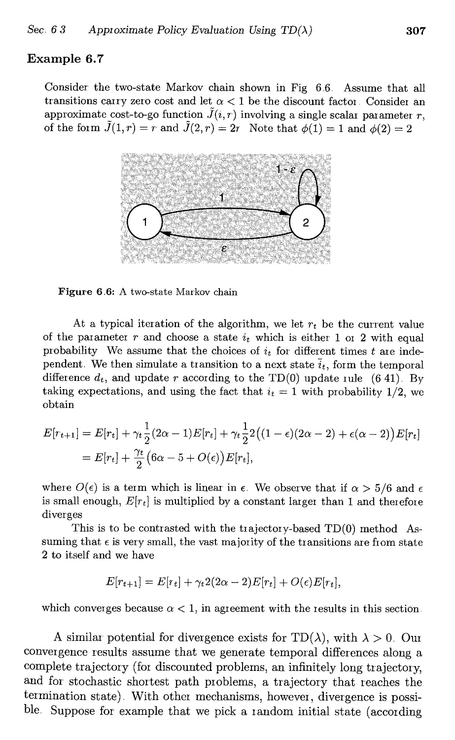
Author: Bertsekas D. P. Tsitsiklis J.N.
Tags: programming computer science optimization and neural computation series athena scientific neuro-dynamic programming neuron networking
ISBN: 1-886529-10-8
Year: 1996


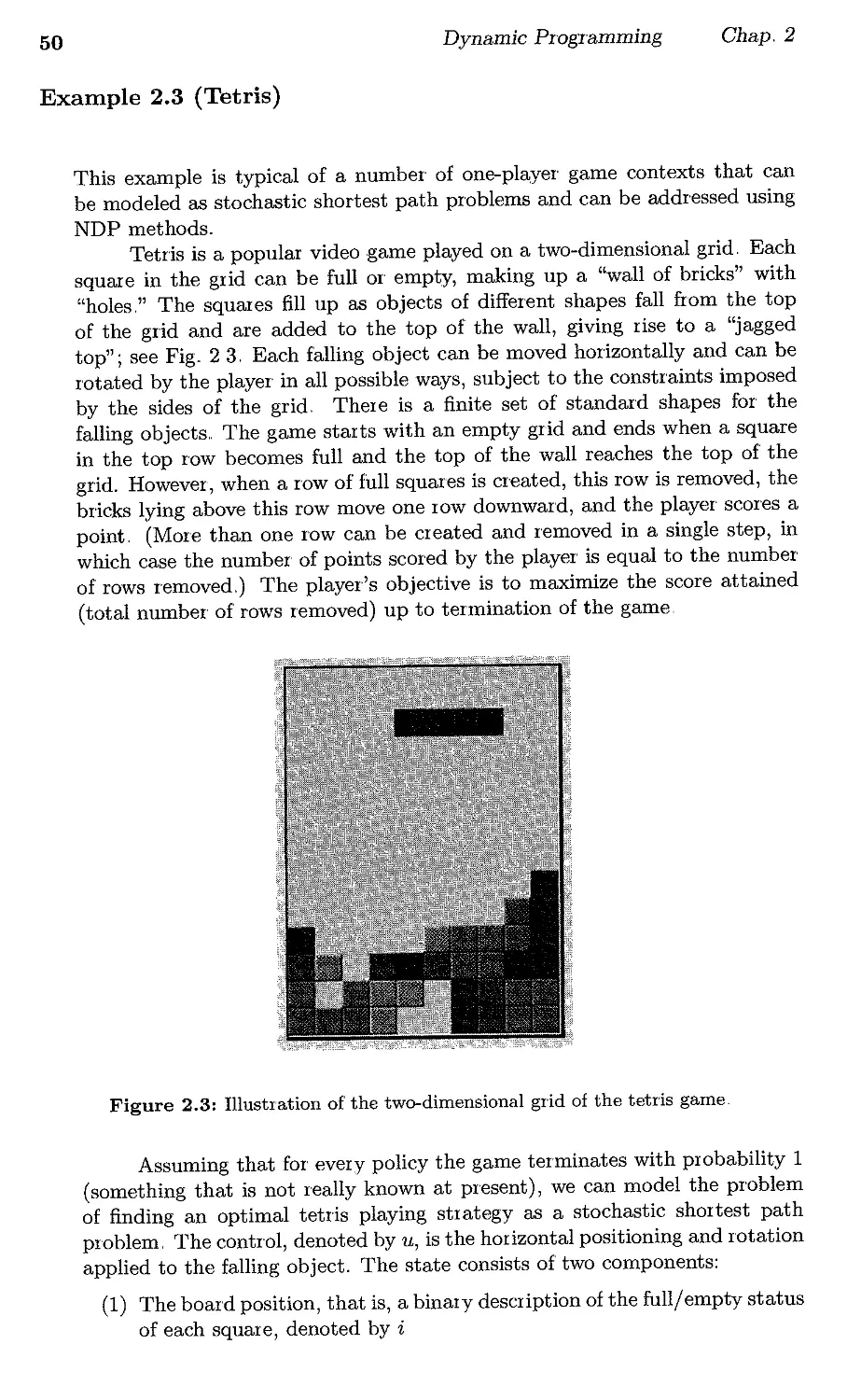
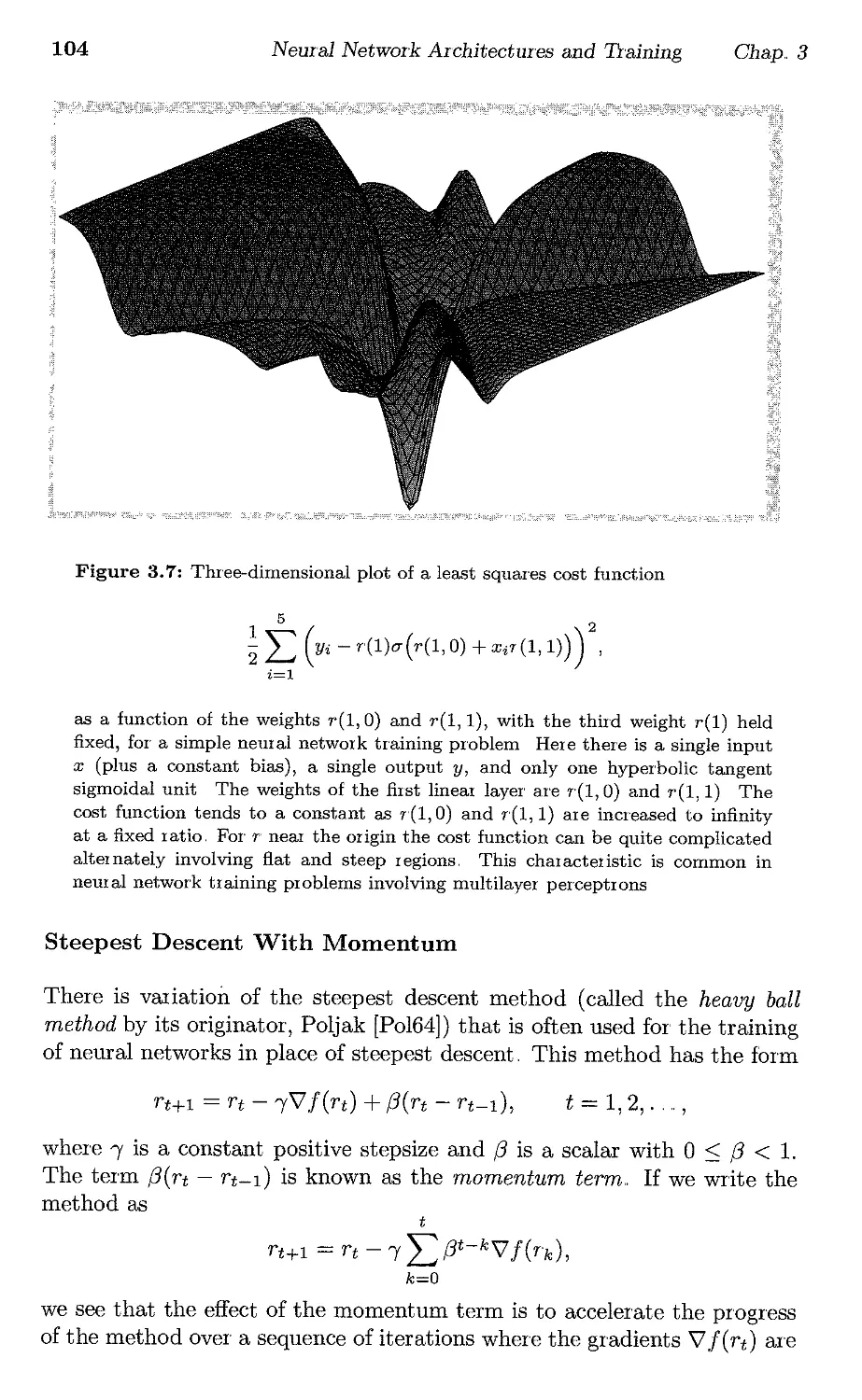
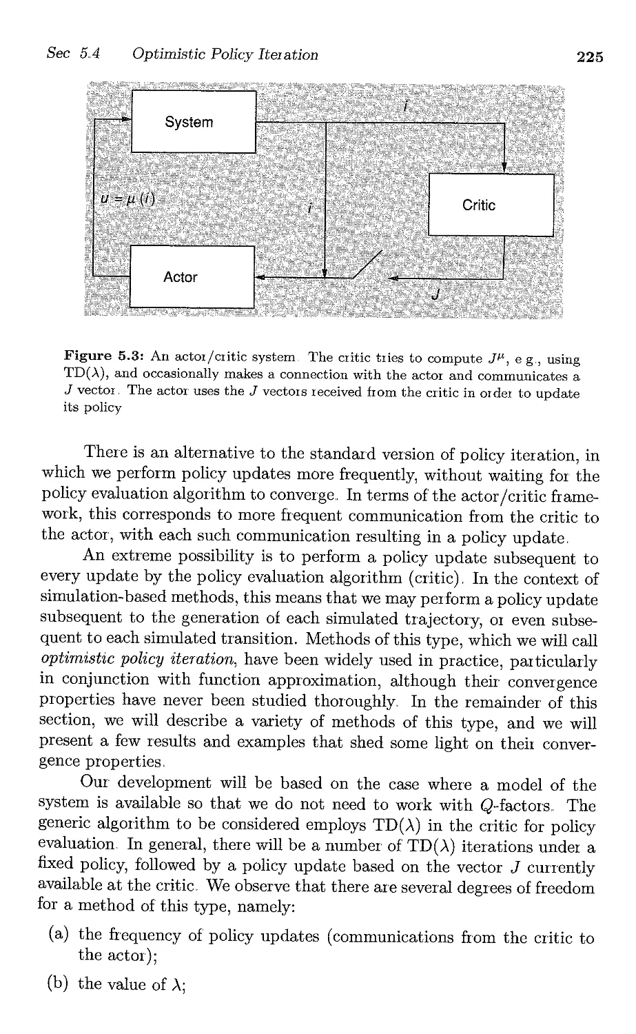
Text
N euro- Dynamic Programming
Dimitri P. Bertsekas and John N. Tsitsiklis
Massachusetts Institute of Technology
WWW site for book information and orders
http://world.std.comrathenasc/
ISJ Athena Scientific, Belmont, Massachusetts
Athena Scientific
Post Office Box 391
Belmont, Mass. 02178-9998
U.S.A.
Email: athenasc@world.std.com
WWW information and orders: http://world.std.com;-athenasc/
Cover Design: Ann Gallager
@ 1996 Dimitri P. Bertsekas and John N. Tsitsiklis
All rights reserved. No part of this book may be reproduced in any form
by any electronic or mechanical means (including photocopying, recording,
or information storage and retrieval) without permission in writing from
the publisher.
Publisher's Cataloging-in-Publication Data
Bertsekas, Dimitri p" Tsitsiklis, John N,
N euro- Dynamic Progr amming
Includes bibliographical references and index
1. Neural Networks (Computer Science), 2" Mathematical Optimization, 3"
Dynamic Programming" I, Title
QA76,,87.B471996 519703 96- 85338
ISBN 1-886529-10-8
To the memory of Dimitri's parents
To John's parents
Contents
1.1. Cost-to-go Approximations in Dynamic Programming
1.2.. Approximation Architectures .
1.3" Simulation and Training
1.4. Neuro-Dynamic Programming
1.5. Notes and Sources
p. 1
p. 3
p. 5
p, 6
p, 8
p. 9
1. Introduction
2"3,,
Introd uction
2.1.1. Finite Horizon Problems
2,,1.2. Infinite Horizon Problems
Stochastic Shortest Path Problems
2,2,1. General Theory
2.2,,2. Value Iteration
2.2.3. Policy Iteration
2,,2.4., Linear Programming
Discounted Problems
2,3,1, Temporal Difference-Based Policy Iteration
Problem Formulation and Examples
Notes and Sources . . . .
. p. 11
p,,12
p,13
p,,14
p. 17
p.18
p, 25
p. 29
p.36
p.37
p,,41
p,,47
p,,57
2. Dynamic Programming
2,1.
2.2
2.4.
2.5.
3. Neural Network Architectures and Training
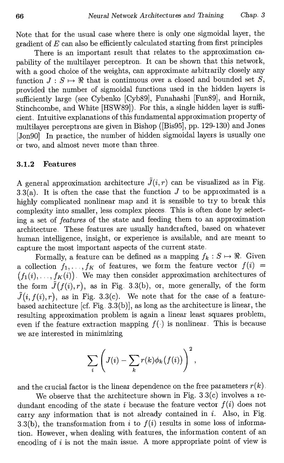
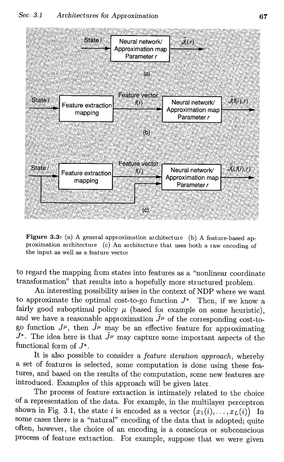
3.1. Architectures for Approximation . . . .
3.1.1. An Overview of Approximation Architectures
31.2. Features . . .
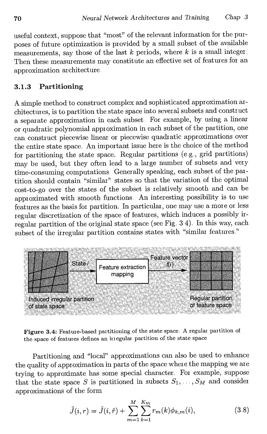
3.1,3 Partitioning . . . .
3,1.4, Using Heuristic Policies to Construct Features
3,2. Neural Network Training,
3.2,,1. Optimality Conditions . .
3,2,2" Linear Least Squares Methods
3.2,3 Gradient Methods
. p. 59
p,60
p 61
p,66
p.70
p. 72
p,76
p,78
p.81
p. 89
v
vi
3.2.4. Incremental Gradient Methods for Least Squares
3.2,5, Convergence Analysis of Incremental Gradient
Methods
3,2.6. Extended Kalman Filtering.
3,2.7. Comparison of Various Methods.
3.3. Notes and Sources
4. Stochastic Iterative Algorithms . . . . . . . .
4,,1. The Basic Model
4.2" Convergence Based on a Smooth Potential Function
4,,2,1. A Convergence Result
4,2,,2. Two-Pass Methods
4..2.3. Convergence Proofs .
4.3.. Convergence under Contraction or Monotonicity
Assumptions .
4,3.1. Algorithmic Model
4.3.2. Weighted Maximum Norm Contractions
4.3,3 Time-Dependent Maps and Additional Noise Terms
4,34. Convergence under Monotonicity Assumptions
4.3.5 Boundedness
4.3,6, Convergence Proofs
4..4. The ODE Approach
4.4.1, The Case of Markov Noise
4.5.. Notes and Sources
5. Simulation Methods for a Lookup Table Representation
5,1. Some Aspects of Monte Carlo Simulation
5,2. Policy Evaluation by Monte Carlo Simulation,
5,2.1. Multiple Visits to the Same State
52.2, Q..Factors and Policy Iteration
5,,3, Temporal Difference Methods .
5.31. Monte Carlo Simulation Using Temporal
Differences .
5.3.2 TD(A) .
5.3.3., Genmal Temporal Difference Methods
5,3.4., Discounted Problems
5,,3,5. Convergence of Off-Line Temporal Difference
Methods
5.3.,6. Convergence of On-Line Temporal Difference
Methods
5.3,,7. Convergence for Discounted Problems
5,4. Optimistic Policy Iteration
5,,5 Simulation-Based Value Iteration
Contents
p,108
p,115
p,,124
p.128
p.129
p. 131
p,134
p 139
p.139
p. 147
p 148
p,,154
p.154
p,,155
p,157
p,158
p,,159
p.161
p"l71
p,173
p. 178
p. 179
p 181
p,186
p,,187
p.192
p,193
p.193
p. 195
p,201
p,,204
p. 208
p.219
p,222
p,,224
p. 237
Contents
5,6, Q-Learning,
5.7, Notes and Sources
6. Approximate DP with Cost-to-Go Function
Approximation . . . . . . . . . . . .
6.1. Generic Issues - From Parameters to Policies
6.1.1. Generic Error Bounds . . .
6"1.2,, Multistage Lookahead Variations
6,1.3 Rollout Policies
61.4 Trading off Control Space Complexity with
State Space Complexity
6,,2. Approximate Policy Iteration. . .
6,,2.1. Approximate Policy Iteration Based on
Monte Carlo Simulation . . . .
6,2.2, Error Bounds for Approximate Policy Iteration
6.2.3. Tightness of the Error Bounds and Empirical Behavior
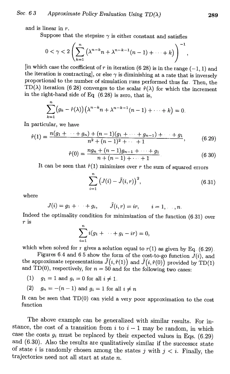
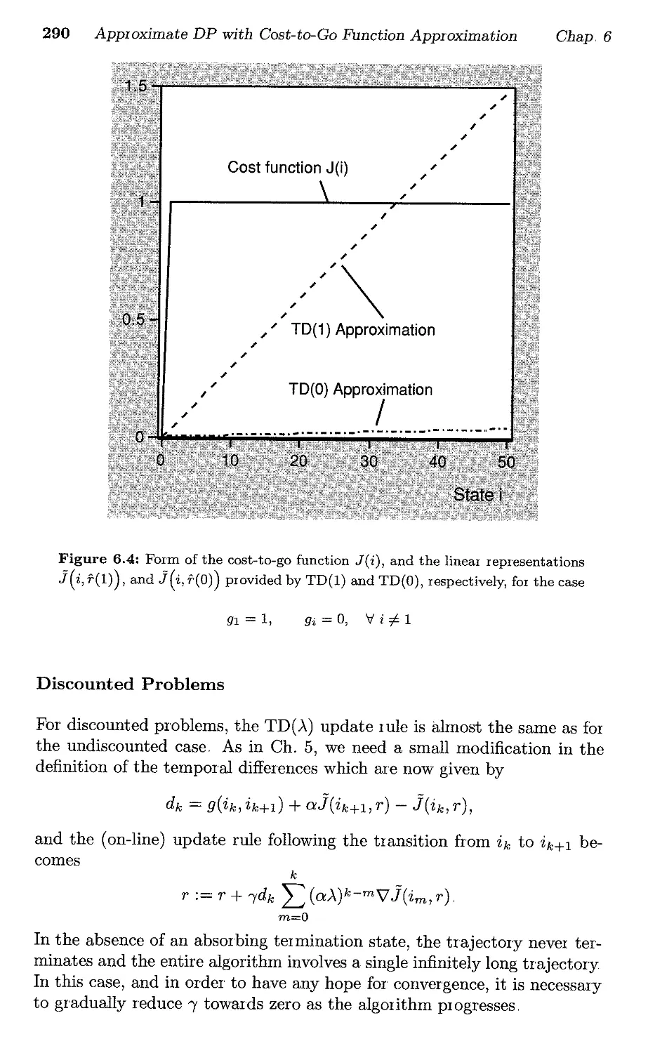
6,,3,A..pproximate Policy Evaluation Using TD(A)
6.3,1. Approximate Policy Evaluation Using TD(l) .
6.32, TD(A) for General A . . . . ."
6 ,3.3. TD(A) with Linear Architectures - Discounted
Problems
6.3.4. TD(A) with Linear Architectures - Stochastic Shortest
Path Problems . . . . . . . .
6.4. Optimistic Policy Iteration . . . . .
6,41 Analysis of Optimistic Policy Iteration . .
6..4.2. Oscillation of Policies in Optimistic Policy Iteration
6.5. Approximate Value Iteration . .
6.5,1. Sequential Backward Approximation for
Finite Horizon Problems . . . .
6,5,2, Sequential Approximation in State Space
6,53 Sequential Backward Approximation for
Infinite Horizon Problems
6.5.4, Incremental Value Iteration,
6.6" Q-Learning and Advantage Updating
6,6,1. Q-Learning and Policy Iteration.
6,62 Advantage Updating
6,7. Value Iteration with State Aggregation
6.7.1. A Method Based on Value Iteration
6,7.,2, Relation to an Auxiliary Problem
6,7.,3, Convergence Results
6,7.4. Error Bounds .
6.7.5, Comparison with TD(O)
6,,7.,6. Discussion of Sampling Mechanisms
vii
p,,245
p,251
p. 255
p. 259
p.262
p. 264
p,266
p, 268
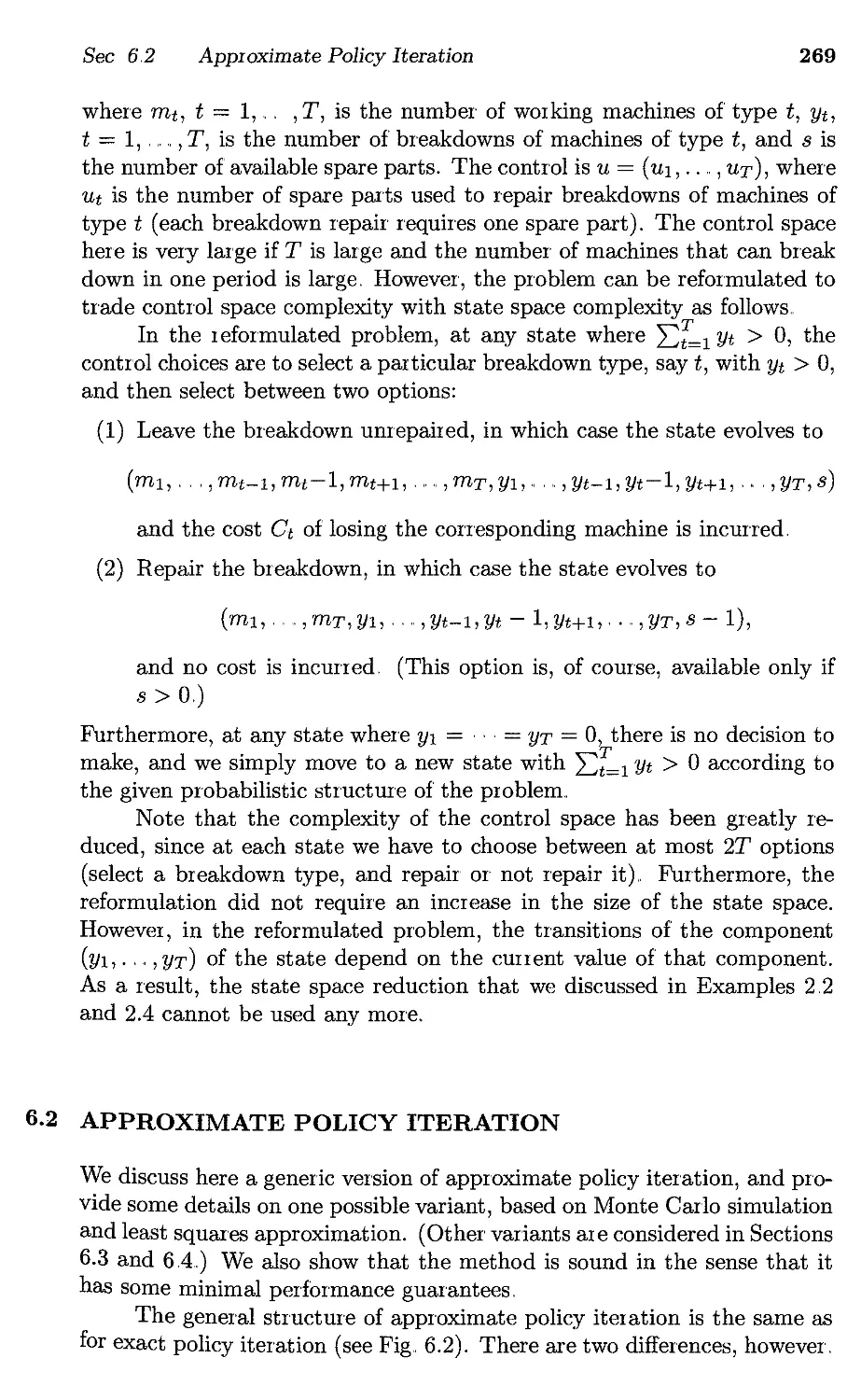
p,269
p,270
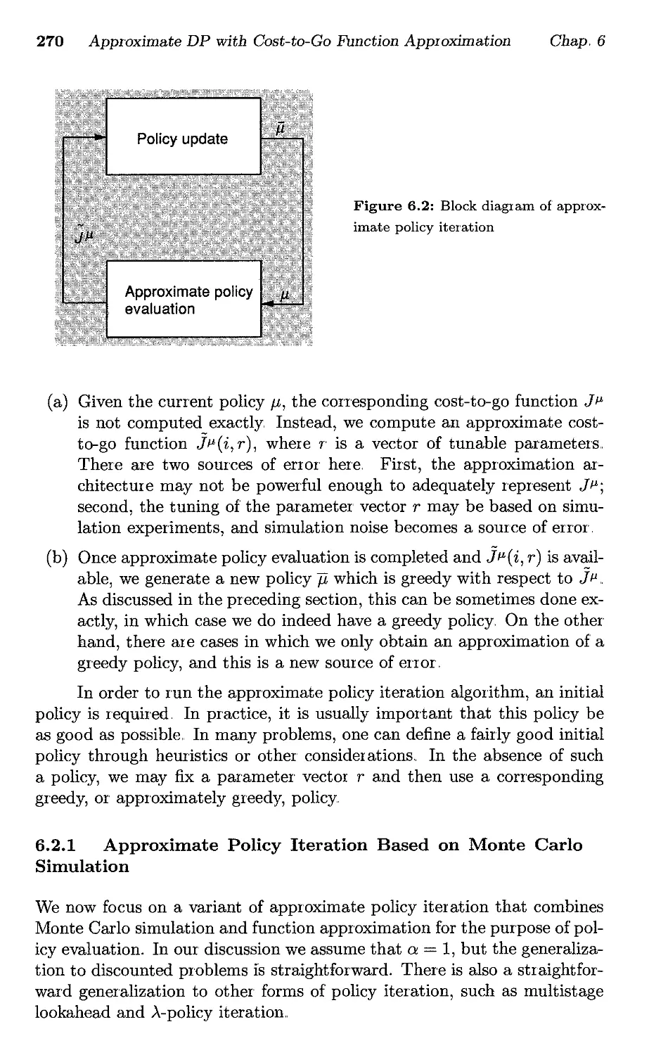
p,,275
p,,282
p. 284
p. 285
p, 287
p. 294
p. 308
p,312
p, 318
p. 320
p.329
p,329
p,331
p,,331
p,,335
p,,337
p, 338
p.339
p, 341
p,342
p.343
p.344
p.349
p.351
p,352
vi
3.2,4, Incremental Gradient Methods for Least Squares
3.2.5.. Convergence Analysis of Incremental Gradient
Methods
3,,2.6. Extended Kalman Filtering.
3,2.7. Comparison of Various Methods.
3.3, Notes and Sources
4. Stochastic Iterative Algorithms . . . . . . . .
4,,1. The Basic Model
4.2, Convergence Based on a Smooth Potential Function
4,,2..1. A Convergence Result
4,2.2. Two-Pass Methods
4.2.3, Convergence Proofs
4.3 Convergence under Contraction or Monotonicity
Assumptions .
4,3.1. Algorithmic Model
4.3.2" Weighted Maximum Norm Contractions
4,,3,3, Time-Dependent Maps and Additional Noise Terms
4..3..4. Convergence under Monotonicity Assumptions
4.3.5, Boundedness
4,3,,6, Convergence Proofs
4,4. The ODE Approach
4,4.1. The Case of Markov Noise
4.5, Notes and Sources
5. Simulation Methods for a Lookup Table Representation
5,1. Some Aspects of Monte Carlo Simulation
5 2. Policy Evaluation by Monte Carlo Simulation ,
52.1. Multiple Visits to the Same State
5,2.2, Q-Factors and Policy Iteration
5,,3., Temporal Difference Methods .
5.3,1. Monte Carlo Simulation Using Temporal
Differences .
5.3.2 TD(A) . ., . .
5.3.3, General Temporal Diff'erence Methods
5"3,4,, Discounted Problems
5,3,5. Convergence of Off-Line Temporal Difference
Methods
5.3,6, Convergence of On-Line Temporal Difference
Methods .
5.3.,7., Convergence for Discounted Problems
5,4. Optimistic Policy Iteration
5,,5, Simulation-Based Value Iteration
Contents
p. 108
p, 115
p,,124
p.128
p,,129
p.131
p, 134
p,,139
p.139
p. 147
p,148
p. 154
p.154
p,,155
p,157
p. 158
p. 159
p, 161
p,l71
p.173
p. 178
p. 179
p,181
p,186
p. 187
p.192
p,193
p.193
p.195
p,201
p,,204
p. 208
p,219
p, 222
p. 224
p. 237
Contents
5.6. Q-Learning ,
5.7. Notes and Sources
6. Approximate DP with Cost-to-Go Function
Approximation . . . . . . . . . . . .
6 ,1. Generic Issues - From Parameters to Policies
6.1.1. Generic Error Bounds . . . .
61,2. Multistage Lookahead Variations
6.1,3. Rollout Policies
6.1.4. Trading off Control Space Complexity with
State Space Complexity
6,2" Approximate Policy Iteration. . . .
6,2,,1. Approximate Policy Iteration Based on
Monte Carlo Simulation
6.2.2. Error Bounds for Approximate Policy Iteration
6,,2,,3., Tightness of the Error Bounds and Empirical Behavior
6,3" } l.pproximate Policy Evaluation Using TD(A)
6,3,,1. Approximate Policy Evaluation Using TD(l) .
6.3.2. TD(A) for General A . . . .
6.3.3. TD(A) with Linear Architectures - Discounted
Problems
6.34" TD(A) with Linear Architectures - Stochastic Shortest
Path Problems . . . . .
6.4. Optimistic Policy Iteration
6.4.1. Analysis of Optimistic Policy Iteration
6.4.2. Oscillation of Policies in Optimistic Policy Iteration
6,5.. Approximate Value Iteration . . . .
6,5.1. Sequential Backward Approximation for
Finite Horizon Problems
6.5,2, Sequential Approximation in State Space
6.5,,3. Sequential Backward Approximation for
Infinite Horizon Problems
6,,5.4. Incremental Value Iteration
6.6, Q-Learning and Advantage Updating
66,1 Q-Learning and Policy Iteration.
6.6,2, Advantage Updating
6,7., Value Iteration with State Aggregation
6.7.1. A Method Based on Value Iteration
6,7.2, Relation to an Auxiliary Problem
6,7,3. Convergence Results
6.7,4, Error Bounds.
6.7.5. Comparison with TD(O)
6,7.,6, Discussion of Sampling Mechanisms
vii
p, 245
p,251
p.255
p. 259
p.262
p. 264
p, 266
p,268
p. 269
p,270
p,275
p,282
p. 284
p.285
p,,287
p. 294
p. 308
p,,312
p, 318
p.320
p,329
p,,329
p, 331
p,331
p,335
p 337
p,,338
p.339
p. 341
p,342
p. 343
p. 344
p. 349
p.351
p.352
viii
6,,7.7. The Model-Free Case
6.8 Euclidean Contractions and Optimal Stopping
6.8,1. Assumptions and Main Convergence Result
6.8..2, Error Bounds
6.8,3, Applicability of the Result
6,,8.4. Q-Learning for Optimal Stopping Problems,
6,9" Value Iteration with Representative States
6.10. Bellman Error Methods. .
610,1. The Case of a Single Policy
6.10,2 Approximation of the Q-Factors
6,10.3 Another Variant, .
6.10.4, Discussion and Related Methods
6,11. Continuous States and the Slope of the Cost-to-Go
612. Approximate Linear Programming
6.13. Overview .
6.14, Notes and Sources
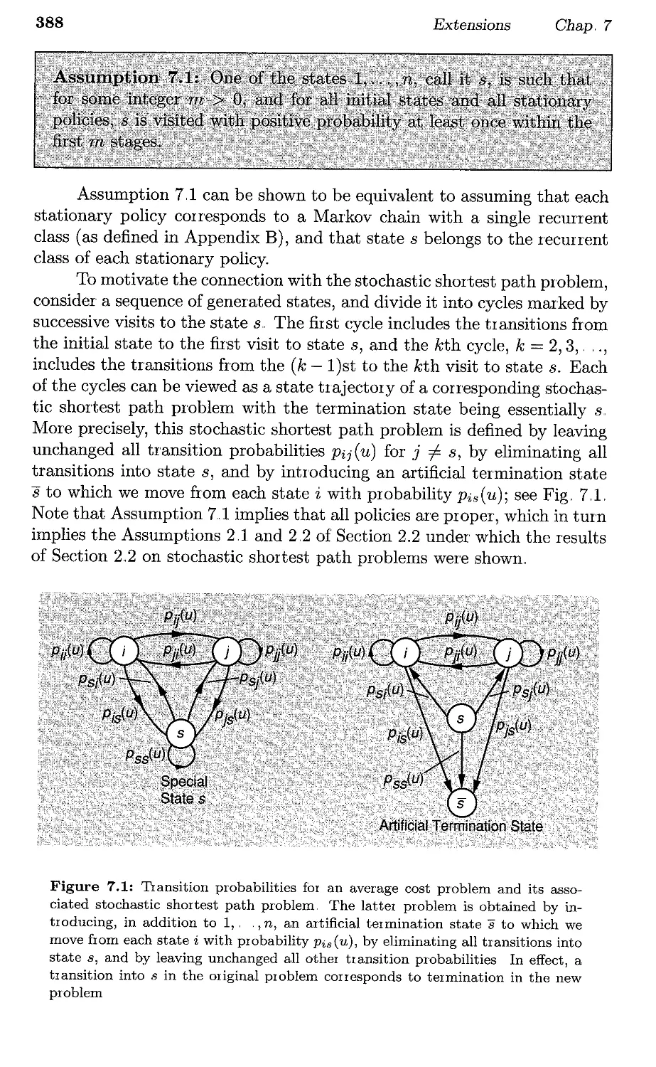
7. Extensions . . . . . .
. . . . . . . . . . . . .
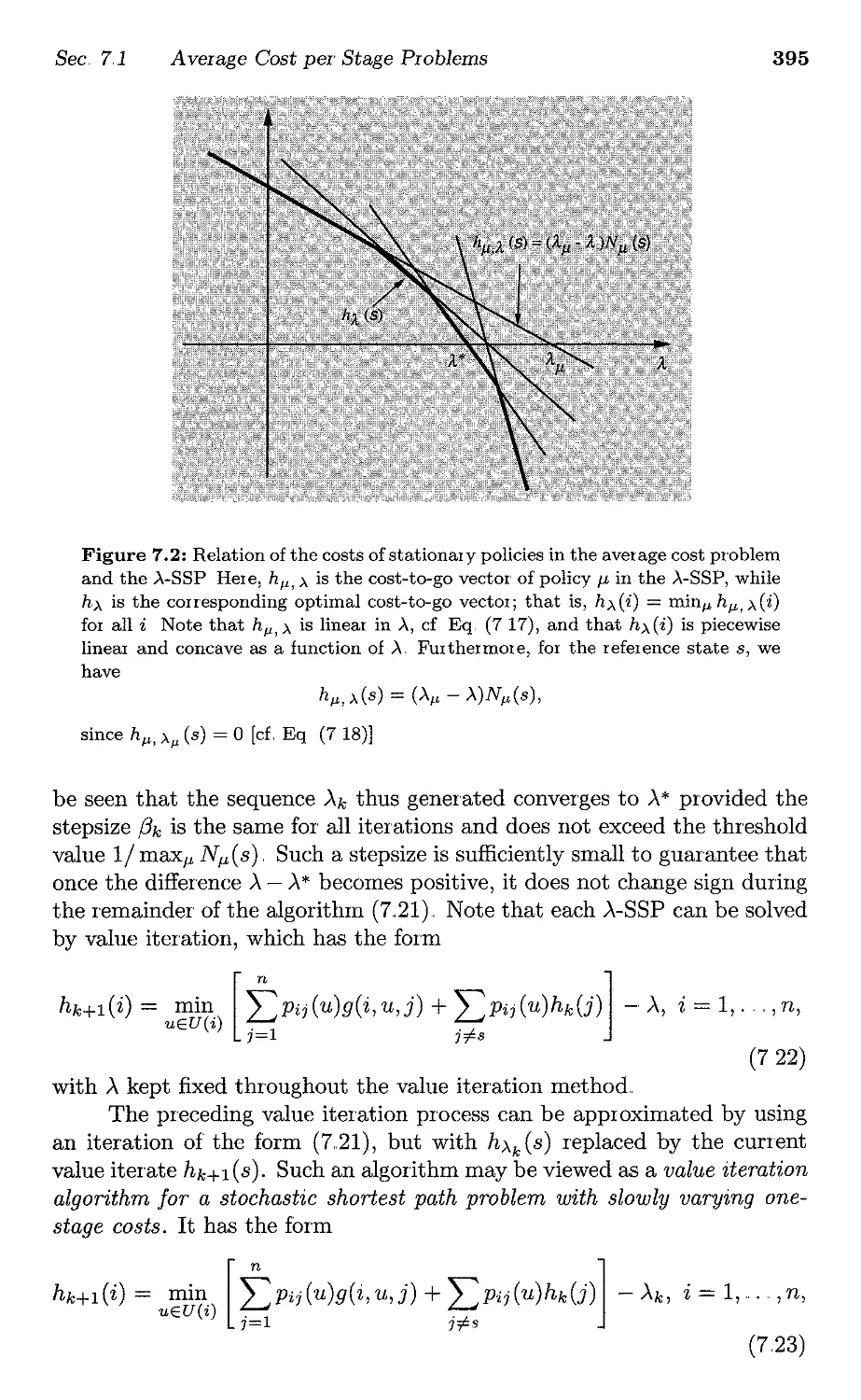
7.1. Average Cost per Stage Problems .,
7.1.1. The Associated Stochastic Shortest Path Problem
7.,1.2 Value Iteration Methods
7.1.3. Policy Iteration .
7,1.4 Linear Programming,
7.1.5, Simulation-Based Value Iteration and Q-Learning
7.1.6, Simulation-Based Policy Iteration
7,1.7. Minimization of the Bellman Equation Error
7.2. Dynamic Games
7.,2.1. Discounted Games. .
7.2.2, Stochastic Shortest Path Games .
7.2,3, Sequential Games, Policy Iteration, and Q-Learning
7. 2..4. Function Approximation Methods
7.3" Parallel Computation Issues
7,4, Notes and Sources
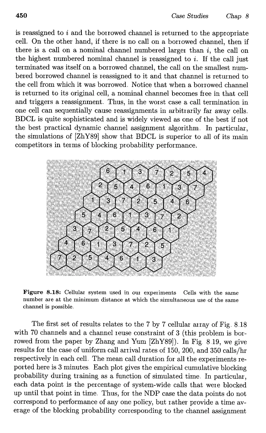
8. Case Studies
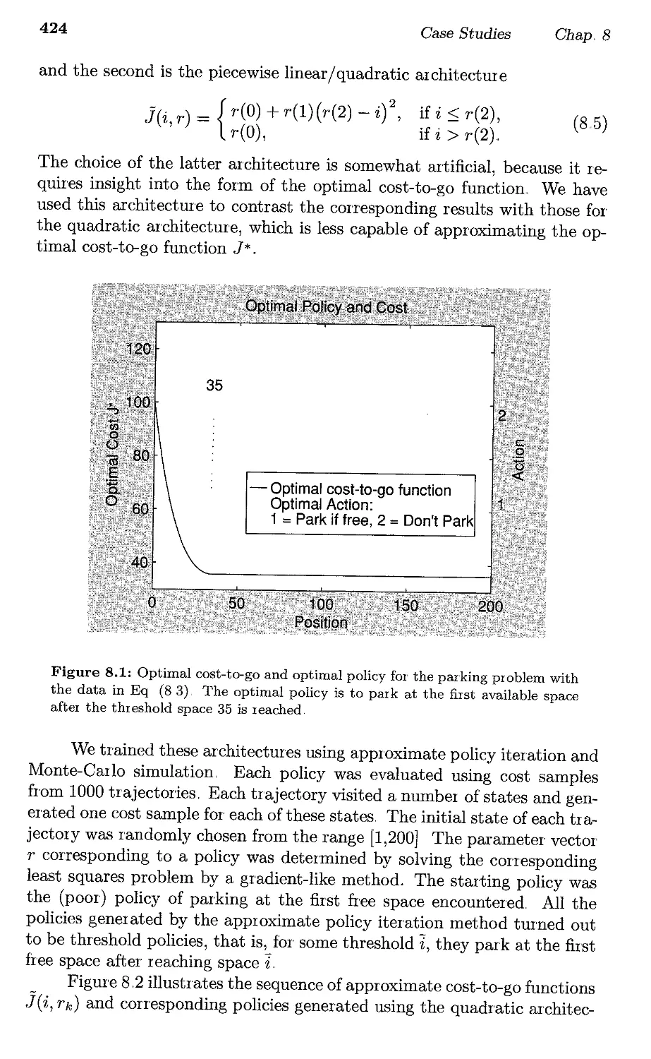
8.1. Parking
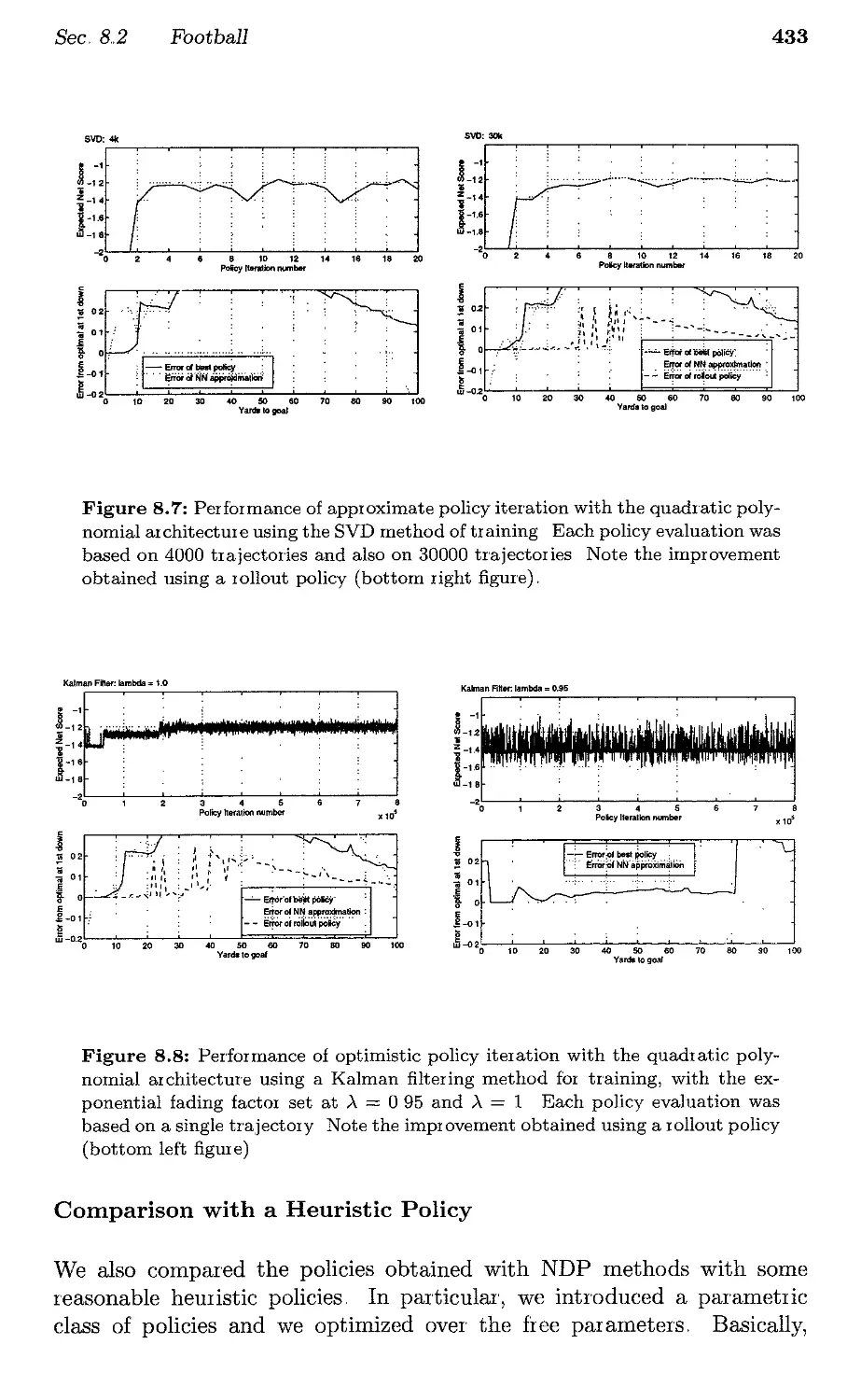
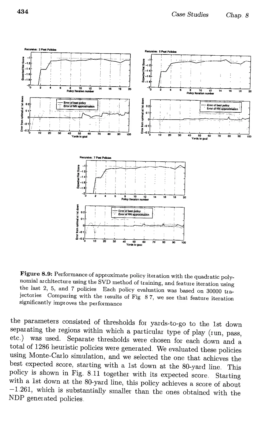
8,,2, Football .
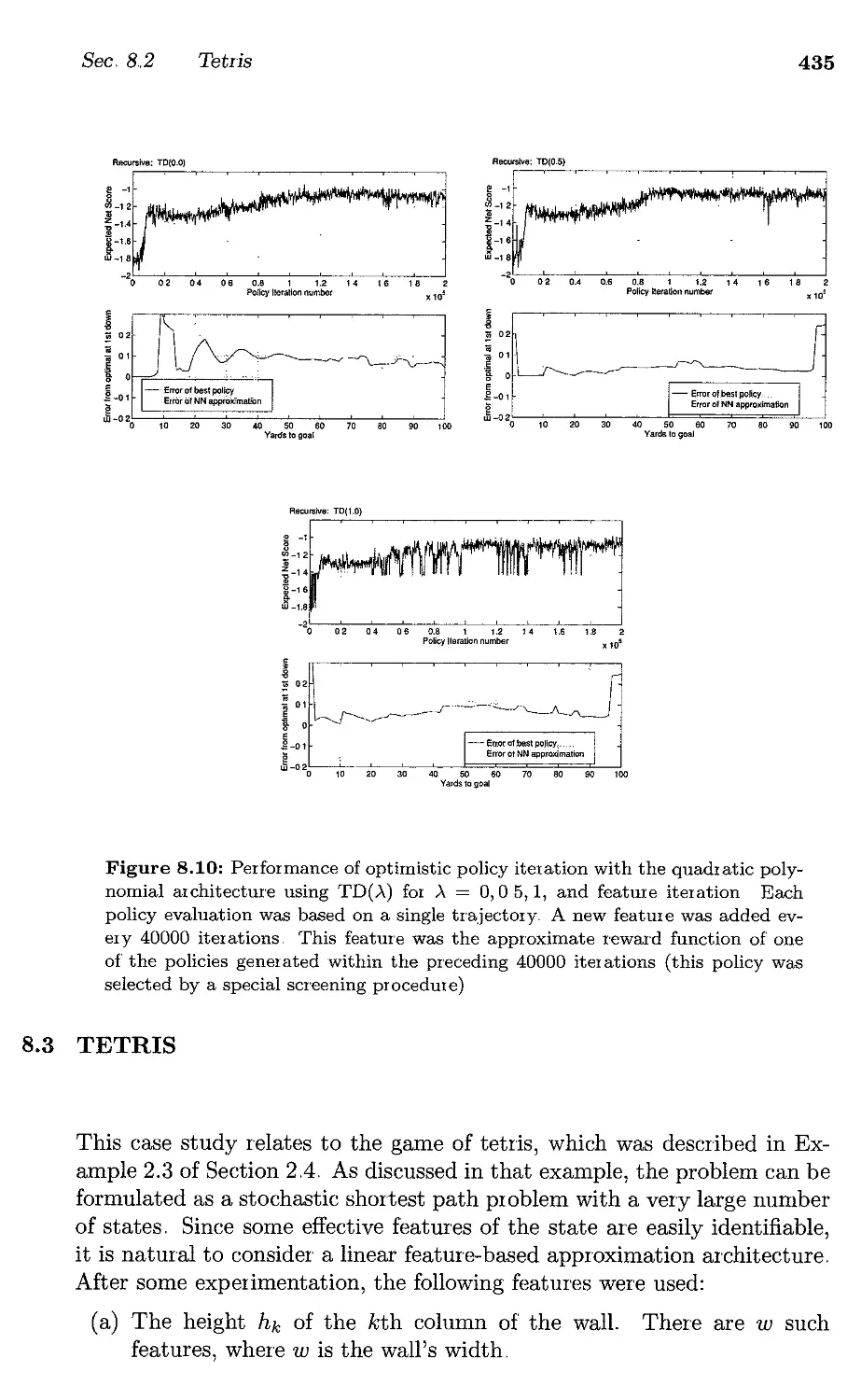
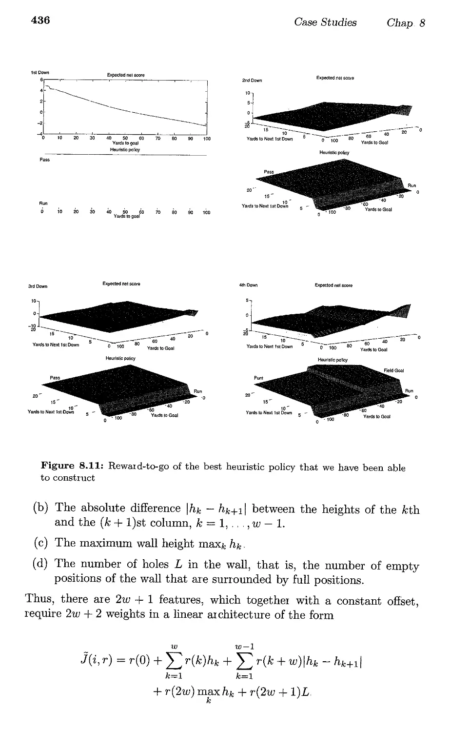
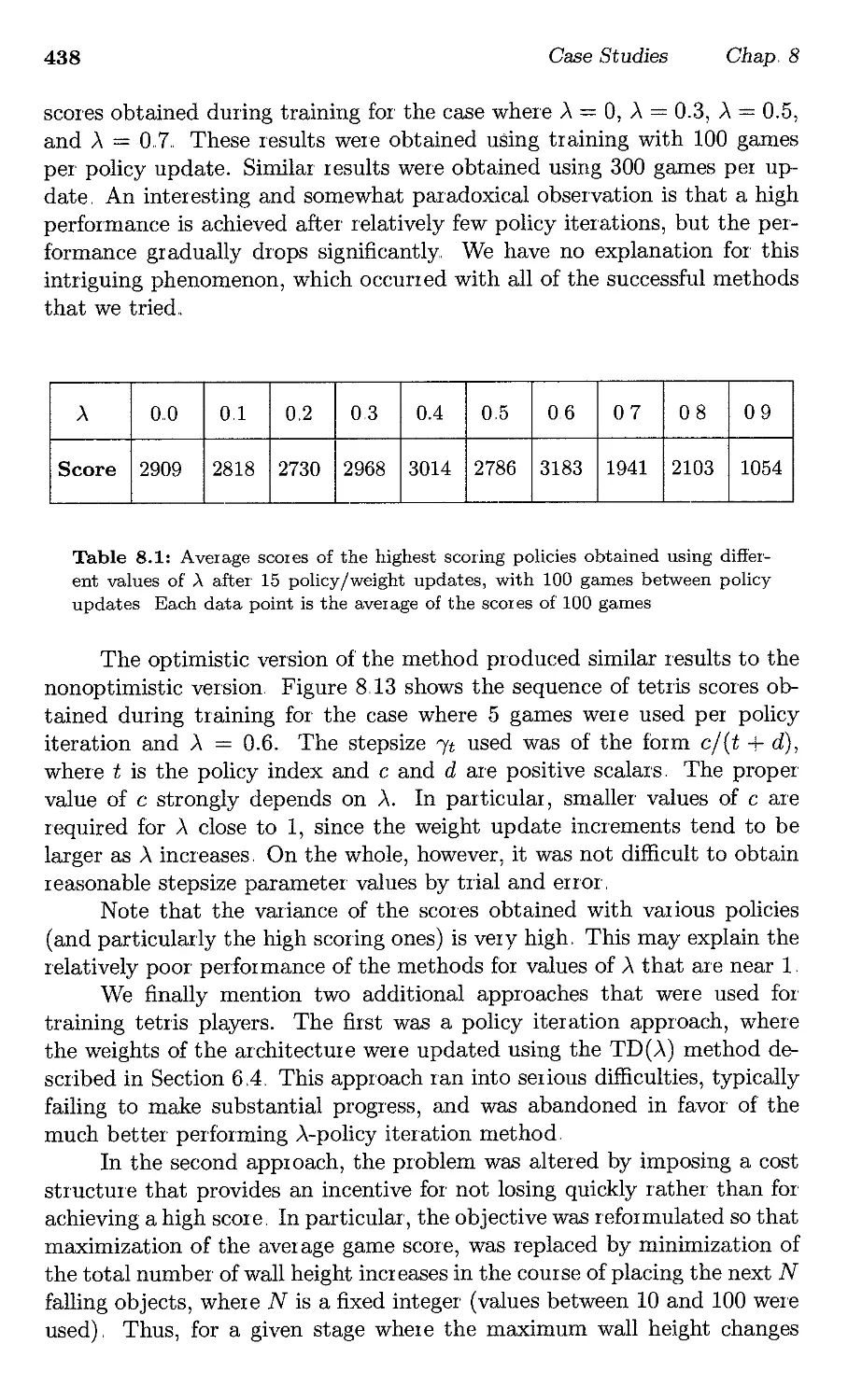
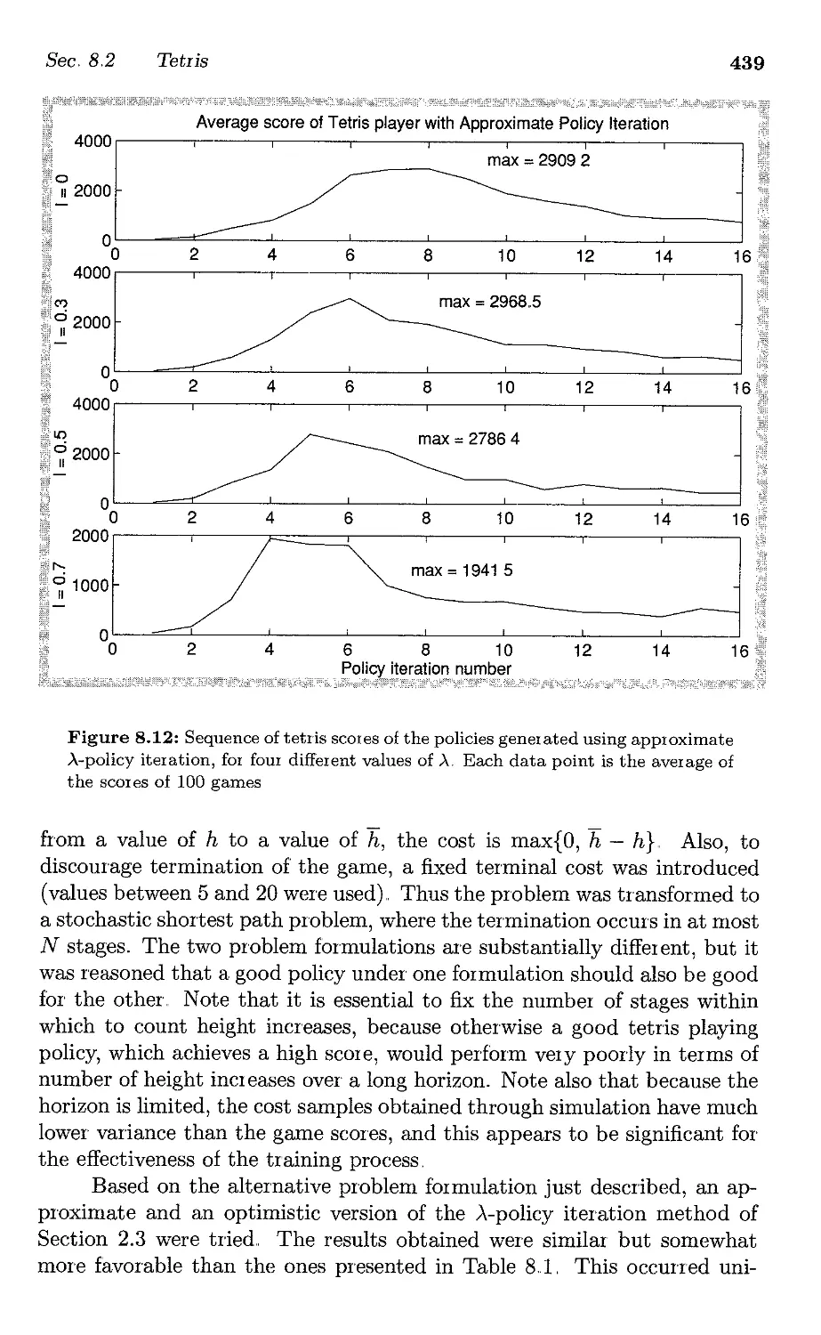
83. Tetris
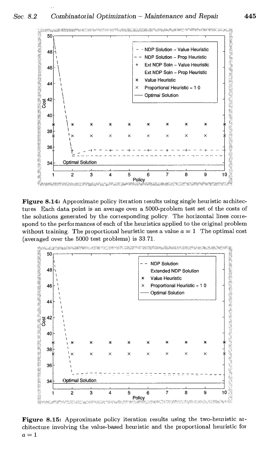
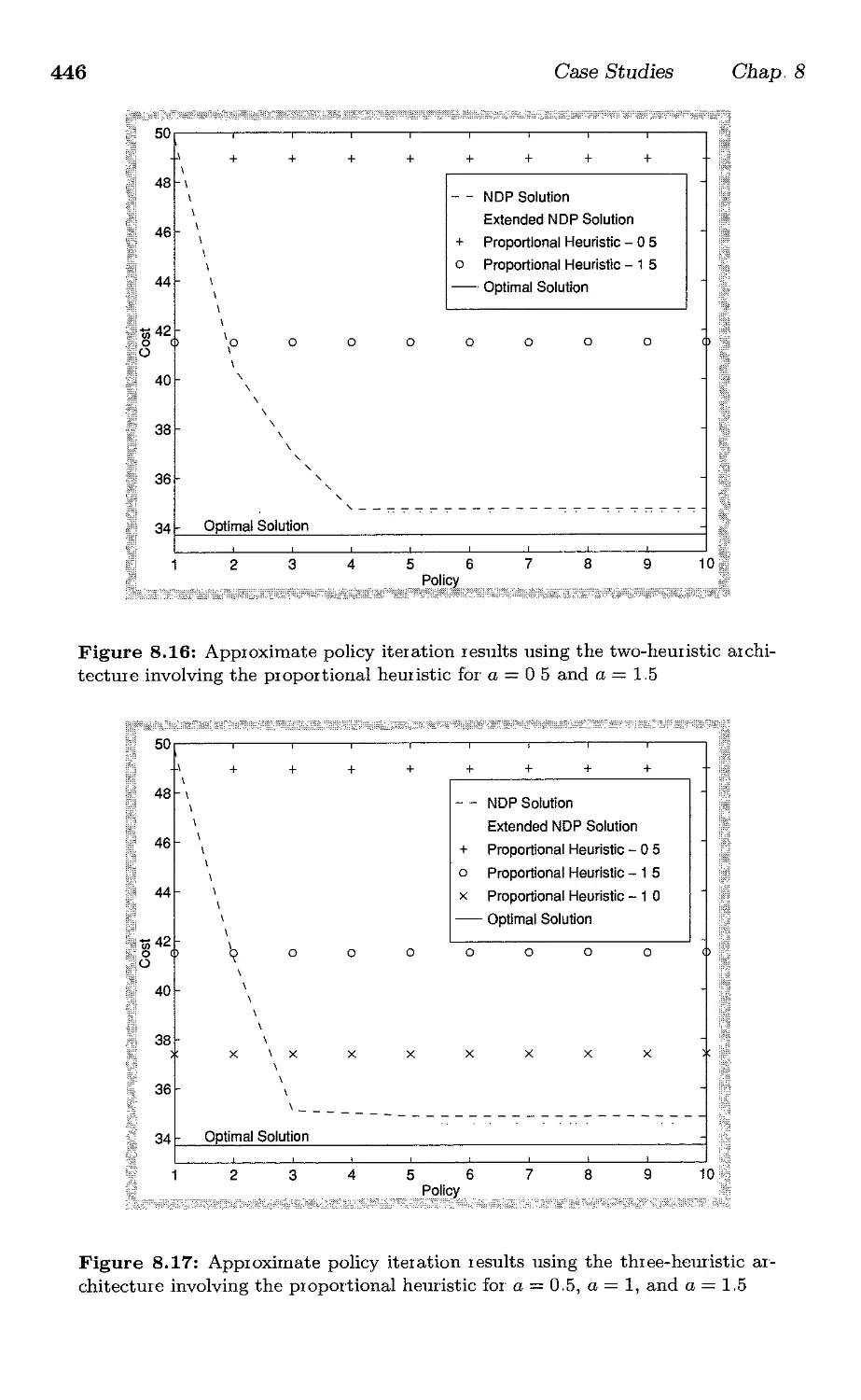
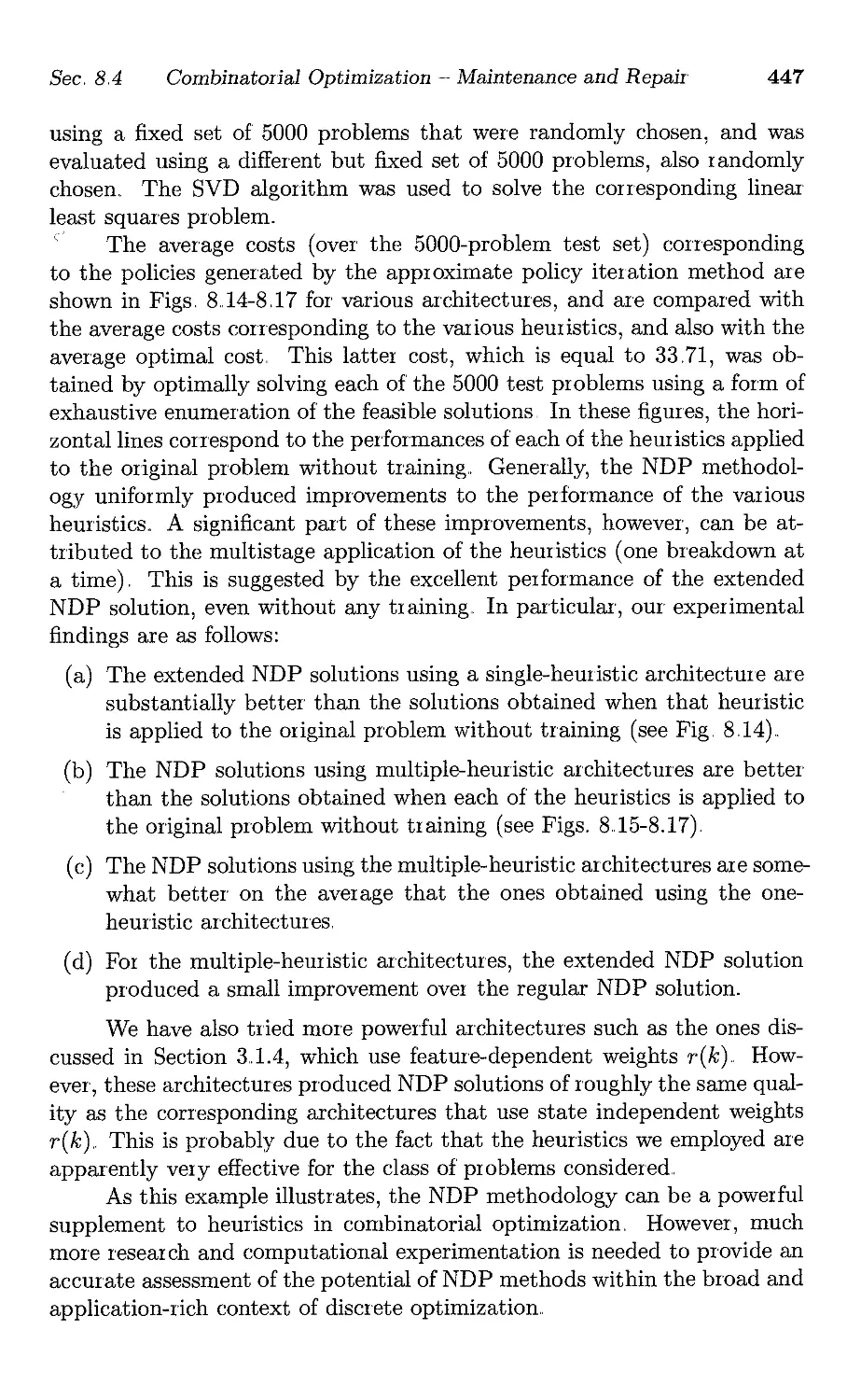
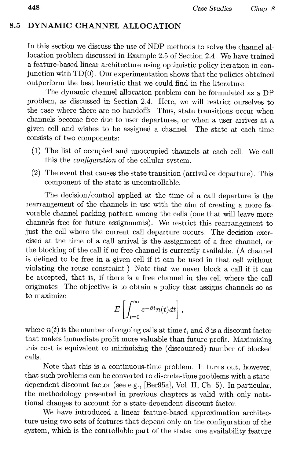
8.4. Combinatorial Optimization - Maintenance and Repair
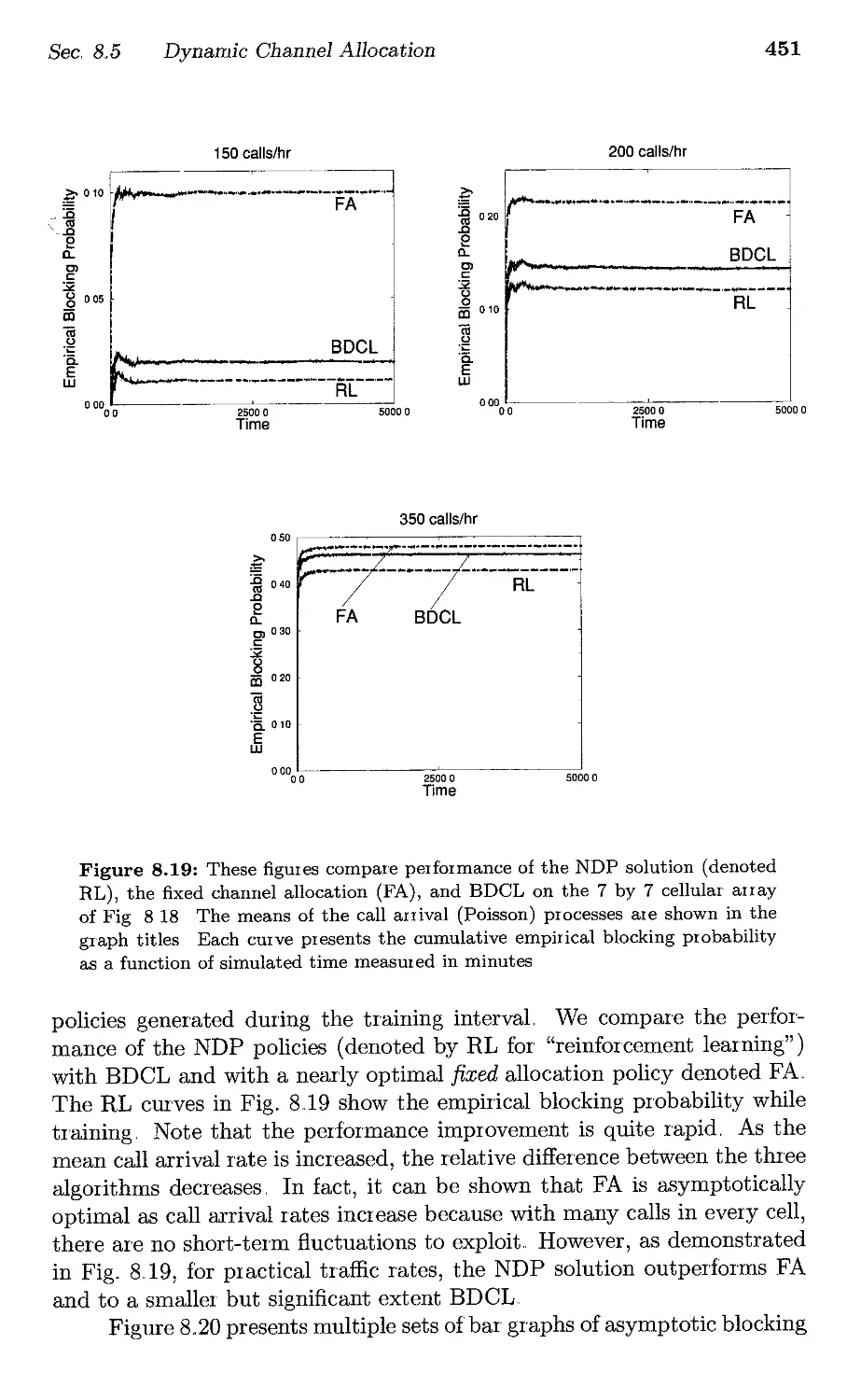
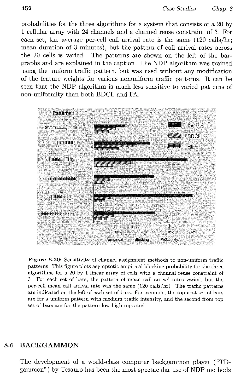
8.5" Dynamic Channel Allocation
8,,6.. Backgammon
8,7. Notes and Sources
Contents
p,352
p,353
p.353
p,,357
p, 358
p, 358
p.362
p.364
p,366
p. 367
p,368
p,369
p,370
p.375
p. 377
p,379
p.385
p,386
p,387
p,,391
p. 397
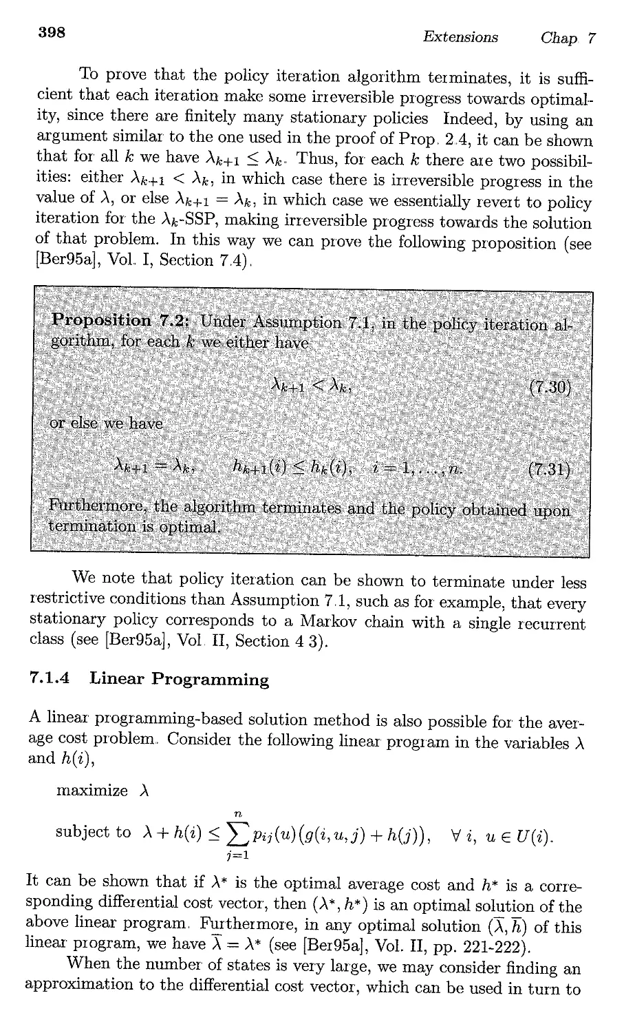
p. 398
p,,399
p,405
p,,408
p.408
p,,410
p,412
p,412
p.416
p 418
p,419
p.421
p,422
p,426
p.435
p. 440
p. 448
p.452
p, 456
Contents
ix
Appendix A: Mathematical Review
A,L Sets
A,2. Euclidean Space
A,3. Matrices
A.4, Analysis,
A.5. Convex Sets and Functions
p.457
p, 458
p,459
p, 460
p.462
p,,465
Appendix B: On Probability Theory and Markov Chains
B.1. Probability Spaces
B.,2. Random Variables
B,,3 Conditional Probability
B.4. Stationary Markov Chains
B.5, Classification of States
B ,6" Limiting Probabilities
B.7. First Passage Times
p.467
p,,468
p.469
p.470
p,,471
p,472
p.472
p,473
References
p,475
Index
p,,487
>0 XIXLpe:cpWV, 1tOAAIXt -t€XVIXL ev a.vSpW1tmc; e:LO"tV ex "tWV ef-l1te:LpLWV
ef-l1tdpc.>C; 'ljup'ljf-leva.v ef-l1te:LptlX f-lev ya.p 1tme:L "tOY a.LWVa. f-lWV
1tOpe:Ue:O"SIXL XIX"ta. "teXv'ljv, a.1te:LptlX oe XIX"ta. "tUX'ljV.
o Chaerephon, many arts among men have been
discovered through pmctice, empirically;'
for experience makes our l fe proceed delibemtely,
but inexperience unpredictably.
(Plato, Gorgias 44&)
Preface
A few years ago our curiosity was aroused by reports on new methods in
reinforcement learning, a field that was developed primarily within the ar-
tificial intelligence community, starting a few decades ago, These methods
were aiming to provide effective suboptimal solutions to complex problems
of planning and sequential decision making under uncertainty, that for a
long time were thought to be intr actable" Our first impression was that
the new methods were ambitious, overly optimistic, and lacked firm foun-
dation, Yet there were claims of impressive successes and indications of a
solid core to the modern developments in reinforcement learning, suggest-
ing that the correct approach to their understanding was through dynamic
programming..
Three years later, after a lot of study, analysis, and experimentation,
we believe that our initial impressions were largely correct, This is indeed
an ambitious, often ad hoc, methodology, but for reasons that we now un-
derstand much better, it does have the potential of success with important
and challenging problems, With a good deal of justification, it claims to
deal effectively with the dual curses of dynamic programming and stochas-
tic optimal control: Bellman's curse of dimensionality (the exponential
computational explosion with the problem dimension is averted through
the use of parametric approximate representations of the cost-to-go func-
tion), and the CUTse of modeling (an explicit system model is not needed,
and a simulator can be used instead), Furthermore, the methodology has a
logical structure and a mathematical foundation, which we systematically
develop in this book. It draws on the theory of function approximation,
xi
xii
Preface
the theory of iterative optimization and neural network training, and the
theory of dynamic programming. In view of the close connection with
both neural networks and dynamic programming, we settled on the name
"neuro-dynamic programming" (NDP), which describes better in our opin-
ion the nature of the subject than the older and more broadly applicable
name "reinforcement learning."
Our objective in this book is to explain with mathematical analysis,
examples, speculative insight, and case studies, a number of computational
ideas and phenomena that collectively can provide the foundation for un-
derstanding and applying the NDP methodology, We have organized the
book in three major parts"
(a) The first part consists of Chapters 2-4 and provides background" It in-
cludes a detailed introduction to dynamic programming (Chapter 2),
a discussion of neural network architectures and methods for training
them (Chapter 3), and the development of general convergence the-
orems for stochastic approximation methods (Chapter 4), which will
provide the foundation for the analysis of various NDP algmithms
later.
(b) The second part consists of the next three chapters and provides the
core NDP methodology, including many mathematical results and
methodological insights that were developed as this book was written
and which are not available elsewhere Chapter 5 covers methods in-
volving a lookup table representation" Chapter 6 discusses the more
practical methods that make use of function approximation. Chap-
ter 7 develops various extensions of the theory in the preceding two
chapters,
( c) The third part consists of Chapter 8 and discusses the practical as-
pects of NDP through case studies"
Inevitably, some choices had to be made regarding the material to be
covered, Given that the reinforcement learning literature often involves a
mixture of heuristic arguments and incomplete analysis, we decided to pay
special attention to the distinction between factually correct and incorrect
statements, and to rely on rigorous mathematical proofs. Because some of
these proofs are long and tedious, we have made an eff'ort to organize the
material so that most proofs can be omitted without loss of continuity on
the part of the reader. For example, during a first reading, a reader could
omit all of the proofs in Chapters 2-5, and proceed to subsequent chapters,
However, we wish to emphasize our strong belief in the beneficial in-
terplay between mathematical analysis and practical algorithmic insight,
Indeed, it is primarily through an eff'ort to develop a mathematical struc-
ture for the NDP methodology that we will ever be able to identify promis-
ing or solid algorithms from the bewildering array of speculative proposals
and claims that can be found in the literature"
Preface
xiii
The fields of neural networks, reinforcement learning, and approxi-
mate dynamic programming have been very active in the last few years
and the corresponding literature has greatly expanded" A comprehensive
survey of this literature is thus beyond our scope, and we wish to apologize
in advance to researchers in the field for not citing their works.. We have
confined ourselves to citing the sources that we have used and that con-
tain results related to those presented in this book. We have also cited a
few sources for their historical significance, but our references are far from
complete in this regard,
Finally, we would like to express our thanks to a number of individu-
als. Andy Barto and Michael Jordan first gave us pointers to the research
and the state of the art in reinforcement learning. Our understanding
of the reinforcement lear'ning literature and viewpoint gained significantly
from interactions with Andy Barto, Satinder Singh, and Rich Sutton. The
first author collaborated with Vivek Borkar on the average cost Q-Iearning
research discussed in Chapter 7, and with Satinder Singh on the dynamic
channel allocation research discussed in Chapter 8.. The first author also
benefited a lot through participation in an extensive NDP project at AI-
phatech, Inc.., where he interacted with David Logan and Nils Sandell,
Jr.. Our students contributed substantially to our understanding through
discussion, computational experimentation, and individual research.. In
particular, they assisted with some of the case studies in Chapter 8, on
parking (Keith Rogers), football (Steve Patek), tetris (Sergey Ioffe and
Dimitris Papaioannou), and maintenance and combinatorial optimization
(Cynara Wu)" The joint researches ofthe first author with Jinane Abounadi
and with Steve Patek are summarized in Sections 7.1 and 7.,2, respectively.
Steve Patek also offered tireless and invaluable assistance with the exper-
imental implementation, validation, and interpretation of a large variety
of untested algorithmic ideas" The second author has enjoyed a fruitful
collaboration with Ben Van Roy that led to many results, including those
in Sections 6.3, 6.7, 6,,8, and 6,9.. We were fortunate to work at the Labo-
ratory for Information and Decision Systems at M.LT" which provided us
with a stimulating research environment, Funding for our research that is
reported in this book was provided by the National Science Foundation, the
Army Research Office through the Center for Intelligent Control Systems,
the Air Force Office of Scientific Research, the Electric Power Research In-
stitute, and Siemens. We are thankful to Prof. Charles Segal of Harvard's
Department of Classics for suggesting the original quotation that appears
at the beginning of this preface, Finally, we are grateful to our families for
their love, encouragement, and support while this book was being written"
Dimitri P. Bertsekas
John N. Tsitsiklis
Cambridge, August 1996
Learning without thought is labour lost;
thought without learning is perilous,
(Confucian Analects)
1
Introduction
2
Introduction
Chap. 1
This book considers systeIllS where decisions are made in stages. The
outcome of each decision is not fully predictable but can be anticipated
to some extent before the next decision is made, Each decision results in
some immediate cost but also affects the context in which future decisions
are to be made and therefore affects the cost incurred in future stages.. We
are interested in decision making policies that minimize the total cost over
a number of stages. Such problems are challenging primarily because of
the tradeoff between immediate and future costs, Dynamic programming
(DP for short) provides a mathematical formalization of this tradeoff,
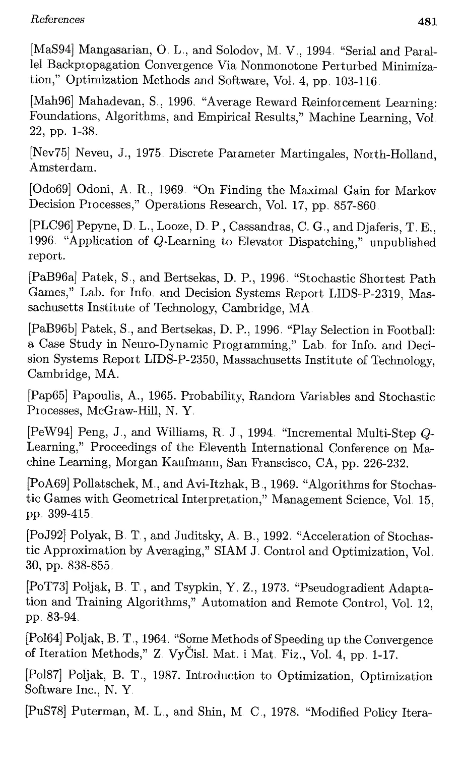
Generally, in DP formulations we have a discrete-time dynamic sys-
tem wbose state evolves according to given transition probabilities that
depend on a decision/control u.. In particular, if we are in state i and we
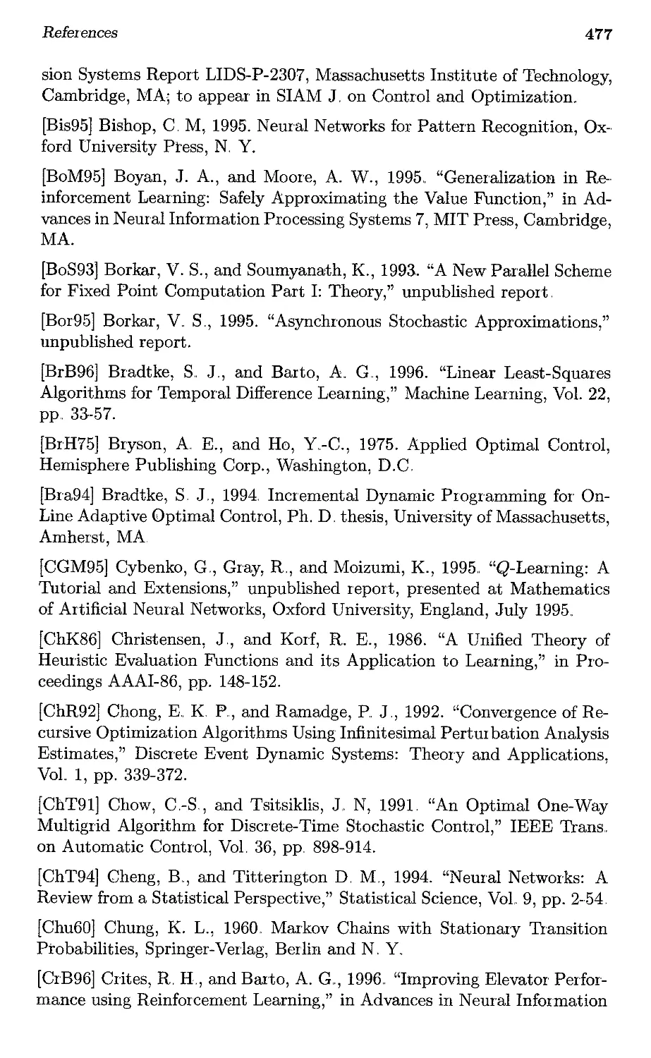
choose control u, we move to state j with given probability Pij(U). The
control u depends on the state i and the rule by which we select the controls
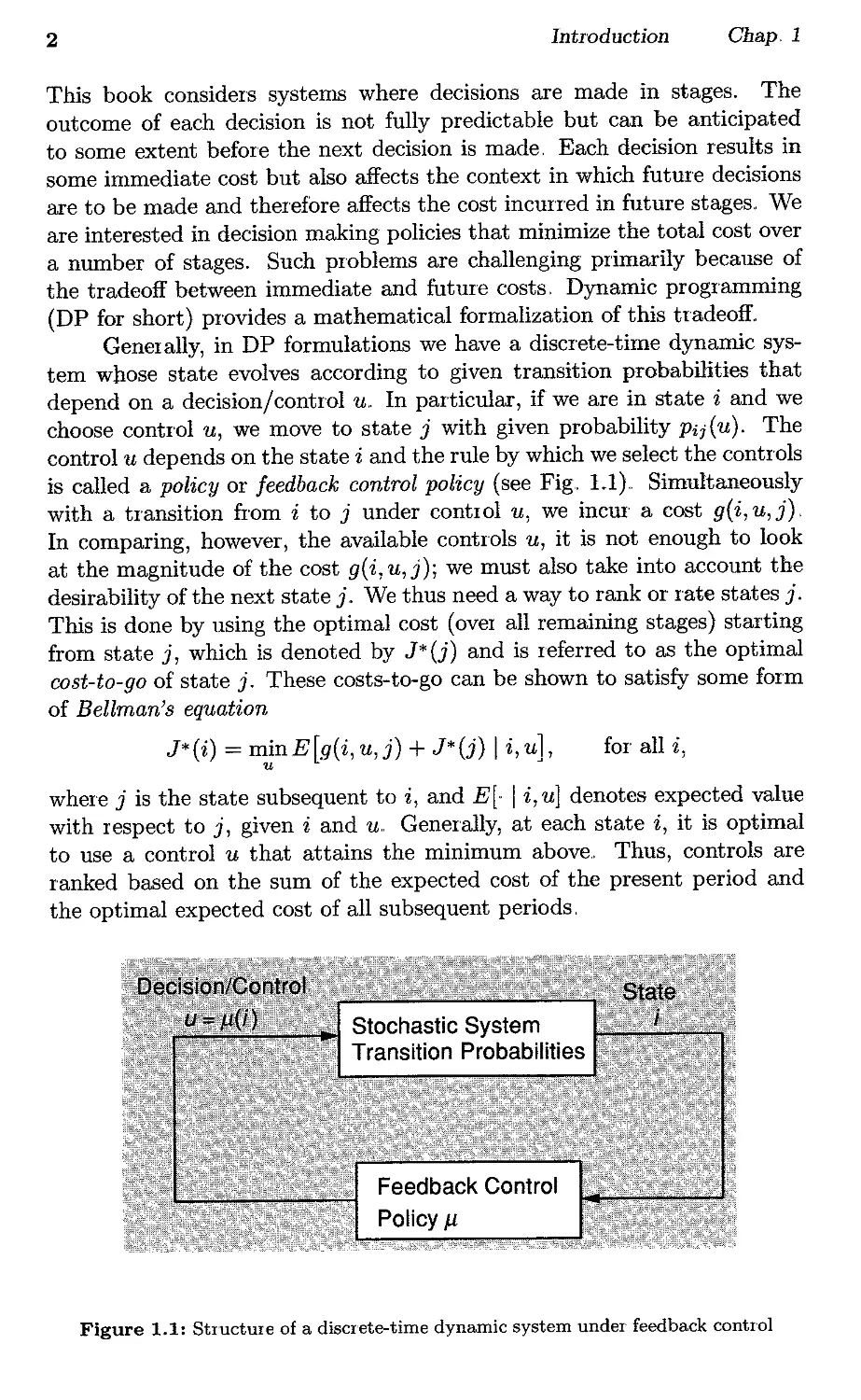
is called a policy or feedback control policy (see Fig., 1.1).. Simultaneously
with a transition from i to j under contIOI u, we incUI' a cost g( i, u, j) ,
In comparing, however, the available controls u, it is not enough to look
at the magnitude of the cost g(i,u,j); we must also take into account the
desirability of the next state j.. We thus need a way to rank or rate states j.
This is done by using the optimal cost (over all remaining stages) starting
from state j, which is denoted by J* (j) and is referred to as the optimal
cost-to-go of state j. These costs-to-go can be shown to satisfy some form
of Bellman's equation
J*(i) = mJnE[g(i,u,j) + J*(j) I i,u],
for all i,
where j is the state subsequent to i, and E[, Ii, u) denotes expected value
with respect to j, given i and u.. Generally, at each state i, it is optimal
to use a control u that attains the minimum above., Thus, controls are
ranked based on the sum of the expected cost of the present period and
the optimal expected cost of all subsequent periods,
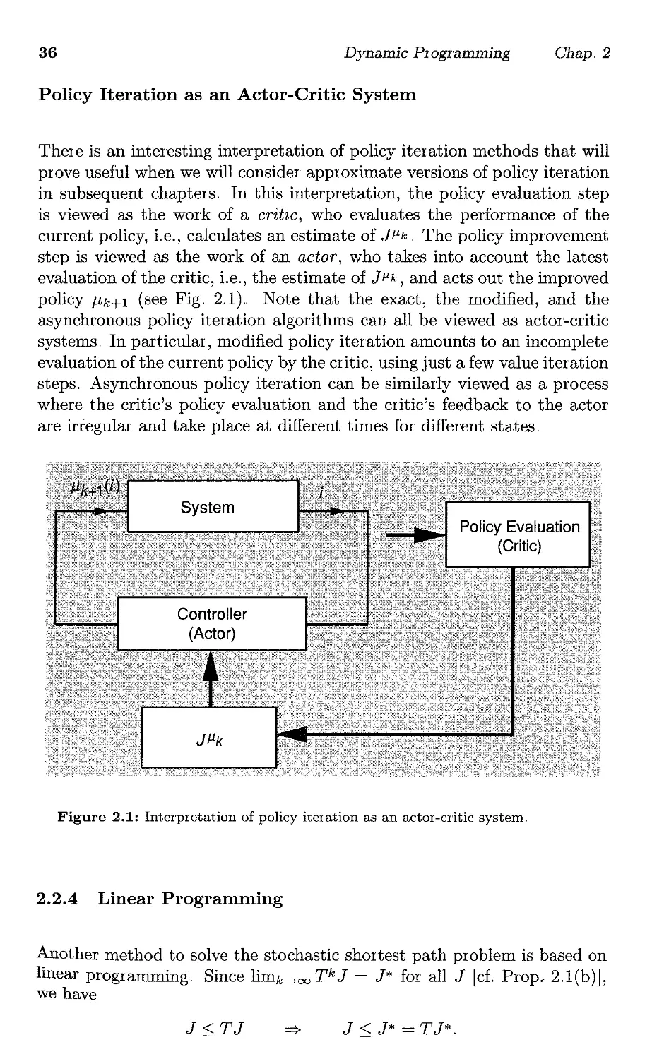
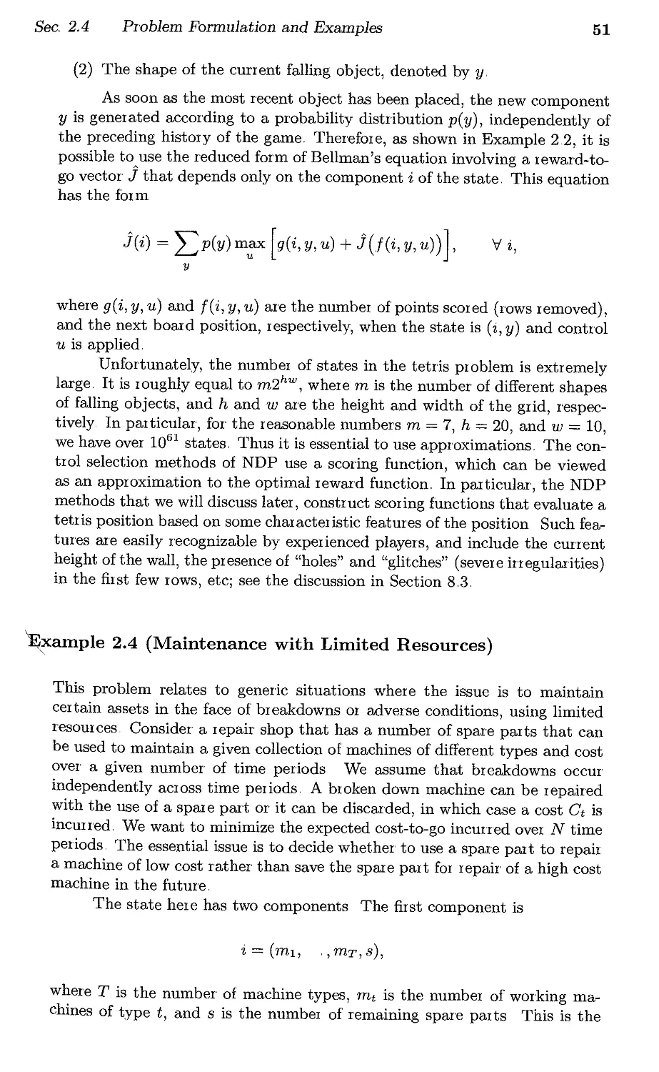
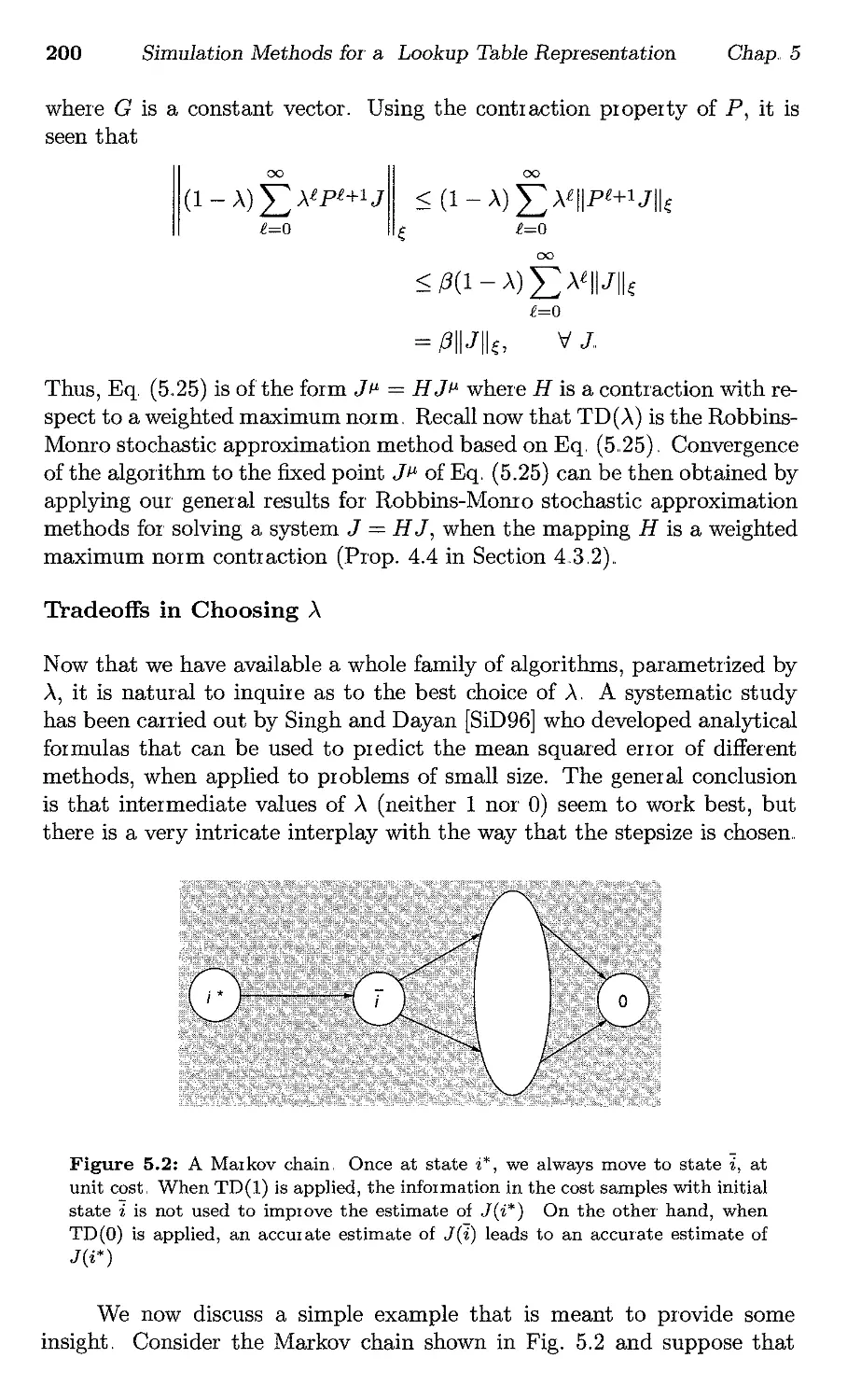
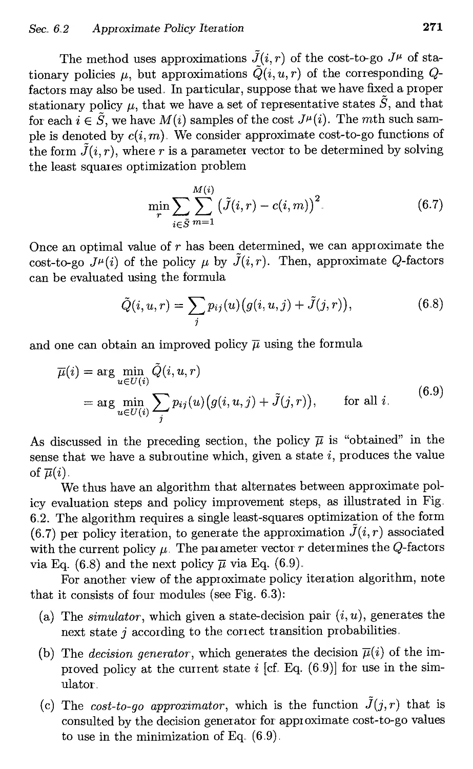
Figure 1.1: Structure of a discrete-time dynamic system under feedback control
Sec. 1..1
Cost-to-go Approximations in Dynamic Programming
3
The objective of DP is to calculate numerically the optimal cost-to-
gO' functiQn J*.. This computation can be done off-line, i.e., before the real
system starts Qperating., An optimal policy, that is, an Qptimal choice of
u for each i, is computed either simultaneously with J*, Qr in real time by
minimizing in the right-hand side Qf Bellman's equation. It is well known,
however, that for many important problems the computational require-,
ments of DP are overwhelming, because the number Qf states and controls
is very large (Bellman's "curse of dimensionality"), In such situations a
suboptimal solution is required.,
1.1 COST-TO-GO APPROXIMATIONS IN DYNAMIC
PROGRAMMING
In this book, we primarily focus on suboptimal methods that center around
the evaluatiQn and approximation of the optimal CQst-to-go function J*,
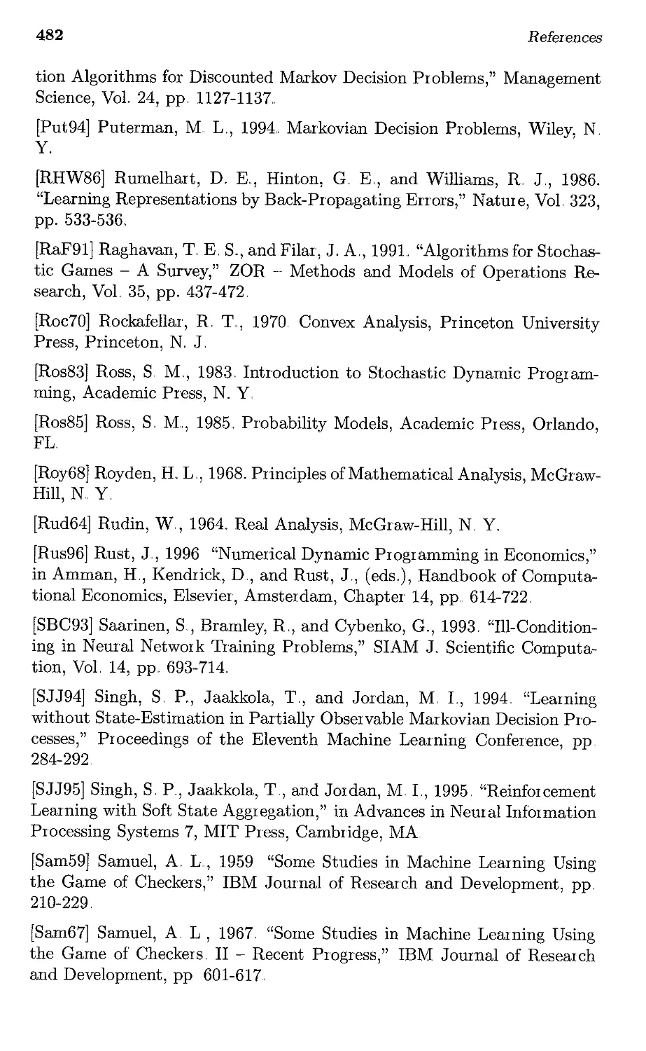
PQssibly thrQugh the use of neural networks and/or simulatiQn.. In partic-
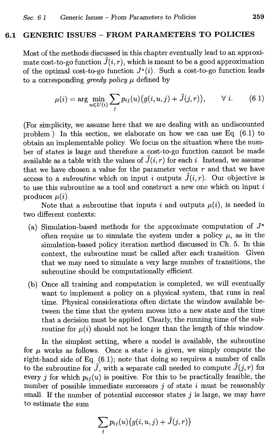
ular, we replace the optimal CQst-to-go J*(j) with a suitable approxima-
tion J(j, r), where r is a vector of parameters, and we use at state i the
(suboptimal) control jl(i) that attains the minimum in the (approximate)
right-hand side Qf Bellman's equation, that is,
jl(i} = argminE[g(i, u,j) + J(j, r) Ii, u]
u
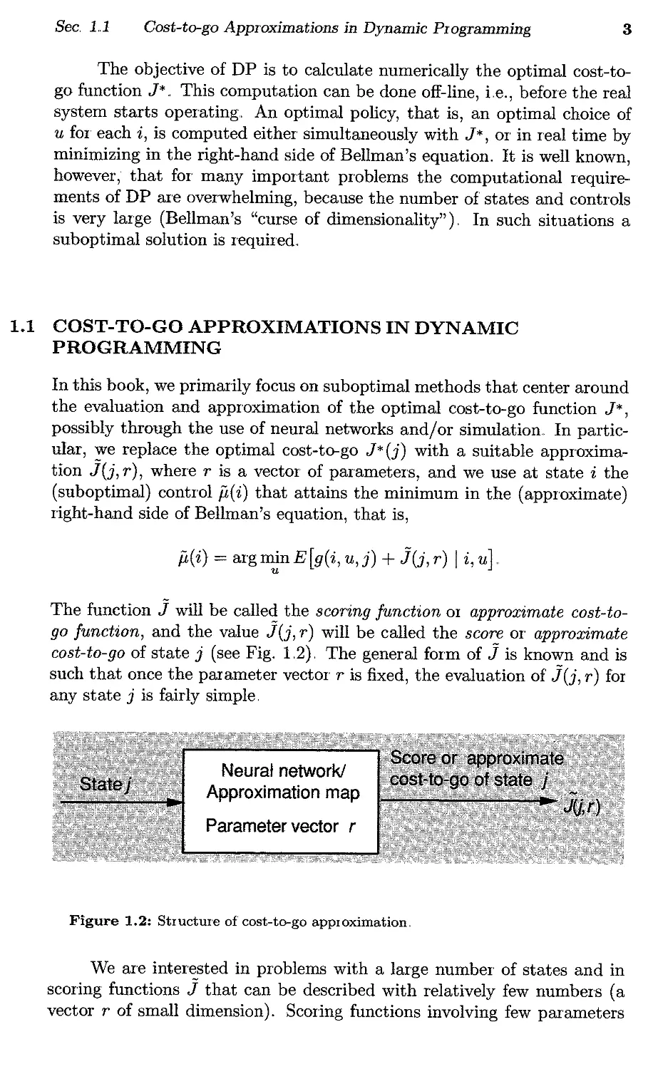
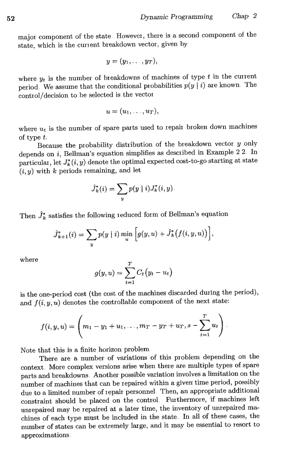
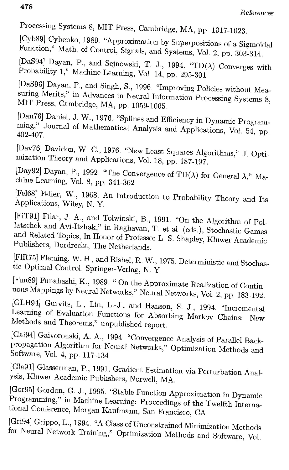
The functiQn J will be called the scoTing function or approximate cost-to-
ga function, and the value J(j, r) will be called the score or approximate
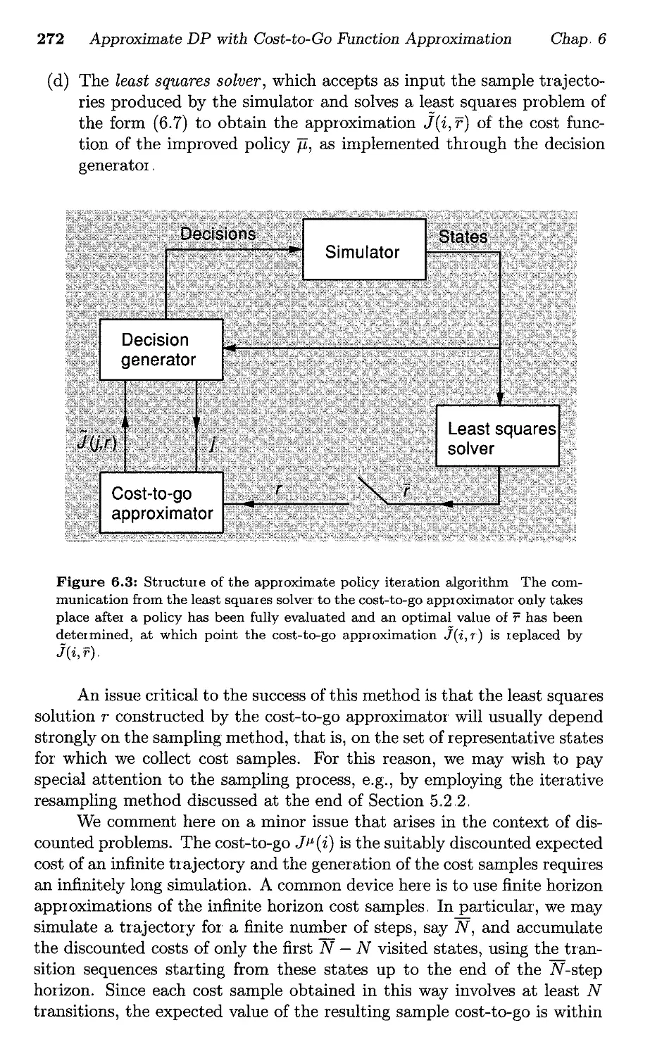
cost-to-go Qf state j (see Fig. 1,2), The general form Qf J is known and is
such that once the par ameter vector r is fixed, the evaluation of J (j, r) for
any state j is fairly simple,
Neural network!
Approximation map
Parameter vector r
Figure 1.2: Structure of cost-to-go appIOximation,
We are interested in probleIllS with a large number of states and in
scoring functiQns J that can be described with relatively few numbers (a
vector r of small dimension). Scoring functions involving few par'ameters
4
IntIOduction
Chap. 1
will be called compact representations, while the tabular description of J*
will be called the lookup table representation. In a lookup table represen-
tation, the values J*(j) for all states j ar'e stored in a table., In a typical
compact representation, only the vector r and the general structure of the
scoring function 1e., r) are stored; the scores l(j, r) are generated only
when needed, For example, if 1(j, r) is the output of some neural network
in response to the input j, then r is the associated vector of weights or
parameters of the neural network; or if l(j, r) involves a lower dimensional
description of the state j in terms of its "significant features," then r could
be a vector of relative weights of the features, Naturally, we would like to
choose r algorithmically so that 1 C, r) approximates well J * (). Thus, de-
termining the scoring function 1(j, r) involves two complementary issues:
(1) deciding on the general structure of the function l(j,r), and (2) cal-
culating the parameter vector r so as to minimize in some sense the error
between the functions J*C) and l(.,r).
We note that in some problems the evaluation of the expression
E[g(i,u,j) + l(j,r) I i,u],
for each u, may be too complicated or too time-consuming for making deci-
sions in real-time, even if the scores 1(j, r) are simply calculated. There are
a number of ways to deal with this difficulty (see Section 6.1)., An impor-
tant possibility is to approximate the expression minimized in Bellman's
equation,
Q*(i,u) = E(g(i,u,j) + J*(j) I i,u],
which is known as the Q-factor corresponding to (i, u). In particular, we
can replace Q*(i, u) with a suitable approximation Q(i, u, r), where r is a
vector of parameters. We can then use at state i the (suboptimal) control
that minimizes the approximate Q-factor corresponding to i:
ji,(i) = argminQ(i,u,r).
u
Much of what will be said about the approximation of the optimal costs-
to-go also applies to the approximation of Q-factors. In fact, we will see
later that the Q-factors can be viewed as optimal costs-to-go of a related
problem We thus focus primarily on approximation of the optimal costs-
to-go.
Approximations of the optimal costs-to-go have been used in the past
in a variety of D P contexts, Chess playing progr ams represent an interest-
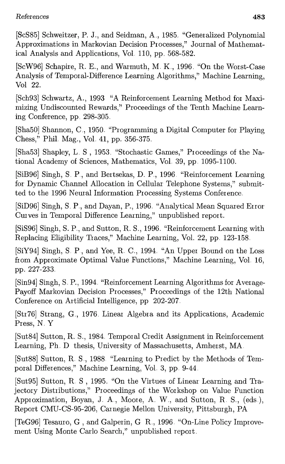
ing example, A key idea in these programs is to use a position evaluator
to rank different chess positions and to select at each turn a move that
results in the position with the best rank. The position evaluator assigns
a numerical value to each position according to a heuristic formula that
includes weights for the various features of the position (material balance,
See 1,2
Approximation Architectures
5
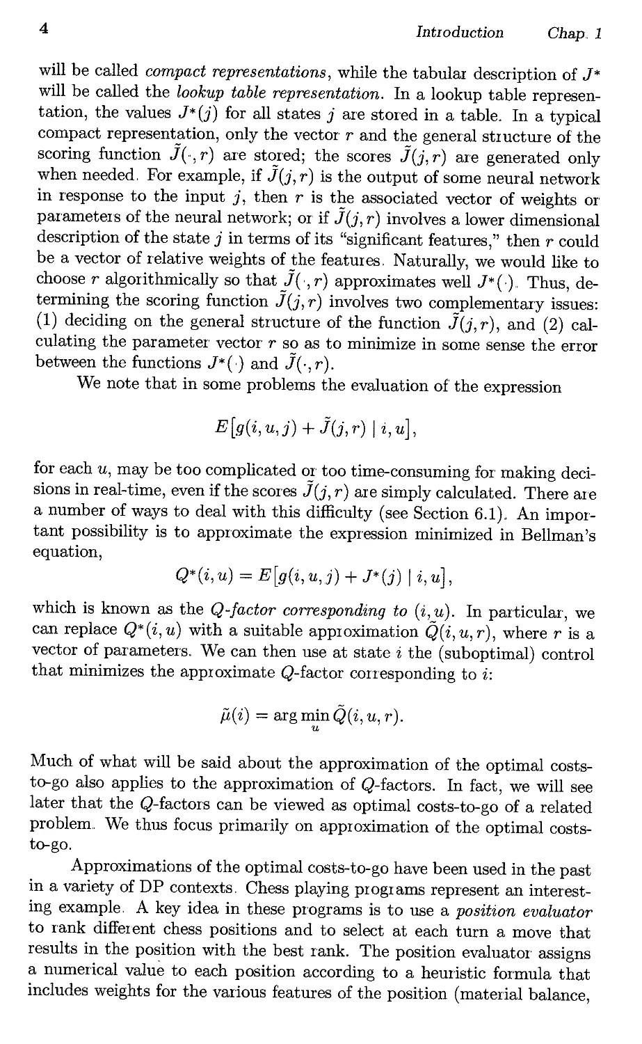
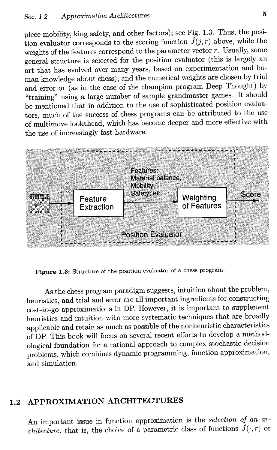
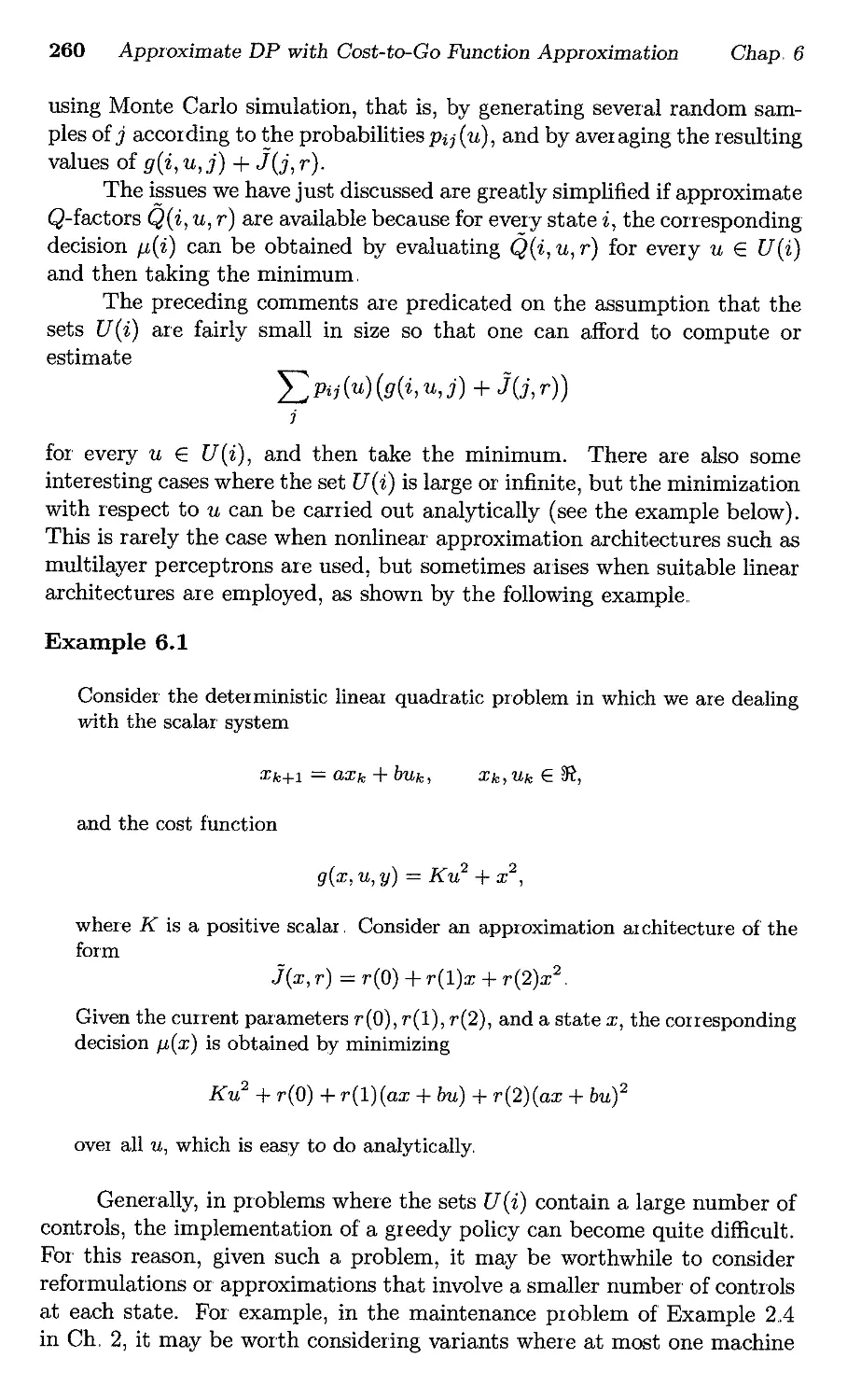
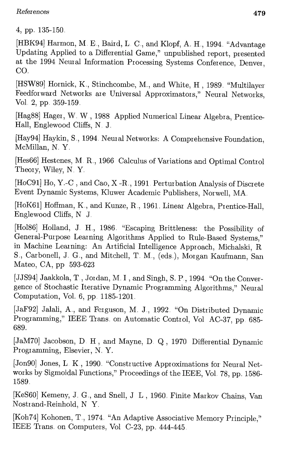
piece mobility, king safety, and other factors); see Fig. 1.3., Thus, the posi-
tion evaluator corresponds to the scoring function J(j, r) above, while the
weights of the features correspond to the par ameter vector r. Usually, some
general structure is selected for the position evaluator (this is largely an
art that has evolved over many years, based on experimentation and hu-
man knowledge about chess), and the numerical weights are chosen by trial
and error or (as in the case of the champion program Deep Thought) by
"training" using a large number of sample grandmaster games, It should
be mentioned that in addition to the use of sophisticated position evalua-
tors, much of the success of chess programs can be attributed to the use
of multimove lookahead, which has become deeper and more effective with
the use of increasingly fast hardware.
Figure 1.3: Stmcture of the position evaluator of a chess program,
As the chess program paradigm suggests, intuition about the problem,
heuristics, and trial and error are all important ingredients for constructing
cost-to-go approximations in DP, However, it is important to supplement
heuristics and intuition with more systematic techniques that are broadly
applicable and retain as much as possible of the nonheuristic characteristics
of DP, This book will focus on several recent efforts to develop a method-
ological foundation for a rational approach to complex stochastic decision
problems, which combines dynamic programming, function approximation,
and simulation.
1.2 APPROXIMATION ARCHITECTURES
An important issue in function approximation is the selection of an ar-
chitecture, that is, the choice of a parametric class of functions JC', r) or
6
Introduction
Chap.. 1
Q(."r) that suits the problem at hand. One possibility is to use a neu-
ral network architecture of some type.. We should emphasize here that in
this book we use the term "neural network" in a very broad sense, essen-
tially as a synonym to "approximating architecture." In particular, we do
not restrict oUI'selves to the classical multilayer perceptron structure with
sigmoidal nonlinearities.. Any type of universal approximator of nonlinear
mappings could be used in our context. The nature of the approximating
structure is left open in our discussion, and it could involve, for example,
radial basis functions, wavelets, polynomials, splines, aggregation, etc.
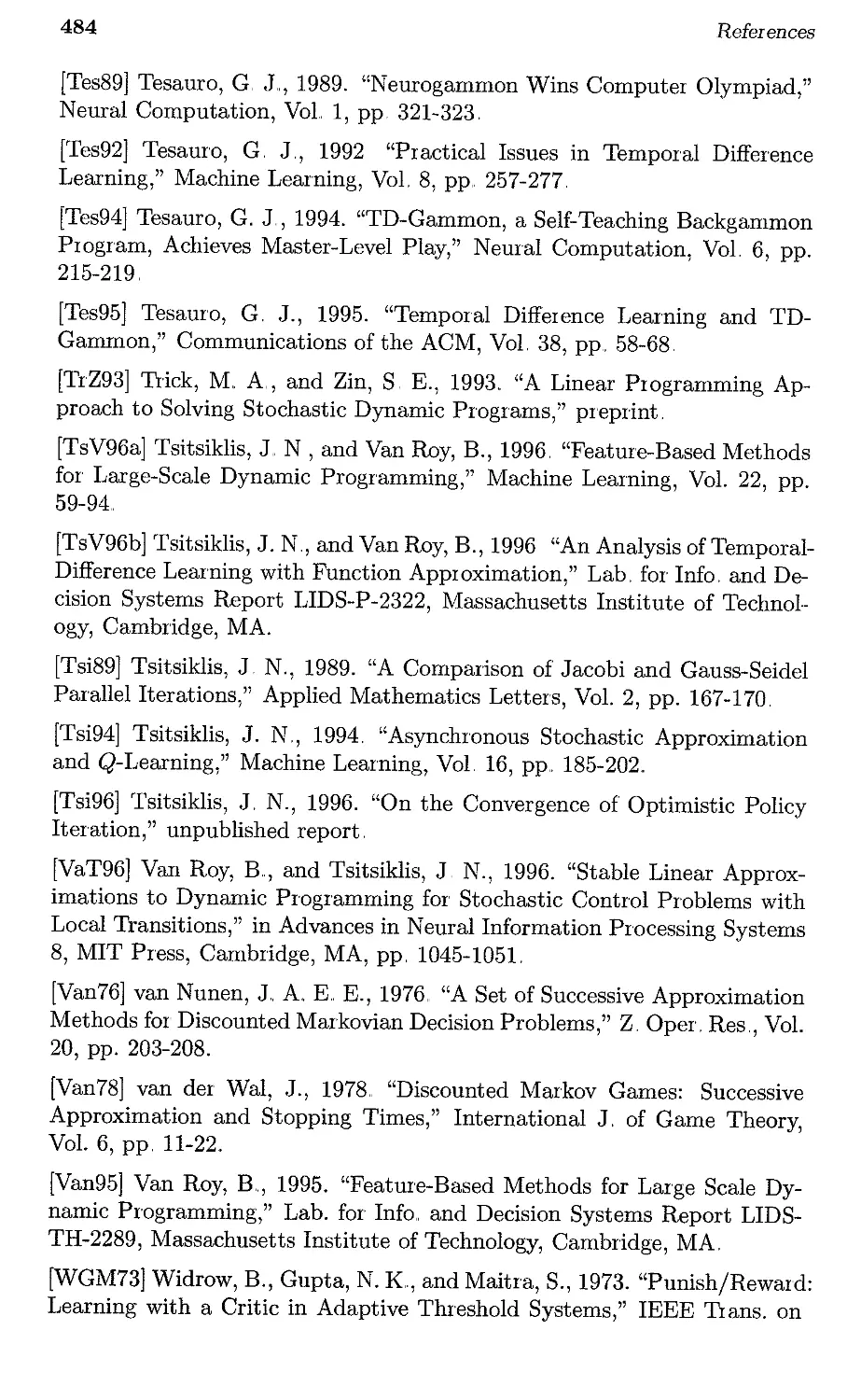
Cost-to-go approximation can often be significantly enhanced through
the use of feature extraction, a process that maps the state i into some vec-
tor f (i), called the feature vector associated with i. Feature vectors sum-
marize, in a heuristic sense, what are considered to be important character-
istics of the state, and they are very useful in incorporating the designer's
prior knowledge or intuition about the problem and about the structure
of the optimal controller.. For example, in a queueing system involving
several queues, a feature vector may involve for each queue a three-valued
indicator that specifies whether the queue is "nearly empty," "moderately
busy," or "nearly full." In many cases, analysis can complement intuition
to suggest the right features for the problem at hand.
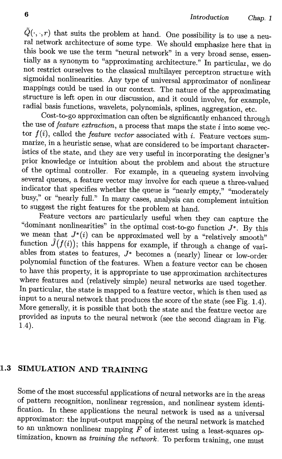
Feature vectors are particularly useful when they can capture the
"dominant nonlinearities" in the optimal cost-to-go function J*. By this
we mean that J*(i) can be approximated well by a "relatively smooth"
function j (J (i) ); this happens for example, if through a change of vari-
ables from states to features, J* becomes a (nearly) linear or low-order
polynomial function of the features. When a featUI'e vector can be chosen
to have this property, it is appropriate to use approximation architectures
where features and (relatively simple) neural networks are used together,.
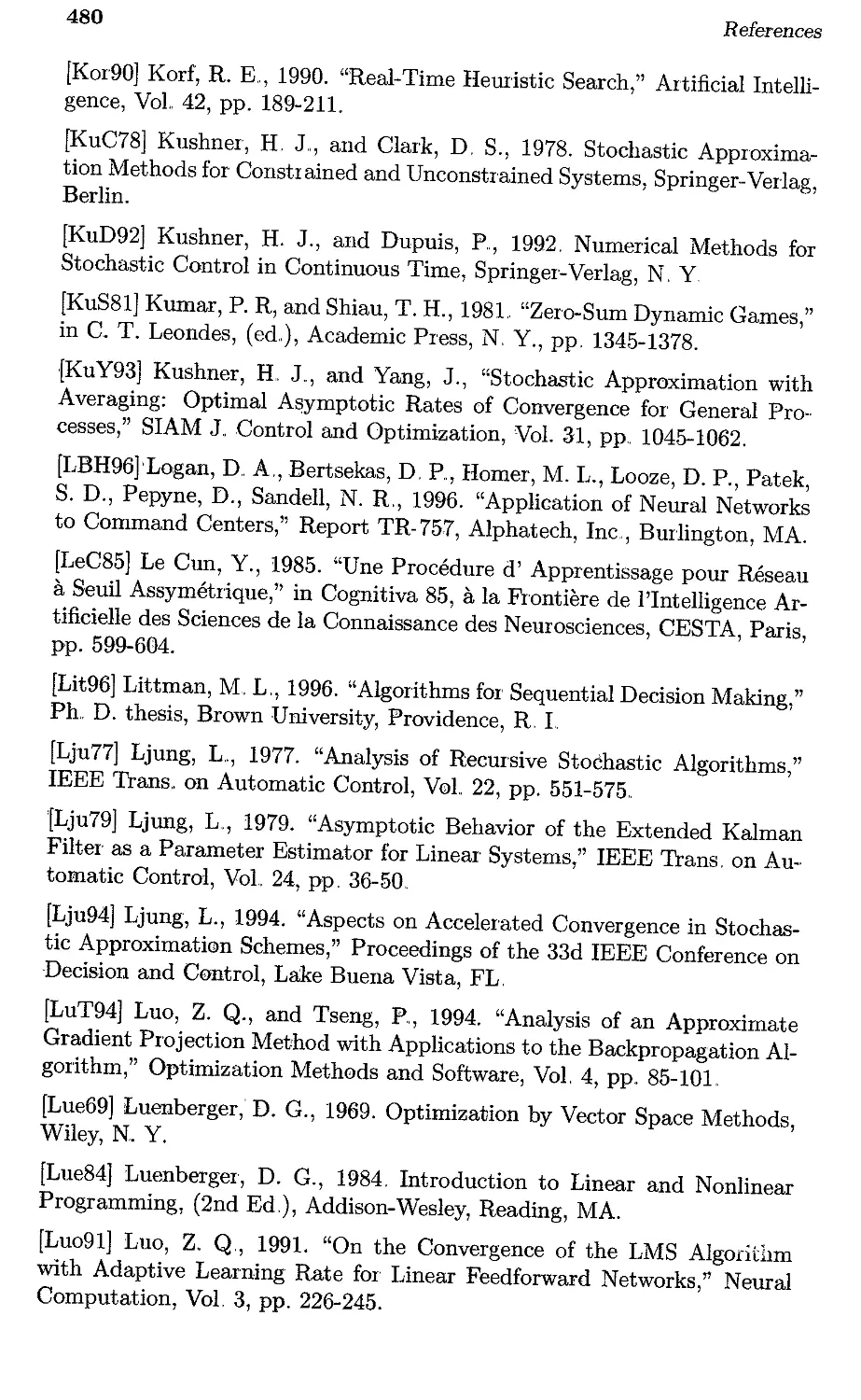
In particular, the state is mapped to a feature vector, which is then used as
input to a neUI'al network that produces the score of the state (see Fig, 1..4).
More generally, it is possible that both the state and the feature vector are
provided as inputs to the neural network (see the second diagram in Fig.
1.4).
1.3 SIMULATION AND TRAINING
Some of the most successful applications of neural networks are in the areas
of pattern recognition, nonlinear regression, and nonlinear system identi-
fication. In these applications the neural network is used as a universal
approximator: the input-output mapping of the neural network is matched
to an unknown nonlinear mapping F of interest using a least-squares op-
timization, known as tmining the network.. To perform training, one must
Sec. 1,3
Simulation and 'ITaining
7
Figure 1.4: Approximation architectures involving featme extlaction and nemal
netwOl ks,
have some training data, that is, a set of pairs (i, F( i)), which is represen-
tative of the mapping F that is approximated.,
It is important to note that in contrast with these neural network
applications, in the DP context there is no readily available training set of
input-output pairs (i, J* (i)) that could be used to approximate J* with a
least squares fit.. The only possibility is to evaluate (exactly or approxi-
mately) by simulation the cost-to-go functions of given (suboptimal) poli-
cies, and to try to iteratively improve these policies based on the simulation
outcomes. This creates analytical and computational difficulties that do
not arise in classical neural network training contexts Indeed the use of
simulation to evaluate approximately the optimal cost-to-go function is a
key new idea that distinguishes the methodology of this book from earlier
approximation methods in DP,
Simulation offers another major advantage: it allows the methods
of this book to be used for systems that are hard to model but easy to
simulate, i..e., problems where a convenient explicit model is not available,
and the system can only be observed, either through a software simulator or
as it operates in real time, For such problems, the traditional DP techniques
are inapplicable, and estimation of the transition probabilities to construct
a detailed mathematical model is often cumbersome or impossible.,
There is a third potential advantage of simulation: it can implicitly
identify the "most important" or "most representative" states of the sys-
tem, It appears plausible that these states are the ones most often visited
during the simulation, and for this reason the scoring function will tend to
approximate better the optimal cost-to-go for these states, and the subop-
timal policy obtained will on the average perform better
o
Introduction
Chap. 1
1.4 NEURO-DYNAMIC PROGRAMMING
In view of the reliance on both DP and neural network concepts, we use the
name neuro-dynamic programming (NDP for short) to describe collectively
the methods of this book. In the artificial intelligence community, where
the methods originated, the name reinforcement learning is also used. In
common artificial intelligence terms, the methods of this book allow sys-
tems to "learn how to make good decisions by observing their own be-
havior, and use built-in mechanisms for improving their actions through
a reinforcement mechanism." In the less anthropomorphic DP terms used
in this book, "observing their own behavior" relates to simulation, and
"improving their actions through a reinforcement mechanism" relates to
iterative schemes for improving the quality of approximation of the opti-
mal costs-to-go, or the Q-factors, or the optimal policy.. There has been a
gradual realization that reinforcement learning techniques can be fruitfully
motivated and interpreted in terms of classical DP concepts such as value
and policy iteration..
In this book, we attempt to clarify some aspects of the current NDP
methodology, we suggest some new algorithmic approaches, and we iden-
tify some open questions.. Despite the great interest in NDP, the theory of
the subject is only now beginning to take shape, and the corresponding lit-
erature is often confusing. Yet, there have been many reports of successes
with problems too large and complex to be treated in any other way. A
particularly impressive success that greatly motivated subsequent research,
was the development of a backgammon playing program by Tesauro [Tes92]
(see Section 8.6). Here a nemal network was trained to approximate the
optimal cost-to-go function of the game of backgammon by using simula-
tion, that is, by letting the program play against itself. After training for
several months, the program nearly defeated the human world champion..
Unlike chess programs, this program did not use lookahead of many stages,
so its success can be attributed primarily to the use of a properly trained
approximation of the optimal cost-to-go function..
Our own experience has been that NDP methods can be impressively
effective in problems where traditional DP methods would be hardly ap-
plicable and other hemistic methods would have limited potentiaL In this
book, we outline some engineering applications, and we use a few compu-
tational studies for illustrating the methodology and some of the art that
is often essential for success.
We note, however, that the practical application of NDP is compu-
tationally very intensive, and often requires a considerable amount of trial
and error, Furthermore, success is often obtained using methods whose
properties are not fully understood. Fortunately, all of the computation
and experimentation with different approaches can be done off-line. Once
the approximation is obtained off-line, it can be used to generate decisions
fast enough for use in real time. In this context, we mention that in the
Sec. 14
Notes and Sources
9
artificial intelligence literature, reinforcement learning is often viewed as
an "on-line" method, whereby the cost-to-go approximation is improved
as the system operates in real time. This is reminiscent of the methods
of traditional adaptive controL We will not discuss this viewpoint in this
book, as we prefer to focus on applications involving a large and complex
system. A lot of training data are required for such systems.. These data
often cannot be obtained in sufficient volume as the system is operating;
even if they can, the corresponding processing requirements are often too
large for effective use in real time.,
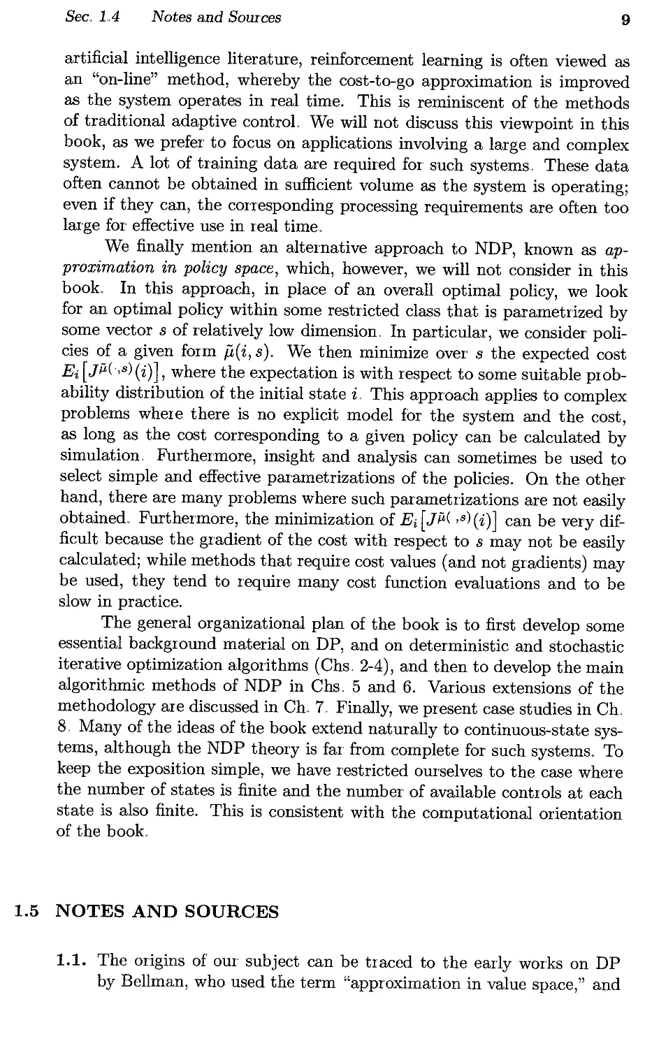
We finally mention an alternative approach to NDP, known as ap-
proximation in policy space, which, however, we will not consider in this
book. In this approach, in place of an overall optimal policy, we look
for an optimal policy within some restricted class that is parametrized by
some vector s of relatively low dimension, In particular, we consider poli-
cies of a given form ji,( i, s). We then minimize over s the expected cost
E i [Jjj,(,s) (i)], where the expectation is with respect to some suitable prob-
ability distribution of the initial state i. This approach applies to complex
problems where there is no explicit model for the system and the cost,
as long as the cost corresponding to a given policy can be calculated by
simulation, Furthermore, insight and analysis can sometimes be used to
select simple and effective par'ametrizations of the policies. On the other
hand, there are many problems where such parametrizations are not easily
obtained., Furthermore, the minimization of Ei[Jjj,( ,s)(i)] can be very dif-
ficult because the gradient of the cost with respect to s may not be easily
calculated; while methods that require cost values (and not gradients) may
be used, they tend to require many cost function evaluations and to be
slow in practice.
The general organizational plan of the book is to first develop some
essential background material on DP, and on deterministic and stochastic
iterative optimization algorithms (Chs, 2-4), and then to develop the main
algorithmic methods of NDP in Chs, 5 and 6. Various extensions of the
methodology are discussed in Ch 7.. Finally, we present case studies in Ch.
8. Many of the ideas of the book extend naturally to continuous-state sys-
tems, although the NDP theory is far from complete for such systems.. To
keep the exposition simple, we have restricted ourselves to the case where
the number of states is finite and the number of available controls at each
state is also finite. This is consistent with the computational orientation
of the book.
1.5 NOTES AND SOURCES
1.1. The origins of our subject can be traced to the early works on DP
by Bellman, who used the term "approximation in value space," and
10
Introduction
Chap. 1
to the works by Shannon [Sha50] on computer chess and by Samuel
[Sam59], [Sam67] on computer checkers.
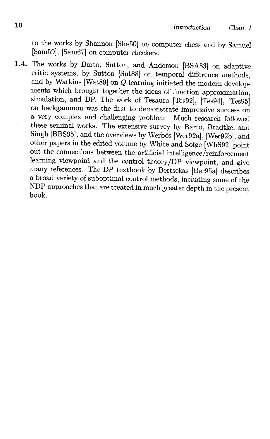
1.4. The works by Barto, Sutton, and Anderson [BSA83] on adaptive
critic systems, by Sutton [Sut88] on temporal difference methods,
and by Watkins [Wat89] on Q-Iearning initiated the modern develop-
ments which brought together the ideas of function approximation,
simulation, and DP.. The work of Tesauro [Tes92], [Tes94], [Tes95]
on backgammon was the first to demonstrate impressive success on
a very complex and challenging problem. Much research followed
these seminal works, The extensive survey by Barto, Bradtke, and
Singh [BBS95], and the overviews by Werbos [Wer92a], [Wer92b], and
other papers in the edited volume by White and Sofge [WhS92] point
out the connections between the artificial intelligence/reinforcement
learning viewpoint and the control theory /DP viewpoint, and give
many references, The DP textbook by Bertsekas [Ber95a] describes
a broad variety of suboptimal control methods, including some of the
NDP approaches that are treated in much greater depth in the present
book.
Philosophy is wTitten in this grand book, the universe,
which stands continually open to our gaze..
But the book cannot be understood
unless one first learns to comprehend the language
and read the letters in which it is composed.
It is written in the language of mathematics,
(Galileo)
2
Dynamic Programming
12
Dynamic Programming
Chap. 2
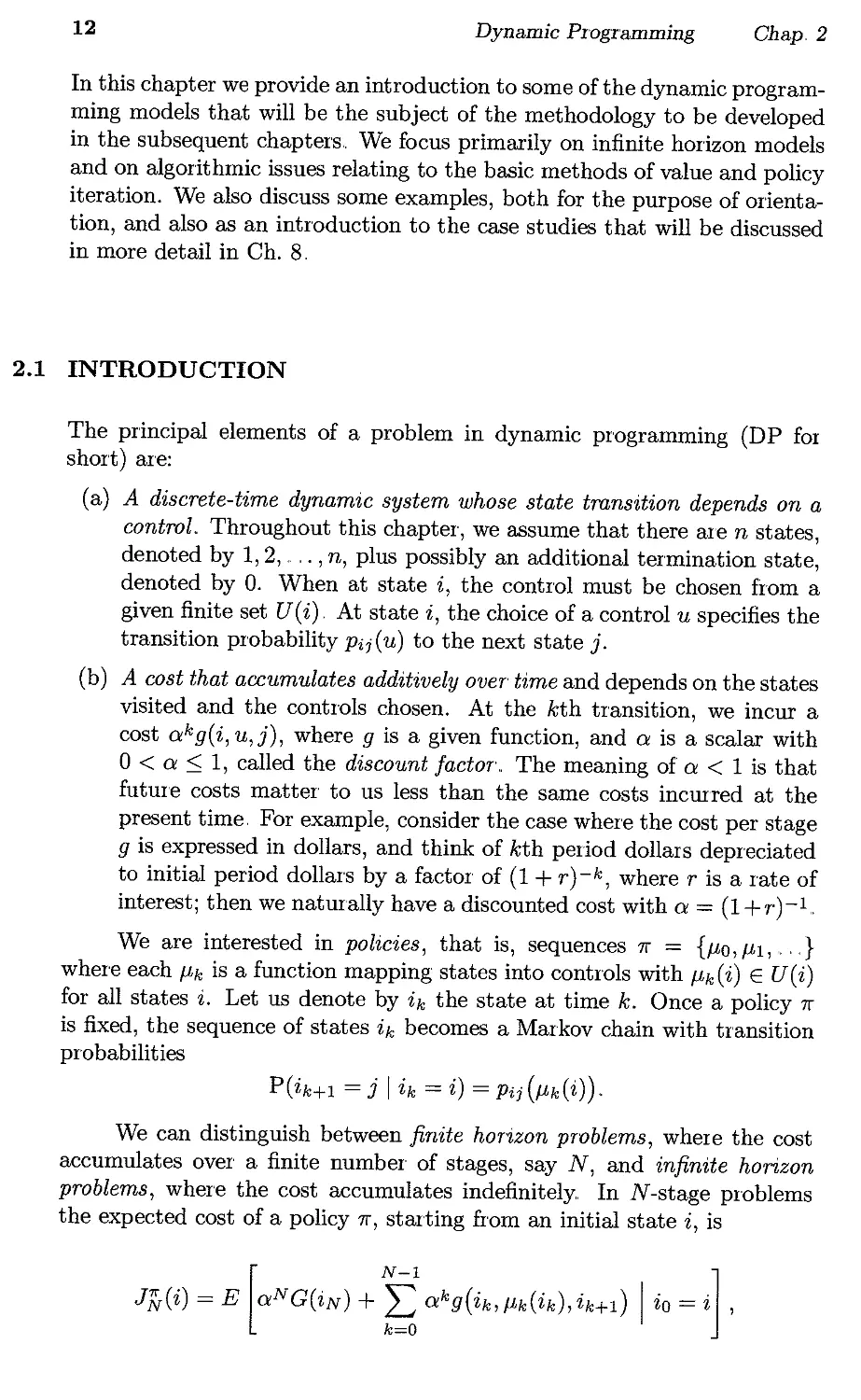
In this chapter we provide an introduction to some of the dynamic program-
ming models that will be the subject of the methodology to be developed
in the subsequent chapters., We focus primarily on infinite horizon models
and on algorithmic issues relating to the basic methods of value and policy
iteration. We also discuss some examples, both for the purpose of orienta-
tion, and also as an introduction to the case studies that will be discussed
in more detail in Ch. 8,
2.1 INTRODUCTION
The principal elements of a problem in dynamic programming (DP for
short) are:
(a) A discrete-time dynamic system whose state tmnsition depends on a
control.. Throughout this chapter, we assume that there are n states,
denoted by 1,2, .. , . , n, plus possibly an additional termination state,
denoted by O. When at state i, the control must be chosen from a
given finite set U (i). At state i, the choice of a control u specifies the
transition probability Pii(U) to the next state j.
(b) A cost that accumulates additively over' time and depends on the states
visited and the controls chosen. At the kth transition, we incur a
cost akg(i, u,j), where g is a given function, and a is a scalar with
o < a :::; 1, called the discount factor', The meaning of a < 1 is that
future costs matter to us less than the same costs incurred at the
present time For example, consider the case where the cost per stage
g is expressed in dollars, and think of kth period dollars depreciated
to initial period dollars by a factor of (1 + r) - k, where r is a rate of
interest; then we naturally have a discounted cost with a = (l+r)-l
We are interested in policies, that is, sequences 1f = {I-lO,l-ll,..,.}
where each I-lk is a function mapping states into controls with I-lk(i) E U(i)
for all states i. Let us denote by ik the state at time k. Once a policy 1f
is fixed, the sequence of states ik becomes a Markov chain with transition
probabilities
Ph+l = j I ik = i) = Pii(l-lk(i)).,
We can distinguish between finite horizon problems, where the cost
accumulates over a finite number of stages, say N, and infinite horizon
problems, where the cost accumulates indefinitely.. In N-stage problems
the expected cost of a policy 1f, starting from an initial state i, is
[ N-l ]
J'N(i) = E aNG(iN) + (; akg(ik,l-lk(ik),ik+1) I io = i ,
Sec, 21
Introduction
13
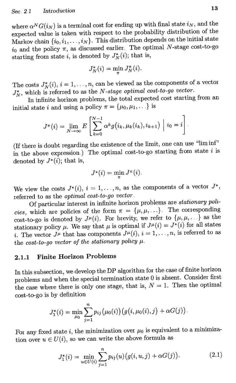
where aN G( iN) is a terminal cost for ending up with final state iN, and the
expected value is taken with respect to the probability distribution of the
Markov chain {io, il,.. " iN}. This distribution depends on the initial state
io and the policy 1f, as discussed earlier, The optimal N-stage cost-to-go
starting from state i, is denoted by J'N(i); that is,
J'N(i) = min IN(i).
7r
The costs J'N(i), i = 1,.. .." n, can be viewed as the components of a vector
J'N, which is referred to as the N-stage optimal cost-to-go vector.
In infinite horizon problems, the total expected cost starting from an
initial state i and using a policy 1f = {/-lO,/-ll,.. ,} is
[ N-l ]
J7r(i) = J oo E L akg(ik,/-lk(ik),ik+l) I io = i .
k=O
(If there is doubt regarding the existence of the limit, one can use "lim inf"
in the above expression.) The optimal cost-to-go starting from state i is
denoted by J*(i); that is,
J*(i) = minJ7r(i)..
7r
We view the costs J*(i), i = 1,.. " n, as the components of a vector J*,
referred to as the optimal cost-to-go vector',
Of particular interest in infinite horizon problems are stationary poli-
cies, which are policies of the form 1f = {/-l, /-l, .. . .}, The corresponding
cost-to-go is denoted by JI-'(i). For brevity, we refer to {/-l, /-l,... ,} as the
stationary policy /-l. We say that /-l is optimal if JI-'(i) = J*(i) for all states
i. The vector JI-' that has components JI-'(i), i = 1,.. "n, is referred to as
the cost-to-go vector of the stationary policy /-l,
2.1.1 Finite Horizon Problems
In this subsection, we develop the DP algorithm for the case of finite horizon
problems and when the special termination state 0 is absent. Consider first
the case where there is only one stage, that is, N = 1. Then the optimal
cost-to-go is by definition
n
Ji(i) = min LPij (/-lo(i)) (g(i, /-lo(i),j) + aG(j)) ,
1-'0 j=l
For any fixed state i, the minimization over /-lO is equivalent to a minimiza-
tion over u E U(i), so we can write the above formula as
n
Ji(i) = min LPij(u)(g(i,u,j) + aG(j)).
uEU(,) j=l
(2.1)
14
Dynamic PIOgr amming
Chap. 2
The interpretation of this formula is that the optimal control choice with
one period to go must minimize the sum of the expected present stage cost
and the expected future cost G(j) appropriately discounted by a. The DP
algorithm expresses a generalization of this idea. It states that the optimal
control choice with k stages to go must minimize the sum of the expected
present stage cost and the expected optimal cost J/:_ 1 (j) with k - 1 stages
to go, appropriately discounted by a; that is,
n
J/:(i) = min LPij(u)(g(i,u,j) + aJ/:__1(j)),
uEU(.) j=l
i = 1, . .. . ,n.. (2..2)
Thus, the optimal N-stage cost-to-go vector IN(i) can be calculated recur-
sively with the above formula, starting with
\
Jr;(i) = G(i),
i = 1,... ,n,
(2.3)
To prove this, we argue as follows. Any policy 1rk for the problem with
k stages to go and initial state i is of the form {u, 1rk-d, where u E U( i) is
the control at the first stage and 7rk-l is the policy for the remaining k - 1
stages. Thus,
n
J/:(i) = min LPij(u)(g(i,u,j) + aJ: 11(j))
uEU(,), 7rk-l j=l
n
= min LPij(U)(g(i,u,j) + a min J: 11(j))
uEU(.) j=l 7rk-l
n
= min LPij(u)(g(i,u,j) +aJ/:_1(j)).
uEU(,) j=l
This argument can also be used to prove that if f.-lN_k(i) attains the min-
imum for each k and i in the DP equation (2.2), then the policy 1r*
{f.-la, f.-li,. ,., f.-lN-l} is optimal for the N-stage problem; that is, IN(i) =
J;'; (i) for all i.
Ideally, we would like to use the DP algorithm (2,2) to obtain closed-
form expressions for the optimal cost-to-go vectors J/: or an optimal policy.
Some interesting models admit analytical solution by DP, but in many prac-
tical cases an analytical solution is not possible, and one has to resort to nu-
merical execution of the DP algorithm. This may be very time-consuming,
because the computational requirements are at least proportional to the
number of possible state-control pairs as well as the number of stages N.
2.1.2 Infinite Horizon Problems
Infinite horizon problems represent a reasonable approximation of prob-
lems involving a finite but very large number of stages. These problems
Sec.. 2,1
Introduction
15
are also interesting because their analysis is elegant and insightful, and the
implementation of optimal policies is often simple. For example, optimal
policies are typically stationary; that is, the optimal rule for choosing con-
trols does not change from one stage to the next. We will consider three
principal classes of infinite horizon problems. In the first two classes, we
try to minimize J1r (i), the total cost over an infinite number of stages given
by
[ N -1 ]
J1r(i) = J oo E L a k g(ik,/tk(ik),ik+1) I io = i .
k=O
(a) Stochastic shortest path problems, Here, a = 1 but we assume that
there is an additional state 0, which is a cost-free termination state;
once the system reaches that state it remains there at no further cost.
The structure of the problem is assumed to be such that termination
is inevitable, at least under an optimal policy., Thus, the objective
is to reach the termination state with minimal expected cost, The
problem is in effect a finite hmizon problem, but the length of the
horizon may be random and may be affected by the policy being
used. We will consider these problems in the next section
(b) Discounted problems.. Here, we assume that a < 1. Note that the
absolute one-stage cost Jg( i, u, j) I is bounded from above by some
constant M, because of our assumption that i, u, and j belong to
finite sets; this makes the cost-to-go J1r (i) well defined because it is
the infinite sum of a sequence of number s that are bounded in absolute
value by the decreasing geometric progression a k M.. We will consider
these problems in Section 2.3,
(c) A vemge cost per stage problems. Minimization of the total cost J1r (i)
makes sense only if J1r(i) is finite for at least some policies 1f and
some initial states i. Frequently, however, we have J1r(i) = 00 for
every policy 1f and initial state i (think of the case where a = 1 and
the cost for every state and control is positive). It turns out that in
many such problems the average cost per stage, given by
1
lim N JN(i),
N->oo
where IN(i) is the N-stage cost-to-go of policy 1f starting at state i, is
well defined as a limit and is finite.. We will consider these problems
in Section 7,1.
A Preview of Infinite Horizon Results
There are several analytical and computational issues regarding infinite
horizon problems. Many of these revolve around the relation between the
16
Dynamic Programming
Chap. 2
optimal cost-to-go vector J* ofthe infinite horizon problem and the optimal
cost-to-go vectors of the corresponding N-stage problems. In particular,
let J'N(i) denote the optimal cost-to-go of the problem involving N stages,
initial state i, one-stage cost g( i, u, j), and zero terminal cost. For all states
i = 1, ' , . ,n, the optimal N-stage cost-to-go is generated after N iterations
of the DP algorithm
n
J;;+l (i) = min LPij(U) (g(i, u,j) + aJ;;(j)),
uEU(t) .
J=r
k = 0, 1, . . . (2.4)
starting from the initial condition Jfj (i) = 0 for all i. (We are assuming
here that the termination state 0 is absent.) Since the infinite horizon cost
of a given policy is, by definition, the limit of the corresponding N-stage
costs as N -+ 00, it is natural to speculate that:
(1) The optimal infinite horizon cost-to-go is the limit of the correspond-
ing N-stage optimal costs-to-go as N -+ 00, that is,
J*(i) = N lim IN(i),
->00
(2.5)
for all states i. This relation is very valuable computationally and
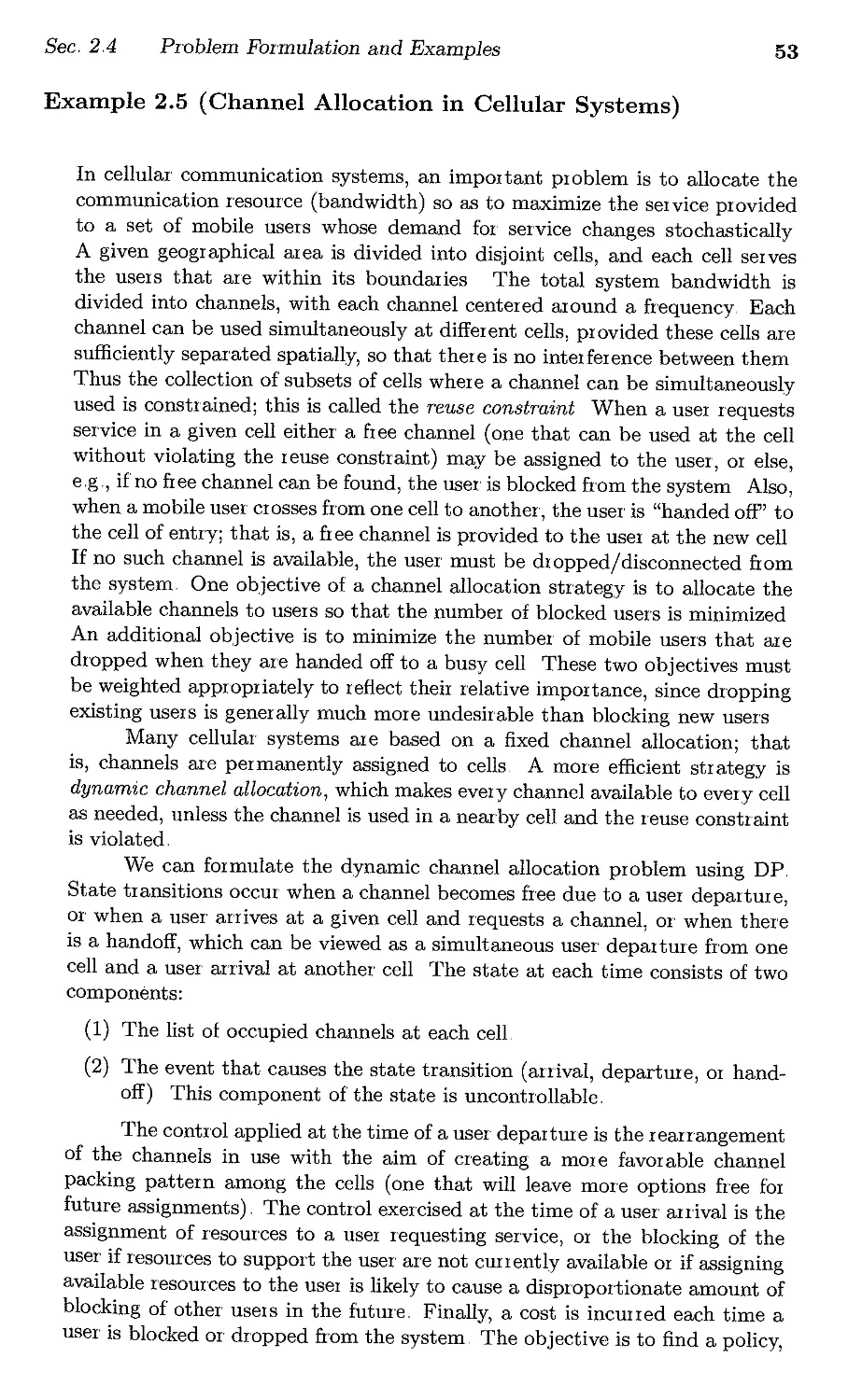
analytically, and fortunately, it typically holds.
(2) The following limiting form of the DP algorithm should hold for all
states i,
n
J*(i) = min LPij(u)(g(i,u,j) + aJ*(j)),
uEU(t) j=l
i = 1, . . . ,n, (2.6)
as suggested by Eqs.. (2.4) and (2.5). This is not really an algorithm,
but rather a system of equations (one equation per state), which has
as a solution the optimal costs-to-go of all the states. It will be
referred to as Bellman's equation, and it will be at the center of our
analysis and algorithms, An appropriate form of this equation holds
for every type of infinite horizon problem of interest to us in this
book.
(3) If f-l(i) attains the minimum in the right-hand side of Bellman's equa-
tion for each i, then the stationary policy f-l should be optimal. This
is true for most infinite horizon problems of interest and in particular,
for the models discussed in this book.
Most of the analysis of infinite horizon problems revolves around the
above three issues and also around the efficient computation of J* and
an optimal stationary policy. In the next three sections we will provide a
discussion of these issues. We focus primarily on results that are useful for
the developments in the subsequent chapters.
Sec, 2.2
Stochastic Shortest Path Problems
17
2.2 STOCHASTIC SHORTEST PATH PROBLEMS
Here, we assume that there is no discounting (a = 1) and, to make the
cost-to-go meaningful, we assume that there exists a cost-free termination
state, denoted by O. Once the system reaches that state, it remains there
at no further cost, that is,
poo(u) = 1,
g(O, U, 0) = 0,
VuE U(O).
We are interested in problems where reaching the termination state is in-
evitable, at least under an optimal policy. Thus, the essence of the problem
is how to reach the termination state with minimum expected cost.
Two special cases of the stochastic shortest path problem are worth
mentioning at the outset:
(a) The (deterministic) shortest path problem, obtained when the system
is deterministic, that is, when each control at a given state leads with
certainty to a unique successor state. This problem is usually defined
in terms of a directed gr aph consisting of n nodes plus a destination
node 0, and a set of arcs (i,j), each having a given cost Cij. The cost
of a path consisting of a sequence of arcs is the sum of the costs of
the arcs of the path. The objective is to find among all paths that
start at a given node and end at the destination, a path that has
minimum cost; this is also called a shortest path. If we identify nodes
with states, the outgoing arcs from a given node with the controls
associated with the state corresponding to the node, and the costs of
the arcs with the costs of the corresponding transitions, we obtain a
special case of the problem of this section..
(b) The finite horizon problem discussed earlier, where transitions and
cost accumulation stop after N stages, We can convert this problem
to a stochastic shortest path problem by viewing time as an extra
component of the state, Transitions occur from state-time pairs (i, k)
to state-time pairs (j, k + 1) according to the transition probabilities
Pij(U) of the finite horizon problem, The termination state corre-
sponds to the end of the horizon; it is reached in a single transition
from any state-time pair of the form (j, N) at a terminal cost G(j)
Note that this reformulation is valid even if the finite horizon problem
is nonstationary; that is, when the transition probabilities depend on
the time k
The above two special cases will often arise in various analytical con-
texts and examples, and while they possess special structure that simpli-
fies their solution, they also incorporate some of the key ingredients of the
generic stochastic shortest path pr oblem structure,
18
Dynamic Programming
Chap, 2
2.2.1 General Theory
In order to guar'antee the inevitability of termination under an optimal
policy, we introduce certain conditions that involve the notion of a proper
policy; that is, a stationary policy that leads to the termination state with
probability one, regardless of the initial state.
With a little thought, it can be seen that f..J, is proper if and only if
in the Markov chain corresponding to f..J" each state i is connected to the
termination state with a path of positive probability transitions. Note from
the condition (2.,7) that
P(i2n =I- 0 I io = i,f..J,) = P(i2n =I- 0 I in =I- O,io = i,f..J,)
X P(i n =I- 0 I io = i,f..J,)
p .
More generally, under a proper policy f..J" we have
P(ik =I- 0 I io = i, f..J,) pl k / nj ,
i = 1,.,. ,n;
(2.8)
that is, the probability of not reaching the termination state after k stages
diminishes to zero as pl k / nj , regardless of the initial state, This implies
that the termination state will eventually be reached with probability 1
under a proper policy. Furthermore, the limit defining the associated total
cost-to-go vector JI-' exists and is finite, since the expected cost incurred in
the kth period is bounded in absolute value by
Lk/nj I ( . ( . ) . ) I
PI-' max 9 z, f..J, z , J .
2,J
(2.9)
Throughout this book and whenever we are dealing with stochastic
shortest path problems, we assume the following,
Sec, 2.,2
Stochastic Shortest Path Problems
19
When specialized to the classical (deterministic) shortest path prob-
lems, Assumption 2.. 1 is equivalent to assuming the existence of at least
one path from each node to the destination in the underlying graph, while
Assumption 2.2 is equivalent to assuming that all cycles in the underlying
graph have positive cost, These are the typical conditions under which
deterministic shortest path problems are analyzed.
Note that a simple condition that implies Assumption 2.2 is that
the expected one-stage cost ,£7=0 Pij (u)g(i, u,j) is strictly positive for all
i i- 0 and u E U (i). Another important case where Assumptions 2,1 and
2.2 are satisfied is when all policies are proper, that is, when termination
is inevitable under all stationary policies.
Some Shorthand Notation
The form of the DP algorithm motivates the introduction of two mappings
that play an important theoretical role and provide a convenient shorthand
notation in expressions that would be too complicated to write otherwise.
For any vector J = (J(l),...., J(n)), we consider the vector T J ob-
tained by applying one iteration of the DP algorithm to J; the components
of T J are
n
(T J)(i) = min LPij(u)(g(i,u,j) + J(j)),
uEU(i) j=O
i = 1"., ,n,
where we will always use the convention that J(O) = 0 instead of viewing
J(O) as a free variable.. Note that T can be viewed as a mapping that
transforms a vector J into the vector T J.. Furthermore, T J is the optimal
cost-to-go vector for the one-stage problem that has one-stage cost g and
terminal cost J,
Similarly, for any vector J and any stationary policy f-l, we consider
the vector Tfl J with components
n
(TflJ)(i) = LPij(f-l(i))(g(i,f-l(i),j) + J(j)),
j=O
i = 1,.., "n,
Again, TflJ may be viewed as the cost-to-go vectm associated with f-l for
the one-stage problem that has one-stage cost g and terminal cost J..
Given a stationary policy f-l, we define the n x n matrix PI' whose ijth
entry is Pij (f-l(i)).. Then, we can write TflJ in vector form as
TflJ = gfl + PflJ,
20
Dynamic Programming
Chap. 2
where g/J. is the n-dimensional vector whose ith component is
n
g/J.(i) = LPij (p,(i))g(i, p,(i),j).
j=O
Note that the entries of the ith row of P/J. sum to less than 1 if the proba-
bility PiO (p,( i)) of a transition to the termination state is positive.
We will denote by Tk the composition of the mapping T with itself k
times; that is, for all k we write
(TkJ)(i) = (T(Tk-lJ)) (i),
i = 1",. ,n.
Thus, Tk J is the vector obtained by applying the mapping T to the vector
Tk-lJ For convenience, we also write
(TOJ)(i) = J(i),
i = 1" ,. ,n.
Similarly, the components of Tft J are defined by
(Tft J) (i) = (T/J. (T:- 1 J) ) (i),
i = 1,..,. ,n,
and
(TgJ)(i) = J(i),
i = 1",. ,n.
It can be seen from Eq, (2.2) that (TkJ)(i) is the optimal cost-to-go for the
k-stage stochastic shortest path problem with initial state i, one-stage cost
g, and terminal cost J. Similarly, (TftJ)(i) is the cost-to-go of a stationary
policy p, for the same problem,
Finally, consider a k-stage policy 1f = {p,o, P,l, ...., P,k-d Then, the
expression (T/J.OTP.l .. T/J.k_l J)(i) is defined recursively by
(T/J.mT/J.mH . TP.k_J) (i) = (Tp.m(T/J.m+l . . TP.k_J)) (i), m = 0,.. ,k-2,
and represents the cost-to-go of the policy 1f for the k-stage problem with
initial state i, one-stage cost g, and terminal cost J,
Some Properties of the Operators T and T/J.
We now derive a few elementary properties of the operators T and Tp. that
will playa fundamental role in the developments of this chapter, as well as
in later chapters.
Sec 22
Stochastic Shortest Path Problems
21
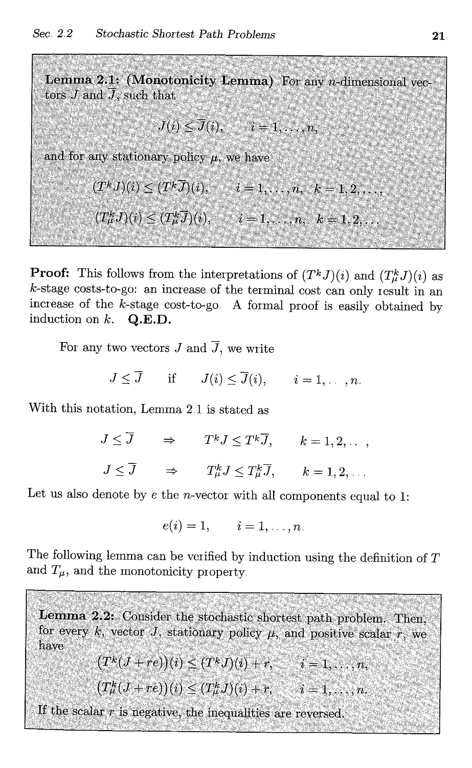
Proof: This follows from the interpretations of (TkJ)(i) and (T J)(i) as
k-stage costs-to-go: an increase of the terminal cost can only result in an
increase of the k-stage cost-to-go.. A formal proof is easily obtained by
induction on k. Q.E.D.
For any two vectors J and J, we write
J-:;.J
if
J(i) -:;. J(i),
i = 1" ,n..
With this notation, Lemma 2..1 is stated as
J-:;.J
=}
TkJ -:;. TkJ,
k = 1,2,
,. ,
J-:;.J
=}
T J -:;. T J,
k = 1,2"
Let us also denote by e the n-vector with all components equal to 1:
e(i) = 1,
i = 1".., ,n,
The following lemma can be verified by induction using the definition of T
and TJ.L, and the monotonicity property.
22
Dynamic ProgI amming
Chap. 2
Main Results
The following proposition gives the main results regarding stochastic short-
est path problems., The proof is fairly sophisticated and can be found in
[BeT89], [BeT91a], or [Ber95a] ,1
t We provide a quick proof of the Bellman equation J* = T J* and also that
TJ.L* J* = T J* implies optimality of p,*, using slightly different assumptions than
those of Prop, 2.1 In particular, we use Assumption 2 1 and we also use the
assumption 'L,7=oP i i(U)g(i,u,j) 2': 0 for all (i,u) (in place of Assumption 2.2,
which will not be used), Let Jo be the zero vector, and consider the sequence
T k J o ' Our nonnegativity assumption on the expected one-stage cost implies
that Jo :S T Jo, so by using the monotonicity of T (Lemma 2.1), we have T k Jo :S
Tk+l J o for all k Hence,
Jo :S T k Jo :S Tk+ 1 Jo:S lim T m Jo,
m --+ 00
where each component of the limit vector above is either a real number or +00 By
the definition and the monotonicity of T, we have for any policy 1r = {p,o , P,l, ,,}
lim T m Jo:S lim TJ.LO TJ.Ll
m.-+oo m--+oo
TJ.Lm Jo = P'
Since the cost-to-go vector of a proper policy has finite components and there
exists at least one proper policy, it follows that the vector J oo = lim m --+ oo T m Jo
has finite components. By taking the limit as k 00 in the relation Tk+ 1 J o =
T(T k Jo) and by using the continuity of T, we obtain J oo = T J oo Let p,* be such
that TJ.L*J oo = T J oo = J oo Then, since Jo :S J oo , we have
JJ.L* lim T;:; Jo:S lim T;:; J oo = J oo
m--+oo m-+co
Since we showed earlier that J oo :S P' for all policies 1r, we obtain JJ.L* = J oo =
J*. The preceding argument also proves that J* is the unique solution of the
equation J = T J within the class of vectors J with J 2': 0
Sec. 22
Stochastic Shortest Path Problems
23
The DP operator T often has some useful structure beyond the mono-
tonicity property of Lemma 2 1, In particular, T is often a contraction
mapping with respect to a weighted maximum nOTm. By this we mean that
there exists a vector = ( (1),.. , ,, (n)) with positive components and a
scalar (3 < 1 such that
liT J - TJII :::; (3IIJ - JII ,
for all vectors J and J, where the weighted maximum norm II..II is defined
by
IJ(i)1
IIJII = . max C- ( . ) ..
z.=1, n Z
We have the following result:
24
Dynamic Programming
Chap. 2
Proof: We first define the vector as the solution of a certain DP problem,
and then show that it has the required property. Consider a new stochastic
shortest path problem where the transition probabilities are the same as
in the original, but the transition costs are all equal to -1 (except at the
termination state 0, where the self transition cost is 0).. Let J(i) be the
optimal cost-to-go from state i in this new problem. By Prop. 2..1(a), we
have for all i = 1" " n, and stationary policies f-l,
n
J(i) = -1 + min LPii(U)J(j)
uEU(i) i=l
n
:::; -1 + LPii(f-l(i))J(j)
i=l
(2..11)
Define
(i) = -J(i),
i = 1,., ,n..
Then for all i, we have (i) ?:: 1, and for all stationary policies f-l, we have
from Eq. (2.11),
n
LPii (f-l(i)) (j) :::; (i) - 1 :::; (3 (i),
i=l
i = 1,..... ,n,
(2.12)
where (3 is defined by
t ( i ) - 1
(3=.max '0, . <1
,=1, ,n ( )
For any stationary policy f-l, any state i, and any vectors J and ], we
have using Eq.. (2.12),
I (T"J) (i) (T"J)(i)1 I t,P" (M(i)) (JU) JU)) I
n
:::; LPii (f-l(i)) !J(j) - ](j)1
i=l
< ( .. ( ( . )) t ( ' )) ( IJ(j)-](j)l )
_ P'1 f-l '0, J . max t ( . )
i=l 1=1"n '0, J
< (3 t ( ' ) I J(j) - ](j) I
'0, max ( ) "
- i=l, .,n j
Dividing both sides by (i) and taking the maximum over i ofthe left-hand
side, we obtain
. max I (T1J) (i) -. (T p ]) (i) I :::; (3 max IJ(j) -?(j) I ,
'=1, ,n ( ) i=l"n (J)
See 2.2
Stochastic Shortest Path Problems
25
so that Tp is a contraction with respect to the weighted maximum norm
II . II .
The preceding calculation also yields
(TpJ)(i) ::; (TpJ)(i) + (3 (i) j!f n IJ(j 0 (j)I ,
and by taking the minimum of both sides over f-l, we obtain
(T J)(i) ::; (TJ) (i) + (3 (i) . max IJ(j) -?(j) I ,
1=1"n (J)
By interchanging the roles of J and J, we also have
(TJ)(i) ::; (T J)(i) + (3 (i) j!f x,n IJ(j 0 (j)I ,
and by combining the last two relations, we obtain
I(T J)(i) - (TJ) (i) I ::; (3 (i) . max IJ(j) -. J(j)I .
1=1"n (J)
Dividing both sides by (i) and taking the maximum over i ofthe left-hand
side, we obtain that T is a contraction with respect to II . II . Q.E.D.
We now discuss a number of different methods for computing the
optimal cost-to-go vector J*,
2.2.2 Value Iteration
The DP iteration that generates the sequence Tk J starting from some J is
called value iteration and is a principal method for calculating the optimal
cost-to-go vector J*.. Generally, the method requires an infinite number of
iterations. However, under special circumstances, the method can termi-
nate finitely, A prominent example is the case of a deterministic shortest
path problem, but there are other more general circumstances where ter-
mination occurs, In particular, let us assume that the transition probability
graph corresponding to some optimal stationary policy f-l* is acyclic By
this we mean that there are no cycles in the graph that has as nodes the
states 0,1,. , "n, and has an arc (i,j) for each pair of states i and j such
that i I- 0 and Pij (f-l*(i)) > 0, Then it can be shown (see [Ber95a], Vol. II,
Section 2.,2.1) that the value iteration method will yield J* after at most n
iterations when started from the vector J given by
J(i) = 00,
i = 1" "n,
26
Dynamic PIOgl amming
Chap.. 2
The preceding acyclicity assumption requires in particular that there
are no positive self-transition probabilities Pii (f-l* (i)) for i -I 0, but it turns
out that under our assumption, a stochastic shortest path problem with
such self-transitions can be converted into another stochastic shortest path
problem where Pii ( u) = 0 for all i -I 0 and u E U (i), In particular, suppose
that Pii(U) -I 1 for all i -10 and u E U(i). Then, it can be shown that the
modified stochastic shortest path problem that has one-stage costs
_ ( ' ' ) ( ' . ) Pii(u)g(i,u,i)
gz,U,] =gz,U,] + 1-pii(u) ,
in place of g( i, u, j), and transition probabilities
i = 1" .. ,n,
{ 0, if j = i,
Pi j ( u) = Pij ( u) if. ..J. i
1-Pii(U)' ] I ,
i = 1,.." ,n,
instead of Pij(U), is equivalent to the original in the sense that it has the
same optimal costs-to-go and policies. This becomes intuitively clear once
we note that Pii (u) / (1- Pii (u)) is the expected number of self- transitions at
state i, so the cost g( i, u, j) is the total expected cost incurred in reaching a
state j other than i, counting the cost of intermediate self-transitions Fur-
thermore, Pij (u) is the probability of transition from state i to a state j -I i,
conditioned on the fact that the next transition is not a self-transition,
Gauss-Seidel Methods and Asynchronous Value Iteration
In the value iteration method, the estimate of the cost-to-go vector is up-
dated for all states simultaneously. An alternative is to update the cost-
to-go at one state at a time, while incorporating into the computation the
interim results, This corresponds to what is known as the Gauss-Seidel
method for solving the nonlinear system of equations J = T J.
For n-dimensional vectors J, define the mapping F by
n
(FJ)(l)= min I>1j(u)(g(1,u,j)+J(j)),
uEU(1) j=O
(2..13)
and, for i = 2, . . , , n,
(F J)(i) = min [ tPij(U)9(i, u,j) + Pij(u)(F J)(j)
UEU(2) j=O j=1
+ t,P';(U)J(j)]
(2.14)
In words, (F J)(i) is computed by the same equation as (T J)(i) except that
the previously calculated values (F J)(l), ,." (F J)(i -1) are used in place
Sec. 2,2
Stochastic Shortest Path Problems
27
of J(l),.. . . , J(i - 1). Note that the computation of F J is as easy as the
computation of T J (unless a parallel computer is used, in which case T J
may potentially be computed much faster than F J; see [BeT91b], [Tsi89]).
The Gauss-Seidel version of the value iteration method consists of
computing J, F J, F2J, "... This method is valid, in the sense that FkJ
converges to J* under the same conditions that Tk J converges to J*. In
fact the same result may be shown for a much more general version of the
Gauss-Seidel method, In this version, it is not necessary to maintain a fixed
order for iterating on the cost-to-go estimates J(i) of the different states;
an arbitrary order can be used, as long as J(i) is iterated infinitely often for
each state i. We call this type of method the asynchronous value iteration
method, and we prove its validity in the next proposition., The method
of proof is typical of convergence proofs of asynchronous algorithms that
satisfy monotonicity conditions (see [BeT89], Section 6.4),
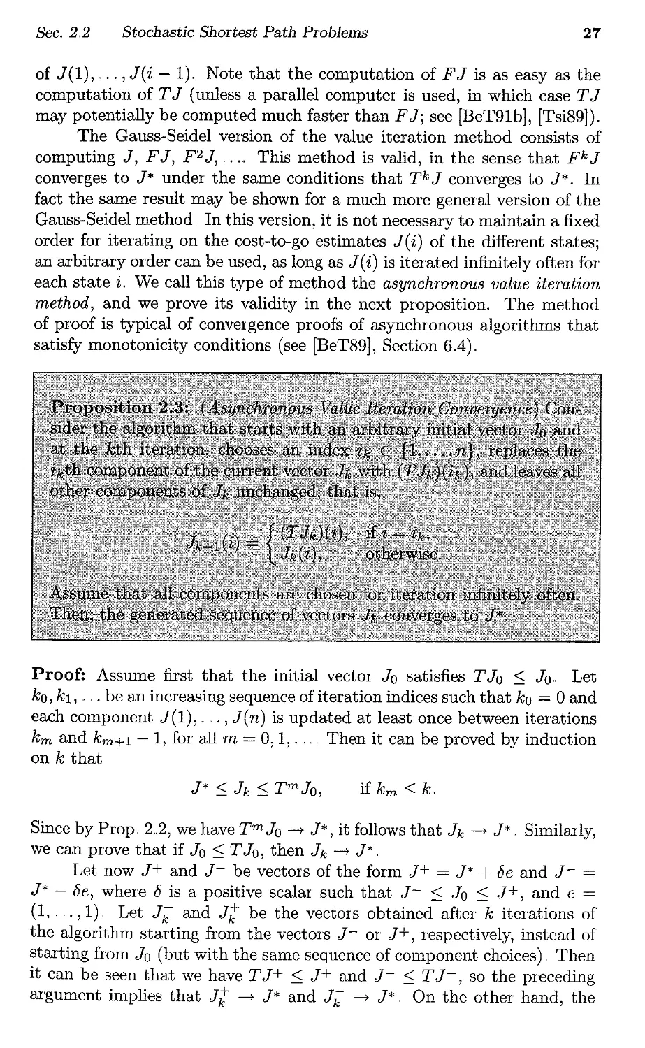
Proof: Assume first that the initial vector Jo satisfies T Jo ::; Jo.. Let
ko, kl, .. , . be an increasing sequence of iteration indices such that ko = 0 and
each component J(l),.. .., J(n) is updated at least once between iterations
k m and k m +1 - 1, for all m = 0, 1,.. "" Then it can be proved by induction
on k that
J* ::; Jk ::; TmJo,
if k m ::; k,
Since by Prop, 2.2, we have TmJo -... J*, it follows that Jk -... J*.. Similarly,
we can prove that if Jo ::; T Jo, then Jk -... J*,
Let now J+ and J- be vectors of the form J+ = J* + be and J- =
J* - De, where b is a positive scalar such that J - ::; Jo ::; J +, and e =
(1, . . . , 1). Let J; and J: be the vectors obtained after k iterations of
the algorithm starting from the vectors J - or J +, respectively, instead of
starting from Jo (but with the same sequence of component choices), Then
it can be seen that we have T J+ ::; J+ and J- ::; T J-, so the preceding
argument implies that J: -... J* and J; -... J* On the other hand, the
28
Dynamic Programming
Chap. 2
relation J- :::; Jo :::; J+ implies that Jr; :::; Jk :::; J;!; for all k. It follows
that Jk --> J*. Q.E.D.
Sequential Space Decomposition and Gauss-Seidel Methods
In some stochastic shortest path problems there is favorable structure,
which allows decomposition into a sequence of smaller problems. In particu-
lar, suppose that there is a sequence of subsets 81, 82, . . . , 8M of {I, 2, ., . , n}
such that each of the states i = 1,..." n belongs to one and only one of
these subsets, and the following property holds:
For all m = 1, ,..., M, and states i E 8m, and under any policy, the
successor state j is either the termination state or else belongs to one
of the subsets 8 m , 8 m -1, . . . ,81'
Then it can be seen that the solution of this problem decomposes into the
sequential solution of M stochastic shortest path subproblems. Each sub-
problem is solved using the optimal solution of the preceding subproblems.
The state space of the mth subproblem is the subset 8m plus a termination
state which corresponds to a transition to one of the states in the subset
{0}U81 U.. .U8m-1 The cost oftransition from a state i E 8m ofthe mth
subproblem to the termination state via a state j E {O} U 81 U .. . U 8m-1
is g(i,u,j) + J*(j).
A more favorable form of decomposition can be obtained when the
following property holds, which requires in addition that transitions from
states in a subset 8m cannot lead to states in the same subset:
For all m = 1,..., M, and states i E 8m, and under any policy, the
successor state j is either the termination state or else belongs to one
of the subsets 8 m -1" ..,,81'
For this case, consider the Gauss-Seidel method that iterates on the states
in the order of their membership in the sets 8m; that is, it first iterates on
the states in the set 81, then iterates on the states in the set 8 2 , etc. It
can be seen by using induction on the index m, that after a single iteration
on the states in the set 8m, the Gauss-Seidel iterates will be equal to
the corresponding optimal costs-to-go because they will satisfy Bellman's
equation, which takes the form
J*(i) = min L Pij(u)(g(i,u,j) + J*(j)),
uEU(i)
jE{O}USIU US m -l
ViE 8m
Thus, only one Gauss-Seidel iteration per state is needed.
An important example of such a decomposition is the finite hmizon
DP algorithm, which first finds the optimal costs-to-go of the states corre-
spo ding to the last stage, then uses these optimal costs-to-go to find the
optImal costs-to-go of the states cOIIesponding to the next-to-last stage,
Sec 2.2
Stochastic Shortest Path PIOblems
29
etc, For another interesting example, suppose that the states are K-tuples
of the form i = (i1,i2,.. ,..,iK), where each ik is a nonnegative integer.
The state (0,0, . . .. ,0) is the termination state. Assume that the transition
probabilities have the property
K K
Pij(U) > 0 only if 2.:>k < L ik
k=1 k=1
For all nonnegative integers m, consider the sets of states
8m = { i = (i1, . .. . , iK) I t ik = m } .
k=1
Then it can be seen that all transitions from states in a set 8m lead to the
termination state or to states in the set 8 1 U ... ,U 8m-1, and the preceding
decomposition method applies,
2.2.3 Policy Iteration
In general, value iteration requires an infinite number of iterations to obtain
the optimal cost-to-go vector.. There is an alternative to value iteration,
called policy iteration, which always terminates finitely, In this algorithm,
we start with a proper policy /-10, and we generate a sequence of new proper
policies /-11, /-12,.. Given the policy /-1k, we perform a policy evaluation step,
that computes JJJ.k (i), i = 1,... " n, as the solution of the (linear) system
of equations
n
J(i) = LPij(/-1k(i)) (g(i, /-1k(i),j) + J(j)),
j=O
i = 1,." ,n,
(2,15)
in the n unknowns J(l), .., J(n) [ef, Prop. 2.1(d)]. [Recall that J(O) is
set to zero and is therefore not an unknown.] We then perfmm a policy
improvement step, which computes a new policy /-1k+1 as
n
/-1k+1(i) = arg min LPij(u)(g(i,u,j) + JJ.Lk(j)) ,
uEU(i) j=O
i = 1".... ,n,
(2.16)
or equivalently, as the policy satisfying
TJ.Lk+l JJ.Lk = T JJ.Lk.
The process is repeated with /-1k+1 used in place of /-1k, unless we have
JJ.Lk+ 1 (i) = JJ.Lk(i) for all i, in which case the algorithm terminates with
30
Dynamic PlOgramming
Chap. 2
the policy f.1k, The following proposition establishes the validity of policy
iteration
Proof: In the typical iteration, given a proper policy f.1 and the correspond-
ing cost-to-go vector JIJ., one obtains a new policy Jl satis(ying TJiJIJ. = T JIJ..
Then we have JIJ. = TIJ.JIJ. TJiJIJ., and using the monotonicity of TJi, we
obtain
k-l
JIJ. > T!5.JJ.L = p!5.JIJ. + P!!'n-;;
- J.L IJ. IJ."IJ.'
m=O
k = 1,2,..
If Jl is not proper, Assumption 2.2 implies that some component of the sum
in the right-hand side of the above relation diverges to 00 as k -+ 00, which
is a contradiction Therefore Jl is proper, and the preceding relation and
Prop. 2,1(d) imply that
JIJ. > lim T!5.JIJ. = fiT
- k-'>oo IJ.
(2,17)
Note that strict inequality J7I(i) < JIJ.(i) holds for at least one state i, if
f.1 is nonoptimal; otherwise we would have JIJ. = T JIJ., and by Prop.. 2.1(a)
it would follow that JJ.L = J*, so that f.1 would be optimal. Therefore, the
new policy is strictly better if the current policy is nonoptimal. Since the
number of proper policies is finite, the policy iteration algorithm terminates
after a finite number of iterations with an optimal proper policy, Q.E.D.
In practice, the policy iteration algmithm typically requires very few
iterations, although there are no themetical guarantees for this.
Multistage Lookahead Policy Iteration
There is a variation of the policy iteration algmithm that uses a lookahead
of several stages in the policy improvement step, The method described
above uses single stage lookahead for generating an improved policy starting
from a given policy f.1: at a given state i, it finds the optimal decision for
a one-stage problem with one-stage cost g( i, u, j) and terminal cost (after
the first stage) JIJ. (j), An m-stage lookahead version finds the optimal
policy for an m-stage DP problem, whereby we start at the current state
i, make the m subsequent decisions, incur the corresponding costs of the
m stages, and pay a terminal cost JIJ.(j), where j is the state after m
stages. This may be a tractable problem, depending on the hmizon m and
Sec 2.2
Stochastk Shortest Path Problems
31
the number of possible successm states from each state. If u is the first
decision of the m-stage optimal policy starting at state i, the improved
policy in the multistage policy iteration method is defined by 71(i) = u.
This policy is then evaluated in the usual way, Le, by solving the linear
system Jii = T"jiJii..
It can be shown that the multistage lookahead policy iteration ter-
minates with an optimal policy under the same conditions as the ordinary
version.. To see this, let {710, 711' , .. . , 71m-l} be an optimal policy obtained
from the m-stage DP algorithm with terminal cost JJ.L; that is,
T"jikTm-k-lJ/l- = Tm-kJ/l-,
k = 0, 1" , . , m - 1.
(2,18)
Since T J/l- :::; T/l-J/l- = J/l-, we have using the monotonicity of T,
Tk+!JJ.L < TkJ/l- < JJ.L
- -,
k = 0,1,..
(2.19)
By combining this equation with Eq. (218), we have
T- Tm-k-IJ/l- = Tm-kJ/l- < Tm-k-IJ/l-
J.Lk -,
k = 0, 1, , . , , m - 1,
from which we obtain for alll 2: 1, using the monotonicity of T/ik'
Tl Tm-k-IJ/l- < T- Tm-k-IJ/l- = Tm-kJ/l-
/l-k - J.Lk ,
k = 0, 1" .. , ,m - 1.
By taking the limit as l ---7 00 and by using Eq. (2,19), it follows that
Jiik < Tm-kJJ.L < JJ.L
- -,
k = 0, 1, . . . , m -- 1.
In particular for the successor policy 71 generated by the m-stage policy
iteration, which is 71 = 710' we have
Jii :::; TmJ/l- :::; J/l-
It follows that 71 is an improved policy relative to J1 Furthermore, if Jii =
J/l-, in view of Eq. (219), we have that T J/l- = J/l- and J1 is optimal. Similar
to the proof of Prop. 24, it follows that the algorithm terminates with an
optimal policy.
Note that the expression TmJ/l-, which is the result of m successive
value iterations applied to JJ.L, provides an upper bound on the cost-to-go
function Jii, This upper bound improves as m increases [ef. Eq. (2.19)],
thereby suggesting that fm many problems, the multistage policy itera-
tion method may perform better than its single stage counterpart. This
is particularly so when cost-to-go function approximations are introduced
(see the discussion of Section 6.1.2).. On the other hand the computation
required to perform the policy improvement step increases rapidly with the
size of the lookahead,
32
Dynamic Programming
Chap.. 2
Modified Policy Iteration
When the number of states is large, solving the linear system in the policy
evaluation step by direct methods such as Gaussian elimination is time-
consuming, One way to get around this difficulty is to solve the linear
system iteratively by using value iteration, as suggested by Prop, 2..l( d)
In fact, we may consider solving the system approximately by executing
a limited number of value iterations The resulting method is called the
modified policy iteration algorithm.
To formalize this method, let Jo be an n-dimensional vector such that
T Jo :::; Jo, Let mo, m1, ,... be positive integers, and let the vectors J1, J2,
and the stationary policies f.10, f.11,. be defined by
T J1I Jk = T Jk, Jk+1 = T;';,k Jk, k = 0,1, .
Thus, a stationary policy f.1k is defined from Jk according to T J1k J k = T Jk,
and the cost-to-go JJ.Lk is approximately evaluated by mk - 1 additional
value iterations, yielding the vector Jk+1, which is used in turn to define
f.1k+1..
Note that if mk = 1 for all k in the modified policy iteration algorithm,
we obtain the value iteration method, while if mk = 00 we obtain the policy
iteration method, where the policy evaluation step is performed iteratively
by means of value iter at ion Analysis and computational experience suggest
that it is usually best to take mk larger than 1 accmding to some heuristic
scheme A key idea here is that a value iteration involving a single policy
(evaluating TJ.LJ for some f.1 and J) is much less expensive than an iteration
involving all policies (evaluating T J for some J), when the number of
controls available at each state is large. The convergence properties of the
modified policy iteration method will be discussed in the context of a more
general algorithm, which we now introduce
Asynchronous Policy Iteration
We may consider a more general policy iteration algorithm, whereby value
iterations and policy updates are executed selectively, for only some of
the states, This type of algorithm generates a sequence Jk of cost-to-go
estimates and a corresponding sequence f.1k of stationary policies. Given
(Jk, f.1k), we select a subset Sk of the states, and we generate the new pair
(Jk+1, f.1k+d in one of two possible ways: either we update Jk according to
J ( . ) = { ( T J1k J k)(i), ifiESk, ( 2.20 )
k+1 Z Jk(i), otherwise,
while we leave the policy unchanged by setting f.1k = f.1k+1, or else we
update f.1k according to
f.1k+1(i) = { argminuEu(i) 'L,7=oPii(U)(g(i,u,j) + Jk(j)),
f.1k(i),
if i E Sk,
otherwise,
(2.21 )
Sec, 22
Stochastic Shortest Path Problems
33
while we leave the cost-to-go estimate unchanged by setting J k = Jk+l'
Note that by combining value and policy updates in various ways, we
may synthesize more structured methods. In particular, if a policy update
is followed by a value update for the same set of states Sk, the latter update
is equivalent to the value iteration update
J ( , ) _ { (T Jk)(i),
k+1 Z - Jk(i),
if i E Sk,
otherwise..
(2.22)
Furthermore, if Sk = {I, .. " ,n} and an "infinite" number of value updates
(2.20) are done before doing a single policy update (2.21), we essentially ob-
tain the policy iteration method. If Sk = {I, . .. .. , n} and mk value updates
(2.20) are done followed by a policy update (2.21), we obtain the modified
policy iteration method (or the value iteration method if mk = 1) On the
other hand, if Sk always consists of a single state and each policy update
(2.21) is followed by a value update (2..20) [01 equivalently by an update
(2.22)], the algorithm reduces to the asynchronous value iteration method
The asynchronous policy iteration algorithm also contains as a special
case a version of the policy iteration method that uses a partition of the
state space into subsets, and perf01ms "partial" policy iterations that are
restricted to one of the subsets at a time. In particular, at the kth iteration,
this method selects one of the subsets, call it Sk, obtains a new policy /-1k+1
via the policy update (2.21), and "evaluates" this policy only for the states
in Sk. The evaluation can be perf01med by using an infinite number of
value updates for all states in Sk, with the cost-to-go values of the states
j fJ. Sk held fixed at Jk(j).. Alternatively, the iteration can be performed by
solving a restricted system of linear equations whose variables are the cost-
to-go values of the states i E Sk only; this can be viewed as an evaluation
step of the policy /-1k+1 for a stochastic shortest path problem that involves
the states i E Sk plus an artificial termination state which is reached at
cost Jk(j) whenever a transition to a state j fJ. Sk occurs..
Finally, let us consider the convergence of the asynchronous policy
iteration method.. For this, we will need some assumptions, including that
the initial conditions Jo and /-10 must be such that T!J.o Jo ::::: Jo (one possi-
bility to obtain such initial conditions is to select /-10 in some way and then
take Jo = J!J.O) , We have the following proposition..
34
Dynamic Programming
Chap. 2
Proof: The idea of the proof is to first use the assumption TJ.LOJo ::; Jo
to show that J* ::; Jk+l ::; Jk for all k, so that the sequence Jk converges
to a limit J.. We will then use the assumption that the value and policy
updates are executed infinitely often for all states to show that J = TJ, so
that J = J*
We first show that for all k, we have
TJ.Lk Jk ::; Jk
=i>
TJ.Lk+l Jk+1 ::; Jk+l ::; J k .
(2,23)
Indeed assume that at iteration k we have TJ.LkJk ::; Jk, and consider two
cases:
(1) The value update (2.20) is executed next.. Then we have
Jk+l(i) = (TJ.LkJk)(i) ::; Jk(i),
if i E Sk,
(2..24)
and
Jk+l(i) = Jk(i),
if i tJ- Sk,
(2.25)
so that Jk+l ::; Jk' Using this inequality, the monotonicity of TJ.Lk'
and the fact J.Lk+l = J.Lk, we obtain
TJ.Lk+l Jk+1 = TJ.LkJk+1 ::; TJ.Lk Jk ..
(2.26)
On the other hand, from Eq. (2.24) we have
(TJ.LkJk)(i) = Jk+l(i),
if i E Sk,
while from Eq (2.25) and the hypothesis TJ.LkJk ::; Jk, we have
(TJ.LkJk)(i) ::; Jk(i) = J k + 1 (i),
ifitJ-Sk'
The above two relations imply that TJ.LkJk ::; Jk+l, which when com-
bined with Eq. (2..26), shows that TJJ.kt-l Jk+l ::; Jk+l and completes
the proof of Eq. (2.23).
(2) The policy update (2.21) is executed next. Then we have Jk+l = Jk,
and by using the relation TJ.LkJk ::; Jk, we obtain
(TJ.Lk+Jk+l)(i) = (TJ.Lk+Jk)(i) = (T Jk)(i) ::; (TJ.LkJk)(i)
:::; Jk(i) = Jk+l(i), if i E Sk,
(2.27)
and
(TJJ.k+l Jk+d(i) = (TJ.LkH Jk)(i) = (TJJ.kJk)(i)
::; Jk(i) = Jk+l(i), if i tJ- Sk,
(2.28)
so that TJJ.k+l J k + 1 ::; Jk+l, and Eq.. (2..23) is shown
Sec. 22
Stochastic Shortest Path Problems
35
Equation (2.23) and the hypothesis TJ.LOJo ::; Jo imply that
Jk+1 :::; Jk,
T Jk ::; TJ.LkJk ::; Jk,
Ie! k.
(2..29)
By using the monotonicity of T, we also have TmJk :::; Jk for all m, and by
taking the limit as m -t 00, we obtain
J* ::; Jk, Ie! k.
From this equation and Eq.. (2.29), we see that Jk converges to some limit
J satisfying
TJ ::; J ::; J k ,
Ie! k.
(2.30)
Furthermore., from Eqs. (2..26)-(2..28), we have
TJ.Lk+l Jk+1 ::; TJ.LkJk,
Ie! k.,
(2,31)
Suppose, to arrive at a contradiction, that there exists a state i such
that (TJ)(i) < J(i), and let k be such that (T Jk)(i) < J(i) for all k ;::: k
(such an integer k exists by the continuity of T). Let k be an iteration index
that satisfies k ;::: k and is such that the policy update (2,21) is executed
for state i, and let k' be the first iteration index with k' > k such that the
value update (2.20) is executed for state i., Then we have
J k '+l(i) = (TJ.Lk,J k , )(i)
::; (TJ.Lk+l Jk+d(i)
::; (TJ.Lk+l Jk)(i)
= (T Jk)(i)
< J(i),
(2..32)
where the first equality follows from the value update (2..20), the first in-
equality follows from Eq. (2.31), the second inequality follows from the
relation Jk+l ::; Jk and the monotonicity of TJ.Lk+l' and the second equality
follows from the policy update (221).. The relation (2..32) contradicts the
relation (2..30). Thus we must have (TJ)(i) = J(i) for all i, which implies
that J = J*, since J* is the unique solution of Bellman's equation by Prop.
2.1(a). Q.E.D.
We note that without the assumption TJ.LOJo ::; Jo, one may construct
counterexamples to the convergence of the asynchronous policy iter ation
method (see Williams and Baird [WiB93]).
36
Dynamic Programming
Chap. 2
Policy Iteration as an Actor-Critic System
There is an interesting interpretation of policy iteration methods that will
prove useful when we will consider approximate versions of policy iteration
in subsequent chapters, In this interpretation, the policy evaluation step
is viewed as the work of a critic, who evaluates the performance of the
current policy, i.,e.., calculates an estimate of JJ.Lk. The policy improvement
step is viewed as the work of an actor, who takes into account the latest
evaluation ofthe critic, i.e., the estimate of Jllk, and acts out the improved
policy J-Lk+l (see Fig. 2.1).. Note that the exact, the modified, and the
asynchronous policy iteration algorithms can all be viewed as actor-critic
systems, In particular, modified policy iteration amounts to an incomplete
evaluation of the current policy by the critic, using just a few value iteration
steps, Asynchronous policy iteration can be similarly viewed as a process
where the critic's policy evaluation and the critic's feedback to the actor
are irregular and take place at different times for different states.
Figure 2.1: Interpretation of policy iteration as an actor-critic system,
2.2.4 Linear Programming
Another method to solve the stochastic shortest path problem is based on
linear programming, Since limk---+oo TkJ = J* for all J [ef. Prop, 2.1(b)],
we have
J5:.TJ
=}
J 5:. J* = T J*.
Sec, 23
Discounted Problems
37
Thus J* is the "largest" J that satisfies the constraint J :S: T J This
constraint can be written as a finite system of linear inequalities
n
J(i) :S: LPij(u)(g(i,u,j) + J(j)),
j=O
i = 1,. ..., n, u E U(i),
and delineates a polyhedron in n, In particular, J*(l), ...,J*(n) solve
the following problem (in the variables AI,.... " An):
n
maximize L Ai
i=l
n
subject to Ai:S:LPij(u)(g(i,u,j)+Aj), i=l""n, UEU(i),
j=O
where AO is fixed at zero.. This is a linear program with n variables and as
many as n x q constraints, where q is the maximum number of elements of
the sets U(i)., As n increases, its solution becomes more complex., For very
large nand q, the linear programming approach can be practical only with
the use of special large-scale linear programming methods.
2.3 DISCOUNTED PROBLEMS
We now consider a discounted problem, where there is a discount factor
a < 1, We will show that this problem can be viewed as a special case of
the stochastic shortest path problem of the preceding section We will then
obtain the associated analytical and algorithmic results by appropriately
specializing the analysis of the preceding section
We first modify the definition of the mappings T and T!J. to account for
the absence of the termination state. For any vector J = ((J(l),. ., J(n)),
we consider the vector T J obtained by applying one iteration of the DP
algorithm to J; the components of T J are
n
(T J)(i) = min LPij(U) (g(i, u,j) + aJ(j)),
UEU(2) j=l
i = 1,.. ,n
Similarly, for any vector J and any stationary policy f.1, we consider the
vector T!J.J with components
n
(T!J.J)(i) = LPij (f.1(i)) (9(i, f.1(i),j) + aJ(j)),
j=l
i = 1" ,n,
38
Dynamic Programming
Chap. 2
Again, T'lJ may be viewed as the cost-to-go vector associated with JL for
the one-stage problem that has one-stage cost g and terminal cost O'.J..
If P/-L is the n x n matrix whose ijth entry is Pij (JL( i)), then T/-LJ can
be written in vector f01m as
T/-LJ = g/-L + O'.P/-LJ,
where g/-L is the n-dimensional vector whose ith component is
n
g/-L(i) = "L"Pij (JL(i))g(i, JL(i),j)
j=l
The following two lemmas parallel Lemmas 2.1 and 2.2 of the preced-
ing section.
Again we denote by e the n-vector with all components equal to 1.
Then, for any vector J and scalar r
(T(J + re))(i) = (T J)(i) + O'.r,
(T/-L(J + re))(i) = (T/-LJ)(i) + O'.r,
i = 1"., ,n,
i = 1"" ,n,
More generally, the following lemma can be verified by induction,
Sec 2.3
Discounted Pmblems
39
We define the maximum norm 11.1100 on n by
IIJlloo = max IJ(i)I..
,
We then have the following contraction property of the DP operators T
and Tw
Proof: Denote
c = . max IJ(i) - J(i)l.
1,=1, "n
Then we have
J(i) - c :::; J(i) :::; J(i) + c,
i = 1,.,.. ,n.
Applying T in this relation and using the Monotonicity Lemma 2.3 as well
as Lemma 2,4, we obtain
(T J)(i) - ooc:::; (TJ)(i) :::; (T J)(i) + ooc,
i = 1,.... ,n.
It follows that
I(TJ)(i) -- (TJ) (i) I :::; ooc,
i = 1".... ,n,
which proves Eq. (2.33). Equation (2.34) follows by applying Eq. (2.33)
to the modified problem where the only control available at state i is f-1(i).
Q.E.D.
We will now show that the discounted cost problem can be converted
to a stochastic sh01test path problem fm which the analysis of the preceding
section holds. To see this, let i = 1, . . . , n be the states of the discounted
problem, and consider an associated stochastic sh01test path problem in-
volving the states 1,. , . , n plus an extra termination state 0, with state
transitions and costs obtained as follows From a state i =I- 0, when control
u is applied, a cost g(i,u,j) is incurred with probability Pij(U); the next
state is j with probability oopij(u), and 0 with probability 1- a; see Fig..
40
Dynamic Programming
Chap. 2
Figure 2.2: Transition probabilities for an a-discounted problem and its associ-
ated stochastic shortest path problem In the latter problem, the probability that
the state is not 0 after k stages is a k
22, Note that all policies are proper for the associated stochastic shortest
path problem, so the assumptions of the preceding section are satisfied,
Suppose now that we use the same policy in the discounted problem
and in the associated stochastic shortest path problem. Then, as long as
termination has not occurred, the state evolution in the two problems is
governed by the same transition probabilities. Furthermore, the expected
one-stage cost at each state i is
n
LPij(u)g(i, u,j)
j=l
for both problems, but it must be multiplied by a. k because of discount-
ing (in the discounted case), or because it is incurred with probability a. k ,
when termination has not yet been reached (in the stochastic shortest path
case). We conclude that the cost-to-go of any policy starting from a given
state, is the same for the original discounted problem and for the associ-
ated stochastic sh01test path problem, Since in the associated stochastic
shortest path problem all policies are proper, we can apply the results of
the preceding section to the latter problem and obtain the following result
Sec 23
Discounted Problems
41
There are also discounted versions of the multistage lookahead, the
modified, and the asynchronous policy iteration algorithms that we dis-
cussed earlier in connection with stochastic shortest path problems.. In
particular, the convergence result of Prop. 2.5 admits a straightforward
extension to the discounted case.
2.3.1 Temporal Difference-Based Policy Iteration
We mentioned earlier that when the number of states is large, it is usually
preferable to carry out the policy evaluation step of the policy iteration
method by using value iteration. A drawback of this approach, however, is
that the value iteration algorithm may converge very slowly. This is true
for many stochastic shortest path problems with a large number of states,
as well as for discounted problems with a discount factor that is close to 1
We are thus motivated to use an approach whereby the discount factor is
effectively reduced in order to accelerate the policy evaluation step.
The idea underlying the approach is that the discount factor can
be reduced without altering the cost-to-go of a given policy only if the
expected value of the one-stage cost under that policy is equal to 0.. We
thus introduce a transformation that asymptotically induces this one-stage
cost structure.. The transformation is based on the notion of temporal
differences (TD for short), which will be of major importance in the context
of the simulation-based methods of Chapters 5-7
We now describe a policy-iteration like algorithm that maintains a
policy-cost vector pair (J k , ILk).. We can view Jk as an approximation to the
42
Dynamic Programming
Chap. 2
cost-to-go vector JJ.Lk, In the typical iteration, given (Jk, J.Lk), we calculate
J.LkH by the policy improvement step
T!J.k+1 Jk = T Jk,
(2.35)
To calculate JkH, we define the TD associated with each transition (i, j)
under J.Lk+l:
dk(i,j) = 9(i,J.Lk+l(i),j) + aJk(j) - Jk(i).
(2.36)
We also consider a parameter A from the range [0,1]., We view dk(i,j) as
the one-stage cost of policy J.Lk+l for an aA-discounted DP problem with
the transition probabilities Pij (J.Lk+ 1 (i)) of the original problem, and we
calculate the corresponding cost-to-go vector. This vect01, denoted by 6.k,
has components given by
00
6.k(i) = L E[(aA)md k (i m ,i m +l) I io = i],
m=O
If i..
(2..37)
The vect01 J kH is then obtained by
JkH = Jk + 6.k. (2.,38)
We refer to the method as the A-policy iteration method,
Note that when A = 1, by using the TD definition (2.36) in the
expression (2,37), we obtain
00
6.k(i) = L E[amdk(im, i m +l) I io = i]
m=O
00
= L E[amg(im' J.LkH(i m ), i m +l)
m=O
+ amHJk(i m +!) - amJk(i m ) I io = i]
00
= L E[amg(im,J.Lk+l(im),im+l) I io = iJ - Jk(i)
m=O
= j/l-k+ 1 (i) - Jk(i)..
Thus, by using Eq. (2,38), we see that J kH = JJ.Lk+l, so the 1-policy itera-
tion method coincides with the standard policy iteration method However,
for A < 1, the two methods are different, and in fact it can be seen from
Eqs, (2.36)-(2.38) that the O-policy iteration method coincides with the value
iteration method for the original problem..
The motivation for the A-policy iteration method is that the aA-
discounted policy evaluation step [cf Eqs (2.37)-(2.38)] can be much easier
Sec.. 2.3
Discounted Problems
43
when A < 1 than when A = 1. In particular, when value iteration is used
for policy evaluation, convergence is faster when A < 1 than when A = 1,
Similarly, when policy evaluation is perf01med using a simulation approach,
as in the NDP methods to be discussed in Chapters 5-7, the variance of
the cost samples that are averaged by simulation is typically smaller when
A < 1 than when A = 1, as can be seen from the definition of t1 k [ef.
Eq. (2.37)].. As a result, the number of cost samples that are required
to evaluate by simulation the cost-to-go of a given policy within a given
accuracy may be much smaller when A < 1 than when A = 1
On the negative side, we will show shortly that the asymptotic conver-
gence rate of the sequence Jk produced by the A-policy iteration method
deteriorates as A becomes smaller, However, this disadvantage may not
be very significant within the NDP approximation context to be discussed
later (ef. Chapter 6). In particular, when the policy evaluation step can-
not be performed with high accuracy, a reasonable practical objective is to
obtain a policy whose cost is within the best "achievable" tolerance from
the optimum, rather than to obtain the optimal cost-to-go function and an
optimal policy, Under these circumstances, the asymptotic rate of conver-
gence of Jk may not be crucial, and using A < 1 often requires a comparable
number of policy iterations to attain the same performance level as using
A=1.
The following proposition introduces a mapping that underlies the A-
policy iteration method, and provides some basic results.. The proposition
applies to both cases where a < 1 and a = 1.
'\
44
Dynamic Programming
Chap.. 2
Proof: (a) For any two vectors J and J, using the definition (2..39) of Mk,
we have
IIMkJ - MkJl1 = IIA(TI'k+l J - TI'k+l J)II
= AIITJ.Lk+l J - TJ.Lk+1 JII
::; ,6AIIJ - JII.
(b) The relation (2,40) holds for m = 1 by the definition (2,39) of Mk
It can be proved for all m :::: 1 by using a straightforward induction. In
particular, we have
M;:'+1J = Mk(Mk'J) = (1- A)TI'k+Jk + ATl'k+l (Mk'J),
and after the expression (2.40) is used in the above equation, we obtain
Eq. (2.40) with m replaced by m + 1.
(c) From the definition (2.37)-(2,38) of Jk+l, we have
J k +1 - Jk = Ilk + CXAPl'k+l (Jk+l - Jk),
(2..42)
where PI'k+l is the transition probability matrix corresponding to the policy
/-1k+l, and Ilk is the vector of expected TD, with components given by
Ilk(i) = LPij(/-1k+l(i))d k (i,j), Vi,
Using the definition (2.36) of the TD, we have
Ilk = Tl'k+l Jk - Jk,
(2,43)
so Eq. (2.42) yields
Jk+1 = Tl'k+1 J k + CXAPI'k+l (Jk+l - Jk)
= TJ.Lk+l Jk + A(Tl'k+l Jk+1 - TJ.Lk+l Jk)
= (1 - A)TJ.Lk+l Jk + ATl'k+l Jk+l
= Mk J k+l'
Sec 2.3
Discounted Problems
45
Thus, Jk+1 is the fixed point of Mk. The expression (241) follows flam
Eq. (240) by taking the limit as m -+ 00. Q.E.D.
The following proposition shows the validity of the A-policy iteration
method and provides its convergence rate.
Proof: (a) Let us first assume that T Jo ::; Jo. We show by induction that
for all k, we have
J* ::; T Jk+1 ::; Jk+l ::; T Jk ::; h
(2.45)
To this end, we fix k and we assume that T Jk ::; Jk. We will show that
J* ::; T Jk+l ::; Jk+1 ::; T J k , and then Eq. (245) will follow from the
hypothesis T Jo ::; Jo
Using the fact T/l k +1 Jk = T Jk [ef, Eq (2.35)] and the definition of
M k [ef. Eq. (2,39)], we have
MkJk = TI'k+l Jk = T Jk ::; J k ,
It follows from the monotonicity of TI'k+l' which implies monotonicity of
M k , that for all positive integers m, we have Mr;+l Jk ::; Mk' Jk ::; T Jk ::;
Jk, so by taking the limit as m -+ 00, we obtain
Jk+1 ::; T Jk ::; h
From the definition of Mk, we have
Mk J k+l = TI'k+l Jk + A (TI'k+l Jk+l - T/lk+l Jk)
= Tl'k+l Jk+l + (1 - A) (TI'k+l Jk - TI'k+l Jk+d,
Using the already shown relation Jk - Jk+l ::::: 0 and the monotonicity of
TJ1.k+l' we obtain TI'k+l J k - TJ1.k+1 Jk+l ::::: 0, so that
(246)
TI'k+l Jk+l ::; M k J k+l.
46
Dynamic Programming
Chap. 2
Since MkJk+l = Jk+l, it follows that
T Jk+1 :::; TJ.Lk+I Jk+l :::; Jk+l.
(2.47)
Finally, the above relation and the monotonicity of TJ.LkH imply that
for all positive integers m, we have Tr:t.,H J k + 1 :::; TJ.LkH Jk+l, so by taking
the limit as m -+ 00, we obtain
J* :::; JJ.Lk+ I :::; TJ.Lk+I Jk+l.. (2.48)
From Eqs. (2.46)-(2..48), we see that the inductive proof of Eq., (2.45) is
complete.,
From Eq. (2..45), it follows that the sequence Jk converges to some
limit J with J* :::; j Using the definition (2.39) of Mk, and the facts
Jk+l = MkJk+1 and TJJ.kH Jk = T Jk, we have
Jk+l = MkJk+l = T Jk + A (TJ.Lk+I Jk+l 0- TJJ.k+I Jk),
so by taking the limit as k-+ 00 and by using the fact Jk+l - Jk -+ 0, we
obtain J = T J. Thus J is a solution of Bellman's equation, and it follows
that J = J*,
To show the result without the assumption T Jo :::; Jo, note that we
can replace Jo by a vector J o = Jo + se, where e = (1,...,1) and s is a
scalar that is sufficiently large so that we have T J o :::; J o ; it can be seen that
for any scalar s:::: (1 - a)-l maxi (TJo(i) - Jo(i)), the relation TJ o :::; J o
holds. Consider the A-policy iteration algorithm started with (J o , /-10), and
let (J k , ilk) be the generated sequence. Then it can be verified by induction
that for all k we have
A _ ( a(l-A) ) k
Jk - Jk - 1 A s,
-a
/-1k = /-1k.
Hence J k - Jk-7 O. Since we have already shown that J k -+ J*, it follows
that Jk -+ J* as well
Since Jk -+ J*, it follows that for all k larger than some index k, /-1k+l
is an optimal policy, so that TJ.LkH J* = T J* = J*, By using this fact, Eq,
(2.41), and the linearity of TJ.Lk+I' we obtain for all k :::: k,
IIh+, - JolI= 11(1- A) I:o Amr;::t:Jk - Jot
(1 - A) lit., AmT,::t:(Jk - Jot
00
:::; (1- A) L A m a m +1IIJk - J*ll oo
m=O
a(l - A)
= l-aA IIJk-J*lIoo
Sec.. 2.4
Problem FOImulation and Examples
47
(b) The proof of this result is identical to the proof of the corresponding
result of part (a). Q.E.D.
The convergence rate result of Prop. 2.8( a) can be generalized to cover
the stochastic shortest path case where a = 1. The proof of Eq. (2.44) can
be adapted to show that if II, II is a norm with respect to which TJ.L* is a
contraction of modulus (3 for all optimal policies /-1*, then
(3(1 - A)
II J k+l - J*II 1- (3A IIJk - J*II,
for all sufficiently large k In the case of a stochastic shortest path problem
where all policies are proper, the above relation holds with II . II being the
weighted maximum norm with respect to which T and all TIJ. are contrac-
tions (cf. Prop. 22)
2.4 PROBLEM FORMULATION AND EXAMPLES
We now provide some examples of infinite horizon DP problems, Some of
these examples will form the basis for the case studies to be discussed in
Ch.8.
Example 2.1 (Reaching a Goal in Minimum Expected Time)
The case where
\
a= 1,
g(i,u,j)=l,
V i of- 0, j, u E U(i),
corresponds to a problem where the objective is to reach the termination
state as fast as possible, on the average, The corresponding optimal cost-to-
go J* (i) is the minimum expected time to termination starting from state
i Under our assumptions, the costs-to-go J* (i) uniquely solve Bellman's
equation, which has the form
J*(i) = min [ 1 + tPij(u)J*(n ] ,
uEU(i)
j=l
i = 1, "n,
In the special case where there is only one stationary policy, J* (i) represents
the mean first passage time from i to 0 in the associated Markov chain (see
Appendix B) These times, denoted by mi, are the unique solution of the
equations
n
mi = 1 + 2'=>ijmj,
j=l
i = 1" ,n
48
Dynamic Programming
Chap. 2
Example 2.2 (Problems with Uncontrollable State Components)
Often in stochastic shOItest path problems there is special structure that can
be exploited to simplify the basic value and policy iteration algorithms, as
discussed earlier We describe here another type of simplification that will
also be used in the three subsequent examples
In many stochastic shOItest path problems of interest the state is a
composite (i, y) of two components i and y, and the evolution of the main
component i can be directly affected by the control u, but the evolution of the
other component y cannot, In particular, we assume that given the state (i, y)
and the control u, the next state (j, z) is determined as follows: j is generated
accOIding to transition probabilities Pij (u, y), and z is generated accOIding to
conditional probabilities p(z I j) that depend on the main component j of the
new state The simplest case arises when z is generated according to a fixed
distribution independently of j, FOI an example, consider the case where z
represents the control of another decision maker whose decision is selected
randomly. As another example, consider a service facility that sequentially
services customers of different types; then the next state consists of pairs
(j, z), where j describes the status of the facility following the service of a
customer and z is the type of the next customer
Let us assume for notational convenience that the cost of a transition
from state (i,y) is of the fOI'll g(i,y,u,j) and does not depend on the un-
controllable component z of the next state (j, z). If 9 depends on z it can be
replaced by
g(i, y, u, j) = 2..::p(z I j)g(i, y, u,j, z)
z
in the analysis that follows,
Stochastic shOItest path problems with this structure admit substantial
simplification. In particular, the value and the policy iteration algOIithms
can be carried out over a smaller state space, the space of the controllable
component i To see this, note that the DP mapping is given for all i, y by
(TJ)(i,y) = min Pii(U,y) ( 9(i,y'U,j) + p(z I j)J(j,Z) ) '
uEU(i,y) 0 0
i=O z
and the corresponding mapping for a stationary policy M is given for all i, y
by
(T"J)(i, y) t,1hj ("( i, y), y) (g(i, y, "(i, V), j) + p(z 1 j)J(j, z))
If we define fOI each J,
J(j) = 2..::p(z I j)J(j, z),
we see that to evaluate (T J)(i, y) OI (Tj.tJ)(i, y), it is sufficient to know the
vector J. FurthermOIe, to calculate an optimal policy, it is not necessary to
Sec, 2..4
Problem Formulation and Examples
49
know the optimal cost-to-go J* (j, z) fOI all (j, z) It is instead sufficient to
know the vector J* given by
J*(j) = 2::p(z I j)J*(j,z),
z
for all i We refer to J* as the reduced optimal cost-to-go vector,
This leads us to introduce simplified versions of the value iteration and
policy iteration algorithms over the space of the controllable state component
i Let us consider the mapping l' defined by
(1'J)(i) = 2::p(y I i)(TJ)(i,y)
y
= "p(Yli) ( min Pij(U'Y)(9(i,y'U,j)+J(j)) )
6 uEU(t,y) 6
y j=O
and the corresponding mapping fOI a stationary policy /1,
(1'I"J)(i) = 2::p(y I i)(TI"J)(i, y)
y
p(y I i) (t,p" ("(i, y), y Hg( i, y, "(i, y),;) + J(j)) )
The simplified value iteration algorithm starts with arbitrary J(i), i =
1, . , . ,n, and sequentially produces l' J, 1'2 J, 1'3 J, etc The simplified policy
iteration algorithm at the typical iteration, given the current policy /1k(i,y),
consists of two steps:
(a)
The policy evaluation step, which computes the unique Jl"k (i), i =
1, , , n, that solve the linear system of equations Jl"k = 1'l"k Jl"k or
equivalently
J"> (i) ply I i) (t,p,; (",(i, y) Hg( i, y, ",(i, y),j) + J"> (j))) ,
for all i = 1, '., n
(b) The policy improvement step, which computes the improved policy
/1k+l (i, y), from the equation 1'l"k+r Jl"k = l' Jl"k or equivalently
n
/1k+1(i,y) = arg min 2::Pij(u,y)(g(i,y,u,j) + Jl"k(j)),
uEU(i,y)
j=O
for all (i, y)
It is possible to show that the preceding modified algOIithms have sat-
isfactory convergence properties under the standard assumptions, In particu-
lar, the simplified value iteration algOIithm converges to the reduced optimal
cost-to-go vectOI J*, which satisfies the reduced form of Bellman's equation
J* = l' J* The simplified policy iteration algorithm converges finitely to an
optimal policy
50
Dynamic Programming
Chap. 2
Example 2.3 (Tetris)
This example is typical of a number of one-player game contexts that can
be modeled as stochastic shortest path problems and can be addressed using
NDP methods.
Tetris is a popular video game played on a two-dimensional grid, Each
square in the grid can be full or empty, making up a "wall of bricks" with
"holes," The squares fill up as objects of different shapes fall from the top
of the grid and are added to the top of the wall, giving rise to a "jagged
top"; see Fig. 2 3, Each falling object can be moved horizontally and can be
rotated by the player in all possible ways, subject to the constraints imposed
by the sides of the grid, There is a finite set of standard shapes for the
falling objects.. The game starts with an empty grid and ends when a square
in the top row becomes full and the top of the wall reaches the top of the
grid. However, when a row of full squares is created, this row is removed, the
bricks lying above this row move one row downward, and the player scores a
point, (More than one row can be created and removed in a single step, in
which case the number of points scored by the player is equal to the number
of rows removed,) The player's objective is to maximize the score attained
(total number of rows removed) up to termination of the game.
Figure 2.3: Illustration of the two-dimensional grid of the tetris game.
Assuming that for every policy the game terminates with probability 1
(something that is not really known at present), we can model the problem
of finding an optimal tetris playing strategy as a stochastic shortest path
problem. The control, denoted by u, is the horizontal positioning and rotation
applied to the falling object. The state consists of two components:
(1) The board position, that is, a binary description of the full/ empty status
of each square, denoted by i
Sec, 2.4
Problem Formulation and Examples
51
(2) The shape of the current falling object, denoted by y.
As soon as the most recent object has been placed, the new component
y is generated according to a probability distribution p(y), independently of
the preceding history of the game, Therefore, as shown in Example 2.2, it is
possible to use the reduced form of Bellman's equation involving a reward-to-
go vector J that depends only on the component i of the state, This equation
has the for m
J(i) = 2:p(y) m [9(i, y, u) + J(f(i, y, u))], Vi,
y
where g(i,y,u) and f(i,y,u) are the number of points scored (rows removed),
and the next board position, respectively, when the state is (i, y) and control
u is applied.
Unfortunately, the number of states in the tetris problem is extremely
large, It is roughly equal to m2 hw , where m is the number of different shapes
of falling objects, and hand ware the height and width of the grid, respec-
tively. In particular, for the reasonable numbers m = 7, h = 20, and w = 10,
we have over 10 61 states. Thus it is essential to use approximations, The con-
trol selection methods of NDP use a scoring function, which can be viewed
as an approximation to the optimal reward function, In particular, the NDP
methods that we will discuss later, construct scoring functions that evaluate a
tetris position based on some characteristic features of the position Such fea-
tures are easily recognizable by experienced players, and include the current
height of the wall, the presence of "holes" and "glitches" (severe irregularities)
in the first few rows, etc; see the discussion in Section 8.3.
xample 2.4 (Maintenance with Limited Resources)
This problem relates to generic situations where the issue is to maintain
certain assets in the face of breakdowns or adverse conditions, using limited
resources. Consider a repair shop that has a number of spare parts that can
be used to maintain a given collection of machines of different types and cost
over a given number of time periods We assume that breakdowns occur
independently across time periods. A broken down machine can be repaired
with the use of a spare part or it can be discarded, in which case a cost C t is
incurred, We want to minimize the expected cost-to-go incurred over N time
periods The essential issue is to decide whether to use a spare part to repair
a machine of low cost rather than save the spare part for repair of a high cost
machine in the future.
The state here has two components The first component is
i = (ml,
,mr,s),
where T is the number of machine types, mt is the number of working ma-
chines of type t, and s is the number of remaining spar'e parts This is the
52
Dynamic Programming
Chap 2
major component of the state. However, there is a second component of the
state, which is the current breakdown vector, given by
Y = (Yl,.. ,YT),
where Yt is the number of breakdowns of machines of type t in the current
period. We assume that the conditional probabilities p(y I i) are known The
control/decision to be selected is the vector
U= (Ul, ,. "UT),
where Ut is the number of spare parts used to repair broken down machines
of type t.,
Because the probability distribution of the breakdown vector Y only
depends on i, Bellman's equation simplifies as described in Example 2 2 In
particular, let Ji: (i, y) denote the optimal expected cost-to-go starting at state
(i, y) with k periods remaining, and let
j (i) = LP(Y I i)Ji,(i,y).
y
Then j satisfies the following reduced form of Bellman's equation
j +r (i) = LP(Y I i) m n [g(y, u) -+ j (f(i, y, u)) J,
y
where
T
g(y, u) = L C t (Yt - Ut)
t=l
is the one-period cost (the cost of the machines discarded during the period),
and f(i, y, u) denotes the controllable component of the next state:
f(i,y,u) = ( ml-Yl-+Ul"."mT-YT-+UT,S- tUt )
t=l
Note that this is a finite horizon problem
There are a number of variations of this problem depending on the
context, More complex versions arise when there are multiple types of spare
parts and breakdowns. Another possible variation involves a limitation on the
number of machines that can be repaired within a given time period, possibly
due to a limited number of repair personnel. Then, an appropriate additional
constraint should be placed on the control. Furthermore, if machines left
unrepaired may be repaired at a later time, the inventory of unrepaired ma-
chines of each type must be included in the state, In all of these cases, the
number of states can be extremely large, and it may be essential to I'esort to
approximations,
Sec, 2.4
Problem Formulation and Examples
53
Example 2.5 (Channel Allocation in Cellular Systems)
In cellular communication systems, an impOltant problem is to allocate the
communication resource (bandwidth) so as to maximize the service provided
to a set of mobile users whose demand for service changes stochastically
A given geographical area is divided into disjoint cells, and each cell serves
the users that are within its boundaries The total system bandwidth is
divided into channels, with each channel centered around a frequency. Each
channel can be used simultaneously at different cells, provided these cells are
sufficiently separated spatially, so that there is no interference between them
Thus the collection of subsets of cells where a channel can be simultaneously
used is constrained; this is called the reuse constraint When a user requests
service in a given cell either a free channel (one that can be used at the cell
without violating the reuse constraint) may be assigned to the user, Ol else,
e.g., if no free channel can be found, the user is blocked from the system Also,
when a mobile user crosses from one cell to another, the user is "handed off" to
the cell of entry; that is, a free channel is provided to the user at the new cell
If no such channel is available, the user must be dropped/disconnected from
the system. One objective of a channel allocation strategy is to allocate the
available channels to users so that the number of blocked users is minimized
An additional objective is to minimize the number of mobile users that are
dropped when they are handed off to a busy cell These two objectives must
be weighted appropriately to reflect their relative impOltance, since dropping
existing users is generally much mOle undesirable than blocking new users
Many cellular systems are based on a fixed channel allocation; that
is, channels ar'e permanently assigned to cells. A more efficient strategy is
dynamic channel allocation, which makes every channel available to every cell
as needed, unless the channel is used in a nearby cell and the reuse constraint
is violated,
We can fOlmulate the dynamic channel allocation problem using DP,
State transitions occur when a channel becomes free due to a user departure,
or when a user arrives at a given cell and requests a channel, or when there
is a handoff, which can be viewed as a simultaneous user departure from one
cell and a user arrival at another cell The state at each time consists of two
components:
(1) The list of occupied channels at each cell.
(2) The event that causes the state transition (arrival, departure, Ol hand-
off) This component of the state is uncontrollable,
The control applied at the time of a user departure is the rearrangement
of the channels in use with the aim of creating a more favOlable channel
packing pattern among the cells (one that will leave more options free for
future assignments), The control exercised at the time of a user arrival is the
assignment of resources to a user requesting service, Ol the blocking of the
user if resources to support the user are not cUIIently available Ol if assigning
available resources to the user is likely to cause a disproportionate amount of
blocking of other users in the future, Finally, a cost is incurred each time a
user is blocked or dropped from the system. The objective is to find a policy,
54
Dynamic Programming
Chap. 2
that is, a choice of control for each possible channel occupancy situation and
type of transition, so as to minimize an infinite horizon cost: a sum of expected
costs for blocking or dropping users, appropriately discounted, If we assume
that all events occur at equally spaced discrete times, we obtain a form of
the discounted cost problem of Section 2,3 Another possibility is to adopt a
continuous-time Markov chain formulation, which, however, may be reduced
to an equivalent discrete-time formulation using a standard transformation
(see e.g., [Ber95a], Vol. II, Ch 5)
To illustrate the qualitative nature of the channel assignment decisions,
suppose that there are two channels and three cells Assume that a channel
may be used simultaneously in cells 1 and 3, but may not be used in channel
2 if it is already used in cellI or in cell 3. Suppose that the system is serving
one call in cell 1 and another call in cell 3. Then serving both users on the
same channel results in a better channel usage pattern than serving them on
different channels, since in the former case the other channel is free to use
in cell 2. The purpose of the channel assignment and channel rean angement
strategy is, roughly speaking, to create such favorable usage patterns that
minimize the likelihood of calls being blocked To illustrate the purpose of
the blocking str ategy, assume that channel 1 is used in cells 1 and 3, and
channel 2 is not used in any cell Then if a new call arrives (in any cell),
it may be preferable to block this call, because assigning it to the available
channel 2 will leave no room to accommodate a handoff to cell 2 of any of the
two existing calls in cells 1 and 3
Unfortunately, the optimal solution of the problem is completely in-
tractable because the number of states is enormous. Thus suboptimal meth-
ods of solution are called for, and we will discuss in Section 8.5 the use of
NDP methods for this problem.
Example 2.6 (Discrete Optimization)
Let us consider a general type of combinatorial optimization problem, that
includes as special cases problems such as assignment, scheduling, matching,
etc The problem is characterized by a set of data d, by a finite set Ud of
feasible solutions, and by a cost function 9d(U) (We parametrize the cost
function and the constraint set by the problem data d for reasons that will
become apparent later) Each solution U has N components; that is, it has
the form U = (Ul, U2, , UN), where N is a positive integer Given problem
data d, we want to find a solution U E Ud that minimizes gd(U).. To simplify
our notation, we will assume that the constraint set Ud has the form
U d = {(Ul". "UN) I U m E Ud,m, m= 1,
,N},
where for every m, Ud,m is a given finite set. There is no loss of generality in
doing so because if Ud does not have the above form, it is typically easy to ----
determine sets Ud,m such that the set U d is contained in the set
Ud={(Ul,
,uN)IU m EUd,m,m=l, "N},
Sec 2.4
Problem FOImulation and Examples
55
We can then define the cost gd(U) to be equal to a very large number for all U
that do not belong to U d , and replace Ud with the set U d , without essentially
changing the problem.
This type of problem arises in many contexts. An example of an im-
portant special case is the general {O, I} integer programming problem For
another example that is particularly relevant to oUI purposes, suppose that
we have a DP problem, say of the stochastic shortest path type discussed in
Section 22. Assume that we have obtained by some means an approximate
cost-to-go function J(i), and that we want to implement a policy based on J;
that is, we want to be able to calculate on-line the control M(i) given by
n
M(i) = arg min 2::'>ii(U)(9(i,u,j) + J(j)),
uEU(i)
i=O
i = 1,
,n,
(2.49)
for any state i, This is a discrete optimization problem, which depending on
the number of elements of U(i), may be quite difficult to solve
Let us view the problem as a deterministic DP problem with N stages
We refer to an n-tuple (u mr , 'u mn ) consisting of n components of a so-
lution as an n-solution, and we associate n-solutions with the nth stage. In
particular, for n = 1, . , " N, the states of the nth stage of the DP problem are
of the form (d, mr, u mr ' '" m n , u mn ), where (u mr , , u mn ) is an n-solution
The initial state is the problem data d From this state we may select any
index mr and move to any state (d,mr,u mr ), where u mr E Ud,mr More
generally, from a state of the form
(d, mr, U mr ,
, mn-l, u mn _ 1 ),
we may select any index
m n tJ. {mr,
, mn-l},
and move to anyone of the states
(d, mr, u mr '
,mn-r,Umn_pmn,Umn) with u mn E Ud,mn
Thus, the controls available at state (d,mr,u mr , ,mn-r,u mn _ r ) can be
identified with the pairs (mn,u mn ), where m n tJ. {mr, ",mn-r} and U mn E
Ud,mn- The terminal states correspond to the N-solutions (ur,. "UN), and
the only nonzero cost is the terminal cost 9d( Ur, , . . , UN).
Unfortunately, in most cases, an optimal solution to the preceding DP
problem cannot be found without examining a large portion or even the entire
set of solutions, However, there is the possibility of an approximate solution
using the NDP methods of this book. Roughly speaking, in the discrete
optimization context, the objective of NDP is to "learn" how to construct,
component-by-component, a solution by using experience gathered from many
example problems that are similar to the one whose solution is sought,
Note that the NDP approach makes sense when we are interested in
solving an entir-e class of similar pTOblems rather than just a single problem;
56
Dynamic Programming
Chap. 2
it is only within such a context that "learning from experience" can be helpfuL
As an illustration, consider a workshop that has to construct its production
schedule on a daily basis so as to optimize a certain criterion The daily
scheduling problems depend on the production targets and the available pro-
duction capacity, which may change from day to day; yet they may be fairly
similar, since they likely involve similar products and a similar production
environment The objective of the NDP approach is to obtain a scheduling
algorithm that can solve every possible daily scheduling problem that may
appear. As another example, consider the minimization over the control con-
straint set in Eq, (2.49), To implement the policy /1, it is necessary to perform
a large number of minimizations corresponding to different states. In many
cases, these minimizations are similar
In Sections 314 and 84, we will discuss a specific NDP method for
solving discrete optimization problems. This method constructs a function
approximation to the optimal cost-to-go of the corresponding DP problem by
using a "training" process involving a large number of sample problems from
the given class. Once the "training" has been completed, the NDP approach
yields an algorithm that obtains an approximately optimal solution to any
given problem from the class in N steps. In particular, at each step, this
algorithm augments a partial solution with one more component, by using
the optimal cost-to-go approximation to evaluate the various candidate com-
ponents, This is similar to evaluating the possible moves in a chess position
by using a "scoring function" (see the discussion in Section 1 1)
Example 2.7 (Discrete Optimization by Local Search)
Let us consider a discrete optimization problem similar to the one in the pre-
ceding example, and discuss an alternative DP formulation, which is amenable
to solution by NDP methods, In contrast to the preceding example, here the
states of the equivalent DP problem will be the complete solutions of the
discrete optimization problem.. We consequently use the suggestive symbol i
to denote a solution In particular, given problem data d, the problem is to
minimize a cost function gd(i) subject to the constraint i E Id, where Id is
a given finite set. Note, that this formulation is flexible enough to allow the
set Id to contain some solutions that are "undesirable" or even infeasible in
a practical sense, since we can assign a very high cost to such solutions by
suitable choice of the cost function gd.
Discrete optimization problems are often approached by local search
methods such as genetic algorithms, tabu search, simulated annealing, and
random search. These search methods are iterative; that is, they generate a
sequence of solutions starting from some initial solution The successor solu-
tions are obtained according to some search rules, which may be probabilistic.
Usually, the search rules are based on various ideas of "local perturbation" of
the current solution.
For example, consider a scheduling problem, where solutions are various
schedules for completing a set of tasks Then a successor schedule may be
obtained by interchanging two tasks of the current schedule, or by scheduling
one currently unscheduled task, or by replacing a scheduled task in the current
Sec 2.5
Notes and Sources
57
schedule by an unscheduled task Similarly, consider an assignment problem
where we want to assign persons to jobs, and a solution is a set of assigned
personjjob pairs. Then a successor assignment may be obtained from the
current assignment by exchanging the jobs of two assigned persons, or by
assigning some unassigned person to an unassigned job, or by switching the
assignment of an assigned job from one person to another.
The final solution of a search method is usually obtained either when
some criterion indicating that exact or approximate optimality has been met
or else when further search is deemed unlikely to generate solutions of lower
cost than the one achieved so far
The success of search methods for discrete optimization crucially de-
pends on how the successor solution is chosen from the set of all possible
successor solutions. DP offers one possible framework for optimizing this
process In particular, assume that given a solution i we have two choices:
(a) Incur a positive cost c, select one of several search options u from a
subset U(i), and generate another solution j according to some given
transition probabilities Pij (u) Here c can be viewed as a cost intended
to discourage very long searches Also, typically the transition prob-
abilities Pij (u) are not available explicitly; instead, transitions can be
simulated by running the search method.
(b) Accept the current solution i, incur the cost gd(i), and terminate the
sear ch
We view this problem as a stochastic shortest path problem with the
obvious identifications of states, controls, costs, and transition probabilities
Because c (the cost per search) is positive, the total cost of never terminat-
ing (which would be incurred under an improper policy) is 00 Since there
exists at least one proper policy (the one that terminates at every solution),
the standing assumptions of Section 22 are satisfied. The cumulative cost
incurred if the search is stopped at a solution i is gd(i), plus c times the num-
ber of successive solutions generated in the process of reaching i Thus by
choosing c sufficiently small, an optimal policy will terminate with a solution
of minimal cost that can be reached from the starting solution.
Unfortunately, an optimal solution to the DP problem is impractical
when the number of possible solutions is large However, there is the possi-
bility of approximate solution using the NDP methodology of this book. The
objective of NDP is to "learn" how to search more intelligently by using ex-
perience gathered from problems that are similar to the one whose solution is
sought. In particular, the objective of the NDP approach is to supplement the
standard search methods with a "scoring function," which is used to evaluate
the search options at each solution,
2.5 NOTES AND SOURCES
2.1. Treatments of DP can be found in a number of textbooks, including
those by Bertsekas [Ber95a], Puterman [Put94], and Ross [Ros83]
58
Dynamic Programming
Chap. 2
These books contain many references to the standard DP literature,
2.2. The analysis of the stochastic shortest path problem (Props, 21 and
2.2) is due to Bertsekas and Tsitsiklis [BeT91a], and can also be found
in the textbooks [BeT89] and [Ber95a].. The proof of Prop. 2.2 is new
and has also been independently discovered by Littman [Lit96].. Asyn-
chronous value iteration algorithms for DP were proposed and ana-
lyzed by Bertsekas [Ber82a]; see also Bertsekas and Tsitsiklis [BeT89]
for a detailed discussion The modified policy iteration algorithm was
proposed and analyzed by van Nunen [Van76], and Puterman and
Shin [PuS78]. The convergence of the asynchronous policy iteration
algorithm was shown by Williams and Baird [WiB93].
2.3. The A-policy iteration alg01ithm and its analysis are new (see Bert-
sekas and Ioffe [BeI96]).
2.4. The formulation of tetris as a DP problem and its solution by NDP
techniques are described by Van Roy [Van95].. The application of
NDP methods to a problem that is similar to the maintenance ex-
ample is described in Logan et. at [LBH96].. The formulation of
combinatorial optimization problems as DP problems in a way that
local search strategies can be learned by NDP techniques follows the
ideas of Zhang and Dietterich [ZhD95], and their solution of some
large scheduling problems (see Section 8.7).
Don't train for so long that you get into a local min ,.
Don't worry, all local mins give about the same accumcy
(On training neural networks - Anonymous)
3
Neural Network Architectures
and Training
60
Neural Network Architectures and Training
Chap 3
In this chapter we develop methods for approximating functions through
the use of neural networks, We use the term "neural networks" to refer
broadly to parametric approximation structures (or architectures), and we
consider the types of parametric approximation that are best suited for the
dynamic programming context. We also discuss in detail the training of
neural networks, that is, the methods used to set the free par'ameters so
as to optimize the quality of the approximation.. The training methods of
this chapter involve primarily deterministic iterative algorithms, In some
contexts, it is more appropriate to use stochastic algorithms for training,
We develop and analyze algorithms of this type in the next chapter
3.1 ARCHITECTURES FOR APPROXIMATION
As discussed in Ch. 1, our objective is to construct approximate represen-
tations of the optimal cost-to-go function or other functions of interest,
because this is the only possible method for breaking the curse of dimen-
sionality in the face of very large state spaces.. While the discussion to fol-,
low is framed in terms of building approximations to the optimal cost-to-go
function, everything applies verbatim to the approximation of Q-factors.,
The first step in the development of an approximate representation is
to choose an approximation architectuTe, that is, a certain functional form
involving a number of free parameters, These par'ameters are to be tuned
so as to provide a best fit of the function to be approximated., The process
of tuning these par'ameters is often referred to as training or learning. A
closely related issue is the choice of a representation or encoding of the
input i.
There are two important preconditions for the development of an ef-
fective approximation" First, we need the approximation architecture to
be rich enough so that it can provide an acceptably close approximation of
the function that we are trying to approximate. In this respect, the choice
of a suitable ar'chitecture requires some practical experience or theoretical
analysis that provides some rough information on the shape of the function
to be approximated, Second, we need effective algorithms for tuning the
parameters ofthe approximation architecture. These two objectives ar'e of-
ten conflicting. Having a rich set of approximating functions usually means
that there is a large number of parameters to be tuned or that the depen-
dence on the parameters is nonlinear" In either case, the computational
complexity of the training problem increases.
In most applications of approximation theory (or neural networks),
we are given training data pairs (Xi, Yi), and we wish to construct a function
Y = f(x) that best explains these data pairs. In our context, since we are
interested in approximating the optimal cost-- to-go function J* , an ideal set
of training data would c01lSist of pairs (i, J* (i)), where i ranges over some
Sec, 31
Architectures for Approximation
61
subset of the state space.. However, the function J* is neither known nor
can it be measured experimentally, and such training data are unavailable..
As a result, NDP is faced with an additional layer of difficulty, as compared
to classical uses of neural networks. In essence, the approximation needs
to be carried out in conjunction with an algorithm that tries to compute
J*.
The situation becomes easier if we ar'e dealing with a single policy p,
because the expected cost- to-go J J1 (i) under that policy can be estimated
by setting the initial state to i and simulating the system under the policy
p,. For this reason, some of the most popular NDP methods focus on a
single policy at anyone time, and try to estimate the cost-to-go function of
this policy by using simulation, Then, on occasion, they switch to another
policy that appears more promising on the basis of the simulation data
obtained, similar to the policy iteration and the modified policy iteration
methods discussed in Ch. 2.
3.1.1 An Overview of Approximation Architectures
The approximation problem can be framed as follows, Suppose that we are
interested in approximating a function J : S f---+ , where S is some set; in
our context, S will usually be the state space of a dynamic programming
problem and J will be the optimal cost-to-go function of the problem or
the cost-to-go function of some policy. We let r be a vect01 of parameters
and we postulate the functional form J(i) ;:::; J(i, r).. Here, J is a known
function describing the architecture that we have chosen and which is easy
to evaluate once the vector r is fixed.. We then try to choose the param-
eter vect01 r so as to minimize some measure of the distance between the
function J that we are trying to fit and the approximant J.
Approximation architectures can be broadly classified into two main
categories: linear and nonlinear ones.. A linear architecture is of the general
form
K
J(i, r) = 2: r(k)tPk(i),
k=O
where r(k), k = 0, 1", " K, are the components of the parameter vector r,
and tPk are fixed, easily computable functions, For example, if the state i
ranges over the integers and if tPk(i) = i k , k = 0, 1,... , K, the approximant
is a polynomial in i of degree K. We will refer to the functions tPk as the
basis functions even though they do not always form a basis of a vector
space in the strict sense of the term, Note that it is common to use the
constant function tPo (i) == 1 as a basis function in linear architectures, so
that Eq.. (3.1) takes the form
(3.1)
K
J(i, r) = r(O) + 2: r(k)tPk(i)
k=l
(3..2)
62
NeUIal Network Architectures and Training
Chap 3
This allows a tunable offset from 0 for the approximation J(i, r), and en-
larges the range of mappings that the linear architecture can effectively
approximate.
If we have some training data pairs (i, J( i)) that we wish to fit using
a linear architecture, we may pose a least squares problem whereby we wish
to minimize
I: (J(i) - I:r(k)q)k(i))2,
, k
over all vectors r. This is a linear least squares problem that can be ad-
dressed using linear algebra techniques. Several well-tested algorithms are
available for this problem and some of these algorithms are discussed later
in this chapter.
With a nonlinear architectuTe, the dependence of J(i, r) on r is non-
linear. In this case, the least squares problem of minimizing
(3.3)
I:(J(i) - J(i,r))2
(3..4)
cannot be reduced to a linear algebraic problem and must be solved by
means of nonlinear programming methods, some of which are discussed in
Section 3.2
Multilayer Perceptrons
A common nonlinear architecture is the multilayeT perceptron or feedfor-
ward neural network with a single hidden layer; see Fig.. 31 (a). Under this
architecture, the state i is encoded as a vector x with components x£(i),
R = 1, ' . .. ,L, which is then transformed linearly through a "linear layer,"
involving the coefficients r(k,R), to give the K scalars
L
I: r(k, R)x£(i),
£=1
k= 1,..."K.
Each of these scalars becomes the input to a function 0-(.), called a sig-
moidal function, which is differentiable, monotonically increasing and has
the property
-00 < lim (T( ) < lim (T( ) < 00;
->-= ->=
see Fig., 3,2. Some common choices are the hyperbolic tangent function
e - e-
(T( ) = tanh( ) = '
e +e-
and the logistic function
1
(T( ) = 1 + e-
Sec. 3.1
Architectures for Approxjmatjon
63
Figure 3.1: (a) A feedforward neural network with a single hidden layer and a
single output, The inputs are xR(i) The outputs of the first linear layer are
L r (k, R.)xR(i)
R
The outputs of the sigmoidal units are
(T ( r(k'R.)XR(i»)
The final output is
c(k)" ( 'Ck'i)"'('))
The term "hidden" refers to the portion of the architecture that is not directly
connected with neither the inputs nor the outputs of the architecture
(b) A feedforward neural network with multiple hidden layers and multiple
outputs.
At the outputs of the sigmoidal functions, the scalars
a (t, r(k,i)X'(i)) ,
k= 1,..",K,
are obtained, These scalars are linearly combined using coefficients r(k) to
64
Neural Network Architectures and TI'aining
Chap 3
produce the final output
K ( L )
J(i,r)=t;r(k)O" {;r(k'£)XR(i) ,
(3,5)
The parameter vector r consists of the coefficients r(k) and r(k,£), which
are also known as the weights of the network We note that it is common
practice to provide the constant 1 as an additional input to the linear
layer, or equivalently to fix one ofthe components of x at the value 1. This
provides a tunable constant bias to each of the inputs of the sigmoidal units,
and expands the range of mappings that the architecture can effectively
approximate, For example, without such a bias, in the case where 0"(0) = 0,
the approximation J(i, r) provided by Eq.. (3..5) would be forced to the value
o when x = o.
Figure 3.2: Some examples of sigmoidal functions
There are also generalizations of the single hidden layer perceptron
architecture that involve alternation of multiple layers of linear and sig-
moidal functions; see Fig. 3,1(b).. Multilayer perceptrons can be repre-
sented compactly by introducing certain mappings to describe the linear
and the sigmoidal layers, In particular, let L 1 ,. ., L m +1 denote the ma-
trices representing the linear layers; that is, at the output of the 1st linear
layer we obtain the" vector L1X and at the output of the kth linear layer
(k > 1) we obtain Lk , where is the output of the preceding sigmoidal
Sec. 3 1
Architectures fOI Approximation
65
layer, Similarly, let 2;1,.. .., 2;m denote the mappings representing the sig-
moidallayers; that is, when the input of the kth sigmoidal layer (k > 1)
is the vector y with components y(j), we obtain at the output the vector
2;kY with components u(y(j)).. The output of the multilayer perceptron is
F(L1, ,. .., L m +1, x) = Lm+12;mLm".. 2; l L 1 x.
The special nature of this formula has an important computational con-
sequence: the gradient (with respect to the weights) of the squared erI01
between the output and a desired output y,
E(L1,.... ,Lm+1) = (Y-F(L1,.,Lm+1,x))2, (3.6)
can be efficiently calculated using a special procedure known as backprop-.
agation, which is just an intelligent way of using the chain rulel In par'-
ticular, the partial derivative of the cost function E(L1' , ,Lm+1) with
respect to Lk(i,j), the ijth component of the matrix Lk, is given by
8E(L1,.. ., Lm+d - _ 'L I: L ... L k+1 I: k L J 2; k - 1 L k - 1 . 2; l L 1 X ,
8 L k(i,j) - e m+1 m m "
where e is the error vect01
(3.7)
e = y - F(L1, , ,., L m + 1 , x),
I: n , n = 1,.. . .. ,m, is the diagonal matrix with diagonal terms equal to the
derivatives of the sigmoidal functions u of the nth hidden layer evaluated
at the appropriate points, and Iij is the matrix obtained from Lk by setting
all of its components to 0 except for the ijth component which is set to l.
This formula can be used to obtain efficiently all of the terms needed in
the partial derivatives (3.7) of E using a two-step calculation:
(a) Use a forward pass through the network to calculate sequentially the
outputs ofthe linear layers L1X, L22;lL 1 x, , .. , , Lm+1 2;mLm' . . 2;lL1X,
This is needed in order to obtain the points at which the derivatives
in the matrices I: n are evaluated, and also in order to obtain e =
y-F(L1,.. .,Lm+1,X),
(b) Use a backward pass through the network to calculate sequentially
the terms e'Lm+1I:mLm... ,Lk+1I:k in the derivative formulas (3,7),
starting with e'Lm+1I: m , proceeding to e'Lm+1I:mLmI: m - 1 , and con-
tinuing to e'L m +1I: m .. .. 'L2I:1'
l' The name backprvpagation is used in several different ways in the neural
networks literature, For example feedforward neural networks of the type shown
in Fig, 3,1 are sometimes referred to as backpT'Opagation networks.
66
Neural Network Architectures and Training
Chap. 3
Note that for the usual case where there is only one sigmoidal layer, the
gradient of E can also be efficiently calculated starting from first principles
There is an important result that relates to the approximation ca-
pability of the multilayer perceptron.. It can be shown that this network,
with a good choice of the weights, can approximate ar'bitrarily closely any
function J : S f-t that is continuous over a closed and bounded set S,
provided the number of sigmoidal functions used in the hidden layers is
sufficiently large (see Cybenko [Cyb89], Funahashi [Fun89], and Hornik,
Stinchcombe, and White [HSW89]).. For this, a single hidden layer is suffi-
cient. Intuitive explanations of this fundamental approximation property of
multilayer perceptrons are given in Bishop ([Bis95], pp. 129-130) and Jones
[Jon90] In practice, the number of hidden sigmoidal layers is usually one
or two, and almost never more than three,
3.1.2 Features
A general approximation architecture J(i, r) can be visualized as in Fig..
33(a). It is often the case that the function J to be approximated is a
highly complicated nonlinear map and it is sensible to try to break this
complexity into smaller, less complex pieces, This is often done by select-
ing a set of features of the state and feeding them to an approximation
ar'chitecture, These features are usually handcrafted, based on whatever
human intelligence, insight, or experience is available, and are meant to
capture the most important aspects of the current state,
Formally, a feature can be defined as a mapping fk : S f-t .. Given
a collection /1,., " fK of features, we form the feature vector f(i) =
(/1 (i), .. ., fK(i)). We may then consider approximation architectures of
the form J(J(i),r), as in Fig. 3.3(b), or, more generally, of the form
J(i, f(i), 'r), as in Fig. 3.3(c). We note that for the case of a feature-
based architecture [ef. Fig. 3.3(b)], as long as the ar'chitecture is linear, the
resulting approximation problem is again a linear least squares problem,
even if the feature extraction mapping fO is nonlinear, This is because
we are interested in minimizing
(J(i) - r(k)fk(t(i)))'.
and the crucial factor is the linear dependence on the free par ameters r( k) ,
We observe that the architecture shown in Fig. 3.3(c) involves a re-
dundant encoding of the state i because the feature vector f(i) does not
carry any information that is not already contained in i. Also, in Fig.
3..3(b), the transformation fiom i to f(i) results in some loss of informa-
tion. However, when dealing with features, the information content of an
encoding of i is not the main issue. A more appropriate point of view is
Sec, 3..1
Architectures EO! AppIOximation
67
Figure 3.3: (a) A general approximation alchitecture (b) A feature-based ap-
proximation architecture (c) An alchitecture that uses both a law encoding of
the input as well as a feature vectOl
to regard the mapping fI'om states into features as a "nonlinear coordinate
transformation" that results into a hopefully more structured problem,
An interesting possibility arises in the context of NDP where we want
to approximate the optimal cost-to-go function J*. Then, if we know a
fairly good suboptimal policy f..l (based f r example on some heuristic),
and we have a reasonable approximation J/-L of the corresponding cost-to-
go function J/-L, then jJ.L may be an effective feature for approximating
J*. The idea here is that jJ.L may capture some imp01tant aspects of the
functional for m of J * .
It is also possible to consider a featuTe iteration approach, whereby
a set of features is selected, some computation is done using these fea-
tures, and based on the results of the computation, some new features are
introduced. Examples of this approach will be given later,
The process of feature extr action is intimately related to the choice
of a representation of the data. For example, in the multilayer perceptron
shown in Fig. 3.1, the state i is encoded as a vector ( Xl (i), .., . , X L (i)). In
some cases there is a "natural" encoding of the data that is adopted; quite
often, however, the choice of an encoding is a conscious or subconscious
process of feature extraction, For example, suppose that we were given
68
Neural Network Architectures and TIaining
Chap. 3
sample data points generated using the function sin( cos x). By simply
eyeballing data points of the f01m (x,sin(cosx)), it is quite difficult to
guess the right form of the functional dependence.. On the other hand, if
we choose y = cos x as a feature, we are faced with the task of fitting a
function to data of the form (y, sin y) which can be easily done visually or
computationally, In this example, the problem was substantially simplified
because we "happened" to use the right feature. Generally, without any
knowledge of how the data to be fit have been generated, we should not
expect to hit upon the most relevant features but, to the extent that we
have some qualitative knowledge about a problem, we should try to use it,
It would be highly desirable to have a theory 01 a computational
mechanism that could be used as a guide in the selection of the most
useful features, While there exist some general purpose methods that try
to discover interesting features from the data in an unsupervised fashion,
often there is no substitute for sound engineering judgment
Feature-Based Aggregation
The use of a feature vector f (i) to represent the state i in an approximation
architecture of the form j (J( i), r) implicitly involves state aggregation, that
is, the grouping of states into subsets, In particular, let us assume that the
feature vector can take only a finite number of values, and let us define for
each possible value v, the subset of states Sv whose feature vector is equal
to v:
Sv = {i I f(i) = v}.
We refer to the sets Sv as the aggregate states induced by the feature vector.
These sets form a partition of the state space, An approximate cost-to-go
function of the form j (J (i), r) is piecewise constant with respect to this
partition; that is, it assigns the same cost-to-go value j(v, r) to all states
in the set Sv,
An often useful approach to deal with problem complexity in DP is
to introduce an "aggregate" DP problem, whose states are some suitably
defined feature vectors f(i) of the original problem. The precise form of
the aggregate problem may depend on intuition and/or heuristic reasoning,
based on our understanding of the original problem.. Suppose now that the
aggregate problem is simple enough to be solved exactly by DP, and let
J(v) be its optimal cost-to-go when the initial value of the feature vector
is v. Then J (J (i)) provides an approximation architecture fm the original
problem, i.e., the architecture that assigns to state i the (exactly) optimal
cost-to-go J(J(i)) of the feature vector f(i) in the aggregate problem.
There is considerable freedom on how one formulates and on how one solves
aggregate problems.. In particular, one may apply the DP methods of
value and policy iteration discussed in Ch.. 2, but one may also use special
simulation-oriented methods of the type to be developed in Ch. 5 and in
Section 6.7..
Sec31
Architectures for Approximation
69
Features Viewed as State Measurements
: A feature extr action mapping that is used for approximation of the cost-
to-go function of a DP problem can be viewed as a measurement device: it
produces a feature vector f(i) that provides partial information about the
state i, In general, we cannot reconstruct the state from its feature vector,
so the feature vectors from preceding periods may provide genuinely useful
additional information about the current state. This can be exploited by
using approximation architectures that depend on several past values of the
feature vector, For example, it may be fruitful to introduce a dependence
on a running average of the past values of some of the features,
In this connection, given a DP problem, it is conceptually useful to
consider a corresponding problem of imperfect state information, where at
time t we are allowed to have access only to the feature vector f (it) in
place of the system state it According to the theory of imperfect state
information DP (see e.g.., [Ber95a]), the optimal cost-to-go function of this
problem at time t depends on the feature vectors of all preceding periods..
It has the general form Jt(J(io),f(il),. ..,f(i t )), where J is some func-
tion, and it provides an upper bound on the optimal cost-to-go function
J* (it) of the original DP problem and a lower bound on the performance
of any policy that is based on an approximation architecture of the form
J(J(it), r). However, the performance gap can be narrowed by consider-
ing an approximation architecture of the form J t (J(io), f(il), .., f(i t ), r)
or an architecture ofthe form J(J(it-k), f(i t - k +1), .... ,f(i t ), r), which in-
volves the current feature vector and the feature vectors of the preceding
k time periods.
Features Viewed as Approximate Sufficient Statistics
Feature extraction mappings take a special meaning when dealing with DP
problems with imperfect state information., In such problems, the control
is chosen on the basis of noise-corrupted measurements of the state, rather
than the state itself. These measurements accumulate over time, and in
order to deal with their expanding number, one often searches for sufficient
statistics, that is, fm quantities which summarize the essential content of
the measurements as far as optimal control is concerned (see [Ber95a], Ch.
5), For example, under favorable circumstances, an estimator that provides
some form of state reconstruction may be such a sufficient statistic. Since
a sufficient statistic is, for optimization purposes, equivalent to the entire
available information, it may be viewed as an "exact" feature extr action
mapping, This leads to the conjecture that good feature extraction map-
pings are provided by "approximate sufficient statistics," that is, mappings
which in a heuristic sense are close to being a sufficient statistic for the
given problem. For example, in some problems, a suboptimal state esti-
mator may serve as a fairly good feature extraction mapping. For another
70
Neural Network ArchUectures and TIaining
Chap 3
useful context, suppose that "most" of the relevant information for the pur-
poses of future optimization is provided by a small subset of the available
measurements, say those of the last k periods, where k is a small in,teger.
Then these measurements may constitute an eff'ective set of features for an
approximation architecture.
3.1.3 Partitioning
A simple method to construct complex and sophisticated approximation ar-
chitectures, is to partition the state space into several subsets and construct
a separate approximation in each subset For example, by using a linear
or quadratic polynomial approximation in each subset of the partition, one
can construct piecewise linear or piecewise quadratic approximations over
the entire state space, An important issue here is the choice of the method
for partitioning the state space. Regular partitions (e.g., grid partitions)
may be used, but they often lead to a large number of subsets and very
time-consuming computations. Generally speaking, each subset of the par-
tition should contain "similar" states so that the variation of the optimal
cost-to-go over the states of the subset is relatively smooth and can be
approximated with smooth functions An interesting possibility is to use
features as the basis for partition. In particular, one may use a more or less
regular discretization of the space of features, which induces a possibly ir-
regular partition of the original state space (see Fig, 3.4).. In this way, each
subset of the irregular partition contains states with "similar features.."
Figure 3.4: Feature-based partitioning of the state space. A regular partition of
the space of features defines an iuegular partition of the state space
Partitioning and "local" approximations can also be used to enhance
the quality of approximation in parts ofthe space where the mapping we are
trying to approximate has some special character.. For example, suppose
that the state space 8 is partitioned in subsets 81, . . ., 8M and consider
approximations of the form
M Km
J(i,r) = J(i,f) + 2:: 2:: r m(k)cPk,m(i),
m=l k=l
(3.8)
Sec. 3.1
Architectures for AppIOximation
71
where each cjJk,m(i) is a basis function which contributes to the approxi-
mation only on the set 8m; that is, it takes the value 0 for i t/:. 8m. Here
J(i, f) is an architecture of the type discussed earlier, such as a multilayer
perceptron, and the parameter vector r consists of f and the coefficients
rm(k) of the basis functions Thus the portion J(i, f) ofthe architecture is
used to capture "global" aspects of the mapping we are trying to approxi-
mate, while each portion L: rm(k)cjJk,m(i) is used to capture aspects of
the mapping that are "local" to the subset 8 m ,
It should be noted that the solution of least squares problems involv-
ing the "local-global" architecture (3.8) can be facilitated with the use of
decomposition. In particular, minimizing
( M Km ) 2
J(i) - J(i, f) -l; (; rm(k)cjJk,m(i) .
over the parameters f and r m = (r m (l), ' . , , rm(Km)), m = 1, .. . .. , M, can
be done in two stages: first solving for the optimal local approximation
with the global parameter f held fixed, and then minimizing over all f In
particular, we first fix f and we minimize for each m separately the cost
function (3..9) over all r m ; fm each m, this is a linear least squares problem
that can be solved in closed f01m (see Section 3.2.2), and that involves only
the squared terms corresponding to i E 8m The optimal values of r m are
linear functions of J(i) - J(i, f), i E 8 m , and when they are substituted in
the cost function (3,9), they yield a "reduced cost function" that depends
exclusively on f, This reduced cost function [which incidentally is quadratic
if J(i, f) is linear in f] can then be minimized with respect to f; see also
our discussion of linear least squares problems in Section 3..2,2.
Still another possibility for partitioning and decomposition arises when
dealing with DP problems that have special structure., As an example,
consider a stochastic shortest path problem that has the sequential decom-
position structure discussed in Section 2.2..2. In particular, assume that
there is a sequence of subsets of states 8 1 , 8 2 ,. , 8M such that each of the
nontermination states belongs to one and only one of these subsets, and
the following property holds:
For all m = 1,. ,M and states i E 8 m , and under any policy, the
successor state j is either the termination state or else belongs to one
of the subsets 8 m , 8 m -I", ",81,
Then, the solution of the problem decomposes into the solution of M
stochastic shortest path problems, each involving the states in a subset
8m If the solutions of these problems are approximated using NDP meth-
ods, each cost-to-go function approximation needs only to be done over the
corresponding subset 8m. Furthermore, one may consider solving exactly
the smaller ones of these problems, so that when the larger problems are
solved approximately, we can use optimal cost-to-go values fm the states
of the smaller problems
(3.9)
72
Neural Network Architectures and llaining
Chap. 3
A potential difficulty with partitioned architectures is that there is
discontinuity of the approximation along the boundaries of the partition
For this reason, a variant, called soft partitioning, is sometimes employed,
whereby the subsets of the partition are allowed to overlap and the dis-
continuity is smoothed out over their intersection. In particular, once a
function approximation is obtained in each subset, the approximate cost-
to-go in the overlapping regions is taken to be a smoothly varying linear
combination of the function approximations of the corresponding subsets,
3.1.4 Using Heuristic Policies to Construct Features
Suppose that we have a difficult DP problem for which we know some rea-
sonable heuristic policies, say ILl" , ., ILK The method by which these poli-
cies have been obtained is immaterial; for example, appropriate heuristic
policies could be guessed, they could be obtained by solving an analyti-
cally tractable variant of the original problem, or they could be generated
by some type of policy iteration What is important for our purposes is
that for each state i and policy ILk, we can calculate fairly easily an approxi-
mate cost-to-go JJ1-k (i), perhaps through a closed-form expression, through
some fast and convenient algorithm, or through some already trained neural
network architecture..
Now suppose that for the states i of interest, at least some of the
evaluations JJ1-k (i) are fairly close to the optimal cost-to-go J* (i). Then
it appears sensible to use JJ1-k (i) as features to be appropriately weighted
in an architecture that aims at approximating J*, In particular, let us
consider the functions JJ1-k (i) as features in an architecture of the form
K
J(i, r) = wo(i, ro) + L wk(i, rk)JJ1-k(i),
k=l
(3..10)
where each Wk(, rk) is a tunable coefficient that depends on the state i as
well as on a parameter vector rk, and r = (ro, rl, .. ... , r K) is the overall
parameter vector of the architecture
The idea behind this architecture is that by using different weights
wk(i, rk) at different states i, we may be able to learn how to identify the
most promising heuristic policy to use at different portions of the state
space, Therefore, with proper training of the parameter vector r, one
may hope to obtain a policy that performs better than all of the heuristic
policies.. Note that the architecture is very general, since by taking wk(i, rk)
to be identically 0 for k = 1, ,..., K, it reduces to the generic form wo(i, ro).,
On the other hand, the architecture may allow very effective approximation
of the optimal cost function J* by using simple parametrizations of the
weights wk(i, rk), since the functions JJ1-k may have already captured the
most important characteristics of J*,
Sec 31
ArchitectUIes fOI Approximation
73
In particular, suppose that we have an M-dimensional feature vector
f(i) = (h(i),....,fM(i)).
Then we may consider a linear parametrization of wk(i, rk) of the form
M
wk(i, rk) = rk(O) -+ L rk(m)fm(i), (3.11)
m=l
where rk = (rk(O),rk(l),. ..,rk(M)) is the parameter vector.
parametrization, the architecture (3.10) is written as
M K
J(i, r) = '10(0) -+ L ro(m)fm(i) -+ L rk(O)Jpk (i)
m=l k=l
M K
+ L L rk (m)fm (i)JPk (i),
m=l k=l
so it is equivalent to a feature-based architecture where the features are
fm(i), JPk(i), and the products fm(i)JPk(i).
Alternatively, let the space offeature vectors f(i) be partitioned into
subsets 81,.,,,, 8L. Then we can consider functions wk(i, rk) that are piece-
wise constant on the (irregular) partition induced by the subsets 81, , .., , 8 L
(cf. Section 3.1.3); that is, functions wk(i, rk) of the form
L
wk(i, rk) = L rk(l)8(f(i) i 8 1 ), (3..13)
1=1
where 8(. 181) is the inaicator function of the set 81,
8 ( f(i) 1 8 1 ) == { 1, f f( ) E 81,
0, rf f(2) rt. 8 1 ,
and rk = (rk(l), rk(2),..., rk(L)) is the parameter' vector. Note that with
the choice (3..13), the architecture (3.10) is written as
L ( K )
J(i,r) = ro(l) + {; rk(l)JPk (i) .8(f(i) i81)' (314)
so it amounts to weighting differently the evaluations of the heuiistic poli-
cies Jpk(i) on each subset {i i f(i) E S!}.
Note that here we are using features in two different ways. On one
hand, in the architecture (3.10), we use the JPk (i) as features to construct
a cost-to-go approximation J. On the other hand, we use a different set of
features fm(i) to represent the weighting coefficients wk(i, rk) of the first
set of features Jl'k(i). Note also that both architectures (3.12) and (3.14)
are linear, and can be trained using linea!" least squares methods
The approach of using heuristic algorithms to construct features is
illustrated through a simple example in Section 84. We close this section
by specializing the approach to an important combinatorial optimization
context.
With this
(3..12)
74
Neural NetwOIk Architectures and TI'aining
Chap. 3
Application to Discrete Optimization Problems
Let us consider the general discrete optimization problem of Example 2,6
in Section 24 The problem is characterized by a set of data d, by a
cost function gd(U), and by a finite set Ud of N-component solutions U =
(Ul"... ,UN), where N is a positive integer As in Example 2.6, we view
the problem as a deterministic DP problem with N stages. For n =
1, ., N, the states of the nth stage of the DP problem are of the form
(d, ml, U ml " , " m n , u mn )' where (u ml , '" u mn ) is an n-solution (a par-
tial solution involving just n components). The initial state is the problem
data d. :From a state of the form
(d, ml, u rnl '.. ,mn-l, u mn _ l ),
we may select any index
m n tJ- {ml,. .,mn-d,
and move to anyone of the states
(d, ml, U ml , " .., mn-l,Umn_l' m n , u mn ) with U mn E Ud,mn
The controls at a state (d, ml, u ml '.. ,.., mn-l, u mn _ l ) can be identified with
the pairs (mn,Umn), where m n tJ- {ml,. ,mn-d and U mn E Ud,mn' The
terminal states correspond to the N-solutions (Ul,... .,UN), and the only
nonzero cost is the terminal cost g d ( U 1 , ,., UN) .
Let us assume that we have K heuristic algorithms, the kth of which,
given problem data d and an n-solution (Umu.' , u rnn ), produces an N-
solution whose cost is denoted by Hk,d(ml, U ml ,. "m n , u mn ). Thus, start-
ing from any partial solution, the heuristic algorithms can generate com-
plete N-component solutions, although there are no guarantees on the qual-
ity of these solutions. Consistently with our earlier discussion, we can use
the heuristic algorithms as feature extraction mappings in an approxima-
tion architecture, In particular, we may use for each n, an architecture of
the form
i(d,ml, u ml ', '., m n , U mn , r) = wo(d, ml,u ml , " "m n , U mn , ro)
K
+ L wk(d, ml,Uml'." " m n , U mn ' rk)Hk,d(ml, U rnl , ., m n , u mn ),
k=l
where Wk are tunable coefficients that depend on the parameter vector r =
(ro, rl, . . . , r K ). The functional form of the coefficients W k may be featur e-
based, that is, it may include a dependence on features of the problem data
d or the n-solution (Uml' . .. , , Um n ), as discussed earlier, Furthermore, the
parameter vector r may include a separ'ate component fm each stage n.
Sec 3..1
Architectures for Approximation
75
Such an architecture can be used to generate, for any problem data
d, a complete N-component solution in N steps as follows.. Given d, at the
first step we generate u m1 by solving the problem
min J(d,ml,um1,r)
ml E{l" ,N}
Urnl EUd,ml
(315)
At the nth step, given the preceding selections ml, U m1 , ,. ., mn-l, umn_l'
we generate U mn by solving the problem
min J(d,ml,u m1 ", ,mn-l,umn_l,mn,umn,r)..
mn9"{ml' ,mn-d
Umn EUd,mn
(3 16)
Note that at each step of this process, several heuristic algorithms are
executed and their corresponding complete N-solutions and costs are gen-
erated, These solutions may be compared with the solution obtained via
the N-step (approximate) DP process (315)-(3.16) in terms of their costs,
and the best solution may be used as the final answer..
Let us now mention a few variants of the pr eceding formulation of
the discrete optimization problem as an N-stage DP problem. A simple
and effective variation is to introduce additional controls/decisions that
correspond to an immediate transition from the current state to a com-
plete N-solution provided by one of the heuristic algorithms starting from
that state. In particular, from a state (d, ml, Uml' . . , ,mn-l, u mn _ 1 ) we
may move to anyone of the states (d, ml, U m1 ,. ,.., mn-l, U mn _ 1 , m n , u mn ),
where m n 1:- {ml".' ,mn-l} and Um n E Ud,m n , OT to the complete N-
solution produced by anyone of the heuristic algorithms starting from
(d,ml,u m1 ,..., ,mn-l,U mn _ 1 ),
Another, more complex possibility involves the use of a local search
algorithm, which given an n-solution (u m1 " ,u mn ), produces a subset S
of n-solutions that includes (Uml'. ., u mn ) as well as some "neighboring"
n-solutions to (u ml1 "., u mn ) (compare with Example 2 7 in Section 2.4).
The nth stage decision, at state (d, ml, u ml1 ,. ., mn-l, u mn _ 1 ), would then
consist of selecting m n 1:- {ml, .. . , ,mn-l} and the value of the component
u mn from the set Ud,mn' and then selecting an n-solution fI'om the corre-
sponding subset S, Examples of suitable local search algorithms abound
in the combinatorial optimization literature; they include interchanging
the order of a few cities in a traveling salesman tour, exchanging the job
assignments of a few persons in a person-to-job assignment problem, etc.
Note that while all of the preceding DP formulations are equivalent
to the original discrete optimization problem, they give rise to different
approximation architectures, Thus, when these architectures are trained by
NDP techniques, they will generate solutions of the original optimization
problem that differ accordingly. Generally, one may hope that a mme
complex DP formulation will result in a more powerful architecture that
76
Neural Network Architectures and TIaining
Chap. 3
is capable of yielding better solutions of the original problem. On the
other hand, a more powerful architecture requires more time-consuming
computations for training, as well as for generating problem solutions after
training has been completed.
3.2 NEURAL NETWORK TRAINING
Neural network training problems are optimization problems where we want
to find the set of parameters or weights of an approximation architecture
that provide the best fit between the input/output map realized by the
architecture and a given set of input/output data pairs Typically, these
problems are of the least squares form
minimize
1 m
"2 I: Ilgi(r)112
i=l
subject to
r E at n ,
where gi is for each i a continuously differentiable vector-valued function.
Throughout this section, II . II will stand for the Euclidean norm, given by
\lx\l = M.
As discussed in Section 3.1, least squares problems arise when we
want to approximate a DP cost-to-go function using sample pairs (i, J(i))
of states i and corresponding (perhaps noisy) cost-to-go estimates J(i)
that have been obtained in some way (for example by simulation). In this
context, depending on the type of architecture used, we will be minimizing
the linear least squares cost function
I: (J(i) - I: r(k)(/Jk(i)) 2,
i k
or its nonlinear version
I: (J(i) -- J(i, r))2,
[ef, Eqs. (3.3) and (3.4)]. To provide some further O1ientation, let us discuss
some other related examples of least squares problems.
Example 3.1 (Model Construction - Curve Fitting)
Suppose that we want to estimate n parameters of a mathematical model
so that it fits well a physical system, based on a set of measurements. In
particular, we hypothesize an approximate relation of the form
y = h(x, r),
Sec.. 3..2
Neural Network 1l'aining
77
where h is a known function representing the model and
r E R n is a vector of unknown parameters,
Y E R' is the model's output,
x E RP is the model's input
Given a set of m input-output data pairs (Xl, YI)" " (x m , Ym) from the phys-
ical system that we are trying to model, we want to find the vector of par'am-
eters r that best matches the data in the sense that it minimizes the sum of
squar'ed enol'S
m
L IIYi - h(xi,r)11 2
i=l
For example, to fit the data pairs by a cubic polynomial approximation, we
would choose
h(x, r) = r(O) + r(l)x + r(2)x 2 + r(3)x 3 ,
where r = (r(O), r(l), r(2), r(3)) is the vector of unknown coefficients of the
cubic polynomial,
Example 3.2 (Least Squares Parameter Estimation)
Consider two jointly distributed random vectors X and y, We view x as a
measurement that provides some information about y. We are interested in
obtaining a function ff), called an estimator, where f(x) is the estimate of
y given x. A commonly used estimator is the least squares estimator, which
is obtained by minimization of the following expected squared enor over all
f(.):
E[lly - f(x)112J
Since
E[IIY-f(x)1I 2 ] =E[E[lly--f(x)11 2 I x J],
it is clear that 1* (-) is a least squares estimator if 1* (x) minimizes the con-
ditional expectation in the right-hand side above for every x. We have for
every fixed vector z,
E[lIy - zl121 xJ = E[IIYI121 x] - 2z'E[y I x] + IIzl1 2
By setting to zero the gradient with respect to z, we see that the above
expression is minimized by z = E[y I x]. Thus the least squares estimator of
Y given x is E[y I x]
Suppose now that E[y I x] is very complicated or otherwise difficult to
calculate, It would then make sense to consider instead minimization over r
of
E[lIy- h(x,r)11 2 J
over a class of estimators from a given architecture h( , r) that depends on a
parameter Vector r, For example, h(x, r) could be provided by some neural
78
Neural Network Architectures and Training
Chap. 3
network. Assume further that we have sample pairs (X1,Y1),. ,,(Xm,Ym).
We can then approximate the preceding expected value by
1 2
m L..J IIYi - h(Xi, ro) II
i=1
Then, if r* minimizes the above sum of squares, h(x, r*) is an approximation
to the least squares estimator E[y I x].
3.2.1 Optimality Conditions
In order to discuss computational methods for least squares problems, it is
most economical to embed them within the gener al class of unconstr ained
minimization problems
minimize f (T)
subject to r E n,
A vector r* is a local minimum of f if it is no worse than its neighbors;
that is, if there exists an E > 0 such that
f(r*) :::; f(r),
V r with Ilr - r* II < E
A vector r* is a global minimum of f if it is no worse than all other vectors;
that is,
f(r*) :::; f(r),
VrE n
The local or global minimum r* is said to be stTict if the corresponding
inequality above is strict for r of- r*. Local and global maxima are similarly
defined. In particular, r* is a local (global) maximum of f, if r* is a local
(global) minimum of the function - f.
The main optimality conditions are given in the following two classical
propositions,
See. 3..2
Neural Network Training
79
Proof: Fix some s E 3t n , Then
s'Vf(r*) = lim f(r* +,s) - f(r*) 2: 0,
,10 ,
where the inequality follows from the assumption that r* is a local mini-
mum.. Since s is arbitr ary, the same inequality holds with s replaced by
-s.. Therefore, s'Vf(r*) = 0 for all s E 3t n , which shows that Vf(r*) = o.
Assume that f is twice continuously differentiable, and let s be any
vector in 3t n F01 all, E 3t, the second order Taylor series expansion yields
"p
f(T* + ,s) - f(r*) = ,V f(r*)' s + -s'V2 f(r*)s + 0(')'2).
2
Using the condition V f (r*) = 0 and the local optimality of r*, we see that
0< f(r* + ,s) - f(r*) = s'V2 f( r* ) s + 0(')'2)
- ,2 2 ,2 '
for sufficiently small, =I- o. Taking the limit as , ---+ 0 and using the fact
lim 0(,2) - 0
,-+0 ,2 - ,
we obtain S'V2 f(r*)s 2: 0 for all s E 3t n , showing that V2 f(r*) is positive
semidefinite. Q.E.D.
In what follows, we refer to a vector r* satisfying the condition
V f (r*) = 0 as a stationary point.
Proof: Let A be the smallest eigenvalue of V2 f (r*).. Then A is positive
since V2f(r*) is positive definite Furtherm01e, s'V2 f(r*)s 2: AIIsll2 for all
80
Neural Network Architectures and TIaining
Chap. 3
s E n. Using this relation, the hypothesis '\7 f (r*) = 0, and the second
order Taylor series expansion, we have for all 8
1
f(T* + s) - f(r*) = '\7f(r*)'s + -s''\72 f(r*)s + 0(11811 2 )
2
A
2: "2llsI12+0(llsI12)
= ( + 0(llsI12) ) 118112
2 IIsl12 .
It is seen that Eq. (3..17) is satisfied for any E > 0 and CY > 0 such that
A oUlsl12)
"2 + 118112 2: CY,
\! 8 with 11811 < E
Q.E.D.
The above conditions can be substantially strengthened when the cost
function f is convex. Appendix A gives the definition and some of the prop-
erties of convex functions In particular, if f is twice differentiable, then f
is convex if and only if for every r the Hessian matrix '\72 f(r) is positive
semidefinite. Furthermore, for convex functions there is no distinction be-
tween local and global minima; it can be shown that every local minimum
is also global. In addition, the first order necessary condition '\7f(T*) = 0
is also sufficient for optimality if f is convex. This last property is an im-
mediate consequence of the relation f(r) 2: f(r*) + '\7 f(r* )'(r - r*), which
holds for all vectors rand r* when f is convex and differentiable.
Example 3.3 (Quadratic Minimization Problems)
Consider the quadratic function
( ) 1, ,
f r ="2T QT - b r,
where Q is a symmetric n x n matrix and b is a vector in R n If r* is a local
minimum of f, we must have, by the necessary optimality conditions,
'Vf(r*) = Qr* - b = 0,
'V 2 f(r*) = Q : positive semidefinite
There are two cases to consider:
(a) Q is not positive semi definite Then I can have no local minima because
the second order necessary condition is violated
(b) Q is positive semidefinite Then f is convex (because its Hessian matrix
is positive semidefinite) and any vector T* satisfying the first order
condition 'V 1(r*) = Qr* - b = 0 is a global minimum of f If Q
is positive definite (and hence invertible), the equation QT* - b = 0
Sec 32
Neural Network TIaining
81
has a unique solution and the vector r* = Q- 1 b is the unique global
minimum. However, if Q is positive semi definite and singular, there are
two possibilities:
(1) The vector b is in the range of the matrix Q, in which case there
exist infinitely many solutions [if Qr = band d is any vector
satisfying Qd = 0, then Q(r + Ed) = b for all scalars E]. All of
these solutions are global minima
(2) The vector b is not in the range of the matrix Q, in which case
the minimal value of the cost function fer) is -00 and no optimal
solution exists.. To see this, take any nonzero vector l' in the
nullspace of Q that is not orthogonal to b (such a vector exists
because b is not in the range of Q, and is therefore not orthogonal
to the nullspace of Q). Consider the cost value fear) of vectors
0'.1' where a is a scalar. Since Qr = 0, we have fear) = -ab'r,
and because b'r f. 0, the cost fear) can be made arbitrarily small
by suitable choIce of a
3.2.2 Linear Least Squares Methods
Consider the least squares problem for the case where the functions gi (r)
are linear of the form
gi(r) = Yi - Xir,
where Yi E mi ar'e given vectors and Xi are given mi x n matIkes.. In
other words, we are trying to fit a linear model to the set of input-output
pairs (Yl, Xl).. ..., (Ym, X m ).. We refer to each such pair as a data block.
The cost functIon has the f01ill
1 m
f(r) = "2 L IIYi - X i r11 2 ,
i=l
and is quadratic as well as convex (cf. Example 3..3). Its gradient and
Hessian matrix are
m
\7f(r) = - LX;(]/i - Xir),
i=l
m
\72 f(r) = LXIX i
i=1
Thus, if the matrix
m
L XIXi
i=l
ig invertible, the problem has a unique solution r*, obtained by setting the
gradient to zeto,
( m ) -r m
r* = XI Xi ?= XIYi,
>=1 >=1
(3.18)
82
Neural Network AlchitectUIes and TIaining
Chap. 3
If the matrix L: 1 X:Xi is not invertible, the problem has an infinite
number of solutions, To see this, note that a convex quadratic problem
that has no optimal solution must have an optimal value that is -00, as
seen in Example 3.3, while in least squares problems, the optimal value
is bounded from below by 0, Thus at least one solution must exist, and
in fact the set of solutions is the linear manifold that is parallel to the
nullspace of L: 1 X:Xi and passes through anyone of the solutions of the
least squares problem..
There are a number of methods for computing the solution when the
solution is unique., We discuss two of the most popular: the singular value
decomposition method and the Kalman filtering algorithm.. These methods
can also be appropriately modified to deal with the case where there is an
infinite number of solutions.
Singular Value Decomposition
The singular value decomposition (SVD) method first performs the factor-
ization
m
LX:Xi = EAE',
;=1
where the matrices E and A have the form
E [e, e, 'd , A [:
(3.19)
o
A2
JJ
o
Here the scalars Ai and the vect01s ei are the nonzero eigenvalues and corre-
sponding orthonormal eigenvectors, respectively, of the matrix L: 1 X: Xi .
In the case where L: 1 X:Xi is invertible, the number of its nonzero
eigenvalues is n and the matrix E is a square orthon01mal matrix, that is,
EE' is the identity matrix The inverse of E is E', so that
(EAE')-1 = EA-1E',
and using Eqs. (318) and (3.19), we see that the unique solution of the
least squares problem has the form
m
r* = EA-1E' LX:Yi;
i=1
(3.20)
see Fig.. 3.5(a)
In the case where L: 1 X:Xi is not invertible, the vector r* given
by the formula (3..20) is still well defined. It can be shown that out of the
infinite set of optimal solutions of the linear least squares problem, r* is the
optimal solution that has minimum Euclidean norm [see Fig. 3.5(b)]. The
computation of r* and the SVD can be performed with well-established
algorithms that can be found in most linear algebra software packages (see
e.g.., the textbooks by Hager [Hag88] or Strang [Str76]).
Sec 3,2
NeUIal Network Training
83
Figure 3.5: (a) Solution of the linear least squares problem when the rows of
the matrices Xi (the vectors x , x;, and x in the figure) span the entire space
and the matrix 2:::':1 X;Xi is invertible. (b) Illustration of the case where the
matrix 2:::':1 X;X i is not invertible Then the set of vectors that are orthogonal
to all the rows of the matrices Xi is a nontrivial subspace The set of all optimal
solutions of the linear least squares problem is a manifold parallel to this subspace
The SVD formula (320) gives the solution of minimum norm on this manifold
Iterative Methods for Linear Least Squares - The Kalman
Filter
The linear least squares estimate can also be computed recursively using the
Kalman filter, This algorithm has many important applications in control
and communication systems, and has been studied extensively. An impor-
tant characteristic of the algorithm is that it processes the least squares
84
Neural Network Architectures and TIaining
Chap. 3
terms IIYi- Xirl12 incrementally, one at a time. To get a sense of how this
can be done, consider the following simple example:
Example 3.4 (Recursive Mean Estimation of a Random Variable)
Suppose that we want to calculate the mean of a random variable Y using
sample values YI, Y2" ,Ym The sample mean is
r* =
YI + Y2 +, . + Ym
m
and can also be calculated as the solution of the problem
1 2
minimize 2" L)Yi - r)
i=I
subject to r E R
It is possible to generate the sample mean by using the recursive formula
1
rHI = rt + t + 1 (Yt+I - rt),
t=o". "m,-l,
(3.21)
starting from the initial condition ro = 0, The scalar rt is the sample mean
(YI + . ... + Yt)/t based on the first t samples, and the optimal solution r*
is equal to r m , the sample mean based on all the samples. Each iteration
using formula (3,21) involves only the new sample Yt+I; the effect of the past
samples YI" , Yt is summarized in their sample mean, Note that the formula
(321) can be generalized to process more than one sample, say s samples, at
each iteration as follows:
s ( L:=I YHi )
rt+s = rt + - - rt
t+ s s
(3.22)
The iterative formulas (321) and (3..22) are special cases of the Kalman fil-
tering algorithm.
Consider the general case of the linear least squares problem where
gi(r) = Yi- Xi r .
The Kalman filter sequentially generates the vectors that solve the partial
least squares subproblems involving only the first i squared terms, where
i = 1,...,m:
i
i = arg r w, L IIYj - Xjr11 2 ,
j=1
i = 1" ..,m.
Sec, 3.2
Neural Network llaining
85
Thus the algorithm first finds 'l/J1 by minimizing the first term IIY1-X1rI12,
then finds 'l/J2 by minimizing the sum of the first two terms IIY1 - X1rl12 +
IIY2 - X2 r 1l2, etc. The solution of the original least squares problem is
obtained at the last step as
r* = 'l/Jm
The method can be conveniently implemented so that the solution of each
new subproblem is easy given the solution of the earlier subproblems, as
will be shown in the following proposition.. We state this proposition for
the more general case where the least squares problem has the form
m
minimize L Am-j IIYj - X j r11 2 ,
j=l
subject to r E n,
where A is a scalar with
o < A ::; 1,
sometimes called the fading factoT or the exponential forgetting factoT.
When A = 1, we obtain the usual linear least squares problem. A value
A < 1 deemphasizes the effect of the initial terms IIYj - Xjr11 2 . This is
sometimes useful in situations where the mechanism that gener ates the
data changes slowly with time..
86
Neural Network Architectures and Training
Chap. 3
Proof: We first establish the result for the case of two squared terms in
the following lemma:
Proof: By carrying out the minimization in Eq. (3.26), we obtain
'l/J1 = (X X1) -1 X Y1, (3.30)
yielding for any 'l/Jo,
'l/J1 = 'l/Jo - (X X1) -1 X X1'l/JO + (X X1) -1 X Y1,
from which the desired Eq. (3.28) follows.
Also, by carrying out the minimization in Eq. (3..27), we obtain
'l/J2 = (X X1 +X X2)-1(X Y1 +X Y2),
or equivalently, using also Eq, (3.30),
(X X1 + X X2)'l/J2 = X Y1 + X Y2
= X X1'l/J1 + X Y2
= (X X1 + X X2)'l/J1 - X X2'l/J1 + X Y2,
Sec 32
Neural Network 1l'aining
87
from which, by multiplying both sides with (X Xl + X XZ)-l, the desired
Eq.. (3.29) follows. Q.E.D.
Proof of Prop. 3.3: Equation (3..25) follows by applying Lemma 3.1 with
the correspondences 'l/Jo '" 'l/Jo, 'l/Jl '" 'l/J:t, 'l/Jz '" 'l/Ji, and
( Yl )
Yl '" : ,
V ,Xi-iYi
( Yi+l )
Yz'" : ,
Yi
Xl '" ( VAi Xl ) ,
V ,Xi-i X,.
,
Xz '" ( V,Xi-i l Xi+l ) ,
Xi
and by carrying out the straightforward algebra. Equation (3.23) is the
special case of Eq (3.25) corresponding to I = i-I. Q.E.D.
Note that the positive definiteness assumption on X Xl in Prop 3,3
is needed to guarantee that the first matrix HI is positive definite and
hence invertible; then the positive definiteness of the subsequent matrices
Hz,. ,Hm follows from Eq, (324). As a practical matter, it is usually
possible to guarantee the positive definiteness of X Xl by lumping a suffi-
cient number of measurements into the first data block (Xl should contain
n linearly independent columns). An alternative is to redefine 'l/Ji as
'l/Ji = arg r r;, { 8Ai11r - 'l/Jollz + t Ai-j IIYj - Xjr11z } ,
J=l
i = 1", "m,
where 8 is a small positive scalar. Then it can be seen from the proof of
Prop. 3..3 that 'l/Ji is generated by the same equations (3.23) and (3.24),
except that the initial condition Ho = 0 is replaced by
Ho = 81,
where I is the identity matrix, so that HI = A81 +X Xl is positive definite
even if XiXl is not. Note, however, that in this case, the last estimate 'l/Jm
is only approximately equal to the least squares estimate r* (the approxi-
mation error depends on the size of 8)..
Decomposition of Linear Least Squares Problems
Some linear least squares problems have special structure that lends itself
to more efficient solution As an example, consider a least squares problem
of the form
M
min L L (Yi - r'cjJ(i) - r cjJm(i))z,
r,r1, ,1'M
m=l iE1m
(3.31)
88
NeUIal NetwOIk ArchitectUIes and Training
Chap. 3
where rand r m , m = 1"..., M, are the unknown parameter vectors,
h,....,IM are subsets of indices, and 4>(i) and 4>m(i), m = 1,..., M, are
known vectors for each i Note that the "local-global" architecture (3.8)
leads to least squares problems of this type, where 4>(i) represents the
"global" feature extraction mapping and 4>m(i), m = 1,... , M, represent
the "local" feature extraction mappings. If the number ]vI of subsets is
large, the dimension of the least squares problem will be proportionally
large. However, thanks to its special structme, problem (3,31) can be de-
composed into problems of lower dimension, as we now describe
The minimization in Eq. (331) can be broken down in two parts: first
minimizing with respect to r m for each m, while keeping r fixed, and then
minimizing with respect to r. The minimization with respect to r m has
the form
min L (Yi - r'4>(i) - r!m4>m(i))2,
Tm
iE1m
(3.32)
and yields an optimal parameter vector rin which is a linear combination
of some vectors Vi weighted by the scalars Yi - r'4>(i), i Elm,
rin = L (Yi - r'4>(i)) Vi,
iE1m
[ef. the general linear least squares solution formula (3.18); Yi - r'4>(i) and
Vi above correspond to Yi and (2::7=1 Xj X j) -1 XL respectively, in that
formula], The vectors Vi can be calculated from the corresponding formula
(3.18). Thus, rin can be expressed as
rin = am + Bmr,
where am and Bm are the vector and matrix given by
am = L YiVi,
iElm
Bm = - L vi4>(i)'.
iE1m
Substituting these expressions into the least squar'es problem (3.31), we see
that this problem is equivalent to
M 2
m}n L L (Yi - a!m4>m(i) - r'(4)(i) + B!m4>m(i))) ,
m=1 iE1m
(3.33)
which involves only the vector r. Thus the decomposition method consists
of the solution of the linear least squares problems (3.32) and (3..33), which
are of much smaller dimension than the originaL
Sec 32
Neural Network Training
89
3.2.3 Gradient Methods
Most of the interesting algorithms for unconstrained minimization of a
continuously differentiable function f : n f-7 rely on an important idea,
called iterative gradient descent, that works as follows.. We start at some
point ro (an initial guess) and we successively gener ate vectors n, r2, ..,
according to the alg01ithm
rt+l = rt +- ,tSt,
t = 0,1".
where It is a positive stepsize, and the direction St is a descent direction,
that is,
\7f(rt)'st < 0,
assuming that \7f(rt) =1= O. If \7f(rt) = 0, then the method stops, that is,
rt+l = rt (equivalently we choose St = 0), We call algorithms of this type
gradient methods.
There is a large variety of possibilities for choosing the direction St in
a gradient method. Here are some examples, which are discussed in more
detail in references such as [Lue84] and [Ber95b]..
Steepest descent method
Here
St = -\7 f(rt)
It can be shown that among all directions S with Iisi/ = 1, the steepest, Le
the one that minimizes \7 f(rt)' s, the first order rate of change of f along the
direction s, is- \7 f(rt)/II\7 f(rt) II. Steepest descent is simple, but suffers from
slow convergence, particularly for cost functions involving "long and narrow"
level sets.
Newton's method
Here
( 2 ) -1
St = - \7 /(rt) \7f(rt),
provided \72 f (rt) is positive definite If \72f(r t) is not positive definite, some
modification is necessary (see e,g, [Ber9Sb]). The idea in Newton's method
is to minimize at each iteration the quadratic approximation of f around the
current point Tt given by
Jt(r) = f(rt) +- \7f(Td(r - rt) +- !(r - rt)'\72 f(rt)(T - rt)
2
By setting the derivative of Jt(r) to zero,
\7 f(rt) + \72 f(rt)(r - rt) = 0,
90
Neural Network Architectures and Training
Chap. 3
we obtain the minimizing point
( 2 ) -1
rt+1 = Tt - \7 f(rt) \7f(rt).
This is the Newton iteration corresponding to a stepsize '"'It = 1 It follows that
Newton's method finds the global minimum of a positive definite quadratic
function in a single iteration (assuming '"'It = 1), More generally, Newton's
method typically converges very fast asymptotically. The price for the gain in
speed of convergence is the overhead required to calculate the Hessian matrix
and to solve the linear system of equations \72 f (T t) St = - \7 f (rt) in order to
find the Newton direction
Quasi-Newton methods
Here
St = -Dt\7f(rt),
where Dt is a positive definite symmetric matrix, Then St is a descent
direction since, by the positive definiteness of Dt, we have \7 f (Tt)' St =
-\7f(rt)'Dt\7f(rt) < 0, assuming that \7f(rt) i- 0, In some of the most
successful methods of this type, the matrix Dt is chosen to be an appIOxi-
mation of the inverse Hessian (\7 2 f(rt)) -1 Diagonal approximations that
simply discard the off-diagonal second derivatives in the Hessian matrix are
a common and simple possibility (see the subsequent discussion on scaling)
More sophisticated appIOaches use gradient information that is collected in
the comse of the algorithm to construct inverse Hessian appIOximations along
increasingly larger subspaces, Examples are the DFP (Davidon-Fletcher-
Powell) method and the BFGS (BIOyden-Fletcher-Goldfarb-Shanno) method
(see e g, [Ber95b] or [Lue84]) These two methods can also be viewed as
special cases of an important class of methods, the class of conjugate direc-
tion methods, which have an interesting property: they require at most n
iterations to minimize an n-dimensional positive definite quadratic function
(as opposed to an infinite number of iterations for steepest descent and only
one iteration for Newton's method) Generally, for nonquadratic functions,
Quasi-Newton methods tend to achieve in part the fast convergence rate of
Newton's method without incmring the extra overhead for calculating the
Newton direction
Gauss.-Newton method
This is a very popular method for least squares problems of the for m
m
minimize f(r) = 119(r)112 = L Jl9i(r)Jl2
i=l
subject to r E R n ,
Sec, 3,2
NeUIal NetwOIk Training
91
where gi is for each i a given function from R n to a Euclidean space Rmi and
9 = (gl, ,gm), Given 1't, the pure form of the Gauss-Newton iteration is
based on linearizing 9 around 1't to obtain the function
9(1', 1't) = g(1't) + \7 g(1't)' (1' - 1't)
and then minimizing the norm of the linearized function 9, that is,
r t+l = arg min _ 2 1119 (1', 1't) 11 2
r E 1R n
= arg min _ 2 1 (1Ig(1't)112 + 2(1' - 1'd\7g(1't)g(1't)
r E1R n
+ (1' - 1't)'\7 g(1't)\7 g(1'd (r - 1't))
Assuming that the nXn matrix \7g(1't)\7g(1't)' is invertible, the above quadratic
minimization yields
1't+l = r t- (\7 g(r t)\7 g(1'd) -1\7 gh)g(1't) (3.34)
Note that if 9 is already a linear function, we have Ilg(1') 11 2 = 119(1', 1't) 11 2 , and
the method converges in a single iteration,
To ensure descent, and to deal with a singular matrix \7g(rt)\7g(1't)'
(and also to enhance convergence when this matrix is nearly singular), the
method is often implemented in the modified form
1't+l = rt - )'t (\7 g(1't)\7 g(1'd + .6. t r 1 \7 g(r t)g(1't),
where )'t is a positive stepsize and .6. t is a diagonal matrix such that
\7g(rt)\7g(rt)' +.6. t is positive definite.
An early proposal, known as the Levenberg-Marqua1'dt method, is to choose
.6. t to be a positive multiple of the identity matrix.
The Gauss-Newton method bears a close relation to Newton's method.
In particular, assuming that each gi is a scalar function, the Hessian of the
cost of the least squares problem is
(335)
m
\72 f(1't) = \7g(1't)\7g(1'd + L \72 gi (rt)gi(1't),
i=l
so it is seen that the Gauss-Newton iteration (334) is an approximation of
Newton's method, where the second order term
m
L \72gi (1't)gi (1't)
i=l
is neglected Thus, in the Gauss-Newton method, we save the computation
of this term at the expense of some deterioration in the convergence rate. If,
however, the neglected second order term is relatively small near a solution,
the convergence rate of the Gauss-Newton method is quite fast, This is often
true in many applications such as for example when the components gi(1') are
nearly linear or when they are fairly small near the solution
92
Neural Network Architectures and Training
Chap. 3
Stepsize Rules
There are also a number of rules for choosing the stepsize It in a gradient
method. We list some that are used widely in practice:
Minimization and Limited Minimization Rule
Here "It is such that the cost function is minimized along the direction St;
that is, "It satisfies
f(rt + "ItSt) = min f(rt + "1St)
')'2:0
The limited minimization rule is a version of the minimization rule, which
is more easily implemented in many cases A fixed scala! "i > 0 is selected
and "It is chosen to yield the greatest cost reduction over all step sizes in the
interval [0, "i], i.e.,
f(rt + "ItSt) = mil!.. f(rt + "1 S t).
')'E[O,')']
The minimization and limited minimization rules must be imple-
mented with the aid of a one-dimensional line search method. In general,
the minimizing stepsize cannot be computed exactly, and in practice, the
line search is stopped once a stepsize It satisfying some termination crite-
rion is obtained., Still, the one-dimensional line search method is typically a
fairly complicated iterative algorithm, and for this reason, the minimization
rules are not used very frequently in neural network training problems..
Constant Stepsize
Here a fixed stepsize "I > 0 is selected and
"It = "I,
t = 0, 1"
The constant stepsize rule is very simple and does not require any cost func-
tion evaluations for its implementation. However, if the stepsize is too large,
divergence will occur, while if the stepsize is too small, the rate of convergence
may be very slow.
Diminishing Stepsize
Here the stepsize converges to zero according to some more or less predeter-
mined formula:
"It o.
This stepsize rule shares with the constant stepsize rule the advantage of
simplicity.. One difficulty with a diminishing stepsize is that it may diminish
Sec, 3.2
Neural Network Training
93
so fast that substantial progress cannot be maintained, even when far from a
stationary point.. For this reason, we require that
00
L "It = 00,
t=O
This condition guarantees that rt does not converge to a nonstationary point
Indeed, if Tt -+ 1', then for any large indexes m and n (m > n) we have
r m Tn r,
Tm Tn - ( "It) \7[(1'),
which is a contradiction when l' is nonstationary and L:;: l "It can be made
arbitrarily large Generally, the diminishing stepsize rule has good theoretical
convergence properties, The associated convergence rate tends to be slow, so
this stepsize rule is used primarily in situations where slow convergence is
inevitable, such as in singular problems or when the gradient is calculated
with error (see the subsequent discussion on gradient methods with errors in
this section)
Convergence Issues
Given a gradient method, ideally we would like the gener ated sequence rt to
converge to a global minimum Unfortunately, this is too much to expect,
at least when f is not convex, because of the presence of local minima that
are not global. Indeed a gradient method is guided downhill by the form of
f near the current iterate, while being oblivious to the global structure of
f, and thus, can easily get attracted to any type of minimum, global or not
Furthermore, if a gradient method starts or lands at any stationary point,
including a local maximum, it stops at that point. Thus, for nonconvex
problems, dealing with local minima is one of the fundamental weaknesses
of gradient methods, and the most we can expect as a guarantee is that
the method converges to a stationary point,
Generally, depending on the nature of the cost function f, the se-
quence rt generated by a gradient method need not have a limit point; in
fact rt is typically unbounded if f has no local minima. Even if rt has a
limit point, convergence to a single limit point may not be easy to guar-
antee in generaL However, there is analysis that shows roughly speaking
that local minima which are isolated stationary points (they are the unique
stationary points within some open sphere), tend to attract most types of
gradient methods; that is, once a gradient method gets sufficiently close to
such a local minimum, it converges to it (see [Ber95b], Prop 1.2.5 for a
proof).. Generally, if there is a connected set of multiple local minima, it is
theoretically possible for rt to have multiple limit points, but the occurrence
of such a phenomenon has never been documented in practice..
94
Neural Network Architectures and Training
Chap. 3
We now address the question whether each limit point of a sequence
rt generated by a gradient method is a stationary point From the first
order Taylor expansion
f(rt+1) = f(rt) + "Yt \l f(rt)' St + o("'!t),
we see that if the slope of f at rt along the direction St, which is \l f (rt)' St,
has "substantial" magnitude, the rate of progress of the method will also
tend to be substantiaL If on the other hand, the directions St tend to be-
come asymptotically orthogonal to the gradient direction as rt approaches
a nonstationary point, the slope \l f(rt)' St will tend to zero, As a result,
there is a chance that the method will get "stuck" near that point. To
ensure that this does not happen, we consider a technical condition on the
directions St, which is either naturally satisfied or can be easily enforced in
most alg01ithms of interest. This condition is that for all t, we have
clll\lf(rt)112 ::; -\lfh)'St,
IIStl1 ::; c211\lf(rt)ll,
(3.36)
where Cl and C2 are some positive scalars, This condition guarantees that
the vectors St and \l f(rt) will not become asymptotically orthogonal near a
nonstationary point, as well as that their norms will be comparable (within
a constant of each other)..
We will provide convergence results for the cases of a constant and of
a diminishing stepsize. A basic idea in the proof is that if the rate of change
of the gradient of f is limited, then one can construct a quadratic function
!t that majorizes f [satisfies !t(rt + "YSt) ::::: f(rt + "YSt) for all "Y ::::: 0]; see
Fig. 3.6,
Sec 3.2
Neural NetwOIk Training
95
Proof: Fix two vectors rand z, let be a scalar parameter, and let g( ) =
f(r + z). The chain rule yields (d9/d )( ) = z'\7 f(r + z). We have
{I dg (I
f(r + z) - f(r) = g(l) - g(O) = J o d ( ) d = J o z'\7 f(r + z) d
::; 1 1 zl\7 f(r) d + /1 1 Z'(\7 f(r + z) - \7 f(r)) d '
::; z'\7f(r) + l11Izll.II\7f(r+ z) - \7f(r)lId
::; z'\7f(r) + IIzlll1 L llzll d
L
= zl\7f(r) + -llzll2
2
Applying this relation with r = rt and z = "(St, we obtain
(3.39)
1
f(rt + "(St) - f(rt) ::; "(\7f(rt)'st + 2"(2LllstI12,
from which by using the conditions (3.36), we have
1
f(rt) -- f(rt+1) 2 cnll\7f(rt) 11 2 - 2"(2Lc II\7fh)112
= "(Lc ( 2C1 _ "( ) 11\7 f(rt) 112.
2 Lc
(3.40)
In view ofthe assumption (3.,38), the above relation implies that the value of
the cost function f(rt) is monotonically nonincreasing Thus either f(rt) ---+
-00 or else f(rt) converges to a finite value. In the latter case, we have
f(rt) - f(rt+d ---+ 0, so Eq. (3.40) implies that \7f(rt) ---+ 0.. Furthermore,
if a subsequence of rt converges to 1", f(rt) must converge to the finite value
f(1"). Thus we have \7 f(rt) ---+ 0, implying that \7 f(1") = O. Q.E.D.
A condition of the form
II\7f(r) - \7f(1") II ::; Lllr - 1"11,
'if r,1" E n,
[ef. Eq. (3.37)] is called a Lipschitz continuity condition on \7 f, and requires
roughly that the "curvature" of f is no more than L in all directions., It is
Possible to show that this condition is satisfied if f is twice differentiable
and the Hessian \72 f is bounded over n. Actually for Prop.. 3.4 to hold, it
is sufficient to have a weaker form of the Lipschitz condition; it is sufficient
that it holds within the set {r 1 f(r) ::; f(ro)} rather than the entire space
n, as can be verified by the readeL Unfortunately, however, it is generally
difficult to obtain an estimate of the constant L, so in most cases the
96
Neural Network Architectures and Training
Chap. 3
Figure 3.6: The idea of the proof of Prop. 3 4. Given rt and the descent direction
St, the cost diflEHence /'(rt + /,St) - f(rt) is majorized by the quadratic function
- , 1 2 2
fth) = /,\lfb) St + -/' Lllstil
2
[based on the Lipschitz assumption (337)] Minimization of this function over /'
yields the stepsize
_ l\lf(rt)'stl
/'=
LII s tll 2
This stepsize reduces the cost function f as well by an amount that is proportional
to II\lf(rt)1I2 [ef Eq (340)].
interval of stepsizes that guarantee convergence [cf. Eq. (3.38)] is unknown,
Thus, experimentation may be necessary to obtain an appropriate range of
stepsizes ,
The convergence proof of the following proposition, for the case of
a diminishing stepsize, bears similarity to the one for a constant stepsize.
We use again the construction of Fig, 3..6 to show that when the stepsize It
becomes sufficiently small, the cost function is decreased by an amount that
is proportional to ,tllV'f(rt) [[2. We then use the hypothesis 'L:olt = 00
to conclude that if f(rt) is bounded below, then liminft->oo [[V'f(rt)1l =
o. With a somewhat technical argument, we strengthen this conclusion
and show that limt->oo V' f(rt) = 0, and that every limit point of rt is a
stationary point of r
Sec, 32
Neural Network Training
97
Proof: Applying Eq., (3.39) with z = "(tSt and using also Eq. (3.36), we
have
fh+d ::::: f(rt) +"(t ( ,,(tLIIStIl2 -1V'f(rt)IStl)
::::: f(rt) - "(t (Cl - "(tC L ) IIV' fh) 11 2
Since "(t ---+ 0, we have for some positive constant c and all t greater than
some index t,
f(rt+d ::::: f(rt) - "(tcllV' f(rt) 11 2 ,
(3.42)
From this relation, we see that fm t ;:: t, f(rt) is monotonically nonincreas-
ing, so either f(rt) ---+ -00 or f(rt) converges to a finite value.. If the former
case holds we are done, so assume the latter case. By adding Eq.. (342)
over all t ;:: t, we obtain
00
c '" "(tllV'f(rdI1 2 ::::: f(ri,) - lim f(rt) < 00.
t---"7CXJ
t=t
We see that ther e cannot exist an E > 0 such that II V' f h ) 11 2 > E for all t
greater than some i, since this would contradict the assumption 2:: 0 "(t =
00.. Therefore, we must have liminft->oo lIV'f(rt) II = 0..
To show that limt-.oo V' f(rt) = 0, assume the contrary; that is,
limsuPt->oo IIV' f(rt) II > 0.. Then there exists an E > 0 such that IIV' f(rt) II <
E/2 for infinitely many t and also IIV' f(rt) II > E for infinitely many t. There-
fore, there is an infinite subset of integers T such that for each t E T, there
exists an integer i(t) > t such that
IIV' f(rt) II < E/2,
E/2::::: IIV'fh)11 ::::: E,
IIV'f(ri(t))11 > E,
ift < i < i(t)..
Since
IIV'f(rt+dll-llV'f(rt)ll::::: IIV'f(rt+r) - V'f(rt) II
::::: Lllrt+l - rtll = "(t L II St II ::::: "(t Lc 211V'f(rt)ll,
98
Neural Network Architectures and Training
Chap. 3
it follows that for all t E T that are sufficiently large so that ItLc2 < 1, we
have
13/4:::; IIV'f(rt)ll;
otherwise, the condition 13/2 :::; IIV' f(rt+l) II would be violated. Without
loss of generality, we assume that the above relations hold for all t E T.
We have for all t E T, using the condition liSt II :::; c211V' f(rt) II and the
Lipschitz condition (341),
13
2:::; lIV'f(ri(t))II-IIV'f(rt)11 :::; lIV'f(ri(t)) - V'f(rt) II
i(t)-l
:::; Llh(t) - rtll :::; L L lillsi!j
i=t
i(t)-l i(t)-l
:::; LC2 L lillV'f(n)11 :::; LC2f L Ii,
i=t
i=t
and finally
i(t)-l
1
- < '" .-y.
2Lc - ".
2 i=t
(3.43)
Using Eq. (3.42) for sufficiently large t E T, and the relation IIV' f(ri) II
13/4 for i = t, t + 1,..., i(t) - 1, we have
2 i(t)-l
f(ri(t)) :::; f(rt) - c G) L Ii,
i=t
VtET.
Since f(rt) converges to a finite value, the preceding relation implies that
i(t)-l
lim L Ii = 0,
t->oo, tET
i=t
contradicting Eq.. (3.43). Thus, limt->oo V' f(rt) = 0.. Finally, if r is a limit
point of rt, then f(rt) converges to the finite value f(r). Thus we have
V'f(rt) --+ 0, implying that V'f(r) = 0, Q.E.D.
A condition that guarantees the existence of at least one limit point
in Props., 3.4 and 3.5 is that the level sets {r I f(r) :::; ,6} are bounded fm
all scalars,6. Since the sequence f(rt) is bounded above, this condition
implies that the sequence rt is bounded, so that it must have a convergent
subsequence. Another condition that guarantees boundedness of rt is that
f is bounded from below and that the set {r I II V' f (rt) II :::; f} is bounded
for some 13 > 0.. This follows from the conclusion IIV' f(rt) II --+ 0, which
holds when limt->oo f(rt) > -00..
Sec, 32
Neural Network Training
99
Rate of Convergence of Steepest Descent
We now discuss the rate (or speed) of convergence characteristics of gra-
dient methods., Many of these characteristics can be understood by ana-
lyzing the special case where the cost function is quadratic. To see why,
assume that a gradient method is applied to the minimization of a twice
continuously differentiable function function f : n I---' , and that it gener-
ates a sequence rt converging to a local minimum r* with positive definite
\72f(r*). Since \7f(r*) = 0, by Taylor's theorem we have
1
f(r) = f(r*) + 2"(r - r*)'\72 f(r*)(r - r*) + o(llr - r* 112).
Therefore, since \72 f(r*) is positive definite, f can be accurately approxi-
mated near r* by the quadratic function
1
f(r*) + -(r - r*)'\72 f(r*)(r - T*).
2
[Note that if \72 f(r*) were singular, this would not necessarily be true,
since the term o(llr - r* 112) could be significant.] We thus expect that
asymptotic convergence rate results obtained for the quadratic cost case
have direct analogs for the general case. This conjecture can indeed be
established by rigorous analysis and has been substantiated by extensive
numerical experimentation.. For this reason, we take the positive definite
quadratic case as our point of departure. We subsequently discuss what
happens when \72 f(r*) is not positive definite, in which case an analysis
based on a quadratic model is inadequate,
Suppose that the cost function f is quadratic with positive definite
Hessian Q. We may assume without loss of generality that f is minimized
at r* = 0 and that f(r*) = 0 [otherwise we can use the change of variables
r f- r - r* and subtract the constant f(r*) from f(r)]. Thus we have
1
f(r) = 2"r'Qr,
\7f(r) = Qr,
\72 f(r) = Q
The steepest descent method takes the form
rt+1 = rt - "It \7 f(n) = (I - "ItQ)rt.
Therefore, we have
Ilrt+1112 = rt'(I - "ItQ)2rt.
Using the properties of eigenvalues of symmetric matrices, we have
max r'(I - "ItQ)2r = maximum eigenvalue of (I - "ItQ)2,
Ilrll=l
100
Neural NetwOIk Alchitectures and Training
Chap. 3
so we obtain
Iln+1112 ::; (maximum eigenvalue of (1 -rtQ)2) Iin 11 2
It can be seen that the eigenvalues of (1 -r t Q)2 are equal to (1 -r tAi )2,
where Ai are the eigenvalues of Q Therefore,
maximum eigenvalue of (I -rtQ)2 = max{ (1 -rtm)2, (1-rtM)2},
where
m: smallest eigenvalue of Q,
M: largest eigenvalue of Q,
It follows that for rt =I- 0, we have
Il r t+ll1 { }
u;. ::; max 11-r tm l, 11-rt M I ..
(344)
It can be shown that the value of rt that minimizes the above bound is
2
r* = M + m'
in which case
Ilrt+111 - 1
---<-,
IIrtll - M.+1
m
This is the best convergence rate bound for steepest descent with constant
stepsize, The bound approaches 1 as the ratio M I m increases, indicating
slow convergence.
The ratio Mlm is called the condition number of Q, and problems
where M 1m is large are referred to as ill-conditioned.. Such problems are
characterized by very elongated elliptical level sets., The steepest descent
method converges slowly for these problems,
The estimate (3,44) shows that for a constant step size rt = r in the
range (0, 21M), the sequence Ihll converges to zero at least as fast as a
geometric progression; this is known as linear or geometric convergence.
On the other hand, for a diminishing stepsize, the estimate (3,44) indicates
that we may have Ilrt+lll/lhll-+ 1; this is known as sublinearconvergence.
Indeed it can be seen that since rt+l differs fI'om rt by rtQrt, we will
typically have Ilrt+1ll/l1rtll --+ 1 whenever rt --+ 0.. Thus, asymptotically,
a diminishing step size leads to a much slower speed of convergence than a
constant stepsize.
Sec. 3 2
Neural Network Training
101
Diagonal Scaling
Many practical problems are ill-conditioned because of poor relative scaling
of the optimization variables By this we mean that the units in which the
variables are expressed are incongruent in the sense that single unit changes
of different variables have disproportionate effects on the cost,
The ill-conditioning in such problems can be significantly alleviated
by changing the units in which the optimization variables are expressed,
which amounts to diagonal scaling of the variables. In particular, we work
with a vector y that is related to r by a transformation,
r= Sy,
where S is a diagonal matrix. In lack of further information, a reasonable
choice of S is one that makes all the diagonal elements of the Hessian
S\l2 f(r)S
of the cost h(y) = f(Sy) approximately equal to 1, that is,
, ( 82 f(r) ) -1/2
s(z) (8r(i)) 2 '
where s(i) is the ith diagonal element of S. With this choice, and for a
positive definite quadratic cost, equal deviations from the optimal solution
along anyone coordinate produce equal cost changes, It can be verified
that steepest descent in the y-coordinate system, when translated to the
r-coordinate system, yields the diagonally scaled steepest descent method
rt+1 = rt - "/tDt \l f(rt),
where Dt is a diagonal matrix with diagonal entries
Dt(i) ( 82 f(rt) ) -1,
(8r(i))2
The resulting method can be viewed as an approximation to Newton's
method where the off-diagonal elements of the Hessian matrix have been
discarded, This scaling method is often surprisingly effective, and also
provides a side benefit: because the direction Dt \l f(rd approximates the
Newton direction, a constant stepsize around 1 often w01ks well.
Some least squar'es problems are special because the variables can be
scaled automatically by scaling some of the coefficients in the data blocks.
As an example consider the linear least squares problem
1 m
minimize "2 L(Yi - x r)2
i=l
subject to r E n
102
Neural Network Architectures and Training
Chap. 3
where Yi are given scalars and Xi are given vect01s in n with coordinates
Xij, j = 1, .., n. The jth diagonal element of the Hessian matrix is
m
LX;j..
i=l
Thus reasonable scaling of the variables is obtained by multiplying for each
j, all coefficients Xij with a common scalar (3j so that they all lie in the
range [-1,1].
We finally note that the method
rt+1 = rt -ltDt \7 f(rt)
can be viewed as a scaled version of steepest descent even in the case where
Dt is a possibly nondiagonal positive definite symmetric matrix.. In partic-
ular, it can be viewed as steepest descent for the function ht(Y) = f(StY),
where St is an invertible matrix that satisfies Dt = StSi and defines a
transformation of variables r = StY. The convergence rate of this method
is governed by the condition number of \72ht(Y) = Si\7 2 f(r)St., Thus, with
an appropriate choice of St, a favorable condition number and correspond-
ing convergence rate can be achieved, In particular, when Dt is chosen
to be equal to (\7 2 f(rt)) -1, which corresponds to Newton's method, the
matrix Si\7 2 f(rt)St is equal to the identity matrix, and the corresponding
condition number has the smallest possible value. Unfortunately, finding
suitable nondiagonal scaling matrices is often difficult, particularly when
second derivatives are unavailable.
Difficult Problems
We now turn to problems where the Hessian matrix either does not exist
or is (nearly) singular near local minima of interest. Expressed mathemat-
ically, there are local minima r* and directions s such that the slope of f
along 8, which is \7 f(r* + 18)'d, changes very slowly or very rapidly with
I' that is, either
. \7f(r*+ls)'8-\7f(r*)'8
hm =:= 00,
,-+0 1
(3.45)
or
. \7f(r* + 18)'8 - \7f(r*)'8
hm =0
,-+0 1
(3.46)
In the case of Eq. (3.45) the cost rises steeply along the direction 8. In
the case of Eq, (346) the reverse is true; the cost is nearly flat along s
and large excursions from r* produce small changes in cost. This situation
occurs often in approximation problems that are overparametrized
Sec, 3.2
Neural Network Training
103
As an example, consider the function
f(r(l), r(2)) = Ir(1)14 + Ir(2)13/2,
where for the minimum r* = (0,0), Eq. (3.46) holds along the direction
s = (1,0) and Eq.. (3.45) holds along the direction s = (0,1) Gradient
methods that use directions with norm that is comparable to the norm
of the gradient may require very small stepsizes in the case of Eq.. (3,45),
and very large stepsizes in the case of Eq. (3.46).. This suggests potential
difficulties in the implementation of a good stepsize rule. For example a
constant step size may lead to an oscillation in the case where Eq, (3.45)
holds, and may lead to very slow convergence in the case where Eq. (346)
holds., From the point of view of speed of convergence one may view the
cases of Eqs. (345) and (3.46) as corresponding to an "infinite condition
number," thereby suggesting slow convergence (see [Ber95b] or [Pol87] for
further analysis)..
Problems with singular Hessian matrices near local minima are not
the only ones for which gradient methods may converge slowly. There are
problems where a given method may have excellent asymptotic rate of con-
vergence, but its progress when far from the eventual limit can be very slow
because of singularity andj01 indefiniteness of the Hessian matrix, giving
rise to complex nonlinearities.. This situation is common in the tr aining of
sigmoidal neural networks. For example, consider the training problem for
a neural netw01k with a single hidden layer involving the minimization of
the cost [ef. Eqs. (3.4) and (3.5)]
(J(i) - r(k)" ( r(k,f)Xl(i)) r
over the weights r(k) and r(k,f).. F01 values of the weights that are large,
the sigmoidal units operate in their flat saturation regions, where the first
and second derivatives a' and a" of a are nearly zero, giving rise to near-
singularity ofthe Hessian matrix. In fact, as illustrated in Fig. 37, the cost
function tends to a constant as the weight vector is changed along lines of
the form r + IS' where I > 0 and s is a direction along which the weights
r(k,f) [but not the weights r(k)] are changed
Generally, there is a tendency to think that difficult problems should
be addressed with sophisticated methods, such as Newton-like methods
This is often true, particularly for problems with a Hessian that is positive
definite but poorly conditioned, However, it is important to realize that
often the reverse is true, namely that for difficult problems it is best to
USe simple methods such as (perhaps diagonally scaled) steepest descent
with simple stepsize rules such as a constant or a diminishing stepsize,
The reason is that methods that use sophisticated descent directions and
stepsize rules often rely on assumptions that are likely to be violated in
difficult problems.
104
Neural Network Architectures and Training
Chap.. 3
Figure 3.7: Three-dimensional plot of a least squares cost function
5 2
L (Yi - r(l)o-(r(l, 0) + xir(l, 1»)) ,
i=l
as a function of the weights r(l,O) and r(l, 1), with the third weight r(l) held
fixed, for a simple neural network training problem Here there is a single input
x (plus a constant bias), a single output y, and only one hyperbolic tangent
sigmoidal unit The weights of the first linear layer are 7'(1,0) and r(l, 1) The
cost function tends to a constant as 7'(1,0) and 7'(1,1) are increased to infinity
at a fixed ratio, For 7' near the origin the cost function can be quite complicated
alternately involving flat and steep regions, This characteristic is common in
neural network training problems involving multilayer perceptrons
Steepest Descent With Momentum
There is variation of the steepest descent method (called the heavy ball
method by its originator, Poljak [Po164]) that is often used for the training
of neural networks in place of steepest descent, This method has the form
rt+l = rt - IV' f(rt) + (3(rt - rt-l),
t = 1,2,.
." ,
where I is a constant positive stepsize and (3 is a scalar with 0 ::; (3 < 1.
The term (3(rt - rt-l) is known as the momentum term.. If we write the
method as
t
rt+1 = rt -I L (3t-kV' f(rk),
k=O
we see that the effect of the momentum term is to accelerate the progress
of the method over a sequence of iterations where the gradients V' f(rt) are
Sec 3.2
Neural NetwOIk Training
105
roughly aligned along the same direction, and to restrict the incremental
changes of the method when successive gradients are roughly opposite to
each other., Furthermore, when inside a "narrow valley," the momentum
term has the effect of reinforcing the "general direction" of the valley and
"filtering out" the corresponding perpendicular directions. It is generally
conjectured that in comparison to steepest descent, the method tends to
behave better for difficult problems where the cost function is alternatively
very flat and very steep.. This type of cost function is common in neural
network training problems (see Fig. 3.7)..
The convergence properties of the method are similar to those of
steepest descent, and one can show corresponding variants of Props., 3,4
and 3,5. It also turns out, that the convergence rate is more favorable than
the one for steepest descent.. In particular, when the heavy ball method is
applied to the positive definite quadratic function f (r) = r' Qr /2, it can be
shown that with optimal choices of, and (3, we have
Ih+ll1 \I'M -. ViTi
-<
Ihll - vM + ViTi'
where m and M are the smallest and the largest eigenvalues of Q, respec-
tively, The proof is based on writing the method as
[r :l ] = [(1 + (3V -,Q
-(31 ] [ rt ]
o rt-l
and then showing that v is an eigenvalue of the matrix in the above equation
if and only if v + (3/v is equal to 1 + (3 -,A where A is an eigenvalue of Q.
Gradient Methods with Random and Nonrandom Errors
Frequently in optimization problems, the gradient \7 f (rt) is not computed
exactly. Instead, one has available
\7 f(rt) + Wt,
where Wt is an uncontrollable error vector. There are several potential
sources of error; roundoff error and discretization error due to finite dif-
ference approximations to the gradient are two possibilities, but there are
other situations of particular relevance to neural network training problems,
which will be discussed later (see the analysis of the incremental gradient
method in the next subsection), Let us consider the method of steepest
descent with errors, where
St = -(\7f(rt) +Wt),
and discuss several qualitatively different cases:
106
Neural Network Architectures and Training
Chap. 3
(a) Wt is small relative to the gradient, that is,
IIWtll < IIV f(rt)lI, V t.
Then, assuming V f(rt) i= 0, St is a direction of descent, that is,
Vf(rt)'st < O. This is illustrated in Fig. 3.8, and is verified by the
calculation
V f(rt)' St = -IIV f(rt) 11 2 - V f(rt)'wt
::; -IIVf(rt)1I2 + IIVf(rt)II.llwtll
= IIVf(rt)II(lIwtll-IIVf(rt)lI)
< o.
(3.4 7)
In this case, convergence results that are analogous to Props. 3.4 and
3.5 can be shown.
Figure 3.8: Illustration of the descent property of the direction St = -(\7 f(rt) +
Wt) If the error Wt has smaller norm than the gradient \7f(Tt), then -St lies
strictly within the sphere centered at \7f(rt) with radius lI\7fh)ll, and thus
makes an angle ofless than 90 degrees with \7!(Tt)
(b) 'Wt is bounded, that is,
IIWtll::;b, Vt,
where b is some scalar. Then by the preceding calculation (3,47), the
method operates like a descent method within the region
{r IIIVf(r)11 > b}.
In the complementary region where IIV f(r) II ::; 15, the method can be-
have quite unpredictably, For example, if the errors Wt are constant,
say Wt == w, then since St = - (V f (r t) + w), the method will essen-
tially be trying to minimize f(r) + w'r and will typically converge to
a point r with V f(r) = --w.. If the errors Wt vary substantially, the
Sec 3.2
Neural Network Training
107
method will tend to oscillate within the region where II\7f(r)11 :S {y
The precise behavior will depend on the precise nature of the errors,
and also on whether a constant or a diminishing stepsize is used (see
also the following cases).
( c) Wt is proportional to the stepsize, that is,
IIWtl1 :S nt, lei t,
where q is some scalar.. If the stepsize is constant, we come under case
(b), while ifthe stepsize is diminishing, the behavior described in case
(b) applies, but with {y -+ 0, so the method will tend to converge to a
stationary point of f In fact, if the stepsize is diminishing, by using
the insight from case (a) above, it can be seen that for convergence
it is sufficient to have for some positive scalars p and q,
IIWtl1 :S rt(q + pll\7fh)II), lei t.
(d) Wt are independent zero mean random vectors with finite
variance, An important special case where such errors arise is when
f is of the form
f(r) = Ev [F(r, v)),
where F : m+n is some function, v is a random vector in m,
and Ev['J denotes expected value. Under mild assumptions it can be
shown that if F is continuously differentiable, the same is true of f
and
\7f(r) = Ev[\7rF(r,v)).
Often an approximation St to \7 f(rt) is computed by simulation or
by using a limited number of samples of \7 r F (r t, v), with potentially
substantial error resulting.. In the extreme case, we have
St = -\7r F (rt,vt),
where Vt is a single sample value. Then the error
Wt = \7rF(rt, Vt) - \7f(rt) = \7rF(rt, Vt) - Ev [\7 r F(rt, v))
need not diminish with II\7f(rdll, but has zero mean, and under ap-
propriate conditions, its effects are "averaged out," What is hap-
pening here is that the descent condition \7 f (rt)' St < 0 holds on the
average at nonstationary points rt It is still possible that for some
sample values of Vt, the direction St is "bad," but with a diminishing
stepsize, the occasional use of a bad direction cannot deteriorate the
cost enough for the method to oscillate, given that on the average
the method uses "good" directions, The analysis of gradient methods
with random errors will be given in Ch, 4.
108
Neural Network Alchitectures and Training
Chap. 3
3.2.4 Incremental Gradient Methods for Least Squares
Let us return to the least squares problem
minimize
11 m
f(r) = "2llg(r)112 = "2 L Ilgi(r)112
i=l
subject to
r E n,
where 9 is a continuously differentiable function with component functions
gl, ..., gm, where gi : n 1--+ mi. Motivated by the problems of primary
interest to us, we will view each component gi as a data block, and we will
refer to the entire function 9 = (gl,.. ." gm) as the data set,
In situations where there are many data blocks, gradient methods,
including Newton's method and the Gauss-Newton method, may be inef
fective because the size of the data set makes each iteration very costly.
For such problems it may be more attractive to use an incremental method
that does not wait to process the entire data set before updating r; instead,
the method cycles through the data blocks in sequence and updates the es-
timate of r after each data block is processed For example, given rt, we
may obtain rt+1 as
rt+1 = 7/Jm,
where 7/Jm is obtained at the last step of the following algorithm
7/Ji = 7/Ji-1 -,th i ,
i = 1,.. ,m,
(3 .48)
where
7/Jo = rt,
(3..49)
It > 0 is a stepsize, and the direction hi is the gr adient of the cost associated
with the ith data block,
hi = 'Vgi(7/Ji-1)gi(7/Ji-!).
(3.50)
(Note that the vectors 7/Ji depend on t, but for simplicity, we suppress this
dependence in our notation.) This method can be written as
m
rt+1 = rt - It L 'V gi (7/Ji-!)gi (7/Ji-!),
i=l
(3.51)
and is used extensively in the training of neural networks. It will be referred
to as the incremental gradient method, and it should be compared with the
steepest descent method (also referred to as the batch gradient method),
which is
m
rt+1 = rt -,t 'V f(rt) = rt -,t L 'V gi(rt)gi(rt).
i=l
(3.52)
See 3.2
Neural Network Training
109
Thus, we see that a cycle of the incremental gradient method through the
data set differs from a pure steepest descent iteration only in that the
evaluation of gi and \7 gi is done at the corresponding current estimates
'l/Ji-l rather than at the estimate rt available at the start of the cycle.
One potential advantage to the incremental approach is that estimates
of r become available as data are accumulated, making the approach suit-,
able for real-time operation. Another advantage is that for a very large
data set, it may converge much faster than the corresponding steepest de-
scent method, particularly when far from the eventual limit . This type of
behavior is most vividly illustrated in the case where the data blocks are
linear and the vector r is one-dimensional, as in the following example.
Example 3.5
Assume that r is a scalar, and that the least squares problem has the form
minimize f(r) = f(air - b i )2
i=l
subject to r E R,
where ai and b i are given scalars with ai 0/= 0 for all i The minimum of each
of the data blocks
1 2
Mr) = Z(air - b i )
is
* bi
ri =-,
ai
while the minimum of the least squares cost function f is
* 2:::1 aibi
r = ,\""m 2
6i=1 a i
It can be seen that r* lies within the range of the data block minima
R = [miinr;, mFr;] ,
and that for all r outside the range R, the gradient
\1fi(r) = ai(air -- b i )
has the same sign as \1 f(r) (see Fig. 39) As a result, the incremental gradient
method
1/Ji = 1/Ji-l -,tai(ai1/Ji-.l - bi)
approaches r* at each step [ef. Eq.. (3.48)), provided the stepsize It is small
enough In fact it is sufficient that
. 1
It < mm2"'
i a i
110
Neural Network Architectures and Training
Chap. 3
However, for r inside the region R, the ith step of a cycle of the incremental
gradient method need not make progress It will approach r* (for small
enough stepsize 'Yt) only if r; and r* lie on the same side of the current
point 'l/Ji-l, This induces an oscillatory behavior within the region R, and
as a result, the incremental gradient method will typically not converge to
r* unless 'Yt -+ o. By contrast, it can be shown that the steepest descent
method, which takes the form
m
rt+l = rt - 'Yt L ai(airt - bi),
i=l
converges to r* for any constant stepsize satisfying
2
'Yt <
2::1 a;
However, unless the stepsize choice is particularly favorable, for r outside
the region R, a full iteration of steepest descent need not make more progress
towards the solution than a single step of the incremental gradient method. In
other words, for this one-dimensional example, far from the solution (outside
R), a single pass through the entire data set by incremental gradient is Toughly
as effective as m passes through the data set by steepest descent,
Figure 3.9: Illustrating the advantage of incrementalism when far from the
optimal solution (cf Example 3 5), The ith step in an incremental gradient
cycle is a gradient step for minimizing (ai r - bi) 2 , so if 7' lies outside the region
of data block minima
R = [mjnr;, mfx7';] ,
and the stepsize is small enough, progress towards the solution r* is made
Sec, 3.2
NeUIal Network Training
111
The pr eceding example relies on r being one-dimensional, but in many
multidimensional problems the same qualitative behavior can be observed
In particular, a pass through the ith data block gi by the incremental
gradient method can make progress towards the solution in the region where
the data block gradient 'Vgi('l/Ji-l)gi('l/Ji-I) makes an angle less than 90
degrees with the cost function gradient 'Vf('l/Ji-l).. If the data blocks gi are
not "too dissimilar," this is likely to happen in a region of points that are
not too close to the optimal solution set..
There is a popular incremental version of the steepest descent method
with momentum discussed earlier.. This method uses the update
'l/Ji = 'l/Ji-l - "'Ythi + (3('l/Ji-l - 'l/Ji-2),
i = 1,.. ,m,
(3.53)
where (3 E [0,1), in place of the update 'l/Ji = 'l/Ji-l - "'Ythi.' The momentum
term 'l/Ji-l -'l/Ji-2 is often helpful in dealing with the peculiar features of the
cost functions of neural network training problems. In addition it helps to
"filter" out the fluctuations of hi caused by dissimilarities of the different
data blocks.
Another popular technique for incremental methods is to reshuffle
randomly the order of the data blocks after each cycle through the data
set, A variation of this method is to pick randomly a data block from the
data set at each iteration rather than to pick each data block exactly once
in each cycle acc01ding to a randomized order. If we take the view that an
incremental method is basically a gradient method with errors, we see that
randomization of the order of the data blocks tends to randomize the size
of the errors, and it appears that this tends to improve the convergence
properties of the method This is further discussed in Ch. 4
Stepsize Selection
The choice of the stepsize "'Yt plays an imp01tant role in the performance
of incremental gr adient methods, On close examination, it turns out that
the direction used by the method differs from the gradient direction by an
error that is proportional to the stepsize, and for this reason a diminishing
stepsize is essential for convergence to a stationary point of f (see the
following discussion and Prop, 3,8 in particular). However, it turns out
that a peculiar form of convergence also typically occurs for a constant but
sufficiently small stepsize, In this case, the iterates converge to a "limit
cycle," whereby the ith iterates 'l/Ji within the cycles converge to a different
limit than the jth iterates 'l/Jj for i =I- j The sequence rt that consists of
the iterates obtained at the end of cycles converges, except that the limit
obtained need not be a stationary point. The limit tends to be close to
a stationary point when the constant stepsize is small; see the following
example and Prop. 3..6
112
NeUIal Network Architectures and Training
Chap 3
Example 3.6 (Limit Cycling When the Stepsize is Constant)
Consider the case where there are two data blocks, 91(r) = Y1 - rand 92(r) =
Y2 - r, where Y1 and Y2 are given scalars. Consider the incremental gradient
method with a constant stepsize I At the first step of cycle t, we generate
'If;1,t = rt - 'Y(rt - Y1),
while at the second step, we obtain the next iterate rt+1 by
rt+1 = 'If;1,t - 1'( 'If;1,t - Y2)
It can be seen that if 0 < l' < 2, the sequences 'If;1,t and rt converge, By
taking the limits in the preceding equations, we can verify that the limit of
the sequence rt is
(1 - 'Y)Y1 + Y2
2-1'
while the limit of the sequence 'If;1,t is
Y1 + (1 - 'Y)Y2
2-1'
We see therefore that within each cycle, there is an oscillation around the
minimum (Y1 + Y2)/2 of (Y1 -- r? + (Y2 - r)2 The size of the oscillation
diminishes as l' approaches o.
The preceding example suggests that the "average" iterate within a
cycle, which is
1 m
- L: 7/Ji,
m
i=l
may be a better estimate of the optimum than the last iterate, which is
7/Jm. Indeed, this is often the case and there is some theoretical support
for various forms of averaging (see the discussion of Section 4,2.,2), Still,
however, when the step size 'Yt does not diminish to zero, the "average"
iterate will typically not converge to an optimal solution..
In practice, it is common to use a constant step size for a (possibly
prespecified) number of iterations, then decrease the step size by a certain
factor, and repeat, up to the point where the stepsize reaches a prespeci-
fied minimum. The stepsize levels and the numbers of iterations between
step size reductions are problem dependent and are typically chosen by trial
and error. An alternative possibility is to use a stepsize rule of the form
'Yt = min { 1', t:;3 } ,
where a, ;3, and l' are some positive scalars, usually chosen by trial and
error
Sec. 3.2
Neural Network Training
113
Incremental Gradient Methods with Constant Stepsize
There are variants of the incremental gradient method that use a constant
stepsize throughout, but involve a diminishing degree of incrementalism
as the method progresses A simple approach to reduce the incremental
nature of the method, called batching, is to lump several data blocks into
bigger data blocks and process them simultaneously. The number of data
blocks lumped together may increase as the method progresses, In the
extreme case where all the data blocks are eventually lumped into one, the
method reverts to the steepest descent method, which is convergent for a
constant but sufficiently small stepsize (cf Prop 3.4).
There is another approach (due to Bertsekas [Ber95eJ) that uses a
constant stepsize, but also involves a time-varying parameter 'TIt 2: 0 to
control the degree of incrementalism and to gradually switch from the in-
cremental gradient method to the steepest descent method. Consider the
method which given rt, generates rt+1 according to
rt+1 = 'l/Jm,
where 'l/Jm is generated at the last step of the algorithm
'l/Ji = rt - '"'(thi,
i = 1,...,m,
(3.54)
and the vectors hi are defined as follows:
hi = LWij('TIt)'V'gj('l/Jj-dgj('l/Jj-1),
j=l
(3.55)
where
'l/Jo = rt,
and
1 i--j
+ 'TIt + . . .. + 'TIt
Wij('TIt) = m-j '
1 + 'TIt + . . . + 'TIt
i = 1, ., . , m, 1:::; j :::; i.
It can be verified using induction that the vectors hi can be generated
recursively using the formulas
hi = 'TIt h i-1 + L j('TIt)'V'gj('l/Jj--dgj('l/Jj-d,
j=l
i = 1,.,,,,m,
(3.56)
where ho = 0 and
1
i('TIt) =
1 + 'TIt + . . . + 'TI'!'-i '
i = 1"..,m..
114
Neural Network Architectures and Training
Chap. 3
Thus the computation of hi using Eq. (3..56) requires no more storage
or overhead per iteration that either the steepest descent method or the
incremental gradient method
Since Wmj(TJt) = 1 for all j, it follows from Eqs (3.54)-(3.55) that the
vector 'l/Jm obtained at the end of a pass through all the data blocks is
m
'l/Jm = rt+1 = rt - "(thm = rt - "(t L'ilgj('l/Jj-I)gj('l/Jj-1).
j=l
In the special case where TJt = 0, we have i(TJt) = wij(TJd = 1 fm all i
and j, and it is seen from Eqs. (3.54)-(3..55)that the method coincides with
the incremental gradient method In the case where TJt ---; 00, it is seen
from Eqs. (3.54)-(3.55) that we have Wij('T/t) ---; 0, hi ---; 0, and 'l/Ji ---; rt for
i = 0, 1, . . . , m -1, so the method approaches the steepest descent method.
Generally, it can be seen that as TJt increases, the method becomes
"less incremental." Geometric convergence of the method can be proved
for the case of a constant but sufficiently small step size "(t under some mild
technical conditions, which require among other things that TJt ---; 00 so that
the method asymptotically approaches the steepest descent method (see
[Ber95e]). In practice, it may be better to change "(t with TJt. In particular,
when TJt is near zero and the method is similar to the incremental gradient
method, the stepsize "(t should be larger, while when TJt is large, the stepsize
should tend to a constant and be of comparable magnitude to a stepsize
that is appropriate for steepest descent. We refer to [Ber95e] for specific
suggestions on how to update TJt and "(t, and for further implementation
details
Scaling
We mentioned earlier that scaling can have a significant effect on the per-
formance of gradient methods, and that in linear least squares problems,
a reasonable form of diagonal scaling can be achieved by input scaling, In
particular, for the linear least squares problem
1 m
minimize '2 L(Yi - x r)2
i=l
subject to r E n
where Yi are given scalars and Xi are given vectors in n with components
Xij, j = 1, " , n, we may multiply for each j, all coefficients Xij with a
common scalar (3j so that they all lie in the range [-1, 1] .
A more general scaling possibility is to preprocess the input vector
through a linear transformation, In particular, we may replace the vec-
tors Xi in the preceding linear least squares problem with AXi, where A
Sec 3,2
NeUIal Network T1:aining
115
is a square invertible matrix. The problem then is transformed into the
equivalent version
minimize
1 m
2" 2:::)Yi - x A'z)2
i=l
subject to z E n
This transformation is equivalent to scaling the vector r in the manner
discussed earlier in Section 3.,2,3, that is, letting r = A' z, The Hessian
matrix of the above cost function is
A ( f XiX ) A',
.=1
and may have a more favorable condition number than the Hessian matrix
2::7:1 XiX of the original problem One possibility is to use a matrix A that
makes the diagonal elements of the above Hessian matrix roughly equal to
each other,
One may similarly use diagonal or nondiagonal scaling for nonlinear
least squares problems, involving for example multilayer perceptrons or
other nonlinear architectmes., Unfortunately, however, finding appropriate
scaling transformations within this context may not be easy.
Initialization
The choice of the starting vector ro can be very important for the success
of a gradient-like method.. Clearly, one should choose this vector to be as
close as possible to the eventual limit of the method, It is also sometimes
necessary to use multiple initial starting points in order to reduce the risk
of convergence to a poor local minimum, In training problems involving
multilayer perceptIOns, it is common to use initial weights that are small
enough so that no sigmoidal unit operates in the saturation region, where
the first and second derivatives of the corresponding sigmoidal function are
nearly zero. A typical method is to choose the initial weights randomly
from a small interval centered at zero,
Generally, it may be said that while incremental methods are used
widely in practical neural network training problems, their effective use
often requires skill, insight into the problem's structure, and trial and error.
3.2.5 Convergence Analysis of Incremental Gradient Methods
We now discuss the convergence properties of the incremental gradient
method
m
rt+1 = rt - '"'(t L\7gi( i-1)gi( i-1)
i=l
116
Neural Network Architectures and TIaining
Chap. 3
[ef., Eqs, (348)-(3.51)]. In Prop. 3.6, we consider the case where the data
blocks are linear, while in Prop. 3.8, we take up the nonlinear case.. The
main idea of the convergence proofs is that the incremental gradient method
can be viewed as the regular steepest descent iteration where the gradient
is perturbed by an error term that is proportional to the stepsize. In
particular, if we compare the above incremental gradient method with the
steepest descent method
m
rt+1 = rt - "It L'Vgih)gih),
i=l
we see that the error term in the gradient direction is
m
L('Vgi('ljii-1)9i('ljii-I) - 'Vgi(rt)gi(n)).
i=l
The norm of this term is proportional to the norms of the differences 'ljii-1 -
rt, which are in turn proportional to the step size "It [ef, Eqs, (3.48)-(3..50)].
The following lemma will be needed for the proof of Prop. 3.6.
Proof: Given any E > 0, we claim that et < E for infinitely many t. Indeed,
assuming this were not so and letting t be such that et ;::: E and CDt ::; E/2
for all t ;::: t, we would have for all t ;::: t
et+1 ::; et - Dtet + cD; ::; et - DtE + DtE/2 = et - DtE/2.
Therefore, fm all m ;::: t we would have
m
e m +l ::; e t - L Dt
t=t
Since 0 ::; e m +l, this contradicts the assumption 2::: 0 Dt = 00
Sec.. 3.,2
Neural Network TI'aining
117
Thus, given any E > 0, there exists t such that CDt < E for all t 2: t
and ei < E, We then have
ei+l :::; (1 - Dt)ei + cD; < (1 - Dt)E + DtE = E,
By repeating this argument, we obtain et < E for all t 2: t. Since E can be
arbitrarily small, it follows that et --+ O. Q.E.D.
Proof: (a) Let It be equal to some I > 0 fm all t, The idea of the proof
is to write the iteration as rt+1 = A({h + b({), where A({) and b({) are
some matrix and vector, respectively, that depend on {. We then show
that for sufficiently small I, the eigenvalues of A({) are strictly within the
unit circle, which guarantees convergence,
We first show by induction that for all i = 1, . . . ,m, the vectors 'l/Ji of
118
Neural Network AlchitectUIes and Training
Chap. 3
Eq. (3.58) have the form
i
'ljJi = rt + ')' L Xi(Yi - Xirt} + ')'2 Li(rt, ')'), (3.59)
i=l
where Li(rt, ')') is a vector function of rt and')' that is independent of t,
and has the form
L 1 (rt,')') = 0,
i-1
Li(rt,')')=L')'i-1(iPiirt+<Pii), i=2,....,m, (3.60)
i=l
where iPij and <Pii are some matrices and vectors, respectively. Indeed, this
relation holds by definition for i = 1, with L1 (rt, ')') = 0.. Suppose that it
holds for i = p. We have, using the induction hypothesis,
'ljJp+1 = 'ljJp + ')'X +l (Yp+1 - X p +1'ljJp)
p
= rt + ')' LXi(Yi - Xirt} + ')'2Lp(rt,')')
i=l
+ ')'X +l (YP+1 - X p +1 r t) -')'X +1 Xp+1 ('ljJp - rt)
p+1
= rt + ')' L Xi (Yi - Xirt) + ')'2 Lp(rt, ')')
j=l
- OX;+! X p +! (0 t X; (Yi - Xi r ,) + 0' Lp(r" 0)) ,
which, by defining
Lp+'(r" 0) Lp(r"O) - X!>"X'*' (t Xi(Yi - Xir,) + OLp(r" 0)) ,
can be seen to be of the form (3.59)-(3.60), thereby completing the induc-
tion.,
For i = m, Eqs.. (3.59) and (3.,60) yield
rt+1 = A(')')rt + b(')'),
(3.61)
with
m m-1
A(')') = I - ')' L Xi Xi + ')'2 L ')'i- 1 iP m i, (3.62)
i=l i=l
m m-1
b(')') = ')' LXiYi +')'2 L ')'i- 1 <pmi, (3.63)
i=l i=l
Sec 3.2
Neural Network Training
119
where q>mj and 4>mj are some matrices and vectors, respectively, Let us
choose'"Y small enough so that the eigenvalues of A('"'{) are all strictly within
the unit circle; this is possible since 2::7'=1 XiXj is assumed positive definite
and the last term in Eq.. (3.62) involves powers of'"Y that are greater than
1. Define
r('"'{) = (1 -- A('"'{)r1b('"'{).
(3..64)
Then b('"'{) = (1 - A('"'{))r('"'{), and by substituting this expression in Eq.
(3.61), it can be seen that
rt+1 - r('"'{) = A('"'{)(rt - r('"'{)) ,
from which we obtain
rt+1 - r('"'{) = A('"'{)t(ro - r('"'{)),
\:j t.
(3.65)
Since all the eigenvalues of A( '"Y) are strictly within the unit circle, we have
A('"'{)t 0, so rt r('"'{).
To prove that lim.y-;o r( '"Y) = r*, we first note that r* is given by
( m ) -1 m
r* = t;XIXi t;XIYi;
(366)
[cf. Eq. (3..18)].. Then, we use Eq. (3.64) to write
r('"'{) = ( i _ A('"'{) ) -1 b('"'{2 ,
'"Y '"Y '"Y
and we see from Eqs (3.62) and (3.63) that
( m ) -1 m
r('"'{) = LXIXi LXIYi = r*
2=1 2=1
(b) For '"Y = '"Yt and i = m, Eqs. (3..59) and (3..60) yield
m
rt+1 = rt + '"Yt LXi(Yj - Xjrt) + '"Yl Et(rt - r*) + '"Ylet, (3.,67)
j=1
where
m-1
Et = L 'Yl- 1 cpmj,
j=1
(3..68)
m-1
'" . 1
et= L..,'"YC (q>mjr*+4>mj).
j=1
(3..69)
120
NeUIal Network Architectures and Training
Chap. 3
Using also the expression (3..66) for r*, we can write Eq. (3..67) as
rt+1 - r* = ( 1 - "'Yt f XjXj + "'Y'l Et ) (rt - r*) + "'Y'let.
1=1
(3.70)
For large enough t, the eigenvalues of "'Yt 'Lj'=1 XjXj are bounded from
above by 1, and hence the matrix 1 - "'Yt 'L 1 XjXj is positive definite.
Without loss of generality, we assume that this is so for all t. Then we have
(I - 0' xix,) Cr, - r'} ,; (1 - o,A)IIr, - r'lI,
(3.71)
where A is the smallest eigenvalue of 'Lj'=1 XjX j . Let also Band b be
positive scalars such that for all t we have
IIEt(rt - r*)11 Bllrt - r*ll,
Iletll b
(3.72)
Combining Eqs.. (3.70)-(3.72), we have
IhH - r'II'; (I - 0' xix,) (r, - r') + oiIIE,(r, - r') II + oill'<l1
(1 - "'YtA + "'Y'l B) Ilrt - r* II + "'Y'lb..
(3.73)
Let t be such that "'YtB Aj2 for all t 2: t. Then from Eq. (3.73) we obtain
Ilrt+1 - r* II (1 - "'Yt A j2) Iin - r* II + "'Y'ftJ, \:j t 2: t,
and Lemma 33 can be used to show that Ilrt - r* II ---; 0.. Q.E.D.
In the case where the data blocks are nonlinear, the qualitative con-
vergence behavior of the incremental gradient method is similar to the one
shown in the above proposition for the linear case. Again, if the step size
is constant, oscillatory behavior within data cycles can be expected. The
size of the oscillation becomes smaller if the constant stepsize is chosen
smaller. Finally, for a diminishing stepsize, convergence to a stationary
point can be generally expected, To addr ess this case, we first gener alize
the convergence result for gradient methods with diminishing stepsize (cf
Prop., 3.5) for the case where the descent direction involves an error that is
proportional to the stepsize. Then we specialize this result to the case of
the incremental gradient method with nonlinear data blocks, We will need
the following lemma.
Sec, 32
Neural Network Training
121
Proof: Let t be any nonnegative integer By adding the relation Yf+l S
Yf + Zt over all t t and by taking the limit superior as t 00, we obtain
00
limsup Yf S 1l + L Zt < 00,
t-HX) _
t=t
By taking the limit inferior of the right-hand side as t 00 and by using
the fact limt-->oo 2: a; Zt = 0, we obtain
lim sup Yf S liJIl inf 1l < 00.
t (X) t oo
This implies that either Yf -00 or else Yf converges to a finite value, In
the latter case, by adding the relation YiH S Yi - Wi + Zi from i = 0 to
i = t, we obtain
t t
LWi S Yo + LZi - Yf+l,
i=O i=O
t = 0, 1,.,.,
which implies that 2::0 Wi S Yo + 2:: 0 Zi - limt-->oo Yf < 00. Q.E.D.
122
Neural NetwOIk Architectures and Training
Chap. 3
Proof: The proof is similar to the convergence proof for gradient methods
with a diminishing stepsize (Prop.. 3.5), with the appropriate modifications
to deal with the error vectors Wt. We apply Eq. (3.39) with r = rt and
Z = "(t(St + Wt). We obtain
"(2L
f(rt+l) f(rt) + "(t V' f(rt)'(St + wt) + T liSt + Wt 11 2 ,
Using our assumptions, we have
V'f(rt)'(St + Wt) -CIIIV'f(rt)/l2 + IIV'f(rt)llllwtll
-Cl/lV' f(rt)112 + "(tqllV' f(rt)/I + "(tPIIV' f(rt) 11 2 ,
and
liSt + wtlI2 211St/l2 + 2J1Wt/l2
2c llV' f(rt) 11 2 + 2"('fq2 + 4"('fpqllV' f(rt) II + 2"('fp211V' f(rt)112
Combining the above relations, we have
f(rt+l) f(rt) -"(t(cl-"(tc L-"(tP-"(fp2L)IIV'f(rt)1I2
+ "('f(q + 2"('fpqL) IIV' f(rt)/I + "(iq2 L.
Since "(t -> 0, we have for some positive constants c and d, and all t
sufficiently large
f(rt+l) f(rt) - "(t c llV'f(rt)/l2 + "('fdllV'f(Tt) II + "(iq2L.
Using the inequality IIV'f(rt)11 1 + IIV'f(rt)112, the above relation yields
for all t
f(rtH) f(rt) - "(t(c - "(td) IIV' f(rt) 11 2 + "('fd + "(iq2 L (3..75)
Sec. 32
Neural NetwOIk 'l}aining
123
Consider Eq.. (3.75) for all t sufficiently large so that c - ,td > o. By
using Lemma 3.4 and the assumption 2:::: 0 Ii < 00, we see that either
f(rt) -+ -00 or else f(rt) converges and
00
L,tllV'f(rt)112 < 00,
t=O
(3..76)
If there existed an £ > 0 and an integer t such that IIV' f h) II ;:::: £ for all
t ;:::: t, we would have
00 00
L It IIV'f(rt) Jl2 ;:::: £2 Lit = 00,
td;
t=t
which contradicts Eq. (3..76). Therefore, liminft->ooJlV'f(rdll = O. From
this point, proving that limt->oo V' f(rt) = 0 and that all limit points of rt
are stationary is very similar to the proof of PlOp. 3..5 following Eq. (342)
[we use Eq., (3..75) in place of Eq. (3.42) at the appropriate point in the
proof]. Q.E.D.
Proof: The idea of the proof is to formulate the incremental gradient
method as a gradient method with errors that are proportional to the
stepsize, and then to apply Prop. 3,7 For simplicity we will assume that
124
Neural Network Architectures and Training
Chap. 3
there are only two data blocks; that is, m = 2. The proof is similar when
m > 2.. We have
'1/;1 = rt - "(t'Vg1 (rt)g1 (rt),
rt+1 = '1/;1 - "(t 'V g2 ('I/;I)g2 ('I/;I)..
By adding these two relations, we obtain
rt+1 = rt + "(t( -'V f(rt) + Wt),
where
Wt = 'Vg2(rt)g2(rt) - 'Vg2('I/;I)g2('I/;I).
We have
IIWtl1 :S; Lllrt - '1/;111 = "(t L II'Vg1(rt)g1(rt)11 :S; "(t(LC + LDII'V f(rt)II).
Thus Prop. 3.7 applies, and by using also the nonnegativity of f(r), the
result follows. Q.E.D.
Since the gradient 'V f (r) is the sum ofthe m terms 'V gi (r) gi (r), the
assumption (3..77) does not seem very restrictive, We note that there is
a convergence result analogous to Prop. 3.8 for the incremental gradient
method with a momentum term of Eq. (3.53) [see Mangasarian and Solodov
[MaS94], who assume boundedness of the generated sequence rt instead of
Eq. (3..77)].
3.2.6 Extended Kalman Filtering
We now consider a generalization of the Kalman filter, known as the ex-
tended Kalman filter (EKF for short).. This method may be viewed as
an incremental version of the Gauss-Newton method, The method starts
with some ro, then updates r via a Gauss-Newton-like iteration aimed at
minimizing
IIg1 (r) 11 2 ,
then updates r via a Gauss-Newton-like iteration aimed at minimizing
Ilg1(r)112 + Ilg2(r)112,
and similarly continues, with the ith step consisting of a Gauss-Newton-like
iteration aimed at minimizing the partial sum
L Ilgj(r)112
j=1
Sec., 3..2
NeUlal Network Training
125
Thus, a cycle through the data set of the EKF sequentially generates
the vectors
'l/Ji = arg min '" II.9j(r,'l/Jj-1)112,
r EW n L...
j=l
i = 1""m,
(3..78)
where .9j(r, 'l/Jj-1) are the linearized functions
.9j(r,'l/Jj-r) = gj('l/Jj-1) + 'Vgj('l/Jj-r)'(r - 'l/Jj-r),
(3.79)
and 'l/Jo = ro is the initial estimate of r.. Using the formulas (3.23) and
(3.24) of Prop.. 3.3 with the identifications
Yi = 9i('l/Ji-1) - 'V9i('l/Ji-1)''l/Ji-1,
Xi = -'Vgi('l/Ji-1)',
the algorithm can be written in the incremental form
'l/Ji = 'l/Ji-1 -- H i - 1 'Vgi('l/Ji-r)9i , ('l/Ji-r)
i = 1,.., "m,
(3.80)
where the matrices Hi are generated by
Hi = H i - 1 + 'Vgi ('l/Ji-1)'Vgi ('l/Ji-1)',
i = 1" ,,,,m,
(3..81)
with
Ho=O.
(3.82)
To contrast the EKF with the pure form of the Gauss-Newton method
(unit stepsize), note that the first iteration of the latter can be written as
m
r1 = arg min '" II.9i(r,ro)1I2
r EW n L...
i=l
(3..83)
Thus, by comparing Eq.. (3.78) for i = m and r = ro with Eq.. (3.83), we
see that a cycle of the EKF through the data set differs from a pure Gauss-
Newton iteration only in that the linearization of the data blocks gi is done
at the corresponding current estimates 'l/Ji-1 rather than at the estimate ro
available at the start of the cycle, This is similar to the relation between
the incremental gradient method and the steepest descent method,
Convergence Issues for the Extended Kalman Filter
We have considered so far a single cycle of the EKF. To obtain an algorithm
that cycles through the data set multiple times, we can simply create a
larger data set by concatenating multiple copies of the original data set,
that is, by forming what we refer to as the extended data set
(gl , g2, . , " , gm, 91, 92, ' .. . , 9m, 91, g2, ' .. .).,
(3.84)
126
Neural Network Architectures and Tr'mning
Chap. 3
The EKF when applied to the extended data set asymptotically re-
sembles a gradient method with diminishing stepsize of the type described
earlier, To get a sense of this, let us denote by rt the iterate at the end of
cycle t through the data set, that is,
rt = 'ljJtm,
t = 1,2"
Then by using Eq (3.25) with i = (t + l)m and z = tm, we obtain
rt+1 = rt - H 1)m ( f'V9i('ljJtm+i-1)9i('ljJtm+i-1) )
.=1
(3.85)
Now H(t+1)m grows roughly in proportion to t + 1 because, by Eq, (3,81),
we have
t m
H(t+1)m = L L 'Vgi('ljJjm+i-1)'Vgi('ljJjm+i-I)l.
j=Oi=l
(3..86)
It is therefore reasonable to expect that the method tends to make slow
progress when t is large, which means that the vectors 'ljJtm+i-1 in Eq.
(3.85) are roughly equal to rt. Thus for large t, the sum in the right-
hand side of Eq. (3.85) is roughly equal to the gradient 'Vgh)gh), while
from Eq.. (3.86), H C t+1)m is roughly equal to (t + l)'Vg(rt)'Vg(rtY, where
9 = (gl, g2, ... " gm) is the original data set. It follows that for large t, the
EKF iteration (3..85) can be written approximately as
1 ( ) -1
rt+1 RO rt - _ 1 'Vg(rt)'Vg(rt)l 'Vg(rt)g(rt),
t+
(3..87)
that is, as an approximate Gauss-Newton iteration with diminishing step-
size,
A variation of the EKF is obtained by introducing a fading factor
A < 1 (cf. Prop 3.3), which determines the influence of old data blocks on
new estimates. To account for A, we should modify the updating f01mula
(3.81) as follows:
Hi = AH i - 1 + 'Vg i ('ljJi-I)'Vgi ('ljJi_1)l,
i = 1,2"",
(3.88)
with Ho = o. Generally, as A tends towards zero, the effect of old data
blocks is discounted faster, and the successive estimates produced by the
method tend to change more rapidly. Thus one may obtain a faster rate
of progress when A < L On the other hand, when A < 1, the matrix H i - 1
generated by the preceding recursion will typically not diminish to zero,
Furthermore, as the following example shows, a limit cycling phenomenon
may occur, similar to the case of the incremental gradient method with a
constant stepsize (cf Example 3.6).
Sec,. 3,2
Neural Network Training
127
Example 3.7
Consider the case where there are two data blocks, 91(1') = Y1-1' and 92(1') =
Y2 - 1', where Y1 and Y2 are given scalars Each cycle ofthe EKF with a fading
factor.>. consists of two steps, At the second step of cycle t, we minimize
t
L (.>.2i-1(Y1 - 1')2 + .>.2i-2(Y2 -- rl) ,
i=l
which is equal to a scalar multiple of the expression '>'(Y1 - 1'? + (Y2 - 1')2
Thus at the second step, we obtain the minimizer of this expression, which is
./, _ '>'Y1 + Y2
<p2t - .>. + 1
At the first step of cycle t, we minimize
t-1
( ) 2 \ """' ( \2i-1 ( ) 2 \2i-2 ( ) 2 )
Y1 - l' + A L... A Y1 - T + A Y2 - l' ,
i=l
which is equal to the following scalar multiple of (Y1 - 1')2 + '>'(Y2 - 1'?
(1 +.>.2 + . + .>.2t-4) ((Y1 _ 1')2 + '>'(Y2 _ r)2),
plus the diminishing term .>.2t-2(Y1 - 1')2, Thus at the first step, we obtain
approximately (for large t) the minimum of (Y1 - 1'? + '>'(Y2 - 1')2,
./, Y1 + '>'Y2
<p2t-1 1 +.>. .
It follows that within each cycle, there is an oscillation around the minimum
(Y1 + Y2)/2 of (Y1 - 1')2 + (Y2- rY The size of the oscillation diminishes as
.>. approaches L
In practice, a hybrid method that uses a different value of A within
each cycle may work best. One may start with a relatively small A to attain
a fast initial rate of convergence, and then progressively increase A towards
1 in order to attain high solution accuracy, The following proposition
shows convergence for the case where A is either identically equal to 1, or
else tends to 1 at a sufficiently fast rate.. Note that the proposition assumes
boundedness of the generated sequence of iterates, It is plausible that this
assumption can be replaced by an assumption such as Eq, (3,77) in Prop.
3.8, but the details have not been worked out.,
128
Neural Network Architectures and Training
Chap.. 3
Proof: (Abbreviated) Using the Kalman filter recursion (3,25), rt satisfies
rt+l = rt - H( l)m ( A -i'V gi( ?/,tm+i-I)9i(?/,tm+i-I))
It can be shown using the continuity of 'V gi, the rank assumption on
'Vgl(r)'Vgl(r)', the growth assumption on At, the boundedness of rt, and
the preceding analysis that the eigenvalues of the matrices Htm are within
an interval [Clt, c2t], where Cl and C2 are some positive constants (see
[Ber95d]). The proof then follows the line of argument of the conver-
gence proof of gradient methods with diminishing stepsize (see Prop. 3.5).
Q.E.D.
Note that because of our assumption Ho = 0, the matrix 'V gl (r)'V 91 (r)'
must have rank n, at least for r = ro, in order for the matrix HI to be
invertible, Proposition 39 can also be proved when Ho is any positive def-
inite matrix rather than Ho = 0.. In this case it is unnecessary to assume
that 'Vgl(r)'Vgl(r)' has rank n, as long as enough alternative assumptions
are imposed to guarantee that the eigenvalues of the matrices Htm are
within an interval [Clt, C2t], where Cl and C2 are some positive constants.
3.2.7 Comparison of Various Methods
A large variety of methods for neural network training was given in this
chapter, so it is worth summarizing their relative strengths and weaknesses,
For linear architectures and the corresponding linear least squares
problems, one must choose between the exact/finite computation meth-
ods such as the SVD and the Kalman filter, and the incremental gradient
Sec. 3,3
Notes and Sources
129
method (possibly with a momentum term), which is simpler but converges
only asymptotically. Surprisingly, in practice, the incremental gradient
method is often preferred because of its simplicity and its small overhead
per iteration. On the other hand, the incremental gradient method can be
very slow, so experimentation with scaling and stepsize selection is often
essential for success,.
For nonlinear architectures, one important choice is between batch
and incremental methods. As we explained earlier, for large data sets,
incremental methods are clearly preferable.. Among incremental methods,
the chief candidates are the incremental gradient method and its variants
(momentum term, data block randomization, etc), and the EKF. The latter
method requires more overhead per iteration, but may converge faster.. As
in the case of a linear architecture, the use of appropriate scaling and
stepsize choice can be crucial for the success of the incremental gradient
method,
Among batch methods, one may use sophisticated algorithms such as
the Gauss-Newton method, Quasi-Newton methods, or Newton's method,
However, despite the power of some of these algorithms, the attainable
speed of convergence may still be poor, because neural network problems
often involve singular local minima and regions where the Hessian matrix
is not positive semidefinite.
Finally, one must strive to be convinced that the final answer obtained
from the training is a reasonable approximation to a (global) optimum
There are no systematic methods for this, but a few heuristics often help. In
particular, in least squares problems, a small cost function value is a strong
indication of success. No method, simple 01 sophisticated, incremental or
batch, can address adequately the issue of multiple local minima. The
technique of using many starting points for the training method is often
useful (but not always successful) in dealing with the difficulties caused by
multiple local minima.,
3.3 NOTES AND SOURCES
3.1. Discussions of various neural network architectures, and multilayer
perceptrons in particular, can be found in many books on neural
networks (see e.g., Haykin [Hay94] and Bishop [Bis95]).. A compara-
tive discussion of neural network and statistical methodologies can be
found in the review paper by Cheng and Titterington [ChT94]. The
quotation appearing in the beginning of this chapter is taken from L.
Breiman's comments in this reference.. The idea of feature-based par-
titioning in conjunction with a "local-global" architecture and least
squares problem decomposition seems to be new, The idea of an archi-
tecture that uses multiple heuristic algorithms as feature-extraction
130
Neural Network Architectures and llaining
Chap.. 3
mappings, and its use in solving combinatorial optimization problems
is also new.
3.2. Detailed discussions of nonlinear optimization can be found in books
such as Luenberger [Lue84], Bazaraa, Sherali, and Shetty [BSS93],
and Bertsekas [Ber95b]. The line of analysis of gradient methods with
diminishing stepsize (Prop. 3.5) and of gradient methods with errors
(Prop. 3.7) is classical (see for example Poljak [PoI87]), However,
our results improve on those found in the literature., In particular,
we show that if f(rt) is bounded below then limhoo V fh) = 0,
while the strongest earlier results under the same assumptions, show
that liminft->oo IIVf(rt) II = 0, and require either convexity of f or
boundedness of rt in order to assert that Vf(rt) ----., 0..
Various practical aspects of neural network training problems and
algorithms are discussed in C;h 6 of Haykin's book [Hay94].. The
ill-conditioned character of these problems is discussed in Saarinen,
Bramley, and Cybenko [SBC93] Incremental gradient methods for
linear least squar'es problems are attributed to Widrow and Hoff
[WiH60]. The application of these methods to nonlinear least squares
probleIllS received wide attention following the work of Rumelhart,
Hinton, and Williams [RHW86].. Related ideas are found in Werb6s
[Wer74] and Le Cun [LeC85] These works were based on informal
gradient descent arguments, and did not contain a rigorous conver-
gence analysis..
The convergence result of Prop.. 3.6 is due to Luo [Luo91], and stems
from an earlier result of Kohonen [Koh74], The convergence result
of Prop. 3.8 was shown by Mangasarian and Solodov [MaS94], un-
der a boundedness assumption on the generated sequence rt. The
alternative result given here and its method of proof based on general
convergence results for gradient methods with errors (cf. Prop 3,7)
are new. For related results and variations of incremental gradient
methods, see Gaivoronski [Gai94], Grippo [Gri94], Luo and Tseng
[LuT94], Mangasarian and Solodov [MaS94], and Bertsekas [Ber95e].
The incremental version of the Gauss-Newton method was proposed,
without a convergence analysis, by Davidon [Dav76] The develop-
ment given here in terms of the EKF and the corresponding conver-
gence result are due to Bertsekas [Ber95d]. An alternative analysis
of the EKF is given by Ljung [Lju79], who assuming A = 1, used
a stochastic formulation (i..e., an infinite data set) and his ODE ap-
proach [Lju77] to prove satisfactory convergence properties for a ver-
sion of the EKF that is closely related to the one considered here.
I of dice possess the science
and in number's thus am skilled.
(From the Mahabamta)
4
Stochastic Iterative Algorithms
132
Stochastic Iterative Algorithms
Chap.. 4
Optimization problems as well as systems of equations ar'e often solved
by means of iterative algorithms; for example, Bellman's equation can be
solved using the value iteration algorithm, described in Ch.. 2. In many situ-
ations, however, the information needed to carry out an iterative algorithm
is not directly available and one has to work with information corrupted
by noise.. (As an example, consider the "noise" introduced by using the
average of several sample values of a random variable, as an estimate of its
expectation.) Stochastic iterative algorithms are variants of deterministic
iterative algorithms that can operate in the presence of noise, In this chap-
ter, we provide a general discussion of stochastic iterative algorithms and
overview some available tools for studying their convergence, These algo-
rithms can be used both for solving optimization problems and for solving
systems of equations They will be used in subsequent chapters to study
the convergence of simulation-based methods for exact and approximate
dynamic programming.
Suppose that we are interested in solving a system of equations of the
form
Hr=r,
where H is a function from n into itself. [Note that we are using the
"operator" notation H r, as opposed to the more conventional notation
H (r).] An interesting special case is obtained if we have
Hr = r - 'Vf(r),
for some cost function f. In that case, the system H r = r is of the form
'V f(r) = 0,
which is closely related to the problem of finding a minimum of the function
f, as discussed in Ch. 3..
One possible algorithm for solving the system H r = r is provided by
the iteration
r:=Hr,
or its small stepsize version
r:=(l-'"Y)r+'"Y Hr ,
(4.1)
where '"Y is a positive step size parameter, usually chosen to be smaller than
1. [For the case where Hr = r - 'Vf(r), Eq. (4..1) reduces to the gradient
method..] If this algorithm converges to a limit r*, and if H is continuous at
r*, then the limit must satisfy H r* = r*, and there are several conditions
available under which such convergence is guaranteed to take place, Sup-
pose now that the functional form of the function H is not known precisely
OJ that an exact evaluation of Hr is difficult, but that we have access to
133
a random variable s of the form s = Hr + w, where w is a random noise
term. For example, s might be generated using simulation or by means of
some experiment whose outcome is corrupted by measurement noise.. It is
then reasonable to use s in place of H r in Eq. (4.1), to obtain
r := (1 -1')r + 1'(Hr + w).
(4.2)
(Note that the gradient methods with errors studied in Section 32.3 are
a special case.) The resulting algorithm is called a stochastic iterative or
stochastic approximation algorithm. In an algorithm of this type, there
is an incentive to use a small stepsize 1', because this reduces the sensi-
tivity to the noise w. On the other hand, smaller values of l' generally
lead to slower progress, This conflict can be resolved by using a variable
stepsize that decreases towards zero as the algorithm progresses.. (Recall
also the discussion of deterministic methods with diminishing stepsize in
Sections 3.2.3 and 3..2..4.)
A more concrete setting is obtained as follows.. Let v be a random
variable with a known probability distribution p(v I r) that depends on r.
Suppose that we are interested in solving for r an equation of the form
E[g(r, v)] = r,
where g is a known function and where the expectation is with respect to the
conditional distribution p( v I r) of the random variable v, One possibility
is to use the deterministic algorithm
r := (l-1')r + 1'E[g(r, v)].
Note that if v is a vector-valued random variable, the expectation E[g(r, v)]
amounts to a multidimensional integral, which is generally hard to evalu-
ate. On the other hand, if the distribution p( v I r) is known or can be
simulated, it is often straightforward to generate random samples v of v
and use them to estimate E[g(r, v)].. For example, we might obtain several
random samples VI,.. ,.., Vk, and carry out an update using the sample mean
1 k
k Lg(r, Vi)
i=1
in the place of E[g(r, v)]. As k becomes large, the sample mean converges
to the true mean and we recover the deterministic alg01ithm r := (l-1')r+
1'E[g(r, v)].. At the other extreme, we may let k = 1 and base an update on
a single sample V. The resulting algorithm, known as the Robbins-Monro
stochastic approximation algorithm, is of the form
r := (1 - 1')r + 1'g(r, v),
134
Stochastic Iterative Algorithms
Chap. 4
where v is a single random sample, generated according to the distribution
p(v I r) If we rewrite the Robbins-Monro algorithm as
r := (1 -1')r + 1'( E[g(r, v)] + g(r, v) - E[g(r, v)]),
we see that we are dealing with the special case of the algorithm
r := (1 -1')r + 1'(Hr + w)
[ef, Eq. (4..2)], where
Hr = E[g(r, v)],
and where
w = g(r, v) - E[g(r, v)]
is a zero mean noise term.
In the remainder of this chapter, we will consider stochastic approxi-
mation algorithms in some detail. After providing a formal model, we will
continue with an overview of a few available convergence results and of the
different methodologies that can be used to establish convergence..
4.1 THE BASIC MODEL
We now provide a precise model of the stochastic approximation algorithms
we will be interested in. This model does not require all components of r
to be updated at each iteration, and is similar in spirit to the asynchronous
value iteration algorithm discussed in Ch. 2
Consider an algorithm that perf01ms noisy updates of a vector r E n,
for the purpose of solving a system of equations of the form
Hr=r,
where H is a mapping from n into itself. A solution, that is, a vector
r* that satisfies H r* = r*, will be called a fixed point of H.. We use
(Hr)(l), ..'., (Hr)(n) to denote the components of Hr, that is,
Hr = ((Hr)(l), . . ., (Hr)(n)),
V r E n.
We use an integer variable t to index the different iterations of the
algorithm.. This variable is simply a counter and need not have any relation
with "real time" Let rt be the value of the vector r at time t, and let rt(i)
denote its ith component,. Let Ti be an infinite set of integers indicating
the set of times at which an update of r( i) is performed. We assume that
rt+1(i) = rt(i),
t tJ- Ti,
(4.3)
Sec, 4,1
The Basic model
135
and
rHl(i) = (l-1't(i))n(i) + 1't(i) ((Hrt) (i) + Wt(i)),
t E Ti
( 4.4)
Here, 1't(i) is a nonnegative step size parameter, Wt(i) is a noise term, and
(Hrt)(i) - rt(i) + Wt(i)
is the step direction Note that the stepsize 1't(i) is allowed to depend on
the component i, which will provide us with some additional flexibility. In
order to bring Eqs. (4.3) and (44) into a common format, it is convenient to
assume that 1't(i) and Wt(i) are defined for every i and t, but that 1't(i) = 0
for t tJ- Ti.. This is indeed what we will do throughout this chapter, and
we will henceforth assume that Eq. (4.4) applies for all times t. Let us
also mention that the stepsizes 1't(i) often need to be viewed as random
variables, for reasons to be discussed later.,
Stepsize Choice
Let us now motivate and introduce some general assumptions on the step-
size choice., Consider a situation where the noise term Wt(i) is statistically
independent from rt and has a constant variance 0- 2 , Suppose that the
stepsize 1't(i) is kept equal to some positive constant l' It follows flom Eq..
(4.4) that the variance of rt+1(i) is at least 1'*0- 2 for all t E Ti. In particu-
lar, rt cannot converge to any limit vector r, In the best of circumstances,
rt will reach a neighborhood of a solution r* and start moving randomly
in that neighborhood. The size of the neighborhood can be controlled and
can be made smaller by using a smaller 1', but cOIlvergence to r* cannot
be obtained as long as l' is a positive constant. If on the other hand, we
allow 1't(i) to decrease to zero, the effect of the noise Wt(i) on the variance
of rHl (i) becomes vanishingly small and the possibility of convergence re-
mains open, Of course, 1't (i) cannot be allowed to decrease too quickly.
The reason is that [ef Eq. (4.4)]
t-l
Irt(i) - ro(i)1 L 1'r(i) I (Hr r )(i) - rr(i) + wr(i) I.
r=O
In particular, ifthe steps (Hr r )(i) - rr(i) +wr(i) have bounded magnitude
and if L =o 1'r(i) A < 00, then the algorithm will be confined within a
fixed radius from ro; if the desired solution r* happens to be outside that
radius, the algorithm will never succeed in getting to r*. This motivates
part (a) of our first assumption
136
Stochastic Iterative Algorithms
Chap. 4
For the case where all components are updated at every time instance,
a common (deterministic) choice that conforms to Assumption 4..1 is given
by it (i) = cjt, for t > 0, where c is a positive constant. MOle generally,
if component i is updated less fI'equently, at times tl, t2,..., we may let
itk(i) = O'.j(k + (3), where 0'. and (3 are positive constants, In this case,
if the order of updating the various components is random, the stepsizes
it (i) are also random, Furthermore, Assumption 4,1 holds if and only if
all components are updated infinitely often, with probability 1.
The following example, among other things, motivates the need for
Assumption 4.1 (b).
Example 4.1 (Estimation of an Unknown Mean)
Let Vt, t = 1,2,.,., be independent identically distributed scalar random
variables with mean /-L and unit variance Suppose that /-L is an unknown
constant that we wish to estimate using the random samples Vt This is the
same as wishing to solve the equation E[v] = l' for 1'. Starting with the
algorithm r := (1 - 1)1' + IE[v] and using a single sample estimate of E[v],
we obtain a Robbins-Monro stochastic approximation algorithm of the form
1't+l = (1 - It)1't + ItVt,
(45)
Let us assume that the sequence It is deterministic Let vt be the variance
of 1't, Since 1't and Vt are independent, the variance of 1't+l is the sum of the
variances of (1 -It)Tt and of ItVt, and we obtain
vt+l = (1 - It)2vt + I;.
With the stepsizes being nonnegative, it can be shown that vt converges to
zero if and only if It converges to zero and E: o It = 00 [ef Assumption
4,1(a)] (Actually, convergence to zero under this assumption follows from
Lemma 3 3 in Section 3.2.4.)
Sec, 4,1
The Basic model
137
Besides convergence of the variance to zero, one is usually interested in
having rt converge to J.1., with probability 1 It is evident frum Eq. (45) that
for rt to converge to J.1., we need it(Vt - J.1.) to converge to zero. As it turns
out, Assumption 4.1(b) is useful in that respect. Under Assumption 4 l(b),
we have
E [ i;(Vt - J.1.?] = i;E[(Vt - J.1.)2]
00
= I>; < 00
t=l
(The interchange of the infinite summation and the expectation can be justi-
fied by appealing to the monotone convergence theorem [Ash72]) It follows
that the random variable 2::1 i ;(Vt - J.1.? must be finite with probability 1
(otherwise, its expectation would be infinite), and we conclude that it (Vt - J.1.)
converges to zero with probability 1, With more technical work, it can be
shown that rt converges to J.1. with probability 1, as desired. A more general
result of this type is provided in the next section
Let us now consider the special case where it = lit for all t > 0
Assuming that r1 = 0, it is easily shown, by induction on t, that
2: =1 V r
Tt+1 = t '
t = 1,2,.
Since the sample mean of the measurements Vt is a sensible estimate of the
true mean J.1., this example suggests that it = lit is a sound choice for the
stepsize parameter, (The convergence of Tt to J.1. for this case is known as the
"strong law of large numbers ")
In practice, the condition 2:: o l';(i) < 00 of Assumption 41(b) is
not always adhered to. One reason is that once the stepsize becomes very
small, the algorithm may stop making any noticeable progress, Another
reason is that in certain on-line situations, the nature of the problem may
slowly change with time, In order for the algorithm to be able to respond
to problem changes, a nonnegligible adaptation rate must be present, and
we need to prevent the stepsize parameter from becoming too small.
Some Conventions
For our purposes, it is convenient to model all of the variables entering the
description of the algorithm as random variables. We wish to allow the
choice of the components r( i) to be updated at any given time t to depend
on the results of previous computations. Since previous results are affected
by the probabilistic ally described noise terms Wt(i), we end up with an
implicitly probabilistic mechanism for choosing which variables to update..
Finally, the choice of whether a variable r(i) is to be updated at time t may
determine whether l't(i) will be zero or not.. To summarize, the variables
l't(i) will in general depend on past noise terms and should be viewed as
138
Stochastic Iterative Algorithms
Chap. 4
random variables. Furthermore, all stated conditions on their values are
implicitly assumed to hold with probability 1.
Let :Ft stand for the entire history of the algorithm up to and including
the point at which the stepsizes '"Yt(i) are selected, but just before the update
direction is determined., More concretely, we may let
:Ft = {ro(i)"..., rt(i), wo(i),.. . ., wt-l(i), '"Yo(i),.... ., '"Yt(i), i = 1, ..,', n},
although, in some cases, we may wish to include in :Ft additional infor-
mation from the past of the algorithm that could be of relevance, (For
example, the generation of the stepsizes or the noise terms might involve
some auxiliary probabilistic mechanisms whose details may need to be in-
cluded in :Ft ,) Nevertheless, we will always assume that :Ft is an increasing
sequence in the sense that the history :Ft+! contains the history :Ft,
Throughout this chapter, whenever we say that a sequence of random
variables converges to another random variable, we mean that we have con-
vergence with probability 1. In the same vein, many of the statements to
be made are true subject to the qualification "with probability 1" How-
ever, we often refrain from making this qualification explicit, so as not to
overburden the discussion,
Lines of Analysis and Results
Given a stochastic approximation algorithm with the structure that we have
postulated, it can be quite difficult to determine whether it converges to the
desired fixed point. The tools used in the analysis of such algorithms are
often sophisticated. In the remaining sections of this chapter, we provide
three different types of convergence results relating to the convergence of
the iteration
rt+!(i) = (1 - '"Yt(i))rt(i) + '"Yt(i) ((Hrt)(i) + wt(i)).
(a) In Section 42, we derive convergence results for the case where the
expected update directions at each iteration are descent directions
with respect to a smooth potential (or Lyapunov) function. This
includes the optimization case where Hr = r - 'V f(r) and the case
where H is a contraction with respect to the Euclidean norm on n..
The line of analysis here is quite similar to the arguments used in the
convergence analysis of Section 32,
(b) In Section 4,3, we consider the case where the mapping H is a con-
traction with respect to a weighted maximum norm or satisfies cer-
tain monotonicity assumptions. These assumptions are intended to
capture the properties of the dynamic programming operator T for
different DP models, and the results are therefore useful in studying
stochastic versions of DP methods such as value iteration..
Sec, 4..2
Convergence Based on a Smooth Potential Function
139
(c) The results in Sections 4.2 and 4,3 more or less require the update
noises Wt(i) to be independent from one iteration to the next, In
Section 4.4 we discuss some analytical tools that allow us to study
convergence when such independence is absent This case is of in-
terest if, for example, the noise Wt(i) is due to the randomness in
some underlying Markov process, e,g.., the Markov chain that we are
interested in controlling..
4.2 CONVERGENCE BASED ON A SMOOTH POTENTIAL
FUNCTION
In this section, we present a few useful convergence results that rely on the
decrease of a smooth potential function Rigorous proofs of these results
are provided at the end of this section and can be skipped without loss of
continuity
4.2.1 A Convergence Result
A common method for establishing the convergence of a deterministic iter-
ative alg01ithm to some r* is to introduce a Lyapunov or potential function
f (r) that provides a measure ofthe distance from r* If the "distance" from
r* keeps decreasing, in the sense that f(rt+1) < f(rt) whenever rt =/:. r*,
and under some minor additional technical conditions, convergence to r*
follows.. An example of this approach was seen during our discussion of
descent methods for deterministic optimization in Ch. 3, where the cost
function of the optimization problem served as the potential function.
For stochastic algorithms, a similar approach can be used except that
in the presence of noise, it would be overly restrictive to require that the
condition f(rt+1) < f(rt) hold at every step. Instead, it is more natural to
assume that the expected direction of update is a direction of decrease of f,
In this section, we consider an alg01ithm of the form
rt+l = rt + '"'ItSt,
(4.6)
and we introduce an assumption that will allow us to establish convergence
using the potential function method. Note that this is slightly more general
than the model introduced in Section 4..1, in which we had
St = H rt- rt + Wt '
For the purposes of this section, we will be using a single scalar stepsize
parameter '"'It for every component that is being updated.. In order to handle
the general case, it suffices to divide every positive '"'It (i) by a certain factor
and multiply St(i) by the same factor, so as to come back to the case where
140
Stochastic Iterative Algorithms
Chap 4
all positive "It (i), i = 1, . .. .. ,n, are equal. Those "It (i) that are zero can also
be set to the common value "It if we redefine the corresponding component
St(i) to be zero.
The assumption that follows is closely related to the descent condition
Cll/V' f(rt) 11 2 ::; -V' f(rt)' St,
that was used in our analysis of gradient methods in deterministic optimiza-
tion, properly adapted to the stochastic setting. Throughout this section,
II. II will stand for the Euclidean norm defined by
IIrll 2 = r'r.
Furthermore, we use :Fi to denote the history of the algorithm until time
t. For example, we may let
:Fi = {ro, '.., rt, So,., " St-l, "10,.." "It},
but additional information can also be included in :Fi, if necessary,
Part (b) of Assumption 4.2 is a smoothness condition on the function
f and was used to establish convergence of deterministic gradient methods
(cf. Props.. 34 and 3.5 in Ch. 3), This condition is satisfied, in particular,
if f is twice differentiable and all of its second derivatives are bounded
(globally) by some constant. Unlike the case of deterministic optimization
Sec, 4.2
Convergence Based on a Smooth Potential Function
141
(cf, the discussion following Prop, 3.4), convergence cannot be guaranteed
if the inequality II\7f(r) - \7f(1') II :::; Lllr - I'll is only imposed for rand
l' belonging to a certain level set of f. The reason is that even if we start
within such a level set, the randomness in the algorithm could always take
us outside. In fact, if the second derivatives of f are finite but unbounded,
adding noise to a convergent deterministic gr adient algorithm can result in
divergence,
Part (c) is a key assumption and requires that the expected direction
E[st 1 .ri] of update make an angle of more than ninety degrees with the
gradient of f; thus, the expected update is in a direction of cost decrease
of the function f. Finally, part (d) provides a bound on the mean square
magnitude of the update; it plays a role similar to the condition
Iisd :::; c211\7fh)11
that we had imposed in the context of deterministic optimization. A no-
table diff'erence, however, is that Assumption 4.2( d) allows St to be nonzero
even if \7 f(rt) is zero,
We now have the following convergence result, which is in many ways
analogous to Prop. 3.5 in Section 3.2. The proof is given in Section 4,2.3.
Proposition 4,1 says nothing about the convergence or boundedness of
the sequence rt.. However, if the function f has bounded level sets, part (a)
of the proposition implies that the sequence rt is bounded If, in addition,
f has a unique stationary point r*, part (c) implies that r* is the only limit
point of rt and, therefore, rt converges to r*..
We now continue with some applications of Prop. 4,1.
142
Stochastic Iterative Algorithms
Chap. 4
Example 4.2 (Stochastic Gradient Algorithm)
The stochastic gradient algorithm for minimizing a cost function f is described
by
rt+l = Tt - 'Yt (\7f(rt) + Wt) (47)
We observe that this is a special case of algorithm (46), with
St = -\7f(rt) - Wt
We assume that the step sizes are nonnegative and satisfy
00
00
L 'Y; < 00
t=o
L 'Yt = 00,
t=o
Furthermore, we assume that the function f is nonnegative and has a Lip-
schitz continuous gradient [Assumptions 4 2(a)-(b)]. Concerning the noise
term Wt, we assume that
E[Wt I .1"tJ = 0,
(4.8)
and
E[lIwtll2lrtJ A + BII\7f(rt)11 2 ,
(4.9)
for some constants A and B,
We now verify that parts (c) and (d) of Assumption 4.2 are satisfied
Indeed, using Eq (48), we have
\7f(rt/E[St l.1"t] = \7f(Tt/( - \7f(rt) - E[wt 1:FtJ) = -1I\7f(rt)1I2,
and Assumption 4..2(c) holds with c = 1 Furthermore, using Eqs (48) and
(4.9),
E[II S tI1 2 I hJ = lI\7fCrt) 11 2 + E[II W tI1 2 l.1"tJ + 2\7f(rt)'E[wt l.1"t]
11\7 f(rt) 11 2 + A + BII\7 fCrt) 11 2
= A + (B + 1)II\7f(rt)11 2 ,
and Assumption 4.2(d) is also satisfied We have used here the fact that the
value of \7 fCrt) is completely determined by.1"t and, therefore, can be pulled
out of the conditional expectation
Under the preceding assumptions, Prop, 4,1 applies and we conclude
that f(rt) converges and that
liill \7 f(rt) = o.
t oo
Furthermore, every limit point of the sequence Tt is a stationary point of f
Our next example deals with the simplest possible application of the
stochastic gradient algorithm and is intimately related to the problem of
estimating the unknown mean of a random variable (cf Example 4.1)..
Sec.. 4..2
Convergence Based on a Smooth Potential Function
143
Example 4.3 (Estimation of an Unknown Mean, ctd.)
Let Vt be independent identically distributed random variables with unknown
mean j.L and finite variance. The Robbins-Monro stochastic approximation
algorithm
rt+l = (1 - /'t)rt + /'tVt,
considered in Example 4.1 [cf Eq.. (4.5)] can be written in the form
rt+l = rt - /'t(rt - j.L) + /'tWt,
where Wt = Vt - j.L This is the stochastic gradient algorithm (4.,7), applied
to the potential function (r - j.L)2/2 Assuming that the stepsizes satisfy
Assumption 41, the gradient of the potential function converges to zero,
which implies that rt converges to j.L,
For a related situation, let rt be a scalar that is updated according to
the recursion
rt+l = (1 - /,t)rt + /'tWt
We assume the usual conditions on the stepsizes /'t and that the noise term
Wt satisfies
E[Wt I h] = 0,
and
E[w; I Y:t] :::; A + Br;
This is the stochastic gradient algorithm applied to the potential function
f(r) = r 2 /2.. By the discussion in Example 42, \llh) converges to zero,
and therefore rt converges to zero
Our next example provides an alternative view of the incremental gra-
dient methods fm deterministic optimization that were discussed in Section
3.24.
Example 4.4 (Incremental Gradient Methods - I)
Consider a nonnegative cost or potential function f : n >-+ of the form
K
f(r) = L: h(r),
k=l
where each fk is a nonnegative function from n into , One possible ap-
proach for minimizing the function f is to use the (deterministic) gradient
algorithm, described by
K
rt+l = rt - -; L: \l.fk(rt)
k=l
In incremental gr adient methods (cf Section 3,24), instead of using the aver-
age of all gradients \l fk(Tt) at each update, one relies instead on the gradient
144
Stochastic Iterative Algorithms
Chap. 4
V' !k(rt) of just one of these functions. In the most common implementation,
the individual gradients V' f'r.: h) are used in a cyclical or der In an alternative
that we consider here, each update involves a single gradient term V'!k(rt)
which is selected at random,
Let us be more specific Let k(t), t = 1,2, , .. .., be a sequence of inde-
pendent random variables, each distributed uniformly over the set {I, , K},
The algorithm under consideration is
rt+l = rt - "ItV'!k(t) (rt),
( 4.10)
where "It is a nonnegative scalar stepsize, We claim that this is a special
case of the stochastic gradient algorithm Indeed, the algorithm (4,10) can
be rewritten as
rt+l = rt - i V'!kh) - "It (V'/k(tj{rt) - V'f'r.:(rt)) ,
which is of the form
rt+l = rt - "It V' !(rt) - "ItWt,
where
K
Wt = V'fk(t) (rt) - LV'!k(rt)
k=l
We now verify that Wt satisfies the assumptions (4.8) and (4.9) that we had
imposed dming our discussion of the stochastic gradient algorithm Due to
the way that k(t) is chosen, we have
K
E[V'!k(t)(rt) I t] = LV'!k(rt),
k=l
from which it follows that E[Wt I t] = 0 and Eq (4.8) is satisfied. We also
have
E[II W tIl 2 I.F t ] = E[I/V'!k(t)(rt)I/ 2 I t] - I/E[V'!k(t)(rt) I t] 11 2
:::; E[I/V'!k(t)(rt) 11 2 I t],
which yields
E[II W t11 2 1 h] :::; mre II V'!k (rt) 11 2
An inequality of this type is not enough to lead to a bound of the type (4.9);
for this reason, we impose some additional conditions on the functions !k, In
particular, let us assume that there exist constants C and D such that
I/V'fk(r) 1/2 :::; C + DI/V' f(r) 1/2,
V k,r
(411)
Sec. 4.2
Convergence Based on a Smooth Potential Function
145
It follows that
E[IIWtI121.rt] ::;C+DIIV'f(rt)11 2 ,
condition (4,9) is satisfied, and convergence of V' f(rt) to zero follows, under
the usual stepsize conditions,
Condition (4 11) is guaranteed to be satisfied if each fk is of the form
fk(r) = r'Qkr + g r + hk,
where each Qk is a positive semidefinite matrix, L =l Qk is positive definite,
each gk is a vector, and each hk is a scalar. (This is the generic situation
encountered in the tr aining problem for linear approximation architectures)
Because of positive definiteness, there exists a unique vector r* at which
V' f (r*) = 0, and this vector is the unique minimizer of f, The function f has
bounded level sets and the convergence of f(rt) implies that the sequence rt
is bounded. Every limit point r ofrt must satisfy V'f(r) = 0, from which we
conclude that rt converges to r*
We close by noting that the incremental gradient algorithm (4.10) can
be generalized to
rt+l = rt - _ I "(t I L V'!kCrt)
Set) kES(t)
Here, Set) is a random subset of {I, , K} and IS(t)! is its cardinality. We
assume that the cardinality of Set) is chosen at the same time that "(t is
chosen [that is, before any of the elements of Set) are sampled] and that
every element of {I, . ,K} has the same probability of belonging to Set)
We can then repeat our earlier arguments and come to the same conclusions
regarding convergence. This more general version of the algorithm, described
as "bat ching" in Chapter 3, allows us to control the noise variance in the
stochastic algorithm. In the beginning, we may use IS(t)! = 1, leading to
high variance estimates of V' fi as the algorithm approaches a minimum of f,
more accurate estimates of V'f can be used, by increasing the cardinality of
Set) With such a modification, we can obtain convergence without the need
for a diminishing stepsize, as long as in the limit we have IS(t)! = K
Example 4.5 (Incremental Gradient Methods - II)
In Example 4.4, we dealt with a cost function that was the sum of finitely
many terms. A similar development is also possible when the cost function is
an integral of a continuum of cost functions,
Consider a nonnegative cost or potential function f : n 1--+ of the
form
fer) = J fe(r) dp(B) = E [fe(r)],
where B is a parameter ranging in some set, p( ) is a probability distribution
over that set, and the expectation above is with respect to this probability
146
Stochastic Iterative Algorithms
Chap 4
distribution. Under some regularity assumptions that allow us to interchange
expectation and differentiation, we have
'\71(r) = E['\7fo(r)]
In this case, an alternative to the deterministic gradient method is obtained by
replacing the above expectation by a single sample estimate More precisely,
we have the following algorithm At each time t, we generate a sample value
Bt of B, sampled according to the probability distribution p( ), and we perform
the update
rtH = rt n "It '\7 fOt (rt)
= rt-- "It '\7 f(rt) - "ItWt,
where
Wt = '\7fotCrt) - E['\7fo(rt) 1Ft].
We have E[Wt I J=t] = 0 and
E[II W tIl 2 I J=t] = E[II'\7fo(rt) 11 2 1Ft] -IIE['\7fo(rt) 1Ft] 11 2
S E[II'\7fo(rt) 11 2 I J=t],
If we impose enough assumptions to guarantee that
E[II'\7fo(rt)1I 2 i J=t] S C+DII'\7f(rt)II 2 ,
for some constants C and D, OUI convergence analysis of stochastic gradient
algorithms (Example 4.2) applies.
Example 4.6 (Euclidean Norm Pseudo-Contractions)
Ih OUI last example for this section, we consider the Robbins-Monro stochastic
approximation algorithm
rt+l = (1 - "It)rt + "It (Hrt + Wt),
where H is a mapping from R n into itself that satisfies
IIHr -- r*1I S ,6llr - r*11,
V r E R n .
(4.12)
Here, ,6 is constant with 0 S ,6 < 1 and r* is a vector that satisfies Hr* = r*,
that is, a fixed point of H We say that the mapping H is a pseudo-contraction
with respect to the Euclidean norm
In order to study this algorithm, we introduce the potential function
fer) = !lIr-r*112,
2
Sec, 4.2
Convergence Based on a Smooth Potential Function
147
and note that 'Vf(r) = r - r* Assuming that E[Wt I J=t] = 0, we obtain
E[St 1 J=t] = Hrt - Tt,
where
St = Hrt - rt + Wt
is the step direction. Using the Schwartz inequality and Eq, (4.12), we obtain
(HT - T*)'(r - r*) :S: IIHr -- r*11 IIr - r*11 :S: ,8llr - r*11 2
We subtract (r - r*)'(r' - r*) from both sides, to obtain
(Hr- r)'(r - r*) :S: -(1- ,8)llr - r*1I 2
With r equal to rt, the latter inequality can be rewritten as
E[St I ft]''Vf(rt):S: -(1- ,8)II'Vfh)1I 2 ,
and the pseudogradient Assumption 4 2(b) is satisfied with c = 1 -,8 If
we now assume that E[IIWtIl2 1ft] ::; A + Blirt - r*1I 2 for some A, B, and
impose the usual stepsize conditions, we conclude that the gradient rt -- T* of
the potential function converges to zero
4.2.2 Two-Pass Methods
The analysis in this section was geared towards methods like the stochastic
gradient algorithm.. There are also stochastic approximation methods that
use second derivative information, such as "stochastic Newton methods.."
Such second order methods tend to converge faster, at the expense of more
complex calculations during each iteration, although of course not as fast
as their deterministic counterparts. Surprisingly, however, second order
methods are in a sense unnecessary in the stochastic context; namely, there
is a variant of the stochastic gradient algorithm, involving a second pass
through the sequence rt, that combines the computational simplicity of first
order methods and the desirable convergence properties of second order
methods,
Consider the stochastic gradient algorithm and suppose that the step-
size '"Y is fixed at some small positive value., We then expect that rt gets
to the vicinity of a local minimum r* and thereafter oscillates around r*,
with the magnitude of these oscillations depending on the size of'"Y (see the
discussion at the end of Subsection 3.2,3). In that case, an estimate of r*
that is better than the current value of rt can be constructed by forming
the average of the past values of rt The estimate of r* generated by such
averaging has some remarkable properties.. Not only does it converge to
r* (under suitable assumptions), but its mean squared error is in a certain
148
Stochastic Itezative Algorithms
Chap.. 4
asymptotic sense at least as good as the mean squared error of any other
method, including methods that exploit second derivative information; see
the notes at the end of the chapter.,
In practical terms, in order for the averaged estimate to outperform
the instantaneous estimate rt, we need the algorithm to reach a "steady-
state" and to be oscillating around r*, In contrast, during the early stages
of the algorithm, that is, when rt is halfway between ro and the vicinity of
r*, there is no reason to expect that the averaged estimate will be of any
particular use.
4.2.3 Convergence Proofs
This subsection contains the proof of Prop, 4,1 and can be skipped without
loss of continuity. In many respects, the proof is similar to the convergence
proofs for deterministic descent algorithms (e..g., Props. 3.4, 3.5, and 3.7);
however, some deep results from probability theory are also required.,
In all of the proofs in this section, we assume that we have already
discarded a suitable set of measure zero, so that we do not need to keep
repeating the qualification "with probability 1,"
Martingales and Supermartingales
The super martingale convergence them em is a key result from probability
theory that lies at the heart of many convergence proofs for stochastic ap-
proximation algmithms.. It is a generalization to a probabilistic context of
the fact that a bounded monotonic sequence converges, and also of Lemma
3.4 of Section 3.2. The proof of this theorem lies beyond the scope of this
treatment and can be found in [Ash72] and [Nev75]. Fm our purposes, we
need a slight generalization of the supermartingale convergence theorem
(see Neveu [Nev75], p, 33).
Sec., 4.2
Convergence Based on a Smooth Potential Function
149
We also provide here a related result that will be of use later on
[Nev75].,
A sequence Xt that satisfies properties (a) and (b) in Prop.. 4,3, to-
gether with the property E[IXtl] < 00 for all t, is called a martingale.. We
note that if the random variables Xt satisfY E[X;] ::; M for some con-
stant M and for all t, we can use the inequality Ixl ::; 1 + x 2 , to obtain
E[IXtl] ::; 1 + M. In conclusion, if the second moment of a martingale Xt
is bounded, the martingale convergence theorem can be applied.
Proof of Proposition 4.1
This proof is similar to the proof of Prop.. 3.5 (convergence of deterministic
gradient methods with diminishing stepsize) and Prop.. 3..7 (convergence
of deterministic gradient methods with errors), in Section 3,23. However,
due to the presence of probabilistic noise, we need to work with suitable
conditional expectations of f(rt). In particular, using a second order Taylor
series expansion of f, we will show that E [fh+1) 1 ft] ::; fh) + Zt, where
Zt satisfies Lt Zt < 00, and we will use the supermartingale convergence
theorem to establish convergence of f(rt). In order to show that \7 f(rt)
converges to zero, we argue as in the proof of Prop, 3..5, except that some
additional technical work is needed (Lemma 4.1), to bound the effects of
the noise during the excursions of \7 f(rt) away from zero..
By Assumption 42(b), the gradient of the potential function f is
Lipschitz continuous and has the property
11\7 f(r) - \7 f(1') II ::; Lllr - 1'11,
Icj r,1',
where L is some positive constant. As shown in the beginning of the proof
of Prop. 3.4 in Section 3..2,3, we have
L
f(1') ::; f(r) + \7f(r)'(1' - r) + "2 11 1' - r11 2 ,
Icj r,1'.
150
Stochastic Iterative AlgOIithms
Chap 4
We apply this inequality with r = rt and r = rt+l = rt + ,tSt and obtain
L
fh+d::::; f(rt) +,tV'f(rt)'st + 2,tllstll2
( 4.13)
We take expectations of both sides of Eq. (4..13), conditioned on :Ft, and
use Assumption 4,2, to obtain
E[f(rt+l) I :Ft]
::::; f(rt) + It V' fh)' E[st I :Ft] + ,t (Kl + K211V' fh) 112)
( LK2/ t ) II 11 2 LKnt
::::; f(rt) -,t C - V'f(rt) + -2-
= fh) - Xt + Zt,
(4..14)
where
Xt = { 't(C- L 2'Yt )lIV'fh)112,
0,
if LK21t ::::; 2c,
otherwise,
and
{ LKn;
Z - ,
t = LK 'Y; -,t(C- L 2'Yt )llV'fh)112,
if LK21t ::::; 2c,
otherwise
Note that Xt and Zt are nonnegative. Furthermore, Xt and Zt are functions
of the random variables in Ft
Using the assumption 2.:::0 It < 00, It converges to zero, and there
exists some finite time after which LK2/t ::::; 2c. It follows that after some
finite time, we have Zt = LKlit /2, and therefore 2.:::0 Zt < 00. Thus, the
supermartingale convergence theorem (Prop.. 4.2) applies and shows that
f(rt) converges and also that 2.::t Xt < 00, Since It converges to zero, we
have LK21t ::::; C after some finite time, and
Xt =It(C- L 2/t )llV'f(rt)112;::: ltllV'f(rt)1I2
Hence,
00
L It IIV'f(rd 11 2 < 00.
t=O
Suppose that there exists some time to and some b > 0 such that
(4.15)
IIV'f(rdI1 2 ;::: b,
'</ t ;::: to.
Since 2.:::0 It = 00, this would provide a contradiction to Eq.. (4.15). We
conclude that IIV'f(rt)11 gets infinitely often arbitrarily close to zero, and
liminf IIV'f(rt)II = o.
t-+oo
Sec. 4.2
Convergence Based on a Smooth Potential Function
151
In order to prove that V' f(rt) converges to zero, we will be studying
its excursions away from zero.. To this effect, we fix a positive constant I:
and we say that the time interval {t, t + 1, .. .. . , t} is an upcrossing interval
(from 1:/2 to 1:) if
I:
IIV'f(rt) II < 2'
IIV'f(rt)11 > 1:,
and
::; IIV'f(rT)11 ::; 1:,
t < T < t.,
We will eventually show that any sample path has a finite number of up-
crossings from 1:/2 to I: Towards this goal, we first develop some machinery
(cf. Lemma 41 below) that will allow us to bound the effects of the noise
terms Wt in the course of an up crossing interval.
Let us define
St = E[st I .rt],
and
Wt = St - St..
Using Assumption 4,2(d), we have
II S tl1 2 + E[II W tI1 2 l.rt] = E[ll s tl1 2 l.rt] ::; Kl + K211V'f(rt)112,
V t,
( 4.16)
We also define
Xt = { I,
0,
if IIV' f(rt) II ::; 1:,
otherwise,
and note that Xt is a function of the random variables in .rt.
Proof: We start by imposing the additional assumption that 2:::0 'Yl ::;
A, where A is some deterministic constant. Later on, we will show how
this assumption can be relaxed..
We first observe that Ut is a function of the random variables in .rt,
because the summation defining Ut runs up to T = t - 1. We also note that
E[Xt'YtWt I .rt] = Xt'YtE[Wt I .rt] = 0,
152
Stochastic Iterative AlgOIithms
Chap. 4
and therefore,
E[Ut+l I .1"t] = Ut,
If Xt = 0, then E[llut+IiI2 l.1"t] = IIutII 2 If on the other hand, Xt = 1, we
have
E[llut+IiI2 l.1"t] = II u tl1 2 + 2uil't E [Wt l.1"t] +'y£ E[ll w tII 2 l.1"tJ
::::; IIutl12 + I't(Kl + K2(2),
where the last inequality is a consequence of Eq. (4.16). By taking uncon-
ditional expectations and summing over t, we obtain
00
E [Ilut 112J ::::; (Kl + K2 (2 )E [L 1'¥] ::::; (Kl + K2(2)A, '</ t,
r=O
and since IIUtl1 ::::; 1 + Ilutl12, we have
sup E [llutIIJ < 00.
t
We can now apply the martingale convergence theorem (Prop, 4..3) to (the
components of) Ut and conclude that Ut converges, with probability L
Let us now consider the general case where I: o I't is finite, but
not necessarily bounded by a deterministic constant Given any positive
integer k, we consider the stopped process uf which is equal to Ut as long
as I: : I't ::::; k, and stays constant thereafter. Using the argument that
we just gave, it follows that for any k, uf converges with probability 1.
Let Ok be the set of sample paths for which uf does not converge. By /
discarding the zero probability set Uk=lOk, we can assume that uf always
converges, for every k, Since I: o I't is finite, for every sample path there
exists some k such that I: o I't ::::; k Hence, for every sample path there
exists some k such that Ut = uf for all t, and Ut converges. Q.E.D.
Let us now consider a sample path with an infinity of upcrossing
intervals and let {tk,. . . ,tk} be the kth such intervaL Using the definitions
of Xt and of upcrossing intervals, we have Xt = 1 for tk ::::; t < tk and using
Lemma 4.1, we obtain
tk- 1
lim L I't W t = o.
k->oo
t=tk
(4.17)
(If this were not the case, the sum of Xt/'tWt could not converge..) For
another useful consequence of Lemma 4.1, we observe that
lim I' t k Wtk = O.
k->oo
(4.18)
Sec. 4,2
Convergence Based on a Smooth Potential Function
153
We now have
IIV'f(rtk+1)11-IIV'fhk)11 ::S IIV'f(rtk+d - V'f(rtk) II
::S Lllrtk+1 - rtk II
= rtk LIIStk + Wtk II
::S rtkLIIStk II + rtkLllWtk II.
(4.19)
Note that the right-hand side converges to zero as k tends to infinity, be-
cause IIStk 11 2 is bounded by Kl + K2E 2 [ef.. Eq. (4.16)], rtk goes to zero, and
also because of Eq.. (4.18).. Since lIV'f(rtk+ 1 ) II ;::: E/2, Eq. (4.19) implies
that for all large enough k, we have
IIV'f(rtk)11 ;::: .
(4.20)
For every k, we also have
::S IIV'f(rtk)II-IIV'f(rtk)11
::S IIV'f(rtJ - V'fhk)11
::S Lllr tk - rtk II
tk-1 tk- 1
::S L L rtllStl1 + LI/ L rtWtll.
t=tk t=tk
Note that the second term in the right-hand side converges to zero, by
Eq. (4.17). Furthermore, for tk::S t::S tk-1, IIStl12 is bounded by Kl +K2E2,
which implies that liSt II is bounded by d = 1 + Kl + K2E 2 [ef. Eq. (4..16)].
Thus, by taking the limit inferior as k tends to infinity, we obtain
tk- 1
liminf L rt ;::: d '
k-HXJ 2L
t=tk
We now note that for tk ::S t < tk, we have IIV'f(rt)11 ;::: E/4. [For
t = tk, this is a consequence of Eq. (4.20)..] Thus,
tk- 1
2 E E 2
liE. f L rtllV'f(rt) II ;::: 2Ld ' 16
t=tk
By summing over all upcrossing intervals, we obtain
00
L r t llV'fh)11 2 = 00,
t=o
154
Stochastic Iterative Algorithms
Chap. 4
which contradicts Eq. (4..15). We conclude that the number of up crossing
intervals is finite
Given that /IV' f(rd II comes infinitely often arbitrarily close to zero
and since there ar'e finitely many upcrossings, it follows that /lV'f(rt)/i can
exceed E only a finite number oftimes, and lim SUPt->oo IIV' f(rt) fl ::::; E Since
E was arbitrary, it follows that limsupt_....oo /lV'f(rt) II = 0, and part (b) of
the proposition has been proved. Finally, if r is a limit point of rt, V'f(r)
is the limit of some subsequence of V' f(rt) and must be equal to 0, which
establishes part (c).. Q.E.D.
4.3 CONVERGENCE UNDER CONTRACTION OR
MONO TONICITY ASSUMPTIONS
The results of the preceding section are very useful in a variety of contexts,
but there are some important exceptions.. For example, in the next chapter
we will study stochastic approximation algorithms that build on the value
iteration algorithm J := T J, Unfortunately, it is unclear whether one can
define a smooth potential function f such that the update of any compo-
nent of J is along a descent direction with respect to f. The only properties
of T that can be exploited are its monotonicity and, under further assump-
tions, the fact that it is a contraction with respect to a weighted maximum
norm, In the latter case, the weighted maximum norm is a natural po-
tential function and has been used, in a deterministic setting, to establish
convergence; on the other hand, it is not differentiable and the results of the
preceding section do not apply. In this section, we state and prove some
convergence results that do not rely on a smooth potential function but
only on certain contraction or monotonicity properties of the algorithm,
The proofs are quite technical and are deferred to the end of the section so
as not to disrupt the continuity of the presentation
4.3.1 Algorithmic Model
For the purposes of this section, we assume that the ith component r(i) of
r is updated according to
rt+1(i) = (l-it(i))rt(i)+it(i)((Hrt)(i)+wt(i)),
t=O,l,.., (4.21)
[ef. Eq. (4..4)], with the understanding that it(i) = 0 if r(i) is not updated
at time t. Here, wt(i) is a random noise term As before, we denote by:Fi
the histmy of the algorithm until time t, which can be defined as
:Fi = {ro(i),... ,rt(i),wo(i), ... ,Wt-l(i),io(i),. , it (i), i = 1,... ,n},
Sec, 4,3
Convergence under Contraction or Monotonicity Assumptions 155
or may include some additional information.
We now introduce some assumptions on the noise statistics. Part (a)
of the assumption below states that wt(i) has zero conditional mean and
part (b) places a bound on its conditional variance.
We continue with our assumptions on the iteration mapping H, and
the corresponding convergence results, The assumptions we will impose
correspond to the properties of the dynamic programming operator T for
different dynamic programming problems.
4.3.2 Weighted Maximum Norm Contractions
We start by recalling some definitions from Ch.. 2. Given any positive vector
, we define the weighted maximum norm II . II by
Ir(i)1
Ilrll = mF (if
When all components of are equal to 1, the resulting nmm is the maximum
norm, denoted by 11..1100. We say that a function H : n n is a weighted
maximum norm pseudo-contraction if there exists some r* E n, a positive
vector = ( (1), ... , (n)) E n, and a constant (3 E [0,1) such that
IIHr - r*II ::; (3llr - r*II , '</ r.
In more detail, the pseudo-contraction condition can be written as
I(Hr)(i) - r*(i)1 Ir(j) - r*(j)1
(i) ::; (3 mF---rri)-'
'</ i, r,
(4.22)
The pseudo-contraction condition implies that r* is a fixed point of H,
that is, H r* = r* It is easily verified that H cannot have other fixed
points.. To see this, consider a vector r that satisfies H r = r, We then
have Ilr - r*II = IIHr - r*ll ::; (311r - r*II ; since (3 < 1, we conclude that
IIr - r* II = 0 and r = r*
156
Stochastic Iterative Algorithms
Chap.. 4
It is well known that if H is a contraction mapping, that is, if it
satisfies
I/Hr - Hrll ,6llr - rl/ ,
Vr,r,
then it is guaranteed to have a fixed point r* (see e.g., [BeT89], p.. 182,
or [Lue69], p.. 272) By letting r = r*, we see that H is automatically a
pseudo-contraction.
We now have the following result.,
Proposition 4.4 will be used in Ch 5 to establish the convergence of
stochastic approximation methods based on the value iteration J := T J
or related algorithms, for the case of discounted problems or stochastic
shortest path problems in which all policies are proper,
We now provide some of the intuition behind Prop, 4.4, by considering
a related but much simpler algorithm. In particular, let us assume that
r* = 0 (this is no loss of generality) and that H is a pseudo-contraction
with respect to the maximum norm II .1/00.. Thus,
IHr(i)1 ,6max Ir(i)l,
2
Vi, r..
Furthermore, let us assume that there is no noise in the algorithm, namely,
Wt(i) = 0 for all i, t, and that the stepsizes 'Yt(i) are either unity [when
r(i) is updated] OJ zero. Suppose that we start with a vector ro and that
1ro(i)1 c for some constant c. (We can always take c = Ilrolloo,) In
words, ro lies within a "cube" of size 2c along each dimension, centered at
the migin. Suppose that rt also lies within that cube and that its ith com-
ponent is updated, to rHl(i) = (Hrt)(i).. Due to the pseudo-contraction
condition, we have h+l (i) I ,6c < c, which shows that given the initial
cube, any subsequent update of any component keeps us within that cube.
Furthermore, any updated component is at most ,6c in magnitude, which
means that when all components have been updated at least once, we find
Sec 4.3
Convergence under Contraction or Monotonicity Assumptions 157
ourselves within a smaller cube, of size 2(3c along each dimension, By con-
tinuing similarly, and assuming that each component is updated an infinite
number of times, we get into progressively smaller cubes, and convergence
to 0 follows. The proof of Prop. 4.4 follows the same lines, except that in
the presence of a small stepsize it will take several updates before we get
into the next smaller cube; in addition, we need to verify that the presence
of the noise terms Wt(i) cannot have an adverse affect on convergence.
4.3.3 Time-Dependent Maps and Additional Noise Terms
We provide here a generalization of Prop. 4..4 that encompasses two addi-
tional elements:
(a) We allow the iteration mapping H to change from one iteration to
another and hence use the notation Ht. We will assume, however,
that all of the mappings Ht are pseudo-contractions under the same
weighted maximum norm, with the same fixed point, and with the
same contraction factor (3.
(b) We allow the algorithm to be driven by some additional noise terms,
not necessarily zero mean. We will impose certain assumptions that
guarantee that these additional terms are insignificant in the limit.
The algorithm we consider is of the form
rt+l(i) = (l-'"Yt(i))rt(i) +'"Yt(i)((Htrt)(i)+Wt(i) +Ut(i)), t = 0, 1,..
(4,23)
Here each Ht is assumed to belong to a family 1{ of mappings. We assume
that the selection at each step of a particular mapping Ht out of the family
1i is made without knowledge of the future. Formally, we require that the
choice of Ht is only a function of the information contained in the past
history:Fi and, in particular, Htrt is determined by :Fi
158
Stochastic Iterative Algorithms
Chap. 4
4.3.4 Convergence under Monotonicity Assumptions
For many stochastic shortest path problems, the dynamic programming
operatm T fails to be a weighted maximum norm pseudo-contraction.. In
such cases, convergence proofs for the deterministic value iteration algo-
rithm r := Tr, as well as for its stochastic counterparts, need to rely on
other properties of T, such as those captured by our next assumption..
Parts (a) and (c) of Assumption 4.4 imply that the mapping H is
continuous; to see this, note that for any r,7' E n, we have 7' :::; r + 117' -
rllooe, which implies that
H7':::; H(r + 117' - rllooe) :::; Hr + 117' - rllooe.
A similar argument yields
Hr:::; H7' + 117' - rllooe..
Sec, 4.3
Convergence under Contraction or Monotonicity Assumptions 159
Therefore,
IIH1' - Hrll oo ::; 111' - rll oo ,
and H is continuous. Note that the last inequality is not strict, in general,
and for this reason, H is not necessarily a maximum norm contraction..
Assumption 4.4 leads to a convergence result, which is somewhat
weaker than our earlier result for weighted maximum norm pseudo-
contractions; in particular, a separate boundedness assumption is imposed..
It is not known whether the same result can be proved without this bound-
edness assumption,
4.3.5 Boundedness
Verifying the boundedness condition in Prop., 4.6 is often difficult and may
require some special arguments tailored to the application at hand.. We
provide below a criterion which is sometimes useful,
160
Stochastic Iterative Algorithms
Chap. 4
Note that whenever Ht is a pseudo-contraction mapping with respect
to a weighted maximum norm, the condition IIHtrt II ::; ,6llrt II + D is
automatically satisfied because
IIHtrtll ::; IIHtrt - r*ll + Ilr*ll
::; ,6lln - r* II + Ilr* II
::; ,6ll r t II + (1 + ,6) Ilr* II ,
Therefore, in this case boundedness is guaranteed, consistently with Props,
4.4-45. Unfortunately, however, Prop. 4.7 does not always apply when H
only satisfies the monotonicity Assumption 4.4,
We now discuss a general purpose approach for guaranteeing bound-
edness of stochastic approximation algorithms. The idea is to modify the
algorithm so that rt gets projected to a bounded set whenever rt tends to
become too large.. Of course, the bounded set must be chosen large enough
so that the desired fixed point r* lies in that set, (This requires some prior
knowledge on the structure of the problem at hand, but such prior knowl-
edge is often available..) Once projections are introduced, the algorithm
has been modified, and in order to establish convergence one needs to ver-
ify that the modified algorithm satisfies all required assumptions For this
reason, some additional technical work is usually required to complete a
convergence proof. Fortunately, this is often feasible
A mathematical description of one possible version of the projection
method is as follows. The method uses two bounded sets, denoted by S
and So, with So c S. At any time t such that rt f:- S, the next update is
governed by
rt+l = 1I"(rt) E So,
instead of the original update equation. Here, the "projection" 11" is an
arbitrary mapping from n into So'
Sec. 4,3
Convergence under Contraction or Monotonicity Assumptions 161
The convergence of stochastic approximation algorithms is usually
established by showing that the algorithm tends to make some progress at
each step, assuming that a suitable measure of progress has been defined. In
order to establish convergence of the projection method, we should choose
the sets 8 and 80 so that whenever a projection is effected, progress is
guaranteed.. For example, if a potential function f is used, we should
choose 8 and 80 so that f(r) < f(r) for every r E 8 0 and every r tj. 8.
4.3.6 Convergence Proofs
In this subsection we prove all of the results that have been stated in this
section, except for Prop. 4.4, which is a special case of Prop. 4.5, Our first
step is to develop a corollary of Prop, 4..1 from the previous section that
will be needed in the proofs to follow.
As in Example 4,3, let rt be a scalar and consider the recursion
rt+1 = (1 -,t)rt + ,tWt
(4.24)
We assume that the stepsizes satisfy It ;::: 0, 2:::0 It = 00, and 2:::0 I; <
00, and that the noise term Wt satisfies
E[Wt I .Ft] = 0
and
E[w; I .Ft] ::::; At,
where At is a random variable which is a function of the random variables
in .Ft. The only difference here from Example 4.3 and Assumption 4.2(d)
is that the conditional variance of Wt is now bounded by a random variable
At.
Proof: We see that all of the assumptions of Prop. 4..1 are satisfied [with
f(r) = r2]. except that the deterministic constant Kl in Assumption
4.2(d) is replaced by the random but bounded sequence At With this
substitution, convergence is established by repeating the proof of Prop. 41;
in particular, we use the boundedness of At to ensure that 2:::0 Zt < 00,
and the rest of the proof remains unchanged. Q.E.D.
We continue with a proof of the boundedness result (Prop. 4..7),
which will be needed for the proof of the weighted maximum norm pseudo-
contraction convergence results (Prop. 4,5),
162
Stochastic Iterative Algmithms
Chap 4
Proof of Proposition 4.7
Before developing a formal proof, we summarize the basic ideas. We first
show that without loss of generality, we can restrict attention to the case
where II .. II is the maximum norm, to be denoted simply by II . II. We then
enclose ro in a "cube" of the form {r IlIrll ::; G}, where G is chosen large
enough so that IIHtrt11 ::; G, whenever Ihll ::; G. In the absence of the
noise terms Ut and Wt, this would imply that rt stays forever in that cube.
On the other hand, in the presence of noise, rt may wander outside the
cube. If it wanders far enough, so that Ih II > (1 + E)G (here E is a positive
constant), we reset G and the corresponding cube so as to again enclose
the current iterate rt, and repeat our arguments,. We use our assumptions
to bound the effects of the noise terms (Lemma 4,2) and show that a reset
of the bound G will take place only a finite number of times (Lemma 4..3),
implying boundedness of rt
We now start the proof by showing that the case of a general positive
weighting vector can be reduced to the special case where = (1,"....,1),
by a suitable coordinate scaling, We define a new vector f by
f = 3- 1 r,
where 3 is a diagonal matrix whose ith diagonal entry is equal to (i); in
particular,
_ ( . ) _ (i)
r2- (i)'
We then define a new mapping fIt by
i = 1,.., ,n,
fId = 3- 1 H t (3f),
and note that
(i)(fId)(i) = (Htr)(i),
i = 1,.,.. ,n.
We use this relation in Eq. (4..23), and we also replace rt(i) by (i)ft(i).
We then divide by (i), to obtain
- ( . ) (1 ( . )) - ( . ) ( . ) ((H - - )( " ) wt(i) Ut(i) )
rt+1 2 = -,t 2 rt 2 + ,t 2 trt 2 + (i) + (i) ,
which is an iteration of the same form except that Ht has been replaced by
fIt. Using assumption (c) in the statement of the proposition, we obtain
- IHtr(i)1
I(Hd)(i)1 = (i) ::; fJllrll + D = fJliflioo + D,
Sec. 43
Convergence under Contraction or Monotonicity Assumptions 163
where II .. 1100 is the maximum norm. We conclude that with this change
of variables we have come to a situation where the norm II . II has been
replaced by the maximum norm 1/..1100'
For the purposes of this proof, let us use the simpler notation II . 1/
to denote the maximum norm, Given the preceding discussion, we can
assume, without loss of generality, that there exist some (3 E [0, 1) and
some D > 0 such that
IIHtrt11 ::::; (3llrtll + D,
'</ t.
(4.25)
Let us choose some G 1 such that (3G + D < G and let TJ satisfy
(3G + D = TJG.. Note that (3 < TJ < 1. Let us also choose E > 0 so that
(1 + E)TJ = 1.
Our next step is to define some scaling factors that will be used to
renormalize the noise terms so as to keep them bounded We define a
sequence G t , recursively, as follows We start with Go = max{llroll,G}.
Assuming that G t has already been defined, let G t + 1 = G t if IIrt+lll ::::;
(1 + E)G t . If IIrt+lll > (1 + E)G t , then let G tH = Go(l + E)k where k is
chosen so that
Go(l + E)k-l < IIrtHII ::::; G o (l + E)k = G t + 1 .
What this definition has accomplished is that we have constructed a non-
decreasing sequence G t 1 such that
Ilrt II ::::; (1 + E)G t ,
'</ t 0,
(4.26)
and
Ilrtil ::::; G t ,
if Gt-l < G t .
(4.27)
We finally note that Ilrt II and G t are functions of the random variables in
:Fi since they are completely determined by ro, Tl".., rt.
We observe that (3E + TJ < TJE + TJ = 1. Let ()* be a small enough
positive constant such that
(3E+TJ+()*(2+E)::::; 1
(4.28)
Finally, let t* be a time such that
()t ::::; ()*,
'</ t t*;
such a time exists since ()t has been assumed to converge to zero.
We will now prove that
I! Htrtll + ()t(llrtl! + 1) ::::; G t ,
'</ t t*.
(4.29 )
164
Stochastic Iterative Algorithms
Chap 4
Indeed, Eqs. (4.25), (4.26), and the definition (3G + D = 'TJG of'TJ yield
IIHtrtll ::::; (3lhll + D
::::; (3(1 + E)G t + D
= (3(1 + E)G t + ('TJ - (3)G
::::; ((3(1 + E) + 'TJ - (3)G t
= ((3E + 'TJ)G t ,
where we have also used the property G t ;::: G. Hence, for t ;::: t*, we have
IIHtrt11 + tlt (Ihll + 1) ::::; ((3E + 'TJ)G t + 8* ((1 + E)G t + 1)
::::; ((3E + 'TJ)G t + 8*(2 + E)G t
::::; G t ,
as desired. [We have used here the property G t ;::: 1, Eq. (4.26), and
Eq. (4.28)..]
In order to motivate our next step, note that as long as there is a
possibility that rt is unbounded, E[w;(i) I .rtJ could also be unbounded
[ef. Assumption 4.3(b)] and results such as Corollary 4.1 are inapplicable.
To circumvent this difficulty, we will work with a suitably scaled version of
wt(i) whose conditional variance is bounded.
We define
_ ( . ) _ wt(i)
Wt 2 - G t '
V t;::: O.
Assumption 4.3 and the fact that G t is a function of the random variables
in .rt imply that
E[Wt(i) l.rt] = E[Wt l.rtJ = 0,
V t;::: 0,
and
E[w;(i) l.rt] = E[W; l.rtJ
t
< A + Bllnl1 2
- G;
< A+B(l +E)2G;
- G;
::::;K,
V t;::: 0,
where K is a deterministic constant.. [Here we made use of Eq. (4.26) to
bound Ih II, as well as the property G t ;::: 1.]
For any i and to;::: 0, we define Wto;to(i) = 0 and
W t + 1 ;to(i) = (1 - "Yt(i))Wt;to(i) + "Yt(i)wt(i),
t ;::: to.
Sec 4.3
Convergence under Contraction or Monotonicity Assumptions 165
Proof: From the convergence result in Example 4.3, we obtain
lim Wt;o(i) = O.
t-'>oo
Fm every t ;::: to, we have, using linearity,
[ t-l ]
Wt;o(i) = II (1- 'YT(i)) Wto;o(i) + Wt;to(i),
T=to
which implies that
IWt;to(i) I :::; IWt;o(i)1 + IWto;o(i)l.
The result follows by letting to be large enough so that IWt;o(i)1 :::; fJj2 for
every t ;::: to, Q.E.D.
We now assume that Tt is unbounded, in order to derive a contradic-
tion. Then, Eq. (4.26) implies that G t converges to infinity, and Eq., (4.27)
implies that the inequality Ilrtll :::; G t holds for infinitely many values of
t, Using also Lemma 4..2, we conclude that there exists some to such that
IITto II :::; G to and
IWt;to(i)! :::; f,
V t ;::: to, Vi.
(4.30)
Furthermore, by taking to large enough we can also assume that
'Yt(i) :::; 1,
Bt :::; B*,
V t ;::: to, i
(4,31)
The lemma that follows derives a contradiction to the unboundedness of
G t and concludes the proof of the proposition,
166
Stochastic Iterative Algorithms
Chap. 4
Proof: The proof proceeds by induction on t. For t = to, the result is
obvious from Iho II :::; G to and Wto;to (i) = o. Suppose that the result is
true for some t and, in particular, G t = G to " We then use the induction
hypothesis and Eq. (4.29) to obtain
rt+l(i) = (l-it(i))rt(i) + it(i) (Htrt) (i) + it (i)Wt(i) +it(i)Ut(i)
:::; (l-it(i)) (G to + Wt;to(i)G to ) + it (i) (Htrt) (i) + it (i)ii!t (i)G to
+ it(i)Bt(lhll + 1)
:::; (1 -it(i)) (G to + Wt;to(i)G to ) + it (i)G to + it (i)Wt (i)G to
= G to + ((l-it(i))W t ;to(i) + it(i)Wt(i))G to
= G to + W t + 1 ;to(i)G to .
A symmetrical argument also yields -G to + W t +1;to (i)G to :::; rt+l (i). Using
Eq. (4..30), we obtain h+l(i)1 :::; G to (l+E), which also implies that G t +l =
G to . Q.E.D.
Proof of Proposition 4.5
This proof follows the general argument outlined at the end of Section 4,32.,
According to that argument, and in the absence of noise, the iterates are
guaranteed to eventually enter and stay inside progressively smaller cubes.
Thus, we only need to show that the effects of the noise are small and
cannot alter this type of behavior,
Without loss of generality, we assume that r* = 0; this can be always
accomplished by translating the origin of the coordinate system.. Further-
more, as in the proof of Prop,. 4..7, we assume that all components of the
vector are equal to 1 and use the notation I!rll instead of I!rll . Notice
that Prop, 4.7 applies and establishes that the sequence rt is bounded.
Proposition 4.7 states that there exists some (generally random) Do
such that Ihl! :::; Do, for all t.. Fix some E > 0 such that /3 + 2E < 1 We
define
Dk+l = (/3 + 2E)Dk,
k? 0,
Clearly, Dk converges to zero,
To set up a proof by induction, suppose that there exists some time
tk such that
Ihll :::; Dk,
V t ? tk.
Since it(i) converges to zero, we can also assume that it(i) :::; 1 for all i
and all t ? tk' We will show that this implies that there exists some time
tk+1 such that Ihl! :::; Dk+1 for all t ? tk+l This will complete the proof
of convergence of rt to zero,
Sec, 43
Convergence under Contraction or Monotonicity Assumptions 167
Let Wo(i) = 0 and
W t +1 (i) = (1 -,t(i) )Wt(i) + ,t(i)Wt(i).
(4.32)
Since rt is bounded, so is the conditional variance of Wt(i). Hence, Corol-
lary 4,1 applies and we have limt-->oo Wt(i) = O. For any time T, we also
define W7";7"(i) = 0 and
W t +l;7"(i) = (1 -,t(i))W t ;7"(i) + ,t(i)Wt(i), t ;::: T. (4..33)
Using the same argument, Corollary 4,1 also implies that limt-->oo W t ;7" (i) =
o for all i and T.
Note that
IUt(i)1 ::::; (h(lhll + 1) ::::; Ot(Dk + 1),
t ;::: tk
Since Ot converges to zero, so does IUt (i) I, Let Tk ;::: tk be such that IUt (i) I ::::;
EDk for all t;::: Tk and all i. We define Y7"k(i) = Dk and
Y't+l(i) = (l-- ,t (i))Y't(i) + It (i){3D k + It(i)EDk, t ;::: Tk (4.34)
Proof: We use induction on t.. Since Y7"k(i) = Dk and W7"k;7"k(i) = 0, the
result is true for t = Tk. Suppose that Eq. (4..35) holds for some t ;::: Tk'
Note that I(Htrt)(i)1 ::::; {3lhll ::::; (3Dk. We then have
rt+l(i) ::::; (1 -,t(i))(Y't(i) + W t ;7"k(i)) + It (i) (Htrt) (i)
+ ,t(i)Wt(i) + It (i)Ut (i)
::::; (l- ,t (i))(Y't(i) + W t ;7"k(i)) + It (i){3Dk +,t(i)Wt(i) + It (i)ED k
= Y't+l(i) + W t +l;7"k(i).
A symmetrical argument yields -Y't+l(i) + Wt+l;7"k(i) ::::; rt+l(i) and the
inductive proof is complete. Q.E.D.
It is evident from Eq.. (4.34) and the assumption 2.:::0 It (i) = 00
that Y't(i) converges to (3Dk + EDk as t ----+ 00.. This fact, together with Eq..
(4..35), and the fact that limt-->oo W t ;7"k(i) = 0, yield
limsup Ihll ::::; ({3 + E)D k < D k +1
t--> 00
Therefore, there exists some time tk+1 such that Ilrtlf ::::; Dk+l for all t ;:::
tk+1 and the induction is complete,
168
Stochastic Iterative Algorithms
Chap. 4
Proof of Proposition 4.6
At a high level, this proof is similar to the proof of Prop. 4,5, where we
showed that rt is guaranteed to enter and stay inside progressively smaller
cubes, However, because we do not have a contraction property anymore,
instead of working with cubes, we need to work with rectangular sets of the
form {r I Lk :::; r :::; Uk}, The vectors Lk and Uk are constructed similar to
the vectors J"k and J: used in the proof of asynchronous value iteration
convergence (Prop. 2.3 in Section 2.2.2), and the entire proof can be viewed
as an adaptation of that argument to account for the presence of noise.
Recall that e stands for the vector with all components equal to 1.
Let Tf be a large enough positive scalar so that
r* - Tfe :::; rt ::; r* + Tfe,
for all t. (Such a scalar exists by the boundedness assumption on rt but is a
random var'iable because SUPt Ilrtlloo could be different for different sample
paths,) Let
LO = (LO(l), ... ., LO(n)) = r* - Tfe
and
UO = (UO(l),..., UO(n)) = r* + Tfe.
Let us define two sequences Uk and Lk in terms of the recursions
Uk+l = Uk + HUk
2 '
k 0,
( 4.36)
and
Lk+l = Lk + HLk
2 '
k 0,
(4.37)
Proof: The proof is by induction on k, Notice that, by Assumption 4 4( c)
and the fixed point property of r*, we have HUo = H(r* + Tfe) :::; Hr* +
Tfe = r* + Tfe = UO, Since Ul is the average of UO and HUo, we obtain
HUo :::; Ul :::; UO Suppose that the result is true for some k The inequality
Uk+l :::; Uk and the monotonicity of H yield HUk+l :::; HUk Equation
Sec. 43
Conve1gence under Contraction 01 Monotonicity Assumptions 169
(4.36) then implies that UH2 :::; UHl Furthermore, since HUHl :::;
HUk :::; UHl and since UH2 is the average of HUHl and Uk+l, we also
obtain HUk+l :::; UH2 The inequalities for Lk follow by a symmetrical
argument. Q.E.D.
Proof: We first prove, by induction, that Uk ::::: r* for all k, This is true
for uo, by definition. Suppose that Uk ::::: r*. Then, by monotonicity,
HUk ::::: H r* = r*, from which the inequality Uk+l ::::: r* follows. There-
fore, the sequence Uk is bounded below, Since this sequence is monotonic
(Lemma 4.5), it converges to some limit U.. Using the continuity of H,
we must have U = (U + HU)j2, which implies that U = HU. Since r*
was assumed to be the unique fixed point of H [Assumption 4..4(b)], it
follows that U = r*. Convergence of Lk to r* follows from a symmetrical
argument. Q.E.D.
We will now show that for every k, there exists some time tk such
that
Lk :::; rt :::; Uk,
V t ::::: tk
( 4.38)
(The value of tk will not be the same for different sample paths and is
therefore a random variable.) Once this is proved, the convergence of rt to
r* follows from Lemma 4.6. For k = 0, Eq. (4..38) is certainly true, with
to = 0, because of the way that UO and LO were defined, We continue by
induction on k. We fix some k and assume that there exists some tk so
that Eq. (4,38) holds Furthermore, since 'Yt(i) converges to zero, we can
assume that 'Yt(i) :::; 1 for all i and all t ::::: tk.
Let Wo(i) = 0 and
Wt+l(i) = (1- 'Yt(i))Wt(i) + 'Yt(i)wt(i).
Note that the bound A + Bllrtl12 on the conditional variance of Wt (cf.
Assumption 4,3) is a random variable Since the sequence rt has been
assumed bounded, Corollary 41 applies and we obtain limt->oo Wt(i) = O.
For any time T, we also define Wr;r(i) = 0 and
Wt+l;r(i) = (1 - 'Yt(i))Wt;r(i) + 'Yt(i)wt(i),
t::::: T
( 4.39)
Using Corollary 4.1 once more, we obtain limt->oo TVt;r(i) = 0, for all T
We also define a sequence Xt(i), t ::::: tk, by letting Xtk(i) = Uk(i)
and
Xt+l(i) = (1- 'Yt(i))Xt(i) + 'Yt(i)(HUk)(i),
t ::::: tk.
(4.40 )
170
Stochastic Iterative Algorithms
Chap. 4
Proof: The proof proceeds by induction on t. For t = tk, the induction
hypothesis (4.38) yields Ttk(i) :::; Uk (i) and, by definition, we have Uk(i) =
Xtk(i) + Wtk;tk(i). Suppose that the result is true for some t.. Then,
Eqs. (4.21), (4.38), (4..40), and (4.39) imply that
Tt+1(i) = (1- /,t(i))Tt(i) + /'t(i) (HTt) (i) + /'t (i)Wt (i)
:::; (1- /'t (i))(X t (i) + Wt;tk(i)) + /,t(i) (HUk)(i) + /,t(i)Wt(i)
= Xt+l(i) + W t +1;tk(i).
Q.E.D.
Let Dk be equal to the minimum of (Uk (i) -- (HUk)(i))j4, where the
minimum is taken over all i for which Uk(i) -- (HUk)(i) is positive. Since
HUk :::; Uk, we see that 8k is well-defined and positive unless Uk = HUk,
But in the latter case, we must have Uk = T* = Uk-t-l, the inequality
Tt :::; Uk implies that Tt :::; Uk+l, and there is nothing more to be proved.
We therefore assume that Dk is well-defined and positive.
Let t be such that t ? tk,
t -l
IT (1 - /'r(i)) :::; ,
r=tk
and
Wt;tk (i) :::; 8k,
for all t ? t and all i Such a t exists because Assumption 4..1(a) implies
that
00
IT (1- /'r(i)) = 0
7.=tk
(this can be checked by taking logarithms and using a first order Taylor
series expansion, or by appealing to Lemma 3..3), and because Wt;tk(i)
converges to zero, as discussed earlier,
Proof: Fix some i. If Uk+1(i) = Uk(i), the inequality Tt(i) :::; Uk+1(i)
follows from the induction hypothesis (4..38). We therefore concentrate
on the case where Uk+l(i) < Uk(i).. Equation (440) and the relation
Sec 4,4
The ODE Approach
171
Xtk(i) = Uk(i) imply that Xt(i) is a convex combination of Uk(i) and
(HUk)(i), of the form
Xt(i) = at(i)Uk(i) + (1- at(i))(HUk)(i),
where
t-l
at(i) = II (1 - /'r(i») :::; ,
r=tk
for t ;:::: t Because HUk :::; Uk, we obtain
1 3
Xt(i) :::; 4Yk(i) + 4( HU k)(i)
III
= -Uk(i) + _(HUk)(i)- - (Uk(i) - (HUk)(i))
2 2 4
:::; Uk-t-l (i) - 8k
This inequality, together with the inequality Wt;tk (i) :::; Dk and Lemma 4,7,
imply that Tt(i) :::; Uk+l(i) for all t;:::: t . Q.E.D.
By an entirely symmetrical argument, we can also establish that
Tt(i) ;:::: Lk+l(i) for all t greater than some t%. By letting tk+l = max{t , t%},
we see that we have proved Eq. (4..38), with k replaced by k + 1, which
concludes the induction, and completes the proof of the proposition
4.4 THE ODE APPROACH
We discuss here another approach for studying the convergence of stochas-
tic approximation algorithms. This method has become known as the ODE
(ordinary differential equation) approach, because it leads to a determinis-
tic differential equation that captures the aggregate behavior of the iterates
Tt. This ODE approach can be developed in full rigor, but it is often used
heuristically (without elaborating on technical conditions) in order to ob-
tain a quick preliminary understanding of a given algorithm, In this section,
we start along this heuristic avenue, and then conclude with a formal result.
Consider a stochastic approximation method of the form
Tt+l = (1 -- /,t)Tt + /'tHrt + /'tWt,
where /,t is a nonnegative deterministic stepsize parameter.. We assume
that L:t /'t = 00 and L:t /'t < 00. Let us define /' to be a small positive
constant and let us choose an increasing sequence k m of integers such that
k m +l- 1
L /'t /'.
t=k m
172
Stochastic Iterative Algorithms
Chap. 4
We will monitor the progress of the algorithm by using a different "clock"
under which the interval [k m , km+1 - 1] is treated as a unit interval.
Let us assume that the infinite sum L:: o "(tWt is convergent with
probability 1. This assumption can be shown to hold if, for example,
E[Wt 1ft] = 0 and E[IIWtIl2 1ft] ::; A, where A is an absolute constant and
ft is the history of the algorithm until time t.. (Under these conditions,
the sequence L:i'=o "(tWt, T = 0,1,. ,., is a martingale with bounded sec-
ond moments and its convergence follows from the martingale convergence
theorem,) Note that under our assumptions, L::: -1 "(tWt converges to
zero as m tends to infinity.
Loosely speaking, we have rt+1 = rt + 0bt), which implies that
rt = rk m + Ob),
if k m ::; t ::; km+1.
(4.41 )
We then have
k m + 1 -1 k m +l- 1
rkm+l = rk m + L "(t(HTt - Tt) + L "(tWt
t=k m t=k m
km+l -1
rk m + L "(t(Hrk m - rk m + Ob))
t=k m
rk m + "((Hrkm - rk m ) + O( 2 ),
where we have used the convergence of L::: -1 "(tWt to zero to eliminate
that term, There is also an implicit assumption that
HTt = Hrk m +0(11rt -rk m II) = Hrkm +Ob),
k m ::; t ::; k m +1. (4.42)
Thus, up to first order in "(, the algorithm is similar to the deterministic
iteration
rkm+l = rk m + "((Hrk m - rk m ),
or
r := r + "((Hr - r).
( 4.43)
As mentioned earlier, we rescale the time axis so that [k m , k m +1 - 1] be-
comes a unit interval. We divide by "(, and take the limit as "( tends to
zero. (This is possible because the preceding argument was carried out for
an arbitrary positive "(.) We then obtain that the algorithm has behavior
similar to the deterministic differential equation
dr
dt = Hr - r.
(4.44)
In conclusion, a preliminary understanding of the long term behavior of
the algorithm can be obtained by focusing on the deterministic iteration
(4.43) or the differential equation (444)..
See. 4,4
The ODE AppIOach
173
The development above is far from rigorous. For example, the as-
sumptions (4.41) and (4.42) need to be given precise meaning and must
be justified under suitable conditions, Furthermore, the assumption that
the sum L::o "itWt converges often requires the boundedness of the con-
ditional variance of Wt which in turn may require Tt to be bounded, For
this reason, rigorous developments of the ODE approach are often based
on an assumption that Tt is bounded, something that needs to be inde-
pendently verified. Nevertheless, it is usually the case that Eqs.. (4.43) or
(4.44) correctly capture the asymptotic behavior of the algorithm.
4.4.1 The Case of Markov Noise
Our development in Sections 4.2 and 4,3 rested on the assumption that the
noise Wt has the property E[Wt 1Ft] = O. In contrast, the ODE approach
is mOle generally applicable; for example, Wt could be a Markov process.
Note that when the stepsize "it is small, Tt changes very slowly, and can
be viewed as a constant over fairly long time intervals, If the Markov
process Wt reaches steady-state during such long intervals, then it is only
the steady-state average value of Wt that matters; if this value is zero, the
situation is similar to having imposed our earlier assumption E[Wt 1Ft] = O.
In this subsection, we derive a result that shows how a Markov process can
be replaced by its mean value, and which will be used in later chapters,
In fact, this result, as presented, does not involve an explicit ODE, but
nevertheless relies on the informal ideas that we introduced earlier.
Let X t , t = 0,1" "be a time-homogeneous Markov process (that is,
its transition probabilities do not depend on time) taking values in some
set S, not necessarily finite. Let A(.) be a mapping that maps every XES
to an n x n matrix A(X). Similarly, let b() be a mapping that maps every
XES to a vector b(X) in n. We consider an algorithm of the form
Tt+l = Tt + "it (A(Xth + b(X t )),
where "it is a nonnegative scalar stepsize,
For the remainder of this section, we let II .. II be the Euclidean norm.
In addition, for any matrix M, we define its Euclidean matrix norm by
M = max IIMxll
II II Ilxll#o Ilxll .
In particular, we have IIMxl1 :s: IIMII'llxll, for every vector x. We introduce
the following assumption.
174
Stochastic Iterative Algmithms
Chap, 4
In words, Assumption 4,5(e) requires that for any initial state Xo, the
expectation of A(X t ) and b(X t ) converges exponentially fast to the steady-
state expectation A and b, respectively, Thus, in a sense, we are assuming
"rapid" convergence to steady-state.
The convergence result that follows is based on a rigorous version
of the informal argument outlined in the beginning of this section.. In
particular, we show that the algorithm has essentially the same behavior
as the deterministic iteration
r:=r+"'((Ar+b),
which is convergent, for small "'(, due to the negative definiteness assumption
on A..
Proof: To simplify notation, we provide the proof for the case where b(X)
is identiCally zero and, therefore, r* = 0, The pr oof for the general case is
Sec, 4..4
The ODE Approach
175
entirely similar. Let us fix a positive constant '"'I that satisfies
e 2 ""t K :::; 2..
We choose an increasing sequence of integers k m such that
k m +l- 1
'"'I:::; L '"'It:::; 2'"'1, V m.
t=k m
We define
k m +l- 1
'Y m = L '"'It,
t=k m
and note that
'"'I :::; 'Y m :::; 2'"'1, V m.
Since '"'It converges to zero, we can assume without loss of generality that
all '"'It are smaller than '"'I, and such a sequence k m is guar anteed to exist,
Furthermore, let us focus on m large enough so that '"'It :::; '"'1 2 for all t 2': k m ,
Let us define qm = Tk m . We have
km+l -1
qmH = qm + L '"'ItA(Xth
t=k m
km+l -1
= qm + L '"'ItAqm
t=k m
km+l -1
+ L '"'It (E[A(X t ) I Xk m ] - A )qm
t=k m
km+l -1
+ L '"'It (A(X t ) - E[A(Xt) I XkmJ)qm
t=k m
k m +l- 1
+ L '"'It (A(Xth - A(Xt)qm).
t=k m
( 445)
We can write Eq. (4.45) in the form
qm+1 = qm + gl,m + g2,m + g3,m + g4,m,
(4.46 )
where gl,m, ,." g4,m are the four sums that appear in the right-hand side
of Eq. (4,45), in that order.. We will now bound each one of these terms.
176
Stochastic Iterative Algorithms
Chap. 4
Since the matrix A is negative definite, there exists some constant
(3 > 0 such that q Aqm -(3l/qmI1 2 . Using this fact, together with the
inequality I/Aqmll Kllqm II, we obtain
k m +l- l
Ilqm + gl,ml1 2 = qm + L ')'tAqm
t=k m
2
= q (I + 'YmA)'(I + 'YmA)qm
= q qm + 2'Ymq Aqm + 'Y;'q A' Aqm
IIqml1 2 - 2mmllqml1 2 + 'Y;, K2 1IqmI/ 2
= (1- 2m m + K2'Y;,)llqmI12.
Let us assume that')' has been chosen small enough so that 2K2')' (3.
Then, K2'Y;' 2K2,),'Ym (3'Ym. We then obtain
Ilqm + gl,ml/ 2 (1- mm)llqml/ 2 (1- (3')')l/qmI/ 2 . (447)
Regarding the second term g2,m, we use Assumption 4.5(e), to obtain
k m +l- l C
I/g2,ml/ L ')'tCpt-kmllqmll ')'2 1_ p l/qmll. (4.48)
t=k m
(We have used here the assumption ')'t ')'2, for t 2: k m .)
Let :f'-m be the history of the algorithm up to and including the time
that Xk m is generated, that is,
:f'-m = {Xo, Xl, .. , Xk m }'
Using the Markov property of X k , we obtain
E[g3,m I :f'-m] = E[g3,m I Xk m ] = O.
( 4..49)
We also note that
Ilg3,mll 4')'Kl/qmll,
(4.50)
In order to bound the magnitude of the fourth term, some more work
is needed and we have the following lemma,
Sec, 4.4 The ODE Approach
177
Proof: Note that
IlrHll1 III+/,tA(Xt)II.11rt11 (l+/'t K )ll r tll..
Hence, for all t satisfying k m t km+l, we have
k m +l- l
Ilrtll Ilqmll II (1 +/'r K ) e 2 "(KIIqm II 211qmll,
r=km
where we have used the inequality
km+l-l { km+l-l }
Jt (1 + /'r K ) exp r m /'r K e 2 "(K,
which is easily proved using the Taylor series expansion of the exponential
function, and our assumption e 2 "(K 2..
We now have, for k m t km+l,
km+l-l k m +l- l
Ilrt - qmll L /'rIIA(Xr)II..lIrrll L /'r K2 l1qmll 4/,Kllqmll.
r=km
r=km
Q.E.D.
Lemma 4.9 yields
k m +l- l
IIg4,mll L /'tIIA(Xt)llllrt-qmll (2/,)K(4K/'lIqmll) = 8K2/,2 IIqm II..
t=k m
(4.51)
We now use Eq. (4.46), to obtain
Ilqm+1II 2 = IIqm + gl,m 11 2 + Ilg2,m + g3,m + g4,m 11 2
+ 2(qm + gl,m)'(g2,m + g3,m + g4,m)
IIqm + gl,mll 2 + Ilg2,m + g3,m + g4,m11 2
+ 2(qm + gl,m)'g3,m + 211qm + gl,mll..llg2,m + g4,mll.
We take expectations of both sides, conditioned on:f m , Note that qm +gl,m
is completely determined by :f:"', and Eq.. (449) yields
E[(qm + gl,m)'g3,m I :f:",J = 0..
We use Eq. (4..47) to bound the term IIqm + gl,m 11 2 We use Eqs. (4.48) and
(4.51) to bound IIg2,m + g4,mll by D/,21Iqmll, for some constant D Finally,
we use Eq (4.50) to bound IIg3,mll by G/'lIqmll, for some other constant
178
Stochastic Iterative Algorithms
Chap. 4
G.. Putting everything together, we see that there exists a constant L such
that
E[lIqm+111 2 l.r ] :::; (1--' 13'"'j + L'"'j2)llqmIl 2 .
Suppose that '"'j was chosen small enough so that L'"'j2 :::; 13'"'j /2., Then,
E[llqm+d 2 l.r ] :::; (1- 13'"'j/2)lIqmI1 2 .
Using the supermartingale convergence theorem (Prop, 42 in Section 4.2),
with the identification Y m = IIqm11 2 , we see that IIqml1 2 converges and
furthermore, L:m Jlqml1 2 < 00, which implies that qm converges to zero.
We then use Lemma 4,9 to conclude that rt must also converge to zero.
Q.E.D.
4.5 NOTES AND SOURCES
4.1. Some general references on stochastic approximation algorithms are
the books by Kushner and Clark [KuC78], and by Benveniste, Metivier,
and Priouret [BMP90]..
4.2. Stochastic approximation algorithms under the pseudogradient as-
sumption have been studied by Poljak and Tsypkin [PoT73] and part
of the proof of Prop. 4.1 given here is adapted from that paper; see
also [PoI87]. However, the convergence of \7 f(rt) to zero is a new re--
suit, the strongest earliest result being lim inft->oo 11\7 f h) II = o. The
connection of incremental gradient methods and the stochastic gradi-
ent algorithm has been made by White [Whi89]. Two-pass methods
have been introduced and studied by Poljak and Juditsky [PoJ92],
and have been further analyzed by Yin [Yin92], and by Kushner and
Yang [Ku Y93]. A heuristic analysis is provided by Ljung [Lju94].
4.3 The results of this section are adapted from Tsitsiklis [Tsi94], and the
proofs use ideas on asynchronous distributed algorithms developed
in a deterministic context by Bertsekas [Ber82a] and expanded in
Bertsekas and Tsitsiklis [BeT89]. An informal proof of Prop.. 44 is
also given by Jaakkola, Jordan, and Singh [JJS94].
The idea of projecting on a bounded set in order to ensure bounded-
ness of a stochastic approximation algorithm has been discussed by
Ljung [Lju77], and by Kushner and Clark [KuC78] A formal proof
of convergence for the case where a smooth potential function is em-
ployed is given by Chong and Ramadge [ChR92]
4.4 The ODE approach has been introduced by Ljung [Lju77]. A more
formal treatment can be found in Kushner and Clark [KuC78]. The
monograph by Benveniste et at [BMP90] provides a comprehensive
treatment and contains results much more general than Prop. 4,8.
You can observe an awful lot
by just watching.,
(Yogi Berra)
5
Simulation Methods for a
Lookup Table Representation
1 '70
180
Simulation Methods for a Lookup Table Representation
Chap. 5
The computational methods for dynamic programming problems that were
described in Ch. 2 apply when there is an explicit model of the cost struc-
ture and the transition probabilities of the system. In many problems,
however, such a model is not available but instead, the system and the cost
structure can be simulated. By this we mean that the state space and the
control space are known and there is a computer program that simulates,
for a given control u, the probabilistic transitions from any given state i to
a successor state j according to the transition probabilities Pij (u), and also
generates the corresponding transition cost g( i, u, j), It is then of course
possible to use repeated simulation to calculate (at least approximately)
the transition probabilities of the system and the expected costs per stage
by averaging, and then to apply the methods discussed in Ch. 2.
The methodology discussed in this chapter, however, is geared to-
wards an alternative possibility, which is much more attractive when one
contemplates approximations: the transition probabilities are not explic-
itly estimated, but instead the cost-to-go function of a given policy is pro-
gressively calculated by generating several sample system trajectories and
associated costs. We consider several possibilities, which will be revisited in
the next chapter in conjunction with approximation methods.. More specif-
ically, we discuss simulation-based methods for policy evaluation, including
the method of so called temporal differences. We also present variants of
the value iteration algorithm that use simulation so as to target the com-
putations on the most important parts of the state space. We finally study
the Q-learning algorithm, which is a simulation-based method for obtaining
an optimal policy when a model of the system is unavailable.
The methods of this chapter involve a lookup table representation of
the cost-to-go function J, in the sense that a separate variable J(i) is kept
in memory for each state i, in contrast with the compact representations
of the next chapter where J is represented as a function of a smaller set of
parameters. While the methods of this chapter cannot be used when the
number of states is large, they are still of interest for several reasons:
(a) These methods are applicable whenever the problem is "easy" in the
sense that the state space is of moderate size, but an exact model is
unavailable.,
(b) Some of the methods in the next chapter are extensions and modifica-
tions of the methods considered here. For this reason, the analysis of
algorithms that use a lookup table representation provides a baseline
against which the results of the next chapter are to be compared.
( c) Finally, some of the approximate methods studied in the next chapter
can be viewed as lookup table methods (of the type considered here)
for a suitable auxiliary (and usually much smaller) problem Thus,
the understanding gained here can be transferred to the study of some
of the methods in the next chapter..
Sec 51
Some Aspects of Monte Carlo Simulation
181
As a final comment, in this chapter we assume that the costs per stage
g( i, u, j) are a deterministic function of i, u, and j. All of the algorithms
to be developed remain applicable if g(i,u,j) is replaced by g(i,u,j) +w,
where w is zero mean random noise with bounded variance, All of our
convergence results generalize to cover this case, with minimal changes in
the proofs. We have chosen, however, not to include this added noise term,
so as to keep notation more manageable.
5.1 SOME ASPECTS OF MONTE CARLO SIMULATION
In this section, we consider some issues related to Monte Carlo simulation
that will set the stage for our subsequent discussion of simulation-based
methods for dynamic programming.. Suppose that v is a random variable
with an unknown mean m that we wish to estimate. The basic idea in
Monte-Carlo simulation is to generate a number of samples VI, . . " VN of
the random variable V and then to estimate the mean of v by forming the
sample mean
1 N
MN = N :::>k.
k=1
Note that the sample mean can be computed recursively according to
1
MN+I = MN + N + 1 (VN+I - MN),
starting with M I = VI '
The Case of LLd. Samples
In the simplest possible setting, the number of samples N is chosen ahead
of time and the samples VI,V2, ,VN are independent, identically dis-
tributed, with mean m. We then have
1 N
E[MN] = N L E[Vk] = m,
k=1
(51)
and the estimator MN is said to be unbiased. Furthermore, the variance of
MN is given by
1 N 2
Var(MN) = N2 LVar(Vk) = ,
k=1
where a 2 is the common variance of the random variables Vk. The variance
of MN converges to zero as N -+ 00 and we say that MN converges to m
182
Simulation Methods for a Lookup Table Representation
Chap. 5
in the mean square sense. This can be used to show that for N large, MN
is close to the true mean m, with high probability. Another property is
provided by the strong law of large numbers which asserts that the sequence
MN converges to m, with probability 1, and we say that the estimator is
consistent, (The strong law of large numbers is actually a special case of
the convergence result in Example 4.3 of Section 4..2, if we let the stepsize
"it be lit.)
The Case of Dependent Samples
Suppose now that the samples Vk are identically distributed, with common
mean and variance m and a 2 , respectively, but that they are dependent,
Equation (5.1) remains valid and we still have an unbiased estimator. On
the other hand, the variance of MN need not be equal to a 2 /N and its cal-
culation requires knowledge of the covariance between the different samples
Vk. In general, the dependence between the samples Vk can have either a
favorable or an adverse effect on the variance of MN, as shown by the
examples that follow,
An interesting question that arises in this context has to do with
the possibility of obtaining better estimators (with smaller variance) by
discarding some of the available samples.. In general, it may be preferable
to use a weighted average of the samples Vk, of the form L:k (kVk, where
(k are nonnegative weights that sum to one. On the other hand, except
for certain singular situations, each sample contains some new and useful
information and should not be entirely discarded; thus, typically all of the
weights (k should be nonzero.
Example 5.1
Suppose that N = 3, that VI and V2 are independent identically distributed,
with unit variance, and that V3 = V2 Then the sample mean is equal to
M3 = VI + V2 + V3 = !VI + V2'
333
Its variance is
Gr + Gr = .
However, the variance of the estimator (VI + v2)/2 is equal to
( ! ) 2 ( ! ) 2 = !
2 + 2 2'
which is smaller, In fact, any estimator of the form (1 VI + (2V2 + (3V3 with
(1 = 1/2 and (2 + (3 = 1/2 has variance equal to 1/2, and it can be shown
that this level of variance is the minimal that can be achieved using estimators
of the form (1 VI + (2V2 + (3V3 that are constrained to be unbiased, that is,
(1 + (2 + (3 = 1. In this example, V3 does not contain any new information
and can be discarded.
Sec 5.1
Some Aspects of Monte Carlo Simulation
183
Example 5.2
Consider a situation where we have 2N samples Vi, ,VN,'fh" ,,'UN, all
with the same mean and with unit variance. Suppose that the random pairs
(Vk, 'Uk) are independent from each other and identically distributed for dif-
ferent k, but that the two samples Vk and 'Uk in the same pair are dependent.
We may then ask whether we are better off using the sample mean
N
M2N = 2 L(Vk + 7h),
k=i
or whether we should discard the dependent data and compute
1 N
MN = N L Vk
k=i
An easy computation shows that
1+p
Var(M2N) = 2N '
where
p = E[(Vk - m)('Uk - m)]
is the correlation coefficient between Vk and 'Uk Because p :::; 1, this is no
worse than the variance 1/N of MN, which means that we do not profit by
discarding dependent data
Regarding the convergence of MN, it can be established that MN
converges to m, with probability 1, as long as the dependence of the ran-
dom variables Vk is weak, e.g.., if the distribution of Vk has a diminishing
dependence on the random variables Vi realized in the remote past. For
a concrete example, consider a finite state Markov chain it with a single
recurrent class and let 1T( i) be the steady-state probability of state i. Sup-
pose that a cost of g(i) is incurred whenever at state i, and let Vt = g(it).
Assuming that the Markov chain starts in steady-state, E[Vt] is equal to
the average cost per stage Ei 1T(i)g(i), for all t. The random variables Vt
are dependent but, nevertheless, it is well known that
1 N
lim N L Vt = '" 1T(i)g(i),
N-->oo
t=l i
with probability 1. More results of this type can be obtained using the
ODE approach discussed in Section 4.4.
184
Simulation Methods for a Lookup Table Representation
Chap. 5
The Case of a Random Sample Size
The situation becomes more interesting and also more complex if the num-
ber of samples N is itself a random variable, In the simplest case, the mean
of VI, . .. , , V N, conditioned on N, is the same as the unconditional mean m.
We then have
E[MN] = E [E [ j t,Vk IN]] = E[m] = m,
and the sample mean is again an unbiased estimator.. If, conditioned on N,
the random variables Vk are independent identically distributed and their
variance (1"2 does not depend on N, then the conditional variance of MN
given N is equal to (1"2/N, according to our earlier discussion It follows
that the unconditional variance of MN is equal to (1"2E[1/N].
Suppose now that the conditional distribution of VI, ' .. .. , VN, condi-
tioned on N, is different than the unconditional one. This would be the
case, for example, if we draw a number of samples and we decide whether
more samples should be drawn depending on the past sample values. We
then have, in general,
E[MN] =I- m,
and the sample mean is a biased estimator.
Example 5.3
Let Vi be independent identically distIibuted random variables that take ei-
ther value 1 or -1, with equal probability. Let us choose the number of
samples as follows We first draw VI If VI = 1, we stop, else we draw one
more sample. There are three possible events:
(a) If VI = 1 (probability 1/2), the sample mean is 1
(b) If VI = -1 and V2 = 1 (probability 1/4), the sample mean is 0
(c) If VI = -1 and V2 = -1 (pIObability 1/4), the sample mean is -1
Thus, the expectation of the sample mean is
1 1 1 1
-x1+-xO+-x(-1)=-
2 4 4 4
Here, the sample mean is a biased estimator of the true mean (which is zeIO)
Fortunately, MN is a consistent estimator, as long as the sequence
VI, V2, . . .. satisfies a strong law of large numbers, To turn this into a formal
statement, suppose that the random number N of samples depends on a
certain parameter K, and that N K -7 ()() as K increases We then have
1 N K 1 n
lim N L Vk = lim - L Vk = m,
K-">oo K k=1 n-">oo n k=1
Sec. 5,1
Some Aspects of Monte Carlo Simulation
185
where the last equality follows hom the assumed strong law of large num-
bers for the sequence VI, V2, .. . .
We close by developing an identity that is very useful when dealing
with samples of a random size Suppose that the random variables VI, V2, '
have a common mean and
E[Vk I N 2: k] = E[VI];
intuitively, the fact that we have decided to go ahead and obtain a kth
sample does not alter our expectation for the value of that sample, We
now claim that
E [t, Vk] = E[VI] E[N],
(5.2)
under certain conditions. Equation (5.2) is known as Wald's identity. :For
a simple proof, notice that
E [t,Vk] = P(N 2: k)E[vk IN 2: k]
00
= E[VI] LP(N 2: k)
k=1
00 00
=E[Vl]LLP(N=n)
k=ln=k
00
= E[Vl] L nP(N = n)
n=l
= E[Vl] E[N]..
The interchange of the expectation and the summation in the first step
of the proof can be justified by appealing to the dominated convergence
theorem [Ash72], if we impose a condition of the form
E[lvkll N 2: k] :::; M, \:j k,
where M is some constant, and if we also assume that E[N] < 00,
One possible corollary of Wald's identity is the following: while the
expected value of the sample mean MN has no simple relation with the
unknown mean m, the sample sum L: =l Vk is a good indicator of the sign
of E[Vl], in the sense that the expected value of the sample sum has the
same sign as E[Vl]..
186
Simulation Methods for a Lookup Table Representation
Chap. 5
5.2 POLICY EVALUATION BY MONTE CARLO SIMULATION
In this section, we assume that we have fixed a stationary policy J-l and that
we wish to calculate by simulation the corresponding cost-to-go vector JJ1..
We consider the stochastic shortest path problem, as defined in Ch. 2, with
state space {O, 1, . . . ,n}, where 0 is a cost-free absorbing state, and we focus
on the case where the policy J-l is proper In order to simplify notation,
we do not show the dependence of various quantities on the policy. In
particular, the transition probability from i to j and the corresponding
cost per stage are denoted by Pij and g( i, j), in place of Pij (J-l( i)) and
g(i,J-l(i),j), respectively.
One possibility is to generate, starting from each i, many sample state
trajectories and average the corresponding costs to obtain an approxima-
tion to JJ1. (i). While this can be done separately for each state i, a possible
alternative is to use each trajectory to obtain cost samples for all states
visited by the trajectory, by considering the cost of the trajectory portion
that starts at each intermediate state,
To formalize the process, suppose that we perform a number of sim-
ulation runs, each ending at the termination state O. Consider the mth
time a given state io is encountered, and let (io, il,. " iN) be the remain-
der of the corresponding trajectory, where iN = O. Let c(io, m) be the
corresponding cumulative cost up to reaching state 0, that is,
c(io,m) = g(io,il) +... + g(iN-l,iN).
We assume that different simulated trajectories are statistically indepen-
dent and that each trajectory is generated according to the Markov process
determined by the policy J-l, In particular, for all states i and for all m, we
have
JJ1.(i) = E[c(i,m)]
We estimate JJ1.(i) by forming the sample mean
(5.3)
K
J(i) = L c(i, m),
m=l
(5.4)
subsequent to the Kth encounter with state i We can iteratively calculate
the sample means in Eq.. (5.4) by using the update formula
J(i):= J(i) +I'm(c(i,m) - J(i)),
m= 1,2" ..,
(5..5)
where
1
I'm = -,
m
m= 1,2,... "
starting with
J(i) = 0..
Sec, 52
Policy Evaluation by Monte Carlo Simulation
187
Consider a trajectory (io, iI, . . . , iN) and let k be an integer between
1 and N. We note that this trajectory contains the subtrajectory (ik, ik+l'
. . . ,iN); this is a sample trajectory with initial state i k and can therefore
be used to update J(ik) according to Eq. (5.5). This leads to the follow-
ing algorithm, At the end of a simulation run that generates the state
trajectory (io,il,...,iN), update the estimates J(ik) by using for each
k = 0,....., N - 1, the fmmula
J( ik) := J( ik) +'Y( ik) (g( ik, ik+l) + g( ik+l, ik+2) + + g( iN -1, iN) - J( ik)),
(5.6)
where the stepsize 'Y(ik) is allowed to change from one iteration to the next
There are many choices for the stepsizes 'Y(ik) under which the algorithm
remains sound. In particular, using the results of Ch. 4, it can be shown
that convergence of iteration (5.6) to the correct cost value JM(ik) is ob-
tained as long as 'Y(ik) diminishes at the rate of one over the number of
visits to state ik; such results will be established in the next section, within
a more general setting,
While the preceding simulation approach is conceptually straightfor-
ward, there are some subtle issues relating to the correlation between dif-
ferent cost samples, which we proceed to discuss.
5.2.1 Multiple Visits to the Same State
It is important to note that if a state i is encountered multiple times within
the same trajectory, Eq. (5.6) amounts to multiple updates of J(i), with
each update based on the cost of the subtrajectory that starts at the time
of a different visit. (We call this the every-visit method..) These subtrajec-
tories are dependent because they are all portions of the same trajectory
(io, iI,. " iN).' Consequently, the cost samples associated to the different
visits are dependent. As discussed in Section 5,1, such dependencies usu-
ally have an effect on the variance of the sample mean.. Furthermore, since
the number of times a given state is encountered is random, the number
of cost samples available for a given state is also random. According to
the discussion in Section 5.1, the sample mean could be a biased estima-
tor, and this is illustrated by the example that follows, Nevertheless, we
will see later that the bias diminishes to zero as we increase the number of
trajectories that are averaged.
Example 5.4
Consider the two-state Markov chain shown in Fig 5.1.. State 0 is a cost-free
absorbing state but every transition out of state 1 carries a cost of 1. Let p
be a shorthand for the probability PIO of moving from state 1 to state 0, Note
that JI" (1) satisfies
JI"(l) = 1 + (1 - p)JI'(l),
188
Simulation Methods for a Lookup Table Representation
Chap. 5
and therefore,
Y'(1) = .! = E[N]
p ,
where N is the number of transitions until the state becomes 0, starting from
state 1,
A typical trajectory starting at state io = 1 is of the form (io,i r " "
iN-r, iN), with io =, = iN-l = 1 and iN = O. Note that (i m , im+l,.. .., iN),
for m = 0" , , , N - 1 is a subtrajectory that starts at state 1, We therefore
have a total of N subtrajectories and the cost sample c(i, m) corresponding
to the mth subtrajectory is equal to
c(i,m) = N - m,
m=O,
,N-L
The sample mean of all the subtrajectory costs is equal to
N-l
'"' (N _ m) = N + 1
N 2 .
m=O
The expectation of the sample mean is equal to
E[N+1]
2
1+p
2P'
which is different than P'(1) and we therefore have a biased estimator.
More generally, if we generate K trajectories and if Nk is the time that
the kth trajectory reaches state 0, a similar calculation shows that the sample
mean of all subtrajectory costs is
:=l Nk(Nk + 1)
2 :=l Nk
and this turns out to be again a biased estimator..
Figure 5.1: The Markov chain in Ex-
ample 5,4.
Example 5,4 has shown that the sample mean of all available sub-
trajectory costs is a biased estimator of JM(i)., Nevertheless, if we average
over many independent trajectories the estimator is consistent as will be
shown next.,
Sec 5.2
Policy Evaluation by Monte Carlo Simulation
189
Consistency of the Every-Visit Method
For the purposes of this discussion, let us focus on a particular state i i=- O.
Suppose that there is a total of K independently generated trajectories and
that K i of these trajectories visit state i Suppose that the kth trajectory
involves nk visits to state i and generates nk corresponding cost samples
c(i, 1, k), c(i, 2, k),. .., c(i, nk, k), Here, c(i, m, k) is the cost sample corre-
sponding to the mth visit to state i during the kth trajectory. We note
that conditioned on nk ;:: 1 (that is, if the kth trajectory visits state i at
least once), the random variables nk are independent and identically dis-
tributed. (The fact that they are identically distributed is a consequence
of the Markov property; once the trajectory gets to state i, the statistics
of the future trajectory and the number of revisits to state i only depend
on i The independence of the nk is a consequence of the assumed in-
dependence of the different trajectories.) For similar reasons, the random
variables I: 1 c(i, m, k), conditioned on nk ;:: 1, are also independent and
identically distributed for different k.
We now assume that as K --7 00, so does Ki; that is, state i is
encountered infinitely many times in the long run.. We use the strong law
of large numbers to see that the sample mean of all available cost samples
c( i, m, k) is given, asymptotically, by
I . I:{klnk21} I: k=l c(i, m, k)
1m =
K-+oo I:{klnk2 1 } nk
l . 1, I:{klnk>l} I: =1 c(i, m, k)
1m 0 -
Ki-+oo Ii I:{klnk21} nk
E [I: k=l c(i, m, k) Ink;:: 1]
E[nk Ink;:: 1]
We now note that E[c(i,m,k) Ink;:: m] = JI"(i), which is a consequence
of the Markov property: each time that state i is visited, the expected
behavim of the remaining trajectory is the same as if state i were the
initial state on the trajectory. Therefore, Wald's identity applies [ef. Eq..
(5..2)] and we have
E [ I: k=l c(i, m, k) Ink;:: 1]
E[nk Ink;:: 1] = E [c(i, 1, k) Ink;:: 1] = JI"(i).
By combining these two relations, we see that for any state i that is visited
infinitely often in the course of the simulation, the mean of all available
cost samples converges to the correct value JI"(i).
The First-Visit Method
The preceding argument has established the consistency of averaging all
available cost samples c(i, m, k), despite their dependence, On the other
190
Simulation Methods for a Lookup Table Replesentation
Chap. 5
hand, the wisdom of doing so has been questioned, primarily because we
end up with a biased estimator when the number of cost samples that
are averaged is finite (d. Example 5,4). In an alternative method, for any
given state i and for each trajectory k, we only use the cost sample c(i, 1, k)
corresponding to the first visit to that state., Formally, this leads to the
estimator
2:{klnk;::l} c(i, 1, k)
Ki
where K i is the number of trajectories that visit state i Let us assume that
the total number K of trajectories and their starting states are fixed ahead
oftime., Then, the mean ofthe cost samples c(i, 1, k), k = 1, ,.. " K i , condi-
tioned on Ki, is the same as the unconditional mean JJ1.(i) and, according
to the discussion in Section 5.1, we have an unbiased estimator.
Example 5.5
Consider the same system as in Example 5,4. Suppose that we generate a
total of K independent trajectories (io, , iNk)' k = 1" ,K, all of them
starting at state io = 1. Here N k is the time that the kth trajectory reaches
state O. Then, the first cost sample c(i, 1, k) obtained from the kth trajectory
is equal to Nk The sample mean computed by the first-visit method is
K
LNk
k=l
Its expectation is equal to E[N k ], which is the same as JI'(l), and we have
an unbiased estimator..
We have seen so far that the first-visit method leads to unbiased
estimates whereas the every-visit method can lead to biased estimates, This
observation in itself does not necessarily mean that the first-visit method is
preferable. For a meaningful comparison, we need to compute and compare
the mean squared error that results from the two alternative methods.
Example 5.6
We consider again the same system as in Examples 5,4 and 5 5 Suppose that
we generate a single trajectory and state 0 is reached at time N, As shown
in Example 5 4, the every-visit method leads to the estimate
J ( 1 ) = N + 1
E 2'
whereas the first-visit method leads to the estimate
J F (l) = N.
Sec.. 5 2
Policy Evaluation by Monte Carlo Simulation
191
The random variable N has a geometric distribution with mean lip and
E[N 2 ] = _ !
p2 P
Thus,
Var(J F (l)) = Var(N) = E[N 2 ] - E[N]2 = 1 2 _!.
p p
On the other hand the mean squared error of the every-visit method is equal
to
E [ ( N + 1 _ ! ) 2 ] = _ 2. + !
2 p 2 p 2 4p 4
It is easily checked that the every-visit method has smaller mean squared
error for every p < 1, even though it is biased
Let us now consider an ar bitrary Markov chain and focus on multiple
visits to a fixed state, say state i. If we look at this Markov chain only
at those times that the state is either i or 0, we obtain a reduced Markov
chain whose state space is {O, i}. A transition from state i to itself in the
reduced Markov chain corresponds to a sequence of transitions (a segment
of a trajectory) in the original Markov chain that starts at i and eventually
returns to i, Let the cost of such a transition in the reduced Markov
chain be random and have the same distribution as the cost of a trajectory
segment in the original chain that starts at i and returns to i. Tr'ansitions
from state i to state 0 in the reduced Markov chain are modeled similarly.
It can be seen that the reduced Markov chain contains all the information
needed to analyze the behavior of the every-visit and first-visit methods,
Thus, Examples 54-5.6 capture the essence of these methods for arbitrary
Markov chains; the only difference is that in the reduced Markov chain
that we have just constructed, the transition costs are random variables,
whereas in Examples 54-5,6 they are equal to unity. The calculations in
Examples 5.4-5,6 can be repeated with this randomness taken into account,
and the same conclusions are reached; in particular, for the case of a single
trajectory, the every-visit method outperforms the first-visit method, as far'
as the mean squared error is concerned [SiS96].
In practice, we are mostly interested in the case of a large number
of simulated trajectories. It can be shown that the bias of the every-visit
method converges to zero, but there is strong evidence, including experi-
mental results, indicating that its mean squared error eventually (as the
number of trajectories increases) becomes larger than the mean squared
error of the first-visit method [SiS96] Even though this may seem para-
doxical, the first-visit method appears to be preferable.
Note, however, that the significance of the comparison of the every-
visit and first-visit methods should not be overemphasized.. For problems
with a large state space, the likelihood of a trajectory visiting the same state
twice is usually quite small and so the two methods essentially coincide.
192
Simulation Methods for a Lookup Table Representation
Chap. i5
5.2.2 Q-Factors and Policy Iteration
Policy evaluation procedures such as the one discussed in this section or the
temporal difference methods to be discussed in the next, can be embedded
within a simulation-based policy iteration approach for obtaining an opti-
mal policy, Let us introduce the notion of the Q-factoT of a state-control
pair (i, u) and a stationary policy fL, defined as
n
QI"(i,u) = LPij(U)(g(i,u,j) + JI"(j)),
j=O
(5.7)
which is the expected cost if we start at state i, use control u at the first
stage, and use policy fL at the second and subsequent stages,
The Q-factors can be evaluated by first evaluating JI" as discussed
earlier, and then using further simulation and averaging (if necessary) to
compute the right-hand side of Eq. (57) for all pairs (i, u). [Of course,
if a model is available, the right-hand side of Eq. (5.7) can be computed
directly.] Once this is done, one can execute a policy improvement step
using the equation
Ji(i) = arg min QI"(i, u),
uEU(i)
i = 1" ",n,
(5.8)
It is thus possible to implement a version of the policy iteration algorithm
that alternates between a policy and Q-factor evaluation step using simu-
lation, and a policy improvement step using Eq.. (5..8).
Strictly speaking, we are dealing here with an approximate version
of policy iteration because policy evaluation is based on simulation rather
than exact computation.. We therefore need to verify that inexact policy
evaluation does not have too adverse an effect on the performance of the
policy iteration algorithm.. This issue will be addressed in greater gener ality
in Section 6.2..
Finally, there are some important practical issues related to the way
that the initial states of the simulated trajectories are chosen.. Any given
policy may have a tendency to steer the state to a restricted region R in
the state space, We then obtain many cost samples for states within Rand
fewer cost samples for states outside R Accordingly, the quality of our
simulation-based estimates of JI"(i) can be poor for states outside R It is
now possible that a policy update results in a new policy that steers the
state to some region R , disjoint from R In that case, the actions of the
new policy at the states that matter most (states in R ) have been designed
on the basis of the poor estimates of J I" (i) for that region, For this reason,
the new policy can perform much worse than the previous one, in sharp
contrast with the improvement guarantees of exact policy iteration These
difficulties suggest that great care must be exercised in choosing the initial
states of simulated trajectories,
Sec, 5.3
Temporal Difference Methods
193
Issues of this type ar'e important not just for approximate policy it-
eration but for any simulation-based method.. The best way of addressing
them usually depends on the nature of the particular problem at hand,
One option, which we call iterative resampling, is the following. Suppose
that under the old policy fL we have high quality estimates for states in
a region R and poor estimates outside. If a policy update leads us to a
new region R outside R, we can postpone the policy update, go back, and
perform further simulations of fL with starting states chosen in R..
5.3 TEMPORAL DIFFERENCE METHODS
In this section, we discuss an implementation of the Monte Carlo policy
evaluation algorithm that incrementally updates the cost-to-go estimates
J(i), following each transition We then provide a generalization of this
method whereby later transitions are given less weight, This leads us to a
family of policy evaluation algorithms, known as temporal difference meth-
ods. We discuss some related issues and close with an analysis of conver-
gence properties.,
Throughout this section, we adopt the following notational conven-
tion: given any trajectory io, iI, .., iN, with iN = 0, we define ik = 0 for all
k > N and accordingly set g(ik, ik+d = 0 for k 2': N. In addition, for any
cost vector J(.) to be considered, we will always assume that J(O) has been
fixed to zero, Finally, the assumption that the policy under consideration
is proper remains in effect.
5.3.1 Monte Carlo Simulation Using Temporal Differences
We recall [ef. Eq. (5.6)] that once a trajectory (io, il,.. ..., iN) is generated,
our cost estimates J(ik), k = 0,... " N - 1, are updated according to
J(ik) := J(ik) + '"Y(g(ik, ik+l) + g(ik+I' ik+2) +, ., + g(iN-I, iN) - J(ik)).
This update formula can be rewritten in the form
J( ik) := J( ik) + '"Y ( (g( ik, ik+d + J( ik+d - J( ik))
+ (g( ik+l, ik+2) + J( ik+2) - J( ik+d)
+
+ (g(iN-I, iN) + J(iN) - J(iN-d)),
where we have made use of the property J(iN) = 0, Equivalently,
J(ik) := J(ik) + '"Y(d k + d k +1 + ..... + dN-d,
(5.9)
194
Simulation Methods for a Lookup Table Representation
Chap. 5
where the quantities d k , which are called temporal differences, are defined
by
d k = g(ik, ik+d + Jh+l) - J(ik)..
(5.10)
The temporal difference dk represents the difference between an estimate
g(ik, ik+l) + J(ik+d
of the cost-to-go based on the simulated outcome of the current stage, and
the current estimate J(ik).. In this sense, the temporal difference provides
an indication as to whether our current estimates J(i) should be raised or
lowered.
Note that the £th temporal difference d£ becomes known as soon as
the transition from i£ to i£+l is simulated. This raises the possibility of
carrying out the update (5..9) incrementally, that is, by setting
J(ik) := J(ik) + "(d£,
£ = k,....., N - 1,
as soon as d£ becomes available.
We observe that the temporal difference d£ appears in the update
formula for J(ik) for every k ::; £. Thus, the final form of the algorithm is
to let
J(ik) := J(ik) + "(d£
= J(ik) + "((g(i£, i£+l) + J(i£+l) - J(i£)),
(5.11)
k = 0,...,,£,
as soon as the transition to i£+1 has been simulated. The stepsize "( can
be different for every state ik and can also be different at every iteration.
One possibility is to let the stepsize used for updating J(ik) be roughly
inversely proportional to the total number of visits to state ik during past
tr ajectories,
In full analogy with the discussion in the previous section, we can dis-
tinguish between the every-visit and the first-visit variant of the algorithm.
For example, in the every-visit variant, the update Eq. (5.11) is carried out
for every k, even if two different ks cmrespond to the same state ik, In
contrast, with the first-visit method, we can have at most one update of
J(i) for the same state i
If the sample trajectory involves at most one visit to each state, the
algorithm (5.11) is mathematically equivalent to the original update rule
(5.6) or (5.9). Otherwise, there is a small difference between the update
rules (5.9) and (5.11), for the following reason.. Suppose that k and £ are
such that k < £ and ik = i£ = i Then, under the rule (5.11), the update
of J(i) effected after the kth transition causes a change in the value of the
temporal difference d£ generated later. The nature of this discrepancy will
be examined in more detail, and in a more general context, towards the
end of the next subsection.
Sec. 5.3
Temporal Difference Methods
195
5.3.2 TD(A)
In this subsection, we motivate the TD(A) algorithm as a stochastic ap-
proximation method for solving a suitably reformulated Bellman equation,
and then proceed to discuss a few of its variants.
The Monte Carlo policy evaluation algorithm of Section 5..2 and Eq..
(5.6) in particular', can be viewed as a Robbins-Monro stochastic approxi-
mation method for solving the equations
JI1(ik) = E [ 9(ik+m,ik+m+1)] ,
(5.12)
for the unknowns JI1(i k ), as ik ranges over the states in the state space, (Of
course, this would be a pretty trivial system of equations if the expectation
could be explicitly evaluated.) One can generate a range of algorithms with
a similar flavor by starting from other systems of equations involving JI1
and then replacing expectations by single sample estimates, For example,
if we start from Bellman's equation
JI1(ik) = E[g(ik' ik+d + JI1(ik+l)),
(5.13)
the resulting stochastic approximation method takes the form
J(ik) := J(ik) + ,,/(g(ik, ik+d + J(ik+l) - J(ik)),
(5.14)
with such an update being executed each time that state ik is visited.
Equation (5.12) relies on the sum of the costs over the entire tra-
jectory whereas Eq. (5.13) only takes into account the immediate cost. A
middle ground is obtained by fixing a nonnegative integer f. and taking into
consideration the cost of the first f. + 1 transitions For example, a stochas-
tic approximation algorithm could be based on the (f. + 1 )-step Bellman
equation
JI1(ik) = E [i; g(ik+m, ik+m+l) + JI1(i k +£+d] .
(5..15)
In the absence of any special knowledge that could make us prefer one
value of f. over another, we may consider forming a weighted average of
all possible multistep Bellman equations.. More precisely, let us fix some
A < 1, multiply Eq. (5.15) by (1 - A)V, and sum over all nonnegative f...
We then obtain
JI1(ik) = (l-A)E [ A£ (i;9(ik+m,ik+m+1)+JI1(ik+£+1))]. (5.16)
196
Simulation Methods for a Lookup Table Representation
Chap. 5
We interchange the order of the two summations in Eq. (5.16) and use the
fact (1 - A) I: m A R = Am, to obtain
JI"(ik)
[ 00 00 00 ]
E (1- A) fa g(ik+m, ik+m+d AI. + JI"(ik+R+d(A R - ,X£+1)
E [fa Am (9(i k + m 'iktm+d + JI"(ik+m+l) - JJ1(ik+m))] + JI"(ik).'
(517)
[Recall here our convention that ik = 0, g( ik, ik+d = 0, and J( ik) = 0 for
k larger than or equal to the termination time N Thus, the infinite sum in
Eq. (5.17) is in reality a finite sum, albeit with a random number of terms]
In terms of the temporal differences d m , given by
d m = g(im,im+d + JI"(i m +l) - JI"(i m ),
(518)
Eq. (5.17) can be rewritten as
JI"(ik) = E [ Am-kdm] + JI"(ik),
(5.19)
which is hardly surprising since from Bellman's equation [cf Eq. (513)],
we have E[d m ] = 0 for all m.
The Robbins-Monro stochastic approximation method based on Eq.
(5.16), or the equivalent Eq. (5.19), is
00
J(ik) := J(ik) + "f L Am-kd m ,
m=k
(5..20)
where "f is a step size parameter, possibly changing from one iteration to
another, The above equation provides us with a family of algorithms, one
for each choice of A, and is known as TD(A), where TD stands for "temporal
differences." The use of a value of A less than 1 tends to discount the effect
of the temporal differences of state transitions in the far future on the cost
estimate of the current state.. (However, this is not to be confused with
having a discount factor in the cost function of the dynamic programming
problem.)
Note that if we let A = 1 in Eq. (5..20), the resulting TD(l) method
is the Monte Carlo policy evaluation method of the preceding subsection
[cf. Eq. (5.9)]., Another limiting case is obtained if we let A = 0; using the
convention Oa = 1, the resulting TD(O) algorithm is
J(ik) := J(ik) + "f(g(ik, i k +1) + J(ik+d - J(ik)),
Sec 5.3
Temporal Difference Methods
197
and coincides with the algorithm (5.14) that was based on the one-step
Bellman equation Note that this update can be carried out by picking
an arbitrary state ik and only simulating the transition to a next state
ik+1 rather than an entire trajectory, Thus, TD(O) can be implemented by
carrying out updates at an arbitrary sequence of states, much the same as
in the asynchronous value iteration algmithm of Ch 2. Nevertheless, we
will reserve the name TD(O) for the variant of the algorithm that gener-
ates complete trajectories and updates J(i) for each state i visited by the
trajectory.
Every- Visit and First-Visit Variants
With the TD(A) algorithm, once a sample trajectory is generated, the
update (5.20) is to be carried out for every state ik visited by the trajectory.
If a state is visited more than once by the same trajectory, then under the
every-visit variant, the update (5..20) is to be carried out more than once,
with each update involving the summation of Am-kd m over the portion of
the trajectory that follows the visit under consideration Mme formally, fix
some state i, and suppose that during a single trajectory, state i is visited
a total of M times, namely, at times m1, m2",.., mM (Note that M is a
random variable.) Then, the total update of J(i) is given by
M 00
J(i) := J(i) + "t L L Am-mjd m .
i=1 m=mj
(5.21)
In essence, this amounts to updating J(ik) using several samples of the
right-hand side of Eq. (5.19).. These samples are in general correlated,
because the same d m may appear in the sum I::=mj A m-mj d m for more
than one j. Nevertheless, the soundness of the method is not affected for
reasons similar to those discussed in Section 5,2,1.
The first-visit variant of the algorithm can be similarly described by
the update formula
00
J(i) := J(i) + "t L Am-m1d m ,
(5.22)
m=ml
where m1 is the time of the first visit to state i.
For A = 1, the two variants of TD(l) are equivalent to the two cor-
responding variants of Monte Carlo policy evaluation that were discussed
in Section 5.,2. Both methods are guaranteed to converge and for a large
enough number of simulated trajectories, the first-visit method is prefer-
able, in the sense that its mean squared error is smaller,
For A < 1, however, the situation is different, Consider, for example,
the first-visit method for the case A = o. Then, the temporal difference
198
Simulation Methods for a Lookup Table Representation
Chap. 5
corresponding to a transition from ik to ik+1 leads to an update only if this
is the first time during the trajectory that state ik was visited, In particular,
at most n temporal differences will be used by the update equations where n
is the number of nonterminal states, Thus, if we are dealing with a problem
for which the typical time to termination N is much larger than n, most of
the information obtained from simulated transitions gets discarded.. This
suggests that first-visit TD(O) and, by extension, first-visit TD(A) for small
A, may not be the best choice. Other, possibly more promising, alternatives
will be introduced later in this section,
Off-Line and On-Line Variants
In the most straightforward implementation of TD(A), all of the updates
are carried out simultaneously, according to Eq.. (5.21), after the entire
trajectory has been simulated. This is called the ojj line version of the
algorithm, In an alternative implementation, called the on-line version of
the algorithm, the running sums in Eq. (5,21) are evaluated one term at a
time, following each transition, as shown below:
J(io) := J(io) + "(do,
{ J(io) := J(io) + "(Adl,
J(iI) := J(il) + "(d l ,
and more generally for k = 0, ,.. "N - 1,
{ J(io) := J(io) + "(Akd k ,
J(;I) := J(i ) + "(Ak-ld k ,
J(ik) := J(ik) + "(d k ,
If the same state is visited more than once by the same trajectory,
then the two implementations are slightly different. The example that fol-
lows is meant to clarify the nature of the updates in the off-line and on-line
algorithm In particular, we shall see that the difference between the two
variants is of second order in the stepsize "( and is therefore inconsequential
as the stepsize diminishes to zero,
following the transition (io, iI),
following the transition (il, i2)
following the transition (ik, ik+l) .
Example 5.7
Consider a trajectory that starts at state 1 and then visits states 2, 1, 0, We
first consider the off-line version of every-visit TD(A), initialized with some
Jo(l) and J o (2) , The results of one iteration of the algorithm are denoted by
Jf(1) and Jf(2). We have
Jf (1) = J o (l) + "((do + Ad! + A 2 d 2 + d 2 )
= Jo(l) + "( ( (g(l, 2) + Jo(2) - Jo(l)) + A(g(2, 1) + Jo(l) - J o (2))
+ A 2 (g(l, 0) - J o (l)) + (g(l,O) - J o (1)) ),
Sec 5.3
Temporal Difference Methods
199
where the last temporal difference term d2 is due to the subtrajectory that
starts with the second visit at state 1 We also have
Jf (2) = J o (2) + 1'( (g(2, 1) + J o (l) - J o (2)) + ..\(g(l, 0) - Jo(l)) ).
We now consider the on-line version of the algorithm, Following the
first transition, from state 1 to 2, we set
Jr (1) = J o (l) + l'(g(l, 2) + Jo(2) - Jo(l)),
J r (2) = Jo(2)
Following the second transition, from state 2 back to state 1, we set
h(l) = J r (l) + 1'..\ (g(2, 1) + Jr(l) - J r (2)),
J2(2) = Jr (2) + l'(g(2, 1) + Jr (1) - J r (2))
(5.23)
Following the last transition, from state 1 back to the final state 0, we set
h(l) = h(l) + 1'(..\2 (g(l, 0) - h(l)) + (g(1, 0) - h(l)) ),
h(2) = h(2) + 1'..\ (g(1, 0) + h(l)).
(5 24)
If in the light-hand side of Eqs. (5.23) and (5.24), J r and h were
replaced by Jo, then Jf and h would be the same.. The difference of J r and
Jo is of the order of 1', which implies that the difference of hand J o is also
of the order of I' It follows that the difference between Jf and J3 is of the
order of 1'2
Preview of Convergence Results
It can be shown that the values J(i) generated by the TD(A) algorithm
are guaranteed to converge to JI"(i), with probability 1, provided that each
state is visited by infinitely many trajectories and the step sizes diminish
towards zero at a suitable rate, A complete proof is provided later in this
section, in a more general setting, Nevertheless, we provide here a summary
of the proof as it would apply to off-line first-visit TD(A).
The first step is to use the properness of the policy fL to conclude
that there exists a positive vector and some (3 E [0,1) such that IIPJI!.; :S
(3IIJII.;, where P is the n x n matrix with the transition probabilities Pij,
i,j = 1" '.., n, under the given policy (d. Prop. 2.2 in Section 2..2.1)., Equa-
tion (5.,16) can be written in vector notation as
00
JI" = G + (1- A) LVP£+lJI",
1'=0
(5,25)
200
Simulation Methods for a Lookup Table Representation
Chap.. 5
where G is a constant vector. Using the contraction property of P, it is
seen that
11(1- A} A'P'HJII, ,; (1 A) A'IIPl+IJII'
00
:; (3(1 - A) E A£IIJII
£=0
= (3IIJII , V J
Thus, Eq. (5,25) is ofthe form JJ1. = H JJ1. where H is a contraction with re-
spect to a weighted maximum norm. Recall now that TD(A) is the Robbins-
Monro stochastic approximation method based on Eq, (5..25), Convergence
of the algorithm to the fixed point JJ1. of Eq. (5.25) can be then obtained by
applying our general results for Robbins-Monro stochastic approximation
methods for solving a system J = H J, when the mapping H is a weighted
maximum norm contraction (Prop. 4.4 in Section 4..3,2)..
Tradeoffs in Choosing A
Now that we have available a whole family of algorithms, parametrized by
A, it is natural to inquire as to the best choice of A, A systematic study
has been carried out by Singh and Dayan [SiD96] who developed analytical
formulas that can be used to predict the mean squared error of different
methods, when applied to problems of small size. The general conclusion
is that intermediate values of A (neither 1 nor 0) seem to work best, but
there is a very intricate interplay with the way that the stepsize is chosen
Figure 5.2: A Markov chain. Once at state i*, we always move to state i, at
unit cost, When TD(l) is applied, the information in the cost samples with initial
state i is not used to improve the estimate of J(i*) On the other hand, when
TD(O) is applied, an accurate estimate of J(i) leads to an accurate estimate of
J( i*)
We now discuss a simple example that is meant to provide some
insight. Consider the Markov chain shown in Fig. 5.2 and suppose that
Sec, 5..3
Temporal Difference Methods
201
every simulated trajectory is initialized with io = i*. Let c( i* , m) be the
cumulative cost in the mth trajectory. Since i* is visited only once by
each trajectory, the average of the sample trajectory costs c( i*, m) is an
unbiased estimate of J/J-(i*) and, furthermore, it is known to be a best
estimate in a precise sense. [For example, it can be shown that the sample
mean minimizes the errOl variance among all unbiased estimates of J/J-(i*)
that depend linearly on the simulated transition costs g(ik' ik+I).] Since
the sample mean is the same as the result of TD(l) with "It = Iii, it follows
that A = 1 should be the preferred choice
The situation becomes mOle complex if there is some additional avail-
able information that could be of help in estimating J/J- (i*). For example,
suppose that an estimate of J/J-(I) is available, possibly because of addi-
tional simulations with I as the initial state. Under TD(l), this additional
information would not be used in the estimation of J/J-(i*).. In contrast,
TD(O) uses such information very efficiently because for "I = 1, it sets
J(i*) to J(I) + 1; if J(I) is a very accurate estimate of J/J-(z), an equally
accurate estimate of J/J-(i*) is obtained in a single step..
In the example we have just discussed, the move from TD(l) to TD(O)
amounts to replacing the simulated cost-to-go c(I, m) from state I, which
might have a high variance, with J(I). Whether TD(l) or TD(O) will be
better involves a comparison of the variance of c(I, m) with the inaccuracy
(bias) of our estimate of J/J-(I); this is commonly referred to as the bias-
variance tradeoff,
As long as we have a convergent algorithm, the quality of the esti-
mates J(i) should improve as the algo,ithm progresses. As the values of
J(i) get closer to J/J-(i) , it seems plausible that we could rely more and
more on the values of J at the nearest downstream states, and we should
use a smaller A, This suggests a strategy whereby we start with a large
value of A and then, as learning progresses, reduce the value of A to zero,
The convergence proofs to be given later on, cover the case where A is al-
lowed to vary from one iteration to another and, therefore, there are no
theoretical obstacles to changing A in the course of the algorithm. However,
a mathematical argument substantiating the possible advantages f such a
strategy is not available at present.,
5.3.3 General Temporal Difference Methods
We will now introduce a generalization of TD(A) that will provide us with
additional flexibility and will allow us to develop a single convergence proof
that covers all variants of interest.
Suppose that a sample trajectory io, iI, . ." has been generated and
let d m be the corresponding temporal differences" We then postulate an
202
Simulation Methods for a Lookup Table Representation
Chap 5
update equation of the form
00
J(i) := J(i) + "t L zm(i)d m ,
m=O
(5..26)
where the zm(i) are nonnegative scalars, called the eligibility coefficients..
We will introduce shortly a number of assumptions on the eligibility co-
efficients but in order to motivate them, we will first discuss a number of
special cases.
Let us concentrate on a particular state i and let ml,.... ., mM be the
different times that the trajectory is at state i. With M being the total
number of such visits, we also use the convention mM+l = 00. Recall that
in TD(A), a temporal difference d m may lead to an update of J(i) only if i
has already been visited by time m For this reason, in all of our examples,
we assume that Zm (i) = 0 for m < ml..
(a) If we let
Zm(i) = Am-ml,
m ml,
we recover the first-visit TD(A) method [cf. Eq., (5..22)]
(b) If we let
Zm(i) = L Am-mj,
{j[mj:S;m}
we recover the every-visit TD(A) method [cf. Eq. (5..21)]
(c) Consider the choice
Zm(i) = Am-mj,
mj :S m < mj+l, 1::/ j.,
With this choice, subsequent to the first visit to i, we start forming the
terms Am-m1d m , as in ordinary TD(A).. Once state i is visited fm a
second time, at time m2, we essentially reset the eligibility coefficients
zm(i) and proceed with TD(A) updates as if we were faced with a new
trajectory that started at time m2 at state i We call this the restart
variant of TD(A) Note that for A = 1, the restart variant coincides
with the first-visit method (the eligibility coefficients stay equal to
1), whereas for A = 0 it coincides with the every-visit method. The
available computational experience suggests that the restart variant
outperforms the every-visit method over the entire range of values of
A [SiS96], and seems to be a better alternative.
(d) Let us define a stopping time as a random variable T such that the
event {T :S k} is completely determined by the history of our simu-
lations up to and including the point that the state ik is generated.
Intuitively, a stopping time is a rule fm making stopping decisions,
that is not allowed to foresee the future: the decision whether 01 not
Sec. 5.,3
Temporal Difference Methods
203
to stop at state ik must be made before generating subsequent states
in the simulated trajectory, Some examples will be discussed shortly.
Given a stopping time T, we let
Zm(i) = Am-ml,
o :S m < T,
and zm(i) = 0 for m T Let us focus, for example, on the case
where A = 1. Then, the update equation for J(i) is
7-1
J(i) := J(i) + "( L d m
m=ml
7-1
= J(i) + "( L (g(i m , i m +1) + J(im+d - J(i m ))
(5..27)
m=ml
7-1
= (1 - "()J(i) + "( L g(i m , im+d + "(J(i 7 )..
m=ml
This update rule is the stochastic approximation algorithm corre-
sponding to a multistep Bellman equation, but with a random number
of steps, namely,
[ 7-1 ]
J(io)=E l;9(im,im+d+J(i7) ..
(e) If S is a subset of the state space, we can consider the stopping time
T defined by T = min{k 1 I ik E S}, that is, the first time that S is
reached. The resulting method essentially treats the states in S the
same way as the termination state o. This method makes most sense if
there is a subset S of the state space for which we are higWy confident
about the quality of oUI estimates J(i), while on its complement we
are less confident, Our confidence on J (i), i E S, means that once
we reach a state i E S, the expected cost-to-go for the remaining
trajectory is readily available and need not be simulated, and this is
exactly what our method does.
(f) Let A = 1 and consider a trajectory that starts at state io = i. Let
the stopping time T be the first positive time that the state either
comes back to state i or reaches the termination state.. For any given
trajectory, there are two possibilities. If the trajectory reaches state
o without returning to state i, then the resulting update is the same
as for TD(l). If on the other hand, the trajectory returns to state i
at time T, we have J(io) = J(i 7 ) and the update rule (5.27) becomes
7-1
J(i) := J(i) + "( L g(im, i m +1).
m=O
204
Simulation Methods for a Lookup Table Representation
Chap 5
Out of the preceding list of possible var'iants, the one involving stop-
ping when high-confidence states are reached [variant (e)] is quite appeal-
ing. However, it has not been systematically investigated, one of the reasons
being that there are no convenient and general methods for measuring the
confidence on the quality of an estimate J(i)..
We now present a list of conditions on the eligibility coefficients zm(i)
that are satisfied by all of the special cases we have discussed.
(a) zm(i) 2: o.
(b) Z-l (i) = O. This is simply a convention to guarantee that the coeffi-
cients are initially zero.
(c) zm(i) :::; zm-l(i) if i m i- i. Due to this condition, together with (b),
the eligibility coefficients remain at zero until the first time that state
i is visited
(d) Zm (i) :::; Zm-l (i) + 1 if i m = i This condition allows the eligibility
coefficients to increase (by at most 1) with each revisit to state i. In
particular, this allows us to capture multiple-visit variants of TD(A)..
(e) zm(i) is completely determined by io,.. .., i m , together possibly with
other information collected before the simulation of the current tra-
jectory began. The essence of this condition is that the weight Zm (i)
given to the temporal difference d m should be chosen before this tem-
poral difference is generated. It is not hard to see that this condition
is satisfied by all of the examples that were discussed earlier.
We finally note that the coefficients Zm (i) play a role analogous to
the stepsize parameter '"'(, For this reason, some additional assumption is
required to guarantee that the terms '"'(zm(i) sum to infinity over the entire
duration of the algorithm. A precise assumption of this form will be in-
troduced in Section 5.,3.5 where convergence of general temporal difference
methods to Jp, will be established
The On-Line Variant
We close by noting that the method described here has an on-line variant
whereby instead of executing the update (5 26) at the end of a trajectory,
we let
J(i) := J(i) + '"'(zm(i)d m ,
as soon as the mth temporal difference is generated. This on-line variant
is also convergent, as will be shown in Section 5.3.6.,
5.3.4 Discounted Problems
Discounted problems can be handled in two different ways, leading to some-
what different types of simulation experiments. We present these two al-
ternatives and discuss their relative merits.
Sec 5.3
Temporal Difference Methods
205
The first approach is to convert a discounted problem into an equiv-
alent stochastic shortest path problem, as discussed in Ch 2, and then
apply TD(A) to the new problem. Recall that this conversion amounts to
viewing the discount factor a as a continuation probability. At each stage,
a transition is simulated and we then decide to terminate the process with
probability 1 - a With this approach, every simulated trajectory is of
finite duration, with probability 1. Its duration is random and can be ar-
bitrarily large; in fact it gets larger, on the average, the closer the discount
factor is to 1. The following example illustrates the variance of the sample
trajectory costs associated with this approach..
Example 5.8
Consider a Markov chain with a single state, namely i = 1 In a small de-
parture from our standard framework, we let the transition cost be a random
variable g, which is independent from one transition to the next Suppose,
for simplicity, that 9 has mean zero and variance (72. Let the discount factor
be 0: < 1. Clearly, JI"(O) = 0
In the equivalent stochastic shortest path problem, we have two states,
namely i = 0 and i = 1. State 0 is a zero-cost termination state. Whenever
at state 1, we move back to state 1 with probability 0: or to state 0 with
probability 1 - 0:; every such transition carries a random cost g, The off-line
first-visit TD(I) method estimates JI-"(I) as the average of the available cost
samples Each cost sample is of the form gl + .. + gN, where gi is the cost
incurred during the ith transition, and N is the number of transitions that
take us back to state 1. The variance of this cost sample is computed to be
CXJ
E[(gl +. +gN)2J = EE[(91 +. ... +gk)2J P(N = k)
k=l
CXJ
= Ek(72p(N = k)
k=l
= (72 E[N]
(72
1-0:
As seen in the preceding example, the algorithm treats the known dis-
count factor a as an unknown probability which is essentially estimated via
simulation. This is a wasteful use of simulation and therefore the method
appears to be inefficient, A more sensible alternative is to develop a method
that does not use the equivalent stochastic shortest path problem and treats
a as a known quantity. This is indeed possible as will be shown next.
The development of a temporal differences method for discounted
problems is essentially a repetition of our earlier derivation of TD(A). We
start with the (£ + I)-step Bellman equation for discounted problems which
206
Simulation Methods for a Lookup Table Representation
Chap. 5
is
JI-'(ik) = E [j; amg(ik+m, ik+m+l) + al+lJI-'(ik+l+d]
(5.28)
Fix some A < 1, multiply Eq.. (5.28) by (1 - A)V, and sum over all non-
negative f. We then obtain
JI-'(ik) = (1- A)E [ Al (j; amg(ik+m, ik+m+d + a l + 1 JI-'(i k + l +1)) ] .
(5 29)
We interchange the order ofthe two summations in Eq. (5.29) and use the
fact (1- A) L: m A l = Am, to obtain
[ = =
JI-'(ik) = E (1- A) J-; amg(ik+m,ik+m+d A l
+ a£+lJI-'(ik+l+d(A l - V+1)]
= E [ Am (amg(ik+m, ik+m+d
+ am+1JI-'(ik+m+d - amJI-'(ik+m))] + JI-'(ik).
(5.30)
In terms of the temporal differences d m , defined by
d m = g(i m , im+d + aJ(im+d - J(i m ),
(5.31 )
Eq.. (5.30) can be rewritten as
JI-'(ik) = E [ (aA)m-kdm] + JI-'(ik),
(5 32)
which is again not surprising since from Bellman's equation, we have E[d m ] =
o for all m.. From here on, the development is entirely similar to the de-
velopment for the undiscounted case. The only difference is that a enters
in the definition of the temporal differences [cf. Eq. (5.31)] and that A is
replaced by aA. In particular, Eq. (5.20) is replaced by
=
J(ik) := J(ik) + l' L (aA)m-kd m
m=k
Sec, 53
Temporal Difference Methods
207
Example 5.9
Let us consider the same problem as in Example 5 8, and apply the off-
line first-visit TD(l) method directly, without a conversion to a stochastic
shortest path problem. We obtain cost samples by simulating infinitely long
trajectories, and by accumulating the properly discounted costs Thus, a
typical cost sample is of the form g1 + ag2 + a 2 g3 +, , where gk is the cost
of the kth transition The variance of such a cost sample is computed to be
[ 00 2 ] 00 2 2
E ( akgk+1) =(!2 a2k= 1 a2 = (1-a)(1+a)
For a close to 1, this is better than the variance of the cost samples considered
in Example 58, by a factor of about 2.. In conclusion, the1e is an advantage
in dealing with the problem directly, rather than through a conversion to
a stochastic shortest path problem On the other hand, each iteration of
the method described here involves a never ending, infinitely long trajectory,
which would have to be truncated with some bias resulting
For discounted problems, the assumption that we eventually reach a
zero-cost absorbing state is not usually imposed.. (Indeed, in Example 59,
there was no zero-cost state.) This implies that a trajectory may never end
and if we use an off line variant of TD(A), we may have to wait infinitely
long before a complete trajectory is obtained. This is not practical and for
this reason, some changes ar'e necessary, We must either truncate trajec-
tories so that their length is finite or we must use an on-line variant We
review these two options in some more detail,
(a) As discussed in the preceding subsection, we can introduce a stopping
time 7 and collect temporal differences only up to that time.. This
stopping time could be deterministic (e..g, stop after 100 transitions)
or random (e.g" stop as soon a certain subset of the state space is
reached). As long as this stopping time is finite with probability 1,
each trajectory would have to be simulated only for a finite number of
steps and the off-line TD(A) method becomes again practicaL In the
context of Example 5.9 this would amount to replacing the infinite
sum gl + ag2 + a 2 g3 + ".. with
gl + ag2 + .. , , + aT-1g T + aT J(i T ),
where the term aT J(i T ) originates from the tempmal difference gen-
eI'ated by the 7th transition, which is, gT +aJ(i T ) - J(iT-l) [compare
with Eq.. (5.28)].
(b) We can let the entire algorithm consist of a single infinitely long tra-
jectory, Since we cannot afford to wait until the end of the trajectory
in order to carry out an update, the on-line version of the algorithm
208
Simulation Methods for a Lookup Table Representation
Chap. 5
must be used, Furthermore, it is essential that the step size "( be grad-
ually reduced to zero in the course of this infinitely long simulation,
The update equation for this case becomes
Jm+l(i) = Jm(i) + "(m(i)zm(i)dm(i), Vi,
where the "(m(i) are nonnegative step size coefficients, The only tem-
poral differences methods that seem sensible in this case are the fol-
lowing:
(i) The every-visit TD(A) method whereby the eligibility coeffi-
cients are determined by
( ' ) _ { £YAZm-l(i),
Zm - ()
£YAZm-l i + 1,
if i m i=- i,
if i m = i
(5.33)
(ii) The restart TD(A) method whereby the eligibility coefficients
are determined by
( . ) _ { £YAZm-l(i),
Zm -
1,
if i m i=- i,
if i m = i,
(5,34)
Convergence of the algorithm to JJ.L is guaranteed for all variants in-
troduced in this subsection, under suitable assumptions, as will be discussed
in more detail in Section 53.7
5.3.5 Convergence of Off-Line Temporal Difference Methods
In this subsection, we consider the most general form of (off-line) tempmal
difference methods for undiscounted problems, as described in Section 5,3..3,
and we prove convergence to the correct vector J/l, with probability 1. The
proof is r ather technical and the reader may wish to read only the formal
description of the algorithm and the statement of the convergence result.
We start with a precise description of the method..
We use a discrete variable t to index the simulated trajectories that
are generated by the algorithm. Let:Ft represent the history of the algo-
rithm up to the point at which the simulation of the tth trajectory is to
commence and let J t be the estimate of the cost-to-go vector available at
that time.
Based on :Ft, we choose the initial state ig of the tth trajectory and
the step sizes "(t (i), i = 1,.. .., n, that will be used for updating each J (i) ,
We generate a trajectory ig, it" "i t' where Nt is the first time that the
trajectory reaches state o. We then update J t by letting
Nt- 1
Jt+l(i) = Jt(i) + "(t(i) L z;,,(i)dm,t,
m=O
(5..35)
Sec 5.3
Temporal Difference Methods
209
where the temporal differences dm,t are defined by
dm,t = g(itr" i +l) +- Jt(i +l) - Jt(itr,),
and where ztr,(i) are the eligibility coefficients which are assumed to have
the following properties (these are the same properties that were introduced
in Section 5.3.,3):
We allow the possibility that no update of J(i) is carried out even
if a trajectory visits state i However, for J(i) to converge to the correct
value, there should be enough trajectories that lead to a nontrivial update
of J (i). For this reason, an additional assumption is needed. To this effect,
we define
qt(i) = P(there exists m such that z (i) > 0 I h),
Note that qt(i) is a function of the past histmy :Ft. We define
Ti = {t I qt(i) > O},
which corresponds to the set of trajectories that have a chance of leading
to a nonzero update of J(i).. Observe that whether t belongs to Ti or not
is only a function of the past history :Ft. We now introduce the following
assumption.
210
Simulation Methods for a Lookup Table Representation
Chap. 5
Assumption 5,2(a) is satisfied by all of the special cases discussed in
Section 533 and is therefore not a major restriction, Assumption 5.2(b)
is not necessary fm the convergence result to be given below, but it is
imposed because it allows for a simpler proof. In fact, Assumption 5,2(b)
is only a minor restriction, as illustrated by the following example, which
is representative of pr actical implementations of the method,
Example 5.10
Suppose that before starting the tth trajectory we choose two subsets Rr,t
and R2,t of the state space The trajectory will be simulated and temporal
differences will be generated only up to the time that the state enters the set
Rr,t Furthermore, TD('>') updates of J(i) will be carried out for all states
i E R2,t that are visited by the trajectory before the set Rr,t is entered Note
that z;" (i) becomes positive for some m if and only if i E R2,t and state i is
visited before the trajectory enters Rr,t The probability that this happens,
which we have defined as qt(i), only depends on Rr,t, R2,t, and the starting
state i6, and can be written as t5(R r ,t,R2,t,i6) For all t such that qt(i)
is positive, we have qt(i) 2': minRl>R2,iO t5(Rr, R2, io), where the minimum
is taken over all Rr, R2, io such that t5(Rr, R2, io) is positive, Since there
are only finitely many states and subsets of the state space, it follows that
whenever qt(i) is positive, it is bounded below by a positive constant t5
Our main result follows.
Proof: In this proof, we will first express the off-line temporal differ-
ence method in the same fmm as the stochastic approximation algorithms
studied in Ch, 4, and we will then apply the convergence results for the
case where the iteration mapping is a weighted maximum norm pseudo-
contraction. Given that the method for setting the eligibility coefficients
can change from one trajectory to the next, we will see that the itera-
tion mapping must be taken to be time-dependent, Furthermore, because
the eligibility coefficients affect the magnitude of each update, they will
have to be incorporated in the stepsize. As it turns out, the argument
outlined towards the end of Section 5,3,2 cannot be used to verify the de-
sired pseudo-contraction property, and a different approach will be taken,
involving Lemma 5,3 below.
We start the proof by recalling that an update of J(i) can take place
Sec 53
Temporal Difference Methods
211
only when t E Ti, For t E Ti, we define
It(i) = {m I i = i},
which is the set of times that the tth trajectory visits state i We also
define
Dt(i) = E [ L z (i) I h ] ,
mElt(i)
t E Ti
Note that for every t E Ti, there is probability qt( i) that zfn (i) is posi-
tive for some m, and that z (i) :::: 1 for some m [see Assumption 5,2(a)]
Furthermore, by Assumption 52(b), qt(i) is at least D, We conclude that
Dt(i) :::: D,
VtETi
For t tj. Ti, we have JtH(i) = Jt(i). For t E Ti, the algmithm (5,35)
can be rewritten in the form
JtH (i) = J t (i) (1 - I't (i )Dt (i))
( E[ L, -ol z (i)dm,t I h] )
+ I't(i)Dt(i) Dt(i) + Jt(i)
L, 1 zfn(i)dm,t - E[ L, 1 z (i)dm,t l.1t]
+ I't(i)Dt(i) Dt(i) ..
(5..36)
We define a mapping Ht : n 1--+ n by letting, for any vector J E n,
. E[ L, 1 z (i)(g(i ,i H) + J(i H) - J(i )) I h] .
(Hd)(2) = Dt(i) + J(2).,
and note that
E[ L, ::Ol z (i)dm,t I h]
(Hdt)(i) = Dt(i) + Jt(i).
Thus, the algorithm (5.36) is a stochastic approximation algorithm of the
form
Jt+l (i) = (1 - 'Yt( i)) J t ( i) + it (i) (Hdt) ( i) + it( i)Wt( i),
where
it(i) = I't(i)Dt(i) = I't(i)E [ L zfn(i) l.1t ] ,
mElt (i)
t E Ti,
212
Simulation Methods for a Lookup Table Representation
Chap. 5
,Yt(i) = 0,
t tJ. Ti,
and
",Nt- 1 zt ( i )d _ E [ ",Nt-l zt ( i ) d l or' ]
Um=O m m,t Um=O m m,t.rt
Wt(i) = 8t(i) ,
We plan to apply Prop.. 4.5 from Section 4.3.3, which deals with the
convergence of stochastic approximation methods based on weighted max-
imum norm pseudo-contractions. To this effect, we need to verify all the
required assumptions. In particular, we need to verifY that the standard
stepsize conditions hold, establish a bound on the variance of the noise
term Wt(i), and finally establish that the mappings Ht are contractions
with respect to a common weighted maximum norm. Note that the term
Ut(i) in Prop. 4.5 is absent in the present context.
We start by discussing the stepsize conditions. Note that by assump-
tion, ')'t (i) is a function of the history:F t The same is true for 8t (i), since
it is a conditional expectation given:Ft. It follows that the new stepsize
i't(i) is a function of the history :Ft, as required, Next we verify that the
new step sizes i't (i) satisfy the usual conditions.
t E Ti
Proof: Recall that 8t(i) ? 8 > 0 for all t E Ti. Using Assumption 5.2(d)
it follows that l::o i't (i) = l:tET;1't (i) ? 8l: tET i/'t (i) = 00..
Next, we derive an upper bound for 8t(i), Recall that Nt is the num-
ber of transitions in the tth trajectory until the termination state is reached,
Since z (i) can increase by at most 1 with each transition [Assumptions
5.1(c)-(d)], we have z (i) :::; Nt for all m. We therefore have
[ Nt- 1 ]
8t(i) = E O z (i) l:Ft :::; E[N;I :Ft].
Because the policy under consideration is proper, the tail of the probabil-
ity distribution of Nt is bounded by a decaying exponentiaL Hence, all
moments of Nt are finite and only depend on the initial state., Since there
are only finitely many states, there exists a deterministic constant K such
that
8t(i) :::; K,
Thus, i't (i) :::; K ')'t (i), and
V t, i
00
L 1'; (i) = L i''f(t) :::; K2 L ')';(t) < 00,
t=O tETi tETi
Sec, 5.3
Temporal Difference Methods
213
where the last step follows from Assumption 5.2(e), Q.E.D.
Next we consider the noise term and show that it satisfies Assumption
4.3 of Section 4..3 1. The condition E[Wt(i) I :Ftj = 0 is a straightforward
consequence of the definition of Wt(i).. The lemma that follows deals with
the variance of Wt (i) and shows that Assumption 4 .3(b) is satisfied.,
Proof: Recall that the denominator Dt (i) in the definition of Wt (i) is
bounded below by the positive constant D, for t E Ti.. We therefore, only
need to concentrate on the numerator, Since the variance of any random
variable is no larger than its mean square, the expectation of the numerator
square is bounded above by
E [ (f: Z:'Ci)d m ,,)' 1;0,] ,
(5.37)
Let G be an upper bound for Ig(i,j)I.. Then, Idm,tl :::; 211Jtll + G, and the
expression (5.,37) is bounded above by
(21IJ,1I +G)'E [(f: zlnCi))' 1;0,]
(5,38)
As argued earlier, zt" (i) is bounded above by the length Nt of the tth
trajectory and
Nt-l
L zt,,(i) :::; Nt
m=O
It follows that the conditional expectation in Eq.. (5..38) is bounded above
by E[N! I :Ftj.. The latter quantity is only a function of the initial state
of the trajectory and is bounded above by a deterministic constant, due to
the properness of the policy. We also use the inequality (211Jt II + G) 2 :::;
811J t l12 + 2G2 in Eq., (5,38), and the desired result follows. Q.E.D.
We now turn to the heart of the proof, which deals with the contrac-
tion property of Ht Om first step is to define a suitable norm,
214
Simulation Methods for a Lookup Table Representation
Chap. 5
Since we are dealing with a proper policy, the n x n matrix with entries
Pij, for i, j = 1,. .., n, is a contraction with respect to some weighted
maximum norm (Prop. 2.,2 in Section 2,21). In particular', there exist
positive coefficients (j) and a constant f3 E [0,1) such that
n
LPkj (j) :::; f3 (k),
j=l
k = 1", " no
(5,39)
We define the corresponding weighted maximum norm II .. II by letting
IIJII = ,max IJ( )I .
1=1, ,n (J)
In order to apply Prop.. 4,5 from Section 4.3..3, it suffices to show that
IIHd - JJLII :::; f3IIJ - JJLlb
\:I J, t.
We start with the observation that Hd is an affine mapping of J In
particular,
(Hd)(i) = (Ad) (i) + bt(i),
where At is the linear mapping defined by
. E[ L,;:' Ol z;,.,(i)(J(i +l) - J(i;,.,)) 1.1t] .
(Ad)( ) = 8t(i) + J( ),
and
E[ ",Nt- 1 t ( ' ) ( 't .t ) I 'T"' ]
. L..m=O Zm 9 m, m+1 J't
bt( ) = 8t(i) .
We plan to show that
IIAdll :::; f311J11 ,
\:I J, t,
(5.40)
and
HtJJL = JJL,
\:It
(5.41)
Once these two properties are shown, the desired contraction property for
Ht follows because
IIHd - JJLII = IIHd - HdJLII = IIAt(J - JJL)II :::; f3IIJ - JJLII .
We start by showing Eq, (5.41). Let :F ,t stand for the history of the
algorithm up to the point that i;,., is generated and the coefficients z;,.,(i)
Sec 53
Temporal Difference Methods
215
are chosen, but just before the next state i +l is generated. Because the
state sequence is a Markov chain, we have
E[9(itn,i +1) + JJL(i +1) - JJL(itn) I :F;"',t]
= E[9(itn,i +1) + JJL(i +l) - JJL(itn) I if]
= 0,
(5.42)
where the last equality is simply Bellman's equation for the case of a fixed
policy,
Conditioned on :F;"',t, ztn(i) is a deterministic constant [cf.. Assump-
tion 5.1(e)] and Eq. (542) yields
E[ztn(i)(9(itn,i +1) + JI-'(i +1) - JJL(itn)) I :F;"',t] = 0
Taking the expectation conditioned on :Ft, we obtain
E[ztn(i)(9(itn,i +1) + JJL(i +l) - JJL(itn)) I :Ft] = 0..
If we add the latter equality for all values of m, and interchange the sum-
mation and the expectation (which can be justified by appealing to the
dominated convergence theorem [Ash72]), we obtain
[ Nt- 1 ]
E fo ztn(i)(g(itn,i +l) + JJL(i +l) - JJL(itn)) l:Ft = 0..
It follows that
(HdJL)(i) = JJL(i),
and Eq.. (5.41) has been established.
We now turn to the proof of Eq. (5..40) By comparing the definition
of (Hd) (i) and (Ad)(i), we see that it is sufficient to prove that IIHdll ::::;
,811J11 for the special case where the transition costs g( i, j) are identically
zero, which we will henceforth assume.
Consider some vector J E at n We define a new vector J by letting
J(i) = (i)IIJII .
Note that
iiJll = IIJII
Also, since IJ(i)1 ::::; (i)IIJII for all i, we see that
IJ(i)1 ::::; J(i), Vi,
216
Simulation Methods for a Lookup Table Representation
Chap. 5
Proof: Let us fix some state i i- 0 and some t E Ti. For the purposes
of this proof only, we suppress t from our notation, and we do not show
explicitly the conditioning on ft Furthermore, having fixed i and t, we
use the notation Zm to indicate ztn(i). Similarly, we use the notation I and
N instead of It(i) and Nt, respectively.
The left-hand side of the inequality in the statement of the lemma is
equal to
[ N-l ]
E fo Zm(J(im+l) - J(i m )) + zmJ(i)
[ N-l ]
= E L (Zm-l - zm)J(i m ) + L zmJ(i) ,
m=O mE!
(5.43 )
where we have made use of the properties Z-l = 0 [ef. Assumption 5.1(b)]
and J(iN) = J(O) = 0.. Note that whenever i m i- i, the coefficient Zm-l -
Zm multiplying J(i m ) is nonnegative [ef, Assumption 51(c)].. Furthermore,
whenever i m = i, the coefficient Zm-l - Zm + Zm multiplying J(i) is also
nonnegative. Thus, the right-hand side in Eq. (5.43) can be upper bounded
by
[ N-l ]
E L (Zm-l - zm)J(i m ) + L zmJ(i) ,
m=O mE!
which is the same as
[ N-l ]
E L Zm(J(im+l) - J(i m )) + L zmJ(i)
m=O mE!
Hence, in mder to prove the lemma, it suffices to show that
[ N-l ]
E L zm(J(i m +1) - J(i m )) + (1-,6) L zmJ(i) :::; O.
m=O mE!
(5,44)
Sec. 53
Temporal Difference Methods
217
Since the vector] is proportional to , Eq, (5.39) yields
n
LPkj](j) (3](k), V k,
j=l
which implies that
E[J(im+1) - ](i m ) I i m ] (3](i m ) - ](i m )
= -(1- (3)J(i m ).,
Hence,
E [Zm (](im+d - ](im))] -(1 - (3)E [zm](i m )]..
Thus, the left-hand side of Eq. (5.44) is upper bounded by
E [ -(1 - (3) 'I: zm](i m ) + (1 - (3) L zm](im) ] ,
m=O mEI
which is clearly nonpositive and the proof of lemma is complete. (We are
using here the fact that for m E I, we have i m = i.) Q.E.D.
Let us now take the result of Lemma 53 and divide both sides by
E [LmEIt (i) zfn (i) I .1t], which is the same as {jt (i). We then obtain
(Ad)(i) (3](i).
By an argument entirely symmetrical to the proof of Lemma 5..3, we obtain
-(3](i) (Ad) (i) ,
Thus,
I(Ad)(i)1 (3](i) = (3 (i)IIJII .
We divide both sides by (i) and take the maximum over all i, to conclude
that
IIAdll (3I1Jlb
as desired.. The proof is now complete because all of the conditions of
Prop. 4,5 are satisfied, and we get convergence with probability 1 to the
common fixed point J/l of the mappings Ht. Q.E.D.
218
Simulation Methods for a Lookup Table Representation
Chap. 5
Remarks on Stepsize Selection
Assumptions 52( d)-( e) on the stepsizes are rather natural, but are they
easily enforced? We discuss a few alternatives.
(a) If we let I't(i) = lit, we have 2::t I't(i) = 00., Still, the desired condi-
tion 2::tETi I't (i) = 00 does not follow unless we introduce additional
assumptions such as a requirement that t E Ti at least once every K
time steps, where K is a constant, In many cases, this latter condition
is natural,
(b) We may let I't (i) = Ilk if t is the kth element of Ti., As long as
Ti is an infinite set, this rule will satisfy Assumptions 5.2(d)-(e), but
is not easy to implement, because at each time t we would have to
determine whether t belongs to Ti or not, which may be nontrivial.
(c) A last and most natural alternative is to let I't (i) = 1 I (k + 1) if there
have been exactly k past trajectories during which J(i) was updated;
that is, if there have been exactly k past trajectories during which
z(i) became positive. This step size rule does satisfy Assumptions
5.2(d)-(e), but this is not entirely obvious, and we provide a proof,
Let us concentrate on some state i We use I't and qt to denote I't (i)
and qt(i), respectively, Let Xt be equal to 1 if z(i) becomes positive at
some point during the tth trajectory; let Xt be zero otherwise. Note that
E[Xt l.1t] = qt which is either zero, if t tj. Ti, or larger than or equal to {j,
if t E Ti. We assume that 2::: 0 Xt = 00, that is, that J(i) is updated an
infinite number of times. (This assumption is clearly necessary in order to
prove convergence,)
Let us look at the sequence I'tXt. We see that I'tXt is nonzero only
if Xt = 1. Furthermore, if this is the kth time that Xt = 1, then I'tXt =
Ilk.. We conclude that the sequence I'tXt is the same as the sequence
Ilk, with zeroes interleaved between the elements Ilk.. In particular, we
obtain 2:::ol'tXt = 00 and 2:::01'; Xt < 00.. The first relation implies that
2::tETi I't = 00 and the validity of Assumption 5.2(d) has been established.
Using the definition qt = E[Xt I .1t] and the fact that I't is a function
of h, we obtain l';qt = Eb;Xt I .1 t ], Taking unconditional expectations,
we obtain Eb;qt] = Eblxt] , Therefore,
E [ I';qt] = E [ l'lxt]
00 1
= L t 2 < 00.
t=O
From this, it follows that 2:::ol';qt < 00, with probability 1. For t E Ti,
we have qt 2': {j [Assumption 5..2(b)]. Hence 2::tETi 1'; < 00 and the validity
of Assumption 5.2(e) has been established.
Sec. 53
Temporal Difference Methods
219
5.3.6 Convergence of On-Line Temporal Difference Methods
We now return to on-line temporal difference methods and once more es-
tablish convergence. The main idea behind the proof is pretty simple..
We show that the update by the on-line method differs from the off line
update by a term which is of second order in the stepsize, thus general-
izing the observations made in the context of Example 57, We therefore
have a stochastic approximation method based on contraction mappings,
together with some additional noise terms that are asymptotically insignif-
icant.. Convergence follows from our general results in Ch 4 (Prop.. 45 in
Section 4.3.3).
We start with a precise definition of the on-line algorithm. In the
beginning of the tth iteration, we have available a vector J2, we pick an
initial state ig, and we simulate a trajectory i starting hom ig. Let Jf,m
be the vector obtained after simulating m transitions of the tth trajectory,
The update equations are as follows:
Jt o(i) = J2(i), Vi,
d?n,t = g(i , i +l) + Jf,m(i +l) - Jt m(i ),
Jf,m+l (i) = Jf,m(i) + '"Yt(i)z (i)d?n,t, Vi,
J2+1(i)=J Nt(i), Vi,
where the superscript 0 is used to indicate that we are dealing with the
on-line algorithm, and where Nt is the length of the tth trajectory Note
that the step sizes '"Yt(i) are held constant during each trajectory We then
have the following convergence result,
Before proving Prop. 52, let us note the additional assumption that
the eligibility coefficients z (i) are bounded This assumption is satisfied
whenever we are dealing with the first-visit or restart variants of TD(A)
because for these variants z (i) is bounded above by 1 Also, if A < 1, it
is easily seen that under the every-visit TD(A) method we have z (i) :S:
1/(1 - A) and our assumption is again satisfied. The only interesting case
where the coefficients z (i) cannot be bounded is the every-visit TD(l)
method. We believe that a convergence result is also possible for this case,
with a somewhat different line of argument, but the details have not been
worked out
220
Simulation Methods EO! a Lookup Table R.epresentation
Chap. 5
Proof of Prop. 5.2: We introduce the notation it = maXi 'Yt(i). Note that
2::til < 00, as a consequence of Assumptions 5.2(c) and 5.2(e). Through-
out this proof, we let II . II stand for the maximum norm.
We will compare the evolution of Jp m in the course of a single tra-
jectory with a related evolution equation 'that corresponds to the off-line
variant. Recall that the off -line algorithm is given by
Nt- 1
It-t-l(i) = Jt(i) +'Yt(i) L ztn(i)dm,t,
m=O
(5.45)
where
dm,t = g(itn, i +l) + Jt(i +l) - Jt(itn)..
We rewrite Eq. (5.45) in incremental form as
Jt,O = Jt(i),
Jt,m+l(i) = Jt,m(i) + 'Yt(i)ztn(i)dm,t,
J t -+1(i) = Jt,Nt(i).
Note that Idm,tl :S: 211J t ll + G, where G is a bound on Ig(itn, i +l)l,
Using also the assumption that ztn(i) :S: C, we conclude that
IJt,m(i) - Jt(i)1 :S: 'Yt(i)N t C(2I1JtII + G), V m.
Let us consider the two variants, starting with the same vector at the
beginning of the tth trajectory, that is, with Jp = k We will prove, by
induction on m, that
IJp'm(i) - Jt,m(i)1 :S: Dmint(i),
(5 .46)
for some Dm Note that Eq.. (5.46) is true for m = 0 with Do = O. We
assume as an induction hypothesis, that it holds for some m.
Our first observation is that
IJp,m(i) - Jt(i) I :S: IJp'm(i) - Jt,m(i) I + IJt,m(i) - Jt(i) I
:S: Dmint(i) + 'Yt(i)NtC(21IJtll + G).
Hence,
Id ,t - dm,tl :S: 211 J p,m - Jtll
:S: 2Dmil + 2itNtC(21lJtll + G).
We therefore have
IJp,m+1(i) - Jt,m+l(i)1 :S: IJp,m(i) - Jt,m(i) I + l'Yt(i)ztn(i)(d ,t - dm,t) I
:S: Dmint(i) + 2D m Ciht(i) + 2int(i)N t C2 (211 J tll + G)
= Dmint(i)(l + 2i t C) + 2int(i)N t C2(21IJtll + G),
Sec 53
Temporal Difference Methods
221
which proves Eq., (546) for m + 1, with
Dm+l = Dm(l + 2itC) + 2NtC2(211Jtll + G), (5.47)
and the induction is complete.
We now use Eq, (5,46) with m = Nt, and obtain
I Jf+l(i) - J t +1(i) I = IJ2, N t(i) - Jt,Nt(i)1 DNtint(i).,
Because Eq.. (5.47) is a linear recurTence in Dm, we obtain
DNt N t (1 + 2i t C)N t 2N t C2 (211Jtll + G)
ANl(l + 2i t C)Nt (IIJt II + 1),
where A is some constant..
Overall, the on-line algmithm is of the form
Jf+l (i) = (1 - 'Yt( i)) Jf( i) + 'Yt( i) (Hdf) ( i) + 'Yt( i)Wt (i) + 'Yt (i)Ut( i),
where Ht and Wt(i) are the same as for the off-line algorithm and 'Yt(i)Ut(i) =
Jf+l (i) -J t +l (i). Note that Ut(i) is bounded in magnitude by DNt it. Hence
IUt(i)1 DNtit itANl(1 + 2itC)Nt (IIJtll + 1).,
We can now apply Prop, 4.5 from Section 4.3.3 and establish convergence
provided that we can show that Ut(i) satisfies the assumptions required by
that proposition. In particular, we need to show that (h, defined by
(h = itNl(1 + 2i t C) Nt ,
)
converges to zero..
Since we are dealing with a proper policy and the state space is finite,
the probability that Nt is equal to k is bounded above by an exponentially
decaying function of k, such as Bpk, where 0 p < 1 Let 1'* > 0 be small
enough so that (1 + 2'Y*C)2 p < 1. Then, whenever it 1'*, we obtain
00
E[N{(l + 2i t C)2Nt I :Fio] B L k 4 (1 + 2'Y*C)2k p k = K,
k=l
where K is a deterministic constant. It follows that
E [Of I :Ft] Kif, if it 1'*,
Let Xt = 1 if it 1'*, and Xt = 0, otherwise, Let
t
'l/Jt+l = L XkO
k=O
We have
E['l/Jt+l I :Fio] = 'l/Jt + E[XtOf I :Ft] 'l/Jt + if K.
Since if sums to a finite value, the supermartingale convergence theorem
(Prop. 4,2 in Section 4 2.3) applies and shows that 'l/Jt converges with prob-
ability 1. It follows that XtOf converges to zero. Since it converges to zero,
Xt converges to L This shows that Ot converges to zeIO and the proof is
complete. Q.E.D.
222
Simulation Methods for a Lookup Table Representation
Chap. 5
5.3.7 Convergence for Discounted Problems
We now review convergence results for the case of discounted problems, for
the alternatives that were introduced in Section 5.3.4.
Methods Based on Finite-Length Trajectories
The first alternative we have discussed is to convert the problem to a
stochastic shortest path problem. In that case, we are back to the sit-
uation considered in Sections 5.35 and 5,36 and we get convergence for
both the on-line and the off-line case,
In a second alternative, we only simulate trajectories for a finite num-
ber Nt of time steps, which is tantamount to setting the eligibility coeffi-
cients ztr,(i) to zero for m :::: Nt. For example, if there are some zero-cost
absorbing states, we may let Nt be the number of steps until one of them
is reached Otherwise, we may let Nt be a stopping time, such as the first
time that a certain subset of the state space is reached, or a predetermined
constant.
The main differences that arise in the discounted case are as follows
First, the discount factor a enters in the definition
d m = g(i m , i m +l) + aJ(im+d - J(i m )
of the temporal differences, A second difference is that we replace Assump-
tion 5.1(c) by the condition
ztr,(i):::; aZ;'_l(i), if i -1= i
(Note that this condition is met by all of the special cases we had consid-
ered in Section 5,3.4.) By carefully inspecting the proofs in Sections 5.,3,5
and 5.3.6, we see that one more condition is required, namely,
P(N t :::: k I h) :::; Apk,
V k, t,
where A and p are nonnegative constants, with p < 1, Subject to these
additional assumptions, the proofs of Props, 5,1 and 5.2 go through with
relatively few modifications and we obtain convergence to J J-L, with prob-
ability 1, for both the off-line and the on-line case, The only place where
a nontrivial modification is needed is in showing that the mapping At in
the proof of Prop.. 5,1 is a contraction mapping. For this reason, we repeat
this part of the proof
We define
. E[ L.;:' Ol z (i)(aJ(i;'+l) - J(i )) 1Ft] .
(Ad)(z) = 8t(i) + J(z),
Sec, 5.3
Temporal Difference Methods
223
Note the presence of a, which comes from the factor a in the definition of
the temporal differences for the discounted case. Instead of introducing a
weighted maximum norm, we will work with the maximum norm, defined
by IIJII = maxi IJ(i)l, and we let J = IIJII. We now have the following
counterpart of Lemma 5.3
Proof: Let us fix some state i =I 0 and some t E Ti. As in the proof of
Lemma 5 3, we suppress t from our notation, and we do not show explicitly
the conditioning on:Fi Furthermore, having fixed i and t, we use the
notation Zm to indicate z$" (i) Similar ly, we use the notation I and N
instead of It(i) and Nt, respectively.
The left-hand side of the inequality in the statement of the lemma is
equal to
[ N-l ]
E 1; Zm (aJ(i m +1) - J(i m )) + zmJ(i)
= E [ t (aZm-l - zm)J(i m ) + L ZmJ(i) ] ,
m=O mEr
(548)
where we have used the properties Z-l = 0 [cf. Assumption 5.1(b)] and
ZN = 0.. Note that whenever i m =I i, the coefficient aZm-l - Zm multiply-
ing J(i m ) is nonnegative Furthermore, whenever i m = i, the coefficient
aZm-l - Zm + Zm multiplying J( i) is also nonnegative.. Thus, the right-hand
side in Eq., (5,48) can be upper bounded by
E [ t (azm-l - Zm)J + L zmJ ] = E [ I=l zm(a - 1) + L zm ] J
m=D mEr m=O mEr
E [ L Zm (a - 1) + L zm ] J
mEr mEr
224
Simulation Methods for a Lookup Table Representation
Chap 5
= a.E [ L zm ] ],
mEI
Q.E.D.
On-Line Method Based on a Single Trajectory
The last set of alternatives that was introduced in Section 5,3..4 was based
on a single infinitely long trajectmy and involved the update equation
J m +l(i) = Jm(i) + 'Ym(i)zm(i)dm(i), Vi,
We gave there two different formulas for the eligibility coefficients corre-
sponding to the restart and the every-visit variants of TD(A), respectively
[ef, Eqs. (5.33) and (5.34)]., Both of these methods can be shown to con-
verge with probability 1. We omit the arguments for the restart version,
The convergence of the every-visit method is proved in Section 6..3.3, in a
much more general setting that incorporates a parametric representation
of the cost-to-go function.
5.4 OPTIMISTIC POLICY ITERATION
In this section, we discuss a variant of policy iteration whereby we perform
policy updates on the basis of only an incomplete evaluation of the current
policy. The method is in many respects similar to the asynchronous policy
iteration algorithm introduced in Section 2,2.3,
The policy iteration algorithm fixes a policy /1, evaluates the asso-
ciated cost-to-go function JI-', possibly using TD(A), and then performs a
policy update.. As discussed in Section 2,2.3, methods of this type are often
viewed as "actor/critic" systems; ef. Fig. 5.3. The actor uses a policy /1 to
control the system, while the critic observes the consequences and tries to
compute JI-'. For the standar'd version of policy iteration, the policy /1 is
fixed for a long time and the critic's computations converge to JI-'; at that
point, the limit JI-' is passed to the actor who takes JI-' into account and
forms a new policy, by performing the minimization in the right-hand side
of Bellman's equation; that is, at each state i, an action u is chosen that
minimizes
LPij(u)(g(i,u,j) + J(j)),
j
over all u E U(i). Note that the communication from the critic to the actm
is very infrequent,
Sec 5..4
Optimistic Policy Itelation
225
Figure 5.3: An actor/critic system. The critic tries to compute JJL, e g., using
TD(A), and occasionally makes a connection with the actor and communicates a
J vector, The actor uses the J vectors received from the critic in order to update
its policy
There is an alternative to the standard version of policy iteration, in
which we perform policy updates more frequently, without waiting for the
policy evaluation algorithm to converge.. In terms ofthe actor/critic frame-
work, this corresponds to more frequent communication from the critic to
the actor, with each such communication resulting in a policy update.
An extreme possibility is to perform a policy update subsequent to
every update by the policy evaluation algorithm (critic). In the context of
simulation-,based methods, this means that we may perform a policy update
subsequent to the generation of each simulated trajectory, 01 even subse-
quent to each simulated transition. Methods of this type, which we will call
optimistic policy iteration, have been widely used in practice, particularly
in conjunction with function approximation, although their convergence
properties have never been studied thoroughly, In the remainder of this
section, we will describe a variety of methods of this type, and we will
present a few results and examples that shed some light on their conver-
gence properties,
Our development will be based on the case where a model of the
system is available so that we do not need to work with Q.-factors. The
generic algorithm to be considered employs TD(A) in the critic for policy
evaluation.. In general, there will be a number of TD(A) iterations under a
fixed policy, followed by a policy update based on the vector J currently
available at the critic.. We observe that there are several degrees of freedom
for a method of this type, namely:
(a) the frequency of policy updates (communications from the critic to
the actor);
(b) the value of A;
226
Simulation Methods for a Lookup Table Representation
Chap. 5
(c) the choice between alternative versions of TD(A), e..g" first-visit vs.
every-visit or restart, off-line vs, on-line, etc,
It turns out that different choices may result in different convergence
behaviors, as will be seen in the remainder of this section. Nevertheless,
there are a few simple facts that relate to all methods of this type, More
specifically, let us assume the following:
(a) the critic's algorithm is sound in the sense that if f-l is held fixed, then
the vector J maintained by the critic converges to JI-';
(b) the critic communicates to the actor an infinite number of times,
Under these assumptions, if the sequence of policies f-l generated by the
actor converges, then the limit must be an optimal policy, To see this,
note that if f-l converges, then the critic's vector J must converge to JI-', by
assumption (a) above Given assumption (b), the vectors J received by the
actor also converge to JI-', Since the policy converges to f-l, we conclude that
the policy updates based on JI-' and the Bellman equation do not result
in any policy changes.. Thus, T JI-' = TI-'JI-' = JI-', and JI-' is a solution of
Bellman's equation, proving that JI-' = J*..
Thus, we have a general guarantee that if f-l converges, we have con-
vergence to the optimal cost-to-go function J* and to an optimal policy,
However, this leaves open the possibility that the algorithm does not con-
verge, Indeed, as will be seen later in this section, there are cases where
the sequence of vectors J converges to a limit different than J* (in which
case, the sequence of policies f-l must oscillate); there are also cases where
J fails to converge..
For the remainder of this section, we assume that we are dealing
with a discounted problem, with discount factm a < 1, and that the state
space is {I,.. , . , n}, We also occasionally refer to stochastic shortest path
problems in which case we assume that the state space is {O, 1, ' . , , n},
that Assumptions 2,1 and 2.2 are satisfied (there exists a proper policy
and every improper policy has infinite cost for some initial state), and we
always use the convention J(O) = 0..
Visualizing Policy Iteration
In this subsection, we develop a way of visualizing policy iteration, which
is particularly useful for the study of its optimistic variants.
Let J be some cost-to-go function. We say that a policy f-l is greedy
with respect to J if f-l attains the minimum in the right-hand-side of Bell-
man's equation, that is, if
LPij(f-l(i))(g(i, f-l(i),j) + aJ(j)) = min LPij(U) (g(i, u,j) + aJ(j)),
. uEU(.) ,
J J
for all states i, Using operator notation, a greedy policy f-l satisfies
TI-'J = TJ.
Sec 5.4
Optimistic Policy Iteration
227
Note that a greedy policy is not always uniquely defined. In particular, if
there is a tie in the minimization with respect to u, there are several greedy
policies.
We will now classify vectors J by grouping together all those vectors
that lead to the same greedy policy. More specifically, fix some policy /1
and let
RJ-L = {J 1/1 is greedy with respect to J},
Equivalently,
J E RJ-L if and only if TJ-LJ = T 1..
In more detail, the above condition becomes
LPij (/1(i)) (g(i, /1(i),j) + aJ(j)) ::; LPij(u)(g(i, u,j) + aJ(j)),
j j
for all i and all u E U(i). This a system of linear' inequalities on the vector
J and we conclude that for every policy /1, the set RJ-L is a polyhedron. We
therefore have a partition of n (the set of all vectors J) into a collection
of polyhedra, and we refer to it as the greedy partition. Strictly speak-
ing though, this is not a partition because the different polyhedra share
common boundaries, Whenever a vector J leads to more than one greedy
policy, that vector belongs to more than one set Rw
Let us now recall that a policy /1 is optimal if and only if TJ-L J J-L = T J J-L;
this is equivalent to the requirement JJ-L E Rw
Example 5.11
Consider the discounted, two-state, deterministic problem shown in Fig, 5A(a)
At each one of the two states, there are two possible decisions: stay, at a cost
of 1, or move to the other state, at a cost of o.
Let us identify the greedy policy associated with an arbitrary vector J,
At state 1, a greedy policy can choose to stay if and only if
1 + aJ(l) 0 + aJ(2),
that is,
J(l) J(2) - .!
a
Similarly, at state 2, a greedy policy can choose to stay if and only if
(549)
1 + aJ(2) 0 + aJ(l),
that is,
J(2) J(l) - .!
a
(5..50)
We will now identify the sets Rp associated with the four possible policies.
228
Simulation Methods for a Lookup Table Representation
Chap. 5
Figure 5.4: A simple deterministic problem is shown in (a). There are four
possible policies, f-/,l, f-/", f-/,g, f-/,w, leading to the transition diagrams shown in
parts (b)-(e), respectively.
Consider the worst policy /-lw, which is the one that always decides to
stay. Its cost is given by
Y'W(I) = J ILW (2) =
1 -- a
For this one to be the greedy policy we need both conditions (5.49) and (5.50)
to hold, which is impossible; hence R ILw is empty,
Consider the "left" policy /-ll that moves from state 2 to state 1 and
stays there, Its cost is given by
JILl (1) = ,
I-a
JILl (2) = _.
1 -- a
It is easily seen that this is a greedy policy if and only if J(1) ::::; J(2) - l/a.
By symmetry, the "right" policy /-lr that moves from state 1 to state 2 and
stays there has cost
JILr (1) = ,
I-a
JILr (2) = ,
I-a
and is a greedy policy if and only if J(2) ::::; J(I) - I/a Finally, the optimal
policy, which is to always move, has zero cost and is a greedy policy if J
satisfies IJ(2) - J(I)I ::::; I/a
Sec 54
Optimistic Policy Iteration
229
Figure 5.5: Visualization of the greedy partition in Example 5.11,
The vectors J/Jo for the different policies and the sets R/Jo are shown in
Fig. 5..5.. Let us now visualize policy iteration.
( a) If we start with a vector J inside R/Jog, the resulting greedy policy is f-tg,
and policy evaluation leads to J* = (0,0).
(b) If we staIt with a vector J in R/Jol' the resulting greedy policy is f-tl, and
policy evaluation takes us to J/Jol, Since J/Jol belongs to R/Jog, a further
policy update leads us to the optimal policy f-tg'
Having developed a way of visualizing the progress of policy iter ation,
we can now move to the study of its optimistic variants..
Optimistic TD(O)
We consider here a variant of the on-line TD(O) algorithm, for discounted
problems. Under a fixed policy f-t, the algorithm is of the form
J(i):= J(i) +'Y(9(i,f-t(i),j)) + oJ(j) - J(i))
= (l--'Y)J(i) +'Y(9(i,f-t(i),j)) + aJ(j)) ,
230
Simulation Methods for a Lookup Table Representation
Chap. 5
where i is the state at which we choose to perform an update and j is the
next state, selected according to the transition probabilities Pij (JL( i)). This
is of the form
J(i) := (1 - ,)J(i) + ,(TpJ)(i) + ,w,
(5..51 )
where w is a zero mean noise term With a diminishing stepsize the effects
of the noise term tend to be averaged out (cf. the discussion in Section 4.4)
and the algorithm behaves like the small-step value iteration algmithm
J(i) := (1 -- ,)J(i) + ,(TpJ)(i),
under a fixed policy, In the context of Example 5,11, if , is small, and if
each J(i) is updated with the same frequency, the trajectory followed has
the structure shown in Fig. 5.6(a).
Figure 5.6: The trajectory followed by: (a) policy iteration based on TD(O); (b)
optimistic policy iteration based on TD(O); (c) partially optimistic policy iteration
based on TD(O) For all three cases, it is assumed that J(i) is updated with the
same frequency for all states i
Sec 5 4
Optimistic Policy Itezation
231
Let us now consider optimistic TD(O). The update rule is similar to
Eq.. (5.51), except that the policy J-t used at each update is a greedy policy
with respect to the current vector J, and satisfies T/-J = T J Thus, the
algorithm is of the form
J(i) := (1 -1')J(i) + I'(T J)(i) + I'W,
(5.52)
where w is again a zero mean noise term. Let us interject here that this
version of TD(O) is only of academic interest: if we have a model of the
system that allows us to determine a greedy policy J-t at each step, this
model can also be used to compute (T J)(i) exactly, instead of using the
noisy estimate g(i, J-t(i),j) + o:J(j) of (T J)(i). In any case, ignoring the
noise term, the algorithm tends to behave like a small-step version of value
iteration., In the context of Example 511, and for smaIlI', the trajectory
followed by this algorithm is of the form shown in Fig. 5..6(b).. Note that
this trajectory is initially the same as the trajectory followed by (non-
optimistic) policy iteration based on TD(O) [ef. Fig.. 5.6(a)]. However, as
soon as the trajectory crosses from R/-Ll into R/-Lg, the optimistic method
updates the policy from J-tl to J-tg.
The noise term w notwithstanding, convergence results for optimistic
TD(O) are immediate consequences of the general results of Section 4..3.
This is because the operator T is either a weighted maximum norm con-
traction (if all policies are proper or if the costs are discounted) or satisfies
the monotonicity Assumption 4.4 of Section 43,4, and the variance of the
noise term w is easily shown to increase only quadratically with J The
only requirement is that an infinite number of updates be carried out at
every state and that the stepsizes used satisfy the usual conditions
Partially Optimistic TD(O)
Let us now consider a partially optimistic variant of TD(O) in which we
fix the policy J-t, perform a number of updates (5.51) under that policy,
and then perform a policy update, In particular', neither do we have a
policy update at each step, nor do we wait for convergence to J/-L in order
to carry out a policy update, In the context of Example 5..11, the resulting
trajectory is of the form shown in Fig.. 5.6(c). The breakpoint in that
trajectory corresponds to the time at which a policy update is carried out.
For deterministic problems, and if l' = 1, partially optimistic policy
iteration is a special case of the asynchronous policy iteration algorithm
introduced in Section 2.23. If l' is less than 1, we have a small stepsize
variant. Does this algorithm converge? Unfortunately, the picture is rather
complicated The following are known to be true:
(a) For deterministic problems and if the algorithm is initialized with a
vector J that satisfies T J :S J, the relation T J :S J is preserved
232
Simulation Methods fOI a Lookup Table Representation
Chap. 5
throughout the algorithm, and we have convergence without any re-
strictions on the sequence according to which the states are updated
(Prop. 2.5 of Section 2,2..3), as long as there is an infinite number of
updates at each state. While that proposition was proved for the case
'Y = 1, the proof goes through when 0 < 'Y < 1, or when the costs are
discounted,
(b) If the condition T J :S J is not initially satisfied, then the algorithm
need not converge. A nonconvergent example, involving a determin-
istic discounted problem, and with stepsize 'Y = 1, was given by
Williams and Baird [WiB93], The example is easily modified to yield
nonconvergence for smaller stepsizes as welL (A large number of up-
dates at a single state, with a small stepsize, have about the same
effect as a single update with 'Y = 1.)
(c) If the noise term w is present, as will be the case in problems other
than deterministic, the condition T J :S J need not be preserved even
if it is initially satisfied. In light of item (b) above, there is no reason
to expect that convergence is guaranteed.
It should be pointed out that the divergent behavior in the above
mentioned examples can be ascribed to a maliciously selected order for
choosing states for an update.. If states are chosen for updates as they
appear along a simulated trajectory, as is the case in TD(O) proper, it is
not clear whether nonconvergence is possible,
Optimistic TD(1)
We now consider the case where TD(l) is used for policy evaluation.. We
focus again on discounted problems, with discount factor ex < 1.
Suppose that we have a fixed policy p" We choose an initial state
io and generate a trajectory (io, il,... .), simulated according to p, Having
done that, and for every state ik on the trajectory, the cumulative cost
g( ik, ikH) + exg( ik+I' ik+2) + .. . .
provides us with an unbiased estimate of JI-L(ik) , ie., it is equal to JI-L(ik) +
w, where w is a zero mean noise term, Thus, with each cost sample for
state i, J(i) is updated with the expected update direction moving it closer
to J I-L (i). However, the nature of the path to be followed by the vector J
depends on the frequency with which cost samples are generated for the
different states.
The workings of policy iteration based on TD (1) are easier to visualize
if we consider the following, somewhat idealized, variant of the method,
which we call synchronous. We generate one trajectory for each possible
initial state, and use a single cost sample ("initial-state-only" variant) to
See. 5. 4
Optimistic Policy Iteration
233
update each J(i); the updates for the different states use the same stepsize
Then, the algorithm is given by
J := (1 - "()J + "(J/-' + "(w,
(5..53)
where w is a zero-mean noise vector,
If "( = 1 and in the absence of noise, this is simply policy evaluation.
For smaller "(, and without noise, the algorithm moves along a straight
path from the current J to J/-'" In the presence of noise, each step is again
targeted at J/-', but noise can cause deviations from the straight path. In
the context of Example 5.11, and if "( is very small, the evolution of the
algorithm is shown in Fig 5.7(a).. Note that we have a straight trajectory
until we reach J/ll, at which point we have a policy update and we switch
to a straight trajectory targeted at J*,
Let us now consider the optimistic variant of synchronous TD(l).
The update equation is the same as (5..53), except that the policy J-t being
employed is a greedy policy with respect to the current J. In the context
of Example 5.11, as soon as the trajectory enters the region R /-'g' the policy
is updated to J-tg, and the trajectory starts moving now in the direction of
J/lg = J*; see Fig,. 5.7(b)..
Finally, let us consider a partially optimistic variant of TD(l) where a
finite number of updates (5.53) are carried out before a policy update We
then obtain a trajectory like the one shown in Fig. 5.7( c). The breakpoint
in that trajectory occurs precisely at the time where the policy is updated
from J-tz to J-tg,
In turns out that the synchronous variant of optimistic TD(l) is guar-
anteed to converge to J* with probability 1, at least for the case of dis-
counted problems [Tsi96], A similar convergence result is obtained for the
initial-state-only variant of optimistic TD(l) if the initial state is chosen
randomly, with all states having the same probability of being selected. It
is also conjectured that the convergence result extends to cover a suitably
defined synchronous optimistic version of TD(A). We omit the detailed
presentation and derivation of these results because they only refer to an
idealized version of the algorithm and it is unclear whether they are rele-
vant to more practical variants (as will be discussed next) or to methods
involving function approximation..
Synchronous optimistic TD(l) provides some useful insights. How-
ever, it is quite restrictive and does not capture the full flavor of the TD (1)
methods that are commonly used, for two reasons:
(a) In the synchronous method, every state is chosen to be the initial
state with the same frequency whereas, in practice, more freedom is
desirable. For example, if there is a natural initial state, we might be
inclined to start all or most trajectories from that initial state.
234
Simulation Methods fOI a Lookup Table Representation
Chap. 5
Figure 5.7: The trajectory followed by: (a) policy iteration based on TD(l); (b)
optimistic policy iteration based on TD(l); (c) partially optimistic policy iteration
based on TD(l) For all three cases, it is assumed that J is updated according to
(5,53), but there are differences in the way that the policy I-L is selected
(b) Having generated a trajectory, we may be inclined to use several of
the generated cost samples, instead of limiting ourselves to using only
the cost sample cmresponding to the initial state.
Unfortunately, the more general variants of optimistic TD(l) are much
harder to analyze. The example that follows shows that optimistic policy
iteration based on (asynchronous) TD(l) can diverge.
Example 5.12
Consider the problem described in Example 5 11 Let us assume that the dis-
count factor Q; is very close to 1 Then, there exists a vector J [see Fig, 58(a)]
with the following properties:
Sec 5.4
Optimistic Policy Iteration
235
(a) The vector "J lies on the boundary of the regions RI1-1 and Rl1-g, that is,
it satisfies ](2) = ](1) + (l/o}
(b) If we form a 2 x 1 rectangle centered at J, any vector J in the interior
of that rectangle satisfies
1
0< J(I) < 1 _ 0: '
and
1 0:
< J(2) < 1 - 0:
We partition this 2 x 1 rectangle into four regions H, '" P 4 , as indi-
cated in Fig. 5.8(a)
Figure 5.8: (a) Illustration of the failure to converge to J* (b) Illustration
of convergence to J when the stepsize is diminishing
We consider optimistic policy iteration based on the initial-state-only
variant of TD(I), Note that at each iteration, there is a single component of
J that gets updated and therefore, an update of J(i) is effected as follows We
generate an infinite trajectory starting at i, using the current policy J.L, and
evaluate the cost JI1-(i) of that trajectory, [Since the problem is deterministic,
there is no noise in the evaluation of JI1-(i)] We then update J(i) according
to
J(i) := (1 -1')J(i) + I'JI1-(i).
We allow the stepsize to change from one update to the next, but we assume
that it is small enough so that , / (1 - 0:) < 1/2. This has the following
implication If 0 < J(i) < 1/(1 - 0:), we use the fact 0 < JI1-(i) < 1/(1 - 0:)
for all J.L, to conclude that the step ,(JI1-(i) - J(i)) is less than 1/2
Suppose that we start the algorithm at some J that belongs to H
and that we update J(I). For J in H, J.Ll is a greedy policy and JI1-1(1) =
236
Simulation Methods for a Lookup Table Representation
Chap. 5
1/(1- a) > J(1) As a consequence, as long as we are inside H, each update
increases the value of J(1) and eventually J enters P2' (Note that J cannot
"jump over" P 2 because each step is bounded by 1/2 )
Inside P 2 , /1g is a greedy policy and JI'g (2) = 0 < J(2). Thus, if we
perform a number of updates of J(2), then J(2) decreases and J eventually
enters P 3 We continue similarly, Once in P 3 , we update J(1) until J enters
P4. Once in P 4 , we update J(2) until J enters H, This process can be
continued ad infinitum. The algorithm stays forever in the 2 x 1 rectangle
centered at J, and does not converge to J*
The example we have constructed is compatible with either a fixed
stepsize 'Y or with a diminishing stepsize, With a fixed stepsize, the algorithm
could converge to a limit cycle centered at J, in which case the greedy policy
corresponding to the current vector J evolves periodically However, aperiodic
(chaotic) behavior also seems possible,
If a diminishing stepsize is employed, the algorithm can be made to
converge to J, as illustrated in Fig, 5,S(b) If we now recall that there was a
lot of freedom in choosing J, we conclude that there is a large (uncountable)
set of possible limit points of the algorithm.
We note a few peculiarities of Example 512:
(a) There is no restriction on the relative frequency of updates at states
1 and 2.
(b) Each update is based on the cost J/l- of an infinitely long trajectory
(c) We use the initial-state-only version of TD(l).
Regarding item (a), we note that the same example goes through if
we require each update of J(l) to be followed by an update of J(2) and
vice versa, as long as we allow the stepsizes to be arbitrary. If we restrict
the updates of J(l) and J(2) to be interleaved, and if we also require the
stepsize to be the same for J(l) and J(2), then we obtain an algorithm
which is almost the same as synchronous optimistic TD(l) and which is
convergent for the case of diminishing stepsize,
Regarding item (b), we could modify our example so that there is
an additional termination state, and at each iteration there is a positive
probability p of terminating. In that case, each update would involve a
trajectory which is finite with probability 1. As long as p is small (espe-
cially, if it is much smaller than 1 - ex), the character of the problem does
not change much and failure to converge should still be possible.
Finally, regarding item (c), we conjecture that other variants ofTD(l)
(e ,g., first-visit or every-visit) are also divergent, especially if there is some
latitude in the choice of the stepsizes..
The above example notwithstanding, there is still the possibility that
one of the simpler variants of optimistic policy iteration could be guar-
anteed to converge to J*, For example, let us suppose that there is a
termination state, that we choose the initial state of each trajectory at
Sec. 5.5
Simulation-Based Value Itemtion
237
random, with a fixed probability distribution, and that we use the off-line
initial-state-only, or the every-visit TD(l) method. If the fixed distribution
is uniform, and if the initial-state-only variant is employed, the method is
known to converge as we discussed earlier If the every-visit method is used
or if the initial distribution is non-uniform, the convergence properties of
the resulting algorithm are not known..
Summary
A high level summary of the results in this section is as follows. We have
a class of methods that are parametrized by A as well as by the time, call
it k, between consecutive policy updates.,
When k = 00, we have ordinary policy iteration, with different choices
of A corresponding to different ways of carTying out policy evaluation We
have convergence for all values of A..
When k = 1, we have optimistic policy iteration. For A = 0, this is
essentially the same as asynchronous value iteration, and we have conver-
gence due to the contraction property, By a continuity argument, it follows
that we must also have convergence for small values of A,
For intermediate values of k and for A = 0, we are dealing with noisy
versions of modified policy iteration The method converges for the right
initial conditions and in the absence of noise.. It can diverge, in generaL
For k = 1 and A = 1, we have optimistic TD(l) which converges
synchronously but can diverge asynchronously.
These results seem to favor optimistic TD(O) as well as non-optimistic
TD(A) for any A. One can never be certain that such theoretical results are
indicative of performance on typical practical problems; nevertheless, they
provide some indications of what could go wrong with any given method.
Of course, all ofthese results refer to lookup table methods. Once we move
into large scale problems and introduce approximations, the picture can
only get more complex. Still, results obtained for the case of lookup table
representations delineate the range of results that might be possible in a
more general context,
5.5 SIMULATION-BASED VALUE ITERATION
We will now investigate simulation-based methods that mimic the value
iteration algorithm. We only discuss the undiscounted case, but the meth-
ods and the results we present are also applicable to discounted problems..
Throughout this section, we assume that an analytical model of the system
is available, (The case where such a model is not available is dealt with in
the next section,) Thus, the only possible use of simulation is to generate
representative states on which the computational effort is to concentrate.
This is of interest primarily if the state space is fairly large and we wish to
avoid updates at states that are highly unlikely to be ever visited.
238
Simulation Methods for a Lookup Table Representation
Chap. 5
The general structure of the algorithm to be considered is as follows.
Using random sampling, simulation, or any other method, we obtain a
sequence of states io, il,. ''', and we carry out updates of the form
n
J(ik):= min LPikj(u)(g(ik,u,j) + J(j))..
uEU(ik) j=O
(5.54)
An interesting possibility here is to choose the states where we update on
the basis of simulated trajectories, but update at the different states in the
reverse of the order that they appeared on these trajectories, because this
may lead to faster convergence.. In any case, the algorithm described here
is simply the asynchronous value iteration algorithm introduced in Ch 2
and is guaranteed to converge to the optimal cost-to-go function, if each
state is visited infinitely often (see Prop.. 2.3 in Section 2.2.2).
The requirement that each state be visited infinitely often is quite
restrictive and may be difficult to satisfy in problems with a large state
space, In pr actice, one may wish to perform updates at only a subset of the
state space. Suppose, for example, that we are dealing with a problem in
which we always have the same initial state, and that we are only interested
in the optimal cost-to-go J*(i) and in the optimal decisions for those states
that may arise while following an optimal policy. If these states are a small
subset of the state space, one would hope that an optimal policy can be
obtained while performing updates only in that subset. There is a difficulty
here because the nature of an optimal policy is not known ahead of time
and, therefore, there is no a priori knowledge of the states at which updates
should be performed Clearly, a certain amount of exploration of the state
space is needed in order to avoid missing a profitable alternative., A nice
way out of such dilemmas is provided by the method described in the next
subsection,
Simulations Based on a Greedy Policy
We concentrate on the special case where there is a single initial state, say
state 1 In our general description of the method (5.54), we had allowed
the states io, il,.. . , to be generated according to some arbitrary mechanism
provided that all states are visited infinitely often, We now assume that
state trajectories are generated by starting at state io = 1 and by following
a greedy policy with respect to the currently available cost-to-go function
J. A formal statement of the algorithm is as follows.. Befme a typical
update, we are at a state ik and have available a cost-to-go function Jk.
We set
n
Jk+1(ik) = min LPikj(u)(g(ik,u,j) + Jk(j)),
uEU(ik) .
}=o
(5.55)
and
Jk+l(i) = Jk(i),
i =1= ik
Sec, 5.5
Simulation-Based Value Iteration
239
We then choose a value of u that attains the minimum in the right-hand
side of Eq. (5..55), and let the next state ik+1 be equal to j with probability
equal to P i k1 (u), The only exception arises if ik+l is the terminal state, in
which case we reset ik+l to be the initial state. The example below shows
that this method may suffer from insufficient exploration,
Figure 5.9: A three-state stochastic shortest path problem State 0 is a cost-free
absOIbing state, Flom state 2, we always move to state 0, at zeIO cost, At state 1,
there are two options: under the first, say u = 1, we move to state 2 at zeIO cost;
under the second, say u = 2, we stay at state 1, with probability p, and move to
state 0, with pIObability 1 - p; the cost of the second option is equal to 1
Example 5.13
Consider the three-state stochastic shortest path problem shown in Fig 5 9,
suppose that p = 1/2, and let io = 1 be the initial state The optimal policy
at state 1 is to move to state 2 Clearly, J*(l) = J*(2) = O. Suppose that
we initialize the algorithm with Jo(l) = 2 and J(2) = 3; as usual, we also set
Jo(O) = 0.. We have
Jl (1) = min { Jo(2), 1 + Jo(1)/2} = 2,
/,
and J(1) remains unchanged. The greedy policy at state 1 is to let u = 2
which means that state 2 is not visited Thus, as long as we keep starting at
state 1, the greedy policy does not visit state 2, the values of J(l) and J(2)
never change, and we are stuck with a non-optimal policy
The failure to converge to an optimal policy in Example 5.13 was due
to the large initial value of J(2) which prevented us from exploring that
state. Suppose now that the algorithm is initialized by setting each J (i) to
some value Jo(i) that satisfies
Jo(i) :::; J*(i),
240
Simulation Methods for a Lookup Table R.epresentation
Chap 5
for all i, We will prove shortly that the algorithm converges to an optimal
policy starting from state 1. The intuition behind this result is as follows.
We use monotonicity of the dynamic programming operator to show that
the inequality J(i) J*(i) is maintained throughout the algorithm, and
all states appear more profitable than they actually are. Consequently, if
a state i is profitably visited under an optimal policy, the cost-to-go J(i)
being an underestimate makes that state appear even more profitable, and
the greedy policy will eventually take us there.
Example 5.14
Consider the same pIOblem as in Example 5 13 and suppose that Jo(1) and
J o (2) are less than or equal to zero As long as the greedy policy selects the
nonoptimal action at state 1, we update J(1) according to
J(l) := 1 + pJ(1)
If this were to continue indefinitely, J(1) would eventually become positive,
hence larger than J(2). Thus, at some point the greedy policy should switch
to the optimal policy,
Suppose now that p = 1, J o (1) = -100, and Jo(2) = o. We then
see that it takes 100 visits to state 1 before the greedy policy switches to the
optimal policy. This indicates that the number of iterations until convergence
to an optimal policy can be very large if the initial underestimates J o are far
below J*
We now state a precise convergence result and provide its proof.
Proof: In this proof, we will view the algmithm as an asynchronous value
iteration method, limited to the states that are visited infinitely often, and
then use a result from Ch. 2 to show that the sequence Jk(i) converges to an
Sec 55
Simulation-Based Value Iteration
241
underestimate Joo(i) of J*(i). For those states i that are visited infinitely
often, we will also show that Joo(i) is the cost-to._go of a particular policy,
and is therefore no smaller than J*(i), thus completing the proof.
Our first step is to prove, by induction on k, that Jk :S J* for all i.
For k = 0, this is true by assumption, Suppose this is true for some k., We
then have
n
Jk+l(ik) = min LPikj(u)(g(ik,u,j) + Jk(j))
uEU('k) j=O
n
:S min LPikj(u)(g(ik,u,j)+J*(j))
uEU('k) j=O
= J*(ik),
and the induction argument has been completed,
Let I be the set of nonterminal states that are visited infinitely often
by the algorithm, together with the termination state O. Let Joo(i) be the
final values of Jk(i) at the remaining states.. Since there exists a time after
which we only have updates at states i belonging to I, we will view this
as the initial time and assume that Jk(i) = Joo(i) for all i rt. I and all k.
We are then dealing with a special case of the asynchronous value iteration
algorithm for a modified stochastic shortest path problem in which all states
i rt. I are treated as terminal states with terminal cost J oo (i). Since the
original problem satisfied Assumptions 2.1 and 2.2, it is easily shown that
Assumptions 21 and 2.2 also hold true for the modified problem.. (The
existence of a proper policy for the original problem implies the existence
of a proper policy for the modified problem, Furthermore, an improper
policy in the modified problem leads to an improper policy for the original
problem and must have infinite cost for at least one initial state in I,
hence verifying Assumption 2.2 for the modified problem..) We can now
use Prop. 2,3 from Section 2,2..3, on the convergence of asynchronous value
iteration, to conclude that J t converges to some J oo . Furthermore, for all
i E I, Joo(i) is equal to the optimal cost-to-go for the modified problem
that we have introduced.
Let us fix some i E I, and let J.l(i) be a decision that is applied
infinitely many times at state i At each time k that action J.l(i) is applied
at state i, we have
n
Jk+l(i) = LPij(J.l(i))(g(i,J.l(i),j) + Jk(j))
j=O
n
= min LPij(u)(g(i,u,j) + Jk(j));
uEU(,) j=O
242
Simulation Methods for a Lookup Table Representation
Chap. 5
this is because the action that is applied must attain the minimum in Eq.
(5.55) Taking the limit as k -+ 00, we obtain
n
Joo(i) = LPij (p,(i)) (g(i, p,(i),j) + Joo(j))
j=O
n
= min LPij(U)(g(i,u,j) + Joo(j)),
uEU(i) j=O
ViET.
This implies that jj, = {p,(i) liE I} is an optimal policy for the modified
problem. In particular, jj, is a proper policy for the modified problem.
Consider any i E I and j rt. I. By definition, decision p,(i) is applied
infinitely often at state i; since state j is only visited a finite number of
times, we must have Pij (p,( i)) = o. Thus, under the policy jj, and starting
in I, the states outside I are never reached. Consider now a policy p, for
the original problem which coincides with jj, on the set I. Starting from
a state i E I, it does not matter whether we are dealing with the original
or the modified problem, since states outside I are never reached, Hence,
for i E I, the cost of jj, in the modified problem, which is Joo(i) , is equal
to the cost JJ1.(i) of p, in the original problem, and Joo(i) = JJ1.(i) 2': J*(i).
On the other hand, we have shown that Jk :S J* for all k, implying that
J oo = limk---+oo Jk :S J*, and we conclude that Joo(i) = J*(i) for all i E I,
and that policy p, is optimal starting from any state i E T, Q.E.D.
According to Prop. 5.3, we obtain a policy p, that is optimal for all the
states that are visited infinitely often by the algorithm, and JJ1(i) = J*(i)
for all such states. For other states, it is possible that JJ1.(i) 1= J*(i), even
if these states are visited by some optimal policy other than p,; see the
example that follows,
Example 5.15
Consider the stochastic shortest path problem shown in Fig 5,10, in which
all policies are optimal and J*(l) = J*(2) = J*(3) = 2 Suppose that the
algorithm is initialized with Jo(l) = 0, Jo(2) = 2, and Jo(3) = O. The greedy
policy at state 1 chooses not to go to state 2 and J(l) is updated according
to
J(l) := 1 + J(1)j2.
No matter how many updates of this form are carried out, J(l) is always
strictly smaller than 2, which means that the greedy policy never visits state
2 or state 3, We see that J(l) converges to the correct value of 2 However,
the value of J(3) is never corrected. Thus, J(3) does not converge to J* (3)
even though state 3 is a state that would be visited under some optimal policy.
According to Prop. 5.3, the algorithm provides us, in the limit, with
an optimal action and with the value of J*(i), for all states i that are
Sec55
Simulation-Based Value Iteration
243
Figure 5..10: A four-state stochastic shortest path problem, The transition costs
are indicated next to each arc, At state 2, either arc can be followed. At state
1, there are two options: the first is to move to state 2, at zero cost; under the
second option, we stay at state 1 with probability 1/2, or we move to state 0,
with probability 1/2.
visited infinitely many times by the algorithm, Is the initial state included
in this set of states? The answer is affirmative, but this needs proof. (In
principle, the algorithm could consist of a single infinitely long trajectory
that never reaches the termination state and, therefore, never revisits the
initial state.)
Proof: For any state i, let U*(i) be the set of all actions at state i that
satisfy
n
n
Pij(u)(g(i,u,j) + J*(j)) = min Pij(v)(g(i,v,j) + J*(j))
j=O vEU(.) .j=O
According to Prop, 5.,3, if state i is visited an infinite number of times and
if action u is selected infinitely often at that state, then u is part of some
optimal policy and, therefore, u E U*(i).. In particular, after some finite
time, the algorithm only chooses actions belonging to the sets U * (i) ,
Note that any policy that satisfies J.L(i) E U*(i) for all i is an optimal
policy and must be proper We apply Prop, 2,2 from Section 2,2,1 to
a new problem in which the sets U(i) are replaced by U*(i). Since all
policies are now proper, there exist positive constants (1)"., , (n), and a
244
Simulation Methods for a Lookup Table Representation
Chap. 5
scalar (3 E [0, 1) such that
n
LPij(U) (j) :::; (3 (i),
j=O
Vi#O, uEU*(i),
where we also use the convention (O) = 0.. Thus, we see that for all times
k greater than some finite time, we have
E[ (ik+1) I ik # 0] :::; (3 (ik),
where ik is the state generated by the algorithm at the kth iteration. This
means that as long as state 0 is not reached, (ik) is a positive super-
martingale, it must converge with probability 1, and because (3 < 1, it can
only converge to zero. But this implies that state 0 must be reached with
probability 1, and therefore the initial state will be revisited. Q.E.D.
The method of this section, specialized to deterministic shortest path
problems, amounts to an algorithm for the shortest path problem for a
single origin-destination pair (we are looking for a shortest path from state
1 to state 0). As illustrated by Example 5.14 (with P = 1), the number
of iterations depends heavily on the initial underestimates Jo, and for this
reason it is not a polynomial-time algorithm.. Nevertheless, it could be an
efficient method if tight underestimates are available
We finally note that the algorithm can be used in the presence of
multiple initial states, if we introduce an artificial initial state that leads
to any of the true initial states with equal probability.
A Generalization
A careful inspection of the proof of Prop, 5,3 reveals that the particular
way in which the system is simulated is not crucial, because we only made
use of the following property: if p,( i) is a decision that is selected infinitely
many times at state i and ifj is any other state, then either state j is
visited infinitely often, or Pij (p,( i)) = o. But this property could also
be enforced by means other than simulation under the greedy policy, An
example is the following: whenever J (i) is updated and a minimizing action
u is determined, then every state j for which Pij (u) > 0 must be picked
for an update of J(j) at some later time. With this observation at hand,
we may now define a related algorithm from which simulation has been
completely eliminated..
The algorithm maintains a priority queue containing states at which
an update must be carried out. During a typical iteration, we pick the
state at the top of the queue, perform an update as in Eq. (555), choose an
action u that attains the minimum in Eq.. (5.55), and insert at the bottom
(or possibly in the middle) of the queue all states j such that Pij (u) > 0
Sec, 56
Q-Learning
245
Proposition 5.3 remains valid for all such variants as long as the algorithm
does not concentrate on a subset of the states and leave some other states
waiting indefinitely in queue, and as long as we have an infinite number of
updates at state 1.
5.6 Q-LEARNING
We now introduce an alternative computational method that can be used
whenever there is no explicit model of the system and the cost structure.
This method is analogous to value iteration and can be used directly in
the case of multiple policies. It updates directly estimates of the Q-factors
associated with an optimal policy, thereby avoiding the multiple policy
evaluation steps of the policy iteration method.
We assume that we are dealing with a stochastic shortest path prob-
lem, with state 0 being a cost-free termination state, and that Assumptions
2.1 and 2..2 of Ch. 2 are satisfied. Let us define the optimal Q-factor Q*(i, u)
corresponding to a pair (i, u), with u E U(i), by letting Q*(O, u) = 0 and
n
Q*(i,u) = LPij(u)(g(i,u,j) + J*(j)),
j=O
i = 1"" ,n,
(5.56)
Bellman's equation can be written as
J*(i) = min Q*(i,u),.
UEU(2)
(5.57)
Combining the above two equations, we obtain
Q*(i,u) = 'tPij(U) ( 9(i,u,j) + min Q*(j, v) ) .
j=O VEU(j)
(5.58)
The optimal Q-factors Q*(i, u) are the unique solution of the above
system, as long as we only consider Q-factors that obey the natural condi-
tion Q(O, u) = 0, which will be assumed throughout. This can be proved
as follows.. If some Q(i,u) solve the system (5.58), then the vector with
components minuEu(i) Q(i, u) is seen to satisfy Bellman's equation There-
fore, using the uniqueness of solutions of Bellman's equation, we have
minuEU(i) Q( i, u) = minuEu(i) Q* (i, u) for all i Using the assumption that
Q(i,u) satisfy Eq. (5.58), we conclude that Q(i,u) = Q*(i,u).
More insight into the meaning of the Q-factors can be obtained by
the following argument. Let us introduce a new system whose states are
the original states 0, 1,...., n, together with all pairs (i, u), u E U(i), i 1= 0;
see Fig. 5.11. Whenever the state is some (i,u), there are no decisions to
246
Simulation Methods for a Lookup Table Representation
Chap. 5
Figure 5.11: An auxiliary problem that provides an interpretation of the Q-
factor s
be made, the next state j is chosen according to the probabilities Pij(U),
and a cost of g( i, u, j) is incurred. Whenever the state is some i, a decision
U E U(i) is made and the next state is (i, u), deterministically, If we let
J*(i) and Q*(i,u) be the optimal cost-to-go in this new system, starting
from state i or state (i, u), respectively, then Eqs. (5..56)-(5..57) are simply
Bellman's equations for the new system and Eq, (5..58) can be viewed as
a two-step Bellman equation, Assuming that the miginal system satisfies
Assumptions 2.1 and 2..2, it is easily shown that the same is true for the
new system. In particular, it follows from the results of Ch 2, that Eqs..
(5.56}-(5.57) have a unique solution and, therefore, Eq. (5.58) also has a
unique solution.
In terms of the Q-factors, the value iteration algorithm can be written
as
Q(i,u):= 'tPij(U) ( 9(i,U,j) + min QU,v) ) ,
j=O vEU(J)
for all (i, u).. (5.59)
A more general version of this iteration is
Q(i,u):= (l-I')Q(i,u)+1' 'tPij(U) ( 9(i,U,j) + min QU,v) ) , (5..60)
j=O vEU(J)
where I' is a stepsize parameter with I' E (0,1], that may change from one
iteration to the next.. The Q-Iearning method is an approximate version of
this iteration, whereby the expectation with respect to j is replaced by a
single sample, i.e.,
Q(i,U):=(1-I')Q(i,U)+1' ( 9(i,U,})+ min Q(j,v) ) ,
vEU(J)
(5.61 )
Here j and g(i, u,j) are generated from the pair (i, u) by simulation, that
is, according to the transition probabilities Pij(U). Thus, Q-Iearning can be
Sec 5.6
Q-Learning
241
viewed as a combination of value iteration and simulation.. Equivalently,
Q-Iearning is the Robbins-Monro stochastic approximation method based
on Eq. (5.58).
In the special case where there is a single policy and the minimization
with respect to v is omitted, Q-Iear'ning uses the same update rule as the
TD(O) algorithm of Section 5.3 [cf. Eq. (5.14)J., Once Q-Iearning is viewed
as an extension of TD(O) to the model-fI'ee case, one is led to look for a
similar extension of TD(A), for A > 0.. A key difficulty here is that there is
no simple and usable i-step Bellman equation that generalizes Eq.. (5.15) to
the case of multiple policies.. Nevertheless, certain extensions of Q-Iearning,
that incorporate a parameter A have been discussed in the literature; see,
e.g., Watkins [Wat89], and Peng and Williams [PeW94J,
The Q-Iearning algorithm has convergence properties that are fairly
similar to those of TD(A), as long as every state-control pair (i, u) is visited
infinitely often and the stepsize 'Y diminishes to zero at a suitable rate. An
example of a stepsize choice that guarantees convergence is the following: if
an update corresponds to the mth visit ofthe pair (i, u), let 'Y = b/(a + m),
where a and b are positive constants.
A rigorous convergence proof is provided in the next subsection but
its substance is easily summarized, We express the algorithm in the form
Q := (1 - 'Y)Q + 'Y(HQ + w), where HQ is defined to be equal to the
right-hand-side of Eq.. (5..59), and w is a zero mean noise term. We then
show that H satisfies the monotonicity Assumption 44 of Section 4,34,
and appeal to our general results on the convergence of stochastic approx-
imation algorithms. For the special case where all policies are proper, it
will be shown that H is also a weighted maximum norm contraction and
this leads to somewhat stronger convergence results,
The Convergence of Q-Learning
In this subsection, we prove formally that the Q-Iearning algorithm con-
verges to the optimal Q-factors Q*(i,u), with probability 1 We start by
writing down a formal description of the algorithm.
We use a discrete variable t to index successive updates and we let
Ti,u be the set of times t that an update of Q(i, u) is performed.. We let:F t
represent the history of the algorithm up to and including the point where
the stepsizes 'Yt( i, u) are chosen, but just before the simulated transitions
needed for the updates at time t and their costs are generated, We are
dealing with the algorithm:
Qt+r(i, u) = (1 - 'Yt(i,u))Qt(i, u) + 'Yt(i, u) ( 9(i' u, z) + mi Qt(z, V) ) ,
vEU(i)
where the successor state z is picked at random, with probability P{i (u)
Furthermore, 'Yt(i, u) = 0 for t tJ. Ti,u, Throughout, we assume that
Qt(O,u) = 0 for all t.
248
Simulation Methods fOI a Lookup Table Representation
Chap. 5
Proof: We define a mapping H that maps a Q-vector to a new Q-vector
H Q according to the formula
(HQ)(i,u) = 'tPij(U) ( 9(i,U,j) + min Q(j,V) ) ,
j=O vEU(J)
i # 0, u E U(i).,
(5.62)
Then, the Q-Iearning algmithm is of the form
Qt+1 (i, u) = (1 - 'Yt(i, u) )Qt(i, u) + 'Yt(i, u) ((HQt)(i, u) + wt(i, u)),
where
n
wt(i,u) =g(i,u,7)+ mi Qt(7,v)- LPij(U)(9(i,u,j) + min Qt(j,v)).
vEU(i) j=O vEU(J)
This is precisely the type of algorithm that was considered in Ch. 4.
Note that E[wt(i, u) I :Fi] = 0 and that
E[w;(i, u) I :Fi] :::; K(l + maxQ;(j, v)),
J,V
where K is a constant.. Thus, Assumption 4.3 in Section 4.31 on the
conditional mean and variance of the noise term is satisfied.,
It now remains to verify that H has the properties required by the
general results of Ch.. 4 on the convergence of stochastic approximation
algorithms..
We consider first the case where all policies are proper. According to
Prop, 2.2 in Section 221, there exist positive coefficients (i), i # 0, and
a scalar (3 E [0,1) such that
n
LPij(U) (j) :::; (3 (i),
j=1
Vi, u E U(i)..
Sec 5.,6
Q-Learning
249
For any vector Q of Q-factors, we define
II Q II = max IQ(i,u)!
i,uEU(i) (i) .
Then, for any two vectors Q and Q , we have
n
I(HQ)(i,u) - ( HQ )(i,u)1 S I>ij(u) 1 min Q(j,v) - min Q (j,v) !
7=1 vEU(j) vEU(j)
n
S I>ii(U) ma IQ(j, v) - Q (j, v)1
i=1 vEU(l)
n
S I>ii(U)I!Q - Q II (j)
i=1
s /3I!Q - Q II (i).
We divide both sides by (i) and take the minimum over all i and u E U(i),
to conclude that IIHQ-- HQ I! s /3I!Q- Q II and, therefore, H is a weighted
maximum norm contraction. Convergence of the Q-Iearning algorithm now
follows from Prop. 4.4 in Section 4,3.2.
Let us now remove the assumption that all policies are proper and
impose instead Assumptions 2.1 and 2,2. It is easily seen that H is a
monotone mapping, namely, if Q s Q , then HQ S H Q . Also, if r is a
positive scalar and e is the vector with all components equal to 1, then it
is easily checked that
HQ - re S H(Q - re) S H(Q + re) S HQ + reo
Finally, the equation HQ = Q, which is the same as Eq. (5.,58), has a
unique solution, as argued earlier in this section, In conclusion, all of the
assumptions of Prop. 4.6 in Section 4..3,4 are satisfied and Qt converges
to Q* with probability 1, provided that Qt is bounded with probability 1.
Q.E.D.
We continue by addressing the boundedness condition in Prop, 5.,5.
One option is to enforce it artificially using the "projection" method, as
discussed in Section 43..5, There is also a special case in which boundedness
is automatically guaranteed, which is the subject of our next result,
250
Simulation Methods for a Lookup Table Representation
Chap 5
Proof: Given the assumptions g( i, u, j) 2': 0 and Qo (i, u) 2': 0, it is evident
from Eq.. (5.60) and the assumption ,t(i,u) ::; 1 that Qt(i,u) 2': 0 for all i,
u, and t, This establishes a lower bound on each Qt(i,u).
Let us now fix a proper policy 11 We define an operator H p by letting
n
(HpQ)(i, u) = LPij(U) (9(i, u,j) + Q(j, /-l(J))), i = 1,... ., n
j=O
The operator Hp is the dynamic programming operator for a system with
states (i, u) and with the following dynamics: from any state (i, u), we
get to state (j,/-l(j)), with probability Pij(U); in particular, subsequent
to the first transition, we are always at a state of the form (i, /-l( i)) and
the first component of the state evolves according to /-l Because /-l was
assumed proper for the original problem, it follows that the system with
states (i, u) also evolves according to a proper policy. Therefore, there
exists some (3 E [0,1) and a weighted maximum norm II .. II.; such that
IIHpQ - QplI.; ::; (3I1Q - QJ1.II.; for all vectors Q, where Qp is the unique
fixed point of Hi-" By comparing the definition (5.62) of H with that of
Hp, we see that for every vector Q 2': 0, we have 0 ::; HQ ::; HJ1.Q.. Using
this and the triangle inequality, we obtain for every Q 2': 0,
IIHQII.; ::; IIHpQII.; ::; !!HpQ - HpQpll.; + IIHJ1.Q p lI.;
::; (3I1Q - QJ1.II.; + IIQpll.; ::; (3I1QII.; + 2I1Q p lI.;.
This establishes that H satisfies the assumptions of Prop., 4.7 in Section
43,5 and the result follows. Q.E.D.
We close by noting that for the case where the costs g( i, u, j) are
allowed to be negative, and without the assumption that all policies are
proper, the question of the boundedness of the Q-learning algorithm for
stochastic shortest path problems has not yet been settled,
Q-Learning for Discounted Problems
A discounted problem can be handled by converting it to an equivalent
stochastic shmtest path problem. Alternatively, one can deal directly with
the discounted problem, using the algorithm
Q(i,u):=(1-,)Q(i,U)+' ( 9(i,u,j)+0: min. Q(j,v) ) . (5.63)
vEU(1)
Here j and g( i, u, j) are generated from the pair (i, u) by simulation, that
is, accmding to the transition probabilities Pij(U), and 0: is the discount
factor.. If we assume the same stepsize conditions as in Prop.. 5,5, we obtain
convergence to the optimal Q-factors Q*(i, u), with probability 1. The
proof is similar to the proof of Prop, 5..5 and is omitted. Suffice to say that
the iteration mapping associated to this algorithm is a contraction with
respect to the maximum norm, with contraction factor 0:, and convergence
follows by applying Prop.. 4,4 in Section 4 3,2..
Sec. 5 7
Notes and Sources
251
Exploration
It should be clear that in order for optimistic policy iteration to perform
well, all potentially important parts of the state space should be explored.
In the case of Q-Iearning, there is an additional requirement, namely, that
all potentially beneficial actions be explored, For example, the convergence
theorem requires that all state-action pairs (i, u) are tried infinitely often..
In a common implementation of Q-learning, a sequence of states is
gener ated by simulating the system under the greedy policy provided by
the currently available Q-factors, which is similar in spirit to optimistic
TD(O). This implies that one only considers state-action pairs of the form
(i, JL( i)), where JL is the current greedy policy. Even if all states i are ad-
equately explored, it is still possible that certain profitable actions u are
never explored., For this reason, sever al methods have been suggested that
occasionally depart from the greedy policy, In one method (see Cybenko,
Gray, and Moizumi [CGM95]), one switches between exploration intervals
where actions are chosen randomly, and intervals during which greedy ac-
tions are employed, In a second method, there is a small positive parameter
E: a greedy action is chosen with probability 1 - E, and a random action is
used with probability E In a third method, when at state i, an action u is
chosen with probability
exp{ -Q(i, u)/T}
LVEU(i) exp{ -Q(i, v)/T}'
where T is a positive "temperature" par'ameter; note that when T is chosen
very small, almost all of the probability goes to an action u that has the
smallest Q(i, u), that is, a greedy action.. All three methods involve pa-
rameters that control the degree of exploration (the frequency and length
of exploration intervals, the probability E, or the temperature T, respec-
tively), and these can be changed in the course of the algorithm, If they
are chosen so that enough exploration is guaranteed, convergence to the
optimal Q-fadors can be established.. If at the same time, exploration is
gradually eliminated, then we asymptotically converge to a greedy policy,
which must be optimal given the convergence of the Q-factms
5.7 NOTES AND SOURCES
5.2. The comparison of the every-visit and first-visit methods, including
Examples 54-56 is due to Singh and Sutton [SiS96].
5.3. Temporal difference methods have been introduced by Sutton [Sut84],
[Sut88], building on related work by Barto, Sutton, and Anderson
252
Simulation Methods for a Lookup Table Representation
Chap. 5
[BSA83]. The restart variant was introduced by Singh and Sutton
[SiS96], who call it the "replace" method, The different variants are
systematically compared by Singh and Dayan [SiD96], on the basis
of analytical formulas that they derive., The formalization of general
temporal difference methods in Section 5.33 is new.
Sutton [Sut88] has shown that under TD(O), the expectation of J t
converges to JI-', Dayan [Day92] extended this result to the case
of general A, However, this is a very weak notion of convergence,
Jaakkola, Jordan, and Singh [JJS94] carried out an argument similar
to the one outlined at the end of Section 5..3,2, to show that off-line
every-visit TD(A) is a stochastic approximation algorithm based on
a contraction mapping, and then argued (somewhat informally) that
this implies convergence. Dayan and Sejnowski [DaS94] sketched an-
other possible approach for proving convergence, based on the ODE
approach. Another, rigorous, proof has been provided by Gurvits,
Lin, and Hanson [GLH94]. The extension of these proofs to cover
cases other than first-visit or every-visit TD(A), e.g., the restart vari-
ant, is not apparent, and this was our motivation for introducing
general temporal difference methods and proving their convergence
(Prop. 5.1), which is a new result, A (nonprobabilistic) worst-case
analysis of the behavior of TD(A) has been carried out by Schapire
and Warmuth [ScW96], Finally, Barnard [Bar93] shows that, gener-
ically, the expected step direction of TD(O) cannot be interpreted as
the gradient of any function, in contrast to TD(l).
Proposition 52 on the convergence of on-line TD(A), for A < 1, is
from Jaakkola et al. [JJS94] who provided an infmmal proof. The
convergence of the on-line method for discounted problems based on
a single infinitely long tr ajectory is a new result,
Bradtke and Barto [BrB96] have introduced a "least squares tem-
poral difference" (LS-TD) method and they prove that under nat-
ural assumptions, it converges to the true cost-to-go vector. The
update equations in their method are similar to the Kalman filter-
ing recursions, and they are more demanding computationally than
TD(O). Recall that the Kalman filter computes at each step the least
squares optimal estimates given the available simulation data and
therefore converges faster than TD(1), which is an incremental gradi-
ent method, For roughly the same reasons, one expects that LS-TD
should converge faster than TD(O)..
5.4. "Optimistic policy iteration" (the term is nonstandard) has been used
explicitly or implicitly in much of the empirical work in reinforcement
learning, but not much was available in terms of theoretical analysis,
with the exception of the somewhat related work of Williams and
Baird [WiB93] The divergent counterexample (Example 5.12) is new
Sec, 5.7
Notes and Sources
253
and was based on insights provided by Van Roy, The convergence
result for the synchronous case is due to Tsitsiklis [Tsi96].
5.5. Asynchronous value iteration with the greedy policy being used for
selecting states to be updated has been called Teal-time dynamic pro-
gramming by Barto, Bradtke, and Singh [BBS95], who discuss it at
some length and also present experimental results for the "racetrack"
problem. For deterministic shortest path problems, Prop.. 5..3 is due
to Korf [Kor90]. The generalization to stochastic shortest path prob-
lems, under a positivity assumption on the costs, is due to Barto et
aL [BBS95]. The extension to nonpositive costs is a new result.
5.6. The Q-Iearning algorithm is due to Watkins [Wat89], Its convergence
was established by Watkins and Dayan [WaD92] for discounted prob-
lems and for stochastic shortest path problems where all policies are
proper. The connection with stochastic approximation was made by
Jaakkola et aL [JJS94] and by Tsitsiklis [Tsi94], The convergence
proof without the assumption that all policies are proper is due to
Tsitsiklis [Tsi94]. The issue of exploration is discussed by Barto et
at [BBS95] who also provide a number of related references.
That is you can't you know tune in
but it's all right. That is I think it's not too bad..
(The Beatles)
6
Approximate DP with Cost-to-Go
Function Approximation
') .,,<
256 Approximate DP with Cost-to-Go Function Approximation
Chap. 6
In this chapter, we discuss several possibilities for the approximate solu-
tion of DP problems. Generally, we are interested in approximations of the
cost-to-go function JI-' of a given policy J-L, of the optimal cost-to-go func-
tion J*, or of the optimal Q-factors Q*(i,u).. This is done using a function
which, given a state i, produces an approximation J(i, r) of JI-'(i), or an
approximation J(i, r) of J*(i), or, given also a control u, an approximation
Q (i, u, r) of Q* (i, u).. The approximating function involves a parameter
vector r, and may be implemented using a neural network, a feature ex-
traction mapping, or any other suitable architecture; see the discussion in
Ch, 3 The parameter vector r is determined by optimization, often using
some type of least squares framework.
We observe that the lookup table representation considered in the
preceding chapter can be viewed as a limiting form of an approximate
representation. In particular, if the dimension of the parameter vector r
is the same as the number of non-terminal states and if J(i, r) = r(i) for
all i, then maintaining the values of the parameter vector r is the same as
keeping the values J(i) in a lookup table. For this limiting case, most of
the algorithms to be developed in this chapter degenerate into the methods
that were discussed in Ch 5.
In approximate DP, there are two main choices:
(a) The choice of an approximation architecture to represent various cost-
to-go functions or Q-factors.
(b) The choice of a training algorithm, that is, a method for updating
the parameter vector r.
These choices are often coupled because some algorithms are guaranteed
to work properly only for certain types of architectures. Thus, while much
of the discussion in this chapter focuses on algorithmic issues, we will often
consider the implications of particular types of architectures, especially
linear ones.
In our study of lookup table methods, in Ch, 5, we concentrated on
the convergence of dilferent algorithms to the optimal cost-to-go function
J*.. Once approximations are introduced, convergence to J* cannot be
expected, for the simple reason that J* may not be within the set of func-
tions that can be represented exactly by the chosen architecture. Thus, the
typical questions to be investigated are:
(a) Does a given algorithm converge?
(b) If an algorithm converges, does the limit possess some desirable prop-
erties, e.g., is it close to J*?
(c) If an algorithm does not converge, doe3 it oscillate within some small
neighborhood of J *?
Our approach to the second and third questions can be roughly described
as follows. We introduce a parameter, call it E, that characterizes the
257
poweT of the approximation architecture, For example, we can define E as
the minimum of II] - J*II, where the minimum is taken over all ] that
can be represented by the chosen architecture, and where II . II is a suitable
norm. Given the limitations imposed by an architecture, no algorithm can
produce results whose distance from J* is less than E, and we have an
absolute standard against which the performance of different algorithms is
to be measured,. We say that an algorithm has an amplification factor of
at most c if the algorithm is guaranteed to converge to a region of radius
CE around J * .
The power E of an architecture is problem specific; it depends on
the number of free parameters (e"g" on the number of "neurons" in a
multilayer perceptron), and on the smoothness properties of the function
to be approximated. On the other hand, in defining the amplification factor
c of an algorithm, we consider the worst case over all possible problems.
As a consequence, the amplification factor becomes a problem-independent
property of a given algorithm.
We will be deriving error bounds, leading to estimates of the am-
plification factors, for a variety of algorithms. For discounted problems,
we sometimes obtain amplification factors of the form 0(1/(1 - a)) or
0(1/(1 -- a)2), which may seem disappointing, because a is usually close
to 1. Nevertheless, the mere finiteness of the amplification factor can be
viewed as a certification that we are dealing with a fundamentally sound
algorithm: as the power of the architecture is improved, that is, as E ! 0,
we are guaranteed to approach the exact solution. Furthermore, a drastic
difference in the amplification factors of two algorithms can be viewed as
serious evidence that one is intrinsically better than the other.
In most of this chapter, we stay within our basic framework, which
assumes a finite-state controlled Markov chain However, once an approxi-
mation architecture is introduced, finiteness of the state space is no longer
required, and most of the algorithms to be presented can be also applied
to problems involving infinite, possibly continuous, state spaces.
Chapter Outline
A broad variety of algorithmic ideas and analyses are given in this chapter.,
We have organized this material in four parts:
(a) Generic issues, applying to all algorithms (Section 61)..
(b) Methods related to policy iteration (Sections 6.2-6 4).
(c) Methods related to value iteration (Sections 6,5-6.9),
(d) Other methods (Sections 6.10-6.12),
The chapter begins with a discussion, in Section 6.1, of some ways of
constructing policies, starting from an approximation of the optimal cost-
to-go function., We also provide performance guarantees for such policies.
258 AppIOximate DP with Cost-to-Go Function Approximation
Chap. 6
In Section 6.2, we discuss approximate policy iteration, whereby the
performance of any given policy is evaluated approximately, eg, by means
of Monte Carlo simulation followed by a least squares fit, We also derive
a bound on the amplification factor of such a method In Section 6,3,
we present temporal difference methods for approximate policy evaluation,
and prove convergence for the case of linearly parametrized approximation
architectures. Then, in Section 6..4, we discuss optimistic policy iteration.
While this method is not completely understood at present, we indicate
that it typically exhibits chattering, whereby the policies obtained keep
oscillating, even though the parameters of the approximation architecture
may converge,
We then turn to algorithms based on value iteration, In Section 6..5,
we discuss methods that perform value iterations at some states, followed
by a least squares fit, as well as some incremental var'iants, and we show that
divergence is possible, In Section 6..6, we consider the model-free case and
present a Q-learning algorithm that is compatible with function approxi-
mation, as well as a very brief discussion of advantage updating.. Because
value iteration can generally diverge, we are motivated to look for special
structures under which convergence is guaranteed.. In Section 6,7, we estab-
lish convergence results and performance guarantees for approximate value
iteration, when state aggregation and a piecewise constant approximation
of the cost-to-go function is employed, In Section 6,8, similar positive
results are obtained under the assumption that the DP operator is a con-
traction with respect to a weighted Euclidean norm, We show that this
assumption is always satisfied for some optimal stopping problems, and we
establish convergence of an algorithm of the Q-Iearning type for such prob-
lems. Finally, in Section 6.9, we consider the case where value iterations
are carried out only at a set of representative states, as is often done when
dealing with discretizations of continuous-state problems, Convergence is
again demonstrated under a further assumption on the par'ametrization of
the approximate cost-to-go function at the remaining states.
In Section 6.10, we introduce a method that directly aims at an ap-
proximate solution of Bellman's equation.. With T being the DP operator,
this method tries to minimize the "Bellman error" liT J - JII, over the class
of functions J that can be represented by the available approximation ar-
chitecture Several implementations and the relation with TD(O) are also
discussed, In Section 611, we note that the "slope" of the cost-to-go func-
tion is often very important and we discuss approaches that aim at learning
this slope directly.. We also discuss some issues that arise from determin-
istic, continuous-time optimal control problems. The last method of this
chapter, which is presented in Section 6.12, is based on linear programming
and capitalizes on the linear programming fmmulation of DP problems, We
then conclude in Section 6.,13, with an overview of the different methods
and of the issues that they raise.
Sec, 61
GeneIic Issues - Flam PaIameters to Policies
259
6.1 GENERIC ISSUES - FROM PARAMETERS TO POLICIES
Most of the methods discussed in this chapter eventually lead to an approxi-
mate cost-to-go function J(i, r), which is meant to be a good approximation
of the optimal cost-to-go function J* (i). Such a cost-to-go function leads
to a corresponding greedy policy J1, defined by
J1,(i) = arg min LPij(u)(g(i,u,j) + J(j,r)),
uEU(i) ,
1
Vi,
(6.1)
(For simplicity, we assume here that we are dealing with an undiscounted
problem,) In this section, we elaborate on how we can use Eq. (6.1) to
obtain an implement able policy. We focus on the situation where the num-
ber of states is large and therefore a cost-to-go function cannot be made
available as a table with the values of J(i, r) for each i Instead, we assume
that we have chosen a value for the parameter vector r and that we have
access to a subroutine which on input i outputs J(i, r)., Our objective is
to use this subroutine as a tool and construct a new one which on input i
produces J1,(i)..
Note that a subroutine that inputs i and outputs J1,(i), is needed in
two different contexts:
(a) Simulation-based methods for the approximate computation of J*
often require us to simulate the system under a policy J1" as in the
simulation-based policy iteration method discussed in Ch, 5. In this
context, the subroutine must be called after each transition Given
that we may need to simulate a very large number of transitions, the
subroutine should be computationally efficient.
(b) Once all training and computation is completed, we will eventually
want to implement a policy on a physical system, that runs in real
time. Physical considerations often dictate the window available be-
tween the time that the system moves into a new state and the time
that a decision must be applied.. Clearly, the running time of the sub-
routine for J1,(i) should not be longer than the length of this window.,
In the simplest setting, where a model is available, the subroutine
for J1, wmks as follows., Once a state i is given, we simply compute the
right-hand side of Eq, (6.1); note that doing so requires a number of calls
to the subroutine for J, with a separate call needed to compute J(j,r) for
every j for which Pij(U) is positive., For this to be practically feasible, the
number of possible immediate successors j of state i must be reasonably
smalL If the number of potential successor states j is large, we may have
to estimate the sum
LPij(U) (g(i, u,j) + J(j, r))
260 Approximate DP with Cost-to-Go Function Approximation
Chap. 6
using Monte Carlo simulation, that is, by generating several random sam-
ples of j according to the probabilities Pij (u), and by aver aging the resulting
values of g(i, u,j) + J(j, r).
The issues we have just discussed are greatly simplified if approximate
Q-factors Q( i, u, r) are available because for every state i, the corresponding
decision J-L(i) can be obtained by evaluating Q(i, u, r) for every u E U(i)
and then taking the minimum,
The preceding comments are predicated on the assumption that the
sets U(i) are fairly small in size so that one can afford to compute or
estimate
LPij(u)(g(i,u,j) + J(j,r))
j
for every u E U(i), and then take the minimum. There are also some
interesting cases where the set U(i) is large or infinite, but the minimization
with respect to u can be carried out analytically (see the example below).
This is rarely the case when nonlinear approximation architectures such as
multilayer perceptrons are used, but sometimes arises when suitable linear
architectures are employed, as shown by the following example..
Example 6.1
Consider the deterministic linear quadratic problem in which we are dealing
with the scalar system
Xk+l = aXk + bUk,
Xk,UkER,
and the cost function
g(X,u,y) = Ku 2 + x2,
where K is a positive scalar, Consider an approximation alchitecture of the
form
lex, r) = reO) + r(l)x + r(2)x2.
Given the current parameters reO), r(l), r(2), and a state x, the corresponding
decision p,(x) is obtained by minimizing
Ku 2 + reO) + r(l)(ax + bu) + r(2)(ax + bu)2
over all u, which is easy to do analytically,
Generally, in problems where the sets U(i) contain a large number of
controls, the implementation of a greedy policy can become quite difficult.
For this reason, given such a problem, it may be worthwhile to consider
reformulations or approximations that involve a smaller number of controls
at each state. For example, in the maintenance problem of Example 2,4
in Ch, 2, it may be worth considering variants where at most one machine
Sec. 6.1
Generic Issues - From ParameteuJ to Policies
261
can break down at anyone time period, so that there are only two possible
decisions (repair or not repair)., Similarly, the channel allocation problem
of Example 2.,5 in Ch. 2 greatly simplifies if the arrival, departure, and
handoff events that trigger state transitions are assumed to occur one-at-a-
time. A more general approach for dealing with problems with a complex
control space is considered in Section 61.4.
Approximation of Q-Factors
We now mention a variant which requires the solution of an additional ap-
proximation problem. In this var'iant, we form an approximation Q( i, u, s),
where the parameter vector s is determined by solving the least squares
problem
m!n L (Q(i,u,s) - Q(i,u,r))2,
(i,u)EY
where Y is a representative set of state-control pairs (i, u), and Q(i, u, r) is
evaluated using the equation
(6.2)
Q(i,u,r) = LPij(U)(g(i,u,j) + J(j,r)),
and either exact calculation or simulation, Note that the optimization
problem (6.2) is solved off-line and the value of s is fixed once and for alL
For the resulting policy to be implemented on-line, we need to minimize
Q(i, u, s) with respect to u whenever the current state is i This variant
could be useful if either a model of the system is unavailable or if for a
typical i and u there exist many j with Pij (u) > O.
Policy Approximation
If all of the preceding methods are so computationally demanding that
JL(i) cannot be evaluated on-line, there is another approach that can be
followed. Given the cost-to-go function J, we use any of the previously
discussed methods and the formula
JL(i) = arg min LPij(u)(g(i, u,j) + J(j, r)),
uEU(.) .
1
Vi,
(6.3)
to compute the policy JL( i) for states i in a representative subset S.. We
then "generalize" the decisions JL(i), i E S, to obtain a policy il(i, v), which
is defined for all states, by introducing a par'ameter vector v and by solving
the least squares problem
min Lllil(i, v) -- JL(i) 11 2
v
iES
(6.4)
262 Approximate DP with Cost-to-Go Function Approximation
Chap. 6
Here, we assume that the controls are elements of some normed space and
II . II denotes the norm on that space.. This approach involves an additional
least squares problem but can accelerate the simulation of a policy: once
v has been fixed, the decision jj,( i, v) is readily obtained, without having
to go through the possibly time consuming calculations in Eq, (6..3), The
approximation architecture that provides us with jj,( i, v) is often called an
action network, to distinguish it from the architecture that provides us
with J(i, r), which is often called a cTitic network.
The least squares problem (6..4) can be s?lved after training is com-
pleted and an approximate cost-to-go function J has become available. One
reason for doing so could be the need for quick on-line computation of the
required decisions when the policy is implemented in real time. However,
an action network can also be useful for speeding up the simulation of a
policy in the course of a simulation-based method.. In that case, the least
squares problem (6..4) has to be solved simultaneously with the training
of J, which means that there will be two approximation architectures (or
"neural networks") that are trained in an interleaved 01 concurrent fashion.
Some more details will be provided later on.
6.1.1 Generic Error Bounds
Approximate DP is based on the hypothesis that if J is a good approxima-
tion of J*, then a greedy policy based on J is close to optimal. We provide
here some evidence in favor of this hypothesis,
Under our standing assumption that there are finitely many states and
that the set of possible decisions at each state is finite, it is easily shown that
when J is sufficiently close to J*, a corresponding greedy policy must be
an optimal policy, The result that follows establishes this fact and provides
bounds on the performance of a greedy policy when J is not necessarily
close to J*,
Proof: We use the DP mappings T and TJ-L defined by
(T J)(i) = min LPii(U) (g(i, u,j) + o:J(j)),
uEU(t) .
J
i = 1" ,., ,n,
Sec 6. 1
Generic Issues - From Pal ametels to Policies
263
and
(Tp.J)(i) = LPij(J.L(i))(g(i,J.L(i),j) + aJ(j)),
i = 1" "n,
We have
IIJp. - J*II = IITp.JP. - J*II
::::: IITp.JP. -- Tp.JII + IITp.J - J* II
::::: allJp. - JII + liT J - J*II
::::: allJp.- J*II + allJ* - JII + allJ - J*II
= allJp. - J*II + 2m,
and the first result follows, We have used above the facts that both T and
Tp. are contractions, and the definition T J = Tp.J of a greedy policy.
Let
fJ = mjn pIT - J* II,
p.
where the minimum is taken over all nonoptimal policies. Since there are
finitely many policies, the minimum is attained and fJ > 0, If E is small
enough so that 2aE/(1 - a) < fJ, then IIJp. - J*II < fJ, and J.L must be
optimaL Q.E.D.
The bounds provided by Prop, 6.1 are tight, as shown by the example
that follows,
Example 6.2
Consider the two-state discounted problem shown in Fig. 6,1, where ( is a
positive number and a E [0,1) is the discount factor. The optimal policy
is to move from state 1 to state 2 and the optimal cost-to-go function is
J* (1) = J* (2) = o. Consider the vector J with J(l) = -( and J(2) = (
Clearly, IIJ - J* II = ( The policy f.k that decides to stay at state 1 is a
greedy policy based on J, because 2w + aJ(1) = w = 0+ aJ(2) We have
JI-'(l) = 2wj(1 - a), and the bound given by Prop. 6.1 holds with equality.
Figure 6.1: A two-state problem. All transitions are deterministic, but at state
1 there are two possible decisions, indicated by the two different outgoing arcs,
The cost of each transition is shown next to the conesponding arc
264 Approximate DP with Cost-to-Go Function Approximation
Chap. 6
For undiscounted problems and if all policies are proper, the operators
T and Tp" for any policy J-L, are contractions with respect to a (common)
weighted maximum norm II, II.; (Prop, 2,2 in Section 2..21)., Let p be the
corresponding contraction factor.. If J satisfies IIJ - J*II.; ::; E, and J-L is a
greedy policy obtained from J, then the proof of Prop, 61 applies verbatim
and leads to the conclusion
IIJp, - J*II.;::; 12 Ep .
For undiscounted problems in which there are improper policies (with
every improper policy having infinite cost for some initial states), it can be
shown that if J is sufficiently close to J*, then a greedy policy is optimaL
However, if J is not close to J*, there is no guarantee that a greedy policy
will be proper and for this reason there are no performance guarantees (see
the example that follows),
Example 6.3
Consider the same problem as in Example 6.2 (cf Fig 61), except that
a = L Suppose that J(l) < -2E and J(2) = 0 The resulting greedy policy
chooses to stay at state 1 and its cost is infinite. On the other hand, if J(l)
is sufficiently close to the correct value J* (1) = 0, the resulting greedy policy
is optimal
6.1.2 Multistage Lookahead Variations
To reduce the effect of the approximation error
J(i, r) - J*(i)
between true and approximate cost-to-go, one can consider lookahead of
several stages in determining a policy J-L. The method adopted earlier,
namely
J-L(i) = arg min LPii(U)(g(i,u,j) + J(j,r)),
uEU(i) .
J
corresponds to single stage lookahead. At a given state i, it finds the
optimal decision for the one-stage problem with immediate cost g( i, u, j)
and terminal cost (after the first stage) J(j, r).
An m-stage lookahead version finds the optimal policy for an m-stage
problem, whereby we start at the current state i, make the m subsequent
decisions with perfect state information, incur the corresponding costs of
the m stages, and pay a terminal cost J(j, r), where j is the state after m
stages.. If u is the first decision of the m-stage lookahead optimal policy
starting at state i, the policy is defined by
J-L(i) = u.
Sec.. 6..1
Generic Issues - From Parametels to Policies
265
Note that we need to perform an m-stage lookahead and solve a
stochastic shortest path problem each time that a decision J.L( i) needs to
be chosen.. This stochastic shortest path problem involves a finite horizon
(namely, m) and its state space consists of all states that can be reached
with positive probability in m or fewer steps, starting from the current
state i. Suppose that for any i, there exist at most B states j such that
Pij (u) > 0 for some u.. Then, the stochastic shortest path problem involves
O(Bm) states and, depending on the values of Band m, a quick solution
may be possible.
If J(j,r) is equal to the exact optimal cost J*(i) for all states i, that
is, if there is no approximation error, then m-stage lookahead gives an
optimal decision, no matter what m is; in particular, one-stage lookahead
suffices On the other hand, in the presence of approximation errors, one
expects multistage lookahead to yield better performance, For example, in
discounted problems, the effects of the approximation error IIJ - J* II are
diminished by a factor of a k through a k-stage lookahead., Similarly, in a
stochastic shortest path problem, as the lookahead becomes larger, so does
the probability that the termination state will be reached within the span of
the lookahead Another reason is that the consequences of different actions
are often clarified as time progresses, in the sense that the approximation
error at the end of the lookahead may tend to be reduced, and this may
give multistage lookahead an advantage. In this connection, it is worth
mentioning a form of selective lookahead, where lookahead is used only at
states for which the cost-to-go error is potentially "large.." For example,
computer chess programs use deept'r lookahead in "unclear" positions,
A more detailed study of the effects of lookahead should involve a
compar'ison of the cost-to-go errors
e(i, r) = J(i, r) - J*(i),
and the lookahead-induced errors
e(i,r) = J(i,r) - J*(i),
where
J(i,T) = min LPij(u)(g(i,u,j) + J(i,r))
uEU(» .
7
(Note that when two-stage lookahead is used with terminal cost J, then J
plays the role of a one-stage lookahead approximate cost-to-go function.)
We may conclude that two-stage lookahead provides some benefit over one-
stage lookahead if the error e is smaller in some sense than e, It can be
seen that the maximum nmm of e is no larger than the maximum norm of
e. In the absence of additional information, it does not seem possible to
draw any further conclusions However, a statistical comparison of e and
e could be helpful in specific contexts.
266 Approximate DP with Cost-to-,Go Function Approximation
Chap. 6
It is well-known that the quality of play of chess programs crucially
depends on the size of the lookahead.. Multistage lookahead has also been
found to be useful to backgammon players, as will be discussed in Section
8.6, This indicates that in many types of problems, multistage lookahead
should be much more effective than single stage lookahead. This improve-
ment in performance must of course be weighed against the considerable
increase in computation to obtain the decisions J-L( i),
6.1.3 Rollout Policies
Suppose that through some method we have obtained a policy J-L that we
can simulate in our system.. Then it is possible (at least in principle) to
implement in real-time, instead of J-L, the improved policy p, that is obtained
by a single exact policy improvement step flom J-L; that is, for all states i
to be encountered in real-time operation of the system, we let
p,(i) = min Q/l(i,u),
uEU(i)
where
Q/l(i, u) = LPij(U)(g(i, u,j) + J/l(j)) ,
(6.5)
The key point here is that while our approximate DP method may provide
only approximations to Q/l(i, u), still the exact values of Q/l(i, u) that are
needed in the above policy improvement step can be calculated by Monte-
Carlo simulation, as follows.. Given any state i that is encountered in
real-time operation of the system, and for every possible control u E U(i),
we simulate trajectories that start at i, use decision u at the first stage,
and use policy J-L for all subsequent stages. The expected cost accumulated
during such trajectories is the Q-fador Q/l(i, u), and by simulating a large
number of trajectories, an accurate estimate of Q/l(i, u) is obtained, We
then implement on the actual system a decision u with the smallest Q-
factor. We refer to the policy p, as the rollout policy based on J-L,
Note that it is also possible to define rollout policies based on a policy
J-L, that make use of multistage (say, m-stage) lookahead What is different
here from the discussion in Section 6.,1.2, is that instead of associating
a cost-to-go J(j, r) to every state j that can be reached in m steps, we
use the exact cost-to-go J/l(j), as computed by Monte Carlo simulation
of several trajectories that start at j and follow policy J-L Clearly, such
multistage lookahead involves much mme on-line computation, but it may
yield better performance than its single-stage counterpart. In what follows,
we concentrate on rollout policies with single-stage lookahead
The viability of a rollout policy depends on how much time is avail-
able to make the decision p,( i) following the transition to state i and on
how expensive the Monte Carlo evaluation of Q/l(i, u) is In particular, it
Sec 6.1
Generic Issues - Flam Parameters to Policies
267
must be possible to perform the Monte Carlo simulations and calculate the
rollout control V(i) within the real-time constraints of the problem. If the
problem is deterministic, a single simulation suffices, and the calculations
are greatly simplified, but in general, the computational overhead can be
substantial However, it is worth emphasizing that the rollout policy V will
always perform better than the current policy J-L, as a consequence of the
general results on the policy iteration method (Prop. 2.4)..
It is possible to speed up the calculation of the rollout policy if we are
willing to accept some potential performance degradation. Here are some
possibilities:
(a) Use an approximation j{t(-, r) of J{t to identify a few promising con-
trols through a minimization of the form
min 2:P i i(U)(g(i,u,j) + j{t(j,r)),
UEU(2) .
1
calculate Q{t(i, u) using fairly accurate Monte Carlo simulation for
these controls, and approximate QI-'(i, u) using relatively few simula-
tion runs for the other controls, Adaptive variants of this approach
are also possible, whereby we adjust the accuracy of the Monte Carlo
simulation depending on the results of the computation..
(b) Use an approximate representation j{t(.., r) of J{t to approximate
QI-'(i, u) by using simulation for N stages, and by estimating the cost
of the remaining stages as j {t (j N , r), where j N is the state after N
stages.
(c) Identify a subset U(i) of promising controls by using the procedures
in (a) above or by using some heuristics, and use the control [L(i)
given by
[L(i) = arg _ min Q{t(i, u),
uEU(i)U{{t(i)}
(6.,6)
where Q{t(i, u) is obtained through accurate Monte-Carlo simulation,
Note that while the policies obtained from possibilities (a) and (b)
may perform worse than J-L, the policy [L in possibility (c) can be shown
to perform at least as well as J-L, i.e, Jp, JI-' This is because Eq, (6.6)
implies that Tp,J{t T{tJ{t = J{t, from which by the Monotonicity Lemma
2.1, we have Jp, = limt->oo TgJ{t Tp,J{t JI-'
It is finally worth mentioning the broad generality of a rollout policy,
It can be used to enhance the performance of any policy J-L, no matter how
obtained.. In particular, J-L does not need to be constructed using NDP
techniques, and may be derived using heuristics,
268 Approximate DP with Cost-to-Go Function Approximation
Chap. 6
6.1.4 Trading off Control Space Complexity with State Space
Complexity
We discussed earlier the difficulty associated with large control constraint
sets U(i): the minimization
min I>ij(U)(g(i,u,j) + J(j,r))
uEU(,) .
1
required to calculate the greedy policy with respect to a given approximate
cost-go function J(j, r) may be very time-consuming., It is thus useful to
know that by reformulating the problem, one can in many cases reduce the
complexity of the control space by increasing the complexity of the state
space. The potential advantage is that the extra state space complexity
may still be dealt with by using function approximation.
In particular, suppose that the control U consists of N components,
U=(UI,....,UN).
Then, at a given state i, we can break down the control U into the se-
quence of the N controls UI, U2, .. , . , UN, and introduce artificial inter-
mediate "states" (i, UI), (i, UI, U2),. '" (i, UI,..., UN-I), and correspond-
ing transitions to model the effect of these controls, The choice of the last
control component UN at "state" (i, UI,. .., UN-I) marks the transition to
state j according to the given transition probabilities Pij(U)., In this way
the control space is simplified at the expense of introducing N - 1 addi-
tionallayers of states, and N -1 additional cost-to-go functions JI(i,uI),
h(i, UI, U2)" " IN-I (i, UI, .., , , uN-I). The dependence of these cost-to-
go functions on the control components is reminiscent of the dependence
of the Q-factors on u, The increase in size of the state space can be dealt
with by using function approximation, that is, with the introduction of
cost-to-go approximations
JI(i, UI, n), J 2 (i, UI, U2, r2),..., IN-I(i, UI,. .. " UN-I, rN-I),
in addition to J(i,r)..
It is worth noting a few variants of the above procedure, First, in-
stead of selecting the controls in a fixed order, it is possible to leave the
order subject to choice. Second, the above procedure can often be sim-
plified by taking advantage of special problem structure.. In particular,
the intermediate "states" (i, UI, , ,., Uk) can be sometimes identified with
"regular" problem states, with simplification in the function approximation
procedure resulting. As an illustration, consider the maintenance problem
of Example 2.4 in Section 2.4, The state here has the form
(m I" .., mT, YI, .. .. , , YT, s),
Sec 6.2
AppIOximate Policy Iteration
269
where mt, t = 1" , T, is the number of wmking machines of type t, Yt,
t = 1, ,.." T, is the number of breakdowns of machines of type t, and s is
the number of available spare parts. The control is U = (UI, . . .. , UT), where
Ut is the number of spare parts used to repair breakdowns of machines of
type t (each breakdown repair requires one spare part). The control space
here is very large if T is large and the number of machines that can break
down in one period is large, However, the problem can be reformulated to
trade control space complexity with state space complexity as follows..
In the reformulated problem, at any state where L-i=1 Yt > 0, the
control choices are to select a particular breakdown type, say t, with Yt > 0,
and then select between two options:
(1) Leave the breakdown unrepaired, in which case the state evolves to
(ml" "mt-I, mt- 1 , mt+l, '"'' mT, YI" ,., Yt-I, Yt- 1 , Yt+l, ,. " YT, s)
and the cost Ot of losing the corresponding machine is incurred,
(2) Repair the breakdown, in which case the state evolves to
(ml, .." mT, YI, , '''' Yt-I, Yt - 1, Yt+I" ." YT, S - 1),
and no cost is incurred (This option is, of course, available only if
s > 0)
Furthermore, at any state where YI = ' , , = YT = 0, there is no decision to
make, and we simply move to a new state with L-i=1 Yt > 0 according to
the given probabilistic structure of the problem"
Note that the complexity of the control space has been greatly re-
duced, since at each state we have to choose between at most 2T options
(select a breakdown type, and repair or not repair it).. Furthermore, the
reformulation did not require an increase in the size of the state space.
However, in the reformulated problem, the transitions of the component
(YI, . " , YT) of the state depend on the current value of that component.
As a result, the state space reduction that we discussed in Examples 2,2
and 2.4 cannot be used any more"
6.2 APPROXIMATE POLICY ITERATION
We discuss here a generic version of approximate policy iteration, and pro-
vide some details on one possible variant, based on Monte Carlo simulation
and least squares approximation. (Other variants are considered in Sections
6.3 and 6.4..) We also show that the method is sound in the sense that it
has some minimal performance guarantees,
The general structure of approximate policy iteration is the same as
for exact policy iteration (see Fig.. 6.2). There are two differences, however,
270 Approximate DP with Cost-to-Go Function AppIOximation
Chap. 6
Policy update
Figure 6.2: Block diagram of approx-
imate policy iteration
Approximate policy
evaluation
(a) Given the current policy fJ" the corresponding cost-to-go function JJ.'
is not computed exactly. Instead, we compute an approximate cost-
to-go function JJ.'(i, r), where T is a vector of tunable parameters..
There are two sources of error here. First, the approximation ar-
chitecture may not be powerful enough to adequately represent JJ.';
second, the tuning of the parameter vector r may be based on simu-
lation experiments, and simulation noise becomes a source of error,
(b) Once approximate policy evaluation is completed and JJ.'(i, r) is av il-
able, we generate a new policy Ii which is greedy with respect to J/l.
As discussed in the preceding section, this can be sometimes done ex-
actly, in which case we do indeed have a greedy policy, On the other
hand, there are cases in which we only obtain an approximation of a
greedy policy, and this is a new source of error.
In order to run the approximate policy iteration algorithm, an initial
policy is required. In practice, it is usually important that this policy be
as good as possible.. In many problems, one can define a fairly good initial
policy through heuristics or other consider ations. In the absence of such
a policy, we may fix a parameter vector r and then use a corresponding
greedy, or approximately greedy, policy.
6.2.1 Approximate Policy Iteration Based on Monte Carlo
Simulation
We now focus on a variant of approximate policy iter ation that combines
Monte Carlo simulation and function approximation for the purpose of pol-
icy evaluation. In our discussion we assume that a = 1, but the generaliza-
tion to discounted problems is straightforward. There is also a straightfor-
ward generalization to other forms of policy iteration, such as multistage
lookahead and A-policy iteration..
Sec.. 6.2
Approximate Policy Iteration
271
The method uses approximations J(i, r) of the cost-to-go Jf.£ of sta-
tionary policies fJ" but approximations Q( i, u, r) of the corresponding Q-
factors may also be used., In particular, suppose that we have fixed a proper
stationary policy fJ" that we have a set of representative states S, and that
for each i E S, we have M(i) samples of the cost Jf.£(i). The mth such sam-
ple is denoted by c(i, m).. We consider approximate cost-to-go functions of
the form J(i, r), where r is a parameter vector to be determined by solving
the least squares optimization problem
M(i)
min L L (J(i,r) - c(i,m)(
r
iES m=l
(6.7)
Once an optimal value of r has been determined, we can appr oximate the
cost-to-go Jf.£(i) of the policy fJ, by J(i,r). Then, approximate Q-factors
can be evaluated using the formula
Q(i, u, r) = LPij(u)(g(i, u,j) + J(j, r)),
(6..8)
and one can obtain an improved policy V using the formula
V(i) = arg min Q(i, u, r)
uEU(i)
= arg min LPij(u)(g(i,u,}) + J(j,r)),
uEU(.) .
1
for all i,
(6.9)
As discussed in the preceding section, the policy V is "obtained" in the
sense that we have a subroutine which, given a state i, produces the value
of V( i).
We thus have an algorithm that alternates between approximate pol-
icy evaluation steps and policy improvement steps, as illustrated in Fig,
6..2. The algorithm requires a single least-squares optimization of the form
(6.7) per policy iteration, to generate the approximation J(i,r) associated
with the current policy fJ" The parameter vector r determines the Q-factors
via Eq. (6.8) and the next policy V via Eq. (6.9)..
For another view of the approximate policy iteration algorithm, note
that it consists of four modules (see Fig. 6..3):
(a) The simulatoT, which given a state-decision pair (i, u), generates the
next state j according to the correct transition probabilities.
(b) The decision genemtoT, which generates the decision V(i) of the im-
proved policy at the current state i [cf Eq. (6.9)] for use in the sim-
ulator,
(c) The cost-to-go approximator, which is the function J(j, r) that is
consulted by the decision generator for approximate cost-to-go values
to use in the minimization of Eq.. (6.9).
272 Approximate DP with Cost-to-Go Function Approximation
Chap. 6
(d) The least squares solver, which accepts as input the sample trajecto-
ries produced by the simulator and solves a least squares problem of
the form (6.7) to obtain the approximation J(i,r) of the cost func-
tion of the improved policy "ji, as implemented through the decision
generatm ,
Simulator
Figure 6.3: Structme of the approximate policy iteration algorithm The com-
munication from the least squares solver to the cost-to-go approximator only takes
place after a policy has been fully evaluated and an optimal value of r has been
determined, at which point the cost-to-go approximation lei, r) is replaced by
1 ( i, r) .
An issue critical to the success of this method is that the least squares
solution r constructed by the cost-to-go approximator will usually depend
strongly on the sampling method, that is, on the set of representative states
for which we collect cost samples. For this reason, we may wish to pay
special attention to the sampling process, e.g., by employing the iterative
resampling method discussed at the end of Section 5.,22.
We comment here on a minor issue that arises in the context of dis-
counted problems. The cost-to-go JJ.L(i) is the suitably discounted expected
cost of an infinite trajectory and the generation of the cost samples requires
an infinitely long simulation. A common device here is to use finite horizon
approximations of the infinite horizon cost samples, In particular, we may
simulate a trajectory for a finite number of steps, say N , and accumulate
the discounted costs of only the first N - N visited states, using the tran-
sition sequences starting from these states up to the end of the N - step
horizon. Since each cost sample obtained in this way involves at least N
transitions, the expected value of the resulting sample cost-to-go is within
Sec 6.2
Approximate Policy Iteration
273
Ga N /(1 - a) of JJ1., where G is an upper bound on Ig(i, u, j)l. By taking
N sufficiently large, the effects of using a finite trajectory can be made
arbitrarily small. An alternative approach is to use a transformation to a
stochastic shortest path problem (cf. Section 2,3), and to simulate trajec-
tories until termination occurs, While this leads to unbiased estimates of
JJ1.(i), the randomness of the termination time adds to the variance of the
cost samples, and it is unclear whether this approach offers any advantages..
Using an Action Network
In our discussion of policy approximation in the preceding section, we have
pointed out that the computation of an improved policy II based on Eq.
(6.9) may be too time consuming to be useful in a simulation context, In
that case, we could compute ll( i) only at a set S of sample states and use
an approximation architecture jj.( i, v) to represent ll, where v is a vector of
tunable parameters, Assuming, for simplicity, that the possible decisions
u are scalars, this can be done by posing the least squares problem
min L (p.( i, v) - ll( i)) 2,
v
iES
which can be solved by means of the incremental gradient iteration
v := v + "("'Vvp.(i, v) (ll(i) - jj.(i, v)),
or by any of the other methods discussed in Ch, 3.. In this case, approx-
imate policy iteration alternates between solutions of two approximation
problems. Given a policy p" we simulate it and perform an approximate
policy evaluation to compute an approximation J of JJ1.. Given J, we
compute the improved policy II for some states and then solve a policy
approximation problem to obtain the new policy jj.C, v).
Suppose now that computing ll(i), according to Eq. (69), is difficult
even if we were to consider only a limited set of representative states i. In
that case, samples of the improved policy II are unavailable. Even so, we
may sometimes be able to evaluate the derivative
:u LPij(U)(g(i, u,j) + J(j, r))
1
at u = jj.(i, v).. (Here, we are departing from our standing assumption of a
finite control set, and assume that u is free to take any scalar value.) The
partial derivative with respect to u suggests a direction along which p,(i)
should be changed to obtain a performance improvement.. We can then
update the parameters v of the action netwmk so that jj.( i, v) moves in the
desired direction. The resulting update rule is
v : = v - "("'V v jj. ( i, v) L Pi j ( U ) (g ( i, u, j) + J (j, r) ) ,
uU .
1
(6 10)
274 Approximate DP with Cost-to-Go Function AppIOximation
Chap. 6
where the partial derivative is evaluated at u = jj,(i, v) Note that Eq. (6.10)
is basically a gradient step that tries to minimize
LPij (ji,(i, v)) (9(i, ji,(i, v),j) + J(j, r)),
j
with respect to v.. Once several updates of the form (6.10) have been carried
out, we can assume that we have constructed a new policy, which we can
then proceed to evaluate, thus initiating the next stage of approximate
policy iteration.
Note that the methods that we have described here involve two ap-
proximation architectures that are trained in an interleaved fashion., Policy
evaluation involves the training of the parameter vector r of the approxi-
mation J(i, r), and a policy update involves the training of the parameter
vector v used to represent the new policy. An alternative approach in
which the two approximation architectures ar'e trained simultaneously will
be discussed in Section 6.4, in the context of optimistic policy iteration.
Solving the Least-Squares Problem
The least squares problem (6.7) that is used to evaluate a policy Jt can be
solved by an incremental gradient method, of the type discussed in Ch 3
Given a sample state trajectory (io, il,...., iN) generated using the policy
Jt, the par'ameter vector r is updated by
N-l ( N--l )
r:=r-I'LV'J(ik,r) J(ik,r)-- Lg(i m ,Jt(i m ),i m +1) ,
k=O m=k
(6..11)
where I' is a stepsize. (Here, as well as throughout this chapter, the gra-
dient is the vector of partial derivatives with respect to the components of
the parameter vector r, unless a subscript is used to indicate otherwise.)
The term multiplied by I' in the right-hand side above is a sample gradient
corresponding to only some of the terms in the sum of squares in prob-
lem (6.7), namely, the cost samples c(ik,.) associated with the states ik
visited by the trajectory under consideration,
Note that the update (6,11) assumes that for each trajectory, we
obtain and use a cost sample that starts from every state visited by the
trajectory (even if the same state is visited twice), In a "first-visit" variant
of the method, the summation hum k = 0 to N -- 1 could be replaced by
a sum over those k such that the state ik is visited at time k for the first
time.. For problems involving a large number of states, multiple visits to
the same state by a single trajectory are unlikely and this issue becomes
less of a concern. Finally, for the case where J(i, r) = r(i) (lookup ta-
ble representation), V' J(i, r) is the ith unit vector and the method (6.11)
reduces to the method discussed in Section 5.2.
Sec, 62
Approximate Policy Iteration
275
The algorithm (6.11) is the incremental gradient method, with each
iteration corresponding to a new simulated trajectory. Another incremen-
tal method that can be used in this context (cf. Ch. 3) is the extended
Kalman filter, which could lead to faster convergence, at the expense of
more computation per iteration.. For the case where the dependence on
the parameter vector r is linear, one can use exact Kalman filtering, which
leads to an optimal solution with a single pass through the training data..
A key advantage of incremental algorithms is that they allow us to decide
whether or not to simulate more trajectories, depending on the quality of
the results obtained so far..
An alternative set of computational methods is obtained if we sim-
ulate a number of trajectories, collect the results, formulate the problem
(6.7), and then solve it in batch mode.. For example, if we are dealing with
a linear least squares problem, the optimality conditions lead to a linear
system of equations in the unknown vector r that can be solved using the
methods discussed in Ch. 3, or simply by applying routines available in
numerical linear algebra packages.
6.2.2 Error Bounds for Approximate Policy Iteration
In this section, we investigate the theoretical guarantees of approximate
policy iteration. We assume that all policy evaluations and all policy up-
dates are performed with a certain error tolerance of E and {j, respectively.,
We then show that approximate policy iteration will produce policies whose
performance differs from the optimal by a factor that diminishes to zero as
E and {j are decreased, as long as improper policies are avoided. The error
bounds to be obtained refer to the worst possible case and may be too
pessimistic to be practically relevant. Nevertheless, they remain of concep-
tual value in that they establish the fundamental soundness of approximate
policy iteration.
Discounted Problems
Let us assume a discounted problem, with discount factor a, We consider
an approximate policy iteration algorithm that generates a sequence of
stationary policies !tk and a corresponding sequence of approximate cost..
to-go functions Jk satisfying
max IJk(i) - JlLk(i)1 :::; E,
"
k = 0,1"
(6..12)
and
max I (TILk+l Jk)(i) - (T Jk)(i)1 :::; {j,
"
k = 0,1,.,
(6.13)
where E and {j are some positive scalars, and !to is some policy. The scalar
E is an assumed worst-case bound on the error incurred during policy eval-
uation (the critic's error) It includes the random eIIors due to simulation
276 Approximate DP with Cost-to-Go Function Approximation
Chap. 6
plus any additional errors due to function approximation. In practice, the
value of E is rarely known; in fact, if there is a small probability of large
simulation errors, E will have to be set to a rather large value.. The scalar {j
is a bound on the error incurred in the course of the computations required
for a policy update., If a model of the system is available, these calculations
can be often done exactly, and {j can be taken to be very small or zero,.
The following proposition shows that the algorithm eventually pro-
duces policies whose performance differs from the optimal by at most a
constant multiple of E and {j,
Proof: Our first step is to establish the following lemma, which shows
that a policy generated by a policy update cannot be much worse than the
previous policy.
Proof: Let
= . max (JIi(i) - JJf.(i))
2=1, ,71.
and let e be the vector with all entries equal to 1. Note that
JIi JJf. + e
and
JIi = TTiJli TTi(JJf. + e) = TTiJJf. + a e
(6.15)
See 6.2
AppIOximate Policy Iteration
277
Using our assumption on ll, we have
o -TJiJ + T J + 8e -TJiJ + TI-'J + 8e.
Using this inequality, together with Eq. (6.15), we obtain
Jii - JI-' TJiJI-' + a e - JI-'
TJiJI-' - TJiJ + TI-'J - JI-' + a e + 8e
allJI-' - Jlle + allJ - J l1 l1e + a e + 8e
2me + a e + 8e..
Thus,
a + 2m + 8,
or
< 8 + 2m
- I-a'
and the desired result follows.
Q.E.D.
Let
k =. max (JI-'k+l(i) - JI-'k(i)).
1.=1, ,n
We apply Lemma 6.1 with ft = ftk and II = ftktl, and obtain
c 8 + 2m
<"k < .
- I-a
(6.16)
We now let
(k = . max (Jl1k(i) - J*(i)).
z=l, ,n
The lemma that follows provides us with some bounds for (k'
Proof: We first note that
JI-'k J* + (ke,
which leads to
T JI-'k T(J* + (ke) = T J* + a(ke = J* + a(k e .
278 Appmximate DP with Cost-to-Go Function Appmximation
Chap 6
We then have
TI-'k+l JI-'k TI-'k+l (Jk -+- Ee)
= Tl1k+l Jk + aEe
T Jk + 8e + aEe
T(J'/lk + Ee) + 8e + me
= T Jilk + De + 2me
T(J* + (ke) + De + 2m
= J* + a(ke + De + 2aEe
Thus,
JI-'k+l = TI-'k+l JI-'k+l
TI-'k+l (JI-'k -+- ke)
= TI-'k+l JI-'k + a ke
J* + a(ke + (8 + 2m)e + a ke,
which leads to the desired result. Q.E.D.
We now start with the inequality provided by Lemma 6.2, take the
limit superior as k 00, and also use Eq. (6..16), to obtain
. D +2m
(1 - a) hm sup (k a + D + 2m.
k->oo 1 - a
This relation simplifies to
. 8+2m
hmsup(k ( ) 2'
k-,oo 1 - a
which proves the proposition Q.E.D.
We note that if fm some reason we can guarantee that k is of the
order of 8 + 2aE, then the result of Lemma 6.2 easily leads to the conclusion
that (k eventually becomes of the order of (8 + 2m)j(1- a). In particular,
if the method converges, we have k = 0 for sufficiently large k, and we
obtain
. D+2m
hmsup(k ..
k->oo 1 - a
However, such convergence is quite uncommon unless E and D are very close
to zero,
Stochastic Shortest Path Problems
Suppose now that we are dealing with a stochastic shortest path problem,
under the usual assumptions (there exists a proper policy and improper
Sec, 6..2
Approximate Policy IteI ation
279
policies have infinite cost for some starting state), We assume that the
state space is {O, 1, .. . . , n}, with state 0 being a cost-free termination state,
We consider the same approximate policy iteration algorithm as in
the preceding subsection [cf. Eqs. (6..12)-(6.13)].. One difficulty with this
algorithm is that, even if the current policy /kk is proper, the next policy
/kkH need not be propel.. In this case, we have Ji'k+l (i) = 00 for some i,
and the method breaks down.. A possible way of dealing with this difficulty
(in theory) is to reduce the tolerances E and fJ in Eqs. (6.12) and (6.13),
It can be shown, that for sufficiently small E and fJ, the next policy will
be proper. In any case, we will analyze the method under the assumption
that all policies generated by the algorithm are proper. This assumption
is of course satisfied if every policy is proper,
The following proposition provides an estimate of the difference Jl'k -
J* in terms of the scalar
p= .max P(in#O/io=i,/k)..
=lJ' .,n
jL:proper
Note that for every proper policy /k and state ir, we have P(i n # 0 I io =
i, /k) < 1 by the definition of a proper policy, and since the number of
proper policies is finite, we have p < 1.
Proof: From Eqs. (6.12) and (6,13), we have fm all k,
Tl'k+1 Jl'k - Ee Tl'k+l J k T Jk -+- fJe,
where e = (1,1,. ..,1), while from Eq. (6.12), we have for all k,
T Jk T Ji'k + Ee
By combining these two relations, we obtain for all k,
TI'k+l Ji'k T Jl'k -+- (fJ + 2E)e Ti'k Jl'k + (fJ + 2E)e.
(6.18)
From Eq. (6..18) and the equation Ti'kJl'k = Jl'k, we have
Tl'k+l Jl'k Jl'k + (fJ + 2E)e.
280 Approximate DP with Cost-to-Go Function Approximation
Chap. 6
By subtracting from this relation the equation TI-'k+l jI-'k+ 1 = JI-'k+l, we
obtain
Tn JI-'k - Tn JI-'k+l < JI-'k - JI-'k+l + ( 8 + 2E ) e
..-k+l ..-k+l - .
This relation can be written as
JI-'k+l - JI-'k ::; PI-'k+l (JI-'k+ 1 - JI-'k) + (8 + 2E)e,
(6.19)
where PI-'k+l is the n x n transition probability matrix corresponding to
J-tk+l.
Proof: (a) Let y(i) = max{O,x(i)}, i = 1, '" ,no Then, x ::; Px + ee ::;
Py + ee, which together with the relation 0 ::; Py + ce, implies y ::; Py + ee,
We then have
y::; P(Py + ce) + ee ::; P2y + 2ee,
By repeating this process fm a total of n - 1 times, we have
y ::; pny + nee.
By the definition of p, we have
pny::; p( maxy(i))e,
.
and it follows that
maxy(i) ::; pmaxy(i) + ne..
. .
Hence, x(i) ::; maxi y(i) ::; ne/(l - p), as desired.
Sec. 6.2
Approximate Policy Iteration
281
(b) Proceeding as in part (a), we obtain
maxYk+n(i) pmaxYk(i) + nc, V k,
where Yk(i) = max{O,xk(i)}. Hence,
lim sup (m Yk+n(i)) plim sup (maxYk(i)) + nc,
k----+oo 'l. k----+oo 'l
and the result follows. Q.E.D.
Let
k = . max (JlLk+l(i) - JlLk(i)).
2=1, ,n
Then Eq. (6.19) and Lemma 6.3(a) yield
c n(6+2E)
<"k < .
- 1-p
(6..20)
Let p,* be an optimal stationary policy and note that p,* must be
proper. From Eq.. (6..18), we have
T/lk+l JlLk T/l*JlLk + (6 + 2E)e
= TIL*J/lk - TIL*JIL* + J* + (6 + 2E)e
= P/l*(JlLk - J*) + J* + (6 + 2E)e.
We also have
T JlLk = JlLkH + T JlLk - T" JILk+l = JlLk+l + p ( JlLk _ J lLk+l )
ILk+l /lk+l ,..k+l ILk+l ..
By subtracting the last two relations and by using Eq. (6.20), we obtain
JILk+l - J* P/l* (JlLk - J*) + P lLk + 1 (JILk+l - JlLk) + (6 + 2E)e
P/l* (JlLk - J*) + kPlLk+l e + (6 + 2E)e
P IL * (JlLk - J*) + ke + (6 + 2E)e (6.21)
< P * (J/lk _ J*) + (1 - P + n)(6 + 2E) e
- IL 1-p
We now use Lemma 6.3(b) with Xk = JlLk - J*, and we obtain
I . ( J IL ( . ) _ J * ( . )) <n(1-p+n)(6+2E)
1m sup k Z Z _ (1 _ )2 ' V i,
k-+oo P
which is the desired result. Q.E.D.
282 Approximate DP with Cost-to-Go Function AppIOximation
Chap. 6
The error bound (6..17) uses the default estimate of the number of
stages required to reach the termination state 0 with positive probability,
which is n, We can strengthen the error bound if we have a better estimate.
In particular, fm all m 1, let
Pm = . max P(i m =I- 0 I io = i, /1),
=1,. .,n
p,: proper
and let r be any m for which Pm < 1, Then the proof of Prop. 6.3 can be
modified to show that
. r(1-pr+r)(6+2E)
hmsup. max jJl'k(i).- J*(i)I :::; ( )2 .
k-.oo .=1, ,n 1 - pr
(6.22)
Note that this bound only depends on r and not on n. In addition, if there
exists some N > 0 such that termination occurs within at most N stages
for all proper policies, then PN = 0 and we obtain
limsup. max IJl'k(i) - J*(i)1 :::; N(l + N)(6 + 2E).
k-+oo 2=1, ,n
If we have a guarantee that the sequence of policies /1k eventually
settles on some limit policy /1, our bounds can be improved with the de-
nominator term (1 - p)2 being replaced by 1 - p. This can be seen from
Eq, (6.21), as follows.. If policies converge, then eventually k becomes zero,
and we obtain
JI-'k+l - J* :::; PI-'*(JI-'k - J*) + (8 + 2E)e.
We then use Lemma 6..3(b) and obtain
. .. ) n(8+2E)
hmsup. max (Jl-'k(Z) - J*(z) :::; ___,
k-.oo .=1, ,n 1 - P
Vi.
However, experience with the algorithm indicates that the sequence of poli-
cies rarely converges, when E and 6 ar'e substantially larger than zero.
6.2.3 Tightness of the Error Bounds and Empirical Behavior
We provide here an example of a discounted problem in which the perfor-
mance loss due to approximations in policy iteration comes arbitrarily close
to (8 + 2aE)/(1 - a)2, proving that the bound in Prop. 62 is tight. The
same example can be also viewed as a stochastic shortest path problem, by
interpreting 1- a as a termination probability. In reference to the notation
used in the bound (6..22), we have r = 1 and Pr = a We thus conclude
that the bound (6.22) is also tight, within a small constant factor.
Sec. 6 2
Approximate Policy Iteration
283
Example 6.4
Consider a discounted problem involving states 1, , n All transitions are
deterministic At state 1, the only option is to stay there at zero cost At
each state i 2 there is a choice of staying, at cost gi, or of moving to state
i-I, at zero cost. The one-stage costs gi of staying are defined recursively
by
g2 = D + 2aE,
gi+l = agi + D + 2m:, i? 2,
where a is the discount factor and 1', D are positive constants Clearly, the
optimal cost-to-go is zero for all states.
Consider an approximate policy iteration method in which each policy
evaluation is allowed to be incorrect by E, as in Eq, (6 12), and the policy
update may involve an error of D, as in Eq (6 13) We will show, using
induction, that after k- 1 iterations (k 2), we can obtain a policy that
decides to stay at state k, and moves to state i-I for every i ¥- k, i 2.
Let us start with the optimal policy, and suppose that J(I) is incorrectly
evaluated to be f, and J(2) is incorrectly evaluated to be -I' For a policy
update at state 2, we compare O+aJ(I), which is aI', with g2+aJ(2), which is
D+2af+a( -E) = D+af Since we allow an error of D in the policy update, we
can choose the policy that stays at state 2, For every state i > 2, suppose that
J(i) has been correctly evaluated to be 0, Then, the policy update compares
gi + aJ(i), which is positive, with aJ(i - 1), which is nonpositive Thus, if
the error in the policy update is zero, the new policy will choose to move to
state i-I This establishes our claim for k = 2,
Let now k 2 be arbitrary and suppose that we have reached a policy
J.l that decides to stay at state k but for all other states i 2, it decides
to move to state i - 1. Under that policy, we have J"(k) = gk/(1 - a) and
JIL(k + 1) = agk/(I-a) Suppose that policy evaluation overestimates JIL(k)
to be J(k) = gk/(1 - a) + f, underestimates JIL(k + 1) to be J(k + 1) =
agk/(1 - a) - f, and that JIL(i) is correctly evaluated for all other states i.
It is easily seen that for all states i different than 1 or k + 1, the resulting
greedy policy chooses to move to state i-I. Let us now consider state
k + 1. To determine a greedy policy, we need to compare 0+ aJ(k), which is
agk/(1 - a) + m, with gk+l + aJ(k + 1), which is gk+l + a 2 gk/(1 - a) - aE
Using the definition of gk+l, it is seen that the choice of moving to state k
dominates by
( a2 gk ) ( agk )
gk+l+--af - -+af =D
I-a I-a
However, since we are allowed an error of D in the policy update, the algorithm
is in fact free to choose the policy that stays at state k + 1
Once, we reach the policy that stays at n, and for i ¥- 1, n, moves to
i-I, a subsequent policy update takes us back to the optimal policy, and the
process can be repeated We thus obtain a periodic sequence of policies and
once every n steps, we have a policy whose cost is gn/(1 - a), followed by
the optimal policy whose cost is zero, Using the recursion for the one-stage
costs gk, we see that for n large, gn approaches (D+2af)/(I-a), This means
that by taking the number of states to be large enough, we have an oscillation
284 Approximate DP with Cost-to-Go Function AppIOximation
Chap.. 6
whose amplitude approaches (8 + 2aE)/(1 - a)2, and therefore the bound in
Prop. 6,2 is tight.
The behavior of approximate policy iteration in practice is in agree-
ment with the insights provided by our error bounds. In the beginning, the
method tends to make rapid and fairly monotonic progress, but eventually
it gets into an oscillatory pattern.. For discounted problems, presumably
this happens after j gets within O((8+2E)/(1-a)2) of J*; thereafter, j os-
cillates fairly randomly within that zone.. This behavior will be illustrated
by our case studies in Ch. 8.
Our bounds, referring to the worst case, are rather pessimistic, es-
pecially as far as the (1 - a)2 term in the denominator is concerned, In
practice, the deviation from J* is smaller than what this theory seems to
predict. Let us also keep in mind that out of the sequence of policies gen-
erated by the algorithm (whose performance will generally oscillate), one
should choose to implement the policy that had the best performance, and
this may lead to further reduction of the distance from optimality.
As indicated by Example 6.4, a policy update in the course of the
approximate policy iteration algorithm, can lead to a policy which is sub-
stantially worse than the previous one. This suggests that one should
exercise caution and move from one policy to the next one in a gradual
fashion. This argument leads to the optimistic policy iteration method, to
be discussed in Section 6.4.
6.3 APPROXIMATE POLICY EVALUATION USING TD(A)
In the preceding section, we discussed one possible method for approxi-
mate policy evaluation, namely Monte Carlo simulation, followed by least
squares approximation, In this section, we develop an alternative imple-
mentation, in terms of temporal differences, that generalizes the TD(l)
method introduced in Ch. 5. We will see in Section 63.1 that TD(l) can
be interpreted as a type of incremental gradient method for solving the
least squares problem associated with the cost-to-go approximation,
As in Ch. 5, we modify TD(l) using a parameter A, and we obtain
a family of methods similar to the TD(A) methods of that chapter The
motivation for TD(A) is not as clear as in Ch. 5, and in fact we will argue
that as A becomes smaller, there is a tendency for the quality of the cost-
to-go approximation to deteriorate. Nonetheless, there are reasons for our
interest in TD(A), for A < 1: there is empirical evidence that for some
problems, particularly those where the costs-to-go have large variance, it
converges faster and leads to better perfmmance than that obtained from
TD(l)
Sec.. 6 3
AppIOximate Policy Evaluation Using TD(>")
285
For the case of lookup table representations, we have seen that TD(A)
converges to the correct vector JI-', for all values of A. However, TD(A)
combined with function approximation, may converge to a different limit
for different values of A, In fact, even the issue of convergence is much
more complex.. The only available convergence results refer to the case of
linearly parametrized approximation architectures and, unlike the results
of Section 5,3, they do not allow for much fI'eedom in the choice of the
eligibility coefficients..
Throughout this section, we assume that a policy fJ, has been fixed.,
Fm this reason, we do not need to show the dependence of various quantities
on fJ" and we employ the notation g(i,j) and Pij instead of g(i,fJ,(i),j) and
Pij (fJ,( i)), respectively..
6.3.1 Approximate Policy Evaluation Using TD(1)
We will now develop TD(l) and interpret it as a gradient-like method
for least squares approximation, We consider a stochastic shmtest path
problem, with 0 being a cost-free absorbing state, and we assume that fJ,
is a proper policy, We use an approximate cost-to-go function J (i, r) to
approximate J/l(i), where r is a vector of tunable parameters. Consistently
with our convention of fixing J(O) to zero, we assume that J(O, r) = 0 for
all r.
In one version of the Monte Carlo method that was discussed in
Section 6.2, we pick an initial state io and generate a sample trajectory
(io, il,. '.., iN), where iN is the first time that state 0 is reached. Once
this trajectory is available, we carry out an incremental gradient update
according to the formula [ef., Eq. (6..11)]
N-I ( N-I )
r:=r-"'( t;\7J(i k ,r) J(ik,r)- ];,9(im,im+I) .
(6.23)
Just as there is a temporal difference implementation of Monte-Carlo sim-
ulation for the lookup table case, there is also a temporal difference imple-
mentation of the incremental gradient iteration (6.23).. We define temporal
differences d k by
dk = g(ik' ik+d + J(ikH, r) - J(ik, r),
k = 0,. "N - 1,
(6.24)
and, using the fact J(iN,r) = J(O,r) = 0, the iteration (6.23) becomes
N-I
r := r + "'( L \7 J(ik, r)(d k + dkH + ... . + dN-I)..
k=O
Instead of waiting for the end of the trajectory to update r as above, we
may perform the part of the update involving dk as soon as dk becomes
286 Approximate DP with Cost-to-Go Function Approximation
Chap. 6
available. This leads to the update equation
k
r := r + "Ydk L V J(i m , r), k = 0,1,.... ., N - 1.
m=O
For example, following the state transition (io, iI), we set
r:= r+"YdoVJ(io,r) (6.25)
Following the state transition (il, i2), we set
r:= r+"Yd1(VJ(io,r) + VJ(il,r)), (6.26)
and similarly for subsequent transitions, Finally, following the state tran-
sition (iN-l,iN), we set
r:= r+"YdN-l(VJ(io,r) + VJ(il,r) +... + VJ(iN-l,r)). (6.27)
For the special case where r has dimension equal to the number of
nonterminal states, and if J(i, r) = r(i) (which is a lookup table represen-
tation), we recover the TD(l) method of Ch. 5, with r(i) playing the role
of J(i).
If all updates of the vector r are performed at the end of a trajectory,
we have a generalization of the off-.line method described in Section 5.3 If
on the other hand, an update is performed subsequent to each transition,
according to Eqs. (6.25)-(6.27), we have a generalization of the on-line
method of Section 5.3. There is a small complication having to do with
the evaluation of the gradient terms VJ(ik,r). While the same gradient
term may appear in several update formulas [e..g" V J(io, r) appears in all
of them], it would be very cumbersome to reevaluate these gradients at
each step, at the current value of r A more practical alternative is to
evaluate the gradient VJ(ik,r) as soon as the state ik is generated, at
the prevailing value of r, and use that value of the gradient in subsequent
updates, even though r may have changed in between.. For the special case
of linear architectures, i,e" if J(i, r) is a linear function of r, the value of
the gradient does not depend on r and this issue does not arise.. In any
case, the effect of such minor changes as well as the difference between the
off-line and the on-line algorithm are of second order in the stepsize and
have negligible effect on convergence properties, for reasons similar to those
discussed in Section 5.3,
Note that in order to expect any kind of convergent behavim, the
stepsize"Y should diminish over time. A popular choice is to let "Y = cj(m+
d) in the course of the mth trajectmy, where c and d are some positive
constants,
We should stress once more the importance of proper sampling. In
particular, the method used for picking the initial states can be crucial to
the quality of the cost-to-go approximation constructed by TD(l). One
generally expects the approximation to be better for those states that are
more fi'equentl T visited, and the identity of these states depends strongly
on the initialization of the simulated trajectories.
Sec. 6.3
Approximate Policy Evaluation Using TD(>")
287
6.3.2 TD(A) for General A
As in Ch. 5, we now generalize from TD(l) to TD(A), where A is a pa-
rameter in [0,1]. In an off-line version of TD(A), a trajectory io, ' . "iN is
simulated and afterwards the parameter vector r is updated by letting
N-l N-l
r:= r + I' L \1 J(i m , r) L dkAk-m
m=O k=m
In the on-line version, the terms involving d k are used for a partial update
of r, as soon as dk becomes available, More specifically, for k = 0,. "N -1,
following the state transition (ik, ikH), we set
k
r := T + I'dk L A k - m \1 J(i m , r)..
m=O
For the case of a lookup table representation, it is easy to check that this
method reduces to the TD(A) method of Section 53.
While this method has received wide attention, its convergence be--
havior is unclear, unless r contains enough parameters to make possible an
exact representation of J/lo(i) by J(i, r) for all states i. In general, when
A < 1, TD(A) resembles an incremental gradient method for the objective
function Li (J( i, r) - J/lo( i)) 2, except that some error terms are added to
the gradient. [Only TD(l) uses the correct gradient (modulo a zero mean
simulation error) ,] These error terms depend on r as well as A, and their
effect cannot be neglected unless A = 1 or a lookup table representation is
used. For this reason, the limit obtained by TD(A), depends in general on
A.
To amplify this point and to enhance our understanding, let us con.-
sider in more detail the algorithm TD(O) obtained by setting A = O. In the
on-line version of the algorithm, a transition from i to j leads to an update
of the form
r:= r+l'd(i,j,r)\1J(i,r),
where d(i,j, r) is the temporal difference g(i,j) + J(j, r) - J(i, r).. Recall
that in the lookup table case, TD(O) can be thought of as a stochastic
approximation method fm solving the system of equations
n
J(i) = LPij (g(i,j) + J(j)),
j=O
i = 1,..... ,n,
With a parametric representation J(i, r), we could similarly try to minimize
(i(i, r) - t,1" (g(i,j) + ](j, r))) "
288 Approximate DP with Cost-to-Go Function Approximation
Chap. 6
with respect to r, An incremental gradient update based on the ith term
of this least squares criterion is of the form
r, r + 0 t,P';d(i,j, r) ( 'i7 J(i, r) - t,P;, 'i7 J(k, r)) .
The term 'L7=oPijd(i,j,r) is the expectation of d(i,j,r) and can be re-
placed by a single sample d( i, j, r), where j is the outcome of a transition
simulated according to the transition probabilities Pij, leading to the up-
date
r:= r+"(d(i,j,r) ( '\lJ(i,r) - 'tPik'\lJ(k,r) ) .
k=O
Thus, TD(O) could be explained as an incremental gradient algorithm, ex-
cept that the term d( i, j, r) 'L =o Pik '\l J(k, r) is omitted. The consequences
of omitting this term are not easy to predict
The example that follows shows that TD(A) not only gives in the limit
a vectm r(A) that depends on A, but also that the quality of J (i, r(A)) as an
approximation to JJ1.(i) can get worse as A becomes smaller than 1. In par-
ticular, the approximation provided by TD(O) can be very poor. This casts
some doubt on the suitability of TD(O) for obtaining good approximations
of the cost-to-go function,
Example 6.5
In this example there is only one policy, and the state transitions and associ-
ated costs are deterministic. In pa:rticular, from statei::::: 1 we move to state
i-I with a given cost gi We use a linea:r approximation of the form
J(i,r) = iT
for the cost-to-go function, Let all simulation runs start at state n and end
at 0 after visiting all the states n -1, n - 2, . . , , 1 in succession The temporal
difference associated with the transition from i to i-I is
gi + J(i -1,r) - J(i,r) = gi - r,
and the corresponding gradient is
VJ(i,r)=i
The iteration of TD(A) corresponding to a complete trajectory is given by
n
r := r + "( L(9k - r) (An-kn + An-k-l(n - 1) + . . + k),
k=l
(6.28)
Sec 6 3
Approximate Policy Evaluation Using TD()')
289
and is linear in r.
Suppose that the stepsize 'Y is either constant and satisfies
0< 7 <2 (t, (>' 'n+ >' H(n_l) + + k)) ',
[in which case the coefficient of r in iteration (6.28) is in the range (-1,1) and
the iteration is contracting], or else 'Y is diminishing at a rate that is inversely
proportional to the number of simulation runs performed thus far Then, the
TD()') iteration (6.28) converges to the scalar f()') for which the increment
in the right-hand side of Eq (6..28) is zero, that is,
n
L(9k - f()')) (),n-kn + ),n-k-1(n -1) +. ... + k) = O.
k=1
In particular, we have
f(l) = n(g1 + .. + gn) + (n - 1)(g1 +. . + gn-r) +
n 2 + (n - 1)2 +. + 1
f(O) = ngn + (n - 1)gn-1 + . . . + g1
n + (n - 1) +. .. + 1
It can be seen that f(l) minimizes over r the sum of squared errors
+g1
(6.29)
(630)
n
L (J(i) - J(i,r))2,
(6.31 )
i=l
where
J(i) = g1 +. . + gi, J(i, r) = ir, i = 1,. , n.
Indeed the optimality condition for minimization of the function (6.31) over
r is
n
L i(g1 + .. + gi - ir) = 0,
i=1
which when solved for T gives a solution equal to r(l) as given by Eq. (6,29),
Figures 6.4 and 65 show the form of the cost-to-go function J(i), and
the approximate representations J (i,r(l)) and J (i, f(O)) provided by TD(l)
and TD(O), respectively, for n = 50 and for the following two cases:
(1) g1 = 1 and gi = 0 for all i =1= 1
(2) gn = -(n - 1) and gi = 1 for all i =1= n
It can be seen that TD(O) can yield a very poor approximation to the cost
function
The above example can be generalized with similar results. For in-
stance, the cost of a transition from i to i-I may be random, in which
case the costs gi must be replaced by their expected values in Eqs. (6.29)
and (6..30). Also the results are qualitatively similar if the successm state
of state i is randomly chosen among the states j with j < i. Finally, the
trajectories need not all start at state n.
290 AppIOximate DP with Cost-to-Go Function Approximation
Chap. 6
Figure 6.4: Form of the cost-to-go function J(i), and the linear representations
l(i, r(l)), and l(i, f(O)) provided by TD(l) and TD(O), respectively, for the case
gl = 1,
gi = 0, 'if i '# 1
Discounted Problems
For discounted problems, the TD(A) update rule is almost the same as for
the undiscounted case, As in Ch. 5, we need a small modification in the
definition of the temporal differences which are now given by
d k = g(ik, ik+d + aJ(ik+l' r) - J(ik, r),
and the (on-line) update rule following the transition from i k to ik+l be-
comes
k
r:= r + "(d k I)aA)k-m\7J(i m ,r)
m=O
In the absence of an absorbing termination state, the trajectory never ter-
minates and the entire algorithm involves a single infinitely long trajectory
In this case, and in order to have any hope for convergence, it is necessary
to gradually reduce 'Y towards zero as the algorithm progresses,
Sec 6.3
Approximate Policy Evaluation Using TD(>-')
291
Figure 6.5: Form of the cost-to-go function J(i), and the linear representations
l(i, 1'(1»), and l( i, 1'(0») provided by TD(I) and TD(O), respectively, for the case
gn = --en - 1),
gi = 1, 'if i =J n
The use of a single infinite trajectmy may be inappropriate in some
cases. For example, if some of the important states of the Markov chain
are transient (e..g" if there is a fixed initial state which is never revisited),
there will be very little training at these states, with a poor approximation
resulting, If this is the case, the trajectory should be frequently reinitial-
ized.
As a last comment, if a is set to a value substantially smaller than 1,
the choice of A has a diminished effect on the update equation, and there
is less of a motivation for using values of A smaller than 1.
TD(A) Can Diverge for Nonlinear Architectures
We will now show that when A = 0, the TD(A) method described in this sec-
tion can fail to converge, even with an appropriately diminishing stepsize,
when the parameter r aff'ects the approximate cost-to-go function J(i, r)
nonlinearly, This is to be contrasted with the case of linear parametriza-
292 Approximate DP with Cost-to-Go Function Approximation
Chap., 6
tions for which convergence guarantees will be provided in the next sub-
section, By a continuity argument, divergence is also possible for TD(A),
for small values of A. At this point it is not known whether divergence is
possible for all values of A smaller than 1,
Example 6.6
We consider a Markov chain with three states, and a transition probability
matrix given by
[ 1/2 0 1/2 ]
P = 1/2 1/2 0 .
o 1/2 1/2
We let the costs per stage be identically equal to zero; we also let a < 1 be
the discount factor
Let Q be the matrix given by
[ 1 1/2 3/2 ]
Q = 3/2 1 1/2,
1/2 3/2 1
and let E be a small positive scalar. We consider an approximate cost-to-go
vector
J(r) = (J(1,r),J(2,r),J(3,r)),
parametrized by a single scalar r Let e = (1,1,1) The form of J is defined
for r :2: 0 by letting J(O) be some nonzero vector that satisfies e' J(O) = 0,
and by requiring that J(r) be the (unique) solution of the linear differential
equation
dJ -
dr (r) = (Q + El)J(r),
(6.32)
where I is the 3 x 3 identity matrix
We make a few observations on the form of J(r)
(a) From Eq. (6.32) we obtain
,dJ , - ,_
e dr (r) = e (Q + El)J(r) = (3 + E)e J(r)
Since the initial condition J(O) satisfies e' J(O) = 0, it follows that
e' J(r) = 0 for all r > O.
(b) It is seen that Q + Q' = 2ee'. Since e' J(r) = 0 for all r, we obtain
J(r)'(Q + Q')J(r) = 2J(r)'ee' J(r) = 0, for all r, which also yields
J(r)'QJ(r) = 0,
Vr
(6.33)
Using Eq. (6.32), we obtain
d: IIJ(r)11 2 = J(r)' (Q + Q')J(r) + 2EIIJ(r) 11 2 = 2EIIJ(r)1I 2 ,
(634)
Sec.. 6,3
Approximate Policy Evaluation Using TD(>-')
293
where 11'11 stands for the Euclidean norm In particular, IIJ(r)1I diverges
to infinity as r increases
The TD(O) algorithm, based on a single infinitely long trajectory leads
to the update equation
r t+ 1 = r t + /,t (it, r t) ( a J ( it+ 1, rt) - J ( it, r) ) ,
where it is the state visited by the trajectory at time t We argue somewhat
heuristically, along the lines of the discussion of the ODE approach in Section
4.4, although the argument can be made fully rigorous.. Since the stepsize
is decreasing to zero, we can think of rt as being temporarily fixed at some
value r while the Markov chain it reaches steady-state. We can then compute
the steady-state expectation of the update and this is the average direction
of motion for r,
We note that the steady-state distribution resulting from P is uniform,
Hence, within a factor of 3, the steady-state expectation of the update direc-
tion is given by
3 - ( 3 )
{;; (i,r) a PiiJ(j,r)-J(i,r)
This is the inner product of the vector dJ/dr, which is (Q + El)J(r), with
the vector with components aL:=lPiiJ(j,r) - J(i,r), which is the vector
apJ(r) - J(r). We conclude that the average direction of motion of the
parameter r is captured by the ordinary differential equation
: = ((Q + tI)J(r))/(aP - I)J(r) = J(r)'(Q' + tI)(aP - I)J(r)..
For t = 0, we have, using Eq (633),
dr - - - I I - a - I I ,-
dt = J(r)/Q'(aP - I)J(r) = aJ(r) Q PJ(r) = "2J(r) (Q P + P Q)J(r).
Note that
[ 25 175 175 ]
Q' P + p' Q = L 75 2 5 1 75 ,
1 75 1 75 2 5
which is easily verified to be positive definite, Hence, there exists a positive
constant c such that
: cIlJ(r)r
(6.35)
By a continuity argument, this inequality remains true (possibly with a
smaller positive constant c) if t is positive but sufficiently small. By com-
bining Eqs. (6.34) and (635), we conclude that both rand IIJ(r)11 diverge to
infinity.
294 Approximate DP with Cost- to-Go Function Approximation
Chap 6
6.3.3 TD(A) with Linear Architectures - Discounted Problems
We now focus on the case where the approximate cost-to-go is a linear
function ofthe parameter vector. In this subsection, we consider discounted
problems and we focus on an on-line method involving the simulation of
a single infinitely long trajectmy. We will show that TD(A) is guaranteed
to converge but, in contrast with the results of Ch.. 5, convergence rests on
a specific method for simulating the system and for setting the eligibility
coefficients.
We consider a linear par'ametrization of the form
K
J(i, r) = L r(k)4>k(i)..
k=l
Here, r = (r(l)" . ,r(K)) is a vector of tunable parameters and 4>k() are
fixed scalar functions defined on the state space. The functions 4>k are
the basis functions in a linearly parametrized approximation architecture;
alternatively, they can be viewed as features of the state that are combined
linearly to form an estimate of the cost-to-go,
It is convenient to define for each state i, a vector 4>( i) by letting
4>( i) = (4)1 (i), .. , 4> K (i) ) .
We also define a matrix <P, of dimensions n x K, whose ith row is the row
vector 4>(i)' and whose kth column is the vector 4>k = (4)k(l), ....., 4>k(n))
That is,
p [ ,
+] [
4>(1)'
1
4>( n)'
Our approximation architecture can be described concisely in the fmm
J(r) = (J(l,r),..., J(n,r)) = <Pr,
and it is seen that
'\1 J(i, r) = 4>(i).
We now develop a mathematically precise description of the algo-
rithm. Starting from some initial state io, we generate a single infinitely
long trajectory (io, ir,. . .,), Suppose that at some time t, the current value
of the parameter vector r is rt. As soon as the transition from it to it+1 is
simulated, we evaluate the temporal difference
d t = g(it,it+d + aJ(itH,rt) - J(it,rt),
Sec, 6.3
Approximate Policy Evaluation Using TD(>")
295
and update rt accmding to the formula
t
rt+l = rt + I' t d t 2:)aA)t-k\7 J(ik, rt)
k=O
t
= rt + I'tdt 2:.)aA)t- k <p(ik) ,
k=O
where I't is a scalar stepsize whose properties will be specified later
A more convenient representation of the method is obtained if we
define an eligibility vector Zt by
t
Zt = 2:) aA)t-k<p( ik),
k=O
Note that Zt is of dimension K, with its fth component Zt(f) being associ-
ated with the fth basis function <PRO.. With this new notation, the TD(A)
updates are given by
rt+l = rt + I'tdtZt,
and the eligibility vectors are updated accmding to
(6.36)
Zt+l = aAZt + <p(it+I) ,
(6.37)
We introduce the following assumptions.
Under Assumption 6.1(b), we are dealing with an aperiodic Markov
chain with a single recurrent class and no transient states, Furthermore,
all states are visited an infinite number of times during an infinitely long
trajectory, Besides the aperiodicity requirement, this assumption results
in no loss of generality, as far as the validity of the convergence result is
concerned. This is because the states that are only visited a finite number
296 Approximate DP with Cost-to-Go Function Approximation
Chap. 6
times can be simply eliminated From a pragmatic point of view, however,
the cost-to-go approximation provided by the limiting vector r will usually
be very poor at the transient states..
In connection with Assumption 6.1(b), we note that the vector 7r =
(7r(1),... ,7r(n)) of steady-state probabilities satisfies
7r' P = 1[".
Furthermore, it is well known from Markov chain theory that the transition
probabilities P(it = j I io = i) converge to 7r(j) at the rate of a geometric
progression These facts will prove useful for our convergence analysis,
Assumption 6.1(c) requires that (h(),.. ., 4>K() be linearly indepen-
dent functions on the state space {I, ' .. , , n}. This results in no loss of
generality because if some function 4>k(.) is a linear combination of the
others, it can be eliminated without changing the power of the approxima-
tion architecture,
We now move towards a convergence result.. Its proof is based on
a technique that is very different from those used in Ch.. 5, and leads to
some new insights. Recall that the transition probability matrix P satisfies
liP Jlloo 1IJ1100 for all J, where II . 1100 is the maximum norm. This
property has been used repeatedly in our earlier development and underlies
the contraction property of the DP operator T, for discounted problems. In
contrast, the proof that follows relies on a different and less known property
of P, namely, the relation IIPJIID IjJIID, where II. liD is the weighted
quadratic norm defined by
n
1IJ111 = J'DJ = L7r(i)J(i)2,
i=l
where D is a diagonal matrix with diagonal entries 7r(1), 7r(2), ..., 7r(n), and
where 7r(i) is the steady-state probability of state i [cf. Assumption 6.1(b)].
For an outline of the proof, we first show that TD(A) can be expressed
in the form
rt+l = rt + /'t(A(Xth + b(X t )),
studied in Section 441, where Xt is a suitably defined auxiliary Markov
process. We then derive formulas for the steady-state expectation of A(X t )
and b(X t ) (Lemma 6..5). Finally, we use an argument involving the norm
II .. liD, to show that the steady-state average of A(X t ) is negative definite
(Lemma 6.6). Convergence then follows once we verify an additional key
assumption of Prop.. 4.8 from Section 4,4.1, which is done in Lemma 67,
Sec. 6,3
Approximate Policy Evaluation Using TD(>-')
297
Proof: As mentioned earlier, the proof rests heavily on the lemma that
follows.
Proof: Let Pij be the ijth entry of P. Then,
IIPJI11 = J'P'DPJ
t, (i) (t,p;,J(j)) 2
n n
S L w(i) LPijJ(j)2
i=l j=l
n n
= L L w(i)PijJ(j)2
j=li=l
n
= L w(j)J(j)2
j=l
=J'DJ
= ilJI11
We have used here the inequality E[J(iHd I it = i]2 E[J(it+1)2 I it =
i], as well as the property w' P = w' of the vector of invariant probabilities.
Q.E.D.
Let Xt = (it,it+1,Zt), It is easily seen that Xt is a Markov process,
with an infinite state space (since Zt takes real values), Indeed, ZH1 and
i H 1 are deterministic functions of X t , and the distribution of i H 2 only
depends on i H 1. This Markov process has a steady-state version, which
can be constructed as follows. We first construct a stationary Markov chain
it, --00 < t < 00, whose transition probabilities are given by P, and we
then let
t
Zt = L (aA)t-Tcj>(i T ).
(6..38)
7=-00
It is easily seen that the resulting process Xt is stationary, i,e, it is a
Markov chain in steady-state, We will use Ea[..] to denote expectation
with respect to the steady-state distribution of X t ,
Note that
d t = g(it, i H 1) + al(i t +1, rt) - l(i t , rt)
= g(it, iHd + acp(iHdrt - cj>(it)'rt.
298 Approximate DP with Cost-to-Go Function Approximation
Chap 6
Hence, the step dtZ t involved in the update of rt is of the fmm
dtZ t = A(Xth + b(X t ),
where b(X t ) is a K-dimensional vector defined by
b(X t ) = Ztg(it, i t +l),
and A(Xd is a K x K matrix defined by
A(X t ) = Zt(o:1>(it+I)' --1>(id')
Let
b = Eo [b(Xt)J,
and
A = Eo [A(Xt)J .
Proof: We observe that for any two vectors J and J, we have
n n
Eo [J(io)J(im)J = L 7r(i) L P(i m = j I io = i)J(i)J(j)
i=l j=l
n
= L 7r(i)J(i) [pmJ] (i)
i=l
= J'DpmJ,
(639)
Sec. 6.3
Approximate Policy Evaluation Using TD(>-')
299
where the notation [pm]](i) stands for the ith component of the vector
pm]. By specializing to the case where J = <I>r, ] = <I>r, we have J(io) =
c/>(io)'r and ](i m ) =; c/>(im)'r, and we obtain
Eo [r'c/>(io)c/>(im)'r] = r'<I>' DPm<I>r.
Since the vectors rand r are arbitrary, it follows that
Eo [c/>(io)c/>(i m )'] = <I>' Dpm<I>
Using Eq.. (6.38), with t = 0 and T = -m, we obtain
Eo [zoc/>(io)'] = Eo [ o c/>(i- m ) (aA)mc/>(i o )']
00
= <I>'D '2)aA)m p m<I>.
m=O
Using a similar argument, we also obtain
00
Eo[zoc/>(i!)'] = <I>'D '2)aA)m p m+l<I>
m=O
Hence,
A = Eo [zo(aC/>(i!)' - c/>(io)')]
00
= <I>' D L (aA)m(apm+l - pm)<I>
m=O
= <I>' D ((1 - A) f; A m (aP)m+1 - I) <I>
= <I>/D(M - I)<I>.
We now use Eq (6.39); with J = <I>r and] = g, to obtain
T'b = Eo [r' zOg( io, il)]
= Eo [r'zog(io)]
= Eo [T' o (aA)mc/>(Lm)g(i o )]
00
= r'<I>' D L (aAP)mg
m=O
Since theevector r is aibitrary, the desired formula for b follows Q.E.D.
300 Approximate DP with Cost-to-Go Function Approximation
Chap. 6
Proof:
(a) Recall that
IIPJIID S IIJIID, V J.
From this, it easily follows that
IIpmJllD S IIJIID,
V J, m;?: O.
Using the definition of M and the triangle inequality, we obtain
11M JIID S (1 - A) Amam+11lJIID = a(l- ) 1I1.IID
W I-a
m=O
(b) Let 11..11 stand for the Euclidean norm. Using the Schwartz inequality,
we have
J'DMJ = 1.'Dl/2Dl/2MJ
S IIDl/2JII . IIDI/2 M JII
= IIJIID ' 11M JIID
S allJIID .IIJIID
= aJ'DJ.
Thus,
J'D(M - 1)1. S -(1 - a)J'DJ < 0,
V J i- 0,
which proves that D(M -1) is negative definite. Using the assumption
that the matrix <I> has full rank, it follows that A = <I> , D(M - 1)<I> is
also negative definite. Q.E.D.
We have established so far that the algorithm is of the form
rtH = rt + I't(A(X t )rt + b(X t )),
and that the steady-state average of A(X t ) is negative definite.. If A(.) and
b() did not depend on X t , convergence would follow at once by considering
Sec. 6 3
Approximate Policy Evaluation Using TD(\)
301
the potential function liT - r*112, where II . II is the Euclidean norm and
r* is the solution of AT + b = O. However, because of the dependence
on the Markov process X t , we need to resort to the convergence results
of Section 4.4. These results require that the dependence of A(X t ) and
b(X t ) on X T , for T S; t, be exponentially decreasing, We will show that
this is indeed the case, using the fact that the dependence of it on io is
exponentially decreasing in ergodic finite state Markov chains, In addition,
the formula for Zt involves an exponentially decaying dependence on the
past, These considerations are translated into a formal argument in the
lemma that follows.
Proof: Let B be a constant such that II1>k(i)11 S; B for all k and i Note
that every component of Zt is bounded in magnitude by B/(l- aA).
We have
E[A(Xt) I Xo] = E[zt(a1>(it+!) -1>(i t ))' I io,i1'zo],
Let us focus on the term E[zt1>(it)' I io,il,ZO]' We have
E[zt1>(it)' I io,il,ZO] = E [to 1>(im)(aA)t-m1>(it)'1 iO,i1,ZO]
= Eo [mtoo 1>(i m )(aA)t-m1>(i t )'] + /1(t) + h(t)
= Eo [zt1>h)'] + /1(t) + h(t),
where
and
/1(t) = E [to 1>(i m )(aA)t-m1>(it)'1 io,i1,ZO]
- Eo [to 1>(i m )(aA)t-m1>(i t )'] ,
h(t) = -Eo [m oo 1>(i m )(aA)t-m1>(i t )'] .
302 Approximate DP with Cost-to-Go Function Approximation
Chap 6
We will now show that h(t) and fz(t) decay exponentially as t tends
to infinity. Regarding fz(t), this is fairly obvious because all entries of
cjJ(im)cjJ(i t )' are bounded by a deterministic constant and because
-1 00
L (aA)t-m = (aA)t L (aA)m,
m=-oo m=1
which is an exponentially decaying function of t.
Regarding h (t), we first consider the differ ence
E[cjJ(im)cjJ(it)'1 io,il,ZOJ - Eo [cjJ(im)cjJ(it)'J
For 1 m t, this is equal to
n
n
LP(i m =j I iI)cjJ(j)E[cjJ(it)'1 i m =jJ - L7f(j)cjJ(j)E[cjJ(it)'1 i m =jJ
j=1 j=1
Because the m-step transition probabilities P(i m = j I iI) converge to the,
steady-state probabilities 7f(j) exponentially fast in m, we conclude that
this difference is bounded in magnitude by C 1 pi for some PI < 1 and some
Cl' For m = 0, the diff'erence under consideration is clearly bounded by a
constant Cl. We then see that the magnitude of h(t) is bounded above by
t
C 1 L (aA)t-m p1 ,
m=O
which decays exponentially to zero as t converges to infinity,
By a similar argument, we also obtain
E[ZtacjJ(it-tI)' I io, iI, zoJ = Eo [ztacjJ(it+I)'] + h(t),
where h(t) decays exponentially with t.. It then follows immediately that
the difference between E[A(Xt) I Xo] and A decays exponentially with t.
The proof for b(X t ) is similar and is omitted.. Q.E.D.
We can now invoke Prop, 4,8 from Section 44.1 and conclude that rt
indeed converges to the unique solution of the system Ar+b = 0 Q.E.D.
Interpretation of the Algorithm and Error Bounds
As shown in the proof of Prop.. 64, the sequence of parameter vectors rt
converges to some limit, call it r*, that satisfies Ar* + b = 0, We now set
out to develop an interpretation of this limiting vector r*, and to derive a
Sec. 6.3
Approximate Policy Evaluation Using TD(>')
303
bound on the magnitude of the difference between the approximate cost-
to-go <I>r* and the true cost-to-go JJ1. of the policy under consideration.,
For O:S: A :S: 1, we define an operator T(>') by letting
00
00
(T(>'U)(i) = (1- A) L Am(ap)m+1J + L (aAP)mg = M J + q, (6.40)
m=O m=O
where M and q have been defined in Lemma 65. Using simple algebra, it
can be verified that for A < 1 we have
(T(>')J)(i) = (1 - A) fo Am E [ atg(it, it+d + a m + 1 J(im+d I io = i] ,
and for A = 1,
00
(T(1)J)(i) = L amE[g(im,im+d I io = iJ = JJ1.(i)
m=O
It is seen that T(>')JJ1. = JJ1. Furthermore, because of the result in Lemma
6,6(a), the mapping T(>') is a contraction mapping with respect to the norm
II. liD..
We have seen in Section 5.3 that the TD(A) method, fm the case of a
lookup table representation, is a Robbins..Monro stochastic approximation
method for solving the system of equations T(>')J = J, and JJ1. is the unique
solution [cf Eq (5.29)]. In particular, given a cost-to-go estimate J, T(>')J
is a new, and hopefully better, estimate based on a weighted average of
m-step Bellman equations, for all nonnegative m,
We now return to the case where function approximation is used, and
where we have convergence to the solution of the system Ar + b = 0, Note
that
Ar + b = <I> , D(M - I)<I>r + <I> , Dq
= <I> , D(M<I>r + q) - <I> , D<I>r
= <I> , DT(>') (<I>r) - <I> , D<I>r
The matrix <I> , D<I> is invertible because D is a diagonal matrix with positive
diagonal entries and the matrix <I> is assumed to have full rank. Hence, the
system Ar + b = 0 can be rewritten as
<I> ( <I> , D<I> )-l<I>' DT(>') (<I>r) = <I>r,
or
IIT(>') (<I>r) = <I>r,
where II is the matrix defined by
II = <I> (<I>' D<I»-l<I>' D.
304 Approximate DP with Cost-to-Go Function Approximation
Chap. 6
The lemma that follows provides an interpretation of the matrix II;
it shows that it corresponds to a projection on the space of all vectors of
the form <I>r, with respect to the norm II .. liD
Proof: We minimize the objective function II<I>r - JII , with respect to r,
by writing it in the form r'<I>' D<I>r - 2r'<I>' DJ + J'DJ., We take the gradient,
and set it to zero, to obtain that the optimal solution <I>r is given by IIJ.
Q.E.D.
Having come to the conclusion that r* satisfies IIT(,),) (<I>r*) = <I>r*, we
can imagine the following algorithm. Start with a vector r and the corre-
sponding approximate cost-to-go function <I>r, and then compute T(,),) (<I>r).,
Because the latter vector need not be within the set of vectors that can be
represented by the approximation architecture, we project it on the space
of possible approximate cost-to-go vectors, to obtain IIT(,),) (<I>r). This al-
gorithm, namely,
J:= IIT(,),) (<I>r),
is guaranteed to converge because T(,),) is a contraction, and II is a non-
expansion in the sense that IIIIJilD :::; IIJIID (this is a generic property of
projections). The TD(A) algorithm can be now understood as a method
that leads to the same limit point, by taking small steps based on simula-
tion, as opposed to using exact calculations and exact projections..
Our next step is to develop error bounds. Because a similar situation
will be encountered in later sections, we first develop a general result, and
then specialize it to the current context..
See. 6. 3
Approximate Policy Evaluation Using TD(>-')
305
Proof: Existence and uniqueness of a solution ] follows hum the con-
traction mapping theorem (see e.g., [BeT89], p. 182, or [Lue69], p. 272),
because the mapping J f-+ lIT J is a contraction. We now have
II] - J*IID :::; liJ - lIJ*IID + IllIJ* - J*IID
= IllIT] - lIT J*IID + IIlIJ* - J*IID
:::; ,811] - J*IID + IllIJ* - J*IID,
and the result follows. Q.E.D.
We now use Lemma 6.9 to obtain error bounds for TD(A). Recall that
the operator TeA) is a contraction (with respect to II..IID), with contraction
factor ,8 = a(l - A)j(l - aA) (cf Lemma 6..6), and its fixed point is JJ1.
Furthermore, the temporal difference algorithm converges to a vector <I>r*
such that lIT(.X)(<I>r*) = <I>r*. We observe that 1 -,8 = 1 - a(l - A)j(l -
aA) = (1 - a)j(l - aA), and we have the following result..
Note the term IllIJJ1. - JJ1.IID.. When the error is measured according
to the norm II . liD, lIJJ1. is the best possible approximation of JP, given
the available approximation architecture, and this sets a lower bound for
the approximation eIIm. For the case A = 1, this lower bound matches
the upper bound, and we have <I>r* = lIJp.. As A decreases, the numerator
term increases and the bound deterior ates. The worst bound, namely,
IllIJP - JJ1.IIDj(l - a) is obtained when A = 0 Although this is only
a bound, it strongly suggests that higher values of A can be expected to
produce more accurate approximations of J*, This is consistent with the
conclusions that were reached in Example 6,5.
The Case of an Infinite State Space
The case of an infinite state space (either discrete or continuous) has not
been addressed before in this book. However, TD(A) is often used in prob-
lems involving infinite state spaces and for this reason, it is important to
point out that Props. 6.4-6,5 extend to that case, under mild assumptions
(see Tsitsiklis and Van Roy [TsV96b]). Some, but not all, of the assump-
tions required are of the following type (see [Ts V96b] for exact statements).
306 Approximate DP with Cost-to-Go Function Approximation
Chap. 6
(a) We need E[A(Xt) I Xo] to converge to its steady-state expectation
A sufficiently fast, which is the case in many applications of practical
interest (compare with Lemma 6.7).
(b) The "basis functions" q;k (.) need not be bounded, as long as their
rate of increase is smaller than the decay rate of the steady-state
probabilities. Fm example, if the state space is the set of all x E n
and if the steady-state probability distribution decays exponentially
with x, the basis functions are allowed to grow polynomially.
Remarks on TD(O) and the Possibility of Divergence
According to our results, for the case of linear architectures, TD(O) is guar-
anteed to converge as long as our updates are based on complete trajecto-
ries, generated according to the policy under consideration. Let us consider
now a version of TD(O) that rests on the simulation of individual, possibly
unrelated transitions.
At stage t of the algorithm, we have available a parameter vector
rt, We choose some state it and simulate a transition to a next state It.
(Unlike our previous development, it+l need not be the same as It.) We
then update rt according to the TD(O) update rule, which is
rt+l = rt + "ttq;(it)d t
= rt + "ttq;(it) (g(it, Zt) + aq;(It)'r -- q;(it)'r)
(6.41 )
If the states it are independent identically distributed samples, drawn ac-
cording to the steady-state probabilities 7r(i), the convergence result of
Prop 6.4 remains valid. What happens is that the random matrices A(X t )
are replaced by independent identically distributed random matrices At
satisfying E[At] = A, and similarly for b(X t ). Thus, the algorithm is of the
form
rt+l = rt + "tt(Atrt + b t ),
with E[At] negative definite, and convergence follows easily from a potential
function argument. This suggests that there is no imperative to select
sample states by simulating trajectories. Any other method that leads
to sample states drawn according to the steady-state probabilities would
do, Realistically, however, simulation of long trajectories is the only viable
method for generating samples of the steady-state distribution,
If we sample states with frequencies other than the steady-state prob-
abilities, the expectation E[AtJ changes, and there is no guarantee that it
is negative definite. In particular, the algorithm can diverge, as shown by
the example that follows.
Sec 6 3
Approximate Policy Evaluation Using TD(>')
307
Example 6.7
Consider the two-state Markov chain shown in Fig 6,6. Assume that all
transitions carry zero cost and let a < 1 be the discount factor Consider an
approximate cost-to-go function J(i, T) involving a single scalar parameter r,
of the form J(l, r) = T and J(2, r) = 2T Note that 4>(1) = 1 and 4>(2) = 2
Figure 6,6: A two-state Markov chain
At a typical iteration of the algorithm, we let rt be the current value
of the parameter r and choose a state it which is either 1 or 2 with equal
probability We assume that the choices of it for different times t are inde-
pendent. We then simulate a transition to a next state it, form the temporal
difference d t , and update r according to the TD(O) update rule (641) By
taking expectations, and using the fact that it = 1 with probability 1/2, we
obtain
1 1
E[Tt+d = E[rt] + 'Yt'2(2oo - l)E[rt] + 'Yt'22((1- E)(2oo - 2) + E(OO - 2))E[rt]
= E[rtJ + (6OO - 5 + O(E) )E[rt],
where O(E) is a term which is linear in E We observe that if a> 5/6 and E
is small enough, E[rt] is multiplied by a constant larger than 1 and therefore
diverges
This is to be contrasted with the trajectory-based TD(O) method As-
suming that E is very small, the vast majority of the transitions are from state
2 to itself and we have
E[rt+l] = E[Tt] + 'Yt2(2oo - 2)E[rt] + O(E)E[Tt],
which converges because a < 1, in agreement with the results in this section.
A similar potential for divergence exists for TD(A), with A > o. Our
convergence results assume that we generate temporal differences along a
complete trajectory (for discounted problems, an infinitely long trajectory,
and for stochastic shortest path problems, a trajectory that reaches the
termination state). With other mechanisms, however, divergence is possi-
ble.. Suppose for example that we pick a random initial state (accmding
308 Approximate DP with Cost-to-Go Function Approximation
Chap. 6
to a fixed distribution), that we run the temporal differences algorithm for
N steps (where N is a fixed constant), and then restart.. This algorithm is
more general than the one considered in Example 6,7 (where we had A = 0
and N = 1), and can therefore diverge
6.3.4 TD(A) with Linear Architectures - Stochastic Shortest
Path Problems
We will now derive convergence results for the TD(A) algorithm applied
to stochastic shortest path problems. We assume that state 0 is absorbing
and cost-free, and that we are dealing with a fixed proper policy. As in the
preceding section, we consider a linear approximation architecture of the
form
J(i, r) = rjJ(i)'r,
i = 0, 1, , n,
together with the convention rjJ(O) = 0..
We focus on an off-line method in which an update of the parame-
ter vector r is carried out whenever a trajectory is completed.. A general
iteration of the algorithm works as follows, We choose an initial state
io randomly and independently from the past of the algorithm, accord-
ing to some fixed probability distribution, We then generate a trajectory
(io, iI, . . , , iN), where N is the first time that state 0 is reached, Given the
current par'ameter vector r, the tempmal differences d t are defined by
d t = g(it,it+l) + rjJ(it+I)'r - rjJ(it)'r,
t = 0,1, ' , "N - 1.
We also define eligibility coefficients Zt, which are initialized with
Zo = rjJ(io),
and are updated according to
Zt+l = AZt + rjJ(it+l),
t = 0, 1, , ,.., N - 2,
At the end of a trajectory, we update the parameter vector r according
to
N-l
r := r + i L Ztdt
t=O
N-l
= r + i L Zt (g(it, it+l) + rjJ(it+l)'r- rjJ(it)'r)..
t=O
We assume that the step size remains constant during each trajectory and
we let ik be the stepsize used in the course of the kth trajectory.
The convergence result that follows will be proved by an argument
similar to the proof of Prop. 64, but there are some differences that make
(6.42 )
See 6.3
Approximate Policy Evaluation Using TD(>')
309
this proof a little easier. In Prop. 64, we used t to index individual tran-
sitions of the Markov chain, whereas here t is used to index trajectories,
Because different trajectories are independently generated, the algorithm
will be expressed in the form
r:= r +,(Ar + b+ w),
where w is a zero mean noise term, which is independent from one iteration
to the next. We argue as in the proof of Prop.. 64 to obtain a formula for
A and show that A is negative definite. Convergence is then established
using the results of Ch. 4.
Proof: We define a matrix A and a vector b by letting
[ N-l ]
A = E Zt(<jJ(iHd' - <jJ(id') ,
and
[ N-l ]
b = E L Ztg(it, it+d .
t=O
Then, the algorithm is of the form
r := r + ,(Ar + b + w),
where w is zero-mean noise, which is independent from one iteration to the
next.. Furthermme, w is affine in r and therefore its variance increases lin-.
early with IIr11 2 . In particular, the assumptions on w that were introduced
in Section 4,2 are satisfied.
We will prove that the matrix A is negative definite. This will imply
that the expected direction of update Ar + b is a descent direction, with
respect to the potential function Ilr - r*1I2, where r* satisfies Ar* + b = 0,
and where II . II is the Euclidean norm. Convergence will then follow from
Prop.. 4.1 in Section 4.,2.
310 Approximate DP with Cost-to-Go Function Approximation
Chap.. 6
We have
[ N-l ]
A = E t; Zt(</J(iHI)' - </J(i t )')
[ N-l t ]
= E t;; N-m</J(i m ) (</J(iHI)' - </J(i t )')
= E [ j; N-m</J(i m ) (</J(iHI)' - </J(i t )')] ,
where the last step uses the convention </J(ik) = </J(O) = 0 for k 2: N.
Let P be the n x n matrix with the transition probabilities Pi}, i, j =
1,.." n, Since the policy is proper, pm converges geometrically to zero..
Let qo(i) = P(io = i); these are the probabilities according to which the
initial state io is chosen. Similarly, let qm(i) = P(i m = i). For m = 0,1, ....,
let Qm be a diagonal matrix whose diagonal entries are qm(i),.
Using the same calculation as in the proof of Lemma 65, we obtain
E[</J(im)</J(i t )'] = iJ?'Qmpt-miJ?,
V t 2: m.
Using this relation, we conclude that
00 t
A = iJ?'L L Qm(Ap)t-m(p - I)iJ?
t=O m=O
Let
00 t
B = L L Qm(AP)t-m(p - I).
t=O m=O
Proof: Rearranging the order of the summation, and letting k = t - m,
we obtain
00 00
B = L Qm L(AP)k(P - I)
m=O k=O
00
= Q L(AP)k(P - I)
k=O
= Q ((1- A) AkPk+l - I)
= Q(M -I),
See 63
Approximate Policy Evaluation Using TD(>")
311
where
00
Q = L Qm,
m=O
and
00
M = (1- A) LAkPk+1
k=O
(Note that Q is finite because the diagonal entries of Qm decay exponen-
tially with m.) By our assumption that all states have positive probability
of being visited, Q has positive diagonal entries and is positive definite.
Note that if A = 1, then B = -Q and we are done We therefme assume
that A < 1.
Let q (respectively, qm) be a vector whose components are the diag-
onal entries of Q (respectively, Qm). It is easily verified that q;".P = q +l
and therefore q' P = q - qo :s; q; that is,
n
L q( i)pij :s; q(j), V j
i=l
We define a norm II .. IIQ by letting IIJII = J'QJ Using an argument
similar to the proof of Lemma 6 4, we obtain
IIPJIIQ :s; IIJIIQ, V J,
which leads to
IlP k +1JIIQ:S; IIJIIQ,
V J, k o.
Let us focus on the case 0 < A < 1. Since M is a weighted average
of the matrices pk+1, we obtain 11M JIIQ :s; IIJIIQ. For any J =I- 0, PkJ
converges to zero, which means that the inequality IIPk+1JIIQ :s; IIJIIQ is
strict for some k It then follows that 11M JIIQ < IIJIIQ for all J =I- 0, which
implies that there exists some p < 1 such that 11M JIIQ :s; pllJIIQ for all J
From here on, we follow the exact same steps as in the proof of Lemma
6.6(b), and conclude that B is negative definite
We now consider the case A = 0 (This case needs separate treat-
ment because we have M = P and the inequality IIPJIIQ < IIJIIQ is not
necessarily true for all J =I- 0.) Using the Schwartz inequality and the fact
IIPJIIQ:S; IIJIIQ, we obtain
JIQPJ:S; IIJIIQ . IIPJIIQ :s; IIJII = J'Q).
(643)
The inequality (643) is strict unless J and PJ are colinear and IIPJIIQ =
IIJIIQ. This implies that the inequality is strict unless P J = J or P J = -J.
In either case, we obtain p2mJ = J for all m O. Since we are dealing
with a proper policy, p2m converges to zero, and we must have J = 0,
312 Approximate DP with Cost-to-Go Function Approximation
Chap. 6
We conclude that the inequality (6.43) is strict for all J i- o. Therefore,
the matrix Q(P - 1) is negative definite, and the desired result has been
established for the case A = 0 as well. Q.E.D.
Due to the full column rank assumption for <1>, negative definiteness of
<1>' B<1> = A follows, and the plOof of the proposition is complete.. Q.E.D.
Example 6.7 can be reformulated as a stochastic shortest path prob-
lem, by interpreting 1 - 0: as a termination probability. Once more, we
see that divergence is possible if the states are sampled according to a
mechanism different than the one assumed in PlOp, 6.6,
Error Bounds
We can define an operator T(A) using the same formula as in the discounted
case [ef. Eq. (6.40)], except that we set 0: = 1. We can then follow the same
line of argument and show that the algorithm converges to a vector r* that
satisfies IIT(>') (<1>r*) = <1>r*, where II is now the projection with respect to
the norm /I .. I/Q. We can also duplicate the argument that led to Prop. 65
and arrive at the error bound
II <1>r* _ J p ll < IIIIJp - JP/IQ
Q- 1-;3 ,
where ;3 is the contraction factor of the operator T(A). Similar to the
discounted case, this is the same as the contraction factor of the matrix
00
M = (1- A) I>kPk+ 1
k=O
It is possible to develop estimates fm the contraction factor of M, in terms
of the rate of convergence of pk to zero, but we do not pursue this subject
any further, We observe, however, that when A = 1, we have M = 0 and
;3 = 0, and we obtain the most favorable bound.,
6.4 OPTIMISTIC POLICY ITERATION
In the approximate policy iteration approach discussed in Section 6,2, we
fix a policy, and construct an approximation j (, r) of J P, by solving a least
squares problem or by running TD(A).. We then perform a policy update by
switching to a new policy Ji which is greedy with respect to J(, r), that is,
a policy Ji that satisfies T j = TJil. An alternative is to perform a policy
update earlier, before the approximate evaluation of Jp converges.. An
extreme possibility, in the spirit of the optimistic policy iteration method of
Sec. 64
Optimistic Policy Iteration
313
Section 5.4, is to use a simulation-based method for approximating J J1. and
to replace J1. with 7l subsequent to the simulation of every state trajectory
or even subsequent to every state transition.. The resulting type of method,
which we will again call optimistic policy iteration, is often used in practice,
sometimes with success, even though there is little understanding of its
convergence behavior.
There are many possible variations of optimistic policy iteration We
mention a few below.
Optimistic TD(A) for Discounted Problems
Consider a discounted problem and let ik stand for the simulated sequence
of states. We will describe here the TD(A)-based variant of optimistic policy
iteration that updates the current policy after every state transition.
At a typical iteration, we are at some state ik and we have a current
parameter vector 'rk. We select Uk E U(ik) such that
n
Uk = arg min LPii<1(u)(g(ik,u,j) +aJ(j,rk))'
uEUhJ j=l
(6.44)
we generate the next state ik+1 by simulating a transition according to the
transition probabilities Pikj (Uk), and finally we perform the TD(A) update
k
rk+l = rk +ikdk L(aA)k-mVJ(im,rk),
m=O
where dk is the temporal difference
d k = g(ik, Uk, iHd + aJ(ik+1, rk) - J(ik, rk)..
In fact, this method is not easily implemented because we need to evaluate
a different gradient V J(i m , rk) for each k and m For this reason, one uses
instead the update rule
k
rk+l = rk + ikdk L (aA)k-mV J(i m , r m ).
m=O
(645)
The gradient V J(i m , r m ) is evaluated just once, when state i m is reached.
If we define the eligibility vector
k
Zk = L(aA)k-mVJ(im,r m ),
m=O
314 ApplOximate DP with Cost-to-Go Function ApplOximation
Chap. 6
the algorithm takes the simpler form
rk+1 = rk + ikdkzk,
where Zk is updated by
Zk+l = aAzk + \7J(ik+1,rk+1).
Note that if we set A = 0, we get an algorithm of the form
rk+1 = rk + ikdk \7 J(ik, rk)
We observe that the expectation of dk given the state of the algorithm up
to time k, is given by
n
E[dk I ik,rk] = LPih;j(uk)(g(ik,uk,j) +aJ(j,rk)) - J(ik,rk)
j=l
= (TJe,rk))(ik)-J(ik,rk),
where Uk is the action chosen by the greedy policy and T is the DP operator.
Since (T J(., rk)) (ik) has to be computed anyway in order to determine the
greedy action Uk, it can be used to replace d k by its expectation, thus re-
moving some of the noise in the algorithm, and leading to the deterministic
update rule
rk+1 = Tk + ik \7 J(ik, rk) ((T Je, rk)) (ik) - J(ik, r k ))
In this case, the only role played by simulation is to generate the trajectory
and select the states ik, but otherwise the algorithm is deterministic, similar
to the simulation-based value iteration algmithm discussed in Section 5.5..
Optimistic TD(A) for Stochastic Shortest Path Problems
For a different variant, suppose that we are dealing with a stochastic short-
est path problem, with all policies proper, that we wish to use TD(A), and
that we update the policy at the end of each trajectory Let rt be the value
of the par'ameter vector at the beginning of the tth trajectory We pick an
initial state io and simulate a trajectory io, iI, , iN, using the policy J1.t
defined by
J1.t(i)=arg min LPij(u)(g(i,u,j)+J(i,rt)), Vi.
UEU(2) .
J
Sec 64
Optimistic Policy Iteration
315
Of course, we do not need to generate the policy for all states i; it is only
when the trajectory reaches a state i that we compute /-It(i) as above. Then,
at the end of the trajectory, we update the par'ameter vector r by letting
N-I k
rt+1 = rt + It L d k L A k - m \7 ](i m , rt)
k=O m=O
N-I
= rt + It L \7](ik,rt)(dk + Ad k +1 +..... + AN-I-kdN_r)
k=O
(6.46)
As discussed earlier (cf Sections 6.2.1 and 6.3.1), if we were dealing with a
fixed policy and A = 1, this would be an incremental gradient method for
solving a least squares approximation problem..
Optimistic A-Policy Iteration
Let us discuss another possibility for optimistic policy iteration, which
is attractive primarily in the case of linear architectures. Consider the
stochastic shortest path problem, let rt be the parameter vector after t
policy updates, and let /-It be the greedy policy with respect to rt We
then simulate a trajectory io, iI, , iN using policy /-It, and we form the
temporal differences
dk = g(ik' /-It(ik) , ik+1) + ](ik+l, rt) - ](ik, rt)..
We then evaluate /-It using a least squar'es minimization that approximates
the policy evaluation step of the A-policy iteration method of Section 231,
where A is a scalar satisfying 0 :::; A < 1. In particular', we calculate
N-I ( N-I ) 2
rt = argm!n L ](ik,r) - L Am-kd m - ](ik,rt) ..
k=O m=k
( 6 .4 7)
The new parameter vector rt+1 is then obtained by interpolation between
rt and rt, i.e"
rt+1 = Tt + It(rt - rt),
(648)
where It is a stepsize that satisfies 0 < It < 1 and diminishes as t increases.
A gradient iteration for performing the least squares minimization
(6.47) has the form
N-I N-I
Tt = rt + It L \7 ](ik, rt) L Am-kd m ,
k=O m=k
(6.49 )
which is identical to the optimistic TD(A) iteration (646). Thus, we can
view the optimistic A-policy iteration (6.48) as aver sion of optimistic
316 Approximate DP with Cost-to-Go Function Approximation
Chap 6
TD(A) where the gradient increment in Eq.. (6.49) is replaced by the least
squares minimization increment rt - rt in Eq, (6.48)..
Note that there are variants of the optimistic A-policy iteration meth-
od that use multiple simulated trajectories at each iteration, and there are
also discounted cost variants. In the extreme case of a very large number of
trajectories per iteration and a stepsize it = 1, we obtain an approximate
(nonoptimistic) version of the A-policy iteration method of Section 23.1.
Optimistic Policy Iteration Using Kalman Filtering
Recall that the TD(l) update rule has been motivated as an incremental
gradient method for solving the least squares problem associated with ap-
proximate policy evaluation. As discussed in Section 6.2,1, the extended
Kalman filter can be used for the same purpose (or the ordinary Kalman
filter, if the approximation architecture is linear). Kalman filters can also
be used to perform parameter updates in optimistic policy iteration; the
algorithm is essentially the same as the one used when simulated trajectory
costs are generated under a fixed policy, Here, one may wish to employ a
weighted least squares criterion (e..g., the exponentially weighted cost dis-
cussed in Section 3.2), that places more emphasis on recently simulated
trajectory costs. As policies change in the course of optimistic policy iter-
ation, the Kalman filtering algorithm will then attempt to provide a good
fit to the more recent simulated trajectory costs, and will therefore reflect
the costs-to-go of recently used policies. Still, if there is to be a hope of
parameter convergence, weighting should be gradually eliminated as the
algorithm progresses
Optimistic Policy Iteration with an Action Network
As discussed in Section 6.2, approximate policy iteration may sometimes re-
quire the use of an action network to represent the current policy, We then
noted that (nonoptimistic) approximate policy iteration consists of a suc-
cession of phases: the cost-to-go approximator is trained during one phase
and the action network during the next, With optimistic policy iteration,
however, the two approximation architectures can be trained concurrently,
as we proceed to illustrate..
Suppose that u is allowed to take ar'bitrary scalar values and let us use
an approximation architecture P( i, v) to represent policies.. One method,
based on optimistic TD(A) is as follows At time k, we have a policy PC Vk),
an approximate cost-to-go function J(, rk), and the current state is ik. We
apply the decision Uk = ji,(ik, Vk), simulate a transition, and update '('k
on the basis of the observed temporal difference dk, as in Eq. (6.45). In
addition, we compute
a" -
au 6 Pi h;j(u)(g(ik,u,j) + J(j,rk)),
J
(6.50)
Sec, 64
Optimistic Policy Iteration
317
evaluated at u = i1(ik, Vk), and update the action network according to
8", -
VkH = Vk - "(\7 vi1(ik, Vk) 8u L-Pikl (u) (g(ik, U, j) + J(j, rk)).
1
(6.51)
Similar to the update equation (6.10) in Section 6.2.1, the form of the
update equation (6.,51) can be motivated as a gradient descent step fm
minimizing
LPikl (i1(ik, v)) (9(ik' ji,(ik, v),j) + J(j, r k ))'
j
with respect to v. This method is of interest if the expression (6..50) is
easier to compute than the greedy decision given by Eq., (6.44)..
Partially Optimistic Policy Iteration
Consistently with the discussion in Section 5.4, there is an intermediate
class of algorithms whereby we update the policy frequently (before the
approximate policy evaluation converges) but not as frequently as every
transition or every trajectory In particular, for the case of a stochastic
shortest path problem, each iteration may consist of the generation of a
fixed number of trajectories using the current policy, and a corresponding
parameter vector update using one of the algorithms discussed so far,
Exploration
Optimistic policy iteration relies on a greedy policy for simulating the sys-
tem, which raises the possibility of inadequate exploration of the state
space, the issues being the same as those discussed in Section 5..5. In par-
ticular, it is possible that certain profitable alternatives are never explored
and remain undiscovered In Section 5,5, this difficulty' was circumvented
by starting with an underestimate of the optimal cost-to-go function J*,
and then ensuring that we have an underestimate throughout the duration
of the algorithm.. However, once function approximation is introduced, the
initial condition J J* cannot guarantee that this relation will remain
true, and inadequate exploration is possible, One possibility for guaran-
teeing adequate exploration of the state space is to frequently restart the
trajectory and to ensure that the initial states employed form a rich and
representative subset of the state space, or to introduce some artificial noise
in the decisions, Exploration is somewhat less of an issue in problems with
a lot of randomness; it is a major concern, however, for deterministic or
close-to-deterministic problems
318 Approximate DP with Cost-to-Go Function Approximation
Chap. 6
6.4.1 Analysis of Optimistic Policy Iteration
We have seen in Section 6.2 that (nonoptimistic) approximate policy it-
eration offers some performance guar'antees but on the other hand, it has
the potential for oscillation.. For example, starting with a moderately good
policy, and with j fairly close to J*, the next policy can be much wmse,
and the evaluation of the new policy can lead to a vector j which is further
away from J*. In contrast, with optimistic policy iteration, once a bad
policy is adopted, j starts moving gradually away from J* and there is the
hope that while this happens, the policy will be updated again to avoid a
move far away from J*. It is unclear whether such a self-correcting mech-
anism will always be operative, but the example that follows gives some
insight into such a phenomenon..
Example 6.8
Consider a discounted problem with the structure shown in Fig, 6.7(a) Sup-
pose that we start with the (optimal) policy /1*, which decides to go to state
2 With approximate policy iteration, we simulate this policy a few times and
average the simulated costs to form an estimate of the cost-to-go J* (1) While
the mean value of the estimate is 0, suppose that the randomness in the sim-
ulation leads us to J(l) < -E/a We then adopt a new policy /1 that chooses
to stay at state 1 The cost-to-go J(l) under policy /1 is E/(l - a) and for a
close to 1, the error in the evaluation of the previous policy is greatly ampli-
fied [cf Fig. 6.7(b)]. A subsequent policy update based on J(l) = E/(l - a),
J(2) = 0, takes us back to the optimal policy /1*
Let us now consider optimistic policy iteration and suppose that at
some point, J(l) becomes less than-E/a, so that the policy /1 of staying at
state 1 is preferred As long as J(l) < -E/a, this policy remains in effect and
the TD(>') updates gradually increase J(l) As soon as J(l) becomes larger
than -E/a, we switch back to the optimal policy /1* [cf. Fig 6.7(c)].. The key
difference between the two methods is that under optimistic policy iteration,
the selection of an erroneous policy was corrected much faster and the size of
the oscillation of J(l) became much smaller.
We have argued that the behavior of optimistic policy iter ation may
be less oscillatory relative to its nonoptimistic variant and we can ask
whether this behavior can be mathematically substantiated, We thus con-
sider the following two questions:
(a) Assuming that the generated policies converge, how close to optimal
is the limit policy?
(b) How common is policy oscillation, and what are the properties of the
policies involved in the oscillation when policy oscillation occurs?
For the lookup table case, we saw in Section 5,4 that if the policies
generated by optimistic policy iteration converge, and if the policy evalua-
tion method employed is sound, then the method converges to an optimal
Sec.. 6.4
Optimistic Policy Iteration
319
Figure 6.7: (a) There are two decisions at state 1: stay at a cost of E > 0,
or move to state 2 and incur a random cost whose mean is equal to 0 Once
at state 2, we must stay there, at zero cost (b) The behavior of approximate
policy iteration. (c) The behavior of optimistic policy iteration
policy. We now develop an analogous result that takes function approxi-
mation into account.. We only discuss the case of discounted problems..
Suppose that the approximation architecture is rich enough and that
the policy evaluation algorithm is sound, in the follo,,::ing sense: if the
policy J.l is held fixed, the algorithm converges to some J that satisfies
max IJ(i) - Jp(i)1 :s:; E,
,
(6.52)
where E is some constant [compare with Eq, (6,12)] Furthermme, suppose
that the sequence of policies generated by optimistic policy iteration con-
verges to some limit policy Jl:... Using our assumption above, this implies
that the sequence of vectors J converges. In addition, the limit policy J.l is
greedy with respect to the limit vector J, because otherwise it would have
been revised; hence,
- -
T J = TpJ
We rewrite Eq. (6.52) in the form
Jp - Ee :s:; J :s:; Jp + Ee,
where e is the vectm with all components equal to 1. Using also Eq. (6.53),
we obtain
(6.53)
T Jp ;::: T(J - Ee) = T J - me = TpJ - aEe ;::: TpJp - 2aEe = Jp - 2me
320 AppIOximate DP with Cost-to-,Go Function Approximation
Chap. 6
By operating on both sides of this inequality with T, we get
T2J/-l :::::: T JJ1. - 2w 2 e :::::: JJ1. - 2E(a + ( 2 )e.
Continuing similarly, we obtain
TkJ/-l :::::: J/-l - 2E(a + 00 2 + . ., + ak)e, V k..
Using the fact that TkJ/-l converges to J*, we obtain
2Ea
JJ1.<J*+-.
- I-a
(6.54)
Recall that the error bounds for nonoptimistic policy iteration were
of the form 0(1/(1 - (0)2) (cf. Prop. 6.2).. The bound (6.54) is better by
a factor of 0(1/(1 - a)), but this does not mean that optimistic policy
iteration is preferable, because our assumption that we have a convergent
sequence of policies typically fails to hold.. In fact, under the comparable
assumption that the policies generated by nonoptimistic approximate pol-
icy iteration converge, the same argument as above leads to the same bound
(6,54). Thus, under the unrealistic assumption of policy convergence the
bounds for the optimistic and nonoptimistic variants are the same,
On the other hand, we will explain in the next subsection that failure
of policies to converge is prevalent,. This leaves us with a major theoret-
ical question.. Is there some variant of optimistic policy iteration that is
guaranteed to lead to policies whose performance is within 0 ( E / (1 - a)),
OJ even O(E/(l - (0)2) of the optimal, where E is some constant that char-
acterizes the power of the approximation architecture? As of this writing,
the answer is not known.
6.4.2 Oscillation of Policies in Optimistic Policy Iteration
We mentioned earlier that a basic characteristic of nonoptimistic policy
iteration is that the par'ameter vector as well as the corresponding policy
may change substantially from one iteration to the next, and that a sus-
tained policy oscillation will often result in the limit. One may hope that
in optimistic policy iteration, where parameter changes are more gradual
and tend to zero because of a typically diminishing stepsize, some form of
convergence of policies may be obtained.,
Unfortunately, however, it tmns out that there is a fundamental struc-
ture, common to all approximate policy iteration methods, that causes os-
cillations. In fact we will see that in optimistic policy iteration, oscillations
are more complex and less well understood than in its nonoptimistic ver-
sion. In particular, we will encounter a phenomenon, called chattering,
whereby there is simultaneously oscillation in policy space and convergence
Sec 6.4 Optimistic Policy Itelation 321
2
1.8
g, 1 6
I
0
j'1 4
u;
812
500 1000 1500 2000 2500 3000 3500 4000
Policy Update Number/200
10
Q) 5
::J
OJ
>
O:i :
(j)
E
<tI
«i -5
Cl.
-10
0 500 1000 1500 2000 2500 3000 3500 4000
Number/200
Figure 6.8: Chattering phenomenon in optimistic policy iteration The plot at
the top shows the oscillatory performance of the sequence of policies generated by
optimistic policy iteration, The plot relates to the football problem discussed in
detail in Section 8 2. Each data point gives the cost-to-go from a fixed initial state,
calculated accurately by Monte Carlo simulation using many thousands of trajec-
tories The plot at the bottom shows the generated sequence of parameters of a
linear architecture based on quadratic polynomials, which is used to approximate
the cost-to-go of the different policies While there is apparent parameter conver-
gence, the limit parameters do not correspond to any of the generated policies,
and cannot be used to approximate the optimal cost-to-go function
in parameter space.. Furthermore, the limit to which the parameter se-
quence converges need not correspond to any of the policies of the problem..
It may instead be a boundary point on some surface that separates policies
in parameter space. Figure 6,8 illustrates the chattering phenomenon with
an example from the football case study (cf. Section 8..2)..
To understand the chattering phenomenon, let us consider the stochas-
tic shortest path problem and let us fix the approximation architecture
J (i, r). We note that J defines for each stationary policy fl., a set RJ1. of
parameter vectors r for which fl. is greedy with respect to J(, r), that is,
R" H
n
,n}
fl.(i) = arg min LPij(U)(g(i,u,j) + J(j,r)), i = 1,
uEU(.) j=O
322 Approximate DP with Cost-to-Go Function AppIOximation
Chap 6
These sets form a partition of the parameter space into the union UJ.LRJ.L,
which we refer to as the greedy partition, and which is a generalization of
the greedy partition introduced in Section 5.4..1.
Let us also consider an iterative policy evaluation method within an
approximate policy iteration scheme, such as for example TD(A) or Monte-
Carlo simulation, and for simplicity, let us assume that if we fix f-l, then the
policy evaluation method converges to a unique parameter vector r J.L Then
the trajectmy of nonoptimistic policy iteration is specified by the choice of
the initial policy f-la [or alternatively the initial parameter vector ra, which
specifies f-la as a greedy policy with respect to J(, ra)] The method first
generates rJ.LO by using the given iterative policy evaluation method, and
then finds a policy f-ll that is greedy with respect to J(, TJ.Lo), ie, a f-ll
such that
rJ.LO E RJ.L1'
The process is then repeated with f-ll replacing f-la If some policy f-lk
satisfying
rJ.Lk E RJ.Lk
(6.55)
is encountered, the method keeps generating that policy. In fact the above
condition is necessary and sufficient for policy convergence in the nonopti-
mistic policy iteration method, In the case of a lookup table representation
where the parameter vectors rJ.L are equal to the cost-to-go vector JJ.L, the
condition TJ.Lk E RJ.Lk is equivalent to TJ.Lk JJ.Lk = T JJ.Lk and is satisfied if
and only if f-lk is optimal When there is function approximation, how-
ever, this condition need not be satisfied for any policy, and it can be
seen that in general the algorithm ends up repeating some cycle of policies
f-lk, f-lk+l,.,., f-lk+m with
rJ.Lk E RJ.Lk+l' rJ.Lk+l E RJ.Lk+2' "rJ.Lk+m-l E RJ.Lk+m' rJ.Lk+m E RJ.Lk; (656)
(see Fig. 6,9). Furthermore, there may be several cycles of this type that
the method may end up converging to. The actual cycle obtained may
depend on the initial policy f-la.
In the case of optimistic policy iteration, the trajectory of the method
is less predictable and depends on the fine details of the iterative policy
evaluation method, such as the stepsize used and the frequency of the
policy updates, Generally, given the current policy f-l, optimistic policy
iteration will move towar'ds the corresponding "target" par'ameter r J.L' for
as long as f-l continues to be greedy with respect to the current cost-to-go
approximation Jc, r), that is, for as long as the current parameter vector
r belongs to the set RJ.L' Once, however, the parameter r crosses into
another set, say R/i, the policy 7I becomes greedy, and r changes course and
starts moving towar'ds the new "target" r/i' Thus, the "targets" rJ.L of the
method, and the corresponding policies f-l and sets RJ.L may keep changing,
similar to nonoptimistic policy iteration. Simultaneously, the parameter
Sec. 6 4
Optimistic PoJjcy Iteration
323
Figure 6.9: Greedy partition and cycle of policies generated by nonoptimistic
policy iteration The algorithm ends up repeating a cycle }1k, J.Lk+l> ,J.Lk+rn
with
r I'k E Rl'k+1' r'l'k+1 E Rl'k+2' ,r I'k+=-l E Rl'k+=' Tl'k+= E Rl'k
vector r will "chatter" along the boundaries that separate the regions RI-'
that the method visits (see Fig. 610) Furthermore, as Fig. 6.10 shows, if
diminishing parameter changes are made between policy updates (such as
for example when a diminishing stepsize is used by the policy evaluation
method) and the method eventually cycles between several policies, the
parameter vectors will tend to converge to the common boundary of the
regions RI-' corresponding to these policies..
Figure 6..10: IllustIation of the trajectory of
optimistic policy iter ation The algor ithm set-
tles into an oscillation between policies J.Ll, }12,
J.L3 with r 1'1 E R1'2' 1'1'2 E R1'3' 1'1'3 E Rl'r
The parameter vectors converge to the com-
mon boundary of these policies
The insight provided by the preceding interpretations leads to a num-
ber of conjectures and practical conclusions:
324 Approximate DP with Cost-to-Go Function Approximation
Chap 6
(a) Even though in optimistic policy iteration the parameter vectms tend
to converge, their limit tends to be on the common boundary of sev-
er al subsets of the greedy partition and cannot always be used to
construct an approximation of the cost-to-go of any policy or the
optimal cost-to-go.
(b) The error bounds on lim sUPk-*oo IIJl'k - J* II are often comparable
for optimistic, nonoptimistic, and partially optimistic methods, since
all of these methods operate on the same greedy partition and often
settle into an oscillation between cycles of policies with the property
(6..56).. Experimental results seem to confirm this conjecture, but for
optimistic policy iteration, the derivation of error bounds that are
comparable to the ones of Props, 6.2 and 63 for the nonoptimistic
version is a major open research question..
(c) At the end of optimistic policy iteration and in contrast with the
nonoptimistic version, one must go back and perform a screening pro-
cess; that is, evaluate by simulation the many policies generated by
the method starting from the initial conditions of interest and select
the most promising one. This is a disadvantage of optimistic pol-
icy iteration that may nullify whatever practical rate of convergence
advantages the method may have over its nonoptimistic counterpart,
(d) The choice of the iterative policy evaluation method [e.g., TD(O) ver-
sus TD(l) versus Monte-Carlo] does not seem crucial for the qual-
ity of the final policy obtained. Using a different policy evaluation
method changes the targets rl' somewhat, but leaves the greedy par-
tition unchanged. As a result, different methods "fish in the same
waters" and tend to yield similar ultimate cycles of policies., This
is in contrast with the case where we want to evaluate a single pol-
icy, where different policy evaluation methods provide different error
bound guarantees, as we saw in Section 6 3
(e) Experiments with simple examples involving relatively few states show
that optimistic policy iteration can exhibit very complex behavim,
This is true for any type of plausible policy evaluation method such
as TD(O), TD(l), Monte-Carlo simulation, A-policy iteration, or gra-
dient methods based on the Bellman equation error approach to be
discussed in Section 610., In particular', optimistic policy iteration
methods may have multiple stable and unstable equilibrium points in
parameter space, Some of the stable equilibrium points may corre-
spond to a limit cycle of policies (lie on the common boundary of some
of the sets Rp. of the greedy partition), and others may correspond
to single policies (lie in the interior of some set Rp.) Furthermme,
the limit cycle of policies or the stable equilibrium point to which
the method converges may depend on the initial choice of par'ameter
vector.. The following examples illustrate the various possibilities:
Sec. 6.4
Optimistic Policy Iteration
325
Example 6.9
Consider a stochastic shortest path problem, where in addition to the termi-
nation state 0, there are two states 1 and 2.. At state 2 there is one control
that moves us to state 1 with cost -1, At state 1 there are two controls: the
first moves us to 0 with cost 1, and the second keeps us at 1 with probability
p and cost c, and moves us to 0 with probability 1 - p and cost 1 There are
two policies: /1 that tries to keep us in state 1, and /1* that moves us from
1 to 0 (policy /1* is optimal if and only if c 2': 0) We consider the linear
approximation architecture
J(i,r) = ir,
involving the scalar par ameter T The policy /1 is gr eedy if and only if the
parameter r is such that at state 1, the expected immediate cost plus the
estimated cost-to-go of /1, which is pc + 1 - p + pr, is no more than the
expected immediate cost plus estimated cost-to-go of /1*, which is 1. Thus, /1
is greedy if and only if T :S 1 - c, and the greedy partition consists of the sets
R = (-00, 1 - c],
R* = [1 - c, (0);
/1 is greedy in R while /1* is greedy in R* The "targets" TJ." and rp.*, to
be denoted by r and r*, respectively, depend on the method used for policy
evaluation Let us consider TD(>') with states generated by simulating full
trajectories starting flam state 2, It can be verified that for the case of the
first visit TD(l) method, we have
1 3pc
r = 5 + 5(1 _ p)'
* 1
r = 5
[To verify this, note that under /1* the sample costs from states 1 and 2 ar'e
1 and 0, respectively, and in first visit TD(l), T* minimizes the least squares
cost (r - 1)2 + (2r?, while under /1 the expected sample costs from states 1
and 2 are 1 + pc/(l - p) and pc/(l - p), respectively, and T minimizes the
expected least squares cost E[(r - cost(l)? + (2T - cost(2))2]..] For the case
of every visit TD(l), it can be verified that
1 - p + pc(3 - 2p)
T=
(1 - p) (5 - 4p) ,
* 1
T = 5.
For the case of every visit TD(O), it can be verified that
1 pc
r = -'3 + 3(1 _ p)'
* 1
T ---
- 3
There ar'e four cases, only the first three of which are possible for first visit
TD(l), every visit TD(l), and every visit TD(O), with appropriate choice of
the parameters p and c> 0 (see Fig 6,11):
(1) rand r* belong to R* Here nonoptimistic policy iteration converges
to r* and generates /1* in at most one iteration Optimistic policy
326
AppIOximate DP with Cost-to-Go Function Approximation
Chap. 6
iteration generates a sequence r k that converges to T* and generates p,*
at all except finitely many iterations.
(2) rand r* belong to R This is case (1) above with the roles of rand r*
reversed,
(3) r belongs to R* and r* belongs to R Here nonoptimistic policy it-
eration oscillates between p, and p,*, Optimistic policy iteration also
oscillates between p, and p,*, and generates a sequence rk that con-
verges to the boundary point 1 - c between Rand R* What happens
here is that when rk gets into R it is pulled back towards T and into
R*, and reversely, when Tk gets into R* it is pulled back towards r*
(4) T belongs to Rand r* belongs to R* Here nonoptimistic policy iteration
converges to rand p, if it is started in R, and converges to r* and p,* if
it is started in R* Optimistic policy iteration generates a sequence rk
that may converge to either r or r*
Figure 6.11: Illustration of the greedy partition and the "targets" of first visit
TD(l) and every visit TD(O) in the first three cases in Example 69 The fourth
case (T E R, r* E R*) is not possible for first visit and every visit TD(1), or
for every visit TD(O), in this example Oscillation of policies occurs in the two
bottom cases where r E R* and r* E R,
Example 6.10
Consider a stochastic shortest path problem, where in addition to the termi-
See, 6.,4
Optimistic Policy Iteration
327
044
042
04
038
0.36
034
032
03
0.28
026
024
026 028 03
.,------r-
042
032
0.34
r(1)
036
04
038
Figure 6.12: Illustration of the greedy partition and optimistic policy iteration
for Example 610, There are four policies: (1) J.l* which moves to 0 at both states
1 and 2, (2) J.l which at state 1 tries to move to state 2, and at state 2 tries to
move to state 1, (3) J.ll which at state 1 tries to move to state 2, and at state 2
moves to state 0, (4) J.l2 which at state 2 tries to move to state 1, and at state
1 moves to state O. The problem data are p = 0.7 and c = 0.7, The partition is
given by
RI-'* = {r I r(l) :::; 0.3, r(2) :::; 03},
RI-' = {r I r(l) :::: 03, r(2) :::: 03},
RI-'l = {r I r(l) :::: 0 3, r(2) :::; 03},
RI-'2 = {r I r(l) :::; 03,7(2) :::: 0.3}
We show the iterates of iterations 17,001 to 20,000 generated by optimistic policy
iteration using every visit TD(l) with states generated by simulating full trajec-
tories starting from state 3 Each iteration involves a single trajectory; that is,
there is both a parameter and a policy update at the end of each trajectory The
chattering at the parameter values 1'(1) = 1'(2) = 0 3 involves all foUI' policies.
nation state 0, there are three states 1, 2, and 3 This example is obtained by
adaptation of the preceding example (state 1 is essentially split in two states),
At state 3 there is one control that moves us to states 1 and 2 with equal
probability 1/2 and with cost --1. At state 2 there are two controls: the first
moves us to 0 with cost 1, and the second moves us to 1 with probability p
and cost e > 0, and moves us to 0 with probability 1 - p and cost 1 Similarly,
at state 1 there are two controls: the first moves us to 0 with cost 1, and the
second moves us to 2 with probability p and cost c > 0, and moves us to
328 Approximate DP with Cost-to-Go Function AppIOximation
Chap. 6
o with probability 1 - p and cost 1. We consider the linear approximation
architecture
{ r(l) ifi=l,
l(i, r(l), r(2)) = r(2) if i = 2,
2(r(1)+r(2)) ifi=3,
involving the parameter vector r = (r(1),r(2)), If the problem data are
p = 0,7 and c = 0..7, it can be verified that nonoptimistic policy iteration
oscillates Figure 6.12 shows the trajectory of optimistic policy iteration for
this choice of p and c.
We end this section with some speculation on the nature of the os-.
cillation when chattering occurs. Suppose that we have convergence to a
parameter vector r and that there is a steady-state policy oscillation in-
volving a collection of policies M. Then, all the policies in M are greedy
with respect to J(i, r), which implies that there is a subset S of states such
that for each i E S, there are at least two different controls /-ll(i) and /-l2(i)
satisfying
min LPij(U) (g(i, u,j) + J(j, r))
UEU(t) .
J
= LPij (/-ll(i)) (9(i, /-ll(i),j) + J(j, r))
j
= L Pij (/-l2( i)) (g( i, /-l2( i), j) + J(j, r) )
j
(6.57)
Each equation of the type above can be viewed as a constraining relation on
the parameter vector r. Thus, if m is the dimension of r, then excluding
singular situations, there will be at most m relations of the form (6.57)
holding. This implies that there will be at most m "ambiguous" states
where more than one control is greedy with respect to J( " r).
Now assume that we have a problem where the total number of states
is much larger than m and, furthermore, there ar'e no "critical" states; that
is, the cost consequences of changing a policy in just a small number of
states (say, of the order of m) is relatively small. It then follows that all
policies in the set M involved in chattering have roughly the same cost..
Furthermore, if TD(l) is used, the cost approximation Je, r) is close to
the cost approximation J(., rJ1.) that would be generated by TD(l) for any
of the policies /-l EM.. From this, we can construct an argument that, for
most states i, and all policies /-l E M,
JJ1.(i) - J*(i) = 0 ( _E_ ) ,
I-a
where E is the power of the architecture [compare with the discussion pre-
ceding Eq. (6.54)]. Note, however, that the assumption of "no critical
See 6 5
AppIOximate Value Iteration
329
states," aside from the fact that it may not be easily quantifiable, will not
be true for many problems..
In a practical implementation where the stepsize does not quite ap-
proach zero, the parameter vectm may end up oscillating within a small
neighborhood instead of converging to a limit r. In that case, the number
of policies involved in chattering may be much larger than the number m
assumed above. This raises the question whether all of these policies have
roughly similar costs-to-go; if yes, the argument given in the preceding
paragraph may still have some validity. An interesting case seems to arise
when the control variable u is continuous rather than discrete.. We can
expect that for many problems, small changes in r can only cause small
changes in the corresponding greedy policy, which would then imply that
the costs-to-go of the policies involved in any chattering phenomenon are
close to each other.
6.5 APPROXIMATE VALUE ITERATION
The value iteration algorithm is of the form
J(i):= min LPii(U)(g(i,u,j) + J(j)),
UEU(2) .
J
or, in more abstract notation, J(i) := (T J)(i), where T is the DP operator.
In this section, we discuss a number of different ways that the value iteration
algorithm can be adapted to a setting involving parametric representations
of the optimal cost function. Our discussion revolves primarily around
the case where a model of the system is available, so that the transition
probabilities Pii (u) and the one-step costs g( i, u, j) are known.. We will
discuss first the finite horizon case and then move on to the case of infinite
horizon problems.
6.5.1 Sequential Backward Approximation for Finite Horizon
Problems
Finite horizon problems, where there is a fixed number N of stages, can be
viewed as a special case of stochastic shortest path problems, by introducing
a cost-free termination state to which the system moves immediately after
the Nth state transition, Fm such problems the finite horizon DP algorithm
can be used., It takes the form
Ji(i) = min LPii(U)(g(i,u,j) + G(j)),
UEU(2) .
J
where G(j) is a given terminal cost for arriving at state j following the last
stage, and
J;;(i) = min LPii (u) (g(i, u,j) + J;;_l (j)),
UEU(2) .
J
k=2" "N,
330 Approximate DP with Cost-to-Go Function Approximation
Chap. 6
Here Ji:(i) is the optimal cost-to-go associated with a k-stage problem,
when the starting state is i
We can introduce approximations to the cost-to-go functions Ji:, by
proceeding recursively. In particular, we approximate the function Ji(i)
by a function
J 1 (i, rI),
where r1 is a parameter vector, which can be obtained by solving the prob-
lem
mjn L v(i) (Ji(i) - J 1 (i,r))2,
iESl
(6..58)
where 81 is a representative set of states and v(i) are some predefined
positive weights indicating the importance of each state i The least-squares
problem (6..58) can be solved using any of the methods discussed in Ch. 3
Furthermore, if a linear architecture is used, this is simply a linear least
squares problem
Once an approximating function J 1 (i, r1) has been obtained, it can
be used to similarly obtain an approximating function J 2 (i, r2)., In par-
ticular, (approximate) cost-to-go function values J 2 (i) are obtained for a
representative subset of states 8 2 through the (approximate) DP formula
J 2 (i) = min LPij(u)(g(i,u,j) + J1(j,r1)),
uEU(,) .
1
i E 8 2
These values are then used to compute an approximation of the cost-to-go
function J:;' (i) by a function
J 2 (i, r2),
where r2 is a parameter vector, which is obtained by solving the problem
mjn L v(i) (J 2 (i) - J 2 (i,r)(
iE S 2
The process can be similarly continued to obtain Jk(i, Tk) up to k = N, by
solving for each k the problem
mjn L v(i) (Jk(i) - J k (i,r))2
iESk
Given approximate cost-to-go functions J 1 (i,T1)"...,J N (i,rN), we
obtain a suboptimal policy by making the decision
iik(i) = arg min LPij(U)(g(i,u,j) + J k - 1 (j,rk-1)),
uEU(,) .
1
(6.59)
Sec 65
Approximate Value Iteration
331
if we are at state i and there are k stages remaining. [For k = 1, J k - l (j, rk-d
is replaced by the terminal cost G(j)] This control can be calculated on-
line, once the state becomes known, as discussed in Section 6.1.
For the method that we have described, one can prove formally that if
the approximation architecture is rich enough, and if the training method is
s ccessful in accurately solving the least squares problem, then the function
Jk generated at each stage is a close approximation of the optimal cost-
to-go function J'k Based on that, one can also show that the performance
of the policy defined by Eq. (6.59) is close to optimal. We do not provide
any details because such results can be obtained as special cases of the
results derived in Section 6.5.,3 for infinite horizon stochastic shortest path
problems..
6.5.2 Sequential Approximation in State Space
We present another approximation method that is similar to (and in fact
generalizes) the one just presented for finite horizon problems.. In this
method, we gradually approximate the cost of a policy 01 the optimal cost
over the state space rather than over time For this, we need a somewhat
restrictive assumption on the structure of the problem, In particular, as in
Section 2,22, we assume that there is a finite sequence 81,8 2 , . . ., 8M of
subsets of the state space such that each state 1,.. , n belongs to one and
only one of these subsets, and the following property holds:
For all m = 1" ., M, all states i E 8 m , and all choices of the control
U E U(i), the successor state j is either the termination state 0 or else
belongs to one of the subsets 8 m -I, ..,8 1 .
Under the preceding assumption, the problem decomposes over the
state space. In particular, for i E 81, we have J* (i) = minu g(i, u, 0), Then
given the optimal cost-to-go J*(i) for i E 81, we can determine the optimal
cost-to-go J* (i) for states i in 82 by stipulating that following a transition
to a state j in 81, there immediately follows a transition to the terminal
state with the (already known) cost-to-go J* (j). Similarly, the optimal
cost-to-go can be determined for all states in the subsets 83, .. ., 8M,
The preceding procedure can be approximated similar to the finite
horizon DP algorithm, First an approximation of the optimal cost-to-go
function over the states in 8 1 will be computed, then an approximation
over 82, etc,
6.5.3 Sequential Backward Approximation for Infinite Horizon
Problems
We now turn to infinite horizon problems. The algorithms that follow
incmporate a discount factor a, but we can always let a = 1 and apply them
to stochastic shortest path problems The main algorithm is essentially
the same as the finite horizon algmithm of Section 6..5.1, except that we
332 Approxjmate DP wjth Cost-to-Go FuncUon ApproxjmaUon
Chap. 6
keep iterating until the algorithm converges, A formal description is as
follows. The algorithm is initialized with a parameter vector ro and a
corresponding cost-to-go function i(i, ro) At a typical iteration, we have
a parameter vector rk, we select a set Sk of representative states, and we
compute estimates of the cost-to-go from the states in Sk by letting
Jk+l(i) = min LPij(u)(g(i, u,j) + ai(j, rk)),
uEU(i) .
J
i E Sk
We then determine a new set of parameters rk+l by minimizing with respect
to r the quadratic cost criterion
L v(i) (J k +1(i) - i(i,r))2,
iESk
(6.60)
where v(i) are some predefined positive weights., In the special case where
the approximation architecture i is linear, we are dealing with a linear
least squares problem that can be solved efficiently, using the algorithms
of Ch. 3
We now discuss the soundness of this method.. We first argue that
under some circumstances the algmithm performs well, We then continue
with a counterexample demonstrating that the algorithm can diverge..
Performance Guarantees
We provide here some error bounds on the cost-to-go functions generated
by approximate value iteration, We first discuss the case of stochastic
shortest path problems, and then consider discounted problems In order
to simplify the argument, and for the purposes of this subsection only, we
use the notation J k to indicate the cost-to-go function i(., rk) obtained
after k iterations of the algorithm,
Let N be such that IITN Jo - J*lloo ::; D, where 11.1100 is the maximum
norm; such an N exists since Tk J converges to J* for every function J..
Suppose in addition, that the approximation architecture is flexible enough
and that the states sampled are rich enough so that at each stage of the
algorithm we have
II J k+l - T Jklloo ::; E.
Intuitively, this requires that carrying out a value iteration at the sample
states and then fitting the results to obtain Jk+l is not very different from
the result T Jk of exact value iteration.,
We first prove, by induction on k, that IITkJo - Jklloo ::; kE. for all k
This is certain1y true for k = O. Assuming it is true for some k, we obtain
IITk+ 1J o - J k +1lloo ::; IITk+1J o - T Jklloo + liT Jk - Jk+1II00
::; IITkJo - Jkll oo + E
::; kE. + E,
Sec 65
Approximate Value Iteration
333
and the induction argument is complete. We conclude that
!lJN - J*lloo :::; !lJN - TN Joll oo + II TN Jo - J*lloo :::; Nf + {;
This shows that when {; and f are small, and N is not very large, a close
approximation of J* will be obtained
For the case of discounted problems, mOle refined eITor bounds are
possible, as we now proceed to show, Let a E (0,1) be the discount factor
and let us again assume that
IIJk+l - T Jklloo :::; f,
(6.61)
for all k We will show that the sequence of cost-to-go functions Jk, ap-
proaches J*, within an error of f/(l- o} To see this, note that Eq.. (6.61)
yields
T Jo -- fe :::; h :::; T Jo + fe,
where e = (1,1,....,1).. By applying T to this relation, we obtain
T2JO - afe:::; T Jl :::; T2Jo + me.
Using Eq. (6..61), we have
T h - fe :::; h :::; T h + fe,
and we obtain
T2Jo - f(1 + a)e :::; h :::; T2Jo + f(l + a)e.
Proceeding similarly, we obtain for all k ;:::: 1,
TkJo - f(1 + a +.. .. + ak-1)e :::; Jk :::; TkJo + f(l + a + '.' + a k - 1 )e..
By taking the limit superior and the limit inferior as k 00, and by using
the fact limk_ oo TkJo = J*, we see that
J* - e:::; liminf Jk :::; limsup Jk :::; J* + e.
1 - a k->oo k->oo 1 - a
It is worth noting that the assumption !lJk+l - T Jk 1100 :::; f [ef. Eq.
(6,61)] that we have used here is qualitatively different from the on€ used
in our analysis of approximate policy iteration [Eqs.. (6.,12) and (6.13)]. In
Section 6.2, we had assumed that the cost-to-go JJ.L of any generated policy
can be approximated within f, In contrast, here we assume that we can
clos€ly approximate functions of the fOlm T Jk, for any Jk generated by the
method, which could be a larger class
334 Approximate DP with Cost-to-Go Function Approximation
Chap 6
Figure 6.13: (a) A deterministic system in which there is a single policy The
cost per stage is zero. (b) Illustration of divergence
The Possibility of Divergence
Unfortunately, the example that follows shows that approximate value it-
eration suffers from potential divergence,
Example 6.11
Consider the deterministic two-state system shown in Fig 613(a) State 2
is absorbing and all transitions are cost-free Let ex < 1 be the discount
factor. Obviously, we have J*(l) = J*(2) = 0, Consider a linear function
approximator, with a single scalar parameter 1', of the form 1(1, 1') = l' and
1(2,1') = 21' Given a value 1'k of 1', we obtain 1(1) = ](2) = 2exTk We form
the least squares problem
min ((1' - 2ark)2 + (21' - 2exTk)2) ,
T
and by setting the derivative to zero, we obtain Tk+I = 6ex1'k/5 Hence, if
ex> 5/6, the algorithm diverges.
A graphical illustration of divergence is provided in Fig 6.13(b) The
solid line assumes a given value of l' and is a plot of 1(i,1') as a function of
i The values of ](1) and ](2), indicated by crosses in the figme, "pull" 1'in
opposite directions For ex> 5/6, the upward pull by ](1) is "stronger" and
l' moves further away from zero, as indicated by the dashed line Note that in
this example there is no E > ° such that the assumption IfJk+I - T Jkll oo E
[ef Eq, (661)] holds, and so the performance guarantees that were derived
earlier do not apply
The same example can be used to show divergence in stochastic shortest
path problems, by letting the discount factor be unity and introducing a
termination probability of 1 - ex at each state.
See 6.5
Approximate Value Itelation
335
We note that the function approximation architecture used in Exam-
ple 6.11 was rich enough to allow an exact representation of the optimal
cost-to-go function J*. As the example demonstrates, this property is not
enough to guarantee the soundness of the algorithm. Apparently, a stronger
condition is needed: the function approximator must be able to closely rep-
resent all of the intermediate cost-to-go functions obtained in the course
of the value iteration algorithm, Given that such a condition is in general
very difficult to verify, one must either accept the risk of a divergent algo-
rithm or else restrict to particular types of function approximators under
which divergent behavior becomes impossible. The latter possibility will
be pursued in Sections 6..7 and 69.
6.5.4 Incremental Value Iteration
The approximate value iteration algmithm that we have described above
proceeds in phases: we obtain estimates J(i) at a number of states i and
then compute a new parameter vector r by solving the least squares prob-
lem (6.60).. This could be done, for example, by means of a gradient algo-
rithm like
r := r + ')' L \7 J( i, r) (J( i) - J( i, r))
iESk
= r + ')' L \7J(i,r) ( min LPii(U)(g(i,u,j) + aJ(j,rk)) - J(i,r) ) .
. S uEU(.) .
.E k 1
(6.62)
If the incremental gradient algorithm is used, this update equation is re-
placed by updates of the form
r:=r+')'\7J(i,r) ( min LPii(U)(g(i,U,j)+aJ(j,rk))-J(i,r) ) ,
uEU(,) ,
1
(6.63)
where we are to cycle over the states i in the set Sk. Note that throughout
this incremental gradient method, the vector rk used to evaluate J(j, rk)
remains constant. Once the algorithm converges, the limiting value of r is
denoted by rk+l, and we are ready to start the next phase of the algorithm.
In an alternative, fully incremental, version of the algorithm, we stop
distinguishing between different phases and instead of freezing rk through-
out an entire phase, we always use the most recently computed value of r
In particular the iteration (6.63) is replaced by
r := r + ')'\7 J(i, r) ( min LPii(U) (g(i, u,j) + aJ(j, r)) - J(i, r) )
uEU(.) .
1
(6.64)
336 Approximate DP with Cost-to-Go Function Approximation
Chap. 6
The iteration (6,64) is to be carried out at a sequence of states i that can
be generated in a number of different ways. For example, we may choose
states randomly according to some distribution, or we may simulate the
system under some policy and perform updates at the states visited by the
simulation..
In the special case where there is a single policy, the sum in Eq. (6.64)
can be replaced by a single sample estimate, leading to the update equation
r:= r + 1'\li(i,r)(g(i,u,j) + ai(j,r) - i(i,r)),
where j is sampled according to the probabilities Pij(U)., We note that this
has the same form as the update equation used in the TD(O) algorithm. The
only difference is that in TD(O), it is assumed that one generates an entire
state trajectory and performs updates along all states on the trajectory,
whereas the sequence of states used for the updates in incremental value
iteration are ar bitrary,
In the special case where the dimension of r is the same as the dimen-
sion of the state space and i(i, r) = r(i) for each i, the algorithm (6..64) is
a small step size version of the asynchronous value iteration algorithm dis-
cussed in Ch. 2, and again in Section 5..5. It is known to converge as long
as every state is visited an infinite number of times and the step size satis-
fies 0 < l' :::; 1, In the presence of function approximation, a diminishing
stepsize is necessary in order to have any hope of convergence.. Unfortu-
nately, this incremental approximate value iteration algorithm suffers from
the same drawbacks as the original approximate value iteration algorithm,
as shown next.
Example 6.12
Consider the incremental approximate value iteration algorithm applied to
the same discounted problem as in Example 6.11 Note that \71(1, r) = 1
and \71(2, r-) = 2 Suppose that we alternate between updates at states 1
and 2, Then, the evolution of l' can be described by
rk+1 =rk + "Yk(2a1'k - rk),
rk+2 =rk+1 + "Yk+12(2ark+1 - 21'k+d,
for every odd k. Assuming that "Yk = "Yk+1 for every odd k, we have
rk+2 = rk (1 + "Yk(2a -- 1))(1 + 4"Yk(a - 1)) = 1'k (1 + "Yk(6a - 5)) + OC"Y ).
It is seen that if "Yk is small enough so as to neglect the O( "Y ) term, and if
a > 5/6, we obtain
1'k+2 ::::: rk(1 + C"'fk),
where c is some positive constant. Under the usual assumption that Lk "Yk =
00, the algorithm diverges,
Sec. 6.6
Q-Learning and Advantage Updating
337
6.6 Q-LEARNING AND ADVANTAGE UPDATING
Recall the form of the Q-learning algorithm under a lookup table repre-
sentation We choose a state-action pair (i, u) and simulate a transition
to a next state j according to the transition probabilities Pij (u).. We then
update Q(i, u) according to
Q(i,u):= Q(i,u) + ' y ( g(i,u,j) + 0: min Q(j,v) - Q(i,u) ) .
vEU(J)
(6.65)
For discounted problems (as well as for certain undiscounted problems),
we have seen in Section 5.6 that this algorithm converges to the optimal
Q.-factors, with probability 1, provided that all state-action pairs are con--
sidered infinitely many times and the stepsizes satisfy the usual conditions,
We now generalize to the case where we have approximate Q-factms of
the form Q(i, u, r), where r is a parameter vector Equation (6,65) provides
us with a desired update direction for Q(i,u,r).. Since we can only control
the parameter r, we compute \7Q(i, u, r), which indicates in which way r
should be updated so that Q(i, u, r) moves in the desired direction. Based
on this heuristic argument, the following iteration has been suggested:
r := r + 1'\7Q(i, u, r) ( g(i, u,j) + 0: min Q(j, v, r) - Q(i, u, r) ) .. (6.66)
vEU(J)
This algmithm is frequently used, especially in the model-free case
where the transition probabilities Pij(U) are unknown.. Nevertheless, theo-
retical justification for this algorithm and convergence results are limited
to the following cases:
(a) The lookup table case (Section 56).
(b) For the case of a single policy, it is essentially the same as TD(O)
and it converges as long as we use a linear parametric representation
and we generate sample states by simulating complete trajectories
according to the given policy (Section 6.3).
(c) The case where the approximation architecture corresponds to state
aggregation (Section 6.7. 7)..
(d) Some specially structured problems such as optimal stopping prob-
lems, to be discussed in Section 6.8, where a variant of Q-Iearning
will be shown to converge.
Other than these convergence results, little can be said, mainly be-
cause there is no interpretation of the method as a stochastic gradient
algorithm.
Whenever Q-learning is used in practice, its performance depends
crucially on the sampling mechanism that is being used, One wants to
concentrate on the most interesting states, and one possibility is to generate
338 Approximate DP with Cost-to-Go Function Approximation
Chap. 6
states by simulating a reasonably good policy; sometimes a greedy policy is
used. On the other hand, one needs to explore the entire state space as well
as all possible decisions (rather than restricting to the decisions given by
a greedy policy), For this reason, the algmithm is often a combination of
steps simulated according to a greedy policy, and of random steps involving
arbitrary decisions u, whose purpose is to enhance exploration
Of course, Q-learning can also be applied even if a model of a system
is available and this raises the question whether this would be a better
method than, say, optimistic policy iteration, which tries to learn only the
cost-to-go function J*, The key difference between these two alternatives
is in the way that the simulated system is controlled and the potential for
exploration With optimistic policy iteration based on TD(A), the degree
of exploration depends largely on the nature of the greedy policies arrived
at by the algorithm, which is outside our control. It is only when the
problem contains a lot of randomness, guaranteeing adequate explmation
independent of policy, that this issue can be bypassed Thus, when there is
a need fm explicitly forcing exploration, Q-learning may be more suitable
6.6.1 Q-Learning and Policy Iteration
We now discuss some variations of Q-Iearning that are closer in spirit to
the approximate policy iteration methods discussed in Sections 62-6.4. We
start by considering the case of a fixed policy.
Suppose that we generate a state trajectory io, il,. . .., according to a
fixed policy p, that is, by employing the actions Uk = p(ik). Then, the
Q-Iearning algorithm (6.66) becomes
r := r + 1'\7Q(ik, Uk, r) (g(ik, Uk, ik+d + aQ(ik+l, Uk+l, r) - Q(ik, Uk, r))
(6.67)
By identifying Q(i,p(i),r) with i(i,r), we see that it is identical to the
TD(O) policy evaluation algorithm studied in Section 63.. In particular, it
is guaranteed to converge for the case of a linear architecture, Extensions
involving a A factor, as in TD(A), are possible, but we do not discuss them
here in order to keep the presentation simple. The algorithm (6.67) can be
used for policy evaluation, followed by a policy update to a new policy 71
defined by
71(i) = arg min Q(i, u, r),
uEU(i)
and the same process can be repeated. There is a difficulty here because
the algorithm (667) is trained only with the actions chosen by the policy
p, and the approximation provided for other actions will be poor For this
reason, the policy p is usually replaced by a randomized policy, call it {l,
which deviates from p and applies a random action, with some positive
probability E One then hopes that the parameter vector r will converge to
Sec 6 6
Q-Learning and Advantage Updating
339
a value such that Q(i, u, r) is a good approximation of
LPij(U) (g(i, u, j) + aJ[i(i)),
for all actions u,
If this algorithm is accepted as a legitimate policy evaluation method
to be used in approximate policy iteration, one may venture into the next
step and consider the following optimistic variant.. Let E be a small positive
constant, At a typical step, we have a current parameter vector rk, we are
at some state ik, and we have chosen an action Uk, We then simulate a
transition to the next state ik+l Finally, we generate the decision Uk+l to
be used at the next state ik+1 as follows. With probability E, we choose an
action Uk+1 randomly and uniformly from the set U(ik+d (other proba-
bilistic mechanisms are also possible), and with probability 1- E, we choose
an action Uk+l that minimizes Q(ik+1,u,rk) over all U E U(ik+d. At that
point, we update rk according to the formula
rk+l = rk + ,,/VQ(ik, Uk, rk)(g(ik, Uk, ik+d + aQ(ik+l, Uk+l, rk)
- Q(ik,uk,rk)),
(6.68)
and we are ready to continue with the next iteration..
The algorithm that we have just described is often called SARSA,
which stands for State-Action-Reward-State-Action, because a typical up-
date involves the state ik, the action Uk, the cost g(ik, Uk, ik+l), the next
state ik+l, and the next action Uk+l' The update equation (668) is almost
the same as for ordinary Q-learning, except that the term
minvEU(ik+l) Q(ik+l' v, rk) in the Q-Iearning algorithm (6.66) is replaced
by Q(ik+l, Uk+l, rk), and the two are different with probability E
This fmm of SARSA is essentially a variant of optimistic policy it-
eration that can be applied without the need for an explicit model of the
system As such, it can be expected to have more or less the same conver-
gence behavim as the optimistic policy iteration methods of Section 64
In particular, there are no conver gence guarantees,
6.6.2 Advantage Updating
A Q-factor Q(i, u) can always be expressed in the form
Q(i, u) = A(i, u) + J(i),
where
J(i) = min Q(i, v)
VEU(i)
340 Approximate DP with Cost-to-Go Function Approximation
Chap 6
is an estimate of the optimal cost-to-go at state i and
A(i, u) = Q(i, u) - min Q(i, v),
VEU(i)
can be viewed as the disadvantage of action u, when compared to the best
possible action, that is, the action v that minimizes Q( i, v),
Let J* (i) be the optimal cost-to-go function, let Q* (i, u) be the corre-
sponding optimal Q-factms, and let A* (i, u) be the resulting disadvantages.
It is clear that in order to construct an optimal policy, we only need to know
the disadvantages A * (i, u). While learning the disadvantages without si-
multaneously estimating the optimal cost-to-go function or the Q-factors
does not seem possible, there have been arguments in favor of using a sep-..
arate approximation architecture for A* and J* [Bai93]. The main idea
is that in some problems, especially continuous time problems and their
discretizations, the range of J*(.) and Q*(, ,) is very large compared to
the range of the disadvantage function A * (',). Learning algorithms, based
on least squares criteria attempt to capture the large scale behavior of the
function being estimated and would therefore make no attempt to capture
the finer scale variations of Q*('). In particular, the dependence of Q* on
u may be lost.
Motivated by the preceding arguments, "advantage updating" algo-
rithms have been proposed by Baird [Bai93], that separately update the
cost-to-go function and the (dis)advantages, With a lookup table represen-
tation, advantage updating has been shown to be mathematically equiva-
lent to Q-Iearning [Bai93] and therefore inherits the convergence properties
of Q-learning.. However, once function approximation is introduced, the
properties of advantage updating methods are largely unknown,
We close with an example which is meant to provide a more concrete
feeling for the issues being discussed here
Example 6.13
Consider a scalar continuous-state discrete-time system described by the equa-
tion
Xt+l = Xt + bUt,
t ::::: 0,
where Xt E 3? is the state, Ut E 3? is the control, and b is a small positive
scalar. We let the cost per stage be of the form
g(X, u) = b(X2 + u 2 )
When b is small, it is interpreted as a small time increment, and the problem
can be viewed as a discrete time approximation of the problem of minimizing
1 00 (x; + u;) dt,
Sec 6,7
Value Iteration with State Aggregation
341
for the continuous-time system described by
dXt
"di" = Ut,
Let us consider for simplicity an approach based on policy iteration,
We start with the policy p, given by p,(x) = -2x Under this policy, we have
Xt = (1 - 2b)t xQ ,
Ut = -2(1 - 2b)t XQ ,
and the cost-to-go is given by
I' _ 2 ) 2t _ 58x2 5 ( ) 2
J (x) - 58x L.....P- 215 - 1 _ (1 _ 28)2 4 1 + 15 x ,
t=Q
where we have ignored terms that are of the order of 15 2 or smaller Ignoring
second order terms in 15, the Q-factors QI' corresponding to this policy are
given by
5
QI'(x, u) :::; 8(x 2 + u 2 ) + 4(1 + b)(X + bu)2
5 2 ( 9 2 2 5 )
:::; -x + 15 -x + u + -xu
4 4 2
(6.69)
Suppose now that we were to train a function approximator so as to learn the
function QI' Assuming that 15 is very small, the parameter s of the architectur e
will be tuned so as to obtain the best possible fit to the function 5x 2 /4.. Note
that all of the information relevant to a policy update is contained in the
term 15 ((9X2/4) +u 2 + (5xuI2)) However, this latter term would be treated
as insignificant by the training algorithm and we would therefore lack any
meaningful basis for carrying out a policy update.
The right-hand side of Eq. (6.69) can be rewritten in the form
( 5 11(5 ) 2 ( 5 ) 2
QI'(x,u):::; 4+1"6 x +15 u+ 4 x
A policy improvement step would lead to u = -5x 1 4 and we recognize
b(U + (5xI4))2 as the disadvantage A(x,u) of any decision u A function
approximator which is to learn the term 15 ( u + (5x 1 4) ) 2 will not be affected
by the presence of 15, as long as the inputs and outputs of the approximation
architecture are suitably scaled As a consequence, the quality of the policy
obtained after a policy update will not be affected by the size of 15,
6.7 VALUE ITERATION WITH STATE AGGREGATION
In this section, we consider the fully incremental approximate value iter-
ation method together with a function approximator derived from state
aggregation. We will show that convergence is guaranteed no matter how
342 Approximate DP with Cost-to-Go Function Approximation
Chap.. 6
states are sampled, and we derive some error bounds, We concentrate
on the case of stochastic shortest path problems, but almost everything
generalizes to the case of discounted problems,
We consider a partition of the set {O, 1, , .., , n} of states into disjoint
subsets SO,Sl,...,SK, with So = {O}. We introduce a K-dimensional
parameter vector r whose kth component is meant to approximate the
value function for all states i E Sk, k i- O. In other words, we are dealing
with the piecewise constant approximation
J(i,r) = r(k), if i E Sk, k i- 0,
together with our usual convention J(O, r) = 0.. As discussed in Ch, 3,
this is a feature-based architecture whereby we assign a common value
r(k) to all states i that share a common feature vector. Note that such
a representation is able to closely approximate J* as long as J* does not
vary too much within each subset, In particular, let us define
E(k) = .max IJ*(i) - J*(j)I,
',1 ES k
which is a measure of the variation of J* on the set Sk. If we choose r so
that
r(k) = min J*(i) + E(k) , V k,
'ESk 2
it is easily seen that
mtx IJ(i, r) - J*(i)1 = mrx f k) .
6.7.1 A Method Based on Value Iteration
We now consider the fully incremental approximate value iteration method
considered in the previous section [cf. Eq. (6.64)] We start by noting that
8J(i, r)j8r(k) is equal to 1 if i E Sk, and is equal to zero, otherwise. Thus,
Eq. (6.64) becomes
n
r(k):= (1- "f)r(k) + "f min LPij(u)(g(i,u,j) + J(j,r)),
UEU(2) j=O
if i E Sk'
(6.70)
Let us use k(j) to denote the index k of the subset Sk to which j belongs;
that is, j E S k(j). In order to have a more precise description, let us assume
that at every iteration t the algorithm considers a state it and performs
the corresponding update We then have
n
rt+I(k) = (1- "ft(k))rt(k) + "ft(k) min LPid(U)(g(it,u,j) + J(j,rt))
uEUC 2 t) .
1=0
n
= (1- "ft(k))rt(k) + "ft(k) min LPid(U) ( 9(i t , u,j) + rt(k(j)) ) ,
UEUC2tJ j=O
(6.71)
Sec, 6.7
Value Iteration with State Aggregation
343
if it E Sk, and
rt+1(k) = n(k), if it 1:. Sk
Here, ,,/t(k) is a positive stepsize parameter and we make the usual assump-
tions that
L "/t(k) = 00,
tETk
L ,,/;(k) < 00,
tETk
V k,
(6.72)
where Tk is the set of times such that it E Sk.. The state it used for the
update at time t can be chosen by a variety of mechanisms In order to
simplify the analysis, we will assume that it is chosen by random sampling
of the type described below.. We first choose, in some arbitrary manner, a
subset Sk to be sampled, and then select a random element i of Sk with
probability q(i I k), independently of the past of the algorithm. In what
follows, we show that the resulting algorithm can be interpreted in terms
of an auxiliary problem, and that it possesses some desirable theoretical
guarantees,
6.7.2 Relation to an Auxiliary Problem
The algorithm described in this section was developed as an approximate
version of value iteration, based on state aggregation, for solving the orig-
inal problem.. We now provide additional insight by demonstrating that it
can also be viewed as an exact value iteration algorithm for an auxiliary
aggregated problem..
We construct an auxiliary stochastic shortest path problem as follows,
We introduce two types of states:
(1) the states i = 0,1, . ", n of the original problem, and
(2) an additional K states, denoted by Sl"..., SK; each Sk is viewed as
an aggregate state representing the subset Sk of the state space..
The dynamics of the auxiliary system are as follows.
(a) Whenever we are at a state Sk, there are no decisions to be made, and
a zero-cost transition to a state i E Sk takes place, with probability
q(i I k).,
(b) Whenever the state is some i i- 0 and a decision u E U(i) is made, the
next state is Sk with probability L.jESkPij(U), in which case a cost
equal to L.jESkPij(u)g(i,u,j), is incurred. Alternatively, the next
state could be state 0, with probability PiO(U), and the associated
transition cost is g( i, u, 0),
If we use R* (Sk) and J* (i) to denote the cost-to-go for the two types
of states in the auxiliary problem, Bellman's equation takes the form
R*(Sk) = L q(i I k)J*(i),
iESk
344 Approximate DP with Cost-to-Go Function Approximation
Chap. 6
K
J*(i) = min L L Pij(u)(g(i,u,j) + R*(Sk))
uEU(,) k=O jESk
n
= min LPij(u)(g(i,u,j) + R*(Sk(j))),
uEU(,) j=O
where we make use of the convention R*(so) = 0, Using the second equa-
tion to eliminate J*(i) from the first, we obtain
n
R*(Sk) = L q(i I k) min LPij(u)(g(i,u,j) + R*(Sk(j)))
. ES uEU(,) '- 0
, k 1-
(6.73)
This equation can be written in the form R* = H R*, where R* = (R* (s1),
. . . , R* (s K )) and where H is a nonlinear mapping such that the kth com-
ponent of HR* is equal to the right-hand side in Eq. (6.73). Note that the
summation over all i E Sk in Eq, (6..73) amounts to taking expectation, with
respect to the probabilities q(i I k), i E Sk The Robbins-Monro stochastic
approximation algorithm based on Eq., (6..73), in which this expectation is
replaced by a single sample i drawn according to the probabilities q(i I k),
is given by
n
R(Sk) := (1- "()R(Sk) + "( u J(i) LPij(u)(g(i, u,j) + R(Sk(j)))..
1=0
We recognize this as being the same as the algorithm (6.71) introduced in
the beginning of this section, provided that we identify R(Sk) with r(k)..
We have therefore succeeded in describing the method of this section
as a stochastic approximation algorithm that attempts to solve exactly the
auxiliary problem. This provides us with two advantages.. First, it allows
us to obtain an intuitive feeling for the workings of the algorithm. If we
believe, based on some understanding of the original problem, that the
auxiliary problem is a reasonable approximation of the original, then we
can expect the method to work welL Second, by realizing that we are
dealing with the Robbins-Monro stochastic approximation method based
on Eq.. (6.73), the general results of Ch. 4 can be brought to bear in order
to establish convergence.
6.7.3 Convergence Results
Suppose that the auxiliary problem is such that all policies are proper,
It follows that the DP operator for the auxiliary system is a contraction
mapping with respect to a suitably weighted maximum norm (Prop.. 2.2
in Section 2.2). The operator H is essentially a two-step DP operatm for
the auxiliary system and it follows easily that H has the same contraction
Sec. 67
Value Iteration with State Aggregation
345
property, (The formal proof of this statement is identical to the argument
carried out during the proof of Prop. 55, in the context of the Q-learning
algorithm, when all policies are propel.) We can now invoke Prop.. 44
of Section 4.3 and conclude that the algorithm (6.71) is guaranteed to
converge to the unique solution of Eq. (6.73)
Let us now make the weaker assumption that there exists at least
one proper policy for the auxiliary system and that every improper policy
has infinite cost., It then follows from Prop.. 4..6 of Section 4.3 that if
the sequence rt is guaranteed to be bounded with probability 1, then the
algorithm again converges. In particular, if all of the costs g(i, u,j) are
nonnegative and if the algorithm is initialized with a nonnegative vector
ro, convergence is guaranteed. (The proof is the same as the one given for
Prop. 5.6 in Section 5.6.)
Note that the convergence results stated in the preceding two para-
graphs require assumptions on the policies associated to the auxiliary sys-
tem. It is important to realize that these assumptions for the auxiliary
system do not necessarily follow from corresponding assumptions fm the
miginal system. This is illustrated by the following example..
Example 6.14
Consider a stochastic shortest path problem in which we have a single (proper)
policy and all transitions are deterministic, as shown in Fig. 6 14(a)
All transition costs starting from states 1,2,3, are unity and state 0 is
a zero-cost absorbing state We let S1 = {I, 3} and S2 = {2} Suppose that
whenever we sample the set S1, we always choose state 1; that is, q(111) = 1.
Then, the update equations become:
r(l) := (1 - ')')r(l) + ')'(1 + r(2)),
r(2) := (1- ')')r(2) + ')'(1 + r(I))
This algorithm cannot converge, since by adding the above two equations we
obtain r(I)+r(2) := r(I)+r(2)+2')'. To understand the reason for divergence,
we form the auxiliary problem; it has the structure shown in Fig 6 14(b) and
we see that we are dealing with an improper policy. In particular, the equation
R = H R does not have a solution.
Let us change the sampling distribution so that q(1 11) = q > 0 and
q(3 11) = 1 - q > O. The resulting auxiliary system has the structure shown
in Fig. 6. 14(c) We are now dealing with a proper policy and it can be seen
that the algorithm is guaranteed to converge to the unique solution of the
system
r(l) = 1 + qr(2),
r(2) = 1 + r(I),
which is given by T (1) = (1 + q) / (1 - q) and r(2) = 2/ (1 - q). Clearly, as q
approaches 1, the quality of the limit, as an approximation of J* , deteriorates
346 AppIOximate DP with Cost-to-Go Function AppIOximation
Chap. 6
Figure 6.14: (a) A simple deterministic problem with a single policy (b)
The transition graph of the auxiliary problem for 81 = {I, 3}, 82 = {2}, and
q(111) = 1; only nonzero probability transitions are shown. (c) The auxiliary
problem when q > 0,
The preceding example amplifies the importance of the sampling dis-
tribution and shows that it can significantly affect the limiting value of
J(i, rt) Nevertheless, as long as all states are sampled with positive prob-
ability, the algorithm does not diverge, as will be shown in the proposition
that follows.
See 6.7
Value Iteration with State Aggregation
347
Proof: (AbbTeviated) Note that there is a one-to-one correspondence be-
tween the policies of the original and of the auxiliary problem. This is
because, in the auxiliary problem, we only get to make decisions at states
1, ' .. .. ,n, but not at the states Sk So, let us fix a policy for the two prob-
lems.. Let Pij be the transition probabilities in the original problem and
let Pij be the probability that starting hom i = 0, 1, ,., n, we end up at
some j = 0,1, . . . , n, after two transitions in the auxiliary problem Note
that if Pij > 0, then there is positive probability of moving from i to Sk(j)
in the auxiliary problem and, given that we are at Sk(j), there is positive
probability that state j is sampled. We conclude that whenever Pij is posi-
tive, Pij is also positive. This implies that any proper policy in the miginal
problem is also proper in the auxiliary problem.
Suppose that all policies in the original problem are propel.. Then,
the same is true for the auxiliary problem and as argued earlier in this
subsection, the operator H is a weighted maximum norm contraction Since
we are dealing with a Robbins-Monro stochastic approximation algorithm
based on H, Prop. 4..4 in Section 4 3 applies and proves convergence. For a
complete proof, we also need to verify that the noise variance does not grow
faster that Ilr11 2 , but this is straightforward and similar to the argument
used in the convergence proof for Q-learning (Prop.. 5.5 in Section 56),
We now move to the case where improper policies are possible.. Con-
sider an improper policy for the auxiliary problem and let us focus on a
recurrent class of states that does not include the termination state. Let S
be the set of states i E {I, .. , n} in that recurrent class. Then, we must
have Pij = 0 for all i E Sand j 1:- 5.. This implies that we also have Pij = 0
for all i E Sand j 1:- S In particular, we have an improper policy p for the
original problem under which the state stays forever in the set S. Since all
improper policies have infinite cost for some initial state (in the original
problem), Lj Pijg( i, p(i), j) must be positive for at least one of the states
in S. Since the two problems have the same expected costs per stage, the
expected cost per stage is positive for at least one nontr ansient state in
the auxiliary problem This argument shows that the auxiliary problem
satisfies the usual assumptions (there exists a proper policy and for every
improper policy some initial state has infinite cost)
Having verified the above, it is easily shown that the iteration map-
ping H has a unique fixed point (because it is closely related to the DP
operatm for the auxiliary problem), We can then apply our convergence
results for stochastic approximation algorithms based on monotone map-
pings. Proposition 4,6 in Section 4.3 establishes convergence as long as the
iterates stay bounded. Boundedness follows from the existence of a proper
policy and the nonnegativity of the costs; the details of the proof are the
same as in the proof of convergence of Q-learning (Prop. 56 in Section 5.6).
Q.E.D.
The nonnegativity assumption in part (b) of the preceding proposition
348 Approximate DP with Cost-to-Go Function Approximation
Chap. 6
cannot be relaxed. The example that follows shows that divergence is
possible in the absence of that assumption, The reason is that even if all
improper policies in the original problem have infinite cost, the auxiliary
problem may possess improper policies with finite cost,
Figure 6.15: (a) The system in Example 615 (b) The transition graph of the
auxiliary system under the policy that chooses to go from state 3 to state 2 and
from state 2 to state 1
Example 6.15
Consider the system shown in Fig, 615(a) All transitions are deterministic
but at states 2 and 3, there are two possible decisions, as indicated in the
figure, The labels next to each arc indicate the transition costs, Note that
every improper policy has infinite cost because the sum of the costs along
every cycle are positive Let 8 1 = {I, 3} and 8 2 = {2}. Let q(l /1) = q > 0
and q(3 11) = 1 - q > 0 The equation r = Hr takes the form
r(l) = q(2 + r(2)) + (1 - q) min {O, r(2)},
r(2) = min { -. 1 + r(l), 1 + r(l)} = -1 + r(1)
Sec. 6 7
Value Iteration with State Aggregation
349
Using simple algebra, it can be verified that if q < 1/2, the equation r = Hr
has no solutions Since the algorithm could only converge to a solution of this
equation, it follows that the algorithm does not converge.
A better understanding of the divergent behavior can be obtained by
considering the policy that chooses to go from state 3 to state 2 and from
state 2 to state LUnder that policy, the auxiliary system has the structure
shown in Fig. 6. 15(b) The expected cost incurred between two consecutive
visits to state 2 in the auxiliary system, is equal to -1 + 2q. (From state 2,
we move to 81, at a cost of '-1; once at 81, we choose state 1 with probability
q and then incur a cost of 2, or choose state 3, with probability 1 - q, and
incur zero cost.) Thus, if q < 1/2, the total expected cost of this policy is
-00, which violates the usual assumption that every improper policy must
have cost +00
Discounted Problems
The algorithm of this section is easily adapted to discounted problems; all
that is required is to insert a factor of a at the usual place in the update
equation, and H becomes a maximum norm contraction, The auxiliary
problem is also a discounted problem Hence, the equation r = Hr has
a unique solution and the algmithm converges to it with probability 1, as
long as each subset Sk is sampled infinitely often, and under the usual
assumptions on the stepsize.
6.7.4 Error Bounds
We continue by introducing some stronger assumptions on the original
problem that will allow us to establish bounds on the quality of the ap-
proximate cost-to-go function obtained in the limit, We assume that there
exists a positive constant a such that for every state i and every decision
U E U(i), we have
PiO(U) 1 - a..
(6.74)
We note that such an assumption is satisfied whenever we start with a
discounted problem (with discount factor a) and convert it to a stochastic
shortest path problem, as discussed in Ch. 2. The bounds to be derived
are also valid for discounted problems that are treated as such (without
converting them to undiscounted ones); the arguments are entirely similar
and will be omitted.
Under condition (6.74), it is easily seen that every policy is proper.
Using oUI earlier discussion, the mapping H described by Eq.. (6.73) is a
contraction and the algorithm converges, with probability 1, to the unique
solution of the system r = Hr, to be denoted by r* Let
E(k) = .max IJ*(i) - J*(j)I,
2,1 ES k
350 Approximate DP with Cost-to-Go Function Approximation
Chap 6
and 10 = maxk E( k). We then have the following result.
Proof: In order to eliminate some details, we make the minor assumption
that g(i, u, 0) = 0 for all i and U E U(i) The proof can be easily extended
to the case where this assumption does not hold, Let us define
10
r(k) = min J*(i) + -,
2ESk 1 - a
k= 1". "K.
We then have
n
(Hr)(k) = L q(i I k) min LPij(U) (9(i, u,j) + r(k(j)))
° ES UEU(2) ° 1
2 k 1=
n
:::; q(i I k) min Pij(U) ( 9(i, u,j) + J*(j) + )
UEU(i) 1- a
iESk j=l
= L q(i I k) ( J*(i) + min tPi j (u)- l 10 )
. S UEU(2) . I -a
'E k 1=
:::; min (J*(i) + E) +
iESk 1 - a
= minJ*(i) +
iESk 1 - a
= r(k).
We have therefore established that Hr:::; r. Since r* = limt_oo Ht r , the
monotonicity of H implies that r* :::; r. This proves the left-hand side
inequality in the proposition's statement.. The right-hand side inequality
is proved similarly by defining
, 10
rJk) = maxJ*(z) --,
2ESk 1 - a
and establishing that Hr r Q.E.D.
It is known tnat the bounds provided by Prop. 6 8 are tight. In
particular, an example is given by Tsitsiklis and Van Roy [TsV96a] where
the approximation error is as large as 10/(1 - a)..
See 6.7
Value Iteration with State Aggregation
351
Using the bounds in Prop 6.8, we can also obtain bounds on the
quality of the resulting policy. Let fL be a greedy policy, defined by
n
fL(i) = arg min I:>ij(U) ( 9(i, u,j) + r* (k(j)) ) , Vi.
UEU(t) j=O
Then, Prop 61 in Section 61 shows that
2af
JI1(i) ::; J*(i) + (1- a)2 '
Vi.
We note that this is similar to the performance guarantees of approximate
policy iteration (cf Prop 6.2 in Section 6,2) However, the two results are
not directly comparable. In approximate policy iteration, we assumed the
ability to approximate any JI1 within 1', where I' is the power of the approx-
imation architecture. In contrast, Prop. 6..8 only assumes that J* can be
approximated with accuracy 1'/2, but with a special type of architecture,
the class of functions that are piecewise constant over the sets Sk
6.7.5 Comparison with TD(O)
Let us now assume that there is a single policy fL, which would be the case,
for example, if we were trying to evaluate a policy within a policy iteration
scheme, The algorithm and the convergence results remain applicable,
with J* replaced by JI1, Fm the single policy case, the algorithm can be
viewed as an adaptation of TD(O) to a particular type of approximation
architectur e,
In order to make a closer connection with the results of Section 6.3,
we define the "projection" IIJJ.L of JJ.L by
IIIIJI1 - J l1 lloo = min 111(., r) - Jl1lloo,
r
and it is easily seen that IIIIJJ.L - JI1II°o = 1'/2 Thus, the error bound of
Prop 6.8 is of the for m
IIJJ.L _ 1(, r*)lloo ::; 2 11 IIJ; :J.Llloo ,
which is very similar to the error bound IIIIJJ.L - JJ.LIID/(l - a) derived
for TD(O) (cf. Prop. 65 in Section 63) Despite the apparent similarity,
the two results are not comparable, neither one implying the other. Leav-
ing aside the fact that different norms are involved, the convergence of
TD(O) is based on a particular sampling mechanism (simulate the policy
under consideration), but it allows for a much more general approximation
architecture than the one considered here,
352 Approximate DP with Cost-to-Go Function Approximation
Chap. 6
6.7.6 Discussion of Sampling Mechanisms
The algorithm considered in this section and our convergence results are a
bit restrictive because of the requirement that the different samples from
the same set Sk are independent identically distributed, In a simulation-
based implementation one might wish to generate random trajectories (un-
der some policy) and perform updates at the states visited by the trajec-
tory; in that case, the independence assumption would be violated. For-
tunately, our convergence results remain valid under much more general
sampling mechanisms.
To be more specific, suppose that there is an underlying finite-state,
stationary, ergodic Markov process Xt and that the state to be sampled
at time t is a function of X t , For example, Xt could be the state of the
system under consideration, when controlled under a fixed policy, We then
define q( ilk) as the steady-state probability that state i is sampled, given
that the partition Sk is selected. In this context, the convergence behavior
of the algorithm is the same as in the case of independent sampling, except
that the proof requires somewhat more sophisticated machinery,
One could also consider a nonstationary sampling mechanism, that
evolves based on the progress of the algorithm. Fm example, if our sampling
is based on simulations of the system using a greedy policy, we get a method
resembling optimistic policy iteration using TD(O).. The convergence of the
resulting method is questionable.
In practice, one would want to combine some aspects of optimistic
policy iteration, so as to ensure that the most important states are visited,
together with some random sampling to ensure that no regions of the state
space remain unexplored.. An alternative is to heuristically design a rea-
sonably good policy and let the sample states be the states visited by that
policy,
6.7.7 The Model-Free Case
If a model of the system is unavailable, but the set U (i) is the same for
all states i in the same subset Sk, we can introduce approximate Q-factors
that remain constant within each subset Sk, of the form
Q(i, u) = Q(Sk, u),
i E Sk, U E U(i)..
We then obtain an algorithm that updates the Q-factms Q(Sk, u), using
the equation
Q(Sk, u) := (1 - 'Y)Q(Sk, u) + 'Y ( 9(i, u,j) + min Q(Sk(j) , v) ) ,
vEU(1)
where i is an element of Sk chosen with probability q(i I k), and j is
the outcome of a transition simulated according to the transition proba-
bilities Pij (u). It is not difficult to see that this algorithm coincides with
Sec. 6,8
EuclMean ContI actions and Optimal Stopping
353
Q-Iearning, with a lookup table representation, applied to the auxiliary
problem. With a suitably decreasing step size and if all pairs (Sk, u) are con-
sidered an infinite number of times, the convergence results for Q-learning
apply (cf. Section 5.6).
We note that if the set U(i) is different for different states i E Sk, or
if the same u has drastically different effects at different states i in Sk, a
method of this type cannot be useful,
6.8 EUCLIDEAN CONTRACTIONS AND OPTIMAL STOPPING
In this section, we focus on the case of a linearly parametrized approxima-
tion architecture. We impose an additional assumption on the DP operatm
T and then proceed to show that approximate value iteration becomes a
convergent algorithm. We close by demonstrating the convergence of Q-
learning when applied to a broad class of optimal stopping problems.
In order to motivate the nature of our assumptions on the DP operator
T, recall that approximate value iteration can be viewed as a combination
of two elements: updates of cost-to-go values, according to the value itera-
tion formula, which amounts to applying the operator T; "projections" on
the set of cost-to-go functions that can be represented by the approximation
architecture. For discounted problems, the DP operator is a contraction
(with respect to the maximum norm) and projection operators are nonex-
pansive (with respect to the Euclidean norm), However, in order to assert
that the composition of the two is also a contraction, we need their proper-
ties to refer to the same norm and this is essentially what will be assumed
in this section. We will be working in terms of weighted quadratic norms;
recall that such norms played a key role in establishing the convergence of
TD(A) for the case of a single policy and linear parametrizations (Section
63)..
6.8.1 Assumptions and Main Convergence Result
Consider a stochastic shortest path problem with state space {O, 1" .. , , n},
where 0 is a cost-free termination state, We assume a linearly parametrized
approximation of the cost-to-go, of the form
J(i, r) = cjJ(i)'r,
i = 1,.. ,n,
where r and each cjJ(i) are K-dimensional vectors, and where cjJ(O) = O.
Let if> be the n x K matrix whose ith row is the row vector cjJ(i)'.. We
may then write, in vector notation, J(r) = if>r, where J(r) is the vector
(J(l,r),.. .,J(n,r)).
Let 7f = (7f(1),.. .., 7f(n)) be a vector with positive components that
sum to 1, and let D be an n x n diagonal matrix with diagonal entries
354 Approximate DP with Cost-to-Go Function Approximation
Chap 6
1f(1),.. ,,1f(n).. As in Section 6..3, we define the weighted quadratic norm
II. liD by IIJllb = J'DJ, for all J E n.
Let us consider the fully incremental approximate value iteration al-
gorithm of Section 6.,5.4 [ef, Eq.. (6.64)], specialized to the case of a linear
approximation architecture. Since \7 J(i, r) = cp(i), Eq. (6.64) becomes
r := r + 'YCP(i) ( min tPij(U) (g(i, u, j) + cp(j)'r) - cp(i)'r )
UEU(2) .
}=o
= r + 'YCP( i) ( (T( q>r) ) (i) - cp( i)'r ) ,
A more precise description of the algorithm is
rt+l = rt + 'Ytcp(i t ) ((T(q>rt)) (it) - cp(it)'rt),
(6..75)
where it is a state chosen for an update at iteration t.
We now introduce the main assumption of this section,
The result that follows shows that if the states it are independently
sampled according to the probability distribution specified by the vectm
1f, then the algorithm converges, with probability L The proof is in some
respects similar to the convergence proofs for TD(A) (Props. 6.4 and 66),
specialized to the case A = O. One difference here is that the update formula
(6.75) depends nonlinearly on r. Nevertheless, the contraction property
that we assume can be used to show that the expected update direction has
a descent property with respect to a certain quadratic potential function.
Sec 6.8
Euclidean ContI actions and Optimal Stopping
355
Proof: Let us define a matrix II by
II = <!I ( <!I' D<!I )-1<!1' D
(6..77)
As shown in Lemma 68 of Section 6.33, for any given vector J, IIJ is a
vector of the form <!IT, where r is chosen so as to minimize II<!Ir - JIID,
and in that sense, II is a projection matrix It then follows that II is
nonexpansive, in the sense that IIIIJIID :S IIJIID, fm all J E n While this
is evident from the geometric interpretation of projections, it can also be
proved algebraically as follows. We have
flJI11 = IIIIJ + (I - II)J111
= IIIIJI11 + 11(1 - II)J111 + 2J'II'D(1 - II)J
= IIIIJI11 + 11(1 - II)J111
:::: IIIIJI11,
where the last equality follows from the relation II'D = II'DII, which is
an easy consequence ofEq, (6.77). We conclude that IIIIJIID:S IIJIID for
all J
Consider now the mapping that maps a vector J to the vector lIT J .
Since T is a contraction and II is nonexpansive (with respect to the norm
II . II D), it follows that this mapping is a contr action mapping.. We now in-
voke the contraction mapping theorem (see e,g , [BeT89], p.. 182, or [Lue69],
p.. 272), which asserts that a contraction mapping from n into itself has
a unique fixed point; we conclude that there exists a unique vectm ] that
satisfies] = lIT] Since] is in the range of II, it follows that there exists
some r* such that] = <!IT* Using Eq.. (6..77), we have
<!Ir* = IIT( <!Ir*) = <!I ( <!I' D<!I )-1<!1' DT( <!Ir*)
(6,78)
Since <!I has linearly independent columns, we obtain
r* = (<!I' D<!I)-l<!1' DT(<!Ir*) ,
and therefore Eq. (6.,76) has a solution [This can also be proved by mul-
tiplying both sides of Eq. (6.78) by (<!I' D<!I )-1<!1' D.]
356 AppIOximate DP with Cost-to-Go Function Approximation
Chap. 6
We now prove the uniqueness of r*. If T is another vectm satisfying
r = (<I>/ D<I> )-1<I>/ DT( <I>r), then both <I>r and <I>r* are solutions (for J) of the
equation J = lIT J which, as shown earlier, has a unique solution Thus,
<I>r = <I>r* and since <I> has full column rank, we conclude that r = r*.
We now continue with the proof of convergence.. Let St be defined by
St = <p( it) ( (T( <I>rt)) (it) - <p( it)'r t ),
and note that the algorithm we are studying is of the form
rt+1 = rt + '"'(tSt.
Some simple algebra yields
n
E[St / rt] = L7r(i)<p(i) ((T(<I>r t )) (i) - <p(i)'r t ) = <I>'DT(<I>rt) - <I>'D<I>rt
i=l
Our convergence proof is based on a stochastic descent property with
respect to the potential function
1
f(r) = 2"l/r - r*I/ ,
where 1/ . 1/2 is the (unweighted) Euclidean norm. As a first step, we es-.
tablish that '\7 f(rt)' E[St / rt] is negative whenever rt =I- r* Omitting, for
simplicity, the subscript t from our notation, we have
'\7f(r)'E[s I r] = (r -- r*)/<I>'D(T(<I>r) - <I>r)
= (r.- r*)/<I>'D(IIT(<I>r) + (1 - II)T(<I>r) - <I>r)
= (<I>r - <I>r*)'D(IIT(<I>r) - <I>r),
where the last equality follows because <I>/ DII = <I>/ D [cf Eq.. (6.77)]. Using
the definition of r* [cf. Eq (6.76)], the contraction assumption on T, and
the nonexpansion property of II, we have
I/IIT(<I>r) - <I>r*I/D = IIIIT(<I>r) - IIT(<I>r*)I/D
:::; I/T(<I>r)- T(<I>r*)/ID (6.79)
:::; ,81/<I>r - <I>r*IID.
We have, using Eq, (6.79) to obtain the first inequality,
,821/<I>r - <I>r*llb 2: I/IIT(<I>r) - <I>r*l/b
= I/IIT(<I>r) - <I>r + (<I>r - <I>r*)l/b
= I/IIT(<I>r) - <I>rl/b + I/<I>r - <I>r*l/b
+ 2 (IIT(<I>r) - <I>r)/ D(<I>r - <I>r*)
2: I/<I>r - <I>r* lib + 2 (IIT( <I>r) - <I>r) / D( <I>r - <I>r*),
Sec.. 6.8
Euclidean Contractions and Optimal Stopping
357
from which it follows that
, 1 - ,62
'\7f(r)'E[s I r] = (IIT(<I>r)-<I>r) D(<I>r-<I>r*):::; --T-II<I>r-<I>r*llt:::; O.
(6,80)
Since <I> has full column rank, <I>' D<I> is positive definite and, therefore, there
exists some c > 0 such that r'<I>'D<I>r cr'r, for all r, Using this inequality
with r-r* in place ofr, we obtain II<I>r--<I>r*llt cllr-r*ll We conclude
that
'\7 f(r)'E[s I r] :::; _ c(l !!. 2) Ilr _ r*ll = _ c(l ,62) II'\7f(r)II .
In order to apply the convergence results from Ch 4, we also need a
bound on E[lIstll I rt]. We have
n 2
E[IIStll I rt] = L 1f(i)llcp(i) ((T(<I>r t )) (i) - cp(i)'r t ) 112
,=1
Using the contraction property of T, it is not hard to show that
IIT(<I>rdI12 :::; A(l + II<I>nI12) :::; B(l + Il r tI12),
for some constants A and B, Using this relation, it follows easily that
E[llstll I rt} :::; C(l + 11rt112)2
:::; C(l + Ilrt -- r*112 + IIr*1I2)2
:::; F(l + Iin - r*IID
= F(l + II'\7f(rt)II ),
for some constants C and F,
We can now apply Prop.. 4.1 from Section 4.2. We obtain that
'\7 f(rt) = n - r* converges to zero, and the proof is complete. Q.E.D.
6.8.2 Error Bounds
We continue with a result that shows that if the approximation architecture
j = <I>r is capable of closely approximating J*, then the limit <I>r* provided
by the algorithm provides a close approximation,
358 Approximate DP with Cost-to-Go Function Approximation
Chap. 6
Proof: Recall that <I>r* has been char'acterized as the solution of the equa-
tion <I>r* = IIT(<I>r*)., Using the contraction assumption on T, the result
follows immediately from Lemma 6.9 in Section 63 3. Q.E.D.
6.8.3 Applicability of the Result
The main difficulty in applying the convergence result of this section is
in defining a suitable norm II .. liD, verifying that T is a contraction with
respect to this norm, and finally generating the sample states according to
the distribution n()
One case arises when we are dealing with a single policy and we
have a discounted problem. Then, we can let n() be the steady-state
distribution. As shown in Section 63, the transition probability matrix
P satisfies liP J II D :::; IIJ II D for every vectm J and it follows that T is a
contraction, with a contraction factor equal to the discount factm. In that
case, we recover the convergence result for TD(O), already shown in Section
63. A second case where Prop 69 applies is discussed in Van Roy and
Tsitsiklis [VaT96], which deals with systems where the states are embedded
in a Euclidean space and all transitions are local. Yet another case is the
subject of the next subsection,
Regarding the sampling mechanism, the discussion in Section 67,6
applies. In particular, a convergence result can be proved without the
assumption that the different samples it are independent, as long as they are
generated according to some Markov process with steady-state distribution
nO; for example, by generating independent trajectories according to some
fixed policy., The proof, however, requires mOIe sophisticated machinery,
6.8.4 Q-Learning for Optimal Stopping Problems
Optimal stopping problems are a special case of DP problems in which we
only get to choose the time at which the process terminates. They arise
in many contexts (see e..g, [Ber95a]), such as search problems, sequential
hypothesis testing, and pricing of derivative financial instruments..
We are given a Markov chain with state space {I, ,.. ,n }, described by
a transition probability matrix P, and which has a steady-state distribution
nO We assume that n(i) > 0 for all states i. Given the current state i,
we assume that we have two options: to stop and incur a termination cost
h(i), OI to continue and incur a cost g(i,j), where j is the next state, We
adopt a discounted formulation, and let a E (0,1) be the discount factor.
We digress to note that a similar development is possible without the
positivity assumption on the steady-state probabilities, but the algorithm
has to be different (we need to keep reinitializing the trajectory so as to
ensure that all transient states are visited infinitely often), and the weights
used to define the norm II liD must be defined differently (The same
Sec. 6.8
Euclidean Contractions and Optimal Stopping
359
choice of norm as the one that was used in Prop. 6,6 of Section 6,34 will
do.) Furthermore, the case of a = 1 can also be handled under suitable
assumptions.,
The DP operator T for the problem that we have defined is given by
(T.J)( i) min { h( i), t Pi; (g( i, j) + a.J(j») } ,
or, in vector notation,
T J = min{h, 9 + aPJ},
where h = (h(l),.. . . , h( n)), and g is a vector whose ith component is equal
to L.j=l Pij g( i, j)
In the spirit of the Q-Iearning algorithm, we associate a Q-factor
with each of the two possible decisions. The Q-factor in the case where the
decision is to stop is equal to the termination cost h(i). The Q-factor in
the case where the decision is to continue is denoted by Q(i). This latter
Q-factor satisfies
n
Q(i) = LPij (9(i,j) + amin {h(j), Q(j)}) ,
j=l
and the Q-Iearning algorithm is
Q(i) := Q(i) + 'Y(g(i,j) + amin {h(j), Q(j)} - Q(i)),
where i is the state at which we choose to update and j is a successor state,
generated randomly according to the transition probabilities Pij
Let us now adopt an approximation architecture and introduce an
approximation Q(i, r) of the Q-factors Q(i), where r is a K-dimensional
parameter vector We assume that the approximation architecture is linear
and that
Q(i, r) = cjJ(i)/r,
where cjJ(i) is a K-dimensional feature vector associated with state i. In
the presence of such function approximation, we can construct the following
Q-Iearning algorithm [cf. Eq. (6..66) in Section 6.6] At the beginning of
the tth iteration we have access to a parameter vector rt. We select the
stepsize 'Yt and a state it, simulate a transition to a state jt, according to
the transition probabilities Piti, and perform the update
rt+1 = rt + 'YtcjJ(i t ) (g( it, jt) + a min {h(jd, Q(jt, rt)} - Q( it, rt)) (6.81)
360 AppIOximate DP with Cost-to-Go Function Approximation
Chap. 6
We rewrite the algorithm in the form
rt+l = rt + "ttcp(it)(9(it,jt) +amin{h(jt),cp(jt)'rt} - cp(it)'r t )
= rt + "ttcp(it) ( (T( <I>rt) ) (it) - cp( it)' rt) + "ttCP( it)Wt,
where
n
(TQ)(i) = LPij (9(i,j) + a min {h(j), Q(j)}),
j=r
and
Wt = g(it,jt) +amin{h(jt),cp(jt)'rt}
n
- LPid (9(it,j) + amin {h(j), cp(j)'rt}),
j=l
is a zero mean noise term,
Let D be the diagonal matrix associated with the steady-state prob-
abilities n(i) and consider the norm II . liD We claim that the operator T
is a contraction with respect to this norm.. Indeed, for any two vectors Q
and Q , we have
n
I(TQ)(i) - ( TQ )(i) I :s: a LPij I min{ h(j), Q(j)} - min{ h(j), Q (j)} I
j=l
n
:s: a LPij/Q(j) - Q (j)/,
j=l
or
ITQ- T Q I :s: aP/Q - Q I,
where we use the notation Ixl to denote a vectm whose components are the
absolute values of the components of x, Hence,
IITQ - T Q IID :s: allPIQ - Q I liD :s: allQ - Q IID,
where the last step used the fact that I/PJIID :s: /lJIID for every vector
J (Lemma 6.4 in Section 6.3.3). We conclude that T has the claimed
contraction property.
If we now assume that the states it are independently sampled ac-
cording to the steady-state distribution, we see that the assumptions of
Prop, 6,9 are satisfied and the Q-Iearning algmithm converges with prob-
ability 1, except for the presence of the additional term Wt, Fortunately,
this additional noise term does not pose any difficulties, Going back to
the proof of Prop. 6.9, we see that the noise term Wt being zero-mean does
not affect the expected direction of motion E[St I rt] and we still have a
descent direction on the average. The variance of Wt is easily seen to be
Sec. 6.8
Euclidean Contractions and Optimal Stopping
361
proportional to 1 + 11rt112 Hence, Prop, 69 does extend and covers the
present algorithm as well, In addition, the error bounds of Prop. 6.10 also
apply. We summarize this discussion in the following result..
In practice, it is difficult to construct independent samples from the
steady.-state distribution ofthe (unstopped) Markov chain, unless one sim-
ulates the Markov chain sufficiently long. Carrying out an independent
long simulation to generate each random sample would be too demanding
computationally. Instead, the most natural version of the algmithm is the
following., Carry out a single, infinitely long simulation of the (unstopped)
Markov chain, let it be the sequence of visited states, and let jt = i t +1
Then, at each time t, update rt according to the update rule in Eq. (6,81)
For this version, the sample states it are obviously dependent and a key as-
sumption of Prop.. 6..9 is violated Nevertheless, this variant is guaranteed
to converge, with probability 1, to the same limit as the variant based on
independent identically distributed samples. One approach for obtaining
such a result rests on the aver aging ideas discussed in Section 4.4 and used
in the convergence proof of on-line TD(A) in Section 6.3,3., In contrast to
these earlier results, the expected update direction involves the nonlinear
DP operatm T and is a nonlinear function ofthe parameter vector r Thus,
Prop.. 48 of Section 4.4 is not enough to establish convergence, but more
powerful results from [BMP90] will do, In an alternative, more elementary
approach to proving convergence, we may add ("lump") all the updates
that take place between successive visits to a fixed reference state, Condi-
tional on the current time t, the direction of a lumped update that starts
at time t is statistically independent from previous lumped updates, Using
calculations similar to those in the proof of Prop. 6.9, this is a descent
direction with respect to the potential function Ilr - r* II and convergence
follows.
362 Approximate DP with Cost-to-Go Function Approximation
Chap. 6
6.9 VALUE ITERATION WITH REPRESENTATIVE STATES
Suppose that a feature vector cjJ( i) has been associated with each state i
If the set of all ossible feature vectors cjJ(i) is rather small, we can lump
together all states sharing the same feature vector and use the aggregation
method described in Section 67, However, the set of possible feature vec-
tors is often huge making it impossible to associate a separate value with
each one of them. This leads us to approximation architectures involving
fewer parameters such as the linear architecture
K
J(i,r) = cjJ(i)'r = LcjJk(i)r(k),
k=l
where cjJ( i) = (cjJl (i), . . . , cjJ K (i)).. In this section, we discuss such a linear
approximation architecture, with some additional special structure, which
leads to demonstrably convergent algorithms,
Let there be a total of n + 1 states with state 0 being, as usual, a
zero-cost absorbing state, We single out K states (K < n) considered to
be sufficiently representative of the entire state space. By possibly renum-
bering the states, we can and will assume that the representative states are
the states 1,...., K, For these states, we use a lookup table representation,
involving the variables J(k), k = 1,.. .., K.. For the remaining states, we
introduce a linear parametrization of the form
K
J(i) = L Bk(i)J(k),
k=l
i = K + 1, '" n,
(6.82)
where the Bk (i) are some fixed nonnegative coefficients that satisfy
K
L Bk(i) = 1,
k=l
i = K + 1,. , n.
Thus, the cost-to-go J(i) of any state i > K is expressed as a weighted
average of the costs-to-go J(k) of the representative states The coefficient
Bk(i) may be viewed as a measure of similarity 01 proximity of state i to the
representative state k.. This approximation architecture is very similar to
what has been traditionally used in the discretization or finite-element ap-
proximation of continuous-state stochastic control problems [KuD92], but
can also be applied to large scale discrete problems, as long as a meaningful
set of representative states can be generated. The example that follows is
meant to amplify the connection with continuous-state problems,
Sec 6. 9
Value Iteration with Representative States
363
Example 6.16
Suppose that each state i can be identified with a point Xi in two-dimensional
Euclidean space. (The discussion below extends to higher dimensions in an
obvious manner.) Let us form a triangulation of the state space That is, we
form a set of triangles with disjoint interiors such that every state lies in one
of these triangles. Furthermore, we require that every vertex of each triangle
is one of the states, and we let the vertices be oUI representative states Then,
every nonrepresentative state Xi lies in some triangle with vertices XiI' Xi2'
Xi3' and there exist nonnegative coefficients Oil (i), Oi2(i), and Oi3(i), that
sum to 1, and such that
Xi = Oil (i)Xil + Oi2 (i)Xi2 + Oi3 (i)Xi3
The parametric representation we have adopted is of the form
J(i) = Oil (i)J(il) + Oi2(i)J(i2) + Oi3(i)J(i3)
In effect, we are considering cost-to-go functions that are linear in each tri-
angle and, therefore, completely determined by the values at the triangle
ver tices
The algmithm we have in mind updates the coefficients J(k), k
1, .. . .. , K, by carrying out value iterations at the representative states, and
uses the parametric representation in Eq, (6,82) to obtain the necessary
costs-to-go at the nonrepresentative states. Mathematically, the algorithm
is of the form
J t + 1 (i) = min tPij(U) ( 9(i, u,j) + t ekU)Jt(k) ) ,
uEU(z) j=O k=l
i = 1" .,K
(6.83)
If this algorithm converges, then the values J(i), i = 1,.. .., K, obtained in
the limit satisfy
n
J(i) = min LPij(u)(g(i,u,j) + J(j))
uEU(i) j=O
min tPij(U) ( 9(i'U,j) + tek(j)J(k) ) ,
uEU(z) j=O k=l
i = 1, ,.. ,K.
(6.84)
Regarding the implementation of the algmithm, if a representative
state has a large number of possible successor states [states j for which
Pij(U) is positive], then the outer summation over j in the right-hand side
of Eq. (6..83) (which is really an expectation over j) may have to be replaced
by an estimate obtained by Monte Carlo simulation
364 AppIOximate DP with Cost-to-Go Function AppIOximation
Chap 6
Relation to an Auxiliary Problem
Equation (6,84) can be interpreted as the Bellman equation for an auxiliary
stochastic shortest path problem with state space {O, 1, . . , ,K}, defined as
follows. Given a current statei:::; K, we make a decision u and choose some
j according to the probabilities Pij (u). If j :::; K, then j is our next state. If
j > K, the next state k is chosen at random according to the probabilities
Bk(j). It is seen that the algorithm defined by Eq.. (6.83) is simply the
ordinary value iteration algorithm for the auxiliary problem. Consequently,
as long as the auxiliary problem satisfies the usual assumptions (there exists
a proper policy and every improper policy has infinite cost for some initial
state), the algorithm is guaranteed to converge to the optimal cost-to-go
function (J*(l),.. ,J*(K)) for the auxiliary problem, which is the unique
solution of the system of equations (6..84).
As in Section 6,7, stronger results are possible under some more as-
sumptions on the problem structure.. For example, for discounted problems,
convergence does not require any assumptions on the nature of the different
policies, Furthermore, error bounds similar to the ones in Prop 68 are ob-
tained by following more or less the same lines of argument (see Tsitsiklis
and Van Roy [TsV96a])
6.10 BELLMAN ERROR METHODS
One possibility for approximation of the optimal cost by a function J(i, r),
where r is a parameter vector, is based on minimizing the error in Bellman's
equation; for example, by solving the problem
min L ( J(i, r) - min LPij(U) (g(i, u,j) + J(j, r)) ) 2,
r _ uEU«) .
iES 1
(6.85)
where S is a suitably chosen subset of "representative" states. Equivalently,
if we define the error D(i, r) in Bellman's equation by
D(i, r) = min LPij(u)(9(i, u,j) + J(j, r)) - J(i, r),
uEU(i) .
1
we are dealing with the problem
mjn L D2(i, r)..
iES
This minimization may be attempted by using some type of gradient or
Gauss-Newton method; some possibilities will be discussed shortly, We
Sec 6 10
Bellman Error Methods
365
observe that if S is the entire state space and if the cost in the problem
(6.,85) can be brought down to zero, then J(i, r) solves Bellman's equation
and we have J( i, r) = J* (i) for all i The set S of representative states may
be selected by means of regular or random sampling of the state space, or
by using simulation to help us focus on the more significant parts of the
state space,
The cost function in the problem (6..85) is the sum of several cost
terms We may therefore use the incremental gradient method which, in-
stead of computing the gradient of the full cost function, it bases each
update on the gradient of a single cost term, The resulting update equa-
tion is given by
r: = r - '"(D(i, r)'V D(i, r)
= r - "fD(i,r)(LPij(u)'VJ(j,r) - 'VJ(i,r)),
j
(6.86)
where u is given by
u = arg min L::Pij(U) (g(i, u,j) + J(j, r)),
uEU(i) .
1
and "f is a stepsize parameter, The method should perform many such
iterations at each of the representative states. One possibility is to cycle
through the set of representative states in some order, which may change
from one cycle to the next, as discussed in Section 3.2., In a second alter-
native, we can let S be the entire state space and choose the state at which
to carry out an update at random according to the uniform distribution; in
that case, the incremental gradient method is a stochastic gradient method,
as discussed in Example 4.4 of Section 4.2, Finally, random sampling under
distributions other than the uniform is possible. For example if state i is
chosen for the next update with probability v(i), then the expected update
direction is equal to
- L v(i)D(i, r)'V D(i, r),
which indicates that we are dealing with a stochastic gradient algorithm
for the weighted Bellman error criterion
L v(i)D2(i, r)
Note that in iteration (6.86) we approximate the gradient of the term
min LPij(u)(g(i, u,j) + J(j, r))
uEU(i) .
1
(6.87)
366 Approximate DP with Cost-to-Go Function Approximation
Chap. 6
by
LPij (u)'V J(j, r),
i
which can be shown to be correct when the above minimum is attained at
a unique u E U(i). The set of values of r for which D(i,r) is nondifferen-
tiable is typically a zero volume set and, in the presence of noise, one can
often safely assume that the algorithm stays clear of points of nondiffer-
entiability On the other hand, some of the key assumptions used in the
convergence analysis of Ch. 3 are violated and the convergence properties
of the iteration (6.86) should be analyzed using the theory of nondiffer-
entiable optimization methods. One possibility to avoid this complication
is to replace the nondifferentiable term (6.87) by a smooth approximation
(see [Ber82b], Ch. 3, or [Ber95b], Section 1.10)..
6.10.1 The Case of a Single Policy
The special case where we want to approximate the cost function of a
given policy fL is particularly interesting. For any given state i that has
been chosen for an update, the iteration (6.86) takes the form
r: = r -I'E[d(i,j,r) I i,fL]E['Vd(i,j,r) I i,fL]
= r-I'E[d(i,j,r) I i,fL] (E['VJ(j,r) I i,fL] - 'VJ(i,r)),
(6.88)
where
d(i,j,r) = g(i,fL(i),j) + J(j,r) - J(i,r),
and E[. I i, fL] denotes expected value over j using the transition proba-
bilities Pij (fL(i)). There is a simpler version of iteration (6.88) that does
not require averaging over the successor states j. In this version, the two
expected values in iteration (6.88) are replaced by two independent single
sample values. In particular, r is updated by
r:= r -l'd(i,j,r)('VJCJ,r) - 'VJ(i,r)),
(6..89)
where j and] correspond to two independent transitions starting ham i
It is necessary to use two independently generated states j and] in order
for the expected value (over j and], given i) of the product
d(i,j,r)('VJCJ,r) - 'VJ(i,r)),
to be equal to the term
E[d(i,j,r) I i,fL] (E['VJ(j,r) I i,fL] - 'VJ(i,r))
appearing in the right-hand side of Eq. (6.88).
Sec. 6.10
Bellman Error Methods
367
If the state i at which an update is carried out is chosen randomly at
each iteration, the incremental gradient method (6.88) can be viewed as a
stochastic gradient method, as discussed in the preceding subsection. By
replacing the expectations in Eq. (688) by random samples, an additional
noise source is introduced, but the expected direction of update is not
changed. For that reason, the method (6..89) is also a stochastic gradient
method..
6.10.2 Approximation of the Q-Factors
The algorithm (6..86) requires a model of the system and the algorithm
in the last subsection deals with the case of a fixed policy. If we wish
to construct an optimal (or close to optimal) policy but a model of the
system is unavailable or is too complex to be useful, we need to work in
terms of approximate Q-factors. We are thus led to consider versions of the
above iterations that update Q-factor approximations rather than cost-to-
go approximations..
Let us introduce an approximation Q( i, u, r) to the optimal Q-factm
Q*(i, u), where r is a parameter vector. Bellman's equation for the Q-
factors is given by [ef. Eq., (5.58) in Section 5.6]
Q*(i, u) = LPij(U) ( g(i, u,j) + min Q*(j, v) ) ,
. vEU(j)
1
In analogy with problem (685), we determine the parameter vector r by
solving the least squares problem
min L ( Q(i,U,r)- LPij(U) ( 9(i,u,j) + min Q(j,v,r) )) 2
T _ . vEU(1)
(i,u)EV 1
(6.90)
where V is a suitably chosen subset of "representative" state-control pairs,
The analog of the incremental gradient methods (6.86) and (6.88) is given
by
r: = r -I'E[d U (i,j, r) I i,u]E[\7d u (i,j, r) Ii, u]
r - E[d'(i,j, r) Ii, uJ ( >ij(U)"Q(j, u, r) - "Q(i, u, r») ,
where dU(i,j,r) is given by
dU(i,j,r)=g(i,u,j)+ min Q(j,v,r)-Q(i,u,r),
vEU(j)
Ii is obtained by
Ii = arg min Q(j, v, r),
vEU(j)
368 Approximate DP with Cost-to-Go Function Approximation
Chap. 6
and"( is a stepsize parameter. In analogy with Eq. (6.,89), the two-sample
version of this iteration is given by
r := r - "(du(i, j, r)('VQ(J, u, r) - 'VQ(i, u, r)),
where j and J are two states independently generated from i according to
the transition probabilities corresponding to u, and
u:;= arg min Q(J, v, r)
vEU(j)
6.10.3 Another Variant
Note that the iteration (6.86), which was based on approximation of the
optimal cost-to-go, does not lead to a two-sample algorithm, and this is
one advantage of using Q-factor approximation. The point is that it is
possible to use single-sample or two-sample approximations in gradient-
like methods for terms of the form E [ min{ " }], such as the one appearing
in Eq. (690), but not for terms of the form min {E[.]}, such as the one
appearing in Eq.. (6,85).
For another example to which the two-sample approximation idea
applies, suppose that we are dealing with a Bellman equation of the form
J(i) = I>(y) min ( 9(i,y,u) + J (J(i,y,u)) ) ,
uEU(,)
y
where p(.) is a probability mass function over a finite set of possible values
for y, and f(i, y, u) is a successor state obtained deterministically horn i,
y, and u, As seen in Section 2.4, such an equation arises in some problems
involving systems with uncontrollable state components (see Examples 2,3-
2.5 in Section 24). This leads us to the optimization problem
min L ( J(i,r) - LP(y) min ( 9(i,y,u) + J(J(i,y,U),r) )) 2,
r _ uEU(,)
iES Y
where S is a suitably chosen set of "representative" states. Because this
problem involves a term of the form E [ min { , }] , a two-sample gradient-like
method is possible. It has the form
r := r - "(d(i, y, r) ('VJ(J(i, y, u), r) - 'VJ(i, r)),
where y and yare two independent random samples drawn according to
the distribution p( .),
d(i,y,r) = min ( 9(i,y,u) + J(J(i,y,u),r) ) - J(i,T),
UEU(,)
and
u= arg min ( 9(i,y,v) + J(J(i,y,v),r) ) ,
vEU(i)
Sec 6,10
Bellman EIIor Methods
369
6.10.4 Discussion and Related Methods
The approximation methods discussed so far are easily generalized to the
case of discounted problems; the only change required is to replace J(j, r)
throughout by aJ(j, r) An extension is also possible to the case of average
cost problems and will be discussed in Ch. 7.
How good are the policies that result from Bellman error minimiza-
tion? If we have a discounted problem, with discount factor a, and if the
method converges to some J that satisfies IIJ -- T Jlloo ::; E, it is easily
shown that IIJ -- J* 1100 ::; E/(l- a).. However, the method ofthis section is
geared towards minimizing the Euclidean norm of the errm vector J - T J..
Whether and under what circumstances this will also lead to a small value
of IIJ - T Jlloo is unclear.
The cost function (6,85) minimized by Bellman error methods can
have multiple local minima (with the exception of problems involving a
single policy and a linear parametrization). Thus, even if a very good fit
is possible, there is no guarantee that an incremental gradient method will
converge to it. In fact, it is even possible that the approximation architec-,
ture can represent J* exactly, and the optimal cost in the problem (6..85)
is zero, but the method converges to some non optimal local minimum with
nonzero cost,
A form of the chattering phenomenon discussed in Section 6,4,2 may
also occur when the Bellman equation error method is used for the case of
multiple policies. For example, there may exist a local minimum r of the
cost function
L ( J(i, r) - min LPij(u)(g(i, u,j) + J(j, r)) ) 2 ,
_ UEU(2) .
iES 1
that lies on a boundary of the greedy partition, so that there is more than
one policy that is greedy with respect to J(, r).. If a gradient method, used
to minimize the Bellman equation error, happens to converge to r, then
chattering between these multiple greedy policies is likely to occur.
There is a close relationship between Bellman error methods and
TD(O) (d the discussion in Section 6..3..2). For example, in the single
policy case, TD(O) involves the same update equation as Eq. (689), except
that the term 'V J(3, r) is omitted. When that term is included, conver-
gence is much more robust because we are dealing with a gradient-based
method.. When that term is omitted, as in TD(O), the method can diverge
but whenever it does converge, convergence is often faster For this reason,
Baird has proposed [Bai95] combining the best aspects of the two methods,
e..g, by using an update equation of the form
r:= r - "fd(i,j,r)(8'VJ(3,r) - 'VJ(i,r)),
370 Approximate DP with Cost-to-Go Function Approximation
Chap. 6
where fJ is a constant between zero and one, to be chosen experimentally,
One would like fJ to be sufficiently large so as to preserve the descent prop-
erty of the update direction, but also small enough so that some of the
accelerated convergence of TD(O) is present. Alternatively, fJ could be
changed adaptively as the algorithm progresses. For example, it could be
set initially to a small value, so as to obtain rapid convergence, and then
increased towards 1 in order to enhance the accuracy of the final approxi-
mation,
6.11 CONTINUOUS STATES AND THE SLOPE OF THE COST-
TO-GO
In many problems of practical importance, the states can be associated with
grid points in some Euclidean space, and state transitions are only possible
between neighboring states.. This is the case, for example, when dealing
with a discretization of a continuous-time problem. In such problems, the
slope of the cost-to-go function becomes important, and we are led to some
new methods that are briefly explored in this section.
As a motivating example, if the state is an n-dimensional vector in-
dicating the number of customers in each of n queues, transitions usu-
ally correspond to a customer arriving, departing, or moving to a different
queue, which means that at most two components of the state will be incre-
mented or decremented by one. For a more concrete illustration, suppose
that we have nl customers in queue 1, n2 customers in queue 2, and that
the optimal cost-to-go function J* is known. If a new customer arrives
who can be routed to either queue, a decision can be made by comparing
J*(nl + 1,n2) to J*(nl,n2 + 1). If only an estimate J of J* is available,
a good decision can be made provided that J(nl + 1, n2) - J(nl, n2 + 1)
is close to J*(nl + 1,n2) - J*(nl,n2 + 1). It is therefore desirable that J
captures correctly the slope of J* in the vicinity of (nl, n2), but there is no
reason to require that J be close to J* Thus, the slope of J* can be more
important than J* itself.
In order to amplify the importance of the slope of J*, let us consider
a continuous-time, continuous-state, deterministic optimal control problem
of the form
minimize
1 00 g(Xt, Ut) dt
dXt
ill = f(Xt, Ut),
Ut E U,
subject to
where Xt and Ut belong to Euclidean spaces n and rn, respectively. If
we let fJ be a small time increment and discretize time, we are led to the
Sec, 611
Continuous States and the Slope of the Cost-to-.Go
371
problem of minimizing
00
{ =g(Xt, Ut),
t=O
subject to
Xt+l = Xt + bf(xt, Ut).
The Bellman equation for the latter problem is
J*(x) = min ( bg(x, u) + J* (x + bf(x, u)) ) .
uEU
We approximate J* (x + bf(x, u)) by J* (x) + 8'V xJ*(x)' f(x, u), and divide
by 8 to arrive at the Hamilton-Jacobi equation
0= min (g(x, u) + 'V xJ*(x)' f(x, u)),
uEU
which is a continuous-time analog of the Bellman equation, Evidently, u
should be chosen so as to minimize g(x,u) + 'VxJ*(x)'f(x,u), and it is
clear that only the gradient of J* matters. (Note that the argument we
just gave is rather informal, bypassing several technical issues, such as the
differentiability of J*, for which we have to refer the reader to the technical
literature; see e.g., Fleming and Rishel [FlR75].)
To gain some more insight, let us follow the steps involved in policy
iteration. Given a policy IJ, the resulting cost-to-go function JfJo satisfies
0= g(x, IJ(x)) + 'VxJ/l(x)' f(x, IJ(x)),
(6.91 )
(this is the Hamilton-Jacobi equation, specialized to the single policy case),
and a policy update leads to the new policy
Ji(x) = arg min (g(x, u) + 'V x JfJo (x )' f(x, u))
uEU
It is then clear that approximate policy evaluation should strive to learn
the function 'V xJ/l rather than J/lo
Learning the Slope Under a Fixed Policy
Suppose that we are using some form of approximate policy iteration and
that we have fixed the current policy IJ Furthermme, suppose that due
to reasons such as the ones just discussed, we wish to modify our training
method so that it tries to approximate the function 'V xJfJo. We will discuss
here a number of possibilities,
The first question is related to the nature of the approximation ar-
chitecture. With the state x assumed n-dimensional, 'VxJ/lo(x) is also
n-dimensional which might suggest a general approximation architecture
372 Approximate DP with Cost-to-Go Function Approximation
Chap. 6
with n outputs instead of one (e.,g.., a multilayer perceptron with n units
at the output layer), However, the fact that V' xJI-' is the gradient of a
scalar function contains useful information that should be exploited.. The
most natural way of doing that is to start with a parametric representation
J(x,r) of JI-'(x) and then view V'xJ(x,r) as the parametric representation
of V'xJI-'(x).
A second question is related to the availability of training data based
on which the parameter vector r is to be tuned. In this respect, we observe
from Eq.. (6.91), that -g(x,p,(x)) provides us with training data for learn-
ing the directional derivative V' x JI-' (x )' j (x, p,(x)).. Suppose that g( x, p,(x))
and j(x,p,(x)) have become available, possibly through simulation, at a
collection X of representative elements x of the state space. We are then
led to the least squares problem
mjn L (g(x, p,(x)) + V'xJ(x, r)' j(x, p,(x)) f,
xEX
which can be solved using the incremental gradient method
r := r - "(V'r (V' xJ(x, r)' j (x, p,(x)) ) (g( x, p,(x)) + V' xJ(x, r)' f (x, p,(x)) )
(6.92)
It turns out that this method is essentially the same as the Bellman er-
ror method for the case of a single policy (d. Section 610.1).. We com-
pare with the two-sample gradient method (6.89) and note that the term
g(x,p,(x)) + V'xJ(x,r)'j(x,p,(x)) plays the role of the temporal difference
d(i,j,r) whereas V'r(V'xJ(x,r)'j(x,p,(x))) can be viewed as the limit of
V'r.J(J, r) - V' rJ(i, r). In conclusion, the objective of Bellman error meth-
ods is very similar to the goal of approximating V' xJI-' Similar arguments
also apply to the multiple policy case.
The method we have just described is trained on the basis of the direc-
tional derivatives of JI-' along the direction of motion, which is f(x,p,(x)).
It is plausible that a better approximation will result if we use training
data for other directions as well, One possibility for generating such train-
ing data is to simulate two trajectmies Xt and Yt, starting from two different
nearby states Xo and Yo, and use the difference of the simulated costs to
form an estimate of the directional derivative V' xJI-'(x)'(yO - xo), In fact,
by taking YO very close to Xo, it is sufficient to simulate one trajectory Xt
and estimate Yt using the formula
8xt
Yt ;::,j Xt + (Yo - xo).
uXo
Here, 8xt/8xo is an nx n matrix of partial derivatives that can be computed
based on the formula
Xt+l =xt+8j(xt,p,(Xt)),
(6.93)
Sec 6..11
Continuous States and the Slope of the Cost-to-Go
373
and the chain rule,
To be more specific, suppose that we have generated K trajectories,
indexed by i, and let xb be the initial state of the ith trajectory Fur-
thermore, suppose that by proper application of the chain rule, we have
calculated \7 x Jfl (xb), We may then pose the least squares problem
K
min L II\7 x J(xb,r) - \7 x Jfl(xb)11 2 ,
r
i=l
which can be solved using the methods of Ch. 3,
Once this methodology is adopted for policy evaluation, it can be used
in conjunction with optimistic policy iteration whereby each trajectory is
simulated using a greedy policy, that is, a policy that at every state x
minimizes over all u the expression
g(x, u) + \7 xJ(x, r)' f(x, u),
where r is the current parameter vector.. However, the convergence behavior
of such a method has not been analyzed..
Let us interject here that estimates of the gradient Jfl(XO) can also
be obtained for certain types of stochastic systems, on the basis of a single
simulation, using a technique known as Infinitesimal Perturbation Analysis;
see, e.g., Ho and Cao [HoC91] or Glasserman [Gla91]
We have discussed a method for fitting \7 x J/J. (x) based on sample val-
ues of this function obtained by simulating complete trajectories, followed
by the solution of a least squares problem.. In that sense, the method is like
TD(l) applied to the estimation of \7 xJ/J.. Methods analogous to TD(O)
are also possible, but we do not pursue this subject any further.
If a model of the system (e.g., the form of the functions f and g)
is not available, knowing the optimal cost-to-go function, or its gradient,
is not enough for making good decisions., As should be clear from the
Hamilton-Jacobi equation, we also need to learn the quantity g(x, u) +
\7xJ*(x)'f(x,u). The latter quantity, when multiplied by fJ, is identical
to the disadvantages introduced in Section 6,6 2, hence the motivation for
advantage updating methods,
We have argued in this section that estimating the gradient of J*
is sometimes more important than estimating J* itself One then asks
whether there are any special circumstances under which an algorithm
that learns J * well is also guaranteed to learn \7 x J * well, In some cases
this is true. For example, suppose that the optimal cost-to-go function is
quadratic, say J*(x) = x' Ax+b'x+c for some A, b, and c. Suppose also that
we use a quadratic approximation architecture of the form J(x) = x' Ax +
b x+c, where A, b, and c are the tunable parameters. If the approximation
J provides a good fit of J*, the parameters in the approximation must be
close to the true parameters.. It follows that \7 xJ is a good approximation of
374 Approximate DP with Cost-to-Go Function Approximation
Chap. 6
V' xJ*, and we need not make an additional effort to learn V' xJ*. However,
this example is somewhat misleading, because the entire argument is based
on the possibility of a perfect fit of J* by the approximation architecture
In problems where a perfect fit is impossible, there is no a priori reason
why V' xJ* will be well approximated; it is such problems that should be
the litmus test of new algorithms,
Using an Action Network
When the current policy is represented by an approximation architecture
ji{, v), where v is a parameter vector, we sometimes need to update the
policy parameter v according to the formula
v := v - "tV'vj1(i, v) :u LPij(U) (g(i, U, j) + J(j, r)),
j
where i is the current state and where the partial derivative with respect to
u is evaluated at u = j1(i,v) [ef Eq. (6..51) in Section 64]. For simplicity,
we are assuming here that u is scalar..
We wish to specialize this update to the continuous-time deterministic
problem discussed in this section., The state i is replaced by x, the cost
per stage g(i, u, j) becomes {jg(x, u), the next state j becomes x + {) f(x, u),
and J(j,r) is approximated by J(x,r) + {jV'xJ(x,r)'f(x,u). With these
substitutions, we end up with the update rule
v := v - "tV'vj1(x, v) ( ; (x, u) + V' xJ(x, r)' (x, u)),
which is just a gradient iteration aimed at minimizing
g(x,j1(x,v)) + V' x J(x,r)'f(x,j1(x,v)).
This update rule is sometimes described as a "backpropagation" through
a sequence of three structures. Given a small change in the parameter v in
the action network, V'vj1(x, v) gives us the direction of change of the control
variable; multiplication by a f / au provides us with the direction of change
of the next state; finally, multiplication by V' xJ gives us the change of the
cost-to-go of the next state. To summarize, we ar'e determining a direction
along which v should be updated so as to improve the quality of the next
state, as evaluated by its approximate cost-to-go.. The derivatives V' v j1( i, v)
and V' xJ(x, r) are easily computed for most approximation architectures;
fm example, if a multilayer perceptron is employed, these derivatives are
obtained with an easy application of the chain rule. The derivatives ag / au
and a f / au can be obtained from an analytical model, if available Other-
wise, one can simulate the system and train separate neural networks to
construct models of these functions.
Sec, 6.12
Appmximate Linear Pmglamming
375
_ The above update rule for v is based on a limited lookahead, as we
use J to evaluate the state that results {) time units later, For deterministic
systems, multistage or "deeper" lookahead is also possible without much
additional effort, The deeper the lookahead, the smaller the importance of
the "critic" j In fact, if one uses infinite lookahead, that evaluates each
action jn terms of the exact cost to be accumulated in the long run, the
critic J can be eliminated altogether, One then recovers more traditional
methods such as "backpropagation through time" [Hay94], that can be
viewed as incremental gradient methods in policy space.
In more detail, the parameter v determines a policy jl(., v), which in
turn determines a cost-to-go function J(x, v), defined by
J(x,v) = Jjj,( ,v)(x).
Note that J (x, v) is available through simulation and \l v J (x, v) can be
computed using the chain rule along the simulated trajectory We can
then use the update equation
v := v - "(\l vJ(x, v),
which is an incremental gr adient method for minimizing over v a cost func-
tion of the form l:xEX J(x, v), where X is a set of representative states.
6.12 APPROXIMATE LINEAR PROGRAMMING
As discussed in Ch, 2, the optimal cost-to-go function J* in stochastic
shortest path problems can be obtained by formulating and solving the
linear programming problem
n
maximize L v(i)J(i)
i=l
n
(6.94)
subject to J(i):; LPij(U) (g(i, u, j) + J(j)),
j=O
\f i, U E U(i),
where the v(i) are arbitrary positive weights, When the state space is large,
such a linear programming problem is difficult to handle because there is
a large number of variables and a large number of constraints. We can
develop, however, an approximate linear programming problem, based on
a parametric representation of the function J, We restrict attention to
linear parametrizations of the form
K
J(i, r) = L r(k)cjJk(i) = cjJ(i)'r,
k=l
(6.95)
376 Approximate DP with Cost-to-Go Function Approximation
Chap 6
where r = (r(l),....., r(K)) is a vectm of free parameters, CPk(i) is the kth
feature of state i, and cp(i) = (CP1(i),. .,CPK(i)), is an associated feature
vectm.. By substituting the functional form (6.95) in the problem (6.94),
we obtain a linear programming problem in the variables r(l), . . , ,r(K):
n K
maximize L v(i) L r(k)cpk(i)
i=l k=l
,object to t, r(k)f,(i) <; Pi;(u) (9(i' u,j) + t, r(k)f,(j)) ,
Vi, u E U(i)
(6..96)
Intuitively, the original problem (6.94) involves an optimization over
a polyhedron P defined by the constraints in that problem, Equation
(6,95) can be viewed as an additional constraint that restricts us to a
K-dimensional subspace 8.. Then, problem (6.96) is essentially the same
as problem (6..94) except that we are now optimizing over the smaller set
Snp.. If the true optimal cost-to-go function J* can be exactly represented
in the form (6.95), and therefore lies in S, the additional constraint is
inconsequential and :;=1 r*(k)cpk(i) = J*(i), where r*(l),.... ,r*(K) is an
optimal solution of (6.96) If J* lies close to the subspace S, it is easily
shown that the optimal costs of the two linear programming problems are
also close; however, the optimal solutions can be quite far and the quality
of the resulting policies cannot be easily predicted..
The linear programming problem (6.96) is easier to solve than the
original one because the number of variables to be optimized has been
reduced to K.. Unfortunately, the number of constraints is still large. This
difficulty can be handled in two different, though related, ways that we
discuss next
Restriction to a Few Representative States
Suppose that we have selected a relatively small subset f of the state space
consisting of states that are considered sufficiently representative. We may
then approximate the problem (6.96) by the following:
K
maximize L v(i) L r(k)cpk(i)
iEI k=l
,object to t, r(k)f,(i) <; p,; (u) (9(i' u,j) + t, r(k)fk(j)) ,
ViEf, uEU(i).
(697)
Sec 613
OVeIyjew
377
This problem can be solved using any general purpose method for linear
programming.
Cutting Plane Method
We first discuss some issues related to the cost function in the problem
(6.96). We note that the cost coefficients L =l v(i)cpk(i) associated with
each variable r(k) ar'e difficult to compute because a summation over the
entire state space is needed. This difficulty can be easily bypassed by
resorting to a Monte Carlo approach., Suppose that we are able to gener-
ate a sequence iI, . . . , i M of independent sample states that are uniformly
distributed over the set of nonterminal states. We may then form the ex-
pression (nIM) L l V (i,;)cpk (i,;) and use it to approximate L =l v(i)cpk(i)..
As M increases, this estimate is guaranteed to converge to the correct value
of L =l v(i)cpk(i)..
Alternatively, if the weights v(i) sum to 1, we may generate sample
states iI, . .., , i M, accOI ding to the probability distribution determined by
these weights, and form the sum (11M) L l CPk(i,;) With the probability
distribution we are using, we have
n
E[CPk(iR)] = L v(i)cpk(i),
i=l
which means that we have again an unbiased estimate of the desired cost
coefficient; this estimate also converges to its mean value as M increases..
The effect of different choices for the weights v(i) are far from un-
derstood.. To appreciate the nature of this problem, we observe that by
suitably choosing v(i), we can get the cost coefficients L =l v(i)cpk(i) in
the reduced linear program (6.96) to be pretty arbitrary, Thus, a lot of ex-
perimentation may be needed to determine a "good" choice for the weights,
Let us now assume that, one way 01 another, we have determined
the cost coefficients to be employed We still have a problem with a large
number of constraints, but problems of this type can be often handled
efficiently using the cutting plane method, which is a general purpose al-
gorithm for dealing with linear programming problems involving a large
number of constraints, At present, there is very little experience with the
linear programming approach outlined in this section, and further study
and experimentation is needed..
6.13 OVERVIEW
In this chapter, we have introduced a large variety of methods, and most
of them present us with a large number of further choices, It would be
therefore proper to pause and take inventory of the available options.. It
378 Approximate DP with Cost-to-Go Function Approximation
Chap 6
would also be desirable to make an assessment of the relative merits of the
various methods, In this respect, theory can be useful in providing insights
and in indicating what kind of convergence behavior can be expected from
any given method.. However, a complete answer can only rely on practical
experience and may often depend on the specifics of the problem at hand.
Unfortunately, there is no work in the literature that has attempted a
systematic and exhaustive comparison of all solution approaches, Most of
the available experience relies on variants of approximate policy iteration,
both optimistic and nonoptimistic, as well as on Q-learning. Temporal
difference methods figure prominently here, One of the reasons is that
gradient-based methods such as TD(l) have some convergence guarantees
but can be very slow. On the other hand, TD(A) with A < 1, is often
surprisingly effective, despite the fact that it has less of a mathematical
basis.
Some insights into the behavim of the different methods will be pro-
vided by the case studies to be presented in Ch.. 8, Nevertheless, much more
experimentation is needed before a complete picture starts to emerge, in-
cluding, for example, more applications of approximate value iteration or
linear programming
We conclude by listing of a few different issues and choices, together
with some brief comments.
(a) Approximation architectuTe
An approximation architecture must be chosen with due regard to
whatever is known about the problem structure, Whenever possible,
linear architectures are preferable, because they can be trained with
faster and more reliable methods..
(b) Representation of policies
Depending on the nature of the action space, an action network may
be needed, leading to a parametric class of policies.. An action net-
work tends to have some advantages whenever the action space is
continuous, or whenever the minimization in the right-hand side of
Bellman's equation is computationally prohibitive
(c ) Model-based versus model-free methods
Whenever a model of the system is available or can be estimated, it
seems plausible that model-based methods will make better use of
available information. In the absence of a model, however, a method
based on Q-factors becomes necessary.
(d) The value of A in temporal d fference methods
Practical experience indicates that intermediate values of A, between
o and 1, often work best. This is particularly so when the cost-to-go
samples obtained through simulation have a large variance. For any
given problem, however, some experimentation with different values
of A is always called for.
Sec 6.14
Notes and Sources
379
(e) The degree of optimism in approximate policy itemtion
In a sense, most approximate policy iteration methods are partially
optimistic, since we cannot run an infinite number of iterations during
policy evaluation. So, the choice of when to switch to a new policy
is a matter of degree.. Once more, this is something that calls for
experimentation.
(f) Exploration
There are two somewhat separate issues here. First, one must explore
all "important" regions of the state space, which requires either a lot
of randomness in the problem itself or, else, avoiding strict adherence
to a rigid policy. Alternatively, the freedom in initializing the different
trajectories can be exploited,. Second, in the absence of a model, one
must also ensure that a rich enough set of actions is tried.
(g) Deterministic problems
Deterministic problems are special in that many quantities of interest
can be computed exactly on the basis of a single trajectory, as opposed
to Monte Carlo simulation. On the other hand, in the absence of
randomness, the need for adequate exploration may become more
pressing..
(h) Learning the slope of the cost-to-go function
If the states are elements of a Euclidean space and if transitions are
mostly local, the slope of the cost-to-go function can be of great im-
portance, and in such cases, one has the choice of using methods that
explicitly attempt to provide a good fit of the slope.
Besides the above catalog, there are many other important issues,
such as the choice of tr aining algorithms (e.g., incremental gradient meth-
ods versus Kalman filters), the choice of stepsizes, the option of using
rollout policies with or without multistage lookahead, etc. Any list of this
type is bound to raise more questions than there are answers. Nevertheless,
it is useful to be aware of the different possibilities and possess as much
insight as theory can provide,
6.14 NOTES AND SOURCES
The methods discussed in this chapter involve several elements whose seeds
can be found in early work in the fields of reinforcement learning, artificial
intelligence, and controL However, different communities placed emphasis
on different aspects of the problem, and due to the absence of interaction,
it took until the late eighties for a coherent picture to start emerging. In
what follows, we provide a very rough schematic description of the different
intellectual threads involved..
380 Approximate DP with Cost-to- Go Function Approximation
Chap 6
Some of the central ideas in the field have their origins in the work
of Samuel [Sam59], [Sam67], who built a checkers-playing program that
made decisions based on multistage lookahead and an approximate cost-
to-go function, represented as a linear combination of a number of features.
(An element of "feature iteration" was also present, whereby some features
would be eliminated and some would be added, out of a fixed pool, depend-
ing on their contribution) Samuel's key innovation was that he trained the
tunable parameters of the approximation architecture, using temporal dif-
ferences to guide the direction of update of each parameter.. (Fm some more
recent works using methods related to those of Samuel, see Christensen and
Korf [ChK86], and Holland [HoI86].)
In Samuel's work, the cost-to-go approximator was trained using suit-
able "reinforcement signals"; once this training was complete, obtaining
good decisions was straightforwar'd., This is to be contrasted to another
trend in reinforcement learning in which a policy or an "action network"
is the central element, The key question then is finding a promising way
for training the parameters of the action network. It was gradually real-
ized that a separate "critic network" (see e.g., Widrow, Gupta, and Maitra
[WGM73]) could be useful for tuning the action network The work of
Barto, Sutton, and Anderson [BSA83] combined an action and a critic
network in a meaningful fashion and used TD(A) for training the critic
network. As the field developed, it was eventually understood that the
critic has to take the central role, whereas an action network is an auxil-
iary device that may or may not be necessary,
While most of the work we have just described was carried out with-
out realizing the close connection with DP, Werb6s took DP as the start-
ing point and suggested a number of methods that make use of approx-
imation to bypass the curse of dimensionality (see, e..g.., [Wer77]). For
example, "heuristic dynamic programming," as described in [Wer77], is
closely related to the approximate value iteration method of Section 6.5,
and the TD(O) method. Drawing upon ideas from the field of differen-
tial dynamic programming [JaM70], he also suggested methods aimed at
learning the partial derivatives of the cost-to-go function ("dual heuristic
progr amming" ).
A major development in the field occurred when Sutton [Sut84],
[Sut88], formalized temporal difference methods, which made them amena-
ble to mathematical analysis.. Subsequently, the work of Watkins [Wat89]
clarified the relation between temporal difference methods and DP, and
introduced Q-learning. At this point, the understanding of the connection
between reinforcement learning and DP had reached a degree of maturity,
and was laid out in an influential overview paper by Barto, Bradtke, and
Singh [BBS95] (which circulated widely as a report in 1993)..
To the above account of the history of the field, we should add that the
idea of approximate DP, using a parametric representation of the cost-to-go
function, goes back to Bellman and his coworkers [BeD59], [BKK73].. Since
Sec, 6,14
Notes and Sources
381
then, approximate DP has been analyzed and applied extensively, with
much of the research focusing on discretizations of continuous state spaces
(see, e.g., Daniel [Dan76], Whitt [Whi78], [Whi79], Chow and Tsitsiklis
[ChT91], Kushner and Dupuis [KuD92]).. However, most of this work was
tar'geted on low-dimensional problems and did not consider the possibility
of making simulation an integral part of the methods. A comprehensive
survey of many recent research directions in approximate DP is provided
by Rust [Rus96].
6.1. Bounds on the performance of greedy policies (Prop. 6.1) have been
known for some time, even though it is har d to find early references,
Recent proofs have been given by Williams and Baird [WiB93], Singh
and Yee [SiY94], and by Tsitsiklis and Van Roy [TsV96a].. The use
of a rollout policy has been suggested by Tesauro in the context of
backgammon, and has been experimentally evaluated by Tesauro and
Galperin [TeG96].
6.2. The error bounds for approximate policy iteration (Props.. 6.2-6.3)
are due to the authors and are also given by Bertsekas in [Ber95a].
Example 6.4 showing the tightness of the error bounds is new.
6.3. Temporal difference methods, in conjunction with function approxi-
mation, are due to Sutton [Sut84], [Sut88]. Example 6..5 showing that
A = 1 may be preferable for the purpose of cost-to-go approximation
is due to Bertsekas [Ber95c]. The divergent example for TD(O) with
nonlinear parametrizations (Example 6,6) is due to Van Roy (unpub-
lished).
For the discounted case, the convergence results and the error bounds
for TD(A) (Props. 6.4-6.5) are due to Tsitsiklis and Van Roy, whose
results extend to the case of an infinite state space [TsV96b], For
stochastic shortest path problems the convergence results in Prop.. 66
have been obtained by Tsitsiklis and Van Roy (unpublished), and by
Gurvits (unpublished) who has also proved extensions to the case
of an infinite state space.. Some of the key ideas, including the use
of a weighted quadratic norm, can be traced back to earlier work
by Gurvits, Lin, and Hanson that dealt with the lookup table case
[GLH94]
The importance of sampling states based on simulated trajectories
has been repeatedly stressed by Sutton (see e.g.., [Sut95]).. The diver-
gent example for TD(O) with linear parametrizations and arbitrary
sampling is due to Tsitsiklis and Van Roy [TsV96a].. Other diver-
gent examples have been constructed by Baird [Bai95] and Gordon
[Gor95]. Further insights can be obtained by the divergent computa-
tional experiments of Boyan and Moore [BoM95]..
An alternative policy evaluation method introduced and analyzed by
382 Approximate DP with Cost-to-Go Function Approximation
Chap 6
Bradtke and Barto [BrB96], which is called the "least squares tem-
poral difference method," has been shown to converge in the case of
linear parametrizations and the limit is the same as for TD(O). In
particular, the error bounds of Prop, 6.5 apply for this method.
6.4. Optimistic policy iteration is due to Sutton [Sut88] and has been used
in many applications., The analysis and the divergent examples in
Section 6 41, as well as the explanation of the chattering phenomenon
in Section 6.4,2, are new, Bradtke [Bra94] proves convergence for
a partially optimistic policy iteration method, based on Q-factors,
applied to a linear quadratic problem, for the case of a quadratic
approximation architecture.
6.5. Approximate value iteration can be traced back to Bellman.. Since
then, it has been used and analyzed a lot, mostly within the context of
discretizations of continuous-state problems, The divergent examples
are due to Tsitsiklis and Van Roy [TsV96a].
6.6. Q-Iearning is due to Watkins [Wat89] Advantage updating has been
proposed by Baird [Bai93]. An application to a simple linear quadratic
problem similar to Example 6..11 is described in the latter paper. An-
other application, involving a linear quadratic differential game has
been carried out by Harmon, Baird, and Klopf [HBK94].
6.7. The development and the results in this section follow Tsitsiklis and
Van Roy [TsV96a], [Van95]. Similar results appear in subsequent
work by Gordon [Gor95].
Related convergence results have been obtained by Singh, Jaakkola,
and Jordan [SJJ94], who consider the discounted case and assume
that decisions are constrained to be constant within each partition,
motivated from problems of imperfect information. They also pro-
vided an argument that Markov, as opposed to independent, sam-
pling would be enough to guarantee convergence, Other work by
the same authors [SJJ95] provides an extension to an approximation
architecture that corresponds to "soft" state aggregation,
6.8. The main result in this section is essentially proved by Van Roy
and Tsitsiklis [VaT96] (that paper only considers the case of the un-
weighted Euclidean norm, but the extension is not difficult).. The
application to Q-Iearning for optimal stopping problems is due to
Tsitsiklis and Van Roy (unpublished).
6.9. The discussion in this section follows Tsitsiklis and Van Roy [TsV96a].
However, the method, and the idea of the convergence proof we have
outlined is classical and is closely related to the finite-element meth-
ods overviewed by Kushner and Dupuis [KuD92].
6.10. Bellman error methods have been discussed by many authors, a rel-
Sec 6..14
Notes and Sources
383
atively early reference being the paper by Schweitzer and Seidman
[ScS85]. The two-sample variant is briefly mentioned by Harmon,
Baird, and Klopf [HBK94], and is also discussed by Bertsekas [Ber95a].
In earlier work, Werbos [Wer90] showed that a single sample Bellman
error method can produce biased results, but did not discuss a two-
sample method. The combination of the gradient direction and the
TD(O) update direction has been advocated by Baird [Bai95].,
6.11. The discussion in the beginning of this section proceeds along the
lines of Dayan and Singh [DaS96] and is closely related to the subject
of advantage updating [Bai93]..
There is a large body of literature on continuous-time optimal control
problems, some of which deals with the technical issues that we did
not address. See, for example, Athans and Falb [AtF66], Hestenes
[Hes66], Bryson and Ho [BrH75], Fleming and Rishel [FlR75], and
Bertsekas [Ber95a].
The importance of learning the slope of the cost-to-go function has
been emphasized by Werbos who has proposed a number of algo-
rithms with that objective in mind; see [Wer92a] and [Wer92b] for an
overview.
6.12. The approximate linear programming method we have described is
due to Schweitzer and Seidman [ScS85]. Trick and Zin [TrZ93] have
applied large scale linear programming methods to obtain approx-
imate solutions of DP problems arising from the discretization of
continuous-state problems,
It is hard to predict,
especially about the future.
(Niels Bohr)
7
Extensions
386
Extensions
Chap 7
In this chapter, we discuss var'ious extensions of the NDP methodology
developed so far, In particular, we consider average cost per stage DP
problems and dynamic games. We will see that the NDP methods for
these problems are less well developed than for discounted and stochastic
shortest path problems, Still, however, there ar'e some methods that can
be tried with a good chance of success.. In the last section of this chapter,
we discuss issues of parallel computation,
7.1 AVERAGE COST PER STAGE PROBLEMS
The methodology discussed so far applies to problems where the optimal
total expected cost is finite either because of discounting or because of
a cost-free termination state that the system eventually enters. In many
situations, however, discounting is inappropriate and there is no natural
cost-free termination state,. It is then often meaningful to optimize the
average cost per stage starting from a state i, which is defined for any
policy IT = {/-lo, /-ll,... .} by
[ N-l ]
J7r(i) = ) oo E L g(ik' /-lk(ik), ikH) I io = i ,
k=O
assuming that the limit exists.
It is important to keep in mind that the average cost per stage of a
policy primarily expresses cost incurred in the long term. Costs incurred
in the early stages do not matter since their contribution to the average
cost per stage is reduced to zero as N --t 00; that is,
) oo E [ t g(ik' /-lkh), ikH) ] = 0,
k=O
(7..1)
for any K that is either fixed or is random and has a finite expected value.
Consider now a stationary policy /-l and two states i and j such that the
system will, under /-l, eventually reach j with probability 1 starting from
i It is then intuitively clear that the average costs per stage starting from
i and from j cannot be different, since the costs incurred in the process
of reaching j from i do not contribute essentially to the average cost per
stage, More precisely, let K ij (/-l) be the first passage time from i to j under
/-l, that is, the first index k for which ik = j starting from io = i under /-l
(see Appendix B). Then the average cost per stage corresponding to initial
Sec 71
A verage Cost per Stage Problems
387
condition io = i can be expressed as
[ Kij(M)-l ]
JM(i) = J oo E L g(ik' /-l(ik), ik+1)
k=O
[ N-l ]
+ J oo E L 9(ik,/-l(ik),ik+l) "
k=Kij(M)
If E [Kif (/-l)] < 00 (which is equivalent to assuming that the system even-
tually reaches j starting from i with probability 1; see Appendix B), then
it can be seen that the first limit is zero [ef. Eq (7.1)], while the second
limit is equal to JM(j).. Therefore,
JM(i) = JM(j),
for all i,j with E[Kii(/-l)] < 00..
We conclude that if under a given policy there is a state that can be reached
from all other states with probability 1, then the average cost per stage of
the policy is independent of the initial state.
The preceding argument suggests that the optimal cost J*(i) should
also be independent of the initial state i under normal circumstances. In-
deed, it can be shown that
J*(i) = J*(j),
'if i,j,
under a variety of fairly natural assumptions that guarantee the accessibil-
ity of some state from the other states (see [Ber95a], Vol. II, Section 4..2)..
Our analysis will be based on such an assumption,
In what follows in this section, we first present, mostly without proofs,
some of the basic results and algorithms relating to the average cost prob-
lem. We then discuss the corresponding NDP methodology. Unfortunately,
this methodology and its underlying theory are not as complete as for
stochastic shmtest path and discounted problems.. One reason is that Bell-
man's equation for the average cost problem does not involve a weighted
maximum norm contraction. Nonetheless, some of the analysis relating to
stochastic shortest path problems can be brought to bear on the average
cost problem thanks to a connection that we now proceed to discuss
7.1.1 The Associated Stochastic Shortest Path Problem
We will make a connection between the average cost problem and an asso-
ciated stochastic shmtest path problem For this we will need the following
assumption:
388
Extensions
Chap. 7
Assumption 7,1 can be shown to be equivalent to assuming that each
stationary policy cmresponds to a Markov chain with a single recurrent
class (as defined in Appendix B), and that state s belongs to the recurrent
class of each stationary policy.
To motivate the connection with the stochastic shortest path problem,
consider a sequence of generated states, and divide it into cycles marked by
successive visits to the state s.. The first cycle includes the transitions from
the initial state to the first visit to state s, and the kth cycle, k = 2,3,. ,.,
includes the transitions from the (k -l)st to the kth visit to state s. Each
of the cycles can be viewed as a state trajectmy of a corresponding stochas-
tic shortest path problem with the termination state being essentially s..
More precisely, this stochastic shortest path problem is defined by leaving
unchanged all transition probabilities Pij (u) for j i= s, by eliminating all
transitions into state s, and by introducing an artificial termination state
s to which we move from each state i with probability Pis(U); see Fig, 7,1.
Note that Assumption 7.1 implies that all policies are proper, which in turn
implies the Assumptions 2,1 and 2.2 of Section 2.2 under which the results
of Section 2.,2 on stochastic shortest path problems were shown..
Figure 7.1: Transition probabilities for an average cost problem and its asso-
ciated stochastic shortest path problem. The latter problem is obtained by in-
troducing, in addition to 1, " n, an artificial termination state s to which we
move from each state i with probability Pis(U), by eliminating all transitions into
state s, and by leaving unchanged all other transition probabilities In effect, a
transition into s in the original problem corresponds to termination in the new
problem
Sec. 7. 1
A verage Cost per Stage Problems
389
We next argue that if we redefine the cost per stage to be
g(i,u,j) - A*,
where A* is the optimal average cost per stage, then the associated stochas-
tic shortest path problem becomes essentially equivalent to the original
average cost per stage problem., Even though A* is unknown, this trans-
forUlation will be conceptually and analytically useful to us. In particular,
Bellman's equation for the associated stochastic shortest path problem will
be viewed as Bellman's equation for the original average cost per stage
problem.
For a heuristic argument of why this is so, note that under all station-
ary policies there will be an infinite number of cycles marked by successive
visits to s, From this, it can be conjectured (and it can also be shown)
that the average cost problem amounts to finding a stationary policy /1
that minimizes the average cycle cost
c!:s
AfJ.= N fJ. '
ss
(7.2)
where
C S : expected cost under /1 starting from s up to the first return to s,
N!:s : expected number of stages to return under /1 to s starting from s.
The optimal average cost per stage A* starting from s, satisfies A* ::; AfJ. for
all/1, so from Eq.. (7.2) we obtain
C S - N!:sA* 2: 0,
(7.3)
with equality holding if /1 is optimal. Thus, to attain an optimal /1, we
must minimize over /1 the expression C!:s - N!:sA*, which is the expected
cost of /1 starting from s in the associated stochastic shortest path problem
with one-stage cost
g(i,u,j) - A*.
(7..4)
Let us denote by h*(i) the optimal cost of this stochastic shortest path
problem when starting at the nontermination states i = 1,. ..., n, Then
by Prop. 2.1(a), h*(l),. ,h*(n) solve uniquely the corresponding Bellman
equation, which has the form
h*(i) = min [ tPii(U)(9(i,U,j) - A*) + LPii(U)h*(j) ] , (7.5)
uEU(,) . 1 .-L
}= } s
since in the stochastic shortest path problem, the transition probability
from i to j =1= s is Pij (u) and the transition probability from i to s is zero
390
Extensions
Chap.. 7
under all u. If f-L* is an optimal stationary policy for the average cost
problem, then this policy must satisfy, in view of Eq.. (7.2),
Css(f-L*) - Nss(f-L*)A* = 0,
and fI'om Eq. (7.3), this policy must also be optimal for the associated
stochastic shortest path problem, It follows that we must have
h*(s) = Css(f-L*) - Nss(f-L*)A* = 0,
(7.6)
so that the missing term Pis(u)h*(s) in the second summation in Eq. (7,.5)
are zero, By including these terms, we can write this equation as
n
A*+h*(i) = min LPij(u)(g(i,u,j)+h*(j)), i=l,....,n. (7.7)
uEU(i) j=l
Note that h* (i) has the interpretation of a relative or differential cost; it is
the minimum of the difference between the expected cost to reach s fIom i
for the first time and the cost that would be incurred if the cost per stage
was the average A * .
Equation (7,7), which is really Bellman's equation for the associated
stochastic shortest path problem, will be viewed as Bellman's equation for
the average cost per stage problem. The preceding argument indicates that
if A* is given, this equation has a unique solution as long as we impose the
constraint h*(s) = 0.. Furthermore, by minimization of its right-hand side
we should obtain an optimal stationary policy, These together with some
additional facts (including that the optimal average cost per stage A* is
well-defined and is the same for all initial states) are summarized in the
following proposition A formal proof can be found in [Ber95a], Vol. I,
Section 7.4.. In the proposition as well as in the remainder of this section,
we will use the shorthand notation involving the mappings T and Tfl" which
take the form
n
(Th)(i) = min LPij(u)(g(i,u,j) + h(j)),
uEU(,) j=l
i = 1"., ,n,
n
(Tfl,h)(i) = LPij (f-L(i)) (g(i, f-L(i),j) + h(j)),
j=l
i = 1,." ,n..
We will also denote by e the n-vector that has all its components equal to
1; that is, e( i) = 1 for all i.
Sec 7. 1
A verage Cost per Stage Problems
391
We note that Prop. 7.1 can be shown to be true under considerably
weaker conditions (see Section 4.2 of [Ber95a], Vol. II), In particular, it
can be proved assuming that all stationary policies have a single recurrent
class, even if their corresponding recurrent classes do not have a state s in
common, Proposition 7.,1 can also be proved assuming that for every pair of
states i and j, there exists a stationary policy under which there is positive
probability of reaching j starting from i However, we will continue to use
Assumption 7,1 because it is essential to some of the subsequent algorithmic
analysis,
7.1.2 Value Iteration Methods
The most natur al version of the value iteration method for the average
cost problem is simply to select arbitrarily a terminal cost function, say Jo,
and to generate successively the corresponding optimal k-stage costs Jdi),
k = 1,2, ,.. This can be done by executing the DP algorithm starting with
Jo, that is, by using the recursion
Jk+l = T Jk.
(710)
392
Extensions
Chap. 7
It is natural to expect that the ratios Jk(i)/k converge to the optimal
average cost per stage A* as k ---+ 00, that is,
lim Jk(i) =A*,
k->(XJ k
i = 1,... ,n,
Indeed, it can be shown that Jk(i)/k converges to A* under any conditions
that guarantee that Bellman's equation (7.8) holds for some vector h* (see
[Ber95a], VoL I, Section 7.4).
The value iteration method just described is simple and straight-
forward, but it is numerically cumbersome, since typically some of the
components of J k diverge to 00 or -00. Furthermore, the method is not
well-suited to simulation-based approximations In what follows in this
section, we discuss several value iteration methods that, to a great extent,
do not suffer from these drawbacks,
Relative Value Iteration
One way to bypass the difficulty with J k diverging to 00 is to subtract the
same constant from all components of the vector Jk, so that the differ-
ence, remains bounded. In particular, we can introduce an algorithm that
iterates on the differences
hk(i) = Jk(i) - Jk(S),
i = 1",.. ,n,
(7.11 )
which have the meaning of cost relative to the reference state s, (Actually,
any state can be used in place of s, as can be verified from the following
calculations..) By using Eq.. (7.10), we obtain
hk+l = J k + 1 - Jk+l(s)e = T Jk - (T Jk)(s)e.
(7.12)
On the other hand, from the definition hk = J k - Jk(s)e, we have the two
relations
Thk = T Jk - Jk(s)e
and
(Thk)(s)e = (T Jk)(s)e - Jk(s)e,
which when subtracted, yield
T Jk - (T Jk)(s)e = Thk - (Thk)(s)e.
(7.13)
By combining Eqs. (7.12) and (7.13), we obtain
hk+l = Thk - (Thk)(s)e.
(7.14)
The above algorithm, known as relative value iteration, is mathe-
matically equivalent to the value iteration method (7.10) that generates
Sec. 71
A verage Cost per Stage Problems
393
the sequence J k . The iterates generated by the two methods merely differ
by a constant [cf. Eq. (7.11)], and the minimization problems involved in
the corresponding iterations of the two methods are essentially the same
However, under Assumption 7.1, it can be shown that the iterates hk(i)
generated by the relative value iteration method are bounded.
Note from Eq. (7.14), that ifthe sequence hk converges to some vector
h, then we have
(Th)(s)e + h = Th
By Prop.. 7.1(b), this implies that (Th)(s) is the optimal average cost per
stage for all initial states, and h is an associated differential cost vector,
On the other hand, Assumption 7.1 is not sufficient to guarantee that
the sequence hk converges to some vector, For this, it is necessary to in-
troduce an additional assumption that in effect implies that the Markov
chains corresponding to the stationary policies of the problem are aperi-
odic. We refer to [Ber95a] (Vol II, Section 4.3) for a statement of this
assumption and for a proof that it implies convergence of hk' We men-
tion parenthetically that we can bypass the need for this assumption by a
slight modification of the relative value iteration algorithm. This modified
algorithm is given by
hk+l = (1 - (3)h k + T((3h k ) - (T((3h k )) (s )e,
(7.15)
where (3 is a scalar such that 0 < (3 < 1. Note that as (3 -. 1, we obtain the
relative value iteration (7.14) The variant (7.15) of relative value iteration
can be shown to converge under just Assumption 7,1 (see Section 43 of
[Ber95a], Vol II)..
We mention also another variant of relative value iteration that has
the form
hk+l = Thk - hk(s)e,
(7.16)
This iteration will be useful to us later.. It can be shown to be equivalent to
the relative value iteration method (7.14) for the slightly modified average
cost per stage problem that involves one additional state from which the
system moves with probability 1 to state s at cost 0 under all policies [the
transition probabilities Pij (u) for all other states are unaffected].. We leave
the verification of this fact for the reader
Contracting Value Iteration and the A-SSP
Contrary to the value iteration methods for discounted and stochastic
shortest path problems, relative value iteration does not involve a weighted
maximum nmm contraction or even a contraction of any kind.. It is possible
to develop a value iteration method that does involve a weighted maximum
norm contr action by exploiting the connection with the stochastic shortest
path problem that we developed earlier (cf. Fig. 7..1) We consider this
394
Extensions
Chap.. 7
problem for a one-stage cost equal to g( i, u, j) - A, where A is a scalar
parameter, and we refer to it as the A-SSP.
Let hfJ., >. (i) be the cost of stationary policy /1 for the A-SSP, starting
from state i; that is, h"" >. (i) is the total expected cost incurred starting
from state i up to the first positive time that we reach the termination
state s, which is the fixed reference state of Assumption 71. Let h>.(i) =
min", hfJ., >. (i) be the corresponding optimal cost of the A-SSP. Then the
following can be shown (see Fig., 7.2):
(a) For all/1, and all scalars A and X, we have
hfJ.,>.(i) = h",,>:(i) + (X -- A)NfJ.(i),
i = 1".., ,n,
where N",(i) is the expected value of the first positive time that s
is reached under /1 starting from state i. This is because the only
difference between the A-SSP and the X-SSP is that the one-stage
costs in the A-SSP are offset from the one-stage costs in the X-SSP
by X - X Thus, in particular, for all scalars A, we have
hfJ.,>.(i) = hfJ.,>.fJ.(i) + (AfJ. - A)NfJ.(i),
i = 1,,,,.. ,n,
(7.17)
where A", is the average cost per stage of /1. Furthermore, because
hfJ.,>.fJ.(s) = 0 [compare with Eq. (7.6)], we have
hfJ.,>.(s) = (AfJ. - A)NfJ.(s)"
(7..18)
(b) The functions
h>.(i) = minhfJ.,>.(i),
fJ.
i = 1,..... ,n,
(7..19)
are concave, monotonically decreasing, and piecewise linear as func-
tions of A, and we have
h>.(s) = 0
if and only if
A = A*.
(7.20)
Furthermore, the vector h>.*, together with A*, satisfies Bellman's
equation A*e + h>.* = Th>.* ,
We can use Fig,. 7,2 to provide several different algorithms for com-
puting A* using the solution of a sequence of A-SSPS, corresponding to
different values of A (see [Ber95a], Vol. II, pp 236-239).. One possibility is
to update A by an iteration of the form
Ak+l = Ak + /3kh>'k(S),
(7..21 )
where /3k is a positive stepsize parameter.. This iteration is motivated by
Fig. 72 where it is seen that A* < A if and only if h>.(s) < O. Indeed, it can
Sec. 71
A verage Cost per Stage Problems
395
Figure 7.2: Relation of the costs of stationary policies in the average cost problem
and the A-SSP Here, hJ1., A is the cost-to-go vector of policy J.L in the A-SSP, while
h A is the corresponding optimal cost-to-go vector; that is, h A (i) = minJ1. hJ1., A (i)
for all i Note that hJ1.,A is linear in A, cf Eq. (717), and that hA(i) is piecewise
linear and concave as a function of A, Furthermore, for the reference state 8, we
have
hJ1., A(8) = (AJ1. - A)NJ1.(8),
since hJ1., A" (8) = 0 [ef. Eq (718)]
be seen that the sequence Ak thus generated converges to A * provided the
stepsize (3k is the same for all iterations and does not exceed the threshold
value 1/ maxp, N p, (s ), Such a stepsize is sufficiently small to guarantee that
once the difference A - A* becomes positive, it does not change sign during
the remainder of the algorithm (7.,21).. Note that each A-SSP can be solved
by value iteration, which has the form
hk+l(i) = min [ t Pi1 (U)9(i,U,j) + L,Pi 1 (U)h k (J) ] -. A, i = 1,." ,n,
UEU(2) . 1 .--1-
J= J,8
(7 22)
with A kept fixed throughout the value iteration method
The preceding value iteration process can be approximated by using
an iteration of the form (7..21), but with h).,k (s) replaced by the current
value iterate hk+l(S). Such an algorithm may be viewed as a value iteration
algorithm for a stochastic shortest path problem with slowly varying one-
stage costs. It has the form
hk+l(i) = min [ tPi1(U)9(i, u,j) + L,Pi 1 (U)h k (j) ] - Ak, i = 1"..., n,
uEU(,) ' 1 .--1-
J= J,8.
(7,23)
396
Extensions
Chap. 7
Ak+l = Ak + (3khk+l(S), (7..24)
where (3k is a positive stepsize., The motivation for this method is that it in-
volves a weighted maximum norm contraction.. In particular, the mapping
F : n -. n with components given by
(Fh)(i) = min [ 'tPii(U)9(i,U,j) + Pii(U)hk(j) ] , i = 1,....., n,
UEU0) . 1 '4
1= 1 S
(7.25)
is a contraction with respect to some weighted maximum norm as shown
in Prop.. 2.2.. Fm this reason, we refer to iteration (7.23)-(7.24) as the
contracting value iteration method. Convergence of this method can be
proved for a variety of stepsize rules, including the case where (3k is a
sufficiently small constant (see Bertsekas [Ber95f]).
We note that the issue of stepsize selection is crucial for the fast
convergence of the contracting value iteration. In particular, if (3k is chosen
constant but very small, or diminishing at the rate of Ilk (as is common in
stochastic approximation algorithms), then A changes slowly relative to h,
which leads to slow convergence. On the other hand, if (3k is too large, Ak
will oscillate and diverge. One possibility that seems to work reliably and
efficiently is to start with a fairly large stepsize (a typical value is (30 = 1),
and gradually diminish it if the value hk(s) changes sign frequently; for
example, we may use
1
(3k = -, (7..26)
mk
where mk is equal to 1 plus the number of times that h( s) has changed
sign up to iteration k The contracting value iteration can also benefit by
projecting A onto an interval defined by some upper and lower bounds on
A*, due to Odoni [Od069], that are obtained in the natural course of the
computation with little computational overhead. We refer to [Ber95f] for
a discussion of this and other related computational issues..
The maximum norm contraction structure is helpful when Q-Iearning
variants of the contracting value iteration are considered. Furthermore, it
is responsible fm the validity of Gauss-Seidel and asynchronous var'iants of
the method, as we now discuss..
Asynchronous Variants of Value Iteration
In the value iteration methods discussed so far, all the components of hare
simultaneously updated One may consider asynchronous variants where
the components are updated one-at-a-time in arbitrary order as in the cor-
responding asynchronous value iteration algorithm of Section 2.2. Unfm-
tunately, no convergent asynchronous version of the relative value iteration
(7.14) is known. In fact, simple counterexamples show that the straight-
forward asynchronous variant of this method may diverge (for one such
counterexample, see [Ber82a])..
Sec.. 7 1
A verage Cost per Stage Problems
397
On the other hand, the weighted maximum norm contraction property
of the mapping F of Eq. (7.,25) can be exploited to construct a valid asyn-
chronous variant of the contracting value iteration, where the components
of h are updated sequentially. In particular, one can show convergence for
the Gauss-Seidel version of the method, given by
hk+1(i) = Gi(h k , Ak),
i = 1,... ,n,
Ak+l = Ak + f3khk+l(S),
where G : n+l -+ n has components given by
Gl(h,A) = min [ t p1j (U)9(1'U,j) + Plj(U)hk(j) ] - A,
uEU(l) . 1 '-L.
1= 1 S
Gi(h,A) = min [ tPij(U)9(i,u,j) + Pij(u)Gj(h,A)
uEU(.) . 1 ' 1 '-L.
1= 1= , 1 S
+. t Pij(U)h(j) ] -A, i=2,...,n.
1=',1#-S
For a proof of this and other related results, we refer to Bertsekas [Ber95f].
Generally, the Gauss-Seidel variant of the contracting value iteration tends
to be faster than the original version of Eqs.. (7.23) and (7.24).
7.1.3 Policy Iteration
It is possible to use a policy iteration algorithm for the average cost prob-
lem. This algorithm is similar to the policy iteration algorithms of Ch
2: given a stationary policy, we obtain an improved policy by means of
a minimization process, and we proceed sequentially until no further im-
provement is possible, In particular, at the typical step of the algorithm,
we have a stationary policy !1k. We then perform a policy evaluation step;
that is, we obtain corresponding average and differential costs Ak and hk(i)
satisfying
Ak e + hk = TI"khk,
hk(s) = 0,
(7.27)
(7.28)
where s is the fixed reference state of Assumption 7.,1. We subsequently
perform a policy improvement step; that is, we find a stationary policy
!1k+l, where
TI"k+l h k = Thk.
(7.29)
If Ak+l = Ak and hk+l(i) = hk(i) for all i, the algorithm terminates;
otherwise, the process is repeated with !1k+l replacing !1k
398
Extensions
Chap. 7
To prove that the policy iteration algorithm terminates, it is suffi-
cient that each iteration make SOlle irreversible progress towards optimal-
ity, since there are finitely many stationary policies Indeed, by using an
argument similar to the one used in the proof of Prop, 24, it can be shown
that for all k we have Ak+1 S Ak Thus, for each k there are two possibil-
ities: either Ak+1 < Ak, in which case there is irreversible progress in the
value of A, or else Ak+1 = Ak, in which case we essentially revert to policy
iteration for the Ak-SSP, making irreversible progress towards the solution
of that problem. In this way we can prove the following proposition (see
[Ber95a], VoL I, Section 7.4),
We note that policy iteration can be shown to terminate under less
restrictive conditions than Assumption 71, such as for example, that every
stationary policy corresponds to a Markov chain with a single recurrent
class (see [Ber95a], Vol. II, Section 4 3).
7.1.4 Linear Programming
A linear programming-based solution method is also possible for the aver-
age cost problem Consider the following linear program in the variables A
and h(i),
maximize A
n
subject to A+h(i)SLPij(u)(g(i,u,j)+h(j)), \:Ii, UEU(i)..
i=1
It can be shown that if A* is the optimal average cost and h* is a corre-
sponding differential cost vector, then (A*, h*) is an optimal solution of the
above linear program, Furthermore, in any optimal solution eX, h) of this
linear program, we have X = A* (see [Ber95a], Vol. II, pp. 221-222).
When the number of states is very large, we may consider finding an
approximation to the differential cost vector, which can be used in turn to
Sec, 7,1
A verage Cost per Stage Problems
399
obtain a (suboptimal) policy by minimizing in Bellman's equation. One
possibility is to approximate the differential costs h(i) with the linear form
m
h(i, r) = L r(k)cpk(i),
k=l
where r = (r(l),,, ..,r(m)) is a vector of parameters, and CPk are some
given basis functions.. We then obtain a corresponding linear program in
the parameter vector r, similar to Section 612,
7.1.5 Simulation-Based Value Iteration and Q-Learning
We now discuss how the value iteration methods discussed earlier can form
the basis fm constructing Q-Iearning algmithms.
Q-Learning Based on Relative Value Iteration
To derive a Q-learning algorithm for the average cost problem, we argue as
in Section 5 6. We form an auxiliary average cost problem by augmenting
the miginal system with one additional state for each possible pair (i, u)
with u E U (i).. The probabilistic transition mechanism IT om the original
states is the same as fm the original problem, while the probabilistic tran-
sition mechanism from an auxiliary state (i, u) is that we move only to
states j of the miginal problem with corresponding probabilities Pij (u) and
costs g( i, u, j), It can be seen that the auxiliary problem has the same op-
timal average cost per stage A as the original, and that the corresponding
Bellman equation is
n
A + h(i) = min LPij(u)(g(i,u,j) + h(j)),
UEU(,) j=l
i = 1, . . . , n, (7.32)
n
A + Q(i, u) = LPij(U) (g(i, u,j) + h(j)),
j=l
i = 1,.. .,n, u E U(i),
(7.33)
w her e Q ( i, u) is the differential cost corresponding to (i, u) Taking the
minimum over u in Eq. (7.33) and substituting in Eq. (7.32), we obtain
h(i) = min Q(i, u),
uEU(i)
i = 1"., ,n,
(7..34)
Substituting the above form of h(i) in Eq.. (7.33), we obtain Bellman's
equation in a form that exclusively involves the Q-factms:
A+Q(i,u) = "tPij(U) ( 9(i,U,j) + min Q(j,v) ) , i = 1,. . ,n, u E U(i)..
j=l vEU(J)
(735)
400
Extensions
Chap. 7
Let us now apply to the auxiliary problem the following variant of
relative value iteration
hk+1 = Thk - hk(s)e,
[see Eq. (7.16)]. We then obtain the iteration
n
h k + 1 (i) = min LPij(u)(g(i,u,j) + hk(j)) - hk(S),
UEU(z) ,
1=1
i = 1,.... ,n,
n
Qk+1(i,u) = LPij(u)(g(i,u,j)+hk(j))-hk(s),
j=l
(7.,36)
i = 1,..., n, u E U(i).
From these equations, we have that
(7..37)
hk(i) = min Qk(i, u),
UEU(i)
i = 1, ,. ,n,
(7..38)
and by substituting the above form of hk in Eq.. (7.37), we obtain the
following relative value iteration for the Q-factors
Qk+1(i,u) = tPij(U) ( 9(i,U,j) + min Qk(j,V) ) - min Qk(S,V).
j=l VEU(j) vEU(s)
(7.39)
This iteration is analogous to the value iteration for the Q-factors in the
stochastic shortest path context, The sequence minuEu(s) Qk(S, u) is ex-
pected to converge to the optimal average cost per stage and the sequences
minuEU(i) Qk(i, u) are expected to converge to the optimal differential costs
h*(i).
A small-step version of the preceding iteration that involves a positive
stepsize 'Y is given by
Q(i,u):= (l-'Y)Q(i,u) + 'Y ( tPij(U) ( 9(i'U,j) + min Q(j,v) )
j=l vEU(j)
- min Q(S,V) ) .
vEU(s)
(740)
A natural form of the Q-Iearning method based on this iteration is obtained
by replacing the expected value above by a single sample, i.e.,
Q(i,U):=(1-'Y)Q(i,u)+'Y ( 9(i,u,j)+ min Q(j,v)- min Q(s,v) ) ,
VEU(j) vEU(s)
(7.41)
where j and g( i, u, j) are generated from the pair (i, u) by simulation.
Sec. 7.1
A verage Cost per Stage Problems
401
Q-Learning Based on the Contracting Value Iteration
We now consider an alternative Q-learning method, which is based on the
contracting value iteration method discussed in Section 7.1.2 [cf. Eqs.. (7.23)
and (7..24)]. If we apply this value iteration method to the auxiliary problem
used above, we obtain the following analogs of Eqs. (736) and (7.37):
hk+1(i) = min [ tPij(U)9(i'U,j) + LPij(U)hk(j) ] - Ak,
UEU(2) . 1 .-J.
]= 1,8
(7.42)
n
Qk+1(i,u) = LPij(u)g(i,u,j) + LPij(u)hk(j) - Ak,
j=l ji-'
(7..43)
Ak+1 = Ak + /3k h k-t-1(S).
From these equations, we have that
hk(i) = min Qk(i, u),
uEU(i)
and by substituting the above form of h k in Eq. (743), we obtain the
following relative value iteration for the Q-factors and for A:
n
Qk+1(i,u) = LPij(u)g(i,u,j) + LPij(U) mJn Qk(j,V) - Ak,
, 1 .-J. vE (1)
1= 1,'
Ak+1=Ak+/3k min Qk+1(S,V).
vEU(s)
This iteration parallels the relative value iteration (739) for the Q-factms.
A small-step version of the preceding iteration is given by
Q(i,u):= (l-"f)Q(i,u) + "f(tPij(U)9(i,U,j)
+ LPij(U) min Q(j,v) -A ) '
'-J. vEU(j)
1,8
A := A + /3 min Q(s, v),
vEU(s)
where "f and /3 are positive stepsizes. A natural form of the Q-Iearning
method based on this iteration is obtained by replacing the expected values
by a single sample, i.e..,
Q(i,u):= (l-"f)Q(i,u) + "f ( 9(i,u,j) + min Q(j,v) - A ) ,
vEU(j)
(744)
402
Extensions
Chap. 7
A := A + fJ min Q(s, v),
VEU(s)
(7.,45)
where
Q(j,v) = { (j,V),
if j i= s,
otherwise,
(7.46)
and j and g(i, u,j) are generated from the pair (i, u) by simulation. Here
the stepsizes "I and fJ should be diminishing, but fJ should diminish "faster"
than "I; that is, the ratio of the stepsizes fJ/'Y should converge to zero.. For
example, we may use "I = C /k and fJ = e/k log k, where C and e are positive
constants and k is the number of iterations performed on the corresponding
pair (i, u) OJ A, respectively,
The algorithm has two components: the iteration (7,44), which is es-
sentially a Q-Iearning method that aims to solve the A-SSP for the current
value of A, and the iteration (7.45), which updates A towards its correct
value A*.. However, A is updated at a slower rate than Q, since the step-
size ratio fJ/'Y converges to zero. The effect of this is that the Q-Iearning
iteration (7.44) is fast enough to keep pace with the slower changing A-SSP..
Convergence Analysis of Q-Learning Algorithms
Let us now discuss briefly the convergence of the Q.-learning algorithms
(7.41) and (7.44)-(7.,46). Unfortunately, the general convergence results of
Ch.. 4 do not apply, because these algorithms involve mappings that are nei-
ther monotone nor contracting.. [Note that while iteration (7,44) involves a
contraction, its companion iteration (7.45) does not..] As a result, we need
an entirely different line of analysis than the one given for stochastic short-
est path and discounted problems in Section 5.6 In particular, we turn
to the ODE approach, which was introduced in Section 4.4.. Convergence
proofs based on this approach have been developed by Abounadi, Bertsekas,
and Borkar [ABB96]. These proofs rely on a sophisticated ODE-type anal-
ysis fm asynchronous stochastic iterative algorithms due to Borkar [Bor95]
We will only sketch the assumptions and the convergence analysis, and we
refer to [ABB96] for a detailed account.
Consider first a formal description ofthe Q-Iearning algorithm (7.41),
based on relative value iteration Using the type of notation established in
Section 5.6, we have
Qt+l(i, u) = (1 - 'Yt(i, u))Qt(i, u) + 'Yt(i, u) (9(i, u, 2) + mi QtCZ, v)
VEU(i)
- min Qt(s, v) ) ,
VEU(s)
(7.47)
where 2 is the next state generated from the pair (i, u) accmding to the
transition probabilities P{i( u), Here we assume that the stepsizes "It (i, u)
Sec, 7,1
A verage Cost per Stage Problems
403
satisfy the following conditions [for a set of more general conditions on
'Yt(i, u), we refer to Borkar [Bor95]]:
(a) Each Q-factor Q(i,u) is updated at an infinite set of times Ti,u, and
'Yt(i, u) = 0 for all t 1- Ti,u
(b) For some positive constants c and d, we have
'Yt(i,u) = V(t,i, ) + d '
where v(t, i, u) is the cardinality of the set {k ::; t I k E Ti,u}, which
is the number of updates of Q(i, u) until time t..
(c) There exists a (deterministic) scalar {j > 0 such that with probability
1 we have
l . . f v(t,i,u) s:
1m In - > u,
t->oo t -
V (i,u).
Under the above assumptions, an analysis of Borkar [Bor95] can be
used to establish a relation between the Q-Iearning algorithm (7.,47) and
the following ODE
Q=HQ-Q-- min Q(s,v)e,
vEU(s)
(748)
where Q is the vector with components the Q-fadors Q(i, u), and H is the
mapping defined by
(HQ)(i,u) = 'tPij(U) ( 9(i,U,j) + min Q(j,V) ) , i = 1,..... ,n, u E U(i)
j=1 vEU(1)
(749)
The convergence results in [Bor95] state that if the ODE (7.48) has a unique
globally stable equilibrium Q* and H has certain special properties, and
also if the generated sequences Qt(i,u) are guaranteed to be bounded with
probability 1, then Qt(i, u) converges to Q*(i, u) with probability 1 for all
(i, u).
The convergence proof given in [ABB96] shows that the ODE (7.48)
has the stability property just described and that the mapping H of Eq.
(7.49) has the required properties In particular, the unique globally stable
equilibrium of the ODE (748) is the unique optimal Q-factor vector of the
average cost problem that satisfies the normalization condition
min Q* (s, v) = 0
VEU(s)
The proof of this is based on a remarkable result of Borkar and Soumyanath
[BoS93], which asserts that if a mapping H is nonexpansive with respect
to the maximum norm and has a nonempty set of fixed points, then the
404
Extensions
Chap. 7
solution of the ODE Q HQ - Q converges to some fixed point of H
(which depends on the initial condition). The proof of asymptotic stability
of the ODE (748) uses the fact that its solution differs from the solution of
the ODE Q = HQ - Q by a multiple ofthe vector e = (1,. .,1) (assuming
the two ODEs start at the same initial condition). A complete convergence
proof also requires that boundedness of the generated sequence Qt (i, u) be
shown rather than assumed.. Whether this is possible is a question that is
presently being investigated.
The ODE approach can also be used to prove convergence of the
Q-Iearning algorithm (744)-(7.46), that is based on the contracting value
iteration method. The stepsize I't(i, u) used in iteration (7.44) is required to
satisfy the conditions (a)-(c) given above. The stepsize /3t used in iteration
(7.45) must satisfy
Jim . /3t . = 0,
t-->oo mm{(i,u) I 'Yt(i,u»O} I't(z, u)
as well as 2:: o /3t = 00" Here it is possible to prove boundedness with
probability 1 of the generated sequences Qt(i, u), once we make sure that
the sequence At is kept bounded.. This can be done by projection on an
interval of real numbers that is known to contain A*. Once this projec-
tion device is introduced, the boundedness proof is similar to the one for
stochastic shortest path problems assuming that all policies are proper (cf
Prop 5.5 in Section 5.6). We refer to [ABB96] for a detailed account..
Q-Learning with Function Approximation
Let us now consider the case where we have approximate Q-factors of the
form Q(i, u, r), where r is a parameter vector, One possibility is to fix A,
apply Q-Iearning with function approximation to the corresponding A-SSP
(ef. Section 6.6), and then adjust A as indicated by Fig.. 72. On the other
hand, as discussed in Section 6.6, there is no real mathematical justification
for this type of algorithm, even when A is fixed.. Alternatively, one may be
tempted, following the heuristic reasoning of Section 6,6, to use a method
of the form [ef Eqs. (7.44)-(746)]
r := (l-I')T + I'\lQ(i, u, r) ( g(i, u,j) + min Q(j, v, r) - A ) ,
vEU(j)
A := A + /3 min Q(s, v, r),
vEU(s)
where
Q(j, v, r) = { (j, v, r),
ifji-s,
otherwise.
Then the situation becomes even less clear, because A is now changing,
and if the Q-factor approximations Q(8, v, r) are poor, the iteration of A is
Sec., 7.1
A verage Cost per Stage Problems
405
strongly affected. For example, if Q(s, v, r) remains bounded from below
by a positive number, we see that A diverges to 00. Thus the proper use
of Q-learning in conjunction with function approximation for average cost
problems is unclear at present,
7.1.6 Simulation-Based Policy Iteration
We now describe how the simulation-based policy iteration methods of
Chs., 5 and 6 can be adapted to work for average cost problems. Given
a stationary policy /1, we may accurately calculate AfJ. by simulating the
system under policy /1 over a very large number of stages and by then
dividing the total accumulated cost by the number of stages. Once we
have the value of AfJ. for the policy /1, the cmresponding differential costs
can be obtained as the costs-to-go of the associated AfJ.-SSP.. In the case of a
lookup table representation, these costs can be calculated exactly by using
the simulation methods of Ch.. 5, If function approximation is involved,
one can use methods described in Ch 6, such as Monte-Carlo simulation
followed by a least squares fit, or temporal difference methods.
Note that it is not necessary to strictly separate the calculation of
AfJ. and the corresponding differential costs. For example to calculate the
differential costs by Monte-Carlo simulation, one may obtain sample costs
starting from various states up to reaching the termination/reference state
s, record the corresponding number of stages to reach s, and then subtract
out the appropriate multiple of AfJ. once an accurate enough value of AfJ.
has been calculated via the simulation.. Note also a potential weakness
of the method: the termination state s must be reached sufficiently often
from the various states in order to accumulate enough cost samples in
reasonable time.. In problems with many states there may not exist a
natural termination state with this property,
To analyze the practically more interesting case where function ap-
proximation is used for the differential costs, we consider a method that
involves approximate policy evaluation and approximate policy improve-
ment. In particular, this method generates a sequence of stationary poli-
cies /1k, a corresponding sequence of average costs AfJ.k' and a sequence of
approximate differential cost functions h k satisfying
hk(S) = 0,
. max Ihk(i) - hfJ.k>Ak(i)1 E,
1..=1, ,n
k = 0,1"..
where
Ak = min AfJ.m,
m=O,l, ,k
hJ.Lk>Ak (i) is the cost-to-go from state i to the reference state s for the Ak-
SSP under policy /1k, and E is a positive scalar quantifying the accuracy of
evaluation of the cost-to-go function of the Ak-SSP, Note that we assume
exact calculation of the average costs AfJ.k' Note also that we may calculate
406
Extensions
Chap. 7
approximate differential costs hk(i, r) that depend on a parameter vector r
without regard to the reference state 8 (for example, by using the Bellman
equation error method to be discussed in Section 7,1.7), These differential
costs may then be replaced by
hk(i) = hk(i, r) - h(8, r),
i = 1".. ,n,
so that the normalization condition h k (8) = 0 holds..
As in the analysis of Ch.. 6, we assume that policy improvement is
carried out by approximate minimization in the DP mapping. In particular,
we assume that there exists a tolerance fJ > 0 such that for all i and k,
fJk+l (i) attains the minimum in the expression
n
min LPij(u)(g(i, u,j) + hk(j)),
UEU(2) j=l
within a tolerance fJ > 0,
We now note that since Ak is monotonically nonincreasing and is
bounded below by A*, it must converge to some scalar X. Since Ak can
take only one of the finite number of values AI" corresponding to the finite
number of stationary policies fJ, we see that Ak must converge finitely to
X; that is, for some k, we have
Ak = X,
V k k.
Let h;:(8) denote the optimal cost-to-go from state 8 in the X-SSP.. Then,
by using Prop. 6..3 in Section 6,2, we have
I . (h _ () _ h _ ()) < n(1-p+n)(fJ+2E)
1m sup .\ 8 ..\ 8 - ( ) 2 '
k--+oo I"b 1 - P
(7.50)
where
p=. max P(ik1=s,k=l,...,nlio=i,fJ),
=1, ,n, J.L
and ik denotes the state of the system after k stages, On the other hand,
as can also be seen from Fig. 73, the relation X AI"k implies that
h _ ..\ (8) > h" k ..\" (8) = o.
J.Lk, - r, r-k
It follows, using also Fig. 7.3, that
h _ ( 8 ) - h- ( s ) > -h- ( 8 ) > -h - ( s ) = ( X - A* ) N *
I"b..\ ..\ - ..\ - 1"*,..\ I" ,
(7.51)
where fJ* is an optimal policy for the A*-SSP (and hence also for the original
average cost per stage problem) and NI"* is the expected number of stages
Sec. 7.1
A verage Cost pel' Stage PIOblems
407
Figure 7.3: Relation of the costs of stationary policies for the A-SSP in the
approximate policy iteration method (compare with Fig 72) Here, NI' is the
expected number of stages to return to state s, starting from s and using J.L Since
Al'k 2: 'X, we have
hl'k'):,(S) 2: hl'k>Al'k (s) = o.
Furthermore, if J.L* is an optimal policy for the '>"*-SSP, we have
h):,(s) :::; hl'*,):,(s) = (.>..* - 'X)NI'*
to return to state s, starting horn s and using f-l* Thus, from Eqs.. (7.,50)
and (7..51), we have
'X _ A* < n(l - p + n)(6 + 2E)
- N p *(l--p)2
(7. 52)
This relation provides, an estimate on the steady state error of the approx-
imate policy iteration method,
We finally note that the form of an appropriate optimistic version of
the preceding approximate policy iter ation method is unclear at present,
The reason is our assumption that the average cost Ap of every generated
policy f-l is exactly calculated; in an optimistic policy iteration method
the current policy f-l does not remain constant for sufficiently long time
to estimate accurately AJ1." We may consider schemes where an optimistic
version of policy iteration is used to solve the A-SSP for a fixed A. The
value of A may occasionally be adjusted downward by calculating "exactly"
through simulation the average cost Ap of some of the (presumably most
promising) generated policies f-l, and by then updating A according to A :=
408
Extensions
Chap. 7
min{A, AJ-L}.. However, this type of algorithm has not been tested as of the
present writing.
7.1.7 Minimization of the Bellman Equation Error
There is a straightforward extension of the method of Section 6.10 for ob-
taining an approximate representation of the average cost A and associated
differential costs h(i), based on minimizing the squared error in Bellman's
equation. Here we approximate h(i) by h(i, r), where r is a vector of un-
known parameters/weights.. We minimize the error in Bellman's equation
by solving the problem
min L ( A + h(i, r) - min tPij(U) (g(i, u,j) + h(j, r)) ) 2,
>',r _ uEU(.) .
iES 1=1
where S is a suitably chosen subset of "representative" states. This min-
imization may be attempted by using some gradient method of the type
discussed in Section 6.10. Much of our discussion in Section 610 remains
applicable.
The Bellman equation error approach may also be used for approxi-
mate evaluation of a given stationary policy in the context of approximate
policy iteration., Within this context it has an advantage over alternative
methods in that it does not require a termination/reference state. Fur-
thermore, the corresponding least squares problem can be solved by the
two-sample gradient method discussed in Section 6.10, However, there are
no error bounds such as the estimate (7.52) for the corresponding approx-
imate policy iteration method.
7.2 DYNAMIC GAMES
In this section, we briefly consider generalizations of the discounted and
stochastic shortest path DP models to the case where there is an opponent
who, at each state i and simultaneously with the choice of u, chooses an-
other control v from a finite constr aint set V (i) with the aim of maximizing
the cost-to-go. To be specific, let us consider the discounted cost problem
with the difference that the transition probabilities and the one-stage costs
have the form
Pij(U, v),
g(i, u, v,j).
We follow the game themetic terminology where U and v are chosen by
players that are referred to as the mimmizer and the maximizeT, respec-
tively.
Sec.. 7..2
Dynamic Games
409
We introduce randomized strategies for the choice of u and v. In
particular, we assume that at a given state i, the minimizer chooses a
probability distribution Y = {Yu I u E U(i)} over the set U(i) and the
maximizer chooses a probability distribution z = {zv I v E V(i)} over
the set V(i).. Here, Yu and Zv are the probabilities of selecting u and v,
respectively, The system moves from state i to state j with probability
L L YuZvPij(U,V),
uEU(i) vEV(i)
and the incurred expected cost is
n
C(i,y,z) = L L YuZv LPij(u,v)g(i,u,v,j).
uEU(i) vEV(i) j=1
A policy 7r M = {/Lo, /L 1, . . .} for the minimizer consists of functions
/Lk that choose at state i the probability distribution /Lk (i) over the set
U(i). A policy 7rN = {vo, VI".. .} for the maximizer is analogously defined.
Stationary policies for the minimizer and the maximizer have the fmm
{/L, /L, , ..} and {v, v, ' ,,}, and are referred to as the stationary policies /L
and v, respectively. The cost-to-go corresponding to an initial state i and
a pair of policies (7rM, 7rN) is
00
J7rM;n:N(i) = L akE[C(ik, /Lk(ik), vk(ik)) I io = i],
k=O
where ik denotes the state of the system at the kth stage, and either a is
equal to 1 or else a is a discount factor from the interval (0, 1), The cost-
to-go corresponding to an initial state i and a pair of stationary policies
(/L, v) is denoted by JJ.1,v(i).
We consider the min-max and max-min costs
,l(i) = minmax J7rM,7rN (i),
7rM 7rN
and
J(i) = maxminJ7r M ,7r N (i),
7rN 7rM
which correspond to the different orders in which the maximizer and mini-
mizer choose their policies. A question of primary interest is whether ,l(i)
and J (i) are equal to a common value J* (i) that can be viewed as the value
or equilibrium value of the game.
410
Extensions
Chap. 7
7.2.1 Discounted Games
Let us consider the discounted case where 0 < a < 1. For this case, it
was shown in an important early paper by Shapley [Sha53] that indeed
J...(i) and J(i) are equal to an equilibrium value J*(i), and that there exist
stationary policies f.L* and v* such that for all i = 1, .. " ,n, we have
JP.*,v*(i) = maxJI"*,v(i) = min Jp.,v* (i) = J(i) = J(i) = J*(i).. (7..53)
v p.
Generally, as long as one considers randomized policies, the results and
algorithms of Ch.. 2 for the one-player discounted case have counterparts for
the two-player discounted case.. In particular, there are analogs of Bellman's
equation, of value iteration, and of policy iteration, which we now proceed
to discuss.
For stationary policies f.L and v, and states i, the components of the
corresponding p.robability distributions f.L(i) and v(i) will be denoted by
f.Lu(i), U E U(i), and vv(i), v E V(i), respectively We introduce the map-
pings
n
(Tp.,vJ)(i) = L L f.Lu(i)vv(i) LPij(U, v) (g(i, U, v,j) + aJ(j)) ,
uEU(i) VEV(i) j=1
('LI"J)(i) = max(Tp.,vJ) (i) ,
v
(TvJ)(i) = min(Tp.,vJ) (i),
I"
(T J)(i) = min max(Tp.,vJ) (i) = maxmin(Tp.,vJ)(i).
p. v v p.
The minima and maxima in the above relations are taken over the corre-
sponding unit simplices, that is, the sets of probability distributions on U (i)
and V(i), respectively. The interchange of "min" and "max" in the last
relation is justified by a fundamental result of game theory, the minimax
theorem (see e..g., [Ber95b], Section 5.4.3), which applies because (Tp.,vJ)(i)
is linear in f.L(i) when v(i) is held fixed, and is also linear in v(i) when f.L(i)
is held fixed.
A key property of the mappings T, 'Lp., Tv, and TI",v is that they
are all contraction mappings with respect to the maximum norm, and with
contraction modulus a This is fairly straightforward to show along the
lines of the corresponding proof for the DP (one-player) contraction prop-
erty of the mapping T. The contraction property shows that Bellman's
equation, which is J* = T J* has a unique solution, and is responsible for
the following proposition, which we state without proof.
Sec, 7.2
Dynamic Games
411
The contraction property of the mappings T, 'LI-" Tv, and TI-"v also
implies the validity of various value iteration methods, such as the method
that starts from some vector J and sequentially generates T J, T2J, ' . , We
have
lim TkJ = J*,
k-+oo
(7.55)
There are also Gauss-Seidel and asynchronous variants of this value itera-
tion method, which also draw their validity from the contraction property
ofT
Finally, one can show the validity of the natural policy iteration al-
gorithm, Here, we start with a stationary policy J-lo and we generate a
sequence of stationary policies J-lk. At the generic step, we have J-lk and we
evaluate the corresponding cost-to-go to the minimizer using J-lk, assum-
ing that the maximizer knows J-lk and plays optimally; that is, we find the
vectm JI-'k defined by
JI-'k(i) = maxJl-'k,v(i),
v
i = 1" ,n,
Note that JI-'k is the optimal reward-to-go vector for a maximization DP
problem: the a-discounted (single player) problem that has a one-stage
reward equal to g(i, J-lk(i), v,j), and involves maximization of JI-'k>v over
/.I, This problem can be solved using some form of value iter ation or policy
iteration and JI-'k satisfies the Bellman equation
JI-'k(i) = ('Ll-'kJl-'k )(i) = max(Tl-'k,vJl-'k )(i),
v
i = 1,
,n
(7 56)
41
Extensions
Chap. 7
Once Jf1.k has been evaluated, we obtain /Lk+l by a policy improvement
step, whereby
/Lk+l(i) = argmin(I:I"Jf1.k)(i),
f1.
i = 1,.,. ,n.
(7.57)
This equation requires solving a (static) game problem for each state i.
It can be shown that this policy iteration algmithm is convergent, in
the sense that limk-+oo Jf1.k = J*, Note that there is also a symmetrical
version of the policy iteration algorithm, where we take the point of view
of the maximizer, In particular, in this version we gener ate a sequence l/k
such that
l/k+l(i) = argmax(TvJvk)(i),
v
V i = 1, .. , , , n,
where JVk = TvkJVk..
7.2.2 Stochastic Shortest Path Games
Consider now the case where a = 1 and there exists a cost-free and ab-
sorbing termination state, If we assume that this state is reached with
probability 1 under all policies for the minimizer and the maximizer, a
small adaptation of the proof of Prop. 2..2 shows that the mappings T, I:f1.'
and Tv are all contr action mappings with respect to some weighted maxi-
mum norm (see Patek and Bertsekas [PaB96a] for a proof)., Furthermore,
the theory and algorithms outlined above for discounted games go though,
with the obvious notational changes.
A more challenging situation arises when the maximizer can force the
game to be prolonged indefinitely for some policies of the minimizer; that is,
with appropriate choice of the minimizer's and maximizer's policies, there
is positive probability that the termination state will never be reached
Then it is necessary to introduce an appropriately modified notion of proper
policies and to provide an analysis that par'allels the one given for stochastic
shortest path problems in Section 2.2. This has been done by Patek and
Bertsekas [PaB96a], to which we refer for a detailed development. In what
follows in this section we will focus on discounted and stochastic shortest
path problems for which the mappings T, I:f1.' and Tv are all contraction
mappings This will allow us to provide a common analysis for both types
of problems,
7.2.3 Sequential Games, Policy Iteration, and Q-Learning
We now focus on an important subclass of dynamic games, where the min-
imizer and the maximizer take turns in selecting u and v (rather that
selecting u and v simultaneously). The choice of each player is selected
Sec, 7.2
Dynamic Games
413
with full knowledge of the preceding choice of the other player and the
state transition resulting from that choice (as is done in board games like
chess and backgammon), We refer to this type of games as a sequential
game,
We can embed sequential games within the general framework given
earlier by using the following device: we introduce a state space of the form
8... U S At a state i of 8..., only the minimizer is allowed to choose au E U( i)
and the system then moves to a statej with probability Pij (u, v), where v
is a special "dummy" selection for the maximizer. Similarly, at a state i of
S, only the maximizer is allowed to choose a v E V(i) and the system then
moves to a state j with probability Pij (1f., v), where JJ is a special "dummy"
selection for the maximize! We continue to assume that the sets 8..., S,
U(i), and V(i) are all finite.
This special structure has some important ramifications. A policy for
the minimizer (or the maximizer) need only be defined on the correspond-
ing portion 8... (or S, respectively) of the state space.. Furthermore, the
mappings T..f1. and Tv are only defined on the corresponding portions of the
state space, and do not involve a maximization over 1/ and a minimization
over f.L, respectively.. In particular, we have
(T..f1.J)(i) = L f.Lu(i) L Ei/U)(flJi,u,j) +aJ(j)),
uEU(i) jE/iUS
ViE 8...,
(TvJ)(i) = L l/v(i) L Pij (v) (g(i, v,j) + aJ(j)) ,
vEV(i) jE/iUS
ViE S,
where we use the notations
p. .(u) = Pij(U, v),
-<7
Pij(V) = Pij(JJ,V),
fl( i, u, j) = g( i, u, v, j),
g(i,v,j) = g(i,JJ,v,j).
A major consequence of this fact is that the minimum of (T..f1.J)(i) over
all probability distributions f.L( i) is attained by a single-point distribution
In particular, there is a distribution that attains the minimum and that
assigns probability 1 to a single u and probability 0 to all other u E U(i);
this is the u E U(i) that minimizes the expression
n
LE ij (u) (fl(i, u, j) + aJ(j))..
j=1
There is also a symmetric property that holds for the maximizer. As a
result, the minimization over probability distributions f.L( i) can be replaced
by minimization over all U E U(i), and the maximization over probability
414
Extensions
Chap 7
distributions I/(i) can be replaced by maximization over all v E V(i).. Thus,
the mapping T can be defined by
{ minuEu(i) L J . E sus p. (u) (g(i, u, j) + o:J(j)),
(T J)(i) = - J =-.. .
maxvEV(i) LjE US Pij (v )(g(z, V,]) + o:J(])),
if i E Q..,
if i E S,
(7.58)
thereby greatly simplifying the value iteration algorithm
Policy Iteration
There is also simplification in the policy iteration algorithm of Eqs (7. 56)
and (7.57), In particular, since the set of choices available at each state is
finite, the number of stationary policies is also finite, and this can be used
to show that the policy iteration algorithm terminates in a finite number
of iterations..
We note, however, that there is an intuitively appealing version ofthe
policy iteration algorithm that does not necessarily work. In this version, we
start with a pair of stationary policies (/Lo, I/o) and we generate a sequence of
stationary policies (/Lk, I/k) as follows: at the generic step, we have (/Lk, I/k)
and we evaluate the corresponding cost-to-go JfJ.k,Vk by solving the system
of linear equations
{ LjESUSPij (/Lk(i))(g(i, /Lk(i),j) + o:JJ1.k,Vk(j)), if i E Q..,
JJ1.k,Vk(i) = - - -
LjE US Pij (I/k (i) )(g(i, I/k( i), j) + o:JfJ.k>Vk (j)), if i E S.
We then obtain (/Lk+l, I/k+d using a policy "improvement" step
(7.59)
/Lk+l(i)=arg min "" p..(u) ( g(i,u,j)+o:JJ1.k,Vk(j) ) ,
uEU(i) _ -'J -
jE US
ViE 5..,
I/k+l(i) = arg max L Pij(v)(g(i,v,j) + o:JfJ.k,Vk , (j))
vEV(,) _
JE US
(7.60)
Vi ES.
(7.61 )
It has been shown by Pollatschek and Avi-Itzhak [PoA69] that this
method can be interpreted as Newton's method for solving the Bellman
equation J = T J. (This interpretation, however, stretches the definition of
Newton's method because T J is not differentiable everywhere as a function
of J.) If this method terminates [i..e., we have (/Lk+l, I/k+d = (/Lk,l/k)], it
can be seen that the pair (/Lk, I/k) is an equilibrium pair.. However, while the
method frequently terminates, there are examples where it fails to do so,
Nonetheless, this version of policy iteration may be wmth trying, since it is
much simpler than the provably correct version of Eqs (7.56) and (7.57);
instead of solviTJ.g a maximizer's DP problem at each iteration, it involves
the much simpler policy evaluation/solution of the linear Eq. (7.59)
Sec, 72
Dynamic Games
415
It is also possible to introduce a positive step size rk in the above
policy iteration algorithm, so that it takes the form
Jk+l = Jk + rk(J/lk,Vk - Jk),
(762)
where Jf1.k,Vk is obtained by solving the policy evaluation equation (7,59),
and the policy pair (/Lk, l/k) is obtained from the equations
/Lk(i)=arg min '" p.(u)(g(i,u,j)+aJk(j)),
uEU(i) _ -'1 -
j E!iuS
ViE 5-, (7..63)
l/k(i) = arg max L Pij(v)(g(i,v,j) + aJk(j)) ,
VEV(,) _
j E!iUS
ViE S. (7.64)
When rk = 1 for all k, we have Jk+l = J/lk>Vk, and the algorithm (7.62)-
(7.64) reduces to the algorithm (7.59)-(761)..
The convergence properties of the stepsize-based policy iteration al-
gorithm (7..62)-(7.64) are not known at present.. However, there has been
encouraging experimentation with a version of the algorithm where rk is
chosen to reduce the square of the norm of the Bellman equation error;
see Filar and Tolwinski [FiT91], who view the algorithm (7.62)-(7.64) as a
fmm of damped Newton's method.
Q- Learning
It is possible to derive a Q-learning algorithm for sequential games similar
to the DP cases we have discussed so far in Sections 5,6 and 71.5. We form
an auxiliary sequential game by augmenting the original system with one
additional state for each possible pair (i, u) with i E 5- and u E U(i), and
one additional state for each possible pair (i, v) with i E S and v E V (i)
The probabilistic transition mechanism from the original states is the same
as for the original problem. The probabilistic transition mechanism from
an auxiliary state (i,1!) with i E 5- is that we move only to states j of the
original problem with corresponding probabilities p. . (u) and costs g( i, u, j),
-'1 -
while from an auxiliary state (i, v) with i E S we move only to states j
of the original problem with corresponding probabilities Pij (v) and costs
g(i, v,j). Similar to our earlier developments, we can obtain a Bellman
equation satisfied by the Q-factors Q(i, u), i E 5-, and by the Q-factors
Q(i,v), i E S. It has the form
Q(i, u) = L Ei/u) (fl(i, u,j) + aJ(j)) ,
jE!iUS
i E 5-, u E U(i), (7.65)
Q(i, v) = L Pij(V) (g(i, v,j) + aJ(j)),
jE!iUS
i ES, v E V(i), (766)
""".LV
Hxtensions
Chap. 7
where
. { minuEu(j) Q(j, u),
J(J) = .
m8XvEV(j) Q(J, v),
if j E Q..,
ifjES..
The natural form of the Q-learning algorithm for the sequential game
problem is thus
Q(i, u) := Q(i, u) + 'Y(fl.(i, u,j) + aJ(j) - Q(i, u)),
i E Q.., u E U(i),
Q(i, v) := Q(i, v) + 'Y(g(i, v, j) + aJ(j) - Q(i, v)),
i E S, v E V(i),
where j and g(i, u,j) or g(i, v, j) are generated from the pair (i, u) or (i, v),
respectively, -by simulation, Convergence results for this method can be
obtained, similar to the cases of discounted and stochastic shortest path
problems, by appealing to the general convergence theory of Ch.. 4 for
stochastic iterative methods involving maximum norm contractions. The
only difference from the analysis of Section 5,6 is that the minimization
becomes maximization for some of the states, However, the underlying
algorithmic mapping is still a maximum norm contraction As a result,
the proof of Prop, 5.5 applies nearly verbatim, and shows convergence with
probability 1 of the sequence of Q-factors to their optimal values.
A further simplification occurs in symmetric sequential games.. These
are games like chess and backgammon, where there is a one-to-one corre-
spondence between the two portions of the state space Q.. and S, and the
maximizer and the minimizer have the same controls available and face
transition costs of opposite signs when they are at the corresponding states
of Q.. and S, respectively, Then if i. and I are corresponding states of Q.. and S,
respectively, we have U(D = V(I), and it can be seen that J*(j,) = -J*(I),
and Q(i.,u) = -Q(I,v) when u = v. This reduces by a factor of two the
number of cost-to-go values and Q factors that one has to calculate, and
accordingly simplifies the value iteration and Q-learning algmithms
7.2.4 Function Approximation Methods
The NDP methodology with cost-to-go function approximation is not very
well developed at present for dynamic games, However, there have been
reports of success with some of the natural extensions of the one-player
NDP methods to sequential games. An interesting and straightforwar'd
possibility is to implement an approximate version of the (flawed) policy
iteration algorithm of Eqs. (7..59)-(7.61)., In particular, we may replace the
policy evaluation of Eq. (7.59) with an approximate evaluation jIJ.k>Vk (, rk),
involving a function approximation architecture, This evaluation involves
the stationary Markov chain corresponding to the policy pair (/Lk, l/k), and
can be performed using Monte-Carlo simulation or TD(A), in exactly the
same way as for discounted and stochastic shortest path problems, The
Sec. 7.2
Dynamic Games
417
"damped" version (7.62) of the policy iteration algorithm then takes the
form
Jk+l = Jk + 'Yk(Jf1.k> V k - Jk).
(7..67)
Unfortunately, there are no results that are comparable to the ones of
Section 6.2 regarding the steady-state accuracy of the approximate version.
There are also optimistic versions of the approximate policy iteration
scheme just discussed. For example, a TD(A)-based method that parallels
the first method given in Section 6.4 operates as follows.. At the typical
iteration, we are at some state ik and we have a current parameter vector
rk If ik E fl.., we select Uk E U(ik) such that
Uk=arg min '" p. .(u)(g(ik,u,j)+aJ(j,Tk)),
uEU(ik) _ -'kl -
jE£US
we generate the next state ik+l by simulating a transition according to the
transition probabilities p. .(Uk), and finally we perform the TD(A) update
-'kl
k
rk+l = rk +'Ykdk L(aA)k-m\7J(i m ,r m ),
m=O
where dk is the temporal difference
d k = fl(ik, Uk, ik+d + aJ(ik+l, rk) - J(ik, rk)
If ik E S, we use the corresponding formulas where Uk is replaced by
Vk = arg max L Pikj(V)(g(ik, v,j) + aJ(j, rk)),
vEV('k) _
j E£US
g(ik,uk,j) is replaced by g(ik,vk,j), and the next state ik+l is generated
by simulating a transition according to the transition probabilities Pikj (Vk)
Similar to the one-player case, no guarantees of success can be offered for
this type of method.
Finally, it is possible to implement a cost function approximation
method based on minimizing the squar'ed residual of the Bellman equation
J = T J [ef. Eq.. (7.58)] using some gradient-like method of the type dis-
cussed in Section 6.10.. The Bellman equation errm approach may also be
used for approximate evaluation of given stationary policies in the context
of approximate policy iteration. The cmresponding least squares problem
can be solved by the two-sample gradient method discussed in Section 6.10.
418
Extensions
Chap. 7
7.3 PARALLEL COMPUTATION ISSUES
It is well-known that Monte-Carlo simulation is very well-suited for par-
allelization; one can simply carry out multiple simulation runs in parallel
and occasionally merge the results. Also several DP-related methods are
well-suited for parallelization; for example, each value iteration can be par-
allelized by executing the cost-to-go updates at different states in different
parallel processors. In fact the parallel updates can be asynchronous. By
this we mean that different processms may execute cost updates as fast as
they can, without waiting to acquire the most recent updates from other
processors; these latter updates may be late in coming because some of
the other processors may be slow or because some of the communication
channels connecting the processors may be slow. Asynchronous parallel
value iteration can be shown to have the same convergence properties as
its synchronous counterpart, and is often substantially faster. We refer to
[Ber82a] and [BeT89] fm an extensive discussion..
There ar'e similar parallelization possibilities in approximate DP, in
several off-line and on-line contexts. These include the generation of tra-
jectories by simulation to use either for training architectures or for im-
plementation of rollout policies, the minimization over all controls in the
right-hand side of Bellman's equation, and the parallelization of various
training algorithms. For example, approximate policy iteration with Monte
Carlo simulation may be viewed as a combination of two operations:
(a) Simulation, which produces many pairs (i, c( i)) of states i and sample
costs c( i) associated with a policy f.l
(b) Training, which obtains the state-sample cost pairs produced by the
simulator and uses them in the least squares optimization of the pa-
rameter vector r of the approximate cost-to-go function Jp.(, r),
The simulation operation can be parallelized in the usual way by
executing multiple independent simulations in multiple processors. The
training operation can also be parallelized to a great extent.. For example,
one may parallelize the gradient iteration
N
r ;= r - 'Y L V' JP.(ik, r) (JP.(ik, r) -- c(ik)),
k=l
that is used for training.. There are two possibilities here:
(1) To assign different components of r to different processors and to
execute the component updates in parallel.
(2) To parallelize the computation of the sample gradient
N
LV'Jp.(ik,r)(Jp.(ik,r) - c(ik))
k=l
Sec., 7.4
Notes and Sources
419
in the gradient iteration, by assigning different blocks of state-sample
cost pairs to different processors.
There are several straightfmward versions of these parallelization methods,
and it is also valid to use asynchronous versions of them (see [BeT89], Ch,
7).
There is still another parallelization approach fm the training process
when a partitioned architecture is used (cf Section 3.1.3). In this case, the
state space is divided into several subsets 8 m , m = 1, . . . , M, and a different
approximation JJ-!(i, r m ) is calculated fm each subset 8m. The parameter
vectors r m can then be obtained by a parallel training process using the
applicable simulation data, that is, the state-sample cost pairs (i, c( i)) with
i E 8m
7.4 NOTES AND SOURCES
7.1. The theory of the average cost DP problem is discussed in all DP
textbooks., The line of development used here, in terms of the as-
sociated stochastic shortest path problem, was introduced in Bert-
sekas [Ber95a].. The relative value iter ation method is due to White
[Whi63] and the contracting value iteration method is due to Bert-
sekas [Ber95f].. Another value iteration iteration algorithm that may
be particularly relevant to the simulation context is given by Jalali
and Ferguson [JaF92]. Q-learning algorithms based on the relative
value iteration have been proposed by Schwartz [Sch93], Singh [Sin94],
and Mahadevan [Mah96]. The version given here differs slightly from
the ones in these references.. The Q-learning algorithm based on the
contracting iteration was given in Bertsekas [Ber95a], None of the
above references on Q-learning contains a convergence analysis. The
convergence results described in Section 7.1 ,5 are due to Abounadi,
Bertsekas, and Borkar [ABB96]. The error bound of Section 71.6 for
the approximate policy iteration method is new.
7.2. Dynamic games with finite state space and discounted cost were in-
troduced by Shapley [Sha53]. The properties of policy iteration for
these problems were analyzed by Pollatschek and A vi-Itzhak [PoA69],
who proposed the simplified policy iteration (759) under some re-
strictive conditions A counterexample to the convergence of this
iteration was given by van der Wal [Van78], and a modification that
improves the convergence properties is proposed by Filar and Tolwin-
ski [FiT91], For an extensive literature survey on dynamic games,
we refer to Haghavan and Filar [RaF91]. Stochastic shortest path
games were analyzed by Patek and Bertsekas [PaB96a] Undiscounted
dynamic games that are more general than stochastic shortest path
420
Extensions
Chap. 7
games were studied by Kumar and Shiau [KuS81].. The convergence
of Q-Iearning algorithms for discounted dynamic games was proved
by Littman [Lit96].,
Whether- white OT black,
it is a good cat if it catches mice.
(Deng Xiao Ping)
8
Case Studies
422
Case Studies
Chap. 8
Our discussion so far has focused primarily on theoretical analysis. How-
ever, success with the solution of challenging problems also requires skill in
applying the NDP methodology. In this chapter we describe some experi-
ences of ourselves and of others using NDP algorithms, We also illustrate
the interplay between problem structure, the choice of approximation ar-
chitecture, and the choice of tr aining methods, through the use of examples
and case studies.
All of the case studies are organized roughly along the following se-
quence:
(a) Formulation of the DP problem, insight into its optimal solution, and
description of the difficulties in solving the problem optimally
(b) Description of the approximation architectures used with NDP meth-
ods.
(c) Description of the NDP training methods implemented.
(d) Evaluation ofthe accuracy ofthe solutions obtained, including a com-
parison with the optimal performance when possible,
(e) Evaluation of the effectiveness of the NDP methodology through com-
parisons with alternative heuristic solution methods when appropri-.
ate.
We have chosen a fairly broad cross-section of case studies and NDP
methods to illustrate many of the major ideas of the preceding chapters.
The computational results presented here are a small but representative
sample of our experimentation. We have made an effort to illustrate some
of the failures as well as some of the successes of the NDP methodology..
Hopefully, this mixture of success and failure conveys to the reader our
own overall impression that the NDP methodology is capable of impressive
achievement, yet requires a lot of time-consuming trial and error experi-
mentation with var'ious methods and parameter settings, Vitally important
for the success of this trial and error process is the understanding of the
properties and limitations of the various NDP methods, as well as the ex-
ploitation of whatever insight can be developed about the practical problem
at hand..
[s.l PARKING
Our first case study involves a well-known academic example., Our objective
is to demonstrate some of the aspects of approximate policy iteration in a
simple and intuitive problem setting.
A driver is looking for inexpensive parking on the way to his destina-
tion. The parking area contains N spaces, The driver starts at space Nand
traverses the parking spaces sequentially; that is, from space i he goes llext
Sec. 81
Parking
423
to space i-I, etc. The destination corresponds to parking space O. Each
parking space is free with probability p independently of whether other
parking spaces are free or not. The driver can observe whether a parking
space is free only when he reaches it, and then, if it is free, he makes a
decision to park in that space or not, If he parks in space i, he incurs a
cost c( i) > O. If he reaches the destination without having parked, he must
park in the destination's garage, which is expensive and costs C > 0.. The
problem is to characterize the optimal parking policy and to approximate
it computationally.
We formulate the problem as a stochastic shortest path problem.. In
addition to the termination state, we have state 0 that corresponds to reach-
ing the expensive garage, and states (i, F) and (i, F ), i = 1,..., N, where
(i, F) [or (i, F )] corresponds to space i being free (or not free, respectively).
The second component of the states (i, F) and (i, F ) is uncontrollable (cf.
Section 2.4), so we can write Bellman's equation in terms of the reduced
state i:
J*(i) = pmin{ c(i), J*(i - I)} + (1 - p)J*(i - 1),
J*(O) = C.
i=l,...,N, (81)
(8..2)
The exact costs-to-go J*(i) can be easily calculated recursively from these
equations, starting from i = 0 and proceeding to higher values of i, Fur-
thermore, an optimal policy has the form
* ( ' ) { park,
f.L = do not park,
if space i is free and c(i) ::; J*(i - 1),
otherwise
From Eq. (81), we have for all i,
J*(i) = pmin{ c(i), J*(i - I)} + (1- p)J*(i - 1)
::; pJ*(i - 1) + (1 - p)J*(i - 1)
= J*(i -1).
Thus J*(i) is monotonically nonincreasing in i From this it follows that if
c(i) is monotonically increasing in i, there exists an integer i* such that it
is optimal to park at space i if and only if i is free and i ::; i*, as illustrated
in Fig. 8.,1.
To illustrate the approximate policy iteration method, we consider
the case where
p = 0.05, c(i) = i, C = 100, N = 200,
(8.3)
and we introduce two approximation architectures for J*. The first is the
quadratic architecture
J(i, r) = r(O) + r(l)i + r(2)i2,
(8A)
424
Case Studies
Chap 8
and the second is the piecewise linear/quadratic architecture
J(i r) = { r(O) + r(1)(r(2) - i)2,
, r(O),
if i ::; r(2),
if i > r(2).,
(8..5)
The choice of the latter architecture is somewhat artificial, because it re-
quires insight into the form of the optimal cost-to-go function.. We have
used this architecture to contrast the corresponding results with those for
the quadratic architecture, which is less capable of approximating the op-
timal cost-to-go function J*.
Figure 8.1: Optimal cost-to-go and optimal policy for the parking problem with
the data in Eq (83) The optimal policy is to park at the first available space
after the thr eshold space 35 is reached.
We trained these architectures using approximate policy iteration and
Monte-Carlo simulation. Each policy was evaluated using cost samples
from 1000 trajectories, Each trajectory visited a number of states and gen-
erated one cost sample for each of these states. The initial state of each tr a-
jectory was randomly chosen from the range [1,200] The parameter vector
r corresponding to a policy was determined by solving the corresponding
least squares problem by a gradient-like method. The starting policy was
the (poor) policy of parking at the first free space encountered. All the
policies generated by the approximate policy iteration method turned out
to be threshold policies, that is, for some threshold z, they park at the first
free space after reaching space Z,
Figure 8.2 illustrates the sequence of approximate cost-to-go functions
J(i, rk) and corresponding policies generated using the quadratic architec-
Sec. 8.1
Parking
425
Figure 8.2: Sequence of approximate cost-to-go functions J(i, rk) and corre-
sponding policies generated using approximate policy iteIation, in conjunction
with Monte-Cado simulation, and the quadratic architecture The actual cost-to-
go of the policy (as estimated by Monte-Carlo simulation) and the approximate
cost-to-go (as estimated by the quadratic architectme) are shown as functions of
position Each generated policy is a threshold policy, that is, a policy that parks
at the first available space after a certain threshold space is reached The sequence
of geneIated thresholds is 200, 100, 59, 45, 44, 42, 43, 44, 43, 44 The threshold
200 conesponds to the initial policy that parks at the first available space The
inegularities of the average cost (solid) curve for i near 200 are due to the way
that trajectories are initialized, which results in fewer sample costs for i near 200
ture, while Fig.. 8,3 shows the corresponding sequences for the piecewise
linear/quadratic architecture, The quadratic architecture cannot provide a
good approximation of J* and the thresholds of the generated policies oscil-
late between 43 and 44. On the other hand the piecewise linear/quadratic
architecture approximates J* much better and the thresholds of the gener-
ated policies oscillate between 34 and 37. (Recall that the optimal threshold
is 35.) We observe here a generic feature of approximate policy iteration:
the generated policies oscillate. However, the performance of the policies
involved in the oscillation depends on the power of the architecture When
the policy evaluation steps involve substantial error, the oscillation may
occur far from the optimum, as illustrated in Fig 82 for the quadratic
architecture..
.., u
Case Studies
Chap 8
Figure 8.3: Sequence of approximate cost-to-go functions J(i, T'k) and corre-
sponding policies generated using approximate policy iteration, in conjunction
with Monte-Carlo simulation, and using the piecewise linear/quadratic architec-
tur e.. The actual cost- to-go of the policy (as estimated by Monte-Carlo simulation)
and the approximate cost-to-go (as estimated by the linear/quadratic architec-
ture) are shown as functions of position Each generated policy is a threshold
policy, that is, a policy that parks at the first available space after a certain
threshold space is reached, The sequence of generated thresholds is 200, 100, 68,
49, 37, 35, 37, 36, 34, 36 The threshold 200 corresponds to the initial policy that
parks at the first available space,
8.2 FOOTBALL
In this section, we discuss a simplified version of the game of American
football, which we cast as a stochastic shortest path problem We focus
on a single offensive drive by one of the teams. The objective is to obtain
a play selection policy that maximizes the expected score during the drive
minus the estimated score of the opposing team at the next drive. We used
two different types of architectures and several versions of policy iteration
to obtain reward-to-go approximations and corresponding play selection
policies, Here are some of the salient features of this case study:
(a) Despite the substantial number of states (ofthe order of 15,000), it is
possible to compute the optimal reward-to-go function and an optimal
policy exactly, and to use them to assess the performance of the NDP
Sec 8.2
Football
427
methods,
(b) We partitioned the state space in four subsets (one for each "down"),
and we used a separate approximation architecture within each sub-
set, We experimented with two different types of architectures: (1)
a multilayer perceptron, and (2) a quadratic polynomial architecture
with feature iteration, whereby we progressively added features to be
used, together with the state, in the quadr atic function approxima-
tion.
(c) We used various forms of approximate and optimistic policy iteration..
The performance of the best policies obtained with these methods was
very close to being optimal and was also substantially better than the
performance of well-designed heuristic policies. We also implemented
rollout policies based on some of the policies obtained by the policy
iteration methods, and we verified that rollout can lead to substantial
performance improvements.,
,
Problem Formulation
We will assume that the reader is somewhat familiar with the game of
American football. The state here is the triplet (x, y, d), where x is the
number of yards to the goal (field position ranging from 1 to 100), y is the
number of yards to go until the next 1st down (ranging from 1 to x), and
d is the down number (which can be 1, 2, 3, or 4). We restrict x and y to
take integer values only. The team starts at some field position with a 1st
down and 10 yards to go to the next 1st down, unless x < 10 in which case
we set y = x. At each state the quarterback must choose one out of four
play options: run, pass attempt, punt, and field-goal attempt.. If a play
yields a smaller number of yards than y, the down number is incremented;
otherwise the team starts again with a 1st down and 10 yards to go to
the next 1st down, unless x < 10 in which case we set y = x. There is
a termination state, which is reached when a touchdown or a field goal
is scored. The termination state is also reached when the ball is turned
over to the opposing team through a punt, or an interception, or when the
team fails to reach a 1st down on a 4th down play. Upon termination,
there is a corresponding reward if a touchdown is scored (6..8 points, that
is, 6 points for the touchdown itself and 1 point for an extra point with
probability 0..8) or a field goal is scored (3 points) or a safety occurs (--2
points).. There is also a terminal cost that depends on the field position at
which the opposing team obtains the balL This latter cost represents our
estimate of the expected score of the opposing team at the next drive and is
assumed to be known, The transitions from state to state are governed by
known probabilities, which depend on the play selected (the precise details
of the model can be found in [PaB96b]; generally we guessed numbers that .
seemed reasonable). With our model, termination is inevitable under all
428
Case Studies
Chap 8
policies, and in fact, depending on the initial state, the maximum number
of transitions to termination is of the order of 40.
The problem is small enough to be solved exactly (the total number
of states is 15,100). On a 120 MHz Pentium PC-type machine, it took
about 2.5 minutes to compute the optimal reward-to-go function and the
optimal policy shown in Fig 8.4 using policy iteration.. To evaluate the
reward-to-go function fm each iterate policy, we used value iteration until
the maximum nmm difference between successive iterates was less than
10- 6 football points. Starting from an initial policy that may be described
as "always run," six policy iterations were required to determine an optimal
policy.
1s1Down
Expecled net score
r--
o 10 30. W W ro 00 00 100
YardslogoaJ
OptlrnalpoUcy
: . J - "U"
Yards 10 goal
3rdOown
ExpeCled net SCOre
'0
-J8 ...-:. :'-.,:. .. - -o
15 10 ---S- _..--ai---ao-- 2Q
Yards to Nexl1st Down 0 100 Yards 10 Goal
Optimal policy
20
10
Yards to NelCt 1s1 Down
2nd Down
ExpecllldnelscDfe
25' - _ . .._ .-io-' -o
Yards 10 Nexl1st Down 0 100 80 Yards to Goal
Optirnalpolicy
4th Down
Expected nel SCOre
28 ....,,--.:.....:.:' .. . _---w.. o
Yards to NeXI1sl' Dwn 5 - - - a slo G:
OplimaJpoJicy
,0.
Yards to Next 1s\ Down
Figure 8.4: Optimal reward-to-go and optimal policy for each of the four downs
in the football problem
Sec, 8..2
Football
429
Approximation Architectures
For a given policy J-t, the approximate reward-to-go function JJ.L(i, r) was
realized as the output of one of the four independently trained parametric
approximators J (i, rd), where i is the state and d E {I, 2, 3, 4} is the down
number. Thus, we can think of r as consisting of the four components
n, r2, r3, r4,
One of the two architectures consisted of a multilayer perceptron
(MLP).. The MLP corresponding to down d accepts as input the field posi-
tion x and the yards-to-next-first down y, produces as output J (x, y, rd),
and involves a single hidden layer consisting of 20 hyperbolic tangent sig-
moidal units.
The second architecture we used was based on a quadratic polynomial
architecture and featuTe iteration. In the simplest version of this architec-
ture, for each down d = 2,3,4, the corresponding approximate reward-to-go
function J (x, y, rd) was given by a quadratic polynomial in x and y. Thus
fm each d = 2,3,4, the vector of parameters rd had 6 components, cor-
responding to the 6 coefficients of the quadratic polynomial. For d = 1
we can only have y = 10, so the architecture was quadratic in x only,
and involved 3 parameters. This is an extremely simple, linear architec-
ture, which did not produce a performance comparable to the one obtained
with a multilayer perceptron, In an effmt to improve the performance, we
used feature iteration; that is, we augmented the state with extra features,
which were the approximate reward-to-go functions of several past policies.
In particular, we fixed an integer m > 0, and we evaluated the approxi-
mate rewar'd-to-go of the current policy J-tk as a quadratic polynomial of
x, y, and the approximate reward-to-go functions of the past in policies
J -/lk-1 ( k-l ) J -J.Lk-ih. ( k-ih. ) h A . {k } UT th
d x, y, r d , . . " d x, y, r d , W er e m = mln , m . vv e us
obtained a richer architecture, which in the end resulted in better perfor-
mance.. This architecture is still linear, and leads to linear least squares
problems that can be solved with exact algorithms such as the SVD (cf
Section 3.2.2).
Training Methods
The methods used for training the architectures were the approximate pol-
icy iteration methods of Sections 62-64. There is a broad range of possi-
bilities here, In particular, one can use several different methods fm policy
evaluation, and one can also use different amounts of training data (num-
bers of simulated system trajectories) between policy updates,
We experimented with the following methods for policy evaluation
(a) For the multilayer perceptrOll architecture, we used TD(A) for A = 0,
A = 0.5, and A = 1. We also used the minimization of the Bell-
man equation errm method with the two-sample gradient method
described in Section 610.
430
Case Studies
Chap. 8
(b) For the quadratic polynomial architecture, we formulated the pol-
icy evaluation problem as a linear least squares problem (cf. Section
3.22), which we solved with the SVD method or with variants of the
Kalman filtering algorithm.
Each of these methods, was implemented in two basic versions:
(1) Approximate policy iteration, which involved using a very lar'ge num-
ber of simulated trajectories to train for each generated policy. Here,
to economize in computation time in the case of the MLP architec-
ture, we used the device of recycling trajectories, that is, generating
a fairly large number of trajectories and reusing them in the training
process several times,
(2) Optimistic policy iteration, which involved using a relatively small
number of simulated trajectories to train for each generated policy.
The method for choosing the initial state for the simulated trajectories
proved to be significant. We tried several possibilities:
(i) Start from a limited set of initial states [1st down, 10 yards to go to
the next 1st down, and a range of yards to go to the goal (around 80
yards)]
(ii) Sequentially step through each element of the state space, ensuring
that all states are used as initial states of trajectories at least a fixed
number of times,
(iii) Randomly select initial states according to some probability distribu-.
tion, which gives preference to regions of the state space that "need"
special attention.
The performance obtained with the first method for choosing the initial
state was not as good as with the other methods, Regarding the second
method, it seems that the ordering itself may cause the approximation
results to become biased. This problem can be avoided with the third
method (the precise probability distribution of the initial state selection is
described in [PaB96bJ). All of the subsequent experimental results were
obtained using method (iii) for initial state sampling.
Experimental Results
Figure 85 gives results obtained with the MLP ar'chitecture and approx-
imate policy iteration. The figure shows the expected net score achieved
by successive policies starting with a 1st down at the 80-yard line (as com-
puted by Monte-Carlo simulation with 8000 sample trajectories) (The
optimal score starting with a 1st down at the 80-yard line was calculated
to be -0.945.) An oscillation fairly close to the optimum can be observed..
The figure also shows an essentially exact evaluation of the error between
the expected score of the "best" of the approximate policies generated and
Sec 8.,2
Football
431
TD [ 'O) LL . ... d .i; ,TD l '5) . . .................. j .. ....... ..... .. . ...
i : ........ i .. .... ...::
-2' ". ;' , -2 . . . -....L...-. .' .
o 2 4 6 8 10 12 14 Hi 18 20 0 2 4 6 8 10 12 14 18 18 20
PaNty Iteration n\mber Policy (teration number
I 02 . "'imt".' ,, .,;. ' ::l
. -errorol Na ximallo.
i 0: . . ._.."; ..: _
-O,
] -0 2 ; -'-----"-- ---I.- ' : . .
o 10 20 M w ro M 90 100
Yard_lagoal
02
i 01 .
to.:
e :'
£-01
!-O'
o
ltI(10)
. -1 ' - :J .
L+ .
I :] fj . ,
o 2 4 8 10 12 14 16 18 20
PoNcy IteraljQn number
0,'
0'
-0,
-0,
o
; ,
90 100
70
so
20
30
40 50 60
Yam. to goal
Selman Error
_' [C .
-12 . : :.---.:..............-----------
-14: . .
1::: : :: ...
-2
o 2 4 6 8 10 12
Poli<:ylteraUonnumber
! -Errorolb.atpowh y .
0 2 :. ;enelr or NN aP;;i xiiilairoh
I 0: ;-. .:« _ _!- - --/
E '
,g-01
.
tfi-o.20 30 40 50 60 70
Yards to goal
'00
Figure 8.5: PerfOlmance of approximate policy iteration with the MLP archi-
tecture using TD(.\) fOl .\ = 0,05,1, and the Bellman equation errOl method
Each approximate policy evaluation was based on 10000 trajectOlies, which were
recycled 100 times each Each figure shows the expected net score from a 1st
down, and an initial field position of x = 80, as a function of policy number The
figures also show the difference between the average score of one of the policies
(judged to be the "best" generated by the corresponding training method) and
the optimal average score, for various starting field positions and a 1st down The
dotted plots give the average sCOle of the "best" policy, as predicted by the neural
netwOlk
the optimal policy, as a function of field position. It can be seen that all
methods produce policies that come within 0,08 of the optimal score. The
best policy, produced by TD(l), is very close to optimal. We also generated
a rollout policy based on that policy, which as shown in the figure, is also
very close to optimal.
Figure 8..6 gives results that are analogous to the ones of Fig, 8.5,
except that optimistic policy iteration was used in place of approximate
432
TD(o,O)
I r ttj
-20 1 2 3 4 5 6 7 8
Polley Iteration number X 10'
O' t '
0' " (".
o . .
-0'
-02 ..
0102030405060
Yarda 10 goaJ
" ,
, ,
,. '.
. . . . ..
................' . ,,,.
'. ,.
. '" .
'. '. .
. .. ..
, "
. . . . .
I ;:;;:'. ..; J
70 80 90 100
'
t1 . .:_
-20 1 2 3 .. 5 6 7 8
Poky 1IeraUon ntmber I( 10$
i 01
"if 0
E
-o,
]-0.2 0
10 30 ro 100
Yardl 10 goa.l
Case Studies
Chap" 8
I
o 1 2 3 .. 5 6 7 8
Policyllerationnunber .105
I : -
"if 0 '"-C . Eii M....",.i'
j: " .". ' . . . MN ...... "",,"
o 10 40 00 ro
Yards to goal
BdmanEtror
_,- ....,.. ,
!-14 .
L:" ...
-20 1 2 3 4 5 6 7 8
Poky Itelation number x 105
!
0.2
0,
"if 0
-o,
!-o2 0
Figure 8.6: Performance of optimistic policy iteration with the MLP architecture
using TD(.\) for .\ = 0,05,1, and the Bellman equation error method, Each policy
evaluation was based on a single trajectory Note the improvement obtained using
a rollout policy (bottom left figure)
policy iteration, The plots shown in the top figures for each method show
fairly accurate performance estimates of the policies (using Monte-Carlo
simulation with 8000 samples), Chattering is clearly occurring here, The
performance achieved was quite good (except perhaps for the Bellman error
method), but not as good as the perfmmance achieved using approximate
policy iteration.. Note that using a rollout policy substantially improves
the performance, as shown in the bottom left figure,
Figures 8.7 and 8 8 parallel Figs. 8,5 and 86, respectively, for the case
ofthe quadratic architecture, The performance, however, is not as good as
fm the MLP architecture, On the other hand, substantial improvement is
obtained when feature iteration is introduced, as indicated in Figs" 89 and
8.10.
Sec 8..2
Football
433
I T ern I T - -1
- 0 2 " IS 8 10 12 1-4 18 18 20 0 2 4 8 8 10 12 14 16 18 20
Poky JWndiorl number Poky lI.,allon numbel
i
02
.
j 01 :
'8' 0:
-Of
i! -0,
w 0
, '
' 1 ; : a ,J I
10 40 50 60
YardltogoaJ
70 80 90
'00
Figure 8.7: Performance of approximate policy iteration with the quadratic poly-
nomial architecture using the SVD method of training Each policy evaluation was
based on 4000 trajectories and also on 30000 trajectories Note the improvement
obtained using a rollout policy (bottom right figure),
Kalmafl Filter: lambda", 1.0
t r'" ",j.tr <" .... "'"1
-20 1 2 3 4 5 6 7 8
porlC)'lterationnumbel' )1105
i
:! 02
.
01
'8' 0
E .
£-01.:
!-O.2 .
o
Kalrnan Filler: lambda = 0.95
."
AI-1.2 . '. :....
! " ' 6 4 " , " " "" "''',' ,
. . . . .. .
-18 ;: :
, ,
, , '
-,
o 1 2 3 .. 5 6 7 8
Policy IteraUon rnmber )1105
100
J
! 02
.
01
! 0
-o,
-o2
o
,-:-: E r 1 b"qio _y ...;
. E'rrOr:ofNN'aPProXim Hon
10 20 30 40 50 60
Yar<h to goal
,00
Figure 8.8: Performance of optimistic policy iteration with the quadratic poly-
nomial architecture using a Kalman filtering method for training, with the ex-
ponential fading factor set at A = 0 95 and A = 1 Each policy evaluation was
based on a single trajectory Note the improvement obtained using a rollout policy
(bottom left figur e)
Comparison with a Heuristic Policy
We also compared the policies obtained with NDP methods with some
reasonable heuristic policies. In particular, we introduced a parametric
class of policies and we optimized over the free parameters. Basically,
434
Raew.lvo: 2 p_ Polcies
IT . - :u
. '" '"
. . '. '"
. . .. ".
!-1! :....:... ....:......... '?- ......:.""'-O.; ,.....
t; ..... '.. . .. · 'r
i. , , .
1- 16 : : : :
-18 ; : " :: ::.
. . . '. "
-2' : ,;;.
o 2 4 6 8 10 12 14 16 18
Poley Ueralion nurrtMtr
i ", ' j "
02 . . I c:;:- : " j .,'
..0' ... """"';"': ' : ''''
L:i,- .,t .,. .
I \i 1 100
YatdstOgoa!
Case Studies
Chap. 8
R oanaiIt9: 5 Put Polcies
I : j r=
o 2 4 6 8 10 12 16 18
Policy Ileralion number
J , .
1i 0 2 : :
,
i ° ;,- -- ".
l-01 . . :.
i! .'
w-oz o 10 20 3Q
, C-:- -:-c-: ,
00 ro 00
Yards 10 goal
100
Recursive: 7PastPolic:in
I r -- l
o 2 4 6 8 10 12 14 16 18 20
Poky ItOfailon number
J
:! 02
i 01
8' °
!-oI,
.
w-oz o
I = :: : :.j,," f .
10
20 3Q 00 ro
Yards 10 goal
100
. . . .
,..,,--, """'''.':'''
Figure 8.9: Performance of approximate policy iteration with the quadratic poly-
nomial architecture using the SVD method of training, and feature iteration using
the last 2, 5, and 7 policies Each policy evaluation was based on 30000 tra-
jectories Comparing with the results of Fig 87, we see that feature iteration
significantly improves the performance
the parameters consisted of thresholds for yards-to-go to the 1st down
separating the regions within which a particular type of play (run, pass,
etc.) was used. Separate thresholds were chosen for each down and a
total of 1286 heuristic policies were generated, We evaluated these policies
using Monte-Carlo simulation, and we selected the one that achieves the
best expected score, starting with a 1st down at the 80-yard line, This
policy is shown in Fig. 811 together with its expected score. Starting
with a 1st down at the 80-yard line, this policy achieves a score of about
-1261, which is substantially smaller than the ones obtained with the
NDP generated policies
Sec 8.2
Tetris
Recursive: TO(Q.O)
.
I , .
-14 .
!-16 . .
11.I-18 .
-,
o 02 04 06 0.8 1 1.2 14 16 18 2
PoflcylleraUonnumbet )(10'
-'-'"""-- - .. ,.---
10
30 40 50 60 70 80 100
Yar<lstogoa!
435
Rew rsive: TO{a.5)
..
!." -
-14
. . .
w_18
-20 02 0.4 0,6 0.8 1 1.2 14 16 18 2
Policylleratlonnumber x10'
$! 02
.
01
g. 0
e
£-01
-02
o
. .-r-
-ErrofQI.b1!:stpoJ cy
ErrorofNNapproxjmation
10 40 50 80 70
Yards to goaJ
Recursive: TD(1.0)
I
W_1.8
-2 '
o 02 04 06 0.8 1 1.2 14 1.6 1.8 2
Policy Iteration number X 10 5
$! 02
01
e
g. 0
e
£-01
e
w-02
o
J-"'---"-<'"---/'
, ----
-EtrorolbestpoJicy
Error 01 NN approximation
10 . ro 00
Yards to goal
100
Figure 8.10: Performance of optimistic policy iteration with the quadratic poly-
nomial architecture using TD(.\) for .\ = 0,0 5,1, and feature iteration Each
policy evaluation was based on a single trajectory. A new feature was added ev-
ery 40000 iterations. This feature was the approximate reward function of one
of the policies generated within the preceding 40000 iterations (this policy was
selected by a special screening procedure)
8.3 TETRIS
This case study relates to the game of tetris, which was described in Ex-
ample 2.3 of Section 2,4. As discussed in that example, the problem can be
formulated as a stochastic shortest path problem with a very large number
of states, Since some effective features of the state are easily identifiable,
it is natural to consider a linear feature-based approximation architecture,
After some experimentation, the following features were used:
(a) The height h k of the kth column of the wall. There are w such
features, where w is the wall's width,
436
Case Studies
Chap. 8
1st Down
l L ----- --
o 10 W 00 W 00 00 100
Yards to goal
Heuristic policy
Expectednelscore
2nd Down
Expected nel SCOre
10
28 -_____ _ ____"- -O
YardstoNext1st wn 5 ---0-100"-00- Ya tOGo:
Heuristic policy
Pass
io 160
Yards to goa!
20""
Roo
3rdDown
Expected nel score
4th Down
Expected net score
10
23 '---,,----:..___ ._ .-,,-.- 0
10 5 - __ -------=-=---00 40
Yards to Next 1st DOW11 0-100 80 Yards to Goal
- g -______ _----;-- 0
10 5 -__________-.---- 60 40
Yards to Next 1st Down 0 100 80 Yards 10 Goal
Heuristic policy
Heuristic policy
'0
10
Yards to Nexl 1st Down
Figure 8.11: Reward-to-go of the best heuristic policy that we have been able
to constr'uct
(b) The absolute difference I hk - hk+ 11 between the heights of the kth
and the (k + l)st column, k = 1, . . ., w - 1.
(c) The maximum wall height maxk h k .
(d) The number of holes L in the wall, that is, the number of empty
positions of the wall that are surrounded by full positions.
Thus, there are 2w + 1 features, which together with a constant offset,
require 2w + 2 weights in a linear architecture of the form
w w-l
J(i, r) = r(O) + L r(k)h k + L r(k + w)lhk - hk+l1
k=1 k=1
+ r(2w) maxh k + r(2w + 1)L.
k
Sec, 8,2
Tetris
437
We tried an approximate version of the A-policy iteration method,
discussed in Section 2,3 To describe the typical iteration of this method,
let rt be the weight vector after t iterations, and let /-It be the greedy policy
with respect to rt, The policy /-It is evaluated using a batch of M (of the
order of 100) games, and the corresponding weight vector rt+1 is obtained
as
M N m
rt+1 = argm;n L L (J(im,k,r) - l(im,k,rt)
m=1 k=O
N m -1
L A'-kd(i m ", i m ,s+1)) 2,
,=k
(8..6)
where (im,o, i m ,1, .., . , im,N m -1, im,N m ) is the sequence of states comprising
the mth game in the batch, with im,N m being equal to the termination
state, and
d(i m ", i m ,,+1) = g(im,s, /-It(i m ,,), i m ,'+1) + 1(im,'+1, rt) - l(i m ,s, rt)
are the corresponding tempmal differences with l(i m ,N m ,rt) being equal
to the terminal value 0., All games were started from the empty board
position (things did not change much when the initial board position was
chosen more randomly),
We also tried an optimistic version of the A-policy iteration method,
whereby a weight vector rt was calculated by solving the minimization
problem in Eq.. (8.6), with the number M of games in the batch being
relatively small (of the order of 5). The new weight vector r t+ 1 was then
computed by interpolation between rt and rt, i.e"
rt+1 = rt + It(rt - rt),
(8.7)
where It is a stepsize that satisfies 0 < It :::; 1 and is diminishing with t.
We now describe some of the results of the computational experimen-
tation The wall width w was taken to be 10, the wall height was taken
to be 20, and the types of falling objects were the 7 possible shapes that
consist of 4 pieces.. Each falling object was chosen with equal probability
from the 7 possible shapes, independently of the shapes of the preceding
objects, The starting set of weights in our experiments was r(2w) = 10,
r(2w + 1) = 1, and r(k) = 0 for k < 2w (this set of weights was derived
from those used by Van Roy [Van95]) With the weights fixed at these
initial values, the corresponding greedy policy scores in the low tens,
The approximate A-policy iteration method quickly gave playing poli-
cies that score in the thousands, except when A = 1, in which case the
method failed to make satisfactory progress, Generally, the maximum score
achieved depended on the value of A.. Table 8.1 gives some illustrative re-
sults with different values of A. Figure 8 12 shows the sequence of tetris
438
Case Studies
Chap. 8
scores obtained during training for the case where A = 0, A = 0.3, A = 0.5,
and A = 0..7. These results were obtained using training with 100 games
per policy update. Similar results were obtained using 300 games per up-
date. An interesting and somewhat paradoxical observation is that a high
performance is achieved after relatively few policy iterations, but the per-
formance gradually drops significantly. We have no explanation for this
intriguing phenomenon, which occurred with all of the successful methods
that we tried.,
A 0..0 0.1 0.2 0.3 0.4 0.5 0.6 07 08 09
Score 2909 2818 2730 2968 3014 2786 3183 1941 2103 1054
Table 8.1: Average scores of the highest scoring policies obtained using differ-
ent values of A after 15 policy/weight updates, with 100 games between policy
updates Each data point is the average of the scores of 100 games
The optimistic version of the method produced similar results to the
nonoptimistic version Figure 8.13 shows the sequence of tetris scores ob-
tained during training for the case where 5 games were used per policy
iteration and A = 0.6. The stepsize "it used was of the form cj(t + d),
where t is the policy index and c and d are positive scalars, The proper
value of c strongly depends on A. In particular, smaller values of care
required for A close to 1, since the weight update increments tend to be
larger as A increases On the whole, however, it was not difficult to obtain
reasonable stepsize parameter values by trial and error,
Note that the variance of the scores obtained with various policies
(and particularly the high scoring ones) is very high. This may explain the
relatively poor perfmmance of the methods for values of A that are near 1.
We finally mention two additional approaches that were used for
training tetris players. The first was a policy iteration approach, where
the weights of the architecture were updated using the TD(A) method de-
scribed in Section 6.4, This approach ran into serious difficulties, typically
failing to make substantial progress, and was abandoned in favor of the
much better performing A-policy iteration method
In the second approach, the problem was altered by imposing a cost
structure that provides an incentive for not losing quickly rather than for
achieving a high score. In particular, the objective was refmmulated so that
maximization of the aver age game score, was replaced by minimization of
the total number of wall height incr eases in the cour se of placing the next N
falling objects, where N is a fixed integer (values between 10 and 100 were
used), Thus, for a given stage where the maximum wall height changes
Sec 8.2
Tetris
Average score of Tetris player with Approximate Policy Iteration
.
2 4 6 8 10 12 14
.
2 4 6 8 10 12 14
4000 t
200:_
o
4000 r
II 200:
o
4000 r
,,200:
o 2 4 6 8 10 12
2OOO
' 100: m ' 19415 __ .
o 2 4 6 8 10 12
439
16
J
16
:J
14 16
d
14
16
Figure 8.12: Sequence of tetris scores of the policies generated using approximate
A-policy iteration, for four difFerent values of A Each data point is the average of
the scor es of 100 games
from a value of h to a value of h, the cost is max{O, h - h} Also, to
discourage termination of the game, a fixed terminal cost was introduced
(values between 5 and 20 were used).. Thus the problem was transformed to
a stochastic shortest path problem, where the termination occurs in at most
N stages. The two problem formulations are substantially different, but it
was reasoned that a good policy under one formulation should also be good
for the other.. Note that it is essential to fix the number of stages within
which to count height increases, because otherwise a good tetris playing
policy, which achieves a high score, would perform very poorly in terms of
number of height increases over a long horizon. Note also that because the
horizon is limited, the cost samples obtained through simulation have much
lower variance than the game scores, and this appears to be significant for
the effectiveness of the training process,
Based on the alternative problem fmmulation just described, an ap-
proximate and an optimistic version of the A-policy iteration method of
Section 2.3 were tried The results obtained were similar but somewhat
more favorable than the ones presented in Table 81, This occurred uni-
440
Case Studies
Chap. 8
Average score of T etris player with Optimistic Policy Iteration
4500
max = 4470 4
4000
3500
3000
8 2500
C/)
(])
C>
(1j
CD 2000
>
(1j
1500
500
50
100
150
200
250
300
350
400
450
500
1000
o
o
Figure 8.13: Sequence of tetris scores of the policies generated using optimistic
A-policy iteration, where A = 0 6 Each data point is the average of the scores of
5 games The cumulative average score is also shown
formly for all values of A, In particular, a maximum scme of 3554 was
obtained for A = 0,3, which should be compared with the best score of
3183 given in Table 8.1 (A = 0.6).
8.4 COMBINATORIAL OPTIMIZATION - MAINTENANCE AND
REPAIR
We discussed in Example 2,6 of Section 2,4 and also in Section 3.1.4 how
NDP techniques can be used to address deterministic discrete optimization
problems, by first converting them to DP problems. In this section, we
provide an example of this solution process. In particular, we consider a
two-stage version of the maintenance problem of Example 2.4 in Section
24, There is a simple optimal policy fm the second stage, so this problem
is in reality a one-stage problem. Still, the first stage problem can be a
difficult combinatorial problem, so we apply the approach in Section 3.14,
Sec. 8.2
CombjnatOIjal OpUmjzaUon - Majntenance and RepajI
441
which uses heuristics as feature extraction mappings in an architecture that
is trained using various NDP methods,
Referring to Example 2.4 in Section 2,4, we have T types of ma-
chines A machine of type t that is operational at the beginning of a stage
breaks down during that stage with probability Pt, independently of other
breakdowns, and may be repaired at the end of the stage, so that it is op-
erational at the beginning of the next stage. Each repair requires the use
of one spare part., The problem is to find the repair policy that maximizes
the total value of surviving machines at the end of the two stages, using
a fixed number of spare parts Equivalently, the objective is to minimize
the total cost of machines that break down and do not get repaired, The
essence of the problem is to trade off repairing the first stage breakdowns
with leaving enough spare parts to repair the most expensive of the second
stage breakdowns We note that the maintenance problem of this section
is typical of a broad and important class of two-stage problems known as
stochastic progmmming problems.
The state has the form (m, y, s); here s is the number of available
spare parts at the beginning of the first stage, and m and yare the vectors
m = (ml"., ,mT),
Y = (YI, . ., , YT),
where mt, t = 1, .. ., T, is the number of wmking machines of type t at
the beginning of the first stage, and Yt, t = 1,....., T, is the number of
breakdowns of machines of type t during the first stage. The control is
U=(UI"."UT),
where Ut is the number of spare parts used to repair breakdowns of machines
of type t at the end of the first stage. We note that during the second
stage, it is optimal to use the remaining spare parts to repair the machines
that break in the order of their cost (that is, repair the most expensive
broken machines, then if spare parts are left over, consider the next most
expensive broken machines, etc) , Thus, if we start the second stage with s
spare parts, and mt machines of type t = 1, ,.. , T, and during the second
stage, 1ft machines of type t break, t = 1,. ., , T, the optimal cost-to-go of
the second stage, which is denoted by G( m , y, s), where
m =( m l" , mT ),
Y = (YI, .." YT),
can be calculated analytically, We will not give the formula fm G, be-
cause it is quite complicated, although it can be easily programmed fm
computation.
Let us denote by R the expected value, over the second stage break-
downs, of the second stage cost
R( m , s) = Ey[G( m , y, s)]
442
Case Studies
Chap. 8
Then in the first stage, the problem is to find U = (U1, . . " , UT) that solves
the problem
T
minimize L Ct(Yt - Ut) + V(m,y,s)(u)
t=l
T
subject to L Ut :S s, 0 :S Ut :S Yt, t = 1,. ., T,
t=l
where
V(m,y,s)(U) = R ( m1 - Y1 + U1" .., mT - YT + UT, S - t Ut ) ,
t=l
and C t is the cost of a machine of type t.. For any given values of the vectors
(m, Y, s) and u, the second stage expected cost V(m,y,s) (u) is computed using
a relatively simple, if time-consuming, routine.
We reformulate this first stage problem as a DP problem, as discussed
in Section 6.1.4. In the reformulated problem, at any state where L.'[=1 Yt >
0, the control choices are to select a particular breakdown type, say t, with
Yt > 0, and then select between two options:
(1) Leave the breakdown unrepaired, in which case the state evolves to
(m1, ,. "mt-1, mt- 1 , mt+1, ' '., mT, Y1" ., Yt-1, Yt-1, Yt+1,.. , "YT, s)
and the cost C t of permanently losing the corresponding machine is
incurred,
(2) Repair the breakdown, in which case the state evolves to
(m1,.,. ,mT,Y1,.., ,Yt-1,Yt -1,Yt+1, ,. ,YT, s -1),
and no cost is incurred.
Once we reach a state of the form ( m 1"..., m T, 0" ,..,0, s), where Y1 =
, .. . = YT = 0, there is no decision to make, and we simply pay the optimal
cost-to-go of the second stage, R( m 1, ,.. " m T, s), and terminate.
We consider an approximation architecture based on heuristic al-
gorithms. We used the following two heuristics, which given the state
(m, y, s), produce a first stage solution u:
(1) Pmportional Heuristic: In this heuristic, given the state, we compute
an estimate N of the total number of second stage breakdowns based
on the probabilities Pt of breakdown of individual machines of type t,
and on a preliminary estimate of the number of remaining machines
Sec 82
Combinatorial Optimization - Maintenance and Repair
443
at the start of the second stage. We form the estimated ratio of first
stage to second stage breakdowns,
f = L. 1 Yt .
N
We then fix the number of spare parts to be used in the first stage to
S1 = afs,
where a is a positive par'ameter. The first stage problem is then
solved by allocating the S1 spare parts to machines of type t in the
order of the costs C t (1 - Pt). (The factor of 1 - Pt is used to account
for the undesirability of repairing machines that are likely to break
again..) The constant a provides a par'ametrization of this heuristic. In
particular, when a < 1, the heuristic is conservative, allocating illme
spare parts to the second stage than the projected ratio of breakdowns
suggests, while if a > 1, the heuristic is more myopic, giving higher
priority to the breakdowns that have already occurred in the first
stage.. The cost ofthe solution produced by the proportional heuristic
for a given value of a is denoted by Ha (m, y, s).
(2) Value-Based Heuristic: In this heuristic, given the state, we assign
val ues of C t and C t (1- Pt) to each spare part used to repair a machine
of type t in the second stage and the first stage respectively. Note
that a repair of a machine in the first stage is valued less than a
repair of the same machine in the second stage, since a machine that
is repaired in the first stage may break down in the second stage and
require the use of an extra spare part. We rank-.order the values C t
and C t (l - Pt), t = 1, .. ., T, and we repair broken down machines
in decreasing order of value, using the estimate pt(mt- yt) for the
number of machines to break down in the second stage, The cost
of the solution produced by the value-based heuristic is denoted by
Hv(m, y, s).
The architectures we used involve affine combinations of the costs
Ha(m,y,s) of the solutions of various proportional heuristics, involving
different values of the proportionality parameter a, and the cost Hv(m, y, s).
of the solution ofthe value-based heuristic (cf. Section 31.4). In particular,
we considered the single proportional heuristic architecture
J(m,y,s,r) = r(O) + r(a)Ha(m,y,s),
in which a single fixed value of a was used; the multiple pmportional heuris-
tic architecture
K
J(m, y, s, r) = r(O) + L r(ak)Hak (m, y, s),
k=1
444
Case Studies
Chap. 8
where aI, ." aK are K different values of a; the single value-based heuTistic
architecture
](m,y,s,r) = r(O) + r(v)Hv(m,y, s);
and the combined proportional and value-based heuTistic architecture
](m, y, s, r) = r(O) + r(a)Ha(m, y, s) + r(v)Hv(m, y, s),
in which a single fixed value of a was used In the above representations,
r(O), r(ai), r(a), and r(v) are tunable weights.
An architecture, together with a set of weights, defines a policy that
generates a suboptimal solution for any given problem by looking at the
given first stage breakdowns, and deciding which of them to repair, We
refer to this as the regular NDP solution. An improvement over the regular
NDP solution is the extended NDP solution. This solution is obtained by
augmenting the decision space of the DP problem so that at anyone state,
in addition to selecting a part type and deciding whether to repair it or
not, we have available some additional decisions, namely whether to adopt
the solution obtained by one of the heuristic algorithms from that state
and then terminate (see the discussion at the end of Section 3.1.4). The
expanded decision space is used in the process of training the architecture.
When calculating a solution to a given problem, after the architecture is
trained, we generated the NDP solution in 2:.'[=1 Yt steps, and we stored
the best solution obtained by completing all the intermediate partial solu-
tions using the heuristics. The extended NDP solution is obtained at the
end, by selecting either the NDP solution or the best of the intermediately
obtained solutions using the heuristics, whichever results in smaller cost.,
It can be seen that given any cost-to-go approximation, when a problem
is submitted for solution by the corresponding greedy policy, the extended
NDP solution will never be worse than the solution obtained by anyone
of the heuristic algorithms for the same problem., Thus the extended NDP
solution offers a minimum performance guarantee that is not affmded by
the regular NDP solution. At the same time, the extended NDP solution
method requires very little additional computation both for training and
for solving individual problems after training.. In our experiments to be
discussed shortly, we have tested both the regular and the extended NDP
solution methods.
We implemented an NDP solution approach for a class of problems
involving 5 machine types, The costs of these machine types are 2, 4, 6, 8,
and 10, respectively, A problem from the class considered involves 0 to 10
machines of each type, a number of spare parts from 0 to the total number
of machines, and a breakdown probability for each machine type randomly
drawn from the range [0,1]. We used approximate policy iteration, with
policy evaluation performed by Monte Carlo simulation. The initial policy
was the greedy policy that repairs as many breakdowns as possible in the
first stage, in the order of their cost.. Each generated policy was trained
Sec 8.,2
Combinatorial Optimization - Maintenance and Repair
445
- - NOP Solution - Value Heuristic
NOP Solution - Prop Heuristic
+ Ext NOP Soln - Value Heuristic
Ext NOP Soln - Prop Heuristic
,. Value Heuristic
x Proportional Heuristic - 1 0
- Optimal Solution
40
,.
,.
,.
,.
,.
,.
,.
,.
38
IX X x X x x x x
\
\
t _ "_ _: . . _. _ ._ . _.-_ _ __ _ . +_.-_ _ -- ._-__ .- -, -_
36
34
Optimal Solution
2
3
4
5
6
7
8
9
10
Figure 8.14: AppIOximate policy iteration results using single heuristic architec-
tures Each data point is an average over a 5000-pIOblem test set of the costs of
the solutions generated by the corresponding policy. The horizontal lines corre-
spond to the performances of each of the heuristics applied to the original problem
without training. The pIOportional heuristic uses a value a = 1 The optimal cost
(averaged over the 5000 test pIOblems) is 33.71.
50
\ - - NOP Solution
\
48 \ Extended NOP Solution
\
\ ,. Value Heuristic
46 \ X Proportional Heuristic - 1 0
\
\ - Optimal Solution
\
44 \
\
I
42 I
I
\
\
40 \
\
I ,. ,. ,. ,. ,. ,. ,. ,.
38 I
'x x X x x x x X
\
\
36 \
I ------------------
, , ------------
... ... .. ...
34 Optimal Soiution
,
1 2 3 4 5 Policy 6 7 8 9 10
Figure 8.15: Approximate policy iteration results using the two-heuristic ar-
chitecture involving the value-based heuristic and the pIOportional heuristic for
a=l
446
Case Studies
Chap. 8
50
, + + + + + + + +
,
48 ,
, - - NOP Solution
, Extended NOP Solution
46 ,
, + Proportional Heuristic - 0 5
,
, 0 Proportional Heuristic - 1 5
44 , -. Optimal Solution
,
,
42 ,
'.0 0 0 0 0 0 0 0
,
40 \
\
\
\
38 \
\
\
,
,
36 ,
,
,
,------------------------
... .... .... .... . .
34 Optlmai Solution
, , , , , ,
1 2 3 4 5 6 7 8 9 10
Policy
Figure 8.16: Approximate policy iteration results using the two-heuristic archi-
tecture involving the proportional heuristic for a = 0 5 and a = 1.5
50
, + + + + + + + +
,
48 , NOP Solution
, - -
, Extended NOP Solution
46 ,
, + Proportional Heuristic - 0 5
,
, 0 Proportional Heuristic - 1 5
44 , x Proportional Heuristic - 1 0
,
, - Optimal Solution
1;; 42 ,
0 0 0 0 0 0 0 0
0
\
40 \
\
\
\
38 \
x \ X X X X X X X
\
\
36 \
\ - - -- - - --
--------------------
34 Optimal Solution
1 2 3 4 5 6 7 8 9 10
Policy
Figure 8.17: Approximate policy iteration results using the three-heuristic ar-
chitecture involving the proportional heuristic for a = 0,5, a = 1, and a = 1.5
Sec. 8.4
Combinatorial Optimization - Maintenance and Repair
447
using a fixed set of 5000 problems that were randomly chosen, and was
evaluated using a different but fixed set of 5000 problems, also randomly
chosen.. The SVD algorithm was used to solve the corresponding linear
least squares problem.
The average costs (over the 5000-problem test set) corresponding
to the policies generated by the approximate policy iteration method are
shown in Figs. 8..14-8.17 for various architectures, and are compared with
the average costs corresponding to the various heuristics, and also with the
average optimal cost.. This latter cost, which is equal to 3371, was ob-
tained by optimally solving each of the 5000 test problems using a form of
exhaustive enumeration of the feasible solutions. In these figures, the hori-
zontallines correspond to the performances of each of the heuristics applied
to the original problem without training.. Generally, the NDP methodol-
ogy uniformly produced improvements to the performance of the various
heuristics. A significant part of these improvements, however, can be at-
tributed to the multistage application of the heuristics (one breakdown at
a time), This is suggested by the excellent performance of the extended
NDP solution, even without any training In particular, our experimental
findings are as follows:
(a) The extended NDP solutions using a single-heuristic architecture are
substantially better than the solutions obtained when that heuristic
is applied to the original problem without training (see Fig. 8.14).
(b) The NDP solutions using multiple-heuristic architectures are better
than the solutions obtained when each of the heuristics is applied to
the original problem without training (see Figs. 8.15-8.17).
(c) The NDP solutions using the multiple-heuristic architectures are some-
what better on the average that the ones obtained using the one-
heuristic architectures
(d) Fm the multiple-heuristic architectures, the extended NDP solution
produced a small improvement over the regular NDP solution.
We have also tried more powerful architectures such as the ones dis-
cussed in Section 31.4, which use feature-dependent weights r(k). How-
ever, these architectures produced NDP solutions of roughly the same qual-
ity as the corresponding architectures that use state independent weights
r(k). This is probably due to the fact that the heuristics we employed are
apparently very effective for the class of problems considered..
As this example illustrates, the NDP methodology can be a powerful
supplement to heuristics in combinatorial optimization, However, much
more research and computational experimentation is needed to provide an
accurate assessment of the potential of NDP methods within the broad and
application-rich context of discrete optimization
448
Case Studies
Chap 8
8.5 DYNAMIC CHANNEL ALLOCATION
In this section we discuss the use of NDP methods to solve the channel al-
location problem discussed in Example 2..5 of Section 2.4. We have trained
a feature-based linear architecture using optimistic policy iteration in con-
junction with TD(O). Our experimentation shows that the policies obtained
outperform the best heuristic that we could find in the literature,
The dynamic channel allocation problem can be formulated as a DP
problem, as discussed in Section 2.4.. Here, we will restrict ourselves to
the case where there are no handoffs Thus, state transitions occur when
channels become free due to user departures, or when a user arrives at a
given cell and wishes to be assigned a channel. The state at each time
consists of two components:
(1) The list of occupied and unoccupied channels at each celL We call
this the configuration of the cellular system.
(2) The event that causes the state transition (arrival or departure). This
component of the state is uncontrollable.
The decision/control applied at the time of a call departure is the
rearrangement of the channels in use with the aim of creating a more fa-
vorable channel packing pattern among the cells (one that will leave more
channels free for future assignments). We restrict this rearr angement to
just the cell where the current call departure occurs. The decision exer-
cised at the time of a call arrival is the assignment of a flee channel, or
the blocking of the call if no free channel is currently available, (A channel
is defined to be free in a given cell if it can be used in that cell without
violating the reuse constraint) Note that we never block a call if it can
be accepted, that is, if there is a free channel in the cell where the call
originates, The objective is to obtain a policy that assigns channels so as
to maximize
E [1: e- 13t n(t)dt] ,
where n(t) is the number of ongoing calls at time t, and,6 is a discount factor
that makes immediate profit more valuable than future profit. Maximizing
this cost is equivalent to minimizing the (discounted) number of blocked
calls.
Note that this is a continuous-time problem. It turns out, however,
that such problems can be converted to discrete-time problems with a state-
dependent discount factor (see e..g., [Ber95a], Vol. II, Ch., 5).. In particular,
the methodology presented in previous chapters is valid with only nota-
tional changes to account for a state-dependent discount factor.
We have introduced a linear feature-based approximation architec-
ture using two sets of features that depend only on the configuration of the
system, which is the controllable part of the state: one availability feature
Sec. 85
Dynamic Channel Allocation
449
for each cell and one packing feature for each cell-channel pair. The avail-
ability feature for a cell is the number of free channels in that cell, while the
packing feature for a cell-channel pair is the number of times that channel
is used within a radius equal to the channel reuse distance. This architec-
ture has the advantage that even though training is centralized, the policy
obtained is decentralized because the features are local: to choose decisions
in a given cell, only the weights of the features from the neighboring cells
(those within the reuse distance) are needed
The architecture was trained using optimistic policy iteration and
TD(O). We used a single, infinitely long trajectory for training. As the
weights of the architecture were trained, the reward-to-go approximation
was used to generate decisions as follows:
Call Arrival: When a call arrives in a given cell, evaluate the next
configuration for each free channel in that cell, and assign the channel
that leads to the configuration with the largest estimated value. If
there is no free channel at all, the call is blocked and no decision has
to be made
Call Termination: When a call terminates in a given cell, each on-
going call in that cell is considered for reassignment to the just heed
channel; the resulting configurations are evaluated and compared to
the value of not doing any reassignment at alL The decision that
leads to the highest value configuration is then chosen..
In our experimentation, all arrivals were simulated as Poisson pro-
cesses with a separate mean for each cell, and call durations were simu-
lated with an exponential distribution. We compared the NDP solution
with a highly regarded heuristic, which is the method of Borrowing with
Directional Channel Locking (BDCL) of Zhang and Yum [Zh Y89]. This
heuristic partitions and assigns the channels to cells taking into account
the reuse constraint The channels assigned to a cell are its nominal chan-
nels. The channels are ordered by their identification number, The idea
of the BDCL heuristic is to try to use low-numbered channels within their
assigned cells, and to allow borrowing of the nominal channels of a given
cell by neighboring cells, starting with the high-numbered channels. In
particular, if a nominal channel is available when a call arrives in a cell,
the smallest numbered such channel is assigned to the call, If no nominal
channel is available, then the set of free channels for the cell (those that are
not in use within the reuse distance) is determined, and the neighbor with
the most nominal channels that are flee is selected The largest numbered
nominal channel that is hee is then borrowed from that neighbor and is
assigned to the call. The call is blocked if there are no free channels at
alL When a call terminates in a cell and the channel so freed is a nominal
channel, say numbered i, of that cell, then if there is a call in that cell on
a borrowed channel, the call on the smallest numbered borrowed channel
450
Case Studies
Chap. 8
is reassigned to i and the bmrowed channel is returned to the appropriate
cell. On the other hand, if there is no call on a borrowed channel, then if
there is a call on a nominal channel numbered larger than i, the call on
the highest numbered nominal channel is reassigned to i. If the call just
terminated was itself on a borrowed channel, the call on the smallest num-
bered borrowed channel is reassigned to it and that channel is returned to
the cell from which it was borrowed, Notice that when a borrowed channel
is returned to its original cell, a nominal channel becomes free in that cell
and triggers a reassignment., Thus, in the worst case a call termination in
one cell can sequentially cause reassignments in arbitrarily far away cells..
BDCL is quite sophisticated and is widely viewed as one of the best if not
the best practical dynamic channel assignment algorithm, In particular,
the simulations of [Zh Y89] show that BDCL is superior to all of its main
competitors in terms of blocking probability performance.
Figure 8.18: Cellular system used in OUI experiments Cells with the same
number are at the minimum distance at which the simultaneous use of the same
channel is possible.
The first set of results relates to the 7 by 7 cellular array of Fig, 8,18
with 70 channels and a channel reuse constraint of 3 (this problem is bor-
rowed from the paper by Zhang and Yum [ZhY89]). In Fig. 8.19, we give
results for the case of uniform call arrival rates of 150, 200, and 350 callsjhr
respectively in each cell, The mean call duration for all the experiments re-
ported here is 3 minutes. Each plot gives the empirical cumulative blocking
probability during training as a function of simulated time In particular,
each data point is the percentage of system-wide calls that were blocked
up until that point in time.. Thus, for the NDP case the data points do not
correspond to performance of anyone policy, but rather provide a time av-
erage of the blocking probability corresponding to the channel assignment
Sec 8.5
Dynamic Channel Allocation
451
SOCL
200 calls/hr
I
= il"'"'- ..'--'._'-".'--'-'-"-'-'-"-'-'-'-
fJ020 FA
.Q
e
0-
'"
c::
:.;;<
o
o
iii 010
C;;
.g
'a.
E
LU
SOCL
150 calls/hr
,-----
0 10 ---_....._-_..,---_._-_._._..
..]5 I FA
,,,2 I
o
a:
'"
c::
:.;;<
g 005
m
C;;
o
.'"
.0.
E
LU
RL
-,.---- -..-----...---RI--'--
000
00
2500 0
Time
5000 0
000
00
2500 0
Time
5000 0
350 calls/hr
050
040
.Q
e
0-
C) 030
c::
:.;;<
8
as 020
C;;
o
: 010
E
LU
-' 1:- : t ::- -R
FA SOCL
000
00
- I
2500 0
Time
5000 0
Figure 8.19: These figmes compare performance of the NDP solution (denoted
RL), the fixed channel allocation (FA), and BDCL on the 7 by 7 cellular aIIay
of Fig 8 18 The means of the call aIIival (Poisson) processes are shown in the
graph titles Each curve presents the cumulative empirical blocking probability
as a function of simulated time measured in minutes
policies generated during the training interval. We compare the perfor-
mance of the NDP policies (denoted by RL for "reinforcement learning")
with BDCL and with a nearly optimal fixed allocation policy denoted FA.
The RL curves in Fig. 8.19 show the empirical blocking probability while
training Note that the performance improvement is quite rapid, As the
mean call arrival rate is increased, the relative difference between the three
algorithms decreases, In fact, it can be shown that FA is asymptotically
optimal as call arrival rates increase because with many calls in every cell,
there are no short-term fluctuations to exploit.. However, as demonstrated
in Fig. 8.19, for practical traffic rates, the NDP solution outperforms FA
and to a smaller but significant extent BDCL..
Figure 8.,20 presents multiple sets of bar graphs of asymptotic blocking
452
Case Studies
Chap.. 8
probabilities for the three algorithms for a system that consists of a 20 by
1 cellular array with 24 channels and a channel reuse constraint of 3. For
each set, the average per-cell call arrival rate is the same (120 callsjhr;
mean duration of 3 minutes), but the pattern of call arrival rates across
the 20 cells is varied. The patterns are shown on the left of the bar-
graphs and are explained in the caption. The NDP algmithm was trained
using the uniform traffic pattern, but was used without any modification
of the feature weights fm various nonuniform traffic patterns. It can be
seen that the NDP algorithm is much less sensitive to varied patterns of
non-uniformity than both BDCL and FA.
Figure 8.20: Sensitivity of channel assignment methods to non-uniform traffic
patterns This figure plots asymptotic empirical blocking probability for the three
algorithms for a 20 by 1 linear array of cells with a channel reuse constraint of
3 For each set of bars, the pattern of mean call arrival rates varied, but the
per-cell mean call arrival rate was the same (120 calls/hr) The traffic patterns
are indicated on the left of each set of bars. For example, the topmost set of bars
are for a uniform pattern with medium traffic intensity, and the second from top
set of bars are for the pattern low-high repeated
8.6 BACKGAMMON
The development of a world-class computer backgammon player ("TD-
gammon") by Tesauro has been the most spectacular use of NDP methods
Sec, 8,5
Backgammon
453
to date. Besides providing insights into the behavior of NDP in practice,
it has also been a source of optimism about the potential for success in
dealing with truly complex problems.
Backgammon is an old two-player boar'd game.. Each one of two play-
- ers (call them white and black) has control of 15 checkers that move in
opposite directions along an essentially linear track. Each player tries to
move the checkers into the last quadrant and then "collect" them, accord-
ing to some rules (For the purposes of this exposition, we will disregard
certain complicating aspects of the game, such as "gammons" and "dou-
bling.") The two players alternate in rolling a pair of dice and then selecting
a legal move, The set of available legal moves depends on the outcome of
the dice roll and the board configuration. The game is complex because
the position of the checkers of one player can restrict the moves available
to the opponent. In addition, single ("unprotected") checkers of one player
can be "hit" by the other player and sent back to the first quadrant., De-
spite the randomness in the outcome of the dice rolls, good play requires
sophisticated tactics and strategy, so that backgammon is mostly a game
of skill rather than a game of chance.
The game can be modeled as a sequential Markov game of the type
discussed in Section 7,2 A typical state consists of a description of the
board configuration (the position of the 30 checkers), the outcome of the
current dice roll, and the identity of the player who is to make a move.
The state space is huge, its cardinality estimated to be of the order of 10 2 0.,
An additional feature of this game, that distinguishes it from chess, is a
large branching factor: there are 21 possible dice roll outcomes and for each
one of them there are typically about 20 legal moves. Thus, the branching
factor is of the order of 400, and unlike chess, only a shallow lookahead is
possible..
Earlier approaches to computer backgammon had involved one of two
methods:
(a) Supervised learning
Here, an approximation architecture such as a multilayer perceptIOn
is fed with a large database of example states together with the move
chosen by an expert human player, Then, the approximation architec-
ture is "trained" and learns how to emulate the moves of the human
trainer. A backgammon player of this type ("Neurogammon"), also
developed by Tesauro [Tes89], won the 1989 Computer Olympiad, but
did not seem able to challenge the best human players..
(b) Handcrafted position evaluatoTs
Many commercial backgammon programs employ a "position evalu-
ator" and each move is selected so as to lead to a state with the best
evaluation Such an evaluation function is often a linear combination
of handcrafted features, judged to be important by expert players,
and its parameters are usually hand-tuned,
454
Case Studies
Chap. 8
The centerpiece of TD-gammon is also a position evaluator (or cost-
to-go function), except that its parameters are selected automatically, based
on self play and a temporal difference training method, In the course of
self-play, there is no teacher available to advise the program as to the desir-
ability of each particular move and learning is only based on the outcomes
of the different games. Figuring out which moves in the course of a game
were responsible for a win 01 a loss, and how to take this information into
account in order to update the cost-to-go function, seems like a formidable
task that has been referred to as the "credit assignment problem" in the
artificial intelligence literature, While exact DP provides a perfect - but
theoretical - solution to the credit assignment problem, it was far from
clear whether NDP could provide an effective solution,
We now provide an overview of the method employed by Tesauro.. Let
i stand for a generic board configuration. Let J*(i,O) be the probability
that white wins, given that the current board position is i, and that it is
white's turn to roll the dice, assuming that both players follow optimal
policies Similarly, we define J*(i, 1) as the probability that white wins,
given that it is black's turn to roll the dice. The function J* (i, l) is ap-
proximated by the output of a multilayer perceptron i(i, l, r), with inputs
i and l E {O, I}, and a vector of weights r.
Tesauro has experimented extensively with a variety of MLP archi-
tectures, by varying the number of hidden layers and the number of units
at each layer, with 40 being a representative choice for the number of hid-
den units. In early work, the input to the MLP was a raw encoding of the
board configuration i, and this was enough to obtain a backgammon player
outperforming all other computer programs, In later versions, a number
of handcrafted functions of the state (features) were also fed as separate
inputs, which led to improved performance.
The training method employed was optimistic TD(A). In mme detail,
the algorithm is as follows, Consider a typical stage in the game where
the parameter vector is rt, the board configuration is it, and it is the
turn of player It E {O, I}, The player rolls the dice, and then chooses a
legal move for which the next position it+! has the best possible value of
i( it+l, It+l, rt).. Upon the completion of a move, we compute the temporal
difference
d t = i(it+l, It+!, rt) - i(i t , It, rt),
and we are ready to proceed to the next stage, The only exception to
the above formula is if a move ends the game in which i(it+l, lHl, rt) is
replaced by 1 or 0, depending on whether white or black was the winning
player. After each move, and once the temporal difference d t is generated,
the parameter vector rt is updated according to the on-line TD(A) rule,
which is
t
rt+l = rt + "(d t L ,Xt-k\l i(ik, lk, rk)..
k=O
Sec 84
Backgammon
455
At the end of a game (Le., at the end of a trajectory, in our terminology),
a new game is started, with ro set at the value obtained at the end of the
preceding game.
The parameter vector r was initialized randomly, The stepsize 'Y was
usually kept to a constant value, chosen through experimentation.. Also,
s veral values for A were tried, although the choice of A was not reported as
being particularly important, Tr'aining was carried out for a large number
of games ranging from 200,000 to more than a million, and the amount of
CPU time spent ranged from a few hours to several weeks, depending on
the architecture and the number of games
Once training is completed, the available cost-to-go function J(i, l, r)
leads to a greedy policy that can be implemented for playing against an
opponent., While the greedy policy corresponds to one-stage lookahead,
even better performance was obtained by performing multistage lookahead,
Due to the high branching factor, such lookahead has to be limited to a
couple of dice rolls, but it is nevertheless beneficiaL Another improvement
involved the use of a rollout policy, as discussed in Section 6.1. This requires
the ability to simulate up to completion a fair number of games before each
move is chosen, and a parallel computer was deployed in order to keep the
time between moves at an acceptable level [TeG96] ,
An interesting aspect of the final cost-to-go function "learned" by TD-
gammon is that it provides a fairly inaccurate estimate of the probability of
winning, Nevertheless, the comparison of different candidate states (which
is all that is needed for move selection) turned out to be much more reliable
The reasons why training with TD(A) results in this desirable property are
not understood
Backgammon has some special features that seem to have helped to
the success of TD-gammon.. First, there is a fair amount of randomness,
which eliminates the need fm explicit exploration. Thus, despite the strict
adherence to a greedy policy in the course of self-play, most of the important
parts of the state space were apparently explored. A second aspect, again
due to randomness, is that the cost-to-go function is a relatively "smooth"
function of position, which often makes approximation easier This is in
contrast to deterministic problems like chess, where the function J* can
only take values 1 (for a win), 0 (for a draw), and -1 (for a loss), and
which can be strongly affected by seemingly minor changes in the board
configuration.. Finally, the game has a certain directionality that drives the
state towards termination, no matter what policy is used, (All meaningful
policies - if not all policies - are proper.) In a sense, we are close to
a situation of a layered state space, which is in general favorable to the
effectiveness of DP,
As of this writing, TD-gammon has been assessed to play "at a strong
grandmaster level and is extremely close to equaling the world's best human
players" [Tes95]. It is not at all unlikely that it will outperform all human
players in the near future,
456
Case Studies
Chap. 8
8.7 NOTES AND SOURCES
8.1. The experimental results ofthis section were obtained by Keith Rogers,
8.2. The material on football comes from the paper by Patek and Bert-
sekas [PaB96b], which contains fmther analytical and experimental
information..
8.3. The NDP approach and the implementation used for tetris was based
on unpublished work by Sergey Ioffe.
8.4. The material on the maintenance problem is based on experiments
conducted by Cynara Wu.
8.5. The material on channel allocation is due to Singh and Bertsekas
[SiB96].
8.6. Tesauro's backgammon work is described in [Tes89], [Tes92], [Tes94],
[Tes95], and [TeG96]. The exposition given here is mostly based on
[Tes95] .
We briefly mention two mOle case studies that involve truly large
scale problems that arise in real-world applications Zhang and Di-
etterich [ZhD95] consider a job-shop scheduling problem that arises
in the planning of NASA space shuttle missions. Any particular in-
stance of the problem is solved by using a sequence of modifications
("repairs") of a candidate (possibly infeasible) schedule The ques-
tion is which particular type of modification to apply, given a current
schedule.. This leads to a DP formulation similar to the one described
in Example 27 of Section 2.4 Zhang and Dietterich used a multi-
layer perceptron architecture and applied optimistic TD(A). They
report obtaining schedules that outperform the best existing conven-,
tional methods. See also [ZhD96] for further results using a more
sophisticated neural network architecture,
Crites and Barto [CrB96] considered the problem of dispatching a
number of elevators that serve a multi-story building, They applied
Q-learning, with a separate set of Q-factors associated with each ele-
vator, and they reported improvements over the best available heuris-
tics for some cases, In their approach, the parametric representation
of the approximate Q-factms consisted of a multilayer perceptron
whose input was the entire state of the system. Pepyne, Looze, Cas-
sandras and Djaferis [PLC96] also used Q-learning on the elevatm
dispatching problem and obtained a dispatcher that outperformed a
commercial one.. In contrast to the approach of Crites and Barto,
they used state aggregation to obtain a problem with a manageable
number of states., They then applied Q-learning with a lookup ta-
ble representation, which is closely related to the method that was
described in Section 6.7.7.
APPENDIX A:
Mathematical Review
4!'i7
458
Mathematical Review
Appendix A
The purpose of this appendix is to provide notation, mathematical def
initions, and results that are used frequently in the text.. For detailed
discussions of linear algebra and analysis, see references [HoK61], [Roy68],
[Rud64], and [Str76].
SETS
If x is a member of a set 8, we write x E 8. We write x €f. 8 if x is not
a member of 8.. A set 8 may be specified by listing its elements within
braces, For example, by writing 8 = {Xl, X2, ' " , Xn} we mean that the set
8 consists of the elements Xl, X2, , .. . , X n A set 8 may also be specified in
the generic form
8 = {x I x satisfies P},
as the set of elements satisfying property P For example,
8 = {x I X real, 0 :S x :S I},
denotes the set of all real numbers x satisfying 0 :S x :S l.
The union of two sets 8 and T is denoted by BUT, and the inter'Section
of 8 and T is denoted by 8 n T. The union and intersection of a sequence
of sets 8 1 ,82, ,..., 8k, ' ,.. is denoted by Uk=18k and n l 8k, respectively.
If 8 is a subset of T (i.e.., if every element of 8 is also an element of T), we
write 8 c T or T :) 8.
Finite and Countable Sets
A set 8 is said to be finite if it consists of a finite number of elements.
It is said to be countable if the elements of 8 can be put into one-to-one
correspondence with a subset of the nonnegative integers Thus, accord-
ing to our definition, a finite set is also countable but not conversely. A
countable set 8 that is not finite may be represented by listing its elements
XO,Xl,X2,.... (i,e" 8 = {XO,Xl,X2", ..}).
Sets of Real Numbers
If a and b are real numbers or +00, -00, we denote by [a, b] the set of
numbers x satisfying a :S x :S b (including the possibility x = +00 or
x = -(0). A rounded, instead of square, bracket denotes strict inequality in
the definition. Thus (a, b], [a, b), and (a, b) denote the set of all x satisfying
a < x :S b, a :S x < b, and a < x < b, respectively,
If 8 is a set of real numbers that is bounded above, then there is a
smallest real number y such that x :S y for all x E 8, This number is called
the least upper bound or supTemum of 8 and is denoted by sup{ x I x E 8}.
Sec A.2
Euclidean Space
459
Similarly, the greatest real number z such that z :::; x for all xES is called
the gTeatest lower bound or infimum of S and is denoted by inf{x 1 XES}.
If S is unbounded above, we write sup{ x 1 xES} = +00, and if it is
unbounded below, we write inf{x I xES} = -00.. If S is the empty set,
then by convention we write inf {x I XES} = +00 and sup{ x I xES} =
-00.
..2 EUCLIDEAN SPACE
The set of all n-tuples of real numbers x = (x(l)"., ,x(n)) constitutes
the n-dimensional Euclidean space, denoted by 3{n. The elements of 3{n
are referred to as n-dimensional vectors or simply vectors when confusion
cannot arise. The one-dimensional Euclidean space 3{1 consists of all the
real numbers and is denoted by 3{. Vectors in 3{n can be added by adding
their corresponding components, They can be multiplied by some scalar
by multiplication of each component by that scalar
. A set of vectors aI, a2,...., ak is said to be linearl dependent if there
eXIst scalars AI, A2, " " Ak, not all zero, such that 2:i=l Aiai = o. If no
such set of scalars exists, the vectors are said to be linearly independent,
The inner product of two vectors x = (x(l)"..., x(n)) and y =
(y(l), . , y(n)) is denoted by x'y and is equal to 2: =1 x(i)y(i). Two
vectors in 3{n are said to be oTthogonal if their inner product is equal to
zero.
A norm II . II on 3{n is a mapping that assigns a scalar Ilxll to every
x E 3{n and that has the following properties:
(a) Ilxll ?: 0 fm all x E 3{n
(b) IIcxll = Icl . Ilxll for every c E 3{ and every x E 3{n.
(c) Ilxll = 0 if and only if x = o.
(d) IIx + yll :::; Ilxll + lIyll for all x, y E 3{n
The Euclidean norm of a vector x = (x(l), ..., x(n)) E 3{n is denoted
by Ilxll and is equal to (X'X)1/2 = (2: =1 x(i)2)1/2 The Schwartz inequality
applies to the Euclidean norm and states that for any two vectors x and y,
we have
Ix'yl:::; Ilxll' Ilyll,
with equality holding if and only if x = a.y for some scalar a... The maximum
norm II .. 1100 (also called sup-norm or Roo-norm) is defined by
Ilxlloo = max{lx(l)\, Ix(2)1, ...., Ix(n)I}.
460
Mathematical Review
Appendix A
A generalization of the maximum norm, called weighted maximum norm,
is defined by
{ Ix(l) I Ix(2) I
Ilxll = max (1) ' (2) ,.
where = ( (1), (2),., (n)) is a vector with positive components.
Given any two norms II . 1/1 and II . 112 in ?)tn, there exists a constant c
(that depends on these norms) such that Ilxlll :S cllxl12 fm all x E ?)tn
This is also called the norm equivalence property of ?)tn..
Ix(n)1 }
.., (n) ,
\..3 MATRICES
An m x n matTix is a rectangular array of numbers, referred to as elements,
which are arranged in m rows and n columns. If m = n the matrix is said
to be square, The element in the ith row and jth column of a matrix A is
denoted by a subscript ij, such as aij, in which case we write A = [aij]. The
n x n identity matrix, denoted by I, is the matrix with elements aij = 0
for i =I- j and aii = 1, for i = 1, ,., n. The sum of two m x n matrices A
and B is written as A + B and is the matrix whose elements are the sum of
the corresponding elements in A and B.. The product of a matrix A and a
scalar A, written as AA or AA, is obtained by multiplying each element of
A by A, The pT'Oduct AB of an m x n matrix A and an n x p matrix B is the
m x p matrix C with elements Cij = L =l aikbkj If b is an n x 1 matrix
(Le., an n-dimensional column vector) and A is an m x n matrix, then Ab is
an m-dimensional (column) vector, We follow the convention, that unless
otherwise explicitly stated, a vector is treated as a column vector ,
The transpose of an m x n matrix A is the n x m matrix A' with
elements a j = aji. A square matrix A is symmetTic if A' = A, An n x n
matrix A is called nonsingulaT or invertible if there is an n x n matrix
called the inverse of A and denoted by A-l, such that A-lA = 1= Ak-l,
where I is the n x n identity matrix.. An n x n matrix is nonsingular' if
and only if the n vectors that constitute its rows are linearly independent
or, equivalently, if the n vectors that constitute its columns are linearly
independent. Thus, an n x n matrix A is nonsingular if and only if the
relation Av = 0, where v E ?)tn, implies that v = 0
Rank of a Matrix
The rank of a matrix A is equal to the maximum number of linearly in-
dependent rows of A. It is also equal to the maximum number of linearly
independent columns, Thus, the rank of an m x n matrix is at most equal
to the minimum of the dimensions m and n. An m x n matrix is said to
be of full rank if its rank is maximal, that is, if it is equal to the minimum
of m and n. A square matrix is of full rank if and only if it is nonsingular
Sec A 3
Matrices
461
Eigenvalues
Given a square n x n matrix A, the determinant of the matrix "II - A,
where I is the n x n identity matrix and "I is a scalar, is an nth degree
polynomial. The n roots of this polynomial are called the eigenvalues of A..
Thus, "I is an eigenvalue of A if and only if the matrix "II - A is singular,
or equivalently, if and only if there exists a nonzero vector v such that
Av = "Iv Such a vector v is called an eigenvectoT corresponding to 'Y- The
eig!'mvalues and eigenvectors of A can be complex even if A is real. The
matrix A is singular if and only if it has an eigenvalue that is equal to zero,
If A is nonsingular, then the eigenvalues of A-I are the reciprocals of the
eigenvalues of A.. The eigenvalues of A and A' coincide
If "11, .., "In ar'e the eigenvalues of A, then the eigenvalues of cI + A,
where c is a scalar and I is the identity matrix, are c + "11, .. , c + "In The
eigenvalues of Ak, where k is any integer, are equal to "If" .. . ,"I . From
this it follows that limk-+oo Ak = 0 if and only if all the eigenvalues of A
lie strictly within the unit circle of the complex plane.. Furthermore, if the
latter condition holds, the iteration Xk+l = AXk + b, where b is a given
vector, converges to x = (I - A)-lb, which is the unique solution of the
equation x = Ax + b
If the n eigenvalues of A are distinct, there exists a set of cmrespond-
ing linearly independent eigenvectors, In this case, if "11, .. . . , "In are the
eigenvalues and VI, " V n are these eigenvectms, every vector x E ?R n can
be decomposed as
n
x = L iVi,
i=1
where the i are some unique (possibly complex) numbers. Furthermore,
we have for all positive integers k,
n
Ak x = L "If iVi.
i=1
A symmetric n x n matrix A has real eigenvalues and a set of n real
linearly independent eigenvectors, which are orthogonal (the inner product
of any pair is 0).. If "11,. ., "In ale the eigenvalues of a symmetric matrix
A, we have
X' Ax
max{"(I,.. ,"In} = W'
II Ax l1
max{bll,...., bnl} = W'
where II . II denotes the Euclidean norm If in addition A has nonnegative
eigenvalues, we have
x' Ax IIAxl1
max{"Il, ... .,"In} = W = W.
462
Mathematical Review
Appendix A
Positive Definite and Semidefinite Matrices
A square n x n matrix A is said to be positive semi definite if x' Ax ;:: 0 for
all x E ?)tn. It is said to be positive definite if x' Ax > 0 for all nonzero
x E ?)tn. The matrix A is said to be negative semidefinite (definite) if -A
is positive semidefinite (definite). It can be shown that if A is positive
definite, then there exists a positive scalar j3 such that x' Ax ;:: j3x'x for all
x E ?)tn,
A positive (negative) definite matrix is invertible and its inverse is
also positive (negative) definite. Also, an invertible positive (negative)
semidefinite matrix is positive (negative) definite.. If A and Bare n x n
positive semidefinite (definite) matrices, then the matrix AA + p,B is also
positive semidefinite (definite) for all A > 0 and p, > o. If A is an n x n
positive semidefinite matrix and G is an m x n matrix, then the matrix
GAG' is positive semi definite. If A is positive definite, and G has rank m
(equivalently, if m ::::; nand G has full rank), then GAG' is positive definite.
An n x n positive definite and symmetric matrix A can be written
as GG' where G is a square invertible matrix If A is positive semidefinite
and symmetric, and its rank is m, then it can be written as GG', where C
is an n x m matrix of full rank
If A is positive semidefinite (definite) and symmetric, its eigenval-
ues are nonnegative (respectively, positive). A positive semidefinite and
symmetric matrix A can be factored as
A = QI:Q',
where I: is a diagonal matrix with the eigenvalues of A along the diagonal,
and Q is a matrix that has as columns cOIIesponding orthonormal eigen-
vectms (orthogonal eigenvectors, which are scaled so that their Euclidean
norm is equal to 1),
L4 ANALYSIS
Convergence of Sequences
A sequence of vectors Xo, Xl, .., Xk, '. , in ?)tn, is denoted by {Xk}, or some-
times, with a slight abuse of notation, just by Xk. Let us fix a norm II . II
in?)tn A sequence {Xk} is said to converge to a limit x if II Xk - x II ----+ 0
as k ----+ 00 (Le" if, given any E > 0, there is an N such that for all k ;:: N
we have Ilxk - xII < E). If {Xk} converges to x, we write Xk ----+ X or
limk-+oo Xk = x.. We have AXk + BYk ----+ Ax + By if Xk ----+ x, Yk ----+ y,
and A, B are matrices of appropriate dimensions. The convergence of a
Sec A.4
Analysis
463
sequence does not depend on the choice of norm; that is, if a sequence
converges with respect to one norm, it converges with respect to all norms;
this is due to the norm equivalence property of n..
A vector x is said to be a limit point of a sequence {Xk} if there is
a subsequence of {Xk} that converges to x, that is, if there is an infinite
subset K of the nonnegative integers such that for any E > 0, there is an
N such that for all k E K with k N we have Ilxk - xii < E.
A sequence ofreal numbers {rk}, which is monotonically nondecreas-
ing (nonincreasing), that is, it satisfies rk :S rk+1 (rk rk+d for all k,
must either converge to a real number or be unbounded above (below),
In the latter case we write limk-->oo rk = 00 (-00).. Given any bounded
sequence of real numbers {rd, we may consider the sequence {Sk}, where
Sk = sup{ri I i k}, Since this sequence is monotonically nonincreasing
and bounded, it must have a limit This limit is called the limit superior
of {rk} and is denoted by lim sUPk-->oo rk The limit inferioT of {rk} is
similarly defined and is denoted by lim infk-->oo rk If {rk} is unbounded
above, we write lim sUPk-->oo rk = 00, and if it is unbounded below, we write
lim infk-->oo rk = -00..
Open, Closed, and Compact Sets
A subset 8 of n is said to be open if for every vector x E 8 one can find
an E > 0 such that {z Illz - xii < E} C 8. A set 8 is closed if and only
if every convergent sequence {Xk} with elements in 8 converges to a point
that also belongs to 8, A set 8 is said to be compact if and only if it is
both closed and bounded (i.,e, it is closed and for some M > 0 we have
Ilxll :S M for all x E 8). A set 8 is compact if and only if every sequence
{Xk} with elements in 8 has at least one limit point that belongs to 8. Any
bounded sequence is contained in a compact set and therefore has at least
one limit point,
Continuous Functions
A function f mapping a set 81 into a set 82 is denoted by f : 81 f-7 82 A
function f : n f-7 m is said to be continuous if for all x, f(xk) -> f(x)
whenever Xk -> x.. Equivalently, f is continuous if, given x E n and E > 0,
there is a (j > 0 such that whenever Ily-xll < 8, we have Ilf(y) - f(x)11 < E
The function
(ad1 + a2h)(.) = ad1() + a2hU
is continuous for any two scalars a1, a2 and any two continuous functions
h,h : n f-7 m. If 81,82,83 are any sets and h : 81 f-7 82, 12 : 82 f-7 83
are functions, the function 12 0 h : 81 f-7 83 defined by (12 0 h)(x) =
h(h(x)) is called the composition of hand h If h : n f-7 m and
12 : m f-7 p are continuous, then 12 0 h is also continuous.
464
Mathematical Review
Appendix A
Weierstrass' Theorem asserts that a continuous function f : ?)tn f-+ ?)t
attains a minimum over any nonempty compact set A, i.e" there exists
x* E A such that f(x*) = inf xEA f(x)..
Derivatives
Let f : ?)tn f-+ ?)t be some function, For a fixed x E ?)tn, the first partial
derivative of f at the point x in the ith coordinate is defined by
of (x) = lim f(x + aei) - f(x) ,
ox(i) <>->0 a
where ei is the ith unit vector. If the partial derivatives with respect to
all coordinates exist, f is called differentiable at x and its gmdient at x is
defined to be the column vector
( al(x) )
ax(1)
V'f(x) = : .
af(x)
ax(n)
The function f is called differentiable if it is differentiable at every x E i}?n.
If V' f(x) exists fm every x and is a continuous function of x, f is said to
be continuously differentiable Such functions admit the first order Taylm
expansion
f(x + y) = f(x) + ylV'f(x) + o(I/yll),
where o(I/yi/) is a function of y with the property limllYII->o o(I/yl/)lllyl/ --7 o.
A related result is the mean value theoTem, which states that if f : ?)tn f-+ ?)t
is continuously differentiable, then for every x, y E ?)tn, there exists Some
a E [0,1] such that
f(y) - f(x) = V' f (x + a(y - x) r (y - x)
If the gr adient V' f (x) is itself a differ entiable function, then f is said
to be twice differentiable. We denote by V'2 f (x) the Hessian matrix of f
at x, that is, the matrix
2 . _ [ 02 f(x) ]
V' f(x) - ox(i)ox(j)
the elements of which are the second partial derivatives of f at x.
If f is twice continuously differentiable, that is, if V'2 f (x) exists and
is continuous, then we have second order versions of the Taylor expansion
and the mean value theorem. In particular, for all x and y, we have
f(x + y) = f(x) + ylV' f(x) + ylV'2 f(x)y + 0(I/yl/2),
Sec A,5
Convex Sets and Functions
465
and there exists some 0: E [0,1] such that
f(x + y) = f(x) + y''V f(x) + yl'V2 f(x + o:y)y
A vector-valued function f : 3{n f--+ 3{m is called differentiable (re-
spectively, continuously differentiable) if each component fi of f is differ-
entiable (respec"ively, continuously differentiable)., The gradient matrix of
f, denoted by 'V f(x), is the n x m matrix whose ith column is the gradient
'Vfi(x) of k Thus,
'Vf(x) = ['V/1(x). . 'Vfm(x)].
The transpose of 'V f is the Jacobian of f, that is, the matrix whose ijth
entry is equal to the partial derivative 8fi/8x(j).
Let f : 3{k f--+ 3{m and g : 3{m f--+ 3{n be continuously differentiable
functions, and let h( x) = g (f (x)). The chain rule for differentiation states
that
'Vh(x) = 'Vf(x)'Vg(f(x)),
for all x E 3{k.
If f : 3{n f--+ 3{m is of the form f(x) = Ax, where A is an m x n matrix, we
have 'Vf(x) = A' Also, if f: 3{n f--+ 3{ is of the form f(x) = x'Axj2, where
A is a symmetric n x n matrix, we have 'V f (x) = Ax and 'V 2 f (x) = A.
CONVEX SETS AND FUNCTIONS
A subset C of 3{n is said to be convex if for every x, y E C and every scalar
0: with 0 S 0: S 1, we have o:x + (1 - o:)y E C. In words, C is convex if
the line segment connecting any two points in C belongs to C. A function
f : C f--+ 3{ defined over a convex subset C of 3{n is said to be convex if for
every x, y E C and every scalar 0: with 0 :S 0: :S 1 we have
f(o:x+ (1- o:)y) :S o:f(x) + (1- o:)f(y).
The function f is said to be concave if (- f) is convex, or, equivalently, if
for every x, y E C and every scalar 0: with 0 :S 0: S 1, we have
f(o:x + (1-- o:)y) :::: o:f(x) + (1- o:)f(y) ,
If f : C f--+ 3{ is convex, then the sets fA = {x I x E C, f(x) :S A} are
also convex for every scalar A. An important property is that a real-valued
convex function on 3{n is continuous,
If /1, h, . . , , f m ar'e convex functions over a convex subset C of 3{n and
0:1,0:2,...,O:m are nonnegative scalars, then the function 0:1/1 + '+O:mfm
is also convex over C. If f : 3{m f--+ 3{ is convex, A is an m x n matrix,
466
Mathematical Review
Appendix A
and b is a vector in ?)tm, the function g : ?)tn f-+ ?)t defined by g( x) =
f(Ax + b) is also convex. If f : ?)tn f-+ ?)t is convex, then the function
g(x) = E[J(x+w)], where w is a random vector in ?)tn, is a convex function
provided the expected value is finite for every x E ?)tn.
For functions f : ?)tn f-+ ?)t that are differentiable, there are alternative
characterizations of convexity. Thus, the function f is convex if and only
if
f(y) ;:::: f(x) + \1f(x)'(y - x),
for all x, y E ?)tn.
If f is twice differentiable, then f is convex if and only if \12 f (x) is a positive
semidefinite symmetric matrix for every x E ?)tn. A quadratic function of
the form f (x) = x' Ax + b' x is convex if and only if the matrix A is positive
semidefinite.
For more material on convex functions and their role in optimization,
we refer to the classic treatise [Roc70] and also to the simpler presentation
in Appendix B of [Ber95b].
APPENDIX B:
On Probability Theory and
Markov Chains
468
On ProbabiJjty Theory and Markov Chains
Appendix B
This appendix lists selectively some of the basic probabilistic notions we
will be using Its main purpose is to familiarize the reader with some of the
terminology we will adopt, It is not meant to be exhaustive, and the reader
should consult references such as [Ash70], [FeI68], [Pap65], and [Ros85] for
detailed treatments, particularly regarding operations with random vari-
ables, conditional probability, Bayes' rule, and so on, For fairly accessible
treatments of measure theoretic probability, see [AdG86] and [Ash72]. For
detailed presentations on finite-state Markov chains, see [Ash70], [Chu60],
[KeS60], [Ros83], and [Ros85].
B.1 PROBABILITY SPACES
A probability space consists of:
(a) A set 0,
(b) A collection :F of subsets of 0, called events, which includes 0 and
has the following properties:
(1) If A is an event, then the complement A = {w E 0 I W A}
is also an event.. (The complement of 0 is the empty set and is
considered to be an event,)
(2) If AI, A 2 ,.... ,Ak,... are events, then Uk=lA k and n lAk are
also events.
(c) A function P(.) assigning to each event A a nonnegative number P(A),
called the probability of the event A, and satisfying
(1) P(O) = 1.
(2) P(U r A k ) = 2::%:1 P(A k ) for every sequence of mutually dis-
joint events AI, A2, . . . , Ak,. . .
The function P is referred to as a probability measure,
Convention for Finite and Countable Probability Spaces
When 0 is finite or countable, we implicitly assume that the associated
collection of events is the collection of all subsets of 0 (including 0 and
the empty set), Then, if 0 is a finite set 0 = {WI, W2, ' .. , , w n }, the
probability space is specified by the probabilities Pl,P2,... ,Pn, where Pi
denotes the probability of the event consisting of Wi. Similarly, if 0 =
{WI, W2, . . . , Wk, " ..}, the probability space is specified by the correspond-
ing probabilities Pl,P2,.. .. ,Pk,... , In either case we refer to (Pl,P2,.... ,Pn)
or (Pl,P2, ,,,. ,Pk, ,..) as a probability distribution over O.
Sec. B.2
Random Variables
469
RANDOM VARIABLES
Given a probability space (0, F, P), a random variable on the probability
space is a function x : 0 H 3? such that for every scalar' A the set
{wEOlx(w) A}
is an event (Le.., belongs to the collection F), An n-dimensional random
vector x = (x(l),.,.. . , x(n)) is an n-tuple of random variables x(l), .' . , x(n),
each defined on the same probability space..
We define the distribution function F : 3? H 3? of a random variable
x by
F(z) = P({w EO I x(w) z}),
that is, F(z) is the probability that the random variable takes a value less
than or equal to z We define the distribution function F : 3?n H 3? of a
random vector x = (x(l),..... ,x(n)) by
F(z(l),.,...., z(n)) = P( {w E 0 I x(l, w) z(l),..., x(n, w) z(n)}).
Given the distribution function of a random vector x = (x(l),.... ,x(n)),
the (marginal) distribution function Fi of each random variable x(i) is
obtained from
Fi(z(i)) = . lim . F(z(l),..,..,z(n)).
Z(1 )->00,1=1'
The random variables x(l), " .. , x(n) are said to be independent if
F (z(l), ., . . ,z(n)) = Fl (z(l)) . Fn (z(n)),
for all scalars z(l), .. . .. , z(n).
The expected value of a random vaTiable x with distribution function
F is defined as
E[x] = I: zdF(z)
provided the integral is well defined, The expected value of a random vector
x = (x(l),.,.. ,x(n)) is the vector
E[x] = (E[x(l)], ... ., E[x(n)])..
470
On PI'Obabili y Theory and Markov Chains
Appendix B
CONDITIONAL PROBABILITY
We shall restrict ourselves to the case where the underlying probability
space 0 is a countable (possibly finite) set and the set of events is the set
of all subsets of o.
Given two events A and B with P(A) > 0, we define the conditional
probability of B given A by
P(B I A) = p(AnB)
P(A) .
If Bl, B2, . . .. are a countable (possibly finite) collection of mutually exclu-
sive and exhaustive events (Le., the sets B i are disjoint and their union is
0) and A is an event, then we have
P(A) = L P(A n Bi)
From the two preceding relations it is seen that
P(A) = L P(B;)P(A I B;).
We thus obtain for every k,
P(B I A) = P(A n Bk) = P(Bk)P(A I B k )
k P(A) L; P(B;)P(A I B i ) ,
provided P(A) > 0.. This relation is referred to as Bayes' rule.
Consider now two random vectors x and y on the (countable) prob-
ability space taking values in 3?n and 3?m, respectively [i.e" x(w) E 3?n,
y(w) E 3?m for all W EO]. Given two subsets X and Y of 3?n and 3?m,
respectively, we denote
P(Xly)=p({wlx(W)EX} I {WIY(W)EY})
For a fixed vector v E 3?n, we define the conditional distribution function
of x given v by
F(z I v) = p({w I x(w):::; z} I {w I y(w) = v}),
and the conditional expectation of x given v by
E[x I v] = r zdF(z I v),
l 1R n
provided the integral is well defined. Note that E[x I v] is a function map-
ping v into 3?n, and is itself a random variable. Its expectation is E[x],
that is,
E[E[x I v]] = E[x].
Furthermore, if w is another random variable, then
E[E[x I v,w] I w] = E[x I w]
Sec B.4
Stationary Markov Chains
471
STATIONARY MARKOV CHAINS
A square n x n matrix [Pij] is said to be a stochastic matrix if all of its
elements are nonnegative, that is, if Pij 0, i, j = 1, ' .. , , n, and the sum of
the elements of each of its rows is equal to 1, that is, "L7=1 Pij = 1 for all
i = 1" "n,
Suppose we are given a stochastic n x n matrix P together with a
finite set of states 8 = {I,... . , n} The pair (8, P) will be referred to as
a stationaTY finite-state Markov chain.. We associate with (8, P) a process
whereby an initial state Xo E 8 is chosen in accordance with some initial
probability distribution
11"0 = (11"0(1),11"0(2),... ,11"o(n)).
Subsequently, transitions are made sequentially from a current state Xk to a
successor state Xk+1 in accordance with a probability distribution specified
by P as follows. The probability that the successor state will be j is equal
to Pij whenever the current state is i, independently ofthe preceding states;
that is
P(Xk+l = j I Xk = i, Xk-l, . ..., xo) = P(Xk+l = j I Xk = i) = Pij, (B.1)
for all i and j. The probability that after the kth transition the state Xk
will be j, given that the initial state Xo is i, is denoted by
ptj=P(xk=jlxo=i), i,j=l,...,n. (B.2)
A str aightforward calculation shows that these probabilities are equal to
the elements of the matrix pk (P raised to the kth power), in the sense
that pt j is the element in the ith row and jth column of pk:
pk = [p k. ]
'1 '
(B.3)
Given the initial probability distribution 11"0 of the state Xo (viewed as a row
vector in n), the probability distribution ofthe state Xk after k transitions
11"k = (11"k(1),11"k(2), ... , 11"k(n)),
(viewed again as a row vector) is given by
11"k = 11"Opk,
k = 1,2,.
(B..4)
This relation follows from Eqs. (B.2) and (B.3) once we write
n n
11"k(j) = L P(Xk = j I Xo = i)11"o(i) = LPt j 11"o(i)
i=l i=l
Finally, if g(Xk) is a function of the state Xk (such as a cost function in the
context of dynamic programming), the expected value E[9(Xk) I Xo = iJ is
the ith component of the vector Pkg, where g is the vector with components
g(l),. .. ,g(n)
472
On Probability Theory and Markov Chains
Appendix B
8.5 CLASSIFICATION OF STATES
Given a stationary finite-state Markov chain (8, P), we say that two states
i and j communicate if there exist two positive integers k 1 and k2 such that
p l > 0 and p l > O. In words, states i and j communicate if one can_ be
reached from the other with positive probability. A subset of states S is
said to be a recurrent class, if all states in S communicate, and for all i E S
and j fj. S, we have P j = 0 for all k.
If S forms by itself a recurrent class (i,e., if all states communicate
with each other), then we say that the Markov chain is irreducible.. It is
possible that there exist several recurrent classes, It is also possible to prove
that at least one recurrent class must exist., States that do not belong to
any recurrent class are called tmnsient. We have
lim P i = 0 if and only if i is transient.
k-><XJ
In other words, if the process starts at a transient state, the probability
of returning to the same state after k transitions diminishes to zero as k
tends to infinity.
The definitions imply that if the process starts within a recurrent
class, it stays within that class.. If it starts at a transient state, it eventually
(with probability one) enters a recurrent class after a number of transitions
and subsequently remains there.
t6 LIMITING PROBABILITIES
An important property of any stochastic matrix P is that the matrix P*
defined by
N-1
P* = lim " pk
N -+<XJ N L..t
k=O
(B.5)
exists [in the sense that the sequences of the elements of (ljN) "2::';;0 1 pk
converge to the corresponding elements of P*]. The elements pT j of P*
satisfy
ptj 2 0,
n
X" p . = 1
L..t '.1 '
j=l
i,j= 1,...,n.
That is, P* is a stochastic matrix.. (For a proof see Prop., 1.1, Ch. 4 of
[Ber95a], VoL II.)
Note that the (i, j)th element of the matrix pk is the probability that
the state will be j after k transitions starting from state i. With this in
mind, it can be seen from the definition (B.5) that pTj can be interpreted
Sec, B4
First Passage Times
473
as the long term expected fIaction of time that the state is j given that
the initial state is i This suggests that for any two states i and if in the
same recurrent class we have p7 j = P:, j' and this can indeed be proved..
In particular, if a Markov chain is irreducible, the matrix P* has identical
rows. Also, if j is a transient state, we have
p7 j = 0,
for all i = 1, , . , , n,
so the columns of the matrix P* corresponding to transient states are
identically zero..
A vector 7[* = (7[* (1),7[* (2), .. ,7[* (n)) such that 7[* P = 7[*, that is,
n
L 7[* (i)Pij = 7[*(j),
i=l
v j = 1, " " n,
is called an invariant or steady-state distribution. If the probability distri-
bution of the initial state Xo is 7[*, then the probability distribution of the
state Xk after any number k of transitions will also be 7[* [cf. Eq. (BA)].
B.7 FIRST PASSAGE TIMES
Let us denote by qfj the probability that the state will be j for the first
time after exactly k 2: 1 transitions given that the initial state is i, that is,
qfj = P(Xk = j, X m i= j, 1 <5, m < k I Xo = i).
Denote also, for fixed i and j,
K ij = min{k 2: 11 Xk = j, Xo = i}.
Then K ij is a random variable, called the first passage time from i to j.
We have, for every k = 1,2, .."
P(K ij = k) = qfj,
and we write
00
P(K ij = (0) = P(Xk i= j, k = 1,2, . . I Xo = i) = 1 - L qfj
k=l
Note that it is possible that L =l qfj < L This will occur, for example, if
j cannot be reached from i in which case qfj = 0 for all k = 1,2,..... The
mean first passage time from i to j is the expected value of Kij:
E[K . . ] _ { L l kqfj' if L l q;j = 1,
t1 - . f ""'oo k
. 00, 1 L..k=r qij < 1.
474
On Probability Theory and Markov Chains
Appendix B
It can be proved that if i and j belong to the same recurrent class then
E[K ij ] < 00.
In fact if there is only one recurrent class and t is a state of that class, the
mean first passage times E[Kit] ar'e the unique solution of the following
linear' system of equations
E[Kit] = 1 + LPijE[K jt ],
j=ft
i = 1, . . , , n, i of. t;
(see Section 2.4, Example 2.,1). If i and j belong to two different recurrent
classes, then E[K ij ] = E[Kji] = 00. If i belongs to a recurrent class and j
is transient, we have E[K ij ] = 00.
References
[ABB96] Abounadi, J, Bertsekas, D. P., and Borkar, V. S, 1996.. "ODE
Analysis for Q-Learning Algorithms," Lab. for Info., and Decision Systems
Draft Report, Massachusetts Institute of Technology, Cambridge, MA
[AdG86] Adams, M, and Guillemin, V., 1986. Measure Theory and Prob-
ability, Wadsworth and Brooks, Monterey, CA.
[Ash70] Ash, R B, 1970. Basic Probability Theory, Wiley, N. Y.
[Ash72] Ash, R B, 1972. Real Analysis and Probability, Wiley, N. Y.
[AtF66] Athans, M.., and Falb, P., 1966 Optimal Control, Mc-Graw Hill,
N. Y.
[BBS95] Barto, A. G., Bradtke, S.. J, and Singh, S. P., 1995. "Learning to
Act Using Real-Time Dynamic Programming," Artificial Intelligence, Vol.
72, pp.. 81-138
[BKK73] Bellman, R, Kalaba, R, and Kotkin, B, 1973. "Polynomial Ap-
proximation - A New Computational Technique in Dynamic Programming:
Allocation Processes," Mathematical Computation, Vol. 17, pp. 155-161.
[BMP90] Benveniste, A., Metivier, M.., and Priouret, P., 1990 Adaptive
Algorithms and Stochastic Approximations, Springer-Verlag, N, Y.
[BSA83] Barto, A. G" Sutton, R S.., and Anderson, G. W., 1983, "Neuron-
like Elements that Can Solve Difficult Learning Control Problems," IEEE
Trans. on Systems, Man, and Cybernetics, Vol. 13, pp, 835-846
[BSS93] Bazaraa, M. S, Sherali, H. D, and Shetty, C. M., 1993.. Nonlinear
Programming Theory and Algorithms (2nd Ed.), Wiley, N.. Y.
[Bai93] Baird, L. C, 1993.. "Advantage Updating," Report WL-TR-93-
1146, Wright Patterson AFB, OR.
[Bai95] Baird, L. C., 1995. "Residual Algorithms: Reinforcement Learning
with Function Approximation," in Machine Learning: Proceedings of the
Twelfth International Conference, Morgan Kaufmann, San Francisco, CA
476
References
[Bar93] Barnard, E.., 1993.. "Temporal Difference Methods and Markov
Models," IEEE Trans, on Systems, Man, and Cybernetics, Vol. 23, pp.
357-365.
[BeD59] Bellman, R E., and Dreyfus, S.. E., 1959.. "Functional Approxima-.
tions and Dynamic Programming," Mathematical Tables and Other Aids
to Computation, Vol. 13, pp.. 247-251.
[BeI96] Bertsekas, D. P., and Ioffe, S.., 1996. "Temporal Differences-Based
Policy Iteration and Applications in Neuro-Dynamic Programming," Lab..
for Info.. and Decision Systems Report LIDS-P-2349, Massachusetts Insti-
tute of Technology, Cambridge, MA,
[BeT89] Bertsekas, D. P., and Tsitsiklis, J.. N., 1989.. Parallel and Distrib-
uted Computation: Numerical Methods, Prentice-Hall, Englewood Cliffs,
N. J.,
[BeT91a] Bertsekas, D.. p" and Tsitsiklis, J. N, 1991. "An Analysis of
Stochastic Shortest Path Problems," Mathematics of Operations Research,
Vol. 16, pp. 580-595.
[BeT91b] Bertsekas, D.. P, and Tsitsiklis, J N, 1991. "Some Aspects of
Parallel and Distributed Iterative Algorithms - A Survey," Automatica,
Vol. 27, pp. 3-21.
[Ber82a] Bertsekas, D.. p" 1982. "Distributed Dynamic Programming,"
IEEE Trans. on Automatic Control, VoL AG.27, pp.. 610-616.
[Ber82b] Bertsekas, D.. P., 1982.. Constrained Optimization and Lagrange
Multiplier Methods, Academic Press, N. Y.
[Ber95a] Bertsekas, D. P., 1995. Dynamic Programming and Optimal Con-
trol, Vols. I and II, Athena Scientific, Belmont, MA.
[Ber95b] Bertsekas, D. P., 1995. Nonlinear Programming, Athena Scientific,
Belmont, MA.
[Ber95c] Bertsekas, D. P., 1995. "A Counterexample to Temporal Differ-
ences Learning," Neural Computation, VoL 7, pp. 270-279..
[Ber95d] Bertsekas, D. P., 1995. "Incremental Least Squares Methods and
the Extended Kalman Filter," Lab. for Info. and Decision Systems Report
LIDS-P-2237, Massachusetts Institute of Technology, Cambridge, MA; to
appear in SIAM J. on Optimization
[Ber95e] Bertsekas, D. P., 1995. "A Hybrid Incremental Gradient Method
for Least Squares Problems," Lab, for Info. and Decision Systems Report
LIDS-P..2257, Massachusetts Institute of Technology, Cambridge, MA; to
appear in SIAM J. on Optimization.
[Ber95f] Bertsekas, D. P., 1995., "A New Value Iteration Method for the
Average Cost Dynamic Programming Problem," Lab.. for Info. and Deci-
References
477
sion Systems Report LIDS-P-2307, Massachusetts Institute of Technology,
Cambridge, MA; to appear in SIAM J. on Control and Optimization,
[Bis95] Bishop, C. M, 1995. Neural Networks for Pattern Recognition, Ox-
ford University Ptess, N. Y.
[BoM95] Boyan, J. A., and Moore, A. W., 1995.. "Generalization in Re-.
inforcement Learning: Safely Approximating the Value Function," in Ad-
vances in Neural Information Processing Systems 7, MIT Press, Cambridge,
MA.
[BoS93] Borkar, V. S., and Soumyana:th, K., 1993. "A New ParaUel Scheme
for Fixed Point Computation Part I: Theory," unpublished report,
[Bor95] Borkar, V.. S " 1995. "Asynchronous Stochastic Approximations,"
unpublished report.
[BrB96] Bradtke, S.. J., and Barto, A. G, 1996. "Linear Least-Squares
Algorithms for Temporal Difference Learning," Machine Learning, Vol. 22,
pp.. 33-57.
[BrR75] Bryson, A. E., and Ho, Y.-C., 1975. Applied Optimal Control,
Hemisphere Publishing Corp., Washington, D.C.
[Bra94] Bradtke, S. J, 1994. Incremental Dynamic Programming for On-
Line Adaptive Optimal Control, Ph. D, thesis, University of Massachusetts,
Amherst, MA
[CGM95] Cybenko, G, Gray, R, and Moizumi, K., 1995.. "Q-Learning: A
Tutorial and Extensions," unpublished report, presented at Mathematics
of Artificial Neural Networks, Oxford University, England, July 1995.,
[ChK86] Christensen, J., and Kmf, R. E., 1986. "A Unified Theory of
Heuristic Evaluation Functions and its Application to Learning," in Pro-
ceedings AAAI-86, pp. 148-152.
[ChR92] Chong, E. K P, and Ramadge, P J, 1992. "Convergence of Re-
cursive Optimization Algorithms Using Infinitesimal Pertur bat ion Analysis
Estimates," Discrete Event Dynamic Systems: Theory and Applications,
VoL 1, pp. 339-372.
[ChT91] Chow, C-S., and Tsitsiklis, J.. N, 1991. "An Optimal One-Way
Multigrid Algorithm for Discrete-Time Stochastic Control," IEEE Trans
on Automatic Control, Vol. 36, pp. 898-914.
[ChT94] Cheng, B., and Titterington D. M, 1994. "Neural Networks: A
Review from a Statistical Perspective," Statistical Science, VoL 9, pp. 2-54.
[Chu60] Chung, K. L., 1960.. Markov Chains with Stationary Transition
Probabilities, Springer-Verlag, BerliR and N. Y.
[CrB96] Crites, R H, and Barto, A. G.., 1996.. "Improving Elevator Perfor-
mance using Reinforcement Learning," in Advances in Neural Information
478
References
Processing Systems 8, MIT Press, Cambridge, MA, pp. 1017-1023,
[Cyb89] Cybenko, 1989. "Approximation by Superpositions of a Sigmoidal
Function," Math.. of Control, Signals, and Systems, VoL 2, pp, 303-314.
[DaS94] Dayan, P., and Sejnowski, T. J , 1994. "TD(A) Converges with
Probability 1," Machine Learning, Vol. 14, pp.. 295-301
[DaS96] Dayan, P, and Singh, S., 1996.. "Improving Policies without Mea-
suring Merits," in Advances in Neural Information Processing Systems 8,
MIT Press, Cambridge, MA, pp. 1059-1065.
[Dan76] Daniel, J. W., 1976. "Splines and Efficiency in Dynamic Program-
ming," Journal of Mathematical Analysis and Applications, VoL 54, pp,
402-407.
[Dav76] Davidon, W C., 1976.. "New Least Squares Algorithms," J. Opti-
mization Theory and Applications, Vol. 18, pp.. 187-197.
[Day92] Dayan, P., 1992. "The Convergence of TD(A) fm General A," Ma-
chine Learning, Vol. 8, pp.. 341-362
[FeI68] Feller, W, 1968. An Introduction to Probability Theory and Its
Applications, Wiley, N. Y
[FiT91] Filar, J A, and Tolwinski, B, 1991. "On the Algmithm of Pol-
latschek and Avi-Itzhak," in Raghavan, T. et al. (eds.), Stochastic Games
and Related Topics, In Honor of Professor L. S. Shapley, Kluwer Academic
Publishers, Dordrecht, The Netherlands..
[FlR75] Fleming, W. H, and Rishel, R W., 1975. Deterministic and Stochas-
tic Optimal Control, Springer-Verlag, N.. Y
[Fun89] Funahashi, K, 1989. " On the Approximate Realization of Contin-
uous Mappings by Neural Networks," Neural Networks, Vol. 2, pp. 183-192.
[GLH94] Gurvits, L.., Lin, L.-J., and Hanson, S. J., 1994. "Incremental
Learning of Evaluation Functions for Absorbing Markov Chains: New
Methods and Theorems," unpublished report..
[Gai94] Gaivoronski, A. A, 1994 "Convergence Analysis of Parallel Back-
propagation Algorithm for Neural Networks," Optimization Methods and
Software, VoL 4, pp. 117-134
[Gla91] Glasserman, P, 1991. Gradient Estimation via Perturbation Anal-
ysis, Kluwer Academic Publishers, Norwell, MA,
[Gor95] Gordon, G.. J., 1995. "Stable Function Approximation in Dynamic
Programming," in Machine Learning: Proceedings of the Twelfth Interna-
tional Conference, Morgan Kaufmann, San Francisco, CA.
[Gri94] Grippo, L., 1994. "A Class of Unconstrained Minimization Methods
for Neural Netwmk Training," Optimization Methods and Software, Vol.
References
479
4, pp.. 135-150..
[HBK94] Harmon, M. E., Baird, L. C., and Klopf, A. H., 1994. "Advantage
Updating Applied to a Differential Game," unpublished report, presented
at the 1994 Neural Information Processing Systems Confer ence, Denver,
Co..
[HSW89] Hornick, K, Stinchcombe, M.., and White, H, 1989. "Multilayer
Feedforward Networks are Universal Approximatms," Neural Networks,
Vol. 2, pp.. 359-159.
[Hag88] Hager, W. W, 1988 Applied Numerical Linear Algebra, Prentice-
Hall, Englewood Cliffs, N. J.
[Hay94] Haykin, S, 1994 Neural Netwmks: A Comprehensive Foundation,
McMillan, N.. Y.
[Hes66] Hestenes, M R, 1966 Calculus of Variations and Optimal Control
Themy, Wiley, N. Y
[HoC91] Ho, Y-C , and Cao, X -R., 1991. Perturbation Analysis of Discrete
Event Dynamic Systems, Kluwer Academic Publishers, Norwell, MA.
[HoK61] Hofhnan, K, and Kunze, R., 1961. Linear Algebra, Prentice-Hall,
Englewood Cliffs, N J..
[Ho186] Holland, J H, 1986. "Escaping Brittleness: the Possibility of
General-Purpose Learning Algorithms Applied to Rule-Based Systems,"
in Machine Learning: An Artificial Intelligence Approach, Michalski, R
S" Carbonell, J.. G., and Mitchell, T. M.., (eds,), Morgan Kaufmann, San
Mateo, CA, pp 593-623
[JJS94] Jaakkola, T, Jordan, M. I , and Singh, S. P., 1994. "On the Conver-
gence of Stochastic Iterative Dynamic Programming Algorithms," Neural
Computation, Vol. 6, pp. 1185-120L
[JaF92] Jalali, A, and Ferguson, M. J, 1992. "On Distributed Dynamic
Programming," IEEE Trans, on Automatic Control, Vol AC-37, pp. 685-
689.
[JaM70] Jacobson, D H, and Mayne, D.. Q, 1970 Differential Dynamic
Programming, Elsevier, N.. Y.
[Jon90] Jones, L K, 1990 "Constructive Approximations for Neural Net-
works by Sigmoidal Functions," Proceedings of the IEEE, VoL 78, pp.. 1586-
1589..
[KeS60] Kemeny, J. G, and Snell, J L, 1960. Finite Markov Chains, Van
Nostrand-Reinhold, N Y.
[Koh74] Kohonen, T., 1974.. "An Adaptive Associative Memory Principle,"
IEEE Trans. on Computers, Vol C-23, pp. 444-445.
480
Refel'ences
[Kor90] Korf, R. E., 1990. "Real-Time Heuristic Search," Artificial Intelli-
gence, VoL 42, pp. 189-211.
[KuC78] Kushner, H. J, and Clark, D. S., 1978. Stochastic Approxima-
tion Methods for Constrained and Unconstrained Systems, Springer,-Verlag,
Berlin.
[KuD92] Kushner, H. J., and Dupuis, P, 1992. Numerical Methods for
Stochastic Control in Continuous Time, Springer-Verlag, N, Y
[KuS81] Kumar, P. R, and Shiau, T. H., 1981. "Zero-Sum Dynamic Games,"
in C. T. Leondes, (ed..), Academic Press, N. Y., pp. 1345-1378.
[KuY93] Kushner, H. J, and Yang, J., "Stochastic Approximation with
Averaging: Optimal Asymptotic Rates of Convergence for General Pro.,
cesses," SIAM J., Control and Optimization, Vol. 31, pp.. 1045-1062.
[LBH96]'Logan, D, A., Bertsekas, D. p" Homer, M. L., Looze, D. P., Patek,
S. D., Pepyne, D., Sandell, N. R., 1996. "Application of Neural Networks
to Command Centers," Report TR-757, Alphatech, Inc, Burlington, MA.
[LeC85] Le Cun, Y., 1985. "Une Procedure d' Apprentissage pour Reseau
it Seuil Assymetrique," in Cognitiva 85, it la Frontiere de l'Intelligence Ar-
tificielle des Sciences de la Connaissance des Neurosciences, CESTA, Paris,
pp. 599-604.
[Lit96] Littman, M. L" 1996. "Algorithms for Sequential Decision Making,"
Ph,. D. thesis, Brown University, :Providence, R. L
[Lju77] Ljung, L., 1977. "Analysis of Recursive Stochastic Algorithms,"
IEEE Trans., on Automatic Control, VoL 22, pp. 551-575..
'[Lju79] Ljung, L., 1979. "Asymptotic Behavior of the Extended Kalman
Filter as a Parameter Estimator for Linear Systems," IEEE Trans, on Au-,
tomatic Control, Vol. 24, pp. 36-50..
[Lju94] Ljung, L., 1994. "Aspects on Accelerated Convergence in Stochas-
tic ApproximatiG)ll Schemes," Proceedings of the 33d IEEE Conference on
Decision and Control, Lake Buena Vista, FL,
[LuT94] Luo, Z. Q., and Tseng, P, 1994. "Analysis of an Approximate
Gradient Projection Method with Applications to the Backpropagation Al-
gorithm," Optimization Methods and Software, Vol. 4, pp, 85-101.
[Lue69] Luenberger, D. G., 1969. Optimization by Vector Space Methods,
Wiley, N. Y.
[Lue84] Luenberger, D. G., 1984. Introduction to Linear and Nonlinear
Programming, (2nd Ed,), Addison-Wesley, Reading, MA.
[Lu091] Luo, Z. Q, 1991. "On the Convergence of the LMS Algorithm
with Adaptive Learning Rate for Linear Feedforward Networks," Neural
Computation, Vol. 3, pp. 226-245.
References
481
[MaS94] Mangasarian, O. L., and Solodov, M.. V, 1994. "Serial and Paral-
lel Backpropagation Convergence Via N onmonotone Perturbed Minimiza-
tion," Optimization Methods and Software, Vol. 4, pp. 103-116.
[Mah96] Mahadevan, S., 1996. "Average Reward Reinforcement Learning:
Foundations, Algorithms, and Empirical Results," Machine Learning, VoL
22, pp. 1-38.
[Nev75] Neveu, J., 1975. Discrete Parameter Martingales, North-Holland,
Amsterdam..
[Od069] Odoni, A. R, 1969 "On Finding the Maximal Gain for Markov
Decision Processes," Operations Research, Vol. 17, pp. 857-860.
[PLC96] Pepyne, D, L., Looze, D.. P., Cassandras, G. G, and Djaferis, T, E.,
1996 "Application of Q-Learning to Elevator Dispatching," unpublished
report.
[PaB96a] Patek, S, and Bertsekas, D.. P., 1996. "Stochastic Shortest Path
Games," Lab. for Info.. and Decision Systems Report LIDS-P-2319, Mas-
sachusetts Institute of Technology, Cambridge, MA
[PaB96b] Patek, S, and Bertsekas, D.. P., 1996 "Play Selection in Football:
a Case Study in Neuro-Dynamic Programming," Lab.. for Info. and Deci-
sion Systems Report LIDS-P-2350, Massachusetts Institute of Technology,
Cambridge, MA.
[Pap65] Papoulis, A" 1965. Probability, Random Variables and Stochastic
Processes, McGraw-.Hill, N. Y
[PeW94] Peng, J, and Williams, R J, 1994. "Incremental Multi-Step Q-
Learning," Proceedings of the Eleventh International Conference on Ma-
chine Learning, Morgan Kaufmann, San Franscisco, CA, pp. 226-232.
[PoA69] Pollatschek, M.., and Avi-Itzhak, B, 1969 "Algorithms for Stochas-
tic Games with Geometrical Interpretation," Management Science, Vol 15,
pp.. 399-415.
[PoJ92] Polyak, B T, and Juditsky, A. B., 1992. "Acceleration of Stochas-
tic Approximation by Averaging," SIAM J, Control and Optimization, Vol.
30, pp. 838-.855.
[PoT73] Poljq,k, B. T., and Tsypkin, Y Z, 1973. "Pseudogradient Adapta-
tion and Tr'aining Algorithms," Automation and Remote Control, Vol. 12,
pp. 83-94..
[Pol64] Poljak, B. T., 1964. "Some Methods of Speeding up the Convergence
of Iteration Methods," Z. VyCisl. Mat. i Mat. Fiz., Vol. 4, pp. 1-17.
[PoI87] Poljak, B. T" 1987. Introduction to Optimization, Optimization
Software Inc., N. Y
[PuS7'8] Puterman, M. L, and Shin, M. C, 1978. "Modified Policy Itera-
482
References
tion Algorithms for Discounted Mar'kov Decision Problems," Management
Science, VoL 24, pp. 1127-1137..
[Put94] Puterman, M.. L, 1994. Markovian Decision Problems, Wiley, N.
y.
[RHW86] Rumelhart, D. E.., Hinton, G. E, and Williams, R J, 1986.
"Learning Representations by Back-Propagating Errors," Nature, Vol. 323,
pp. 533-536.
[RaF91] Raghavan, T. E S., and Filar, J. A, 1991. "Algorithms for Stochas-
tic Games - A Survey," ZOR - Methods and Models of Operations Re-
search, Vol. 35, pp. 437-472.
[Roc70] Rockafellar, R. T, 1970. Convex Analysis, Princeton University
Press, Princeton, N.. J,
[Ros83] Ross, S. M, 1983 Introduction to Stochastic Dynamic Program-
ming, Academic Press, N. Y
[Ros85] Ross, S. M.., 1985. Probability Models, Academic Press, Orlando,
FL.
[Roy68] Royden, H. L, 1968. Principles of Mathematical Analysis, McGraw-
Hill, N.. Y
[Rud64] Rudin, W, 1964.. Real Analysis, McGraw-Hill, N. Y
[Rus96] Rust, J, 1996 "Numerical Dynamic Programming in Economics,"
in Amman, H" Kendrick, D, and Rust, J, (eds..), Handbook of Computa-
tional Economics, Elsevier, Amsterdam, Chapter 14, pp.. 614-722,
[SBC93] Saarinen, S, Bramley, R., and Cybenko, G., 1993. "Ill-Condition-
ing in Neural Network Training Problems," SIAM J., Scientific Computa-
tion, Vol. 14, pp.. 693-714..
[SJJ94] Singh, S. P., Jaakkola, T, and Jordan, M. I, 1994 "Learning
without State-Estimation in Partially Observable Markovian Decision Pro-
cesses," Proceedings of the Eleventh Machine Learning Conference, pp
284-292.
[SJJ95] Singh, S. P., Jaakkola, T., and Jordan, M. I, 1995 "Reinfmcement
Learning with Soft State Aggregation," in Advances in Neural Information
Processing Systems 7, MIT Press, Cambridge, MA.
[Sam59] Samuel, A L.., 1959 "Some Studies in Machine Learning Using
the Game of Checkers," IBM Journal of Research and Development, pp,
210-229.
[Sam67] Samuel, A L, 1967. "Some Studies in Machine Learning Using
the Game of Checkers, II - Recent Progress," IBM Journal of Research
and Development, pp 601-617
References
483
[ScS85] Schweitzer, P. J., and Seidman, A, 1985. "Generalized Polynomial
Approximations in Markovian Decision Processes," Journal of Mathemat-
ical Analysis and Applications, VoL 110, pp. 568-582.
[ScW96] Schapire, R. E., and Warmuth, M. K., 1996. "On the Worst-Case
Analysis of Temporal-Difference Learning Algorithms," Machine Learning,
Vol 22.
[Sch93] Schwartz, A., 1993 "A Reinforcement Learning Method for Maxi-
mizing Undiscounted Rewards," Proceedings of the Tenth Machine Learn-
ing Conference, pp. 298-305
[Sha50] Shannon, C, 1950 "Programming a Digital Computer for Playing
Chess," PhiL Mag., Vol 41, pp. 356-375.
[Sha53] Shapley, L. S, 1953. "Stochastic Games," Proceedings of the Na-
tional Academy of Sciences, Mathematics, VoL 39, pp. 1095-1100.
[SiB96] Singh, S. P, and Bertsekas, D.. P, 1996. "Reinfmcement Learning
for Dynamic Channel Allocation in Cellular Telephone Systems," submit-
ted to the 1996 Neural Information Processing Systems Conference
[SiD96] Singh, S. P, and Dayan, P., 1996.. "Analytical Mean Squared Error
Curves in Temporal Difference Learning," unpublished report.
[SiS96] Singh, S. P, and Sutton, R. S., 1996. "Reinforcement Learning with
Replacing Eligibility Traces," Machine Learning, VoL 22, pp. 123-158
[SiY94] Singh, S.. P, and Yee, R G, 1994. "An Upper Bound on the Loss
from Approximate Optimal Value Functions," Machine Learning, VoL 16,
pp. 227-233..
[Sin94] Singh, S.. P., 1994. "Reinforcement Learning Algorithms for Average-
Payoff Markovian Decision Processes," Proceedings of the 12th National
Conference on Artificial Intelligence, pp 202-207
[Str76] Strang, G, 1976. Linear Algebra and its Applications, Academic
Press, N, Y
[Sut84] Sutton, R S., 1984 Temporal Credit Assignment in Reinforcement
Learning, Ph, D thesis, University of Massachusetts, Amherst, MA
[Sut88] Sutton, R S., 1988 "Learning to Predict by the Methods of Tem-
poral Differences," Machine Learning, VoL 3, pp. 9-44.
[Sut95] Sutton, R S , 1995.. "On the Virtues of Linear Learning and Tra-
jectory Distributions," Proceedings of the Workshop on Value Function
Approximation, Boyan, J.. A., Moore, A, W" and Sutton, R S.., (eds.),
Report CMU-CS-95-206, Carnegie Mellon University, Pittsburgh, PA
[TeG96] Tesauro, G, and Galperin, G R, 1996 "On-Line Policy Improve-
ment Using Monte Car'lo Search," unpublished report,
484
References
[Tes89] Tesauro, G. J, 1989. "Neurogammon Wins Computer Olympiad,"
Neural Computation, VoL 1, pp. 321-323
[Tes92] Tesauro, G. J" 1992 "Practical Issues in Temporal Difference
Learning," Machine Learning, Vol. 8, pp.. 257-277,
[Tes94] Tesauro, G. J, 1994. "TD-Gammon, a Self-Teaching Backgammon
Program, Achieves Master-Level Play," Neural Computation, Vol. 6, pp.
215-219.
[Tes95] Tesauro, G, J., 1995. "Temporal Difference Learning and TD-
Gammon," Communications of the ACM, Vol. 38, pp, 58-68
[TrZ93] Trick, M. A, and Zin, S E., 1993. "A Linear Programming Ap-
proach to Solving Stochastic Dynamic Programs," preprint,
[TsV96a] Tsitsiklis, J. N, and Van Roy, B., 1996. "Feature-Based Methods
for Large-Scale Dynamic Programming," Machine Learning, Vol. 22, pp.
59-94..
[TsV96b] Tsitsiklis, J. N, and Van Roy, B., 1996 "An Analysis of Temporal-
Difference Learning with Function Approximation," Lab. for Info. and De-
cision Systems Report LIDS-P-2322, Massachusetts Institute of TechnoI--
ogy, Cambridge, MA.
[Tsi89] Tsitsiklis, J. N., 1989. "A Comparison of Jacobi and Gauss-Seidel
Parallel Iterations," Applied Mathematics Letters, Vol. 2, pp. 167-170,
[Tsi94] Tsitsiklis, J. N, 1994. "Asynchronous Stochastic Approximation
and Q-Learning," Machine Learning, Vol. 16, pp.. 185-202.,
[Tsi96] Tsitsiklis, J. N., 1996. "On the Convergence of Optimistic Policy
Iteration," unpublished report.
[VaT96] Van Roy, B.., and Tsitsiklis, J N., 1996. "Stable Linear Approx-
imations to Dynamic Programming for Stochastic Control Problems with
Local Transitions," in Advances in Neural Information Processing Systems
8, MIT Press, Cambridge, MA, pp, 1045-1051.
[Van76] van Nunen, J, A. E., E., 1976.. "A Set of Successive Approximation
Methods for Discounted Markovian Decision Problems," Z, Oper, Res" Vol.
20, pp. 203-208.
[Van78] van der Wal, J., 1978.. "Discounted Markov Games: Successive
Approximation and Stopping Times," International J, of Game Theory,
Vol. 6, pp, 11-22.,
[Van95] Van Roy, B, 1995. "Feature-Based Methods for Large Scale Dy-
namic Programming," Lab. for Info.. and Decision Systems Report LIDS-
TH-2289, Massachusetts Institute of Technology, Cambridge, MA.
[WGM73] Widrow, B., Gupta, N. K, and Maitra, S., 1973. "Punish/Reward:
Learning with a Critic in Adaptive Threshold Systems," IEEE Trans. on
References
485
Systems, Man, and Cybernetics, Vol. 3, pp.. 455-465.,
[WaD92] Watkins, G. J. C. H., and Dayan, P., 1992. "Q-Learning," Machine
Learning, VoL 8, pp. 279-292.
[Wat89] Watkins, C. J. C. 'H., ,1989.. "Learning from Delayed Rewards,"
Ph.D. Thesis, Cambridge University, Cambridge, England.
[Wer74] WerbOs, P J, 1974.. "Beyond Regression: New Tools for Prediction
and Analysis in the Behavioral Sciences," Ph.D. Thesis, Harvard University,
Cambridge, MA.
[Wer77] Werbos, p, J, 1977.. "Advanced Forecasting Methods for Global
Crisis Warning and Models of Intelligence," General Systems Yearbook,
VoL 22, pp. 25-38.
[Wer90] Werbos, p, J., 1990. "Consistency of HDP Applied to a Simple
Reinforcement Learning Problem," Neural Networks, VoL 3, pp. 179-189,
[Wer92a] Werbos, P. J, 1992. "Approximate Dynamic Programming for
Real-Time Control and Neural Modeling," in D. A. White and D. A. Sofge,
(eds.), Handbook of Intelligent Control, Van Nostrand, N. Y.
[Wer92b] Werbos, P. J, 1992. "Neurocontrol and Supervised Learning: an
Overview and Valuation," in D. A. White and D.. A. Sofge, (eds.), Hand-
book of Intelligent Control, Van Nostrand, N. Y
[WhS92] White, D. A., and Sofge, D. A" (eds.), 1992. Handbook of Intel.
ligent Control, Van Nostrand, N. Y.
[Whi63] White, D. J., 1963. "Dynamic Programming, Markov Chains, and
the Method of Successive Approximations," Journal of Mathematical Anal-
ysis and Applications, Vol. 6, pp, 373-,376.
[Whi78] Whitt, W., 1978. "Approximations of DynamiC Programs I," Math-
ematics of Operations Research, Vol. 3, pp. 231-243.
[Whi79] Whitt, W., 1979. "Approximations of Dynamic Programs II,"
Mathematics of Operations Research, Vol. 4, pp. 179..185..
[Whi89] White, H., 1989, "Some Asymptotic Results for Learning in Sin-
gle Hidden-Layer Feedforward Network Models," Journal of the American
Statistical Association, Vol. 84, pp. 1003..1013.
[WiB93] Williams, R. J., and Baird, L. C., 1993. "Analysis of Some In-
cremental Variants of Policy Iteration: First Steps Toward Understanding
Actor..Critic'Learning Systems," Report NU-CCS.-93-11, College of Com-
puter Science, Northeastern University, Boston, MA.
[WiH60] Widrow, B., and Hoff, M. E, 1960.. "Adaptive Switching Circuits,"
Institute of Radio Engineers, Western Electronic Show and Convention,
Convention Record, part 4, pp. 96..104.
486
References
[Yin92] Yin, G., 1992. "On Extensions of Polyak's Averaging Approach to
Stochastic Approximation," Stochastics, Vol 36, pp 245-264.
[ZhD95] Zhang, W., and Dietterich, T G, 1995. "A Reinfmcement Learn-
ing Approach to Job-Shop Scheduling," Proceedings of the Fourteenth In-
ternational Joint Conference on Artificial Intelligence, pp. 1114-1120.
[ZhD96] Zhang, W, and Dietterich, T. G, 1996. "High-Performance Job-
Shop Scheduling with a Time-Delay TD(A) Network," in Advances in Neu-
ral Information Processing Systems 8, MIT Press, Cambridge, MA, pp.
1024-1030.
[ZhY89] Zhang, M, and Yum, T-S. P, 1989.. "Comparisons of Channel-
Assignment Strategies in Cellular Mobile Telephone Systems," IEEE Trans,
Vehic. TechnoL, Vol. 38, pp. 211-215.
INDEX
A
Action network, 262, 273, 316, 374,
380
Actor, 36, 224
Advantages, 339, 382
Aggregation of states, 68, 341, 382
Approximation in policy space, 9,
261
Architectures, 5, 60
linear, 61
local-global, 71, 88
nonlinear, 62
power, 257
Average cost problems, 15, 386
B
Backgammon, 8, 452
Backpropagation, 65, 374, 375
Basis functions, 61
Batch gradient method, 108
Batching, 113
Bellman's equation, 2, 16, 22, 40,
389, 411
reduced, 49, 51, 52, 368
Bellman error methods, 364, 408
Boundedness
in stochastic approximation, 159,
178
C
Cellular systems, 53
Chain rule, 465
Channel allocation, 53, 448
Chattering, 320, 369
Checkers, 380
Chess, 4
Combinatorial optimization, 54, 56,
58, 74, 440, 456
Compact representations, 4, 180
Condition number, 100, 115
Consistent estimator, 182
Continuous-state problems, 305, 370
Continuously differentiable functions,
464
Contraction, 154
weighted Euclidean norm, 353
weighted maximum norm, 23, 155
Control space complexity, 268
Convergence
A- policy iteration, 45
approximate value iteration, 344,
354, 364
asynchronous policy iteration, 33
asynchronous value iteration, 27,
240
constant stepsize gradient meth-
ods, 94
diminishing stepsize gradient meth-
ods, 96
extended Kalman filter, 125
geometric, 100
gradient methods with errors, 121
incremental gradient methods, 115,
123, 143, 145
issues, 93
linear, 100
martingale, 149
off line TD methods, 208
on-line TD methods, 219
policy iteration, 30, 41
TD(A) with linear architectures,
294, 308
Q-learning, 247, 337, 361, 402
rate of heavy ball method, 105
rate of steepest descent, 99
simulation-based value iteration,
240
stochastic approximation, 154
stochastic gradient methods, 142
487
488
stochastic pseudogradient meth-
ods, 141, 148
sublinear, 100
supermartingale, 148
synchronous optimistic TD(l), 232
TD(A), 199
TD-based policy iteration, 45
TD methods for discounted prob-
lems, 222
Convex sets and functions, 80, 465
Cost-to-go, 2, 13
approximate, 3, 256
reduced, 49, 51
Critic, 36, 224, 262, 380
D
Data block, 81, 108
Decomposition
of linear least squares problems,
87
state space, 28, 71, 331
Descent direction, 89, 140
Differential cost, 390
Discount factor, 12
Discounted problems, 15, 37
conversion to stochastic shortest
paths, 39
error bounds, 275, 262
optimistic TD(A), 313
TD methods, 204, 222, 290, 294
Q-learning, 250
Discrete optimization, 54, 56, 74
Dual heuristic DP, 380
Dynamic programming operator, 19,
37
E
Eigenvalues, 461
Elevator dispatching, 456
Eligibility coefficients, 202, 209, 295
Error bounds
approximate policy iteration, 275,
381
Index
approximate value iteration, 332,
349, 357
Bellman error methods, 369
greedy policies, 262
optimistic policy iteration, 318,
328
Q-learning, 361
TD(A), 302, 312
Every-visit method, 187, 189, 194,
197, 202, 251
Exploration, 238, 251, 317
Exponential forgetting, 85
Extended NDP solution, 444
F
Fading factor, 85, 126
Features, 6, 66
and aggregation, 68
and heuristic policies, 72, 441
feature iteration, 67, 380, 427
Finite horizon problems, 12, 13, 17,
329
First passage time, 47, 473
First-visit method, 189, 194, 197,
202, 251
Fixed point, 134
Football, 426
G
Games, 408, 453
Gauss-Newton method, 90, 124, 126,
130
Global minimum, 78
Gradient, 464
Gradient matrix, 465
Gradient methods, 89
initialization, 115
with errors, 105, 121, 142
H
Hamilton-Jacobi equation, 371
Heavy ball method, 104
Heuristic DP, 380
Heuristic policies, 72, 433
Hidden layer, 62
Index
I
Ill-conditioning, 100, 103
Imperfect state information, 69
Incremental gradient methods 108
, ,
130, 143, 145, 178, 275, 335, 365,
367, 372
convergence, 115, 123, 143, 145
with constant stepsize, 113
Infinite horizon problems, 12, 14
Initialization, 115
Invariant distribution, 473
Iterative resampling, 193
J
Jacobian, 465
Job-shop scheduling, 456
K
Kalman filter, 83, 128, 252, 275,
316, 430
extended, 124, 130
L
Least squares, 77
Levenberg-Marquardt method, 91
Limit cycling, 112
Limit inferior, 463
Limit point, 463
Limit superior, 463
Linear programming, 36, 375, 383,
398
Linear least squares, 81, 128
incremental gradient methods, 117
Linearly (in)dependent vectors, 459
Upschitz continuity, 95
Local minimum, 78
Local search, 56
Logistic function, 62
Lookup table representations, 4, 180
Lyapunov function, 139
M
Maintenance P roblem 51 58 2 68
, , , ,
440
Markov noise, 173
489
Martingales, 149
Maximum norm, 39
Mean value theorem, 464
Momentum term, 104, 111
Monotone mappings, 158
Monotonicity lemma, 21, 38
Monte Carlo simulation, 181
and policy iteration, 270
and temporal differences, 193
Multilayer perce p trons 62 129 42 9
, , , ,
454
approximation capability, 66
Multista g e lookahead 30 41 2 64
, , , ,
266
N
Neural networks, 6, 62, 76, 103,
129
Newton's method, 89, 91, 101
Norm, 459
Euclidean, 459
maximum, 39, 459
weighted maximum, 23, 155,460
weighted quadratic, 296
o
ODE approach, 171, 178, 183, 402
Optimal stopping, 358
Optimality conditions, 78
p
Parameter estimation, 77
Parking, 422
Partition, greedy, 227, 322
Partitioning, 70, 427
Policy, 2, 12
greedy, 226, 238, 259
improper, 18
proper, 18
stationary, 13
Policy evaluation, 29, 186
approximate, 271, 284, 366, 371
Policy improvement, 29, 192
Policy iteration, 29, 41
A-policy iteration, 42, 58, 315, 437
490
approximate, 269
asynchronous, 32, 41, 58
average cost problems, 397,405
convergence, 30
games, 412, 414
modified, 32, 41, 58
multistage lookahead, 30
optimistic, 224, 252, 312, 427, 430,
437, 448, 454
partially optimistic, 231, 317
Q-learning, 338
simulation-based, 192
temporal difference-based, 41, 437
Potential function, 139
Position evaluators, 4, 453
Positive definite matrices, 462
Projection, 304
in stochastic approximation, 160
Pseudo-contraction
Euclidean norm, 146
weighted maximum norm, 155
Pseudogradient, 140, 178
Q
Q-factors, 4, 192, 245, 256, 260,
261, 271, 367
Q-learning, 180, 245, 253, 337, 352,
358, 380, 399, 415
Quadratic minimization, 80, 99
Quasi-Newton methods, 90
R
Rank, 460
Real-time dynamic programming,
253
Recurrent class, 472
Regular NDP solution, 444
Reinforcement learning, 8, 10
Robbins-Monro, 133, 195, 196
Rollout policy, 266, 455
S
SARSA, 339
Scaling
diagonal, 101
Index
input, 114
Selective lookahead, 265
Semidefinite matrices, 462
Sequential games, 412, 453
Sigmoidal function, 62
Singular value decomposition, 82,
128, 430, 447
Soft partitioning, 72
Stationary point, 79
Steady-state distribution, 473
Steepest descent method, 89, 99
diagonally scaled, 101
with momentum, 104, 111
Stepsize, 92
diminishing, 92, 111, 129
incremental gradient methods, Ill,
120
randomness, 137
stochastic approximation, 135
TD methods, 218
Stochastic approximation, 133
Stochastic gradient method, 142,
365
Stochastic matrix, 471
Stochastic programming, 441
Stochastic shortest paths, 15, 17
Stopping time, 202
Strict minimum, 78
Strong law of large numbers, 182
Sufficient statistics, 69
Super martingale convergence, 148
Supervised learning, 453
T
TD(O), 196, 229, 231, 287, 306, 325,
336, 337, 351, 369, 448
TD(l), 196,232, 284, 285, 289, 325,
327, 328
TD(A), 195,429,438,454
approximate policy evaluation, 284
choice of A, 200
convergence, 199
discounted problems, 204, 290, 294
divergence, 291
every-visit, 197, 202
dex Index
first-.visit, 197, 202
games, 417
least squares, 252
off-line, 198, 208, 286
on-line, 198, 204, 219, 224, 252,
S2, 286
optimistic, 225, 313, 314, 454
replace, 252
restart, 202, 252
stepsize selection, 218
synchronous, 232
Temporal differences, 41, 180, 193,
381
general temporal difference meth-
ods, 201
Ill, least squares, 252
Monte Carlo simulation, 193
Termination state, 15, 17
Tetris, 50, 58, 435
Training, 6, 60, 76
Transient states, 472
2, Two-pass methods, 147, 178
Two-sample methods, 366, 368, 382
U
Unbiased estimator, 181
V
Value iteration, 25, 42
approximate, 329, 341, 353, 362
asynchronous, 26, 58, 396
average cost problems, 391
contracting, 393, 401
Gauss-Seidel, 26, 28
), incremental, 335
relative, 392, 399
), simulation-based, 237
with state aggregation, 341
W
84 Wald's identity, 185
Weighted maximum norm, 23, 155
14 contractions, 23
Weights, neural netwmk, 64