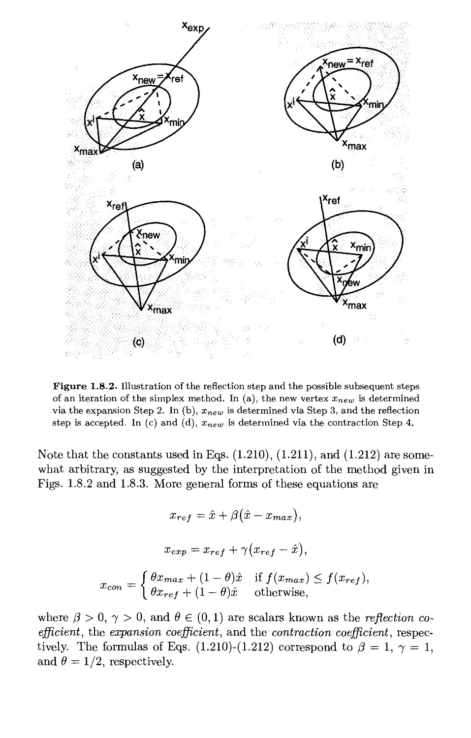
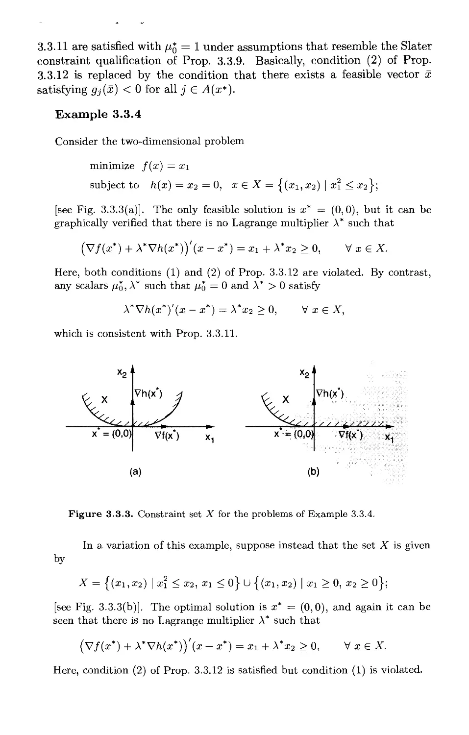
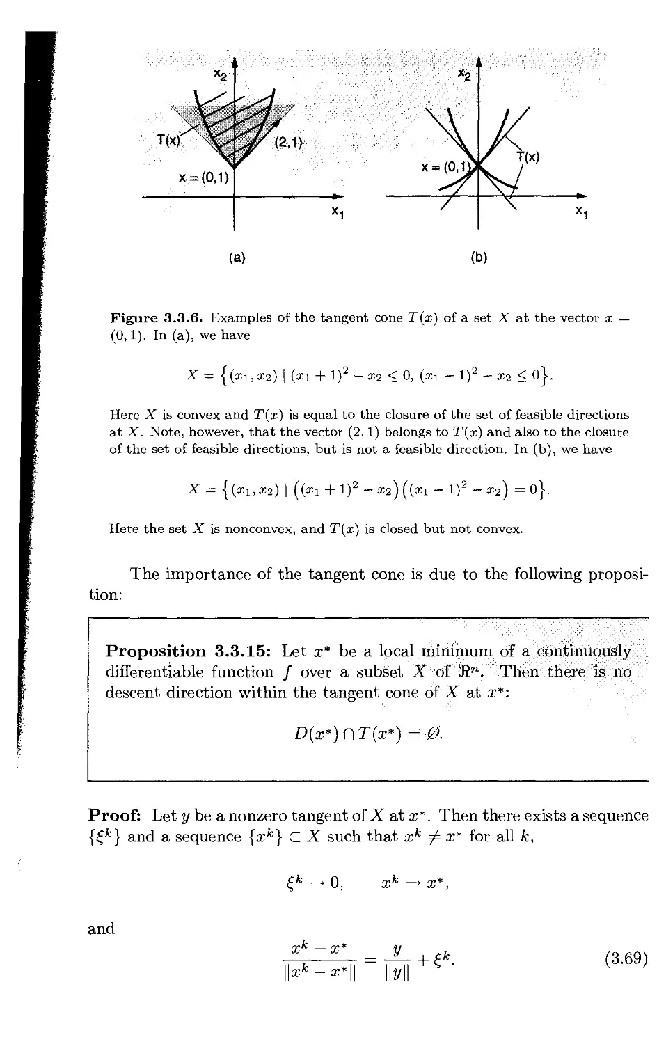
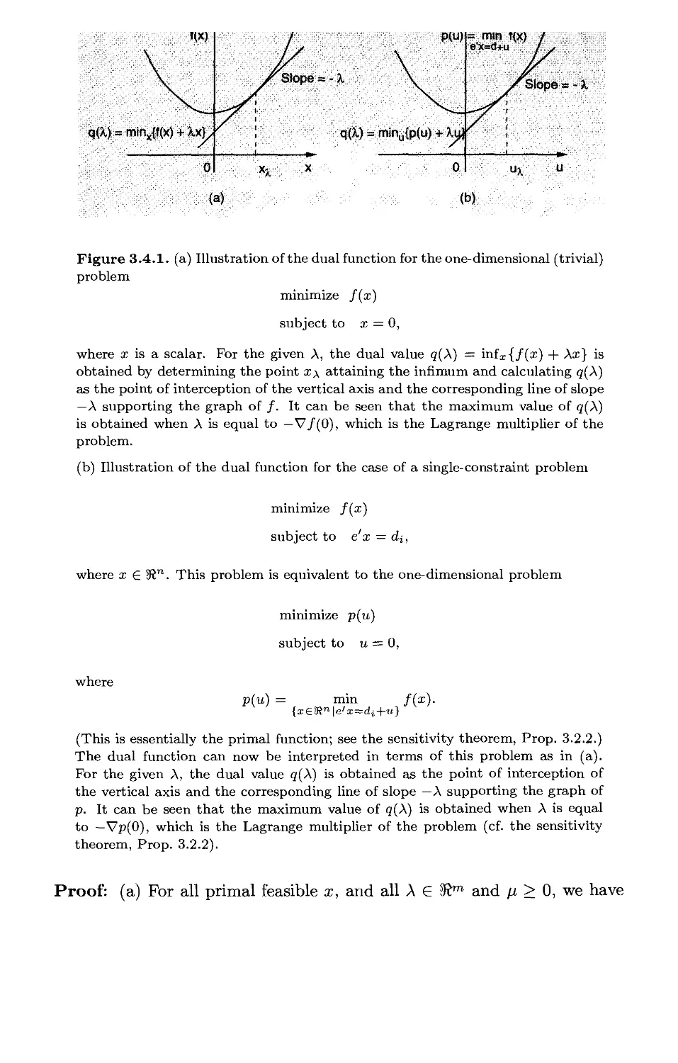
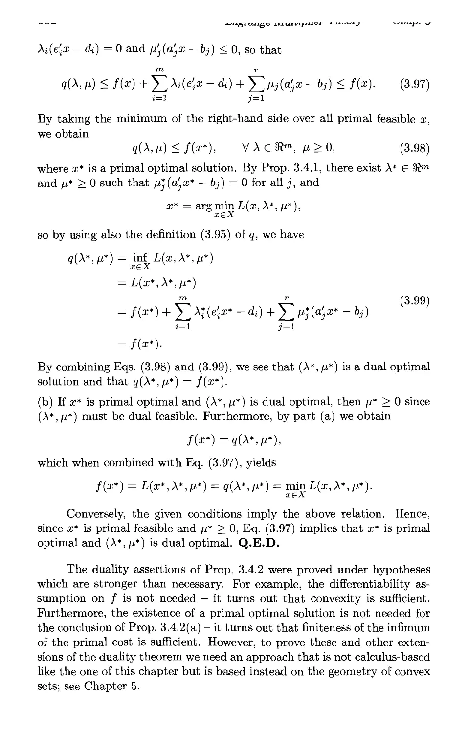
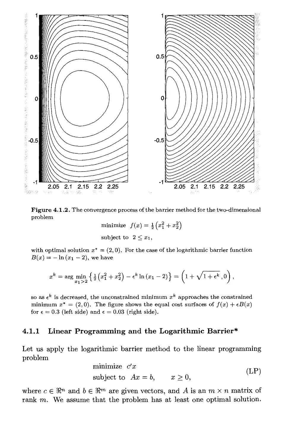
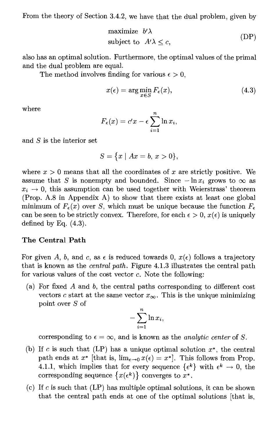
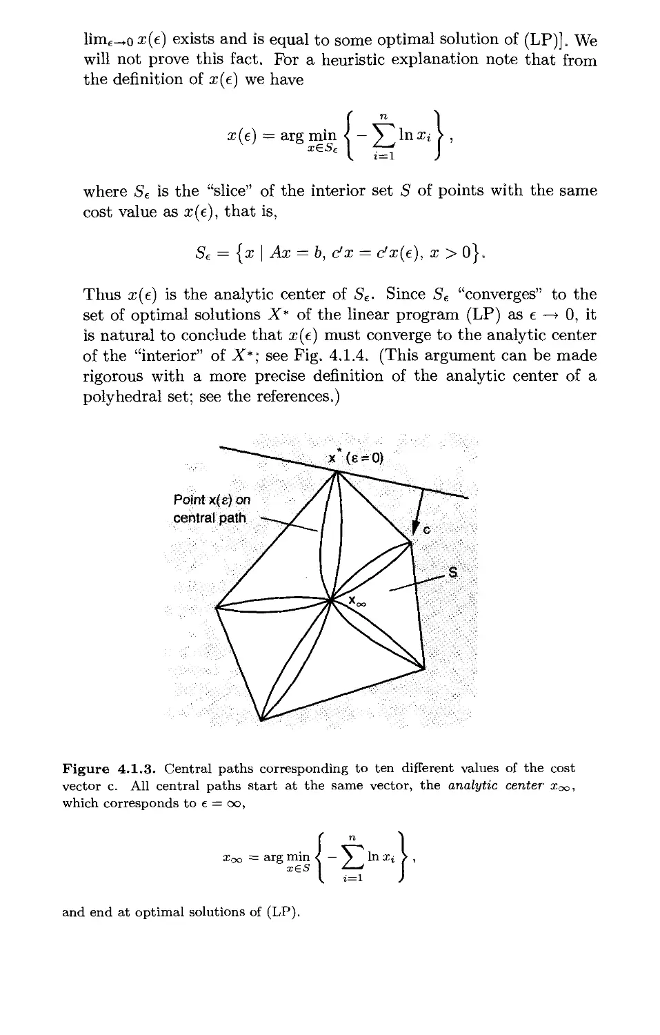
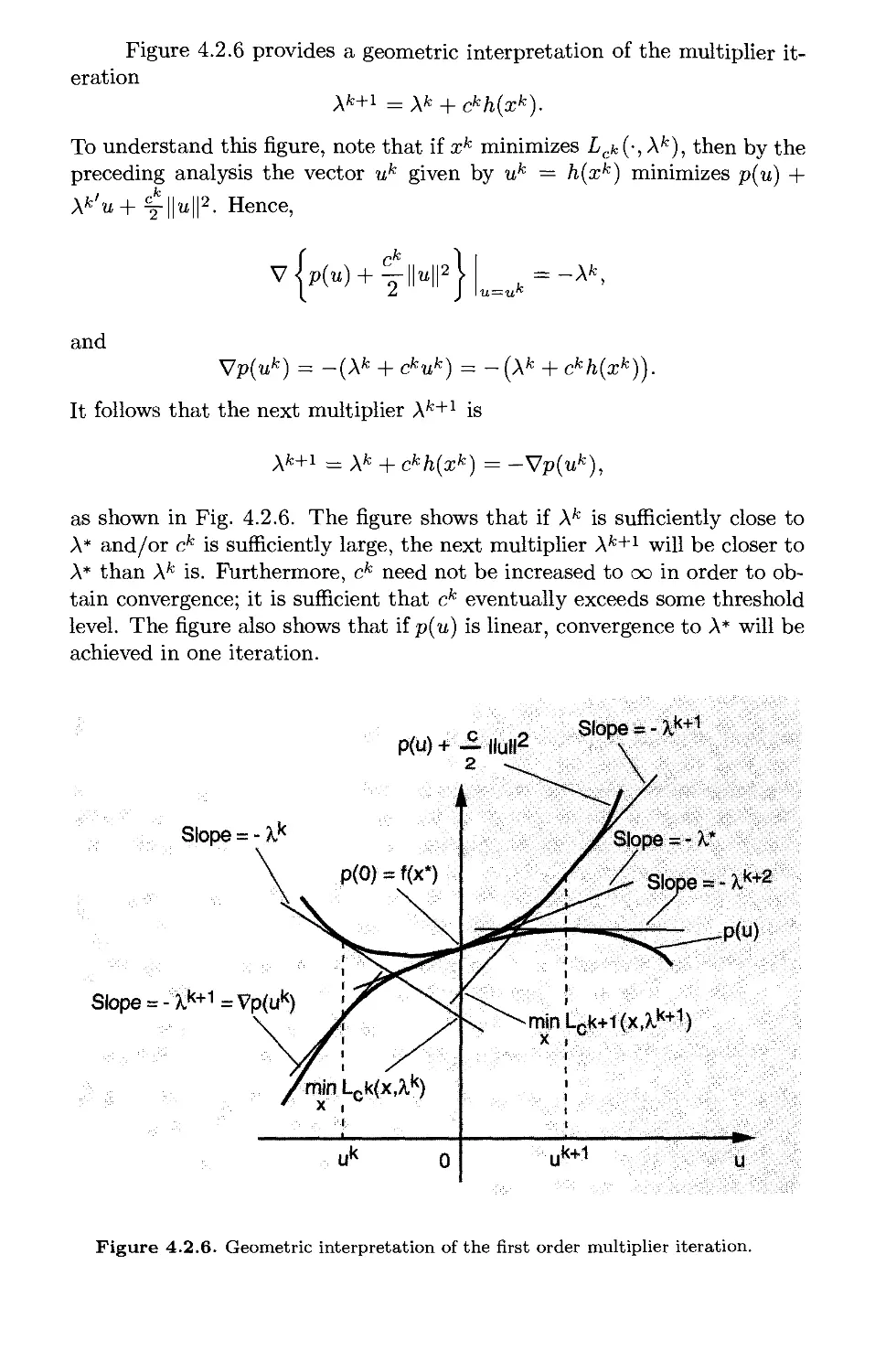
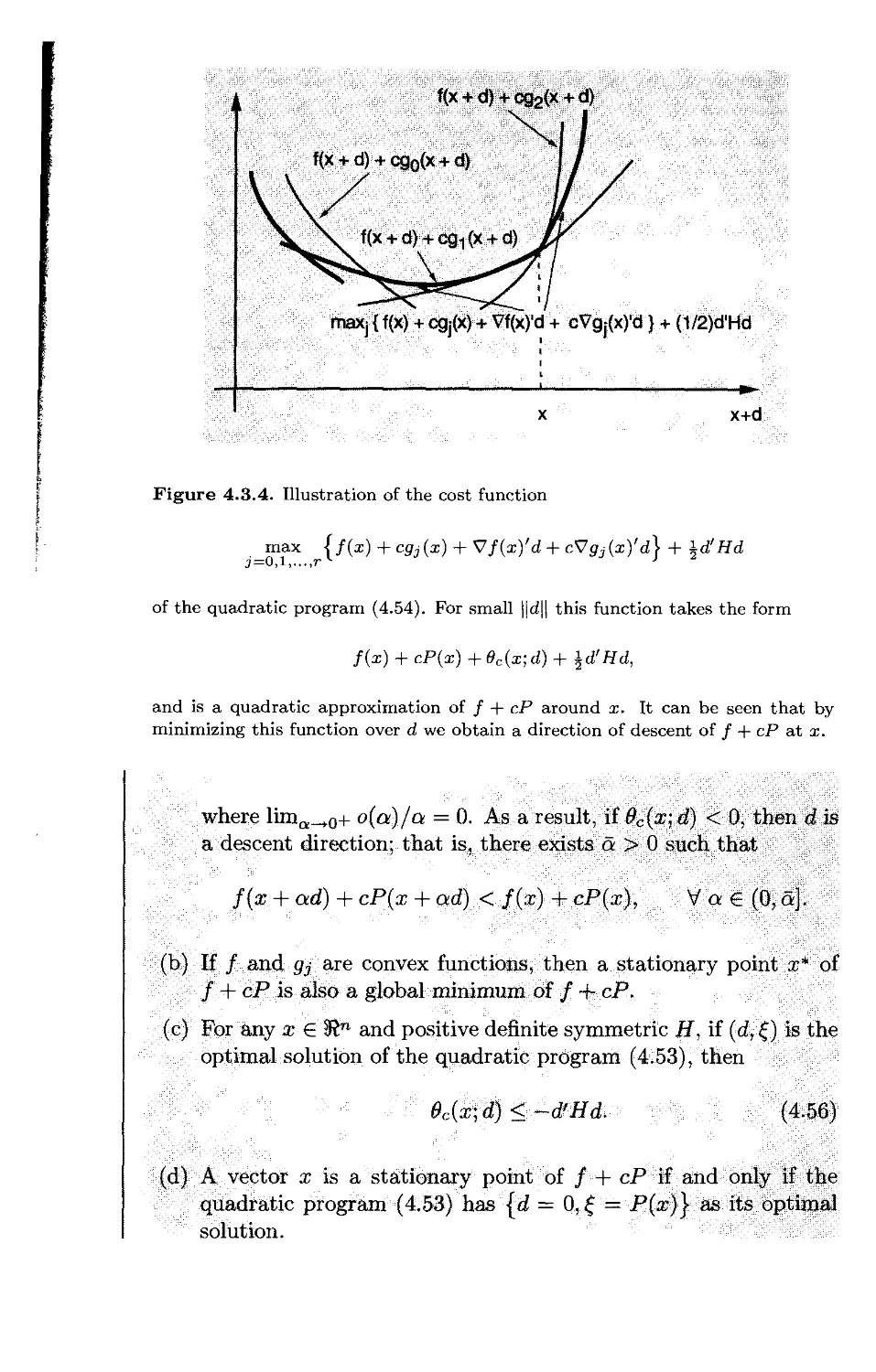
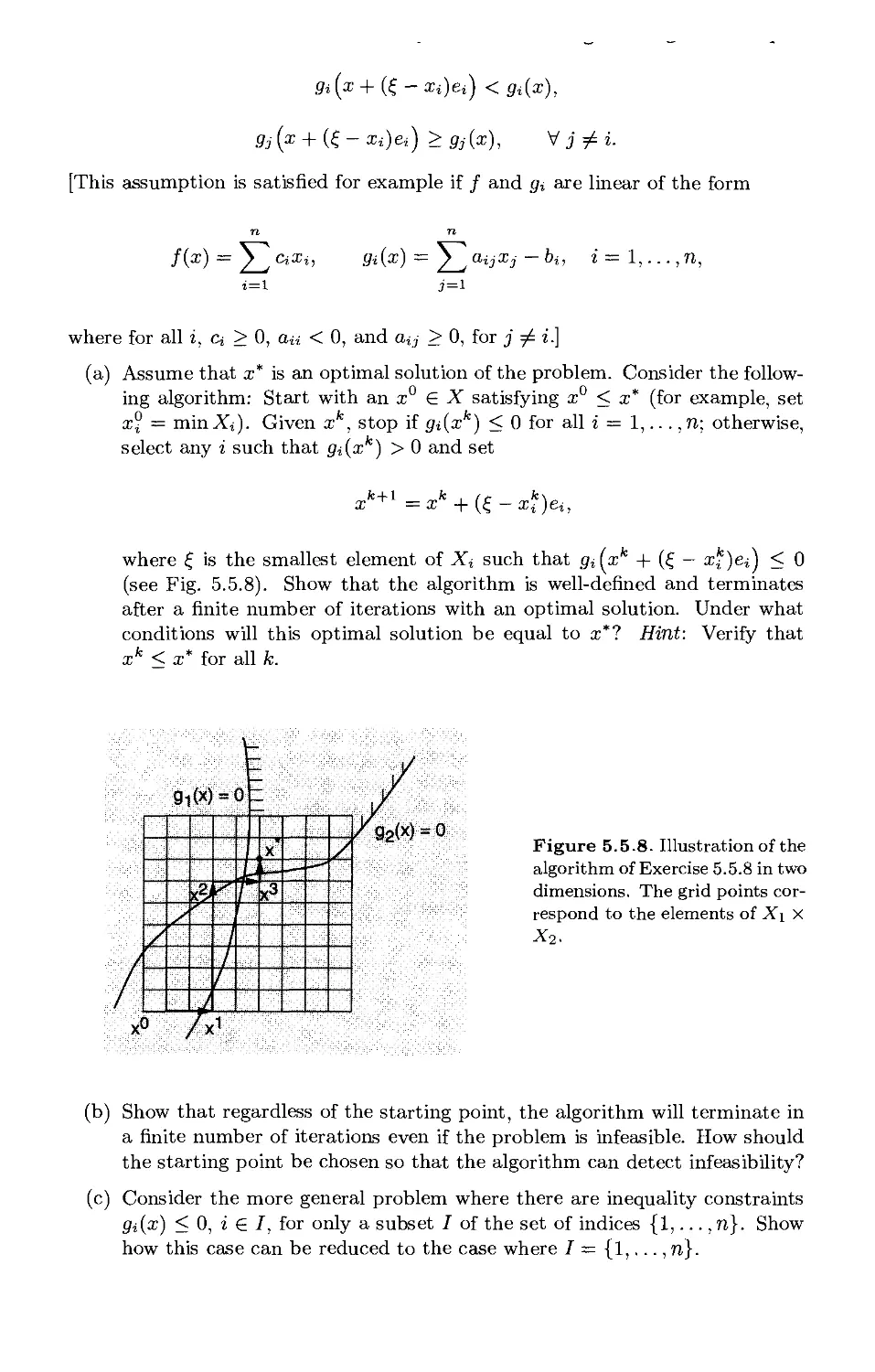
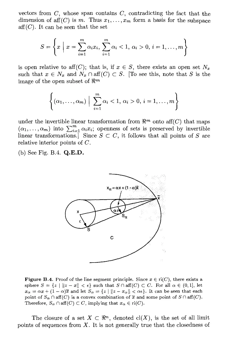
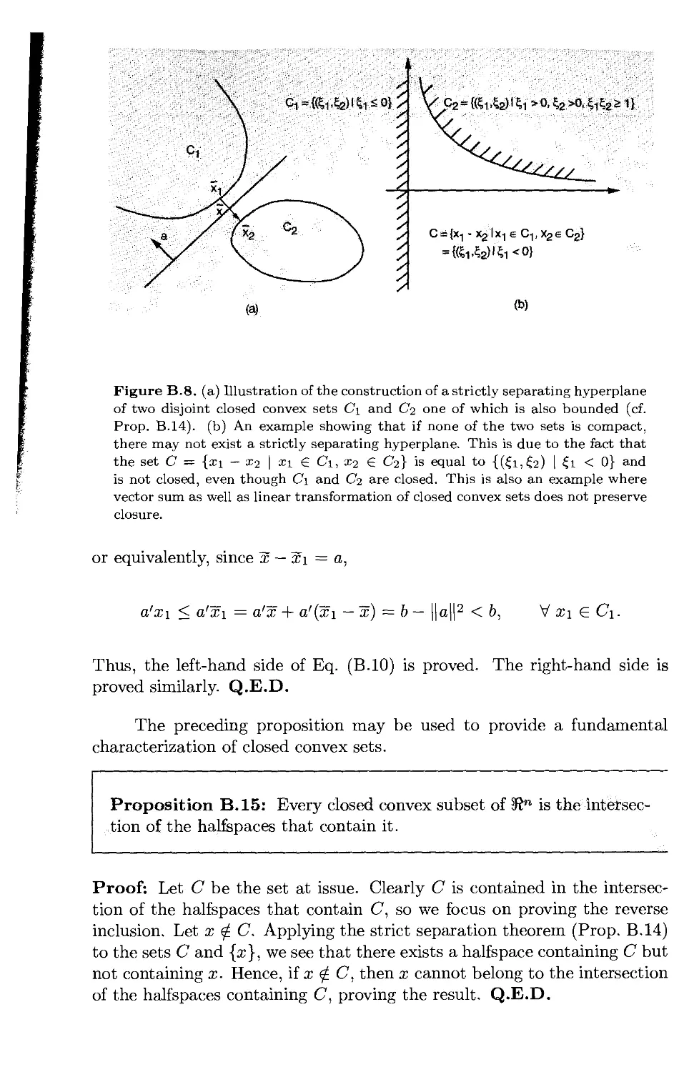
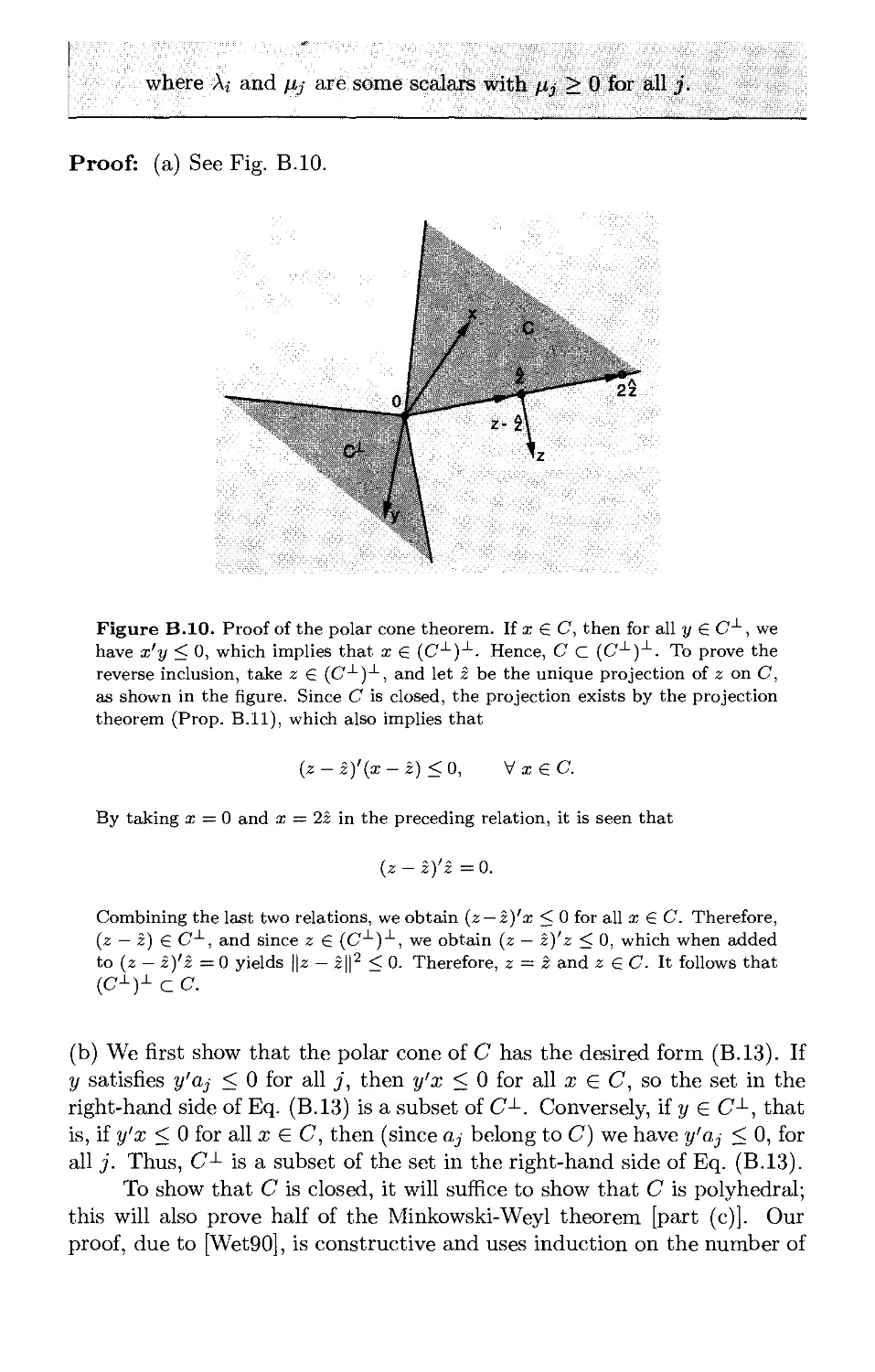
/

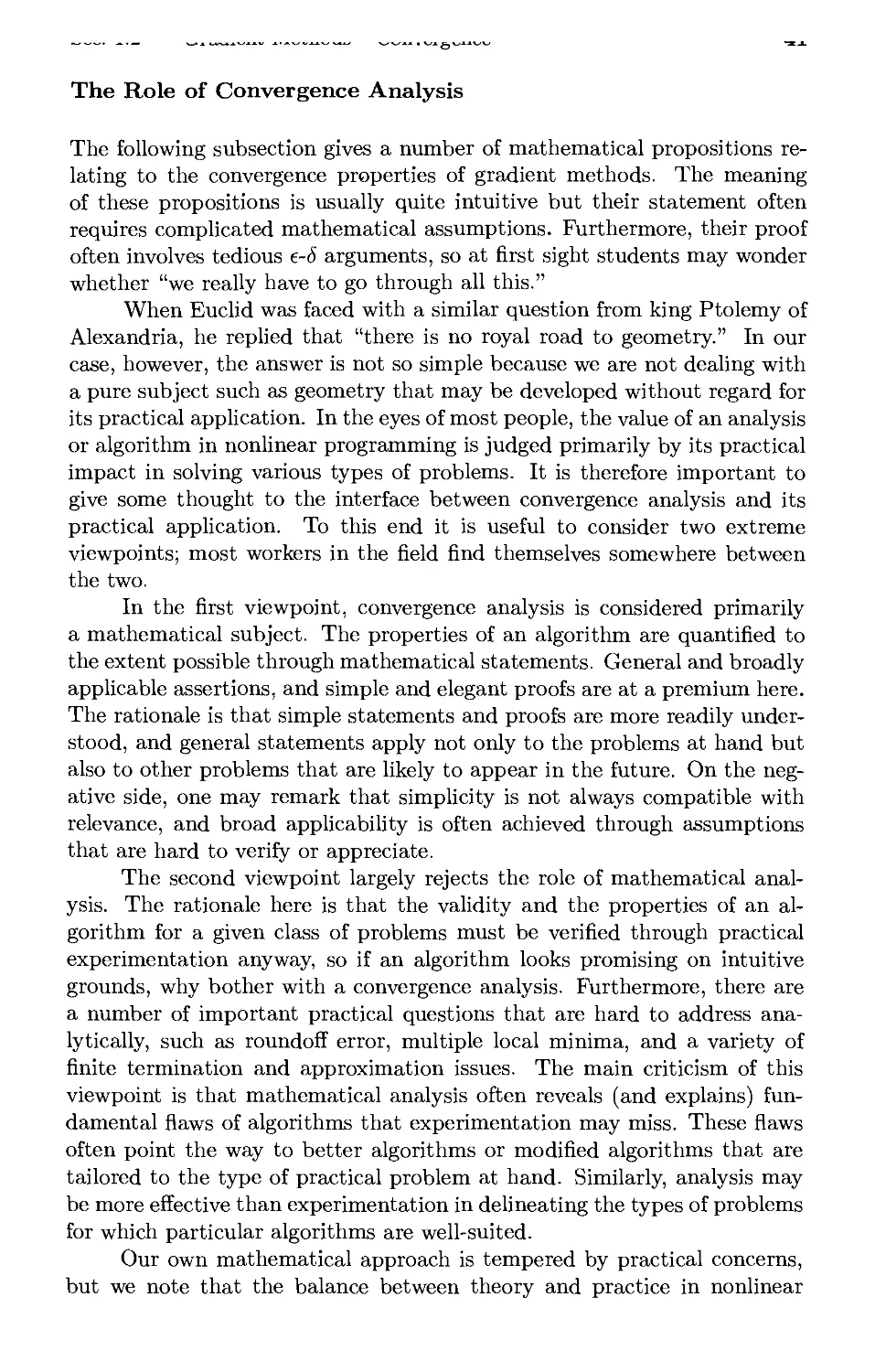

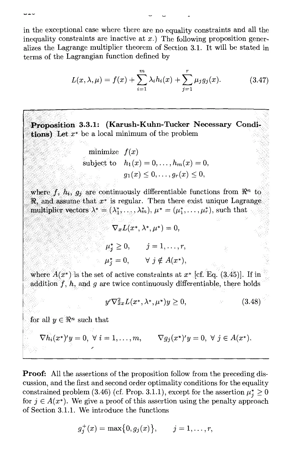

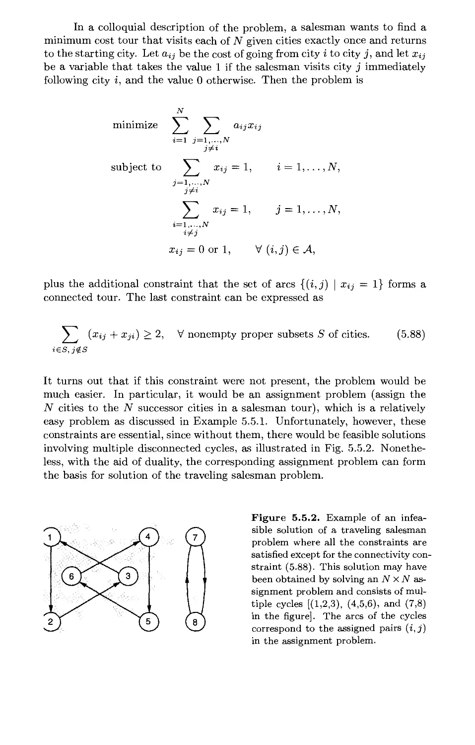


Text
Nonlinear Programming
SECOND EDITION
Dimitri P. Bertsekas
Massachusetts Institute of Technology
WWW site for book information and orders
http://world.std.com/~athenasc/index.html
b
Athena Scientific, Belmont, Massachusetts
ATHENA SCIENTIFIC
OPTIMIZATION AND COMPUTATION SERIES
1. Dynamic Programming and Optimal Control, Vols. I and II, by
Dimitri P. Bertsekas, 1995, ISBN 1-886529-11-6, 704 pages
2. Nonlinear Programming, Second Edition, by Dimitri P.
Bertsekas, 1999, ISBN 1-886529-00-0, 791 pages
3. Neuro-Dynamic Programming, by Dimitri P. Bertsekas and John
N. Tsitsiklis, 1996, ISBN 1-886529-10-8, 512 pages
4. Constrained Optimization and Lagrange Multiplier Methods, by
Dimitri P. Bertsekas, 1996, ISBN 1-886529-04-3, 410 pages
5. Stochastic Optimal Control: The Discrete-Time Case by Dimitri
P. Bertsekas and Steven E. Shreve, 1996, ISBN 1-886529-03-5,
330 pages
6. Introduction to Linear Optimization by Dimitris Bertsimas and
John N. Tsitsiklis, 1997, ISBN 1-886529-19-1, 608 pages
7. Parallel and Distributed Computation: Numerical Methods by
Dimitri P. Bertsekas and John N. Tsitsiklis, 1997, ISBN 1-886529-
01-9, 718 pages
8. Network Flows and Monotropic Optimization by R. Tyrrell Rock-
afellar, 1998, ISBN 1-886529-06-X, 634 pages
9. Network Optimization: Continuous and Discrete Models by
Dimitri P. Bertsekas, 1998, ISBN 1-886529-02-7, 608 pages
Contents
1. Unconstrained Optimization p. 1
1.1. Optimality Conditions p. 4
1.1.1. Variational Ideas p. 4
1.1.2. Main Optimality Conditions p. 13
1.2. Gradient Methods - Convergence p. 22
1.2.1. Descent Directions and Stepsize Rules p. 22
1.2.2. Convergence Results p. 43
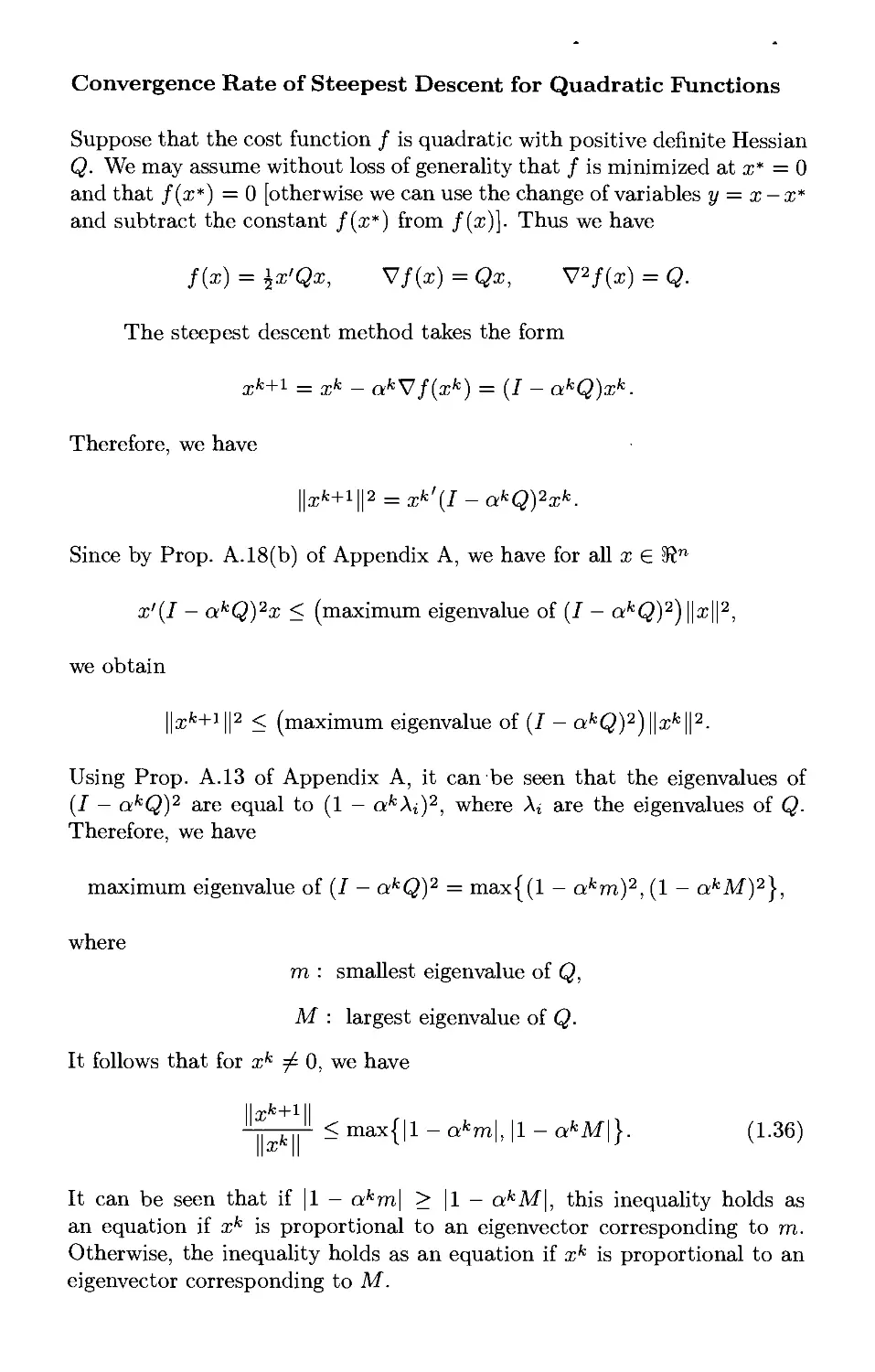
1.3. Gradient Methods - Rate of Convergence p. 62
1.3.1. The Local Analysis Approach p. 64
1.3.2. The Role of the Condition Number p. 65
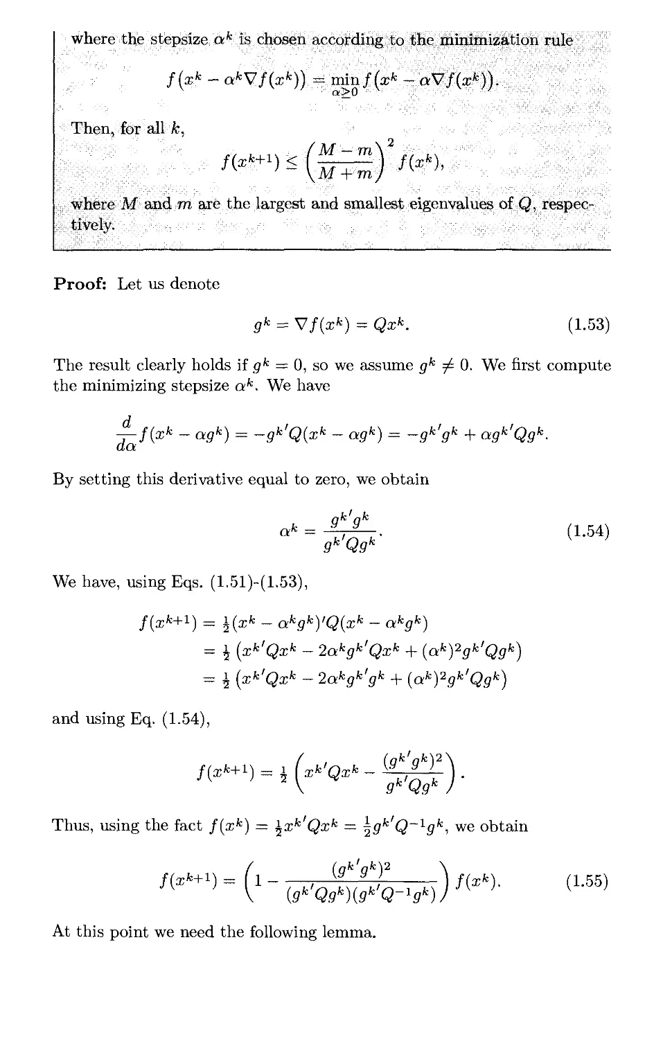
1.3.3. Convergence Rate Results p. 75
1.4. Newton's Method and Variations p. 88
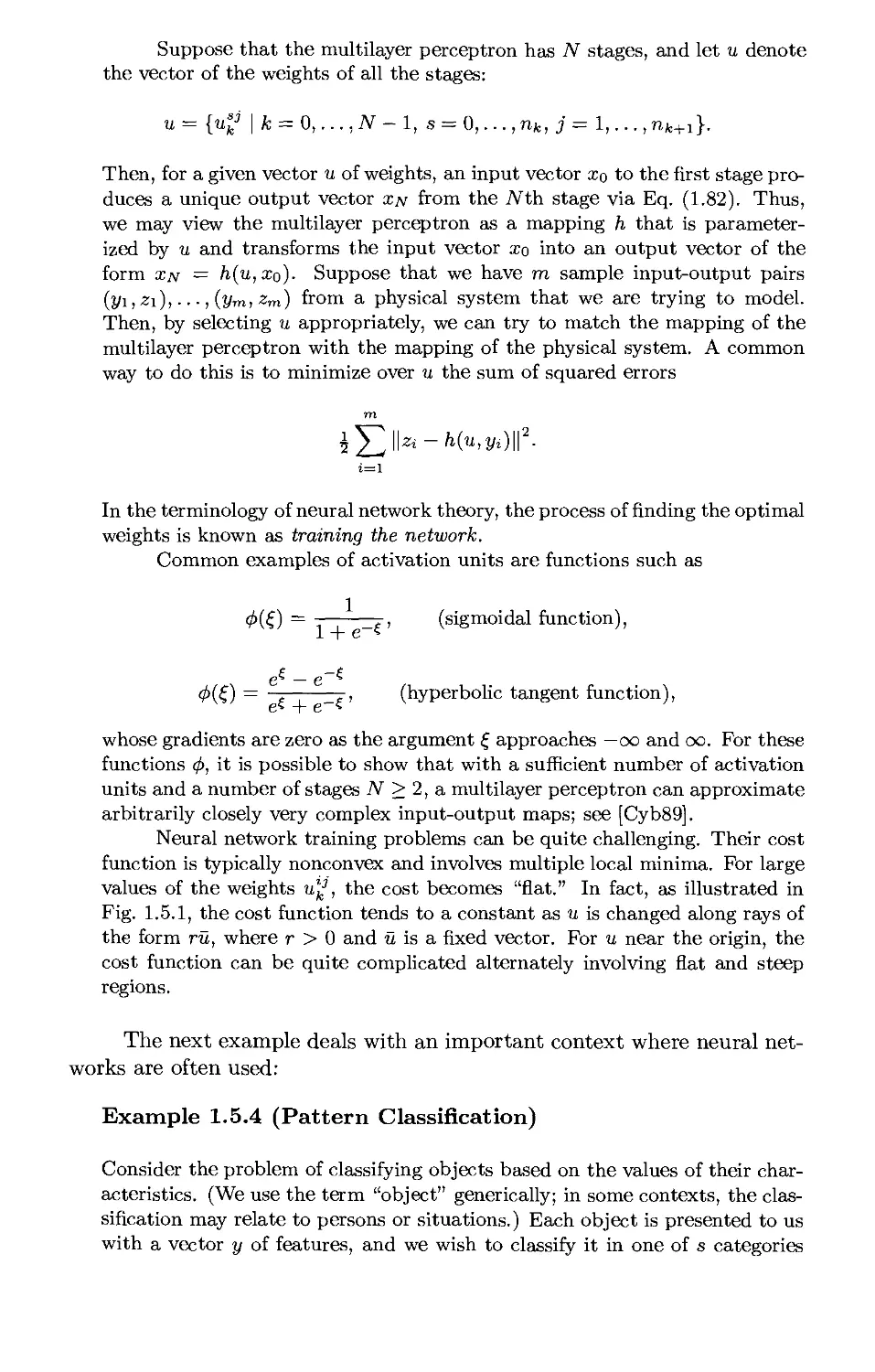
1.5. Least Squares Problems p. 102
1.5.1. The Gauss-Newton Method p. 107
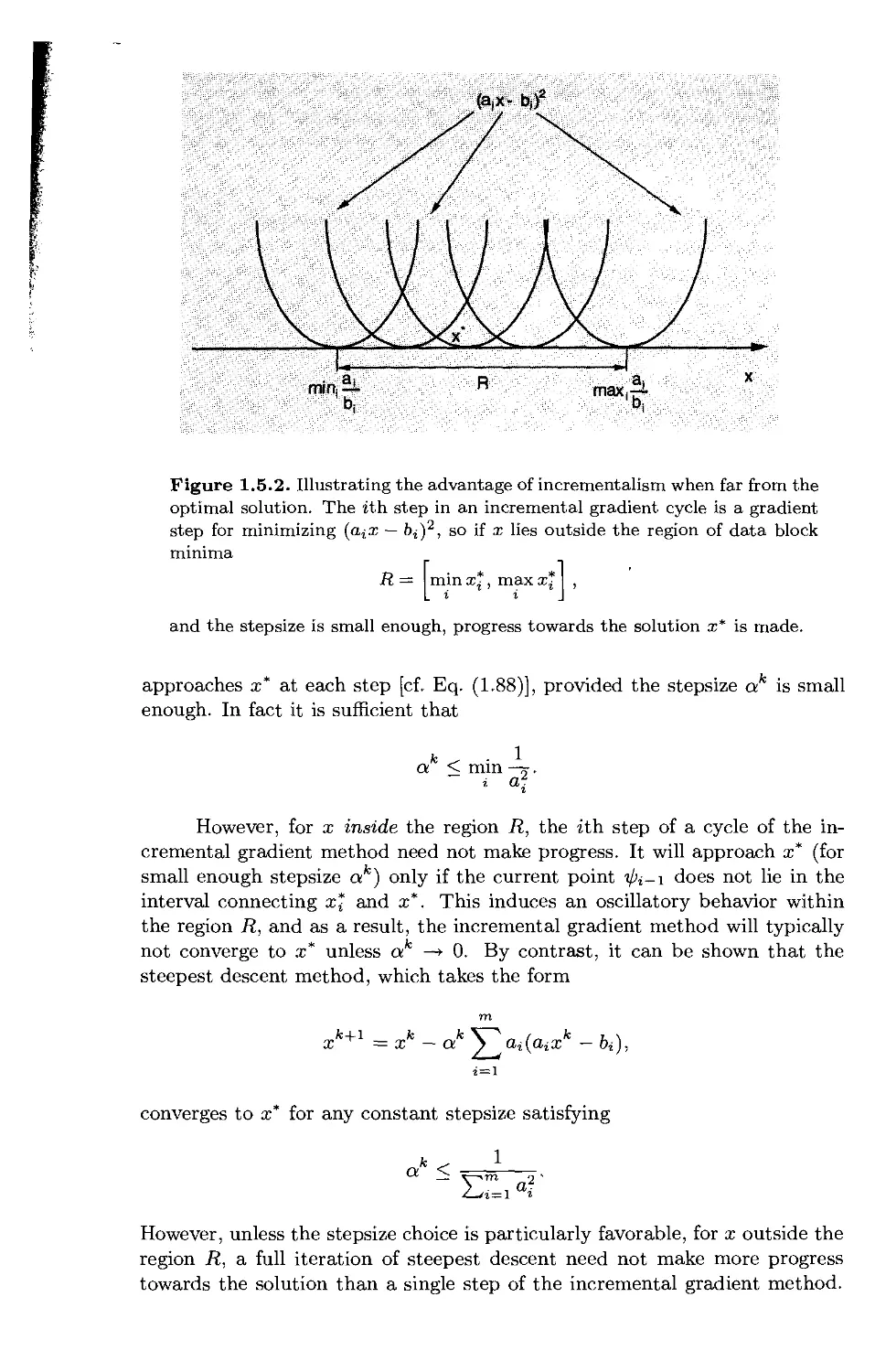
1.5.2. Incremental Gradient Methods* p. 108
1.5.3. Incremental Forms of the Gauss-Newton Method* .... p. 119
1.6. Conjugate Direction Methods p. 130
1.7. Quasi-Newton Methods p. 148
1.8. Nonderivative Methods p. 158
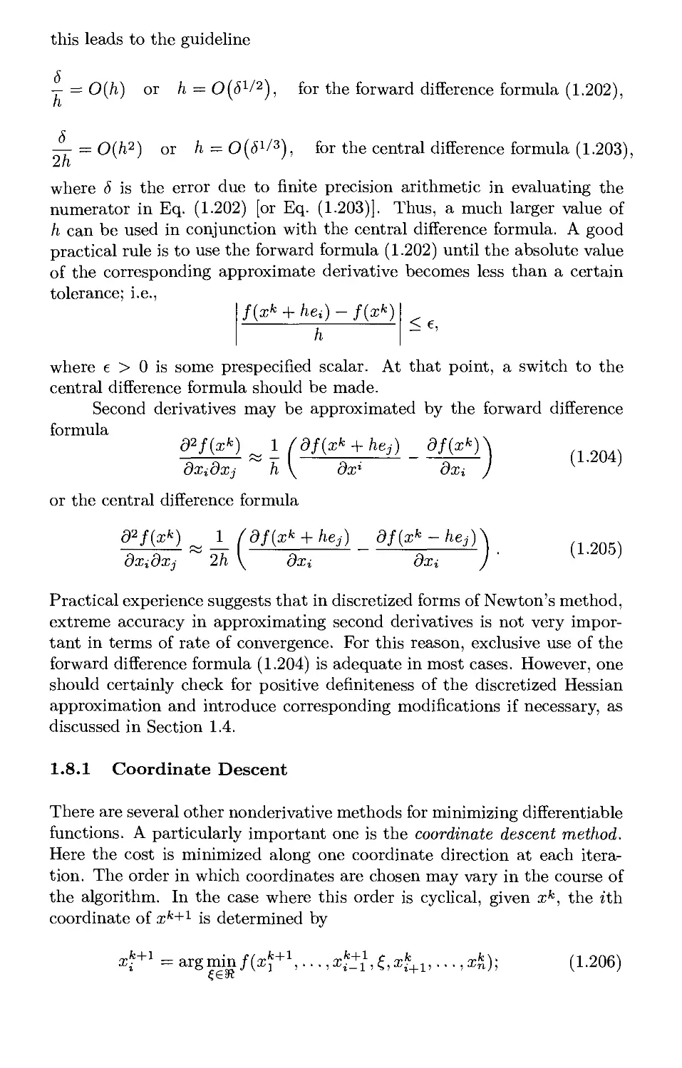
1.8.1. Coordinate Descent p. 160
1.8.2. Direct Search Methods p. 162
1.9. Discrete-Time Optimal Control Problems* p. 166
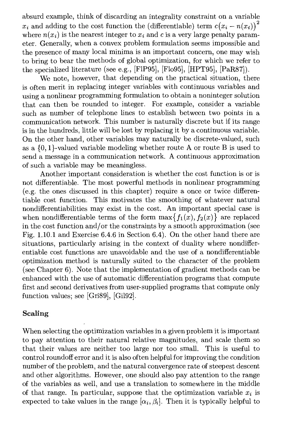
1.10. Some Practical Guidelines p. 183
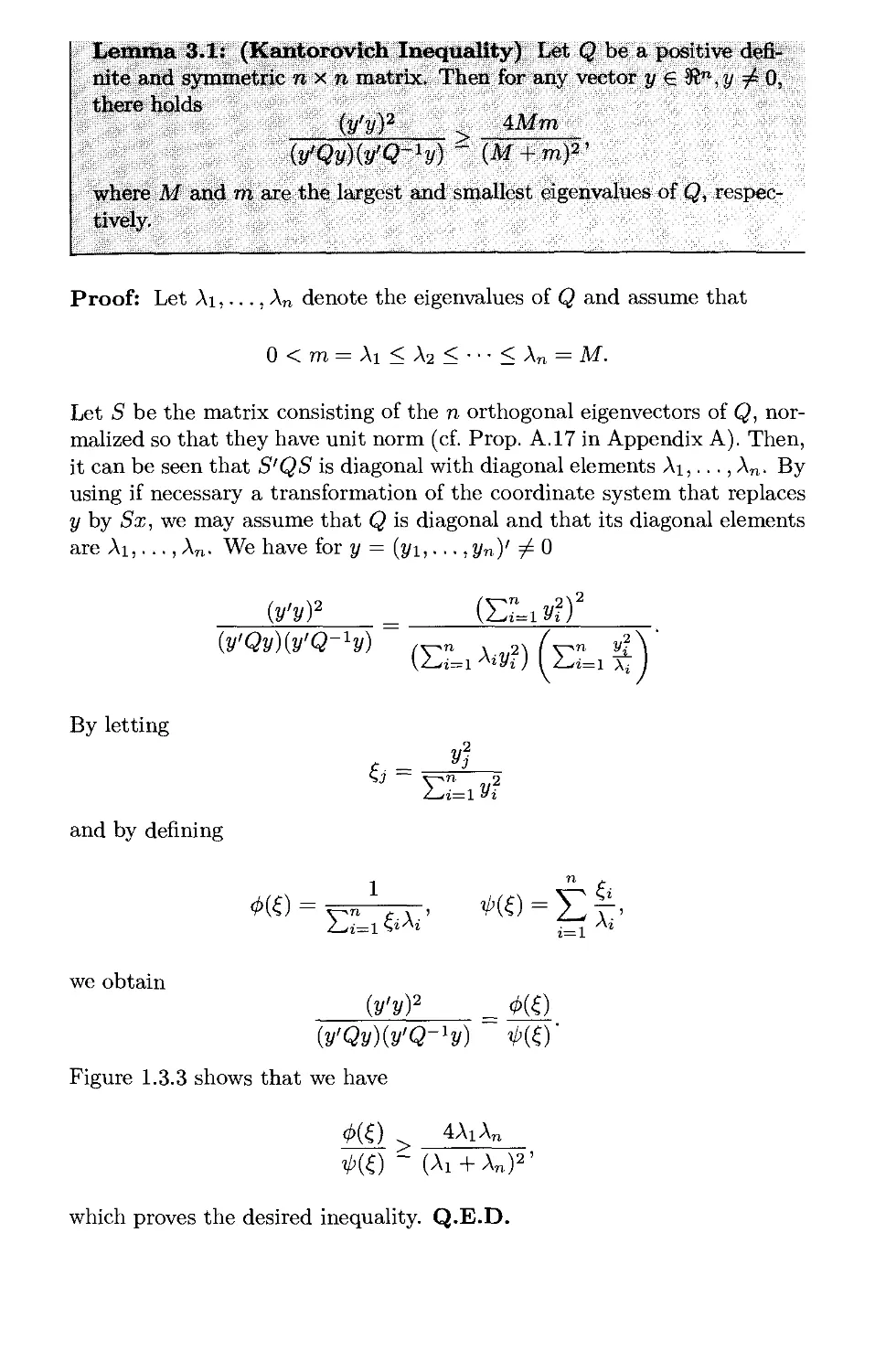
1.11. Notes and Sources p. 187
2. Optimization Over a Convex Set p. 191
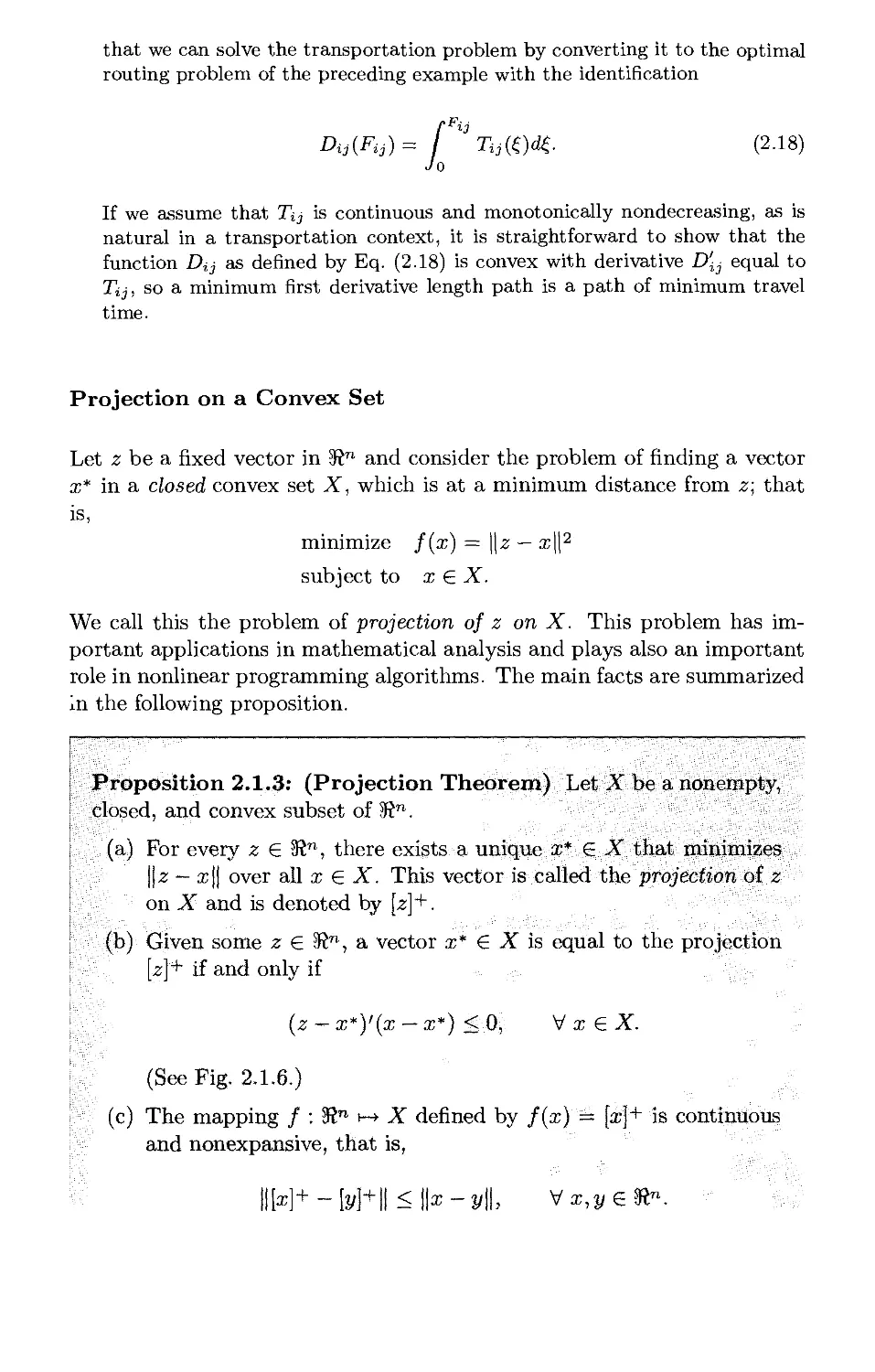
2.1. Optimality Conditions p. 192
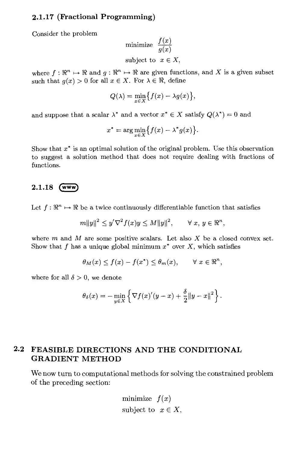
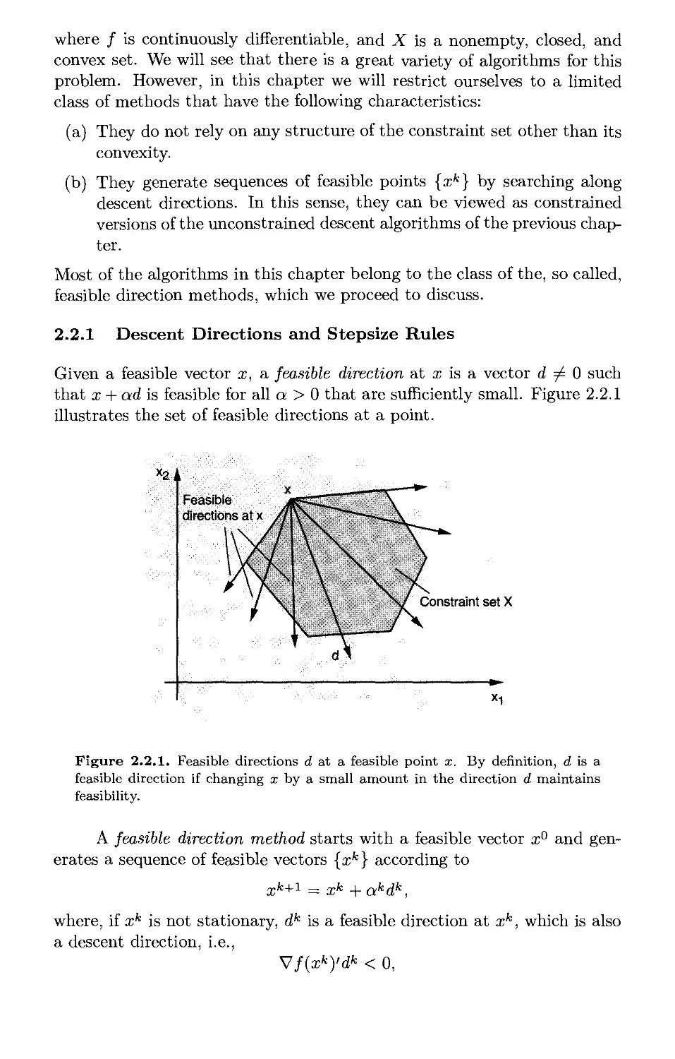
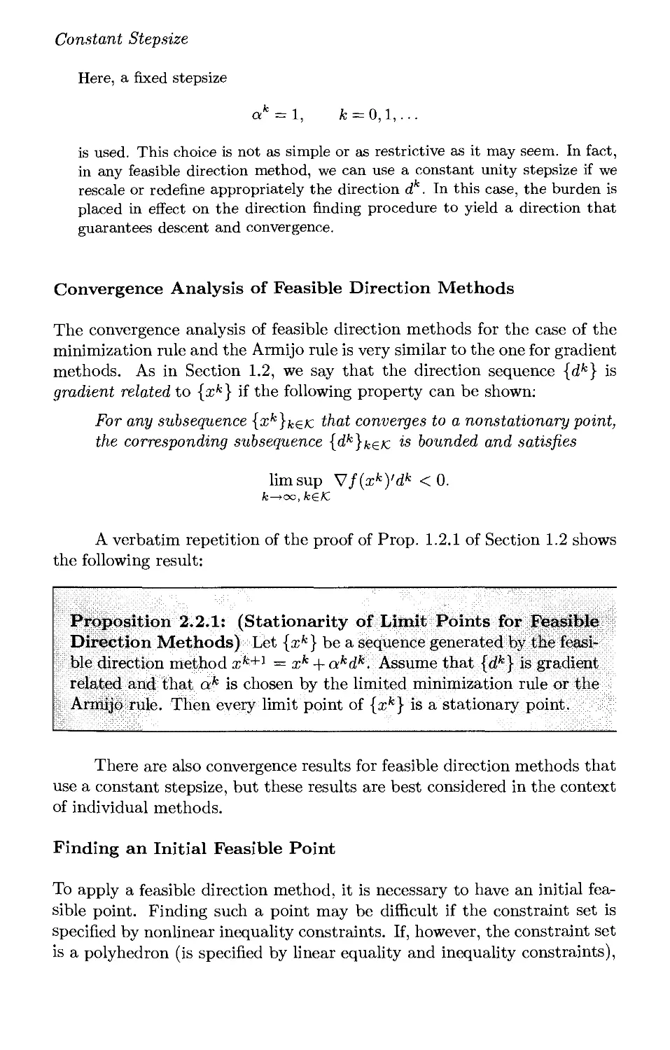
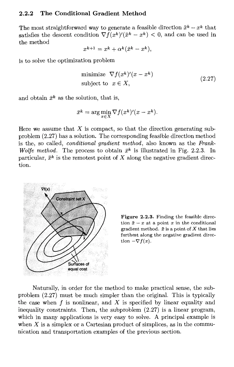
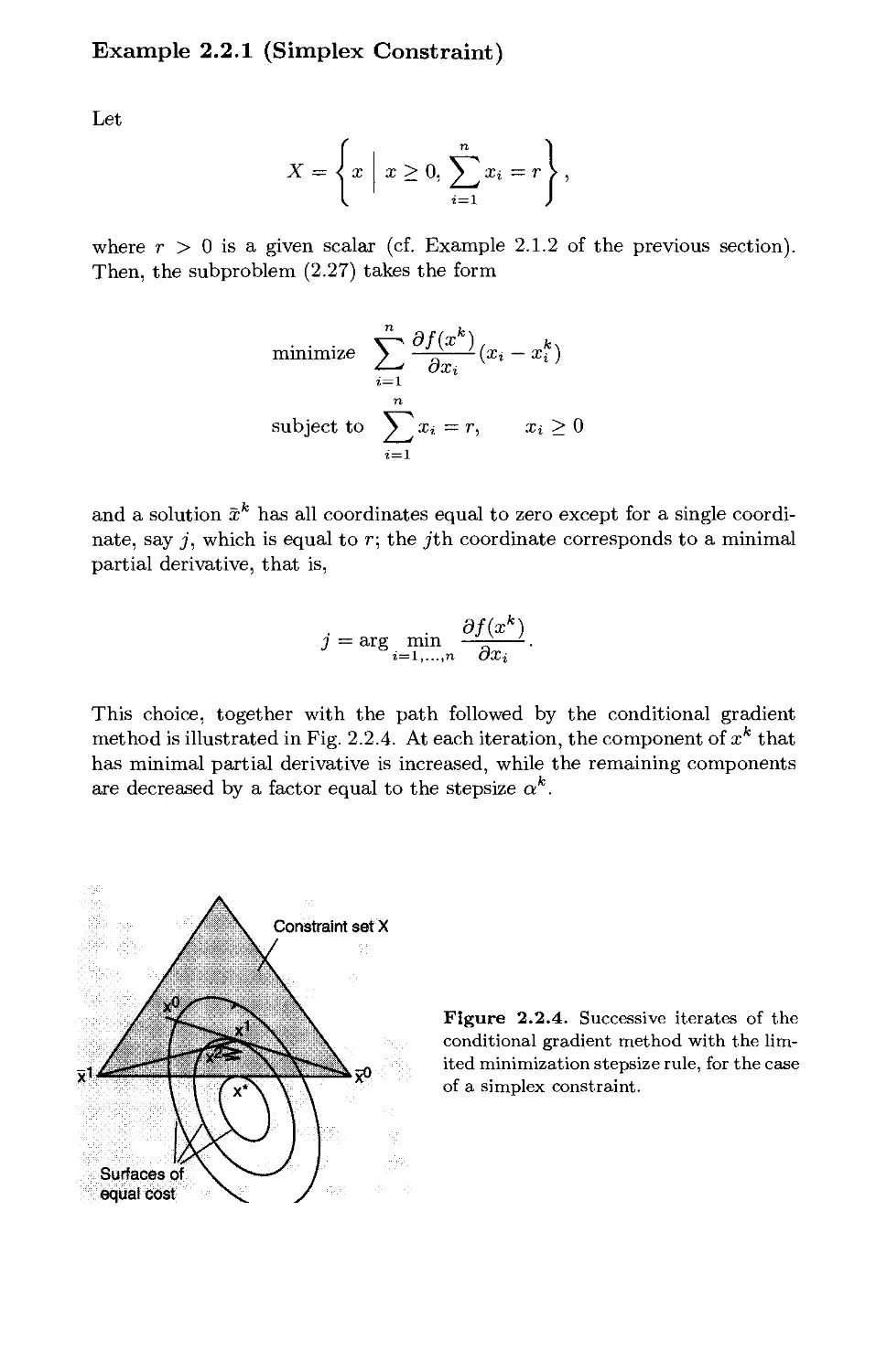
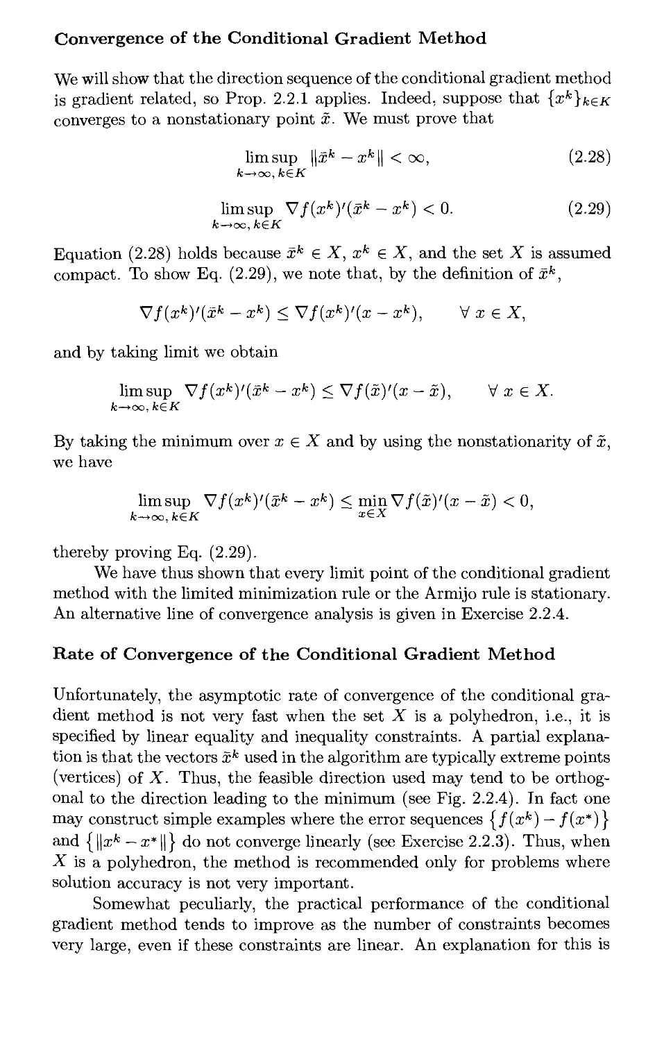
2.2. Feasible Directions and the Conditional Gradient Method . . p. 209
2.2.1. Descent Directions and Stepsize Rules p. 210
2.2.2. The Conditional Gradient Method p. 215
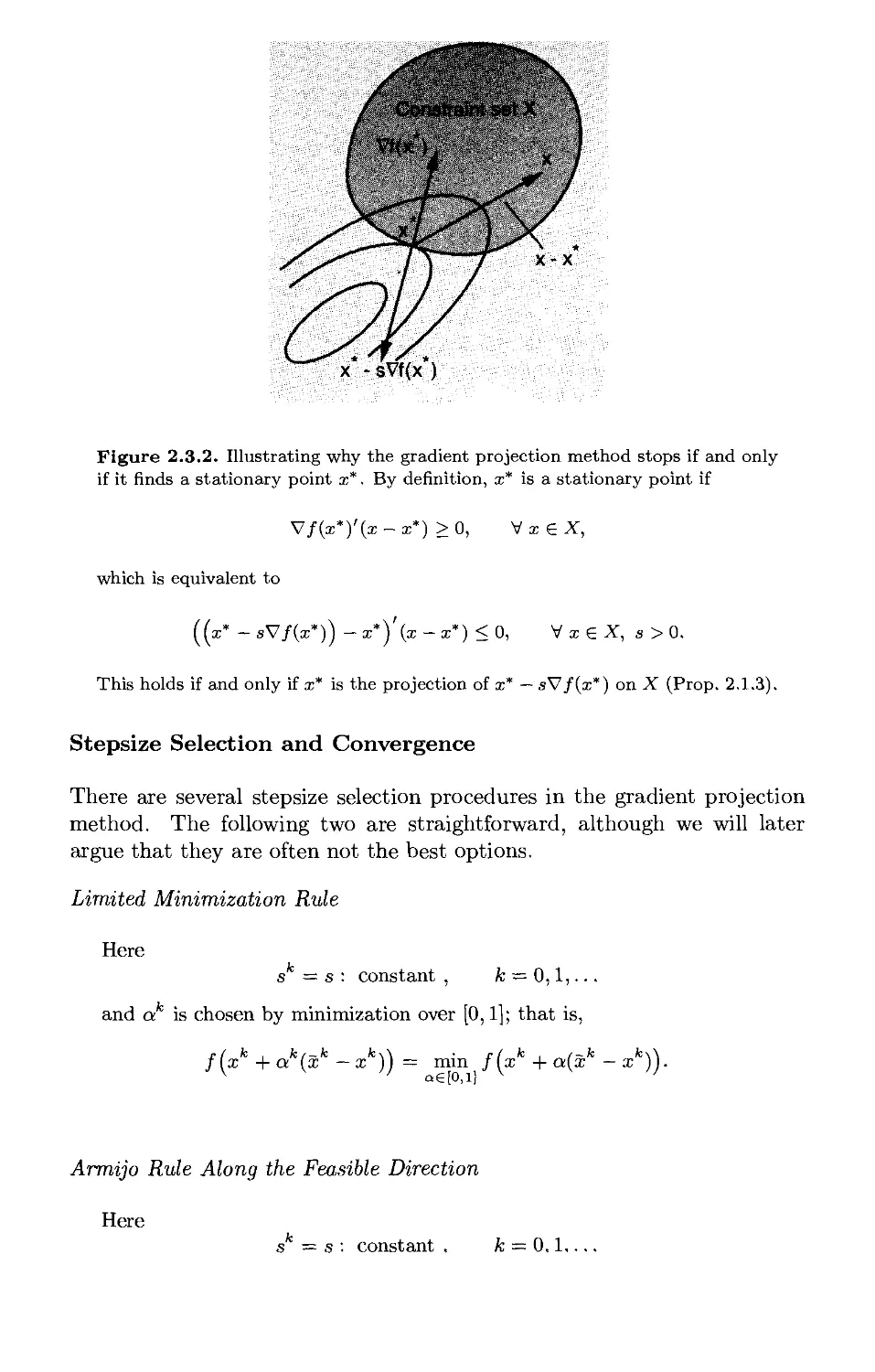
2.3. Gradient Projection Methods p. 223
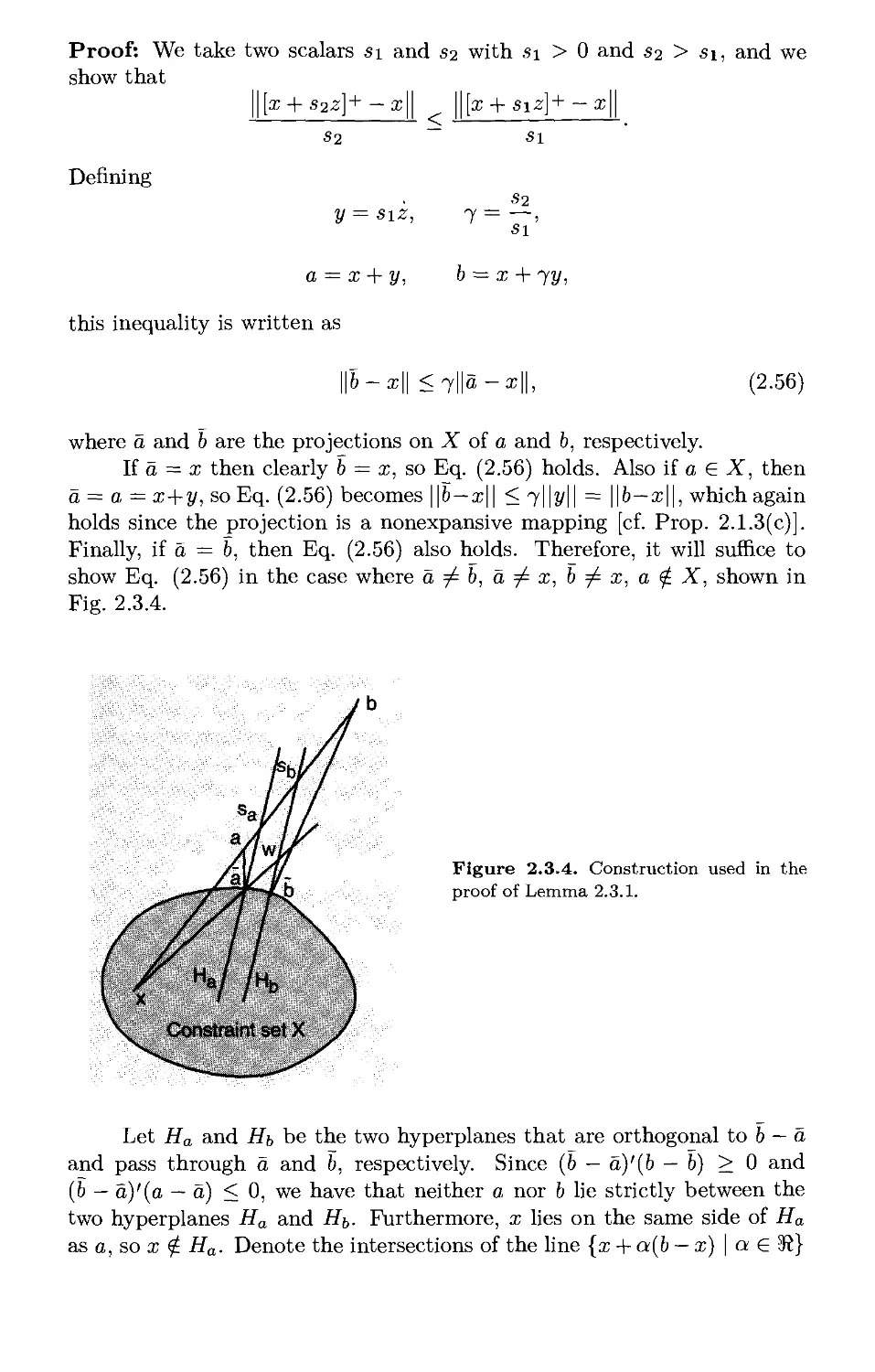
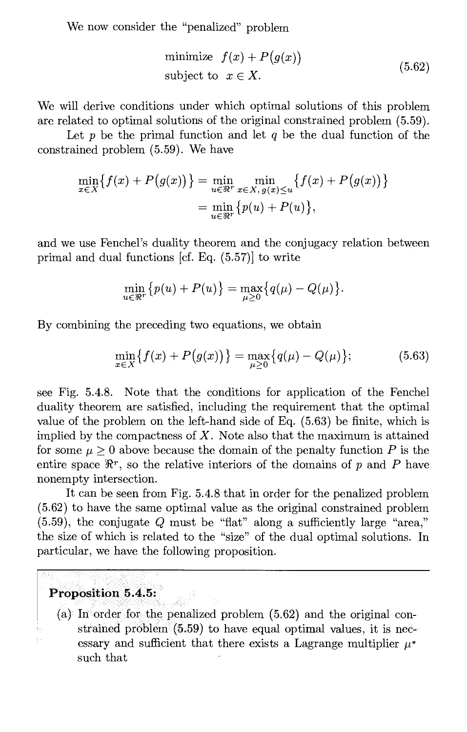
2.3.1. Feasible Directions and Stepsize Rules Based on Projection p. 223
v
v; Contents
2.3.2. Convergence Analysis* p. 234
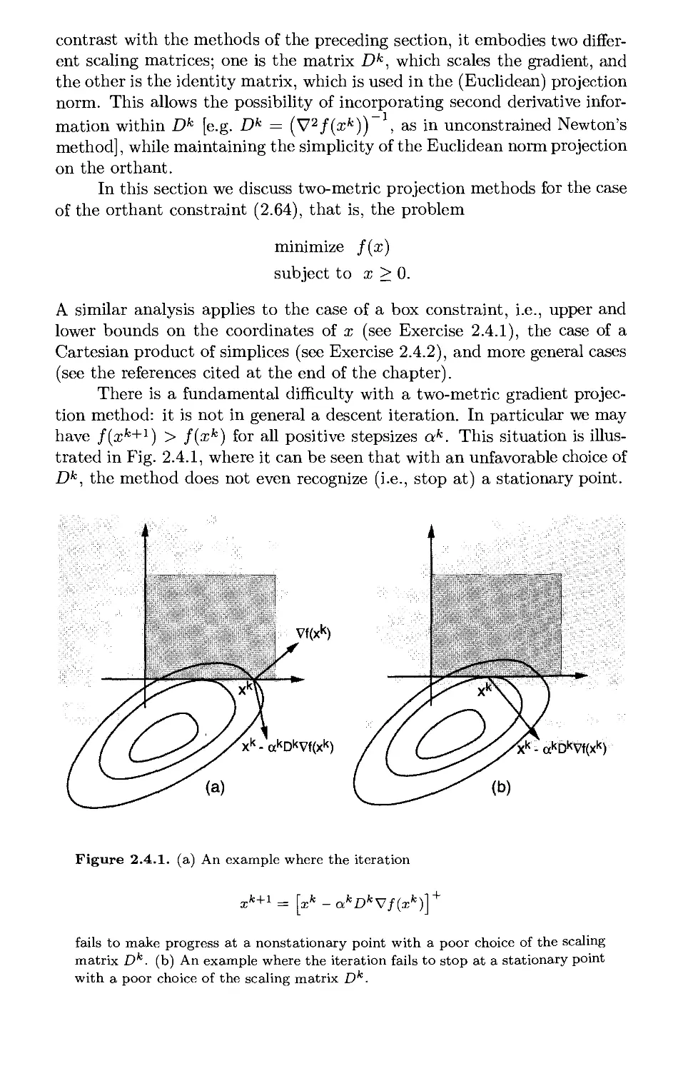
2.4. Two-Metric Projection Methods p. 244
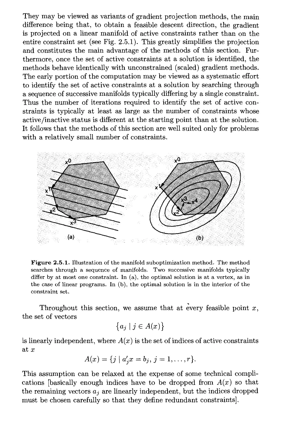
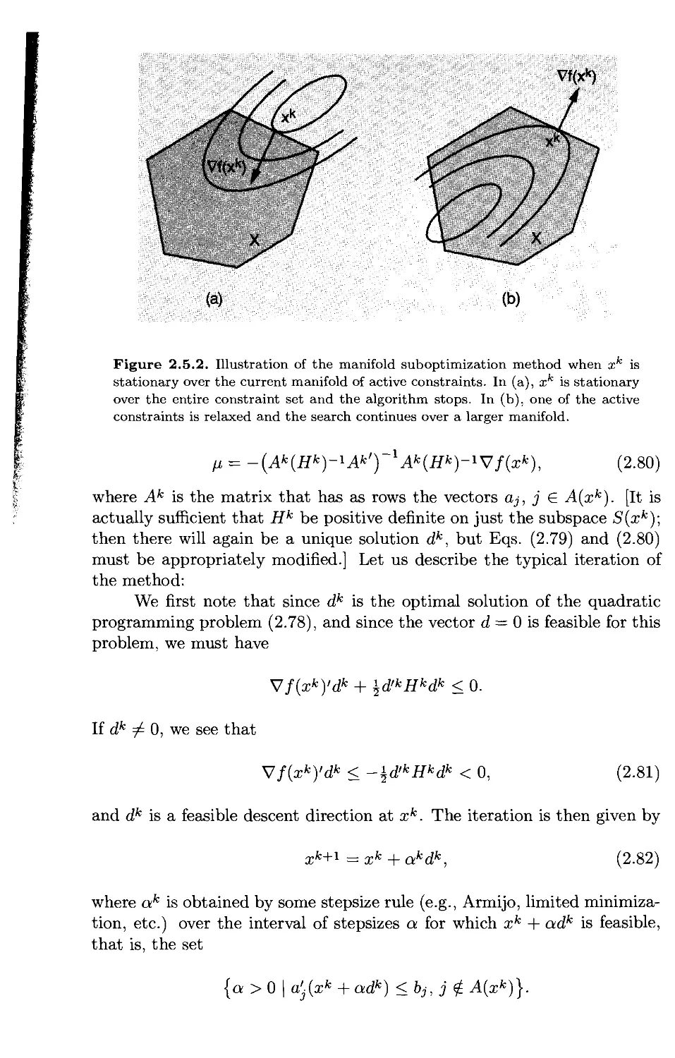
2.5. Manifold Suboptimization Methods p. 250
2.6. Affine Scaling for Linear Programming p. 259
2.7. Block Coordinate Descent Methods* p. 267
2.8. Notes and Sources p. 272
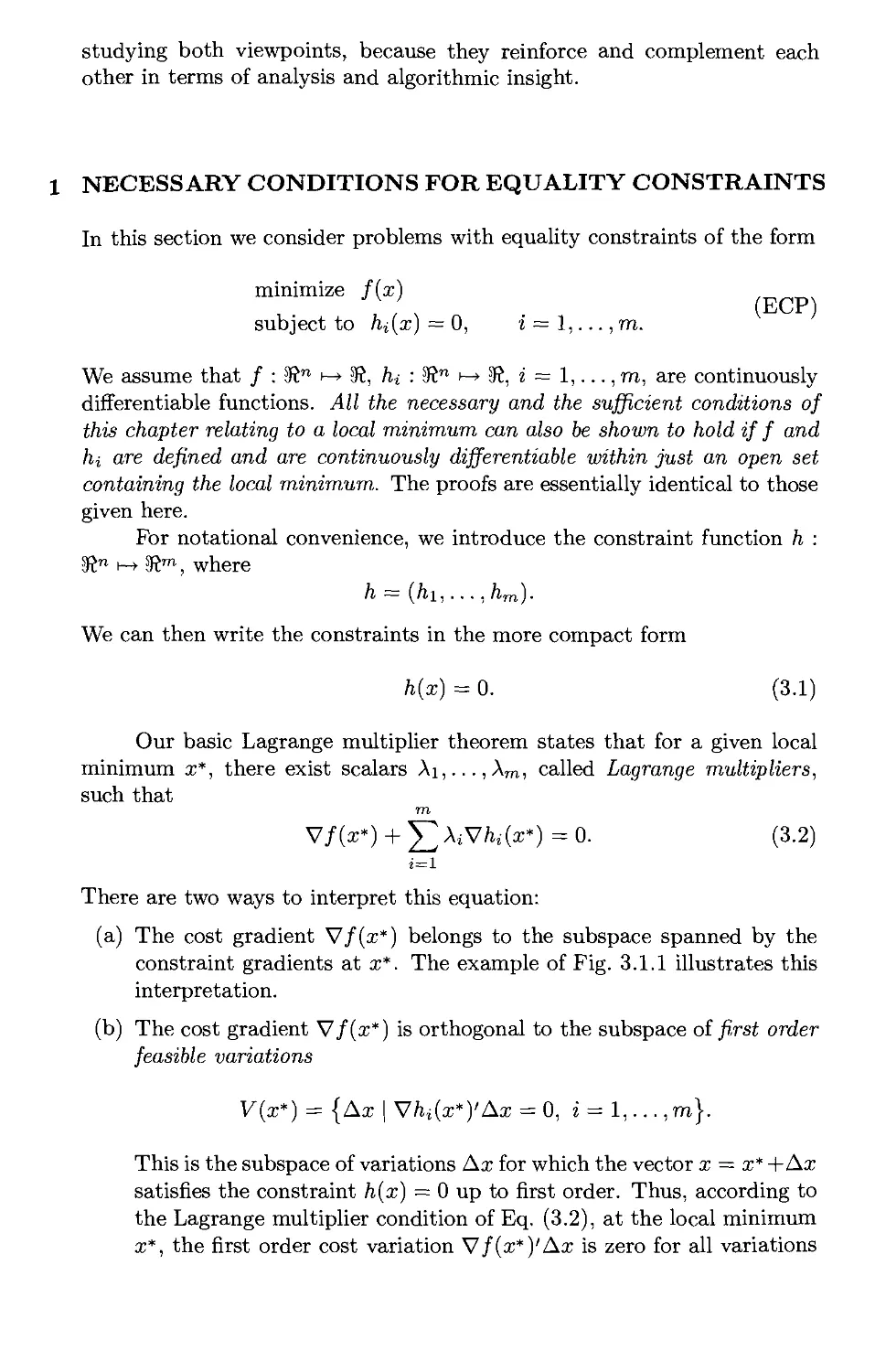
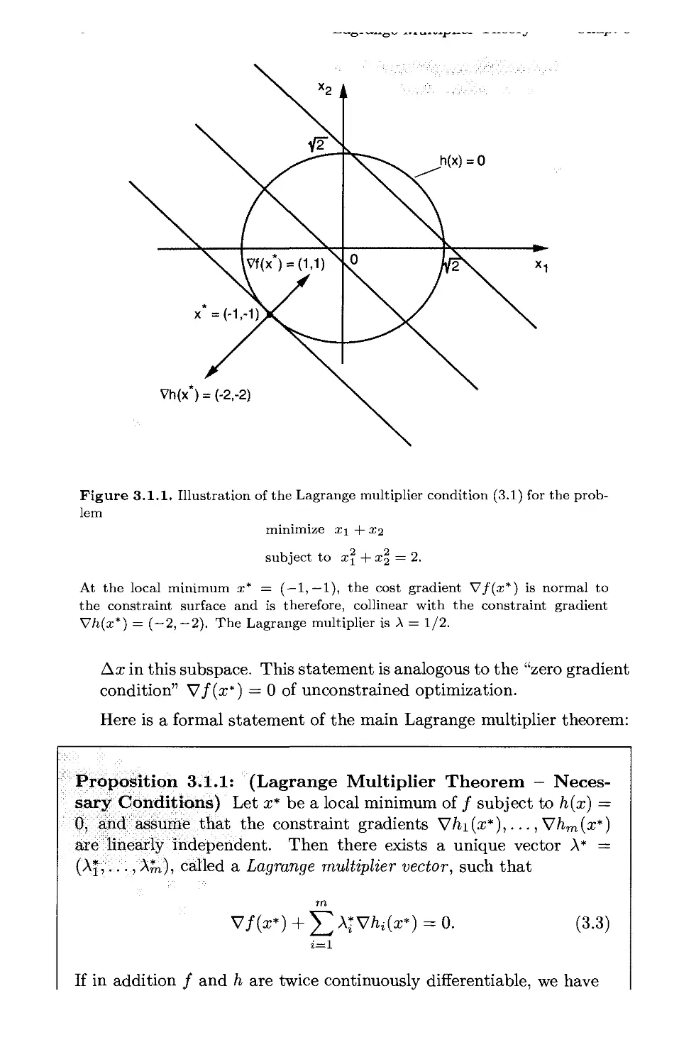
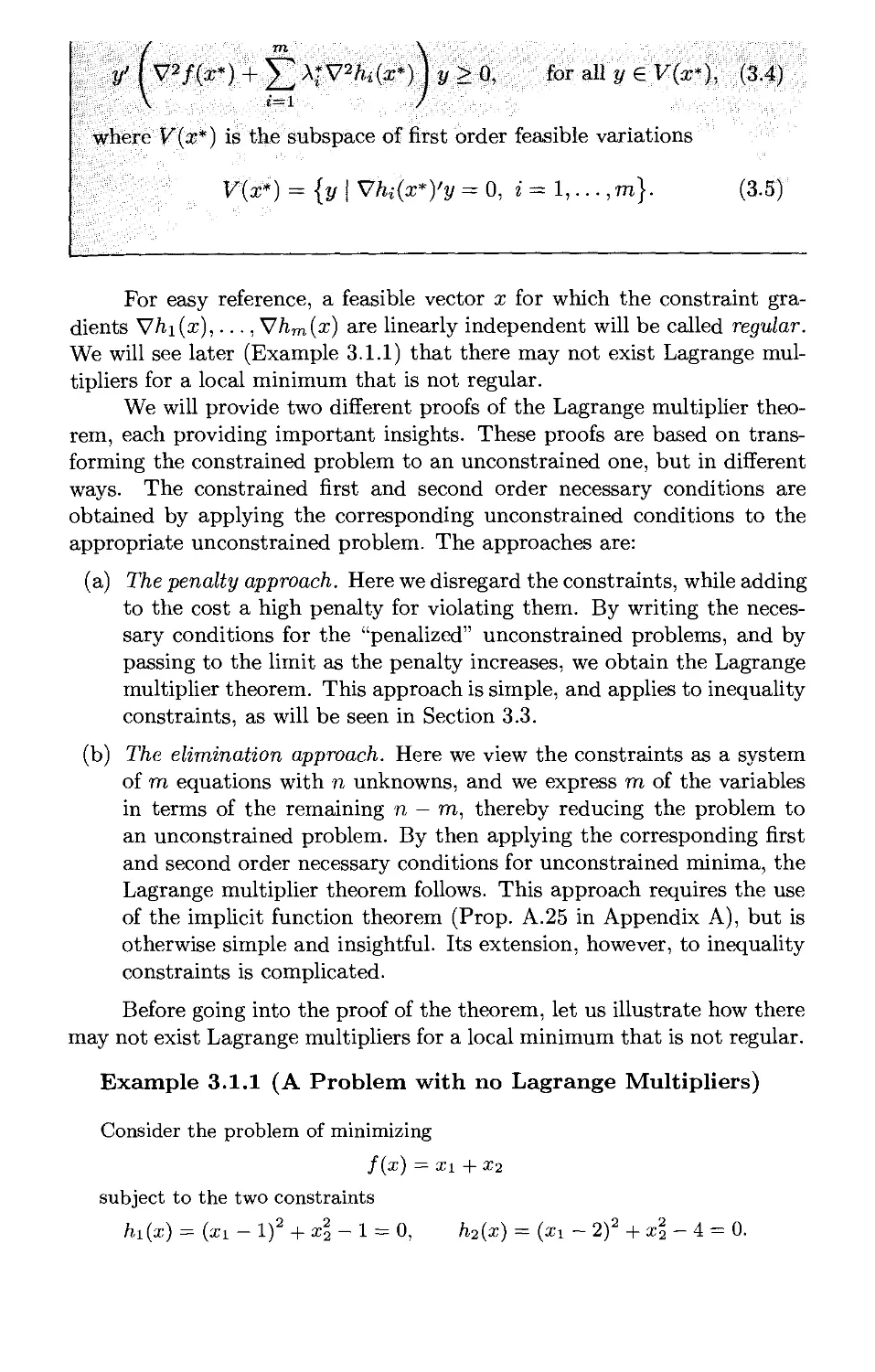
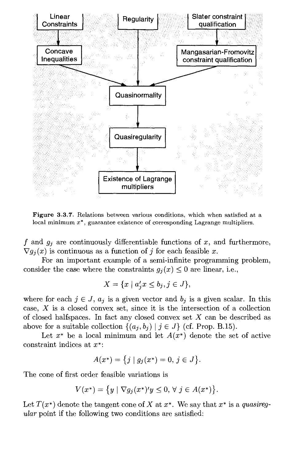
3. Lagrange Multiplier Theory p. 275
3.1. Necessary Conditions for Equality Constraints p. 277
3.1.1. The Penalty Approach p. 281
3.1.2. The Elimination Approach p. 283
3.1.3. The Lagrangian Function p. 287
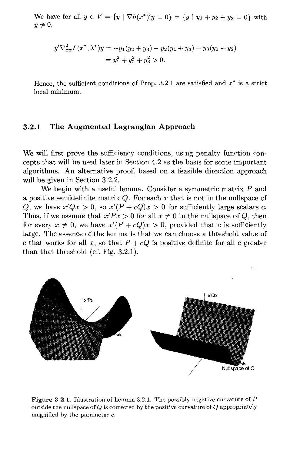
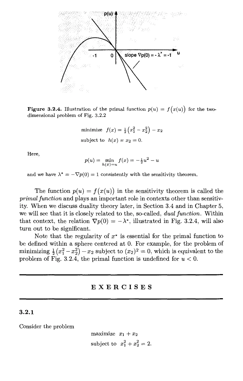
3.2. Sufficient Conditions and Sensitivity Analysis p. 295
3.2.1. The Augmented Lagrangian Approach p. 297
3.2.2. The Feasible Direction Approach p. 300
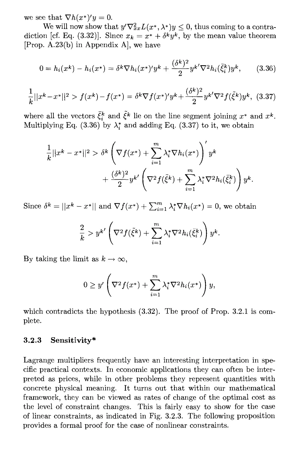
3.2.3. Sensitivity* p. 301
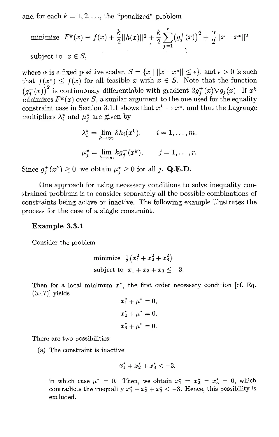
3.3. Inequality Constraints p. 307
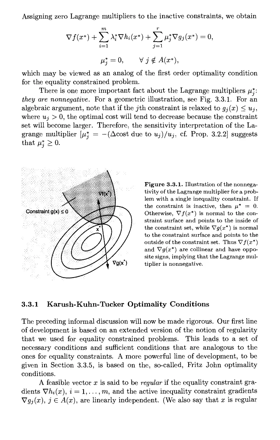
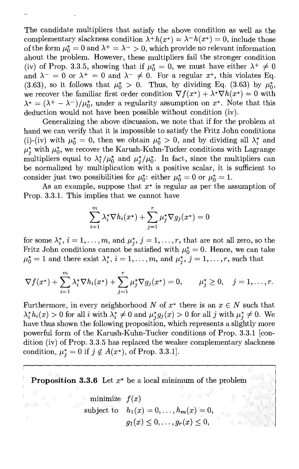
3.3.1. Karush-Kuhn-Tucker Optimality Conditions p. 309
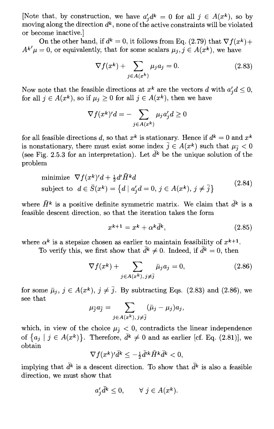
3.3.2. Conversion to the Equality Case* p. 312
3.3.3. Second Order Sufficiency Conditions and Sensitivity* ... p. 314
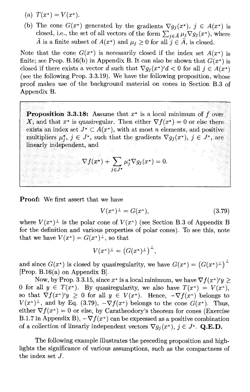
3.3.4. Sufficiency Conditions and Lagrangian Minimization* . . p. 315
3.3.5. Fritz John Optimality Conditions* p. 317
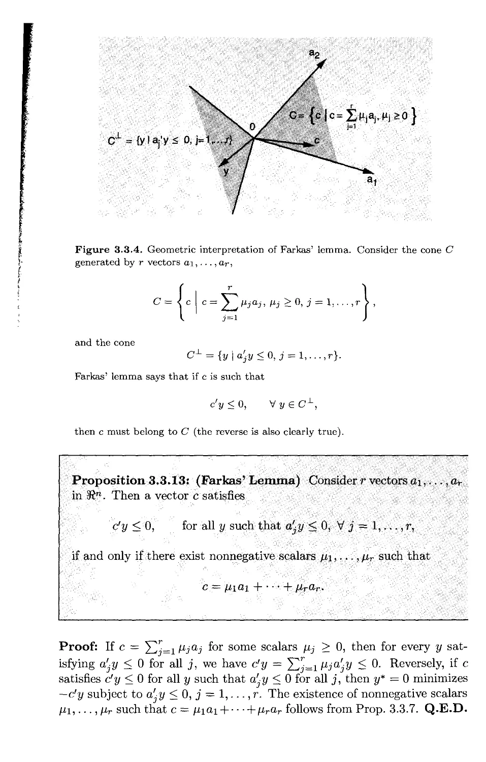
3.3.6. Refinements* p. 330
3.4. Linear Constraints and Duality* p. 357
3.4.1. Convex Cost Functions and Linear Constraints p. 357
3.4.2. Duality Theory: A Simple Form for Linear Constraints . . p. 359
3.5. Notes and Sources p. 367
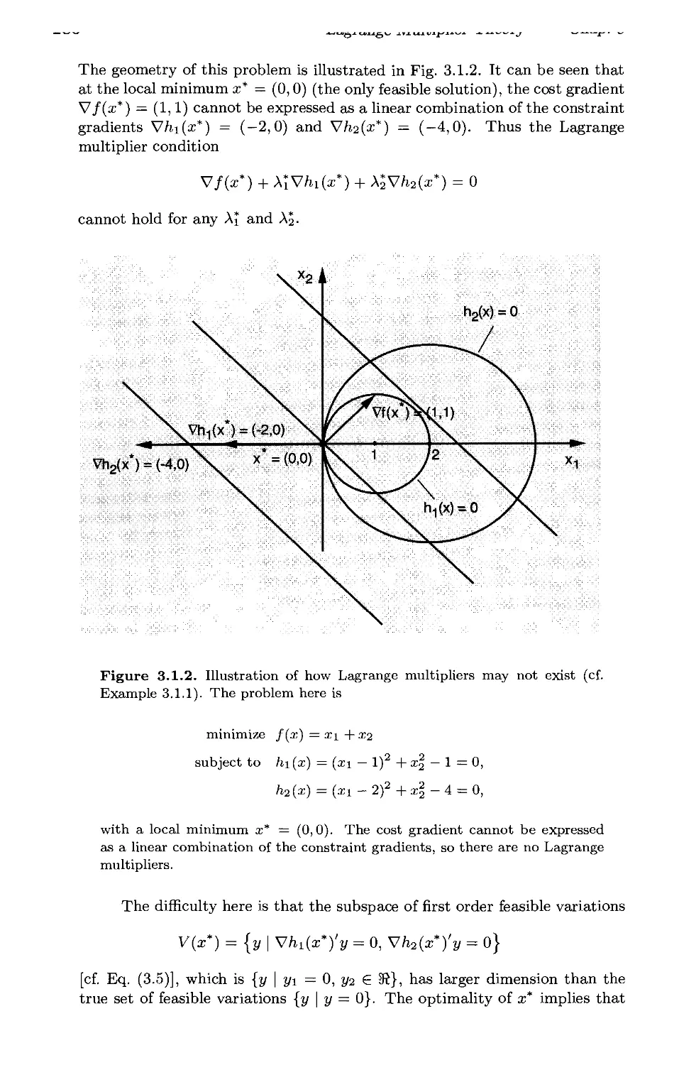
4. Lagrange Multiplier Algorithms p. 369
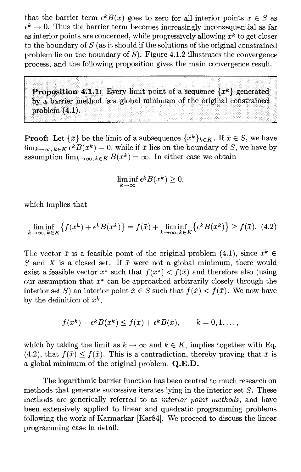
4.1. Barrier and Interior Point Methods p. 370
4.1.1. Linear Programming and the Logarithmic Barrier* .... p. 373
4.2. Penalty and Augmented Lagrangian Methods p. 388
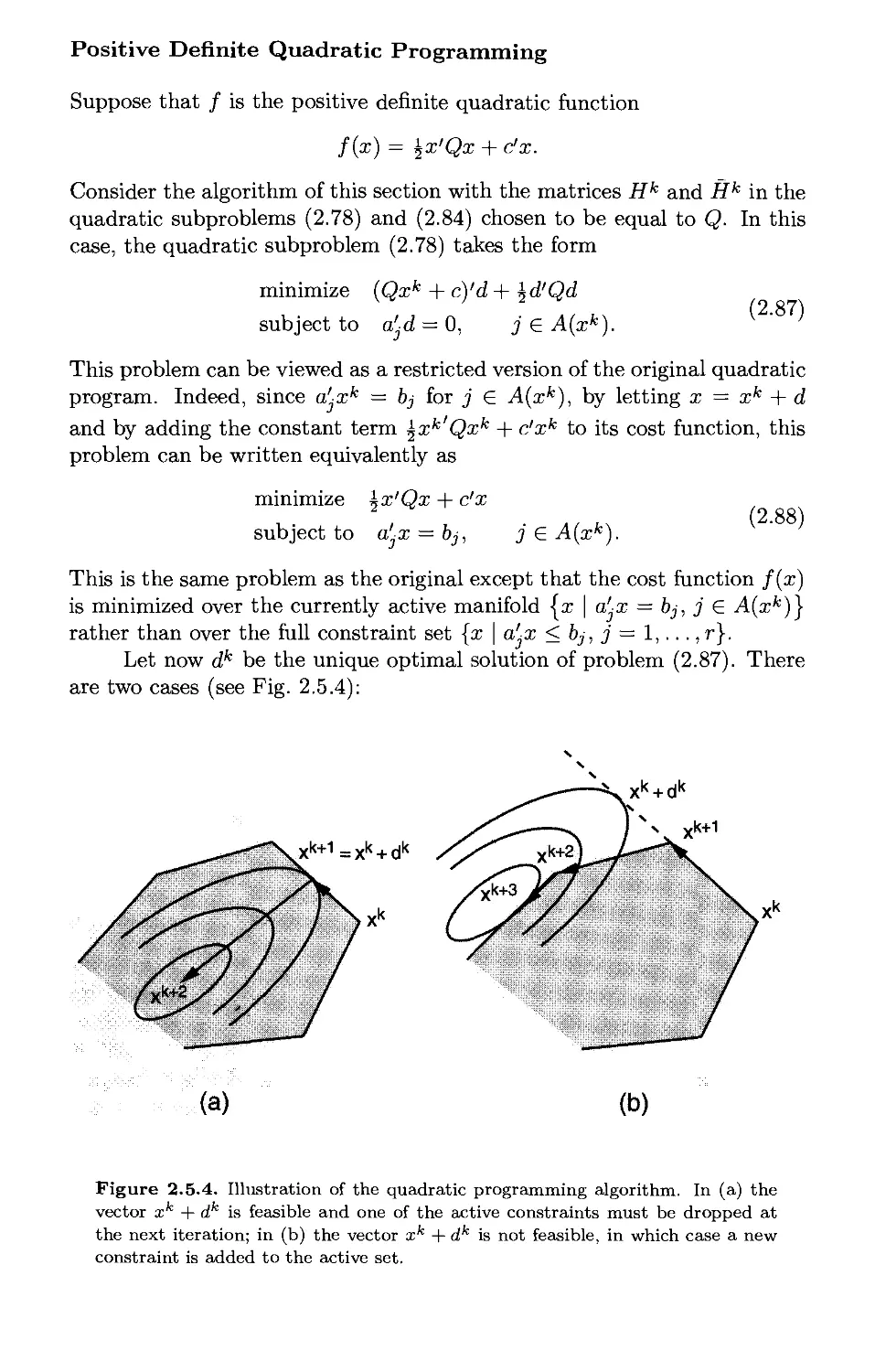
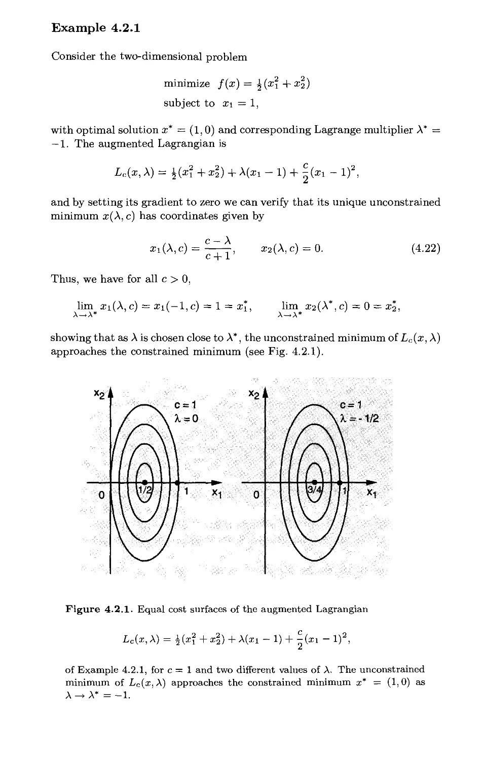
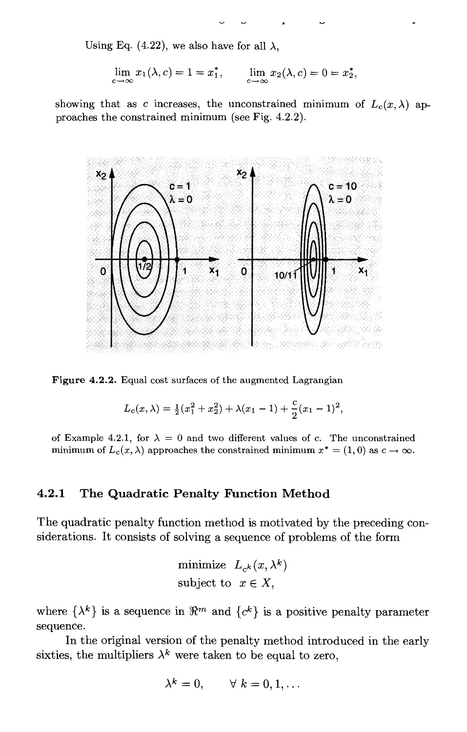
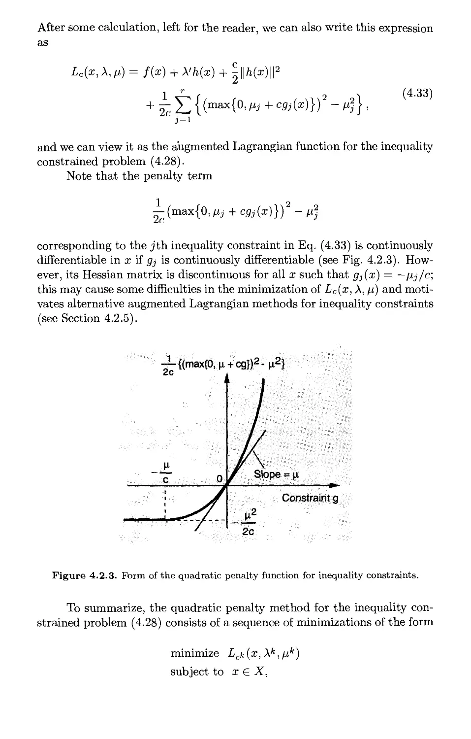
4.2.1. The Quadratic Penalty Function Method p. 390
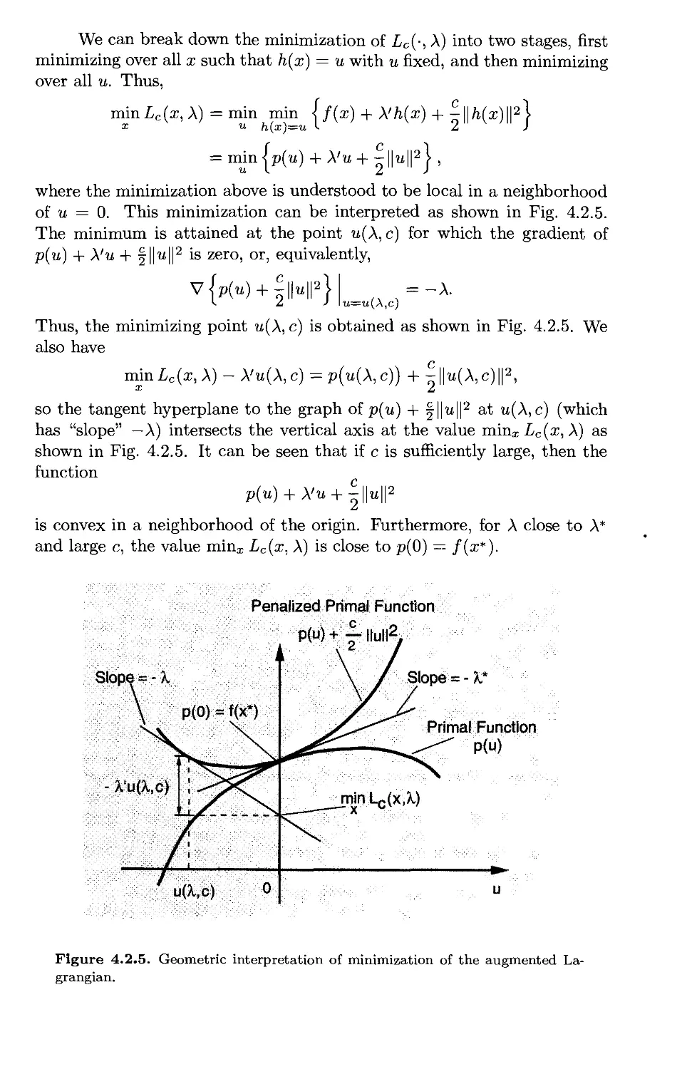
4.2.2. Multiplier Methods - Main Ideas p. 398
4.2.3. Convergence Analysis of Multiplier Methods* p. 407
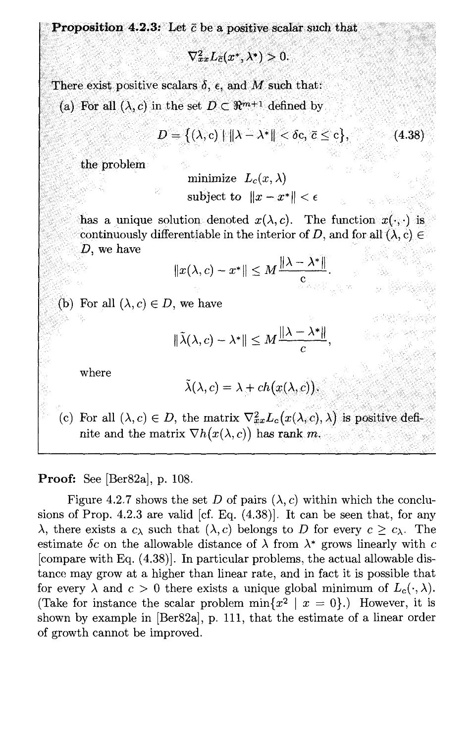
4.2.4. Duality and Second Order Multiplier Methods* p. 410
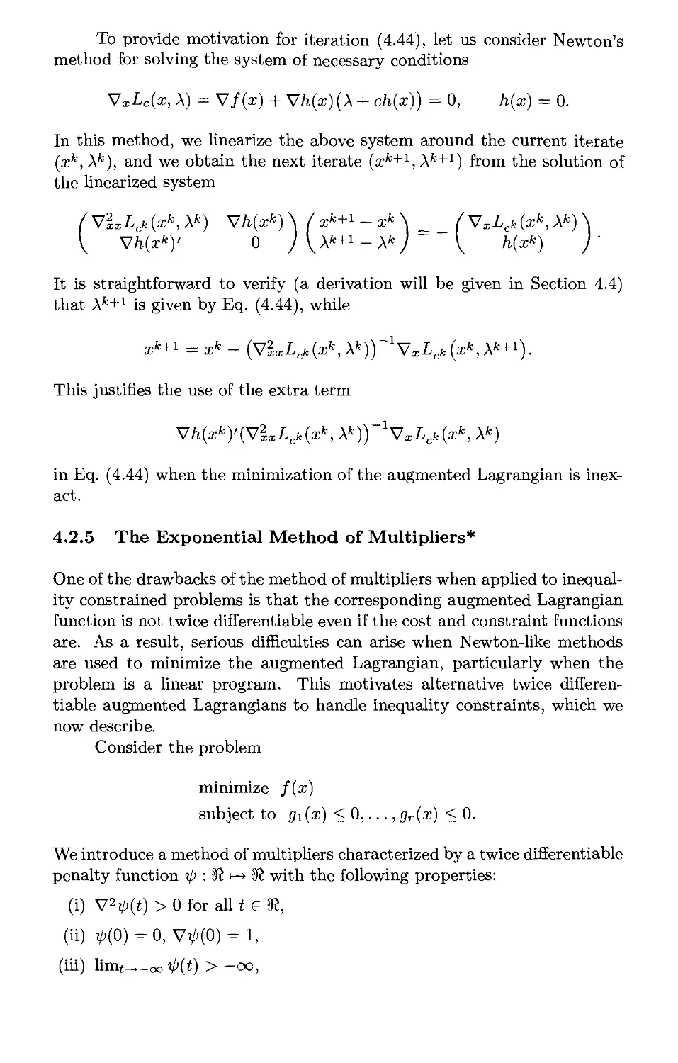
4.2.5. The Exponential Method of Multipliers* p. 413
4.3. Exact Penalties - Sequential Quadratic Programming* ... p. 421
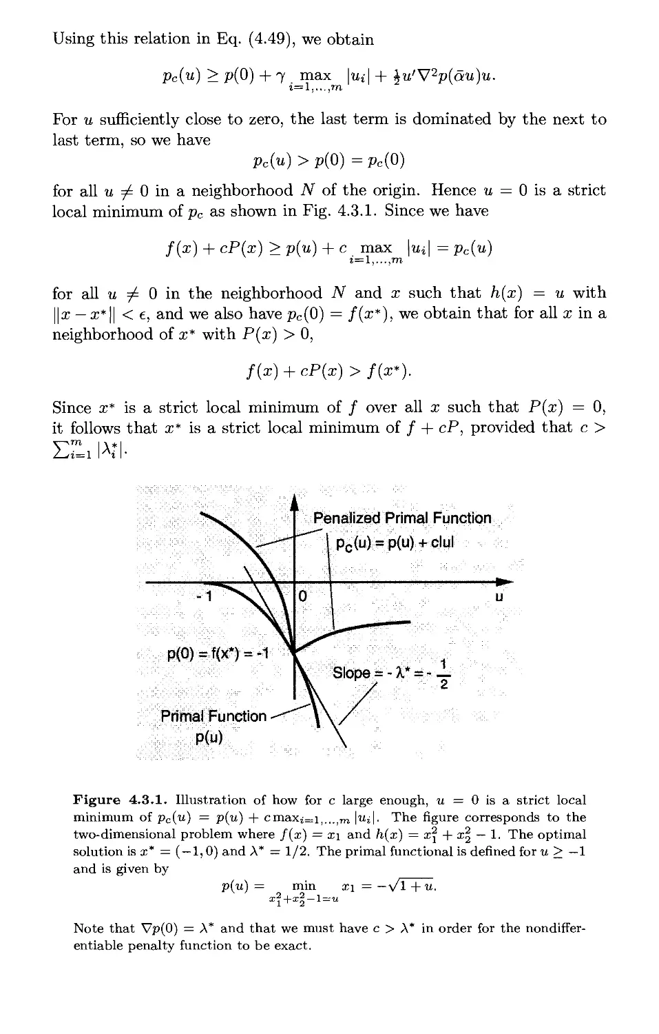
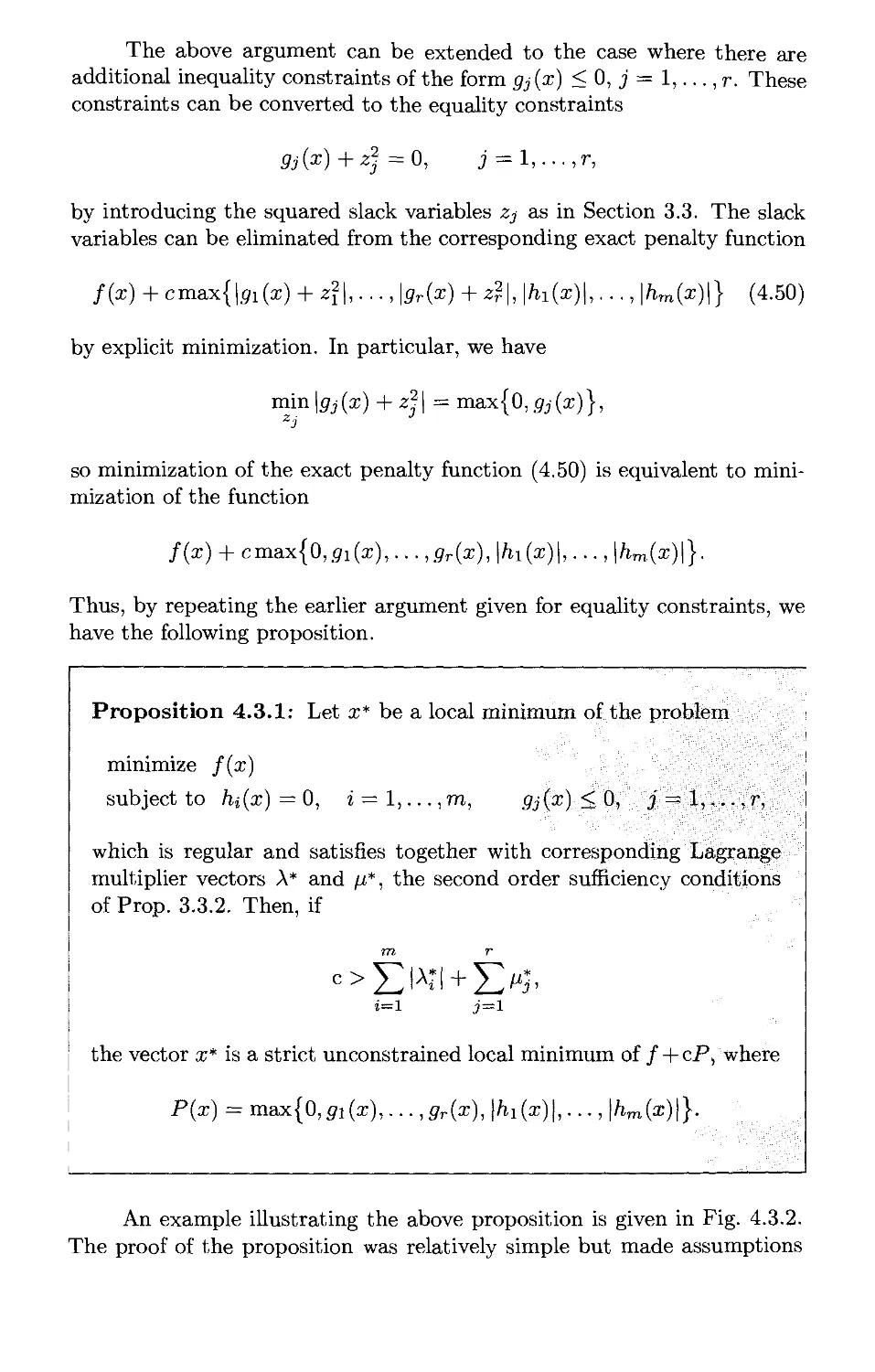
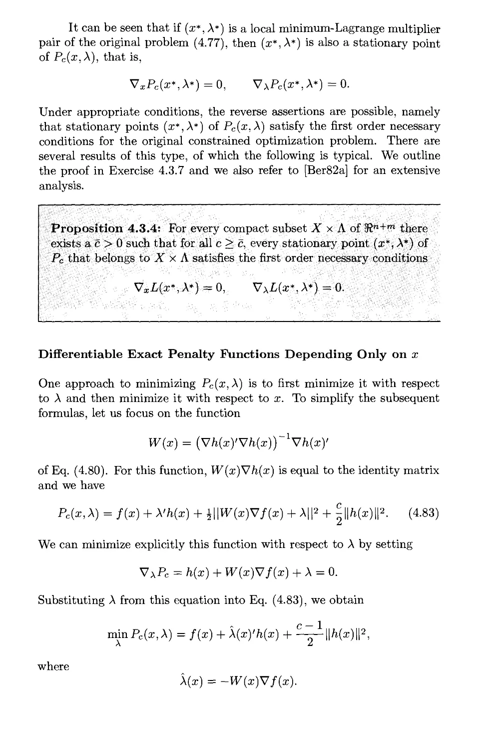
4.3.1. Nondifferentiable Exact Penalty Functions p. 422
4.3.2. Differentiable Exact Penalty Functions p. 439
4.4. Lagrangian and Primal-Dual Interior Point Methods* .... p. 446
4.4.1. First-Order Methods p. 446
4.4.2. Newton-Like Methods for Equality Constraints p. 450
4.4.3. Global Convergence p. 460
Contents vii
4.4.4. Primal-Dual Interior Point Methods p. 463
4.4.5. Comparison of Various Methods p. 471
4.5. Notes and Sources p. 473
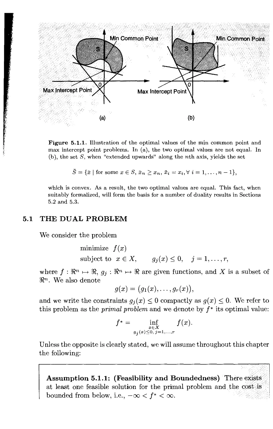
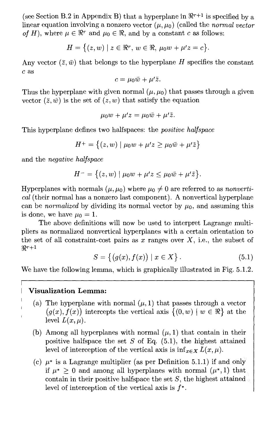
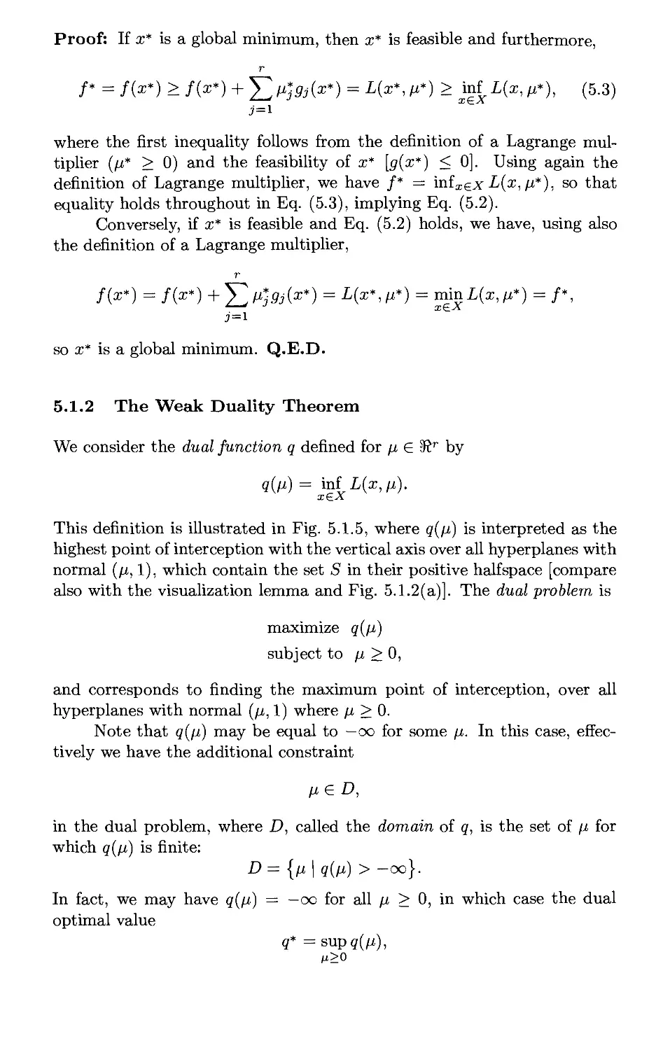
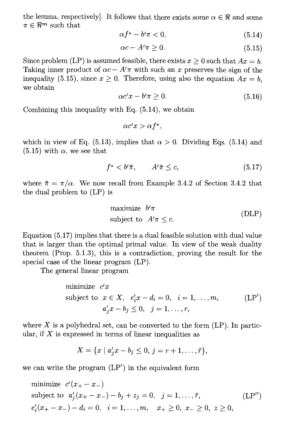
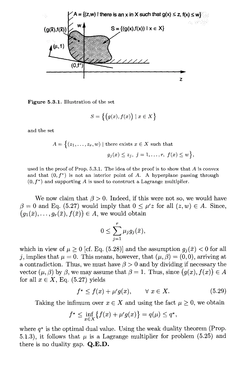
5. Duality and Convex Programming p. 477
5.1. The Dual Problem p. 479
5.1.1. Lagrange Multipliers p. 480
5.1.2. The Weak Duality Theorem p. 485
5.1.3. Characterization of Primal and Dual Optimal Solutions . . p. 490
5.1.4. The Case of an Infeasible or Unbounded Primal Problem . p. 491
5.1.5. Treatment of Equality Constraints p. 493
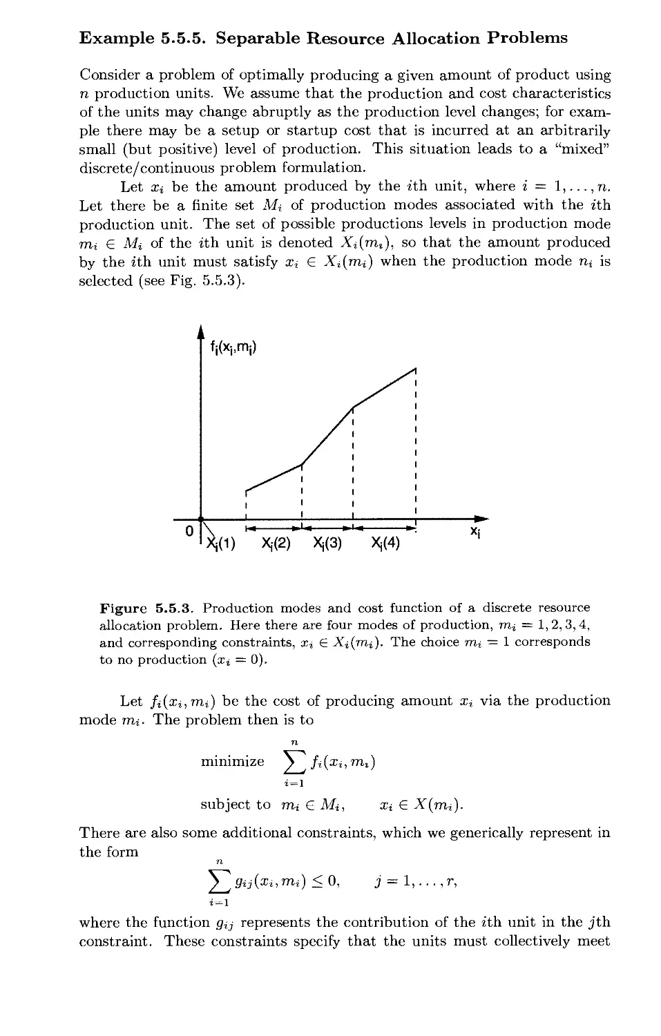
5.1.6. Separable Problems and Their Geometry p. 494
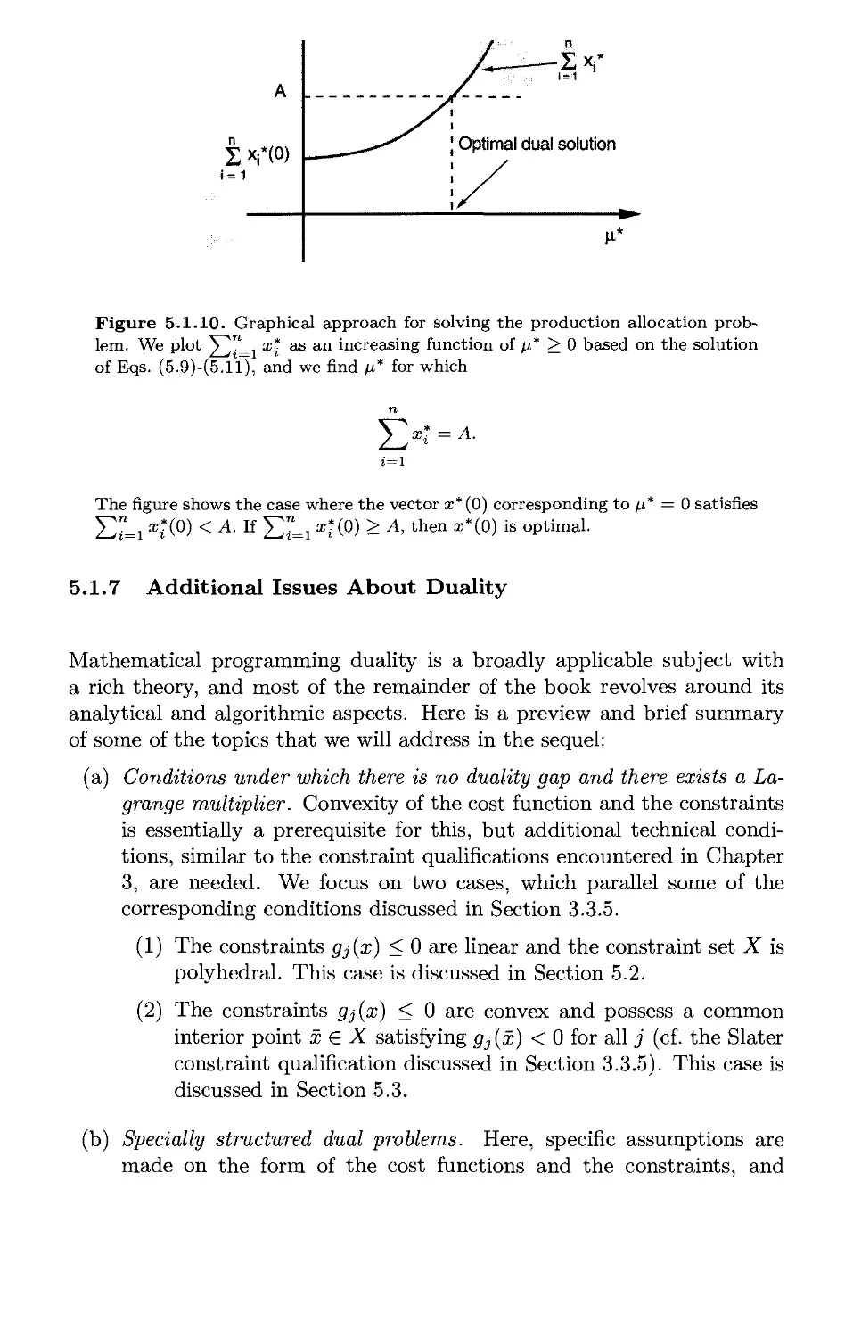
5.1.7. Additional Issues About Duality p. 498
5.2. Convex Cost - Linear Constraints* p. 503
5.2.1. Proofs of Duality Theorems p. 505
5.3. Convex Cost - Convex Constraints p. 511
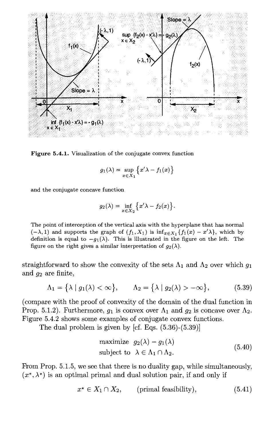
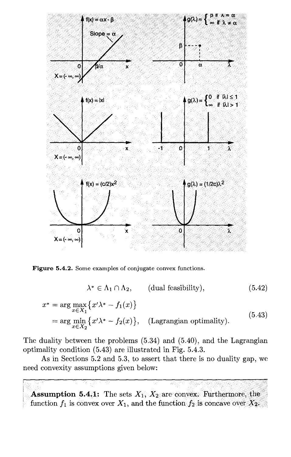
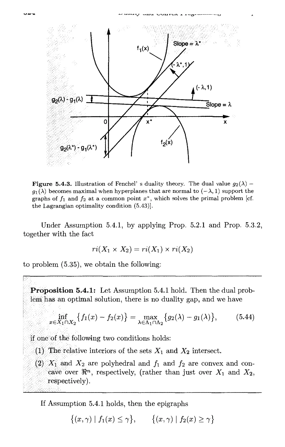
5.4. Conjugate Functions and Fenchel Duality* p. 521
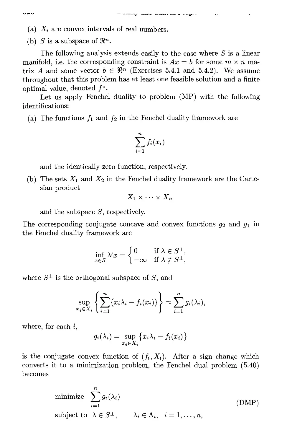
5.4.1. Monotropic Programming Duality p. 525
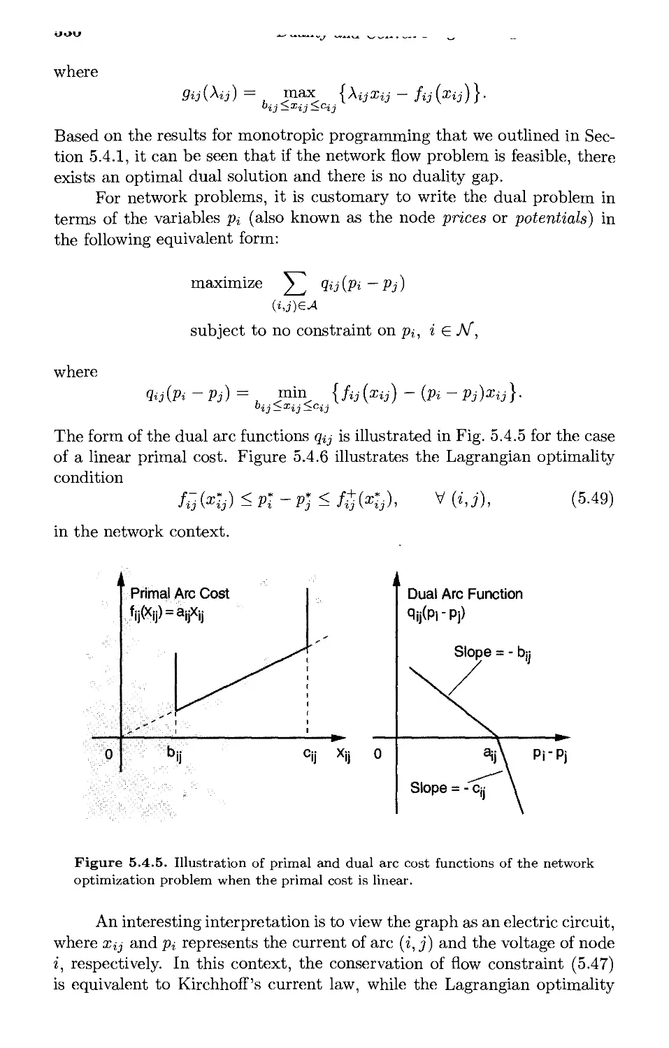
5.4.2. Network Optimization p. 529
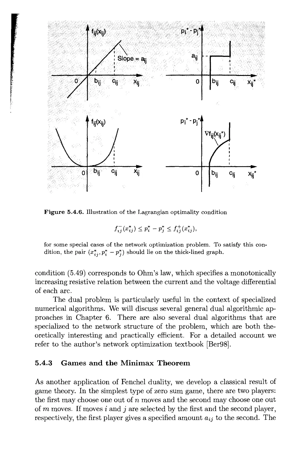
5.4.3. Games and the Minimax Theorem p. 531
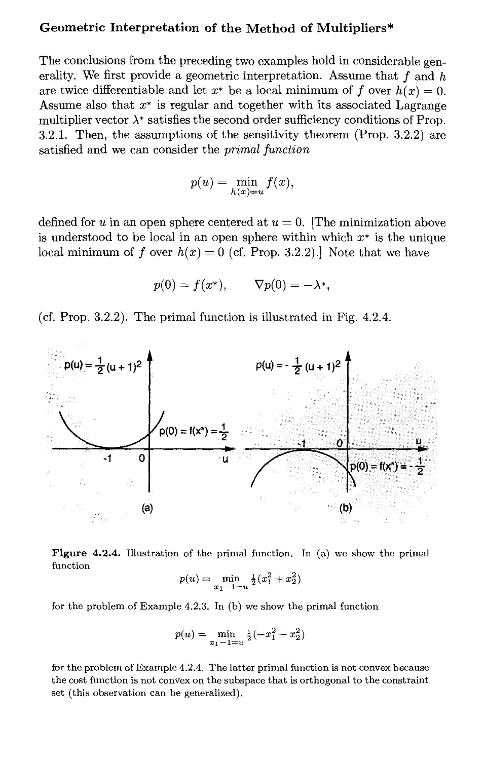
5.4.4. The Primal Function p. 534
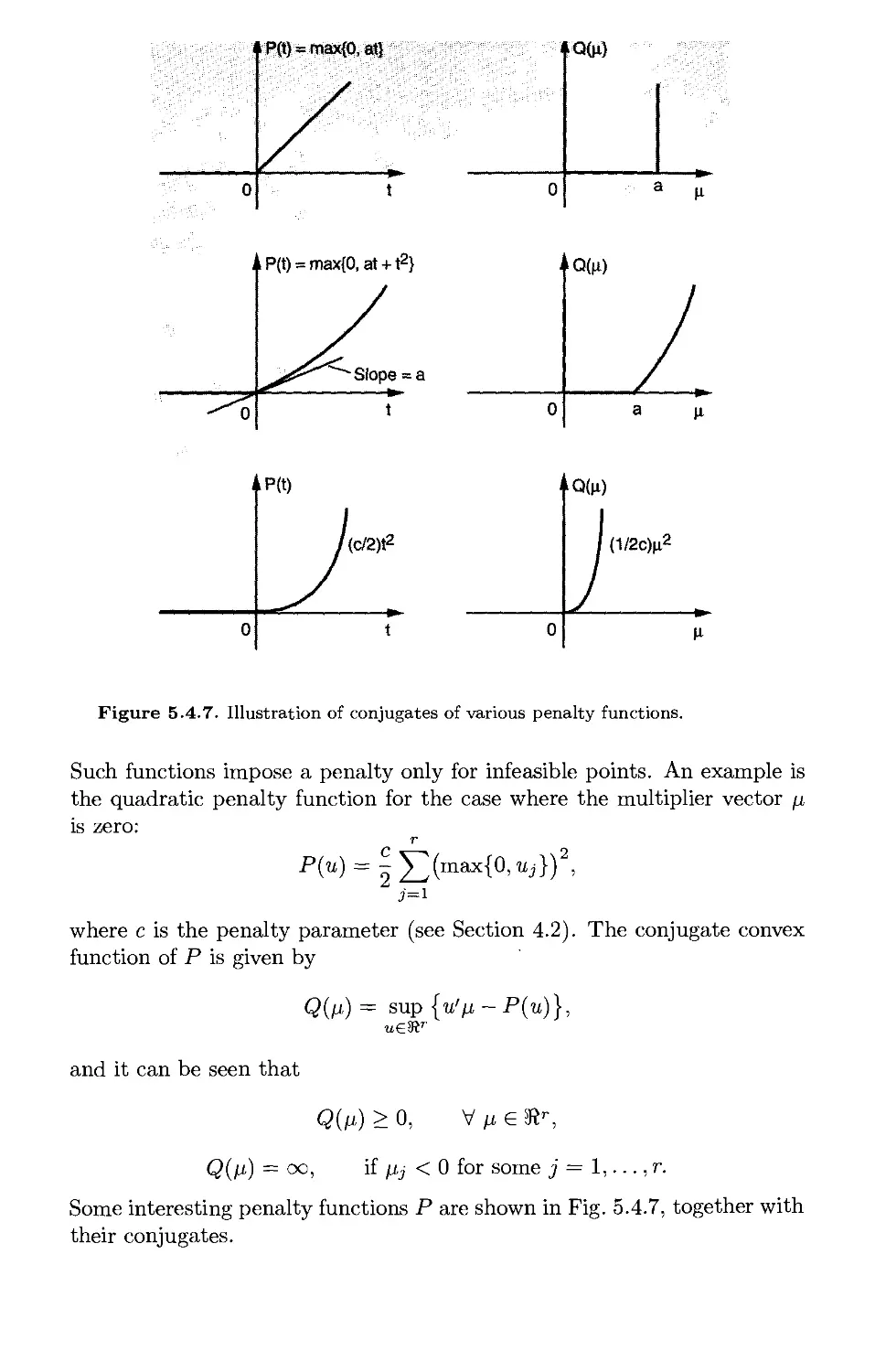
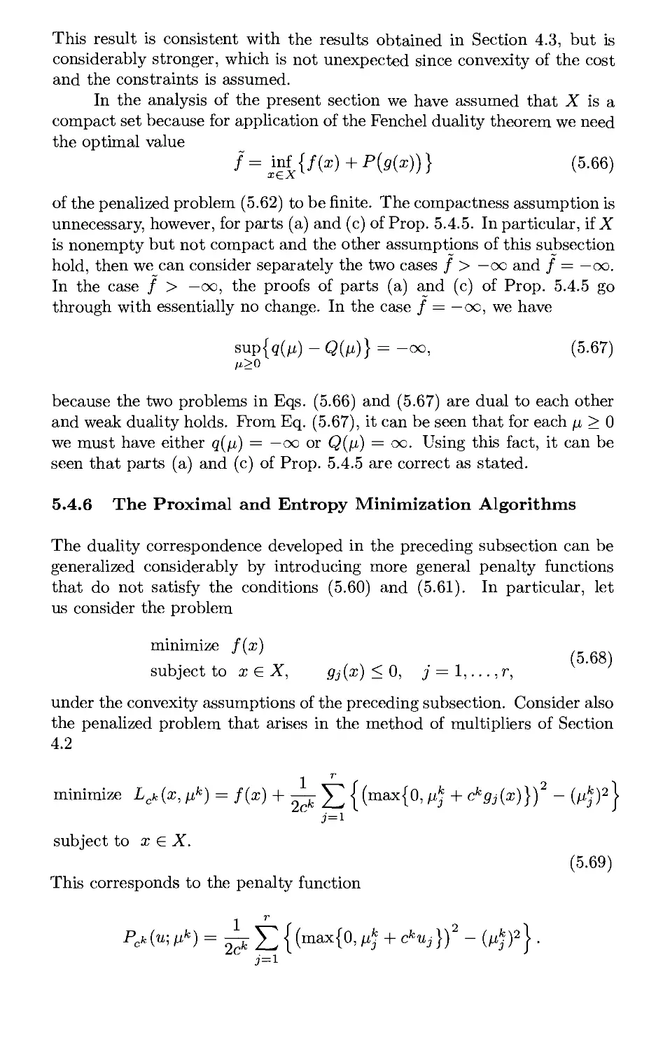
5.4.5. A Dual View of Penalty Methods p. 536
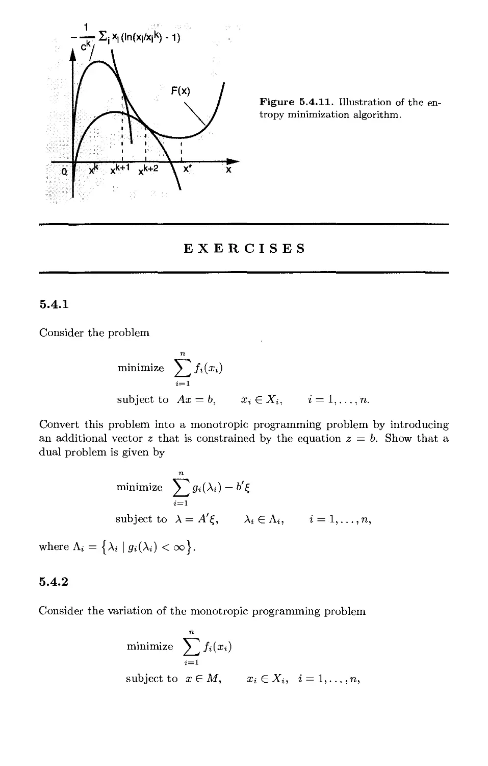
5.4.6. The Proximal and Entropy Minimization Algorithms ... p. 542
5.5. Discrete Optimization and Duality p. 558
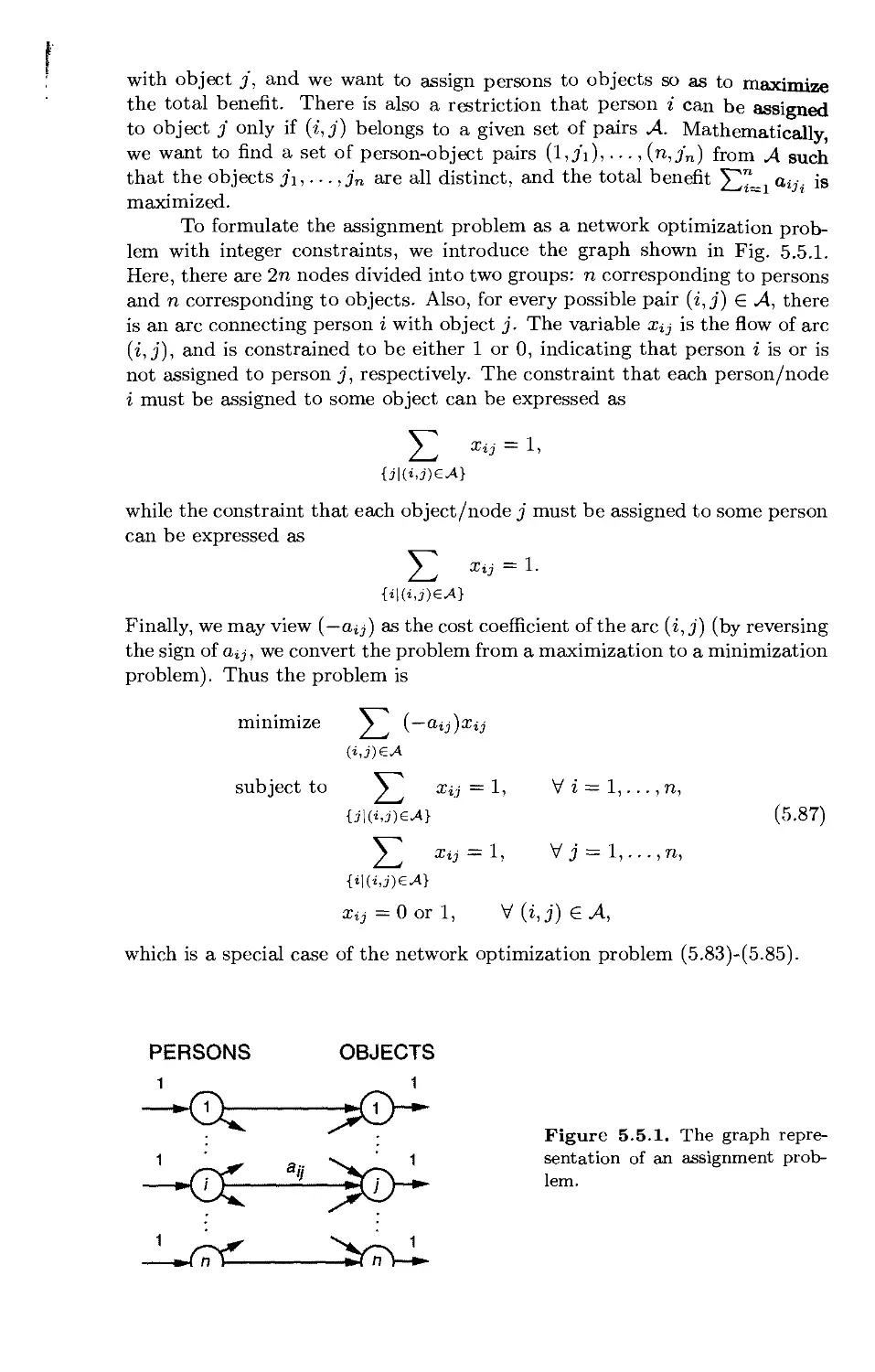
5.5.1. Examples of Discrete Optimization Problems p. 559
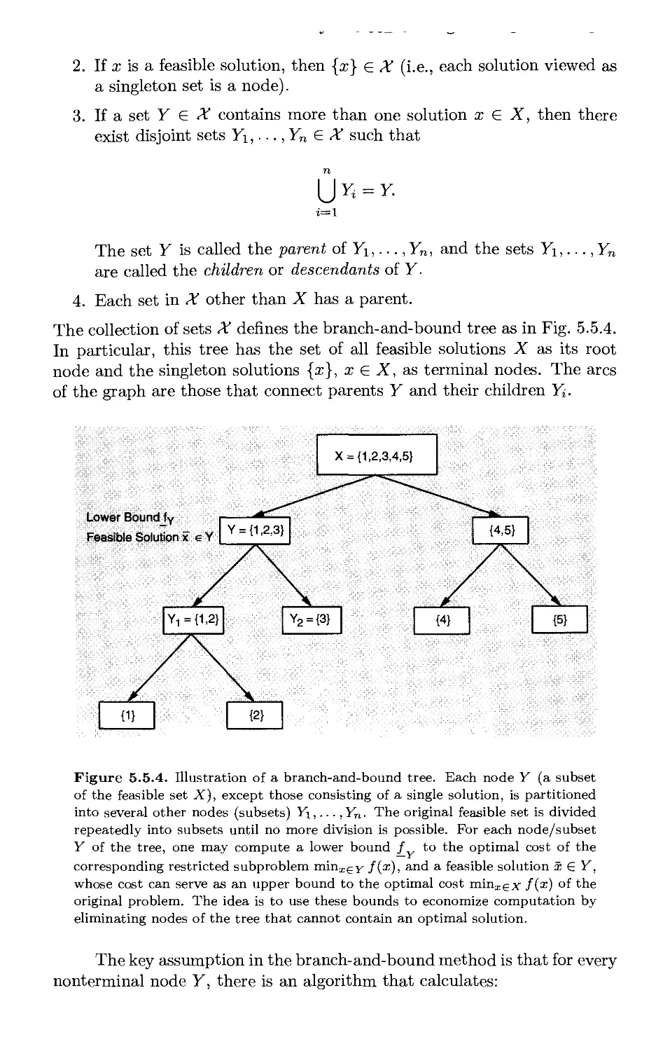
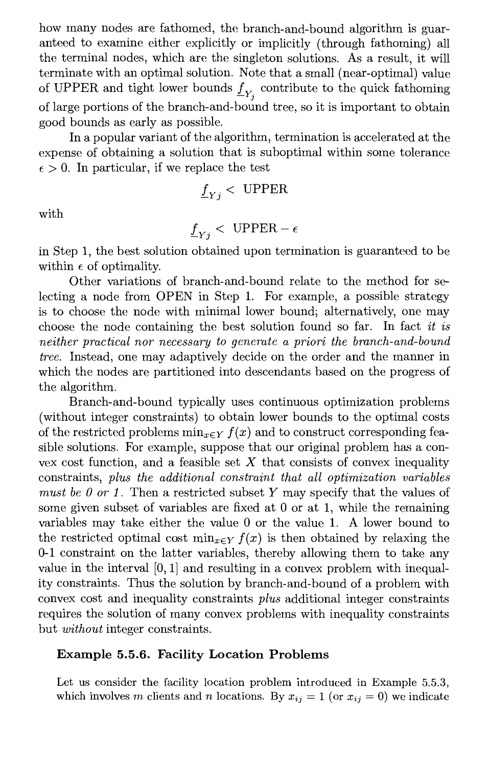
5.5.2. Branch-and-Bound p. 567
5.5.3. Lagrangian Relaxation p. 576
5.6. Notes and Sources p. 587
6. Dual Methods p. 591
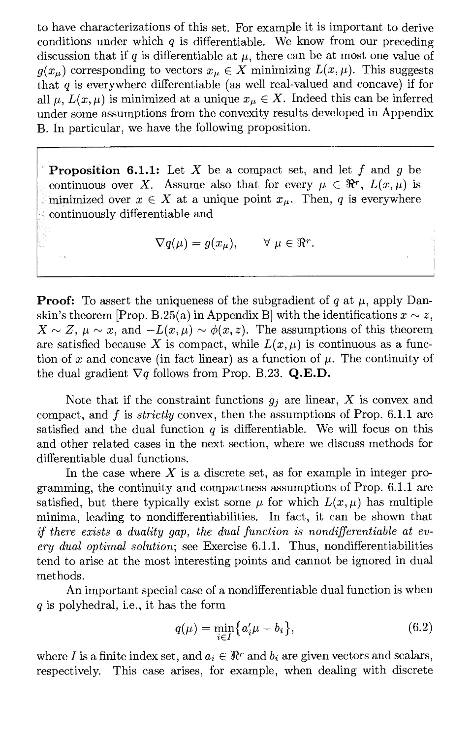
6.1. Dual Derivatives and Subgradients* p. 594
6.2. Dual Ascent Methods for Differentiable Dual Problems* ... p. 600
6.2.1. Coordinate Ascent for Quadratic Programming p. 600
6.2.2. Decomposition and Primal Strict Convexity p. 603
6.2.3. Partitioning and Dual Strict Concavity p. 604
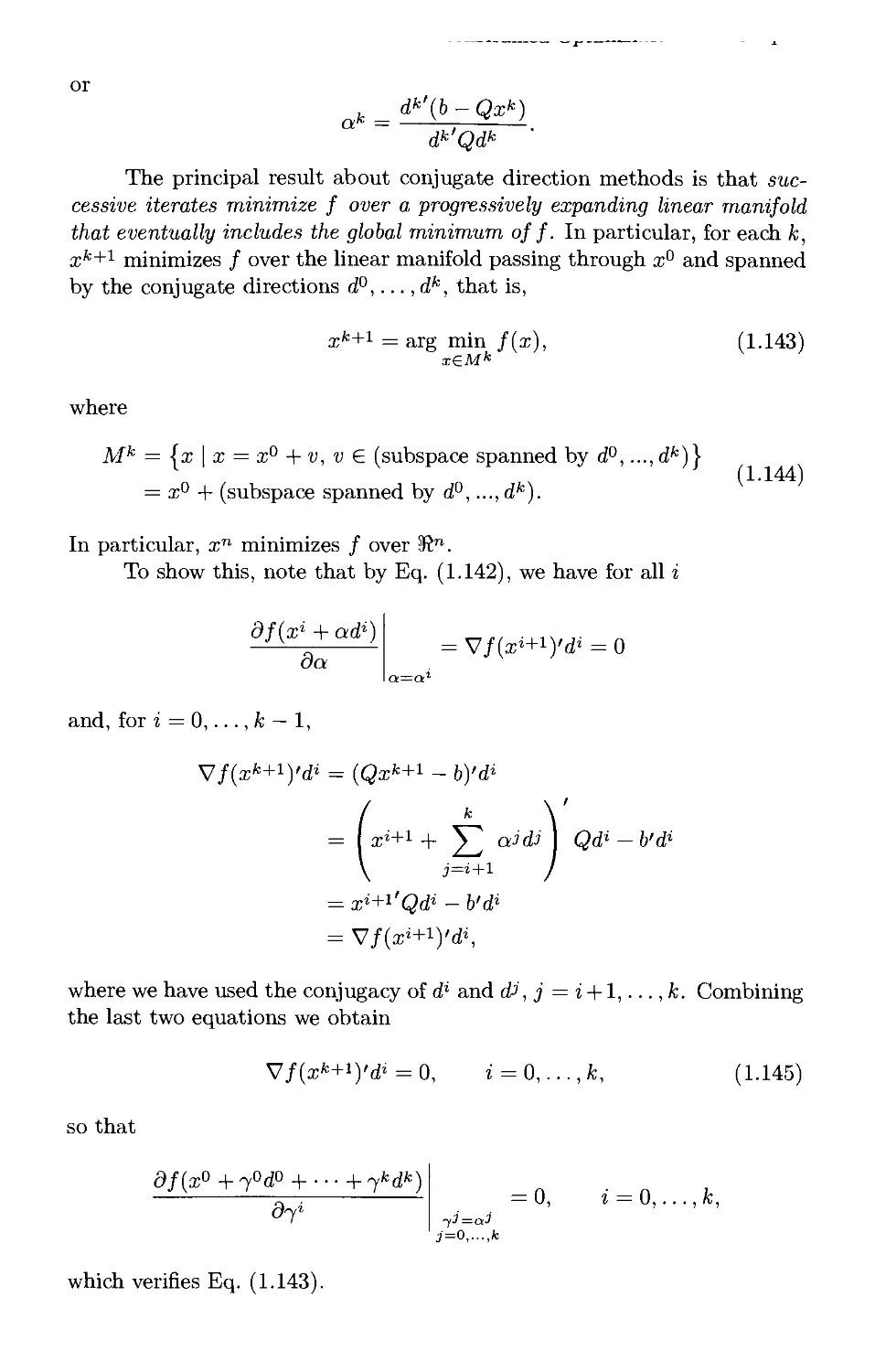
6.3. Nondifferentiable Optimization Methods* p. 609
6.3.1. Subgradient Methods p. 610
6.3.2. Approximate and Incremental Subgradient Methods ... p. 614
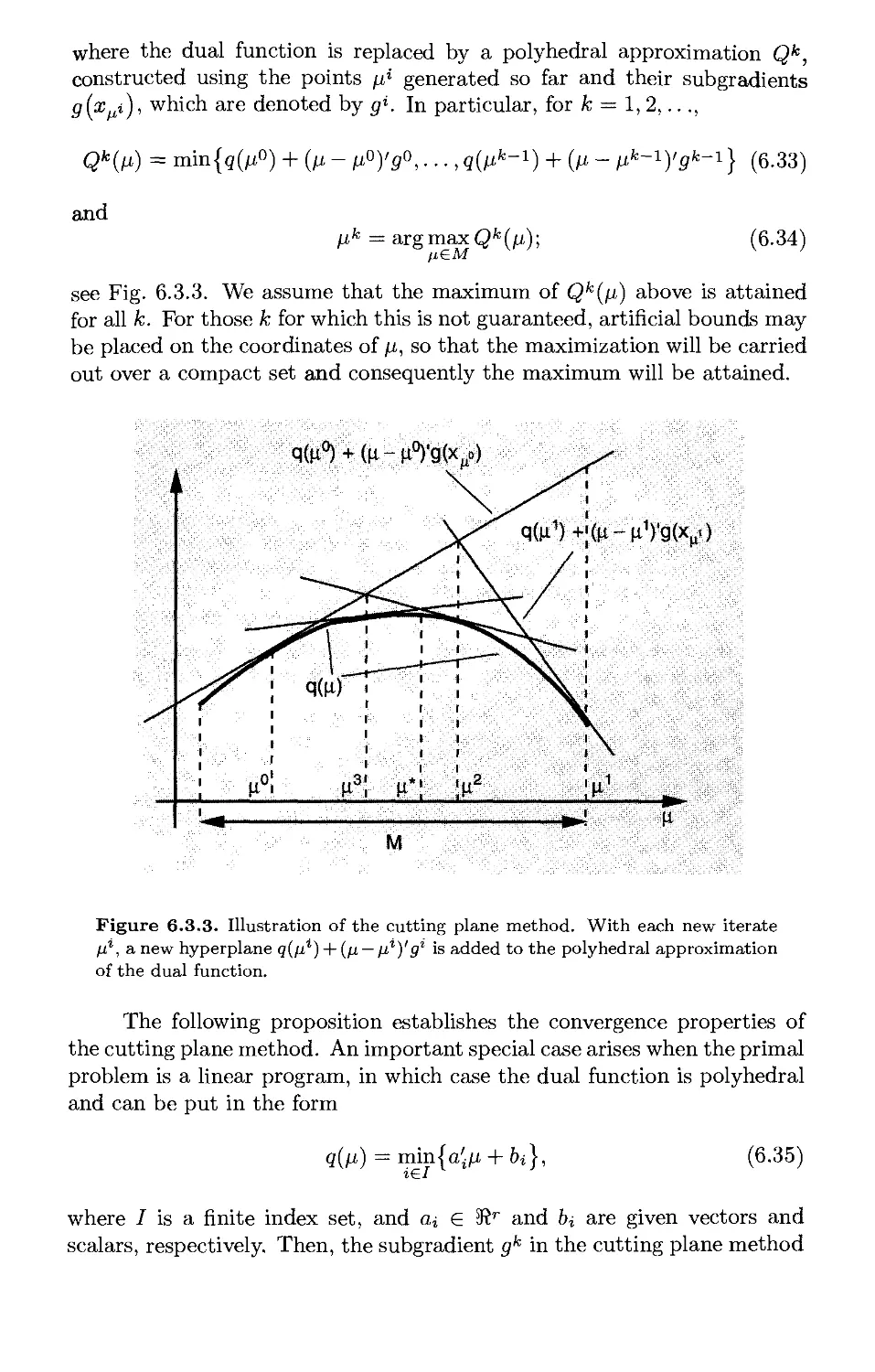
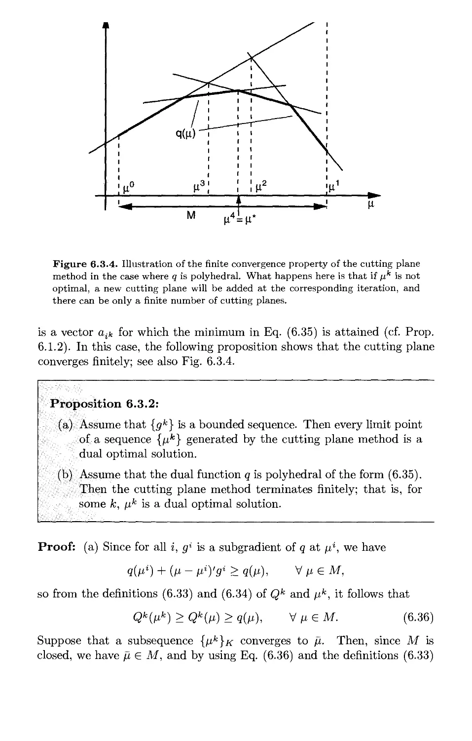
6.3.3. Cutting Plane Methods p. 618
6.3.4. Ascent and Approximate Ascent Methods p. 625
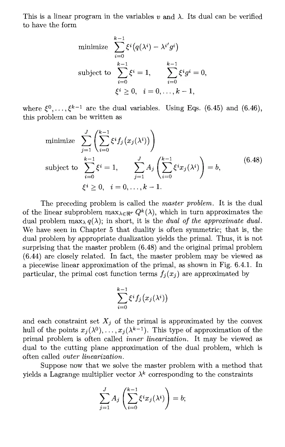
6.4. Decomposition Methods* p. 638
6.4.1. Lagrangian Relaxation of the Coupling Constraints . . . . p. 639
6.4.2. Decomposition by Right-Hand Side Allocation p. 642
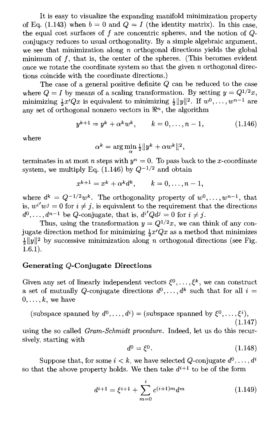
6.5. Notes and Sources p. 645
Vlll
Appendix A: Mathematical Background p. 647
A.l. Vectors and Matrices p. 648
A.2. Norms, Sequences, Limits, and Continuity p. 649
A.3. Square Matrices and Eigenvalues p. 656
A.4. Symmetric and Positive Definite Matrices p. 659
A.5. Derivatives p. 664
A.6. Contraction Mappings p. 669
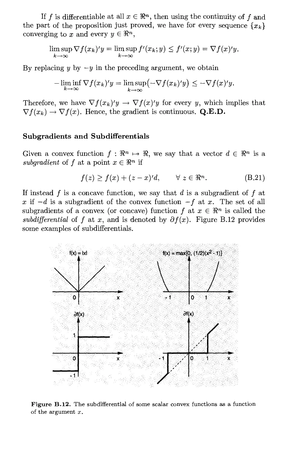
Appendix B: Convex Analysis p. 671
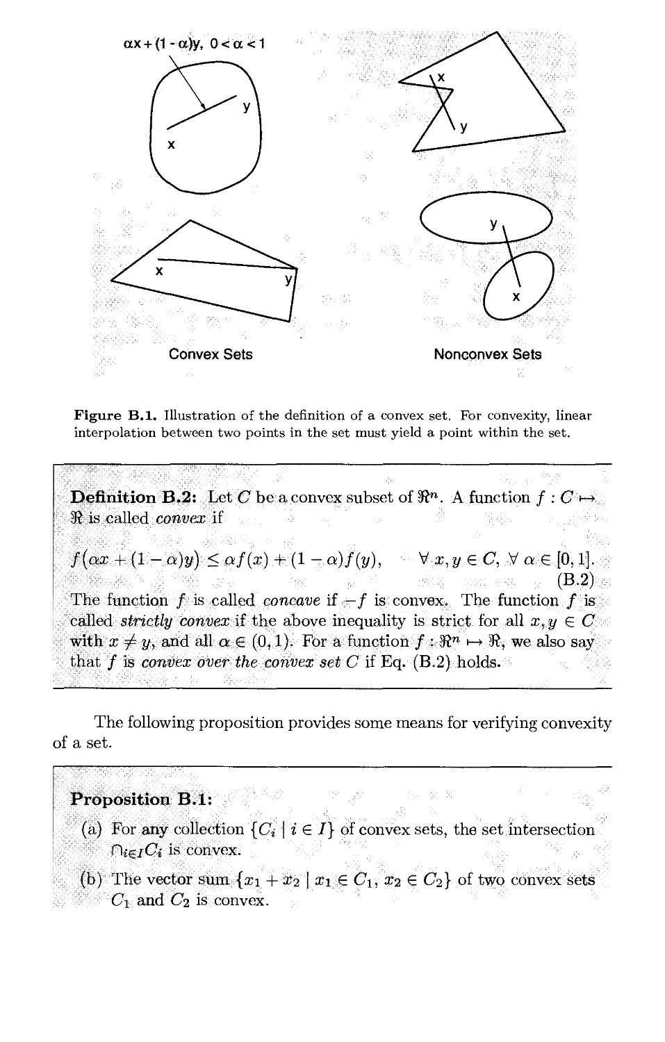
B.l. Convex Sets and Functions p. 671
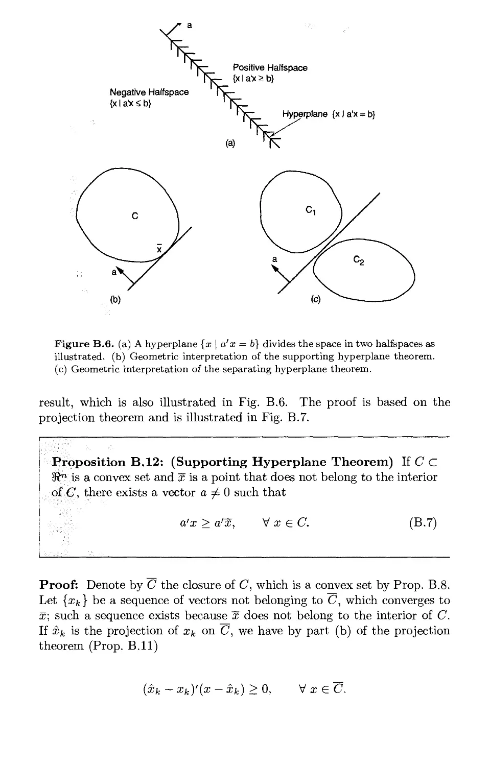
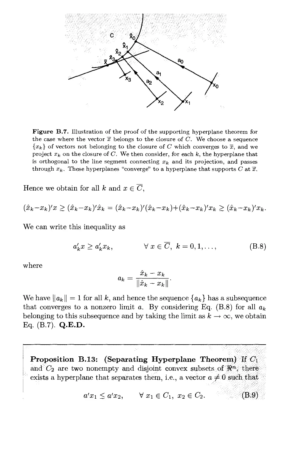
B.2. Separating Hyperplanes p. 689
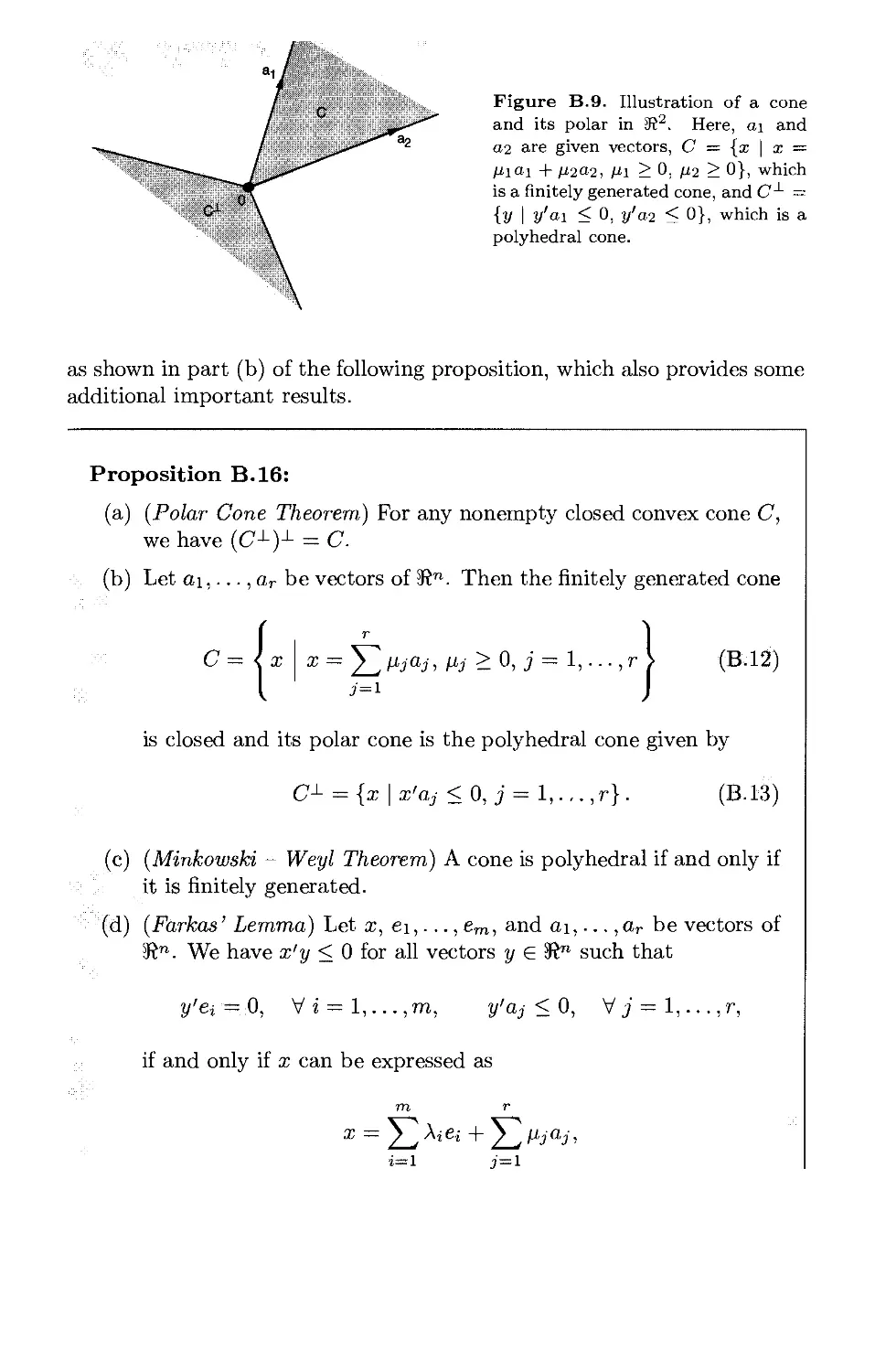
B.3. Cones and Polyhedral Convexity p. 694
B.4. Extreme Points p. 701
B.5. Differentiability Issues p. 707
Appendix C: Line Search Methods p. 723
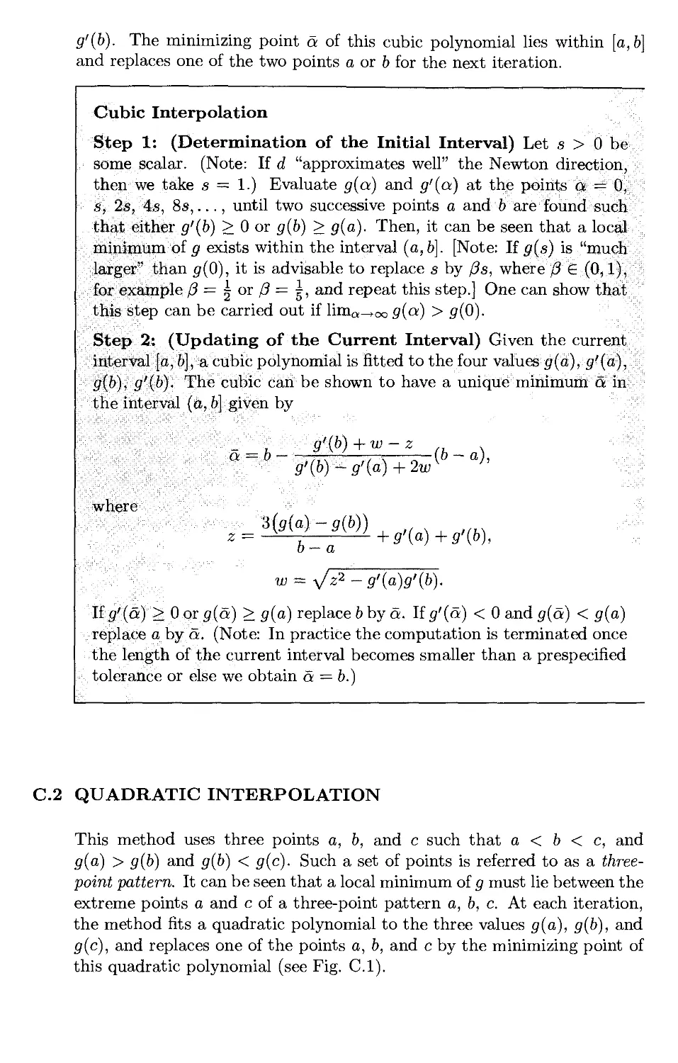
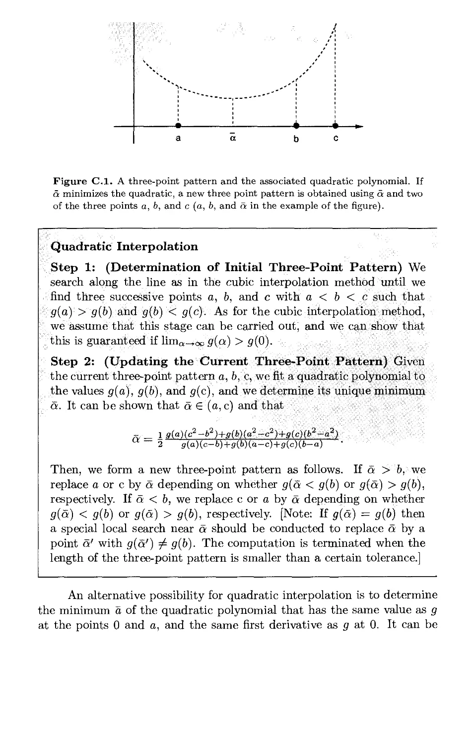
C.l. Cubic Interpolation p. 723
C.2. Quadratic Interpolation p. 724
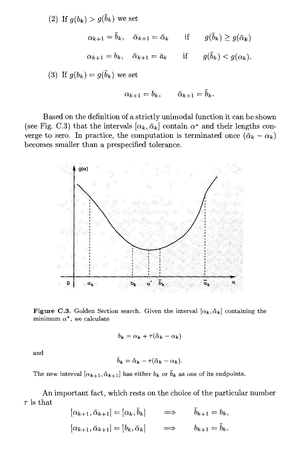
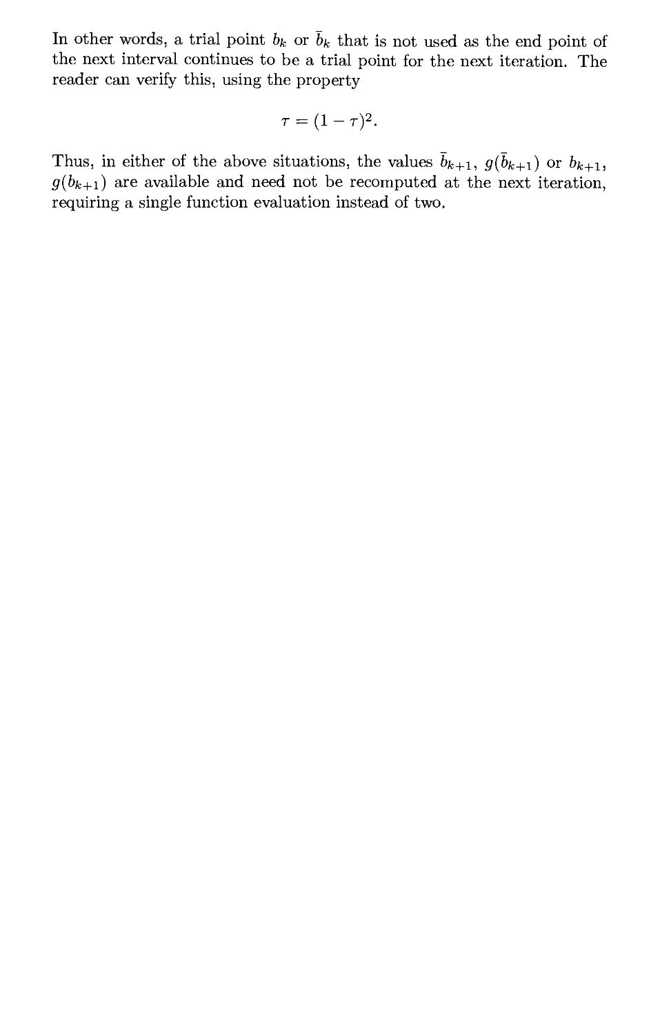
C.3. The Golden Section Method p. 726
Appendix D: Implementation of Newton's Method . . . p. 729
D.l. Cholesky Factorization p. 729
D.2. Application to a Modified Newton Method p. 731
References p. 735
Index p. 773
Preface
Nonlinear programming is a mature field that has experienced major
developments in the last ten years. The first such development is the merging
of linear and nonlinear programming algorithms through the use of
interior point methods. This has resulted in a profound rethinking of how we
solve linear programming problems, and in a major reassessment of how
we treat constraints in nonlinear programming. A second development,
less visible but still important, is the increased emphasis on large-scale
problems, and the associated algorithms that take advantage of problem
structure as well as parallel hardware. A third development has been the
extensive use of iterative unconstrained optimization to solve the difficult
least squares problems arising in the training of neural networks. As a
result, simple gradient-like methods and stepsize rules have attained
increased importance.
The purpose of this book is to provide an up-to-date, comprehensive,
and rigorous account of nonlinear programming at the beginning graduate
student level. In addition to the classical topics, such as descent
algorithms, Lagrange multiplier theory, and duality, some of the important
recent developments are covered: interior point methods for linear and
nonlinear programs, major aspects of large-scale optimization, and least
squares problems and neural network training.
A further noteworthy feature of the book is that it treats Lagrange
multipliers and duality using two different and complementary approaches:
a variational approach based on the implicit function theorem, and a convex
analysis approach based on geometrical arguments. The former approach
applies to a broader class of problems, while the latter is more elegant and
more powerful for the convex programs to which it applies.
The chapter-by-chapter description of the book follows:
Chapter 1: This chapter covers unconstrained optimization: main
concepts, optimality conditions, and algorithms. The material is classic, but
there are discussions of topics frequently left untreated, such as the
behavior of algorithms for singular problems, neural network training, and
discrete-time optimal control.
ix
X
± X. CIW^V/
Chapter 2: This chapter treats constrained optimization over a convex
set without the use of Lagrange multipliers. I prefer to cover this
material before dealing with the complex machinery of Lagrange multipliers
because I have found that students absorb easily algorithms such as
conditional gradient, gradient projection, and coordinate descent, which can
be viewed as natural extensions of unconstrained descent algorithms. This
chapter contains also a treatment of the affine scaling method for linear
programming.
Chapter 3: This chapter gives a detailed treatment of Lagrange
multipliers, the associated necessary and sufficient conditions, and sensitivity
analysis. The first three sections deal with nonlinear equality and
inequality constraints. The last section deals with linear constraints and develops
a simple form of duality theory for linearly constrained problems with dif-
ferentiable cost, including linear and quadratic programming.
Chapter 4: This chapter treats constrained optimization algorithms that
use penalties and Lagrange multipliers, including barrier, augmented La-
grangian, sequential quadratic programming, and primal-dual interior point
methods for linear programming. The treatment is extensive, and borrows
from my 1982 research monograph on Lagrange multiplier methods.
Chapter 5: This chapter provides an in-depth coverage of duality theory
(Lagrange and Fenchel). The treatment is totally geometric, and
everything is explained in terms of intuitive figures.
Chapter 6: This chapter deals with large-scale optimization methods
based on duality. Some material is borrowed from my Parallel and
Distributed Algorithms book (coauthored by John Tsitsiklis), but there is also
an extensive treatment of nondifferentiable optimization, including subgra-
dient, e-subgradient, and cutting plane methods. Decomposition methods
such as Dantzig-Wolfe and Benders are also discussed.
Appendixes: Four appendixes are given. The first gives a summary of
calculus, analysis, and linear algebra results used in the text. The second
is a fairly extensive account of convexity theory, including proofs of the
basic polyhedral convexity results on extreme points and Farkas' lemma,
as well the basic facts about subgradients. The third appendix covers
one-dimensional minimization methods. The last appendix discusses an
implementation of Newton's method for unconstrained optimization.
Inevitably, some coverage compromises had to be made. The subject
of nonlinear optimization has grown so much that leaving out a number
of important topics could not be avoided. For example, a discussion of
variational inequalities, a deeper treatment of optimality conditions, and
a more detailed development of Quasi-Newton methods are not provided.
Also, a larger number of sample applications would have been desirable. I
hope that instructors will supplement the book with the type of practical
examples that their students are most familiar with.
The book was developed through a first-year graduate course that
I taught at the Univ. of Illinois and at M.I.T. over a period of 20 years.
The mathematical prerequisites are matrix-vector algebra and advanced
calculus, including a good understanding of convergence concepts. A course
in analysis and/or linear algebra should also be very helpful, and would
provide the mathematical maturity needed to follow and to appreciate the
mathematical reasoning used in the book. Some of the sections in the book
may be ommited at first reading without loss of continuity. These sections
have been marked by a star. The rule followed here is that the material
discussed in a starred section is not used in a non-starred section.
The book can be used to teach several different types of courses.
(a) A two-quarter course that covers most sections of every chapter.
(b) A one-semester course that covers Chapter 1 except for Section 1.9,
Chapter 2 except for Sections 2.4 and 2.5, Chapter 3 except for Section
3.4, Chapter 4 except for parts of Sections 4.2 and 4.3, the first three
sections of Chapter 5, and a selection from Section 5.4 and Chapter
6. This is the course I usually teach at MIT.
(c) A one-semester course that covers most of Chapters 1, 2, and 3, and
selected algorithms from Chapter 4. I have taught this type of course
several times. It is less demanding of the students because it does not
require the machinery of convex analysis, yet it still provides a fairly
powerful version of duality theory (Section 3.4).
(d) A one-quarter course that covers selected parts of Chapters 1, 2, 3,
and 4. This is a less comprehensive version of (c) above.
(e) A one-quarter course on convex analysis and optimization that starts
with Appendix B and covers Sections 1.1, 2.1, 3.4, and Chapter 5.
There is a very extensive literature on nonlinear programming and
to give a complete bibliography and a historical account of the research
that led to the present form of the subject would have been impossible. I
thus have not attempted to compile a comprehensive list of original
contributions to the field. I have cited sources that I have used extensively,
that provide important extensions to the material of the book, that survey
important topics, or that are particularly well suited for further reading.
I have also cited selectively a few sources that are historically significant,
but the reference list is far from exhaustive in this respect. Generally, to
aid researchers in the field, I have preferred to cite surveys and textbooks
for subjects that are relatively mature, and to give a larger number of
references for relatively recent developments.
Finally, I would like to express my thanks to a number of individuals
for their contributions to the book. My conceptual understanding of the
subject was formed at Stanford University while I interacted with David
xii
Luenberger and I taught using his books. This experience had a lasting
influence on my thinking. My research collaboration with several colleagues,
particularly Joe Dunn, Eli Gafni, Paul Tseng, and John Tsitsiklis, were
very useful and are reflected in the book. I appreciate the suggestions and
insights of a number of people, particularly David Castanon, Joe Dunn,
Terry Rockafellar, Paul Tseng, and John Tsitsiklis. I am thankful to the
many students and collaborators whose comments led to corrections and
clarifications. Steve Patek, Serap Savari, and Cynara Wu were particularly
helpful in this respect. David Logan, Steve Patek, and Lakis Polymenakos
helped me to generate the graph of the cover, which depicts the cost
function of a simple neural network training problem. My wife Joanna cheered
me up with her presence and humor during the long hours of writing, as
she has with her companionship of over 30 years. I dedicate this book to
her with my love.
Dimitri P. Bertsekas
November, 1995
Preface to the Second Edition
This second edition has expanded by about 130 pages the coverage of the
original. Nearly 40% of the new material represents miscellaneous additions
scattered throughout the text. The remainder deals with three new topics.
These are:
(a) A new section in Chapter 3 that focuses on a simple but far-reaching
treatment of Fritz John necessary conditions and constraint
qualifications, and also includes semi-infinite programming.
(b) A new section in Chapter 5 on the use of duality and Lagrangian
relaxation for solving discrete optimization problems. This section
describes several motivating applications, and provides a connecting
link between continuous and discrete optimization.
(c) A new section in Chapter 6 on approximate and incremental subgra-
dient methods. This material is the subject of ongoing joint research
with Angelia Geary, but it was thought sufficiently significant to be
included in summary here.
One of the aims of the revision was to highlight the connections of
nonlinear programming with other branches of optimization, such as
linear programming, network optimization, and discrete/integer optimization.
This should provide some additional flexibility for using the book in the
classroom. In addition, the presentation was improved, the mathematical
background material of the appendixes has been expanded, the exercises
were reorganized, and a substantial number of new exercises were added.
A new internet-based feature was added to the book, which
significantly extends its scope and coverage. Many of the theoretical exercises,
quite a few of them new, have been solved in detail and their solutions have
been posted in the book's www page
http://world.std.com/"' athenasc/nonlinbook.html
These exercises have been marked with the symbol (www)
xiii
xiv
The book's www page also contains links to additional resources, such
as computer codes and my lecture transparencies from my MIT Nonlinear
Programming class.
I would like to express my thanks to the many colleagues who
contributed suggestions for improvement of the second edition. I would like to
thank particularly Angelia Geary for her extensive help with the internet-
posted solutions of the theoretical exercises.
Dimitri P. Bertsekas
bertsekas@lids.mit.edu
June, 1999
Unconstrained Optimization
Contents
1.1. Optimality Conditions p. 4
1.2. Gradient Methods - Convergence p. 22
1.3. Gradient Methods - Rate of Convergence p. 62
1.4. Newton's Method and Variations p. 88
1.5. Least Squares Problems p. 102
1.6. Conjugate Direction Methods p. 130
1.7. Quasi-Newton Methods p. 148
1.8. Nonderivative Methods p. 158
1.9. Discrete-Time Optimal Control* p. 166
1.10. Some Practical Guidelines p. 183
1.11. Notes and Sources p. 187
1
Mathematical models of optimization can be generally represented by a
constraint set X and a cost function f that maps elements of X into real
numbers. The set X consists of the available decisions x and the cost f(x)
is a scalar measure of undesirability of choosing decision x. We want to
find an optimal decision, i.e., an x* € X such that
f(x*)<f(x), VxeX.
In this book we focus on the case where each decision x is an n-dimensional
vector; that is, x is an n-tuple of real numbers {x\,... ,xn). Thus the
constraint set X is a subset of 3?n, the n-dimensional Euclidean space.
The optimization problem just stated is very broad and contains as
special cases several important classes of problems that have widely
differing structures. Our focus will be on nonlinear programming problems, so
let us provide some orientation about the character of these problems and
their relations with other types of optimization problems.
Perhaps the most important characteristic of an optimization problem
is whether it is continuous or discrete. Continuous problems are those
where the constraint set X is infinite and has a "continuous" character.
Typical examples of continuous problems are those where there are no
constraints, i.e., where X = 5ftn, or where X is specified by some equations
and inequalities. Generally, continuous problems are analyzed using the
mathematics of calculus and convexity.
Discrete problems are basically those that are not continuous, usually
because of finiteness of the constraint set X. Typical examples are
combinatorial problems, arising for example in scheduling, route planning, and
matching. Another important type of discrete problems is integer
programming, where there is a constraint that the optimization variables must take
only integer values from some range (such as 0 or 1). Discrete problems are
addressed with combinatorial mathematics, and other special methodology,
some of which relates to continuous problems.
Nonlinear programming, the case where either the cost function / is
nonlinear or the constraint set X is specified by nonlinear equations and
inequalities, lies squarely within the continuous problem category. Several
other important types of optimization problems have more of a hybrid
character, but are strongly connected with nonlinear programming.
In particular, linear programming problems, the case where / is linear
and X is a polyhedron specified by linear inequality constraints, have many
of the characteristics of continuous problems. However, they also have in
part a combinatorial structure: according to a fundamental theorem [Prop.
B.21(d) in Appendix B], optimal solutions of a linear program can be found
by searching among the (finite) set of extreme points of the polyhedron X.
Thus the search for an optimum can be confined within this finite set, and
indeed one of the most popular methods for linear programming, the
simplex method, is based on this idea. We note, however, that other important
linear programming methods, such as the interior point methods to be
discussed in Sections 2.6, 4.1, and 4.4, and some of the duality methods in
Chapters 5 and 6, rely on the continuous structure of linear programs and
are based on nonlinear programming ideas.
Another major class of problems with a strongly hybrid character is
network optimization. Here the constraint set X is a polyhedron in 3¾71
that is defined in terms of a graph consisting of nodes and directed arcs.
The salient feature of this constraint set is that its extreme points have
integer components, something that is not true for general polyhedra. As a
result, important combinatorial or integer programming problems, such as
for example some matching and shortest path problems, can be embedded
and solved within a continuous network optimization framework.
Our objective in this book is to focus on nonlinear programming
problems, their continuous character, and the associated mathematical analysis.
However, we will maintain a view to other broad classes of problems that
have in part a discrete character. In particular, we will consider extensively
those aspects of linear programming that bear a close relation to nonlinear
programming methodology, such as interior point methods and polyhedral
convexity (see Sections 2.5, 2.6, 4.1, 4.4, B.3, and B.4). We will discuss
various aspects of network optimization problems that relate to both their
continuous and their discrete character in Sections 2.1 and 5.5 (a far more
extensive treatment, which straddles the boundary between continuous and
discrete optimization, can be found in the author's network optimization
textbook [Ber98]). Finally, we will discuss some of the major methods for
integer programming and combinatorial optimization, such as branch-and-
bound and Lagrangian relaxation, which rely on duality and the solution
of continuous optimization subproblems (see Sections 5.5 and 6.3).
In this chapter we consider unconstrained nonlinear programming
problems where X = ^Rn:
minimize fix)
subject to x £ 5ftn.
In subsequent chapters, we focus on problems where X is a subset of 5ftn
and may be specified by equality and inequality constraints. For the most
part, we assume that / is a continuously differentiable function, and we
often also assume that / is twice continuously differentiable. The first and
second derivatives of / play an important role in the characterization of
optimal solutions via necessary and sufficient conditions, which are the main
subject of Section 1.1. The first and second derivatives are also central
in numerical algorithms for computing approximately optimal solutions.
There is a broad range of such algorithms, with a rich theory, which is
discussed in Sections 1.2-1.8. Section 1.9 specializes the methodology of
the earlier sections to the important class of optimal control problems that
involves a discrete-time dynamic system. While the focus is on uncon-
4
Unconstrained uptimizauuu
strained optimization, many of the ideas discussed in this first chapter are
fundamental to the material in the remainder of the book.
1.1 OPTIMALITY CONDITIONS
1.1.1 Variational Ideas
The main ideas underlying optimality conditions in nonlinear programming
usually admit simple explanations although their detailed proofs are
sometimes tedious. For this reason, we have chosen to first discuss informally
these ideas in the present subsection, and to leave detailed statements of
results and proofs for the next subsection.
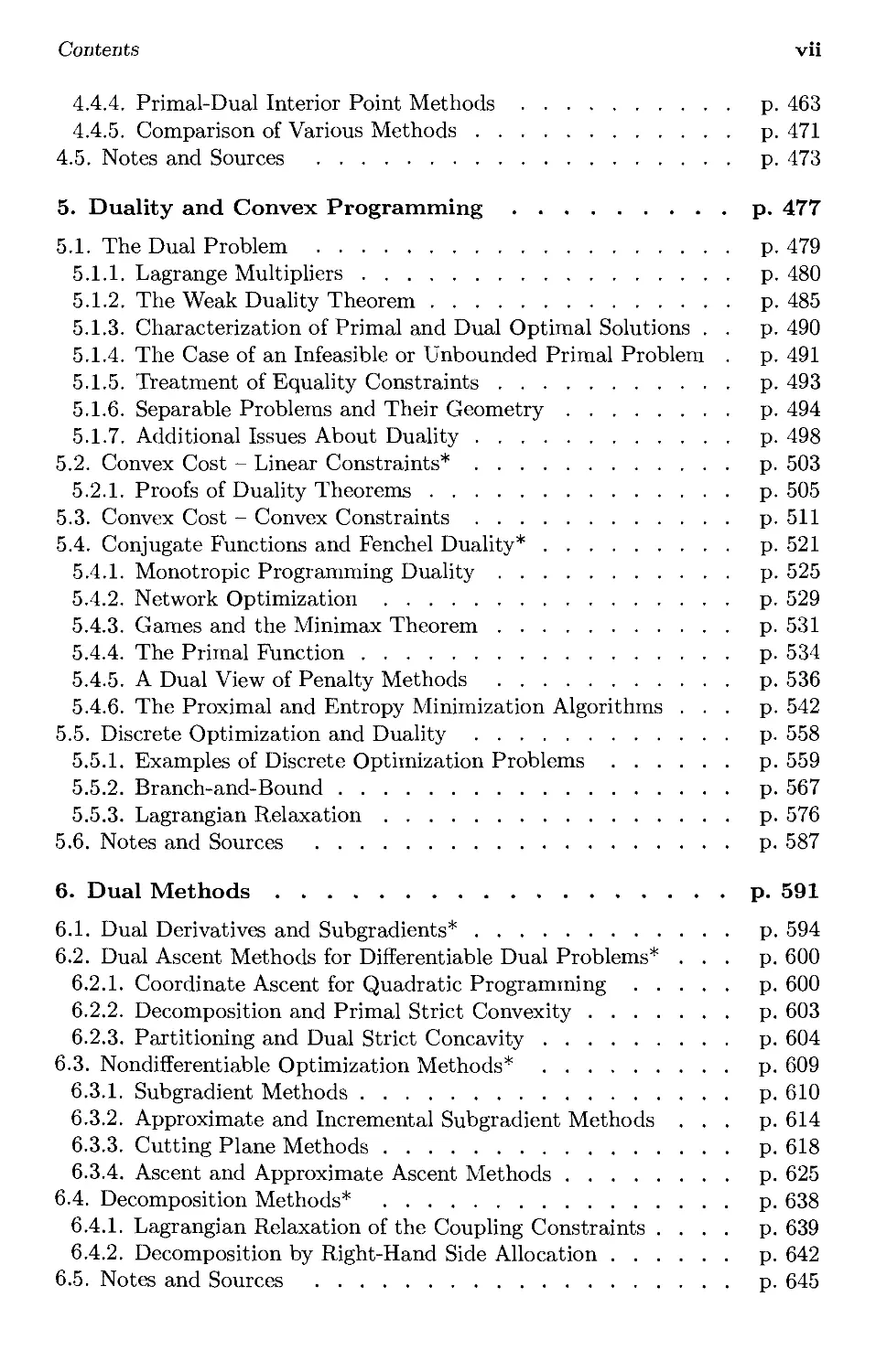
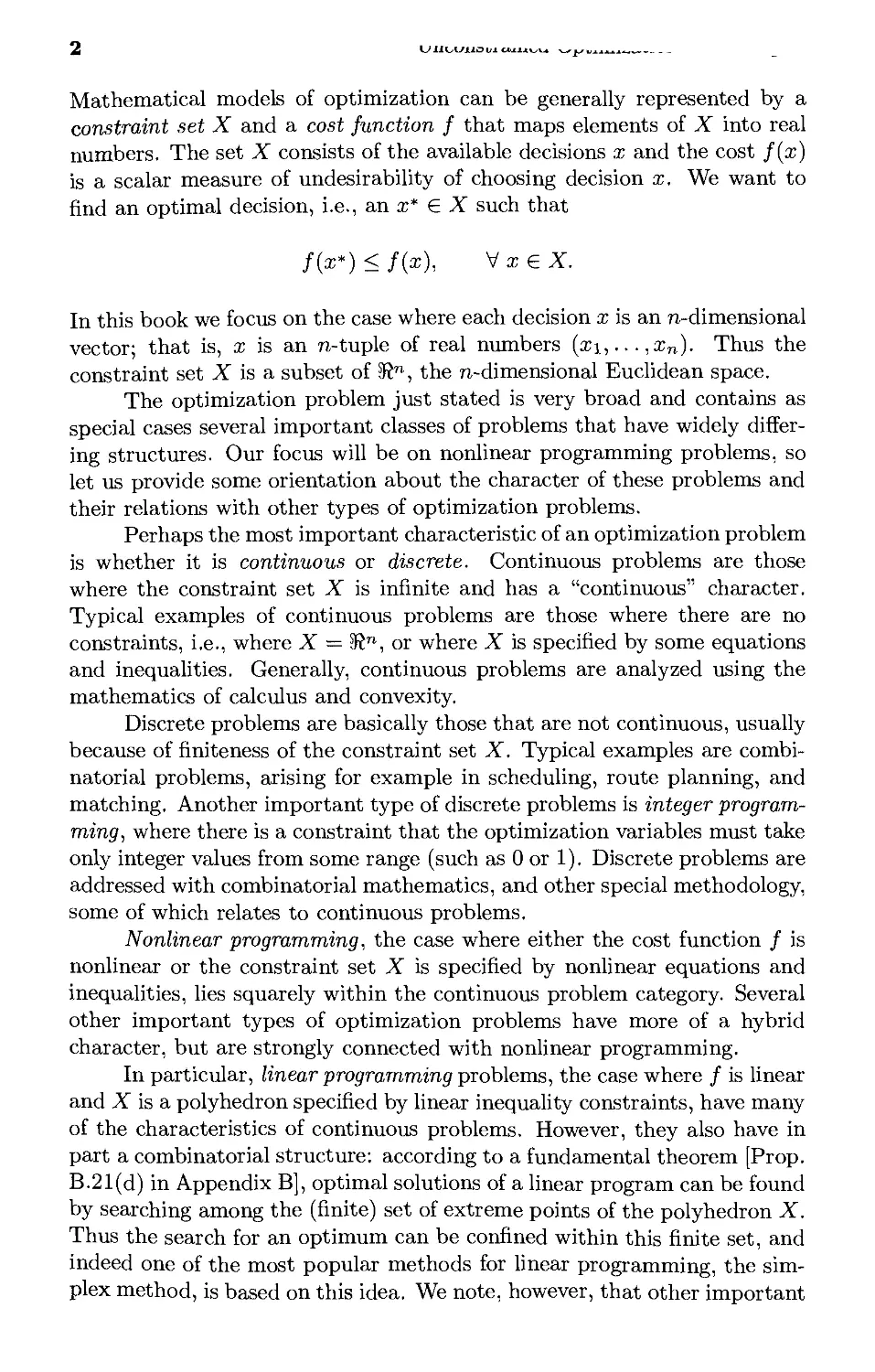
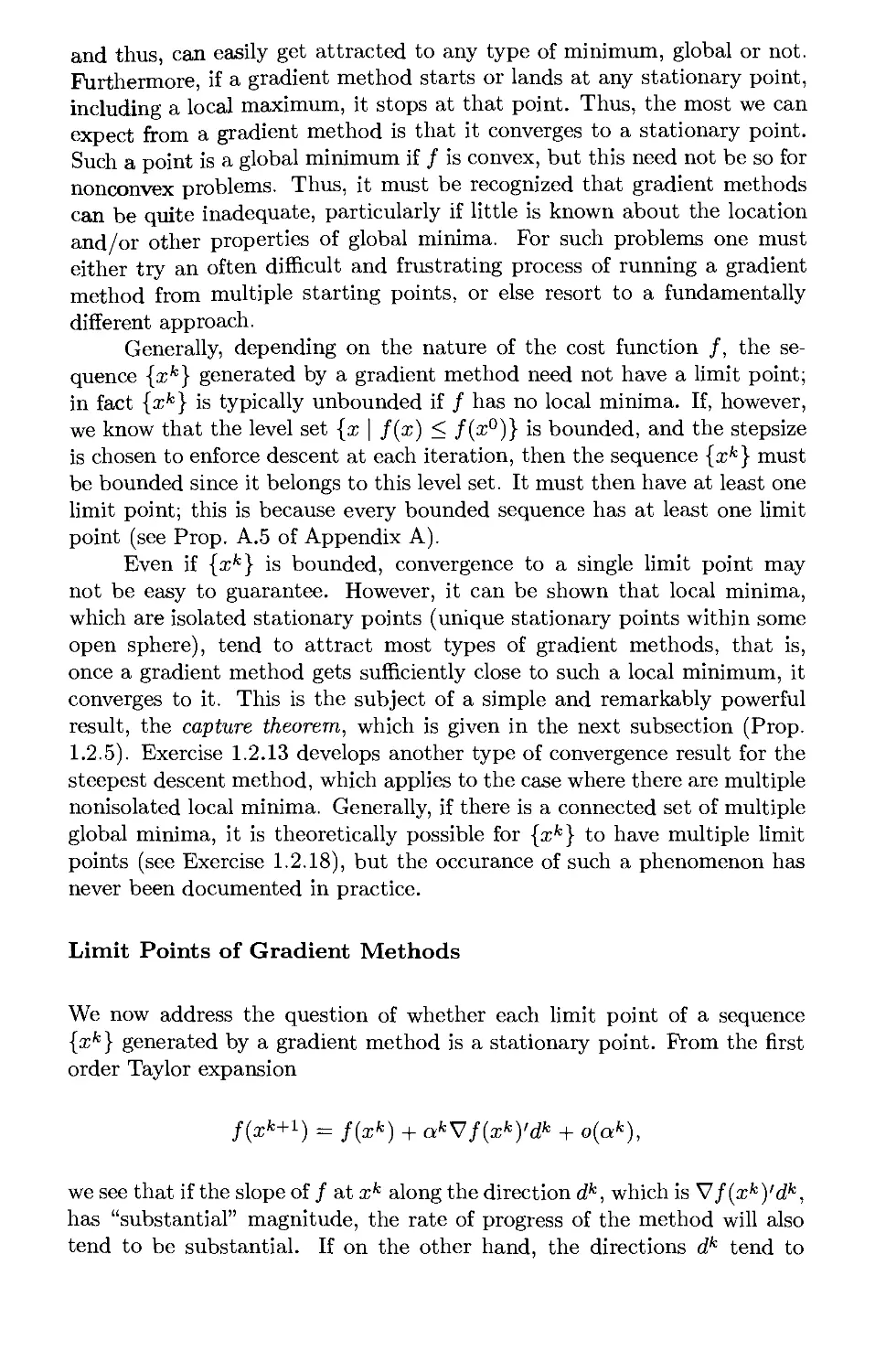
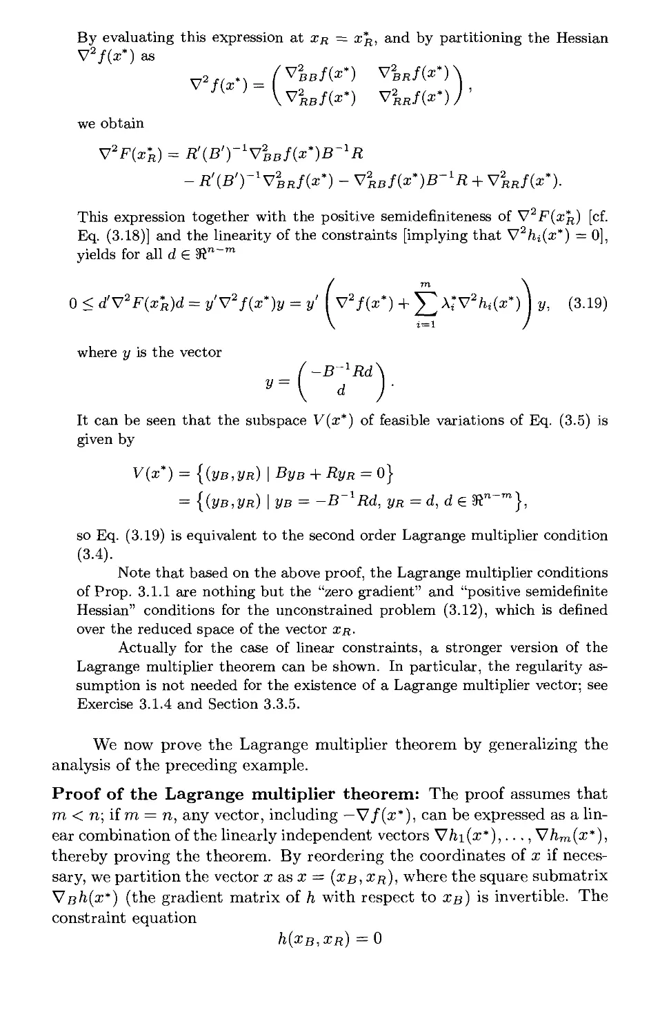
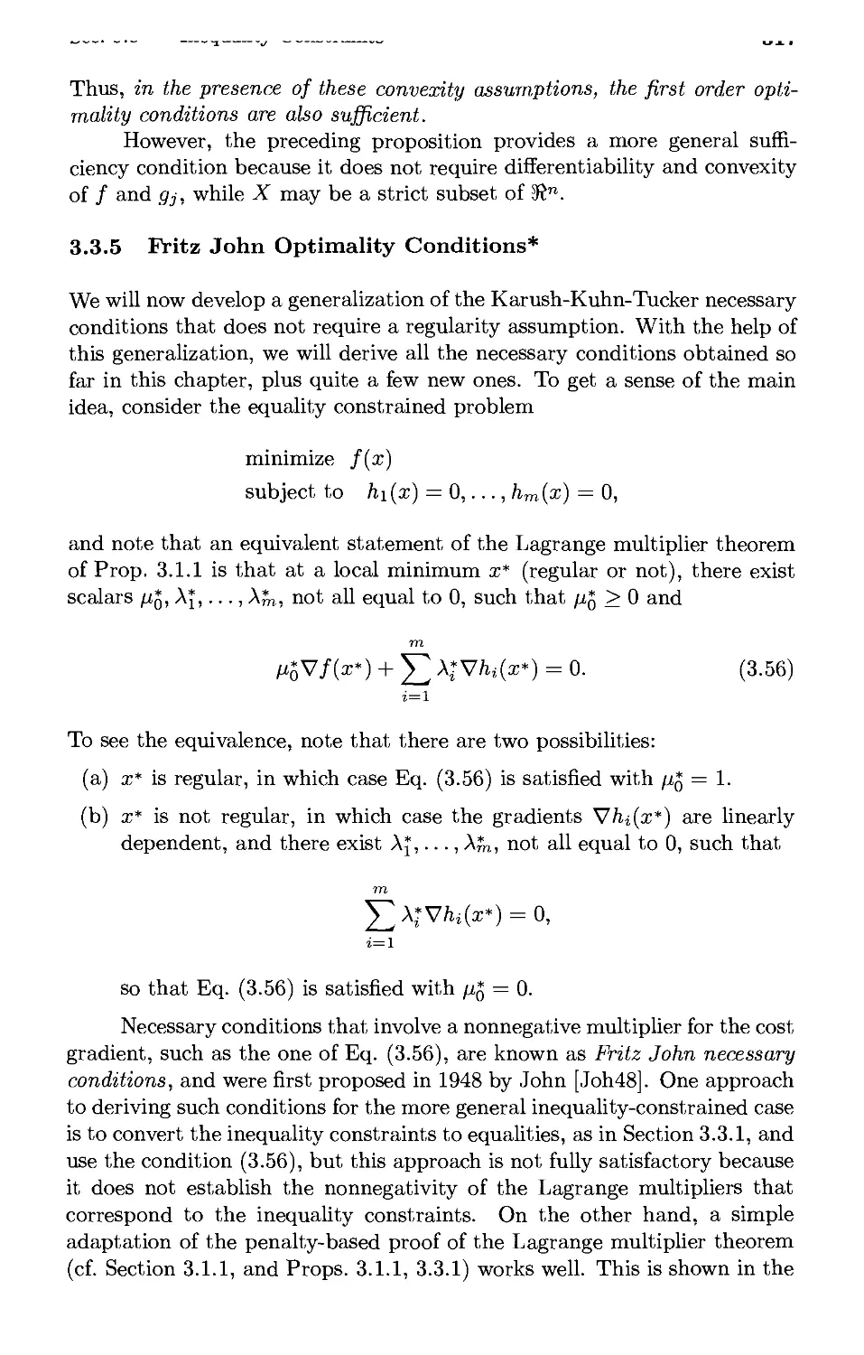
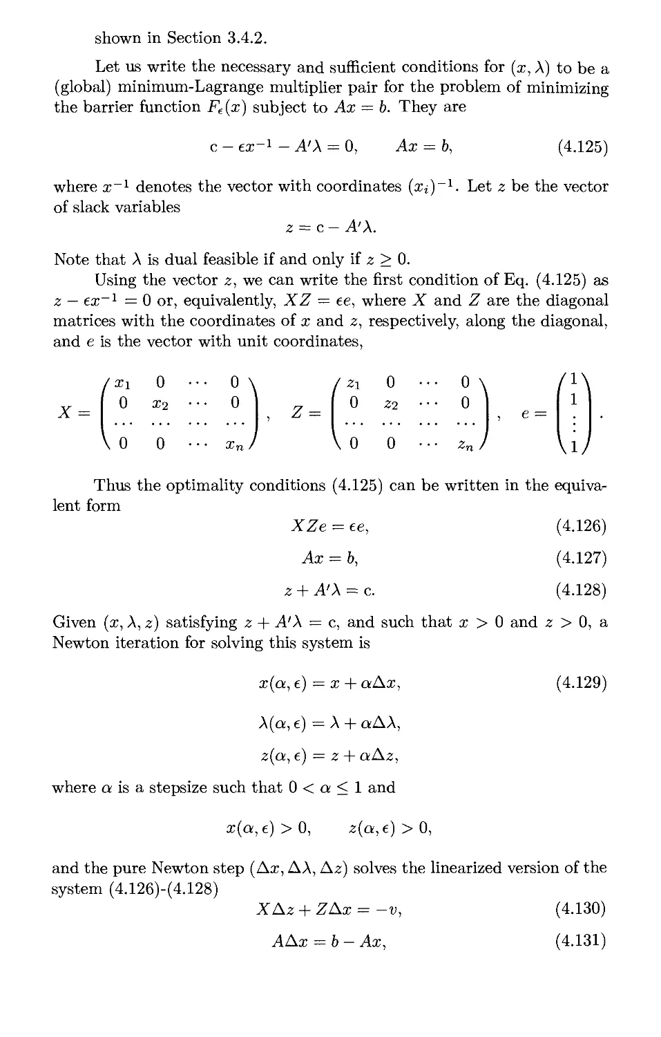
Local and Global Minima
A vector x* is an unconstrained local minimum of / if it is no worse than
its neighbors; that is, if there exists an e > 0 such that
/(x*) < /(x), V x with ||x — x*|| < e.
(Unless stated otherwise, we use the standard Euclidean norm ||x|| = \/x'x.
Appendix A describes in detail our mathematical notation and
terminology.)
A vector x* is an unconstrained global minimum of / if it is no worse
than all other vectors; that is,
/(x*)</(x), VxeJR".
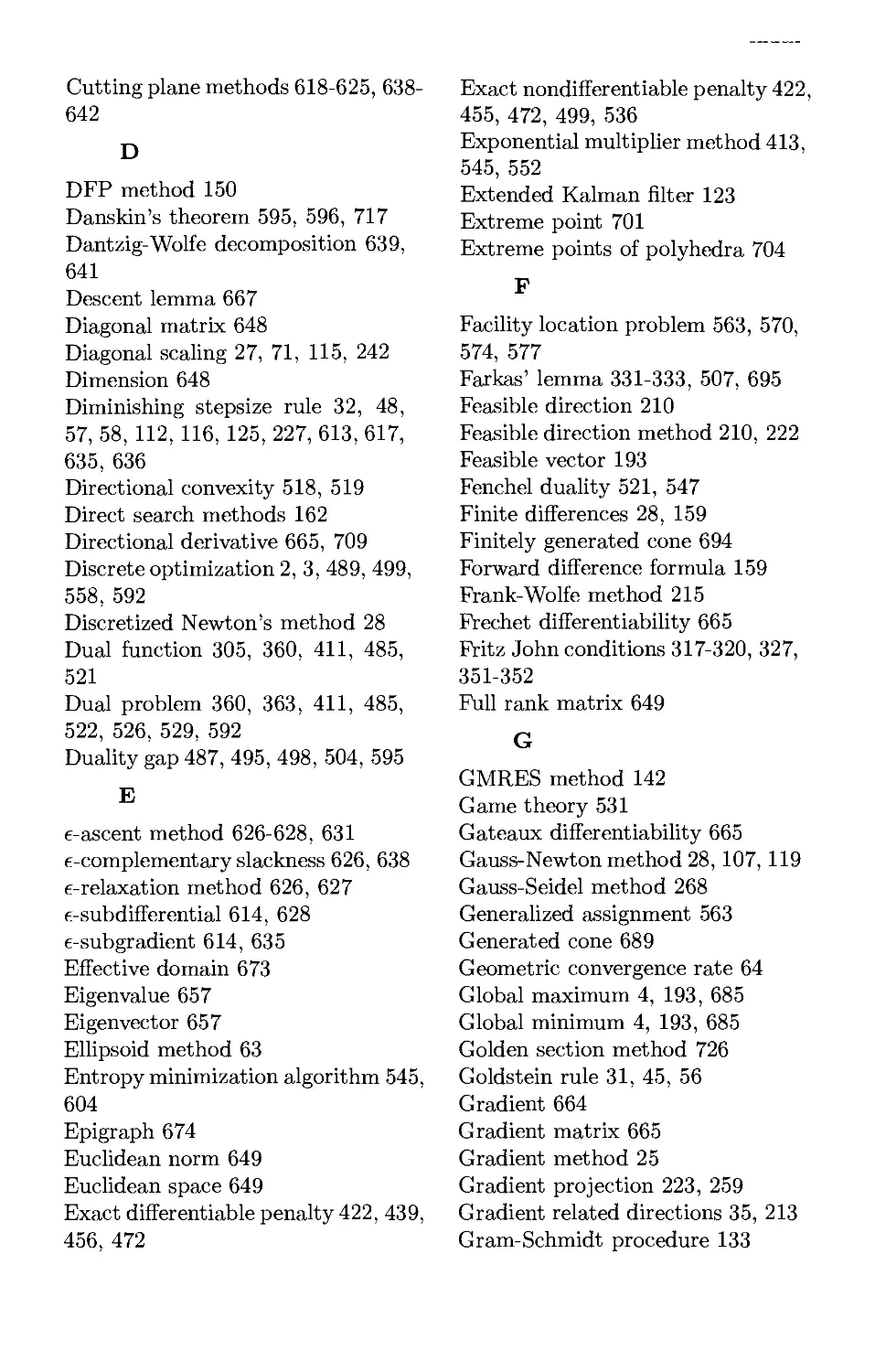
The unconstrained local or global minimum x* is said to be strict
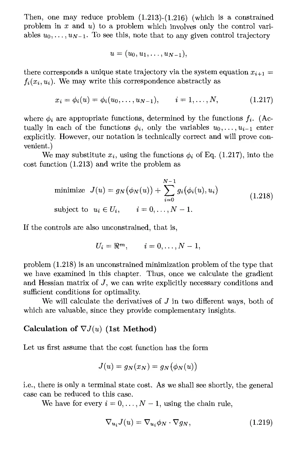
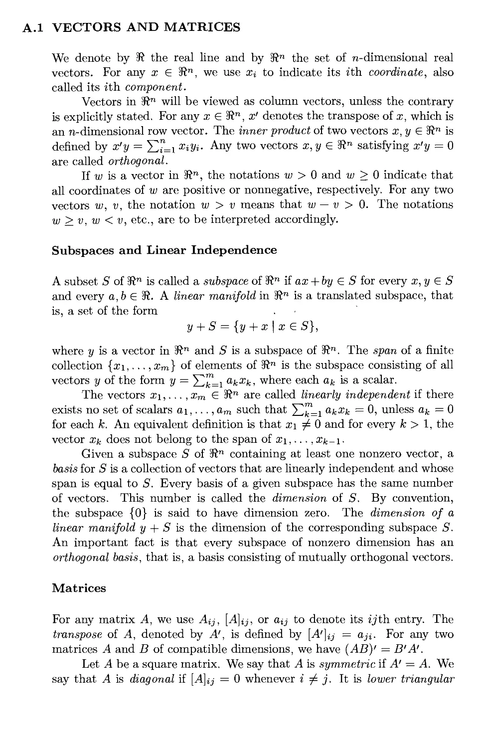
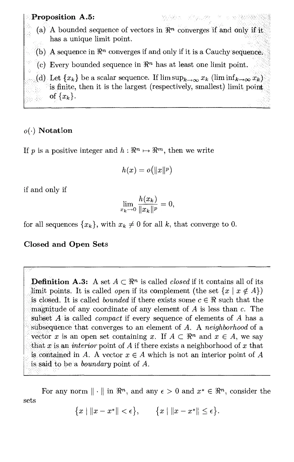
if the corresponding inequality above is strict for x ^ x*. Figure 1.1.1
illustrates these definitions.
The definitions of local and global minima can be extended to the
case where / is a function defined over a subset X of 3¾71. In particular, we
say that x* is a local minimum of / over X if x* £ X and there is an e > 0
such that /(x*) < /(x) for all x e X with ||x — x*|| < e. The definitions of
a global and a strict minimum of / over X are analogous.
Local and global maxima are similarly defined. In particular, x* is
an unconstrained local (global) maximum of /, if x* is an unconstrained
local (global) minimum of the function —/.
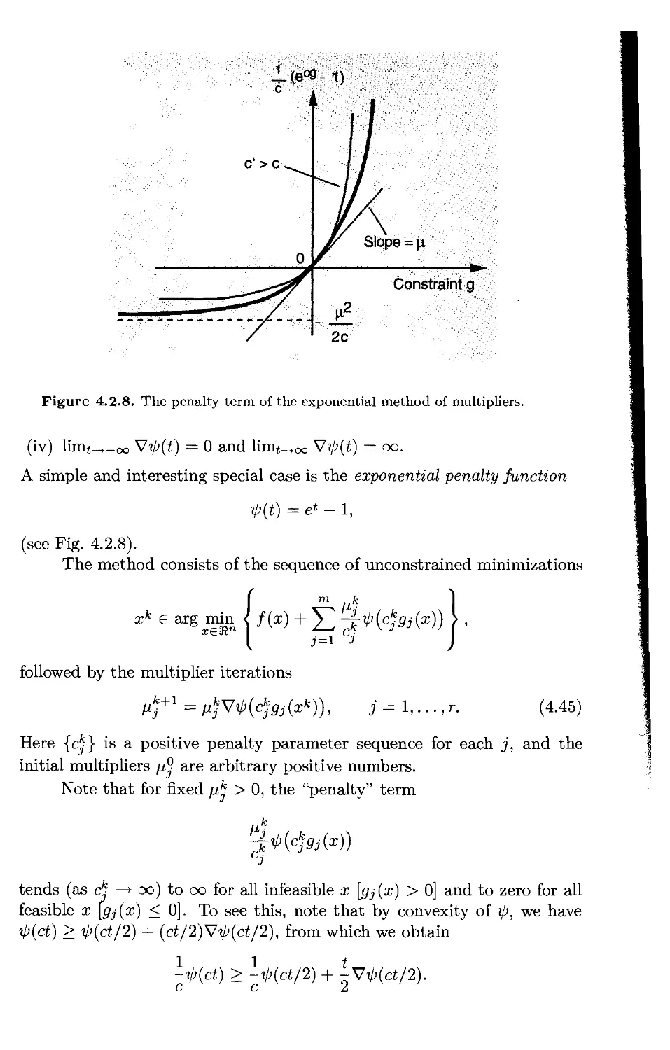
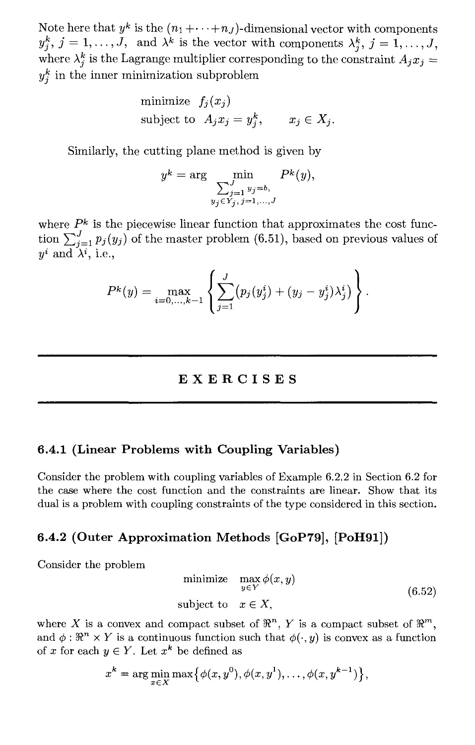
Strict Local Local Minima Strict Global
Minimum Minimum
Figure 1.1.1. Unconstrained local and global minima in one dimension.
Necessary Conditions for Optimality
If the cost function is differentiable, we can use gradients and Taylor series
expansions to compare the cost of a vector with the cost of its close
neighbors. In particular, we consider small variations Ax from a given vector
x*, which approximately, up to first order, yield a cost variation
f(x* + Ax) - f(x*) « V/(x*)'Ax
and, up to second order, yield a cost variation
/(x* + Ax) - /(x*) « V/(x*)'Ax + ±Ax'V2/(x*)Ax.
We expect that if x* is an unconstrained local minimum, the first
order cost variation due to a small variation Ax is nonnegative:
V/(x*)'Ax = Y ^^-Axi > 0.
«=i
In particular, by taking Ax to be positive and negative multiples of the
unit coordinate vectors (all coordinates equal to zero except for one which
is equal to unity), we obtain df(x*)/dxi > 0 and df(x*)/dxi < 0,
respectively, for all coordinates i = 1,..., n. Equivalently, we have the necessary
condition
V/(x*) = 0,
[originally formulated by Fermat in 1637 in the short treatise "Methodus
as Disquirendam Maximam et Minimam" without proof (of course!)]. This
condition is proved in Prop. 1.1.1, given in the next subsection.
We also expect that the second order cost variation due to a small
variation Ax must also be nonnegative:
V/(x*)'Ax + iAx'V2/0*)Ax > o.
Since V/(x*)'Ax = 0, we obtain
Ax'V2/(x*)Ax > o,
which implies that
V2/(x*) -.positive semidefinite.
We prove this necessary condition in the subsequent Prop. 1.1.1. Appendix
A reviews the definition and properties of positive definite and positive
semidefinite matrices.
In what follows, we refer to a vector x* satisfying the condition
V/(x*) = 0 as a stationary point.
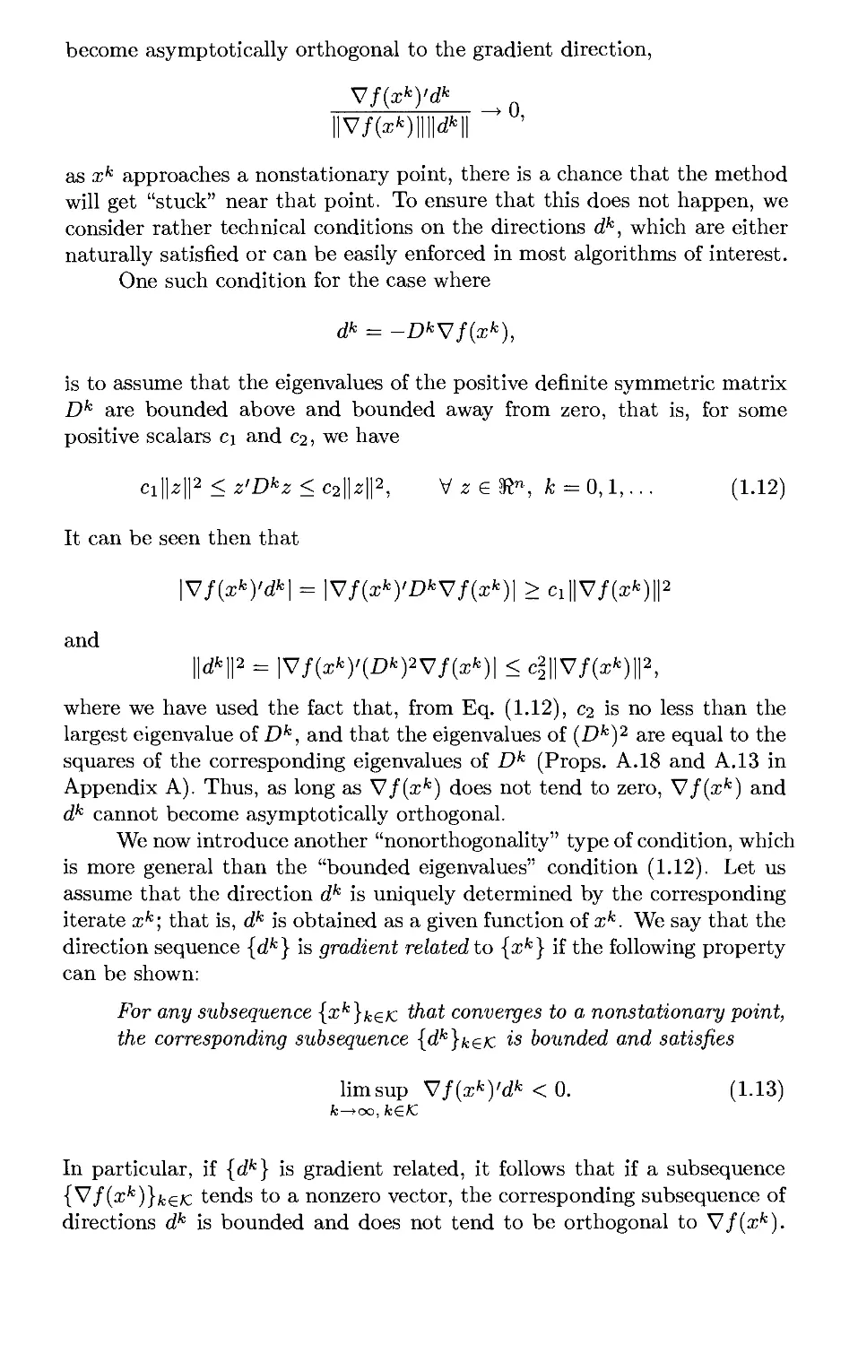
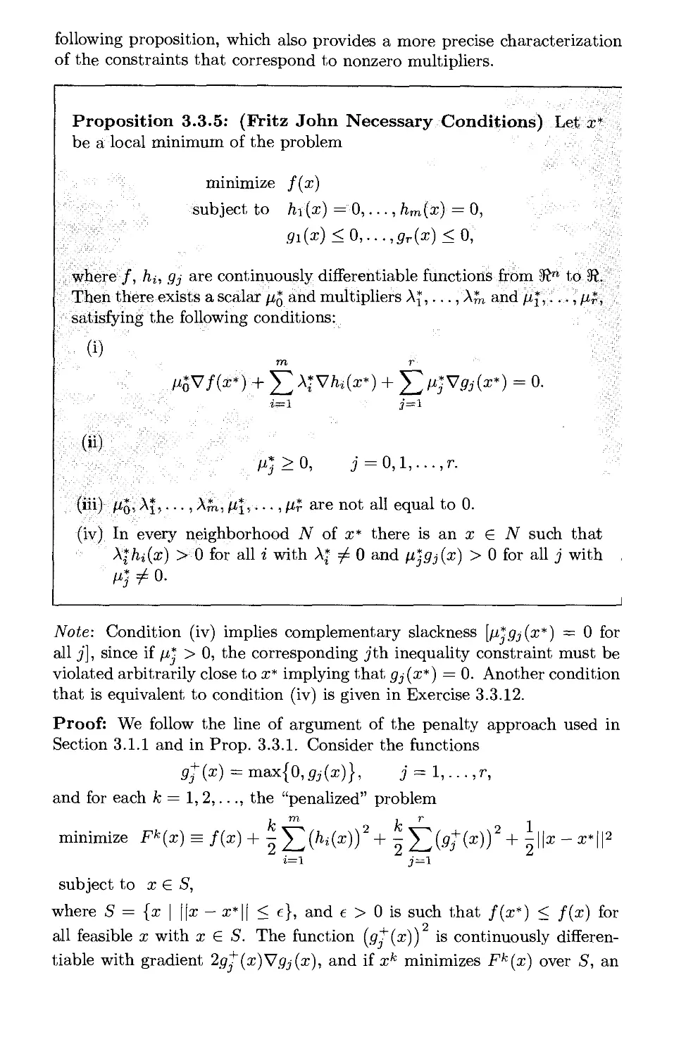
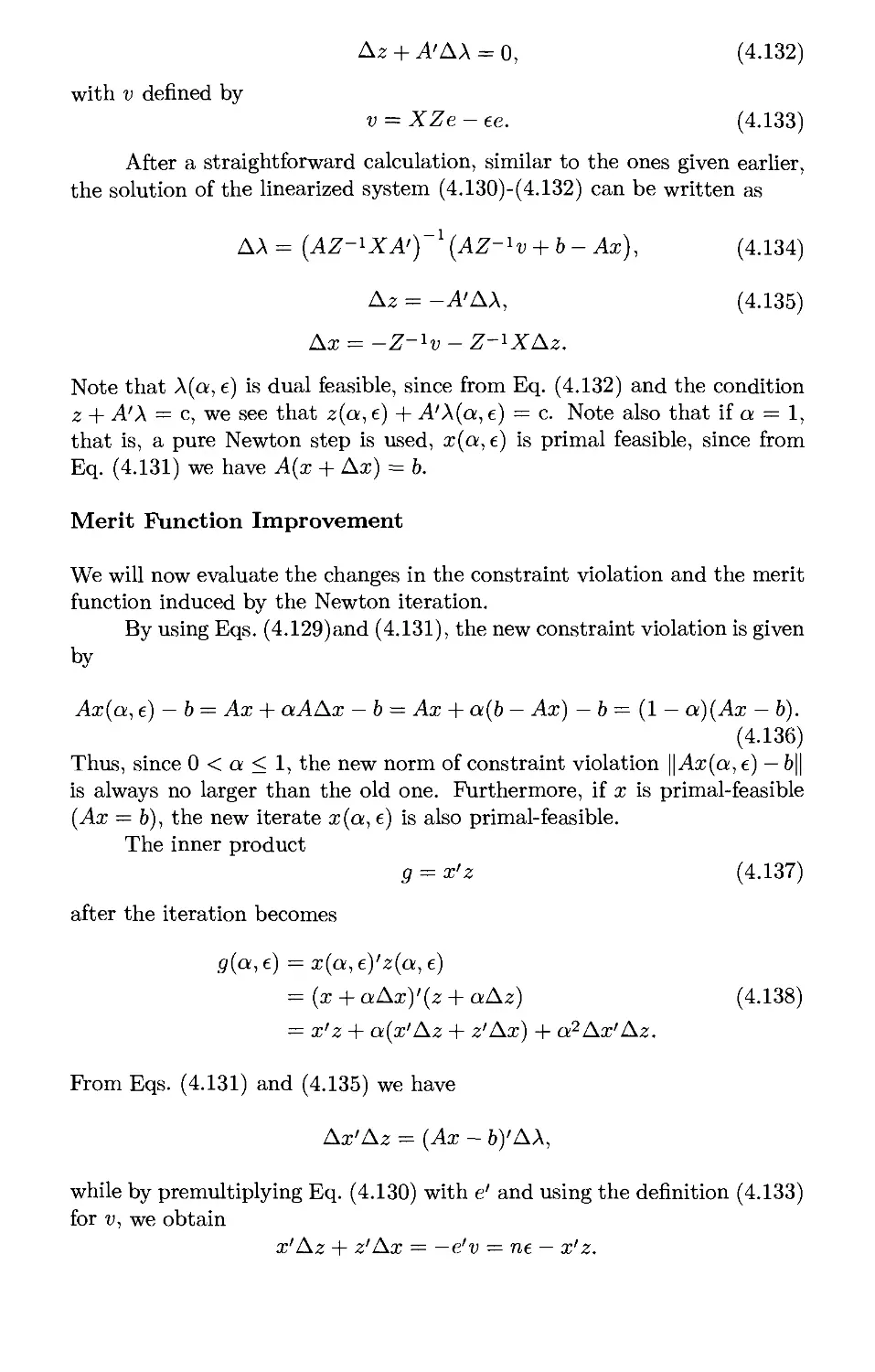
The Case of a Convex Cost Function
Convexity notions, reviewed in Appendix B, play a very important role
in nonlinear programming. One reason is that when the cost function /
is. convex, there is no distinction between local and global minima; every
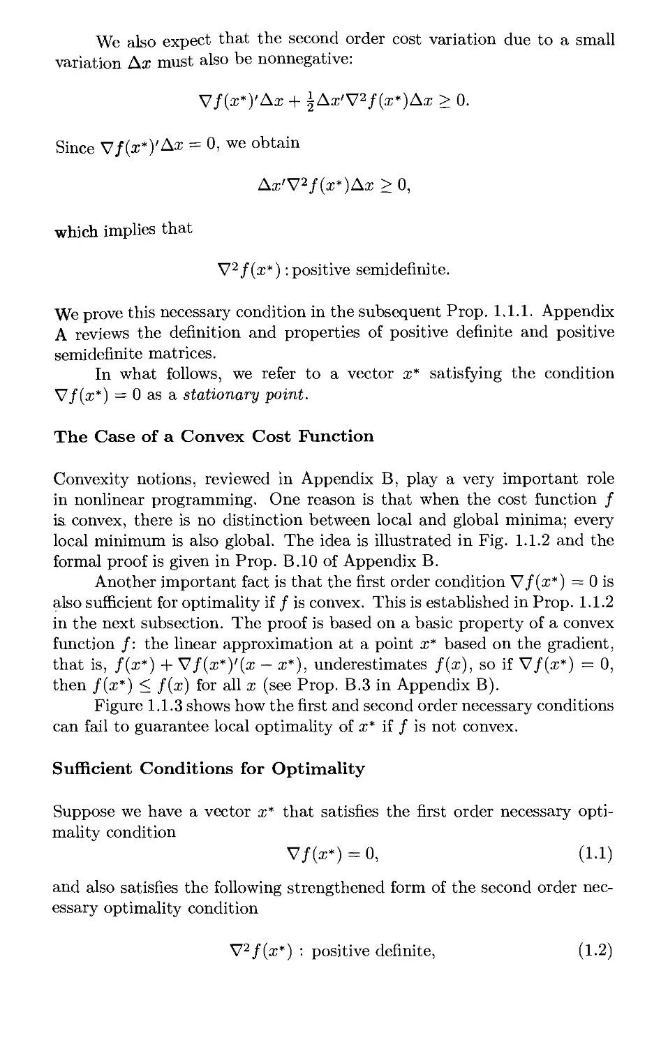
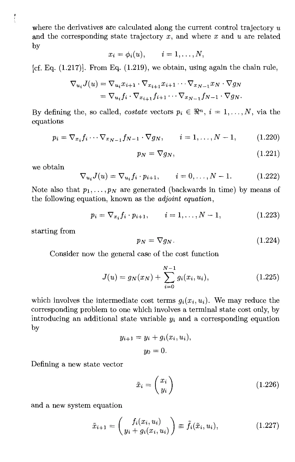
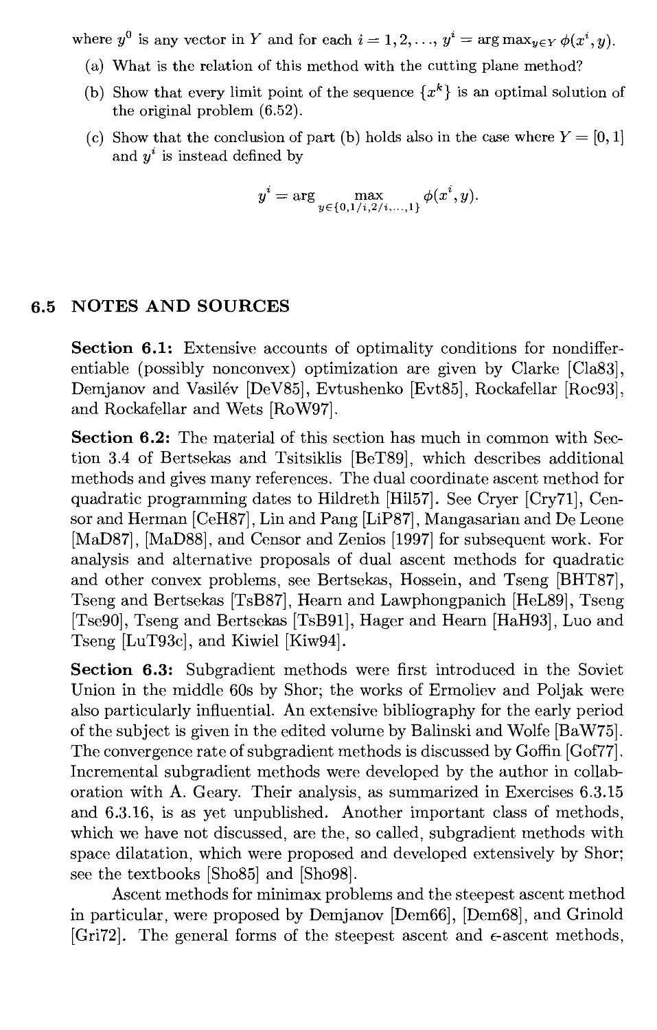
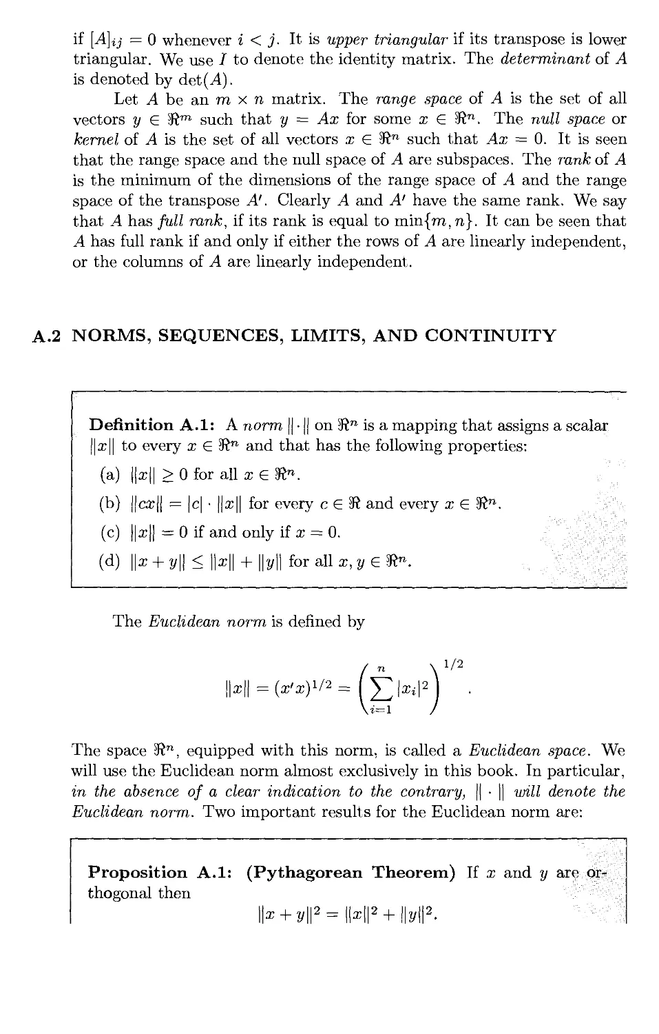
local minimum is also global. The idea is illustrated in Fig. 1.1.2 and the
formal proof is given in Prop. B.10 of Appendix B.
Another important fact is that the first order condition V/(x*) = 0 is
also sufficient for optimality if / is convex. This is established in Prop. 1.1.2
in the next subsection. The proof is based on a basic property of a convex
function /: the linear approximation at a point x* based on the gradient,
that is, /(x*) + V/(x*)'(x — x*), underestimates /(x), so if V/(x*) = 0,
then /(x*) < /(x) for all x (see Prop. B.3 in Appendix B).
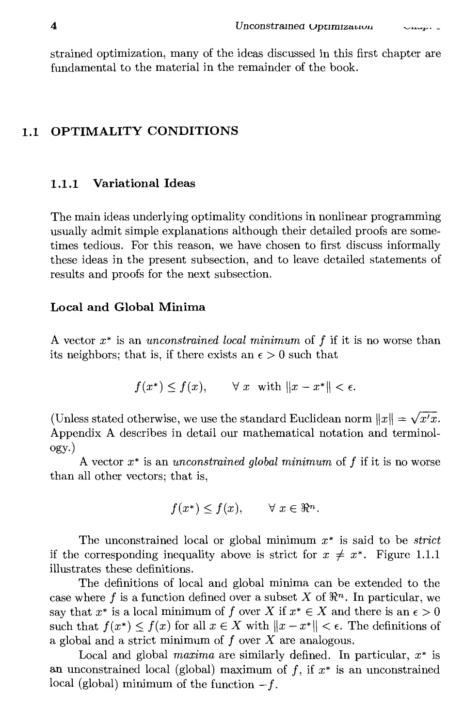
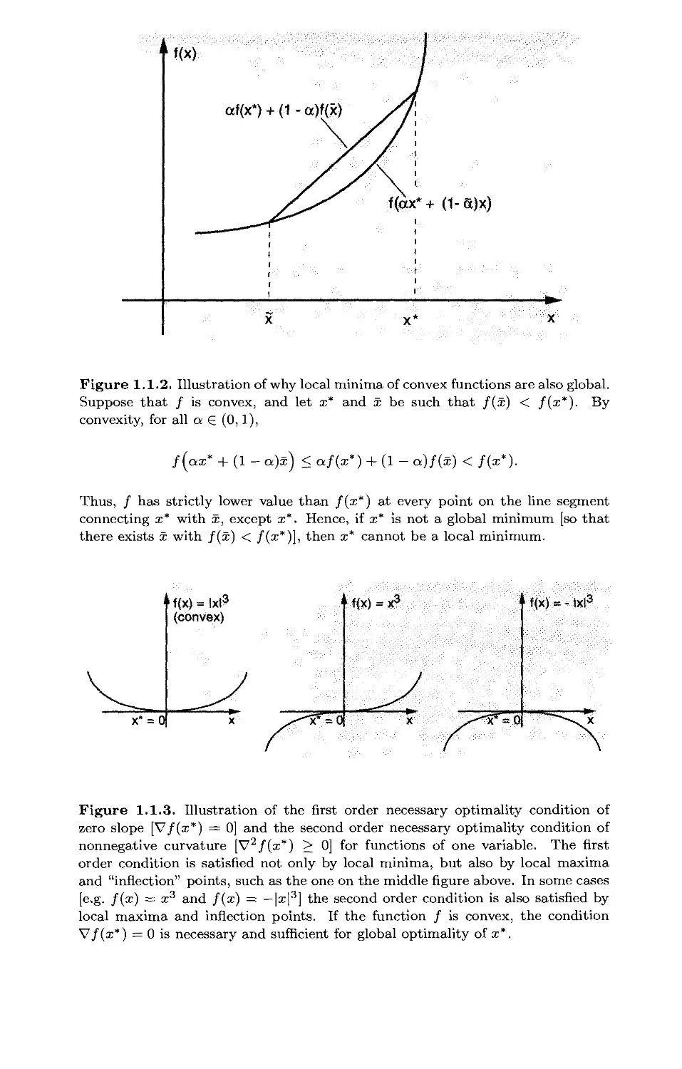
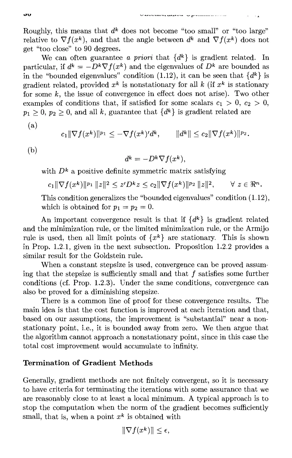
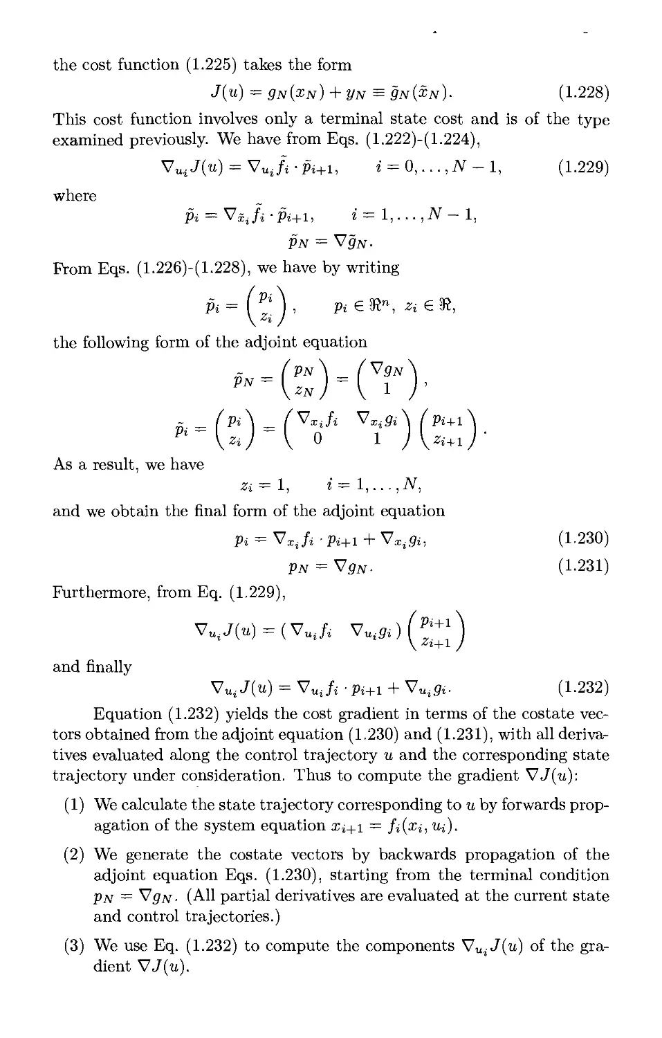
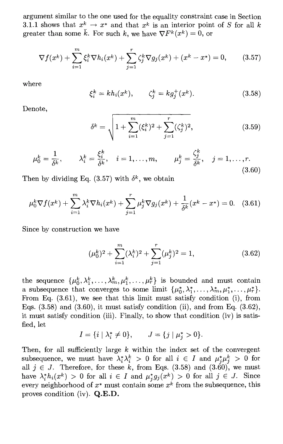
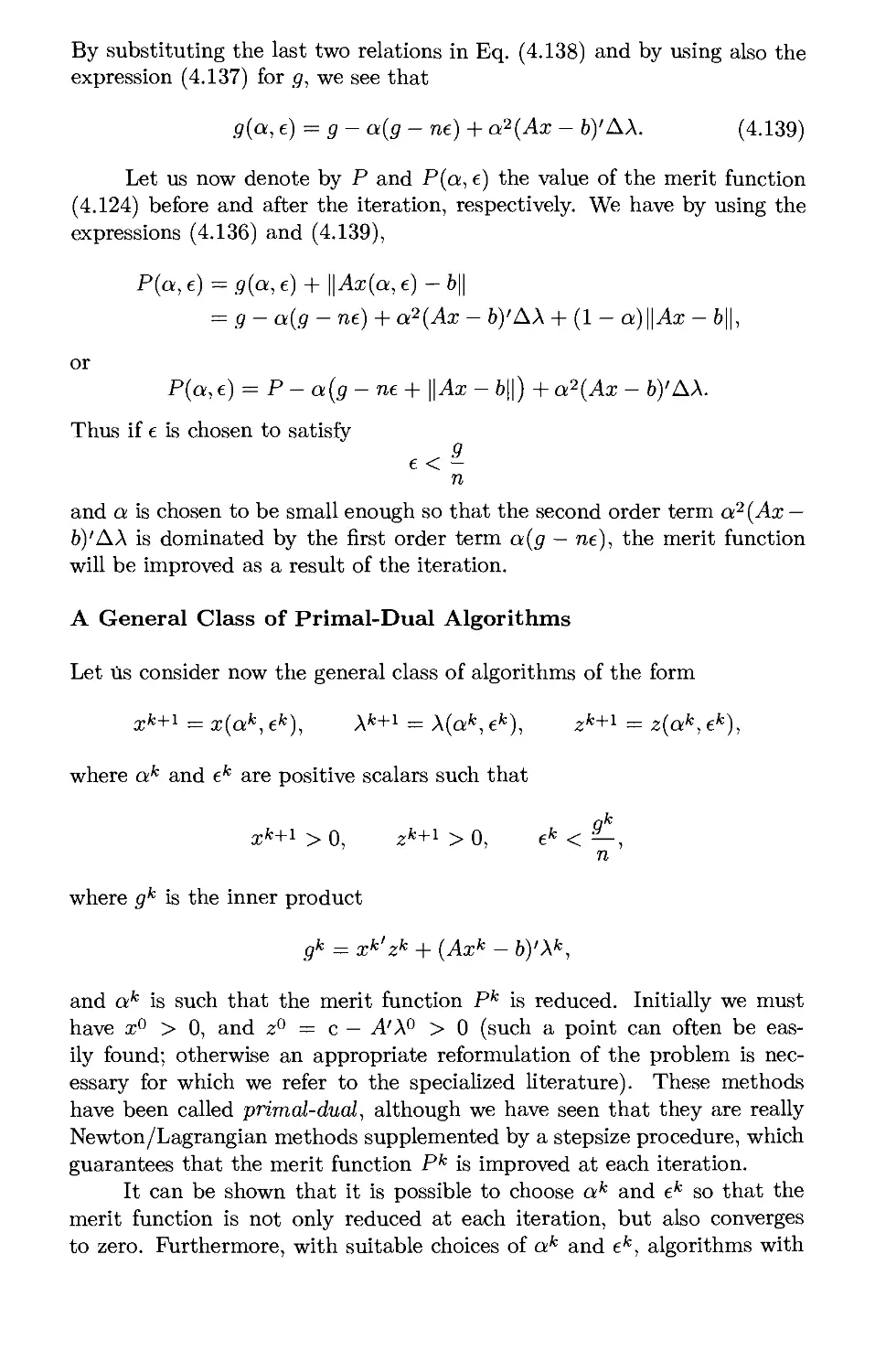
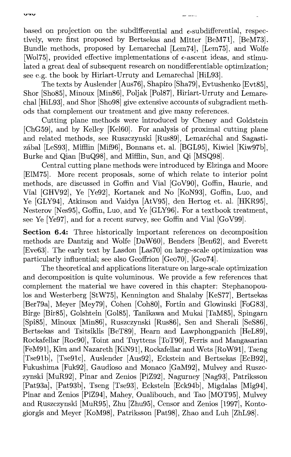
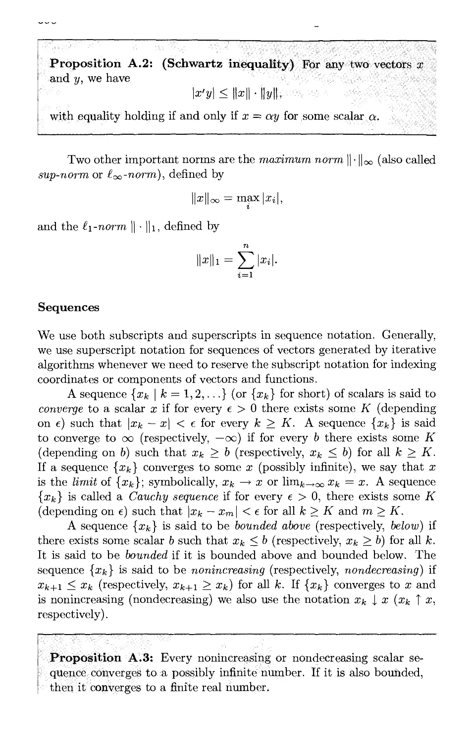
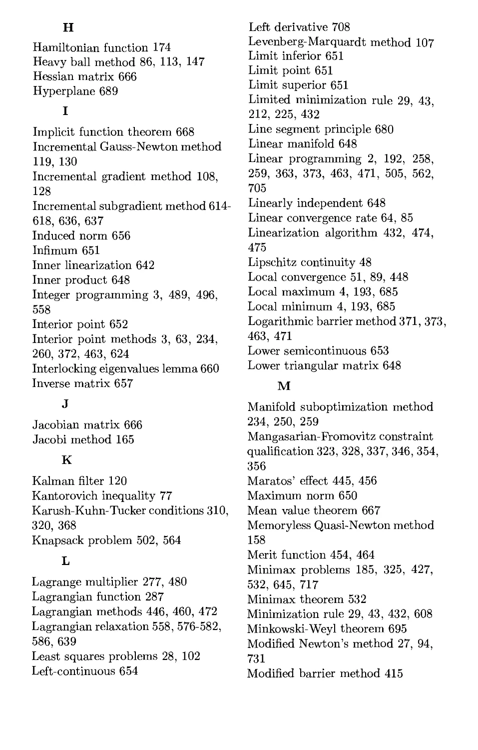
Figure 1.1.3 shows how the first and second order necessary conditions
can fail to guarantee local optimality of x* if / is not convex.
Sufficient Conditions for Optimality
Suppose we have a vector x* that satisfies the first order necessary
optimality condition
V/(x*)=0, (1.1)
and also satisfies the following strengthened form of the second order
necessary optimality condition
V2/(x*) : positive definite,
(1.2)
f(x
af(x*) + (1 - a)f(x)
f(ax* + (1-S)x)
x*
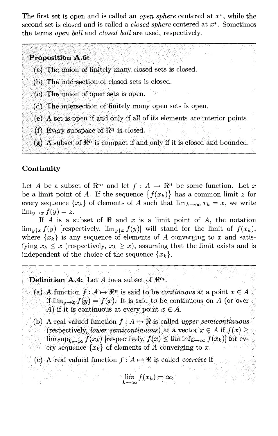
Figure 1.1.2. Illustration of why local minima of convex functions are also global.
Suppose that / is convex, and let x* and x be such that /(x) < /(x*). By
convexity, for all a 6 (0,1),
/(ax* + (1- a)x) < a/(x*) + (1- a)/(x) < /(x*).
Thus, / has strictly lower value than /(x*) at every point on the line segment
connecting x* with x, except x*. Hence, if x* is not a global minimum [so that
there exists x with /(x) < /(x*)], then x* cannot be a local minimum.
x* = 0
f{x) = Ixl3
(convex)
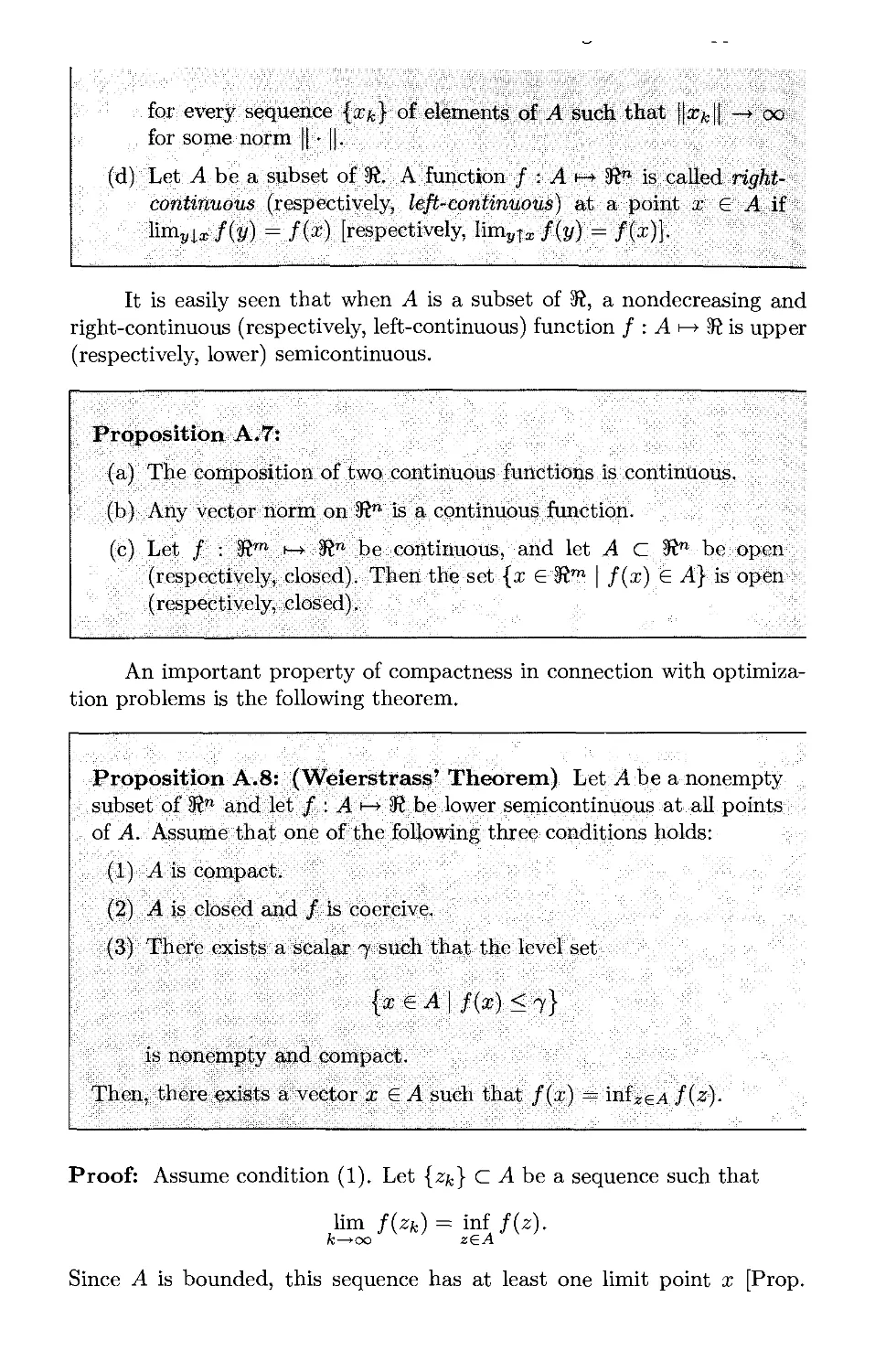
f(x):
'' f(x) = - Ixl3
Figure 1.1.3. Illustration of the first order necessary optimality condition of
zero slope [V/(x*) = 0] and the second order necessary optimality condition of
nonnegative curvature [V2/(x*) > 0] for functions of one variable. The first
order condition is satisfied not only by local minima, but also by local maxima
and "inflection" points, such as the one on the middle figure above. In some cases
[e.g. /(x) = x3 and /(x) = — |x|3] the second order condition is also satisfied by
local maxima and inflection points. If the function / is convex, the condition
V/(x*) = 0 is necessary and sufficient for global optimality of x*.
8
Unconstrained L/ptuiuzauvu
(that is, the Hessian is positive definite rather than semidefinite). Then,
for all Ax ^ 0 we have
Ax'V2/(x*)Ax > 0,
implying that at x* the second order variation of / due to a small nonzero
variation Ax is positive. Thus, / tends to increase strictly with small
excursions from x*, suggesting that the above conditions (1.1) and (1.2)
are sufficient for local optimality of x*. This is established in Prop. 1.1.3.
Local minima that don't satisfy the sufficiency conditions (1.1) and
(1.2) are called singular; otherwise they are called nonsingular. Singular
local minima are harder to deal with for two reasons. First, in the absence
of convexity of /, their optimality cannot be ascertained using easily
verifiable sufficiency conditions. Second, in their neighborhood, the behavior of
the most commonly used optimization algorithms tends to be slow and/or
erratic, as we will see in the subsequent sections.
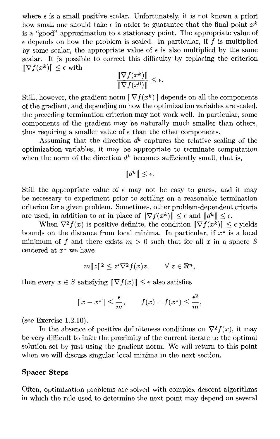
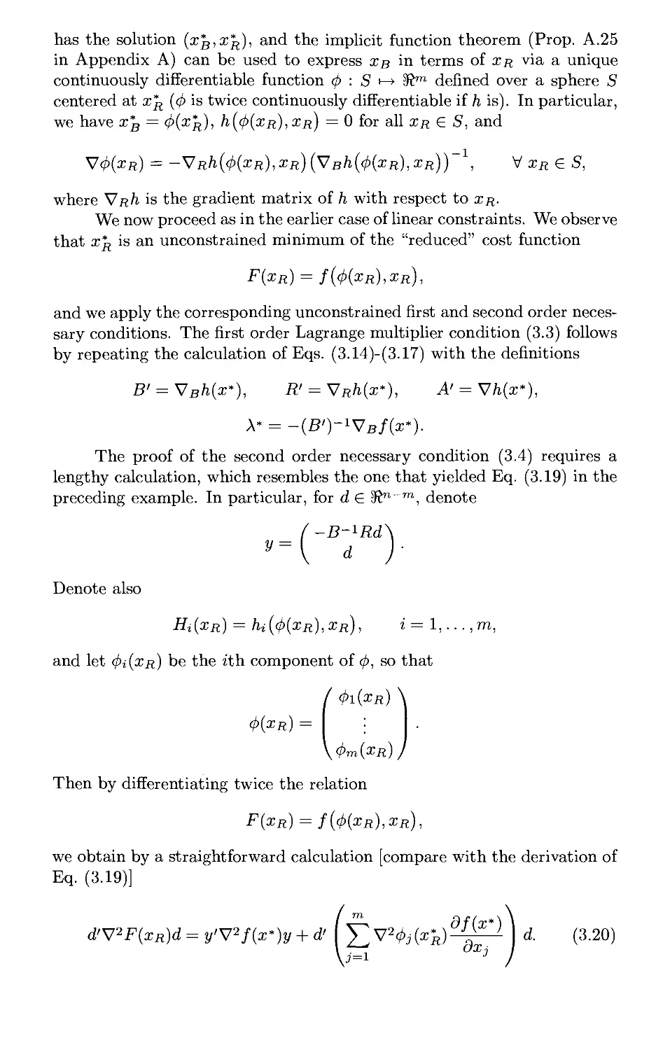
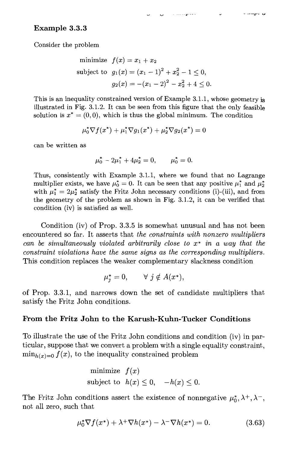
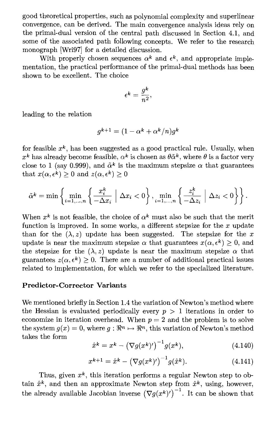
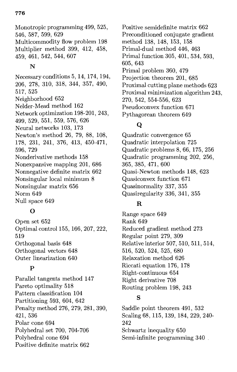
Quadratic Cost Functions
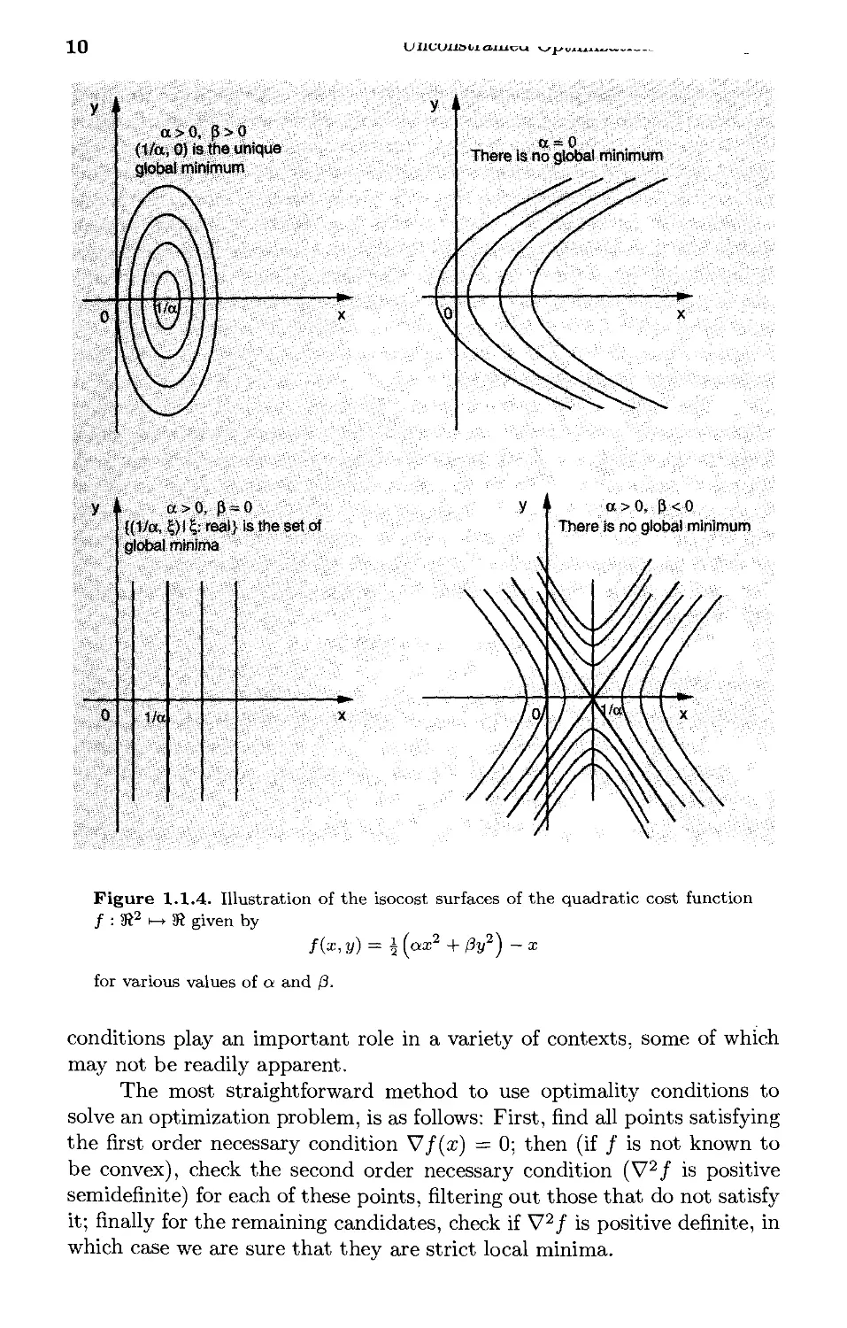
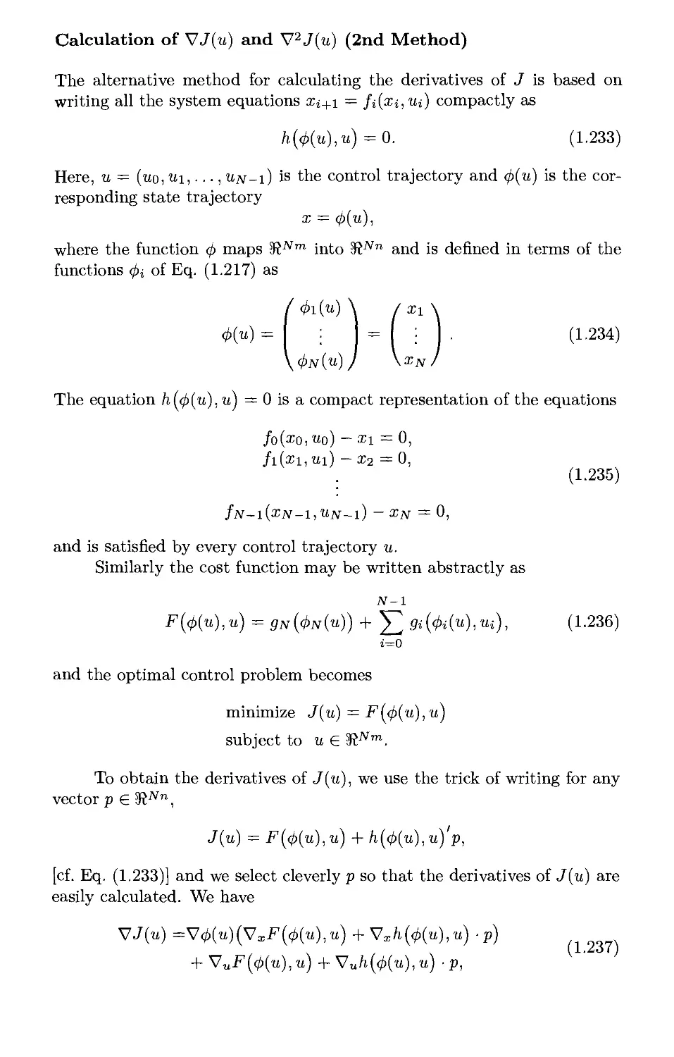
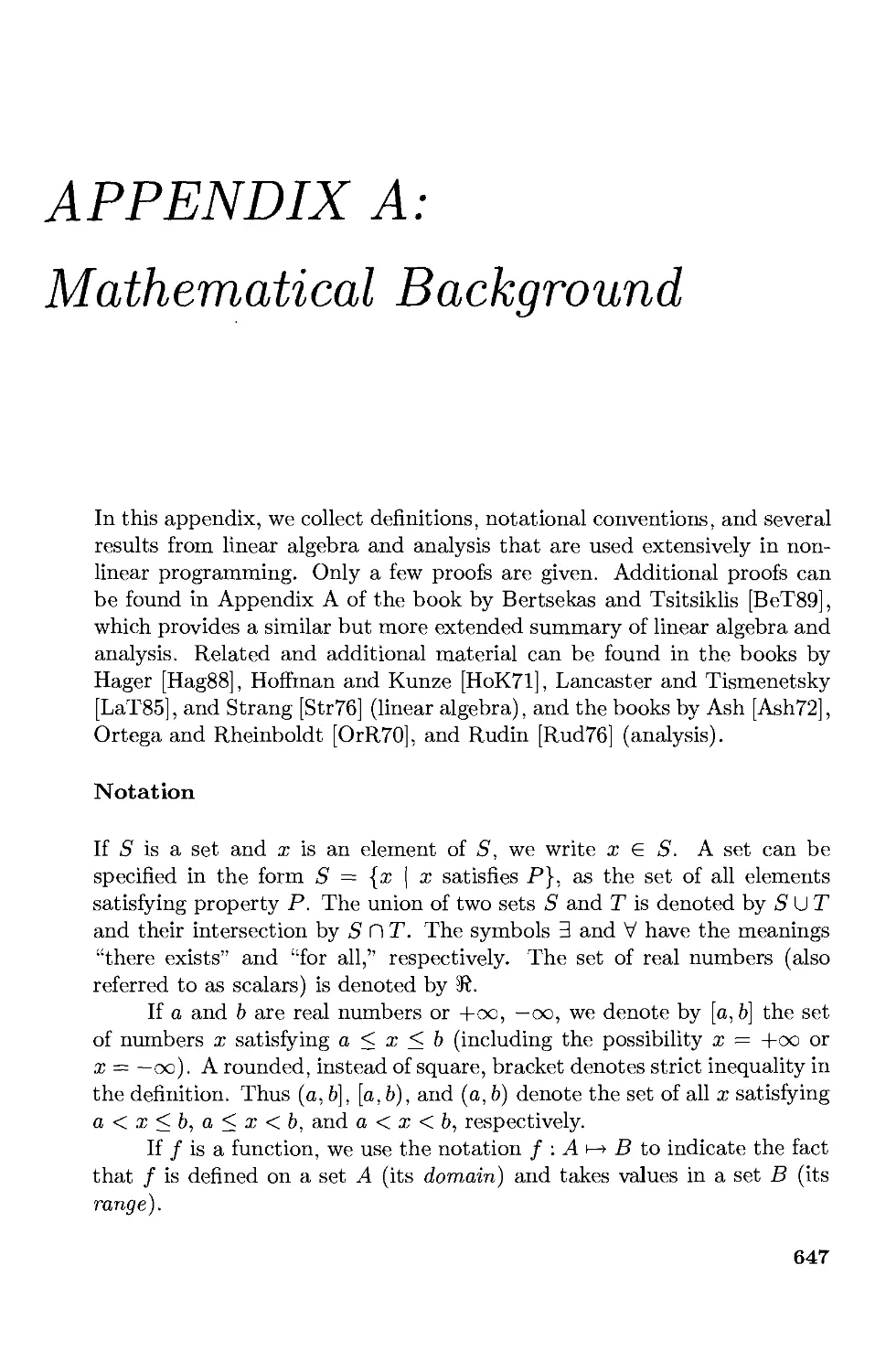
Consider the quadratic function
/(x) = jx'Qx — fr'x,
where Q is a symmetric n x n matrix and b is a vector in 3¾71. If x* is a
local minimum of f, we must have, by the necessary optimality conditions,
V/(x*) = Qx* — b = 0, V2/(x*) = Q : positive semidefinite.
Thus, if Q is not positive semidefinite, / can have no local minima. If Q
is positive semidefinite, / is convex [Prop. B.4(d) of Appendix B], so any
vector x* satisfying the first order condition V/(x*) = Qx* — b = 0 is a
global minimum of /. On the other hand there might not exist a solution
of the equation V/(x*) = Qx* — b = 0 if Q is singular. If, however, Q is
positive definite (and hence invertible, by Prop. A.20 of Appendix A), the
equation Qx* — b = 0 can be solved uniquely and the vector x* = Q~1b
is the unique global minimum. This is consistent with Prop. 1.1.2(a) to
be given shortly, which asserts that strictly convex functions can have at
most one global minimum [f is strictly convex if and only if Q is positive
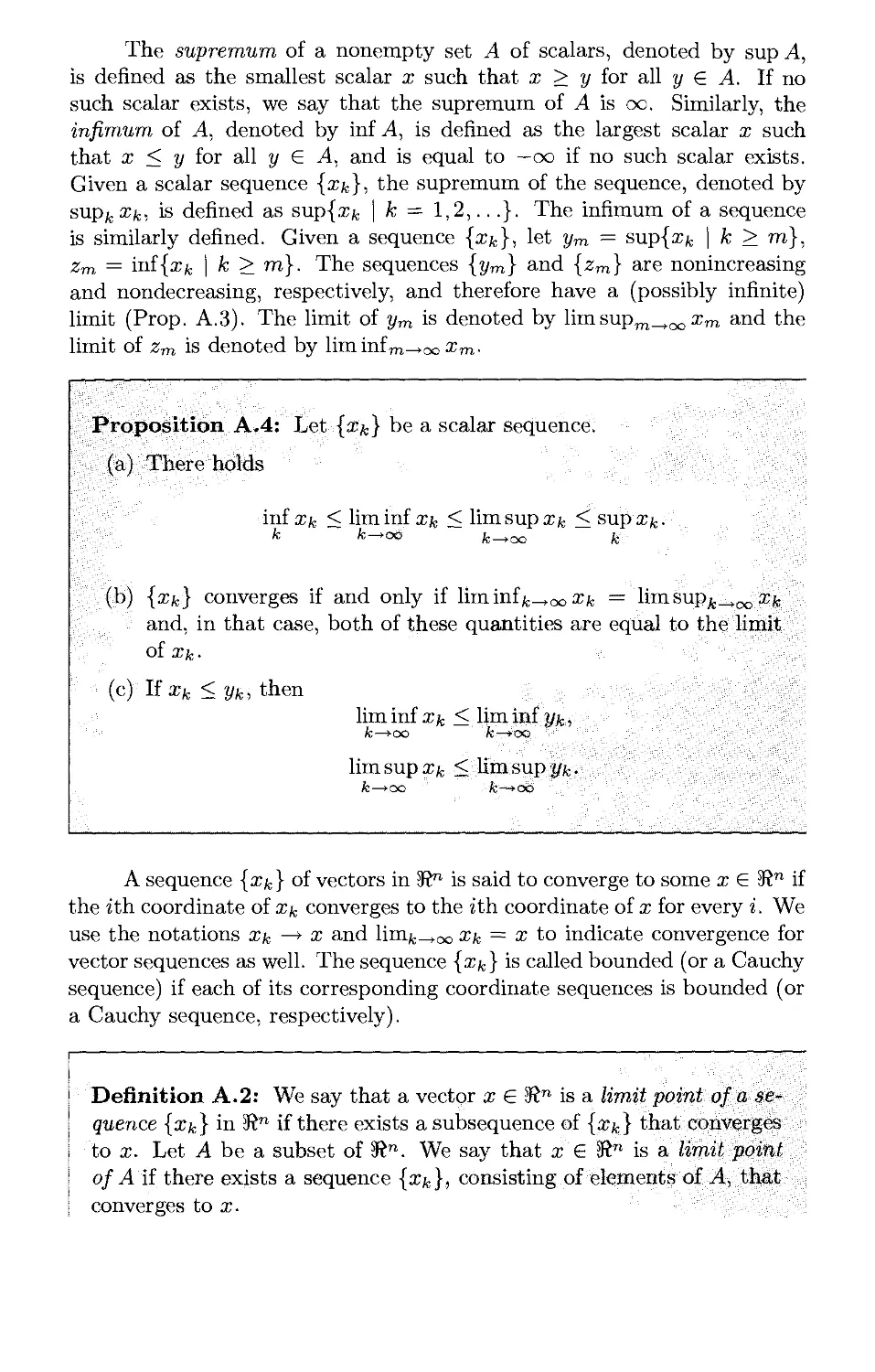
definite; Prop. B.4(d) of Appendix B]. Figure 1.1.4 illustrates the various
special cases considered.
Quadratic cost functions are important in nonlinear programming
because they arise frequently in applications, but they are also important
for another reason. From the Taylor expansion
/(x) = /(x*) + ^(x-x*)'V2/(x*)(x-x*) + o(||x-x*||2),
it is seen that a nonquadratic cost function can be approximated well by a
quadratic function near a nonsingular local minimum x* [V2/(x*): positive
definite]. This means that we can carry out much of our analysis and
experimentation with algorithms using positive definite quadratic functions
and expect that the conclusions will largely carry over to more general cost
functions near convergence to such local minima. However, for local minima
near which the Hessian matrix either does not exist or is singular, the
higher than second order terms in the Taylor expansion are not negligible
and an algorithmic analysis based on quadratic cost functions will likely be
seriously flawed.
Existence of Optimal Solutions
In many cases it is useful to know that there exists at least one global
minimum of a function / over a set X. Generally, such a minimum need
not exist. For example, the scalar functions f{x) = x and f{x) = ex have
no global minima over the set of real numbers. The first function decreases
without bound to — oo as x tends toward — oo, while the second decreases
toward 0 as x tends toward — oo but always takes positive values. Given
the range of values that f(x) takes as x ranges over X, that is, the set of
real numbers
{f(x)\xex},
there are two possibilities:
1. The set {/(x) | x G X} is bounded below, that is, there exists a
scalar M such that M < f(x) for all x G X. In this case, the greatest
lower bound of {/(x) | x G X} is a real number, which is denoted by
infx6x f{x)- For example, infx6sR ex = 0 and infx<o ex = 0.
2. The set {/(x) | x G A~} is unbounded below (i.e., contains arbitrarily
small real numbers). In this case we write
inf /(x) = -oo.
Existence of at least one global minimum is guaranteed if / is a
continuous function and X is a compact subset of 5ftn. This is the Weierstrass
theorem, (see Prop. A.8 in Appendix A). By a related result, also shown in
Prop. A.8 of Appendix A, existence of an optimal solution is guaranteed if
/ : 5ftn i—> 5ft is a continuous function, X is closed, and / is coercive, that
is, /(x) —> oo when ||x|| —> oo.
Why do we Need Optimality Conditions?
Hardly anyone would doubt that optimality conditions are fundamental to
the analysis of an optimization problem. In practice, however, optimality
10
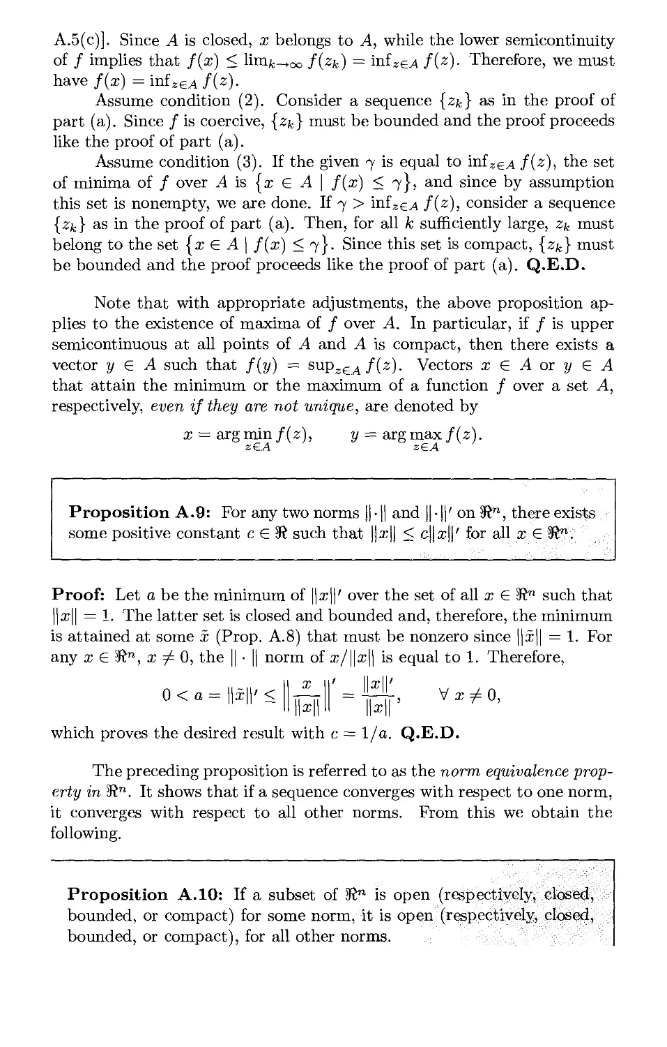
{J IlVUUOliL aiii^%-t v^L*(/iiju
y a
y a
a>0, P>0
(1/a, 0) is the unique
global minimum
a = 0
There is no global minimum
yf a>0, p = 0
{(1/a, 5)l£ real} is the set of
global minima
1/a
a > 0, p < 0
There is no global minimum
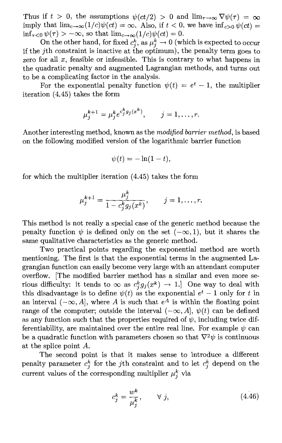
Figure 1.1.4. Illustration of the isocost surfaces of the quadratic cost function
/ : S2 i-+ SR given by
f(x,y) = A (ax2 +/¾2) -x
for various values of a and /3,
conditions play an important role in a variety of contexts, some of which
may not be readily apparent.
The most straightforward method to use optimality conditions to
solve an optimization problem, is as follows: First, find all points satisfying
the first order necessary condition V/(x) = 0; then (if / is not known to
be convex), check the second order necessary condition (V2/ is positive
semidefinite) for each of these points, filtering out those that do not satisfy
it; finally for the remaining candidates, check if V2/ is positive definite, in
which case we are sure that they are strict local minima.
A slightly different alternative is to find all points satisfying the
necessary conditions, and to declare as global minimum the one with smallest
cost value. However, here it is essential to know that a global minimum
exists. As an example, for the one-dimensional function
/(x) = x2 — X4,
the points satisfying the necessary condition
V/(x) = 2x - 4x3 = 0
are 0, l/\/2, and —1/\/2, and of these, 0 gives the smallest cost value.
However, we cannot declare 0 as the global minimum, because we don't
know if a global minimum exists. Indeed, in this example none of the
points 0, l/\/2, and —1/\/2 is a global minimum, because / decreases to
—oo as |x| —► oo, and has no global minimum. Here is another example:
Example 1.1.1 (Arithmetic-Geometric Mean Inequality)
We want to show the following classical inequality [due to Cauchy (1821)]
En
i=l Xi
{XlX2- ■■■£„) ■ ^.
n
for any set of positive numbers By making the change of
variables
yt = ln(a;i), i = 1,... ,n,
we have Xi = eVi, so that this inequality is equivalently written as
wiH—Yvn evi + ■ ■ ■ + eVn
e n <
n
which must be shown for all scalars j/i,..., y„. Note that with this
transformation, the nonnegativity requirements on the variables have been eliminated.
One approach to proving the above inequality is to minimize the
function
eV\ _|_ . . . _|_ eVn Vi + ---+Vn
and to show that its minimal value is 0. An alternative, which works better
if we use optimality conditions, is to minimize instead
e"1 + ■ ■ ■ + evn,
over all y = (j/i,..., yn) such that yi + ■ ■ ■ + yn = s for an arbitrary scalar
s, and to show that the optimal value is no less than neS//n. To this end,
we use the constraint j/i + ■ ■ ■ + yn = s to eliminate the variable yn, thereby
obtaining the equivalent unconstrained problem of minimizing
g(yi,.. .,»„_!) = ew + ... + e»n-i + e«-vi—-Vn-^
over 2/1,..., 2/n-i- The necessary conditions dg/dyi = 0 yield the system of
equations
eWi=e»-Wl Wn-^ i = l,...,n-l,
or
J/t = S —J/1- 2/n-l, i = 1,...,71- 1.
This system has only one solution: y* = s/n for all i. This solution must
be the unique global minimum if we can show that that there exists a global
minimum. Indeed, it can be seen that the function 3(2/1,... ,2/n-i) is coercive,
so it has an unconstrained global minimum. Therefore, {s/n,..., s/n) is this
minimum. Thus the optimal value of evi + ■ ■ - + eVn is neS//n, which as argued
above, is sufficient to show the arithmetic-geometric mean inequality.
It is important to realize, however, that except under very favorable
circumstances, using optimality conditions to obtain a solution as described
above does not work. The reason is that solving for x the system of
equations V/(x) = 0 is usually nontrivial; algorithmically, it is typically as
difficult as solving the original optimization problem.
The principal context in which optimality conditions become useful
will not become apparent until we consider iterative optimization
algorithms in subsequent sections. We will see that optimality conditions often
provide the basis for the development and the analysis of algorithms. In
particular, algorithms recognize solutions by checking whether they satisfy
various optimality conditions and terminate when such conditions hold
approximately. Furthermore, the behavior of various algorithms in the
neighborhood of a local minimum often depends on whether various optimality
conditions are satisfied at that minimum. Thus, for example, sufficiency
conditions play a key role in assertions regarding the speed of convergence
of various algorithms.
There is one other important context, prominently arising in microe-
conomic theory, where optimality conditions provide the basis for analysis.
Here one is interested primarily not in finding an optimal solution, but
rather in how the optimal solution is affected by changes in the problem
data. For example, an economist may be interested in how the prices of
some raw materials will affect the availability of certain goods that are
produced by using these raw materials; the assumption here is that the
amounts produced are the variables of a profit optimization problem, which
is solved by the corresponding producers. This type of analysis is known
as sensitivity analysis, and is discussed next.
Sensitivity*
Suppose that we want to quantify the variation of the optimal solution as
a vector of parameters changes. In particular, consider the optimization
problem
minimize /(x, a)
subject to x £ 5ftn,
where / : 3?m+n h-> 3¾ is a twice continuously difFerentiable function
involving the m-dimensional parameter vector a. Let x(a) denote the global
minimum corresponding to a, assuming for the moment that it exists and
is unique. By the first order necessary condition we have
Vx/(i(o),o)=0, VaeS™,
and by differentiating this relation with respect to a, we obtain
Vx(a)VL/(x(a),a) + VL/(x(a),a) =0,
where the elements of the mxn gradient matrix Vx(a) are the first partial
derivatives of the components of x(a) with respect to the different
components of a. Assuming that the inverse below exists, we have
Vx(a) = -VL/(x(a),a) (VL/(x(a),a)) \ (1.3)
which gives the first order variation of the components of the optimal x
with respect to the components of a.
For the preceding analysis to be precise, we must be sure that x(a)
exists and is difFerentiable as a function of a. The principal analytical
framework for this is the implicit function theorem (Prop. A.25 in
Appendix A). With the aid of this theorem, we can define x(a) in some sphere
around a minimum x = x(a) corresponding to a nominal parameter value
a, assuming that the Hessian matrix Vlx/(x,a) is positive definite. Thus,
the preceding development and the formula (1.3) for the matrix Vx(a) can
be justified provided the nominal local minimum x is nonsingular.
We will postpone further discussion of sensitivity analysis for Section
3.2, where we will provide a constrained version of the expression (1.3) for
Vx(a).
1.1.2 Main Optimality Conditions
We now provide formal statements and proofs of the optimality conditions
discussed in the preceding section.
Proposition 1.1.1: (Necessary Optimality Conditions) Let x*
be an unconstrained local minimum of / : 5ft" >—> 5ft, and assume that
/ is continuously differentiable in an open set S containing x*. Then
V/(x*) = 0. (First Order Necessary Condition)
If in addition / is twice continuously differentiable within S, then
V2/(x*): positive semidefinite. (Second Order Necessary Condition)
Proof: Fix some d £ 5ft". Then, using the chain rule to differentiate the
function g(a) = f(x* + ad) of the scalar a, we have
0 < lim /(^ + ^-/M = m = d,V/(x*),
aj.o a da
where the inequality follows from the assumption that x* is a local
minimum. Since d is arbitrary, the same inequality holds with d replaced by
—d. Therefore, d'V/(x*) = 0 for all d £ 5ft", which shows that V/(x*) = 0.
Assume that / is twice continuously differentiable, and let d be any
vector in 5ft". For all a £ 5ft, the second order Taylor series expansion yields
f(x* + ad) - f(x*) = aVf(x*)'d + ^-d'V2f(x*)d + o(a2).
Using the condition V/(x*) = 0 and the local optimality of x*, we see that
there is a sufficiently small e > 0 such that for all a with a £ (0, e),
o < /C- + "*)-/(*•) = 4d,vv(*-)d+ ^.
az az
Taking the limit as a —> 0 and using the fact
lim -^- = 0,
a^O az
we obtain d'V2/(x*)d > 0, showing that V2/(x*) is positive semidefinite.
Q.E.D.
The following proposition handles the case of a convex cost.
Proposition 1.1.2: (Convex Cost Function) Let / : X »-> 3¾ be
a convex function over the convex set X.
(a) A local minimum of / over X is also a global minimum over X.
If in addition / is strictly convex, then there exists at most one
global minimum of /.
(b) If / is convex and the set X is open, then V/(x*) = 0 is a
necessary and sufficient condition for a vector x* £ X to be a
global minimum of / over X.
Proof: Part (a) is proved in Prop. B.10 of Appendix B. To show part (b),
note that by Prop. B.3 of Appendix B, we have
/(x) > f{x*) + V/(x*)'(x-x*), VxeX.
If V/(x*) = 0, we obtain /(x) > /(x*) for all x £ X, so x* is a global
minimum. Q.E.D.
In the absence of convexity, we have the following sufficiency
conditions for local optimality.
Proposition 1.1.3: (Second Order Sufficient Optimality
Conditions) Let f : §?n h-> 5ft be twice continuously differentiable in an
open set S. Suppose that a vector x* £ S satisfies the conditions
V/(x*) ~ 0, V2/(x*): positive definite.
Then, x* is a strict unconstrained local minimum of /. In particular,
there exist scalars 7 > 0 and e > 0 such that
f{x)>f{x*) + ^\\x-x*P, Vx with ||x-x*|| < f. (1.4)
Proof: Let A be the smallest eigenvalue of V2/(x*). By Prop. A.20(b) of
Appendix A, A is positive since V2/(x*) is positive definite. Furthermore,
by Prop. A.18(b) of Appendix A, d'V2/(x*)d > A||d||2 for all d £ 5ft". Using
this relation, the hypothesis V/(x*) = 0, and the second order Taylor series
expansion, we have for all d
f(x* + d)- f{x*) = Vf{x*)'d + id'V2/(x*)d + o(||d||2)
>^||d||2 + 0(||d||2)
16 Unconstrained Optimization Chap. 1
= U + idFj«d«a-
It is seen that Eq. (1.4) is satisfied for any e > 0 and 7 > 0 such that
Q.E.D.
EXERCISES
1.1.1
For each value of the scalar /3, find the set of all stationary points of the following
function of the two variables x and y
f(x,y) = x2 + y2 + 0xy + x + 2y.
Which of these stationary points are global minima?
1.1.2
In each of the following problems fully justify your answer using optimality
conditions.
(a) Show that the 2-dimensional function f(x, y) = (x2 — A)2 + y2 has two
global minima and one stationary point, which is neither a local maximum
nor a local minimum.
(b) Find all local minima of the 2-dimensional function f(x, y) = ^x2 +xcosy.
(c) Find all local minima and all local maxima of the 2-dimensional function
f(x, y) = sin a; + sin y + sin(a; + y) within the set {(a;, y) | 0 < x < 2n, 0 <
x < 2-71-}.
(d) Show that the 2-dimensional function f(x, y) = (y — x2)2 — x2 has only one
stationary point, which is neither a local maximum nor a local minimum.
(e) Consider the minimization of the function / in part (d) subject to no
constraint on x and the constraint — 1 < y < 1 on y. Show that there exists
at least one global minimum and find all global minima.
Sec. 1.1 Optimality Conditions
17
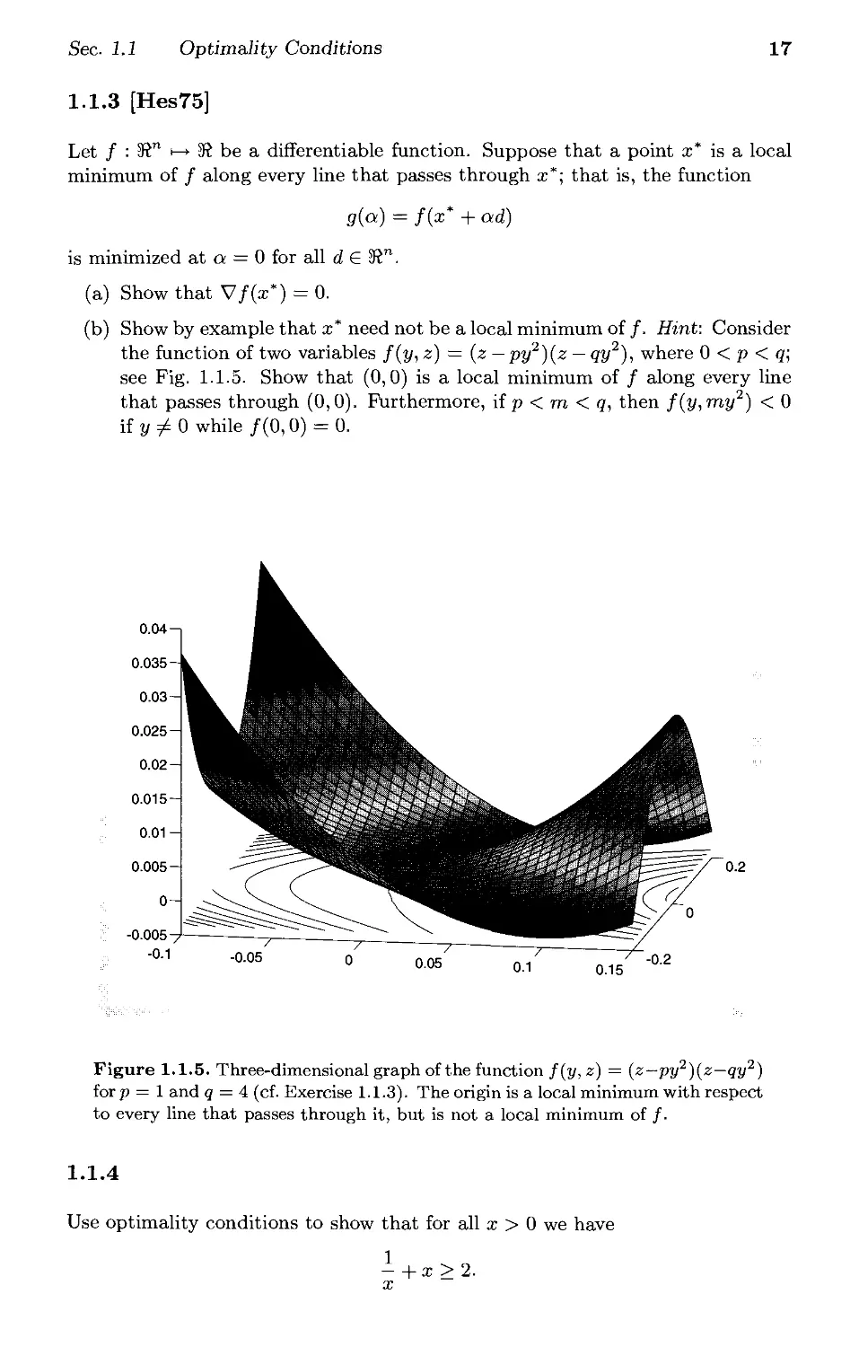
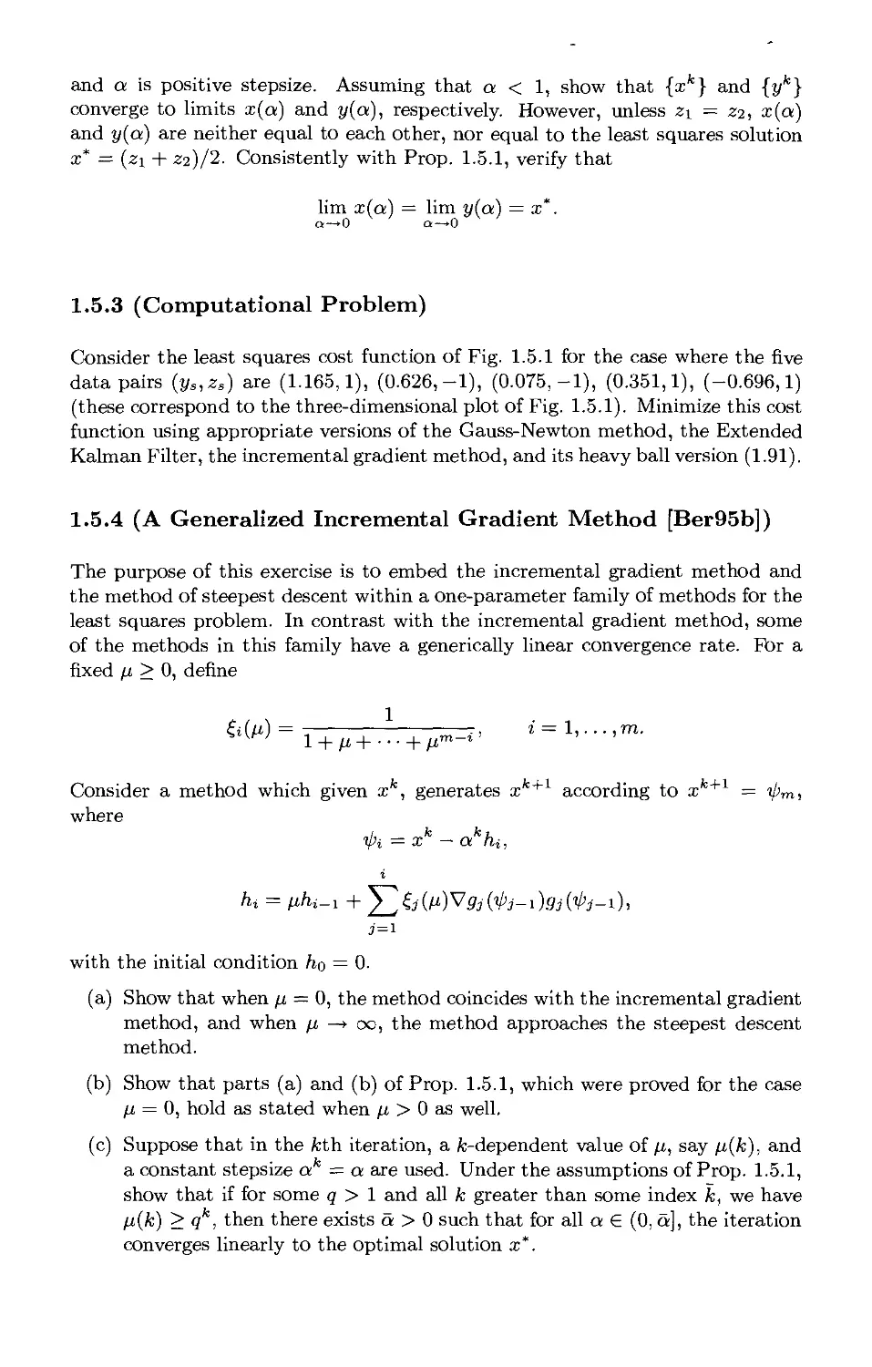
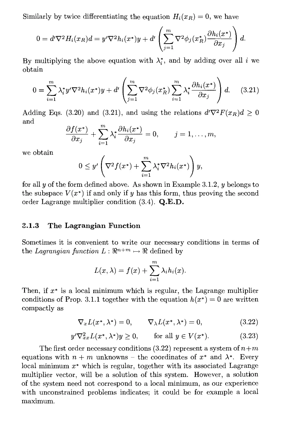
1.1.3 [Hes75]
Let / : S" h> S be a differentiable function. Suppose that a point a;* is a local
minimum of / along every line that passes through a;*; that is, the function
g(a) = f(x* +ad)
is minimized at a = 0 for all deS".
(a) Show that V/(a;*) = 0.
(b) Show by example that a;* need not be a local minimum of f. Hint: Consider
the function of two variables f(y, z) = (z — py2)(z — qy2), where 0 < p < q;
see Fig. 1.1.5. Show that (0,0) is a local minimum of / along every line
that passes through (0,0). Furthermore, if p < m < q, then f(y,my2) < 0
if y + 0 while /(0,0) = 0.
Figure 1.1.5. Three-dimensional graph of the function f(y, z) = (z—py2)(z—qy2)
for p = 1 and q = 4 (cf. Exercise 1.1.3). The origin is a local minimum with respect
to every line that passes through it, but is not a local minimum of /.
1.1.4
Use optimality conditions to show that for all x > 0 we have
-+x>2.
x
18 KJIluuuabia,i±id*-i v/ym«a^«^.
1.1.5
Find the rectangular parallelepiped of unit volume that has the minimum surface
area. Hint: By eliminating one of the dimensions, show that the problem is
equivalent to the minimization over x > 0 and y > 0 of
f(x,y) = xy-\ h -■
x y
Show that the sets {(x,y) \ f(x,y) < 7, x > 0, y > 0} are compact for all scalars
7-
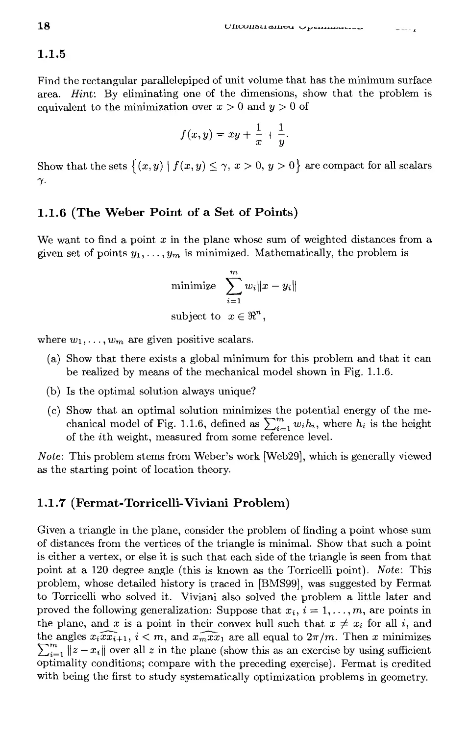
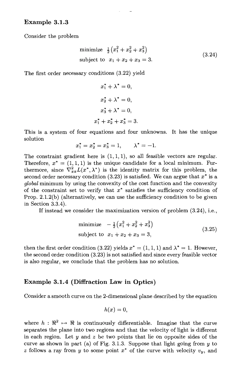
1.1.6 (The Weber Point of a Set of Points)
We want to find a point x in the plane whose sum of weighted distances from a
given set of points 3/1,..., ym is minimized. Mathematically, the problem is
m
minimize \ uii\\x — j/i||
i = \
subject to i£Si",
where w\, ■.., wm are given positive scalars.
(a) Show that there exists a global minimum for this problem and that it can
be realized by means of the mechanical model shown in Fig. 1.1.6.
(b) Is the optimal solution always unique?
(c) Show that an optimal solution minimizes the potential energy of the
mechanical model of Fig. 1.1.6, defined as Y^iLi Wihi, where hi is the height
of the ith weight, measured from some reference level.
Note: This problem stems from Weber's work [Web29], which is generally viewed
as the starting point of location theory.
1.1.7 (Fermat-Torricelli-Viviani Problem)
Given a triangle in the plane, consider the problem of finding a point whose sum
of distances from the vertices of the triangle is minimal. Show that such a point
is either a vertex, or else it is such that each side of the triangle is seen from that
point at a 120 degree angle (this is known as the Torricelli point). Note: This
problem, whose detailed history is traced in [BMS99], was suggested by Fermat
to Torricelli who solved it. Viviani also solved the problem a little later and
proved the following generalization: Suppose that Xi, i — 1,.. ., m, are points in
the plane, and a; is a point in their convex hull such that x ^ Xi for all i, and
the angles iiiii+i, i < m, and x^xxi are all equal to 27r/m. Then x minimizes
YLT=\ II2 ~ ^11 over a^ z in tne pla116 (show this as an exercise by using sufficient
optimality conditions; compare with the preceding exercise). Fermat is credited
with being the first to study systematically optimization problems in geometry.
Figure 1.1.6. Mechanical model (known as the Varignon frame) associated with
the Weber problem (Exercise 1.1.6). It consists of a board with a hole drilled
at each of the given points yi. Through each hole, a string is passed with the
Corresponding weight u>i attached. The other ends of the strings are tied with a
knot as shown. In the absence of friction or tangled strings, the forces at the knot
reach equilibrium when the knot is located at an optimal solution x*.
1.1.8 (Diffraction Law in Optics)
Let p and q be two points on the plane that lie on opposite sides of a horizontal
axis. Assume that the speed of light from p and from q to the horizontal axis is v
and w, respectively, and that light reaches a point from other points along paths
of minimum travel time. Find the path that a ray of light would follow from p
to q.
1.1.9 (www)
Let / : S" h> S be a twice continuously differentiable function that satisfies
m\\y\\2 < y'V2f(x)y < M\\y\\2, Vi.je »n,
where m and M are some positive scalars. Show that / has a unique global
minimum a;*, which satisfies
^||V/(z)||2 < /(*) - f{x*) < ^IIV/(x)||2, V x € »",
and
y II* " **f < /(*) " fix*) < y ||* - x*||2, VxeS".
Hint: Use a second order expansion and the relation
min [Vf{x)\y - x) + ^\\y - x\\2} >= -i||V/(x)||2, V a > 0.
20
Unconstrained Optimization Chap. 1
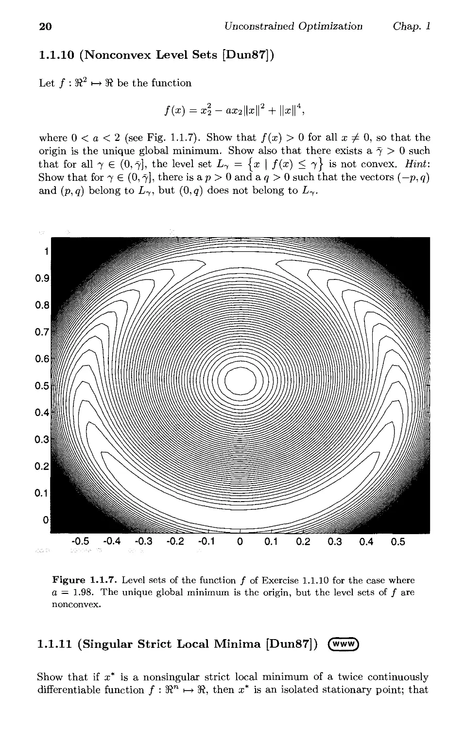
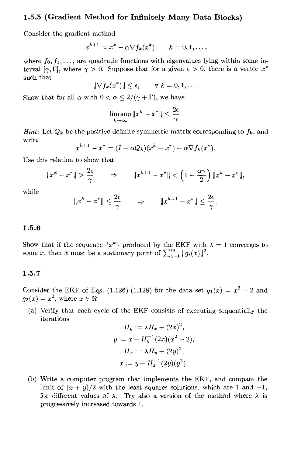
1.1.10 (Nonconvex Level Sets [Dun87])
Let / : K2 h-> K be the function
f(x) =x2- aa;2||a;||2 + ||a;|| ,
where 0 < a < 2 (see Fig. 1.1.7). Show that f(x) > 0 for all x ^ 0, so that the
origin is the unique global minimum. Show also that there exists a 7 > 0 such
that for all 7 6 (0,7], the level set L7 = {a: | f(x) < 7} is not convex. Hint:
Show that for 7 € (0,7], there is a p > 0 and a q > 0 such that the vectors (— p, q)
and (p, q) belong to L7, but (0,q) does not belong to L7.
Figure 1.1.7. Level sets of the function / of Exercise 1.1.10 for the case where
a = 1.98. The unique global minimum is the origin, but the level sets of / are
nonconvex.
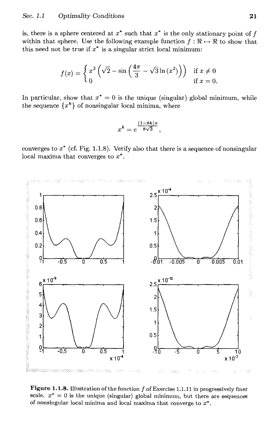
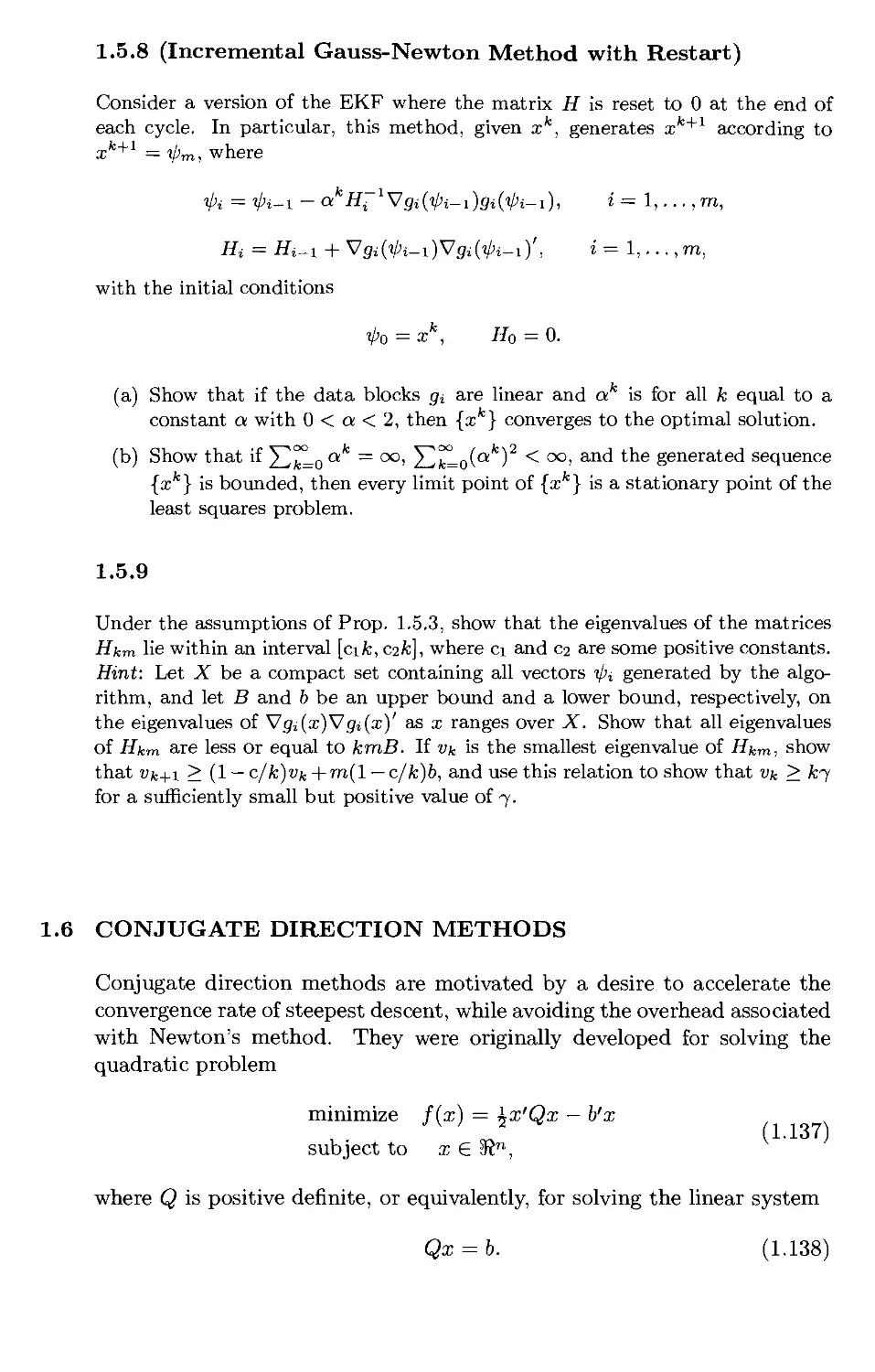
1.1.11 (Singular Strict Local Minima [Dun87]) (www)
Show that if a;* is a nonsingular strict local minimum of a twice continuously
differentiable function / : Kn 1—> K, then a;* is an isolated stationary point; that
Sec. 1.1 Optimality Conditions
21
is, there is a sphere centered at a;* such that a;* is the only stationary point of /
within that sphere. Use the following example function / : K t—► K to show that
this need not be true if a;* is a singular strict local minimum:
/(*)
fx2(V2-sin(^--V3ln(x2))) if x ^ 0
I 0 if x = 0.
In particular, show that a;* = 0 is the unique (singular) global minimum, while
the sequence {a;*} of nonsingular local minima, where
(l-8fc)7T
xk = e sv^ .
converges to a;* (cf. Fig. 1.1.8). Verify also that there is a sequence of nonsingular
local maxima that converges to a;*.
. x 10'*
HOI -0.005
0.005 0.01
x10
_x10"
Figure 1.1.8. Illustration of the function / of Exercise 1.1.11 in progressively finer
scale, a;* = 0 is the unique (singular) global minimum, but there are sequences
of nonsingular local minima and local maxima that converge to a;*.
1.1.12 (Stability) (www)
We are often interested in whether optimal solutions change radically when the
problem data are slightly perturbed. This issue is addressed by stability analysis,
to be contrasted with sensitivity analysis, which deals with how much optimal
solutions change when problem data change. An unconstrained local minimum
a;* of a function / is said to be locally stable if there exists a & > 0 such that all
sequences {a;*} with f(xk) —» f(x*) and ||a;fc — a;*|| < S, for all k, converge to a;*.
Suppose that / is a continuous function and let a;* be a local minimum of /.
(a) Show that a;* is locally stable if and only if a;* is a strict local minimum.
(b) Let g be a continuous function. Show that if a;* is locally stable, there exists
a d > 0 such that for all sufficiently small e > 0, the function f(x) + eg(x)
has an unconstrained local minimum xe that lies within the sphere centered
at a;* with radius d. Furthermore, xe —» a;* as e —» 0.
1.1.13 (Sensitivity) (www)
Let / : Kn t—► K and g : Kn t—► K be twice continuously differentiate functions,
and let a;* be a nonsingular local minimum of /. Show that there exists an e > 0
and a 5 > 0 such that for all e 6 [0,e) the function f(x) + eg(x) has a unique
local minimum xe within the sphere {a; | ||a; — a;*|| < 5}, and we have
xe = x* - e(V2f(x*)y\g(x*) + o(e).
Hint: Use the implicit function theorem (Prop. A.25 in Appendix A).
1.2 GRADIENT METHODS - CONVERGENCE
We now start our development of computational methods for unconstrained
optimization. The conceptual framework of this section is fundamental in
nonlinear programming and applies to constrained optimization methods
as well.
1.2.1 Descent Directions and Stepsize Rules
As in the case of optimality conditions, the main ideas of unconstrained
optimization methods have simple geometrical explanations, but the
corresponding convergence analysis is often complex. For this reason we first
discuss informally the methods and their behavior in the present
subsection, and we substantiate our conclusions with rigorous analysis in Section
1.2.2.
Consider the problem of unconstrained minimization of a continuously
differentiable function / : 3?n i—> 3R. Most of the interesting algorithms for
this problem rely on an important idea, called iterative descent that works
as follows: We start at some point x° (an initial guess) and successively
generate vectors x1, x2,..., such that / is decreased at each iteration, that
is
/(xfc+i)</(xfc), k = 0,1,...,
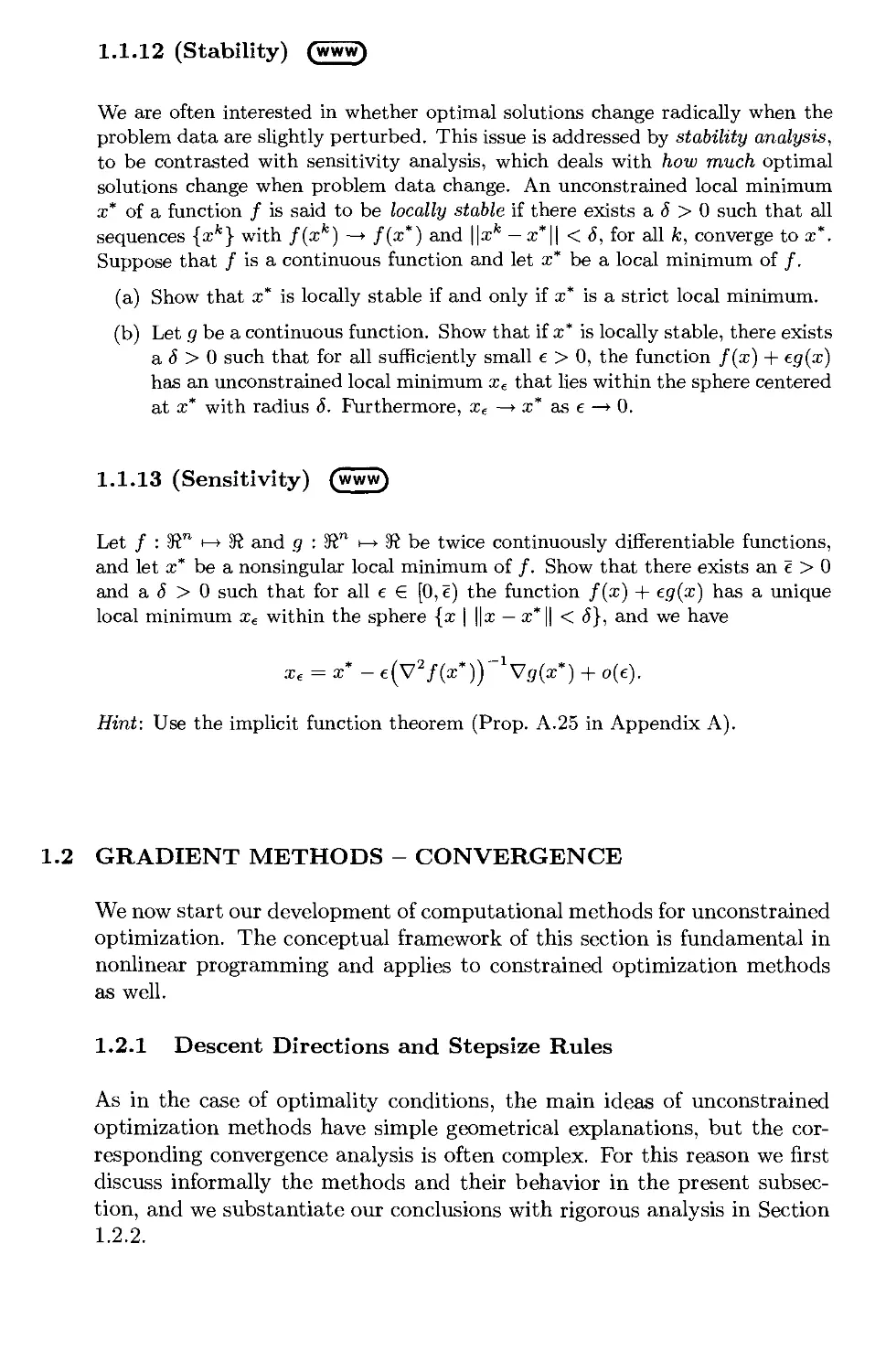
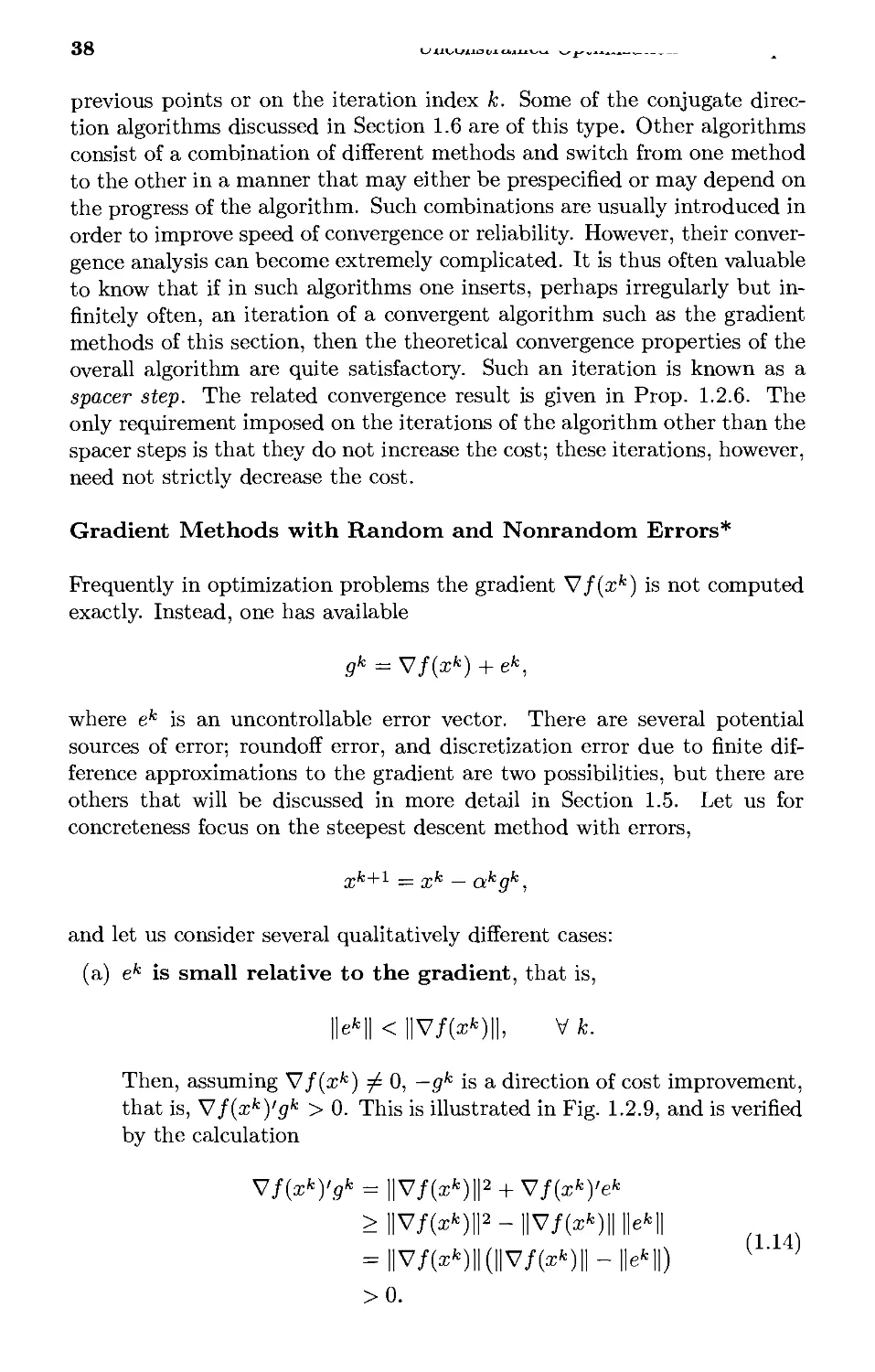
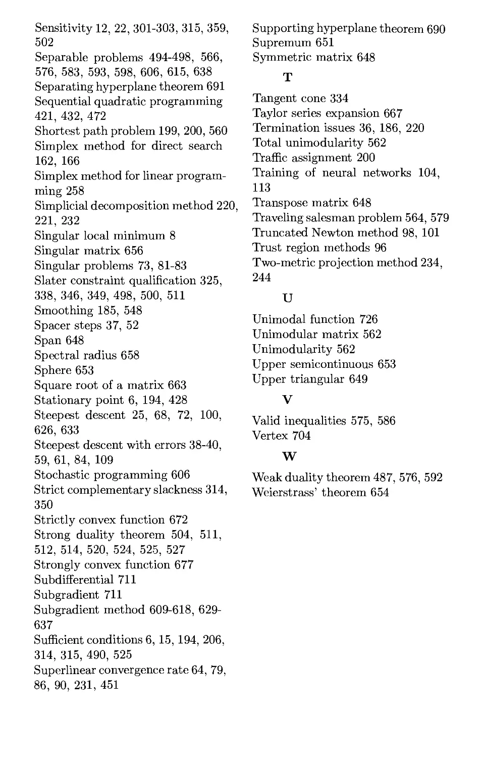
(cf. Fig. 1.2.1). In doing so, we successively improve our current solution
estimate and we hope to decrease / all the way to its minimum. In this
section, we introduce a general class algorithms based on iterative descent,
and we analyze their convergence to local minima. In Section 1.3 we
examine their rate of convergence properties.
Figure 1.2.1. Iterative descent for
minimizing a function /. Each
vector in the generated sequence has a
lower cost than its predecessor.
Gradient Methods
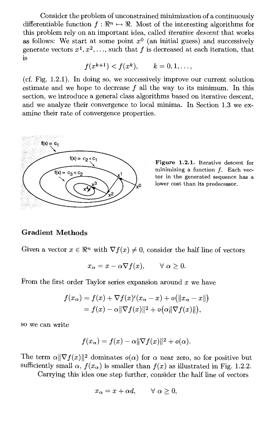
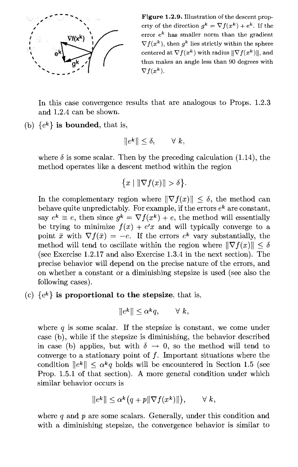
Given a vector x e 3?n with V/(x) ^ 0, consider the half line of vectors
xa = x — aV/(x), V a > 0.
From the first order Taylor series expansion around x we have
f{xa) = f{x) + V/(x)'(xQ - x) + o(||xQ - x||)
= /(x)-a||V/(x)|p + 0(a||V/(x)||),
so we can write
f(xa) = f(x)-a\\Vf(xW + o(a).
The term a||V/(x)||2 dominates o(a) for a near zero, so for positive but
sufficiently small a, f(xa) is smaller than fix) as illustrated in Fig. 1.2.2.
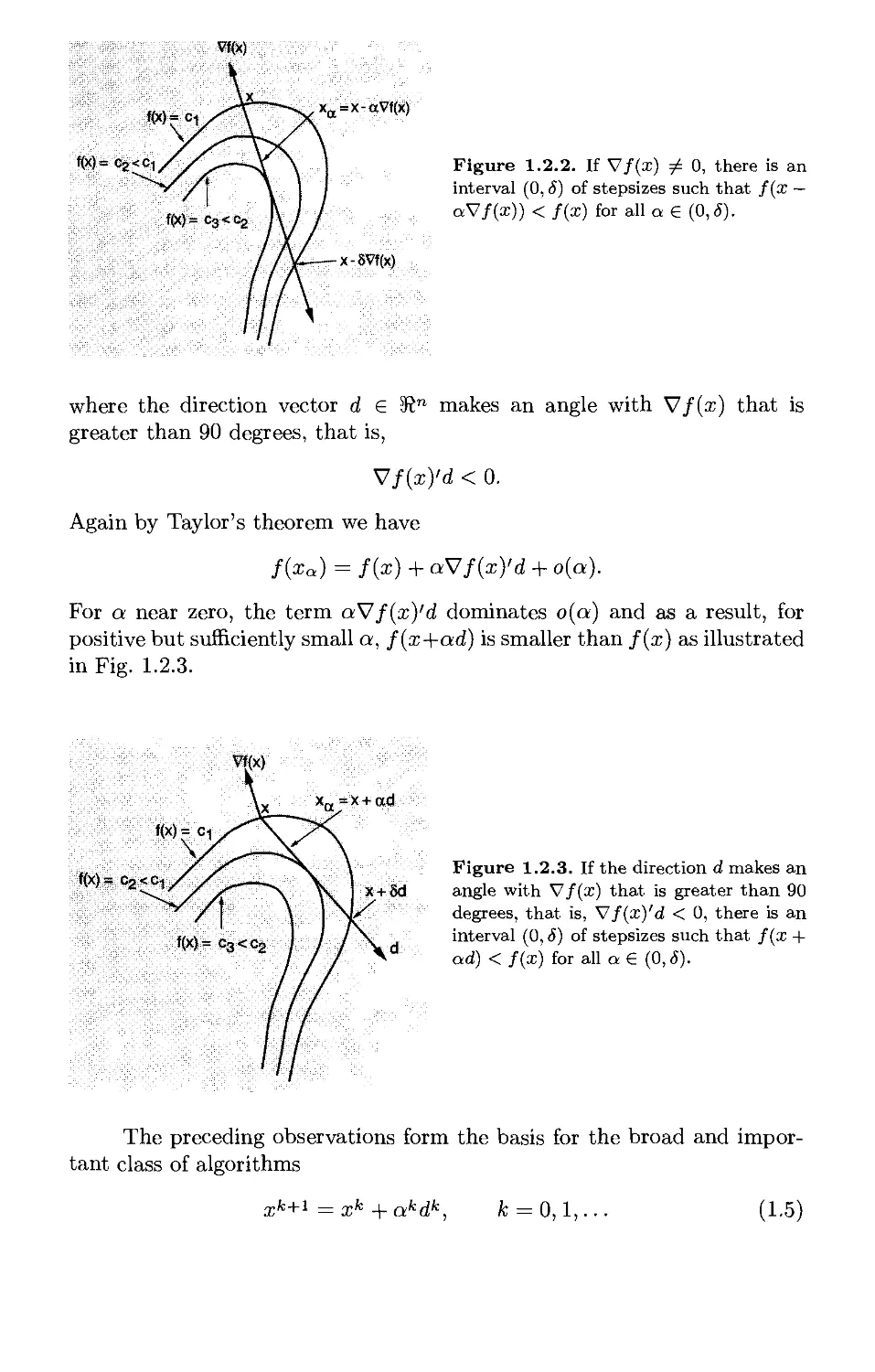
Carrying this idea one step further, consider the half line of vectors
xa = x + ad, V a > 0,
Vf(x)
M=ci
f(X) = Cg < C-|
xa=x-aVf(x)
x-8Vf(x)
Figure 1.2.2. If Vf(x) ^ 0, there is an
interval (0, S) of stepsizes such that f(x —
aV/(i)) < f(x) for all a € (0,6).
where the direction vector d e 3?n makes an angle with V/(x) that is
greater than 90 degrees, that is,
V/(x)'d < 0.
Again by Taylor's theorem we have
f{xa) = /(x) + aVf{x)'d + o{a).
For a near zero, the term aV/(x)'d dominates o(a) and as a result, for
positive but sufficiently small a, f(x+ad) is smaller than /(x) as illustrated
in Fig. 1.2.3.
Vf(x)
f(x)= c2<c1
Figure 1.2.3. If the direction d makes an
angle with Vf(x) that is greater than 90
degrees, that is, Vf(x)'d < 0, there is an
interval (0, S) of stepsizes such that f(x +
ad) < f(x) for all a€ (0,8).
The preceding observations form the basis for the broad and
important class of algorithms
ck+i = xk _|_ akdk,
0,1,.
(1.5)
where, if V/(xfc) ^ 0, the direction dk is chosen so that
Vf(xk)'dk < 0, (1.6)
and the stepsize ak is chosen to be positive. If V/(xfc) = 0, the method
stops, i.e., xk+1 = xk (equivalently we choose dk = 0). In view of the
relation (1.6) of the direction dk and the gradient V/(xfc), we call algorithms
of this type gradient methods. [There is no universally accepted name for
these algorithms; some authors reserve the name "gradient method" for the
special case where dk = —V/(xfc).] The majority of the gradient methods
that we will consider are also descent algorithms; that is, the stepsize ak
is selected so that
f(xk +akdk) < f(xk), fc = 0,l,... (1.7)
However, there are some exceptions.
There is a large variety of possibilities for choosing the direction dk
and the stepsize ak in a gradient method. Indeed there is no single gradient
method that can be recommended for all or even most problems.
Otherwise said, given any one of the numerous methods and variations thereof
that we will discuss, there are interesting types of problems for which this
method is well-suited. Our principal analytical aim is to develop a few
guiding principles for understanding the performance of broad classes of
methods and for appreciating the practical contexts in which their use is
most appropriate.
Selecting the Descent Direction
Many gradient methods are specified in the form
xk+i =xk - akDkVf(xk), (1.8)
where Dk is a positive definite symmetric matrix. Since dk = —DkVf(xk),
the descent condition V/(xfc)'dfc < 0 is written as
V/(xfc)'DfcV/(xfc) > 0,
and holds thanks to the positive definiteness of Dk.
Here are some examples of choices of the matrix Dk, resulting in
methods that are widely used:
Steepest Descent
Dk = I, k = 0,1,...,
where I is the n x n identity matrix. This is the simplest choice but it often
leads to slow convergence, as we will see in Section 1.3. The difficulty is
illustrated in Fig. 1.2.4 and motivates the methods of the subsequent examples.
The name "steepest descent" is derived from an interesting property of the
(normalized) negative gradient direction dk = —V/(a;fe)/1| V/(a;fc) ||; among
all directions rfeS" that are normalized so that ||d|| = 1, it is the one that
minimizes the slope Vf(xk)'d of the cost f(xk + ad) along the direction d at
a = 0. Indeed, by the Schwartz inequality (Prop. A.2 in Appendix A), we
have for all d with ||d|| = 1,
Vf(xk)'d>-\\Vf(xk)\\.\\d\\=-\\Vf(xk)\\,
and it is seen that equality is attained above for d equal to — V/ (xk) /11V/ (xk) 11
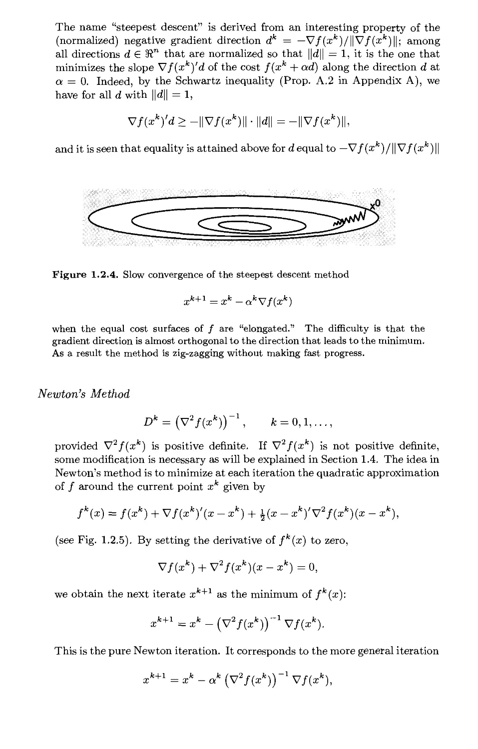
Figure 1.2.4. Slow convergence of the steepest descent method
xk+1=xk-akVf(xk)
when the equal cost surfaces of / are "elongated." The difficulty is that the
gradient direction is almost orthogonal to the direction that leads to the minimum.
As a result the method is zig-zagging without making fast progress.
Newton's Method
Dk = (V2f(xk))-\ k = 0,1,...,
provided V2f(xk) is positive definite. If V2f(xk) is not positive definite,
some modification is necessary as will be explained in Section 1.4. The idea in
Newton's method is to minimize at each iteration the quadratic approximation
of / around the current point xk given by
fk(x) = f(xk) + Vf{xk)\x -xk)+i(x- xk)'V2f(xk){x - xk),
(see Fig. 1.2.5). By setting the derivative of fk(x) to zero,
Vf(xk) + V2f(xk)(x -xk)=0,
we obtain the next iterate xk+1 as the minimum of fk(x):
xk+1 =xk - (V2/(xfc))_1 Vf(xk).
This is the pure Newton iteration. It corresponds to the more general iteration
xk+1 =xk -ak (V2/(^))_1 V/(xfc),
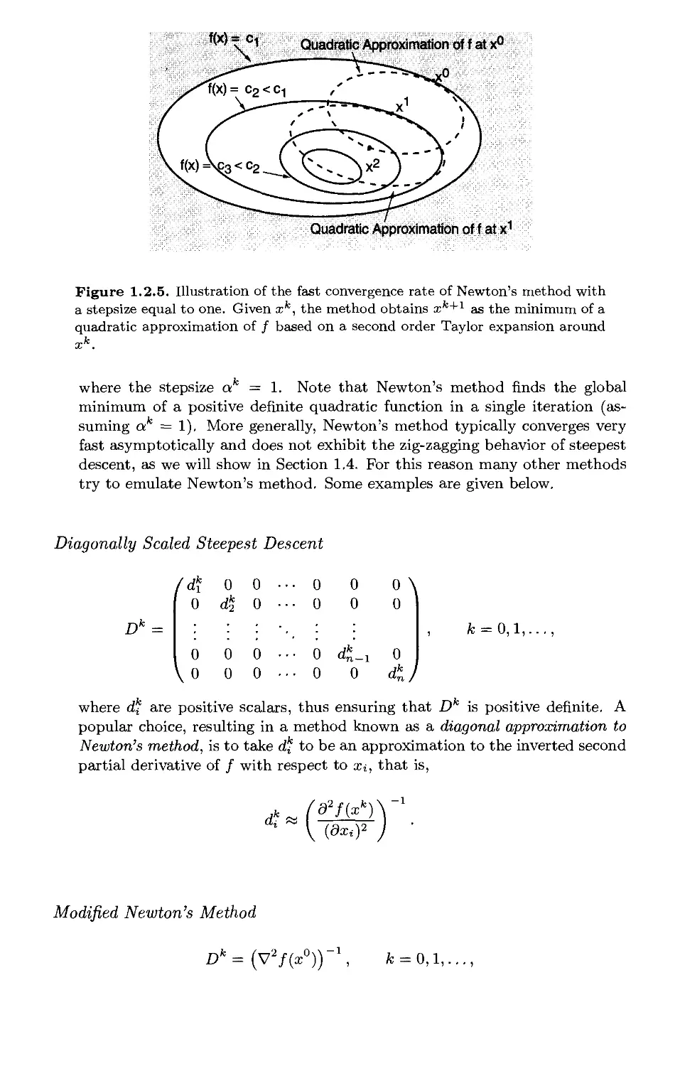
•M - Ci Quadratic Approximation of f at x°
Quadratic Approximation of f at x1
Figure 1.2.5. Illustration of the fast convergence rate of Newton's method with
a stepsize equal to one. Given xk, the method obtains xk+1 as the minimum of a
quadratic approximation of / based on a second order Taylor expansion around
where the stepsize ak = 1. Note that Newton's method finds the global
minimum of a positive definite quadratic function in a single iteration
(assuming ak = 1), More generally, Newton's method typically converges very
fast asymptotically and does not exhibit the zig-zagging behavior of steepest
descent, as we will show in Section 1,4. For this reason many other methods
try to emulate Newton's method. Some examples are given below.
Diagonally Scaled Steepest Descent
Dk
(dk
0
0
Vo
0
dk2
0
0
0 •
0 •
0 •
0 •
• 0
• 0
• 0
• 0
0
0
dk
"n-1
0
°\
0
0
</
fc = 0,l,
where dk are positive scalars, thus ensuring that Dk is positive definite, A
popular choice, resulting in a method known as a diagonal approximation to
Newton's method, is to take dk to be an approximation to the inverted second
partial derivative of / with respect to xi, that is,
d2f(xk
{dxif
Modified Newton's Method
Dk={V*f{x°))-\.
k = 0,1,...,
28
Unconstrained Optimization Chap. 1
provided V2/(a;°) is positive definite. This method is the same as Newton's
method except that to economize on overhead, the Hessian matrix is not
recalculated at each iteration. A related method is obtained when the Hessian
is recomputed every p > 1 iterations.
Discretized Newton's Method
Dk=(H(xk)y\ /= = 0,1,...,
where H(xk) is a positive definite symmetric approximation of V2f(xk),
formed by using finite difference approximations of the second derivatives,
based on first derivatives or values of /.
Gauss-Newton Method
This method is applicable to the problem of minimizing the sum of squares
of real valued functions gi,..., gm, a problem often encountered in statistical
data analysis and in the context of neural network training (see Section 1.5).
By denoting g = (gi,... ,gm), the problem is written as
m
minimize f(x) = ^||g(a;)||2 = }, ^{gi(x))
i = l
subject to x € 5Rn.
We choose
Dk = (Vg(xk)Vg(xk)'y\ k = 0,1,...,
assuming the matrix Vg(x )Vg(x )'is invertible. The latter matrix is always
positive semidefinite, and it is positive definite and hence invertible if and only
if the matrix X7g(xk) has rank n (Prop. A.20 in Appendix A). Since
Vf(xk) = Vg(xk)g(xk),
the Gauss-Newton method takes the form
xk+1 =xk-ak (Vg{xk)Vg{xk)') ~\g(xk)g(xk). (1.9)
We will see in Section 1.5 that the Gauss-Newton method may be viewed as
an approximation to Newton's method, particularly when the optimal value
of ||g(a;)||2 is small,
Other choices of Dk yield the class of Quasi-Newton methods
discussed in Section 1,7. There are also some interesting methods where the
direction dk is not usually expressed as dk = — Z?fcV/(xfc). Important
examples are the conjugate gradient method and the coordinate descent
methods discussed in Sections 1.6 and 1.8, respectively.
Sec. 1.2 Gradient Methods - Convergence
29
Stepsize Selection
There are a number of rules for choosing the stepsize ak in a gradient
method. We list some that are used widely in practice:
Minimization Rule
Here ak is such that the cost function is minimized along the direction dk,
that is, ak satisfies
f(xk+akdk) = mm f(xk +adk). (1.10)
Limited Minimization Rule
This is a version of the minimization rule, which is more easily implemented
in many cases. A fixed scalar s > 0 is selected and ak is chosen to yield the
greatest cost reduction over all stepsizes in the interval [0, s], i.e.,
f(xk+akdk) = min f(xk+adk).
ag[0, s]
The minimization and limited minimization rules must typically be
implemented with the aid of one-dimensional line search algorithms (see
Appendix C). In general, the minimizing stepsize cannot be computed
exactly, and in practice, the line search is stopped once a stepsize ak
satisfying some termination criterion is obtained. Some stopping criteria are
discussed in Exercise 1.2.16.
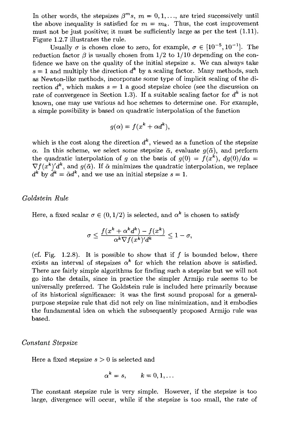
Successive Stepsize Reduction - Armijo Rule
To avoid the often considerable computation associated with the line
minimization rules, it is natural to consider rules based on successive stepsize
reduction. In the simplest rule of this type an initial stepsize s is chosen, and
if the corresponding vector xk + sdk does not yield an improved value of /,
that is, f(xk +sdk) > f(xk), the stepsize is reduced, perhaps repeatedly, by a
certain factor, until the value of / is improved. While this method often works
in practice, it is theoretically unsound because the cost improvement obtained
at each iteration may not be substantial enough to guarantee convergence to
a minimum. This is illustrated in Fig. 1.2.6.
The Armijo rule is essentially the successive reduction rule just
described, suitably modified to eliminate the theoretical convergence difficulty
shown in Fig. 1.2.6. Here, fixed scalars s, /3, and a, with 0 < /3 < 1, and
0 < a < 1 are chosen, and we set ak = f3mks, where 77¾ is the first nonnega-
tive integer m for which
f(xk) - f(xk + j3msdk) > -apmsVf(xk)'dk. (1.11)
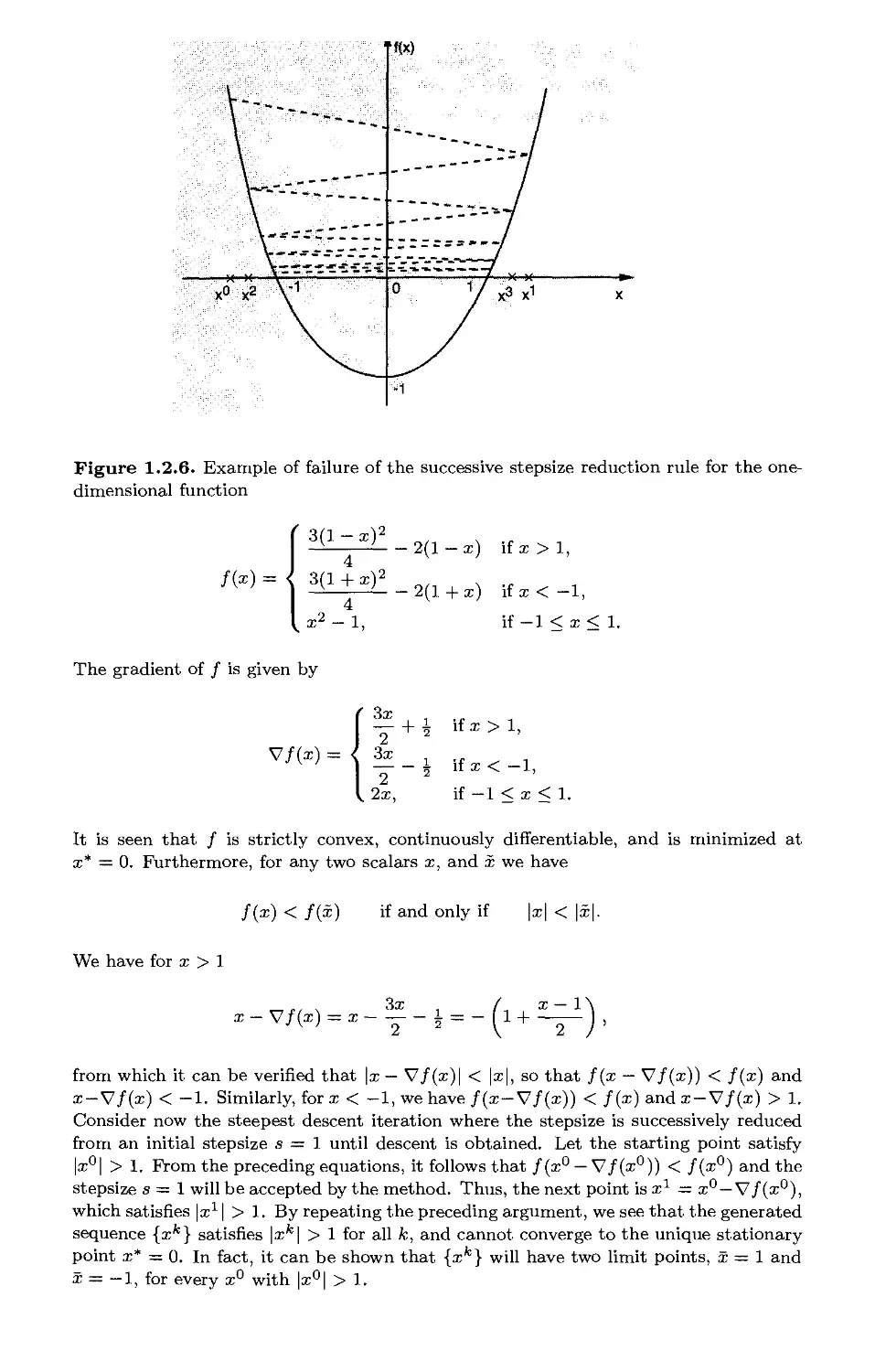
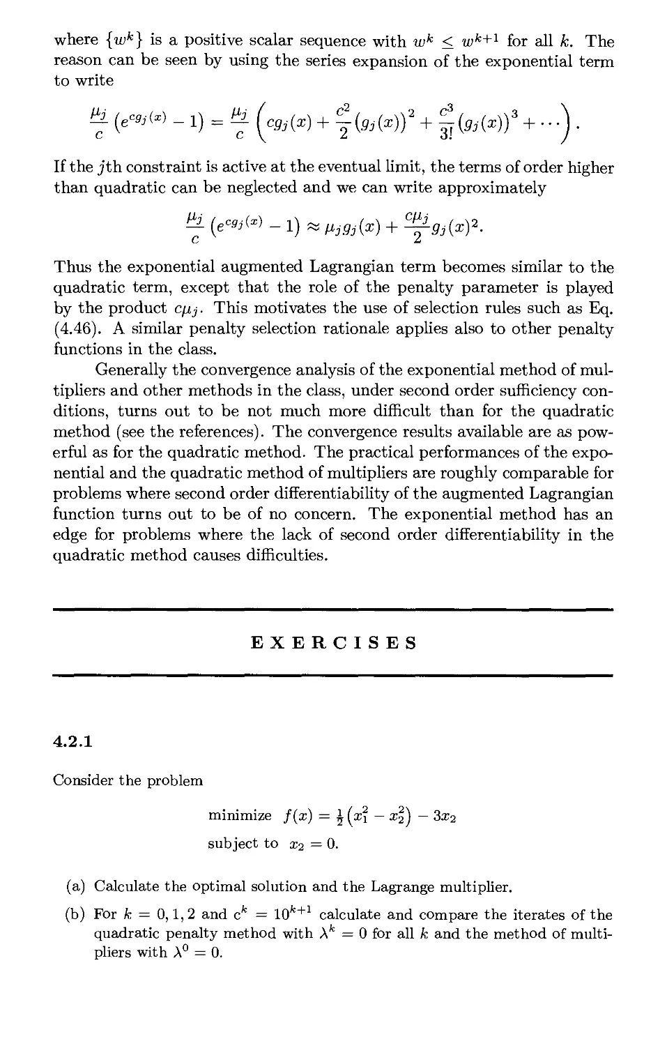
Figure 1.2.6. Example of failure of the successive stepsize reduction rule for the one-
dimensional function
' 3(1 -x)2
4
fix) = I 3(1 + x)2
4
, x2 - 1,
The gradient of / is given by
■ 2(l-a:) ifx>l,
■2(l+x) ifx<-l,
if — 1 < x < 1.
Y + i ifx>i,
v/(x)=<; l_ .fx<_1;
2
2x,
if -1 < x < 1.
It is seen that / is strictly convex, continuously differentiable, and is minimized at
x* = 0. Furthermore, for any two scalars x, and x we have
/(x) < /(x) if and only if |x| < |x|.
We have for x > 1
,, s 3x , / x- 1\
.V/(x) = x-T-i = -(l+—),
from which it can be verified that |x — V/(x)| < |x|, so that /(x — V/(x)) < /(x) and
x—V/(x) < —1. Similarly, for x < —1, we have /(x—V/(x)) < /(x) and x —V/(x) > 1.
Consider now the steepest descent iteration where the stepsize is successively reduced
from an initial stepsize s = 1 until descent is obtained. Let the starting point satisfy
|x°| > 1. From the preceding equations, it follows that /(x° — V/(x0)) < /(x°) and the
stepsize s = 1 will be accepted by the method. Thus, the next point is x1 = x° —V/(x°),
which satisfies |xx | > 1. By repeating the preceding argument, we see that the generated
sequence {xk} satisfies \xk\ > 1 for all k, and cannot converge to the unique stationary
point x* = 0. In fact, it can be shown that {xfc} will have two limit points, x = 1 and
x = —1, for every x° with |x°| > 1.
In other words, the stepsizes /3ms, m = 0,1,..., are tried successively until
the above inequality is satisfied for m = mk- Thus, the cost improvement
must not be just positive; it must be sufficiently large as per the test (1.11).
Figure 1.2.7 illustrates the rule.
Usually a is chosen close to zero, for example, a € [10_5,10-1]. The
reduction factor /3 is usually chosen from 1/2 to 1/10 depending on the
confidence we have on the quality of the initial stepsize s. We can always take
s = 1 and multiply the direction d by a scaling factor. Many methods, such
as Newton-like methods, incorporate some type of implicit scaling of the
direction dk, which makes s = 1 a good stepsize choice (see the discussion on
rate of convergence in Section 1.3). If a suitable scaling factor for dk is not
known, one may use various ad hoc schemes to determine one. For example,
a simple possibility is based on quadratic interpolation of the function
g(a) = f(xk + adk),
which is the cost along the direction dk, viewed as a function of the stepsize
a. In this scheme, we select some stepsize a, evaluate g(a), and perform
the quadratic interpolation of g on the basis of g(0) = f(xk), dg(0)/da =
Vf(xk)'dk, and g(a). If a minimizes the quadratic interpolation, we replace
dk by dk = ad , and we use an initial stepsize s = 1.
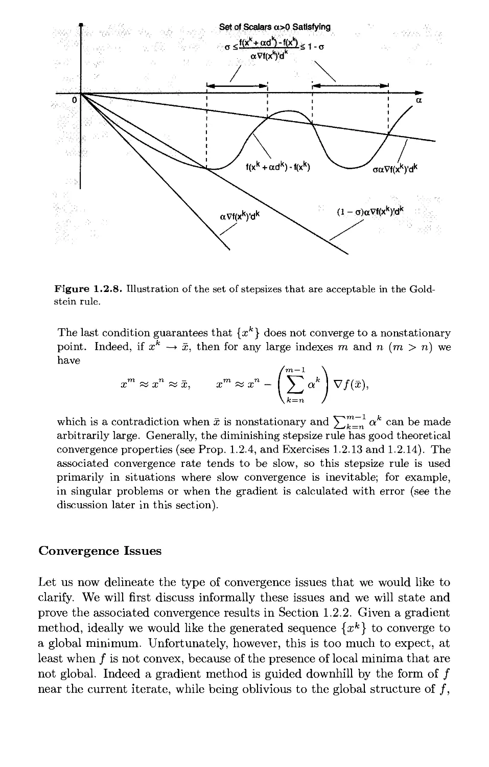
Goldstein Rule
Here, a fixed scalar a € (0,1/2) is selected, and ak is chosen to satisfy
T<f(xk + akdk)-f(xk)
akVf(xk)'dk
(cf. Fig. 1.2.8). It is possible to show that if / is bounded below, there
exists an interval of stepsizes a for which the relation above is satisfied.
There are fairly simple algorithms for finding such a stepsize but we will not
go into the details, since in practice the simpler Armijo rule seems to be
universally preferred. The Goldstein rule is included here primarily because
of its historical significance: it was the first sound proposal for a general-
purpose stepsize rule that did not rely on line minimization, and it embodies
the fundamental idea on which the subsequently proposed Armijo rule was
based.
Constant Stepsize
Here a fixed stepsize s > 0 is selected and
ak = s, A; = 0,1,...
The constant stepsize rule is very simple. However, if the stepsize is too
large, divergence will occur, while if the stepsize is too small, the rate of
Figure 1.2.7. Line search by the Armijo rule. We start with the trial stepsize s
and continue with /3s,/32s,..., until the first time that /3ms falls within the set of
stepsizes a satisfying the inequality
f(xk) - f(xk + adk) > -aaVf(xk)'dk.
While this set need not be an interval, it will always contain an interval of the
form [0,<S] with S > 0, provided Vf(xk)'dk < 0. For this reason the stepsize ak
chosen by the Armijo rule is well defined and will be found after a finite number
of trial evaluations of / at the points (xk + sdk), (xk + /3sdk),...
convergence may be very slow. Thus, the constant stepsize rule is useful only
for problems where an appropriate constant stepsize value is known or can be
determined fairly easily. (A method that attempts to determine automatically
an appropriate value of stepsize is given in Exercise 1.2.20.)
Diminishing Stepsize
Here the stepsize converges to zero,
This stepsize rule is different than the preceding ones in that it does not
guarantee descent at each iteration, although descent becomes more likely as
the stepsize diminishes. One difficulty with a diminishing stepsize is that it
may become so small that substantial progress cannot be maintained, even
when far from a stationary point. For this reason, we require that
oo
Y^ak = oo.
k=0
Set of Scalars a>0 Satisfying
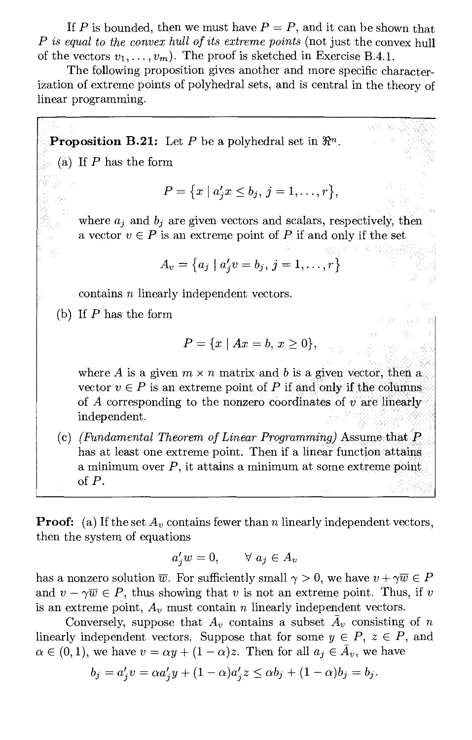
::f(xk+adk)-f(xl')::1 g
Figure 1.2.8. Illustration of the set of stepsizes that are acceptable in the
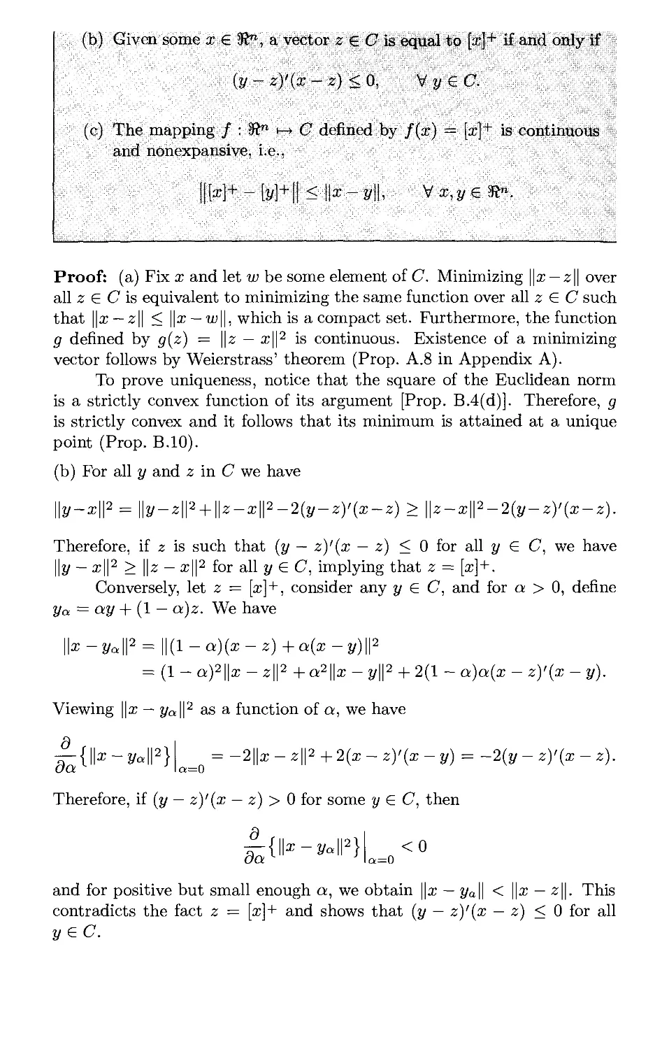
Goldstein rule.
The last condition guarantees that {xk} does not converge to a nonstationary
point. Indeed, if xk —» x, then for any large indexes m and n (m > n) we
have
/m-l \
a; « a; « a;, a; mi - ) a I \7j(x),
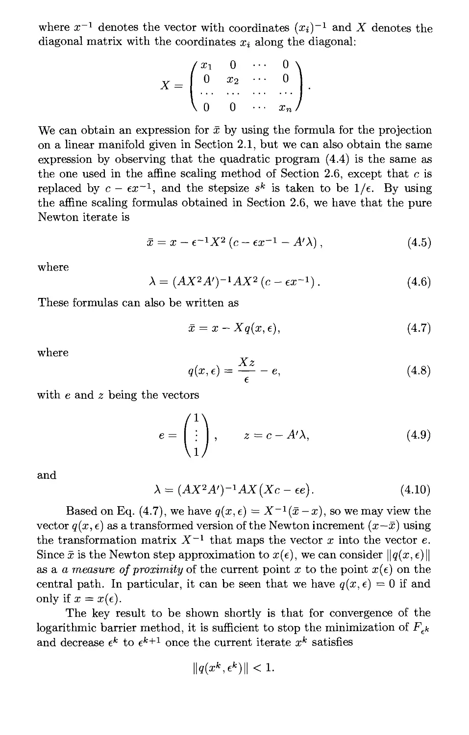
which is a contradiction when x is nonstationary and JZfcLn ak can ^e made
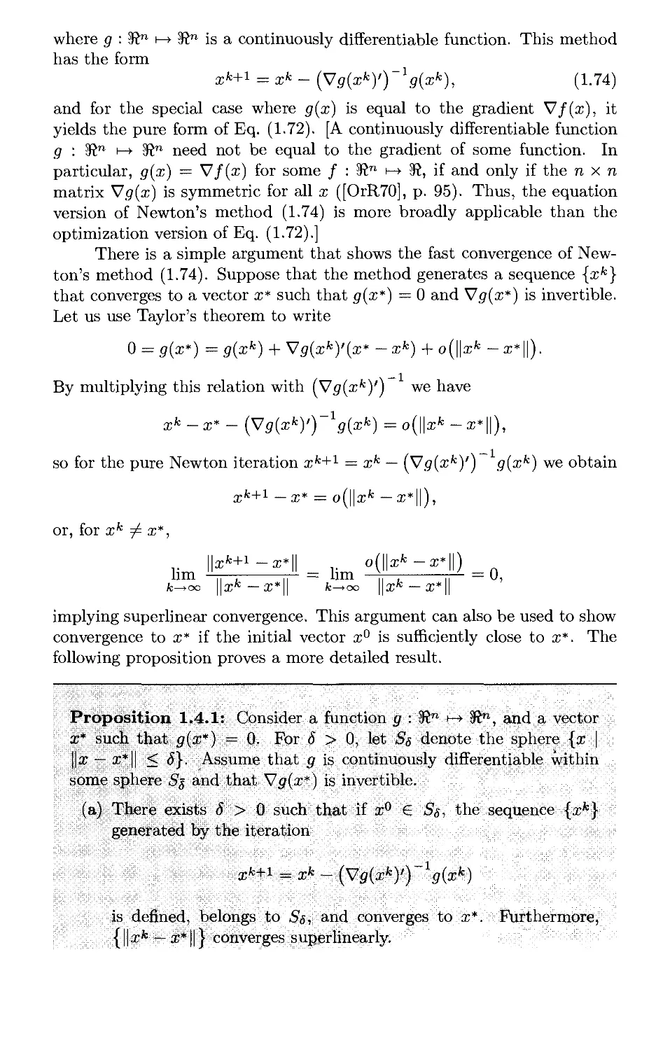
arbitrarily large. Generally, the diminishing stepsize rule has good theoretical
convergence properties (see Prop. 1.2.4, and Exercises 1.2.13 and 1.2.14). The
associated convergence rate tends to be slow, so this stepsize rule is used
primarily in situations where slow convergence is inevitable; for example,
in singular problems or when the gradient is calculated with error (see the
discussion later in this section).
Convergence Issues
Let us now delineate the type of convergence issues that we would like to
clarify. We will first discuss informally these issues and we will state and
prove the associated convergence results in Section 1.2.2. Given a gradient
method, ideally we would like the generated sequence {xk} to converge to
a global minimum. Unfortunately, however, this is too much to expect, at
least when / is not convex, because of the presence of local minima that are
not global. Indeed a gradient method is guided downhill by the form of /
near the current iterate, while being oblivious to the global structure of /,
and thus, can easily get attracted to any type of minimum, global or not.
Furthermore, if a gradient method starts or lands at any stationary point,
including a local maximum, it stops at that point. Thus, the most we can
expect from a gradient method is that it converges to a stationary point.
Such a point is a global minimum if / is convex, but this need not be so for
nonconvex problems. Thus, it must be recognized that gradient methods
can be quite inadequate, particularly if little is known about the location
and/or other properties of global minima. For such problems one must
either try an often difficult and frustrating process of running a gradient
method from multiple starting points, or else resort to a fundamentally
different approach.
Generally, depending on the nature of the cost function /, the
sequence {xk} generated by a gradient method need not have a limit point;
in fact {xk} is typically unbounded if / has no local minima. If, however,
we know that the level set {x \ f(x) < /(x0)} is bounded, and the stepsize
is chosen to enforce descent at each iteration, then the sequence {xk } must
be bounded since it belongs to this level set. It must then have at least one
limit point; this is because every bounded sequence has at least one limit
point (see Prop. A.5 of Appendix A).
Even if {xfc} is bounded, convergence to a single limit point may
not be easy to guarantee. However, it can be shown that local minima,
which are isolated stationary points (unique stationary points within some
open sphere), tend to attract most types of gradient methods, that is,
once a gradient method gets sufficiently close to such a local minimum, it
converges to it. This is the subject of a simple and remarkably powerful
result, the capture theorem, which is given in the next subsection (Prop.
1.2.5). Exercise 1.2.13 develops another type of convergence result for the
steepest descent method, which applies to the case where there are multiple
nonisolated local minima. Generally, if there is a connected set of multiple
global minima, it is theoretically possible for {xk} to have multiple limit
points (see Exercise 1.2.18), but the occurance of such a phenomenon has
never been documented in practice.
Limit Points of Gradient Methods
We now address the question of whether each limit point of a sequence
{xk} generated by a gradient method is a stationary point. From the first
order Taylor expansion
f(xk+l) = f(xk) + akVf(xk)'dk + o(ak),
we see that if the slope of / at xk along the direction dk, which is V/(xfc)'dfc,
has "substantial" magnitude, the rate of progress of the method will also
tend to be substantial. If on the other hand, the directions dk tend to
become asymptotically orthogonal to the gradient direction,
Vf(xk)'dk
||V/(**)|||K|I ~" '
as xk approaches a nonstationary point, there is a chance that the method
will get "stuck" near that point. To ensure that this does not happen, we
consider rather technical conditions on the directions dk, which are either
naturally satisfied or can be easily enforced in most algorithms of interest.
One such condition for the case where
dk = -DkVf{xk),
is to assume that the eigenvalues of the positive definite symmetric matrix
Dk are bounded above and bounded away from zero, that is, for some
positive scalars c\ and c%, we have
ci\\z\\2 < z'Dkz < c2p||2, VzeS", k = 0,1,... (1.12)
It can be seen then that
\Vf{xk)'dk\ = |V/(xfc)'DfcV/(xfc)| > ci||V/(xfc)||2
and
\\dk\\* = \Vf(xk)>(Dk)*Vf(xk)\ < c|||V/(xfc)|P,
where we have used the fact that, from Eq. (1.12), cz is no less than the
largest eigenvalue of Dk, and that the eigenvalues of (Dk)2 are equal to the
squares of the corresponding eigenvalues of Dk (Props. A.18 and A.13 in
Appendix A). Thus, as long as V/(xfc) does not tend to zero, V/(xfc) and
dk cannot become asymptotically orthogonal.
We now introduce another "nonorthogonality" type of condition, which
is more general than the "bounded eigenvalues" condition (1.12). Let us
assume that the direction dk is uniquely determined by the corresponding
iterate xfc; that is, dk is obtained as a given function of xk. We say that the
direction sequence {dk } is gradient related to {xfc } if the following property
can be shown:
For any subsequence {xk}keic that converges to a nonstationary point,
the corresponding subsequence {dk}keic is bounded and satisfies
limsup Vf{xk)'dk < 0. (1.13)
k—>oo, fcG^C
In particular, if {dk} is gradient related, it follows that if a subsequence
{V/(xfc)}fcg;c tends to a nonzero vector, the corresponding subsequence of
directions dk is bounded and does not tend to be orthogonal to V/(xfc).
Roughly, this means that dk does not become "too small" or "too large"
relative to V/(xfc), and that the angle between dk and V/(xfc) does not
get "too close" to 90 degrees.
We can often guarantee a priori that {dk} is gradient related. In
particular, if dk = — DkV f(xk) and the eigenvalues of Dk are bounded as
in the "bounded eigenvalues" condition (1.12), it can be seen that {dk} is
gradient related, provided xk is nonstationary for all k (if xk is stationary
for some k, the issue of convergence in effect does not arise). Two other
examples of conditions that, if satisfied for some scalars c\ > 0, c% > 0,
Pi > 0, P2 > 0, and all k, guarantee that {dk} is gradient related are
(a)
Cl||V/(xfc)|h < -Vf(xk)'dk, \\dk\\ < c2\\Vf(xk)\\P2.
(b)
dk = -DkVf(xk),
with Dk a positive definite symmetric matrix satisfying
ci||V/(xfc)||Pi p||2 < z'Dkz < c2||V/(xfc)||P2 \\z\\2, v zeS".
This condition generalizes the "bounded eigenvalues" condition (112),
which is obtained for pi = p2 = 0.
An important convergence result is that if {dk} is gradient related
and the minimization rule, or the limited minimization rule, or the Armijo
rule is used, then all limit points of {xfc} are stationary. This is shown
in Prop. 1.2.1, given in the next subsection. Proposition 1.2.2 provides a
similar result for the Goldstein rule.
When a constant stepsize is used, convergence can be proved
assuming that the stepsize is sufficiently small and that / satisfies some further
conditions (cf. Prop. 1.2.3). Under the same conditions, convergence can
also be proved for a diminishing stepsize.
There is a common line of proof for these convergence results. The
main idea is that the cost function is improved at each iteration and that,
based on our assumptions, the improvement is "substantial" near a non-
stationary point, i.e., it is bounded away from zero. We then argue that
the algorithm cannot approach a nonstationary point, since in this case the
total cost improvement would accumulate to infinity.
Termination of Gradient Methods
Generally, gradient methods are not finitely convergent, so it is necessary
to have criteria for terminating the iterations with some assurance that we
are reasonably close to at least a local minimum. A typical approach is to
stop the computation when the norm of the gradient becomes sufficiently
small, that is, when a point xk is obtained with
HV/(x*)||<e,
where e is a small positive scalar. Unfortunately, it is not known a priori
how small one should take e in order to guarantee that the final point xfc
is a "good" approximation to a stationary point. The appropriate value of
e depends on how the problem is scaled. In particular, if f is multiplied
by some scalar, the appropriate value of e is also multiplied by the same
scalar. It is possible to correct this difficulty by replacing the criterion
||V/(xfc)|| <ewith
HV/(zfc)ll <
liv/(*°)|| - •
Still, however, the gradient norm ||V/(xfc)|| depends on all the components
of the gradient, and depending on how the optimization variables are scaled,
the preceding termination criterion may not work well. In particular, some
components of the gradient may be naturally much smaller than others,
thus requiring a smaller value of e than the other components.
Assuming that the direction dk captures the relative scaling of the
optimization variables, it may be appropriate to terminate computation
when the norm of the direction dk becomes sufficiently small, that is,
IKII<e-
Still the appropriate value of e may not be easy to guess, and it may
be necessary to experiment prior to settling on a reasonable termination
criterion for a given problem. Sometimes, other problem-dependent criteria
are used, in addition to or in place of ||V/(xfc)|| < e and ||dfc|| < e.
When V2/(x) is positive definite, the condition ||V/(xfc)|| < e yields
bounds on the distance from local minima. In particular, if x* is a local
minimum of f and there exists m > 0 such that for all x in a sphere S
centered at x* we have
m\\z\\2 < z'V2f{x)z, VzeS",
then every x € S satisfying ||V/(x)|| < e also satisfies
||x-x*||<-, f{x) - f{x*) < -,
m m
(see Exercise 1.2.10).
In the absence of positive definiteness conditions on V2/(x), it may
be very difficult to infer the proximity of the current iterate to the optimal
solution set by just using the gradient norm. We will return to this point
when we will discuss singular local minima in the next section.
Spacer Steps
Often, optimization problems are solved with complex descent algorithms
in which the rule used to determine the next point may depend on several
previous points or on the iteration index k. Some of the conjugate
direction algorithms discussed in Section 1.6 are of this type. Other algorithms
consist of a combination of different methods and switch from one method
to the other in a manner that may either be prespecined or may depend on
the progress of the algorithm. Such combinations are usually introduced in
order to improve speed of convergence or reliability. However, their
convergence analysis can become extremely complicated. It is thus often valuable
to know that if in such algorithms one inserts, perhaps irregularly but
infinitely often, an iteration of a convergent algorithm such as the gradient
methods of this section, then the theoretical convergence properties of the
overall algorithm are quite satisfactory. Such an iteration is known as a
spacer step. The related convergence result is given in Prop. 1.2.6. The
only requirement imposed on the iterations of the algorithm other than the
spacer steps is that they do not increase the cost; these iterations, however,
need not strictly decrease the cost.
Gradient Methods with Random and Nonrandom Errors*
Frequently in optimization problems the gradient V/(xfc) is not computed
exactly. Instead, one has available
gk = yj(xfc) +ek,
where ek is an uncontrollable error vector. There are several potential
sources of error; roundoff error, and discretization error due to finite
difference approximations to the gradient are two possibilities, but there are
others that will be discussed in more detail in Section 1.5. Let us for
concreteness focus on the steepest descent method with errors,
xk + l — xk _ akgk ^
and let us consider several qualitatively different cases:
(a) ek is small relative to the gradient, that is,
||e*|| < ||V/(xfc)||, Vfc.
Then, assuming V/(xfc) ^ 0, —gk is a direction of cost improvement,
that is, Vf(xk)'gk > 0. This is illustrated in Fig. 1.2.9, and is verified
by the calculation
Vf(xk)'gk = ||V/(xfc)||2 + Vf(xk)'ek
> HV/(x*)||2 - ||V/(x*)|| ||e*||
= l|V/(x*)||(||V/(x*)|| -^11)
>0.
(1.14)
Figure 1.2.9. Illustration of the descent
property of the direction gk = V/(xfc) + ek. If the
error ek has smaller norm than the gradient
V/(xfc), then gk lies strictly within the sphere
centered at V/(xfc) with radius || V/(xfc)||, and
thus makes an angle less than 90 degrees with
V/(xfc).
In this case convergence results that are analogous to Props. 1.2.3
and 1.2.4 can be shown.
(b) {efc} is bounded, that is,
\\ek\\<6, Vfc,
where 6 is some scalar. Then by the preceding calculation (1.14), the
method operates like a descent method within the region
{x|||V/(x)||>5}.
In the complementary region where ||V/(x)|| < 5, the method can
behave quite unpredictably. For example, if the errors efc are constant,
say efc = e, then since gk = V/(xfc) + e, the method will essentially
be trying to minimize fix) + e'x and will typically converge to a
point x with V/(x) = —e. If the errors efc vary substantially, the
method will tend to oscillate within the region where ||V/(x)|| < 6
(see Exercise 1.2.17 and also Exercise 1.3.4 in the next section). The
precise behavior will depend on the precise nature of the errors, and
on whether a constant or a diminishing stepsize is used (see also the
following cases).
(c) {efc} is proportional to the stepsize, that is,
||efc||<afcg, Vfc,
where q is some scalar. If the stepsize is constant, we come under
case (b), while if the stepsize is diminishing, the behavior described
in case (b) applies, but with 5 —> 0, so the method will tend to
converge to a stationary point of f. Important situations where the
condition ||efc|| < akq holds will be encountered in Section 1.5 (see
Prop. 1.5.1 of that section). A more general condition under which
similar behavior occurs is
\\ek\\<ak(q+p\\Vf(xk)\\), Vfc,
where q and p are some scalars. Generally, under this condition and
with a diminishing stepsize, the convergence behavior is similar to
the case where there are no errors (see the following Prop. 1.2.4 and
Exercise 1.2.21).
(d) {efc} are independent zero mean random vectors with finite
variance. An important special case where such errors arise is when
/ is of the form
f(x) = Ew{F(x,w)}, (1.15)
where F : $tm+n —> 3¾ is some function, w is a random vector in 3?m,
and Ew{-} denotes expected value. Under very mild assumptions it
can be shown that if F is continuously differentiable, the same is true
of / and furthermore,
Vf{x) = Ew{VxF{x,w)}.
Often an approximation gk to V/(xfc) is computed by simulation or
by using a limited number of samples of VF(x,u>), with potentially
substantial error resulting. In an extreme case, we have
gk = 'VxF(xk,wk),
where wk is a single sample value corresponding to xk. Then the error
ek = VxF{xk,wk) - V/(xfc) = VxF(xk,wk) - Ew{VxF{xk,w)}
need not diminish with ||V/(xfc)||, but has zero mean, and under
appropriate conditions, its effects are "averaged out." What is
happening here is that the descent condition V f(xk)'gk > 0 holds on the
average at nonstationary points xk. It is still possible that for some
sample values of ek, the direction gk is "bad", but with a diminishing
stepsize, the occasional use of a bad direction cannot deteriorate the
cost enough for the method to oscillate, given that on the average
the method uses "good" directions. The detailed analysis of gradient
methods with random errors is beyond the scope of this text. We
refer to the literature (see e.g. [BeT89], [KuC78], [KuY97], [LPW92],
[Pfl96], [PoT73a], [Pol87], [TBA86], [BeT96]). Let us mention one
representative convergence result, due to [BeT99], which parallels the
following Prop. 1.2.4 that deals with a gradient method without
errors: if in the iteration
xk+\ — xk _ akVxF(xk,wk)
the random variables w°, wl,... are independent with finite variance,
the stepsize is diminishing and satisfies
oo oo
ak —> 0, ^afc = oo, yVafc)2 < oo,
fc=o fc=o
and some additional technical conditions hold, then with probability
one, we either have /(xfc) —> —oo or else V/(xfc) —> 0.
The Role of Convergence Analysis
The following subsection gives a number of mathematical propositions
relating to the convergence properties of gradient methods. The meaning
of these propositions is usually quite intuitive but their statement often
requires complicated mathematical assumptions. Furthermore, their proof
often involves tedious e-<5 arguments, so at first sight students may wonder
whether "we really have to go through all this."
When Euclid was faced with a similar question from king Ptolemy of
Alexandria, he replied that "there is no royal road to geometry." In our
case, however, the answer is not so simple because we are not dealing with
a pure subject such as geometry that may be developed without regard for
its practical application. In the eyes of most people, the value of an analysis
or algorithm in nonlinear programming is judged primarily by its practical
impact in solving various types of problems. It is therefore important to
give some thought to the interface between convergence analysis and its
practical application. To this end it is useful to consider two extreme
viewpoints; most workers in the field find themselves somewhere between
the two.
In the first viewpoint, convergence analysis is considered primarily
a mathematical subject. The properties of an algorithm are quantified to
the extent possible through mathematical statements. General and broadly
applicable assertions, and simple and elegant proofs are at a premium here.
The rationale is that simple statements and proofs are more readily
understood, and general statements apply not only to the problems at hand but
also to other problems that are likely to appear in the future. On the
negative side, one may remark that simplicity is not always compatible with
relevance, and broad applicability is often achieved through assumptions
that are hard to verify or appreciate.
The second viewpoint largely rejects the role of mathematical
analysis. The rationale here is that the validity and the properties of an
algorithm for a given class of problems must be verified through practical
experimentation anyway, so if an algorithm looks promising on intuitive
grounds, why bother with a convergence analysis. Furthermore, there are
a number of important practical questions that are hard to address
analytically, such as roundoff error, multiple local minima, and a variety of
finite termination and approximation issues. The main criticism of this
viewpoint is that mathematical analysis often reveals (and explains)
fundamental flaws of algorithms that experimentation may miss. These flaws
often point the way to better algorithms or modified algorithms that are
tailored to the type of practical problem at hand. Similarly, analysis may
be more effective than experimentation in delineating the types of problems
for which particular algorithms are well-suited.
Our own mathematical approach is tempered by practical concerns,
but we note that the balance between theory and practice in nonlinear
programming is particularly delicate, subjective, and problem dependent.
Aside from the fact that the mathematical proofs themselves often provide
valuable insight into algorithms, here are some of our reasons for insisting
on a rigorous convergence analysis:
(a) We want to delineate the range of applicability of various methods.
In particular, we want to know for what type of cost function (once or
twice differentiable, convex or nonconvex, with singular or nonsingu-
lar minima) each algorithm is best suited. If the cost function violates
the assumptions under which a given algorithm can be proved to
converge, it is reasonable to suspect that the algorithm is unsuitable for
this cost function.
(b) We want to provide information about the qualitative behavior of
various methods. For example, we want to know whether convergence
of the method depends on the availability of a good starting point,
whether the iterates xk or just the function values f(xk) are
guaranteed to converge, etc. This information may supplement and/or
guide the computational experimentation.
(c) We want to provide guidelines for choosing a few algorithms for
further experimentation out of the often bewildering array of candidate
algorithms that are applicable for the solution of a given type of
problem. One of the principal means for this is the rate of convergence
analysis to be given in Section 1.3. Note here that while an algorithm
may provably converge, in practice it may be entirely inappropriate
for a given problem because it converges very slowly. Experience has
shown that without a good understanding of the rate of convergence
properties of algorithms it may be difficult to exclude bad candidates
from consideration without costly experimentation.
At the same time one should be aware of some of the limitations of
the mathematical results that we will provide. For example, some of the
assumptions under which an algorithm will be proved convergent may be
hard to verify for a given type of problem. Furthermore, our convergence
rate analysis of Section 1.3 is largely asymptotic; that is, it applies near the
eventual limit of the generated sequence. It is possible, that an algorithm
has a good asymptotic rate of convergence but it works poorly in practice
for a given type of problem because it is very slow in its initial phase.
There is still another viewpoint, which is worth addressing because it
is often adopted by the casual user of nonlinear programming algorithms.
This user is really interested in a particular application of nonlinear
programming in his/her special field, and is counting on an existing code or
package to solve the problem (several such packages are commercially or
publicly available). Since the package will do most of the work, the user
may hope that a superficial acquaintance with the properties of the
algorithms underlying the package will suffice. This hope is sometimes realized
but unfortunately in the majority of the cases it is not. There are a number
of reasons for this. First, there are many packages implementing a lot of
different methods, and to choose the right package, one needs to have
insight into the suitability of different methods for the special features of the
application at hand- Second, to use a package one must often know how to
suitably formulate the problem, how to set various parameters (e.g.
termination criteria, stepsize parameters, etc.), and how to interpret the results
of the computation (particularly when things don't work out as hoped
initially, which is often the case). For this, one needs considerable insight into
the inner workings of the algorithm underlying the package. Finally, for a
challenging practical optimization problem (e.g. one of large dimension), it
may be essential to exploit its special structure, and packages often do not
have this capability. As a result the user may have to modify the
package or write an altogether new code that is tailored to the application at
hand. Both of these require an intimate understanding of the convergence
properties and other characteristics of the relevant nonlinear programming
algorithms.
1.2.2 Convergence Results
We now provide an analysis of the convergence behavior of gradient
methods. The following proposition is the main convergence result.
Proposition 1.2.1: (Stationarity of Limit Points for Gradient
Methods) Let {xk} be a sequence generated by a gradient method
xk+i — xk + akdk, and assume that {dk} is gradient related [cf. Eq.
(1.13)] and ak is chosen by the minimization rule, or the limited
minimization rule, or the Armijo rule. Then every limit point of {xk} is a
stationary point.
Proof: Consider the Armijo rule, and to arrive at a contradiction, assume
that x is a limit point of {xk} with V/(i) ^ 0. Note that since {f(xk)} is
monotonically nonincreasing, {f(xk)} either converges to a finite value or
diverges to —oo. Since / is continuous, f(x) is a limit point of {f(xk)}, so
it follows that the entire sequence {/(xfc)} converges to f(x). Hence,
f(xk) - /(xfc+i) -> 0.
By the definition of the Armijo rule, we have
f(xk) - f(xk+l) > -aakVf(xk)'dk. (1.16)
Hence, akV'f(xk)'dk —> 0. Let {xk}/c be a subsequence converging to x.
Since {dk} is gradient related, we have
limsupV/(xfc)'dfc < 0,
A:—*oo
keK,
and therefore
{ak}K - 0.
Hence, by the definition of the Armijo rule, we must have for some index
k > 0
f(xk) - f(xk + (ak/(3)dk) < -a{ak/p)Vf{xk)'dk, V k e /C, k>k,
(1.17)
that is, the initial stepsize s will be reduced at least once for all k e /C,
k > k. Denote
dfc _, afc||dfc||
pfc == rvk =
K||' /? '
Since {dk} is gradient related, {||dfc||}x is bounded, and it follows that
{ak}K - 0.
Since ||pfc|| = 1 for all k £ /C, there exists a subsequence {pfc}x of {pk}ic
such that
where p is some vector with ||p|| = 1 [Prop. A.5(c) in Appendix A]. From
Eq. (1.17), we have
f(xk) - f{xk + akpk) < _aV/(xfc)/pfc; \/ k£)C, k>k. (1.18)
By using the mean value theorem, this relation is written as
-V/(xfc + akpk)'pk < -crV/(xfc)'pfc, Vte£, fc > k,
where ak is a scalar in the interval [0,afc]. Taking limits in the above
equation we obtain
-Vf{x)'p < -aVf(x)'p
or
0 < (1 - a)Vf{x)'p.
Since a < 1, it follows that
0 < Vf{x)'p. (1.19)
On the other hand, we have
Vf(xk)ipk = ^^k)'d\
S[ )P \\dk\\ ■
By taking the limit as k £ K., k —> oo,
v/(x) P < —y ! irjrji— < 0,
hmsupfc^^.fcg^ dk
which contradicts Eq. (1.19). This proves the result for the Armijo rule.
Consider now the minimization rule, and let {xk}/c converge to x with
Vf(x) ^ 0. Again we have that {f(xk)} decreases monotonically to f(x).
Let xk+l be the point generated from xk via the Armijo rule, and let ak
be the corresponding stepsize. We have
f(xk) - f(xk+l) > f(xk) - f{xk+l) > -aakVf{xk)'dk.
By repeating the arguments of the earlier proof following Eq. (1.16),
replacing ak by ak, we can obtain a contradiction. In particular, we have
{ak}K - 0,
and by the definition of the Armijo rule, we have for some index k > 0
f(xk) - f(xk + (ak/(3)dk) < -a(ak/(3)Vf(xk)'dk, V k € /C, k > k,
[cf. Eq. (1.17)]. Proceeding as earlier, we obtain Eqs. (1.18) and (1.19)
(with ak = ak\\dk\\/P), and a contradiction of Eq. (1.19).
The line of argument just used establishes that any stepsize rule that
gives a larger reduction in cost at each iteration than the Armijo rule
inherits its convergence properties. This also proves the proposition for the
limited minimization rule. Q.E.D.
The following proposition can be shown similar to Prop. 1.2.1. Its
proof is left for the reader.
Proposition 1.2.2: The conclusions of Prop. 1.2.1 hold if {dk} is
gradient related and ak is chosen by the Goldstein rule.
The next proposition establishes, among other things, convergence
for the case of a constant stepsize. The idea is that if the rate of growth of
the gradient of / is limited (i.e., the curvature of / is limited), then one can
construct a quadratic function fk that majorizes /; see Fig. 1.2.10. Given
xk and dk, an appropriate constant stepsize ak can then be obtained within
an interval around the scalar ak that minimizes fk along the direction dk.
aVf(xk)'dk
f(xk + adk)-f(xk)
Figure 1.2.10. The idea of the proof of Prop. 1.2.3. Given xk and the descent
direction dk, the cost difference f(xk+adk) — f(xk) is majorized by aV/(ifc)'iifc +
Aa2L||dfe||2 (see the proof of Prop. 1.2.3). Minimization of this function over a
yields the stepsize
_k=\vf(xkYdk\_
L\\dkP '
which reduces the cost function / as well (see the proof of Prop. 1.2.3).
Proposition 1.2.3: (Convergence for a Constant Stepsize) Let
{xk} be a sequence generated by a gradient method xk+1 = xk + akdk,
where {dk} is gradient related. Assume that for some constant L > 0,
we have
||V/(a;)-V/(ff)||<£||a:-j/||, Vz.j/eR", (1.20)
and that for all k we have dk j^ 0 and
e < ak < (2 - e)ak, (1.21)
where
aK
\Wf(xk)'dk\
L||#||2
and e is a fixed positive scalar. Then every limit point of {xk} is a
stationary point of /.
Note: The gradient related assumption on {dk} does not quite
guarantee that an e satisfying Eq. (1.21) exists (since this assumption relates to
subsequences only). However, standard conditions that imply the gradient
related assumption also guarantee that an e satisfying Eq. (1.21) exist. In
particular, if {dk} is such that there exist positive scalars c\, ci such that
for all k we have
c1||V/(x'=)||2<-V/(xfc)'dfc, ||dfc|l2<C2||V/(xfc)||2, (1.22)
then Eq. (1.21) is satisfied if for all k we have
e<afc<£i(Lli). (1.23)
LC2
In the case of steepest descent [dk = —V/(xfc)], we can take c\ = ci = 1,
and the condition on the stepsize becomes
e < ak < —-—.
Li
Furthermore, if for all k, we have dk = — Z?fcV/(xfc) with Dk positive
definite symmetric and having eigenvalues in an interval [7, T], the condition
(1.22) can be seen to hold with
c\ = 7i c2 = r2.
Proof: By using the descent lemma (Prop. A.24 of Appendix A), we obtain
f{xk + akdk) - f(xk) < akVf(xk)'dk + ^(afc)2L||dfc||2
= Qr*(ia*i||d*||2 — |V/(aj*yd*|).
The right-hand side of Eq. (1.21) yields
afcL||dfc||2 - |V/(xfc)'dfc| < -^e|V/(xfc)'dfc|.
Using this relation together with the condition ak > e in the inequality
(1.24), we obtain the following bound on the cost improvement obtained
at iteration k:
f{xk) - f{xk + akdk) > ^e2|V/(xfc)'dfc|. (1.25)
Now if a subsequence {xk}/c converges to a nonstationary point x, we must
have, as in the proof of Prop. 1.2.1, f(xk) - f{xk+l) -> 0, and Eq. (1.25)
implies that |V/(xfc)'dfc| —> 0. This contradicts the hypothesis that {dk}
is gradient related. Hence, every limit point of {xk} is stationary. Q.E.D.
A condition of the form
l|V/(x) - V/(y)|| < L\\x - 2/||, V x,y e 5R",
[cf. Eq. (1.20)] is called a Lipschitz continuity condition on V/. Exercise
1.2.3 provides an example showing that this condition is essential for the
validity of Prop. 1.2.3. The Lipschitz condition requires roughly that the
"curvature" of / is no more than L in all directions. In particular, it is
possible to show that this condition is satisfied for some L > 0, if / is twice
differentiable and the Hessian V2/ is bounded over 3¾71. Unfortunately,
however, it is generally difficult to obtain an estimate of L, so in most cases
the range of stepsizes that guarantee convergence [cf. Eq. (1.21) or (1-23)] is
unknown, and experimentation may be necessary to obtain an appropriate
range of stepsizes (a method that attempts to determine an appropriate
value of stepsize automatically is given in Exercise 1.2.20). Even worse,
many types of cost function /, though twice differentiable have Hessian
V2/ that is unbounded over 3?n [this is so for any function f(x) that grows
faster than a quadratic as x —> oo, such as f(x) = ||x||3].
Fortunately, the Lipschitz condition can be significantly weakened, as
shown in Exercise 1.2.5. In particular, it is sufficient that it holds for all
x,y in the set {z \ f(z) < f{x0)}, in which case, however, the range of
stepsizes that guarantee convergence depends on the starting point x°.
The Lipschitz continuity condition also essentially guarantees
convergence for a diminishing stepsize, as shown by the following proposition.
Proposition 1.2.4: (Convergence for a Diminishing Stepsize)
Let {xk} be a sequence generated by a gradient method xk+1 = xk +
akdk. Assume that for some constant L > 0, we have
\\Vf(x)-Vf(y)\\<L\\x-y\\, V x,</G 5R». (1.26)
and that there exist positive scalars c\, ci such that for all k we have
c, ||V/(x*0||2 < _y/(xfc)'dfc, IKH2 < ca||V/(a:fc)||2. (1.27)
Suppose also that
oo
ak —+ 0, /Zak ~ °°-
fe=o
Then either f(xk) —+ —oo or else {f(xk)} converges to a finite value
and V/(xfc) -+ 0. Furthermore, every limit point of {xk} is a
stationary point of /.
Proof: Combining Eqs. (1.24) and (1-27), we have
/(xfc+1) < f(xk) + ak (^afcL||dfc||2 - |V/(xfc)'dfc|)
< f(xk) - ak (ci - $akc2L) ||V/(xfc)||2.
Since the linear term in ak dominates the quadratic term in ak for
sufficiently small ak, and ak —> 0, we have for some positive constant c and all
k greater than some index k,
f(xk+1) < f{xk) - afcc||V/(xfc)||2. (1.28)
Prom this relation, we see that for k > k, {/(xfc)} is monotonically
decreasing, so either f(xk) —> — oo or {/(xfc)} converges to a finite value. In
the latter case, by adding Eq. (1.28) over all k > k, we obtain
c Vafc||V/(xfc)||2 < f(xk) - lim f(xk) < oo.
*—± k~»oo
k=k
We see that there cannot exist an e > 0 such that ||V/(xfc)||2 > e for all k
greater than some k, since this would contradict the assumption J2kLo °-k =
oo. Therefore, we must have liminffc^oo ||V/(xfc)|| = 0.
To show that V/(xfc) —> 0, assume the contrary; that is,
lim sup ||V/(xfc)|| > e > 0. (1.29)
k—>oo
Let {rrij} and {rij} be sequences of indexes such that
rrij < rij < m,j+i,
| < ||/(xfc)|| form, <k<nh (1.30)
||/(zfe)||<! forni<fc<mi+1. (1.31)
Let also j be sufficiently large so that
oo 2
5>M|V/(x*)P<^-=. (1.32)
For any j > j and any m with m3 < m < n3■ — 1, we have
rij — l
||V/(x"0 - V/(x™)|| < ^ ||V/(xfc+i) - V/(xfc
k=m
< L ]T \\xk+1 ~xk\\
fc=m
71 j ~^
= L £<** |K II
fc=m
<Lv^^aM|V/(xfc)||
fc=m
rij — 1
^ 3ZV§! ^afc||v/(a;fc)||2
fc=m
< 3Lv^ e2
e 9Ly^
e
where the last two inequalities follow using Eqs. (1.30) and (1.32). Thus
||V/(x")|| < ||V/(x"OII + l< y, V3>l,rn3<m<n3- 1.
Thus, using also Eq. (1.31), we have for all m > mj
HV/(x")|| < |.
This contradicts Eq. (1.29), implying that limfc^oo V/(xfc) = 0.
Finally, if x is a limit point of xfc, then f(xk) converges to the finite
value /(x). Thus we have V/(xfc) -+ 0, implying that V/(x) = 0. Q.E.D.
Under the assumptions of the preceding proposition, descent is not
guaranteed in the initial iterations. However, if the stepsizes are all
sufficiently small [e.g., they satisfy the right-hand side inequality of Eq. (1-23)],
descent is guaranteed at all iterations. In this case, it is sufficient that
the Lipschitz condition ||V/(x) — V/(y)|| < L||x — y\\ holds for all x,y in
the set {z \ f(z) < f(x0)} (see Exercise 1.2.5); otherwise the Lipschitz
condition must hold over a set larger than {z \ f(z) < /(x0)} to guarantee
convergence (see Exercise 1.2.15).
The following proposition explains to some extent why sequences
generated by gradient methods tend in practice to have unique limit points.
It states that local minima which happen to be isolated stationary points
tend to attract gradient methods; once the method gets close enough to
such a minimum it remains close and converges to it.
Proposition 1.2.5: (Capture Theorem) Let / be continuously
differentiable and let {xk} be a sequence satisfying f(xk+1) < f(xk)
for all k and generated by a gradient method xk+1 = xk + akdk, which
is convergent in the sense that every limit point of sequences that it
generates is a stationary point of /. Assume that there exist scalars
s > 0 and c > 0 such that for all k there holds
ak<s, ||dfc||<c||V/(xfc)||.
Let x* be a local minimum of /. which is the only stationary point of
/ within some open set. Then there exists an open set S containing
x* such that if xk G S for some k > 0, then xk G S for all k > k and
{xk} —+ x*. Furthermore, given any scalar e > 0, the set S can be
chosen so that llx — x*II < e for all x £ S.
Note: The conditions f(xk+1) < f(xk) and ak < s are satisfied for the
Armijo rule and the limited minimization rule. They are also satisfied
for a constant and a diminishing stepsize under conditions that guarantee
descent at each iteration (see the proofs of Props. 1.2.3 and 1.2.4). The
condition ||eZfe|| < c||V/(a;fe)|| is satisfied if dk = -DkVf(xk) with the
eigenvalues of Dk bounded from above.
Proof: Suppose that p > 0 is such that
f(x*)<f(x), V x with ||x-x*|| <p.
Define for t € [0, p]
{x\t<\\x-x*\\<p}
and note that <fi is a monotonically nondecreasing function of t, and that
</>(£) > 0 for all t G (0, p]. Given any e e (0, p], let r G (0, e] be such that
||x-x*||<r => ||x-x*||+sc||V/(x)|| <e. (1.33)
Consider the open set
S={x\\\x- x*\\ < e, f{x) < f(x*) + ${r)}.
We claim that if xk G S for some k, then xk+l G S.
Indeed if xk G S, from the definition of <j> and S we have
4>(\\xk-x*\\) <f{xk)-f{x*)<<t>(r).
Since </> is monotonically nondecreasing, the above relation implies that
\\xk -x*\\ < r, so that by Eq. (1.33),
\\xk -x*\\ + sc||V/(xfc)|| < e.
We also have by using the hypotheses ak < s and ||dfc|| < c||V/(xfc)||
||xfc+i - x*|| < \\xk - x*\\ + \\akdk\\ < \\xk - x*\\ + sc||V/(xfc)||,
so from the last two relations it follows that ||xfc+1 — x*|| < e. Since
/(xfc+1) < f(xk), we also obtain f(xk+1) - f(x*) < 4>{r), so we conclude
that xk+l G S.
By using induction it follows that if xk G S for some k, we have xk G S
for all k >k. Let S be the closure of S. Since S is compact, the sequence
{xk} will have at least one limit point, which by assumption must be a
stationary point of /. Now the only stationary point of / within S is the
point x* (since we have ||x —x* || < p for all x G S). Hence xk —> x*. Finally
given any e > 0, we can choose e < e in which case we have ||x — x*|| < e
for all x G 5. Q.E.D.
Finally, we state a result that deals with the convergence of algorithms
involving a combination of different methods. It shows that for convergence
it is enough to insert, perhaps irregularly but infinitely often, an iteration
of a convergent gradient algorithm, provided that the other iterations do
not degrade the value of the cost function. The proof is similar to the one
of Prop. 1.2.1, and is left for the reader.
Proposition 1.2.6: (Convergence for Spacer Steps) Consider a
sequence {xfc} such that
f(xk+l)<f(xk), fc = 0,1,...
Assume that there exists an infinite set K. of integers for which
xk+l=xk +akdk, VfcG/C,
where {dk}ic is gradient related and ak is chosen by the minimization
rule, or the limited minimization rule, or the Armijo rule. Then every
limit point of the subsequence {xk}>c is a stationary point.
EXERCISES
1.2.1
Consider the problem of minimizing the function of two variables f(x, y) = 3x2 +
(a) Apply one iteration of the steepest descent method with (1,-2) as the
starting point and with the stepsize chosen by the Armijo rule with s = 1,
a = 0.1, and /3 = 0.5.
(b) Repeat (a) using s = l,u=0.1,/3 = 0.1 instead. How does the cost of the
new iterate compare to that obtained in (a)? Comment on the tradeoffs
involved in the choice of /3.
(c) Apply one iteration of Newton's method with the same starting point and
stepsize rule as in (a). How does the cost of the new iterate compare to
that obtained in (a)? How about the amount of work involved in finding
the new iterate?
1.2.2
Describe the behavior of the steepest descent method with constant stepsize s
for the function f(x) = |H|2+/3, where /3 > 0. For which values of s and a;0 does
the method converge to x* = 0. Relate your answer to the assumptions of Prop.
1.2.3.
1.2.3
Consider the function / : Kn i—► K given by
/(*) = IWI3/2,
and the method of steepest descent with a constant stepsize. Show that for this
function, the Lipschitz condition ||V/(a;) — V/(y)|| < L\\x — y\\ for all x and y
is not satisfied for any L. Furthermore, for any value of constant stepsize, the
method either converges in a finite number of iterations to the minimizing point
x* = 0 or else it does not converge to a;*.
1.2.4
Apply the steepest descent method with constant stepsize a to the function / of
Exercise 1.1.11. Show that the gradient V/ satisfies the Lipschitz condition
l|V/(x)-V/(j,)||<L||x-j,||, Vz.j/eR,
for some constant L. Write a computer program to verify that the method is a
descent method for a e (0, 2/L). Do you expect to get in the limit the global
minimum x* = 0?
1.2.5 (www)
Suppose that the Lipschitz condition
IIW(x) - V/(j/)|| < L\\x - y\\, V x,y € Kn,
[cf. Eq. (1-20)] is replaced by the condition that for every bounded set A C Kn,
there exists some constant L such that
l|V/(x)-V/(j,)||<L||x-j,||, Vx,j,eA.
Show that:
(a) Condition (i) is always satisfied if the level sets |x | f(x) < c} are bounded
for all c 6 K, and / is twice continuously differentiable.
(b) The convergence result of Prop. 1.2.3 remains valid provided that the level
set
A={x\f(x)<f(x0)}
is bounded and the stepsize is allowed to depend on the choice of the initial
vector x°. Hint: The key idea is to show that xk stays in the set A, and
to use a stepsize ak that depends on the constant L corresponding to this
set. Let
R = max{||x|| | x € A},
G = max{||V/(x)|||x6A},
and
B = {x | Hxll <R+2G}.
Using condition (i), there exists some constant L such that ||V/(x) —
V/(j/)|| < L\\x — 2/H, for all x,y 6 B. Suppose the stepsize ak satisfies
0 < e < ak < (2 - ¢)7^ min{l, 1/L},
where
fc_ \Vf(xk)'dk
T IIJfc||2
Let /3fc = ak(~fk - Lak/2), which can be seen to satisfy f3k > e2^k /2 by our
choice of a . Show by induction on k that with such a choice of stepsize,
we have xk € A and
/(x + )</(x )-/r||<n, Vjfc>0.
1.2.6
Suppose that / is quadratic and of the form f(x) = \x'Qx — b'x, where Q is
positive definite and symmetric.
(a) Show that the Lipschitz condition ||V/(a;) — V/(y)|| < L\\x — y\\ is satisfied
with L equal to the maximal eigenvalue of Q.
(b) Consider the gradient method a;*^1 = xk — sDVf(xk), where D is positive
definite and symmetric. Show that the method converges to x* = Q~1b for
every starting point a;0 if and only if s € (0,2/L), where L is the maximum
eigenvalue of Dl/2QD1/2.
1.2.7
An electrical engineer wants to maximize the current I between two points A and
B of a complex network by adjusting the values Xi and X2 of two variable resistors,
where 0 < x\ < Ri, 0 < X2 < R2, and R\, R2 are given. The engineer does not
have an adequate mathematical model of the network and decides to adopt the
following procedure. She keeps the value X2 of the second resistor fixed and
adjusts the value of the first resistor until the current I is maximized. She then
keeps the value x\ of the first resistor fixed and adjusts the value of the second
resistor until the current I is maximized. She then repeats the procedure until no
further progress can be made. She knows a priori that during this procedure, the
values xi and X2 can never reach their extreme values 0, Ri, and i?2- Explain
whether there is a sound theoretical basis for the engineer's procedure. Hint:
Consider how the steepest descent method works for two-dimensional problems.
1.2.8
Consider the gradient method a;*^1 = xk + akdk, where ak is chosen by the
Armijo rule or the line minimization rule and
" 0 ■
0
0 .
where i is the index for which \df(xk)/dxj is maximized over j = 1,..., n. Show
that every limit point of {a;*} is stationary.
1.2.9
Consider the gradient method xk+1 = xk + akdk for the case where / is positive
definite quadratic, and let ak be the stepsize corresponding to the line
minimization rule. Show that a stepsize ak satisfies the inequalities of the Goldstein rule
if and only if
2aak <ak < 2(1 - a)ak.
1.2.10 (www)
Let / be twice continuously differentiable. Suppose that x* is a local minimum
such that for all x in an open sphere S centered at x*, we have, for some m > 0,
m||d||2 < d'v2f(x)d, Vder.
M-MsWg
Show that for every x
||z-z*||
6 S, we have
„ IIW(x)||
— J
m
Hint: Use the relation
V/(y) = V/(x) + ( V2f(x + t(y-x))(y-x)dt.
Jo
See also Exercise 1.1.9.
1.2.11 (Alternative Assumptions for Convergence) (www)
Consider the gradient method 0^+1 = xk +akdk. Instead of {dk} being gradient
related, assume one of the following two conditions:
(i) It can be shown that for any subsequence {xk}keic that converges to a
nonstationary point, the corresponding subsequence {dk}keic is bounded
and satisfies
liminf Vf(xk)'dk <0.
fe—*oo, kEfC
(ii) ak is chosen by the minimization rule, and for some c > 0 and all k, we
have
|V/(^)'dfc|>c||V/(^)||||dfc||.
Show that the result of Prop. 1.2.1 holds.
1.2.12 (Behavior of Steepest Descent Near a Saddle Point)
Let f(x) = (l/2)x'Qx, where Q is symmetric, invertible, and has at least one
negative eigenvalue. Consider the steepest descent method with constant stepsize
and show that unless the starting point a;0 belongs to the subspace spanned by
the eigenvectors of Q corresponding to the nonnegative eigenvalues, the generated
sequence {a;*} diverges.
1.2.13 (Convergence to a Single Limit) (www)
Consider the steepest descent method a;*^1 = xk — akV f(xk) and assume that
for all x, y, we have
»«<(v/W-v/(»))V«).
(It can be shown that this condition holds if / is convex, twice continuously
differentiable and its Hessian matrix has eigenvalues that are less than or equal
to L.) Assume also that / has at least one stationary point. Show that {a;*}
converges to a stationary point of / under one of the following two conditions:
(i) For some e > 0, we have
e<ak < ^-^, V k.
(ii) ak — 0 and ]T~0 ak = 00.
Hint: Show that for any stationary point x we have
||^+1 - x||2 < ||x* - x||2 - ak (| - ak) \\Vf{xk)f.
1.2.14 (Steepest Descent with Diminishing Stepsize [CoL94]) (www
Consider the steepest descent method
x = x —a vj(x ),
assuming that the function / is convex.
(a) Use the convexity of / to show that for any j/ 6 S", we have
\\xk+l - y\\2 < \\xk - yf - 2ak(f(xk) - f(y)) + {ak\\Vf(xk)\\)2.
(b) Assume that
k=0
1.3 GRADIENT METHODS - RATE OF CONVERGENCE
The second major issue regarding gradient methods relates to the rate (or
speed) of convergence of the generated sequences {xk}. The mere fact that
{xk } converges to a stationary point x* will be of little practical value unless
the points xk are reasonably close to x* after relatively few iterations. Thus,
the study of the rate of convergence provides what are often the dominant
criteria for selecting one algorithm in favor of others for solving a particular
problem.
Approaches for Rate of Convergence Analysis
There are several approaches towards quantifying the rate of convergence
of nonlinear programming algorithms. We will discuss briefly three
possibilities and then concentrate on the third.
(a) Computational complexity approach: Here we try to estimate the
number of elementary operations needed by a given method to find
an optimal solution exactly or within an e-tolerance. Usually, this
approach provides worst-case estimates, that is, upper bounds on the
number of required operations over a class of problems of given
dimension and type (e.g. linear, convex, etc.). These estimates may also
involve parameters such as the distance of the starting point from the
optimal solution set, etc.
(b) Informational complexity approach: One difficulty with the
computational complexity approach is that for a diverse class of problems,
it is often difficult or meaningless to quantify the amount of
computation needed for a single function or gradient evaluation. For
example, in estimating the computational complexity of the gradient
method applied to the entire class of differentiable convex functions,
how are we to compare the overhead for finding the stepsize and for
updating the x vector with the work needed to compute the cost
function value and its gradient? The informational complexity approach,
which is discussed in detail by Nemirovsky and Yudin [NeY83] (see
also [TVW80]), bypasses this difficulty by estimating the number of
function (and possibly gradient) evaluations needed to find an exact or
approximately optimal solution (as opposed to the number of
necessary computational operations). In other respects, the informational
and computational complexity approaches are similar.
(c) Local analysis: In this approach we focus on the local behavior of
the method in a neighborhood of an optimal solution. Local analysis
can describe quite accurately the behavior of a method near the
solution by using Taylor series approximations, but ignores entirely the
behavior of the method when far from the solution.
The main potential advantage of the computational and informational
complexity approaches is that they provide information about the method's
progress when far from the eventual limit. Unfortunately, however, this
information is usually pessimistic as it accounts for the worst possible
problem instance within the class considered. This has resulted in some striking
discrepancies between the theoretical model predictions and practical real-
world observations. For example, the most widely used linear programming
method, the simplex method, is categorized as a "bad" method by worst-
case complexity analysis, because it performs very poorly on some specially
constructed examples, which, however, are highly unlikely in practice. On
the other hand, the ellipsoid method of Khachiyan [Kha79] (see [BGT81]
or [BeT97] for a survey and discussion of this method), which was the
first linear programming method with a polynomial complexity bound, is
categorized as much better than the simplex method by worst-case
complexity analysis, even though it performs very poorly on most practical
linear programs.
The computational complexity approach has received considerable
attention in the context of interior point methods. These methods, discussed
in Sections 2.6, 4.2, and 4.4, were primarily motivated by Karmarkar's
development of a linear programming algorithm with a polynomial
complexity bound that was more favorable than the one of the ellipsoid method
[Kar84]. It turned out, however, that the worst-case predictions for the
required number of iterations of these methods were off by many orders of
magnitude from the practically observed number of iterations.
Furthermore, the interior point methods that perform best in practice have poor
worst-case complexity, while the ones with the best complexity bounds are
very slow in practice.
The local analysis approach, which will be adopted exclusively in
this text, has enjoyed considerable success in predicting the behavior of
various methods near nonsingular local minima where the cost function
can be well approximated by a quadratic. However, the local analysis
approach also has some important drawbacks, the most important of which
is that it does not account for the rate of progress in the initial iterations.
Nonetheless, in many practical situations this is not a serious omission
because progress is fast in the initial iterations and slows down only in
the limit (the reasons for this seem hard to understand; they are problem-
dependent). Furthermore, often in practice, starting points that are near a
solution are easily obtainable by a combination of heuristics and experience,
in which case local analysis becomes more meaningful.
Local analysis is not very helpful for problems which either involve
singular local minima or which are difficult in the sense that the principal
methods take many iterations to get near their solution where local analysis
applies. It may be said that at present there is little theory and experience
to help a practitioner who is faced with such a problem.
1.3.1 The Local Analysis Approach
We now formalize the basic ingredients of our local rate of convergence
analysis approach. These are:
(a) We restrict attention to sequences {xk} that converge to a unique
limit point x*.
(b) Rate of convergence is evaluated using an error function e : 3?n h-> 3¾
satisfying e(x) > 0 for all x £ 3?n and e(x*) = 0. Typical choices are
the Euclidean distance
e(x) = \\x - x*||
and the cost difference
e(x) = |/(x)-/(x*)|.
(c) Our analysis is asymptotic, that is, we look at the rate of convergence
of the tail of the error sequence {e(xfc)}.
(d) The generated error sequence {e(xfc)} is compared with some
"standard" sequences. In our case, we compare {e(xfc)} with the geometric
progression
Pk, k = 0,1,...,
where (3 £ (0,1) is some scalar. In particular, we say that {e(xfc)}
converges linearly or geometrically, if there exist q > 0 and (3 £ (0,1)
such that for all k
e(xk) < qj3k.
It is possible to show that linear convergence is obtained if for some
/3 £ (0,1) we have
e(xfc+i)
limsup </?,
fc^oo e(xfc)
that is, asymptotically, the error is dropping by a factor of at least
j3 at each iteration (see Exercise 1.3.6, which gives several additional
convergence rate characterizations). If for every /3 £ (0,1), there
exists q such that the condition e(xk) < q(3k holds for all k, we say
that {e(xfc)} converges superlinearly■ This is true in particular, if
e(xfe+i)
limsup — = 0.
fc^oo e(xfc)
To quantify further the notion of superlinear convergence, we may
compare {e(xfc)} with the sequence
(P)pk, k = 0,1,...,
(this is /3 raised to the power p raised to the power k) where j3 € (0,1),
and p > 1 are some scalars. This sequence converges much faster
than a geometric progression. We say that {e(xfc)} converges at least
superlinearly with order p, if there exist q > 0, j3 € (0,1), and p > 1
such that for all k
e(xk) <q{/3)Pk.
The case where p = 2 is referred to as quadratic convergence. It is
possible to show that superlinear convergence with order p is obtained
if
e(xfc+1)
limsup < oo,
fc^oo e(xk)P
or equivalently, e(xfc+1) = 0(e(xfc)p); see Exercise 1.3.7.
Most optimization algorithms that are of interest in practice produce
sequences converging either linearly or superlinearly, at least when they
converge to nonsingular local minima. Linear convergence is a fairly
satisfactory rate of convergence for nonlinear programming algorithms,
provided the factor (3 of the associated geometric progression is not too close
to unity. Several nonlinear programming algorithms converge superlinearly
for particular classes of problems. Newton's method is an important
example, as we will see in the present section and also in Section 1.4. For
convergence to singular local minima, slower than linear convergence rate
is quite common.
1.3.2 The Role of the Condition Number
Many of the important convergence rate characteristics of gradient methods
reveal themselves when the cost function is quadratic. To see why, assume
that a gradient method is applied to minimization of a twice continuously
differentiable function function / : 5ftn t—> 5ft, and it generates a sequence
{xk} converging to a nonsingular local minimum x*. By Taylor's theorem
we have
/(x) = /(x*) + ^(x - x*)'V2/(x*)(x - x*) + o(\\x - x*||2).
Therefore, since V2/(x*) is positive definite, / can be accurately
approximated near x* by the quadratic function
/(x*) + $(x - x*)'V2/(x*)(x - x*).
We thus expect that asymptotic convergence rate results obtained for the
quadratic cost case have direct analogs for the general case. This conjecture
can indeed be established by rigorous analysis and has been substantiated
by extensive numerical experimentation. For this reason, we take the
positive definite quadratic case as our point of departure. We subsequently
discuss what happens when V2/(x*) is not positive definite, in which case
an analysis based on a quadratic model is inadequate.
Convergence Rate of Steepest Descent for Quadratic Functions
Suppose that the cost function f is quadratic with positive definite Hessian
Q. We may assume without loss of generality that f is minimized at x* = 0
and that fix*) = 0 [otherwise we can use the change of variables y = x — x*
and subtract the constant fix*) from f(x)]. Thus we have
f{x) = \x'Qx, V/(x) = Qx, VV(x) = Q.
The steepest descent method takes the form
xfc+i = xk _ akVfixk) = (/- akQ)xk.
Therefore, we have
||xfc+l||2=xfc'(7_afcQ)2xfc.
Since by Prop. A. 18(b) of Appendix A, we have for all x £ 3¾71
x'il - akQ)2x < (maximum eigenvalue of (/ - akQ)2) \\x\\2,
we obtain
||xfc+i||2 < (maximum eigenvalue of (/ — afc<5)2)||xfc||2.
Using Prop. A. 13 of Appendix A, it can be seen that the eigenvalues of
(/ — akQ)2 are equal to (1 — ak\i)2, where \i are the eigenvalues of Q.
Therefore, we have
maximum eigenvalue of (/ — akQ)2 = max{(l — akm)2, (1 — akM)2},
where
m : smallest eigenvalue of Q,
M : largest eigenvalue of Q.
It follows that for xk ^ 0, we have
||Tfc+i||
".. fc||" <max{|l-afcm|,|l-afcM|}. (1.36)
\\x II
It can be seen that if |1 - akm\ > |1 - akM\, this inequality holds as
an equation if xk is proportional to an eigenvector corresponding to m.
Otherwise, the inequality holds as an equation if xk is proportional to an
eigenvector corresponding to M.
max {11 -ami, 11 -aMI}
Stepsizes that
Guarantee Convergence
Figure 1.3.1. Illustration of the convergence rate bound ||a:fc+1||/||xfc|| < max{|l —
am\, |1 — aM\ } for steepest descent. The bound is minimized when a is such that
1 - am = aM - 1, i.e., for a = 2/{M + m).
Figure 1.3.1 illustrates the convergence rate bound of Eq. (1.36) as
a function of the stepsize ak. It can be seen that the value of ak that
minimizes the bound is
2
a*
M + m'
in which case
r*H-l|
r-fcll -
M-
m
M + m
This is the best convergence rate bound for steepest descent with constant
stepsize.
There is another interesting convergence rate result, which holds when
ak is chosen by the line minimization rule. This result quantifies the rate
at which the cost decreases and has the form
f(xk+i) (M-m
f(xk)
<
M + m
(1.37)
The above inequality is verified in Prop. 1.3.1, given in the next subsection,
where we collect and prove the more formal results of this section. It can
be shown that the inequality is sharp in the sense that given any Q, there
is a starting point x° such that this inequality holds as an equation for all
k (see Fig. 1.3.2).
The ratio M/m is called the condition number of Q, and problems
where M/m is large are referred as ill-conditioned. Such problems are
X^-l-ICafV. J.
characterized by very elongated elliptical level sets. The steepest descent
method converges slowly for these problems as indicated by the convergence
rate bounds of Eqs. (1.36) and (1-37), and as illustrated in Fig. 1.3.2.
Scaling and Steepest Descent
Consider now the more general method
xfc+i = xk _ akDkVf(xk), (1.38)
where Dk is positive definite and symmetric; most of the gradient methods
of interest have this form as discussed in Section 1.2. It turns out that we
may view this iteration as a scaled version of steepest descent. In
particular, this iteration is just steepest descent applied in a different coordinate
system, which depends on Dk.
Indeed, let
s = (Dky/2
denote the positive definite square root of Dk (cf. Prop. A.21 in Appendix
A), and consider a transformation of variables denned by
x = Sy.
Then, in the space of y, the problem is written as
minimize h{y) = f(Sy)
subject to y £ 5ftn.
The steepest descent method for this problem takes the form
yk+i =yk _ akVh(yk). (1.40)
Multiplying with S, we obtain
Syk+i = gyk _ akSVh{yk).
By passing back to the space of x, using the relations
xk=Syk, Vh(yk)=SVf(xk), S2 = Dk, (1.41)
we obtain
xk+\ = xk _ akDkVf[xk).
Thus the above gradient iteration is nothing but the steepest descent
method (1.40) in the space of y.
"xn
Vm
r^
^<r
<^f\/\ / \f^ „
f^X^ "
Figure 1.3.2. Example showing that the convergence rate bound
/(x^1) < /M-m\2
f(xk) ~ \M + m)
is sharp for the steepest descent method with the line minimization rule. Consider
the quadratic function
n
/(x) = i^Aix2,
i=l
where 0 < m = \\ < A2 < • • • < An = M. Any positive definite quadratic
function can be put into this form by transformation of variables. Consider the
starting point
x° = (m_1,0, ...,0, M-1)'
and apply the steepest descent method xk+1 = xk — akVf(xk) with ak chosen
by the line minimization rule. We have V/(x°) = (1, 0,..., 0,1)' and it can
be verified that the minimizing stepsize is 00 = 2/(M + m). Thus we obtain
x\ = 1/m - 2/(Af + m), x\ = 1/Af - 2/(Af + m), x\ = 0 for i = 2,..., n - 1.
Therefore,
x = [TT, ) (m-1, 0,..., 0,-M"1)
and, we can verify by induction that for all fe,
\M+mJ \M+mJ
Thus, there exist starting points on the plane of points x of the form x =
(fi, 0,..., 0, fn)'i ?i 6 S, $n 6 0?, in fact two lines shown in the figure, for
which steepest descent converges in a way that the inequality
/(x^1) K /M-m\2
f(xk) - \M + m)
is satisfied as an equation at each iteration.
We now apply the convergence rate results for steepest descent to the
scaled iteration yk+l = yk — akVh(yk), obtaining
\\yk+1
,,, < maxjll - akmk\, 11 - akMk\\
yk\\ ~ u ;
and
h(yk+l) (Mk-mk\2
k
[cf. the convergence rate bounds (1.36) and (1.37), respectively], where m
and Mk are the smallest and largest eigenvalues of the Hessian V2/i(y),
which is equal to SV2f{x)S = (Dk)l/2Q{Dky/2, Using the equations
yk = (£>fc)-l/2xfc; yfc+l = (£)fc)-l/2xfc+l
to pass back to the space of x, we obtain the convergence rate bounds
Tk+l'( r)k\-lTk+l
-yi—-f -— < max{(l - afcmfc)2, (1 - akMk)2} (1.42)
xfc (£)fc)-ixfc
and
where
mfc : smallest eigenvalue of (Dk)1/2Q(Dk)1/2,
Mk : largest eigenvalue of (Dfc)1/2Q(L>fc)1/2,
The stepsize that minimizes the right-hand side bound of Eq. (1.42) is
2
Mk + mfc'
(1.44)
The important point is that if Mk/mk is much larger than unity,
the convergence rate can be very slow, even if an optimal stepsize is used.
Furthermore, we see that it is desirable to choose Dk as close as possible
to Q-i, so that (Dfc)V2 is close to Q~V2 (cf. Prop. A.21 in Appendix A)
and Mk ss mk ss 1. Note that if Dk is so chosen, Eq. (1.44) shows that the
stepsize a = 1 is near optimal.
Diagonal Scaling
Many practical problems are ill-conditioned because of poor relative scaling
of the optimization variables. By this we mean that the units in which the
variables are expressed are incongruent in the sense that single unit changes
of different variables have disproportionate effects on the cost.
As an example, consider a financial problem with two variables,
investment denoted X\ and expressed in dollars, and interest rate denoted £2
and expressed in percentage points. If the effect on the cost function / due
to a million dollar increment of investment is comparable to the effect due
to a percentage point increment of interest rate, then the condition number
will be of the order of 1012!! [This rough calculation is based on estimating
the condition number by the ratio
d2/Qi,x2) f d2f(xi,x2)
(dxl) J (dxtf '
approximating the second partial derivatives by the finite difference
formulas
d2f(xi,x2) ^ f(xi + hi,x2) + f{xi - hi,x2) - 2/(xi,x2)
(dxO2 % h\
d2/(xi,x2) ^ /(xi,x2 + h2) + f(xi,x2 - h2) - 2/(xi,x2)
(dx2)2 W h2
and using the relations /(xi + h\,x2) « f(x\,x2 + h2): f(x\ — h\,x2) «
/(xi,X2 — h2), and h\ = 106, h2 = 1, which express the comparability of
the effects of a million dollar investment increment and an interest rate
percentage point increment.]
The ill-conditioning in such problems can be significantly alleviated by
changing the units in which the optimization variables are expressed, which
amounts to diagonal scaling of the variables. By this, we mean working in
a new coordinate system of a vector y related to x by a transformation,
x = Sy,
where 5 is a diagonal matrix. In the absence of further information, a
reasonable choice of S is one that makes all the diagonal elements of the
Hessian of the cost
SV2/(x)S
in the y-coordinate system approximately equal to unity. For this, we must
have «
^ /d2/(x)\~1/2
where Si is the ith diagonal element of S. As discussed earlier, we may
express any gradient algorithm in the space of variables y as a gradient
algorithm in the space of variables x. In particular, steepest descent in the
y-coordinate system, when translated in the x-coordinate system, yields
the diagonally scaled steepest descent method
xk+\ _ xk _ akDkVf(xk),
where
Dk
(d\ 0 0
0^0
0 0 0
V 0 0 0
0
0
0
0 d*_! 0
0 0 dk)
and
1 ~ I (?XiY
This method is also valid for nonquadratic problems as long as dk are
chosen to be positive. It is not guaranteed to improve the convergence
rate of steepest descent, but it is simple and often surprisingly effective in
practice.
Nonquadratic Cost Functions
It is possible to show that our main conclusions on rate of convergence carry
over to the nonquadratic case for sequences converging to nonsingular local
minima.
Let / be twice continuously differentiable and consider the gradient
method
xfc+i = xk _ akDkVf(xk), (1.45)
where Dk is positive definite and symmetric. Consider a generated sequence
{xfc}, and assume that
xk __> x*; V/(x*) = 0, V2/(x*) : positive definite,
and that xk ^ x* for all k. Then, denoting
mk : smallest eigenvalue of (Dk)l/2V>f(xk)(Dk)1/2,
Mk : largest eigenvalue of (Dfc)1/2V2/(xfc)(Dfc)1/2;
it is possible to show the following:
(a) There holds
(xfc+! - x*)'(Dk)-l(xk+l - x*)
^^ (xfc - x*)'(L>fc)-1(xfc - x*)
= limsupmax{|l - akmk\2, |1 - akMk\2},
k—>oo
(1.46)
(b) If ak is chosen by the line minimization rule, there holds
f(xk+1)-f(x*) ,. {Mk-mk\2
lmsup J\, ' // ' < limsup — z . 1.47)
fc^oo f{xk)~f{x*) - fc^oo VMfc+m /
The proof of these facts essentially involves a repetition of the proofs
for the quadratic case. However, the details are complicated and tedious
and will not be given. Exercise 1.3.11 provides an alternative result for the
case of the Armijo rule.
Prom Eq. (1-47), we see that if Dk converges to some positive definite
matrix as xfc —► x*, the sequence {/(xfc)} converges to /(x*) linearly. When
Dk _, V2/(X*)-l)
we have limfc^oo Mk = limfc^oo mk = 1 and Eq. (1.47) shows that the
convergence rate of {/(xfc)} is superlinear. A somewhat more general version
of this result for the case of the Armijo rule is given in the Prop. 1.3.2,
which is given in the next subsection. In particular, it is shown that if the
direction
dk = -DkVf(xk)
approaches asymptotically the Newton direction — (V2/(xfc)) V/(xfc) and
the Armijo rule is used with initial stepsize equal to one, the rate of
convergence is superlinear.
There is a consistent theme that emerges from our analysis, namely
that to achieve asymptotically fast convergence of the gradient method
xfc+i _ xk _ akDkVf(xk),
one should try to choose the matrices Dk as close as possible to (V2/(x*))
so that the maximum and minimum eigenvalues of (Dfc)1/2V2/(x*)(Dfc)1/2
satisfy Mk ss 1 and mk ss 1. Furthermore, when Dk is so chosen, the initial
stepsize s = 1 is a good choice for the Armijo rule and other related rules,
or as a starting point for one-dimensional minimization procedures used in
minimization stepsize rules. This finding has been supported by extensive
numerical experience and is one of the most reliable guidelines for selecting
and designing optimization algorithms for unconstrained problems. Note,
however, that this guideline is valid only for problems where the cost
function is twice differentiable and has positive definite Hessian near the points
of interest. We discuss next problems where this condition is not satisfied.
Singular and Difficult Problems
We now consider problems where the Hessian matrix either does not exist
or is not positive definite at or near local minima of interest. Expressed
mathematically, there are local minima x* and directions d such that the
slope of / along d, which is V/(x* + ad)'d, changes very slowly or very
rapidly with a, that is, either
lim V/(*- + "0'd-V/(*-)'d = 0> (L48)
lim V/(*-+<**)'<*-?/(*•)'<* = ^ (L49)
The case of Eq. (1-48) is characterized by flatness of the cost along the
direction d; large excursions from x* along d produce small changes in
cost. In the case of Eq. (1.49) the reverse is true; the cost rises steeply
along d. An example is the function
f(xi,x2) = |xi|4 + |x2|3/2,
where for the minimum x* = (0,0), Eq. (1.48) holds along the direction
d = (1, 0) and Eq. (1.49) holds along the direction d = (0,1). Gradient
methods that use directions that are comparable in size to the gradient
may require very large stepsizes in the case of Eq. (1.48) and very small
stepsizes in the case of Eq. (1.49). This suggests potential difficulties in the
implementation of a good stepsize rule; certainly a constant stepsize does
not look like an attractive possibility. Furthermore, in the Armijo rule,
the initial stepsize should not be taken constant; it should be adjusted
according to a suitable scheme, although designing such a scheme may not
be easy.
From the point of view of speed of convergence one may view the
cases of Eqs. (1-48) and (1.49) as corresponding to an "infinite condition
number," thereby suggesting slower than linear convergence rate for the
method of steepest descent. Proposition 1.3.3 of the next subsection
quantifies the rate of convergence of gradient methods for the case of a convex
function whose gradient satisfies the Lipschitz condition
l|V/(x)-V/(2/)||<L||x-2/||, (1.50)
for some L, and all x and y in a neighborhood of x* [this assumption is
consistent with the "flat" cost case of Eq. (1.48), but not with the "steep"
cost case of Eq. (1.49)]. It is shown in particular that for a gradient method
with the minimization rule, we have
/(xfc) - f(x*) = o(l/fc).
This type of estimate suggests that for many practical singular problems
one may be unable to obtain a highly accurate approximation of an optimal
solution. In the "steep" cost case where Eq. (1.49) holds for some directions
d, computational examples suggest that the rate of convergence can be
slower than linear for the method of steepest descent, although a formal
analysis of this conjecture does not seem to have been published.
It should be noted that problems with singular local minima are not
the only ones for which gradient methods may converge slowly. There
are problems where a given method may have excellent asymptotic rate
of convergence, but its progress when far from the eventual limit can be
very slow. A prominent example is when the cost function is
continuously differentiable but its Hessian matrix is discontinuous and possibly
singular in some regions that are outside a small neighborhood of the
solution; such functions arise for example in augmented Lagrangian methods
for inequality constrained problems (see Section 4,2). Then the powerful
Newton-like methods may require a very large number of iterations to get
to the small neighborhood of the eventual limit where their convergence
rate is favorable. What happens here is that these methods use second
derivative information in sophisticated ways, but this information may be
misleading due to the Hessian discontinuities.
Generally, there is a tendency to think that difficult problems should
be addressed with sophisticated methods, such as Newton-like methods.
This is often true, particularly for problems with nonsingular local minima
that are poorly conditioned. However, it is important to realize that often
the reverse is true, namely that for problems with "difficult" cost functions
and singular local minima, it is best to use simple methods such as (perhaps
diagonally scaled) steepest descent with simple stepsize rules such as a
constant or a diminishing stepsize. The reason is that methods that use
sophisticated descent directions and stepsize rules often rely on assumptions
that are likely to be violated in difficult problems. We also note that for
difficult problems, it may be helpful to supplement the steepest descent
method with features that allow it to deal better with multiple local minima
and peculiarities of the cost function. An often useful modification is the
heavy ball method, discussed in Exercise 1.3.9.
1.3.3 Convergence Rate Results
We first derive the convergence rate of steepest descent with the
minimization stepsize rule when the cost is quadratic.
Proposition 1.3.1: Consider the quadratic function
/Or) = \x'Qx, (1.51)
where Q is positive definite and symmetric, and the method of steepest
descent
xk+i = xk _ akVf{xk), (1.52)
where the stepsize ak is chosen according to the minimization rule
f(xk - akVf(xk)) = minf(xk - aVf(xk)).
Then, for all A\
M-ms 2
/0lfc+1) * ( MT7n ) '<**>'
where M and m are the largest and smallest eigenvalues of Q,
respectively.
Proof: Let us denote
gk = V/(xfc) = Qxk. (1.53)
The result clearly holds if gk = 0, so we assume gk ^ 0. We first compute
the minimizing stepsize afc. We have
—/(xfc — a<?fc) = — gk Q(xk — agk) = —gk gk + agk Qgk.
da
By setting this derivative equal to zero, we obtain
(1.54)
ak =
We have, using Eqs. (1.51)-(1.53),
gk'gk
gk'Qgk
f(xk+l) = \(xk - akgk)'Q(xk - akgk)
= Jj (xk'Qxk - 2akgk'Qxk + (ak)2gk'Qgk)
= % (xk'Qxk - 2akgk'gk + (ak)2gk'Qgk)
and using Eq. (1.54),
(gk'gk)2
/(a;fc+i)= i xfc'Q
;x"
Thus, using the fact f(xk) = \xk'Qxk - \gk'Q~lgk, we obtain
'^''-('-(FftW^H- (1-55)
At this point we need the following lemma.
Lemma 3.1: (Kantorovich Inequality) Let Q be a positive
definite and symmetric n x n matrix. Then for any vector y € 5f", y ^ 0,
there holds
(y'y)2 4Mm
(y'Qy)(y'Q-ly) ~ (M + m)*'
where M and m are the largest and smallest eigenvalues of Q,
respectively.
Proof: Let Ai,..., An denote the eigenvalues of Q and assume that
0 < m = Ai < A2 < ■ • ■ < A„ = M.
Let S be the matrix consisting of the n orthogonal eigenvectors of Q,
normalized so that they have unit norm (cf. Prop. A.17 in Appendix A). Then,
it can be seen that S'QS is diagonal with diagonal elements Ai,..., An. By
using if necessary a transformation of the coordinate system that replaces
y by Sx, we may assume that Q is diagonal and that its diagonal elements
are Ai,..., A„. We have for y = (yi,..., yn)' ^ 0
(y'y)2 (ElUy?)2
(y'Qy)(y'Q~ly) ,Vn , „2x f™ yj\ '
\2^i=l AiVi) \L,i=l Ai )
By letting
y2
£. = Zl
and by defining
L,i=l MAi i=1 Ai
we obtain
(y'y)2 ^ m
(y'Qy)(y'Q-yy) V>(£)'
Figure 1.3.3 shows that we have
¢{0 4AiAn
which proves the desired inequality. Q.E.D.
Figure 1.3.3. Proof of the Kantorovich inequality. Consider the function 1/A.
The scalar ^■_1 £iK represents, for any £ = (?i,• • •, ?n) with f; > 0, 2^i=1 ?i =
1, a point in the line segment [Ai,An]. Thus, the values <£(£) = 1/ ^.—1 £iK
correspond to the thick part of the curve 1/A, On the other hand, the value */>(£) =
V\ (£i/^i) is a convex combination of 1/Ai,..., 1/An and hence corresponds
to a point in the shaded area in the figure. For the same vector f, both <£(£) and
ip(£) are represented by points on the same vertical line. Hence,
The minimum is attained for A = (Ai + An)/2 and we obtain
*(0
4AiA„
<K?) " (Ai + An)2 '
which is used to show the result.
Returning to the proof of Prop. 1.3.1, we have by using the
Kantorovich inequality in Eq. (1.55)
f(xk+l) < 1
4Mm
(M+~m)2
f(xk)
M - m
M + m
f(xk).
Q.E.D.
The following proposition shows superlinear convergence for methods
where dk approaches the Newton direction — (V2/(x*)) V/(xfc) and the
Armijo rule is used.
Proposition 1.3.2: (Superlinear Convergence of Newton-Like
Methods) Let / be twice continuously differentiable. Consider a
sequence {xk} generated by the gradient method xk+l — xk + akdk
and suppose that
xk _> a;*) Vf(x*) ~ 0, V2f(x*) : positive definite. (1.56)
Assume further that Vf(xk) ^ 0 for all k and
r ||#+^/(.7-))^/(^)11 n ., „.
Then, if ak is chosen by means of the Armijo rule with initial stepsize
s = 1 and a < 1/2, we have
lim ^ ^r=0. (1.58)
Furthermore, there exists an integer k > 0 such that cvfc = 1 for all
k > k (i.e., eventually no reduction of the initial stepsize will be taking
place).
Proof: We first prove that there exists a fc > 0 such that for all fc > fc,
f{xk + dk) - f{xk) < erV/(a;fe)'#,
that is, the unity initial stepsize passes the test of the Armijo rule. By the
mean value theorem, we have
f(xk + dk) - f(xk) = Vf(xk)'dk + \dk'V2f{xk)dk,
where xk is a point on the line segment joining xk and xk + dk. Thus, it
will be sufficient to show that for fc sufficiently large, we have
Vf(xk)'dk + \dkV2f{xk)dk < oVf{xk)'dk.
By defining
fc = Vf(xk) dk
P liv/(^)||' q ~ ||V/(^)||'
this condition is written
(1 - a)pk'qk + \qk'V2f{xk)qk < 0. (1.59)
Prom Eq. (1.57), we have qk + {V2f{x*))~1pk ->• 0. Since V2/(x*) is
positive definite and ||pfc|| = 1, it follows that {qk} is a bounded sequence,
and in view of qk = dfc/||V/(xfc)|| and V/(xfc) ->• 0, we obtain dk ->• 0.
Hence, xk + dk —> x*, and it follows that xk —► x* and V2/(xfc) —► V2/(x*).
We now write Eq. (1.57) as
qk = -(V2/(x*))"V+/?fc,
where {/?fc} denotes a vector sequence with j3k —► 0. By using the above
relation and the fact V2/(xfc) —► V2/(x*), we may write Eq. (1.59) as
(1 - cr)pfc'(V2/(x*))" V - ^fc'(V2/(x*))~V > 7fc,
where {7fc} is some scalar sequence with 7fc —> 0. Thus Eq. (1.59) is
equivalent to
(¾ - cr)pfc'(V2/(x*))_V > 7fc-
Since 1/2 > a, ||pfc|| = 1, and V2/(x*) is positive definite, the above
relation holds for sufficiently large k. Thus, the unity initial stepsize is
acceptable for sufficiently large k, as desired.
To complete the proof, we note that from Eq. (1.57), we have
dk + (V2/(x*))-1V/(xfc) = ||V/(xfc)||,5fc, (1.60)
where 6k is some vector sequence with 5k —> 0. Prom Taylor's theorem we
obtain
V/(xfc) = V2/(x*)(xfc - x*) + o(||xfc - x*||),
from which
(V2/(x*))_1V/(xfc) =xk -x* + o(\\xk - x*||),
IIV/OE^Ofllz* -a;*||).
Using the above two relations in Eq. (1.60), we obtain
dk +xk -x* = o(||xfc -x*||). (1.61)
Since for sufficiently large k we have dk + xk = xfc+1, Eq. (1.61) yields
xfc+i _x* _ 0Q|xfc -x*||),
from which
lim »f ^-^1=1^^-^=0.
fc^oo ||xfe — X*|| fc^oo ||xfc — X*\\
Q.E.D.
Note that the equation
,. Ilxfc+1
hm
fc^oo ||X
k _ .
implies that {||xfc — x*||} converges superlinearly (see Exercise 1.3.6). In
particular, we see that Newton's method, combined with the Armijo rule
with unity initial stepsize, has the property that when it converges to a local
minimum x* such that V2/(x*) is positive definite, its rate of convergence is
superlinear. The capture theorem (Prop. 1.2.5) together with the preceding
proposition suggest that Newton-like methods with the Armijo rule and a
unity initial stepsize converge to a local minimum x* such that V2/(x*) is
positive definite, whenever they are started sufficiently close to such a local
minimum. The proof of this is left as Exercise 1.3.2 for the reader.
We finally consider the convergence rate of gradient methods for
singular problems whose cost is sufficiently fiat for a Lipschitz condition on
the gradient to hold.
Proposition 1.3.3: (Convergence Rate of Gradient Methods
for Singular Problems) Suppose that the cost function / is convex
and its gradient satisfies for some L the Lipschitz condition
l|V/(x)-V/(y)||<L||a;-y||, Vi,y€»». (1.62)
Consider a gradient method xfc+1 = xfc + akdk where ak is chosen by
the minimization rule, and for some c > 0 and all k we have
V/(xfc)'dfc < -c||V/(xfc)|| ||d*||. (1.63)
Suppose that the set of global minima of / is nonempty and bounded.
Then
f(xk)-f*=o(l/k),
where /* = mills /(x) is the optimal value.
Proof: We assume that V/(xfc) ^ 0 and therefore also dk ^ 0 for all
k; otherwise the method terminates finitely at a global minimum and the
result holds trivially. Let
|V/(x^|
L||d*||2 ' [ '
xk =xk +akdk. (1.65)
By using the descent lemma (Prop. A.24 in Appendix A), and Eqs. (1.63)
and (1.64), we have
f{xk) - f{xk) < -afc|V/(xfc)'dfc| + %{ak)2L\\dk\\2
= afc(-|V/(x*0'dfc| + i,\Vf(xk)'dk\)
= -Y|V/(x^)'^|
|V/(xfc)'dfc|2
2i|Mfcll2
c2||V/(xfe)|p
2L
Using this relation together with the fact /(xfc+1) < /(xfc), we obtain
/(xfc+1)</(xfc)_c2llV/^fc)H2, (L66)
Let X* be the set of global minima of /. Since X* is nonempty and
compact, all the level sets of / are compact (Prop. B.9 in Appendix B).
Thus, {xfc} is bounded, and by Prop. 1.2.1, all limit points of {xfc} belong
to X*, and the distance of xfc from X*, denned by
d(xk,X*) = min ||xfc-x*||,
converges to 0. Using the convexity of /, we also have for every global
minimum x*
/(xfc)-/(x*) < V/(xfc)'(xfc-x*) < ||V/(xfc)|| • ||xfc-x*||,
from which, by minimizing over x* £ X*,
f(xk) - /* < ||V/(xfc)|| d(z*,X*). (1.67)
Let us denote for all k
ek = j(xfc)_ y*_
Combining Eqs. (1.66) and (1.67), we obtain
ek+1^ek-2Ld{Ux*r Vfc' (L68)
where we assume without loss of generality that d(xk,X*) ^ 0.
We will show that Eq. (1.68) implies that ek = o(l/k). Indeed we
have
0 <ek+l <ek | 1-
2Ld(xk,X*)2J '
0 <!-■
cze
2Ld(xk,X*)2'
from which
,2Pk \ 1 / c2efc
(e^)-1>(efc)-1 l-or^fc Vm„) >(c*)-Ml +
2Ld(xk,X*)2J ~v ' \ 2Ld{xk,X*)2
= (efc)-i +
,,2
2Ld(xfc,X*)2"
Summing this inequality over all k, we obtain
fc-i
2L
efc< ((goj-i + ^^d^x.)-
i=0
or
fce^(i + 2Tfcgd^x^2) • ^
Since d(xi,X*) —> 0, we have d(x%X*)-2 —> oo and
fc-i
2Lk
c2 v-^
2_^d(x\X*)-2 -> oo.
i=0
Therefore the right-hand side of Eq. (1.69) tends to 0, implying that ek =
o{l/k). Q.E.D.
Note that the preceding proof can be modified to cover the case where
the Lipschitz condition (1.62) holds within the set {x | /(x) < /(x0)}.
Furthermore, the proof goes through for any stepsize rule for which a relation
of the form /(xfc+1) < f(xk) — 7||V/(xfc)||2 can be established for some
7 > 0 [cf. Eq. (1.66)]; see Exercise 1.3.8.
With additional assumptions on the structure of the function / some
more precise convergence rate results can be obtained. In particular, if /
is convex, has a unique minimum x*, and satisfies the following growth
condition
/(x) - /(x*) > q\\x - x* ||/3, V x such that /(x) < /(x°),
for some scalars q > 0 and /3 > 2, it can be shown (see [Dun81]) that for
the method of steepest descent with the Armijo rule we have
f(xk)-f(x*)=o' *
A
1.3.11 (Convergence Rate of Steepest Descent with the
Armijo Rule) (www)
Let / : S" i-t K be a twice continuously differentiable function that satisfies
m\\y\\2 < y'V2f(x)y < M\\y\\\ VilVe »n,
where m and M are some positive scalars. Consider the steepest descent method
xk+i __ xk _ ak\7f(xif) with ak determined by the Armijo rule. Let a;* be the
unique unconstrained minimum of / and let
_ 4m/3a(l — cr)
r~ M '
Show that for all k, we have
f(xk+1) - /(**) <r(f(xk) -/(**)),
and
where q is some constant.
\\xk-x*\\2<qrk,
1.4 NEWTON'S METHOD AND VARIATIONS
In the last two sections we emphasized a basic tradeoff in gradient
methods: implementation simplicity versus fast convergence. We have already
discussed steepest descent, one of the simplest but also one of the slowest
methods. We now consider its opposite extreme, Newton's method, which
is arguably the most complex and also the fastest of the gradient methods
(under appropriate conditions).!
f Newton's method is often referred to as the "Newton-Raphson method."
We all know of Newton, one of the greatest mathematicians of all time, but who
was Raphson? According to a popular joke, Raphson was "Newton's
programmer," but this is unfair, for Raphson was an eminent scientist in his time and a
personal friend of Newton. In fact Raphson was made a member of the Royal
Society in 1691 on the strength of his book "Analysis Aequationum Universalis,"
which was published in 1690 and contained the Newton method for approximating
the roots of an equation. The same method is described by Newton in "Method
of Fluxions," which although written in 1671, was not published until 1736. Thus
Raphson published the method nearly 50 years before Newton. While the origins
of the discovery of the method are not entirely clear, it appears that Raphson
has as much claim to it as Newton.
Newton's method consists of the iteration
xk+i =xfc_afc(V2y(xfc)) 1Vf(xk), (1.70)
assuming that the Newton direction
dk = _(v2/(xfc))_1V/(xfc) (1.71)
is denned and is a direction of descent [i.e., dfc'V/(xfc) < 0]. As explained
in the preceding section, one may view this iteration as a scaled version of
steepest descent where the "optimal" scaling matrix (V2/(xfc)) is used.
It is worth mentioning in this connection that Newton's method is "scale-
free, " in the sense that it cannot be affected by a change in coordinate
system as is true for steepest descent (see Exercise 1.4.1).
When the Armijo rule is used with initial stepsize s = 1, then no
reduction of the stepsize will be necessary near a nonsingular minimum
(positive definite Hessian), as shown in Prop. 1.3.2. Thus, near convergence
the method takes the form
xk+i = xk _ (V2/(x*0)-1V/(xfc), (1.72)
which will be referred to as the pure form of Newton's method. On the
other hand, far from such a local minimum, the Hessian matrix may be
singular or the Newton direction of Eq. (1.71) may not be a direction of
descent because the Hessian V2/(xfc) is not positive definite. Thus the
analysis of Newton's method has two principal aspects:
(a) Local convergence, dealing with the behavior of the pure form of the
method near a nonsingular local minimum.
(b) Global convergence, addressing the modifications that are necessary
to ensure that the method is valid and is likely to converge to a local
minimum when started far from all local minima.
We consider these issues in this section and we also discuss some
variations of Newton's method, which are aimed at reducing the overhead
for computing the Newton direction.
Local Convergence
The local convergence result for gradient methods (Prop. 1.2.5) together
with the superlinear convergence result for Newton-like methods (Prop.
1.3.2) suggest that the pure form of Newton's method converges superlin-
early when started close enough to a nonsingular local minimum. Results
of this type hold for a more general form of Newton's method, that can be
used to solve the system of n equations with n unknowns
g(x) = 0,
(1.73)
where g : 3?" k-> 3?" is a continuously difFerentiable function. This method
has the form
xfc+i = xk _ {yg[xky)~1g(xk), (1.74)
and for the special case where g[x) is equal to the gradient V/(x), it
yields the pure form of Eq. (1.72). [A continuously differentiable function
g : 3?n i—> 3?n need not be equal to the gradient of some function. In
particular, g(x) = V/(x) for some / : 3?n h-> 3?, if and only if the n x n
matrix V<?(x) is symmetric for all x ([OrR70], p. 95). Thus, the equation
version of Newton's method (1.74) is more broadly applicable than the
optimization version of Eq. (1.72).]
There is a simple argument that shows the fast convergence of
Newton's method (1.74). Suppose that the method generates a sequence {xfc}
that converges to a vector x* such that g(x*) = 0 and V<?(x*) is invertible.
Let us use Taylor's theorem to write
0 = g(x*) = g(xk) + Vg(xk)'(x* -xfc) + o(||xfc -x*||).
By multiplying this relation with (V<?(xfc)') we have
xk -x* - (V5(xfc)')~ g(xk) = o(||xfc -£*||),
so for the pure Newton iteration xk+l = xk — (V<?(xfc)') g(xk) we obtain
xfc+l -x* — 0(||xfc -x*||),
or, for xk / x*,
||xfc+i-x*|| o(l|xfc-x*||)
lim ——7 r— = hm -jr-r ir- = 0,
fc^oo \\xk — X*\\ fc^oo \\Xk — X*\\
implying superlinear convergence. This argument can also be used to show
convergence to x* if the initial vector x° is sufficiently close to x*. The
following proposition proves a more detailed result.
Proposition 1.4.1: Consider a function g : 3?" h-> 3?n, and a vector
x* such that g(x*) = 0. For S > 0, let ,¾ denote the sphere {x \
\\x — a;*|| < 8}. Assume that g is continuously differentiable within
some sphere Sg and that V<?(x*) is invertible.
(a) There exists 6 > 0 such that if a;0 G Ss. the sequence {xk}
generated by the iteration
2-fc+i = xk _ ^3(.^)^^9(^)
is defined, belongs to Sa, and converges to x*. Furthermore,
{||xfc —a;*||} converges superlinearly.
(b) If for some L > 0, M > 0, S > 0, and for all x and y in Ss,
\\Vg(x)-Vg(y)\\<L))x-y\), (V5(s)') * < M, (1.75)
then, if x° G -Sj, we have
||a;fc+i_x*|| < £lL\\xk-x*\\2t VJfc = 0,1,...,
so \fLMS/2 < 1 and a;0 G 5,j, {||a;fc-a;*||} converges superlinearly
with order at least two.
Proof: (a) Let 5 > 0 be such that (yg(x)') exists within S$ and let
M > 0 be such that
{vgixyy1
<M, VieSj.
Assuming x & Ss, and using the relation
g{xk) = / V#(x* +t{xk -x*))'dt{xk -x*),
Jo
we estimate ||a;fc+1 — x*\\ as
\\xk+i-x*\\ =
xk - x* - (Vg(xk)') Xg(xk)
(Vg(xk)'y1(Vg(xk)'(xk - x*) - g(xk))
(Vgix^'y1 (vg(xk)'~ J Vg(x* +t(xk - x*))'dt\ (xk - x*)
(Vg(xky)~l ( / X7g{xky - Vg(x* + t(xk - x*))' dt) (xk - x*)
< M ( / \\Vg(xk) -\>g(x* +t(xk -x*))\\dt\ \\xk - x*\\.
By continuity of Vg, we can take 5 sufficiently small to ensure that the
term under the integral sign is arbitrarily small. The convergence xk —* x*
and the superlinear convergence of \\xk — x*\\ follow.
(b) If the condition (1.75) holds, the preceding relation yields
Gf
xk+i - a;*|| < M / Lt\\xk - x*\\dt \\xk - x*
LM,
\\xk — x*\\2.
Q.E.D.
A related result is the following. Its proof is left for the reader.
Proposition 1.4.2: Under the assumptions of Prop. 1.4.1(a), given
any r > 0, there exists a 6 > 0 such that if \\xk — x*\\ < 6, then
Ha-fc+i — as*|| < r||xfc - x*||, ||s(a:fc+1)|| < r||5(a;fc)||.
Thus, once it gets "near" a solution x* where V<?(x*) is invertible,
the pure form of Newton's method converges extremely fast, typically
taking a handful of iterations to achieve very high solution accuracy; see Fig.
1.4.1. Unfortunately, it is usually difficult to predict whether a given
starting point is sufficiently near to a solution for the fast convergence rate of
Newton's method to become effective right away. Thus, in practice one can
only expect that eventually the fast convergence rate of Newton's method
will become effective. Figure 1.4.2 illustrates how the method can fail to
converge when started far from a solution.
Global Convergence
Newton's method in its pure form for unconstrained minimization of / has
several serious drawbacks.
(a) The inverse (V2/(xfc)) may fail to exist, in which case the method
breaks down. This will happen, for example, in regions where / is
linear (V2/ = 0).
(b) The pure form is not a descent method; it may happen that /(xfc+1) >
/(x*).
(c) The pure form tends to be attracted by local maxima just as much
as it is attracted by local minima. It just tries to solve the system of
equations V/(x) = 0.
For these reasons, it is necessary to modify the pure form of Newton's
method to turn it into a reliable minimization algorithm. There are several
schemes that accomplish this by converting the pure form into a gradient
method with a gradient related direction sequence. Simultaneously the
modifications are such that, near a nonsingular local minimum, the
algorithm assumes the pure form of Newton's method (1-72) and achieves the
attendant fast convergence rate.
A simple possibility is to replace the Newton direction by the steepest
descent direction (possibly after diagonal scaling), whenever the Newton
k
0
1
2
3
4
5
xk
- 1.00000
0.71828
0.20587
0.01981
0.00019
0.00000
g(*k)
-0.63212
1.05091
0.22859
0.02000
0.00019
0.00000
Figure 1.4.1. Fast convergence of Newton's method for solving the equation
ex - 1 = 0.
Figure 1.4.2. Divergence of Newton's method for solving an equation g(x) = 0
of a single variable x, when the starting point is far from the solution. This
phenomenon typically happens when ||Vg(cc)|| tends to decrease as ||cc|| —» oo.
direction is either not defined or is not a descent direction.! With proper
f Interestingly, this motivated the development of steepest descent by M.
Augustin Cauchy. In his original paper [Cau47], Cauchy states as motivation for
the steepest descent method its capability to obtain a close approximation to the
solution, in which case "... one can obtain new approximations very rapidly with
safeguards, such a method has appropriate convergence and asymptotic
rate of convergence properties (see Exercise 1.4.3 and for a related method,
see Exercise 1.4.4). However, its performance at the early iterations may be
quite slow, whether the Newton direction or the steepest descent direction
is used in these iterations.
Generally, no modification of Newton's method can be guaranteed
to converge fast in the early iterations, but there are schemes that can use
second derivative information effectively, even when the Hessian is not
positive definite. These schemes are based on making diagonal modifications
to the Hessian; that is, they obtain the direction dk by solving a system of
the form
(V2/(xfc) + Ak)dk = -V/(x*0,
whenever the Newton direction does not exist or is not a descent direction.
Here Afc is a diagonal matrix such that
V2/(xfc) + Afc : positive definite.
We outline some possibilities.
Modified Cholesky Factorization*
It can be shown that every positive definite matrix Q has a unique
factorization of the form
Q = LL',
where L is a lower triangular matrix; this is known as the Cholesky
factorization of Q (see Appendix D). Systems of equations of the form Qx = b can
be solved by first solving for y the triangular system Ly = b, and then by
solving for x the triangular system L'x = y. These triangular systems can
be solved easily [in 0(n2) operations as opposed to general systems, which
require 0(n3) operations; see Appendix D]. Since calculation of the Newton
direction involves solution of the system
V2f(xk)dk = -Vf(xk),
it is natural to compute dk by attempting to form the Cholesky factorization
of V2f(xk). During this process, one can detect whether V2f(xk) is either
nonpositive definite or nearly singular, in which case some of the diagonal
elements of V2f(xk) are suitably increased to ensure that the resulting matrix
is positive definite. This is done sequentially during the factorization process,
so in the end we obtain
LkLk' = V2f(xk) + Ak,
where Lk is lower triangular and nonsingular, and Ak is diagonal.
the aid of the linear or Newton's method ..." (Note the attribution to Newton
by Cauchy.)
As an illustration, consider the 2-dimensional case (for the general case,
see Appendix D). Let
and let the desired factorization be of the form
We choose a, /3, and 7, so that V2f(xk) = LL' if V2f(xk) is positive definite,
and we appropriately modify /in and /122 otherwise. This determines the first
diagonal element a according to the relation
V /in if /in > 0
V/in + 5i otherwise
where 5i is such that /in + Si > 0. Given a, we can calculate 7 by equating
the corresponding elements of V2 f(xk) and LL'. We obtain ■ya = /112 or
_ /112
a
We can now calculate the second diagonal element /3 by equating the
corresponding elements of V2f(xk) and LL', after appropriately modifying /122 if
necessary,
0 _ f \/h22 - 72 if /122 > 72,
I v/122 — 72 + #2 otherwise,
where 82 is such that /122 — 72 + #2 > 0. The method for choosing the
increments 5i and 82 is largely heuristic. One possibility is discussed in Appendix
D, which also describes more sophisticated versions of the above procedure
where a positive increment is added to the diagonal elements of the
Hessian even when the corresponding diagonal elements of the factorization are
positive but very close to zero.
Given the Lk Lk factorization, the direction dk is obtained by solving
the system
LkLk'dk = -Vf(xk).
The next iterate is
xk+1=xk+akdk,
where ak is chosen according to the Armijo rule or one of the other stepsize
rules we have discussed.
To guarantee convergence, the increments added to the diagonal
elements of the Hessian can be chosen so that {dk} is gradient related (cf. Prop.
1.2.1). Also, these increments can be chosen to be zero near a nonsingular
local minimum. In particular, with proper safeguards, near such a point, the
method becomes identical to the pure form of Newton's method and achieves
the corresponding superlinear convergence rate (see Appendix D).
»
Trust Region Methods*
As explained in Section 1.2, the pure Newton step is obtained by minimizing
over d the second order Taylor series approximation of / around xk, given by
fk(d) = f(xk) + Vf(xk)'d + \d'V2f{xk)d.
We know that fk(d) is a good approximation of f(xk + d) when d is in a
small neighborhood of zero, but the difficulty is that with unconstrained
minimization of fk(d) one may obtain a step that lies outside this neighborhood.
It therefore makes sense to consider a restricted Newton step dk obtained by
minimizing fk(d) over a suitably small neighborhood of zero, called the trust
region:
dfc = arg min fk(d), (1.76)
l|d||<7fc
where ^k is some positive scalar. [It can be shown that the restricted Newton
step dk also solves a system of the form (y2f(xk) + 5kl)d= -Vf(xk), where
I is the identity matrix and Sk is a nonnegative scalar (a Lagrange multiplier
in the terminology of Chapter 3), so the preceding method of determining
dk fits the general framework of using a correction of the Hessian matrix by
a positive semidefinite matrix.] An approximate solution of the constrained
minimization problem of Eq. (1.76) can be obtained quickly using the fact
that it has only one constraint (see [MoS83]).
An important observation here is that even if V2f(xk) is not positive
definite or, more generally, even if the pure Newton direction is not a descent
direction, the restricted Newton step dk improves the cost, provided V f(xk) ^-
0 and 7fc is sufficiently small. To see this, note that we have for all d with
\\d\\<lk
f(xk + d) = fk(d) + o((7k)2),
so that
f(xk + dk) = fk(dk) +0((7fc)2)
= /(**)+ min {Vf{xk),d+l<tV2f{xk)d} + o((rrk)2).
I|d||<7fc
Therefore, denoting
-j. _ V/(a*) k
HV/(x*)||7 '
we have
f(xk + dk) <f(xk) + Vf(xk)'~dk + \dk'v2f{xk)dk + 0((7fc)2)
=/(**) - 7fc||V/(x")|| + 2||^)||2V/(xfe)'V2/(^)V/(xfe)
+ 0((-/1)2).
For 7fc sufficiently small, the negative term —7fc||V/(a;fc)|| dominates the last
two terms on the right-hand side above, showing that
f(xk+1) < f(xk).
It can be seen in fact from the preceding relations that a cost improvement
is possible even when Vf(xk) — 0, provided ^k is sufficiently small and /
has a direction of negative curvature at xk, that is, V2 f(xk) is not positive
semidefinite. Thus the preceding procedure will fail to improve the cost only
if Vf(xk) = 0 and V2f(xk) is positive semidefinite, that is, xk satisfies the
first and second order necessary conditions. In particular, one can typically
make progress even if xk is a stationary point that is not a local minimum.
We are thus motivated to consider a method of the form
fe+i mfe , ife
x = x + a ,
where dk is the restricted Newton step corresponding to a suitably chosen
scalar ^k as per Eq. (1.76). Here, for a given xk, ^k should be small enough so
that there is cost improvement; one possibility is to start from an initial trial
■yk and successively reduce ^k by a certain factor as many times as necessary
until a cost reduction occurs \f(xk+1) < f(xk)}. The choice of the initial
trial value for ^k is crucial here; if it is chosen too large, a large number
of reductions may be necessary before a cost improvement occurs; if it is
chosen too small the convergence rate may be poor. In particular, to maintain
the superlinear convergence rate of Newton's method, as xk approaches a
nonsingular local minimum, one should select the initial trial value of 7fc
sufficiently large so that the restricted Newton step and the pure Newton
step coincide.
A reasonable way to adjust the initial trial value for ^k is to increase
this value when the method appears to be progressing well and to decrease
this value otherwise. One can measure progress by using the ratio of actual
over predicted cost improvement [based on the approximation fk (d)]
k = f(xk) - f(xk+')
f(xk) - fk(dk) ■
In particular, it makes sense to increase the initial trial value for 7 (-fk+1 > 7fc)
if this ratio is close to or above unity, and decrease 7 otherwise. The following
algorithm is a typical example of such a method. Given xk and an initial trial
value 7fc, it determines a;*"*"1 and an initial trial value 7^+1 by using two
threshold values o\, 01 with 0 < o\ < 01 < 1 and two factors /3i, /¾ with
0 < /3i < 1 < /¾ (typical values are o\ = 0.2, a2 = 0.8, /3i = 0.25, /¼ = 2).
Step 1: Find
dk=&rg min fk(d), (1.77)
\\d\\<~fk
If fk(dk) — f(xk) stop (xk satisfies the first and second order necessary
conditions for a local minimum); else go to Step 2.
Step 2: If f(xk + dk) < f(xk) set
xk+1=xk+dk (1.78)
calculate
jk_/(*fc)-/(sfc+1)
r =
f(xk) - fk(dk)
(1.79)
and go to Step 3; else set ^k := /3i||dfc|| and go to Step 1.
Step 3: Set
[ I3i\\dk\\ ifrfc<c7i,
7fc+1 = < /327fc if 02 < rk and ||dfc|| = 7fc, (1.80)
17fc otherwise.
Go to the next iteration.
Assuming that / is twice continuously differentiable, it is possible to
show that the above algorithm is convergent in the sense that if {xk} is a
bounded sequence, there exists a limit point of {a; } that satisfies the first
and the second order necessary conditions for optimality. Furthermore, if
{a;*} converges to a nonsingular local minimum a;*, then asymptotically, the
method is identical to the pure form of Newton's method, thereby attaining a
superlinear convergence rate; see the references given at the end of the chapter
for proofs of these and other related results for trust region methods.
Newton's Method with Periodic Reevaluation of the Hessian
A variation of Newton's method is obtained if the Hessian matrix V2/
is recomputed every p > 1 iterations rather than at every iteration. In
particular, this method, in unmodified form, is given by
xfc+i _ xk _ akDkVf{xk),
where
DHH-3 = (V2/(x^))_1, j = 0,1,...,p-1, i = 0,1,-
The idea here is to save the computation and the inversion (or factorization)
of the Hessian for the iterations where j ^ 0. This reduction in overhead
is achieved at the expense of what is usually a small degradation in speed
of convergence.
Truncated Newton Methods*
We have so far implicitly assumed that the system V2/(xfc)dfc = -V/(xfc)
will be solved for the direction dk by Cholesky factorization or Gaussian
elimination, which require a finite number of arithmetic operations [0(n3)].
When the dimension n is large, the calculation required for exact solution of
the system may be prohibitive, and one may have to be satisfied with only
an approximate solution. Such an approximation may be obtained by using
an iterative method. This approach is often used for solving very large
linear systems of equations, arising in the solution of partial differential
equations, where an adequate approximation to the solution can often be
obtained by iterative methods quite fast, while the computation to find the
exact solution can be overwhelming.
Generally, solving for d any system of the form Hkd = —V/(xfc),
where Hk is a positive definite symmetric n x n matrix, can be done by
solving the quadratic optimization problem
minimize \d'Hkd + V f{xk)'d
subject to d £ $ln,
whose cost function gradient is zero at d if and only if Hkd = —V/(xfc).
Suppose that an iterative descent method is used for solution and the
starting point is d° = 0. Since the quadratic cost is reduced at each iteration
and its value at the starting point is zero, we obtain after each iteration
a vector dk satisfying %dk Hkdk + Vf{xk)'dk < 0, from which, using the
positive definiteness of Hk,
Vf(xk)'dk < 0.
Thus the approximate solution dk of the system Hkd = —V/(xfc), obtained
after any positive number of iterations, is a descent direction. Possible
iterative descent methods include the conjugate gradient method to be
presented in Section 1.6 and the coordinate descent methods to be discussed
in Section 1.8.
Conditions on the accuracy of the approximate solution dk that
ensure linear or superlinear rate of convergence are given in Exercise 1.4.5.
Generally, the superlinear convergence rate property of the method to a
nonsingular local minimum is maintained if the approximate Newton
directions dk satisfy
\\V*f(xk)dk+Vf(xk)\\
kTx ||v/(**)||
(compare with Prop. 1.3.2). Thus, for superlinear convergence rate, the
norm of the residual error in solving the Newton system must become
negligible relative to the gradient norm in the limit.
EXERCISES
1.4.1
The purpose of this exercise is to show that Newton's method is unaffected by
linear scaling of the variables. Consider a linear invertible transformation of
variables x = Sy. Write Newton's method in the space of the variables y and
show that it generates the sequence yk — S~1xk, where {a;'"} is the sequence
generated by Newton's method in the space of the variables x.
1.4.8
(a) Apply the pure form of Newton's method to minimization of the function
f(x) = \\x\l13, where /3 > 1. For what starting points and values of /3 does
the method converge to the optimal solution? What happens when /3 < 1?
(b) Repeat part (a) for the case where Newton's method with the Armijo rule
is used.
1.5 LEAST SQUARES PROBLEMS
In this section we consider methods for solving least squares problems of
the form
m
minimize f(x) = ^||5(x)||2 = £ ]T ||5i(x)||2 ., 01.
subject to x G 3?",
where g is a continuously difFerentiable function with component functions
gi,...,gm, where gi : 3?n —> 3?r*. Usually n = 1, but it is sometimes
notationally convenient to consider the more general case.
Least squares problems are very common in practice. A principal case
arises when g consists of n scalar-valued functions and we want to solve
the system of n equations with n unknowns g(x) = 0. We can formulate
this as the least squares optimization problem (1.81) [x* solves the system
g(x) = 0 if and only if it minimizes £ \\g(x) ||2 and the optimal value is zero].
Here are some other examples:
Example 1.5.1 (Model Construction — Curve Fitting)
Suppose that we want to estimate n parameters of a mathematical model
so that it fits well a physical system, based on a set of measurements. In
particular, we hypothesize an approximate relation of the form
z = h(x,y),
where ft is a known function representing the model and
x € Kn is a vector of unknown parameters,
z € Kr is the model's output,
y € Kp is the model's input.
Given a set of m input-output data pairs (j/i, z\),..., (ym, zm) from
measurements of the physical system that we try to model, we want to find the vector
of parameters x that matches best the data in the sense that it minimizes the
sum of squared errors
b^Wzt - h(x,yi
For example, to fit the data pairs by a cubic polynomial approximation, we
would choose
h(x,y) = x3y3 + x2y2 + xiy + x0,
where x = (xo,xi,X2,xs) is the vector of unknown coefficients of the cubic
polynomial.
The next two examples are really special cases of the preceding one.
Example 1.5.2 (Dynamic System Identification)
A common model for a single input-single output dynamic system is to relate
the input sequence {yk} to the output sequence {zk} by a linear equation of
the form
n n
^ctjZk-j = y^0jyk-j.
3=0 3=0
Given a record of inputs and outputs j/i, z\,..., ym, zm from the true system,
we would like to find a set of parameters {otj, /¾ | j = 0,1,...,n} that
matches this record best in the sense that it minimizes
m / n n \
52 ( Yl aiZk-i ~ Yl PiVk-i ) '
k=n \j=0 j=0 /
This is a least-squares problem.
Example 1.5.3 (Neural Networks)
A least squares modeling problem that has received a lot of attention is
provided by neural networks. Here the model is specified by a multistage system,
also called a multilayer perceptron. The fcth stage consists of rik activation
units, each of which is a single input-single output mapping of a given form
4> : K >—> K to be described shortly. The output of the jth activation unit of
the (k + l)st stage is denoted by xJk+1 and the input is a linear function of
the output vector Xk = (x\,..., x^k) of the fcth stage. Thus
4+1=^KJ+li4^j> J = I,-., n*+i. a-82)
where the coefficients usk3 (also called weights) are to be determined.
Suppose that the multilayer perceptron has N stages, and let u denote
the vector of the weights of all the stages:
u = {uskJ | k = 0,..., N - 1, s = 0,..., nfc, j — 1,..., nfc+i}.
Then, for a given vector u of weights, an input vector xo to the first stage
produces a unique output vector xn from the iVth stage via Eq. (1.82). Thus,
we may view the multilayer perceptron as a mapping h that is
parameterized by u and transforms the input vector xo into an output vector of the
form xn — h(u,xo). Suppose that we have m sample input-output pairs
(3/1,2:1),..., (j/m, Zm) from a physical system that we are trying to model.
Then, by selecting u appropriately, we can try to match the mapping of the
multilayer perceptron with the mapping of the physical system. A common
way to do this is to minimize over u the sum of squared errors
m
i5^ii«i-M«»j/i)ii2-
In the terminology of neural network theory, the process of finding the optimal
weights is known as training the network.
Common examples of activation units are functions such as
4>(0 — "; ZT> (sigmoidal function),
e? - e-?
¢(0 = ~c rj> (hyperbolic tangent function),
whose gradients are zero as the argument £ approaches —00 and 00. For these
functions <j>, it is possible to show that with a sufficient number of activation
units and a number of stages N > 2, a multilayer perceptron can approximate
arbitrarily closely very complex input-output maps; see [Cyb89].
Neural network training problems can be quite challenging. Their cost
function is typically nonconvex and involves multiple local minima. For large
values of the weights u%, the cost becomes "flat." In fact, as illustrated in
Fig. 1.5.1, the cost function tends to a constant as u is changed along rays of
the form ru, where r > 0 and u is a fixed vector. For u near the origin, the
cost function can be quite complicated alternately involving flat and steep
regions.
The next example deals with an important context where neural
networks are often used:
Example 1.5.4 (Pattern Classification)
Consider the problem of classifying objects based on the values of their
characteristics. (We use the term "object" generically; in some contexts, the
classification may relate to persons or situations.) Each object is presented to us
with a vector y of features, and we wish to classify it in one of s categories
Figure 1.5.1. Three-dimensional plot of a least squares cost function
5
5 >(zi -0(wiS/i+wo)) >
i=\
for a neural network training problem where there are only two weights uq and
ui, five data pairs, and (p is the hyperbolic tangent function. The data of the
problem are given in Exercise 1.5.3. The cost function tends to a constant as it is
changed along rays of the form ru, where r > 0 and u is a fixed vector.
1,..., s. For example, the vector y may represent the results of a collection of
tests on a medical patient, and we may wish to classify the patient as being
healthy or as having one of several types of illnesses.
A classical pattern classification approach is to assume that for each
category j = 1,...,s, we know the probability p(j\y) that an object with
feature vector y is of category j. Then we may associate an object with feature
vector y with the category j*(y) having maximum posterior probability, that
is,
j*(y) = arg max p(j\y). (1.83)
j=l,...,s
Suppose now that the probabilities p(j\y) are unknown, but instead we
have a sample consisting of m object-category pairs. Then we may try to
estimate p(j\y) based on the following simple fact: out of all functions fj(y)
of y, p(j\y) is the one that minimizes the expected value of (¾ - fj(y))2,
where
{1 if y is of category j,
0 otherwise.
In particular, let yt denote the feature vector of the ith object. For each
category j = 1,..., s, we estimate the probability p(j\y) with a function
hj(xj,y) that is parameterized by a vector Xj. The function hj may be
provided for example by a neural network (cf. Example 1.5.3). Then, we can
obtain Xj by minimizing the least squares function
i£(*5
i(x3>yi)Y
where
Al
if yi is of category j,
otherwise.
This minimization approximates the minimization of the expected value of
(zj — fj(y))2- Once the optimal parameter vectors x*,j = 1,..., s, have been
obtained, we may use them to classify a new object with feature vector y
according to the rule
Estimated Object Category = arg max hj(x*j,y),
which approximates the maximum posterior probability rule (1.83).
For the simpler case where there are just two categories, say A and B, a
similar formulation is to hypothesize a relation of the following form between
feature vector y and category of an object:
Object Category ={^ j|^ I \
where ft is a given function and x is an unknown vector of parameters. Given
a set of m data pairs (zi, j/i),..., (zm, j/m) of representative objects of known
category, where yi is the feature vector of the ith object, and
if y is of category A,
if y is of category B,
we obtain x by minimizing the least squares function
-{U
2
i=l
[zi - h(x,yi)Y
The optimal parameter vector a;* is used to classify a new object with feature
vector y according to the rule
Estimated Object Category = { % \ J(£ j) > J
There are several other variations on the above theme, for which we
refer to the specialized literature. Furthermore, there are several
alternative optimization-based methods for pattern classification, some of which are
based on linear programming (see Mangasarian [Man93] for a survey).
1.5.1 The Gauss-Newton Method
Let us consider now specialized methods for minimizing the least squares
cost (l/2)||g(x)||2, starting with the most commonly used method, the
Gauss-Newton method. Given a point xfc, the pure form of the Gauss-
Newton iteration is based on linearizing g to obtain
g(x,xk) = g(xk) + Vg(xk)'(x - xk)
and then minimizing the norm of the linearized function g:
xk+l — arg min Jj||<?(x,xfc)||2
x£5ftn
= arg min U||5(xfc)||2 + 2(x - xk)'Vg[xk)g{xk)
x£5ftn
+ (x — xfc)'V<?(xfc)V<?(xfc)'(x — xfc)}.
Assuming that the n x n matrix Vg(xfc)V<7(xfc)' is invertible, the above
quadratic minimization yields
xfc+i = Xk-(V g{xk)V g{xk)>ylV g{xk)g{xk). (1.84)
Note that if g is already a linear function, we have ||<?(x)||2 = ||g(x,xfc)||2,
and the method converges in a single iteration. Note also that the direction
-(V5(xfc)V5(xfc)')_1V5(xfc)5(xfc)
used in the above iteration is a descent direction since V'g(xk)g(xk) is
the gradient at xk of the least squares cost function (l/2)||g(x)||2 and
(V5(xfc)V<7(xfc)') is a positive definite matrix.
To ensure descent, and also to deal with the case where the matrix
V'<?(xfc)Vg(xk)' is singular (as well as enhance convergence when this matrix
is nearly singular), the method is often implemented in the modified form
xfc+i =xk - ak(V5(xfc)V'g(xk)' + Aky1'Vg(xk)g(xk), (1.85)
where ak is a stepsize chosen by one of the stepsize rules that we have
discussed, and Afc is a diagonal matrix such that
Vg{xk)Vg(xk)' + Afc : positive definite.
For example, Afc may be chosen in accordance with the Cholesky
factorization scheme outlined in Section 1.4. An early proposal, known as the
Levenberg-Marquardt method, is to choose Afc to be a positive multiple of
the identity matrix. With these choices of Afc, it can be seen that the
directions used by the method are gradient related, and the convergence
results of Section 1.2 apply.
Relation to Newton's Method
The Gauss-Newton method bears a close relation to Newton's method. In
particular, assuming each gi is a scalar function, the Hessian of the cost
(l/2)||5(x)||2is
m
V g{xk)V g(xky + ^ V25i(xfc)5i(xfc), (1.86)
i=l
so it is seen that the Gauss-Newton iterations (1.84) and (1.85) are
approximate versions of their Newton counterparts, where the second order
term
m
^V25i(xfc)5l(xfc) (1.87)
i=l
is neglected. Thus, in the Gauss-Newton method, we save the computation
of this term at the expense of some deterioration in the convergence rate.
If, however, the neglected term (1.87) is relatively small near a solution,
the convergence rate of the Gauss-Newton method is satisfactory. This
is often true in many applications such as for example when g is nearly
linear, and also when the components gi (x) are small near the solution. In
the case where m = n and the problem is to solve the system g[x) = 0,
the neglected term is zero at a solution. In this case, assuming V<?(xfc) is
invertible, we have
(V5(xfc)V5(xfc)')_1V5(xfc)5(xfc) = (V5(xfc)')_15(xfc),
and the pure form of the Gauss-Newton method (1-84) takes the form
xfc+i = xk _ (V5(xfc)')-15(xfc),
which is identical to Newton's method for solving the system g[x) = 0
[rather than Newton's method for minimizing ||<?(x)||2]. Thus, the
convergence rate is typically superlinear in this case, as discussed in Section
1.4.
1.5.2 Incremental Gradient Methods*
Let us return to the model construction Example 1.5.1, where we want to
find a vector x £ 5ft" of model parameters based on data obtained from
a physical system. Each component gi in the least squares formulation
is referred to as a data block, and the entire function g = (51,... ,gm) is
referred to as the data set.
In many problems of interest where there are many data blocks, the
Gauss-Newton method may be ineffective, because the size of the data
set makes each iteration very costly. For such problems it may be more
attractive to use an incremental method that does not wait to process the
entire data set before updating x; instead, the method cycles through the
data blocks in sequence and updates the estimate of x after each data block
is processed.
An example of such a method operates as follows: given xfc, we obtain
xk+1 at the last step of a cycle through the data blocks, which starts with
i/>o = xk
and consists of the following m steps
i}>i = 4>i-i-akVgi(4>i-i)gi(4>i-i), £= 1,..., m. (1.88)
Here ak > 0 is a stepsize, and the direction used is the gradient of the ith
data block,
V(*||$i(z)||2) =Vfli(^-i)fli(^_i). (1.89)
^=■01-1
This method can be written as
m
xk+i = xk -akYlV9iWi-i)9i(il>i-i), (1-90)
i=i
and it differs from the steepest descent method in that it uses the direction
^V5i(^i-i)5i(^i-i)
i=i
in place of the gradient
Vf(xk)=J2V9i(xk)9i(xk).
i=i
We consequently call the method (1.90) incremental gradient method, and
we note that it can also be viewed as a steepest descent method with errors.
In particular, we have
xfc+i _ xk _ ak (y/(xfc) + efc),
where the errors efc are given by
m
ek = Yl(V9i{^i~i)9i{^i-i) ~ Vgi(xk)gi(xk)).
i=i
There are two significant potential advantages to an incremental
approach:
(a) Estimates of x become available as data is accumulated, making the
approach suitable for real-time operation.
(b) If the data set is very large, one hopes to obtain a good estimate of x
after a single cycle through the data set. This is particularly so if the
data blocks are statistically homogeneous, in the sense that the mini-
mizers of all the terms ||5i(x)||2 are not too different. More generally,
for a large data set one hopes to attain a faster rate of convergence
with an incremental approach than with an ordinary gradient method,
particularly when far from the eventual limit. This type of behavior
is most vividly illustrated in the case where the data blocks are linear
and the vector x is one-dimensional, as in the following example.
Example 1.5.5
Assume that a; is a scalar, and that the least squares problem has the form
minimize f(x) = J; / (atx — bi
subject to ie$,
where at and bi are given scalars with en ^ 0 for all i. The minimum of each
of the squared data blocks
ft(x) = ^(aiX-bi)2
is
* "i
while the minimum of the least squares cost function / is
Em 9 "
It can be seen that x* lies within the range of the data block minima
R
mm xa , max xf
and that for all x outside the range R, the gradient
Vfi(x) = ai(a,iX-bi)
has the same sign as V/(a;) (see Fig. 1.5.2). As a result, when outside the
region R, the incremental gradient method
ipi = V>i-i - a a,i(a,iipi-i - bi)
(ajX- b,)2
Figure 1.5.2. Illustrating the advantage of incrementalism when far from the
optimal solution. The ith step in an incremental gradient cycle is a gradient
step for minimizing (a4x — ftj)2, so if x lies outside the region of data block
minima
R = min x*, max x*
i i
and the stepsize is small enough, progress towards the solution x* is made.
approaches x* at each step [cf. Eq. (1.8
enough. In fact it is sufficient that
provided the stepsize ak is small
k <, ■ 1
a < mm —^
However, for x inside the region R, the ith step of a cycle of the
incremental gradient method need not make progress. It will approach x* (for
small enough stepsize ak) only if the current point ipi-i does not lie in the
interval connecting x*l and a;*. This induces an oscillatory behavior within
the region R, and as a result, the incremental gradient method will typically
not converge to x* unless ak —> 0. By contrast, it can be shown that the
steepest descent method, which takes the form
X T = X
a 2_^ai(aixk - k),
converges to x* for any constant stepsize satisfying
1
a <
Em o •
However, unless the stepsize choice is particularly favorable, for x outside the
region R, a full iteration of steepest descent need not make more progress
towards the solution than a single step of the incremental gradient method.
In other words, with comparably intelligent stepsize choices, far from the
solution (outside R), a single pass through the entire data set by incremental
gradient is roughly as effective as m passes through the data set by steepest
descent.
The preceding example relies on x being one-dimensional, but in many
multidimensional problems the same qualitative behavior can be observed.
In particular, a pass through the ith data block gt by the incremental
gradient method can make progress towards the solution in the region where the
data block gradient Vgi(ipi-\)gi(ipi-\) makes an angle less than 90 degrees
with the cost function gradient V/(V'i-i)- If the data blocks gt are not "too
dissimilar", this is likely to happen in a region of points that are not too
close to the optimal solution set; see also Exercise 1.5.5. This behavior has
been verified in many practical contexts, including the training of neural
networks (cf. Example 1.5.3), where incremental gradient methods (1.90)
have been used extensively, frequently under the name back-propagation
methods (see e.g., [BeT96], [Bis95], and [Hay98]).
The choice of the stepsize ak plays an important role in the
performance of incremental gradient methods. On close examination, it turns
out that the direction used by the method differs from the gradient
direction by an error that is proportional to the stepsize, and for this reason
a diminishing stepsize is essential for convergence to a stationary point of
/. However, it turns out that a peculiar form of convergence also typically
occurs for a constant but sufficiently small stepsize. In this case, the
iterates converge to a "limit cycle", whereby the zth iterates ipi within the
cycles converge to a different limit than the jth iterates ipj for i ^ j. The
sequence {xk} that consists of the iterates obtained at the end of cycles
converges, except that the limit obtained need not be a stationary point
of / (see Exercise 1.5.2 and the following analysis). The limit tends to be
close to a stationary point when the constant stepsize is small (see the
following Prop. 1.5.1). In practice, it is common to use a constant stepsize for
a (possibly prespecified) number of iterations, then decrease the stepsize
by a certain factor, and repeat, up to the point where the stepsize reaches
a prespecified minimum. An alternative possibility is to use a stepsize rule
of the form
ak = min < 7, > ,
l * + 72 J
where 7, 71, and 72 are some positive scalars. There are also variants of the
incremental gradient method that use a constant stepsize throughout, and
generically converge to a stationary point of / at a linear rate. The degree
of incrementalism in these methods gradually diminishes as the method
progresses (see Exercise 1.5.4 and [Ber95b]).
We note a popular modification of the incremental gradient method,
which uses the update
\ ipi-i - akVgi(ipi-i)gi(ipi-i)
if i = 1,
i) + P(ipi-i - ¢1-2) Hi = 2,...,m,
(1.91)
where p £ [0,1), in place of the update
ipi = V>i-i - akVgi(4n-\)gi{4>i-i).
This method may be viewed as an incremental version of the heavy ball
method given in Exercise 1.3.9 of Section 1.3. The term (V>i-i - ^1-2)
is known as a momentum term, and is often helpful in dealing with the
peculiar features of the cost functions of neural network training problems.
Another popular technique for incremental methods is to reshuffle
randomly the order of the data blocks after each cycle through the data
set. A related alternative is to select randomly the data block from the
data set at each iteration. If we take the view that an incremental method
is basically a gradient method with errors, we see that randomization of the
order of the data blocks tends to randomize the size of the errors, and under
certain circumstances, this tends to improve the convergence properties of
the method. The following example illustrates some of the issues involved.
Example 1.5.6
Assume that a; is a scalar, and that the least squares problem has the form
(m m \
VVz -1)2 + VVz +1)2 ]
i=l i=l /
subject to ie£
[This example is somewhat peculiar because the 2m terms in the least squares
cost function consist of m copies of just two functions, (a; — 1)2 and (a; + l)2,
but is suitable for our purposes.] Let us assume that the stepsize is a constant
a. Then, if a < 2, it can be shown that the method will converge to a limit
cycle, the size of which depends on the order for processing the data blocks.
Let us determine the size of the limit cycle under various rules for selecting
the data block to be iterated on.
Consider the case where the m terms (a; — 1)2 are processed first, the m
terms (a; + 1)2 are processed next, and the process is repeated (it can be seen
that this is the order that produces the largest size of limit cycle). Then, if
•00 is the iterate in the beginning of a cycle, the first m iterates within the
cycle are given by
ipi = V'i-i - a(ifa-i -1) = (1- a)i/>i-i + a, i = 1,..., m,
leading to the mid-cycle iterate
V,m = (1 - Q)"Vo + «(1 + (1 - a) + ■ ■ ■ + (1 - a)m-1)
= (l-Oo+(l-(l-a)m).
The final m iterates within the cycle are given by
tpm+i = ipm+i-i - a(ipm+i-i + 1) = (1 - a)ipm+i-i -a, i = 1,..,, m,
leading similarly to the final iterate in the cycle
V*m = (l-a)mV>m-(l-(l-a)m). (1.93)
Thus, by combining Eqs. (1.92) and (1.93), we have
v,2m = (i-Q)2mvo-(i-(i-«r)2.
In the limit, we must have ip2m = ipo, from which we obtain the limit values
of the start (and end) iterate of the limit cycle
1-(1- a)m
Using this equation and Eq. (1.92), we see that the limit value of the iterate
1pm is
_ i-q-«r
^ - 1 + (1 _ a)m ■
Thus the width of the limit cycle is
2(1 - (1 - a)m)
rpm-rpo = — 7 r-^-, (1.94)
^^ 1 + (1 - a)m y '
and for small values of a it is of order 0(ma).
Consider now the variant of the incremental gradient method that
selects randomly (with equal probability l/2m) the data block from the data
set at each iteration. This method has the form
fc-M k / k k\ /-, n\k . k
x = x — a(x —w ) = (1- a)x + aw ,
where wk takes the value 1 with probability 1/2 [corresponding to the data
block (a; — 1)], and the value -1 with probability 1/2 [corresponding to the
data block (a; + 1)]. The second moment of xk obeys the recursion
E[(xk+1)2]=(l-a)2E[(xk)2]+a2E[(wk)2].
The steady-state value of the second moment of x (which is also the steady-
state value of the variance of xk, since the expected value E[xk] converges to
0) is given by
fc\21
X
lim E\(„ , ,
k^oo LV ' J 1-(1-a)2 2-a
Thus, the standard deviation of xk is of order 0(^/a). Compared with the
estimate (1.94) of the width of the limit cycle of the (deterministic)
incremental gradient method, we see that for small values of a, the deterministic
method is superior in that it has a smaller limit cycle width. For moderate
values of a and large enough values of m, we see that the stochastic method
is superior.
Let us also note that diagonal scaling of the gradients of the squared
norm terms ||si(£)||2 is possible and is helpful in many problems. Such
scaling can be implemented by replacing the incremental gradient iteration
tjji = -0i_i — akht, where hi = V^V'i-i )51(^1-1)1 with the iteration
ipi = Vi-i " OikDhi, i = 1,..., rn,
where D is a diagonal positive definite matrix, which may change from
cycle to cycle.
Generally, it may be said that while incremental methods are used
widely in practice, their effective use often requires skill, insight into the
problem's structure, and trial and error.
Convergence Analysis of Incremental Gradient Methods
We now analyze the convergence of the incremental gradient method of Eq.
(1.90) for the case where the data blocks are linear. The main idea is that
the method can be viewed as a steepest descent iteration where the gradient
is perturbed by an error term that is proportional to the stepsize (see the
subsequent analysis). The qualitative behavior of the method then is as
discussed in Section 1.2. The following lemma will be used in the proof.
Lemma 1.5.1: Let {ek} be a nonnegative sequence satisfying
e*+i < (i_7*r)efe+Jg*r) Vfc =0,1,...,
where {[3k} and {7*'} are nonnegative sequences such that
7fc —> 0, 2_]7fc = °°' ~k ~~* 0-
fc=0
Then ek -> 0.
Proof: We first show that given any e > 0, we have ek < e for infinitely
many k. Indeed, assuming this were not so and letting k be such that
ek > e and j3k j^k < e/2 for all k > k, we would have for all k > k
efc+i < ek _ ycefc + pk < ek _ 7fce + 7*;e/2 = ek - 7fce/2.
Therefore, for all m > k we would have
m
em+i < ek _ (e/2)^7fe.
k=k
This contradicts the nonnegativity of {ek} and the assumption X^fclo 7fe =
oo.
Thus, given any e > 0, there exists k such that /3k/'yk < e for all
/c > k and e^ < e. We then have
efc+i < (1 - 7fc)es + /?fc < (1 - 7fc)e + 7fce — e.
By repeating this argument, we obtain ek < e for all k >k. Since e can be
arbitrarily small, it follows that ek —> 0. Q.E.D.
Proposition 1.5.1: Consider the case of linear data blocks,
gi(x) = Zi — dx. i = 1,..., m, (1.95)
and the incremental gradient method
m
xk+i = xk + ak NpC'.(z. _ CiA-i)., (1.96)
where ipo = xk and
ih = -0<-i + afcC-(zi - d-ipi-i), i = 1,...,m. (1.97)
Assume that X^li CiC» is a positive definite matrix and let x* be the
optimal solution of the corresponding least squares problem. Then:
(a) There exists a > 0 such that if ak is equal to some constant a £
(0, a) for all k, {xk} converges to some vector x(a). Furthermore,
the error \\xk — x(a) || converges to 0 linearly. In addition, we have
lima-,oa;(a) = x*.
(b) If ak > 0 for all k, and
ak —+ 0, yjafc = oo,
fc=o
then {xk} converges to a;*.
I
Proof: (a) We first show by induction that for alH = 1,... ,m, the vectors
ipi of Eq. (1.97) have the form
i i—\
^i = x* + aY^ C'^zj - CjXk) + J2 aJ+^ijxi' + &,■)> (1-98)
j=i i=i
where 3¾ and faj are some matrices and vectors, respectively, which are
independent of k. Indeed, this relation holds by definition for i = 1 [the
last term in Eq. (1.98) is zero when i = 1]. Suppose that it holds for i = p.
We have, using the induction hypothesis,
V>p+i = ipP + aCp+1(zp+i - Cp+itpp)
P p-i
= xk + a Y^ C>(Zj - CjXk) + Y, ai+^%jxk + 0pi)
i=i i=i
+ aCp+1(zp+i - Cp+ixk) - aC'p+1Cp+i(ipp - xk)
p+i p—l
= xk + a Y, C'j(zj - CjXk) + Yaj+1(%jxk + <M
i=i i=i
(p p-i
a Y C'^Zj - C3xk) + Y ai+l{%jxk + <t>Pj)
which is of the form (1.98), thereby completing the induction.
For i = m, Eq. (1.98) yields
xfc+i = A(a)xk + b(a), (1.99)
where
m m—1
A(a) = I-a^2C'jCj + ^ aJ+l$mj, (1.100)
m m.— l
b(a) =a^C'jZj + Y aj+l^rnj- (1.101)
j = l j = l
Let us choose a small enough so that the eigenvalues of A{a) are all strictly
within the unit circle; this is possible since Y^JLi ^'jCj is assumed positive
definite and the last term in Eq. (1.100) involves powers of a that are
greater or equal to 2. Define
x{a) = (I- A(a))_16(a). (1.102)
Then b(a) = (/ — A(a))x(a), and by substituting this expression in Eq.
(1.99), it can be seen that
rk+i
s(a) = A{a)(xk — x(a)),
from which
xk - x(a) = A(a)k (x° - x(a)), V k. (1.103)
Since all the eigenvalues of A(a) are strictly within the unit circle, we have
A(a)k —> 0 (Prop. A.16 in Appendix A), so \\xk — x(a)\\ —> 0 linearly.
To prove that \ima^ox(a) = x*, we first calculate x*. We set the
gradient of ||5(x)||2 to zero, to obtain
J2 C[{CiX* -Zi)=0,
i=i
so that
-l
Ec*c* £<?<*■
(1.104)
(1.105)
*=i
Then, we use Eq. (1.102) to write x(a) = {I/a - A(a)/a) (b(a)/a), and
we see from Eqs. (1.100) and (1.101) that
/ m \ — * m
limx(a)= (Y,C'iC*) £^i = x*.
\i=l
*=1
(b) For i = m and a = ak, Eq. (1.98) yields
xfc+i = xfc +afc Y^C'j{zj ~CjXk) + (ak)2Hk(xk-x*) + (ak)2hk, (1.106)
i=i
where
771—1
ftfc = ^2(aky-l($mjX* + <j>mj)-
Using also the expression (1.105) for x*, we can write Eq. (1.106) as
(1.107)
(1.108)
xfc+i_x*= \l-ak^C'jCj + {akyHk \ {xk -x*) + (ak)2hk. (1.109)
For large enough k, the eigenvalues of ak YlT=i CjCj are bounded from
above by 1, and hence the matrix I — ak Y^T=i CjCj is positive definite.
Without loss of generality, we assume that this is so for all k. Then we
have
I-o^Y^C'fj ] (xk-x*)
i=i
< {l-akA)\\xk -x*\\, (1.110)
where A is the smallest eigenvalue of ^jLiCjCj. Let also B and 6 be
positive scalars such that for all k we have
\\Hk(xk -x*)\\ < B\\xk -x*
Combining Eqs. (1.109)-(1.111), we have
\hk\\ <6.
(1.111)
ck+i _ x* || < | i _ ak ^2 C'jCj (xk - x*)
+ {akY\\Hk{xk -x*)|| + (afc)2||Afc||
< (1 - ak A + (ak)2B) \\xk - x* \\ + (ak)25.
(1.112)
Let k be such that akB < A/2 for all k > k. Then from Eq. (1.112) we
obtain
||xfc+i _ x*|| < (i _ akA/2)\\xk -x*\\ + (ak)25, V k>k,
and Lemma 1.5.1 can be used to show that \\xk — x*\\ —> 0. Q.E.D.
In the case where the data blocks are nonlinear, stationarity of the
limit points of sequences {xk} generated by the incremental gradient method
has been shown under certain assumptions (including Lipschitz continuity
of the data block gradients) for the case of the stepsize ak = j/(k + 1),
where 7 is a positive scalar [see [BeT96], Prop. 3.8, [BeT99], and [MaS94],
which in addition analyzes the heavy ball-like method (1.91)]. The
convergence proof is similar to the one of the preceding proposition, but it is
technically more involved.
In the case of a constant stepsize and nonlinear data blocks, it is also
possible to show a result analogous to Prop. 1.5.1(a), but again the proof
is technically complex.
1.5.3 Incremental Forms of the Gauss-Newton Method*
We now consider incremental versions of the Gauss-Newton method. An
example of such a method starts with some x°, then updates x via a Gauss-
Newton-like iteration aimed at minimizing
IISiWH2,
then updates x via a Gauss-Newton-like iteration aimed at minimizing
A||5i(x)P + ||52(x)P,
where A is a scalar with
0< A< 1,
and similarly continues, with the zth step consisting of a Gauss-Newton-like
iteration aimed at minimizing the weighted partial sum
i
^A-i||5i(x)|p. (1.113)
3 = 1
Once the entire data set is processed, the cycle is restarted.
The parameter A determines the influence of old data blocks on new
estimates. Generally, with smaller values of A, the effect of old data blocks
is discounted faster, and successive estimates produced by the method tend
to change more rapidly. Thus one may obtain a faster rate of progress of
the method when A < 1, and this is often desirable, particularly when the
data blocks are obtained in real time from a model whose parameters are
slowly changing.
The Kalman Filter for Linear Least Squares
When the data blocks are linear functions, it takes a single pure Gauss-
Newton iteration to find the least squares estimate, and it turns out that
this iteration can be implemented with an incremental algorithm known
as the Kalman filter. This algorithm has many important applications in
control and communication theory, and has been studied extensively. We
first develop this algorithm for linear data blocks, and we then extend it
to the case of nonlinear data blocks.
Suppose that the functions <?i are linear of the form
gi(x) = Zi - Cix, (1-114)
where z% € 5ftr* are given vectors and Ci are given ri x n matrices. In
other words, we are trying to fit a linear model to the set of measurements
zi,..., zm- Let us consider the incremental method that sequentially
generates the vectors
%
ipi — arg min ^Ai--?||^ - Cjx\\2, i = 1,...,m. (1.115)
Then, for A = 1, the least squares solution is obtained at the last step as
x* = 1pm-
Furthermore, the method can be conveniently implemented as shown by
the following proposition:
Proposition 1.5.2: (Kalman Filter) Assuming that the matrix
C[C\ is positive definite, the least squares estimates
i
ipi = arg min S^ A':~J 11¾ - Cjx\\2, i = 1,. ... m.
x€3tn *—*
j = l
can be generated by the algorithm
tfr = tfi-i + tffJCJ(j8i-CW<i-i), i = 1,..., m, (1.116)
where xpo is an arbitrary vector, and the positive definite matrices Hi
are generated by
Hi = XHi-! + CI&, 1 = 1,..., m, (1.117)
with
ffo=0.
More generally, for all integers i and i with 1 < i < i < m we have
i
-^=^ + /^1 J] A'-iqfo - CM). (1.118)
i=»+i
Proof: We first establish the result for the case of two data blocks in th
following lemma:
Lemma 1.5.2: Let (1, (2 be given vectors, and Ti,
T2 be
trices such that r^Ti is positive definite. Then the vectors
¢1 = arg min ||(i -Tixl)2,
x€3t"
and
^2 = arg min {||Ci - I^P + ||£2 - r2a:||2}
x€3tn
are also given by
^1=^ + (1^1)-1^(6-1^),
given ma-
(1.119)
(1.120)
(1.121)
wnere ipo is an arDitrary vector.
Proof: By carrying out the minimization in Eq. (1.119), we obtain
^, = (riri) 'nci, (1.123)
yielding for any Vo,
Vi = Vo - (nri) ^1^0 + (1^) VjCi,
from which the desired Eq. (1.121) follows.
Also, by carrying out the minimization in Eq. (1.120), we obtain
^ = (^1+1^2)^(1^1+1½).
or equivalently, using also Eq. (1.123),
(1^,+1^2)^2=1^1+1½
= riri^i + r2c2
= (riri + r2r2)v>i - r2r2</>i + r2(2,
from which, by multiplying both sides with (r^Ti + r2r2)_1, the desired
Eq. (1.122) follows. Q.E.D.
Proof of Prop. 1.5.2: Equation (1.118) follows by applying Lemma 1.5.2
with the correspondences ifo ~ V>o, "4>i ~ ih, "4>2 ~ tpi, and
Ci [
\
C,2 ~
r2
V ^
and by carrying out the straightforward algebra. Equation (1.116) is the
special case of Eq. (1.118) corresponding to i = i — 1. Q.E.D.
Note that the positive definiteness assumption on C{Ci in Prop. 1.5.2
is needed to guarantee that the first matrix H\ is positive definite and
hence invertible; then the positive definiteness of the subsequent matrices
H2, ■ ■ ■, Hm follows from Eq. (1.117). As a practical matter, it is possible to
guarantee the positive definiteness of C[C\ by lumping a sufficient number
of measurements into the first data block (Ci should contain n linearly
independent columns). An alternative is to redefine ipi as
ipi = arg min I SX^x-ip0\\2 +5^-^11¾ - Cjx\\2 ? , i = 1,..., m,
where 6 is a small positive scalar. Then it can be seen from the proof of
Prop. 1.5.2 that ipi is generated by the same equations (1.116) and (1.117),
except that the initial condition Ho = 0 is replaced by
Ho = SI,
so that H\ = X6I + C[C\ is positive definite even if C[C\ is not. Note,
however, that in this case, the last estimate ipm is only approximately equal
to the least squares estimate x*, even if A = 1 (the approximation error
depends on the size of S).
The Extended Kalman Filter
Consider now the general case where the data blocks §i are nonlinear. Then
a generalization of the Kalman filter, known as the extended Kalman filter
(EKF for short), can be used. Like the Gauss-Newton method, it involves
linearization of the data blocks and solution of linear least squares
problems. However, these problems are solved incrementally using the Kalman
filtering algorithm, and the linearization of each data block is done at the
latest iterate that is available when this data block is processed. In
particular, a cycle through the data set of the algorithm sequentially generates
the vectors
i
V'i = argmm^Ai--i||^(x,^--i)||2, t = 1,..., m, (1.124)
where gj(x,ipj-i) are the linearized functions
9j{x,ipj~i) =gj{ijjj-i) +V5i(V'j-i)'(x-Vj-i), (1.125)
and ipo is an initial estimate of x. Using the formulas (1.116) and (1.117)
of Prop. 1.5.2 with the identifications
Zi = Si(V>i-i) - V5i(i/>i-i)'i/>i-i, Ci - -V5i(V>i-i)',
this algorithm can be written in the incremental form
ipi = ipi-i- H~lVgi(4>i-.i)gi(4>i-i), i = 1,...,m, (1.126)
where the matrices Hi are generated by
#i=A#;-i+V5i(V>i-i)V5i(Vi-i)', i = 1,..., m, (1.127)
with
H0 = 0. (1.128)
To contrast the EKF with the pure form of the Gauss-Newton method
(unit stepsize), note that a single iteration of the latter can be written as
m
xfc+i = arg min Y] \\gi(x,xk)\\2. (1.129)
2 = 1
Using the formulas of Prop. 1.5.2 with the identifications
Zi = gi(xk) - Vgi{xk)'xk, d = -Vgi(xk)',
we can generate xk+l by an incremental algorithm as
xk+l = ^m;
where
ipi = ipi-i -Hr1Vgi(xk)(gi{xk) + V5l(xfc)'(^_i -xk)), i = 1
,...,1
,m,
(1.130)
ipo = xk, and the matrices Hi are generated by
Hi = Hi-1+Vgx(xk)Vgi(xk)i, i= 1,..., m, (1.131)
with
Ho = 0. (1.132)
Thus, by comparing Eqs. (1.126)-(1.128) with Eqs. (1.130)-(1.132),
we see that, if A = 1, a cycle of the EKF through the data set differs from
a pure Gauss-Newton iteration only in that the linearization of the data
blocks gi is done at the corresponding current estimates ipi~i rather than
at the estimate xk available at the start of the cycle.
Convergence Issues for the Extended Kalman Filter
We have considered so far a single cycle of the EKF. To obtain an algorithm
that cycles through the data set multiple times, we can simply create a
larger data set by concatenating multiple copies of the original data set,
that is, by forming what we refer to as the extended data set
(5i, 52,---,5)71, 51,52, •.., gm, 51,52,.-.). (1.133)
The EKF when applied to the extended data set often works well in
practice, although its convergence properties as the number of cycles increases
to infinity have not been fully investigated, particularly when A < 1.
The basic reason why the algorithm works is that asymptotically it
resembles a gradient method with diminishing stepsize of the type described
in Section 1.2. To get a sense of this, assume that the EKF is applied to
the extended data set (1.133) with A = 1. Let us denote by xk the iterate
at the end of the fcth cycle through the data set, that is,
Xk=1pkm, fc=l,2, ...
Then by using Eq. (1.128) with i = (k + l)m and i = km, we obtain
xk+l = xk _ H(k\1)m (j2V9i(^km+t-l)gi{^km+i-l) j • (1.134)
Now H(k+i)m. grows roughly in proportion to fc + 1 because, by Eq. (1.117),
we have
k m
H(k+l)m = 52 52 V5i(V'jm+i-l)V5i(V'im+i-l)'- (1.135)
j=0 i=l
It is therefore reasonable to expect that the method tends to make slow
progress when k is large, which means that the vectors ipkm+i-i in Eq.
(1.134) are roughly equal to xk. Thus for large k, the sum in the right-
hand side of Eq. (1.134) is roughly equal to the gradient Vg(xk)g(xk), while
from Eq. (1.135), H(k+i)m is roughly equal to (fc + l)Vg(xfc)Vg(xfc)', where
9 — (91,92,- ■■ ,9m) is the original data set. It follows that for large k, the
EKF iteration (1.134) can be written approximately as
xfc+i ~ xk _ ^_(v5(xfc)v5(xfc)/)-1y5(xfc)5(xfc); (1.136)
that is, as an approximate Gauss-Newton iteration with diminishing step-
size.
When A < 1, the matrix H^1 generated by the EKF recursion (1.127)
will typically not diminish to zero, and {xfc} may not converge to a
stationary point of Y^lLi ^m~i\\9i{x)\\2■ Furthermore, as the following
example shows, the sequences {V>fcm+i} produced by the EKF using Eq. (1.126),
may converge to different limits for different i:
Example 1.5.7
Consider the case where there are two data blocks, gi(x) = x — ci and g2(x) =
x — C2, where ci and C2 are given scalars. Each cycle of the EKF consists of
two steps. At the second step of the fcth cycle, we minimize
^(A^z-c^ + A^z-ca)2),
which is equal to the following scalar multiple of A(a; — ci)2 + (a; — C2)2,
(1 + A2 + • • • + \2k-2)(x(x - Cl)2 + (x - c2)2).
Thus at the second step, we obtain the minimizer of A(a; — ci)2 + (a; — C2)2,
, Aci + c2
At the first step of the fcth cycle, we minimize
(x - Cl)2 + A]T (X2^(x - Cl)2 + X2i~2(x - c2)2) ,
which is equal to the following scalar multiple of (a; — ci)2 + X(x — C2)2
(1 + A2 + • • • + A2fc~4)((:c - Cl)2 + X(x - c2)2),
plus the diminishing term A2fc_2(a; — ci)2. Thus at the first step, we obtain
approximately (for large k) the minimizer of (a; — ci)2 + A(x — C2)2,
, ci + Ac2
V 1 + A
We see therefore that within each cycle, there is an oscillation around the
minimizer (ci + 02)/2 of (a; — ci)2 + (a; — C2)2. The size of the oscillation
diminishes as A approaches 1.
Generally, for a nonlinear least squares problem, the convergence rate
tends to be faster when A < 1 than when A = 1, essentially because the
implicit stepsize does not diminish as in the case A = 1. For this reason, a
hybrid method that uses a different value of A within each cycle may work
best in practice. One may start with a relatively small A to attain a fast
initial rate of convergence, and then progressively increase A towards 1 in
order to attain high solution accuracy. An example that the reader may
try is given in Exercise 1.5.7. The following proposition shows convergence
for the case where A tends to 1 at a sufficiently fast rate.
Proposition 1.5.3: Assume that V<?j(x) has full rank for all x and
i = 1,...,m, and that for some L > 0, we have
\\Vgi(x)gi{x)-Vgi{y)gi(y)\\ < L||a;-y||, Vx,y £ Mn, i = 1,... ,m.
Assume also that there is a constant c > 0 such that the scalar A
used in the updating formula (1.127) within the fcth cycle, call it A(fc),
satisfies
0<l-(A(fc))m<-£, V Jfe = 1,2,
Then if the EKF applied to the extended data set (1.133) generates a
bounded sequence of vectors ipi, eacn °f the limit points of {xk} is a
stationary point of the least squares problem.
Proof: (Abbreviated; for a complete proof see [Ber94]) We have using the
Kalman filter recursion (1.118) that xk satisfies
xk+i = xk _ H^+l)m ( ^(A(fc))m"'V5i(V'fcm+i-l)5i(^fcm+i-l) j •
It can be shown using the rank assumption on V<?i(x), the growth
assumption on Xk, the boundedness of {xk}, and the preceding analysis that the
eigenvalues of the matrices H^m are within an interval [c\k,C2k], where c\
and C2 are some positive constants (see Exercise 1.5.9). The proof then
follows the line of argument of the convergence proof of gradient methods
with diminishing stepsize (Prop. 1.2.4 in Section 1.2). Q.E.D.
EXERCISES
1.5.1
Consider the least squares problem (1.81) for the case where m < n and ti = 1
for all i.
(a) Show that the Hessian matrix is singular at any optimal solution a;* for
which g(x*) = 0.
(b) Consider the case where g is linear and of the form g(x) = z — Ax, where A
is an m x n matrix. Show that there are infinitely many optimal solutions.
Show also that if A has linearly independent rows, a;* = A'(AA')~lz is one
of these solutions.
1.5.2 [Luo9l]
Consider the least squares problem
minimize ^ {(z\ — x) + (zi — x~) }
subject to i£R
and the incremental gradient algorithm that generates 0^+1 from xk according
to
fe+l k t k \
x T = y - a{y - z2),
where
yk = xk - a(xk - Zl),
and a is positive stepsize. Assuming that a < 1, show that {a;*} and {yk}
converge to limits x(a) and y(a), respectively. However, unless z\ = Z2, x(a)
and y(a) are neither equal to each other, nor equal to the least squares solution
a;* = (zi + 22)/2. Consistently with Prop. 1.5.1, verify that
lim x(a) = lim y(a) = x*.
1.5.3 (Computational Problem)
Consider the least squares cost function of Fig. 1.5.1 for the case where the five
data pairs (ys,zs) are (1.165,1), (0.626,-1), (0.075,-1), (0.351,1), (-0.696,1)
(these correspond to the three-dimensional plot of Fig. 1.5.1). Minimize this cost
function using appropriate versions of the Gauss-Newton method, the Extended
Kalman Filter, the incremental gradient method, and its heavy ball version (1.91).
1.5.4 (A Generalized Incremental Gradient Method [Ber95b])
The purpose of this exercise is to embed the incremental gradient method and
the method of steepest descent within a one-parameter family of methods for the
least squares problem. In contrast with the incremental gradient method, some
of the methods in this family have a generically linear convergence rate. For a
fixed /x > 0, define
£i(u) = r, i= 1,..., m.
nw l + /xH \-nm-1
Consider a method which given xk, generates xk+1 according to xk+1 = ipm,
where
ipi = xk — a hi,
i
hi = nhi-! + ^&(M)Vgj(^j-i)gj(^-i).
3 = 1
with the initial condition ho = 0.
(a) Show that when /x = 0, the method coincides with the incremental gradient
method, and when /j, —> 00, the method approaches the steepest descent
method.
(b) Show that parts (a) and (b) of Prop. 1.5.1, which were proved for the case
/x = 0, hold as stated when /x > 0 as well.
(c) Suppose that in the fcth iteration, a fc-dependent value of /x, say /x(fc), and
a constant stepsize ak = a are used. Under the assumptions of Prop. 1.5.1,
show that if for some q > 1 and all k greater than some index k, we have
M^) ^ 9fci tnen there exists a > 0 such that for all a € (0, a], the iteration
converges linearly to the optimal solution x*.
1.5.5 (Gradient Method for Infinitely Many Data Blocks)
Consider the gradient method
xk+1 = xk - aVfk(xk) k = 0,1,...,
where /0,/1,---, are quadratic functions with eigenvalues lying within some
interval [7,r], where 7 > 0. Suppose that for a given e > 0, there is a vector a;*
such that
l|V/fc(x*)||<e, Vfc = 0,1,....
Show that for all a with 0 < a < 2/(7 + T), we have
limsup||x — x*|| <—•
fe—*oo 7
Hint: Let Qk be the positive definite symmetric matrix corresponding to fk, and
write
^+1 _ x* = (I - aQk)(xk - x*) - aVfk(x*).
Use this relation to show that
\\xk-x*\\>^ => ||xfc+1-x*||<(l-^)||xfc-x*||,
while
\\xk-x*\\<- =* \\xk+l - x*|| <-.
1.5.6
Show that if the sequence {xk} produced by the EKF with A = 1 converges to
some x, then x must be a stationary point of YlT=i \\9i(x)\\2-
1.5.7
Consider the EKF of Eqs. (1.126)-(1.128) for the data set gi(x) = x2 - 2 and
g2(x) = x2, where x € K.
(a) Verify that each cycle of the EKF consists of executing sequentially the
iterations
Hy := XHX + (2x)2,
y — x-H-l(2x)(x2-2),
Hx := XHy + {2y)2,
x:=y-H-\2y){y2).
(b) Write a computer program that implements the EKF, and compare the
limit of (x + 2/)/2 with the least squares solutions, which are 1 and —1,
for different values of A. Try also a version of the method where A is
progressively increased towards 1.
1.5.8 (Incremental Gauss-Newton Method with Restart)
Consider a version of the EKF where the matrix H is reset to 0 at the end of
each cycle. In particular, this method, given xk, generates a;*^1 according to
xk+l = ipm, where
ipi = ipi-i - ol U~xVgi{^>i-x)gi{^>i-x), i=l,..., m,
Hi = Hi-i + Vgi(ipi-i)Vgi(tpi-i)', i = 1,..., m,
with the initial conditions
ipo = xk, H0 = 0.
(a) Show that if the data blocks gi are linear and a is for all k equal to a
constant a with 0 < a < 2, then {a;*} converges to the optimal solution.
(b) Show that if X^fclo a>C = °°' SfcLo(a'C)2 < °°> anc^ ^e generated sequence
{a;*} is bounded, then every limit point of {a;*} is a stationary point of the
least squares problem.
1.5.9
Under the assumptions of Prop. 1.5.3, show that the eigenvalues of the matrices
Hkm lie within an interval [cifc, C2A;], where ci and C2 are some positive constants.
Hint: Let X be a compact set containing all vectors ipi generated by the
algorithm, and let B and b be an upper bound and a lower bound, respectively, on
the eigenvalues of \7gi(x)\7gi(x)' as x ranges over X. Show that all eigenvalues
of Hkm are less or equal to kmB. If Vk is the smallest eigenvalue of Hkm, show
that Vk+x > (1 — c/k)vk + m(l — c/k)b, and use this relation to show that % > ky
for a sufficiently small but positive value of 7.
1.6 CONJUGATE DIRECTION METHODS
Conjugate direction methods are motivated by a desire to accelerate the
convergence rate of steepest descent, while avoiding the overhead associated
with Newton's method. They were originally developed for solving the
quadratic problem
minimize fix) = \x'Qx — b'x
JK ' ^ (1.137)
subject to x e SRn,
where Q is positive definite, or equivalently, for solving the linear system
Qx = b.
(1.138)
They can also be used for solution of the more general system Ax = b, where
A is invertible but not symmetric or positive definite, after conversion to
the positive definite system A'Ax = A'b.
Conjugate direction methods can solve these problems after at most n
iterations but they are best viewed as iterative methods, since usually fewer
than n iterations are required to attain a sufficiently accurate solution,
particularly when n is large. They can also be used to solve nonquadratic
optimization problems. For such problems, they do not in general terminate
after a finite number of iterations, but still, when properly implemented,
they have attractive convergence and rate of convergence properties. We
will first develop the methods for quadratic problems and then discuss their
application to more general problems.
Given a positive definite nxn matrix Q, we say that a set of nonzero
vectors dl,... ,dk are Q-conjugate, if
dt'QdJ = 0, for all i and j such that i ^ j. (1.139)
If dl,... ,dk are Q-conjugate, then they are linearly independent, since if
one of these vectors, say dk, were expressed as a linear combination of the
others,
dk = aldl -\ h a*-1***-1,
then by multiplication with dk Q we would obtain using the Q-conjugacy
of dk and dJ, j = 1,... ,k — 1,
dk'Qdk = aldk'Qdl +■■■+ ak~ldk'Qdk-1 = 0,
which is impossible since dk ^ 0 and Q is positive definite.
For a given set of n Q-conjugate directions d°,..., dn~l, the
corresponding conjugate direction method for unconstrained minimization of the
quadratic function
f(x) = \x'Qx - b'x, (1.140)
is given by
xk+i =xk +akdk, k = 0,...,71-1, (1-141)
where x° is an arbitrary starting vector and ak is obtained by the line
minimization rule
f(xk+akdk)= min f(xk+adk). (1.142)
a
In particular, by setting to zero the derivative of f(xk + adk) with respect
to a, we obtain
0 = Jy '- = dk'Vf(xk + akdk) = dk'(Q{xk + akdk) - b),
a,fc dk'(b-Qxk)
dk'Qdk '
The principal result about conjugate direction methods is that
successive iterates minimize f over a progressively expanding linear manifold
that eventually includes the global minimum of f. In particular, for each k,
xk+1 minimizes f over the linear manifold passing through x° and spanned
by the conjugate directions d°,... ,dk, that is,
xk+i = arg min j-(x)5 (1.143)
x£Mk
where
Mk = {x | x = x° + v, v £ (subspace spanned by d°,...,dk)}
= x° + (subspace spanned by d°,..., dk).
In particular, xn minimizes f over 5ftn.
To show this, note that by Eq. (1.142), we have for all i
(1.144)
df(xi + ad*)
Vf{xi+l)'di = 0
da
and, for i = 0,..., k — 1,
Vf(xk+l)'di = {Qxk+l - b)'di
y
i+l + Y2 a3dJ Qdt ~ b'dt
= xi+i'Qd? - b'tf
= V/(xi+1)'di,
where we have used the conjugacy of d1 and d>', j = i +1,..., k. Combining
the last two equations we obtain
V/(xfc+1)'* = 0, i = 0,...,k, (1.145)
so that
df{x° +j°d° + ---+jkdk)
which verifies Eq. (1.143).
= 0, i = 0,.
3=0 fc
It is easy to visualize the expanding manifold minimization property
of Eq. (1.143) when 6 = 0 and Q = I (the identity matrix). In this case,
the equal cost surfaces of / are concentric spheres, and the notion of Q-
conjugacy reduces to usual orthogonality. By a simple algebraic argument,
we see that minimization along n orthogonal directions yields the global
minimum of /, that is, the center of the spheres. (This becomes evident
once we rotate the coordinate system so that the given n orthogonal
directions coincide with the coordinate directions.)
The case of a general positive definite Q can be reduced to the case
where Q = I by means of a scaling transformation. By setting y = Ql/2x,
minimizing \x'Qx is equivalent to minimizing £||j/||2. If w°,... ,wn~l are
any set of orthogonal nonzero vectors in 3?n, the algorithm
yk+l = yk + akwk, k = 0,...,n - 1, (1.146)
where
ak = argminill?/fc + awfc|l2,
a
terminates in at most n steps with yn = 0. To pass back to the x- coordinate
system, we multiply Eq. (1.146) by Q~1/2 and obtain
xk+l =xk +akdk, fe = 0,..., n-1,
where dk = Q~l/2wk. The orthogonality property of w°,..., wn_1, that
is, wl wi = 0 for i ^ j, is equivalent to the requirement that the directions
d°,.. .,dn~l be Q-conjugate, that is, d^'Qdi = 0 for i ^ j.
Thus, using the transformation y = Ql/2x, we can think of any
conjugate direction method for minimizing \x'Qx as a method that minimizes
2 IMP by successive minimization along n orthogonal directions (see Fig.
1.6.1).
Generating Q-Conjugate Directions
Given any set of linearly independent vectors £°,..., £fc, we can construct
a set of mutually Q-conjugate directions d°,... ,dk such that for all i =
0,..., k, we have
(subspace spanned by d°,..., d*) = (subspace spanned by £°,..., £*),
(1.147)
using the so called Gram-Schmidt procedure. Indeed, let us do this
recursively, starting with
d° = C°- (1.148)
Suppose that, for some i < k, we have selected Q-conjugate d°,..., dl
so that the above property holds. We then take di+1 to be of the form
i
rfi+i = £i+i + y^ c<-i+1'>mdm (1.149)
m=0
d0 = Q-1/2w0
d1=Q-1/2w1
Figure 1.6.1. Geometric interpretation of conjugate direction methods in terms
of successive minimization along n orthogonal directions. In (a) the function \\y\\2
is minimized successively along the directions w°,.
1, which are orthogonal
in the usual sense (wl w3 = 0 for i ^ j). When this process is viewed in the
coordinate system of variables x = Q~l'2y, it yields the conjugate direction
method that uses the Q-conjugate directions dP,..., dn~x with d* = Q~ll2w%, as
shown in (b).
and choose the coefficients c(i+1)m so that di+1 is Q-conjugate to d°,..., di.
This will be so if for each j = 0,..., i,
di+i'Qdi = £i+i'Qdi + ( Y^ c^+^d™ j Qdi = 0.
\m=0
(1.150)
Since d°,..., di are Q-conjugate, we have dm'QdJ = 0 if m ^ j, and Eq.
(1.150) yields
ci,+lh■ = -lew- i = 0 ;- (L151)
Note that the denominator di'Qdi in the above equation is nonzero, since
d°,... ,dl are assumed Q-conjugate and are therefore nonzero. Note also
that dl+l ^ 0, since otherwise from Eqs. (1.147) and (1.149), £i+1 would
be a linear combination of £°,..., £*, contradicting the linear independence
of C°,---,Cfc- Finally, note from Eq. (1.149) that £i+1 lies in the sub-
space spanned by d°,... ,di+1, while di+1 lies in the subspace spanned by
£°,...,£i+1, since d°,...,di and £°, ...,£* span the same space [cf. Eq.
(1.147)]. Thus, Eq. (1.147) is satisfied when i is increased to i + 1 and the
Gram-Schmidt procedure denned by Eqs. (1.148), (1.149), and (1.151), has
the property claimed. Figure 1.6.2 illustrates the procedure.
It is also worth noting what will happen if the vectors £°,... ,£* are
linearly independent, but the next vector £i+1 is linearly dependent on these
vectors. In this case it can be seen (compare also with Fig. 1.6.2) that the
equations (1.149) and (1.151) are still valid, but the new vector di+l as
d1=S1+c1°d°
.c10d0 50 = d0
Figure 1.6.2. Illustration of the Gram-Schmidt procedure for generating Q-
conjugate directions cP,... ,dk from a set of linearly independent vectors f °,..., £k,
so that
(subspace spanned by cr,..., d ) = (subspace spanned by f °,
,€*)•
Given cP,..., dl ~ *, the ith direction is obtained as dl = f - f, where ^' is a
vector on the subspace spanned by dP,..., dl~1 (or f°,..., f1-1) chosen so that
<f is Q-conjugate to cP,..., di~1. (It can be shown that the vector £,1 is the
projection of £* on this subspace with respect to the norm \\x\\q = iJx'Qx, i.e.,
minimizes ||£* — x\\q over all x in this subspace; see Exercise 1.6.1.)
given by Eq. (1.149) will be zero.f We can use this property to construct a
set of Q-conjugate directions that span the same space as a set of vectors
£°,...,£fc that are not a priori known to be linearly independent. This
construction can be accomplished with an extended version of the Gram-
Schmidt procedure that generates directions via Eqs. (1.149) and (1.151),
but each time the new direction di+l as given by Eq. (1.149) turns out to
be zero, it is simply discarded rather than added to the set of preceding
directions.
The Conjugate Gradient Method
The most important conjugate direction method, the conjugate gradient
method, is obtained by applying the Gram-Schmidt procedure to the
gradient vectors £° = —g°,... ,£,n~l = — gn~l, where we use the notation
gk = V/(xfc) = Qxk - b.
(1.152)
f From Eq. (1.149) and the linear independence of £°,... ,£\ it is seen that
<F+1 can be uniquely expressed as dl+1 = ^^=0^^> wnere 7™ ^6 some
scalars. By multiplying this equation with d? Q and by using the Q-conjugacy of
the directions d°,..., <f and Eq. (1.150), we see that 7"1 = 0 for all m = 0,..., i.
Thus the conjugate gradient method is defined by
xk+i = xk + akdk, (1.153)
where the stepsize ak is obtained by line minimization, and the direction
dk is obtained by applying the fcth step of the Gram-Schmidt procedure
to the vector — gk and the preceding directions d°,..., dk~l. In particular,
from the Gram-Schmidt equations (1.149) and (1.151), we have
dk = _gk + y i!^Ldj. (1.154)
3=0 ^
Note here that
d° = -g°
and that the method terminates with an optimal solution if gk = 0. The
method also effectively stops if dk = 0, but we will show that this can only
happen if gk = 0.
The key property of the conjugate gradient method is that the
direction formula (1.154) can be greatly simplified. In particular, all but one of
the coefficients in the sum of Eq. (1.154) turn out to be zero because, in
view of the expanding manifold minimization property, the gradient gk is
orthogonal to the subspace spanned by d°,... ,dk~l [cf. Eq. (1.145)]. This
simplification of the direction formula will be shown as part of the following
proposition.
Proposition 1.6.1: The directions of the conjugate gradient method
are generated by
do = _9o.
dk = -gk + 0kdk-l_ ^ = 1...., n- 1,
where Bk is given by
<Jk Qk
gk-l'gk-l'
Furthermore, the method terminates with an optimal solution after at
most n steps.
Proof: We first use induction to show that all the gradients gk
generated up to termination are linearly independent. We have that g° by itself
is linearly independent, unless g° = 0, in which case the method
terminates. Suppose that the method has not terminated after k steps, and
that g°,... ,gk~1 are linearly independent. Then, since the method is by
definition a conjugate direction method, we have
(subspace spanned by d°,... ,dk~1) = (subspace spanned by g°,... ,gk~1)
(1.155)
[cf. Eq. (1.147)]. There are two possibilities:
(a) gk ~ 0, in which case the method terminates.
(b) gk ^ o, in which case the expanding manifold minimization property
of the conjugate direction method implies that
gk is orthogonal to d°,..., dk~l (1.156)
[cf. Eq. (1.145)]. Since the subspaces spanned by (d°,... ,dfc_1) and
by (5°, • • • ,Sfc_1) are tne same [cf. Eq. (1.155)], we see that
gk is orthogonal to g°,... ,gk~1. (1.157)
Therefore, gk is linearly independent of g°,... ,gk~l, thus completing
the induction.
Since at most n linearly independent gradients can be generated, it
follows that the gradient will be zero after at most n iterations and the
method will terminate with the minimum of /.
To conclude the proof, we use the orthogonality properties (1.156)
and (1.157) to verify that the calculation of the coefficients multiplying d?
in the Gram-Schmidt formula (1.154) can be simplified as stated in the
proposition. We have for all j such that gi ^ 0,
gj+i - gi = Q(XJ+1 -xJ) = aiQdJ, (1.158)
[cf.Eqs. (1.152) and (1.153)]. We note that a.i ^0, since if ai = 0 we would
have gi+l = gi implying, in view of Eq. (1.157), that gi = 0. Therefore,
we have using Eqs. (1.157) and (1.158)
1 , f0 if j = 0,..., *- 2,
gi'QdJ = —gt'igi+i - gi) = I 1 , t .
ajy va a ' I —gl gl if j = i - 1,
and also that
di'Qdi = ^-dJ'(gi+i - go).
Substituting the last two relations in the Gram-Schmidt formula (1.154),
we obtain
dk =-gk+/3kdk~l, (1.159)
where
flfc = V-M. . (1.160)
Prom Eq. (1.159) we have dk~l = -gk~l + pk~ldk~2. Using this equation,
and the orthogonality of gk and gk~l, and of dk~2 and gk — gk~l [cf. Eqs.
(1.156) and (1.157)], the denominator in Eq. (1.160) is written as gk~1'gk-1,
and the desired formula for f3k follows. Q.E.D.
Note that by using the orthogonality of gk and gk~l the formula
qk nk
^ = ^1^31 (1-161)
of Prop. 1.6.1 can also be written as
^ = ^^^^ (L162)
While the alternative formulas (1.161) and (1.162) produce the same
results for quadratic problems, their differences become significant when the
conjugate gradient method is extended to nonquadratic problems, as we
will discuss shortly.
Preconditioned Conjugate Gradient Method
This method is really the conjugate gradient method implemented in a new
coordinate system. Suppose we make a change of variables, x = Sy, where
S is an invertible symmetric n x n matrix, and we apply the conjugate
gradient method to the equivalent problem
minimize h(y) = f(Sy) = \y'SQSy - b'Sy
subject to y 6 3¾71.
The method is described by
yk+i =yk +akdk, (1.163)
where ak is obtained by line minimization and dk is generated by [cf. Eqs.
(1.159) and (1.161)]
d° = -V%°), dk =-Vh{yk)+Pkdk-\ k = 1,... ,n-l, (1.164)
where
Vft(y*)'Vft(y*)
P Vh{yk-iyVh{yk-1)' y '
Setting xk = Syk, Vh(yk) = Sgk, dk = Sdk, and H = S2, we obtain from
Eqs. (1.163)-(1.165) the equivalent method
xk+i =xk +akdk, (1.166)
d° = -Hg°, dk = -Hgk+/3kdk-1, k = 1,... ,n - 1, (1.167)
where
ak>Hak
<* = psn' ('■"»)
and afc is obtained by line minimization.
The method described by the above equations is called the
preconditioned conjugate gradient method with scaling matrix H. To see that this
method is a conjugate direction method, note that since V2h(y) = SQS,
the vectors d°,..., dn~l are (SQ-S^-conjugate. Since dk = Sdk, we obtain
that d°, ...,dn~1 are Q-conjugate. Therefore, the scaled method
terminates with the minimum of / after at most n iterations, just as the ordinary
conjugate gradient method. The motivation for scaling is to improve the
rate of convergence within an n-iteration cycle (see the following analysis).
This is important for a nonquadratic problem, but it may be important
even for a quadratic problem if n is large and we want to obtain an
approximate solution without waiting for the method to terminate.
Application to Nonquadratic Problems
The conjugate gradient method can be applied to the nonquadratic problem
minimize f(x)
subject to ieS".
It takes the form
xk+l =xk + akdk, (1.169)
where ak is obtained by line minimization
f(xk+akdk) =minf(xk + adk), (1.170)
a
and dk is generated by
dk = -V/(xfc) + Pkdk-\ (1.171)
The most common way to compute f3k is [cf. Eq. (1.162)]
P V/(xfc-!)'V/(xfc-i) • K ■ ' )
The direction dk generated by the formula dk = —V/(xfc) + f3kdk~l is a
direction of descent, since from Eq. (1.170) we obtain V/(xfc)'dfc_1 = 0, so
that
Vf{xk)'dk = -||V/(xfc)||2 + (3kVf{xk)'dk-1 = -||V/(xfc)||2.
For nonquadratic problems, the formula (1.172) is typically superior
to alternative formulas such as
Qk = IS 1 IS 1 I lyo\
P V/(xfc-i)'V/(xfc-i)' { '6)
[cf. Eq. (1.161)]. A heuristic explanation is that due to nonquadratic terms
in the objective function and possibly inaccurate line searches, conjugacy
of the generated directions is progressively lost and a situation may arise
where the method "jams" in the sense that the generated direction dk is
nearly orthogonal to the gradient V/(xfc). When this occurs, we have
V/(xfc+1) cz V/(xfc). In that case, the scalar /?fc+1, generated by
= V/(xfc+i)'(V/(xfc+i)-V/(xfc))
P Vf(xk)'Vf(xk)
will be nearly zero and the next direction dk+1 = —V/(xfc+1) + f3k+ldk
will be close to — V/(xfc+1) thereby breaking the jam. By contrast, when
Eq. (1.173) is used, under the same circumstances the method typically
continues to jam.
Regardless of the direction update formula used, one must deal with
the loss of conjugacy that results from nonquadratic terms in the cost
function. The conjugate gradient method is often employed in problems
where the number of variables n is large, and it is not unusual for the
method to start generating nonsensical and inefficient directions of search
after a few iterations. For this reason it is important to operate the method
in cycles of conjugate direction steps, with the first step in the cycle being
a steepest descent step. Some possible restarting policies are:
(a) Restart with a steepest descent step n iterations after the preceding
restart.
(b) Restart with a steepest descent step k iterations after the preceding
restart with k < n. This is recommended when the problem has
special structure so that the resulting method has good convergence
rate (see the following Prop. 1.6.2).
(c) Restart with a steepest descent step if either n iterations have taken
place since the preceding restart or if
|V/(x*0'V/(xfc-i)| >7||V/(xfc-i)||2, (1.174)
where 7 is a fixed scalar with 0 < 7 < 1. The above relation is a test
on loss of conjugacy, for if the generated directions were conjugate,
then we would have V/(xfc)'V/(xfc-1) = 0.
Note that in all these restart procedures the steepest descent iteration
serves as a spacer step and guarantees global convergence (Prop. 1.2.6 in
Section 1.2). If the scaled version of the conjugate gradient method is
used, then a scaled steepest descent iteration is used to restart a cycle.
The scaling matrix may change at the beginning of a cycle but should
remain unchanged during the cycle.
An important practical issue relates to the line search accuracy that
is necessary for efficient computation. On one hand, an accurate line search
is needed to limit the loss of direction conjugacy and the attendant
deterioration of convergence rate. On the other hand, insisting on a very accurate
line search can be computationally expensive. Some trial and error may
therefore be required in practice. For a discussion of implementations that
are tolerant of line search inaccuracies see Perry [Per78] and Shanno [Sha78]
(see also Exercise 1.7.6).
Conjugate Gradient-Like Methods for Linear Systems*
The conjugate gradient method can be used to solve the linear system of
equations
Ax = b,
where A is an invertible n x n matrix and b is a given vector in 5ftn. One
way to do this is to apply the conjugate gradient method to the positive
definite quadratic optimization problem
minimize \x' A' Ax — b1 Ax
subject to x 6 SRn,
which corresponds to the equivalent linear system A'Ax = A'b. This,
however, has several disadvantages, including the need to form the matrix
A1 A, which may have a much less favorable sparsity structure than A.
An alternative possibility is to introduce the vector z defined by
x — A'z
and to solve the system AA'z — b or equivalently the positive definite
quadratic problem
minimize ^z'AA'z — b'z
subject to z 6 5ftn,
whose cost function gradient is zero at z if and only if AA'z = b. By
streamlining the computations, it is possible to write the conjugate gradient
method for the preceding problem directly in terms of the vector x, and
without explicitly forming the product AA'. The resulting method is known
as Craig's method; it is given by the following iteration where H is a positive
definite symmetric preconditioning matrix:
xk+\ — xk _|_ akflk ak —
where the vectors rk and dk are generated by the recursions
rfc+i'rfc+i
rfc+i =rk + akHAdk, dk+l = -A'Hrk+l H -, dk
with the initial conditions
r° = H(Ax° - b), d° = -A'Hr°.
The verification of these equations is left for the reader.
There are other conjugate gradient-like methods for the system Ax =
b, which are not really equivalent to the conjugate gradient method for
any quadratic optimization problem. One possibility, due to Saad and
Schultz [SaS86], and known as the Generalized Minimum Residual method
(GMRES), is to start with a vector x° and obtain xk as the vector that
minimizes \\Ax — b\\2 over the linear manifold x° + Sk, where
Sk = (subspace spanned by the vectors r, Ar, A2r,..., Ak~1r),
and r is the initial residual
r = Ax° - b.
This successive subspace minimization process can be efficiently
implemented, but we will not get into the details further (see [SaS86]). It can be
shown that xk is a solution of the system Ax = b if and only if Akr belongs
to the subspace Sk (write the minimization of 11 Ax — b \ |2 over x° + Sk as the
equivalent minimization of ||£ — r\\2 over all £ in the subspace ASk). Thus
if none of the vectors x°,..., xn~2 is a solution, the subspace S™-1 is equal
to 5ftn, implying that xn~l is an unconstrained minimum of \\Ax — b\\2,
and therefore solves the system Ax = b. It follows that the method will
terminate after at most n iterations.
GMRES can be viewed as a conjugate gradient method only in the
special case where A is positive definite and symmetric. In that case it
can be shown that the method is equivalent to a preconditioned conjugate
gradient method applied to the quadratic cost \\Ax — b\\2. This is based on
the expanding subspace minimization property of the conjugate gradient
method (see also Exercise 1.6.4). Note, however, that GMRES can be used
for any matrix A that is invertible.
Rate of Convergence of the Conjugate Gradient Method*
There are a number of convergence rate results for the conjugate gradient
method. Since the method terminates in at most n steps for a quadratic
cost, one would expect that when viewed in cycles of n steps, its rate of
convergence for a nonquadratic cost would be comparable to the rate of
Newton's method. Indeed there are results which roughly state that if the
method is restarted every n iterations and {xk} converges to a nonsingular
local minimum x*, then the error ek = \\xnk —x*\\ converges superlinearly.
(Note that here the error is considered at the end of cycles of n iterations
rather than at the end of each iteration.) Such results are reassuring but not
terribly interesting because the conjugate gradient method is most useful
in problems where n is large (see the discussion at the end of Section 1.7),
and for such problems, one hopes that practical convergence will occur after
fewer than n iterations. Therefore, the single-step rate of convergence of
the method is more interesting than its rate of convergence in terms of
n-step cycles. The following analysis gives a result of this type, based on
an interpretation of the conjugate gradient method as an optimal process.
Assume that the cost is positive definite quadratic of the form
f{x) = \x'Qx.
(To simplify the following exposition, we have assumed that the linear term
fx is zero, but with minor modifications, the following analysis holds also
when b ^ 0.) Let gi denote as usual the gradient V/(xi) and consider an
algorithm of the form
xi =xo + 7oo50)
X2 =xo + 7io5o + 7n5i)
xfc+i = xo + 1kogo H +1kkgk^ (1.175)
where 7^' are arbitrary scalars. Since gi = Qxi, we see that for suitable
scalars cfc% the above algorithm can be written for all k as
xk + \ = x0 + cfcOQxO + cklQ2x0 + ...+ ckkQk+lx0 = (7 + QPk{Q))x°,
where Pk is a polynomial of degree k.
Among algorithms of the form (1.175), the conjugate gradient method
is optimal in the sense that for every k, it minimizes f(xk+1) over all sets
of coefficients 7fc0, ...,7fcfc. It follows from the equation above that in the
conjugate gradient method we have, for every k,
/(xfc+i) = min \x°'Q{I + QPk{Q)fx°. (1.176)
Let Ai,..., An be the eigenvalues of Q, and let ei,..., en be corresponding
orthogonal eigenvectors, normalized so that ||ei|| = 1. Since e\,..., en form
a basis, any vector x° 6 5ftn can be written as
n
for some scalars £*. Since
Qx° = ^&Qei = y^A^,
i=l i=l
we have, using the orthogonality of e\,..., en and the fact ||ei|| = 1,
(n \ ' I n \ n
i=l / \i=l / i=l
Applying the same process to Eq. (1.176), we obtain for any polynomial
Pk of degree k
n
i=i
and it follows that
f{xk+l) < max(l + \iPk(Xt))2f(x°), V Pk, k. (1.177)
One can use this relationship for different choices of polynomials Pk to
obtain a number of convergence rate results. We provide one such result,
which explains a behavior often observed in practice: after a few relatively
ineffective iterations, the conjugate gradient method produces substantial
and often spectacular cost improvement. In particular, the following
proposition shows that the first k conjugate gradient iterations in an n-iteration
cycle eliminate the effect of the k largest eigenvalues of Q.
Proposition 1.6.2: Assume that Q has n — k eigenvalues in an
interval [a. b] with a > 0, and the remaining k eigenvalues are greater
than b. Then for every x°, the vector xk+x generated after k+ 1 steps
of the conjugate gradient method satisfies
i \ 2
b — a
This relation also holds for the preconditioned conjugate gradient
method (1.166)-(1.168) if the eigenvalues of Q are replaced by those
of HWQHV2.
Proof: Let Ai,..., Afc be the eigenvalues of Q that are greater than b and
consider the polynomial Pk defined by
1 + AP^ = (a + b)Ai-Afc (^ - A) (Al - A)'"' ^ - A)" (L1?9)
Since 1 + \iPk(\i) = 0, we have, using Eqs. (1.177), (1.179), and a simple
calculation,
/(xfc+1) < max ^'^a + bff{xo) = (bf^)2f{xo).
Q.E.D.
One consequence of the above proposition is that if the eigenvalues of
Q take only k distinct values, then the conjugate gradient method will find
the minimum of the quadratic function / in at most k iterations. (Take
a = b.) Some other possibilities are explored in the problem section.
It is worth mentioning some additional rate of convergence results
regarding the conjugate gradient method, as applied to the positive definite
quadratic function
f(x) = %(x - x*)'Q(x - x*).
Let M and m be the largest and smallest eigenvalues of Q, respectively.
Then, for any starting point x° and any iteration index k, it can be shown
that
... ,, ^ n ( M\1'2 ( y/M - yfa\k .. n
xfc-x* <2 — -=—-— x°-x*.
" "- \m) [y/M+V^J
This result is a consequence of a view of the conjugate gradient method
as a two-step iterative method (see Exercise 1.6.5 and compare also with
the heavy ball method of Exercise 1.3.9). Another related convergence rate
estimate is
,. .. M||x°-x*||2
A j- 2(2fc+l)2 '
see [Pol87]. These estimates suggest a more favorable convergence rate
than the one of steepest descent; compare with the results of Section 1.3.
EXERCISES
1.6.1
Show that the Gram-Schmidt procedure has the projection property stated in
Fig. 1.6.2.
1.6.2 [Lue84]
Assume that Q has all its eigenvalues concentrated in two intervals of the form
[a,b], [a+ 5, b + 5],
where a, b, S are some positive scalars. Show that for every a;0, the vector x2
generated after two steps of the conjugate gradient method satisfies
Hint: Proceed as in the proof of Prop. 1.6.2, using an appropriate polynomial.
1.6.3 (Hessian with Clustered Eigenvalues [Ber82a]) (www)
Assume that Q has all its eigenvalues concentrated at k intervals of the form
[zi - Si,Zi +Si], i= 1,...,k,
where we assume that Si > 0, i = 1,..., k, 0 < z\ — 8\, and
0 < z\ < 22 < •• • < Zk, Zi + Si < zi+i - Si+i, i = 1,..- ,k - 1.
Show that the vector 0^+1 generated after k + 1 steps of the conjugate gradient
method satisfies
f(xk+1) < Rf(x°),
where
U 5l(z2 + S2-z^
n — max < 2 , „ „ ,...,
I zl z\z2
Sl(zk +Sk- zif{zk + Sk- Z2)2 ■■■(zk + Sk- zk-i)2 1
zl2:2 zk J
1.6.4 (www)
Consider the conjugate gradient method applied to the minimization of f(x) =
^x'Qx — b'x, where Q is positive definite and symmetric. Show that the iterate
x minimizes / over the linear manifold
x + (subspace spanned by g ,Qg ,..., Q ~1g ),
where g° = Vf(x°).
1.6.5 (www)
Consider a method whereby the first iteration is a steepest descent iteration with
the stepsize determined by line minimization, and subsequent iterations have the
form
xk+1 = xk - akgk + f3k(xk -x*'1), fc = 1,2,...,
where ak and (3k are chosen to minimize / (compare with the heavy ball method
of Exercise 1.3.9). Thus, for k > 1, the (k + l)st iteration finds xk+1 that
minimizes / over the two-dimensional linear manifold
x + (subspace spanned by gk and xk — xk~1).
Show that if f(x) = ^x'Qx — b'x, where Q is positive definite and symmetric,
this method is equivalent to the conjugate gradient method, in the sense that the
two methods generate identical iterates if they start with the same point.
1.6.6 (PARTAN)
Let the cost function be f(x) = i,x'Qx — b'x, where Q is positive definite and
symmetric. Show that in the method of Exercise 1.6.5 the minimization over the
two-dimensional manifold
x + (subspace spanned by gk and xk — x _1)
can be done using just two line searches:
(1) Find the vector yk that minimizes / over the line ya = xk — agk, a > 0.
(2) Find a;*^1 as the vector that minimizes / over the line connecting xk~l
and yk.
(This is known as the method of parallel tangents or PARTAN, due to Shah,
Buehler, and Kempthorne [SBK64].) Hint: Show that gk is orthogonal to both
gk~l and Vf(yk). Conclude that gk is orthogonal to the gradient V/(j/) of any
vector y on the line segment connecting a;*-1 and yk.
1.6.7 (www)
Let the cost function be f(x) = ^x'Qx — b'x, where Q is positive semidefinite and
symmetric. Apply the conjugate gradient method to this function. Show that if
an optimal solution exists, the method will find one such solution in at most m
steps, where m is the rank of Q. What happens if the problem has no optimal
solution?
1.6.8 [Pow64], [Zan67a] (www)
Let the cost function be f(x) = ^x'Qx - b'x, where Q is positive definite and
symmetric. Suppose that x\ and X2 minimize / over linear manifolds that are
parallel to subspaces Si and S2, respectively. Show that if x\ ^- X2, then xx — X2
is Q-conjugate to all vectors in the intersection of S\ and S2- Use this property
to suggest a conjugate direction method that does not evaluate gradients and
uses only line minimizations.
1.6.9
Suppose that d°,..., dk are Q-conjugate directions, let a;1,..., a;*^1 be the vectors
generated by the corresponding conjugate direction method, and assume that
xz+l ^ xl for alH = 0,..., k. Show that a vector dk+l is Q-conjugate to d°,..., dk
if and only if dk+l ^- 0 and dk+1 is orthogonal to the gradient differences gl+1—gl,
i = 0,...,k.
1.6.10 [Ber74]
Let the cost function be f(x) = ^x'Qx — b'x, where Q has the form
Q = M + ^ViVi,
where M is positive definite and symmetric, and Vi are some vectors in Kn. Show
that the vector 0^+1 generated after k +1 steps of the conjugate gradient method
satisfies
«*"'>£(£)/(«•>
where a and b are the smallest and largest eigenvalues of M, respectively. Show
also that the vector a;*^1 generated by the preconditioned conjugate gradient
method with H = M~l minimizes /. Hint: Use the interlocking eigenvalues
lemma [Prop. A. 18(d) in Appendix A].
1.7 QUASI-NEWTON METHODS
Quasi-Newton methods are gradient methods of the form
xk+i =xk + akdk, (1.180)
dk = -DkVf{xk), (1.181)
where Dk is a positive definite matrix, which may be adjusted from one
iteration to the next so that the direction dk tends to approximate the
Newton direction. Some of these methods are quite popular because they
typically converge fast, while avoiding the second derivative calculations
associated with Newton's method. Their main drawback relative to the
conjugate gradient method is that they require storage of the matrix Dk
as well as the matrix-vector multiplication overhead associated with the
calculation of the direction dk (see the subsequent discussion).
An important idea for many quasi-Newton methods is that two
successive iterates xk, xk+l together with the corresponding gradients V/(xfc),
V/(xfc+1), yield curvature information by means of the approximate
relation
qk ss V2/Ofc+1)Pfc, (1.182)
where
pk=xk+l-xk, (1.183)
qk = V/(xfc+!)- V/(xfc). (1.184)
In particular, given n linearly independent iteration increments p°,..., pn_1
together with the corresponding gradient increments q°,..., qn~1, we can
obtain approximately the Hessian as
V2/(x") fv[q° ■■■ qn-i][p° ■■■ pn~l]~\
and the inverse Hessian as
V2/(x")-! « [p° ■■■ pn-i][q° ■■■ qn~l}~\
When the cost is quadratic, this relation is exact. Many interesting quasi-
Newton methods use similar but more sophisticated ways to build curvature
information into the matrix Dk so that it progressively approaches the
inverse Hessian. This is true in particular for the quasi-Newton methods
we will focus on in this section, and which we now introduce.
In the most popular class of quasi-Newton methods, the matrix Dk+1
is obtained from Dk, and the vectors pk and qk by means of the equation
Dfc+i = Dfc + g-gi - D 3 g, ^ +£kTkvkvk', (1.185)
pk gk qk JJkqk
where
pk £)kqk
yk —
pk'qk Tk
Tk _ qk JJkqk^
the scalars £fc satisfy, for all k,
(1.186)
(1.187)
0<Cfc < 1,
(1.188)
and D° is an arbitrary positive definite matrix. The scalars £fc parameterize
the method. If £fc = 0 for all k, we obtain the Davidon-Fletcher-Powell
(DFP) method, which is historically the first quasi-Newton method. If
£fc = 1 for all k, we obtain the Broyden-Fletcher-Goldfarb-Shanno (BFGS)
method, for which there is substantial evidence that it is the best general
purpose quasi-Newton method currently known.
We will show that the matrices Dk generated in the above manner
indeed encode curvature information as indicated in Eqs. (1.182)-(1.184).
In particular, we will see in the proof of Prop. 1.7.2 that for a quadratic
problem and all k we have
Dk+lql=p\ i = 0,...,k,
from which after n — 1 iterations, we obtain
Dn = [p° ■■■ pn~i][q° ••• g™-1]-1 = V2/(x™)-!.
We first show that under a mild assumption, the matrices Dk generated by
Eq. (1.185) are positive definite. This is a very important property, since
it guarantees that dk is a descent direction.
Proposition 1.7.1: If Dk is positive definite and the stepsize ak is
chosen so that xk+l satisfies
Vf{xk)'dk < V/(xfc+!)'dfc, (1.189)
then Dk+1 as given by Eq. (1.185) is positive definite.
Note: If xk is not a stationary point, we have V/(xfc)'dfc < 0, so in order
to satisfy condition (1.189), it is sufficient to carry out the line search to a
point where
\Vf{xk+l)'dk\ < |V/(xfc)'dfc|.
In particular, if ak is determined by the line minimization rule, then we
have Vf{xk+l)'dk = 0 and Eq. (1.189) is satisfied.
Proof: We first note that Eq. (1.189) implies that ak ^ 0, qk ^ 0, and
pk'qk = afcdfc'(v/(xfc+i) - V/(xfc)) > 0. (1.190)
Thus all denominator terms in Eqs. (1.185) and (1.186) are nonzero, and
Dk+l is well defined.
Now for any z/Owe have
(z'vk)2 (ak'Dkz\2
z'Dk+^z = z'Dkz + y , ; - ~ '- + fkTk(vk'z)2. (1.191)
pk'qk qk'Dkqk s v ' v '
Using the notation a = {Dk)lJ2z, b = (Dky/2qk, this equation is written
as
*»»- M':i;Pw+%?+e^^. (1.1»,
Prom Eqs. (1.187) and (1.190), and the Schwartz inequality [Eq. (A.2)
in Appendix A], we have that all terms on the right-hand side of Eq. (1.192)
are nonnegative. In order that z'Dk+lz > 0, it will suffice to show that we
cannot have simultaneously
||a||2||&||2 = (a'b)2 and z'pk=0.
Indeed if ||a||2||b||2 = (a'b)2, we must have a = \b or equivalently, z — \qk.
Since z ^ 0, it follows that A ^ 0, so if z'pk = 0, we must have qk'pk = 0,
which is impossible by Eq. (1.190). Q.E.D.
An important property of the algorithm is that when applied to the
positive definite quadratic function f(x) = \x'Qx — b'x, with the stepsize
ak determined by line minimization, it generates a Q-conjugate direction
sequence, while simultaneously constructing the inverse Hessian Q~l after
n iterations. This is the subject of the next proposition.
Proposition 1.7.2: Let {xk}, {dk}, and {Dk} be sequences
generated by the quasi-Newton algorithm (1.180)-(1.181), (1.185)-(1.188),
applied to minimization of the positive definite quadratic function
f(x) = \x'Qx — b'x,
with ak chosen by
f(xk+akdk) =mmf(xk +adk). (1.193)
a
Assume that none of the vectors x°,... ,xn~1 is optimal. Then:
(a) The vectors d°,..., dn~l are Q-conjugate.
(b) There holds
Proof: We will show that for all k
di'Qdi = 0, 0 < i < j < k, (1.194)
Dk+lQpi=pi, 0<i<k. (1.195)
Equation (1.194) proves part (a) and it can be shown that Eq. (1.195)
proves part (b). Indeed, since for i < n, none of the vectors xi is optimal
and di is a descent direction [cf. Eq. (1.181) and Prop. 1.7.1], we have that
p{ =/= 0. Since pi = aidi and d°,... , dn_1 are Q-conjugate, it follows that
p°,...,pn_1 are linearly independent and therefore, Eq. (1.195) implies
that DnQ is equal to the identity matrix.
We first verify that
Dk+lQpk=pk, V fc. (1.196)
From the equation Qpk = qk and the updating formula (1.185), we have
Dk+iQpk = Dk+lqk
= w + PkPk'ik _ ^WW krkvkvk, k
H pk'qk qk'Dkqk
= Dkqk + pk - Dkqk + £kTkvkvk'qk
= pk + £krkvkvk'qk.
From Eqs. (1.186) and (1.187), we have that vk'qk = 0 and Eq. (1.196)
follows.
We now show Eqs. (1.194) and (1.195) simultaneously by induction.
For fc = 0 there is nothing to show for Eq. (1.194), while Eq. (1.195) holds
in view of Eq. (1.196). Assuming that Eqs. (1.194) and (1.195) hold for fc,
we prove them for fc + 1. We have, for i < fc,
V/(xfc+!) = V/(x*+!) + Q(j)*+l + ■■■ + pk). (1.197)
The vector pi is orthogonal to each vector in the right-hand side of this
equation; it is orthogonal to Qpi+1,..., Qpk because p°,...,pk are Q-
conjugate (since p{ = a^d1) and it is orthogonal to V/(xi+1) because of
the line minimization property of the stepsize [cf. Eq. (1.193)]. Therefore
from Eq. (1.197) we obtain
piV/(xfc+1) = 0, 0 < i < fc.
From this equation and Eq. (1.195),
pi'QDfc+1V/(xfc+1) =0, 0<i<fc,
and since pi = a*d* and dk+l = -Dfc+1V/(xfc+1), we obtain
d*'Qdk+l = 0, 0 < i < fc. (1.198)
This proves Eq. (1.194) for fc + 1.
From the induction hypothesis (1.195) and Eq. (1.196), we have for
all i with 0 < i < k,
qk+i'Dk+iQp - qk+i'pi = pk+i'Qpi = ak+iaidk+i'Qd* = 0. (1.199)
From Eq. (1.185), we have, for 0 < i < k,
vk+\vk+\'ai nk+iak+\ak+i'r)k+iai
Dk+2qi = Dk+^qi + - -. ~-± —
pk+i'qk+i qk+\'Dk+\qk+\ (1.200)
_|_ ^k+lTk+lvk+lvk+l' gi _
Since pk+l'q{ = pk+l'Qpi = ak+laidk+1'Qdi = 0, we see that the second
term in the right-hand side of Eq. (1.200) is zero. Similarly, Eq. (1.195)
implies that qk+l'Dk+lqi = qk+l'Dk+lQpl = qk+*'pi = pk+i'Qpi = 0 and
we see that the third term in the right-hand side of Eq. (1.200) is zero.
Finally, a similar argument using the definition (1.186) of vk+1, shows
that the fourth term in the right-hand side of Eq. (1.200) is zero as well.
Therefore, Eqs. (1.200) and (1.195) yield
Dk+2Qpi = Dk+2qi = Dk+lqi = Dk+lQpi =p\ 0<i<k.
Taking into account also Eq. (1.196), this proves Eq. (1.195) for k + 1.
Q.E.D.
The following proposition sharpens the preceding one and clarifies
further the relation between quasi-Newton and conjugate gradient methods.
Proposition 1.7.3: The sequence of iterates {xk} generated by the
quasi-Newton algorithm applied to minimization of a positive definite
quadratic function as in Prop. 1.7.2 is identical to the one that would
be generated by the preconditioned conjugate gradient method with
scaling matrix H = D°.
Proof: It is sufficient to show that for k = 0,1,..., n — 1, the vector xk+l
minimizes / over the linear manifold
Mk = {z | z = x° + j°D°V/(x°) + ■ ■ ■ + jkD°V/(xfc), 7°,..., jk € 3¾}.
This can be proved for the case where D° = I by verifying through
induction that for all k there exist scalars /¾ such that
k k
Dk=I+J2J^P><jVf(x*)Vf(xiy.
i=0 j=0
J. <*J.iJ.CAJ
Therefore, for some scalars bk and all k, we have
k
dk = -DkVf{xk) = ^2bkWf{xi).
i = 0
Since by Prop. 1.7.2, the algorithm is a conjugate direction method, for
each k, xk+1 minimizes / over the manifold
{z | z = x0 + 7°d° + •■■ + 7fcdfc, 7°,...,7fc e K},
which by the equation dk — J2i=o ^W(xi) Just shown and the linear
independence of d°,..., dk, is the same as the manifold
Mk = {z | z = x° + 7°V/(x°) + ■ ■ ■ + 7fcV/(xfc), 7°,..., 7fc e 3¾}.
Thus, when D° = /, the algorithm satisfies the defining property of the
conjugate gradient method (for all k, xk+1 is the unique minimum of /
over Mk). For the case where D° ^ I, the proof follows by making a
transformation of variables so that in the transformed space the initial
matrix is the identity. Q.E.D.
A consequence of the above proposition is that if the minimization
stepsize rule is used and the cost is quadratic, the generated iterates by
the quasi-Newton algorithm do not depend on the values of the scalar £fc.
Thus the DFP and the BFGS methods perform identically on a quadratic
function if the line minimization is perfect. It turns out that this can be
shown even when the cost is nonquadratic (as shown by Dixon [Dix72a],
[Dix72b]), which is a rather surprising result. Thus the choice of £fc makes
a difference only if the line minimization is inaccurate.
We finally note that multiplying the initial matrix D° by a positive
scaling factor can have a significant beneficial effect on the behavior of the
algorithm in the initial iterations of an n-iteration cycle, and also more
generally in the case of a nonquadratic problem. A popular choice is to
compute
D° = ^^D°' (L201)
once the vector x1 (and hence also p° and q°) has been obtained, and use
D° in place of D° in computing D1. Sometimes it is beneficial to scale Dk
even after the first iteration by multiplication with pk qk/qk Dkqk. This is
the idea behind the self-scaling algorithms introduced by Oren [Ore73], and
Oren and Luenberger [OrL74]. The rationale for these algorithms is that
if the scaling (1.201) is used, then the condition number Mk/mk, where
Mk = max eigenvalue of (Dk)l/2Q(Dk)1/2,
mk = min eigenvalue of (Dk)l/2Q(Dk)1/2,
is not increased (and is usually decreased) at each iteration (see Exercise
1.7.5).
Comparison of Quasi-Newton Methods with Other Methods
Let us now consider a nonquadratic problem, and compare the quasi-
Newton method of Eqs. (1.180)-(1.181), (1.185)-(1.188) with the conjugate
gradient method. One advantage of the quasi-Newton method is that when
line search is accurate, the algorithm not only tends to generate conjugate
directions but also constructs an approximation to the inverse Hessian
matrix. As a result, near convergence to a local minimum with positive definite
Hessian, it tends to approximate Newton's method thereby attaining a fast
convergence rate. It is significant that this property does not depend on
the starting matrix D°, and as a result it is not usually necessary to
periodically restart the method with a steepest descent-type step, which is
something that is essential for the conjugate gradient method.
A second advantage is that the quasi-Newton method is not as
sensitive to accuracy in the line search as the conjugate gradient method. This
has been verified by extensive computational experience and can be
substantiated to some extent by analysis. A partial explanation is that, under
essentially no restriction on the line search accuracy, the method generates
positive definite matrices Dk and hence directions of descent (Prop. 1.7.1).
To compare further the conjugate gradient method and the quasi-
Newton method, we consider their computational requirements per
iteration when n is large. The fcth iteration of the conjugate gradient method
requires computation of the cost function and its gradient (perhaps several
times in the course of the line minimization) together with 0(n)
operations to compute the conjugate direction dk and the next point xk+l. The
quasi-Newton method requires roughly the same amount of computation for
function and gradient evaluations together with 0(n2) operations to
compute the matrix Dk and the next point xk+l. If the computation needed for
a function and gradient evaluation is larger or comparable to 0(n2)
operations, the quasi-Newton method requires only slightly more computation
per iteration than the conjugate gradient method and holds the edge in view
of its other advantages mentioned earlier. In problems where a function
and gradient evaluation requires computation time much less than 0(n2)
operations, the conjugate gradient method is typically preferable. As an
example, we will see in Section 1.9, that in optimal control problems where
typically n is very large, a function and a gradient evaluation typically
requires 0(n) operations. For this reason the conjugate gradient method is
typically preferable for these problems.
In general, both the conjugate gradient method and the quasi-Newton
algorithm require less computation per iteration than Newton's method,
which requires a function, gradient, and Hessian evaluation, as well as
0(n3) operations at each step for computing the Newton direction. This
is counterbalanced by the faster speed of convergence of Newton's method.
Furthermore, in some cases, special structure can be exploited to compute
the Newton direction efficiently. For example in optimal control problems,
Newton's method typically requires 0(n) operations per iteration versus
0(n2) operations for the quasi-Newton method (see Section 1.9).
EXERCISES
1.7.1 (Rank One Quasi-Newton Methods) (www)
Suppose that D° is symmetric and that Dk is updated according to the formula
n*^1 — nk j- y y
~ ' k* kJ
git yK
where yk = pk — Dkqk. Show that we have
Dk+1qi = p\ for all k and i < k.
Conclude that for a positive definite quadratic problem, after n steps for which
n linearly independent increments q°,..., qn_1 are obtained, Dn is equal to the
inverse Hessian of the cost function.
1.7.2 (BFGS Update) (www)
Verify the following alternative formula for the BFGS update:
Z?**1 = Dk + (l + 1k'Vk1k) Pkf _ Dk1kPk'+Pk1k'Dk
1.7.3 (Limited Memory BFGS Method [Noc80]) (www)
A major drawback of quasi-Newton methods for large problems is the large
storage requirement. This motivates methods that construct the quasi-Newton
direction dk = ~DkVf(xk) using only a limited number of the vectors pl and q%
(for example, the last m). This exercise shows one way to do this.
(a) Use Exercise 1.7.2 to show that the BFGS updating formula can be written
as
Dk+1 = Vk'D kVk + pkpkpk',
where
k -^- T/fe T k k k1
P = ~i^~k~' V =I~P 1 P ■
qK pK
(b) Show how to calculate the direction dk = -DkVf(xk) using D° and the
past vectors pl, ql, i = 0,1,..., k — 1.
1.7.4 (Hessian Approximation Updating Formula) (www)
The matrices Dk generated by the updating formula of this section can be viewed
as approximations of the inverse Hessian. An alternative is to generate and
update approximations of the Hessian. It turns out that the inverses Hk =
(Dk)~1 can be updated by formulas similar to the ones for Dk, except that qk is
replaced by pk and reversely. This can be traced to the fact that the relations
L>fc+Y = Dk+lQpi =p, 0<i<k,
shown in Prop. 1.7.1 can also be written as
Hk+1pi=Hk+1Q-1qi=qi, 0<i<k.
In particular, use the BFGS formula given in Exercise 1.7.2 to show that if Dk (or
Hk) is updated by the DFP formula, then Hk (or Dk, respectively) is updated
by the BFGS formula.
1.7.5 (Condition Number of a Quasi-Newton Iteration) (www)
Consider a positive definite quadratic problem. If we view the quasi-Newton
iteration xk+1 = xk —akDkX7f(xk) as a scaled gradient method, its convergence rate
(per step) is governed by the condition number of the matrix (Dk)1^2Q(Dk)1^2,
or equivalently the condition number of the matrix
Rk = Ql/2DkQ1'2.
(a) Suppose that Dk is updated using the DFP formula. Let Ai < ■ ■ ■ < An
be the eigenvalues of Rk and suppose that 1 € [Ai,An]- Show that the
eigenvalues of Rk+1 are contained in the range [Ai, An], so that the condition
number of Rk+1 is no worse than the condition number of Rk. Furthermore,
1 is an eigenvalue of Rk+1. Hint: Let
k ^1/2 k
r —Q'p.
Show that Rk is generated by
rkrk' T}kr-kr-k' Rk
pM-i _ r>k r r H r r H
XX — XX -\ —.—— — ~t—r—r— .
Use the interlocking eigenvalues lemma [Prop. A.18(d) in Appendix A] to
show that the eigenvalues /j,i ,..., n„ of the matrix
fc Rkrkrk'Rk
satisfy
0 = Ml < Ai < jj.2 < ■ ■ ■ < Hn < An-
Furthermore, r is an eigenvector corresponding to the eigenvalue jj,\ = 0.
Use the interlocking eigenvalues lemma again to show that the eigenvalues
of Rk+1 are p2, ■ ■ ■, Mn and 1.
(b) Show that the property 1 € [\i, An] of part (a) holds if the scaling (1.201)
is used.
(c) Show the result of part (a) for the case of the BFGS update. Hint: Work
with an update formula for (Rk)~1; see Exercise 1.7.4.
1.7.6 (Memoryless Quasi-Newton Method [Per78], [Sha78]) (www
This exercise provides the basis for an alternative implementation of the conjugate
gradient method, which incorporates some of the advantages of quasi-Newton
methods. Denote for all k, gk = Vf(xk), and consider an algorithm of the form
fe+l k . k jfe
x — x + a a ,
where
d° = -g°, dk+1 = -Dk+1gk+1, it = 0,1,...
The matrix Dk+l is obtained via the BFGS update of Exercise 1.7.2 starting with
the identity matrix:
Dk+l =I+(l+ qk'qk\ pkpk' - iV +Pk1k'
V pk'qk J pk'qk pk'qk
Furthermore, the line search is exact, so that pk gk+1 — 0. Assume that the cost
function is positive definite quadratic.
(a) Show that
(nk + l nkVnk + 1
,fc+l _ _k+\ , (9 -9)9 jk
- 9 + ||gfc||2
so that the method coincides with the conjugate gradient method.
(b) Let D be a positive definite symmetric matrix and assume that
d° = -£>g°, dk+1 = -Dk+1gk+\ it = 0,1,...
where
Dk+i = D+(1 + 1k'D1k \ P'P'' D1kPk' + Pk1k'D
pk gk J pk gk
Show that the method coincides with a preconditioned version of the
conjugate gradient method.
1.8 NONDERIVATIVE METHODS
All the gradient methods examined so far require calculation of at least
the gradient V/(xfc) and possibly the Hessian matrix V2/(xfc) at each
generated point xk. In many problems, either these derivatives are not
available in explicit form or they are given by very complicated expressions.
In such cases, it may be preferable to use the same algorithms as earlier
with all unavailable derivatives approximated by finite differences.
First derivatives may be approximated by the forward difference
formula
W^lI « 1 (/(xfc + het) - f{x")) (1.202)
or by the central difference formula
d/(xfc) l
dxx 2h
(f(xk + he%) -f(xk- hf*)). (1.203)
In these relations, h is a small positive scalar and e* is the ith unit vector
(ith column of the identity matrix). In some cases the same value of h
can be used for all partial derivatives, but in other cases, particularly when
the problem is poorly scaled, it is essential to use a different value of h for
each partial derivative. This is a tricky process that often requires trial
and error; see the following discussion.
The central difference formula requires twice as much computation as
the forward difference formula. However, it is much more accurate. This
can be seen by forming the corresponding Taylor series expansions, and by
verifying that (in exact arithmetic) the absolute value of the error between
the approximation and the actual derivatives is 0(h) for the forward
difference formula, while it is 0(h2) for the central difference formula. Note
that if the central difference formula is used, one obtains at essentially no
extra cost an approximation of each diagonal element of the Hessian using
the formula
~~S- « Y2 (f(*k + M + f(x« - he%) - 2/0**)).
\OXij
These approximations can be used in schemes based on diagonal scaling.
To reduce the approximation error, we would like to choose the
finite difference interval h as small as possible. Unfortunately, there is a
limit on how much h can be reduced due to the roundoff error that occurs
when quantities of similar magnitude are subtracted by the computer. In
particular, an error 5 due to finite precision arithmetic in evaluating the
numerator in Eq. (1.202) [or Eq. (1.203)], results in an error of 5/h (or
S/2h, respectively) in the first derivative evaluation. Roundoff error is
particularly evident in the approximate formulas (1.202) and (1.203) near a
stationary point where V/ is nearly zero, and the relative error size in the
gradient approximation becomes very large.
Practical experience suggests that a good policy is to keep the scalar h
for each derivative at a fixed value, which roughly balances the
approximation error against the roundoff error. Based on the preceding calculations,
this leads to the guideline
_ = 0(h) or h = O^1/2), for the forward difference formula (1.202),
— = 0(/i2) or /i^O^1/3), for the central difference formula (1.203),
where 6 is the error due to finite precision arithmetic in evaluating the
numerator in Eq. (1.202) [or Eq. (1.203)]. Thus, a much larger value of
h can be used in conjunction with the central difference formula. A good
practical rule is to use the forward formula (1.202) until the absolute value
of the corresponding approximate derivative becomes less than a certain
tolerance; i.e.,
f(xk + ha) - f(xk)
h
<e,
where e > 0 is some prespecified scalar. At that point, a switch to the
central difference formula should be made.
Second derivatives may be approximated by the forward difference
formula
d2f(xk) ^ 1 fdf(xk + hej) _ df(xk)\
dxidxj h \ dxi dxi J
or the central difference formula
d2f(xk) w J_ (df^ + hej) _ df(xk~hej)\ _
dxidxj 2h \ dxi dxi J
Practical experience suggests that in discretized forms of Newton's method,
extreme accuracy in approximating second derivatives is not very
important in terms of rate of convergence. For this reason, exclusive use of the
forward difference formula (1.204) is adequate in most cases. However, one
should certainly check for positive definiteness of the discretized Hessian
approximation and introduce corresponding modifications if necessary, as
discussed in Section 1.4.
1.8.1 Coordinate Descent
There are several other nonderivative methods for minimizing differentiable
functions. A particularly important one is the coordinate descent method.
Here the cost is minimized along one coordinate direction at each
iteration. The order in which coordinates are chosen may vary in the course of
the algorithm. In the case where this order is cyclical, given xk, the ith
coordinate of xk+l is determined by
xk+l = argmin/(x?+1,.. .,xk+l^xk+l,... ,xk); (1.206)
see Fig. 1.8.1. The method can also be used for minimization of / subject
to upper and lower bounds on the variables xi (the minimization over £ € 3¾
in the preceding equation is replaced by minimization over the appropriate
interval). We will analyze the method within this more general context in
the next chapter.
An important advantage of the coordinate descent method is that it
is well suited for parallel computation. In particular, suppose that there
is a subset of coordinates Xi^, x^,..., %im , which are not coupled through
the cost function, that is, fix) can be written as J2T=i fir(x)> where for
each r, fir(x) does not depend on the coordinates Xis for all s ^ r. Then
one can perform the m coordinate descent iterations
XtV+1 = ar§ min fir (xk + &ir ) ) r =1,..., HI,
independently and in parallel. Thus, in problems with special structure
where the set of coordinates can be partitioned into p subsets with the
independence property just described, one can perform a full cycle of
coordinate descent iterations in p (as opposed to n) parallel steps (assuming
of course that a sufficient number of parallel processors is available); see
[BeT89] for an extensive discussion of these issues.
The coordinate descent method generally has similar convergence
properties to steepest descent. For continuously differentiable cost
functions, it can be shown to generate sequences whose limit points are
stationary, although the proof of this is sometimes complicated and requires some
additional assumptions (see Prop. 2.7.1 in Section 2.7, which deals with a
constrained version of coordinate descent and requires that the minimum
of the cost function along each coordinate is uniquely attained). There is
also a great deal of analysis of coordinate descent in a context where its
use is particularly favorable, namely in solving dual problems (see Section
6.2). Within this context, the unique attainment assumption of Prop. 2.7.1
is neither satisfied nor is it essential (see the references given in Chapter
6). The convergence rate of coordinate descent to nonsingular and singular
local minima can be shown to be linear and sublinear, respectively,
similar to steepest descent. Often, the choice between coordinate descent and
steepest descent is dictated by the structure of the cost function. Both
methods can be very slow, but for many practical contexts, they can be
quite effective.
Figure 1.8.1. Illustration of the
coordinate descent method.
xu«
1.8.2 Direct Search Methods
In the coordinate descent method we search along the fixed set of coordinate
directions and we are guaranteed a cost improvement at a nonstationary
point because these directions are linearly independent. This idea can be
generalized by using a different set of directions and by occasionally
changing this set of directions with the aim of accelerating convergence. There
are a number of methods of this type: Rosenbrock's method [Ros60a], the
pattern search algorithm of Hooke and Jeeves [H0J6I], and the simplex
algorithms of Spendley, Hext, and Himsworth [SHH62], and Nelder and
Mead [NeM65]. Unfortunately, the rationale of these methods often
borders on the heuristic, and their theoretical convergence properties are often
unsatisfactory. However, these methods are often fairly simple to
implement and like the coordinate descent method, they do not require gradient
calculations. We describe the Nelder and Mead simplex method (not to
be confused with the simplex method of linear programming), which has
enjoyed considerable popularity.
At the typical iteration of this method, we start with a simplex, that
is, the convex hull of n+1 points, x°, x1,..., xn, and we end up with another
simplex. Let xmin and xmax denote the "best" and "worst" vertices of the
simplex, that is the vertices satisfying
f(xmin) = . min /(^), (1.207)
1=0,1,,,,,71
/(xmax)= max /(x*). (1.208)
i—Q, l,...,n
Let also x denote the centroid of the face of the simplex formed by the
vertices other than xmax
x = ^{-xmax + Y^xi). (1.209)
The iteration replaces the worst vertex xmax by a "better" one. In
particular, the reflection point xre/ = 2x — xmax is computed, which lies
on the line passing through xmax and x, and is symmetric to xmax with
respect to x. Depending on the cost value of xre/ relative to the points of
the simplex other than xmax, a new vertex xnew is computed, and a new
simplex is formed from the old by replacing the vertex xmax by xnew, while
keeping the other n vertices.
Typical Iteration of the Simplex Method
Step 1: (Reflection Step) Compute
Xref = 2X - Xrnax- (1.210)
Then compute xnew according to the following three cases:
(1) (xr,f has min cost) If f(xmin) > f(xref), go to Step 2.
(2) (xref has intermediate cost) If max{f(xi) | x{ ^ xmax} >
f(Xref) > f(xmin), gO to Step 3.
(3) (xre/ has max cost) If f{xref) > raax{/(a;*) | xi ^ xmax}, go
to Step 4.
Step 2: (Attempt Expansion) Compute
Xt-xp = 2xre/ - x. (1.211)
Define
( Xref
if f{x,:xp) < f(xref),
otherwise.
and form the new simplex by replacing the vertex xmax with xnKW.
Step 3: (Use Reflection) Define .xm.„, = xre/, and form the new
simplex by replacing the vertex xmax with xncw.
Step 4: (Perform Contraction) Define
{{xmax + x) if f{xmax) < f{xref), ,{ 212>
^ (xrnf + x) otherwise, '
and form the new simplex by replacing the vertex xmax with x.
new-
The reflection step and the subsequent possible steps of the iteration
are illustrated in Fig. 1.8.2 (a)-(d). The entire method is illustrated in Fig.
1.8.3. Exercise 1.8.3 shows a cost improvement property of the method
in the case where / is strictly convex. However, there are no known
convergence results for the method. Furthermore, when the cost function is
not convex, it is possible that the new simplex vertex xnew has larger cost
value than the old vertex imol. In this case a modification that has been
suggested is to "shrink" the old simplex towards the best vertex xmin, that
is, form a new simplex by replacing all the vertices xl, i = 0,1,..., n, by
•^ = SV*^ i Xminji 1 — U, 1, . . . , Tl.
The method as given above seems to work reasonably well in
practice, particularly for problems of relatively small dimension (say up to 10).
However, it is not guaranteed to have desirable convergence properties,
and in fact a convergence counterexample is given in [McK98]. Reference
[Tse95a] provides a relatively simple modification with satisfactory
convergence properties. There are also a number of related methods, some of
which have demonstrable convergence properties; see [DeT91] and [Tor91].
max
max
(c)
(d)
Figure 1.8.2. Illustration of the reflection step and the possible subsequent steps
of an iteration of the simplex method. In (a), the new vertex xnew is determined
via the expansion Step 2. In (b), xnew is determined via Step 3, and the reflection
step is accepted. In (c) and (d), xnew is determined via the contraction Step 4.
Note that the constants used in Eqs. (1.210), (1.211), and (1.212) are
somewhat arbitrary, as suggested by the interpretation of the method given in
Figs. 1.8.2 and 1.8.3. More general forms of these equations are
%ref — % i P\% Xmaxji
Vexp — ^re/ + 'Jy^ref ^)-,
= f OXmax +(1- 0)X
\ 0xref + (1- 0)x
if f{Xmax) < f{Xref),
otherwise,
where (3 > 0, 7 > 0, and 0 £ (0,1) are scalars known as the reflection
coefficient, the expansion coefficient, and the contraction coefficient,
respectively. The formulas of Eqs. (1.210)-(1.212) correspond to /3 = 1, 7 = 1,
and 0 = 1/2, respectively.
Figure 1.8.3. Illustration of three iterations of the simplex method, which
generate the points x3, x4, and x5, starting from the simplex x°,xl,x2. The simplex
obtained after these three iterations consists of x2, x4, and x5.
EXERCISES
1.8.1
Let / : Kn >—► K be continuously diflerentiable, let pi,... ,p„ be linearly
independent vectors, and suppose that for some x*, a = 0 is a stationary point of each
of the one-dimensional functions Qi(a) = f(x* + api), i = 1,..., n. Show that
x* is a stationary point of /. Suggest a minimization method that does not use
derivatives based on this property,
1.8.2 (Stepsize Selection in Jacobi Methods)
Let / : fi" m $ be a continuously diflerentiable convex function. For a given
iCS" and alii = 1,..., n, define the vector x by
Xi = a,rgmmf(xi,.,. ,Xi-i,£,xi+i,,,, ,x„).
The Jacobi method is defined by the iteration
x := x + a(x — a;),
where a is a positive stepsize parameter.
(a) Show that if x does not minimize /, then the Jacobi iteration reduces the
value of / when a = 1/n.
(b) [Rus95] Consider the case where / has the form
j I n
f(x) = ^ fj ( /C ^^
where o^i are given scalars. Let m = maxj=i,...,j rrij, where rrij is the
number of indices i for which dji is nonzero. Show that if x does not
minimize /, the Jacobi iteration reduces the value of / when a = 1/m.
1.8.3
Consider the simplex method applied to a strictly convex function /. Show that
at each iteration, either f(xmax) decreases strictly, or else the number of vertices
xl of the simplex such that f(xl) = f(xmax) decreases by at least one.
1.9 DISCRETE-TIME OPTIMAL CONTROL PROBLEMS*
In this section, we consider a class of optimization problems involving a
discrete-time dynamic system, i.e., a vector difference equation. Such
problems arise often in applications and are frequently challenging because of
their large dimension. Continuous-time versions of these problems are the
focus of the modern theory of the calculus of variations and the Pontryagin
maximum principle, and give rise to some of the most fascinating
mathematical problems of optimization. We will focus on some structural
aspects of optimal control problems, which can be effectively exploited both
in analysis and computation.
Let us consider the problem of finding sequences u = (uo, u\,..., un-i)
and x = (xj,X2,... ,£jv), which minimize
N-l
gN{xN)+Y^9i(xi,Ui), (1.213)
i=0
subject to the constraints
xt+i = fi{xi,Ui), i = 0,..., N -1, (1.214)
x0 : given,
lieliCS", i = 1,..., N,
(1.215)
uteUiCU™, i = 0,..., N-l. (1.216)
We refer to ut as the control vectors, and to u = (uo, ui,..., ujv-i) as
a control trajectory. We refer to Xj as the siaie vectors, and to the sequence
x = (xo,xi,... ,Xjv) as a state trajectory. The equation Xi+i = fi(xt, m) is
called the system equation, and for a given initial state xo, specifies uniquely
the state trajectory, which corresponds to a given control trajectory. The
functions fi : 5ftn x 5ftm i—> 5ftn are given and they will be assumed once
or twice difFerentiable for the most part of the following. The sets Xi and
Ui specify constraints on the state and control vectors, respectively. They
are usually represented by equations or inequalities. However, for the time
being we will not specify them further. A more general constraint, that we
will discuss on occasion has the form
(xi,Ui) efli CSR" x SR"\ i = 0,...,N-l.
The functions gN : 3?n i-> 3¾ and 5; : 3?n x 3?m i-> 3?, i = 0,..., TV - 1,
are given and for the most part, they will be assumed to be once or twice
difFerentiable.
Example 1.9.1 (Reservoir Regulation)
Let Xi denote the volume of water held in a reservoir at the ith of N time
periods. The volume Xi evolves according to
xi+i = Xi-Ui, V i = 0,..., N - 1,
where Ui is water used for some productive purpose in period i. This is the
system equation, with the volume Xi viewed as the state and the outflow Ui
viewed as the control. There is a cost G(xn) for the terminal state being xn
and there is a cost gi(Ui) for outflow in at period i. For example, when m is
used for electric power generation, gi(v,i) may be equal to minus the value of
power produced from u,. We want to choose the outflows uo, Mi, ■ ■ ■, «w-i so
as to minimize
G(xn) + y^gi(Mi),
t=0
while observing some constraints on the volume Xi (e.g. x% should lie between
some upper and lower bounds) and some constraints on the outflow Ui (e.g.
Ui > 0).
There are also multidimensional versions of the problem, involving
several reservoirs that are interconnected in the sense that the outflow Ui from
one becomes inflow to another (in addition to serving some other productive
purpose). This leads to an optimal control formulation where the state and
control vectors are multidimensional with dimension equal to the number of
reservoirs.
Let us consider the case where there are no state constraints, i.e.,
Xi = sR", i = 1,..., N.
Then, one may reduce problem (1.213)-(1.216) (which is a constrained
problem in x and u) to a problem which involves only the control
variables uo, ■ ■ ■, un-i- To see this, note that to any given control trajectory
U = (U0,U\, .. . , lijv-l),
there corresponds a unique state trajectory via the system equation xi+1 =
fi(xi, m). We may write this correspondence abstractly as
Xi = fa(u) = fa(u0,...,uN-i), i = 1,---, N, (1.217)
where fa are appropriate functions, determined by the functions fa.
(Actually in each of the functions fa, only the variables uo,... ,Ui-i enter
explicitly. However, our notation is technically correct and will prove
convenient.)
We may substitute Xi, using the functions fa of Eq. (1.217), into the
cost function (1.213) and write the problem as
JV-l
minimize J(u) = gN^N(u)) + V gi(fa(u),Ui)
~5 (1.218)
subject to m £Ui, i = 0,...,N — 1.
If the controls are also unconstrained, that is,
Ui = $tm, i = 0,...,N-l,
problem (1.218) is an unconstrained minimization problem of the type that
we have examined in this chapter. Thus, once we calculate the gradient
and Hessian matrix of J, we can write explicitly necessary conditions and
sufficient conditions for optimality.
We will calculate the derivatives of J in two different ways, both of
which are valuable, since they provide complementary insights.
Calculation of VJ(u) (1st Method)
Let us first assume that the cost function has the form
J(u) = gN(xN) = gN^N(u))
i.e., there is only a terminal state cost. As we shall see shortly, the general
case can be reduced to this case.
We have for every i = 0,..., N — 1, using the chain rule,
VUi J(u) = VUi«<w ■ V5N, (1.219)
where the derivatives are calculated along the current control trajectory u
and the corresponding state trajectory x, and where x and u are related
by
Xi = 0i(u), i = 1,...,N,
[cf. Eq. (1.217)]. Prom Eq. (1.219), we obtain, using again the chain rule,
VUi J(u) = VUiXi+i ■ VXi+1Xi+i ■ ■ ■ VXN_1 XN ■ VfliV
= VUi/i ■ VXi+1/i+i ■ ■ ■ VXN_1/iv_i ■ VgN-
By denning the, so called, costate vectors pi € 3?n, i = 1,... ,N, via the
equations
Pi = Vxi/i---VxN_1/jv-i -Vfljv, * = 1,--.,JV -1, (1-220)
Pat = V5iv, (1.221)
we obtain
VUiJ(u) = VUi/i-pi+i, t = 0,..., AT -1. (1.222)
Note also that p\,... ,pn are generated (backwards in time) by means of
the following equation, known as the adjoint equation,
Pi = VXifi-Pi+i, i = 1,..., N -1, (1.223)
starting from
PN = VgN- (1.224)
Consider now the general case of the cost function
N-l
J(u) = gN(xN)+^gi(xi,Ui), (1.225)
i=0
which involves the intermediate cost terms gi(xi,Ui). We may reduce the
corresponding problem to one which involves a terminal state cost only, by
introducing an additional state variable yi and a corresponding equation
by
2/i+i = yi +gi{xi,ui),
yo = 0.
Defining a new state vector
*i=(w) (L226)
and a new system equation
^I = (/&l))S*4 (L22?)
the cost function (1.225) takes the form
J(u) = gN(xN) + yN =gN(xN)- (1.228)
This cost function involves only a terminal state cost and is of the type
examined previously. We have from Eqs. (1.222)-(1.224),
VUiJ(u) = VUi/i-pi+i, t = 0,..., JV-1, (1.229)
where
Pi = V5i/i-pi+i, i = 1,..., N- 1,
Pn = V<?at.
Prom Eqs. (1.226)-(1.228), we have by writing
&=(%)> Pi €£»,*€»,
the following form of the adjoint equation
M»)-(vr)-
As a result, we have
Zi = l, i =1,..., N,
and we obtain the final form of the adjoint equation
Pi = Vx</i ■ Pi+i + VXi5i, (1-230)
Pn = VgN- (1-231)
Furthermore, from Eq. (1.229),
VUlJ(u) = (Vuji Vutgi)
and finally
VUi J{u) = VUi/i ■ pi+i + Vu,g,. (1.232)
Equation (1.232) yields the cost gradient in terms of the costate
vectors obtained from the adjoint equation (1.230) and (1.231), with all
derivatives evaluated along the control trajectory u and the corresponding state
trajectory under consideration. Thus to compute the gradient VJ(«):
(1) We calculate the state trajectory corresponding to u by forwards
propagation of the system equation Xj+i = fi(xi, Ui).
(2) We generate the costate vectors by backwards propagation of the
adjoint equation Eqs. (1.230), starting from the terminal condition
Pn = V<?at ■ (All partial derivatives are evaluated at the current state
and control trajectories.)
(3) We use Eq. (1.232) to compute the components VUi J(u) of the
gradient VJ(m).
Pi+i
Zi+l
Calculation of VJ(u) and V2 J(u) (2nd Method)
The alternative method for calculating the derivatives of J is based on
writing all the system equations Xi+i = fi(%i, Ui) compactly as
h(${u),u)=0. (1.233)
Here, u = (mo, ui, ■ ■ ■, un-i) is the control trajectory and (f)(u) is the
corresponding state trajectory
x = ¢(11),
where the function <j> maps lRNm into lRNn and is defined in terms of the
functions 0j of Eq. (1.217) as
0i(«) \
0(«) =
Xi
(1.234)
<j>N(u) ) \xN,
The equation h((f)(u),u) = 0 is a compact representation of the equations
/o(x0,mo) -zi = 0,
/i(xi,mi) -x2 = 0,
(1.235)
fN-l(xN-l,UN~l) - Xjv = 0,
and is satisfied by every control trajectory m.
Similarly the cost function may be written abstractly as
AT-l
F(¢{11),11) = gN{<t>N(u)) + ^ gi(fa{u),Ui), (1.236)
i=0
and the optimal control problem becomes
minimize J(u) = F((f)(u),u)
subject to ii£ 9lNm.
To obtain the derivatives of J(u), we use the trick of writing for any
vector p e UNn,
J{u) = F(4{u),u) + h(4{u),u)'p,
[cf. Eq. (1.233)] and we select cleverly p so that the derivatives of J(u) are
easily calculated. We have
VJ(u)=V0(u)(V«F(0(u),u)+Vx/i(0(u))u)-p)
+ VuF(0(m), u) + Vuh($(u), u) ■ p,
where in the preceding equation, Vx denotes gradient with respect to the
first argument [x = <j>(u)], Vu denotes gradient with respect to the second
argument u, and V0(u) is the Nm x Nn gradient matrix of <j> evaluated at
u, i.e.,
V0(u) = [Vu0i(m) : Vu02(m) : ■■■ : Vu0jv(«)].
Equation (1.237) holds for every p £ 3tNn. Suppose that p is selected
so that it satisfies the equation
Vx^OKu), u) + Vx/i(<K«),«) ' P(«) = 0, (1.238)
where we denote by p(u) the particular value of p satisfying the equation
above. We will see shortly that Eq. (1.238) has a unique solution with
respect to p, so our notation is justified. We have then from Eq. (1.236),
VJ(u) = VuF(0(u), u) + Vu/i(0(u), u) ■ p{u). (1.239)
For notational convenience, we introduce the function L : ?RNn x ?RNrn x
SftATn ^ Sft gjven by
L(x, u, p) = F(x, u) + h(x, u)'p. (1.240)
We then have
VJ(u) = VuL(0(u), u,p(u)). (1.241)
To compute the Hessian matrix of the cost, we write Eq. (1.237) as
VJ(u) = Vcj>{u)VxL{cj>{u),u,p) + VuL(0(u),u,p)
and we differentiate this equation with respect to u. By using also the
equation
VxL(0(u),u,p(u)) =0
[cf. Eq. (1.238)] we obtain for p = p(u)
V2 J{u) =V0(u)Vxx£(0(u), u,p(u))V0(u)' + V0(u)VguL(0(u), u,p(u))
+ VL£(0(u), «,p(m))V^«j)'.
(1.242)
In order to calculate the derivatives of J, we must calculate the
solution p(u) of Eq. (1.238) and then evaluate the derivatives of L. We have:
JV-1 N
L(x,u,p) = gN(xN)+^ 9i(xi,Ui)+^(fi-i(xi-i,Ui-i)-Xi)'pi. (1.243)
i=0 i=l
Equation (1.238) can be written as VxL{<j)(u), u,p(u)) = 0, or by using Eq.
(1.243),
VxN_15iv-i
VXN_25iV_2
\ Vxi5i J
Va!N_1/Ar_l
+
0
\
0 0
-I 0
Va;N_2/jV-2 -I
0
0 0
By rewriting this equation, we have
Pi = VXi/i ■ pi+i + VXi9i, i = 1
Pn = Vgjv,
... 0 \
... o
... o
... _/yj
f PN \
PN-l
PN-2
\ PI J
= 0.
,JV-1,
(1.244)
(1.245)
which is the same as the adjoint equation derived earlier [Eqs. (1.230) and
(1.231)]. Thus, the adjoint equation specifies uniquely p{u).
Also, from Eqs. (1.240), (1.241), and (1.243),
VUi J(u) = VuJi ■ Pi+1 + VUi5i, t = 0,..., JV - 1,
(1.246)
which is the same equation for the gradient V J as the one obtained earlier.
Concerning the Hessian matrix V2 J, it is given by Eqs. (1.242) and
(1.243). We only give here the form of the gradient matrix V0(u)
V0(u) =
/ VUo /o VXl /i ■ Vuo /o
0 VUl/i
V
.i/jv-i ■■ ■ Vxi/i ■ Vuo/o\
Vxjv^/jV-l ■ ■ ■ VX2/2 ■ Vui/i
xN.
V o
0
VUn_1/at_i
/
The expression (1.242) for V2J is quite complex, but will be useful when
we will discuss Newton's method later in this section.
Example 1.9.2 (Neural Networks)
Recall Example 1.5.3 in Section 5.1, which describes how the neural network
training problem can be posed as a least squares problem. It can be seen that
this problem can also be viewed as an optimal control problem, where the
weight vector at each stage is the control vector for that stage.
Mathematically, the problem is to find the control trajectory u that minimizes
m
J"=l
where
Jj(u) = ^11¾ ~Hu,yj)\\2,
(zj,Vj) is the jth input-output pair in the training set, and ft is an appropriate
function defined by the functional relationship between input and output of
the neural network. Each gradient V J3 (u) can be calculated as described
earlier via the corresponding adjoint equation, and the cost gradient is obtained
as
m
vj(«) = ^vjj(w):
3=1
The process of calculating the gradient by means of the adjoint equation is
sometimes called back-propagation and corresponding gradient-like methods
are sometimes called back-propagation methods.
First Order Necessary Condition
The preceding expressions for the cost gradient can be used to write the
first order necessary optimality condition
VJ(««) = 0,
for
u* = (u$,u*1,...,u*N_1)
to be a local minimum of J. It is customary to write this condition in
terms of the Hamiltonian function, defined for each i by
Hi(xi,Ui,pi+i) = gi(xi,Ui) + p'i+1fi(xi,ui). (1.247)
By using the expression of VJ(m*) [cf. Eq. (1.244)-(1.246)] we obtain:
Proposition 1.9.1: Let u* = (uq, m*, ..., wjv-i) ^e a local minimum
control trajectory and let x* = (x*,^, ■ • ■ ,x*N) be the corresponding
state trajectory. Then we have
V^ifiJ, K,p*+l) = 0, * = 0...., N - 1, (1.248)
where the costate vectors p*l,...,p*N are obtained from the adjoint
equation
V* = V^.^.K,^,), i= 1,...,N-l, (1.249)
with the terminal condition
Example 1.9.3 (Linear System and Quadratic Cost)
Consider the case where the system is linear
xi+i = AiXi + BiUi, £ = 0,..., AT-1 (1.251)
and the cost function is quadratic of the form
J(u) = - < XnQnXn + 22(X'iQiXi + U'iRiUi) f • (1.252)
Z { 7^o J
The n x n matrices Ai and the n x m matrices Bi are given. The matrices
Qi are assumed symmetric and positive semidefinite, and the matrices Ri are
assumed symmetric and positive definite. There are no constraints on the
state or control vectors.
Let u* = (uq, u*, ..., Ujv_i) be an optimal control trajectory and let
x* = (x*,X2,... ,x*N) be the corresponding state trajectory. The adjoint
equation is given by
P*i = A'iP*+1 + Qix*, i = 1,..., N - 1, (1.253)
P*n = Qnx*n. (1.254)
It can be seen from Eq. (1.251), that the state trajectory x is linearly
related to the control trajectory u, so the cost function J(u) of Eq. (1.252) is a
quadratic function of u. Because the matrices Qi and Ri are assumed
positive semidefinite and positive definite, respectively, J(u) is a convex, positive
(1.250)
definite, quadratic function. Therefore, the necessary optimality condition
VJ(u*) = 0 of Prop. 1,8.1 is also sufficient. It can be written as
VUiHi(x*,u*,Pi+1) = VUi {Pi+i'BiU* + \u*'RiU* + %x*'QiX*} = 0
or equivalently
RiUi + B'iP*i+1 = 0, i = 0,..., AT-1,
from which
u* = -R-lB'iP*+l, i = 0,..., N -1. (1.255)
We will obtain a more convenient expression for u* by verifying a
relation of the form
p*+i = Ki+1x*+1, (1.256)
where Ki+\ is a positive semidefinite symmetric matrix, which can be
explicitly calculated. We show this relation by induction, first noting that it holds
for i = N — 1 with
Kn = Qn,
[cf. Eq. (1.254)]. Assume that it holds for some i < N—1. Then, by combining
Eqs. (1.255) and (1.256), we have
u* = -R^Bti*^ = -^B'tKi+ixt^. (1.257)
With the substitution a;*+1 = A,x* + BiU*, this equation yields
u* = -R-1 B'iKi+^AiX* +BiU*)
or equivalently, by solving for u*,
u* = -(& + B'iKi+iB^B'iK^Ax*, t = 0,..., AT - 1. (1.258)
We thus obtain
x*+1 = AiX* + BiU* = AiX* - Bi(Ri + B'iKi+iBi)-1 B'iKi+iAiX*.
Multiplying both sides with A[Ki+i and using Eq. (1.256), we see that
A'tPi+i = A'iKi+1AiX* - A'iKi+^BiiRi + BlKi+^B'tKi+^BiAiX*.
Adding QiX* to both sides, we obtain
P* = A'ip*+1 + QiX* = KiX*,
where
Ki = A'i(Ki+1 - Ki+1Bi(Rl + B'.K^B^BlKi+^Ai + Qi, (1.259)
thus completing the induction proof of Eq. (1.256).
Equation (1.259) is known as the Riccati equation. It generates the
matrices K\, K2, ■ ■ ■ Kn-i from the terminal condition
Kn = Qn.
Given K\, we may obtain Uq using Eq. (1.258) and the given initial state xo-
Then, we may calculate a;* from the system equation (1.251) and the vector u*
from Eq. (1.258) using K2. Similarly we may calculate a;*, u|,..., uN-i,x*N.
Gradient Methods for Optimal Control
The application of gradient methods to unconstrained optimal control
problems is straightforward in principle. For example the steepest descent
method takes the form
uk+1=uk~akVUiHi(xk,uk,pk+l), i = 0,..., N - 1, (1.260)
where Hi denotes the Hamiltonian function
Hi(xi,Ui,pi+i) = gi(xi,Ui) +p'i+1fi{xi,Ui),
uk = {u^,u\,... ,ukN_1} is the kth control trajectory, xk = (x§,xf,... ,xkN)
denotes the kth state trajectory, and pk = (pi,k ,... ,pkN) denotes the kth
costate trajectory
Pk = VXiHi(xk,uk,pk+1), i =1,...,N -1,
PkN = VgN{xkN).
Thus, given uk, one computes xk by forward propagation of the system
equation, and then pk by backward propagation of the adjoint equation.
Subsequently, the steepest descent iteration (1.260) is performed with the
stepsize ak chosen, for example, by the Armijo rule or some line
minimization rule. An important point that guides the selection of the stepsize rule
is that a gradient evaluation in optimal control problems with many control
variables is usually not much more expensive than a function evaluation.
Therefore, it is worth considering stepsize rules that aim at efficiency by
using intelligently gradient calculations to save substantially on the number
of function evaluations.
While steepest descent is simple, its convergence rate in optimal
control problems is often very poor. This is particularly so when the underlying
dynamic system tends to be unstable (see Exercise 1.9.1). For this reason
scaling of the control variables is recommended if suitable scaling factors
can be determined with reasonable effort. Otherwise, one should use either
the conjugate gradient method or Newton's method.
Conjugate Gradient Method for Optimal Control
The application of the conjugate gradient method to unconstrained optimal
control problems is also straightforward. The search direction is a linear
combination of the current gradient and the preceding search direction,
as discussed in Section 1.6. The performance of the method can often be
improved through the use of preconditioning. One possibility is to use a
diagonal approximation to the Hessian matrix as preconditioning matrix,
but in some cases, far more effective preconditioning schemes are possible;
see Exercise 1.9.2 and [Ber74],
Newton's Method for Optimal Control
We first note that the next iterate of the pure form of Newton's method
xk+i = xk _ (V2/(xfc))_1V/(xfc) (1.261)
can be obtained by minimizing the second order Taylor series expansion of
/ around xk given by
f(xk) + V/(xfc)'(x - xk) + $(x - xk)'V2f{xk){x - xk).
Carrying the argument one step further, assume that fk : 3?n h-» 3¾ is a
quadratic function such that
V~fk{xk) = V/(x*0, V2P(x*0 = V2/(x>=).
Then fk has the form
fk(x) = c + V/(xfc)'0 - xk) + §(x - xfc)'V2/(xfc)(x - xk),
where c is some constant, and hence the next iterate xk+l of Eq. (1.261) is
obtained by minimizing the quadratic function fk.
This viewpoint is particularly valuable in unconstrained optimal
control problems, where it is impractical to evaluate explicitly the Hessian
matrix V2 J(u) and find the control trajectory uk+l from
uk+i = uk- (y>J(uk)y\j{uk).
Instead, given uk, we formulate a linear-quadratic optimal control problem
with cost function Jfc(w) such that
VJk(uk) = VJ{uk), V2Jk{uk) = V2J(wfc). (1.262)
The optimal solution uk+1 of the linear quadratic problem can be obtained
conveniently via a Riccati equation (cf. Example 1.9.3) and according to
our previous discussion, it represents the next iterate of the pure form of
Newton's method as applied to minimization of J(u).
The linear quadratic problem that corresponds to a control
trajectory uk = (uk,uk,... ,ukN_x) and the associated states xo,xk,... ,xkN, and
costates v\^v\i ■ • ■, p^v,. involves a linearized version of the original system.
It has the form
JV-l
minimize Jfc(fot) = \bx'NQ^bxN + a'N5xN + Y^ \bx\Qibxi + a'^Xi
i=0
JV-l JV-l
i=0 i=l
subject to <5x0 = 0, fci+i = AiSxi + BiSui, i= 1,...,N — 1,
(1.263)
where
Ai = VxJl, Bi = VuJ[, i = 0,..., N -1,
Qn =V25iv, aN=^9N,
Qi=VlixiHi, en = VXi5i, i = 1,..., iV-1,
-Ri = VliUiHi, bi-VUigi, i = 0,..., N -1,
Mi = V2UiXiHi, i = 0,..., AT -1,
i?i(xi,Mi,p^+1) =5i(xi,tii)+p^+17i(xi,tii). (1.264)
The partial derivatives appearing above are evaluated along the current
control and state trajectories
uk = (11^,11^,...,11^^), xfc = (x0,xf,...,x^), (1.265)
and the corresponding costate vectors vX-,v\, ■ ■ • ,P%- The problem (1.263)
involves the variations
OXj — OCi X^
(5lii = Mi - uk
from the nominal trajectories uk,xk, where xk is the trajectory
corresponding to the linearized system
xki+l = AiXk + BiUk, z = 0,..., TV-1 (1.266)
Xq = xo : given initial state.
It is straightforward to verify that the cost function J(u) for our
original problem has a gradient V J{uk) and Hessian matrix V2 J{uk) evaluated
at uk, which are equal to the corresponding gradient and Hessian matrix
VJk(5uk), V2Jk(5uk) of the problem (1.263)-(1.264). This can be shown
by comparing the expressions for the gradient and Hessian of the two
problems given earlier [cf. Eqs. (1.241)-(1.243)]. Hence, according to our earlier
discussion, the solution of problem (1.263)-(1.264) yields the next iterate
of Newton's method.
We now turn to the linear-quadratic problem (1.263)-(1.264). It is
possible to show using the necessary conditions for optimality, similarly as
in Example 1.9.3, that the solution of this problem (provided it exists and
is unique) may be obtained in feedback form as follows:
8uk = -{Ri + B(Ki+iBi)-i({Mi + BtKi+iAi^x* + h + B'zXi+l),
i = 0,...,N~l,
(1.267)
where
8xk = 0,
6xk+1 = AtSx* + BiSu**, i = 0,..., JV-1, (1.268)
the matrices K\, K2,.. ■, Kn are given recursively by the equation
Kn = Qn
Kt = A^Ki+tAi + Qt~ (BlKi+1Ai + Mt)'(Ri + B^K^Bi)-*
(B'K^A + Mi), * = 1,...,JV-1, ( ' '
and the vectors A1; A2,..., Ajv are given recursively by
Xn — dN,
Xi = ai + A^Xt+i - AliKi+1Br(Ri + 5^+^)-1(^ + B<Ai+1). (1.270)
The next iterate of the pure form of Newton's method is obtained
from Eq. (1.267) and if a stepsize ak is introduced, then we obtain the
iteration
uk+1 = uk + ak8uk, i = 0,..., JV-1, (1.271)
with
8uk = -(^ + 5^^50-^(^ + ^^+1^0^,-+^ + 5^+1). (1.272)
The computations of the typical iteration of Newton's method are
carried out in the following sequence.
fcth Iteration of Newton's Method
Step 1: Given the current control trajectory uk the corresponding
state trajectory xk is calculated.
Step 2: The solution K\,.. .,Kn of Eq. (1.269) and the solution
Ai,..., Ajv of Eq. (1.270) are calculated (backwards, from the
terminal conditions) together with all the necessary data for calculation of
the optimal control in equation (1.267). This is done by calculating
simultaneously the costate vectors p\,... ,pkN, which are needed to
evaluate the second derivatives of the Hamiltonian (i.e., Qi, Ri, Mi).
Step 3: The Newton direction 8uk is generated as follows:
1) Calculate <5m§ using Eq. (1.272),
8uk = -(ifc + B'QKiB0)-i{bo + BfcAi).
2) Calculate 8xk using Eq. (1.268) and the fact Sxfa = 0.
3) Calculate 5uk using 5x\ and Eq. (1.272).
4) Continue similarly to compute 6uk and 5xk for all i.
Step 4: A stepsize ak is obtained using some stepsize rule: the next
control trajectory is
u?+1 = u* + cM'ttf, i=0,...,N-I.
In the computation of the solution of the Riccati equation it is
necessary that (Ri + B^K^iBi)"1 exist and be positive definite. If any of these
inverses is not positive definite, it can be seen that V2 J{uk) is not positive
definite and hence the Newton iteration must be modified. Under these
circumstances one should replace Ri by (Ri + Ei) where 2¾ is a positive
definite diagonal matrix such that (Ri + Ei + B^Ki+iBi) is positive definite,
as discussed in Section 1.4. In a neighborhood of a local minimum u* with
V2 J{u*) > 0, the solution of the Riccati equation exists and the Newton
iteration can be carried out as described.
It is interesting to note that our analysis yields as a byproduct a
sufficient condition for optimality of a control trajectory u*. Clearly u*
will be optimal if the corresponding linear-quadratic problem (1.263) with
all derivatives evaluated at u* has 6u = 0 as an optimal solution. This can
be guaranteed when
VUiHi = 0, i = 0,..., N — 1, (1st order condition),
R* + B*'K*+1B* > 0, i = 0,... ,N -1, (2nd order condition),
where
R*=VliU%Hl, B*=VuJl, i = 0,..., N -1,
K*+1 is given by the Riccati equation (1.269) corresponding to u*, and all
derivatives above are evaluated along u* and the corresponding state and
costate trajectories.
Finally, we mention a variant of Newton's method that offers some
computational advantages. It uses in place of Eqs. (1.271) and (1.272) the
following two equations:
uk+1 =u\- a*{Ri + BtKi+tBi)-* {{Mi + B^R^Ai)^1 - x*=)
+ A + B-Ai+i),
(1.273)
where
^-^ = /.-.(^^^)^-1(^,,^). (1-274)
In other words, the first order variation <5x^, which is obtained from the
linearized system equation (1.268), is replaced in Eq. (1.272) by the actual
variation (xk+1 - xk) of Eq. (1.274). Since (x^+1 -xk) and 5xk differ by
terms which are of second or higher order, the two methods are
asymptotically equivalent. The advantage of using Eqs. (1.273) and (1.274) is
that the matrices Ai, Bi need not be stored (or recalculated) for use in Eq.
(1.268). In addition, the trajectory xk+1 corresponding to uk+1 may be
used in the next iteration, if the pure form of Newton's method is used or
the stepsize ak turns out to be equal to one.
EXERCISES
1.9.1
Calculate the condition number of the optimal control problem involving the
quadratic cost function x2N + X^i=n u* anc^ ^e scalar system Xi+i = axi + Ui,
where a > 1. Show that it tends to oo as N —> oo.
1.9.2 [Ber74]
Consider the special case of the linear quadratic problem of Eqs. (1.251) and
(1.252) where Qi = 0 for alii = 0,..., N — 1. Derive a preconditioned conjugate
gradient method that converges in at most n + 1 steps. Hint: Consider the
structure of the Hessian matrix and use the result of Exercise 1.6.10 of Section
1.6.
1.9.3
Consider a discrete-time optimal control problem, which us similar to the one of
this section, except that the system equation has the form
Xi±l = Ji\Xi±i, Xi, Ui J,
and the continuously differentiable function ft is such that the above equation
can be solved uniquely for xt+i in terms of Xi and Ui. Assume also that when
linearized along any control trajectory and corresponding state trajectory, the
above equation can also be solved uniquely for 5xi+x in terms of Sxt and Sui.
Derive analogs of the steepest descent and the conjugate gradient methods.
1.10 SOME PRACTICAL GUIDELINES
Practical nonlinear programming problems can be very challenging. They
require an iterative process that can be slow and may in the end lead to just
a local minimum. It is thus useful to follow a few basic practical guidelines.
Keep in mind, however, that in nonlinear programming, just as there is no
foolproof method, there is also no foolproof advice.
Problem Formulation
In the real world, optimization problems seldom come neatly formulated
as mathematical problems. Thus, usually the first step is to select the cost
function and to delineate the constraints. One potential difficulty here is
that there may be multiple and possibly competing objectives; for example
in an engineering design problem one may simultaneously want to minimize
cost and maximize efficiency. In this case one usually encodes all objectives
except one in the constraints and embodies the remaining objective in the
cost function. However, the division between objective function and
constraints may be arbitrary and one may have to reconsider the formulation
after evaluating the results of the optimization. It is important here to
properly correlate the problem formulation with the objectives of the
investigation. For example if only an approximate answer is required, there
is no point in constructing a highly detailed model.
The most critical task in problem formulation is to capture the
realism of the practical context while obtaining an analytically or
computationally tractable model. This is where experience and insight into both
the application and the methodology is very important. In particular, it is
important to be able to recognize the models that are easily solvable and
those that are essentially impossible to solve. Two rules of thumb here are:
(a) Convex cost and constraint sets are preferable to nonconvex ones.
(b) Linear programming problems are easier than nonlinear programming
problems, which are in turn easier than integer/discrete combinatorial
problems.
While (a) is generally true because of the lack of local minima and other
spurious stationary points in convex problems, there are many exceptions
to (b). For example there is a widespread practice of replacing nonlinear
functions by piecewise linear ones that lead to linear programming
formulations, so that linear programming codes can be used. This may work out
fine, but unfortunately it may also lead to vastly increased dimensionality
and loss of insight (solutions to continuous problems often have elegant
features that are lost in discrete approximations). Another example along
similar lines arises when essentially combinatorial problems are formulated
as highly nonconvex nonlinear programming problems whose local minima
correspond to the feasible solutions of the original problem. For a somewhat
absurd example, think of discarding an integrality constraint on a variable
Xi and adding to the cost function the (differentiable) term c(xi — n(x<))
where n(xi) is the nearest integer to Xi and c is a very large penalty
parameter. Generally, when a convex problem formulation seems impossible and
the presence of many local minima is an important concern, one may wish
to bring to bear the methods of global optimization, for which we refer to
the specialized literature (see e.g., [F1P95], [Flo95], [HPT95], [PaR87]).
We note, however, that depending on the practical situation, there
is often merit in replacing integer variables with continuous variables and
using a nonlinear programming formulation to obtain a noninteger solution
that can then be rounded to integer. For example, consider a variable
such as number of telephone lines to establish between two points in a
communication network. This number is naturally discrete but if its range
is in the hundreds, little will be lost by replacing it by a continuous variable.
On the other hand, other variables may naturally be discrete-valued, such
as a {0,1}-valued variable modeling whether route A or route B is used to
send a message in a communication network. A continuous approximation
of such a variable may be meaningless.
Another important consideration is whether the cost function is or is
not differentiable. The most powerful methods in nonlinear programming
(e.g. the ones discussed in this chapter) require a once or twice
differentiable cost function. This motivates the smoothing of whatever natural
nondifferentiabilities may exist in the cost. An important special case is
when nondifferentiable terms of the form max{/i(x), /2(2)} are replaced
in the cost function and/or the constraints by a smooth approximation (see
Fig. 1.10.1 and Exercise 6.4.6 in Section 6.4). On the other hand there are
situations, particularly arising in the context of duality where
nondifferentiable cost functions are unavoidable and the use of a nondifferentiable
optimization method is naturally suited to the character of the problem
(see Chapter 6). Note that the implementation of gradient methods can be
enhanced with the use of automatic differentiation programs that compute
first and second derivatives from user-supplied programs that compute only
function values; see [Gri89], [Gil92].
Scaling
When selecting the optimization variables in a given problem it is important
to pay attention to their natural relative magnitudes, and scale them so
that their values are neither too large nor too small. This is useful to
control roundoff error and it is also often helpful for improving the condition
number of the problem, and the natural convergence rate of steepest descent
and other algorithms. However, one should also pay attention to the range
of the variables as well, and use a translation to somewhere in the middle
of that range. In particular, suppose that the optimization variable Xi is
expected to take values in the range [a*,/?*]. Then it is typically helpful to
Y(t) = max{0,t}
1
*2
2o \i
\
!
,
X
c
y(U,c)
0
(1- V2 U
2c/A
1- X
c
t
Figure 1.10.1. Smoothing of nondifferentiable terms. The function / : 5ftn —> 5ft
given by
/(x) = max{/i(x),/2(x)} = /i(x) + max|o,/2(x) -/i(x)}
is replaced by
/i(x) + 7(/2(x)-/1(x),A,c),
where j(t, A, c) is a differentiable function that approximates 7(t) = max{0, t}.
This function depends on a parameter A e [0,1] and a parameter c > 0. It has
the form
' (l"A)a !fl_.
7(t,A,c)= ^
2c
c 9
At + -t2
2
_A^
2c
if
< t
if-^ < t <
if t <
shown in the figure. The accuracy of the approximation increases as c increases.
The scalar A plays the role of a Lagrange multiplier; see Exercise 5.4.6 in Section
5.4. This smoothing method can be generalized for the case
/(x) = max{/i(x),...,/m(x)};
see [Ber75c], [Ber77], [Geo77], [Ber82a], [Pap81], [Pol79] for further analysis. An
alternative smooth approximation of / is the function
i >n K>^) .
where c > 0 and Aj are positive numbers with J^™ , Ai = 1 (see [Ber82a], Section
5.1.3).
use the transformation of variables
Xi-(ai+Pi)/2
Vi
(Pi - ai)/2
so that the new variable yt takes values in the range [—1,1]. Note that this
preliminary scaling of the variables complements but is not a substitute for
the iteration-dependent scaling that we discussed in Section 1.3 and which
is inherent in Newton-like methods.
Some least squares problems are special because the variables can be
scaled automatically by scaling some of the coefficients in the data blocks.
As an example consider the linear least squares problem
m
minimize /_A2/i — a^x)2
subject to x £ 5ftn
where yi are given scalars and a,i are given vectors in 3¾71 with coordinates
oij, j = 1,..., n. The jth diagonal element of the Hessian matrix is
i=i
Thus reasonable scaling of the variables is often obtained by multiplying
for each j, all coefficients a,ij with a common scalar Sj so that they all lie
in the range [—1,1].
Method Selection
An important consideration here is whether a one-time solution of a given
problem is sought or whether the problem (with data variations) will be
solved many times on a production basis. In the former case any method
that will do the job is sufficient, so one should aim for speed of code
development, perhaps through the use of an existing optimization package.
In the latter case, efficiency and accuracy of solution become important,
so careful experimentation with a variety of methods may be appropriate
in order to obtain a method that solves the problem fast and exploits its
special structure.
Throughout this chapter we emphasized the fast convergence rate of
Newton-like methods when derivatives are available and the problem is
nonsingular. It is worth repeating, however, that for singular and difficult
problems, simpler steepest descent-like methods with simple scaling may
be more effective. Generally, in lack of a clear choice it is best to start with
a simple method that can be easily coded and understood, and be prepared
to proceed with more sophisticated choices.
Once a type of method is selected, it must be tuned to the problem
at hand. In particular, stepsize rule parameters and termination criteria
must be chosen. This often requires trial and error, particularly for first
order methods, for a diminishing or constant stepsize, and for difficult
(e.g., singular) problems. Termination criteria should be scale-free to the
extent possible. For example it is preferable to use as termination tests
||xfc_xfc-i|| < e||xfc|| or ||V/(xfc)|| < e||V/(x°)|| rather than \\xk-xk-1\\ < e
or ||V/(xfc)|| < e, respectively.
Validation
Finally one must strive to be convinced that the answers obtained from the
computation are reasonable approximations to a (global) minimum. There
are no systematic methods for this, but a few heuristics tailored to the
problem at hand are adequate in most cases. In particular, suppose that
some special case or variation of the given problem has a known optimal
solution. Then it is reassuring if the coded method succeeds in finding this
solution. Similarly, if a lower bound to the optimal value is known, it is
reassuring when the algorithm comes close to achieving this lower bound.
For example, in least squares problems, a small cost function value is a
strong indication of success.
Another frequently used technique is to start the algorithm from
widely varying starting points and see if it will give a better answer. This
is particularly recommended in the case of multiple local minima. Finally,
one may vary the parameters of the algorithm and also try alternative
algorithms to see if substantial improvements can be obtained.
1.11 NOTES AND SOURCES
Section 1.2: The steepest descent method dates to Cauchy [Cau47], who
attributes to Newton the unity stepsize version of what we call Newton's
method. The modern theory of gradient methods evolved in the 60's, when
on one hand, several practical stepsize rules were proposed starting with
the work of Goldstein [Gol62], [Gol64], and on the other hand, general
methods of convergence analysis were formulated starting with the work of
Zangwill [Zan69], which was followed by the works of Ortega and Rhein-
boldt [OrR70], Daniel [Dan71], and Polak [Pol71]. The Armijo stepsize
rule [Arm66] is the most popular of a broad variety of rules that enforce
descent without requiring a full line minimization. Stepsize rules that do
not enforce strict descent at each iteration, while aiming at faster
convergence, are discussed in Grippo, Lampariello, and Lucidi [GLL91], and also
in Barzilai and Borwein [BaB88], and Raydan [Ray93]. The capture
theorem (Prop. 1.2.5) was formulated and proved by the author for the case
of a nonsingular local minimum in [Ber82a], and was extended to the form
given here by Dunn [Dun93c]. ^Gradient methods with errors are discussed
in Poljak [Pol87], and Bertsekas and Tsitsiklis [BeT96], [BeT99].
Parallel and asynchronous versions of these methods converge under very weak
conditions; see Tsitsiklis, Bertsekas, and Athans [TBA86], and Bertsekas
and Tsitsiklis [BeT89].
Section 1.3: For further discussion on various measures of rate of
convergence, see Ortega and Rheinboldt [OrR70], Bertsekas [Ber82a], and Barzilai
and Dempster [BaD93]. The convergence rate of steepest descent with line
minimization was analyzed by Kantorovich [Kan45], The case of a
constant stepsize was analyzed in Goldstein [Gol64], and Levitin and Poljak
[LeP65]. For analysis of the convergence rate of steepest descent for
singular problems see Dunn [Dun81], [Dun87], and Poljak [Pol87].
Section 1.4: The local convergence of Newton's method was analyzed by
Kantorovich [Kan49]. For an analysis of the case where the method
converges to a singular point, see Decker and Kelley [DeK80], Decker, Keller,
and Kelley [DKK83], and Hughes and Dunn [HuD84]. The modification
to extend the region of convergence of Newton's method by modifying the
Cholesky factorization is described in Gill and Murray [GiM74]; see also
Gill, Murray, and Wright [GMW81]. The use of a trust region has been
discussed by More and Sorensen [MoS83]. Extensive accounts of various
aspects of Newton-like methods are given in Goldstein [Gol67], Gill,
Murray, and Wright [GMW81], Dennis and Schnabel [DeS83], and Nazareth
[Naz94], The truncated Newton method is discussed in Dembo, Eisenstadt,
and Steihaug [DES82], Nash [Nas85], and Nash and Sofer [NaS89].
Section 1.5: Incremental gradient methods for linear least squares
problems are attributed to Widrow and Hoff [WiH59]. For recent analyses, see
Gaivoronski [Gai94], Grippo [Gri94], Luo and Tseng [LuT94a], Mangasar-
ian and Solodov [MaS94], Tseng [Tse98], Solodov [Sol98], and Bertsekas
and Tsitsiklis [BeT96], [BeT99]. Proposition 1.5.1 is due to Luo [Luo91]
and stems from an earlier result of Kohonen [Koh74]. The incremental
Gauss-Newton method was proposed in Davidon [Dav76] on an empirical
basis. The development given here in terms of the extended Kalman filter
and the corresponding convergence analysis is due to Bertsekas [Ber94]. In
the case where A < 1, and for some x* we have g(x*) = 0 and V<?(x*):
nonsingular, the method has been shown to converge to x* linearly with
convergence ratio A when started sufficiently close to x* (Pappas [Pap82]).
For a description of methods for neural network training problems, see
Bishop [Bis95] and Haykin [Hay98]. The ill-conditioned character of these
problems is discussed in Saarinen, Bramley, and Cybenko [SBC 93].
Section 1.6: Conjugate direction methods are due to Hestenes and Stiefel
[HeS52]. The convergence rate of the conjugate gradient method is
discussed in Fadeev and Fadeeva [FaF63], and also in Luenberger [Lue84],
which we follow in our discussion. The conjugate gradient method with the
formula (1.172) is known as the Poljak-Polak-Ribiere method and its
convergence was analyzed by Poljak [Pol69a], and Polak and Ribiere [PoR69].
An extensive discussion of conjugate direction methods can be found in the
monograph by Hestenes [Hes80].
Section 1.7: The DFP method is due to Davidon [Dav59]. It was
popularized primarily through the work of Fletcher and Powell [F1P63]. The BFGS
method is independently due to Broyden [Bro70], Fletcher [Fle70a], Gold-
farb [Gol70], and Shanno [Sha70]. For surveys and extensive discussions of
quasi-Newton methods, including convergence analysis for a nonquadratic
cost function, see Dennis and More [DeM77], Dennis and Schnabel [DeS83],
Nazareth [Naz94], and Polak [Pol97].
Section 1.8: For further material on direct search methods, see Gill and
Murray [GiM74], and Avriel [Avr76].
Section 1.9: An extensive reference on optimality conditions for discrete-
time optimal control is Canon, Cullum, and Polak [CCP70]. For
computational methods see Polak [Pol71], [Pol97], and also the survey by Polak
[Pol73]. The implementation of Newton's method given here is due to Dunn
and Bertsekas [DuB89], and was also independently derived by Pantoja and
Mayne [PaM89] (see Mitter [Mit66] for a continuous-time version of this
algorithm). An alternative approach to discrete-time optimal control is
based on dynamic programming; see e.g. Bertsekas [Ber95a], Discrete-time
optimal control problems often arise from discretization of their continuous-
time counterparts. The associated issues are discussed in Cullum [Cul71]
and Polak [Pol97].
Section 1.10: A great deal of material on the implementation of nonlinear
programming methods is given by Gill, Murray, and Wright [GMW81]. A
description of available software packages is provided by More and Wright
[MoW93].
2
Optimization over a Convex Set
Contents
2.1. Optimality Conditions p. 192
2.2. Feasible Directions and the Conditional Gradient Method p. 209
2.3. Gradient Projection Methods p. 223
2.4. Two-Metric Projection Methods p. 244
2.5. Manifold Suboptimization Methods p. 250
2.6. Affine Scaling for Linear Programming p. 259
2.7. Block Coordinate Descent Methods* p. 267
2.8. Notes and Sources p. 272
191
In this chapter we consider the constrained optimization problem
minimize f(x)
subject to x £ X,
where we assume throughout that:
(a) X is a nonempty and convex subset of 3¾71. When dealing with
algorithms, we assume in addition that X is closed.
(b) The function / : 3?n i—» 3¾ is continuously differentiable over X.
This problem generalizes the unconstrained optimization problem of the
preceding chapter, where X = 5ftn. We will see that the main algorithmic
ideas for solving the unconstrained and the constrained problems are quite
similar.
Usually the set X has structure specified by equations and
inequalities. If we take into account this structure, some new ideas, based on
Lagrange multipliers and duality theory, come into play. These ideas will
not be discussed in the present chapter, but they will be the focus of
subsequent chapters.
The problem of this chapter also contains as a special case the general
linear programming problem. This is the case where / is linear and X is a
polyhedron. This chapter focuses primarily on the general case where / is
nonlinear. However, there is quite a bit of algorithmic material that relates
to linear programming in this chapter, particularly Sections 2.5 (manifold
suboptimization methods) and 2.6 (afrine scaling methods). Also, Sections
B.3 and B.4 of Appendix B contain a fairly detailed treatment of
polyhedral convexity, including a discussion of polyhedral cones, extreme points
of polyhedra, and proofs of some of the fundamental theorems of linear
programming.
Similar to the preceding chapter, the methods of this chapter are
based on iterative descent along suitable directions. However, these
directions must have the additional property that they maintain feasibility
of the iterates. Such directions are called feasible, and as will be seen in
Sections 2.2-2.7, they are usually obtained by solving certain optimization
subproblems. As a general rule, these direction finding subproblems tend
to be simpler when-the constraint set X is a polyhedron, and for this reason
the methods of this chapter tend to be most suitable for linear constraints.
2.1 OPTIMALITY CONDITIONS
In this section we consider the main necessary and sufficient optimality
conditions for our problem, and we provide some examples of their
application.
Local and Global Minima
Throughout this book, a vector satisfying the constraints of a given problem
will be called a feasible vector for that problem. A vector x* £ X is a local
minimum of f over the set X if it is no worse than its feasible neighbors;
that is, if there exists an e > 0 such that
f(x*)<f(x), Vx £X with ||x-x*|| < e.
A vector x* £ X is a global minimum of f over the set X if it is no worse
than all other feasible vectors, that is,
/(x*)</(x), VxeX
The local or global minimum x* is said to be strict if the corresponding
inequality above is strict for x ^ x*. Figure 2.1.1 illustrates these
definitions. Local and global maxima of f over X are similarly defined; they are
the local and global minima of the function — f over X.
If in addition to X, the cost function f is also convex, a local minimum
is also global. In particular, we have the following proposition, which is
proved as Prop. B.10 in Appendix B.
Proposition 2.1.1: If / is a convex function, then a local minimum
of / over X is a global minimum. If in addition / is strictly convex
over X, then there exists at most one global minimum of / over X.
Figure 2.1.1. Local and global minima of / over X.
1»4
Necessary and Sufficient Conditions for Optimality
As in unconstrained optimization, we expect that at a local minimum x*,
the first order variation V/(x*)'Ax due to a small feasible variation Ax
is nonnegative. Because X is convex, the feasible variations are of the
form Ax = x — x*, where x € X. Thus the condition V/(x*)'Ax > 0
translates to the necessary condition V/(x*)'(x - x*) > 0 for all x G X.
The following proposition formally proves this condition and also shows
that it is a sufficient condition for optimality when / is convex.
Proposition 2.1.2: (Optimality Condition)
(a) If x* is a local minimum of / over X. then
V/(x*)'(x - x*) > 0, V x G X. (2.1)
(b) If / is convex over X, then the condition of part (a) is also
sufficient for x* to minimize / over X.
Proof: (a) Suppose that V/(x*)'(x - x*) < 0 for some x G X. By the
mean value theorem (Prop. A.22 of Appendix A), for every e > 0 there
exists an s £ [0,1] such that
/(x* + e(x - x*)) = /(x*) + eV/(x* + se(x - x*))'(x - x*).
[Here the mean value theorem is applied to the function g(e) = f(x* +
e(x —x*)).] Since V/ is continuous, we have for all sufficiently small e > 0,
V/(x* + se(x - x*))'(x - x*) < 0 and it follows that /(x* + e(x - x*)) <
f(x*). The vector x* + e(x — x*) is feasible for all e G [0,1] because X is
convex, so we obtain a contradiction of the local optimality of x*.
(b) Using the convexity of / and Prop. B.3 of Appendix B, we have
/(x) > f(x*) + V/(x*)'(x - x*),V x G X.
If the condition V/(x*)'(x - x*) > 0 holds for all x G X, we obtain /(x) >
/(x*), so x* minimizes / over X. Q.E.D.
Figure 2.1.2 interprets the optimality condition (2.1) geometrically.
Figure 2.1.3 shows how the condition can fail in the absence of convexity
of the constraint set X.
A vector x* satisfying the optimality condition (2.1) is referred to as
a stationary point. In the absence of convexity of /, this condition may
also be satisfied by local maxima and other points. To see this, note that
Constraint set X
Surfaces of equal cost f(x)
Figure 2.1.2. Geometric interpretation
of the optimality condition of Prop. 2.1.2.
At a local minimum x*, the gradient
V/(x*) makes an angle less than or equal
to 90 degrees with all feasible variations
x — x*, x £ X.
Constraint set X
Figure 2.1.3. Illustration of how the
necessary optimality condition may fail
when X is not convex. Here x* is a
local minimum but we have
V/(x*)'(x-x*) < 0
for the feasible vector x shown.
if X = 5ftn or if x* is an interior point of X, the condition (2.1) reduces to
the stationarity condition V/(x*) = 0 of unconstrained optimization. We
now illustrate the condition (2.1) in some examples.
Example 2.1.1 (Optimization Subject to Bounds)
Consider a positive orthant constraint
X = {x | x > 0}.
Then the necessary condition (2.1) for a;* = (x\,... ,£*) to be a local
minimum is
E°f(x ) i ^ ^
-dx-{Xl'Xl)-
0, V Xi > 0, i = l,..., n.
(2.2)
Let us fix i. By letting Xj = x* for j ^- i and Xi = a;* + 1 in Eq. (2.2), we
obtain
d_f_(x'_)
dx.:
> 0, V i.
(2.3)
Furthermore, if we have x* > 0, by letting Xj = x* for j ^ i and xt = \x*
in Eq. (2.2), we obtain df(x*)/dxi < 0, which when combined with Eq. (2.3)
yields
^ = 0, if*:>o.
dxi
(2.4)
The necessary conditions of Eqs. (2.3) and (2.4) are illustrated in Fig. 2.1.4.
Figure 2.1.4. Illustration of the optimality condition for an orthant
constraint. At a minimum x*, all the partial derivatives <9/(x*)/<9xj are nonneg-
ative, and they are zero for the inactive constraint indices, i.e. the indices i
with x* > 0. If all constraints are inactive, the optimality condition reduces
to the unconstrained optimization condition V/(x*) = 0.
Consider also the case where the constraints are upper and lower bounds
on the variables, that is,
X = {x \ oti < Xi < fa, i = 1,... ,n},
(2.5)
where (¾ and /¾ are given scalars. We leave it as an exercise for the reader
to verify that if x* is a local minimum, then
df(x*)
dxi
df(x*)
dx,
df(x*)
dxi
>0,
<0,
if x* = at
if x* = /3i
= 0, if an < x* < Pi
(2.6)
(2.7)
(2.8)
Finally, suppose that / is convex. Then, it can be seen that the
conditions (2.3) and (2.4) imply the condition (2.2), which, by Prop. 2.1.2(b), is
sufficient for optimality of x* in the case of nonnegativity constraints.
Similarly, the conditions (2.6)-(2.8) are sufficient for optimality in the case of a
convex /, and the upper and lower bound constraints of Eq. (2.5).
Example 2.1.2 (Optimization Over a Simplex)
Consider the case where the constraint set is a simplex
X = < a: a: > 0, > xt = r
where r > 0 is a given scalar. Then the necessary condition (2.1) for x* =
(x\,... , x*n) to be a local minimum is
]T 9fQx^(Xi ~ X^ ~ °' V Xi~ ° With ^Z ^ = r- (2-9)
i=l t=l
Fix an index i for which a;* > 0 and let j be any other index. By using the
feasible vector x = (xi,. .. ,xn) with xi = 0, Xj = a;* + x*, and a^m = x*m for
all m ^ i, j in Eq. (2.9), we obtain
df(x*) df{x*)\x,
dxj dxi J l
or equivalently
Thus, all coordinates which are positive at the optimum must have minimal
(and equal) partial cost derivatives.
Assuming that / is convex, we can show that Eq. (2.10) is also sufficient
for global optimality of x*. Indeed, suppose that x* is feasible and satisfies
Eq. (2.10), and let
• df(x*)
A = min -^—'-.
i=l,...,n OXi
For every x € X, we have Y^=i(Xi ~ xi) = 0> so tnat
o = ^a(i4-i;)< Yl ^x~{Xi'x*i)+ Yl A(^-<)-
i=l {i\xt>x*} {i\Xi<x*}
If i is such that Xi < x*, we must have x* > 0 and, by condition (2.10),
A = df(x*)/dxi. Thus A can be replaced by df(x*)/dxi in the right-hand
side of the preceding inequality, thereby yielding Eq. (2.9), which by Prop.
2.1.2(b), implies that x* is optimal. Thus, when / is convex, condition (2.10)
is necessary and sufficient for optimality of x*.
There is a straightforward generalization of this example to the case
where X is a Cartesian product of several simplices. Then, there is a separate
condition of the form (2.10) for each simplex; that is, the condition
df(x*) < df(x*)
dxi ~ dxj
holds for all i with x* > 0 and all j for which Xj is constrained by the same
simplex as Xi.
Example 2.1.3 (Optimal Routing in a Communication
Network)
We are given a directed graph, which is viewed as a model of a data
communication network. We are also given a set W of ordered node pairs w = (i,j).
The nodes i and j are referred to as the origin and the destination of w,
respectively, and w is referred to as an OD pair. For each w, we are given
a scalar rw referred to as the input traffic of w. In the context of routing
of data in a communication network, rw (measured in data units/second) is
the arrival rate of traffic entering and exiting the network at the origin and
the destination of w, respectively. The routing objective is to divide each rw
among the many paths from origin to destination in a way that the resulting
total arc flow pattern minimizes a suitable cost function. We denote:
Pw: A given set of paths that start at the origin and end at the destination
of w. All arcs on each of these paths are oriented in the direction from
the origin to the destination.
xp: The portion of rw assigned to path p, also called the flow of path p.
The collection of all path flows {xp \ p € Pw, w € W} must satisfy the
constraints
Y^xp = rw, VraGW, (2.11)
pepw
xp>0, Vp€Pw,w€W, (2.12)
as shown in Fig. 2.1.5. The total flow Fij of arc (i,j) is the sum of all path
flows traversing the arc:
F^ = ]T xp- (2-13)
all paths p
containing (i,j)
Consider a cost function of the form
J^A^Fy). (2.14)
The problem is to find a set of path flows {:½} that minimize this cost function
subject to the constraints of Eqs. (2.11)-(2.13). We assume that Dij is a
convex and continuously differentiable function of Ftj with first derivative
denoted by D^. In data routing applications, the form of Dij is often based
on a queueing model of average delay (see [BeG92]).
The preceding problem is known as a multicommodity network flow
problem. The terminology reflects the fact that the arc flows consist of several
different commodities; in the present example, the different commodities are
the data of the distinct OD pairs.
By expressing the total flows Fij in terms of the path flows in the cost
function (2.14) [using Eq. (2.13)], the problem can be formulated in terms of
Origin of 1-''1/^V^\/-- Destination of
ODpairw ^&% ^---7!?^>i^.ODPairw
Figure 2.1.5. Constraints for the path flows of an OD pair w. The path
flows xp of the paths p 6 Pw, should be nonnegative and add up to the given
traffic input r-w of the OD pair.
the path flow variables {xp \ p € Pw, w € W} as
minimize D(x)
subject to \ xp = rw, V w € W,
pepw
xp>0, Vp 6 Pw, w € W,
where
£(*)=£>, Yl
(i,j) \ all paths p
\ containing (i,j)
and x is the vector of path flows xp.
This problem, viewed as a problem in the variables {xp}, has a
convex and differentiable cost function and a constraint set that is a Cartesian
product of simplices. Therefore, we can apply the condition (2.10) developed
in the preceding example, separately, for the path flows of each OD pair. In
particular, we will show that optimal routing directs traffic exclusively along
paths that are shortest with respect to arc lengths that depend on the flows
carried by the arcs. To this end, we first derive the partial derivative of D
with respect to xp. It is given by
all arcs (i,j)
on path p
where the first derivatives D\j are evaluated at the arc flows Fy corresponding
to x. Prom this equation, it is seen that dD/dxp is the length of path p when
the length of each arc (i,j) is taken to be the first derivative D^ evaluated
at Fij. Consequently, in what follows, dD/dxp is called the first derivative
length of path p.
By using the necessary and sufficient optimality condition (2.10) of the
preceding example, we obtain for all w € W and p € Pw
x>0 =► «££Q <«££>, V*/6P„. (2.16)
OXp OXpi
In words, the above condition says that a set of path flows is optimal if and
only if path flow is positive only on paths with a minimum first derivative
length. The condition also implies that at an optimum, the paths along
which the input flow rw of OD pair w is split must have equal length (and
less than or equal length to that of all other paths of w).
Example 2.1.4 (Traffic Assignment)
We are given a directed graph, which is viewed as a model of a
transportation network. The arcs of the graph represent transportation links such as
highways, rail lines, etc. The nodes of the graph represent junction points
where traffic can exit from one transportation link and enter another. Similar
to the preceding example, we are given a set W of OD pairs. For OD pair
w = (i,j), there is a known input rw > 0 representing traffic entering the
network at the origin node i of w and exiting the network at the destination
node j of w. The input rw is to be divided among a set Pw of paths starting
at the origin node of w and ending at the destination node of w. Let xp
denote the portion of rw carried by path p and let x be the vector having as
coordinates all the path flows xp, p € Pw, w € W. Thus, the constraint set
is the Cartesian product of simplices defined by Eqs. (2.11) and (2.12) of the
preceding example.
For each arc (i,j),we are given a function Tij(Fij) of the total traffic Fij
carried by arc (i,j) [cf. Eq. (2.13)]. This function models the time required
for traffic to travel from the start node to the end node of the arc (i,j). An
important problem is to find a path flow vector x* € X that consists of path
flows that are positive only on paths of minimum travel time. That is, for all
w € W and paths p 6 Pw, we require that
x*p > 0 =*> tp(x*) < tpl(x*), Vp'eP^VwEW, (2.17)
where tp(x), the travel time of path p, is defined as the sum of the travel
times of the arcs of the path,
tp(x) = ]T TijiFij), Vp€Pw,Vw€W.
all arcs (i,j)
on path p
The preceding problem draws its validity from a hypothesis, called the
user-optimization principle, which asserts that traffic equilibrium is
established when each user of the network chooses, among all available paths, a
path requiring minimum travel time. Thus, assuming that the
user-optimization principle holds, a path flow vector x* that solves the problem also models
accurately the distribution of traffic through the network, and can be used
for traffic projections when planning modifications to the network.
We now observe that the minimum travel time hypothesis (2.17) is
identical with the optimality condition (2.16) if we identify the arc travel
time TijiFij) with the cost derivative D'^Fij) [cf. Eq. (2.15)]. It follows
that we can solve the transportation problem by converting it to the optimal
routing problem of the preceding example with the identification
I
Da(Fii)= / Tij{t)dt. (2.18)
If we assume that Tij is continuous and monotonically nondecreasing, as is
natural in a transportation context, it is straightforward to show that the
function Aj as defined by Eq. (2.18) is convex with derivative D\j equal to
Tij, so a minimum first derivative length path is a path of minimum travel
time.
Projection on a Convex Set
Let zbea fixed vector in 3?n and consider the problem of finding a vector
x* in a closed convex set X, which is at a minimum distance from z; that
is,
minimize /(x) = \\z — x\\2
subject to x £ X.
We call this the problem of projection of z on X. This problem has
important applications in mathematical analysis and plays also an important
role in nonlinear programming algorithms. The main facts are summarized
in the following proposition.
Proposition 2.1.3: (Projection Theorem) Let X be a nonempty,
closed, and convex subset of lHn.
(a) For every z £ 3?n, there exists a unique x* 6 X that minimizes
||z — x|| over all x £ X. This vector is called the projection of z
on X and is denoted by [z]+.
(b) Given some z £ 3?n, a vector x* £ X is equal to the projection
[z]+ if and only if
(z-x*)'(x-x*) < 0, VxeX.
(See Pig. 2.1.6.)
(c) The mapping / : 3?n »-» X defined by f(x) = [x}+ is continuous
and nonexpansive, that is,
|IN+-bJ+||<||x-3/||, Vx,2/e5K
(d) In the case where X is a subspace, a vector x* G X is equal to
the projection [z]+ if and only if z - x* is orthogonal to X, that
is,
(z - x*)'x = 0, V x G X.
Figure 2.1.6. Illustration of the
necessary and sufficient condition for x* to
be the unique projection of z on the
closed convex set X. The angle
between z—x" and x—x* should be greater
or equal to 90 degrees for all x e X.
Proof: Parts (a) and (c) are proved in Prop. B.ll of Appendix B. Part
(b) is also proved in Prop. B.ll and is equivalent to the necessary and
sufficient condition of Prop. 2.1.2, specialized to the projection problem.
To prove part (d), note that since X is a subspace, the vectors x* + x and
x* - x belong to X for all x G X. Applying the condition of part (b) with
these vectors replacing x, we obtain (z - x*)'x < 0 and (z - x*)'(-x) < 0,
which imply the desired result. Q.E.D.
Example 2.1.5 (Equality-Constrained Quadratic Programming)
Consider the quadratic programming problem
minimize ^\\x\\ + cx
subject to Ax = 0,
(2.19)
where c is a given vector in Kn and A is an m x n matrix of rank m.
By adding the constant term i ||c||2 to the cost function, we can
equivalent^ write this problem as
minimize ^||c + a;||
subject to Ax = 0,
which is the problem of projecting the vector —c on the subspace X = {x \
Ax = 0}. By Prop. 2.1.3(d), a vector x* such that Ax* = 0 is the unique
projection if and only if
(c + x*)'x = 0, V x with Ax = 0.
It can be seen that the vector
x* = -(1-A'(AA'y1 A)c (2.20)
satisfies this condition and is thus the unique solution of the quadratic
programming problem (2.19). [The matrix AA' is invertible because A has rank
m (Prop. A.20 in Appendix A).]
Note that x* is zero if and only if c is orthogonal to the subspace
X = {x\ Ax = 0}, or equivalently from Eq. (2.20),
c = A'(AA'y1Ac.
Thus, in this case, c can be expressed in the form A'p,, for some p, 6 Km, i.e.,
as a linear combination of the rows of A. Conversely, it is seen that every
vector of the form A'p,, with fj, € Km, is orthogonal to the subspace X.
The conclusion is that the orthogonal complement X of X (the set
of all vectors orthogonal to all x with Ax — 0), is the subspace {x \ x =
A'fj,, fj, € Km}. Our proof of this fact assumed that A has rank m but can
be easily modified for the case where the rows of A are linearly dependent by
eliminating a sufficient number of dependent rows of A. Also a more general
version of the preceding analysis, involving cones rather than subspaces, is
given in Prop. B.16 of Appendix B.
Consider now the more general quadratic program
minimize l(x — x)'H(x — x) + c'(x — x)
5 (2.21)
subject to Ax = b,
where c and A are as before, H is a positive definite symmetric matrix, b is
a given vector in Km, and x is a given vector in Kn, which is feasible, that
is, satisfies Ax = b. By introducing the vector y = Hll2(x — x), we can write
this problem as
minimize £||y|| + (H~1' c) y
subject to AH~l/2y = 0.
Using Eq. (2.20) we see that the solution of this problem is
y* = -(l- H-l/2A' (AH-'A'y1 AH'1'2) tf-^c
and by passing to the ^-coordinate system through the transformation x* —
x = H~ll2y*, we obtain the optimal solution
x* ^x-H'^c-A'X), (2.22)
where the vector A is given by
X=(AH~1A') l AH-lc. (2.23)
The quadratic program (2.21) contains as a special case the program
minimize i x' Hx + c'x
(2.24)
subject to Ax = b.
This special case is obtained when x is given by
x = H'1A'(AH'1A'y1b. (2.25)
Indeed x as given above satisfies Ax = b as required, and for all x with Ax = b,
we have
x'Hx = x A'(AH-1 A'Y1 b = b'(AH-1A')~1b,
which implies that for all x with Ax = b
%(x-x)' H(x-x) + c'(x-x) = ^x'Hx+cx+^xHx-c'x-b'iAH^A'y^).
The last term in parentheses on the right-hand side above is constant, thus
establishing that the programs (2.21) and (2.24) have the same optimal
solution when x is given by Eq. (2.25). By combining Eqs. (2.22) and (2.25), we
obtain the optimal solution of program (2.24):
x* = ~H~l (c - A'\ - A'(AH'1 A')"1fe) ,
where A is given by Eq. (2.23).
EXERCISES
2.1.1 (Heron's Problem)
In three-dimensional space, consider a two-dimensional plane and two points z\
and Z2 lying outside the plane. Use the optimality condition of Prop. 2.1.2 to
characterize the vector a;*, which minimizes ||zi — a;|| + 11¾ — a:|| over all x in the
plane.
2.1.2 (Euclid's Problem)
Among all parallelograms that are contained in a given triangle, find the ones
that have maximal area. Show that the maximal area is equal to half the area of
the triangle. Hint: First argue that an optimal solution can be found among the
parallelograms that share one angle with the triangle. Then, reduce the problem
to maximizing xy subject to x + y = a, x > 0, y > 0, where a is a constant.
2.1.3 (Kepler's Planimetric Problem)
Among all rectangles contained in a given circle show that the one that has
maximal area is a square.
2.1.4 (Tartaglia's Problem)
Divide the number 8 into two nonnegative parts x and y so as to maximize
xy(x — y). Answer: x = 4 + 4/a/3, y = 4 — 4/V3-
2.1.5
Among all pyramids whose base is a given triangle and whose height is given,
show that the one that has minimal surface area (sum of areas of the triangular
sides) has the following property: its vertex that lies outside the triangle projects
on the point in the triangle that is at equal distance from all the sides. Hint:
First argue that the projection point must lie within the triangle. Let a:i, X2, x$
be the distances to the sides of the triangle and let Oi, 02, 03 be the lengths of
the corresponding sides. Express the surface of the pyramid in terms of x\, X2,
X3, and show that £\ constant. Formulate the problem as a problem
of minimization over a simplex.
2.1.6
Consider the problem
maximize x^x^2 ■
n
subject to \ Xi
where at are given positive scalars
unique.
2.1.7
Let Q be a positive definite symmetric matrix. State and prove a generalization
of the projection theorem that involves the cost function (z — x)'Q(z — x) in place
of \\z — a;||2. Hint: Use a transformation of variables.
1, Xi > 0, i = 1,... ,n,
Find a global maximum and show that it is
2.1.8
Consider a closed convex set X on a plane and a point z outside the plane whose
projection on the plane is z. Characterize the projection of z on X in terms of
the position of z relative to X. Work out the details of the case where X is a
triangle.
2.1.9 (www)
Verify the necessary optimality conditions of Eqs. (2.6)-(2.8). Show that,
assuming / is convex, they are also sufficient for optimality of x*.
2.1.10 (Second Order Necessary Optimality Condition) (www)
Show that if x* is a local minimum of the twice continuously differentiable
function / : Kn i—* K over the convex set X, then
(x-x*)'V2f{x*)(x-x*) >0
for all x € X such that Vf(x*)'(x - x*) = 0.
2.1.11 (Second Order Sufficiency Conditions) (www)
Show that a vector x* € X is a local minimum of a twice continuously
differentiable function / : Kn i—> K over the convex set X if
X7f(x*)'(x-x*) >0, VzeX,
and one of the following three conditions holds:
(1) X is polyhedral and we have
(x-x*)'V2f(x*)(x-x*) >0
for all x 6 X satisfying x ^ x* and Vf(x*)'(x — x*) = 0.
(2) We have p'V2f(x*)p > 0 for all nonzero p that are in the closure of the set
{d\d = a(x- x*), x € X, a > 0} and satisfy Vf(x*)'p = 0.
(3) For some 7 > 0, we have
(x - x*)'V2f(x*)(x - x*) > j\\x - x*\\2, VieX.
Give an example showing that the polyhedral assumption is needed in (1) above.
2.1.12 (Projection on a Simplex)
(a) Develop an algorithm to find the projection of a vector zona simplex.
This algorithm should be almost as simple as a closed form solution.
(b) Modify the algorithm of part (a) so that it finds the minimum of the cost
function
n
f(x) = ^2 {aixi + h@iXi)
over a simplex, where on and /¾ are given scalars with /¾ > 0. Consider
also the case where /¾ may be zero for some indices i.
2.1.13
Let Oi,..., om be given vectors in Kn, and consider the problem of minimizing
X]"Li \\x ~ ai II2 over a convex set X. Show that this problem is equivalent to the
problem of projecting on X the center of gravity ^ 5Z"Li ai-
2.1.14 (Optimal Control — Minimum Principle)
Consider the problem of finding sequences u = (u0, u1;. .. ,Ujv_i) and x =
(xi,x2,... ,xn) that minimize
JV-l
gN(xN) + 2J 9i(xi, ui)i
t=0
subject to the constraints
xi+i — fi(xi,Ui), i = 0,..., N -1, xo : given,
MiGUiCr, i = 0,..., N -1.
All functions Qi and /j are assumed continuously differentiable, and the sets Ui
are assumed convex. Show that if u* and x* are optimal, then
V UiHi{x* ,u* ,p*+l) (ut -u*)>0, V m € Ui, i = 0, ...,N - 1,
where
Hi(xi,Ui,pi+i) = gi(xi,Ui) + Pi+ifi{xi,Ui)
is the Hamiltonian function, and the vectors p\,..., p*N are obtained from the
adjoint equation
p* =VItft(i*,ti*,p*+1), i= 1,..., N - 1,
with the terminal condition
Pn = VgN(x*N).
If, in addition, the Hamiltonian H* is a convex function of Ut for any fixed xt and
Pi+i, we have
u* = arg min Hi(xt,Ui,p*+1), V i = 0,..., N - 1.
(The last condition is known as the minimum principle.) Hint: Apply Prop.
2.1.2 and use the results of Section 1.9.
2.1.15
A farmer annually producing Xi units of a certain crop stores (1 — Ui)Xi units
of his production, where 0 < Ui < 1, and invests the remaining vnxi units, thus
increasing the next year's production to a level Xi+i given by
xt+i = Xi + wUiXi, i = 0,1,..., N — 1,
where raisa given positive scalar. The problem is to find the optimal investment
sequence no, • • •, un-i that maximizes the total product stored over N years
N-l
XN + 2J(1 - Ui)xt.
i=0
Show that one optimal sequence is given by:
(1) If w > 1, Uq = • • • = u*n-i = 1-
(2) If 0 < w < 1/N, u5 = ■ ■ ■ = «;,_! = 0.
(3) If 1/N < w < 1,
«o = ••• = «JV-I-1 = 1,
u*N-i = ■■■ = u*N-i = 0,
where i is such that l/(i + 1) < w < 1/i.
2.1.16
Let Xi denote the number of educators in a certain country at time i and let
Hi denote the number of research scientists at time i. New scientists (potential
educators or research scientists) are produced during the ith period by educators
at a rate 7 per educator, while educators and research scientists leave the field
due to death, retirement, and transfer at a rate 5, where 7 and 5 are given
scalars with 0 < 7 and 0 < S < 1. By means of incentives a science policy
maker can determine the proportion m of new scientists produced at time i who
become educators. Thus the number of research scientists and educators evolves
according to the equations
xi+i =(1- S)xi + Ui^xi,
j/i+i = (1- S)yt + (1- Ui)yxi.
The initial numbers xo, yo are known, and the Ui are constrained by
0<a<Ui</3<l, i = 0,1,..., N- 1,
where the scalars a and /3 are given. Find a sequence {uq, ..., 11^^} that
maximizes the final number j/jv of research scientists.
2.1.17 (Fractional Programming)
Consider the problem
• • • f(x)
minimize . .
Six)
subject to x € X,
where / : Kn i—> K and g : Kn i—> K are given functions, and X is a given subset
such that g(x) > 0 for all x 6 X. For A 6 K, define
Q(A) = min{/(x)-Ag(x)},
and suppose that a scalar A* and a vector x* 6 X satisfy Q(A*) = 0 and
x* = argmin{/(x) - \*g(x)\.
Show that x* is an optimal solution of the original problem. Use this observation
to suggest a solution method that does not require dealing with fractions of
functions.
2.1.18 (www)
Let / : Sn i-» K be a twice continuously differentiable function that satisfies
m\\yf < y'V2f(x)y < M\\yf, V x, y € »n,
where m and M are some positive scalars. Let also X be a closed convex set.
Show that / has a unique global minimum x* over X, which satisfies
eM(x)<f(x)-f(x')<em(x), Vief,
where for all S > 0, we denote
9s(x) = - min {Vf(x)'(y - x) + 5-\\y - *||2} .
2.2 FEASIBLE DIRECTIONS AND THE CONDITIONAL
GRADIENT METHOD
We now turn to computational methods for solving the constrained problem
of the preceding section:
minimize f{x)
subject to x 6 X,
where f is continuously difFerentiable, and X is a nonempty, closed, and
convex set. We will see that there is a great variety of algorithms for this
problem. However, in this chapter we will restrict ourselves to a limited
class of methods that have the following characteristics:
(a) They do not rely on any structure of the constraint set other than its
convexity.
(b) They generate sequences of feasible points {xk} by searching along
descent directions. In this sense, they can be viewed as constrained
versions of the unconstrained descent algorithms of the previous
chapter.
Most of the algorithms in this chapter belong to the class of the, so called,
feasible direction methods, which we proceed to discuss.
2.2.1 Descent Directions and Stepsize Rules
Given a feasible vector x, a feasible direction at x is a vector d ^ 0 such
that x + ad is feasible for all a > 0 that are sufficiently small. Figure 2.2.1
illustrates the set of feasible directions at a point.
*2k
Feasible
directions at x
Constraint set X
X1
Figure 2.2.1. Feasible directions d at a feasible point x. By definition, d is a
feasible direction if changing x by a small amount in the direction d maintains
feasibility.
A feasible direction method starts with a feasible vector x° and
generates a sequence of feasible vectors {xk} according to
xfc+i _ xk _|_ akdk,
where, if xk is not stationary, dk is a feasible direction at xk, which is also
a descent direction, i.e.,
Vf(xk)'dk < 0,
and the stepsize ak is chosen to be positive and such that
xk + akdk e X.
If xk is stationary, the method stops, i.e., xk+l = xk (equivalently, we set
dk = 0). We will primarily concentrate on feasible direction methods that
are also descent algorithms; i.e., the stepsize ak is selected so that
f(xk +akdk) < f(xk), V k.
Figure 2.2.2 illustrates a feasible direction method.
Figure 2.2.2. Sequence generated by a feasible direction method. At the current
point xk, we choose a feasible direction dk that is also a direction of descent
[Vf(xk)'dk < 0], and we obtain a new feasible point xk+1 — xk +akdk along dk.
In our case where X is a convex set, there is an alternative and
equivalent characterization of feasible direction methods. In particular, it
can be seen that the feasible directions at xk are the vectors of the form
dk = 7(Sfc — xk), 7 > 0,
where xk is some feasible vector different from xk. Thus, taking into
account that xk + akdk € X, a feasible direction method can be written in
the form
xk+\ — xk _|_ ak(xk — xk),
where
ak 6(0,1],
and if xk is nonstationary,
xk e X, Vf{xk)'{xk - xk) < 0. (2.26)
Note that because the constraint set X is convex, we have xk +ak (xk-xk) G
X for all ak G [0,1] when xk G X, so that the generated sequence of iterates
{xk} is feasible. Furthermore, if xk is nonstationary, there always exists a
feasible direction xk — xk with the descent property (2.26), since otherwise
we would have V/(xfc)'(x — xk) > 0 for all x G X, implying that xk is
stationary.
We will henceforth assume that the feasible direction dk in any feasible
direction method under consideration is of the form
dk = xk — xk,
where xk satisfies Eq. (2.26).
Stepsize Selection in Feasible Direction Methods
Most of the rules for choosing the stepsize ak in gradient methods apply
also to feasible direction methods. Here are some of the most popular ones,
where we assume that the direction dk is scaled so that the vector xk + dk
is feasible.
Limited Minimization Rule
Here, a is chosen so that
f(xk+akdk)= min f(xk+adk).
a£[0,l]
Note that there is no loss of generality in limiting the stepsize to the interval
[0,1], since different stepsize ranges can in effect be used by redefining the
direction dk.
Armijo Rule
Here, fixed scalars /3, and a > 0, with /3 € (0,1), and a € (0,1) are chosen,
and we set ak = /3mk s, where mu is the first nonnegative integer m for which
f(xk) - f(xk + /3mdk) > -af3mVf(xk)'dk.
In other words, the stepsizes 1, /3, /32,..., are tried successively until the above
inequality is satisfied for m = mk.
Constant Stepsize
Here, a fixed stepsize
ak = l, fc = 0,1,...
is used. This choice is not as simple or as restrictive as it may seem. In fact,
in any feasible direction method, we can use a constant unity stepsize if we
rescale or redefine appropriately the direction dk. In this case, the burden is
placed in effect on the direction finding procedure to yield a direction that
guarantees descent and convergence.
Convergence Analysis of Feasible Direction Methods
The convergence analysis of feasible direction methods for the case of the
minimization rule and the Armijo rule is very similar to the one for gradient
methods. As in Section 1.2, we say that the direction sequence {dk} is
gradient related to {xk} if the following property can be shown:
For any subsequence {xk}keK. that converges to a nonstationary point,
the corresponding subsequence {dk}keic is bounded and satisfies
limsup V/(xfc)'dfc < 0.
fc—>oo, fcG^C
A verbatim repetition of the proof of Prop. 1.2.1 of Section 1.2 shows
the following result:
Proposition 2.2.1: (Stationarity of Limit Points for Feasible
Direction Methods) Let {xk } be a sequence generated by the
feasible direction method xk+l = xk + akdk. Assume that {dk} is gradient
related and that ak is chosen by the limited minimization rule or the
Armijo rule. Then every limit point of {xk} is a stationary point.
There are also convergence results for feasible direction methods that
use a constant stepsize, but these results are best considered in the context
of individual methods.
Finding an Initial Feasible Point
To apply a feasible direction method, it is necessary to have an initial
feasible point. Finding such a point may be difficult if the constraint set is
specified by nonlinear inequality constraints. If, however, the constraint set
is a polyhedron (is specified by linear equality and inequality constraints),
one can find an initial feasible point by solving the linear programming
problem involving the same constraints and an arbitrary linear cost
function.
An alternative method is based on introducing an additional artificial
variable y, which is constrained to be nonnegative but is heavily penalized
in the cost so that it is zero at the optimum. In particular, consider the
problem
minimize f(x)
subject to a\x = bi, i = 1,...,m, x > 0,
where ai and bi are given vectors in 5ftn and scalars, respectively. This
problem can be replaced by the problem
minimize fix) + cy
( n \
subject to a\x + I h — V^ <Hj y = h, i = 1,..., m, x > 0, y > 0,
where c is a very large cost coefficient, aij is the jth coordinate of the vector
ai. The vector (x, y) with x3: = 1, j = 1,..., n, y = 1 is feasible for the
modified problem. Note that this vector is interior to the bound constraints
x > 0, y > 0; this is significant for interior point methods, which will be
discussed in Section 2.6.
Similarly, the problem
minimize f(x)
subject to a'jX <bj, j = 1,..., r,
can be converted to the problem
minimize f{x) + cy
subject to a'jX — y <bj, j = 1,..., r, y > 0,
where c is a very large cost coefficient. For any vector x that is infeasible
for the original problem, the vector (x, y) where
y = max {a\x — bj}
j = l,...,r J
is feasible for the modified problem, while the vector [x, y + 1) is feasible,
as well as interior to the inequality constraints of the modified problem.
2.2.2 The Conditional Gradient Method
The most straightforward way to generate a feasible direction xk — xk that
satisfies the descent condition V/(xfc)'(£fc — xk) < 0, and can be used in
the method
xfc+i _ xk + ak(xk - xfc),
is to solve the optimization problem
minimize V/(xfc)'(x — xfc)
subject to x £ X,
(2.27)
and obtain xk as the solution, that is,
xk = argminV/(xfc)'(x — xk).
Here we assume that X is compact, so that the direction generating sub-
problem (2.27) has a solution. The corresponding feasible direction method
is the, so called, conditional gradient method, also known as the Frank-
Wolfe method. The process to obtain xk is illustrated in Fig. 2.2.3. In
particular, xk is the remotest point of X along the negative gradient
direction.
Vf(x)
Surfaces of
equal cost
Figure 2.2.3. Finding the feasible
direction x — x at a point x in the conditional
gradient method. £ is a point of X that lies
furthest along the negative gradient
direction —V/(x).
Naturally, in order for the method to make practical sense, the sub-
problem (2.27) must be much simpler than the original. This is typically
the case when / is nonlinear, and X is specified by linear equality and
inequality constraints. Then, the subproblem (2.27) is a linear program,
which in many applications is very easy to solve. A principal example is
when X is a simplex or a Cartesian product of simplices, as in the
communication and transportation examples of the previous section.
Example 2.2.1 (Simplex Constraint)
Let
X = <x
> 0, 2, xi — '•
where r > 0 is a given scalar (cf. Example 2.1.2 of the previous section).
Then, the subproblem (2.27) takes the form
minimize
E^c-f)
dxi
subject to \ >0
and a solution x has all coordinates equal to zero except for a single
coordinate, say j, which is equal to r; the jth coordinate corresponds to a minimal
partial derivative, that is,
j — arg mm
df(xk
i=l,...,n dXi
This choice, together with the path followed by the conditional gradient
method is illustrated in Fig. 2.2.4. At each iteration, the component of a;* that
has minimal partial derivative is increased, while the remaining components
are decreased by a factor equal to the stepsize ak.
Constraint set X
Surfaces of
equal cost
Figure 2.2.4. Successive iterates of the
conditional gradient method with the
limited minimization stepsize rule, for the case
of a simplex constraint.
Convergence of the Conditional Gradient Method
We will show that the direction sequence of the conditional gradient method
is gradient related, so Prop. 2.2.1 applies. Indeed, suppose that {xk}keK
converges to a nonstationary point x. We must prove that
limsup \\xk — xk\\ < oo, (2.28)
fc->oo,fceK
limsup V/(xfc)'(xfc - xk) < 0. (2.29)
fc->oo,fceK
Equation (2.28) holds because xk e X, xk e X, and the set X is assumed
compact. To show Eq. (2.29), we note that, by the definition of xk,
V/(xfc)'(xfc - xk) < V/(xfc)'(x - xk), V x € X,
and by taking limit we obtain
limsup V/(xfc)'(xfc -xk) < V/(x)'(x-x), V x € X.
k-*oc,keK
By taking the minimum over x € X and by using the nonstationarity of x,
we have
limsup V/(xfc)'(xfc - xk) < min V/(x)'(x - x) < 0,
fc-+oo,fcSK xex
thereby proving Eq. (2.29).
We have thus shown that every limit point of the conditional gradient
method with the limited minimization rule or the Armijo rule is stationary.
An alternative line of convergence analysis is given in Exercise 2.2.4.
Rate of Convergence of the Conditional Gradient Method
Unfortunately, the asymptotic rate of convergence of the conditional
gradient method is not very fast when the set X is a polyhedron, i.e., it is
specified by linear equality and inequality constraints. A partial
explanation is that the vectors xk used in the algorithm are typically extreme points
(vertices) of X. Thus, the feasible direction used may tend to be
orthogonal to the direction leading to the minimum (see Fig. 2.2.4). In fact one
may construct simple examples where the error sequences {/(xfc) — /(x*)}
and {||xfc — x*||} do not converge linearly (see Exercise 2.2.3). Thus, when
X is a polyhedron, the method is recommended only for problems where
solution accuracy is not very important.
Somewhat peculiarly, the practical performance of the conditional
gradient method tends to improve as the number of constraints becomes
very large, even if these constraints are linear. An explanation for this is
given by Dunn [Dun79], [DuS83], where it is shown that the convergence
rate of the method is linear when the constraint set is not polyhedral but
rather has a "positive curvature" property (for example it is a sphere).
When there are many linear constraints, the constraint set tends to have
very many closely spaced extreme points, and has this "positive curvature"
property in an approximate sense.
EXERCISES
2.2.1 (Computational Problem)
Consider the three-dimensional problem
minimize f(x) = ^ (a^ + x\ + 0.1¾) + 0.550¾
subject to 11+12 + 13 = 1, 0 < x\, 0 < £2, 0 < £3.
Show that the global minimum is x* = (1/2,1/2,0). Write a computer program
implementing the conditional gradient method with the line minimization stepsize
rule. (Here, there is a closed form expression for the minimizing stepsize.) Verify
computationally that for a starting point (£1,62,63) with £4 > 0 for all i, and
£1 7^ £2, the rate of convergence is not linear in the sense that
/(sfc+1) -/(a*)
2.2.2
Apply the conditional gradient method to the optimal routing problem of
Example 2.1.3 in Section 2.1. Show that the feasible direction is generated by solving
certain minimum length path problems.
2.2.3 (Sublinear Rate of Convergence of the Conditional
Gradient Method)
Consider the two-dimensional problem
minimize f(x) — xx + (X2 + 1)
subject to — 1 < xi < 1, 0 < X2,
with global minimum x* = (0,0). Successive iterates of the conditional gradient
method are shown in Fig. 2.2.5. Show that
lim/(**+1)-/(*') =1
*i™ /(x*)-/(x*)
and therefore the rate of convergence of {f(xk) — f(x*)} is not linear. Hint:
This is a tricky problem. Show that for all k > 1, we have f(xk) — f(x*) =
2(cos/3K
1 = sin(2a ), where a and /3 are the angles shown in Fig. 2.2.5.
Figure 2.2.5. Successive iterates of the
conditional gradient method for the
problem of minimizing the distance of the
point (0,-1) from the constraint set
shown (cf. Exercise 2.2.3). The
directions used (asymptotically) become
horizontal and the convergence rate is sub-
linear.
2.2.4 (Another Convergence Proof of the Conditional Gradient
Method)
Assume that the gradient of / satisfies
|| W(x) - V/(j/)|| < L\\x - y\\, VI.J6X,
where L is a positive constant,
(a) Show that if d is a descent direction at x, then
min f(x + ad) < f(x) + S,
aG[0,l]
where 5 is the negative scalar given by
(£V/(x)'d iiVf(x)'d+L\\
5=< \Vf(x)'d\2 ,_ .
I 2LJP °therwlSe'
where R is the diameter of X, that is,
<0,
R = max ||x — y\\.
x,y£X
Hint: Use the descent lemma (Prop. A.24 of Appendix A), which shows
that
f(x + ad)<f(x)+aX7f(xyd+^\\d\\2.
Minimize over a 6 [0,1] both sides of this inequality,
(b) Consider the conditional gradient method
k4-l k . k ik
x = x + a a
with the limited minimization stepsize rule. Show that every limit point
of {a;*} is stationary. Hint: Argue that, if Sk corresponds to xk as in part
(a), then Sk —> 0, and therefore we have Vf(xk)'dk —» 0. Take the limit in
the relation Vf{xk)'dk < Vf(xk)'(x - xk) for all x € X.
2.2.5
Consider the conditional gradient method, assuming that the gradient of /
satisfies
||V/(x) - V/(j/)|| < L\\x - y\\, Vx,y€X,
where L is a positive constant. Show that if the stepsize a* is given by
k ■ l\ Vf(xk)'(xk - xk) \
then every limit point of {a; } is stationary. Hint: Use the line of analysis of
Exercise 2.2.4.
2.2.6 (Termination Criterion)
Show that if / is convex, then in the conditional gradient method we have the
easily computable bounds
f(xk) > min f(x) > f(xk) + Vf{xk)\xk - xk),
and the upper and lower bound difference, Vf(xk)'(xk — xk), tends to zero as
k —» oo.
2.2.7 (Simplicial Decomposition Method [Hol74], [Hoh77],
[HLV87], [VeH93]) (www)
Assume that X is a bounded polyhedron. Let xk be defined as an extreme point
of X satisfying
x =argminV/(a; )'(x — x ),
and suppose that x + is a stationary point of the optimization problem
minimize f(x)
subject to x 6 Xk,
where Xk is the convex hull of a;0 and the extreme points x ,. .., xk,
Xk
: - (3x° + 5^7^, /3 > 0,7i > 0, /3 + 53 7i = 1 > ■
Using the fact that the number of extreme points of X is finite, show that the
method finds a stationary point of / over X in a finite number of iterations.
V*{x2)I.
Figure 2.2.6. Successive iterates of the simplicial decomposition method; cf.
Exercise 2.2.7. The figure shows how given the initial point x°, and the calculated
extreme points x°, x1, we determine the next iterate x2 as a stationary point of
/ over the convex hull X1 of x°, x°, and 21. Then the new extreme point x2
is determined from x2 as in the conditional gradient method, and the process is
repeated to obtain x3.
2.2.8 (A Variation of the Simplicial Decomposition Method)
Consider the method of Exercise 2.2.7 with the difference that the set Xk is any
closed subset of the set
{k k \
x I x = (3x0+ ^2^, /3>0, 7i >0, /3 + 53^ = 1 \
that contains the segment connecting xk and xk. Prove that every limit point
of a sequence {a; } generated by this method is a stationary point. Hint: Use
the fact that for every k, the cost reduction f(xk) — f(xk+1) is larger than the
cost reduction that would be obtained by using an Armijo rule along the segment
connecting xk and xk (cf. Props. 1.2.1 and 2.2.1).
2.2.9 (Zoutendijk's Method of Feasible Directions [Zou60])
Consider the problem
minimize f(x)
subject to gj(x) < 0, j = 1,..., r,
where / : Kn t—► K is continuously differentiable, and gj : Kn i—> K are convex and
continuously differentiable functions. For any e > 0 and feasible vector x, define
by A(x; e) the set of e-active constraints, that is,
A(x;e) = {j\-e<gi(x)<0}
and let cf>(x; e) be the optimal value of the following linear programming problem
in the vector (d, z) € »n+1
minimize z
subject to ||d||oo < 1, Vf{x)'d < z (PX)e)
Vgj(x)'d < z, VjeA(x;e)
where || • ||oo denotes the maximum norm.
Zoutendijk's method uses two scalars e > 0 and 7 6 (0,1), and determines
a feasible descent direction dk at a nonstationary vector xk so that (dk,cf>(xk; e*))
is a solution of problem (Pxk ek), where ek = ^mke and 1¾ is the first nonnegative
integer m for which
<t> (x , 7 «j < -7 e-
(a) Show that dk is obtained after solving a finite number of problems {Pxk ek)-
Furthermore, dk is a feasible descent direction at xk.
(b) Prove that {dk} is gradient related, thus establishing stationarity of the
limit points of {a^}.
2.2.10 (Min-iJ Method for Optimal Control)
Consider the problem of finding sequences u = (uo,Ui,... ,un-i) and x =
(a^i, a^2, •••, xn) that minimize
N-l
gN(xN) + 2J 9i(xi, ui),
i=0
subject to the constraints
ti,6ft, i = 0,..., AT-1,
xi+i = 4>i(xi) + BiUi, i = 0,..., N -1, xo : given,
where Bi are given matrices of appropriate dimension. We assume that the
functions gi and (f>i are continuously differentiable, and the sets Ui are convex. We
further assume that Qi(xi,-) is convex as a function of Ui for all Xi. Consider
the algorithm that, given uk = (uk, .. . ,u5v_i), and the corresponding state and
costate trajectories xk = (a;J,... ,a;jv) and pk = (pi, • • • ,Pjv), respectively,
generates uk+1 by
uk+1 = uk + ak(uk - uk), i = 0,..., N-l,
where ak is generated by the Armijo rule or the limited minimization rule, and
uk is given by
uk = arg min Hi(xk ,Ui,pi+1), i = 0,..., N -1,
with
Hi(xi,Ui,pi+i) = gi(xi,Ui) +pi+1fi(xi,Ui)
denoting the Hamiltonian function. Show that this is a feasible direction method.
2.3 GRADIENT PROJECTION METHODS
The conditional gradient method uses a feasible direction obtained by
solving a subproblem with linear cost. Gradient projection methods use
instead a subproblem with quadratic cost. While this subproblem may be
more complex, the resulting convergence rate is typically better. There
are many variations of gradient projection methods, which may be viewed
collectively as constrained analogs of the gradient methods of Section 2.2.
2.3.1 Feasible Directions and Stepsize Rules Based on Projection
We first develop informally the main ideas regarding projection methods,
leaving the detailed results and proofs for the next subsection.
The simplest gradient projection method is a feasible direction method
of the form
xk+\ =xfc +ak(xk ~xk), (2.30)
where
xk = [xk - skVf(xk)] + .
Here, [•]+ denotes projection on the set X, ak € (0,1] is a stepsize, and
sk is a positive scalar. Thus, to obtain the vector xk, we take a step
—sfcV/(xfc) along the negative gradient, as in steepest descent. We then
project the result xk—skVf(xk) on X, thereby obtaining the feasible vector
xk. Finally, we take a step along the feasible direction xk — xk using the
stepsize ak.
Figure 2.3.1. Illustration of a few iterations of the gradient projection method
for the case where ak = 1 for all k. Note that when xk — skVf(xk) belongs to
X, the iteration reduces to an unconstrained steepest descent iteration.
We may also view the scalar sk as a stepsize. This becomes evident
when we select ak = 1 for all k, in which case xfc+1 = xk and the method
becomes
xfc+i = [xk _ sfcy/(xfc)]+ (2.31)
(see Fig. 2.3.1). If xk — sfcV/(xfc) is feasible, the gradient projection
iteration becomes an unconstrained steepest descent iteration, in either the form
(2.30) or the form (2.31). In this case, Eq. (2.30) takes the form xk+l =
xk _ akVf(xk), while Eq. (2.31) takes the form xk+l = xk - sfcV/(xfc).
Note that we have x* = [x* - sV/(x*)] for all s > 0 if and only if
x* is stationary (see Fig. 2.3.2). Thus, the method stops if and only if it
encounters a stationary point.
In order for the method to make practical sense, it is necessary that
the projection operation is fairly simple. This will be so if X has a relatively
simple structure. For example, when the constraints are bounds on the
variables,
X = {x | ai < Xi < Pi, i = 1,..., n},
the ith coordinate of the projection of a vector x is given by
{ai if Xi < ai,
Pi Hxi>pi,
Xi otherwise.
x - sVf(x )
Figure 2.3.2. Illustrating why the gradient projection method stops if and only
if it finds a stationary point x*. By definition, x* is a stationary point if
V/(x*)'(x-x*) >0, VxGX,
which is equivalent to
((x* - sV/(x*)) - x*)'(x - x*) < 0, V x e X, s > 0.
This holds if and only if x* is the projection of x* — sV/(x*) on X (Prop. 2.1.3).
Stepsize Selection and Convergence
There are several stepsize selection procedures in the gradient projection
method. The following two are straightforward, although we will later
argue that they are often not the best options.
Limited Minimization Rule
Here
s = s : constant
k = 0,1,...
and a is chosen by minimization over [0,1]; that is,
f(xk+ak(xk -xk)) = min f(xk+a(xk-xk)).
y ' q£[0,1] v
Armijo Rule Along the Feasible Direction
Here
s = s : constant , k = 0.1...
and ak is chosen by the Armijo rule over the interval [0,1]. In particular,
fixed scalars /3 and a > 0, with /3 6 (0,1) and a € (0,1) are chosen, and we
set ak = pmk, where mt is the first nonnegative integer m for which
f(xk) -f(xk+ /3m(xk - xk)) > -apmVf(xky(xk - xk).
Our general convergence result for feasible direction methods (Prop.
2.2.1) applies to the gradient projection method with the above two stepsize
rules, provided we can show that the direction sequence is gradient related.
Indeed this can be proved (see the following Prop. 2.3.1), so every limit
point of a sequence generated by the gradient projection method with the
line minimization rule or the Armijo rule is stationary.
Armijo Rule Along the Projection Arc
Here the stepsize ak is fixed at unity,
(/ = 1, k = 0,1,,..
and the stepsize sk is determined by successive reduction until an Armijo-like
inequality is satisfied. This means that a;*^1 is determined by an Armijo-like
search on the "projection arc"
{xk(s)\s>0},
where, for all s > 0, xk(s) is defined by
xk(s)=[xk-sVf(xk)] + . (2.32)
In particular, fixed scalars s, /3, and a > 0, with s > 0, /3 € (0,1), and
<y € (0,1) are chosen, and we set sk = /3Tn'cs, where m^ is the first nonnegative
integer m for which
/(**) - f{xk((3ms)) > aVf(xk)'(xk - xk((3ms)). (2.33)
Figure 2.3.3 illustrates the Armijo rule on a projection arc.
The convergence properties of the gradient projection method for the
Armijo rules along the feasible direction and along the projection arc are
essentially the same, although the convergence proofs differ substantially
[see the following Prop. 2.3.3, which also shows that the stepsize rules are
well defined, i.e., a stepsize will be found after a finite number of trials
based on the test (2.33)].
Projection are
f(xk(s))-f(xk)
(b)
Figure 2.3.3. (a) Illustration of the successive points tested by the Armijo rule
along the projection arc. (b) Illustration of the successive tests of the Armijo
inequality (2.33).
Constant Stepsize
Here, sk is also fixed at some constant s > 0 and ak is fixed at unity, that is,
s =s: constant, a =1, fc = 0,l,...
Similar to unconstrained gradient methods, it is possible to show that
the limit points of a sequence generated by the gradient projection method
with a constant stepsize are stationary, provided s is sufficiently small and
the gradient satisfies a Lipschitz continuity condition (see the following
Prop. 2.3.2).
Diminishing Stepsize
Here, ak is fixed at unity and
oo
sk-*0, VV = oo.
fc=0
Z2
The convergence properties of the diminishing stepsize rule are
similar to the ones of their unconstrained counterpart. We cannot guarantee
descent at each iteration, but descent is more likely as the stepsize
diminishes. The convergence rate tends to be slow, so this stepsize rule is used
primarily for singular problems or when there are errors in the gradient
calculation. Note that if the constraint set is bounded, the generated sequence
{xk} is bounded, and this tends to enhance the convergence properties of
the method (see Prop. 1.2.4 in Section 1.2). For this reason, an artificial
bounded constraint set is sometimes introduced even for unconstrained
problems, when a diminishing stepsize rule is used.
Identification of the Set of Active Constraints*
The main difference between the Armijo rules along the feasible direction
and along the projection arc, is that the iterates produced by the latter are
more likely to be at the boundary of the constraint set X than the iterates
produced by the former. To formalize this idea, let us assume that X is
specified by linear inequality constraints
X = {x\a'Jx<bJ}.
The set of active constraints at a point x £ X is the set of indices of the
constraints that are satisfied as equations at x, that is, the set
A{x) = {j\a!jx = bj}.
We say that at the fcth iteration the jth constraint is active, if a'xfc = bj.
It can be shown under fairly mild assumptions, that the set of active
constraints at x* are finitely identified using the Armijo rule along the
projection arc (this was first shown in [Ber76c] for the case of bound
constraints; for analysis of more general cases, see [GaB84], [Dun87], [BuM88],
[Bon89a], [A1K90], [Fla92], [DeT93], [Wri93a]). By this we mean that the
set of active constraints at xk is the same as the set of active constraints
at x* for all sufficiently large k. By contrast an analogous result cannot
be shown for the gradient projection method using the Armijo rule along
the feasible direction. Generally, the property of finite identification of the
active constraints is significant, because it leads to a sharper rate of
convergence analysis and because it facilitates the combination of the gradient
projection method with other iterations, which are applicable when the set
of active constraints stays fixed.
Rate of Convergence
The convergence rate properties of the gradient projection method are
essentially the same as those of the unconstrained steepest descent method.
As an example, assume that f is quadratic of the form
f(x) = \x'Qx — b'x,
where Q is positive definite, and let x* denote the unique minimum of /
over X. Consider the case of a constant stepsize (ak = 1 and sk = s for all
k). Using the nonexpansive property of the projection [Prop. 2.1.3(c)] and
the gradient formula V/(x) = Qx — b, we have
||xfc+i _x*|| = || |yc _svy(xfc)]+_ jz* _svy(x*)] + ||
< || (x* - sVfix*)) - (x* - sVf(x*)) ||
= ||(/ - sQ)(xk - x*)\\
< max{|l - sm\, |1 - sM|}||xfc - x*||,
where m and M are the minimum and maximum eigenvalues of Q. This is
precisely the rate of convergence estimate obtained for the unconstrained
steepest descent method with constant stepsize [cf. Eq. (2.30) and Fig. 1.3.1
in Section 1.3].
We conclude that the gradient projection method suffers from the
same type of slow convergence as steepest descent. This motivates us to
consider scaling, i.e., application of the gradient projection method in a
different coordinate system.
Scaled Gradient Projection
Scaling for gradient projection is derived similar to steepest descent. In
particular, at the fcth iteration, let Hk be a positive definite matrix and
consider a transformation of variables defined by
x= (wyviy.
Then, in the space of y, the problem is written as
minimize hk(y) = f {[Hk)~ll2y)
subject to y £ Yk,
where Yk is the set
Yk = {y\(Hk)-ll2yeX). (2.35)
The gradient projection iteration for this problem takes the form
yk + l =yk + ak(jjk _ yk^ (2.36)
where
yk — [yk _ SfcV/lfc(2/fc)] + .
Equivalently, yk can be defined as the vector that minimizes the expression
||y—2/fc+sfcVh.fc(j/fc)||2 = (sfc)2||V/ifc(2/fc)||2+2sfcV/ifc(?/fc)'(?/-?/fc) + ||2/-2/fc||2,
over y € Yk. By neglecting the constant term (sfc)2||V/ifc(2/fc)||2 and by
dividing by 2sk in the right-hand side of the above expression, we see that
yk =argmin {v/ifc(2/fc)'(2/-2/fc) + ^rl|2/-2/fc||2}. (2.37)
By using the identifications
x = (Hk)~l/2y, xk = (Hk)-V2yk, xk = (Hk)~l/2yk,
Vhk(yk) = (Hk)-l/2Vf(xk)
and the definition (2.35) of the set Yk, we see that the iteration (2.36) can
be written as
xk+i =xk +ak(xk -xfc), (2.38)
where xk is given by [cf. Eq. (2.37)]
xk = argmin<jV/(xfc)'(x-xfc) + —^(x - xk)'Hk(x - xk) I . (2.39)
We refer to the iteration defined by the two preceding equations as the
scaled gradient projection method.
Note that we can view the quadratic problem in Eq. (2.39) as a
generalized projection problem. In particular, it can be verified that xk
is the vector of X, which is at minimum distance from the vector xk —
sfc(i?fc)_1V/(xfc), but with distance measured in terms of the norm ||£||fffc =
Vz'Hkz (see Exercise 2.3.1).
Note also that positive definiteness of the scaling matrix Hk is not
strictly necessary for the validity of the method. What is needed is that
Hk satisfies
(x - xk)'Hk(x - xk) > 0, V x e X with x ^ xk.
In particular, if the set X is contained in some linear manifold of 5ftn, Hk
need only be positive definite over the subspace that is parallel to this
manifold.
The convergence properties of the scaled gradient projection method
are the same as the ones of the unsealed version, provided that the
sequence {Hk } satisfies a condition guaranteeing that the generated direction
sequence is gradient related (see the following Prop. 2.3.4).
The convergence rate of the scaled gradient projection method is
governed by mk and Mk, the smallest and largest eigenvalues of the Hessian
V2Hk(yk), which is equal to (Hk)-l/2V2f(xk){Hk)-1/2. As in
unconstrained optimization, this suggests that one should try to choose the
scaling matrix Hk as close as possible to the Hessian matrix V2/(xfc). Using
a diagonal approximation to the Hessian is a particularly useful choice
because it maintains the simplicity of the quadratic subproblem of Eq. (2.39),
when the constraint set X is simple (see Exercise 2.3.3). If Hk = V2/(xfc),
we obtain a constrained version of Newton's method, which we proceed to
describe.
Constrained Newton's Method
Let us assume that / is twice continuously differentiable and that the
Hessian matrix V2/(xfc) is positive definite for all x £ X. Consider the scaled
gradient projection method with scaling matrix Hk = V2/(xfc). It is given
by
xfc+i = xk + ak(xk -xfc), (2.40)
where
xk = argmin< V/(xfc)'(x- xk) + —r(x - xfc)'V2/(xfc)(x - xk)
x&x ^ 2sk
(2.41)
Note that if sk = 1, the quadratic cost above is the second order Taylor
series expansion of / around xk (except for a constant term). In particular,
when
ak _ x; sk = 1,
xfc+1 is the vector that minimizes the second order Taylor series expansion
around xk, just as in the case of unconstrained optimization. We expect,
therefore, that for a starting point x° sufficiently close to a local minimum
x*, the method with unity stepsizes ak and sk converges to x* superlinearly.
Indeed this can be shown using a nearly identical proof to the one for the
corresponding unconstrained case (see the following Prop. 2.3.5).
When a good starting point is unknown, one of the Armijo rules with
unity initial stepsize may be used to improve the convergence properties
of the method. The convergence and rate of convergence results that can
be proved for such methods hold no surprises and are very similar to the
corresponding unconstrained optimization results of Sections 1.3 and 1.4
(see Exercise 2.3.2).
The main difficulty with Newton's method is that the quadratic
direction finding subproblem (2.41) may not be simple, even when the constraint
set X has a simple structure. Thus the method typically makes practical
sense only for problems of small dimension. This motivates the
development of methods that attain the fast convergence of Newton's method,
while maintaining the simplicity of the direction finding subproblem when
X is a simple set. We will discuss methods of this type in Section 2.4.
Variations of the Scaled Gradient Projection Method*
There are several variations of the scaled gradient projection method. We
describe some of the simpler possibilities here and we discuss three major
variations in Sections 2.4, 2.5, and 2.6. In all these variations, X is specified
by linear inequality constraints
X = {x\a'jx< bj,j = 1,...,r}.
Projecting on an Expanded Constraint Set
In this variation, we modify the direction finding quadratic subproblem of
Eq. (2.39) by considering only the active or nearly active constraints at the
current point xk. In particular, we fix a positive scalar e and obtain a vector
xk as
xk = arg mm |v/(x*)'(x - xk) + ^(x - xk)'Hk(x - xk)} , (2.42)
where
Xk = {x | a'j-x < bj, for all j with bj - e < a'jXk < b3}. (2.43)
Note that Xk potentially involves a much smaller number of constraints than
X, so there may be an advantage in solving the quadratic subproblem of Eq.
(2.42) rather than the subproblem of Eq. (2.39). Note also that xk need not
be a feasible point because X may contain X strictly. A feasible descent
direction can be obtained, however, 3iS X X , where
xk = ^xk + (1- y)xk (2.44)
and 7 is the largest 7 € [0, 1] such that ^xk + (1- '))xk € X. The next iterate
xk+1 is obtained by the usual formula
fe + l k . kf~k k\ /r» jr\
x =x + a (x — x ), (2.45)
where ak is calculated using either the limited minimization or the Armijo
rule. The convergence and rate of convergence analysis of this section apply
with minor modifications to this method; see Exercise 2.3.4.
Projecting on a Restricted Constraint Set
This variation is similar to the simplicial decomposition method described in
Exercise 2.2.7 in Section 2.2.
At the fcth iteration, let x be defined as an extreme point of X
satisfying
xk = a,rgmmVf(xk)'(x-xk) (2.46)
and define xk as
xk = arg min (vf(xk)'(x -xk) + ^(x- xk)'Hk(x - xk) j , (2.47)
where Xk is the convex hull of x° and the extreme points x°,..., xk,
Xk :
Ix x = /3x0 + ^7^\/3>0, 7* >0,/3 + ^7* = l I. (2.
I i=0 i=0 J
48)
Note that Xk is the convex hull of the preceding subset Xk~x and the extreme
point xk and that it is possible that xk 6 Xk~1, in which case Xk = Xk~l.
Using the fact that the number of extreme points of X is finite, we can show
that the method
xk+1=xk+ak(xk-xk), (2.49)
with ak obtained by either the limited minimization or the Armijo rule has
the same convergence properties as the regular scaled gradient projection
method (Exercise 2.3.5). Note that by using the subset Xk in place of X,
the direction finding subproblem may be greatly simplified. For an example
where this simplification is important, see Exercise 2.3.6.
Combinations with Unconstrained Optimization Methods
We mentioned earlier that when the Armijo rule along the projection arc is
used, the gradient projection method tends to identify the active constraints
at a minimum in a finite number of iterations. Thus, for sufficiently large k
the method becomes equivalent to steepest descent over a linear manifold
{a; | a'jX = bj,j €A{x*)},
where A(x*) is the set of active constraints at the eventual limit a;*. Once this
occurs, one may introduce iterations that implement a Newton-like method
along this manifold. There is an endless range of possibilities here; any kind of
unconstrained minimization method can be adapted fruitfully in this context.
The stepsize rule for these methods should be modified so that the generated
iterates are feasible, i.e. the stepsize ak is small enough so that the vector
xk + ak(xk — xk) does not violate any of the inactive constraints a'jX < bj,
3 i Mxk).
A difficulty with the type of combined method just described is that
one can never really be sure that the active constraints have been identified.
Thus a trial and error approach is usually followed, whereby one switches to
the unconstrained method after one or more consecutive gradient projection
iterations do not change the active set, and one switches to the gradient
projection method following a change in the set of active constraints. There are
many possibilities along these lines, some of which may be found in [Ber76c],
[DeT83], [MoT89], [CGT91].
The Main Limitation of the Gradient Projection Method —
Alternatives
The principal drawback of the gradient projection method is the substantial
overhead for computing the projection at each iteration. To obtain a good
convergence rate, nondiagonal (Newton-like) scaling must often be used,
as for example in the iteration (2.40)-(2.41). Unfortunately, in this case,
even if the constraints are simple, such as bounds on the variables, the
corresponding quadratic program can be very time-consuming.
The next three sections discuss different ways to overcome the
difficulty for the case where the constraint set is a polyhedron. This is done
by modifying the basic method to simplify the projection problem. One
possibility is to solve equality constrained quadratic programs in place of
inequality constrained quadratic programs. Solving an equality constrained
quadratic program is much simpler, because it amounts to projection on
a subspace and involves just the solution of an associated system of linear
equations (see Example 2.1.5 in Section 2.1).
In Section 2.4, we discuss the two-metric projection method, given by
xfc+i = [xk _ akDkVf{xk)]+,
for the case of bound constraints. This is a natural and simple adaptation
of unconstrained Newton-like methods. The main difficulty here is that an
arbitrary positive definite matrix Dk will not necessarily yield a descent
direction. However, it turns out that if some of the off-diagonal terms of
Dk are zero, one can obtain descent. Furthermore, one can select Dk as the
inverse of a partially diagonalized version of the Hessian matrix V2/(xfc)
and attain the superlinear rate of Newton's method.
In Section 2.5, we discuss manifold suboptimization methods, which
are based on scaled gradient projection on the manifold of active
constraints. The motivation for these methods is similar to the one for the
previously discussed combinations of gradient projection iterations (aimed
at identifying the active constraints) with unconstrained iterations on the
manifold of active constraints. The main difference is that at the typical
iteration of a manifold suboptimization method, at most one constraint
can be added or subtracted from the active set.
Finally, in Section 2.6, we discuss some interior point methods, which
generate sequences of points that are interior to the constraint set. These
methods have proved particularly effective for linear programming
problems. They can be viewed as scaled projection methods, but the choice of
the scaling matrix is crucial for good performance. We discuss the so called
affine scaling method, which has performed well in practice.
2.3.2 Convergence Analysis*
Generally, the convergence results for (unsealed) gradient projection are
similar to those for steepest descent. The details, however, are somewhat
more complicated, particularly for the Armijo rule along the projection arc.
The following three propositions, each relating to different stepsize rules,
are the main results.
Proposition 2.3.1: (Armijo Rule and Limited Minimization
Rule Along the Descent Direction) Let {xk} be a sequence
generated by the gradient projection method with ak chosen by the limited
minimization rule or by the Armijo rule along the feasible direction.
Then every limit point of {xk} is stationary.
Proof: We will show that the direction sequence {xk — xk} is gradient
related. Then, application of Prop. 2.2.1 proves the result. Indeed, suppose
that {xk}keK converges to a nonstationary point x. We must prove that
limsup \\xk -xk\\ < oo, (2.50)
fe-^oo, k£K
limsup Vf(xk)'(xk ~xk) <0. (2.51)
k —>oo, ksK
By the continuity of the projection [Prop. 2.1.3(c)], we have
lim xk = [x~sVf(x)}+, (2.52)
k—>oo, k£K
so Eq. (2.50) holds because {\\xk — xfcll}fcGA: converges to ||[x — sV/(x)] + —
x\\. To show Eq. (2.51), we note that, by the characteristic property of the
projection [Prop. 2.1.3(b)], we have
(xfc -sV/(xfc) -xk)\x-xk) < 0, Viel
Applying this relation with x = xk, we obtain
Vf(xk)'(xk - xk) < --\\xk - xk\\2. (2.53)
By taking limit in the above relation, we obtain
1 n +i 2
limsup V/(xfc)'(zfc - xk) <—\\x- [x - sV/(x)] || .
fc^oo,fceK s
Since x is nonstationary, the right-hand side of the above inequality is
negative (cf. Fig. 2.3.2), proving Eq. (2.51). Q.E.D.
Proposition 2.3.2: (Constant Stepsize) Let {xk} be a sequence
generated by the gradient projection method with ak = 1 and sk — s
for all k. Assume that for some constant L > 0, we have
||V/(x)-V/(y)||<L||x-j/||, Vx,yeX. (2.54)
Then, if 0 < s < 2/L. every limit point of {xk} is stationary.
Proof: By using the descent lemma (Prop. A.24 in Appendix A), we have
/(Xfc+1) _ /(Xfc) = /(xfc) _ /(xfc) < V/(xfc)'(xfc - Xk) + | \\xk - xfc||2.
Prom this equation and Eq. (2.53), we obtain
/(Xfc+1) - f(xk) < (k _ l\ ||xfc _ ^ip.
If s < 2/L, the right-hand side of the above relation is nonpositive, so if
{xk} has a limit point, the left-hand side tends to 0. Therefore, \\xk —
xk\\ —> 0, which implies that for every limit point x of {xk} we have [x —
sV/(x)]+ = x [cf. Eq. (2.52))], so x is stationary (cf. Fig. 2.3.2). Q.E.D.
An extension of the above proposition that substantially weakens the
Lipschitz assumption (2.54), is given in Exercise 2.3.7. The next
proposition, originally shown by Gafni and Bertsekas [GaB82], requires a fairly
sophisticated proof.
Proposition 2.3.3: (Armijo Rule Along the Projection Arc)
(a) For every iGX there exists a scalar sx > 0 such that
f{x)-f(x(s)) >aVf{x)>(x-x{s)), V»e[0,4 (2.55)
where x{s) = [x - sVf{x)]+ [cf. Eq. (2.32)].
(b) Let {xk} be a sequence generated by the gradient projection
method with ak = 1 for all k and with the stepsize sk chosen by
the Armijo rule along the projection arc. Then every limit point
of {xk} is stationary.
Proof: We first show the following lemma.
Lemma 2.3.1: For every x e X and zeSf", the function g : [0, oo) h+
9? defined by
g{s) = !lL- J 1!, Vs>0,
s
is monotonically nonincreasing.
Proof: We take two scalars si and S2 with si > 0 and S2 > si, and we
show that
|| [x + S2Z]+ — x|| \\[x + Siz]+ — x\\
S2 ~ Si '
Defining
S2
y = siz, 1=—,
s\
a = x + y, b = x + jy,
this inequality is written as
p-x||<7||a-x||, (2.56)
where a and b are the projections on X of a and b, respectively.
If a = x then clearly 6 = x, so Eq. (2.56) holds. Also if a € X, then
a = a = x+y, so Eq. (2.56) becomes ||6 — x|| < "f\\y\\ = \\b—x||, which again
holds since the projection is a nonexpansive mapping [cf. Prop. 2.1.3(c)].
Finally, if a = b, then Eq. (2.56) also holds. Therefore, it will suffice to
show Eq. (2.56) in the case where a ^ b, a ^ x, b ^ x, a $ X, shown in
Fig. 2.3.4.
Let Ha and Hb be the two hyperplanes that are orthogonal to b — a
and pass through a and b, respectively. Since (b — a)'(b — b) > 0 and
(b — a)'(a — a) < 0, we have that neither a nor b lie strictly between the
two hyperplanes Ha and Hi,- Furthermore, x lies on the same side of Ha
as a, so x ¢. Ha. Denote the intersections of the line {x + a(b — x) | a G 3¾}
with Ha and Hb by sa and Sb, respectively. Denote the intersection of the
line {x + a(a - x) \ a e 3¾} with Hb by w. We have
\\b-x\\ \\sb-x\
7= 77" ZjT ^
|a-x|| ||sa-x||
liy — xll \\w — all + \\a — x\
\\a — x\\ \\a — x\\
> Hb-oll + llo-sll > \\b-x\
(2.57)
a — x
where the second equality is by similarity of triangles, the next to last
inequality follows from the orthogonality relation (w — b)'(b — a) = 0, and
the last inequality is obtained from the triangle inequality. Prom Eq. (2.57),
we obtain Eq. (2.56), which was to be proved. Q.E.D.
We now return to the proof of Prop. 2.3.3:
(a) By the projection theorem, we have
(x - x(s))'(x - sV/(x) - x(s)) < 0, V x e X, s > 0.
Hence
V/(x)'(x-x(s)) > HX~X(S)H VieX, s>0. (2.58)
If x is stationary, the conclusion holds with sx being any positive
scalar, so assume that x is nonstationary and therefore ||x — x(s)|| ^ 0 for
all s > 0. By the mean value theorem, we have for all x G X and s > 0,
f{x) - f{x(s)) = V/(x)'(x - x(s)) + (V/(£s) - V/(x))'(x - x(s)),
where £s lies on the line segment joining x and x(s). Therefore, Eq. (2.55)
can be written as
(1 - a)V/(x)'(x - x(s)) > (V/(x) - V/(£s))'(x - x(s)). (2.59)
From Eq. (2.58) and Lemma 2.3.1, we have for all s e (0,1],
V/(x)'(x - x(s)) > WX~X(S>\\ > ||x _ x(i)|| . ||x _ x(s)||.
Therefore, Eq. (2.59) is satisfied for all s G (0,1] such that
(1 - «7)11* - x(l)|| > (V/(x) - V/(£s))' ,,^¾.
\\x-x{s)\\
It is seen that there exists sx > 0 such that the above relation, and therefore
also Eqs. (2.59) and (2.55), are satisfied for s G (0, sx].
(b) Part (a), together with Eq. (2.58) and the definition of the Armijo rule
along the projection arc [cf. Eqs. (2.32) and (2.33)], show that sk is well
denned as a positive number for all k. Let x be a limit point of {xfc } and let
{xk}K be a subsequence converging to x. Since {/(xfc)} is monotonically
nonincreasing, we have f(xk) —> fix). Consider two cases:
Case 1: liminffc^oo,fceK sk > s for some s > 0. Then, from Eq. (2.58)
and Lemma 2.3.1, we have for all k G K that are sufficiently large
/(xfc) - f(xk+l) > crV/(xfc)'(xfc - xfc+!)
ll 112
\\Xk — Xk+l\\
> a^—■ : U-
>
SK
ask\\xk -xk+l\\2
crs||xfc — xfc(s)||
where s is the initial stepsize of the Armijo rule. Taking limit as k —> oo,
k G K, we obtain
s2
Hence x = x[s) and it follows that x is stationary (cf. Fig. 2.3.2).
Case 2: liminffc^ootkeK sk = 0. Then there exists a subsequence {sk}^,
K C K, converging to zero. It follows that for all A; G K, which are
sufficiently large, the Armijo test (2.33) will be failed at least once (i.e.,
mk > 1) and therefore
f[xk) - /(xfc(/3-!sfc)) < crV/(xfc)'(xfc - xk{p-1sk)). (2.60)
Furthermore, for all such k G K, xk cannot be stationary, since for
stationary xfc, we have sk = s. Therefore,
\\xk -xk{l3-lsk)\\>0. (2.61)
By the mean value theorem, we have
f{xk) - /(xfc(/3-isfc)) = Vf(xk)'(xk - xk((3-^sk))
+ (V/(Cfc) - V/(xfc))'(xfc - xk((3-lsk)),
(2.62)
where ^fc lies in the line segment joining xk and xk (/3~1sk). Combining
Eqs. (2.60) and (2.62), we obtain for all k G K that are sufficiently large
(1 - cr)V/(xfc)'(xfc - xfc(/3-!sfc)) < (V/(xfc) - V/(Cfc))'(xfc - xfc(/3-isfc)).
Using Eq. (2.58) and Lemma 2.3.1, we obtain
||rfc _ rk(»-lok\\\2
Vf(xk)'(xk-xk(^sk)) > 1^ lP j|1
> 3||xfc - xfc(s)|| • \\xk - xfc(/3-!sfc)||.
Combining the preceding two relations, and using the Schwartz inequality,
we obtain for all k G K that are sufficiently large
—^||xfc -xfc(s)||-||xfc -xfc(/3-1sfc)||
< (V/(xfc) - V/(Cfc))'(xfc - a;fc(/3-isfc)) (2"63)
< ||V/(xfc) - V/(Cfc)|| • \\xk - a;fc(/3-is*)||.
Using Eqs. (2.61) and (2.63), we obtain
^||xfc-xfc(s)||<||V/(xfc)-V/(Cfc)||.
Since sk —> 0 and xfc —> x as A; —> oo, A; G X, it follows that £fc —> x, as
k —> oo, k G K. Taking the limit in the above relation as k —> oo, k G K,
we obtain
||x-x(s)|| < 0.
Hence x = x(s) and it follows that x is stationary. Q.E.D.
Proposition 2.3.4: (Convergence of Scaled Gradient
Projection) Let {xk} be a sequence generated by the scaled gradient
projection method with ak chosen by the limited minimization rule or by
the Armijo rule along the feasible direction. Assume that, for some
positive scalars ci and C2, the scaling matrices Hk satisfy
ci\\z\\2<z'Hkz<c2\\z\\2, Vze3?™, A: = 0,1,...
Then every limit point of {xfc} is stationary.
Proof: Almost identical to the proof of Prop. 2.3.1; left for the reader.
Q.E.D.
Proposition 2.3.5: (Convergence of Newton's Method) Let /
be twice continuously differentiable with positive definite Hessian for
all x S X and let x* be a local minimum of / over X. There exists a
5 > 0 such that if \\xo — x*\\ < 8, then the sequence {xk} generated by
the constrained version of Newton's method [Eqs. (2.40) and (2.41)]
with ak = 1 and sk = 1 for all k, satisfies ]]xk — x*]\ < 6 for all k and
xk -+ a;*. Furthermore. \\xk — x*\\ converges to zero superlinearly.
Proof: (Abbreviated) Denote Hk — V2/(xfc) and consider the vector norms
defined by ||^||fffc = Vz'Hkz for z e B", and the corresponding norms
||^4||fffc = sup2-£0(||J4^||Hfc/||^||Hfc) for n x n matrices A. Let also [z]+
denote the projection of z on X with respect to the norm || • \\Hk (cf. Exercise
2.3.1). We have, using the result of Exercise 2.3.1 and the nonexpansive
property of projections [Prop. 2.1.3(c) in Section 2.1, which can be
generalized for the case of projections with respect to the norm || • \\Hk],
||xfc+i-x*||Hfc = \\[xk-{Hk)-iVf(xk)}+ -x*\\Hk
< \\xk - {Hk)~lVf{xk) - x*\\Hk.
Using this relation, we obtain as in the proof of Prop. 1.4.1
\\xk+i - x*\\Hk <MU \\V2f{xk)-V2f(x*+t(xk-x*))\\Hkdt\
■ \\xk -X*\\Hk,
for some M > 0. By continuity of V2/, we can take 5 sufficiently small to
ensure that for \\xk — x* \\ < 6, the term under the integral sign is arbitrarily
small. Prom this, the superlinear convergence of \\xk — x*|| to zero follows.
Q.E.D.
EXERCISES
2.3.1 (Scaled Gradient Projection Method)
Let Hk be a positive definite matrix and define xk by
xk = argmin |v/(a;fc)'(a; - xk) + ~(x - xk)'Hk(x - xk)\ .
Show that xk solves the problem
minimize £ ||a; - (xk - sk(Hk)~lVf(xk^ "2
Hk
subject to x € X,
where || • \\Hk is the norm defined by ||«||^¾ = \Zz'Hkz.
2.3.2
Let / be twice continuously differentiable with positive definite Hessian for all
x 6 X. Consider a sequence {a;*} generated by the constrained Newton method
of Eqs. (2.40) and (2.41), where for each k, either sk = 1 and ak is chosen by
means of the Armijo rule along the feasible direction, or ak = 1 and sk is chosen
by the Armijo rule along the projection arc with initial stepsize s = 1. Assume
that xk converges to a local minimum x* with positive definite Hessian. Show
that \\\xk — x*||} converges superlinearly and that there exists an integer k > 0
such that sk = 1 for all k >k.
2.3.3 (Gradient Projection with Diagonal Scaling)
Consider the gradient projection method with a diagonal scaling matrix having
the terms Hk along the diagonal.
(a) Show that for the case of bound constraints, X = {x | (¾ < Xi < f3i, i =
1,..., n}, the ith coordinate of the vector x is given by
^i It X; —-77 ^- \ (Xi
-k
Xi
if fc sk df(xk) >„
11 X* Hk dxi - P^
sk df(xk)
Xi - j^ q otherwise.
(b) Derive a simple algorithm for calculating xk in the case of a simplex
constraint.
2.3.4 (www)
Consider the unsealed gradient projection method with projection on an
expanded constraint set [Eqs. (2.42)-(2.45) with sk = s]. Show that:
(a) x — x is a feasible descent direction when x is nonstationary.
(b) Every limit point of a sequence {a;*} generated by the method is stationary.
(c) Consider a variant of the method involving a constant stepsize and show
that for this variant, the convergence rate estimate of Eq. (2.34) holds for
x sufficiently close to a;*.
2.3.5
Consider the unsealed method with projection on a restricted constraint set [Eqs.
(2.46)-(2.49)]. Show that the conclusions of parts (a)-(c) of Exercise 2.3.4 hold.
2.3.6 (Gradient Projection for Optimal Routing [BeT89],
[BeG92], [LuT94b])
Describe the application of the diagonally scaled gradient projection method
with projection on a restricted constraint set to the optimal routing problem of
Example 2.1.3 in Section 2.1. Why is this method preferable to the ordinary
diagonally scaled gradient projection method? Hint: The number of all possible
paths may be astronomical, but typically only a few of these paths carry positive
flow.
2.3.7 (www")
Suppose that the Lipschitz condition
l|V/(x) - Vf(y)\\ < L\\x - y\\, Vx,y£X,
[cf. Eq. (2.54)] is replaced by the following two conditions:
(i) For every bounded set A C X, there exists some constant L such that
llW(x) - V/(J/)|| < L\\x-y\\, \/x,y€A.
(ii) The set {a; 6 X \ f(x) < c} is bounded for every c 6 K.
Show that the convergence result of Prop. 2.3.2 remains valid provided that
the constant stepsize s is allowed to depend on the choice of the initial vector
x . Hint: Choose a stepsize that guarantees that xk stays within the level set
{x€X\f(x)<f(x0)}.
2.3.8 (The Proximal Minimization Algorithm) (www)
Consider the algorithm
^+1 = argmin \f(x) + -^\\x - a;fc||2}
for the case of the quadratic function f(x) = (l/2)a;'Qa; + b'x, and for a sequence
of positive scalars {ck} such that Q + (l/ck)I is positive definite for all k (Q
is assumed symmetric but not necessarily positive definite). (This algorithm is
reconsidered from a different point of view in Exercise 2.7.1 and in Section 5.4.6.)
(a) Show that this algorithm is equivalent to the scaled gradient projection
method (2.38)-(2.39) for the special choice of the scaling matrix Hk =
Q + (l/ck)I and for stepsizes sk = 1, ak = 1. Hint: Write / as
fix) = Vf(xk)'(x -xk) + i,(x- xk)'Q(x - xk) + Vf(xk)'xk - \xk'Qxk.
(b) Consider the following generalized version of the algorithm:
fc+l k . k/~k k\
X = X + a [X — X ),
where ak € (0,1],
x = argmin \f(x) + ^(x — x )'M (x — x )\ ,
and Mk is such that Q+Mk is positive definite. Show that it can be viewed
as a scaled gradient projection method.
(c) Assume that X = Kn, Mk = Q, and that ak = 2. Assuming Q is positive
definite, show that the algorithm of part (b) converges in a single step.
2.4 TWO-METRIC PROJECTION METHODS
We mentioned in the preceding section that gradient projection methods
make practical sense only when the projection can be carried out fairly
easily. A typical example is the case of an unsealed or diagonally scaled
gradient projection method and an orthant constraint
X = {x | x > 0}. (2.64)
On the other hand we have seen that the convergence rate of the diagonally
scaled gradient projection method is often unacceptably slow. This
motivated the use of more general, nondiagonal scaling. Then, however, the
scaled projection becomes a fairly complex quadratic programming
problem, even for the case of the simple orthant constraint (2.64).
To resolve the slow convergence/complex implementation dilemma
one may think of the method
xfc+i = j-xfc _ akDkVf(xk)]+.
Here, Dk is a positive definite, not necessarily diagonal, matrix, and [■]+
denotes the usual easy projection on the orthant with respect to the
Euclidean norm. Thus, except for the projection operation, this method is
identical with the usual scaled gradient iteration for unconstrained
minimization. We call this method a two-metric projection method because, in
contrast with the methods of the preceding section, it embodies two
different scaling matrices; one is the matrix Dk, which scales the gradient, and
the other is the identity matrix, which is used in the (Euclidean) projection
norm. This allows the possibility of incorporating second derivative
information within Dk [e.g. Dk = (V2/(xfc)) , as in unconstrained Newton's
method], while maintaining the simplicity of the Euclidean norm projection
on the orthant.
In this section we discuss two-metric projection methods for the case
of the orthant constraint (2.64), that is, the problem
minimize f(x)
subject to x > 0.
A similar analysis applies to the case of a box constraint, i.e., upper and
lower bounds on the coordinates of x (see Exercise 2.4.1), the case of a
Cartesian product of simplices (see Exercise 2.4.2), and more general cases
(see the references cited at the end of the chapter).
There is a fundamental difficulty with a two-metric gradient
projection method: it is not in general a descent iteration. In particular we may
have f(xk+1) > f(xk) for all positive stepsizes ak. This situation is
illustrated in Fig. 2.4.1, where it can be seen that with an unfavorable choice of
Dk, the method does not even recognize (i.e., stop at) a stationary point.
Vf(xk)
Figure 2.4.1. (a) An example where the iteration
xk+1 = [xk -akDkVf(xk)] +
fails to make progress at a nonstationary point with a poor choice of the scaling
matrix Dk. (b) An example where the iteration fails to stop at a stationary point
with a poor choice of the scaling matrix Dk.
It turns out, however, that there is a class of nondiagonal matrices
Dk for which descent is guaranteed. This class is sufficiently wide to
allow superlinear convergence when Dk properly embodies second derivative
information. We introduce this class of matrices and we prove its key
properties.
Let us denote for all x > 0
I+{x)
OXi
(2.65)
We say that a symmetric nxn matrix D with elements dij is diagonal with
respect to a subset of indices I C {1,..., n}, if
dij = 0, V i e I, j = 1,..., n, j ^ i.
Proposition 2.4.1: Let x > 0 and let D be a positive definite
symmetric matrix which is diagonal with respect to I+(x). Denote
x(a)= [x-aDVf(x)] + , V a > 0.
(a) The vector x is stationary if and only if
x = x(a), V a > 0.
(b) If x is not stationary, there exists a scalar a > 0 such that
f(x(a))<f(x), Vae(0,a]. (2.66)
Proof: (a) By relabeling the coordinates of x if necessary, we will assume
that for some integer r we have
I+(x) = {r +1,...,n}.
The following proof also applies with minor modifications when 1+ (x) is
empty. Since D is diagonal with respect to 1+ (x), it has the form
D
/D 0 0
' 0 dr+i 0
0 0 dr+2
V
0 0
0
0
dn/
(2.67)
where D is positive definite and di > 0, i = r + 1,..., n. Denote
p = DVf(x). (2.68)
Assume that a; is a stationary point. Then, from the necessary optimality
conditions [Eqs. (2.3) and (2.4) in Section 2.1] and the definition (2.65) of
I+(x), we have
df(x) n
OX;
dxi
>0,
Vi = l,...,r,
V i = r + 1,... ,n.
These relations and the positivity of di imply that
Pi = 0, Vi = 1,..., r,
Pi > 0, V i = 7-+ 1,.. .,71.
Since Xi(a) = [xi — api]+ and Xi = 0 for i = r + 1,..., n, it follows that
Xi(a) = Xi for all i, and a > 0.
Conversely assume that a; = a;(a) for all a > 0. Then, we must have
Pi =0,
Pi>0,
Vi = l,.
Vi = l,.
., n with £i > 0,
., n with £i = 0.
Now by the definition of I+ (x), we have that if Xi — 0 and i ¢. 1+ (x), then
df(x)/dxi < 0. This, together with the relations above, imply that
i=l
dfjx)
dxi
<0.
Since by Eqs. (2.67) and (2.68),
Pi
-Pr.
= D
r 9/(^) -i
dxi
df(x)
while D is positive definite, we also have
df{x)
E
i=l
Pi
fei
>o,
and it follows that
Pi — o — u:
aa;i
Vi = l,
Since for i = r + 1,..., n, we have df(x)/dxi > 0 and xt = 0, we see that
a; is a stationary point.
(b) Let r be as in the proof of part (a). For i = r + 1,...,n, we have
df(x)/dxi >0,Xi = 0, and from Eqs. (2.67) and (2.68), we see that
Xi = Xi(a) = 0, Va>0, i = r+ 1,...,n. (2.69)
Consider the set of indices
h = {i | xt > 0 or (xi = 0 and pi < 0), z = 1,..., r}, (2.70)
h = {i | xt = 0 and Pi > 0, i = 1,..., r}. (2.71)
Let
oil = sup{a | xt - api > 0, V i e ii}. (2.72)
Note that, in view of the definition of h, ai is either positive or +oo.
Define the vector p with coordinates
Pi iiieh,
0 if i e /2 or i e I+(x).
(2.73)
Using Eqs. (2.69)-(2.73), we have
x(a) =x - ap, V a € (0, cki). (2-74)
In view of the definition of h and I+(x), we obtain
0/(z)
and hence
< o, V i e h
E f^». 0.7»)
iei2
Now using Eqs. (2.73) and (2.75), we have
ie/i i=l
Since a; is not a stationary point, by part (a) and Eq. (2.74), we must have
x ^ x(a) for some a > 0 and hence also, in view of Eq. (2.69), pi ^ 0
for some i € {1,... ,r}. In view of the positive definiteness of D, and Eqs.
(2.67) and (2.68),
v- df(x)
i—1
It follows from Eq. (2.76) that
Vf{x)'p > 0.
Combining this relation with Eq. (2.74) and the fact a\ > 0, yields that p
is a feasible descent direction at x and there exists a scalar a > 0 for which
the desired relation (2.66) is satisfied. Q.E.D.
Based on Prop. 2.4.1 we conclude that to guarantee descent, the
matrix Dk in the iteration
xk+i = [xk _ akDkVf{xk)] +
should be chosen diagonal with respect to a subset of indices that contains
I+(xk)
*-*.»-*£>*}
However, it turns out that to guarantee convergence one should implement
the iteration more carefully. The reason is that the set I+(xk) exhibits an
undesirable discontinuity at the boundary of the constraint set, whereby
given a sequence {xk} of interior points that converges to a boundary point
x the set I+(xk) may be strictly smaller than the set I+(x). This causes
difficulties in proving convergence of the algorithm and may have an
adverse effect on its rate of convergence. To bypass these difficulties one
may add to the set I+(xk) the indices of those variables xk that satisfy
df(xk)/dxi > 0 and are "near" zero (i.e., 0 < xk < e, where e is a small
fixed scalar). With such a modification and with a variation of the Armijo
rule on the projection arc given in Section 2.3, one can prove a satisfactory
convergence result. It is also possible to construct Newton-like algorithms,
where the nondiagonal portion of the matrix Dk consists of the inverse of
the Hessian submatrix corresponding to the indices not in I+{xk), and to
show a quadratic rate of convergence result under the appropriate
assumptions. This analysis can be found in Bertsekas [Ber82a], [Ber82b].
EXERCISES
2.4.1
Consider the problem
minimize f(x)
subject to a <x < /3,
■Slstl-HAXA£JCH/J.\SJ.± \S VCI t*
where a and /3 are given vectors. Formulate and prove a result that parallels
Prop. 2.4.1.
2.4.2 (Simplex Constraints [Ber82b])
Consider the problem
minimize f(x)
n
subject to x > 0, > Xi = 1.
i=l
For a feasible vector a:, let i be an index such that x\ > 0, and to simplify
notation, assume without loss of generality that i = n. Let y = (xi,... ,a:n_i),
let
h(y) = f I £1,...,a;„-i,l ~22Xi ) '
and let
i+(y)
«=°^>°>-
Suppose that D is an (n— 1) x (n— 1) positive definite matrix, which is diagonal
with respect to I+(y), and define
y(a)=[y-aDVh(y)] + , a > 0,
Show that:
(a) a: is a stationary point if and only if a: = x(a) for all a > 0.
(b) If x is not stationary, there exists a scalar a > 0 such that
f(x(a))<f(x), VaG(0,fi].
(c) State a descent method of the Newton type in terms of the first and second
derivatives of /.
2.5 MANIFOLD SUBOPTIMIZATION METHODS
The methods of this section are feasible direction methods for the linearly
constrained problem
minimize f(x)
subject to a'jX < bj,
They may be viewed as variants of gradient projection methods, the main
difference being that, to obtain a feasible descent direction, the gradient
is projected on a linear manifold of active constraints rather than on the
entire constraint set (see Fig. 2.5.1). This greatly simplifies the projection
and constitutes the main advantage of the methods of this section.
Furthermore, once the set of active constraints at a solution is identified, the
methods behave identically with unconstrained (scaled) gradient methods.
The early portion of the computation may be viewed as a systematic effort
to identify the set of active constraints at a solution by searching through
a sequence of successive manifolds typically differing by a single constraint.
Thus the number of iterations required to identify the set of active
constraints is typically at least as large as the number of constraints whose
active/inactive status is different at the starting point than at the solution.
It follows that the methods of this section are well suited only for problems
with a relatively small number of constraints.
Figure 2.5.1. Illustration of the manifold suboptimization method. The method
searches through a sequence of manifolds. Two successive manifolds typically
differ by at most one constraint. In (a), the optimal solution is at a vertex, as in
the case of linear programs. In (b), the optimal solution is in the interior of the
constraint set.
Throughout this section, we assume that at every feasible point x,
the set of vectors
{aj \j€A(x)}
is linearly independent, where A(x) is the set of indices of active constraints
at x
A(x) = {j \ a'jx =bj,j = 1,...,r}.
This assumption can be relaxed at the expense of some technical
complications [basically enough indices have to be dropped from A(x) so that
the remaining vectors aj are linearly independent, but the indices dropped
must be chosen carefully so that they define redundant constraints].
The iteration at a vector xk proceeds roughly as follows:
We try to find a feasible descent direction from the subspace
S(xk) = {d | a'jd = 0, j G A(xk)}. (2.77)
This is the subspace which is parallel to the manifold of active constraints,
so a small movement along any d G S(xk) does not change the set of active
constraints.
There are two possibilities:
(a) A feasible descent direction dk G S(xk) is found, in which case the
next point xk+1 is given by
xk+\ — xk _|_ akdk,
where ak is obtained by some stepsize rule within the interval of
stepsizes
{a > 0 | xk + adk is feasible}.
(b) No feasible descent direction d G S(xk) can be found because xk is
stationary over the manifold xk + S(xk) of active constraints.
In case (b), there are two possibilities: either xk is stationary over the
entire constraint set
{x | a'-x < bj, j = l,...,r},
in which case the algorithm stops, or else one of the active constraints, say
j, is relaxed and a feasible descent direction belonging to the subspace
S(xk) = {d | a'jd = 0, j G A(x"), j + j]
is obtained (see Fig. 2.5.2). We will describe shortly how j is selected and
how the corresponding direction is computed.
Central to manifold optimization methods are quadratic
programming problems of the form
minimize Wf{xk)'d + ^d'Hkd
subject to d G S(xk)
where Hk is a symmetric positive definite matrix and S(xk) is the subspace
given by Eq. (2.77). Note that the solution of this problem can be viewed
as a scaled projection of the gradient J\/f(xk) on the subspace S(xk). The
unique optimal solution is (see Example 2.1.5 in Section 2.1)
dk = -(Hk)-i(Vf{xk) + Ak'ii), (2.79)
(a) (b)
Figure 2.5.2. Illustration of the manifold suboptimization method when x is
stationary over the current manifold of active constraints. In (a), xk is stationary
over the entire constraint set and the algorithm stops. In (b), one of the active
constraints is relaxed and the search continues over a larger manifold.
fi = -(Ak(Hk)-lAk'y1Ak(Hk)-^f(xk), (2.80)
where Ak is the matrix that has as rows the vectors aj, j € A{xk). [It is
actually sufficient that Hk be positive definite on just the subspace S(xk);
then there will again be a unique solution dk, but Eqs. (2.79) and (2.80)
must be appropriately modified.] Let us describe the typical iteration of
the method:
We first note that since dk is the optimal solution of the quadratic
programming problem (2.78), and since the vector d = 0 is feasible for this
problem, we must have
Vf(xk)'dk + ^d'kHkdk < 0.
If dk ^ 0, we see that
Vf(xk)'dk < -\d!kRkdk < 0, (2.81)
and dk is a feasible descent direction at xk. The iteration is then given by
xk+l =xk+akdk, (2.82)
where ak is obtained by some stepsize rule (e.g., Armijo, limited
minimization, etc.) over the interval of stepsizes a for which xk + adk is feasible,
that is, the set
{a > 0 | a'j(xk + adk) < bj, j £ A(xk)}.
[Note that, by construction, we have a'jdk = 0 for all j G A(xk), so by
moving along the direction dk, none of the active constraints will be violated
or become inactive.]
On the other hand, if dk = 0, it follows from Eq. (2.79) that Vf(xk) +
Ak'fj, = 0, or equivalently, that for some scalars /j,j, j G A(xk), we have
Vf(xk) + ^ njaj=0. (2.83)
jeA(xk)
Now note that the feasible directions at xk are the vectors d with a'jd < 0,
for all j G A(xk), so if /jlj > 0 for all j G A(xk), then we have
Vf{xk)'d=- ^, fJ-ja'jd^O
j£A(xk)
for all feasible directions d, so that xk is stationary. Hence if <i* = 0 and xk
is nonstationary, there must exist some index j G A(xk) such that /j,j<0
(see Fig. 2.5.3 for an interpretation). Let dk be the unique solution of the
problem
minimize Vf(xk)'d+ ld'Hkd
(2 841
subject to d G S(xk) = {d | a'jd = 0, j G A(xk), j ^ ]}
where Hk is a positive definite symmetric matrix. We claim that dk is a
feasible descent direction, so that the iteration takes the form
xk+l =xk + akdk, (2.85)
where ak is a stepsize chosen as earlier to maintain feasibility of £^+1.
To verify this, we first show that dk ^ 0. Indeed, if dk = 0, then
Vf(xk)+ ^ Ji3a3 =0, (2.86)
jeA(xk),j^tj
for some flj, j G A(xk), j ^ j. By subtracting Eqs. (2.83) and (2.86), we
see that
Vjaj = Yl (P-J-fJ-j)aJ^
jeA(xk),j7t]
which, in view of the choice //j < 0, contradicts the linear independence
of {aj | j G A(xk)}. Therefore, dk ^ 0 and as earlier [cf. Eq. (2.81)], we
obtain
Vf(xk)'dk < -\d'kHkdk < 0,
implying that dk is a descent direction. To show that dk is also a feasible
direction, we must show that
a'3dk < 0, V j G A{xk).
Figure 2.5.3. Dropping a constraint when xk is a stationary point on the
manifold of active constraints. In this example, x is a vertex and coincides with
the manifold of active constraints. Therefore, x is by default stationary on the
manifold of active constraints, and one of the two constraints must be dropped.
This is the constraint a'-^x = bi for which the corresponding scalar /xi is negative
(notice that dropping the other constraint does not allow further descent).
We know that a'Ak = 0 for all j € A(xk) except j = j, and we will show
that a'~.dk < 0. Indeed, by taking inner product of Eq. (2.83) with dk, we
obtain
Vf{xk)'dk + ^, /^#=0
jeA(xk)
and since by construction [cf. Eq. (2.84)], we have a'Ak = 0 for all j €
A(xk), j ^ j, we obtain
Since /z- < 0 and JVf(xk)'dk < 0, we see that a'-.dk < 0. Thus, dk is
a feasible descent direction and a small movement along dk makes the
jth constraint inactive, while it maintains the active status of all other
constraints that are active at xk.
We have thus completed the description of the manifold suboptimiza-
tion iteration, together with a method for modifying the manifold of active
constraints when no more progress is possible on the current active
constraint manifold. It is given by iterations (2.82) or (2.85), depending on
whether the scaled projection is done on the manifold of active constraints,
or on the manifold obtained after one of the constraints is dropped,
respectively.
Positive Definite Quadratic Programming
Suppose that / is the positive definite quadratic function
f(x) = \x'Qx + c'x.
Consider the algorithm of this section with the matrices Hk and Hk in the
quadratic subproblems (2.78) and (2.84) chosen to be equal to Q. In this
case, the quadratic subproblem (2.78) takes the form
minimize (Qxk + c)'d + ^d'Qd
subject to a'A = 0, j € A{xk).
(2.87)
This problem can be viewed as a restricted version of the original quadratic
program. Indeed, since a'-xk = bj for j G A{xk), by letting x = xk + d
and by adding the constant term \xk'Qxk + c'xk to its cost function, this
problem can be written equivalently as
minimize \x'Qx
c'x
subject to a'jX = bj, j € A{xk).
(2.88)
This is the same problem as the original except that the cost function f{x)
is minimized over the currently active manifold [x \ a',x = bj, j € A(xk)}
rather than over the full constraint set {x | a',x < bj, j = 1,... ,r}.
Let now dk be the unique optimal solution of problem (2.87). There
are two cases (see Fig. 2.5.4):
*vxk + dk
= xk + dk
(a)
(b)
Figure 2.5.4. Illustration of the quadratic programming algorithm. In (a) the
vector xk + dk is feasible and one of the active constraints must be dropped at
the next iteration; in (b) the vector xk + dk is not feasible, in which case a new
constraint is added to the active set.
(1) dk = 0. Then, one of the active constraints j G A{xk) involving a
negative coefficient fij, must be dropped to form the enlarged
manifold of active constraints. Once this is done, we obtain dk as the
unique solution of the problem
minimize (Qxk + c)'d + \d'Qd
subject to a'jd = 0, j G A(xk), j ^ j
and proceed as in the following case (2).
(2) dk ^ 0. Then, there are two possibilities:
(a) xk + dk is feasible, in which case we set
xk+l = xk _|_ (]k.
Then, since problems (2.87) and (2.88) are equivalent, xk+1
minimizes f(x) over the current manifold [x \ a'.x = bj, j G A(xk)},
and in the next iteration, we will drop a constraint as in case
(1) above.
(b) xk + dk is not feasible, in which case we set
xk+i = xk +01^,
where
ak = max{ai > 0 | xk + adk : feasible}.
Then, at least one (and typically just one) new constraint will
be added to the active set for the next iteration.
In a practical algorithm, the operations of adding and dropping
constraints from the active set, together with the solution of the corresponding
quadratic subproblems (2.88) can be done using efficient linear algebra
operations (see [GiM74] and [GMW81] for a more detailed discussion).
We finally show that the quadratic programming algorithm
terminates with the unique optimal solution in a finite number of iterations. To
this end, let us classify the manifold of active constraints xk+S(xk) as one
of two types: if the unique minimizer of / over xk + S(xk) is feasible, we
say that the manifold is of type F and otherwise we say that the manifold
is of type N. We note that a manifold of type F can be visited at most
once because if xk belongs to such a manifold, then xk+1 is the unique
minimizer of / over the manifold and a descent algorithm cannot generate
the same point twice. On the other hand, each time the algorithm visits
a manifold of type N, at the next iteration it visits a manifold involving
at least one more constraint. Therefore, there can be at most n successive
iterations in manifolds of type N. Thus, if the number of manifolds of type
F is m, the number of iterations is bounded by mn.
Manifold Suboptimization and Linear Programming
Manifold suboptimization methods relate to one of the oldest and most
popular optimization algorithms, the simplex method for linear
programming. This method applies to problems of the form
minimize c'x
subject to x € X
where X is a polyhedron in !R™ that has at least one vertex (extreme point)
and c is a given vector. For these problems, the fundamental theorem of
linear programming [Prop. B.21(c)] states that if the cost attains a
minimum over X, then this minimum is attained at some vertex of X. The idea
of the simplex method is to start at some vertex of X and then (assuming
the optimal cost is finite) to generate a sequence of vertices of X. These
vertices satisfy two properties:
(a) Each vertex, if it is not optimal, it has a lower cost than the preceding
vertices.
(b) Two successive vertices are connected by an edge; that is, they both
lie on some one-dimensional active constraint manifold.
Assuming the optimal cost is finite, the method is guaranteed to
terminate in a finite number of iterations at an optimal vertex. The reason
is that X has a finite number of vertices (as shown in Appendix B), and a
vertex cannot be repeated because of property (a) above.
The selection of the next vertex starting from a given vertex in the
simplex method is guided by iterative descent; that is, out of all the edges
that lead to neighboring vertices, one that corresponds to a descent
direction is chosen. If we view a vertex as an active constraint manifold of
dimension 0 and an edge as an active constraint manifold of dimension 1,
it is seen that the movement to a neighboring vertex of lower cost
encapsulates the basic operations of the manifold suboptimization method: first
dropping a constraint at a vertex, then moving along a descent direction on
the corresponding one-dimensional manifold (edge), until a new constraint
is encountered and the active manifold becomes a vertex again. The choice
of a constraint to drop is identical with the one of the manifold method
(except for streamlining the linear algebra). Thus the behavior of the manifold
method, when applied to linear programs and is started at a vertex of the
constraint polyhedron, is identical to the one of the simplex method. The
versions of the simplex method used in practice involve a lot of important
implementation technology, which is beyond the scope of this book. This
technology is needed to enhance efficiency and also to deal with degeneracy
(more than n linear constraints active at a given vertex). Manifold sub-
optimization methods can benefit from the use of some of this technology.
We refer to the literature (particularly, Gill, Murray, and Wright [GiM74],
[GMW81], [GMW91]) for more details.
EXERCISES
2.5.1
Use the method of this section to solve the three-dimensional quadratic problem
minimize f(x) = Xi + 2x2 + 3x3
subject to xi + X2 + xz > 1, 0 < xi, 0 < a:2, 0 < £3,
starting from the point x° = (0,0,1).
2.5.2
Show by example that in the method of this section, if several constraints a'jX <
bj with negative values /^- are simultaneously dropped, then the corresponding
vector dk need not be a feasible direction.
2.6 AFFINE SCALING FOR LINEAR PROGRAMMING
The gradient projection methods for linear inequality constraints
considered so far obtain the descent direction by solving some quadratic
programming problem. We saw two extreme types of methods with several
others lying in between. In the first type of method, discussed in Sections
2.3 and 2.4, the projection is done by solving an inequality constrained
quadratic problem involving all of the linear constraints; here the set of
active constraints may change radically from one iteration to the next. In
the second type of method, the manifold suboptimization methods
discussed in the preceding section, the projection is done by solving an easier
equality constrained quadratic problem; here the set of active constraints
typically changes by no more than one constraint per iteration. As a result
the method may require a large number of iterations to identify the set of
active constraints.
In this section we consider a third type of gradient projection method,
which has proved particularly interesting for linear programming problems.
It shares with the manifold suboptimization method the advantage of
solving equality (rather than inequality) constrained quadratic programming
problems; however, the optimal solution is approached through the
interior of the constraint set, thereby obviating the inefficiency of identifying
a large number of active constraints, one-by-one.
We will focus on the linear programming problem
minimize ex
subject to Ax = b, x > 0,
where c G 3?" and b G 3?m are given vectors, and A is an m x n matrix
of rank m. We assume that the optimal cost mmAx=b,x>oc'x is finite.
Suppose that we have a feasible vector xk such that xk > 0, that is, xk > 0
for i = 1,..., n (an initial vector x° > 0 can be found as discussed in
Section 2.2.1).
The scaled gradient projection iteration considered in Section 2.3.1
[cf. Eqs. (2.38) and (2.39)] is given by
xk+l =xk + ak(xk ~xk), (2.89)
where ak is a positive stepsize and xk solves a quadratic programming
problem of the form
minimize c'(x — xk) + -—r(x — xk)'Hk(x — xk)
v ' 2sfcV ' K ' (2.90)
subject to Ax = b, x > 0.
Here, Hk is a positive definite matrix and sk is a positive parameter.
We now observe that for a fixed Hk, the constraints x > 0 are
inactive at the solution Sfc of the quadratic programming problem (xk > 0),
provided sk is small enough. Indeed, based on Example 2.1.5 in Section
2.1, we see that the solution of the equality constrained problem
minimize c'(x — xk) + —ri^ ~ xk)'Hk(x — xk)
subject to Ax = b
is given by
where
xk =xk -sk(Hk)-l(c- A'\k), (2.91)
\k = (A(Hk)-lA')~1A(Hk)-^c. (2.92)
Prom Eq. (2.91), we see that if sk is sufficiently small, then since xk > 0,
we also have xk > 0, implying that the constraints x > 0 of the quadratic
program (2.90) are superfluous, and that xk as given by Eqs. (2.91) and
(2.92) solves that program.
By using the expression (2.91) for xk in iteration (2.89), and by
lumping the scalar sk into the stepsize parameter ak, we obtain the iteration
xk+\ =xk _ ak{Hk)-l{c - A'\k), (2.93)
where Xk is given by Eq. (2.92) and ak is chosen small enough to ensure
that xk+1 > 0; see Fig. 2.6.1. In particular we must have ak < ak where
ak is the maximum stepsize for which xk+1 is feasible, that is,
ak = maxja | xk - a^)"1^ - A'\k) > 0}. (2.94)
We know that xk — xk is a descent direction, so the cost decrease is
proportional to the size of ak; this argues for a value of ak close to ak. On
the other hand if ak is very close to ak, then ^+1 will be very close to the
constraint boundary, restricting large cost improvements in subsequent
iterations. In practice it is common to choose ak between 0.9ak and 0.999(5^.
Note that ak is well-defined as a positive scalar by Eq. (2.94), since if we
had xk - a{Hk)~l{c — A'\k) > 0 for arbitrarily large stepsizes a, then
we would be able to make the cost c'x arbitrarily small, contradicting our
assumption that the optimal cost is finite.
An important question has to do with the choice of the scaling
matrices Hk. Not every type of scaling matrix can lead to convergence through
the interior of the constraint set. For example, it can be seen that choosing
Hk to be the identity for all k, which corresponds to unsealed gradient
projection, does not work because for a linear cost, the projected
gradient direction will change only if Hk changes. What is needed is a matrix
with the property that it "bends" the direction xk — xk "away from the
boundary" of the constraint set.
A particularly interesting choice is
Hk = (X*)-2,
where Xk is the diagonal matrix having the (positive) coordinates xk, i =
1,... ,n, along the diagonal. The iteration (2.93) then takes the form
xk+\ = xk _ ak{Xk)2{c - A'\k), (2.95)
where
Xk = (AiX^A^A^X^c, (2.96)
and is known as the affine scaling method. It was invented in 1967 by Dikin
[Dik67], but it received a lot of attention in the West following the proposal
by Karmarkar of a different but related method [Kar84]. Karmarkar's
method has been shown to have nicer theoretical properties than the affine
scaling method (a polynomial worst-case computational complexity), but
in practice the affine scaling method is generally thought to be superior.
The use of the scaling matrix Hk = (Xk)~2 corresponds to an
unsealed gradient projection iteration in the coordinate system y = (Xk)~1x.
The vector xk is mapped in this system onto the unit vector yk = (1,..., 1).
Since the coordinates of yk are uniformly far from the boundary of the
constraint y > 0, this choice of scaling tends to allow large steps and associated
cost reductions. Figure 2.6.2 illustrates the iteration in the two coordinate
systems.
Figure 2.6.1. Illustration of the gradient projection method (2.93) applied to a
linear program with three variables and one constraint. The new iterate xk+1 is
obtained by solving the problem
minimize c'(x - xk) H t{x - xk)'Hk(x — xk)
subject to Ax = b,
where ak is such that xk+1 > 0. The scaling matrix Hk determines the shape
of the ellipsoid corresponding to the iteration. Clearly, Hk must change at each
iteration, so that the ellipsoid "adapts" to the boundary of the feasible region.
The affine scaling method uses the choice H = (X )~2, so that if a coordinate
Xi is small, the corresponding axis of the ellipsoid is also small.
Figure 2.6.2. An iteration of the affine scaling method in the original and in the
transformed coordinate system under the transformation y = (Xk)~ 1x.
Inequality Constrained Linear Programs*
Consider now the problem
maximize b1 A . „ „
(LP2)
subject to A'X < c,
where A G 3?m is the vector of decision variables, and b, c, and A are as in
problem (LP1). It will be shown in Section 3.4 that problems (LP1) and
(LP2) are dual to each other, in the sense that optimal solutions x of (LPl)
and A of (LP2) are related by c'x = b1 A, but this duality relation will not
concern us here. We will develop a version of the affine scaling method,
applied to problem (LP2).
Let w G 3?" be a vector satisfying Aw = b. [It can be shown that such
a vector exists if problem (LP2) has an optimal solution. A proof is given
in Chapter 3; see Section 3.4.2, Prop. 3.4.2, and Example 3.4.2.] Then by
making the transformation x = c — A'X, we obtain b'X = w'A'X = w'(c-x),
so problem (LP2) can equivalently be written as
minimize w'x
(2.97)
subject to x > 0, and x = c — A'X for some A G 3?m.
Since the constraint x = c — A'X for some A G 3?m defines a linear manifold,
this is a linear program of the form (LPl) to which the affine scaling method
can be applied. The /cth iteration takes the following form:
Given xk and Xk with xk = c — A'Xk > 0, we solve the problem
minimize w'(x — xk) -\ (x — xk)'Hk(x — xk)
v ' 2sk v ' K ' (2.98)
subject to x — xk = —A'(A — Xk) for some A G 3?m,
where
Hk = (x*)-2
and Xk is the diagonal matrix with the coordinates of the vector xk =
c — A'Xk along the diagonal. The affine scaling iteration has the form
xk+1 =xk+ak(xk-xk), (2.99)
where xk solves problem (2.98) and ak is a positive stepsize that maintains
the condition ^+1 > 0. Equivalently, using the relation Aw = b, problem
(2.98) can be written in terms of the vector A as
minimize -6'(A - Xk) + -^(A - Xk)'AHkA'(X - Xk)
2sk
subject to x — xk = —A'(A — Xk) for some A G 3?m.
The solution is
\k = xk + sk(AHkA')~1b
and by using the relation xk —xk = —A'(Xk —Xk), the amne scaling iteration
(2.99) can be written as
xk+i = xk _ akA'{AHkA')-lb.
By using the transformation xk = c — A'Xk, we obtain
A>\k+i = A'\k+akA'(AHkA')-lb.
By multiplying this iteration by (AA')~lA, we can write it as
A*+i = \k + ak(AHkA')-lb, (2.100)
where ak is a positive stepsize maintaining the condition c — A'Xk+1 > 0.
This is the affine scaling iteration applied to Xk.
Because of the duality of problems (LPl) and (LP2) mentioned
earlier, iteration (2.100) is called the dual affine scaling method for problem
(LPl). In contrast, the iteration (2.95) is called the primal affine
scaling method for problem (LPl). However, as we have seen above, the dual
method is the same as the primal method applied to the equivalent problem
(2.97).
Convergence Analysis of the Affine Scaling Method*
The affine scaling method, in the form described above, typically performs
very well in practice, but its theoretical convergence to the optimum can
be shown only under certain restrictive nondegeneracy assumptions, to
be discussed shortly. In particular, let us write the primal affine scaling
method (2.95), (2.96) as
xk+\ =xk _ (3ak(Xk)2zk, (2.101)
where
zk =c-A'Xk,
Xk = (A(Xk)*A')~1A(Xk)*c,
ak is the maximum stepsize for which the new iterate is feasible [cf. Eq.
(2.94)]
ak = max(a I xk — a(Xk)2zk > 0\
-i (2-102)
= mm{(xkzk) | zk >0, i = 1,...,n},
and /3 is a scalar in (0,1), which for good performance should be very close
to 1 (say (3 = 0.99).
We will derive an expression for the amount of cost improvement at
the /cth iteration. We have, using the fact A(xk — xk+1) = 0,
Acost = c'(xk - xk+x)
= {c-A>\k)>{xk -xk+l)
= zk'((3ak(Xk)2zk)
= (3ak\\Xkzk\\2,
and by using the expression (2.102) for ak, we have
Acost = 0\\Xkzk ||2 maxK^^)"1 \zk >0, i = 1,...,n}.
Combining this relation with the fact
/ n \ 1/2
iix***h = f J2(xiz")2)
> mm{xkzk \ zk >0, i —1,...,n}
1
we finally obtain
maxK^^) l \zk >Q,i = l,...,ny
Acost >/3\\Xkzk\\
=f3(J2(*k4y
1/2
,2 \
\i=l /
1=1
Thus the cost improvement at the /cth iteration is at least proportional
to each of the products \xkzk |, implying that
xkzk-^0, i = 1,..., n. (2.103)
Suppose that the sequence {(o^A*)} converges to some (5, A), and let
z = c- A'X. Then from Eq. (2.103), we have
XiZi = 0, i = 1,..., n, (2.104)
from the feasibility of a;*1, we have
Ax = 6, S > 0, (2.105)
and from Eq. (2.101), we have
z > 0 (2.106)
[if Zi < 0 for some i, then from Eq. (2.101) it would follow that xk+1 >
xk > 0 for all k, implying Xi > 0 and contradicting Eq. (2.104)].
It can be shown that Eqs. (2.104)-(2.106) imply that x is an optimal
solution of the primal problem (LPl), and A is an optimal solution of
the dual problem (LP2). This is a consequence of the duality theory to be
developed in Section 3.4.2 (particularly Example 3.4.2); we refer the reader
to that section since the optimality of x and A will not be used further in
this section.
We have thus shown that if the sequence {(xk, Afc)} converges to some
(5, A), then x and A are optimal primal and dual solutions, respectively.
Unfortunately, however, it is not possible to guarantee the convergence
of Uxk,\k)} without additional quite restrictive assumptions generally
known as nondegeneracy. One such assumption is that for each primal
feasible solution x we must have Xi > 0 for at least m indices i, and that
for each dual feasible solution A and corresponding vector z = c — A'X,
we must have z% > 0 for at least n — m indices i. Another type of
nondegeneracy assumption under which convergence can be proved is developed
in Exercise 2.6.2. Such nondegeneracy assumptions are seldom satisfied in
practice, but have often been used to simplify various linear programming
analyses. If we do not assume nondegeneracy, it is necessary to modify
the stepsize procedure of the affine scaling method in order to prove
convergence to the optimum (see the references). Unfortunately, while the
theoretical convergence properties of the method are then improved, the
practical performance becomes substantially slower.
EXERCISES
2.6.1
Consider the linear program
minimize X\ + 2a:2 + 3a: 3
subject to ¢1+12+13 = 1, x > 0.
Write a computer program to implement the affine scaling method for this
problem. Solve the problem for the starting points x° = (.8,.15,.05) and x° =
(.1,.2,.7).
2.6.2 (Convergence of the Affine Seeding Method)
This exercise deals with the convergence of the primal affine scaling method
(2.95), (2.96) under a nondegeneracy assumption, and requires some knowledge
of the theory of polyhedral convex sets given in Sections B.3 and B.4 of Appendix
B. Show that {xk} converges to the optimal primal solution x* and {Afc} converges
to an optimal dual solution A*, assuming the following:
(1) Every vector z of the form z = c — A'X, where A 6 5ftm, has at most m zero
coordinates.
(2) The extreme points of the polyhedron X = {x | Ax = b, x > 0} have
distinct costs and the primal optimal solution is unique.
(3) The matrix AX2A' is nonsingular for all x € X.
Hint: Complete the details in the following argument. Assumption (3) implies
that the inverse (AX2A')~l is continuous over X, and that if x € X, then x
must have at most n — m zero coordinates. Assumption (2) implies that for every
scalar 7, the level set {x | c'x < 7, Ax = b, x > 0} is bounded, so that {xk}
is bounded, and therefore also that {Afc} and {zk} (where zk = c — A'\k) are
bounded. If (x, z) is any limit point of {(xk, zfc)}, we have Xz = 0. Then x
has exactly n — m zero coordinates, and z has exactly m nonzero coordinates,
implying that x is an extreme point of the polyhedron X. Using assumption (2),
conclude that {xk} converges, implying that {Afc} also converges.
2.7 BLOCK COORDINATE DESCENT METHODS*
We briefly discussed unconstrained coordinate descent methods in Section
1.7. We will now generalize these methods to solve the problem
minimize f(x)
V ' (CP)
subject to x € X,
where X is a Cartesian product of closed convex sets Xi,..., Xm:
X = Xi x X2 x ■ • • x Xm. (2.107)
We assume that Xi is a closed convex subset of !Rnt and n = n\ -\ \-nm.
The vector x is partitioned as
X == \X\ , £2, • ■ • , 2-rn),
where each Xi belongs to 3?™*, so the constraint x G X is equivalent to
Xi e Xi, i= 1,...,m.
Let us assume that for every x € X and every i = 1,..., m, the
optimization problem
minimize f(xi,..., Xi-\, £, xi+x,..., xm)
subject to £, £ Xi,
has at least one solution. The following algorithm, known as block
coordinate descent or nonlinear Gauss-Seidel method, generates the next iterate
xk+\ — [x\+x,..., £m+1), given the current iterate xk = (xk,..., x$n),
according to the iteration
xk+1 =argmin/(^+1,..., xk+^,^,xk+1,... ^t), i = 1,...,m.
(2.108)
Thus, at each iteration, the cost is minimized with respect to each of the
"block coordinate" vectors xk, taken in cyclic order. Naturally, the method
makes practical sense if the minimization in Eq. (2.108) is fairly easy. This
is frequently so when each X{ IS EL scalar, but there are also other cases of
interest, where x% is a multidimensional vector.
The following proposition gives the basic convergence result for the
method. It turns out that it is necessary to make an assumption implying
that the minimum in Eq. (2.108) is uniquely attained, as first suggested
by Zangwill [Zan69]. The need for this assumption is not obvious but has
been demonstrated by an example given by Powell [Pow73]. Exercise 2.7.2
provides a modified version of the algorithm, which does not require this
assumption.
Proposition 2.7.1:
scent) Suppose? that
(Convergence of Block Coordinate
/is
continuously diffen
of Eq. (2.107). Furthermore, suppose that for
minimum below
min
«ex;
is uniquely attained.
coordinate descent m
a stationary point.
/(*i,
...,Xi-i,£,Xi+i,..
Let {xk} be the sequence
ithod
mtiable over the s(
each i and x £ X
• : %m)
De-
it X
the
generated by the block
(2.108). Then, every limit point of {x
fc}is
Proof: Let
~k _ („k+l k+1 k „k \
^i ~~ ^xl j---ixi >xi+l> • • • i X«V •
Using the definition (2.108) of the method, we obtain
f(x") > f(z1) > /(4) > • • • > /(^) > /(**+!), V k. (2.109)
Let x = (xi,... ,xm) be a limit point of the sequence {xk}. Notice that
x £ X because X is closed. Equation (2.109) implies that the sequence
{/(zfc)} converges to f{x). It now remains to show that x minimizes /
over X.
Let {xki | j = 0,1,...} be a subsequence of {xk} that converges to x.
k -4-1 k •
We first show that {xx3 — xx3} converges to zero as j —> oo. Assume the
contrary or, equivalently, that {zxj ~ xki} does not converge to zero. Let
*lkj = \\Zi — xki\\. By possibly restricting to a subsequence of {kj}, we
may assume that there exists some 7 > 0 such that 7¾ > 7 for all j. Let
Si = (zi -xki)/~fki. Thus, Zi = xki +7^8^, \s^\ = 1, and s^ differs
k ■
from zero only along the first block-component. Notice that s^ belongs
to a compact set and therefore has a limit point Si. By restricting to a
k ■
further subsequence of {kj}, we assume that s1J converges to si.
Let us fix some e £ [0,1]. Notice that 0 < ej < 7¾. Therefore,
xki + e^fs^ lies on the segment joining xki and xki + ~iki sxJ = zx', and
k ■
belongs to X because X is convex. Using the fact that z-^3 minimizes /
over all x that differ from xki along the first block-component, we obtain
f(zkj) = /(^+7^) < f(xki+t^) < f(xki).
Since f{xk) converges to f(x), Eq. (2.109) shows that f(zk) also converges
to f(x). We now take the limit as j tends to infinity, to obtain f(x) <
f(x + ejsi) < f{x). We conclude that f(x) = f(x + e^ysi), for every
e £ [0,1], Since 7S1 ^ 0, this contradicts the hypothesis that / is uniquely
minimized when viewed as a function of the first block-component. This
k ■ 4-1 k •
contradiction establishes that xx3 — x^ converges to zero. In particular,
k3 i. -
zx converges to x.
Prom the definition (2.108) of the algorithm, we have
fW) < f{xi,x2j,...,Xri), Vn 6I1.
Taking the limit as j tends to infinity, we obtain
f(x) < f(xi,x2,...,xm), VneXi.
Using the conditions for optimality over a convex set (Prop. 2.1.2 in Section
2.1), we conclude that
Vi/(S)'(a;i-Si)>0, VneXi,
where Vi/ denotes the gradient of / with respect to the component Xi.
k ■
Let us now consider the sequence {zi}. We have already shown
k ■ _
that zx3 converges to x. A verbatim repetition of the preceding argument
k -4-1 k ■
shows that x2J —x23 converges to zero and V2f(x)'(x2— X2) > 0 for every
X2 € X2- Continuing inductively, we obtain V»/(S)'(a;» — Xi) > 0 for every
Xi £ Xi and for every i. Adding these inequalities, and using the Cartesian
product structure of the set X, we conclude that Vf(x)'(x — x) > 0 for
every x £ X. Q.E.D.
Block coordinate descent methods are often useful in contexts where
the cost function and the constraints have a partially decomposable
structure with respect to the problem's optimization variables. The following
example illustrates the idea.
Example 2.7.1 (Hierarchical Decomposition)
Consider an optimization problem of the form
m
minimize / Ji(x-,Vi)
subject to x € X, yi€Yi, i = 1,...,m,
where X and Yi, i = 1,...,m, are closed, convex subsets of corresponding
Euclidean spaces, and the functions ft are continuously differentiable. This
problem is associated with a paradigm of optimization of a system consisting
of m subsystems, with the cost function ft associated with the operations of
the ith sybsystem. Here yt is viewed as vector of local decision variables that
influences the cost of the ith subsystem only, and x is viewed as a vector of
global or coordinating decision variables that affects the operation of all the
subsystems.
The coordinate descent method takes advantage of the decomposable
structure and has the form
Vi+1 =arg min fi{xk,yi), i = 1,...,m,
m
zfc+1=argmin V fi(x,y*+1).
x£X ' *
i=\
The method has a natural real-life interpretation: at each iteration, each
subsystem optimizes its own cost, taking the global variables as fixed at their
current values, and then the coordinator optimizes the overall cost for the
current values of the local variables.
EXERCISES
2.7.1 (The Proximal Minimization Algorithm)
Let | : SB™ h Si be a continuously differentiable function, let X be a closed
convex set, and let c be a positive scalar.
(a) Show that the algorithm
xk+1 = arg min \f{x) + — \\x - xk ||2 )
x£X L 2c )
(cf. Exercise 2.3.8 in Section 2.3 and Section 5.4.6) is a special case of the
block coordinate descent method applied to the problem
minimize f(x) + — \\x - y\f
subject to x € X, t/eSR",
which is equivalent to the problem of minimizing / over X.
(b) Derive a convergence result based on Prop. 2.7.1 for the algorithm of part
(a).
(c) Assume that / is convex. Show that if / has at least one minimizing point
over X, the entire sequence {x } converges to some such point. Hint: We
have by definition
f(xk+1) + i||*fc+1 - xkf < f(x) + in* - xk\\2, Vx€X,
so that ||a:fc+1 - xk\\ < \\x - xk\\ for all x in the set
Xk = {x£X\f(x)<f(xk+1)}.
Hence xk+l is the unique projection of xk on Xk, and we have (a:fc+1 —
xk)'(x — xk) > 0 for all x € Xk. Conclude that for every x* that minimizes
/ over X, we have \\x* -xk+1\\ < \\x* - xk\\.
2.7.2 [GrS98]
Consider the following variation of the method (2.108):
xk+1 = arg min f(xk+\ ... ,xkil,^, xk+u... ,xkm) + l||f - xkf, i = 1,...,m,
where c is a positive scalar. Assuming that / is convex, show that every limit
point of the sequence {xk} is a global minimum. Hint: Apply the result of Prop.
2.7.1 to the cost function
g(x,y) = f(x) + ±\\x-y\\2.
For an analysis of this algorithm without the convexity assumption on /, see
Grippo and Sciandrone [GrS98].
2.7.3 (Parallel Projections Algorithm)
We are given m closed convex sets Xi, X2, ■ ■ ■, Xm in 5ft", and we want to find a
point in their intersection. Consider the equivalent problem
minimize ^ \ \\yt — x\
2
subject to iefi", j/i£ Xi, i = 1,..., m,
where the variables of the optimization are x,y\,... ,ym. Derive a block
coordinate descent algorithm involving projections on each of the sets Xi that can
be carried out independently of each other. State a convergence result for this
algorithm.
2.8 NOTES AND SOURCES
Section 2.2: Feasible direction methods were first systematically
investigated by Zoutendijk [Zou60]. Convergence analyses and additional methods
are given by Topkis and Veinott [ToV67], Polak [Pol71], Pironneau and
Polak [PiP73], and Zoutendijk [Zou76]. The conditional gradient method was
first proposed for quadratic programs by Frank and Wolfe [FrW56].
Extensive discussions of its application to more general problems are given in
Levitin and Poljak [LeP65], and Demjanov and Rubinov [DeR70]. The
convergence rate of the method was analyzed in Canon and Cullum [CaC68],
Dunn [Dun79], [Dun80a], and Dunn and Sachs [DuS83].
Section 2.3: Gradient projection methods with a constant stepsize were
first proposed by Goldstein [Gol64], and Levitin and Poljak [LeP65]. The
Armijo rule along the projection arc was proposed by Bertsekas [Ber76c].
For convergence analysis, see Dunn [Dun81], Gafni and Bertsekas [GaB82],
[GaB84], Calamai and More [CaM87], and Dunn [Dun87], [Dun88a]. For
analysis of various aspects of the convergence rate, see Bertsekas [Ber76c],
Dunn [Dun81], Bertsekas and Gafni [BeG82], Dunn and Sachs [DuS83],
Dunn [Dun87], Tseng [Tse91a], Luo and Tseng [LuT92b], [LuT93a],
[LuT93b], [LuT94b], and Gilmore and Kelley [GiK95]. Surveys are given
by Dunn [Dun88a], [Dun94]. Variations of gradient projection methods
that are based on constraint identification are given by Bertsekas [Ber76c],
Dembo and Tulowitzki [DeT83], More and Toraldo [MoT89], Burke, More,
and Toraldo [BMT90], and McKenna, Mesirov, and Zenios [MMZ95].
The gradient projection method is particularly well-suited for large-
scale problems with relatively simple constraint structure. Examples of
such problems arise in optimal control (see e.g., Polak [Pol73], Bertsekas
[Ber76c], [Ber82b], Dunn [Dun88a], [Dun91a], [Dun94]), and in multicom-
modity flow problems from communications and transportation (see e.g.,
Bertsekas and Gafni [BeG83], Bertsekas, Gafni, and Gallager [BGG84],
Tsitsiklis and Bertsekas [TsB86], Bertsekas and Tsitsiklis [BeT89],
Bertsekas and Gallager [BeG92], Luo and Tseng [LuT94b], Florian and Hearn
[F1H95]). Newton's method for constrained problems is discussed by Dunn
[Dun80b], and Hughes and Dunn [HuD84].
Section 2.4: Two metric-projection methods were proposed by Bertsekas
[Ber82b] and were generalized by Gafni and Bertsekas [GaB84]; see also
Bertsekas and Gafni [BeG83]. For subsequent work see Dunn [Dun88b],
[Dun91a], [Dun91b], [Dun93a], [Dun93b], [Dun94], Gawande and Dunn
[GaD88], and Pytlak [Pyt98].
Section 2.5: Manifold suboptimization methods draw their origin from
the gradient projection method of Rosen [Ros60b]. Extensive discussions
of these methods can be found in Gill and Murray [GiM74], and Gill,
Murray, and Wright [GMW81]. An important method of this type, which has
been used as the basis for general purpose nonlinear programming soft-
ware, is the reduced gradient method; see Lasdon and Waren [LaW78]. A
convergence analysis of Rosen's gradient projection method is given by Du
and Zhang [DuZ89]. The application of manifold suboptimization
methods to quadratic programming is discussed by Zangwill [Zan69]. Efficient
implementations are given by Gill and Murray [GiM74], Gill, Murray, and
Wright [GMW81], [GMW91], and Goldfarb and Idnani [GoI82]. Quadratic
programming is a special case of the linear complementarity problem, which
is discussed in detail by Cottle, Pang, and Stone [CPS92].
Section 2.6: The affine scaling method was first proposed by Dikin [Dik67],
and was rediscovered many years later by Barnes [Bar86], and Vander-
bei, Meketon, and Preedman [VMF86], following the emergence of interior
point methods as serious competitors to the simplex method for linear
programming applications. The convergence of the method without restrictive
nondegeneracy assumptions is analyzed by Tsuchiya [Tsu91], Tseng and
Luo [TsL92], Monteiro, Tsuchiya, and Wang [MTW93], and Tsuchiya and
Muramatsu [TsM95]. Note that while we have focused on the linear
programming case, the ideas of the affine scaling method apply to problems
with a more general cost function.
Section 2.7: The convergence to a unique limit and the rate of convergence
of the coordinate descent method are analyzed by Luo and Tseng [LuT91],
[LuT92a]. Coordinate descent methods are often well suited for solving
dual problems (see Section 6.2), and within this specialized context there
has been much convergence analysis (see the references given for Section
6.2).
3
Lagrange Multiplier Theory
Contents
3.1. Necessary Conditions for Equality Constraints .... p. 277
3.2. Sufficient Conditions and Sensitivity Analysis p. 295
3.3. Inequality Constraints p. 307
3.4. Linear Constraints and Duality* p. 357
3.5. Notes and Sources p. 367
275
276
i-ia.gra.nge iviuiviyum ^
The methods I set forth require neither constructions
nor geometric or mechanical considerations.
They require only algebraic operations
subject to a systematic and uniform course.
Lagrange
The constraint set of an optimization problem is usually specified in terms
of equality and inequality constraints. If we take into account this
structure, we obtain a sophisticated collection of optimality conditions, involving
some auxiliary variables called Lagrange multipliers. These variables
facilitate the characterization of optimal solutions, but also provide valuable
sensitivity information, quantifying up to first order the variation of the
optimal cost caused by variations in problem data.
Lagrange multipliers will be central in almost all of the subsequent
material in the book. In Chapter 4, we will see how they can be used
within computational methods. In Chapter 5, we will see how they can be
viewed as the optimization variables of auxiliary optimization problems,
called dual problems. The computational solution of dual problems will be
the subject of Chapter 6. The present chapter also contains an introductory
discussion of duality.
The theory of Lagrange multipliers can be developed in a variety of
ways, and in this chapter we will follow two basic lines of analysis:
(a) The penalty viewpoint, whereby we disregard the constraints, while
adding to the cost a high penalty for violating them. By then working
with the "penalized" unconstrained problem, and by passing to the
limit as the penalty increases, we obtain the desired Lagrange
multiplier theorems. This approach is surprisingly simple and powerful,
and forms the basis for important algorithms, which will be more fully
explored in Chapter 4.
(b) The feasible direction viewpoint, which similar to Chapter 2, relies on
the fact that at a local minimum there can be no cost improvement
when traveling a small distance along a direction that leads to feasible
points. This viewpoint needs to be modified somewhat when the
constraint set is not convex, resulting in a fair amount of mathematical
complication, but in the end works well, and yields powerful results
and useful geometric insight.
We will use primarily the simpler penalty viewpoint, but we will develop
the feasible direction viewpoint as well, in a parallel and self-contained
manner. It is possible to study the present chapter selectively, by focusing
initially on just one of these two viewpoints, and the choice may be largely
based on taste and background. We note, however, that after gaining some
basic familiarity with Lagrange multipliers, the reader will benefit from
studying both viewpoints, because they reinforce and complement each
other in terms of analysis and algorithmic insight.
1 NECESSARY CONDITIONS FOR EQUALITY CONSTRAINTS
In this section we consider problems with equality constraints of the form
minimize f(x)
subject to hi(x) = 0, i = 1,...,m.
We assume that / : 3?™ i—> !R, hi : !R™ >—> !R, i = 1,..., m, are continuously
difFerentiable functions. All the necessary and the sufficient conditions of
this chapter relating to a local minimum can also be shown to hold if f and
hi are defined and are continuously differentiable within just an open set
containing the local minimum. The proofs are essentially identical to those
given here.
For notational convenience, we introduce the constraint function h :
3?" h-> 3?m, where
h = (hi,... ,hm).
We can then write the constraints in the more compact form
h(x) = 0. (3.1)
Our basic Lagrange multiplier theorem states that for a given local
minimum x*, there exist scalars Ai,...,Am, called Lagrange multipliers,
such that
m
V/(z*) + ]T AiVft,-(a;*) = 0. (3.2)
i=i
There are two ways to interpret this equation:
(a) The cost gradient J\/f(x*) belongs to the subspace spanned by the
constraint gradients at x*. The example of Fig. 3.1.1 illustrates this
interpretation.
(b) The cost gradient J\/f(x*) is orthogonal to the subspace of first order
feasible variations
V(x*) = {Ax | Vhi(x*)'Ax = 0, i = 1,...,rn}.
This is the subspace of variations Ax for which the vector x = x* +Ax
satisfies the constraint h(x) = 0 up to first order. Thus, according to
the Lagrange multiplier condition of Eq. (3.2), at the local minimum
x*, the first order cost variation Vf(x*)'Ax is zero for all variations
Figure 3.1.1. Illustration of the Lagrange multiplier condition (3.1) for the
problem
minimize xi + x2
subject to x1 + x2 = 2.
At the local minimum x* = ( — 1,-1), the cost gradient V/(x*) is normal to
the constraint surface and is therefore, collinear with the constraint gradient
S7h(x*) = (-2,-2). The Lagrange multiplier is A = 1/2.
Ax in this subspace. This statement is analogous to the "zero gradient
condition" V/(z*) = 0 of unconstrained optimization.
Here is a formal statement of the main Lagrange multiplier theorem:
Proposition 3.1.1: (Lagrange Multiplier Theorem —
Necessary Conditions) Let x* be a local minimum of / subject to h(x) =
0, and assume that the constraint gradients V/ii(a:*),..., J\/hm(x*)
are linearly independent. Then there exists a unique vector A* =
(A*,.... Am), called a Lagrange multiplier vector, such that
m
V/(s*) + Y, \*V/ii(z*) = 0. (3.3)
i—l
If in addition / and h are twice continuously differentiable, we have
y> I V2/(;r*) + ^2 \;V2hi{x*) )y>0, for all y € V(x*), (3.4)
where V(x*) is the subspace of first order feasible variations
V{x*) = {y | Vhi(x*)'y = 0, i = 1,..., m}. (3.5)
For easy reference, a feasible vector x for which the constraint
gradients V/ii(a;),..., V/im(aO are linearly independent will be called regular.
We will see later (Example 3.1.1) that there may not exist Lagrange
multipliers for a local minimum that is not regular.
We will provide two different proofs of the Lagrange multiplier
theorem, each providing important insights. These proofs are based on
transforming the constrained problem to an unconstrained one, but in different
ways. The constrained first and second order necessary conditions are
obtained by applying the corresponding unconstrained conditions to the
appropriate unconstrained problem. The approaches are:
(a) The penalty approach. Here we disregard the constraints, while adding
to the cost a high penalty for violating them. By writing the
necessary conditions for the "penalized" unconstrained problems, and by
passing to the limit as the penalty increases, we obtain the Lagrange
multiplier theorem. This approach is simple, and applies to inequality
constraints, as will be seen in Section 3.3.
(b) The elimination approach. Here we view the constraints as a system
of m equations with n unknowns, and we express m of the variables
in terms of the remaining n — m, thereby reducing the problem to
an unconstrained problem. By then applying the corresponding first
and second order necessary conditions for unconstrained minima, the
Lagrange multiplier theorem follows. This approach requires the use
of the implicit function theorem (Prop. A.25 in Appendix A), but is
otherwise simple and insightful. Its extension, however, to inequality
constraints is complicated.
Before going into the proof of the theorem, let us illustrate how there
may not exist Lagrange multipliers for a local minimum that is not regular.
Example 3.1.1 (A Problem with no Lagrange Multipliers)
Consider the problem of minimizing
f(x) = xi +x2
subject to the two constraints
hi{x) = {xi - 1)2 + x\ - 1 = 0, h2(x) = (Xl - 2)2 + xl - 4 = 0.
The geometry of this problem is illustrated in Fig. 3.1.2. It can be seen that
at the local minimum x* = (0,0) (the only feasible solution), the cost gradient
Vf(x*) = (1,1) cannot be expressed as a linear combination of the constraint
gradients Vhi(x*) = (—2,0) and Vh,2(x*) = (—4,0). Thus the Lagrange
multiplier condition
Vf(x*) + XlVhiix*) + \*2Vh2(x*) = 0
cannot hold for any Ai and A£.
Vh2(x) = (-4,0)
h2(x) = 0
Figure 3.1.2. Illustration of how Lagrange multipliers may not exist (cf.
Example 3.1.1). The problem here is
minimize /(2) = x\ + 22
subject to /11(2) = (21 — 1)
fe2(x) = (21-2)2
1=0,
■4 = 0,
with a local minimum 2* = (0,0). The cost gradient cannot be expressed
as a linear combination of the constraint gradients, so there are no Lagrange
multipliers.
The difficulty here is that the subspace of first order feasible variations
V(x*) = {y I Vfti(a:*)'tf = 0, Wh2{x*)'y = 0}
[cf. Eq. (3.5)], which is {j/ | j/i = 0, 2/2 6 5ft}, has larger dimension than the
true set of feasible variations {y \ y = 0}. The optimality of x* implies that
Vf(x*) is orthogonal to the true set of feasible variations, but for a Lagrange
multiplier to exist, V/(a;*) must be orthogonal to the subspace of first order
feasible variations. , If the constraint gradients Vhi(x*) and Vfi2(x*) were
linearly independent, the set of feasible variations and the subspace of first
order feasible variations would have the same dimension and this difficulty
would not have occurred. It turns out that the equality of the two sets
of feasible variations plays a fundamental role in the existence of Lagrange
multipliers, and will be explored further in Section 3.3.6 within a broader
context. I
3.1.1 The Penalty Approach
Here we approximate the original constrained problem by an unconstrained
optimization problem that involves a penalty for violation of the
constraints. In particular, for k = 1, 2,..., we introduce the cost function
F*(x) = f(x) + ^\\h(x)\\* + ^\\x-x*\\*,
where x* is the local minimum of the constrained problem and a is some
positive scalar. The term (/c/2)||/i(a;)||2 imposes a penalty for violating
the constraint h{x) = 0, while the term (a/2)||a; — x*\\2 is introduced for
technical proof-related reasons [to ensure that x* is a strict local minimum
of the function f{x) + (a/2)\\x — x*\\2 subject to h(x) = 0].
Since x* is a local minimum, we can select e > 0 such that f[x*) <
f(x) for all feasible x in the closed sphere
S= {x | ||z-z*|| < e}.
Let xk be an optimal solution of the problem
minimize Fk(x)
V ; (3.6)
subject to x £ S.
[An optimal solution exists because of Weierstrass' theorem (Prop. A.8 in
Appendix A), since S is compact.] We will show that the sequence {xk}
converges to x*.
We have for all k
Fk(xk) = f(xk) + -\\h(xk)\\2 + -\\xk - x*\\2 < Fk(x*) = f{x*) (3.7)
and since f{xk) is bounded over S, we obtain
:—>oo
otherwise the left-hand side of Eq. (3.7) would become unbounded above
as k —» oo. Therefore, every limit point x of {xk} satisfies h(x) = 0.
Furthermore, Eq. (3.7) yields f{xk) + {a/2)\\xk - x*\\2 < f{x*) for all k,
so by taking the limit as k —» oo, we obtain
f(x) + ^\\x-x*\\i<f(x*).
Since x € S and x is feasible, we have f{x*) < f(x), which when combined
with the preceding inequality yields \\x — x*\\ = 0 so that x = x*. Thus
the sequence {xk} converges to x*, and it follows that xk is an interior
point of the closed sphere S for sufficiently large k. Therefore xk is an
unconstrained local minimum of Fk(x) for sufficiently large k. We will now
prove the Lagrange multiplier theorem by working with the corresponding
unconstrained necessary optimality conditions.
Proof of the Lagrange multiplier theorem: From the first order
necessary condition, we have for sufficiently large k
0 = VFk(xk) = Vf(xk) + kVh{xk)h{xk) + a{xk - x*). (3.8)
Since Vh(x*) has rank m, the same is true for Vh(xk) if k is sufficiently
large. For such k, V'h(xk)'V'h(xk) is invertible (Prop. A.20 in Appendix
A), and by premultiplying Eq. (3.8) with (JVh(xk)'Vh(xk))~ljVh(xk)', we
obtain
kh{xk) = -(V/i(a;'c)'V/i(a;'c))_1V/i(a;'c)'(V/(a;'c) + a(xk - x*)).
By taking the limit as k —> oo and xk —> x*, we see that \kh{xk)) converges
to the vector
A* = -(JVh(x*yjVh(x*))~ljVh(x*yjVf(x*).
By taking the limit as k —» oo in Eq. (3.8), we obtain
V/(z*) +JVh(x*)X* =0,
proving the first order Lagrange multiplier condition (3.3).
By using the second order unconstrained optimality condition for
problem (3.6), we see that the matrix
m
V2Fk(xk) = V2f(xk) + kVh{xky7h{xk)' + k^ h^x^V^h^) + al
is positive semidefinite, for all sufficiently large k and for all a > 0. Fix
any y € V(x*) [that is, Vh(x*)'y = 0], and let yk be the projection of y on
the nullspace of Vh(xk)', that is,
yk =y- Vh(xk) (Vh(xk)'Vh(xk))_1 Vh(xk)'y, (3.9)
(cf. Example 2.1.5 in Section 2.1). Since Vh{xk)'yk = 0 and V2Fk{xk) is
positive semidefinite, we have
0<yk'V2Fk(xk)yk = yk' \.V2f{xk) + k'^hi{xk)V2hi{xk)\ j/fc+a||j/fc||2.
Since khi(xk) —» A?, and from Eq. (3.9), together with the facts xk —» x*
and Vh(x*)'y — 0, we have yk —» y, we obtain
0 < y'[ V2/(z*) + ]T AJV2fti(a;*) ) y + a||y||2, V y <E V(x*).
Since a can be taken arbitrarily close to 0, we obtain
0<y' (v2/(z*) + j^\*V2/ii(z*) )y, Vy£V(x*),
i=l
which is the second order Lagrange multiplier condition. The proof of the
Lagrange multiplier theorem is thus complete. Q.E.D.
3.1.2 The Elimination Approach
We introduce the elimination approach by considering first the easier case
where the constraints are linear.
Example 3.1.2 (Lagrange Multipliers for Linear Constraints)
Consider the problem
minimize fix)
(3.10)
subject to Ax = b,
where A is an m x n matrix with linearly independent rows and b € 5ftm
is a given vector. By rearranging the coordinates of x if necessary, we may
assume that the first m columns of A are linearly independent, so that A can
be partitioned as
A = (B R),
where B is an invertible m x m matrix and R is an m x (n — m) matrix. We
also partition x as
Xb
x =
xr
where xB € 5ftm and ifieS(i° m. We can then write problem (3.10) as
minimize f(xB,XR)
(3.11)
subject to Bxb + Rxr = b.
By using the constraint equation to express xb in terms of xr as
xB = B~1{b-RxR)
and by substitution in the cost function, we can convert problem (3.11) into
the unconstrained optimization problem
minimize F(xr) = /(B_1(b — RxR), xr)
subject to xR € 9fT-m.
If (xB, xR) is a local minimum of the constrained problem (3.10), then
xR is an unconstrained local minimum of the "reduced" cost function F, so
we have
0 = VF(xr) = -R'(B')-1 VB/(z*) + Vk/(z*), (3.13)
where Vs/ and Vh/ denote the gradients of / with respect to Xb and xr,
respectively. By defining
A* = -(B'r'Vsfix*), (3.14)
Eq. (3.13) is written as
Vb/(z*) + fl'A* = 0, (3.15)
while Eq. (3.14) is written as
VB/(z*) + B'A* = 0. (3.16)
Equations (3.15) and (3.16) can be combined as
V/(z*)+.4'A*=0, (3.17)
which is the Lagrange multiplier condition of Eq. (3.3) specialized to the case
of the linearly constrained problem (3.10). Note that the vector A* satisfying
this condition is unique because of the linear independence of the columns of
A'.
We next show the second order necessary condition (3.4), by showing
that it is equivalent to the second order unconstrained necessary condition
0<d'V2F(xR)d, Vde3fT_m (3.18)
We have using Eqs. (3.12) and (3.13)
V2F(xR) = v( - R'{B'Y^Bf{B-x(b - RxR), Xr)
+VRf(B-\b-RxR),xR)y
By evaluating this expression at xR — x*R, and by partitioning the Hessian
V2f(x*) as
V f(x ) =
we obtain
V2F(x*R) = R'iB'y'vlBfix^B-'R
- R'iB'r'vlxHx*) - Vlsfix^B-'R + V2RRf(x*).
This expression together with the positive semidefiniteness of V2F(xR) [cf.
Eq. (3.18)] and the linearity of the constraints [implying that S72hi(x*) = 0],
yields for all d € 3fT~m
i=l
0 < d'V2F{xR)d = y'V2f(x*)y = y' I V2f{x*) + ^ A*V2^^*) ) y, (3.19)
where y is the vector
-B^Rd
d
It can be seen that the subspace V(x*) of feasible variations of Eq. (3.5) is
given by
V(x*) = {(vb,Vr) I ByB + RyR = 0}
= {(vb,Vr) I VB = -B^Rd, yR=d,d€ W1^},
so Eq. (3.19) is equivalent to the second order Lagrange multiplier condition
(3.4).
Note that based on the above proof, the Lagrange multiplier conditions
of Prop. 3.1.1 are nothing but the "zero gradient" and "positive semidefinite
Hessian" conditions for the unconstrained problem (3.12), which is defined
over the reduced space of the vector xR.
Actually for the case of linear constraints, a stronger version of the
Lagrange multiplier theorem can be shown. In particular, the regularity
assumption is not needed for the existence of a Lagrange multiplier vector; see
Exercise 3.1.4 and Section 3.3.5.
We now prove the Lagrange multiplier theorem by generalizing the
analysis of the preceding example.
Proof of the Lagrange multiplier theorem: The proof assumes that
m < n; if m = n, any vector, including — V/(a;*), can be expressed as a
linear combination of the linearly independent vectors Vhi(x*),..., Vhm(x*),
thereby proving the theorem. By reordering the coordinates of x if
necessary, we partition the vector x as x = (xb,xr), where the square submatrix
Vfl/i(a;*) (the gradient matrix of h with respect to xb) is invertible. The
constraint equation
h(xB,xn) = 0
has the solution {x*B,x*R), and the implicit function theorem (Prop. A.25
in Appendix A) can be used to express xb in terms of xr via a unique
continuously differentiable function <j> : S >—> !Rm denned over a sphere S
centered at xR (<f> is twice continuously differentiable if h is). In particular,
we have x*B = <p{x*R), h(cf>{x r) , x r) = 0 for all xr £ S, and
V0(xR) = -VRh(4>(xR),XR)(JVBh(4>(xR),XR)y , \/xR€S,
where Vi?/i is the gradient matrix of h with respect to xr.
We now proceed as in the earlier case of linear constraints. We observe
that xR is an unconstrained minimum of the "reduced" cost function
F(xR) = f(0(xR),xR),
and we apply the corresponding unconstrained first and second order
necessary conditions. The first order Lagrange multiplier condition (3.3) follows
by repeating the calculation of Eqs. (3.14)-(3.17) with the definitions
B' = Vfl/i(x*), R' = VRh(x*), A' = Vh(x*),
A* = -(B')-iVB/(i*).
The proof of the second order necessary condition (3.4) requires a
lengthy calculation, which resembles the one that yielded Eq. (3.19) in the
preceding example. In particular, for d € !R"~m, denote
-B-lRd
y '
Denote also
Hi{xR) = hi(<f>(xR),xR), i =l,...,m,
and let <j>i{xR) be the ith component of <j>, so that
(4>i(xr)
':
4>m{XR)
Then by differentiating twice the relation
F{xR) = f(<j>{xR),xR),
we obtain by a straightforward calculation [compare with the derivation of
Eq. (3.19)]
d'^F(xR)d = y'^f{x*)y + d' ^V2^(^)^^ J d. (3.20)
Similarly by twice differentiating the equation Hi(xn) = 0, we have
0 = d'V*Hi(LxR)d = y'V*hi(x*)y + d' I f^ V2^^)^^^ \ d.
By multiplying the above equation with A*, and by adding over all i we
obtain
m /to ro /)¾ / *\\
0 = ^AtYV%(x*)y + d' ^V^,K)^A*^i d. (3.21)
Adding Eqs. (3.20) and (3.21), and using the relations d'V2F(xR)d > 0
and
df(x*) ™ dhijx*) .
-^- + 2.^-^- = 0- j = i--"».
J i=l J
we obtain
0 < y I V2/(^*) + f^AJV^Ca;*) J y,
for all ?/ of the form denned above. As shown in Example 3.1.2, y belongs to
the subspace V(x*) if and only if y has this form, thus proving the second
order Lagrange multiplier condition (3.4). Q.E.D.
3.1.3 The Lagrangian Function
Sometimes it is convenient to write our necessary conditions in terms of
the Lagrangian function L : !R"+TO h^ 3¾ defined by
m
L(x,\) = /(1) + ^ Xihifr).
i=l
Then, if x* is a local minimum which is regular, the Lagrange multiplier
conditions of Prop. 3.1.1 together with the equation h{x*) = 0 are written
compactly as
VxL(x*,\*)=0, VxL(x*,\*) = 0, (3.22)
y'VhL(x*, \*)y > 0, for all y e V(x*). (3.23)
The first order necessary conditions (3.22) represent a system of n+m
equations with n + m unknowns - the coordinates of x* and A*. Every
local minimum x* which is regular, together with its associated Lagrange
multiplier vector, will be a solution of this system. However, a solution
of the system need not correspond to a local minimum, as our experience
with unconstrained problems indicates; it could be for example a local
maximum.
Example 3.1.3
Consider the problem
minimize A (x1 + x\ + xV\
V ' (3.24)
subject to x\ -\- X2 + X3 = 3.
The first order necessary conditions (3.22) yield
xl+X* = 0,
X2 + A* = 0,
x*3 + A* = 0,
Xt+X2+Xs= 3.
This is a system of four equations and four unknowns. It has the unique
solution
Xi = x2 = x3 = 1, A = -1.
The constraint gradient here is (1,1,1), so all feasible vectors are regular.
Therefore, x* = (1,1,1) is the unique candidate for a local minimum.
Furthermore, since V^L(a:*, A*) is the identity matrix for this problem, the
second order necessary condition (3.23) is satisfied. We can argue that x* is a
global minimum by using the convexity of the cost function and the convexity
of the constraint set to verify that x* satisfies the sufficiency condition of
Prop. 2.1.2(b) (alternatively, we can use the sufficiency condition to be given
in Section 3.3.4).
If instead we consider the maximization version of problem (3.24), i.e.,
minimize — A (x1 + x2 + x3)
V ' (3.25)
subject to x\ + X2 + X3 = 3,
then the first order condition (3.22) yields x* = (1,1,1) and A* = 1. However,
the second order condition (3.23) is not satisfied and since every feasible vector
is also regular, we conclude that the problem has no solution.
Example 3.1.4 (Diffraction Law in Optics)
Consider a smooth curve on the 2-dimensional plane described by the equation
h(x) = 0,
where h : 5ft2 i—» 5ft is continuously differentiable. Imagine that the curve
separates the plane into two regions and that the velocity of light is different
in each region. Let y and z be two points that lie on opposite sides of the
curve as shown in part (a) of Fig. 3.1.3. Suppose that light going from y to
z follows a ray from y to some point x* of the curve with velocity vy, and
then follows a ray from x* to z with velocity vz. Assuming that light follows
a path of minimum travel time, we will show that x* is characterized by the
following diffraction law:
(3.26)
where 4>y and
are the angles shown in Fig. 3.1.3.
Indeed, the travel time can be expressed as
T(s*)
\\y-x \\ \\z-x'
and the Lagrange multiplier theorem states that the gradient
VT(z*) =
+ ■
vy\\x* — 2/|| vz\\x*
(3.27)
is a scalar multiple of Vh(x*). [For this we need that x* is regular, that
is, Vh(x*) 7^ 0, which we assume.] To interpret this condition, consider the
vectors
y — x* __ * , z — x*
y = x +
vy\\y-x*\\:
Z = X +
vz\\z - a;*I
and the parallelogram with sides y — x* and z — x*, which by Eq. (3.27),
has -VT(i') as one of its diagonals. From part (b) of Fig. 3.1.3, we see
that the Lagrange multiplier condition states that the diagonal -VT(i*) of
the parallelogram is normal to the curve at x*. From Euclidean geometry
it follows that the distances of y and z from the vertical diagonal are equal.
Since \\y — x*\\ = l/vy and \\z — x*\\ = l/vz, this is equivalent to the diffraction
law (3.26).
Vh(x')
Length 1/v.
(a)
formed by the normal line to the curve at x* [which is V/i(x*)], and the vectors
y — x* and z — x*, respectively.
Example 3.1.5 (Optimal Portfolio Selection)
Consider an investor who wants to allocate one unit of wealth among n assets
offering random rates of return ei,...,en, respectively. The means ei =
E{ei), i = 1,..., n, and the covariance matrix
/ £{(ei-e!)2} ... E{(e1-e1)(en-en)}'
q=1 ; ... ;
\E{(en -e„)(ei -ei)} ... E{(en-en)2}
are known, and we assume that Q is invertible. If xt is the amount invested
in the ith asset, the mean and the variance of the return of the investment
V = DILi eiXi aie
y = E{y} = ^eia
and
a2 = E{{y -y)2} = E I \y^{el-ei)xi
n n
= '^2'^2E{(ei -6,)(¾ -ej)}xiXj =x'Qx.
i=i j=i
The investor's problem is to find the portfolio x = [x\,.. .xn) that
minimizes the variance EUy — y)2\ to achieve a given level of mean return
E{y}, say E{y} = m. Thus the problem is
minimize x Qx
n n
subject to \ Xi = 1, 2 £'xi = m-
i=l i=l
We want to see how the solution varies with m. Note that the solution of
the problem "scales" with the amount of wealth available for investment. In
particular, it can be seen that if w is the amount available for investment and
wm is the desired mean, then the optimal portfolio is wx*, where x* is the
optimal portfolio corresponding to one unit of wealth and a desired mean of
m.
Let Ai and A2 be Lagrange multipliers for the constraints X/™=i xi = 1
and 5^™_j e-iXi = m, respectively. The first order optimality condition is
2Qx* + \iu + Me = 0,
where u = (1,..., 1)' and e = (ei,..., en)'. (Strictly speaking, in order to
use the Lagrange multiplier theorem of Prop. 3.1.1, we must assume that the
vectors u and e are linearly independent. However, even if they are not, the
existence of a Lagrange multiplier is guaranteed because the constraints are
linear; see Example 3.1.2 and Exercise 3.1.4.) Equivalently,
x* = -iQ_1uAi - ^Q_1eA2, (3.28)
and by substitution in the constraints u'x* = 1 and e'x* = m, we obtain
1 = u'x* = —\u'Q~1u\i — ^u'Q~ e\2,
m = e x* = — \e Q~ uAi — \e Q~ e\2.
By solving these equations for Ai and A2 we obtain
Ai = £1 + Cim,
A2 = Cm + (mm,
for some scalars ^i, Ci, Cm, Cm- Thus substitution in Eq. (3.28) yields
x* = mv + w (3.29)
for some vectors v and w that depend on Q and e. The corresponding variance
of return is
a2 = (mV + w)'Q(mv + w) = (am + /3)2 + 7, (3.30)
where a, /3, and 7 are some scalars that depend on Q and e.
Figure 3.1.4. Efficient frontier for
optimal portfolio selection. Every portfolio
corresponding to a mean-variance pair on
the efficient frontier can be achieved as a
linear combination of two portfolios
corresponding to two pairs on the efficient
frontier.
Equation (3.30) specifies the locus of pairs (a, m) that are achievable
by optimal portfolio selection. Suppose now that one of the assets is riskless,
that is, its return is fixed at some known value ey and the variance of its
return is zero. Then 7 must be zero since when m = ey, the variance is
minimized (set to zero) by investing exclusively in the riskless asset. In this
case, from Eq. (3.30) we obtain
a = \am + /3\.
Thus, assuming a > 0, portfolios of interest correspond to mean-variance
pairs of the form
it = am + ft m>e.f,
as shown in Fig. 3.1.4. This is known as the efficient frontier. To
characterize the efficient frontier it is sufficient to determine one more point on it.
Efficient Frontier a = am + p
Every other point is determined as a linear combination of this point and the
point (0,e/). Furthermore, by Eq. (3.29), every pair (a,m) on the efficient
frontier can be achieved by an appropriate linear combination of two
portfolios, one consisting of exclusive investment on the riskless asset, and the other
corresponding to some pair (a, m) on the efficient frontier with a ^ 0.
(Economic arguments can be used to construct a second portfolio on the efficient
frontier, leading to the celebrated CAPM theory of finance; see e.g. [HuL88],
[Lue98].) Thus, while different investors with different preferences towards
risk may prefer different points on the efficient frontier, their preferences can
be obtained by appropriate mixtures of just two portfolios.
EXERCISES
3.1.1
Use the Lagrange multiplier theorem to solve the following problems:
(a) f(x) = \\x\\2,h(x) = ^=1xz-l.
(b) f(x) = ^=1xt,h(x) = \\x\\2-l.
(c) f(x) = \\x\\2, h(x) = x'Qx — 1, where Q is positive definite.
3.1.2
Consider all rectangular parallelepipeds with given length of diagonal; i.e., x\ +
x2 + x3: fixed where £1,2:2,2:3 are the lengths of the edges. Find one that has
maximal surface area (sum of areas of the rectangular sides) and one that has
maximal perimeter (sum of lengths of the edges).
3.1.3 (Fermat's Principle in Optics)
Consider a smooth curve on the plane described by the equation
/1(2:) = 0,
where h : 5ft2 1—> 5ft is continuously differentiable. Let y and z be two points
that lie in relation to the curve as shown in Fig. 3.1.5. Show that if a point x*
minimizes the sum of the Euclidean distances
Ms/ — £»= || + ||z -a;||
over all points x on the curve, then the angles <j>y, <j>z shown in Fig. 3.1.6 must
be equal.
Figure 3.1.5. Fermat's principle; cf. Exercise
3.1.3. The angles <j>y, <j>z must be equal.
3.1.4
Show that if the constraints are linear, the regularity assumption is not needed
in order for the Lagrange multiplier conditions to hold, except that the Lagrange
multiplier vector need not be unique. Hint: Discard the redundant equality
constraints, and assign to them zero Lagrange multipliers.
3.1.5
Consider a symmetric n x n matrix Q. Define
Ai = min x'Qx, ei = arg min x'Qx,
and for k = 0,. .., n — 1,
Afc+i =
x'Qx, efc+i = arg
e'.x=0, i=l,...,fc
x'Qx.
e'.x=0, i— l,...,fc
(a) Show that
Ai < A2 < ■■■ < A„.
(b) Show that the vectors ei,..., en are linearly independent.
(c) Interpret Ai,..., An as Lagrange multipliers, and show that Ai,... , An are
the eigenvalues of Q, while ei,..., e„ are corresponding eigenvectors.
3.1.6 (Arithmetic-Geometric Mean Inequality)
Let ai,..., a„ are positive scalars with ^2"=1 at = 1. Use a Lagrange multiplier
to solve the problem
minimize aixi + a2X2 + ■ ■ ■ + anxn
subject to x"1 x^2 ■ ■ ■ x°n = 1, Xi > 0, i = 1,..., n.
Establish the arithmetic-geometric mean inequality
1 2 ' ' ' n —^ /
%Xi,
for a set of positive numbers Xi, i = 1,... , n. Hint: Use the change of variables
yi = ln(xt).
3.1.7
Let ai,...,am be given vectors in 5ft", and consider the problem of
minimizing Y^-i \\% — a,j\\2 subject to ||a:||2 = 1. Consider the center of gravity a =
— ^"1, % of the vectors ai,... , am. Show that if a ^ 0, the problem has a
unique maximum and a unique minimum. What happens if a = 0?
3.1.8
Show the angles x, y, and z of a triangle maximize sin x sin y sin z if and only if
the triangle is equilateral.
3.1.9
(a) Show that of all triangles circumscribed about a given circle, the one
possessing minimal area is the equilateral. Hint: Let x, y, and z be the lengths
of the tangent lines from the vertices of the triangle to the circle, and let
p be the radius of the circle. The area of the triangle is A = p(x + y + z),
and it can also be expressed as A = yxyz{x + y + z) (a theorem by Heron
of Alexandria). Consider the problem of minimizing x + y + z subject to
xyz = p2(x + y + z).
(b) Consider the unit circle and two points a and b in the plane. Find a point
x on the circle such that the triangle with vertices a, b, and x has maximal
area, by maximizing ||a: — x\\2 over ||a:||2 = 1, where x is the projection of
x on the line that passes through a and b. Show that the line connecting x
and x passes through the center of the circle.
(c) Show that of all triangles inscribed in a given circle, the one possessing
maximal area is the equilateral. Hint: Use part (b).
(d) Show that among all polygons in the plane with a given number of sides
that are inscribed in a given circle the one that has maximal area is regular
(all its sides are equal). Hint: Use part (b).
3.1.10
Consider the unit circle and two points a and b in the plane.
(a) Find points x on the circle such that the triangle with vertices a, b, and
x has minimal and maximal perimeter. Characterize the optimal solutions
by relating the problem to Fermat's principle (Exercise 3.1.3). Use your
analysis to show that of all triangles inscribed in a given circle, the one
possessing maximal perimeter is the equilateral.
(c) Find points x on the circle such that the inner product (a: — a)'(a: — b) is
minimum or maximum.
3.1.11
Consider the problem min/l(a;)=o f(x), suppose that x* is a local minimum, that is
a regular point, and let I = {i | A* ^ 0}, where A* is the corresponding Lagrange
multiplier. Extend the proof based on the penalty approach of Section 3.1.1 to
show that for each neighborhood N of x*, there exists anieJV such that
X*hi(x)>0, Vie/.
Hint: In the proof of Section 3.1.1, use the fact that A^ = khi(xk) converges to
A* for each i.
3.1.12
Consider the problem mmh(x)=o f(x), and suppose that x* is a local minimum
such that V/(a;*) ^ 0. Show that x* is a local minimum of the equality
constrained problem
min f(x),
IIM*)ll2=o
and that for this problem there is no Lagrange multiplier.
3.2 SUFFICIENT CONDITIONS AND SENSITIVITY ANALYSIS
As shown by Example 3.1.3 of the preceding section, the first order
necessary condition may be satisfied by both local minima and local maxima
(and possibly other vectors). The second order necessary condition is useful
in narrowing down the field of candidates for local minima. To guarantee
that a given vector is a local minimum, we need sufficient conditions for
optimality, which are given by the following proposition.
Proposition 3.2.1: (Second Order Sufficiency Conditions)
Assume that / and h are twice continuously differentiable, and let x* €E
5R™ and A* G Km satisfy
VxL{x*,\*)=0, VxL(x*,\*)=0, (3.31)
y'VlxL{x*,\*)y > 0, for all y ^ 0 with Vh(x*)'y = 0. (3.32)
Then a;* is a strict local minimum of / subject to /1(2:) = 0. In fact,
there exist scalars 7 > 0 and e > 0 such that
/Or) > f{x*) + ^\\x-x*\\2, V x with h{x) =0 and ||a;-a;*|| < e.
Note that the above sufficient conditions do not include regularity of
the vector x*. We will prove Prop. 3.2.1 in two different ways, in Sections
3.2.1 and 3.2.2, respectively. We first give an example.
Example 3.2.1
Consider the problem
minimize — {x\X2 + X2X3 + X1X3)
subject to x\ + X2 + X3 = 3.
(If X\, X2, and X3 represent the length, width, and height of a rectangular
parallelepiped P, respectively, the problem can be interpreted as maximizing
the surface area of P, subject to the sum of the edge lengths of P being fixed.)
The first order necessary conditions are
—x2 — x3 + A = 0,
-xx - x3 + A = 0,
—Xi — x2 + A = 0,
x\ +x*2 +x*3 = 3,
which have the unique solution x\ = x\ = x\ = 1, A* = 2. The Hessian of
the Lagrangian is
/ 0 -1-1
V2xxL(x\\*)= -1 0 -1
V-l -1 0
We have for all y € V = {y | Vh(x*)'y = 0} = {y | y\ + 2/2 + y3 = 0} with
y'VlxL(x*,X*)y = -3/1(2/2 +2/3) - 2/2(2/1 + 2/3) -2/3(2/1 +2/2)
= v\ + vl + 2/1 > 0.
Hence, the sufficient conditions of Prop. 3.2.1 are satisfied and x* is a strict
local minimum.
3.2.1 The Augmented Lagrangian Approach
We will first prove the sufficiency conditions, using penalty function
concepts that will be used later in Section 4.2 as the basis for some important
algorithms. An alternative proof, based on a feasible direction approach
will be given in Section 3.2.2.
We begin with a useful lemma. Consider a symmetric matrix P and
a positive semidefinite matrix Q. For each x that is not in the nullspace of
Q, we have x'Qx > 0, so x'(P + cQ)x > 0 for sufficiently large scalars c.
Thus, if we assume that x'Px > 0 for all x 7^ 0 in the nullspace of Q, then
for every x 7^ 0, we have x'(P + cQ)x > 0, provided that c is sufficiently
Itirge. The essence of the lemma is that we can choose a threshold value of
c that works for all x, so that P + cQ is positive definite for all c greater
than that threshold (cf. Fig. 3.2.1).
Figure 3.2.1. Illustration of Lemma 3.2.1. The possibly negative curvature of P
outside the nullspace of Q is corrected by the positive curvature of Q appropriately
magnified by the parameter c.
Lemma 3.2.1: Let P and Q be two symmetric matrices. Assume that
Q is positive semidefinite and P is positive definite on the nullspace of
Q, that is, x'Px > 0 for all x ^ 0 with x'Qx = 0. Then there exists a
scalar c such that
P + cQ : positive definite, \/ c> c.
Proof: Assume the contrary. Then for every integer k, there exists a
vector xk with ||a;fc|| = 1 such that
xk pxk _|_ fcxk Qxk < o.
Since {xk} is bounded, there is a subsequence {xk}keK converging to some
x [Prop. A.5(c) in Appendix A], and since ||a;fc|| = 1 for all k, we have
11 a; 11 = 1. Taking the limit superior in the above inequality, we obtain
x'Px + limsup {kxk'Qxk) < 0. (3.33)
k—>oo, k£K
Since, by the positive semidefiniteness of Q, xk Qxk > 0, we see that
{xk Qxk}keK must converge to zero, for otherwise the left-hand side of
the above inequality would be +oo. Therefore, x'Qx = 0 and from our
hypothesis we obtain x'Px > 0. This contradicts Eq. (3.33). Q.E.D.
Let us introduce now the augmented Lagrangian function
Lc(x,X) = f(x) + X'h(x) + ^\\h(xW,
where c is a scalar. This is the Lagrangian function for the problem
minimize f(x) + -\\h(x)\\2
subject to h{x) = 0,
which has the same local minima as our original problem of minimizing
f(x) subject to h(x) = 0. The gradient and Hessian of Lc with respect to
x are
V,Lc(i, A) = V/(z) + Vh(x) (A + ch(x)),
m
V2xxLc{x, A) = V2f(x) + J2(Ai + chi(x)) V*hi(x) + cV h(x)V h(x)'.
i=\
In particular, if x* and A* satisfy the sufficiency conditions of Prop. 3.2.1,
we have
VxLc{x\\*) = Vf(x*)+Vh(x*)(\*+ch(x*)) =VxL(x*,X*) = 0, (3.34)
m
VL£c(z*,A*) = V2f{x*) + ^\*V*hi(x*)+cVh{x*)Vh{x*y
= V2xxL(x*,X*) + cVh(x*)Vh(x*)'.
By the sufficiency condition (3.32), we have that y'^xx L(x*,X*)y > 0 for
all y ^ 0 such that y'Vh{x*)Vh{x*)'y — 0, so by applying Lemma 3.2.1
with P = VxxL(x*,X*) and Q = Vh(x*)Vh(x*y, it follows that there
exists a c such that
VxxLc(x*,X*) : positive definite, \/ c> c. (3.35)
Figure 3.2.2. Illustration of how x* is an unconstrained minimum of the
augmented Lagrangian Lc{-, A*) for sufficiently large c. Consider the two-dimensional
problem
minimize f(x) = \ (x\ — i|) — X2
subject to X2 = 0.
Here, x* = (0,0) is the unique global minimum, and A* = 1 is a corresponding
Lagrange multiplier. The augmented Lagrangian function is
Lc(x,X*) = \{x\ -x22) -x2 +A*i2 + fi| = \{x\ -xf) + \x\
and has x* = (0,0) as its unique unconstrained minimum for c > 1. The figure
shows the equal cost surfaces of / (left side) and of Lc(', A*) for c = 2 (right side).
Using the sufficient optimality condition for unconstrained
optimization (cf. Prop. 1.1.3), we conclude from Eqs. (3.34) and (3.35), that for
c > c, x* is an unconstrained local minimum of LC(-,X*). In particular,
there exist 7 > 0 and e > 0 such that
Lc(x,X*) > Lc(x*,X*) + ^\\x- x*\\2, V x with \\x - x*\\ < e.
Since for all x with h(x) = 0 we have Lc(x, A*) = f(x), and by Eq. (3.31),
V\L(x*,X*) = h{x*) = 0, it follows that
f(x) > f(x*) + ^\\x- x*\\2, V x with h(x) = 0, and \\x - x*\\ < e.
Thus x* is a strict local minimum of / over h(x) = 0. The proof of Prop.
3.2.1 is complete.
The preceding analysis also shows that we can try to minimize /
over h(x) = 0 by computing an unconstrained minimum of the augmented
Lagrangian Lc{-, A*), as illustrated in Fig. 3.2.2. The difficulty here is that
the Lagrange multiplier A* is unknown, but it turns out that by using in
place of A*, readily computable approximations to A*, we can obtain useful
algorithms; see Section 4.2.
3.2.2 The Feasible Direction Approach
Let us now prove the sufficiency conditions of Prop. 3.2.1 using a
descent/feasible direction approach. In particular, we assume that there are
points of lower cost arbitrarily close toi*, focus on the directions leading
to these points, and come to a contradiction. This method of proof can
also be used to obtain fairly refined sufficiency conditions for problems with
inequality constraints (see Exercise 3.3.7).
We first note that x* is feasible, since, by Eq. (3.31), Va£(£*,A*) =
h(x*) = 0. Assume, to obtain a contradiction, that the conclusion of the
proposition does not hold, so that there is a sequence {xk} such that xk —>
x*, and for all k, xk ^x*, h(xk) =0, and f(xk) < f (x*) + (1/k)\\xk-x*\\2.
Let us write xk = x* + 5kyk, where
^ = 11^-^11, y* =||^Z ^11 •
The sequence {yk} is bounded, so it must have a subsequence converging
to some y with ||y|| = 1. Without loss of generality, we assume that the
whole sequence {yk} converges to y. By taking the limit as Sk —> 0 in the
relation
_ hj(xk) - hj(x*) _ hj(x* + 5kyk) - hj(x*) _ o(5k)
u_ sk ~ Sk ~ l ' Sk '
we see that Vh{x*)'y = 0.
We will now show that y'V%xL(x*,X*)y < 0, thus coming to a
contradiction [cf. Eq. (3.32)]. Since Xk = x* + 5kyk, by the mean value theorem
[Prop. A.23(b) in Appendix A], we have
0 - hi{xk) - hi{x*) = 5kVhi(x*)'yk + ^Lyfc'v2^^)^, (3.36)
1 (Sk)2
r\\xk-x*\\2 > f(xk)-f(x*) = 5kVf(x*)'yk + ^—!-yk'V2f(£k)yk, (3.37)
k 2
where all the vectors £* and £,k lie on the line segment joining x* and xk.
Multiplying Eq. (3.36) by A* and adding Eq. (3.37) to it, we obtain
" '" "" > 5k lvf(x*)+Y2\*Vhi(x*) ) yk
k
^V h2f(ik) + X>*v2M^)J vk-
Since Sk = \\xk - x*|| and V/(x*) + Y^i A*Vfti(x*) = 0, we obtain
I > Vk' f V2/(£*) + JT A*V2/u(^) J yk.
By taking the limit as k —> oo,
0>y' (v2/(z*)+^\*V2M^*)W
which contradicts the hypothesis (3.32). The proof of Prop. 3.2.1 is
complete.
3.2.3 Sensitivity*
Lagrange multipliers frequently have an interesting interpretation in
specific practical contexts. In economic applications they can often be
interpreted as prices, while in other problems they represent quantities with
concrete physical meaning. It turns out that within our mathematical
framework, they can be viewed as rates of change of the optimal cost as
the level of constraint changes. This is fairly easy to show for the case
of linear constraints, as indicated in Fig. 3.2.3. The following proposition
provides a formal proof for the case of nonlinear constraints.
J-j&grange Multiplier nieuiy ^uay. u
Figure 3.2.3. Illustration of the sensitivity theorem for a problem involving a
single linear constraint,
minimize f(x)
subject to a x = b.
Here, x* is a local minimum and A* is a corresponding Lagrange multiplier. If
the level of constraint b is changed to b + Ab, the minimum x* will change to
x* + Ax. Since b + Ab = a'(x* + Ax) = a'x* +a'Ax = b + a'Ax, we see that the
variations Ax and Ab are related by
a1 Ax = Ab.
Using the Lagrange multiplier condition V/(i*) = — A* a, the corresponding cost
change can be written as
Acost =/(i* +Ax)-f(x*) = V/(i*)'Ai + o(||Aa;||) = -A'a'Ai + o(||Ai||).
By combining the above two relations, we obtain Acost = —A* Ab + o(||Ai||), so
up to first order we have
Acost
A*
Ab
Thus, the Lagrange multiplier A* gives the rate of optimal cost decrease as the
level of constraint increases.
In the case where there are multiple constraints a^x = bi, i = 1,..., m, the
preceding argument can be appropriately modified. In particular, we have
Acost = f(x* + Ax) - f(x*)
= Vf(x*)'Ax + o(\\Ax\\)
m
= -Y^Ka'Ax + o{\\Ax\\),
i=l
and a'tAx = Abi for all i, so we obtain Acost = - ^27=1 KAbi + °(\\AxW)-
Proposition 3.2.2: (Sensitivity Theorem) Let .r* and A* be a
local minimum and Lagrange multiplier, respectively, satisfying the
second order sufficiency conditions of Prop. 3.2.1. Consider the family
of problems
minimize f(x) /
,,\ (3-38)
subject to h(x) = u,
parameterized by the vector u G !Rm. Then there exists an open sphere
S centered at u = 0 such that for every u G S, there is an x{u) 6 !R™
and a A(u) £ 9?m, which are a local minimum-Lagrange multiplier
pair of problem (3.38). Furthermore, x(-) and A(-) are continuously
differentiable functions within S and we have x(0) = x*, A(0) = A*.
In addition, for all u G 5 we have
Vp(u) = -A(u),
where p(w) is the optimal cost parameterized by u, that is,
p(u) = f(x(u)).
Proof: Consider the system of equations
Vf(x) + Vh(x)X = 0, h(x) = u. (3.39)
For each fixed u, this system represents n + m equations with n + m
unknowns - the vectors x and A. For u = 0 the system has the solution
(x*,X*). The corresponding (n + m) x (n + m) Jacobian matrix with
respect to (x, A) is given by
_/VL£(z*,A*) Vh(x*)\
\ vh(x*y o J'
Let us show that J is nonsingular. If it were not, some nonzero vector
(y',z')' would belong to the nullspace of J, that is,
VlxL(x*,\*)y + Vh(x*)z = 0, (3.40)
Vh(x*)'y = 0. (3.41)
Premultiplying Eq. (3.40) by y' and using Eq. (3.41), we obtain
y'VlxL(x*,X*)y = 0.
In view of Eq. (3.41), it follows that y = 0, for otherwise our second order
sufficiency assumption would be violated [cf. Eq. (3.32)]. Since y = 0, Eq.
(3.40) yields Vh{x*)z = 0, which in view of the linear independence of the
columns Vhi(x*), i = 1,... ,m, of Vh(x*), yields z = 0. Thus, we obtain
y = 0, z = 0, which is a contradiction. Hence, J is nonsingular.
Returning now to the system (3.39), it follows from the nonsingularity
of J and the implicit function theorem (Prop. A.25 in Appendix A) that
for all u in some open sphere S centered at u = 0, there exist x{u) and A(u)
such that x(0) = x*, A(0) — A*, the functions x(-) and A(-) are continuously
differentiate, and
V/(z(u)) + Vh(x(u))\(u) = 0, (3.42)
h(x(u)) = u.
For u sufficiently close to 0, the vectors x(u) and A(u) satisfy the second
order sufficiency conditions for problem (3.38), since they satisfy them by
assumption for u = 0. This is straightforward to verify by using our
continuity assumptions. [If it were not true, there would exist a sequence {uk}
with uk —» 0, and a sequence {yk} with \\yk\\ = 1 and V/i(a;(u'c)) yk = 0
for all k, such that
yk'\JlxL(x{uk), \{uk))yk < 0, V k.
By taking the limit along a convergent subsequence of {yk}, we would
obtain a contradiction of the second order sufficiency condition at (x*, A*); cf.
Eq. (3.32).] Hence, x(u) and A(u) are a local minimum-Lagrange multiplier
pair for problem (3.38).
There remains to show that Vp(u) = Vw {/(a;(u))} = —A(u). By
multiplying Eq. (3.42) by Vx(u), we obtain
Vf(x(u)) + Vx(u)Vh(x(u))X(u) = 0.
By differentiating the relation h(x(u)) = u, it follows that
I = Vu {h(x(u))} = Vx(u)Vh(x(u)), (3.43)
where I is the my. m identity matrix. Finally, by using the chain rule, we
have
Vp(u) = Vu {/(z(u))} = Va;(u)V/(a;(u)).
Combining the above three relations, we obtain
Vp(u) + A(u) = 0, (3.44)
and the proof is complete. Q.E.D.
Figure 3.2.4. Illustration of the primal function p(u) = f (x(u)j for the two-
dimensional problem of Fig. 3.2.2
minimize f(x) = 1 (x1 — x|j — X2
subject to h(x) — X2 = 0.
Here,
p(u) = min f{x) = -iu2 — u
h(x)—u
and we have A* = — Vp(0) = 1 consistently with the sensitivity theorem.
The function p(u) = /(a;(u)) in the sensitivity theorem is called the
primal function and plays an important role in contexts other than
sensitivity. When we discuss duality theory later, in Section 3.4 and in Chapter 5,
we will see that it is closely related to the, so-called, dual function. Within
that context, the relation Vp(0) — -A*, illustrated in Fig. 3.2.4, will also
turn out to be significant.
Note that the regularity of x* is essential for the primal function to
be denned within a sphere centered at 0. For example, for the problem of
minimizing \ (x\ —x^) —X2 subject to (^2)2 = 0, which is equivalent to the
problem of Fig. 3.2.4, the primal function is undefined for u < 0.
EXERCISES
3.2.1
Consider the problem
maximize x\ + X2
subject to x\ + x2 = 2.
(This is the problem of maximizing the perimeter of a rectangle inscribed in a
given circle.)
(a) Show that it has a unique global maximum and a unique global minimum.
(b) Calculate the primal function corresponding to the maximum and the
minimum and verify that its gradient is related to the Lagrange multiplier as
specified by the sensitivity theorem.
3.2.2
Consider the problem of Example 3.1.3 in Section 3.1. Calculate the primal
function corresponding to the minimum and verify that its gradient is related to
the Lagrange multiplier as specified by the sensitivity theorem.
3.2.3
Use sufficiency conditions to verify optimality in the following problems:
(a) Among all rectangular parallelepipeds with given sum of lengths of edges,
find one that has maximal volume.
(b) Among all rectangular parallelepipeds with given volume, find one that has
minimal sum of lengths of edges.
(c) Among all rectangular parallelepipeds that are inscribed in an ellipsoid
■<W)
2 2 2
x y z
h — H = 1
a2 b2 c?
and have sides that are parallel to the axes of the ellipsoid, find one that
has maximal volume.
3.2.4
The purpose of this exercise is to show that under certain circumstances one
may exchange the cost function with one of the constraints and obtain a new
optimization problem whose solution is the same as the original. Consider the
problem of minimizing f(x) subject to hi(x) = 0, i = 1,... , m. Assume that
x* together with Lagrange multipliers A* satisfy the second order sufficiency
conditions of Prop. 3.2.1. Let j be a constraint index such that A* ^ 0.
(a) Show that if A^ > 0, then x* is a local minimum of h3(x) subject to the
constraints f(x) = f(x*) and hi(x) = 0, i = 1,..., j — l,j + 1,... ,m.
(b) Show that if \*- < 0, then x* is a local maximum of hj(x) subject to the
constraints f(x) = f{x*) and hi(x) = 0, i = 1,.. ., j — 1, j + 1,... ,m.
3.2.5 (Archimedes' Problem)
A spherical segment is the intersection of a sphere with one of the halfspaces
corresponding to a 2-dimensional plane that meets the sphere. The area of a
spherical segment is the area of the portion of its surface that is also part of the
surface of the sphere. Note that if r is the radius of the sphere and h is the height
of a spherical segment, the volume enclosed by the segment is 7r/i2()— h/3) and
its spherical area is 2-Krh. Show that among all spherical segments with the same
spherical area, the one that encloses the largest volume is a hemisphere.
3.2.6 (www)
Let x* be a feasible point which is regular and together with some A* satisfies
the first and second order necessary conditions of Prop. 3.1.1. Show that x* and
A* satisfy the second order sufficiency conditions of Prop. 3.2.1 if and only if the
matrix
/VlxL(x%\') Vh(x*)\
\ vh(x*y o J
is nonsingular. Hint: For the reverse assertion, see the proof of the
sensitivity theorem. For the forward assertion, suppose that there exists a y such
that Vh{x*)'y = 0 and y'VxxL(x*,\*)y = 0. Use the fact that y minimizes
y'V2xxL(x* ,\*)y over all y with Vh(x*)'y = 0.
3.2.7 (Hessian of the Primal Function) (www)
Under the assumptions of the sensitivity theorem, show that for every scalar c
for which the matrix
Ac(u) = V2xxL(x(u),\(u)) + cVh(x(u))Vh(x(u))'
is invertible, we have
V2p(u) = (vh(x(u))'Ac(u)~1Vh(x(u)) J - c/.
Hint: Differentiate Eqs. (3.42) and (3.44), and use Eq. (3.43).
3.3 INEQUALITY CONSTRAINTS
We now consider a problem involving both equality and inequality
constraints
minimize f{x)
subject to hi(x) = 0,..., hm(x) = 0, (ICP)
gi(x) < 0,..., gr{x) < 0,
where f, hi, gj are continuously differentiable functions from 3?" to 3¾.
More succinctly, we can write this problem as
minimize f{x)
subject to h(x) = 0, g(x) < 0,
where h : 3ft™ h^ 3?m and g : 3?" ^ 3?r are the functions
h= (hi,...,hm), g = (gi,...,gr).
We will first use a simple approach to this problem that relies on
the theory for equality constraints of the preceding sections. This leads
to a straightforward development, which is however limited by regularity
assumptions. Such assumptions are quite general for problems with
nonlinear equality constraints, but are somewhat restrictive for problems with
inequalities. The reason is that in many types of important problems
(linear programs is an example) there may be many (possibly more than n)
inequality constraints that are satisfied as equalities at a local minimum,
and the corresponding constraint gradients are often dependent. With this
motivation, we will develop later, starting in Section 3.5.5, a Lagrange
multiplier theory that is not based on regularity-type assumptions. Still this
theory is not too complicated and relies on the penalty approach that we
have used for equality constraints in Section 3.1.1.
For any feasible point x, the set of active inequality constraints is
denoted by
A(x) = {j\9j(x)=0}. (3.45)
If j ¢. A{x), we say that the jth constraint is inactive at x. We note that
if x* is a local minimum of the inequality constrained problem (ICP), then
x* is also a local minimum for a problem identical to (ICP) except that
the inactive constraints at x* have been discarded. Thus, in effect, inactive
constraints at x* don't matter; they can be ignored in the statement of
optimality conditions.
On the other hand, at a local minimum, active inequality constraints
can be treated to a large extent as equalities. In particular, if x* is a local
minimum of the inequality constrained problem (ICP), then x* is also a
local minimum for the equality constrained problem
minimize f{x)
subject to hi(x) =0,... ,hm(x) =0, gj(x) = 0, V j € A(x*).
(3.46)
Thus, if re* is regular for the latter problem, there exist Lagrange multipliers
AJ,..., Am, and //*, j € A(x*) such that
m
V/(z*) + ]TA?Vfti(a;*)+ J2 ^9i(x*) = 0.
* = 1 j€A(x*)
Assigning zero Lagrange multipliers to the inactive constraints, we obtain
m r
i=l J = l
which may be viewed as an analog of the first order optimality condition
for the equality constrained problem.
There is one more important fact about the Lagrange multipliers fi*-:
they are nonnegative. For a geometric illustration, see Fig. 3.3.1. For an
algebraic argument, note that if the jth constraint is relaxed to gj{x) < Uj,
where Uj > 0, the optimal cost will tend to decrease because the constraint
set will become larger. Therefore, the sensitivity interpretation of the
Lagrange multiplier [/j,j = — (Acost due to uj)/uj, cf. Prop. 3.2.2] suggests
that fj,* > 0.
Figure 3.3.1. Illustration of the nonnega-
tivity of the Lagrange multiplier for a
problem with a single inequality constraint. If
the constraint is inactive, then fi* = 0.
Otherwise, V/(x*) is normal to the
constraint surface and points to the inside of
the constraint set, while Vg(x*) is normal
to the constraint surface and points to the
outside of the constraint set. Thus V/(x*)
and Vg(x*) are collinear and have
opposite signs, implying that the Lagrange
multiplier is nonnegative.
3.3.1 Karush-Kuhn-Tucker Optimality Conditions
The preceding informal discussion will now be made rigorous. Our first line
of development is based on an extended version of the notion of regularity
that we used for equality constrained problems. This leads to a set of
necessary conditions and sufficient conditions that are analogous to the
ones for equality constraints. A more powerful line of development, to be
given in Section 3.3.5, is based on the, so-called, Fritz John optimality
conditions.
A feasible vector x is said to be regular if the equality constraint
gradients Vhi(x), i = 1,..., m, and the active inequality constraint gradients
V<7j(a0, J e A(x), are linearly independent. (We also say that x is regular
Constraint g(x) < 0
in the exceptional case where there are no equality constraints and all the
inequality constraints are inactive at a;.) The following proposition
generalizes the Lagrange multiplier theorem of Section 3.1. It will be stated in
terms of the Lagrangian function denned by
m r
L{x,X,n) = f(x) +^2Xihi(x) +^2iijgj(x). (3.47)
Proposition 3.3.1: (Karush-Kuhn-Tucker Necessary
Conditions) Let x* be a local minimum of the problem
minimize f{x)
subject to /ii (x) = 0,..., hm(x) = 0,
gi(x) < 0,..., gr(x) <0,
where f, hi, gj are continuously differentiable functions from 3?" to
5i, and assume that x* is regular. Then there exist unique Lagrange
multiplier vectors A* == (X\,..., Am), n* = (n*,..., /it*), such that
VxL(x*,\*,n*) = 0,
M*>0, j = 1,...,r,
//)=0, \/j£A{x*),
where A(x*) is the set of active constraints at x* [cf. Eq. (3.45)]. If in
addition f, h, and g are twice continuously differentiable, there holds
y'VlxL{x*,X*,^)y>0, (3.48)
for all y€$ln such that
Vhi(x*)'y = 0, Vi = 1,...,to, Vgj{x*)'y = 0, V j £ A(x*),
Proof: All the assertions of the proposition follow from the preceding
discussion, and the first and second order optimality conditions for the equality
constrained problem (3.46) (cf. Prop. 3.1.1), except for the assertion \x*. > 0
for j € A(x*). We give a proof of this assertion using the penalty approach
of Section 3.1.1. We introduce the functions
g+(x) = max{0,gj(x)}, j = 1,..., r,
and for each k = 1,2,..., the "penalized" problem
minimize Fk(x) = f{x) + -\\h(x)\\2 + - J^^t^f + "ll* " x*
2" v '" 2^-fw v " 2
subject to x € S,
where a is a fixed positive scalar, S = {x \ \ \x — x* \ \ < e}, and e > 0 is such
that f{x*) < f{x) for all feasible x with x € S. Note that the function
(gt(x)) 1S continuously differentiable with gradient 2g+(x)\Jgj{x). If xk
minimizes Fk (x) over S, a similar argument to the one used for the equality
constraint case in Section 3.1.1 shows that xk —* x*, and that the Lagrange
multipliers A* and fx*- are given by
A* = lim khi(xk), i= 1,...,m,
k—>oo
fj,* = lim kg+(xk), j = l,...,r.
Since 5+ (xk) > 0, we obtain /j* > 0 for all j. Q.E.D.
One approach for using necessary conditions to solve inequality
constrained problems is to consider separately all the possible combinations of
constraints being active or inactive. The following example illustrates the
process for the case of a single constraint.
Example 3.3.1
Consider the problem
minimize \ (x\ + x\ + £3)
subject to xi + X2 + X3 < —3.
Then for a local minimum x*, the first order necessary condition [cf. Eq.
(3.47)] yields
x\ + /x* = 0,
x*2 + n* = 0,
xl + fi* = 0.
There are two possibilities:
(a) The constraint is inactive,
x{ +xl +x\ < -3,
in which case /x* = 0. Then, we obtain x\ = x^ = x*3 = 0, which
contradicts the inequality £* + x^ + x%, < —3. Hence, this possibility is
excluded.
(b) The constraint is active,
x\ + %2 + x*3 = -3.
Then we obtain x\ = x\ — x\ = — 1 and /x* = 1, which satisfy all the
necessary conditions for a local minimum. Since every point is regular
it follows that x* — (—1,-1,-1) is the unique candidate for a local
minimum. We may proceed further and verify that x* and /x* satisfy
the second order sufficiency conditions for optimality (to be provided in
Section 3.3.3) and conclude that x* is indeed the unique local minimum
for this problem. Alternatively, we can verify the sufficiency conditions
based on convexity (to be provided in Section 3.3.4) and conclude that
x* is the unique global minimum.
The condition \x*a = 0 for all j £ A(x*) can also be succinctly written
as
H*gj(x*) = 0, j = 1,..., r,
and is called complementary slackness condition. The name derives from
the fact that for each j, whenever the constraint gj(x*) < 0 is slack
[meaning that gj(x*) < 0], the constraint \x*- > 0 must not be slack (meaning that
[i*a = 0), and reversely. A stronger form of the complementary slackness
condition will be shown in Section 3.3.5 (see Prop. 3.3.5).
3.3.2 Conversion to the Equality Case*
We now provide an alternative proof of the Karush-Kuhn-Tucker
conditions of Prop. 3.3.1, based on converting the inequality constrained
problem (ICP) into an equality constrained problem and then using the
corresponding necessary conditions of the previous section. This approach is
straightforward and is also useful in other contexts. For example, it will be
used in the next subsection to provide an easy proof of sufficiency
conditions for inequality constraints. It is not as general, however, as our earlier
approach in this section, because it requires twice differentiability of the
problem functions.
Consider the equality constrained problem
minimize f(x)
subject to h\ (x) = 0,..., hm(x) — 0, (3.49)
g\{x) +zf = 0,..., gr(x) + z? = 0,
where we have introduced additional variables Z\,..., zr.
Let x* be a local minimum for our original problem (ICP). Then
(x*,z*) is a local minimum for problem (3.49), where z* = [z*,...,zf),
Zj = (-9j(x*))1/2, j = 1,..., r.
(y' w)
y ) > 0, (3.51)
It is straightforward to verify that x* is regular for problem (ICP), if and
only if (x*,z*) is regular for problem (3.49); we leave this as an exercise
for the reader. By applying the first order necessary conditions for equality
constraints (Prop. 3.1.1) to problem (3.49), we see that there exist Lagrange
multipliers Af,..., Am, H\,..., n* such that
m r
Vf(x*) + J2 AJVMz*) + Yl ^9i(x*) = 0,
2n*z* = 0, j = 1,..., r.
i liy
Since z* = (—Sj(x*)) > 0 f°r 3 ^ A(x*), the last equation can also be
written as
/^=0, MjiA(x*). (3.50)
Thus, to prove Prop. 3.3.1, there remains to show the nonnegativity
condition /4 > 0 and the second order condition (3.48). For this purpose
we use the second order necessary condition for the equivalent equality
constrained problem (3.49). It yields [cf. Eq. (3.23) in Section 3.1]
/VLL(z*,A*,/j*) 0 \
2/i* 0 ... 0
0 2u; ... 0
0 ...
V 0 0 ... 2fj,* I
for all y € 3?", w € 5ftr satisfying
Vfc(a;')'y = 0, Vgj(x*)'y + 2z*Wj = 0, j = 1,..., r. (3.52)
We will now try different pairs (j/, w) satisfying Eq. (3.52) and obtain
the desired results from Eq. (3.51). First let us select w by
0 iij€A(x*),
Then Vgj(x*)'y + 2z*Wj - 0 for all j ^ A(x*), z*Wj = 0 for all j € A(x*),
and by taking into account the fact /^ = 0 for j ¢. A{x*) [cf. Eq. (3.50)], we
also have fi^Wj = 0 for all j. Thus we obtain from Eqs. (3.51) and (3.52)
y'Vd:XL(x*,\*,iJ,*)y>0,
for all y such that Vh(x*)'y — 0 and Vgj{x*)'y = 0 for all j € A(x*),
thereby verifying the second order condition (3.48).
Next let us select, for every j € A(x*), a vector (y,w) with y — 0,
Wj ^ 0, u>k = 0 for all k ^ j. Such a vector satisfies the condition of Eq.
(3.52). By using such a vector in Eq. (3.51), we obtain 2fji*-w^ > 0, and
H*>0, Vj€A(x*).
Thus, the conversion to the equivalent equality constrained problem (3.49)
has yielded all the Karush-Kuhn-Tucker conditions for the inequality
constrained problem.
Wi = < Vgj(x*)'y
3.3.3 Second Order Sufficiency Conditions and Sensitivity*
We now derive sufficiency conditions for the inequality constrained
problem (ICP) using the transformation to an equality constrained problem
described in Section 3.3.2.
Proposition 3.3.2: (Second Order Sufficiency Conditions)
Assume that /, h, and g are twice continuously differentiable, and let
x* € 9£", A* e 9£m, and fj,* € 3ftr satisfy
VxL(x*,X*,n*) =0, h(x*)=0, g(x*)<0,
/^ >0, j = 1,..., r,
y'VlxL(x*,\*,n*)y>0,
for all y ^ 0 such that
Vhi(x*)'y = 0, V i = 1,..,, m, S7gj(x*)'y = 0, V j e A(z*).
(3.53)
Assume also that
/^ >0, VjeA(x*). (3,54)
Then a;* is a strict local minimum of / subject to h(x) = 0, g{x) < 0.
Proof: (Abbreviated) It is straightforward to verify using our assumptions,
that for the equivalent equality constrained problem (3.49), the second
order sufficiency conditions are satisfied by (x*, z*,. • •, z*), A*, fj,*, where
z*, = (—gj(x*)) . Hence (x*, z{,..., z*) is a strict local minimum for
problem (3.49) and the result follows. Q.E.D.
The condition (3.54) is known as the strict complementary slackness
condition. Exercise 3.3.7 provides a sharper version of the preceding
sufficiency theorem, where the strict complementary slackness condition is
somewhat weakened. However, this assumption cannot be entirely
discarded as the following example shows.
Example 3.3.2
Consider the two-dimensional problem
minimize \ (x1 — x2)
subject to X2 < 0.
It can be verified that x* = (0,0) and /x* = 0 satisfy all the conditions of
Prop. 3.3.2 except for the strict complementary slackness condition. It is
seen that x* is not a local minimum, because the cost can be decreased by
moving from x* along the feasible direction (0,-1). This direction does not
satisfy the condition (3.53). The problem here is that the constraint is active
but degenerate, in the sense that its Lagrange multiplier is zero (see Exercise
3.3.7).
Using the transformation to an equality constrained problem of
Section 3.3.2, together with the corresponding sensitivity result of Prop. 3.2.2,
we can also obtain the following proposition. The proof is left for the
reader.
Proposition 3.3.3: (Sensitivity) Let x* and A* be a local
minimum and Lagrange multiplier, respectively, satisfying the second order
sufficiency conditions of Prop. 3.3.2. Consider the family of problems
minimize f(x)
y ' , (3.55)
subject to h{x) = u, g(x) < v,
parameterized by the vectors u G !Rm and v G !Rr. Then there exists an
open sphere S centered at (u, v) = (0,0) such that for every {u, v) € S
there is an x(u, v) € !Rn and X(u, v) € !Rm, fJ,(u,v) e 5Rr, which are a
local minimum and associated Lagrange multiplier vectors of problem
(3.55). Furthermore, x(-), A(-), and fi(-) are continuously differentiable
in S and we have x(0,0) = x*, A(0,0) = A*, /^(0,0) = n*. In addition,
for all (m, v) g S, there holds
Vup(w, v) = -X(u,v),
Vvp(u, v) = -fj,(u,v),
,where p(u,v) is the optimal cost parameterized by (u,v),
p(u,v) = f(x(u, v)).
3.3.4 Sufficiency Conditions and Lagrangian Minimization*
The sufficiency conditions that we have discussed so far involve second
derivatives and Hessian positive definiteness assumptions. Our experience
with unconstrained problems suggests that the first order Lagrange
multiplier conditions together with convexity assumptions should also be suf-
ficient for optimality. Indeed this is so, as we will demonstrate shortly.
In fact we will not need to impose convexity or even differentiability
assumptions explicitly. A minimization condition on the Lagrangian function
turns out to be sufficient.
Proposition
the problem
3.3.4:
minimize
subject to
where / and
subset, of 3K
m* = (**;,■ ••
(General Sufficiency Condition) <
x € X,
gj(x)<Q, j = 1,...,r,
g-j are real valued functions on 3?" and X is
Let x* be a feasible vector which together with
/ir), satisfies
and minimizes the L
Then x* is a
»} * °>
,^=0,
igrangian
J = 1,---,r,
V JiA{x*),
function L(x,fj,*) over x G X:
x* — axgmin L(x,fj,*).
x£X
global minimum
of the problem.
Consider
a given
a vector
Proof: We have
f{x*) = f{x*) + n*'g{x*)
= mm{f(x) + n*'g(x)}
< min \f{x) + u*'q(x)\
~ x£X,g(x)<01 V ' ^V '>
< min f{x),
xEX,g(x)<0
where the first equality follows from the hypothesis, which implies that
fj,*'g(x*) = 0, and the last inequality follows from the nonnegativity of n*.
Q.E.D.
Note that if / and gj are differentiate convex functions and X =
3ft™, the Lagrangian function L(x,/j,*) is convex as a function of x, so the
Lagrangian minimization condition is equivalent to the first order condition
r
Vf(x*) + J2^gj(x*) = 0.
Thus, in the presence of these convexity assumptions, the first order opti-
mality conditions are also sufficient.
However, the preceding proposition provides a more general
sufficiency condition because it does not require differentiability and convexity
of / and gj, while X may be a strict subset of 3?™.
3.3.5 Fritz John Optimality Conditions*
We will now develop a generalization of the Karush-Kuhn-Tucker necessary
conditions that does not require a regularity assumption. With the help of
this generalization, we will derive all the necessary conditions obtained so
far in this chapter, plus quite a few new ones. To get a sense of the main
idea, consider the equality constrained problem
minimize f{x)
subject to hi(x) = 0,..., hm(x) = 0,
and note that an equivalent statement of the Lagrange multiplier theorem
of Prop. 3.1.1 is that at a local minimum x* (regular or not), there exist
scalars /tig, Af,..., Am, not all equal to 0, such that /^ — 0 and
m
fi*o'Vf(x*) + ^X*Vhi(x*) = 0. (3.56)
To see the equivalence, note that there are two possibilities:
(a) x* is regular, in which case Eq. (3.56) is satisfied with /itg = 1.
(b) x* is not regular, in which case the gradients Vhi(x*) are linearly
dependent, and there exist A^,..., Am, not all equal to 0, such that
m
£A?Vfti(**) = 0,
i=\
so that Eq. (3.56) is satisfied with fj,£ = 0.
Necessary conditions that involve a nonnegative multiplier for the cost
gradient, such as the one of Eq. (3.56), are known as Fritz John necessary
conditions, and were first proposed in 1948 by John [Joh48]. One approach
to deriving such conditions for the more general inequality-constrained case
is to convert the inequality constraints to equalities, as in Section 3.3.1, and
use the condition (3.56), but this approach is not fully satisfactory because
it does not establish the nonnegativity of the Lagrange multipliers that
correspond to the inequality constraints. On the other hand, a simple
adaptation of the penalty-based proof of the Lagrange multiplier theorem
(cf. Section 3.1.1, and Props. 3.1.1, 3.3.1) works well. This is shown in the
following proposition, which also provides a more precise characterization
of the constraints that correspond to nonzero multipliers.
Proposition 3.3.5: (Fritz John Necessary Conditions) Let x*
be a local minimum of the problem
minimize f(x)
subject to h\(x) = 0,..., hm(x) = 0,
9\{x) < 0,...,gT{x) <0,
where /, hi, gj are continuously differentiate functions from --R." to K.
Then there exists a scalar /4o and multipliers A^,..., A,*„ and /ij",..., /if,
satisfying the following conditions:
(i)
m r
M5V/(a;*) + Y, AJVfti(a;*) + £>*V&(z*) = 0.
(ii)
A**>0, j = 0,l,...,r.
(iii) fJ,Q, AJ,. ■., Am, pL\,..., fir are not all equal to 0.
(iv) In every neighborhood N of x* there is an i e JV such that
Xihi(x) > 0 for all i with A? =^ 0 and fi^gj(x) > 0 for all j with
/^0.
7Vo£e: Condition (iv) implies complementary slackness [fj,*gj(x*) — 0 for
all j], since if fj,j > 0, the corresponding jth inequality constraint must be
violated arbitrarily close to x* implying that gj(x*) = 0. Another condition
that is equivalent to condition (iv) is given in Exercise 3.3.12.
Proof: We follow the line of argument of the penalty approach used in
Section 3.1.1 and in Prop. 3.3.1. Consider the functions
gf(x) =max.{0, gj(x)}, j = 1,..., r,
and for each k = 1, 2,..., the "penalized" problem
lc m lc r 1
minimize F*(x) = f{x) + -J2(hl(x))2+ - £(5+(*))2 + -\\x - x*\\*
subject to x € S,
where S — {x \ \\x - x*\\ < e}, and e > 0 is such that f(x*) < f(x) for
all feasible x with x € S. The function (gf(x)) is continuously differen-
tiable with gradient 2g^{x)Wgj{x), and if xk minimizes Fk(x) over S, an
argument similar to the one used for the equality constraint case in Section
3.1.1 shows that zfe —> x* and that xk is an interior point of S for all k
greater than some k. For such k, we have J\/Fk{xk) = 0, or
Vf{xk) + ]TtfVfti(a;fc) + ]TC*V&(a;fc) + (** ~ **) = °. (3-57)
where
Denote,
$ = khi{xk), (k = kg+{xk). (3.58)
5k
\
i + E(^)2+E(^)2' (3-59)
i=i j=i
l ^fc c^
^0 = ^- A^ = #' ' = !.■••.™. ^ = ^- J' = 1.---.r-
(3.60)
Then by dividing Eq. (3.57) with 5k, we obtain
m r ..
/*gV/(a;*) + £ A?VM*fc) + 5>*V<&(a;*) + ^(*fe - a;*) = 0. (3.61)
Since by construction we have
Sk
the sequence {/it§, Af,..., Am,/^,... ,/Ur} is bounded and must contain
a subsequence that converges to some limit {/ttg, A*,..., Am,At*,... ,/it*}.
From Eq. (3.61), we see that this limit must satisfy condition (i), from
Eqs. (3.58) and (3.60), it must satisfy condition (ii), and from Eq. (3.62),
it must satisfy condition (iii). Finally, to show that condition (iv) is
satisfied, let
I = {i | A* ^ 0}, J = {j\n*j> 0}.
Then, for all sufficiently large k within the index set of the convergent
subsequence, we must have X*Xk > 0 for all i G I and fj,jfj,k > 0 for
all j € J- Therefore, for these k, from Eqs. (3.58) and (3.60), we must
have X*hi(xk) > 0 for all i € I and fJ,*gj(xk) > 0 for all j € J. Since
every neighborhood of x* must contain some xk from the subsequence, this
proves condition (iv). Q.E.D.
Example 3.3.3
Consider the problem
minimize f(x) = Xi + a:2
subject to gi(x) = (x± — 1)2 + x\ — 1 < 0,
52(z) = -(zi-2)2 -z|+4<0.
This is an inequality constrained version of Example 3.1.1, whose geometry is
illustrated in Fig. 3.1.2. It can be seen from this figure that the only feasible
solution is x* = (0,0), which is thus the global minimum. The condition
MSV/(z*) + /4V5i(z*) + P^9i{x") = 0
can be written as
fio - 2/xt + 4/½ = 0, no = 0.
Thus, consistently with Example 3.1.1, where we found that no Lagrange
multiplier exists, we have /xj = 0. It can be seen that any positive /x* and /xj
with /xt = 2/xJ satisfy the Fritz John necessary conditions (i)-(iii), and from
the geometry of the problem as shown in Fig. 3.1.2, it can be verified that
condition (iv) is satisfied as well.
Condition (iv) of Prop. 3.3.5 is somewhat unusual and has not been
encountered so far. It asserts that the constraints with nonzero multipliers
can be simultaneously violated arbitrarily close to x* in a way that the
constraint violations have the same signs as the corresponding multipliers.
This condition replaces the weaker complementary slackness condition
/x*=0, \tj£A(x*),
of Prop. 3.3.1, and narrows down the set of candidate multipliers that
satisfy the Fritz John conditions.
From the Fritz John to the Karush-Kuhn-Tucker Conditions
To illustrate the use of the Fritz John conditions and condition (iv) in
particular, suppose that we convert a problem with a single equality constraint,
min/j^^o f(x), to the inequality constrained problem
minimize f(x)
subject to h{x) < 0, -h{x) < 0.
The Fritz John conditions assert the existence of nonnegative /Xq, A+,A~,
not all zero, such that
H*0Vf{x*) + X+Vh(x*) - X~Vh(x*) = 0. (3.63)
The candidate multipliers that satisfy the above condition as well as the
complementary slackness condition X+h(x*) — X~h(x*) = 0, include those
of the form /tig = 0 and A+ = A~ > 0, which provide no relevant information
about the problem. However, these multipliers fail the stronger condition
(iv) of Prop. 3.3.5, showing that if /jj$ = 0, we must have either A+ ^ 0
and A~ = 0 or A+ = 0 and A~ ^ 0. For a regular x*, this violates Eq.
(3.63), so it follows that ^ > 0. Thus, by dividing Eq. (3.63) by /4$,
we recover the familiar first order condition V/(z*) + X*Vh(x*) — 0 with
\* — (A+ — X-)/Hq, under a regularity assumption on x*. Note that this
deduction would not have been possible without condition (iv).
Generalizing the above discussion, we note that if for the problem at
hand we can verify that it is impossible to satisfy the Fritz John conditions
(i)-(iv) with Hq = 0, then we obtain fj,£ > 0, and by dividing all A* and
[i*- with Hq, we recover the Karush-Kuhn-Tucker conditions with Lagrange
multipliers equal to X\/fXQ and fJ.jffJ.Q- In fact, since the multipliers can
be normalized by multiplication with a positive scalar, it is sufficient to
consider just two possibilities for fj^: either fj,Q = 0 or fj,Q = 1.
As an example, suppose that x* is regular as per the assumption of
Prop. 3.3.1. This implies that we cannot have
m r
£A?Vfti(z*) + 5>*V5,0r*) = 0
for some A*, i = 1,..., m, and fx*p j = 1,...,r, that are not all zero, so the
Fritz John conditions cannot be satisfied with /jj$ = 0- Hence, we can take
fj,Q = 1 and there exist A*, i = 1,... ,m, and fx*-, j = 1,...,r, such that
m r
V/(z*) + £AJVMa;*)+5>;V(&(a;*)=0, ^ > °- j = l,---,r.
i=i j=i
Furthermore, in every neighborhood N of x* there is an x € N such that
X*hi(x) > 0 for all i with A* ^ 0 and H*gj{x) > 0 for all j with \x) ^ 0. We
have thus shown the following proposition, which represents a slightly more
powerful form of the Karush-Kuhn-Tucker conditions of Prop. 3.3.1
[condition (iv) of Prop. 3.3.5 has replaced the weaker complementary slackness
condition, \x*, = 0 if j ¢. A(x*), of Prop. 3.3.1].
Proposition 3.3.6 Let x* be a local minimum of the problem
minimize f{x)
subject to h\(x) = 0,..., hm(x) = 0,
gi(x) <0,...,gr(x)<0,
whore /, hi, and .¾ are continuously differentiable functions from 5R"
to K, and assume that, a;* is regular. Then there exist Lagrange
multipliers A*,..., \m and /i*...., /4, satisfying the following conditions:
(i)
m r
V/(z*) + ]T AJVfti(a;*) + £>;Vfc-(a;*) = 0.
(«)
/i*>0, j = l,...,r.
(iii) In every neighborhood N oi x* there is an x € N such that
X*hi(x) > 0 for all i with A| ^ 0 and ^gj{x) > 0 for all j with
,^0.
As another example, we consider in the following proposition the case
where there are linear equality and concave (or, as a special case, linear)
inequality constraints. The proof of the proposition relies strongly on the
Fritz John condition (iv) of Prop. 3.3.5, the key fact being that if at least
one A* or \x*, is nonzero, there exists an x arbitrarily close to x* such that
Proposition 3.3.7: (Linear/Concave Constraints) Let x* be a
local minimum of the problem
minimize f(x)
subject to h\(x) — 0,...,hm(x) = 0,
gi(x) < 0,...,gT{x) < 0,
whore /, hi, and .¾ are continuously differentiable functions from 3?"
to K. Assume that all the functions ht are linear and all the functions
gj are concave. Then x* satisfies the necessary conditions of Prop.
3.3.6.
Proof: We consider a set of A*, i = 1,... ,m, and /^, j = 0,1,. ..,r,
satisfying the Fritz John conditions, and we assume that /tig = 0. We will
come to a contradiction, implying that we can take nfc = 1, thereby proving
the proposition. Indeed, for any x € 3ft", we have, by the linearity of hi
and the concavity of gj,
hi{x) = hi{x*) + Vhi(x*)'(x - x*), i = 1,...,m,
gj(x) < gj(x*) + Vgj(x*)'(x - x*), j = 1,...,r.
By multiplying these two relations with A| and fx*,, and by adding over i
and j, respectively, we obtain
m r m r
Y,A*hi(x) +]T>5<fe(aO < J2KHX*) + ][>;& (**)
i=l j=l i~l j=l
(m, r \
5^AJVfti(a;*) + ^/J*V5j(z*) (a; - a;*)
= 0,
(3.64)
where the last equality holds because we have \*hi(x*) = 0 for all i and
iA9j(x*) = 0 f°r a^ 3 [by the Fritz John condition (iv)], and
m r
£AJVfti(**) + 5>*V5j(**) = 0
[by the Fritz John condition (i)]. On the other hand, by the Fritz John
condition (iii), we know that since /jj$ = 0, there exists some i for which
A* ^ 0 or some j for which fj,* > 0. By the Fritz John condition (iv), there
is an x satisfying \%hi(x) > 0 for all i with A* ^ 0 and n*gj(x) > 0 for
all j with /j,* > 0. For this x, we have YliLi K^(x) + Y?j=\ tf9j(x) > 0>
contradicting Eq. (3.64). Q.E.D.
We next consider conditions that guarantee the existence of Lagrange
multipliers in cases where the equality constraints are nonlinear and/or
the inequality constraints are not concave. There are a number of such
conditions, which are often referred to as constraint qualifications. The
following proposition was shown by Arrow, Hurwitz, and Uzawa [AHU61]
for the case of inequality constraints only, and was generalized to the case
where there are equality constraints as well by Mangasarian and Fromovitz
[MaF67]. (An alternative proof is given in Exercise 3.3.5 for the case where
there are no equality constraints; see also Exercise 3.3.18.)
Proposition 3.3.8: (Mangasarian-Promovitz Constraint
Qualification) Let x* be a local minimum of the problem
minimize f(x)
subject to h\(x) = 0,..., hm(x) = 0,
9i(x) < 0,...,gr(x) <0,
where /, hi, and gj are continuously differentiate functions from !R™
to 3¾. Assume that the gradients Vhi(x*), i = 1,... ,m, are linearly-
independent, and that there exists a vector d such that.
Vhi(x*)'d = 0, Vi = 1,...,m, Vgj(x*)'d<0, Vj&A(x*).
Then x* satisfies the necessary conditions of Prop. 3.3.6.
Proof: We consider a set of multipliers A*, i = 1,...,m, fij, j = 0,1,..., r,
satisfying the Fritz John conditions, and we assume that /itjjj = 0, so that
m r
£ AJVMz*) + j>;V<fe(**) = 0. (3.65)
Since not all the A* and fj,j can be zero, we conclude that fx*- > 0 for at least
one j G A(x*); otherwise we would have YliLi A*V/ii(z*) = 0 with not all
the AJ equal to zero, and the linear independence of the gradients V/ij(z*)
would be violated. Since [i* > 0 for all j, with /-^=0 for j ¢. A{x*) and
fj,j > 0 for at least one j, we obtain
m r
where d is the vector of the hypothesis. This contradicts Eq. (3.65).
Therefore, we must have /ttg > 0> s0 that we can take /Ltg = 1- Q.E.D.
Note that the existence of a vector d satisfying the condition of Prop.
3.3.8 is equivalent to the more easily verifiable hypothesis that for each
j G A(x*), there exists a vector d> such that
Vhi(x*)'dJ =0, i= 1,...,m,
Vgj(x*)'dJ < 0, Vg3{x*)'di < 0, V 'j € A{x*), 'j £ j.
Indeed, the vector d = J2jeA(x*) & satisfies the condition of Prop. 3.3.8.
Figure 3.3.2 illustrates the character of the Mangasarian-Fromovitz
constraint qualification.
Figure 3.3.2. Illustration of the
Mangasarian-Fromovitz constraint qualification. There
exists a vector d such that Vgy(x*)'d < 0 for
all j £ A(x*). As a result, if at least one of
the fi* is positive, we cannot have
r
The following proposition, due to Slater [Sla50], is really a special
case of the preceding one, and was one of the first shown for inequality
constraints.
Proposition 3.3.9: (Slater Constraint Qualification for
Convex Inequalities) Let x* be a local minimum of the problem
minimize f(x)
subject, to hi(x) = 0,..., hm(x) = 0,
gi(x)< 0,.,,,gr(x)<0,
where / and gj are continuously differentiable functions from 3J™ to
3?, and the functions hi are linear. Assume that the functions gj are
convex and that there exists a feasible vector x satisfying
.9-,(5:) < 0, V j € A{x*).
Then x* satisfies the necessary conditions of Prop. 3.3.6.
Proof: In view of the linearity of hi, we can assume with no loss of
generality that the gradients Whi{x*) are linearly independent; otherwise we
can eliminate a sufficient number of equalities, while assigning to them
zero Lagrange multipliers, to obtain a set of linearly independent equality
constraints. Using the convexity of gj,
0 > 9j{x) > gj(x*)+Vgj(x*y(x-x*) = Vgj{x*)'{x-x*), V j G A{x*),
and by the feasibility of x and the linearity of hi,
0-Vhi(x*)'(x-x*), i- 1,..., m.
Now let d = x — x* and apply the result of Prop. 3.3.8. Q.E.D.
Minimization problems where the cost function is the maximum of
several functions can be easily transformed to inequality constrained
optimization problems for which the Lagrange multiplier theory developed so
far applies. In this way we obtain the following proposition.
Proposition 3.3.10: (Minimax Problems) Let a;* be a local
minimum of the problem
minimize max{/i(a;),..., fP(x)}
subject to hi (x) = 0,..., hm(x) = 0,
where fj and hi are continuously differentiable functions from 3?" to
Sft. Assume that the gradients Vhi{x*), i = 1,...,m, are linearly
independent. Then there exists a vector A* = (Aj* Am) and a
vector fj,* = (n*,.... up) such that.
(i)
p m
J2 li*Vfj(x*) + £ KVhi(x*) = 0.
(ii)
p
/i*>o, I]m) = i-
(iii) For all j = 1,..., p, if /i* > 0, then
/^^maxj/!^*),...,/^*)}.
(iv) In every neighborhood N of x*, there is an x £ N such that
\$hi(x) > 0 for all i with A* ^ 0.
Proof: We introduce an additional scalar variable z, and the problem
minimize z
subject to hi (x) = 0,
/i(z) < z,
Let
z* =max{fi(x*),...Jp(x*)}.
It can be seen that (x*,z*) is a local minimum of the above problem, and
satisfies the Mangasarian-Fromovitz constraint qualification of Prop. 3.3.8
with d = (0,1). The conclusion of that proposition, as applied to this
problem, implies the desired assertions. Q.E.D.
The preceding proposition can be easily extended to the case where
there are additional inequality constraints gj (x) < 0, satisfying V#j [x*)'d <
0 for some d (cf. Prop. 3.3.8). By adding these constraints to the ones of
problem (3.66), and by applying Prop. 3.3.8, we obtain a corresponding
Lagrange multiplier theorem.
Additional Convex Set Constraints
Let us now consider a more general version of the equality/inequality
constrained problem, whereby there is the additional constraint x € X, where
...,hm(x)=0, (3.66)
..., fp(x) < z.
X is a closed convex set. Then, the Fritz John conditions can be
appropriately generalized. We have the following extension of Prop. 3.3.5.
Proposition 3.3.11: (Fritz John Conditions for an Additional
Convex Set Constraint) Let x* be a local minimum of the problem
minimize f(x)
subject to hi (x) = 0,..., hm(x) = 0,
gi{x)< 0,...,gr(x)<0, xeX,
where /, hi, gj are continuously differentiable functions from 3?" to 3?,
and X is a closed convex set. Then there exists a scalar /Jq and
Lagrange multipliers \\,..., Am and n\,...,n$, satisfying the following
conditions:
(i) For all x e X, we have
(ii)
/^ >0, j = 0,1,..., r.
(iii) [j,q, X\,..., Am, /4> • • • > M* ^° not' RU equal to 0.
(iv) In every neighborhood N of x* there is an a; € N D X such that
\*hi{x) > 0 for all i with A* ^ 0 and fi*gj{x) > 0 for all j with
Proof: The proof is very similar to the one of Prop. 3.3.5. We follow
the same penalty approach. The penalized cost Fk(x) is minimized over
x € InS, where S = {x \ \\x — x*\\ < e}, and e > 0 is such that
f(x*) < f[x) for all feasible x with x G S, yielding a vector xk. Similar
to Prop. 3.3.5, we have that xk —> x*. For sufficiently large k, xk is an
interior point of S, so that VFk(xk)'(x - xk) > 0 for all x € X, or
m r \
V/(x*) + 5^^Vfti(a;*) + ]TC*Vfc-(a;*) + (xk - x*) (x - xk) > 0,
»=i i=i /
for all a; G X, where
Zk = khi(xk), a = kg+{xk).
The proof from this point is essentially identical to the one of Prop. 3.3.5.
Q.E.D.
The following proposition gives an extension of the Mangasarian-
Fromovitz constraint qualification, which guarantees that /ig > 0 in the
above Fritz John conditions.
Proposition 3.3.12: (Mangasarian-Fromovitz Constraint
Qualification for an Additional Convex Set Constraint) Let x* be
a local minimum of the problem of Prop. 3.3.11, and assume that the
following two conditions hold:
(1) There does not exist a nonzero vector A = (Ai,..., Am) such that
[j^AiVMz*) ) (x-x*) >0, VzeX
(2) There exists a feasible direction d of X at x* such that
Vhi(x*)'d = Q, i = l....,m, Vgj(x*)'d<0, VjeA(x*).
Then the Fritz John conditions of Prop. 3.3.11 hold with /ijj = 1.
Proof: We consider a set of multipliers A*, i = 1,..., m, fij, j = 0,1,..., r,
satisfying the Fritz John conditions of Prop. 3.3.11, and we assume that
/Xq = 0, so that
J2X*Vhi(x*) + J2HjV9j(x*) ] (x-x*)>0, Vi€l (3.67)
Since not all the A* and fi*, can be zero, we conclude that fi* > 0 for at
least one j € A(x*); otherwise assumption (1) would be violated. Since
fJ-j > 0 for all j, with fij = 0 for j ¢ A(x*) and fi* > 0 for at least one j,
we obtain
m r
Y,KVhi{x*)'d + Y,^gj{x*)'d <0,
i=i j=\
where d is the vector of the hypothesis. This contradicts Eq. (3.67).
Therefore, we must have /Xq > 0, so that we can take ^ = 1. Q.E.D.
In the case where the functions hi are linear and the functions gj
are convex, it is possible to show that the Fritz John conditions of Prop.
3.3.11 are satisfied with Hq = 1 under assumptions that resemble the Slater
constraint qualification of Prop. 3.3.9. Basically, condition (2) of Prop.
3.3.12 is replaced by the condition that there exists a feasible vector x
satisfying gj{x) < 0 for all j G A(x*).
Example 3.3.4
Consider the two-dimensional problem
minimize f(x) = x\
subject to h(x) = X2 = 0, x € X = {(xi, 2:2) \ x\ < 2:2};
[see Fig. 3.3.3(a)]. The only feasible solution is x* = (0,0), but it can be
graphically verified that there is no Lagrange multiplier A* such that
(Vf(x') + \*Vh(x*))'(x - x*) = xi + \*x2 > 0, Vi£l.
Here, both conditions (1) and (2) of Prop. 3.3.12 are violated. By contrast,
any scalars /xj, A* such that /xj = 0 and A* > 0 satisfy
\*Vh(x*)'(x-x*) = \*x2 >0, VxeX,
which is consistent with Prop. 3.3.11.
x2'
x* = (0,0)
Vh(x*) 4
Vf(x*) Xl
x* = (0,0)
1
Vh(x')
1
Vf(x*) X1
Figure 3.3.3. Constraint set X for the problems of Example 3.3.4.
In a variation of this example, suppose instead that the set X is given
by
X = {(2:1,2:2) I Xi < X2, x\ < 0} U {(2:1,2:2) I Xi > 0, 2:2 > 0};
[see Fig. 3.3.3(b)]. The optimal solution is x* = (0,0), and again it can be
seen that there is no Lagrange multiplier A* such that
(V/(a:*) + \*Vh(x*))'(x - x*) = xi + \*x2 > 0, V x € X.
Here, condition (2) of Prop. 3.3.12 is satisfied but condition (1) is violated.
3.3.6 Refinements*
In our derivation of optimality conditions for inequality-constrained
optimization problems, we have used a penalty function approach: we have
disregarded the constraints, while adding to the cost a penalty for their
violation, and we have worked with the "penalized" unconstrained problem.
By passing to the limit as the penalty increases to oo, we have obtained all
the necessary conditions thus far in this section. This approach has led to
powerful results and simple proofs.
In this section, we consider an alternative line of analysis, which is
based on a descent/feasible direction approach. The starting point here is
the fact that at a local minimum there can be no cost improvement when
traveling a small distance along a direction that leads to feasible points.
This approach is straightforward when the constraint set is convex, as we
have seen in Chapter 2 in the context of the feasible direction methodology.
However, when nonlinear equality and/or nonconvex inequality constraints
are involved, the notion of a feasible direction must be substantially
modified before it can be used for analysis. With a fair amount of mathematical
complication, this can be done and can be used to obtain optimality
conditions as well as useful insight in many types of constrained problems,
including some where the penalty approach does not work well.
Our aim in this section is to develop the descent/feasible direction
approach, and to use it to obtain alternative derivations of some of our
earlier results, as well as some new results, relating for example to problems
with an infinite number of inequality constraints. We begin with Farkas'
lemma, a basic fact relating to the geometry of polyhedral sets, which is
useful in several constrained optimization contexts. Farkas' lemma says
that the cone C generated by r vectors a\,..., ar,
C
consists of all vectors c satisfying
c'y < 0, for all y such that a^y < 0, V j = 1,..., r,
(see Fig. 3.3.4).
Farkas' lemma can be proved in several different ways. We give here
a simple proof based on the Fritz John optimality conditions and the
attendant Lagrange multiplier theorem for linear constraints (Prop. 3.3.7);
an alternative proof, based on polyhedral convexity arguments, is given in
Prop. B.16(d) in Appendix B.
C ={ylaj'y< 0,j=1,../}
C= {c|c=2^aj,^so}
Figure 3.3.4. Geometric interpretation of Farkas' lemma. Consider the cone C
generated by r vectors ai,..., ar,
C= <c
c = 2_^ Mj«j, Mj > 0, j = 1,. .., r
i=i
and the cone
C± = {y\a'jy<0,j = l,...,r}.
Farkas' lemma says that if c is such that
c'y<0, VyeC1,
then c must belong to C (the reverse is also clearly true).
Proposition 3.3.13: (Farkas' Lemma) Consider r vectors a\,..., ar
in sJtn. Then a vector c satisfies
c'y < 0, for all y such that a'^y < 0, V j = 1,..., r,
if and only if there exist nonnegative scalars /xi,..., /x,- such that
6' = /UlO] + h/ir-a,-.
Proof: If c = Y^j=i^iai f°r some scalars /ij > 0, then for every y
satisfying a'y < 0 for all j, we have c'y = 2j=i ^Ja'jV — 0- Reversely, if c
satisfies c'y < 0 for all y such that o!-y < 0 for all j, then y* = 0 minimizes
—c'y subject to a' y < 0, j = 1,..., r. The existence of nonnegative scalars
fii,..., jir such that c = ji\a,i + - ■ - + jirar follows from Prop. 3.3.7. Q.E.D.
Farkas' lemma, viewed as a mathematical result, is in fact equivalent
to the existence of Lagrange multipliers in problems with differentiable cost
and linear constraints. Indeed, the proof of Farkas' lemma given above was
based on the existence of Lagrange multipliers for such problems, and it
turns out that a reverse argument is possible, i.e., starting from Farkas'
lemma, we can assert the existence of Lagrange multipliers for linearly
constrained problems. This is illustrated in Fig. 3.3.5 for the case where
there are inequality constraints only (linear equality constraints can be
handled by conversion into two linear inequality constraints). In fact, in
several textbooks, the construction given in this figure is the basis for proofs
of Lagrange multiplier theorems, starting from Farkas' lemma.
Farkas' lemma can be used to interpret the existence of Lagrange
multipliers for the problem
minimize f(x)
subject to h\(x) = 0,... ,hm{x) = 0, (3.68)
9\{x) < 0,...,gr{x) <0,
where f, hi, and gj are continuously differentiable functions from !R" to 3¾.
Let us consider the following two cones:
(a) The cone of first order feasible variations at x
V{x) = {y | Vhi(x)'y = 0, i = 1,...,m, Vgj(x)'y < 0, j e A(x)}.
(b) The cone of descent directions of / at x
D{x) = {y | Vf{x)'y < 0}.
We have the following:
Proposition 3.3.14: Let x* be a local minimum of the equality and
inequality constrained problem (3.68). Then there exist Lagrange
multipliers A*,..., A*„ and fx\,... ,/j,*, satisfying
m r
V/(a:*) + ]T A*VMx*) + ]T $Vgj(x*) = 0,
/ij>0, j = 0,1,..., r, M*=0, j¢A(x*),
if and only if there is no descent direction within the cone of first order
feasible variations V{x*):
D{x*) n V{x*) = 0.
Constraint set
{xlaj'x <bj, j = 1 r}
\ Cone generated by aj, j e A(x )
C= {c|c=2Hjaj,Hj>o}
Figure 3.3.5. Proof of existence of Lagrange multipliers for linearly constrained
problems, starting from Farkas' lemma. A local minimum x* of / subject to
a'.x < bj, j = 1,.. ., r, is also a local minimum for the problem
minimize fix)
subject to a'jX<bj, j £ A(x*),
where A(x*) is the set of active constraints at x*■ By Prop. 2.1.2 in Section 2.1,
we have that
Vf(x*)'(x - x") > 0, Vi such that a'jX < bj, j £ A{x*).
Since a constraint a'.x < bj, j £ A(x*) can also be expressed as a'Ax — x") < 0,
the preceding condition is equivalent to
V/(a:*)'j/ > 0, V y such that a^y < 0, j £ A{x*).
From Farkas' lemma, it follows that there exist nonnegative scalars n*,, j £ A(x*),
such that
vjV)+ JI ^=°-
j&A(x»)
By letting fj,* = 0 for all j ¢ A(x*), the desired Lagrange multiplier conditions
r
V/(i*) +J2 ^0^ = 0,
^* = 0, Vj^A(i*),
follow.
Proof: Assume first that there are no equality constraints. The condition
that D{x*)C\V{x*) = 0is equivalent to having Vf(x*)'y > 0 for all y with
Vgj(x*)'y < 0 for all j € A(x*), which by Farkas' lemma is equivalent to
the existence of Lagrange multipliers fx*- with the properties stated in the
proposition. If there are some equality constraints hi{x) = 0, they can be
converted to the two inequality constraints hi(x) < 0 and —hi(x) < 0, and
the result follows similarly. Q.E.D.
The preceding proposition asserts that the problems where Lagrange
multipliers do not exist at a local minimum x* are precisely those problems
where there is a descent direction d that is also a direction of first order
feasible variation. As a result, since J is a descent direction, points near
x* along d have lower cost than x*, and since x* is a local minimum, these
points must be infeasible. The only way this can happen is if the true set
of feasible variations starting from x* is "much different" than what the
cone of first order feasible variations V(x*) suggests (see Example 3.1.1
and Fig. 3.1.2 for one such situation). In order to fully understand this
phenomenon, we need a concept that allows us to describe more precisely
the local character of the feasible set around x*.
The Tangent Cone
Let us introduce another cone that is important in connection with opti-
mality conditions.
Definition 3.3.1: Given a subset 1 of S" and a vector x € X, a
vector y is said to be a tangent of X at x if either y = 0 or there exists
a sequence {xk} C X such that xk ^ x for all k and
\\x"-x\\ \\y\l
The set. of all tangents of X at x is called the tangent cone of X at x,
and is denoted by T(x).
Thus a nonzero vector y is a tangent at x if it is possible to
approach x with a feasible sequence {xk} such that the normalized direction
sequence (xk —x)/\\xk — x\\ converges to J//||j/||, the normalized direction
of y. Figure 3.3.6 illustrates the tangent cone with some examples. It is
easily verified that T(x) is a cone. Furthermore, it can be shown that T(x)
is closed. In addition, if X is convex and does not consist of just the vector
x, the cone T(x) is equal to the closure of the set of feasible directions at x.
We leave the verification of these facts for the reader (see Exercise 3.3.15).
(a)
(b)
Figure 3.3.6. Examples of the tangent cone T(x) of a set X at the vector x =
(0,1). In (a), we have
X = {(11,12) I (XI + 1)2 -X2 <0, (11 -1)2-I2 <0}.
Here X is convex and T(x) is equal to the closure of the set of feasible directions
at X. Note, however, that the vector (2,1) belongs to T(i) and also to the closure
of the set of feasible directions, but is not a feasible direction. In (b), we have
X = {(11,12) I ((xi + 1)2 -x2)((xi-l)2 -x2) =0}.
Here the set X is nonconvex, and T(x) is closed but not convex.
The importance of the tangent cone is due to the following
proposition:
Proposition 3.3.15: Let x* be a local minimum of a continuously
differentiable function / over a subset X of JR™. Then there is no
descent direction within the tangent cone of X at x*:
D(x*)nT(x*) = 0.
Proof: Let y be a nonzero tangent of X at x*. Then there exists a sequence
{£,k} and a sequence {xk} C X such that xk ^ x* for all k,
0,
x*,
and
xk — x*
\\xk — x*\
\\y\\ ?
(3.69)
By the mean value theorem, we have for all k
/(a;*) = f{x*) + Vf(xk)'(xk - a;*),
where xk is a vector that lies on the line segment joining xk and x*. Using
Eq. (3.69), the last relation can be written as
f{xk) = /Or*) + Jl^ZpHlv/(5*)'y*, (3.70)
where
yk = y + \\y\\£,k-
If the tangent y is a descent direction of / at x*, then Wf{x*)'y < 0,
and since xk —> x* and yk —» y, we obtain for all sufficiently large k,
Vf(xk)'yk < 0 and [from Eq. (3.70)] f{xk) < f{x*). This contradicts the
local optimality of x*. Q.E.D.
In many problems the condition D(x*) C\T{x*) = 0 can be translated
into more convenient necessary conditions. For example if X is a convex
set, the feasible directions at x* are all the vectors of the form x — x*,
where x G X, and these vectors belong to T(x*). We thus obtain the
familiar necessary condition
Vf(x*)'(x-x*) >0, \/x€X,
which formed the basis for much of the analysis of Chapter 2.
We next explore the use of the tangent cone in the case where the
constraint set X is specified by equality and inequality constraints.
Quasiregularity, Quasinormality, and Lagrange Multipliers
Consider the special case of the constraint set
X = {x\ hi(x) = 0,..., hm(x) =0,51 (a;) < 0,... ,gT{x) <0},
where hi, and gj are continuously differentiate functions. A vector x G X
is said to be a quasiregular point if the tangent cone at x is equal to the
cone of first order feasible variations at x:
T{x) = V(x).
Figure 3.3.6(b) provides an example where there is a point that is not
quasiregular [at the point x = (0,1), we have V/i(z) = 0, so V(x) is equal
to !R2, which strictly contains T{x); every other vector in X is regular]. See
also Fig. 3.1.2 for another similar example.
By combining Props. 3.3.14 and 3.3.15, we obtain the following
proposition.
Proposition 3.3.16: Let x* be a local minimum of the problem
minimize f(x)
subject to hi(x) = 0,..., hm(x) = 0,
gi(x)< 0,...,gr(x)<0,
where /, hi, and .¾ are continuously differentiable functions from !Rn
to 3¾. If x* is a quasiregular point, there exist Lagrange multipliers
X\,..., Am and /zj,..., /4, satisfying
m r
7 = 1 j = l
,i*>0, j = 1,..., r, ^=0, HA{x*).
We will now develop a connection between the notion of quasiregu-
larity and the Fritz John necessary conditions of Prop. 3.3.5. In particular,
let us say that a feasible vector x* is quasinormal if there is no set of scalars
Ai,..., Am, fJ-i, ■ ■ ■ ,fJ-r, such that:
(i) Efei AiVM**) + E;=i WW**) = 0.
(ii) fj,j > 0, j = 1,...,r.
(iii) Ai,..., Am, hi ,..., \xT are not all equal to 0.
(vi) In every neighborhood N of x* there is an x G N such that \ihi(x) >
0 for all i with Aj ^ 0 and fj,jgj (x) > 0 for all j with /jj ^ 0.
Thus if x* is a quasinormal local minimum, the Fritz John conditions of
Prop. 3.3.5 cannot be satisfied with /Jj$ = 0, so that there exist
corresponding Lagrange multipliers satisfying the standard necessary conditions
implied by quasiregularity (cf. Prop. 3.3.16).
By reviewing the proofs of Props. 3.3.6-3.3.9, it can be seen that x*
is quasinormal under any one of the following conditions.
(a) x* is a regular point.
(b) The constraint functions hi and gj are linear (or, more generally, the
hi are linear and the gj are concave).
(c) x* satisfies the Mangasarian-Fromovitz constraint qualification, as
given in Prop. 3.3.8.
(d) x* satisfies the Slater constraint qualification, as given in Prop. 3.3.9.
Traditional treatments of Lagrange multiplier theory revolve around
establishing conditions that guarantee quasiregularity of the given local
minimum x* (see e.g., Luenberger [Lue84], p. 298, Hestenes [Hes75], p. 221,
and Bazaraa, Sherali, and Shetty [BSS93], p. 191). In particular, it can
be shown among others, that any one of the preceding conditions (a)-(d)
guarantees quasiregularity of x*. We will show next that quasinormality
implies quasiregularity, thus providing an alternative proof that any one of
the preceding conditions (a)-(d) implies quasiregularity of x*.
Proposition
hi(x) --
3.3.17: Assume that x* satisfies the constraints
= 0,..., hm (x) = 0, gi(x) < 0,..., g,
(x) < 0.
where hi and gj are continuously differentiate functions from
3¾. If x* is quasinormal, it is also quasiregular.
SR"
to
Proof: The proof is fairly intricate and relies on a simplification, developed
in Exercise 3.3.21, which allows us to essentially treat inequality constraints
as equalities (we work with the set X of that exercise). In particular, based
on the result of Exercise 3.3.21(c), it is sufficient to consider the case where
all the constraints are inequalities, which are active at x* and are such that
for each j, there is no vector y € V{x*) with Vgj(x*)'y < 0.
We will first show that T(x*) C V{x*) and then show the reverse
inclusion. Indeed, let y be a nonzero tangent of X aX x*. Then there exists
a sequence {£k} and a sequence {xk} C X such that xk ^ x* for all k,
^-^0, xk->x*,
and
By the mean value theorem, we have
0 > gj(xk) = gj(x*) + Vgj(xk)'(xk - x*) = Vgj(xk)'(xk - x*),
where xk is a vector that lies on the line segment joining xk and x*. This
relation can be written as
<-**/£ /Y** II
"Vgj-(a*)'y*<0,
where yk = y + £,k\\y\\, or equivalently
v<fe(£*)'y*<o, yk = y + e\\y\V
— A- £k
~h\\K '
for all i and k
Taking the limit as k —> oo, we obtain Vgj(x*)'y < 0 for all j, thus proving
that y £ V{x*), and T(x*) C V{x*).
To show that V{x*) C T(x*), let !/ be a nonzero vector in V{x*).
Then we have, using the assumption stated at the beginning of the proof,
V<fe(a;*)'y = 0, j = 1,..., r. (3.71)
For each t > 0, choose an z(i) that solves the problem
minimize —\\x—x*—ty\\2
2t" *"' (3.72)
subject to gj{x) < 0, j = 1,..., r.
[Such a choice is possible since the cost function is coercive and the
constraint set is closed; cf. Prop. A.8(b).] Prom the Pritz John conditions of
Prop. 3.3.5 applied to problem (3.72), we see that there exist multipliers
Ho(t),fJ,i(t),... ,fj,r(t) such that
r
(/i0(i))2 + ^(W(i))2 = l, w(*)>0, j = 0,1,..., r, (3.73)
IM>(t) ^-X* _^ +J>(t)V<fc(*(*)) = 0, (3.74)
and in every neighborhood of x(t) there is an x such that if fj,j(t) > 0 then
Hj(t)gj(x) > 0. We will now show that for some sequence tk converging to
0, we have (x(tk) — x*)/tk —> y, from which it will follow that y € T(x*).
Indeed, we have
\\x(t)-x*-ty\\* < \\x* -x* -ty\\i = \\ty\\>,
from which we obtain \\x(t) — x*\\ < 2\\ty\\, and hence
teLzfa<2„i, v«>o.
Thus, we can select a sequence {tk} with tk —> 0 such that the limit
x{tk)-x*
V = lim Tk , (3.75)
k^oo tK
exists. Since gj(x(tk)) < 0, by using the mean value theorem, we have for
all k, SJgj(xk)'(x(tk) — x*) < 0, where xk is a vector in the line segment
connecting x(tk) and x*. By taking the limit as k —> oo, and using Eq.
(3.75) and the assumption stated at the beginning of the proof, we obtain
Vgj(x*)>y = 0, j = 1,..., r. (3.76)
In view of Eq. (3.73), we can assume without loss of generality that
the sequences {nj{tk)} converge to some /j,j, and we have
(/*>)2 + £(w)2 = i> W>0, j = 0,1,...,r,
r
W{V - V) + YlHV9j(x*) = 0, (3.77)
J=l
and in every neighborhood of x* there is an a; such that if hj > 0 then
fj,jgj{x) > 0. By the quasinormality of x*, we have no > 0. Hence by
multiplying Eq. (3.77) with y' and by using Eq. (3.71), we see that y'(y —
y) = 0. Similarly, by multiplying Eq. (3.77) with y' and by using Eq. (3.76),
we see that y'{y — y) = 0. Thus,
y'{y-y) = y'(y-y),
which implies that \\y — y\\2 = 0 or y = y. Prom Eq. (3.75), we have
x(tk) — x* = tk{y + £fc) for some sequence £,k with £k —> 0. This implies
thatlimfc_oo(a;(<*)-a;*)/lla;(**)-a;1l = lirnk^°°(y+tk)/\\y+£k\\ =V/\\v\\-
Hence y € T(x*), and since y is an arbitrary nonzero vector in V(x*), we
conclude that V(x*) c T{x*). Q.E.D.
Figure 3.3.7 summarizes the relations of various conditions that
guarantee existence of Lagrange multipliers corresponding to a local minimum
of / subject to a finite number of equality and inequality constraints. Each
of the implications in this figure is one-directional. In particular, while
quasinormality implies quasiregularity, the reverse is not true (see Exercise
3.3.20 for a counterexample).
We will now extend the definition of quasiregularity and use the
tangent cone to obtain a Lagrange multiplier theorem for problems involving
an infinite number of constraints.
Semi-Inflnite Programming
Consider the case of a problem with an infinite number of inequality
constraints:
minimize fix)
' (3.78)
subject to x e X,
where
X = {x\gj(x)<0, je J},
and J is an index set that is a compact subset of some Euclidean space.
Such problems are called semi-infinite programming problems (a finite
number of variables but an infinite number of constraints). We assume that
Linear
Constraints
Regularity
Concave
Inequalities
Slater constraint
qualification
Mangasarian-Fromovitz
constraint qualification
Existence of Lagrange
multipliers
Figure 3.3.7. Relations between various conditions, which when satisfied at a
local minimum x*, guarantee existence of corresponding Lagrange multipliers.
/ and gj are continuously differentiate functions of x, and furthermore,
Vgj(x) is continuous as a function of j for each feasible x.
For an important example of a semi-infinite programming problem,
consider the case where the constraints gj{x) < 0 are linear, i.e.,
X = {x | a'jX < bj,j £ J},
where for each j € J, aj is a given vector and bj is a given scalar. In this
case, X is a closed convex set, since it is the intersection of a collection
of closed halfspaces. In fact any closed convex set X can be described as
above for a suitable collection {(a,j,bj) \ j € J} (cf. Prop. B.15).
Let x* be a local minimum and let A(x*) denote the set of active
constraint indices at a;*:
A(x*) = {j\9j(x*) = 0,j£j}.
The cone of first order feasible variations is
V(x*) = {y | Vgj(x*)'y < 0, V j G A(x*)}.
Let T(x*) denote the tangent cone of X at x*. We say that x* is a quasireg-
ular point if the following two conditions are satisfied:
(a) T{x*) = V(x*).
(b) The cone G{x*) generated by the gradients Vgj(x*), j £ A(x*) is
closed, i.e., the set of all vectors of the form J2jeA W V<?j(a;*), where
A is a finite subset of A(x*) and /j,j > 0 for all j £ A, is closed.
Note that the cone G{x*) is necessarily closed if the index set A(x*) is
finite; see Prop. B.16(b) in Appendix B. It can also be shown that G(x*) is
closed if there exists a vector d such that Vgj{x*)'d < 0 for all j £ A(x*)
(see the following Prop. 3.3.19). We have the following proposition, whose
proof makes use of the background material on cones in Section B.3 of
Appendix B.
Proposition 3.3.18: Assume that x* is a local minimum of / over
X, and that x* is quasiregular. Then either V/(a;*) = 0 or else there
exists an index set ./* C A(x*), with at most n elements, and positive
multipliers fij, j £ ./*, such that the gradients Vgj(x*), j £ ./*, are
linearly independent, and
V/(z*)+ ^2^V9j(x*) = 0.
jeJ*
Proof: We first assert that we have
Vix*)1- = G(x*), (3.79)
where Vix*)1- is the polar cone of V{x*) (see Section B.3 of Appendix B
for the definition and various properties of polar cones). To see this, note
that we have V(x*) = G(x*)±, so that
Vix*)1- = (G^*)-1)"1,
and since G{x*) is closed by quasi regularity, we have G{x*) = (G(a;*)-L)
[Prop. B. 16(a) on Appendix B].
Now, by Prop. 3.3.15, since x* is a local minimum, we have Vf(x*)'y >
0 for all y £ T(x*). By quasiregularity, we also have T(x*) = V(x*),
so that Vf(x*)'y > 0 for all y £ V{x*). Hence, -V/(z*) belongs to
V{x*Y, and by Eq. (3.79), -V/(z*) belongs to the cone G{x*). Thus,
either Vf(x*) = 0 or else, by Caratheodory's theorem for cones (Exercise
B.1.7 in Appendix B), -V/(z*) can be expressed as a positive combination
of a collection of linearly independent vectors Vgj(x*), j £ J*. Q.E.D.
The following example illustrates the preceding proposition and
highlights the significance of various assumptions, such as the compactness of
the index set J.
Example 3.3.5
Consider the following problem in 5ft2:
minimize — (xi + X2)
subject to xi coscf) + X2 sincj) < 1,
e ¢,
where $ is a given compact subset of the set [0, 2n]. To visualize the constraint
set, note that for each <f>, the equation X\ cos (f> + X2 sin <f> — 1 specifies a line
that is tangent to the unit circle, as shown in Fig. 3.3.8(a). It can be seen
that since there can be at most one active constraint at any feasible vector,
quasiregularity is satisfied everywhere.
x1 cos <|> + x2 sin <|)
(a)
< *\ /
M 1 M 1,1/6
M
Jt/6
-Vf(x*)
x1
(b)
Figure 3.3.8. (a) The linear constraints in Example 3.3.5. (b) Constraint
set and optimal solution for the case $ = [0,7r/6] U [7r/3,7r/2].
Consider first the case where $ = [0,2-71-]. Then the constraint set of
the problem is the unit circle. In this case, the optimal solution is x* =
(72/2,72/2), and it can be seen that the only constraint that is active
corresponds to <f> = 7r/4. From the condition Vf(x*) + ^ . JH, n*jVgj(x*) = 0,
we see that the corresponding Lagrange multiplier is
/½
0
V2
if,
if,
■ ^ */4,
, = 7r/4.
Consider next the case where $ = [0,7r/6] U [it/3,it/2]. Then the
constraint set is as shown in Fig. 3.3.8(b). It can be seen from this figure that the
optimal solution is x* = (1/(1 + 73),1/(1 + ^3)). There are two constraints
that are active, corresponding to 0 = 7r/6 and <fi = 7r/3. The corresponding
Lagrange multiplier is
0
H
1 + 73
if,
if,
>^7r/6,7r/3,
' = 7r/6 or 4> -
tt/3.
It is interesting to observe that if we exclude the points 7r/6 and 7r/3 from $,
so that $ is the noncompact set [0,7r/6) U (7r/3,7r/2], the optimal solution x*
will remain the same, but there will be no active constraints and
corresponding Lagrange multipliers. This indicates the significance of the compactness
assumption in the problem formulation.
Similarly, it can be seen that for any choice of the compact set $,
there are at most two active constraints at the optimal solution, and the
corresponding Lagrange multipliers are positive. We finally note that if we
introduce some additional inequality constraints [such as for example the
constraint X\ > £2 or the constraint X\ < 1/(1 + y/3) in the case of Fig.
3.3.8(b)], it is still always possible to select a Lagrange multiplier vector,
where at most two of the Lagrange multipliers are nonzero, even if the number
of active constraints is larger than two. This is consistent with Prop. 3.3.18.
We now provide a condition that guarantees quasiregularity.
Proposition 3.3.19: Let x* be a local minimum of / over X, and
assume that there exists a vector d such that
Vgj(x*)'d < 0, Vie A(x*). (3.80)
Then x* is quasiregular and the conclusions of Prop. 3.3.18 hold.
Proof: For any vector y G V(x*), the vector y+a(d— y), where 0 < a < 1,
satisfies Vgj(x*)'(y + a{d — y)) < 0 for all j € A{x*), and based on this
property, it can be shown that y + a(d — y) is a feasible direction at x*
so that it belongs to the tangent cone T(x*) (see Exercise 3.3.17). Hence
V{x*) is a subset of the closure of T(x*), and since T{x*) is closed, we have
V(x*) C T{x*).
The reverse inclusion, T{x*) C V{x*), is also true. To see this, let y
be a nonzero tangent of X at a;*. Then there exists a sequence {£,k} and a
sequence {xk} C X such that xk ^ x* for all k and
£fc —> 0, xk —> x*,
and
xk — x*
\\xk -x*\\
By the mean value theorem, we have
0 >gj(xk) =gj(x*) + JVgj(xk)'(xk - x*) = Vgj(xk)'(xk - x*),
where xk is a vector that lies on the line segment joining xk and x*. This
relation can be written as
o>llxk~y^vgj(xkyyk,
-£*■
for all j € A(x*) and k
or equivalently
V(fc(z*)'y* < 0,
where yk = y + £,k\\y\\- Taking the limit as k —> oo, we obtain
Vgj(x*)>y<0, \/j€A(x*),
showing that y G V(x*). Thus, we have T(x*) C V(x*), completing the
proof that T{x*) = V{x*).
To show quasiregularity of x*, there remains to show that the cone
G(x*) generated by the set of gradients
R= {Vgj(x*) | je A(x*)}
is closed. Let us first note that since Vgj(x*) is continuous with respect to
j, the set A(x*) is closed, and since J is compact, A(x*) is also compact. It
follows that the set R, which is the image of the compact set A(x*) under
a continuous mapping, is compact.
Consider any sequence {yk} C G(x*) converging to some y ^ 0. We
will show that y G G{x*). Indeed, by Caratheodory's theorem (Prop. B.6
in Appendix B), for each k, there are indices jk,..., j*+1 and nonnegative
scalars /?f,..., /?*+1 not all zero, such that
yk = /3kVgk(x*) +■■■ + /3*+1V5,fc (a;*).
•'I Jn-\-\
Let
P = Pi + "' ' + Pri+H 7j = /jT' J = Jl>- •• >Jn+l-
Then we have
—y* = 7*^.}, (a;*) + • • • + 7*+i V5jfc+i (*•). (3.81)
The sequences V# -¾ (a;*),..., V5 -¾ (a;*) lie in the compact set R, while the
sequences 7^,..., 7^+1 are nonnegative and satisfy X)mt=i 7« = 1-
Therefore, from Eq. (3.81), we see that there is a subsequence {yk//3k}keic that
converges to a vector of the form
g = 7iVsj! (a;*) + • - • + 7„+i V3jn+1 (a;*),
where the scalars 71,. ■. ,7«+i are nonnegative with Y^=\ 7m = 1> and
the indices j\,... ,jn+i belong to A{x*). In view of the assumption (3.80),
we must have g ^ 0. This together with the fact yk —> y imply that the
subsequence {/3k}keic must converge to some /3 > 0, and that we must have
y = (3g. Since g G G{x*) it follows that 3/ G G(a;*). Therefore, G(a;*) is
closed. Q.E.D.
The assumption of the above proposition resembles the Mangasarian-
Promovitz constraint qualification of Prop. 3.3.8, and in fact reduces to it
for the case where there is only a finite number of inequality constraints
and no equality constraints. A related assumption that resembles the Slater
constraint qualification of Prop. 3.3.9 is that the functions gj are convex
and there exists a feasible vector x such that
&■(£)< 0, \/j£A(x*).
It can then be seen that the vector d = x — x* satisfies the assumptions of
Prop. 3.3.18, so x* is quasiregular under this assumption as well.
Finally, suppose that the function / and the functions gj, j G J,
are all convex over 3?™, and suppose that we have a feasible vector x*, a
nonempty and finite index set J* C A(x*), and positive multipliers /j,j,
j € J*, such that
V/(z*)+ £>;V(fe(a;*) = 0.
jeJ*
Then by the convexity of / and gj, x* minimizes f(x) + ^2jeJ* fJ.jgj(x)
over x G 3?™, and the proof of Prop. 3.3.4 can be used to assert that x* is
a global minimum of / subject to gj(x) < 0, j G J. Thus, under convexity
assumptions on / and gj, the necessary condition of Prop. 3.3.18 is also
sufficient for optimality.
Example 3.3.6
Given a compact set C in 5ft", consider the problem of finding the smallest
sphere that contains C. We formulate this as the minimax problem
• ■ ■ II 112
minimize max a; — c
c£C
subject to x € 5ft",
where x is the unknown center of the sphere. Since the cost function is strictly
convex and coercive, we conclude that there exists a unique optimal solution
x*. By introducing an additional variable z, the problem is equivalently
written as
minimize z
subject to x € 5ft", ||z - c||2 < z, V c € C,
which is a semi-infinite programming problem with convex cost and
constraints. It can be seen, that the assumption (3.80) of Prop. 3.3.18 is satisfied
with d = (0,1), and taking also into account the preceding discussion, we
conclude that x* is the optimal solution if and only if the optimality
conditions of Prop. 3.3.18 hold. After a little calculation, it then follows that there
"*i*- «""*v
exist elements ci,...,cs of C, with s < n + 1, and corresponding positive
multipliers /ii,. .., /is, such that
s s
5>J = 1, z* = 5>,*c„ (3.82)
3=1 3=1
and the radius R of the optimal sphere satisfies
R=\\x*-cj\\, Vj =1,..., s.
Let us now show that the radius satisfies the inequality
*<<W« (3-83)
due to John [Joh48], where the scalar d is the diameter of the set {ci,..., cs}-.
d = max ||Ci - c,||.
i,j' = l,...,s
Indeed, let
Uij = 11 Ci ~ Cj 11 >
and note that
Dij = \\a - Cj\\2 = ||(ci - x*) - (¾ - z*)||2 = 2R2 - 2(¾ - z*)'(c, - a:*).
Multiplying this equation with /x*/x}, adding over i and j, and using the
conditions (3.82), we have
^tifiDa = 2R2 [J2ri) ~ ^>!(Ci - x*) 1 X^*(c,
U' = l / \i=l / \3=1
2R2.
Since Dij < d2 and Da = 0, we thus obtain
2R < d y fJ-ifJ-}*-
Since
s
j=i
it can be seen that
s
3=1
so that
By combining the last two relations, we obtain the desired bound
EXERCISES
3.3.1
Solve the two-dimensional problem
minimize (x - a)2 + (y — b)2 + xy
subject to 0 < x < 1, 0 < y < 1,
for all possible values of the scalars a and b.
3.3.2
Given a vector y, consider the problem
maximize y'x
subject to x'Qx < 1,
where Q is a positive definite symmetric matrix. Show that the optim
yy'Q~xy and use this fact to establish the inequality
(x'y)2 < {x'Qx){y'Q-ly).
3.3.3
Solve Exercise 2.1.15 of Section 2.1 using Lagrange multipliers.
3.3.4
Solve Exercise 2.1.16 of Section 2.1 using Lagrange multipliers.
3.3.5 (Constraint Qualifications for Inequality Constraints) (www
The purpose of this exercise is to explore a condition that implies all of the
existence results for Lagrange multipliers that we have proved in this section for
the case of inequality constraints only. Consider the problem
minimize f(x)
subject to gj(x)<0, j = 1,...,r.
For a feasible x, let F(x) be the set of all feasible directions at x defined by
F(x) — \d | d f^ 0, and for some a > 0, g(x + ad) < 0 for all a € [0, a]}
and denote by F(x) the closure of F(x). Let x* be a local minimum. Show that:
(a)
Vf(x*)'d>o, vdeF(i*).
(b) If we have F(x*) = V(x*), where
V(x*) = {d | V9j(x*)'d < 0, V j € A(x*)},
then there exists a Lagrange multiplier vector jj* > 0 such that
r
V/(z*) + 52 fi Vft(x*) = 0, /x* = 0, V j £ A{x").
Hint: Use part (a) and Farkas' Lemma (Prop. 3.3.13).
(c) The condition of part (b) holds if any one of the following conditions holds:
1. The functions (¾ are linear.
2. (Arrow, Hurwitz, Uzawa [AHU61]) There exists a vector d such that
Vgj(x*Yd<0, Vj€A(x*).
Hint: Let d satisfy Vgj(x*)'d < 0 for all j € A(x*), and let dy = ^d+ (1 —
7)d. From the mean value theorem, we have for some e € [0,1]
gj(x* + ad-,) = gj(x*) + aVgj(x* + tad-,)''d7
< a(yVgj(x* + ead7)'d+ (1 - ^)S7gj(x* + ead7)'3).
For a fixed 7, there exists an a > 0 such that the right-hand side above is
nonpositive for a € [0,5]. Thus d7 € F(x*), for all 7 and lim7^o d7 = d.
Hence 5 G F(z*).
3. (Slater [Sla50]) The functions (¾ are convex and there exists a vector x
satisfying
g3(x)<0, Vj€A(x*).
Hint: Let d = x - x* and use condition 2.
4. The gradients Vpy(x*), j e ^4(a:*), are linearly independent. Hint: Let d
be such that Vgj(x*)'d = -1 for all j € A(x*) and use condition 2.
(d) Consider the two-dimensional problem with two inequality constraints where
f(x1,x2) = Xl + x2,
, x J -x\ + X2 if Xi > 0,
9^**) = {_X\ + X2 tfJB1<0;
[ a:x — ^2 if £i < 0.
Show that x* = (0,0) is a local minimum, but each of the conditions 1-4
of part (c) is violated and there exists no Lagrange multiplier vector.
(e) Consider the equality constrained problem minh(x)=0 f(x), and suppose
that x* is a local minimum such that Vf(x*) ^ 0. Repeat part (d) for the
case of the equivalent inequality constrained problem
min f(x).
IIM*)ll2<o
3.3.6 (Gordan's Theorem of the Alternative) (www)
Let A be an m x n matrix. Then exactly one of the following two conditions
holds:
(i) There is an x € 5Rn such that Ax < 0 (all components of Ax are strictly
negative).
(ii) There is a /x € 5Rm such that A'fi = 0, /x ^ 0, and /x > 0.
(A nonlinear version of this theorem is given in Exercise 5.3.8.) Hint: Assume
that there exist x and /x satisfying simultaneously (i) and (ii), and reach a
contradiction. Use Prop. 3.3.10 for a suitable minimax problem to show that if (i)
fails to hold, then (ii) must hold.
3.3.7 (Sufficiency Without Strict Complementarity) (www)
Show that the sufficiency result of Prop. 3.3.2 holds if the strict complementary
slackness condition (3.54) is removed, but the assumption on the Hessian of the
Lagrangian is strengthened to read
y,V2xxL(x\\\li*)y>0
for all y ^ 0 satisfying
Vhi(x*)'y = 0, i= 1,..., m,
Vft(z*)'2/ = 0, VjeA(x*) with/x* >0,
^9}{x*)'y < 0, V j £ A(x*) with /x* = 0.
Hint: Extend the proof of Prop. 3.2.1, based on the descent approach, given in
Section 3.2.2. Show that the vector y in that proof satisfies the above conditions.
3.3.8
Find ^1,^2)/^01 /^1)/^2 satisfying the Fritz John conditions for the following two-
dimensional problems with inequality constraints:
(a) f(xi,x2) = -xi, gi(xi,x2) = x2-(1-xi)3, g2(xi,x2) =-x2.
(b) f(xi,x2) - x\ +x2, g\(x\,x2)-x\+xl-2, g2{xi,x2) = -x\ -x\ + 2.
(c) f(xi,x2) = x\ +x2, gi(xi,x2) =x1+x2-2, g2(xi,x2) = x\ + x\ - 2.
(d)
f(Xi,X2) = Xi +x2,
5i(xi,x2) = Hi+*2 ***<>>
[ —Xi + x2 if x\ < 0,
[ xi - x2 if x\ < 0.
3.3.9
Consider the equality constrained problem minh^=0 f(x), and suppose that x*
is a local minimum such that h(x) is identically zero in a neighborhood of x*.
Use the Fritz John conditions to show that Vf(x*) = 0.
3.3.10 (Relation of Fritz John and KKT multipliers) (www)
Consider the equality/inequality constrained problem
minimize f(x)
subject to hi(x) = 0,..., hm(x) = 0,
9i (x) < 0,.. .,gr(x) < 0,
let x* be a (not necessarily regular) local minimum and assume that there
exist multipliers \\,..., A^ and /x£,. .., /x* that satisfy the Karush-Kuhn-Tucker
conditions of Prop. 3.3.1.
(a) Show by example that /xq = 1 and \\,... , A™ and /xj,..., /x* need not
satisfy the Fritz John conditions of Prop. 3.3.5 (the last condition may be
violated).
(b) Show that there exist some Ai,..., Am and /xi,..., /xr (possibly other than
A* and /x*), which together with /xo = 1 satisfy all the Fritz John conditions
of Prop. 3.3.5, and are such that the vectors Vhi(x*) with A, ^ 0, and
Vgj(x*) with (ij > 0 are linearly independent, ffini: Express Vf(x*) as a
linear combination of a minimal number of constraint gradients and show
that the coefficients of the linear combination have the desired property.
3.3.11 (www)
Consider the problem of minimizing f(x) subject to gj(x) < 0, j = 1,... , r, and
assume that g\,..., gr are convex over 5R". Let x* be a local minimum which
together with multipliers /xj$, Mi, • • •, £V satisfies the Fritz John conditions of Prop.
3.3.5 with /xq = 0. Show that gj(x) = 0 for all feasible vectors x and all j with
/x* > 0. In particular, there exists an index j such that gj(x) = 0 for all feasible
vectors x. Hint: Write )i*gj(x) > )i*gj(x*) + /x*Vgj(x*)'(x — a:*) and add over j.
3.3.12 (An Alternative Fritz John Condition) (www)
Consider a version of Prop. 3.3.5 where condition (iv) is replaced by the following:
In every neighborhood JV of x* there is an x € N that simultaneously violates all
the constraints corresponding to nonzero Lagrange multipliers. Show that this
version of Prop. 3.3.5 is equivalent to the one given in the text, in the sense that
each version of the proposition follows from the other. Hint: The condition above
is clearly implied by condition (iv) in the Prop. 3.3.5 given in the text. To show
the reverse, replace each equality constraint hi(x) = 0 with the two constraints
hi(x) < 0 and -hi(x) < 0.
3.3.13 (Fritz John Conditions for Nondifferentiable Cost) (www)
Let x* be a local minimum of the problem
minimize f(x)
subject to h\(x) = 0,..., hm(x) = 0,
gi(x) < 0,...,gr(x) < 0,
where / is a convex function, and ht and (¾ are continuously differentiable
functions from 5R" to 5R.
(a) Adapt the proof of Prop. 3.3.5 to show that there exists a scalar /xq and
Lagrange multipliers AJ,...,Am and /xj,... ,/x*, satisfying the following
conditions:
(i) The vector
m r
- ^A*V/ii(z*) - y^^*Vgj(x*)
is a subgradient of the function /xo/(-) at x* ■
CO
(iii) no, ^i, ■ ■ ■, Kn,lA,- • •, M* are not a11 equal to 0.
(iv) In every neighborhood N oix* there is an x € N such that \*hi(x) >
0 for all i with A* ^ 0 and (J,*j9i(x) > ° for all j with /x* ^ 0.
Hint: Verify that if x* is an unconstrained local minimum of /i (a:) + /2(3:),
where /1 is convex and /2 is continuously differentiable, then —V/^a;*) is
a subgradient of /1 at x*. Use Prop. B.24.
(b) Prove that one can take /zj$ = 1 if the constraint functions hi and (¾ are
linear (cf. Prop. 3.3.7).
(c) Prove that one can take Ho — 1 under conditions that are analogous to
the Mangasarian-Fromovitz and Slater constraint qualifications (cf. Props.
3.3.8 and 3.3.9).
3.3.14 (www)
Consider the problem of finding a sphere of minimum radius that contains given
vectors y\,... , yp in 5Rn. Formulate this problem as the minimax problem
minimize max{||a; — j/i|| ,..., \\x — yp\\2\
subject to x € 5R",
and write the corresponding optimality conditions of Prop. 3.3.10. Characterize
the optimal solution and the Lagrange multipliers in the special case where p = 3.
3.3.15 (www)
Consider a subset X of 5R", and let 1 be a point in X. Show that the tangent
cone T(x) of X at x has the following properties:
(a) T(x) is a closed cone.
(b) If X is convex and contains at least one feasible direction at x, T(x) is
equal to the closure of the set of feasible directions at x.
3.3.16 (www)
Consider the subset of 5R" defined by
X={x\9j(x)<0,j = l,...,r},
where g^ : 5R" 1—> 5R are concave and differentiable functions over 5R". Show that
every point in X is quasiregular.
3.3.17 (www)
Consider the set
X={x\gj(x)<0,j€j},
where J is an index set that is a compact subset of some Euclidean space, and
assume that the gj are continuously differentiable functions of £, and furthermore,
Vgj(x) is continuous as a function of j. Let x* be a vector in X, and let A(x*) =
{j I 9j(x*) — 0}. Let y be a vector such that Vgj(x*)'y < 0 for all j € A(x*).
Show that y is a feasible direction of X at x* and belongs to the tangent cone
T(x*). Hint: By the continuity of Vgj(x*), there exists a neighborhood N of x*
and a neighborhood A of A(x*) (relative to J) such that Vgj(x)'y < 0 for all
x € N and j € A. Furthermore, N can be chosen so that gj(x) < 0 for all x € N
and j in the compact set J — A. Choose S > 0 so that x* + ay is in N when
0 < a < 5. Show that gj(x* + ay) < 0 for all a with 0 < a < 5.
3.3.18 (www)
Use the elimination approach to prove the existence of Lagrange multipliers
under the Mangasarian-Fromovitz and Slater constraint qualifications (cf. Props.
3.3.8 and 3.3.9) starting from the special case of this result where there are no
inequality constraints. Hint: As in Section 3.1.2, use the implicit function
theorem to express m of the variables in terms of the remaining variables, while
eliminating the equality constraints.
3.3.19 (Boundedness of the Set of Lagrange Multipliers
[Gau77], [K1H98]) (www)
Let x* be a local minimum of / subject to hi(x) = 0, i = 1,... ,m, gj(x) < 0,
j — 1,...,r, where /, hi, and gj are continuously differentiable. Consider the set
of pairs (A*,/x*) that are Lagrange multipliers [i.e., satisfy /x* > 0, )i*gj(x*) = 0
for all j, and VL(x*, A*, /x*) = 0]. Show that this set is nonempty and bounded if
and only if the Mangasarian-Fromovitz constraint qualification (cf. Prop. 3.3.8)
holds. Hint: Suppose that {Afc,/xfc} is a sequence of Lagrange multipliers with
l|Afc|| + ||/xfc|| ^oo. Define
and show that V/i(z*)/3+Vp(z*b = 0 for all limit points (/3,7) of {/3fc,7fc}. Show
that this is a contradiction of the Mangasarian-Fromovitz constraint qualification.
For the converse, use the theorem of the alternative of Exercise 3.3.6.
Note: A more general version of this result which applies to the case of an
additional convex set constraint x € X (cf. Prop. 3.3.12) is given in Exercises
5.3.1 and 5.3.3.
3.3.20 (www)
Consider the subset X = {a: | h\{x) = 0, /12(2:) = OJ of 5R2, where
I 0 if xi = 0.
Show that h\ and /12 are continuously differentiable, and that the vector x* =
(0,0) is a quasiregular but not a quasinormal vector of X.
3.3.21 (www)
Consider the set
X= {a: I hi (a;) = 0, i = 1,... ,m, gj(a:) < 0, j = 1,... ,r},
where hi, and (¾ are continuously differentiable functions, and let x* be a vector
in X. Let J be the set of indices j € A(x*) with the property that Vgj(x*)'y = 0
for all y in the cone of first order feasible variations V(x*). Define
X — {a: I hi(x) = 0,i = 1,... ,m, gj(x) < 0, j € j}.
(In the degenerate case where there are no equalities and the set J is empty, we
have X = 5R" by convention. In this case, every vector is a quasiregular and a
quasinormal vector of X.) Show that:
(a) x* is a quasinormal vector of X if and only if it is a quasinormal vector
of X. Hint: For the hints of this exercise, we assume without loss of
generality that all inequality constraints are active at x*, and that there are
no equality constraints [it can be seen that x* is quasinormal with respect
to the constraints hi (a:) = 0, gj(x) < 0 if and only if it is quasinormal
with respect to the constraints hj(a:) < 0, —hi(x) < 0, gj(x) < 0, so each
equality constraint can be converted to two inequalities for the purposes
of the proof]. Complete the details of the following argument. If x* is a
quasinormal vector of X, it is clearly a quasinormal vector of X, based
on the definition of quasinormality. Conversely, suppose, to arrive at a
contradiction, that x* is a quasinormal vector of X, but not a quasinormal
vector of X. Then there exist fij > 0, not all zero, satisfying
r
^^Vft(z*)=0, (3.84)
and such that there exist x arbitrarily close to x* satisfying fijgj(x) > 0
for all j with fij > 0. We must have fij > 0 for some j ¢. J, since otherwise
x* would not be a quasinormal vector of X. Take a y € V(x*) such that
Vg-j(x*)'y < 0, and multiply Eq. (3.84) with y to reach a contradiction.
(b) If x* is a quasiregular vector of X it is also a quasiregular vector of X.
Hint: Complete the details of the following argument. In general, T(x*),
the tangent cone of X at x*, is a closed cone and satisfies T(x*) C V(x*).
From these facts it follows that x* is a quasiregular vector of X if and only
if V(x*) CT(x*), where
V(x*) = {y | V9j(x*)'y = 0, j € J, Vgi{x*)'y < 0, j $ 1}
[the closure of V(x*) is V(x*)]. The hypothesis that x* is a quasiregular
vector of X, implies that V(x*) C V(x*) = T(x*), where VV) and T(x*)
are the cone of first order feasible variations and the tangent cone of X at
x*, respectively. We complete the proof by showing that V(x*) C T(x*)
as follows. Take any y € V(x*) with y ^ 0. Since y € T(x*), there exists a
sequence {xk} C X such that xk ^ a:* for all fc and
r" _> x* **-** _> _^_
Ik*-ill ||2/|| •
We have for all j,
lim 9i(x")-9i(x') = lim Vff3(^)'(^-^) = Vgj^)^
fc^oo ||a;fc-a;*|| fc-oo ||a;fc-a;*|| ||y||
from which we see that for all j ¢. J, we have gj(xk) < 0 for sufficiently
large k. Hence xk € X for all sufficiently large k, and it follows that y is a
tangent of X at x*. Thus, we have V(x*) C T(x*), which as shown earlier,
implies that x* is a quasiregular vector of X.
(c) Combine parts (a) and (b) to conclude that if every quasinormal vector of
X is a quasiregular vector of X, then every quasinormal vector of X is a
quasiregular vector of X.
3.3.22 (An Alternative Version of the Mangasarian-Fromovitz
Constraint Qualification) (www)
Let x* be a local minimum of the problem
minimize f(x)
subject to h\ (x) - 0,..., hm(x) - 0,
9i(x) < 0,..., gr(x) < 0,
where hi are linear functions, and / and gj are continuously differentiable
functions. Let J be the subset of indices j € A(x*) such that gj is a concave function.
Assume that there exists a vector d such that
Vhi(x*)'d = 0, i = l,...,m,
Vgj(x*)'d<0, Vj€J,
Vgj(x*)'d<0, V j € A(x*), j £ J.
Then x* satisfies the necessary conditions of Prop. 3.3.6. Hint: Combine the
proofs of Props. 3.3.7 and 3.3.8.
3.4 LINEAR CONSTRAINTS AND DUALITY*
Problems with linear constraints have a remarkable property, which we
derived in Prop. 3.3.7: they possess Lagrange multipliers always, even for
local minima which are not regular. In this section we use this property to
develop a duality theory for a problem with differentiable convex cost and
linear constraints. In particular, we show that there is another problem,
called dual, that has the same optimal value and has as optimal solutions
the Lagrange multipliers of the original. This is an important relationship,
which will be discussed extensively and generalized considerably in Chapter
5. Here, we develop some of the simpler aspects of duality theory, which
follow easily from the theory developed so far in this chapter.
3.4.1 Convex Cost Functions and Linear Constraints
As one expects based on the corresponding results of Chapter 2 and Prop.
3.3.4, if / is convex, the necessary optimality conditions for linear
constraints are also sufficient. In fact a sharper necessary and sufficient
condition can be derived, involving minimization of a Lagrangian function. This
minimization may involve any subset of the inequality constraints, while
the remaining constraints are taken into account by the Lagrange
multipliers, as shown in the following proposition. The flexibility of assigning
Lagrange multipliers to only some of the constraints, while dealing with
the other constraints explicitly is often very useful.
Proposition 3.4.1: (Optimality Conditions for Convex Cost
and Linear Constraints) Consider the problem
minimize f(x)
subject to e^x = di, i — 1,..., m,
a'jxKbj, j= 1,...,r,
where a, aj, and di, bj are given vectors and scalars, respectively, and
/ : 3Jn k-> 3¾ is convex and continuously differentiable. Let I be a
subset of the index set {1,..., m}, and J be a subset of the index set
{1,..., r}. Then x* is a global minimum if and only if x* is feasible
and there exist scalars X*, i G I, and «*, j g J, such that
fj > 0, j G J, (3.85)
H*. = 0, V j e J with j ¢ A(x*), (3.86)
J-iCL&l O/llgXZ JV1 UJL1JJ1JCJ i lil-l/l J V^.i.IUj-'. f
x* = arg min i /(a:) + V A?{e'tx - 4) + VV;(a'ix ~bi)\
(3.87)
Proof: For simplicity, we assume that all the constraints are inequalities.
Assume that x* is a global minimum. Then by Prop. 3.3.7, there exist
nonnegative scalars fj,\,..., fj,* such that
/^(^-^) = 0, j = 1,..., r, (3.88)
and
r
V/(z*)+5>*a,=0.
Using the convexity of /, the last relation implies that
X* = argS ] f{-x) +Y,^a'jx - hi) \ ■ (3-89)
Combining Eqs. (3.88) and (3.89), we obtain
/(**) = min | /(*) + £ y*{a'jX - b3) \ . (3.90)
Since \x*j > 0, it follows that
Hjia'jX - bj) < 0 if a'jx - bj < 0,
so Eq. (3.90) implies that
f(x*)< min i/(z)+X>;(ai*-&j)[
< min </(*)+£^(^-6,) I
3jj' y ^ )
i$3
</(**) +5>;K**-&;)
= /(**),
(3.91)
where the last equality holds by Eq. (3.88). Thus, x* attains the minimum
in the above relations, proving the desired Eq. (3.87).
Conversely, assume that x* is feasible and there exist scalars /j,*-, j £
J, satisfying conditions (3.85)-(3.87). Then, using Prop. 3.3.4, it follows
that x* is a global minimum. Q.E.D.
Note that given x*, the vectors A* and /j* satisfying conditions (3.85)-
(3.87) in the preceding proof are independent of the index subsets I and J;
they are the vectors A* and /j* corresponding to I = {1,..., m} and J =
{1,...,r}, respectively, but they satisfy condition (3.87) for any subsets I
and J. This is not surprising in view of the sensitivity interpretation of
Lagrange multipliers.
Example 3.4.1 (Optimization Over a Simplex)
Consider the case where / is convex and the constraint set is the simplex
x > 0, 2_jXi = r ( '
V i=l J
where r > 0 is a given scalar. We will use the optimality condition of Prop.
3.4.1 to recover the conditions obtained in Example 2.1.2 of Section 2.1.
By Prop. 3.4.1, if x* is a global minimum, there exists a scalar A* such
that
x* = argmin \ f(x) + A* r - ^Zj J V . (3.92)
By applying the optimality conditions for an orthant constraint (cf. Example
2.1.1 in Section 2.1), we obtain from Eq. (3.92)
d-f^ >A*, i = l,...,n, (3.93)
dx i
dxi
= A*, ifz* >0. (3.94)
We see therefore that all positive coordinates x* must have partial cost
derivatives which are minimal and equal to the Lagrange multiplier A*. By Prop.
3.4.1, this condition is also sufficient for a feasible vector x* to be optimal.
3.4.2 Duality Theory: A Simple Form for Linear Constraints
Consider the problem
minimize f(x)
subject to e^x = di, i = 1,..., m, (P)
a'jX^bj, j = 1,...,7-, x e X,
where et, clj, and di, bj are given vectors and scalars, respectively, / : 3?n —>
3¾ is a convex continuously differentiable function, and X is a polyhedral
set, i.e., a set specified by a finite collection of linear equality and inequality
constraints. We refer to problem (P) as the primal problem.
Define the Lagrangian function
m r
L(x,\,n) = f{x) +^Xi{e'ix - di) + ^/^0^-^)-
i=i i=i
Consider also the duct/ function defined by
q(\,n) = inf L(x,X,n). (3.95)
The dual problem is
maximize g(A, y)
subject to A e 9£m, /j > 0.
Note that if the polyhedral set X is bounded, then it is also compact (every
polyhedral set is closed since it is the intersection of closed subspaces), and
the infimum in Eq. (3.95) is attained for all (A, /j) by Weierstrass' theorem
(Prop. A.8 in Appendix A). Thus if X is bounded, the dual function takes
real values. In general, however, q(X, fj) can take the value — oo. Thus in
effect, the constraint set of the dual problem (D) is the set
Q = {(A, n) | n > 0, q(X, n) > -oo}.
Figure 3.4.1 illustrates the definition of the dual function for the case
of a problem involving a single constraint. As the figure illustrates, the
optimal primal value is equal to the optimal dual value, and the optimal
dual solutions are Lagrange multipliers of the primal problem. This is the
essence of the following basic result.
! Proposition 3.4.2: (Duality Theorem)
, (a) If the primal problem (P) has an optimal solution, the dual
problem (D) also has an optimal solution and the corresponding op-
! timal values are equal.
i (b) In order for x* to be an optimal primal solution and (A*,/j*) to
be an optimal dual solution, it is necessary and sufficient that x*
is primal feasible, ji* > 0, fij = 0 for all j ¢ A{x*), and
x* - asgmmL(x, A*,//*). (3.96)
T(X)
q(X) = mirUf(x) + Xx)
PW
Slope = - X
q(X.) = minu{p(u) + Xi
x-, x
min t(x)
Slope = - X
ux u
(a)
(b)
Figure 3.4.1. (a) Illustration of the dual function for the one-dimensional (trivial)
problem
minimize f(x)
subject to i = 0,
where a; is a scalar. For the given A, the dual value q(A) = mfx{f(x) + \x} is
obtained by determining the point x\ attaining the infimum and calculating q(A)
as the point of interception of the vertical axis and the corresponding line of slope
—A supporting the graph of /. It can be seen that the maximum value of q(A)
is obtained when A is equal to — V/(0), which is the Lagrange multiplier of the
problem.
(b) Illustration of the dual function for the case of a single-constraint problem
minimize f(x)
subject to e'x = di,
where x £ 3?n. This problem is equivalent to the one-dimensional problem
minimize p(u)
subject to u = 0,
where
p(u) = min f(x)-
(This is essentially the primal function; see the sensitivity theorem, Prop. 3.2.2.)
The dual function can now be interpreted in terms of this problem as in (a).
For the given A, the dual value q(A) is obtained as the point of interception of
the vertical axis and the corresponding line of slope —A supporting the graph of
p. It can be seen that the maximum value of q(A) is obtained when A is equal
to — Vp(0), which is the Lagrange multiplier of the problem (cf. the sensitivity
theorem, Prop. 3.2.2).
Proof: (a) For all primal feasible x, and all A € !Rm and fj, > 0, we have
JLJagXCUIgC ±ViU.lVi±s***ji iiJuvi^ \-t±j.*A,frt. ts
Ai(e-x - di) = 0 and ^(cl'jX - bj) < 0, so that
m r
</(A, /i) < /(*) + Y, M<x -di) + J2 WK* - bj) < /(*)■ (3.97)
i=i j=i
By taking the minimum of the right-hand side over all primal feasible x,
we obtain
q(X, n) < f[x*), V A e 3£™, n > 0, (3.98)
where x* is a primal optimal solution. By Prop. 3.4.1, there exist A* G IR™
and n* > 0 such that /j,*-(a'jX* — bj) = 0 for all j, and
£* = argminL(a;, A*,/i*),
so by using also the definition (3.95) of q, we have
q(X*,/j.*)= ini L(x,X*,n*)
= L(x*,\*,H*)
m t (3 gg\
= f(X*) + Y.xWix* -di)+E^K^ - w
i=l 3=1
= f(x*).
By combining Eqs. (3.98) and (3.99), we see that (A*, n*) is a dual optimal
solution and that q(X*,fj,*) = f(x*).
(b) If x* is primal optimal and (A*,/it*) is dual optimal, then (j,* > 0 since
(A*,/j*) must be dual feasible. Furthermore, by part (a) we obtain
f(x*)=q(\*,ij.*),
which when combined with Eq. (3.97), yields
f(x*) = L(x*, X*, (j,*) = q(X*,fj,*) = minL(x,X*,fj,*).
Conversely, the given conditions imply the above relation. Hence,
since x* is primal feasible and n* > 0, Eq. (3.97) implies that x* is primal
optimal and (A*, /j,*) is dual optimal. Q.E.D.
The duality assertions of Prop. 3.4.2 were proved under hypotheses
which are stronger than necessary. For example, the differentiability
assumption on / is not needed - it turns out that convexity is sufficient.
Furthermore, the existence of a primal optimal solution is not needed for
the conclusion of Prop. 3.4.2(a) - it turns out that finiteness of the infimum
of the primal cost is sufficient. However, to prove these and other
extensions of the duality theorem we need an approach that is not calculus-based
like the one of this chapter but is based instead on the geometry of convex
sets; see Chapter 5.
Example 3.4.2 (The Dual of a Linear Program)
Consider the linear program
minimize ex
(LP)
subject to e'iX = di, i = 1,...,m, x > 0,
where c and et are given vectors in 5ft™, and di are given scalars. We consider
the dual function
^ = l>o | 51 ( °j ~ 51 XiSij ) Xj + 5Z Xidi f '
where ey is the jth coordinate of the vector ei. It is seen that if c,- —
X^i=i ^«e»j Si 0 f°r a^ ii the infimum above is attained for x — 0, and we
have q(\) — "}2hLi -^^- On the other hand, if Cj — ^".j A,eij < 0 for some
j, we can make the expression in braces above arbitrarily small by taking xj
sufficiently large, so that we have q(\) = —oo in this case. Thus, the dual
problem is
maximize
i=l
(DLP)
subject to > \ieij<Cj, j = l,...,n.
By the optimality conditions of Prop. 3.4.2, (a:*, A*) is a primal and dual
optimal solution pair if and only if x* is primal feasible, and the Lagrangian
optimality condition
x* = argmin < I c — > \*ei ] x + > \\di >
holds [cf. Eq. (3.96)]. The above condition is equivalent to c > Y^iLi ^ie'
(otherwise the minimum above would not be achieved at a:*), a:* > 0, and the
following two relations
Xj > 0 =4- yjA*ey=Cj, j = l,...,n, (3.100)
m
^A*e^<Cj => x*=0, j = 1,...,71, (3.101)
i=l
known as the complementary slackness conditions for linear programming.
Let us consider now the dual of the dual problem (DLP). We first
convert this program into the equivalent minimization problem
minimize
i=l
i=l
m
subject to > \eij < Cj, j = 1,..., n.
Assigning a Lagrange multiplier Xj to the jth inequality constraint, the dual
function of this problem is given by
m / n
P{X) = xft™ i 2 ( 2 ^Xj ~ * I A* - ]C °jXj
(. t=i \j=i / j=\
_ ( —ex if e'iX = di, i = 1,..., m,
I — oo otherwise.
The corresponding dual problem is
maximize p(x)
subject to x > 0,
or equivalently
minimize c x
subject to etX = di, i = 1,..., m, x > 0,
which is identical to the primal problem (LP). We have thus shown that the
duality is symmetric, that is, the dual of the dual linear program (DLP) is the
primal problem (LP).
The pair of primal and dual linear programs (LP) and (DLP) can also
be written compactly in terms of the mxn matrix E having rows e[,..., e'm,
and the vector d having coordinates di,... ,dm;
min c'x -£=*> max d'\.
Bx=d, x>0 E'\<c
Other linear programming duality relations that can be verified by the reader
include the following:
min c'x -£=*> max b'/x,
A'x>b Afi=c, n>0
min ex -£=*> max b'/x.
A'x>b, x>0 A|i<c, fi>0
Example 3.4.3 (The Dual of a Quadratic Program)
Consider the quadratic programming problem
minimize kx'Qx + c'x
2 (QP)
subject to Ax < b,
where Q is a given nxn positive definite symmetric matrix, A is a given rxn
matrix, and b € 5Rr and c £ 5R" are given vectors. The dual function is
q((i) = inf {fa'Qx + cx +n'(Ax — b)} .
The infimum is attained for x = — Q~1(c + A'/i), and a straightforward
calculation after substituting this expression in the preceding relation, yields
q(M) = -^'AQ^A'ii - ii'(b + AQ-'c) - ic'Q^c.
The dual problem, after dropping the constant ^c'Q"1c and changing the
minus sign to convert the maximization to a minimization, can be written as
minimize lu'Pti + t'p,
(DQP)
subject to (i > 0,
where
P = AQ-1A', t = b+AQ~1c.
If fi* is any dual optimal solution, then the optimal solution of the primal
problem is
a^-Q-^c + ^V).
Note that the dual problem is also a quadratic program, but it has simpler
constraints than the primal. Furthermore, if the row dimension r of A is
smaller than its column dimension n, the dual problem is defined on a space of
smaller dimension than the primal, and this can be algorithmically significant.
EXERCISES
3.4.1
A company has available for sale a quantity of Q units of a certain product that
will be sold in n market outlets. For each i — 1,..., n, the quantity di, which is
demanded at outlet i, and the price of sale pi are known. The company wishes
to determine the quantities s* with 0 < s* < di to be sold at each outlet that
maximize the revenue 2~2,n=1PiSi from the sale. Assuming that di > 0, Pi > 0,
and 5^"=1 dt > Q, show that there exists a cutoff price level y such that for each
i, if pi > y, then s* = di, and if pt < y, then s* = 0. What happens if Pi = yl
Describe a procedure for obtaining s*.
3.4.2
Consider a problem of finding the best way to place bets totalling A dollars
(A > 0) in a race involving n horses. Assume that we know the probability pt,
that the ith horse wins, and the amount s, > 0 that the rest of the public is
betting on the ith horse. The track keeps a proportion 1 — c of the total amount
(0 < 1 — c < 1) and distributes the rest among the public in proportion to the
amounts bet on the winning horse. Thus, if we bet Xi on the ith horse, we receive
^E
if the ith horse wins. The problem is to find x*, i = 1,.. .,n, which maximize
the expected net return
or, equivalently,
E
PiXj
Si -\~ Xi
subject to Y^i"=i Xi = A, Xi > 0, i = 1,. ■ ■ ,n.
Assume that
Pi P2 Pn
«1 «2 S„
and show that there exists a scalar A* such that the optimal solution is
"i = S V A*
1°
for i = m* + 1,... ,n,
where m* is the largest index m for which ^21 > A*.
3.4.3 (www)
Verify the linear programming duality relations
min c'x -£=*> max b'/x,
A'x>b Afi=c, fi>0
min c x -£=*> max b'fi,
A'x>b, x>0 Ap.<c, fi>0
show that they are symmetric, and derive the corresponding complementary
slackness conditions [cf. Eqs. (3.100) and (3.101)].
3.4.4 (Duality for Transportation Problems) (www
Suppose that a quantity of a certain material must be shipped from m supply
points to n demand points so as to minimize the total transportation cost. The
supply at point i is denoted on and the demand at point j is denoted /3-,-. The unit
transportation cost from i to j is aij. Letting xtj denote the quantity shipped
from supply point i to demand point j, the problem is
minimize
subject to
n
j=i
m
7 , X*3
i=l
0 < Xij,
/ ^lijXjj
i, j
= OLi,
= /¼.
V i, j,
* = 1,
where on and /3.,- are positive scalars, which for feasibility must satisfy
1> = 5>-
(a) Assign Lagrange multipliers to the equality constraints and derive the
corresponding dual problem.
(b) Introduce a price Pj that demand point j will pay per unit delivered at
j. Show that if x* is an optimal solution of the transportation problem,
there is a set of prices {p* \ j = 1,..., n} such that if x*j > 0 then j offers
maximum net profit for i, i.e.,
p* - aij = max {pi - aik}.
k—1,...,ti
(c) Relate prices to dual feasible solutions, and show that every dual optimal
solution has a property of the type described in (b) above.
5 NOTES AND SOURCES
Section 3.1: The material on Lagrange multipliers is classical. For
further analysis using penalty functions, see Hestenes [Hes75], For an
alternative proof of the Lagrange multiplier theorem, using an approach based
on differentiable curves, see Hestenes [Hes75] and Luenberger [Lue84]. In
this approach, differentiate curves x(t), parameterized by a scalar t, are
constructed using the implicit function theorem so that they lie on the
constraint surface and pass through x*, i.e., x" = x(0). The unconstrained
optimality condition df(x(t))/dt\t=o = 0 is then applied to yield the first
order Lagrange multiplier condition. This approach is insightful, but is
considerably more complicated than the penalty approach we have followed.
Section 3.2: For a textbook treatment of sensitivity, see Fiacco [Fia78].
For sensitivity analysis and related topics under weaker assumptions than
the second order sufficiency conditions that we have assumed, see Dontchev
and Tongen [D0T86], Robinson [Rob87], Gauvin and Janin [GaJ88], Shapiro
[Sha88], Auslender and Cominetti [AuC90], Kyparisis [Kyp90], Bonnans
[Bon92], King and Rockafellar [KiR92], Ioffe [Iof94], Bonnans and Shapiro
[BoS98], and Bonnans, Cominetti, and Shapiro [BCS99].
Section 3.3: Lagrange multiplier theorems for inequality constraints
became available considerably later than their equality constraint
counterparts. Important early works are those of Karush [Kar39] (an unpublished
MS thesis), John [Joh48], and Kuhn and Tucker [KuT51], The survey by
Kuhn [Kuh76] gives a historical account of the development of the subject.
There has been considerable effort to derive optimality conditions under
weaker assumptions than regularity. Such conditions are generically called
constraint qualifications. Important examples are those of Arrow, Hurwicz,
and Uzawa [AHU61], Dubovitskii and Milyutin [DuM65], Abadie [Aba67],
Mangasarian and Fromovitz [MaF67], and Guignard [Gui69]. For textbook
treatments see Mangasarian [Man69] and Hestenes [Hes75]. There has been
much subsequent work on the subject, some of which addresses nondifferen-
tiable problems, e.g., Gould and Tolle [GoT71], [GoT72], B Goode,
and Shetty [BGS72], Ben-Tal [Ben80], Ben-Tal and Zowe [BeZ82], Clarke
[Cla83], Demjanov and Vasilev [DeV85], Mordukhovich [Mor88], and
Rockafellar [Roc93]. Our treatment of Fritz John theory in Section 3.3.5, and
its use in obtaining Lagrange multiplier theorems differs significantly from
standard treatments. It is largely based on the work of Hestenes [Hes75],
which has not received much attention thus far. Hestenes in turn relied
on the penalty-based proof of the Karush-Kuhn-Tucker theorem given by
McShane [McS73]. The material of Section 3.3.6 is also based on Hestenes
[Hes75]. For further material on optimality conditions and computational
methods for semi-infinite programming, see the articles in the edited
volume by Reemtsen and Ruckman [ReR98], and the book by Polak [Pol97].
Section 3.4: Duality theory has its origins in the work of von Neuman
on zero sum games. The proof of linear programming duality was given
by Gale, Kuhn, and Tucker [GKT51]. Most of the research on duality has
been done under the weaker assumptions and the geometrical framework
of Chapter 5; see the references in Section 5-5-
4
Lagrange Multiplier Algorithms
Contents
4.1. Barrier and Interior Point. Methods p. 370
4.2. Penalty and Augmented Lagrangian Methods p. 388
4.3. Exact Penalties - Sequential Quadratic Programming* p. 421
4.4. Lagrangian and Primal-Dual Interior Point Methods* . p. 446
4.5. Notes and Sources p. 473
In this chapter, we consider several computational methods for problems
with equality and inequality constraints. All of these methods use some
form of Lagrange multiplier estimates and typically provide in the limit not
just stationary points of the original problem but also associated Lagrange
multipliers. Additional methods using Lagrange multipliers will also be
discussed in the next two chapters after the development of duality theory.
The methods of this chapter are based on one of the two following
ideas:
(a) Using a penalty or a barrier function. Here a constrained problem
is converted into a sequence of unconstrained problems, which
involve an added high cost either for infeasibility or for approaching
the boundary of the feasible region via its interior. These methods
are discussed in Sections 4.1-4.3 and include interior point linear
programming methods based on the logarithmic barrier function.
(b) Solving the necessary optimality conditions, viewing them as a
system of equations and/or inequalities in the problem variables and the
associated Lagrange multipliers. These methods, discussed in Section
4.4, guarantee only local convergence in their pure form; that is, they
converge only when a good solution estimate is initially available.
However, their convergence region can be enlarged by using various
penalty and barrier functions.
Generally, the methods of this chapter are particularly well-suited for
nonlinear constraints, because, contrary to the feasible direction methods of
Chapter 2, they do not involve projections or direction finding subproblems,
which tend to become more difficult when the constraints are nonlinear.
4.1 BARRIER AND INTERIOR POINT METHODS
Barrier methods apply to inequality constrained problems of the form
minimize f(x)
Jy ' (4.1)
subject to x € X, 9j(x) < 0, j = 1,...,r,
where / and gj are continuous real-valued functions, and X is a closed set.
The interior (relative to X) of the set defined by the inequality constraints
is
S = {x€X\gj(x)<0,j = l,...,r}.
We assume that S is nonempty and that any feasible point that is not in
S can be approached arbitrarily closely by a vector from S; that is, given
any feasible x and any 5 > 0, there exists x € S such that \\x — x\\ < 5.
It can be seen, using the line segment principle [Prop. B.7(b) in Appendix
B], that the latter property holds automatically if the constraint functions
gj are convex.
In barrier methods, we add to the cost a function B(x) that is defined
in the interior set S. This function, called the barrier function, is
continuous and goes to oo as any one of the constraints gj (x) approaches 0 from
negative values. The two most common examples of barrier functions are:
r
B(x) = — ]Pln{—3j(a;)}, logarithmic,
B{x)
£
I9j(x)'
inverse.
Note that both of these barrier functions are convex if all the constraint
functions gj are convex. Figure 4.1.1 illustrates the form of B{x).
Figure 4.1.1. Form of a barrier function.
The barrier method is defined by introducing a parameter sequence
{ek } with
0<ek+1<ek, k = 0,1,..., ek -+ 0.
It consists of finding
xk = argmin{/(a;) + ekB(x)},
0,1,..
Since the barrier function is defined only on the interior set S, the successive
iterates of any method used for this minimization must be interior points.
If X = 3?", one may use unconstrained methods such as Newton's method
with the stepsize properly selected to ensure that all iterates lie in S; an
initial interior point can be obtained as discussed in Section 2.2. Note
that the barrier term ekB(x) goes to zero for all interior points x £ S as
ek —+ 0. Thus the barrier term becomes increasingly inconsequential as far
as interior points are concerned, while progressively allowing xk to get closer
to the boundary of S (as it should if the solutions of the original constrained
problem lie on the boundary of S). Figure 4.1,2 illustrates the convergence
process, and the following proposition gives the main convergence result.
Proposition 4.1.1: Every limit point of a sequence {xk} generated
by a barrier method is a global minimum of the original constrained
problem (4.1).
Proof: Let {x} be the limit of a subsequence {xk}keK• If x £ S, we have
lirrifc—oo.fceif ekB(xk) = 0, while if x lies on the boundary of S, we have by
assumption limfc_,oo,fce.ftr B[xk) = oo. In either case we obtain
liminf £^5(^) > 0,
k—+oo
which implies that.
liminf {f(xk) + ekB(xk)} = f(x) + liminf {ekB(xk)\ > f(x). (4.2)
k—too, k€K k—too, k€K
The vector x is a feasible point of the original problem (4.1), since xk £
S and X is a closed set. If x were not a global minimum, there would
exist a feasible vector x* such that f{x*) < f(x) and therefore also (using
our assumption that x* can be approached arbitrarily closely through the
interior set S) an interior point x £ S such that f{x) < f{x). We now have
by the definition of xk,
f{xk) + ekB{xk) < f{x) + ekB(x), k = 0,1,...,
which by taking the limit as k —> oo and k £ K, implies together with Eq.
(4.2), that f(x) < f(x). This is a contradiction, thereby proving that x is
a global minimum of the original problem. Q.E.D.
The logarithmic barrier function has been central to much research on
methods that generate successive iterates lying in the interior set S. These
methods are generically referred to as interior point methods, and have
been extensively applied to linear and quadratic programming problems
following the work of Karmarkar [Kar84]. We proceed to discuss the linear
programming case in detail.
Figure 4.1.2. The convergence process of the barrier method for the two-dimensional
problem
minimize fix) = \ (x^ + x2j
subject to 2 < xi,
with optimal solution x* = (2, 0). For the case of the logarithmic barrier function
B(x) = — In (xi — 2), we have
xk =arg min {\{x\+xfj - tk In {xi - 2)} = (l + y/l + tk ,o\ ,
so as efc is decreased, the unconstrained minimum xk approaches the constrained
minimum x* = (2, 0). The figure shows the equal cost surfaces of f(x) + tBix)
for e = 0.3 (left side) and e = 0.03 (right side).
4.1.1 Linear Programming and the Logarithmic Barrier*
Let us apply the logarithmic barrier method to the linear programming
problem
minimize c'x
(Lr J
subject to Ax = b, x > 0,
where c € 3?" and b € !Rm are given vectors, and A is an m x n matrix of
rank m. We assume that the problem has at least one optimal solution.
From the theory of Section 3.4.2, we have that the dual problem, given by
maximize b'X
subject to A'X < c,
also has an optimal solution. Furthermore, the optimal values of the primal
and the dual problem are equal.
The method involves finding for various e > 0,
x(e) = argminF£(a;),
where
n
Fe(x) = c'x — e yjln^i,
i=\
and S is the interior set
S = {x | Ax = b, x > 0},
where x > 0 means that all the coordinates of x are strictly positive. We
assume that S is nonempty and bounded. Since — IriXi grows to oo as
Xi —> 0, this assumption can be used together with Weierstrass' theorem
(Prop. A.8 in Appendix A) to show that there exists at least one global
minimum of Fe(x) over S, which must be unique because the function Fe
can be seen to be strictly convex. Therefore, for each e > 0, x(e) is uniquely
defined by Eq. (4.3).
The Central Path
For given A, b, and c, as e is reduced towards 0, x(e) follows a trajectory
that is known as the central path. Figure 4.1.3 illustrates the central path
for various values of the cost vector c. Note the following:
(a) For fixed A and b, the central paths corresponding to different cost
vectors c start at the same vector Xoo. This is the unique minimizing
point over S of
n
-^Tlnzi,
i=l
corresponding to e = oo, and is known as the analytic center of S.
(b) If c is such that (LP) has a unique optimal solution x*, the central
path ends at x* [that is, lim£—0^(^) = x*]. This follows from Prop.
4.1.1, which implies that for every sequence {ek} with ek —> 0, the
corresponding sequence {^(e*)} converges to x*.
(c) If c is such that (LP) has multiple optimal solutions, it can be shown
that the central path ends at one of the optimal solutions [that is,
(DP)
(4.3)
lim£—o x(e) exists and is equal to some optimal solution of (LP)]. We
will not prove this fact. For a heuristic explanation note that from
the definition of x{t) we have
x(e) = arg min < - ^Jlnzi > ,
where Se is the "slice" of the interior set S of points with the same
cost value as x(e), that is,
Se = {x | Ax = b, c'x = c'x(e), x > 0}.
Thus x(t) is the analytic center of S£. Since S£ "converges" to the
set of optimal solutions X* of the linear program (LP) as e —> 0, it
is natural to conclude that x(e) must converge to the analytic center
of the "interior" of X*; see Fig. 4.1.4. (This argument can be made
rigorous with a more precise definition of the analytic center of a
polyhedral set; see the references.)
x (e = 0)
Point x(e) on
central path
Figure 4.1.3. Central paths corresponding to ten different values of the cost
vector c. All central paths start at the same vector, the analytic center ioo,
which corresponds to e = oo,
loo = arg min < — > In Xi
and end at optimal solutions of (LP).
{x I Ax = b, x > 0}
Figure 4.1.4. Illustration of how the central path i(e) converges to an optimal
solution as e —> 0. Each point x(e) is the analytic center of the slice Se of the
interior set S of points with the same cost value as x(e).
Following Approximately the Central Path
The most straightforward way to implement the logarithmic barrier method
is to use some iterative algorithm to minimize the function Fek for some
decreasing sequence {ek} with ek —> 0. This is equivalent to finding a
sequence \x(ek)} of points on the central path. However, this approach is
inefficient because it requires an infinite number of iterations to compute
each point x(ek).
It turns out that a far more efficient approach is possible, whereby
each minimization is done approximately through a few iterations (possibly
only one) of the constrained version of Newton's method that was given in
Section 2.3. For a fixed e and a given x £ S, this method replaces x by
x = x + a(x — x),
where x is the pure Newton iterate defined as the optimal solution of the
quadratic program in the vector z £ !R™
minimize VFe(x)'(z - x) + \(z - xyv2Fe(x)(z - x)
subject to Az = b
and a is a stepsize selected by some rule. We have
VFe(x) = c- ex~\ V2Fe(x) = eX~2,
where x 1 denotes the vector with coordinates (¾)-1 and X denotes the
diagonal matrix with the coordinates xt along the diagonal:
Xi
0
0
0 ■
XI ■
0 •
■ 0
•■ 0
Xr
X
We can obtain an expression for x by using the formula for the projection
on a linear manifold given in Section 2.1, but we can also obtain the same
expression by observing that the quadratic program (4.4) is the same as
the one used in the affine scaling method of Section 2.6, except that c is
replaced by c — ex~1, and the stepsize sk is taken to be 1/e. By using
the affine scaling formulas obtained in Section 2.6, we have that the pure
Newton iterate is
x = x - e-!X2 (c - ex-1 - A'X), (4.5)
where
X=(AX2A')-lAX2(c-ex-1). (4.6)
These formulas can also be written as
x = x-Xq(x,e), (4.7)
where
Xz
q(x,e) = — -e, (4.8)
with e and z being the vectors
r
z = c- A'X, (4.9)
and
X=(AX2A')-1AX(Xc-ee). (4.10)
Based on Eq. (4.7), we have q{x, e) = X~1{x — x), so we may view the
vector q(x, e) as a transformed version of the Newton increment (x—x) using
the transformation matrix X-1 that maps the vector x into the vector e.
Since x is the Newton step approximation to x{e), we can consider \\q{x, e) ||
as a a measure of proximity of the current point x to the point x(e) on the
central path. In particular, it can be seen that we have q(x, e) = 0 if and
only if x = x (e).
The key result to be shown shortly is that for convergence of the
logarithmic barrier method, it is sufficient to stop the minimization of Fek
and decrease ek to £^+1 once the current iterate xk satisfies
||9(a;*,e*)||<l.
Central Path
Figure 4.1.5. Following approximately
the central path. For each efc, it is
sufficient to carry out the minimization of
Fek up to the point where ||g(a:,efc)|| < 1.
Another way to phrase this result is that if a sequence of pairs {(xk, e*)}
satisfies
||g(a;*,e*)||<l, 0<ek+l<ek, k = 0,1,..., ek -+ 0,
then every limit point of {xk} is an optimal solution of (LP); see Fig. 4.1.5.
The following proposition establishes this result.
Proposition 4.1.2: If x > 0. Ax = b. and \\q(x, e)\\ < 1, then
c'x- f* <c'x-b'X < e(n+ \\q{x,e)\\s/n) < e(n + y/n), (4.11)
where A is given by Eq. (4.10), and /* is the optimal value of (LP),
that is.
Ay=b, y>0
Proof: Using the definition (4.8)-(4.10) of q, we can write the hypothesis
lk(z,e)H < 1 as
X(c - A'X)
< 1.
(4.12)
Thus the coordinates of (X{c — A'X)/e) — e must lie between -1 and 1,
implying that the coordinates of X(c—A'X) are positive. Since the diagonal
elements of X are positive, it follows that the coordinates of c — A'X are
also positive. Hence c > A'X, and for any optimal solution x* of (LP), we
obtain (using the fact x* > 0)
/* = c'x* > X'Ax* = X'b.
(4.13)
On the other hand, since ||e|| = y/n, we have using Eq. (4.12),
,fX(c-A'X)
e
and by using also Eq. (4.13),
X(c - A'X)
—i l — e
= \/n||sr(z,e)|| < ^/n,
(4.14)
/ fx(c-A'x) _ p\ _ x'(c-A'X) _r> _ c'x -b'\ _n> c'x - /*
(4.15)
n = n > n.
e I e e t
By combining Eqs. (4.14) and (4.15), the result follows. Q.E.D.
Note that from Eq. (4.11), c'x — b'\ provides a readily computable
upper bound to the (unknown) cost error c'x — f*. What is happening here
is that x and A are feasible solutions to the primal and dual problems (LP)
and (DP), respectively, and the common optimal value /* lies between the
corresponding primal and dual costs c'x and b'\.
Path-Following by Using Newton's Method
Since in order to implement the termination criterion ||g(a;,e)|| < 1, we
must calculate the pure Newton iterate x = x — Xq{x, e), it is natural to
use a convergent version of Newton's method for approximate minimization
of F€. This method replaces x by
x — x + a(x — x),
where a is a stepsize selected by the minimization rule or the Armijo rule
(with unit initial stepsize) over the range of positive stepsizes such that
x is an interior point. We expect that for x sufficiently close to x(e), the
stepsize a can be taken equal to 1, so that the pure form of the method
is used and a quadratic rate of convergence is obtained. The following
proposition shows that the "termination set" {x \ \\q(x,e)\\ < 1} is part of
the region of quadratic convergence of the pure form of Newton's method.
Proposition 4.1.3: If x > 0, Ax = b, and ||g(a;,e)|| < 1, then the
pure Newton iterate x = x — Xq(x, e) is an interior point, i.e., x € S.
Furthermore, we have ||g(x, e)|| < 1 and in fact
Ux,e)\\<Ux,e)\\\ (4.16)
Proof: Let us define p = Xz/e = X{c — A'\)/e, so that q(x,e) = p — e
[cf. Eqs. (4.7) and (4.8)]. Since ||p - e|| < 1, we see that the coordinates
of p satisfy 0 < pi < 2 for all i. We have x = x — X(p — e), so that
Xi = (2 —pi)xi > 0 for all i, and since also AS = b, it follows that x is an
interior point.
It can be shown (Exercise 4.1.3) that the vector A corresponding to
x in the manner of Eq. (4.10) satisfies
are min
X(c-A>t)
— e
where X is the diagonal matrix with Xi along the diagonal. Hence,
X(c - A'A)
lkGM)ll =
Since x = 2x — Xp, we have
<
X{c - A'X)
\XX-lp-e\}
XX~lp = (2X - XP)X~1p =2p- Pp,
where P is the diagonal matrix with pi along the diagonal. The last two
relations yield
i=l
\\q(x,eW < Pp -Pp~ e||2 < ^(2Pl - p\ - l)2 = ^(Pi - 1)^
<(j2(Pi-l)2) =\\p-e\\* = \\q(x,eW.
Vi=l
This proves the result. Q.E.D.
The preceding proposition shows that if ||g(x,e)|| is substantially less
than 1, then a single pure Newton step, changing x to x, reduces ||g(x,e)||
by a substantial factor [cf. Eq. (4.16)]. Thus, we expect that if e is not much
smaller than e and \\q(x, e)|| is substantially less than 1, then ||g(S,e)|| will
also be substantially less than 1. This means that by carefully selecting
the e-reduction factor ek+1/ek in combination with an appropriately small
termination tolerance for the first minimization of F€ (k = 0), we can
execute all the subsequent approximate minimizations of Fek (k > 1) in a
single pure Newton step; see Fig. 4.1.6. One possibility is, given ek and xk
such that \\q{xk, ek)\\ < 1, to obtain £^+1 by a single Newton step and then
to select £^+1 so that \\q{xk+l,ek+l)\\ is minimized. This minimization can
be done in closed form because \\q{x, e)\\ is quadratic in 1/e [cf. Eq. (4.8)].
Another possibility is shown in the next proposition.
Central Path
Set {x I llq(x,e'
Figure 4.1.6. Following approximately
the central path by using a single
Newton step for each efc. If efc is close to
efc+1 and xk is close to the central path,
one expects that xk+1 obtained from
xk by a single pure Newton step will
also be close to the central path.
Proposition 4.1.4: Suppose that x > 0, Ax = b, and that \\q(x, e)|| <
7 for some 7 < 1. For any 5 € (0, n1/2), let e = (1 — 5n~1/2)e. Then
In particular, if
we have ||g(£,e)|| < 7.
!teOM)|| <
5<
72 + 5
1 - (5»-Va'
7(1 ~ 7)
1+7 '
(4.17)
Proof: Let 0 = Sn-1/2. We have using Eq. (4.8)
,_ -x Xz Xz
Thus, using also Eq. (4.16),
q(x,e) + e
1-
■(q(x,e)+9e).
ll9(S,£)||<I3g(|k(5,£)||+0||e||)
1 -(\\q(x,e)\\+en^)
l-i
-L^(\\q(x,e)\\2 + 5)
72 + 5
1-6 '
Finally, Eq. (4.17) can be written as (72 + 5)/(1-5) < 7, which, in
combination with the relation just proved, implies that ||g(S,e)|| < 7. Q.E.D.
Note that in the preceding proposition one can maintain x very close
to the central path (7 << 1) provided one takes 5 to be very small [cf.
Eq. (4.17)], or equivalently, one uses an e-reduction factor 1 - <5n-1/2 that
is very close to 1. Unfortunately, even when 7 is close to 1, in order to
guarantee the single-step attainment of the tolerance \\q(x, e)|| < 7, it is
still necessary to decrease e very slowly. In particular, since we must take
5 < 1 in order for \\q(x, e)\\ < 7 [cf. Eq. (4.17)], the reduction factor e/e
must exceed 1 — n-1/2, which is very close to 1. This means that, even
though each approximate minimization after the first will require a single
Newton step, a very large number of approximate minimizations will be
needed to attain an acceptable accuracy. Thus, it may be more efficient in
practice to decrease ek at a faster rate, while accepting the possibility of
multiple Newton steps before switching from ek to e*^1, as illustrated in
Fig. 4.1.7.
(a) Short-step method (b) Long-step method
Figure 4.1.7. Following approximately the central path by decreasing ek slowly
as in (a) or quickly as in (b). In (a) a single Newton step is required in each
approximate minimization at the expense of a large number of approximate
minimizations.
The preceding results form the basis for worst-case estimates of the
number of Newton iterations required to reduce the error c'xk — f* below
some tolerance, where xk is obtained by approximate minimization of Fek
using different termination criteria and reduction factors ek+1 /ek. Exercise
4.1.5 provides a sample of this type of analysis.
We would like to caution the reader, however, that while many
researchers consider a low estimate of number of iterations a good indicator
of algorithmic performance, the worst-case estimates that have been
obtained for interior point methods are so unrealistically high that they are
entirely meaningless if taken literally. One may hope that these estimates
are meaningful in a comparative sense, i.e., the practical performance of
two algorithms would compare consistently with the corresponding worst-
case estimates of required numbers of iterations. Unfortunately, this does
not turn out to be true in practice. Thus one must view these worst-case
analyses of the required number of iterations with skepticism; they should
be primarily considered as an analytical vehicle for understanding better
the corresponding methods. As an indication of the unreliability of the
complexity-based conclusions, we note that the lowest estimates of the
required number of iterations have been obtained for the so-called short-step
methods, where ek is reduced very slowly so that the corresponding
approximate minimization can be done in a single Newton step (cf. Prop.
4.1.4). The best practical performance, however, has been obtained with
the so-called long-step methods, where ek is reduced at a much faster rate.
Decomposition of the Newton Direction
There is an interesting interpretation of the Newton direction for
minimizing the barrier function Fe. Using Eqs. (4.5) and (4.6), we can write this
direction as
dN = -e-iX2(c - ez-i - A'(Xa ~ eAc)),
where
Equivalently, we have
where
Aa = (AX2A>)-iAX2c,
Ac = (AX*A')-iAXe.
dN = e-1da +dc,
(4.18)
d„ = -X2(c-A\«),
dc = -Xe + X2A>XC. (4.19)
It can be seen that da is the affine scaling direction defined in Section
2.6. We claim that dc is the Newton direction for the problem
minimize
y^lnzj
4=1
subject to x G S,
whose unique solution is the analytic center Zoo of S; this is called the
centering direction. Indeed this Newton direction is the one that solves the
quadratic program
minimize VC(x)'d + \d'V2C(x)d
subject to Ad = 0,
where C is the function
n
C{x) = - y^lnzj.
i=i
Using the results of Example 2.1.5 in Section 2.1, the optimal solution can
be written as
-V2C(x)-1 (vC(x) - A'(AV2C(x)-lA'YlAV2C{x)-^C{x)\ .
By making the substitutions
VC(x)=x-\ V2C(x)=X-2,
it is straightforward to verify that this solution is equal to the direction dc
ofEq. (4.19).
We thus conclude from Eq. (4.18) that the barrier/Newton direction
(In can be decomposed into an affine scaling component da that aims at
reducing the linear cost c'x, and a centering component dc that aims at
bringing the next iterate near the analytic center £oo, thereby keeping it
away from the constraint boundary; see Fig. 4.1.8. Note that the centering
component does not depend at all on the cost vector c and that none of
the two components depends on the barrier parameter e. The role of e is
to control the relative weight of the centering component: as e —> 0, the
affine scaling component dominates, and when e = 0 the Newton/barrier
iteration coincides with the affine scaling iteration.
Many of the interior point methods that have been proposed use
directions that combine the affine scaling direction and the centering direction
with some weights. Any such method can be viewed as just the
Newton/barrier method with a specific rule for choosing the relative weight
parameter e at each iteration. For further discussion of alternative
methods and the corresponding practical implementation issues, we refer to the
sources at the end of the chapter.
Figure 4.1.8. Decomposition of the Newton direction djy into an affine scaling
component da and a centering component dc. The centering component is the
Newton direction aimed at finding the analytic center 1^.
Quadratic and Convex Programming
The logarithmic barrier method in conjunction with Newton's method can
also be fruitfully applied to the convex programming problem
minimize f(x)
subject to Ax = b, x > 0,
where / : !R™ i—> 3¾ is a convex function. The implementation of the method
benefits from the extensive experience that has been accumulated from the
linear programming case. For the special case of the quadratic
programming problem
minimize c'x + \x'Qx
subject to Ax = b, x > 0,
the performance and the analysis of the method are similar to that for
linear programs. We refer to the references at the end of this chapter for a
detailed treatment.
EXERCISES
4.1.1
Consider the linear program
minimize X\ + 2x2 + 3a: 3
subject to Ji+i2+^3 = l, x > 0.
Sketch on paper the central path. Write a computer program to implement a
short-step and a long-step path-following method based on Newton's method for
this problem. Compare the number of Newton steps for a given solution accuracy
for the starting points x° = (.8, .15, .05) and x° = (.1, .2, .7).
4.1.2
Given x, show how to find an e > 0 that minimizes ||g(a;,e)|| [cf. Eq. (4.8)]. How
would you use this idea to accelerate convergence in a short-step path-following
method?
4.1.3
Show that the vector A of Eq. (4.10) satisfies
X(c - A'O
A = arg min
£.£Rm
4.1.4
Let 5 = ||g(a;, e)||, where q(x,e) is the scaled Newton step defined by Eq. (4.8),
and assume that S < 1. Show that we have
\X^(x-x(e))\\ <^-
6'
Fe(z)-Fe(z(£))<T^)
lc>x^c'x{e)l<5J±±3l^
4.1.5 (Complexity of the Short-Step Method)
The purpose of this exercise is to show that the number of iterations required by
the short-step logarithmic barrier method to achieve a given accuracy is
proportional to y/n. Consider the linear programming problem (LP), a vector x € S,
and a sequence {ek} such that ||q(zV0)|| < 1/2 and ek+1 = (1 - 6)ek, where
9 = l/(6n1/2) (cf. Prop. 4.1.4). Let xk+1 be generated from xk by a pure Newton
step aimed at minimizing F ^. For a given integer r, let k be the smallest integer
k such that - ln(nefc) > r and let r° = - ln(ne°). Show that k < 6(r - r0)^
and
cx — f < -e
J — o
Note: We have assumed here that a vector a:0 with ||q(a:0, e°)|| < 1/2 is available.
It is possible to show that such a point can be found in a number of Newton steps
that is proportional to -y/n.
4.1.6
(a) Show that if the interior set {a: | Ax = b, x > 0} of (LP) is nonempty,
then it is bounded if and only if the interior set {A | A'X < c} of the dual
problem (DP) is nonempty.
(b) Show that if the interior set {A | A'X < c} of (DP) is nonempty, then it
is bounded if and only if the interior set {a: | Ax = b, x > 0} of (LP) is
nonempty.
4.1.7 (The Dual Problem as an Equality Constrained Problem)
Consider the dual problem
maximize b'A
(DP)
subject to A'\ < c
and its equivalent version
maximize b'A
subject to A'X + z = c, z > 0,
that involves the vector of additional variables z. Let Pa be the matrix that
projects a vector x onto the nuUspace of the matrix A, and note that using the
analysis of Example 2.1.5 in Section 2.1, we have
PA = I-A'(AA')~1A.
Show that the dual linear program (DP) is equivalent to the linear program
minimize xz
(4.20)
subject to Paz = Pac, z > 0,
where x is any primal feasible vector, that is, Ax = b, x > 0.
4.1.8 (Dual Central Path)
Consider the dual problem (DP). Using its equivalent reformulation (4.20) of
Exercise 4.1.7, it is seen that the appropriate definition of the central path of the
dual problem is
(e) = arg min < xz — \ Inz*
PAz=PAc,z>0 I -^-^
where x is any primal feasible vector. Show that the primal and dual central
paths are related by
z(e) = ez(e)-1,
and that the corresponding duality gap satisfies
cx(e) — b'A(e) = ne,
where A(e) is any vector such that A'\(e) = c — z(e).
4.2 PENALTY AND AUGMENTED LAGRANGIAN METHODS
The basic idea in penalty methods is to eliminate some or all of the
constraints and add to the cost function a penalty term that prescribes a high
cost to infeasible points. Associated with these methods is a penalty
parameter c that determines the severity of the penalty and as a consequence,
the extent to which the resulting unconstrained problem approximates the
original constrained problem. As c takes higher values, the approximation
becomes increasingly accurate. We focus attention primarily on the
popular quadratic penalty function. Some other penalty functions, including
the exponential, are discussed in Section 4.2.5.
Consider first the equality constrained problem
minimize f(x) ,
Jy ' (4.21)
subject to h{x) = 0, x € X,
where / : 3?" i—> 3?, h : 3?" i—> 3?m are given functions, and X is a given
subset of 3?™.
Much of our analysis in this section will focus on the case where
X = 3?™, and x* together with a Lagrange multiplier vector A* satisfies
the sufficient optimality conditions of Prop. 3.2.1. At the center of our
development is the augmented Lagrangian function Lc : 3?" x 3?m i—> 3?,
introduced in Section 3.2 and given by
Lc(x,\) = f(x) + \>h(x) + ^\\h(xW,
where c is a positive penalty parameter.
There are two mechanisms by which unconstrained minimization of
Lc(-, A) can yield points close to x*:
(a) By taking A close to A*. Indeed, as shown in Section 3.2.1, if c is
higher than a certain threshold, then for some 7 > 0 and e > 0 we
have
Lc(x,X*) > Lc(x*,X*) + ]-\\x-x*\\2, \/ x with ||z-z*|| < e,
so that x* is a strict local minimum of the augmented Lagrangian
I/c(-, A*) corresponding to A*. This suggests that if A is close to A*, a
good approximation to x* can be found by unconstrained
minimization of I/c(-, A).
(b) By taking c very large. Indeed for high c, there is high cost for infeasi-
bility, so the unconstrained minima of Lc(-, A) will be nearly feasible.
Since Lc(x,X) = f(x) for feasible x, we expect that Lc(x,X) « f{x)
for nearly feasible x. Therefore, we can also expect to obtain a good
approximation to x* by unconstrained minimization of Lc(-, A) when
c is high.
Example 4.2.1
Consider the two-dimensional problem
minimize f(x)= ^{x\ + x%)
subject to xi = 1,
with optimal solution x* = (1,0) and corresponding Lagrange multiplier A* =
— 1. The augmented Lagrangian is
Lc(x, A) = %(xl+ x\) + \(Xl -l) + ^(a;i- l)2,
and by setting its gradient to zero we can verify that its unique unconstrained
minimum x(\,c) has coordinates given by
zi(A,c) =
c-A
z2(A,c) = 0.
(4.22)
c + 1'
Thus, we have for all c > 0,
lim xi(\,c) = £i(-l,c) = 1 = xl, lim X2(X*, c) = 0 = x%,
showing that as A is chosen close to A*, the unconstrained minimum of Lc(x, A)
approaches the constrained minimum (see Fig. 4.2.1).
Figure 4.2.1. Equal cost surfaces of the augmented Lagrangian
Lc(x, A) = i(xl+ x%) + A(n -1) + ^(^- l)2,
of Example 4.2.1, for c = 1 and two different values of A. The unconstrained
minimum of Lc(i,A) approaches the constrained minimum x* = (1,0) as
A^ A* =-1.
Using Eq. (4.22), we also have for all A,
lim X\(\, c) = 1 = a:*, lim ^(A, c) = 0 = x\,
c—>oo c—>oo
showing that as c increases, the unconstrained minimum of Lc(x,\)
approaches the constrained minimum (see Fig. 4.2.2).
Figure 4.2.2. Equal cost surfaces of the augmented Lagrangian
Lc{x,X) = i(xl +!§) + A(xi -1) + |(a:i - l)2,
of Example 4.2.1, for A = 0 and two different values of c. The unconstrained
minimum of Lc(x, A) approaches the constrained minimum x* = (1, 0) as c —> oo.
4.2.1 The Quadratic Penalty Function Method
The quadratic penalty function method is motivated by the preceding
considerations. It consists of solving a sequence of problems of the form
minimize Lck (x, Xk)
subject to x e X,
where {\k} is a sequence in !Rm and {ck} is a positive penalty parameter
sequence.
In the original version of the penalty method introduced in the early
sixties, the multipliers Xk were taken to be equal to zero,
A*=0, Vfe = 0,l,...
The idea of using Xk that are "good" approximations to a Lagrange
multiplier vector was not known at that time. In our development here we
allow Xk to change in the course of the algorithm but for the moment, we
give no rule for updating Xk. Thus the method depends for its validity
on increasing ck to oo. The following proposition is the basic convergence
result.
Proposition 4.2.1: Assume that / and h are continuous functions,
that X is a closed set, and that the constraint set {x £ X \ h(x) = 0}
is nonempty. For k = 0,1,..., let xk be a global minimum of the
problem
minimize Lck (x, \k)
subject to x € X,
where {Xk} is bounded, 0 < ck < ck+1 for all k, and cfc —+ oo. Then
every limit point of the sequence {xk} is a global minimum of the
original problem (4.21).
Proof: Let a; be a limit point of {xk}. We have by definition of xk
Lck{xk,\k)<Lck{x,\k), VzeX. (4.23)
Let /* denote the optimal value of the original problem (4.21). We have
/* = inf f{x)
h(x)=0,xEX
inf \f(x)+Xk'h(x) + ^-\\h(x)A
=o,xex i 2 )
h(x)=0,xeX
= inf Lk(x,Xk).
h(x)=0,x£X
Hence, by taking the infimum of the right-hand side of Eq. (4.23) over
x € X, h{x) = 0, we obtain
Lck(xk, Xk) = f{xk) + Xk'h{xk) + °— ||ft(a;*)||2 < /*.
The sequence {Xk} is bounded and hence it has a limit point A. Without
loss of generality, we may assume that Xk —+ A. By taking the limit superior
in the relation above and by using the continuity of / and h, we obtain
k
/(2) + X'h(x) + limsup^r\\h(xk)\\2 < f*. (4.24)
k—>oo 2
Since 11/1(^)112 > 0 and ck —+ oo, it follows that h{xk) —+ 0 and
h{x) = 0, (4.25)
for otherwise the left-hand side of Eq. (4.24) would equal oo, while /* < oo
(since the constraint set is assumed nonempty). Since X is a closed set,
we also obtain that x £ X. Hence, x is feasible, and since from Eqs. (4.24)
and (4.25) we have /(£) < /*, it follows that x is optimal. Q.E.D.
Lagrange Multiplier Estimates — Inexact Minimization
Proposition 4.2.1 assumes implicitly that the minimum of the augmented
Lagrangian is found exactly. On the other hand, unconstrained
minimization methods are usually terminated when the cost gradient is sufficiently
small, but not necessarily zero. In particular, when X = 3?™, and / and h
are differentiable, the algorithm for solving the unconstrained problem
minimize Lck(x,Xk)
subject to leS™
will typically be terminated at a point xk satisfying
where ek is some small scalar. We address this situation in the next
proposition, where we show in addition that we can usually obtain a Lagrange
multiplier vector as a by-product of the computation.
Proposition 4.2.2: Assume that A' = .%", and / and h are
continuously differentiable. For k = 0,1 let xk satisfy
||VxLcfc(ife,A*)||<c*,
where {Xk} is bounded, and {ek} and {ck} satisfy
0<cfc<cfe+i, \/ k, ck -* oo,
0 < ek, V k, ek -+ 0.
Assume that a subsequence {xk}n converges to a vector x* such that
Vh(x*) has rank m. Then
{\k +ckh{xk)}K-+ A*,
where A* is a vector satisfying, together with x*. the first order
necessary conditions
V/(a;*) + Vh{x*)\* = 0, h{x*) = 0.
Proof: Without loss of generality we assume that the entire sequence {xk}
converges to x*. Define for all k
Xk = Xk + ckh(xk).
We have
WxLck (xk, Xk) = Vf(xk) + Vh(xk) (Xk + ckh{xk)) = Vf{xk) + Vh{xk)Xk.
(4.26)
Since Vh(x*) has rank m, J\/h(xk) has rank m for all k that are sufficiently
large. Without loss of generality, we assume that Vh(xk) has rank m for
all k. Then, by multiplying Eq. (4.26) with
(Vh(xk)'Vh(xk))~1Vh(xky,
we obtain
xk = (vh(xkyvh(xk))~1vh(xky(vxLck(xk,\k)-vf(xk)). (4.27)
The hypothesis implies that VxLck(xk, Xk) -+ 0, so Eq. (4.27) yields
A* -+ A*,
where
A* = -(Vh(x*yjVh(x*))~ljVh(x*yjVf(x*).
Using again the fact VxLck(xk, Xk) -+ 0 and Eq. (4.26), we see that
V/(z*) + Vh(x*)X* = 0.
Since {Xk} is bounded and Xk + ckh{xk) -+ A*, it follows that {ckh{xk)}
is bounded. Since ck —+ oo, we must have h(xk) —+ 0 and we conclude that
h(x*)=0. Q.E.D.
Practical Behavior — Ill-Conditioning
Let us now consider the practical behavior of the quadratic penalty method.
Assume that the /cth unconstrained minimization of Lck(x,Xk) is
terminated when
||Vx£cfc(a;*,A*)|| <ek,
where ek —+ 0. There are three possibilities:
(a) The method breaks down because an xk satisfying ||VxLck(xk,Xk)\\ <
ek cannot be found.
(b) A sequence {xk} with ||VxIcfc(a;fc, Afc)|| < ek for all k is obtained,
but it either has no limit points, or for each of its limit points x* the
matrix Vh(x*) has linearly dependent columns.
(c) A sequence {xk} with ||VxLcfc(a;fc, Afc)|| < ek for all k is found and it
has a limit point x* such that Vh(x*) has rank m. Then, by Prop.
4.2.2, x* together with A* [the corresponding limit point of {A* +
ckh(xk)}] satisfies the first order necessary conditions for optimality.
Possibility (a) usually occurs when Lck(-,Xk) is unbounded below as
discussed following Prop. 4.2.1.
Possibility (b) usually occurs when Lck(-,Xk) is bounded below, but
the original problem has no feasible solution. Typically then the penalty
term dominates as k —+ oo, and the method usually converges to an infea-
sible vector x*, which is a stationary point of the function ||/i(a;)||2. This
means that
Vh{x*)h{x*) = ^V{||/i(z*)||2} = 0>
implying that Vh{x*) has linearly dependent columns.
Possibility (c) is the normal case, where the unconstrained
minimization algorithm terminates successfully for each k and {xk} converges to
a feasible vector, which is also regular. It is of course possible (although
rare in practice) that {xk} converges to a local minimum a;*, which is not
regular. Then, if there is no Lagrange multiplier vector corresponding to
x*, the sequence {A* + ckh(xk)} diverges and has no limit point.
Extensive practical experience shows that the penalty function method
is on the whole quite reliable and usually converges to at least a local
minimum of the original problem. Whenever it fails, this is usually due to the
increasing difficulty of the minimization
minimize Lck(x,Xk)
subject to x € X
as ck —+ oo. In particular, let us assume that X = 3?™, and / and h are twice
differentiable. Then, according to the convergence rate analysis of Section
1.3, the degree of difficulty depends on the ratio of largest to smallest
eigenvalue (the condition number) of the Hessian matrix V%xLck(xk, Xk),
and this ratio tends to increase with ck. We illustrate this by means of an
example. A proof is outlined in Exercise 4.2.8.
Example 4.2.2
Consider the problem of Example 4,2.1
minimize f(x) = \(x\ + x%)
subject to xi = 1.
The augmented Lagrangian is
Lc(x, A) = \{x\ + xl) + \{Xl - 1) + |(*i - l)2,
and its Hessian is
VlxLc(x,\)=I + c(l)(l 0)=^° °\
The ratio of largest to smallest eigenvalue of the Hessian is 1 + c and tends to
ooasc-» oo. The associated ill-conditioning can also be observed from the
narrow level sets of the augmented Lagrangian for large c in Fig. 4.2.2.
To overcome ill-conditioning, it is recommended to use a Newton-like
method for minimizing Lck{\Xk), as well as double precision arithmetic to
deal with roundoff errors. It is common to adopt as a starting point for
minimizing Lck(-, Xk) the last point xk~l of the previous minimization. In
order, however, for xk~l to be near a minimizing point of Lck(',Xk), it is
necessary that ck is close to ck~l. This in turn requires that the rate of
increase of the penalty parameter ck should be relatively small. There is
a basic tradeoff here. If ck is increased at a fast rate, then {xk} converges
faster, but the likelihood of ill-conditioning is greater. Usually, a sequence
{ck} generated by ck+l = (3ck with (3 in the range [4,10] works well if a
Newton-like method is used for minimizing Lck(-,Xk); otherwise, a smaller
value of /3 may be needed. Some trial and error may be needed to choose
the initial penalty parameter c°, since there is no safe guideline on how to
determine this value. For an indication of this, note that if the problem
data / and h are scaled by multiplication with a scalar s > 0, then c° should
be divided by s to maintain the same condition number for the Hessian of
the augmented Lagrangian.
Inequality Constraints*
The simplest way to treat inequality constraints in the context of the
quadratic penalty method, is to convert them to equality constraints by
using squared additional variables. We have already used this device in
our discussion of optimality conditions for inequality constraints in Section
3.3.2.
Consider the problem
minimize f{x)
subject to h\(x) = 0,... ,/im(z) = 0, (4.28)
9i{x)< 0,...,gr(x)<0.
As discussed in Section 3.3.2, we can convert this problem to the equality
constrained problem
minimize f(x)
subject to h\{x) = 0,... thm(x) — 0, (4.29)
gi(x) + z\ = 0,..., gr{x) + z? = 0,
where zi,...,zr are additional variables. The quadratic penalty method
for this problem involves unconstrained minimizations of the form
mmLc(x,z,X,iJ,) = f(x) + X'h(x) + ^\\h(x)\\2
x,z Z
r
+ E{wM^ + ^2) + ^(z) + ^2l2}
for various values of A, fi, and c. This type of minimization can be done
by first minimizing Lc(x, z, A, /j.) with respect to z, obtaining
Lc(x, A, n) = min Lc(x, z, A, /it),
2
and then by minimizing Lc(x,XtfJ,) with respect to x. A key
observation is that the first minimization with respect to z can be carried out in
closed form for each fixed x, thereby yielding a closed form expression for
Lc(x,X,n).
Indeed, we have
mmLc(x,z,X,n) = f(x) + X'h(x) + -\\h(x)\\2
z 2,
r
+ Hmin fwGfcO»0 + zj) + 7j\9j(x) + z]\2} ,
(4.30)
and the minimization with respect to Zj in the last term is equivalent to
mm {nj(gj(x) + Uj) + ||sj(z) + Uj\2j .
The function in braces above is quadratic in Uj. Its constrained minimum
is u*- = max{0, Uj}, where Uj is the unconstrained minimum at which the
derivative /j,j + c(gj(x) + Uj) is zero. Thus,
u* = max JO, -(^-+ 9j(x)) } •
Denoting
5j+0,/J,c) = max.^gj(x),-^-j, (4.31)
we have gj{x) + u*- = g~j~(x, /j,, c). Substituting this expression in Eq. (4.30),
we obtain a closed form expression for Lc(x,X,n) = min2 Lc(x,z, A, fj)
given by
Lc(x,\,ii)=f(x) + \'h(x)+^\\h(x)\\*
(4.32)
+ Ys{^9j~(x,H,c) + \ (3/(^,^,c))2|.
i=i
After some calculation, left for the reader, we can also write this expression
Lc(x,\^)= f(x) + \ih(x) + -\\h(x)\\2
1 r
+ 2C H {(maX{0'^ + ^'(Z)})2 ~ tf] :
(4.33)
i=i
and we can view it as the augmented Lagrangian function for the inequality
constrained problem (4.28).
Note that the penalty term
1 2
— (max{0, fj,j + cgj(x)}) - /it-
corresponding to the jth inequality constraint in Eq. (4.33) is continuously
differentiable in x if gj is continuously differentiable (see Fig. 4.2.3).
However, its Hessian matrix is discontinuous for all x such that gj{x) = ~fj,j/c;
this may cause some difficulties in the minimization of Lc(x, A, fi) and
motivates alternative augmented Lagrangian methods for inequality constraints
(see Section 4.2.5).
■^{(max{0,n + cg})2-n2}
Figure 4.2.3. Form of the quadratic penalty function for inequality constraints.
To summarize, the quadratic penalty method for the inequality
constrained problem (4.28) consists of a sequence of minimizations of the form
minimize Lck(x, Xk,fj,k)
subject to x G X,
where Lc(x,Xk,nk) is given by Eq. (4.32) or Eq. (4.33), {Xk} and {nk}
are sequences in !Rm and !Rr, with coordinates denoted by A^ and fj,k,
respectively, and {ck} is a positive penalty parameter sequence. Since this
method is equivalent to the equality-constrained method applied to the
corresponding equality-constrained problem (4.29), our convergence result
of Prop. 4.2.1 applies with the obvious modifications.
Furthermore, if X = 3?™, and the generated sequence {xk} converges
to a local minimum x* which is also regular, application of Prop. 4.2.2 to the
equivalent equality constrained problem (4.29) shows that the sequences
{Xk + ckhi(xk)}, max{(),/ajf+c*Sj(a;*)} (4.34)
converge to the corresponding Lagrange multipliers A? and fx*- [for the jth
inequality constraint, the Lagrange multiplier estimate is
^k +ckgj~(xk,fjik,ck),
which is equal to max{0, ^ + ckgj(xk)} in view of the form (4.31) for gf].
4.2.2 Multiplier Methods - Main Ideas
Let us return to the case where X = !R™ and the problem has only equality
constraints,
minimize f{x)
subject to h{x) = 0.
We mentioned earlier that optimal solutions of this problem can be
well approximated by unconstrained minima of the augmented Lagrangian
Lc(-, A) under two types of circumstances:
(a) The vector A is close to a Lagrange multiplier.
(b) The penalty parameter c is large.
We analyzed in the previous subsection the quadratic penalty method
consisting of unconstrained minimization of Lck{-, \k) for a sequence ck —+
oo. No assumptions on the sequence {Xk} were made other than bounded-
ness. Still, we found that, under minimal assumptions on / and h
(continuity), the method has satisfactory convergence properties (Prop. 4.2.1).
We now consider intelligent ways to update Xk so that it tends to a
Lagrange multiplier. We will see that under some reasonable assumptions,
this approach is workable even if ck is not increased to oo, thereby
alleviating much of the difficulty with ill-conditioning. Furthermore, even when
ck is increased to oo, the rate of convergence is significantly enhanced by
using good updating schemes for Xk.
The Method of Multipliers
A first update formula for Xk in the quadratic penalty method is
\k+i = \k + ckh(xk). (4.35)
The rationale is provided by Prop. 4.2.2, which shows that, if the generated
sequence {xk} converges to a local minimum x* which is regular, then
{Xk + ckh(xk)} converges to the corresponding Lagrange multiplier A*.
The quadratic penalty method with the preceding update formula for
\k is known as the method of multipliers. There are a number of interesting
convergence and rate of convergence results regarding this method, which
will be given shortly. We first illustrate the method with some examples.
Example 4.2.3
Consider again the problem of Examples 4.2.1 and 4.2.2
minimize f(x) = ^(x1 + x\)
subject to xi = 1,
with optimal solution x* = (1,0) and Lagrange multiplier A* = —1. The
augmented Lagrangian is
Lc(x, A) = i (Z? + x\) + \{Xl -1) + ^(Xl - 1)2.
The vectors xk generated by the method of multipliers minimize Lcfc(-,Afc)
and are given by
Using this expression, the multiplier updating formula (4.35) can be written
as
Afc+1 = Xk+ck(fe£ -l]= -^ - -A,
or by introducing the Lagrange multiplier A* = — 1,
Xk+1 - A* = ~ A
cK + 1
From this formula, it can be seen that
(a) Afc —♦ A* = — 1 and xk —* x* = (1,0) for every nondecreasing sequence
{cfc} [since the scalar l/(cfc + l) multiplying Afc — A* in the above formula
is always less than one].
(b) The convergence rate becomes faster as ck becomes larger; in fact {| Afc —
A*|} converges superlinearly if c —+ oo.
Note that it is not necessary to increase ck to oo, although doing so results
in a better convergence rate.
Example 4.2.4
Consider the problem
minimize ^(—Xi + x2)
subject to Xi = 1
with optimal solution x* = (1,0) and Lagrange multiplier A* = 1. The
augmented Lagrangian is given by
Lc(x, A) = i (-xi + xl) + A(zi -1) + |(aji - 1)2.
The vector xk minimizing Lck(x, Afc) is given by
For this formula to be correct, however, it is necessary that ck > 1; for ck < 1
the augmented Lagrangian has no minimum, and the same is true for c = 1
unless Afc = 1. The multiplier updating formula (4.35) can be written using
Eq. (4.36) as
f r-k \k \ \k r-k
Afc+1 = Afc + cM £-=4__il =— A
ck — 1 I ck — 1 ck — 1 '
or by introducing the Lagrange multiplier A* = 1,
A^-A* = -^1. (4.37)
From this iteration, it can be seen that similar conclusions to those of
the preceding example can be drawn. In particular, it is not necessary to
increase ck to oo to obtain convergence, although doing so results in a better
convergence rate. However, there is a difference: whereas in the preceding
example, convergence was guaranteed for all positive sequences {c }, in the
present example, the minimizing points exist only if ck > 1. Furthermore, it
is seen from Eq. (4.37) that to obtain convergence, the penalty parameter ck
must eventually exceed 2 [so that the scalar —l/(cfc — 1) multiplying Afc has
absolute value less than one]. Thus in the present example, there is a threshold
value that the penalty parameter must exceed in order for the method to work.
We will see later that this threshold is due to the nonconvexity of the cost
function.
Geometric Interpretation of the Method of Multipliers*
The conclusions from the preceding two examples hold in considerable
generality. We first provide a geometric interpretation. Assume that / and h
are twice differentiable and let x* be a local minimum of / over h(x) = 0.
Assume also that x* is regular and together with its associated Lagrange
multiplier vector A* satisfies the second order sufficiency conditions of Prop.
3.2.1. Then, the assumptions of the sensitivity theorem (Prop. 3.2.2) are
satisfied and we can consider the primal function
PO) = min /O),
defined for u in an open sphere centered at u = 0. [The minimization above
is understood to be local in an open sphere within which x* is the unique
local minimum of / over h(x) = 0 (cf. Prop. 3.2.2).] Note that we have
p(0) = /(**), Vp(0) = -A*,
(cf. Prop. 3.2.2). The primal function is illustrated in Fig. 4.2.4.
pm=4-(u+i)2'
V ,
-1 0
t
/p(0)=f(x*)=l
U
p(u) =
r
-T<« + 1>2'
-1 0
i
P(0) = f(x*) =
u
—►
1
" 2
(a)
(b)
Figure 4.2.4. Illustration of the primal function. In (a) we show the primal
function
p(u) = min 5(11+12)
X\—1=U
for the problem of Example 4.2.3. In (b) we show the primal function
p(u) = min i(—x\ + x%)
x\ — 1— u
for the problem of Example 4.2.4. The latter primal function is not convex because
the cost function is not convex on the subspace that is orthogonal to the constraint
set (this observation can be generalized).
We can break down the minimization of Lc(-, A) into two stages, first
minimizing over all x such that h(x) = u with u fixed, and then minimizing
over all u. Thus,
minlc(a;, A) = min min \ f(x) + X'h(x) + -\\h(x)\\2 \
x u h{x)=u I. 2 J
= min{p(u) + A'u + |||u||2},
where the minimization above is understood to be local in a neighborhood
of u = 0. This minimization can be interpreted as shown in Fig. 4.2.5.
The minimum is attained at the point u(A, c) for which the gradient of
p(u) + X'u + |||m||2 is zero, or, equivalently,
v{p(«) + |||«||2}| ix =-X.
Thus, the minimizing point u(A, c) is obtained as shown in Fig. 4.2.5. We
also have
nunic(i,A) - A'u(A,c) =p(u(A,c)) + -||w(A,c)||2,
so the tangent hyperplane to the graph of p(u) + |||w||2 at u(A, c) (which
has "slope" —A) intersects the vertical axis at the value minxLc(^, A) as
shown in Fig. 4.2.5. It can be seen that if c is sufficiently large, then the
function
p(«) + A'u + -||u||2
is convex in a neighborhood of the origin. Furthermore, for A close to A*
and large c, the value minx Lc(x, A) is close to p(0) ~ f(x*).
Penalized Primal Function
P(u) + — Hull2
Slope = -1.
\ P(0) = f(x*)
- X'u(X,c)
Slope = - X,*
Primal Function
P(")
Figure 4.2.5. Geometric interpretation of minimization of the augmented La-
grangian.
Figure 4.2.6 provides a geometric interpretation of the multiplier
iteration
\k+l =\k + ckh{xk).
To understand this figure, note that if xk minimizes Lck (•, Afe), then by the
preceding analysis the vector uk given by uk = h{xk) minimizes p(u) +
Afe'u+^||u||2. Hence,
V^(«) + ylH|2
-A*
and
Vp(ufe) = -(Xk + ckuk) = -(Afe + ckh(xk)).
It follows that the next multiplier Afe+1 is
^fe+i = Afe + ckh{xk) = -Vp(uk),
as shown in Fig. 4.2.6. The figure shows that if Afe is sufficiently close to
A* and/or ck is sufficiently large, the next multiplier Afe+1 will be closer to
A* than Afe is. Furthermore, ck need not be increased to oo in order to
obtain convergence; it is sufficient that ck eventually exceeds some threshold
level. The figure also shows that if p(u) is linear, convergence to A* will be
achieved in one iteration.
Slope = - >.k+1
Slope = - Xk
Slope = -Jik+1=Vp(uk) '
Figure 4.2.6. Geometric interpretation of the first order multiplier iteration.
In summary, the geometric interpretation of the method of multipliers
just presented suggests the following:
(a) If c is large enough so that cl + V2p(0) is positive definite, then the
"penalized primal function"
p(«) + |NI2
is convex within a sphere centered at u = 0. Furthermore, a local
minimum of the augmented Lagrangian Lc(x, A) that is near x* exists
if A is close enough to A*. The reason is that V%xLc(x*, A*) is positive
definite if and only if cl + V2p(0) is positive definite, a fact the reader
may wish to verify as an exercise.
(b) If ck is sufficiently large [the threshold can be shown to be twice the
value of c needed to make cl + V2p(0) positive definite; see Exercise
4.2.4], then
||A/c+i_a*|| < ||Afe-A*||
and Afe -+ A*.
(c) Convergence can be obtained even if ck is not increased to oo.
(d) As cfe is increased, the rate of convergence of Afe improves.
(e) If V2p(0) = 0, the convergence is very fast.
These conclusions will be formalized in Section 4.2.3.
Computational Aspects — Choice of Parameters
In addition to addressing the problem of ill-conditioning, an important
practical question in the method of multipliers is how to select the initial
multiplier A0 and the penalty parameter sequence. Clearly, in view of the
interpretations given earlier, any prior knowledge should be exploited to
select A0 as close as possible to A*. The main considerations to be kept in
mind for selecting the penalty parameter sequence are the following:
(a) ck should eventually become larger than the threshold level necessary
to bring to bear the positive features of the multiplier iteration.
(b) The initial parameter c° should not be too large to the point where
it causes ill-conditioning at the first unconstrained minimization.
(c) cfe should not be increased too fast to the point where too much ill-
conditioning is forced upon the unconstrained minimization routine
too early.
(d) cfe should not be increased too slowly, at least in the early
minimizations, to the extent that the multiplier iteration has poor convergence
rate.
A good practical scheme is to choose a moderate value c° (if necessary
by preliminary experimentation), and then increase ck via the equation
cfe+i = pck, where (3 is a scalar with /3 > 1. In this way, the threshold level
for multiplier convergence will eventually be exceeded. If the method used
for augmented Lagrangian minimization is powerful, such as a
Newtonlike method, fairly large values of (3 (say (3 € [5,10]) are recommended;
otherwise, smaller values of /3 may be necessary, depending on the method's
ability to deal with ill-conditioning.
Another reasonable parameter adjustment scheme is to increase ck
by multiplication with a factor /3 > 1 only if the constraint violation as
measured by \\h(x(\k, ck))\\ is not decreased by a factor 7 < 1 over the
previous minimization; i.e.,
rk+i-i^ if ||ft(x*)||> 711^^)11,
\ck if ||ft(a;*)||<7||ft(a;*-i)||.
A choice such as 7 = 0.25 is typically recommended.
Still another possibility is to use a different penalty parameter ck for
each constraint hi{x) = 0, and to increase by a certain factor the penalty
parameters of the constraints that are violated most. For example, increase
ck if the constraint violation as measured by \hi{xk)\ is not decreased by a
certain factor over \hi(xk~1)\.
Inexact Minimization of the Augmented Lagrangian*
In practice the minimization of Lck (x, Xk) is typically terminated early. For
example, it may be terminated at a point xk satisfying
||V^cfc(^,Afe)||<efe,
where {ek} is a positive sequence converging to zero. Then it is still
appropriate to use the multiplier update
\k+l =\k + ckh{xk),
although in theory, some of the linear convergence rate results to be given
shortly will not hold any more. This deficiency does not seem to be
important in practice, but can also be corrected by using the alternative
termination criterion
||Vx£cfc(a;fc,Afc)|| < min{e*,7*||ft(a;*)||},
where {ek} and {7^} are positive sequences converging to zero; for an
analysis see [Ber75b], [Ber76a], and [Ber82a].
In Section 4.4, we will see that with certain safeguards, it is possible
to terminate the minimization of the augmented Lagrangian after a few
Newton steps (possibly only one), and follow it by a second order
multiplier update of the type that will be discussed later in this section. Such
algorithmic strategies give rise to some of the most effective methods using
Lagrange multipliers.
Inequality Constraints*
To treat inequality constraints gj (x) < 0 in the context of the method of
multipliers, we convert them into equality constraints gj(x) + z? = 0, using
the additional variables zj [cf. problems (4.28) and (4.29)]. In particular,
the multiplier update formulas are
\k+\ =\k + ckh{xk),
/^+1 = max {0, ix) + ckgj(xk)} ,
[cf. Eq. (4.34)], where xk minimizes the augmented Lagrangian
Lck(x,X",^) = f{x) + \k'h(x) + ^\\h(x)\\2
i r
Many problems encountered in practice involve two-sided constraints
of the form
aJ < 9j{x) < Ph
where otj and /3j are given scalars. Each two-sided constraint could of
course be separated into two one-sided constraints. This would require,
however, the assignment of two multipliers per two-sided constraint, and
is somewhat wasteful, since we know that at a solution at least one of
the two multipliers will be zero. It turns out that there is an alternative
approach that requires only one multiplier per two-sided constraint (see
Exercise 4.2.7).
Partial Elimination of Constraints*
In the preceding multiplier algorithms, all the equality and inequality
constraints are eliminated by means of a penalty. In some cases it is convenient
to eliminate only part of the constraints, while retaining the remaining
constraints explicitly. A typical example is a problem of the form
minimize f(x)
subject to h(x) = 0, x > 0.
While, in addition to h(x) = 0, it is possible to eliminate by means of a
penalty the bound constraints x > 0, it is often desirable to handle these
constraints explicitly by a gradient projection method of the type discussed
in Sections 2.3 and 2.4.
More generally, the method of multipliers with partial elimination of
constraints for the problem
minimize f(x)
subject to h(x) = 0, g(x) < 0,
consists of finding xk that solves the problem
minimize f(x) + Xk h(x) + -\\h(x)\\2
subject to g(x) < 0,
followed by the multiplier iteration
\k+l = \k + ckh{xk).
It is not essential that just the equality constraints are eliminated by means
of a penalty above. Any mixture of equality and inequality constraints can
be eliminated by means of a penalty and a multiplier, while the remaining
constraints can be explicitly retained. For a detailed treatment of partial
elimination of constraints, we refer to [Ber77], [Ber82a], [Dun91a], and
[Dun93b].
4.2.3 Convergence Analysis of Multiplier Methods*
We now discuss the convergence properties of multiplier methods and
substantiate the conclusions derived informally earlier. We focus attention
throughout on the equality constrained problem
minimize f{x)
subject to h{x) = 0,
and on a particular local minimum x*. We assume that x* is regular
and together with a Lagrange multiplier vector X* satisfies the second order
sufficiency conditions of Prop. 3.2.1. In view of our earlier treatment
of inequality constraints by conversion to equalities, our analysis readily
carries over to the case of mixed equality and inequality constraints, under
the second order sufficiency conditions of Prop. 3.3.2,
The convergence results described in this section can be strengthened
considerably under additional convexity assumptions on the problem. This
is discussed further in Section 5.4,6; see also [Ber82a],
Existence of Local Minima of the Augmented Lagrangian
A first basic issue is whether local minima xk of the augmented Lagrangian
Lck(-,Xk) exist, so that the method itself is well-defined. We have shown
that for the local minimum-Lagrange multiplier pair (x*,X*) there exist
scalars c > 0, 7 > 0, and e > 0, such that
Lc(x,X*) > Lc(x*,X*) + -\\x-x*\\2, V x with \\x-x*\\ < e, and c > c,
(cf. the discussion following Lemma 3.2,1), It is thus reasonable to infer
that if A is close to A*, there should exist a local minimum of Lc(-, A) close
to £* for every c > c. More precisely, for a fixed c > c, we consider the
system of equations
VxLc(x, A) = V/(z) + Vft(x) (A + ch{x)) = 0,
and we use the implicit function theorem in a neighborhood of (x*,X*).
[This can be done because the Jacobian of the system with respect to x is
VxLc{x*, A*), and is positive definite since c > c.] Thus, for A sufficiently
close to A*, there is an unconstrained local minimum x{X, c) of LC(-,X),
which is denned via the equation
V/(z(A, c)) + Vh(x(X, c)) (A + ch(x(X, c))) = 0.
A closer examination of the preceding argument shows that for
application of the implicit function theorem it is not essential that A be close
to A* but rather that the vector A + c/i(z(A, c)) be close to A*. Proposition
4.2,2 indicates that for any A, if c is sufficiently large and x(X,c) minimizes
Lc(x, A), the vector A + ch(x(X, c)) is close to A*. This suggests that there
should exist a local minimum of Lc{-, A) close to x* even for X that are far
from X*, provided c is sufficiently large. This can indeed be shown, and in
fact it turns out that for existence of the local minimum x(X, c), what is
really important is that the ratio ||A — X*\\/c be sufficiently small.
However, proving this simultaneously for the entire range of values c € [c, 00)
is not easy. The following proposition, due to [Ber82a], provides a precise
mathematical statement of the existence result, together with some error
estimates that quantify the rate of convergence. The proof requires the
introduction of the variables A = A + ch(x), and t = (A — A*)/c, together
with the system of equations VxLo(x, A) = 0 and an analysis based on a
more advanced form of the implicit function theorem that the one given in
Appendix A.
Proposition 4.2.3: Let c be a positive scalar such that
V%xLc{x*,\*) >0.
There exist positive scalars 5, e. and M such that:
(a) For all (A,c) in the set D c 3ftm+1 defined by
D = {(A,c) | ||A - A*|| < 5c, c < c}, (4.38)
the problem
minimize Lc(x, A)
subject to ||# — ar*|| < e
has a unique solution denoted x(A, c). The function x(-,-) is
continuously differentiable in the interior of D. and for all (A, c) e
D, we have
\\x(\,c)-x*\\<M^X~X*K
c
(b) For all (A, c) € D, we have
||A(A,c)-A*||<M^~A*il.
c
where
A(A,c) = A + cft(x(A,c)).
(c) For all (A,c) € £>, the matrix VxxLc{x{X, c), A) is positive
definite and the matrix V/i(:r(A,c)) has rank m.
Proof: See [Ber82a], p. 108.
Figure 4.2.7 shows the set D of pairs (A, c) within which the
conclusions of Prop. 4.2.3 are valid [cf. Eq. (4.38)]. It can be seen that, for any
A, there exists a c\ such that (A,c) belongs to D for every c > c\. The
estimate 5c on the allowable distance of A from A* grows linearly with c
[compare with Eq. (4.38)]. In particular problems, the actual allowable
distance may grow at a higher than linear rate, and in fact it is possible that
for every A and c > 0 there exists a unique global minimum of LC(-,A).
(Take for instance the scalar problem min{a;2 | x = 0}.) However, it is
shown by example in [Ber82a], p. Ill, that the estimate of a linear order
of growth cannot be improved.
Figure 4.2.7. Illustration of the set
D= {(A,c) | ||A- A*|| <8c,c< c}
within which the conclusions of Prop. 4.2.3 are valid.
Convergence and Rate of Convergence
Proposition 4.2.3 yields both a convergence and a convergence rate result
for the multiplier iteration
\k+i = Xk + ckh{xk).
It shows that if the generated sequence {Xk} is bounded [this can be
enforced if necessary by leaving \k unchanged if Xk + ckh(xk) does not belong
to a prespecified bounded open set known to contain A*], the penalty
parameter ck is sufficiently large after a certain index [so that (Xk,ck) € D],
and after that index, minimization of Lck(-, Xk) yields the local minimum
xk = x(Xk,ck) closest to x*, then we obtain xk —> x*, Xk —> A*.
Furthermore, the rate of convergence of the error sequences {\\xk — x*\\} and
{||Afc — A* ||} is linear, and it is superlinear if ck —> oo.
It is possible to conduct a more refined convergence and rate of
convergence analysis that supplements Prop. 4.2.3. This analysis quantifies
the threshold level of the penalty parameter for convergence to occur and
gives a precise estimate of the convergence rate. We refer to [Ber82a] for
an extensive discussion; see also Exercise 4.2.4.
4.2.4 Duality and Second Order Multiplier Methods*
Let c, S, and e be as in Prop. 4.2.3, and define for (A, c) in the set
D= {(A,c) | ||A-A*|| <5c,c<c]
the dual function qc by
gc(A) = min Lc(x, A) = Lc(x(X,c), A). (4.39)
\\X-X*\\<(L
Since x(-, c) is continuously differentiable (Prop. 4.2.3), the same is true for
Recalling qc a dual function is not inconsistent with the duality
theory already formulated in Section 3.4 and further developed in Chapter 5.
Indeed qc is the dual function for the problem
c
minimize f{x) + -\\h(x)\\2
subject to ||a; — x*\\ < e, /i(z) = 0,
which for c>c, has x* as its unique optimal solution and A* as the
corresponding Lagrange multiplier.
We compute the gradient of qc with respect to A. Prom Eq. (4.39),
we have
Vgc(A) = Vaz(A,c)V*£c(z(A,c), A) + h(x(X,c)).
Since J\/xLc(^x(X, c), A) = 0, we obtain
Vqc(X) = h(x(X,c)), (4.40)
and since x(-,c) is continuously differentiable, the same is true for V</c-
Next we compute the Hessian V2qc. Differentiating V</c as given by
Eq. (4.40) with respect to A, we obtain
V2gc(A) = VAz(A, c)Vh(x(X, c)). (4.41)
We also have, for all (A, c) in the set D,
VxLc(x(X,c),X) = 0.
Differentiating with respect to A, we obtain
V xx(X,c)VxxLc(x(X,c), X) +V2XxLc(x(X,c), X) =0,
and since
V2AxLc(z(A,c),A)=V%(A,c))',
we obtain
Vaz(A,c) = -Vh(x(X,c))' {V2xxLc(x(X,c), X)}~1.
Substitution in Eq. (4.41) yields the formula
V2gc(A) = -Vh(x(X,c))'{VlxLc(x(X,c), X)}~1Vh(x(X,c)). (4.42)
Since VxxLc(x(X,c),X) is positive definite and Vh(x(X,c)) has rank
m for (A,c) e D (cf. Prop. 4.2.3), it follows from Eq. (4.42) that V2gc(A)
is negative definite for all (A, c) € D, so that qc is concave within the set
{A | ||A — A*|| < 5c}. Furthermore, using Eq. (4.40), we have, for all c> c,
Vqc(X*) = h(x(X*,c)) = h(x*) = 0.
Thus, for every c > c, X* maximizes qc(X) over the set {A | ||A — A*|| < 5c}.
Also in view of Eq. (4.40), the multiplier iteration can be written as
A*+i = Xk+ckVqck(Xk), (4.43)
so it is a steepest ascent iteration for maximizing qck ■ When ck = c for all
k, then Eq. (4.43) is the constant stepsize steepest ascent method
A*+i = Xk + cVqc(Xk)
for maximizing qc.
The Second Order Method of Multipliers
In view of the interpretation of the multiplier iteration as a steepest ascent
method, it is natural to consider the Newton-like iteration
A*+i = xk - (V2gcfc(Afc))"1Vgcfc(A'c),
for maximizing the dual function. In view of Eqs. (4.40) and (4.42), this
iteration can be written as
A*+i = Xk + (Bk)-1h(xk),
where
Bk =Vh(xk)' {VxxLck(xk,Xk)}~lVh(xk)
and xk minimizes Lc(-,Xk).
An alternative form, which turns out to be more appropriate when
the minimization of the augmented Lagrangian is inexact is given by
A*+i = Xk + (B*)-i (h{xk) - Vh(xk)'(V2xxLck(xk,Xk)y\xLck(xk, Xk)).
(4.44)
When VxLck(xk, Xk) = 0, the two forms are equivalent.
To provide motivation for iteration (4.44), let us consider Newton's
method for solving the system of necessary conditions
VxLc(x, A) = Vf(x) + \Jh{x) (A + ch(x)) = 0, h(x) = 0.
In this method, we linearize the above system around the current iterate
(xk, Xk), and we obtain the next iterate (xk+1, Xk+1) from the solution of
the linearized system
( VixLcfc (xk, Xk) Vh(xk) \ ( xk+i - xk \ _ ( VxLck (xk, Xk) \
\ vh(xky o J \xk+l-xk) v Hxk) J'
It is straightforward to verify (a derivation will be given in Section 4.4)
that Xk+1 is given by Eq. (4.44), while
a-fc+i =a;*- (vix£cfc(a;*)A*))~1Vx£cfc(a;*,A*+1).
This justifies the use of the extra term
Vh(xky(ylxLck(xk,Xk))~\xLck{xk,Xk)
in Eq. (4.44) when the minimization of the augmented Lagrangian is
inexact.
4.2.5 The Exponential Method of Multipliers*
One of the drawbacks of the method of multipliers when applied to
inequality constrained problems is that the corresponding augmented Lagrangian
function is not twice differentiable even if the cost and constraint functions
are. As a result, serious difficulties can arise when Newton-like methods
are used to minimize the augmented Lagrangian, particularly when the
problem is a linear program. This motivates alternative twice
differentiable augmented Lagrangians to handle inequality constraints, which we
now describe.
Consider the problem
minimize f{x)
subject to g\{x) < 0,..., gr{x) < 0.
We introduce a method of multipliers characterized by a twice differentiable
penalty function tp : 3¾ h-> 3¾ with the following properties:
(i) V2ip(t) > 0 for all t € 3?,
(ii) ^(0) = 0, VV(0) = 1,
(iii) limi^_oo 4>{t) > -oo,
Figure 4.2.8. The penalty term of the exponential method of multipliers.
(iv) Km*—-oo V?/)(i) = 0 and Hindoo V?/>(i) = oo.
A simple and interesting special case is the exponential penalty function
m =
i,
(see Fig. 4.2.8).
The method consists of the sequence of unconstrained minimizations
m uk
xk € arg min { f{x) + ^ -^ip(ckgj(x))
i€S™
followed by the multiplier iterations
^+1 = rfVil>{$gj(xi°j), j= 1,...,r. (4.45)
Here {ck} is a positive penalty parameter sequence for each j, and the
initial multipliers /j9 are arbitrary positive numbers.
Note that for fixed fj,j > 0, the "penalty" term
tends (as ck- —> oo) to oo for all infeasible x [gj(x) > 0] and to zero for all
feasible x [gj(x) < 0]. To see this, note that by convexity of ip, we have
tp(ct) > ip(ct/2) + (ci/2)V?/)(ci/2), from which we obtain
-ip(ct) > -ip(ct/2) + |w(c</2).
Thus if t > 0, the assumptions tp(ct/2) > 0 and limT^oo V?/>(t) = oo
imply that l\mc-,oo(l/c)ip(ct) = oo. Also, if t < 0, we have infc>0 i>(ct) =
infT<o V'C7") > —oo, so that limc—oo(l/c)?/>(ct) = 0.
On the other hand, for fixed ck, as \xk —> 0 (which is expected to occur
if the jth constraint is inactive at the optimum), the penalty term goes to
zero for all x, feasible or infeasible. This is contrary to what happens in
the quadratic penalty and augmented Lagrangian methods, and turns out
to be a complicating factor in the analysis.
For the exponential penalty function ip(i) = e* — 1, the multiplier
iteration (4.45) takes the form
^=^^, j = l,...,r.
Another interesting method, known as the modified barrier method, is based
on the following modified version of the logarithmic barrier function
V(*) = -ln(l-t),
for which the multiplier iteration (4.45) takes the form
/+1 = ti , j = 1,..., r.
This method is not really a special case of the generic method because the
penalty function ip is denned only on the set (—oo, 1), but it shares the
same qualitative characteristics as the generic method.
Two practical points regarding the exponential method are worth
mentioning. The first is that the exponential terms in the augmented
Lagrangian function can easily become very large with an attendant computer
overflow. [The modified barrier method has a similar and even more
serious difficulty: it tends to oo as ckgj(xk) —> 1.] One way to deal with
this disadvantage is to define ip(t) as the exponential e* — 1 only for t in
an interval (—oo, A], where A is such that eA is within the floating point
range of the computer, outside the interval (~oo,A], ip(t) can be defined
as any function such that the properties required of ip, including twice
differentiability, are maintained over the entire real line. For example ip can
be a quadratic function with parameters chosen so that V2?/> is continuous
at the splice point A.
The second point is that it makes sense to introduce a different
penalty parameter ck- for the jth constraint and to let ck depend on the
current values of the corresponding multiplier ph via
<$ = -*. VJ. (4-46)
where {wk} is a positive scalar sequence with wk < wk+1 for all k. The
reason can be seen by using the series expansion of the exponential term
to write
^(ecS,(,)_l)=^^.(;E)+|(5.(^ + ^(5,(^))3 + ...).
If the jth constraint is active at the eventual limit, the terms of order higher
than quadratic can be neglected and we can write approximately
Thus the exponential augmented Lagrangian term becomes similar to the
quadratic term, except that the role of the penalty parameter is played
by the product cfj,j. This motivates the use of selection rules such as Eq.
(4.46). A similar penalty selection rationale applies also to other penalty
functions in the class.
Generally the convergence analysis of the exponential method of
multipliers and other methods in the class, under second order sufficiency
conditions, turns out to be not much more difficult than for the quadratic
method (see the references). The convergence results available are as
powerful as for the quadratic method. The practical performances of the
exponential and the quadratic method of multipliers are roughly comparable for
problems where second order differentiability of the augmented Lagrangian
function turns out to be of no concern. The exponential method has an
edge for problems where the lack of second order differentiability in the
quadratic method causes difficulties.
EXERCISES
4.2.1
Consider the problem
minimize f(x) = ^ (x\ — x%\ — 3x2
subject to X2 = 0.
(a) Calculate the optimal solution and the Lagrange multiplier.
(b) For k = 0,1,2 and ck = 10fc+1 calculate and compare the iterates of the
quadratic penalty method with Xk = 0 for all k and the method of
multipliers with A0 = 0.
(c) For this problem, draw the figure that interprets geometrically the methods
(cf. Figs. 4.2.5 and 4.2.6), and plot the iterates of the two methods on this
figure for k — 0,1,2.
(d) Suppose that c is taken to be constant in the method of multipliers. For
what values of c would the augmented Lagrangian have a minimum and
for what values of c would the method converge?
4.2.2
Consider the problem
minimize f(x) = \{x\ + |a:2|p) + 2x2
subject to X2 = 0,
where p > 1.
(a) Calculate the optimal solution and the Lagrange multiplier.
(b) Write a computer program to calculate the iterates of the multiplier method
with A0 = 0, and ck = 1 for all k. Show computationally that the rate of
convergence is sublinear if p — 1.5, linear if p = 2, and superlinear if p = 3.
(c) Give a heuristic argument why the rate of convergence is sublinear if p < 2,
linear if p = 2, and superlinear if p > 2. What happens in the limit where
p=l?
4.2.3
Consider the problem of Exercise 4.2.1. Verify that the second order method of
multipliers converges in one iteration provided c is sufficiently large, and estimate
the threshold value for c.
4.2.4 (Convergence Threshold and Convergence Rate of the
Method of Multipliers) (www)
Consider the quadratic problem
minimize \x Qx
subject to Ax = b,
where Q is symmetric and iisanmxn matrix of rank m. Let /* be the optimal
value of the problem and assume that the problem has a unique minimum x*
with associated Lagrange multiplier A*. Verify that for sufficiently large c, the
penalized dual function is
qc(\) = -£(A - \*)'A{Q + cA'AylA'{\ - A*) + /*.
(Use the quadratic programming duality theory of Section 3.4 to show that qc is
a quadratic function and to derive the Hessian matrix of qc. Then use the fact
that qc is maximized at A* and that its maximum value is /*.) Consider the first
order method of multipliers.
(a) Use the theory of Section 1.3 to show that for all k
\\\k+1 -\*\\<rk\\\k-\*l
where
rfc=max{|l-cfc£cfc|, |l-cfcecfc|}
and Ec and ec denote the maximum and the minimum eigenvalues of the
matrix A(Q + cA''A)'1A'',
(b) Using the matrix identity (/ + c^Q"1^')-1 = I - ckA(Q + ckA'A)~l A'
(cf. Section A.3 in Appendix A), relate the eigenvalues of the matrix A(Q +
ckA'A)~1A' with those of the matrix AQ~l A'. Show that if 71,... ,7™ are
the eigenvalues of (AQ~lA')~l, we have
k
r = max
1=1,... ,TT
7*
7t +ck
(c) Show that the method converges to A* if c > c, where c = 0 if 7, > 0 for
all i, and c = —2 min{7i,..., 7™} otherwise.
4.2.5 (Stepsize Analysis of the Method of Multipliers) (www)
Consider the problem of Exercise 4.2.4. Use the results of that exercise to analyze
the convergence and rate of convergence of the generalized method of multipliers
Afc+1 =\k + ak(Axk-b),
where ak is a positive stepsize. Show in particular that if Q is positive definite
and ck = c for all k, convergence is guaranteed if 5 < ak < 2c for all k, where 5 is
some positive scalar. (For a solution and further analysis, see [Ber82a], p. 126.)
4.2.6
A weakness of the quadratic penalty method is that the augmented Lagrangian
may not have a global minimum. As an example, show that the scalar problem
... 4
minimize — x
subject to i = 0
has the unique global minimum x* = 0 but its augmented Lagrangian
k
Lck(x,Xk) = -x4 + \kx + ^-x2
has no global minimum for every ck and \k. To overcome this difficulty, consider
a penalty function of the form
§||fc(s)ll2 + IIM*)llp.
where p > 4, instead of (c/2)||/i(a:)||2. Show that Lck(x,Xk) has a global minimum
for every Xk and ck > 0.
4.2.7 (Two-Sided Inequality Constraints [Ber77], [Ber82a])
The purpose of this exercise is to show how to treat two-sided inequality
constraints by using a single multiplier per constraint. Consider the problem
minimize f(x)
subject to aj <gj(x)</3j, j = 1,..., r,
where / : 5ftn >—> 5ft and (¾ : 5ftn >—> 5ft are given functions, and aj and /3-,-,
j = 1,... ,r, are given scalars with aj < /¾. The method consists of sequential
minimizations of the form
minimize f(x) + ^ Pj (gj(x), fik,ck)
subject to i eSn,
where
Pj (gj(x),iik,ck) = ■ min I fikUj + %-\uj\2 I .
Uje[gj(x)-0j,gj(x)-<Xj] y 2. J
Each of these minimizations is followed by the multiplier iteration
[ £ + ck (gj(xk) - /¾) if rf + ck (gj(xk) - Pj) > 0,
m"+1 = <rf + ck(gj(xk) - a3) if fi + ck(9j(xk) - a,) < 0,
^ 0 otherwise,
where xk is a minimizing vector. Justify the method by introducing artificial
variables Uj, by converting the problem to the equivalent form
minimize f{x)
subject to aj < gj(x) — uj < Pj, Uj = 0, j = 1,..., r,
and by applying a multiplier method for this problem, where only the constraints
Uj = 0 are eliminated by means of a quadratic penalty function (partial
elimination of constraints).
4.2.8 (Proof of Ill-Conditioning as ck —> oo)
Consider the quadratic penalty method (ck —> oo) for the equality constrained
problem of minimizing f(x) subject to h(x) = 0, and assume that the generated
sequence converges to a local minimum x* that is also a regular point. Show that
the condition number of the Hessian VxxLck(xk, \k) tends to oo. Hint: We have
V2xxLck(xk,\k) = V2xxL0(xk,\k)+ckVh(xk)Vh(xk)'
where \k = \k + ckh(xk). The minimum eigenvalue m(xk, \k, ck) of this matrix
satisfies
m(xk,\k,ck)= min z'V2xxLck(xk,Xk)z
H*ll = i
< min z'V2xxLck{xk,Xk)z
\\z\\ = iyh(Xk)'z=0
= min z'VxxLo(x, A )z.
l\z\\ = l,Vh(XkYz=0
The maximum eigenvalue M(xk, Xk,ck) satisfies
M(xk,\k,ck) = max z'V2xxLck(xk,\k)z
ll*ll=i
> min z'VxxL0(xk,\k)z + ck max z'Vh(xkWh(xk)'z.
- Il*ll=i V ' ll*ll = i "■ ' "■ '
Use Prop. 4.2.2 to show that
,. M(xk,\k,ck)
llm i k \k k\ = °°-
4.2.9 (www)
Let {xk} be a sequence generated by the logarithmic barrier method. Formulate
conditions under which the sequences {— e /gj(x )} converge to corresponding
Lagrange multipliers. Hint: Compare with the corresponding result of Prop.
4.2.2 for the quadratic penalty function.
4.2.10
State and prove analogs of Props. 4.2.1 and 4.2.2 for the case where the penalty
function (c/2)||/1(2:)||2 + ||/i(a:)||p with p > 1 is used in place of the quadratic
(c/2)\\h(x)\\2.
4.2.11 (Primal-Dual Methods not Using a Penalty) (www)
Consider the equality constrained problem
minimize f(x)
subject to h(x) = 0,
where / and h are twice continuously differentiable, and let x* be a local minimum
that is regular. Let A* be the associated Lagrange multiplier vector, and assume
that the Hessian VxxL(x*, A*) of the (ordinary) Lagrangian
L(x,X) = f(x) + X'h(x)
is positive definite. (Note that this is stronger than what is required by the
second order sufficiency conditions.) Consider the iteration
\k+1 =\k + ah(xk),
where a is a positive scalar stepsize and x minimizes L(x, Xk) (the minimization
is local in a suitable neighborhood of x*). Show that there exists a threshold
a > 0 and a sphere centered at A* such that if A0 belongs to this sphere and
a < a, then Afc converges to A*. Consider first the case where / is quadratic and
h is linear, and sketch an analysis for the more general case. Hint: Even though
there is no penalty parameter here, the method can be viewed as a first order
method of multipliers for the artificial problem
minimize f(x) — —\\h(x)\\2
subject to h(x) = 0.
Use the threshold of Exercise 4.2.4(c) to verify that a can be twice the minimum
eigenvalue of Vh(x*)' (V2xxL(x*, \*)} Vh(x*).
4.3 EXACT PENALTIES - SEQUENTIAL QUADRATIC
PROGRAMMING*
In this section we consider penalty methods that are exact in the sense that
they require only one unconstrained minimization to obtain an optimal
solution of the original constrained problem.
To get a sense of how this is possible, consider the equality constrained
problem
minimize f(x)
subject to hi{x) = 0, i = 1,...,m,
where / and hi are continuously differentiable, and let
L{x, A) = f{x) + \'h{x)
be the corresponding Lagrangian function. Then by minimizing the
function
P(x,X) = ||V,L(^,A)||2+ ||h(a;)||2 (4.48)
over (x, A) € !Rn+m we can obtain local minima-Lagrange multiplier pairs
(x*, A*) satisfying the first order necessary conditions
VxL(x*,X*) = 0, h(x*)=0.
We may view P(x, A) as an exact penalty function, that is, a function whose
unconstrained minima are (or strongly relate to) optimal solutions and/or
Lagrange multipliers of a constrained problem.
The exact penalty function P{x, A) of Eq. (4.48) has been used
extensively in the special case where m = n and the problem is to solve the
system of constraint equations h(x) = 0 (in this case, any cost function
/ may be used). However, both in this special case and more generally,
P{x, A) has significant drawbacks because it does not discriminate between
local minima and local maxima, and it may also have local minima {x, A)
that are not global and do not satisfy the necessary optimality conditions,
i.e., P(x,\) > 0. There are, however, more sophisticated exact penalty
functions that do not have these drawbacks.
We may distinguish between differentiable and nondifferentiable exact
penalty functions. The former have the advantage that they can be
minimized by the unconstrained methods we have already studied in Chapter
1. The latter involve nondifferentiabilities, so the methods of Chapter 1
are not directly applicable. We will develop special algorithms, called
sequential quadratic programming methods, for their minimization.
Nondifferentiable exact penalty methods have been more popular in
practice than their differentiable counterparts, and they will receive most
of our attention. On the other hand, differentiable exact penalty methods
have some interesting advantages; see [Ber82a], which treats extensively
both types of methods.
4.3.1 Nondifferentiable Exact Penalty Functions
We will show that solutions of the equality constrained problem (4.47) are
related to solutions of the (nondifferentiable) unconstrained problem
minimize f{x) + cP(x)
subject to x € 3R™,
where c > 0 and P is the nondifferentiable penalty function denned by
P(x) = max \hi(x)\.
Indeed let a;* be a local minimum, which is a regular point and satisfies
together with a corresponding Lagrange multiplier vector A*, the second
order sufficiency conditions of Section 3.2 (Prop. 3.2.1). Consider also the
primal function p defined in a neighborhood of the origin by
p(u) = min{/(a;) | h{x) = u, \\x — x*\\ < e},
where e > 0 is some scalar; see the sensitivity theorem (Prop. 3.2.2). Then
if we locally minimize f + cP around x*, we can split the minimization in
two: first minimize over all x satisfying h{x) = u and then minimize over
all possible u. We have
inf <f(x) + c max \hi(x)\
||x-x*||<£ [ t=l,...,m'
= inf inf 1 f(x) + c max |/ii(a;)|
u€U€ {x\h(x)=u,\\x-x*\\<e} { t=l,...,m'
= inf Pc(u),
u€Ue
where
U€ = {u | h{x) = u for some x with ||a; — a;*|| < e},
and
Pc{u) = p{u) + c max |itj|.
Since, according to the sensitivity theorem, we have Vp(0) = —A*,
we can use the mean value theorem to write for each u in a neighborhood
of the origin
p(u) = p(0) - u'A* + ^u'V2p(au)u,
where a is some scalar in [0,1]. Thus
m
pc(u) = p(0) - y^ UiX* + c max \m\ + \u'V2p{au)u. (4.49)
^-^ i=l,...,m
i=l
Assume that c is sufficiently large so that for some 7 > 0,
m
i=l
Then it follows that
c max \m\ > y^|A;| +7 I max \ui\
i=l,...,m \ t—' I i=l,...,m
\t=l /
>y^UjA*+7 max \m\.
^-^ i=l,...,m
Using this relation in Eq. (4.49), we obtain
Pc{u) > p(0) + 7 max |uj| + %u'V2p{au)u.
i=l,...,m
For u sufficiently close to zero, the last term is dominated by the next to
last term, so we have
pc(u) > p(0) = pc(0)
for all u ^ 0 in a neighborhood N of the origin. Hence u = 0 is a strict
local minimum of pc as shown in Fig. 4.3.1. Since we have
f(x) + cP(x) > p(u) + c max \ui\ = pc(u)
i=l,...,m
for all u ^ 0 in the neighborhood N and x such that h(x) = u with
\\x -x*\\ < e, and we also have pc(0) = f(x*), we obtain that for all a; in a
neighborhood of x* with P(x) > 0,
f(x) + cP(x) > f(x*).
Since x* is a strict local minimum of / over all x such that P{x) = 0,
it follows that x* is a strict local minimum of / + cP, provided that c >
£™i|A*|.
Penalized Primal Function
pc(u) = p(u) + clul
p(0) = f(x*) = -1
Primal Function
P(u
Figure 4.3.1. Illustration of how for c large enough, u = 0 is a strict local
minimum of pc(u) = p(u) + cmaxi=i m |u;|. The figure corresponds to the
two-dimensional problem where f(x) = x\ and h(x) = x\ + x\ — 1. The optimal
solution is x* = (—1,0) and A* = 1/2. The primal functional is defined for u > — 1
and is given by
p(u) = min x\ = —\/l + u.
Note that Vp(0) = A* and that we must have c > A* in order for the nondiffer-
entiable penalty function to be exact.
The above argument can be extended to the case where there are
additional inequality constraints of the form gj (x) < 0, j = 1,..., r. These
constraints can be converted to the equality constraints
9j(.x)+Zj =0, j = 1,...,7-,
by introducing the squared slack variables z3- as in Section 3.3. The slack
variables can be eliminated from the corresponding exact penalty function
f(x) + cmax{|5i(z) + zj\,..., \gr(x) + z?\, \hi(x)\,..., \hm(x)\} (4.50)
by explicit minimization. In particular, we have
min \g3\x) + z)\ = max{0, gj{xj),
Zj
so minimization of the exact penalty function (4.50) is equivalent to
minimization of the function
f{x) + cmax{0,5i(z),.. .,gr{x), |/ii(a;)|,..., \hm(x)\}.
Thus, by repeating the earlier argument given for equality constraints, we
have the following proposition.
Proposition 4.3.1: Let x* be a local minimum of the problem
minimize f{x)
subject to hi{x) = 0, i = 1,...,m, gj(x) < 0, j = 1,...,r,
which is regular and satisfies together with corresponding Lagrange
multiplier vectors A* and fj,*, the second order sufficiency conditions
of Prop. 3.3.2. Then, if
rn r
c>EiA*i + E^*'
the vector x* is a strict unconstrained local minimum of / + cP, where
P(x) = max{0,gi (x),..., gr(x), |/ii (a;)|,..., \hm(x)\}.
An example illustrating the above proposition is given in Fig. 4.3.2.
The proof of the proposition was relatively simple but made assumptions
that are stronger than necessary. There are related results that do not
require second order differentiability assumptions. In particular, it is shown
in Exercise 4.3.4 that if c is sufficiently large, a regular local minimum x*
is a "stationary" point of the exact penalty function f + cP (in a sense
to be made precise shortly). The reverse is not necessarily true. In
particular, there may exist local minima of / + cP that do not correspond
to constrained local minima of / regardless of the value of c; see Exercise
4.3.1. Under convexity assumptions the situation is more satisfactory; see
the theory developed in Section 5.4.5.
Figure 4.3.2. Contours of the function / + cP for the two-dimensional problem
where
f(x) = xi, h(x) = Xi + x2 — 1
(cf. Fig. 4.3.1). For c greater than the Lagrange multiplier A* = 1/2, the optimal
solution x* = ( — 1, 0) is a local minimum of / + cP. This is not so for c < A*.
The figure Corresponds to c = 0.8.
Local Minima and Stationary Points of Exact Penalties
In order to simplify notation in what follows, we will assume that all the
constraints are inequalities. All the analysis and algorithms to be given
admit simple extensions to the equality constrained case simply by converting
each equality constraint into two inequalities. We assume throughout that
the cost and constraint functions are at least once continuously differen-
tiable.
We will develop an algorithm for minimizing / + cP, where c > 0 and
P(x) = max{g0(x),gi(x),...,gr(x)}, V z e 3£", (4.51)
go(x) = 0, \/x£$n. (4.52)
We first introduce some definitions and develop some preliminary results.
For x € 3?™, d € 3?™, and c > 0, we introduce the index set
J{x) = {j | 9j(x) = P{x), j = 0,1,...,r},
and we denote
6c(x;d) = max{Vf(x)'d + cVgj(x)'d | j € J{x)}.
The function 6C plays the role that the gradient would play if the function
f + cP were differentiable. In particular,
f{x)+cP{x)+6c{x;d)
may be viewed as a linear approximation of / + cP for variations d around
x; see Fig. 4.3.3.
f(x + d) + cP(x + d) f(X + d) + cg2(x + d)
f(x) + cP(x)+ 6c(x;d)
x+d
Figure 4.3.3. Illustration of 6c(x;d) at a point x. It is the first order estimate
of the variation
/(x + d) + cP(x + d)- f{x) - cPix)
of / + cP around x.
Since at an unconstrained local minimum x*, f + cP cannot decrease
along any direction, the preceding interpretation of 6C motivates us to call
a vector x* a stationary point of / + cP if for all d € !R™ there holds
Oc(x*;d) >0.
The following proposition shows that local minima of / + cP must
be stationary points (in fact global minima under convexity assumptions).
Furthermore, descent directions of / + cP at a given point x can be found
only if x is nonstationary. Such directions can be obtained from the
following (convex) quadratic program, in (d, £) e 3^+1,
minimize Vf(x)'d + ^d'Hd + c£
subject to (d, £) € 3£"+i, g3 (x) + V9j{x)'d < £, j
where c > 0 and H is a positive definite symmetric matrix
a fixed d, the minimum with respect to £ is obtained at
£ = . max {^(a;) + Vsj(a;)'d},
so by eliminating the variable £, and by adding to the cost the constant
term f(x), we can write the quadratic program (4.53) in the alternative
form
minimize max {f{x) + cgj(x) + V/(z)'d + cVgj(x)'d\ + id'Hd
j=0,l,...,r '
subject to d € 3f™.
(4.54)
For small ||d||, the maximum over j is attained for j £ J{x), so we can
substitute P(x) in place of gj{x). The cost function then takes the form
f{x) + cP{x) + 6c{x- d) + id'Hd,
so locally, for d near zero, the problem (4.54) can be viewed as minimization
of a quadratic approximation of / + cP around x; see Fig. 4.3.4. Also
since the cost function of problem (4.54) is strictly convex in d, its optimal
solution is unique, implying also that the quadratic program (4.53) has a
unique optimal solution (d, £).
Proposition 4.3.2:
(a) A local minimum of / + cP is a stationary point. Furthermore,
for all x € ;R", d € 3?™, and a > 0,
f(x + ad) + cP(x + ad)-f(x)-cP(x) = aOc(x;d)+o(a), (4.55)
0,1,..., r,
(4.53)
Note that for
f (x + d) + cg2(x + d)
f(x + d) + cg0(x + d)
maxj {f(x) + cgj(x) + Vf(x)'d + cVgj(x)'d} + (1/2)d'Hd
x+d
Figure 4.3.4. Illustration of the cost function
max {/(x) + c9j(x) + Vf(x)'d + cVgj{x)'d\ + ±d'Hd
of the quadratic program (4.54). For small \\d\\ this function takes the form
f(x) + cP(x)+6c(x;d) + Id'Hd,
and is a quadratic approximation of / + cP around x. It can be seen that by
minimizing this function over d we obtain a direction of descent of / + cP at x.
where 1^^^0+ o(a)/a = 0. As a result, if 9c(x;d) < 0, then d is
a descent direction; that is, there exists a > 0 such that
f{x + ad) + cP(x + ad) < f(x) + cP(x), V a e (0, a].
(b) If / and gj are convex functions, then a stationary point :r* of
/ + cP is also a global minimum of / + cP.
(c) For any x G Un and positive definite symmetric H. if (d, £) is the
optimal solution of the quadratic program (4.53), then
6<:{x;d)<-d'Hd.
(4.56)
(d) A vector a; is a stationary point of / + cP if and only if the
quadratic program (4.53) has {d = 0, £ = P(x)} as its optimal
solution.
Proof: (a) We have for all a > 0 and j £ J(x),
f(x + ad) + cgj{x + ad) = f(x) + aVf(x)'d + c(gj{x) + aVgi(x)'d)
+ Oj(a),
where limQ^0+ Oj(a)/a = 0. Hence, by using the fact gj(x) = P(x) for all
3 e J(x),
f(x + ad) + cmax.{gj(x + ad) \ j £ J(x)}
= f(x) + aVf(x)'d + cmax{gj(x) + aVgj(x)'d | j e J(x)} + o(a)
= f{x) + cP{x) + a9c{x; d) + o{a),
where limQ^0+ o{a)/a = 0. We have, for all a that are sufficiently small,
max.{gj(x + ad) | j £ J(x)} = max{gj(x + ad) \ j = 0,1,... ,r}
= P(x + ad).
Combining the two above relations, we obtain
f{x + ad) + cP{x + ad) = f{x) + cP(x) + aOc(x; d) + o{a),
which is Eq. (4.55).
If x* is a local minimum of / + cP, then by Eq. (4.55), we have, for
all d and a > 0 such that \\d\\ and a are sufficiently small,
aec{x*\d) + o{a) > 0.
Dividing by a and taking the limit as a —» 0, we obtain 8c{x*;d) > 0, so
x* is stationary.
(b) By convexity, we have (cf. Prop. B.3 in Appendix B) for all j and
x e3£",
f(x) + cgj(x) > f(x*) + cgj(x*) + (V/(z*) + c^7gj(x*))\x - x*).
Taking the maximum over j, we obtain
f(x) + cP(x) > max {f{x*) + cgj{x*)+Nf{x*) + cVgj{x*))\x-x*)}.
,7=0,1,...,^ '
For a sufficiently small scalar e and for all x with ||a;—x* || < e, the maximum
above is attained for some j £ J(x*). Since gj(x*) = P(x*) for all j £
J{x*), we obtain for all x with ||a; — a;*|| < e,
f{x) + cP{x) > f(x*) + cP(x*) + 6c{x*;x - x*) > f(x*) + cP{x*),
where the last inequality holds because x* is a stationary point of / + cP.
Hence x* is a local minimum of the function / + cP, and in view of the
convexity of / + cP, x* is a global minimum.
(c) We have gj(x) + Vgj{x)'d < £ for all j. Since gj(x) = P{x) for all
j S J(x), it follows that Vgj(x)'d < £ — P(x) for all j € J(x) and therefore
using the definition of 6C we have
9c(x; d) < Vf{x)'d + c(£ - P(x)). (4.57)
Let {fJ.j} be a set of Lagrange multipliers for the quadratic program
(4.53). The optimality conditions yield
r
V/(z)+#d + ^WV5j(z)=0, (4.58)
j=o
r
c- £^=0, (4.59)
j=o
5j-(a;) + V5i(a;)'d < £, W > 0, j = 0,1,..., r,
Hj(gj(x) + Vgj(x)'d -0=0, j = 0,1,..., r.
By adding the last equation over all j and using Eq. (4.59), we have
r r r
^2 VjVgjixyd = ^2 W£ ~ ]C M9i(x)
j=o j=0 j=0
r
^yiviit- ^x 9m{x))
*—* m=0,l,...,r
r
= c(£-P(z)).
Combining this equation with Eq. (4.58) we obtain
Vf(x)'d + d'Hd + c(f - P(x)) < 0, (4.60)
which in conjunction with Eq. (4.57) yields
0c(x;d)+d'Hd<0,
thus proving Eq. (4.56).
(d) x is stationary if and only if 6c(x; d) > 0 for all d, which by Eq. (4.56)
is true if and only if {d = 0, £ = P(x)} is the optimal solution of the
quadratic program (4.53). Q.E.D.
The Linearization Algorithm
We now introduce an iterative descent algorithm for minimizing the exact
penalty function / + cP. It is called the linearization algorithm or
sequential quadratic programming, and like the gradient projection method, it
calculates the descent direction by solving a quadratic programming sub-
problem. It is given by
xk+l — xk _|_ akdk^
where a* is a nonnegative scalar stepsize, and dk is a direction obtained
by solving the quadratic program in (d, £)
minimize Vf(xkYd+ld'Hkd + c£,
, 2 s ,4 61
subject to gj(xk) + Vgj(xk)'d < f, j = 0,1,...,r.
We require that Hk is a positive definite symmetric matrix. Proposition
4.3.2(c) implies that the solution d is a descent direction of / + cP at xk.
The initial vector x° is arbitrary and the stepsize ak is chosen by any one
of the stepsize rules listed below:
(a) Minimization rule: Here ak is chosen so that
f{xk + akdk) + cP{xk + akdk) = mm{f(xk + adk) + cP(xk + adk)}.
(b) Limited minimization rule: Here a fixed scalar s > 0 is selected and
ak is chosen so that
f(xk + akdk)= min f(xk + adk).
a£[0,s]
(c) Armijo rule: Here fixed scalars s, /3, and a with s > 0, /3 € (0,1),
and a £ (0, £), are selected, and we set ak = /3m'=s, where m^ is the
first nonnegative integer m for which
f{xk) + cP{xk) - f{xk + (3msdk) - cP{xk + (3msdk) > a(3msdk'Hkdk.
(4.62)
It can be shown that if dk ^ 0, the Armijo rule will yield a stepsize
after a finite number of arithmetic operations. To see this, note that by
Prop. 4.3.2(a) and Eq. (4.56), we have for all a > 0,
f(xk) + cP(xk) - f(xk + adk) - cP(xk + adk) = -a0c(xk; dk) + o(a)
> adk'Hkdk + o(a).
We then obtain
f{xk)+cP{xk)-f{xk+adk)-cP{xk+adk) > aadk>Hkdk, V a € (0,a],
where a > 0 is such that for all a e (0, a] we have (1-0-)0^^^ + 0(0) >
0. Therefore, if dk ^ 0, there is an integer m such that the Armijo test
(4.62) is passed, while if dk = 0, by Prop. 4.3.2(d), xk is a stationary point
of / + cP.
We have the following convergence result. Its proof is patterned after
the corresponding proof for gradient methods for unconstrained
minimization (cf. Prop. 1.2.1 in Section 1.2), but is considerably more complicated
due to the constraints.
Proposition 4.3.3: Let {xk} be a sequence generated by the
linearization algorithm, where the stepsize ak is chosen by the
minimization rule, the limited minimization rule, or the Armijo rule. Assume
that there exist positive scalars 7 and F such that
7||z||2 < Z'HkZ < r||z|]2, \/ze^n: k = 0.1....,
(this condition corresponds to the assumption of a gradient-related
direction sequence in unconstrained optimization). Then every limit
point of {xk} is a stationary point of / + cP.
Proof: We argue by contradiction. Assume that a subsequence {xk}x
generated by the algorithm using the Armijo rule converges to a vector x
that is not a stationary point of / + cP. Since f{xk) + cP{xk) is monoton-
ically decreasing, we have
f{xk) + cP{xk)^f(x) + cP(x)
and hence also
f{xk) + cP{xk) - f{xk+1) - cP(xk+1) -+ 0.
By the definition of the Armijo rule, we have
f{xk) + cP{xk) - f{xk+1) - cP(xk+1) > aakdk'Hkdk.
Hence
akdk'Hkdk -+ 0. (4.63)
Since for k € K, dk is the optimal solution of the quadratic program (4.61),
we must have for some set of Lagrange multipliers {^} and all k € K,
r r
Vf(xk) + Y, ^9j(xk) + Hkdk = 0, c = Y, /4' (4-64)
j=0 j=0
fik > 0, rf(gj(xk) + Vgj(xk)'dk -^)=0, j = 0,1,---, r, (4.65)
where
^ = . max {gj{xk)+Vgj{xk)'dk\.
j^O,l,...,r
The relations c = X^=o A** an^ A** ^ 0 imply that the subsequences {/j,^}
are bounded. Hence, without loss of generality, we may assume that for
some fj,j, j = 0,1,..., r, we have
{rf}K-+fij, j = 0,1,..., r. (4.66)
Using the assumption 7||.z||2 < z'Hkz < r||,z||2, we may also assume
without loss of generality that
{Hk}K -+ H (4.67)
for some positive definite matrix H.
Now from the fact akdk'Hkdk -+ 0 [cf. Eq. (4.63)], it follows that
there are two possibilities. Either
or else
liminf ||d*|| = 0, (4.68)
k—>oo, k€K
liminf afc = 0, liminf ||dfc|| >0. (4.69)
k—>oo, k€K k—>oo, k€K
If Eq. (4.68) holds, then we may assume without loss of generality that
{dk}x —► 0, and by taking the limit in Eqs. (4.64) and (4.65), and using
Eq. (4.66), we have
r r
v/(s) + Y, fijVai (*) = o, c = 52 fij>
i=o j=o
P-3 ^ °> A» (3j(S) - £) = 0, i = 0,1,..., r,
where £ = maXj=o,i,...,rS.j(S)- Hence the quadratic program (4.53)
corresponding to x has {d = 0, £ = P(a;)} as its optimal solution. From Prop.
4.3.2(d), it follows that x is a stationary point of / + cP, thus contradicting
the hypothesis made earlier.
It will thus suffice to arrive at a contradiction assuming that Eq.
(4.69) holds. We may assume without loss of generality that
{ak}K -+ 0.
Since Eqs. (4.64), (4.66), and (4.67) show that {dk}K is a bounded
sequence, we may also assume without loss of generality that
W
K
where d is some vector which cannot be zero in view of Eq. (4.69).
Since {ak}x —+ 0, it follows, in view of the definition of the Armijo
rule, that the initial stepsize s will be reduced at least once for all k € K
after some index k. This means that for all k £ K, k > k,
f{xk) + cP{xk) - f{xk + akdk) - cP{xk + akdk) < aakdk>Hkdk, (4.70)
where ak = ak/(3-
Define for all k and d
(k(d)=Vf(xk)'d + c max {gj(xk) + Vgj(xk)'d} - cP(xk),
j€J(xk)
and restrict attention to k € K, k > k, that are sufficiently large so that
ak < 1, J{xk) C J{x), and J{xk + akdk) C J{x). It will be shown that
f(xk)+cP(xk)-f(xk+akdk)-cP(xk+akdk) = -(k(akdk)+o(ak), (4.71)
where
lim ^P- = 0. (4.72)
k^oo,k£K ak
Indeed, we have
f(xk + akdk) = f{xk) + akVf(xk)'dk + o0(afc ||dfc||)
gj{xk + akdk) = gj{xk) + akJVgj(xk)'dk + Oj(ak\\dk\\), j € J{xk),
where Oj(-) are functions satisfying lim^oo Oj(ak||dfc||)/afc = 0. Adding
and taking the maximum over j £ J{x), and using the fact J(xk +akdk) C
J{x) [implying that P{xk + akdk) = max? gj(xk + akdk)], we obtain for
sufficiently large k,
f{xk + akdk) + cP{xk + akdk) = f{xk) + akVf(xk)'dk
+ c max {gj(xk) + akVgj(xkydk}+ o(ak\\dk
j£J(x*)
= f{xk) + cP{xk) + (k(akdk) + o{ak),
thus proving Eq. (4.71).
We also claim that
_Ck{akdk) ^ _^dkj > dk'Hkdk, (4.73)
Indeed, let (dk,£k) be the optimal solution of the quadratic program
minimize Vf(xk)'d+^d'Hkd + c£,
subject to gj(xk) + Vgj{xk)'d < £, j = 0,1,..., r.
We have
(,k = =max {gj(xk) + Vgj(xk)'dk} > max {gj(xk) + Vgj(xk)'dk}
Ck(dk)-Vf(xk)'dk
= h r[xK).
c '
On the other hand, in the proof of Prop. 4.3.2(c) we showed [cf. Eq. (4.60)]
that
c(£fc - P{xk)) - Vf(xk)'dk > dk'Hkdk.
The last two equations, together with the relation (k(akd) < ak(k(d),
which follows from the convexity of Cfc(-), prove Eq. (4.73).
By dividing Eq. (4.70) with ak and by combining it with Eq. (4.71),
we obtain
,,,„,,, (k(akd) o(ak)
adk Hkdk > - _. ' + —r1,
ak ak
which in view of Eq. (4.73), yields
(1 - a)dk'Hkdk + ^^ < 0.
v ' ak
Since {Hk}x —+ H, {dk}x —+ d, H is positive definite, d ^ 0, and
o(ak)/ak —► 0 [cf. Eq. (4.72)], we obtain a contradiction. This completes
the proof of the proposition for the case of the Armijo rule.
Consider now the minimization rule and let {xk}x converge to a
vector x, which is not a stationary point of / + cP. Let xk+1 be the point
that would be generated from xk via the Armijo rule and let ak be the
corresponding stepsize. We have
f(xk) - f(xk+l) > f{xk) - f(xk+l) > aakdk'Hkdk.
By replacing ak by ak in the arguments of the earlier proof, we obtain
a contradiction. This line of argument establishes that any stepsize rule
that gives a larger reduction in the value of / + cP at each iteration than
the Armijo rule inherits its convergence properties, so it also proves the
proposition for the limited minimization rule. Q.E.D.
Application to Constrained Optimization Problems
Given the inequality constrained problem
minimize f(x)
subject to gj{x) < 0, 3 = 1
(4.74)
,...,/,
one can attempt its solution by using the linearization algorithm to
minimize the corresponding exact penalty function f + cP for a value of c that
exceeds the threshold Y7j=i Vj (,<$■ Prop. 4.3.1).
There are a number of complex implementation issues here. One
difficulty is that we may not know a suitable threshold value for c. Under
these circumstances, a possible approach is to choose an initial value c° for
c and increase it as necessary at each iteration k if the algorithm indicates
that the current value ck is inadequate. An important question is to decide
on the conditions that would prompt an increase of ck. The most common
approach here is based on trying to solve the quadratic program
minimize JVf(xk)'d+^d'Hkd
subject to gj(xk) + Vgj(xk)'d < 0, j = 1,..., r
which differs from the direction finding quadratic program
minimize Vf(xk)'d + ^d'Hkd + c£
subject to gj(xk) + Vgj(xkyd<£, j = 0,1,...,
(4.75)
(4.76)
of the linearization method in that £ has been set to zero. If program (4.75)
has a feasible solution, then it must have a unique optimal solution dk and
a set of Lagrange multipliers fj,k,..., fj,k, since its cost function is a strictly
convex quadratic and its constraints are linear. It can then be verified by
checking the corresponding optimality conditions (Exercise 4.3.3) that for
all c > Y^j=i A*j > the pair {dk, £ = 0} is the optimal solution of the quadratic
program (4.76). Thus the direction dk can be used as a direction of descent
for minimizing f + ckP, where X^=i lA provides an underestimate for the
appropriate value for ck. The penalty parameter may be updated by
where 7 is some positive scalar. Note that by the optimality conditions of
the quadratic program (4.75) we have approximately, for small ||<ifc||,
V/(z*)+5>*V&(a;*)«0, ^(^)^0, j= 1,..., r,
so near convergence, the scalars fj,k are approximately equal to Lagrange
multipliers of the constrained problem (4.74). This is consistent with the
strategy of setting ck at a somewhat higher value than Y^j=i^j- ^ on
the other hand, the quadratic program (4.75) has no feasible solution, one
can set ck = ck~x and obtain a direction of descent dk for the quadratic
program (4.76).f
One of the drawbacks of this approach is that the value of the penalty
parameter ck may increase rapidly during the early stages of the algorithm,
while during the final stage of the algorithm a much smaller value of ck
may be adequate. A large value of ck results in very sharp corners of the
surfaces of equal cost of the penalized cost f+ckP along the boundary of the
constraint set, and can have a substantial adverse effect on the effectiveness
of the stepsize procedure and thus on algorithmic progress (see Fig. 4.3.2).
In this connection, it is interesting to note that if the system
gj(xk)+Vgj(xk)'d<0, j= 1,..., r,
is feasible, then the direction dk obtained from the quadratic program (4.75)
is independent of ck, while the stepsize ak depends strongly on ck. For
this reason, it may be important to provide schemes that allow for the
reduction of ck if circumstances appear to be favorable. The details of this
can become quite complicated and we refer to [Ber82a] for a discussion of
some possibilities.
An important question relates to the choice of the matrices Hk. In
unconstrained minimization, one tries to employ a stepsize ak = 1 together
with matrices Hk that approximate the Hessian of the cost function at a
solution. A natural analog for the constrained case would be to choose Hk
close to the Hessian of the Lagrangian function
L(x,n) = f{x) + n'g{x),
evaluated at (x*,fj,*); a justification for this is provided in the next
section, where it is shown that the direction dk calculated by the linearization
algorithm can be viewed as a Newton step.
There are two difficulties relating to such an approach. The first
is that W%xL{x*, fx*) may not be positive definite. Actually this is not
as serious as might appear. As we discuss more fully in the next section,
what is important is that Hk approximate closely W%xL(x*, fj,*) only on the
f It is possible that because of the constraint nonlinearities the quadratic
program (4.75) has no feasible solution. This will not happen if the constraint
functions (¾ are convex and the original inequality constrained problem (4.74)
has at least one feasible solution, say x; it can be seen that the vector dk = x — xk
is a feasible solution of the quadratic program (4.75) since
9j(xk) + Vgj(xkY(x - xk) < gj(x) < 0
by Prop. B.3 of Appendix B. Usually, even if the constraints are nonconvex, the
quadratic problem (4.75) is feasible, provided the constrained problem (4.74) is
feasible.
subspace tangent to the active constraints. Under second order sufficiency
assumptions on (x*,fj,*), this can be done with positive definite Hk, since
then VxxL(x*,fj,*) is positive definite on this subspace.
The second difficulty relates to the fact that even if we were to choose
Hk equal to the (generally unknown) matrix VxxL(x*, n*) and even if this
matrix is positive definite, it may happen that arbitrarily close to x* a
stepsize ak = 1 is not acceptable by the algorithm because it does not
decrease the value of / + cP; this can happen even for very simple problems
(see Exercise 4.3.9). Reference [Ber82a] discusses this point in detail and
introduces modifications to the basic linearization algorithm that allow a
superlinear convergence rate.
Extension to Equality Constraints
The development given earlier for inequality constraints can be extended
to the case of additional equality constraints simply by converting each
equality constraint hi(x) = 0 to the two inequalities
hi(x)<0, -fn(x)<0.
For example, the direction finding quadratic program of the linearization
method is
minimize Wf(xk)'d + %d'Hkd + c£
subject to gj(xk)+Vgj(xkyd<t, j = 0,1,...,r,
\hi(xk)+Vhi(xk)'d\<^ i = 1,..., m.
This program yields a descent direction for the exact penalty function
f(x) + cmax{0, ch(z),... ,gr(x), \hi(x)\,..., \hm{x)\),
and can be used as a basis for an algorithm similar to the one developed
for inequality constraints.
4.3.2 Differentiable Exact Penalty Functions
We now discuss briefly differentiable exact penalty functions for the equality
constrained problem
minimize f{x)
subject to hi{x) = 0, i = 1,..., m.
We assume that / and hi are twice continuously differentiable.
Furthermore, we assume that the matrix V/i(z) has rank m for all x, although
much of the following analysis can be conducted assuming Vh{x) has rank
m in a suitable open subset of 3?™. Motivated by the exact penalty function
\\VxL(x,X)\\* + \\h(x)\\*
discussed earlier, we consider the function
Pc(x,X) = L{x,X) + ^\\W{x)VxL{x,X)\? + ^\\h(x)P, (4.78)
where
L(x,X) = f(x) + X'h(x)
is the Lagrangian function, c is a positive parameter, and W{x) is any
continuously differentiable m x n matrix such that the m y. m matrix
W{x)Vh{x) is nonsingular for all x.
The idea here is that by introducing the Lagrangian L(x, A) in the
cost, we build a preference towards local minima rather than local maxima.
The use of the matrix function W(x) cannot be motivated easily, but will
be justified by subsequent developments. Two examples of choices of W(x)
that turn out to be useful are
W{x) = Vh(x)>, (4.79)
W(x) = (Vh{x)>Vh(x)Y\h{x)>. (4.80)
Reference [Ber82a] discusses in greater detail the role of the matrix W{x)
and also considers a different type of method whereby W(x) is taken equal
to the identity matrix.
Let us write W{x) in the form
where Wi : !Rn i—> !Rn are some functions, and let ei,..., em be the columns
of the my. m identity matrix. It is then straightforward to verify that
V*PC = V*L + ( VixW + J2 VwiVxieJ J WVXL + cVhh, (4.81)
VAPC = h + Vh'W'WVxL, (4.82)
where all functions and gradients in the above expressions are evaluated at
the typical pair (x, A).
It can be seen that if (a;*, A*) is a local minimum-Lagrange multiplier
pair of the original problem (4.77), then (a;*, A*) is also a stationary point
of Pc(x,X), that is,
V*Pc(z*,A*)=0, VAPc(z*,A*)=0.
Under appropriate conditions, the reverse assertions are possible, namely
that stationary points (a;*, A*) of Pc(x, A) satisfy the first order necessary
conditions for the original constrained optimization problem. There are
several results of this type, of which the following is typical. We outline
the proof in Exercise 4.3.7 and we also refer to [Ber82a] for an extensive
analysis.
Proposition 4.3.4: For every compact subset X x A of 3?«+m there
exists a c > 0 such that for all c > c, every stationary point (x*, A*) of
Pc that belongs to X x A satisfies the first order necessary conditions
VxL(x*,\*) = 0, VaL(.'C*.A*)=0.
Differentiable Exact Penalty Functions Depending Only on x
One approach to minimizing Pc(a;, A) is to first minimize it with respect
to A and then minimize it with respect to x. To simplify the subsequent
formulas, let us focus on the function
W{x) = (Vh(x)'Vh(x))~1Vh(xy
of Eq. (4.80). For this function, W(x)Vh(x) is equal to the identity matrix
and we have
Pc(x,X) = f(x) + X'h{x) + t\\W(x)Vf(x) + A|P + ^11^(^)112. (4.83)
We can minimize explicitly this function with respect to A by setting
VAPC = h{x) + W(x)Vf(x) + A = 0.
Substituting A from this equation into Eq. (4.83), we obtain
mmPc(x,X) = f{x) + X(x)'h(x) + ^i||ft(^)ll2,
where
X(x) = ~W{x)Vf{x).
Figure 4.3.5. Contours of the differentiable exact penalty function Pc(x) for the
two-dimensional problem where
f(x) = x\, h(x) = x-y + x\ — 1
(cf. Figs. 4.3.1 and 4.3.2). The figure corresponds to c = 2. Note that there is a
singularity at (0,0), which is a nonregular point at which X(x) is undefined. The
function Pc (x) takes arbitrarily large and arbitrarily small values sufficiently close
to (0,0). This type of singularity can be avoided by using a modification of the
exact penalty function (see Exercise 4.3.8).
Replacing c — 1 by c, it is seen that the function
Pc{x) = f{x) + \{x)'h{x) + ^\\h(x)P (4.84)
is an exact penalty function, inheriting its properties from the exact penalty
function Pc(x,X). Figure 4.3.5 illustrates the function Pc{x) for the same
example problem that we used to illustrate the nondifferentiable exact
penalty function / + cP in Fig. 4.3.2. It can be seen that the two
exact penalty functions Pc and / + cP have quite different structures. For a
detailed analysis of the convergence issues, extensions to inequality
constraints, and methods to choose the penalty parameter c, we refer to
[Ber82aj.
EXERCISES
4.3.1
Consider a one-dimensional problem with two inequality constraints where f(x) —
0, gi{x) = -x, g2(x) = 1 — x2. Show that for all c, x = (1/2)(1 - \/5) and x = 0
are stationary points of / + cP, where P is the nondifferentiable exact penalty
function (4.51)-(4.52), but are infeasible for the constrained problem. Plot P(x)
and discuss the behavior of the linearization method for this problem.
4.3.2
Let H be a positive definite symmetric matrix. Show that the pair (a:*,/x*)
satisfies the first order necessary conditions of Prop. 3.3.1 for the problem
minimize f(x)
subject to gj(x)<0, j = 1,...,7-,
if and only if (0, /x*) is a global minimum-Lagrange multiplier pair of the quadratic
program
minimize Vf(x*)'d + ^d' Hd
subject to gj(x*) + Vgj(x*)'d < 0, j = 1,...,7-.
(See [Ber82a], Section 4.1 for a solution.)
4.3.3
Show that if (d, /x) is a global minimum-Lagrange multiplier pair of the quadratic
program
minimize Vf(x)''d+ ^d'Hd
subject to gj(x) + Vgj(x)'d < 0, j = 1,...,r,
where H is positive definite symmetric, and
r
c> ]Pmj>
j = i
then (d, £ = 0, p,) is a global minimum-Lagrange multiplier pair of the quadratic
program
minimize Vf(x)'d + \d!Hd + c£
subject to (x,0€&n+\ Sj(z)+V5j(z)'d<£, j = 0,1,..., r,
where Jlj = /Xj for j = 1,.. ■, r, p,0 = c — Y^=i /4j> and So (a:) = 0. (See [Ber82a],
Section 4.1 for a solution.)
4.3.4
Show that if the pair (a;*, /x*) satisfies the first order necessary conditions of Prop.
3.3.1 for the problem
minimize f(x)
subject to gj(x)<0, j = 1,..., r,
then x* is a stationary point of / + cP for all c > $^=1 /4- Hint: Combine the
results of Exercises 4.3.2 and 4.3.3.
4.3.5
Show that when the constraints are linear, the linearization method based on the
quadratic program (4.75) is equivalent to one of the gradient projection methods
of Section 2.3.
4.3.6
For the one-dimensional problem of minimizing (1/6)¾3 subject to x = 0, consider
the differentiable exact penalty function Pc(x,\) of Eq. (4.78) with W(x) given
by Eq. (4.79) or Eq. (4.80). Show that it has two stationary points: the pairs
(0,0) and (c— 1, (1 — c2)/2). Are both of these local minima of Pc(x, A)? Discuss
how your analysis is consistent with Prop. 4.3.4.
4.3.7
Prove Prop. 4.3.4. Hint: By Eq. (4.82), the condition Va-Pc = 0 at some point
of X x A implies WVXL = -{Vh'W')~lh. If at this point VXPC = 0 also holds,
we obtain after some calculation
0 = WVXPC
= \ cWVh - ll + wl V2XXLW' + ^2 ^wtVxLe'i J J (V/i'W')~l \ h.
Show that there exists c > 0 such that for all c > c and stationary points within
X x A, the matrix within braces is nonsingular, implying that at such points
h = 0. Conclude that we also have WVXL = 0 so that from Eq. (4.81), VXL = 0.
4.3.8 (Dealing with Singularities [Ber82a], p. 215)
A difficulty with the penalty function Pc{x, A) of Eq. (4.78) is the assumption that
the matrix Vh(x) has rank m for all x. When this assumption is violated, the
A-dependent terms of Pc may be unbounded below. Furthermore, the function
Pc of Eq. (4.84) is undefined at some points and singularities of the type shown in
Fig. 4.3.5 at x = 0 may arise. To deal with this difficulty, introduce the following
modified version of Pc:
PClT(x, A) = L(x,\) + %\\Vh(x)VxL(x, A)||2 + ° + ^ \\h(x)\\2,
where r is an additional positive parameter.
(a) Show that Pc,T(x, A) is bounded from below if the function /(a:)+(c/2)||/i(a:)||2
is bounded from below.
(b) Obtain a corresponding differentiable penalty function depending only on
x, by minimizing Pc,T(x, A) with respect to A.
(c) Plot the contours of this function for the problem of Fig. 4.3.5 and verify
that the singularity exhibited in that figure does not occur.
4.3.9 (Maratos' Effect [Mar78])
This example illustrates a fundamental difficulty in attaining superlinear
convergence using the nondifferentiable exact penalty function for monitoring
descent. (This difficulty does not arise for differentiable exact penalty functions;
see [Ber82a], pp. 271-277.) Consider the problem
minimize f(x) = X\
subject to h(x) — x\ + x\ — 1 = 0
with optimal solution x* = ( — 1,0) and Lagrange multiplier A* = 1/2 (see Figs.
4.3.1, 4.3.2, and 4.3.5). For any x, let (d, A) be an optimal solution-Lagrange
multiplier pair of the problem
minimize V/(z) + \d'V2L(x* ,\*)d
subject to h(x) + Vh(x) d = 0.
(Note that d is the Newton direction; see also the next section.) Show that for
all c,
f(x + d)+ c\h(x + d)\ - f(x) - c\h(x)\ = Xh(x) - c\h(x)\ + (c - A*)||df.
Conclude that for c > 2A*, there are points x arbitrarily close to x* for which
the exact penalty function f(x) + c\h(x)\ is not reduced by a pure Newton step.
(For a solution of the exercise and for a broader discussion of this phenomenon,
see [Ber82a], p. 290.)
4.4 LAGRANGIAN AND PRIMAL-DUAL INTERIOR POINT
METHODS*
The algorithms of this section may be viewed as methods for solving the
system of necessary optimality conditions of the equality constrained
minimization problem
minimize f(x)
subject to h(x) = 0.
Thus the necessary optimality conditions
V/(z) + Vh(x)X = 0, h{x) = 0, (4.85)
are treated as a system of (n + m) nonlinear equations with (n + m)
unknowns, the vectors x and A.
This system, referred to as the Lagrangian system, can be solved by
Newton's method as discussed in Section 1.4. The difficulty with Newton's
method, as well as with most other methods for solving nonlinear systems
of equations, is that they guarantee only local convergence, that is,
convergence from a starting point that is sufficiently close to a solution. To
enlarge the region of convergence, it is necessary to use some type of line
search based on the improvement of some merit function. While the
existence of such a function for the Lagrangian system (4.85) is not obvious, it
turns out that a number of functions, such as the augmented Lagrangian
function, the exact penalty functions of Section 4.3, and other functions
can serve as the basis for globally convergent versions of Newton's method.
In what follows in this section, we consider various methods for
solving the Lagrangian system (4.85), starting with a first order method, which
does not require second derivatives. We then examine Newton-like
methods. We focus initially on local convergence properties. Our presentation,
however, is geared towards preparing the ground for modified versions with
improved global convergence properties, which are discussed in Section
4.4.3 for the case of general nonlinear programs, and in Section 4.4.4 for
the case of linear programs.
4.4.1 First Order Methods
We will consider algorithms for solving the Lagrangian system
V/(z) + Vh(x)X = 0, h{x) = 0.
These algorithms, called Lagrangian methods, have the generic form
3*+! = G(x*, Xk), Afc+! = ff (a;*, Xk), (4.86)
where G : 3ftn+m i-+ 3?" and H : 3?™+m i-> 3?" are continuously differentiable
functions. Since the above iteration can only converge to a pair (a;*, A*)
such that
x* = G(x*,X*), X* = H(x*,X*),
the functions G and H must be chosen so that local minima-Lagrange
multiplier pairs satisfy the above equations.
The simplest Lagrangian method (also known as the first order La-
grangian method) is given by
xk+\ = xk _ aVxL(xk, Xk), (4.87)
\k+i = \k +ah(xk), (4.88)
where L is the Lagrangian function
L(x,X) = f(x)+X'h(x)
and a > 0 is a scalar stepsize. To motivate this method, consider the
function
P(x,\) = W*L(x,\W + h\\h(xW-
This function is minimized at a local minimum-Lagrange multiplier pair, so
it can be viewed as an exact penalty function (cf. the discussion of Section
4.3.2).
Let us consider the direction
d(xk,Xk) = (-VxL(xk,Xk),h(xk))
used in the first order Lagrangian iteration (4.87)-(4.88) and derive
conditions under which it is a descent direction of the exact penalty function
P(x,X). We have
Y7P/ u_ [VxxL(x,X)VxL(x,X) + Vh(x)h(x)\
V^*.A)-^ Vh(x)'VxL(x,X) )'
so that
d(xk,Xk)'VP(xk,Xk) = -VxL(xk,Xk)'(V2xxL(xk,Xk)VxL(xk,Xk)
+ Vh(xk)h(xk)) + h(xk)'Vh(xk)'VxL(xk, Xk)
= -VxL(xk, Xk)'V2xxL(xk, Xk)VxL(xk, Xk).
If the Hessian of the Lagrangian VxxL(xk,Xk) is positive definite, we see
that d(xk,Xk) is not an ascent direction of the exact penalty function P
[and is a descent direction when J\/xL(xk, Xk) ^ 0]. Note, however, that
positive definiteness of WxxL{xk,Xk) (which is essential for the preceding
argument) is a stronger condition than what is required by the second order
sufficiency conditions of Section 3.2, even near (x*,X*).
To analyze the convergence of the first order Lagrangian iteration
(4.87)-(4.88), we cannot quite use the convergence methodology for descent
methods of Chapter 1 because d(xk,Xk) is not always a descent direction
of the exact penalty function P. Thus we need some new tools, and to this
end, we develop a general result on the local convergence of methods for
solving systems of nonlinear equations. A pair (a;*, A*) is said to be a point
of attraction of the iteration (4.86) if there exists an open set S C !R"+m
such that if (a;0, A0) € S, then the sequence {(xk,Xk)} generated by the
iteration belongs to S and converges to (x*,X*). The following proposition
is very useful for our purposes.
Proposition 4.4.1: Let G : Un+m h-> Di™ and H : S"+m h-> 3?« be
continuously differentiable functions. Assume that (x*,X*) satisfies
x* = G(x*,X*), X* = H(x*,X*),
and that all eigenvalues of the (n + m) x (n + m) matrix
VxG(x*,\*) Vxtf(i*,A*)\ ,,R<n
Va<T;(x*,A*) VxH(x*,X*)J [ y;
lie strictly within the unit circle of the complex piano. Then (a;*, A*)
is a point of attraction of the iteration
.^-+1 = G{xk, Xk), Afc+! = H(xk, A*), (4.90)
and when the generated sequence {(xk, Afc)} converges to (x*. A*), the
rate of convergence of ||xfc — x*\\ and \\Xk — X*\\ is linear.
Proof: Denote y = (a;, A), yk = (xk,Xk), y* = {x*,X*), and consider the
function M : 3?™+m i-> 3?™+m given by M(y) = (G(x,X),H(x,X)). By the
mean value theorem, we have for any two vectors y and y,
M{y) - M{y) = R'{y - y),
where R is the matrix having as ith column the gradient VM^t/") of the ith.
component of M evaluated at some vector yi on the line segment connecting
y and y. By taking y and y sufficiently close to y*, we can make R as close
to the matrix R* of Eq. (4.89) as desired, and therefore we can make the
eigenvalues of the transpose R' lie within the unit circle [the eigenvalues of
R and R' coincide by Prop. A. 13(f) of Appendix A], It follows from Prop.
A. 15 of Appendix A that there exists a norm || ■ || and an open sphere S
with respect to that norm centered at (x*,X*) such that, within S, the
induced matrix norm of R' is less than 1 — e where e is some positive scalar.
Since
||M(j/)-M(y)||<p2'||||y-y||,
R* =
it follows that within the sphere S, M is a contraction mapping as defined in
Appendix A. The result then follows from the contraction mapping theorem
(Prop. A.26 in Appendix A). Q.E.D.
We now prove the local convergence of the first order Lagrangian
iteration (4.87)-(4.88).
Proposition 4.4.2: Assume that / and h are twice continuously
differentiate, and let (x*,X*) be a local minimum-Lagrange multiplier
pair. Assume also that x* is regular and that the matrix X7%xL(x*, A*)
is positive definite. Then there exists a > 0, such that for all a € (0, a],
(a:*. A*) is a point of attraction of iteration (4.87) and (4.88), and if
the generated sequence {(xk, Afc)} converges to (x*, A*), then the rate
of convergence of ||a:fc — a:*|| and \\Xk — A*|| is linear.
Proof: The proof consists of showing that, for a sufficiently small, the
hypothesis of Prop. 4.4.1 is satisfied. Indeed for a > 0, consider the mapping
Ma : 3£™+m i-> IRn+m defined by
^^1-(^¾¾)
7xL(x,X)J-
Clearly (a;*, A*) = Ma(x*,X*), and we have
VMa(x*,X*)> = I-aB, (4.91)
where
„ /VLL(**,A*) Vh(x*)\
*'{ -vh(x*y o ) ■ {^l)
We will show that the real part of each eigenvalue of B is strictly positive,
and then the result will follow from Eq. (4.91) by using Prop. 4.4.1. For any
complex vector y, denote by y its complex conjugate, and for any complex
number 7, denote by Re(-y) its real part. Let /3 be an eigenvalue of B, and
let (z,w) /Obea corresponding eigenvector where z and w are complex
vectors of dimension n and m, respectively. We have
Re{(z> u>')s(*)}=fle{/3(i' *&') (^) } = Re(/3)(\\*W2 + IIHI2).
(4.93)
while at the same time, by using Eq. (4.92),
Re I (z' w')B (z\\= Re{z'VlxL{x*,X*)z+z'Vh{x*)w-w'^h{x*)'z}.
(4.94)
Since for any real n x m matrix M, we have
Re{z'M'w} = Re{w'Mz},
it follows from Eqs. (4.93) and (4.94) that
Re{z>V2xxL(x*, X*)z} = Re ((z> w')B ( * ) } = R<P)(\\42 + IIHI2)-
(4.95)
Since for any positive definite matrix A, we have
Re{z'Az} > 0, V^O,
it follows from Eq. (4.95) and the positive definiteness assumption on
VlxL(x*,X*) that either Re((3) > 0 or else z = 0. But if z = 0, the
equation
yields
Vh(x*)w = 0.
Since Vh(x*) has rank m, it follows that w = 0. This contradicts our
earlier assumption that (2;, w) ^ 0. Consequently, we must have Re(/3) > 0.
Q.E.D.
By appropriately scaling the vectors x and A, we can show that the
result of Prop. 4.4.2 holds also for the more general iteration
xk+i =xk_ aDVxL(xk, Xk), A^1 = Xk + aEVxL(xk, Xk),
where D and E are any positive definite symmetric matrices of appropriate
dimension. However, the restrictive positive definiteness assumption on
VxxL(x*,X*) is essential for the conclusion to hold.
4.4.2 Newton-Like Methods for Equality Constraints
Let us write the Lagrangian system
V/(z) + Vh(x)X = 0, h(x) = 0,
as
VL(x,X) =0.
Newton's method for solving this system is given by
xk+i =xk + /^ \k+i = yk + /±xk, (4.96)
where (Axk, AXk) € !R"+m is obtained by solving the system of equations
VU(xk,Xk) (^fA = -VL(**,A*). (4.97)
We say that (xk+1,Xk+1) is well-defined by the Newton iteration
(4.96), (4.97) if the matrix V2L(xk,Xk) is invertible. Note that if x*
is a local minimum that is regular and together with a Lagrange
multiplier A* satisfies the second order sufficiency condition of Prop. 3.2.1, then
V2L(x*,X*) is invertible; this was shown as part of the proof of the
sensitivity theorem (Prop. 3.2.2). As a result, V2£(z, A) is invertible in a
neighborhood of (a;*, A*), and within this neighborhood, points generated
by the Newton iteration are well-defined. In the subsequent discussion,
when stating various local convergence properties of the Newton iteration
in connection with such a pair, we implicitly restrict the iteration within a
neighborhood where it is well-defined.
The local convergence properties of the method can be inferred from
the results of Section 1.4. For purposes of convenient reference, we provide
the corresponding result in the following proposition.
Proposition 4.4.3: Let x* be a strict local minimum that is regular
and satisfies together with a corresponding Lagrange multiplier
vector A* the second order sufficiency conditions of Prop. 3.2.1. Then
(x*. A*) is a point of attraction of the Newton iteration (4.96), (4.97).
Furthermore, if the generated sequence converges to (x*. A*), the rate
of convergence of {||(a:fc, Afc) — (x*,A*)||} is superlinear (at least
order two if V2/ and V2/i,;, i = 1,..., m. are Lipschitz continuous in a
neighborhood of x*).
Proof: See Prop. 1.4.1 in Section 1.4. Q.E.D.
The Newton iteration (4.96), (4.97) has a rich structure that can
be used to provide interesting implementations, three of which we discuss
below.
A First Implementation of Newton's Method
Let us write the Hessian of the Lagrangian function as
where
Hk = VixL(xk, Xk), Nk = Vh(xk).
Thus, the system (4.97) takes the form
(£ ?)(£)~(v-&f)- «■«»
Let us assume that Hk is invertible and Nk has rank m. Then we
can provide a more explicit expression for the Newton iteration. Indeed
the Newton system (4.98) can be written as
HkAxk + NkAXk = -VxL(xk,Xk), (4.99)
Nk'Axk = -h(xk). (4.100)
By multiplying the first equation with Nk'(Hk)~1 and by using the second
equation, it follows that
-h(xk) + Nk'(Hk)-iNkA\k = -Nk'{Hk)-lVxL(xk,\k).
Since Nk has rank m, the matrix Nk'(Hk)~1Nk is nonsingular, and we
obtain
\k+i -\k = AA* = (JV*'^*)-1^*)-1 (h{xk) - Nk\Hk)-lVxL(xk, Xk)).
(4.101)
We have
VxL(xk, Xk) = Vf(xk) + NkXk
= Vf(xk) + NkXk+l - NkAXk
= VxL(xk,Xk+1)-NkAXk,
and by using this equation to substitute VxL(xk,Xk) in Eqs. (4.99) and
(4.101), we finally obtain
\k+i = (JV*'(JJ*)-iJV*)-1(ft(a;*) - Nk'{Hk)-lVf(xk)), (4.102)
xk+i = xk _ (Hk)~lVxL(xk, Xk+l). (4.103)
These equations provide a first basic implementation of the Newton
iteration (under the assumption that Hk is invertible and Nk has rank m).
Note that the solution of systems of dimension at most n is required [as
opposed ton + m, which is the dimension of V2L(xk, Xk)].
A Second Implementation of Newton's Method
Another way to write the system of equations (4.99) and (4.100) is based
on the observation that, for every scalar c, we have from Eq. (4.100),
cNkNk'Ax = -cNkh(xk),
and adding to Eq. (4.99) yields
(Hk + cNkNk')Axk + NkAXk = -VxL(xk, Xk) - cNkh{xk)
-VxL(xk,Xk +ch{xk)).
Thus, if {Hk +cNkNk)~l exists, we obtain by the same type of calculation
used to obtain Eqs. (4.102) and (4.103)
xk+i = xk _ (Hk + cNkNk')-1VxL(xk,Xk+1),
Xk+i = \k+i _ ch(xk), (4.104)
where
\k+i = (Nk'(Hk+cNkNk')~1Nk)~1 (h(xk)-Nk'(Hk+cNkNk')~1Vf(xk))
(4.105)
By observing that
VxL(xk,Xk+1+ch(xk)) =VxLc(xk,Xk+i),
we see that an alternative way to write the update equation for xk is
xk+i = xk _ (Hk +cNkNk')~1VxLc(xk,Xk+1). (4.106)
An advantage that the implementation of Eqs. (4.104)-(4.106) may
offer over the one of Eqs. (4.102) and (4.103) (which correspond to c = 0)
is that the matrix Hk may not be invertible while Hk + cNkNk may be
invertible for some values of c. For example, for c sufficiently large, we
have that Hk + cNkNk is not only invertible but also positive definite
near (x*,X*) (see Lemma 3.2.1 in Section 3.2). An additional advantage
offered by this property is that it allows us to differentiate between local
minima and local maxima (near a local maximum-Lagrange multiplier pair,
Hk +cNkNk is not likely to be positive definite for any positive value of c).
Note that positive defmiteness of Hk +cNkNk can be easily detected if the
Cholesky factorization method is used for solving the various linear systems
of equations in Eqs. (4.105) and (4.106) (compare with the discussion of
Section 1.4).
Another property, which is particularly important for enlarging the
region of convergence of Newton's method (see Section 4.4.3), can be
inferred from Eq. (4.106): if c is large enough so that Hk+cNkNk is positive
definite, ^+1 — xk is a descent direction of the augmented Lagrangian
function Lc (-^+1) at xk.
An Implementation of Newton's Method Based on Quadratic
Programming
A third implementation of the Newton iteration is based on the observation
that the Newton system (4.99)-(4.100) can be written as
Vf(xk) + HkAxk + A^A*^1 = 0, h{xk) + Nk'Axk = 0,
which are the necessary optimality conditions for (Axk, Xk+X) to be a global
minimum-Lagrange multiplier pair of the quadratic program
minimize Vf(xk)'Ax + lAx'HkAx
, (4.107)
subject to h(xk) + Nk Ax = 0.
Thus we can obtain (Axk, Xk+1) by solving this problem.
This implementation is not particularly useful for practical purposes
but provides an interesting connection with the linearization method. This
relation can be made more explicit by noting that the solution Axk of the
quadratic program (4.107) is unaffected if Hk is replaced by any matrix of
the form Hk +cNkNk , where c is a scalar, thereby obtaining the program
minimize Vf(xk)'Ax + lAx'(Hk + cNkNk')Ax
V ; , 5 V ' (4.108)
subject to h(xk) + Nk Ax = 0.
To see that problems (4.107) and (4.108) have the same solution Axk,
simply note that they have the same constraints while their cost
functions differ by the term cAx'NkNk Ax, which is equal to c||/i(a;fc)||2 and is
therefore constant. Near a local minimum-Lagrange multiplier pair (x*,X*)
satisfying the sufficiency conditions, we have that Hk + cNkNk is
positive definite if c is sufficiently large (Lemma 3.2.1 in Section 3.2), and the
quadratic program (4.108) is positive definite.
We see therefore that, under these circumstances, the Newton
iteration can be viewed in effect as a special case of the linearization method of
Section 4.3 with a constant unity stepsize, and scaling matrix
Hk = Hk+cNkNk',
where c is any scalar for which Hk is positive definite.
Merit Functions and Descent Properties of Newton's Method
Since we would like to improve the global convergence properties of
Newton's method, it is interesting to look for appropriate merit functions,
that is, functions for which (^+1 — xk) is a descent direction at xk or
(xk+t - xk, Xk+1 - Xk) is a descent direction at (xk,Xk). By this, we mean
functions F such that for a sufficiently small positive scalar a, we have
F(xk +a(xk+1-xk)) <F(xk), Va£ (0,a],
or
F(xk + a{xk+^ - xk),Xk + a(Xk+1 - Xk)) < F(xk, Xk), V a 6 (0, a}.
The following proposition shows that there are several possible merit
functions.
Proposition AAA: Let x* be a local minimum that is a regular point
and satisfies together with a corresponding Lagrange multiplier vector
A* the second order sufficiency conditions of Prop. 3.2.1. There exists a
neighborhood 5 of (#*, A*) such that if (xk, Xk) € 5 and xk ^ x*. then
(xk+1, Xk+1) is well-defined by the Newton iteration and the following
hold:
(a) There exists a scalar c such that for all c > c, the vector (xk+l —
xk) is a descent direction at xk for the exact penalty function
f(x)+c max \hi(x)\. (4.109)
i=l,.,,,m
(b) The vector (xk+i— xk, Xk+i — Xk) is a descent direction at (xk,Xk)
for the exact penalty function
P(a:,A) = i||VL(a:,A)||2.
Furthermore, given any scalar r > 0, there exists a S > 0 such
that if
IK**-a-*, A*-A* )|| <5,
we have
P{xk+\Xk+l) < rP{xk,Xk). (4.110)
(c) For every scalar c such that Hk + cNkNk is positive definite, the
vector (xk+1 — xk) is a descent direction at xk of the augmented
Lagrangian function Lr(-,A*+1).
Proof: (a) Take c > 0 sufficiently large and a neighborhood S of (a;*, A*),
which is sufficiently small, so that for (xk,Xk) S S, the matrix Hk+cNkNk
is positive definite. Since Axk is the solution of the quadratic program
(4.108), it follows from Prop. 4.3.2 of Section 4.3 that if xk ^ x*, then Axk
is a descent direction of the exact penalty function (4.109) for all c > c.
(b) We have
(J+I -t) = ~^L{xk,Xk)-^L{xk,Xk)
and
VP(xk,Xk) = V2L(xk,Xk)VL(xk,Xk).
So
((^+1 - xky, (\k+i - xky)vp(xk,xk) = -\\vL(xk, xk)\\2 < o,
and the descent property follows.
From Prop. 1.4.1 in Section 1.4, we have that, given any f > 0, there
exists a 5 > 0 such that for \\(xk — x*,Xk — A*)|| < 5, we have
||(a;*+1-a;*)A*+1-A*)|| < f \\(xk - x*, Xk - A*)||. (4.111)
For every (x,X), we have, by the mean value theorem,
where each row of B is the corresponding row of V2L evaluated at a point
between (a;, A) and (a;*, A*). Since V2L(x*,X*) is invertible, it follows that
there is an e > 0 and scalars fj, > 0 and M > 0 such that for ||(a; — x*,X —
A*)|| < e, we have
n\\(x-x*,\-\*)\\ < ||VL(z,A)|| < M||(a;-a;*,A-A*)||. (4.112)
From Eqs. (4.111) and (4.112), it follows that for each f > 0 there exists
S > 0 such that, for \\(xk - x*,Xk - A*)|| < S,
||VL(a;'c+1,A'c+1)|| < (Mr/n)\\VL(xk,Xk)\\.
or, equivalently,
P(xk+l,Xk+l) < (M2f2/n2)P(xk,Xk).
Given r > 0, we take f = (n/M)y/r in the relation above, and Eq. (4.110)
follows.
(c) We have shown that xk+l - xk = -{Hk + cNkNk')-lVxLc(xk, Xk+l)
[cf. Eq. (4.106)], which implies the conclusion. Q.E.D.
It is also possible to use the differentiable exact penalty functions of
Section 4.3.2 as merit functions for Newton's method. The verification of
this is somewhat tedious, so we refer to [Ber82a], p. 219, and [Ber82c] for
an analysis. These references also show that differentiable exact penalty
functions, while more complicated, have an interesting advantage over the
nondifferentiable penalty function (4.109): they are not susceptible to the
Maratos' effect discussed in Exercise 4.3.9 of Section 4.3, and they allow
superlinear convergence of Newton-like methods without any complex
modifications, as first shown in [Ber80] (see also [Ber82a], pp. 271-277).
Variations of Newton's Method
There are a number of variations of Newton's method, which are obtained
by introducing some extra terms in the left-hand side of the Newton system.
These variations have the general form
xk+1=xk + Axk, Xk+1=Xk+AXk,
where
(V>L(xk,Xk) + Vk(xk,Xk)) (^5) =~VL(xk,Xk),
where the extra term Vk(xk,Xk) is "small" enough relative to V2L(xk, Xk),
so that the eigenvalues of the matrix
/- (V2L(xk,Xk) +Vk(xk,Xk))~\2L(xk,Xk)
are within the unit circle and the convergence result of Prop. 4.4.1 applies.
In the case where the extra term Vk(xk, Xk) converges to zero, superlinear
convergence is attained; otherwise, the rate of convergence is linear (cf.
Prop. 4.4.1).
An interesting approximation of Newton's method is obtained by
adding a term — (l/ck)AXk in the left-hand side of the equation Nk Axk =
— h(xk), where ck is a positive parameter, so that Axk and AXk are
obtained by solving the system
HkAxk + NkAXk = ~VxL(xk,Xk), (4.113)
Nk'Axk ~(l/ck)AXk = -h(xk). (4.114)
As ck —+ oo, the system asymptotically becomes identical to the one
corresponding to Newton's method.
We can show that the system (4.113), (4.114) has a unique solution if
either (if*)-1 or {Hk + ckNkNk')~l exists. Indeed when (Hk)-1 exists, we
can write explicitly the solution. By multiplying Eq. (4.113) by Nk (H1*)-1
and by using Eq. (4.114), we obtain
(l/c*)AA* - h{xk) + Nk'(Hk)~lNkAXk = -Nk'(Hk)-^xL(xk,Xk),
from which
AXk = ((l/ck)I + JV*'(ff*)-iJV*)_1 (h(xk) - Nk\Hk)~lVxL(xk, Xk))
and
A*+i = Xk+((l/ck)I+Nk'(Hk)-lNk)~1(h(xk)-Nk'(Hk)-lVxL(xk,Xk)).
Prom Eq. (4.113), we then obtain
xk+\ =xk_ (Hk)-^xL{xk, Xk+l).
Also if {Hk +ckNkNk')~1 exists, by multiplying Eq. (4.114) with
ckNk and adding the resulting equation to Eq. (4.113), we obtain
(Hk+ckNkNk')Axk = -VxL(xk,Xk) -ckNkh(xk),
and finally,
xk+i =xk-(Hk + ckNkNk')-lVLck(xk,Xk), (4.115)
where Lck is the augmented Lagrangian function. Furthermore, from Eq.
(4.114), we obtain
\k+i = xk + ck (h{xk) + Nk'{xk+l - xk)). (4.116)
Note that the preceding development shows that Nk need not have
rank m in order for the system (4-113), (4-114) to have a unique solution,
while this is not true for the Newton iteration. Thus by introducing the
term (l/ck)A\k in the second equation, we avoid potential difficulties due
to linear dependence of the constraint gradients.
The preceding analysis suggests that if ck is taken sufficiently large,
then the approximate Newton iteration (4.115), (4.116) should converge
locally to a local minimum-Lagrange multiplier pair (x*, A*) under the same
conditions as the exact Newton iteration (cf. Prop. 4.4.3). Furthermore,
the rate of convergence should be superlinear if ck —+ oo. The proof of
this, using Prop. 4.4.1, is straightforward, but is tedious and will not be
given; see [Ber82a], pp. 240-243, where some variations of the method of
Eqs. (4.115) and (4.116) are also discussed.
There is another type of approximate Newton's method, which is
obtained by introducing extra terms in the right-hand side (rather than the
left-hand side) of the Newton system. For local convergence to (x*,X*),
it is essential that the extra terms tend to zero. We will discuss such
variations in Section 4.4.4 in connection with primal-dual methods for linear
programming.
Connection with the First Order Method of Multipliers
From Eq. (4.115) it is seen that if Hk +ckNkNk' is positive definite, then
(xk+i — xk^ is a descent direction for the augmented Lagrangian function
Lck(-, Xk). Furthermore, if the constraint functions hi are linear, then Eq.
(4.116) can be written as
Xk+i = \k+ckh(xk+l^
(4.117)
while if in addition / is quadratic and Hk + ckNkNk' is positive definite,
then from Eq. (4.115), xk+l is the unique minimizing point of the
augmented Lagrangian Lck{-, \k). Hence, it follows that if the constraints are
linear and the cost function is quadratic, then the iteration (4.115), (4.116)
is equivalent to the first order method of multipliers of Section 4.1.
Since near a local minimum-Lagrange multiplier pair the more general
problem admits a quadratic approximation, it is natural to consider the
iteration
a-fc+i =a;*-Vgx£ck(a;*,A*)-1V*£ck(a;*,A*), (4.118)
followed by the first order multiplier iteration
Xk+i = \k + ckh{xk+l). (4.119)
This is simply the first order multiplier iteration where the minimization
of the augmented Lagrangian is replaced by a single pure Newton step, a
method known as the diagonalized method of multipliers; see Tapia [Tap76].
For ck large and xk close to x*, the Hessian VxxLck(xk,Xk) is nearly equal
to Hk + ckNkNk , and h(xk+1) is nearly equal to h(xk) + Nk (xk+l —
xk). Thus the diagonalized method of multipliers (4.118), (4.119) can be
viewed as an approximation to the variation of Newton's method (4.115),
(4.116) discussed earlier. This suggests that if ck is taken larger than some
threshold for all k, then the method should converge locally to a local
minimum-Lagrange multiplier pair (a;*, A*) under the conditions of Prop.
4.4.3. The proof of this may be found in [Tap76] and [Ber82a], pp. 241-243,
where it is also shown that the rate of convergence is superlinear if ck —+ oo.
Extension to Inequality Constraints
Let us consider the inequality constrained problem
minimize f(x)
subject to gj(x) < 0, j = 1,...,r,
and focus on a local minimum x* that is regular and together with a
Lagrange multiplier fj,*, satisfies the second order sufficiency conditions of
Prop. 3.3.2.
We can develop a Newton method for this problem, which is an
extension of the quadratic programming implementation given earlier for equality
constraints [cf. Eq. (4.107)]. This method is also similar to the constrained
version of Newton's method for convex constraint sets given in Section 2.3
(in fact the two methods coincide when all the constraints are linear). In
particular, given (xk,/j,k), we obtain (xk+l,/j,k+l) as an optimal solution-
Lagrange multiplier pair of the quadratic program
minimize Wf{xk)'{x - xk) + %{x - xk)'JV'xxL(xk, fj,k)(x - xk)
subject to gj(xk)+Vgj(xk)'(x-xk)<0, j = 1,...,r.
It is possible to show that there exists a neighborhood S of (x*,/j,*) such
that if (xk,/j,k) is within S, then (xk+l,fxk+l) is uniquely defined as an
optimal solution-Lagrange multiplier pair within S (an application of the
implicit function theorem is needed to formalize this statement).
Furthermore, (xk,nk) converges to (x*,fj,*) superlinearly. The details of this
development are quite complex, and we refer to [Ber82a], Section 4.4.3, and
the literature cited at the end of the chapter for further material.
4.4.3 Global Convergence
In order to enlarge the region of convergence of Lagrangian methods, it
is necessary to combine them with some other method that has
satisfactory global convergence properties. We refer to such a method as a global
method. The main ideas here are similar to those underlying modifications
of Newton's method for unconstrained minimization (compare with Section
1.4), although the resulting implementations tend to be somewhat more
complex. Basically, we would like to have a combined method that when
sufficiently close to a local minimum satisfying the second order sufficiency
conditions switches automatically to a superlinearly convergent Lagrangian
method, while when far away from such a point switches automatically to
the global method, which is designed to make steady progress towards
approaching the set of optimal solutions. Prime candidates for use as global
methods are multiplier methods and exact penalty methods.
There are many possibilities for combining global and Lagrangian
methods, and the suitability of any one of these depends strongly on the
problem at hand. For this reason, our main purpose in this section is
not to develop and recommend specific algorithms, but rather to focus on
the main guidelines for harmoniously interfacing global and Lagrangian
methods while retaining the advantages of both.
Once a global and a Lagrangian method have been selected, the main
issue to be settled is the choice of what we shall call the switching rule and
the acceptance rule. The switching rule determines at each iteration, on the
basis of certain tests, whether a switch should be made to the Lagrangian
method. The tests depend on the information currently available, and their
purpose is to decide whether an iteration of the Lagrangian method has
a reasonable chance of success. As an example, such tests might include
verification that V/i has rank m and that W%XL is positive definite on the
subspace {y \ Vh'y = 0}. We hasten to add here that these tests should not
require excessive computational overhead. In some cases a switch might
be made without any test at all, subject only to the condition that the
Lagrangian iteration is well-defined.
The acceptance rule determines whether the results of the Lagrangian
iteration will be accepted as they are, whether they will be modified, or
whether they will be rejected completely and a switch will be made back to
the global method. Typically, acceptance of the results of the Lagrangian
iteration is based on reducing the value of some exact penalty function.
Combinations with Multiplier Methods
One possibility for enlarging the region of convergence of Lagrangian
methods is to combine them with the first or second order methods of multipliers
discussed in Section 4.2. The resulting methods tend to be very reliable
since they inherit the robustness of the method of multipliers. At the same
time they typically require fewer iterations to converge within the same
accuracy than pure methods of multipliers (see Glad [Gla79] for analysis
and computational results).
The simplest possibility is to switch to a Lagrangian method at the
beginning (or at the end) of each (perhaps approximate) unconstrained
minimization of a method of multipliers and continue using the Lagrangian
method as long as the value of the exact penalty function || VL||2 is being
decreased by a certain factor at each iteration. If satisfactory progress in
decreasing ||VI/||2 is not observed, a switch back to the method of
multipliers is made. Another possibility is to attempt a switch to a Lagrangian
method at each iteration. As an example, consider the following method for
solving the equality constrained problem, which combines Newton's method
for unconstrained minimization of the augmented Lagrangian together with
the approximate Newton/Lagrangian iterations (4.115)-(4.119), which
correspond to the first order method of multipliers.
At iteration k, we have xk, Xk, and a penalty parameter ck. We
also have a positive scalar wk, which represents a target value of the
exact penalty function ||VI/||2 that must be attained in order to accept the
Lagrangian iteration, and a positive scalar ek that controls the accuracy of
the unconstrained minimization of the method of multipliers. At the kth
iteration, we determine xk+1, Xk+1, wk+l, and £^+1 as follows:
We form the Cholesky factorization LkLk> of V%xLck{xk,Xk) as in
Section 1.4. In the process, we modify J\/xxLck(xk,Xk) if it is not
"sufficiently positive definite" (compare with Section 1.4). We then find the
Newton direction
dk = -(LkLk')-lVxLck(xk,Xk), (4.120)
and if VxxLck(xk,Xk) was found "sufficiently positive definite" during the
factorization process, we also carry out the Lagrangian iteration [compare
with Eqs. (4.118) and (4.119)]:
xk = xk + dk, (4.121)
Xk = Xk + ckh(xk). (4.122)
[The analog of Eq. (4.116) could also be used in place of Eq. (4.122).]
If
||VL(S*,A*)||2<ti;*,
then we accept the Lagrangian iteration and we set
^fc+i _ 5fc) xk+l = Xk, ck+1 = ck, £^+1 = efc,
wk+i =7||VL(xfc,Afc)||2,
where 7 is a fixed scalar with 0 < 7 < 1.
Otherwise, we do not accept the results of the Lagrangian iteration,
that is we do not update \k. Instead we revert to minimization of the
augmented Lagrangian Lck(-, Xk) by performing an Armijo-type line search.
In particular, we set
xk+\ — xk _|_ (yk&k^
where the stepsize is obtained as
ak _ pmk ^
where mk is the first nonnegative integer m such that
Lck (xk, Xk) - Lck (xk + (3mdk, Xk) > -a(3mdk'VxLck (xk, Xk)
and (3 and a are fixed scalars with /3 G (0,1) and a € (0, |). If
||V*Lc*(a;*+i,A*)|| <ek,
implying termination of the current unconstrained minimization, we do the
ordinary first order multiplier iteration, setting
Xk+l = Xk + ckh(xk), (4.123)
ek+i = 7e^ ck+i = rcfcj wk+i = 7||VL(a;'c+1,A'c+1)||2,
where r is a fixed scalar with r > 1. If
\\VxLck(xk+i,Xk)\\ >ek,
we set
Xk+i = Xk, ek+l = ek, c^+^c*, wk=i=wk,
and proceed with the next iteration.
An alternative combined algorithm is obtained by using, in place of
the first order iteration (4.122), the second order iteration
\k = (Nk'(Hk + ckNkNk')-1Nk)~l
(h{xk) ~ Nk'{Hk + ckNkNk')~lVf(xk)) - ckh(xk),
where xk is obtained by a pure Newton step
xk = xk + dk = xk - (LkLk')-lVxL(xk,Xk),
[cf. Eq. (4.120)]. This corresponds to the second implementation of New- *
ton's method of Eqs. (4.104)-(4.106)]. One could then obtain the vector xk
by a line search on the augmented Lagrangian Lck (•, Xk) along the direction
dk. The first order multiplier update (4.123) could also be replaced by a
second order update. This combination of Newton's method and the second
order multiplier method has outstanding rate of convergence properties,
particularly if relatively good starting points are known. The combination
given earlier based on the first order multiplier updates (4.122) and (4.123)
is simpler, particularly if second derivatives are hard to compute and/or a
Quasi-Newton approximation is used in Eq. (4.120) in place of the inverse
Hessian of the augmented Lagrangian (LkLk )-1.
4.4.4 Primal-Dual Interior Point Methods
We now focus on the linear program
minimize c'x
(LP)
subject to Ax = b, x > 0,
where c G 3?" and b G 3?"1 are given vectors, and A is an m x n matrix of
rank m. The dual problem, derived in Section 3.4, is given by
maximize b1 A
(DP)
subject to A'X < c.
As shown in Section 3.4, (LP) has an optimal solution if and only if (DP)
has an optimal solution. Furthermore, when optimal solutions to (LP) and
(DP) exist, the corresponding optimal values are equal.
Recall that the logarithmic barrier method, discussed in Section 4.1.1,
involves finding for various e > 0,
x{e) = argminFe(a;),
x£S
where
n
Fe(x) = c'x — ey^lnzj,
i=l
and S is the interior set
S= {x | Ax = b, x >0}.
We assume that S is nonempty and bounded.
In Section 4.1.1 we discussed the approach of following the central
path {x(e) | e > 0} by minimizing approximately the barrier function Fek(-)
over S for a sequence {ek} that converges to zero. Each minimization
requires one or more Newton iterations, aimed at iteratively decreasing
FA-)-
We now consider a Lagrangian approach, where we apply Newton's
method for solving the system of optimality conditions for the problem of
minimizing Ffc(-) over S. The salient features of this approach are:
(a) Only one Newton/Lagrangian iteration is carried out for each value
of ek.
(b) For every k, the pair (xk, Xk) is such that xk is an interior point of
the positive orthant, that is, xk > 0, while Xk is an interior point of
the dual feasible region, that is,
c - A'\k > 0.
(However, xk need not be primal-feasible, that is, it need not satisfy
the equation Ax = b as it does in the path-following approach of
Section 4.1.1.)
(c) Global convergence is enforced by using as the merit function the
expression
Pk = xk'zk + \\Axk - b\\, (4.124)
where zk is the vector of slack variables
zk = c- A'Xk.
The expression (4.124) consists of two nonnegative terms: the first
term is xk zk, which is positive (since xk > 0 and zk > 0) and can be
written as
xk'zk = xk'(c _ A'\k) = c'xk - V\k + (b- Axk)'\k.
Thus when xk is primal-feasible (Axk = b), xk zk is equal to the
duality gap, that is, the difference between the primal and the dual costs,
c'xk — b'Xk. The second term is the norm of the primal constraint
violation \\Axk — b\\. In the method to be described, neither of the
terms xk zk and \\Axk — b\\ may increase at each iteration, so that
pk+i < pk (and typically Pk+l < Pk) for all k. If we can show that
Pk —+ 0, then asymptotically both the duality gap and the primal
constraint violation will be driven to zero. Thus every limit point of
{(xk, Xk)} will be a pair of primal and dual optimal solutions, in view
of the duality relation
min c'x = max b' A,
Ax=b,x>0 A'\<c
shown in Section 3.4.2.
Let us write the necessary and sufficient conditions for (x, A) to be a
(global) minimum-Lagrange multiplier pair for the problem of minimizing
the barrier function Fe(x) subject to Ax = b. They are
c-ex~l - A'A = 0, Ax = b, (4.125)
where x~l denotes the vector with coordinates [xi)~l. Let z be the vector
of slack variables
z = c - A'X.
Note that A is dual feasible if and only if z > 0.
Using the vector z, we can write the first condition of Eq. (4.125) as
z — ex~l = 0 or, equivalently, XZ = ee, where X and Z are the diagonal
matrices with the coordinates of x and z, respectively, along the diagonal,
and e is the vector with unit coordinates,
(zi 0 ••• 0 \ / zi 0 ■■■ 0 \ /1'
.°. X2. ::: .°. . *= .°. * ::: .°.I e= 1
0 0 • • • x„J \ 0 0 ■■■ zn) \\
Thus the optimality conditions (4.125) can be written in the
equivalent form
XZe = ee, (4.126)
Ax = 6, (4.127)
z + A'X = c. (4.128)
Given (x, A, z) satisfying z + A'X = c, and such that x > 0 and z > 0, a
Newton iteration for solving this system is
x(a,e) = x + aAx, (4.129)
A(a,e) = A + aAA,
z{a, e) = 2 iaAz,
where a is a stepsize such that 0 < a < 1 and
x(a, e) > 0, z(a, e) > 0,
and the pure Newton step (Ax, AA, Az) solves the linearized version of the
system (4.126)-(4.128)
XAz + ZAx = -v, (4.130)
AAx = b-Ax, (4.131)
Az + A'AX = 0, (4.132)
with v denned by
v = XZe-ee. (4.133)
After a straightforward calculation, similar to the ones given earlier,
the solution of the linearized system (4.130)-(4.132) can be written as
AA = (AZ-lXA')~l(AZ~lv + b- Ax), (4.134)
Az = -A'AX, (4.135)
Ax = -Z~lv-Z-iXAz.
Note that X(a, e) is dual feasible, since from Eq. (4.132) and the condition
z + A'X = c, we see that z{a, e) + A'X(a, e) = c. Note also that if a = 1,
that is, a pure Newton step is used, x(a,e) is primal feasible, since from
Eq. (4.131) we have A{x + Ax) = b.
Merit Function Improvement
We will now evaluate the changes in the constraint violation and the merit
function induced by the Newton iteration.
By using Eqs. (4.129)and (4.131), the new constraint violation is given
by
Ax(a, e) - 6 = Ax + aAAx -b = Ax + a(b- Ax) -6=(1- a) (Ax - b).
(4.136)
Thus, since 0 < a < 1, the new norm of constraint violation || Ax(a, e) — b\\
is always no larger than the old one. Furthermore, if x is primal-feasible
(Ax = b), the new iterate x(a, e) is also primal-feasible.
The inner product
g = x'z (4.137)
after the iteration becomes
g(a,e) = x(a,e)'z(a, e)
= (x + aAx)'(z + aAz) (4.138)
= x'z + a(x'Az + z'Ax) + a2Ax'Az.
From Eqs. (4.131) and (4.135) we have
Az'A,z = (Ax - by AX,
while by premultiplying Eq. (4.130) with e' and using the definition (4.133)
for v, we obtain
x'Az + z'Ax = — e'v = ne — x'z.
By substituting the last two relations in Eq. (4.138) and by using also the
expression (4.137) for g, we see that
g(a, e) = g - a(g - ne) + a2(Ax - b)'AX. (4.139)
Let us now denote by P and P(a, e) the value of the merit function
(4.124) before and after the iteration, respectively. We have by using the
expressions (4.136) and (4.139),
P(a,e) = g(a,e) + \\Ax(a,e) - b\\
= g-a(g- ne) + a2(Ax - b)'AX + (1- a)\\Ax - b\\,
or
P(a, e) = P - a(g - ne + \\Ax - b\\) + a2(Ax - b)'AX.
Thus if e is chosen to satisfy
e<9-
n
and a is chosen to be small enough so that the second order term a2 (Ax —
b)'AX is dominated by the first order term a(g — ne), the merit function
will be improved as a result of the iteration.
A General Class of Primal-Dual Algorithms
Let us consider now the general class of algorithms of the form
xk+i =x(ak,ek), Xk+X = X(ak, ek), zk+l = z(ak, ek),
where ak and ek are positive scalars such that
k
xk+\ > 0) zk+\ > o, ek < ^-,
n
where gk is the inner product
gk - xk'zk _|_ (Axk _ b)'Xk,
and ak is such that the merit function Pk is reduced. Initially we must
have x° > 0, and z° = c — A'X° > 0 (such a point can often be
easily found; otherwise an appropriate reformulation of the problem is
necessary for which we refer to the specialized literature). These methods
have been called primal-dual, although we have seen that they are really
Newton/Lagrangian methods supplemented by a stepsize procedure, which
guarantees that the merit function Pk is improved at each iteration.
It can be shown that it is possible to choose ak and ek so that the
merit function is not only reduced at each iteration, but also converges
to zero. Furthermore, with suitable choices of ak and ek, algorithms with
good theoretical properties, such as polynomial complexity and super linear
convergence, can be derived. The main convergence analysis ideas rely on
the primal-dual version of the central path discussed in Section 4.1, and
some of the associated path following concepts. We refer to the research
monograph [Wri97] for a detailed discussion.
With properly chosen sequences ak and ek, and appropriate
implementation, the practical performance of the primal-dual methods has been
shown to be excellent. The choice
e« = £
fk =
leading to the relation
gk+i — (i _ ak _|_ ak/n)gk
for feasible xk, has been suggested as a good practical rule. Usually, when
xk has already become feasible, ak is chosen as 0ak, where 6 is a factor very
close to 1 (say 0.999), and ak is the maximum stepsize a that guarantees
that x(a,ek) > 0 and z(a,ek) > 0
mm
l,...,n 1 — Axi
Axi < 0 > , min
zk
= 1,. ..,n 1 —Azi
Azi < 0
When xk is not feasible, the choice of ak must also be such that the merit
function is improved. In some works, a different stepsize for the x update
than for the (A, z) update has been suggested. The stepsize for the x
update is near the maximum stepsize a that guarantees x(a,ek) > 0, and
the stepsize for the (A, z) update is near the maximum stepsize a that
guarantees z(a,ek) > 0. There are a number of additional practical issues
related to implementation, for which we refer to the specialized literature.
Predictor-Corrector Variants
We mentioned briefly in Section 1.4 the variation of Newton's method where
the Hessian is evaluated periodically every p > 1 iterations in order to
economize in iteration overhead. When p = 2 and the problem is to solve
the system g(x) = 0, where g : !R™ i—> 3?™, this variation of Newton's method
takes the form
xk = xk- (Vg(xk)')~1g(xk), (4.140)
xk+\ =±k - (Vg(xk),y1g(xk). (4.141)
Thus, given xk, this iteration performs a regular Newton step to
obtain xk, and then an approximate Newton step from xk, using, however,
the already available Jacobian inverse CVg(xk)') . It can be shown that
if xk —► x*, the order of convergence of the error \\xk — x*\\ is cubic, that
is,
11^+1 -x* II
limsup -~r ^- < oo,
fc^oo Hi*-!* ||3
under the same assumptions that the ordinary Newton's method (p = 1)
attains a quadratic order of convergence; see [OrR70], p. 315. Thus, the
price for the 50% saving in Jacobian evaluations and inversions is a small
degradation of the convergence rate over the ordinary Newton's method
(which attains a quartic order of convergence when two successive ordinary
Newton steps are counted as one).
Two-step Newton methods such as the iteration (4.140), (4.141),
when applied to the system of optimality conditions (4.126)-(4.128) for the
linear program (LP) are known as predictor-corrector methods (the name
comes from their similarity with predictor-corrector methods for solving
differential equations). They operate as follows:
Given (x, z, A) with x > 0, and z = c—A'X > 0, the predictor iteration
[cf. Eq. (4.140)], solves for (Ax, Az, AA) the system
XAz + ZAx = -i>, (4.142)
AAx = b-Ax, (4.143)
Az + A'A\ = 0, (4.144)
with v denned by
v = XZe - ee, (4.145)
[cf. Eqs. (4.130)-(4.133)].
The corrector iteration [cf. Eq. (4.141)], solves for (Ax, Az, AA) the
system
XAz + ZAx = -v, (4.146)
AAx = b- A{x + Ax), (4.147)
Az + A'AA = 0, (4.148)
with v denned by
7> = (X + AX)(Z + AZ)e-ee, (4.149)
where AX and AZ are the diagonal matrices corresponding to Ax and Az,
respectively. Here e and e are the barrier parameters corresponding to the
two iterations.
The composite Newton direction is
Ax = Ax + Ax,
Az = Az + Az,
AA = AA + AA,
and the corresponding iteration is
x(a, e) = x + aAx,
\(a, e) = A + ckAA,
z(a,e) = z + aAz,
where a is a stepsize such that 0 < a < 1 and
x(a, e) > 0, z(a, e) > 0.
Adding Eqs. (4.142)-(4.144)and Eqs. (4.146)-(4.148), we obtain
X(Az + Az)z + Z(Ax + Ax) = -v - v, (4.150)
A{Ax + Ax)x = 6- Ax + b- A{x + Ax), (4.151)
Az + Az + A'(A\ + A\)=0, (4.152)
We now use the fact
b - A[x + Ax) = 0
[cf. Eq. (4.143)], and we also use Eqs. (4.149) and (4.142) to write
v = (X + AX){Z + AZ)e - ee
= XZe + AXZe + XAZe + AXAZe - ee
= XZe + ZAx + XAz + AXAZe - ee
= XZe -v + AXAZe - ee.
Substituting in Eqs. (4.150)-(4.152) we obtain the following system of
equations for the composite Newton direction (Ax, Az, AA) = (Ax + Ax, Az +
Az,AX + AX):
XAz + ZAx = -XZe - AXAZe + ee, (4.153)
AAx = b-Ax, (4.154)
Az + A'A\ = 0. (4.155)
To implement the predictor-corrector method, we need to solve the
system (4.142)-(4.145) for some value of e to obtain (AX, AZ), and then to
solve the system (4.153)-(4.155) for some value of e to obtain (Ax, Az, AA).
It is important to note here that most of the work needed for the first
system, namely the factorization of the matrix
AZ-^XA'
ap — 6 min <
i—1,...,n 1
ao = 0 min <
i=l,...,n
a;*
-Axi
4
-Azi
in Eq. (4.134), need not be repeated when solving the second system, so
that solving both systems requires relatively little extra work over solving
the first one.
In an implementation proposed in [Meh92], which has proved very
successful in practice, e is taken to be zero, so that the solution of the first
system, (Af, Az, AA), is the affine scaling primal-dual direction.
Furthermore, e is chosen on the basis of the solution of the first system according
to the formula
9 \ 9
x'zj n'
where g is the duality gap that would result from a feasibility-restricted
primal-dual affine scaling step, as given by
g = {x + apAx)'(z + ar>Az),
where
Axi < 0
Azi <0
and 0 is a factor very close to 1 (say 0.999). Note that this formula chooses
a small e when good progress can be made in the affine scaling direction
and a large value of e otherwise. We refer to the specialized literature for
further details [Meh92], [LMS92], [Wri97], [Ye97].
4.4.5 Comparison of Various Methods
Quite a few barrier, penalty, and Lagrange multiplier methods were given
in this chapter, so it is worth reflecting on their suitability for different
types of problems. Even though it is hard to provide reliable guidelines,
one may at least delineate the relative strengths and the weaknesses of the
various methods in specific practical contexts.
The barrier methods of Section 4.1, generally must solve a sequence of
minimization problems that are increasingly ill-conditioned. This is a
disadvantage relative to the multiplier methods of Section 4.2, whose sequence
of minimization problems need not be ill-conditioned, and also relative to
the exact penalty methods of Section 4.1, which have to solve only one
minimization problem. However, for linear and for quadratic programs there
is special structure that makes the logarithmic barrier and also the primal-
dual interior point methods of Section 4.4.4 preferable to multiplier and
exact penalty methods, from the theoretical and apparently the practical
point of view. Whether, there are other important classes of problems for
which this is also true, is currently an open question.
Multiplier methods are excellent general purpose constrained
optimization methods. In fact some of the most popular software packages
for solving nonlinear programming problems are based on multiplier
methods. The main advantages of multiplier methods are simplicity and
robustness. They take advantage of the well-developed unconstrained
optimization technology, and they require fewer assumptions for their validity
relative to their competitors. In particular, they can deal with
nonlinear equality constraints, and they do not rely on the existence of second
derivatives and on regularity of the generated iterates (although they can
be made more efficient when second derivatives can be used and when the
iterates are regular).
The main disadvantage of multiplier methods relative to exact penalty
methods is that they require a sequence of unconstrained minimizations as
opposed to a single minimization. This disadvantage can be ameliorated by
making the minimizations inexact or by combining the multiplier method
with a Lagrangian method as described in Section 4.4.3. Still, practice has
shown that minimization of an exact penalty function by a Newton-like
method can require substantially fewer iterations relative to a multiplier
method. Note, however, that each of these iterations may require a
potentially costly subproblem (as in the linearization method) or may require
complex calculations (as in differentiable exact penalty methods).
Generally, both multiplier methods and exact penalty methods
require some trial and error to obtain appropriate values of the penalty
parameter and also to ensure that there are no difficulties with ill-conditioning.
However, multiplier methods typically are easier to "tune" than exact
penalty methods, and deal more comfortably with the absence of a good
starting point. Thus, if only a limited number of optimization runs are
required in a given practical problem after development of the optimization
code, one is typically better off with a method of multipliers than with an
exact penalty method. If on the other hand, repetitive solution of the same
problem with minor variations is envisioned, solution time is an issue, and
the associated overhead per iteration is reasonable, one may prefer to use
an exact penalty method.
EXERCISES
4.4.1
Consider the problem
minimize — x\X2
subject to x\ + X2 = 2.
Write the implementation (4.102)-(4.103) of Newton's method, and show that it
finds the optimal solution in a single iteration, regardless of the starting point.
Write also the approximate implementation (4.115)-(4.116) for the starting point
x° = (0,0), A0 = 0, and for the two values c = 10~2 and c = 102. How does the
error after a single iteration depend on c?
4.4.2
Consider the linear program
minimize x\ + 2¾ + 3x3
subject to x\ + X2 + X3 = 1, x > 0.
Write a computer program to implement a primal-dual interior point method
and its predictor-corrector variant, and solve the problem for the starting points
x° = (.8, .15, .05) and x° = (.1, .2, .7), and A0 = 0.
4.4.3
Use Prop. 4.4.1 to derive a local convergence result for the approximate
implementation (4.115)-(4.116) of Newton's method. Do the same for iteration
(4.118)-(4.119).
4.5 NOTES AND SOURCES
Section 4.1: The logarithmic barrier method dates to the work of M.
R. Frisch in the middle 50's [Fri56]. Other barrier methods have been
proposed by Carroll [Car61]. An important early reference on penalty
and barrier methods is Fiacco and McCormick [FiM68]. Properties of the
central path are investigated by McLinden [McL80], Sonnevend [Son86],
Bayer and Lagarias [BaL89], and Guler [Gul94]. For surveys of logarithmic
barrier interior point methods for linear programming, which give many
additional references, see Gonzaga [Gon92] and den Hertog [Her94]. The
line of analysis that we use is due to Tseng [Tse89], which also gives a
computational complexity result along the lines of Exercise 4.1.5 (see also
Gonzaga [Gon91]).
There has been a lot of effort to efficiently apply interior point
methods to broader classes of problems, such as quadratic programming (Anstre-
icher, den Hertog, Roos, and Terlaky [AHR93], Wright [Wri96]), linear
complementarity problems (Kojima, Meggido, Noma, and Yoshise [KMN91],
Tseng [Tse92], Wright [Wri93c]), matrix inequalities (Alizadeh [Ali92],
[Ali95], Nesterov and Nemirovskii [NeN94], Vandenberghe and Boyd [VaB95]
general convex programming problems (Wright [Wri92], Kortanek and Zhu
[KoZ93], Anstreicher and Vial [AnV94], Jarre and Saunders [JaS95],
Kortanek and Zhu [KoZ95]), and optimal control (Wright [Wri93b]). The
research monographs by Nesterov and Nemirovskii [NeN94], Wright [Wri97],
and Ye [Ye97] are devoted to interior point methods for linear, quadratic,
and convex programming.
Section 4.2: The method of multipliers for equality constraints was
independently proposed by Hestenes [Hes69], Powell [Pow69], and Haarhoff and
Buys [HaB70]. These references contained very little analysis and empirical
evidence, but much subsequent work established the convergence
properties of the method and proposed various extensions. Surveys by Bertsekas
[Ber76b] and Rockafellar [Roc76] summarize the work up to 1976, and
the author's research monograph [Ber82a] provides a detailed analysis and
many references. The global convergence of the method under a variety
of conditions is discussed by Poljak and Tretjakov [PoT73b], Bertsekas
[Ber76a], Polak and Tits [P0T8O], Bertsekas [Ber82a], and Conn, Gould,
and Toint [CGT91].
The class of nonquadratic penalty methods given in Section 4.2.5
was introduced by Kort and Bertsekas [KoB72], with a special focus on
the exponential method of multipliers. The convergence properties of the
sequence {xk} generated by this method are quite intricate and are
discussed by Bertsekas [Ber82a], Tseng and Bertsekas [TsB93], and Iusem
[Ius98] for convex problems. For nonconvex problems under second order
sufficiency conditions, the convergence analysis follows the pattern of the
corresponding analysis for the quadratic method of multipliers (see Nguyen
and Strodiot [NgS79]). The exponential method was applied to the
solution of systems of nonlinear inequalities by Bertsekas [Ber82a], Section
5.1.3, and Schnabel [Sch82]. The modified barrier method was proposed
and developed by Polyak; see [Pol92] and the references given therein.
There has been considerable recent research interest on the
exponential penalty, the modified barrier, and other related methods that use non-
quadratic penalty functions; see Freund [Fre91], Guler [Gul92], Teboulle
[Teb92], Chen and Teboulle [ChT93], Tseng and Bertsekas [TsB93],
Eckstein [Eck94a], Iusem, Svaiter, and Teboulle [IST94], Iusem and Teboulle
[IuT95], Ben-Tal and Zibulevsky [BeZ97], Kiwiel [Kiw97a], Polyak and
Teboulle [PoT97], Doljansky and Teboulle [DoT98], Iusem [Ius98], and
Wei, Qi, and Birge [WQB98].
Section 4.3: Nondifferentiable exact penalty methods were first proposed
by Zangwill [Zan67b]; see also Han and Mangasarian [HaM79], who survey
the subject and give many references. The linearization method is due
to Pschenichny [Psc70] (see also Pschenichny and Danilin [PsD76]), and
was also derived independently by Han [Han77]. Convergence rate issues
and modifications to improve the convergence rate of sequential quadratic
programming algorithms and to avoid the Maratos' effect (Exercise 4.3.9)
are discussed in Boggs, Tolle, and Wang [BTW82], Coleman and Conn
[CoC82a], [CoC82b], Gabay [Gab82], Mayne and Polak [MaP82], Panier
and Tits [PaT91], Bonnans, Panier, Tits, and Zhou [BPT92], and Bon-
nans [Bon89b], [Bon94]. Combinations of the linearization method and the
two-metric projection method discussed in Section 2.4 have been proposed
by Heinkenschloss [Hei96]. Note that since the linearization method can
minimize the nondifferentiable exact penalty function f(x) + cP(x), it can
also be used to minimize
P{x) =max{g0(x),gi(x),...,gr(x)},
which is a typical version of a minimax problem.
Exact differentiable penalty methods involving only x were introduced
by Fletcher [Fle70b]. Exact differentiable penalty methods involving both
x and A were introduced by DiPillo and Grippo [DiG79]. The relation
between these two types of methods, their utility for sequential quadratic
programming, and a number of variations were derived by Bertsekas [Ber82c]
(see also [Ber82a], which contains a detailed convergence analysis).
Extensions to inequality constraints are given by Glad and Polak [G1P79], and
Bertsekas [Ber82a]; see also Mukai and Polak [MuP75], Boggs and Tolle
[B0T8O], Bertsekas [Ber82c], and DiPillo and Grippo [DiG89].
Differentiable exact penalty functions are used by Nazareth [Naz96], and Nazareth
and Qi [NaQ96] to extend the region of convergence of Newton-like methods
for solving systems of nonlinear equations.
Section 4.4: First order Lagrangian methods were introduced by Arrow,
Hurwicz, and Uzawa [AHU59]. They were also analyzed by Poljak [Pol70],
whom we follow in our presentation.
A Newton-like Lagrangian method for inequality constraints was
proposed by Wilson [Wil63]. For this method, a superlinear convergence rate
was established by Robinson [Rob74] under second order sufficiency
conditions, including strict complementarity. Superlinear convergence results
of a variant of the method were shown under weaker conditions by Wright
[Wri98] and Hager [Hag99]. An extensive discussion of Newton-like
Lagrangian methods is given in the author's research monograph [Ber82a].
Among interior point algorithms, primal-dual methods are widely
considered as generally the most effective; see e.g., McShane, Monma, and
Shanno [MMS91]. They were introduced for linear programming through
the study of the primal-dual central path by Megiddo [Meg88]. They were
turned into path-following algorithms in the subsequent papers by Kojima,
Mizuno, and Yoshise [KMY89], and Monteiro and Adler [MoA89a]. Their
convergence, rate of convergence, and computational complexity are
discussed in Zhang and Tapia [ZhT92], [ZTP93], [ZhT93], Potra [Pot94], and
Tapia, Zhang, and Ye [TZY95]. The predictor-corrector variant was
proposed by Mehrotra [Meh92]; see also Lustig, Marsten, and Shanno [LMS92].
There have been several extensions to broader classes of problems, including
quadratic programming (Monteiro and Adler [MoA89b]), and linear
complementarity (Wright [Wri94] and Tseng [Tse95b]). The research
monograph by Wright [Wri97] provides an extensive development of primal-dual
interior point methods.
5
Duality and Convex Programming
Contents
5.1. The Dual Problem p. 479
5.2. Convex Cost - Linear Constraints* p. 503
5.3. Convex Cost - Convex Constraints p. 511
5.4. Conjugate Functions and Fenchel Duality* p. 521
5.5. Discrete Optimization and Duality p. 558
5.6. Notes and Sources p. 587
477
a^eujfjLeTprjTOS fj,r]6eis ecaLTOj
(No one ignorant of geometry shall enter)
Door inscription at Plato's Academy
Our analysis of earlier chapters was primarily calculus-based, comparing
local minima to their close neighbors using first and second derivatives of
the cost and the constraints. In this chapter we use a fundamentally
different line of analysis. In particular, we will be concerned exclusively with
global minima, as opposed to local minima, and at least in the beginning,
we will make no differentiability or even continuity assumptions on the cost
and constraint functions.
An important consequence of the generality of our framework is that
much of the theory that we will develop is very broadly applicable. For
example, it is useful for discrete optimization problems, such as integer
programming, as we will show in Section 5.5. On the other hand, the power
of the theory is enhanced as the problem becomes more structured, and
the existence of Lagrange multipliers can be guaranteed. In particular, the
strongest results of this chapter apply only when the cost and constraints
are convex.
The central notion of this chapter is duality. We have already
encountered a simple version of duality in Section 3.4, which was developed
under differentiability assumptions on the cost function and linearity
assumptions on the constraints. Our analysis in this chapter will be deeper
and more powerful, making full use of intuitive geometrical notions such
as hyperplanes, and their convex set support and separation properties.
Because our development is geometry-based, the duality results that we
develop and their proofs can be easily visualized. As an example, we
provide two abstract problems, dual to each other, that will prove particularly
relevant in the context of the subsequent analysis. Let S be a subset of !R™
and consider the following two problems.
(a) Min Common Point Problem: Here, among all points that are
common to both S and the nth axis, we want to find the one whose nth
coordinate is minimum.
(b) Max Intercept Point Problem: Here we consider all hyperplanes that
intersect the nth axis and support the set S from "below" (see Fig.
5.1.1). We want to find the maximum point of interception of the nth
axis with such a hyperplane.
Figure 5.1.1 shows that the optimal value of the max intercept point
problem is no larger than the optimal value of the min common point problem,
and that under favorable circumstances the two optimal values are equal.
Min Common Point
Max Intercept Point
(a)
(b)
Figure 5.1.1. Illustration of the optimal values of the min common point and
max intercept point problems. In (a), the two optimal values are not equal. In
(b), the set S, when "extended upwards" along the nth axis, yields the set
S = {x | for some x 6 S, xn > x„, 3¾ = Xi, V i = 1,... ,n — 1},
which is convex. As a result, the two optimal values are equal. This fact, when
suitably formalized, will form the basis for a number of duality results in Sections
5.2 and 5.3.
5.1 THE DUAL PROBLEM
We consider the problem
minimize f(x)
subject to x G X,
gj(x)<0, j = 1,...,7-,
where / : 3?" i—> 3?, gj : 3?" i—> 3¾ are given functions, and X is a subset of
3?". We also denote
g{x) = (gi(x),...,gr(x)),
and we write the constraints gj(x) < 0 compactly as g{x) < 0. We refer to
this problem as the primal problem and we denote by /* its optimal value:
/*
inf
xex
gj(x)<0, j = l,...,r
/(*)■
Unless the opposite is clearly stated, we will assume throughout this chapter
the following:
Assumption 5.1.1: (Feasibility and Boundedness) There exists
at least one feasible solution for the primal problem and the cost is
bounded from below, i.e., — oo < /* < oo.
At several points, however, we will pause to discuss what happens
when this assumption is violated.
5.1.1 Lagrange Multipliers
We want to define a notion of a Lagrange multiplier that is not tied to a
specific local or global minimum, and does not assume differentiability of
the cost and constraint functions. To this end, we draw motivation from
the case where X = 3?", and / and gj are convex and differentiable. Then,
if x* is a global minimum and a regular point, there exists a vector fj,* =
(Hi,..., fj,*) such that \x*^ > 0 and n*gj(x*) = 0 for all j, and VxL{x*, fj,*) =
0 or equivalently,
f*=f(x*)= mmL(x,n*),
x£itfcn
where L : !Rn+r i—> 3¾ is the Lagrangian function
r
L(x,n) = f(x) + ^2njgj(x) = f(x) + n'g(x).
We are thus led to the following definition:!
Definition 5.1.1: A vector \i* = (//*,.... y£) is said to be a Lagrange
multiplier vector (or simply Lagrange multiplier) for the primal
problem if
m;>o, j = l r,
and
/* = inf L(x,u*).
To visualize the definition of a Lagrange multiplier, as well as other
concepts related to duality, it is useful to consider hyperplanes in the space
of constraint-cost pairs (g(x), f(x)) (viewed as vectors in 3?r+1). We recall
f From here until the end of the book, we will use the term "Lagrange
multiplier" in accordance with Definition 5.1.1. This differs somewhat from our earlier
usage of the term. In particular, a vector that qualifies as Lagrange multiplier in
the local, calculus-oriented context of Chapter 3 (cf. Prop. 3.1.1) may not
qualify as Lagrange multiplier under the global, geometrically-motivated Definition
5.1.1 of this chapter, and reversely. It would have been more proper to use a
different term here than in Chapter 3, but we have chosen to use a single term
for multipliers to emphasize their common essential use, which is to facilitate the
solution process by eliminating some or all of the constraints.
(see Section B.2 in Appendix B) that a hyperplane in 3^+1 is specified by a
linear equation involving a nonzero vector (/it, Ho) (called the normal vector
of H), where fj, e 3?r and Ho € 3?, and by a constant c as follows:
H = {(z,w) | z € 3?r, w e 3?, now + n'z = c}.
Any vector (I, u>) that belongs to the hyperplane i? specifies the constant
c as
c = now + pJz.
Thus the hyperplane with given normal {h,Ho) that passes through a given
vector (z,w) is the set of (z,w) that satisfy the equation
How + h'z = How + fj,'z.
This hyperplane defines two halfspaces: the positive half space
H+ = {(z,w) | now + h'z > How + h'z}
and the negative halfspace
H~ = {(z,w) | how + h'z < How + h'z}-
Hyperplanes with normals (h,Ho) where ho ^ 0 are referred to as nonverti-
cal (their normal has a nonzero last component). A nonvertical hyperplane
can be normalized by dividing its normal vector by Ho, and assuming this
is done, we have ho = 1-
The above definitions will now be used to interpret Lagrange
multipliers as normalized nonvertical hyperplanes with a certain orientation to
the set of all constraint-cost pairs as x ranges over X, i.e., the subset of
S={(g(x),f(x))\x€X}. (5.1)
We have the following lemma, which is graphically illustrated in Fig. 5.1.2.
Visualization Lemma:
(a) The hyperplane with normal {h, 1) that passes through a vector
(g{x), f(x)) intercepts the vertical axis {(0,u>) | w € 3¾} at the
level L(x, h)-
(b) Among all hyperplanes with normal (h, 1) that contain in their
positive halfspace the set S of Eq. (5.1), the highest attained
level of interception of the vertical axis is inix€x L(x, h)-
(c) H* is a Lagrange multiplier (as per Definition 5.1.1) if and only
if h* > 0 and among all hyperplanes with normal (/J*,l) that
contain in their positive halfspace the set S, the highest attained
level of interception of the vertical axis is /*.
S=,{(g(x),f(x))lx<=X}
__..i-L(x,n) = f(x) + n'g(x)
(b)
n
w
(HM) ( J
0
z
H = {(z,w)lf* = w + 2;jn]Zj}
(c)
Set of pairs (g(x),f(x)) corresponding to x
that minimize L(x, p,*) over X
(d)
Figure 5.1.2. (a) Geometrical interpretation of the Lagrangian value L(x,fi)
as the level of interception of the vertical axis with the hyperplane with normal
(fi, 1) that passes through (g(x), f(x)). (b) A case where there is no Lagrange
multiplier. Here, there is no hyperplane that passes through the point (0,/*)
and contains S in its positive halfspace. (c) and (d) Illustration of a Lagrange
multiplier vector fj,* in the cases fi* yt 0 and fi* = 0, respectively. It defines
a hyperplane H that has normal (fi*, 1), passes through (0,/*), and contains S
in its positive halfspace. Note that the common points of H and S (if any) are
the pairs (g(x), f(x)) corresponding to points x that minimize the Lagrangian
L(x, fi*) over x £ X. In (c), the point (0,/*) belongs to S and corresponds to
optimal primal solutions for which the constraint is active (as well as to some
infeasible primal solutions). In (d), the point (0,/*) does not belong to S and
corresponds to an optimal primal solution for which the constraint is inactive.
Proof: (a) By the preceding discussion, the hyperplane with normal (/j, 1)
that passes through (g(x), f(x)) is the set of (z,w) satisfying
w + fji'z = f(x) + fj,'g(x) = L(x, n).
The only vector in the vertical axis satisfying this equation is (0, L(x, /j)).
(b) The hyperplane with normal (/it, 1) that intercepts the vertical axis at
level c is the set of vectors (z, w) that satisfy the equation
w + fj,'z = c,
and this hyperplane contains S in its positive halfspace if and only if
L{x,n) = f(x) + n'g{x)>c, Viel.
Therefore the maximum point of interception is c* = mix^x L(x,fj,).
(c) Follows from the definition of a Lagrange multiplier and part (b).
Q.E.D.
The hyperplane with normal (fj,, 1) that attains the highest level of
interception of the vertical axis, as in part (b) of the visualization lemma,
is seen to "support" the set S (the notion of a supporting hyperplane is
defined more precisely in Section B.2 of Appendix B). Figure 5.1.3 gives
some examples where there exist one or more Lagrange multipliers. Figure
5.1.4 shows cases where there is no Lagrange multiplier.
S = {(g(x),f(x))lx<=X}
min f(x) = x
s.t. g(x) = x2<0
xeX= R
(-1/2,0;
(0,P) = (0,0)
s={(g(x),f(x))ix6x}
min f(x) = -x
s.t. g(x) = x -1/2<0
xeX = {0,1}
'(1/2,-1)
(b)
Figure 5.1.4. Examples where there exists no Lagrange multiplier. In (a), a
Lagrange multiplier does not exist because the only hyperplane that supports S
at (0,/*) is vertical. In (b), we have an integer programming problem, where
the set X is discrete. Here there is no Lagrange multiplier because there is no
hyperplane that supports S and passes through (0,/*).
,1
OiM)
\A (o.U,
(-1,0)\. 0
(0,-1)
S = {(g(x),f(x))IXEX}
(a)
min f(x) = x1-x2
s.t. g(x) = x1 +x2-1 SO
xeX = {(xi,x2) lx-| >0, X2^0}
-21
/
:-1,0) o
■S = {(g(x),f(x))|XEX}
(b)
min f(x)=(1/2)(x12 + x22)
s.t. g(x) = Xi -1 s 0
xeX = R2
S = {(g(x),f(x))IX€X}
min f(x) = lx-|l+X2
s.t. g(x) = x1<0
x e X = {(Xi ,x2) I X2 > 0}
Figure 5.1.3. Examples where there exists at least one Lagrange multiplier. In
(a), there is a unique Lagrange multiplier, fx* = 1. In (b), there is a unique
Lagrange multiplier, fx* = 0. In (c), the set of Lagrange multipliers is the interval
[0,1].
If a Lagrange multiplier fj,* is known, then all optimal solutions x*
can be obtained by minimizing the Lagrangian L{x,fx*) over x G X, as
indicated in Fig. 5.1.2(c) and shown in the following proposition. However,
there may be vectors that minimize L{x, /j,*) over x G X but do not satisfy
the inequality constraints g{x) < 0 [cf. Figs. 5.1.2(c) and 5.1.3(a)].
Proposition 5.1.1: Let /j,* be a Lagrange multiplier. Then x* is a
global minimum of the primal problem if and only if x* is feasible and
argminZ,(a;,/Lt*),
/4&(z*
o,
j = 1,...,r. (5.2)
Proof: If x* is a global minimum, then x* is feasible and furthermore,
r
f* = /(**) > f(x*) + Y^^M**) = L(x*,/i*) > mixL(x,^), (5.3)
where the first inequality follows from the definition of a Lagrange
multiplier (/it* > 0) and the feasibility of x* [g(x*) < 0]. Using again the
definition of Lagrange multiplier, we have /* = mixex L(x, fj,*), so that
equality holds throughout in Eq. (5.3), implying Eq. (5.2).
Conversely, if x* is feasible and Eq. (5.2) holds, we have, using also
the definition of a Lagrange multiplier,
r
f(x*) = f(x*)+^2fj,*jgj(x*) = L(x*,n*) = ramL(x,n*) = /*,
so x* is a global minimum. Q.E.D.
5.1.2 The Weak Duality Theorem
We consider the dual function q defined for fj, € 3?r by
¢0) = inf L(x,n).
l£A
This definition is illustrated in Fig. 5.1.5, where q(n) is interpreted as the
highest point of interception with the vertical axis over all hyperplanes with
normal (fi, 1), which contain the set S in their positive halfspace [compare
also with the visualization lemma and Fig. 5.1.2(a)]. The dual problem is
maximize q(fj,)
subject to fj, > 0,
and corresponds to finding the maximum point of interception, over all
hyperplanes with normal (fj,, 1) where n > 0.
Note that q{fj) may be equal to — oo for some fx. In this case,
effectively we have the additional constraint
in the dual problem, where D, called the domain of q, is the set of fj, for
which q(fj,) is finite:
D= {n\ q{n) > -oo}.
In fact, we may have q(fj,) = — oo for all fj, > 0, in which case the dual
optimal value
q* =supq(n),
M>0
(H.1)
Support points correspond1 «
minimizers of l(x,u) over X ^
n
—•-».
\
S = {(g(x),f(x))lxeX}
) Optimal
1 Dual Value
L^3
— n(|i)= inf 1 (yji)
V xs X
A
H = {(z,w) I w + u'z = q(u)}
Figure 5.1.5. Geometrical interpretation of the dual function.
is equal to — oo (situations where this can happen will be discussed later).
Regardless of the structure of the cost and constraints of the primal
problem, the dual problem has nice convexity properties, as shown by the
following proposition.
Proposition 5.1.2: The domain D of the dual function q is convex
and q is concave over D.
Proof: For any x, fj,, p,, and a G [0,1], we have
L{x, afj, + (1 — a)p.) = aL(x, fj,) + (1 — a)L(x, p,).
Taking the infimum over all x € X, we obtain
inf L(x, afj, + (1 — a)p.) > a inf L(x, fj) + (1 — a) inf L(x,p,)
x£X
xEX
x£X
or
q(afj, + (1- a)/x) > aq(n) + (1- a)q(^).
Therefore if n and /x belong to D, the same is true for an + (1 — a)/j,, so D
is convex. Furthermore, q is concave over D. Q.E.D.
The concavity of q can also be verified by observing that q is denned as
the infimum of a collection of the concave (in fact linear) functions L(x, •)
parameterized by x € X; such a function is concave by Prop. B.2(d) in
Appendix B.
Another important property is that the optimal dual value is always
an underestimate of the optimal primal value. This is evident from the
geometric interpretation of Fig. 5.1.5 and is formally shown in the next
proposition.
Proposition 5.1.3: (Weak Duality Theorem) We have
Proof: For all fj, > 0, and x € X with g(x) < 0, we have
supq(fj,)< inf f(x) = f*
M>0 xEX,g(x)<0
Q.E.D.
If q* = /* we say that there is no duality gap and if q* < /* we say
that there is a duality gap. Note that if there exists a Lagrange multiplier
fji*, the weak duality theorem (q* < /*) and the definition of a Lagrange
multiplier [/* = q(fj,*) < q*] imply that there is no duality gap. However,
the converse is not true. In particular, it is possible that no Lagrange
multiplier exists even though there is no duality gap [cf. Fig. 5.1.4(a)]; in
this case the dual problem does not have an optimal solution, as implied
by the following proposition.
Proposition 5.1.4:
(a) If there is no duality gap, the set of Lagrange multipliers is equal
to the set of optimal dual solutions.
(b) If there is a duality gap, the set of Lagrange multipliers is empty.
Proof: By definition, a vector fj,* > 0 is a Lagrange multiplier if and only
if f* = g(/i*) < q*, which by the weak duality theorem, holds if and only
if there is no duality gap and fj,* is a dual optimal solution. Q.E.D.
The preceding results are illustrated in Figs. 5.1.6 and 5.1.7 for the
problems of Figs. 5.1.3 and 5.1.4, respectively.
qfrO
f*=-i
N
min f(x) = x1 -x2
s.t. g(x) = Xj + x2 -1 < 0
xeX = {(x1,x2) I x-i >0, x2>0}
q(n) = mm {x1 -x2 + \i(x-\ +x2-1)} ={
x1 >0 I
x2>0
H if n 2 1
°° if n<1
q(ti), i
r = o
min f(x)= (1/2)(x12 + x22)
s.t. g(x) = x-i -1 < 0
xeX = R2
ti q(ti)= min {(1/2)(x12 + x22) + n(x1-1)} = -(1/2)n2-n
xs R2
(b)
«-
f* = 0.
(c)
min f(x) = lx1l+x2
s.t. g(x) = x, < 0
X€X = {(x1,x2) I x2>0}
■ n i , / 0 if lul < 1
q(n)= mm {lx1l + x2 + nx1} = <
x220 l-~ i* lnl>1
Figure 5.1.6. The duals of the problems of Fig. 5.1.3. In all these problems,
there is no duality gap and the set of Lagrange multipliers is equal to the set of
dual optimal solutions (cf. Prop. 5.1.3). In (a), there is a unique dual optimal
solution ix* = 1. In (b), there is a unique dual optimal solution n* = 0; at the
corresponding primal optimal solution (x* = 0) the constraint is inactive. In (c),
the set of dual optimal solutions is {n* | 0 < n* < 1}.
Duality theory is most useful when there is no duality gap. To
guarantee that there is no duality gap and that a Lagrange multiplier exists,
it is typically necessary to impose various types of convexity conditions on
the cost and the constraints of the primal problem; we will develop some
of these conditions in Sections 5.2-5.4. However, even with a duality gap,
the dual problem can be useful, as indicated by the following example.
Example 5.1.1 (Integer Programming, and Branch-and-
Bound)
Many important practical optimization problems of the form
minimize f(x)
subject to x £ X, 9j{x) < 0, j = 1,..., r,
min f(x) = x
s.l. g(x) = x2<0
xeX = R
., 2, f-1/(4n) if n>0
q(n)= min {x + (txz}=<
xe R l-» if (ISO
min f(x) = - x
s.t. g(x) = x -1/2 <; 0
xeX = {0,1}
q(H)= min {- x + n(x-1/2)} = mtn{- (i/2, n/2-1}
xm {0,1}
Figure 5.1.7. The duals of the problems of Fig. 5.1.4. In these problems, there is
no Lagrange multiplier. In (a), there is no duality gap and the dual problem has
no optimal solution (cf. Prop. 5.1.3). In (b), there is a duality gap (/* — q* = 1/2).
The dual problem has a unique optimal solution fi* = 1, which is the Lagrange
multiplier of a "convexified" version of the problem, where the constraint set
X = {0,1} is replaced by its convex hull, the interval [0, 1] (this observation can
be generalized).
have a finite constraint set X. An example is integer programming, where the
coordinates of x must be integers from a bounded range (usually 0 or 1). An
important special case is the linear 0-1 integer programming problem
minimize c'x
subject to Ax < b, xt = 0 or 1, i = 1,..., n.
A principal approach for solving such problems is the branch-and-bound
method, which will be described in Section 5.5. This method relies on
obtaining lower bounds to the optimal cost of restricted problems of the form
minimize f(x)
subject to x e X, gj{x) < 0, j = 1,..., r,
where X is a subset of X; for example in the 0-1 integer case where X specifies
that all Xi should be 0 or 1, X may be the set of all 0-1 vectors x such that
one or more coordinates restricted to satisfy Xi = 0 for all x e X or
Xi = 1 for all x e X. These lower bounds can often be obtained by finding
a dual-feasible (possibly dual-optimal) solution /x of this problem and the
qui),
f* = 0
(a)
q(n),
f* = 0
-1/2
-1,
,
1
n
(b)
corresponding dual value
q(fi) = inf \ f(x) +y2fijgj(x) \ ,
which by the weak duality theorem, is a lower bound to the optimal value
of the restricted problem rninX£x,g(x)<o f(x)- One is interested in finding as
tight lower bounds as possible, so the usual approach is to start with some dual
feasible solution and iteratively improve it by using some algorithm. A major
difficulty here is that the dual function q(ji) is typically nondifferentiable, so
the methods developed so far cannot be used. We will develop special methods
for optimization of nondifferentiable cost functions in the next chapter. Note
that in many problems of interest that have favorable structure, the value
q(/x) can be calculated easily, and we will see in the next chapter that other
quantities that are needed for application of nondifferentiable optimization
methods are also easily obtained together with q(/x).
5.1.3 Characterization of Primal and Dual Optimal Solutions
There are powerful characterizations of primal and dual optimal solution
pairs, given in the following two propositions. Note, however, that these
characterizations are useful only if there is no duality gap, since otherwise
there is no Lagrange multiplier [cf. Prop. 5.1.4(b)], even if the dual problem
has an optimal solution.
Proposition 5.1.5: (Optimality Conditions) (x*,/i*) is an
optimal solution-Lagrange multiplier pair if and only if
x* G X. g(x*) < 0. (Primal Feasibility), (5.4)
fi* > 0, (Dual Feasibility), (5.5)
x* = argminL(x./i*). (Lagrangian Optimalitv), (5.6)
/j,jgj(x*) = 0, j = 1 r. (Complementary Slackness).
(5.7)
Proof: If (x*, fj,*) is an optimal solution-Lagrange multiplier pair, then x*
is primal feasible and \x* is dual feasible. Equations (5.6) and (5.7) follow
from Prop. 5.1.1.
Conversely, using Eqs. (5.4)-(5.7), we obtain
/* < Z(z*) = L{x*,n*) = mmL{x,n*) = q{n*) < q*.
Using the weak duality theorem (Prop. 5.1.3), we see that equality holds
throughout in the preceding relation. It follows that x* is primal optimal
and n* is dual optimal, while there is no duality gap. Q.E.D.
Proposition 5.1.6: (Saddle Point Theorem) (x*.
mal solution-Lagrange multiplier pair if and only if x"
and (x*,/j,*) is a saddle point of the Lagrangian, in the
L{x*,ii) < L(x*.fi*) < L(x.fi*). Vi£l \l
/i*) is
G X.
sense
>o.
an opti-
/i* > o,
that
(5.8)
Proof: If (x*, n*) is an optimal solution-Lagrange multiplier pair, then x*
is primal optimal and fj,* is dual optimal, so that x* G X, fj,* > 0, and Eq.
(5.6) holds, thereby proving the right-hand side of Eq. (5.8). Furthermore,
for all n > 0, using the fact g(x*) < 0, we have L{x*,y) < f(x*) and in
view of Eqs. (5.6) and (5.7), we obtain
L(x*,ti)<f(x*) = L(x*,n*),
proving the left-hand side of Eq. (5.8).
Conversely, assume that x* G X, fj* > 0, and Eq. (5.8) holds. We
will show that the four conditions (5.4)-(5.7) of Prop. 5.1.5 hold. We have
supL(z*, n) = sup { f(x*) + > fijgj(x*) ,,, ,,.
M>o m>o I ^ I I +°° otherwise.
Therefore, from the left-hand side of Eq. (5.8), we obtain that g{x*) < 0,
and f(x*) = L(x*,n*). Thus, Eqs. (5.4) and (5.5) hold, and we have
Sj=i V-*j9j{x*) = 0- Since fj,* > 0 and g{x*) < 0, we obtain fi*gj(x*) = 0
for all j, and taking into account the right-hand side of Eq. (5.8), we see
that Eq. (5.6) holds. From Prop. 5.1.5 it follows that {x*, n*) is an optimal
solution-Lagrange multiplier pair. Q.E.D.
5.1.4 The Case of an Infeasible or Unbounded Primal Problem
We now consider what happens when our standing Assumption 5.1.1
(feasibility and boundedness) does not hold.
Suppose that the primal problem is unbounded, i.e., /* = — oo. Then,
it is seen that the proof of the weak duality theorem still applies and that
q(n) = —oo for all fj, > 0. As a result the dual problem is infeasible.
Suppose now that X is nonempty but the primal problem is infeasible,
i.e., the set {x £ X \ g{x) < 0} is empty. Then, by convention, we write
/* = oo.
The dual function q{fj) = mix^x L(x, fj) satisfies q{fx) < oo for all /j,, but
it is possible that q* = oo, in which case the dual problem is unbounded.
It is also possible, however, that q* < oo or even that q* — — oo, as the
examples of Fig. 5.1.8 show. For linear programs, it will be shown in the
next section that — oo < q* < oo implies — oo < /* < oo. However, even
for linear programs, it is possible that both the primal and the dual are
infeasible, i.e., /* = oo and q* = —oo (see Exercise 5.1.5).
Ziii
S = {(g(x),f(x))lxeX}
(a)
min f(x) = 1/x
s.l. g(x) = x < 0
x € X = {x I x > 0}
f* =
q* = .
min f(x) = x
s.l. g(x) = x2 < o
xeX = {x I x>0}
f* =
q* = 0
z ,i
', S = «g(x),f(x))lx€X}
= {(z,w)lz>0}
(c)
min f(x) = x1 + x2
s.l. g(x) = x1 <0
xe X = {(x1,x2)lx1 >0}
f* = <
q* = -°
Figure 5.1.8. Examples where X is nonempty but the primal problem is
infeasible. In (a), we have /* = q* = oo. In (b), we have /* = oo and -oo < q* < oo.
In (c), we have /* = oo and q* = -oo.
5.1.5 Treatment of Equality Constraints
The theory developed so far in this section can be extended to handle
additional equality constraints of the form hi{x) — 0, i — 1,... , m. A
constraint of this type can be converted into the two inequality constraints
hi(x) < 0, -hi(x) < 0.
In particular, consider the problem
minimize f(x)
subject to x € X, 9j{%) < 0, j = 1,...,r, hi(x) = 0, i = 1,.. . m.
If we replace each equality constraint by two inequalities as above, we see
that a vector (/u*,..., /j,*, A|~, A^,.. •, Am, Am) is a Lagrange multiplier if
H) > 0 for all j, A+ > 0 and A^ > 0, for all i, and
{r m I
f(x) + "£ fj9j(x) + J^iXt - K)hi(x) \ ,
j=l i=l J
where A^" corresponds to the constraint fu(x) < 0 and A^ corresponds to
the constraint —hi(x) < 0. By replacing A^~ — A~ with a single scalar A*
with unrestricted sign in the above expression, we are led to introduce a
Lagrangian function of the form
r m
L(x, n, A) = f(x) + Y^ Vi9j{x) + Yl Xihi(x)-
j=i i=i
We say that (/j*, A*) is a Lagrange multiplier, if fj,* > 0 and
/*= ML(x,ij,*,X*).
We also define the dual problem
maximize q(fJ,,X)
subject to /j, > 0, A e 3?m,
where the dual function q is defined by
q(H,X) = mi L(x,n,X).
IEA
It is straightforward to verify that Props. 5.1.1 through 5.1.6 have analogs
where the sign of Xi is unrestricted.
5.1.6 Separable Problems and their Geometry
Suppose that x has m components x\,..., xm of dimensions n\,..., nm,
respectively, and the problem has the form
m
minimize y^fi{xj)
i=\
m
subject to ^2gij(xi) < 0, j = 1,...,r,
Xi € Xi, i = 1,...,m,
where ft : 3?™» i—> 3¾ and (¾ : 3?™* h-> 3¾ are given functions, and Xi are
given subsets of 3?™». We note that if the constraints Y^iLi9ij(xi) ^ 0
were not present, it would be possible to decompose this problem into m
independent subproblems. This motivates us to consider the following dual
problem that involves Lagrange multipliers for these constraints:
maximize q(fj,)
subject to fj, > 0,
where the dual function is given by
and
li(fj,) = inf I ft(xi) + Y]Hj9ij{xi) } , i = 1,...,m.
xi^xi I • 1
Note that the minimization involved in the calculation of the dual function
has been decomposed into m simpler minimizations. These minimizations
are often conveniently done either analytically or computationally, in which
case the dual function can be easily evaluated. This is the key advantageous
structure of separable problems.
The separable structure is additionally helpful when the cost and/or
the constraints are not convex. In particular, in this case the duality gap
turns out to be relatively small and can often be shown to diminish to zero
relative to the optimal primal value as the number m of separable terms
increases. As a result, one can often obtain a near-optimal primal solution,
starting from a dual-optimal solution, without resorting to costly branch-
and-bound procedures (cf. Example 5.1.1).
The small duality gap size is a consequence of the structure of the set
of constraint-cost pairs
S={(g(x),f(x))\xeX}.
In the case of the separable problem, this set can be written as a vector
sum of ra sets, one for each separable term, i.e.,
S = Si + ■ ■ ■ + Sm,
where
Si = {(9i(xi),fi(xi)) | Xi € Xi},
and gi : 5R™* >-> SR^ is the function gi{xi) = (ga(xi),..., c/jTO(xi)).
Generally, a set S C 5R™ that is the vector sum of a large number of possibly
nonconvex but roughly similar sets "tends to be convex" in the sense that
any vector in the convex hull of S can be closely approximated by a vector
in S. As a result, the duality gap tends to be relatively small, as illustrated
in Fig. 5.1.9. An example is given in Exercise 5.1.7. The analytical
substantiation is based on a theorem by Shapley and Folkman (see [Ber82a],
Section 5.6.1). In particular, it can be shown under some reasonable
assumptions that the duality gap satisfies
f*-q*<(r+ 1) max pt,
i=l,...,m
where for each i, pi is a nonnegative scalar that depends on the structure
of the functions fi, gij, j — 1,..., r, and the set Xi. This estimate suggests
that as ra —> oo, the duality gap is bounded. Thus, if |/*| -^ooasm^ oo,
the "relative" duality gap (/* — q*)/\f*\ diminishes to 0 as ra —> oo.
Let us close this section with a simple but important example of a
separable problem.
Example 5.1.2 (Separable Problem with a Single Constraint)
Suppose that at least A units of a certain commodity (for example, electric
power) must be produced by n independent production units at minimum
cost. Let Xi denote the amount produced by the ith unit and let fi(xi) be
the corresponding production cost. The problem is
n
minimize N fi{xi)
%=i
n
subject to \ Xi > A, on < Xi < f3i, i = 1,,..,n,
i=l
where a, and /¾ are known lower and upper bounds on the production
capacity of the ith unit.
We assume that each /j is continuously differentiable and convex, and
that X/"=i P* — A, so that the problem has at least one feasible solution.
By Prop. 5.1.5, (x* ,n*) is an optimal solution-Lagrange multiplier pair if and
m = 2
m = 4
i.a
1
0.5
n
0.5
-1
+
++'"
++■
++
+
+
^+ 4.'
..+>+ +i+ +
+++ y ++
++ *++ +
+++ +
: + ++
+
I.U
1
O.b
0
0 5
-1
+
' ' +^i+-+'
+t^ffiS|fe+
++^™ffi]^fe;+
++1^^fe++
^+++¾¾ .
+
-2
-1
-2
-1
Figure 5.1.9. Illustration of the set of constraint-cost pairs
S = {(g(x), f(x)) \ x e X}
for the case of a separable problem. It can be expressed as the vector sum S
Si H + Sm, where
S% = {(,9i(zi),fi(xi)) | xt G Xi}.
The figure shows S for the integer programming problem
m
minimize — > r^j
to £—i
i=l
m
subject to — \ WiXi < 0.25, Xi = —1 or 1,
to -^-'
for various values of to, and for r, and Wi chosen randomly from the range [-2,0]
and [0,2], respectively, according to a uniform distribution. It can be seen that
the duality gap diminishes relative to the optimal primal value. For an analytical
substantiation, based on a theorem by Shapley and Folkman, see [Ber82a], Section
5.6.1.
only if x* is primal feasible, /j,* > 0, M'EiLi x* ~ ^) = °> and the Lagrangian
optimality condition
i*=arg min <S^ (fi(xi) - n*Xi) + n* A}
i=l,...,n V 1 = 1 )
holds. Thanks to the separable structure of the problem, the last condition
can be decomposed into the n conditions
x* = arg min \fi{xi) - /J,*Xi), i = 1,...,n.
Using the differentiability and convexity of ft, it is seen that this condition is
equivalent to the following three conditions
Vfi{x*) = n\ iim< x* < A, (5.9)
V/i(i*)>M*, if a* =^, (5.10)
V/i(i*)<M*, if a:,* =/¾. (5.11)
The gradient V/i(ij) is also called the marginal production cost of the ith
unit. Thus, at an optimum, all units not operating at the upper or lower
bound must operate at points of equal marginal production cost.
The computational solution of the problem typically involves duality.
For example, in many situations the dual problem can be written in a
convenient closed form and it can be solved by a one-dimensional search (cf.
Appendix C). In an alternative but related approach, one may try to find a
solution (x*,n*) of the Lagrangian optimality conditions of Eqs. (5.9)-(5.11)
and the primal feasibility condition
n
/ x* > A, a, < x* < f3i, i = 1,..., n.
»=i
Let us assume for convenience that each fi is strictly convex on [aj,/?j], so
that for every /j,*, the equation Vfi(x*) = /j,* has a unique solution for x\.
Then, for each //*, Eqs. (5.9)-(5.11) yield a unique x*. Furthermore, it is seen
that 5Zr=i xi increases as M* increases, in view of the convexity of /,. Thus,
we may plot '^2r_1x* versus n*. The point of interception of the resulting
graph with the level A yields the optimal dual solution as shown in Fig. 5.1.10.
In the preceding example, we may view the dual solution method
illustrated in Fig. 5.1.10 as a coordination mechanism. A coordinator sets
the price of the commodity to be produced at the optimal dual value /i*.
The production units then respond by acting in their own self-interest,
setting their production levels to the values
x* = arg min {fi(xi) - \x*x{\, i = 1,..., n,
that minimize their net production cost (cost of production minus revenue
from sale of the product). This interpretation of separable problem duality
can be easily extended to the case where multiple commodities are being
produced, and there is a demand inequality constraint for each commodity.
Figure 5.1.10. Graphical approach for solving the production allocation
problem. We plot 5Z™_, xi as an mcreasmS function of fj.* > 0 based on the solution
of Eqs. (5.9)-(5.11), and we find /i* for which
£<
The figure shows the case where the vector x*(0) corresponding to fj,*
Y7i=i xi(°) < A- If YTi=\ ==.-(°) ^ A' then x*(°) is optimal.
0 satisfies
5.1.7 Additional Issues About Duality
Mathematical programming duality is a broadly applicable subject with
a rich theory, and most of the remainder of the book revolves around its
analytical and algorithmic aspects. Here is a preview and brief summary
of some of the topics that we will address in the sequel:
(a) Conditions under which there is no duality gap and there exists a
Lagrange multiplier. Convexity of the cost function and the constraints
is essentially a prerequisite for this, but additional technical
conditions, similar to the constraint qualifications encountered in Chapter
3, are needed. We focus on two cases, which parallel some of the
corresponding conditions discussed in Section 3.3.5.
(1) The constraints gj(x) < 0 are linear and the constraint set X is
polyhedral. This case is discussed in Section 5.2.
(2) The constraints gj(x) < 0 are convex and possess a common
interior point x € X satisfying g3 (x) < 0 for all j (cf. the Slater
constraint qualification discussed in Section 3.3.5). This case is
discussed in Section 5.3.
(b) Specially structured dual problems. Here, specific assumptions are
made on the form of the cost functions and the constraints, and
strengthened versions of duality theorems and/or other specialized
results are accordingly obtained. A principal example is Fenchel
duality, developed in Section 5.4, which relies on the theory of conjugate
functions to derive an alternative framework for obtaining duality
results in specially structured problems. Examples of such problems
include:
(1) Monoiropic programming. This class of problems, discussed in
Section 5.4.1, involve a separable cost and a subspace constraint,
and include linear and quadratic programming problems. The
duality results here are symmetric and very strong. In fact,
monotropic programming problems form the largest class of
nonlinear programming problems with a duality theory that is as
sharp as the one for linear programs.
(2) Network optimization problems with a single commodity and no
side constraints. This is a practically important class, including
problems such as shortest path, assignment, max-flow, etc. The
duality theory here is a special case of monotropic programming
duality.
(c) Exact penalty function methodology. There is a strong and insightful
relation between the nondifferentiable exact penalty functions
discussed in Section 4.3 and Fenchel duality theory. This relation
provides the connecting link between a seemingly disparate set of topics
relating to penalty and augmented Lagrangian methods, sensitivity,
and smoothing approaches for nondifferentiable optimization. These
connections are explored in Sections 5.4.5 and 5.4.6.
(d) Discrete optimization methodology. Discrete optimization problems
are often approached via duality, as indicated earlier in Example 5.1.1.
In particular, the solution of dual problems provides lower bounds to
the corresponding optimal primal values, which can be used in the
context of the branch-and-bound technique to be discussed in Section
5.5.
(e) Dual algorithmic methodology. There are several important
methods for large scale optimization that rely on duality. In effect these
methods try to solve the dual problem directly, while exploiting the
available special structure. Several generic dual approaches will be
discussed in Chapter 6.
(f) Infinite dimensional problems. Since duality theory is based on
geometrical constructions, it is not surprising that it has far-reaching
application to problems with optimization variables taking values in
infinite dimensional linear spaces, where convexity notions can be
readily defined. Extensions of this type can be challenging and
complicated, but the advanced reader can verify that the entire frame-
work, analysis, and results presented so far in this section can be used
in an infinite dimensional context with essentially no modification. In
particular, the definitions and derivations given in this section for the
problem
minimize f(x)
subject to x € X, gj(x) < 0, j = 1,...,r,
apply nearly verbatim to the case where x belongs to an arbitrary
linear vector space rather than the Euclidean space Kn. Furthermore,
while we will not go into the development of the corresponding theory,
the advanced reader can verify that the proof of the Lagrange
multiplier theorem of Prop. 5.3.1 under the Slater constraint qualification
(see Section 5.3) also carries through.
EXERCISES
5.1.1
Find the sets of all optimal solutions and all Lagrange multipliers, and sketch the
dual function for the following two-dimensional convex programming problems:
minimize x\
subject to \x\\ + \x?\ < 1, x € X = 3R ,
and
minimize x\
subject to \x\\ + |rc21 < 1, x e X = {x \ \x\\ < 1, \x2\ < l}.
5.1.2
Consider the problem
minimize f(x) = Wxi + 3i2
subject to 5x\ + x-i > 4, x\,X2 = 0 or 1.
(a) Sketch the set of constraint-cost pairs
{(4 — 5x\ - X2,10ii + 3^2) I 11,12 = 0 or l}.
(b) Sketch the dual function.
(c) Solve the problem and its dual, and relate the solutions to your sketch in
part (a).
5.1.3
Derive the dual of the projection problem
• • • ii i-
mimmrze \\z — x\\
subject to Ax = 0,
where the m x n matrix A and the vector z £ x" are given. Show that the dual
problem is also a problem of projection on a subspace.
5.1.4 (www)
Use duality to show that in three-dimensional space, the (minimum) distance
from the origin to a line is equal to the maximum over all (minimum) distances
of the origin from planes that contain the line.
5.1.5
Show that the dual of the (infeasible) linear program
minimize x\ — x-i
subject to x G X = {x \ x\ > 0, xi > 0}, x\ + 1 < 0, 1 — x\ — X2 < 0
is the (infeasible) linear program
maximize n\ + [12
subject to p,\ > 0, H2 > 0, —p,\ + //2 — 1 < 0, 112 + 1 < 0.
5.1.6
Consider the optimal control problem of minimizing ^.T \iii\2 subject to
Xi+i = AiXi + Bim, i = 0,..., N — 1,
xo : given,
xn > c,
where c is a given vector. Show that a dual problem is of the form
minimize h'Q/j, + /j, d
subject to /j, > 0,
where Q is an appropriate n x n matrix (n is the dimension of xn) and d G Xn
is an appropriate vector.
5.1.7 (Duality Gap of the Knapsack Problem) (www)
Given objects i = 1,..., n with positive weights w, and values vt, we want to
assemble a subset of the objects so that the sum of the weights of the subset does
not exceed a given A > 0, and the sum of the values of the subset is maximized.
(a) Show that this problem can be written as
n
maximize > «jij
n
subject to \ WiXi < A, ij 6 {0,1}, i = 1,..., n.
(b) Use a graphical procedure to solve the dual problem where a Lagrange
multiplier is assigned to the constraint ^Z =i wixi ^ A.
(c) Let /* and q* be the optimal values of the primal and dual problems,
respectively. Show that
0 < q* — f* < max Vi.
i—l:...:n
(d) Consider the problem where A is multiplied by a positive integer k and
each object is replaced by k replicas of itself, while the object weights and
values stay the same. Let f*(k) and q*{k) be the corresponding optimal
primal and dual values. Show that
g*(k) - f*(k) 1 maxi=i„„,n«j
/*(fc) " k f*
so that the relative value of the duality gap tends to 0 as k —> oo.
5.1.8 (Sensitivity) (www)
Consider the class of problems
minimize f(x)
subject to x £ X, gj(x)<Uj, j = 1,...,r,
where u = (tii,..., ur) is a vector parameterizing the right-hand side of the
constraints. Given two distinct values u and u of u, let / and / be the corresponding
optimal values, and let p, and jj, be corresponding Lagrange multipliers. Assume
that —oo < / < oo and —oo < f < oo. Show that
(u - u)'jj. <f-f<(u- u)'jj,.
5.1.9 (Upper Bounds to the Optimal Dual Value [Ber97]) (www)
Consider the problem
minimize f(x)
subject to x £ X, 9j{x) < 0, j = 1,... , r,
where X is a nonempty subset of 3R", and / : 3R" i—» 3R, gj : 3R" i—» 3R are given
functions. Let /* and q* be the optimal primal and dual value, respectively:
/* = inf f{x), <j*=supq(m),
xeX u>0
gj(x)<0,j=l,...,r M-
where q : 3Rr \—» [-00,+00) is the dual function q([i) = inf^gx L(x,[i). Assume
that we have two vectors xf and xi from X such that:
(1) xf is feasible, i.e., g(xp) < 0.
(2) xi is infeasible, i.e., gj(xi) > 0 for at least one j.
(3) f(Xl) < /(1,).
Let
r = inf{7>0 I gj(:cj) < -79j(zF),i= 1,...,r}.
Show that
r 1
and that this inequality provides a tighter upper bound to q* than /(if).
5.2 CONVEX COST - LINEAR CONSTRAINTS*
We saw in Section 3.3.5 that problems with differentiable cost and linear
constraints are special because they possess Lagrange multipliers, even for
local minima that are not regular points. We traced this fact to properties
of polyhedral convexity and we discussed a connection with Farkas' lemma.
It turns out that these same properties are responsible for powerful duality
results for the linearly constrained problem
minimize f(x)
subject to x G X, e\x — di = 0, i = 1,..., to, (5-12)
a'jX-bj < 0, j = 1,...,r,
where / : 5R™ 1—> 5R is a convex (not necessarily differentiable) function and
X is a polyhedral subset of K". We state below the main result of this
section, and we prove it later in Section 5.2.1.
Proposition 5.2.1: (Strong Duality Theorem - Linear
Constraints) Assume that problem (5.12) is feasible and its optimal value
/* is finite. Let also / be convex over 3ft" and let X be polyhedral.
Then there is no duality gap and there exists at least one Lagrange
multiplier.
Actually, we have already shown Prop. 5.2.1 for the special case where
/ is continuously differentiable and there exists a primal optimal solution;
see Prop. 3.4.2 in Section 3.4.2. On the other hand, proving Prop. 5.2.1
in the general case is considerably more challenging. The proof given in
Section 5.2.1 first shows existence of an optimal primal solution for linear
programs, and then uses this result to show a nonlinear version of Farkas'
lemma, from which Prop. 5.2.1 follows.
We note that convexity of / over X is not enough for Prop. 5.2.1
to hold; it is essential that / be convex over the entire space 5R™, as the
following example shows.
Example 5.2.1 (A Convex Problem with a Duality Gap)
Consider the two-dimensional problem
minimize f(x)
subject to ii = 0, x G X = {x \ x > 0},
where
f{x) = e'^^^, ViCX,
and f(x) is arbitrarily denned for x ¢. X. Here it can be verified that / is
convex over X (its Hessian is positive definite in the interior of X). Since for
feasibility, we must have xi = 0, we see that /* = 1. On the other hand, for
all n > 0 we have
q(n) = inf {e-^^ + nxA =0,
x>0 J
since the expression in braces is nonnegative for x > 0 and can approach zero
by taking x\ —> 0 and in2 —» oo. It follows that q* = 0. Thus, there is a
duality gap, /* — q* = 1. The difficulty here is that f(x) is not defined as a
convex function over 3R2.
Proposition 5.2.1 asserts that the dual problem has an optimal
solution when the optimal value is finite and the constraint set is nonempty and
polyhedral. If this constraint set is also bounded, then the primal problem
has an optimal solution by Weierstrass' theorem (Prop. A.8 in Appendix
A), since / is a convex function and therefore is also continuous (Prop. B.9
in Appendix B). In the important special case of a linear program, where
the cost function / is linear, however, it turns out that this boundedness
assumption is not needed to guarantee that the primal problem has an
optimal solution. This is a fundamental result, which we state as a proposition
and we prove in Section 5.2.1.
Proposition 5.2.2; (Linear Programming Duality) Assume that
problem (5.12) is feasible and its optimal value /* is finite. Let also /
be a linear function and X be a polyhedral subset of 5ft". Then, the
primal and the dual problem have optimal solutions, and there is no
duality gap.
5.2.1 Proofs of Duality Theorems
The proof of Prop. 5.2.1 is based on a nonlinear version of Farkas' lemma,
which we will prove by using the following linear programming result.
Lemma 5.2.1: (Existence of Primal Optimal Solutions of
Linear Programs) Assume that problem (5.12) is feasible and its
optimal value /* is finite. Let also / be linear and X be polyhedral. Then,
problem (5.12) has at least one optimal solution.
Proof: We will first prove the result for the special case where the linear
program is
minimize c'x
(LP)
subject to Ax = b, x > 0,
where A is an m x n matrix, c G K™, and b G 5Rm. We will subsequently
generalize by showing that any linear program can be expressed in the form
(LP).
We argue by contradiction. Assume that (LP) has no optimal
solution. Then, we have
c'x>f*, V x > 0 such that Ax = b, (5.13)
and thus there exists no x > 0 such that
We now use Farkas' lemma [Prop. B.16(d) in Appendix B; in applying the
lemma, identify (/*, —b>), x, and the rows of (c, —A')' with x, /i, and aj of
the lemma, respectively]. It follows that there exists some a € 5R and some
7r € 5Rm such that
af* - b'-n < 0, (5.14)
ac-A'-ir>0. (5.15)
Since problem (LP) is assumed feasible, there exists x > 0 such that Ax = b.
Taking inner product of ac — A'tt with such an x preserves the sign of the
inequality (5.15), since x > 0. Therefore, using also the equation Ax = b,
we obtain
ac'x - b'-n > 0. (5.16)
Combining this inequality with Eq. (5.14), we obtain
ac'x > af*,
which in view of Eq. (5.13), implies that a > 0. Dividing Eqs. (5.14) and
(5.15) with a, we see that
/* < 6'tt, A'tt<c, (5.17)
where n = ir/a. We now recall from Example 3.4.2 of Section 3.4.2 that
the dual problem to (LP) is
maximize b'-n
(DLP)
subject to A'tt < c.
Equation (5.17) implies that there is a dual feasible solution with dual value
that is larger than the optimal primal value. In view of the weak duality
theorem (Prop. 5.1.3), this is a contradiction, proving the result for the
special case of the linear program (LP).
The general linear program
minimize c'x
subject to x G X, e\x — di = 0, i = 1,..., m, (LP')
a'jX - bj < 0, j = 1,...,r,
where X is a polyhedral set, can be converted to the form (LP). In
particular, if X is expressed in terms of linear inequalities as
X = {x\a'jx-bj <0,j = r+1,..., f},
we can write the program (LP') in the equivalent form
minimize c'{x+ — x_)
subject to a'-(x+ — x_) — bj + Zj — 0, j = 1,..., f, (LP")
e£(x+ — x-) — di = 0, i = 1,... ,ra, x+ > 0, x~ > 0, z > 0,
where x+, x_, and z are new variables. The program (LP") is in the
form (LP) and therefore by what has been proved so far, it has an optimal
solution (x*+,x*_,z*). It can be seen that x* = x*+ — x*_ is an optimal
solution of problem (LP'). Q.E.D.
We now provide a generalization of Farkas' lemma. In this lemma, we
use the notion of relative interior of a set, which is discussed in Section B.l.
In particular, let C be a convex subset of K™. We recall from Appendix B
that the affine hull of C, denoted aff(C) is the intersection of all linear
manifolds containing C. The relative interior of C, denoted ri(C), is the
set of all x G C for which there exists an e > 0 such that
{z\\\z-x\\<e, zeaff(C)}cC,
i.e., ri(C) is the interior of C relative to aff(C). Every nonempty convex
set has a nonempty relative interior (Prop. B.7 in Appendix B).
Lemma 5.2.2: (Extended Farkas' Lemma) Let C be a convex
subset of 3R™ and let F : C h-» SR be a function that is convex over C.
Let also ay € 3R™ and bj € SR, j' = 1,..., r, be given vectors and scalars,
respectively. Assume that the set
S = {x\a'jx<bj, j = l,...,r} (5.18)
contains a point in the relative interior of C. and that
F(x) > 0, V x e S O C.
Then, there exist scalars \xj > 0, j = 1,..., r, such that
r
F(x)+Y^Vj{a'jx-bj)>^ VxeC. (5.19)
i=i
Proof: Consider the convex subsets A \ and A^ of 5R™+1 defined by
^i = {(x,w) \xeC, F(x) < w}, A2 = {(x,0) | x e S},
(cf. Fig. 5.2.1), and assume first that C has a nonempty interior.
In view of the hypothesis F(x) > 0 for all x G S (1 C, we see that A i
and A2 are disjoint. Hence, there exists a hyperplane separating ^4i and
A2, i.e., a vector (£,/?) 7^ (0,0) such that
£>z<£'y + f3w, \/(y,w)eA1, zgS. (5.20)
A2 = {(x,0)lxeS}
Figure 5.2.1. Separating hyperplane argument used for the proof of Lemma
5.2.2.
In view of the definition of ^41, it is seen that /3 > 0, since otherwise the
right-hand side in Eq. (5.20) may be decreased without bound. If /3 = 0,
then we must have £ ^ 0, while Eq. (5.20) yields 0 < (,'(y — z) for all y e C
and z £ S. Let x be a point of S, which is in the interior of C. Then,
since we have 0 < £'(?/ — x) for all y G C, it follows that £ = 0, which is a
contradiction. Therefore, /3 > 0 and by normalizing (£, /3) if necessary, we
may assume that (3 = 1. Thus, using the definition (5.18) of the set S and
Eq. (5.20), we obtain
sup $/x < inf {F(x)+£'x}.
(5.21)
The linear program in the left-hand side of Eq. (5.21) is feasible and
bounded, so by Lemma 5.2.1, it has an optimal solution x*. By the
Lagrange multiplier theorem for linear constraints (Prop. 3.4.1 in Section
3.4.1), it follows that there exist nonnegative scalars jj,\,... ,jj,r such that
e = E
Hjdji
(5.22)
Hj = 0, V j with a'jX* < bj. (5.23)
Taking the inner product of both sides of Eq. (5.22) with x* and using Eq.
(5.23), we obtain
£>x* = J^Hjd'jX* = J2njbj,
i=i i=i
Using Eqs. (5.22) and (5.24) in Eq. (5.21), we obtain
(5.24)
^Hjbj < hrf I F(x) + ^Hjdj
i=i X I \i=i
or equivalently,
0< mfiF(x) +J2 tij^x-bA.
This proves the desired relation (5.19).
If C has empty interior, a slight modification of the preceding
argument works. In particular, we reformulate the problem so that it is defined
over the subspace that is parallel to the affine hull aff(C). The vector
£ in the preceding argument is taken to belong to this subspace, and the
vector x is taken to be in the intersection of S and the relative interior of
C. Q.E.D.
We are now ready to prove Prop. 5.2.1.
Proof of Prop. 5.2.1: Without loss of generality, we assume that there
are no equality constraints, so we are dealing with the problem
minimize /(x)
subject to x G X, a'x — bj <0, j = 1,..., r,
(each equality constraint can be converted into two inequality constraints,
as discussed in Section 5.1.5). Let X be expressed in terms of linear
inequalities as
X ={x\ a'jX - bj < 0, j = r + 1,... ,p},
where p is an integer with p > r. By applying Lemma 5.2.2 with C = 5R™,
S = {x | a'jX — bj < 0, j = 1,... ,p}, and F(x) = f(x) — /*, we see that
there exist /ii,..., \xv with [ij > 0 for all j, such that
f*<f{x) + j^N{a'jX-bj), VxG5R«.
i=i
Since for x G X, we have \Xj{a!,x — bj) < 0 for all j — r+1,... ,p, the above
equation yields
r
/*</(aO + 5>iKz-&j), VxeX,
i=i
from which
f* < ini:.L(x,n)=q(n)<q*.
Using the weak duality theorem (Prop. 5.1.3), it follows that \x is a Lagrange
multiplier and that there is no duality gap. Q.E.D.
The proof of Prop. 5.2.2 is obtained by combining Prop. 5.2.1 and
Lemma 5.2.1. Note that Exercise 5.2.2 provides a version of the strong
duality theorem of Prop. 5.2.1, which relaxes the requirement that X be a
polyhedral set. Instead, X is assumed to be the intersection of a polyhedron
and a general convex set C. However, there is a requirement that there
exists a feasible solution, which is a relative interior point of C (this is
needed in order to fulfill the relative interior point condition of the extended
Farkas' lemma 5.2.2).
EXERCISES
5.2.1
Consider the problem
X>(*)
minimize
i=0
subject to i£X„ i = 0,1,..., m,
where /, : 3R" i—► 3R are convex functions and X, are bounded polyhedral subsets
of 3R" with nonempty intersection. Show that a dual problem is given by
maximize <jo(Ai H + Am) + VJ qi(Xi)
i=l
subject to Xt G 5ft",
where the functions (¾ : 5R" i—► 5R are given by
<2o(A) = min {/0(1) - \'x\,
<2i(A) = min \fi(x) + X'x\, i = 1,... ,m.
x£Xi
Show that the primal and dual problems have optimal solutions, and that there
is no duality gap.
5.2.2 (A Stronger Version of the Duality Theorem) (www)
For the problem (5.12) of this section with /* > —oo, show that the conclusions
of Prop. 5.2.1 hold if the assumption that X is a polyhedron and / : ft™ i—► ft is
convex over ft™ is replaced by the following assumptions:
(1) X is the intersection of a polyhedron P and a convex set C.
(2) / : ft" >-,. ft is convex over C.
(3) There exists a feasible solution of the problem that belongs to the relative
interior of C.
Use Example 5.2.1 to demonstrate the need for assumption (3). Hint: Assume
that there are no inequality constraints, and express P as
P — {x | a'jX — bj<0, j = r + 1,... ,p},
where p is an integer with p > r. Apply Lemma 5.2.2 and proceed as in the proof
of Prop. 5.2.1.
5.3 CONVEX COST - CONVEX CONSTRAINTS
We now consider the nonlinearly constrained problem
minimize f(x)
,, (5-25)
subject to x G X, 9j(x) < 0, j — 1,..., r,
under convexity assumptions. In particular, we will assume the following.
Assumption 5.3.1: (Convexity and Interior Point) Problem
(5.25) is feasible and its optimal value /* is finite. Furthermore, the set
X is a convex subset of 3J™ and the functions / : Kn i-> 5R, gj : 3Jn >-> ?R
are convex over X. In addition, there exists a vector iel such that
gj(x)<0, Vj = 1,...,r. (5.26)
The interior point condition (5.26) is known as the Slater constraint
qualification [Sla50] (compare also with the analysis of Section 3.3.5). The
following is the central result of this section.
Proposition 5.3.1: (Strong Duality Theorem - Inequality
Constraints) Let the convexity and interior point Assumption 5.3.1 hold
for problem (5.25). Then there is no duality gap and there exists at
least one Lagrange multiplier.
Proof: Consider the subset of 5Rr+1 given by
A = {(z\,..., zr, w) | there exists x G X such that
9j(x) < Zj, j = 1,...,r, f(x) < w},
(cf. Fig. 5.3.1). We first show that A is convex. To this end, we consider
vectors {z, w) G A and (z, w) G A, and we show that their convex
combinations lie in A. The definition of A implies that for some x G X and x G X,
we have
f{x) < w, gj{x) <Zj, j = 1,...,r,
f(x) < w, gj{x) <zj, j = 1,...,r.
For any a G [0,1], we multiply these relations with a and 1—a, respectively,
and add. By using the convexity of / and gj, we obtain
f(ax + (1 — a)x) < af(x) + (1 — a)f(x) < aw + (1 — a)w,
gj(ax+(l~a)x) < agj(x) + (l-a)gj(x) < azj + (l-a)zj, j = 1,...,r.
In view of the convexity of X, we have ax+(1—a)x G X, so these equations
imply that the convex combination of (z,w) and (z,w), i.e., (az +(1-
a)z, aw + (1- a)w), belongs to A. This proves the convexity of A.
We next observe that (0,/*) is not an interior point of A; otherwise,
for some e > 0, the point (0,/* — e) would belong to A, contradicting the
definition of /* as the primal optimal value. Therefore, by Prop. B.12 of
Appendix B, there exists a hyperplane passing through (0,/*) and
containing A in one of the two corresponding half spaces. In particular, there
exists a vector (n, (5) ^ (0, 0) such that
Pf* </3w + n'z, W(z,w)eA. (5.27)
This equation implies that
P>0, W>0, Vj = l,...,r, (5.28)
since for each (z, w) G A, we have that (z, w + 7) G A and (z\,...,Zj +
7,..., zr, w) G A for all 7 > 0 and j.
'A = {(2,w) I there is an x in X such that g(x) < z, f(x) < w}
S = {(g(x),f(x))lxeX}
Figure 5.3.1. Illustration of the set
S={(g(x),f(x)) \x€X}
and the set
A =- i(z\,..., zr,w) | there exists x € X such that
9j<» < Zj, j = 1, • • •, r, f(x) <w},
used in the proof of Prop. 5.3.1. The idea of the proof is to show that A is convex
and that (0,/*) is not an interior point of A. A hyperplane passing through
(0,/*) and supporting A is used to construct a Lagrange multiplier.
We now claim that /3 > 0. Indeed, if this were not so, we would have
/3 = 0 and Eq. (5.27) would imply that 0 < yJz for all (z, w) £ A. Since,
(gi(x),... ,gr(x), /(5)) S A, we would obtain
r
0< ^Mj5i(5),
j=i
which in view of jjl > 0 [cf. Eq. (5.28)] and the assumption gj(x) < 0 for all
j, implies that jjl = 0. This means, however, that (^, /3) = (0,0), arriving at
a contradiction. Thus, we must have /3 > 0 and by dividing if necessary the
vector (fj,, (3) by /3, we may assume that /3=1. Thus, since (g(x), f(x)) G A
for all x e X, Eq. (5.27) yields
f* <f(x) + i_i>g(x), Viel (5.29)
Taking the infimum over iel and using the fact jjl > 0, we obtain
/* < inf {/(x) + ij.'g(x)} - g(/x) < g*,
where g* is the optimal dual value. Using the weak duality theorem (Prop.
5.1.3), it follows that /j, is a Lagrange multiplier for problem (5.25) and
there is no duality gap. Q.E.D.
The one-dimensional problem
minimize f(x) = x
subject to g(x) = x2 < 0, x G X = 5R,
[cf. Fig. 5.1.4(a)], for which there is no Lagrange multiplier, shows that the
interior point condition of Assumption 5.3.1 is necessary for Prop. 5.3.1 to
hold.
Convex Inequality and Linear Equality Constraints*
Consider now the case where in addition to the convex inequality
constraints in problem (5.25), there are linear equality constraints
minimize f(x)
subject to x G X, gj(x) < 0, j — 1,...,r, e'tx — di = 0, i = 1,...,m.
(5.30)
Even after each equality constraint e\x — dt = 0 is converted to the two
inequality constraints e\x — di < 0 and — e^x + di < 0, Prop. 5.3.1 cannot be
applied to this problem, because the interior point condition of Assumption
5.3.1 is violated. To cover this case, we develop a related result, which
involves an assumption regarding the relative interior ri(X) of the set X.
The following assumption extends Assumption 5.3.1 to deal with additional
equality constraints.
Assumption 5.3.2: (For the Equality Constrained Problem
(5.30)) The set X is a convex subset of 5Rn and the functions / :
5R™ (-* 5R, gj : 5R™ i-» 5R are convex over X. Furthermore, the optimal
value /* is finite and there exists a vector x 6 ri(X) such that
9j(x)<0, j = 1,..., r,
e';X — di = 0, i = 1,..., m.
The proof of the following proposition parallels the one of Prop. 5.3.1.
A slightly stronger version of the proposition, together with an alternative
method of proof, based on the extended Farkas' lemma 5.2.2, is outlined in
Exercise 5.3.7.
Proposition 5.3.2: (Strong Duality Theorem - Equality
Constraints) Let Assumption 5.3.2 hold for problem (5.30). Then there
is no duality gap and there exists at least one Lagrange multiplier.
Proof: (Abbreviated) We first assume in addition that X has a nonempty
interior and that the vectors ei,...,em are linearly independent. Under
these assumptions, we prove the result with an argument that closely
parallels the one of Prop. 5.3.1. In particular, we consider the set
A = {(zi,..., zr, 2/i, • • • ,2/m, w) | there exists x G X such that
9j(x) < Zj, V j, e\x - ^ = yi, V i, f(x) < w).
Similar to the proof of Prop. 5.3.1, we show that A is convex and that
the vector (0, 0, /*) is not an interior point of A. Therefore, there exists a
vector (n, A, /3) such that
Pf* < 0w + pJz + X'y, \/(z,y,w)eA. (5.31)
As in the proof of Prop. 5.3.1, we argue that [x > 0 and /3 > 0. If /3 = 0,
then, using Eq. (5.31), the fact e\x = di, and the definition of A it follows
that
r m
0 < ^2iijgj(x) + ^2xie'i(x-x), V x £ X. (5.32)
Applying this relation with x = x, we obtain
r
0< J2njgj(x),
j=i
which in view of /it > 0 and the assumption gj(x) < 0 for all j, implies that
H = 0. Thus, Eq. (5.32) yields
0 < ( ^2 X*ei ) (x ~ 5)> V x G X
Since x is an interior point of X, it follows that Y^iLi ^*e* = 0> which in
view of the linear independence of ei,..., em, implies that A = 0. This
means that (/?, /j,, A) = (0,0, 0), arriving at a contradiction. Thus, we must
have /? > 0 and we may assume that (3 = 1. As in the proof of Prop. 5.3.1,
it follows that
/* = inf. I f{x) + Y,Mj{*) + J2M^ -di)\, (5.33)
[ j=l i=l
so (/ti, A) is a Lagrange multiplier.
If the vectors e\,..., em are linearly dependent, let {ei \ i G /} be a
linearly independent set that spans the same space as ei,..., em. Then,
since the equality constraints have at least one feasible solution, the
equations e'tx — di = 0, i ¢ /, can be expressed in terms of the remaining
equations. Thus, we can consider a modified problem where the equality
constraints e\x — di = 0, i ¢ I, have been eliminated. The proof for the
case of linear independent vectors e* applies to this problem and yields
Lagrange multipliers jjl > 0, and Aj, ie I. Defining Xi = 0 for i ¢ I, we
recover Eq. (5.33), implying that (jjl, A) is a Lagrange multiplier.
Finally, in the case where X has an empty interior, we reformulate
the problem so that it is defined over the subspace which is parallel to the
affine hull of X. Relative to this subspace, x is an interior point of X and
the preceding proof shows that there exists a Lagrange multiplier. Q.E.D.
To see that Assumption 5.3.2 is necessary for Prop. 5.3.2 to hold,
consider the problem of Example 5.2.1, where there is a duality gap. This
problem satisfies all the conditions of Assumption 5.3.2, except that the
feasible set and the relative interior of X have no common point. For
another example, which involves linear cost and constraint functions (but
nonpolyhedral set X), consider the following two-dimensional problem:
minimize f(x) = x\
subject to X2 = 0, x G X — {(xi,X2) | x\ < X2}.
Here, the unique optimal solution is x* = (0, 0) and the primal optimal
value is /* = 0. The dual function is given by
z?<*2 J \-oo if A < 0 \-oo if A <
There is no duality gap here, but there is no dual optimal solution and
therefore there is no Lagrange multiplier (cf. Prop. 5.1.4). The difficulty is
that the feasible set and the relative interior of X have no common point.
EXERCISES
5.3.1 (Boundedness of the Set of Lagrange Multipliers) (www)
Assume that X is convex, / and (¾ are convex over X, and — 00 < /* < 00.
Show that the set of Lagrange multipliers is nonempty and bounded if and only
if there exists ani£X such that gj(x) < 0 for all j. Hint: Show that if x € X
such that gj{x) < 0 for all j, then for every Lagrange multiplier n, we have
w < —
^ 3 mm]=i,...,r{~gj{x)}
Conversely, assume that there is no vector x € X such that gj(x) < 0 for all j.
Use the line of proof of Prop. 5.3.1 to show that there exists a nonzero vector
7 > 0 such that 7'g{x) > 0 for all ifl, and conclude that the set of Lagrange
multipliers must be unbounded.
5.3.2 (Optimality Conditions for Nonconvex Cost) (www)
Consider the problem
minimize f(x)
subject to x € X, 9j{x)<0, j = 1,...,r,
where / is continuously differentiable, and X C 3Rn is a closed convex set. Let
x* be a local minimum.
(a) Assume that the gj are convex over X, and that there exists a vector x € X
such that gj(x) < 0 for all j = 1,...,r. Show that there exists a vector
H* > 0 such that
x* = argmin-| Vf{x*)'x + ^Li*9j{x) \ , H9j{x*) = 0, j = l,...,r
(b) Assume that the (¾ are continuously differentiable, and that there exists a
feasible direction d of X at 1* such that
V9](x*)'d<0, Vj€A(x*).
Show that there exists a vector /j,* > 0 such that
x* = a,TgmmVxL(x*,n*)'x, n*gj(x*) = 0, j = l,...,r.
5.3.3 (Boundedness of Lagrange Multipliers for Nonconvex
Constraints) (www)
Consider the problem
minimize f(x)
subject to x € X, gj{x) ^ 0> J = 1> • • • > r->
where /, and the gj are continuously differentiable, and X C 5Rn is a closed
convex set. Let x* be a local minimum, and let M* be the set of vectors p, > 0
such that
1* = argmin Va;L(a:*,^)'i, n'g{x*) = 0.
Show that M* is nonempty and bounded if and only if there exists a feasible
direction d of X at a;* such that
Vgj(x*)'d<0, Vj€A(x*)-
Hint: Combine Prop. 3.3.12 and Exercise 5.3.1.
5.3.4 (Characterization of Pareto Optimality) (www)
A decisionmaker wishes to choose a vector x € X, which keeps the values of two
cost functions /i : 3Rn i—» 3R and /2 : 3Rn i—» 3R reasonably small. Since a vector x*
minimizing simultaneously both /1 and /2 over X need not exist, he/she decides
to settle for a Pareto optimal solution, i.e., a vector x* € X with the property
that there does not exist any vector x € X that is strictly better than x*, in the
sense that either
fl(x)<fl(x*), f2(x)<f2(x*)
or
h(x) < h(x*), f2(x) < f2(x*).
(a) Show that if x* is a vector in X, and A* and X2 are two positive scalars
such that
\lh(x*) + \*2f2(x*) = mm{\lh(x) + \*2f2(x)},
then x* is a Pareto optimal solution.
(b) Assume that X is convex and /1, /2 are convex over X. Show that if x*
is a Pareto optimal solution, then there exist non-negative scalars A*, A2,
not both zero, such that
Kh(x*) + \*2f2(x*) = min{\tfi{x) + Xy2{x)}.
Hint: Consider the set
A = Uz\,z2) I there exists x €. X such that fi(x) < z\, /2(2:) < 22}
and show that it is a convex set. Use hyperplane separation arguments.
(c) Generalize the results of (a) and (b) to the case where there are m cost
functions rather than two.
5.3.5 (Directional Convexity) (www)
Consider the following problem, which involves a pair of optimization variables
(x,u):
minimize f(x,u)
subject to h(x, u) = 0, u € U,
where / : 3Rn+s 1-» 3R and h : 3Rn+s 1-» 3Rm are given functions, and U is a subset
of 3RS. Assume that:
(1) The following subset of 3Rm+1
{(2,11/) I there exists (x,u) e 3Rn+s such that
h{x,u) = 2, f{x,u) <w,ueU}
is convex. (This property is known as directional convexity.)
(2) There exists an e > 0 such that for all z € 5Rm with \\z\\ < e, we have
h(x, u) = z for some u € U and i € 3Rn.
Show that there exists A € 3Rm such that
where /* is the optimal value of the problem. Furthermore, if (x*,u*) is an
optimal solution, we have
u* = argmin{/(i*,M) + \'h(x*, u)\.
■U.GU l '
If in addition, / and h are continuously differentiable with respect to x for each
u € U, we have
Vxf{x*,u*) + Vxh{x*,u*)\ = 0.
Hint: Follow the proof of Prop. 5.3.1.
5.3.6 (Directional Convexity and Optimal Control) (www)
Consider finding sequences u = (uq,Ui, ... ,un~i) and x = (i1,i2, • • • ,xn),
which minimize
(ijv) + ) ]g%{xi,Ui),
9n
subject to the constraints
Xi+i = fi(xi,Ui), i = 0,..., iV-1, x0: given,
«i€J7iC5Rm, i = 0,..., JV-1.
We assume that the functions gi and /, are continuously differentiable with
respect to Xi for each Ui € Ui, and we also assume that the set
{z,w)
Ci+i = fi{xi,Ui) + Zi, 9n{xn) + ~^2gi{xi,Ui) < w, Ui e Ui >
V i=0 )
is convex; this is a directional convexity assumption (refer to the preceding
exercise). Furthermore, there exists a e > 0 such that for all z = (20,..., 2jv-i) with
||z|| < e, we have Xi+\ = fi(xi,Ui) + Zi for some xt+i, Ui € Ui, and all i. Show
that if u* and x* are optimal, then the minimum principle
u* =arg min Hi(x*,Ui,p*+l), V i = 0,..., N - 1,
holds, where
fli(a;j,Ui,Pj+i) = gi(xi,Ui) + p'i+ifi{xi,Ui)
is the Hamiltonian function, and the vectors p*,...,p% are obtained from the
adjoint equation
p* =VXiHi(x*,u*,p*+1), i = 1,..., JV- 1,
with the terminal condition
P*n = VgN{x*N).
5.3.7 (Strong Duality for Mixed Linear and Nonlinear
Constraints) (www)
Consider the problem with mixed linear and nonlinear constraints
minimize f(x)
subject to x € X, e^x — dn = 0, i = 1,..., m,
9j{x)<0, j-1,...,f, a'jX-bjKO, j = r + 1,..., r.
The set X is a convex subset of 3Rn and the functions / : 3Rn i—» 3R, #j : 3Rn i—» 3R
are convex over X. Furthermore, the optimal value /* is finite, and there exists
a feasible vector x that belongs to ri(X) and is such that
9j{x)<0, 3 = 1,...,f.
Show that there exists at least one Lagrange multiplier and that there is no
duality gap. Hint. Use Prop. 5.3.1 to show that there exist /j,* >0,j = l,...,r,
such that
/*= , mf |/(z) + 5>*9i(z)l-
xeX,a'.x-bi<0,j=r+l,...,r z—' I
3 J~ \ j=l )
Apply the result of Exercise 5.2.2 to the optimization problem of the above
equation.
5.3.8 (Inconsistent Convex Systems of Inequalities) (www)
Let gj : 3Rn \—» 3R, j = 1,..., r, be convex functions over the nonempty convex set
X C 3Rn. Show that the system
9j(z)<0, j = 1,..., r,
has no solution within X if and only if there exists a vector n € 3Rr such that
r
^/ij = l, m > 0,
m's(^) > o, Viex.
ifinfc Consider the convex program
minimize y
subject to x € X, y € 3R, 9j(^) < 2/, J = 1,...,7-.
5.4 CONJUGATE FUNCTIONS AND FENCHEL DUALITY*
In this section we consider the problem
minimize /i(x)-/2(x)
subject to x e X\ n X2,
where /1 and /2 are real-valued functions on 5ft™, and X\ and X2 are subsets
of 5ft™. We assume throughout that this problem has a feasible solution and
a finite optimal value, denoted /*.f
We will explore a classical form of duality, which is useful in many
contexts. This duality was developed by W. Fenchel, a Danish
mathematician who pioneered in the 40s the use of geometric convexity methods in
optimization. One way to derive Fenchel duality is to convert problem
(5.34) to the following problem in the variables y G 5ft™ and z G 5R™
(5.35)
minimize /1(2/) - f2(z)
subject to z = y, y e Xi, z e X2,
and to dualize the constraint z = y. The dual function is
g(A) = inf {/1(2/) - f2{z) + (z - y)'\)
2/6Ai,z6A2
= inf {z'X - /2(2)} + inf {/1(2/) - y'X}
or, equivalently,
9(A) = 52(A) -5i(A), (5.36)
where the functions gi : 5ft™ 1—> (—00, 00] and 52 '• Si™ 1—* [—00, 00) are
defined by
5i (A) = sup{x'A-/i(x)}, (5.37)
xeXi
52(A) = inf {x'A-/2(x)}. (5.38)
The function 51 is known as the conjugate convex function
corresponding to the pair (fi,X\), while the function 52 is known as the
conjugate concave function corresponding to (/2,¾) (see Fig. 5.4.1). It is
I Much of the literature dealing with the material of the present section
treats the functions /1 and /2 as extended real-valued functions, which are denned
over 3Rn but take the value 00 outside the sets Xi and X2, respectively. There
are notational advantages to this format, but it is simpler for our purposes,
to maintain the framework of real-valued functions, while keeping explicit the
(effective) domains of /1, /2, and other related functions (e.g., the conjugate
functions g\ and gi that will be introduced shortly).
inf {f1(x)-x'X} = -gi(A.)
xeXi
Figure 5.4.1. Visualization of the conjugate convex function
gi (A) = sup \x'\- fi(x)\
and the conjugate concave function
92(A)= inf (x'X-Mx)}.
The point of interception of the vertical axis with the hyperplane that has normal
(—A, 1) and supports the graph of (fi,X\) is m{xeXl{fl(x) — x'^}, which by
definition is equal to — <?i(A). This is illustrated in the figure on the left. The
figure on the right gives a similar interpretation of 92(A).
straightforward to show the convexity of the sets Ai and A2 over which g\
and 52 are finite,
Ai = {A |5i(A) < 00}, A2 = {A I 52(A) >-oo},
(5.39)
(compare with the proof of convexity of the domain of the dual function in
Prop. 5.1.2). Furthermore, g\ is convex over Ai and 52 is concave over A2.
Figure 5.4.2 shows some examples of conjugate convex functions.
The dual problem is given by [cf. Eqs. (5.36)-(5.39)]
maximize 52(A)— 51(A)
subject to A G Ai n A2.
(5.40)
From Prop. 5.1.5, we see that there is no duality gap, while simultaneously,
(x*, A*) is an optimal primal and dual solution pair, if and only if
x* e Xi n X2, (primal feasibility), (5-41)
/if(x) = ocx-p
l , f(x) = Ixl
0
X = (-=,..)
i ,, > f P it a. = a
ng(A.)=< „ .
I °° if a, * a
p ----,
1
t
1
0
a r
ig(X)={° nxls1
v l~ if IXI > 1
-1 0
1 X
'' f(x) = (c/2)x2
X = (-~,~)
g(X) = (1/2c)X2
Figure 5.4.2. Some examples of conjugate convex functions.
A* G AinA2,
x* = arg maxjx'A* — fi(x)\
xeXi
(dual feasibility),
= arg min {x'X* — /2(2)}, (Lagrangian optimality).
16¾
(5.42)
(5.43)
The duality between the problems (5.34) and (5.40), and the Lagrangian
optimality condition (5.43) are illustrated in Fig. 5.4.3.
As in Sections 5.2 and 5.3, to assert that there is no duality gap, we
need convexity assumptions given below:
Assumption 5.4.1: The sets X\, X-i are convex. Furthermore, the
function /1 is convex over Xt, and the function /2 is concave over X2.
g2W-giW3
g2(^)-g#*)
Slope = V
Figure 5.4.3. Illustration of Fenchel' s duality theory. The dual value 92(A) —
<?l(A) becomes maximal when hyperplanes that are normal to (—A, 1) support the
graphs of /1 and /2 at a common point x*, which solves the primal problem [cf.
the Lagrangian optimality condition (5.43)].
Under Assumption 5.4.1, by applying Prop. 5.2.1 and Prop. 5.3.2,
together with the fact
ri(Xi x X2) = ri(Xi) x ri(X2)
to problem (5.35), we obtain the following:
Proposition 5.4.1: Let Assumption 5.4.1 hold. Then the dual
problem has an optimal solution, there is no duality gap, and we have
inf {/!(*) - /2(x)} = max {52(A) - 9l(X)}, (5.44)
2:6^1(1¾ AsAjnA2
if one of the following two conditions holds:
(1) The relative interiors of the sets X\ and X2 intersect.
(2) X\ and X2 are polyhedral and /1 and /2 are convex and
concave over 5Rn, respectively, (rather than just over X\ and X%,
respectively).
If Assumption 5.4.1 holds, then the epigraphs
{(x,7)|/i(x)<7}, {(x,7)|/2(x)>7}
are convex subsets of 3^+1. If these epigraphs are also closed, it is possible
to show that the conjugate convex function of (<?i, Ai) is
sun JA't - o, (AU - //l(x) ifxeXl>
and the conjugate concave function of (<?2, -¾) is
mi{X'x-92(X)} = {f2^ %XlX^
A6A2l n \ -00 if x £ X2.
A proof of this fact, which is fundamental in the theory of convex functions,
is sketched in Exercise 5.4.7. It follows that under Assumption 5.4.1, the
duality is symmetric; i.e., the dual problem is of the same type as the
primal problem, and by dualizing the dual problem, we obtain the primal.
Thus, by applying Prop. 5.4.1, we obtain the following:
Proposition 5.4.2: Let Assumption 5.4.1 hold. Then there exists
an optimal primal solution and there is no duality gap if one of the
following two conditions holds:
(1) The relative interiors of Ai and A2 intersect.
(2) Ai and A2 are polyhedral, and g\ and g? can be extended to a
real-valued convex and concave function, respectively, which are
defined over the entire space SRn.
Furthermore, (x*,\*) are a primal and dual optimal solution pair if
and only if the primal and dual feasibility conditions (5.41) and (5.42)
hold, together with the alternative Lagrangian optimality condition
A* = arg max{A'.x* - #i(A)} = arg min {X'x* — 52(A)}. (5.45)
A£Ai AGA2
We now discuss a few applications of Fenchel duality.
5.4.1 Monotropic Programming Duality
Monotropic programming problems have the generic form
^2fi(xi)
minimize
i=l
subject to x €. S, Xi € X%, i = 1,..., n,
(MP)
where
(a) Xi are convex intervals of real numbers.
(b) S is a subspace of 5R™.
The following analysis extends easily to the case where S is a linear
manifold, i.e. the corresponding constraint is Ax = b for some m x n
matrix A and some vector b € 5R™ (Exercises 5.4.1 and 5.4.2). We assume
throughout that this problem has at least one feasible solution and a finite
optimal value, denoted /*.
Let us apply Fenchel duality to problem (MP) with the following
identifications:
(a) The functions /1 and /2 in the Fenchel duality framework are
n
and the identically zero function, respectively.
(b) The sets X\ and X2 in the Fenchel duality framework are the
Cartesian product
X\ X • • • X Xn
and the subspace S, respectively.
The corresponding conjugate concave and convex functions 32 and g\ in
the Fenchel duality framework are
inf X'x = J '
0 ifAeS-L,
xis " " \ -00 [^¢3^-,
where S1- is the orthogonal subspace of S, and
sup < ^2(xi\i - fi{xi)) \ = ^2gi(\i),
XieX* U=l J i=l
where, for each i,
5i(A») = sup {xiXi - fi(xi)}
xteXi
is the conjugate convex function of (fi,Xi). After a sign change which
converts it to a minimization problem, the Fenchel dual problem (5.40)
becomes
minimize >^ Qi(Xi)
£1 (DMP)
subject to AeS1, Aj e Aj, i = 1,...,n,
where Aj is the domain of <#,
Ai = {Ai | 9i{\i) < oo}.
Here, the dual problem has an optimal solution and there is no duality gap
if the functions fi are convex and one of the following two conditions holds:
(1) The relative interiors of S and X\ x • • • x Xn intersect.
(2) The intervals Xi are closed and the functions fi are convex over the
entire real line.
These conditions correspond to the two conditions for no duality gap in
Prop. 5.4.1. At least one of these conditions is satisfied by the great
majority of practical monotropic programs.
Finally, let us consider the Lagrangian optimality condition, which
together with primal and dual feasibility, guarantees that x* is primal
optimal, A* is dual optimal, and there is no duality gap. This condition takes
the form [cf. Eq. (5.43)]
x* = arg max {xiA* -/i(xi)}, Vi= 1,..., n. (5.46)
Xi£Xi
We can express this condition in terms of the right and left derivatives of
the function fi over the set Xi. Denote
{oo if Xi is a right endpoint of Xi,
lim Mxi + 7) -M*) oth
{—oo if Xi IS & left endpoint of Xi,
nm Mxj +7) -UK) otherw.se_
7T0 7
Then the Lagrangian optimality condition (5.46) can be written as
/r«)<A*</+(x*), Vi = 1,..., n,
as illustrated in Fig. 5.4.4.
The theory of monotropic programming can be developed under more
refined assumptions than the ones used in this section, and a sharper duality
result can be obtained. In fact, monotropic programming problems form
the largest class of nonlinear programming problems, where equality of the
primal and dual optimal values can be shown under conditions as weak as
for linear programs. We state the corresponding result below, and for the
proof we refer to the books [Roc84] and [Ber98], which develop monotropic
programming in detail.
Proposition 5.4.3: Assume that the subsets of JR2
{(1,,7)1^1,,/^)^7}
nfj(Xj) = CjXj
V"
Cj --
0
J-j
Xi X|
Figure 5.4.4. Illustration of the Lagrangian optimality condition
/-(x*)<A*</+(x*),
V i — 1,..., n,
for several special cases of the function /j. To satisfy this condition, the pair
(x*, A*) should lie on the thick-lined graph.
are closed and convex for all i = 1,..., n. Then if there exists at
least one feasible solution to the primal problem (MP), or at least one
feasible solution to the dual problem (DMP), the optimal primal and
dual costs are equal.
Note that part of the assertion of the above proposition is that if
the primal problem is feasible but unbounded, then the dual problem is
infeasible (the optimal costs of both problems are equal to —oo), and that if
the dual problem is feasible but unbounded, the primal problem is infeasible
(the optimal costs of both problems are equal to oo).
5.4.2 Network Optimization
We now consider an important special case of a monotropic programming
problem. Consider a directed graph consisting of a set M of nodes and a
set A of directed arcs. Letting Xij be the flow of the arc (i,j), the problem
is to minimize
/ y Jij \xij )
(i,j)6-4
subject to the constraints
J2 xij~ J2 x^ = 0' Vie AT, (5.47)
{i!(i>i)e-4} {j\U,i)e-A}
and
kj <Xij<cih V(i,j)eA, (5.48)
where bij, (¾ are given scalars, and fy : 5R h-> 5R are convex functions.
The constraints (5.47), known as the conservation of flow constraints,
specify that the total inflow into each node must be equal to the total
outflow from that node. This formulation of the network optimization
problem, where the right-hand side in the constraint (5.47) is zero for all
nodes i, is called the circulation format. In a different formulation, the
right-hand side of the constraint (5.47) may involve nonzero "supplies" or
"demands" for some nodes i, but it is possible to convert the problem to the
circulation format by introducing an artificial node to which all supplies
and demands accumulate (see e.g., [Ber98]). In some formulations, the
arc flow bounds (5.48) may not be present. The following development
can be easily modified in this case, provided the directional derivatives of
each arc cost function fij tend to — oo and oo as Xij tends to — oo and oo,
respectively.
The problem is in the form of the monotropic program (MP), where
the subspace S corresponds to the conservation of flow constraints (5.47).
The orthogonal subspace Sy is given by
S1- = {X | Xij = Pi — pj for some scalars pi, i G J\T},
so the dual problem is
minimize YJ 9ij(^ij)
(i,j)£A
subject to Xij — pi — pj for some scalars Pi, i G AT,
where
gij(Xij) = max {XijXij - /0(2¾)}.
Based on the results for monotropic programming that we outlined in
Section 5.4.1, it can be seen that if the network flow problem is feasible, there
exists an optimal dual solution and there is no duality gap.
For network problems, it is customary to write the dual problem in
terms of the variables pi (also known as the node prices or potentials) in
the following equivalent form:
maximize y. Qij (Pi ~~ Pi)
(i,i)6-4
subject to no constraint on pi, i G J\f,
where
Qij(Pi - Pj) = , min {ftj (x^) - (pi -Pj)xij}.
The form of the dual arc functions qij is illustrated in Fig. 5.4.5 for the case
of a linear primal cost. Figure 5.4.6 illustrates the Lagrangian optimality
condition
in the network context.
Primal Arc Cost
fij(xij)= aijxij
Cij Xij 0
Dual Arc Function
qij(Pi - Pj)
Slope = - on
Slope = - a
Figure 5.4.5. Illustration of primal and dual arc cost functions of the network
optimization problem when the primal cost is linear.
An interesting interpretation is to view the graph as an electric circuit,
where x^ and pi represents the current of arc (i, j) and the voltage of node
i, respectively. In this context, the conservation of flow constraint (5.47)
is equivalent to Kirchhoff's current law, while the Lagrangian optimality
fij(Xij)
Slope = a,-;
bij cij X|j
Pl*-Pj"
0
1
1
1
1
1
bij cy X|j*
"W
bjj cy Xjj
Figure 5.4.6. Illustration of the Lagrangian optimality condition
/,7(*:j)<p:-p;</,-$K),
for some special cases of the network optimization problem. To satisfy this
condition, the pair (x*.,p* — p*-) should lie on the thick-lined graph.
condition (5.49) corresponds to Ohm's law, which specifies a monotonically
increasing resistive relation between the current and the voltage differential
of each arc.
The dual problem is particularly useful in the context of specialized
numerical algorithms. We will discuss several general dual algorithmic
approaches in Chapter 6. There are also several dual algorithms that are
specialized to the network structure of the problem, which are both
theoretically interesting and practically efficient. For a detailed account we
refer to the author's network optimization textbook [Ber98].
5.4.3 Games and the Minimax Theorem
As another application of Fenchel duality, we develop a classical result of
game theory. In the simplest type of zero sum game, there are two players:
the first may choose one out of n moves and the second may choose one out
of ra moves. If moves i and j are selected by the first and the second player,
respectively, the first player gives a specified amount a^ to the second. The
objective of the first player is to minimize the amount given to the other
player, and the objective of the second player is to maximize this amount.
The players use mixed strategies, whereby the first player selects a
probability distribution x = [x\,... ,xn) over his n possible moves and the
second player selects a probability distribution z = (z\,... ,zm) over his
m possible moves. Since the probability of selecting i and j is XiZj, the
expected amount to be paid by the first player to the second is ^ . aijXiZj
or x'Az, where A is the n x m matrix with elements atj. If each player
adopts a worst case viewpoint, whereby he optimizes his choice against the
worst possible selection by the other player, the first player must minimize
maxz x'Az and the second player must maximize minx x'Az.
Let us denote
x = \x\ J2xt = 1;x-°r' Y =
l i=l J I J' = l
y = Az, Y^ zj = 1, z > 0
Since a selection of a probability distribution z by the second player has
the same effect on the payoff as a selection of the vector y = Az from the
set Y, the first player's optimal value (or guaranteed upper bound on the
expected amount he must pay) is
minmaxx'w.
x€X y€Y
This is also the minimum amount that the first player would pay if the
second player chooses his move optimally with knowledge of the first player's
probability distribution x. The second player's optimal value (or
guaranteed lower bound on the expected amount he will receive) is
maxminx'w.
y€Y x€X
This is also the maximum amount that the second player would obtain if
the first player chooses his move optimally with knowledge of the second
player's probability distribution z.
The main result here is that these two optimal values are equal,
implying that there is an amount that can be meaningfully viewed as the
value of the game for its participants. The following proposition proves
and extends this result.
Proposition 5.4.4: (Minimax Theorem) Let X and Y be nonempty,
convex, and compact subsets of 5R". Then
min max x'y = max min x'y.
xex yeY yeY xex
Proof: We apply the Fenchel duality theory, with the identifications
/i(x) = maxx'2/, /2(x) = 0, Xx = 31«, X2 = X. (5.50)
yeY
For each x, the maximum above is attained by Weierstrass' theorem (Prop.
A.8 in Appendix A), since Y is compact. Hence /i (x) is finite for all x and
convex over 5ft™ [Prop. B.2(d) in Appendix B], so that Assumption 5.4.1
is satisfied. Furthermore, the relative interiors of X\ and X2 intersect,
because ri(X\) = 5ft™ and ri(X2) is nonempty [the relative interior of every
nonempty convex set is nonempty; see Prop. B.7(a)]. Therefore, there is
no duality gap and we have [cf. Eq. (5.44)]
minmaxx'w= max (52(A) — 01(A)), (5.51)
xex yeY y AeAinAa^ v ' s l /J' K '
where 51, 52 and Ai, A2 are given by Eqs. (5.37)-(5.39). Using the
identifications (5.50), and the definitions of the conjugates [cf. Eqs. (5.37) and
(5.38)], we have
52(A) = inf X'x, (5.52)
xEX
51(A) = sup {X'x- fi(x)\
x€SRn
= sup < X'x — max x'
= — inf <maxx'w — x'X
x€SRn (_ yeY
(5.53)
= — inf maxx'(w — A).
x€SR« yeY y* '
If A G Y, then for every x G 5R™, we have
maxx'(y - A) > 0, x G 5ft";
yeY
i.e. maxyeyx'(2/ — A) is at least as large as zero, which is the value of
x'(y — A) obtained for y = X. Thus, the minimum of maxyey x'(y — A) is
attained for x = 0 and we have
inf maxx'(2/-A) = 0, if A G Y. (5.54)
xeSR" yeY y ' y
If A ¢ Y, then because Y is convex and compact, there exists a hyper-
plane passing through A, not intersecting Y, and such that Y is contained
in one of the corresponding halfspaces; that is, there exists x G 5ft™ such
that
x'y < x'X, V y eY.
Therefore, since Y is compact,
maxx'(2/ - A) < 0,
y£Y
so by taking x = ax for a arbitrarily large, we see that
inf maxx'(« - A) = -oo, if \4Y. (5.55)
x€Mn yeY y ^ v '
Combining Eqs. (5.53)-(5.55), we see that
/U /0 ifAeY,
5l(A) = loo ifA*y.
Using this equation together with Eqs. (5.51) and (5.52), we obtain
minmaxx'w = max minx'A,
xex yeY XeY xex
which by replacing A with y, gives the desired result. Q.E.D.
5.4.4 The Primal Function
Let / : 5R™ i—> Jf and gj :i—> 5R be given functions, and X be a given subset
of 5R™. Consider the family of problems
minimize f(x)
subject to x G X, 9j(x) < Uj, j = 1,..., r,
parameterized by u = (u\,..., ur), and let p(u) denote the corresponding
optimal value, i.e.,
p(u)= inf f{x).
-7 = 1,---,^
The function p : 5Rr h-> [—oo, oo] is called the primal function of the problem
minimize fix)
M ' (5.56)
subject to x G X, 9j(x) < 0, j = 1,..., r,
We encountered versions of this function in Chapter 3.
Let P be the domain of p, i.e., the set of all u for which the constraint
set {x G X | #j(x) < %, J = 1,..., r} is nonempty and, consequently,
p(u) < oo,
P = {u | p(u) < oo}.
There are some interesting connections between the primal and dual
functions. In particular, let us write for every jjl > 0,
«(/•0 = «rf I f(x) + Ylto9j(x) >
= inf \ f(x) +/ Hi9i(x)
{(u,x)|u€P,x€JC,^(x)<^,i=l,...,r} j j^ J
(
= inf < fix) + > UjUj
{(u,x)|u€P,x€JC,Si(x)<uj,i=l,...,r} I ^
ueP xex,gj(x)<u;j,
j=l,...,r \ 3 = l
inf inf < /(x) + Y^uyi
and finally
g(/x) = inf {p(u) + n'u}, V /z > 0. (5.57)
Thus, we have q(iJ,) = — supueP{(—/i)'M — p(w)}, implying that
g(/x) = -/»(-/*), V n > 0,
where /i is the conjugate convex function of (p, P).
Generally, neither the primal function nor its domain have any
convexity properties. However, if we assume that X is convex, / and gj are
convex over X, and p(u) > —oo for all u G P, it can be shown that P is a
convex set and p is convex over P. The proof is the same as the one given
in Prop. 3.4.3.
Under the preceding convexity assumptions, we can show that the
structure of the primal function around u = 0 determines the existence
of Lagrange multipliers. In particular, if jjl* is a Lagrange multiplier for
problem (5.56), then we have q(n*) = f* = p(0), and from Eq. (5.57) we
see that
p(0) < p(u) + u'/j,*, Vue$ir. (5.58)
This implies that —/j,* is a subgradient of p(u) at 0. Conversely, if the above
equation holds for some (j,*, then since p(u) is monotonically nonincreasing
with respect to the coordinates of u, we have jjl* > 0 [otherwise the right
side of Eq. (5.58) would be unbounded below]. Furthermore, from Eqs.
(5.58) and (5.57), it follows that
/* = p(0) < mip{p(u) + u'n* } = g(/x*),
530
which, in view of the weak duality theorem (Prop. 5.1.3), implies that fj,*
is a Lagrange multiplier. In conclusion, if the problem is feasible and p is
convex and real-valued over P, we have
—fj,* is a subgradient of p at u = 0
■i—j- a* is a Lagrange multiplier of the problem min f (x).
xeX,g(x)<0
This result is consistent with the sensitivity analyses of Sections 3.2, 3.3,
and 3.4, and characterizes the subdifferential of p at u = 0. More generally,
by replacing the constraint g(x) < 0 with a constraint g(x) < u, where
u G P, we see that if p is convex and real-valued over P, we have
—[x is a subgradient of p at u G P
<==$■ n is a Lagrange multiplier of the problem min f(x).
x£X, g(x)<u
The relation of the primal and the dual functions, and their subgradients
is further discussed in Exercises 5.4.7 and 5.4.8.
5.4.5 A Dual View of Penalty Methods
In Section 4.3 we developed a local version of the theory of nondifferentiable
exact penalty functions for nonconvex problems. In this section, we develop
a generalized version of this theory for convex problems by using the Fenchel
duality theorem.
We consider the problem
minimize fix)
, s (5-59)
subject to x G X, gj(x)<0, j = 1,...,r,
where / : 5R™ <—* 5R, gj : 5R™ h-> 5R are convex functions, and X is a convex
subset of Kn. We denote
9{x)= (gi(x),...,gr(x)).
We assume that the optimal value f* is finite and that there is no duality
gap. We also assume that the constraint set X is compact; at the end of
this section, we will discuss what happens when X is not compact.
We consider penalty functions i-*: 3¾7- i—*• 3¾ that are convex and satisfy
P(u) = 0, V u < 0, (5.60)
P(u) > 0, if Uj > 0 for some j = 1,...,r. (5.61)
11 P(t) = max{0, at}
*Q(H)
..PWsmaxJO.at + t2}
Slope = a
t
■'Qfci)
aP(t)
f(c/2)t2
>Q(n)
(1/2C)H2
Figure 5.4.7. Illustration of conjugates of various penalty functions.
Such functions impose a penalty only for infeasible points. An example is
the quadratic penalty function for the case where the multiplier vector [x
is zero:
r
where c is the penalty parameter (see Section 4.2). The conjugate convex
function of P is given by
Q(fj) = sup {u'fj, - P(u)},
and it can be seen that
Q{li) > 0, V /x G 3^,
Q(/u) = cxd, if jiij < 0 for some j = 1,..., r.
Some interesting penalty functions P are shown in Fig. 5.4.7, together with
their conjugates.
We now consider the "penalized" problem
minimize f(x)+P(q(x))
y ' V y " (5.62)
subject to x G X.
We will derive conditions under which optimal solutions of this problem
are related to optimal solutions of the original constrained problem (5.59).
Let p be the primal function and let q be the dual function of the
constrained problem (5.59). We have
min{/(x) + P(g(x)) } = min min {/(x) + P(g(x))}
l£A u£!Rr x£X,g(x)<u
= min \p(u) + P(u)\,
and we use Fenchel's duality theorem and the conjugacy relation between
primal and dual functions [cf. Eq. (5.57)] to write
min \p(u) + P(u)\ = max{q(u) - Q(n)}.
By combining the preceding two equations, we obtain
min{/(x) +P(g(x))} = max{5(M) - Q(M)}; (5.63)
see Fig. 5.4.8. Note that the conditions for application of the Fenchel
duality theorem are satisfied, including the requirement that the optimal
value of the problem on the left-hand side of Eq. (5.63) be finite, which is
implied by the compactness of X. Note also that the maximum is attained
for some [x > 0 above because the domain of the penalty function P is the
entire space 5Rr, so the relative interiors of the domains of p and P have
nonempty intersection.
It can be seen from Fig. 5.4.8 that in order for the penalized problem
(5.62) to have the same optimal value as the original constrained problem
(5.59), the conjugate Q must be "flat" along a sufficiently large "area,"
the size of which is related to the "size" of the dual optimal solutions. In
particular, we have the following proposition.
Proposition 5.4.5:
(a) In order for the penalized problem (5.62) and the original
constrained problem (5.59) to have equal optimal values, it is
necessary and sufficient that there exists a Lagrange multiplier (j,*
such that
Figure 5.4.8. Illustration of the
duality relation (5.63), and the
optimal values of the penalized and the
dual problem. Here /* is the
optimal value of the original problem,
which is assumed to be equal to the
optimal dual value q*, while f is the
optimal value of the penalized
problem,
min{/0r) + P(90r))}.
The point of contact of the graphs
of the functions / + Q(/i) and q(^)
corresponds to the vector jX that
attains the maximum in the relation
f-
■ max{<j(/i) - Q(/i)}.
/A>0
u'n*<P(u), VweSK
(5.64)
(b) In order for some optimal solution of the penalized problem (5.62)
to be an optimal solution of the constrained problem (5.59), it is
necessary that there exists a Lagrange multiplier fj,* such that
u'jjl* < P(u), V u 6 §?r.
(c) In order for the penalized problem (5.62) and the constrained
problem (5.59) to have the same set of optimal solutions, it is
sufficient that there exists a Lagrange multiplier jjl* such that
u'n* < P(u), V u e 5Rr with Uj > 0 for some j. (5.65)
Proof: (a) Since P(g(x)) = 0 for all feasible solutions of the constrained
problem (5.59), we have using the Fenchel duality relation (5.63)
/* > min{/(x) + P(g(x))} = max{5(M) - Q(M)}.
X^zsy fj, J*U
Thus /* = mmxeX{f(x) + P(g(x))} if and only if /* = q(p) - Q(M*)
for all vectors fj* attaining the maximum above. Since Q{n*) > 0 for all
jjl* > 0 and we have /* > q(n*) with equality if and only if /j,* is a Lagrange
multiplier, it follows that /* = m.inxex {f (x) + P(g(x))} if and only if there
is a Lagrange multiplier jjl* satisfying Q{n*) = 0. Using the definition of Q,
it is seen that the relation Q{n*) = 0 is equivalent to the desired relation
(5.64).
(b) If x* is a common optimal solution of problems (5.59) and (5.62), then
by feasibility of x*, we have P(g(x*)) = 0, so these two problems have
equal optimal values. The result then follows from part (a).
(c) If x* is an optimal solution of the constrained problem (5.59), then
P(g{x*)) = 0, so we have
/* = f(x*) = f(x*) + P(g(x*)) > min{/(x) + P(g(x))}.
By part (a), the given condition (5.65) implies that equality holds
throughout in the above relation, showing that x* is also an optimal solution of
the penalized problem (5.62).
Conversely, if x* is an optimal solution of the penalized problem
(5.62), then x* is either feasible [satisfies g(x*) < 0], in which case it is an
optimal solution of the constrained problem (5.59) [in view of P(g(x)) = 0
for all feasible vectors x], or it is infeasible in which case gj(x*) > 0 for
some j. In the latter case, by using the given condition (5.65), it follows
that there exists an e > 0 such that
g(x*)>i_i*+e<P(g(x*)).
Let x be a feasible vector such that /(x) < /* + e. Since P(g(x)) = 0 and
/* = minxejc{/(x) +g{x)'n*}, we obtain
/(x) + P(g(x)) = f(x) </*+e< f{x) + 5(x)V + c
By combining the last two equations, we obtain
/(x) + P(5(x))</(x*)+P(s(x*)),
which contradicts the hypothesis that x* is an optimal solution of the
penalized problem (5.62). This completes the proof. Q.E.D.
Note that in the case where the necessary condition (5.64) holds but
the sufficient condition (5.65) does not, it is possible that the constrained
problem (5.59) has optimal solutions that are not optimal solutions of the
penalized problem (5.62), even though the two problems have the same
optimal value. This can be seen from Fig. 5.4.8 and corresponds to the
case where the conjugate Q is "flat" over an area that includes some but
not all Lagrange multipliers.
As an application of Prop. 5.4.5, consider the penalty function
r
P(u) = c^max{0,%},
j=i
where c > 0. The condition u'p* < P(u) for all u e 5Rr [cf. Eq. (5.64)], is
equivalent to
M] < c, V j = 1,..., r.
Similarly, the condition u'/j,* < P(u) for all u G 5Rr with Uj > 0 for some j
[cf. Eq. (5.65)], is equivalent to
H*<c, Vj = 1,...,7-.
Finally, consider the penalty function
P(u) = cmax{0, U\,..., ur}
that we used in Section 4.3 in connection with sequential quadratic
programming. The condition
u'n*<P(u), VMG5Rr
[cf. Eq. (5.64)], is equivalent to
r
y^^'jUj < cmax{0,Mi,... ,ur}, V u G 5Rr,
which with a little thought is seen to be equivalent to
r
Similarly, the condition (5.65) that guarantees that the optimal solution
sets of the constrained problem (5.59) and the penalized problem (5.62)
are the same, is equivalent to
r
This result is consistent with the results obtained in Section 4.3, but is
considerably stronger, which is not unexpected since convexity of the cost
and the constraints is assumed.
In the analysis of the present section we have assumed that X is a
compact set because for application of the Fenchel duality theorem we need
the optimal value
f=M{f(x)+P(g(x))} (5.66)
of the penalized problem (5.62) to be finite. The compactness assumption is
unnecessary, however, for parts (a) and (c) of Prop. 5.4.5. In particular, if X
is nonempty but not compact and the other assumptions of this subsection
hold, then we can consider separately the two cases / > —oo and / = —oo.
In the case / > —oo, the proofs of parts (a) and (c) of Prop. 5.4.5 go
through with essentially no change. In the case / = — oo, we have
sup{q(n) - Q(n)} = -oo, (5.67)
/i>0
because the two problems in Eqs. (5.66) and (5.67) are dual to each other
and weak duality holds. From Eq. (5.67), it can be seen that for each [x > 0
we must have either q(/j,) = —oo or Q{jjl) = oo. Using this fact, it can be
seen that parts (a) and (c) of Prop. 5.4.5 are correct as stated.
5.4.6 The Proximal and Entropy Minimization Algorithms
The duality correspondence developed in the preceding subsection can be
generalized considerably by introducing more general penalty functions
that do not satisfy the conditions (5.60) and (5.61). In particular, let
us consider the problem
minimize fix)
Jy ' 5.68)
subject to x G X, 9j(x) < 0, j = 1,...,r,
under the convexity assumptions of the preceding subsection. Consider also
the penalized problem that arises in the method of multipliers of Section
4.2
i T
minimize Lck{x,^) = /(x) + ^ {(max{0, [x] + ckgj(x)})2 - (^fc)2}
subject to x G X.
(5.69)
This corresponds to the penalty function
1 T
PAu;nk) = ^fe E {(max{°>M,fc + cku0})2 - {^y) .
i=1
The conjugate of this function can be verified to be
Qcfc(M;Mfc)=J2^||M-Mfcll2 ifM>0,
l oo otherwise.
By using the Fenchel duality theorem similar to Eq. (5.63), the
minimization of the augmented Lagrangian can be written as
mmLck(x,iJ,k) = min{p(u) +Pcfc(u;/z*)}
f 1 1 (5-70)
=i?>aox(5(M)~^llM"Mfc||2r
where q is the dual function of problem (5.68). The maximization above
can be visualized as in Fig. 5.4.9, and it can be seen that the optimal value
is near the maximal value of the dual function if ck is large and/or /ifc is
near a Lagrange multiplier of problem (5.68). This is consistent with our
conclusions regarding the quadratic augmented Lagrangian in Section 4.2.
Figure 5.4.9. Dual view of the minimization of the augmented Lagrangian and
the first order multiplier method.
Let xk attain the minimum of the augmented Lagrangian in (5.69).
Then uk — g(xk) attains the minimum in Eq. (5.70), and from the
Lagrangian optimality condition (5.45), the vector /xfc+1 that attains the
maximum in Eq. (5.70) satisfies
^fc+i = argmax \^,'uk - ——\\n -/xfc||2 > .
/i>o I 2cfe J
Equivalently,
Hj+ = max{0,/zj? + cfeufe} = maxfO,^ + ckgj(xk)}.
This is precisely the first order multiplier iteration for inequality constraints
(see Section 4.2).
We have thus reached the conclusion that the first order multiplier
method of Section 4.2 can equivalently be written as
/xfc+i=argmax|5(/x)-^||/x-/x'=||2j. (5.71)
Conversely, the iteration above when applied to any function q that is the
dual function of a convex programming problem is equivalent to the first
order method of multipliers applied to that problem.
The preceding observation motivates us also to consider the problem
minimize F(x)
subject to x G X,
where F : 5R™ h-> 5R is a convex function, and X is a nonempty closed convex
set, and the iteration
rk + l
argminJF(x) + ^r||x-xfc||2J. (5.72)
This is known as the proximal minimization algorithm, and we have seen
that it is essentially equivalent to the first order method of multipliers [the
only difference is the presence of the constraint /x > 0 in Eq. (5.71), but if
we consider equality constraints, the maximization in Eq. (5.71) becomes
unconstrained]. We have also interpreted the algorithm as a gradient
projection method (Exercise 2.3.8 of Section 2.3) and as a block coordinate
descent method (Exercise 2.7.1 of Section 2.7), under various assumptions
on /. The chief utility of the algorithm is that it regularizes the original
problem in the sense that the quadratic term \\x — xk\\2 makes the cost
function of problem (5.72) strictly convex.
The proximal minimization algorithm has a number of interesting
convergence and rate of convergence properties (a detailed textbook
analysis is given in Section 3.4 of [BeT89]). Chief among its properties is that
it converges to some global minimum of F(x) over X provided at least one
such minimum exists. Furthermore, when F is linear and X is polyhedral
(a linear program), the algorithm converges to an optimal solution in a
finite number of iterations (see Exercise 5.4.16). Figure 5.4.10 interprets
graphically the convergence process of the algorithm.
(a) (b)
Figure 5.4.10. Illustration of the convergence of the proximal minimization
algorithm. When F is linear and X is polyhedral as in (b), convergence occurs in
a finite number of iterations.
The Entropy Minimization Algorithm
When the exponential penalty function is used in place of the quadratic,
the preceding analysis can be used to show that the dual counterpart of
the exponential method of multipliers is the so called entropy minimization
algorithm, which is given by
^^argminJF^ + lgx^ln^)-!)}.
This algorithm is illustrated in Fig. 5.4.11, and can be used to solve the
problem
minimize F(x)
subject to x G X,
where F : 5R™ \—> 5R is a convex function, and X is a nonempty closed subset
of the nonnegative orthant.
The convergence properties of the entropy minimization algorithm are
quite similar to those of the proximal minimization algorithm. However, the
analysis is considerably more difficult because when one of the coordinates
x\ tends to zero, the fraction of the corresponding entropy term tends to
infinity. We refer to the literature cited at the end of the chapter.
Figure 5.4.11. Illustration of the
entropy minimization algorithm.
EXERCISES
5.4.1
Consider the problem
5>o>
minimize > ji{Xi
i=l
subject to Ax = b, Xi 6 Xi, i = 1,..., n.
Convert this problem into a monotropic programming problem by introducing
an additional vector z that is constrained by the equation z = b. Show that a
dual problem is given by
n
minimize /]gi(A,) — b'£
i = \
subject to A = A'£, Xi G A;, i = 1,...,n,
where A; = {A, | gi(Xi) < oo}.
5.4.2
Consider the variation of the monotropic programming problem
n
minimize > fi{xi)
i=l
subject to x G M, Xi G Xi, i = 1,..., n,
"V
where M is a linear manifold given by M = x + S, where a; is a given vector and
5 is a subspace. Derive a dual problem by translating the origin to the vector x.
5.4.3 (www)
Consider the problem
minimize f(x)
subject to x G X f~l C,
where X is a convex subset of 5R™, C is a cone in 3R", and / : 3R" i—» 3R is convex
over X. Derive conditions under which we have
inf fix) = max — g(A),
xexnc -asc-L
where C± is the polar cone of C and g is defined by
g{\) = sup{A'a;-/(a;)}.
xex
5.4.4 (Extension of the Fenchel Duality Theorem [Roc70])
Consider the problem
minimize fi(x) — f2{Ax)
subject to i£Xi, Ax G X2,
where A is an m x n matrix, X\ and X2 are convex subsets of 3R" and 3Rm,
respectively, and /1 and /2 are real-valued functions that are convex over Xi and
X2, respectively. Assume that this problem has a feasible solution and a finite
optimal value, denoted /*. Derive conditions under which we have
min {/1(1) -f2(Ax)}= max {g2(X) - gi{A'A)}, (5.73)
where the functions g\ : 3Rm 1—► (—00,00] and 92 : 5ft" >—» [—00, 00) are defined by
9i(0 = sup {x'£-fi(x)},
xex1
92(A) = inf {z'A-/2(*)},
zex2 L J
and the sets Ai and A2 are given by
Ai = {£|si(0<°°}, A2 = {A I 92(A) >-00}.
Derive also primal feasibility, dual feasibility, and Lagrangian optimality
conditions, which are necessary and sufficient for x* and A* to be optimal for the two
problems in Eq. (5.73).
5.4.5 (Smoothing of Nondifferentiabilities [Ber75c], [Ber77],
[Ber82a], [Pap81], [Pol79]) (www)
A simple and effective technique to handle nondifferentiabilities in the cost or the
constraints of optimization problems is to replace them by smooth
approximations and then use gradient-based algorithms. This exercise develops a general
technique for deriving such approximations. Let 7 : 5R™ 1—» 5R be a convex real-
valued function with conjugate convex function given by
g{\) = sup |m'A-7(m)}.
For each t G 5R™, define
Pc(t)=miri{~f(t-u) + ±\\u\\2},
where c is a positive constant.
(a) Use the Fenchel duality theorem to show that
Pc(t)= sup {i'A-g(A)-£|| A||2}.
Show also that Pc is convex and differentiate, and that the gradient VPc(i)
is the unique vector A attaining the supremum in the above equation. Hint:
Interpret Pc{t) as the primal function of a suitable problem, and use the
theory of Section 5.4.4.
(b) Derive g(X) and Pc(t) for the following functions, the first three of which
are defined on 5ft,
7(i) = max{0,i},
7(0 = 1*1,
7(i) = —t , (s is a positive scalar),
7(i) = max{ii,..., t„}.
(c) Show that Pc(t) is real-valued and that for all t, limc^oo Pc{t) = 7(i), so the
accuracy of the approximation can be controlled using c. Verify graphically
this property for the first three functions in (b).
(d) Repeat (a) and prove results analogous to (b) and (c), when Pc is instead
defined by
Pc(t)= inf {7(t-«)+»'«+f IN2},
where y is some fixed vector in 3ftn.
5.4.6 (Symmetry of the Conjugacy Operation) (www)
Let / : 3R" i—» 3R be a function and let X be a nonempty subset of 3?™. Define the
conjugate convex function
g(\) = sup{a:'A-/(a:)}
and the set D over which g is finite
D={\\g(\)<<x}.
Define also the conjugate of the conjugate
f(x) = supJA'i -g(\)\
AeD
and the set X over which / is finite
X={x\f(x)<^}.
(a) Show that
X D X, f(x) < f{x), VxEX.
(b) Show that if the epigraph of (/, X), i.e., the subset of 3R"+1
{{x,~f)\xeX,f(x)<1},
is closed and convex, then
x = x, f(x) = f(x), \/xex.
Hints: For a closed convex set C in 3R"+1:
(1) Use the fact that C is the intersection of all the halfspaces that contain C
(Prop. B.15), to show that if C contains no vertical lines [sets of the form
{(z,w) | w G 3R}, where 2 is a fixed vector in 3?™], then C is contained in
a halfspace corresponding to a nonvertical hyperplane; that is, there exists
(£, C) such that £ G ft", C S ft, C / 0, and /3 e 3R such that
£'« + Cw>/3, V(2,to)eC.
(2) Show that if C is closed and contains no vertical lines and (2, w) does
not belong to C, there exists a nonvertical hyperplane strictly separating
(z, w) from C. [Take a suitable convex combination with the nonvertical
hyperplane of hint (1).]
5.4.7 (Symmetry of Duality) (www)
Consider the primal function
p(u) = inf f(x)
x€X, g(x)<u
of the problem
minimize f(x)
subject to x G X, 9j(x) SO, j = 1,..., r,
(5.74)
Consider also the problem
(5.75)
minimize p(u)
subject to u G P, u < 0,
where P is the domain of p,
P = [u | there exists iGX with g{x) < w}.
Assume that —oo < p(0) < oo.
(a) Show that problems (5.74) and (5.75) have equal optimal values and equal
sets of Lagrange multipliers.
(b) Consider the dual functions of problems (5.74) and (5.75) and show that
they are equal on the positive orthant, i.e., for all p, > 0,
q(n) = inf \ }{x)+S^jijgj(x) ) = inf' {p{u) + n'u\.
I 3=1 )
(c) Assume that the epigraph
{(w,7) \p(u) <7}
is a closed and convex subset of 3Rr+1. Show that u* is an optimal solution
of problem (5.75) if and only if — u* is a Lagrange multiplier for the dual
problem
maximize q(n)
subject to /j, > 0,
in the sense that
q* =sup{q(^) - n'u*\.
Hint: Use the result of the preceding exercise.
5.4.8 (www)
Consider the problem
minimize f(x)
subject to ||x|| < 1,
where the function / : 5R™ i—> 5R is given by
f(x) = maxx'y,
veY
and Y is a convex and compact set. Show that this problem can be solved as a
problem of projection on the set Y.
5.4.9
Show that
minmaxji'j/ + F(x) — G(y)\ = maxminji'y + F(x) — G(y)\,
xGX ysY L ' y£Y x€X L '
where X and Y are convex and compact subsets of 5ft™, F is a continuous convex
function over X, and G is a continuous concave function over Y.
5.4.10 (Network Optimization and Kirchhoff's Laws)
Consider a linear resistive electric network with node set M and arc set A. Let
Vi be the voltage of node i and let i^ be the current of arc (i,j). Kirchhoff's
current law says that for each node i, the total outgoing current is equal to the
total incoming current
{J\(id)£A} {j\(j,i)£A}
/ , X'i-
Ohm's law says that the current 2¾ and the voltage drop Vi — Vj along each arc
(i, j) are related by
Vi Vj — ilijXij Z-ij'■,
where Rij > 0 is a resistance parameter and tij is another parameter that is
nonzero when there is a voltage source along the arc (i, j) (tij is positive if the
voltage source pushes current in the direction from i to j).
(a) Consider the problem
minimize > \\RijXij — tijXij\
(i'j)eA (5.76)
subject to \ xtj = y Xjt, V i G A/".
{j\(i,j)eA} U\U,i)eA}
(The quadratic cost above has an energy interpretation.) Give a set of
necessary and sufficient conditions for a set of variables {2¾ | (i,j) G A\
and {vi I i G A/"} to be an optimal solution-Lagrange multiplier pair for
this problem.
(b) Show that if a set of currents {2¾ | (i,j) £ «4} and voltages {«, | i G A/"},
satisfy Kirchhoff's current law and Ohm's law, then {2¾ | (i,j) G A\ solve
problem (5.76).
5.4.11
Consider the case where in Prop. 5.4.5 the function P has the form
r
P(*) = ]£>;(*;),
3=1
where P, : 3ft i—»■ 3ft are convex real-valued functions satisfying
Pjizj) = 0, V2j< 0, P,{zj) > 0, V Zj > 0.
Show that the conditions (5.64) and (5.65) of Prop. 5.4.5 are equivalent to
ti< lim £&d, j = l,...,r,
and
-^(¾) ■ ■,
Hj < hm , J = 1,...,r,
respectively.
5.4.12 (Geometric Interpretation of the Exponential Method of
Multipliers [KoB72]) (www)
Consider the primal function
p(u) = inf f(x)
gj(x)<Uj,j=l r,
xeX
and the following "penalized" primal function
pc{u) = inf }{x)
^4>(cgj(x))<upj=\,...,r,
xGX
where ip(-) belongs to the class of penalty functions of Section 4.2.5 (cf. the
exponential method of multipliers), and c > 0 is the penalty parameter. Consider
Fig. 5.4.12, which provides an interpretation of the multiplier iteration
frj =VjVi>(c9j{x)), 3 = 1,..., r,
where x minimizes
1 r
Lc{x,n) = f(x) + -y^j>(cgj{x)).
State conditions under which the primal functions p and pc are convex as in the
figure, and for which we have
qc(n) <q{p) <qc{fi),
as indicated in the figure, where
q(n) = inf L(x,n), qc(n) = inf Lc(x,n).
x€X x€X
.Slope - (j.
Figure 5.4.12. Geometric interpretation
of a nonquadratic method of multipliers
in terms of the primal function p and a
"penalized" primal function pc; compare
with the geometric interpretations of the
method of multipliers in Section 4.2.2.
5.4.13 (Convexification of Nonconvex Problems [Ber79a]) (www)
Consider the problem
minimize f(x)
subject to Ax = b
where f(x) is a quadratic but not necessarily positive semidefinite function, and
suppose that it has a unique optimal solution x*. Consider the iteration
r.fc+1
r*S {'(*> + £ II* -^1121
(5.77)
and show that it converges to x*. What is the connection with the proximal
minimization algorithm? Note: The idea of this exercise extends to problems
where / is nonquadratic and the constraint is nonlinear. The algorithm (5.77)
is useful if there is a particularly advantageous method for finding the minimum
in Eq. (5.77), which, however, requires convexity of the cost function f(x) +
(l/2c)||i — a;fc||2. This requirement can be met by choosing c sufficiently small.
Prominent examples are methods that rely on separability of the cost and the
constraints (see the next chapter). For an analysis in the case of nonquadratic cost
and a nonlinear equality constraint, see [Ber79a]. Related methods are discussed
in [StW75] and [TaM85].
5.4.14 (Partial Proximal Minimization Algorithm [BeT94]) (www
For each c > 0, let Fc be the real-valued convex function on 3R" defined by
Fc(x) = min\f(y) + —-\\y-x\\2\,
y£X I. ZC J
where / is a convex function over the closed convex set X. Let I be a subset of
the index set {1,..., n}. For any x G 3R", consider a vector x satisfying
Eargmin J/(l/) + ± £
y% - Xi\2
and let x be the vector with components
(Xi
\xi
Vie i,
V i ¢. I.
(a) Show that
x e arg min Fc(y),
x = argmm\f(y) + —\\y-x\\2\ .
vex i zc )
(b) Interpret x as the result of a coordinate descent step followed by a proximal
minimization step, and show that Fc(x) < f(x) < Fc(x) < f(x).
5.4.15 (Convergence Rate of the Proximal Minimization
Algorithm [KoB76])
Consider the problem of minimizing F(x) over x G X, where F : 3R" i-» 3R is a
convex function, and X is a nonempty closed convex set. Assume that the set
X* of minimizing points is nonempty and that there exist /3 > 0, 8 > 0, and
a G (1,2] such that
F* + (3{p(x))a < F{x), V x e X with p(x) < 8,
where F* = min^gx F(x) and
p(x) = min \\x — x*\\.
x*ex* " "
Let {xk} be a sequence generated by the proximal minimization algorithm
rgmm^ + ^lk-^ll2},
and assume that limjc^oo p{xk) = 0 and that xk £ X* for all k. Show that:
(a) If a < 2 and for some c > 0 we have c > c for all k, then
p{xk+1)
lim sup ~—— < oo,
*-~ (pix"))1'1"-"
so the convergence of p(x ) is superlinear of order l/(a — 1). Hint: Part
(a) and the following parts (b) and (c) are based on the relation
p(xk+1)+f3ck(p(xk+1))a-1 <p(xk). (5.78)
To show this relation, let x denote the projection of any x on the closed
and convex set X* and let d = xk+1 — xk+1. Consider the function
ff(7) = F(xk+1 + 7d) + ~ \\xk+1 +1d -xk\\2.
Since H is minimized at 7 = 0, its right derivative H+ (0) is nonnegative,
from which we obtain
0 < //+(0) = F'(xk+1;d) + \(xk+1 - xk)'(xk+1 - xk+1)
k+ls 1 /fc+1 fcw/.fc+l -.fc+l\
< F* - F{xk+1) + -^{xk+1 - xk)'{x
■ X
Using the hypothesis, it follows that
(3ck(p(xk+1))a <(xk+1-xk)'(xk+1-xk+1),
for k sufficiently large. We now add to both sides (xk+1 -xk)'(xk+1-xk+1)
and we use the fact
Ha-fc+i _£*+i||2 < (xk+i-Zk)'(xk+1 -xk+1),
(which follows from the projection theorem) to obtain
+ (3ck(p(xk^))a<
1 k - k 1111 fc+1 " fc+1 1
a; — x \\\\x T — a;
from which the desired relation follows using the assumption p(x + ) > 0.
(b) If a = 2 and limfc^oo ck = c < 00 then
hm sup < —
fc^oo p{xk) l+/3c'
(c) If a =: 2 and limk_»oo c = oo, p(xk) converges superlinearly.
(d) If F is a positive definite quadratic function, X = 5ft™, a = 2 and lim^oo c*
c < oo, then
,. P(xk+1) ^ 1
hm sup , <
p{xk) - 1 + 2/35'
Show by example that this estimate is tight. Hint: Let x* be the minimizing
point of F over a; G 5ft™, and let y denote the unique vector that minimizes
P\\x-x*\\2 + (l/2c)\\x-y\\2 oveixe 5R". Show that y~x* = (l + 2/?c)(j/-
x*), and that ||a;(j/, c) — a;*|| < \\y — x*\\, where x(y,c) denotes the unique
vector that minimizes F{x) + (l/2c)||a; — y\\2 over x G 5ft™.
5.4.16 (Finite Convergence of the Proximal Minimization
Algorithm [Ber75a])
Consider the proximal minimization algorithm as in Exercise 5.4.15, and assume
that X* is nonempty. Assume further that there exists a scalar j3 > 0 such that
F*+(3p{x) <F{x), VxEX,
where F* and p(x) are as in Exercise 5.4.15. (This assumption is satisfied if F is
linear and X is polyhedral.) Show that if J^fcLo °k ~ °°> ^e algorithm converges
to X* finitely [that is, there exists k > 0 such that xk G X* for all k > k].
Furthermore, for a given a;0, the algorithm converges in a single iteration if c° is
sufficiently large. Hint: Prove the following analog of Eq. (5.78) for a = 1 and
xk+1 £X*:
p(xk+1)+f3ck<p(xk).
5.4.17 (Second-Order Cone Programming) (www)
Consider the problem
minimize c x
subject to \\AjX+ bj\\ < e'jX+ dj, j = l,...,r,
where x G 5R™, and c, Aj, bj, ej, and dj are given and have appropriate dimension.
Assume that the problem is feasible. Consider the equivalent problem
minimize c x
, (5-79)
subject to 11¾ || < tj, Uj = AjX + bj, tj = ejX + dj, j = 1,..., r,
where Uj and tj are auxiliary optimization variables.
(a) Show that problem (5.79) has cone constraints of the type described in
Exercise 5.4.3.
(b) Use the duality theory of Exercise 5.4.3 to show that a dual problem is
given by
maximize — N (¾¾ + djWj)
r
subject to \ {A'jZj + ejWj) = c, \\zj\\ < Wj, j = 1,... ,r.
Furthermore, show that there is no duality gap if either there exists a
feasible solution of problem (5.79) or a feasible solution of problem (5.80)
satisfying strictly all the corresponding inequality constraints.
5.4.18 (Quadratically Constrained Quadratic Problems
[LVB98]) (www)
Consider the quadratically constrained quadratic problem
minimize x'Pqx + 2q'0x + ro
subject to x PiX + 2qtx + n < 0, i = 1,... ,p,
where Po, Pi, ■.., Pp are symmetric positive definite matrices. Show that the
problem can be converted to one of the type described in Exercise 5.4.17 and
derive the corresponding dual problem. Hint: Consider the equivalent problem
• • • II r>l/2 , r>-l/2 I,
minimize \\P0 x + P0 qo\\
subject to WP^x + p-WqiW^in-JiP^qi)1'2, i = 1,...,p.
5.4.19 (Minimizing the Sum or the Maximum of Norms
[LVB98]) (www)
Consider the problems
p
minimize } \\FiX + gAl
tr (5.81)
subject to a; £ 5ft™,
and
minimize max \\FiX + gt\\
i=1'-'p (5.82)
subject to x G 5ft™,
where F, and g, are given matrices and vectors, respectively. Convert these
problems to second-order cone programming problems (cf. Exercise 5.4.17) and
derive the corresponding dual problems.
5.4.20 (Complex h and Zoo Approximation [LVB98]) (www)
Consider the complex h approximation problem
minimize ||Ac — i>||i
subject to i£C",
where C" is the set of n-dimensional vectors with complex components. Show
that it is a special case of problem (5.81) and derive the corresponding dual
problem. Repeat for the complex 1^ approximation problem
minimize 11 Ax — t»||oo
subject to x G C".
5.5 DISCRETE OPTIMIZATION AND DUALITY
Many optimization problems, in addition to the usual equality and
inequality constraints, involve integer constraints. For example, the variables Xi
may be constrained to be 0 or 1. Problems where some or all of the
optimization variables take values in a finite set are generally referred to as
discrete optimization problems. There is a large variety of practical
problems of this type, arising for example in scheduling, resource allocation, and
engineering design. The methodology for their solution is quite diverse, but
an important subset of this methodology relies on the solution of
continuous optimization subproblems, as well as on duality. In this section, we
explore this interface between discrete and continuous optimization, and
we illustrate it through analysis, algorithms, and paradigms.
We first discuss, in Section 5.5.1, some examples of discrete
optimization problems that are suitable for the use of duality, and provide vehicles
for illustrating the methodology to be discussed later. Then, in Section
5.5.2, we describe the branch-and-bound method, which is in principle
capable of producing an optimal solution to an integer-constrained problem.
This method relies on upper and lower bound estimates of the optimal cost
of various problems that are derived from the given problem. Usually, the
upper bounds are obtained with various heuristics, while the lower bounds
are obtained through integer constraint relaxation (neglecting the integer
constraints) or through Lagrangian relaxation (using the weak duality
theorem) .
The methods for obtaining lower bounds are elaborated on in Section
5.5.3, and the Lagrangian relaxation method is discussed in detail. This
method requires the optimization of nondifferentiable functions, and some
of the major relevant algorithms, subgradient and cutting plane methods,
will be discussed in Chapter 6. The effectiveness of duality-based methods
for discrete optimization is greatly enhanced when there is a small duality
gap. As discussed in Section 5.1.6, separability, the structural property
that most enhances duality, also tends to diminish the size of the duality
gap in relative terms, particularly when the number of variables is much
larger than the number of constraints that couple the variables.
The material in this section is fairly elementary. It is based on the
main duality ideas of Section 5.1, but does not rely on the material of the
subsequent Sections 5.2-5.4. However, it does require some background on
directed graphs and associated optimization concepts, since many of the
interesting discrete optimization problems involve a graph structure. The
author's text on the subject [Ber98] provides an introductory treatment,
as do several other sources given at the end of the chapter.
5.5.1 Examples of Discrete Optimization Problems
There is a very large variety of integer-constrained optimization problems.
Furthermore, small changes in the problem formulation can often make a
significant difference in the character of the solution. As a result, it is not
easy to provide a taxonomy of the major problems of interest. It is helpful,
however, to study in some detail a few representative examples that can
serve as paradigms when dealing with other problems that have similar
structure.
Example 5.5.1. Integer-Constrained Network Optimization
Let us consider network optimization problems, various forms of which we
have already discussed several times so far. In particular, in Section 2.1, we
discussed convex multicommodity flow problems arising in communication
and transportation networks, and in Section 5.4.2 we considered a convex
network problem that is a special case of a monotropic programming problem.
Here we will focus on the combinatorial aspects of linear cost network flow
problems where integer constraints are involved.
Consider a directed graph consisting of a set M of nodes and a set A of
directed arcs. The flow 2¾ of each arc (i,j) is constrained to be an integer.
The problem is to minimize
2J atjXij (5.83)
subject to the constraints
^ xtj - ^2 xji = si> Vie A/", (5.84)
{j\(i,j)eA} {j\U,i)eA}
and
hj<Xij<ci3, \/{i,j)eA, (5.85)
where ay are given scalars, and si; by, and cy are given integers.
We refer to the constraints (5.84) and (5.85) as the conservation of flow
constraints, and the flow bound constraints, respectively. The conservation
of flow constraint at a node i expresses the requirement that the difference
between the total flows coming into and out of i must be equal to the given
amount s,, which may be viewed as a supply provided by node i to the outside
world.
For a typical application of the minimum cost flow problem, think of the
nodes as locations (cities, warehouses, or factories) where a certain product
is produced or consumed. Think of the arcs as transportation links between
the locations, each with transportation cost ay per unit transported. The
problem then is to move the product from the production points to the
consumption points at minimum cost while observing the capacity constraints of
the transportation links. However, the minimum cost flow problem has many
applications that are well beyond the transportation context just described, as
will be seen from the following examples. These examples illustrate how some
important discrete/combinatorial problems can be modeled as minimum cost
flow problems, and highlight the important connection between continuous
and discrete network optimization.
Let us consider the classical shortest path problem. Here, to each arc
(i, j) of a graph, we assign a scalar cost ay and we define the cost of a path
consisting of a sequence of arcs (ii, 12), (12,13),..., (in-i, in) to be the sum of
the costs of the arcs X/kii aikik+i • Given an origin node s and a destination
node t, the shortest path problem is to find a path that starts at s, ends at t,
and has minimum cost.
It is possible to cast this problem as the following network optimization
problem with integer constraints:
minimize > ayiy
subject to \ xtj — y Xji = < — 1 if i = t, \ • >
{j\(i,j)eA} {j\(j,i)£A} { 0 otherwise,
Xij = 0 or 1, V (i,j) G A.
Indeed, because of the form of the conservation of flow constraint, it can be
seen that the feasible solutions x are associated with the paths P from s to (
via the one-to-one correspondence
(i
if (i, j) belongs to P,
0 otherwise.
Furthermore, the cost of x is the length of the corresponding path P. Thus,
the path corresponding to an optimal solution of the network optimization
problem (5.86) is shortest.
Another interesting combinatorial optimization problem is the
assignment problem. Here we have n persons and n objects, which we have to match
on a one-to-one basis. There is a benefit or value ay for matching person i
with object j, and we want to assign persons to objects so as to maximize
the total benefit. There is also a restriction that person i can be assigned
to object j only if (i,j) belongs to a given set of pairs A. Mathematically,
we want to find a set of person-object pairs (l,ji),.-., (n,jn) from A such
that the objects j\, ■ ■. ,jn are all distinct, and the total benefit J^™ a^. is
maximized.
To formulate the assignment problem as a network optimization
problem with integer constraints, we introduce the graph shown in Fig. 5.5.1.
Here, there are 2n nodes divided into two groups: n corresponding to persons
and n corresponding to objects. Also, for every possible pair (i, j) € A, there
is an arc connecting person i with object j. The variable Xij is the flow of arc
(i, j), and is constrained to be either 1 or 0, indicating that person i is or is
not assigned to person j, respectively. The constraint that each person/node
i must be assigned to some object can be expressed as
/ ^¾ ~ -m
while the constraint that each object/node j must be assigned to some person
can be expressed as
^2 Xij = L
{i\(i,j)£A}
Finally, we may view (—a^) as the cost coefficient of the arc (i, j) (by reversing
the sign of a^j, we convert the problem from a maximization to a minimization
problem). Thus the problem is
minimize > (—a,ij)xij
subject to y Xij = 1, V i = 1,. .., n,
{j\(id)eA}
^y Xij-l, V j = 1,...,n,
{i\(i,j)£A}
Xij = 0 or 1, V (i, j) e A,
which is a special case of the network optimization problem (5.83)-(5.85).
PERSONS OBJECTS
1 1
—<Dz ~j©-~
(5.87)
Figure 5.5.1. The graph
representation of an assignment
problem.
The most important property of the network optimization problem
(5.83)-(5.85) is that the integer constraints can be neglected. By this we
mean that the relaxed problem, i.e., the linear program of minimizing the
cost ^2ti ■■, aijXij subject to the conservation of flow and bound constraints
(5.84) and (5.85), but without the integer constraints, has the same optimal
value as the integer-constrained original. This remarkable fact will be shown
as a consequence of a structural property of the network problem, called uni-
modularity, which is discussed in the following example.
Example 5.5.2. Unimodular Problems
An important fact about linear programs of the form
minimize a'x
subject to Ex = d, b < x < c,
is that if they attain an optimal solution, they attain one among the set of
extreme points of the constraint polyhedron
P = {x | Ex = d, b < x < c}.
This is the fundamental theorem of linear programming, given as Prop. B.21(c)
in Appendix B. Thus if we knew that all the extreme points of P are integer,
we would be assured that the above linear program and its integer-constrained
version, where the components of x are further constrained to be integer, share
some optimal solutions. Furthermore, given the integer-constrained version
of the problem, we could neglect the integer constraints, solve the resulting
linear program with a method that finds an optimal extreme point (such as
the simplex method), and thus solve the original integer-constrained version.
It turns out that the extreme points of a polyhedron P = {x \ Ex =
d, b < x < c} are integer provided that the components of E, b, c, and
d are integer, and the matrix E has a property called total unimodularity.
To introduce this property, let us say that a square matrix A with integer
components is unimodular if its determinant is 0, 1, or -1. Unimodularity can
be used to assert the integrality of solutions of linear systems of equations.
To see this, note that by Kramer's rule, if A is invertible and unimodular,
then the inverse matrix A-1 has integer components. Therefore, the unique
solution x of the system Ax = b is integer for every integer vector b.
A rectangular matrix with integer components is called totally
unimodular if each of its square submatrices is unimodular. Using the property of
unimodular matrices just described, we can show the integrality of all the
extreme points (vertices) of a polyhedron of the form {x \ Ex = d, b < x < c},
where E is totally unimodular and b, c, and d are vectors with integer
components. This follows from standard linear programming theory, which asserts
that every extreme point x of this polyhedron is the solution of an equation
of the form Ex = d, where E is a square invertible submatrix of E and d is
a subvector of d (see Prop. B.21).
It turns out that the conservation of flow constraints (5.84) of the
network optimization problem (5.83)-(5.85) involve a matrix that is totally uni-
modular, and as a result, the extreme points of the associated constraint
polyhedron are integer. This matrix, denoted E is the, so-called, arc
incidence matrix of the underlying graph. It has a row for each node and a column
for each arc. The component corresponding to the ith row and a given arc
is a 1 if the arc is outgoing from i, is a -1 if the arc is incoming to i, and
is a 0 otherwise. Indeed, we can show that the determinant of each square
submatrix of E is 0, 1, or -1 by induction on the dimension of the submatrix.
In particular, the submatrices of dimension 1 of E are the scalar components
of E, which are 0, 1, or -1. Suppose that the determinant of each square
submatrix of dimension n > 1 is 0, 1, or -1. Consider a square submatrix
of dimension n + 1. If this matrix has a column with all components 0, the
matrix is singular, and its determinant is 0. If the matrix has a column with
a single nonzero component (a 1 or a -1), by expanding its determinant along
that component and using the induction hypothesis, we see that the
determinant is 0, 1, or -1. Finally, if each column of the matrix has two components
(a 1 and a -1), the sum of its rows is 0, so the matrix is singular, and its
determinant is 0.
The network optimization problem (5.83)-(5.85) is the most important
example of an integer programming problem with polyhedral constraints that
has the unimodular property. However, there are other interesting examples
for which we refer to specialized sources, such as [NeW88] and [Sch86].
Example 5.5.3. Generalized Assignment and Facility Location
Problems
Consider a problem of assigning m jobs to n machines. If job i is performed at
machine j, it costs a,j and requires tij time units. We want to find a minimum
cost assignment of the jobs to the machines, given the total available time Tj
at machine j. We assume that each job must be performed in its entirety at a
single machine, and this introduces a combinatorial character to the problem.
Let us introduce for each job i and machine j, a variable Xij which
takes the value 1 or 0 depending on whether the job is or is not assigned to
machine j, respectively. Then the problem takes the form
m n
minimize > > aijXij
i=l j=l
n
subject to > Xij = 1, i = 1,..., m,
m
J tij Xij \ 1 j, J — l,...,Ti,
Xij — 0 or 1, i = 1,. .. , m, j — 1,.. ■, n.
The constraint Yll=i Xii ~ 1 specifies that each job i must be assigned to
some machine, and the constraint Yl'iLi UjXij < Tj specifies that the total
working time of machine j must not exceed the available Tj.
When there is only one machine, the index j is superfluous, and the
problem becomes equivalent to the classical knapsack problem (cf. Exercise
5.1.7). Here we want to place in a knapsack the most valuable subcollection
out of a given collection of objects, subject to a total weight constraint
y wiXi < t,
where T is a given total weight threshold, Wi is the weight of object i, and
Xi is a variable which is 1 or 0 depending on whether the ith object is placed
in the knapsack or not. The value to be maximized is Yl'iLi vixi> where vt is
the value of the ith object.
For another variant of the generalized assignment problem, let us
introduce a setup cost bj for using machine j, that is, for having $^i=1 Xij > 0.
We then obtain an integer-constrained problem of the form
m n n
minimize > \ OijXij + > bj-yj
»=i j=\ j=i
n
subject to y Xij = 1, i = 1,..., m,
3 = 1
y tijXij ^. 1 jyj, J — 1, . . . , 77.,
i=l
Xij = 0 or 1, i = 1,. .., m, j = 1,..., n,
yj = 0 or 1, j = 1,. .., n,
where yj = 1 indicates that the jth machine is used. When tij = 1 for all
pairs (i, j), this problem is also known as the facility location problem. Within
this context, we must select a subset of locations from a given candidate set,
and place in each of these locations a "facility" that will serve the needs of
certain "clients" up to a given capacity bound. The 0-1 decision variable
yj corresponds to selecting location j for facility placement. To make the
connection with the generalized assignment problem, associate clients with
jobs, and locations with machines.
Example 5.5.4. Traveling Salesman Problem
An important model for scheduling a sequence of operations is the classical
traveling salesman problem. This is perhaps the most studied of all
combinatorial optimization problems. In addition to its use as a practical model, it
has served as a testbed for a large variety of formal and heuristic approaches
in discrete optimization.
In a colloquial description of the problem, a salesman wants to find a
minimum cost tour that visits each of N given cities exactly once and returns
to the starting city. Let ay be the cost of going from city i to city j, and let 2¾
be a variable that takes the value 1 if the salesman visits city j immediately
following city i, and the value 0 otherwise. Then the problem is
minimize
i=l j = l,..-,N
subject to y Xij = 1, i = 1,..., N,
j = l,...,N
^2 Xij = l, j = 1,..., N,
i=l,...,JV
Xij = 0 or 1, V (i,j) <= A,
plus the additional constraint that the set of arcs {(i,j) \ Xij = 1} forms a
connected tour. The last constraint can be expressed as
y (xij + Xji) > 2, V nonempty proper subsets S of cities. (5.88)
i£S,j£S
It turns out that if this constraint were not present, the problem would be
much easier. In particular, it would be an assignment problem (assign the
N cities to the N successor cities in a salesman tour), which is a relatively
easy problem as discussed in Example 5.5.1. Unfortunately, however, these
constraints are essential, since without them, there would be feasible solutions
involving multiple disconnected cycles, as illustrated in Fig. 5.5.2.
Nonetheless, with the aid of duality, the corresponding assignment problem can form
the basis for solution of the traveling salesman problem.
ft
Figure 5.5.2. Example of an infea-
sible solution of a traveling salesman
problem where all the constraints are
satisfied except for the connectivity
constraint (5.88). This solution may have
been obtained by solving an N x N
assignment problem and consists of
multiple cycles [(1,2,3), (4,5,6), and (7,8)
in the figure]. The arcs of the cycles
correspond to the assigned pairs (i,j)
in the assignment problem.
Example 5.5.5. Separable Resource Allocation Problems
Consider a problem of optimally producing a given amount of product using
n production units. We assume that the production and cost characteristics
of the units may change abruptly as the production level changes; for
example there may be a setup or startup cost that is incurred at an arbitrarily
small (but positive) level of production. This situation leads to a "mixed"
discrete/continuous problem formulation.
Let Xi be the amount produced by the ith unit, where i = 1,..., n.
Let there be a finite set Mi of production modes associated with the ith
production unit. The set of possible productions levels in production mode
rrii £ Mi of the ith unit is denoted Xi(mt), so that the amount produced
by the ith unit must satisfy Xi £ Xi(irii) when the production mode n, is
selected (see Fig. 5.5.3).
ii
fi(Xi,mi)
X|(1) )(,(2) Xi(3) Xi(4)
Figure 5.5.3. Production modes and cost function of a discrete resource
allocation problem. Here there are four modes of production, m; = 1,2,3,4,
and corresponding constraints, Xi & Xi{m,i). The choice mi — 1 corresponds
to no production (xj = 0).
Let fi(xi,irii) be the cost of producing amount Xi via the production
mode m,i. The problem then is to
n
minimize y^fi{xj,ml)
i=l
subject to mi e Mi, Xi e X(rrii).
There are also some additional constraints, which we generically represent in
the form
n
'^2gij{xt,mi) <0, j = 1,...,r,
i=l
where the function gij represents the contribution of the ith unit in the jth
constraint. These constraints specify that the units must collectively meet
certain requirements (such as satisfying a given demand d, i.e., ]P™ x Xi > d),
security constraints (such as a lower bound on the number of units involved
in production), etc.
An important characteristic of this problem is that it has a separable
structure. As discussed in Section 5.1.6, this structure is particularly well-
suited for the application of duality for two reasons: first, the computation of
the dual function values is facilitated through decomposition, and second, the
duality gap tends to be small in relative terms, particularly as the dimension
n increases. In what follows, we will illustrate how these properties enhance
the application of various solution algorithms.
5.5.2 Branch-and-Bound
The branch-and-bound method implicitly enumerates all the feasible
solutions, using optimization problems that involve no integer constraints. The
method can be very time-consuming, but is in principle capable of yielding
an exactly optimal solution. The idea of the method is to partition the
feasible set into smaller subsets, and then calculate certain bounds on the
attainable cost within some of the subsets to eliminate from further
consideration other subsets. This idea is encapsulated in the following simple
observation.
Bounding Principle
Giver
lie
Then
cost c
the problem of minimizing
X and Y2 C X, suppose that
/1 < min/(x),
f(x) over x G X, and two subsets
we have bounds
/2> mmf{x).
xt=Y2
if /2 < /,, the solutions in Y\ may be disregarded
annot be smaller than the cost of the best solution in
since
Y2.
their
The branch-and-bound method uses suitable upper and lower bounds,
and the bounding principle to eliminate from consideration substantial
portions of the feasible set. To describe the method, consider a general discrete
optimization problem
minimize f(x)
subject to x G X,
where the feasible set X is a finite set. The branch-and-bound algorithm
uses an acyclic graph known as the branch-and-bound tree, which
corresponds to a progressively finer partition of X. In particular, the nodes of
this graph correspond to a collection X of subsets of X, which is such that:
1. X G X (i.e., the set of all solutions is a node).
2. If x is a feasible solution, then {x} e X (i.e., each solution viewed as
a singleton set is a node).
3. If a set Y G X contains more than one solution x G X, then there
exist disjoint sets Y\, ■ ■., Yn EX such that
n
The set Y is called the parent of Y\,..., Yn, and the sets Y\,...,Yn
are called the children or descendants of Y.
4. Each set in X other than X has a parent.
The collection of sets X defines the branch-and-bound tree as in Fig. 5.5.4.
In particular, this tree has the set of all feasible solutions X as its root
node and the singleton solutions {x}, x G X, as terminal nodes. The arcs
of the graph are those that connect parents Y and their children Yi.
X = {1,2,3.4,5}
Lower BoundJY
Feasible Solution x e Y
/
{4}
{4.5}
/\
\
{5}
Figure 5.5.4. Illustration of a branch-and-bound tree. Each node Y (a subset
of the feasible set X), except those consisting of a single solution, is partitioned
into several other nodes (subsets) Y\,... ,Yn. The original feasible set is divided
repeatedly into subsets until no more division is possible. For each node/subset
Y of the tree, one may compute a lower bound f to the optimal cost of the
corresponding restricted subproblem min^gy f(x), and a feasible solution x € V,
whose cost can serve as an upper bound to the optimal cost min^gx f(x) of the
original problem. The idea is to use these bounds to economize computation by
eliminating nodes of the tree that cannot contain an optimal solution.
The key assumption in the branch-and-bound method is that for every
nonterminal node Y, there is an algorithm that calculates:
(a) A lower bound / to the minimum cost over Y
fY <min/(x).
(b) A feasible solution x G Y, whose cost f{x) can serve as an upper
bound to the minimum cost over Y (as well as over X).
These bounds are used to save computation by discarding the nodes/subsets
of the tree that have no chance of containing a solution that is better than
the best currently available. In particular, the algorithm selects nodes Y
from the branch-and-bound tree, and checks whether the lower bound /
exceeds the best available upper bound [the minimal cost f(x) over all
feasible solutions x found so far]. If this is so, we know that Y cannot contain
an optimal solution, so all its descendant nodes in the tree need not be
considered further.
To organize the search through the tree, the algorithm maintains a
node list called OPEN, and also maintains a scalar called UPPER, which
is equal to the minimal cost over feasible solutions found so far. Initially,
OPEN contains just X, and UPPER is equal to oo or to the cost f(x) of
some feasible solution x G X.
Branch-and-Bound Algorithm
Step 1: Remove a node Y from OPEN. For each child Yj of Y, do the
following: Find the lower bound / and a feasible solution x 6¾. If
fY < UPPER,
place Yj in OPEN. If in addition
f(x) < UPPER,
set
UPPER =/(.¾)
and mark x as the best solution found so far.
Step 2: (Termination Test) If OPEN is nonempty, go to step 1.
Otherwise, terminate; the best solution found so far is optimal.
A node Yj that is not placed in OPEN in Step 1 is said to be
fathomed. Such a node cannot contain a better solution than the best solution
found so far, since the corresponding lower bound fv is not smaller than
—
UPPER. Therefore nothing is lost when we drop this node from further
consideration and forego the examination of its descendants. Regardless of
how many nodes are fathomed, the branch-and-bound algorithm is
guaranteed to examine either explicitly or implicitly (through fathoming) all
the terminal nodes, which are the singleton solutions. As a result, it will
terminate with an optimal solution. Note that a small (near-optimal) value
of UPPER and tight lower bounds / contribute to the quick fathoming
of large portions of the branch-and-bound tree, so it is important to obtain
good bounds as early as possible.
In a popular variant of the algorithm, termination is accelerated at the
expense of obtaining a solution that is suboptimal within some tolerance
e > 0. In particular, if we replace the test
fv.< UPPER
with
fv < UPPER - e
—Y]
in Step 1, the best solution obtained upon termination is guaranteed to be
within e of optimality.
Other variations of branch-and-bound relate to the method for
selecting a node from OPEN in Step 1. For example, a possible strategy
is to choose the node with minimal lower bound; alternatively, one may
choose the node containing the best solution found so far. In fact it is
neither practical nor necessary to generate a priori the branch-and-bound
tree. Instead, one may adaptively decide on the order and the manner in
which the nodes are partitioned into descendants based on the progress of
the algorithm.
Branch-and-bound typically uses continuous optimization problems
(without integer constraints) to obtain lower bounds to the optimal costs
of the restricted problems min^y f(x) and to construct corresponding
feasible solutions. For example, suppose that our original problem has a
convex cost function, and a feasible set X that consists of convex inequality
constraints, plus the additional constraint that all optimization variables
must be 0 or 1. Then a restricted subset Y may specify that the values of
some given subset of variables are fixed at 0 or at 1, while the remaining
variables may take either the value 0 or the value 1. A lower bound to
the restricted optimal cost min^y f(x) is then obtained by relaxing the
0-1 constraint on the latter variables, thereby allowing them to take any
value in the interval [0,1] and resulting in a convex problem with
inequality constraints. Thus the solution by branch-and-bound of a problem with
convex cost and inequality constraints plus additional integer constraints
requires the solution of many convex problems with inequality constraints
but without integer constraints.
Example 5.5.6. Facility Location Problems
Let us consider the facility location problem introduced in Example 5.5.3,
which involves m clients and n locations. By 2¾ = 1 (or Xij = 0) we indicate
that client i is assigned to location j at a cost atj (or is not assigned,
respectively). We also introduce a 0-1 integer variable yj to indicate (with yj = 1)
that a facility is placed at location j at a cost bj. The problem is
minimize
^2 ^2 aijXij + 5Z bjVj
i=l j = l ] = 1
subject to \ Xij — 1,
3 = 1
TTL
^xtj <Tjyj, j = 1,... ,n,
i=i
ijj = 0 or 1, V (i, j),
» = 0 or 1, j = 1,...,n,
where Tj is the maximum number of customers that can be served by a facility
at location j.
The solution of the problem by branch-and-bound involves the partition
of the feasible set X into subsets. The choice of subsets is somewhat arbitrary,
but it is convenient to select subsets of the form
X(J0, Ji) = {(a;, y) : feasible | % = 0, V j e Jo, % = 1, V j e Ji},
where Jo and Ji are disjoint subsets of the index set {1,... ,n} of facility
locations. Thus, X( Jo, Ji) is the subset of feasible solutions such that:
a facility is placed at the locations in Ji,
no facility is placed at the locations in Jo,
a facility may or may not be placed at the remaining locations.
For each node/subset X(Jo, Ji), we may obtain a lower bound and a feasible
solution by solving the linear program where all integer constraints are relaxed
except that the variables yj, j € Jo U Ji are fixed at either 0 or 1.
As an illustration, let us work out the example shown in Fig. 5.5.5,
which involves 3 clients and 2 locations. The facility capacities at the two
locations are T\ = T2 = 3. The cost coefficients a^ and bj are shown next
to the corresponding arcs. The optimal solution corresponds to y\ = 0 and
2/2 = 1, i.e., placing a facility only in location 2 and serving all the clients at
that facility. The corresponding optimal cost is
r = 5.
Let us apply the branch-and-bound algorithm using the tree shown in
Fig. 5.5.5. We first consider the top node (Jo = 0, Ji = 0), where neither
yi nor j/2 is fixed at 0 or 1. The lower bound / is obtained by solving the
(relaxed) linear program
minimize (2in + i12) + (2i2i + 122) + (131 + 2132) + 3yi + 2/2
subject to in + 112 = 1, 121 + £22 = 1, X31 + X32 = 1,
Hi + Z21 + £31 < 32/1, 112 + 122 + X32 < 32/2,
0 < x^ < 1, V (i,j),
0 < 2/1 < 1, 0 < 2/2 < 1.
^
CLIENTS
-^-Gtf--
1 •"vJ-^C
—*\i)Ci/^
0
LOCATIONS
^p,<3/i
-^^-^6-1=3
--¾¾—*"
i>2 = 1
Feasible Solution Cost = 7
Lower Bounc
= 4.66
Feasible Solution Cost = 5
Lower Bound = 5
J0 = (1),4=0
j0=m,Ji
0, 4 = 0
4 = (1,2),4=0
•
Lower Bound
~~-^FATHOMED
4 = 0,4=(1}
/
4 = 0,4=(1,2}
S
\
= 6.66
4 = (2),4 = (1}
Figure 5.5.5. Branch-and-bound solution of a facility location problem with
3 clients and 2 locations. The facility capacities at the two locations are T\ =
T-2. — 3. The cost coefficients a^j and bj are shown next to the corresponding
arcs. The relaxed problem for the top node (Jo = 0, J\ = 0), corresponding
to relaxing all the integer constraints, is solved first, obtaining the lower and
upper bounds shown. Then the relaxed problem corresponding to the left
node (Jo = {1}, J\ = 0) is solved, obtaining the lower and upper bounds
shown. Finally, the relaxed problem corresponding to the right node (Jo =
0, J\ = {1}) is solved, obtaining a lower bound that is higher than the current
value of UPPER. As a result this node can be fathomed, and its descendants
need not be considered further.
The optimal solution of this program can be obtained by a linear programming
algorithm and can be verified to be
x
t _ fl if (i,j) = (1,2),(2,2),(3,1),
13 10 otherwise,
yx = 1/3, 2/2 = 2/3.
The corresponding optimal cost (lower bound) is
LY = 4-66-
A feasible solution of the original problem is obtained by rounding the
fractional values of y\ and j/2 to
2/1 = 1, 2/2 = 1,
and the associated cost is 7. Thus, we set
UPPER = 7,
and we place in OPEN the two descendants (Jo = {1}, J\ = 0) and (j0 =
0, Ji = {1}), corresponding to fixing 2/1 at 0 and at 1, respectively.
We proceed with the left branch of the branch-and-bound tree, and
consider the node (Jq = {1}, Ji = 0), corresponding to fixing 2/1 as well as
the corresponding variables x\\, 121, and 131 to 0. The associated (relaxed)
linear program is
minimize X12 + 122 + 2132 + 2/2
subject to x\2 = 1, 122 = 1, 132 = 1,
x\2 + 122 + 132 < 3y2,
0 < 112 < 1, 0 < 122 < 1, 0 < 132 < 1,
0 < 2/2 < 1.
The optimal solution (in fact the only feasible solution) of this program is
3:,- = /1 if(i'j) = (1.2),(2,2),(3,2),
tJ 10 otherwise,
2/2 = 1,
and the corresponding optimal cost (lower bound) is
The optimal solution of the relaxed problem is integer, and its cost, 5, is lower
than the current value of UPPER, so we set
UPPER = 5.
The two descendants, (j0 = {1}, Ji = {2}) and (Jo = {1,2}, Jx = 0),
corresponding to fixing 2/2 at 1 and at 0, respectively, are placed in OPEN.
We proceed with the right branch of the branch-and-bound tree, and
consider the node (j0 = 0, J\ = {1}), corresponding to fixing 2/1 to 1. The
associated (relaxed) linear program is
minimize (2iu + ^12) + (22¾ + 122) + (131 + 2132) + 3 + 2/2
subject to in + x\2 = 1, £21 + 122 = 1, £31 + £32 = 1,
in + x2\ + 131 < 3, xX2 + 122 + x32 < 32/2,
0<Xij<l, V (i,j),
0 < 2/2 < 1.
The optimal solution of this program can be verified to be
3,.. = /1 if (i,j) = (1, 2), (2, 2), (3,1),
tJ 10 otherwise,
2/2 = 2/3,
and the corresponding optimal cost (lower bound) is
fv = 6.66.
-Y
This is larger than the current value of UPPER, so the node can be fathomed,
and its two descendants are not placed in OPEN.
We conclude that one of the two descendants of the left node, (J0 =
{1}, Jj = {2}) and (J0 = {1, 2}, Ji = 0) (the only nodes in OPEN), contains
the optimal solution. We can proceed to solve the relaxed linear programs
corresponding to these two nodes, and obtain the optimal solution. However,
there is also a shortcut here: since these are the only two remaining nodes
and the upper bound corresponding to these nodes coincides with the lower
bound, we can conclude that the lower bound is equal to the optimal cost
and the corresponding integer solution (yi = 0, yi = 1) is optimal.
Generally, for the success of the branch-and-bound approach it is
important that the lower bounds are as tight as possible, because this
facilitates the fathoming of nodes, and leads to fewer restricted problem
solutions. On the other hand, the tightness of the bounds strongly depends
on how the problem is formulated as an integer programming problem.
There may be several possible formulations, some of which are "stronger"
than others in the sense that they provide better bounds within the branch-
and-bound context. The following example provides an illustration.
Example 5.5.7. Facility Location - Alternative Formulation
Consider the following alternative formulation of the preceding facility
location problem
m n
minimize ^^0^+^]¾¾
i=l j = l j=l
n
subject to y xtj = 1, i = 1,..., m,
m
^Xij <Tjyj, j = 1,..., n,
i=l
xtj <y3, V (i,j),
xi:j =0 or 1, V (i,j),
y3 = 0 or 1, j = 1,...,n.
This formulation involves a lot more constraints, but is in fact superior to the
one given earlier (cf. Example 5.5.6). The reason is that, once we relax the
0-1 constraints on xi3 and y3, the constraints YlT=\Xii — TjVj of Example
5.5.6 define a larger region than the constraints 52™, 2¾ < Tjy3 and xtj < yj
of the present example. As a result, the lower bounds obtained by relaxing
some of the 0-1 constraints are tighter in the alternative formulation just
given, thereby enhancing the effectiveness of the branch-and-bound method.
In fact, it can be verified that for the example of Fig. 5.5.5, by relaxing the
0-1 constraints in the stronger formulation of the present example, we obtain
the correct optimal integer solution at the very first node of the branch-and-
bound tree.
The preceding example illustrates an important fact: it is possible to
accelerate the branch-and-bound solution of a problem by adding constraints
that do not affect the set of feasible integer solutions. Such constraints,
referred to as valid inequalities, may improve the lower bounds obtained by
relaxing the 0-1 constraints. Basically, when the integer constraints are
relaxed, one obtains a superset of the feasible set of integer solutions, so with
more constraints, the corresponding superset becomes smaller and
approximates better the true feasible set (see Fig. 5.5.6). Thus one should strive
to select a problem formulation and/or try to generate additional valid
inequalities so that when the integer constraints are relaxed, the feasible set
is as small as possible. In particular, this leads to a variant of branch-and-
bound, called branch-and-cut, which generates suitable valid inequalities
at several nodes of the branch-and-bound tree, together with the
associated bounds. We refer to the surveys [JRT95], [LuB96], and [CaF97] for
accounts of recent progress on this subject.
Figure 5.5.6. Illustration of the effect of
additional constraints. They do not
affect the set of feasible integer solutions,
but they reduce the set of "relaxed
solutions," that is, those x that satisfy all the
constraints except for the integer
constraints. This results in improved lower
bounds and a faster branch-and-bound
solution.
We note that the subject of characterizing the feasible set of an
integer programming problem, and approximating it tightly with a polyhedral
set has received extensive attention. In particular, there is a lot of theory
and accumulated practical knowledge on characterizing the feasible set in
specific problem contexts; see the references cited at the end of the
chapter. A further discussion of branch-and-bound is beyond our scope. We
refer to sources on linear and combinatorial optimization, such as Zou-
tendijk [Zou76], Papadimitriou and Steiglitz [PaS82], Schrijver [Sch86],
Nemhauser and Wolsey [NeW88], Bertsimas and Tsitsiklis [BeT97], Cook,
Cunningham, Pulleyblank, and Schrijver [CCP98], Wolsey [Wol98], which
Additional
Constraints
Integer
Solutions
also describe many applications.
5.5.3 Lagrangian Relaxation
In this section, we consider an important approach for obtaining lower
bounds to use in the branch-and-bound method. Let us consider the
problem
minimize f(x)
subject to gj(x) < 0, j = 1,...,r,
x e X,
where X is a finite set of vectors in 5R™.
In the Lagrangian relaxation approach, we eliminate the constraints
9j(x) < 0 by using nonnegative multipliers (j,j, and by forming the
Lagrangian function
r
L{x,n) = f(x) + J2^9j(x)-
As in Section 5.1, the dual function is
q{n) = min L(x, ju)
xEX
and the dual problem is
maximize q(fj.)
subject to n > 0.
A key fact here is that for any jjl > 0, the dual value q(/j,) provides a lower
bound to the optimal primal value /*, and so does the optimal dual value
q*. This is the weak duality theorem (Prop. 5.1.3). Thus solving the dual
problem (even approximately) provides a lower bound that can be used in
the context of the branch-and-bound procedure.
The minimization of L(x, /j.) is facilitated when the cost function /,
the constraint functions gj, and the set X have a special structure, such as
a separable structure, since then one can take advantage of the associated
decomposition, as discussed in Section 5.1.6. More generally, the
minimization of L(x,n) is facilitated when by eliminating the constraints gj(x) < 0
using multipliers, one obtains an easily solvable problem. A major case
of this type is when the cost and constraint functions / and gj are linear,
and the finite set X is the constraint set of an integer-constrained network
optimization problem discussed in Example 5.5.1. Then the minimization
of L(x, (j,) over X can be done with fast specialized network flow algorithms
such as shortest path, max-flow, assignment, transportation, and minimum
cost flow algorithms (see network optimization books, such as the author's
[Ber98], for an extensive discussion).
Example 5.5.8. Facility Location - Lagrangian Relaxation
Consider the facility location problem as formulated in Example 5.5.7:
m n n
minimize N^ /_] a-ijXij + 2_. bjUj
i=i j=\ j=i
n
subject to y Xij = 1, i = 1,...,m,
3 = 1
771
^2x^ <TiVj, j = 1,...,n,
i = X
Xij<Vj, V(i,j),
x^ =0 or 1, V (i,j),
!/j=0orl, j = 1,..., n.
The solution of the problem by branch-and-bound involves the
partition of the feasible set into subsets whereby some of the integer variables are
fixed at the 0 or 1 value, while the 0-1 constraints on the remaining variables
are replaced by interval constraints. In particular, at the typical subprob-
lem/node of the branch-and-bound tree we select two disjoint subsets Jo and
Ji of the index set {1,..., n}. These subsets correspond to:
placing a facility at the locations in J\,
placing no facility at the locations in Jo,
leaving open the placement of a facility at the remaining locations.
We must then obtain a lower bound and a feasible solution of the restricted
integer program where the variables yj, j € Jo U Ji have been fixed at either
0 or 1:
m n n
minimize > > atjXij + > bjy3 (5.89)
i = l j=l 3=1
subject to y Xij = 1, i = 1,...,m,
3=1
^xtj <TjVj, j ¢ Jo,
Xij <y3, j ¢- Jo,
x^ = 0 or 1, V (i,j) with j ¢. Jo,
x^ = 0, V (i,j) with j e Jo,
%=0orl, VjgJoUJi,
% = 0, V j € Jo, S/j = 1, V j e Ji.
Here are three ways to obtain a lower bound. The first is based on
constraint relaxation, as in Examples 5.5.6 and 5.5.7, and the last two are
based on Lagrangian relaxation:
(a) We replace the 0-1 integer constraints on the variables 2¾ and yj by
[0,1] interval constraints. The resulting linear problem is then solved
by standard linear programming methods.
(b) We eliminate the constraints Y^iiLi Xii ^ ^jVh 3 ¢- Jo, using multipliers
fij > 0, and the constraints Xij < yj, j ^ Jo, using multipliers £ij > 0.
The corresponding Lagrangian function,
L(x, y, n, £) = Y2 5Z (a*i + W + £,ij)xi] + ^2 [b3~ VjTj ~ Y2 & J %'>
i=l 3$Jq j£Jo V i=l /
is then minimized over the remaining constraints. This minimization is
decoupled with respect to x and y. Minimization over yj yields optimal
values
fe={;
0 if j € Jo, or bj - p3T3 - YjT=\ &j ^ ° and 3 & Jl>
otherwise.
Minimization over Xij can be done by finding for each i, an index j; ^ Jo
such that
ani + Hi + &H = arS min{ai;/ + w + &i},
•JS-'O
and then obtaining the optimal values
The value L(x,y, p, £), which is the dual value corresponding to p and
£, is a lower bound to the optimal cost of the restricted integer
program (5.89). This lower bound can be strengthened by maximizing
L(x,y, n, £) over p, > 0 and £ > 0, thereby obtaining the optimal dual
value/lower bound (we discuss later the issues associated with this
maximization).
(c) We eliminate only the constraints, 2¾ < yj, j ¢. Jo, using multipliers
£ij > 0. The corresponding Lagrangian function,
m / m \
l{x, y, 0 = y^ Yl (aij+^Xi:> + Y1 (^ - Xa ) %>
is then minimized over the remaining constraints for x. This
minimization is decoupled with respect to x and y. Minimization over yj yields
optimal values
Vi
_ f 0 if j e Jo, or bj - Y,7=\ Zij > ° and 3 i J\,
I. 1 otherwise.
The minimization over xtj does not decompose over the clients i as in
case (b) above. Instead it has the form
minimize NJ V^[atj + £,ij)xij
n
subject to y Xij = 1, i = 1,..., m,
"Y^Xij <Tj, V j with yj = 1,
Xij = 0 or 1, V (i,j) with j)j = 1,
x^ = 0, V (i,j) with yj - 0.
This problem is an integer-constrained network optimization problem
(cf. Example 5.5.1), known as a transportation problem, which can be
solved efficiently with specialized algorithms. The value L(x,y,£), is
the dual value corresponding to £, and is a lower bound to the optimal
cost of the restricted integer program (5.89). The optimal lower bound
is obtained by maximizing L(x,y, £) over £ > 0.
Note that the three lower bounds involve qualitatively different
computations. In particular, in cases (b) and (c), which involve Lagrangian
relaxation, an easy optimization problem is solved many times in the context of
the algorithm that maximizes the dual function. By contrast, in constraint
relaxation [case (a)], a single optimization problem is solved to obtain the
lower bound, but the solution of this problem is complicated by the presence
of extra constraints.
Regarding the quality of the three bounds, it turns out that the lower
bound obtained by constraint relaxation, and the two lower bounds obtained
by Lagrangian relaxation, are all equal thanks to the linearity of the cost
function, as we will demonstrate shortly in some generality.
Example 5.5.9. Traveling Salesman Problem — Lagrangian
Relaxation
Consider the traveling salesman problem of Example 5.5.4. Here, we want to
find a minimum cost tour in a complete graph where the cost of arc (i,j) is
denoted a,ij. We formulate this as the discrete optimization problem
inimize
bject to
E
t=l 3 =
E
3 = 1,--
E
= 1,...,JV
3*i
Xij
,N
aXJx.
= 1,
(5.90)
^iuivca. j. 1^
]T *« = 1, j = 1,..., JV, (5.91)
a,...,jv
**;
iij = Oorl, V(i,j)eA (5.92)
i=l,. ..,JV
the subgraph with node-arc set (A/-, {(i, j) \ Xij = 1}) is connected. (5.93)
We may express the connectivity constraint (5.93) in several different
ways, leading to different Lagrangian relaxation and branch-and-bound
algorithms. One of the most successful formulations is based on the notion of a
1-tree, which consists of a tree that spans nodes 2,... , N, plus two arcs that
are incident to node 1. Equivalently, a 1-tree is a connected subgraph that
contains a single cycle passing through node 1 (see Fig. 5.5.7). Note that if the
conservation of flow constraints (5.90) and (5.91), and the integer constraints
(5.92) are satisfied, then the connectivity constraint (5.93) is equivalent to
the constraint that the subgraph LAf, {{i,j) \ Xij = 1}) is a 1-tree.
Figure 5.5.7. Illustration of a 1-tree. It
consists of a tree that spans nodes 2,..., N, plus
two arcs that are incident to node 1.
Let Xi be the set of all x with 0—1 components, and such that the
subgraph (jV,{(i,j) | Xij = 1}J is a 1-tree. Let us consider a Lagrangian
relaxation approach based on elimination of the conservation of flow
equations. Assigning multipliers Ui and vj to the constraints (5.90) and (5.91),
respectively, the Lagrangian function is
L(x,u,v) = 2_, {dij +Ui +Vj)xij - 2^ux - y\
JV
i,3,1^3 »=1 j = l
The minimization of the Lagrangian is over all l-trees, leading to the problem
+ Ui +Vj)Xij > .
If we view a^- + Ui + vj as a modified cost of arc (j, j), this minimization
is quite easy. It is equivalent to obtaining a tree of minimum modified cost
that spans the nodes 2,... ,N, and then adding two arcs that are incident to
node 1 and have minimum modified cost. The minimum cost spanning tree
problem can be easily solved using a variety of efficient algorithms such as
the Prim-Dijkstra algorithm (see e.g., [BeT97], [Ber98], [Mur92], [PaS82]).
The preceding examples illustrate an important characteristic of
Lagrangian relaxation: as we eliminate the troublesome constraints gj(x) < 0,
the problem is often simplified enough so that we also essentially eliminate
the integer constraints. This should be contrasted with the integer
constraint relaxation approach, where we eliminate just the integer constraints,
while leaving the other inequality constraints unaffected.
Comparing Lagrangian and Constraint Relaxation
Let us now compare the lower bounds obtained by relaxing the integer
constraints and by dualizing the inequality constraints. We focus on the
special case of a convex cost function /(x) and the constraints
a'jX^bj, j = 1,...,7-,
Xi e Xi, i = 1,...,n,
where Xi are given finite subsets of the real line, and aj and bj are given
vectors and scalars, respectively. Let /* denote the optimal primal cost,
/* = inf f(x),
a .x<b~ , 7 = 1,...,r
x^(^Xi , i = l ,...,n
and let q* denote the optimal dual cost,
q* = sup q(n) = sup inf L{x,jjl), (5.94)
/i>0 /i>0 xieXi,i=\,...,n
where
r
L{x,n) = f(x) + ^MiK* - bj)
i=i
is the Lagrangian function. Let Xi denote the interval which is the convex
hull of the set Xi, and denote by / the optimal cost of the problem, where
each set Xi is replaced by Xi,
f= , inf f(x). (5.95)
a .x<bj , j — l,...,r
3 ~
Note that / is the lower bound obtained by constraint relaxation.
We will show that
so that for a convex cost and linear inequality constraints, the lower bound
q* obtained by Lagrangian relaxation is no worse that the lower bound f
obtained by constraint relaxation. Indeed by using Prop. 5.2.1, we see that
problem (5.95) has no duality gap, so / is equal to the corresponding dual
cost, which is
q = sup inf L(x,(j,). (5.96)
fj,>0 xi^Xi, i— l,...,n
By comparing Eqs. (5.94) and (5.96), we see that q < q*, so we conclude
that / = q <q*.
Let us now focus on the special case where / is linear. Then, the
Lagrangian function L(-, jjl) is also linear and the minimization in the two
dual problems (5.94) and (5.96) yields identical results, so that / = q = q*.
Thus, when the cost and the inequality constraints are linear, the lower
bounds obtained by Lagrangian and constraint relaxation are equal. In fact,
the preceding argument also shows that the same is true if the Lagrangian
function L(-, jjl) is concave for each fixed [x > 0.
Weaknesses of Lagrangian Relaxation
Finally, let us point out that the Lagrangian relaxation method has several
weaknesses. First, the minimization of L(x, jjl) over the set X may yield an
x that violates some of the constraints gj(x) < 0, so it may be necessary
to adjust this x for feasibility using heuristics. There is not much one can
say in generality about such heuristics because they are typically problem-
dependent.
Second, the maximization of the dual function q(/j,) over [x > 0 may
be quite nontrivial for a number of reasons, including the fact that q is
typically nondifferentiable. In Chapter 6, we will discuss the algorithmic
methodology for solving the dual problem, including the subgradient and
cutting plane methods, which have enjoyed a great deal of popularity for
nondifferentiable optimization.
EXERCISES
5.5.1
Apply branch-and-bound to solve the problem
minimize 5ii + 2i2 + 13
subject to n + 2^2 + 2^3 > 3, 11,12,13 € {0,1}.
5.5.2
Apply branch-and-bound to solve the problem of Exercise 5.1.2. Obtain lower
bounds using Lagrangian relaxation and constraint relaxation, and verify that
they are identical.
5.5.3 (Separable Problems with Integer/Simplex
Constraints) (www)
Consider the problem
n
minimize > fj{xj)
n
subject to 2, Xj < A,
Xj e{0,1,...,mj}, j = 1,...,n,
where A and mi,...,mn are given positive integers, and each function fj is
convex over the interval [0,77¾]. Consider an iterative algorithm (due to Ibaraki
and Katoh [IbK88]) that starts at (0,...,0) and maintains a feasible vector
(xi,..., x„). At the typical iteration, we consider the set of indices J = {j | Xj <
rrij}. If J is empty or 5Z™=1 Xj = A, the algorithm terminates. Otherwise, we
find an index j € J that maximizes fj{xj) — fj{xj + 1). If fj{xf} —/j(a;j + l) < 0,
the algorithm terminates. Otherwise, we increase xj by one unit, and go to the
next iteration. Show that upon termination, the algorithm yields an optimal
solution. Note: The book by Ibaraki and Katoh [IbK88] contains a lot of material
on this problem, and addresses the issues of efficient implementation.
5.5.4 (Monotone Discrete Problems [WuB99]) (www)
Consider the problem
minimize f(x)
subject to gi{x) < 0, i — 1,..., n,
Xi € Xi, i = 1,...,n,
where the functions / : 3R" i—► 3R and gi : 3R" i—► 3R are given, and the sets Xi are
finite subsets of real numbers. Let X denote the Cartesian product Xi x • • • x Xn
and let e, = (0,..., 0,1,0,..., 0)' denote the ith unit vector. Assume that for all
x = (xi,... ,x„) € X, all i = 1,... ,n, and all £ > i;, we have
f{x + (t-Xi)ei) >f(x),
9i(x + {£-Xi)ei) < gi(x),
9j (x + {£- Xi)ei) > gj(x), V j ^ i.
[This assumption is satisfied for example if / and g-i are linear of the form
n n
}{x) = ^CjXj, p»(a;) = ^Joyij-6j, i= 1,..., n,
x=i j=i
where for all i, c, > 0, an < 0, and a^- > 0, for j ^ i.]
(a) Assume that x* is an optimal solution of the problem. Consider the
following algorithm: Start with an i° € X satisfying a;0 < x* (for example, set
x® = min Xi). Given x , stop if gt(x ) < 0 for all i = 1,...,n; otherwise,
select any i such that g%{xk) > 0 and set
fc+l k . (f k\
x T =x + (£ -Xijd,
where £ is the smallest element of Xt such that gt(xk + (£ — xk)e^j < 0
(see Fig. 5.5.8). Show that the algorithm is well-defined and terminates
after a finite number of iterations with an optimal solution. Under what
conditions will this optimal solution be equal to x*l Hint: Verify that
xk < x* for all k.
Figure 5.5.8. Illustration of the
algorithm of Exercise 5.5.8 in two
dimensions. The grid points
correspond to the elements of X\ x
X2.
(b) Show that regardless of the starting point, the algorithm will terminate in
a finite number of iterations even if the problem is infeasible. How should
the starting point be chosen so that the algorithm can detect infeasibility?
(c) Consider the more general problem where there are inequality constraints
9i{x) < 0, i € /, for only a subset I of the set of indices {1,..., n}. Show
how this case can be reduced to the case where I = {1 ..., n}.
/
/
/
'
9lM
/
$
s'
= 0
/}
'
I
1
x
c~
V
——
—*
/
92M = 0
5.5.5 (www)
Show that an m x n matrix E is totally unimodular if and only if every subset J
of {1,..., n} can be partitioned into two subsets J\ and J2 such that
< 1, Vi=l,...
5.5.6 (www)
Let E be a matrix with entries that are either 1 or -1 or 0. Suppose that E has
at most two nonzero entries in each column. Show that E is totally unimodular.
5.5.7 (www)
Let E be a matrix with entries that are either 0 or 1. Suppose that in each
column, all the entries that are equal to 1 appear consecutively. Show that E is
totally unimodular.
5.5.8 (Birkhoff's Theorem for Doubly Stochastic Matrices)
A doubly stochastic n x n matrix X — {xi0} is a matrix such that the elements
of each of its rows and columns are nonnegative, and add to one. Thus the set
2
of doubly stochastic matrices can be identified with the polyhedron S of 3R"
specified by the inequalities
Vi= 1,
Vj = 1,..., n,
Vi, j = 1,...,n.
A permutation matrix is a doubly stochastic matrix whose elements are either
one or zero.
(a) Show that the extreme points of S are the permutation matrices.
(b) Verify that the matrix specifying the polyhedron S is totally unimodular.
(c) Show that every doubly stochastic matrix X can be written as X/i=i 7>-^i\
where X* are permutation matrices and 7* > 0, X/x=i 7* = ■*■•
n
Xij > 0
5.5.9 (Constructing Valid Inequalities [Gom58])
Consider the polyhedron
P= \x >0 I ^atxi <b\ ,
where a\,... ,an and b are given vectors in 5ft™, and the coordinates
of x. Let m be any vector with nonnegative coordinates. Show that the following
steps produce progressively tighter inequalities, which are satisfied by all x € P
that are integer.
(1) YTj=iu'aix] ^u'b-
(2) e;=1l«'^j^ <«'«»•
(3) £;=1L«V|^<L«'&J-
Note: This procedure is important both for theoretical representations of valid
inequalities and for use in algorithms (see e.g., [Wol98], p. 120).
5.5.10 (www)
The purpose of this problem is to show that potentially better bounds can be
obtained from Lagrangian relaxation by dualizing as few constraints as possible.
Consider the problem
minimize fix)
' (5.97)
subject to x € X, 9j{x) < 0, j = 1,.. ., r,
where X is a subset of 5ft™, and / : 5R™ i—► 5R, gj : 5R™ i—► 5ft are given functions.
We assume that the problem is feasible and that its optimal value /* satisfies
r > -oo.
Let r be an integer with 1 < r < r, consider the set
X = {xeX | gr+i{x)< 0,...,gr{x) <0},
and the problem
minimize f(x)
_ (5.98)
subject to ieX, 9j(x) < 0, j = 1,.. ., r.
Let q* and q* be the optimal dual values of problems (5.97) and (5.98),
respectively.
(a) Show that q* < q* < f*.
(b) Show that if problem (5.97) has no duality gap, the same is true for problem
(5.98). Furthermore, if (//*,... ,//*) is a Lagrange multiplier for problem
(5.97), then (//*,.. . ,n~) is a Lagrange multiplier for problem (5.98).
(c) Construct an example to show that it is possible that q* < q* = /*.
5.5.11 (Integer Approximations of Feasible Solutions)
(a) Given a feasible solution x of the network optimization problem of Example
5.5.1, show that there exists an integer feasible solution x satisfying
\xij -Xij\<l, V (i,j) € A.
Hint: For each arc (i,j), define the integer flow bounds
Oij = [_a;ij J, ctj = \Xij \.
(b) Generalize the result of part (a) for the case of a unimodular problem of
Example 5.5.2.
5.6 NOTES AND SOURCES
Section 5.1: An extensive account of duality theory for convex
programming is given by Rockafellar [Roc70]. Estimates of the duality gap for
separable problems are given by Aubin and Ekeland [AuE76], and by Bert-
sekas [Ber82a], Section 5.6.1, which we follow in our discussion.
Section 5.3: For a recent weakening of the Slater constraint
qualification (cf. Assumption 5.3.1), see Jeyakumar and Wolkowicz [JeW92]. The
use of directional convexity in duality theory and optimality conditions
for discrete-time optimal control (Exercise 5.3.6) is discussed by Cannon,
Cullum, and Polak [CCP70].
Section 5.4: Fenchel duality theory and the theory of conjugate convex
functions were developed by Fenchel [Fen49], [Fen51], where the relation
with the classical Legendre transformation was noted. An extensive
development, including extensions, is given by Rockafellar [Roc70]; see also
Luenberger [Lue69].
Monotropic programming has been developed by Rockafellar [Roc67],
[Roc69], following the work of Minty [Min60], who treated the special case
where the constraint subspace is specified by conservation of flow
constraints in a network (cf. Section 5.4.2). An extensive account of monotropic
programming theory, associated algorithms, and application to network
optimization are given in Rockafellar's book [Roc84]. A more condensed
version of this theory, including a proof of the main duality result (Prop. 5.4.3),
is given in the author's network optimization book [Ber98]. Primal-dual
algorithms for monotropic programming are given by Rockafellar [Roc84],
and Tseng and Bertsekas [TsB90]. The paper by Tseng [Tse98] gives a
complexity analysis for monotropic programming based on a dual algorithm.
The exact penalty function analysis based on Fenchel's duality
theorem is based on Bertsekas [Ber75a]; see also Yokohama [Yok92]. Finite
convergence of the quadratic method of multipliers for linear programming
problems (cf. Exercise 5.4.16) was shown by Poljak and Tretjakov [PoT74].
The proximal minimization algorithm has been proposed by
Martinet [Mar70], [Mar72] and was extensively developed in a more general
setting that applies to solution of equations and variational inequalities by
Rockafellar [Roc76a]. The relation of the algorithm with the method of
multipliers is discussed by Rockafellar [Roc76b], following his earlier work
in [Roc73]. The convergence rate has been discussed under various
conditions by Kort and Bertsekas [KoB76] (see Exercise 5.4.15), Rockafellar
[Roc76a], and Luque [Luq84]. A survey is given by Lemaire [Lem89].
The entropy minimization algorithm together with its primal
counterpart, the exponential method of multipliers, were introduced in the paper
by Kort and Bertsekas [KoB72], and the thesis by Kort [Kor75], in the
context of broad classes of methods involving nonquadratic augmented La-
grangians (see also Kort and Bertsekas [KoB76], and Bertsekas [Ber82a]).
There has been much recent work in this area, directed at obtaining
additional classes of methods, sharper convergence results, and an
understanding of the properties that enhance computational performance; see Censor
and Zenios [CeZ92], Guler [Gul92], Teboulle [Teb92], Chen and Teboulle
[ChT93], [ChT94], Tseng and Bertsekas [TsB93], Bertsekas and Tseng
[BeT94], Eckstein [Eck94a], Iusem, Svaiter, and Teboulle [IST94], Iusem
and Teboulle [IuT95], Polyak and Teboulle [PoT95], Auslender, Cominetti,
and Haddou [AHR97], Kiwiel [Kiw97a], Doljansky and Teboulle [DoT98],
and Iusem [Ius98].
Section 5.5: There is a great variety of integer constrained
optimization problems, and the associated methodological and applications
literature is vast. For textbook treatments at various levels of sophistication,
some of which are restricted to network optimization, see Lawler [Law76],
Zoutendijk [Zou76], Papadimitriou and Steiglitz [PaS82], Minoux [Min86],
Schrijver [Sch86], Nemhauser and Wolsey [NeW88], Bazaraa, Jarvis, and
Sherali [BJS90], Bogart [Bog90], Murty [Mur92], Pulleyblank, Cook,
Cunningham, and Schrijver [PCC93], Cameron [Cam94], Bertsimas and Tsit-
siklis [BeT97], Bertsekas [Ber98], Cook, Cunningham, Pulleyblank, and
Schrijver [CCP98], Wolsey [Wol98], and Sherali and Adams [ShA99].
Volumes 7 and 8 of the Handbooks in OR/MS, edited by Ball, Mag-
nanti, Monma, and Nemhauser [BMM95a], [BMM95b], are devoted to
network theory and applications, and include several excellent survey
papers with large bibliographies. O'hEigeartaigh, Lenstra, and Rinnoy Kan
[OLR85] provide an extensive bibliography on combinatorial optimization.
The paper by Dantzig, Fulkerson, and Johnson [DFJ54] introduced
the branch-and-bound method in the context of the traveling salesman
problem. This paper was followed by Croes [Cro58], Eastman [Eas58],
and Land and Doig [LaD60], who considered versions of the branch-and-
bound method in the context of various integer programming problems.
Balas and Toth [BaT85], Nemhauser and Wolsey [NeW88], and Wolsey
[Wol98] provide extensive surveys of branch-and-bound and its variations.
Lagrangian relaxation was suggested in the context of discrete optimization
by Held and Karp [HeK70], [HeK71], and was applied to the traveling
salesman problem.
In many practical discrete optimization problems, the branch-and-
bound method is too time-consuming for exact optimal solution, so it can
only be used as an approximation scheme. There are other approaches,
which do not offer the theoretical guarantees of branch-and-bound, but are
much faster in practice. Local search methods, such as genetic algorithms,
tabu search, and simulated annealing are among the most popular of such
alternative possibilities. For some textbook references that also include
bibliographies, see Aarts and Lenstra [AaL97], Bertsimas and Tsitsiklis
[BeT97], Bertsekas [Ber98], Glover and Laguna [G1L97], Goldberg [Gol89],
Korst, Aarts, and Korst [KAK89].
6
Dual Methods
Contents
6.1. Dual Derivatives and Subgradients* p. 594
6.2. Dual Ascent Methods for Differentiable Dual Problems* p. 600
6.3. Nondifferentiable OptiTnization Methods* p. 609
6.4. Decomposition Methods* p. 638
6.5. Notes and Sources p. 645
591
In this chapter we consider dual methods, i.e., methods for solving dual
problems. In particular, we focus on the primal problem
minimize fix)
(P)
subject to x G X, 9j{x) < 0, j = 1,...,r,
and its dual
maximize q(u)
y ' (D)
subject to [x > 0,
where / : 5R™ i—> 5R, gj : 5R™ i—> 5R are given functions, X is a subset of K™,
and
«(M) = inf ^(x,m)= inf {/(x)+m'5(x)}
is the dual function (cf. Section 5.1). We may also consider additional
equality constraints in the primal problem, and on occasion we pause to
discuss special issues regarding their treatment.
As we embark on the study of dual methods, it is worth reflecting on
the potential incentives for solving the dual problem in place of the primal.
These are:
(a) The dual is a concave problem (concave cost, convex constraint set).
By contrast, the primal need not be convex.
(b) The dual may have smaller dimension and/or simpler constraints than
the primal.
(c) If there is no duality gap and the dual is solved exactly to yield a
Lagrange multiplier jjl* , all optimal primal solutions can be obtained
by minimizing the Lagrangian L(x, n*) over x £ X [however, there
may be additional minimizers of L(x, n*) that are primal-infeasible].
Furthermore, if the dual is solved approximately to yield an
approximate Lagrange multiplier jjl, and xM minimizes L(x, jjl) over x £ X,
then it can be seen by applying Prop. 5.1.5 of Section 5.1, that xM
also solves the problem
minimize /(x)
subject to x G X, 9j{x) <9j{x^), j = 1,...,r.
Thus if the constraint violations 5j(xM) are not much larger than zero,
xM may be an acceptable practical solution.
(d) Even if there is a duality gap, for every jjl > 0, the dual value q(n) is a
lower bound to the optimal primal value (the weak duality theorem;
Prop. 5.1.3). This lower bound may be useful in the context of discrete
optimization and branch-and-bound procedures (cf. Section 5.5).
We should also consider some of the difficulties in solving the dual
problem. The most important ones are the following:
(a) To evaluate the dual function at any [x requires minimization of the
Lagrangian L{x,[x) over x <= X. In effect, this restricts the utility of
dual methods to problems where this minimization can either be done
in closed form or else is relatively simple; for example, when there
is special structure that allows decomposition, as in the separable
problems of Section 5.1.6 and the monotropic programming problems
of Section 5.4.1.
(b) In many types of problems, the dual function is nondifferentiable, in
which case the algorithms of Chapters 1,2, and 4 do not apply.
(c) Even if we find an optimal dual solution jjl* , it may be difficult to
obtain a primal feasible vector x from the minimization of L(x, /j,*)
over x G X as required by the primal-dual optimality conditions of
Prop. 5.1.5, since this minimization can also yield primal-infeasible
vectors.
Another important point regarding large-scale optimization problems
is that there are several different ways to introduce duality in their solution.
For example an alternative strategy to take advantage of separability, often
called partitioning, is to divide the variables in two subsets, and minimize
first with respect to one subset while taking advantage of whatever
simplification may arise by fixing the variables in the other subset. In particular,
the problem
minimize F(x) + G(y)
subject to Ax + By = c, x G X, y G Y
can be written as
minimize F(x) + inf G(y)
' By=c-Ax,yeY v '
subject to x G X,
or
minimize F(x) +p(c — Ax)
subject to x G X,
where p(-) is the primal function of the minimization problem involving y
above:
p(u) = inf G(y).
By=u,y£Y
Assuming no duality gap, this primal function and its subgradients can be
calculated using the corresponding dual function and associated Lagrange
multipliers, as discussed in Section 5.4.4.
Naturally, the differentiability properties of dual functions are a very
important determinant of the type of dual method that is appropriate for
a given problem. We consequently develop these properties first in Section
6.1. In Section 6.2, we consider methods for the case where q is differ-
entiable, and discuss the applicability of various gradient-based methods
from Chapters 1 and 2. In Sections 6.3 and 6.4, we consider methods for
coping with nondifferentiability in the dual cost, and we discuss specific
methods for large problems with special structure.
6.1 DUAL DERIVATIVES AND SUBGRADIENTS*
In this section, we will use some properties of subgradients of a convex
or a concave function, developed in Appendix B, to characterize various
differentiability properties that are of interest in the context of duality.
We have already characterized in Section 5.4.4 the subgradients of the
primal function in terms of optimal solutions of the dual problem, assuming
no duality gap. We now focus on differentiability properties of the dual
function.
For a given [i G 5Rr, suppose that xM minimizes the Lagrangian L(x, jjl)
over x G X,
x,j, = a,TgmmL(x,n) = argmin{/(x) + /j,'g(x)\.
An important fact for our purposes is that g{Xfj) is a subgradient of the
dual function q at jjl, i.e.,
q(p-) <5(M) + (fi -l>)'9{x»), VjSeH*-. (6.1)
To see this, we use the definition of q and xM to write for all j2 G 5Rr,
q(P-) = int{ f(x)+fl'g(x)}
</(½) + £'s(zaO
= /(½) + M's(zaO + {P- ~ M)'5(av)
= q{n) + (/2 -n)'g(x^).
Note that this calculation is valid for all jjl G 5Rr for which there is a
minimizing vector xM, regardless of whether jjl > 0.
What is particularly important here is that we need to compute xM
anyway in order to evaluate the dual function at jjl, so a subgradient g{x^) is
obtained essentially at no cost. All of the dual methods to be discussed solve
the dual problem by computing the dual function value and a subgradient
at a sequence of vectors {nk}. It is not necessary to compute the set of all
subgradients at nk in these methods; a single subgradient is sufficient.
Despite the fact that the full set of subgradients at a point is not
needed for the application of the following methodology, it is still useful
to have characterizations of this set. For example it is important to derive
conditions under which q is differentiable. We know from our preceding
discussion that if q is differentiable at jjl, there can be at most one value of
g{xf_l) corresponding to vectors xM G X minimizing L(x, jjl). This suggests
that q is everywhere differentiable (as well real-valued and concave) if for
all /j,, L(x, jjl) is minimized at a unique xM G X. Indeed this can be inferred
under some assumptions from the convexity results developed in Appendix
B. In particular, we have the following proposition.
Proposition 6.1.1: Let X be a
compact
continuous over X. Assume also that for
minimized over x G X at a unique
continuously differentiable and
V<2(m) = 5(av),
point x
VM
set, and
every jjl
„. Then,
G5Rr.
let
G 5ft'
q is
/ and
", L[x
9 be
M) is
everywhere
Proof: To assert the uniqueness of the subgradient of q at jjl, apply Dan-
skin's theorem [Prop. B.25(a) in Appendix B] with the identifications x ~ z,
X ~ Z, [x ~ x, and —L(x, jjl) ~ <j>(x, z). The assumptions of this theorem
are satisfied because X is compact, while L(x,jjl) is continuous as a
function of x and concave (in fact linear) as a function of jjl. The continuity of
the dual gradient Vq follows from Prop. B.23. Q.E.D.
Note that if the constraint functions gj are linear, X is convex and
compact, and / is strictly convex, then the assumptions of Prop. 6.1.1 are
satisfied and the dual function q is differentiable. We will focus on this
and other related cases in the next section, where we discuss methods for
differentiable dual functions.
In the case where X is a discrete set, as for example in integer
programming, the continuity and compactness assumptions of Prop. 6.1.1 are
satisfied, but there typically exist some jjl for which L(x,/j,) has multiple
minima, leading to nondifferentiabilities. In fact, it can be shown that
if there exists a duality gap, the dual function is nondifferentiable at
every dual optimal solution; see Exercise 6.1.1. Thus, nondifferentiabilities
tend to arise at the most interesting points and cannot be ignored in dual
methods.
An important special case of a nondifferentiable dual function is when
q is polyhedral, i.e., it has the form
q(n) = min{a^ + 6j}, (6.2)
where I is a finite index set, and ai G 5Rr and bi are given vectors and scalars,
respectively. This case arises, for example, when dealing with discrete
problem where X is a finite set. The set of all sub gradients of q is then
the convex hull of the vectors a; for which the minimum is attained in Eq.
(6.2), as shown in the following proposition.
Proposition 6.1.2: Let the dual function q be polyhedral of the form
(6.2), and for every [x G Ur, let 1^ be the set of indices attaining the
minimum in Eq. (6.2),
I p. = {i G I | a\[x + h = q(n)}.
The set of all subgradients of q at [x is given by
dq(fJ-) = I 9 9=Y1 &a'' & - °' Yl & = l \ ■
Proof: Apply Danskin's theorem [Prop. B.25(b) in Appendix B]. Q.E.D.
Even though a subgradient may not be a direction of ascent at points
jjl where q{n) is nondifferentiable, it still maintains an important property
of the gradient: it makes an angle less than 90 degrees with all ascent
directions at jjl, i.e., all the vectors aifi—jx) such that a > 0 and q(j2) > q(/J-).
In particular, a small move from jx along any subgradient at jx decreases the
distance to any maximizer jx* of q. This property follows from Eq. (6.1)
and is illustrated in Fig. 6.1.1. It will form the basis for a number of dual
methods that use subgradients (see Section 6.3).
Second Derivatives
Under particularly favorable circumstances, the dual function may be twice
differentiable, which opens up the possibility of using Newton's method to
solve the dual problem.
To illustrate this, let us assume the following:
(a) X = 5R™.
(b) / and gj are twice continuously differentiable convex functions.
(c) There exists a primal and dual optimal solution pair (x*,/x*) such
that
VxxL(x*,ix*)\ positive definite. (6.3)
Consider the system of n equations
VxL(x,ix)=0, (6.4)
(-2,1
Direction of ascent
atn = (0,y)
(2,-1)
Set of all subgradients
aq(n)atn = (0,Y),Y>0
M-1
Figure 6.1.1. Illustration of the set of all subgradients dq(fi) at /i = (0,1) of the
function
q(fi) = -2|/ii| - \fii\.
By expressing this function as
q(fi) = min{-2^i —/i2,2/ii -/i2,—2/ii + ^2,2^ i + ^2>,
we see that dq(i±) is the convex hull of the gradients of the functions attaining
the above minimum (cf. Prop. 6.1.2). Thus, for /i = (0,7), 7 > 0, the minimum
is attained by the first two functions having gradients (—2,-1) and (2,-1). As
the result, dq(/i) is as shown in the figure. Note the characteristic property of a
subgradient at /1; it makes an angle less than 90 degrees with every ascent direction
at /1. As a result, a small move along a subgradient decreases the distance from
the maximizing point /1* = (0,0).
with the (n + r) unknowns (x, jjl). The pair [x*,jjl*) is a solution of this
system and the Jacobian with respect to x at this solution is VXxL(x*, jjl*),
which is positive definite by assumption (c). Therefore, the implicit
function theorem (Prop. A.25 in Appendix A) applies and asserts that there
exist neighborhoods Sx* and 5M* of x* and ji*, respectively, such that Eq.
(6.4) has a unique solution xM within Sx* for every /j, G 5^*, i.e.,
VxL(xM,M)=0, V^V (6-5)
For jjl > 0, the Lagrangian L(x, jjl) is convex as a function of x, so it follows
that xM minimizes L(x, /j.) over x G 5R™ for all /j, G S^* with [x > 0, and the
dual function satisfies
q{n) = min L(x, n) = L(xM, n),
v /z e s> n {/* I /x > o}. (6.6)
We can derive the Hessian matrix of q by differentiating twice the
above equation. Here, we will use the implicit function theorem to infer
that xM is continuously differentiable as a function of [x with an n x r
gradient matrix denoted VxM. By differentiating Eq. (6.6) and by using
the fact VxL(Xfj,,fj,) = 0 [cf. Eq. (6.5)], we obtain
Vq(m) = VxMVxL(xM,^) + g(x/J,) = 5(xM),
which, incidentally, is consistent with the dual function differentiability
result of Prop. 6.1.1 [cf. Eq. (6.2)]. By differentiating again this relation,
we have
V25(M) = Vx/iV5(xM), (6.7)
while by differentiating the relation VxL(xM,/i) = 0, we obtain
Vx/iVLL(x/i, /x) + Vg{xp)' = 0. (6.8)
By taking the neighborhood 5M* sufficiently small if needed, we can assert
that
VxxL(x,j,, fj.) : positive definite, V^eS,,*,
so that (VXxL(xfJl,n)) exists. From Eq. (6.8) we see that
VxM = -Vg{x^)'(ylxL{x^,n)Y ,
which by substitution in Eq. (6.7), yields the desired Hessian of the dual
function
VMm) = -V5(x/i)'(VLL(x/i,M))"V5(x/i). (6.9)
Example 6.1.1 (Separable Problems)
Consider the separable problem
minimize > fi{xi)
i = \
n
subject to 2J9aixi) < 0, j = 1,...,r,
where ft : 3R 1—» 3R, (¾ : 3R 1—» 3R, are twice continuously differentiable convex
functions. An important consequence of separability is that the Hessian of
the Lagrangian is a diagonal matrix. In particular, assuming that (x*,n*)
is a primal and dual optimal solution pair, and that the positive definiteness
condition (6.3) is satisfied, we have using Eq. (6.9)
^2 , s _ _ V"^ GjGt __ _ V"^ GjGj
where G; is the row vector (dga/dxi,... ,dgir/dxi), and all derivatives are
evaluated at iM. Thus, since V^.^.L is a scalar, the calculation of V2q does
not involve a matrix inverse, thereby greatly simplifying the use of Newton's
method for solving the dual problem.
EXERCISES
6.1.1
This exercise shows that nondifferentiabilities of the dual function often tend to
arise at the most interesting points and thus cannot be ignored. Consider problem
(P) and assume that for all p, > 0, the infimum of the Lagrangian L(x, n) over X
is attained by at least one iM G X. Show that if there is a duality gap, then the
dual function q(n) = inf^gx L(x,n) is nondifferentiable at every dual optimal
solution. Hint: If q is differentiate at a dual optimal solution [i*, by Prop.
B.24(f), we must have dq(n*)/dnj < 0 and ifjdq{p*)/dpj = 0 for all j. Use this
to show that any vector iM* = argmin^gx L(x,n*) together with n* satisfy the
conditions for an optimal solution-Lagrange multiplier pair of Section 5.1.
6.1.2
Consider the separable problem of Example 6.1.1 for the case where each n is
not a scalar coordinate but rather is an m-dimensional vector. Write a form of
V2q that involves inversion of order m.
6.1.3
Consider the monotropic programming problem of Section 5.4.1
n
minimize > fi{xi)
i=l
subject to i£S, xt G X,, i = 1,..., n.
Assume that the sets X, are closed intervals, and that the functions /; : 3R \—» 3¾
are strictly convex and satisfy
lim f(xt) = oo.
1^1-.00
Use Danskin's theorem (Prop. B.25 in Appendix B) to show that the dual function
has the form
n
and is everywhere real-valued and differentiable, where g, is the conjugate of
9i(Ai) = sup {xiXi —fi{xi)\.
6.1.4
Let g(X) be the convex conjugate function of a pair (/, X) (cf. Section 5.4):
g (A) = sup {A'i-/(*)}, A G »".
Show that if x\ attains the supremum above, then x\ is a subgradient of g at A.
6.2 DUAL ASCENT METHODS FOR DIFFERENTIABLE DUAL
PROBLEMS*
If the dual problem is differentiable, we can apply the methodology for
unconstrained and simply constrained problems of Chapters 1 and 2. For
example, the use of scaled steepest ascent, gradient projection, and
Newtonlike methods is straightforward using the formulas for the first and the
second derivatives developed in Section 6.1. (See Exercise 4.2.11 in
Section 4.2 for a simple method of analysis of the steepest ascent method.)
In some cases, even methods requiring line search, such as the conjugate
gradient method, become possible thanks to the special structure of the
dual function (see Exercise 6.2.1). In a dual context, coordinate ascent
methods often become particularly interesting because of the structure of
the dual problem. We first discuss such methods for the case of a strictly
convex quadratic programming problem. We then consider various special
structures and we delineate the type of assumptions that are needed in
order to use methods that rely on differentiability.
6.2.1 Coordinate Ascent for Quadratic Programming
Consider the quadratic programming problem
minimize Ix'Qx + c'x
(6.10)
subject to Ax < b,
where Q is a given nxn positive definite symmetric matrix, A is a given mx
n matrix, and b G 5Rm and c G 5R™ are given vectors. Based on the duality
theory developed in Section 3.4, the dual of the quadratic programming
problem of Eq. (6.10) is given by
minimize \ [x1 P [x + V jx
subject to [x > 0,
where
P = AQ~1A', t = b + AQ-1c
It is shown in Section 3.4 that if /x* solves the dual problem, then x* =
—Q-1 (c+A'n*) solves the primal problem of Eq. (6.10). The dual problem
has a simple constraint set, so it may be easier to solve than the primal.
Furthermore, it turns out to be particularly well suited to the use of parallel
algorithms; see e.g. Bertsekas and Tsitsiklis [BeT89], Censor and Zenios
[CeZ97].
Let a,j denote the jth column of A'. We assume that a,j is nonzero for
all j (if aj = 0, then the corresponding constraint a',x < bj is meaningless
and can be eliminated). Since Q is symmetric and positive definite, the
jth diagonal element of P, given by pjj = a',Q^xa^ is positive. This
means that for every j, the dual cost function is strictly convex along the
jth coordinate. Therefore, the strict convexity assumption of Prop. 2.7.1
in Section 2.7 is satisfied and it is possible to use the coordinate ascent
method. Because the dual cost is quadratic, the minimization with respect
to [x along each coordinate can be done analytically, and the iteration can
be written explicitly.
The first partial derivative of the dual cost function with respect to
Hj is given by
m
fc=i
where pjk and tj are the corresponding elements of the matrix P and
the vector t, respectively. Setting the derivative to zero, we see that the
unconstrained minimum of the dual cost along the jth coordinate starting
from [x is attained at jxj given by
H = -— ^ + Y^PjkVk = Mi [tj+ YlPi^k ■
Pjj V ^i / Pjj \ fc=i '
Taking into account the nonnegativity constraint jxj > 0, we see that the
jth coordinate update has the form
IXj := max{0,/2j} = max < 0, ixj I tj + ^PjfcMfc I ( ■ (6-11)
I p" V fc=i / J
The matrix A often has a sparse structure in practice, and one would
like to take advantage of this structure. Unfortunately, the matrix P =
AQ~XA' typically has a less advantageous sparsity structure than A.
Furthermore, it may be undesirable to calculate and store the elements of P,
particularly when ra is large. It turns out that the coordinate ascent
iteration (6.11) can be performed without explicit knowledge of the elements
Pjk of the matrix P; only the elements of the matrix AQ~l are needed
instead. To see how this can be done, consider the vector
v = -A'[x. (6.12)
We have
P/j, = AQ~1A>ij,= -AQ-1i;,
and the jth component of this vector equation yields
Ylpik
jkHk = -w'-v, (6.13)
3
fc=l
where «/ is the jth row of AQ~1. We also have
3
P33=W'ja3: (6-14)
where a,j is the jth column of A'. The coordinate ascent iteration (6.11)
can now be written, using Eqs. (6.13) and (6.14), as
max < 0, Mi ;—(tj - w'.u) > if i = j,
3
\H if i ¥" j,
Mi := S | J w'jttj
or, equivalently,
li:=li- min \ hj, -^-(tj - w'jV) \ eh (6.15)
Wjdj
where tj is the jth unit vector (all its elements are 0 except for the jth,
which is 1). The corresponding iteration for the vector v of Eq. (6.12) is
obtained by multiplication of Eq. (6.15) with — A' yielding
v := v + min < /j,j, ——(tj - w'jV) > a,j. (6.16)
[ wjaJ J
The coordinate ascent method can now be summarized as follows.
Initially, jjl is any vector in the nonnegative orthant and v = —A'jjl. At
each iteration, a coordinate index j is chosen and jjl and v are iterated
using Eqs. (6.15) and (6.16).
6.2.2 Decomposition and Primal Strict Convexity
Consider a strictly convex version of the separable problem discussed in
Section 5.1.6:
]C^(Xi)
minimize
i=l
^ (6.17)
subject to 2^ 9ij (xi) < 0, j = 1,..., r,
i-l
Xi G Xi, i = 1,...,m,
where fi : 3tni t—> 5R are strictly convex functions, Xi are the components of
x, gij are given convex functions on 5R™», and Xi are given convex and
compact subsets of 5R™i. We derived the following dual problem that involves
Lagrange multipliers for the inequality constraints:
maximize q(/j,)
subject to n > 0,
where the dual function is given by
{ml r \ 1 m
i-l y j=l J J i=l
and
qi(n) = mm I fi(xi) + V Hj9ij(xi) > , i = 1,... ,m. (6.18)
x*eX* I J^t
By applying Prop. 6.1.1, we see that strict convexity of fi implies that
the dual function is continuously differentiable, and that if the minimum
in Eq. (6.18) is attained at the point Xi{n), the partial derivative of q with
respect to jjlj is given by
■4~ = J29ij(x^))'
3m.
where x((jl) = {x\(ij,), ..., xTO(/i)}. Since the dual function is differentiable,
we can apply methods considered in Chapters 1 and 2, such as coordinate
ascent and gradient projection. The application of these methods is
enhanced by the separable structure of the problem, which in turn greatly
facilitates the evaluation of the dual function.
Example 6.2.1 (Price Coordination and Hierarchical
Decomposition)
Ascent methods for solving the dual problem of the separable problem (6.17)
admit an interesting interpretation in the context of optimization of a system
consisting of m subsystems, where the cost function /j is associated with the
operations of the ith subsystem, and there are r resources to be shared by
the subsystems. Here Xi is viewed as a vector of local decision variables that
influences the cost of the ith subsystem only, and each of the constraints
X/"^i 9a(xi) < 0 is viewed as a restriction of the availability of the jth
resource. In particular, g%j(xi) accounts for the portion of the jth resource
consumed by the ith subsystem when its decision variables are Xi.
We may interpret the dual variable fij as a price of the jth resource,
which is set by a coordinator. Given a price vector /j,, the subsystems respond
by setting their local decision variables to values Xi{n) that minimize their
total cost fi(xi) + ^, -=i ^j9ij(xi)j including the cost of the resources at the
given price vector ^. A dual ascent algorithm can be viewed as an iterative
adjustment by the coordinator, which aims to set the prices at levels such
that the subsystems, acting in their own best interest, minimize the overall
system cost subject to the given resource constraints.
Unfortunately, in many convex separable problems the functions /j
are not strictly convex, so even though there is typically no duality gap,
the dual function is not differentiable. In such cases it is possible to
approach the problem via the proximal or entropy minimization algorithms
of Section 5.4.6, and introduce strict convexity by adding to the primal
cost function YllLi fi(xi) the corresponding strictly convex proximal term.
Thus the problem is solved by solving a sequence of strictly convex
separable problems, each of which has a differentiable dual problem. It turns out
that this approach is additionally attractive when a parallel computer is
available, because the differentiable dual problems often have structure that
is suitable for parallel computation; see Bertsekas and Tsitsiklis [BeT89],
Censor and Zenios [CeZ97], which describe a number of related algorithms.
6.2.3 Partitioning and Dual Strict Concavity
We now consider a different way to take advantage of separability, which
is based on the partitioning approach outlined in the introduction to this
chapter. Our starting point is the problem
minimize F(x) + G(v)
; ; W (6.19)
subject to Ax + By = c, x G X, y e Y.
Here F : 5R™ i—> 5R and G : 3?m i—> 3? are convex functions, X and Y are
convex subsets of 5R™ and 3?m, respectively, and A is an r x n matrix, B is
an r x to matrix, and c G 3?r is a given vector. The optimization variables
are x and y, and they are linked through the constraint Ax + By = c.
The idea here is to eliminate y by expressing its opti
function of x. In particular, we first consider optimization
y for a fixed value of x, i.e.,
minimize G{y)
subject to By = c — Ax, y G Y,
and then minimize with respect to x. Suppose that an optimal solution,
denoted y(x), of this problem exists for each x G X. Then if x* is an
optimal solution of the problem
minimize Fix) + G(y(x))
V V ' (6.21)
subject to x G X,
it is clear that (x* ,y{x*]) is an optimal solution of the original problem
(6.19). We call problem (6.21) the master problem. The following
proposition summarizes its differentiability properties.
Proposition 6.2.1: Assume that problem (6.20) has an optimal
solution and at least, one Lagrange multiplier for each x € X.
(a) The master problem (6.21) can also be written as
(6.22)
minimize F(x) + p(c — Ax)
subject to x € X.
where p(-) is the primal function of problem (6.20)
p(u)= inf G(y).
Bxj=xi. y£Y
(1)) The set of subgradients of p at c — Ax is the set of all —A. where
A is a Lagrange multiplier of the problem
minimize G(y)
subject to By = c — Ax, y € Y,
corresponding to the constraint By = c — Ax.
(c) We have
p{c - Ax) = max{g(A) - A'(c - Ax)}, (6.23)
whore
q(\)=toiY{G(y)+\'By}.
Furthermore, p is differentiable at c — Ax if q is strictly concave over
the set {A \q(X) > -co}.
Proof: Parts (a) and (b) follow from the analysis of Section 5.4.4. For part
(c), we use the fact that q(X) — \'(c—Ax) is the dual function corresponding
to p, so p is differentiable at c — Ax if there is a unique A attaining the
maximum in Eq. (6.23). Q.E.D.
The preceding proposition suggests a solution approach whereby we
first find an optimal solution x* of the master problem (6.21), and then solve
the corresponding problem (6.20) to obtain y(x*). An iterative method can
be used for this; the required values and gradients or subgradients of Q at
the iterates can be calculated by solving problems of the form (6.20), as
shown by Prop. 6.2.1. In some special cases, the function p can be explicitly
calculated; see Exercise 6.2.2.
Example 6.2.2 (Coupling Variables — Stochastic
Programming)
Suppose that y = (y\,..., yj), that G and Y have the separable form
j
G(y) = 53Gj(W), Y = {y\yjeYj,j = l,..., J},
and that the constraint Ax + By = c also has the separable form
Ajx + Bjyj=cj, j = 1,..., J.
Thus the constraint matrix is block diagonal with the blocks being coupled
by the entries Aj that correspond to x. We refer to x as the vector of coupling
variables, since without this vector, the problem would be entirely decoupled
into J subproblems, one for each yj.
Separable problems involving coupling variables arise often in practice.
A representative example is stochastic programming, which can also be viewed
as a two-stage stochastic optimal control problem (see e.g. the textbooks
by Kail and Wallace [KaW94], Prekopa [Pre95], and Birge and Louveaux
[BiL97], and the survey by Ruszczynski [Rus97]). Here, once a vector x £ X
is selected, a random event occurs that has J possible outcomes wi,..., wj.
Another vector y 6 Y is then selected with knowledge of the outcome that
occurred; thus for optimization purposes, we need to specify a different vector
yj EY for each outcome Wj. The problem is then to minimize the expected
cost
j
F(x) + 5^7^(¾).
3=1
where Gj(yj) is the cost associated with the occurrence of Wj and 7Tj is the
corresponding probability. If there are constraints of the form AjX + Bjj/j =
Cj, the stochastic programming problem becomes a special case of the problem
with coupling variables formulated above.
The corresponding master problem may be solved by a gradient-based
iterative method. The typical iteration at x involves solving the J subprob-
lems
minimize Gj(yj)
subject to Bjyj = cj - AjX, Vj G Y3
j j
to obtain the value of p(c — Ax). The gradient of p(c— Ax) is given in terms of
the vector of the Lagrange multipliers Xj, j = 1,..., J, of these subproblems,
assuming that the functions
qj(\j) = inf {Gj(yj) + X'jBjVj}
are strictly concave.
By Prop. 6.2.1(c), we can apply a differentiable descent method for
solving the master problem (6.22) if F is differentiable and q is strictly
concave. If q is not strictly concave we can consider adding to q a strictly
concave proximal quadratic term —(l/2^/fc)||A — Afc||2, where 7fc > 0. By
the theory of the proximal minimization algorithm of Section 5.4.6, this is
equivalent to considering the augmented Lagrangian function
k
Llk (x, y, Xk) = G(y) + Xk'(Ax + By-c) + ^- \\Ax + By - c\\\
and replacing p(c — Ax) in the master problem (6.22) by
pjk(c - Ax, Xk) =imnLlk(x,y,Xk).
However, once the solution xk of the master problem
minimize F(x) + p k (c — Ax, Xk)
subject to x G X
and the corresponding vector
yk = argmmL k(xk,y,Xk)
are obtained, Afc must be updated by
Afc+! = Afc + >yk(Axk + Byk - c),
and a new master problem mmx€x{F(x) +pJk+i (c - Ax, Xk+X)} must be
solved.
EXERCISES
6.2.1 (Line Search in Dual Ascent Methods [Pan84])
Consider the convex programming problem minAx=b, xex f(x) and its dual
function <j(A). Given a vector A and a direction d, suppose that we want to find a
stepsize a* by the line search
a* = arg max q(A + ad).
Show that a* is a Lagrange multiplier for the problem
minimize f(x) + X'Ax
subject to d' (Ax — b) < 0, x G X.
6.2.2 (Thevenin Decomposition [Ber93])
Consider problem (6.19), and assume that the matrix B has rank r, and that
G(y) = i,y,Ry + w'y, Y = {y\Dy = d},
where R is a positive definite symmetric m x m matrix, D is a given matrix,
and d, w are given vectors. Assume further that the constraint set {y | By =
c — Ax, Dy = d} is nonempty for all x.
(a) Show that the function p appearing in the master problem (6.22) is given
by
p(c-Ax)= min G(y) = I (Ax - b)'M(Ax - b) +7,
By=c—Ax, y£Y
where M is a r x r positive definite symmetric matrix, 7 is a constant, and
b = c- By,
with
y = arg min G(y).
yeY
Furthermore, the vector
M(Ax - b)
is the unique Lagrange multiplier of the problem
minimize G(y)
subject to By = c — Ax, y EY,
[cf. Eq. (6.20)] associated with the constraint By = c — Ax.
(b) Suppose that the matrix A has rank r. Show how to calculate the columns
of M by solving r problems of the form (6.20) with x equal to each of r
vectors such that the corresponding vectors Ax — b are linearly independent.
6.3 NONDIFFERENTIABLE OPTIMIZATION METHODS*
We now consider algorithms for the case of a nondifferentiable dual
function. We view the dual function value
«(M) = inf£(a:,M) = inf {/(x) + /j,'g(x)}
as being defined for all [x G 5Rr, even though this value may be equal to
—oo for some jjl. We focus on the dual problem
maximize q(n)
subject to (i£M,
where the constraint set M is given by
M = {/J, | (j, > 0, q(n) > -oo}. (6.24)
We assume throughout this section that for every (j, G M, some vector xM
that minimizes L(x, jj) over x G X can be calculated, yielding a subgradient
g{Xft) of q at /j, [cf. Eq. (6.1)].
Note that if the dual function is real-valued [q{n) > — oo for all ^3^],
then it is continuous, since it is concave [cf. Prop. B.9(a)]. In general, q
need not be real-valued, but it is always upper-semicontinuous, i.e., for any
sequence \ik converging to a vector jit, we have
limsupq(|iifc) < q{n).
k—>oo
To see this, note that we have
q(nk) = inf L(z,nk) < L(x,nk), V x G X,
zex
so that
limsupq(|iifc) < L(x,n), VxEX.
k—>oo
Hence
limsupq(/ifc) < inf L(x,fj.) = q(fj-).
The upper-semicontinuity of q implies that the domain {/j, | q(n) > —oo} of
q is a closed set, and therefore the set M of Eq. (6.24) is also closed. While
the discussion of this section focuses on the case where q is a dual function,
the analysis and the results apply to any function q : Jft7" i—> [—oo, oo) that
is upper-semicontinuous and concave, and for which we can calculate a
subgradient at any jjl in the set M of Eq. (6.24)-
We discuss two algorithms, both of which calculate a single
subgradient at each iteration: the subgradient method, in Section 6.3.1, which
at each iteration uses only the current subgradient, and the cutting plane
method, in Section 6.3.3, which at each iteration uses all the subgradi-
ents previously calculated. Despite similarities, the philosophies
underlying these two methods are quite different. The subgradient method may
be viewed as an extension of the gradient and gradient projection methods,
and uses subgradients as directions of improvement of the distance to the
optimum. On the other hand, the cutting plane method uses subgradients
in an approximation scheme, to construct increasingly accurate polyhedral
approximations to the dual problem.
6.3.1 Subgradient Methods
The subgradient method generates a sequence of dual feasible points
according to the iteration
Mfc+i = [Mfc + Sfc5fc] + , (6.25)
where gk is the subgradient g(x k), [•]+ denotes projection on the closed
convex set M, and sk is a positive scalar stepsize. The iteration looks like
the gradient projection method of Section 2.3, except that the subgradient
gk is used in place of the gradient (which may not exist). This difference is
quite fundamental, however, because in contrast with the gradient
projection method, the new iterate may not improve the dual cost for all values
of the stepsize; that is, for some k we may have
q([nk + sgk} + ) <5(Mfc), V s > 0;
see Fig. 6.3.1.
What makes the subgradient method work is that for sufficiently small
stepsize sk, the distance of the current iterate to the optimal solution set
is reduced, as illustrated in Fig. 6.3.2. This is shown in the following
proposition, which also provides an estimate for the range of appropriate
stepsizes:
Proposition 6.3.1: If /j,k is not optimal, then for every dual optimal
solution /u*. we have
||Mfc+i - ij,*\\ < ||Mfc - ,u*||,
for all stepsizes sk such that
2(<?0*) -5(Mfc))
0<Sk< llnfc||2 • ^26)
Figure 6.3.1. Illustration of how the iterate [fik + sgk}+ may not improve the
dual function with a particular choice of subgradient gk, regardless of the value
of the stepsize s.
Figure 6.3.2. Illustration of how, given a nonoptimal fik, the distance to any
optimal solution /i* is reduced using a subgradient iteration with a sufficiently
small stepsize. The crucial fact, which follows from the definition of a subgradient,
is that the angle between the subgradient gk and the vector /i* — )ik is less than
90 degrees. As a result, the vector fik + skgk is closer to /i* than /ik for s^ small
enough. Through the projection on M, [/J* +skgk}+ gets even closer to /i*.
Proof: We have
||Mfc + gkgk _ M»||2 = ||Mfc _ M*||2 _ 2sfc(M» _ phygk + (afc)2||5fc||2j
and by using the subgradient inequality,
(/z* -Mfc)'5fc >5(M*)"5(Mfc),
we obtain
||Mfc + sfc5fc _ M*||2 < ||Mfc _ M*||2 _ 2sfc(q(M*) - 5(Mfc)) + (afc)2||5fc||2.
We can verify that for the range of stepsizes of Eq. (6.26) the sum of the
last two terms in the above relation is negative. In particular, with a
straightforward calculation, we can write this relation as
ii fc _!_ fe fc .112^11 fc .112 7fc(2-7fc)(g(M*)-g(Mfc))2 ,
||Mfc + skgk _ M*||2 < ||Mfc_M*||2 1__ l_) (6.27)
where
7fc= sfcll5fcH2
«(M*) -5(Mfc)'
If the stepsize sfc satisfies Eq. (6.26), then 0 < jk < 2, so Eq. (6.27) yields
\\^+skgk- /z*|| < ||Mfc-M*ll-
We now observe that since /j,* €. M and the projection operation is nonex-
pansive [Prop. 2.1.3(c) in Section 2.1], we have
||[,ufc + skgk]+ - n*\\ < ||Mfc + skgk - n*\\.
By combining the last two inequalities, the result follows. Q.E.D.
The inequality (6.27) can also be used to establish convergence and
rate of convergence results for the subgradient method with stepsize rules
satisfying Eq. (6.26) (see Exercise 6.3.1). Unfortunately, however, unless
we know the dual optimal value q(/j,*), which is rare, the range of stepsizes
(6.26) is unknown. In practice, typically one uses the stepsize formula
aklqk _ q(iik)\
'k = iw • (6'28)
where qk is an approximation to the optimal dual value and
0 <ak < 2.
To estimate the optimal dual value from below, we can use the best
current dual value
qk = max qiu?).
0<i<fc
As an upper bound, we can use any primal value f(x) corresponding to a
primal feasible solution x; in many circumstances, primal feasible solutions
are naturally obtained in the course of the algorithm (see also Exercise
5.1.9, which provides a method to obtain improved upper bounds from
primal feasible solutions). Finally, the special structure of many problems
can be exploited to yield improved bounds to the optimal dual value.
Here are two common ways to choose ak and qk in the stepsize formula
(6.28):
(a) qk is the best known upper bound to the optimal dual value at the
fcth iteration and ak is a number, which is initially equal to one and
is decreased by a certain factor (say, two) every few (say, five or ten)
iterations. An alternative formula for ak is
1 + m
a —
k + to'
where to is a fixed positive integer. This formula satisfies the usual
conditions for a diminishing stepsize
o, J2ak =
oo,
fc=0
and in fact, one can show various convergence results for subgradient
methods with a diminishing stepsize (see Exercises 6.3.13 and 6.3.14).
(b) ak = 1 for all k and qk is given by
qk = (l + /3(k))qk, (6.29)
where qk is the best current dual value qk = maxo<i<fc q(^).
Furthermore, /3(fc) is a number greater than zero, which is increased by
a certain factor if the previous iteration was a "success", i.e., it
improved the best current dual value, and is decreased by some other
factor otherwise. This method requires that qk > 0. Also, if upper
bounds qk to the optimal dual value are available as discussed earlier,
then a natural improvement to Eq. (6.29) is
qk = min{qfc, (l + /3(k))qk}.
A number of convergence properties of the subgradient method are
developed in the exercises under various assumptions. For example a
convergent variation is given in Exercise 6.3.2. However, the theoretical
convergence properties of the schemes often used in practice, including the
ones given above, are neither solid nor well understood. Clearly, there are
problems where the subgradient method works very poorly; think of an
ill-conditioned differentiable problem, in which case the method becomes a
variant of gradient projection.
On the other hand, the subgradient method is simple and works well
for many types of problems, yielding good approximate solutions within a
few tens or hundreds of iterations. Also, frequently a good primal solution
can be obtained thanks to effective heuristics, even with a fairly suboptimal
dual solution. There is no clear explanation of these fortuitous phenomena;
apparently they are due to the special structure of many of the important
types of practical problems.
There are several variations of subgradient methods that aim to
accelerate the convergence of the basic method (see e.g., [CFM75], [Sho85],
[Min86], [Sho98], [ZhL98], [ZLW99]). We develop some of these variations
in exercises, and we discuss in some detail one type of variation in the
following section.
6.3.2 Approximate and Incremental Subgradient Methods
Similar to their gradient counterparts, discussed in Section 1.2, subgradient
methods with errors arise naturally in a variety of contexts. For example, if
for a given [x € M, the dual function value q(n) is calculated by minimizing
approximately L(x, jjl) over x € X, the subgradient obtained [as well as the
value of q(jLi)] will involve an error.
To analyze such methods, it is useful to introduce a notion of
approximate subgradient. In particular, given a scalar e > 0 and a vector j2 with
q(/2) > — oo, we say that g is an e-subgradient at /2 if
q(li) < q(fi)+e + 9' (/x — ju), V^6»r.
The set of all e-subgradients at /2 is called the e-subdifferential at /2 and is
denoted by <9eq(/2). Note that every subgradient at a given point is also an
e-subgradient for all e > 0. Generally, however, an e-subgradient need not
be a subgradient, unless e = 0:
dq{p) = doq{fi) C deq{fi), V e > 0.
An approximate subgradient method is defined by
Mfc+i = [Mfc + sfc5fc] + ; (6.30)
where gk is an efc-subgradient at /j,k. A convergence analysis for this method
is outlined in Exercises 6.3.12 and 6.3.13, where it is shown that it converges
to within 2e of the optimal dual value, assuming that efc —> e and the
stepsize is appropriately chosen.
For an interesting context where this method applies, suppose that
we minimize approximately L{x, nk) over x € X, thereby obtaining a vector
xk e X with
£(zfc,Mfc) < inf L(x,Mfc) + efc. (6.31)
We claim that the corresponding constraint vector, g(xk), is an efc-subgra-
dient at \ik. Indeed, we have for all [i € 5Rr
«(M)= inf {f(x)+n'g(x)}
< f(xk) + n'g(xk)
= f(xk) + nk'g(xk) + g(xk)'(n - nk)
= q{nk) + ek + g(xk)'(ij, - nk),
where the last inequality follows from Eq. (6.31). Thus we can view a
subgradient method with errors in the Lagrangian minimization, as in Eq.
(6.31), as a special case of the approximate subgradient method (6.30).
Another interesting type of approximate subgradient method is an
incremental variant that is patterned after the incremental gradient method,
discussed in Section 1.5.2. Assume that the dual function has the form
m
where the q* are concave and continuous over M (i.e., the structure
corresponding to separable problems). The idea of the incremental method is to
sequentially take steps along the subgradients of the component functions
qt, with intermediate adjustment of jjl after processing each component
function. Similar to the incremental approach for least squares of Section
1.5.2, an iteration is viewed as a cycle of m subiterations. If [xk is the
vector obtained after k cycles, the vector nk+1 obtained after one more cycle
is
where ipm is obtained after the ra steps
1>i = [il>i-i + skgi]+, i = 1,..., m, (6.32)
with gi being a subgradient of qi at tpi-i. The cycle starts with
ipo = Mfc-
As in Section 1.5.2, the motivation for the incremental subgradient
method is faster convergence. In particular, we hope that far from the
solution, a single cycle of the incremental subgradient method will be as
effective as several (as many as to) iterations of the ordinary subgradient
method. This type of behavior is illustrated in the following example.
Example 6.3.1
Assume that /j, is a scalar, and that the problem has the form
2(M+JV)
maximize q(/t) = > <2i(A0
i=l
subject to // G !R,
where the component functions q, are given by
{—|m - 1| for i = 1,... ,M,
-|M + 1| fori = M + l,...,2M,
-j/i| for i = 2M + 1,..., 2(M + N),
and, to illustrate most prominently the effects of incrementalism, we assume
that the integers M and N are large and comparable, in the sense that
M/N = O(l). For simplicity here, we assume that p, is unconstrained; a
similar example can be constructed when there are constraints. The
maximum of q is attained for fj," = 0.
Consider the incremental subgradient method with a constant stepsize
s G (0,1). Then for n outside the interval [—1,1] that contains the maxima
of the component functions q,, the subgradient of q, is
_/l if a* < —1,
9i-\-l if/z>l.
Thus each of the steps
ij)i = in-\ + sgi
of Eq. (6.32) makes progress towards the maximum /j* = 0 when /j, ¢. [—1,1],
and in fact we have \tpi\ = \tpi-i\ — s.
However, once the method enters the interval [—1,1], it exhibits the type
of oscillatory behavior that is also characteristic of the incremental gradient
method of Section 1.5.2. In particular, when a function qj of the form — |/i—1|
(or —\fj, + 1|) is processed, the method takes a step of size s towards 1 (or
-1, respectively). Thus the method generically oscillates, and the asymptotic
size of the oscillation witin a cycle is roughly proportional to s.
It is important to note that the size of the oscillation also depends
substantially on the order in which the functions q, are processed within
a cycle. The maximum oscillation size occurs when iV functions — \fj,\ are
processed, followed by the M functions — \fi + 1|, followed by N functions
— \fj,\, and followed by the M functions — \fj,— 1|. Then it can be seen that the
size of the oscillation is of order Ms. The minimum oscillation size occurs
when the processing of the M functions — \fi + 1| is interleaved with the
processing of the M functions — \fj, — 1|. Then within the interval [—1,1], the
steps corresponding to the functions —\fj, + 1| are essentially canceled by the
steps corresponding to the functions —\fj,— 1|, and asymptotically the size of
the oscillation is a small integer multiple of s (depending on the details of
when the component functions —\fj,\ are processed).
The preceding example illustrates several characteristics of the
incremental subgradient method, which tend to manifest themselves in some
generality:
(a) When far from the solution, the method can make much faster progress
than the nonincremental subgradient method, particularly if the
number of component functions ra is large. The rate of progress also
depends on the stepsize.
(b) When close to the solution, the method oscillates and the size of the
oscillation (from start to end of a cycle) is proportional to the step-
size. Thus there is a tradeoff between rapid initial convergence (large
stepsize) and size of asymptotic oscillation (small stepsize). With a
diminishing stepsize the method is capable of attaining convergence
(no asymptotic oscillation).
(c) The size of the oscillation depends also on the order in which the
component functions (¾ are processed within a cycle.
To address the potentially detrimental effect of an unfavorable order
of processing the component functions, one may consider randomization.
Indeed, a popular technique for incremental gradient methods, discussed in
Section 1.5.2, is to reshuffle randomly the order of the component functions
after each cycle. A variation of this method is to pick randomly a function qi
at each step rather than to pick each qi exactly once in each cycle according
to a randomized order. This idea seems to be particularly effective in the
nondifferentiable context. As an illustration, consider the dual function
of Example 6.3.1, and a randomized variant of the method which uses a
small constant stepsize s, and at each step, selects with equal probability
1/2(M + N) an index i from the range [l,2(Af + JV)] and executes the
iteration
j2 = n + sgt.
If the starting point is an integer multiple of s, then all the points generated
by the algorithm will be integer multiples of s. As a result, the algorithm
can be modeled by a Markov chain of the random walk type. The stationary
probability distribution of the chain can be easily calculated, and one can
show that asymptotically, the expected value of jjl will be the optimal n* =
0, and that its variance will be within a small integer multiple of s, which
does not depend on the number of components m = 2(M + N). Thus, the
effect on the oscillation size of a poor order of processing of the components
qi within a cycle is mitigated by randomization. It is interesting to compare
the nature of this result with the corresponding result for differentiable cost
functions (see Example 1.5.6), where we showed that randomization has a
qualitatively different and less advantageous effect.
Let us now focus on the connection between the incremental and the
approximate subgradient methods (6.30) and (6.32). An important fact
here is that if two vectors jjl and ft are "near" each other, then subgradients
at n can be viewed as e-subgradients at /j,, where e is "small." In particular,
if g € dq (/2), we have for all w € 5Rr,
q{w) <q(fi)+g'(w-p.)
< q(n) + g'(w -n) + 5(/2) - q{n) + g'{^ - /2)
< q(n) + g' {w - n) + e,
where
e=k(/i)-5(M)l + ll5||-||M-Ml|.
Thus, we have g € deq(n), and e is small when /2 is near /i.
We now observe from Eq. (6.32) that the ith step within a cycle of
the incremental subgradient method involves the direction gi, which is a
subgradient of qi at the corresponding vector tpi-i- If the stepsize sk is
small, then V'i-i is close to the vector \ik available at the start of the cycle,
and hence gi is an e^-subgradient at qi at nk, where Ci is small. Let us
ignore the projection operation in Eq. (6.32), and let us also use the easily
shown formula
de!«(M) H h 5em5(M) C d£q(fi), V \i with q(n) > -oo,
where e = ei + • • • + em, to approximate the e-subdifferential of the sum q =
YHL\ qi- Then, it can be seen that the incremental subgradient iteration
can be viewed as an approximate subgradient iteration with efc = e\ H h
eTO. The size of efc depends on the size of sk, as well as the dual function
q, and we generally have ek —> 0 as sk —> 0.
The view of the incremental subgradient method that we outlined
above, parallels the view of the incremental gradient method for least
squares problems as a gradient method with errors (see Section 1.5.2).
The convergence analysis of the incremental subgradient method is similar
in spirit to the one for the least squares case, but considerably more
complicated in its details. Some representative analysis is outlined in Exercises
6.3.15 and 6.3.16, together with various methods for choosing the step-
size sk. Computational experimentation with the method has been quite
encouraging.
6.3.3 Cutting Plane Methods
Consider again the dual problem
maximize q(n)
subject to [x € M.
The cutting plane method consists of solving at the fcth iteration the
problem
maximize Qk{jj)
subject to [x € M,
where the dual function is replaced by a polyhedral approximation Qk,
constructed using the points ju* generated so far and their subgradients
g(x *), which are denoted by gi. In particular, for k = 1, 2,...,
Qfe(M) = min{5(M°) + (/i - M°)'5°, • • •, ¢(/^1) + (/x - /i*-1)'^"1} (6.33)
and
^ifc = argmaxQfe(ju); (6.34)
see Fig. 6.3.3. We assume that the maximum of Qfc(jii) above is attained
for all k. For those k for which this is not guaranteed, artificial bounds may
be placed on the coordinates of /J,, so that the maximization will be carried
out over a compact set and consequently the maximum will be attained.
Figure 6.3.3. Illustration of the cutting plane method. With each new iterate
/i*, a new hyperplane q()ii) + (fi — /J*)'g' is added to the polyhedral approximation
of the dual function.
The following proposition establishes the convergence properties of
the cutting plane method. An important special case arises when the primal
problem is a linear program, in which case the dual function is polyhedral
and can be put in the form
5(,11) = min{a'^ + bi}, (6.35)
where 7 is a finite index set, and ai e 3tr and bi are given vectors and
scalars, respectively. Then, the subgradient gk in the cutting plane method
Figure 6.3.4. Illustration of the finite convergence property of the cutting plane
method in the case where q is polyhedral. What happens here is that if )ik is not
optimal, a new cutting plane will be added at the corresponding iteration, and
there can be only a finite number of cutting planes.
is a vector a^ for which the minimum in Eq. (6.35) is attained (cf. Prop.
6.1.2). In this case, the following proposition shows that the cutting plane
converges finitely; see also Fig. 6.3.4.
Proposition 6.3.2:
(a) Assume that {gk} is a bounded sequence. Then every limit point
of a sequence {nk} generated by the cutting plane method is a
dual optimal solution.
(b) Assume that the dual function q is polyhedral of the form (6.35).
Then the cutting plane method terminates finitely; that is, for
some k, [xk is a dual optimal solution.
Proof: (a) Since for all i, g* is a subgradient of q at jjl1, we have
5(/^) + (/1-/^)^5(/0. VMeM,
so from the definitions (6.33) and (6.34) of Qk and nk, it follows that
Qfc(Mfc) > Qfc(/0 > 5(/0, V,iieAf. (6.36)
Suppose that a subsequence {nk}K converges to p. Then, since M is
closed, we have p G M, and by using Eq. (6.36) and the definitions (6.33)
and (6.34) of Qk and /ifc, we obtain for all k and i < k,
g(/z*) + (Mfc - /i*)'5* > Qfc(Mfc) > Qk(P-) > «(/*)■ (6.37)
We will now take the limit above as i —> oo, k —> oo, i G if, fc G if. We
have using the upper-semicontinuity of q,
limsup q(^) < ¢(/2). (6.38)
i—>oo, i£iC
Also by using the assumption that the subgradient sequence {g1} is bounded
we have
lim (/ifc - ^)'gi = 0. (6.39)
i—*oo, k—*oo,
i£K, fceK
By combining Eqs. (6.37)-(6.39), we see that
q(/2) > limsup Qk(nk) > liminf Qk(nk) > q(j2),
k^<x>,k£K k^oo,kEK
and hence
lim Qfc(Mfc) = 5(^)-
fc—>00, fc£i<"
Combining this equation with Eq. (6.36), we obtain
5(/2) > g(/x), V /i G M,
showing that /2 is a dual optimal solution.
(b) Let ik be an index attaining the minimum in the equation
5(/ifc) = min{a>fc + 6i},
so that atk is a subgradient at /ifc. From Eq. (6.36), we see that
Qfc(/ifc) = q(/ifc) =*> /ifc is dual optimal.
Therefore, if \ik is not dual optimal, we must have Qfc(/ifc) > q(/ifc) =
a'.kHk +btk. Since
QkUk) = min {<m/ifc + 6,m},
v y 0<m<fc-l l
the pair [a^.b^) is not equal to any of the pairs (^0,^0),..., (0^-1,6^-1)
It follows that there can be only a finite number of iterations for which /ifc
is not dual optimal. Q.E.D.
The reader may verify [using Prop. B.24(c)] that the boundedness
assumption in Prop. 6.3.2(a) can be replaced by the assumption that 5(/1)
is real-valued for all jjl G 5Rr, which can be ascertained if X is a finite set, or
alternatively if / and gj are continuous, and X is a compact set. Despite
the finite convergence property shown in Prop. 6.3.2(b), the cutting plane
method often tends to converge slowly, even for problems where the dual
function is polyhedral. Indeed, typically one should base termination on
the upper and lower bounds
Qk(uk) > maxq(u) > max alu*),
mem y 0<i<k-\ '
[cf. Eq. (6.36)], rather that wait for finite termination to occur.
Nonetheless, the method is often much better suited for solution of particular types
of large problems than its competitors; see Section 6.4.
Linearly Constrained Versions
Consider the case where the constraint set M is polyhedral of the form
M = {/i|yi/i + A<0,te/})
where 7 is a finite set, and 7* and /¾ are given vectors and scalars,
respectively. Let
w(M) = max{7^ + /?i}.
i€l
It is then possible to consider a variation of the cutting plane method,
where both functions q and w are replaced by polyhedral approximations
Qk and Wk, respectively. The method is
[xk = arg max Qk(n).
Wk(/J,)<0
As earlier,
QHM) = min{5(Mo) + (M _ Moy50;...;^fc-i) + (/i _ ^fc-iy^-i},
with gi being a subgradient of q at ^. The polyhedral approximation Wk
is given by
Wk{n) = max{7i'^ + /3*},
ieik
where Ik is a subset of 7 generated as follows: 7° is an arbitrary subset of
7, and 7fc is obtained from 7fc~1 by setting Ik = 7fc_1 if w(nk) < 0, and by
adding to 7fc_1 one or more of the indices i ¢ 7fc~1 such that ^i'[ik +/?* > 0
otherwise.
The convergence properties of this method are very similar to the
ones of the earlier method. In fact a proposition analogous to Prop. 6.3.2
can be formulated and proved.
Proximal Cutting Plane Methods
One of the drawbacks of the cutting plane method is that it can take large
steps away from the optimum even when it is close to (or even at) the
optimum (cf. Exercise 6.3.7). This phenomenon is referred to as instability,
and has another undesirable effect, namely, that \ik~x may not be a good
starting point for the algorithm that minimizes Qk(n)- A way to limit the
effects of this phenomenon is to add to the polyhedral function
approximation a quadratic term that penalizes large deviations from the current
point. Thus in this method, nk+1 is obtained as
Mfc+i = argmax (q^+Hm) " AllM " Mfcll2} , (6-40)
/i£M (_ ICK J
where {cfc} is a positive nondecreasing scalar parameter sequence, and as
in Eq. (6.33),
Qfc+i(M) = min{q(Mo) + (M _ ^0)/,,0,...; q^ + ^_ Mfcy5fc}.
We recognize this as an approximate version of the proximal
minimization algorithm of Section 5.4.6, where the polyhedral approximation
Qfc+i is usecj m piace of the dual function q. One advantage of this method
is that the maximum in Eq. (6.40) is guaranteed to be attained
regardless of the nature of the constraint set M. It can also be shown that the
method maintains the finite termination property of Prop. 6.3.2(b) in the
case where q is polyhedral (combine Prop. 6.3.2 with Exercise 5.4.16 in
Section 5.4).
The proximal cutting plane method idea can be strengthened by
introducing scaling in the proximal term, yielding the method
^fc+i _ argmax{Qfc+!(^) - ^(^ - nk)'Hk(iJ, - nk)},
where Hk is a positive definite symmetric matrix. The subgradient
information collected in the cutting plane iterations can be used to improve the
quality of the scaling matrices Hk via quasi-Newton updating formulas.
Some of the ideas underlying this process are described in Exercise 2.3.8 of
Section 2.3; see the references cited at the end of the chapter.
Central Cutting Plane Methods
These methods maintain a polyhedral approximation
QHM) = min{5(M°) + (/i - M°)'S°, • • • MP1"1) + (M " /x*-1)'^-1}
to the dual function q, but they generate the next vector [xk by using a
somewhat different mechanism. In particular, instead of maximizing Qk as
in Eq. (6.34), the methods obtain [xk by finding a "central pair" (nk,zk)
within the subset
Sk = {(/i,2) | M e M, qk < q(n), qk < z < Qk(n)},
where qk is the best lower bound to the optimal dual value that has been
found so far,
qk = max qtu1).
i=0,...,fc-l
The set 5fc is illustrated in Fig. 6.3.5.
q(H°) + (n-n°)'g(x^)
Figure 6.3.5. Illustration of the set
S* = {(^, z)\y.€M,qk< q(v), ? < z < Qk(.v)},
in the central cutting plane method.
There are several possible methods for finding the central pair (nk, zk).
Roughly, the idea is that the central pair should be "somewhere in the
middle" of S. For example, consider the case where S is polyhedral with
nonempty interior. Then (nk, zk) could be the analytic center of S, where
for any polyhedron P = {y \ a'vy < cp, p = 1,..., m} with nonempty
interior, its analytic center is the unique maximizer of Y^,T=i m(cp ~ a'pV) over
y G P. Another possibility is the ball center of S, i.e., the center of the
largest inscribed sphere in S; for the generic polyhedron P = {y \ a'py <
cp, p = 1,..., to} with nonempty interior, the ball center can be obtained
by solving the following problem with optimization variables (y, a):
maximize a
subject to a'p(y + d) < cp, V \\d\\ < a, p = 1,...,m.
It can be seen that this problem is equivalent to the linear program
maximize a
subject to a'py + \\ap\\(T < cp, p= 1,..., m.
The convergence properties of central cutting plane methods are
satisfactory, even though they do not terminate finitely in the case of a
polyhedral q. Furthermore, these methods have benefited from advances in the
implementation of interior point methods; see the references cited at the
end of the chapter.
6.3.4 Ascent and Approximate Ascent Methods
The subgradient and cutting plane methods are not monotonic in the sense
that they do not guarantee a dual function improvement at each iteration.
We will now briefly discuss some of the difficulties in constructing ascent
methods, i.e., methods where the dual function is increased at each iterate.
For simplicity, we will restrict ourselves to the case where the dual function
is real-valued, and the dual problem is unconstrained (i.e., M = 3tr). Note,
however, that constraints may be lumped into the dual function by using
a nondifferentiable penalty function as discussed in Sections 4.3 and 5.4.
Coordinate Ascent
It is possible to consider the analog of the coordinate ascent method
discussed in Section 1.8. Here we maximize the dual function successively
along each coordinate direction. Unfortunately there is a fundamental
difficulty. It is possible to get stuck at a corner from which it is impossible
to make progress along any coordinate direction (see Fig. 6.3.6). This
difficulty does not arise in some problem types (see Exercise 6.3.9), but may
be hard to overcome in general.
* s— \
Figure 6.3.6. The basic difficulty with
coordinate ascent for a nondifferentiable dual
function. At some points it may be
impossible to improve the dual function along
any coordinate direction.
Contours of the
dual function
In some important special cases, however, such as when the primal
problem is a network optimization problem of the type discussed in Sections
5.4.2 and 5.5, it is possible to modify the coordinate ascent method to
make it workable. For such problems, two types of approaches have been
introduced by the author:
(a) The relaxation method, first proposed for the assignment problem in
[Ber81], and extended to linear cost network flow problems with and
without arc gains [Ber85], [BHT87], [BeT88]. Here, ascent directions
involving several coordinates are constructed, whenever no progress
can be made along any coordinate direction,
(b) The auction algorithm, first proposed for the assignment problem
in [Ber79b], and extended to linear cost network flow problems
under the name e-relaxation, [Ber86], [BeE88], (See [BeT89], [Ber91],
[Ber98] for textbook presentations of these methods, [Ber92] for a
tutorial survey, and [BPT95], [TsB97] for extensions to the convex arc
cost case with and without arc gains.) The main idea is to allow a
single coordinate to change even if this worsens the dual function.
When a coordinate is changed, however, it is set to e plus the value
that maximizes the dual function along that coordinate, where e is
a positive number. If e is small enough, the algorithm can
eventually approach the optimal solution as illustrated in Fig. 6.3.7. The
proper choice of coordinate at each iteration is made using the notion
of e-complementary slackness, which is in turn also related to
approximate subgradients (see Exercise 6.3.17 that can be used as the basis
for approximate subgradient algorithms for separable problems).
Steepest Ascent and e-Ascent Methods
The steepest ascent direction d^ of a concave function q : 5R™ i—> 5R at a
vector [x is obtained by solving the problem
maximize q'(n;d)
subject to \\d\\ < 1,
where
q'(,;d) = limq^ + ad)-qM
a|0 a
is the directional derivative of q at jjl in the direction d. Using Prop. B.24
of Appendix B (and making an adjustment for the concavity of q), we have
q'(lJ,;d) = min d'g,
gedq(fi)
and by the minimax theorem of Section 5.4.3 [using also the compactness
of dq(n); cf. Prop. B.24], we have
maxo'(u;d)= max min d'q = min max d'g = min llgll.
||d||<i \\d\\<i gedqfa) gedqfa) \\d\\<i gedg^)"
M
Figure 6.3.7. Path of the e-relaxation method. When e is small, it is possible to
approach the optimal solution even if each step does not result in a dual function
improvement. The method eventually reaches a small neighborhood of the optimal
solution if the problem has a favorable (typically a network) structure.
It follows that the steepest ascent direction is
d --^-
"~ 115,11'
where g^ is the unique minimum-norm subgradient at jjl,
5, = arg min ||5||. (6.41)
The steepest ascent method has the form
Hk+l = nk + akgk,
where gk is the vector of minimum norm in dq(nk), and ak is a positive
stepsize that guarantees that q(nk+1) > q(nk) if Mfc is not optimal. One
disadvantage of this method is that to calculate the steepest ascent
direction, one needs to compute all subgradients at the current iterate. It is
possible, however, to compute an approximate steepest ascent direction by
employing approximations to the subdifferential that involve only a finite
number of subgradients (see Exercise 6.3.4).
A more serious drawback of the steepest ascent method is that,
depending on the stepsize rule, it may get stuck far from the optimum. This
can happen even if the stepsize is chosen by line maximization; see the
example of Exercise 6.3.8 and Fig. 6.3.8. The difficulty in this example is
that at the limit, q is nondifferentiable and has sub gradients that cannot be
approximated by subgradients at any one of the iterates, arbitrarily close
to the limit (this would not happen if q were continuously differentiable at
the limit).
One way to construct a variant of steepest ascent that is convergent,
is to obtain a direction by projecting in the manner of Eq. (6.41) on a
larger set than the subdifferential. Such a set should include not only the
subgradients at the current iterate, but also the subgradients of
neighboring points. One possibility is to replace the subdifferential dq(n) in the
projection of Eq. (6.41) with the e-subdifferential 9eq(^) at n, where e is
a positive scalar. The resulting method, called the e-ascent method, and
first introduced by Bertsekas and Mitter [BeM71], [BeM73], has the form
^+1 = jxk -\- akgk,
where
fffc = arg min ||5||. (6.42)
g£d£q(fj.k)
It can be implemented by either calculating explicitly the e-subdifferential
<9eq(|ii) (in problems with favorable structure) or by approximating 9eq(^)
with a finite number of e-subgradients, generated with a procedure
described in Exercises 6.3.4 and 6.3.5. This procedure is due to Lemarechal
[Lem74], who also developed in [Lem75] a class of methods, called bundle
methods, which are closely related to the e-ascent method. We refer to the
specialized literature (particularly Hiriart-Urruty and Lemarechal [HiL93])
for further discussion.
An interesting variation of the e-ascent method applies to the case
where the dual function consists of the sum of several concave functions:
«(m) = «i(m)h— +qm(fJ-).
As we have seen, this is very common, particularly for problems with
separable structure. Then, we can approximate the e-subdifferential of q with
the vector sum
deq{v) = deqiin) H h deqm{ii)
in the projection problem (6.42). The method (also proposed by Bertsekas
and Mitter [BeM71]) consists of the iteration
jXk +1 = j^k _|_ akgk ^
where
gk = arg min \\g\\, (6.43)
gedfq(ij,k)
In many cases, the approximation dfq{n) may be obtained much more easily
than the exact e-subdifferential deq{n), thereby resulting in an algorithm
that is much easier to implement. For an application of this algorithm
to monotropic programming, we refer to Rockafellar [Roc81], [Roc84], and
Bertsekas [Ber98]. The algorithm draws its validity from the fact
deq(n) C deq(iJ,) C dmeq(^),
in combination with the properties of e-subdifferentials discussed in
Exercise 6.3.5.
EXERCISES
6.3.1 (Convergence of the Subgradient Method [Pol69b]) (www)
Consider the subgradient method fj,k+1 = [p,k + skgk] +, where
\\9k\\2
and q* is the optimal dual value. Assume that there exists at least one optimal
dual solution.
(a) Use Eq. (6.27) to show that {nk} is bounded.
(b) Assuming that {gk} is bounded, use Eq. (6.27) to show that q(fj,k) —> q*,
and that {/j,k } converges to some optimal dual solution.
(c) Show that {gk} is bounded provided that q(/j.) is real-valued for all p, € 3Rr.
Hint: Use Prop. B.24 in Appendix B.
6.3.2 (A Convergent Variation of the Subgradient Method) (www
Consider the subgradient method /j,k+1 = [p,k + skgk] +, where
\\9k\\2 '
(a) Suppose that q is an underestimate of the optimal dual value q* such that
q(/J,k) < q < q*■ [Here q is fixed and the algorithm stops at /j,k if q(n ) >
q.\ Assuming that {gk} is bounded, show that either for some k we have
<J V) > <? or else {/ifc} converges to some jl with q(jl) > q. Hint: Consider
the function min{q(^), q} and use the results of Exercise 6.3.1.
(b) Suppose that q is an overestimate of the optimal dual value, i.e., q > q*.
Assuming that {gk} is bounded, show that the length of the path traveled
by the method is infinite, i.e.,
Efc 11 fcM V^ <? ~ <2(M J
Note: Parts (a) and (b) provide the basis for a method that uses an
adjustable level q in the stepsize formula. The method uses two positive
scalars 5° and B, and operates in cycles during which q is kept constant.
Cycle 0 begins with the starting point //°. At the beginning of the typical
cycle fc, we have a vector /j,k and we set q = q(fj.k) + 5k, Cycle k consists of
successive subgradient iterations that start with n and end when one of
the following two occurs:
(1) The dual value exceeds q(fj.k) + 5k/2.
(2) The length of the path traveled starting from n exceeds B.
Then cycle k + 1 begins with /j,k+1 equal to the vector that has the highest
dual value within cycle k, and either 5^+1 = 5k or 5^+1 = Sk/2, depending
on whether cycle k terminated with case (1) or case (2), respectively. This
method was proposed by Brannlund [Bra93] who showed that it has
satisfactory convergence properties; Goffin and Kiwiel [GoK99] provide a more
refined convergence result.
6.3.3 (Convergence Rate of the Subgradient Method) (www)
Consider the subgradient method of Exercise 6.3.1 and assume that {g } is a
bounded sequence.
(a) Show that
liminf^fc(,j* -q{nk)) =0.
Hint: Use Eq. (6.27) to show that YlkLoil* ~ li^)) < °°- Assume that
yk(q* — q{nk)\ > e for some e > 0 and arbitrarily large k, and reach a
contradiction.
(b) Assume that for some a > 0 and all k, we have q(n*) — q(nk) > a||M* ~
H ||, where n* is some dual optimal solution. Use Eq. (6.27) to show that
|||/i — H*\\\ converges linearly. In particular, for all k we have
VII <i-|V — A**II,
where r = \J\ — a?/b2 and b is an upper bound for \\g
6.3.4 (Generating Ascent Directions of Concave Functions
[Lem74], [Lem75]) (www)
Let q : 5ft" i—► 5ft be a concave function and fix a vector p € Jft™. A vector d € Jft™ is
said to be an ascent direction of q at p if the corresponding directional derivative
of q satisfies
q'(p;d) > 0.
This exercise provides a method for generating an ascent direction in
circumstances where obtaining a single subgradient at p is relatively easy.
Assume that p does not maximize q and let g1 be some subgradient of q at
p. For k = 2, 3,..., let m;'1 be the vector of minimum norm in the convex hull of
1 nk-l
g ,---,9 ,
w =arg min ||p||.
g£conv{g*- ,...,gk 1}
If wk is an ascent direction stop; else let g be an element of dq{p) such that
k' k - i k i / k\
g w = mm gw = q (p;w ),
gGBq(iJ,)
[cf. Prop. B.24(b)]. Show that this process terminates in a finite number of
steps with an ascent direction. Hint: If w is not an ascent direction, then
gl'wk > \\wk\\2 > \\g*\\2 > 0 for all i = 1,..., k - 1, where g* is the subgradient
of minimum norm, while at the same time gk wk < 0. Consider a limit point of
6.3.5 (e-Ascent Method [BeM71], [BeM73]) (www)
Consider the unconstrained maximization of a concave function q : 3Rr i—» 3R, and
for e > 0, consider the e-subdifferential at a vector p,
&«(/*) = {9 I Q(P) < iM + g'fa -n)+e,\/pe$r}.
(a) Use the line of proof of Prop. B.24 [parts (a) and (b)] to show that deq(p)
is nonempty, convex, and compact, and that
q(p + sd) - q(p) - e . ,
sup — —^ = mi d g.
s>0 s 9£9£9(m)
(b) Show that 0 € deq(p) if and only if p is an e-optimal solution, i.e.,
sup q{p) - e < q(p).
(c) Show that if a direction d is such that infs€ge9(M) d'g > 0 , then
sup q(p + sd) > q(p) + e.
s>0
(d) Show that if 0 ¢. dcq{p), then the direction
9m = arg min , \\g\\
satisfies g'^g > 0 for all g € dtq{p),
(e) Consider the following procedure (first given in [Lem74]) that parallels the
one of Exercise 6.3.4. Given /j,, let g\ be some e-subgradient of q at p. For
k = 2,3,..., let wk be the vector of minimum norm in the convex hull of
g\...,gk-\
wk = arg min ||p||.
g€conv{g*- ,.--,9^ *}
If wk = 0, stop; we have 0 € deq(fi), so suppe3}r q(jl) — e < q(n), by part
(b). Otherwise, by a search along the line {/j, + sw \ s > 0}, determine
whether there exists a scalar s such that q(/j, + sw ) > q(n) — e. If such a
s can be found, stop and replace p with p + sw (the dual value has been
improved by at least e). Otherwise let g be an element of deq(p) such that
k' k ■ ik
g w = mm gw ,
[note that from part (a), we have gk wk < 0]. Show that this process will
terminate in a finite number of steps with either an improvement of the
dual value by at least e, or by confirmation that /j, is an e-optimal solution.
(f) Generalize parts (a)-(d) to the case of constrained maximization of the
concave function q over a convex set M. Hint: Redefine the e-subdifferential
at a vector p, € M to be the set
{g I q(n) < 9(m) + g'(n - M) + «, V p, € Af}.
6.3.6 (A Variation of the Subgradient Method [CFM75]) (www)
Consider the dual problem and the following variation of the subgradient method
fc+l r k . k iki +
where
\gk+i
dk _ I gK if k = 0,
< " /3^-1 if fc > 0,
sfc and /?fc are scalars satisfying
0 c.fc<g(^)-g(^")
< S ll^ll2 '
10 otherwise,
with 7 e [0,2], and n* is an optimal dual solution. Assuming /j,k ^ //*, show that
Furthermore,
Hm*-/+1II<IIm*-/I
(H*-Hk)'dk {n*-nk)'gk
\\dk\\ ~ \\9k\\ '
i.e., the angle between dk and n* — /j,k is no larger than the angle between gk and
* ,.k
6.3.7
Give an example of a one-dimensional problem where the cutting plane method
is started at an optimal solution but does not terminate finitely.
6.3.8 (Counterexample for Steepest Ascent [Wol75])
Consider the maximization of the two-dimensional function
9(Mi>M2)
-5(9/z? + 16M|)1/2 ifAti>|At2|
-(9Mi + 16|/i2|) if A*i < lA*2|
using the steepest ascent method with the line maximization stepsize rule.
Suppose that the algorithm starts anywhere in the region {(//1,//2) | /ii > |/«| >
(9/16)2|/j,i |}. Show that it converges to the nonoptimal point (0,0). See Fig.
6.3.8.
Figure 6.3.8. Contours and steepest ascent path for the function of Exercise
6.3.8.
6.3.9 (Coordinate Ascent for Problems with Special Structure)
Consider the maximization of a function q : ffl" i—» 3R subject to /j,j > 0, j =
1,..., r. Assume that q has the form
r
<?(m) = Q(m) + 5Z*(^)'
where Q ; 3Rr i—» 3R is concave and differentiate, and the functions g^ : 3¾ i—»■ 3ft
are concave (possibly nondifferentiable). Show that the coordinate ascent method
improves the value of q at every /j, that is not optimal.
6.3.10 (Solution of Linear Inequalities) (www)
Consider the problem of finding a point in the intersection of m halfspaces
C = {/j. | a'ifj. — bi > 0, i = 1,..., mj,
which is assumed to be nonempty. Consider the algorithm that stops if p € C
and otherwise sets
fc+l k . k
H = n + s aik,
where ik is the index of the inequality al/j, — bi > 0 that is most violated at /j,k,
and
fc hik-aikPk
IMP '
Show that this algorithm is a subgradient method for a suitable function and
prove its convergence to a point of C,
6.3.11 (Ascent Directions of Some Nondifferentiable Functions)
Consider the problem
maximize q(n) = <Ji(aO + <?2(a0
subject to p, € M,
where <ji : 5Rr \—» 3¾ and <j2 : 3?r i—» 3¾ are concave functions, and M is a closed
convex set. Assume that <ji is differentiate and that for some L > 0,
||Vqi(/x)-Vqi(M)|| <L\\]i-ii\\, Vji,^M,
(a) Given /j, € M, let //^+1 be the optimal solution of the problem
maximize Vqi(p )'(fj, - pk) - — |Im - p, || +92(//)
2s
subject to p € M,
Show that if 0 < s < 1/L, then either pk maximizes q over M, or else
q(/J.k+1) > q(nk)- Hint: Use the descent lemma (Prop. A.24 in Appendix
A).
(b) Suppose that <j2 and M have a separable structure. Construct a method
based on part (a) that exploits separability.
6.3.12 (Approximate Subgradient Method) (www)
Let the dual function be real-valued [q(p) > —oo for all p € 3Rr], and let p* be a
dual optimal solution. Consider the subgradient iteration
+
fc+i
„fc , g(M*) ~g(M ) fc
with the difference that g is an e-subgradient at p [i.e., gfc € deq(pk)], where
e > 0. Show that as long as p is such that q(/z ) < q{p") — 2e, we have
\\pk+1 - M* II < IIm* - M* II- ffini: Similar to the proof of Prop. 6.3.1, show that if
gk is an e-subgradient, then for all p € M we have
||/+1 ~ Mil2 < 11/ ~ Mil2 - 2S*(q(M) - q(pk) - e) + (sk)2\\gk\\2,
6.3.13 (Approximate Subgradient Method with Diminishing
Stepsize [CoL94]) (www)
Let the dual function be real-valued [q(p) > —oo for all p € W\. Consider the
iteration
fc + l r k , k kl +
p = [p +s g \ ,
where g is an e -subgradient at pk [i.e., g € d^kqin )], and we have
oo
Xy = oo, ^n/ii2-o,
efc > 0, k -> e.
(a) Use the hint of the preceding exercise to show that
sup q(p) — e < limsupq(^ ) < sup q(p)-
/j,£M k—>co /J.€M
(b) Assume that ek = 0 for all fc and that
oo oo
^y=00, ^(
a*)2 < OO.
Show that limsupj.^^ q(p ) = supM€M <j(//) and that p converges to a
maximizing point of q over M if there exists at least one such point.
6.3.14 (Subgradient Method with Fixed and with Diminishing
Stepsize [Sho85]) (www)
Let the dual function be real-valued [q(p) > — oo for all p, e 5Rr]. Consider the
subgradient iteration
fc + 1
fc . k 9
V +a TTFi
lis1*!
where a is a positive scalar.
(a) Assume that ak is fixed (ak = a for all fc). Show that for any e > 0 and
any dual optimal solution /i*, there exists an index fc and a point Ji € M
such that q(p.) = q{nk) and ||/x - n*\\ < a(l + e)/2.
(b) Assume that a*1 —> 0 and J^fclo "^ = °°' an<^ t'iat t'le set °^ dual optimal
solutions M* is nonempty and compact. Show that either /j,k € M* for
some index fc, or else
lim min \\n —/i*||=0, lim q(fj. ) = maxg(/i).
6.3.15 (Incremental Subgradient Method with Diminishing
Stepsize [GeB99]) (www)
Consider the problem of maximizing over the closed set M the function q : 3Rr
3R given by
9(m) = 5Z*(^'
where each <ji : 3Rr i—» 3R is a concave function. The incremental subgradient
method for this problem is given by
fc + 1 , m, k
where ipm>k is obtained after the m steps
, i,k \„i.i—l,fc . fc i.fcl + i.fc ,_ q / /*—l.fc\
^ • = [i/> +aj'j , p ' €dqi{ip ),
starting with
Assume the following conditions:
(i) We have maxM€M qiin) = q* < oo, and the set {p \ %(a0 = qt} is nonempty
for all i. Furthermore, at least one of the functions qt has bounded level
sets.
(ii) The sequence of subgradients {<?*'*} is bounded, i.e., for some C > 0 we
have
11^*11 <C, Vi.fc.
(This is true in particular if each function (¾ is polyhedral.)
Show that the set of optimal solutions M* is nonempty. Furthermore, the
following hold:
(a) If the stepsize sequence {ak} is bounded, then a sequence {/j.k} generated
by the method is bounded.
(b) If the stepsize sequence {ak} satisfies
oo
k \ "* k
lim a = 0, > a — oo,
k^oo ^-^
k=0
then either nk € M* for some fc, or else
lim min \\/j, —/i*||=0, lim q(/j, )=max<j(/t).
(c) If the stepsize sequence {a } satisfies
oo oo
k=0 k=0
then {/j,k} converges to some optimal solution.
(a ) < oo,
6.3.16 (Incremental Subgradient Method with Dynamically
Changing Stepsize [GeB99]) (www)
Consider the incremental subgradient method of Exercise 6.3.15 and assume that
each qi : W \—» 3R is a concave function, the optimal value q* = maxM€M <j(aO is
finite, and the optimal solution set M* is nonempty. Assume also that for each
i, Ci is a scalar satisfying
||fl||<C«, Vgedqifa^UdqiW-1*), k = 0,1, ...,
and let C = YlT=i C»- Let the stepsize be given by
fc_7fc(g* -9(/))
where the sequence {7 } satisfies for some scalars 7; and 7«
0 < 7i < lk < 7« < 2, V k > 0.
Show that either /j,k € M* for some fc, or else {{ik} converges to some optimal
solution.
6.3.17 (e-Complementary Slackness and Approximate
Subgradients) (www)
Consider the separable problem
n
minimize y fi(xi)
i-l
n
subject to 2_^9ij(xi) <0, j = 1,...,r, on < Xi < Pi, i = 1,...,n,
i=l
where /; : 3R i—» 3R, (¾ : 3R i—» 3¾ are convex functions. For an e > 0, we say that a
pair (x,jl) satisfies e-complementary slackness (see e.g., [BeT89], [Ber98] and the
references given there for more on this notion) if p > 0, z, € [a»,/?i] for all i, and
r r
0 < /+(^)+^^^(^)+^, Vi e /", /f (50+53/*;fly(S«)-e - °' V* e /+
where I~ = {i \ x{ < /3;}, /+ = {i | a, < ij}, /~,g~- and /+,9,+ denote the left
and right derivatives of ft, gij, respectively. Show that the r-dimensional vector
with jth component Yl"=i 9^(¾) *s an e-subgradient of the dual function q at /x,
where e = e$^"=1(/?i — (¾). (Based on unpublished joint work with P. Tseng.)
6.4 DECOMPOSITION METHODS*
In this section we consider nondifferentiable optimization methods for
solving the duals of separable problems of the form
J
minimize y. fj (xj)
j (6.44)
subject to Xj € Xj, j = 1,..., J, y^AjXj = b.
Here fj : 5R™J >—> 5R and Xj are given subsets of 3inj. The r x rij matrices Aj
and the vector b G 5Rr specify the constraint JZ ■ x -AjXj = b, which couples
the components Xj. Note that we are making no convexity assumptions on
Xj or fj.
The methodology of this section is based on converting the basic
problem with coupling constraints (6.44) into a nondifferentiable optimization
problem using two different approaches:
(a) Lagrangian relaxation of the coupling constraints.
(b) Decomposition by right-hand side allocation.
We will apply the subgradient and cutting plane methods of the previous
section within the context of each of these two approaches.
6.4.1 Lagrangian Relaxation of the Coupling Constraints
The basic idea here is to solve the dual problem obtained by relaxing the
coupling constraints. The dual function is
J
«(A) = ^xmi% {fj(xi) + X'AJxj} - x'b-
We will assume throughout this subsection that for all j and A one can find
a vector Xj(X) attaining the minimum above. Thus the dual value is
J
«(A) = E {fifaW) + X'AJxjW} - ^ (6-45)
i=i
and a subgradient at A is
J
gx = ^2Ajxj(X)-b, (6.46)
(cf. the discussion of Section 6.1). Thus, both q(A) and g\ can be calculated
by solving a number of relatively small subproblems (one for each j),
We now discuss the computational solution of the dual problem
minimize q(X)
(6.47)
subject to A e 5Rr.
The application of the subgradient method is straightforward, so we
concentrate on the cutting plane method.
Cutting Plane Method — Dantzig-Wolfe Decomposition
The cutting plane method consists of the iteration
Afc = are max Qk(\),
where Qk(\) is the piecewise linear approximation of the dual function
based on the preceding function values q(X°),... ,q(Xk~l), and the
corresponding subgradients g°,..., gk~l, i.e.,
Qk(X) = min{5(A°) + (A - A°)'5°,..., q(Xk~^) + (A - A*"1)'^-1}.
Let us take a closer look at the subproblem of maximizing Qk(X). By
introducing an auxiliary variable v, we can write this problem as
maximize v
subject to v < q(A*) + (A- A*)'^, i = 0,...,k-l.
This is a linear program in the variables v and A. Its dual can be verified
to have the form
fc-i
minimize y^(g(A') - A*V)
i=0
fc-i fc-i
subject to 53 ^ = 1, Yl ?? = °.
i=0 i=0
£*>0, i = 0,..., fc-1,
where £°,...,£fc_1 are the dual variables. Using Eqs. (6.45) and (6.46),
this problem can be written as
J /fc-i \
minimize 53(13^(^(^)))
j=l \i=o /
fc-i J /fc-i \ (6.48)
subject to 53 £< = 1, 53 ^- 53 £%■ (A<) = 6,
i=0 j=l \i=0 /
fi > 0, J = 0,..., fc-1.
The preceding problem is called the master problem. It is the dual
of the linear subproblem maxAgsRr- Qfc(A), which in turn approximates the
dual problem maxAQ(A); in short, it is the dual of the approximate dual.
We have seen in Chapter 5 that duality is often symmetric; that is, the
dual problem by appropriate dualization yields the primal. Thus, it is not
surprising that the master problem (6.48) and the original primal problem
(6.44) are closely related. In fact, the master problem may be viewed as
a piecewise linear approximation of the primal, as shown in Fig. 6.4.1. In
particular, the primal cost function terms fj(xj) are approximated by
fc-i
£^'MAi))
and each constraint set Xj of the primal is approximated by the convex
hull of the points Xj(X°),...,Xj(Afc_1). This type of approximation of the
primal problem is often called inner linearization. It may be viewed as
dual to the cutting plane approximation of the dual problem, which is
often called outer linearization.
Suppose now that we solve the master problem with a method that
yields a Lagrange multiplier vector Afc corresponding to the constraints
J /fc-i \
5>; £ ?xj (A*) )=b;
Figure 6.4.1. Viewing the master problem as a piecewise linear approximation of
the primal problem. Each cost function term fj(xj) of the primal is approximated
by a piecewise linear function with break points at Xj(\°),
7(A*"i).
one possibility is to use a method that solves simultaneously both the
primal and the dual of a linear program, such as the simplex method. Then,
the dual of the master problem [which is the cutting plane subproblem
maxA<2fc(A)] is solved by the Lagrange multiplier Afc. Therefore, Afc is the
next iterate of the cutting plane problem.
We can now piece together the typical cutting plane method.
Cutting Plane - Dantzig-Wolfe Decomposition Method
Start with any A0 and for all j = 1,..., J, obtain a solution Xj(X°) of
the subproblem
minimize fj(xj) + X° AjXj
subject to xj € Xj.
Step 1: Given A0,..., Afc_1, and the vectors Xj{Xi) for j = 1,..., J
and i — 0,..., k — 1, solve the master problem (6.48) and obtain Afc,
which is a Lagrange multiplier vector of the constraints
J /fc-i \
j=l \i=0 /
Step 2: For all j — 1,..., J, obtain a solution Xj{\k) of the subprob-
lem
minimize fj(xj) + Xk AjXj
subject to Xj € Xj.
Step 3: Modify the master problem by adding one more variable £k
with cost coefficient
and constraint column
and go to Step 1.
Note that adding one more variable to the master problem (cf. Step
3), amounts to adding one more break point to the piecewise linear
approximation of each primal cost term fj(xj), as well as adding one more
extreme point to the convex hull approximations of the sets Xj (cf. Fig.
6.4.1).
The method of this subsection is variously known as the Dantzig-
Wolfe decomposition or column generation or inner linearization method.
As we have seen, it is just the cutting plane method applied to a dual
problem where only the coupling constraints X]j=i -^-jxj = b of the original
problem (6.44) are dualized.
6.4.2 Decomposition by Right-Hand Side Allocation
We now consider a different method for decomposing the original primal
problem (6.44), which resembles the partitioning methodology of Section
6.2.2. By introducing auxiliary variables yj, j = 1,..., J, we can write this
problem as
J
minimize / y fj{xj)
subject to Xj G Xj, j = 1,..., J,
J
J2vj = b, AjXj=yj, j = 1,..., J,
or equivalently,
J
minimize > min fj{xj)
j (6.49)
subject to ^2yj=b, Vj^Yj, j = 1,..., J,
3=1
where Yj is the set of all vectors yj for which the inner minimization
problem
minimize fj (xj )
subject to AjXj = yj, Xj G Xj
has at least one feasible solution.
Let us define
Pi(Vi)= , _min cV fi(xi)- (6-50)
Then, problem (6.49) can be written as
J
minimize >_^ Pj{yj)
j=i
J
subject to ^2yj=b, yj eYj, j = 1,..., J.
3=1
(6.51)
This problem, called the master problem, may be solved by nondifferen-
tiable optimization methods. Note from Eq. (6.50), that pj may be viewed
as a primal function of a certain minimization problem. Using this
observation and the theory developed in Section 5.4.4, it can be seen that a
subgradient of Pj(yj) at yj is equal to —Xj, where Xj is the Lagrange
multiplier vector corresponding to the constraint AjXj = yj in the definition
(6.50) oi pj. Thus, we have
J
Subgradient of ~^^Pj(yj) = —(Ai,..., Xj)'.
i=i
We can now write explicitly the subgradient and cutting plane
methods for solving the master problem. In particular, the subgradient method
is given by
yk + l _ [yk _|_ Sfc,\fc] + ,
where sk is a positive stepsize, [•]+ denotes projection on the constraint set
y\ ~52yj = b> vj G Y3
Note here that yk is the (n\ -\ hnj)-dimensional vector with components
yk, j = 1,..., J, and Afc is the vector with components Xk, j — 1,..., J,
where Xk is the Lagrange multiplier corresponding to the constraint AjXj =
yk in the inner minimization subproblem
minimize fj(xj)
*j xi ~ yj > ^3 c yvj ■
subject to AjXj = yk, Xj G Xj.
Similarly, the cutting plane method is given by
yk = arg min Pk(y),
where Pk is the piecewise linear function that approximates the cost
function £j=1 Pj(yj) of the master problem (6.51), based on previous values of
yi and A% i.e.,
Pk(y) = max { \ (Pj{y)) + (¾ - y^X)) } .
EXERCISES
6.4.1 (Linear Problems with Coupling Variables)
Consider the problem with coupling variables of Example 6.2.2 in Section 6.2 for
the case where the cost function and the constraints are linear. Show that its
dual is a problem with coupling constraints of the type considered in this section.
6.4.2 (Outer Approximation Methods [GoP79], [PoH91])
Consider the problem
minimize max (j>{x,y)
yeY (6.52)
subject to x € X,
where X is a convex and compact subset of K™, Y is a compact subset of Km,
and (j) : K™ x Y is a continuous function such that (p(-,y) is convex as a function
of x for each y € Y. Let xk be denned as
x = argminmax{<^(i,y ),4>(x,y ),. .. ,4>(x,y ~ )},
where y° is any vector in Y and for each i = 1,2,..., yl = arg maxv6y <j>{x%, y).
(a) What is the relation of this method with the cutting plane method?
(b) Show that every limit point of the sequence {xk} is an optimal solution of
the original problem (6.52).
(c) Show that the conclusion of part (b) holds also in the case where Y = [0,1]
and yl is instead denned by
y = arg max Six1 ,y).
6.5 NOTES AND SOURCES
Section 6.1: Extensive accounts of optimality conditions for nondiffer-
entiable (possibly nonconvex) optimization are given by Clarke [Cla83],
Demjanov and Vasilev [DeV85], Evtushenko [Evt85], Rockafellar [Roc93],
and Rockafellar and Wets [RoW97].
Section 6.2: The material of this section has much in common with
Section 3.4 of Bertsekas and Tsitsiklis [BeT89], which describes additional
methods and gives many references. The dual coordinate ascent method for
quadratic programming dates to Hildreth [Hil57]. See Cryer [Cry71],
Censor and Herman [CeH87], Lin and Pang [LiP87], Mangasarian and De Leone
[MaD87], [MaD88], and Censor and Zenios [1997] for subsequent work. For
analysis and alternative proposals of dual ascent methods for quadratic
and other convex problems, see Bertsekas, Hossein, and Tseng [BHT87],
Tseng and Bertsekas [TsB87], Hearn and Lawphongpanich [HeL89], Tseng
[Tse90], Tseng and Bertsekas [TsB91], Hager and Hearn [HaH93], Luo and
Tseng [LuT93c], and Kiwiel [Kiw94].
Section 6.3: Subgradient methods were first introduced in the Soviet
Union in the middle 60s by Shor; the works of Ermoliev and Poljak were
also particularly influential. An extensive bibliography for the early period
of the subject is given in the edited volume by Balinski and Wolfe [BaW75].
The convergence rate of subgradient methods is discussed by Goffin [Gof77].
Incremental subgradient methods were developed by the author in
collaboration with A. Geary. Their analysis, as summarized in Exercises 6.3.15
and 6.3.16, is as yet unpublished. Another important class of methods,
which we have not discussed, are the, so called, subgradient methods with
space dilatation, which were proposed and developed extensively by Shor;
see the textbooks [Sho85] and [Sho98].
Ascent methods for minimax problems and the steepest ascent method
in particular, were proposed by Demjanov [Dem66], [Dem68], and Grinold
[Gri72]. The general forms of the steepest ascent and e-ascent methods,
uiw
based on projection on the subdifferential and e-subdifferential,
respectively, were first proposed by Bertsekas and Mitter [BeM71], [BeM73].
Bundle methods, proposed by Lemarechal [Lem74], [Lem75], and Wolfe
[Wol75], provided effective implementations of e-ascent ideas, and
stimulated a great deal of subsequent research on nondifferentiable optimization;
see e.g. the book by Hiriart-Urruty and Lemarechal [HiL93].
The texts by Auslender [Aus76], Shapiro [Sha79], Evtushenko [Evt85],
Shor [Sho85], Minoux [Min86], Poljak [Pol87], Hiriart-Urruty and
Lemarechal [HiL93], and Shor [Sho98] give extensive accounts of subgradient
methods that complement our treatment and give many references.
Cutting plane methods were introduced by Cheney and Goldstein
[ChG59], and by Kelley [Kel60]. For analysis of proximal cutting plane
and related methods, see Ruszczynski [Rus89], Lemarechal and Sagasti-
zabal [LeS93], Mifflin [Mif96], Bonnans et. al. [BGL95], Kiwiel [Kiw97b],
Burke and Qian [BuQ98], and Mifflin, Sun, and Qi [MSQ98].
Central cutting plane methods were introduced by Elzinga and Moore
[E1M75]. More recent proposals, some of which relate to interior point
methods, are discussed in Goffin and Vial [GoV90], Goffin, Haurie, and
Vial [GHV92], Ye [Ye92], Kortanek and No [KoN93], Goffin, Luo, and
Ye [GLY94], Atkinson and Vaidya [AtV95], den Hertog et. al. [HKR95],
Nesterov [Nes95], Goffin, Luo, and Ye [GLY96]. For a textbook treatment,
see Ye [Ye97], and for a recent survey, see Goffin and Vial [GoV99].
Section 6.4: Three historically important references on decomposition
methods are Dantzig and Wolfe [DaW60], Benders [Ben62], and Everett
[Eve63]. The early text by Lasdon [Las70] on large-scale optimization was
particularly influential; see also Geoffrion [Geo70], [Geo74].
The theoretical and applications literature on large-scale optimization
and decomposition is quite voluminous. We provide a few references that
complement the material we have covered in this chapter: Stephanopou-
los and Westerberg [StW75], Kennington and Shalaby [KeS77], Bertsekas
[Ber79a], Meyer [Mey79], Cohen [Coh80], Fortin and Glowinski [FoG83],
Birge [Bir85], Golshtein [Gol85], Tanikawa and Mukai [TaM85], Spingarn
[Spi85], Minoux [Min86], Ruszczynski [Rus86], Sen and Sherali [SeS86],
Bertsekas and Tsitsiklis [BeT89], Hearn and Lawphongpanich [HeL89],
Rockafellar [Roc90], Toint and Tuyttens [ToT90], Ferris and Mangasarian
[FeM91], Kim and Nazareth [KiN91], Rockafellar and Wets [RoW91], Tseng
[Tse91b], [Tse91c], Auslender [Aus92], Eckstein and Bertsekas [EcB92],
Fukushima [Fuk92], Gaudioso and Monaco [GaM92], Mulvey and
Ruszczynski [MuR92], Pinar and Zenios [PiZ92], Nagurney [Nag93], Patriksson
[Pat93a], [Pat93b], Tseng [Tse93], Eckstein [Eck94b], Migdalas [Mig94],
Pinar and Zenios [PiZ94], Mahey, Oualibouch, and Tao [MOT95], Mulvey
and Ruszczynski [MuR95], Zhu [Zhu95], Censor and Zenios [1997], Konto-
giorgis and Meyer [KoM98], Patriksson [Pat98], Zhao and Luh [ZhL98].
APPENDIX A:
Mathematical Background
In this appendix, we collect definitions, notational conventions, and several
results from linear algebra and analysis that are used extensively in
nonlinear programming. Only a few proofs are given. Additional proofs can
be found in Appendix A of the book by Bertsekas and Tsitsiklis [BeT89],
which provides a similar but more extended summary of linear algebra and
analysis. Related and additional material can be found in the books by
Hager [Hag88], Hoffman and Kunze [HoK71], Lancaster and Tismenetsky
[LaT85], and Strang [Str76] (linear algebra), and the books by Ash [Ash72],
Ortega and Rheinboldt [OrR70], and Rudin [Rud76] (analysis).
Notation
If S is a set and x is an element of S, we write x G S. A set can be
specified in the form S = {x \ x satisfies P}, as the set of all elements
satisfying property P. The union of two sets S and T is denoted by S U T
and their intersection by S H T. The symbols 3 and V have the meanings
"there exists" and "for all," respectively. The set of real numbers (also
referred to as scalars) is denoted by 5R.
If a and b are real numbers or +00, —00, we denote by [a, b] the set
of numbers x satisfying a < x < b (including the possibility x = +00 or
x = —00). A rounded, instead of square, bracket denotes strict inequality in
the definition. Thus (a, b], [a, b), and (a, b) denote the set of all x satisfying
a < x < b, a < x < b, and a < x < b, respectively.
If / is a function, we use the notation / : A <—> B to indicate the fact
that / is defined on a set A (its domain) and takes values in a set B (its
range).
647
A.l VECTORS AND MATRICES
We denote by 5R the real line and by 5R™ the set of n-dimensional real
vectors. For any x G Kn, we use Xi to indicate its ith coordinate, also
called its ith component.
Vectors in 5R™ will be viewed as column vectors, unless the contrary
is explicitly stated. For any x G Kn, x' denotes the transpose of x, which is
an n-dimensional row vector. The inner product of two vectors x, y G 5R™ is
defined by x'y = Yl7=i Xjj/j. Any two vectors x, y G 5R™ satisfying x'y = 0
are called orthogonal.
If w is a vector in 5R™, the notations w/ > 0 and w/ > 0 indicate that
all coordinates of w are positive or nonnegative, respectively. For any two
vectors w, v, the notation w > v means that w — v > 0. The notations
w > v, w < v, etc, are to be interpreted accordingly.
Subspaces and Linear Independence
A subset S of 5R™ is called a subspace of 5R™ if ax + by G S for every x,y G 5
and every a, 6 G 5R. A linear manifold in 5R™ is a translated subspace, that
is, a set of the form
y + S = {y + x | x G S},
where y is a vector in 5R™ and 5 is a subspace of Kn. The span of a finite
collection {xi,..., xm} of elements of 5R™ is the subspace consisting of all
vectors y of the form y — XX=i akxk, where each 0¾ is a scalar.
The vectors xi,... ,xm £ 5Rn are called linearly independent if there
exists no set of scalars ai,,,,, am such that Y^k=\ akXk — 0, unless a^ = 0
for each k. An equivalent definition is that x\ ^ 0 and for every k > 1, the
vector Xfc does not belong to the span of x\,..., Xk-i ■
Given a subspace S of 5R™ containing at least one nonzero vector, a
basis for S is a collection of vectors that are linearly independent and whose
span is equal to S. Every basis of a given subspace has the same number
of vectors. This number is called the dimension of S. By convention,
the subspace {0} is said to have dimension zero. The dimension of a
linear manifold y + S is the dimension of the corresponding subspace S.
An important fact is that every subspace of nonzero dimension has an
orthogonal basis, that is, a basis consisting of mutually orthogonal vectors.
Matrices
For any matrix A, we use Aij, [A]ij, or aij to denote its ijth entry. The
transpose of A, denoted by A', is defined by [A']ij — a,ji. For any two
matrices A and B of compatible dimensions, we have (AB)1 = B'A',
Let A be a square matrix. We say that A is symmetric if A' — A. We
say that A is diagonal if [A]ij = 0 whenever i ^ j. It is lower triangular
if [A)ij = 0 whenever i < j. It is upper triangular if its transpose is lower
triangular. We use I to denote the identity matrix. The determinant of A
is denoted by det(^4).
Let A be an m x n matrix. The range space of A is the set of all
vectors y G 5Rm such that y = Ax for some x G Kn. The nuZZ space or
kernel of ^4 is the set of all vectors x G 5R™ such that ^4x = 0. It is seen
that the range space and the null space of A are subspaces. The rank of A
is the minimum of the dimensions of the range space of A and the range
space of the transpose A'. Clearly A and A' have the same rank. We say
that A has full rank, if its rank is equal to min{ra, n}. It can be seen that
A has full rank if and only if either the rows of A are linearly independent,
or the columns of A are linearly independent.
A.2 NORMS, SEQUENCES, LIMITS, AND CONTINUITY
Definition A.l: A norm || • || on 5Rn is a mapping that assigns a scalar
||x|| to every x G 5Rn and that has the following properties:
(a) ||x|| > 0 for all x G 3?".
(b) ||ca;|| = |c| • ||x|| for every c G 5R and every x G 5ftn.
(c) ||x|| = 0 if and only if x = 0.
(d) \\x + y\\ <\\x\\ + ||2/|| for all x, y G 5R«.
The Euclidean norm is defined by
/„ X1/2
!|*||=(*'*)l/2=/£N2J ,
The space Kn, equipped with this norm, is called a Euclidean space. We
will use the Euclidean norm almost exclusively in this book. In particular,
in the absence of a clear indication to the contrary, || • || will denote the
Euclidean norm. Two important results for the Euclidean norm are:
Proposition A.l: (Pythagorean Theorem) If x and y are
orthogonal then
||a; + !/||2=H2 + IMI2.
Proposition A.2: (Schwartz inequality) For any two vectors x
and y, we have
ky|<WI-||y||,
with equality holding if and only if x = ay for some scalar a.
Two other important norms are the maximum norm || • ||oo (also called
sup-norm or loo-norm), defined by
||a:||oo = max|:ri|,
i
and the £\-norm || • ||i, denned by
n
i=l
Sequences
We use both subscripts and superscripts in sequence notation. Generally,
we use superscript notation for sequences of vectors generated by iterative
algorithms whenever we need to reserve the subscript notation for indexing
coordinates or components of vectors and functions.
A sequence {xk | k = 1,2,...} (or {xk} for short) of scalars is said to
converge to a scalar x if for every e > 0 there exists some K (depending
on e) such that \xk — x\ < e for every k > K. A sequence {xfc} is said
to converge to oo (respectively, —oo) if for every b there exists some K
(depending on b) such that Xk > b (respectively, Xk < b) for all k > K.
If a sequence {xk} converges to some x (possibly infinite), we say that x
is the limit of {xfc}; symbolically, Xk —> x or \im.k^ao Xk = x, A sequence
{xfc} is called a Cauchy sequence if for every e > 0, there exists some K
(depending on e) such that \xk — xm\ < e for all k > K and m > K.
A sequence {xk} is said to be bounded above (respectively, below) if
there exists some scalar b such that Xk <b (respectively, Xk > b) for all k.
It is said to be bounded if it is bounded above and bounded below. The
sequence {xk} is said to be nonincreasing (respectively, nondecreasing) if
Xk+i < Xk (respectively, Xfc+i > Xk) for all k. If {xk} converges to x and
is nonincreasing (nondecreasing) we also use the notation Xk | x {xk T x,
respectively).
Proposition A.3; Every nonincreasing or nondecreasing scalar
sequence converges to a possibly infinite number. If it is also bounded,
then it converges to a finite real number.
The supremum of a nonempty set A of scalars, denoted by sup A,
is defined as the smallest scalar x such that x > y for all y £ A. If no
such scalar exists, we say that the supremum of A is oo. Similarly, the
infimum of A, denoted by inf A, is defined as the largest scalar x such
that x < y for all y £ A, and is equal to — oo if no such scalar exists.
Given a scalar sequence {xfc}, the supremum of the sequence, denoted by
supfcXfc, is defined as sup{xfc | k = 1,2,,,,}, The infimum of a sequence
is similarly defined. Given a sequence {xfc}, let ym = sup{xfc | k > to},
zm = inf{xfc | k > to}. The sequences {ym} and {zm} are nonincreasing
and nondecreasing, respectively, and therefore have a (possibly infinite)
limit (Prop. A.3). The limit of ym is denoted by limsupyj^^Xm and the
limit of Zm is denoted by liminfm—>oc%m-
Proposition A.4: Let (¾} be a scalar sequence.
(a) There holds
inf Xk < liminf xfc < limsupxfc < supxfc.
fc fc^OO fc^oo k
(b) {xfc} converges if and only if liminffc^ooXfc = limsupA^coXfc
and, in that case, both of these quantities are equal to the limit
Of Xfc.
(c) If xk < yk, then
liminf Xjt < liminf yk,
fc—*oo k—*oo
limsupxfc < limsupi/fc.
k—>oo fc—>oo
A sequence {xk} of vectors in 5R" is said to converge to some x G 5R™ if
the ith coordinate of Xk converges to the ith coordinate of x for every i. We
use the notations Xk —> x and limfc^oo Xk = x to indicate convergence for
vector sequences as well. The sequence {xk} is called bounded (or a Cauchy
sequence) if each of its corresponding coordinate sequences is bounded (or
a Cauchy sequence, respectively).
Definition A.2: We say that a vector x £ 5ft™ is a limit point of a
sequence {xk} in 5R™ if there exists a subsequence of {xk} that converges
to x. Let A be a subset of 5ft™. We say that x € 5ft" is a limit point
of A if there exists a sequence {xk}, consisting of elements of A. that
converges to x.
Proposition A.5:
(a) A bounded sequence of vectors in >Rn converges if and only if it
has a unique limit point.
(b) A sequence in 5Rn converges if and only if it is a Cauchy sequence.
(c) Every bounded sequence in -Rn has at least one limit point.
(d) Let {^¾} be a scalar sequence. If limsup^^ Xk (lim inf^-,^ Xk)
is finite, then it is the largest (respectively, smallest) limit point
of {xfc}.
o(-) Notation
If p is a positive integer and h : 5Rn i—> 5Rm, then we write
h(x) = o(\\x\\p)
if and only if
,. h(xk)
lim -—77- = 0,
*fc-0 \\xk\\P
for all sequences {xu}, with xfc ^ 0 for all k, that converge to 0.
Closed and Open Sets
Definition A.3: A set A C 5Rn is called closed if it contains all of its
limit points. It is called open if its complement (the set {x \ x ¢ ^4})
is closed. It is called bounded if there exists some c € 5R such that the
magnitude of any coordinate of any element of A is less than c. The
subset A is called compact if every sequence of elements of A has a
subsequence that converges to an element of A. A neighborhood of a
vector x is an open set containing x. If A C 5Rn and x £ A, we say
that a; is an interior point of ^4 if there exists a neighborhood of x that
is contained in A. A vector x € A which is not an interior point of A
is said to be a boundary point of A.
For any norm || • || in 5Rn, and any e > 0 and x* € 5Rn, consider the
sets
[x | ||x - x*|| < e}, {x | \\x - x*\\ < e}.
The first set is open and is called an open sphere centered at x*, while the
second set is closed and is called a closed sphere centered at x*. Sometimes
the terms open ball and closed ball are used, respectively.
Proposition A.6:
(a) The union of finitely many closed sets is closed.
(b) The intersection of closed sets is closed.
(c) The union of open sets is open.
(d) The intersection of finitely many open sets is open.
(e) A set is open if and only if all of its elements are interior points.
(f) Every subspace of jR" is closed.
(g) A subset of 9?n is compact if and only if it is closed and bounded.
Continuity
Let A be a subset of 5Rm and let / : A \—> 5Rn be some function. Let x
be a limit point of A. If the sequence {/(xfc)} has a common limit z for
every sequence {xfc} of elements of A such that liirifc^oo Xfc — x, we write
limy^x f(y) = z.
If A is a subset of 5R and x is a limit point of A, the notation
liiriy|x f(y) [respectively, limy^x f(y)) will stand for the limit of /(xfc),
where {xfc} is any sequence of elements of A converging to x and
satisfying Xfc < x (respectively, Xfc > x), assuming that the limit exists and is
independent of the choice of the sequence {xfc}.
Definition A.4: Let A be a subset of 3?m.
(a) A function /:.4i-» R™ is said to be continuous at a point x € A
if limv-,T /((/) = f(x). It is said to be continuous on A (or over
.4) if it is continuous at every point x £ A.
(b) A real valued function / : A >-> 3? is called upper sernicontinuous
(respectively, lower sernicontinuous) at a vector x 6 A if f(x) >
limsupfc^^ f(xk) [respectively, f{x) < lirninffc. >oc f(xk)] for
every sequence {xk} of elements of A converging to x.
(c) A real valued function / : A i—> JR is called coercive if
:—»OC
for every sequence {xk} of elements of A such that \\xk\\ —► oo
for some norm || • ||.
(d) Let A be a subset of 5ft. A function / : A h-> sft« is called right-
continuous (respectively, left-continuous) at a point x G A if
lim^/(it/) = /(.r) [respectively, \\mv]xf{y) = /(./•)].
It is easily seen that when A is a subset of 3?, a nondecreasing and
right-continuous (respectively, left-continuous) function / : A i—> 3? is upper
(respectively, lower) semicontinuous.
Proposition A.7:
(a) The composition of two continuous functions is continuous.
(b) Any vector norm on 9?" is a continuous function.
(c) Let / : 9?m h-> 5?n be continuous, and let .4 C 3?" be open
(respectively, closed). Then the set {x G 9?m | /(x) G A} is open
(respectively, closed).
An important property of compactness in connection with
optimization problems is the following theorem.
Proposition A.8: (Weierstrass' Theorem) Let A be a nonempty
subset of 3?" and let f : A i—> 3? be lower semicontinuous at all points
of A. Assume that one of the following three conditions holds:
(1) A is compact.
(2) A is closed and / is coercive.
(3) There exists a scalar 7 such that the level set
{x G A I f(x) < 7}
is nonempty and compact.
Then, there exists a vector x G A such that f(x) = h\{zeA f{z).
Proof: Assume condition (1). Let (¾} C A be a sequence such that
lim /(¾) = inf' f(z).
k—>oo z£A
Since A is bounded, this sequence has at least one limit point x [Prop.
A.5(c)]. Since A is closed, x belongs to A, while the lower semicontinuity
of / implies that /(x) < limfc^oo /(¾) = miz^A f(z)- Therefore, we must
have f(x) = inizeA f{z).
Assume condition (2). Consider a sequence (¾} as in the proof of
part (a). Since / is coercive, (¾} must be bounded and the proof proceeds
like the proof of part (a).
Assume condition (3). If the given 7 is equal to miz€A f(z), the set
of minima of / over A is {x G A | f(x) < 7}, and since by assumption
this set is nonempty, we are done. If 7 > miz€A f(z), consider a sequence
(¾} as in the proof of part (a). Then, for all k sufficiently large, 2¾ must
belong to the set {x G A \ f(x) < 7}. Since this set is compact, (¾} must
be bounded and the proof proceeds like the proof of part (a). Q.E.D.
Note that with appropriate adjustments, the above proposition
applies to the existence of maxima of / over A. In particular, if / is upper
semicontinuous at all points of A and A is compact, then there exists a
vector y G A such that f(y) = swpz€A f(z). Vectors x G A or y G A
that attain the minimum or the maximum of a function / over a set A,
respectively, even if they are not unique, are denoted by
x = argmin/(2;), y = argmax/(2;).
z€A z€A
Proposition A.9: For any two norms ||-|| and ||-||' on Sftn, there exists
some positive constant c G 3? such that ||x|| < c||x||' for all x G 5Rn.
Proof: Let a be the minimum of ||x||' over the set of all x G 5R™ such that
||x|| = 1. The latter set is closed and bounded and, therefore, the minimum
is attained at some x (Prop. A. 8) that must be nonzero since ||i|| = 1. For
any x G 5R™, i/0, the || • || norm of x/||x|| is equal to 1. Therefore,
0< a= Hill'<
Vx^O,
.. .. IMI
which proves the desired result with c = 1/a. Q.E.D.
The preceding proposition is referred to as the norm equivalence
property in 5R™. It shows that if a sequence converges with respect to one norm,
it converges with respect to all other norms. From this we obtain the
following.
Proposition A.10: If a subset of 5ftn is open (respectively, closed,
bounded, or compact) for some norm, it is open (respectively, closed,
bounded, or compact), for all other norms.
\JUHJ
Matrix Norms
A norm || • || on the set of n x n matrices is a real-valued mapping that has
the same properties as vector norms do when the matrix is viewed as an
element of 5R™ . The norm of an n x n matrix A is denoted by \\A\\.
We are mainly interested in induced norms, which are constructed as
follows. Given any vector norm || • ||, the corresponding induced matrix
norm, also denoted by || • ||, is defined by
\\A\\ = max \\Ax\\. (A.l)
The set over which the maximization takes place above is closed [Prop.
A.7(c)] and bounded; the function being maximized is continuous [Prop.
A. 7(b)] and therefore the maximum is attained (Prop. A. 8). It is easily
verified that for any vector norm, Eq. (A.l) defines a bona fide matrix
norm having all the required properties.
Note that by the Schwartz inequality (Prop. A.2), we have
||,4|| = max 11^4x11 = max \y'Ax\.
" " 11-11=1 ||y||=NI=i' '
By reversing the roles of x and y in the above relation and by using the
equality y'Ax = x'A'y, it follows that
\\A\\ = \\A'\\. (A.2)
A.3 SQUARE MATRICES AND EIGENVALUES
Definition A.5: A square matrix A is called singular if its
determinant is zero. Otherwise it is called nonsingular or invertible.
Proposition A.'ll:
(a) Let A be an n x n matrix. The following are equivalent:
(i) The matrix A is nonsingular.
(ii) The matrix A' is nonsingular.
(iii) For every nonzero x € Sftn, we have Ax ^ 0.
(iv) For every y € Sftn, there exists a unique x € 5ftn such that
Ax = y.
(v) There exists an n x n matrix B such that AB = I — BA.
(vi) The columns of A are linearly independent,
(vii) The rows of A are linearly independent.
(b) Assuming that A is nonsingular, the matrix B of statement (v)
(called the inverse of A and denoted by .4-1) is unique.
(c) For any two square invertible matrices A and B of the same
dimensions, we have (AB)~l = B~]A~].
Let A and B be square matrices and let C be a matrix of appropriate
dimension. Then we have
(A + CBC')"1 = A-i - A-*C(B-i + C'A-^C)-lC'A-\
provided all the inverses appearing above exist. For a proof, multiply the
right-hand side by A + CBC and show that the product is the identity.
Another useful formula provides the inverse of the partitioned matrix
M =
A B
C D
There holds
M-1
Q -QBD-i
-D-WQ D~l+D-WQBD~i
where
Q = (A-BD~W)
-1
provided all the inverses appearing above exist. For a proof, multiply M
with the given expression for M~l and verify that the product is the
identity.
Definition A.6: The characteristic polynomial d> of an n x n matrix
A is defined by </>(A) = det(A7 — A), where I is the identity matrix of
the same size as A. The n (possibly repeated and complex) roots of
<f> are called the eigenvalues of A. A vector x (with possibly complex
coordinates) such that Ax = \x, where A is an eigenvalue of A, is
called an eigenvector of A associated with A.
Proposition A. 12:
(a)
(b)
Let A be a square
A complex number A is an eigenv
exists
a nonzero eigenvector associ
A is singular if
zero.
and only if it has
matrix.
alue of A if and
ated with A.
only if there
an eigenvalue that is equal to
Note that the only use of complex numbers in this book is in relation
to eigenvalues and eigenvectors. All other matrices or vectors are implicitly
assumed to have real components.
Proposition A. 13: Let A be an n x n matrix.
(a) The eigenvalues of a triangular matrix are equal to its diagonal
entries.
(b) If S is a nonsingular matrix and B = SAS~l, then the
eigenvalues of A and B coincide.
(c) The eigenvalues of cl + A are equal to c + Ai,..., c + A„, where
Ai,..., An are the eigenvalues of A.
(d) The eigenvalues of Ak are equal to Af,..., An, where Ai,..., A„
are the eigenvalues of A.
(e) If A is nonsingular, then the eigenvalues of A~l are the
reciprocals of the eigenvalues of A.
(f) The eigenvalues of A and A' coincide.
Definition A.7: The spectral radius p(A) of a square matrix A is
defined as the maximum of the magnitudes of the eigenvalues of A.
It can be shown that the roots of a polynomial depend continuously
on the coefficients of the polynomial. For this reason, the eigenvalues of a
square matrix A depend continuously on A, and we obtain the following.
Proposition A. 14: The eigenvalues of a square matrix A depend
continuously on the elements of A. In particular, p(A) is a continuous
function of A.
The next two propositions are fundamental for the convergence theory
of linear iterative methods.
Proposition A.15: For any induced matrix norm || • || and any square
matrix A we have
lim \\Ak\\Vk = p(A) < \\A\\.
fc—»00
Furthermore, given any e > 0, there exists an induced matrix norm
|| • || such that
\\A\\=p(A) + e.
Proposition A. 16: Let A be a square matrix. We have lim.fc_>oo Ak
0 if and only if p(-4) < 1.
A corollary of the above proposition is that the iteration xk+l = Axk
converges to 0 for every initial condition x° if and only if p(A) < 1.
A.4 SYMMETRIC AND POSITIVE DEFINITE MATRICES
Symmetric matrices have several special properties, particularly with
respect to their eigenvalues and eigenvectors. In this section, || ■ || denotes
the Euclidean norm throughout.
Proposition A. 17:
Let Abea symmetric n x
(a) The eigenvalues of A are real.
n matrix.
Then:
(b) The matrix A has a set of n mutually orthogonal, real,
nonzero eigenvectors x\,..,, xn.
(c) Suppose that the eigenvectors in part (b)
so that ||xj|| = 1 for each i. Then
n
»=1
have been
and
normalized
where Aj is the eigenvalue corresponding to Xj.
Proposition A. 18: Let A be a symmetric n x n matrix, let Ai <
• ■• < A„ be its (real) eigenvalues, and let x \...., xn be associated
orthogonal eigenvectors, normalized so that ||xj|| = 1 for all i. Then:
(a) II^H = p(A) = max{|Ai|, |A„|}, where || • || is the matrix norm
induced by the Euclidean norm.
(b) Xi\\y\\2 < y'Ay < Xn\\y\\2 for all y e »".
(c) (Courant-Fisher Minimax Principle) For all i, and for all i-dimen-
sional subspaces Si and all (n — i + 1)-dimensional subspaces Sit
there holds
min y'Ay < Xi < max _ y'Ay.
Furthermore, equality on the left (right) side above is attained
if S_i is the subspace spanned by Xi,. ■., xn (Si is the subspace
spanned by x\,..., x», respectively).
(d) (Interlocking Eigenvalues Lemma) Let Ai < A2 < - • • < An be
the eigenvalues of A + bb', where b is a vector in 5ft™. Then,
Xi < Ai < A2 < A2 < • ■ • < A„ < A„.
Proof: (a) We already know that ||^4.|| > p(A) (Prop. A.15) and we need
to show the reverse inequality. We express an arbitrary vector y G 5ft™
in the form y = Xa=i£*x*> where each £j is a suitable scalar. Using the
orthogonality of the vectors x» and the Pythagorean theorem (Prop. A.l),
we obtain \\y\\2 = $^=1 l£«l2" llx*ll2- Using the Pythagorean theorem again,
we obtain
Uy\\2 - ||E A*HI = E iAi'2 ■ 1^12 ■ IM2 ^ p2(A)\\y\\2-
Since this is true for every y, we obtain ||.A|| < p(A) and the desired result
follows.
(b) As in part (a), we express the generic y G 5ft™ as y = 5^=1 £iX»- We
have, using the orthogonality of the vectors x», i = 1,..., n, and the fact
11^11 = 1,
^2/ = ^^1^1211^112 = ^^1612
and
NI2 = £l£i|2INI2 = £l£i|2-
These two relations prove the desired result.
(c) Let JQ be the subspace spanned by x\,..., x». The subspaces 2£» and
5i must have a common vector xq with ||xo|| = 1, since the sum of their
dimensions is n + 1 [if there was no common nonzero vector, we could
take sets of basis vectors for JL% and Si (a total of n + 1 in number),
which would have to be linearly independent, yielding a contradiction].
The vector xo can be expressed as a linear combination xo = ^}=iCixj;
and since ||xo|| = 1 and ||xj|| = 1 for all i = 1,..., n, we must have
3 = 1
We also have using the expression A = S?=i ^jxjxj [CI- Prop. A.17(c)],
r'0Ax0 = J2^]<^ £#
t2
Combining the last two relations, we obtain Xq^xo < Ai, which proves
the left-hand side of the desired inequality. The right-hand side is proved
similarly. Furthermore, we have x\Axi = Ai, so equality is attained as in
the final assertion.
(d) From part (c) we have
Ai = max min mMm < max min y'(A + bb')y<\i,
so that Ai < Ai for all i. Furthermore, from part (c), for some (n — i + 1)-
dimensional subspace _5i we have
Ai = min y'(A + bb')y.
Ilt/||=i.t/e£
Using this relation and the left-hand side of the inequality of part (c),
applied to the subspace {y | y G 5,, fr'y = 0}, whose dimension is at least
(n — i), we obtain
Ai < min 2/'(^4 + bb')y = min 2/'^2/ < Ai+i,
\\y\\=-i-,y&£i,b'v=o 111/11=1,1/6^,^1/=0
and the proof is complete. Q.E.D.
Proposition A.19: Let A be a square matrix, and let || ■ || be the
matrix norm induced by the Euclidean norm. Then:
(a) If A is symmetric, then ||j4fc|| = ||.A||fe for any positive integer k.
(b) P||2=||^|| = P^||.
(c) If A is symmetric and nonsingular, then ||-4_1|| is equal to the
reciprocal of the smallest of the absolute values of the eigenvalues
of A
Proof: (a) If A is symmetric then Ak is symmetric. Using Prop. A. 18(a),
we have ||^fc|| = p(Ak). Using Prop. A.13(d), we obtain p(Ak) = p(A)k,
which is equal to ||^||fc by Prop. A.18(a).
(b) For any vector x such that ||x|| = 1, we have, using the Schwartz
inequality (Prop. A.2),
\\Ax\\* = x'A'Ax < \\x\\ ■ \\A'Ax\\ < \\x\\ ■ \\A'A\\ ■ \\x\\ = \\A'A\\,
Thus, P||2 < \\A'A\\. On the other hand,
\\A'A\\ = max \y'A'Ax\ < max \\Ay\\ ■ \\Ax\\ = \\A\\*.
ll»ll=NI=i IMI=IMI=i
Therefore, P||2 = \\A'A\\. The equality P||2 = \\A'A\\ is obtained by
replacing A by A' and using Eq. (A.2).
(c) This follows by combining Prop. A.13(e) with Prop. A.18(a). Q.E.D.
Definition A.8: A symmetric nxn matrix A is called positive definite
if x'Ax > 0 for all x G Sft™, x ^ 0. It is called nonnegative definite or
positive semidefinite if x'Ax > 0 for all x G Sft™.
Throughout this book, the notion of positive and negative defmiteness
applies exclusively to symmetric matrices. Thus whenever we say that a
matrix is positive or negative (semi)definite, we implicitly assume that the
matrix is symmetric.
Proposition A. 20:
(a) For any rax n matrix A, the matrix A'A is symmetric and non-
negative definite. A'A is positive definite if and only if A has
rank n. In particular, if ra = n, A'A is positive definite if and
only if A is nonsingular.
(b) A square symmetric matrix is nonnegative definite (respectively,
positive definite) if and only if all of its eigenvalues are
nonnegative (respectively, positive).
(c) The inverse of a symmetric positive definite matrix is symmetric
and positive definite.
Proof: (a) Symmetry is obvious. For any vector x € 9?n, we have x'A'Ax =
||^4x||2 > 0, which establishes nonnegative definiteness. Positive definite-
ness is obtained if and only if the inequality is strict for every i/O, which
is the case if and only if Ax ^ 0 for every x ^ 0. This is equivalent to A
having rank n.
(b) Let A, i / 0, be an eigenvalue and a corresponding real eigenvector
of a symmetric nonnegative definite matrix A. Then 0 < x' Ax = Xx'x =
A||x||2, which proves that A > 0. For the converse result, let y be an
arbitrary vector in 9?n. Let Ai,..., An be the eigenvalues of A, assumed to
be nonnegative, and let x\,... ,xn be a corresponding set of nonzero, real,
and orthogonal eigenvectors. Let us express y in the form y = Y17=i^iXi-
Then y'Ay = (£)™=1 &xi)'(Sr=i &AiXj). From the orthogonality of the
eigenvectors, the latter expression is equal to £)™=1 £?Ai||xi||2 > 0, which
proves that A is nonnegative definite. The proof for the case of positive
definite matrices is similar.
(c) The eigenvalues of A~x are the reciprocal of the eigenvalues of A [Prop.
A.13(e)], so the result follows using part (b). Q.E.D.
Proposition A.21: Lot A be a square symmetric nonnegative
definite matrix.
(a) There exists a symmetric matrix Q with the property Q2 = A.
Such a matrix is called a symmetric square root of A and is
denoted by Avl2.
(b) A symmetric square root A1/2 is invertible if and only if A is
invertible. Its inverse is denoted by A~~ll'2.
(c) There holds A-WA'1/2 = A'1.
(d) There holds AA^2 = A1/'2A.
Proof: (a) Let Ai,..., \n be the eigenvalues of A and let be
corresponding nonzero, real, and orthogonal eigenvectors normalized so
that ||xfc|| = 1 for each k. We let
A^ = J2\l/2xkx'k,
fc=i
where Xk is the nonnegative square root of Afc. We then have
n n n
41/241/2 = TT\\'2\l'\iX'iXkX'k = T\kxkx'k = A.
/ j / j % k •"t-'i-"^"'k / j '
i=l fc = l fc=l
Here the second equality follows from the orthogonality of distinct
eigenvectors; the last equality follows from Prop. A.17(c). We now notice that
each one of the matrices xkx'k is symmetric, so A1/2 is also symmetric.
(b) This follows from the fact that the eigenvalues of A are the squares of
the eigenvalues of A1/2 [Prop. A.13(d)].
(c) We have (A-l/2A~l/2)A = A~l/2(A~l/2Al/2)A1/2 = A~l/2IA1/2 = I.
(d) We have AA1/2 = A1/2A1/2A1/2 = A1/2A. Q.E.D.
A symmetric square root of A is not unique. For example, let A1/2 be
as in the proof of Prop. A.21(a) and notice that the matrix —A1/2 also has
the property (-^4^2)(-^41^) = A. However, if A is positive definite, it can
be shown that the matrix A1/2 we have constructed is the only symmetric
and positive definite square root of A,
A.5 DERIVATIVES
Let / : 5R™ h-> 5R be some function, fix some x G 5R™, and consider the
expression
a-»0 a
where ej is the ith unit vector (all components are 0 except for the ith
component which is 1). If the above limit exists, it is called the ith partial
derivative of / at the point x and it is denoted by (df/dxi)(x) or df(x)/dxi
(xi in this section will denote the ith coordinate of the vector x). Assuming
all of these partial derivatives exist, the gradient of / at x is defined as the
column vector
M
V/(x)
df(x
For any y € K™, we define the one-sided directional derivative of / in
the direction y, to be
/'(x;,)=lim/(x + a^-/(x),
/ ' '. •
provided that the limit exists. We note from the definitions that
f'(x; ei) = -f'(x; -¾) =► f'(x; a) = (df/dxi)(x).
If the directional derivative of / at a vector x exists in all directions
y and f'(x;y) is a linear function of y, we say that / is differentiable at
x. This type of differentiability is also called Gateaux differentiability. It
is seen that / is differentiable at x if and only if the gradient V/(x) exists
and satisfies Vf(x)'y = f'(x; y) for every y G Kn. The function / is called
differentiable over a given subset S of 5R™ if it is differentiable at every
x G S. The function / is called differentiable (without qualification) if it is
differentiable at all x G Kn.
If / is differentiable over a set S1 and the gradient V/(x) is continuous
at all x E S, f is said to be continuously differentiable over S. Such a
function is also continuous over S and has the property
lim/(*+,)-/(*)-v/(*y, VxG5;
»-" 112/11
where || • || is an arbitrary vector norm. The above equation can also
be used as an alternative definition of differentiability. In particular, /
is called Frechet differentiable at x if there exists a vector g satisfying
Eq. (A.3) with V/(x) replaced by g. If such a vector g exists, it can
be seen that all the partial derivatives (df/dxi)(x) exist and that g =
V/(x). Frechet differentiability implies (Gateaux) differentiability but not
conversely (see for example [OrR70] for a detailed discussion). In this book,
when dealing with a differentiable function /, we will always assume that
/ is continuously differentiable over a given set [V/(x) is a continuous
function of x over that set], in which case / is both Gateaux and Frechet
differentiable, and the distinctions made above are of no consequence.
Note that the definitions concerning differentiability of / at a point x
only involve the values of / in a neighborhood of x. Thus, these definitions
can be used for functions / that are not defined on all of Kn, but are defined
instead in a neighborhood of the point at which the derivative is computed.
If / : 5R™ 1—> 5Rm is a vector-valued function, it is called differentiable
(respectively, continuously differentiable) if each component f% of / is
differentiable (respectively, continuously differentiable). The gradient matrix
of /, denoted V/(x), is the n x ra matrix whose ith column is the gradient
V/i(x)of/i. Thus,
V/(x)= V/i(x)---V/m(x) .
The transpose of V/ is called the Jacobian of / and is a matrix whose ijth
entry is equal to the partial derivative dfi/dxj.
Now suppose that each one of the partial derivatives of a function
/ : 5R™ i—> 5R is a continuously differentiable function of x. We use the
notation (d2f/dxidxj)(x) to indicate the ith partial derivative of df/dxj at
a point x G Kn. The Hessian of / is the matrix whose ijth entry is equal to
(d2f/dxidxj)(x), and is denoted by V2/(x). We have (d2f/dxidxj)(x) =
(d2f/dxjdxi)(x) for every x, which implies that V2/(x) is symmetric.
If / : 5Rm+™ h-> 5R is function of (x, y), where x = (xi,..., xm) G 5Rm
and 2/ = (2/1,..., j/n) S Kn, we write
Vx/(x;2/)=| : , Vy/(x;2/)= :
8/(x,j/) / \ df(x,y)
dxm ' x dyn
72
' XX
/(*.») = (SS?)> Vly/(x, ,)= (^1),
"yyj
<//(z, 2/)-( 9yia * j •
If / ; sR™+™ H-f »r, / = (/!, /2,..., /r), we write
Vx/(x,2/) = (Vx/i(x, 2/)---Vx/r(x, 2/)),
Vy/(X,2/) = (Vy/l (X, 2/)- --Vy/r(x, 2/)).
Let / : 5Rfc h-> Jfm and g : 5Rm >-> Jf™ be continuously differentiable
functions, and let /1 be their composition, i.e.,
h(x)=g(f(x)).
Then, the chain rule for differentiation states that
V/i(x) = V/(x)V5(/(x)), VxeKfc.
Some examples of useful relations that follow from the chain rule are:
V(f(Ax)) = A'Vf(Ax), V2(f(Ax)) = A'V2f(Ax)A,
where A is a matrix,
Vx(f(h(x),y)) =Vh(x)Vhf(h(x),y),
Vx(/(/i(x),5(x))) = Vh(x)Vhf(h(x),g(x)) + Vg(x)Vgf(h(x),g(x)).
We now state the principal theorems relating to difFerentiable func
tions that will be useful for our purposes.
Proposition A.22: (Mean Value Theorem) If / : 5R i-+ 3¾ is
continuously difFerentiable over an open interval I, then for every x, y G
I, there exists some £ € [x,2/] such that
/(:!/)- /(*) = V/(0(y -x).
Proposition A.23: (Second Order Expansions) Let / : Un <-+ 5R
be twice continuously differentiable over an open sphere S centered at
a vector x.
(a) For all y such that x + y £ S,
f{x + ?/) = f{x) + y'Vfix) + \y< (/,,1 (/0* V2/(x + ry)dr) dt) y.
(b) For all y such that ar + y G 5, there exists an a e [0,1] such that
/(x + 2/) = /(x) + 2/'V/(x) + §2/'V2/(x + a?/)?/-
(c) For all y such that iljeS there holds
fix + 2/)= /(x) + y'Vfix) + i2/'V2/(x)2/ + o(||2/||2).
Proposition A.24: (Descent Lemma) Let / : 5ftn i—> 5ft be
continuously differentiable, and let x and 2/ be two vectors in 5Rn. Suppose
that
||V/(x + tj,) - V/(x)|| < Lt\\y\\, V t € [0,1],
where L is some scalar. Then
/(x + 2/)</(x)+2/'V/(x) + |||j/||2.
Proof: Let t be a scalar parameter and let g{t) = f(x + ty). The chain
rule yields (dg/dt)(t) = y'Vf(x + ty). Now
f(x + y)- f(x) = 5(1) - 5(0) = J ft(t)dt = J y'Vf{x + ty) dt
< I y'Vf(x)dt+ [ y'(Vf(x + ty)-Vf(x))dt
Jo Jo
< f y'Vf(x)dt+ f \\y\\<\\Vfix + ty)-Vfix)\\dt
Jo Jo
< v'Vfix) + \\y\\ I Lt\\y\\dt
Jo
= 2/'V/(*) + ^N|2.
Q.E.D.
Proposition A.25: (Implicit Function Theorem) Let / : 5R"+m h-
5Rm be a function of x € ft" and y e 5Rm such that:
(1) /(5,5) = 0.
(2) / is continuous, and has a continuous and nonsingular gradient
matrix Vyf(x,y) in an open set containing (x,y).
Then there exist open sets Sx C 5ft" and Sy C 5ftm containing x and
y, respectively, and a continuous function 4> : Sx "—> Sy such that
y = <p(x) and /(x,0(x)) = 0 for all x € Sx- The function ^ is unique
in the sense that if x € Sx, y € Sy, and f(x,y) = 0, then y = <?i>(x).
Furthermore, if for some p > 0, / is p times continuously differentiable
the same is true for </>, and we have
V4>{x) = -Vx/(x,^(a;))(VJ//(x,^x)))-1, V x e Sx-
As a final word of caution to the reader, let us mention that one can
easily get confused with gradient notation and its use in various formulas,
such as for example the order of multiplication of various gradients in the
chain rule and the implicit function theorem. Perhaps the safest guideline
to minimize errors is to remember our conventions:
(a) A vector is viewed as a column vector (an n x 1 matrix).
(b) The gradient V/ of a scalar function / : 5ft™ i—> 5ft is also viewed as a
column vector.
(c) The gradient matrix V/ of a vector function / : 5R™ i—> 5Rm with
components /1,..., /m is the n x to matrix whose columns are the
(column) vectors V/i,..., V/m-
With these rules in mind one can use "dimension matching" as an effective
guide to writing correct formulas quickly.
A.6 CONTRACTION MAPPINGS
Many iterative algorithms can be written as
xk+l=g(xk), k = 0,1,...,
where g is a mapping from a subset X of 5R™ into itself and has the property
\\9(x) - g(y)\\ <-y\\x - y\\, \fx,y€X. (A.4)
Here || • || is some norm, and 7 is a scalar with 0 < 7 < 1. Such a mapping
is called a contraction mapping, or simply a contraction. The scalar 7
is called the contraction modulus of g. Note that a mapping g may be a
contraction for some choice of the norm || • || and fail to be a contraction
under a different choice of norm.
Let there be given a mapping g : X >—> X. Any vector x* € X
satisfying g(x*) = x* is called a fixed point of <? and the iteration xk+1 = g(xfc)
is an important algorithm for finding such a fixed point. The following is
the central result regarding contraction mappings.
Proposition A.26: (Contraction Mapping Theorem) Suppose
that g : X >-> X is a contraction with modulus 7 € [0,1) and that X
is a closed subset of ;ftn. Then:
(a) {Existence and Uniqueness of Fixed Point) The mapping g has
a unique fixed point x* € X.
(b) {Convergence) For every initial vector x° G X, the sequence {xk}
generated by xk+1 = g{xk) converges to x*. In particular,
\\xk-x*\\ <yk\\x®-x*l Vk>0.
Proof: (a) Fix some x° e X and consider the sequence {xk} generated by
xfc+i = g{xk). We have, from inequality (A.4),
l|xfc+i _xfc|| < 7||a.fc -xfc-1!!,
for all k > 1, which implies
||xfc+! -xk\\ <yk\\xl -x°||, Vfc>0.
It follows that for every k > 0 and ra > 1, we have
m
||xfc+m _ xfc|| < ^2 ||xfc+i - Xfc+i~1||
< 7fc(l + 7 H 1- 7m~1)||x1 - x°||
<-^-||xi-xO||.
1-7
Therefore, {xk} is a Cauchy sequence and must converge to a limit
x* (Prop. A.5). Furthermore, since X is closed, x* belongs to X. We have
for all k > 1,
\\g(x*) - x*\\ < \\g(x*) - xk\\ + \\xk - x*\\ < 7||x* - xk~l\\ + \\xk - x*\\
and since xk converges to x*, we obtain g(x*) = x*. Therefore, the limit
x* of xk is a fixed point of g. It is a unique fixed point because if y* were
another fixed point, we would have
l|z* - y*|| = ||5(x*) - 5(r)|| < l\\x* - y*||,
which implies that x* = y*.
(b) We have
\\xk' - x*\\ = Hc/^'-1) - g(x*)\\ < 7^^-1 - x*||,
for all k' > 1, so by applying this relation successively for k' = k, k — 1,
.. .,1, we obtain the desired result. Q.E.D.
APPENDIX B:
Convex Analysis
Convexity is a central concept in nonlinear programming. In this appendix,
we collect definitions, notational conventions, and several results from the
theory of convex sets and functions. A classical and extensive reference
on convex analysis is Rockafellar's book [Roc70]. Related and additional
material can be found in Stoer and Witzgall [StW70], Ekeland and Te-
man [EkT76], Rockafellar [Roc84], Hiriart-Urruty and Lemarechal [HiL93],
and Rockafellar and Wets [RoW97]. A discussion of generalized notions
of convexity, including quasiconvexity and pseudoconvexity, and their
applications in optimization can be found in the books by Avriel [Avr76],
Bazaraa, Sherali, and Shetty [BSS93], Mangasarian [Man69], and the
references quoted therein.
B.l CONVEX SETS AND FUNCTIONS
The notions of a convex set and a convex function are defined below and
are illustrated in Figs. B.l and B.2, respectively.
Definition B.l: Let C be a subset of 5R™. We say that C is convex
if
ax + (1 - a)y € C, V x, y G C, V a € [0,1]. (B.l)
671
ax + (1 - a)y, 0 < a < 1
^
Convex Sets
Nonconvex Sets
Figure B.l. Illustration of the definition of a convex set. For convexity, linear
interpolation between two points in the set must yield a point within the set.
Definition B.2: Let C be a convex subset of 3ft™. A function / : C >—>
JR is called convex if
f(ax + (1- a)y) < af(x) + (1- a)f(y), V x. y€C,Va6 [0,1].
(B.2)
The function / is called concave if —/ is convex. The function / is
called strictly convex if the above inequality is strict for all x, y € C
with x ^= y, and all a e (0,1). For a function / : ;Rra i-> >R, we also say
that / is convex over the convex set C if Eq. (B.2) holds.
The following proposition provides some means for verifying convexity
of a set.
Proposition B.l:
(a) For any collection {d | i € 1} of convex sets, the set intersection
Hig/Ci is convex.
(b) The vector sum {xi + X2 | x\ € Ci, 2¾ € C2} of two convex sets
6\ and C2 is convex.
Figure B.2. Illustration of the definition of a convex function. The linear
interpolation af(x) + (1 — a)f(y) overestimates the function value f(ax + (1- ct)y).
Note that the domain of the function must be a convex set.
(c)
(d)
The image of a convex set under a linear transformation is
convex.
If C is a convex set and / : C i-+ 5R is a convex function, the level
sets {x G C | f(x) < a} and {x G C \ f(x) < a} are convex for
all scalars a.
Proof: The proof is straightforward using the definitions (B.l) and (B.2).
For example, to prove part (a), we take two points x and y from Dig/Ci,
and we use the convexity of d to argue that the line segment connecting
x and y belongs to all the sets Cj, and hence, to their intersection. The
proofs of parts (b)-(d) are similar and are left as exercises for the reader.
Q.E.D.
We occasionally deal with convex functions that can take the value of
infinity. A function / : C i—> (—00,00], where C is a convex subset of Kn,
is also called convex if condition (B.2) holds. (Here the rules of arithmetic
are extended to include 00 + 00 — 00, 0 ■ 00 = 0, and a ■ 00 = 00 if a > 0.)
The effective domain of / is the convex set
dom(/) = {xeC\ f(x) < 00}.
By restricting the definition of a convex function to its effective domain we
can avoid calculations with 00, and we will often do this. However, in some
analyses it is more economical to use convex functions that can take the
value of infinity.
The epigraph of a function / : C \—> (—00,00], where C is a convex
subset of Kn, is the subset of 3^+1 given by
epi(/) = {(x,w) \xeC,we% f(x) < w}.
It can be seen that / is convex if and only if epi(f) is a convex set. This is
a useful property, since it allows us to translate results about convex sets
into results about convex functions. Another useful property, obtained
by repeated application of inequality (B.2), is that if xi,... ,xm G C,
ai,...,am > 0, and Yh=i ai = *> then
(m \ m
^ani \<^2aif(xi). (B.3)
i=l / i=l
This is a special case of Jensen's inequality and can be used to prove a
number of interesting inequalities in applied mathematics and probability
theory.
The following proposition provides some means for recognizing convex
functions.
Proposition B.2:
(a) A linear function is convex.
(b) Any vector norm is convex.
(c) The weighted sum of convex functions, with positive weights, is
convex.
(d) If I is an index set, C C S" is a convex set, and /i : C 1—>■ 3¾
is convex for each i G I, then the function h : C <—> (—00, 00]
defined by
h(x) = sup fi(x)
iei
is also convex.
Proof: Parts (a) and (c) are immediate consequences of the definition of
convexity.
Let || • || be a vector norm. For any x, y G 5R™ and any a G [0,1], we
have
\\ax +(1- a)y\\ < \\ax\\ + ||(1 - a)y\\ = a\\x\\ + (1- a)\\y\\,
which proves part (b).
For part (d), let us fix some x,y G C, a G [0,1], and let z = ax +
(1 — a)y. For every i G /, we have
fi[z) < afi(x) + (1- a)h(y) < ah(x) + (1- a)h(y).
Taking the supremum over all i G I, we conclude that h(z) < ah(x) + (1-
a)h(y), so h is convex. Q.E.D.
Characterizations of Differentiate Convex Functions
For differentiable functions, there is an alternative characterization of
convexity, given in the following proposition and illustrated in Fig. B.3.
Proposition B.3: Let C C 5ft™ be a convex set and let / : 5R™ i-+ 5R
be differentiable over C.
(a) The function / is convex over C if and only if
f(z) > f{x) + (z- x)'V/(x), V x,z e C. (B.4)
(b) If the inequality (B.4) is strict whenever x ^ z, then / is strictly
convex over C.
Proof: (a) Suppose that / is convex. Let x G C and z G C. By the
convexity of C, we obtain x+a(z—x) G C for every a G [0,1], Furthermore,
/(2: + 0(2:-2:))-/(2:) vn,, - ,„ _.
hm— = (z - x)'Vf(x). (B.5)
a|0 a
Using the convexity of /, we have
/(a: + a(2 - ¢)) < af[z) + (1- a)/(i), V a G [0,1],
from which
/(' + a(';g))~/(g) </(*)-/(*), VaG[0,l].
Taking the limit as a j 0 and using Eq. (B.5), we obtain Eq. (B.4).
For the proof of the converse, suppose that inequality (B.4) is true.
We fix some x,y G C and some a G [0,1]. Let z = ax + (1 — a)y. Using
inequality (B.4) twice, we obtain
fix) > f(z) + (x- z)'Vf(z),
f(y)>f(z) + (y-z)'Vf(z).
We multiply the first inequality by a, the second by (1 — a), and add them
to obtain
af(x) + (1- a)f(y) > f(z) + (ax + (1- a)y - z)'Vf{z) = f(z),
f(z) + (z-x)'Vf(x)
Figure B.3. Characterization of convexity in terms of first derivatives. The
condition /(z) > f(x) + (z — x)'V/(x) states that a linear approximation, based
on the first order Taylor series expansion, underestimates a convex function.
which proves that / is convex.
(b) The proof for the strictly convex case is almost identical to the proof of
the corresponding statement of part (a) and is left for the reader. Q.E.D.
For twice differentiable convex functions, there is another
characterization of convexity as shown by the following proposition.
Proposition B.4: Let C C ?ftn be a convex set, let / : 5ft" i-+ 5ft be
twice continuously differentiable over C, and let Q be a real symmetric
n x n matrix.
(a) If V2/(a;) is positive semidefinite for all ieC, then / is convex
over C.
(b) If V2/(./') is positive definite for every x G C, then / is strictly
convex over C.
(c) If C = 3tn and / is convex, then V2/(x) is positive semidefinite
for all .x € C.
(d) The quadratic function f(x) = x'Qx, where Q is a symmetric
matrix, is convex if and only if Q is positive semidefinite.
Furthermore;, / is strictly convex if and only if Q is positive definite.
Proof: (a) By Prop. A. 23(b) of Appendix A, for all x, y G C we have
/(2/) = fix) + (?/- x)'Vf(x) + \{y - x)>V2f(x + a(y - x)){y - x)
for some a e [0,1]. Therefore, using the positive semidefiniteness of V2/,
we obtain
f(y)>f(x) + (y-x)'Vf(x), Vx,yeC.
Prom Prop. B.3(a), we conclude that / is convex.
(b) Similar to the proof of part (a), we have f(y) > f(x) + (y - x)'Vf(x)
for all x, y G C with x ^ y, and the result follows from Prop. B.3(b).
(c) Suppose that / : 5ft™ i—> 5ft is convex and suppose, to derive a
contradiction, that there exist some x G 5ft™ and some 2 e 3!" such that
z'V2f(x)z < 0. Using the continuity of V2/, we see that we can choose
the magnitude of z to be small enough so that z'V2f(x + az)z < 0 for
every a G [0,1]. Then, using again Prop. A.23(b) of Appendix A, we obtain
f(x + z) < f(x) + z'Vf(x), which, in view of Prop. B.3(a), contradicts the
convexity of /.
(d) An easy calculation shows that V2f(x) ~ 2Q for all x G 5ft™. Hence,
from parts (a) and (c), we obtain that / is convex if and only if Q is positive
semidefinite.
If Q is positive definite, then strict convexity of / follows from part
(b). For the converse, suppose that / is strictly convex. Then part (c)
implies that Q is positive semidefinite and it remains to show that Q is
actually positive definite. In view of Prop. A.20(b) of Appendix A, it
suffices to show that zero is not an eigenvalue of Q. Suppose the contrary.
Then there exists some x ^ 0 such that Qx = 0. It follows that
!(/(*) + /(-*)) =0 = /(0),
which contradicts the strict convexity of /. Q.E.D.
The conclusion of Prop. B.4(c) also holds if C is assumed to have
nonempty interior instead of being equal to 5ft"; see Exercise B.1.2. The
following proposition considers a strengthened form of strict convexity
characterized by the following equation:
(V/(x) - Vf(y))'(x -y)> a\\x - y\\2, Vx,ye^, (B.6)
Convex functions with this property are called strongly convex.
Proposition B.5: (Strong Convexity) Let / : 5ft" i-> 51? be
continuously differentiable and let a be a positive; scalar. If / is strongly
convex then / is strictly convex. Furthermore, if / is twice
continuously differentiable, then strong convexity of / is equivalent to the
positive seinidefiniteness of V2/(x) — al for every x G 5Rn, where I is
the identity matrix.
Proof: Fix some x, y G 5ft™ such that x ^ y, and define the function
h : 5ft 1—> 5ft by h(t) = f(x + t(y — x)). Consider some t,t' G 5ft such that
' C-rt. ^~i X±*Ji±J i.
t < V. Using the chain rule and Eq. (B.6), we have
( dh , , dh , s\ ,
= (v/(x + t'(y - x)) - V/(x + t(y - x)))\y - x){t' - t)
> a(t' - t)2\\x - y\\2 >0.
Thus, dh/dt is strictly increasing and for any t G (0,1), we have
h(t) - h(o) _ir*(T)dT<i_ f dA{T) dT _ Mi) - Kt)
t J0 dr 1 — t Jt dr 1 — t
Equivalents, th(l) + (1- t)h(0) > h(t). The definition of h yields tf(y) +
(1 — t)f(x) > f(ty + (1 — t)x). Since this inequality has been proved for
arbitrary t G (0,1) and x ^ y, we conclude that / is strictly convex.
Suppose now that / is twice continuously differentiable and Eq. (B.6)
holds. Let c be a scalar. We use Prop. A.23(b) of Appendix A twice to
obtain
and
f{x + cy) = f{x) + cy'Vf(x) + -y'V2f{x + tcy)y,
f{x) = f{x + cy) - cy'Vf{x + cy) + — y'V2f{x + scy)y,
for some t and s belonging to [0,1]. Adding these two equations and using
Eq. (B.6), we obtain
jy'(V2f(x+scy)+V2f(x+tcy))y = (Vf{x+cy)-Vf{x))\cy) >ac2\\y\\2.
We divide both sides by c? and then take the limit as c —> 0 to conclude
that y'V2f(x)y > a\\y\\2. Since this inequality is valid for every y G K™, it
follows that V2/(x) — al is positive semidefinite.
For the converse, assume that V2/(x) — al is positive semidefinite
for all x G K™. Consider the function g : 5R i—> 5R defined by
g(t)=Vf(tx+(l-t)y)'(x-y).
Using the mean value theorem (Prop. A.22 in Appendix A), we have
(V/(x) - Vf(y))'(x -y) = g(l) - g(0) = (dg/dt)(t) for some t G [0,1].
The result follows because
^(t) = (x- y)'V2f(tx + (1- t)y)[x -y)> a\\x - y\\2,
where the last inequality is a consequence of the positive semidefiniteness
of V2/(te + (1- t)y) - al. Q.E.D.
Convex and Affine Hulls
Let X be a subset of 5R™. A convex combination of elements of X, is a vector
of the form Y1T=\ a*xJ> where x\,..., xm belong to X and a\,..., aTO are
scalars such that
m
oti > 0, i = 1,..., ra, 2_,ai = ^--
The convex hull of X, denoted conv(X), is the set of all convex
combinations of elements of X. In particular, if X consists of a finite number of
vectors x\,..., xm, its convex hull is
conv
({xi,...,xm}) = I 22aiXi «i > 0, i = 1, ...,m, 22a
i=l
It is straightforward to verify that conv(X) is a convex set, and using this,
to assert that conv(X) is the intersection of all convex sets containing X.
We recall that a linear manifold M is a set of the form x + S = {z \
z — x G S}, where S is a subspace, called the subspace parallel to M. If 51 is
a subset of 5R™, the affine hull of S, denoted aff(S'), is the intersection of all
linear manifolds containing S. Note that aff(S') is itself a linear manifold
and that it contains conv(S'). It can be seen that the affine hull of S and
the affine hull of conv(S') coincide.
The following is a fundamental characterization of convex sets.
Proposition B.6: (Caratheodory's Theorem) Let X be a subset
of Sftn. Every element of conv(X) can be represented as a convex
combination of no more than n + 1 elements of X.
Proof: Let x G conv(X). Then, we can represent x as J^iLi aixi f°r some
vectors Xi G X and scalars (¾ > 0 with YllLi 0¾ = 1- Let us assume that
ra is the minimal number of vectors for which such a representation of x is
possible; in particular, this implies that (¾ > 0 for all i. Suppose, in order
to arrive at a contradiction, that ra > n + 1, and let S be the subspace
parallel to aff(X). The ra — 1 vectors X2 — £i,... ,xm —x\ belong to S, and
since ra — 1 > n, they must be linearly dependent. Therefore, there exist
scalars A2,..., ATO at least one of which is positive, such that
m
2J Ai(Xj - Xl) = 0.
Letting [a = A» for i = 2,..., ra and Hi = - YHL2 ^*> we see tnat
m m
^3 Mi^ = 0, Y^ Vi = 0,
while at least one of the scalars ^2, ■ ■ ■, /itm is positive. Define
5^ = (¾ — 77^, i = 1,..., m,
where 7 > 0 is the largest 7 such that 0¾ — 7^ > 0 for all i. Then, since
SHi Mix* = 0) we see that x is also represented as SHi 5i^i-
Furthermore, in view of the fact YliLi M« = 0 and the choice of 7, the coefficients
5i are nonnegative, sum to one, and at least one of them is zero. Thus, x
can be represented as a convex combination of fewer that ra vectors of X,
contradicting our earlier assumption. Q.E.D.
Closure and Continuity Properties
We now explore some generic topological properties of convex sets and
functions.
Let C be a convex subset of K™. We say that x is a relative interior
point of C, if x G C and there exists a neighborhood N of x such that
TV naff (C) C C, that is, if x is an interior point of C relative to aff(C). The
relative interior ofC, denoted ri(C), is the set of all relative interior points
of C. For example, if C is a line segment connecting two distinct points in
the plane, then ri(C) consists of all points of C except for the end points.
Proposition B.7:
(a) (Nonemptiness of Relative Interior) If C is a nonempty convex
set, ri(C) is nonempty and has the same affine hull as C.
(1)) (Line Segment Principle) If C is a convex set, x G ri(C) and
x G C, then all points on the line segment connecting x and x,
except possibly x, belong to ri(C). i.e., ax + (1 — a)x G ri(C) for
all a G (0,1].
Proof: (a) By using a transformation argument if necessary, we assume
without loss of generality that 0 G C. Then, the affine hull of C, aff(C),
is a subspace with dimension denoted by ra. If ra = 0, then C and aff (C)
consist of a single point, which satisfies the definition of a relative interior
point. If ra > 0, we can find ra linearly independent vectors x\,... ,xm
from C; otherwise there would exist a set of r < ra linearly independent
vectors from C, whose span contains C, contradicting the fact that the
dimension of aff(C) is m. Thus x\,...,xm form a basis for the subspace
aff(C). It can be seen that the set
x = 2,aixi, y,ai < 1) ai > 0, i = 1,. • •
,m
is open relative to aff(C); that is, if x G S, there exists an open set Nx
such that x e Nx and Nx n aff(C) C 5. [To see this, note that S is the
image of the open subset of 5Rm
(ai,... ,am) 2j«i < 1, a» > 0, i = 1,...
,m
under the invertible linear transformation from 5Rm onto aff(C) that maps
(ai,...,aTO) into J]ZLia*xJ) openness of sets is preserved by invertible
linear transformations.] Since S C C, it follows that all points of S are
relative interior points of C.
(b) See Fig. B.4. Q.E.D.
Figure B.4. Proof of the line segment principle. Since x 6 ri(C), there exists a
sphere S = {z \ \\z - x\\ < e} such that S n aff(C) C C. For all a 6 (0,1], let
xa = ax + (1 — a)5 and let Sa = {z \ \\z — xa\\ < at}. It can be seen that each
point of Sa (~1 aff(C) is a convex combination of x and some point of S (1 aff(C).
Therefore, Sa naff(C) C C, implying that xa 6 ri(C).
The closure of a set X C K™, denoted cl(X), is the set of all limit
points of sequences from X. It is not generally true that the closedness of
convex sets is preserved by taking vector sums, applying linear
transformations, or forming convex hulls (for examples, see the subsequent Fig. B.8).
We have, however, the following:
Proposition B.8:
(a) The closure cl(C) and the relative interior ri(C) of a convex set
C are convex sets.
(b) The vector sum of two closed convex sets at least one of which
is compact, is a closed convex set.
(c) The image of a convex and compact set under a linear
transformation is a convex and compact set.
(d) The convex hull of a compact set is compact-
Proof: (a) Let Se = {x + z | x G C, \\x - z\\ < e}. Then cl(C) =
(le>oSe, and since each set Se can be seen to be convex, the same is true
of cl(C). The convexity of ri(C) follows from the line segment principle
[Prop. B.7(b)].
(b) Let C\ and C2 be closed convex sets and suppose that Ci is compact.
Their vector sum C = {xi + X2 | x\ G C\, X2 G C2} is convex by Prop.
B.l(b). To show that C is also closed, consider a convergent sequence
{x'l + x\} C C with {x\} C Ci and {x^} C C2. Then {x^} is bounded,
since C2 is compact, and since {x\ + x^} converges, it follows that {x^}
is also bounded. Thus, {(x^x^)} is bounded, and {(xj^Xj)} has a limit
point (xi,X2) with i\ G C\ and £2 G C2, since C\ and C2 are closed. The
vector x\ + £2, which is the limit of {x\ + x^}, must therefore belong to
C, proving that C is closed.
(c) Let C be a convex and compact set, A be a matrix, and {Axk} be a
sequence with {xfc} C C. Then, {xfc} has a convergent subsequence {xk\K
and the subsequence {Axk}K is also convergent. Therefore, the image of
C under A is compact. It is also convex by Prop. B.l(c).
(d) Let X be a compact subset of 5R™. By Caratheodory's theorem (Prop.
B.6), a sequence in conv(X) can be expressed as I Y^i=i aixt f > where for
all k and i, Oi\ > 0, x\ G X, and XX=i at = -*-• Since the sequence
\{a1,..., &n+i, Xj,..., xn+1)j
belongs to a compact set, it has a limit point {(ai,..., an+\, x\,..., xn+i)}
such that X^i a» = li and for all i, ai > 0, and x, G X. Thus, the vector
Sr=i aixii which belongs to conv(X), is a limit point of the sequence
I J27=i aixi fi showing that conv(X) is compact. Q.E.D.
The following result will also be very useful to us.
Proposition B.9:
(a) If / : SJ'1 i—» 9J is convex, then it is continuous. More generally, if
C C 3?n is convex and / : C >—> 3¾ is convex, then / is continuous
in the relative interior of C.
(b) Let X* be the set of minimizing points of a convex function
/ : 3R™ i—> Sft over a closed convex set X, and assume that X* is
nonempty and bounded. Then the level set
La = {x € X I /(.x) < a)
is compact for each scalar a.
Proof: (a) Restricting attention to the affine hull of C and using a
transformation argument if necessary, we assume without loss of generality, that
the origin is an interior point of C and that the unit cube S = {z | ||x||oo <
1} is contained in C. Let a, i = 1,..., 2™, be the corners of S, that is, each
d is a vector whose entries belong to { — 1,1}. It is not difficult to see that
any x G S can be expressed in the form x = z2i=i aiei> where each at is a
nonnegative scalar and 5Zi=1 a-i = 1. Let A = maxi/(ej). From Jensen's
inequality [Eq. (B.3)], it follows that f(x) < A for every x G S.
Let {xfc} be a sequence in 5R™ that converges to zero. For the purpose
of proving continuity at zero, we can assume that Xk £ S for all k. Using
the definition of a convex function [Eq. (B.2)], we have
/(Xfc)<(l-||xfc||oo)/(0) + ||xfc||oo/
Letting k tend to infinity, ||xfc||oo goes to zero and we obtain
limsup/(xfc) < /(0) +^limsup||xfc||oo = /(0).
k—>oo k—>oo
Inequality (B.2) also implies that
/(0) " INlll + i7 (pi) + Nkfi/(li)
and letting k tend to infinity, we obtain /(0) < liminffc^oo/(xfc). Thus,
limfc^oo f(xk) = /(0) and / is continuous at zero.
(b) If X is bounded, then using also the continuity of /, which was proved
in part (a), it follows that La is compact. We thus assume that X is
Xk
\Xk\
unbounded. Fix some x* G X* and let b G 5R be such that a;^I* for all x
with ||x — x*|| = b (there exists such a b because X* is bounded). Denote
Sb = {xeX\\\x- x* || = b}, f = inf f(x).
xesb
Since X is unbounded, closed, and convex, it is seen that Sb is nonempty
and compact, and since / is continuous, it follows from Weierstrass'
theorem (Prop. A.8 in Appendix A) that the infimum above is attained at some
point of Sb and we have
/ > /(**).
For each x G X with ||x - x*|| > b, let
a = - -, x = (1 — a)x* + ax.
\\x~x*\\ v '
By convexity of X, we have x G X, and by convexity of /, we have
(i-d)/(x*) + d/(x)>/(x).
Since ||x — x*|| = a\\x — x*\\ = b, we also have x G Sb, so that
/(*) > /•
Combining these two relations and using the definition of a, we obtain
a
f{x.) + L-H£l\\x-x.\\.
Since / > f(x*), we see that if x G X and /(x) < a, then
6(a-/(x*))\
\x — x*\\ < max < b,
/-/(«*)
Hence the level set La is bounded and it is also closed by continuity of /.
Q.E.D.
Another way to phrase Prop. B.9(b) is that if one level set of a convex
function f : 5R™ i—> 5R is compact, all level sets are compact.
Local and Global Minima
Let X C 5R™ and let / : X h-> 5R be a function. A vector x G X is called
a iocai minimum of / if there exists some e > 0 such that f(x) < f(y\
for every y G X satisfying \\x - y\\ < e, where || ■ || is some vector norm.
A vector x G X is called a global minimum of / if /(x) < /(y) for every
y G X. A local or global maximum is defined similarly (compare also with
Section 1.1).
Under convexity assumptions, the distinction between local and global
minima is unnecessary as shown by the following proposition.
Proposition B.10: If C C JRn is a convex set and / : C >-> 3? is a
convex function, then a local minimum of / is also a global minimum.
If in addition / is strictly convex, then there exists at most one global
minimum of /.
Proof: Suppose that x is a local minimum of / but not a global minimum.
Then there exists some y ^ x such that f(y) < f(x). Using inequality
(B.2), we conclude that f(ax + (1- a)y) < f(x) for every a G [0,1). This
contradicts the assumption that x is a local minimum.
Suppose that / is strictly convex, and two distinct global minima x
and y exist. Then their average (x + y)/2 must belong to C, since C is
convex, and the value of / must be smaller at the average than at x and y
by the strict convexity of /. Since x and y are global minima, we obtain a
contradiction. Q.E.D.
The Projection Theorem
We close this section with a basic result of analysis and optimization, which
will also be used later in this appendix.
PropositionB.il: (Projection Theorem) Let C be a closed
convex set and let || • || bo the Euclidean norm.
(a) For every x G JRn. there exists a unique vector z € C that
minimizes ||2 — a;|| over all z G C. This vector is called the projection
of x on C, and is denoted by [x}+. i.e..
fa;l+ = argmin \\z — a;II.
L J O l| II
(b)
(c)
Given some x e Kn, a vector z £ C is equal to [x]+ if and only if
{y - z)'{x -z)<0, V y G C.
The mapping / : Kn >-» C denned by f(x) = [x}+ is continuous
and nonexpansive, i.e.,
\\[x}+- [y}+\\ < \\x - y\\, V^i/es-.
Proof: (a) Fix x and let w be some element of C. Minimizing \\x — z\\ over
all z G C is equivalent to minimizing the same function over all z G C such
that \\x — z\\ < \\x — w\\, which is a compact set. Furthermore, the function
g defined by g(z) = \\z — x\\2 is continuous. Existence of a minimizing
vector follows by Weierstrass' theorem (Prop. A.8 in Appendix A).
To prove uniqueness, notice that the square of the Euclidean norm
is a strictly convex function of its argument [Prop. B.4(d)]. Therefore, g
is strictly convex and it follows that its minimum is attained at a unique
point (Prop. B.10).
(b) For all y and z in C we have
||?/-x||2 = ||?/-2||2 + ||2:-x||2-2(?/-2:)'(x-2:) > \\z-x\\2-2{y-z)'(x-z).
Therefore, if z is such that (y — z)'(x — z) < 0 for all y G C, we have
\\y — x\\2 > \\z — x\\2 for all y G C, implying that z = [x] + .
Conversely, let z = [x] + , consider any y G C, and for a > 0, define
ya = ay + (1 — a)z. We have
\\x-ya\\2 = 11(1 -a){x-z) +a(x-y)\\2
= (1 - a)2||x - z\\2 +a2\\x - y\\2 + 2(1 - a)a{x - z)'(x - y).
Viewing \\x — ya\\2 as a function of a, we have
d_
da
{\\x - ya\\2} = -2\\x - z\\2 + 2(x - z)'(x - y) = ~2(y - z)'(x - z).
a=0
Therefore, if (y — z)'(x — z) > 0 for some y G C, then
<0
i-{\\*-y*m
da
a=0
and for positive but small enough a, we obtain ||x — ya\\ < \\x — z\\. This
contradicts the fact z = [x]+ and shows that (y — z)'(x — z) < 0 for all
yeC.
(c) Let x and y be elements of 5Rn, Prom part (b), we have (w — [x]+\ (x —
[x]+) < 0 for all w e C. Since [y]+ e C, we obtain
([y}+-[x}+)'(x-[x}+)<0.
Similarly,
([x}+-[y}+)'{y-[y}+)<0.
Adding these two inequalities, we obtain
([y}+-[x}+)'{x~[x}+~y + [y]+) <0.
By rearranging and by using the Schwartz inequality, we have
\\[y}+ - [x} + \\2 < {[y]+ - [x}+)'(y -x)< \\[y}+ - [x]+\\ ■ \\y - x\\,
showing that [•]+ is nonexpansive and a fortiori continuous. Q.E.D.
Figure B.5 illustrates the necessary and sufficient condition of part
(b) of the projection theorem.
Figure B.5. Illustration of the condition
satisfied by the projection [x] +. For each
vector y € C, the vectors x — [x]+ and y —
[x]+ form an angle larger than or equal to
90 degrees or, equivalently, (y — [x]+)'(x —
N+) < o.
EXERCISES
B.l.l
Let g be a convex, monotonically nondecreasing function of a single variable [i.e.,
9(y) ^ 9(y) f°r y < S/]> and let / be a convex function defined on a convex set
C C 3R". Show that the function h defined by
Hx)=g(f{x))
is convex on C. Use this fact to show that the function h{x) — e0x Qx, where /3
is a positive scalar and Q is a positive semidefinite symmetric matrix, is convex
over ft".
B.1.2
Use the line segment principle and the method of proof of Prop. B.4(c) to show
that if C is a convex set with nonempty interior, and / : 3R" i—* 3R is twice
continuously differentiable over C with V2/(i) positive semidefinite for all x G C,
then / is convex over C.
B.1.3 (Arithmetic-Geometric Mean Inequality)
Show that if a\,..., an are positive scalars with ^ =1 (¾ = 1, then for every set
of positive scalars xi,... ,x„, we have
i, i2' ■ ■ -x„ < a\X\ + 012X2 + ■ ■ ■ + anxn,
with equality if and only if x\ = 2¾ = ■ ■ • = xn. Hint: Show that - lax is a
strictly convex decreasing function on (0, 00).
B.1.4
Use the result of Exercise B.1.3 to verify Young's inequality
„ xp yq
xy< — + —,
p q
where p > 0, q > 0, 1/p + 1/q = 1, x > 0, and y > 0. Then, use Young's
inequality to verify Holder's inequality
/ n \1/P / " \1/q
B.1.5
Let / : 3R"+m 1-» 3R be a convex function. Consider the function F : 5R" >-► 3R
given by
F(i) = inf f(x,u),
where [/ be any nonempty and convex subset of 3Rm such that F(x) > —00 for
all x G 3?™. Show that F is convex, i/ini: There cannot exist a G [0,1], x\, X2,
«1 6 f/, «2 € C/ such that Ftaxi +(1- a)x2) > af(x\,U\) + (1- 0)/(^2,^2)-
B.1.6
Let / : 3R" 1—* 3R be a differentiable function. Show that / is convex over a convex
set C if and only if
{Vf{x)-Vf{y))\x-y)>0, \/x,yeC.
Hint: The condition above says that the function /, restricted on the line segment
connecting x and y, has monotonically nondecreasing gradient; see also the proof
of Prop. B.5.
B.1.7 (Caratheodory's Theorem for Cones)
Let X be the cone generated by a subset of vectors S C 5ft™, i.e., the set of vectors
x of the form
X — y QiXi,
where I is a finite index set, and for all i G I, Xi G S and a, is a nonnegative
scalar. Show that any nonzero vector from X can be represented as a positive
combination of no more than n vectors from S. Furthermore, these vectors can
be chosen to be linearly independent. Hint: Let ibea nonzero vector from X,
and let m be the smallest integer such that x has the form JZ"!, diXi, where
Oj > 0 and ij £S for all i = 1,... , m. If the vectors Xi were linearly dependent,
there would exist scalars Ai,..., Am, at least one of which is positive, and such
that Y^iLi ^iXi = 0- Consider the linear combination Y^tLii^ ~ l^i)xi> where
7 is the largest 7 such that a, — 7A, > 0 for all i, to arrive at a contradiction.
B.1.8 (Properties of Relative Interiors) [Roc70]
(a) If C is a convex set in 3R", then:
(i) cl(C) = cl(ri(C)).
(ii) ri(C) =ri(cl(C)).
(iii) r\{A ■ C) = A- ri(C) for all m x n matrices A.
(b) If C\ and C2 are convex sets in 3R", then:
(i) ri(C1+C2)=ri(C1)+ri(C2).
(ii) ri(CinC2) = ri(Ci)nri(C2), provided the sets ri(Ci) andri(Ci) have
a nonempty intersection.
(c) If C\ and C2 are convex subsets of 3R" and 3Rm, respectively, then
ri(Ci x C2) = ri(Ci) x ri(C2).
B.2 SEPARATING HYPERPLANES
A hyperplane is a set of the form {x \ a'x ~ b}, where a G Kn, a ^ 0,
and b G 5R, as illustrated in Fig. B.6. An equivalent definition is that a
hyperplane in 5R™ is a linear manifold of dimension n — 1. The vector a
called the normal vector of the hyperplane (it is orthogonal to the difference
x — y of any two vectors x and y of the hyperplane). The two sets
{x I a'x > b}, {x I a'x < b},
are called the halfspaces associated with the hyperplane (also referred to as
the positive and negative halfspaces, respectively). We have the following
Figure B.6. (a) A hyperplane {x \ a'x = 6} divides the space in two halfspaces as
illustrated, (b) Geometric interpretation of the supporting hyperplane theorem.
(c) Geometric interpretation of the separating hyperplane theorem.
result, which is also illustrated in Fig. B.6. The proof is based on the
projection theorem and is illustrated in Fig. B.7.
Proposition B.12: (Supporting Hyperplane Theorem) If C C
Sft" is a convex set and x is a point that does not belong to the interior
of C, there exists a vector a ^ 0 such that
a'x > a'x, V x e C. (B.7)
Proof: Denote by C the closure of C, which is a convex set by Prop. B.8.
Let {xfc} be a sequence of vectors not belonging to C, which converges to
x; such a sequence exists because x does not belong to the interior of C.
If Xfc is the projection of Xk on C, we have by part (b) of the projection
theorem (Prop. B.ll)
(xfc ~xk)'{x -xk) > 0, V x e C.
Figure B.7. Illustration of the proof of the supporting hyperplane theorem for
the case where the vector x belongs to the closure of C. We choose a sequence
{xj;} of vectors not belonging to the closure of C which converges to x, and we
project Xfc on the closure of C. We then consider, for each k, the hyperplane that
is orthogonal to the line segment connecting Xk and its projection, and passes
through Xfc. These hyperplanes "converge" to a hyperplane that supports C at x.
Hence we obtain for all k and x e C,
(xk~xk)'x > (xk-xk)'xk = (xk~xk)'(xk-xk)+(xk~xk)'xk > (xk~xk)'xk.
We can write this inequality as
a'kx>a'kxk, VxeC, fc = 0,1,..., (B.8)
where
ak
xk xk
\\xk ~xk\
We have ||afc|| = 1 for all k, and hence the sequence {ak} has a subsequence
that converges to a nonzero limit a. By considering Eq. (B.8) for all ak
belonging to this subsequence and by taking the limit as k —> oo, we obtain
Eq. (B.7). Q.E.D.
Proposition B.13: (Separating Hyperplane Theorem) If d
and C2 are two nonempty and disjoint convex subsets of Sftra, there
exists a hyperplane that separates them, i.e., a vector a ^ 0 such that
a'x\ < a'x2, V x\ e C\, £2 € C2.
(B.9)
Proof: Consider the convex set
C = {x | x = X2 — xi, xi e C\, X2 e C2}.
Since C\ and C2 are disjoint, the origin does not belong to C, so by the
supporting hyperplane theorem there exists a vector a ^ 0 such that
0 < a'x, V x e C,
which is equivalent to Eq. (B.9). Q.E.D.
Proposition B.14: (Strict Separation Theorem) If 6\ and C2
are two nonempty and disjoint convex sets such that Ci is closed and
C2 is compact, there exists a hyperplane that strictly separates than,
i.e., a vector a ^ 0 and a scalar b such that
a'xi < b < a'x2, V x\ e C\, x2 € C2. (B.10)
Proof: Consider the problem
minimize ||xi - x2\\
subject to x\ G C\, X2 S ^2.
The set
C = {xi — X2 I xi G Ci, X2 S C2}
is convex and closed by Prop. B.8(b). Since problem (B.ll) is the
problem of projecting the origin on C, we conclude using Prop. B.ll (a), that
problem (B.ll) has at least one solution (xi,X2). Let
X2 — xi _ xi +¾ ,
a= , x= , b = a'x.
Then, a ^ 0, since xi G Ci, 12 £ C2, and C\ and C2 are disjoint. The
hyperplane
{x I a'x = b}
contains x, and it can be seen from problem (B.ll) that x\ is the projection
of x on Ci, and X2 is the projection of x on C2 (see Fig. B.8). By Prop.
B.11(b), we have
(x-xi)'(xi-xi) < 0, VxiGCi
C2={Ki,42)i5i>o^2>o,^52>i}
C = {x-| - X2IX1 e C^Xae C2}
(a)
(b)
Figure B.8. (a) Illustration of the construction of a strictly separating hyperplane
of two disjoint closed convex sets C\ and C2 one of which is also bounded (cf.
Prop. B.14). (b) An example showing that if none of the two sets is compact,
there may not exist a strictly separating hyperplane. This is due to the fact that
the set C — {x\ - x2 | x\ € C\, x2 € C2} is equal to {(£1,¾) | £1 < 0} and
is not closed, even though C\ and C2 are closed. This is also an example where
vector sum as well as linear transformation of closed convex sets does not preserve
closure.
or equivalently, since x — x\ = a,
i'x\ < a'x\ = a'x + a'(x\ — x) = b — \\a\\2 < b, V x\ G C\.
Thus, the left-hand side of Eq. (B.10) is proved. The right-hand side is
proved similarly. Q.E.D.
The preceding proposition may be used to provide a fundamental
characterization of closed convex sets.
Proposition B.15: Every closed convex subset of 5ft" is the
intersection of the halfspaces that contain it.
Proof: Let C be the set at issue. Clearly C is contained in the
intersection of the halfspaces that contain C, so we focus on proving the reverse
inclusion. Let 2;^C. Applying the strict separation theorem (Prop. B.14)
to the sets C and {x}, we see that there exists a halfspace containing C but
not containing x. Hence, if x ^ C, then x cannot belong to the intersection
of the halfspaces containing C, proving the result. Q.E.D.
EXERCISES
B.2.1
Let Ci and Ci be two nonempty, convex sets, which are at positive Euclidean
distance from each other, that is,
inf ||a;i -X2H > 0.
xi£C\,X2£C2
Show that there exists a hyperplane that strictly separates them. Hint: Adapt
the proof of Prop. B.14.
B.3 CONES AND POLYHEDRAL CONVEXITY
We now develop some basic results regarding cones and also discuss the
geometry of polyhedral sets. A set C C 5R" is said to be a cone if ax G C
for all a > 0 and x G C. We introduce three important types of cones.
Given a cone C, the cone given by
C-L = {y I y'x < 0, V x G C},
is called the polar cone of C.
A cone C is said to be finitely generated, if it has the form
C
x = ^Hjaj, \ij > 0, j = 1,.
where ai,..., ar are some vectors.
A cone C is said to be polyhedral, if it has the form
C={x\a'jX<0,j = l,...,r},
where ai,..., ar are some vectors.
Figure B.9 illustrates the above definitions. It is straightforward to
show that the polar cone of any cone, as well as all finitely generated and
polyhedral cones are convex, by verifying the definition of convexity of Eq.
(B.l). Furthermore, polar and polyhedral cones are closed, since they are
intersections of closed halfspaces. Finitely generated cones are also closed
Figure B.9. Illustration of a cone
and its polar in 3¾2. Here, ai and
ai are given vectors, C — {x | x —
/iiai + /J202, M > 0, /12 > 0}, which
is a finitely generated cone, and C1- =
{y I y'ai < 0, y'a2 < 0}, which is a
polyhedral cone.
as shown in part (b) of the following proposition, which also provides some
additional important results.
Proposition B.16:
(a) (Polar Cone Theorem) For any nonempty closed convex cone C,
we have (C^)1- = C.
(b) Let ai,..., ar be vectors of 5R™. Then the finitely generated cone
C = I x x = ^2 Hjaj, hj > 0, j = 1,..., r \ (B.12)
is closed and its polar cone is the polyhedral cone given by
C-L = {x \x'a.j < 0,.7 = 1,...,r}. (B.13)
(c) (Minkowski - Weyl Theorem) A cone is polyhedral if and only if
it is finitely generated.
(d) (Parkas' Lemma) Let x, e\,..., em, and ai,.., ,ar be vectors of
Kn. We have x'y < 0 for all vectors i/6ft" such that
y'ei=0, Vi = 1,..., m, y'aj<0, Vj = 1,...,r,
if and only if x can be expressed as
m r
where A,- and /xy are some scalars with fij > 0 for all j.
Proof: (a) See Fig. B.10.
Figure B.10. Proof of the polar cone theorem. If x € C, then for all y € C1-, we
have x'y < 0, which implies that x € (C-1)-1. Hence, C C (C-1)-1. To prove the
reverse inclusion, take 2 € (C-1)-1-, and let 2 be the unique projection of 2 on C,
as shown in the figure. Since C is closed, the projection exists by the projection
theorem (Prop. B.ll), which also implies that
(2-2/(3:-2) <0,
VieC.
By taking x — 0 and x — 1z in the preceding relation, it is seen that
(2-2/2 =0.
Combining the last two relations, we obtain (2 — z)'x < 0 for all x & C. Therefore,
(2 — 2) € C1-1, and since 2 € (C-1)-1-, we obtain (2 — 2/2 < 0, which when added
to (2 — z)'z —0 yields
I2 — 2II2 5; 0- Therefore, 2 = z and 2 € C. It follows that
(b) We first show that the polar cone of C has the desired form (B.13). If
y satisfies y'aj < 0 for all j, then y'x < 0 for all x G C, so the set in the
right-hand side of Eq. (B.13) is a subset of C-1. Conversely, if y G C-1, that
is, if y'x < 0 for all x G C, then (since ay belong to C) we have y'ay < 0, for
all j. Thus, C-1- is a subset of the set in the right-hand side of Eq. (B.13).
To show that C is closed, it will suffice to show that C is polyhedral;
this will also prove half of the Minkowski-Weyl theorem [part (c)]. Our
proof, due to [Wet90], is constructive and uses induction on the number of
vectors r. We will also give an alternative proof, which is simpler than the
first but does not show simultaneously half of part (c).
To start the induction, we assume without loss of generality that
a\ = 0. Then, for r = 1, we have C = {0}, which is polyhedral, since it
can be expressed as
{x | u\x < 0, — u^x < 0, i = 1,..., n},
where Mj is the ith unit coordinate vector.
Assume that for some r > 2, the set
r-l
Cr~\ = { x x = 2_\ HjO-j, Mi — 0
i=i
has a polyhedral representation
Pr-l = {x\b'jX<0, j = 1,..., m}.
Let
Pj=a'rbj, j = 1,..., m,
and define the index sets
J- = {j I /¼ < 0}, J° = {j | /¼ - 0}, J+ = {j | /¾ > 0}.
Let also
bi,k = bi - §-bk, V/GJ+, fee J".
Pfc
We will show that the set
CV= Ix
x = ^2lij<ij, Hj >0
i=i
has the polyhedral representation
Pr = {x I ^-x < 0, j G J- U J°, 6[]fcx < 0, I e J+, fc G J"},
thus completing the induction.
We have Cr C Pr because by construction, all the vectors a,\,..., ar
satisfy the inequalities defining Pr- To show the reverse inclusion, we fix a
vector x £ Pr and we verify that there exists \iT > 0 such that
X LL'pCLf t -* 7~— 15
which is equivalent to
7 < )JLr < S,
where
r b'.x "j y.x
7 = max < 0, max -~ } , 5 = min -~.
I jeJ+ Pj J jeJ- Pj
Since i G Fr, we have
0<^, VfcGJ", (B.14)
Pfc
and also fy kx < 0 for alH G J+, fc G J-, or equivalently
^<^, VJEJ+, fcGJ-. (B.15)
Pi Pfc
Equations (B.14) and (B.15) imply that 7 < 5, thereby completing the
proof.
We now give an alternative proof that C is closed, which is based
again on induction on the number of vectors r. When r = 1, C is either
{0} (if a\ = 0) or a halfline, and is therefore closed. Suppose, for some
r > 1, all cones of the form
x
are closed. Then, we will show that a cone of the form
r+l
Cr+1 = < X
= J2^ijaj, Hj >0
is also closed. Without loss of generality, assume that ||aj|| = 1 for all j.
There are two cases: (i) The vectors — a\,..., — ar+\ belong to Cr+i, in
which case CV+i is the subspace spanned by a 1,..., ar+i and is therefore
closed, and (ii) The negative of one of the vectors, say — ar+i, does not
belong to Cr+\- In this case, consider the cone
Cr= <x
which is closed by the induction hypothesis. Let
m = mm a',,x.
xecv, ||x||=i +1
Since, the set {x G CV | \\x\\ = 1} is nonempty and compact, the minimum
above is attained at some x* by Weierstrass' theorem. We have, using the
Schwartz inequality,
ra = a'r+1x* > -||ar+i|| ■ ||x*|| = -1,
with equality if and only if x* = — ar+\- It follows that
ra > —1,
since otherwise we would have x* = —ar+i, which violates the hypothesis
(—cir+i) ¢ Cr. Let {xfc} be a convergent sequence in Cr+i- We will prove
that its limit belongs to Cr+i, thereby showing that Cr+i is closed. Indeed,
for all k, we have Xfc = £fcar+i + Vk, where £fc > 0 and yk S Cr. Using the
fact ||ar_|_i|| = 1, we obtain
INII2 = ^ + IMI2 + 2£fc<+12/fc
>^ + l|2/fc||2+2ma||2/fc||
= (a-|l2/fc||)2 + 2(l+m)a||2/fc||.
Since {xfc} converges, £fc > 0, and 1 + ra > 0, it follows that the sequences
{£&} and (¾} are bounded and hence, they have limit points denoted by
£ and y, respectively. The limit of {xk} is
lim (Cfcflr+i + yk) = C^r+i + y,
k—>oo
which belongs to Cr+i, since £ > 0 and y G Cr (by the closure hypothesis
on Cr). We conclude that Cr+\ is closed, completing the proof.
(c) We have already shown in the proof of part (b) that a finitely
generated cone is polyhedral. To show the reverse, we use parts (a) and (b) to
conclude that the polar of any polyhedral cone [cf. Eq. (B.13)] is finitely
generated [cf. Eq. (B.12)]. The finitely generated cone (B.12) has already
been shown to be polyhedral, so its polar, which is the "typical" polyhedral
cone (B.13), is finitely generated. This completes the proof.
(d) Define ar+{ = ej and ar+m+i = — ej, i = 1,..., ra. The result to be
shown translates to
xeC <^=> xeP-L,
where
{r+2m 1
X X= ^2 MjOj, Mi > 0 > ,
P = {y\y>aj<0,j = l,...,r + 2m}.
Since by part (b), P = C1- and C is closed, we have by part (a), P1- =
(C-L)"1 = C. Q.E.D.
Polyhedral Sets
A nonempty subset of 5R™ is said to be a polyhedral set (or polyhedron) if
it is of the form
P= {x | a'jx <bj,j = 1,...,r},
where % are some vectors and bj are some scalars.
The following is a fundamental result, showing that a polyhedral set
can be represented as the sum of the convex hull of a finite set of points and
a finitely generated cone. The proof is based on an interesting construction
that can be used to translate results about polyhedral cones to results about
polyhedral sets.
Proposition B.17: A set P is polyhedral if and only if there
exist a nonempty and finite set of vectors {m, ■ ■ ■ ,vm}, and a finitely
generated cone C such that
P= <x
Proof: Assume that P is polyhedral. Then, it has the form
P= {x | a'jX <bj,j= 1,...,r},
for some vectors aj and some scalars bj. Consider the polyhedral cone of
SJfJn+l
P = {(x, w) I 0 < w, a'-x < bjW, j = 1,...,r}
and note that
P={x\(x,l)eP}.
By the Minkowski - Weyl theorem [Prop. B. 16(c)], P is finitely generated,
so it has the form
{mm J
(x,w) x = ^2hjVj, w = ^Hjdj, fj,j > 0, j = 1,... ,m \ ,
j=\ j=\ )
for some vectors vj and scalars dj. Since w > 0 for all vectors (x,w) G P,
we see that dj > 0 for all j. Let
J+ = {j | dj > 0}, J" = {j | dj = 0}.
By replacing fj,j by m/dj for all j G J+, we obtain the equivalent
description
p = {(x, w) J x = ^2 wh w= Y m> m - °> j = *> ■ ■ ■'m
i=i jeJ+ i
Since P = {x \ (x, 1) G P}, we obtain
P= ^x
x= Y wj + 5Z «"j> Y v-j = i, Mi > o, j = i,..., 1
i€J+ i€J° jeJ+
Thus, P is the vector sum of the convex hull of the vectors Vj, j G J+, plus
the finitely generated cone
{Yl V3V3 I Mi >0, j G J0}.
i€J°
To prove that the vector sum of the convex hull of a finite set of
points with a finitely generated cone is a polyhedral set, we use a reverse
argument; we pass to a finitely generated cone description, we use the
Minkowski - Weyl theorem to assert that this cone is polyhedral, and we
finally construct a polyhedral set description. The details are left as an
exercise for the reader. Q.E.D.
B.4 EXTREME POINTS
A vector x is said to be an extreme "point of a convex set C if x belongs
to C and there do not exist vectors y G C and z G C, with y ^ x and
z ^ x, and a scalar a G (0,1) such that x = ay + (1 — a)z. An equivalent
definition is that x cannot be expressed as a convex combination of some
vectors of C, all of which are different from x.
An important fact that forms the basis for the simplex method of
linear programming, is that if a linear function / attains a minimum over
a polyhedral set C having at least one extreme point, then / attains a
minimum at some extreme point of C (as well as possibly at some other
nonextreme points). We will prove this fact after considering the more
general case where / is concave and C is closed and convex. We first show
a preliminary result.
Proposition B.18: Let C be a nonempty, closed, convex set in 5ft™.
(a) If H is a hyperplane that passes through a boundary point of C
and contains C in one of its halfspaces, then every extreme point
of T = C n H is also an extreme point of C.
(b) C has at least one extreme point if and only if it does not contain
a line, that is, a set L of the form L = {x + ad | a G 5ft} with
Proof: (a) Let x be an element of T which is not an extreme point of C.
Then we have x = ay + (1 — a)z for some a G (0,1), and some y G C and
z G C, with y ^ x and z ^ x. Since x G #, x is a boundary point of C,
and the halfspace containing C is of the form {x \ a'x > a'x}, where a^O.
Then a'y > a'x and a'z > a'x, which in view of x = ay + (1 — a)z, implies
that a'y = a'x and a'z = a'x. Therefore, t/Gl and z £ T, showing that x
cannot be an extreme point of T.
(b) Assume that C has an extreme point x and contains a line L = {x+ad |
a G 5R}, where d ^= 0. We will arrive at a contradiction. For each integer
n > 0, the vector
x„ = I 1 ) x H—(x + nd) = x + d -\—(x — x)
\ n J n n
lies in the line segment connecting x and x + nd, so it belongs to C. Since
C is closed, x + d = limn^oo x„ must also belong to C. Similarly, we show
that x — d must belong to C. Thus x — d, x, and x + d all belong to C,
contradicting the hypothesis that x is an extreme point.
Conversely, we use induction on the dimension of the space to show
that if C does not contain a line, it must have an extreme point. This is
true in the real line 5R1, so assume it is true in SR™^1. If a nonempty, closed,
convex subset C of 5R™ contains no line, it must have some boundary point
x. Take any hyperplane H passing through x and containing C in one of
its halfspaces. Then, since H is an (n — 1)-dimensional manifold, the set
C C\H lies in an (n — l)-dimensional space and contains no line, so by the
induction hypothesis, it must have an extreme point. By part (a), this
extreme point must also be an extreme point of C. Q.E.D.
We say that a set C C 5ft™ is bounded from below if there exists a
vector b G 5ft™ such that x > b for all x G C.
Proposition B.19: Let C be a closed convex set which is bounded
from below and let / : C >—> 5ft be a concave function. Then if / attains
a minimum over C, it attains a minimum at some extreme point of C.
Proof: We first show that / attains a minimum at some boundary point
of C. Let x* be a vector where / attains a minimum over C. If x* is a
boundary point we are done, so assume that x* is an interior point of C.
Let
L = {x | x = x* + Xd, X e 5R}
be a line passing through x*, where d is a vector with strictly positive
coordinates. Then, using the boundedness from below, convexity, and closure
of C, we see that the set C n L contains a set of the form
{x* + Xd | Ai < A < A2}
for some A2 > 0 and some Ai < 0 for which the vector
x = x* + X\d
is a boundary point of C. If /(x) > /(x*), we have by concavity of /,
/<1-)s J^tJW + (1 - aT^at) /(i" + A2<i)
> ^/(-) + (/-^)/(- + ^)-
It follows that /(x*) > /(x* + A2<i). This contradicts the optimality of x*,
proving that /(x) = /(x*).
We have shown that the minimum of / is attained at some boundary
point x of C. If x is an extreme point of C, we are done. If it is not an
extreme point, consider a hyperplane H passing through x and containing
C in one of its halfspaces. The intersection T\ = C n H is closed, convex,
bounded from below, and lies in a linear manifold Mi of dimension n — 1.
Furthermore, / attains its minimum over Ti at x. Thus, by the preceding
argument, it also attains its minimum at some boundary point x\ of T\.
If xi is an extreme point of T\, then by Prop. B.18, it is also an extreme
point of C and the result follows. If x\ is not an extreme point of T\, then
we view M\ as a space of dimension n — 1 and we form T2, the intersection
of T\ with a hyperplane in Mi that passes through xi and contains T\
in one of its halfspaces. This hyperplane will be of dimension n — 2. We
can continue this process for at most n times, when a set T„ consisting of
a single point is obtained. This point is an extreme point of Tn and, by
repeated application of Prop. B.18, an extreme point of C. Q.E.D.
As a corollary we have the following:
Proposition B.20-
Let C be
be a concave function. Assume
A and some b € 9?"
Then if / attains a
extreme point of C.
we have
Ax > b
a closed
that for
Vx
minimum over C, it
convex set and let /
some
eC.
:C^5R
invertible n x n matrix
attains a minimum
at some
Proof: Consider the transformation x = A~ly and the problem of
minimizing
h(y) = f(A-iy)
over Y = {y \ A~ly G C}. The function h is concave over the closed
convex set Y. Furthermore, y > b for al y G Y and hence Y is bounded
from below. By Prop. B.19, h attains a minimum at some extreme point
y* of Y. Then / attains its minimum over C at x* = A~ly*, while x* is an
extreme point of C, since it can be verified that invertible transformations
of sets map extreme points to extreme points. Q.E.D.
Extreme Points of Polyhedral Sets
We now consider a polyhedral set P and we characterize the set of its
extreme points (also called vertices). By Prop. B.17, P can be represented
as
P = C + P,
where C is a finitely generated cone C and P is the convex hull of some
vectors v\,..., vm:
P =
x = ^VjVj, ^2^ = !> Mi > 0, j = 1,.
i=i i=i
We note that an extreme point x of P cannot be of the form x = c + x,
where c / 0, c G C, and x G P, since in this case x would be the midpoint
of the line segment connecting the distinct vectors x and 2c+ x. Therefore,
an extreme point of P must belong to P, and since P C P, it must also be
an extreme point of P. An extreme point of P must be one of the vectors
vi, ...,»m, since otherwise this point would be expressible as a convex
combination of v\,..., wTO. Thus the set of extreme points of P is either
empty or finite. Using Prop. B.18(b), it follows that the set of extreme
points of P is nonempty and finite if and only if P contains no line.
If P is bounded, then we must have P = P, and it can be shown that
P is equal to the convex hull of its extreme points (not just the convex hull
of the vectors v\,. ■ ■, vm)- The proof is sketched in Exercise B.4.1.
The following proposition gives another and more specific
characterization of extreme points of polyhedral sets, and is central in the theory of
linear programming.
Proposition B.21: Let P be a polyhedral set in 3?n.
(a) If P has the form
P={x\a'jx<bj,j = l,. ..,/•},
where a,j and bj are given vectors and scalars, respectively, then
a vector v G P is an extreme point of P if and only if the set
Av = {aj | a'jv = bj,j = 1,...,r}
contains n linearly independent vectors.
(b) If P has the form
P = {x | Ax = b, x > 0},
where A is a given ra x n matrix and b is a given vector, then a
vector v G P is an extreme point of P if and only if the columns
of A corresponding to the nonzero coordinates of v are linearly
independent.
(c) (Fundamental Theorem of Linear Programming) Assume that P
has at least one extreme point. Then if a linear function attains
a minimum over P, it attains a minimum at some extreme point
of P.
Proof: (a) If the set Av contains fewer than n linearly independent vectors,
then the system of equations
a'jW = 0, V aj G Av
has a nonzero solution W. For sufficiently small 7 > 0, we have v + yw G P
and v — yw G P, thus showing that v is not an extreme point. Thus, if v
is an extreme point, Av must contain n linearly independent vectors.
Conversely, suppose that Av contains a subset Av consisting of n
linearly independent vectors. Suppose that for some y G P, z G P, and
a G (0,1), we have v = ay + (1 - a)z. Then for all aj G Av, we have
bj = a'jV = aa'-y + (1- a)a'-z < abj + (1- a)bj = bj.
Thus v, y, and z are all solutions of the system of n linearly independent
equations
a'jW = bj, V a,j e Av.
Hence v = y = z, implying that v is an extreme point.
(b) Let k be the number of zero coordinates of v, and consider the matrix
A, which is the same as A except that the columns corresponding to the
zero coordinates of v are set to zero. We write P in the form
P = {x | Ax < b, -Ax < -b, -x < 0},
and apply the result of part (a). We obtain that v is an extreme point if and
only if A contains n — k linearly independent rows, which is equivalent to
the n — k nonzero columns of A (corresponding to the nonzero coordinates
of v) being linearly independent.
(c) Since P is polyhedral, it has a representation
P = {x | Ax > 6},
for some mxn matrix A and some b G 5Rm. If A had rank less than n, then
its nullspace would contain some nonzero vector x, so P would contain
a line parallel to x, contradicting the existence of an extreme point [cf.
Prop. B. 18(b)]. Thus A has rank n and hence it must contain n linearly
independent rows that constitute an n x n invertible submatrix A. If b is
the corresponding subvector of b, we see that every x e P satisfies Ax > b.
The result then follows using Prop. B.20. Q.E.D.
EXERCISES
B.4.1
Show that a polyhedron of the form
P=ix x = 22fijVh 2_j^j = 1, w >0, j = 1,..., m \ . (B.16)
I 3 = 1 3=1 )
is the convex hull of its extreme points. Hint: Use induction on the dimension of
the space. Suppose that all bounded polyhedra of (n — l)-dimensional spaces have
a representation of the form (B.16), but there is a bounded polyhedron PcR"
and a vector iff, which is not in the convex hull Pe of the extreme points of
P. Let x be the projection of x on Pe and let ibea solution of the problem
maximize (x — x)'z
subject to z € P.
The polyhedron
P = Pn{z\(x- x)'z = (x- x)'x)
is equal to the convex hull of its extreme points by the induction hypothesis.
Show that PgflP = 0, while, by Prop. B.18(a), each of the extreme points of P
is also an extreme point of P, arriving at a contradiction.
B.5 DIFFERENTIABILITY ISSUES
Convex functions have interesting differentiability properties, which we
discuss in this section. We first consider convex functions of a single variable.
Let I be an interval of real numbers, and let / : 1i—> 5R be convex. If
x,y, z G I and x < y < z, then we can show the relation
m-m Km-m ^jw-m
(B.17)
y ~ x z — x z — y
which is illustrated in Fig. B.ll. For a formal proof, note that, using the
definition of a convex function [cf. Eq. (B.2)], we obtain
/00 <
y-x
m-
y
fix)
z — x J \z — x /
and either of the desired inequalities follows by appropriately rearranging
terms.
Figure B.ll. Illustration of the inequalities (B.17). The rate of change of the
function / is nondecreasing with its argument.
Let a and b be the infimum and the supremum, respectively, of I, also
referred to as the end points of I. For any x G I, x ^ b, and for any a > 0
such that x + a G I, we define
s+(x,a)=f{X + a)a-f{x).
Let 0 < a < a'. We use the first inequality in Eq. (B.17) with y = x + a
and z = x + a' to obtain s+(x,a) < s+(x,a'). Therefore, s+(x,a) is a
nondecreasing function of a and, as a decreases to zero, it converges either
to a finite number or to — oo. Let /+(x) be the value of the limit, which
we call the right derivative of / at the point x. Similarly, if x G I, x ^ a,
a > 0, and x — a G I, we define
_ i x /0*0 - f(x - a)
which is, by a symmetrical argument, a nonincreasing function of a. Its
limit as a decreases to zero, denoted by f~(x), is called the left derivative
of / at the point x, and is either finite or equal to oo.
In the case where the end points a and b belong to the domain I of
/, we define for completeness f~(a) = —oo and f+(b) = oo.
Proposition B.22: Let I C 3R be a convex interval and let / : I \—> 5R
be a convex function. Let a and 6 be the end points of I.
(a) We have f~(y) < f+(y) for every y E I.
(1)) If x belongs to the interior of I, then f+{x) and f~(x) are finite.
(c) If x, 2 G / and x < 2, then /+(x) < /"(z).
(d) The functions /~, /+ : J i—> [-oo, +oo] are nondecreasing.
(e) The function /+ (respectively, /-) is right- (respectively, left-)
continuous at every interior point of I. Also, if a € I
(respectively, b G I) and / is continuous at a (respectively, b), then /+
(respectively, /-) is right- (respectively, left-) continuous at a
(respectively, b).
(f) If / is differentiable at a point x belonging to the interior of I,
then f+(x) = /-(x) = (df/dx)(x),
(g) For any x,z G I and any <i satisfying /_(x) < d < f+(x), we
have
f(z)>f(x)+d(z-x).
(h) The function/+ -. / i—> (—00,00] [respectively, /- : 7 1—> [—00,00)]
is upper (respectively, lower) semicontinuous at every x £ I.
Proof: (a) If y is an end point of I, the result is trivial because f~(a) =
—oo and /+(6) = oo. We assume that y is an interior point, we let a > 0,
and use Eq. (B.17), with x = y — a and z = y + a, to obtain s~(y, a) <
s+(y, a). Taking the limit as a decreases to zero, we obtain f~(y) < f+(y).
(b) Let x belong to the interior of I and let a > 0 be such that x — a G I.
Then f~(x) > s"(x,a) > —oo. For similar reasons, we obtain /+(x) < oo.
Part (a) then implies that f~(x) < oo and f+(x) > —oo.
(c) We use Eq. (B.17), with y = (z + x)/2, to obtain s+(x, (z - x)/2) <
s~(z, (z—x)/2). The result then follows because f+(x) < s+(x, (z—x)/2)
and s-(z,{z-x)/2) < f~{z).
(d) This follows by combining parts (a) and (c).
(e) Fix some x G I, x ^ b, and some positive 5 and a such that x+5+a < b.
We allow x to be equal to a, in which case / is assumed to be continuous
at a. We have f+(x + S) < s+(x + S, a). We take the limit, as S decreases
to zero, to obtain lim^|o/+(a; + S) < s+(x,a). We have used here the
fact that s+(x,a) is a continuous function of x, which is a consequence of
the continuity of / (Prop. B.9). We now let a decrease to zero to obtain
lim^|o/+(a; + 5) < f+(x). The reverse inequality is also true because /+
is nondecreasing and this proves the right-continuity of /+. The proof for
/""is similar.
(f) This is immediate from the definition of /+ and /~.
(g) Fix some x,z G I. The result is trivially true for x = z. We only
consider the case x < z; the proof for the case x > z is similar. Since
s+(x,a) is nondecreasing in a, we have (f(z) — f(x))/(z — x) > s+(x,a)
for a belonging to (0, z — x). Letting a decrease to zero, we obtain (f(z) —
f(x))/(z — x) > /+ (x) > d and the result follows.
(h) This follows from parts (a), (d), (e), and the definition of semicontinuity
(Definition A.4 in Appendix A), Q.E.D.
We now consider the directional derivative f'(x; y) of a convex
function / : 5R™ i—> 5R at a vector x G 5R™ in the direction y G 5R™. This
derivative is equal to the right derivative F^j~(0) of the convex scalar function
Fy(a) = f(x + ay) at a = 0, i.e.,
f(^) = lim/HMzM = M^zM = f+(0), (B.18)
and the limit in the above equation is guaranteed to exist. Similarly, the left
derivative -^(0) of Fy is equal to —f'(x; —y) and, by using Prop. B.22(a),
we obtain -^(0) < F^(0), or equivalently,
-f'(x;-y)<f'(x;y), V y G »™. (B.19)
V^VJU VL/A -i \.±XIM±J l
The directional derivative can be used to provide a necessary and
sufficient condition for optimality in the problem of minimizing a convex
function / : 5R™ i—> 5R over a convex set X C Kn. In particular, x* is a
global minimum of / over X if and only if
f'(x*;x-x*)>0, Vi£l
This follows from the definition (B.18) of directional derivative, and from
the fact that the difference quotient
f(x* + a(x — x*)) — /(x*)
a
is a monotonically nondecreasing function of a.
The following proposition generalizes the upper semicontinuity
property of right derivatives of scalar convex functions [Prop. B.22(h)], and
shows that if / is differentiable, then its gradient is continuous.
Proposition B.23: Let / : 9?" >—> 3¾ be convex, and let {/&} be a
sequence of convex functions _/> : 3ft™ i—> 5ft with the property that
limfr_oo fk(xk) = f(x) for every x G 9?" and every sequence {xk} that
converges to x. Then for any a; G Kn arid j/ G JRn, and any sequences
{xa} and {t/k} converging to x and y, respectively, we have
limsup f'k(xk:yk) < f'(x;y). (B.20)
A-—too
Furthermore, if / is differentiable at all x G K", then its gradient
V/(x) is a continuous function of x.
Proof: For any jjl > /'(x; y), there exists an a > 0 such that
f(x + ay)-f(x)< Vq^_
a
Hence, for a < a, we have
fk{xk + ayk) - fkjxk)
a
for all sufficiently large k, and using Eq. (B.18), we obtain
limsup/^(xfc;2/fc) < jjl.
fc—>oo
Since this is true for all jjl > f'(x;y), inequality (B.20) follows.
If / is differentiable at all x G 3J™, then using the continuity of / and
the part of the proposition just proved, we have for every sequence {xk}
converging to x and every y G Kn,
limsupV/(xfc)'2/ = lim sup/'(xfc-,2/) < f'{x\y) = Vf(x)'y.
k—>oo k—>-oo
By replacing y by — y in the preceding argument, we obtain
-liminf V/(xfe)'j/ = limsup(-V/(xfc)'2/) < -Vf(x)'y.
Therefore, we have Vf(xk)'y —> Vf(x)'y for every j/, which implies that
V/(xfc) —> V/(x). Hence, the gradient is continuous. Q.E.D.
Subgradients and Sub differentials
Given a convex function / : 5R™ i—> 5R, we say that a vector d G 5R™ is a
subgradient of / at a point x G 5R™ if
/(z)>/(a:) + (z-a:)'d, V z G 5R™.
(B.21)
If instead / is a concave function, we say that d is a subgradient of / at
x if — d is a subgradient of the convex function — / at x. The set of all
subgradients of a convex (or concave) function / at x G 5R™ is called the
subdifferential of / at x, and is denoted by df(x). Figure B.12 provides
some examples of subdifferentials.
f(x) = max{0,(1/2)(x2-1)}
3f(x)
/
■1 0 1
dm
£
0 1
Figure B.12. The subdifferential of some scalar convex functions as a function
of the argument x.
We next provide the relationship between the directional derivative
and the subdifferential, and prove some basic properties of subgradients.
Proposition B.24: Let / : 5ft™ v-> 3¾ be convex. For every x € 5ft",
the following hold:
(a) A vector d is a subgradient of / at x if and only if
f'(x;y)>y'd, V j, € 5ft™.
(b) The subdifferential df(x) is a nonempty, convex, and compact
set, and there holds
f'(x;y)= max j/'d, V y € &n. (B.22)
rfea/(s)
In particular, / is differentiate at x with gradient V/(x), if and
only if it has V/(x) as its unique subgradient at x. Furthermore,
if X is a bounded set, the set Ux€x<9/(x) is bounded.
(c) If a sequence {:¾} converges to x and dfc G <9/(xfc) for all &,
the sequence {(¾} is bounded and each of its limit points is a
subgradient of / at x.
(d) If / is equal to the sum /1 + ■ • ■ + /m of convex functions fj :
5ft™ i-+ 5ft, j = 1,..., m, then 9/ (x) is equal to the vector sum
dft(x) + ■■■+dfm{x).
(e) If / is equal to the composition of a convex function h : 5ftm i-+ 5ft
and an m x n matrix A [f(x) = h(Ax)}, then df(x) is equal to
A'dh(Ax) = {A'g \ g € dh{Ax)}.
(f) x minimizes / over a convex set X C 5ft™ if and only if there
exists a subgradient d £ df(x) such that
d'(z - x) > 0, V z € X
Proof: (a) The subgradient inequality (B.21) is equivalent to
fi* + «U)-f{x) v„€!R»,a>0.
a
Since the quotient on the left above decreases monotonically to f'(x;y) as
a I 0 [Eq. (B.17)], we conclude that the subgradient inequality (B.21) is
equivalent to f'(x;y) > y'd for all y G 5ft™. Therefore we obtain
dedf(x) ^ f'(x;y)>y'd, V y G 5ft™. (B.23)
(b) Prom Eq. (B.23), we see that df(x) is the intersection of the closed
halfspaces {d | y'd < f'(x;y)}, where y ranges over the nonzero vectors
of 5ft™. It follows that df(x) is closed and convex. It is also bounded,
since otherwise, for some y € 5ft™, y'd could be made unbounded by proper
choice of d G df(x), contradicting Eq. (B.23). Since df(x) is both closed
and bounded, it is compact.
To show that df(x) is nonempty and that Eq. (B.22) holds, we first
observe that Eq. (B.23) implies that f'(x;y) > maxdegy(x) y'd [where the
maximum is — oo if df(x) is empty]. To show the reverse inequality, take
any x and y in 5ft™, and consider the subset of 5ft™+1
C, = {(M,2) | M >/(*)},
and the half-line
C2 = {(n,z) | [x = f(x) + af'(x;y), z = x + ay, a > 0};
see Fig. B.13. Using the definition of directional derivative and the
convexity of /, it follows that these two sets are nonempty, convex, and disjoint.
By applying the separating hyperplane theorem (Prop. B.13), we see that
there exists a nonzero vector (7, w) G 5ft™+1 such that
1H+w'z < 'j(f(x)+af'(x;y))+w'(x+ay), Va > 0, z G 5ft™, jjl > f(z).
(B.24)
We cannot have 7 > 0 since then the left-hand side above could be made
arbitrarily large by choosing jjl sufficiently large. Also if 7 = 0, then Eq.
(B.24) implies that w = 0, which is a contradiction. Therefore, 7 < 0 and
by dividing with 7 in Eq. (B.24), we obtain
H+(z-x)'(w/*i) > f(x)+af'(x;y)+ay'(w/'j), Va > 0, z G 5ft™, p, > f(z).
(B.25)
By taking the limit in the above relation as a J. 0 and [x J. /(2), we obtain
f(z) > f(x) + (z-x)'(-iv/i) for all z G 5ft™, implying that (-10/7) G df(x).
By taking z = x and a = 1 in Eq. (B.25), and by taking the limit as jjl {
f(x), we obtain y'(—w/i) > f'(x;y), which implies that maxd£df(x) y'd ^
f'(x;y). The proof of Eq. (B.22) is complete.
From the definition of directional derivative, we see that / is differ-
entiable at x with gradient V/(x) if and only if the directional derivative
f'(x\ y) is a linear function of the form f'(x; y) = Vf(x)'y. Thus, from Eq.
(B.22), / is differentiate at x with gradient V/(x), if and only if it has
V/(x) as its unique subgradient at x.
Finally, let X be a bounded set. To show that Uxejc<9/(x) is bounded,
we assume the contrary, i.e. that there exists a sequence {xfc} C X, and a
sequence {dk} with dk G df(xk) for all k and \\dk\\ —> 00. Without loss of
generality, we assume that dk ^ 0 for all fc, and we denote yk = dk/\\dk\\.
Figure B.13. Illustration of the sets C\ and C2 used in the hyperplane separation
argument of the proof of Prop. B.24.
Since both {xfc} and {yk} are bounded, they must contain convergent
subsequences. We assume without loss of generality that Xk converges to some
x and j/fc converges to some y with \\y\\ = 1. By Eq. (B.22), we have
f'{xk\Vk) >d'kyk = \\dk\\,
so it follows that f'(xk;yk) —> 00. This contradicts, however, Eq. (B.20),
which implies that limsup,.^^ f'(xk;yk) < f'(x;y).
(c) By part (b), the sequence {dk} is bounded, and by part (a), we have
y'dk<f'(xk;y), VyeK™.
If d is a limit point of {dk}, we have by taking limit in the above relation
and by using Prop. B.23
y'd< limsup f'(xk;y) < f'{x;y), V y € 3K
k—>oo
Therefore, by part (a), we have d € df(x).
(d) It will suffice to prove the result for the case where / = /1+/2- If
d\ € dfi(x) and d2 € ¢)/2(2), then from the subgradient inequality (B.21),
we have
h{z)>h{x) + (z-x)'d^ Vzeft™,
/2(2) > /2(3:) + (z- x)'d2, V z e 5R™,
so by adding, we obtain
/(2)>/(a:) + (2-a:)'(di+d2), V z € »".
Hence di + d2 € df{x), implying that 9/i(x) + 9/2(2:) C df{x).
To prove the reverse inclusion, suppose to come to a contradiction,
that there exists a d € 9/(x) such that d ¢ <9/i(x) + ^/2(2). Since by
part (b), the sets 9/i(x) and 9/2(x) are compact, the set 9/i(x) + 9/2 (x)
is compact (cf. Prop. B.8), and by Prop. B.14, there exists a hyperplane
strictly separating {d} from 9/i(x) +9/2(2), i.e., a vector 2/ and a scalar b
such that
I/'(di + d2) < b < y'd, V di € 9/i (x), d2 € 9/2(x).
From this we obtain
max y'd\ + max y'd2 < y'd,
dje9/i(x) d2edf2(x)
or using part (b),
f'i(x;y) + f2(x;y) <y'd.
By using the definition of directional derivative, f[(x; y)+f'2{x;y) = f'(x;y),
so we have
f'(x;y) <y'd,
which is a contradiction in view of part (a).
(e) It is seen using the definition of directional derivative that
f'(x;y) = h'(Ax;Ay), V y € H™.
Let g € dh(Ax) and d = ^4/<?. Then by part (a), we have
g'z<h'(Ax;z) V z € 5Rm,
and in particular,
g'^lj/ < /i'(^x; Ay) V 2/ € 5R™,
or
04'S)'2/</(*;?/), V2/S5R™.
Hence, by part (a), we have A'g € 9/(x), so that A'dh(Ax) C 9/(x).
To prove the reverse inclusion, suppose to come to a contradiction,
that there exists a d € 9/(x) such that d ^ ^9/1(^4¾). Since by part (b),
the set dh(Ax) is compact, the set A'dh(Ax) is also compact (cf. Prop.
B.8), and by Prop. B.14, there exists a hyperplane strictly separating {d}
from A'dh(Ax), i.e., a vector y and a scalar 6 such that
y'(A'g) <b< y'd, V g € 9/i(,4x).
\sut.j. v ca .
From this we obtain
or using part (b),
^ XAV)'9 < V'd,
g£oh(Ax)
h'(Ax;Ay) < y'd.
Since h'(Ax; Ay) = f'(x;y), it follows that
f'(x;y) <y'd,
which is a contradiction in view of part (a).
(f) Suppose that for some d € df(x) and all z € X, we have d'(z — x) > 0.
Then, since from the definition of a subgradient we have f(z) — f{x) >
d'(z — x) for all 2 6 I, we obtain f(z) — f(x) > 0 for all z € X, so x
minimizes / over X.
Conversely, suppose that x minimizes / over X. Consider the set of
feasible directions of X at x
W = {w 7^ 0 I x + aw € X for some a > 0},
and the cone
W = {d I d'w > 0, V w e W}
(this is equal to —W-1, the set of all d such that —d belongs to the polar
cone W-1). If df(x) and W have a point in common, we are done, so to
arrive at a contradiction, assume the opposite, i.e., df(x) C\W = 0. Since
df(x) is compact and W is closed, by Prop. B.14 there exists a hyperplane
strictly separating df(x) and W, i.e., a vector y and a scalar c such that
g'y <c< d'y, V 5 € d/(x), Vdet.
Using the fact that W is a closed cone, it follows that
c < 0 < d'y, VdelV, (B.26)
which when combined with the preceding inequality, also yields
max g'y < c < 0.
gedf(x)
Thus, using part (b), we have f'(x;y) < 0, while from Eq. (B.26), we
see that y belongs to the polar cone of M^1, which by the polar cone
theorem [Prop. B.16(a)], implies that y is in the closure of the set of feasible
directions W. Hence for a sequence yk of feasible directions converging to
y we have f'(x;yk) < 0, and this contradicts the optimality of x. Q.E.D.
Note that Prop. B.24(f) generalizes the optimality condition of
Chapter 2 for the case where / is differentiablei 'Vf(x)'(z — x)>0 for all z € X.
In the special case where X = 5R", we obtain a basic necessary and sufficient
condition for unconstrained optimality of x:
0 € 8f(x).
This optimality condition is also evident from the subgradient inequality
(B.21).
Danskin's Min-Max Theorem
We next consider the directional derivative and the subdifferential of the
function f(x) = maxz£z <j)(x,z).
Proposition B.25: (Danskin's Theorem) Let Z c Um be a
compact set, and let 0 : 5ft" x Z i-+ 5ft be continuous and such that
¢(-, z) : §?" i—>■ 3¾ is convex for each z £ Z.
(a) The function / : 3?" i-> K given by
f{x) = max <p(x, z) (B.27)
is convex and has directional derivative given by
f'(x:y)= max d/(x,z;y), (B.28)
z£Z(x)
where 0'(x, z; y) is the directional derivative of the function ¢(-, z)
at .r in the direction y. and Z(x) is the set of maximizing points
in Eq. (B.27)
Z(x) = < z Mx,z) = max0(x,z) > .
In particular, if Z(x) consists of a unique point z and ¢(-, z) is
differentiable at x, then / is differentiable at x, and V/(x) =
Vx<i>(x,~z), where S7x0(x,z) is the vector with coordinates
50(.7,-, z)
<9.7,"j
(b) If ¢(-, z) is differentiable for all z € Z and Vx0(cc, •) is continuous
on Z for each x, then
(9/(x) = conv{Vx0(x, 2) | z € Z(a:)}, V x € 3K
In particular, if 0 is linear in x for all z €. Z, i.e.,
0(x, z) = a'zx + bz, ^ z € Z,
then
df(x) = conv{az j z € Z(x)}.
Proof: (a) The convexity of / has been established in Prop. B.2(d). We
note that since 4> is continuous and Z is compact, the set Z[x) is nonempty
by Weierstrass' theorem (Prop. A.8 in Appendix A) and / is finite. For
any z € Z(x), y € Kn, and a > 0, we use the definition of / to obtain
f(x + ay) - f{x) > 4>(x + ay,z) -(j>(x,z)
a ~ a '
Taking the limit as a decreases to zero, we obtain f'(x;y) > (p'(x,z;y).
Since this is true for every z € Z(x), we conclude that
f'(x;y)> sup 4>'{x, z;y), V y € H™. (B.29)
z£Z(x)
To prove the reverse inequality and that the supremum in the right-
hand side of the above inequality is attained, consider a sequence {afc} of
positive scalars that converges to zero and let Xk = x + a^y. For each k,
let Zk be a vector in Z{xk). Since (¾} belongs to the compact set Z, it
has a subsequence converging to some "z € Z. Without loss of generality,
we assume that the entire sequence (¾} converges to z. We have
4>{xk,zk) > 4>(xk, z), V z € Z,
so by taking the limit as k —> oo and by using the continuity of (p, we obtain
4>(x, z) > <j)(x, z), V z € Z.
Therefore, z € Z{x). We now have
f(x + aky) - f(x)
f'(x;y)<
<
OLk
4>(x + aky,Zk) -<j)(x,z)
Oik
4>(x + aky,Zk) - <P(x,Zk)
(B.30)
Oik
< -4>'(x + aky,Zk;-y)
< 4>'(x + aky,Zk;y),
where the last inequality follows from inequality (B.19). We apply Prop.
B.23 to the functions /¾ defined by /*.(•) = ¢(-, Zk), and with Xk = x + ctky,
to obtain
\imsup(p'(x + aky,zk;y) < <j>'(x,z;y). (B.31)
k—>oo
We take the limit in inequality (B.30) as k —> oo, and we use inequality
(B.31) to conclude that
f'(x;y) < 4>'(x,z;y).
This relation together with inequality (B.29) proves Eq. (B.28).
For the last statement of part (a), if Z(x) consists of the unique point
z, Eq. (B.28) and the differentiability assumption on (ft yield
f'(x; y) = <ft'(x,z; y) = y'Vx<ft(x,z), V y € ft",
which implies that V/(x) = Vx(ft(x,z).
(b) By part (a), we have
f'(x;y)= max Vx(p(x,z)'y,
z€Z(x)
while by Prop. B.24, we have
f'(x;y)= max. d'y.
zedf(x)
For all z € Z{x) and y € Kn, we have
f(y) =max(ft(y,z)
z<EZ
> 0(2/,¾
> (ft(x, z) + Vx<ft(x, z)'(y - x)
= f(x) + Vx<ft(x,z)'(y-x).
Therefore, Vx<fi(x, z) is a subgradient of / at x, implying that
conv{Vx0(x, z) I z € Z(x)} C df(x).
To prove the reverse inclusion, we use a hyperplane separation argument.
By the continuity of Vx<fi(x, •) and the compactness of Z, we see that Z(x)
is compact, and therefore also the set {'Vx(p(x, z) \ z € Z(x)} is compact.
By Prop. B.8(d), it follows that conv{'Vx(p(x,z) | z € Z(x)} is compact. If
d € df(x) while d ¢ conv{Vx0(x, z) \ z € Z(x)}, by the strict separation
theorem (Prop. B.14), there exists y ^ 0, and 7 € 5R, such that
d'y>1>Wx4>{x,z)'y, V z € Z{x).
Therefore, we have
d'y > max Vx(p(x,z)'y = f'(x;y),
z£Z(X)
contradicting Prop. B.24. Therefore, df(x) C conv {Vx<ft{x,z) \zeZ(x)}
and the proof is complete. Q.E.D.
Subgradients of Extended-Real Valued Convex Functions
In this book the major emphasis is on real-valued convex functions / :
5ft™ i—> 5ft, which are defined over the entire space 5ft™ and are convex over 5ft™.
There are, however, important cases, prominently arising in the context of
duality, where we must deal with functions g : D i—> 5ft that are defined over
a convex subset D of 5ft™, and are convex over D. This type of function may
also be specified as the extended real-valued function / : 5ft" i—> (—oo, oo]
given by
| oo otherwise,
with D referred to as the effective domain of /.
The notion of a subdifferential and a subgradient of such a function
can be developed along the lines of the present section. In particular, given
a convex function / : 5ft™ i—> (—00,00], a vector d is a subgradient of / at a
vector x such that f(x) < 00 if the subgradient inequality holds, i.e.,
f(z)>f(x) + (z-x)'d, V^€5ft™.
If g : D 1—> 5ft is a concave function (that is, —5 is a convex function
over the convex set D), it can also be represented as the extended real-
valued function /:S"m [—00, 00), where
f,x\=\g{x) iix€D,
\ — 00 otherwise.
As earlier, we say that d is a subgradient of / at an x € D if — d is a
subgradient of the convex function —g at x.
The subdifferential df(x) is the set of all subgradients of the convex
(or concave) function /. By convention, df(x) is considered empty for all
x with f(x) = 00. Note that contrary to the case of real-valued functions,
df(x) may be empty, or closed but unbounded. For example, the extended
real-valued convex function given by
k \ i —\fx if 0 < x < 1,
fix) = < v , ~ . ~
[00 otherwise,
has the subdifferential
{~27S if 0 < x < 1,
[-1/2,00) ifx = l,
0 if x < 0 or 1 < x.
Thus, df(x) can be empty and can be unbounded at points x that belong
to the effective domain of / (as in the cases x = 0 and x = 1, respectively,
of the above example). However, it can be shown that df(x) is nonempty
and compact at points x that are interior points of the effective domain of
/, as also illustrated by the above example.
One can provide generalized versions of the results of Props. B.24 and
B.25 within the context of extended real-valued convex functions, but with
appropriate adjustments and additional assumptions to deal with cases
where df(x) may be empty or noncompact. The reader will find a detailed
account of the corresponding theory in the book by Rockafellar [Roc70].
APPENDIX C:
Line Search Methods
In this appendix we describe algorithms for one-dimensional minimization.
These are iterative algorithms, used to implement (approximately) the line
minimization stepsize rules.
We briefly present three practical methods. The first two use
polynomial interpolation, one requiring derivatives, the second only function
values. The third, the Golden Section method, also requires just function
values. By contrast with the interpolation methods, it does not depend on
the existence of derivatives of the minimized function and may be applied
even to discontinuous functions. Its validity depends, however, on a certain
unimodality assumption.
In our presentation of the interpolation methods, we consider
minimization of the function
g(a) = f(x + ad),
where / is continuously differentiable. By the chain rule, we have
g'(a) = ^^ = V/(x + ad)'d.
We assume that g'(0) = V/(x)'d < 0, that is, d is a descent direction at
x. We give no convergence or rate of convergence results, but under some
fairly natural assumptions, it can be shown that the interpolation methods
converge superlinearly.
C.l CUBIC INTERPOLATION
The cubic interpolation method successively determines at each iteration an
appropriate interval [a, b\ within which a local minimum of g is guaranteed
to exist. It then fits a cubic polynomial to the values g(a), g(b), g'(a),
723
g'(b). The minimizing point a of this cubic polynomial lies within [a, b]
and replaces one of the two points a or b for the next iteration.
Cubic Interpolation
Step 1: (Determination of the Initial Interval) Let s > 0 bo
some scalar. (Note: If d "approximates well" the Newton direction,
then we take s — 1.) Evaluate g(a) and g'(a) at the points a = 0,
.s, 2s, 4.s, 8s,..., until two successive points a and b are found such
that either g'(b) > 0 or g(b) > g(a). Then, it can be seen that a local
minimum of g exists within the interval (a, b). [Note: If g(s) is "much
larger" than g(0), it is advisable to replace s by (3 s, where (3 G (0,1),
for example (3 = | or (3 = ^, and repeat this step.] One can show that
this step can be carried out if lima^oo5(«) > 5(0)-
Step 2: (Updating of the Current Interval) Given the current
interval [a, b], a cubic polynomial is fitted to the four values g(a), g'(a),
g{b). g'(b). The cubic can be shown to have a unique minimum a in
the interval (a, b] given by
- u 9'(P) +w-z ,
a = b-7(b)-*(a) + *»ib-a)'
where
w ~ y/z2 -g'(a)g'(b).
lig'(a) > 0 or g(a) > g(a) replace b by a. If g'(a) < 0 and g(a) < g(a)
replace a by a. (Note: In practice the computation is terminated once
the length of the current interval becomes smaller than a prespecified
tolerance or else we obtain a = b.)
C.2 QUADRATIC INTERPOLATION
This method uses three points a, b, and c such that a < b < c, and
g(a) > g(b) and g(b) < g(c). Such a set of points is referred to as a three-
point pattern. It can be seen that a local minimum of g must lie between the
extreme points a and c of a three-point pattern a, b, c. At each iteration,
the method fits a quadratic polynomial to the three values g(a), g(b), and
g(c), and replaces one of the points a, b, and c by the minimizing point of
this quadratic polynomial (see Fig. C.l).
* 1 4 4.
a a be
Figure C.l. A three-point pattern and the associated quadratic polynomial. If
a minimizes the quadratic, a new three point pattern is obtained using a and two
of the three points a, 6, and c (a, 6, and a in the example of the figure).
Quadratic Interpolation
Step 1: (Determination of Initial Three-Point Pattern) We
search along the line as in the cubic interpolation method until we
find three successive points a, b, and c with a < b < c such that
g(a) > g(b) and g(b) < g(c). As for the cubic interpolation method,
we assume that this stage can be carried out, and we can show that
this is guaranteed if lima_too g(a) > 5(0).
Step 2: (Updating the Current Three-Point Pattern) Given
the current three-point pattern a, b, c, we fit a quadratic polynomial to
the values g(a), g(b), and 5(c), and we determine its unique minimum
a. It can be shown that a € (a, c) and that
n,- lg(a)(c2-b2)+g(b)(a2-c2)+g(c)(b2-a2)
" ~ 2 g(a)(c-b)+g(b)(a-c)+g{c){b-a)
Then, we form a new three-point pattern as follows. If 5 > b, we
replace a or c by a depending on whether g(a < g(b) or g{a) > g(b),
respectively. If a < b, we replace c or a by a depending on whether
g(a) < g(b) or g(a) > g(b), respectively. [Note: If g(a) = g(b) then
a special local search near a should be conducted to replace 5 by a
point & with g(a') ^= g(b). The computation is terminated when the
length of the three-point pattern is smaller than a certain tolerance.]
An alternative possibility for quadratic interpolation is to determine
the minimum a of the quadratic polynomial that has the same value as g
at the points 0 and a, and the same first derivative as g at 0. It can be
verified that this minimum is given by
5'(0)a2
2(g'(0)a + g(0)-g(a))-
C.3 THE GOLDEN SECTION METHOD
Here, we assume that g(a) is strictly unimodal in the interval [0, s), as
defined in Fig. C.2. The Golden Section method minimizes g over [0, s] by
determining at the fcth iteration an interval [afc,5fc] containing a*. These
intervals are obtained using the number
T =
75
which satisfies r = (1-t)2 and is related to the Fibonacci number sequence.
The significance of this number will be seen shortly.
Figure C.2. A strictly unimodal
function g over an interval [0, s] is defined as
a function that has a unique global
minimum a* in [0, s] and if ai, (¾ are two
points in [0, s] such that ai < (¾ < a*
or a* < ai < ai, then g(a\) > #((¾) >
g(a*) or g(a*) < g(ai) < 9(^2),
respectively. An example of a strictly unimodal
function, is a function which is strictly
convex over [0, s\.
Initially, we take
[a0,5o] = [0,s].
Given [afc,5fc], we determine [afe+i,5fc+i] so that a* G [afe+i,afe+i] as
follows. We calculate
bk = ak +T(ak -oik)
h=&k- T(ak - ak)
and g(bk), g(bk). Then:
(1) If g(bk) <g(bk) we set
ak+i=ak, ak+i=bk if g{ak) < g{bk)
ak+i=ak, ak+i=bk if g{ak)> g{bk).
(2) li g(bk) > g(bk) we set
<%+i=frfc, 5fc+i = 5fc if g(bk)>g{ak)
ak+i=bk, 5fc+i = Sfc if g(h) < g(ak).
(3) If 5(¾) = g(bk) we set
c*fc+i = bfc, 5fc+i = bfc-
Based on the definition of a strictly unimodal function it can be shown
(see Fig. C.3) that the intervals [afc,5fc] contain a* and their lengths
converge to zero. In practice, the computation is terminated once (ctk — ctk)
becomes smaller than a prespecified tolerance.
' > 9(a)
ak
bk a* bk
ak
Figure C.3. Golden Section search. Given the interval [ajc,ajc] containing the
minimum a*, we calculate
fyc = «k + T(<*k - Ctk)
and
i>k = ctk - T~(ak - ctk).
The new interval [ctk+i,ak+i] has either bk or bk as one of its endpoints.
An important fact, which rests on the choice of the particular number
t is that
[ak,bk] =>• bfc+i = bfc,
[ak+i,ak+i\
[ak+i,ctk+i)
1^,¾]
bk+i = bk.
In other words, a trial point bk or bk that is not used as the end point of
the next interval continues to be a trial point for the next iteration. The
reader can verify this, using the property
t = (1-t)2.
Thus, in either of the above situations, the values bk+i, g(bk+i) or bk+i,
g(bk+i) are available and need not be recomputed at the next iteration,
requiring a single function evaluation instead of two.
APPENDIX D:
Implementation of Newton's
Method
In this appendix we describe a globally convergent version of Newton's
method based on the modified Cholesky factorization approach discussed
in Section 1.4. A computer code implementing the method is available from
the author on request.
D.l CHOLESKY FACTORIZATION
We will give an algorithm for factoring a positive definite symmetric matrix
A as
A = LL>,
where L is lower triangular. This is the Cholesky factorization. Let aij be
the elements of A and let Ai be the ith leading principal submatrix of A,
that is, the submatrix
Ai =
It is seen that this submatrix is positive definite, since for any y £ 5R;,
y ^0, we have by the positive definiteness of A
an
£121
ail
ai2 •
ail ■
aa •
• ai
• 02
• at
y>Aiy = [y< Q]A
>0.
729
The factorization of A is obtained by successive factorization of A\, A2,
Indeed we have Ai = L\L\, where L\ = [y/an\. Suppose we have the
Cholesky factorization of Ai-i,
Ai-i = Li-\L\_X,
Let us write
where /¾ is the column vector
/3'i an
(D.l)
(D.2)
an
fli-l,:
(D.3)
Based on Eqs. (D.1)-(D.3), it can be verified that
Ai=LiL'i,
where
'Li-i 0
and
H — -^i_i/3i) Mi — VO-ii
(D.4)
(D.5)
The scalar Xu is well defined because it can be shown that an — I'M > 0.
This is seen by defining b = Ai_1Pi, and by using the positive definiteness
of Ai to write
0<[6' ~l]Ai =blAi-1b-2b'Pi + au
= b'/3i - 2b'^ + an = an - b'fc
= an - ftAr^fc = an - #(1^1^)-1/¾
= an - {L-\(3i)>(L-\(3i) = an - Ifc.
The preceding construction can also be used to show that the Cholesky
factorization is unique among factorizations involving lower triangular
matrices with positive elements along the diagonal. Indeed, A\ has a unique
such factorization, and if Ai-i has a unique factorization Ai-i = Li-\L'i_1)
then Li is uniquely determined from the requirement Ai = LiL[ with the
diagonal elements of Li positive, and Eqs. (D.4) and (D.5).
Cholesky Factorization by Columns
In the preceding algorithm, we calculate L by rows, that is, we first calculate
the first row of L, then the second row, etc. An alternative and equivalent
method is to calculate L by columns, that is, first calculate the first column
of L, then the second column, etc. To see how this can be done, we note
that the first column of A is equal to the first column of L multiplied with
Zn, that is,
aii = hiki, i = 1,. •., n,
from which we obtain
; ail • o
hi = —-, i = 2,..., n.
hi
Similarly, given columns 1, 2,..., j — 1 of L, we equate the elements of the
jth column of A with the corresponding elements of LL' and we obtain the
elements of the jth column of L as follows:
\
j-i
£
'2
a33 /__, 'jm>
m=l
ai3 Z^m=l hmHm
H3 -, , i=J +1,..., n.
l33
D.2 APPLICATION TO A MODIFIED NEWTON METHOD
Consider now adding to A a diagonal correction E and simultaneously
factoring the matrix
F = A + E,
where E is such that F is positive definite. The elements of E are
introduced sequentially during the factorization process as some diagonal
elements of the triangular factor are discovered, which are either negative
or are close to zero, indicating that A is either not positive definite or is
nearly singular. As discussed in Section 1.4, this is a principal method
by which Newton's method is modified to enhance its global convergence
properties. The precise mechanization is as follows:
We first fix positive scalars in and ^2, where m < \ii- We calculate
the first column of the triangular factor L of F by
_ if Mi < aii)
rr~ otherwise,
1 ail • o
tii = j—, 1 = 2,...,n.
hi
Similarly, given columns 1, 2,..., j - 1 of L, we obtain the elements of the
jth column from the equations
aw - $3 ^ if ^1 <au - ^™=i zi
Y^ otherwise,
m'
i = j + 1,..., n.
In words, if the diagonal element of LL' comes out less than ui, we bring
it up to H2-
Note that the jth diagonal element of the correction matrix E is equal
to zero \i jjl\ < ajj — J2m=i Am anc* is equal to
M2 - ajj - ^Z '2
i-i
>
\ m=l /
otherwise.
The preceding scheme can be used to modify Newton's method, where
at the fcth iteration, we add a diagonal correction Afc to the Hessian
V2/(xfc) and simultaneously obtain the Cholesky factorization LkLk of
V2/(xfc) + Afc as described above. A modified Newton direction dk is then
obtained by first solving the triangular system
Lky = -V/(xfc),
and then solving the triangular system
Lk dk = y.
Solving the first system is called forward elimination and is accomplished
in 0(n2) arithmetic operations using the equations
df(xk)/dXl
2/i = —r1 ,
ni
a/^y^ + EtTiiW" . 9 n
<Jl — . , l — L, . . . ,11,
Hi
where Um is the irath element of Lk. Solving the second system is called
back substitution and is accomplished again in 0(n2) arithmetic operations
using the equations
j- yn
J~1.£S£SAA\^W"—'— -- -
di = ; , 1 = 1,. ..,n-l.
Hi
The next point xk+1 is obtained from
xk + \ _ xfc _|_ (ykfjk ^
where afc is chosen by the Armijo rule with unity initial step whenever
the Hessian is not modified (Afc = 0) and by means of a line minimization
otherwise.
Assuming fixed values of [X\ and [Xi, the following may be verified for
the modified Newton's method just described:
(a) The algorithm is globally convergent in the sense that every limit
point of {xk} is a stationary point of /. This can be shown using
Prop. 1.2.1 in Section 1.2.
(b) For each local minimum x* with positive definite Hessian, there exist
scalars [x > 0 and e > 0 such that if /xi < (j, and ||x° — x*|| < e,
then xk —> x*, Afc = 0, and ak = 1 for all k. In other words if jjl\ is
not chosen too large, the Hessian will never be modified near x*, the
method will be reduced to the pure form of Newton's method, and
the convergence to x* will be superlinear. The theoretical
requirement that hi be sufficiently small can be eliminated by making jjl\
dependent on the norm of the gradient (e.g. m = c||V/(xfc)||, where
c is some positive scalar).
Practical Choice of Parameters and Stepsize Selection
We now address some practical issues. As discussed earlier, one should try
to choose hi small in order to avoid detrimental modification of the
Hessian. Some trial and error with one's particular problem may be required
here. As a practical matter, we recommend choosing initially Hi = 0 and
increasing Hi only if difficulties arise due to roundoff error or extremely
large norm of calculated direction. (Choosing m = 0, runs counter to our
convergence theory because the generated directions are not guaranteed
to be gradient related, but the practical consequences of this are typically
insignificant.)
The parameter \ii should generally be chosen considerably larger than
fii. It can be seen that choosing [xi very small can make the modified
Hessian matrix LkLk' nearly singular. On the other hand, choosing \i2 very
large has the effect of making nearly zero the coordinates of dk that
correspond to nonzero diagonal elements of the correction matrix Afc.
Generally, some trial and error is necessary to determine a proper value of \i2.
A good guideline is to try a relatively small value of jjl2 and to increase
H2 if the stepsize generated by the line minimization algorithm is
substantially smaller than unity. The idea here is that small values of jjl2 tend to
produce directions dk with large value of norm and hence small values of
stepsize. Thus a small value of stepsize indicates that [X2 is chosen smaller
than appropriate, and suggests that an increase of [xi is desirable. It is also
possible to construct along these lines an adaptive scheme that changes the
values of \i\ and jjl2 in the course of the algorithm.
The following scheme to set and adjust /j,\ and [X2 has worked well
for the author. At each iteration k, we determine the maximal absolute
diagonal element of the Hessian, that is,
wk = max
and we set jjl\ and jj,2 to
)JL\ = riWK, [X2 = T2WK.
The scalar n is set at some "small" (or zero) value. The scalar T2 is
changed each time the Hessian is modified; it is multiplied by 5 if the
stepsize obtained by the minimization rule is less than 0.2, and it is divided
by 5 each time the stepsize is larger than 0.9.
Finally, regarding stepsize selection, any of a large number of possible
line minimization algorithms can be used for those iterations where the
Hessian is modified (in other iterations the Armijo rule with unity initial
stepsize is used). One possibility is to use quadratic interpolation based on
function values; see Section C.2 in Appendix C.
It is worth noting that if the cost function is quadratic, then it can
be shown that a unity stepsize results in cost reduction for any values of [x\
and [i2- In other words if / is quadratic (not necessarily positive definite),
we have
/(a;fc-(F*)-iV/(a;fc)) < f(xk),
where Fk = V2/(xfc) + Afc and Afc is any positive definite matrix such that
Fk is positive definite. As a result, a stepsize near unity is appropriate for
initiating the line minimization algorithm. This fact can be used to guide
the implementation of the line minimization routine.
d2f(xk)
(*i)2
,...,
d2f(xk)
(Xn)2
eferences
[AHR97] Auslender, A., Cominetti, R., and Haddou, M., 1997.
"Asymptotic Analysis for Penalty and Barrier Methods in Convex and Linear
Programming, Math. Operations Res., Vol. 22, pp. 43-62.
[AHR93] Anstreicher, K. M., den Hertog, D., Roos, C, and Terlaky, T.,
1993. "A Long Step Barrier Method for Convex Quadratic Programming,"
Algorithmica, Vol. 10, pp. 365-382.
[AHU58] Arrow, K. J., Hurwicz, L., and Uzawa, H., (Eds.), 1958. Studies in
Linear and Nonlinear Programming, Stanford Univ. Press, Stanford, CA.
[AHU61] Arrow, K. J., Hurwicz, L., and Uzawa, H., 1961. "Constraint
Qualifications in Maximization Problems," Naval Research Logistics
Quarterly, Vol. 8, pp. 175-191.
[AaL97] Aarts, E., and Lenstra, J. K., 1997. Local Search in Combinatorial
Optimization, Wiley, N. Y.
[Aba67] Abadie, J., 1967. "On the Kuhn-Tucker Theorem," in Nonlinear
Programming, Abadie, J., (Ed.), North Holland, Amsterdam.
[A1K90] Al-Khayyal, F., and Kyparisis, J., 1990. "Finite Convergence of
Algorithms for Nonlinear Programs and Variational Inequalities," J. Opt.
Theory and Appl., Vol. 70, pp. 319-332.
[Ali92] Alizadeh, F., 1992. "Optimization over the Positive-Definite Cone:
Interior Point Methods and Combinatorial Applications," in Pardalos, P.,
(Ed.), Advances in Optimization and Parallel Computing, North Holland,
Amsterdam.
[Ali95] Alizadeh, F., 1995. "Interior-Point Methods in Semidefinite
Programming with Applications in Combinatorial Applications," SIAM J. on
Optimization, Vol. 5, pp. 13-51.
[AnV94] Anstreicher, K. M., and Vial, J.-P., 1994. "On the Convergence
of an Infeasible Primal-Dual Interior-Point Method for Convex
Programming," Optimization Methods and Software, Vol. 3, pp. 273-283.
[Arm66] Armijo, L., 1966. "Minimization of Functions Having Continuous
Partial Derivatives," Pacific J. Math., Vol. 16, pp. 1-3.
735
INDEX
A
Active constraint identification 228
Affine hull 679
Affine scaling 234, 259
Analytic center 374, 383, 624
Assignment problem 560, 626
Arithmetic-geometric mean
inequality 11, 293, 688
Armijo rule 29, 43, 79, 84, 88, 212,
226, 235, 236, 242, 432, 433, 734
Auction algorithm 626
Augmented Lagrangian 298, 388,
455, 458, 462, 543, 607
B
BFGS method 150, 156-158
Back-propagation 112, 174
Ball center 624
Barrier function 371
Barrier method 371, 463, 471
Basis 648
Boundary point 652
Bounded sequence 650, 651
Bounded set 652
Branch-and-bound 488, 567, 592
Branch-and-cut 575
C
Capture theorem 34, 51
Caratheodory's theorem 679, 689
Cauchy sequence 650, 651
Central difference formula 159, 160
Central cutting plane methods 623
Central path 374, 387
Chain rule 666
Characteristic polynomial 657
Cholesky factorization 94, 453, 729
Closed set 652
Coercive 9, 653, 654
Column generation 642
Compact set 652
Complementary slackness 312, 314,
318, 320, 321, 363, 490
Concave function 672
Condition number 67
Conditional gradient method 215,
218, 219
Cone 694
Cone generated by a set 689, 694
Cone of descent directions 332
Cone of first order feasible
variations 279, 332
Conjugacy 521, 549
Conjugate concave function 521
Conjugate convex function 521
Conjugate direction method 131
Conjugate directions 131
Conjugate gradient method 135, 153
155, 158, 177
Constant stepsize rule 31, 46, 213,
227, 235
Constraint qualification 323, 349
Continuous function 653
Continuously differentiable function
665
Contraction mapping 449, 669
Contraction modulus 669
Convergence rate 62-88, 90, 142-
146, 217, 228, 249, 417, 448-451,
554, 630
Convex function 672
Convex hull 679
Convex set 671
Coordinate ascent/descent methods
160, 268, 600, 625, 634
Courant-Fisher minimax principle
660
Craig's method 141
Cubic interpolation 723
773
Cutting plane methods 618-625, 638-
642
D
DFP method 150
Danskin's theorem 595, 596, 717
Dantzig-Wolfe decomposition 639,
641
Descent lemma 667
Diagonal matrix 648
Diagonal scaling 27, 71, 115, 242
Dimension 648
Diminishing stepsize rule 32, 48,
57, 58, 112, 116, 125, 227, 613, 617,
635, 636
Directional convexity 518, 519
Direct search methods 162
Directional derivative 665, 709
Discrete optimization 2, 3, 489, 499,
558, 592
Discretized Newton's method 28
Dual function 305, 360, 411, 485,
521
Dual problem 360, 363, 411, 485,
522, 526, 529, 592
Duality gap 487, 495, 498, 504, 595
E
e-ascent method 626-628, 631
e-complementary slackness 626, 638
e-relaxation method 626, 627
e-subdifferential 614, 628
e-subgradient 614, 635
Effective domain 673
Eigenvalue 657
Eigenvector 657
Ellipsoid method 63
Entropy minimization algorithm 545,
604
Epigraph 674
Euclidean norm 649
Euclidean space 649
Exact differentiable penalty 422, 439,
456, 472
Exact nondifferentiable penalty 422,
455, 472, 499, 536
Exponential multiplier method 413,
545, 552
Extended Kalman filter 123
Extreme point 701
Extreme points of polyhedra 704
F
Facility location problem 563, 570,
574, 577
Farkas' lemma 331-333, 507, 695
Feasible direction 210
Feasible direction method 210, 222
Feasible vector 193
Fenchel duality 521, 547
Finite differences 28, 159
Finitely generated cone 694
Forward difference formula 159
Frank-Wolfe method 215
Frechet differentiability 665
Fritz John conditions 317-320, 327,
351-352
Full rank matrix 649
G
GMRES method 142
Game theory 531
Gateaux differentiability 665
Gauss-Newton method 28, 107, 119
Gauss-Seidel method 268
Generalized assignment 563
Generated cone 689
Geometric convergence rate 64
Global maximum 4, 193, 685
Global minimum 4, 193, 685
Golden section method 726
Goldstein rule 31, 45, 56
Gradient 664
Gradient matrix 665
Gradient method 25
Gradient projection 223, 259
Gradient related directions 35, 213
Gram-Schmidt procedure 133
H
Hamiltonian function 174
Heavy ball method 86, 113, 147
Hessian matrix 666
Hyperplane 689
I
Implicit function theorem 668
Incremental Gauss-Newton method
119, 130
Incremental gradient method 108,
128
Incremental subgradient method 614-
618, 636, 637
Induced norm 656
Innmum 651
Inner linearization 642
Inner product 648
Integer programming 3, 489, 496,
558
Interior point 652
Interior point methods 3, 63, 234,
260, 372, 463, 624
Interlocking eigenvalues lemma 660
Inverse matrix 657
J
Jacobian matrix 666
Jacobi method 165
K
Kalman filter 120
Kantorovich inequality 77
Karush-Kuhn-Tucker conditions 310,
320, 368
Knapsack problem 502, 564
L
Lagrange multiplier 277, 480
Lagrangian function 287
Lagrangian methods 446, 460, 472
Lagrangian relaxation 558, 576-582,
586, 639
Least squares problems 28, 102
Left-continuous 654
Left derivative 708
Levenberg-Marquardt method 107
Limit inferior 651
Limit point 651
Limit superior 651
Limited minimization rule 29, 43,
212, 225, 432
Line segment principle 680
Linear manifold 648
Linear programming 2, 192, 258,
259, 363, 373, 463, 471, 505, 562,
705
Linearly independent 648
Linear convergence rate 64, 85
Linearization algorithm 432, 474,
475
Lipschitz continuity 48
Local convergence 51, 89, 448
Local maximum 4, 193, 685
Local minimum 4, 193, 685
Logarithmic barrier method 371, 373,
463, 471
Lower semicontinuous 653
Lower triangular matrix 648
M
Manifold suboptimization method
234, 250, 259
Mangasarian-Fromovitz constraint
qualification 323, 328, 337, 346, 354,
356
Maratos' effect 445, 456
Maximum norm 650
Mean value theorem 667
Memoryless Quasi-Newton method
158
Merit function 454, 464
Minimax problems 185, 325, 427,
532, 645, 717
Minimax theorem 532
Minimization rule 29, 43, 432, 608
Minkowski-Weyl theorem 695
Modified Newton's method 27, 94,
731
Modified barrier method 415
776
Monotropic programming 499, 525,
546, 587, 599, 629
Multicommodity flow problem 198
Multiplier method 399, 412, 458,
459, 461, 542, 544, 607
N
Necessary conditions 5, 14, 174, 194,
206, 278, 310, 318, 344, 357, 490,
517, 525
Neighborhood 652
Nelder-Mead method 162
Network optimization 198-201, 243,
499, 529, 551, 559, 576, 626
Neural networks 103, 173
Newton's method 26, 79, 88, 108,
178, 231, 241, 376, 413, 450-471,
596, 729
Nonderivative methods 158
Nonexpansive mapping 201, 686
Nonnegative definite matrix 662
Nonsingular local minimum 8
Nonsingular matrix 656
Norm 649
Null space 649
O
Open set 652
Optimal control 155, 166, 207, 222,
519
Orthogonal basis 648
Orthogonal vectors 648
Outer linearization 640
P
Parallel tangents method 147
Pareto optimality 518
Pattern classification 104
Partitioning 593, 604, 642
Penalty method 276, 279, 281, 390,
421, 536
Polar cone 694
Polyhedral set 700, 704-706
Polyhedral cone 694
Positive definite matrix 662
Positive semidefinite matrix 662
Preconditioned conjugate gradient
method 138, 148, 153, 158
Primal-dual method 446, 463
Primal function 305, 401, 534, 593,
605, 643
Primal problem 360, 479
Projection theorem 201, 685
Proximal cutting plane methods 623
Proximal minimization algorithm 243,
270, 542, 554-556, 623
Pseudoconvex function 671
Pythagorean theorem 649
Q
Quadratic convergence 65
Quadratic interpolation 725
Quadratic problems 8, 66, 175, 256
Quadratic programming 202, 256,
365, 385, 471, 600
Quasi-Newton methods 148, 623
Quasiconvex function 671
Quasinormality 337, 355
Quasiregularity 336, 341, 355
R
Range space 649
Rank 649
Reduced gradient method 273
Regular point 279, 309
Relative interior 507, 510, 511, 514,
516, 520, 524, 525, 680
Relaxation method 626
Riccati equation 176, 178
Right-continuous 654
Right derivative 708
Routing problem 198, 243
S
Saddle point theorem 491, 532
Scaling 68, 115, 139, 184, 229, 240-
242
Schwartz inequality 650
Semi-infinite programming 340
Sensitivity 12, 22, 301-303, 315, 359,
502
Separable problems 494-498, 566,
576, 583, 593, 598, 606, 615, 638
Separating hyperplane theorem 691
Sequential quadratic programming
421, 432, 472
Shortest path problem 199, 200, 560
Simplex method for direct search
162, 166
Simplex method for linear
programming 258
Simplicial decomposition method 220,
221, 232
Singular local minimum 8
Singular matrix 656
Singular problems 73, 81-83
Slater constraint qualification 325,
338, 346, 349, 498, 500, 511
Smoothing 185, 548
Spacer steps 37, 52
Span 648
Spectral radius 658
Sphere 653
Square root of a matrix 663
Stationary point 6, 194, 428
Steepest descent 25, 68, 72, 100,
626, 633
Steepest descent with errors 38-40,
59, 61, 84, 109
Stochastic programming 606
Strict complementary slackness 314,
350
Strictly convex function 672
Strong duality theorem 504, 511,
512, 514, 520, 524, 525, 527
Strongly convex function 677
Subdifferential 711
Subgradient 711
Subgradient method 609-618, 629-
637
Sufficient conditions 6, 15, 194, 206,
314, 315, 490, 525
Superlinear convergence rate 64, 79,
86, 90, 231, 451
Supporting hyperplane theorem 690
Supremum 651
Symmetric matrix 648
T
Tangent cone 334
Taylor series expansion 667
Termination issues 36, 186, 220
Total unimodularity 562
Traffic assignment 200
Training of neural networks 104,
113
Transpose matrix 648
Traveling salesman problem 564, 579
Truncated Newton method 98, 101
Trust region methods 96
Two-metric projection method 234,
244
U
Unimodal function 726
Unimodular matrix 562
Unimodularity 562
Upper semicontinuous 653
Upper triangular 649
V
Valid inequalities 575, 586
Vertex 704
W
Weak duality theorem 487, 576, 592
Weierstrass' theorem 654