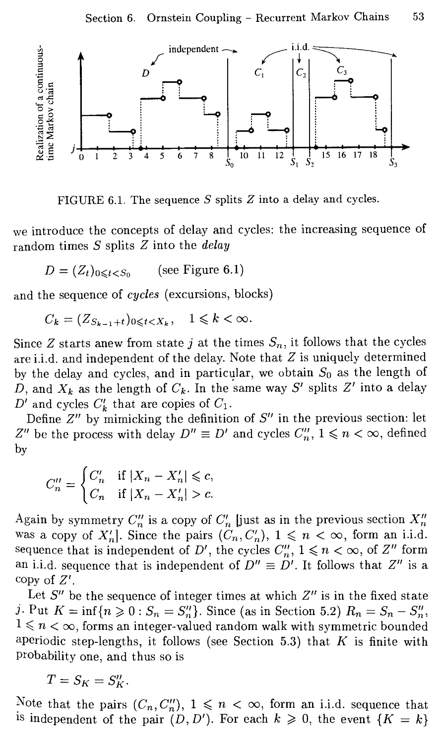
/


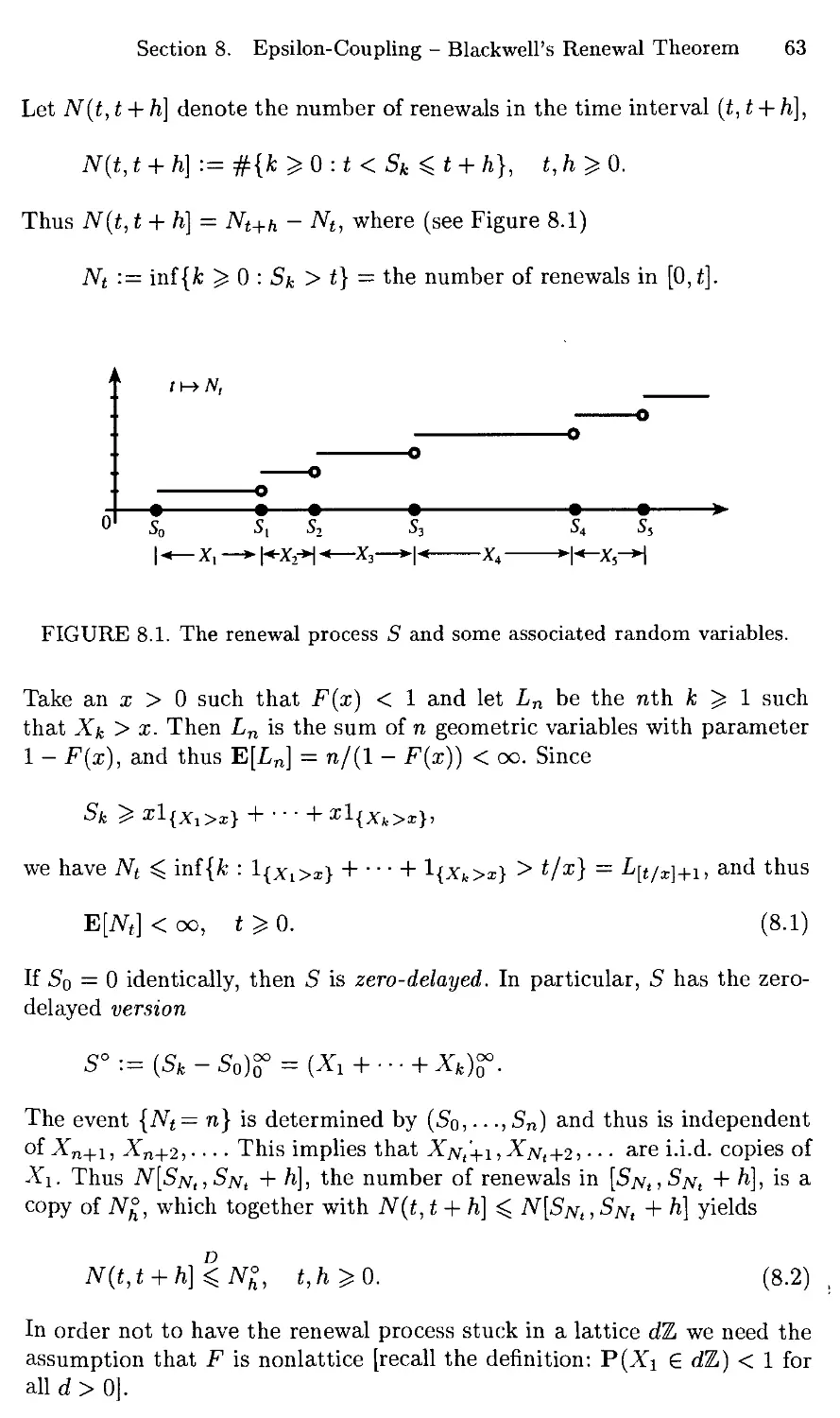
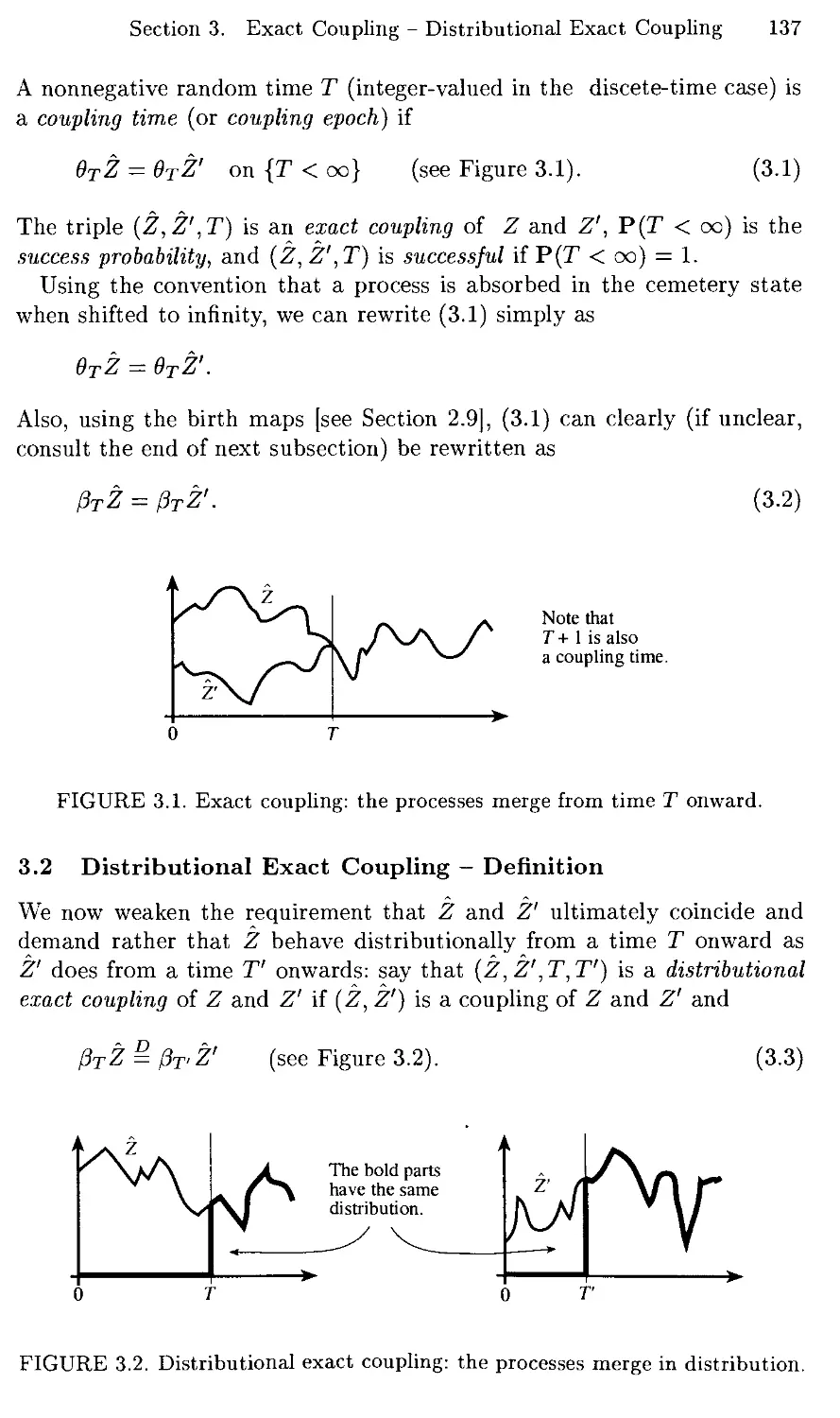
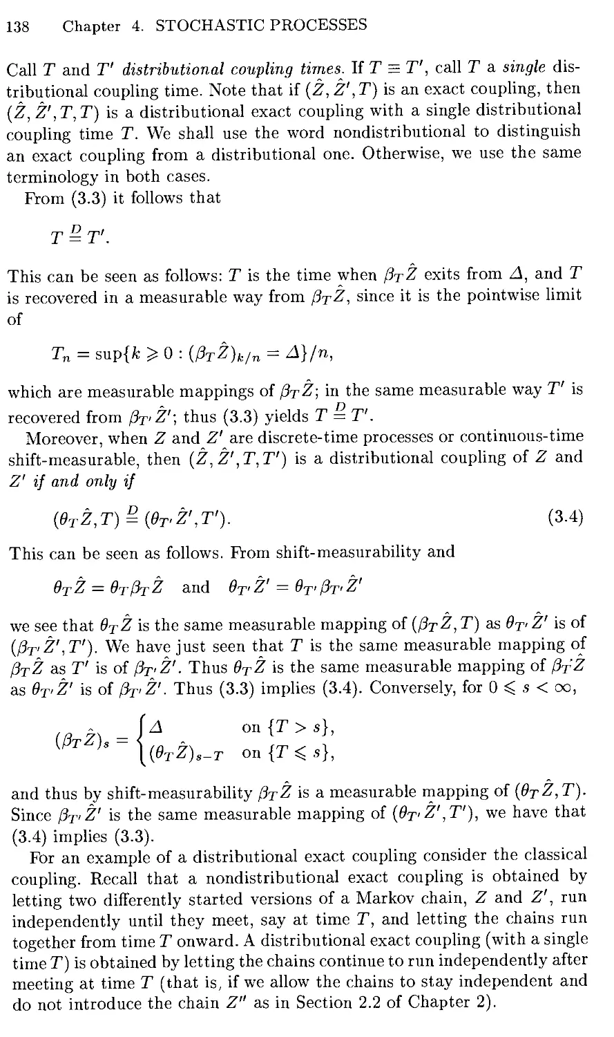


Text
Probability and its Applications
A Series of the Applied Probability Trust
Editors: J. Gani, C.C. Heyde, T.G. Kurtz
Springer
New York
Berlin
Heidelberg
Barcelona
Hong Kong
London
Milan
Paris
Singapore
Tokyo
Probability and its Applications
Anderson: Continuous-Time Markov Chains.
Azencott/Dacunha-Castelle: Series of Irregular Observations.
Bass: Diffusions and Elliptic Operators.
Bass: Probabilistic Techniques in Analysis.
Choi: ARMA Model Identification.
de la Pena/Gine: Decoupling: From Dependence to Independence.
Galambos/Simonelli: Bonferroni-type Inequalities with Applications.
Gani (Editor): The Craft of Probabilistic Modelling.
Grandell: Aspects of Risk Theory.
Gut: Stopped Random Walks.
Guyon: Random Fields on a Network.
Kallenberg: Foundations of Modern Probability.
Last/Brandt: Marked Point Processes on the Real Line.
Leadbetter/Lindgren/Rootzen: Extremes and Related Properties of Random Sequences
and Processes.
Nualart: The Malliavin Calculus and Related Topics.
Rachev/Ruschendorf: Mass Transportation Problems. Volume I: Theory.
Rachev/Ruschendorf: Mass Transportation Problems. Volume II: Applications.
Resnick: Extreme Values, Regular Variation and Point Processes.
Shedler: Regeneration and Networks of Queues.
Thorisson: Coupling, Stationarity, and Regeneration.
Todorovic: An Introduction to Stochastic Processes and Their Applications.
Hermann Thorisson
Coupling, Stationarity,
and Regeneration
With 27 Illustrations
Springer
Hermann Thorisson
Science Institute
University of Iceland
Dunhaga 3
107 Reykjavik
Iceland
E-mail: hermann@hi.is
Homepage: www.hi.is/~hermann
Series Editors
J. Gani
Stochastic Analysis
Group, CMA
Australian National
University
Canberra ACT 0200
Australia
C.C. Heyde
Stochastic Analysis
Group, CMA
Australian National
University
Canberra ACT 0200
Australia
T.G. Kurtz
Department of
Mathematics
University of Wisconsin
480 Lincoln Drive
Madison, WI 53706
USA
Mathematics Subject Classification (1991): 60Gxx, 60Jxx, 60Kxx, 60D05, 60B15, 60A10, 60F99
Library of Congress Cataloging-in-Publication Data
Thorisson, Hermann.
Coupling, stationarity, and regeneration / Hermann Thorisson.
p. cm. — (Probability and its applications)
Includes bibliographical references and index.
ISBN 0-387-98779-7 (hardcover : alk. paper)
1. Random variables. 2. Stochastic processes.
I. Title. II. Series.
QA273.T4395 2000
519.2—dc21 99-40961
Printed on acid-free paper.
© 2000 Springer-Verlag New York, Inc.
All rights reserved. This work may not be translated or copied in whole or in part without the
written permission of the publisher (Springer-Verlag New York, Inc., 175 Fifth Avenue, New York,
NY 10010, USA), except for brief excerpts in connection with reviews or scholarly analysis. Use
in connection with any form of information storage and retrieval, electronic adaptation, computer
software, or by similar or dissimilar methodology now known or hereafter developed is forbidden.
The use of general descriptive names, trade names, trademarks, etc., in this publication, even if the
former are not especially identified, is not to be taken as a sign that such names, as understood by
the Trade Marks and Merchandise Marks Act, may accordingly be used freely by anyone.
Production managed by Jenny Wolkowicki; manufacturing supervised by Jeffrey Taub.
Typeset by Thorir Magnusson using the author's TgX files.
Printed and bound by Maple-Vail Book Manufacturing Group, York, PA.
Printed in the United States of America.
987654321
ISBN 0-387-98779-7 Springer-Verlag New York Berlin Heidelberg SPIN 10660218
TileinkaS per Rannveig
Solarhjort
leit ek sunnan fara,
hann teymdu tveir saman;
faetr hans
stoSu foldu &,
en toku horn til himins.
Ur Solarljodum
Preface
This is a book on coupling, including self-contained treatments of station-
arity and regeneration. Coupling is the central topic in the first half of the
book, and then enters as a tool in the latter half. The ten chapters are
grouped into four parts as follows:
Chapters 1-2 form an introductory part presenting basic
elementary couplings (Chapter 1 on random variables) and the classical
triumphs of the coupling method (Chapter 2 on Markov chains, random
walks, and renewal theory).
Chapters 3-7 present a general coupling theory highlighting
maximal couplings and convergence characterizations for random
elements, stochastic processes, random fields, and random elements
under the action of a transformation semigroup.
Chapters 8-9 present Palm theory of stationary stochastic processes
associated with a simple point process. Chapter 8 treats the one-
dimensional case and Chapter 9 the higher-dimensional case.
Chapter 10 deals with regeneration, both classical regenerative
processes and three generalizations: wide-sense regeneration (as in Harris
chains); time-inhomogeneous regeneration (as in time-inhomogeneous
recurrent Markov chains); and taboo regeneration (as in transient
Markov chains). It ends with a section on perfect simulation
(coupling from-the-past). This enormous chapter is thrice the size of a
normal chapter, and is really a book within the book.
For more information on the content of the book, see the introductions to
the chapters. Also, the table of contents provides a structural review.
viii Preface
The book should be of interest to students and researchers in probability,
stochastic modelling, and mathematical statistics. It is written with a Ph.D.
student in mind, and the first two chapters can be read at the master's level
and even at an advanced undergraduate level.
The book is mathematically self-contained, relying only on basic measure-
theoretic probability. Measure-theoretic language is suppressed in the first
two chapters, and then enters heavily in Chapter 3 to be used explicitly
for the rest of the book; Ash (1972) is used as reference, but Billingsley
(1986) is also fine. Some prior knowledge of elementary Markov chain
theory would be useful, at least in Chapter 2; Karlin and Taylor (1975) and
Cinlar (1975) are excellent, and the compact first two sections of the first
two chapters in Asmussen (1987).
Some Conventions
In order to make clear what results belong to the measure-theoretic
background, the term 'Fact' is used for results stated without proof, while the
terms 'Theorem' and 'Lemma' are reserved for results that are proved here.
Facts of basic importance throughout the book are restricted to Chapter 3
(Sections 3 and 4).
Sections are enumerated within chapters. For instance, the 4th section
in the 3rd chapter is referred to within the chapter only as 'Section 4'; but
in the other chapters as 'Section 4 in Chapter 3' or 'Chapter 3 (Section 4)'.
Subsections are enumerated within chapters and sections: the 5th
subsection of the 4th section in the 3rd chapter is referred to within the chapter
as 'Section 4.5'; but in the other chapters as 'Section 4.5 in Chapter 3'.
The same goes for Theorems, Lemmas, Facts, Remarks, and Figures.
Definitions are stated in the text, and only indicated by writing the
concept being defined in italics (we also use italics for emphasis). Figures
are placed in the text precisely where they should be consulted (mostly),
but the text does not rely on them. We use both parenthesis () and brackets
[] for comments that can be skipped. Historical and bibliographic notes are
deferred to a separate section at the end of the book.
The symbol X (and X', X, X\, ...) is reserved for real-valued random
variables. The symbol Sk always denotes a sum, Sk = Sq+ Xx + 1- -X*.
On the other hand, S is either a sequence of Sk (one-sided sequence in
Chapters 2, 3, and 10; two-sided in Chapter 8), or a d-dimensional random
vector (Chapters 7 and 9). The symbol U is reserved for a variable uniform
on [0,1]. The symbol Z is reserved for processes. The symbol Yoften denotes
a random element in a general space; and P(Y € •) is the distribution of Y.
Errors are bound to abound in the book, in spite of all the thinning
attempts. For errata, and even some notes and references, see my homepage
(www. hi. is/~hermann) or Springer's (www. springer-ny. com). If you find
an error or have a comment, please send me an informal note by e-mail
(To: hermann@hi.is; Subject: book).
Preface ix
Acknowledgements
It took four long years to write this book, word for word, from the first
word on the first page to the last word on page four-hundred-seventy-eight.
Previously, the book had been in preparation for five years; and before that,
subconsciously for years.
I would like to thank Torgny Lindvall for introducing me to this field
of study and for grooming me for this task, and Peter Jagers for his
influence and for the focused comments on the book. Also thanks to S0ren
Asmussen, Karl Sigman, Peter Glynn, Serguei Foss, and Richard Gill, who
have influenced this work in various ways throughout the years.
Special thanks to Olle Nerman, Olav Kallenberg, David Blackwell, Henry
Berbee, Jakob Yngvason, Peter Donnelly, and Olle Haggstrom for
illuminating observations; to Rolando Rebolledo, who got me started on this
project by inviting me to Chile to lecture in the fall of 1991; to Vladimir
Kalashnikov for the collaboration on the Petrozavodsk proceedings, which
helped get things into perspective; to Christian Meise for reading and
rereading the book, and for the thicket of detailed comments; to Diemer
Salome for comments on the first four chapters; to Damien White, Remco
van der Hofstad, Erik van Zwet, Karma Dajani, Ronald Meester, and Adam
Shwartz for comments on the first two; to Vladimir Bogachev and Andrew
Nobel for comments on the third; to David Svensson for comments on
the eighth; to my next-door colleague Magnus Halld6rsson for reading and
commenting on parts of the book, and for the many discussions; and to my
fellow probabilist Ott6 Bjornsson for his long-lasting interest and support.
Also thanks to the copyeditor David Kramer for excellent suggestions while
basically accepting my Icelandic English, and for all the commas; to my
colleague Robert Magnus for straightening out many unclear sentences, and
for some British moderation; and to the production editor Jenny Wolkow-
icki for the insightful finishing touch. After all this feedback the book should
be in pretty good shape; but whatever mistakes there are, they are all mine.
I would like to thank John Kimmel, Springer's statistics editor, for his
deep understanding of what a work like this is about, and for never rushing
me in spite of the writing going almost two years beyond deadline and the
book becoming more than twice the planned size.
Many thanks to Porir Magnusson for his expert LaTeX-ing, and for
his support and the patience it must have taken to work along with me
these four years. Also thanks to my son Freyr (Hermannsson) for calmly
FreeHand-ing the figures during these hectic last weeks.
I am grateful to the University of Iceland and its Science Institute for
funding this project, and for providing the freedom necessary for this task.
I am also grateful to the Icelandic Science Foundation for travel grants.
And now, as this book goes to print, I am informed that I have been
awarded the Olafur Danielsson Prize in Mathematics for my research, most
ofwhich can be found in some form in this book. I am deeply moved and will
use the generous sum to recover from this work, and prepare for the next.
x Preface
Music, - from Johann Sebastian Bach to Par Lindh Project (PLP), - played
an important role in getting me through the composition of this book. So,
on another note, thank you Keith Emerson for the High Level Fugue and
the Endless Enigma; evermoving without ever moving. Also thanks to Ian
(Thick as a Brick) Anderson for Twelve Dances with God, and to King
Crimson for both Discipline and Indiscipline, and for completing this trinity
of sons IN THE COURT OF THE CRIMSON KING.
Finally, Rannveig, Freyr, and Nanna, thank you for so lovingly supporting
me through these Ten Dances with Chance.
Reykjavik
October 1999
Hermann Porisson
Contents
Preface vii
1 RANDOM VARIABLES 1
1 Introduction 1
2 The i.i.d. Coupling - Positive Correlation 2
3 Quantile Coupling - Stochastic Domination 3
4 Coupling Event - Maximal Coupling 6
5 Poisson Approximation - Total Variation 11
6 Convergence of Discrete Random Variables 15
7 Continuous Variables - Hitting the Limit 18
8 Convergence in Distribution and Pointwise 21
9 Quantile Coupling - Dominated Convergence 26
10 Impossible Coupling - Quantum Physics 27
2 MARKOV CHAINS AND RANDOM WALKS 33
1 Introduction ' 33
2 Classical Coupling - Birth and Death Processes 33
3 Classical Coupling - Recurrent Markov Chains 38
4 Classical Coupling - Rates and Uniformity 44
5 Ornstein Coupling - Random Walk on the Integers 47
6 Ornstein Coupling - Recurrent Markov Chains 52
7 Epsilon-Coupling - Nonlattice Random Walk 57
8 Epsilon-Coupling - Blackwell's Renewal Theorem 62
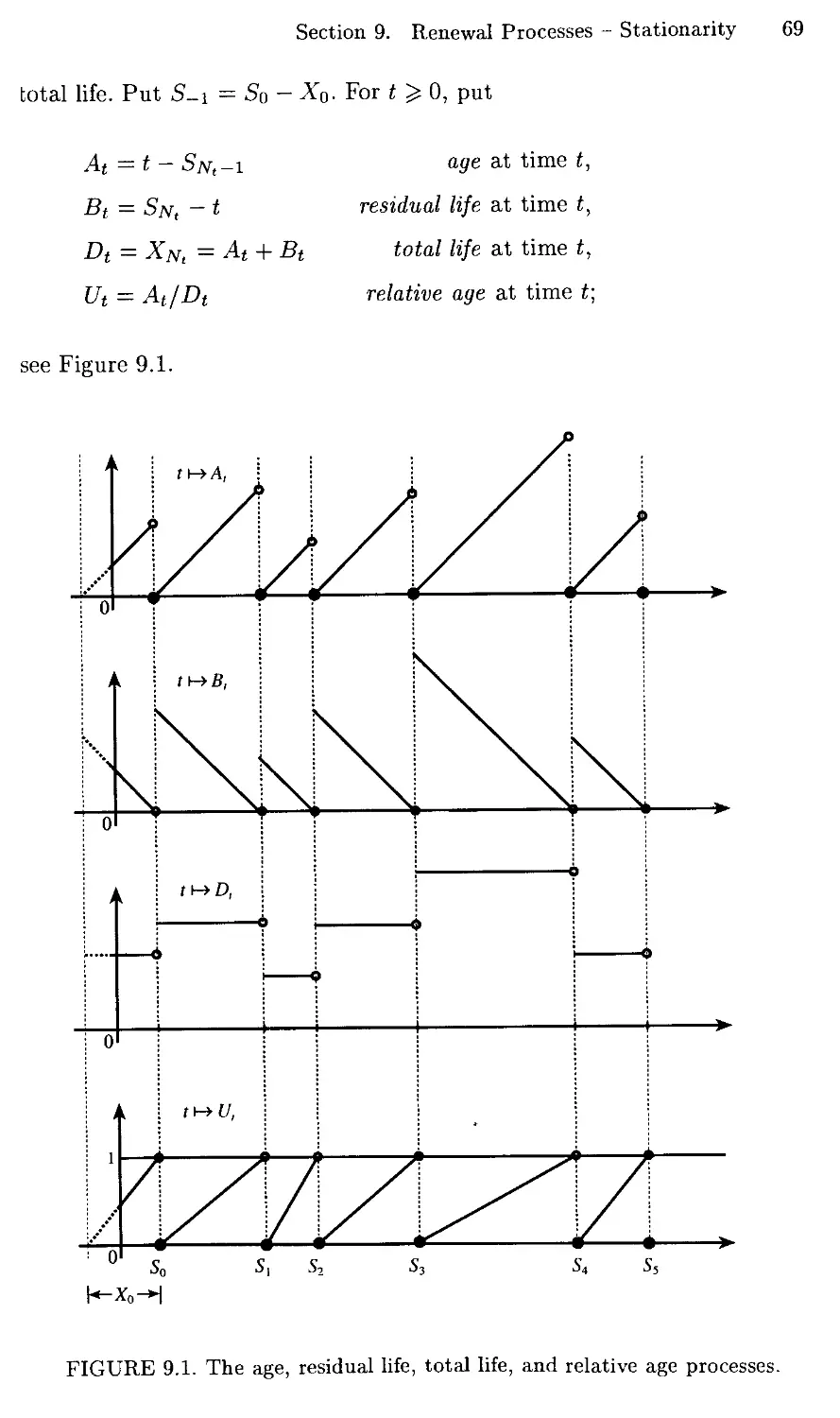
9 Renewal Processes - Stationarity 68
10 Renewal Processes - Asymptotic Stationarity 72
xii Contents
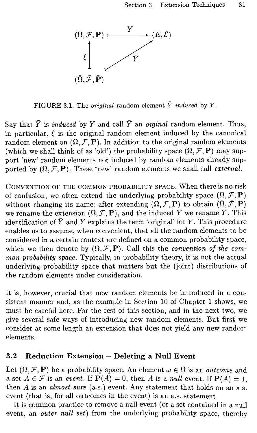
3 RANDOM ELEMENTS 77
1 Introduction 77
2 Back to Basics - Definition of Coupling 78
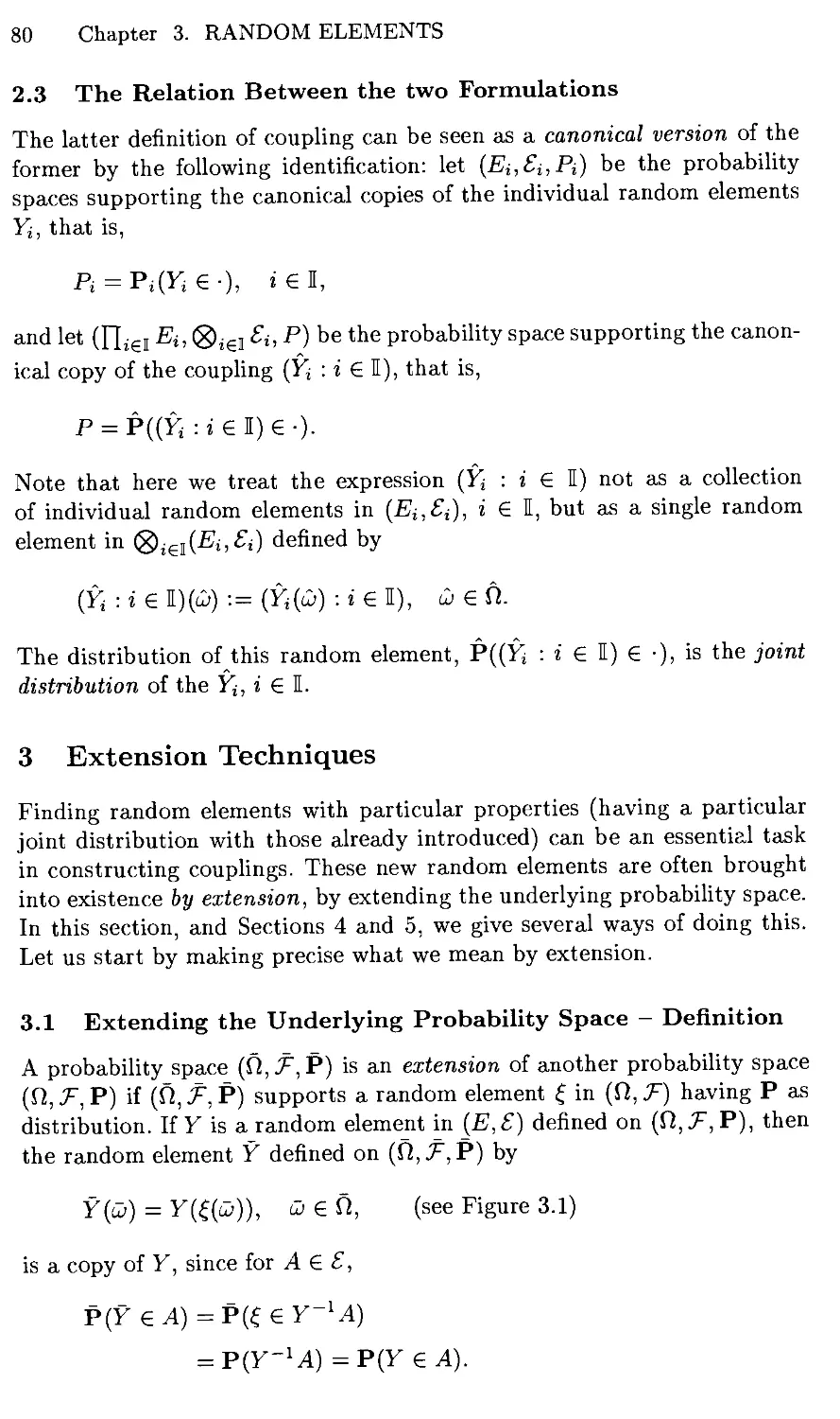
3 Extension Techniques 80
4 Conditioning - Transfer 86
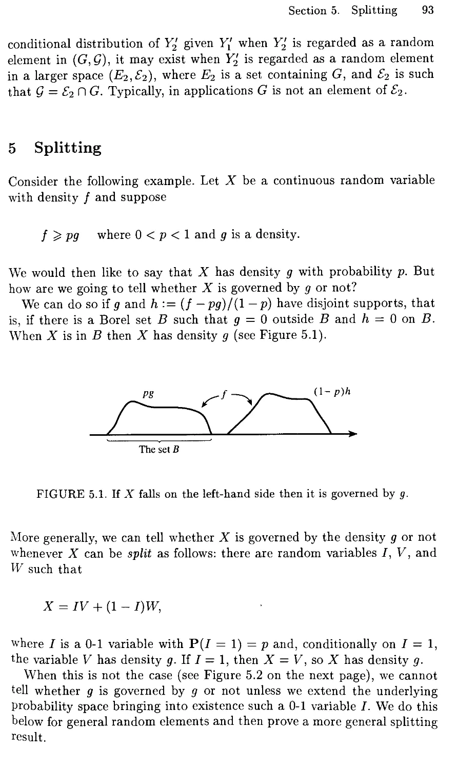
5 Splitting 93
6 Random Walk with Spread-Out Step-Lengths 98
7 Coupling Event - Maximal Coupling 104
8 Maximal Coupling Two Elements - Total Variation 107
9 Hitting the Limit 113
10 Convergence in Distribution and Pointwise 117
4 STOCHASTIC PROCESSES 125
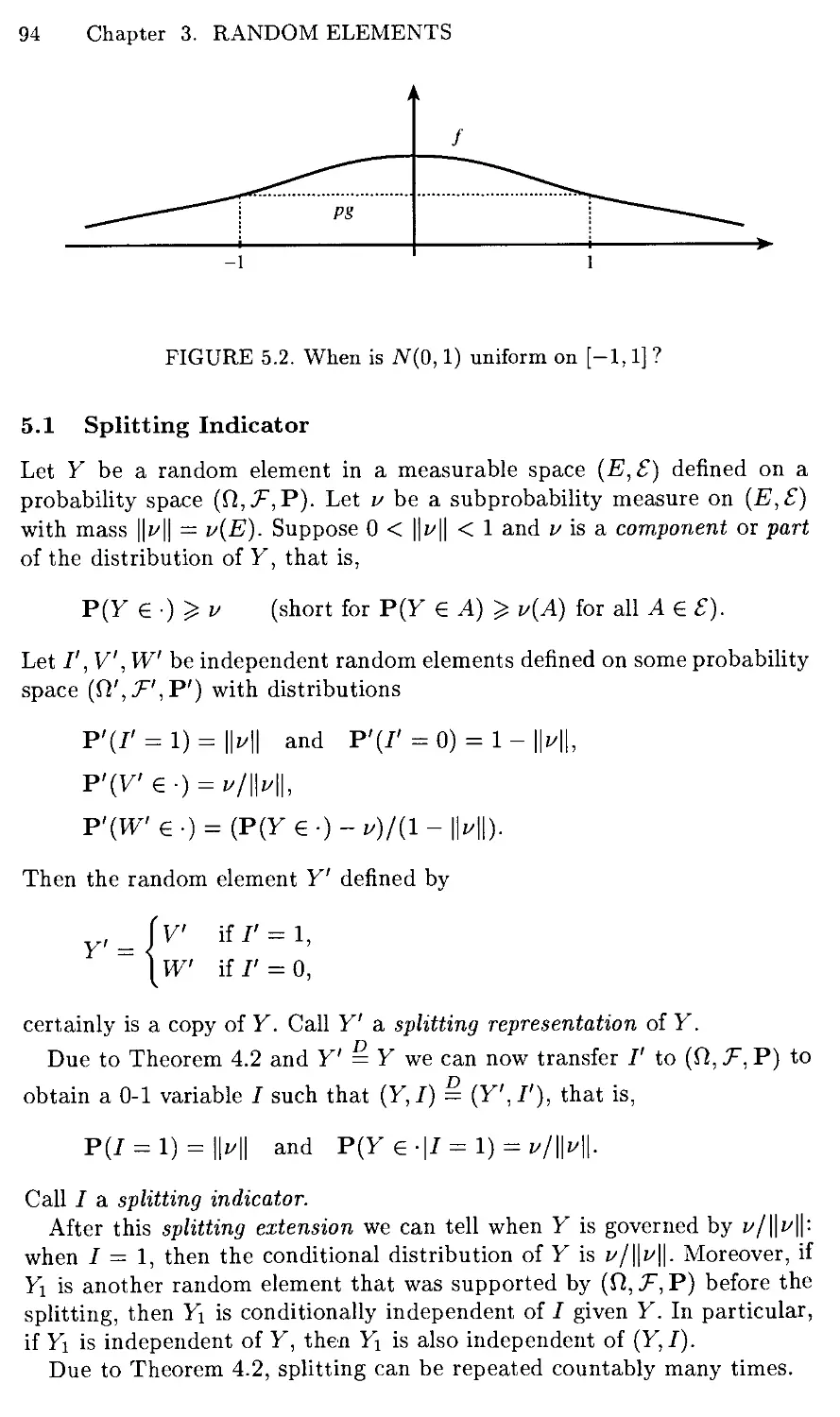
1 Introduction 125
2 Preliminaries - What Is a Stochastic Process? 126
3 Exact Coupling - Distributional Exact Coupling 136
4 Distributional Coupling 140
5 Exact Coupling - Inequality and Asymptotics 142
6 Exact Coupling - Maximality 146
7 Coupling with Respect to a Sub-cr-Algebra 149
8 Exact Coupling - Another Proof of Theorem 6.1 153
9 Exact Coupling - Tail cr-Algebra - Equivalences 156
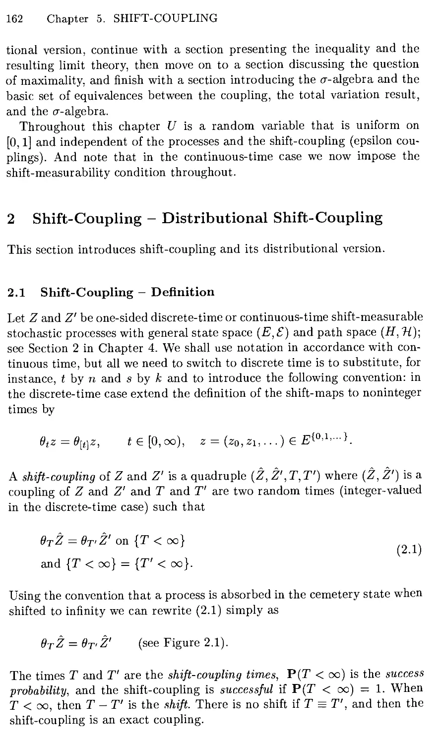
5 SHIFT-COUPLING 161
1 Introduction 161
2 Shift-Coupling - Distributional Shift-Coupling 162
3 Shift-Coupling - Inequality and Asymptotics 165
4 Shift-Coupling - Maximality 169
5 Shift-Coupling - Invariant cr-Algebra - Equivalences .... 174
6 e-Coupling - Distributional e-Coupling 178
7 e-Coupling - Inequality and Asymptotics 180
8 e-Coupling - Maximality 187
9 e-Coupling - Smooth Tail cr-algebra - Equivalences 188
6 MARKOV PROCESSES 195
1 Introduction 195
2 Mixing and Triviality of a Stochastic Process 195
3 Markov Processes - Preliminaries 201
4 Exact Coupling 204
5 Shift-Coupling 207
6 Epsilon-Coupling 209
7 Stationary Measure 213
7 TRANSFORMATION COUPLING 217
1 Introduction 217
Contents xiii
2 Shift-Coupling Random Fields 218
3 Transformation Coupling 222
4 Inequality and Asymptotics 225
5 Maximality 228
6 Invariant a-Algebra and Equivalences 231
7 Topological Transformation Groups 238
8 Self-Similarity - Exchangeability - Rotation 241
9 Exact Transformation Coupling 244
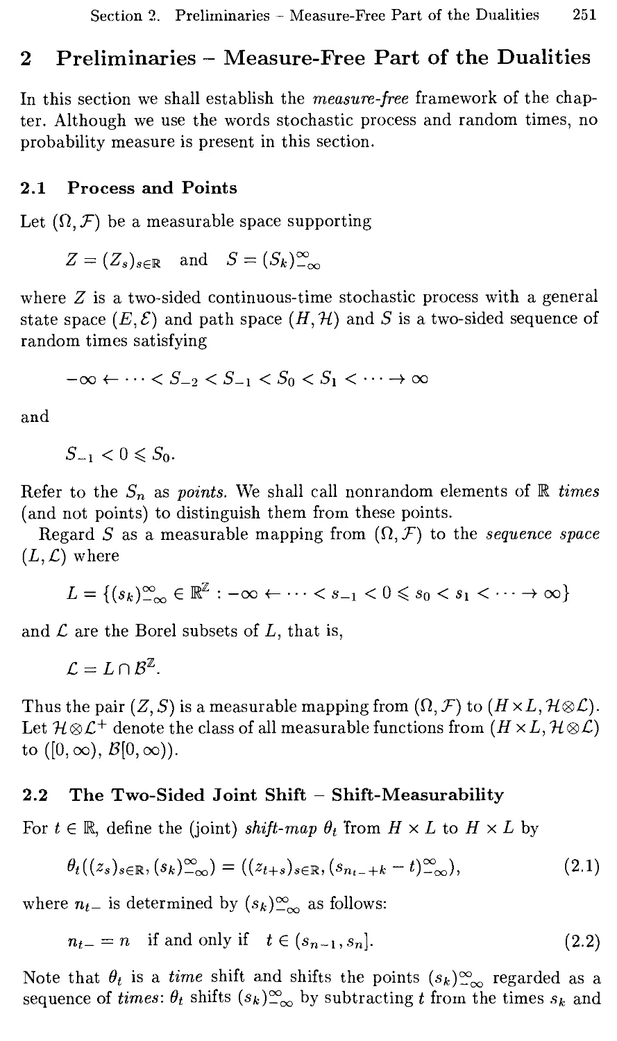
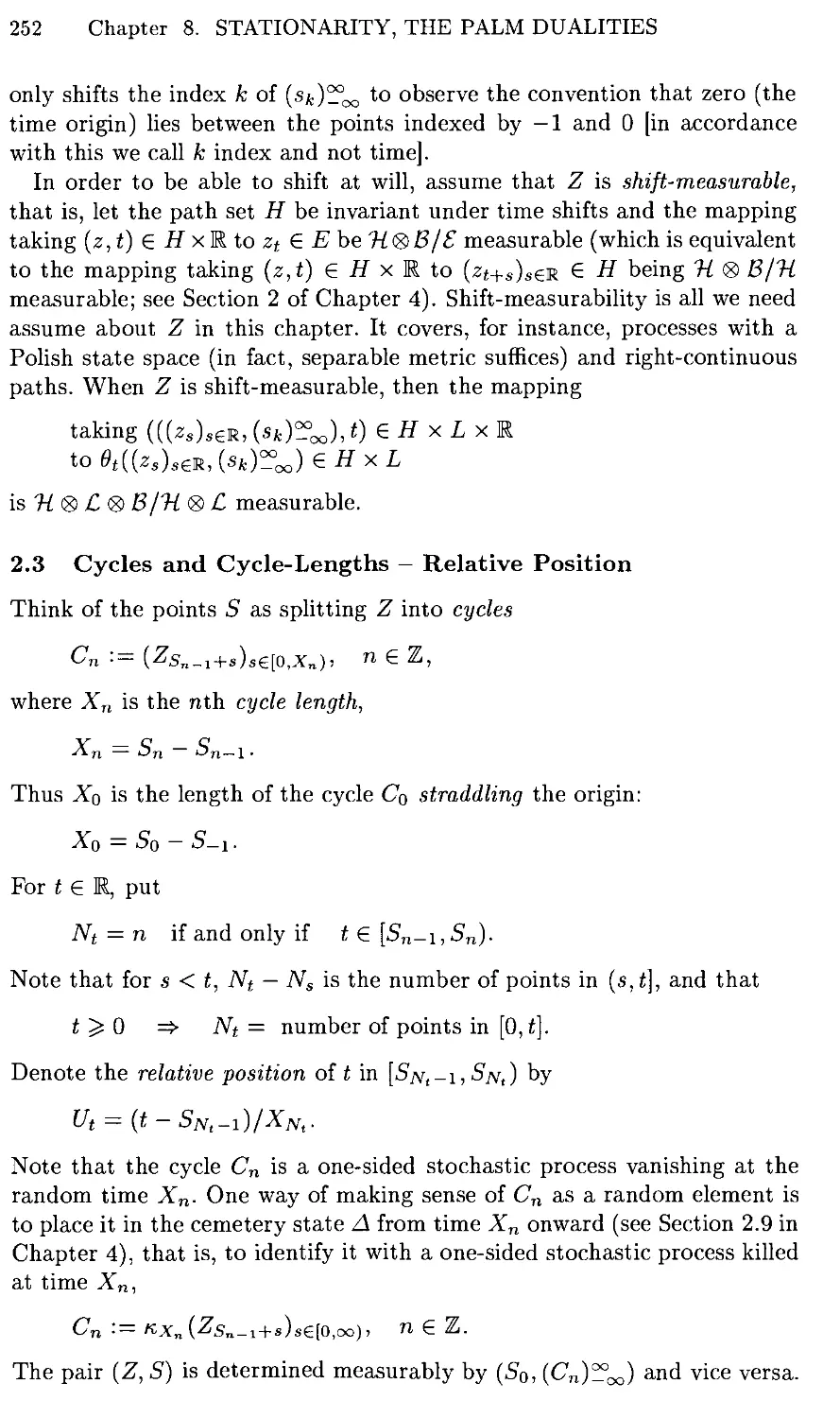
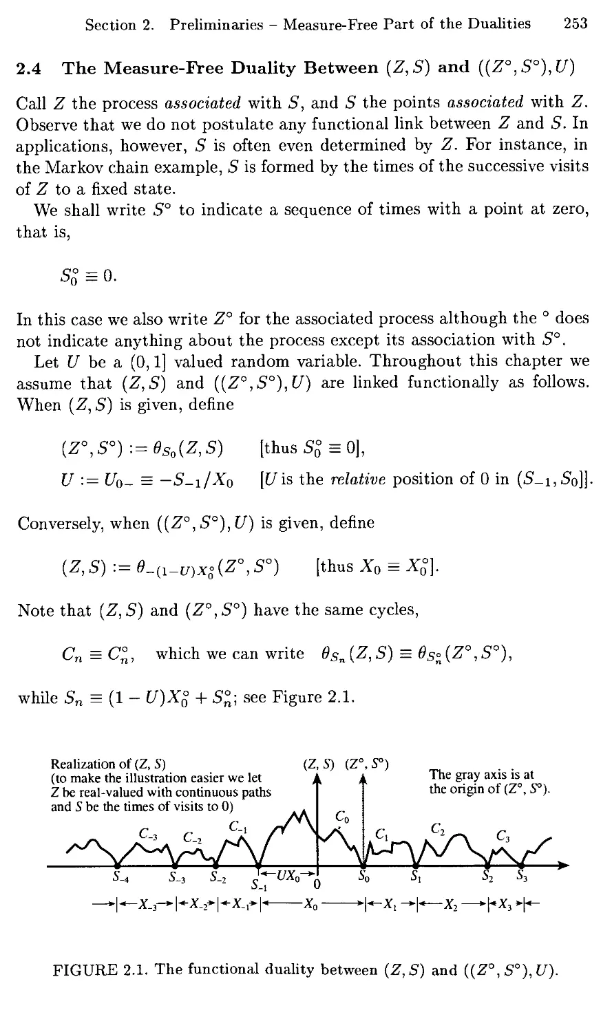
8 STATIONARITY, THE PALM DUALITIES 249
1 Introduction 249
2 Preliminaries - Measure-Free Part of the Dualities 251
3 Key Stationarity Theorem 254
4 The Point-at-Zero Duality 258
5 Interpretation - Point-Conditioning 264
6 Application - Perfect Simulation 271
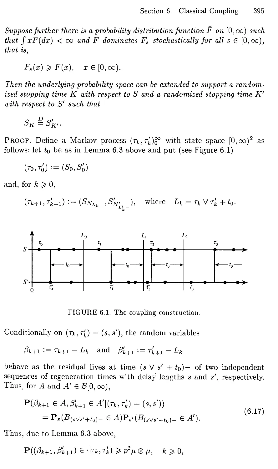
7 The Invariant cr-Algebras I and J 281
8 The Randomized-Origin Duality 284
9 Interpretation - Cesaro Limits and Shift-Coupling 288
10 Comments on the Two Palm Dualities 290
9 THE PALM DUALITIES IN HIGHER DIMENSIONS 295
1 Introduction 295
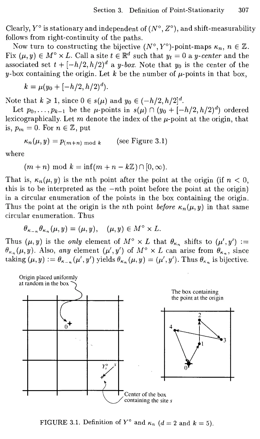
2 The Point-Stationarity Problem 296
3 Definition of Point-Stationarity 302
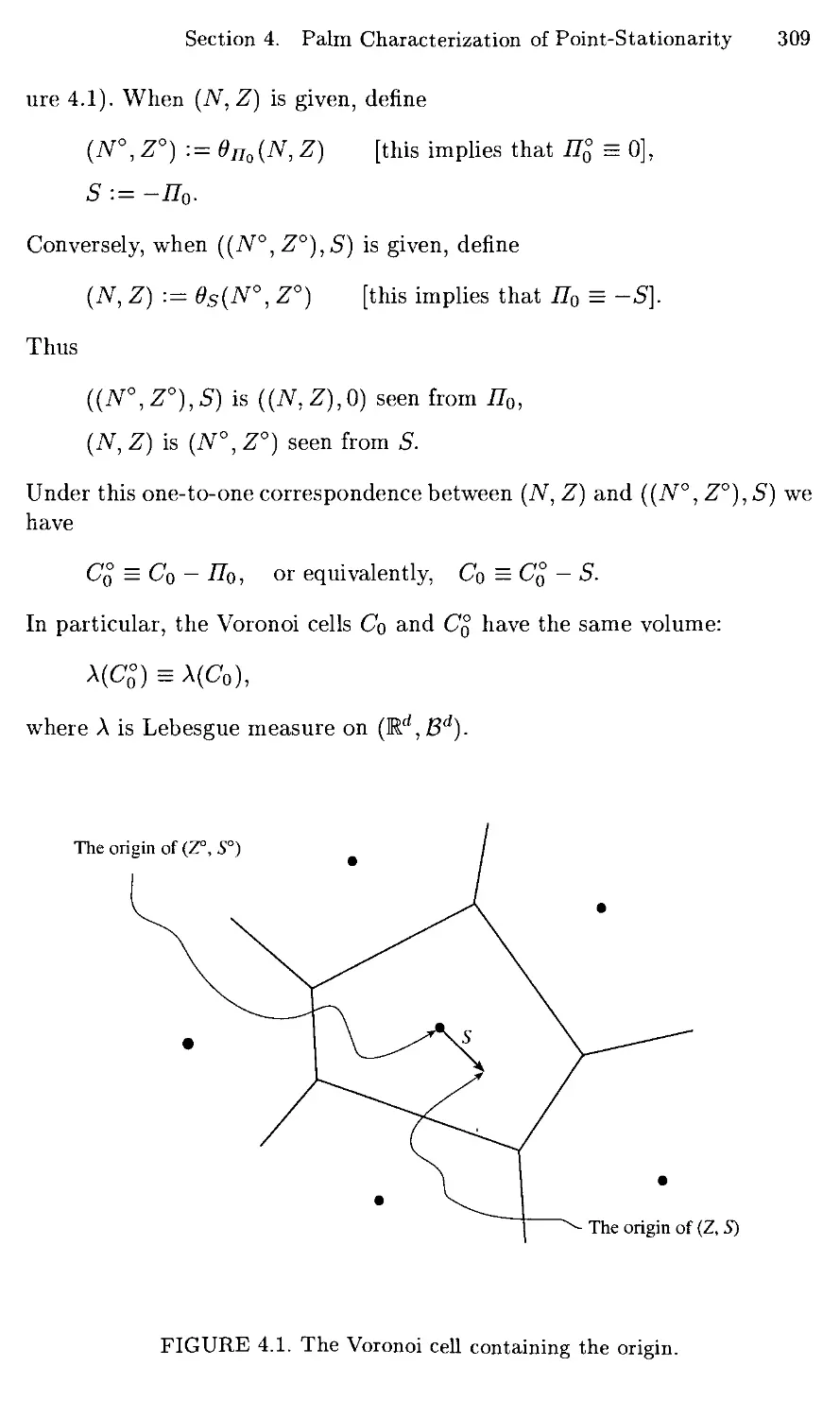
4 Palm Characterization of Point-Stationarity 308
5 Point-Stationarity Characterized by Randomization 317
6 Point-Stationarity and the Invariant a-Algebras 320
7 The Point-at-Zero Duality 323
8 The Randomized-Origin Duality 328
9 Comments 335
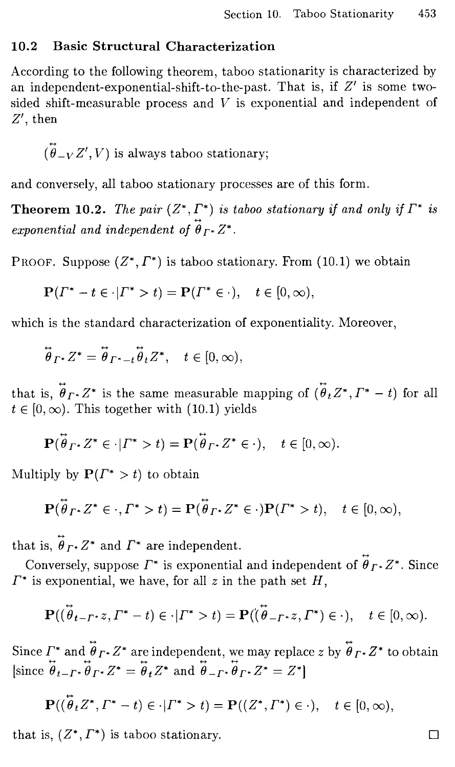
10 REGENERATION 337
1 Introduction 337
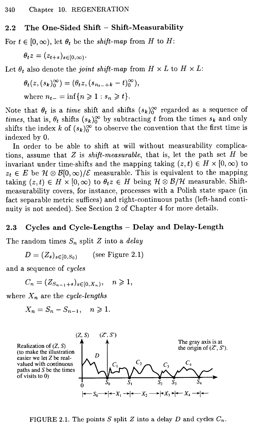
2 Preliminaries - Stationarity 339
3 Classical Regeneration ' 346
4 Wide-Sense Regeneration - Harris Chains - GI/GI/k .... 358
5 Time-Inhomogeneous Regeneration 372
6 Classical Coupling 385
7 The Coupling Time - Rates and Uniformity 399
8 Asymptotics From-the-Past 422
9 Taboo Regeneration 436
10 Taboo Stationarity 451
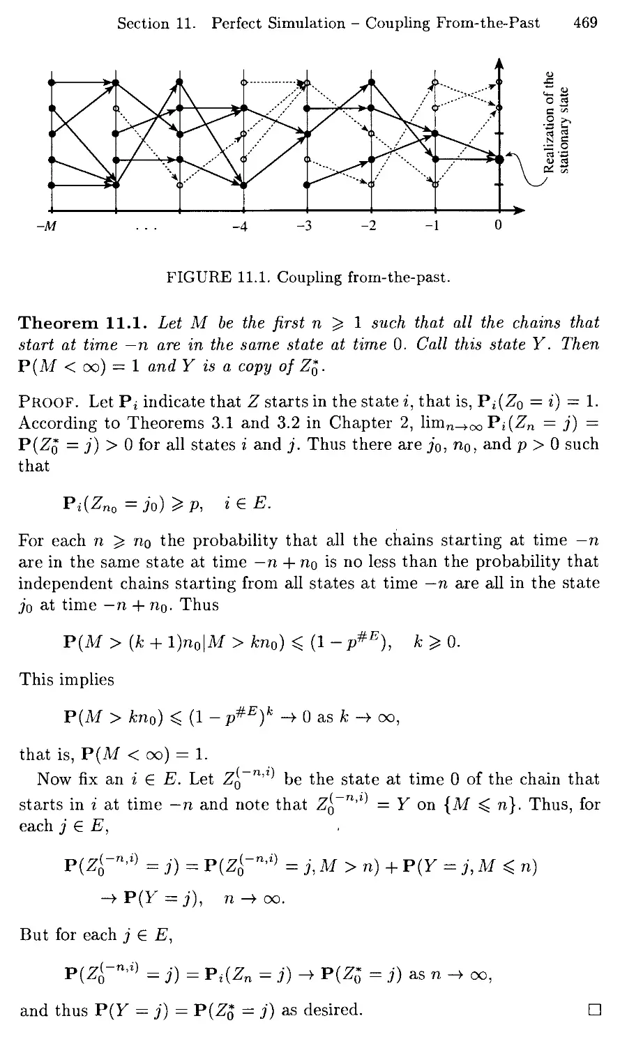
11 Perfect Simulation - Coupling From-the-Past 467
xiv Contents
Notes 479
References 491
Index 509
Notation 517
Chapter 1
RANDOM VARIABLES
1 Introduction
Coupling means the joint construction of two or more random variables (or
processes), usually in order to deduce properties of the individual variables
or gain insight into distributional similarities or relations between them.
In this chapter and the next the method is introduced through a series of
basic elementary examples. The arguments are carried out in full detail at
an undergraduate level, suppressing measure-theoretic language. Advanced
readers should be able to fill in any missing measure-theoretic notation or
find it at the beginning of Chapter 3, where we return to the definition of
coupling.
Let us spend a few lines on terminology before turning to the examples.
A copy or a representation of a random variable X is a random variable X
with the same distribution as X. Denote this by
X^X.
A coupling of a collection of random variables Xi, i € I, [where I is some
index set] is a family of random variables (Xi : i € I) such that
Xi = xu i e i.
Note that only the individual Xt are copies of the individual Xi, while the
whole family (X, : i 6 I) is typically not a copy of the family (Xi : i 6 I). In
other words, the joint distribution of the Xt need not be the same as that of
1
2 Chapter 1. RANDOM VARIABLES
the Xi. In fact, the Xi need not even have a (specified) joint distribution.
On the other hand, we write (Xi : i 6 I) in parentheses to stress that
the Xi have a joint distribution. A trivial but often useful coupling is the
independence coupling consisting of independent copies of the Xi.
Thus a coupling has fixed marginal distributions (the distributions of
the individual Xi), and the trick is to find a dependence structure (joint
distribution) that fits one's purposes.
2 The i.i.d. Coupling - Positive Correlation
A self-coupling of a random variable X is a family (Xt : i £ I) where each
Xi is a copy of X. A trivial (and not so useful) self-coupling is the one
with all the Xi identical. Another trivial self-coupling is the i.i.d, coupling
consisting of independent copies of X. As an example of an efficient use of
the i.i.d. coupling we shall prove the following result.
For every random variable X and nondecreasing bounded functions /
and g, the random variables f(X) and g(X) are positively correlated,
that is,
Cov[f(X),g(X)]^0. (2.1)
In order to prove this claim let X' be an independent copy of X [thus
(X, X') is an i.i.d. coupling of X]. The additivity of covariances yields
Cov[/(X) - f(X'),g(X) - g(X')} = Cov[f(X),g(X)}
- Cov[f(X),g(X')] - Cov[f(X'),g(X)} + Cov[f(X'),g(X%
Since X and X' are independent, the middle terms on the right are zero,
and since X and X' have the same distribution, the remaining terms on
the right are identical. Thus
Cov[f(X),g(X)] = i Cov[/(X) - f(X'),g(X) - g(X')}.
Since the mean of both f(X) - f(X') and g{X) - g{X') is zero, we have
Cov[f(X)-f(X'),g(X)-g(X')}
= E[(f(X)-f(X'))(g(X)-g(X'))},
which is positive, since / and g nondecreasing implies that
f(x) — f(y) and g(x) — g(y) are either both ^ 0 or both ^ 0.
Thus (2.1) holds.
Section 3. Quantile Coupling - Stochastic Domination 3
3 Quantile Coupling — Stochastic Domination
In this section we produce a coupling that turns so-called stochastic
domination into ordinary (pointwise) domination. Another application can be
found in Section 8. See also Section 9.
3.1 The Coupling
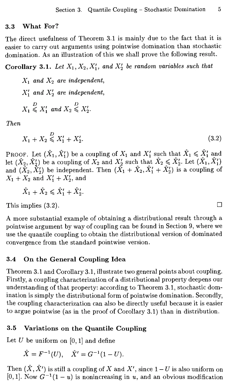
Consider a random variable X with distribution function F, that is,
P{X ^ x) = F(x), i£l
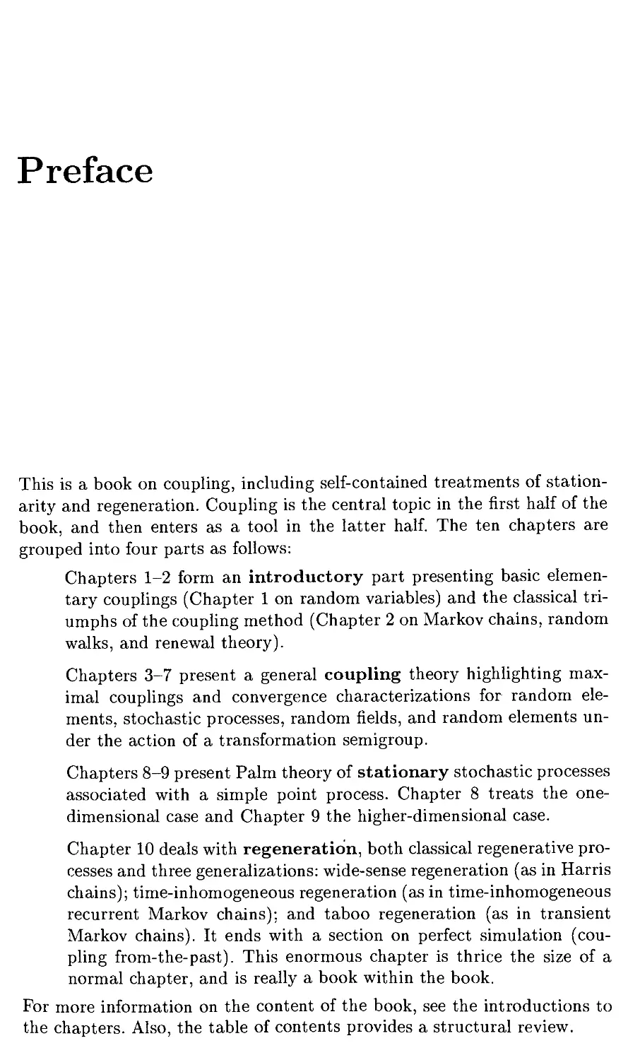
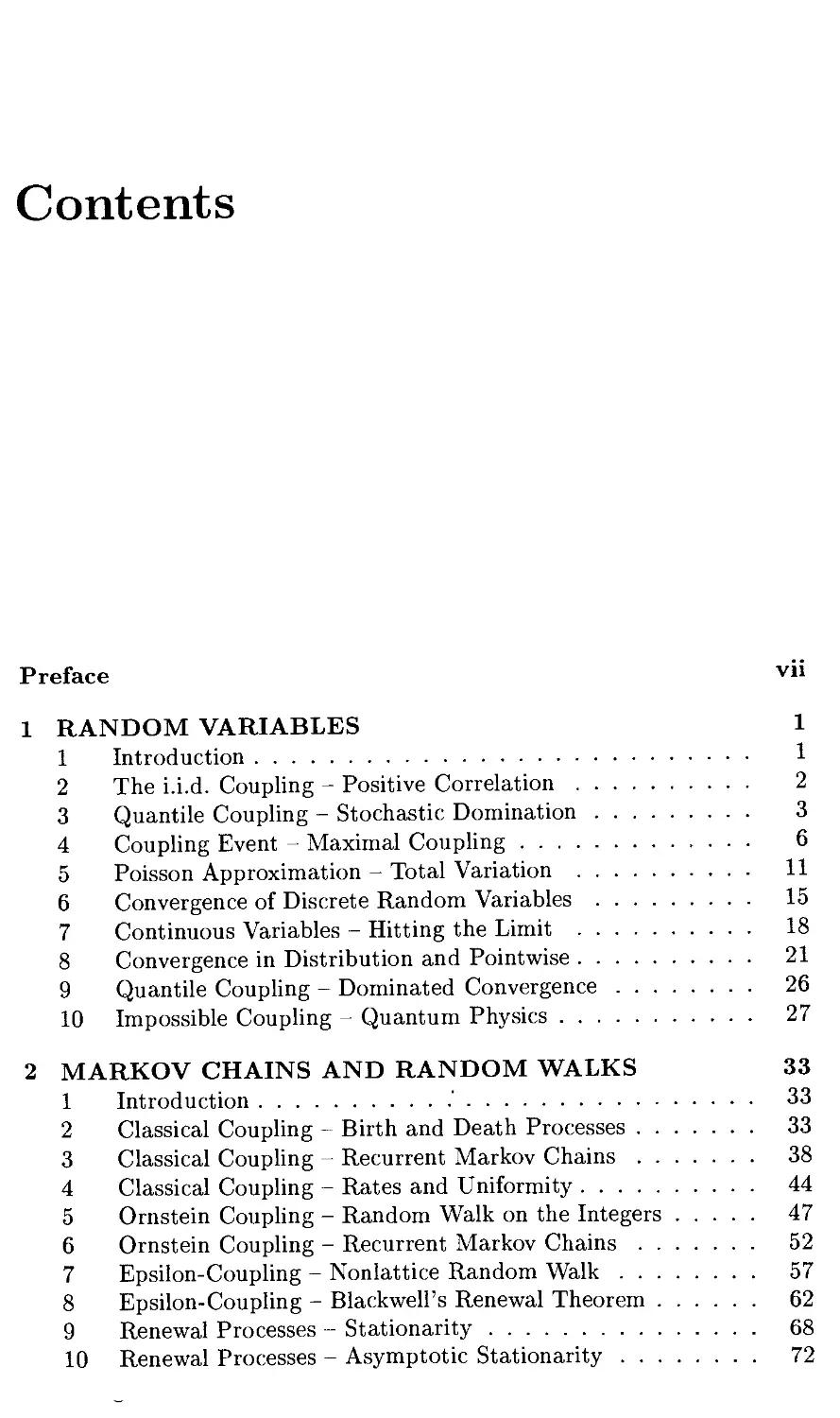
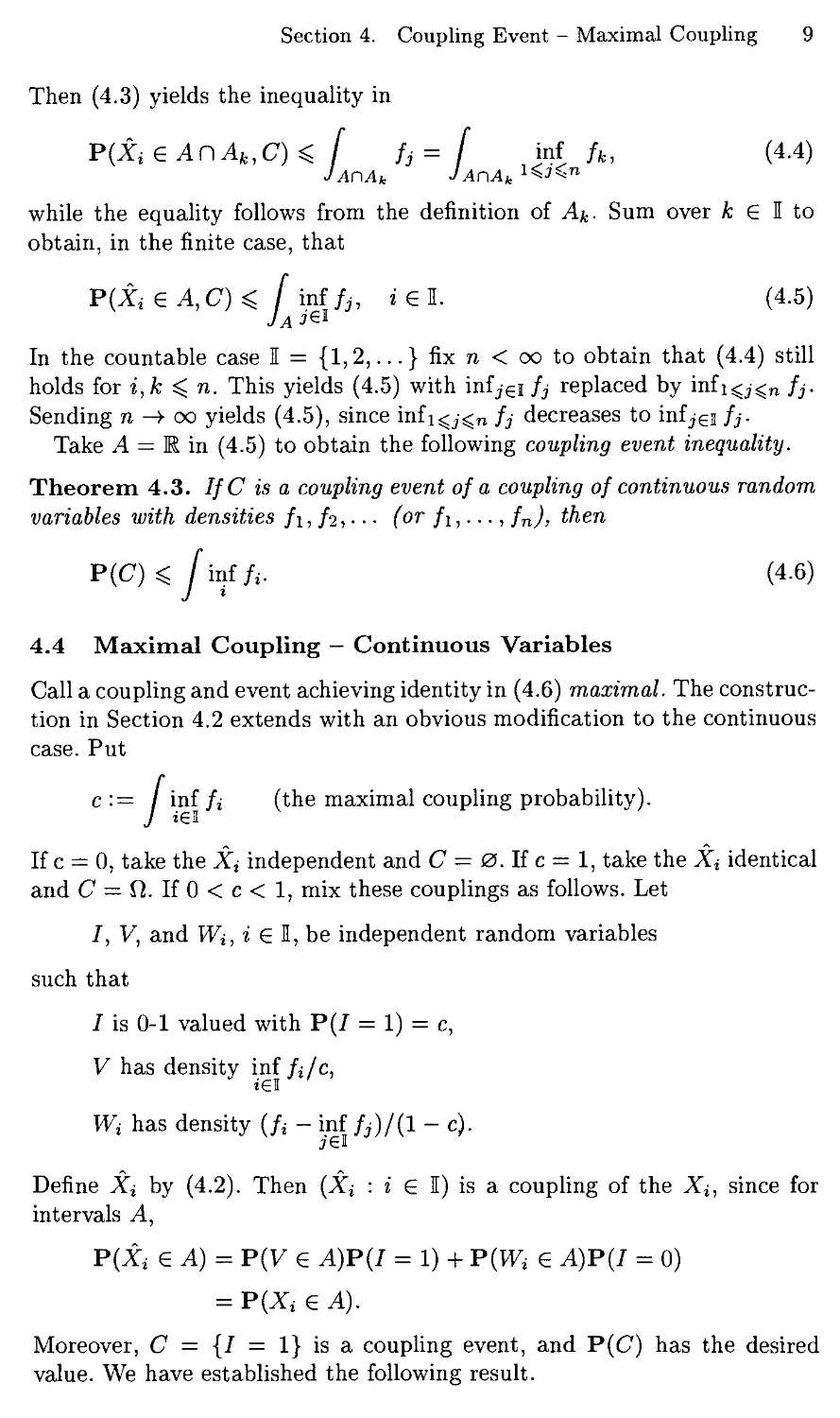
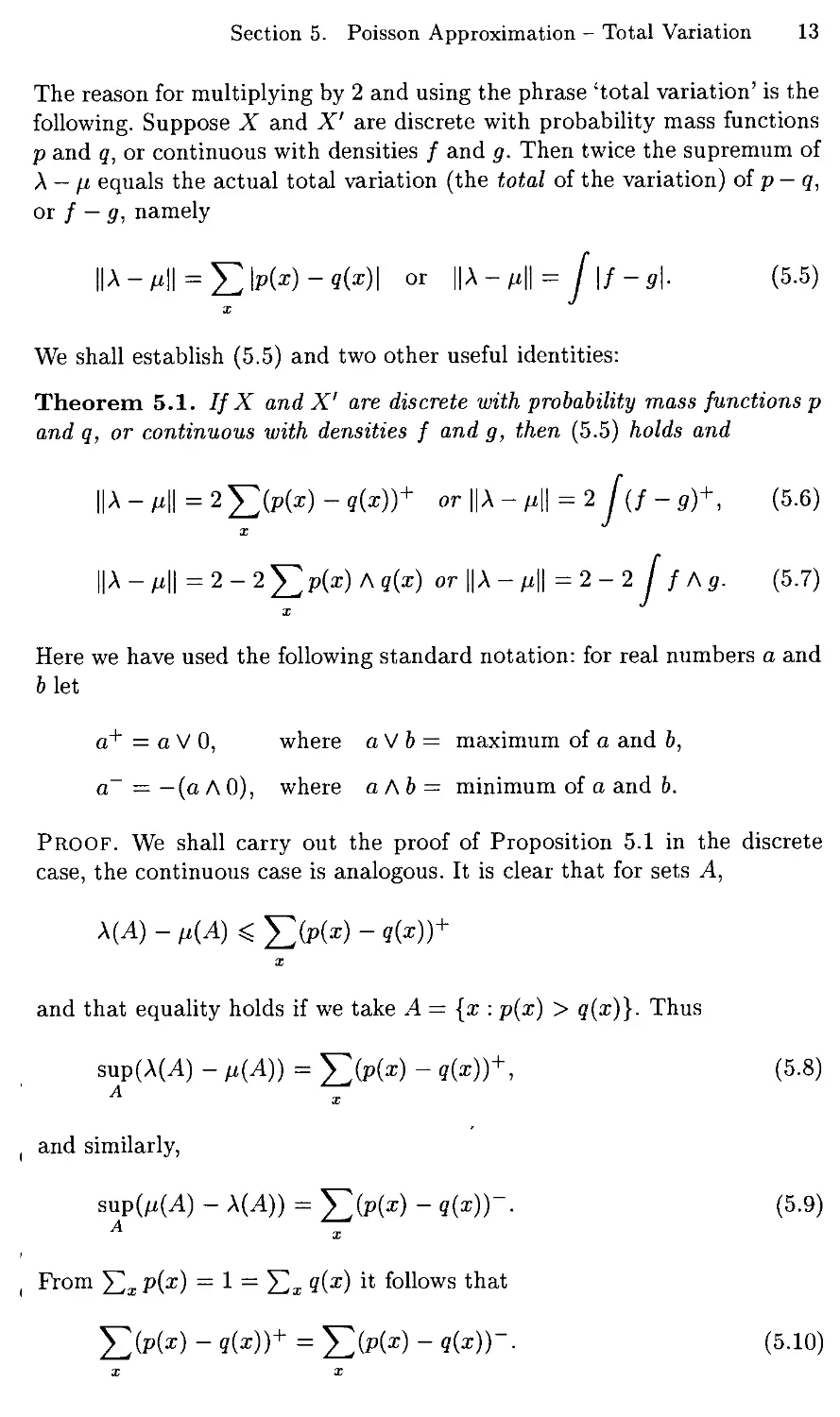
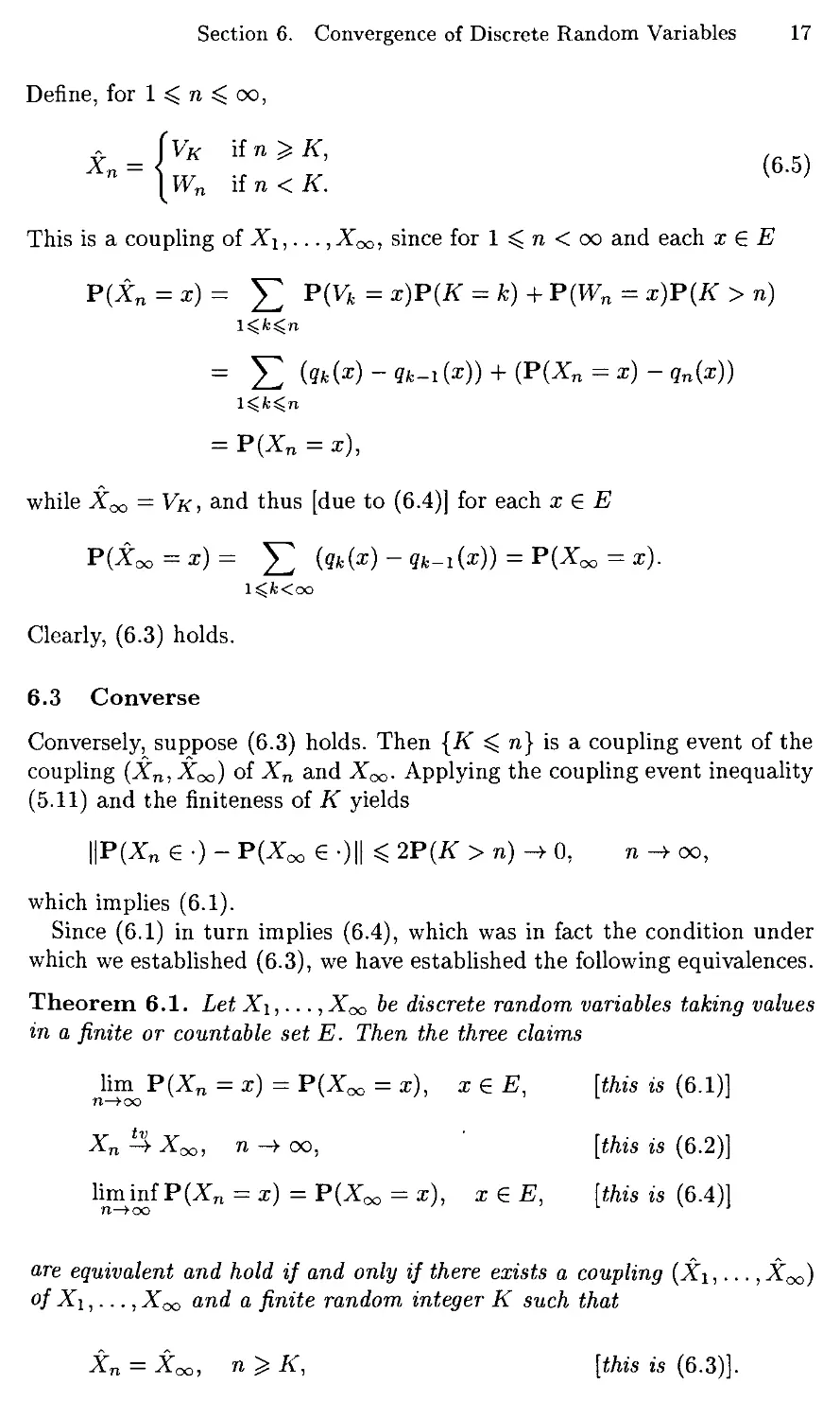
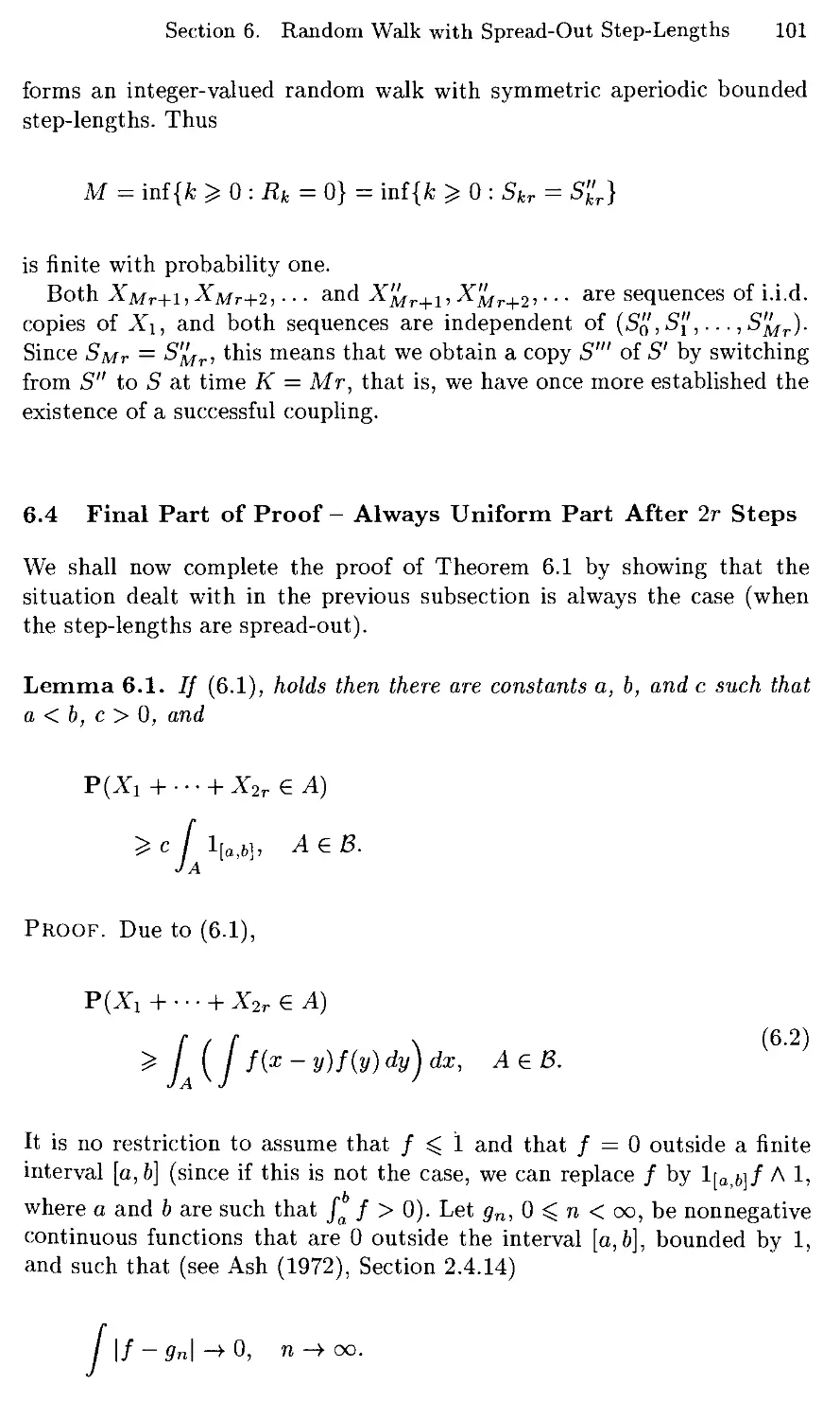
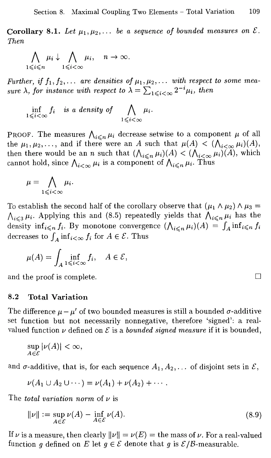
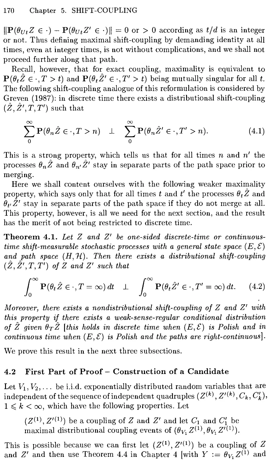
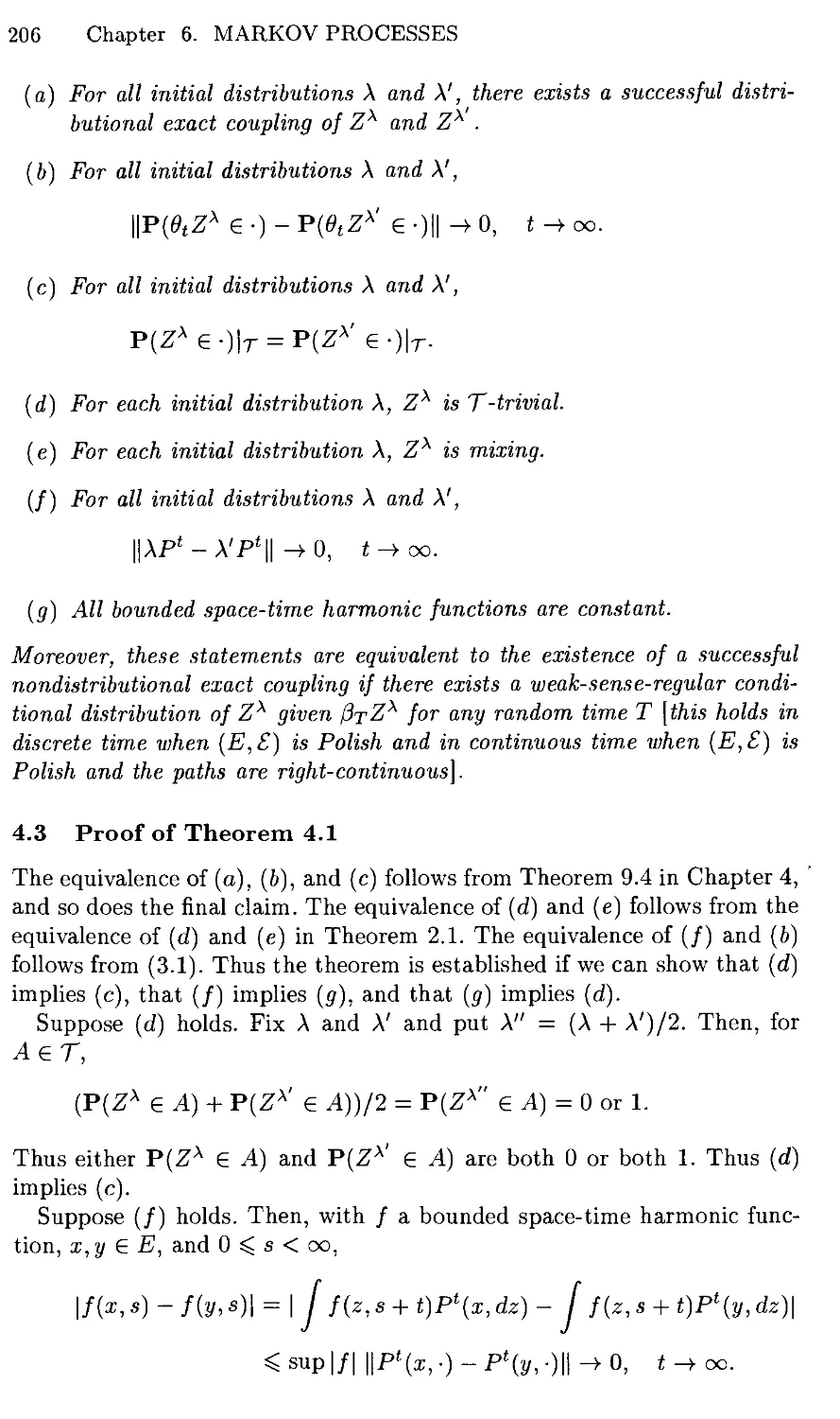
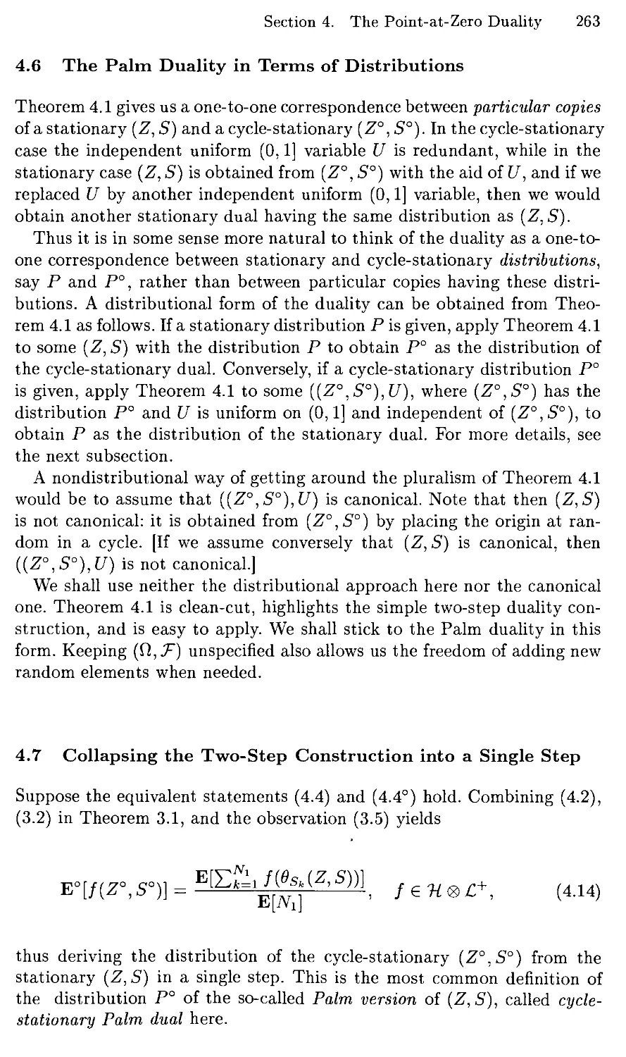
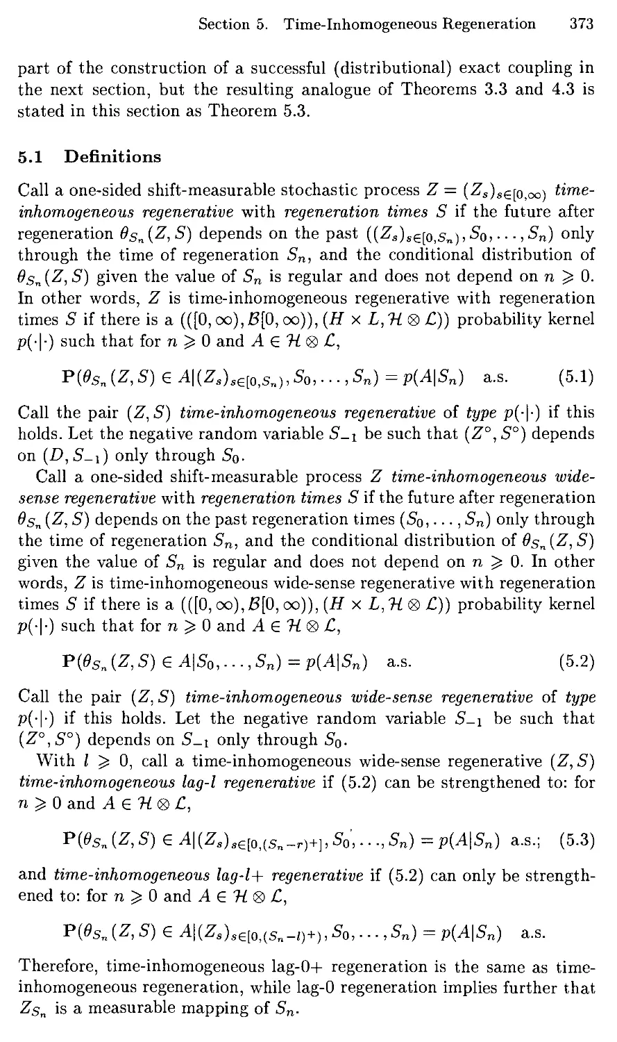
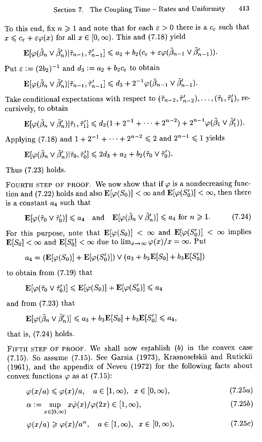
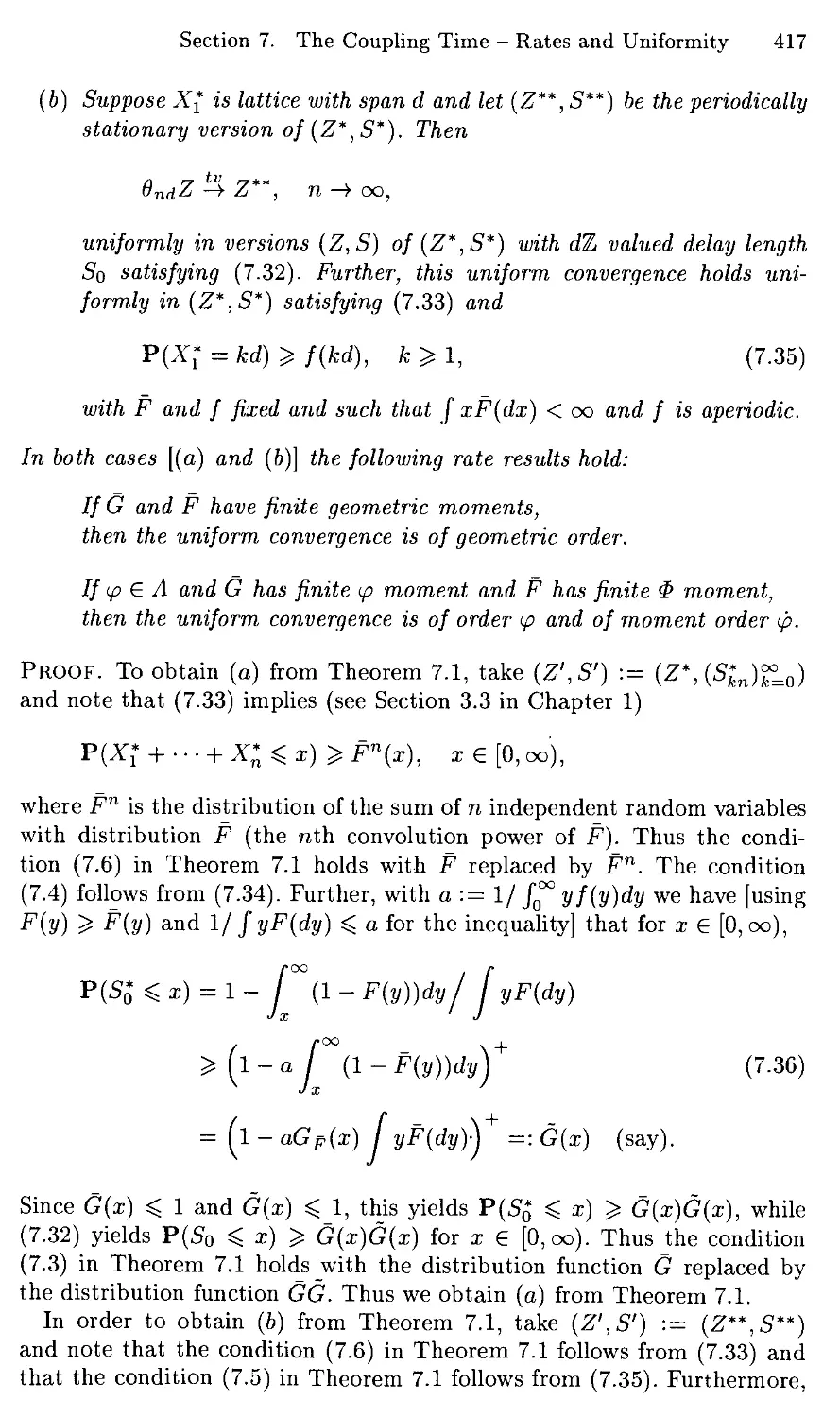
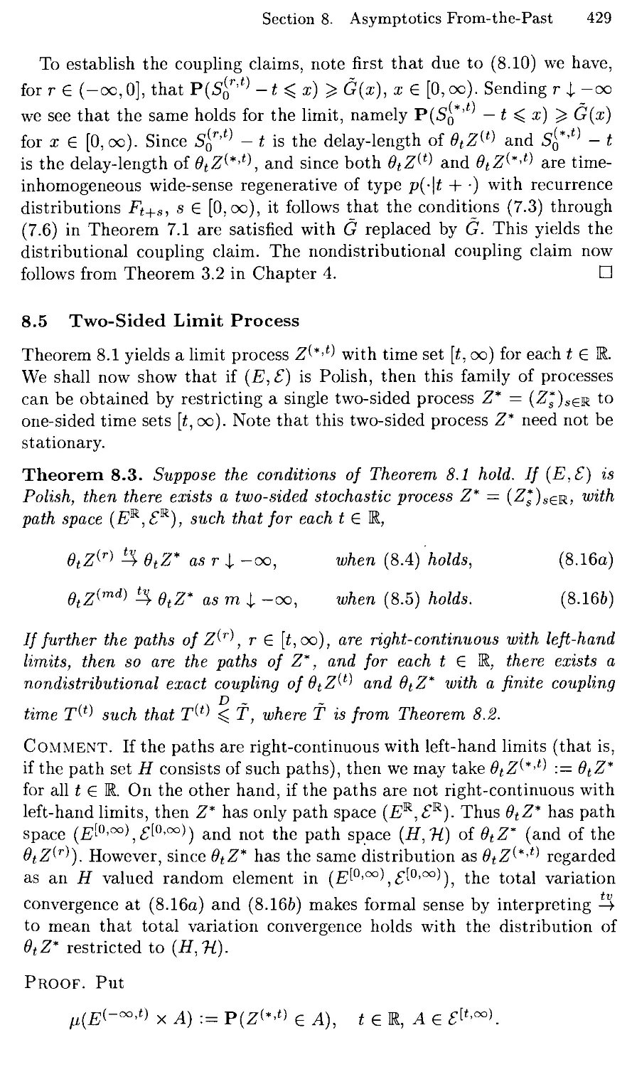
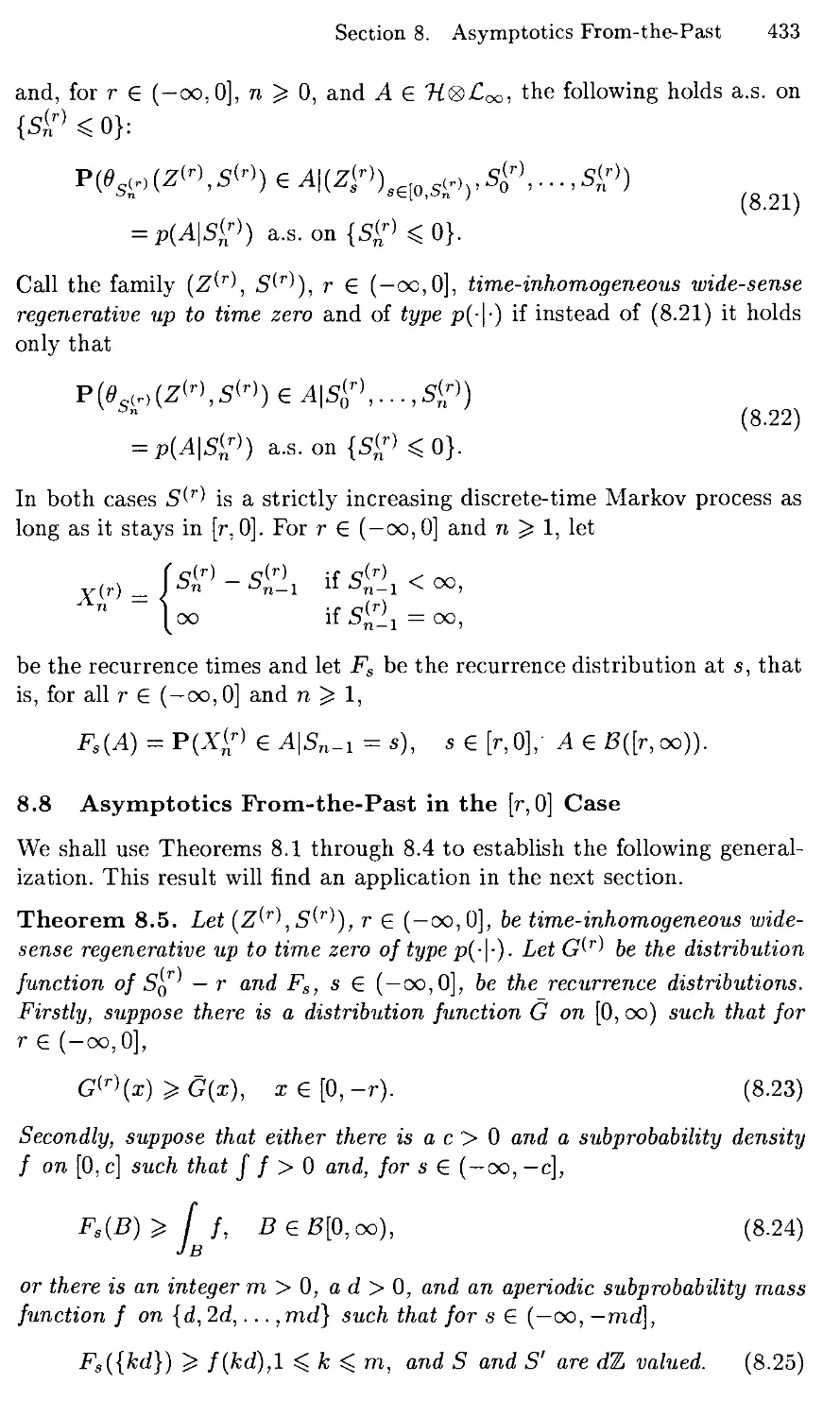
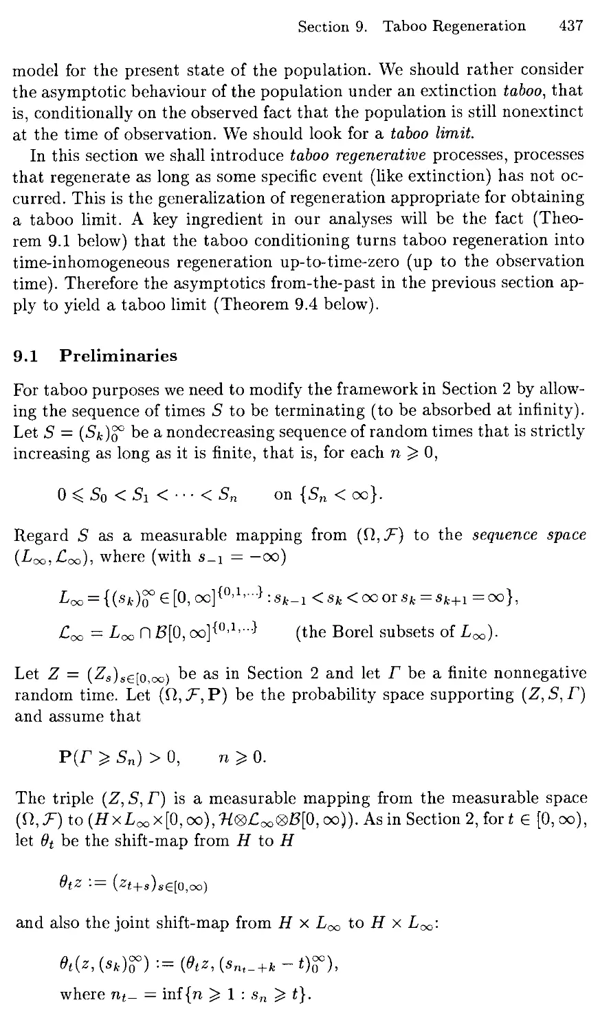
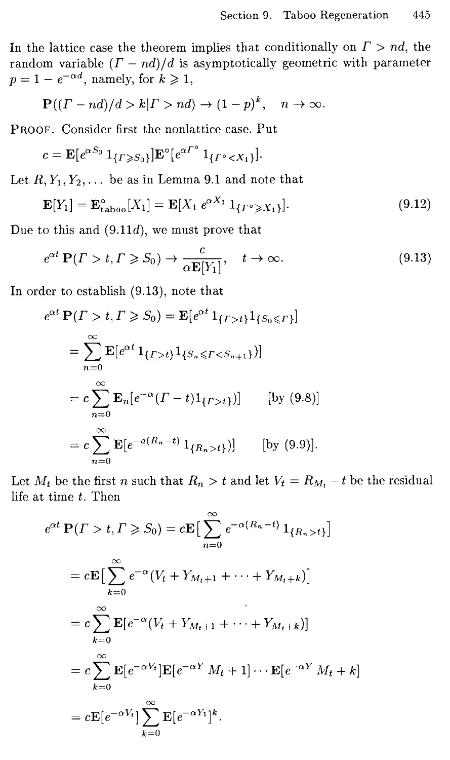
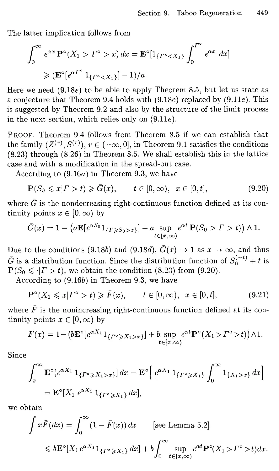
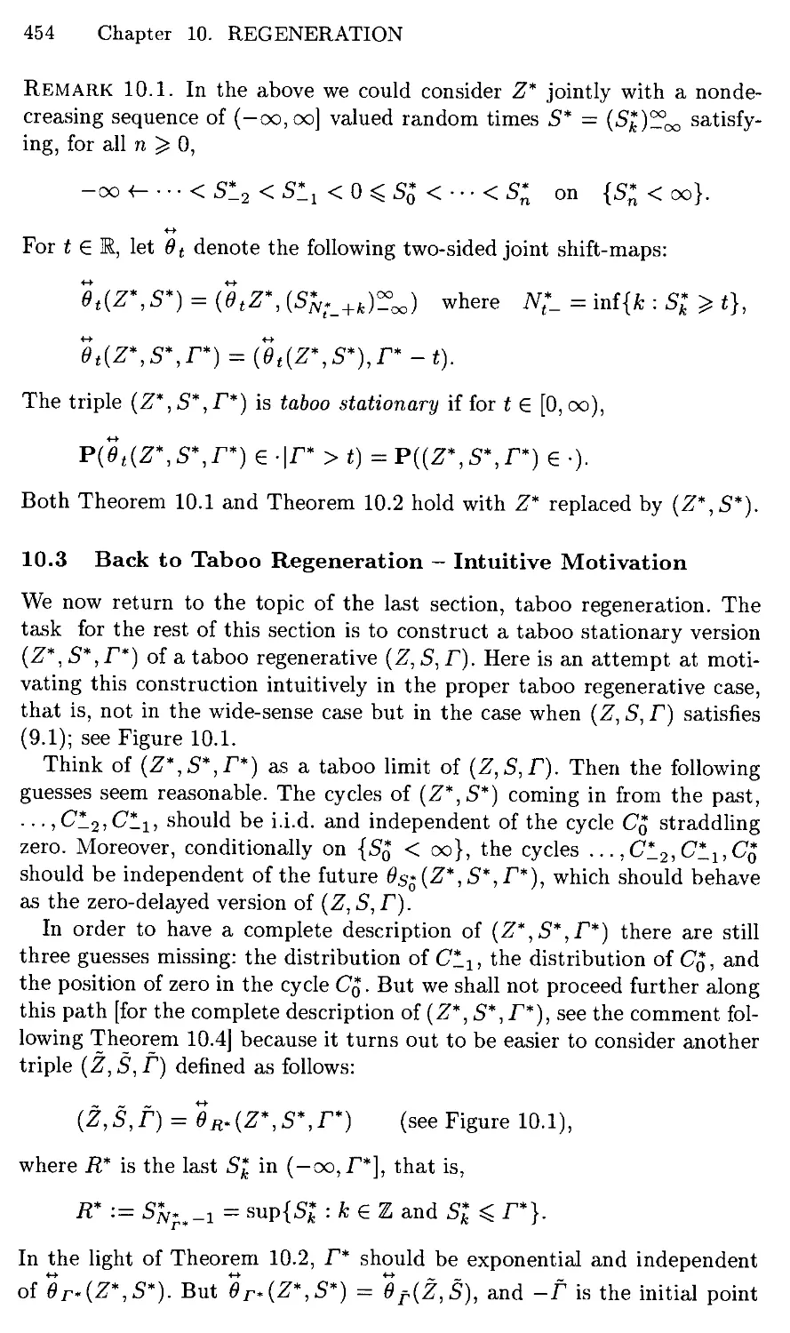
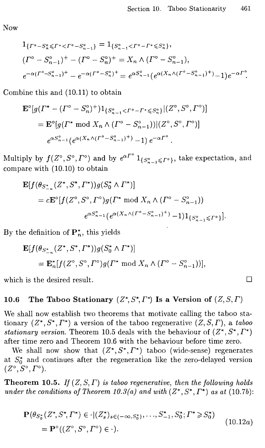
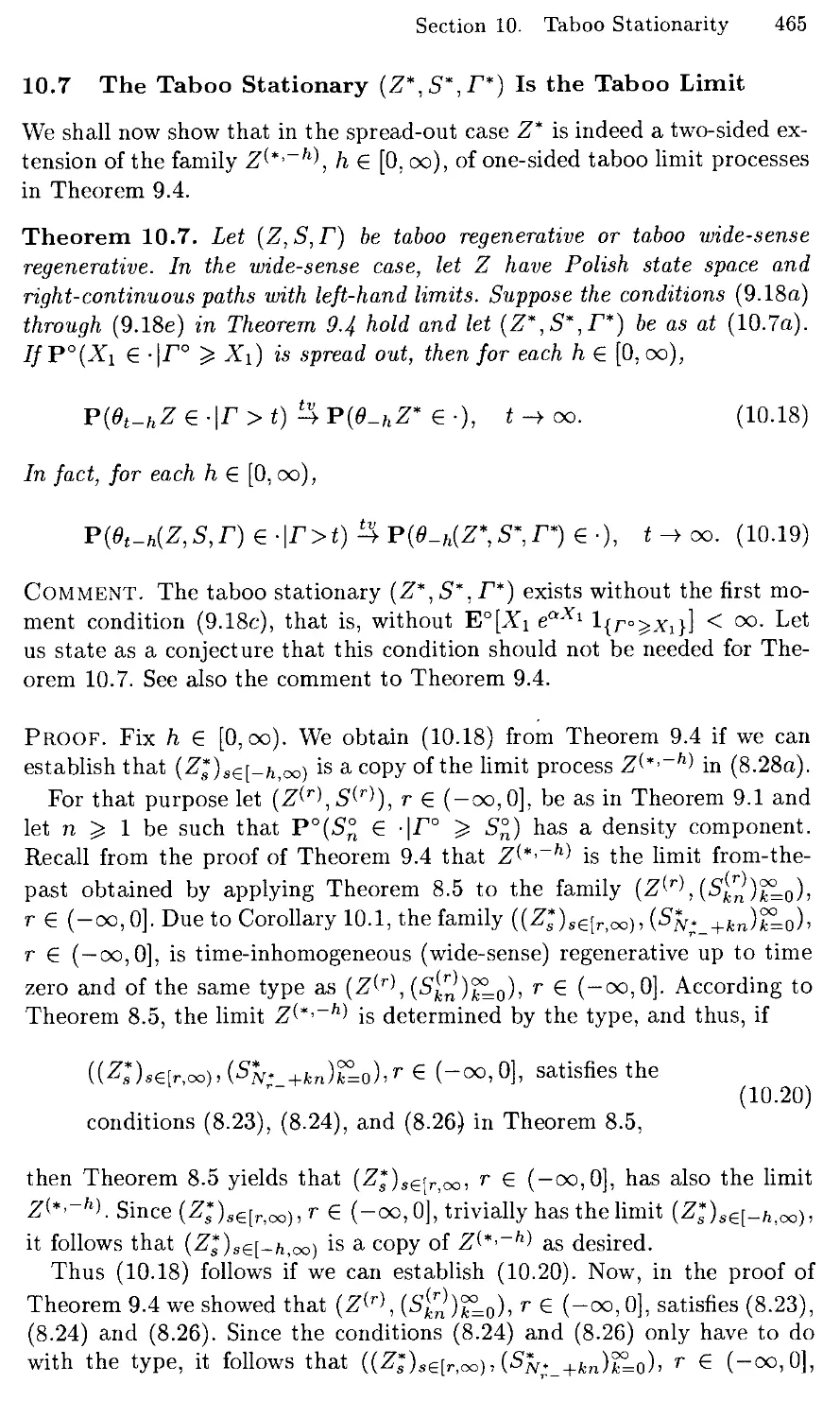
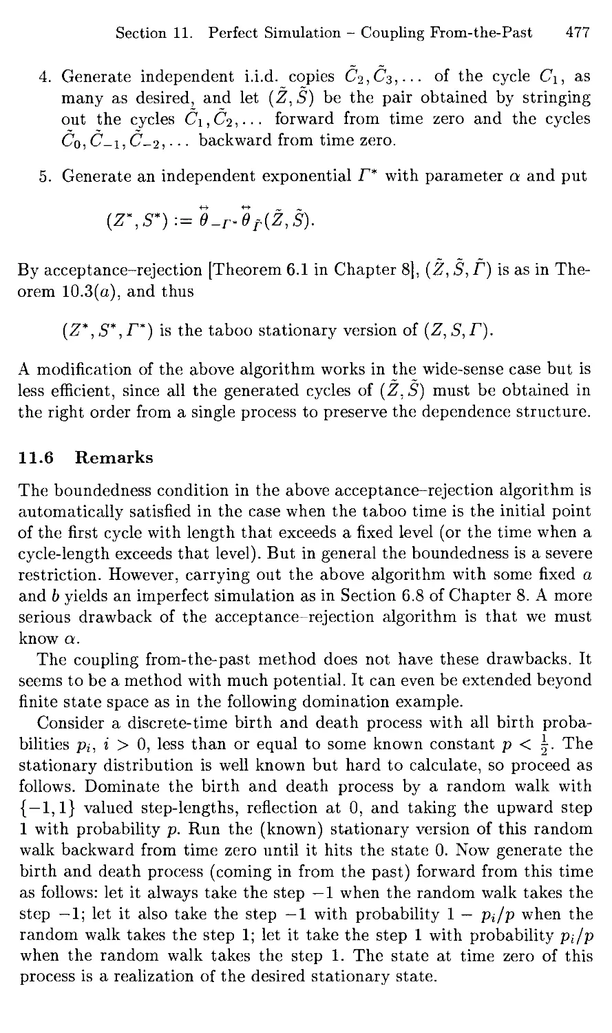
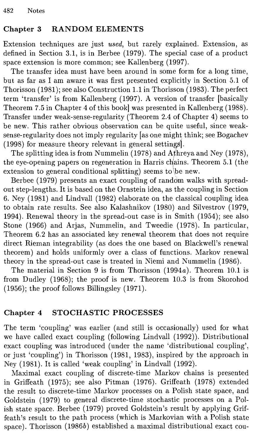
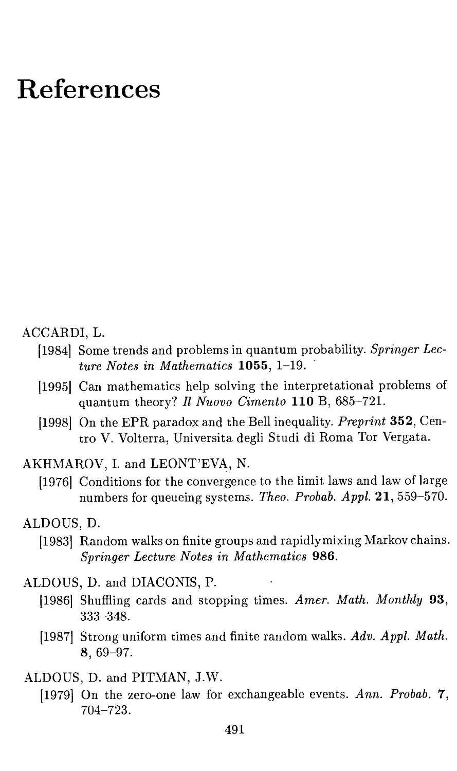
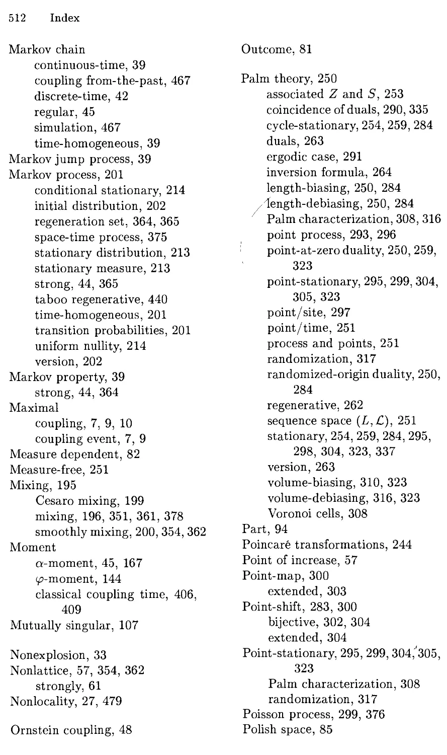
Let F"1 be the generalized inverse of F (or quantile function) defined by
F-1{u) = ini{xeR:F{x)^u}, u e [0,1].
Note that if F is continuous and strictly increasing, then F_1 is the ordinary
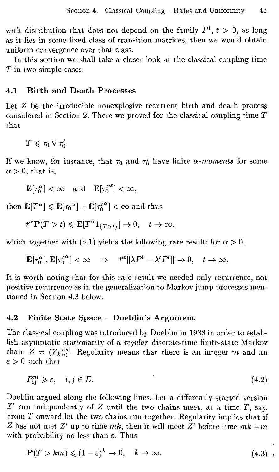
inverse of F (see Figure 3.1).
FIGURE 3.1. The generalized inverse F_1.
Let U be uniform on [0,1] (this is short for saying that U is a random
variable that is uniformly distributed on [0,1]). Then the random variable
X = F~1(U)
is a copy of X, since [note that F-1(u) ^ x if and only if u ^ F(x)]
P{X < i) = P(F_1 {U) ^x) = P(U ^ F{x)) = F(x), xeR.
Thus letting F run over the class of all distribution functions (using the
same U) yields a coupling of all differently distributed random variables.
Call it the quantile coupling.
Since F_1 is nondecreasing, we have, according to Section 2, that the
quantile coupling consists of positively correlated random variables. We
might even think of this coupling as a maximal dependence coupling
because knowing the value of only one of its variables, namely the value of U
itself, gives us the value of all the others.
4 Chapter 1. RANDOM VARIABLES
3.2 Application — Stochastic Domination
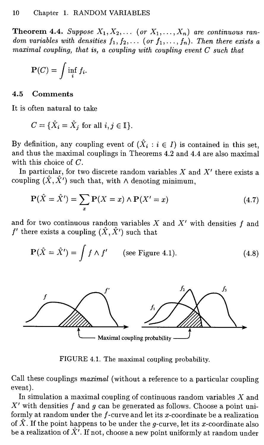
Let X and X' be two random variables with distribution functions F and
G, respectively. If there is a coupling (X, X') of X and X' such that X is
pointwise dominated by X', that is,
X^X',
then {X ^ x} D {X' ^ x}, which implies P(X ^ x) ^ P(X' ^ x) and
thus
F(x) ^ G(x), x e M.
(3-1)
If (3.1) holds, then X is said to be stochastically dominated (or dominated
in distribution) by X'. Denote this by
D
X ^ X'.
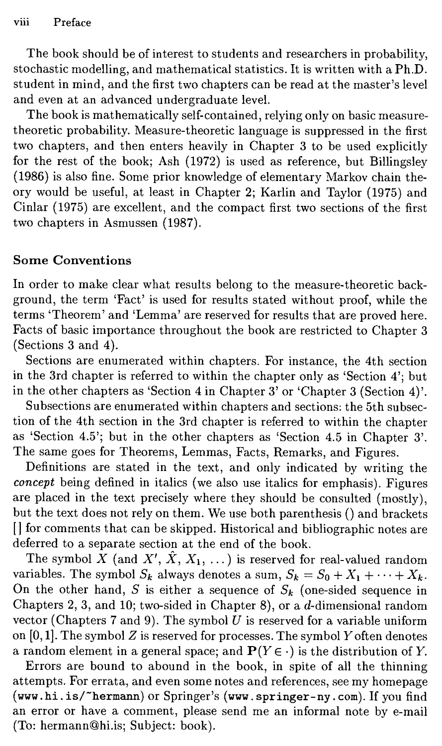
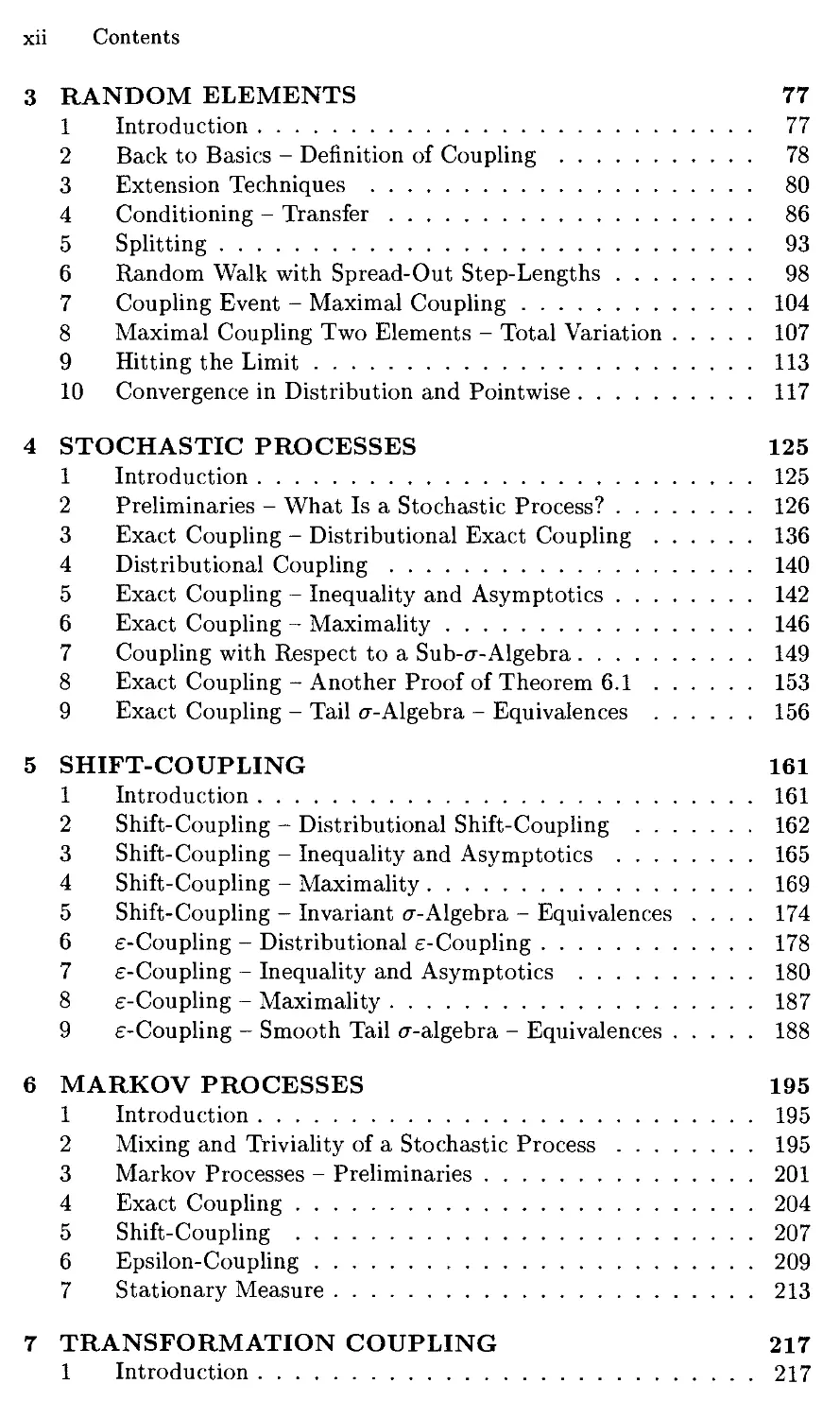
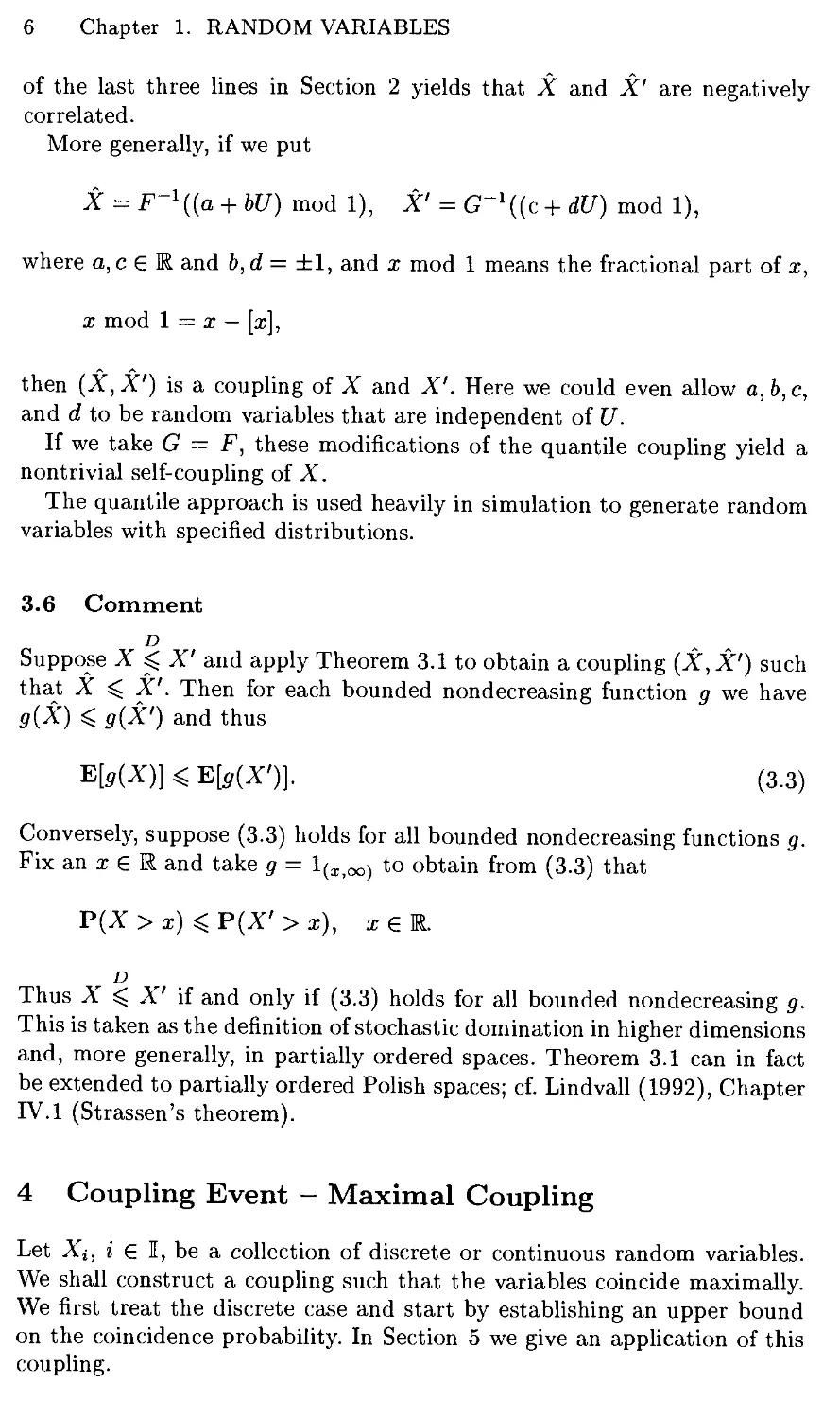
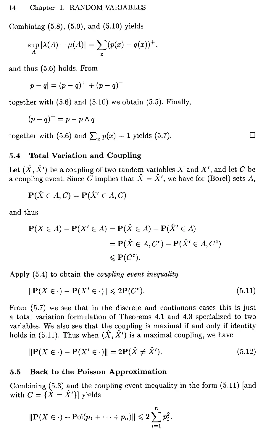
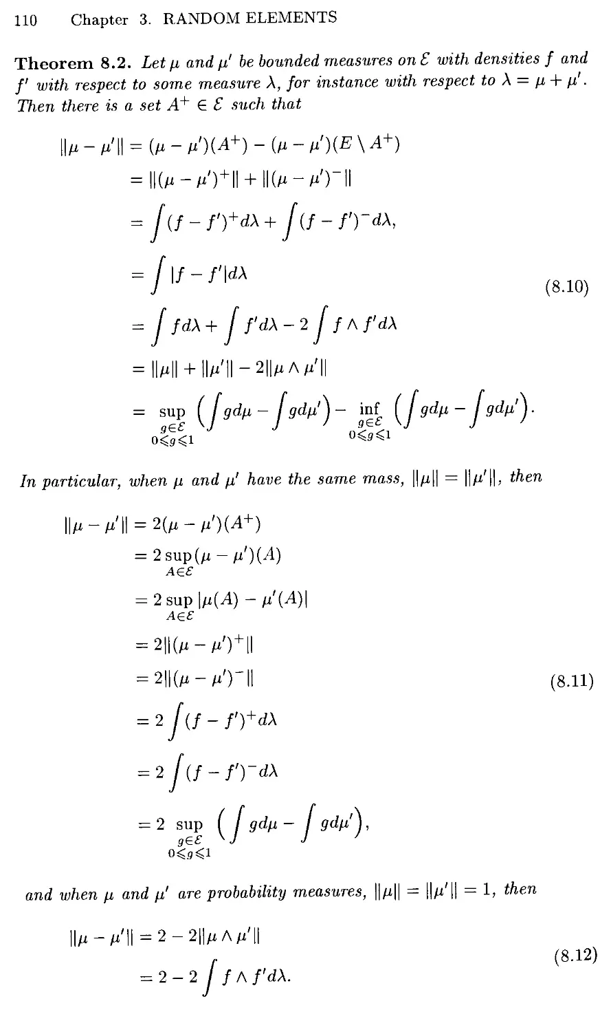
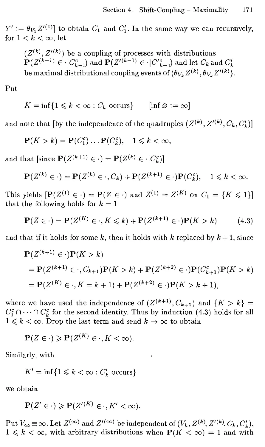
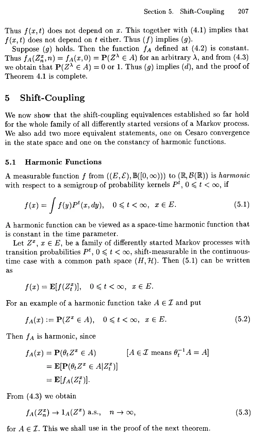
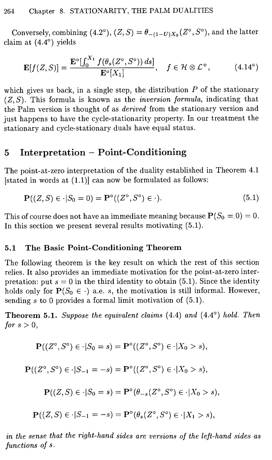
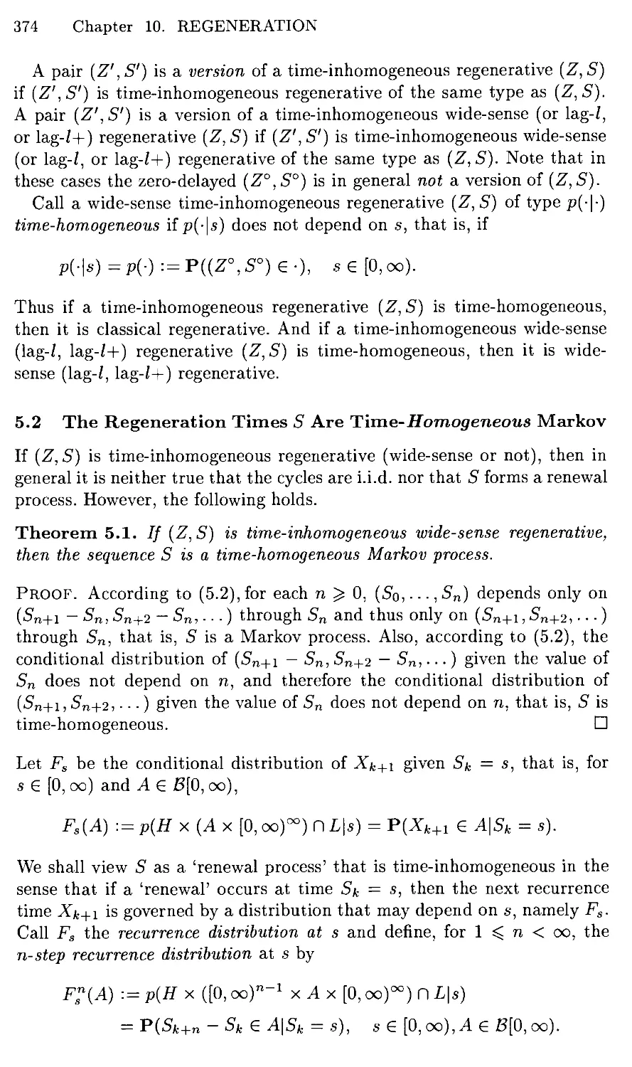
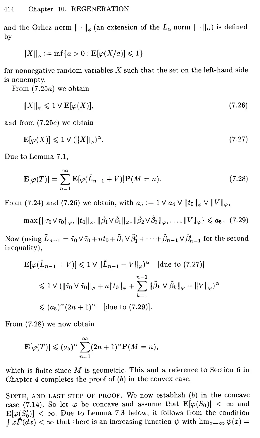
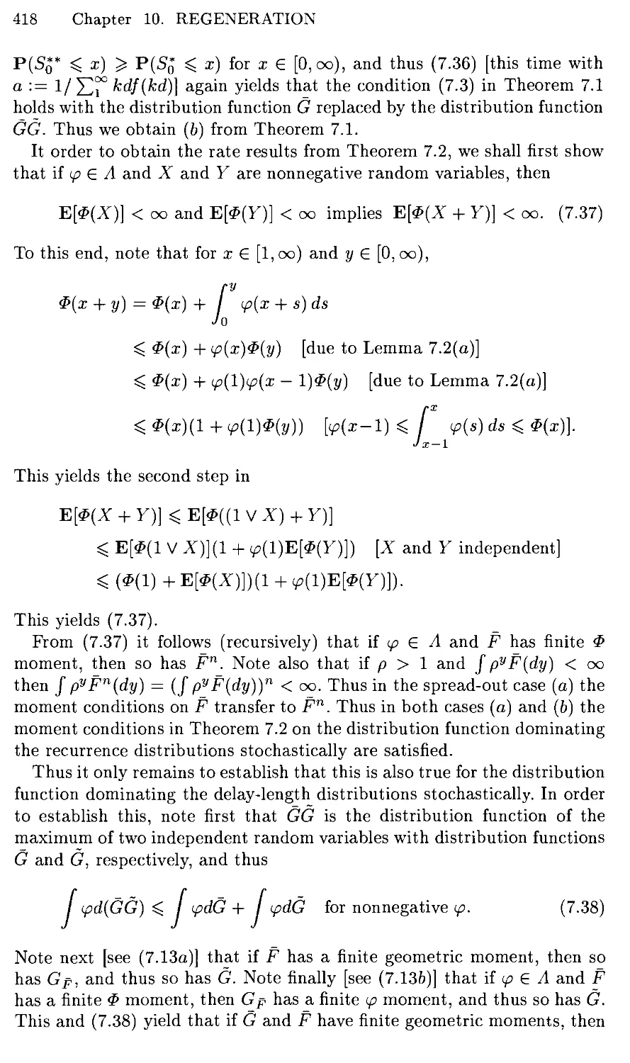
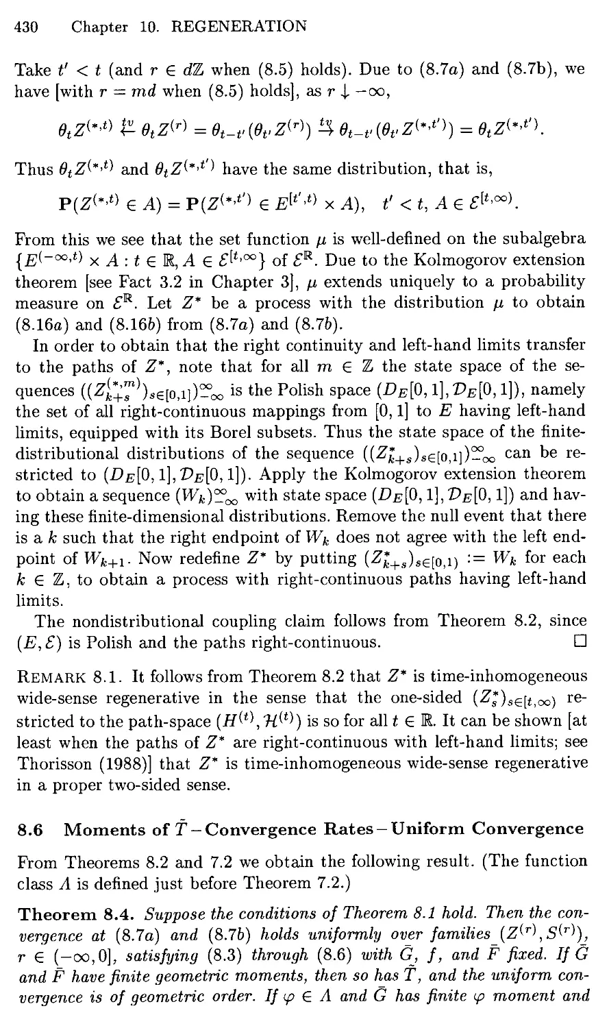
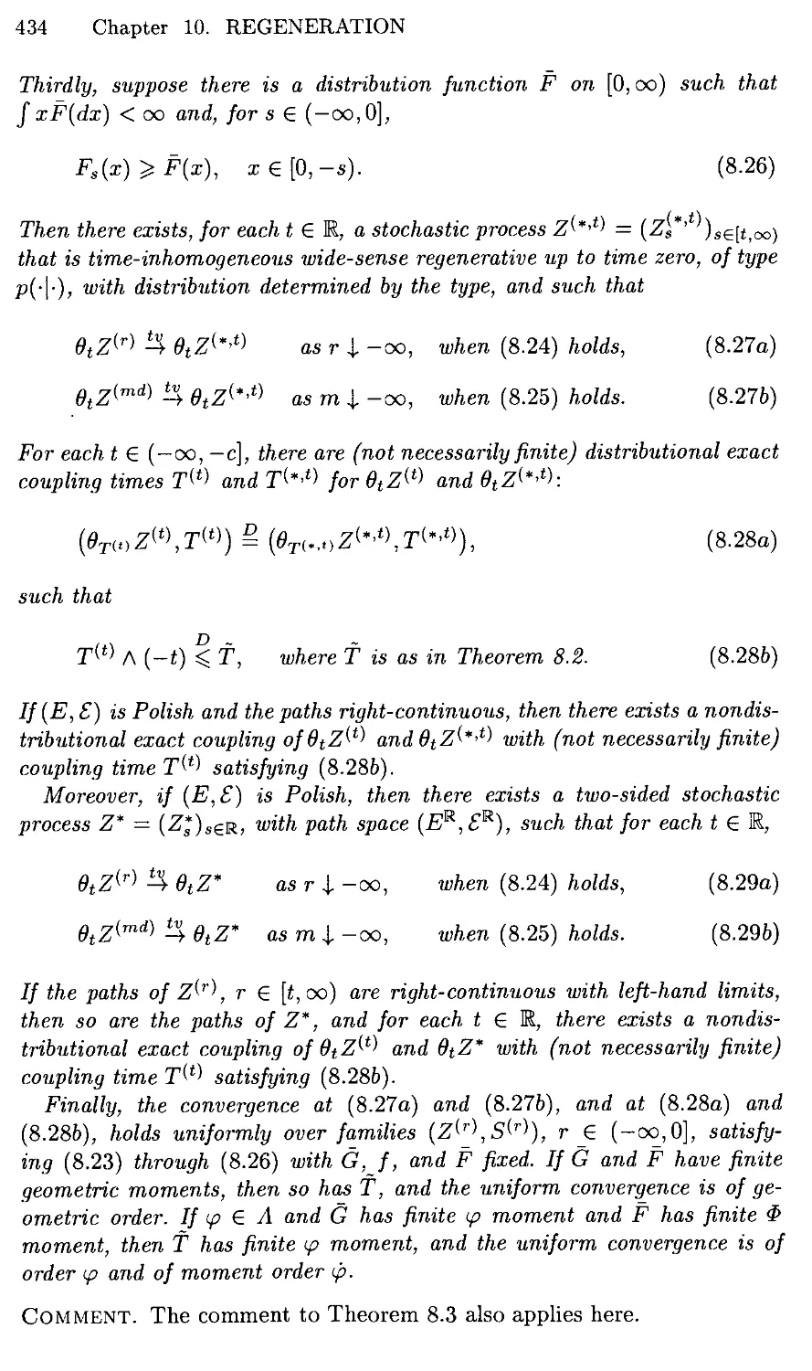
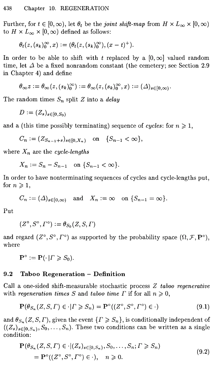
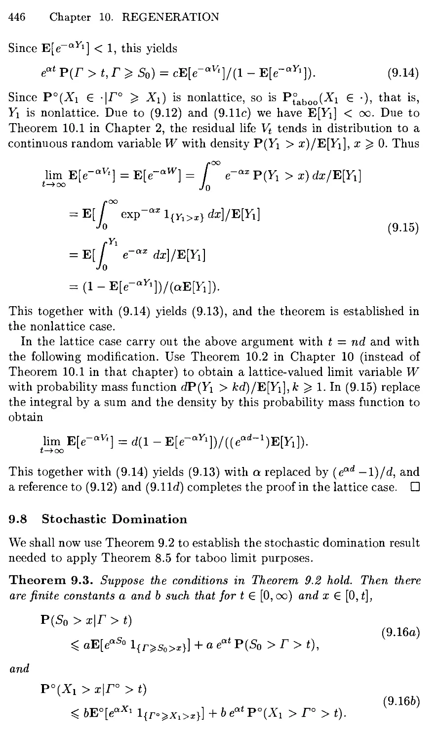
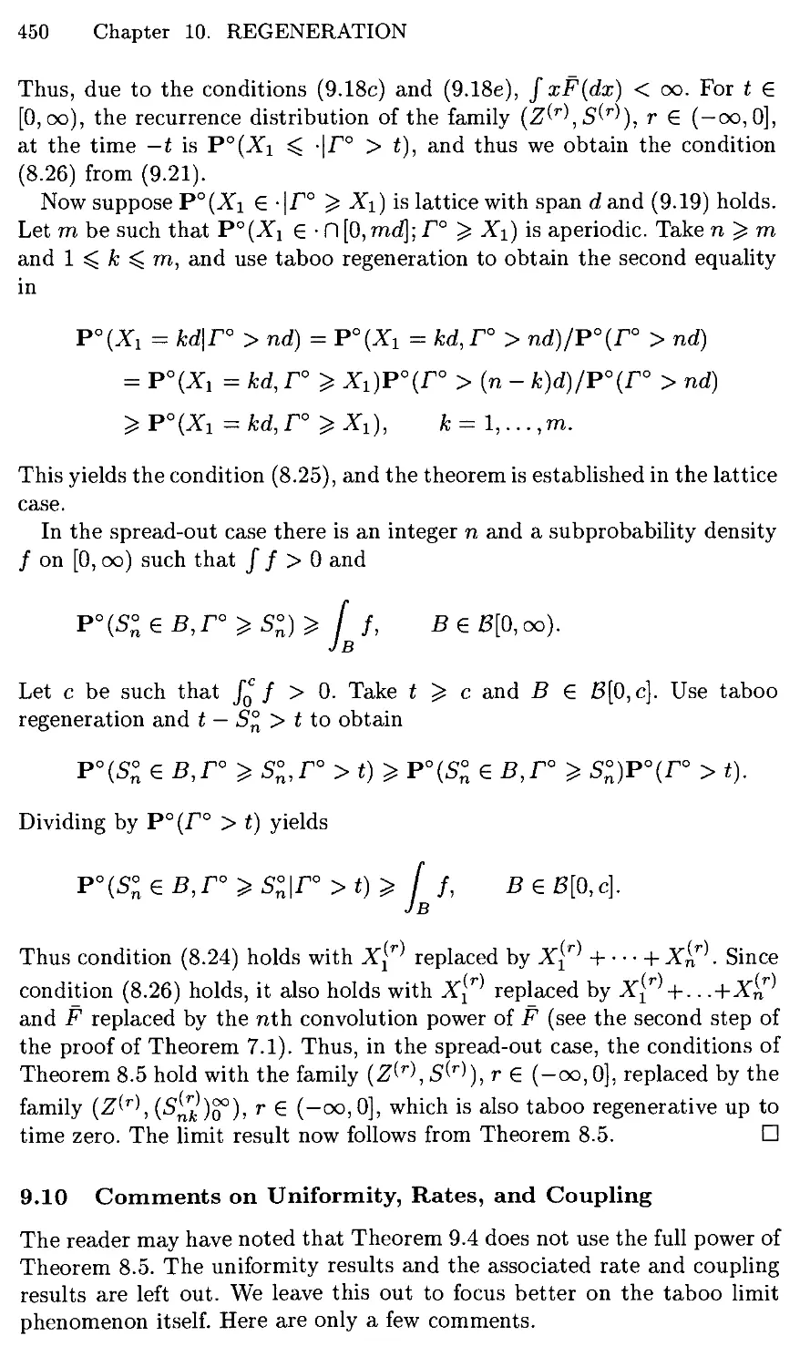
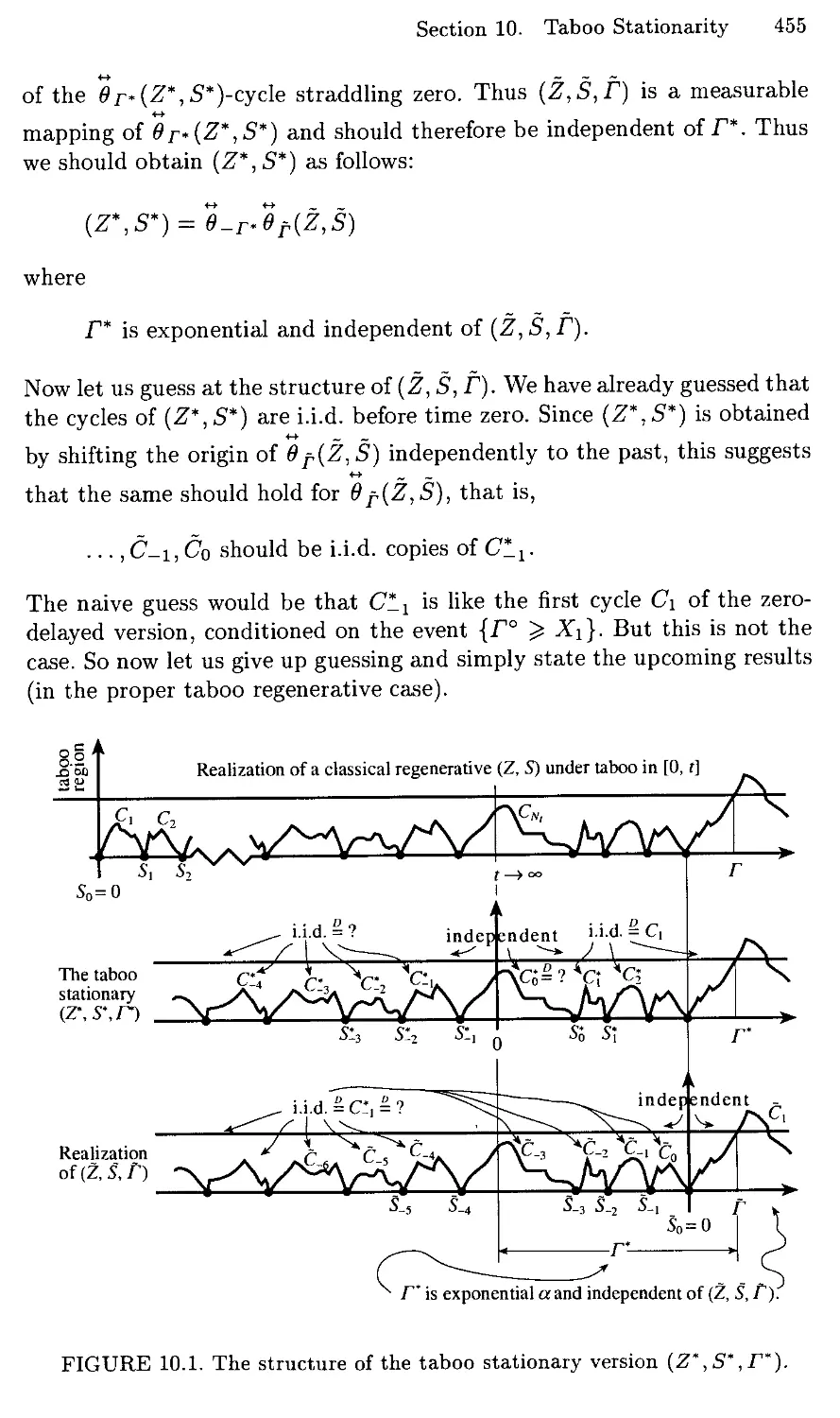
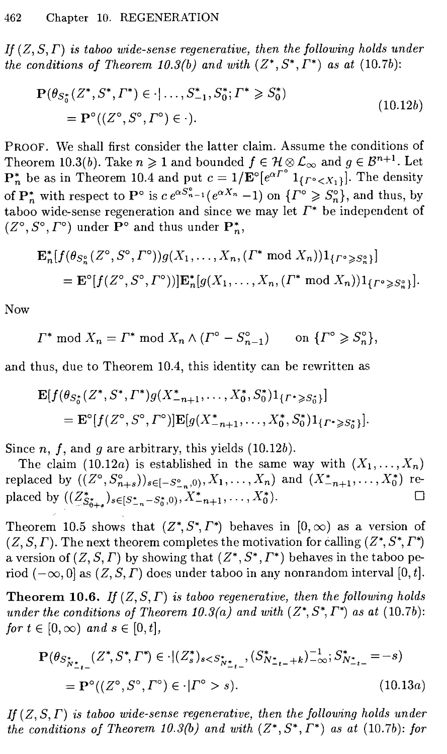
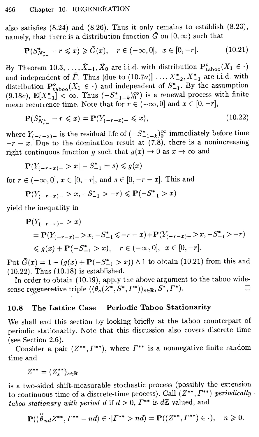
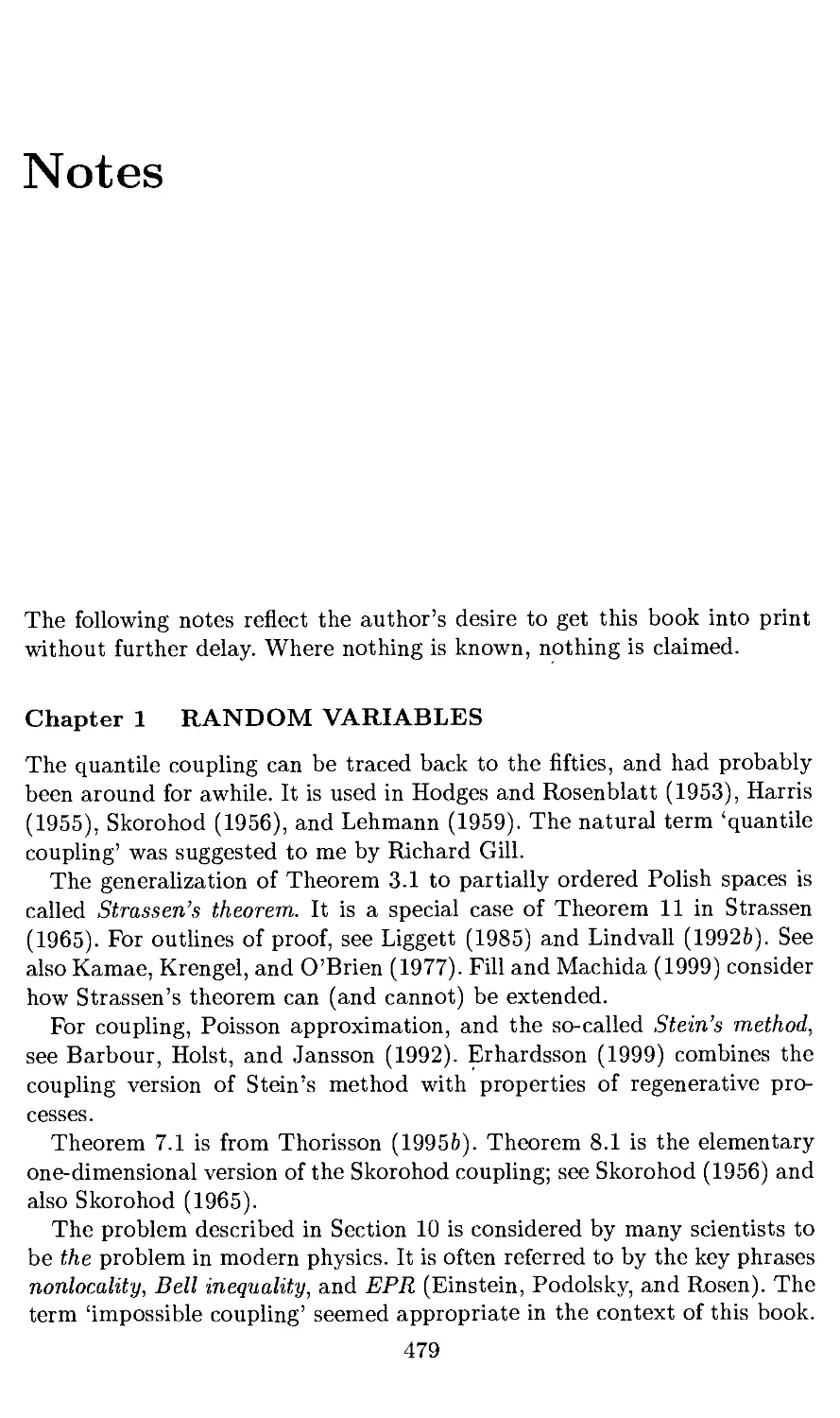
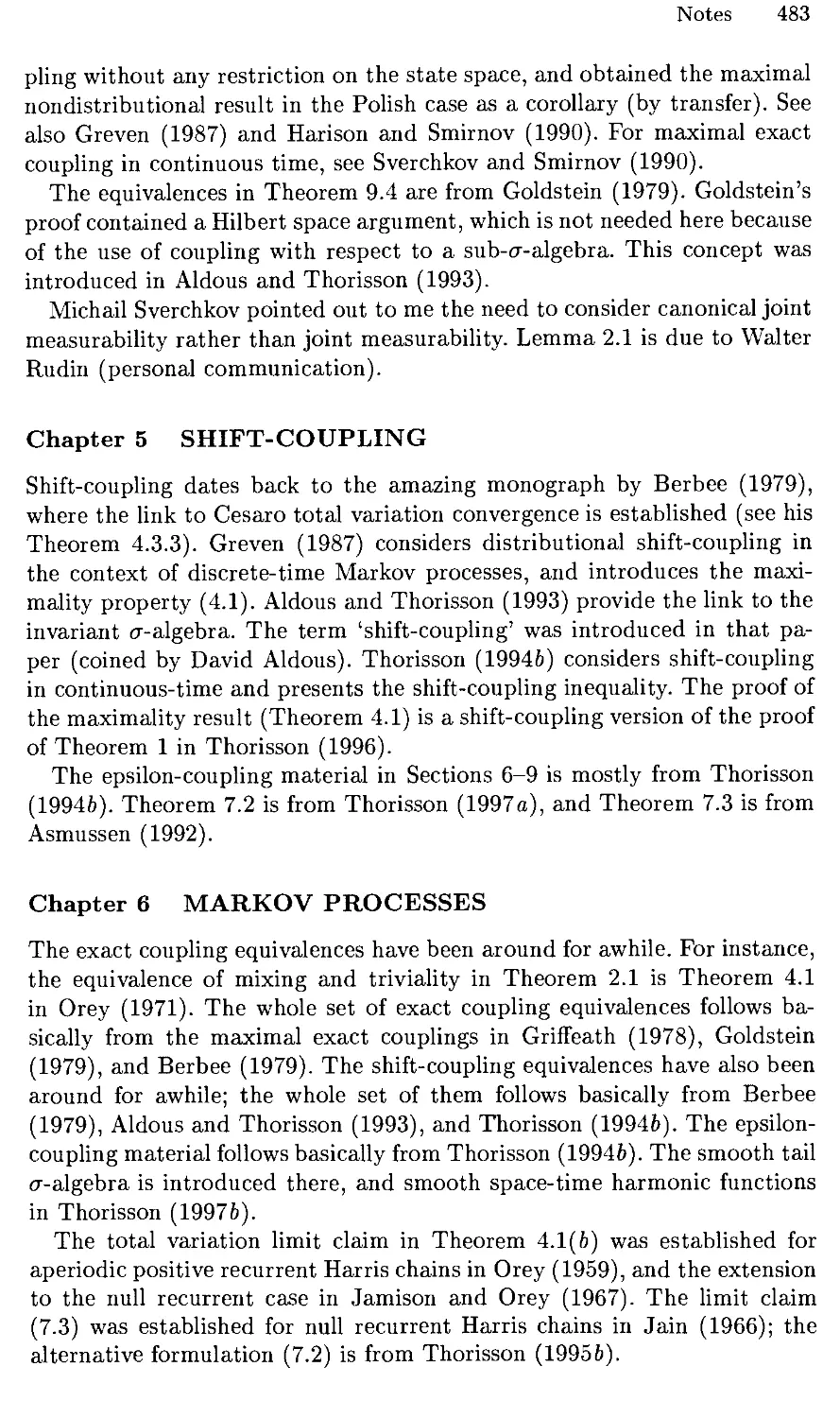
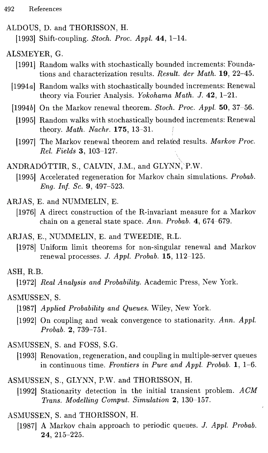
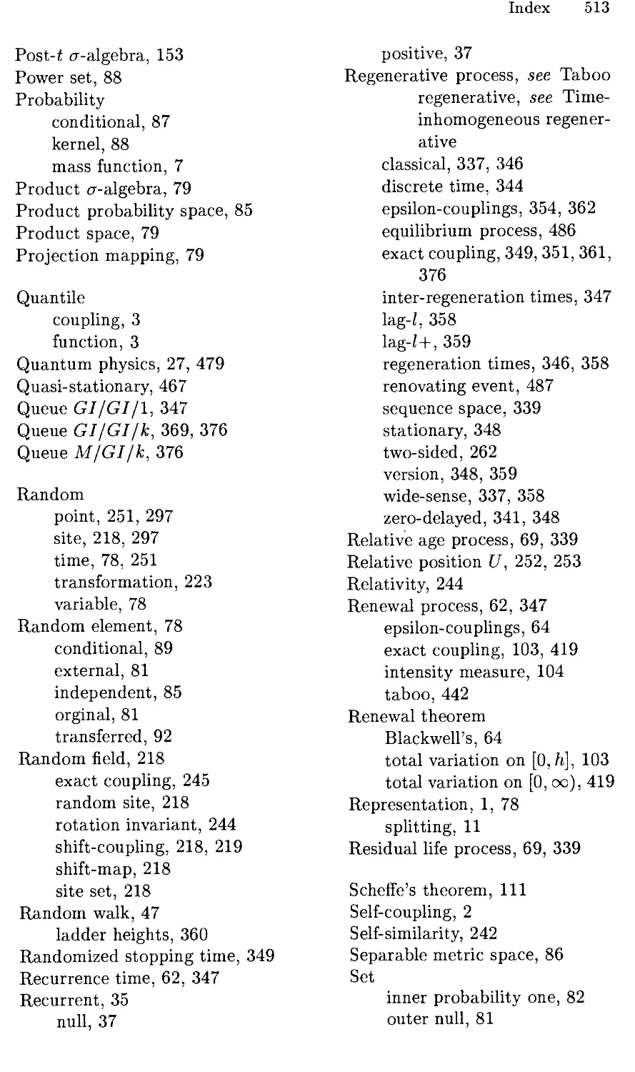
We shall now show that the quantile coupling turns stochastic domination
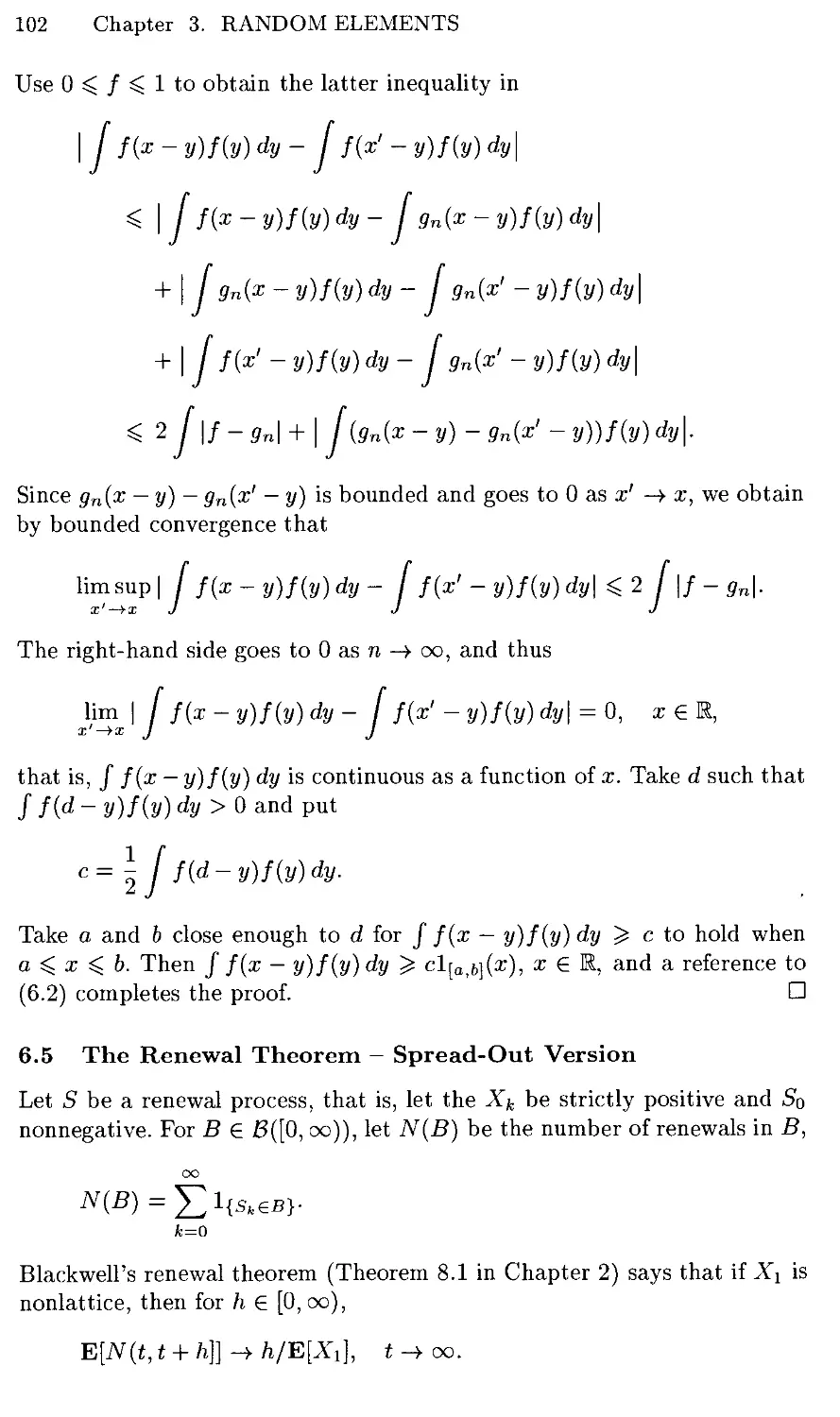
back into pointwise domination: due to (3.1), G(x) ^ u implies F(x) ^ u
and thus
{x e R : G{x) )ti}C{iel: F(x) ^ u}
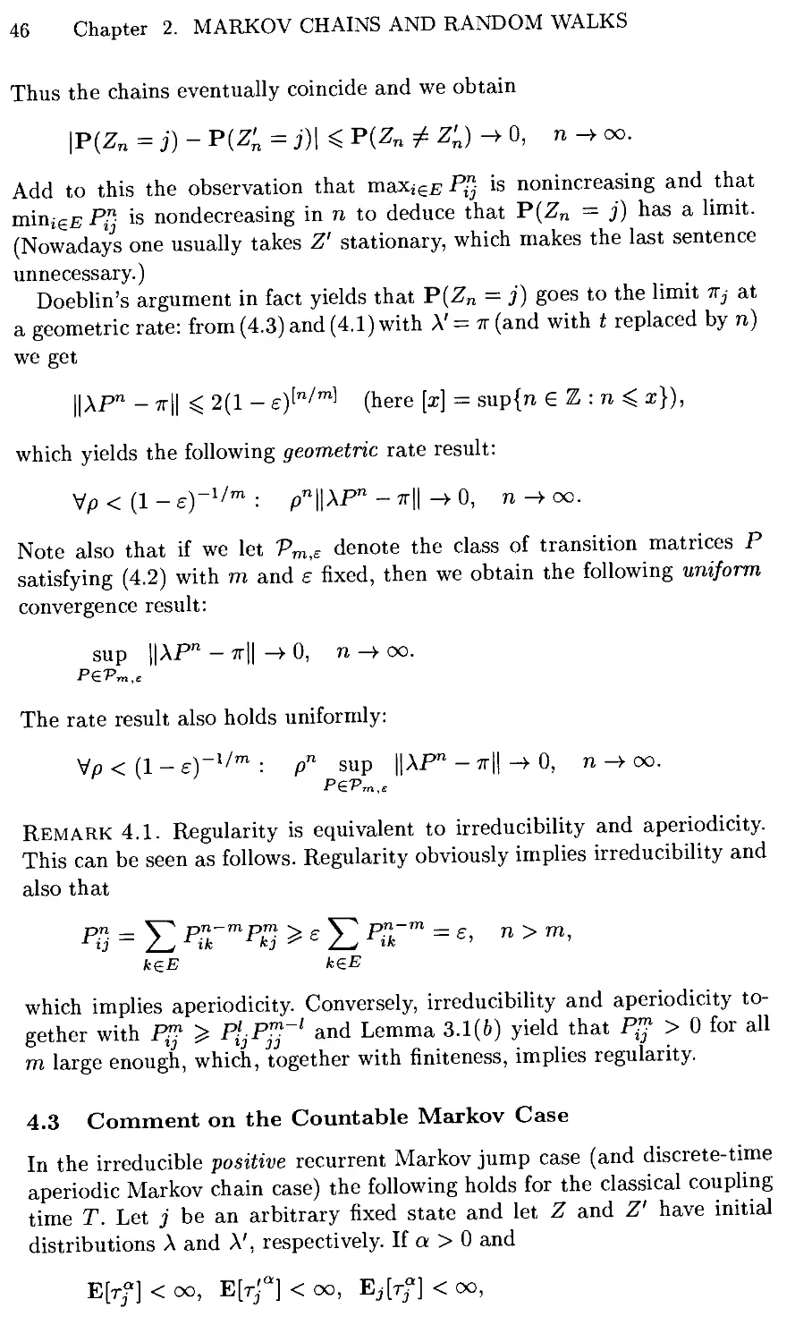
and thus F~\u) ^ G~\u), which yields F~\U) ^ G~\U) [see Figure 3.2].
FIGURE 3.2. Turning stochastic domination into pointwise domination.
We have established the following result.
Theorem 3.1. Let X and X' be random variables. Then
D
X ^X'
if and only if there is a coupling (X,X') of X and X' such that
X <X'.
Section 3. Quantile Coupling - Stochastic Domination 5
3.3 What For?
The direct usefulness of Theorem 3.1 is mainly due to the fact that it is
easier to carry out arguments using pointwise domination than stochastic
domination. As an illustration of this we shall prove the following result.
Corollary 3.1. Let Xi,X2,X[, and X2 be random variables such that
X\ and X2 are independent,
X[ and X'2 are independent,
Xx J X[ and X2 J X2.
Then
X1+X2^X[+X2. (3.2)
Proof. Let (Xi,X[) be a coupling of Xi and X[ such that XY ^ X[ and
let {X2,X^} be a coupling of X2 and X2 such that X2 f X2. Let {XUX[)
and (X2,X2) be independent. Then (Xi + X2,X{ + X2) is a coupling of
Xi + X2 and X[ + X2, and
Xl+X2^X[+X'2.
This implies (3.2). □
A more substantial example of obtaining a distributional result through a
pointwise argument by way of coupling can be found in Section 9, where we
use the quantile coupling to obtain the distributional version of dominated
convergence from the standard pointwise version.
3.4 On the General Coupling Idea
Theorem 3.1 and Corollary 3.1, illustrate two general points about coupling.
Firstly, a coupling characterization of a distributional property deepens our
understanding of that property: according to Theorem 3.1, stochastic
domination is simply the distributional form of pointwise domination. Secondly,
the coupling characterization can also be directly useful because it is easier
to argue pointwise (as in the proof of Corollary 3.1) than in distribution.
3.5 Variations on the Quantile Coupling
Let U be uniform on [0,1] and define
X = F-\U), X' = G~1(1-U).
Then (X, X') is still a coupling of X and X', since 1 — U is also uniform on
[0,1]. Now G_1(l — u) is nonincreasing in u, and an obvious modification
6 Chapter 1. RANDOM VARIABLES
of the last three lines in Section 2 yields that X and X' are negatively
correlated.
More generally, if we put
X = F~l{(a + bU) mod 1), X' = G'1 ((c + dU) mod 1),
where a,c € M and b, d = ±1, and x mod 1 means the fractional part of x,
x mod 1 = x — [x],
then (X,X') is a coupling of X and X'. Here we could even allow a,b,c,
and d to be random variables that are independent of U.
If we take G = F, these modifications of the quantile coupling yield a
nontrivial self-coupling of X.
The quantile approach is used heavily in simulation to generate random
variables with specified distributions.
3.6 Comment
D „ „
Suppose X ^ X' and apply Theorem 3.1 to obtain a coupling (X, X') such
that X ^ X'. Then for each bounded nondecreasing function g we have
g(X) ^ g(X') and thus
E[g(X)} < E[P(X')]. (3.3)
Conversely, suppose (3.3) holds for all bounded nondecreasing functions g.
Fix anigl and take g = l^oo) to obtain from (3.3) that
P(X >x)^ P{X' > x), x € BL
Thus X ^ X' if and only if (3.3) holds for all bounded nondecreasing g.
This is taken as the definition of stochastic domination in higher dimensions
and, more generally, in partially ordered spaces. Theorem 3.1 can in fact
be extended to partially ordered Polish spaces; cf. Lindvall (1992), Chapter
IV.1 (Strassen's theorem).
4 Coupling Event - Maximal Coupling
Let Xi, i € I, be a collection of discrete or continuous random variables.
We shall construct a coupling such that the variables coincide maximally.
We first treat the discrete case and start by establishing an upper bound
on the coincidence probability. In Section 5 we give an application of this
coupling.
Section 4. Coupling Event - Maximal Coupling 7
4.1 The Coupling Event Inequality — Discrete Variables
Suppose (Xi : i £ I) is a coupling of X^, i £ I, and let C be an event such
that if C occurs, then all the Xi coincide, that is,
C C {Xi = Xj for all j, j £ I}.
Call such an event a coupling event.
Consider first the discrete case: let all the Xi take values in a finite or
countable set E and denote the probability mass functions by pi, that is,
for x £ E,
P(Xi=x)=Pi(x).
For all i,j £ I and x £ E we have
P(Xi =x,C) = P(Xj = x,C)^ Pj{x)
and thus for all i £ I and x £ E
P{Xi =x,C) ^infp^x).
Summing over x £ E yields the following basic coupling event inequality.
Theorem 4.1. If C is a coupling event of a coupling of discrete random
variables Xi, i £ I, taking values in a finite or countable set E, then
P(C) <Y,infPi(x). (4.1)
4.2 Maximal Coupling — Discrete Variables
We shall now construct a coupling with a coupling event C such that (4.1)
holds with identity. Call such a coupling maximal and C a maximal
coupling event. Put
c := 2_, inf Pj(x) (the maximal coupling probability).
xeE'€
If c = 0, take the Xi independent and C = 0. If c = 1, take the Xi
identical and C = 0 = the set of all outcomes. If 0 < c < 1, let us mix
these couplings as follows. Let
/, V, and Wi, i £ I, be independent random variables
such that
/ is 0-1 valued with P(I = 1) = c,
P(y = x) =mipi(x)/c, x £ E.
P(Wi =x) = (pi{x) - cP{V = x))/(l -c), x£ E.
8 Chapter 1. RANDOM VARIABLES
Define, for each i £ I,
[Wi if 7 = 0. K J
Then
P(Xt =x)= P(V = x)P(I = 1) + P(Wi = x)P(7 = 0)
= P(Xi = a:).
Moreover, C= {1= 1} is a coupling event and P(C) has the desired value c.
We have established the following result.
Theorem 4.2. Suppose Xi, i £ I, are discrete random variables taking
values in a finite or countable set E. Then there exists a maximal coupling,
that is, a coupling with coupling event C such that
P(C) = £ MPi(x).
»€I
x€E
4.3 The Coupling Event Inequality — Continuous Variables
Now let the X{ be continuous random variables with densities /,, that is,
for intervals A
P{Xi £ A) = / fi (which is short for / fi(x)dx).
J A J A
It is a little harder to establish the coupling event inequality in this case,
and we shall make the simplifying assumption that the X, are either finitely
or count ably many, that is,
I = {l,...,n} or I={1,2,...}.
Suppose (Xi : » £ I) is a coupling of Xi, i £ I, and C is a coupling event.
Then, for intervals A and i,j £ I,
P(Xi £A,C) = P(Xj £A,C)^ [ fj. (4.3)
J A
Consider first the finite case I = {1,..., n} and define a partition of E by
A1 ={x£ E: /!(x) = inf fj(x)}
and recursively for 1 < k ^ n
Ak = {x £ E : fk(x) = inf fj(x)}\(A1U---UAk-1).
Section 4. Coupling Event - Maximal Coupling 9
Then (4.3) yields the inequality in
P(Xi GAnAk,C)^ [ fj= [ inf fk, (4.4)
JAr\Ak JAnAk Kj<n
while the equality follows from the definition of Ak- Sum over A; £ I to
obtain, in the finite case, that
P(Xi g A,C)^ /inf/j, iGl. (4.5)
Ja^1
In the countable case I = {1,2,...} fix n < oo to obtain that (4.4) still
holds for i,k ^ n. This yields (4.5) with infjgi fj replaced by infi^j^n fj.
Sending n —> oo yields (4.5), since infi^-^n fj decreases to inf j€i fj.
Take A = E in (4.5) to obtain the following coupling event inequality.
Theorem 4.3. If C is a coupling event of a coupling of continuous random
variables with densities f\, fi,... (or /i,..., fn), then
P(C)^Jmifi- (4-6)
4.4 Maximal Coupling — Continuous Variables
Call a coupling and event achieving identity in (4.6) maximal. The
construction in Section 4.2 extends with an obvious modification to the continuous
case. Put
/inf
J iGI
fi (the maximal coupling probability).
If c = 0, take the Xt independent and C = 0. If c = 1, take the Xt identical
and C = 0. If 0 < c < 1, mix these couplings as follows. Let
/, V, and Wi, i £ I, be independent random variables
such that
/ is 0-1 valued with P(I = 1) = c,
V has density inf file,
i€I
Wi has density (fi - inf /j)/(l - c).
JGI
Define Xi by (4.2). Then (Xj : i 6 I) is a coupling of the Xi, since for
intervals A,
P{Xi £i) = P{V £ A)P(7 = 1) + P(Wi £ A)P(7 = 0)
= P(Xi e A).
Moreover, C = {I = 1} is a coupling event, and P(C) has the desired
value. We have established the following result.
10 Chapter 1. RANDOM VARIABLES
Theorem 4.4. Suppose X\,X2, ■ ■ ■ (or X\,..., Xn) are continuous
random variables with densities /i, /2, • • • (or f\,..., /„). Then there exists a
maximal coupling, that is, a coupling with coupling event C such that
\C) = Jmifi.
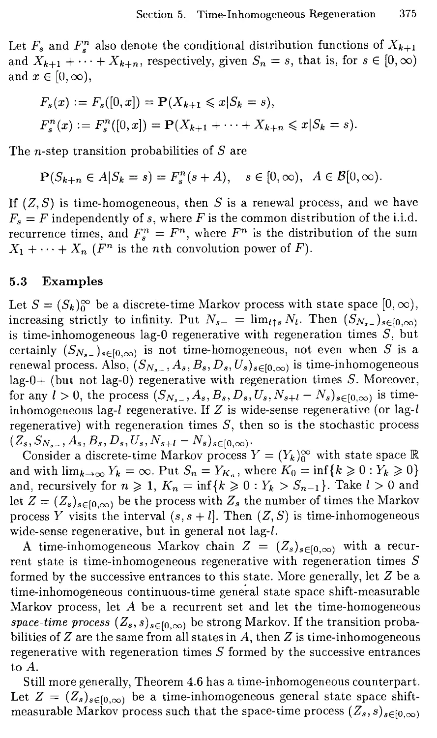
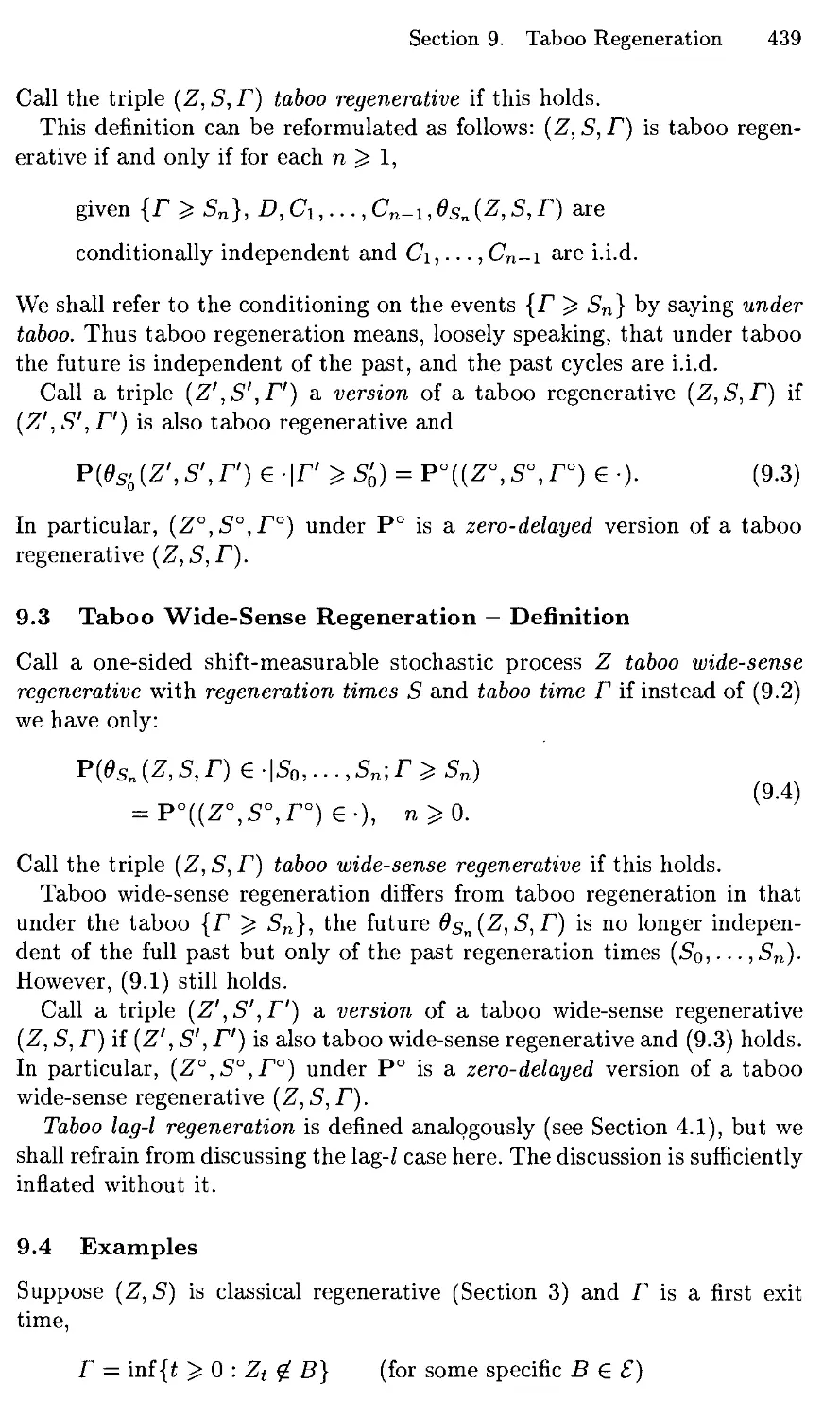
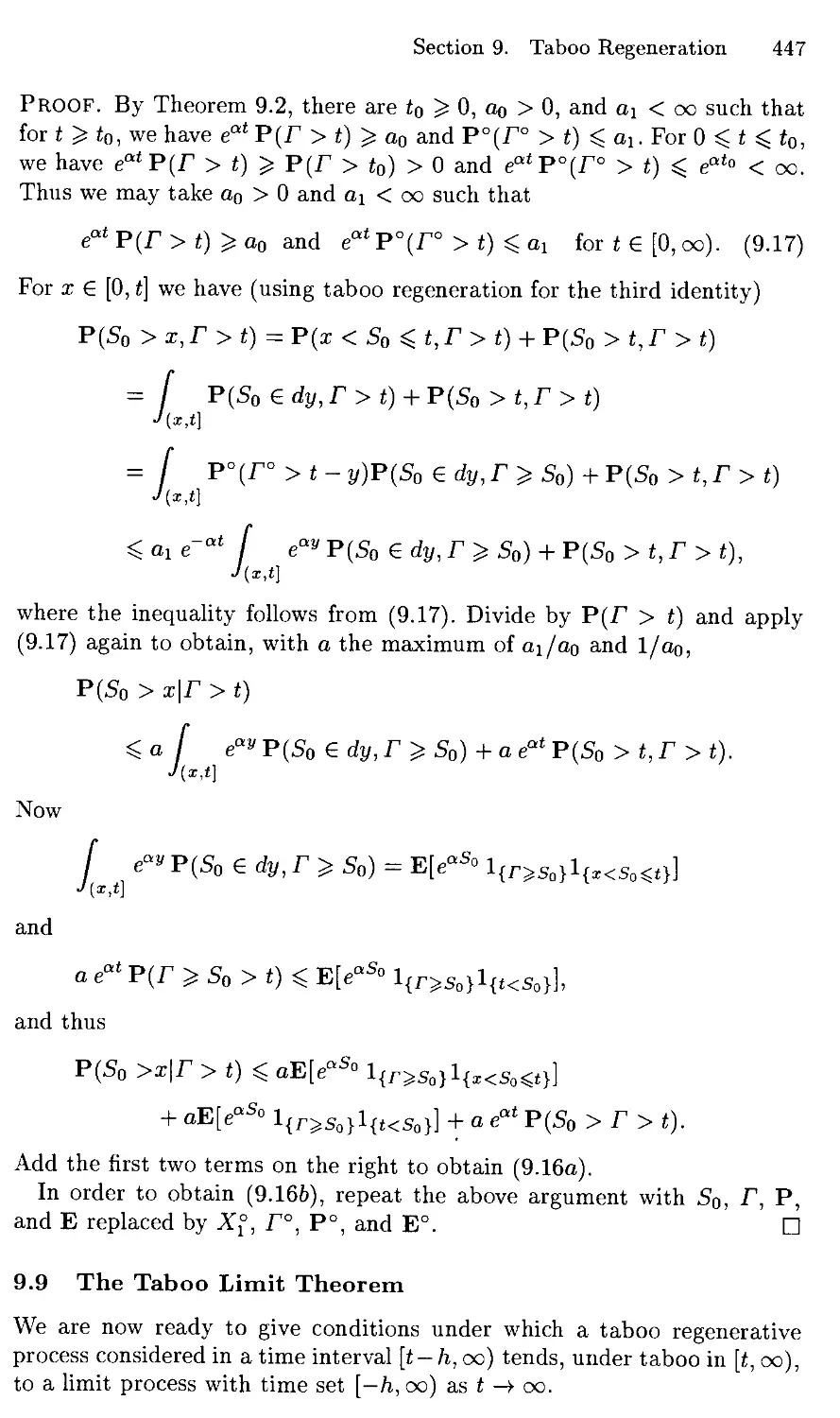
4.5 Comments
It is often natural to take
C={Xi = Xj for alH,./el}.
By definition, any coupling event of (Xt : i £ I) is contained in this set,
and thus the maximal couplings in Theorems 4.2 and 4.4 are also maximal
with this choice of C.
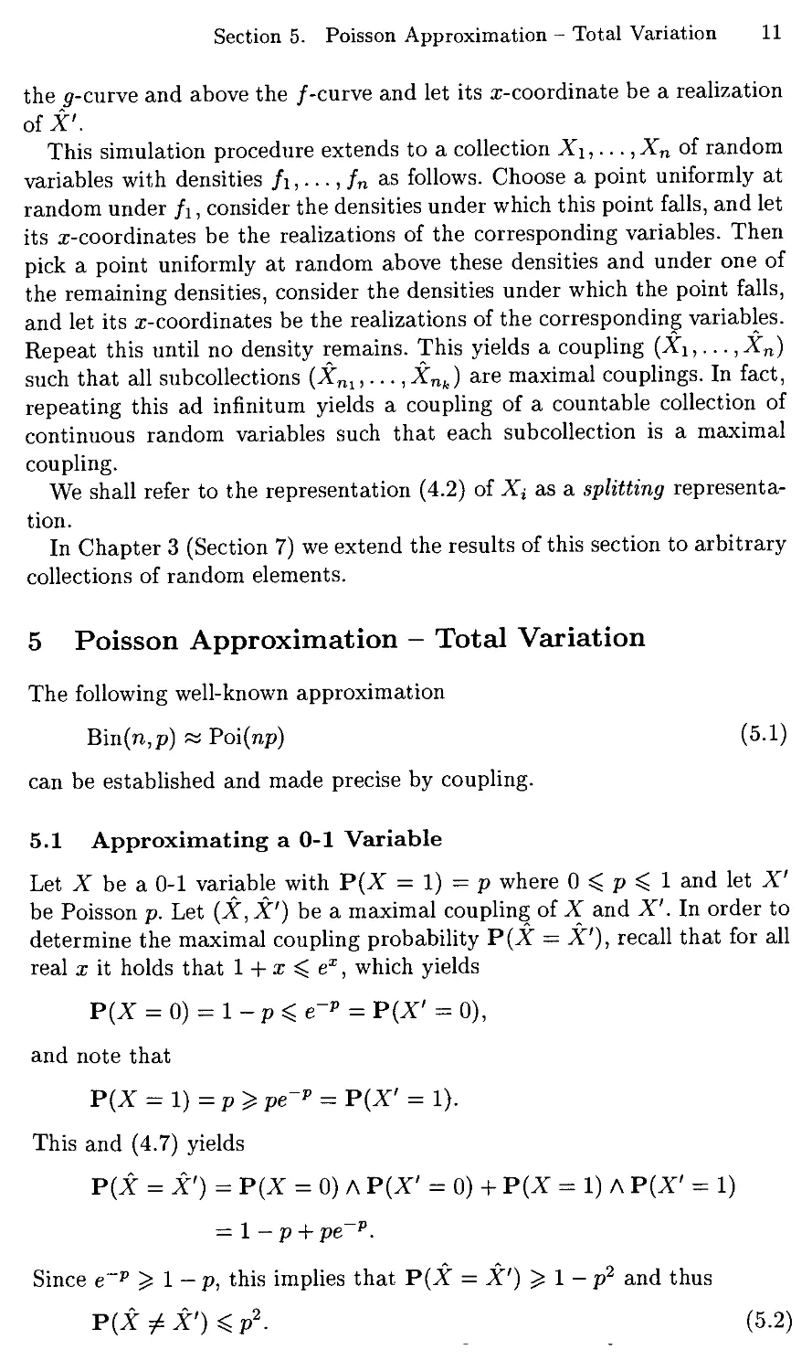
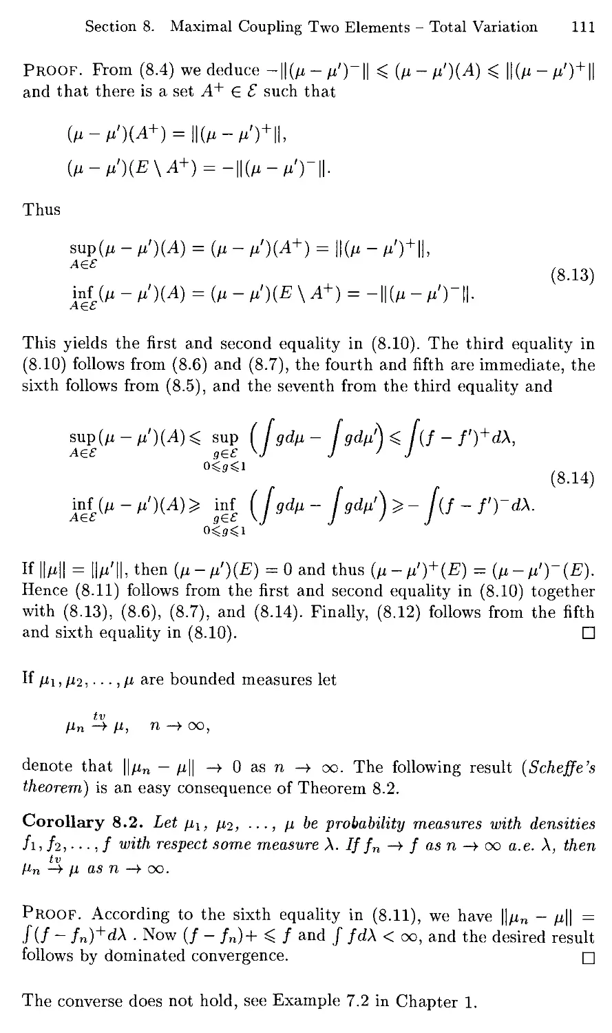
In particular, for two discrete random variables X and X' there exists a
coupling (X,X') such that, with A denoting minimum,
p(i = i') = ^p(i = i)AP(r = i) (4.7)
X
and for two continuous random variables X and X' with densities / and
/' there exists a coupling (X,X') such that
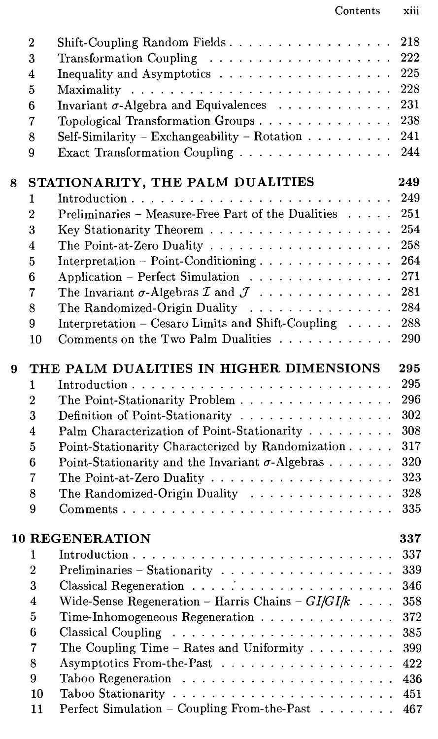
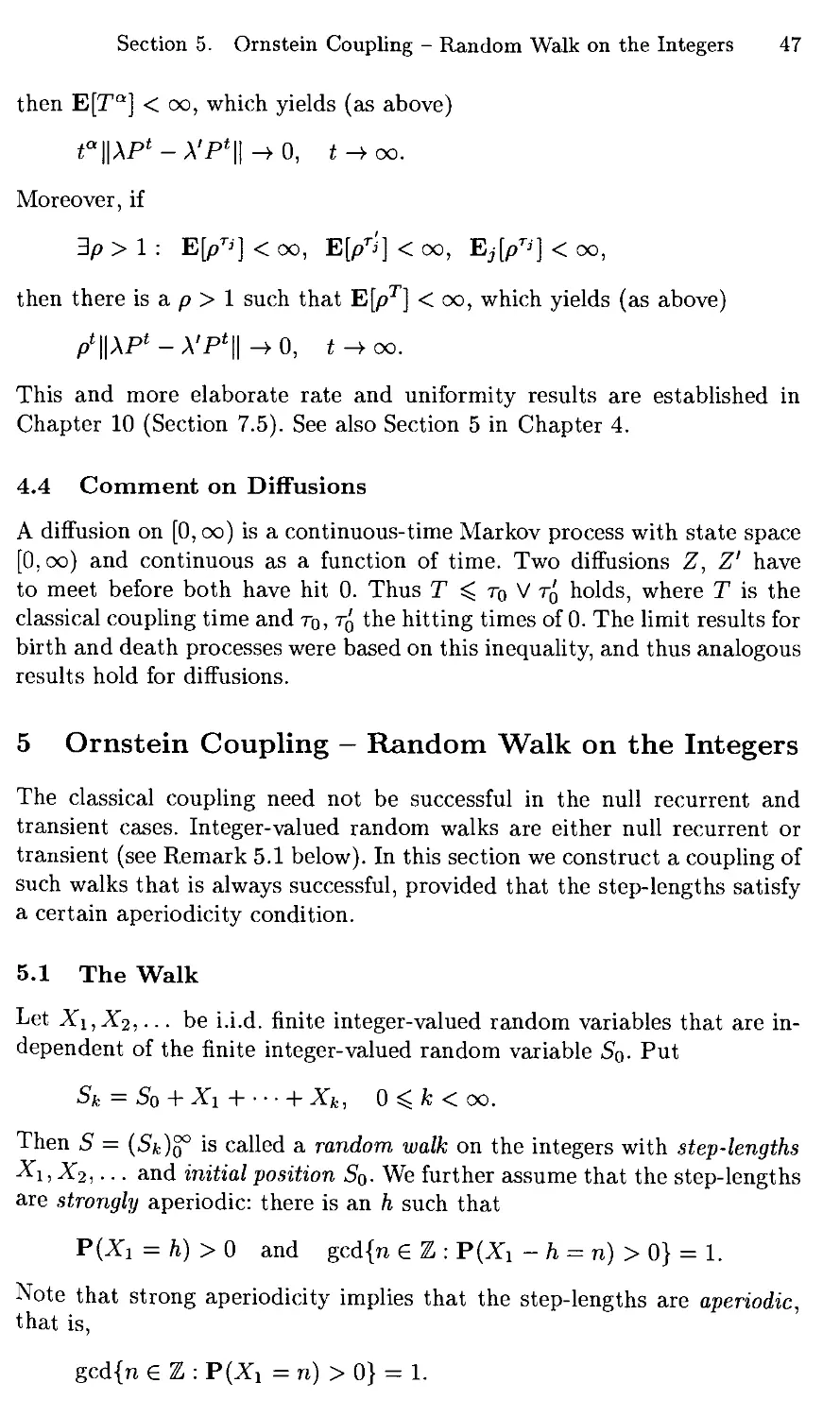
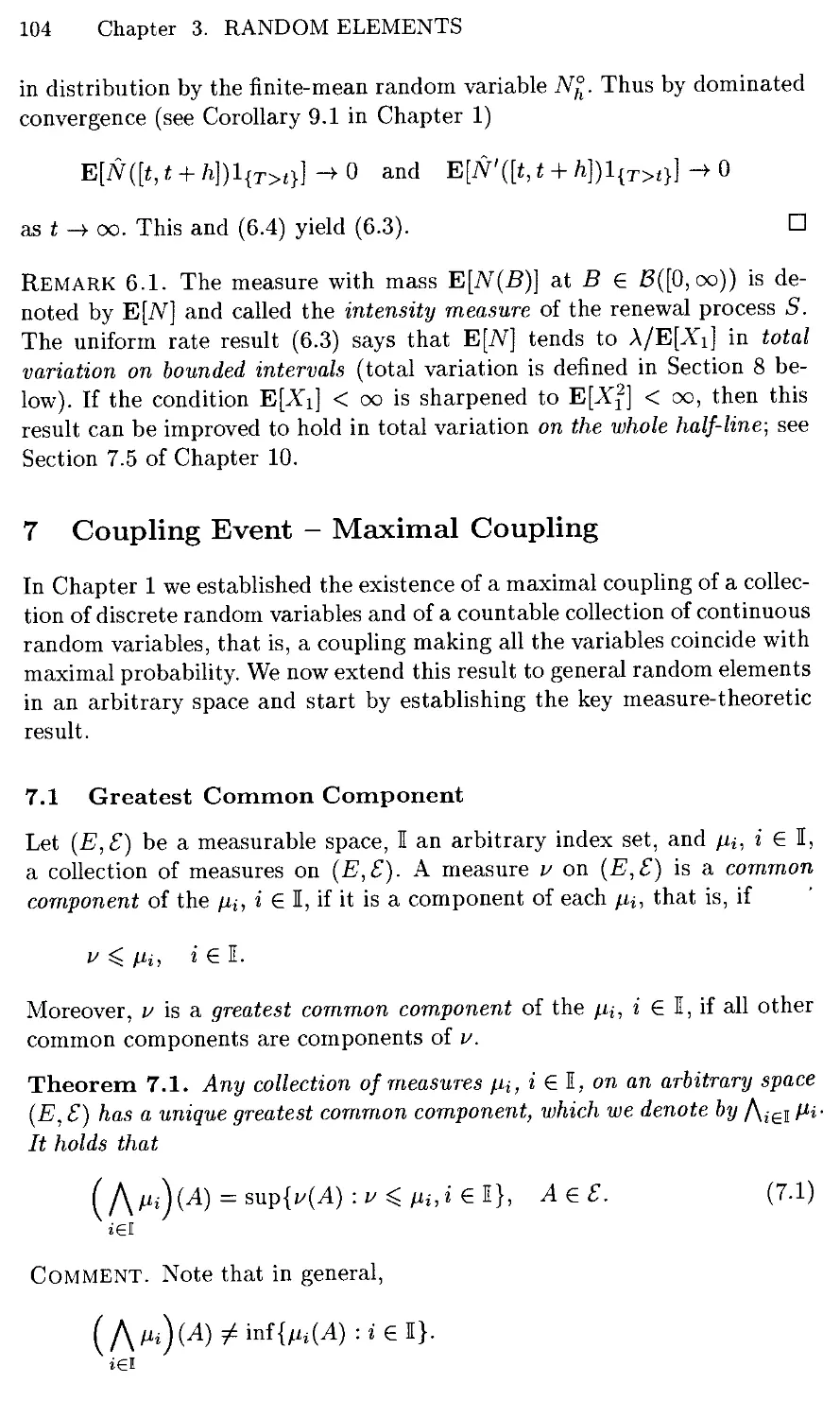
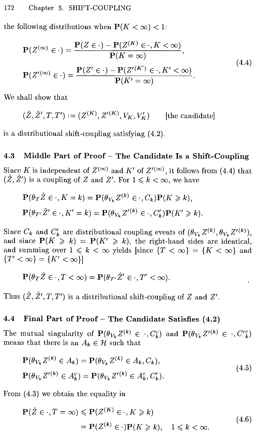
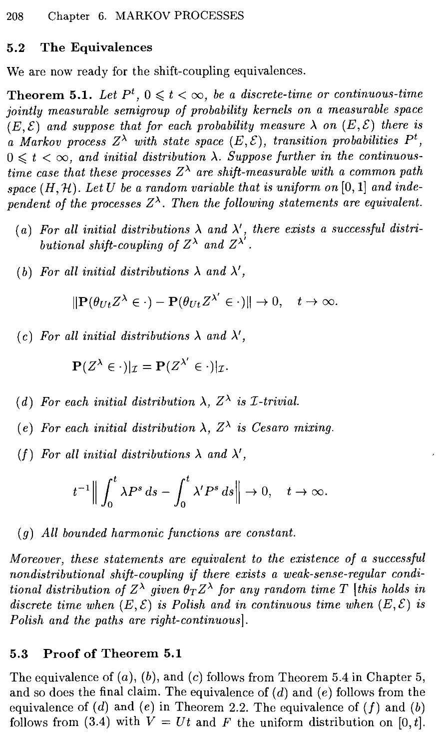
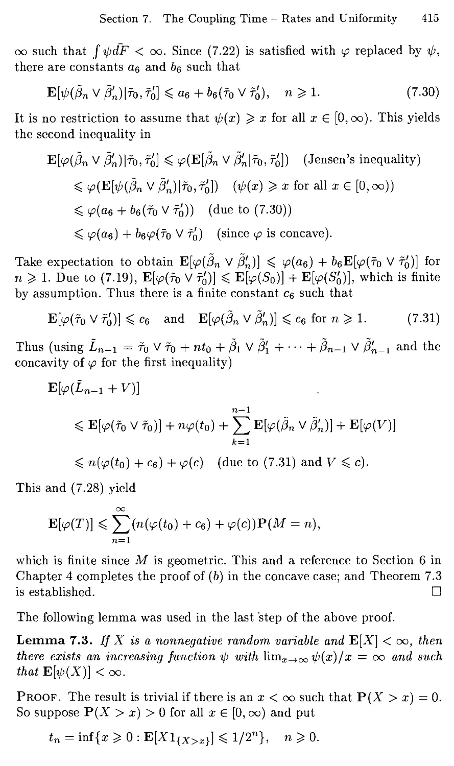
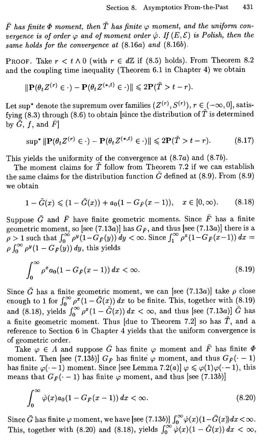
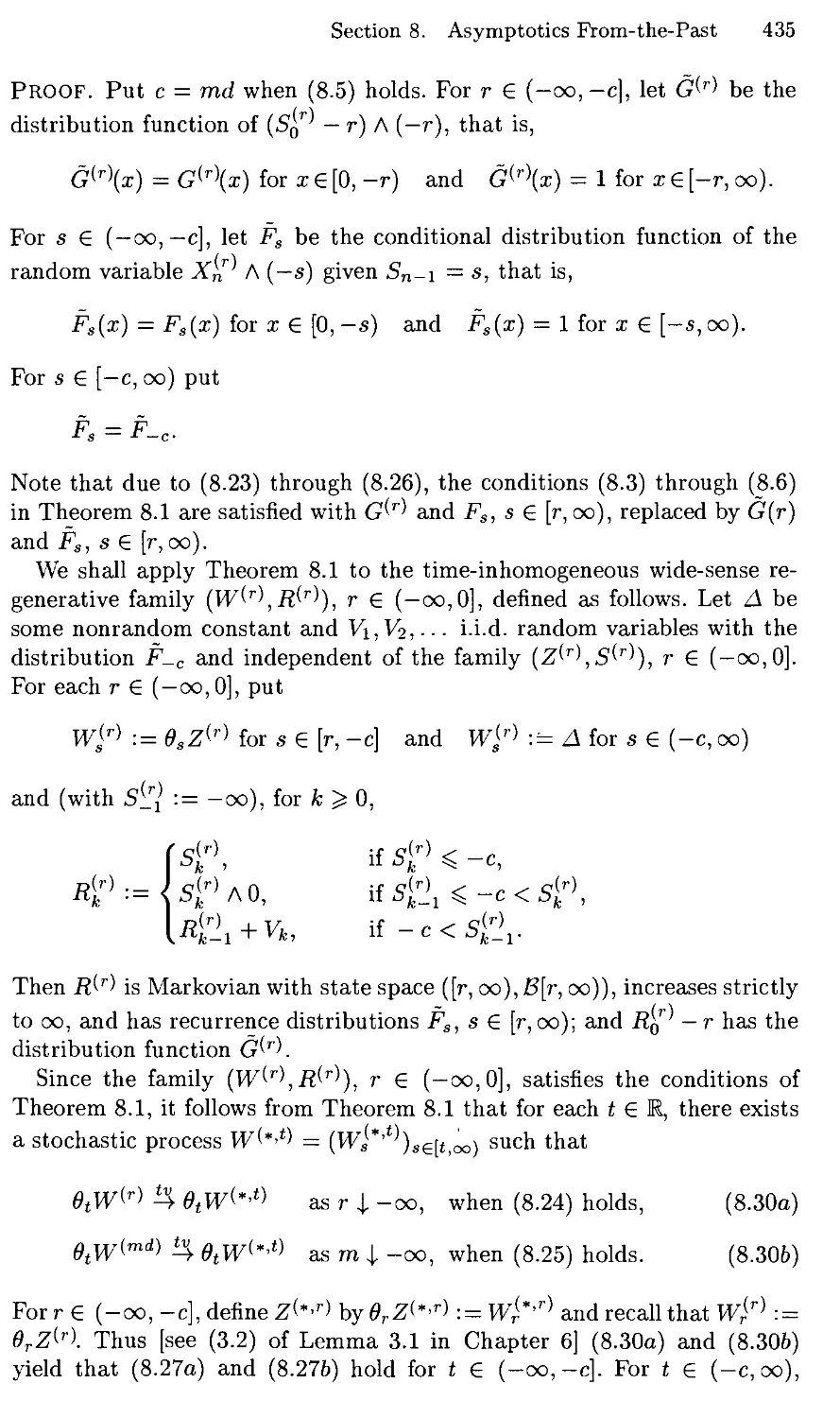
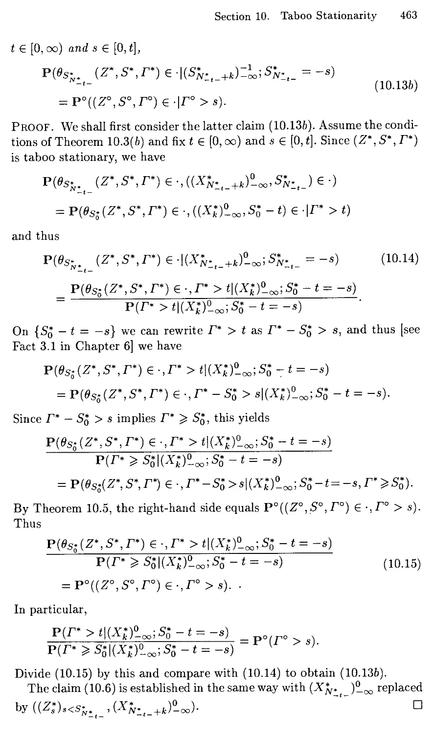
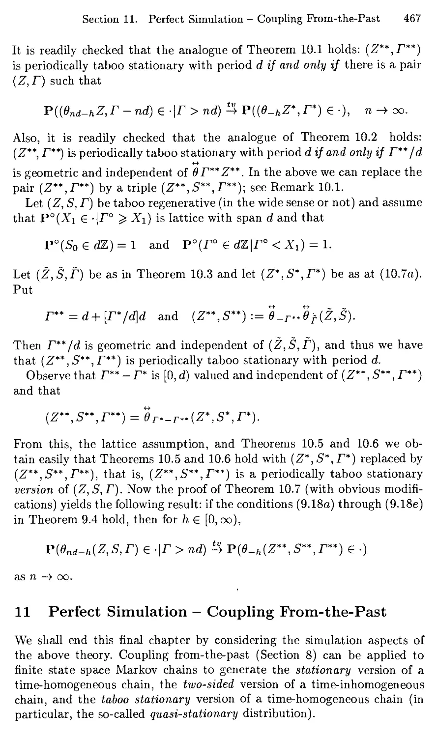
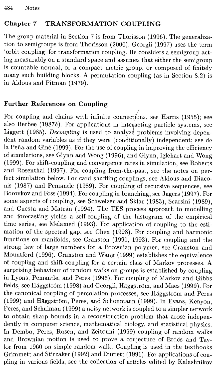
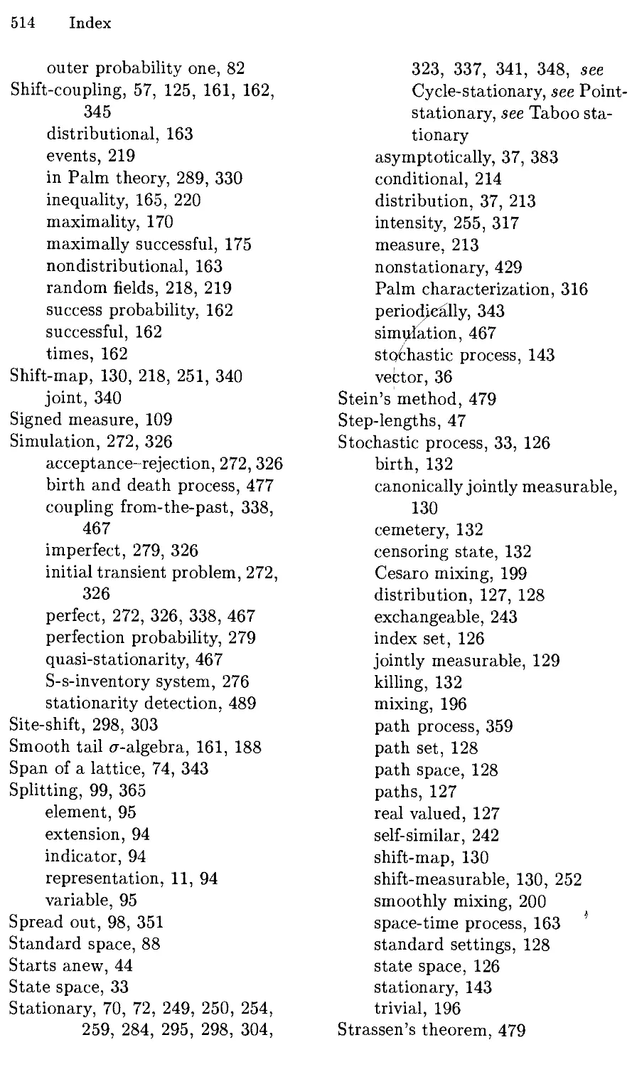
P(X = X')= f fAf' (see Figure 4.1). (4.8)
t
v Maximal coupling probability ■
FIGURE 4.1. The maximal coupling probability.
Call these couplings maximal (without a reference to a particular coupling
event).
In simulation a maximal coupling of continuous random variables X and
X' with densities / and g can be generated as follows. Choose a point
uniformly at random under the /-curve and let its ^-coordinate be a realization
of X. If the point happens to be under the g-curve, let its x-coordinate also
be a realization of X'. If not, choose a new point uniformly at random under
Section 5. Poisson Approximation - Total Variation 11
the g-curve and above the /-curve and let its x-coordinate be a realization
oiX'.
This simulation procedure extends to a collection Xi,..., Xn of random
variables with densities fi, ■ ■ ■, fn as follows. Choose a point uniformly at
random under fx, consider the densities under which this point falls, and let
its x-coordinates be the realizations of the corresponding variables. Then
pick a point uniformly at random above these densities and under one of
the remaining densities, consider the densities under which the point falls,
and let its ^-coordinates be the realizations of the corresponding variables.
Repeat this until no density remains. This yields a coupling (Xi,... ,Xn)
such that all subcollections (Xni,..., Xnk) are maximal couplings. In fact,
repeating this ad infinitum yields a coupling of a countable collection of
continuous random variables such that each subcollection is a maximal
coupling.
We shall refer to the representation (4.2) of X, as a splitting
representation.
In Chapter 3 (Section 7) we extend the results of this section to arbitrary
collections of random elements.
5 Poisson Approximation - Total Variation
The following well-known approximation
Bin(n,p) « Poi(np) (5.1)
can be established and made precise by coupling.
5.1 Approximating a 0-1 Variable
Let X be a 0-1 variable with P(X = 1) = p where 0 ^ p ^ 1 and let X'
be Poisson p. Let (X, X') be a maximal coupling of X and X'. In order to
determine the maximal coupling probability P(X = X'), recall that for all
real x it holds that 1 + x ^ ex, which yields
P(X = 0) = 1 - p ^ e~p = P{X' = 0),
and note that
P(X = l)=p> pe-p = P(X' = 1).
This and (4.7) yields
P(X = X') = P{X = 0) A P(X' = 0) + P(X = 1) A P{X' = 1)
— 1 — p + pe~p.
Since e~p ^ 1 - p, this implies that P(X = X') ^ 1 - p2 and thus
P(XjtX')^p2. (5.2)
12 Chapter 1. RANDOM VARIABLES
5.2 Sums of Independent 0-1 Variables
Let Xi,... ,Xn be independent 0-1 variables with P(Xi = 1) = pi, where
0 < pi ^ 1. Put
x = x1 + --- + xn.
Let X[,...,X'n be independent Poisson variables, X[ with parameter p;.
Recall that
X' := X[ + ■ ■ ■ + X'n is Poisson pi + • ■ • + p„.
Let (Xi, X[),..., (Xn, X^) be independent pairs such that for each i, (Xi, X[)
is a maximal coupling of Xi and Xs'. Put
X = Xx+--- + Xn and X' = X{+--- + X;.
Then (X,X') is a coupling of X and X', and
P(X ^ X') ^ P(Xi ^ Xs' for some i) ^ ^ P(X< ^ X?).
Applying (5.2) yields
P(X ^ X') ^ ^ pi (5.3)
If we take pi = p, then X is binomial (n,p), and thus we have the following
clear and intuitively appealing random variable formulation of (5.1):
Bin(n,p) differs from Poi(np) with probability at most np2.
In order to use the above coupling to formulate (5.1) in terms of total
variation distance between distributions we take an excursion into that
topic for the next two subsections.
5.3 Total Variation — Definition and Identities
Let X and X' be random variables with distributions A and /i, that is, for
each (Borel) set A,
X(A) = P{X g A) and n(A) = P{X' € A).
The total variation distance between A and // is simply twice the supremum
distance
||A-/i||:=2sup|A(A)-/i(A)|. (5.4)
A
Section 5. Poisson Approximation - Total Variation 13
The reason for multiplying by 2 and using the phrase 'total variation' is the
following. Suppose X and X' are discrete with probability mass functions
p and q, or continuous with densities / and g. Then twice the supremum of
A — /t equals the actual total variation (the total of the variation) of p — q,
or / — <?, namely
IIA -/ill = $>(*)-<?(*)| or ||A-/i|| = ||/-3|. (5.5)
X
We shall establish (5.5) and two other useful identities:
Theorem 5.1. If X and X' are discrete with probability mass functions p
and q, or continuous with densities f and g, then (5.5) holds and
||A -/i|| = 2 ^(x)-<?(*))+ or ||A-/i|| = 2 /"(/-$)+, (5.6)
x J
||A - /*|| = 2 - 2 5^p(a:) A g(a:) or ||A - /i|| = 2 - 2 f f A g. (5.7)
x •*
Here we have used the following standard notation: for real numbers a and
b let
a+ = a V 0, where a V b = maximum of a and 6,
a~ = — (aAO), where aA6= minimum of a and 6.
Proof. We shall carry out the proof of Proposition 5.1 in the discrete
case, the continuous case is analogous. It is clear that for sets A,
X(A) - p(A) < 5>(*) - q(x))+
X
and that equality holds if we take A = {x : p(x) > q(x)}. Thus
sup(A(A) - n(A)) = $>(*) - q(x))+, (5.8)
A x
( and similarly,
sup(/i(A) - \{A)) = Y,(p(x) ~ <?(*))-• (5-9)
A
( From Yl,x P(x) — 1 = Sx <z(x) ^ follows that
£(p(a:) - g(x))+ = 5Z(p(a:) - «(*))-. (5.10)
14 Chapter 1. RANDOM VARIABLES
Combining (5.8), (5.9), and (5.10) yields
Sup|A(A)-MA)|=5>(a0-*(a0)+>
A
and thus (5.6) holds. From
\p-q\ = (p-1)+ + (p - g)~
together with (5.6) and (5.10) we obtain (5.5). Finally,
(p - q)+ = p - p A q
together with (5.6) and ^p(i) = 1 yields (5.7). □
5.4 Total Variation and Coupling
Let (X, X') be a coupling of two random variables X and X', and let C be
a coupling event. Since C implies that X = X', we have for (Borel) sets A,
P(XeA,c) = P(x'eA,c)
and thus
P{x e A) - P(x' e A) = P(x e A) - P{x' g A)
= P(x e A, cc) - P(x' e A, cc)
^ P(CC).
Apply (5.4) to obtain the coupling event inequality
||P(Xe-)-P(*'e-)IK2P(<7c). (5.n)
From (5.7) we see that in the discrete and continuous cases this is just
a total variation formulation of Theorems 4.1 and 4.3 specialized to two
variables. We also see that the coupling is maximal if and only if identity
holds in (5.11). Thus when (X,X') is a maximal coupling, we have
||P(x e •) - P(x' g -)ll = 2P(^ ¥> x'). (5.12)
5.5 Back to the Poisson Approximation
Combining (5.3) and the coupling event inequality in the form (5.11) [and
with C = {X = X'}} yields
n
||P(XG0-Poi(pi + ---+Pn)|K2^p2_
»=i
Section 6. Convergence of Discrete Random Variables 15
In particular, if p, = p, then X is binomial (n,p), and thus we have the
following precise formulation of (5.1):
|| Bin(n,p) - Poi(np)|| ^ 2np2.
If a Poisson parameter c is given and n ^ c, then taking p = c/n yields
|| Bin(n, c/n) - Poi(c) || ^ 2c2/n.
tv
Sending n to infinity yields in particular, with —> denoting convergence in
total variation,
Bin(n,c/n) -4 Poi(c), n ->■ oo, (5.13)
which further implies
0
(c/n)x(l-c/n)n-x -> eTc— asn->oo, iEZ+, (5.14)
where Z+ are the nonnegative integers.
5.6 Comment
The above results can be much sharpened and extended; see Barbour, Hoist,
and Janson (1992). We just mention here Le Cam's theorem: with X as in
Section 5.2,
||P(X£-)-Poi(p1+---+pn)|| ^2 max p^
and in particular,
||Bin(n,p)-Poi(np)|| ^ 2p.
6 Convergence of Discrete Random Variables
Let Xi,..., Xqo be discrete random variables taking values in a finite or
countable set E. We shall first show that convergence in total variation,
like (5.13), is (somewhat surprisingly) equivalent to the apparently weaker
pointwise convergence of probability mass functions, like (5.14). We shall
then show that these distributional modes of convergence can be turned by
coupling into a convergence where the random variables actually hit the
limit and stay there.
6.1 Mass Function Convergence <& Total Variation Convergence
Suppose
P(Xn = x) —)■ P(Xoo = x) as n —> oo for each x £ E. (6.1)
16 Chapter 1. RANDOM VARIABLES
Then (P(Xoo = x) - P(Xn = x))+ ->• 0, and since
(P(Xoo = x) - P(Xn = X))+ ^ P(Xoo = X)
and
53 P(^oo = x) = 1< 00,
xeE
we have by dominated convergence that
53(P(Xoo=x)-P(Xn = x))+^0, n^oo.
xeE
Now (5.6) yields convergence in total variation:
Xn % Xoo, n ->• oo. (6.2)
Conversely, it is clear that (6.2) implies (6.1). Thus (6.1) and (6.2) are
equivalent.
6.2 Hitting the Limit
We now show that if (6.1) holds, then there exists a coupling {X\,..., Xoo)
of X\,..., Xqo and a finite random integer K such that
Xn = Xoo, n>K. (6.3)
We obtain this by elaborating on the maximal coupling construction in
Section 4.2. Note that (6.1) implies, for all x £ E,
qn(x) := inf P(Xk = x) t PiX^ = x) as n -> oo. (6.4)
Put go = 0 and let K, V\, V2,..., W\, Wi,... be independent random
variables such that for 1 ^ n < oo and x £ E
P(K = n)=^2 gn(x) - 53 9n-i(x),
P(y = ^ = /(«n(a:) - ff„-i(a:))/P(A- = n) if P(K = n) > 0,
1 " ^ [arbitrary if P{K = n) = 0,
PW = ^ = /(P(X» = *) - ?n(x))/P(ir > n) if P{K > n) > 0,
1 " X; [arbitrary if P(K > n) = 0.
The random variable _K" is finite, since by dominated convergence and (6.4)
P{K ^ n) = 53 Q1"^) T 53 p(^°° = a;) = 1 as n ->■ oo.
Section 6. Convergence of Discrete Random Variables 17
Define, for 1 < n ^ oo,
Xn=[V« i{n>K> (6.5)
\Wn \{n<K.
This is a coupling of Xi,..., Xoo, since for 1 ^ n < oo and each x £ E
P(Xn =x)= Y, P(Vk = X^P(K = fc) + P(Wn = X^P(K > n)
= Y (qk(x) - qk-i(x)) + (P{Xn = x) - qn(x))
= P(Xn = x),
while Xqo = Vk, and thus [due to (6.4)] for each x £ E
P{X00=x) = Y (9k(x)-qk-i{x))=P{X0O=x).
l<fc<oo
Clearly, (6.3) holds.
6.3 Converse
Conversely, suppose (6.3) holds. Then {K ^ n} is a coupling event of the
coupling (Xn,Xoo) of Xn and Xqo. Applying the coupling event inequality
(5.11) and the finiteness of K yields
||P(Xn G •) - P(*oo G Oil < 2P(K >n)^0, n ^ oo,
which implies (6.1).
Since (6.1) in turn implies (6.4), which was in fact the condition under
which we established (6.3), we have established the following equivalences.
Theorem 6.1. Let X\,..., Xoo be discrete random variables taking values
in a finite or countable set E. Then the three claims
lim P{Xn =x) = P(X00 = x), x G E, [this is (6.1)]
n—»oo
Xn -4 Xqq, n —> oo, [£/i«s is (6.2)]
liminf P(Xn = x) = P(X00 = x), x G £, [ttis is (6.4)]
are equivalent and hold if and only if there exists a coupling (Xi,..., X^)
ofXu...,X oo and a finite random integer K such that
Xn — Xoo, n ^ K,
[this is (6.3)].
18 Chapter 1. RANDOM VARIABLES
7 Continuous Variables - Hitting the Limit
Let X\,..., Xqo be continuous random variables with densities /i, •• •, /oo-
How should Theorem 6.1 be extended to this case? This section is
structured as the previous one and gives the answer at the end.
7.1 Density Convergence =>■ Total Variation Convergence
Replacing probability mass functions by densities in the argument in
Section 6.1 yields that the following analogue of (6.1):
the densities /i, • ■ ■, /oo can be chosen so that
(7.1)
fn{x) —> foa(x) as n —> oo for each x £ E,
implies convergence in total variation,
Xn 4 Xoo, n -> oo. (7.2)
However, the converse is not as obvious. In fact, it is no longer true, as we
shall see in a while.
7.2 Hitting the Limit
We shall now show that the condition (7.1) is sufficient to hit the limit, that
is, if (7.1) holds, then there exists a coupling (Xi,..., X^) of Xi,..., Xao
and a finite random integer K such that
Xn = X00, n > K. (7.3)
This follows by a coupling construction analogous to the one in Section 6.2.
Let us go through the essential part of it again. Put
go = 0 and for n > 1 gn= inf fk-
Let K, V\, V2, ■ ■ ■, Wi, W2, ... be independent random variables such that
for 1 ^ n < 00,
K is integer valued and V(K = n) = / gn — I gn~\,
V has Jdensity (#" ~ 9n-i)/P(K = n) if P(K = n) > 0,
[arbitrary density if Y?{K = n) = 0,
w hag f density (/„ - gn)/P(K > n) if P(K > n) > 0,
(arbitrary density if P(K > n) = 0.
Defining Xn as at (6.5) yields the desired result, since (7.1) implies that
gn t /oo as n ->■ 00.
Section 7. Continuous Variables - Hitting the Limit 19
7.3 Converse?
Note that (7.3) was actually established under gn f /oo, that is, under
liminf /„ is a density of X^, (7.4)
n—>oo
which is weaker than (7.1). We shall now show that (7.4) is the correct
condition, that is, that (7.4) is implied by (7.3).
Suppose there is a coupling and a finite K such that (7.3) holds. Then
{K ^ n} is a coupling event of the coupling (Xn,..., Xco) of Xn,...,X^,
and (4.5) yields for (Borel) sets A,
P(i"oo &A,K^n)^gn, 1 ^ n < oo.
J A
Now, gn increases to liminf n_>oo /n, and thus [by monotone convergence
and since K < oo]
P(Xoo G A) < / liminf /„. (7.5)
yA n->oo
Also, since J gn ^ J fn = 1, we have J" lim infn_>oo /n ^ 1- Thus, for each
(Borel) set A,
1 = P^ £i) + P(Xoo G Ac)
^ / liminf/„+ / liminf/n^l.
J A n^°° Va= n^°°
This cannot hold unless (7.5) holds with identity. Thus (7.4) holds.
7.4 Pointwise Convergence of Densities Is Too Strong
We have established the equivalence of (7.3) and (7.4). For discrete
variables there were two more equivalences, which both break down in the
continuous case. We start with (7.1) and (7.4): certainly, (7.1) implies (7.4),
and the following example shows that (7.1) is, in fact, strictly stronger than
(7.4).
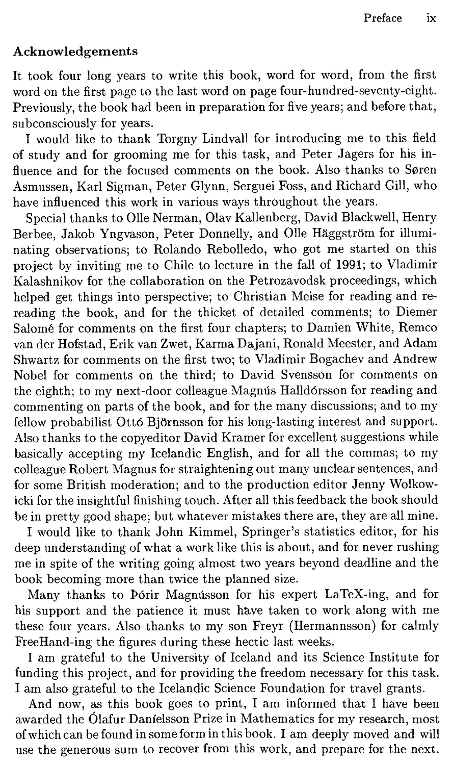
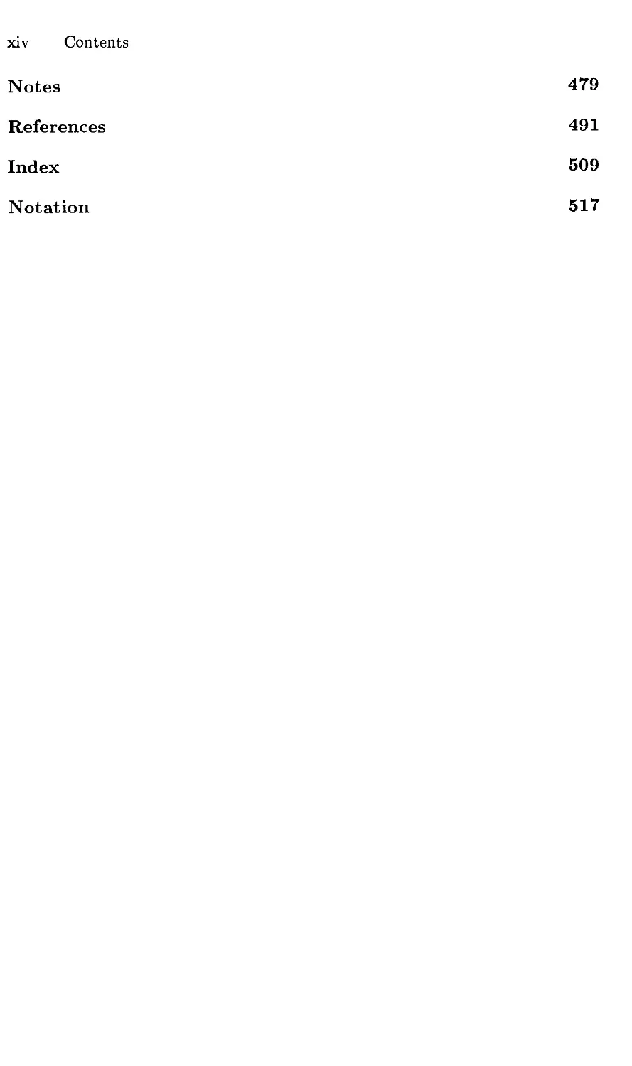
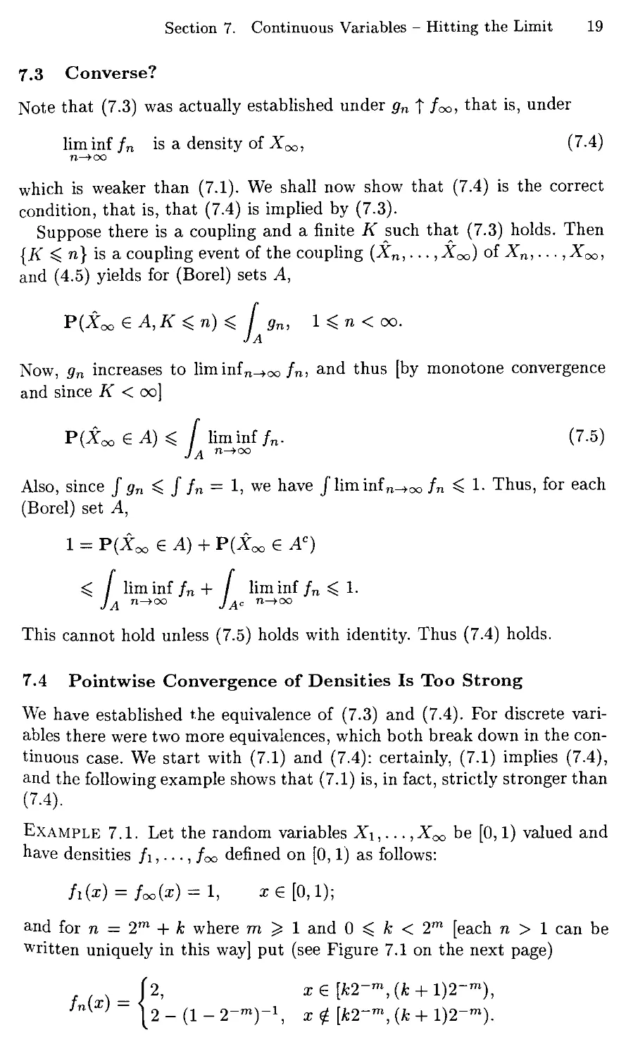
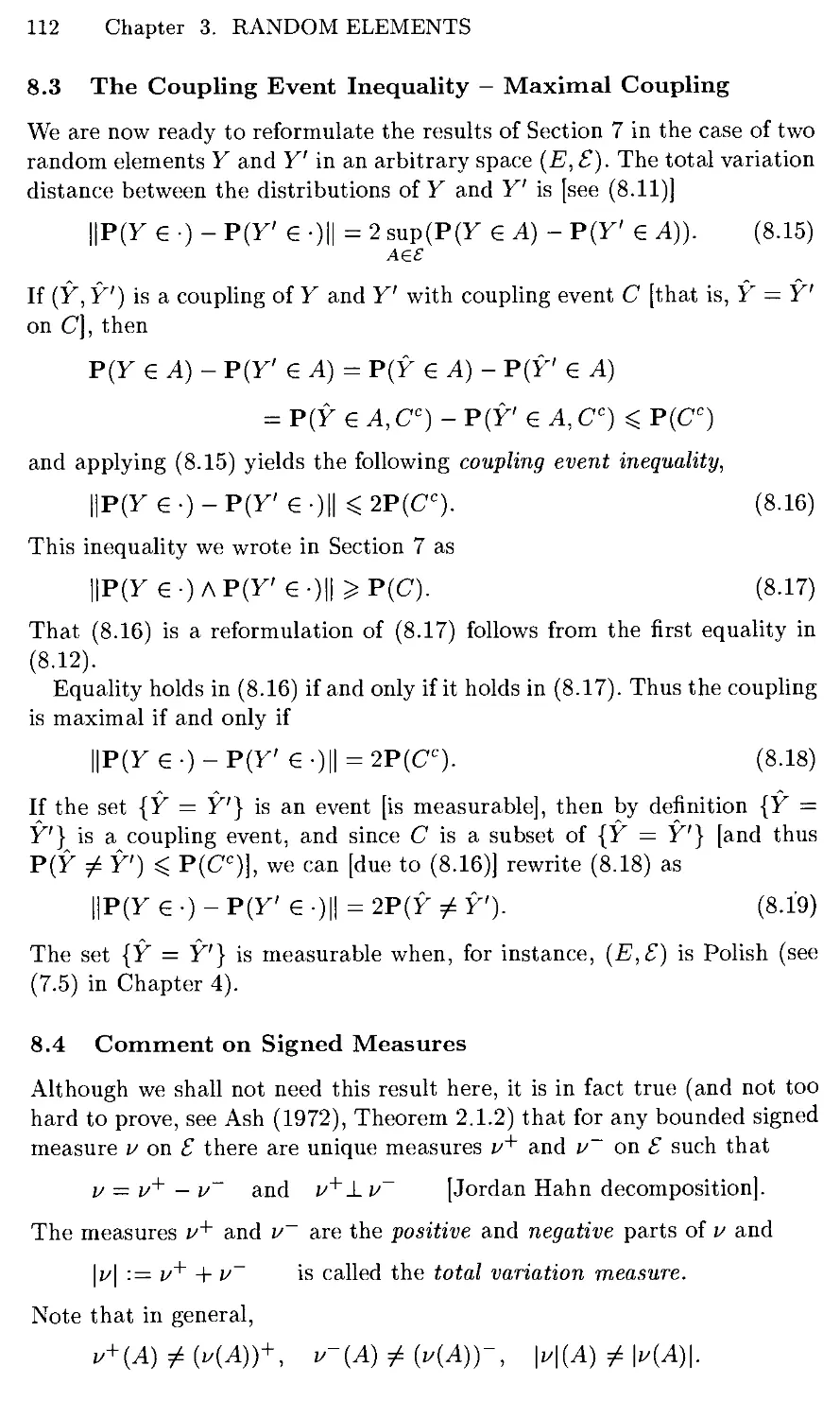
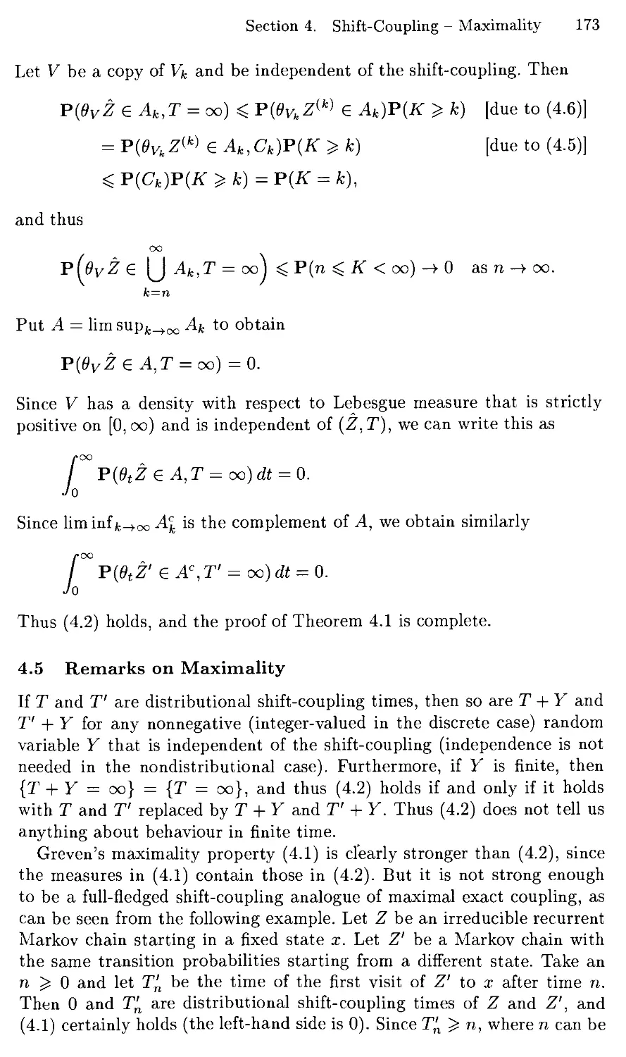
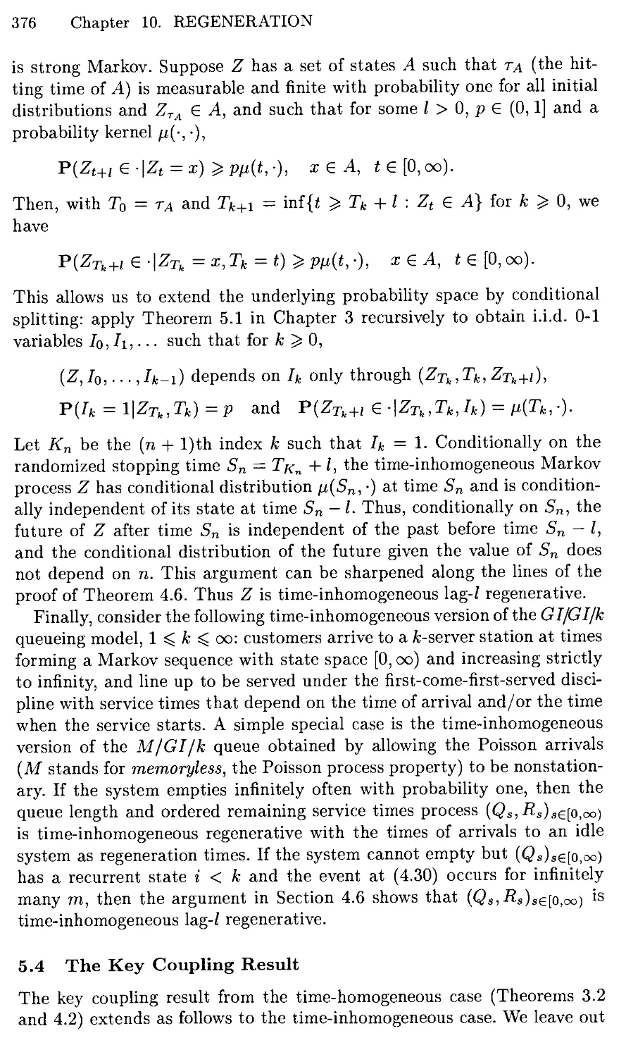
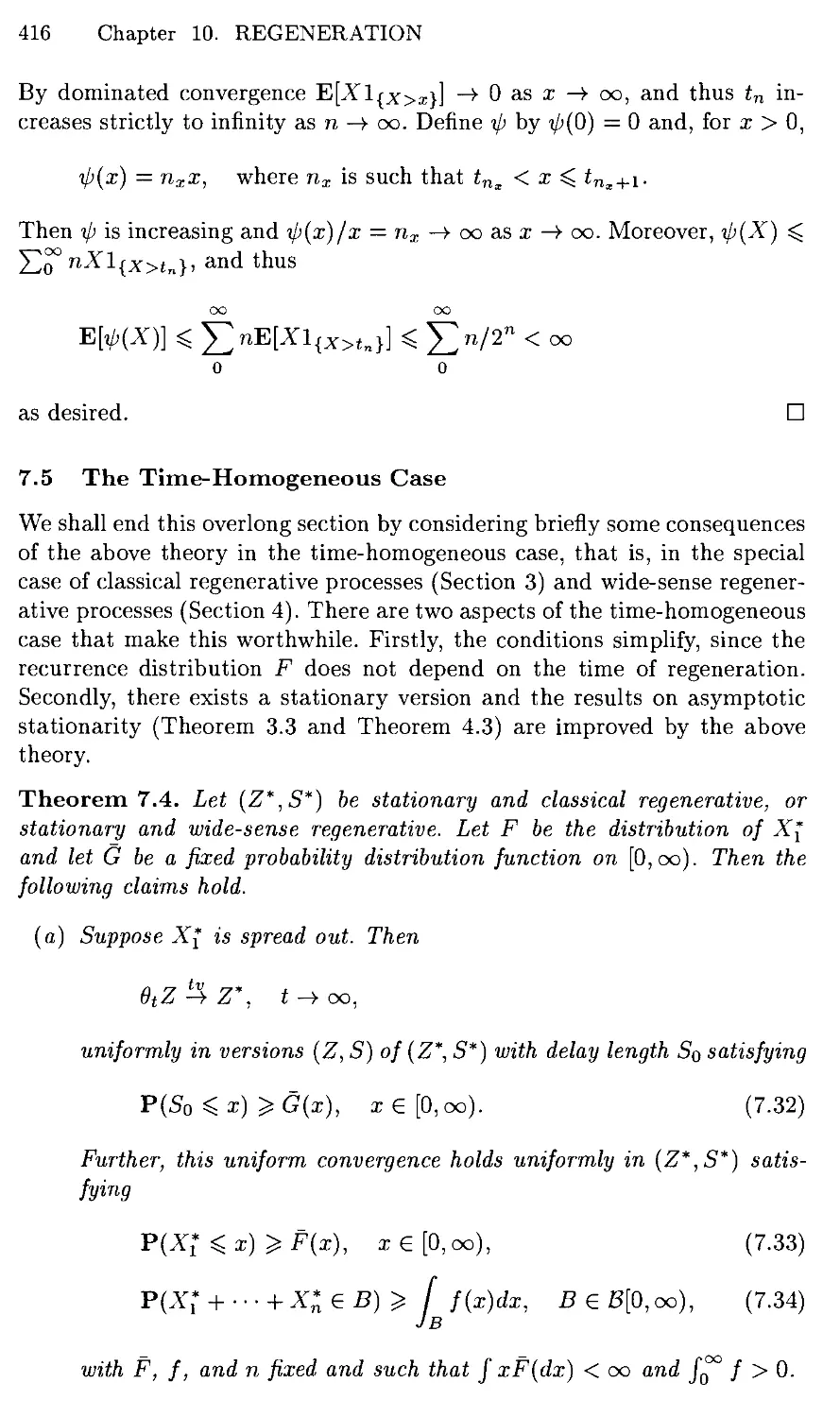
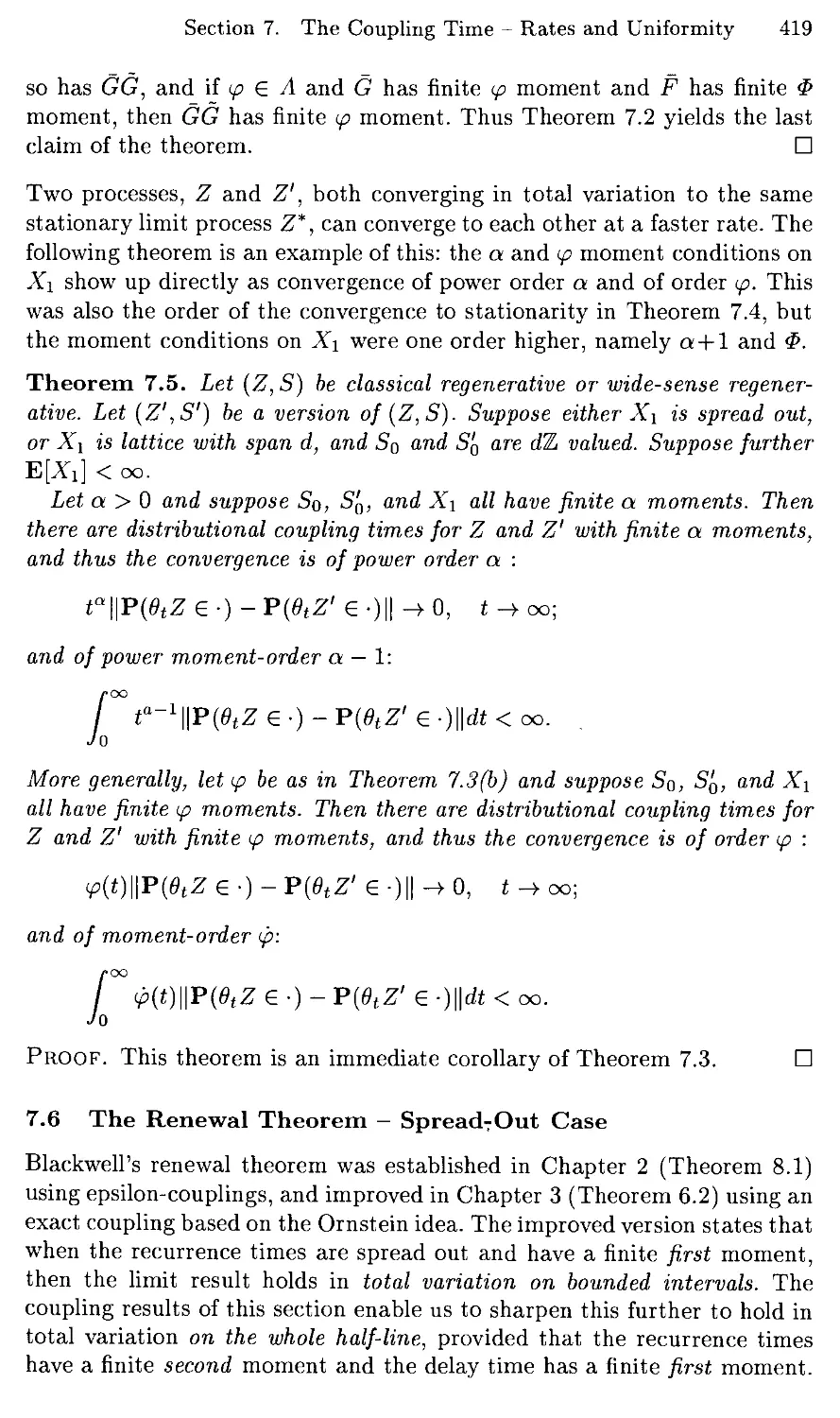
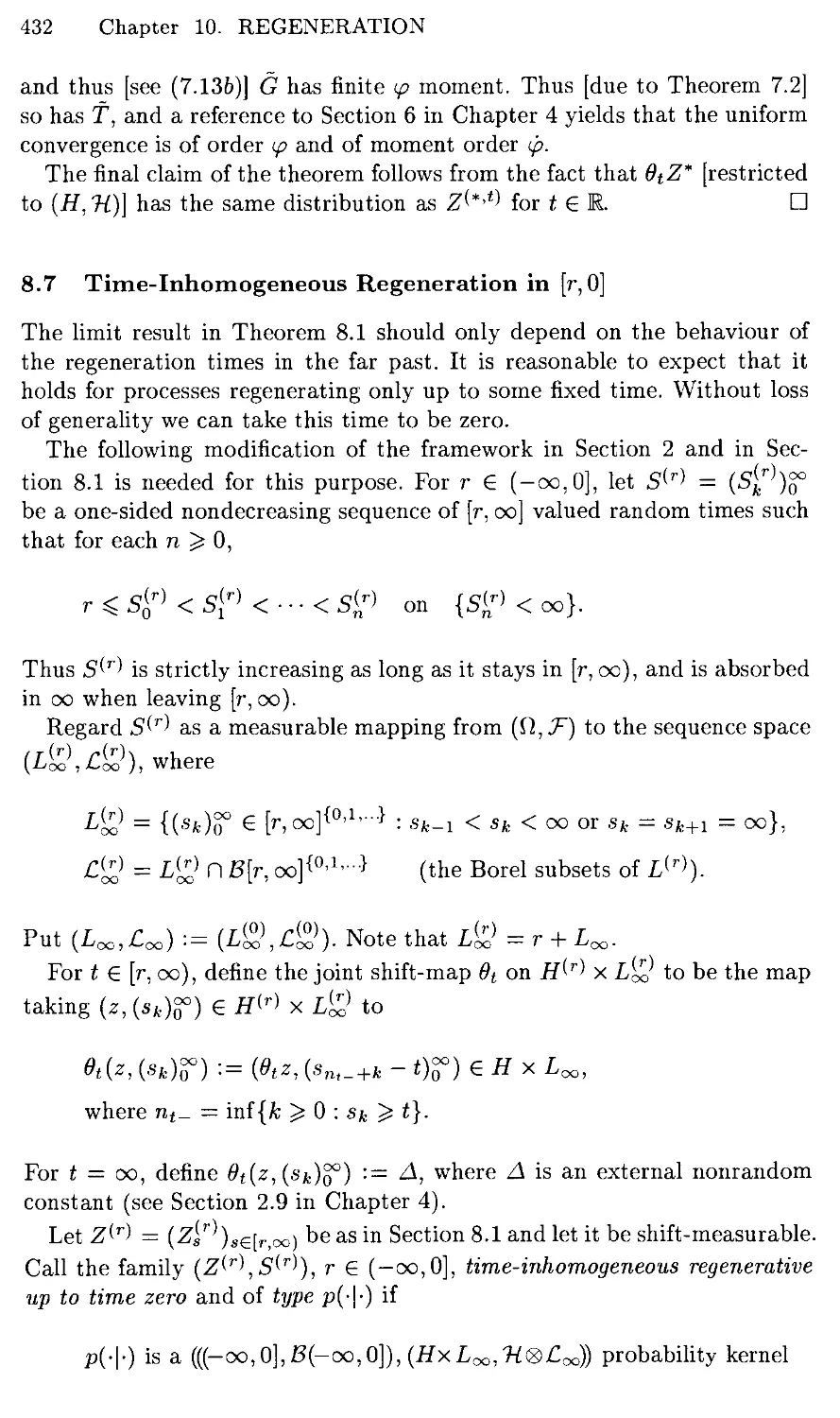
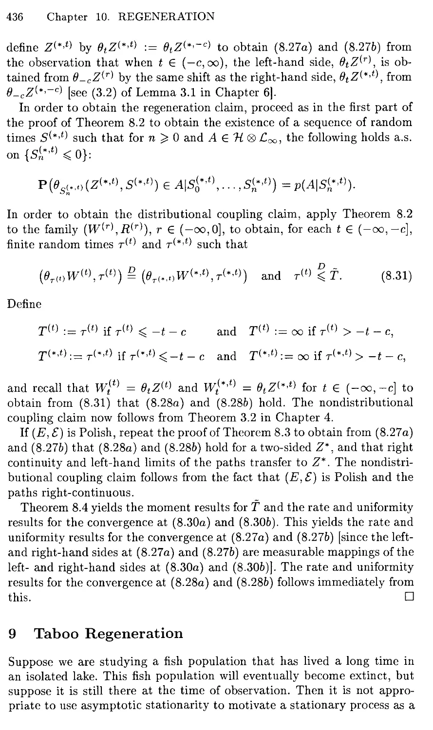
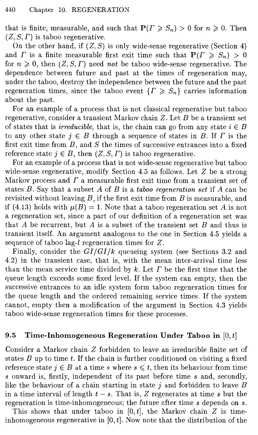
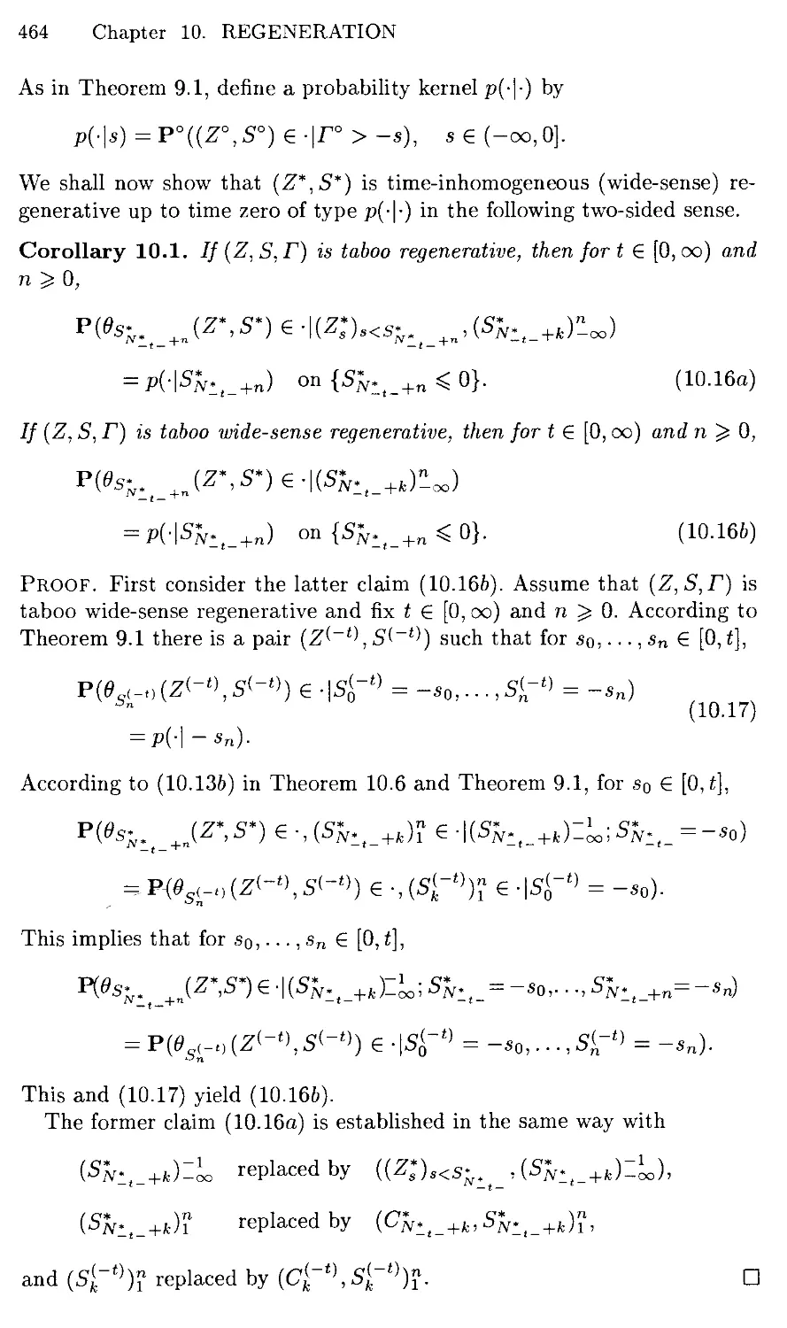
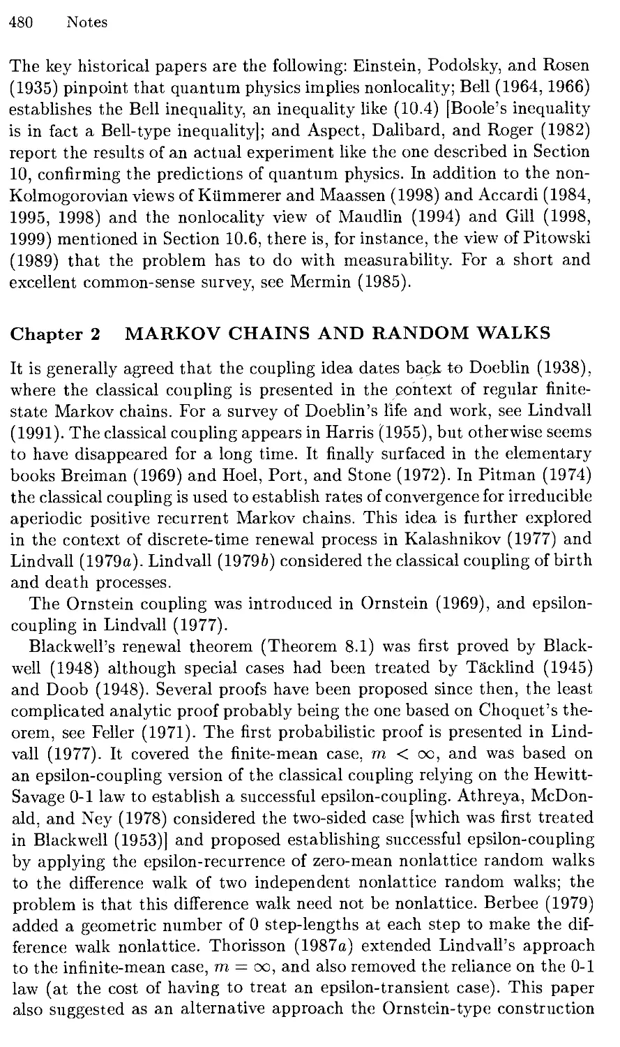
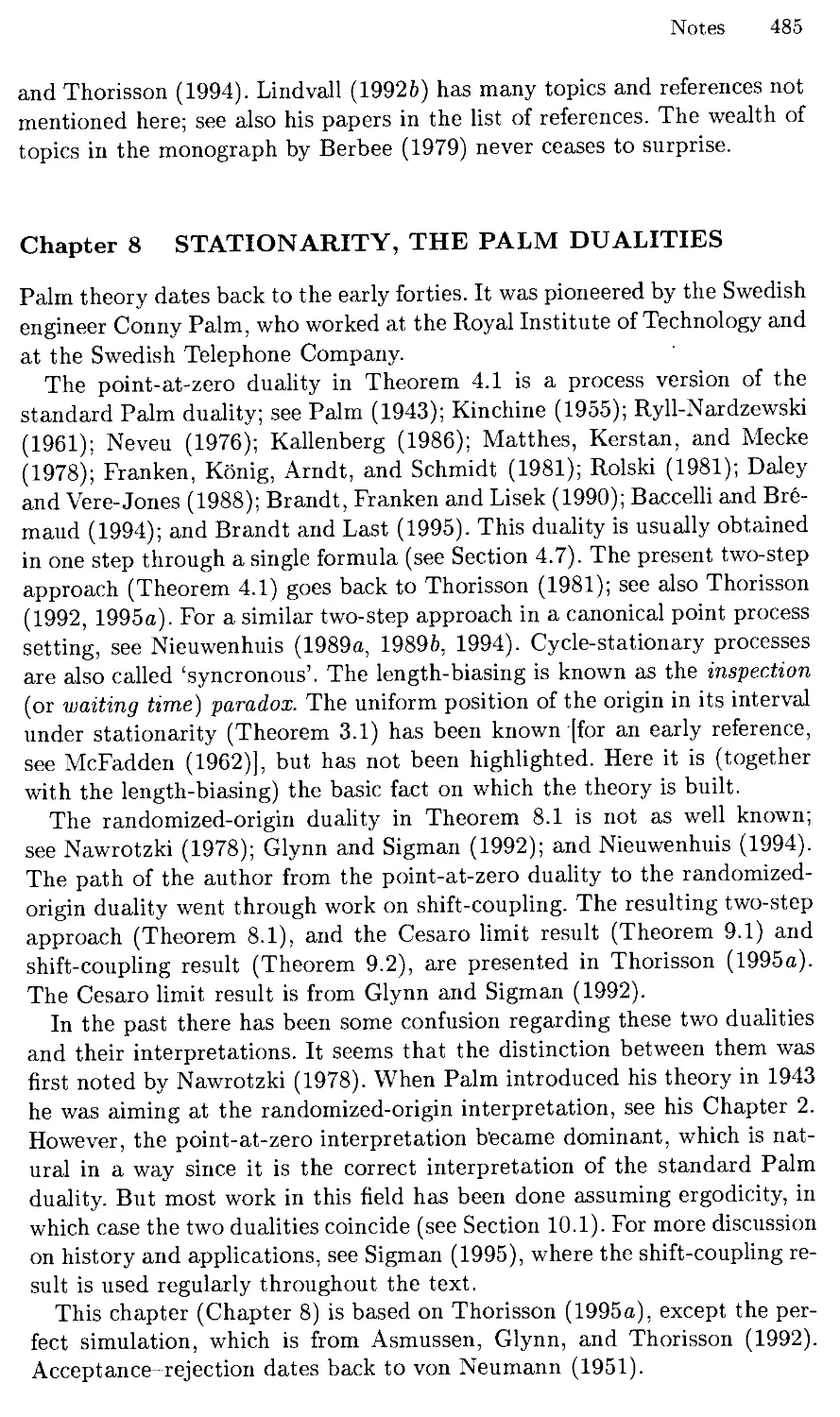
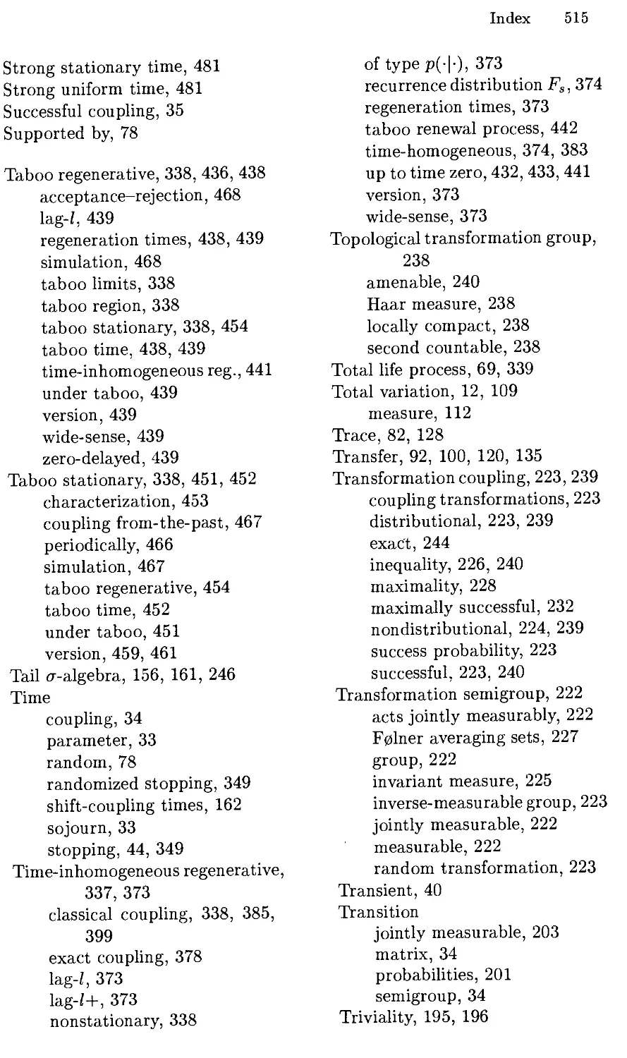
Example 7.1. Let the random variables X\,.. .,Xoa be [0,1) valued and
have densities /i,..., /«, defined on [0,1) as follows:
/i(a:) = /0o(a:) = l) *€[0,1);
and for n = 2m + k where m > 1 and 0 < k < 2m [each n > 1 can be
written uniquely in this way] put (see Figure 7.1 on the next page)
(2, arG[*2-"\(A + l)2-m),
W 1 2 — (1 — 2-m)-1, x$ [k2-m,{k+l)2-m).
20 Chapter 1. RANDOM VARIABLES
Example 7.1
Example 7.2
FIGURE 7.1. The functions /„ when n = 12 (m = 3 and k = 4).
Then for each x G [0,1) there are infinitely many n such that fn(x) = 2,
and thus
limsup/n(x) = 2^ 1 =/oo(x), x G [0,1).
n—>oo
Hence (7.1) does not hold.
On the other hand, for each x G [0,1),
2-(l-2~m)-1 ^gn(x)<l.
This yields, as n —> oo,
gn(x) ->• 1 = /oo(a:), a; £ [0,1),
and thus (7.4) holds.
7.5 Total Variation Convergence Is Too Weak
Finally, consider (7.4) and (7.2). In Section 7.2 we showed that (7.4) implies
(7.3) and in Section 7.3 that (7.3) implies (7.2). Thus (7.4) implies (7.2),
and the following example shows that (7.4) is, in fact, strictly stronger than
(7.2).
Example 7.2. Let the random variables Xi,... ,Xoo be [0,1) valued and
have densities /i,..., /oo defined on [0,1) as follows:
foo(x) = l, a:€ [0,1);
and for n = 2m + k where m > 0 and 0 ^ k < 2m put (see Figure 7.1)
(0, x G [k2~m, (k + l)2"m),
{X |(l-2-m)-\ xi [fc2"m,(fc+l)2-m).
Then, due to (5.6),
||P(Xn G •) - P(*oo G Oil = 2/(/oo - fn) +
= 2-2~m->0, n->oo.
Section 8. Convergence in Distribution and Pointwise 21
Hence (7.2) holds. On the other hand, for each x £ [0,1) there are infinitely
many n such that fn{x) = 0, which yields
liminf fn(x) = 0, x <= [0,1),
n—»oo
and thus (7.4) does not hold.
7.6 What Has Been Achieved?
In Sections 7.2-7.5 we have established the following result.
Theorem 7.1. If X\,...,Xoo are continuous random variables with
densities fi, ■■■, foo, then
lim /„ is a density of X^ [this is (7.1)]
n—»oo
is strictly stronger than
liminf/„ is a density of X^, [this is (7.4)]
n—»oo
which is strictly stronger than
Xn -4 Xqo, n ->■ oo. [this is (7.2)]
Moreover, (7.4) holds if and only if there exists a coupling (X\,... ,-Xqo) of
X\,..., Xqo a-nd a finite random integer K such that
Xn = Xqo, n ^ K. [this is (7.3)]
In Chapter 3 (Section 9) we shall extend this coupling result to general
random elements.
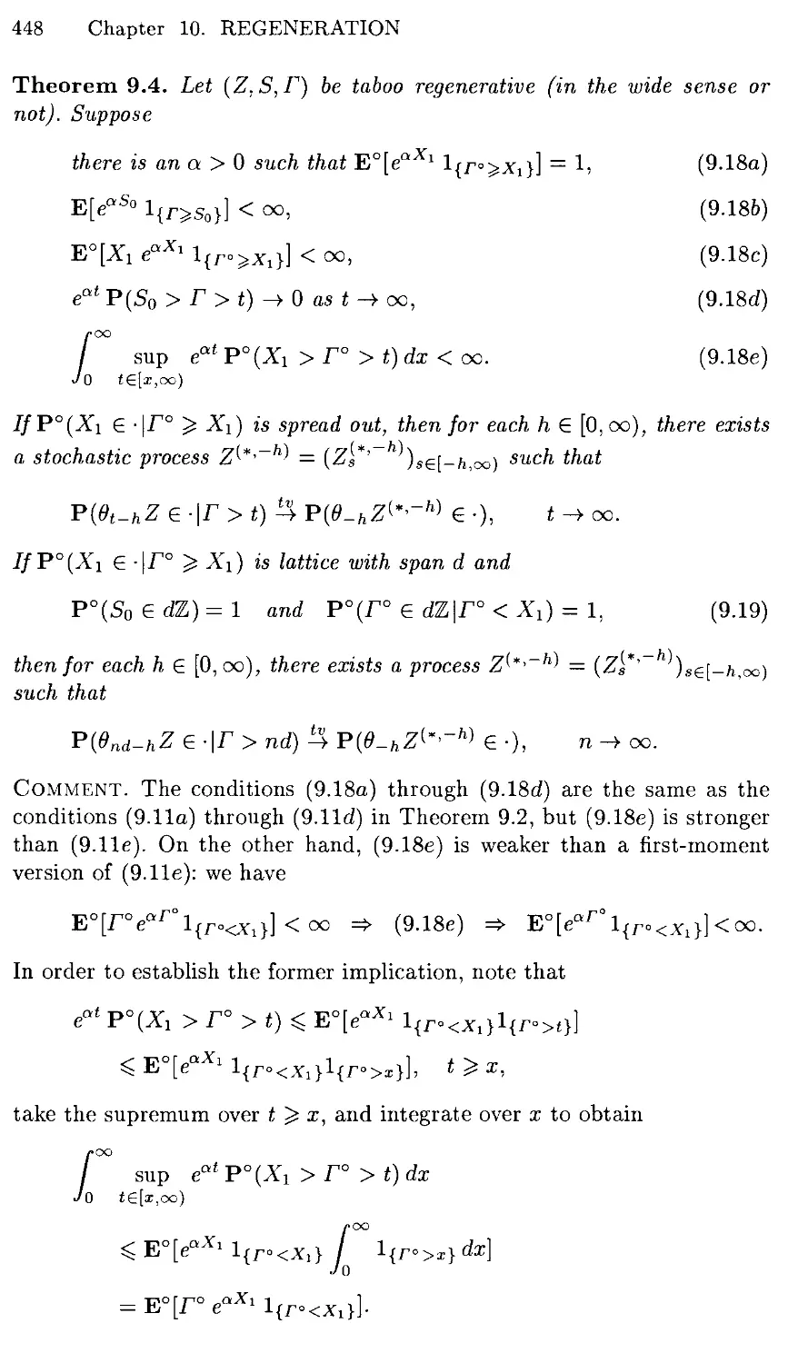
8 Convergence in Distribution and Pointwise
Let Xi,..., Xoo be random variables with distribution functions Fi,..., Fqo-
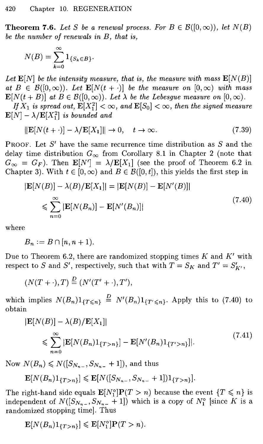
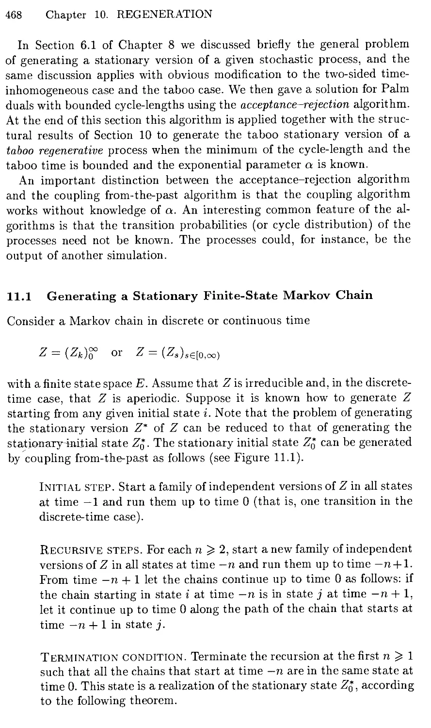
The Xn tend pointwise (or surely, or realizationwise) to Xoo if
Xn ->• Xoo, n ->• oo, (8.1)
which is short for
Xn(u>) —> Xoo(w), n —)• oo, for all outcomes to.
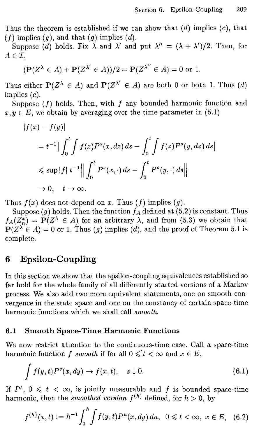
22 Chapter 1. RANDOM VARIABLES
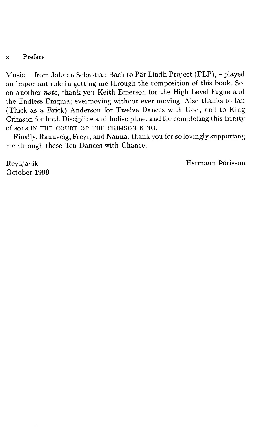
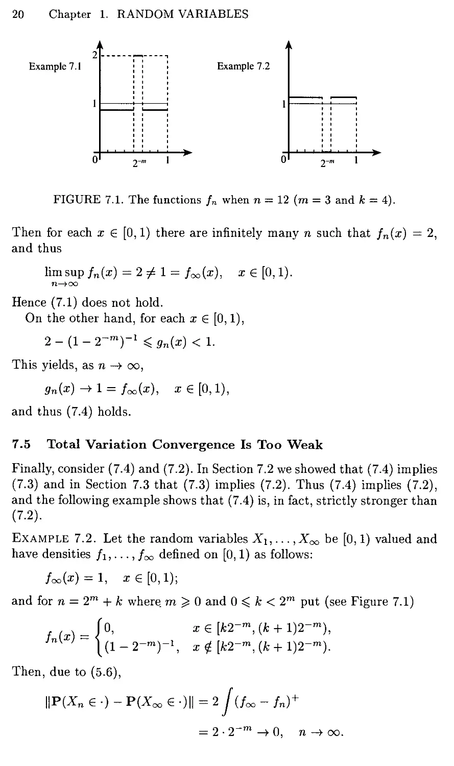
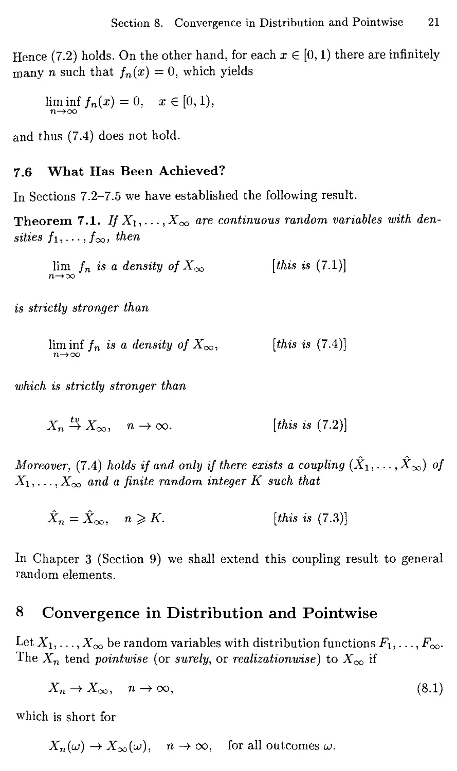
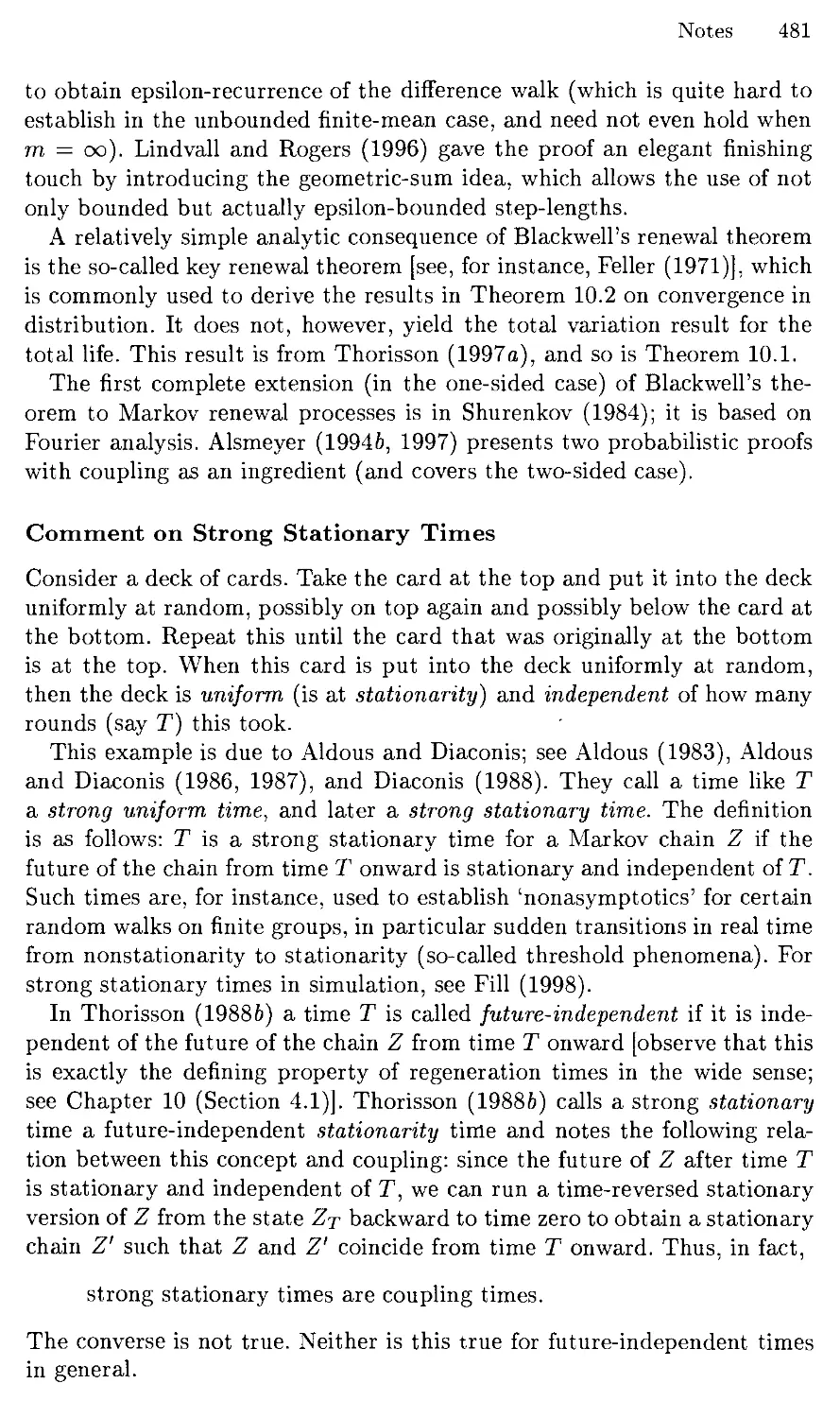
This means that the Xn close in on the limit without necessarily hitting
it as in (7.3). In order to compare (8.1) to (7.3) note that (8.1) can be
rewritten as follows: for each e > 0 there is a finite random integer Ke such
that
\Xn — Xoo| ^ e, n > Ke, (see Figure 8.1).
(8.2)
11 Illustration of (7.3)
n i-» X„(co)
XJlfo)
K(fo)
i k Illustration of (8.1), that is, of (8.2)
n H> XJfit)
XO0)
KM
FIGURE 8.1. Comparison of (7.3) and (8.1).
In this section we shall dig out the distributional form of pointwise
convergence. The result, once more, is stated at the end of the section.
8.1 Total Variation Convergence Is Too Strong
The distributional condition we are looking for should be implied by point-
wise convergence. This excludes convergence in total variation, as can be
seen by the following example. Put Xn = \jn and X^ = 0. Then certainly
(8.1) holds, but Xn does not tend to Xoo in total variation, since clearly
||P(xne-)-P(*ooe-)ll = 2^o.
Even the much weaker condition
Fn(x) ->-F0O(x), n->oo, iel, (8.3)
is too strong, since in our example
Fn(0) = 0/>1 = FQO(0).
8.2 Pointwise Convergence =>■ Convergence in Distribution
The distributional form of pointwise convergence turns out to be the
following slight weakening of (8.3):
Fn(x) —> Foo(x), n —> oo, for all x where Fqq is continuous. (8.4)
Section 8. Convergence in Distribution and Pointwise 23
This is called convergence in distribution and is denoted by
Xn -> Xqo, n ->■ oo.
In order to see that pointwise convergence implies convergence in
distribution assume that (8.1) holds and apply its equivalent form (8.2) to obtain
that for all x £ E and e > 0
Fn(x) = P(Xn ^x,Ke^n) + P{Xn ^x,KE>n)
^P(Xoo ^x + e)+P(Ke >n)
->• Fqo (x + e), n ->■ oo,
and
Fn{x) >P{Xn^x,Ks^n)
^PiXcc ^x~e,Ke^n)
—> Fqo (x — e), n —> oo.
Thus for all x <E E and e > 0
Fqo (x - e) ^ lim inf Fn (x) ^ lim sup Fn (x) ^ F*, (x + e),
and sending e to 0 shows that (8.4) holds.
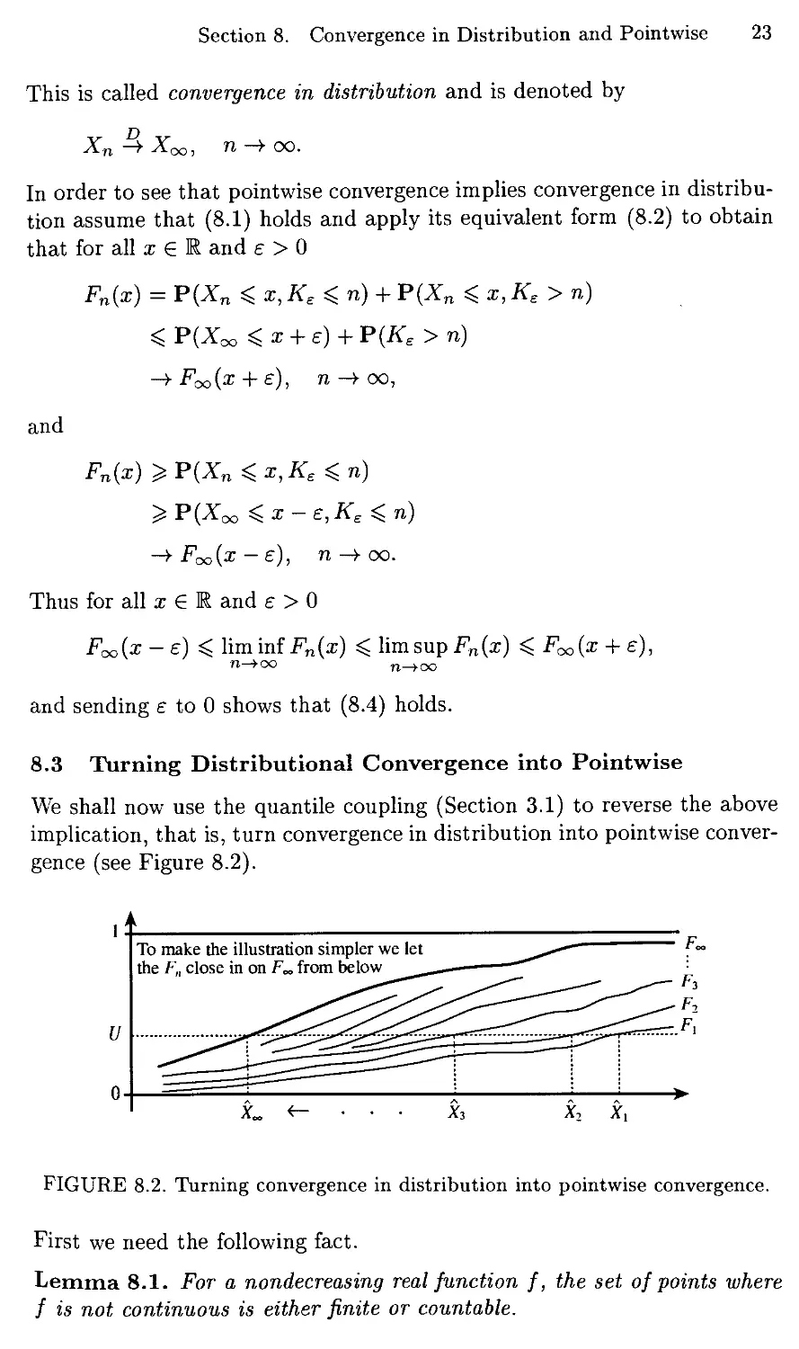
8.3 Turning Distributional Convergence into Pointwise
We shall now use the quantile coupling (Section 3.1) to reverse the above
implication, that is, turn convergence in distribution into pointwise
convergence (see Figure 8.2).
FIGURE 8.2. Turning convergence in distribution into pointwise convergence.
First we need the following fact.
Lemma 8.1. For a nondecreasing real function f, the set of points where
f is not continuous is either finite or countable.
24 Chapter 1. RANDOM VARIABLES
Proof. That / is not continuous at u is equivalent to the left-hand limit
being less than the right hand limit, f(u—) < f(u+). To each such u we
can associate a rational number that lies in the interval [f(u—),f(u+)).
These intervals are disjoint (because / is nondecreasing), and thus we have
established a one-to-one correspondence between {ti£l: f(u~) < f(u+)}
and a subset of the rational numbers. Since the rationals are countable, the
set {u £ E : f{u—) < /(«+)} is either finite or countable. □
Recall that the generalized inverse of a distribution function F is
F_1(w) =inf{a:e E : F(x) > w}, w<E[0,l].
Clearly, F~l is nondecreasing,
F(F-l{u)-)^u^F(F-l(u)), «G[0,1], (8.5)
and
F"1 is continuous at u
and F(x-) ^ w ^ F(x)
Since F^1 is nondecreasing, the set of points where F^1 is not continuous
is finite or countable. Thus there is a random variable U that is uniform
on [0,1] and takes values in the set of points at which F^1 is continuous.
Use this U to define the quantile coupling
Xn = F~1(U), O^n^oo.
We shall show that (8.4) implies
FnXu) ~* •P,o^1(u)> n-t-oo, for all u where F^1 is continuous, (8.7)
which yields the desired result that Xn —> Xoo as n —> oo.
8.4 Establishing That (8.4) Implies (8.7)
Fix u G [0,1] and put
x = liminf F~l(u).
Since F^ is nondecreasing and thus is discontinuous at only finitely or
countably many points, we can fix an arbitrarily small e > 0 such that
Foo is continuous at both x — e and x + s. Let rik,k ^ 1, be a sequence of
integers such that
F_1(m) =x.
(8.6)
x - s < F~* (u) ^ x + e, k > 1.
Section 8. Convergence in Distribution and Pointwise 25
Applying (8.5) yields
Fnk(x-e) ^ u ^ Fnk{x+e), k > 1.
Send k to infinity and use (8.4) and the choice of e to deduce
Fxj
(x - e) ^ u ^ Fqo(x +e).
Then send s to zero to obtain
Fooix-) ^u^ Foo(a:). (8.8)
Replace x by
i/ = lim sup F^^tt)
n—>oo
in the above argument to obtain
Fcoiy-) ^u^ Food/). (8-9)
If Fj;1 is continuous at u, we obtain from (8.6), (8.8), and (8.9) that
F-1(«) = ^ = liminfF-1H,
n—j-oo
F^(u) = 2/ = limsupF-1(M).
n—j-oo
Thus (8.7) holds.
8.5 What Has Been Achieved?
In Sections 8.2-8.4 we have established the following result.
Theorem 8.1. Let X\,..., Xqq be random variables. Then
V D V
A„ -» Aqo, n -» 00,
if and only if there exists a coupling (Xi,..., X^) of X\,..., X^ such that
Xn ->• Xqo, n ->■ oo.
We finally mention that the definition (8.4) of convergence in distribution
can be seen to be equivalent to
E[/(Xn)] -»■ E[/(Xoo)], n -»■ oo,
for all bounded continuous functions /. This is taken to be the definition
of convergence in distribution for random elements in metric spaces. In
Chapter 3 (Section 10) we extend Theorem 8.1 to random elements in a
separable metric space.
26 Chapter 1. RANDOM VARIABLES
9 Quantile Coupling - Dominated Convergence
The pointwise version of the dominated convergence theorem [see Ash (1972)]
states that if Xi, X2,.. ■,X,*,,X are random variables such that
|Xn| sj X, 1 ^ n < oo,
E[X] < oo and Xn ->• X^ as n ->■ oo,
then
E[|Xoo|] < oo and E[Xn] ->• E[Xoo] as n ->• oo. (9.1)
Using the quantile coupling it is straightforward to extend this result to
the following distributional form.
Theorem 9.1. // X\, X2, ■ ■ •, Xqo, X are random variables such that
D
\Xn\ sj X, 1 ^ n < oo,
E[X] < oo and Xn —> X,*, as n -^ oo,
then (9.1) ZioMs.
Proof. Under the assumptions of the theorem we have
d D
X+ ^ X and X+ ->• X+, as n ->■ oo,
_ D r>
Xn ^ X and Xn —>■ X^ as n —>• oo.
Apply the quantile coupling in Sections 3 and 8 to turn these distributional
relations into pointwise ones, that is, to obtain copies of X+ and X~ that
are pointwise dominated by a copy of X (Section 3) and converge pointwise
to copies of X+, and X^, respectively (Section 8). By the pointwise version
of dominated convergence, this together with E[X] < oo implies
E[X+] < oo and E[X+] ->• E[X+] as n ->• oo,
E[X^] < oo and E[X"] ->• E[X^] as n ->• oo.
Thus E[|Xoo|] = E[X+] + E[X-] < oo and
E[Xn] = E[X+] - E[X"]
-> E[X+] - E[X"] = E[Xoo] as n -> oo,
and the proof is complete. D
In Chapter 2 we shall need the following extension to a continuous index.
Section 10. Impossible Coupling - Quantum Physics 27
Corollary 9.1. If Xt, t £ [0, oo], and X are random variables such that
\xt\^x, te[o,oo),
E[X] < oo and Xt —> Xqo as t —» oo,
then
E[|Xoo|] < oo and ~E[Xt] -> E[Xoo] as t -t oo.
Proof. A collection of real numbers like E[Xt], t e [0, oo), tends to a limit
if and only if it tends to this limit along all subsequences E[Xt(nj], n ^ 1,
where the t(n) increase to oo as n —> oo. Apply Theorem 9.1 to Xt^ to
obtain E[Xt{n)] ->■ E[X oo] as n -> oo. D
10 Impossible Coupling - Quantum Physics
We end this first chapter on a rather different note: the coupling aspect of
a (the?) problem in quantum physics.
10.1 A Surprising Experimental Result
The following experiment has been carried out. Some material (calcium,
carefully excited by laser) sends off particles (photons) in pairs, one particle
to the left and the other to the right. Measuring devices are placed on each
side of this material with measurements made when particles pass through.
What is being measured is the so-called polarization of the particle, which
can be either 1 or —1 and depends on the angle in the plane orthogonal to
the direction of movement.
0. When the measuring devices are aligned to measure polarization in
the same direction, say 0°, the same measurement is always recorded
on both sides.
1. When the left device is tilted 30° and the right device is kept at the
initial 0° position, then the measurements agree | of the time.
2. When the left device is rotated back to its 0° position and the right
device is tilted —30° (that is, 30° in the opposite direction), then the
measurements also agree | of the time.
3. When the left device is again tilted 30° and the right device is kept
at its new —30° position (that is, the total relative rotation is 60°),
then the measurements agree ~ of the time.
28 Chapter 1. RANDOM VARIABLES
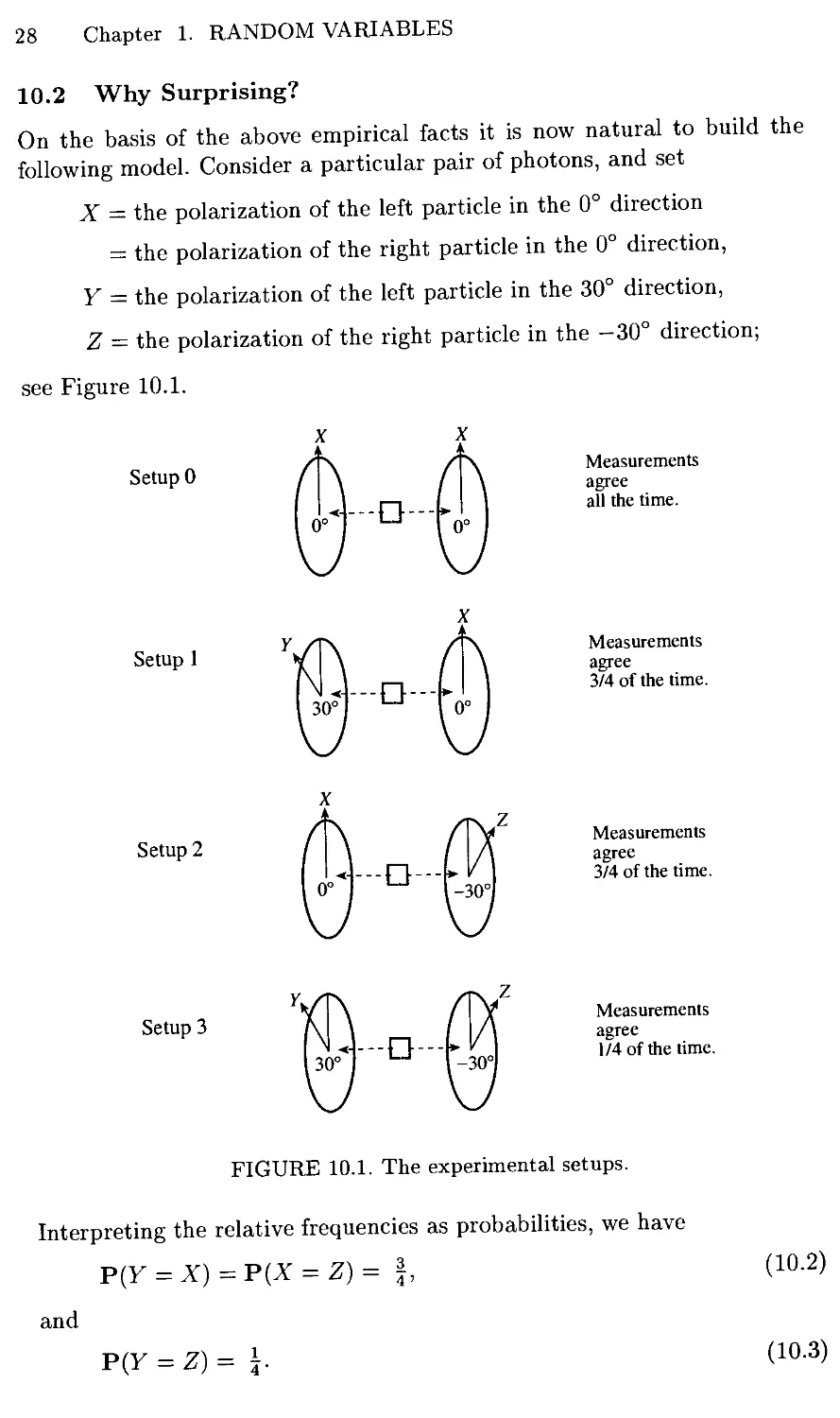
10.2 Why Surprising?
On the basis of the above empirical facts it is now natural to build the
following model. Consider a particular pair of photons, and set
X = the polarization of the left particle in the 0° direction
= the polarization of the right particle in the 0° direction,
Y = the polarization of the left particle in the 30° direction,
Z ~ the polarization of the right particle in the -30° direction;
see Figure 10.1.
Setup 0
-D-
Measurements
agree
all the time.
Setup 1
-D-
Measurements
agree
3/4 of the time.
Setup 2
-D-
Measurements
agree
3/4 of the time.
Setup 3
-D-
Measurements
agree
1/4 of the time.
FIGURE 10.1. The experimental setups.
Interpreting the relative frequencies as probabilities, we have
and
P(Y = X)=I>(X = Z)= f,
P(Y = Z)=\.
Section 10. Impossible Coupling - Quantum Physics 29
By basic rules of probability,
P{Y = Z) ^P(Y = Z,X = Z)
= P(Y = X,X = Z)
= P(F = X) - P{Y = X,X^Z)
^P(Y = X)-P{X^Z)
= P(Y = X) + P{X = Z)-l,
that is,
P{Y = Z)^P(Y = X) + P{X = Z)-l. (10.4)
Combine this, (10.2), and (10.3) to obtain the following contradiction:
This contradiction is derived in an ordinary probabilistic way from
straightforward empirical facts: real life seems to contradict probability theory...
10.3 Predicted by Quantum Theory
Because of this apparent contradiction it is all the more annoying (for
probabilists) that the empirical results are in fact predicted by quantum
mechanics, which calculates the probabilities as follows:
P(F = X)= P{X = Z) = cos2 30° = 1 - sin2 30° = 1 - (|)2 = |,
P(F = Z)=cos260° = (f)2= I.
10.4 No Contradiction at the Level of Observation
Note that X, Y, and Z refer to polarization as intrinsic properties of the
particles, thought of as existing simultaneously without interaction with
the macro world (without being measured). If we instead stay at the level
of observation (measurement), then it turns out that the contradiction
disappears.
It is clear that we are dealing with three experimental setups (leaving
out the one with the measuring devices aligned).
First consider Setup 1: the case when the left device is tilted 30° and the
right device is kept at the initial 0° position. Put
X\ = observed polarization of the right particle in the 0° direction,
Y\ — observed polarization of the left particle in the 30° direction.
30 Chapter 1. RANDOM VARIABLES
In addition to the measurements agreeing | of the time it has been recorded
that —1 and 1 are observed in equal proportions on both sides. Specify the
complete joint distribution of X\ and Yx as
p(x1 = -i,r1 = -i) = p(x1 = i,y, = i)= §,
p(x1 = -i,r1 = i) = P(A:1 = i,Yi = -i)= |.
This is in accordance with the relative frequencies since
P(Yi=-l)=P(X!=-l)
= P(Xi = -l,Yi = -1) +P(X1 = -l,Yi = 1)
_ i_
~ 2'
P(X, = Yx) = P(Xi = -1, Yi = -1) + P(Xi = 1, Yi = 1)
_ 3
4"
Now consider Setup 2: the case when the left device is at the 0° position
and the right device is tilted —30°. Put
X2 = observed polarization of the left particle in the 0° direction,
Z2 = observed polarization of the right particle in the —30° direction.
Letting (X2,Z2) have the same distribution as (Xi,Y\) again yields
probabilities in accordance with the relative frequencies,
P(Y2 = -1) = P(X2 = -1) = \ and P(X2 = Y2) = f.
Finally, consider Setup 3: the case when the left device is tilted 30° and
the right device -30°. Put
Y3 = observed polarization of the left particle in the 30° direction,
Z3 = observed polarization of the right particle in the —30° direction.
The measurements now agree only | of the time, but it has still been
recorded that —1 and 1 are observed in equal proportions on both sides.
Specify the complete joint distribution of Y3 and Z3 as
p(y3 = -i, z3 = -i) = P(r3 = 1, z3 = 1) = |,
p(y3 = -1, z3 = 1) = P(y3 = 1, z3 = -i) = §.
This is in accordance with the relative frequencies,
P(y3 = -1) = P(Z3 = -1) = I and P(y3 = Z3) = \.
We have managed to account for all three experiments, and thus the
contradiction is not at the level of observation. The contradiction appears when
we assume that each particle has a polarization in a direction where we do
not make a measurement.
Section 10. Impossible Coupling - Quantum Physics 31
10.5 What Has This to Do with Coupling?
We have created three pairs (Xi,Y\), (X2,Z2), and (Y3,Zz)- What we
proved in Section 10.2 is that there is no coupling of these pairs such that
the X-variables agree, the y-variables agree, and the Z-variables agree.
More precisely, there is no jointly distributed triple (X, Y, Z) such that
(X,Y) = (X^Y,), (X,Z) = (X2,Z2), (Y,Z)^(Y3,Z3).
That is, although reality seems to be able to construct a coupling, we can't.
10.6 Does Probability Not Suffice in the Micro World?
It is one of the implications of quantum theory that polarization cannot
be measured simultaneously in all three directions; only one measurement
on each particle is possible. The reason we have measurements in pairs is
that we have two particles. The above contradiction further suggests that
polarization exists in the micro world only through interaction with the
macro world (only by being measured).
Is there then nothing, no reality, behind the observations? Or does
probability not suffice to describe it?
One school of thought claims that classical probability (that is,
Kolmogorov's axioms) is too narrow. It should be replaced by quantum
probability (an axiom system more general than Kolmogorov's) in a similar way
as Newton's theory had to be replaced by Einstein's in physics.
Applying quantum probability there is no longer a contradiction to be derived
from the assumption that polarization exists in all three directions. See
Kummerer and Maassen (1998) and Accardi (1998) for such viewpoints.
Note that there are finitely many possible outcomes in each individual
experiment, so the contradiction does not appear to have to do with
countable additivity. Since Kolmogorov's axioms otherwise reflect properties of
relative frequencies, it is hard to swallow that they should not apply. And
so it is not surprising that there are other attempts to get rid of the
contradiction. See Maudlin (1994) and Gill (1998, 1999) for the following point
of view.
Behind the attempt in Section 10.2 to create a model are several
implicit assumptions. One assumption is that measuring the polarization in a
particular direction does not affect the polarization in the other directions.
In other words, an interplay between the micro and macro worlds is not
allowed. Allowing a local interplay is not a serious crime against physical
ideas, but it turns out that a nonlocal interplay is needed to get rid of
the contradiction. Nonlocal means that the experimental setup on the left,
for instance, affects the polarization of a particle measured on the right.
This is not easy to accept, but for an Einsteinian realist this is easier to
accept than having to discard Kolmogorov's axioms, which is too close to
discarding 2 + 2 = 4.
32 Chapter 1. RANDOM VARIABLES
10.7 What Does This Teach Us About Coupling?
The above excursion into the quantum experience shows that we have to
be careful when assuming existence of couplings. For empirical or
intuitive reasons joint distributions may appear to exist when they do not.
In Chapter 3 (Sections 3 through 5) we shall consider some safe methods
for constructing couplings. The next chapter, however, is devoted to the
classical triumphs of the coupling method.
Chapter 2
MARKOV CHAINS
AND RANDOM WALKS
1 Introduction
We now turn to the coupling of Markov chains in discrete and
continuous time, random walks, and renewal processes, the aim being to establish
asymptotic properties such as asymptotic stationarity. We start with the
earliest example, the classical coupling, which we present first in the
pleasant context of birth and death processes.
2 Classical Coupling - Birth and Death Processes
A continuous-time irreducible nonexplosive birth and death process is a
collection of random variables (stochastic process)
Z = (2s)sg[0,oo)
taking values in the state space E = {0,1,...} and developing in time (as
the time parameter s increases) in such a way that Z changes state only
finitely often in finite time intervals (nonexplosion) and whenever Z visits
a state i, it stays there an exponential length of time (sojourn time) with
parameter depending only on i, and then jumps either one step up to i + 1
(a birth) or one step down to i — 1 (a death, this occurs only if i > 0)
with positive probabilities depending only on i. Irreducibility follows from
the positivity of the birth and death probabilities (irreducibility means
that each state is visited with positive probability starting from any other
33
34 Chapter 2. MARKOV CHAINS AND RANDOM WALKS
state). Finally, we let the paths be right-continuous, that is, Zt = Zt+,
where Zt+ = lims;t Zs.
2.1 Notation
Let A be the distribution of Zq, the initial distribution. Let P\ indicate this.
Let Pj indicate that Z starts in state j, that is, Z0 = j. The semigroup of
transition matrices is
Pl = (Ptj:i,j e E), t > 0, [semigroup because PlPs = Pt+S]
where P'- denotes the probability of going from i to j in a time interval of
length t,
P£ =P(Z.+t=j|Z. = t), s,t^Q, i,j€E.
If we treat the initial distribution A as a row vector, then the row vector
AP* represents the distribution of Zt,
px(zt = j) = \pj, t^o, jeE.
2.2 The Classical Coupling
Let Z' be a differently started independent version of Z, that is, Z' is
independent of Z and has the same semigroup of transition matrices but
another initial distribution A', say. Let T be the time when Z and Z' first
meet,
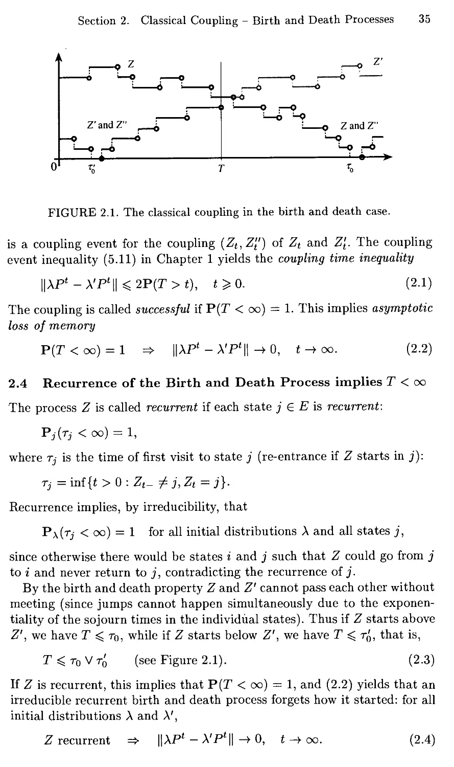
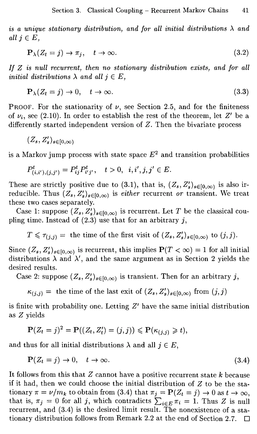
T = inf{i >0 : Zt = Z[) (see Figure 2.1).
Let Z" be the process that follows the path of Z' up to T and then switches
to Z,
z,,[z't if*<r,
' \zt iit^T.
At time T the processes Z and Z' are in the same state and will continue
as if they both were starting anew in that state. Therefore, modifying Z'
by switching to Z at time T does not change its distribution, that is, Z" is
a copy of Z'. Thus (Z, Z") is a coupling of Z and Z', the classical coupling.
2.3 The Coupling Time T - Asymptotic Loss of Memory
The time T when Z and Z" merge is called a coupling time or coupling
epoch. By definition (Section 4.1 in Chapter 1) the event
{T < t} = {Zt = Z't'}
Section 2. Classical Coupling - Birth and Death Processes 35
FIGURE 2.1. The classical coupling in the birth and death case.
is a coupling event for the coupling (Zt, Z[') of Zt and Z[. The coupling
event inequality (5.11) in Chapter 1 yields the coupling time inequality
||XPl - \'Pl || < 2P(T > t), t ^ 0. (2.1)
The coupling is called successful if P(T < oo) = 1. This implies asymptotic
loss of memory
P(T<oo) = l => ||AP* -A'P'H -+0, t-^oo. (2.2)
2.4 Recurrence of the Birth and Death Process implies T < oo
The process Z is called recurrent if each state j £ E is recurrent:
Pj(tj < oo) = 1,
where r,- is the time of first visit to state j (re-entrance if Z starts in j):
Tj=M{t>0:Zt- ?j,Zt=j}.
Recurrence implies, by irreducibility, that
Pa(tj < oo) = 1 for all initial distributions A and all states j,
since otherwise there would be states i and j such that Z could go from j
to i and never return to j, contradicting the recurrence of j.
By the birth and death property Z and Z' cannot pass each other without
meeting (since jumps cannot happen simultaneously due to the exponen-
tiality of the sojourn times in the individual states). Thus if Z starts above
Z', we have T < r0, while if Z starts below Z', we have T < Tq, that is,
T < t0 V To (see Figure 2.1). (2.3)
If Z is recurrent, this implies that P(T < oo) = 1, and (2.2) yields that an
irreducible recurrent birth and death process forgets how it started: for all
initial distributions A and A',
Z recurrent => ||XP* - A'P*|| -> 0, t -> oo. (2.4)
36 Chapter 2. MARKOV CHAINS AND RANDOM WALKS
2.5 Recurrence Implies Existence of a Stationary Vector
Let Z be recurrent. Fix an arbitrary state k and let i/, be the expected
amount of time spent in i between two entrances to k,
Ei
rTk
/ 1{Za=i}
Jo
ds
i e E.
(2.5)
Then the row vector v with entries i/j, i 6 E, is stationary:
vPl = v, t > 0. (2.6)
This can be seen as follows. Note that
Vi = E*
r-oo poo
I l{z,=i,Tk>s}ds = / Pk(Zs = i,rk >
Jo J Jo
s) ds.
Note also that we can tell whether the event {rk > s} happens or not
by observing Z only in the time interval [0, s], and thus, conditionally on
{Zs = i,rk > s}, the process Z starts anew in state i at time s, that is,
Ptij=Pk(Zs+t = j\Zs=i,rk >s).
These two observations yield
/•OO
ViP^ = / Pk (Zs+t =j,Zs = i,rk> s) ds.
Jo
Sum over i to obtain the first equation in
/•OO r-Tk
*=j Pk(Zs+t=j,Tk>s)ds = Ek[J l{Za+t-_
= E4/ liz,=j}ds
vP]
■■3}
ds
r fTk ~\ r rTk+t
= Efc[j l{Zs=j}ds\+Ek[J 1
{Z,=j}
ds\.
Since Z starts anew in state k at time rk, the last term can be replaced by
Efc[Jo l{z„=j} ds]. This yields the first equation in
V.=j} ds
= Efc[y l{z.=j}ds
+ E;
U'
!{Z.=j} rfs
that is, (2.6) holds.
Note also that
5>i = E J P 53 l{Zj=i} dsl = Efc [ I'" ll - Etlnt]. (2.7)
Section 2. Classical Coupling - Birth and Death Processes 37
2.6 Positive Recurrence Implies Asymptotic Stationarity
The process Z is called positive recurrent if each state j £ E is positive
recurrent:
rrij := Ej[r,] < oo.
In this case, due to (2.6) and (2.7), the row vector ir = u/mk is a stationary
distribution for Z, that is,
irPt=Tr, t^Q, and yVj = 1.
Choose Z' stationary to obtain that Z is asymptotically stationary: putting
A' = 7r in (2.4) yields
\ nt tv
XP ->• 7T, t ->• OO.
In other words (cf. Theorem 6.1 in Chapter 1), we have established the
following result: for all initial distributions A and all j £ E it holds that
Z positive recurrent => P(Zt = j) —> ftj, t —> oo. (2.8)
Remark 2.1. The proof of (2.8) works for all stationary distributions ir.
Thus 7r must be unique. In particular, 7r does not depend on the arbitrary
fixed state k. For each j e E, let hj be the expected sojourn time in j,
hj = E^inf {t > 0 : Zt- = j, Zt ? j}}, (2.9)
and note that v^ = h^. This yields (by taking k = j) that the unique
stationary distribution tt is given by
7Tj = hj/m.j, j G E.
2.7 Null Recurrence Implies Asymptotic 'Nullity'
A recurrent process Z is called null recurrent if each state j e E is null
recurrent:
mJ = %h] = °°-
In this case (2.6) yields ViP\k ^ uk, and since vk = hk < oo (A* is the
expected value of an exponential random variable and thus hk < oo) and
P\h > 0 for all t > 0 (some t > 0 suffices of course), we obtain
Vi < oo, ie E. (2.10)
Take a finite set of states B and put A' = v(-\B), that is,
V = \vjlY,i£Bvu J e B,
J 10, j^B.
38 Chapter 2. MARKOV CHAINS AND RANDOM WALKS
Then A' ^ vIY^i£Bvi [entrywise], which implies X'Pj ^ ^V XagB ^
and thus by (2.6),
*'^<"j/I>. 3€E. (2.11)
i£B
This yields the second inequality in \Z' has initial distribution A']
p(zt = j) < \p(zt = j) - p(z; = j)\ + p(z; = j)
*Z\P(Zt=])--P(Z't=j)\ + uj/,£iui.
Apply (2.4) to obtain
limsupP(Zt=j)<^/2I/i- (2-12)
Sending B "[ E yields ^ieB Vi t X)ieB "» = mfc = °°) an(l tnus we have
established the following result: for all initial distributions A and all j £ E,
Z null recurrent =*■ P(Zt = j) ->• 0, t ->• oo.
Remark 2.2. In the null recurrent case no stationary distribution exists,
since if a stationary 7r existed, then we could let it be the initial distribution
of Z and obtain ttj = P{Zt = j) —► 0 as t —► oo, that is, 7Tj = 0 for all j,
which contradicts Y^i^E^i ~ 1-
Remark 2.3. The result in Section 2.6 that limt_).00P(Zt = j), j £ E, is
a stationary distribution was obtained under the condition my. < oo for
some state k. The result in this subsection that limt_>00P(Zt = j) = 0,
j £ E, was obtained under the condition m^ = oo for some state fc. Since
a stationary distribution cannot be identically 0, it follows that either all
states are positive recurrent or all states are null recurrent. That is, a
recurrent Z is either positive recurrent or null recurrent.
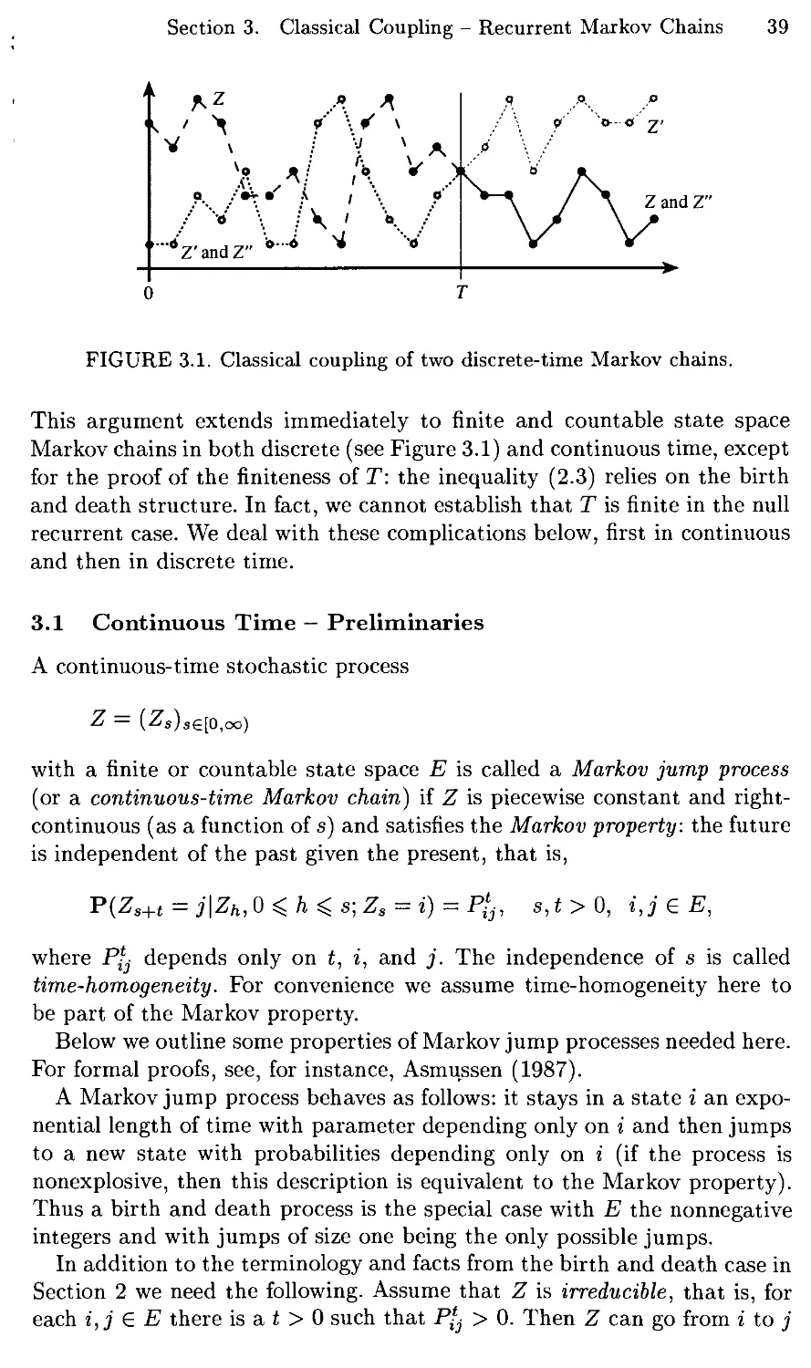
3 Classical Coupling - Recurrent Markov Chains
The argument in the previous section went basically as follows. In order
to deduce asymptotic properties of the process Z, let a differently started
version Z' run independently of Z until it hits Z, at time T, say. At time T
switch from Z' to Z to obtain a copy Z" of Z' that sticks to Z from time
T onward. Establish that T is finite with probability one to deduce that Z
and Z' have the same asymptotic behaviour. In the positive recurrent case,
choose Z' stationary to obtain that Z is asymptotically stationary. In the
null recurrent case, choose Z' such that P(Zt' = j) is close to 0 for all t to
obtain that P(Zt = j) is close to 0 asymptotically.
Section 3. Classical Coupling - Recurrent Markov Chains 39
*Z'andZ" ° *
/ \ p '0--0' 2'
0 T
FIGURE 3.1. Classical coupling of two discrete-time Markov chains.
This argument extends immediately to finite and countable state space
Markov chains in both discrete (see Figure 3.1) and continuous time, except
for the proof of the finiteness of T: the inequality (2.3) relies on the birth
and death structure. In fact, we cannot establish that T is finite in the null
recurrent case. We deal with these complications below, first in continuous
and then in discrete time.
3.1 Continuous Time — Preliminaries
A continuous-time stochastic process
Z = (-^s)se[o,oo)
with a finite or countable state space E is called a Markov jump process
(or a continuous-time Markov chain) if Z is piecewise constant and right-
continuous (as a function of s) and satisfies the Markov property: the future
is independent of the past given the present, that is,
P(Z.+t=j\Zh,0 4:h4:8;Za = i) = P!j, s,t>0, i,j £ E,
where P/- depends only on t, i, and j. The independence of s is called
time-homogeneity. For convenience we assume time-homogeneity here to
be part of the Markov property.
Below we outline some properties of Markov jump processes needed here.
For formal proofs, see, for instance, Asmussen (1987).
A Markov jump process behaves as follows: it stays in a state i an
exponential length of time with parameter depending only on i and then jumps
to a new state with probabilities depending only on i (if the process is
nonexplosive, then this description is equivalent to the Markov property).
Thus a birth and death process is the special case with E the nonnegative
integers and with jumps of size one being the only possible jumps.
In addition to the terminology and facts from the birth and death case in
Section 2 we need the following. Assume that Z is irreducible, that is, for
each i, j £ E there is a t > 0 such that Py > 0. Then Z can go from i to j
40 Chapter 2. MARKOV CHAINS AND RANDOM WALKS
through a finite sequence of states i = io,«i, ■ • -in-i;*n — j- Conditionally
on going through these states the sojourn times in io,i\,... ,in are
distributed like independent exponential random variables, say X0,... ,Xn,
with parameters depending on these states. Since for all t > 0 we have
P{X0 H 1- Xn_i < t < X0-\ h Xn) > 0, it follows that Z can enter
the state j before time t and not leave it until after time t, that is, Z can
be in j at time t. Thus irreducibility implies that
Ftj >0, t>0, i,j€E. (3.1)
The process Z is transient if each state j E E is transient:
Pj{Tj < CO) < 1.
Transience implies (since each time Z leaves the state j it has the
probability Pj(tj = oo) > 0 of never entering j again) that
P\(kj < oo) = 1 for all initial distributions A and all j E E
where (with sup 0=0)
Kj = sup{£ > 0 : Zt = j} — the time of the last exit from j.
An irreducible Markov jump process is either recurrent or transient. This
can be seen as follows. Let Z start in some state i and suppose there exists
a recurrent state j. Then, by irreducibility, Z is sure to visit j (because
otherwise it could go from j to i and never return to j, contradicting
the recurrence of j). Each time Z leaves j it has a positive probability of
visiting i before returning to j (because otherwise it would always return
to j before visiting i and thus could not go from j to i, contradicting the
irreducibility of Z). Since, by irreducibility of Z and by recurrence of j,
Z leaves j infinitely often, it will eventually get back to i with probability
one, that is, i is also recurrent. This yields the desired result that if one
state is recurrent, then all the states are recurrent.
3.2 Continuous Time - The Theorem
We shall now establish the following result.
Theorem 3.1. Let Z be an irreducible recurrent Markov jump process with
a finite or countable state space E. Then, with k a fixed state, the row
vector v with entries defined at (2.5) is stationary and the entries are finite.
Further, Z is either positive recurrent or null recurrent.
If Z is positive recurrent, then the classical coupling (defined in
Section 2.2) is successful, the row vector
■k — (hj/m.j : j € E) [hj is expected sojourn time in j, see (2.9)]
Section 3. Classical Coupling - Recurrent Markov Chains 41
is a unique stationary distribution, and for all initial distributions A and
all j e E,
PX{Zt=j)-^7Tj, £->0O. (3.2)
// Z is null recurrent, then no stationary distribution exists, and for all
initial distributions A and all j 6 E,
Px{Zt=j)^Q, i->oo. (3.3)
Proof. For the stationarity of v, see Section 2.5, and for the flniteness
of Vi, see (2.10). In order to establish the rest of the theorem, let Z' be a
differently started independent version of Z. Then the bivariate process
\ZS, Zs)sg[0jOo)
is a Markov jump process with state space E2 and transition probabilities
pUi'Hi,r) = pijpi'j'^ l > °> *'*'. J'.J" e E-
These are strictly positive due to (3.1), that is, (Zs,-Zs)se[o,oo) is also
irreducible. Thus (Zs, Zj)se[o>00) is either recurrent or transient. We treat
these two cases separately.
Case 1: suppose (Zs, Zj)se[0>Oo) is recurrent. Let T be the classical
coupling time. Instead of (2.3) use that for an arbitrary j,
T ^ T(jj) — tne time of the first visit of (Zs, Z's)s&[0,oo) t0 (hi)-
Since (Zs, Zj)se[0jOo) is recurrent, this implies P(T < oo) = 1 for all initial
distributions A and A', and the same argument as in Section 2 yields the
desired results.
Case 2: suppose (Zs, Z's)S£[0,oo) is transient. Then for an arbitrary j,
KU'i) = t'ie ilme of the last exit of (Zs, Zj)se[o,oo) from (j,j)
is finite with probability one. Letting Z' have the same initial distribution
as Z yields
P(Zt = j)2 = P((Zt,Zfi = (j,j)) ^ P(kuj) > t),
and thus for all initial distributions A and all j £ E,
P(Zt = j) -)• 0, t -)• oo. (3.4)
It follows from this that Z cannot have a positive recurrent state k because
if it had, then we could choose the initial distribution of Z to be the
stationary ■k = v/mk to obtain from (3.4) that ttj = P(Zt = j) —> 0 as t —> oo,
that is, itj = 0 for all j, which contradicts ^ieE^i = 1- Thus Z is null
recurrent, and (3.4) is the desired limit result. The nonexistence of a
stationary distribution follows from Remark 2.2 at the end of Section 2.7. □
42 Chapter 2. MARKOV CHAINS AND RANDOM WALKS
3.3 Discrete Time — Preliminaries
A discrete-time stochastic process
Z = (Zt)8°
with a finite or countable state space E is called a Markov chain in discrete
time if
P(Z„+i =j\Z0,...,Zn-i;Zn = i) =Pij, n>0, i,j £ E,
where P$j depends only on i and j. As in the continuous-time case we
assume here that time-homogeneity (the fact that P^ does not depend
on n) is part of the Markov property. The matrix Pn of n-step transition
probabilities is the nth power of P = (Pij : i,j £ E).
We use notation and terminology from the continuous-time case with the
following modification (to conform with standard practice even if it is not
formally needed): let tj be the time of first visit to state j (revisit if Z
starts in j), that is,
Tj = inf{n > 0 : Zn - j}.
Again the same argument as in Section 2.5 yields vP — v, where v is the
row vector with entries {k is a fixed state)
r n ~\
Vi = Efc 2_, l{z„=i} (note that now v^ = 1). (3.5)
We can use the same facts as in the continuous-time case except (3.1).
Irreducibility means that Pf" > 0 for some n > 0, and this does not imply
that it holds for all n > 0. In particular, periodicity can pop up in discrete
time. Therefore, we need the following property. The Markov chain Z is
called aperiodic if each state j 6 E is aperiodic:
gcd{n > 1 : P£ > 0} = 1;
here gcd denotes greatest common divisor, the largest integer that is a
factor of all the integers in the set.
3.4 Discrete Time — The Theorem
We shall now establish the following result.
Theorem 3.2. Let Z be an irreducible recurrent Markov chain in discrete
time with a finite or countable state space E. Then, with k a fixed state, the
row vector v with entries defined at (3.5) is stationary and the entries are
finite. Further, Z is either positive recurrent or null recurrent, and either
is aperiodic or has no aperiodic state.
Section 3. Classical Coupling - Recurrent Markov Chains 43
If Z is aperiodic and positive recurrent, then the classical coupling
(defined in Section 2.2) is successful, the row vector
■k = (1/rrij :jEE)
is a unique stationary distribution, and for all initial distributions A and
all j e E,
P\(Zn=j)-^TTj, n-^oo.
If Z is aperiodic and null recurrent, then no stationary distribution exists,
and for all initial distributions A and all j 6 E,
P\(Zn = j) ->0, n->oo.
Proof. Suppose Z has an aperiodic state h. Then, by Lemma 3.1(6)
below, there is an integer n such that P£h > 0 and P^1 > 0 [take
B = {k ^ 0 : Pfih > 0}]. For alii £ E and all integers /, k and m ^ 0,
we have p^k+m ^ P\hPhh^bA- ^v irreducibility, we can find / and m such
that P\h > 0 and P% > 0. Thus P/+n+m > 0 and pl.+n+1+m > 0. Thus
either all states are aperiodic or no state is aperiodic.
The rest of the proof is the same as in the continuous-time case (see
the proof of Theorem 3.1), except that the irreducibility of the bivariate
Markov chain (Zk,Z'k)1f is harder to establish, since we cannot rely on
(3.1). We have only that Pf™ > 0 for some n > 0, not necessarily all.
In order to establish that (Z&, ZjJ.)g° is irreducible, let h £ E be fixed and
hjii'ij' € E arbitrary. We must show that there is an n such that both
P"j > 0 and P"-, > 0. We have, for all integers l,m,l',m' ^ 0 and for all
n ^ (l + m) V(/' + m'),
P"i v- pi pn-1 — m r>m „„J pn v. of pn—l' — m'pm'
ij ^ rihrhh rhi ana r{,y ^ rilhrhh rhy.
Use the irreducibility of Z to find l,m,l',m' such that
p/h>o, ph™>o, p/;h>o, p$>o.
According to Lemma 3.1(6) below, if we take n large enough, then both
PhY'~m > 0 and P^l'-m' > 0 [take B = {k > 0 : P*fc > 0}]. □
Lemma 3.1. (a) Let A be a subset of Z that is aperodic [gcd A = 1],
additive [a, 6 6 A implies a + b £ A], and closed under negation [a 6 A =>
-ae 4]. Then A = 1.
(6) Lei B be a subset of the nonnegative integers that is aperiodic and
additive. Then there is an integer ub such that n 6 B for all n ^ rig.
PROOF, (a) Since A is closed under addition and negation, it follows that
A contains dZ, where d = min{fc ^ 1 : k £ A}. For each 6 £ A there is
44 Chapter 2. MARKOV CHAINS AND RANDOM WALKS
a k £ Z such that 0 ^ b — kd < d, and due to the definition of d we have
b - kd = 0. Thus A = dZ, and the aperiodicity of ^4 yields d = 1.
(6) It is no restriction to assume that 0£B. The set
i:={fc£Z: there is an n^ € B such that n^ + k £ B}
is aperiodic [since B is so, take n^ = 0 to see that B is a subset of ^4],
additive [take na+b — na + nb], and closed under negation [take n_a =
na + a\. Thus A = Z, due to (a). Thus IgtI. We shall show that nB = n\
does the trick. Each n~^n\ can be written in the form
n = n\ + mn\ + k, where m ^ 0 and 0 ^ k < m.
Thus n = (ni + m — k)rii + k{n\ + 1), which lies in B [since B is additive,
since both n\ and n\ + 1 are in B, and since both n\ + m — k and k are
nonnegative]. □
3.5 Comment on the Strong Markov Property
A countable state space Markov jump process Z satisfies the strong Markov
property at hitting times: for a hitting time r = inf{i > 0 : Zt £ A}
of a subset A of E it holds that, conditionally on r < oo, the process
(Zr+S)se[0ioo) is a version of Z and is conditionally independent of (Zs)s€[0 T\
given ZT. In other words, at the time r the process Z starts anew in state
ZT independently of how it got there. The same comment applies to Markov
chains in discrete time.
Thus, when proving in Section 2.2 that Z" is a copy of Z', we were
actually using the strong Markov property of the bivariate process (Zs, Zj)s€[0oo)
at
T = hitting time of the diagonal {(j,j) ■ j £ E} of E2.
In fact, the strong Markov property holds at stopping times, that is,
random times r such that for each t ^ 0 the event {r ^ t} is determined
(measurably) by (Zs)s€[0t] [see, for instance, Theorem 3.1 in Chapter 1 of
Asmussen (1987)]. A Markov process with this property is called a strong
Markov process.
4 Classical Coupling - Rates and Uniformity
Have another look at the coupling time inequality (2.1)
||APt-A'P'|K2P(T>i). (4.1)
If we knew not only that T is finite but also how fast P(T > t) goes to
zero, then we would obtain a rate result for the convergence of the Markov
process. Also, if T is stochastically dominated by a finite random variable
Section 4. Classical Coupling - Rates and Uniformity 45
with distribution that does not depend on the family Pl, t > 0, as long
as it lies in some fixed class of transition matrices, then we would obtain
uniform convergence over that class.
In this section we shall take a closer look at the classical coupling time
T in two simple cases.
4.1 Birth and Death Processes
Let Z be the irreducible nonexplosive recurrent birth and death process
considered in Section 2. There we proved for the classical coupling time T
that
T ^ T0 V T0.
If we know, for instance, that tq and t'0 have finite a-moments for some
a > 0, that is,
E[t£] < oo and E^"] < oo,
then E[Ta] < E[r0a] + E[r^a] < oo and thus
taP(T > t) < E[Tal{T>t}] -> 0, £ -> oo,
which together with (4.1) yields the following rate result: for a > 0,
E[r0a],E[r^a]<oo => ia||AP' - A'P*|| -> 0, t -> oo.
It is worth noting that for this rate result we needed only recurrence, not
positive recurrence as in the generalization to Markov jump processes
mentioned in Section 4.3 below.
4.2 Finite State Space — Doeblin's Argument
The classical coupling was introduced by Doeblin in 1938 in order to
establish asymptotic stationarity of a regular discrete-time finite-state Markov
chain Z = (Zfc)g°. Regularity means that there is an integer m and an
s > 0 such that
P%>e, i,jeE. ■ (4.2)
Doeblin argued along the following lines. Let a differently started version
Z' run independently of Z until the two chains meet, at a time T, say.
From T onward let the two chains run together. Regularity implies that if
Z has not met Z' up to time mk, then it will meet Z' before time mk + m
with probability no less than e. Thus
P(T > km) < (1 -e)k -> 0, k -> oo.
(4.3)
46 Chapter 2. MARKOV CHAINS AND RANDOM WALKS
Thus the chains eventually coincide and we obtain
|P(Z„ = j) - P(Z'n = j)\ *C P(Zn ?Z'n)^0, n^ oo.
Add to this the observation that maxie£ P,™ is nonincreasing and that
mini€E P?j is nondecreasing in n to deduce that P(Zn = j) has a limit.
(Nowadays one usually takes Z' stationary, which makes the last sentence
unnecessary.)
Doeblin's argument in fact yields that P(Zn = j) goes to the limit itj at
a geometric rate: from (4.3) and (4.1) with A' = ■k (and with t replaced by n)
we get
||APn - tt|| < 2(1 - £)["/m' (here [x] = sup{n e Z : n < x}),
which yields the following geometric rate result:
Vp< {l-e)-l/m : pn||APn-7r|| -> 0, n -> oo.
Note also that if we let Vm,e denote the class of transition matrices P
satisfying (4.2) with m and e fixed, then we obtain the following uniform
convergence result:
sup ||APn - tt|| -> 0, n -> oo.
The rate result also holds uniformly:
Vp < (1 - e)~l/m : pn sup ||APn — vr|| —> 0, n -> oo.
Pevm,£
Remark 4.1. Regularity is equivalent to irreducibility and aperiodicity.
This can be seen as follows. Regularity obviously implies irreducibility and
also that
which implies aperiodicity. Conversely, irreducibility and aperiodicity
together with PV> ^ PljPj]~l and Lemma 3.1(6) yield that PV> > 0 for all
m large enough, which, together with finiteness, implies regularity.
4.3 Comment on the Countable Markov Case
In the irreducible positive recurrent Markov jump case (and discrete-time
aperiodic Markov chain case) the following holds for the classical coupling
time T. Let j be an arbitrary fixed state and let Z and Z' have initial
distributions A and A', respectively. If a > 0 and
E[7f ] < oo, E[rja] < oo, Ej[r.,a] < oo,
Section 5. Ornstein Coupling - Random Walk on the Integers 47
then E[Ta] < oo, which yields (as above)
ilAP'-A'P'H-^O, t->oo.
Moreover, if
3p>l: E[pTj] < oo, E[pT'i] < oo, Ej[pTi]<oo,
then there is a p > 1 such that E[pT] < oo, which yields (as above)
^IIAP'-A'P'H-^O, t->oo.
This and more elaborate rate and uniformity results are established in
Chapter 10 (Section 7.5). See also Section 5 in Chapter 4.
4.4 Comment on Diffusions
A diffusion on [0, oo) is a continuous-time Markov process with state space
[0, oo) and continuous as a function of time. Two diffusions Z, Z' have
to meet before both have hit 0. Thus T < r0 V Tq holds, where T is the
classical coupling time and tq, Tq the hitting times of 0. The limit results for
birth and death processes were based on this inequality, and thus analogous
results hold for diffusions.
5 Ornstein Coupling — Random Walk on the Integers
The classical coupling need not be successful in the null recurrent and
transient cases. Integer-valued random walks are either null recurrent or
transient (see Remark 5.1 below). In this section we construct a coupling of
such walks that is always successful, provided that the step-lengths satisfy
a certain aperiodicity condition.
5.1 The Walk
Let X\,X%,... be i.i.d. finite integer-valued random variables that are
independent of the finite integer-valued random variable So- Put
Sk = S0 + X! + --- + Xk, 0<fc<oo.
Then 5 = (5fc)g° is called a random walk on the integers with step-lengths
X^,X2, ■ ■ ■ and initial position So- We further assume that the step-lengths
are strongly aperiodic: there is an h such that
P(Xi = ft) > 0 and gcd{n 6 Z : P(Xi - h = n) > 0} = 1.
Note that strong aperiodicity implies that the step-lengths are aperiodic,
that is,
gcd{n 6 1 : P(Xi = n) > 0} = 1.
48 Chapter 2. MARKOV CHAINS AND RANDOM WALKS
The converse is not true, however. The step-lengths can be aperiodic
without being strongly aperiodic. For instance, step-lengths with distribution
P(Xi = 1) = P(-X"i = —1) = | are aperiodic but not strongly aperiodic.
Note in this example that the difference X\ — X[ of two i.i.d. step-lengths
X\ and X[ will take the values 2, 0, and -2, that is, the difference is not
aperiodic. This is the reason we assume strong aperiodicity: we shall need
step-length aperiodicity for the difference of two walks.
Remark 5.1. Clearly, 5 is a Markov chain with state space Z. When 5
is irreducible and aperiodic, it will be either transient or null recurrent. It
cannot be positive recurrent because if it were, then Theorem 3.2 would
yield that 7r = (1/rrij : j £ Z) is a stationary distribution, but the expected
recurrence times m.j are obviously all identical, say rrij = a, and positive
recurrence would imply Y^^j = 2 l/a = °°i which contradicts X^j = 1-
5.2 Ornstein Coupling
Let 5' be a differently started independent version of 5, that is, 5' is a
random walk on the integers,
S'k = S^ + X[ + --- + X'k, 0^fc<oo,
that is independent of S and has the same step-length distribution. Let
h be as above. Since X\ — h is aperiodic, there is a constant c such that
X\ — h is aperiodic on {|^i — h\ ^ c}, that is, we can take c large enough
so that
gcd{n 6 Z : P(Xi - h = n, \XX - h\ < c) > 0} = 1. (5.1)
Put S£ = S£ and for k ^ 1,
x,l = [X'k ii\Xk-X'k\^c,
k \Xk ii\Xk-X'k\>c.
By symmetry [since (Xk,X'k) ^ (X'k,Xk)}
P(Xk = n, \Xk - X'k\ < c) = P(X'k = n, \Xk - X'k\ < c),
which yields the second equality in
P(X'k' = n)
= P(X'k = n, \Xk - X'k\ <c)+ P(Xk = n, \Xk - X'k\ > c)
= P(X'k =n), n e Z.
Thus the step-length distribution of the random walk 5",
S'k'= SH + X^ + ■ ■ ■ + X'k\ 0^k<oo,
Section 5. Ornstein Coupling - Random Walk on the Integers 49
is the same as that of 5'. Since the initial positions are the same, 5" is a
copy of 5'.
The random walk R = {Rk)^ defined by
Rk = Sk- S'k\ 0 < k < oo,
has step-lengths Xk — Xj!, k > 1, which are symmetric and bounded:
Xi - X[' = X'l - XY and \XX - X['\ < c.
Further, with h as above and n 6 Z, we have
P(Xi - X[' = n) > P(Xi -X'1=n, \XY -X[\^c)
> P(Xi - h = n, \Xi - h\ < c, X{ = h)
= P(Xi - A = n, |Xi - /iK c)P(X{ = A),
which together with (5.1) and P(X[ = h) > 0 implies that R has aperiodic
steplengths, that is,
gcd{n 6 Z : P(Xi - X(' = n) > 0} = 1.
Such a random walk is irreducible and recurrent (see next subsection), and
thus
K = inf{fc > 0 : Sk = Sk} = the time of the first visit of R to 0
is finite with probability one. Let 5'" be the copy of 5' that sticks to the
path of 5" up to time K and then switches to 5. Then (5,5'") is a coupling
of 5 and 5' with coupling time K. This together with the coupling time
inequality
\\P(Ske-)-P(S'ke-)\\^2P(K>k)
yields the following result.
Theorem 5.1. Let S be an integer-valued random walk with strongly
aperiodic step-lengths. Let S' be a differently started version of S. Then there
exists a successful coupling of S and S', and
\\P(Ske-)-P(S'ke-)\\^o, k^oo.
The above coupling of random walks was introduced by Ornstein in 1968
and is named after its inventor.
50 Chapter 2. MARKOV CHAINS AND RANDOM WALKS
5.3 The Difference Walk R is Irreducible and Recurrent
Here is an elementary argument showing that an integer-valued random
walk R = (-Rfc)o° witn symmetric bounded aperiodic step-lengths is
irreducible and recurrent (as a Markov chain).
Put R° = (RDF, where R°k = Rk - fl0- Clearly, the set
A = {n G Z : P(R°k = n) > 0 for some k}
is additive. Due to the step-length symmetry, A is closed under negation.
Due to the step-length aperiodicity, A is aperiodic. Thus A coincides with
the integers [see Lemma 3.1(a)]. Thus the Markov chain R is irreducible.
In order to establish recurrence, we shall first show that
P( sup |Jfc|=oo) =1. (5.2)
^0<fc<oo '
Fix an r > 0 and an n > 0 so large that p := P(fl° G [-2r, 2r}) < 1. Then,
for 1 ^ k < oo,
P(K € [-r,r],R°2n G [~r,r],... ,R%n G [~r,r}) ^pk.
Send k —»• oo to obtain P(sup0<fc<oo |.R£n| ^ r) = 0. Since r is arbitrary,
this yields P(sup0^fc<oo \Rk\ = oo) = 1. This implies (5.2).
Next, note that by step-length symmetry,
P( sup Rk = oo) =p( inf Rk = -oo). (5.3)
^0^k<oo ' \0^k<oo I
Put M„ = sup0^fc^n Rk and M^ = sup0^fe<oo flfc. Since {Moo = oo} =
{sup0<fc<oo(.Rn+fc — Rn) — oo}, it follows by the step-length independence
that the events {Mx = oo} and {Mn > x} are independent and thus
P(M„ > x, Moo = oo) = P(Mn > x)P(Moo = oo).
Send n -» oo to obtain P(Moo = oo) = P(Moo > z)P(Moo = oo) and then
x —> oo to obtain
P(Moo = 00) = P(Moo = OO)2.
Thus P(sup0<fc<oo Rk — oo) = 0 or 1 (example of Kolmogorov's 0-1 law).
This, together with (5.3) and (5.2), shows that
P( sup Rk = oo ) = 1 and P( inf Rk = -oo ) = 1.
^O^fc<oo ' \0^k<oo I
Thus R changes sign infinitely often. Due to the step-length bounded-
ness, there is a constant c such that R cannot change sign without visiting
{0,1,..., c - 1}. Thus R visits a finite set of states infinitely often. Thus,
due to irreducibility, the Markov chain R is recurrent.
Section 5. Ornstein Coupling - Random Walk on the Integers 51
Remark 5.2. Note that the proof of the infinite number of visits to [0, c)
does not depend on R having integer-valued step-lengths. Thus we have
established the following result. Let R be a random walk on R with symmetric
step-lengths that are nonzero with positive probability and bounded by a
constant c > 0 with probability one. Then R visits [0, c) with probability
one.
5.4 Comment on Nonidentically Distributed Step-Lengths
The Ornstein coupling can be modified to apply to step-lengths Xi, X2, ■ ■ ■
that are independent but not identically distributed and not necessarily
integer valued. Assume there is an integer-valued strongly aperiodic random
variable V and a p > 0 such that for each k > 1,
P(Xk =n) >pP(V = n), nel.
Let (this is no restriction, see Section 5 in Chapter 3) Ii,I2,... be i.i.d. 0-1
variables such that the pairs (Xi,Ii), (X2,I2), ■ • • are independent and, for
each k > 1,
P(Xk=n,Ik = l)=pP(V=n), neZ.
Let Vi, V2, ■ ■ ■ be i.i.d. copies of V, let V\, V2, ■ ■ ■ be independent of (Xi,Ii),
(X2,h), ■ ■ ■, and put, for k > 1,
x, (yfc if 4 = 1,
k \xk if 4 = 0.
Let So and 50 be independent, integer valued, and independent of (Xi ,I\),
(X2,I2),..., and Vi, V2,.... Put, for k > 1,
Sk =S0 + X1 +...+Xk and S'k = 50 + X[ + ■ ■ ■ + X'k.
It is no restriction to assume that V is bounded. Then
Rk=Sk-S'k, 0^fc<oo,
forms an integer-valued random walk with symmetric bounded aperiodic
step-lengths. Thus the time K of the first visit of this random walk to 0
is finite, and we have established a successful coupling of the differently
started versions 5 and 5'.
Remark 5.3. Another coupling that works for step-lengths that are
independent, integer valued, but not necessarily identically distributed is the
Mineka coupling; see Lindvall (1992), Section 14 in Chapter 2.
52 Chapter 2. MARKOV CHAINS AND RANDOM WALKS
6 Ornstein Coupling - Recurrent Markov Chains
The Ornstein argument went as follows: in order to make two random walks
meet, start with independent walks and then change them by letting the
step-lengths coincide when the step-length difference is large. We shall now
apply this trick in the recurrent Markov case to the random walk formed
by times of visits to a fixed state: let the excursions of the process between
two visits coincide when the difference of the excursion-lengths is large.
This yields a coupling that is successful even when the recurrence is null.
Trivial modifications are needed: in continuous time to have the random
walk integer valued, in discrete time to have the random walk strongly
aperiodic.
6.1 Continuous Time
Let Z — (Z«)s€[o)00) be an irreducible recurrent countable state space
Markov jump process. Fix a state j and let Sn be the time of the (n + l)st
visit to j at integer time, that is,
S0=mi{keZ+:Zk=j},
and recursively for n ^ 0,
5„+i = inf{fc 6 Z+ : k > Sn and Zk = j}.
That P(5„ < oo) = 1, n > 0, can be seen as follows. By recurrence the state
j is entered infinitely often (with probability one). Since at each entrance to
j the process starts anew, the sojourn times in state j form an i.i.d. sequence
of exponential random variables, and thus (with probability one) there are
infintely many sojourn times greater than 1. Each sojourn interval that is
greater than 1 contains an integer, and thus (with probability one) there
are infinitely many integers k such that Zk = j. Thus P(5n < oo) = 1,
n >0.
Clearly, 5 = (5„ ){j° is a random walk [since Z starts anew from the state
j at the times 5„] on the integers, and the step-lengths Xk, k ^ 1, are
strongly aperiodic because, due to (3.1),
P(X1 = l) = Pj(Zi=j)>0,
P{X1 =2)2 Pj(Zi = i)Pi{Z1 = j) > 0, i ± j.
Let Z' be a differently started independent version of Z and define 5' in
the analogous way. Then 5' is a differently started independent version
of S, and due to the strong aperiodicity, the Ornstein construction in the
previous section yields a successful coupling of 5 and 5'. But this does
not suffice; we need a successful coupling of Z and Z'. For that purpose
Section 6. Ornstein Coupling - Recurrent Markov Chains 53
<*- u
o >
a o
§•£
'5 a
|S
as. -a
f
independent -
D
0 1 2 3 4 5 6 7
8 10 11 12 15 16 17 18
S0 St S2 Sj
FIGURE 6.1. The sequence S splits Z into a delay and cycles.
we introduce the concepts of delay and cycles: the increasing sequence of
random times 5 splits Z into the delay
D = (Zt)0^t<So (see Figure 6.1)
and the sequence of cycles (excursions, blocks)
Ck = (ZSk^+t)o^t<xk, 1 < k < oo.
Since Z starts anew from state j at the times Sn, it follows that the cycles
are i.i.d. and independent of the delay. Note that Z is uniquely determined
by the delay and cycles, and in particular, we obtain So as the length of
D, and Xk as the length of Ck- In the same way 5' splits Z' into a delay
D' and cycles C'k that are copies of C\.
Define Z" by mimicking the definition of 5" in the previous section: let
Z" be the process with delay D" = D' and cycles C£, 1 < n < oo, defined
by
C" =
Again by symmetry C" is a copy of C'n [just as in the previous section X'^
was a copy of X'n\. Since the pairs (Cn,C'n), 1 ^ n < oo, form an i.i.d.
sequence that is independent of D', the cycles C£, 1 < n < oo, of Z" form
an i.i.d. sequence that is independent of D" = D'. It follows that Z" is a
copy of Z'.
Let 5" be the sequence of integer times at which Z" is in the fixed state
3- Put K = inf{n > 0 : Sn = S£}. Since (as in Section 5.2) Rn = S„ - S£,
1 ^ n < oo, forms an integer-valued random walk with symmetric bounded
aperiodic step-lengths, it follows (see Section 5.3) that K is finite with
probability one, and thus so is
T = SK = S'Ji.
Note that the pairs (C„,C^'), 1 < n < oo, form an i.i.d. sequence that
is independent of the pair (D,D'). For each k > 0, the event {K = k}
54 Chapter 2. MARKOV CHAINS AND RANDOM WALKS
is determined by (D, D",Ci,C",..., Ck,C'£) and thus is independent of
(Cfc+„,CJ[.'+n), 1 < n < oo. It follows that the cycles
Ck+i,Ck+2,- ■■ and CK+1,CK+2, ■ ■ ■
are i.i.d. copies of C\ and independent of
(D,Clt...,CK) and (D",C^...,C'k).
Thus both Z and Z" start anew at time T from the state j independently
of how they got there. Let Z"' be the process that sticks to the path of Z"
up to time T and then switches to Z, that is, Z'" has delay D"' = D" and
cycles
n [Cn iin>K.
Then Z'" is a copy of Z" (and thus of Z'), since both Z and Z" start anew
at time T independently of how they got there. Thus (Z, Z'") is a coupling
of Z and Z' with coupling time T, and since T is finite, we have obtained
the following result (apply the coupling time inequality (2.1) for the latter
statement).
Theorem 6.1. There exists a successful coupling of two differently started
versions of an irreducible recurrent countinuous-time countable state space
Markov jump process. Moreover, with Pl, t ^ 0, denoting the semigroup of
transitiori matrices,
HAP'-A'P'H-^O, i-*oo,
for all initial distributions A and A'.
This result enables us to improve the convergence result in the null
recurrent case (Theorem 3.1).
Corollary 6.1. With k a fixed state let v be the row vector with entries
defined at (2.5). Let c be a finite constant. In the null recurrent case,
P(Zt 6 A) -> 0, t->oo,
uniformly in subsets A of E satisfying ^2ie^ Vi ^ c.
Proof. As in Section 2.7 let A' be the stationary vector v conditioned on
a finite set of states B. Use (2.11) to obtain the second inequality in
P(Zt e A)< £ A'P/+ ||AP'- A'P'U
i£A i£B
Section 6. Ornstein Coupling - Recurrent Markov Chains 55
Thus, with sup„A<jc denoting supremum in A C E satisfying ~^2ieA Vi < c,
sup P(zt eA)^c/J2"i + Wxpt ~ x'ptW
■msJc ieB
-+cl2_,vii * —^ oo, (by Theorem 6.1)
i£B
->0, BtE,
since Eies^i -*• Y.ieEvi =mk = oo- n
6.2 Discrete Time
Let Z = (Zjt)§° be an irreducible aperiodic recurrent discrete-time
countable state space Markov chain. If the random walk formed by the visits to a
fixed state j has strongly aperiodic step-lengths, then the argument in the
continuous-time case works as it stands. If this is not the case, we proceed
as follows.
Let Jo,Ii,... be independent 0-1 variables such that P(Ik = 1) = \ for
k > 1. Then (Zk,Ik)'o' ls an irreducible aperiodic recurrent countable state
space Markov chain. Let j be a fixed state and Tj{n) be the time of the nth
(re)visit of Z to j. Clearly, the set
B = {k > 1 : Pj(Tj(n) = k) > 0 for some n}
is aperiodic and additive. Thus by Lemma 3.1(6) there are integers n, n'
and h such that both Pj(r,-(n) = ft) > 0 and Pj(r,-(n') = h + 1) > 0. This
and
P(i,i)(T-a,i)=*)>2-"Pi(ri(n)=fc), Ol, n>l, (6.1)
yields the strong aperiodicity of the time r^i) between two (Zk,Ik)'o' visits
to (j, 1). Put
So = inf{fc 6 Z+ : (Zk,Ik) = (j, 1)} = tWi1)
and recursively, for n > 0,
5n+1 = inf{fc 6 Z+ : k > Sn and (Zk,Ik) = (j, 1)} = r(jil)(n + 1).
Then [repeating the argument starting with the second paragraph of the
previous subsection with Z replaced by (Zk, h)™} there is a successful
coupling ((Zk,Ik)?,(Zk",Ik")%>) of (Zfc,Jfc)8° and (Z£,I£)8°, where (Z^)°°
is any differently delayed version of (Zk, 4)g°. Then (Z, Z'") is a successful
coupling of (Z, Z'), and we obtain a discrete-time version of Theorem 6.1.
Theorem 6.2. There exists a successful coupling of two differently started
versions of an irreducible aperiodic recurrent discrete-time countable state
56 Chapter 2. MARKOV CHAINS AND RANDOM WALKS
space Markov chain. Moreover, with P denoting the one-step transition
matrix,
\\XPn - A'Pn|| -> 0, n-+oo,
for all initial distributions A and A'.
As in the continuous-time case this result enables us to improve the
convergence result in the null recurrent case (Theorem 3.2). The proof is the
same as that of Corollary 6.1.
Corollary 6.2. With k a fixed state let v be the row vector with entries
defined at (3.5). Let c be a finite constant. In the null recurrent case,
P(Z„ £A)->0, n -> oo,
uniformly in subsets A of E satisfying ^2n^A Vi ^ c.
Remark 6.1. A coupling of discrete time Markov chains that has not been
mentioned here is the Vasershtein coupling (see Lindvall (1992)). It is
obtained by simply maximal coupling (as in Section 4 of Chapter 1) at each
step the transitions of two differently started versions Z and Z' of a discrete
time Markov chain. This should not be confused with Griffeath's maximal
coupling which obtains identity at all times in the coupling time inequality:
||P(Z„ € ■) - P(Z'n 6 -)ll - 2P(T >n), n> 0,
see Theorem 6.1(a) in Chapter 3 and the observation at (3.1) in Chapter 6.
6.3 Aperiodicity Versus Strong Aperiodicity — Shift-Coupling
Although the 0-1 variable trick in Section 6.2 results in a successful coupling
of the Markov chains, it does not result in a successful coupling of the
random walks (r3'(n))^=0 and (tJ(^))^=0 formed by successive visits to the
fixed state j; the two walks will not merge in the end. We only obtain that
there are two finite random times M and M'" [namely the random integers
M and M'" such that Tj(M) = t^"{M'") = T = tUa)(K) = t^a)(K)] such
that
rj(M + fc) = rj"(M'"+fc), Jb > 0,
that is, the random walks (rj(n)^L0 and (r'"(n)^=0 merge in the end only
modulo the random time shift M — M'".
Applying the 0-1 variable trick in the Ornstein coupling of integer-valued
random walks S and 5' in Section 5 allows us to replace strong aperiodicity
of the step-lengths by the weaker condition that the step-lengths are only
aperiodic. This results in a coupling such that the walks merge only up to
a random time shift (see Section 7.5 for a formal statement).
Section 7. Epsilon-Coupling - Nonlattice Random Walk 57
Such a coupling is called a successful shift-coupling. It does not yield the
limit result ||P(S* e •) - P(S'k £ -)ll -> 0 as fc -> oo but only the weaker
time-average (Cesaro) result
n-l
r«-1^P(Ske-)-n-1^P(S[£-)
fc=o fc=o
0, k -» oo.
We establish this and many more results about shift-coupling in Chapters 5
and 6.
7 Epsilon-Coupling - Nonlattice Random Walk
We shall now apply the Ornstein approach and the 0-1 variable trick from
Section 6.2 to random walks with step-lengths that do not take values
exlusively in the integers or in any other lattice dlj,d> 0. We will only be
able to make the random walks come e-close and stay e-close from there
on; they will not merge. In fact, they will not even come e-close at the same
time; they come e-close only modulo a random time shift (cf. Section 6.3
above and Section 7.7 below). In spite of these limitations we can use
this coupling to prove Blackwell's renewal theorem (Section 8) and other
important renewal results (Section 10).
Although the arguments are now becoming familiar, we once more go
through the details.
7.1 Nonlattice Random Walks
A random variable X, and its distribution function F, is nonlattice if
Vd>0: P(XedZ)<l.
Note that a discrete random variable can be nonlattice (for instance, X
can have 1 and y/2 as its only values). Say that X can be close to a point
x, and that a; is a point of increase of F, if
V<5 > 0 : P(X e [x - S, x + 6}) > 0 [that is, F(x - S) < F{x + 6)}.
Thus X is nonlattice if and only if the points of increase of F are not all
contained in the same lattice.
Let S and S' be differently started independent versions of a random
walk (see Section 5.1) with nonlattice step-lengths.
7.2 Merge When Difference of Geometric Sums Is Not e-Small
Let Ii, I2, ... , I[, I'2, ... be i.i.d. 0-1 variables that are independent of 5
and 5' and such that P(/i = 1) = \. Put K0 = 0 and recursively for n ^ 1
Kn = ini{k > Kn-i : h = !}■
58 Chapter 2. MARKOV CHAINS AND RANDOM WALKS
The Kn split the step-lengths into cycles
C„ = {XKn-x+\,- ■ ■ ,Xk„), n^l,
that are i.i.d. and independent of the initial position So- Let Yn be the sum
over the cycle Cn,
Yn = XKn_1+1+---+XKn, n>\.
Define C'n and Y'n in the analogous way. Fix an e > 0 and define a new
sequence of cycles C^, n ^ 1, as follows:
fc; if|yn-^K£)
n \cn if \Yn - y^\ > e.
By symmetry [since {Cn,C'n) = (C'n,Cn)\
P(Cn e B, \Yn - yj ^ e) = P(c; g b, |Y„ - y;\ <: s)
for sets B of cycle values. This yields the second equality in
p(c;' g b) = p(c; g b, |y„ - y^i ^ e) + P(cn g b, |y„ - y^\ > £)
= P(CnGB), n^l.
Thus
C'^Cn, n^l.
Also, note that the pairs of cycles (Cn, C^'), n ^ 1, form an i.i.d. sequence
that is independent of (So, S0). Let Y^' be the sum over the cycle C'^, that
is,
y„ [^ if \Yn~Y^\^s,
n \y„ if |yn - y^| > e.
7.3 The Difference Walk Has Nontrivial Step-Lengths
Let R = (fln)o° be the random walk with initial position So — S'0 and
step-lengths Yn — Y£, n ^ 1. These are symmetric and bounded by e:
Yj. - Y/' = Y{' - yx and | y - Y/' | sC e.
We shall prove that P(Yi - Y{' ^ 0) > 0 [recall that e > 0 is arbitrary].
Put
A — {x G K : Yi - Y/ can be close to x}.
Section 7. Epsilon-Coupling - Nonlattice Random Walk 59
Firstly, A is nonlattice, since X\ is nonlattice and if Xi can be close to x,
then x is in A: for all 6 > 0,
P(Y1 -Y{£[x-S,x + S\)
> 2"3P(X! + X2 - X[ £ [x - 6, x + 6})
> 2-3P(Xx £ [x - 6/3, x + 6/3})3 > 0.
Secondly, A is additive, since Yi - Y{ can be close to x if and only if there
are k and k! such that Xi + • • • + X^ — X{ — • • • — X'k, can be close to x
and since for all 6 > 0,
P(Xi + • • • + Xk+n -X[ X'k,+n, £[x + y-S,x + y + 6})
> P(XX + • • • + Xfc - X[ X'k, £ [x - 6/2,x + 6/2])
P(Xj +... + Xn-X[ X'n,£[y- 6/2,y + 6/2}).
Thirdly, if x £ A, then —x £ A, since Y\ - Y{ is symmetric. Fourthly, if
Xk £ A and xk —> x as k —» oo, then x £ A, since for each 6 > 0 there is
a k such that |xfc — x\ < 6/2 and thus, with F the distribution function of
Vi -1?.
F(i - <J) ^ F(xfc - 6/2) < F{xk + 6/2) <C F{x + 6).
The only subset of K with these four properties is K itself (see Lemma 7.1
below). Thus Y\-Y{ can be close to e/2. Thus Yi-Y/' can be close to e/2.
Thus P(Yi - Y/' ^ 0) > 0.
7.4 The Epsilon-Coupling
A random walk like R with step-lengths that are symmetric, bounded by e,
and nonzero with positive probability visits [0, e) with probability one (see
Remark 5.2). Thus
M = inf{ra > 0 : Rn £ [0,e)}
is finite with probability one. Define a new sequence of cycles C^", n > 1,
by switching from the C£ to the C„ after the Mth cycle:
c,u = {Cl ifn^M,
[Cn if n>M.
The C^", n > 1, are i.i.d. copies of Ci and independent of 5q [since both
CM+n, n ^ 1, and C^^, n > 1, are i.i.d. copies of Ci and independent of
(So.C'i', • • • ,Cm)]- For fc > 1, let X'k" and 4" be such that [with K% the
nth. k such that J£" = 1]
(X^Li+1,...,X£-',„) = C", n>i.
60 Chapter 2. MARKOV CHAINS AND RANDOM WALKS
The random walk 5'" with initial position S'0" = S'0 and step-lengths X{",
X'-l', ... is a copy of 5', since 5'" has the same initial position as 5', since
the step-lengths of S'" are obtained in the same way from the cycles C^",
n > 1, as those of 5' from the cycles C'n, n > 1, and since both cycle
sequences are independent of S'Q and both contain i.i.d. copies of C\.
This yields the following result.
Theorem 7.1. For an arbitrary e > 0, the pair (5,5'") is a coupling of
the differently started nonlattice random walks S and S'. Moreover, Km
and KM are finite and
SKu+k-S%,»+k = RM€[0,e), k>0.
Finally, Km is a randomized stopping time for S in the presence of S'Hm,
that is, for each n ^ 0,
the event {Km = n} and the variable S'^„,
are conditionally independent of S given (S0,..., 5„);
and K'm is a randomized stopping time for S'" in the presence of Skm ■
Proof. Only the randomized stopping time claim has not been proved.
The event {KM=n} and the variable S'^„, are determined by (Ik)o°> (^)o°)
5', and (50, ■.. ,5n), which are independent of (Xk)^+i- Thus {Km =n),
S'^,,,, and [So, ■ ■ ■, Sn) are independent of (XjOIh-i- Since 5 is determined
by (So, ■ ■ ■ ,Sn) and (Xk)^+i, we obtain that {Km = n) and S'^„, are
conditionally independent of 5 given (So, ■ ■ ■, Sn). In the same way we see
that K'm is a randomized stopping time for 5'" in the presence of Skm ■ ^
7.5 Analogous Result for Integer-Valued Random Walks
A straightforward modification of the above argument yields the following
result.
Theorem 7.2. Let S and S' be differently started versions of an integer-
valued random walk with aperiodic step-lengths. Then there exists a coupling
(S,S') of S and S' and two finite random integers K and K' such that
SK+k = S'K,+k, 0 ^ k < 00,
and such that K is a randomized stopping time for S, that is, for n ^ 0,
{K = n} is conditionally independent of S given (So, ■ ■ ■, Sn),
and such that K' is a randomized stopping time for 5".
Section 7. Epsilon-Coupling - Nonlattice Random Walk 61
Proof. In Section 7.2 take e = 1 to obtain that Y\ — Y[' can at most take
the values —1, 0, and 1. In Section 7.3 take 5 = 0 to obtain that
A = {x£l: P(Xi - Y( = x) > 0}
is aperiodic and additive and closed under negation. Thus A = Z by
Lemma 3.1(a). Thus Yi - Y{' can take all the values —1, 0, and 1. In
Section 7.4 take e = 1 to obtain the desired result. □
7.6 The Reals Have No Proper Closed Nonlattice Subgroup
In Section 7.3 we needed the following result.
Lemma 7.1. Let A be a subset of M. that is nonlattice [there is no d > 0
such that dTL contains A], additive [x,y £ E implies x + y £ E], closed
under negation \x £ E implies —x £ E], and closed [xk £ A and Xk —>• x
as k —» oo implies x £ A}. Then A = E.
Proof. Since A is nonlattice and closed under negation, A n (0, oo) is not
empty. Put
d = inf AD (0,oo).
Then d £ A [since A is closed], and thus A contains dJL [since A is closed
under addition and negation]. There is an x £ A such that x 0 dZ [since
A is nonlattice], and thus d = 0 [since if d > 0 there would be an integer k
such that 0 < x — kd < d, but x — kd£ A, contradicting the definition of d].
Take dk £ A n (0, oo) such that dk i d = 0. Let x be an arbitrary real
number and let n* be such that n^dk ^ x < rikdk + dk- Then nud^ —> x,
and thus x £ A [since n^dk £ A and A is closed]. Thus A = E. □
7.7 Comment on Nonlattice Versus Strongly Nonlattice
Call a random variable X with distribution function F strongly nonlattice
if there is a point x such that X can be close to x and X — x is nonlattice.
Suppose S and S' have strongly nonlattice step-lengths (instead of only
nonlattice). Then the Ornstein construction in Section 5 yields a difference
walk Rk — Sfc — S'l having symmetric nonlattice step-lengths bounded by
some (large enough) constant c. Such a walk is e-recurrent for all e > 0 (in
order to establish this we can use the result from Remark 5.2 that R visits
[0, c] infinitely often: to be able to deduce that [0,e] is also visited infinitely
often it only remains to show that the symmetry and nonlatticeness implies
that each time R is in [0, c] it has a conditional probability greater than
some strictly positive p of hitting [0,e]). Thus we obtain the result that the
coupling (5,5'") of the strongly nonlattice random walks 5 and 5' satisfies
SK+k - S'H+k =RK£[0,e], k> 0,
where K = inf{fc > 0 : Rk £ [0,e]}. That is, the walks really come (and
stay) e-close, not only modulo a random time shift.
62 Chapter 2. MARKOV CHAINS AND RANDOM WALKS
7.8 Comment on Successful Coupling
Consider a random walk S with nonlattice step-lengths taking only rational
values. Let S have a rational initial position and let S" be a version of S
having a nonrational initial position. Then Sk is rational for all k, and S'k
is nonrational for all k, and thus there can be no random integers K and
K' such that Sk = S'K,. In particular, there can be no successful coupling
of S and S' (that is, no K such that Sk = S'K).
There are, however, nonlattice step-lengths that allow successful
coupling, for instance continuous step-lengths. We shall prove this (and a more
general result, 'spread-out' step-lengths) in Chapter 3 when we have
introduced the most useful 'conditioning' and 'splitting' techniques.
8 Epsilon-Coupling - Blackwell's Renewal Theorem
Informally, Blackwell's renewal theorem can be stated as follows. A room is
lit by one light bulb. When it burns out, a new one is installed immediately.
Then, as time passes, the expected number of light bulb installations in a
time interval of length h will tend to h/m, where m is the expected life
length of a light bulb.
This is one of those intuitively obvious facts with no elementary proof.
Or so it seemed for many years until a coupling proof emerged. Even the
coupling argument was not fully elementary at the begining but has little
by little been refined down to the acceptably elementary form presented in
the previous section.
Below we introduce renewal terminology, state the theorem, and
complete the proof.
8.1 The Renewal Process
A renewal process S = (Sfc)^0 is a random walk with nonnegative initial
position and strictly positive step-lengths, that is, So is a nonnegative random
variable and
Sk = So+Xi +---+Xk, 0 O < oo,
where Xi,X2, ... are i.i.d. strictly positive random variables that are
independent of So. It is customary to think of the Sk as times when something
happens. Thus in renewal context we refer to the k in Sk as index, not
as time. Call So [the time when the first light bulb is installed] the delay
time and denote its distribution function by G. Call X\, X2, ■ ■ ■ [the life
lengths of the successive light bulbs] the recurrence times and denote their
common distribution function by F. Say that a renewal takes place at time
Sit [the time of the (k + l)th light bulb installation]. Put
m = E[Xi] = the mean recurrence time.
Section 8. Epsilon-Coupling - BlackwelPs Renewal Theorem 63
Let N(t, t + h] denote the number of renewals in the time interval (t, t + h],
N(t, t + h]:= #{k ^0:t<Sk^t + h}, t, ft > 0.
Thus N(t, t + h) = Nt+h - Nt, where (see Figure 8.1)
Nt '■= inf {k ^ 0 : Sk > t} = the number of renewals in [0, i\.
o
o
o
o
-—• •—• • • • ►
o s0 s, s, s3 s4 s5
I <«— x, —*• h-x,-*i -<—x3—*-\+ x4 *-h-x5-*i
FIGURE 8.1. The renewal process S and some associated random variables.
Take an x > 0 such that F(x) < 1 and let Ln be the nth k > 1 such
that Xk > x. Then Ln is the sum of n geometric variables with parameter
1 - F(x), and thus E[Ln] = ra/(l - F(x)) < oo. Since
Sk > xl{Xl>x} H 1- a;l{Xfc>x},
we have Nt ^ inf{fc : l{x!>x} H 1" !{xfc>x} > V1} = ^[t/sl+i. and thus
E[Nt] < oo, t > 0. (8.1)
If S0 = 0 identically, then S is zero-delayed. In particular, 5 has the zero-
delayed version
S° := (Sk - 50)C° = (X1 + ■ ■ ■ + Xfc)~.
The event {Nt— n} is determined by (So, ■ ■ •, S„) and thus is independent
of Xn+i, Xn+2, This implies that Xn,'+i,Xn,+2, ■ ■ ■ are i.i.d. copies of
Xi. Thus N[SN,,SNt + ft], the number of renewals in [Sn,, SWt + ft], is a
copy of N%, which together with N(t, t + ft] ^ N[SNt, SNt + ft] yields
N(t,t + h]^N%, £,ft>0. (8.2)
In order not to have the renewal process stuck in a lattice dZ we need the
assumption that F is nonlattice [recall the definition: P(Xi £ dZ) < 1 for
all d > 0].
64 Chapter 2. MARKOV CHAINS AND RANDOM WALKS
8.2 Blackwell's Renewal Theorem - Idea of Proof
We are now ready to state Blackwell's renewal theorem. [Sharpened versions
of this result can be found in Chapter 3 (Theorem 6.2) and Chapter 10
(Theoerem 7.6).]
Theorem 8.1. If F is nonlattice, then
lim E[N(t, t + h]]- h/m [= 0 if m = oo]
for all delay time distributions G-
The obvious coupling approach to proving this theorem would be [station-
arity part] to look for a version S' with a delay distribution G' making
E[iV'(£, t + h]] = h/m (close to 0 when m = oo) for all t
and then [coupling part] construct a coupling such that the two processes
have common renewals from some random time T onwards. It turns out
that e-close renewals (Theorem 7.1) suffice; everything works out fine by
sending e 4- 0 in the end.
We carry out the proof in the next four subsections.
8.3 Stationarity Part of the Proof
The following is the key stationarity result (we use the corollaries).
Theorem 8.2. For the zero-delayed renewal counting process N° we have
f
Jo
(1 - F{x))E[N°_x] dx = t, 0^t<oo.
PROOF. Note that (5°+1 - Xi)^ is a copy of S°. This yields the
distributional identity in
oo oo oo
Nt-x - 22 1{S°n<it-x} = 2^ l{S»-X!^t-i} = 2^ l{x+S°-X!^t}-
Since Xi is independent of Yln=\ ^{x+s^~Xi^.t}^ this yields
oo
(1 - F(x))E{N?_x] = E[l{Xl>x} J2 Mx+sz-x^t}} •
n=l
Integrate over x (and move out sum and expectation) to obtain
/■oo °° r pXi
/ (l-F(x))E[N^x]dx = Y,V \ l{x+s^Ximdx\.
Jo n=1 lJo J
Section 8. Epsilon-Coupling - Blackwell's Renewal Theorem 65
Variable substitution yields the first equality in
r°° °° r rs*
/ (l-F(x))E[N?_x}dx = J2v\ W>
J° „=i lJs?t-x1
dy
= 5^E[5°At-(5°-X1)At'
n=l
oo
= £(E[S° At]- E[5°_! A t]) (since (5° - X>) £ S°_J
n=l
= lim E[5° At]- E[5n A t] (telescoping sum)
n—>oo
= t, (S° A t increases to t as n —» oo and 5q A t = 0)
and the theorem is established. □
When m < oo define a distribution function Goo by
Goo(x) = E[Xi A x]/m, 0 ^ x < oo.
Corollary 8.1. If m < oo, t/ten Gqo /tas density (1 — F)/m and
G = Goo => E[JV(i,i + ft]] = ft/m, t,h>0.
Proof. For 0 ^ i ^ oo we have Xi A x = J"0X l{Xi>j/} dy, which yields the
first equality in
H[X1Ax]=E[[ l{Xl>y}dy]
Jo
= [Xp(X1>y)dy= [\l-F(y))dy.
Jo Jo
This shows that Goo has density (1 — F)/m. Take G = Goo and use this
density to obtain the second equality in
E[Nt] = E[Nt°_So]
= m_1 / (1 - F(x))E[N?_Jdx = t/m (by Theorem 8.2)
Jo
and thus E[N(t, t + h]] = E[JVt+h] - E[iVt] = ft/m as desired. □
For 0 < a < oo, define a distribution function Ga by
= JE[Xi A x]/E[Xi A o], 0 < i <C o,
1 1, a ^. x < oo.
66 Chapter 2. MARKOV CHAINS AND RANDOM WALKS
Corollary 8.2. For a < oo, Ga has density (1 — F)l[0,a]/E[Xi A a] and
G = Ga =>• E[N(t,t + h]] ^h/E[Xl A a], t,h>0.
Proof. The first display in the proof of Corollary 8.1 shows that Ga has
the desired density. Take G = Ga and use this density to obtain the second
equality in
E[N(t,t + h}} = E[JV°+ft_5o] - E[N°_So]
= E[XX A a]"1 f (1 - F(x))(E[N°+h_x] - E[iV°_J) dx
Jo
/•oo
^ E[XX A a]"1 / (1 - F(i))(E[^.J - E[JV°_J) di
Jo
= E[Xi A a]"1 ((t + h) -t) (due to Theorem 8.2)
and thus E[N(t, t + h]] ^ A/E[Jf i A a] as desired. D
Note that h/E[Xi Ao] 4- ft/m as a —» oo, and thus Corollary 8.2 implies that
we can choose the delay time distribution G' of N' so that E[N'(t,t + h]]
is close to zero uniformly in t when m = oo.
8.4 Coupling Part of the Proof
The proof of Theorem 8.1 is based on Theorem 7.1. Let N"' be the counting
process associated with S'" and put
T - Skm ■
In the time interval [T, oo) the renewals of S stay at distance Rm ahead of
those of 5"', and thus
t>T =>• iV"'(i-RM,* + ft-fiM] = iV(i,i + /i].
Now, Rm £ [0,e), and thus for e < h,
N'"(t, t + h- e]l{Tm ^ N(t, t + h]l[T<t} ^ N'"{t -e,t + h].
Subtract the term (N'"(t,t + h] - N'"(t,t + h - e])l{r>t} on tlie left and
add the term N(t,t + h]l^r>t} m tne middle and on the right to obtain
(after taking expectations and using N"' = N') the coupling inequality
E[N'(t, t + h-e]]- E[N"'(t, t + h}l{T>t}}
<^E[N{t,t + h}} (8.3)
^ E[N'(t -e,t + h]) + E[N{t,t + h)l{T>t}).
Section 8. Epsilon-Coupling - Blackwell's Renewal Theorem 67
8.5 Completing the Proof When m < oo
When m < cxd put G' = Goo and subtract E[N'(t,t + h]} = h/m on all
three sides of (8.3) to obtain
\E[N(t,t + h]]-h/m\
<; e/m + E[N'"(t, t + h}l{T>t}] + E[N(t, t + h]l{T>t}].
Both N'"(t,t + h]l{T>t} and N(t,t + h]l{T>t} tend to 0 with probability
one as t —>• oo and both are [see (8.1) and (8.2)] stochastically dominated
by the finite mean random variable N%. Thus by dominated convergence
(see Corollary 9.1 in Chapter 1),
E[N"'{t,t + h]l{T>t}]-+0, t-+oo,
E[N(t,t + h]l{T>t}]->0, *-^co, (8.4)
which yields
lim sup |E[iV(t, t + h]]- h/m\ < e/m.
t—too
Sending e 4- 0 yields the desired result when m < oo.
8.6 Completing the Proof When m = oo
Whenm = oo put G' =Ga and apply E[N'(t-e, t + h]] < (h + e)/E[Xi Aa]
to the second inequality in (8.3) to obtain
E[N(t, t + h]}^(h + e)/E[Xl A a] + E[N(t, t + h}l{T>t}}.
Send t —»• oo and use (8.4) to obtain the inequality in
lim sup E[N(t, t + h]]^(h + e)/E[Xi Aa]->Oaso-^oo,
t—>oo
while the limit result is due to monotone convergence. This completes the
proof of Blackwell's renewal theorem.
8.7 Comment on the Two-Sided Case
If we drop the condition that the Xn are strictly positive and only assume
(in addition to the nonlatticeness) that the random walk S has positive
drift, that is,
0 < m := E[Xi] < oo,
then Theorem 8.1 still holds. This can be established along the above lines
(since Theorem 7.1 holds for any nonlattice random walk) with the
following modifications.
68 Chapter 2. MARKOV CHAINS AND RANDOM WALKS
Note that
Nt ■■= inf{fc ^ 0 : 5fc > 0
no longer equals
N[0,t]:=#{k>0:0^Sk^t}.
Both are, however, finite with probability one due to the strong law of large
numbers, which says that P(Sfc/fc —> m as k —>• oo) = 1 and thus (since
m > 0) P(Sfc -» oo as k -» oo) = 1. In fact, E[iVt] < oo and E[iV(-oo, ft]] <
oo; see, for instance, Asmussen (1987). Moreover, (SN,+k — Sn,)^Lo 1S a
zero-delayed version of S, and (t,t + h] C (—oo, Sn, + h], which yields,
instead of (8.2), that
N(t,t + h] ^N°{-oo,h}.
This allows us to use dominated convergence in Section 8.5.
Finally, the stationarity results hold if we replace (1 - F(x))E[N^_x] by
P(S°No > x)E[N°(-x,t - x}} in Theorem 8.2 and redefine
Ga(x) = E[S%S A a A x]/E[S%. A a], 0 ^ x < oo,
Goo(:r) = E[5^. A i]/E[5^.], 0 ^ x < oo.
9 Renewal Processes — Stationarity
We shall now establish a full-fledged stationarity result for renewal
processes using a method that differs from the one in Section 8.3, where we
only established a minimal stationarity result in order to prove Blackwell's
renewal theorem. The result below will be used in the next section together
with epsilon-coupling to obtain asymptotic stationarity for nonlattice
renewal processes. The constructive approach of this section will be used
in Chapter 8 to develop a general theory (Palm theory) on the relation
between stationary processes and processes consisting of a stationary
sequence of cycles. In Chapter 9 we move on with the same idea to processes
with d-dimensional time parameter (random fields).
9.1 Structure of the Stationary Version - Intuitive Motivation
Let 5 be a renewal process with m < oo (see Section 8.1). Let Xq be a
random variable such that Xo ^ So and such that the pair (Xo,5o) is
independent of Xi,X2, If we think of 5 as a sequence of times when a
light bulb burns out and is replaced by a new one, then So can be seen as
the residual life of the light bulb in use just before time 0, and Xo as its
Section 9. Renewal Processes - Stationarity 69
total life. Put S-i = S0 - X0. For t ^ 0, put
At =t - Sn,-i
Bt = SNt-t
Dt = XNt =At + Bt
Ut = At/Dt
age at time t,
residual life at time t,
total life at time t,
relative age at time t;
see Figure 9.1.
FIGURE 9.1. The age, residual life, total life, and relative age processes.
70 Chapter 2. MARKOV CHAINS AND RANDOM WALKS
In order to get an intuitive feeling for the stationary version of the Markov
process (As,Bs,Ds,Us)se[o,oo), suppose F has a density /, consider a zero-
delayed renewal process and make the thought experiment of selecting a
time r uniformly at random in [0, oo).
Then the Markov process from time r onward should be stationary.
Further, the relative position of r in the renewal interval where it landed
should be uniform. Finally, the probability of r being in an interval of
length x should be proportional to xf(x)dx because (due to the law of
large numbers) the relative number of intervals of length x is f(x) dx and
the probability of landing in a particular interval of length x is proportional
to x (this length-biasing , the fact that an interval selected in this manner is
longer than an ordinary interval, is called the inspection paradox or waiting
time paradox).
Thus a stationary version should be obtained by placing the origin
uniformly in the initial interval after choosing its length Xo according to the
density xf(x)/m, that is, according to the distribution function
F00(x) = E[X1l{Xl^x})]/m.
Note that if Xo has this distribution, then for nonnegative (Borel
measurable) functions g,
E[g(X0)} = E[Xl5(X!)]/m. (9.1)
9.2 The Stationarity Theorem - Proof
We shall now prove that the above guesswork is correct.
Theorem 9.1. Let S be a renewal process with finite mean recurrence
times and delay time So = (1 — Uq)Xq, where
Xo has the distribution F^ and is independent of (Xi,X2, ■ ■ ■)
and Uq is uniform on (0,1) and independent of(Xo, Xi, X2, ■ ■ ■ )■
Then (AS,BS,DS,US) se[o,oo) «s stationary and
S0 = (1 - Uo)X0 and - S-i = U0X0
both have the distribution function Goo from Section 8.3.
PROOF. Since U0 and (1 — U0) are both uniform on [0,1] and both
independent of Xo, it holds that So and — S_i have the same distribution, and
the common distribution function is Goo, since
P(U0Xo ^x) = P(U0^ (Xo A x)/Xo)
= E[(X0Aa;)/Xo]
= E[Xi A x]/m (due to (9.1))
= G00(x). (by definition)
Section 9. Renewal Processes - Stationarity 71
Note that the process
Z° = (^s:-Bs>-Ds't/s°)s6[0,oo)
is determined by (X\, X2, X3,...) in the same way as the process
Z = (As_l+S, Bs_1+S, Ds_1+S, Us_1+S)se[o,oo)
by (X0,Xi,X2,...)- Since
(X2,X3!.-.) = (^i>^2,...), (9-2)
this yields the first equality in
1 r-Xa+t
E[T0It l^dS
Xq = x
r 1 rXi+t
= E
-an
Xi=x
l{z;<*}d*
Xi=x
, 0 < x < 00, z €
With z fixed call this expression g(x) and apply (9.1) to obtain
Efei l{Z^}dS
= E
r-x'i+t
/" 1+ 1 /
/ l{z,°<z}dsj/m.
(9.3)
Since J70 is independent of Z and since (At, Bt, Dt, Ut) = Zu0x0+t, we have
1 [Xa+t
in
r 1 rXo+t
P((At,Bt,Dt,Ut)<z) = E[TJ l{z.$z}d8
Combining this and (9.3) yields the first identity
mP{{At,Bt,Dt,Ut)^z) = E
r
*{z;&}ds
fx1+t
+ E / • l{z°^z}ds
lJXi
= E[Jt Mzs^yds
= E[| ' l{z.<z}da]+n[J l{z^z}ds\ (by (9.2))
Thus the distribution of (At,Bt,Dt,Ut) does not depend on t. Since the
process (AS,BS,DS, ^s)o<s<<x> is Markovian, this implies stationarity. □
72 Chapter 2. MARKOV CHAINS AND RANDOM WALKS
10 Renewal Processes - Asymptotic Stationarity
The e-coupling constructed in Section 7 can be used for more than Black-
well's renewal theorem. Below we apply it together with Theorem 9.1 to
obtain total variation convergence of the total life and convergence in
distribution of the age, the remaining life and the relative age, in the nonlattice
case. The lattice case is dealt with at the end of the section using the results
for Markov chains from Section 3. We start with a general coupling result.
10.1 Epsilon-Coupling and Piecewise Constant Processes
Let Z — (Zs)se[o,oo) an<l Z' = (^s)s6[o,oo) be two continuous-time
stochastic processes. For e > 0, say that (Z,Z',T,T') is a successful e-coupling
of Z and Z' if (Z, Z') is a coupling of Z and Z', and T and T' are finite
random times such that
Zt+s = Z'T,+S, 0 ^ s < oo,
\T-T'\ ^e.
A stochastic process Z is stationary if
(Z(+S)s6[o,oo) = Z, 0 ^ t < 00.
Theorem 10.1. Let Z and Z' be piecewise constant right-continuous
processes with finitely many jumps in finite time intervals. Suppose Z' is
stationary and there is for each e > 0 a successful e-coupling of Z and Z'.
Then
Zt -* Zqi * "*■ °°-
PROOF. Let Z and Z' be an e-coupling (0 < e < 1) of Z and Z' with finite
times T and T". From the piecewise constancy we deduce that for t > 1,
Zt = Z't on C = {TVT' ^t, no Z' jump in [t-e,t + e]}.
Thus (by definition) C is a coupling event of the coupling (Zt,Z't) of Zt
and Zj, and the coupling event inequality (5.11) in Chapter 1 yields
||P(zte-)-P(^e-)ll
^ 2P(T V T' > t) + 2P(Z' jumps in [t-e,t + e]),
since Cc - {T\/T > i}\J {Z' jumps in [t- e,t+e]}. Use the stationarity
of Z' and Z' = Z' to obtain
||P(ZtG-)-P(^G-)ll
^ 2P(T V T > t) + 2P(Z' jumps in [1 - e, 1 + e]).
Section 10. Renewal Processes - Asymptotic Stationarity 73
Sending t —>• oo yields
limsup||P(Zt e-)-P(Zo g-)II ^ 2P(Z'jumps in [l-e,l+e]).
t—>oo
The right-hand side tends to P(Z' jumps at 1) as e 4- 0, and thus
limsup||P(Zt £-)-P(Zo G-)ll < 2P(Z'jumps at 1).
t—>oo
Let V be uniform on [1,2] and independent of Z' and use the stationarity
of Z' to obtain P(Z' jumps at 1) = P(Z' jumps at V"). Since there are only
finitely many jumps in finite intervals and V is uniform and independent
of Z', we have P(Z' jumps at V) = 0. Thus
limsup ||P(zte-)-P(Zoe 011 = 0,
t—>oo
and the proof is complete. □
10.2 Nonlattice Renewal Processes
We now use Theorems 7.1, 9.1, and 10.1 to establish asymptotic stationarity
(see Sections 8.1 and 9.1 for the definitions of S, At, Bt, Dt, and Ut).
Theorem 10.2. Let S be a renewal process with nonlattice finite mean
recurrence times. Let Y and U be independent random variables, Y with
distribution Fqq and U uniform on [0,1). Then
Dt%Y,
Ut%U,
both At and Bt 4 UY,
P{Ut ^u,Dt < x) -tuF^x), we [0,1], i€[0,oo),
P(At >x,Bt >y) -> 1-Goo(i+j/), x,y e [0,oo),
as t —> oo.
Proof. Theorem 7.1 yields a successful e-coupling of the stochastic process
(AS,BS,DS, Us)se[o,oo) and its stationary version (Theorem 9.1) and thus
of each of the piecewise constant processes
[0,oo)i (l{C/^u,£)^x})se[0,oo), (l{^,>x,BJ>y})s6[0,oo)j
and their stationary versions. A reference to Theorem 10.1 yields Dt % Y
and
P{Ut <u,Dt^x) -+P(U^u,Y^x),
P{At >x,Bt>y)-+ P(UY > x, (1 - U)Y > y).
74 Chapter 2. MARKOV CHAINS AND RANDOM WALKS
Since P(UY > x) = 1 - G00(x), it only remains to check that
P{UY >x,(l- U)Y >y) = P(UY >x + y).
This follows from the independence of U and Y and the following [condition
or\Y = z and take a = x/z and b = y/z]:
P{U > a, (1 - U) > b) = P(a < U < 1 - 6)
= P(C/>a + 6), a, 6^0,
and we are through. □
Remark 10.1. If the recurrence times are continuous (or, more generally,
spread out), then the above convergence in distribution can be replaced by
convergence in total variation, since then the successful epsilon coupling can
be replaced by a successful (exact) coupling; see Theorem 6.1 in Chapter 3.
Remark 10.2. Since the events {At < x}, {Bt < x}, and {Dt < x} are
all contained in {N[t — x, t + x] > 0} and since
P(N[t - x,t + x] > 0) < E[JV(t -2x,t + x}},
it follows from Blackwell's renewal theorem (Theorem 8.1) that for every
0 ^ x < oo,
m = oo
P(At < x) -> 0, t-*oo,
P(Bt < i) -> 0, t -> oo,
P(D( < x) -> 0, t-^-oo.
But P(C/f ^ u) should still go to u, or what? I don't know.
10.3 Integer-Valued Renewal Processes
The lattice version of Theorem 10.2 is easily deduced from Theorem 3.2.
Without loss of generality we can take the span of the lattice dZ+ to be
one, d = 1. The result for general d follows by change of scale, that is, by
replacing 5 by (Sk/d)f=0.
Theorem 10.3. Let S be an integer-valued renewal process with aperiodic
recurrence times, that is, P(Xi € nZ+) < 1 for all n > 1. If m < oo, then
for all integers i > j ^ 0,
P(Dn = i,An = j) -*• P(Xi = i)/m, n -> oo.
If m = oo, then for all integers i and j,
P(£>„ = i, An = j) -» 0, n -> oo.
Section 10. Renewal Processes - Asymptotic Stationarity 75
Proof. Apply Theorem 3.2 to ((Dn,An) : n ^ 0), which is an irreducible
aperiodic recurrent Markov chain with state space
E = {(i,j):P(Xl=i)>0, i>j>0}.
The time between two ((£>„, An) : n ^ 0) visits to (i,j) € E is of the form
X\ H + Xk, where K is the first k such that Xk = i.
Since Kis geometric with parameter P(Xi =t), we have E[K] = l/P(Xi=i).
Since the event {K < k} is determined by X\,... ,Xk-i, it is independent
of Xk- Thus the expected time between two (Dn, An)g° visits to (i,j) is
m/P(Xi = i), due to the following lemma. □
Lemma 10.1. Let K be a nonnegative random variable. Then
E[K] = P{K ^ 1) + P{K ^ 2) + ... .
Further, if X\, X2, ... are nonnegative random variables such that for
all k ^ 1 it holds that E[Xk] = E[Xi] and that the event {K < k} is
independent of Xk, then
E[Xi +...+XK] = E[K]E[Xi] (Wald's identity).
Proof. The first claim follows from K = 1{k^i} + ^{k^2} + The
second claim follows from
E[Xi +---+XK] = E[X!l{x^1}] + E[X21{K^2}] + ...
= E[Xl}E[l{K^1}] + E[X2}E[l{K^2}}} + ...
= E[X1}(P(K>1)+P(K>2) + ...)
= EiX^EiK],
where the second equality is due to {K ^ k} being the complement of
{K < k] and thus independent of Xk, and the third equality is due to
E[Xk] = E[Xi]. D
10.4 More on Integer-Valued Renewal Processes
The limit result in the finite mean case, m < oo, can be stated as follows.
As time passes the total life becomes length-biased, that is, for integers i
such that P(Xi = i) > 0,
P{Dn = i)/P{Xi = i) -> i/m, n -> oo,
and the age becomes uniformly distributed on the total life, that is, for
integers i > j ^ 0 such that P(Xi = i) > 0,
P{An = j\Dn = i) -> 1/t, n -^ oo.
Results for the residual life Bn are easily deduced from Theorem 10.3
because Bn = Dn — An. In particular, we have the following results.
76 Chapter 2. MARKOV CHAINS AND RANDOM WALKS
Corollary 10.1. Let S be an integer-valued renewal process with aperiodic
recurrence times. Then for all integers J ^ 0 and k ^ 1,
P(^n = j, Bn = k) -> P(Xi = j + k)/m, n -> oo,
P{Bn =j + l)= P{An = j) -> P(Xi > j)/m, n -»• oo.
The lattice version of Blackwell's renewal theorem follows immediately from
the last observation by noting that
N{n} := #{fc > 0 : 5fc = n) = \{An=0}
and thus E[iV{n}] = P(An = 0):
Corollary 10.2. // 5 is an integer-valued renewal process with aperiodic
recurrence times, then
E[N{n}] -> 1/m, n -^ oo.
Summary
This chapter started by presenting the classical coupling (Sections 2, 3, 4).
We showed that it is successful for irreducible recurrent birth and death
processes and for irreducible (aperiodic in the discrete-time case) positive
recurrent Markov chains. Then the Ornstein coupling was introduced
(Sections 5 and 6). We showed that it is successful for integer-valued random
walks with strongly aperiodic step-lengths without any recurrence
condition and then applied it to construct a successful coupling of irreducible
(aperiodic in the discrete-time case) null recurrent Markov chains. Finally
(Sections 7 through 10), the Ornstein idea was used to construct successful
epsilon-couplings of random walks with nonlattice step-lengths. When
applied to renewal processes, this rendered Blackwell's renewal theorem and
several other results on asymptotic stationarity.
* * *
This ends the introductory part of the book. The next five chapters present
a general coupling theory:
Let me take you down 'cause I'm going to Strawberry Fields,
Nothing is real
Chapter 3
RANDOM ELEMENTS
1 Introduction
This chapter consists of two parts: Sections 2-5 and Sections 6-10. The
first part introduces general coupling tools, and the second part generalizes
some of the results from Chapters 1 and 2.
After a measure-theoretic review of terminology in Section 2, Section 3
explains what is meant by extending the underlying probability space and
collects some extension techniques. Sections 4 and 5 are devoted to
particularly important extension techniques: conditioning, transfer, and splitting.
These sections may seem rather technical, but the extension methods are
quite probabilistic in nature, and are used frequently throughout the book.
In Section 6, transfer and splitting are used to construct a successful
coupling of random walks with step-lengths that are spread out
(continuous step-lengths are a special case of spread out). In Section 7, splitting is
used to construct a maximal coupling of an arbitrary collection of random
elements. In Section 8, we consider the special case of two random elements
and formulate the maximal coupling result in terms of total variation. In
Section 9, splitting is used to turn lim inf convergence of distributions to a
distribution into a pointwise convergence where the random elements
actually hit the limit and stay there. In Section 10, we use transfer (and
Theorem 6.1 in Chapter 1) to turn convergence in distribution into pointwise
convergence for random elements in a separable metric space (Dudley's
extension of the Skorohod coupling), and then re-prove this result in the case
when the space is also complete (the Skorohod coupling) after generalizing
of the quantile coupling.
77
78 Chapter 3. RANDOM ELEMENTS
2 Back to Basics - Definition of Coupling
A random element in a measurable space (E,£) defined on a probability
space (ft, J7, P) is a measurable mapping Y from (ft, J7, P) to (E,£), that
is,
{Y G A} 6 T, A G £,
where
{Y G A} := {w G ft : Y(w) G A} =: Y~l A.
We also say that Y is supported by (ft, J7, P) and that Y is an ,F/£
measurable mapping from ft to E. Note that if we replace P by another probability
measure Q, then Y is the same measurable mapping but a different random
element. Also, if we replace J7 by a, larger a-algebra and/or £ by a smaller,
then Y is the same mapping but not the same measurable mapping. If we
replace T by a smaller cr-algebra and/or £ by a larger, then Y need not
even be measurable.
A random variable X is a random element in (R, B), where E denotes
the set of real numbers (the line) and B its Borel subsets, that is, B is the
smallest cr-algebra on R containing the open sets (the cr-algebra generated
or induced by the open sets),
B = B{R) = a{A C E : A open}.
An extended random variable X is a random element in
([-oo,oo],B([-oo,oo])).
When the line is regarded as time, we often call an extended random
variable T a random time. If T cannot take the values — oo and oo, then T is
a finite random time.
The distribution of a random element Y [under P] is the probability
measure on (E,£) induced by Y, namely PY"-1. Since
P(Y G A) =PY~lA, A££,
a more probabilistic notation for the distribution of Y is P(V G •).
A random element Y is canonical if Y is the identity mapping, that is, if
(ft, J7) = {E, £) and Y(u) = u, u G ft.
ThenP(Y G ■) = P-
A random element Y in {E,£) defined on a probability space (ft,^", P)
is a copy or representation of Y if
P(Y g-) =P(YG-); this is denoted by Y = Y.
A random element Y has always a canonical representation, the canonical
random element on (E,£,P(Y G ■)).
Section 2. Back to Basics - Definition of Coupling 79
2.1 Coupling Random Elements — Definition
For each i in an index set I let Yi be a random element in a measurable space
(Ei,£i) defined on a probability space (fij,.^,?;). A family of random
elements (Y : i G I) defined on a common probability space {(l,^, P) is a
coupling of Yi, i € I, if
Yi^Y
for each j£l.
Note that the Yi need not be defined on a common probability space,
in other words need not have a joint distribution. Thus 'coupling' can be
seen to refer to the fact that the copies % are defined on a common
probability space, have a joint distribution, live together. Writing (Y : i £ I) in
parentheses indicates that this is the case.
For any collection of random elements Yi, i € I, there is always at least
one coupling, the independence coupling , consisting of independent copies
of the Yi. This follows from the product measure theorem (Fact 3.1 below).
2.2 Coupling Probability Measures — Rephrasing the Definition
In terms of distributions the definition of coupling can be rephrased as
follows. For each i in an index set I let Pi be a probability measure on a
measurable space (Ei,£i). Define the product space
0(^i,fO:=(II£;*'0f')
i€l i€l iel
where Y\ieI Ei is the Cartesian product of the Ei,
YI Ei := {y = {yi : i £ I) : Vi £Ei,i£ I},
and 0ieI £t is the product cr-algebra, that is, the smallest cr-algebra on
Yli^jEi making the ith projection mapping taking y in Yliei^i to ^i Vlx
Ei measurable for all i £ I (the cr-algebra generated or induced by the
projection mappings):
(g) Si := a{{y : y{ G A} : i G I and A G Si}.
iei
A probability measure P on (&i€i(Ei,Si) is a coupling of Pj, i G I, if Pj
is the ith marginal of P, that is, if Pi is induced by the ith projection
mapping:
P({y.yi&A}) = Pi(A), AeSh iel.
80 Chapter 3. RANDOM ELEMENTS
2.3 The Relation Between the two Formulations
The latter definition of coupling can be seen as a canonical version of the
former by the following identification: let (Ei,£i,Pi) be the probability
spaces supporting the canonical copies of the individual random elements
Yi, that is,
Pi = Pi{Yi € ■), » € I,
and let (fliei ^i) ®iei &> P) be the probability space supporting the
canonical copy of the coupling (Y* : i € I), that is,
P = P((£ :<€!)€■).
Note that here we treat the expression (Yi : i € I) not as a collection
of individual random elements in (Ei,£i), i € I, but as a single random
element in 0ieI(.Ej,£j) defined by
{Yi-.iG I)((j) := (Yi{u>) : i € I), w € ft.
The distribution of this random element, P((li : i € I) € •), is the joint
distribution of the Yt, i € I.
3 Extension Techniques
Finding random elements with particular properties (having a particular
joint distribution with those already introduced) can be an essential task
in constructing couplings. These new random elements are often brought
into existence by extension, by extending the underlying probability space.
In this section, and Sections 4 and 5, we give several ways of doing this.
Let us start by making precise what we mean by extension.
3.1 Extending the Underlying Probability Space - Definition
A probability space (£l,!F, P) is an extension of another probability space
(ft, T, P) if (Q,^", P) supports a random element £ in (fi, J") having P as
distribution. If Y is a random element in {E,£) denned on (fi, T, P), then
the random element Y defined on (A,^, P) by
Y{Q) = Y{£(Q)), Q£&, (see Figure 3.1)
is a copy of Y, since for A € £,
P(Y £A) = P((erU)
= P(Y~1A) =P(y € A).
Section 3. Extension Techniques 81
(fi,J-,P)i »{E,£)
(ft.-F.P)
FIGURE 3.1. The original random element Y induced by Y.
Say that Y is induced by Y and call Y an orginal random element. Thus,
in particular, £ is the original random element induced by the canonical
random element on (ft, T, P). In addition to the original random elements
(which we shall think of as 'old') the probability space (A,^,P) may
support 'new' random elements not induced by random elements already
supported by (ft, T, P). These 'new' random elements we shall call external.
Convention of the common probability space. When there is no risk
of confusion, we often extend the underlying probability space (ft, T, P)
without changing its name: after extending (ft, T, P) to obtain (Cl,!F,P)
we rename the extension (ft, J7, P), and the induced Y we rename Y. This
identification of Y and Y explains the term 'original' for Y. This procedure
enables us to assume, when convenient, that all the random elements to be
considered in a certain context are defined on a common probability space,
which we then denote by (ft,T,P). Call this the convention of the
common probability space. Typically, in probability theory, it is not the actual
underlying probability space that matters but the (joint) distributions of
the random elements under consideration.
It is, however, crucial that new random elements be introduced in a
consistent manner and, as the example in Section 10 of Chapter 1 shows, we
must be careful here. For the rest of this section, and in the next two, we
give several safe ways of introducing new random elements. But first we
consider at some length an extension that does not yield any new random
elements.
3.2 Reduction Extension - Deleting a Null Event
Let (ft, T, P) be a probability space. An element lj € ft is an outcome and
a set A € T is an event. If P(A) = 0, then A is a null event. If P(A) = 1,
then A is an almost sure (a.s.) event. Any statement that holds on an a.s.
event (that is, for all outcomes in the event) is an a.s. statement.
It is common practice to remove a null event (or a set contained in a null
event, an outer null set) from the underlying probability space, thereby
Y
82 Chapter 3. RANDOM ELEMENTS
getting rid of some unpleasant outcomes (turning some a.s. statement into
a pointwise one). Although this is certainly a reduction of the space, it is
in fact an extension in the above sense of the word. This can be seen as
follows.
Let fi be a subset of Cl of inner probability one, that is, containing an
almost sure event A. (Note that Cl has inner probability one if and only if
its compliment, which we are going to delete, is an outer null set.)
Reduction extension. Define f, P, and £ by
T := JFn Cl : = {B D Cl : B € T), [the trace of Cl on T ],
P(Bnfi):=P(5), -BeJT, (3.1)
£(u>) := u>, Q G ft.
Note that P is well-defined on T because if B nCl = B' nft, then BC\A =
B' n A, and thus
P(B) = P(B n A) = P{B' n A) = P(B').
The above reduction is an extension, since {£ € B} = B D fi, and thus
P({GB)=P(B), B£J,
that is, £ has distribution P, as desired.
We can remove a countable number of null events, since their union is a
null event, but not an uncountable number unless, of course, we know that
their union is a null event. It is also worth noting that deleting a null event
is measure dependent: a null event with respect to P need not be a null
event with respect to another probability measure Q unless, for instance,
Q has density with respect to P (which is the same as saying that Q is
absolutely continuous with respect to P, that is, the null events of P are
also null events of Q).
3.3 Reduction Extension — Deleting an Inner Null Set
We shall now show that the above reduction extension (3.1) can be
generalized to a set Cl with outer probability one, that is, to a set Cl $ T such
that
P(A) = 1 for all A e F that contain Cl.
Note that Cl has outer probability one if and only if its complement is
an inner null set, that is, if and only if the complement of Cl has inner
probability zero:
P(A) = 0 for all A £ T contained in the complement of Cl.
Section 3. Extension Techniques 83
Thus reduction to a set of outer probability one is the same as deleting an
inner null set. In order to show that this is allowed we must check that if
(ft, T, P) is a probability space and A is a subset of ft with outer probability
one, then P as defined at (3.1) is well-defined on T. This follows by noting
that if B and B' are two sets in T such that B n fi = B' (1 fl, then the
events B\B' and B' \B are both in the complement of ft, and thus both
have probability zero, that is, P(B) - P(-B'). Thus Bnft = B'nft implies
P(J5 D fl) = P(B' n ft), that is, P is well-defined.
The reduction extension cannot be generalized beyond sets ft of outer
probability one because the complement of such a set would contain a
nonnull event, and thus deleting it would result in loss of mass.
We must be careful when deleting two or more inner null sets because the
union of two inner null sets need not be an inner null set, as the following
trivial example shows. Consider T = {0, ft} where ft has more than one
element; let P be the 0-1 measure. Then any nonempty proper subset A of
ft is an inner null set, since it contains only one element of J-', namely 0,
which is a null event. But ft \ A is also an inner null set. Thus if we first
delete A and then ft \ A, we have deleted all of ft. The lesson to be drawn
from this example is that after deleting an inner null set the next subset to
be deleted must be an inner null set of the reduced space (in the example
ft\ A is not a null set of {0, ft \ A}). This is never the case when the second
set is the complement of the first as in the above example.
Also, more care must be shown when deleting a single inner null set than
when deleting a single null event. For instance, if Y is a random element
in (E,£), A € £, and P(Y G A) = 0, then the event {Y G A} is a null
event and may be deleted. But what if A g £ and P(F G B) = 0 for
all B G £ contained in A? Then, in general, {Y G A} cannot be deleted,
because although A is an inner null set with respect to P(Y G •), the
set {Y G A} need not have inner measure zero with respect to P, as the
following trivial example shows. Let ft = {a, &}, T = {0, {a}, {&}, {a, &}},
and P({a}) = P({6}) = \. Let Y be the random element in (ft,{0,ft})
defined by Y(a) = a and Y(b) = b. Then A = {a} is an inner null set with
respect to the 0-1 measure P(Y G •) on (ft, {0,ft}). But {Y G A} = {a},
and thus {Y e A} is an event with positive probability P(Y G A) = \,
that is, {Y £ A} is not an inner null set with respect to P.
However, although not allowed in general, we shall in the next subsection
consider an important case where {Y G A} can be deleted if A is an inner
null set with respect to P(Y G •). This is the case when (ft, T) is the product
of two measurable spaces and Y is the projection on the second space. This
is a particularly important case because all our remaining extensions (all
the proper extensions, the product space extensions) yield a new random
element Y satisfying this condition and reduction is often carried out at
the end of such an extension (see Remark 4.1 below).
84 Chapter 3. RANDOM ELEMENTS
3.4 Deleting an Inner Null Set of a Product Space Component
Let P be a probability measure on the product space
(fi,.F) = (ni,.Fi)®(n2,Jr2)
and let Y be the random element in {Sl2,J-2) defined on (ft,T) by
Y(loi,u2) = u2 [Y is the projection of (ft,T) on (ft2,fa)]-
Let G be a subset of ft2 of outer probability one with respect to P(Y € •).
We shall show that the set {Y g G} = fti x Gc can be deleted from (ft, T).
[Since the reduction extension cannot be stretched beyond subsets ft of
outer probability one, this of course means implicitly that fti x G has in
fact outer probability one with respect to P.]
Put
ft := Q,i x G and define fa P and £ as at (3.1).
We must prove that P is well-defined on T. First consider product sets:
if B\ and B[ are in fa, and B2 and B'2 are in fa, and Bi x (B2 D G) =
B[ x (B2 n G), then ^ = B[ and both B2 \ B2 and B2 \ B2 are in the
complement of G, which implies
P(Y € B2 \ B'2) = P(r € B2 \ B2) = 0.
Hence
\P{B, x B2) - P(B[ x B2)|
= |P(5! x (B2 \ B'2)) - P(Bl x (B'2 \ B2))\
^ P{Y e B2 \ B'2) + P(Y e B'2 \ B2) = 0.
Thus Bj x (B2nG) = B[ x (-B2nG) implies P(Bi xB2) = P(B[ x52), that
is, P is well-defined on T\ x (T2 PlG). Since P is a probability measure, it
follows from this that P as denned at (3.1) is a well-defined probability
measure on the algebra of all finite unions of disjoint sets in T\ x (J"2nG). Thus,
by the Caratheodory extension theorem (see Ash (1972), Theorem 1.3.10),
P extends from this algebra to a unique probability measure (denote it by
P) on f. Now,
P(f £BiX B2) = P(B! x (B2 n G))
= P{Bl xB2), Bx£Ty, B2 £T2,
and thus £ has distribution P under P, as desired. This together with
{£ e A} = An ft finally yields thatP satisfies P(A n ft) = P{A) for all
Aef, that is, P is well-defined on T by (3.1).
Section 3. Extension Techniques 85
3.5 Independence Extension
In Chapters 1 and 2 we freely introduced new independent random elements
without changing the name of the previously introduced elements or the
probability measure. Although this could (together with deleting a null
event) be named the 'tool of the unconscious probabilist', it is in line with
the convention of the common probability space and is allowed due to the
following product measure theorem.
Fact 3.1. Let I be an arbitrary index set. For each i€l let Pi be a
probability measure on a measurable space (Ei,£i). Then there exists a unique
probability measure 0iel Pi on ®;6i(-E'i,£i) such that
^^({y&YlEi-.yi, £Ah,...,yin € Ain})
iel iel
= Pi1(Ail)---Pin(Ain)
for all integers n > 0, all i\,... ,i„ € I, and all A^ E S^,..., Ain € £ jn .
For a proof, see Halmos (1950), Section 38, Theorem B and comment (2).
(When I is countable, then Fact 3.1 is a consequence of Fact 4.3 below;
comment (2) in Halmos takes care of generalization to an arbitrary I.)
The measure ®iej Pi is called the product measure and
®(Ei,£i,Pi) := (l[Ei,(g)£i,(g)Pi)
iei iei iei iei
the product probability space.
Suppose (ft, T, P) is the probability space we wish to extend to support
independent random elements Y;, i € I, that are independent of the random
elements already supported by (ft, T, P). If Yt is to be a random element
in (Ei,£i) and to have distribution Pt, then this is achieved by putting
(n.^.P) := (H,^,P) ®^{Ei,£uPi),
iei
£(uj,y) :=uj, weft, yeJjEi,
Yi(u,y) := y{, i€l, weft, y £^\Ej.
jei
Call an external random element Yi obtained in this way independent (it
is independent of the original random elements).
3.6 Consistency Extension
If we wish to introduce dependent random elements, some restrictions are
needed. A measurable space (E,£) is Polish if there exists a metric on E
86 Chapter 3. RANDOM ELEMENTS
such that E is complete (each Cauchy sequence converges to a limit in E)
and separable (E has a countable dense subset) and such that £ is generated
by the open sets.
If our (fi, !F) is Polish, then we can introduce any collection of random
elements, provided that they take values in Polish spaces and that the
proposed finite-dimensional distributions are internally consistent and
consistent with P. This is due to the Kolmogorov extension theorem.
Fact 3.2. For each i in an arbitrary index set I let (Ei,£i) be Polish.
Assume that for each finite nonempty subset J of I we are given a probability
measure Pj on ®ipj{Ei,£i). Assume that the Pj are consistent, that is,
if K is a subset of J, then
Pj({(yi :i€J)€Y[Ei:(yi:i€K)€ A}) = PK(A), A G (g) £.
Then there exists a unique probability measure P on 0i6l(.Ej,£i) such that
for all J
P({(»i : i G I) G Y[Ei : (Vi : i G J) G A}) = Pj(A), A G ® fc.
i€/ i€J
For a proof, see Ash (1972), Section 4.4.3.
The extension of (fi, T, P) is analogous to the one in the previous
subsection. We shall not use this extension much because the methods in the next
two sections fit our purposes better, in particular by not demanding that
(fi,.F) be Polish.
4 Conditioning — Transfer
In this section we consider an extension technique that is particularly
useful for coupling purposes. The idea is straightforward: if the value of some
random element is y, then we introduce a new random element with
conditional distribution depending on y. Let us first recall some properties of
conditional distributions before giving the restriction needed for this to be
allowed.
4.1 Conditional Distribution — Regularity — Probability Kernel
Let (fi, J-,P) be a probability space supporting the random variable X. If
X is nonnegative, then the expectation (or expected value, or mean) of X
is
E[X]:= fxdl>= f X{u)P{dj).
Section 4. Conditioning - Transfer 87
If X is not nonnegative, then the expectation of X is
E[X] := E[X+] - E[X~],
provided that either E[X+] < oo or E[X~] < oo.
Let Q be a sub-cr-algebra of T. If X has a well-defined expectation, then
the conditional expectation of X given Q is the a.s. unique Q/B{[— oo, oo])
measurable function E[X|<?] from ft to [-00,00] satisfying
f E[X\g\{u)P{du) = [ X{u)P(du), A eg,
J A J A
that is,
E[E[X\g]lA] = E[X1A], A €Q.
Here a.s. unique means that two functions with this property are a.s.
identical, they are called versions of E[X|£].
If Y\ is a random element in {E\,S\) supported by (ft,T,P), then the
conditional expectation of X given Y\ is the a.s. unique cr(Yi)/B([— 00,00])
measurable function
E[X\Y1]:=E[X\a(Y1)]
while the conditional expectation of X given the value of Y\ is the a.s.
unique £i/B([—00,00]) measurable function E[X|Yi = •] satisfying
/ E[X|yi = y]P(Y1 g dy) = E[Xl{Yl€B}], BgS,.
Jb
A cr(Vi)/B([—00,00]) measurable function h is a version of E[X|Fi = •] if
and only if h(Yi) is a version of E[X|Fi].
The conditional probability of an event A € T given g, given Y\, or given
the value of Y\, is
P{A\YX)
V{A\Y, = ■)
= E[U|r1],
= E{1A\Y1=.],
respectively.
If Y2 is a random element in (E2,S2) supported by (ft,T,P) and we
Pick a particular version of P(Y2 G B\Yi = •) for each B £ £2, then
P(^2 G -\Y\ = ■) is the conditional distribution of Y2 given the value of Yi.
Another pick results in a different version of P(Y2 € -|Vi = •)• The random
element Y2 is conditionally independent of another random element Y0 given
Yi if P(r2 G -|^i = 0 is a version of P(Y2 G MY^Yo) = (-,•))•
88 Chapter 3. RANDOM ELEMENTS
If we consider P(Y2 € B\Yi = y) as a function of B keeping y fixed,
then it need not be a probability measure for all y. If P(>2 € -|Yi = y) is
a probability measure for each y € E\, then we say that the conditional
distribution V{Y2 € -\Y\ = •) is regular. Obviously there exists a regular
version of P(l*2 G -|Vi = •) if Y\ is discrete, that is, if E\ is finite or
countable and S\ the power set of E\ containing all its subsets. A more
useful condition is given by the following theorem, where the condition is
placed on Y2 rather than Yi.
Two measurable spaces {E,£) and {G,G) are Borel equivalent (or Borel
isomorphic) if there exists a bijection (that is, an invertible mapping) /
from E to G such that / is £/Q measurable and its inverse f~l is Q/£
measurable. The bijection / is a Borel equivalence. A measurable space
{E,£) is a standard space if it is Borel equivalent to (G,G), where G is a
Borel subset of [0,1] and Q are the Borel subsets of G.
Fact 4.1. There exists a regular version ofP(Y2 6 -|Yi = •) if (£2,£2) is
a standard space. Any Polish space is a standard space.
For a proof, see Ash (1972), Theorem 6.6.5 and Problem 8 in Section 4.4
(and the solution on pages 442-443).
A function Q(-, •) from E\ x £2 to [0,1] is an ((Ei,£i), (E2,£2)) probability
kernel if
Q(-,A) is £i/B([0,1]) measurable for each A e £2 and
Q{y, ■) is a probability measure on (E2,£2) for each y € E\.
Thus P(l2 € -|Yi = •) is regular if and only if it is a probability kernel.
4.2 Conditioning In
Suppose we need the existence of a random element Y2 having a particular
conditional distribution given the value of another random element Y\.
Then the underlying probability space can be extended to support Y2,
provided that the proposed conditional distribution is regular, is a probability
kernel. This is due to the following theorem.
Fact 4.2. Let Pi be a probability measure on (Ei,£i) and let Q(-, ■) be an
((Ei,£i), (E2,£2)) probability kernel. Then there exists a unique probability
measure P on (Ei,£i) ® (E2,£2) such that
P(AlxA2)= f Q{yi,A2)Pi{dyi), A^£x, A2 € £2.
For a proof, see Ash (1972), Section 2.6.2.
We can now condition in a new random element as follows. Let Yi be
a random element in (Ei,£i) defined on (Q,?,P) and let Q{-,-) be an
Section 4. Conditioning - Transfer 89
((Ei,£i),{E2,£2)) probability kernel. Note that
Q{Yl (•),•) is an ((fi, T), {E2,£2)) probability kernel.
Conditioning extension. Define T, P, £, Y, and Y2 by
($,?):= (n,F)®(E2,£2),
P{AxB):= [ Q{Y1(uj),B)P{(Lj), A£T, B e £2,
J A
£(u,y):=u, u € 0, y £ E2,
Yl{u,y):=Yl{u), lo € ft, y G E2,
y2(w,y) :=y, wen, !/e£2-
Theorem 4.1. T/ie conditional distribution ofY2 given Y\ is Q(Yi,-) or,
equivalently, for y € E\,
the conditional distribution ofY2 given Y\ = y is Q{y,-)-
Moreover, ifYo is a random element defined on (fi, T', P) and YQ its induced
copy, then
Y2 is conditionally independent of Yo given Y\.
Proof. With B € £2 and A e £\ ® £0,
P(Y2 € B,(Yl,Y0) € A) = P({(yi,lo) & A} x B)
= E{l{iYl,yo)eA}Q(Y1,B)}.
Thus [since (Y\,Yo) is a copy of (Yi, Yo)]
P(Y2 € B,(YUY0) EA) = E[l{(PliP2)eA}Q(Yi,B)],
that is, Q(Yi,-) is a version of P(Y2 € -|Yi, Y0), which yields the desired
results. □
Call an external random element Y2 obtained by the conditioning extension
conditional.
4.3 Conditioning in Countably Many Times
It is clear that the conditioning extension can be repeated finitely many
times. It is not as clear, however, that it can be repeated countably many
times, but this is in fact true due to the Ionescu Tulcea theorem.
90 Chapter 3. RANDOM ELEMENTS
Fact 4.3. Let (E\,£i), (E2,£2), • ■ • be a sequence of measurable spaces. Let
Pi be a probability measure on (Ei,£i) and let, for 2 ^ n < oo,
Q„{-,-) be an ( (^) (Ei,£i),(En,£n)\ probability kernel.
Then there exists a unique probability measure P on ®Ki<00{Ei,£i) such
that
P{AY x---xAnx Y[ Ei)
n<i<oo
= / (/ (•••(/ Qn{{yi,---,yn-i),dyn))---)Q2{yi,dy2))Pi{dyl)
JA\ J A2 J An
for all finite n ^ 2 and all Al € £j,..., An € £n.
For a proof, see Ash (1972), Section 2.7.2.
4.4 On Conditional Independence
Conditional independence comes up naturally when conditioning in a new
random element, and since it can be quite tricky to handle, we shall have
a look here at some of its basic properties.
Let Y0,Yi,... be random elements in (E0,£o)> (Ei,£i), ■ ■ ■, respectively,
defined on a probability space (n,J",P). Interpret the statements below
about P(-|lo) to mean that there is a version of P(-|Y0) sucn that the
statements hold.
Say that Y\ and Yi are conditionally independent given Ya if
P(Yi e -,Y2 e -\Y0) = P(Yi € -\Y0)P{Y2 £-\Y0), (4.1)
that is, for all bounded £i/B measurable functions ft, i = 0,1,2, it holds
that
V[fo(Y0)f1(Y1)f2(Y2)}=E[fo(Y0)E{f1(Y1)\Y0}E[f2(Y2)\Y0}}. (4.2)
This is equivalent to
p(y2 e -|y0,Fi) = p(f2 e -|io), (4.3)
that is, for all bounded £i/B measurable functions fi,i = 0,1,2, it holds
that
E[f0(Y0)fl(Yl)f2(Y2)]=E[f0(Y0)f1(Y1)E[f2(Y2)\Yo}}. (4.4)
In order to establish this equivalence note that the left-hand sides of (4.2)
and (4.4) coincide, and so do the right-hand sides, since
E[/o(io)E[/1(yi)|yo]E[/2(y2)|r0]]
= E[E[/0(y0)/i(Vi)E[/2(y2)|yo]in]]
= E[fo{Y0)f1(Y1)E[f2(Y2)\Y0]].
Section 4. Conditioning - Transfer 91
Due to (4.3), we also say (as in Section 4.1) that Y2 is conditionally
independent of Y\ given Yo, or that Y2 depends on Y\ only through Yq. It is
clear from (4.1) that conditional independence is symmetric in Yi and Y2.
Note that in (4.4) we may replace /o(Y0)/i(Yi) by g(Y0,Yi) where g is any
bounded S0 ®£\/B measurable function.
Lemma 4.1. The statement
Y3 depends on Y2 only through (Yi,Y0)
(4.5)
and on Yi only through Yo
is equivalent to the statement
Y3 depends on (Y2, Yi) only through Y0. (4.6)
Proof. If (4.5) holds then
P(Y3 € -\Y2, Yi, Yo) = P(Y3 G -\YU Y0) = P(Y3 G -\Y0),
that is, (4.6) holds. Conversely, if (4.6) holds then so does the latter part
of (4.5) since
P(Y3 € -in, Y0) = E[P(Y3 e -\Y2, Yu Y0)\Ylt Y0] = P(Y3 G -|^o),
which in turn yields the second equality in
P(Y3 € -|Y2, Yu Y0) = P(Y3 € -\Y0) = P(Y3 € -^i, Y0),
that is, the first part of (4.5) holds also. □
A random element Y\ and an event A are conditionally independent given
a random element Y0 if Y\ and 1^ are conditionally independent given Y0.
This implies that Y\ and Ac are conditionally independent given Y0.
Two random elements Y\ and Y2 are conditionally independent given an
event A, P{A) > 0, if
P(Yi £-,Y2£-\A)= P(Yi € -|A)P(y2 € -\A).
Note that this does not imply that Y\ and Y2 are conditionally independent
given Ac.
Conditional independence extends to more than two random elements as
follows: Yi,..., Yn are conditionally independent given Yq if
P(Yi €•,...,Yn€-|Y0)=P(Y1 €-|Yo')---P(Yn€-|Yo).
This is equivalent to any subfamily (Yj : i £ I) being conditionally
independent of the rest (Yj : i £ I) given Y0. Countably many random elements
Yi,Y2,... are conditionally independent given Y0 if Y\,...,Yn are so for
each n.
Finally, Yi,..., Yn (or Y\, Y2,... ) are conditionally i.i.d. given Y0 if they
are conditionally independent given Y0 and the conditional distribution of
Yi given the value of Y0 has a version that does not depend on i.
92 Chapter 3. RANDOM ELEMENTS
4.5 Typical Application - Transfer
The conditioning extension is often applied in the following situation. Let Y\
be a random element in (Ei,E\) defined on (fi,T,P) and suppose we have
managed to construct a pair (Y{,Y2) on some probability space (fi',.F',P')
where Y2 is a random element in some measurable space (£2,£2) and Y[
is a random element in (2?i,£i) such that
Further, suppose there exists a regular version Q(-, •) of the conditional
distribution of Y2 given Y{ (according to Fact 4.1 this holds in particular
when (£^,£2) is Polish, or standard, which is the main reason why we
sometimes assume Polishness). Then we can transfer Y2 to (fl,,?-,P) as
follows.
Theorem 4.2. With (Y{,Y2) as above the conditioning extension yields a
random element Y2 such that
(yuy2)Z(y;,y±),
and given Y\ the external random element Y2 is conditionally independent
of any original random element Yq. This transfer procedure can be repeated
countably many times.
Proof. This follows immediately from Theorem 4.1 except the final claim,
which is due to Fact 4.3. □
Thus if we are working with Y0 and Y\ defined on (fi,.F,P), then by the
common probability space convention we could have taken (fi,.F,P) large
enough to support a random element Y2 such that (Y\,Y2) is a copy of
(Y{,Y2) and such that, given Yi, the random element Y2 is conditionally
independent of Y0- Call such an external random element Y2 transferred
{Y2' has been 'transferred' from (fi',.F,P') to (fi,.F,P)).
We give an application of this transfer approach in Sections 5, 6, and 10,
and then repeatedly in the next chapters.
Remark 4.1. In the next chapters (see Section 2.12 of Chapter 4) we will
have use for the following immediate consequence of the reduction result
in Section 3.4 above [which is applicable because Y2 is the projection of
(n,T)®(E2,£2)on(E2,S2)}:
If Y2 takes values in a subset G of E2 or, more generally,
if G has outer measure one with respect to P'^' € ■),
then we may assume that Y2 takes values in G.
This can be a useful observation because we may need a random element
Y2 in a space (G,Q), and although there is not a regular version of the
Section 5. Splitting 93
conditional distribution of Y2' given Y{ when Y£ is regarded as a random
element in (G, Q), it may exist when Y"2' is regarded as a random element
in a larger space (£2,£2), where E2 is a set containing G, and £2 is such
that Q = £2 H G. Typically, in applications G is not an element of £2-
5 Splitting
Consider the following example. Let X be a continuous random variable
with density / and suppose
/ > pg where 0 < p < 1 and g is a density.
We would then like to say that X has density g with probability p. But
how are we going to tell whether X is governed by g or not?
We can do so if g and h := (/ - pg)/(l — p) have disjoint supports, that
is, if there is a Borel set B such that g = 0 outside B and h = 0 on B.
When X is in B then X has density g (see Figure 5.1).
(l-p)ft
The set B
FIGURE 5.1. If X falls on the left-hand side then it is governed by g.
More generally, we can tell whether X is governed by the density g or not
whenever X can be split as follows: there are random variables /, V, and
W such that
X = IV + {1- I)W,
where / is a 0-1 variable with P(7 = 1) = p and, conditionally on J = 1,
the variable V has density g.li I = 1, then X = V, so X has density g.
When this is not the case (see Figure 5.2 on the next page), we cannot
tell whether g is governed by g or not unless we extend the underlying
probability space bringing into existence such a 0-1 variable i\ We do this
below for general random elements and then prove a more general splitting
result.
94 Chapter 3. RANDOM ELEMENTS
PS
FIGURE 5.2. When is N(0,1) uniform on [-1,1] ?
5.1 Splitting Indicator
Let Y be a random element in a measurable space {E,£) defined on a
probability space (fi, J7,P). Let v be a subprobability measure on {E,£)
with mass \\u\\ = i/(E). Suppose 0 < \\u\\ < 1 and v is a component or part
of the distribution of Y, that is,
P(F £-)^v (short for P(Y € A) ^ v{A) for all A € £).
Let I' ,V, W be independent random elements defined on some probability
space (fi', JF',P') with distributions
P'(/' = 1) = ||i/|| and P'(/' = 0) = 1 - ||i/||,
P'(V'G-) = "/IIHI,
P'(W €.) = (P(Y€.)-*,)/(!-H).
Then the random element Y' defined by
Y' =
if I' = 1,
if J' = 0,
certainly is a copy of Y. Call Y' a splitting representation of V.
Due to Theorem 4.2 and Y' = Y we can now transfer /' to (fi, T, P) to
obtain a 0-1 variable / such that (Y,I) — (Y',I'), that is,
P(J = 1)
and P(Y e-|J= 1) = W
Call / a splitting indicator.
After this splitting extension we can tell when Y is governed by *VIMI:
when / = 1, then the conditional distribution of Y is ^/||^||. Moreover, if
Y\ is another random element that was supported by (fi, T, P) before the
splitting, then Y\ is conditionally independent of / given Y. In particular,
if Y\ is independent of Y, then Y\ is also independent of (Y, I).
Due to Theorem 4.2, splitting can be repeated countably many times.
Section 5. Splitting 95
5.2 Generalization Beyond a Single Component
Let 1/1,1/2,- ■ ■ be subprobability measures on {E,£) and suppose
P(Y £•) = J/j +l/2 + ....
Then clearly an analogous argument to the one in the previous subsection
yields an extension of ($l,T, P) supporting a nonnegative integer-valued
random variable K (a splitting variable) that tells us which of the
components Vi, 1 ^ i < oo, governs the distribution of Y, that is,
P(K = t) = INI,
P(Y g -\K = i) = i/i/\\i/i\\ (arbitrary when H^H = 0).
More generally, let Y\ and Y2 be random elements in (E\,£\) and (E2,£2),
respectively, defined on a probability space (fi, T, P). Let /i be a
probability measure on a Polish space (E3,£3), let v{-, ■) be an ((E3,£3), (E2,£2))
probability kernel, and suppose
P(Y2 G A) = /" i/(i, A)/i(di), A € £2.
Then (fi, JF, P) can be extended to support a random element Y3 (a splitting
element) in (£3,£3) having distribution /i and such that
P(Y2£-\Y3 = y) = l/(y,-), y € E3.
Furthermore, Y\ is conditionally independent of Y3 given Y2, and in
particular, if Yi is independent of Y2, then Y\ is independent of (Y2,Y3).
This generalized splitting can be repeated countably many times. It is a
special case of Theorem 5.1 below (take Yq nonrandom).
5.3 Conditional Splitting
In the next section we shall need to be able to split conditionally on the
value of a random element Y0.
Theorem 5.1. LetY0, Y\, andY2 be random elements in (E0,£0), {E\,£\),
and (E2,£2), respectively, supported by a probability space (il,J-, P). Let
{E3,£3) be a Polish space and /i(-, •) be an ((Eo, £0), (E3, £3)) probability
kernel. Let v{-,-) be an {{E0,£o)®(E3,£3),{E2,£2)) probability kernel and
suppose, for yQ € EQ and A £ £2, that
P(Y2 £ A\Y0 =y0) = J v{(y0, y3), A)^(y0,dy3). (5.1)
Then (fi, T, P) can be extended to support a random element Y3 in (E3,£3)
such that for y0 € E0 and y3 € E3,
P(Y3e-\Y0 = y0) = ti(y0,-),
P(^2 € -\Y0 = y0,Y3 = y3) = v({y0,y3),-). (5.2)
96 Chapter 3. RANDOM ELEMENTS
Moreover, Y\ is conditionally independent ofY3 given (Yb,l^), and in
particular, ifY\ is independent of [Yq,Y2), thenYi is independent of (lo,^2,^3) •
Conditional splitting can be repeated countably many times.
Proof. Due to Fact 4.2, there is a probability space (ft', T', P') supporting
random elements yo', Y2', and F3' such that for A0 € £0, A2 € £2, and
A3 € £3,
p'(y0'€^0,y2'€^2,y3'€^3)
r r (5-3)
= / (/ "{{yo,y3),A2)n{yo,dy3))P{Y0 £dy0).
J A0 J A3
Take A3 = E3 and compare with (5.1) to see that (Y0',Y2') is a copy of
{Yo,Y2). Since (E3,£3) is Polish, this allows us to transfer (Theorem 4.2)
Y3' to (ft,T,P) to obtain a random element Y3 such that (lo^,^) is a
copy of (y0',r2',y3'). Thus
p(y2 e -\y0 = -,y3 = -) = p'(y2' e -|y0' = -,y3' = •)•
Due to (5.3), the right-hand side equals ^((-,-)j') and (5.2) follows.
Theorem 4.2 also yields that Y\ is conditionally independent of Y3 given (Y0, Y2).
This in turn yields the independence claim. Finally, due to Theorem 4.2,
this type of extension can be carried out countably many times. □
In Chapter 10 (Section 4.5 on Harris chains) we need the following
conditional version of the 0-1 variable splitting in Section 5.1 above.
Corollary 5.1. LetYo, Y\, andY2 be random elements in some measurable
spaces (Eo,£q), {E\,£\), and (.E^,^), respectively, supported by a
probability space (ft, T, P). Suppose P(y2 € -\Yo = •) has a regular version Q{-; ■)
and there is a subprobability measure v on (£^,£2) such that 0 < ||j/|| < 1
and
Q{yo, 0 >v, y0£E0. (5.4)
Then (Cl,J-,P) can be extended to support a 0-1 variable I such that for
y0 £ E0 and y2 £ E2,
Y\ is conditionally independent of I given (yo,y2), (5.5a)
P(j = i|y0=»o) = IHI, (5-56)
P(y2G-|yo = 0o,-T=l) = jAj, (5.5c)
P(f = l|y0=y0, Y2=y2)= V{dy^ (5.5rf)
Q{yo,dy2)
This conditional splitting can be repeated countably many times.
Section 5. Splitting 97
Proof. In Theorem 5.1 take E3 = {0,1} and, for y0 £ E0,
Myo,{i}) = IMI and Myo,{o}) = i-|HI,
"((2/o, 1), 0 = Tj^jj and i/((y„, 0), •) = t _ ^
to obtain (5.1) from (5.4). This yields the desired results (take I = Y3)
except (5.5rf). In order to obtain (5.5d), take A0 £ £q and A2 £ £2 and
deduce from (5.56) and (5.5c) that
P(y0 € A0,Y2 £A2,I = 1) = P(y0 e A))K^2)-
Combine this and
v{dy2)
II
J An J A
A0 Ja2 Q{yo,dy2)
u{dy2)
II
JAo J A;
P(Y0 edy0,Y2 edy2)
P{Y0 £dy0)Q(y0,dy2)
Ia2 Q{Vo,dy2)
= 11 P(Vo € dy0)p{dy2)
J An J A2
= P(y0 e a0)p{a2)
to obtain
P(Y0£A0,Y2 £A2,I = l)
v{dy2)
-II
J An J A:
P(Y0£dy0,Y2£dy2).
Ia0Ja2 Q(Vo,dy2)
This yields (5.5rf). □
5.4 Review of Splitting - Brownian Motion
As a review of this section, consider the example of a standard Wiener
process (Brownian motion), namely, a real-valued Markov process (VFs)se[0,oo)
with continuous paths, W0 = 0, and stationary independent increments.
Then for each t £ [0,oo), Wt is normal with mean 0 and variance t. In
particular, W\ is N(0,1); see Figure 5.2.
According to the first subsection (take Y — W\), we can introduce a
splitting indicator I such that 7 = 1 indicates that W\ is uniform on [-1,1].
The reason why this is more useful than a splitting representation (V, /'),
where Y' is only a copy of W\ and not W\ itself, is that by introducing I
we can split without losing the process (Ws)se[0iOOy
This means, for instance, that we can repeatedly split in the same
process: first split W\, then W2, and so on. This yields a sequence of splitting
98 Chapter 3. RANDOM ELEMENTS
indicators 7i,/2,... such that for each n ^ 1, 7n = 1 indicates that the
N(0,n) variable Wn is uniform on [—1,1].
Moreover, suppose we allow Wq to be a random variable taking values
in a bounded interval [a, 6]. Then the conditional distributions of W\ given
W0 = x, x € [a, 6], have a common uniform component. Thus according to
Corollary 5.1 (take Y0 = W0 and Y2 = W\), we can split W\ such that I
is independent of W0, and such that given I = 1, W\ is uniform on [—1,1]
and independent of Wq.
6 Random Walk with Spread-Out Step-Lengths
In this section we apply splitting and transfer to the coupling of random
walks. At the end of the section the coupling result is used to sharpen
Blackwell's renewal theorem.
Let S = (5fc)g° be a random walk on the line, that is,
Sk =S0 + Xl +--- + Xk, 00<oo,
where the step-lengths Xi, X2,... are i.i.d. finite random variables that
are independent of the initial position S0. Let S' be a differently started
version of S, that is, let S' be a random walk with the same step-length
distribution as 5.
In Chapter 2 we showed in the lattice case (for integer-valued walks with
strongly aperiodic step-lengths, Theorem 5.1 of Chapter 2) that there exists
a successful coupling of S and 5', that is, a coupling (5, S') of S and 5',
and a finite random integer K such that
Sn = S'n, n ^ K.
In the nonlattice case (when the step-lengths are strongly nonlattice,
Section 7.7 in Chapter 2) we only managed to obtain that for each e > 0, there
is a coupling (5, S') of S and S' and a finite random integer K such
\Sn - S'n\ = \SK -S'K\^e, n> K.
In this section we shall establish that a successful coupling actually exists
in the nonlattice case, provided that we assume that the step-lengths are
spread owf, namely, provided that there exists an integer r ^ 1 and a
nonnegative Borel measurable function / such that J*R / > 0 and
P(Jfi+ ■■■ + *,.€ A) £ //, A£B. (6.1)
J A
Theorem 6.1. Let S and S' be differently started versions of a random
walk with spread-out step-lengths. Then there exists a successful coupling
(S,S') ofS andS', and
||P(5„G-)-P(S;e-)H-^0, m-kx),
Section 6. Random Walk with Spread-Out Step-Lengths 99
where || • || denotes the total variation norm. Moreover, the coupling time
K is a randomized stopping time for both S and S'.
We prove this coupling result in the next four subsections. (The limit result
follows in the standard way; see Chapter 2, Section 2.3, or the next chapter,
Theorem 5.1. And the randomized stopping time claim follows in the same
way as in the proof of Theorem 7.1 in Chapter 2.)
6.1 Key Idea of Proof - Uniform Step-Lengths
Suppose (6.1) holds with r = 1 and / = l[0,2]/2, that is, the step-lengths
are uniformly distributed on [0,2]. Suppose also that S0 = 1 and S'0 = 0.
Let S" be the copy of S' with Stf — 0 and fcth step-length defined by
„ .= [Xk + 1 if Xk^ 1,
* ' \Xk-l \iXk> 1.
Then Rk := Sk — SJj.', 0 ^ k < oo, forms an integer-valued random walk
with symmetric aperiodic bounded step-lengths, and thus (see Chapter 2,
Section 5.3)
M : = inf{fc ^ 0 : Rk = 0} = inf{fc ^ 0 : Sk = S'£}
is finite with probability one. Define a copy S"' of 5' by switching from S"
to S at time M,
g.^is- if n<M,
" \Sn if n^M,
(and delete the null set {M = oo}) to obtain that (5, S'") is a successful
coupling of S and S' with time K = M.
6.2 Splitting Part of Proof - Step-Lengths with Uniform Part
Now suppose (6.1) holds with r = 1 and / = c\a,b] f°r some constants a < b
and c > 0. Clearly, (6.1) still holds if we replace [a,b] by the subinterval
[a, a + 2d(s, s')], where s and s' are any real numbers and
d(s,s') '■= sup{x € [0, (6 - a)/2] : \s — s'\/x is an integer}.
By recursive conditional splitting (see Section 5) extend the underlying
probability space to support 0-1 variables h, I2,... such that given (50,5q),
the pairs (X\, /i), (X2, h), ■■■ are conditionally i.i.d. and such that for each
k ^ 1 and all real s and s',
P(Ik = l\(S0,S'0) = (s,s')) = 2cd{s<sl)
100 Chapter 3. RANDOM ELEMENTS
and, given (S0,SQ,Ik) = (s, s',1), the conditional distribution of Xk is
uniform on [a, a + 2d(s>s/)].
Let S" be the copy of S' with S0' = S0 and fcth step-length defined by
(Xk if Jfc = 0,
X£ := < Xk + d{So,S'0) if 4 = 1 and Xk^a + d{So,s'0),
[Xk - rf(s0,s^) if h = 1 and Xfc > a + rf(s0,s^)-
Conditionally on (S0,S0'),
fl*:=(S*-S£')Ms„,sj'). 0<*<oo,
forms an integer-valued random walk with symmetric aperiodic bounded
step-lengths. Thus
M := mi{k > 0 : Rk = 0} = inf{fc ^ 0 : Sk = S£}
is finite with probability one.
Now note that both IM+1,Ijf+2,... and X^f+1,X^f+2,... are
sequences of i.i.d. copies of X\ and that both sequences are independent
of (So, S",..., S'm). Since Sm = S^, this means that we again obtain a
copy S"' of S' by switching from S" to S at time -R" = M, that is, we have
again established the existence of a successful coupling.
6.3 Transfer Part of Proof - Uniform Part After r Steps
Now allow r > 1 but still assume that / = cl[a b]. Then the random walk
(Skr)kxL0 with initial position S0 and fcth step-length
Lk '■= -X"(fc-l)r+l + • • ■ + Xkr
has a uniform component in one step. Proceed as in the previous subsection
to obtain a copy L'k' of Lk such that given (So,S0), Lk — L'k is symmetric
and takes the values 0 and ±d(s0,s") with positive probabilities, and
(-X"(fc-i)r+i, • • • ,Xkr,Lk,Lk), k ^ 1,
is a conditionally i.i.d. sequence. Since L'fc' is a copy of Lk, we can recursively
apply the transfer extension (Theorem 4.2) to obtain (-X"(/t_i)r+1, • • • :Xkr)
such that -XV'fc-D,..!, • • •, Xkr are i.i.d. copies of X\ with sum L'fc' and, given
(S0,S0),
(-X"(fc-l)r+l, • • • >-X"fcr,£fc,£fc,-X"(fc_l)r + l, • • • ,Xkr), K ^ 1,
is a conditionally i.i.d. sequence. Let S" be the copy of S' with S0' = S0
and step-lengths X[',X%,.... Conditionally on (S0, S0'),
ijfc := (Sfcr - 5i'r)/d(So,5»), 0 ^ fc < oo,
Section 6. Random Walk with Spread-Out Step-Lengths 101
forms an integer-valued random walk with symmetric aperiodic bounded
step-lengths. Thus
M = inf{k ^0:Rk=0} = inf{fc ^ 0 : Skr = Skr}
is finite with probability one.
Both XMr+i,XMr+2,--- and X^r+1,X^r+2,... are sequences of i.i.d.
copies of X\, and both sequences are independent of (Sq , S",..., 5^r).
Since Smv = "5^r, this means that we obtain a copy S'" of S' by switching
from S" to S at time K = Mr, that is, we have once more established the
existence of a successful coupling.
6.4 Final Part of Proof - Always Uniform Part After 2r Steps
We shall now complete the proof of Theorem 6.1 by showing that the
situation dealt with in the previous subsection is always the case (when
the step-lengths are spread-out).
Lemma 6.1. // (6.1), holds then there are constants a, b, and c such that
a < b, c > 0, and
P(X1+--- + X2r£A)
> c / 1M], A£B.
J A
Proof. Due to (6.1),
P(Xj + --- + x2re A)
> J (Jf(x-y)f(y)dy)dx, AeB.
(6.2)
It is no restriction to assume that / ^ 1 and that / = 0 outside a finite
interval [a,b] (since if this is not the case, we can replace / by l[a,b]f A 1,
where a and b are such that faf> 0). Let gn, 0 ^ n < oo, be nonnegative
continuous functions that are 0 outside the interval [a,b], bounded by 1,
and such that (see Ash (1972), Section 2.4.14)
/
|/-ffn|-»0, n -» oo.
102 Chapter 3. RANDOM ELEMENTS
Use 0 ^ / ^ 1 to obtain the latter inequality in
| J f{x - y)f(y) dy- J f(x' - y)f(y) dy\
^ | f{x-y)f(y)dy- gn(x-y)f(y)dy\
+ | / 9n(x-y)f{y)dy- / gn{x' -y)f(y)dy\
+ | J f(x' - y)f(y) dy- J gn{x' - y)f(y) dy\
^ 2 / \f ~9n\ + | (gn(x-y) -gn(x' -y))f(y)dy\.
Since gn(x — y) — gn(x' — y) is bounded and goes to 0 as x' —> x, we obtain
by bounded convergence that
limsupl [ f(x-y)f{y)dy- [ f(x' - y)f(y) dy\ ^ 2 /' \f - gn\.
x'—^x J J J
The right-hand side goes to 0 as n —> oo, and thus
lim \ [f{x- y)f(y) dy - [ f(x' - y)f(y) dy\ = 0, x G R,
x'->x J J
that is, J f(x — y)f(y) dy is continuous as a function of x. Take d such that
/ f{d - V)f(y) dy >0 and put
= \jf(d-y)f(y)
dy.
Take a and b close enough to d for J f(x — y)f(y) dy ^ c to hold when
a ^ x ^ b. Then J f(x — y)f(y)dy ^ cl[a,i,](a;), a; G K, and a reference to
(6.2) completes the proof. □
6.5 The Renewal Theorem - Spread-Out Version
Let 5 be a renewal process, that is, let the X^ be strictly positive and So
nonnegative. For B G B([0, oo)), let N(B) be the number of renewals in B,
oo
k=0
Blackwell's renewal theorem (Theorem 8.1 in Chapter 2) says that if Xt is
nonlattice, then for h G [0, oo),
E[N(t,t + h]]->h/E[Xi], t-»oo.
Section 6. Random Walk with Spread-Out Step-Lengths 103
When Xi is spread out and E[Xj] < oo, Theorem 6.1 can be used to
sharpen this to hold with (t, t + h] replaced by t + B where B is any Borel
subset of [0, h]; and the convergence is uniform in B.
Theorem 6.2. Let S be a renewal process such that Xx is spread out and
E[X\\ < oo. Then, for each h € [0, oo) and with A the Lebesgue measure
on [0, oo),
E[N(t + B)] -> A(S)/E[X!] uniformly in B e B([0, h]), (6.3)
as t —¥ oo.
COMMENT. Note that (6.3) cannot hold for general nonlattice renewal
processes (with EfXJ < oo) as the following example shows. Let B be the
nonrational subset of [0, h] and note that X(B) = h. Let S be zero-delayed
with rational recurrence times. Then for all rational t, E[N(t + B)] = 0,
which does not tend to h/E[Xi].
PROOF. Let S' have the same recurrence time distribution as S and the
delay time distribution Goo from Corollary 8.1 in Chapter 2. According to
that corollary, E[N'{0,t]] = t/E[Xi], t e [0,oo). Thus the measure with
mass E[N'(B)] at B £ B([0,oo)) must coincide with A/E[Xi]. Let S, S',
and K be as in Theorem 6.1, put T = Sk, and take h g [0, oo) and
BeB{[0,h]).Then
E[N(t + B)] = E[N(t + B)],
E[N'(t + B)] = E[N'{t + B)} = A(B)/E[A-!],
N(t + B) = N'(t + B) on{T^t}-
This yields the two equalities in
\E[N{t + B)] - A(S)/E[X1]| = |E[JV(* + B)] - E[N'{t + B)]\
^E[\N(t + B)-N'(t + B)\]
= E[\N(t + B)-N'(t + B)\l{T>t}}.
Since \N{t + B) - N'(t + B)\ ^ N([t, t + h}) + N'([t, t + h}), we obtain
sup \E[N(t + B)] - A(B)/E[Jfi]|
BeB{[o,h}) (64)
< E[N([t, t + h})l{T>t}] + E[N'([t, t + h])l{r>t}].
BothN{[t,t + h])l{T>ty and N'([t,t + h])l{T>t} tend to 0 with probability
one as t -> oo, and both are [see (8.1) and (8.2) in Chapter 2] dominated
104 Chapter 3. RANDOM ELEMENTS
in distribution by the finite-mean random variable N%. Thus by dominated
convergence (see Corollary 9.1 in Chapter 1)
E[N([t,t + h])l{T>t}]->0 and E[N'([t,t + h])l{T>t}] -> 0
as t -¥ oo. This and (6.4) yield (6.3). □
Remark 6.1. The measure with mass E[N(B)] at B G B([0,oo)) is
denoted by E[N] and called the intensity measure of the renewal process S.
The uniform rate result (6.3) says that E[N] tends to A/E[Xi] in total
variation on bounded intervals (total variation is defined in Section 8
below). If the condition E[Xi] < oo is sharpened to E[Xj] < oo, then this
result can be improved to hold in total variation on the whole half-line; see
Section 7.5 of Chapter 10.
7 Coupling Event - Maximal Coupling
In Chapter 1 we established the existence of a maximal coupling of a
collection of discrete random variables and of a countable collection of continuous
random variables, that is, a coupling making all the variables coincide with
maximal probability. We now extend this result to general random elements
in an arbitrary space and start by establishing the key measure-theoretic
result.
7.1 Greatest Common Component
Let (E,£) be a measurable space, I an arbitrary index set, and m, i G I,
a collection of measures on (E,£). A measure v on {E,£) is a common
component of the /jj, i G I, if it is a component of each Hi, that is, if
v ^ m, i G I.
Moreover, v is a greatest common component of the /x*, i G I, if all other
common components are components of v.
Theorem 7.1. Any collection of measures pn, i G I, on an arbitrary space
(E, £) has a unique greatest common component, which we denote by f\iej Hi-
It holds that
(/\/ii)(i4) = sup{i/(A):i/<A*<,«'eI}, Ae£. (7.1)
Comment. Note that in general,
(/^(AJjMnfi/^AJiiel}.
t€l
Section 7. Coupling Event - Maximal Coupling 105
In order to see this, consider a collection of probability measures Hi, i G I,
and suppose there is a j and a k such that Hj(Ac) = Hk{A) = 0. Then
( /\ &)(E) = ( f\/*)(Ac) + ( /\ w)(A) < ^(Ac) + N(A) = 0,
iei iei iei
while inf{/Xj(£) : i G 1} = 1.
PROOF. Uniqueness is obvious: if v and z/ are two greatest common
components, then by definition, v(A) ^ v'(A) and v(A) ^ ^'(^4), A £ £, and
thus v = v'.
In order to establish existence define a set function n by
/i(A) := sup{v(A) : v ^ Hi,i & I}.
Clearly, /j ^ /jj, j 6 I, and z/ ^ /x for all common components v. Thus the
set function n is a greatest common component if it is a measure. Since \x
is nonnegative, it only remains to show that /j, is u-additive.
For that purpose, let Ai,A2}... be an arbitrary sequence of disjoint sets
in £. We must establish that
H{AY U A2 U • • •) = ji(Ai) + /i(A2) + • ■ • . (7.2)
For each j ^ 1, let v^\, i/j2, ■ ■ ■ be a sequence of common components of
the [ii,i € I, such that
"jkiArftfiiAj), fc->oo.
For each k ^ 1, define a common component vk of the m, i G I, by
Vk :=^u(-nAi) + z/2/fc(-nA2) + •••
and note that for each j we have Vk{Aj) = Vjk(Aj). Thus
"t(^)tM^j). fc->oo, j ^ 1,
and
/x(^! \jA2U---)^vk(A1uA2U---)
= VkiAi) + vk(A2) + ■ ■ ■ .
Sending k —> oo yields, due to monotone convergence,
fi{Al U42U-)^ M^O + /i(A2) + • • ■ . (7.3)
In order to establish the converse inequality, let v[, v'2,... be a sequence of
common components of the /i;, i G I, such that
v'k(A1UA2U---)-tn(A1uA2U---), k^oo.
106 Chapter 3. RANDOM ELEMENTS
Since for k ^ 1,
i/k{A1uA2\J---) = i/t(Ai) + i/k(A2) + ■■■
^ n{Ai) +/i{A2) + • • ■ ,
we obtain, by sending k —» oo,
/i(Ai U A2 U • • • ) ^ M^l) + M^) + • • • •
This together with (7.3) yields the desired result, (7.2). □
7.2 Coupling Event Inequality
Let Yi, i e I, be a collection of random elements in a general space (E,£).
Call an event C a coupling event of a coupling (Y, : i 6 I) of Yi, i e I, if
Y, = y} on C, i,j e I.
Call lc a coupling indicator if C is a coupling event.
Theorem 7.2. If C is a coupling event, then
/\p(yie-)^P(^e-,C), jel, (7.4)
and, with || • || denoting total mass (total variation norm),
|| /\P(yj € -)|| ^ P(C)- COUPLING EVENT INEQUALITY (7.5)
Proof. Fix a j e I. For all i e I,
P(Yi e •) = P(£ € •) ^ P(£ € -,C) = P(y,- e -.C).
Thus P(Yj e -,C) is a common component of the P(Yi € •), i € I, which
yields (7.4), and (7.5) follows by evaluating (7.4) at E. □
7.3 Maximal Coupling
A coupling (Yi : t e I) with coupling event C is maximal if the coupling
event inequality is an equality,
||/\p(yie-)|| = P(C). (7-6)
This is equivalent to
/\P(Yie-) = P(^e-,C), jel, (7.7)
ten
Section 8. Maximal Coupling Two Elements - Total Variation 107
since (7.6) follows by evaluating (7.7) at E, and conversely, if (7.7) does
not hold, then with fi := f\ielP{Yi € ■), there is a j and an A such that
n{A) >P(Yj e A, C), by (7.4), which together with fi(Ac) ^ P(Yj &AC,C)
yields ||p|| > P(Yj e A,C) + P(YJ e AC,C) = P(C), that is, if (7.7) does
not hold, then neither does (7.6).
Theorem 7.3. There exists a maximal coupling of any collection of
random elements Yi, i g I, in an arbitrary space (E,£).
Proof. Let I, V, and Wj, j e I, be independent. Let I be a 0-1 variable
with
p(/ = i) = ||/\p(yi€-)|.
iei
When P(I = 1) = 0, let the Yj, j e I, be independent and take C = 0.
When P(J = 1) = 1, let the Yj, j e I, be identical and take C = fi. When
0 < P(J = 1) < 1, let V and Wj, j e I, be independent random elements
in {E, £) that are independent of I and have distributions
P(Ve-) = /\P(Yi&.)/p(l=i),
iei
P(Wj e ■) = (P(Vi e •) - Ap(y» e -))/p(^ = 0).
Put, for j e I,
V if 1=1,
Y =
J 'K if/ = 0,
and C = {/ = 1} to obtain the desired result. □
8 Maximal Coupling Two Elements - Total Variation
We shall now consider the case of only two random elements Y and Y' in
an arbitrary space (E, £) and formulate the results of the previous section
in terms of total variation distance between the distributions of Y and Y'.
We first establish a decomposition result for differences of measures, like
P(Y e •) — P(Y' e •), then have a look at some basic properties of the
total variation norm, and finally present the reformulation.
8.1 Difference of Measures — Mutual Singularity
Two measures v+ and v~ on £ are mutually singular if they put all their
mass in separate parts of E, that is, if there is a set A+ e £ such that
v+{E\A+)=0 and v~{A+) = 0. (8.1)
108 Chapter 3. RANDOM ELEMENTS
Denote this by v+ Lv . According to the next theorem
v+Lv~ <£> z/+ A v~ (E) = 0; (8.2)
here v+ A v~ is the greatest common component of v+ and v~.
Theorem 8.1. Let [i and // be bounded measures on £ and let /1A/1' be
their greatest common component. Then
(fi- fi')+ := fi - fi A fi',
(8.3)
(fi-fj,') := fi'- fi A fi',
are the unique measures satisfying
fi-fi' = {fi- fi')+ -{n- fi')~,
(8.4)
Further, let f and f be densities of [i and fi' with respect to some measure
X, for instance with respect to A = [i + fi'. Then
/ A /' is a density of /jA/i', (8.5)
(/ - f')+ *s a density of (/j - /i')+, (8.6)
(/ — /')" is a density of (fi — //)". (8.7)
Proof. Let / and /' be densities of \x and fi' with respect to some measure
A, and note that
/A/' = /-(/-/')+=/' -(/-/')"• (8-8)
Let v be the measure with density /A/', and note that v ^ fiA/j,'. Also, fi—u
and // — v have densities (/ — /')+ and (/ — /')~ and are mutually singular
since (/ - /')+ = 0 outside B+ = {x : f(x) > f'(x)} and (/ - /')~ = 0
on B+. Now, [i A n' — v is a component of both [i — v and n' — v and thus
has mass zero both outside and inside B+. Thus v' = \x A fi', and we have
established the theorem except for the uniqueness result.
In order to establish uniqueness of the decomposition (8.4), suppose there
is another decomposition /j, — fi' = v+ — v~ where v+ ± v~. Let A+ be as at
(8.1) and B+ be such that (/x - n')+(E \B+) = 0 and (/x - /x')~(s+) = °-
Then
(»-»')(■ n A+) = v+> o,
(/x-/x')(-nB+) = (/x-/x')+^0,
and thus by additivity (fi - fi'){- n (A+ U £?+)) ^ 0. In the same way we
obtain (fj, - //)(• n (A+ n B+)c) ^ 0. Therefore,
(li - aO(- n (A+ u B+) n (A+ n B+V) = °>
which implies (fi - //)(■ n B¥) = (/j - /j')(- n A+), that is, i/+ = (/j - /x')+-
Thus also v~ = (fi — /i')~. □
Section 8. Maximal Coupling Two Elements - Total Variation 109
Corollary 8.1. Let Hi,H2,--- be a sequence of bounded measures on £.
Then
f\ Hii f\ m, n->oo.
Further, if ft, fi, ■ ■ ■ are densities of Hi, [i2, ■ ■ ■ with respect to some
measure X, for instance with respect to X = ^2l<i<oc 2~lHi> then
inf fi is a density of A Hi-
l<i<oo ' x
l^i<oo
Proof. The measures f\i<nHi decrease setwise to a component \x of all
the n\,H2,---, and if there were an A such that n(A) < (f\i<oc m)(A),
then there would be an n such that {/\i<n Hi){A) < {f\i<oc Hi){A), which
cannot hold, since f\i<oc Hi is a component of f\i<nHi- Thus
/* = f\ Hi-
l^i<oo
To establish the second half of the corollary observe that (h\ A H2) A H3 =
f\i<3Hi- Applying this and (8.5) repeatedly yields that f\i<nHi has the
density inf^„/j. By monotone convergence {/\i^nHi){A) = JA inf i^n ft
decreases to JA infi<0O ft for A e £. Thus
fi{A) = / inf ft, Ae£,
J A l$«<oo
IA
and the proof is complete. □
8.2 Total Variation
The difference \x — h' oi two bounded measures is still a bounded u-additive
set function but not necessarily nonnegative, therefore 'signed': a real-
valued function v defined on £ is a bounded signed measure if it is bounded,
sup \v{A)\ < 00,
Ae£
and (j-additive, that is, for each sequence Ai,A2,... of disjoint sets in £,
v{Ax U A2 U • • •) = u{Ai) + v(A2) + ■■■ .
The total variation norm of v is
|H| := sup v{A) - inf v{A). (8.9)
A€£ Ae£
If v is a measure, then clearly ||i/|| = v{E) = the mass of v. For a real-valued
function g defined on E let g € £ denote that g is £/B-measurable.
110 Chapter 3. RANDOM ELEMENTS
Theorem 8.2. Let fi and fi' be bounded measures onS with densities f and
f with respect to some measure X, for instance with respect to X = [i + fi'.
Then there is a set A+ € £ such that
Ha* - a*'II = (a* - »')(A+) - (a* - n')(E \ A+)
= ll(^-/x') + || + ||(/x-/x')-|l
= J(f-f')+d\ + J(f-f')-d\,
= f\f-f'\dX
J (8.10)
= f fdX+ f f'dX - 2 f f A f'dX
= ||Ai|| + ||A«'||-2||AiAAi'||
= SUP [ 9dn - gd/i'j - inf N gdfi - gdfi'j.
In particular, when [i and fi' have the same mass, ||/j|| = \\(J.'\\, then
\\li-fi'\\=2fr-n')(A+)
= 2snp(fi-fi')(A)
Ae£
= 2 sup \/i(A) - fj,'{A)\
Ae£
= 2||(/x-//) + l
= 211^-^)"!
= 2J(f-f')+dX
= 2 ju-fydx
= 2 sup ( gdfi- gdfi'j,
(8.11)
and when [i and fi' are probability measures, \\fi\\ = ||/i'|| = 1, then
||At-Ai'|| = 2-2||A.AAi'||
= 2-2 [fAf'dX.
(8.12)
Section 8. Maximal Coupling Two Elements - Total Variation 111
Proof. From (8.4) we deduce -\\(/i - //)"ll ^ {fi- fi')(A) ^ ||(/i - fi')+\\
and that there is a set A+ € S such that
(fl-fl')(A+) = \\(n-n')+\\,
(n-n')(E\A+) = -\\(ii-fi')-\\.
Thus
sup(/x - a*') W = (A* - A*')(^+) = ll(A* - A«')+ll,
^ (8.13)
inf (ax - fi'){A) = (a, - a*')(S \ A+) = -||(a. - A»')"ll-
This yields the first and second equality in (8.10). The third equality in
(8.10) follows from (8.6) and (8.7), the fourth and fifth are immediate, the
sixth follows from (8.5), and the seventh from the third equality and
sup (ax - n'){A) < sup ( fgdfi - [gdfi) < /(/ - f')+d\,
Ae£ ge£ V J ' J
f(Ax-Ax')(^)^ mf (Jgdti-Jgdfi')^-J(f-f')-dX
in
Ae£
If ||Ai|| = ||Ai'||,then(Ai-Ai')(£) = 0 and thus (a* - fi')+{E) = (A» - A»')~(£)-
Hence (8.11) follows from the first and second equality in (8.10) together
with (8.13), (8.6), (8.7), and (8.14). Finally, (8.12) follows from the fifth
and sixth equality in (8.10). □
If a*i , At2, ■ ■ ■, A4 are bounded measures let
tv
fln -t (1, Tl ->■ 00,
denote that ||ax„ — a*|| -> 0 as n -> oo. The following result (Scheffe's
theorem) is an easy consequence of Theorem 8.2.
Corollary 8.2. Let fix, fi2, ..., fi be probability measures with densities
Ai fi, ■ • • i / with respect some measure A. If fn —¥ f as n —► oo a.e. X, then
tv
fin —¥ fi as n —► oo.
Proof. According to the sixth equality in (8.11), we have ||At„ — At|| =
/(/ - fn)+d\ . Now (/-/„)+ ^ / and / fdX < oo, and the desired result
follows by dominated convergence. □
The converse does not hold, see Example 7.2 in Chapter 1.
112 Chapter 3. RANDOM ELEMENTS
8.3 The Coupling Event Inequality - Maximal Coupling
We are now ready to reformulate the results of Section 7 in the case of two
random elements Y and Y' in an arbitrary space (E, £). The total variation
distance between the distributions of Y and Y' is [see (8.11)]
||P(y g ■) - p(y' e Oil =2 suP(P(r g A) - p(y g a)). (8.15)
If (Y, Y') is a coupling of Y and y with coupling event C [that is, Y — Y'
on C], then
P(r G A) - P(y' G A) = P(f G A) - P(f' G A)
= p(y g a, cc) - P(y' g a, cc) < P(CC)
and applying (8.15) yields the following coupling event inequality,
||P(y G •) - P(i" G OIK 2P(CC). (8.16)
This inequality we wrote in Section 7 as
||P(y G0AP(y'G0ll ^P(C). (8.17)
That (8.16) is a reformulation of (8.17) follows from the first equality in
(8.12).
Equality holds in (8.16) if and only if it holds in (8.17). Thus the coupling
is maximal if and only if
||P(y GO- P(l" G Oil = 2P(CC). (8.18)
If the set {y = Y'} is an event [is measurable], then by definition {Y —
Y'} is a coupling event, and since C is a subset of {Y = Y'} [and thus
P(y jt f) ^ P(CC)], we can [due to (8.16)] rewrite (8.18) as
l|P(y go- p{y' g oil = 2P(f ? y'). (8.19)
The set [Y = Y'} is measurable when, for instance, (E,£) is Polish (see
(7.5) in Chapter 4).
8.4 Comment on Signed Measures
Although we shall not need this result here, it is in fact true (and not too
hard to prove, see Ash (1972), Theorem 2.1.2) that for any bounded signed
measure v on £ there are unique measures v+ and v~ on £ such that
v = v+ — v~ and v+± v~ [Jordan Hahn decomposition].
The measures v+ and v~ are the positive and negative parts of v and
\v\ := i/+ + v~ is called the total variation measure.
Note that in general,
v+(A) jt MA))+, v-{A)jt(v{A))-, \u\(A)jt\u(A)\.
Section 9. Hitting the Limit 113
9 Hitting the Limit
In Chapter 1 (Sections 6 and 7) we established that a sequence of discrete
random variables can be coupled in such a way that the variables hit the
limit in finite time and stay there if and only if their probability mass
functions converge pointwise to the probability mass function of the limit
variable, and that a sequence of continuous random variables can be coupled
in this way if and only if the lim inf of their densities is a density of the
limit variable. We shall now extend this to random elements in an arbitrary
space.
9.1 Coupling Index Inequality
Let Y\,..., Yqc be random elements in an arbitrary space (E, £). Call a
random variable K in {1,..., oo} a coupling index of a coupling (1t\,..., Y^)
ofY1,...,Y00ii
Y„ = Yoo for n ^ K.
Theorem 9.1. If K is a coupling index, then for 0 ^ n ^ oo,
l\ p(ne)^p(y00G-,K^n),
|| f\ P(Yfc € -)ll ^ V{K ^ n)> COUPLING INDEX INEQUALITY
||P(yooe-)- A P(ne-)ll<P(tf>n)- (9-1)
PROOF. This follows from Theorem 7.2, since {K ^ n} is a coupling event
for the coupling (Yn,..., Y^) of Yn,..., Y^. □
9.2 Hitting the Limit
If K is finite, we obtain from (9.1) that
/\ Pfte-)tP(^e-), n-K». (9-2)
In fact the following holds.
Theorem 9.2. Let Y\,..., Y^ be random elements in an arbitrary space.
There exists a coupling with a finite coupling index if and only if (9.2) holds
and if and only if
/\ P(y*G-)tP(noG-). n-Kx>, (9.3)
114 Chapter 3. RANDOM ELEMENTS
and if and only if
liminf//t is a density of Y^, (9-4)
k—+oo
where /i, /2, • • • are the densities o/Yi, Y%,... with respect to some measure
A, for instance with respect to A = Xa</t<oo 2-fcP(YJs: G •).
Comment. In Chapter 1, Theorems 6.1 and 7.1, we showed that these
equivalent conditions are in general strictly stronger than total variation
convergence [Yn —>• Y^ as n —>■ oo], except in the discrete case [when E is
finite or countable).
PROOF. By Corollary 8.1, f\n<k<00 ~P(Yk <E •) has density infnsjfc<00 fk.
As n —► oo, this density increases to lim infk->oo fk and thus by monotone
convergence f\n<k<oc PQ'fc £ ') increases setwise to a measure with density
liminffc^oo fk. Thus (9.4) and (9.3) are equivalent.
From (9.3) we obtain that An<fc<t30P(y* G ") ^ P(^oo € •) and
therefore A„^<00P(n € •) = A„a<°oP(y* e 0; hence (9.3) implies (9.2).
Conversely, since AnO^oo p(** G ') ^ A„£*<ooP(** e 0. we have that
(9.2) implies that lim^oo /\n<k<00 P(Yk € •) ^ P(Voo € •)> and since
liirin^oo An</fc<ooP(^: e ') has mass ^ 1, it follows that (9.3) holds. Thus
(9.2) and (9.3) are equivalent.
Due to (9.1), the existence of a coupling with a finite coupling index
implies (9.2), and the converse follows from the next theorem. □
9.3 Maximality at Each Index
Call a coupling (Y\,..., Yoo) with coupling index K maximal at each index
if the coupling index inequality is an equality,
|| [\ P(ne-)||=P(*"<n), 0<n<oo, (9.5)
or equivalently [see (7.6) and (7.7)], if
f\ P(n G-)=P(Y00 €-,-K"<n), (Kn<oo. (9.6)
Theorem 9.3. For any sequence of random elements in an arbitrary space
there exists a coupling that is maximal at each index.
Proof. Let fi\,... , fioo be the distributions of Y\,... , l^oo- Put
vn= /\ (*k, 1 ^ n < oo,
Vaa = lim A \xk and Vq — 0.
n~+00 ' *
Section 9. Hitting the Limit 115
Let Vi,V2, ■ ■ ■ ,Wi,..., Woo, K be independent random elements. Let K be
{1,..., oo} valued with distribution
Y{K = n) = \\vn\\-\\vn-X\\, 1 ^ n < oo,
P(tf = oo) = l-||"oo||,
and note that
P(K^n) = J2 (lkl|-|l"*-ill) = IKII, K"<oo. (9.7)
For 1 ^ n < oo, let the distribution of Vn be
-p(Vn G •) = K - ^n-\)fP(K = n) (arbitrary if ¥{K = n) = 0).
For 1 ^ n ^ oo, let the distribution of Wn be [note that P(K ^ n + 1) =
1 — ||i/n||, even for n = oo]
P(TynG-) = (/in-^n)/P(^^n + l) (arbitrary if P(K^n + l) =0).
Put
f = (V*r on{K<n + l},
" [Wn on{K^n + l}.
Then (Yi,..., Yoo) is a coupling of Y\,..., Y^, since
p(fnG-)= Y. ?(vke-)'P(K = k) + -p(Wne-)-p(Kzn + i)
l^k<n+l
= fin, 1 ^ n ^ 00.
Clearly, K is a coupling index, and by (9.7) the coupling is maximal at
each index. □
9.4 No Final Element
Suppose a sequence Yi, Y^,... (without a final element Y^) is given. Call
K a coupling index if {K ^ n} is a coupling event for Yn, Yn+i,... for all
n < oo. Then
|| /\ P(Yke-)\\>P(K^n), l^n<oo.
n^fc<oo
116 Chapter 3. RANDOM ELEMENTS
Let Yoo be a random element such that
P(yoo G ") 2 lim A P(n G •)•
n—>oo ' *
Then Theorem 9.3 yields the following: there exists a coupling of Yx, Yi, • • •
that is maximal at each index, that is, a coupling with coupling index K
such that
|| f\ P(ne.)ll=P(tf<n)> (Kn< oo.
And Theorem 9.2 yields the following: there exists a coupling of Yx, y2, • • •
with a finite coupling index if and only if
lim A P(Yjfc G •) is a probability measure
and if and only if lim inf k-^oa fk is a probability density.
9.5 Continuous Index
Consider a continuous index family Yt, t £ (0, 00]. Then a random variable
K in (0, 00] is a coupling index if
Yt = Yoo for t ^ K.
Since ~P(K ^ t) is right-continuous in t, while || A(<s<oo PQ's G -)ll need
not be [and not left-continuous either], it is clear that Theorem 9.3 must be
modified. We also leave out the density part of Theorem 9.2, but the rest
of the above results can be transferred from discrete to continuous index.
Theorem 9.4. Let Yt, t € (0, oo], be random elements in an arbitrary
space. If K is a coupling index, then
||P(^ocG-)- A P(nG-)ll<P(tf>*). 0<t<oo,
and there exists a coupling with a finite coupling index if and only if
/\ P(y, e-)tP(noG-), t->oo.
Further, let t\,t2,--- be an increasing sequence of positive real numbers
such that tn —¥ 00 as n —> 00. There is a coupling that is maximal at each
index in {^1,^2, ■ • • }, that is,
|| /\ P(Yse-)\\ = P(K^t), te{h,t2,...},
Section 10. Convergence in Distribution and Pointwise 117
or equivalently,
/\ P(ys6-) = P(te-,if^t), *€{*,,t2,...}.
PROOF. Let /xs be the distribution of Ys. Put t(s) = tn if tn ^ s < tn+\.
In the proof of Theorem 9.3 replace {1, ...,oo} by {ti,t2, ■ ■ ■ ,00} and
W\,..., Woo by Ws, s G (0, 00], where Ws is a random element with
distribution (/xs — z/((s))/(l — ||^t(»)||) if Ik^s)!! < 1 and otherwise an arbitrary
distribution. This yields a {*i, *2i - - - } valued coupling index K. The rest
of the theorem follows as in the discrete index case. □
10 Convergence in Distribution and Pointwise
In Chapter 1 (Section 8) we turned convergence in distribution for random
variables into pointwise convergence. We shall now extend this result to
random elements in a space {E, £) where E is separable metric and £
its Borel subsets. In Section 1 below we have a look at the definition of
convergence in distribution and its basic properties and then prove the
coupling result in Section 2.
In Chapter 1 the quantile coupling was used to turn convergence in
distribution into pointwise convergence. The quantile coupling represents all
random variables as measurable functions of a uniform random variable.
In Section 3 below we extend this result to random elements in a Polish
space and in Section 4 use the construction to give another proof of the
coupling result in the special case of a Polish space. This latter coupling
result is due to Skorohod (1956), while the extension to a separable space
was established by Dudley (1968).
10.1 Convergence in Distribution
The following result is basic.
Fact 10.1. Let Y\,Yz,..., Y be random elements in (E,£) where E is a
metric space with metric d and £ are the Borel subsets of E. The following
four conditions are equivalent:
(a) for bounded continuous functions f from E to M.,
lim E[/(y„)] = E[/(y)],
n—>oo
(6) for Ae£ with P(Y G boundary of A) = 0,
lim P(Yn G A) = P{Y G A),
n—+00
118 Chapter 3. RANDOM ELEMENTS
(c) for open subsets A of E,
liminf P(yn GA)Z P(Y G A),
n—>oo
(d) /or closed subsets A of E,
HmsupP(y„ G A) < P(y G A).
n—>oo
Moreover, if E is the real line and F\, F2,. ■ ■, -F are the distribution
functions of the random variables Y\, Y2,.. ■, Y then these equivalent conditions
are also equivalent to
(e) for x GM. such that F is continuous at x,
lim Fn(x) = F(x).
n—>oo
For a proof, see Ash (1972), Theorem 4.5.1 and Theorem 4.5.4. (The first
of these theorems is the basic result for so-called weak convergence of
measures. We have stated the result here in the special case of probability
measures and in a random element form).
The sequence Y\,Yi,. ■. is said to converge in distribution to Y if one of
the equivalent conditions in Theorem 10.1 holds (and the distributions are
said to converge weakly). Denote this by
Yn —> y, n —► 00.
Note that convergence in distribution is weaker than convergence in total
variation. The latter is defined for {E, £) arbitrary [see Section 8.2] and
means that (a) holds uniformly in / G £ bounded by one [or any fixed
constant] and without the continuity restriction. Total variation convergence
also means that (6) holds uniformly in A G £ and without the restriction
that P(y G boundary of A) = 0.
Further, note that if the sequence Yi,Y2,... converges pointwise to Y,
that is,
Yn->Y, n ->■ 00, (short for lim d(Y{to),Yn(to)) = 0,w G 0)
n—>oo
then f(Yn) —► f(Y) pointwise as n —> 00 for continuous functions /, and
thus by bounded convergence it follows from (a) that pointwise convergence
implies convergence in distribution.
Finally, note that if Yn %■ Y and Yn 4 Y', then, due to (a), E[f(Y)] =
E[/(y')] for bounded continuous functions /, and thus [since bounded
continuous function are a measure determining class] Y and Y' have the same
distribution, that is, the limit random element is distributionally unique.
Section 10. Convergence in Distribution and Pointwise 119
10.2 Turning Distributional Convergence into Pointwise
We shall now show that if Y\,Yi,. ■. ,Y are random elements in a space
(E,£), where E is a separable metric space and £ its Borel subsets, then
V D V
Yn-¥Y, n -¥ oo,
if and only if there is a coupling (Yi, Yi,..., Y) of Y\, Yi,..., Y such that
Yn —> Y, n —► oo.
The 'if part was established in Section 10.1, and the 'only if part follows
from the next theorem.
Theorem 10.1. Let E be a separable metric space and £ its Borel subsets.
If a sequence of random elements in (E,£) with distributions Pi,P2,...
converges in distribution to a random element with distribution P then there
exist random elements Y^\Y^2\ ... ,Y with distributions Pi,P2, ■ ■ ■ ,P such
that y(n) —>■ Y pointwise in the metric as n —>■ oo.
PROOF. Let d be the metric. A set A in £ is called a P-continuity set if
P(dA) — 0 where dA denotes the boundary of A. Due to separability, for
any fixed k ^ 1, E can be covered with countably many sets of diameter
less than 1/k. Further, these sets may be taken to be P-continuity sets
since d{x £ E : d(y,x) < r} is a subset of {x £ E : d(y,x) = r} and the
spheres around y are P-continuity sets except for countably many radii r.
Note also that the sets can be made disjoint because d(A D B) is a subset
of dA n dB.
Let {An, A\2, • ■ • } be a countable partition of E into P-continuity sets
with diameter less than 1. Let {A^iijA^a,--.} be a countable partition
of An into P-continuity sets with diameter less than |. Continue this
recursively: let {A(k+i)i1...iki,-*4-(fc+i)ii...ifc2) • • • } be a countable partition of
Au\...ik into P-continuity sets with diameter less than 1/fc. Since countable
unions of countable classes are countable, it follows that for each k ^ 1,
{^kii...ik '■ (ii, • • • ,ik) € {1,2,... }k} is a countable partition of the set E
into P-continuity sets with diameter less than 1/k.
Let Y be a random element with distribution P and define a sequence
of positive random integers Mi, M2,... by
(Afi,...,Aft) = (ii,...»*) if YeAkil...ik. (10.1)
Thus
T>((M1,...,Mk) = (i1,...,ik))=P(Akh...ik).
For each n ^ 1, let M[n\ M2, ■ ■ ■ be a sequence of positive random
integers with distribution defined by
P((M1(n))...,Afin)) = (ii,...it))=Pn(Atil...<J.
120 Chapter 3. RANDOM ELEMENTS
We shall prove in the next subsection that the M[n', M% , ■ ■ ■ can be
chosen in such a way that for each 1 ^ k < oo there exists a finite random
integer Nk such that
(M[n\...,Mikn)) = (M1,...,Mk), n^Nk. (10.2)
Assume at this point that (10.2) holds.
Let Vfcj- i be an Aki1...ik valued random element that is independent
of (M{ ,..., Mfc ) and has distribution Pn(-\Aki1...ik). Define a random
element Y^ by
n(B) = *&U if (Af1(B),...,AfW) = (i1>...,ifc)-
Then Y^n' has the distribution Pn. Since j ^ k implies that Aji1..jj is a
subset of i4fci1...jfc, it follows from (10.1) and (10.2) that if n ^ Nk and
j ^ fc, then y and y("' are in the same Aki1...ik set. Thus
d(Y,Y!>n)) < Ilk if n ^ ATfc and j ^ k.
Define
y(") = yfc^) where kn = sup{fc ^ n : P(Nk > n) < l/k}.
Then y(n) has distribution Pn,kn —► oo as n —► oo, fc„ ^ km if n ^ m, and
d(y,y(n)) < l/fcm if O Nkm and n ^ m.
Since the iVjfc are finite, this yields
limsup d(yy'n^) ^ l/km -> 0 as m -> oo,
n—>oo
that is, limn-yoo d(y, y(")) = 0. Thus it only remains to establish (10.2) to
complete the proof. □
10.3 Proof of (10.2) - Transfer
We now show that the Al[n\ M^n\ ... can be chosen so that (10.2) holds. In
the proof we shall use Theorem 6.1 in Chapter 1 and the transfer extension
(Section 4.5 of this chapter) inductively.
Since P{dAki1...ik) = 0, we have the following convergence of probability
mass functions: for all (ii,...ik) € {1,2,... }k,
P((M<n\...,Af<n>) = (i1,...,it))
->P((Mi,...,Mfc) = (h,...,ik)), n-> oo.
Section 10. Convergence in Distribution and Pointwise 121
Take k = 1 and apply Theorem 6.1 in Chapter 1: there is a coupling
(M[1\m[2),...,Mi) of M1(1),M1(2),...,Mi and a finite random integer
N\ such that
M[n)=Mx, n>N1. (10.3)
Apply transfer: since M\ is discrete, there exists a regular conditional
distribution of (M[l), m[2\ ..., Mu Nx) given M\, which together with
Mi = Mi means that we may take Mi := M\. Then apply transfer count-
ably many times recursively in n: each M{ ' is discrete, and thus there
exists a regular conditional distribution of (Mj ,M^ , ■■■) given M[n',
which together with M[n) = M[n) implies that we may take M[n) := M[n)
for all n. Due to Mi = Mi and M[n) = M[n\ 1 ^ n < oo, we obtain from
(10.3) that (10.2) holds for k = 1.
In order to establish (10.2) inductively for finitely many k, repeat the
above argument. Fix k ^ 2 and suppose (10.2) holds with k replaced by 1
through k — 1. Apply Theorem 6.1 in Chapter 1 to obtain that there is a
coupling
((M[1\...,M^),(M[2\...,Mi2)),...,(Ml,...,Mk))
of the collection of /c-dimensional random integer vectors
(M1(1),...,M(1)),(M1(2),...,Mf)),...,(M1,...,Mfc)
and a finite random integer Nk such that
(Min),...,Min)) = (M1,...,Mk), n^Nk. (10.4)
Apply transfer to obtain that we may take
(Mi,...,Mk):=(Mi,...,Mk),
(M1^,...)M^)1):=(Af1(n))...,Af^1), l^noo.
(10.5)
Then apply transfer countably many times recursively in n to obtain that
we may take
M{kn) := M{kn\ lsCn<oo. (10.6)
Due to (10.5) and (10.6), we obtain from (10.4) that (10.2) holds for k.
In order to establish (10.2) for all k note that in the Arth step of the
recursive transfer construction of
(Mi,M2, ...),(Ni,N2,...), and {M[n\ M<n),...), 1 sC n < oo,
we did not [see (10.5) and (10.6)] redefine
(Mi,M2, ...),(NU..., Nk-!), and {M[n\ ..., M{kn_\), 1 ^ n < oo.
Thus the recursive transfer construction is consistent and can be repeated
countably many times recursively in k. Thus (10.2) holds for all k.
122 Chapter 3. RANDOM ELEMENTS
10.4 Representation on the Lebesgue Interval
The Lebesgue interval is the probability space ([0,1],<B[0,1], A) where A
is the Lebesgue measure on ([0,1],$[0,1]). We shall now generalize the
quantile coupling (Section 3 in Chapter 1) by showing that all random
elements in Polish spaces can be represented as measurable mappings of a
single uniform variable. This result can be stated as follows.
Theorem 10.2. For each probability measure P on a Polish space (E,£)
there is a random element, defined on the Lebesgue interval, with
distribution P.
Proof. Recall that (E,£) Polish means that there is a metric d on E
making E a complete [Cauchy sequences converge] separable [there is a
countable dense subset] metric space with S the Borel sets.
For each k ^ 1, construct a countable [E is separable] partition Ak —
{Ak\,Ak2, ■ ■ ■ } of E into sets (in £) of diameter less than 1/k. Let Ak+i
refine Ak, that is, let each set in Ak be a union of sets in Ak+i [see the second
paragraph of the proof of Theorem 10.1 and note that the P-continuity
requirement is not needed in this proof]. Then construct countable partitions
h = {hi,Ik2,---} of [0, 1] into subintervals whose length is
X(Iki) = P{Akl)
with Ik+i refining Ik- Arrange the indexing so that Aki 2 Ak+i,i if and
only if Iki 2 h+i,i- The construction can be carried out inductively because
if ai,a,2, ■.. are nonnegative numbers adding to the length of an interval,
then the interval can be split into subintervals of lengths ai, <i2,....
Let \jki be some element of A^ and define, for u G [0,1],
Yk(u) = yki if uelki. (10.7)
Since [for fixed w] the set {Yk (u), Yk+i («),...} is a subset of a single element
of {Aki, Ak2, ■ ■ ■ }, its diameter is at most 1/k. Thus Yjt(u), Yk+i (u),... is
a Cauchy sequence for each u. Thus the limit Y(u) exists \E is complete]
and
d(Y(u),Yk(u))^l/k. (10.8)
For B G £ let Bk be the closure of
{y G E : d(y, x) < 1/k for some x £ B} (1/k neighborhood of B).
With k fixed and L the set of positive integers i such that B n A^ /0we
have
X(Yk GB)^ X(Yk G (J Aki) = £ \(Yk G Aki) = £ \(Iki)
= Y,P(Akt) = P([JAkt) = P( U AkinB)^P(Bk).
Section 10. Convergence in Distribution and Pointwise 123
If B is closed, then Bk decreases to B as k —> oo, and it follows that
limsup X(Yk € B) ^ P(B), for closed subsets B of E.
Thus, by definition [see (d) of Fact 10.1], it holds that Yk converges in
distribution to a random element with distribution P. Now Yk converges to
Y pointwise, and thus in distribution. Since such a limit is distributionally
unique, we deduce that Y has distribution P. □
10.5 The Skorohod Coupling in the Polish Case
We shall now elaborate on the construction in the previous subsection to
reprove Theorem 10.1 in the special case of random elements in a Polish space
(which means that in addition to separability we also have completeness).
The proof is quite different and yields the extra result that the random
elements are all supported by the Lebesgue interval.
Theorem 10.3. // a sequence of random elements in a Polish space (E,£)
with distributions P\,P2,... converges in distribution to a random
element with distribution P, then there exist, on the Lebesgue interval,
random elements Y^\Y^2\ ... ,Y with distributions P\,P2, ■ ■ ■, P such that
y(n) _^ Y pointwise in the metric as n —> oo.
PROOF. Construct the countable partitions Ak of the preceding proof, but
this time require that each Aki be a P-continuity set [see the first paragraph
of the proof of Theorem 10.1]. Consider the countable partitions Ik as
before and, for each n, construct successively finer [as k increases] partitions
^{/^^•■.Iwith
A(/£>) = Pn(Akl).
Inductively, arrange the indexing so that
il? < iff if and on\y if Iki < Ikj
[here I < J means that the right endpoint of / does not exceed the
left endpoint of J). In other words, arrange that for each k the families
Ik, Ik \lk ■>••■ are ordered similarly.
Define Yk by (10.7), as before, where yki 6 Aki, and define
Yln\u) = yki if uElff.
Again Yk(u) converges to a limit Y(u) satisfying (10.8) and Y^n\u)
converges as k —> oo to a limit Y^n\u) satisfying
d(Y^(u),Yk{n)(u)) ^l/k. (10.9)
124 Chapter 3. RANDOM ELEMENTS
And again Y has distribution P and Y^ distribution Pn.
Since the Aki are P-continuity sets, we have by the convergence in
distribution assumption [see (6) of Fact 10.1]
A(Ffc(n) = Vti) = Pn(Aki) -»■ P(Aki) = X(Yk = yki), n -»■ oo,
that is, for each fc, the probability mass functions of Yk converge pointwise
to that of Yfc as ra —► oo. Theorem 6.1 in Chapter 1 now yields that Y^
tends to Yk in total variation as n -> oo, and thus [since X(Yk' = yki) =
M^ki ) an^ -M^* = 2/fcj) — ^(^fci)] for any set L of nonnegative integers
A(U4?))^A(U/^)' n^°°- (10-10)
Fix /c and j and choose
L = {i21:Iki<Ikj} = {i21:lW<I%)}
to obtain from (10.10) that the left endpoint of/^ goes to the left endpoint
of Ikj as n —> oo. Similarly, the right endpoint of /Ji," goes to the right
endpoint of Ikj.
Hence, if u is in the interior of Ikj, then for all sufficiently large n, u lies
in 4"\ so that Yk(n)(u) = Yk(u) and, by (10.8) and (10.9),
d(Y(u),Y^(u))^d(Y(u),Yk(u))+0 + d(Y^(u),Yk{n)(u))^2/k.
Send first n —► oo and then k —> oo to obtain
if w is not an endpoint of any Ikj, then Y^n\u) -» Y(u) as n —► oo.
The set of endpoints of the Ikj is countable and thus has Lebesgue measure
zero so that if Y^n\u) is redefined as Y{u) on this set, then Y^™) still has
distribution Pn, and there is now convergence for all u. D
Chapter 4
STOCHASTIC PROCESSES
1 Introduction
In this chapter we shall be concerned with coupling general stochastic
processes (in one-sided time) in such a way that they ultimately merge. This
was our main concern in the first half of Chapter 2 and in Section 5 of
Chapter 3. Recall, for instance, the classical coupling: two differently started
versions of a Markov chain run independently until they meet, at a time T
say, and then run together from time T onward.
For lack of a better term we shall call this kind of coupling exact coupling.
The qualifier 'exact' here refers to the fact that the processes coincide
exactly from T onward as opposed to what was the case in the latter part
of Chapter 2 and will be the case in Chapter 5, where the processes merge
only modulo a random time shift (shift-coupling, epsilon-coupling). Exact
coupling is in fact what some writers still call only 'coupling'. The word
coupling then refers to the merging, and not to joint construction in general
as in this book and as is becoming more and more common.
Section 2 starts with preliminaries establishing notation and discussing
the definition of a stochastic process to make sure that our simple abstract
framework and the reasons why it is chosen are understood.
Section 3 then introduces exact coupling and its distributional version,
which is obtained by replacing pointwise merging by distributional merging.
Distributional exact coupling is not as intuitively appealing as its nondis-
tributional counterpart but has several merits. It applies (slightly?) more
generally and has the same distributional implications. It is easier to
establish and can serve as a first step in constructing a nondistributional exact
125
126 Chapter 4. STOCHASTIC PROCESSES
coupling. Section 4 takes a brief look at distributional coupling in general
and establishes the coupling event inequality.
Section 5 presents the coupling time inequality and the resulting limit
theory. Section 6 proves the central maximality result, and Section 8
reformulates the proof after the concept of coupling with respect to a sub-
c-algebra has been introduced in Section 7. Section 9 introduces the tail
cr-algebra T and proves a result on maximal coupling with respect to T
that leads to a basic set of equivalences between successful exact coupling,
convergence in total variation, and distributional identity on T■
This chapter is followed by Chapter 5, where analogous theory is
established for two generalizations of exact coupling: shift-coupling and epsilon
couplings. Chapter 6 then considers the implications of these three sets
of coupling results in the Markov case, while Chapter 7 extends the view
beyond stochastic processes.
2 Preliminaries - What Is a Stochastic Process?
Before turning to the coupling theory we spend a number of pages (a third
of the chapter!) on some general but simple aspects of stochastic processes
that are basic for our purposes. The impatient reader could skim rapidly
through this section. Much of it is a motivation for the technically
straightforward property of 'shift-measurability', which we often impose in order to
be able to shift our processes randomly, and which is satisfied in the
standard settings such as when the state space is Polish and the paths right
continuous.
2.1 Classical Definition
The classical definition of a stochastic process goes as follows: a stochastic
process with index set 1 and state space (E,£) is a family Z = (Zs)s^i,
where the Zs are random elements defined on a common probability space
(0, T, P) and all taking values in (E,£).
We shall here think of the index set as time and mostly restrict the use
of the term 'stochastic process' to the following four cases:
I = R two-sided continuous time,
I = [0, oo) one-sided continuous time,
I = Z two-sided discrete time,
I = {0,1, 2,... } one-sided discrete time.
In this chapter we shall, in fact, only be concerned with one-sided processes.
But in this section the index set I is kept general for later purposes.
Warning. To avoid misunderstanding it should be stressed that here the
role of the index set I is different from the role it had in Chapter 3. We
are not going to couple the collection of random elements Zs, s 6 I, that is,
Section 2. Preliminaries - What Is a Stochastic Process? 127
their joint distribution will be fixed. We shall couple Z and another process
Z'\ the collection to be coupled will be Z and Z'.
2.2 Stochastic Process as a Random Mapping in {El,£l)
Let (El,£l) denote the product space
{E\£l):=®{E,£).
Rather than regarding Z in the classical way as a family of random elements
in (E,£), we can equivalently regard Z as a random mapping, that is, as a
single random element in {El,£l) defined by
Z(w) = (Zs(u>))sei, a; G ft.
The two points of view are equivalent because each Zs is a measurable
mapping from (Cl, T) to (E, £) if and only if Z is a measurable mapping
from (ft,.?-) to(E\£l).
The distribution of a stochastic process Z is the distribution of Z as a
random element in (El,£l). The distribution of Z is uniquely determined
by the finite-dimensional distributions, that is, by the distributions of the
(En,£n) valued random elements {Ztx, ■ ■ ■ ,Ztn), t\,...,tn G I, n ~£ 1.
These finite-dimensional distributions are in turn determined by
p(ztl e Ai,...,ztn e Ai), Au...,Ane£, h,...,tnei, n > 1.
In particular, when Z is real valued, that is, (E,£) = (R, B), then the
finite-dimensional distributions are determined by the finite-dimensional
distribution functions
P(Ztt < xi,...,Ztn < xn), xi,...,xneR, ti,...,tn e I, n > 1.
Finally, for Polish (E,£), Kolmogorov's consistency theorem (Fact 3.2 in
Chapter 3) states that if a consistent collection of finite-dimensional
distributions is given, then there always exists a stochastic process having these
finite-dimensional distributions.
2.3 Path Space {H,%) - Standard Settings
The paths of Z are the realizations Z(u)),u> G ft, of the random mapping Z.
Sometimes restrictions are put on the paths, for instance in the continuous-
time case that they are continuous, or right-continuous, or right-continuous
with left-hand limits, or more generally that they lie in some subset H of
El. In this case it is natural to consider Z as a random element not in
{El,£l) but in (H,H), where H is the a-algebra on H generated by the
128 Chapter 4. STOCHASTIC PROCESSES
projection mappings taking z in H to zt in E, t 6 I. Note that H is the
trace of H on £l, that is,
ft := £l n# := {inffiie^1}.
Again the two points of view are equivalent: Z has H valued paths and
each Zt is a measurable mapping from (fi, .F) to (£, £) if and only if Z is a
measurable mapping from (0, J7) to (H,H). When a particular patft set iJ
is given, call (H,"H) the pot/i space of Z. (One could conceive of allowing
7i to be more general than just the trace of H on £l, but we shall not do
so here.)
Note that H need not be an element of £l. In particular, H is not an
element of £l in the standard settings in continuous time when (E, £) is
Polish, I = R or I = [0, oo), and # is one of the sets
Ce(P) = continuous maps from I to E,
-De (I) = right-continuous maps from I to E with left-hand limits,
■Re(I) = right-continuous maps from I to E.
Both C.e(I) and -De(I) can be metrized such that the Borel cr-algebras,
Ce(I) and T>e(I), are the traces of the respective path sets Ce(I) and -De(I)
on £l (see Ethier and Kurtz (1986)), but we shall not need this fact here
[except for three isolated results, Theorem 7.4 in Chapter 5, Theorem 5.4
in Chapter 8, and the (v)-part of Theorem 3.4(6) in Chapter 10].
The distribution of a stochastic process Z with path space (H, V.) is the
distribution of Z as a random element in (H,H). The distribution is again
uniquely determined by the finite-dimensional distributions.
However, even if (E, £) is Polish and a consistent collection of finite-.
dimensional distributions is given, there need not be a stochastic process
with path space (H,H) having these finite-dimensional distributions. This
has to be checked in each individual case. One example where it can be
established is for the Wiener process: there is a one-sided continuous-time
real-valued process with path space (C,e(I),C,e(I)) having independent
stationary increments (see Billingsley (1986) or Kallenberg (1997), we will
only use this fact for an isolated example, Section 8.1 in Chapter 7).
2.4 Observing a Process at a Random Time
We would like to be able to observe a stochastic process at a random time.
There is no complication with this in discrete time, but in continuous time
there is. So let Z be a one-sided continuous-time stochastic process with
state space (E,£) and let T be a random time in [0, oo). By Zt we mean
the E valued mapping defined on fi in the obvious way:
zT{w) ■■= zT(W)(w), w e fi.
Section 2. Preliminaries - What Is a Stochastic Process? 129
This mapping need not be T'/£ measurable.
A condition sometimes imposed to take care of measurability
complications is the following: a continuous-time one-sided stochastic process Z is
jointly measurable if
the mapping taking (u, t) 6 ft x [0, oo) to Zt(uj) 6 E
is T ® B[0, oo)/£ measurable.
This condition implies that Zt is measurable, since Zt is the composition
of two measurable mappings: the first, taking u> to (ui,T(ui)), is TjT®
B[0,oo) measurable, and the second, taking (u>,T(u>)) onward to Zt(u\(u>),
is T ® B[0, oo)/£ measurable.
However, Zt being measurable is not all we need, as is illustrated in the
next subsection.
2.5 Joint Measurability Is Not Enough
Consider the following example.
Example 2.1. Take (£,£) = (R,B) and let (Q,f,P) be the Lebesgue
interval:
ft =[0,1], T =£([0,1]), P = Lebesgue measure.
Put T(u) = u and let Z, Z' be the one-sided continuous-time stochastic
processes defined by
Zs(u) =0, s € [0,oo), weft,
Z;(w) = l{0,i,...}(s-w), s6[0,oo), weft.
Trivially, Z is jointly measurable. Also, Z' is jointly measurable, since as
a mapping from ft x [0, oo) to E, it is a composition of two measurable
mappings: the first,
taking (w, t) in ft x [0, oo) to t — u in R,
is T ® B[0, oo)/5-measurable, and the second,
taking t — uj in R onward to l{o,i,...} (t — cj) in R,
is B/B-me&sm&ble.
Now, the finite-dimensional distributions of Z and Z' are identical, and
thus Z and Z' have the same distribution. In fact, for 0 ^ u ^ 1,
P(Z'ti =0,...,Zi=0,T^u)
= P(Ztl =0,...,ZK =0,T^u)=u.
Thus (Z,T) = (Z',T). In spite of this, ZT and ZT do not h ave the same
distribution, since certainly Zt = 0, while ZT = 1.
130 Chapter 4. STOCHASTIC PROCESSES
2.6 Canonical Joint Measurability May Be Needed
Example 2.1 shows the following: knowing that (Z,T) = (Z',T) and that
Zt and Z'T are random elements does not suffice to deduce that Zt and
Z'T have the same distribution. This is typically the sort of conclusion we
would like to be able to draw, so what went wrong?
Not surprisingly, the condition we need is joint measurability of the
canonical versions of the processes: say that a continuous-time one-sided
stochastic process with path space (H, T-Cj is canonically jointly measurable
if
the mapping (z, t) 6 H X [0, oo) to zt 6 E
is H ® B[0, oo)/£ measurable.
This is the condition needed to draw the conclusion, from the fact that
(Z,T) and (Z',T) have the same distribution, that Zt and ZT also have
the same distribution.
Thus in Example 2.1 there is no way to find a path space such that the
processes are canonically jointly measurable. Canonical joint measurability
on the other hand implies joint measurability, since a canonically jointly
measurable Z, as a mapping from fi x [0, oo) to E, is the composition
of two measurable mappings: the first, taking (u,t) to (Z(u),t), is T ®
B[0, oo)/?^® B[0, oo) measurable, and the second, taking (Z(u),t) onward
to Zt(oj), is H®B[Q, oo)/£ measurable. Hence, canonical joint measurability
is a strictly stronger condition than joint measurability.
2.7 In Fact, Shift-Measurability May Be Needed
Rather than observing our process only at a random time we would also
like to be able to observe the whole process from that time onward. Say-
that a path set H of a one-sided continuous-time stochastic process Z is
internally shift-invariant if
{(zt+s)se[o,°o) ■ z € H} = H, t e [0, oo).
When this is the case, define the shift-maps 8t, t 6 [0, oo), from H to H
by
OtZ = (Zt+s)s€[0,oo)> Z E H.
Say that Z is shift-measurable if Z has a path set H that is internally
shift-invariant and
the mapping taking (z,t) 6 H x [0, oo) to 6tz 6 H
is H <8> B[0, oo)/?^ measurable.
A stochastic process with an internally shift-invariant path set H is shift-
measurable if and only if it is canonically jointly measurable: canonical
Section 2. Preliminaries - What Is a Stochastic Process? 131
joint measurability is (trivially) equivalent to the mapping taking (z, t + s)
to zt+s being H ® #[oj00)/£ measurable for each s £ [0, oo), which in turn
is equivalent to shift-measurability, since % is generated by the projection
mappings.
2.8 Shift-Measurability Holds in the Standard Settings
The standard cases where the state space (E, £) is Polish and the path
sets are Ce[0,oo), De[0,oo), and Re[0, oo), respectively, are all covered
by shift-measurability. In fact, we only need E separable metric but not
necessarily complete.
This is a corollary of the next theorem, as can be seen as follows. First
note that Ce[0, oo), De[0, oo), and Re[0, oo) are all internally shift-invariant
and thus it suffices to establish canonical joint measurability. Now recall
that separability of a metric space is equivalent to second countability,
that is, every open cover has a countable subcover. Thus if G, is open we
can cover it by open balls whose closure lies in G. And since G is second
countable as a subspace of E, we can cover it by countably many of these
balls.
Theorem 2.1. Suppose E is topological, £ is generated by the open sets,
and the paths of Z are right-continuous (an element of E is a limit of a
function if the function eventually stays in any neighbourhood of the
element). If every open G C E is the union of countably many open sets Gj
whose closure Gj lies in G, then Z is canonically jointly measurable.
PROOF. Let H consist of the right-continuous elements oi E^°'°°K In order
to show that
g : (z, t) h-> zt is H ® B[0, oo)/£ measurable,
take d > 0, put Ld = {0,d,2d,...} and [t\d = sup{s 6 Ij : s < t}, and
define
9d ■ (z,t) ^ z[t]d+d.
Note that
(z, t) t-» (z, [t]d + d) is H <g> B[0, oo)/H'® B{Ld) measurable,
(z,t) t-» zt is H ® B(Ld)/£ measurable,
gd is a composition of these two mappings.
Thus gd is %®B[Q, oo)/£ measurable. By right-continuity, gd —» g pointwise
as d I 0, and thus the measurability of g follows from the next lemma. □
Lemma 2.1. Suppose E is topological, £ is generated by the open sets, fn
are measurable mappings from some measurable space (K,JC) into (E,£),
132 Chapter 4. STOCHASTIC PROCESSES
and fn —¥ f pointwise as n —> oo. // every open G C E is the union
of countably many open sets Gj whose closure Gj lies in G, then f is
measurable.
Proof. We must show that f~1(G) G K. for open G C E. Now,
xef-\G)
f(x) GG => 3j: f{x) G Gj
if a-
3j : fix) eGj 4= 3j,i : fn(x) eGj, n^i,
3j,i : x G f^iGj), n Js i,
lj,i:xef)f^(Gj)
j,i n^i
and the proof is complete. □
2.9 Killing - Birth - Shifting to Infinity
Consider a one-sided continuous time stochastic process with state space
(E, £). (The following applies also to processes in discrete and/or two-sided
time with obvious modifications.)
In order to be able to hide the process from a random time onward
(killing) and/or prior to a random time (birth) we introduce a new state
A icemetery or censoring state) external to E. For 0 $C t $C oo, define the
killing maps Kt taking z G (E U {Zi})!0-00) to ntz G (E U {Zi})[°'°°) by
\zs H0^s<t,
\A if t ^ s < oo,
and the birth maps pt taking z G (£U {Zi})!0-00) to j3tz G (El) {Zi})!0-00'
by
fzi ifO<a<t,
\ zs if t -C s < oo.
Section 2. Preliminaries - What Is a Stochastic Process? 133
Note that there are no joint measurability complications with killing and
birth: the mapping
taking (z, t)G(EU {A})^0'^ x [0, oo] to ntz 6(£U {A}f^
is (a(S U {{4}}))!0-00) ® B[0, oo}/(a(£ U {{Zi}}))^00) measurable, and so
is the mapping taking (z, t) to j3tz.
If the process has a path space (H,7i), it is natural to consider nt and
fit as mappings from the set Ha to Ha where
Ha := |J KtPsH.
This set is internally shift-invariant, and if the process is shift-measurable,
then so are processes with state space (E U {A}, a(£ U {{Zi}})) and path
space (Ha,T-La), where 1-La is (of course) generated by the projection
mappings.
It can be convenient to have the shift maps also defined for t = oo. Let
that is, #oo is the mapping from Ha to Ha defined by
(900z)s = A, 00<oo, zGHa-
For t < oo extend the definition of 9t in the obvious way to Ha-
6tz = (zt+s)s€[o,oo), z 6 Ha-
If Z is a one-sided stochastic process and T a nonnegative random time
then 8tZ,PtZ and ktZ denote the Ha valued mappings defined on fi by
(6tZ)(lu) = 6T(L0)Z{u),
(f3TZ)(oj) = f3T(Lo)Z(oj),
(nTZ)(u>) = kt(u)Z{u),
for w£(l.
2.10 A Countable Product of Polish Spaces Is Polish
Existence of regular conditional distributions is the key to applying the
conditioning extension (Chapter 3, Section 4), which we use quite heavily.
According to the following result, discrete-time stochastic processes Z with
a Polish state space have also a Polish path space and thus (Chapter 3,
Fact 4.1) have regular conditional distributions.
Theorem 2.2. A countable product of Polish spaces is Polish.
134 Chapter 4. STOCHASTIC PROCESSES
Proof. Let (Ei,£i), (E2,£2),-- ■ be a sequence of Polish spaces. Let dk
be a metric making Ej. complete and separable and £k its Borel subsets.
Define a metric d on rji° E/. by
oo
d = Y^2~k Adk-
1
In order to show that d is complete let zn = (z^)^=1, 1 ^ n < oo, be
a Cauchy sequence in rji° E/. with respect to d. Then z%, 1 ^ n < oo,
is a Cauchy sequence in Ej. with respect to dk, for each k, and since E\.
is complete, this sequence has a limit Zk- Put z = (zk)f. Since for each
k, dk(z^,Zk) -> 0 as n -> oo, it follows by dominated convergence that
d(zn, z) —> 0 as n —> oo. Thus d is complete.
In order to establish separability let, for each k, Ak be a dense countable
subset of Ej. with respect to dk and let ak be a fixed element of Ak- Then
the YlT Ek subset
oo
A = [j A1x-- xAkx {ak+1} x {ak+2} x ■■■
is countable, since the finite product Ai x ■ ■ ■ x Ak is countable and since
a countable union of countable sets is countable (note that A is different
from the uncountable set ni°^*)- Fix a z = (zfc)i° m TIT Ek- For each
e > 0 there is an n such that 2~n < 2_1e and for each k < n a bk in Ak
such that dk(zk,bk) ^ 2_1e. Put b = (blt... ,bn,an+i,an+2,. ■ ■ )■ Then b is
in A and
n oo
d(z, b) sC 2~xe Yl2~k + Y1 2~k ^ 2_l£ + 2~" < e-
1 n+l
Thus the countable set A is dense in \\T Ek, that is, \\T Ek is separable.
In order to establish that 0^° Sk is the Borel c-algebra BIXYT Ek), reca^
that separability and second countability are equivalent for a metric space,
and thus each Ek has a countable base. The sets
AiX ■■■ x Anx En+l x En+2 x • ■ ■ , 1 ^ n < oo,
where the Ak range over the countable base of Ek, form a countable base for
\\T ^k- Thus #(ni° Ek) is contained in ®^° £k- Conversely, for a fixed n
let A be the largest sub-c-algebra of £n making the nth projection mapping
<B(ni° Ek)/A measurable, that is,
oo
A= {Ae£n:E1 x ■■■xEn_1 xAxEn+l x ■•• G fi(JJ^*)}-
Section 2. Preliminaries - What Is a Stochastic Process? 135
Then A contains the open sets of £n and thus A = £n. Hence, for each n,
the nth projection mapping is B(Y[^° E/.)/£n measurable. It follows that
0J°£fc is contained in B([\f Ek), that is, we have proved that ®^°£fc =
m? Ek). □
2.11 Weak-Sense-Regular Conditional Distributions
In the standard settings in continuous time we shall not establish the
existence of regular conditional distributions [in fact, (CE([0, oo)),Ce([0, oo))
and (De([0, oo)),T>e([0, oo)) are both Polish when (E,£) is Polish; see
Ethier and Kurtz (1986), but we shall not use this fact here]. We shall
establish a weaker result, which turns out (next subsection) to be all we
need to carry out the much-used transfer extension.
Let Y\ and Y2 be random elements in some measurable spaces [E\,£\)
and (£2,£2), respectively, defined on the probability space (fi,T,P). Say
that there exists a weak-sense-regular conditional distribution of Y2 given
Yi if (.E2,£2) can be embedded into a larger measurable space where
regular conditional distributions exist, that is, if there is a measurable space
(£3, £3) and a subset G of E3 (typically G £ £3) such that
(£2, £2) and (G, £3 C\G) are Borel equivalent and there exists a
regular version of I3 given Y\ where Y3 is the random element
in (£3,£3) defined by Y3 = /(I2) with / the Borel equivalence.
Theorem 2.3. Let Z be a one-sided continuous-time stochastic process
with a Polish state space (E,£) and right-continuous paths. Let Y be some
random element defined on the same probability space (fi, T, P) as Z. Then
there exists a weak-sense-regular conditional distribution of Z given Y.
PROOF. Let Q+ be the nonnegative rationals. In the above definition put
Yx := Y,
Y2:=Z and (E2,£2) := (RE([0, oo)),nE([0,oo))),
(£3,£3):=(£°+,£0+) and G := {(zs)seQ+ : z G KE([Q, 00))}.
Let / be the bijection from Re([0, 00)) to G defined by
f(z) = (zs)seQ+, z S Re([0, 00)).
Now Y3:=(Zs)sm+ is a random element in (JE°+,£°+) and (Zs)sm+ =f(Z).
By Theorem 2.2, (£°+,£°+) is Polish, and thus [Fact 4.1 in Chapter 3]
there exists a regular conditional distribution of (Zs)s6q+ given Y. □
2.12 Transfer Revisited
We shall now show that weak-sense-regularity (and thus Theorem 2.3)
suffices for extension purposes. Consider again the transfer extension in
Section 4.5 of Chapter 3, that is, let Yx be a random element in (£i,£i)
136 Chapter 4. STOCHASTIC PROCESSES
defined on a probability space (fi, T, P) and suppose we have managed to
construct on another probability space (fi', T', P') a pair (Y{, Y2) where Y2
is a random element in some measurable space (Z?2, £2) and Y{ is a random
element in (E\,£i) such that
This time assume only that there exists a weafc-serase-regular version of the
conditional distribution of Y2' given Y{.
Theorem 2.4. With Y\ and (Y/, Y2) as above, (fi, T, P) can be extended
to support a random element Y2 in (£2,£2) such that
(YUY2) = {YIX)- (2-1)
Proof. Let / be the bijection (the Borel equivalence) from E2 to the
subset G of Ez and let Y3' be the random element in (E3,£3) defined by
YI = /(Y2). Since (by assumption) there exists a regular version of the
conditional distribution of Y3' given Y{, we can use the transfer extension
of Section 4.5 in Chapter 3 (see Remark 4.1 at the end of that subsection)
to obtain a G valued random element Y3 in (E3,£3) such that
(YltY3)2(Y{,Y& (2-2)
Since both Y3 and Y3 are G valued, they can be considered as random
elements in {G,£% C\G) rather than (£3,£3). After this modification, (2.2)
still holds and also Y2 = /_1(Y3'), and finally we can define Y2 = f~1(Yz)
to obtain from (2.2) that (2.1) holds, as desired. □
It is also readily checked that given Y\, Y2 is conditionally independent of
any random element Yq supported by (fi, T, P) before the extension.
3 Exact Coupling - Distributional Exact Coupling
After these lengthy preliminaries we now return to coupling. This section
introduces exact coupling and its distributional version.
3.1 Exact Coupling — Definition
Let Z and Z' be one-sided discrete- or continuous-time stochastic processes
with a general state space (E, £) and a general path space (H, %). We shall
use notation in accordance with continuous time, but all we need to switch
to discrete time is to substitute, for instance, t and s by n and k.
Recall that (Z, Z') is a coupling of Z and Z' if
Z = Z and Z' = Z'.
Section 3. Exact Coupling - Distributional Exact Coupling 137
A nonnegative random time T (integer-valued in the discete-time case) is
a coupling time (or coupling epoch) if
6TZ = 6TZ' on {T < 00} (see Figure 3.1).
(3.1)
The triple (Z,Z',T) is an exact coupling of Z and Z', P(T < 00) is the
success probability, and (Z, Z',T) is successful if P(T < 00) = 1.
Using the convention that a process is absorbed in the cemetery state
when shifted to infinity, we can rewrite (3.1) simply as
6tZ = 6tZ .
Also, using the birth maps [see Section 2.9], (3.1) can clearly (if unclear,
consult the end of next subsection) be rewritten as
pTz = pTz'.
(3.2)
Note that
T+ 1 is also
a coupling time.
FIGURE 3.1. Exact coupling: the processes merge from time T onward.
3.2 Distributional Exact Coupling — Definition
We now weaken the requirement that Z and Z' ultimately coincide and
demand rather that Z behave distributionally from a time T onward as
Z' does from a time X" onwards: say that (Z,Z',T,T') is a distributional
exact coupling of Z and Z' if (Z, Z') is a coupling of Z and Z' and
D
(3TZ = Pt'Z1 (see Figure 3.2).
(3.3)
The bold parts
have the same
distribution.
jO/hy
0 r
FIGURE 3.2. Distributional exact coupling: the processes merge in distribution.
138 Chapter 4. STOCHASTIC PROCESSES
Call T and X" distributional coupling times. If T s T', call T a single
distributional coupling time. Note that if (Z, Z',T) is an exact coupling, then
(Z,Z',T,T) is a distributional exact coupling with a single distributional
coupling time T. We shall use the word nondistributional to distinguish
an exact coupling from a distributional one. Otherwise, we use the same
terminology in both cases.
From (3.3) it follows that
rp D fit
This can be seen as follows: T is the time when flrZ exits from A, and T
is recovered in a measurable way from /3tZ, since it is the pointwise limit
of
Tn = sup{fc J> 0 : (PrZ)k/n = A}/n,
which are measurable mappings of (3tZ; in the same measurable way X" is
recovered from /3T>Z'; thus (3.3) yields T = T".
Moreover, when Z and Z' are discrete-time processes or continuous-time
shift-measurable, then (Z,Z',T,T') is a distributional coupling of Z and
Z' if and only if
(6TZ,T) = (6T,Z',T'). (3.4)
This can be seen as follows. From shift-measurability and
QTZ = eT^rZ and QT.Z' = 6TI(3T,Z'
we see that 9TZ is the same measurable mapping of (PtZ, T) as 9t> Z' is of
(PtiZ'jT1). We have just seen that T is the same measurable mapping of
(3tZ as X" is of Pt'Z1 . Thus 6tZ is the same measurable mapping of /3t'Z
as 9T'Z' is of /3T'Z'. Thus (3.3) implies (3.4). Conversely, for 0 ^ s < oo,
(B Z) ={A on{T>5},
{PT )s \{6TZ)S-T on{T^5},
and thus by shift-measurability PtZ is a measurable mapping of (9tZ,T).
Since faZ' is the same measurable mapping of (8t'Z\T'), we have that
(3.4) implies (3.3).
For an example of a distributional exact coupling consider the classical
coupling. Recall that a nondistributional exact coupling is obtained by
letting two differently started versions of a Markov chain, Z and Z', run
independently until they meet, say at time T, and letting the chains run
together from time T onward. A distributional exact coupling (with a single
time T) is obtained by letting the chains continue to run independently after
meeting at time T (that is, if we allow the chains to stay independent and
do not introduce the chain Z" as in Section 2.2 of Chapter 2).
Section 3. Exact Coupling - Distributional Exact Coupling 139
3.3 The Hats May Be Dropped in the Distributional Case
We shall now show that if we have a distributional exact coupling of Z and
Z', then we can take Z and Z' to be the original processes Z and Z'.
Theorem 3.1. Suppose (Z, Z',T,T') is a distributional exact coupling of
Z and Z'. Then the underlying probability space can be extended to support
random times T and X" such that
(Z, T) = (Z, f) and (Z', T) = (Z', f").
In particular,
(3TZ = (3T.Z'. (3.5)
PROOF. This follows from the transfer extension in Section 4.5 of
Chapter 3. In order to obtain T take Yx := Z and (Y{,Y2) := (Z,T) and define
T : = Y2. In order to obtain T" take Yx := Z' and (Y{,Y£) := (Z',f') and
define T':=Y2. D
This theorem motivates dropping the hats when discussing distributional
coupling, at least when there is no danger of confusion. We shall say that
T and X" are distributional coupling times for Z and Z' if (3.5) holds.
3.4 Turning Distributional into Nondistributional
In the standard settings a distributional exact coupling can always be
turned into a nondistributional one.
Theorem 3.2. Let (Z,Z',T,T') be a distributional exact coupling of Z
and Z'. Suppose there exists a weak-sense-regular conditional distribution
of Z given (3fZ [this holds in discrete time when the state space is Polish
and in continuous time when the state space is Polish and the paths are
right-continuous}. Then the underlying probability space (fi,^7,P) can be
extended to support T and Z" such that
(Z, T) = (Z, f) and (Z", T) = (Z', f")
and (Z,Z",T) is a nondistributional exact coupling of Z and Z'
PROOF. Let T be as in Theorem 3.1. Obtain Z" by applying the transfer
extension in Section 2.12 as follows. Take Yx := pTZ and (F/,!^') : =
{Pf,Z',Kf,Z') to obtain Y2 such that
(PrZ,Y2) = (l3t.Z',KT,Z').
Define Z" by
((3tZ",KTZ"):=(PtZ,Y2).
140 Chapter 4. STOCHASTIC PROCESSES
Since (/3tZ",ktZ") is a copy of (/3f,Z',Kf,Z'), it follows that (Z",T) is a
copy of (Z',2") because (Z",T) is determined in the same measurable way
by {PtZ",ktZ") as (Z1 ,f') is by (/3f,Z',Kf,Z'). D
4 Distributional Coupling
Distributional coupling concepts will play some role in what follows, and
before continuing with stochastic processes, we shall now devote a whole
section to the simplest of them all, the distributional version of a coupling
event. The section ends with a general comment on distributional coupling.
4.1 Distributional Coupling Events
Let (Y,Y') be a coupling of two random elements Y and Y' in an arbitrary
space (E,£). Two events C and C" are distributional coupling events of
(Y,Y') if Y has the same distribution on C as Y' has on C", that is, if
p(y e-,C) = P(y'e-,c"). (4.1)
Note that P(C) = P(C"). If C = C, call C a single distributional coupling
event. If C is a coupling event [Y = Y' on C], then clearly C is a single
distributional coupling event. We shall use the word nondistributional to
distinguish a coupling event from a distributional one.
We shall first show that a coupling with distributional coupling events
can always be unhatted, that is, we can take Y and Y' to be the original
Y and Y'.
Theorem 4.1. Let (Y,Y') be a coupling of Y and Y' with distributional
coupling events C and C'. Then the underlying probability space can be
extended to support events C and C' such that
(y,ic) = (r,i(j) and (Y',ic>) = (Y',id,).
In particular,
P(Y e-;C) = P(y'G-;C"). (4-2)
Proof. Apply the splitting extension in Section 5.1 of Chapter 3. Due to
(4.1), P(f G -,C) is a component of both P(Y G ■) and P(Y' G •)■ Let I
and /' be 0-1 variables such that
P(y e -,/ = 1) = P(Y' G -,/' = 1) = P(y G -,C).
Take C = {I = 1} and C" = {/' = 1} to obtain the desired result. □
We now show that a coupling with distributional coupling events can always
be turned into a coupling with a nondistributional coupling event.
Section 4. Distributional Coupling 141
Theorem 4.2. Let (Y,Y') be a coupling of Y and Y' with distributional
coupling events C and C". Then the underlying probability space can be
extended to support an event C and a Y" such that
(Y,lc) = (Y,ld) and (F", lc) = (f, ld.)
and (Y,Y") is a coupling ofY and Y' with C a nondistributional coupling
event.
Proof. Let C be as in Theorem 4.1. Let W be a random element in (E, £)
that is independent of C and has distribution P(F' € -\C'C). Define Y" by
Y" := Y on C and Y" : = W on Cc. D
4.2 The Coupling Event Inequality — Maximality
The distributional coupling event inequality is a corollary to the
nondistributional one. (It can also be established directly in exactly the same way
as in the nondistributional case.)
Theorem 4.3. Let (Y,Y') be a coupling of Y and Y' with distributional
coupling events C and C. Then, with \\ • || the total variation norm,
||P(F € •) - P(F' € -)l| <2P(CC). COUPLING EVENT INEQUALITY
PROOF. This follows from Theorem 4.2 and the coupling event inequality
in the nondistributional case [Section 8.3 in Chapter 3]. □
A coupling with distributional coupling events such that the coupling event
inequality is an identity is distributionally maximal and its events are distri-
butionally maximal. Such a coupling always exists, since a nondistributional
maximal coupling (Section 8.3 in Chapter 3) is in particular distribution-
ally maximal. We now show that there exists an 'unhatted' coupling that
is distributionally maximal.
Theorem 4.4. Let Y and Y' be random elements in an arbitrary space
(E,£). Then the underlying probability space can be extended to support
events C and C such that (4.2) holds and
||P(Fe-)-P'CF'(E-)ll=2P(Cc),
that is, (Y,Y',C,C) is distributionally maximal.
Proof. This is an immediate consequence of Theorem 4.1 and the
existence of a maximal coupling in the nondistributional case [Section 8.3 in
Chapter 3]. □
142 Chapter 4. STOCHASTIC PROCESSES
4.3 Comment on Distributional Coupling
Up to now we have been concerned with using coupling to turn
distributional properties and relations into their pointwise counterparts. The
distributional versions of both exact coupling and coupling events are steps in
the reverse direction: they loosen up pointwise relations, turning them into
distributional relations. In fact, to obtain a distributional exact coupling
we no longer need to couple Z and Z', we only need the times T and X"
[Theorem 3.1]. Similarly, to obtain distributional coupling events we need
not couple Y and 1", we only need the events C and C [Theorem 4.1].
We shall see in the upcoming sections and chapters that this can be quite
convenient.
Distributional exact coupling assumes nothing about the joint
distribution of the pairs (Z,T) and (Z1, T"). They could in principle be defined on
different probability spaces: the pairs are only linked distributionally, that
is, through the distributional relation PtZ = (3t'Z' rather than through
the pointwise and therefore, necessarily, defined-on-a-common-probability-
space relation firZ = p\Z'. Thus Z and Z' need not be a coupling of Z and
Z', that is, although Z and Z' should have the same distributions as Z and
Z', respectively, they need not really be defined on a common probability
space as in the formal definition of coupling.
A similar comment applies to a coupling (Y, Y') with distributional
coupling events C and C": we assume nothing about the joint distribution of
(Y,C) and (Y',C).
We could formalize this as follows:
Let Y and Y' be random elements in an arbitrary space (E, £) defined
on the probability spaces (0, T', P) and (0', J7', P'), respectively. Call
two random elements Y and Y' defined on some probability spaces
(Ct,J-,P) and (fi',.F',P'), respectively, a distributional coupling ofY
and Y' if Y is a copy of Y and Y' is a copy of Y'.
According to this definition we should write (Z,T) and (Z',T") for a
distributional exact coupling rather than (Z, Z', T, X"). In fact, writing (Z, T)
and (Z',T') indicates nicely that we assume nothing about the joint
distribution of the pairs.
We shall not use this definition, however, due to the convention of the
common probability space (Chapter 3, Section 3.1). This is mentioned here
only because it may be an illuminating observation.
5 Exact Coupling - Inequality and Asymptotics
Section 3 was devoted to the definition of exact coupling and its
distributional version. We shall now go on to the limit implications.
Section 5. Exact Coupling - Inequality and Asymptotics 143
5.1 Coupling Time Inequality
The following inequality (encountered repeatedly in Chapter 2) explains
much of the interest in exact coupling.
Theorem 5.1. Let Z and Z' be one-sided discrete- or continuous-time
stochastic processes with a general state space (E, S) and an arbitrary path
space [H,T-L). If there is an exact coupling (nondistributional or
distributional) of Z and Z' with time T, then for 0 ^ t < oo,
\\P{OtZ £■)- P(6tZ' € -)ll COUPLING TIME
^ 2P(T > t). INEQUALITY
Proof. In the nondistributional case {T ^ t} is clearly a coupling event of
the coupling (9tZ,0tZ') oiOtZ and 9tZ', and the coupling event inequality
(Section 8.3 in Chapter 3) yields the coupling time inequality.
In the distributional case we lean on the distributional version of the
coupling event inequality (Theorem 4.3). Clearly,
9tZ = 9tj3TZ on {T ^ t} and 9tZ' = 8tj3T>Z' on {T1 ^ t],
and thus we obtain from $tZ — fir1 Z1 that
P(9tz eA,T^t) = P(6tz' eA,T'^ t), A en.
In Theorem 4.3 take
Y = 9tZ, Y'=9tZ', C = {T^t}, C' = {T'^t},
to obtain the coupling time inequality. □
5.2 Finite T — Plain Total Variation Convergence
The coupling time inequality is of basic importance for total variation
asymptotics. We first note that if there exists a successful exact coupling
(nondistributional or distributional) of Z and Z', then P(T > t) -> 0 as
t —> oo, which yields
\\P(9tZe-)-P{9tZ'e-)\\^0, f->oo. (5.1)
If Z' is stationary, that is,
9tZ' = Z', t> 0,
then (5.1) can be rewritten as
8tZ % Z', t -> oo, (asymptotic stationarity). (5.2)
144 Chapter 4. STOCHASTIC PROCESSES
5.3 Finite Moments of T — Rates of Convergence
Results on rates of convergence can be obtained from the coupling time
inequality if we know how fast P(T > t) goes to zero (examples were given
in Chapter 2, Section 4).
Let ip be a nondecreasing function from [0, oo) to [0, oo). If
<p{t)P{T > t) -> 0, t -> oo, (5.3)
then clearly the total variation convergence is of order ip, that is,
<p(t)\\P{8tZe-)--p(8tZ'G-)\\^0, t^oo. (5.4)
Common functions to consider are
<p(t) — ta where a > 0 (power order a),
<p(t) = pl where p > 1 (exponential or geometric order p).
Also, logarithmic order comes to mind and mixtures of these orders. More
general classes of functions will be considered in Chapter 10 (Section 7),
where the observations in this section are applied to regenerative processes.
Often a finite (p-moment of T, E[<p(T)] < oo, is what we have rather
than the rate condition (5.3). Note that
<p(t)P(T > t) < E[ip(T); T >t) for nondecreasing <p
-> 0 as t -> oo if E[ip(T)] < oo
by dominated convergence (since ip(T)l{T>t} ^ V(^) and goes to zero
pointwise as t —> oo). Thus a finite (^-moment implies (5.3), and we obtain
E[<p(T)] < oo
(5.5)
=> <p(t)\\P(6tze-)-P(6tZ'e-)\\^o, i^oo,
for nondecreasing functions ip.
5.4 Finite Moments of T — Moment Rates of Convergence
Now E[(/?(T)] < oo is stronger than the rate condition (5.3) and should
yield a stronger rate result.
Consider first continuous time and suppose ip(Q) = 0 and that <p has a
density, that is, there is a nonnegative measurable function ip such that
tp(t) = / ip(s) ds, 0 ^ t < oo.
Jo
Clearly f* <p(s) ds = J™ v(s)l{t>s} ds and thus <p(T) = f™ v(s)l{T>s} ds,
Section 5. Exact Coupling - Inequality and Asymptotics 145
which yields
/•OO
E[<p(T)] = / (p(t)P(T > t) dt [by Fubini].
Jo
Combine this and the coupling time inequality to obtain that the total
variation convergence is of moment-order ip, that is,
E[<p(T)] < oo
(5.6)
/
Jo
<p(t)WP(0tz e •) - p(<?tz' e Oil dt < oo,
(5.7)
for nondecreasing ip having a density 0. When ip(t) = ta where a > 0, then
we have convergence of power moment-order a — 1. When tp(t) = pl where
p > 1, then we have convergence of exponential (or geometric) moment-
order p.
In the discrete-time case let A<p denote the difference function (here A
is not the cemetery state!)
A<p(0) = <p(0) and A<p(k) = <p(k) - <p(k - 1), k^ 1.
Then, instead of (5.5) we clearly have
E[<p(T)] < oo
=> Y, AvWWkZ e •) - p(^^' e Oil < °°-
0
Remark 5.1. The integrand in (5.6) is measurable because
\\P(9tze-)-P{9tZ'e-)\\
= 2 sup |P(Z e El0'*' x A) - P(Z' e El0-" x A)\,
AeH
which clearly is nonincreasing (and thus measurable).
5.5 Stochastically Dominated T — Uniform Convergence
Let Z be a class of discrete- or continuous-time stochastic processes on
a general state space. An example of such a class is the collection of all
differently started Markov chains having the same transition probabilities.
Suppose there exists a finite random variable T such that for all pairs of
processes Z, Z' e Z there is an exact coupling (distributional or not) of Z
and Z' with time T such that
T < T [that is, P(T > t) < P(T > t) for 0 < t < oo].
146 Chapter 4. STOCHASTIC PROCESSES
Then the coupling time inequality yields that for 0 ^ t < oo,
||P(0tz e •) - P{Btz' e OIK 2P(T > i), z, z' e 2,
and we obtain uniform convergence over the class Z:
sup ||P(0(Ze-)-p(0tz'<E-)ll ->0, £->oo. (5.8)
z,Z'ez
Rates of convergence are obtained in the same way as in the previous
subsection under conditions on T rather than T: for nondecreasing functions
<p it holds that
E[yj(f)] < 00
=> <p(t) sup ||P(0tze-)-P(0tZ'e-)ll->o, ^^ (5.9)
z,z'ez
in the continuous-time case the stronger result
E[<p(f)} < oo
r°° (5.10)
=> / <p{t) sup ||P(6»(ze-)-p(^z'e-)ll*<oo
70 Z,Z'£Z
holds, provided that ip has a density 0, while in the discrete-time case
E[ip(f)} < oo
~ (5.11)
=> V^A) sup ||P(flfcZG-)-P(«fc^'G-)ll<oo-
o z,z'ez
In Chapter 10 (Section 7) we make a thorough use of the results of this
section in the case of regenerative processes.
6 Exact Coupling - Maximality
We now turn to the task of reversing the implications in the previous
section: we shall show that there is always an exact coupling that is good
enough. In this section we prove this by a direct measure-theoretic
construction, but in Section 8 we shall reformulate the proof after introducing
the concept of maximal coupling with respect to a sub-cr-algebra in
Section 7.
6.1 The Maximality Theorem
Call an exact coupling (distributional or not) of Z and Z' with time T
maximal at time t if the coupling time inequality is an equality at t:
\\P(6tZ e ■) ~ 'PifitZ' G -)l| = 2P(T > t).
Section 6. Exact Coupling - Maximality 147
Call an exact coupling (distributional or not) of Z and Z' with time T
maximal if it is maximal at all times:
\\P(9tz e •) - F(°tZ' e -)ll = 2P(T > *), o ^ i < oo.
A maximal exact coupling brings the processes together maximally fast
(has a minimal coupling time).
We shall now show that a maximal distributional exact coupling always
exists in discrete time. In continuous time, however, the left-hand side of
the coupling time inequality need not be right-continuous in t, whereas the
right-hand side is. Thus in continuous time, equality cannot be achieved in
general and we shall content ourselves here with showing that equality can
be achieved at a sequence of times increasing to infinity.
Theorem 6.1. (a) Let Z and Z' be one-sided discrete-time stochastic
processes with a general state space (E,£). Then there exists a maximal
distributional exact coupling (Z, Z', T, T') of Z and Z'. Moreover, there exists
a maximal nondistributional exact coupling of Z and Z' if there exists a
weak-sense-regular conditional distribution of Z given 9tZ [this holds when
{E,£) is Polish}.
(b) Let Z and Z' be one-sided continuous-time stochastic processes with
a general state space (E,£) and an arbitrary path space (H,T{). Let to <
t\ < ■ ■ ■ be a sequence of nonnegative real numbers increasing to infinity.
Then there exists a distributional exact coupling (Z,Z',T,T') of Z and Z'
(with to, t\,..., oo valued times) which is maximal at the times tn, that is,
||P(0t„ Z e •) - P(0t„ Z' e -)ll = 2P(T > tn), 0 ^ n < oo. (6.1)
Moreover, there exists a nondistributional exact coupling of Z and Z' with
this property if there exists a weak-sense-regular conditional distribution
of Z given (3tZ [this holds when (E,£) is Polish and the paths are right-
continuous].
Remark 6.1. Thus in discrete time, total variation convergence implies
the existence of a successful distributional coupling, and the same holds in
continuous time because ||P(0tZ G •) — P(6tZ' G -)II is nonincreasing (see
Remark 5.1).
6.2 Preparation for the Proof of Theorem 6.1
The following lemma is the key part of the proof of Theorem 6.1.
Lemma 6.1. Let n be a bounded measure on a measurable space (£,£).
Let A be a sub-a-algebra of C and A a component of the restriction h[a of
H from C to A- Then there exists a component v of ^ such that
v\A = A.
148 Chapter 4. STOCHASTIC PROCESSES
PROOF. Define a nonnegative set function v on £ by
v{A) = Jn(A\A)d\, AeC, [here p(A\A) := (l*/M)(A\A)].
For A e A we have p.(A|yl) = lA ^ a.e. and thus v\a = A. Since A ^ /j,\a,
we have v ^ J" ju(-|^4)d/u, that is, v ^ ^u. Since the null sets of ju|^ are
null sets of A, it follows that v does not depend on the version of ^-\A).
Thus for a given sequence of sets in £ we can choose a version that is a-
additive for that particular sequence. Hence v is u-additive, and the lemma
is established. □
6.3 Proof of Theorem 6.1
We shall prove (a) and (b) simultaneously. To simplify notation in the
continuous case we carry out the proof for tn = n; the proof for general tn
is analogous (replace 0,1,2,... by t0,ti, £2, • • • throughout). Due to
Theorem 3.2 we only need to find a distributional coupling such that (6.1) holds.
Put
tt:=P(ZG-) and V := P(Z' e •)•
If there are measures vo,..., v^ and i/J,...,^oiiW such that
it = v0-\ h j/oo and n' = i/'0-\ V v'^, (6.2)
then we can use the splitting extension (Section 5.2 in Chapter 3) to obtain
integer-valued random times T and X" such that
V{Z e-,T = n) = vn and P(Z' e -,T' = n) = v'n, 0 < n ^ 00.
Then (Z, Z', T, T') would be a distributional exact coupling of Z and Z' if
P(0nZ € A,T = n) = P(9nZ' e A,T' = n), 0 ^ n < 00, A e H, which is
equivalent to
vn\rn = ^nlr„, 0 ^ n < 00, where Tn = 0~l1-L. (6.3)
And (Z,Z',T,T') would be maximal at integer times, that is, (6.1) would
hold, if we establish ||7r|r„ ^tt'\t„ II = P(^ ^ n) (see Section 8 in Chapter 3,
in particular display (8.12), and recall that A denotes greatest common
component), which is equivalent to
(i>0-\ \-vn)\rn = t|t„ A7r'|r„. 0 ^ n < 00. (6.4)
Thus all we have to do is find subprobability measures vq,...,Voo and
(/0,...,i/>nW such that (6.2), (6.3), and (6.4) hold.
Since the measure 7r|r„-i A 7r'|T^_i is a component of both ir\j-n_1 and
tt'\t„-i and since 7^ is a sub-u-algebraof Tn-\, it is clear that the restriction
Section 7. Coupling with Respect to a Sub-cr-Algebra 149
of 7r|r„-i A ir'\r„-i to Tn is a component of both -k\t„ and ir'\r„, that IS>
(^iTn-i A ^'iTn-i)!^ is a component of 7r|r„ A 7r'(7-^. Thus we can define
subprobability measures An on Tn by
Ao = 7T A 7r',
A« =7r|r„ Att'It,, -(t|t„-i A7r'|r„-i)lr„, 1 <« < 00.
Make the induction assumption that there are subprobability measures
vo,... ,vn on % such that
^|rfc=Afc, 0 ^ fc ^ n, and f0 H h t-„ ^ 7r; (6.5)
this certainly holds for n = 0, since % = H. In Lemma 6.1 put n = 7r —
(i/0H hi>„) and A = An+i to obtain that there is a subprobability measure
vn+i on % such that vn+i\rn+i = ^n+i and vn+\ ^ it - (vQ + ■ ■ ■ + vn).
Thus (6.5) holds with n replaced by n + 1.
By induction we have proved that for all n < 00 there are
subprobability measures v0,... ,vn on % such that (6.5) holds, that is, there are
subprobability measures u0,u\,... on H such that
vn\fn = An, 0 ^ n < 00, and 1/0 + v\ + ■ ■ ■ ^ it.
In the same way we obtain subprobability measures v'Q, v\,... on % such
that
v'n\rn = A„, 0 ^ n < 00, and f0 + ^i H < 7I''-
Thus (6.3) and (6.4) hold, and defining v^ and u'^ by
^00 = 7T - (^0 + v\ H ) and 1/^ = 7r' - (i/q + v\ -\ )
yields (6.2) and completes the proof of Theorem 6.1.
7 Coupling with Respect to a Sub-cr-Algebra
In this section we extract a concept hidden in the argument of the last
section; it will be used in Section 8 to reformulate the proof of Theorem 6.1.
We have noted earlier that if (Z, Z', T) is an exact coupling, then {T ^ t) is
a coupling event of (9tZ, 9tZ') for each finite t. On the other hand, {T ^ t}
is in general not a coupling event of (Z, Z1). We remedy this by extending
the concept of a coupling event.
7.1 Coupling Event with Respect to a Sub-cr-Algebra
Let (Y, Y') be a coupling of two random elements Y and Y' in a measurable
space (E^S). Let A be a sub-cr-algebra of £. Call an event C an A-coupling
event if Y and Y' are A-identical (or A-indistinguishable) on C, that is, if
{Y e A} n c = {Y1 e A} n c, AeA.
150 Chapter 4. STOCHASTIC PROCESSES
This is equivalent to C being a coupling event for the coupling (1a(Y),
1a(Y')) of 1a(Y) and l/t(F') for each A £ A. This in turn is equivalent to
C being a coupling event for the coupling (f(Z), f(Z')) of f(Z) and f(Z')
for all real-valued A/B measurable functions /.
Call two events C and C" distributional A- coupling events if Y and Y'
have the same distribution on C and C", respectively, when considered as
random elements in (E,A):
P(F eA,C) = P{Y'eA,C), AeA. (7.1)
If we regard the F's as random elements in (E,A) rather than in {E,£),
then (Y,Y') is still a coupling of Y and Y', and C and C" are ordinary
distributional coupling events of this coupling. The converse of this does
not hold: although F and Y have the same distribution when regarded as
random elements in (E, A), they need not have the same distribution when
regarded as random elements in (E,£).
We shall first show that a coupling with distributional ^4-coupling events
can always be unhatted, that is, we can take F and F' to be the original
F and Y'.
Theorem 7.1. Let (Y,Y') be a coupling of Y and Y' with distributional
A-coupling events C and C. Then the underlying probability space can be
extended to support events C and C such that
(F,1C) = (F,16) and (Y',lc>) = (Y',lGl).
In particular,
p(ye-,c)U = P(r'e-,c")U. (7.2)
PROOF. This follows immediately from Theorem 4.1 by regarding the F's
as random elements in (E,A) rather than (E,£). D
Say that a coupling has a single distributional ^4-coupling event if (7.1)
holds with C" = C. Certainly, a nondistributional ^4-coupling event C is a
single distributional ^4-coupling event. We next show that a coupling with
two distributional ^4-coupling events can always be turned into a coupling
with a single distributional y4-coupling event (the question of when such a
coupling can be made nondistributional is discussed in Remark 7.1 below).
Theorem 7.2. Let (Y,Y'j be a coupling of Y and Y' with distributional
A-coupling events C and C'. Then the underlying probability space can be
extended to support an event C and a Y" such that
(Y,lc) = (Y,ld) and (Y",lc) = (Y',ld,)
and (F, F") is a coupling of Y and Y' with C a single distributional A-
coupling event.
Section 7. Coupling with Respect to a Sub-cr-Algebra 151
Proof. Let C be as in Theorem 7.1. Let V and W be random elements
in (E,£) that are independent of the event C and have the distributions
P(Y' G -\C') and P(Y' G -|C"C), respectively. Define Y" by Y" := V on C
and Y" := W on Cc. D
7.2 ^4-Coupling Event Inequality — Distributional Maximality
The ^4-coupling event inequality is a corollary to the distributional coupling
event inequality.
Theorem 7.3. // C and C are A-coupling events (distributional or not)
of a coupling (Y,Y') ofY andY', then
\\P(Y G -)U - P(^' e -)UII ^-COUPLING EVENT
< 2P(CC). INEQUALITY
Proof. This follows immediately from Theorem 4.3 by regarding the Y's
as random elements in (E,A) rather than (E,£). D
Call a coupling (Y,Y') maximal with respect to A if there is an ^4-coupling
event C such that the ^-coupling event inequality is an equality. Call
(Y, Y') distributionally maximal with respect to A if there are
distributional ^4-coupling events C and C such that the inequality is an equality.
Call the (distributional) ^4-coupling event(s) C (and C") maximal if this is
the case. A coupling (Y, Y') with distributional ^4-coupling events C and
C" is maximal in this sense if and only if [recall that _L denotes mutual
singularity]
P(Ye-,Cc)\A ± P(Y'e-,C'c)\A (7.3)
and if and only if
||P(ye-)UAP(F'e-)UII=P(C); (7.4)
see Section 8 in Chapter 3.
Theorem 7.4. There always exists a coupling with a single distributionally
maximal A-coupling event.
Proof. Use the splitting extension of Section 5.1 in Chapter 3 as follows.
Regard Y as a random element in (E, A) and take
i/:=P(FGOUAP(K'G-)U
to obtain a 0-1 variable / such that
P(Y e -,I = i)U = v<Y e -)U aP(F' g -)U-
152 Chapter 4. STOCHASTIC PROCESSES
In the same way we obtain a 0-1 variable I' such that
P(F' e -,!' = 1)U = P(Y £ -)U A P(F' G -)U-
Thus C = {/ = 1} and C" = {/' = 1} are maximal distributional A-
coupling events of the (unhatted) coupling (Y,Y'). Apply Theorem 7.2 to
complete the proof. □
Remark 7.1. Theorem 7.4 claims only the existence of a coupling that
is distributionally maximal with respect to A. The existence of a coupling
that is nondistributionally maximal with respect to A would follow if we
found a way to turn a coupling with distributional ^-coupling events into
a coupling with a nondistributional ^.-coupling event. When there exists a
regular version of the conditional distribution of Y' given Y' regarded as a
random element in (E,A), then the conditioning extension can be used to
turn a coupling with distributional ^-coupling events into a coupling with
an almost sure ^4-coupling event, that is, with an event C such that for
AeA,
P(f e A,Y" e A,C) = P(Y eA,C) = P(Y' e A,C).
So the question is when the a.s. can be removed. According to the next
theorem this can be done, in particular, when A is generated by a
measurable mapping g taking values in a separable metric space equipped with its
Borel subsets.
7.3 Gluing Together on a Function Value
Note that if E is a separable metric space and £ its Borel subsets, then .
£ <S> £ contains the diagonal {(y, y) : y € E}. (7-5)
This can be seen as follows. By separability E has a countable dense subset
A. For each e > 0 and a € A, let BE(a) be the open e-ball around a. Since
£ is generated by the open sets, Be{a) € £, and thus BE(a) xBE(a) € £®£.
Let A£ denote the union of Be(a) x Be{a) over a £ A. Since A is countable,
Ae G £ ® £■ Since A is dense, the diagonal is contained in each Ae, and
thus the diagonal is the decreasing limit of the Ae, which yields the desired
result (7.5).
We shall need the following result in the proof of Theorem 3.2 in
Chapter 7.
Theorem 7.5. Let Y and Y' be random elements in some measurable
spaces (K,K.) and {K1 ,K,'), respectively. Let g and g' be measurable
mappings from (K,K.) and (K',K.'), respectively, to a measurable space {E,£).
Suppose there exists a weak-sense-regular conditional distribution of Y'
(7.6)
Section 8. Exact Coupling - Another Proof of Theorem 6.1 153
given g'(Y') [holds when (K',IC') is Polish] and
£ ® £ contains the diagonal {(y,y) : y € E}
[holds if (E,£) is separable metric and £ its Borel subsets].
If
9(Y) = g'{Y'),
then there exists a coupling (Y,Y') of Y and Y' such that
g(Y)=g'(Y')
and Y can be identified with Y.
Proof. Take Y : — Y and obtain Y' by applying the transfer extension in
Section 2.12 as follows. Take 7, := g{Y) and (Y{,Y£) := (g'(Y'),Y') and
define Y' := Yi to obtain
(g(Y),Y')^(g>(Y'),Y'Y
This implies
(g(Y),g'(Y'))^(g'(Y'),g'(Y')). (7.7)
Since £®£ contains the diagonal {(y,y) : y e E}, the set {g{Y) = g'(Y')}
is an event, and we obtain from (7.7) the second equality in
F(g(Y) = g'(Y')) = P((g(Y), g'(Y')) €{(y,y):ye E})
= V{{g\Y'),g\Y1)) e {(y,y) : y G E}).
Thus P(g(Y) — g'{Y')) = 1, and the desired result follows by deleting a
null event. □
8 Exact Coupling - Another Proof of Theorem 6.1
We now return to stochastic processes and use Theorem 7.4 to rephrase
the proof of Theorem 6.1.
8.1 The Post-i a-Algebra
Again consider continuous- or discrete-time stochastic processes Z and Z'
having a general state space (E, £) and an arbitrary path space (H, %). We
shall apply the above theory to the post-t a-algebra, the sub-u-algebra of
H defined by
Tt :=6>r1H = {£[0,t) xA:Aen}, 0^t<oo.
154 Chapter 4. STOCHASTIC PROCESSES
Theorem 8.1. Let (Z, Z') be a coupling of Z and Z' and let 0 ^ t < oo. //
T is a coupling time, then {T ^ t} is a Tt-coupling event. If T and T' are
distributional coupling times, then {T ^ t} and {T' ^ t} are distributional
Tt-coupling events.
Proof. Take an arbitrary A G Tt and note that A = E^') x 6tA. Thus
{Z e A} = {8tZ g 6tA} and {Z' G A} = {8tZ' G 6tA}, which yields (with
T" = T in the nondistributional case)
{ZeA,T^t} = {0tZ G M,T ^ t] = {6tpTZ G 9tA,T ^ t},
{Z1 eA,T'^t} = {8tZ' G 8tA,T' ^t} = {6t(3T>Z' G 8tA,T' ^ t}.
In the nondistributional case the right-hand sides are identical, and in the
distributional case they have the same probability. □
From Theorem 8.1 and the 7f-coupling event inequality we obtain
||P(ZG-)h-P(^'e-)klU2P(r>i), o ^ t < oo. (8.1)
This inequality also follows from the coupling time inequality and the
observation [Remark 5.1] that for 0 ^ t < oo,
||P(Z G 01-73 - P(Z' G Ok II = \\P(8tZ G •) - PtftZ' G -)||. (8-2)
8.2 Another Proof of Theorem 6.1
Due to Theorem 3.2, it suffices to establish the distributional part. We shall
prove (a) and (&) simultaneously. To simplify notation in the continuous
case we carry out the proof for tn = n; the proof for general tn is analogous
(replace 0,1, 2,... by to, t\, £2, • • • throughout).
From Theorem 8.1 and (8.1) and (8.2) we see that a distributional exact
coupling is maximal at t if and only if the distributional 7f-coupling event
{T ^ t} is maximal. This suggests using Theorem 7.4 (the existence of a
maximal coupling with respect to a sub-cr-algebra) recursively to obtain a
distributional exact coupling maximal at the integers.
Let (Z(n),Z'("),Cn), 0 ^ n ^ 00, be independent triples with the
following properties. Let
(Z(°>, Z'(°>) be a coupling of Z and Z'with a single
maximal distributional 7o-coupling event Cq.
Recursively, for 0 < n < 00, let
(Z(™\ Z'(n') be a coupling of processes with distributions
P(Z<"-1) G -|C^-i) and P(Z'("-1) G -|C£-i) with a single (8.4)
maximal distributional 7^-coupling event Cn.
Section 8. Exact Coupling - Another Proof of Theorem 6.1 155
Put
T = inf{0 ^ n < oo : C„ occurs} [inf 0 := oo]
and note that [due to the independence of the triples (Z("', Z'(n\Cn)]
P(T>n)=P(C0c)---P(C£), (Kn<oo,
and that [since P(Z<n+1) e •) = P(Z<n) G -|C£)], for 0 ^ n < oo,
P(Z<n> e-) = P(^(n) g •,<?„)+ P(Z<n+1> g-)P(0
This yields [P(Z(°) G •) = P(Z G •) and Z<°) = Z<T) on C0 = {T ^ 0}]
that the following holds for n = 0,
P(Ze-)=P(#) e-,T^n)+P(Z("+1) e-)P(r>n), (8.5)
and that if it holds for n, then it holds with n replaced by n + 1, since
P(Z("+1» G-)p(T>«)
= P(Z("+1> G -,C„+i)P(r > n) + P(Z<n+2> 6 -)P(C^+1)P(T > n)
= P(Z<T> G-,T = n + l)+P(Z("+2) G-)P(r>n + l),
where we have used the independence of (Z^n+1\Cn+\) and {T > n} =
Cq Pi • • • n C^ for the second identity. Thus by induction (8.5) holds for all
0 ^ n < oo. Dropping the last term and sending n to infinity yields
P(Ze-) ^P(Z(T) e-,r < oo).
Similarly, P(Z' G •) ^ P(^'(T) G -,T < oo). Let Z(°°) and Z'(co) be
independent with arbitrary distributions when P(T = oo) = 0 and with
the following distributions when P(T = oo) > 0 :
P(Z(co' G •) := (P(Z G •) - P(Z(T) G -.T < oo))/P(T = oo),
P(Z'(oo) G •) := (P(Z' G ■) - P(Z'(T» G -,r < oo))/P(T = oo).
Then (Z(T),Z'(T)) is a well-defined coupling of Z and Z'. Further, for
0 ^ n < oo and AeTi,
P(0TZ<T) GA,T = n)
= P(Z(") G 0-xA,C„)P(r £ n) [independence]
= P(Z'(n) G 9-lA,Cn)Y(T > n) [Cn single T„-event]
= P(6»TZ'(T) € A,T = n) [independence]
156 Chapter 4. STOCHASTIC PROCESSES
and thus T is a single distributional coupling time. Finally, due to (8.5),
P(Z(T> e -,T > n) = P(Z("+1> G -)P(T > n)
and similarly
P(Z'(T) G -,T > n) = P(Z'(n+1) G -)P(T > ").
Since P(Z("+1) g -)k -L P(Z'(n+1) G -)k, this yields that
P(Z<T> G-,r>n)|r„ ±P(Z'(T) G-,r>n)|rn,
that is, {T > n} is a maximal distributional 7^-coupling event. This
completes our second proof of Theorem 6.1.
Comment. Lemma 6.1 is implicitly re-proved in the second sentence of
the proof of Theorem 7.4.
9 Exact Coupling — Tail cr-Algebra - Equivalences
In this section we introduce the tail u-algebra, which is intimately linked
to exact coupling, and establish a basic set of equivalences.
9.1 The Tail a-Algebra
The tail a-algebra is the decreasing limit of the post-i u-algebras
T:= |-| 71.
For an example of a set in T let B be some set in £ and put
A\ = {z G H : Zk G B for infinitely many integers k}.
More generally, if B0, B\,... is a sequence of sets in £, then
A2 = {z G H : Zk G Bk for infinitely many integers k ^ 0}
is in T. For real-valued processes we can, for instance, take Bk = {&}•
Then in discrete time A2 is the set where the space-time diagonal is visited
infinitely often.
Restrict attention to the continuous-time shift-measurable case. Then,
with B G £,
A3 = {z G H : {s ^ 0 : zs G B} has infinite Lebesgue measure}
is in T. And for real-valued processes, for instance,
A4 = {z G H : {s ^ 0 : zs = s} has infinite Lebesgue measure}
is in T.
Section 9. Exact Coupling - Tail a-Algebra - Equivalences 157
9.2 The Inequality
The following theorem explains what the tail u-algebra has to do with
exact coupling. (Recall that \x\a denotes the restriction of a measure /j, to
a sub-u-algebra A.)
Theorem 9.1. Let (Z,Z') be a coupling of the discrete- or continuous-
time stochastic processes Z and Z' with a general state space (E, £) and a
general path space (H,H). If T is a coupling time, then {T < oo} is a T-
coupling event. IfT andT' are distributional coupling times, then {T < oo}
and {T' < oo} are distributional 7-coupling events. In both cases
||P(Z G -)\t ~ P(Z' G -)lrll ^ 2P(T = oo). (9.1)
Proof. Consider first the nondistributional case. Since T is contained in
each 7f, we have by Theorem 8.1 that for 0 ^ t < oo,
{Z eB,T ^t} = {Z'eB,T^t}, BeT,
and thus sending t —> oo renders the desired result
{Z e B,T < oo} = {Z'e B,T < oo}, B eT.
In the distributional case the first of these identities (with T" instead of T
on the right) holds in distribution due to Theorem 8.1 and thus so does the
second. The inequality follows from Theorem 7.3. □
Note that we cannot expect a coupling with coupling time T to have
coupling event {T < oo}, since this would imply ||P(Z G •) - P(Z' G -)|| ^
2P(T = oo), while it is even possible that ||P(Z G •) - P(Z' G -)ll = 2 and
P(T = oo) = 0.
9.3 Maximally Successful Exact Coupling
Clearly, the exact coupling in Theorem 6.1 that is maximal at, for instance,
integer times is also maximally successful, that is, attains the supremum of
the success probabilities over all exact couplings. The converse is not true,
since if T is the time of an exact coupling'that is maximal at integer times,
then replacing T by T+1, for instance, yields an exact coupling that is not
maximal at integer times; however, it is still maximally successful because
P(T+1 = oo) = P(T = oo).
We shall now establish that this maximally successful exact coupling in
fact yields a maximal T-coupling event (attains identity in (9.1)), which in
particular shows that
maximal success probability = ||P(Z G -)lr A P(Z' G -)lr||-
158 Chapter 4. STOCHASTIC PROCESSES
Theorem 9.2. Let Z and Z' be one-sided discrete- or continuous-time
stochastic processes with a general state space (E, £) and a general path
space (H,H). The distributional exact coupling (Z, Z',T,T') of Z and Z'
in Theorem 6.1, which is maximal at the integers, is such that {T < oo}
and {T" < oo} are maximal distributional T-coupling events, that is,
||P(Z G -)\T - P(Z' G Olrll = 2P(T = oo). (9.2)
Proof. Since (Z, Z',T,T') is maximal at the integers, we obtain from
Theorem 8.1 together with (8.2) and (7.3) that
P(ZG-,T>n)|Tn ± P(Z'e-,T'>n)|r„.
Since {T = oo} C {T > n}, this implies that P(Z G -,T = oo)|Tn and
P(Z' G -,T" = oo)|rn are also mutually singular, that is,
3An G Tn : P(Z G An, T = oo) = 0 and P(Z' G Acn, T = oo) = 0.
Put
CO CO
A = limsupylri := f] \J Ak
"^°° n=Ok=n
and note that A eT and that Ac = liminfn^oo A^ to obtain
3A G T: P(Z G A, T = oo) = 0 and P(Z' G Ac, T' = oo) = 0,
that is, P(Z G -,T = 00)7- and P(Z' G -,T' = 00)7- are mutually singular,
which is equivalent to (9.2). □
9.4 A Total Variation Limit Result
The following theorem explains what the tail u-algebra has to do with total
variation convergence.
Theorem 9.3. Let Z and Z' be one-sided discrete- or continuous-time
stochastic processes with a general state space (E, £) and a general path
space (11,%). Then as t —> 00,
||P(0(Z g •) - P(etZ' G Oil -+ l|P(Z G Olr - P(Z' G Olrll-
Proof. Let T be as in Theorem 9.2 and send t -* 00 in the coupling time
inequality (Theorem 5.1) to obtain (due to (9.2)) that
limsup \\P{OtZ GO- P(0tZ' G Oil ^ ||P(Z G Olr - P(Z' G Olrll-
t—>co
Since T is contained in each Tt, we have
||P(Z g Olr - P(^' G Olrll ^ ||P(Z G Ok - P(Z' G Okll,
Section 9. Exact Coupling - Tail cr-Algebra - Equivalences 159
and since the right-hand side equals ||P(0tZ G ■) — P(8tZ' G -)||, we have
||P(Z G -)lr - P(^' G Olrll ^ Hminf ||P(6>tZ G ■) - P(6»tZ' G Oil-
The first and last inequality yield the desired result. □
REMARK 9.1. By a similar argument we can obtain the inequality (9.1)
directly:
||P(Z G -)|r - P(Z' G -)|rll ^ HP(fl^ GO- P{etZ' G Oil
< 2P(T> t) -+2P(T = oo), i ->■ ex),
without the concept of coupling with respect to a u-algebra.
9.5 Equivalences
We can now tie together exact coupling, total variation convergence, and
the tail u-algebra as follows.
Theorem 9.4. Let Z and Z' be one-sided discrete- or continuous-time
stochastic processes with a general state space (E,£) and a general path
space (H,T-C). The following statements are equivalent.
(a) There exists a successful distributional exact coupling of Z and Z'.
(b) \\P(9tZ €■)- P(0tZ' G Oil -> 0 as t ->■ oo.
(c) P(ZGOIr = P(Z'GO|r-
Moreover, these statements are equivalent to the existence of a successful
nondistributional exact coupling if there exists a weak-sense-regular
conditional distribution of Z given firZ for any random time T [this holds in
discrete time when (E, £) is Polish and in continuous time when (E, £) is
Polish and the paths are right-continuous}.
PROOF. By the coupling time inequality, (a) implies (&), see (5.1). By
Theorem 9.3, (6) implies (c). By Theorem 9.2, (c) implies (a). The final
claim of the theorem follows from Theorems 3.1 and 3.2. □
o
Chapter 5
SHIFT-COUPLING
1 Introduction
The previous chapter dealt with coupling one-sided stochastic processes in
such a way that their paths eventually merge. This we called exact coupling
to distinguish it from the more general shift-coupling to be considered in
this chapter. Shift-coupling means that the paths eventually do not merge
'exactly' but only modulo a random time shift. In this chapter we shall also
consider an issue that arises only in continuous time: what happens when
the random time shift can be made arbitrarily small, that is, when epsilon
couplings exist.
It turns out that both shift-coupling and epsilon-couplings have a theory
paralleling that of exact coupling: they can be linked to a mode of
convergence (Cesaro and smooth total variation convergence, respectively) and to
a (7-algebra (the invariant and the smooth tail u-algebra, respectively) in
the same way as exact coupling is linked to plain total variation convergence
and to the tail cr-algebra. For both shift-coupling and epsilon-coupling we
introduce inequalities that play the same- key role as the coupling time
inequality in the exact coupling case.
In order to stress the similarities (and the dissimilarities) between these
three types of coupling and to make comparison easier, the treatment of
first shift-coupling (Sections 2 through 5) and then epsilon-couplings
(Sections 6 through 9) is organized in the same way as that of exact coupling
(Sections 3, 5, 6, and 9 in Chapter 4): the sections have analogous titles,
and the subsections and theorems are enumerated in the same way (when
possible). We start with a section defining the concept and its distribu-
161
162 Chapter 5. SHIFT-COUPLING
tional version, continue with a section presenting the inequality and the
resulting limit theory, then move on to a section discussing the question
of maximality, and finish with a section introducing the u-algebra and the
basic set of equivalences between the coupling, the total variation result,
and the u-algebra.
Throughout this chapter U is a random variable that is uniform on
[0, l] and independent of the processes and the shift-coupling (epsilon
couplings). And note that in the continuous-time case we now impose the
shift-measurability condition throughout.
2 Shift-Coupling - Distributional Shift-Coupling
This section introduces shift-coupling and its distributional version.
2.1 Shift-Coupling - Definition
Let Z and Z' be one-sided discrete-time or continuous-time shift-measurable
stochastic processes with general state space (E,£) and path space (H,l-t);
see Section 2 in Chapter 4. We shall use notation in accordance with
continuous time, but all we need to switch to discrete time is to substitute, for
instance, t by n and s by k and to introduce the following convention: in
the discrete-time case extend the definition of the shift-maps to noninteger
times by
etz = e[t]z, te[0,oo), z = (z0,z1,...)eE^1'-K
A shift-coupling of Z and Z' is a quadruple (Z, Z',T,T') where (Z, Z') is a
coupling of Z and Z' and T and T" are two random times (integer-valued
in the discrete-time case) such that
8TZ = 8T'Z' on {T < oo}
(2.1)
and {T <oo} = {T' < oo}.
Using the convention that a process is absorbed in the cemetery state when
shifted to infinity we can rewrite (2.1) simply as
8TZ = 6T'Z' (see Figure 2.1).
The times T and T" are the shift-coupling times, P(T < oo) is the success
probability, and the shift-coupling is successful if P(T < oo) = 1. When
T < oo, then T - V is the shift. There is no shift if T = T', and then the
shift-coupling is an exact coupling.
Section 2. Shift-Coupling - Distributional Shift-Coupling 163
The bold parts
are identical.
W^
0 T
FIGURE 2.1. Nondistributional shift-coupling: merging modulo a time shift.
2.2 Distributional Shift-Coupling — Definition
Say that (Z, Z', T, T') is a distributional shift-coupling of Z and Z' if (Z, Z')
is a coupling of Z and Z', and T and T" are nonnegative random times such
that
j*yZ — ut' Z ;
(2.2)
here we again use the convention that the shifted processes are absorbed
in the cemetery state when T and T' are infinite.
Certainly a shift-coupling is also a distributional shift-coupling. We shall
use the word nondistributional to distinguish a shift-coupling from a
distributional one. Otherwise, we use the same terminology in both cases.
For an example of a successful distributional shift-coupling consider two
independent differently started versions, Z and Z', of a countable state
space irreducible recurrent Markov chain and let T and T' be the times
when Z and Z', respectively, first hit a fixed state. Then (Z, Z',T,T') is a
distributional shift-coupling of Z and Z'. A nondistributional shift-coupling
is obtained by letting the chains continue in the same way after hitting the
state.
Note that (2.2) implies nothing about T and T" except that P(T < oo) =
P(T' < oo). It is an interesting observation, however, that a distributional
shift-coupling of the space-time processes (-Zs, s)sg[o,co) and (Z's, s)s6[o,co)
is a distributional exact coupling of Z and Z', since
9t(Zs, s)se[o,co) — #T'(Zs,s)se[o,co)
is equivalent to (6tZ,T) = (8t'Z',T'). And in the nondistributional case
a shift-coupling of the space-time processes is equivalent to T — T' and
eTz = eTz'.
164 Chapter 5. SHIFT-COUPLING
2.3 The Hats May Be Dropped in the Distributional Case
If we have a distributional shift-coupling of Z and Z', then we can take Z
and Z1 to be the original processes Z and Z1.
Theorem 2.1. Suppose (Z, Z',T,T") is a distributional shift-coupling of
Z and Z'. Then the underlying probability space can be extended to support
random times T and T' such that
{Z, T) = (Z, f) and (Z', T') = (Z', f').
In particular,
6tZ = 6t>Z'. (2.3)
PROOF. This follows from the transfer extension in Section 4.5 of
Chapter 3. In order to obtain T take Fx := Z and (F/,F2') := (Z,T) and define
T : = Y2. Similarly, in order to obtain T' take Yx := Z' and {Y{,Y2') : =
(Z',f") and define T':=y2. D
This theorem motivates again dropping the hats when discussing
distributional shift-coupling, when there is no danger of confusion. Say that T and
T' are distributional shift-coupling times of Z and Z' if (2.3) holds.
2.4 Turning Distributional into Nondistributional
In the standard settings a distributional shift-coupling can always be turned
into a nondistributional one.
Theorem 2.2. Let (Z, Z', T, T') be a distributional shift-coupling of Z and
Z'. Suppose there exists a weak-sense-regular conditional distribution of
Z' given 9f,Z' [this holds in discrete time when the state space is Polish
and in continuous time when the state space is Polish and the paths are
right-continuous]. Then the underlying probability space (ft, J7,P) can be
extended to support T, Z", and T" such that
{Z,T) = (Z,f) and (Z",T") = {Z',f>)
and (Z, Z",T,T") is a nondistributional shift-coupling of Z and Z'.
Proof. Let T be as in Theorem 2.1. To obtain (Z",T") use the transfer
extension in Section 2.12 of Chapter 4 as follows. Take Y\ := 8tZ and
(Y{,Y^) := (6f,Z',Kf,Z') to obtain Y2 such that [see Section 2.9 of
Chapter 4 for the definition of the killing maps nt]
(eTz,Y2)B{et,z',Kt,z').
Define {Z",T") by
(6t»Z",kt»Z") := {9TZ,Y2) (thus 9TZ = 0T»Z").
Section 3. Shift-Coupling - Inequality and Asymptotics 165
Since {eT„Z",KT»Z") is a copy of (eflZ',KflZ'), it follows that (Z",T")
is a copy of (Z',T') because (Z", T") is determined in the same measurable
way by {eT„Z" ,kt»Z") as {Z',f') is by (9f,Z',Kf,Z'). D
3 Shift-Coupling — Inequality and Asymptotics
The last section was devoted to the definition of shift-coupling and its
distributional version. We shall now go on to the limit implications.
3.1 Shift-Coupling Inequality — And Its Reformulations
Rather than shifting Z to a nonrandom t as in the coupling time inequality
we now shift to a point picked uniformly at random in [0, t\.
Theorem 3.1. Let Z and Z1 be one-sided discrete-time or continuous-time
shift-measurable stochastic processes with a general state space (E,£) and
path space (H,"H). If there is a distributional shift-coupling of Z and Z' with
times T and T', then the underlying probability space can be extended to
support a copy R ofT' such that {T < oo} = {R < oo} and, forO ^ t < oo,
\\P(9UtZ 6 •) - P(QutZ' 6 -)ll SHIFT-COUPLING
^ 2P(T V R > Ut), INEQUALITY
where U is uniform on [0,1] and independent of Z, Z', T, and R. In the
nondistributional case we can take R := T' and the shift-coupling inequality
becomes
\\P{6UtZ e •) - P(0utZ' € OIK 2P(T V T' > Ut).
PROOF. With {/independent of the shift-coupling (Z,Z',T,T'), note that
the remainder when T + Ut is divided by t,
(T + Ut) mod t := {T/t + U- [T/t + U])t,
is uniform on [0,t] and independent of Z. Therefore, 9(r+ut) mod t% 1S a
copy of 6UtZ. Similarly, 0(T'+ut) mod tZ' is a copy of 9UtZ'. Thus
{9(T+Ut) mod tZ,6(T' + Ut) mod t% )
\^ )
is a coupling of dutZ and dutZ'.
In the nondistributional case 9TZ = 9t'Z' yields the second identity in
0(T+ut) mod tZ = Out^rZ — 9ut9r'Z'
= 0(T'+Ut) mod tZ' On {Ut^t-TVT},
166 Chapter 5. SHIFT-COUPLING
while the other two follow from the fact that 'mod V can be removed on
both sides when Ut ^t-TVT'. Thus {Ut ^ t - T V T'} is a coupling
event of the coupling at (3.1), and the coupling event inequality [see (8.16)
in Chapter 3] yields the desired result, since
¥{Ut >t-TVT') = P(T V T' > (1 - U)t) = P(T V T' > Ut).
In the distributional case, 6tZ = 8t'Z' allows us to apply the conditioning
extension in Section 4.5 of Chapter 3 as follows. First take (lo,^i) '■ =
{{Z,T),eTZ) and (Y{,Y{) := {0T>Z',T') and define R := Y2. Then take
{YcYi) := {{Z',T'),eT,Z') and {Y{,Y±) := {9TZ,T) and define R' := Y2.
This yields
(6TZ,T,R)^(8T,Z',R',V),
which in turn yields the second identity in
P(0(T+£/t) mod J € -, Ut < t - T V R)
= P(eut0TZ £-,Ut^t-TVR)
= ¥{9ut9T,Z' e-,Ut^t-T'vR')
= P(9(T' + Ut) mod tZ'€;Ut^t-T'\/ R').
Thus {Ut ^ t - T V R} and [Ut ^ t - T'V R1} are distributional
coupling events of the coupling at (3.1), and the distributional coupling event
inequality yields the shift-coupling inequality. □
Reformulations. The left-hand side (l.h.s.) of the shift-coupling
inequality can clearly be rewritten in the following Cesaro (time-average) form in
the continuous-time case,
l.h.s. =
\ f P{9SZ e •) *» - 7 / P{9SZ' €-)ds , (3.2)
t Jo Wo
and in the discrete-time case (recalling that then t = n and 9unZ =
9{Un}Z),
II 1 n 1 ™
l.h.s. =\\-'Vp{0kZe-)--'yiP{8kz'e-)
\\n t-*1 n ^—'
o o
The right-hand side (r.h.s.) can be rewritten in several ways:
'TV R
r.h.s. = P ( ?-~ >*)= YEKT V R) A t) = E
t
Al
(3.3)
(3.4)
Section 3. Shift-Coupling - Inequality and Asymptotics 167
here the first and last equalities are obvious, and the one in the middle
follows from
tP{TvR> Ut) = E[ / 1{Tvr>s} ds)
Jo
/•CO
= E[/ l{{TvR)At>s]ds]=E[(TvR)At}.
Jo
Since (T V R) A t ^ T + R, we have in particular, (since E[R] = E[T'])
/ V{9SZ £-)ds- f P{9SZ' e-)ds ^ 2(E[T] + E[T'\). (3.5)
Jo Jo
The analogy between the coupling time inequality and the shift-coupling
inequality is stressed in a different way by the following reformulation of
the latter: for 0 «C t < oo,
/ P(0sZ e •) ds - ( P(8SZ' e-)ds ^ 2 / P(T V R > s) ds.
Jo Jo Jo
3.2 Finite T — Cesaro Total Variation Convergence
In the same way as the coupling time inequality is basic for plain total
variation asymptotics, the shift-coupling inequality is basic for Cesaro (or
time-average) total variation asymptotics.
If there exists a successful shift-coupling, then clearly
P l—jj- > t) -*0, *-Noo
and thus
WP{OutZe-)--p{eutZ'e-)\\-+o, t^oo.
(3.6)
In particular, if Z' is stationary, then OutZ' has the same distribution as
Z', and (3.6) can be rewritten as
dutZ —> Z', t —> oo, (Cesaro asymptotic stationarity).
3.3 Finite Moments of T and T" — Rates of Convergence
If a 6 (0,1) and both E[Ta] and E [T'a] are finite, then, since U and (T, R)
are independent and (T V R)a = Ta V Ra ^ Ta + Ra,
E
TVfl
U
E[[/-a]E[(T V R)a] ^ E[U-a]E[Ta + Ra],
168 Chapter 5. SHIFT-COUPLING
which yields, since E[[/-a] < oo for a < 1 and E[Ra] = E[T'a], that
TViT "
E
U
< oo.
Thus (see Section 5.3 in Chapter 4) taP (^^ > t) ->■ 0 as £ -> oo, and the
shift-coupling inequality yields convergence of power order a
0 < a < 1 and E[Ta] and E[T'a] < oo
=> ta||P(0t/tZe-)-P(0t/^'G-)ll->o, *^oo.
(3.7)
From the inequality we cannot obtain rates of order a = 1 or higher. What
can be deduced from (3.5), however, is the following boundedness result:
E[T] and E[T'] < oo
sup
0<t<co
/ P{9SZ e-)ds- f P{9SZ'
Jo Jo
ds
< oo.
3.4 Finite Moments of T and T" — Moment Rates of Convergence
If a 6 (0,1) and both E[Ta] and E[T'a] are finite, then we have just shown
that E[(-^j^) ] < oo, which yields a stronger result than (3.7), namely a
rate of convergence of power moment-order a — 1:
0 < a < 1 and E[Ta] and E[T'a] < oo
/•OO
=> / t^WPidutZe^-PieutZ'e-)\\dt<
Jo
oo;
see Section 5.4 in Chapter 4. (In discrete time the integral is replaced by a
sum.)
3.5 Stochastically Dominated T and T' — Uniform Convergence
Let Z be a class of discrete- or continuous-time shift-measurable
stochastic processes on a general state space. Suppose there exist finite random
variables T and T' such that for all pairs of processes Z, Z' € Z there is a
shift-coupling (distributional or not) of Z and Z' with times T and T" such
that
D _ D _
T ^T and T' < T'.
Since P(T V R> Ut) ^ P(T > E/£) + P(# > C/t) and since P(i? > f/i) =
P(T' > C/0, we have P(T V i? > C/i) < P(f > C/t) + P(f" > C/t)- ThuS
the shift-coupling inequality yields that for 0 < t < oo and Z,Z' & Z,
\\P(dutZ € •) - P(0t/tZ' € -)ll < 2P(f > t/i) + 2P(f' > t/i),
Section 4. Shift-Coupling - Maximality 169
and we obtain uniform convergence over the class Z:
sup ||P(9[/tZ6-)-P(W G-)l| -+0, £->oo.
Z,Z'£Z
Rates of convergence are obtained in the same way as in the previous
subsection under conditions on T and T" rather than on T and T'\
0 < a < 1 and E[Ta] and E[T'a] < oo
=> ta sup ||P(^Ze-)-P(^c/^'e
Z,Z'£Z
0,
t -^ oo,
and in the continuous-time case we have the stronger result
0 < a < 1 and E[fa] and E[f"a] < oo
/•OO
=> / T"1 sup \\P{eUtZ e-)-P{9UtZ'e-)\\dt<oo,
JO Z,Z'£Z
while in the discrete-time case
0 < a < 1 and E[fa] and E[f"a] < oo
CO
=> Vfc""1 sup ||P(6>[l/fc]Ze-)-P(0[t/*]^'G-
j Z,Z'£Z
Also, due to (3.5) and E[T] < E[f] and E[T'] < E[f'],
E[f] and E[f'] < oo
/ P(8sZe-)ds- [ P(8sz'e-)ds
Jo Jo
< oo.
sup
0<t<oo
Z,Z'£Z
< oo.
4 Shift-Coupling - Maximality
In this section we shall not establish a shift-coupling analogue of maximal
exact coupling. We only establish a result that enables us to show in the
next section that there is a shift-coupling that is both maximally successful
and also successful when the Cesaro total variation convergence (3.6) holds.
But we will not be able to reverse the rate results in the previous section.
The maximality question is further discussed in Section 4.5 below.
4.1 The Maximality Theorem
The right-hand side of the shift-coupling inequality is nonincreasing, but
the left-hand side need not be. For a simple counterexample let Z be a
nonrandom periodic function with period d > 1 and put Z' — 9\Z; then
170 Chapter 5. SHIFT-COUPLING
\\P(8utZ € •) - ¥(9utZ' € -)|| = 0 or > 0 according as t/d is an integer
or not. Thus defining maximal shift-coupling by demanding identity at all
times, even at integer times, is not without complications, and we shall not
proceed further along that path.
Recall, however, that for exact coupling, maximality is equivalent to
P{9tZ €-,T >t) and P{9tZ' € ■ ,V > t) being mutually singular for all t.
The following shift-coupling analogue of this reformulation is considered by
Greven (1987): in discrete time there exists a distributional shift-coupling
(Z,Z',T,T') such that
OO OO
^P(SnZ6-,T>n) 1 ^P(0„Z'e-,T'>n). (4.1)
o o
This is a strong property, which tells us that for all times n and n' the
processes 9nZ and 9niZ' stay in separate parts of the path space prior to
merging.
Here we shall content ourselves with the following weaker maximality
property, which says only that for all times t and t' the processes 9tZ and
9t'Z' stay in separate parts of the path space if they do not merge at all.
This property, however, is all we need for the next section, and the result
has the merit of not being restricted to discrete time.
Theorem 4.1. Let Z and Z' be one-sided discrete-time or continuous-
time shift-measurable stochastic processes with a general state space (E, £)
and path space (H,T-L). Then there exists a distributional shift-coupling
(Z,Z',T,T') of Z and Z' such that
/•OO />00
/ P{9tZ e-,T=oo)dt ± / P(6tZ' e-,T' = oo)dt. (4.2)
Jo Jo
Moreover, there exists a nondistributional shift-coupling of Z and Z' with
this property if there exists a weak-sense-regular conditional distribution
of Z given 9tZ [this holds in discrete time when (E,£) is Polish and in
continuous time when (E,£) is Polish and the paths are right-continuous}.
We prove this result in the next three subsections.
4.2 First Part of Proof — Construction of a Candidate
Let V\, V2,... be i.i.d. exponentially distributed random variables that are
independent of the sequence of independent quadruples (Z^k\ Z'^k\Ck, C'k),
1 < k < 00, which have the following properties. Let
(Z*1), Z"^>) be a coupling of Z and Z' and let Cx and C[ be
maximal distributional coupling events of (9y1Z(-1\ 9v1Z'^).
This is possible because we can first let (Z^,Z'^) be a coupling of Z
and Z' and then use Theorem 4.4 in Chapter 4 [with Y :— 9vxZ^ and
Section 4. Shift-Coupling - Maximality 171
Y' := (Vi-Z^1)] to obtain C\ and C[. In the same way we can recursively,
for 1 < k < oo, let
(Z(fc),Z'(fc)) be a coupling of processes with distributions
P(Z(fc-1) £-|C^_1)andP(Z'(fc-1) e-\C'%_^ aadletCtand C'k
be maximal distributional coupling events of (9ykZ^k\ 9vkZ'^).
Put
K = inf{1 ^. k < oo : Ck occurs} [inf 0 := oo]
and note that [by the independence of the quadruples (Z(fc), Z'^k\ Ck, C'k)\
P{K>k)=P{Cc1)...P{Cck), l^fc<oo,
and that [since P(Z<fc+1) € •) = P{Z^ € -\Cck)\
P(Z(fc) e-)=P(^(fc) e-,Cfc) + P(Z<fc+1) e-)P(^), l ^ fc < 00.
This yields [P(Z(1) e •) = p(z € •) and Z*1) = Z^ on d = {K «C 1}]
that the following holds for k = 1
P(Z e •) = P(Z<*> e -, AT < Jfc) + P(Z<fc+1> e -)P(^ > *0 (4-3)
and that if it holds for some k, then it holds with k replaced by k +1, since
P(z(fc+1) e-)P{K> k)
= P(Z(fc+1) e -,Ck+1)P{K >k) + P(Z(fc+2) e -)P(C£+1)P(iir > k)
= p(zW e-,ii" = fc + i)+P(z(fc+2) e-)P(tf> Jfc + i),
where we have used the independence of (Z(fc+1), Cfc+1) and {if > k} =
C{ fl • • • fl Ck for the second identity. Thus by induction (4.3) holds for all
1 «C k < oo. Drop the last term and send k —> oo to obtain
P(Ze-) ^P(zW e-,ii"<oo).
Similarly, with
K' = inf{l ^ k < oo : C'k occurs}
we obtain
P(Z'e-)^P(^'w e-,if'<oo).
Put ^ = 00. Let Z(°°) and Z'(°°> be independent of (V*, Z<fc), Z'(fc), Cfc, C'k),
1 ^ fc < oo, with arbitrary distributions when P(K < oo) = 1 and with
172 Chapter 5. SHIFT-COUPLING
the following distributions when P{K < oo) < 1:
pr7(oo) G , = P(Ze.)--p(zWe;K<oo)
{ j P(K = oc)
(4-4)
pr7,(oo) G s = P(Z'e-)-P(Z'(«)e-,K><oc)
{ ' P{K' = oo)
We shall show that
{Z,Z',T,T') := {Z(K\Z'(K),VK,Vji) [the candidate]
is a distributional shift-coupling satisfying (4.2).
4.3 Middle Part of Proof - The Candidate Is a Shift-Coupling
Since K is independent of Z(°°) and K' of Z'(°°\ it follows from (4.4) that
(Z, Z') is a coupling of Z and Z'. For 1 «C k < oo, we have
P(9TZ e-,K = k) = P{eVkZM € ;Ck)P(K > k),
P(8T'Z' €-,K' = k) = P{9VkZ'W e-,C'k)P{K' >k).
Since Cfc and C'k are distributional coupling events of {9vkZ^k\9vkZ'^),
and since P{K ^ k) = P(K' ^ fc), the right-hand sides are identical,
and summing over 1 ^ k < oo yields [since {T < oo} = {K < oo} and
{V < oo} = {K1 < oo}]
P(9TZ e -,T < oo) = P(6T>Z' e -,T' < oo).
Thus (Z, Z',T,T') is a distributional shift-coupling of Z and Z'.
4.4 Final Part of Proof - The Candidate Satisfies (4.2)
The mutual singularity of P(%Z(fc) € -,Cck) and P{9VkZ'^ € -,C"£)
means that there is an Ak & % such that
P(9VkZ^ e Ak) =P(9VkZ^ e Ak,Ck),
P(9Vkz'^ e A£) = P(%z'(fc) e Al,C'k).
From (4.3) we obtain the equality in
P(Ze-,T = oo) <P(Z<*) e.iK^k)
(4.6)
= P{Z^ e-)P(K^k), l«Cfc<oo.
Section 4. Shift-Coupling - Maximality 173
Let V be a copy of Vk and be independent of the shift-coupling. Then
P(8VZ e Ak,T = oo) ^ V{9VkZ(k) e Ak)P{K > k) [due to (4.6)]
= P{8VhZW E Ak,Ck)P(K > k) [due to (4.5)]
< P(Ck)P(K >k) = P(K = k),
and thus
CO
p(evZ e (J Ak,T = ooW P{n ^ K < oo) ->■ 0 as n ->■ oo.
fc=n
Put A = limsupj..^ ^ to obtain
P{dvZ e A,T = oo) =0.
Since V has a density with respect to Lebesgue measure that is strictly
positive on [0, oo) and is independent of (Z,T), we can write this as
P{6tZ e A,T= oo)dt = 0.
Since liminffc^oo Ack is the complement of A, we obtain similarly
P{9tZ' eAc,T' = oo)dt = 0.
Thus (4.2) holds, and the proof of Theorem 4.1 is complete.
4.5 Remarks on Maximality
If T and T' are distributional shift-coupling times, then so are T + Y and
T' + Y for any nonnegative (integer-valued in the discrete case) random
variable Y that is independent of the shift-coupling (independence is not
needed in the nondistributional case). Furthermore, if Y is finite, then
{T + Y = oo} = {T = oo}, and thus (4.2) holds if and only if it holds
with T and V replaced by T + Y and T + Y. Thus (4.2) does not tell us
anything about behaviour in finite time.
Greven's maximality property (4.1) is clearly stronger than (4.2), since
the measures in (4.1) contain those in (4.2). But it is not strong enough
to be a full-fledged shift-coupling analogue of maximal exact coupling, as
can be seen from the following example. Let Z be an irreducible recurrent
Markov chain starting in a fixed state x. Let Z' be a Markov chain with
the same transition probabilities starting from a different state. Take an
n ^ 0 and let T'n be the time of the first visit of Z' to x after time n.
Then 0 and T'n are distributional shift-coupling times of Z and Z', and
(4.1) certainly holds (the left-hand side is 0). Since T'n ^ n, where n can be
174 Chapter 5. SHIFT-COUPLING
chosen arbitrarily large, this is not a sufficiently sharp maximality property:
it should have picked Tq.
In particular, we can see from the above example that (4.1) on its own
is not sufficient to reverse the rate results in the last section. We can find
Z and Z' such that Tq = 1, and Section 3.4 yields Cesaro total variation
convergence with (for instance) moment rate of order —|. But (4.1) holds
for T = 0 and T = T'N where N is independent of Z' with E[N^2] = oo
which implies E[T;1/2] = oo.
5 Shift-Coupling - Invariant a-Algebra - Equivalences
In this section we introduce the invariant cr-algebra, which is linked to
shift-coupling in the same way as the tail cr-algebra to exact coupling, and
establish an analogous set of equivalences as in the exact coupling case.
5.1 The Invariant a-Algebra
The invariant a-algebra consists of path sets in % that do not depend on
where the time origin is placed. It is defined as follows:
1= {A e n : e'1 A = A,0 ^ t < oo}.
This is a cr-algebra because if A is the union of sets Ak satisfying O^Ak =
A/., then 9^1A = A (certainly 1 is closed under complementation and
contains H). Since AeV. and A = 9^1A imply A G O^H = Tt, we have
1CT.
For examples of sets in 1, and not in 1, consider the sets A\, A2, A3, At in
Section 9.1 of Chapter 4. In the discrete-time case A\ G X but A2 £ 1. In
the continuous-time case A3 G 1 but A\, A2, and A4 $.T. Thus in general
the inclusion is strict.
We note at this point the following pleasant result.
Lemma 5.1. Let Z be a discrete-time or continuous-time shift-measurable
stochastic process with a general state space (E,£) and path space {!!,%)■
IfT is a random time, then
{z e A,T< 00} = {6Tz e A,T < 00}, Aei.
In particular, ifT is finite, then {Z G A} = {8tZ G A] for A el.
Proof. With A el and 0 ^ t < 00 we have
{Z eA,T = t} = {Ze 9^A,T= t}
= {9tz e a,t = t} = {eTz eA,T = t}.
Section 5. Shift-Coupling - Invariant <T-Algebra - Equivalences 175
Take the union over 0 ^ t < oo to obtain the desired result. (Note that
uncountable union is no problem here because the union itself is
measurable.) □
5.2 The Inequality
The following theorem explains what the invariant cr-algebra has to do with
shift-coupling.
Theorem 5.1. Let (Z, Z') be a coupling of the discrete-time or continuous-
time shift-measurable stochastic processes Z and Z' with a general state
space (E,£) and path space (H,TL). If T is a shift-coupling time, then
{T<oo} is aX-coupling event. IfT andT' are distributional shift-coupling
times, then {T < oo} and {T' < oo} are distributional X-coupling events.
In both cases
||P(Z g -)|i - P(Z' e -)|z|| ^ 2P(T = oo). (5.1)
Proof. For A G X we have, due to Lemma 5.1,
{Z G A,T < 00} = {9TZ eA,T< 00},
{Z1 G A,T < 00} = {Or,Z' G A,T' < 00}.
In the nondistributional case the right-hand sides are identical, and in the
distributional case they have the same probability. And (5.1) is the I-
coupling event inequality (Theorem 7.3 in Chapter 4). □
5.3 Maximally Successful Shift-Coupling
We shall now show that the coupling in Theorem 4.1 yields equality in
(5.1). Thus there is a maximally successful shift-coupling (attaining the
supremum of the success probabilities over all shift-couplings), and
maximal success probability = ||P(Z G 0|z A P(Z' G -)|ill-
Theorem 5.2. Let Z and Z' be one-sided discrete-time or continuous-time
shift-measurable stochastic processes with a general state space [E, £) and
path space {H,%). The distributional shift-coupling (Z,Z',T,T') of Z and
Z' in Theorem 4-1 is such that {T < 00} and {T1 < 00} are maximal
distributional X-coupling events, that is,
||P(Z G -)|i ~ P(Z' G Olill = 2P(T = 00). (5.2)
Proof. According to Theorem 4.1 there is a set A E H such that
oo
P(6»(ZG A,T = 00) dt = 0,
CO
P(0(Z'G AC,T = 00) dt = 0,
176 Chapter 5. SHIFT-COUPLING
which we can rewrite as
E
E
Put
/•OO
[/ 1{etzeA}dt'T=0O}=°>
/•OO
IJ 1{9lz'eA^}dt'T' = oo]=0.
(5.3)
/•OO
B = {ze H : / l{etzeA} dt = oo}
Jo
and note that JQ l{stZ£A} dt < oo implies f™ l{stZ£Ac} dt = oo and thus
/•CO
Bc = {zeH: / l{dtzeA} dt < oo}
./o
/•CO
C {z E H : / l{etzeAc} dt = oo}.
./o
This and (5.3) yields
P(Z e B, T = oo) = 0 and P(Z' G Bc, T' = oo) = 0. (5.4)
Now, for 0 ^ t < oo,
8rlB={zeH: J l{93zeA}ds = oo}=B.
Thus Be 1, which, together with (5.4), implies that P(Z G -,T = oo)|z
and P(Z' G -,T' = oo)|j are mutually singular, that is, (5.2) holds. □
5.4 A Cesaro Total Variation Limit Result
The following theorem explains what the invariant cr-algebra has to do with
Cesaro total variation convergence.
Theorem 5.3. Let Z and Z' be one-sided discrete time or continuous time
shift-measurable stochastic processes with a general state space (E,£) and
path space {H,W). Then as t -^ oo,
\\P(9utz e ■) - P(6utz' e -)|| -+ ||P(Z g -)li - p(z' e Olill.
where U is uniform on [0,1] and independent of Z and Z'.
Proof. Let T be as in Theorem 5.2 and send t ->• oo in the shift-coupling
inequality (Theorem 3.1) to obtain (due to (5.2))
limsup \\P(9utz e ■) - P(eutz' e Oil ^ l|P(Z € Ok - P(Z' g -)lill-
t—>co
Section 5. Shift-Coupling - Invariant a-Algebra - Equivalences 177
By Lemma 5.1 we have, for 0 ^ t < oo,
||P(Z g -)|i - P(Z' g oiill = \\v{Butz e -)|i - P(emz' e Okll,
and since the right-hand side is ^ \\P{9UtZ G •) - V{6UtZ' G -)||, we nave
||P(Z G Oil - P(Z' e Olill < Uminf ||P(0t«Z G0~ P(0t/t^' £ Oil-
t—»co
These two inequalities yield the desired result. □
REMARK 5.1. By a similar argument we can obtain the inequality (5.1)
directly:
||P(Z G Oil - P(Z' G Olill ^ \\^(0UtZ e 0 - ?(0utZ' G Oil
^ 2P(TV.R> Ut) ->■ 2P(T = oo), £-+oo,
without the concept of coupling with respect to a cr-algebra.
5.5 Equivalences
We can now tie together shift-coupling, Cesaro total variation convergence,
and the invariant cr-algebra as follows.
Theorem 5.4. Let Z and Z' be one-sided discrete-time or continuous-time
shift-measurable stochastic processes with a general state space (E,£) and
path space (H, %). Let U be uniform on [0,1] and independent of Z and
Z'. The following statements are equivalent.
(a) There exists a successful distributional shift-coupling of Z and Z'.
(6) \\P{9mZ GO- P(9utZ' G Oil ->■ 0 as t -+ oo.
(c) P(Ze-)\I = P(Z'e-)\I .
Moreover, these statements are equivalent to the existence of a successful
nondistributional shift-coupling if there exists a weak-sense-regular
conditional distribution of Z given 9tZ for any random time T [this holds in
discrete time when (E,£) is Polish and in continuous time when (E,£) is
Polish and the paths are right-continuous].
PROOF. By the shift-coupling inequality, (a) implies (6); see (3.6). By
Theorem 5.3, (6) implies (c). By Theorem 5.2, (c) implies (a). The final claim
follows from Theorems 2.1 and 2.2. □
Corollary 5.1. Suppose Z and Z' are both stationary. Then Z and Z'
have the same distribution if and only ifP(Z € -)j = P(Z' G Or-
178 Chapter 5. SHIFT-COUPLING
Proof. IfP(Ze ■) = P(Z'G • ),then in particular P(ZG -)x = T{Z' G -)i,
since 1 C U. Conversely, iiP(Ze-)i = P{Z'e -)i, then (6) in Theorem 5.4
holds, which together with the stationarity of Z and Z' yields
||P(z e •) - P(Z' e -)|| = \\P(emz e ■) - ?(emz' e oil -+ o
as i ->• oo. Thus P(Z G 0 = p(^' 6 0 as desired. □
Corollary 5.2. Suppose for all A EH,
P(eutz ei)4 P(z' eA), * ->■ oo. (5.5)
Then dutZ 4Z' as ^ ->• oo.
Proof. Due to Lemma 5.1, we have V{QUtZ £ A) = P(Z G A) for iel
Thus, (5.5) implies that P(Z G Oil = p(z' ^ Oil- Thus (c) in Theorem 5.4
holds and the desired result follows from (6). □
Chapter 7 will mainly be devoted to extending the above shift-coupling
theory to general random elements under a semigroup of transformations.
We shall show there that the limit result (6) in Theorem 5.4 can be much
generalized. We can, for instance, replace Ut by a random variable that
is uniform on tB for any B G B[0, oo) with positive finite Lebesgue
measure. This follows from a corresponding generalization of the shift-coupling
inequality.
6 e-Coupling - Distributional e-Coupling
In the next four sections we shall only be concerned with continuous time
shift-measurable processes and treat an issue that does not arise in
discrete time: what happens when the shift of a shift-coupling can be made
arbitrarily small? These four sections mimic the pattern from the exact
coupling and shift-coupling cases. This section introduces £-coupling and
its distributional version.
6.1 £-Coupling — Definition
Let Z and Z' be one-sided continuous-time shift-measurable stochastic
processes with a general state space (E,£) and path space {H,%). For e > 0,
an e-coupling of Z and Z' is a shift-coupling (Z,Z',T,T') such that
\T-T'\^e on{T<oo}. (6.1)
Certainly an exact coupling is an £-coupling with V — T, for each e > 0.
We shall refer to a collection (Z^, Z'(e\ Te, T'e), e > 0, of £-couplings
simply as epsilon-couplings. Call limsup£|0P(^ < oo) tne success
probability. Say that the epsilon-couplings are successful if
limsupP(T£ <oo) = 1.
ei.0
Section 6. e-Coupling - Distributional e-Coupling 179
Remark 6.1. In Chapter 2 we proved BlackwelFs renewal theorem by ep-
silon coupling random walks (the discrete-time processes formed by the
renewal times) in space: the random walks got £-close in the state space
(at different times). In this chapter we use the term epsilon-couplings for
getting close in time, not in space.
6.2 Distributional £-Coupling - Definition
The distributional version of £-coupling is not as obvious as that of
exact coupling and shift-coupling. The definition (which is best motivated
by Theorems 6.2 and 7.1 below) goes as follows. For e > 0, say that
(Z, Z', T, T', R, R') is a distributional e-coupling of Z and Z' if (Z, Z', T, V)
is a distributional shift-coupling of Z and Z', and R and R! are nonnegative
random times such that
{T < oo} = {R < oo} and {T' < oo} = {R' < oo},
{9TZ,T,R) = {9T'Z',R',T'), (6.2)
\T-R\ <e on {T<oo} and \T' - R'\ < e on {T' < oo}.
It can be helpful to think of R as a substitute for T" and of R' as a substitute
for T (such R and R! have already appeared in Theorem 3.1 and its proof).
Note that an £-coupling (Z,Z',T,T') is a distributional £-coupling in
the sense that (Z,Z',T,T',T',T) is a distributional £-coupling. We shall
use the word nondistributional to distinguish an £-coupling from a
distributional e-coupling. Otherwise, we use the same terminology in both cases.
6.3 The Hats May Be Dropped in the Distributional Case
If we have a distributional £-coupling of Z and Z', then we can take Z and
Z' to be the original processes Z and Z'.
Theorem 6.1. Let e > 0 and suppose (Z,Z',T,T',R,R') is a
distributional e-coupling of Z and Z1. Then the underlying probability space can be
extended to support random times T, T', R, and R! such that
(Z,T,R) = (Z,f,R) and (Z',T',R') = (Z',f',R').
In particular,
(eTZ,T,R) = (9T>Z,,R,,T'). (6.3)
Proof. This follows from the transfer extension in Section 4.5 of
Chapter 3. In order to obtain T and R take Yi := Z and (Y{, Y2') := (Z, (f, R))
and define (T',R') := Y2. Similarly, in order to obtain T' and R' take
Yi := Z' and (Y{,YJ) := {Z1, (f',R')) and define (T',R') := Y2. □
180 Chapter 5. SHIFT-COUPLING
This theorem motivates once more dropping the hats when discussing a
(single) distributional £-coupling, when there is no danger of confusion.
Since the transfer extension can be applied countably many times, we can
drop the hats simultaneously when considering, for instance, distributional
^-couplings, 1 ^ k < oo. In fact, the hats can be dropped simultaneously
even when we have an uncountable collection of £-couplings, e > 0: see the
proof of Theorem 2.2 in Chapter 7.
6.4 Turning Distributional into Nondistributional
In the standard settings a distributional £-coupling can always be turned
into a nondistributional one.
Theorem 6.2. Let e > 0 and let (Z,Z',f,f',R,R') be a distributional e-
coupling of Z and Z'. Suppose there exists a weak-sense-regular conditional
distribution of Z' given 9f,Z' [this holds when the state space is Polish and
the paths are right-continuous}. Then the underlying probability space can
be extended to support T, Z"', and T" such that
{Z, T, T") = [Z, f, R) and (Z", T", T) = (Z',f, R')
and (Z,Z",T,T") is a nondistributional e-coupling of Z and Z'.
Proof. Let T and R be as in Theorem 6.1 and put T" := R. To obtain
Z" use the transfer extension in Section 2.12 of Chapter 4 as follows. Take
Yi := (8TZ,T,T") and (Y{,Y{) := ((6»t,Z', R',f'),KflZ') to obtain Y2
such that
(6TZ,T,T",Y2) = (6f,Z',R',f',Kf,Z').
Define Z" by
(eT"Z",KTnZ") := {eTZ,Y2) (thus 9TZ = 9T»Z").
Now (0T» Z", T, T", kT" Z") is a copy ot(0flZ',R',f', Kfl Z'), and it follows
that (Z",T",T) is a copy of (Z',f',R') because (Z",T",T) is determined
in the same measurable way by (6T»Z", T, T", kt»Z") as (Z\ f', R') is by
(9t,Z',R',f',Kf,Z'). D
7 e-Coupling — Inequality and Asymptotics
The last section was devoted to the definition of £-coupling and its
distributional version. We shall now go on to the limit implications. This
section differs from Section 3 (and from Section 5 in Chapter 4) in two
ways. Firstly, we will not be able to establish any rate results. Secondly,
we shall consider two types of convergence in addition to the one (smooth
total variation convergence) that turns out (Section 9) to be appropriately
linked to epsilon-couplings.
Section 7. e-Coupling - Inequality and Asymptotics 181
7.1 £-Coupling Inequality
Rather than shifting to a point picked at random in [0,t] as in the shift-
coupling case, the appropriate thing to do here is to shift to a t as in the
exact coupling case and then blur t slightly (we can also think of the time
origin of the processes as blurred slightly).
Theorem 7.1. Let Z and Z' be one-sided continuous-time
shift-measurable stochastic processes with a general state space (E,£) and path space
(H,'H). Let e > 0 and suppose (Z,Z',T,T',R, R') is an e-coupling of Z
and Z' (distributional or not). Then, for all h > 0 and t £ [0, oo),
\\P(8t+UhZ G •) - ?{9t+UhZ' e -)|| £-COUPLING
^ 2P(T > t) + 2-, INEQUALITY
h
where U is uniform on [0,1] and independent of Z and Z1.
Proof. Let U be uniformly distributed on [0,1] and independent of Z,
Z', and (Z, Z', T, T', R, R'). Clearly ((T - R)+ + Uh) mod h [the
remainder when (T — R)+ + Uh is divided by h] is uniform on [0, h] and
independent of Z. Therefore 9t<T-R)++Uh) mod h.Z is a copy of OuhZ. Similarly,
8((T>-R')++Uh) mod hZ' is a copy of 8UhZ'. Thus
(QtO((T-R) + + Uh) mod hZ, 9t8((T' ~R') + + Uh) mod h.Z )
is a coupling of 6t+UhZ and 6t+UhZ'■
Since
9t8((T-R)++uh) mod h.Z = Qt+(T-R)++uhZ on {Uh ^ h - \T — R\]
and (due to (T - R)+ = T - T A R)
9t+(T-R) + + UhZ = Ot-TAR+UhQrZ On {T^t},
we have
8t8({T-R)Jr + Uh) mod h^ = ^t-TAR+UhOrZ
on
C:= {T^«,t//i^/i-|r-.R|}.
Similarly,
9t8((T'-R') + + Uh) mod /i-^ = 8t-T'AR' + Uh^T'Z'
on
c" = {i?'^,t//i^/i-|fl'-r'|}.
182 Chapter 5. SHIFT-COUPLING
These two identities together with (9TZ, T, R, U) = (Ot>Z', R', V, U) imply
P(8t8((T-R) + + Uh) mod h% S •, C)
= P(9t9((T'-R') + + Uh) mod h% G">C)-
Thus C and C" are distributional coupling events for the coupling at (7.1),
and the distributional coupling event inequality (Theorem 4.3 in Chapter 4)
yields
\\P(8t+Uhz e ■) - P(9t+Uhz' e -)IK 2P(CC). (7.2)
Observing that
P(CC) ^P(T>t) + P(Uh>h-\T-R\) (7.3)
and
P{Uh >h-\T-R\)^ P(Uh > h - e) = |
completes the proof. □
Remark 7.1. When we have a nondistributional £-coupling (Z,Z',T,T')
then R = T" and .R' = T, and in the proof C = C, and C is a
nondistributional coupling event of the coupling at (7.1).
Reformulation. The left-hand side (l.h.s.) of the e-coupling inequality
can be rewritten in the following smooth form:
1 rt+h -. rt+h
- P(esze-)ds-- P(esz'e-)ds
Thus, in the same way as the coupling time and shift-coupling inequalities-
are basic for plain and Cesaro total variation asymptotics, respectively, the
£-coupling inequality is basic for smooth total variation asymptotics.
7.2 Finite T£'s — Smooth Total Variation Convergence
Let (Z(s\,Z'(s\Te,T£,Re,R'e) be £-couplings. The £-coupling inequality
yields, for h > 0,
limsup \\P(9t+UhZ e ■) - P(9t+uhZ' G -)ll < 2P(^ = oo) + 2£-.
t->oo n
Thus if there exist successful epsilon-couplings (distributional or not), then
taking lim inf as e goes to 0 yields
V/i>0: \\P(9t+UhZ e-)-P(9t+uhZ'e-)\\-+0, t->oo. (7.4)
If Z' is stationary, then 9t+uhZ' has the same distribution as Z', and (7.4)
can be rewritten as
V/i > 0 : 9t+uhZ %Z\ t-+ oo. (7.5)
Section 7. e-Coupling - Inequality and Asymptotics 183
7.3 Stochastically Dominated T£'s - Uniform Convergence
In order to obtain rate results a more sophisticated £-coupling inequality
is needed, but uniform convergence follows easily.
Let 2bea class of continuous-time shift-measurable stochastic processes
on a general state space. Suppose there exists, for each £ > 0, a finite
random variable Te such that for each pair of processes Z, Z' 6 Z there is
an £-coupling (distributional or not) of Z and Z' with time Te such that
D _
Te < TV
Then the £-coupling inequality yields that for all h > 0 and t 6 [0, oo),
sup \\P(6t+Uhz e •) - PWt+uhZ' e OIK 2P(re > t) + ie-.
Send first t —> oo and then £ 4- 0 to obtain the following result on uniform
convergence over the class Z:
sup \\p(Ot+uhZe-)-P(Ot+Uhz'e-)\\->o, t^oo.
Z,Z'6Z
7.4 Total Variation Convergence in the State Space
In Section 7.2 we showed that successful epsilon couplings of Z and Z',
where Z' is stationary, imply smooth total variation convergence to station-
arity in the path space, namely (7.5). This certainly implies the following
weaker result on smooth total variation convergence to stationarity in the
state space
V/i>0: Zt+uh'AZ'a, t -> oo.
This latter result can be sharpened to total variation convergence if we put
a severe condition on the paths (while in the path space we will still have
only smooth total variation convergence; see, however, Section 7.2 in the
next chapter).
Theorem 7.2. Let Z and Z' be one-sided continuous-time stochastic
processes with a general state space (E, £) and path space (H, %) where H
consists of paths that are piecewise constant and right-continuous (in the
discrete topology) with finitely many jumps in finite time intervals. Suppose
further that Z' is stationary and that there are successful epsilon couplings
(Z^\Z'^,Te,T^,Re,R'e), £ > 0, ofZ andZ' (distributional or not). Then
t -> Zq, t -> oo.
Proof. In the nondistributional case this is Theorem 10-1 in Chapter 2.
The following modification of the proof is needed to cover the distributional
184 Chapter 5. SHIFT-COUPLING
case. Note firstly that
Zt = Z(+(T_fi)
on the event
C = {TvR<:t-E1 no Z jump in [(T- R) + t - e,(T- R)+ t + e]},
secondly that Zt+(T-R) is determined in the same measurable way by
(9TZ, T, R) on C as Z[ is by (6T,Z', R', V) on the event
C = {T V R' ^ t - e, no Z' jump in[t-e,t + e]},
and thirdly that C is determined in the same measurable way by (OrZ, T, R)
as C" is by (9t'Z',R',X"). These three observations yield
P(zte-,C) = P(zi'e-,C"),
that is, C and C are distributional coupling events of the coupling (Zt, Z't)
of Zt and Zq. The rest of the proof is now the same as in the nondistribu-
tional case (using 2P(C"C) rather than 2P(CC) to bound the total variation
distance). □
7.5 Distributional Convergence in the State Space
We shall now show that successful epsilon-couplings yield convergence in
distribution (see Section 10 in Chapter 3) in the state space, provided that
the state space is metric and the paths are right-continuous.
Theorem 7.3. Let Z and Z' be one-sided continuous-time stochastic
processes with state space (E,£) and path space (H,!!), where E is met- ■
ric, £ its Borel subsets, and the paths are right-continuous {that is, H =
Re{[0, oo))). Let Z' be stationary and suppose there are successful epsilon-
couplings of Z and Z' (distributional or not). Then
Zt —> Zq, t —> oo.
Proof. We must prove that
lim|E[/(Zt)]-E[/(Z£)]|=0 (7.6)
t—>oo
for an arbitrary real-valued bounded continuous function / defined on E.
It is no restriction to take |/| ^ 1. For notational convenience fix an
£ > 0 and let (Z,Z',T,T',R, R') be the unhatted copy of the e-coupling
(ZlE\Z'W,Te,Tl,Re,R'E); see Theorem 6.1. Then
/(Zt) - f(Z't) = f(Zt)l{T>t} - f(Z't)l{R,>t]
+ f(Zt)^{T^t] ~ f{Z't+T'-R')l{R'^t}
+ f(Zt+T'-R')^{R'^t} ~ f{Z't)^{R'^t}-
Section 7. e-Coupling - Inequality and Asymptotics 185
Now, f(Zt)l{T^t] is determined in the same measurable way by (6tZ, T, R)
as f(Z't+T,_R,)l{Rl^t} is by (0T,Z',R',T'). Thus, by the definition of
distributional £-coupling, f(Zt)l{T^t] and f{Z't+T,_Ri)l{R'^t} have the same
distribution and thus the same expectation. Hence the mid-part on the
right-hand side cancels when we take expectations, and we obtain (after
taking absolute value)
|E[/(Zt)] - E[/(Zt')]| ^\nf(Zt)l{T>t}}\ + |E[/(Zt')l{K'>t}]|
+ \E[f(Zl+T,_R,)l{R,m - f(Z't)l{R%i]]\.
Use |/| ^ 1 and \R' — T'\ ^ e, respectively, to dominate the terms on the
right and obtain (recalling that both T and R' are copies of Te)
|E[/(Zt)]-E[/(Zt')]|<2P(rE>t) + E[ sup |/(Z('+J-/(Z;)|].
—e^u^e
Applying the stationarity of Z' on both sides yields
|E[/(Zt)]-E[/(Zi)]|^2P(rE>t)+E[ sup \}{Z'u)-f{Z'e)\}.
Send t to infinity to obtain
limsup|E[/(Zt)]-E[/(Z£)]|
t—»00
^2P(T, = cx))+E[ sup \f(Z'u)-f(Z'e)\].
Now,
sup |/(z:)-/(z;)K|/(z^)-/(z;)|+ sup |/(z;)-/(z^)|,
0^u^.2e 0^u^2e
and thus, by the continuity of / and the right continuity of the paths,
suPo<u<2e \f(Z'u) — f(Z'£)\ —> 0 pointwise as e decreases to zero, and bounded
convergence yields
limsup|E[/(Zi)]-E[/(Z^)]|^21immfP(re = oo).
Since the epsilon-couplings are successful, this yields (7.6). □
7.6 Distributional Convergence in the Path Space
Under the conditions of Theorem 7.3 we have in fact finite-dimensional
distributional convergence with respect to the product metric: for n ^ 1
and *i,... ,tn ^ 0,
(Zt+il,..., Zt+tn) 4 (Z'u,..., Z'tJ, t -> oo.
186 Chapter 5. SHIFT-COUPLING
This follows by applying Theorem 7.3 to the processes
(Zt+ti. • • • > Zt+tn )t£[o,oo) and (Z't+t! i • • • > Z't+tn )<e[o,oo) >
since they are right-continuous in the product metric on En and since an
£-coupling of Z and Z' yields an £-coupling of these vector processes.
Now instead of the finite-dimensional vector (Zt+tl,..., Zt+tn) consider
the whole process beyond t, namely 6tZ. Then distributional convergence
still holds, provided that we impose more conditions: let (E,£) be Polish
and let the paths not only be right-continuous but also have left-hand limits,
that is, take % = VE([0, oo)). Then [see Ethier and Kurtz (1986)] for each
path z in De([0, oo)) the mapping from [0, oo) to De([0, oo)) taking t to 6tz
is right-continuous in the so-called Skorohod topology. Moreover, this
topology can be metrized in such a way that % — T>e([0, oo)) is generated by the
open subsets of De([0, oo)). (This metric makes (De([0,co)),T>e([0,oo)))
Polish, but we shall not need this fact here). By convergence in distribution
in the path space we mean distributional convergence with respect to this
metric.
Theorem 7.4. Let Z, Z1 be one-sided continuous-time stochastic processes
with a Polish state space (E,£) and path space (De([0, oo)),2?e([0, oo))).
Let Z' be stationary and suppose there are successful epsilon-couplings of
Z and Z'. Then
9tZ S> Z', t -> oo.
Proof. This follows by applying Theorem 7.3 to the processes
(0tZ)te[o,oo) and (8tZ')t<=[o,oo)-
These processes have the metric state space (De([0, oo)),T>e([0, oo)) and
have right-continuous paths. Moreover, an £-coupling of Z and Z' yields an
£-coupling of (04Z)t6[O,oo) and (6>(Z')<e[o,oo)- □
Remark 7.2. Since successful epsilon-couplings imply convergence in the
path space in both distribution and smooth total variation, the question
arises of what the relation is between these two modes of convergence. Due
to Theorem 9.4 below, smooth total variation convergence is equivalent
to the existence of successful epsilon-couplings. The same is not true of
convergence in distribution, as the following simple counterexample shows:
Take Zt = 1/t and Z't=0, 0 ^ t < oo,
to obtain 9tZ -> Z' as t -> oo,
while obviously there are no successful epsilon-couplings.
Thus convergence in distribution is in general strictly weaker than smooth
total variation convergence.
Section 8. e-Coupling - Maximality 187
8 e-Coupling - Maximality
In this section we only establish the following straightforward consequence
of the continuous-time maximality result for exact coupling (Theorem 6.1
in Chapter 4). As in the shift-coupling case this result enables us to show in
the next section that there are epsilon-couplings that are both maximally
successful and also successful when the smooth total variation convergence
(7.4) holds. But the question of how to define an appropriate analogue of
maximal exact coupling is otherwise left open.
Theorem 8.1. Let Z and Z' be one-sided continuous-time shift-measurable
stochastic processes with a general state space (E, £) and path space (H, %).
For eache > 0 there is a distributionale-coupling {Z^e\ Z'(e>, Te,T'e, R£,R'e)
of Z and Z' such that
\\P{6ne+U£Z e ■) ~ P(0ns+ueZ' € -)ll = 2P(Te > ne + e), (8.1)
for 0 ^ n < oo, and
\\p(6Uez e Olr - P(Ousz' e OH! = 2P(T£ = oo), (8.2)
where U is uniform on [0,1] and independent of Z and Z'.
Moreover, there exist nondistributional e-couplings with this property if
there exist weak-sense-regular conditional distributions of Z^e> given 6tc Z^
[this holds when (E,£) is Polish and the paths are right-continuous].
Proof. Fix an e > 0. According to Theorem 6.1 in Chapter 4 there is a
distributional exact coupling of 6usZ and 6usZ' maximal at the times ne,
n ^ 0, and having {ne : 0 ^ n ^ oo} valued coupling times. According
to Theorem 3.1 in Chapter 4 this distributional exact coupling can be
unhatted, that is, the underlying probability space can be extended to
support {ne : 0 ^ n ^ oo} valued random times Le and L'e such that
(6Lt6UsZ,Ls) = (6L,c6UsZ',L's)
and, for all integers n ^ 0,
\\p{9n£eUez e o - v{0nS6Uez' e Oil = 2P(Le > ne). (8.3)
Due to Theorem 9.2 in Chapter 4 it holds that
\\P(0ueZ e Olr - PtfueZ' e Olrll - 2P(LS = oo). (8.4)
Apply the conditioning extension in Section 4.5 of Chapter 3 twice to
obtain first a random variable V [take Y\ := {0Lc9u£Z,Le) and (l7/,!^) : =
{{9L.e0UeZ',L'e),U) and put V := Y2] such that
(8Lc8UeZ,L£,V) £ (0K0UeZ',L't,U)
188 Chapter 5. SHIFT-COUPLING
and then a random variable V [take Yx := {QL,QUeZ', L'e,U) and (Y{, K,') : =
((9LJUeZ,Le,V),U) and put V := Y2\ such'that
(6Lc6UeZ,Le,V,U)^(6L,6UeZ',L'e,U,V'),
which implies
(6Lc+UeZ, Le + Ue, Le + Ve) = (6L,+U£Z', L'e + Ve, L'e + Ue).
Since
\{Le + Ue)- (Le + Ve)\ = \U-V\e^e on {Le < oo},
\(L'e + Ue)-(L'e + V'e)\ = \U-V,\e^e on {L'e < oo},
it follows that (Z,Z',Le + Ue,L'£ + Ue,Le + Ve,L'e + V'e) is a distributional
£-coupling. Since Le is {ne : 0 ^ n ^ oo} valued and C/ is uniform on [0,1],
it holds that
P(Le > ne) = P(Le ^ ne + e) = P(Le + Ue > ne + e),
and thus (8.3) yields (8.1). Finally, P(L6 = oo) = P{L6 + Ue = oo), and
thus (8.4) yields (8.2). □
9 e-Coupling — Smooth Tail cr-algebra - Equivalences
It turns out that there is a cr-algebra playing the same role for epsilon-
couplings as the tail cr-algebra for exact coupling and the invariant a-.
algebra for shift-coupling. We shall call it the smooth tail cr-algebra. In
this section we introduce it, link it to epsilon-couplings, and establish an
analogous set of equivalences as in the exact coupling and shift-coupling
cases.
9.1 The Smooth Tail cr-Algebra
It seems there is no direct way of defining the smooth tail cr-algebra by
explicitly specifying the sets it contains. We shall define it by specifying a
generating class of functions.
Let iS° be the class of tail functions that are right-continuous in time,
that is,
S° = {fET: f{0tz) -> f{z) asijO.ze H}.
Define the smooth tail a-algebra by
<S = cr{<S°}.
Section 9. £-Coupling - Smooth Tail cr-algebra - Equivalences 189
We first note that
1CSCT.
Here <S C T is obvious, while 1 C S follows by observing that if A 6 2,
then 1^(^(2;) = 1a{z) and thus trivially 1^(^(2;) —> 1a(z) as £ 4- 0, that is,
I4 6 <S° and consequently A 6 <S.
Secondly, we note that <S° (and thus S) contains smoothed tail functions,
that is, functions f(h\ h > 0, defined by
fh
f{h)(z) = /T1 / f(0sz)ds, zE H, f £ T and bounded. (9.1)
Jo
That fW e 5° follows from
|/W(0(2)-/«(2)|=ri f(6sz)ds- f(6sz)ds\
Jt Jo
rt+h ft
= /i"1| / }{6sz)ds- / /(e.z)ds|
Jh JO
^2isup|/|//i-^0, U0.
This shows in particular that the inclusion X C S is in general strict.
Finally, in order to see that the inclusion S C T is in general strict,
consider the following example.
EXAMPLE 9.1. Consider real-valued nonnegative processes with path space
H consisting of right-continuous piecewise linear paths having slope —1 and
finitely many jumps in finite intervals and having left-hand limit 0 at the
jumps and rational lengths between jumps (that is, the jump sizes are
rational). Then the set
A5 = {z 6 H : z0 is rational}
equals the set {z 6 H : zt is rational} when t is rational and equals its
complement when t is not rational. Thus A5 6 % for arbitrarily large t.
Thus A5 6 T. But the indicator of A5 is not in <S°, since \j\5{9tz) =
1 — 1,4,5(2) when t is not rational and thus lA5(6tz) cannot go to 1a5{z)
as t 4- 0. This suggests that A5 is not in <S. We shall show indirectly that
A5 is not in S. The set H is the path set of the remaining life process
(see Section 9.1 in Chapter 2) of a nonlattice renewal process with rational
recurrence times. In Chapter 2 (Theorem 7.1) we showed that there are
successful epsilon-couplings of two differently started versions of such a
process. According to Theorem 9.4 below this implies that the distributions
of the two processes agree on S. But if we let one of the processes have a
rational delay and the other have an irrational delay, then the probabilities
of the processes being in A5 are one and zero, respectively. Thus A5 cannot
be in S.
190 Chapter 5. SHIFT-COUPLING
9.2 The Inequality
The following theorem explains what the smooth tail cr-algebra has to do
with epsilon-couplings.
Theorem 9.1. Let Z and Z' be one-sided continuous-time shift-measurable
stochastic processes with a general state space (E, £) and path space (H, 7i).
For each s > 0 let {Z^e\Z'^,Te,T'e,Re,R'e) be an e-coupling of Z and Z'
{distributional or not). Then
||P(Z G .)\s - P(Z' G .)lsll ^ 21iminf P(Te = oo).
eJ.0
Proof. Apply Theorem 9.3 in Chapter 4 to the processes OuhZ and OyhZ'
to obtain
\\p{6teuhz e ■) -T>{6teUhz' e -)\\
-> \\P(6UhZ g -)\T - P(0UhZ' g -)lrll, t -> oo.
Thus sending t —> oo in the £-coupling inequality (Theorem 7.1) yields
\\P(0uhZ G -)\T - P(6uhZ' G -)\r\\ ^ 2P(T£ = oo) + 2e/h.
Take lim inf as e \. 0 to obtain
\\P(6UhZ G -)lr " PtfuhZ' G Olrll < 2liminf P(Te = oo), h> 0.
eJ.0
A reference to the following lemma completes the proof. □
Lemma 9.1. It holds that
\\P(Ze-)\s~P(Z'e-)\s\\
= sup \\P(6UhZ e -)lr - P(^fc^' e Olrll-
/i>0
Proof. Put
./ = P(Ze-)lr-P(^e-)lr,
i/<fc> = p(0™z g -)\T - P(oUhz' g -)lr, fc > o.
For bounded / G T let /CO be defined by (9.1) and recall that /CO G 5°.
Note also that if / G <S°, then /CO -> / pointwise as /i 4- 0.
We must prove
|H5||=sup||I/W||.
h>0
For that purpose take an A G S such that |Ms|| = 2v(A) [see Theorem 8.2
in Chapter 3, the first equality in (8.11)] and fix an e > 0. It is a basic
Section 9. e-Coupling - Smooth Tail cr-algebra - Equivalences 191
fact of bounded measures [see Ash (1972), Theorem 1.3.11] that if a cr-
algebra is generated by an algebra, then each set in the cr-algebra can
be approximated in measure by a set in the algebra (the measure of the
symmetric difference of the sets can be made arbitrarily small). Now, <S is
generated by the algebra
{{(/i, ...,/„) £ B} : A,..., /„ G S°, B e B(Rn), 1 ^ n < oo},
and thus there is an n ^ 1 and a B 6 B(Rn) and functions fi,.-.,fn in <S°
such that
/
lA-lB(fi,...,fn)\d\v\^e. (9.2)
Moreover, it is a basic fact of bounded measures on (En,Z?(En)) [see Ash
(1972), Theorem 2.4.14] that the indicator of any set in B(Rn) can be
approximated by a [0,1] valued continuous function in such a way that the
integral of the absolute value of their difference can be made arbitrarily
small (approximation in L\). Apply this to the measure |^|(/i, • • •, /n)_1
to find a continuous function a from En to [0,1] such that
/
lfl(/i,...,/„)-/|dH^e, where / = a(/,,..., /„). (9.3)
Since /i,..., /n are in 5° and a is continuous, it follows that / is in 5°,
which implies /W —> / pointwise as h \. 0. Hence, by bounded convergence,
there is an h > 0 such that J \f — f^\ d\v\ ^ £, which together with (9.2)
and (9.3) yields
J\lA-fw\d\v\^3e.
Combine this,
u(A) = f /(fc) dv + f(lA - f{h)) dv,
and / /(h) dv = J f dv^ to obtain
v(A) ^ f fdvW +3e.
Since \\v\s\\ = 2v(A) and
||i/(h)|| =2 sup gdv(h) [see Theorem 8.2 in Chapter 3],
geT J
this yields \\v\s\\ ^ suph>0 \\v^\\ + 3e. Since e > 0 is arbitrary, we obtain
\v\s\\ ^ sup||i/
h>0
CO I
192 Chapter 5. SHIFT-COUPLING
The converse ||i>|s|| ^ suph>0 \\v^\\ holds, since g 6 T implies g^ 6 <S
and thus
Hs||£2 sup /Vfc>di/=|l"(fc)ll>
0<C9<:i
and the lemma is established. □
9.3 Maximally Successful Epsilon-Couplings
Once more equality can be obtained in the inequality. Thus there exist
maximally successful epsilon-couplings (attaining the supremum of the success
probabilities over all collections of epsilon-couplings) and
maximal success probability = ||P(Z 6 -)|s A P(Z' 6 -)lsll-
Theorem 9.2. Let Z and Z' be one-sided continuous-time shift-measurable
stochastic processes with a general state space (E, £) and path space (H, Ti).
The distributional epsilon-couplings {Z^\Z'^\Te,T'e,Re,R'e), e > 0, of Z
and Z' in Theorem 8.1 are such that
||P(Z e -)\s - P(Z' e -)|sll = 2supP(T, = oo)
= 2limP(T£. = oo).
PROOF. The first equality follows from Theorem 8.1 and Lemma 9.1.
Certainly,
limsupP(Te = oo) ^ supP(Te = oo)
ej.0 £>0
and thus the second equality follows from the first and Theorem 9.1. □
Remark 9.1. There are distributional epsilon-couplings
such that
P|{T,<oo} and p|{T;<oo}
e>0 e>0
are maximal distributional <S-coupling events of Z and Z'. In fact, we may
take the epsilon-couplings such that
the events C — {Te < oo} and C = {T'e < oo} do not depend on e;
on Cc the processes Z^6\e > 0, are identical;
on C'c the processes Z'(6\e > 0, are identical.
Section 9. e-Coupling - Smooth Tail cr-algebra - Equivalences 193
In order to establish this let (Z, Z') be a coupling of Z and Z' with maximal
distributional <S-coupling events C and C. Then
||P(Ze-|C)|s-P(Ze-|C")ls|l=o,
and thus according to Theorem 9.2, there is for each e > 0 a successful
distributional £-coupling of the processes with distributions P(Z 6 -\C)
and P(Z' 6 -|C"). We may let this £-coupling be independent of C and C.
On C take (Z^\Te,Re) from this e-coupling and on Cc let {Z^e\Te,Re)
be (Z,oo,oo). Similarly, on C" take {Z'(e\T'e,R'e) from this £-coupling and
on C"c let {Z'(e\T'e,R'e) be (Z',oo,oo).
9.4 A Smooth Total Variation Limit Result
The following limit result is quite different from Theorem 9.3 in Chapter 4
and Theorem 5.3 in this chapter.
Theorem 9.3. Let Z and Z' be one-sided continuous-time shift-measurable
stochastic processes with general state space (E,£) and path space (H,T-L).
Then as h 10,
\\P(6Uhz e -)\T - P(eUhz' e -)lrll -> ||P(z e -)\s - P(Z' e -)ls||,
where U is uniform on [0,1] and independent of Z and Z'.
PROOF. The distributional epsilon-couplings in Theorem 8.1 satisfy
\\P{0UeZ € -)|r - P(0ueZ' € -)|rll = 2P(Te = oo), e > 0,
and a reference to the limit result in Theorem 9.2 completes the proof. □
9.5 Equivalences
We can now tie together epsilon-couplings, smooth total variation
convergence, and the smooth tail cr-algebra as follows.
Theorem 9.4. Let Z and Z' be one-sided continuous-time shift-measurable
stochastic processes with general state space (E,£) and path space (H,H).
Let U be uniform on [0,1] and independent of Z and Z'. The following
statements are equivalent.
(a) There exist successful distributional epsilon-couplings of Z and Z'.
(b) For each h > 0, \\P(6t+UhZ e •) - P{6t+UhZ' e -)ll -> 0 as t -> oo.
(c) P(Ze-)\s = P(Z'e-)\s.
These statements are also equivalent to each of the following claims,
(a!) For eache>0, there is a successful distributional e-coupling of Z, Z'.
194 Chapter 5. SHIFT-COUPLING
(c') For each h>0, P(8UhZ e -)lr = P(0uhZ' £ -)lr •
Finally, these statements are equivalent to the existence of a successful
nondistributional e-coupling of Z and Z1 for each £ > 0, if there exists a
weak-sense-regular conditional distribution of Z given &tZ for each random
time T [this holds when (E, £) is Polish and the paths are right-continuous}.
PROOF. By the £-coupling inequality, (o) implies (6); see (7.4). By
Theorem 9.4 in Chapter 4, (6) implies (c'). By Theorem 9.3, (c') implies (c). By
Theorem 9.2, (c) implies (a'). Certainly (o') implies (o). The final claim
of the theorem follows from Theorems 6.1 and 6.2. □
Corollary 9.1. Suppose the equivalent statements in Theorem 9-4 hold.
Then, for each h > 0, the underlying probability space can be extended to
support finite times Th and T'h such that (6uhZ,6uhZ'jT^jT^) is a
successful distributional exact coupling of OuhZ and OuhZ'■ Moreover, if there
exists a weak-sense-regular version of the conditional distribution of Z given
6tZ for each random time T, then for each h > 0, the underlying probability
space can be further extended to support a copy (Z^h\Uh) of (Z',U) such
that (OuhZjOuhhZ^jTh) is a nondistributional exact coupling ofOuhZ and
OuhZ' .
PROOF. According to Theorem 9.4 in Chapter 4, the statement (c')
implies the existence of a successful exact coupling of OuhZ and OuhZ'. This
together with Theorem 3.1 in Chapter 4 yields the distributional claim.
Establish the nondistributional claim by applying the transfer extension
of Section 2.12 in Chapter 4 as follows. Take Y\ := (9Th&uhZ,Th) and
(Yi',y2') := ((OrxOuhZ'^), {KTi'+Uh)Z',U)) to obtain a Y2 such that
{{0TjuhZ,Th),Y2) = {{eT,heUhZ',Th),{KT,h+UhZ',U)). (9.4)
Define (ZW,Uh) by
(KTh+uhhZlh\Uh) := Y2 and 6Th6UhhZ^ := 6Th6UhZ.
Then, due to (9.4), (Z^,Th,Uh) is a copy of (Z',T'h,U). □
Chapter 6
MARKOV PROCESSES
1 Introduction
In this chapter we apply the three sets of coupling equivalences established
in the previous two chapters (Theorem 9.4 in Chapter 4 and Theorems 5.4
and 9.4 in Chapter 5) to Markov processes. To each set of equivalences we
add four more equivalent statements: on triviality, on mixing, on
convergence in the state space, and on the constancy of harmonic functions.
In Section 2 we start by applying the equivalences to a single process
(not necessarily Markovian) adding the triviality and mixing aspects.
Markov processes enter in Section 3, which contains preliminaries. Then
each set of equivalences gets one section (Sections 4, 5, and 6) adding the
two remaining aspects, on convergence in the state space and on harmonic
functions. Section 7 concludes the chapter by considering the implication
of these results in the case when there exists a stationary measure for the
Markov process.
As in the previous two chapters we denote the time parameter by s and
t in accordance with continuous time, but all we need to switch to discrete
time is to restrict s and t to be integer and replace integration (over time)
by summation.
2 Mixing and Triviality of a Stochastic Process
In this non-Markovian section we consider a single one-sided discrete- or
continuous-time stochastic process Z with a general state space (E, £) and
195
196 Chapter 6. MARKOV PROCESSES
some path space (H,H). We shall apply the three sets of coupling
equivalences to the two processes obtained by conditioning Z on being in two
arbitrary sets of paths A and B £ %. To each set of equivalences we add
a triviality aspect and a mixing aspect: a sub-cr-algebra A of 7i is trivial
with respect to Z, and Z is A-trivial, if
P(Zei) = 0orl, AeA,
while mixing properties have to do with asymptotic independence of events
happening early and events happening late in the process.
2.1 Exact coupling: T-Triviality <£> Mixing •«••••
The word 'mixing' is used to indicate some sort of independence between
what happens in a process early on and in the far future. We shall use the
following definition. The process Z is mixing if as t —> oo,
sup \P(6tz eA,zeB)- p(6tz e A)P(z e B)\ -» o, (2.1)
Aen
for each B £ H. Equivalently, Z is mixing if and only if (2.1) holds for all
B of the finite-dimensional form
B = {zeH:ztleAi,...,ztneAn}, (2.2)
where n > 1 and 0 ^ ti < ■ ■ ■ < tn and Ai,...,An £ £. This equivalence
follows from Lemma 2.3(6) below [take Yt = 6tZ\.
Theorem 2.1. Let Z be a one-sided discrete- or continuous-time stochas7
tic process with a general state space (E, £) and a general path space (H, H).
Then the following statements are equivalent.
(a) For each B £ H such that P(Z 6 B) > 0, there exists a successful
distributional exact coupling of Z and the process with distribution
P{Ze-\Z eB).
(b) For each B £ U such that P(Z £ B) > 0,
\\P{6tz e ■) - p(etz £-\ze B)\\ -> o, t -> oo.
(c) For each B £ U such that P(Z £ B) > 0,
p(Ze-)\T = P(Ze-\zeB)\T.
(d) The process Z is T-trivial.
(e) The process Z is mixing.
Section 2. Mixing and Triviality of a Stochastic Process 197
Moreover, in (a) we may replace distributional by nondistributional if there
exists a weak-sense-regular conditional distribution of Z given (5tZ for any
random time T [this holds in discrete time when (E, £) is Polish and in
continuous time when (E,£) is Polish and the paths are right-continuous].
Finally, in each of (a), (b), and (c) we may restrict B £ % to be finite-
dimensional as at (2.2).
PROOF. The equivalence of (a), (6), and (c) follows from Theorem 9.4
in Chapter 4 [take Z' with distribution P(Z £ -\Z £ B)], and so does
the nondistributional claim. The equivalence of (d) and (c) follows from
Lemma 2.1 below [take A = 7"]. The equivalence of (e) and (b) follows from
Lemma 2.2 below [take Yt = 6tZ]. The equivalence of (a), (6), and (c) with
B restricted to be finite-dimensional follows from Theorem 9.4 in Chapter 4
[take Z' with distribution P(Z £ -\Z £ B)]. The equivalence of (c) and (c)
with B restricted to be finite-dimensional follows from Lemma 2.3(a) below
[take A = T\. □
Lemma 2.1. Let A be a sub-a-algebra ofH. The process Z is A-trivial if
and only if
p(Ze-|ZeB)U = p(Ze-)U (2-3)
for all B EH such that P(Z £ B) > 0.
Proof. To establish the 'only-if part take A £ A and B £ % such that
P(Zefl)>0 and note that .4-triviality implies that P(Z £ A\Z e B) = 0
or 1 according as P(Z 6 A) = 0 or 1. To establish the 'if part take B e A
such that P(Z 6 B) > 0 and note that the distributional identity on A
implies that P(Z e B\Z £ B) = P(Z £ B), that is, P(Z £ B) = 1. □
Lemma 2.2. Let Yt, 0 ^ t < oo, 6e random elements in some measurable
space (G,Q). Then, for all B £ %,
sup|P(rt £ A,Z eB)-P(Yt eA)P(ZeB)\ -»0, t->oo, (2.4)
AGS
if and only if for all B £ % such that P(Z £ B) > 0,
\\P(Yt £ •) - P{Yt e-\Ze B)\\ -> 0, . t -> oo.
PROOF. The first limit claim trivially holds if P(Z £ B) = 0, while if
P(Z eB) > 0, then
sup |P(rt £ A, Z £ B) - P(rt £ A)P(Z £ B)\
AeG
= 2-xP(Z £ B)||P(yi £ •) - P(n £ -|Z £ B)||,
and thus the two limit claims are equivalent.
□
198 Chapter 6. MARKOV PROCESSES
Lemma 2.3. (a) Let A be a sub-a-algebra ofH. If (2.3) holds for all B of
the finite-dimensional form (2.2) and such that P(Z 6 B) > 0, then (2.3)
holds for all B Eli such that P(Z e B) > 0.
(b) Let Yt, 0 ^ t < oo, be random elements in some measurable space
(G,Q). If (2.4) holds for all B of the finite-dimensional form (2.2), then
(2.4) holds for all B en.
Proof. It is a basic fact of bounded measures [see Ash (1972),
Theorem 1.3.11] that if a cr-algebra is generated by an algebra, then each set
in the cr-algebra can be approximated in measure by a set in the algebra.
Thus for each Ben and e > 0 there is an n ^ 1 and 0 ^ ii < • • • < tn
and A\,...,An e £ such that with
B£ = {zeH:ztl eAu...,ztn e An}
we have
P(Z eB,Z £BS) + P(Z eBs,Z$B) <e. (2.5)
In order to establish (a), suppose (2.3) holds for finite-dimensional sets.
Fix B e n such that P(ZeB)>0 and take A e A. Then
|p(z e A, z e B) - P(z e A)P(z e B)\
^ \p{z eA,zeB)-p{z eA,z e Be)\
+ \P(z eA,ZeBe)- p(z e A)p(z e Be)\
+ \P(z e A)P(z e Be) - p(z e A)P(z e B)\.
Since (2.3) holds for sets like Be, the middle term on the right is zero, and
due to (2.5), the first and last are less than e. Since e > 0 is arbitrary, this
means that
|P(Z eA,ZeB)- P(Z e A)P(Z e B)\ = 0, as desired.
In order to establish (6), suppose (2.4) holds for finite-dimensional sets. Fix
BG^andAeg. Then
\P{Yt eA,ZeB)- P{Yt e A)P(z e B)\
^ \P{Yt eA,zeB)-p(Yt eA,ZeBs)\
+ \P(Yt eA,ZeBe)- p(Yt e A)P(Z e Be)\
+ \P(Yt e A)P(Z e Be) - p{Yt e A)P(z e B)\,
which together with (2.5) yields
sup |p(rt e A, z e B) - P{Yt e A)p{z e B)\
A€G
^ e + sup |p(rt e A, z e Be) - p(Yt e A)P{Z e Be)\ + e.
Aeg
Section 2. Mixing and Triviality of a Stochastic Process 199
Since (2.4) holds for sets like BE, the middle term on the right tends to
zero as t —> oo. Since e > 0 is arbitrary, this yields (2.4). □
2.2 Shift-Coupling:' X-Triviality O- Cesaro Mixing O • • •
Let U be uniform on [0,1] and independent of Z. In the continuous-time
case assume now that Z is shift-measurable. Recall that in the discrete-
time case we extend the definition of the shift-maps to noninteger times by
etz = e[t]z,te[o,oo).
The process Z is Cesaro mixing if as t —> oo,
sup \P(0utz eA,z e B) - P(8utz e A)p(z e B)\ -> o (2.6)
for each B EH. Equivalently, Z is Cesaro mixing if and only if (2.6) holds
for all B of the finite-dimensional form (2.2). This equivalence follows from
Lemma 2.3(6) above [take Yt = 6utZ].
Theorem 2.2. Let Z be a one-sided discrete-time or continuous-time shift-
measurable stochastic process with a general state space (E, £) and path
space (H,7i). Let U be uniform on [0,1] and independent of Z. Then the
following statements are equivalent.
(a) For each B £ 7i such that P(Z £ B) > 0, there exists a successful
distributional shift-coupling of Z and the process with distribution
P(z e-\z eB).
(b) For each B £ U such that P(ZeB)>0,
\\p{8utz e •) - PtfmZ e-\ze B)\\ -> o, t -> oo.
(c) For each B eV. such that P(Z £ B) > 0,
P(Ze-)\I = p(Ze-\zeB)\I.
(d) The process Z is I-trivial.
(e) The process Z is Cesaro mixing.
Moreover, in (a) we may replace distributional by nondistributional if there
exists a weak-sense-regular conditional distribution of Z given OtZ for any
random time T [this holds in discrete time when (E, £) is Polish and in
continuous time when {E,£) is Polish and the paths are right-continuous].
Finally, in each of (a), (b), and (c) we may restrict B £ V. to be finite-
dimensional as at (2.2).
PROOF. The equivalence of (a), (b), and (c) follows from Theorem 5.4
in Chapter 5 [take Z' with distribution P(Z £ -\Z £ B)], and so does
200 Chapter 6. MARKOV PROCESSES
the nondistributional claim. The equivalence of (d) and (c) follows from
Lemma 2.1 above [take A = I\. The equivalence of (e) and (b) follows from
Lemma 2.2 above [take Yt = 8utZ]. The equivalence of (a), (b), and (c) with
B restricted to be finite-dimensional follows from Theorem 5.4 in Chapter 5
[take Z' with distribution P(Z £ -\Z £ B)]. The equivalence of (c) and (c)
with B restricted to be finite-dimensional follows from Lemma 2.3(a) above
[take A = 1}. □
2.3 Epsilon Couplings: <S-Triviality <£> Smooth Mixing <£>•••
Finally, assume that Z is a continuous-time shift-measurable process and
let U be uniform on [0,1] and independent of Z.
The process Z is smoothly mixing if as t —> oo,
sup\P(6t+UhZeA,ZeB)-P(6t+uhZeA)P(ZeB)\->0 (2.7)
Aen
for each B £% and /i > 0. Equivalently, Z is smoothly mixing if and only
if (2.7) holds for all B of the finite-dimensional form (2.2). This equivalence
follows from Lemma 2.3(6) above [take Yt = 6t+uhZ\-
Theorem 2.3. Let Z be a one-sided continuous-time shift-measurable
stochastic process with a general state space (E,£) and path space (H^H).
Let U be uniform on [0,1] and independent of Z. Then the following
statements are equivalent.
(a) For each B £ 7i such that P(Z 6 B) > 0, there exist successful
distributional epsilon couplings of Z and the process with distribution
F(ze-\zeB).
(b) For each B £ H such that P(Z £B)>0 and each h > 0,
\\P(6t+Uhz e.) - P(ot+Uhz e-\ze B)\\ ->■ o, t -> oo.
(c) For each B £ % such that P(Z eB)>0,
p(Ze-)\s = P(Ze-\zeB)\s.
(d) The process Z is S-trivial.
(e) The process Z is smoothly mixing.
These statements are also equivalent to each of the following claims.
(a1) For each B £ % such that P(Z £ B) > 0 and all e > 0, there
exists a successful distributional e-coupling of Z and the process with
distribution P(Z £ -\Z £ B).
Section 3. Markov Processes - Preliminaries 201
(c') For each B £ % such that P(Z £ B) > 0 and each h > 0,
P(0Uhz e -)lr = P(0Uhz e-\ze B)\T.
Moreover, in (a') we may replace distributional by nondistributional if there
exists a weak-sense-regular conditional distribution of Z given 6tZ for any
random time T [this holds when (E,£) is Polish and the paths are right-
continuous}. Finally, in each of (a), (b), (c), (a'), and (c') we may restrict
B E Ti to be finite-dimensional as at (2.2).
PROOF. The equivalence of (a), (b), (c), (a'), and (c') follows from
Theorem 9.4 in Chapter 5 [take Z' with distribution P(Z £ -\Z £ B)\, and
so does the nondistributional claim. The equivalence of (d) and (c) follows
from Lemma 2.1 above [take A = S]. The equivalence of (e) and (6) follows
from Lemma 2.2 above [take Yt = 8t+uhZ}. The equivalence of (a), (6),
(c), (a'), and (c') with B restricted to be finite-dimensional follows from
Theorem 9.4 in Chapter 5 [take Z' with distribution P(Z £ -\Z £ B)\. The
equivalence of (c) and (c) with B restricted to be finite-dimensional follows
from Lemma 2.3(a) above [take A = S\. □
3 Markov Processes - Preliminaries
In this section we recall some bare-bone basics for Markov processes and
then reduce total variation convergence in the path space to total variation
convergence in the state space.
3.1 Basics
A discrete- or continuous-time stochastic process Z with a general state
space (E, £) and a general path space (H, H) is a Markov process if the
future depends on the past only through the present, that is, if for all t ^ 0,
6tZ is conditionally independent of KtZ given Zt.
A Markov process Z is time-homogeneous if the conditional distribution of
8tZ given the value of Zt does not depend on t.
If Z is a time-homogeneous Markov process and there is, for 0 ^ s, t < oo,
a regular version Ps of the conditional distribution of Zt+S given the value
ofZt,
P{Zt+s eA\zt = x) = ps(x,A), xeE, Ae£,
then the family of probability kernels Pl, 0 ^ t < oo, is called the semigroup
of transition probabilities, semigroup because Ps+t = PsPl, that is,
Ps+t(x,A)= f Pt(y,A)Ps{x,dy), 0 ^ s,t < oo, x £ E, Ae£.
202 Chapter 6. MARKOV PROCESSES
In the discrete-time case Pn is simply the nth power of the one-step
transition probabilities P = P1.
The distribution of a Markov process Z with transition semigroup Pl,
0 ^ t < oo, is determined by the semigroup and the initial distribution
A = P(Zo 6 0: tne finite-dimensional distributions are
p(ztoeA0,...,ztk eAk)
= [■■[ Ptk-tk-1(xk-1,dxk)---Ph{x0,dxl)\(dx0),
JA0 JAk
0 = t0 < ■■■ <tk, A0,...,Ak £ £, l^k<oo.
Conversely, the following holds. In discrete time, for each probability kernel
P and each probability measure A on (E, £) there exists a time-homogeneous
Markov process Z with P as one-step transition probabilities and A as
initial distribution (Ionescu Tulcea theorem, Fact 4.3 in Chapter 3). And in
continuous time, if (E,£) is Polish and H = £t0.°°); then for each
semigroup of probability kernels Pl, 0 ^ t < oo, and each probability measure
A on (E,£) there exists a time-homogeneous Markov process Z with P(,
0 ^ t < oo, as transition probabilities and A as initial distribution (Kol-
mogorov extension theorem, Fact 3.2 in Chapter 3). This need not be the
case when F/El0-00).
Another Markov process is a version or a differently started version of
Z if it has the same semigroup of transition probabilities. We shall denote
by Zx a version with initial distribution A. Thus \Pl is the distribution of
P(ZX e A) = \Pl(A) := ( P\x, A)\{dx), Ae£.
When Zq = x we write Zx.
3.2 Total Variation Reduced from Path Space to State Space
For Markov processes total variation convergence in the path space reduces
to total variation convergence in the state space, since
||P(6»tzA e ■) - P{8tZx' e -)|| = ||AP( - A'P'H (3.1)
due to the following lemma [take Y = 6tZx, Y' = 6tZx', g(Y) = Z?, and
9{Y') = Zfl
Lemma 3.1. Let Y and Y' be random elements in a measurable space
(E, £) and let g be a measurable mapping from (E, £) to a measurable space
(G,g). Then
\\P(g(Y) e •) - P(s(n e Oil ^ IIP(^ e 0 - p(*" e Oil- (3.2)
Section 3. Markov Processes - Preliminaries 203
Moreover, if the conditional distribution ofY given the value of g(Y) is the
same as that ofY' given the value of g{Y'), then
||P(5(Y) 6 •) - P(3(n 6 Oil = \\P<X GO- P(l" G Oil- (3-3)
Proof. For B e Q we have g~lB e £. Thus
\P(g(Y) eB)- P(g(Y') G B)| ^ sup \P(Y e A) - P(Y' 6 A)\.
Take the supremum in B e G and multiply by 2 to obtain (3.2).
In order to establish (3.3), note that by assumption there is, for each
ie^.a function Q{-,A) from (G,G) to ([0,1],B[0,1]) such that
P(Y eA)- P(Y' 6 A) = E[Q(g(Y), A)} - E[Q(g(Y'),A)}.
Thus
P{Y EA)- P(r € A) < sup E[f(g(Y))} - E[f{g(Y'))].
/ee
Take the supremum in A £ £ and multiply by 2 to obtain the reverse of
(3.2), that is, (3.3) holds. □
3.3 Cesaro and Smooth Total Variation Can Also Be Reduced
In order to reduce Cesaro and smooth total variation convergence from the
path space to the state space we need to be able to replace t in (3.1) by a
random variable that is independent of the processes.
The semigroup of transition probabilities is jointly measurable if for
each Ae £, the mapping taking (x,t) to Pl{x,A) is £ x B[0,oo)/B[0,l]-
measurable.
Lemma 3.2. Let Pl, 0 ^ t < oo, be a discrete-time or continuous-time
jointly measurable semigroup of probability kernels on a measurable space
(E, £) and suppose that for each probability measure A on (E, £) there is
a Markov process Zx with state space (E,£), transition probabilities Pl,
0 ^ t < oo, and initial distribution A. Suppose further in the continuous-
time case that these processes Z are shift-measurable with a common path
space (H, %). Let V be a nonnegative random variable that is independent of
the processes Zx and denote its distribution by F. Then 6yZx is a version
of Zx with initial distribution
P(Z£ € A) = f XPt(A)F{dt), Ae£,
and for all initial distributions A and A',
\\P(0vZxe-)--p(6vZx' e-)\\
(3.4)
I\PlF{dt)- f \'PtF{dt)\\.
204 Chapter 6. MARKOV PROCESSES
Proof. Due to Fact 3.1 below [take Y = V, Y' = Zx, and g{V,Zx) =
U{9vZx)],
P(0vZx 6 A\V = t) = P{6tZx eA\V = t), 0 <^t < oo, AeV..
Due to the independence of V and Zx this yields
~P{6VZX e A\V = t) = P{6tZx €A), 0^t<oo, Aen.
Now P{6tZx 6 A) = JP{ZX € A)APe(da;), and thus
P(<VZA 6 A) = ffp{Zx 6 A)APe(da;)F(dO, 4eE
This means that flyZ* is a version of Zx with J \PtF(dt) as initial
distribution, and (3.4) follows from (3.1). □
3.4 Two Useful Facts
The following fact formalizes the intuitively reasonable idea that when we
condition on the value of a random element Y = y, then we may replace
random elements of the form g(Y, Y') by g{y, Y').
Fact 3.1. Let Y and Y' be random elements in the measurable spaces
{E,£) and (E',£') and suppose there is a regular conditional
distribution Q{-,-) of Y' given the value of Y. If g is a measurable mapping from
(E,£) <g> (E',£') to (ffi,£(ffi)) such that E[g(Y,Y')] exists, then
E[g{Y,Y'W = y} = J9{y,y')Q{y,dy') = E[g{y,Y')\Y = y],
forP{Y £■) a.e. y &E.
For a proof, see Ash (1972), Problem 1 in Section 6.6 and the solution on'
page 450.
Below we shall need the following fact, the earliest and simplest of the
martingale convergence theorems.
Fact 3.2. Let X be a bounded random variable defined on a probability
space (n,T,P) and Tn, 1 ^ n < oo, an increasing sequence of sub-a-
algebras of T. Let T^ be generated by the J-n. Then
E[X\Fn) -> EfXI^oo] a.s., t -> oo.
For a proof, see Ash (1972), Theorem 7.6.2.
4 Exact Coupling
In this section we show that the exact coupling equivalences established so
far hold for the whole family of all differently started versions of a Markov
process. We also add two more equivalent statements, one on convergence in
the state space and one on the constancy of space-time harmonic functions.
Section 4. Exact Coupling 205
4.1 Space-Time Harmonic Functions
A measurable function / from ((£,£) ® ([0,oo), B{[0,oo))) to (K,E(R))
is called space-time harmonic with respect to a semigroup of probability
kernels P(, 0 ^ t < oo, if
f{x,s)= I f{y,8 + t)Pt{x,dy), 0^s,t<<x, xeE. (4.1)
If Zx, a; £ £?, is a family of differently started Markov processes with
transition probabilities Pl, 0 ^ t < oo, then (4.1) can be written as
f{x,s)=E[f{Zx,s + t)], 0^s,t<oo, xeE.
For an example of a space-time harmonic function take A &T and put
fA{x,t) :=P{ZX €M), 0^i<oo, i eE. (4.2)
Then /^ is space-time harmonic, since A € T implies that #SA 6 T, which
implies that 6^l6t6sA = 9SA, which yields the first equality in
fA(x,s) = p(etzxeeteaA)
= E[P(etz* e etetA\zf)] = E[fA{zx,s +t)}.
Note that {9nZx e 0nA} = {Zx e A} ior A e T- This yields the second
equality in
fA(Zx,n) = P(6nZx € e„A|K„Z*,Z*) [Markov property]
= P(Z*eA|KnZ*,^)
-> P(Z* e A|Z*) a.s., in oo, [by Fact 3.2].
Since P(ZX 6 A|ZX) = 1A{ZX) a.s., we obtain
fA(Zx,n) ^ 1A(ZX) a,.s., moo, (4.3)
for A &T- This we shall use in the proof of the next theorem.
4.2 The Equivalences
We are now ready for the exact coupling equivalences.
Theorem 4.1. Let Pl, 0 ^ t < oo, be a discrete- or continuous-time
semigroup of probability kernels on a measurable space (E, £) and suppose
that for each probability measure X on (E,£) there is a Markov process Zx
with state space (E,£), transition probabilities Pl, 0 ^ t < oo, and initial
distribution X. Let {H,H) be some common path space. Then the following
statements are equivalent.
206
Chapter 6. MARKOV PROCESSES
(a) For all initial distributions A and A', there exists a successful
distributional exact coupling of Zx and Zx .
(b) For all initial distributions A and A',
\\P{6tZx £-)-P(9tZx' e-)H-K), i^oo.
(c) For all initial distributions A and A',
P(ZAe-)lr = P(ZA'e-)lr-
(d) For each initial distribution A, Z is T-trivial.
(e) For each initial distribution X, Zx is mixing.
(/) For all initial distributions A and A',
IIAP'-A'P'H-^O, t^oo.
(<?) All bounded space-time harmonic functions are constant.
Moreover, these statements are equivalent to the existence of a successful
nondistributional exact coupling if there exists a weak-sense-regular
conditional distribution of Zx given (3tZx for any random time T [this holds in
discrete time when {E,£) is Polish and in continuous time when {E,£) is
Polish and the paths are right-continuous].
4.3 Proof of Theorem 4.1
The equivalence of (a), (b), and (c) follows from Theorem 9.4 in Chapter 4,
and so does the final claim. The equivalence of (d) and (e) follows from the
equivalence of (d) and (e) in Theorem 2.1. The equivalence of (/) and (b)
follows from (3.1). Thus the theorem is established if we can show that (d)
implies (c), that (/) implies (<?), and that (<?) implies (d).
Suppose (d) holds. Fix A and A' and put A" = (A 4- A')/2. Then, for
AeT,
{P{ZX eA) + P(ZX' € A))/2 = P(ZX" € A) = 0 or 1.
Thus either P{ZX 6 A) and P(ZV 6 A) are both 0 or both 1. Thus (d)
implies (c).
Suppose (/) holds. Then, with / a bounded space-time harmonic
function, x,y 6 E, and 0 ^ s < oo,
|/(i, s) - f(y, s)\ = \J f(z, s + t)P\x, dz) - j f(z, s + t)Pl{y, dz)\
<sup\f\\\P\x,.)-P\y,-)\\^0, t^cxi.
Section 5. Shift-Coupling 207
Thus f(x,t) does not depend on x. This together with (4.1) implies that
f{x,t) does not depend on t either. Thus (/) implies (g).
Suppose (g) holds. Then the function fA defined at (4.2) is constant.
Thus fA{Zx,n) = fA{x,0) = P(ZA £ A) for an arbitrary A, and from (4.3)
we obtain that P(ZA £ A) = 0 or 1. Thus (g) implies (d), and the proof of
Theorem 4.1 is complete.
5 Shift-Coupling
We now show that the shift-coupling equivalences established so far hold
for the whole family of all differently started versions of a Markov process.
We also add two more equivalent statements, one on Cesaro convergence
in the state space and one on the constancy of harmonic functions.
5.1 Harmonic Functions
A measurable function / from ((£,£), B([0, oo))) to (ffi, B(R)) is harmonic
with respect to a semigroup of probability kernels Pl, 0 ^ t < oo, if
f{x) = J f(y)Pt(x,dy), 0^*<oo, x 6 E. (5.1)
A harmonic function can be viewed as a space-time harmonic function that
is constant in the time parameter.
Let Zx, x € E, be a family of differently started Markov processes with
transition probabilities Pl, 0 ^ t < oo, shift-measurable in the continuous-
time case with a common path space {H,H). Then (5.1) can be written
as
f[x) = E[/(Zf)], 0^i<oo, xeE.
For an example of a harmonic function take A 6 X and put
fA{x) := P{ZX € A), 0 ^ t < oo, x 6 E. (5.2)
Then fA is harmonic, since
fA{x) = P{6tZx eA) [AeX means 0"1 A = A]
= E[P{6tZx 6 A\ZX))
= nfA(zn}.
From (4.3) we obtain
fA(Zx) -»■ lA(Zx) a.s., n ^ oo, (5.3)
for A £l. This we shall use in the proof of the next theorem.
208 Chapter 6. MARKOV PROCESSES
5.2 The Equivalences
We are now ready for the shift-coupling equivalences.
Theorem 5.1. Let Pl, 0 ^ t < oo, be a discrete-time or continuous-time
jointly measurable semigroup of probability kernels on a measurable space
(E, £) and suppose that for each probability measure A on (E, £) there is
a Markov process Zx with state space {E,£), transition probabilities Pl,
0 ^ t < oo, and initial distribution A. Suppose further in the continuous-
time case that these processes Zx are shift-measurable with a common path
space {H,7i). Let U be a random variable that is uniform on [0,1] and
independent of the processes Zx. Then the following statements are equivalent.
(a) For all initial distributions A and A', there exists a successful
distributional shift-coupling of Zx and Zx .
{b) For all initial distributions A and A',
\\P{6UtZx € ■) - V{9utZx' € -)ll -► 0, t ->■ oo.
(c) For all initial distributions A and A',
P(ZAeO|i = P(zv eOIz-
(d) For each initial distribution A, Zx is X-trivial.
(e) For each initial distribution A, Zx is Cesaro mixing.
(/) For all initial distributions A and A',
0 / \Psds- / \'Psds
" Jo Jo
t —► 00.
(<?) All bounded harmonic functions are constant.
Moreover, these statements are equivalent to the existence of a successful
nondistributional shift-coupling if there exists a weak-sense-regular
conditional distribution of Zx given 9tZx for any random time T [this holds in
discrete time when (E, £) is Polish and in continuous time when (E, £) is
Polish and the paths are right-continuous].
5.3 Proof of Theorem 5.1
The equivalence of (a), (b), and (c) follows from Theorem 5.4 in Chapter 5,
and so does the final claim. The equivalence of (d) and (e) follows from the
equivalence of (d) and (e) in Theorem 2.2. The equivalence of (/) and (b)
follows from (3.4) with V — Ut and F the uniform distribution on [0,t].
Section 6. Epsilon-Coupling 209
Thus the theorem is established if we can show that (d) implies (c), that
(/) implies (<?), and that (g) implies (d).
Suppose (d) holds. Fix A and A' and put A" = (A + A')/2. Then, for
A el,
(P(ZA e A) + P(ZV e A))/2 = P{ZX" 6 A) = 0 or 1.
Thus either P(ZA 6 A) and P(ZV 6 A) are both 0 or both 1. Thus (d)
implies (c).
Suppose (/) holds. Then, with / any bounded harmonic function and
x,y € E, we obtain by averaging over the time parameter in (5.1)
\m-m\
= t-11 J J f(z)Ps(x, dz) ds- J f f(z)Ps(y, dz) ds\
^ sup|/| HI / Ps{x,-)ds- [ Ps{y,-)ds
11 Jo Jo
-> 0, t -^ oo.
Thus f(x) does not depend on x. Thus (/) implies (<?).
Suppose (<?) holds. Then the function /a defined at (5.2) is constant. Thus
fA{Z^) = P(ZA 6 A) for an arbitrary A, and from (5.3) we obtain that
P{ZX 6 A) = 0 or 1. Thus (g) implies (d), and the proof of Theorem 5.1 is
complete.
6 Epsilon-Coupling
In this section we show that the epsilon-coupling equivalences established so
far hold for the whole family of all differently started versions of a Markov
process. We also add two more equivalent statements, one on smooth
convergence in the state space and one on the constancy of certain space-time
harmonic functions which we shall call smooth.
6.1 Smooth Space-Time Harmonic Functions
We now restrict attention to the continuous-time case. Call a space-time
harmonic function / smooth if for all 0 ^ t < oo and x € E,
I
f{y,t)P'{x,dy)->f{x,t), siO. (6.1)
If Pl, 0 ^ * < oo, is jointly measurable and / is bounded space-time
harmonic, then the smoothed version /(ft) defined, for h > 0, by
f^h\x,t) := h~l J ff{y,t)Pu{x,dy)du, 0^t<oo, x € E, (6.2)
210 Chapter 6. MARKOV PROCESSES
is smooth space-time harmonic: smoothing (4.1) yields that /(h) is space-
time harmonic, and the smoothness follows from
J fih)(y,t)Ps(x,dy)-f^(x,t)
. rs+h r rh r
= h~l\ f(z,t)Pu(x,dz)du- f(y,t)Pu(x,dy)du
= h~l | J' J f(z, t)Pu(x, dz) du- J J f(y, t)Pu(x, dy) du
^ 2/T1sup|/| s ->0, slO.
Note that if / is smooth space-time harmonic, then /(h) —y f pointwise as
hlO.
If Zx, x 6 E, is a family of differently started Markov processes that are
shift-measurable and have a common path space (H, %) and jointly
measurable transition probabilities P4, 0 ^ t < oo, then (6.1) can be written
as
E[/(Z.V)1-►/(*,0, no,
and (6.2) as
fW(x,t)=E[f(Z*Uh,t)},
where U is uniform on [0,1] and independent of Zx.
6.2 The Equivalences
We are now ready for the epsilon-coupling equivalences.
Theorem 6.1. Let Pl, 0 ^ t < oo, be a continuous-time jointly
measurable semigroup of probability kernels on a measurable space {E, £) and
suppose that for each probability measure A on (E, £) there is a Markov
process Zx with state space (E,£), transition probabilities Pl, 0 ^ t < oo,
and initial distribution A. Suppose further that these processes Zx are shift-
measurable with a common path space (H,7{). Let U be a random variable
that is uniform on [0,1] and independent of the processes Zx. Then the
following statements are equivalent.
(a) For all initial distributions A and A', there exist successful
distributional epsilon-couplings of Zx and Zx .
(b) For all initial distributions A and A' and all h > 0,
\\P(9t+UhZx G •) - ?(0t+UhZx' G -)ll -► 0, t ->■ oo.
Section 6. Epsilon-Coupling 211
(c) For all initial distributions A and \',
P{Zxe-)\s = P{Zy e-)|s.
{d) For each initial distribution A, Z is S-trivial.
(e) For each initial distribution X, Zx is smoothly mixing.
(/) For all initial distributions A and A' and each h > 0,
/ \Pt+sds- [ \'Pt+sds
Jo Jo
-t 0, t -> oo.
(<?) All bounded smooth time-harmonic functions are constant.
These statements are also equivalent to each of the following claims.
(a') For all initial distributions A and A' and each e > 0, there exists a
successful distributional e-coupling of Zx and Zx .
(c') For all initial distributions A and A' and each h > 0,
P{eUhzxe-)\T = P{8uhZx' e-)lr-
Finally, these statements are equivalent to the existence of a successful
nondistributional e-coupling of Zx and Zx for all initial distributions A
and A' and each e > 0 if there exists a weak-sense-regular conditional
distribution of Zx given 8tZx for any random time T [this holds when (E, S)
is Polish and the paths are right-continuous].
6.3 Proof of Theorem 6.1
The equivalence of (a), (b), (c), (a'), and (c') follows from Theorem 9.4 in
Chapter 5, and so does the final claim. The equivalence of (d) and (e) follows
from the equivalence of (d) and (e) in Theorem 2.3. The equivalence of (/)
and (b) follows from (3.4) with V = t + Uh and F the uniform distribution
on [t,t + h]. Thus the theorem is established if we can show that (d) is
equivalent to (c), that (/) implies (g), and that (g) implies (c').
Suppose (d) holds. Fix A and A' and put A" = (A + A')/2. Then, for
A 6 S,
{P{ZX eA) + P{ZX' 6 A))/2 = P(ZX" 6 A) = 0 or 1.
Thus either P(ZX £ A) and P(ZX' e A) are both 0 or both 1. Thus (d)
implies (c).
Suppose (c) holds. Then, for each time t and initial distribution A,
P{6tZx eA)= P{9tZx e A\KtZx, Zx) a.s, AGS, (6.3)
212 Chapter 6. MARKOV PROCESSES
since 9tZx is a version of Zx (Markov property and time-homogeneity)
and since, conditionally on its initial value and past, 6tZx is a differently
started version of itself (Markov property). With A £ S, this yields the
second equality in
P(ZA 6 A) = P(9nZx £ 6nA) [holds for any tail set A]
= P{6nZx 6 enA\nnZx, Zx) a.s. [due to (6.3)]
= P(ZA 6 A\nnZx, Zx) a.s. [holds for any tail set A]
-> P(ZA e A\ZX) a.s., ri -> oo, [due to Fact 3.2].
Thus P(ZA 6 A) -> U(ZA) a.s. as n -> oo, that is, P(ZA 6 A) = 0 or 1.
Thus (c) implies (d).
Suppose (/) holds. Then, with / a bounded smooth space-time
harmonic function and /(h) the smoothed version defined at (6.2), we have, for
x,y € E and 0 ^ t < oo,
\fW{x,t)-fW{y,t)\
= j f(h\z,t + s)P'(x,dz)
- J f^{z,t + s)Ps{y,dz)\ [by (4.1) applied to f^]
= h~1\ f f{z,t + s)( f Ps+U{x,dz)du^j
-Jf(z,t+s)(J Ps+U(y,dz)du)\ [by (6.2)]
/ Pu+s{x,-)du- / Pu+s{y,-)du
Jo Jo
—> 0, s —> oo.
Thus f(h\x,i) does not depend on x. This together with (4.1) implies that
f(h\x,t) does not depend on t either. Since /(h) —► / pointwise as h J. 0,
f{x,t) depends on neither a; nor t. Thus (/) implies (<?).
Suppose (g) holds. With A € T and /^ the bounded space-time harmonic
function defined at (4.2), we have that the smoothed version fA ' satisfies
fAh){x,t)=P{eUhZx eM), h>0, 0^t<oo, xeE.
Since }{A\x,t) is constant in x (and £), we obtain that P(6UhZx e •) does
not depend on the initial state x. Thus (5) implies (c'), and the proof of
Theorem 6.1 is complete.
Section 7. Stationary Measure 213
7 Stationary Measure
Consider a discrete- or continuous-time Markov process Z with state space
(E, S) and a semigroup of transition probabilities Pl, 0 ^ t < oo. A measure
it on (E, S) is a stationary measure for Z if
WP1 = 7T, 0 ^ * < OO.
A stationary measure with mass one is a stationary distribution.
In Chapter 2 (Section 3) we established the existence of a unique
stationary distribution for irreducible aperiodic positive recurrent Markov chains
and the existence of a <r-finite stationary measure in the null recurrent case.
(See Chapter 10, Theorems 3.1 and 4.1 and Section 4.5, for stationarity in
the case of regenerative Markov processes.)
7.1 Stationary Distribution — Asymptotic Stationarity
If there exists a stationary distribution it, then the equivalent statements
in Theorems 4.1, 5.1, and 6.1, respectively, are clearly equivalent to each
of the following claims:
VA : XPl 4 7T, t ->• oo, [add to Theorem 4.1]
i-t
VA : / XPS ds % 7T, t -> oo, [add to Theorem 5.1]
Jo
VA, V/i >0:h~1 \Pt+s ds 4 tt, t -> oo, [add to Theorem 6.1].
Jo
When there exists a stationary measure with finite mass, then dividing
by the mass yields the existence of a stationary distribution. Thus if the
equivalent statements in Theorem 5.1 hold, then a finite stationary measure
is unique up to multiplication by a constant.
7.2 Stationary Distribution — Piecewise Constant Paths
Taking a stationary distribution as initial distribution clearly yields (due to
the time-homogeneity) a stationary version of the Markov process. When
further the paths are piecewise constant with finitely many jumps in finite
intervals, then according to Theorem 7.2 in Chapter 5, the existence of
successful epsilon-couplings implies total variation convergence to stationarity
in the state space.
Thus, if there exists a stationary distribution and the paths are piecewise
constant with finitely many jumps in finite intervals, then the equivalent
statements of Theorem 6.1 imply the stronger statements in Theorem 4.1,
that is, the equivalent statements of Theorem 6.1 are equivalent to those
in Theorem 4.1.
214 Chapter 6. MARKOV PROCESSES
In particular, the existence of successful epsilon-couplings implies the
existence of a successful exact coupling. This is surprising, but not too
surprising because the sojourn times in the states visited are exponential.
We leave open the question whether this holds without the assumption that
there exists a stationary distribution.
7.3 A cr-Finite Stationary Measure — Uniform Nullity
Suppose there exists a a-finite stationary measure w with infinite mass,
that is,
tt(E) = co,
and there is a sequence of sets A\,A2,--- £ £ such that
ir(An) < co and An t E as n —>• oo.
Let ir(-\An) be the conditional stationary measure, that is, ^(-^n) is the
probability measure on (E, £) defined by
ir(A\An) = ir(AnAn)/ir(An), Ae£.
Clearly, n(-\A„) ^ w/-ir(An) and thus
w(-\An)P\A) 4: vP\A)MAn) = ir(A)/ir(An).
Thus
A = tt(-|A„) =► P(ZeA G •) ^ ir/ir(An), 0 < * < oo. (7.1)
This can be used to deduce the following result on 'uniform nullity'.
Theorem 7.1. (i) Suppose the equivalent statements of Theorem 4-1
hold. If there exists a a-finite stationary measure it with infinite mass,
then for each initial distribution X and each c < oo, as t —> oo,
XPl(A) ->■ 0 uniformly in A £ £ such that it {A) ^ c, (7.2)
or equivalently, for each initial distribution X and each e > 0, as
t —> oo,
XPt(A)
Vtt ->■ 0 uniformly in Ae £. (7.3)
e + ir(A) " v ;
(ii) Suppose the equivalent statements of Theorem 5.1 hold. If there
exists a a-finite stationary measure it with infinite mass, then for each
initial distribution X and for each c < oo, as t —► oo,
t~l I XPS{A) ds^O uniformly in A £ £ such that n(A) ^ c
Jo
Section 7. Stationary Measure 215
or equivalently, for each initial distribution A and each e > 0, as
t —>• oo,
f1 /' XPs(A)ds A „
ttt > 0 uniformly in A G £.
e + ir(A)
(Hi) Suppose the equivalent statements of Theorem 6.1 hold. If there
exists a a-finite stationary measure it with infinite mass, then for each
initial distribution A, each h > 0, and each c < oo, as t —> oo,
jt+s/
/ \Pt+s(A) -> 0 uniformly in A£ £ such that n(A) ^ c,
Jo
or equivalently, for each initial distribution A, each h > 0, and each
e > 0, as t —> oo,
tfxpt+'iA)
— r~r, ► 0 uniformly in A G £.
e + n(A)
7.4 Proof of Theorem 7.1
Let Z have an arbitrary initial distribution A and let Z' have the initial
distribution 7r(-|v4„). Since
P(Zt eA)< \\P(Zt e •) - P(Z't e Oil + P(3 e A)
and since [due to (7.1)]
P(Z't G •) ^ 7r/7r(An), (7.4)
we obtain
sup P(Ze G A) ^ \\P(Zt g •) - P(Z(' G -)ll + c/tt(A„).
Since one of the equivalent statements in Theorem 4.1 claims that
||P(ZtG-)-P(3e-)ll->o, ^0O;
this yields
limsup sup P(Zt Ei)^ c/ir(An).
Send n —>• oo to obtain (7.2).
216 Chapter 6. MARKOV PROCESSES
In order to see that (7.2) implies (7.3) suppose (7.2) holds. Then
\Pf(A) ^ suPw(AKcAP'(A) l
Ae£e + 7r(^4) e e + c
, t -> co, [due to (7.2)]
e + c
—> 0, c —>• oo.
In order to establish the converse suppose (7.3) holds. Then
XPt(A)
sup XPt(A)^(e + c) sup i—f- -> 0, * -> oo.
Aef Aef £ + Tr(A)
Thus (i) is established.
To establish (ii) and (Hi), let [/ be uniform on [0,1] and independent of
Z and Z' and note that (7.1) yields both
P(Z'ut G •) ^ 7r/7r(An), 0 ^ t < oo,
and
P(Z't+Uh G •) ^ 7r/7r(An), 0 ^ t < oo.
In'The above argument use these inequalities rather than (7.4) and replace
P(Zt £ A) by P(Zut e A) and P(Zt+uh € A), respectively, to obtain (ii)
and (m). Theorem 7.1 is established.
For more on Markov processes, see Section 4.5 in Chapter 10 (in particular,
Remark 4.2).
Chapter 7
TRANSFORMATION
COUPLING
1 Introduction
The last three chapters were concerned with shifting one-sided stochastic
processes, 6fZ = (Zt+S)o^s<00. This chapter extends the view to an abstract
setup where general random elements replace stochastic processes and a
semigroup of transformations G replaces the shift-maps 6t, 0 ^ t < oo.
As mental preparation for this leap, we start off in Section 2 by observing
that the shift-coupling theory of Chapter 5 (Sections 2 through 5) extends
from one-sided processes to two-sided processes, Z = (Zs)_00<s<00. The
two-sided case is even easier to deal with, since, while the one-sided shifts
do not form a group, the two-sided shifts, 6tZ := (Zt+s)-oo<s<oo, do: if
we shift the origin to t, we have not lost what happened before time t and
can shift back, 8-t8tZ = Z. The same observation applies to random fields
with the index set B.d (processes in d-dimensional time).
The main part of the chapter, Sections 3 through 6, then deals with
transformation coupling: the generalization of shift-coupling. In order to
stress similarities (and dissimilarities), the treatment parallels that of shift-
coupling presented in Sections 2 through 5 of Chapter 5: we use analogous
section titles and enumerate the theorems in the same way. Several proofs
are more or less replicas of the proofs in the shift-coupling case, but we
go through all details again to explicate where the abstract conditions
enter. One of these conditions is the existence of an invariant measure (an
analogue of the Lebesgue measure), which is essential in this theory and
is simply assumed. This semigroup theory applies, for instance, to random
fields with index set [0, oo)d.
217
218 Chapter 7. TRANSFORMATION COUPLING
In Section 7 we spell out the implications of transformation coupling in
the special case when G is a locally compact second countable topological
group. This has similarities with the step from one-sided processes to two-
sided, but this step is even more pleasant because it hands us the existence
of an invariant measure, the Haar measure. Section 8 indicates applications:
selfsimilarity, exchangeability, rotational invariance, ...
Section 9 rounds off by considering briefly a possible generalization of
exact coupling, taking random fields as a specific example.
2 Shift-Coupling Random Fields
In this section we consider shift-coupling of random fields in d dimensions,
highlighting aspects that distinguish this case from the case of one-sided
stochastic processes. This is in part a preview of what is to come because
for several claims we refer to the theory of transformation coupling to be
developed in the subsequent sections.
2.1 Preliminaries
Call a stochastic process (see Section 2 of Chapter 4) with the index set
B.d(d ^ 1) a random field in d dimensions. Thus, in this terminology, a two-
sided continuous-time stochastic process is a random field in one dimension.
Call B.d the site set and a random element in (B.d,B(B.d)) a random site.
Let
Z - (Zs)s€Rd and Z' = (Z's)s€Rd
be two shift-measurable random fields with a general state space (E,£)
and path space {H.'H). Define the shift-maps 6t, t £ B.d, by
6tz = (zt+s)seRd, z £ H.
Shift-measurability means that 8tH = H,t £ B.d, and that the mapping
taking (z,t) in Hx Rd to 6tz in H is n®B(Rd)/'H measurable [that is, the
mapping taking (z,t) in H x Rd to zt in E is 7i <g> B(Rd)/£ measurable].
Shift-measurability holds in the standard settings [when (E,£) is Polish
and the processes right-continuous; see Section 2.8 in Chapter 4]. Unlike
what was the case in Chapter 5, we need never impose any restrictions
beyond shift-measurability in this section.
2.2 Shift-Coupling — Distributional Shift-Coupling
Say that (Z,Z',T,T',C) is a (nondistributional) shift-coupling of Z and
Z' if (Z, Z') is a coupling of Z and Z', T and T' are random sites, and C
is an event such that
6TZ = 6T'Z' on C.
(2.1)
Section 2. Shift-Coupling Random Fields 219
Say that (Z,Z',T,T',C,C) is a distributional shift-coupling of Z and Z'
if (Z, Z') is a coupling of Z and Z', T and X" are random sites, and C and
C are events such that
P(0r£e-,C)=P(0T'£'e-,C). [thus P(C) = P(C")] (2.2)
The shift-coupling (distributional or not) is successful if P(C) = 1. In
this case we somtimes leave out the events and only write (Z,Z',T) or
(Z, Z',T,T') for the shift-coupling.
Observe that for one-sided processes we obtain the shift-couplings of
Chapter 5 (Section 2) from (2.1) and (2.2) by taking C = {T < oo} and
C" = {X" < oo}. In the present case it is no longer natural to use {T < oo}
and {T' < oo} for the shift-coupling events C and C".
With these definitions the shift-coupling results in Chapter 5 (Sections 2
through 5) still hold. This can be seen either by repeating the arguments
in Chapter 5 with straightforward modifications, or by referring to the
abstract group theory in Section 7 below. In fact, the present case is easier
to deal with, since [unlike the one-sided shifts in Chapter 5] the shift-maps
now form a group: if we shift the origin to t, we have not lost a part of the
process and can shift back to the initial origin. In particular, this yields
[see Theorem 3.2 below] that now
distributional shift-coupling can always be made nondistributional
without assuming [as we had to do in Theorem 2.2 of Chapter 5] that (E, S)
is Polish and the processes right-continuous.
2.3 Shift-Coupled Fields Identical, Only with Different Origins
The group property allows us also to simplify the definition of
nondistributional shift-coupling. With
S:=T-T'
definition (2.1) can be rewritten as
6SZ = Z' on C. (2.3)
Thus on C the two random fields are really the same, only with different
origins.
Call (Z, Z', S, C) a shift-coupling of Z and Z' with shift S if (2.3) holds.
The distributional version of this is as follows: call (Z,Z',S,C,C) a
distributional shift-coupling of Z and Z' with shift S if
P(0sze-,C) = P(z'e-,C").
In the successful case this becomes
6sZ = Z',
and we can immediately turn the distributional shift-coupling (Z, Z1, S)
into the nondistributional shift-coupling (Z,6sZ,S).
220 Chapter 7. TRANSFORMATION COUPLING
2.4 Shift-Coupling Inequality - F0lner Averaging Sets
The shift-coupling inequality and the associated Cesaro total variation
convergence over intervals [0, t] in Chapter 5 (Section 3) extend naturally to
the sets [0,t]d, but also to [-£,0]d and to {-t,t]d. In fact the sets can be
quite general.
Let A be the Lebesgue measure on B(Rd) and for all B £ B(Rd) such
that 0 < X(B) < co, let A(-|£) be the uniform distribution on B, that is,
X(A\B) := X(A n B)/X(B), A £ B(Rd).
The following shift-coupling inequality holds (see Section 7.3 below): for
B £ B(Rd) such that 0 < X(B) < oo,
||P(0t,B Z £ •) - P(0Ub Z' € -)||< 2 - 2E[X(S + £|£); C], (2.4)
where [/^ is uniform on B [that is, Ub has the distribution A(-|£)[ and
independent of Z and Z'.
Thus the Cesaro total variation convergence extends to the following
general class of averaging sets. Call a family Bh £ B(Rd), 0 < h < oo,
F0lner averaging sets if
0 < X{Bh) < oo,
(2.5)
X{t + Bh\Bh) -> 1 as /i-s-co, tel"1.
When P(C) = 1, we obtain from (2.5) [take B = Bh m (2.4)] the Cesaro
total variation convergence
l|P(0t/BhZeO-P(0£/BhZ'eOII->o, ft ^oo. (2.6)
This generalization of the Cesaro total variation convergence is not
restricted to random fields with index set B.d. It works for one-sided processes
and for random fields with index set [0, oo)d; see Section 4 below.
2.5 The Sets hB Are F0lner
We shall now give a nice example of F0lner averaging sets, which shows
clearly how general they are.
Theorem 2.1. If B £ B(Rd) and 0 < X(B) < oo, then the family
hB := {hs € Ud : s £ B}, 0 < h< oo,
ore F0lner averaging sets.
Proof. Note first that
X{hBf)(t + hB))/X(hB) = X(B<l(t/h + B))/X(B), t€Rd, (2.7)
Section 2. Shift-Coupling Random Fields 221
and that [with || • H2 denoting the L2 norm with respect to A ]
X(B) - \(B n (t/h + £?)) = 2"1 [(1b - It/h+B? d\
J (2.8)
= 2-1(||lB-le/h+B||2)2.
Let /„, n ^ 1, be a sequence of bounded continuous functions such that
His — /„j|2 —>■ 0, n-+00, [see Ash (1972), Theorem 2.4.14]
to obtain [use \\lt/h+B - fn(- ~ t/h)h = ||ls - fnh in tlie first steP]
Ills - h/h+Bh < 2||1B - /„||2 + ||/„ - /„(■ - t/h)h
->2||lB-/n||2 as/n-oo
—> 0 asn-> 00.
From this and (2.8) we obtain X(B) - \(B n (t/h + B)) -+ 0 as h -+ co,
and a reference to (2.7) completes the proof. □
2.6 The Invariant cr-Algebra — Equivalences
Define the invariant a-algebra by
l={Aen:8tA = A,te Rd}.
Note that I also equals {A £ 7i : 6~[lA = A,t £Rd}, since 0t-1 = 0_e for
(el'i. The following claims are equivalent [see the end of Section 7 below]:
(a) There exists a successful distributional shift-coupling of Z and Z'.
(a1) There exists a random site T such that 8tZ = Z'.
(b) For some F0lner averaging sets Bh, 0 < h < 00, (2.6) holds.
(6') For all F0lner averaging sets Bh, 0 < h < 00, (2.6) holds.
(c) P(Ze-)z = P(Z'e-)i-
When Z' is stationary [that is, Z' = 6tZ' for all t£Rd], then (2.6) becomes
eUBhziAzl, h^oo.
It follows from the equivalence of (c) and (6) that two stationary
random fields agree in distribution on I if and only if they are identically
distributed.
222 Chapter 7. TRANSFORMATION COUPLING
2.7 Shifting a Single Random Field to Obtain Them All
We shall end this section by showing that all shift-measurable random fields
that agree in distribution on the invariant u-algebra can be represented as
a single random field with the origin at different random sites.
Theorem 2.2. Let Z be a shift-measurable random field with site set Rd
defined on a probability space (fi, T, P). All random fields Z' agreeing with
Z in distribution on I can be represented in the form 9tZ on the same
extension of (fi, T, P).
Proof. Extend (fi, T, P) to support independent variables U\,.. ■ ,Ud that
are uniform on [0,1] and independent of Z. For an arbitrary Z'
agreeing with Z in distribution on I let (Z,Z',T) be a successful nondistribu-
tional shift-coupling [exists because (c) implies (a1)]. Let T, denote the ith
component of T, that is, T = (T\,... ,Td)- Let Pj(-|-) be a regular
version of P(fj e •|(Z',fi,...,f'i_1) = •), and let Fj(-|-) be the associated
distribution function and F~1(-\-) its generalized inverse [see Chapter 1,
Section 3]. Define recursively, for i — l,...,d, the components of T by
Ti = Fr\Ui\{Z,Tu...,Ti-1)). □
3 Transformation Coupling
We now turn to the abstract semigroup setup. This section introduces
transformation coupling and its distributional version.
Let G be a class of measurable mappings [transformations) from a
measurable space (E, £) to itself. With 7 £ G and y £ E we write 72/ rather
than 7(2/) in the same way as we wrote 6fZ when shifting paths in the
stochastic processes case. With 7 and r/ £ G let 777 denote the mapping
taking y € E to ■yqy. Assume that G is a semigroup, that is,
7 and 7] e G => 77? £ G, (3.1)
and say that G is a transformation semigroup acting on (E,£).
Further, let Q be a u-algebra of subsets of G and assume that the
measurable semigroup (G, Q) is jointly measurable, that is,
the mapping from G x G to G taking (7, if) to 777
is Q ® G/G measurable,
and that (G, G) acts jointly measurably on (E,£), that is,
the mapping from G x E to E taking (7, y) to -yy
is G <8> £/£ measurable.
The class G is a group if in addition to the semigroup property (3.1), it
holds that
7 £ G => 7 has an inverse 7 : and 7 'eG.
Section 3. Transformation Coupling 223
If G is a group, call G inverse-measurable if
the mapping from G to G taking 7 to 7-1 is Q/Q measurable.
For an example, consider a random field with state space (E,£), site set
[0,oo)d, and an internally shift-invariant path set H C £;[°>°°) . Then the
shift-maps G = {8t : t £ [0, oo)d} form a transformation semigroup acting
on the path space (//,%). We can identify G with [0,oo)d under addition
and let Q be the Borel subsets of [0, oo)d. If we replace the site set [0, oo)d
by Rd, then the shift-maps G = {8t : t £ Rd } form a transformation group
acting on the path space (//,%). In this case we can identify G with Rd
under addition and let Q be the Borel subsets of Rd. In both cases (G, Q)
is jointly measurable. And in both cases (G, Q) acts jointly measurably
if and only if the random field is canonically jointly measurable (that is,
shift-measurable).
More examples of transformation groups are given in Section 8:
permuting the index set of a random field with a countable index set, rescaling
time and space of a real-valued stochastic process, rotating a random field
with site set Rd.
3.1 Transformation Coupling — Definition
Let Y and Y' be random elements in (E, £) defined on a probability space
(fi, T, P). A random transformation is a random element r in (G,Q). The
expression rY denotes the random element in (E, £) defined by
(rY)(u) := r(u)Y(u), wefi.
Call (y, y', r, r1, C) a transformation coupling of Y and Y' if (Y, Y') is a
coupling of y and Y', r and i~" are random transformations, and C is an
event such that
rY = r'Y' on C. (3.2)
The transformations r and i~" are the coupling transformations, P(C) is
the success probability, and (Y,Y',r,r',C) is successful if P(C) = 1.
3.2 Distributional Transformation Coupling — Definition
Call (Y,Y',r,r',C,C) a distributional transformation coupling oiY and
y' if (Y,Y') is a coupling of Y and Y', r and P are random
transformations, and C and C" are events such that
p(ry e-,C) = p(r'y'e-,c") [thus P(C) = p(C)]. (3.3)
When P(C) = 1, this becomes
rt = r'Y'.
224 Chapter 7. TRANSFORMATION COUPLING
A transformation coupling can be seen as a distributional transformation
coupling by identifying (Y,Y',r,r',C) with (Y,Y',r,r',C,C). Use the
word nondistributional to distinguish a transformation coupling from a
distributional one.
Let A be a fixed element not in E (the censoring state). Let Aq be the
constant mapping Aoy = A for all y £ E. Let A\ be the identity mapping
A\y — y for all y € i?. Then we can rewrite (3.3) as
AlcrY^Alc,r'Y'.
3.3 Dropping the Hats in the Distributional Case
Unlike in the shift-coupling case, we now need conditions for dropping the
hats: when we have a distributional transformation coupling of Y and Y',
then we can take Y and Y' to be the original random elements Y and Y'
if, for instance, (G, Q) is Polish.
Theorem 3.1. Suppose (Y,Y',r,r',C,C') is a distributional
transformation coupling of Y and Y'. If
there exist weak-sense-regular versions of t given Y
and of f" given Y' [this holds when (G,Q) is Polish],
then the underlying probability space can be extended to support random
transformations r and jT' and events C and C such that
(Y,r,lc) = (Y,f,lG) and (Y',r',lc-) = (Y',f',l6,).
In particular,
P(rY e-,C) = P(r'r'e-,c").
Proof. This follows from the conditioning extension in Section 2.12 of
Chapter 4. In order to obtain r take Yx := Y and (Y{, Y2') := (Y, (f, ld))
and define (P, lc) :=Y2.ln order to obtain P take YX:=Y' and (Y{, y2') : =
(Y', (/", 1&)) and define (J", lc-) := ^2- □
3.4 Turning Distributional into Nondistributional
When either (E, £) is Polish or (G, Q) is a Polish inverse-measurable group,
then a distributional transformation coupling can be turned into a
nondistributional one.
Theorem 3.2. Let (Y,Y',r,r",C,C') be a distributional transformation
coupling ofY andY'. Suppose either
there exists a weak-sense-regular conditional distribution
of Y' given t'Y' and £ ® £ contains the diagonal (3.4)
{(y,y) '■ V £ E] [both conditions hold when (E,£) is Polish]
Section 4. Inequality and Asymptotics 225
or (G, Q) is an inverse-measurable group and
there exists a weak-sense-regular conditional distribution
(3-5)
of r' given rY' [this holds when {G,Q) is Polish].
Then there is a nondistributional transformation coupling (Y,Y',r,r',C)
of Y and Y' such that
(Y,r,ic) = (Y,r,ic) and (Y',r',ic) = (Y',f',i6,)
and (Y,r,C) can be identified with (Y,r,C).
Proof. If (3.4) holds, apply Theorem 7.5 in Chapter 4 as follows. Let both
g and g' be the mapping taking (7, y, i) in G x E x {0,1} to A^y. Put
V:=(Y,t,ld) and V := (?',/", l&).
Then
g(V) = AletY ^ Ale,t'Y' = g'(V),
and we obtain the desired result [since a(£ U {0, {^\}}) <8> cr(£ U {0, {^}})
contains the diagonal of E U {A} x E U {A}].
If (G, 5) is an inverse-measurable group and (3.5) holds, take (Y, r, lc) '■ =
(Y,r, 1q) and obtain (Y',r') by applying the transfer extension in
Section 2.12 of Chapter 4 as follows. Take Yi := AicTY and (Y{,Y^) : =
(Aic,r'Y', ?') and define T' := Y2 to obtain
(z\lcrf,r') = (z\lc,r'f,f')-
Since G is an inverse-measurable group, this implies that A\cr'~lrY =
A\ Y\ where r"_1 denotes the group inverse of J1'-1 [that is, for each
fixed outcome u, r"_1(o;) is the group inverse of r'(u); thus here T'-1 is
not the inverse of i~" as a mapping of w ]. Let W be a random element
in (£, £) that is independent of C and has the distribution P(Y' € -|C"C).
Define Y' by f' := ^icT'-^y on C and f" := W on Cc. D
4 Inequality and Asymptotics
The last section was devoted to the definition of transformation coupling
and its distributional version. We shall now go on to the associated
inequality and to the limit implications. For this purpose we need an analogue of
the Lebesgue measure. So let us assume now that there exists a finite or
cr-finite measure A on (G,Q) that is right-invariant, that is, A is nontrivial
[A(G) > 0] and
A<y G Q and X(Aj) = X(A), A&g, 7 g G. (4.1)
226 Chapter 7. TRANSFORMATION COUPLING
Recall that A is a-finite if X(G) = oo and G is the union of disjoint sets in
G each with finite mass. For B G G such that 0 < X(B) < oo, let X(-\B) be
the probability measure obtained by conditioning on B, that is,
X(A\B) = X(AnB)/X(B), A£G. (4.2)
4.1 Transformation Coupling Inequality
Here is a generalization of the shift-coupling inequality.
Theorem 4.1. Let Y and Y' be random elements in a general space (E, £).
Let (G, G) be a jointly measurable semigroup acting jointly measurably on
(E,£). Let (Y,Y',r,r',C,C) be a transformation coupling ofY andY',
distributional or not. Suppose
there exists a finite or a-finite right-invariant measure X on (G,G)-
Then, for B G G such that 0 < X(B) < oo,
WP(UBY G •) - P(UBY' G -)ll TRANSFORMATION
^ 2E[1 - X(Br\B);C] COUPLING
+ 2E[1 - X(Br'\B); C] + 2P(Ce), INEQUALITY
where Ub has distribution X(-\B) and is independent ofY andY'.
Comment. This inequality can clearly be rewritten in the following form:
/ p(7r g -)A(d7) - / p(7y g -)A(d7)
Jb Jb
^2F,[X(B)-X(BrnB);C]
+ 2E[A(B) - X(Br' n B);C'] + 2X(B)P(CC).
Proof. Since A is right-invariant, we have for A G £ and B G G,
J l{7y6j4}A(d7) - J l{7rye^}A(d7)
= J hrteAyWl) ~ J^ l{7ye^}A(rf7)
ib JBr
^x(B)-x(BnBr).
Dividing by X(B) and taking expectations over C yields
P(UBY £A,C)~ V{UBrt £A,C)^ E[l - X(Br\B);C].
Similarly,
P{UBr'Y' G A, C) - P{UBY' G A, C') ^ E[l - X{Br'\B); C'}.
Section 4. Inequality and Asymptotics 227
Since P((UB,rY) G -,C) = P{(UB,r'Y') G -,C"), we have
P(UBTY £A,C)- P(UBr'Y' G A,C") = 0.
Summing the last two inequalities and this equality yields
P(UBY £A,C)- P(UBY' G A,C)
< E[l - \{Br\B)\ C] + E[l - \(Br'\B); C'}.
Certainly, P(UBY £ A,CC) - P(UBY' g ^,G'e) ^ P(Ce), and thus
P(UBY £A)- P(UBY' G A)
^ E[l - A(Br|B); C] - E[l - A(Br'|B); C] + P(Ce).
Taking the supremum in A and multiplying by 2 completes the proof. □
4.2 Successful Transformation Coupling — Finite A
Suppose there exists a successful transformation coupling (distributional
or not). Then the transformation coupling inequality simplifies to
\\P(UBYe-)-P(UBY'e-)\\
^ 2E[1 - X(Br\B)} + 2E[1 - \(Br'\B)}.
If A(G) < co, then
A(GDG7) = A(G), 7eG,
since, due to the right-invariance, A(G7) = A(G) = the full measure, and
the intersection of two sets of full (finite) measure has full measure. Dividing
by A(G) yields
A(G) < oo => A(G7|G) = 1, 7 G G. (4.4)
Take B = G in (4.3) to obtain that the right-hand side is zero and thus
UGY = UGY', (4.5)
that is, we need not take a limit to obtain a Cesaro result.
4.3 Successful Transformation Coupling — F0lner Sets
If A is not finite but only cr-finite, then there need not even be a Cesaro
limit result at all. In order to obtain one we must assume the existence of
F0lner averaging sets, that is, a family of sets Bh G Q, 0 < h < oo, such
that
0 < X(Bh) < co,
228 Chapter 7. TRANSFORMATION COUPLING
and, for all 7 £ G,
\{Bhl\Bh) -► 1, h -> 00; (4.6)
see Theorem 2.1 for an example of such sets in the random field case.
If there exists a successful transformation coupling, then (4.3), (4.6), and
dominated convergence yield the Cesaro limit result
||P([/Bhye-)-P(^hre-)II^O, ft->oo. (4.7)
In particular, when Y' is distributionally invariant under G, that is,
7r ^ r, 7 e g,
then (4.7) can be rewritten as
UBhY%Y', h-+oo.
Results on rates of convergence and uniform convergence can of course be
obtained if more is known about the behaviour of E[l — A(.B/j.r|£?/»)] and
E[l - X(Bhr'\Bh)} as functions of h.
5 Maximality
In this section we shall establish a transformation coupling analogue of the
maximality result for shift-coupling, Theorem 4.1 in Chapter 5. The proof
is basically the same, but we repeat it in the present general framework for
the sake of completeness.
5.1 The Maximality Theorem
Note that in the following theorem we do not assume the existence of F0lner
averaging sets, not even the existence of an invariant measure (although
we shall apply the theorem in the next section with n = A).
Theorem 5.1. LetY andY' be random elements in a general space (E,£).
Let (G, G) be a jointly measurable semigroup acting jointly measurably on
(E,£). Let /j, be a finite or a-finite measure on (G,Q). Then there exists
a distributional transformation coupling (Y,Y',r,r',C,C') of Y andY'
such that
f P(jY € -,Cc)Md7) ± / P(lY' e ;C,c)»{drt). (5.1)
JG JG
Moreover, there exists a nondistrihutional transformation coupling of Y and
Y' with this property if either there exists a weak-sense-regular conditional
distribution ofY' given FY' and 8®8 contains the diagonal {(y,y) ■ y £ E}
[this holds when (E,£) is Polish] or (G,G) is an inverse-measurable group
and there exists a weak-sense-regular conditional distribution of f' given
FY' [this holds when (G,G) is Polish].
We prove this result in the next three subsections.
Section 5. Maximality 229
5.2 First Part of Proof- Construction of a Candidate
Since /j, is finite or er-finite, there are disjoint sets £?i,i?2,-'" G G with
union G and such that n(Bn) < oo, n ^ 1. Let i~i, i~2,. ■ ■ be i.i.d. random
transformations in (G, 5) with common distribution
1
The important property of this distribution is that it has the same null sets
as ix. Let F\, i~2, • • • be independent of a sequence of independent quadruples
(Yk,Yl,Ck,C'k), 10<oo,
which have the following properties. Let
(Yi, Y{) be a coupling of V and Y' and let Ci and C[ be maximal
distributional coupling events of (-TiYi, AYi').
This is possible because we can first let (Yi,Y{) be a coupling of V and Y'
and then use Theorem 4.4 in Chapter 4 to obtain C\ and C{. In the same
way we can recursively, for 1 < k < 00, let
(Yk, YD be a coupling of random elements with distributions
P(yfc_i G -|Cfc_i) and P(^'_! G -|Cfc-i) and let Ck and q
be maximal distributional coupling events of (A^j A^')-
Now put
AT = inf {1 < fc < 00 : Cfc occurs} [inf 0 = 00]
and note that [due to the independence of the quadruples (Yjt, Yfc', C^, Cj(.)]
P(K>fc)=P(C,1C)...P(C^), 10<00,
and that [since P(Yfc+i £ •) = p(*fc G "1^)]
p(n e •) = p(n e ;Ck) + p(n+i e -)p(^), 1 ^ * < oo.
This implies [since P(Yi e •) = P(Y~ £ •) and Yi = Yk on Ci = {K ^ 1}]
that the following holds for k = 1,
P(y e-) = P(Yir e-.#«;*)+ P(n+i e-)P(tf>*), (5-2)
and that if it holds for some k, then it holds with k replaced by k + 1, since
p(n+i e -)p(k > k)
= p(n+i e -,cfc+1)p(K > t) + p(n+2 g -)p(C£+1)p(a" > *)
= P(Yk e •, A" = * + !)+P(yfc+2 G-)P(if>* + l),
230 Chapter 7. TRANSFORMATION COUPLING
where we have used the independence of (Yk+\,Ck+i) and {K > k} —
C\ D • • • D Ck for the second identity. Thus by induction (5.2) holds for all
1 ^ k < oo. Drop the last term in (5.2) and send k —► oo to obtain
P(Ye-)^P(YKe-,K<oo). (5.3)
Similarly, with
K' = inf{l ^ k < co : C'k occurs}
we obtain
P(l" € •) ^ P(*K' £;K'<oo). (5.4)
Note that K' is a copy of K and, in particular, ~P{K < oo) = P(2f' < oo).
Let .Too be some fixed element of G and let Yx, and Y^ be
independent of (A, Yfc,Yk\Ck,C'k), 1 ^. k < oo, with arbitrary distributions when
P(K < oo) = 1 and with the following distributions when ~P{K < oo) < 1:
P(Yoo e •) = (P(Y e •) - P(YK e-,K< oo))/p(k = oo),
P(K4 e •) = (P(Y' e •) - P(i^. €-,#'< oo))/P(if' = oo). (5'5)
These distributions are well-defined due to (5.3) and (5.4).
We shall show that the candidate
(Y,Y',r,r',c,C) := (YK,Yk,,rK,rK,,{K < oo},{#' < oo})
is a distributional transformation coupling satisfying (5.1).
5.3 Mid-Part of Proof - Candidate Is Transformation Coupling
If ~P(K < oo) = 1, we obtain from (5.3) and (5.4) that
p(y e •) = P(y e •) and P(Y' e-) = P(Y' e-).
If P(K < oo) < 1, we obtain this same result from (5.5), since K is
independent of Yoo and K' of Y^. Thus (Y, Y') is a coupling of Y and Y'.
For 1 ^ k < oo, we have
p(rY e -,# = *) = P(r*n e -,ck)P(K > A),
p(rf e-,K' = k) = P(rkYk' e -,c;)P(K' > *).
Since C^ and Cjj. are distributional coupling events of (AYt, rkYk) jjind
since P(ii' ^ k) = P(K' > fc), the right-hand sides are identical, and
summing over 1 ^ k < oo yields
p(rYe-,C) = P(rY'e-,c").
Thus (Y,Y',r,r',C,C) is a distributional transformation coupling of Y
and Y'.
Section 6. Invariant cr-Algebra and Equivalences 231
5.4 Final Part of Proof- The Candidate Satisfies (5.1)
The maximality of Ck and C'k means that the subprobability measures
P(A1* £ -,Cck) and P(rkYk' £ -,C"£) are mutually singular, that is, there
is an Ak £ E such that
P(r*n e Ak) = P(An e ^,c,), (5.6)
p(rkYk' e ^) = P(W G 4£, C£). (5.7)
From (5.2) we obtain the equality in
P(Ye-,Cc)^P(YKe-,K^k)
(5.8)
= P(Yk £ -)P(K > A), 0 s$ A < oo.
Let T0 be a copy of rfc and be independent of (Y,Y',r,r',C,C). Then
p(r0y e ^,ce) ^ P(rkYk e ^)P(# > A) [due to (5.8)]
= P(An e Ak,Ck)P(K > A) [due to (5.6)]
^P(Ck)P(K^k)
= P(K = k),
and thus
P(r0Y £ |J ^,CeWp(n ^if <oo) ->0 asn->oo.
ra^fc<oo
Put A = limsup^oo Aj; to obtain
P(r0Y £A,Cc)=0.
Since Jo is independent of (Y, Cc) and has a distribution that has the same
null sets as n, we can write this as
[ P(1YeA,Cc)»(d1) = 0.
Jg
Since liminfjfc-^oo Ak is the complement of limsupj._>00 Ak, we obtain
similarly [using (5.7) rather than (5.6)] that
[ P(1Y'eAc,Cc)»(d1) = 0.
Jg
Thus (5.1) holds, and the proof of Theorem 5.1 is complete.
6 Invariant a-Algebra and Equivalences
In this section we introduce the invariant cr-algebra and extend the set of
equivalences for shift-coupling (Chapter 5, Section 5) to the transformation
coupling case.
232 Chapter 7. TRANSFORMATION COUPLING
6.1 The Invariant a-Algebra
The invariant a-algebra is defined as follows:
1={A££:1-1A = A,1£G}.
The following observation is useful [note that here we really do not need r
to be measurable, nor the transformation class G to be a semigroup].
Lemma 6.1. Let Y be a random element in (E,£). If T is a random
transformation, then
{ry ei} = {ye4 At I.
Proof. With iel and 7 £ G we have
{rYzA,r = 1} = {1Y£A,r = 1}
= {Y£1-lA,r = 1} = {Y£A,r = 1}.
Taking the union over 7 £ G yields the desired result. □
6.2 The Inequality
The following result explains what the invariant er-algebra has to do with
transformation coupling.
Theorem 6.1. Let (Y,Y') be a coupling of random elements Y and Y'
in a general space (E,£). Suppose (G,Q) is a measurable semigroup acting
jointly measurably on (E,£). If C is a transformation coupling event, then
it is an I-coupling event. If C and C' are distributional transformation
coupling events, then they are distributional I-coupling events. In both cases
||P(y e -)li - P(l" e -)lzll *S 2P(CC). (6.1)
Proof. For A £ I we have, due to Lemma 6.1,
{Y eA}nC = {rYeA}nc,
{Y' ei}nC" = {r'Y1 e A] nC".
In the nondistributional case the right-hand sides are identical, and in the
distributional case they have the same probability. And (6.1) is the I-
coupling event inequality (Theorem 7.3 in Chapter 4). □
6.3 Maximally Successful Transformation Coupling
We shall now give conditions under which the coupling in Theorem 5.1
yields equality in (6.1). Thus there is, under these conditions, a maximally
successful transformation coupling (attaining the supremum of the success
probabilities over all transformation couplings), and
maximal success probability = ||P(y G -)|i A p(^' e Olill-
Section 6. Invariant tr-Algebra and Equivalences 233
Theorem 6.2. Let Y and Y' be random elements in a general space (E, £).
Let (G, Q) be a jointly measurable semigroup acting jointly measurably on
(E,£). Suppose
there is a finite or a-finite right-invariant measure A on (G,G)
and suppose one of the following conditions holds:
(i) G is a group,
(ii) X(G) < oo,
(Hi) G is normal [that is, G7 = -yG for all 7 € G],
(iv) Gr]ip C Grj for all rj and ipgG.
Then the distributional transformation coupling (Y,Y',r,r',C,C) of Y
and Y' in Theorem 5.1 with fi = A is such that C and C are maximal
distributional I-coupling events, that is,
||P(yG-)|i-P(ir'G-)lill = 2P(Cc). (6.2)
Comment. Note that (Hi) holds when G is a group and when G is Abelian
[that is, 777 = 777 for all 7 and 77 € G\. Also note that (Hi) implies (iv) since
[due to the semigroup property] <pG C G and thus r^pG C r\G, which
[together with (Hi)] yields Gr]ip C Gr\.
Proof. Let (Y,Y',r,r',C,C) be as in Theorem 5.1 with \i = A. Thus
there is a set A € S such that
/ P(7F G A,Cc)X(dj) = 0 = / P(7F' G Ae,C'c)\(d~t),
Jg Jg
which we can rewrite as
v[JGlhyeA}\(dj);Cc] =0 = -E[JGl{yyleAc}\(d~t);C'c]. (6.3)
Case (i): suppose G is a group. Put
B:={y£E: J l{yyeA}X(d7) > o}.
Then Bc C{y £E : JG l{yyeAc}X(d-y) > 0}, and (6.3) yields
P(Y &B,CC) = Q and P(f e BC,C'C) = 0. (6.4)
Further, for y> € G,
y G <p_1S » W£B O / lhvyeA}X(dy) > 0
J G
<=> / l{7yeJ4}A(d7) > 0 [since A is right-invariant]
JG<p
(6.5)
234 Chapter 7. TRANSFORMATION COUPLING
Since G is a group, we have G<p = G, which yields, together with (6.5), the
first equivalence in
yev~lB «. / l^y€A}X(dj) > 0 o y£B. (6.6)
Jg
Thus B € I, which, together with (6.4), implies mutual singularity on I,
that is, (6.2) holds.
Case (ii): suppose X(G) < oo. First note that (6.5) and (6.4) still hold.
Then note that [due to the right-invariance] X(G<p) = \{G), and thus [due
to X(G) < oo] we have X(G\Gip) = 0 [since the difference set of two sets of
full finite measure has measure zero], which together with (6.5) yields the
first equivalence in (6.6). Thus B £ 1, which, together with (6.4), implies
mutual singularity of P(Y € -,Cc)\i and P(Y' € -,C"e)|i, that is, (6.2)
holds.
Case (iii): suppose G is normal. We observed in the comment
immediately after the theorem that (iii) implies (iv), and thus Case (iii) is a
special case of Case (iv).
Case (iv): suppose Grjtp ^ Grj for all rj and <p £ G. Redefine
B:={yGE: jf 1^ 1{^A}Hdy)=0}X(dr]) = o},
and observe that y £ B implies that there is at least one rj such that
Jg?) ^{tyeA}^^) > 0 and thus [since Gr\ C G]
BC {y&E:J l{^yeA}X(d7) > o}. (6.7)
Note also that y £ Bc implies that there is at least one rj such that
Igt, ^{-ryeA}^(d7) = 0 which in turn implies J*G l^yeAcyX(d'j) > 0 and
thus [since Grj C G]
Bcc{y&E: J lhyeAc}X(dy)>0}. (6.8)
The two inclusions (6.7) and (6.8) together with (6.3) yield that (6.4) also
holds with this definition of B. Hence in order to complete the proof it
only remains to show that B £ 1. For that purpose take ip € G. Since [by
assumption] Gr]ip C Gr], we have
JG lUa„ i{„,c=AjA(d7)=o>A(*7) > JG lUG„ i{lv,A}x(dy)=o}Hdr,). (6.9)
Conversely, since A is right-invariant, we have
Section 6. Invariant tr-Algebra and Equivalences 235
which together with G<p Q G and (6.9) implies
JG l{So,v U-,yzA}Hd-r)=o}x(dv) = Jg l{fan i{„eA}A(d7)=o}A(dij).
This yields the final equivalence in
y G <p~lB <=> <py G B
** JG hfo, i{,.»eA}A(d7)=o}A(d»7) = 0
** / ^-W i{„€A,A(d7)=o}A(^) = 0 [A is right-invariant]
<=> y & B.
Hence B G I, which, together with (6.4), implies mutual singularity of
P(y G -,Cc)\i and P(y' G -,C'c)\i, that is, (6.2) holds. D
6.4 The Cesaro Total Variation Result
In the following theorem we impose a maximal set of conditions (all the
conditions encountered up to now).
Theorem 6.3. Let Y and Y' be random elements in a general space (E, £).
Let (G, Q) be a jointly measurable semigroup acting jointly measurably on
(E,£). Suppose
there exists a finite or a-finite right-invariant measure A on (G, Q)
and let, for each B G Q such that 0 < \{B) < oo, Ub have distribution
A(-|J3) and be independent ofY and Y'.
If X(G) < oo, then
\\P(UGY G •) - P(UGY' G -)|| = \\P(Y G -)|z - P(l" € Olzll-
// A(G) = oo and there exist F0lner averaging sets Bh G Q, 0 < h < oo,
then as h —^ oo,
\\P(UBhY G •) - P(UBhY' G -)ll -+ \\P(Y G -)|z - P(Y' G Olzll,
provided that one of the conditions
G is a group,
G is normal [that is, G-y — ■yG for all 7 G G],
Gr)ip C Gr] for all 77 and <p G G,
holds.
236 Chapter 7. TRANSFORMATION COUPLING
Proof. If X(G) < oo, apply the transformation coupling inequality
(Theorem 4.1) with B = G to the transformation coupling in Theorem 6.2 to
obtain [see (4.4)]
\\P(UGY G •) - P(UGY' G OK \\P(X G Oil - P(3" G Olill-
By Lemma 6.1 we have
||P(Y G Oil - P(X' G Olill = \\P(UGY G Oil - P(UGY' G OHI,
and since the right-hand side is at most ||P([/gY G 0 - P(UgY' G Oil, we
obtain the reversed inequality
||P(Y g oii - P(r g oiill ^ \\p(ugy go- p(ugy' g oil-
If A(G) = oo, apply the transformation coupling inequality with B = Bh
to the transformation coupling in Theorem 6.2 and send h —> oo to obtain
limsup \\P(UBkY GO- P(UBhY' G Oil
h—)-oo
^||P(yG0li-P(Y'G0lill-
By Lemma 6.1 we have, for 0 ^ h < oo,
||P(Y G Oil - P(Y' G Olill = \\P(UBhY G Oil - P(UBhY' G OHI,
and since the right-hand side is at most ||P([/BhY GO- P(UBhY' G Oil,
we have
||P(yG Oli-P(y'e 01x11
^ liminf \\P(UBhY G 0 - P(UBhY' G Oil-
These two inequalities yield the desired result. □
Remark 6.1. By a similar argument we can obtain the inequality (6.1)
directly:
||P(Y g ok - P(r g OHI < HP^r eO- P(uBhY' g oil
^ 2E[1 - X(Bhr\Bh); C] + 2E[X{Bhr'\Bh); C] + 2P(Ce)
-> 2P(CC), h -> oo,
without the concept of coupling with respect to a cr-algebra, but under
unnecessarily strong conditions.
Section 6. Invariant a-Algebra and Equivalences 237
6.5 Equivalences
We can now tie together transformation coupling, Cesaro total variation
convergence, and the invariant cr-algebra as follows.
Theorem 6.4. Let Y and Y' be random elements in a general space (E, £).
Let (G, Q) be a jointly measurable semigroup acting jointly measurably on
(E,£). Suppose
there exists a finite or a-finite right-invariant measure A on (G, Q)
and let, for each B € Q such that 0 < \{B) < oo, Ub have distribution
A(-|.B) and be independent of Y and Y'. Suppose further that one of the
following conditions holds:
G is a group,
\(G) < oo,
G is normal [that is, G~f = jG for all 7 € G],
Gr]ip C Gr\ for all 77 and ip €. G.
Then the following two statements are equivalent:
(a) There is a successful distributional transformation coupling ofY, Y';
(c) P(ye-)|z = P(i"e-)lz-
If X(G) < 00, then the equivalent statements (a) and (c) are equivalent to
(b - finite case) UGY = UGY'.
If A(G) = 00 and there exist F0lner averaging sets Bh € G, 0 < h < 00,
then the equivalent statements (a) and (c) are equivalent to
(b - infinite case) \\P{UBhY € ■) - T>{UBhY' € ■)\\ ->■ 0 as h ->■ 00.
Moreover, these equivalent statements are equivalent to the existence of a
successful nondistributional transformation coupling if either there exists
a weak-sense-regular conditional distribution of Y' given TY' and £ <g> £
contains the diagonal {(y,y) ■ y G E} [this holds when (E,£) is Polish] or
(G, Q) is an inverse-measurable group and there exists a weak-sense-regular
conditional distribution of T' given r'Y1 [this holds when {G,Q) is Polish].
Proof. By Theorem 6.1, (a) implies (c). By Theorem 6.2, (c) implies
(a). By the transformation coupling inequality [see (4.6) when \(G) < 00
and (4.7) when A(G) = 00], (a) implies (6). By Theorem 6.3, (b) implies
(c). The nondistributional coupling claim is due to the final statement of
Theorem 6.2. □
238 Chapter 7. TRANSFORMATION COUPLING
The (almost) omnipresent condition that there exists a right-invariant
measure on (G,Q) is annoying in its abstractness. It holds, however, when G
is a locally compact second countable topological group (and Q its Borel
subsets) or a subsemigroup of such a group. In the next section we spell
out the streamlined theory that results from this fact in the group case.
7 Topological Transformation Groups
This section collects the transformation coupling results of Sections 3-6 in
the special case when G is a locally compact second countable topological
group. In this case all the conditions needed in Sections 3-6 hold, except
the existence of F0lner averaging sets.
7.1 Preliminaries
Let G be a class of measurable mappings (transformations) from a
measurable space {E,£) to itself. Assume that G is a topological group, that is, in
addition to the group properties
7 and rj € G => 777 £ G,
7 € G => 7 has an inverse 7-1 £ G,
let G have a topology with respect to which
the mapping from G x G (with the product topology)
to G taking (7, rf) to 777 and the mapping from G to G
taking 7 to 7-1 are both continuous.
Let Q be the Borel subsets of G and note that (G, Q) is both jointly
measurable and inverse-measurable.
Assume further that G is locally compact and second countable. Then,
according to the following two theorems, there exists a finite or cr-finite
right-invariant measure A on (G, Q) and (G, Q) is Polish.
Fact 7.1. A locally compact topological group possesses right- and left-
invariant measures, the right and left Haar measures. Further, a locally
compact second countable topological group is either compact, in which case
the Haar measures are finite, or a-compact, in which case the Haar
measures are cr-finite.
For a proof, see Halmos (1950), pages 254 and 256.
Fact 7.2. A locally compact first countable topological group has an
invariant metric inducing the topology. Further, a locally compact second
countable metric space is separable and topologically complete (that is, has a
topologically equivalent metric that is complete).
Section 7. Topological Transformation Groups 239
For a proof, see Montgomery and Zippin (1955), page 34; Bourbaki (1948),
page 25; and Bourbaki (1951), page 27. (In fact, any locally compact second
countable topological space has a metric inducing the topology and is either
compact or cr-compact; see Ash (1972).)
Finally, assume that (G, Q) acts jointly measurably on (E, £), let Y and Y'
be random elements in (£,£), and for B € Q such that 0 < \{B) < oo, let
Ub have distribution \{-\B) and be independent of Y and Y'.
7.2 Transforming Y into a Copy of Y' and Vice Versa
Recall that (Y,Y',r,r',C) is a transformation coupling oiY and Y' if
fY = f'Y' onC.
Since G is a group, this can be written as
<PY = Y" on C, (7.1)
where
# = f'~1f [here T'-1 denotes the group inverse of f'\.
Also, we can write this as
Y = S'Y' on C, where <£' = #-1.
Thus transformation coupling means that on C each random element can
be transformed into the other and vice versa.
Recall that (Y,Y',r,r",C,C') is a distributional transformation
coupling of Y and Y' if
P(fY€-,C') = P(f'y-'e ■,(?').
Since (G,G) is Polish, Theorem 3.1 gives us the existence of an unhatted
version of (Y,Y',t,r',C:C'): and Theorem 3.2 gives us the existence of
a nondistributional version.
This means that we can first turn a distributional transformation
coupling into a nondistributional one, then write it in the form (7.1), and finally
unhat (7.1). That is, any transformation coupling (Y,Y',f,f',C,C'),
distributional or not, has an unhatted version (Y,Y',$,C,C) where # is a
random transformation and C and C" are events such that
{Y,1C) = {Y,16) and (Y1, lc-) = (Y', 1&)
and
p($y e-,c) = P(re-,c").
240 Chapter 7. TRANSFORMATION COUPLING
In particular, any successful transformation coupling (Y,Y',f,f'),
distributional or not, has an unhatted version (Y,Y',$) such that
#y = Y'. (7.2)
Thus a successful transformation coupling means that the original Y can
be transformed into a copy of the original Y' and vice versa.
7.3 Transformation Coupling Inequality
A transformation coupling (distributional or not) can always be
transformed to the form (7.2), that is, one of the coupling transformations can
be taken to be the identity mapping. Thus one of the terms in the
transformation coupling inequality (Theorem 4.1) disappears and we obtain the
following simplification: for B G Q such that 0 < X(B) < oo, it holds that
\\P(UBY G •) - P(UBY' G -)ll TRANSFORMATION
^ 2E[1 - \{B$\B); C] + 2P(CC). coupling inequality
If there exists a successful transformation coupling (distributional or not),
then this transformation coupling inequality simplifies further to
\\P(UBY G •) - P(UBY' G -)|| «S 2E[1 - \{B$\B)].
If G is compact (that is, \{G) < oo), then the inequality yields [take B = G
and use G# = G to obtain E[l - \(G$\Gj\ = 0]
UGY = UGY'.
If G is cr-compact (that is, X(G) = oo) and there exist F0lner averaging
sets Bh G Q, 0 < h < oo, then
\\P{UBhY£-)-P{UBhY'£-)\\-+0, A->oo.
Groups possessing F0lner averaging sets are called amenable.
7.4 Maximality — Invariant a-Algebra — Equivalences
According to Theorem 5.1, for any finite or cr-finite measure (i on (G,Q),
in particular for \i = A, there exists a nondistributional transformation
coupling (Y, Y', f, /", C) of Y and Y' such that
/ P(7F G -,Cc)M(d7) -L [ P(7Y' G -,Cc)Kdj). (7.3)
Jg Jg
According to Theorem 6.1, a (distributional) transformation coupling event
C is a (distributional) J-coupling event, and
||P(ye0li-P(^'G-)lill^2P(cc).
Section 8. Self-Similarity - Exchangeability - Rotation 241
According to Theorem 6.2 and Theorem 3.2, there exists a nondistribu-
tional transformation coupling with event C such that
||P(ye-)|i-P(i"e-)lill = 2P(Cc).
According to Theorem 6.3, if G is compact (that is, X(G) < oo), then
\\P(UGY G •) - V(UgY' G -)H = \\P(Y G Oil - PG" G Olzll.
and if G is cr-compact (that is, X(G) — oo) and there exist F0lner averaging
sets Bh G Q, 0 < h < oo, then as h —> oo,
\\P(UBhY GO- P(UBhY' G Oil -+ l|P(^ G Ok - PO" G OMI-
According to Theorem 6.4 and Section 7.2, the following statements are
equivalent:
(a) There is a successful distributional transformation coupling of Y, Y'.
(a1) There exists a random transformation # such that $Y = Y'.
(c) P(re0lz = PO"e0lz-
If G is compact (that is, X(G) < oo), then the equivalent statements (a),
(a1), and (c) are equivalent to
(6 - finite case) UGY = C/Gy'.
If G is cr-compact (that is, X(G) = oo) and there exist F0lner averaging
sets Bh G Q, 0 < h < oo, then the equivalent statements (a), (a'), and (c)
are equivalent to
(6 - infinite case) \\P{UBhY G 0 - P([/b„1" G Oil -> 0 as /i ->■ oo.
Finally, if the distribution of 1" is invariant under G [jY' = Y' for 7 G £],
then (6) can be rewritten as
C/Gy = y' when G is compact |A(G) < 00],
UbhY —> Y' as /i —> 00 when G is cr-compact \X{G) = 00].
It follows from the equivalence of (c) and (b) that two random elements
with distributions that are invariant under G agree in distribution on I if
and only if they have the same distribution.
8 Self-Similarity - Exchangeability - Rotation
The streamlined group theory of the previous section has many potential
applications that are largely unexplored. In this section we shall indicate
applications in a few fields, but these are only stumbling first steps.
242 Chapter 7. TRANSFORMATION COUPLING
8.1 Application to Brownian Motion — Self-Similarity
Let W = (Wt)te[o,oo) be a standard Brownian motion (or standard Wiener
process). This means that W is a one-sided continuous-time real-valued
stochastic process with continuous paths and independent increments [that
is, the increments Wtj — Wt2,..., Wtn_1 —Wtn are independent for all n > 0
and 0 = t\ < ■ ■ ■ < tn] and
Wt is normal with E[W4] = 0 and Var[Wt] = t, t£ [0, oo).
Then W is self-similar in the sense that
lrW = W, 0 < r < oo,
where 7r is the rescaling defined for a path z = {zt)te[o,oo) by
7rZ= {r1/2zt/r)te[0tOO).
Clearly, 7,.7,, = ^rs and 7"* = 7i/r, 0 < r < 00, that is,
G = {7,. : 0 < r < 00}
is a group that can be identified with (0, 00) under multiplication, which in
turn can be identified with K under addition. Thus we are in the framework
of the previous section.
Let Z be another one-sided continuous-time real-valued process with
continuous paths. According to Section 7.4 [the equivalence of (a1) and
(c)], Z and W have the same distribution on measurable sets that are
invariant under the rescalings 7,-, 0 < r < 00, if and only if there exists a
strictly positive finite random variable R such that
jRZ = W.
Further, according to Section 7.4 [the final claim] and since W is self-similar,
the above equivalent claims hold if and only if
■yRhZ%W, h-+oo,
for Rh = eUBh, where Bh € B, 0 < h < 00, is any family of F0lner averaging
sets with respect to the Lebesgue measure A (for instance, Bh = hB where
B € B is such that 0 < X(B) < 00; see Theorem 2.1) and Ush is uniform
on Bh and independent of Z.
8.2 Application in Exchangeability
Let Z and Z' be one-sided discrete-time stochastic processes on a general
state space. For a path z — (2fc)o° and with p a finite permutation of
{0,1,... } define the exchange tt by
■KZ = (Zp(fc) )S^o-
Section 8. Self-Similarity - Exchangeability - Rotation 243
The exchangeable a-algebra consists of measurable sets invariant under
such finite exchanges. A stochastic process is called exchangeable if its
distribution is invariant under finite exchanges [that is, ttZ' = Z1 for finite
exchanges tt].
According to Section 7.4 [the equivalence of (a1) and (c)], Z and Z' have
the same distribution on the exchangeable cr-algebra if and only if there
exists a finite random exchange II such that
IIZ = Z' (permutation coupling).
Further, if Z' is exchangeable, then according to Section 7.4 [the final
claim], the above equivalent claims hold if and only if
UnZ 4Z', n —> oo,
where Un is the random exchange associated with a uniformly distributed
random permutation of {0,..., n} that is independent of Z.
It should be possible to extend this result to one-sided continuous-time
real-valued stochastic processes with right-continuous paths having left-
hand limits: replace finite permutations by splitting a finite interval into
finitely many subintervals (open to the right and closed to the left) and
permuting them. A similar comment applies to random fields.
8.3 Rotational Invariance
Let
Z = (Zs)sERd and Z' = {Z's)seRd
be random fields with a general state space (E, £) and path space (H, %)
and site set Rd, where d ^ 1. Let § be the rotation group, the group of
orthogonal real dxd matrices with determinant 1 (if we allow determinant
— 1, then we get reflections also). This is a compact topological group. Here
let rt denote a rotation of t £ M.d by r € S. Define the rotation maps pr,
r e §, by
prz = {zrt)te^d, z € H.
Assume that Z and Z' are rotation measurable, that is, prH= H,r£§, and
the mapping taking (z, r) in H x § to prz in H is V. <g> £?(§)/% measurable.
The rotation maps G = {pr : r £ §} form a group, which can be identified
with §.
According to Section 7.4 [the equivalence of (a') and (c)], Z and Z'
have the same distribution on measurable sets that are invariant under the
rotation maps pr, r € S, if and only if there exists a random rotation R in
(§,#(§)) such that
PrZ = Z' (rotation coupling).
244 Chapter 7. TRANSFORMATION COUPLING
Further, if the distribution of Z' is invariant under rotations \prZ' = Z' for
r G §], then according to Section 7.4 [the final claim], the above equivalent
claims hold if and only if
PuZ = Z'
where U is uniformly distributed on (§,£(§)).
More generally, the theory of Section 7 applies to finite combinations of
rotations and shifts, and to Lorentz transformations and Poincare
transformations (relativity).
9 Exact Transformation Coupling
This chapter has up to now been concerned with the generalization of shift-
coupling. In this final section we shall comment briefly on the possible
generalization of exact coupling without going into much detail.
9.1 Exact Transformation Coupling
In the same way as exact coupling is the special case of shift-coupling
when the times are identical [T = T'\ we can define exact transformation
coupling to be a transformation coupling with identical transformations. In
this case the framework can be made more general, for instance, we need
not necessarily assume that the transformations form a semigroup nor even
that they take values in the same space as the random elements.
Let Y and Y' be random elements in a general space (E,E). Let G
be a class of measurable mappings (transformations) from (E, S) to some
measurable space (E',81) and let Q be a cr-algebra of subsets of G.
Call (Y, Y1, r, C) an exact transformation coupling of Y and Y' if (Y, Y')
is a coupling of Y and Y', r is a random transformation in (G, Q), and C
is an event such that
rY = TY' on C. (9.1)
Call (Y,Y',r,r',C,C) a distributional exact transformation coupling of
Y and Y' if (Y,Y') is a coupling of Y and Y', T and J1' are two random
transformations, and C and C" are two events such that
p((ry,r) e -,c) = p((r'y',r') e -,c'). (9.2)
Note that if G is a group, then rY = rY' is equivalent to Y = Y', and
thus (9.1) is only a complicated way of writing Y — Y' on C, that is, C
is just a coupling event of Y and Y'. Similarly, when G is a group acting
jointly measurably on {E,£) then (9.2) means only that C and C" are
distributional coupling events of (Y, T) and (Y',r'), nothing more, nor
Section 9. Exact Transformation Coupling 245
less. Thus in order to obtain a nontrivial theory we must now stay away
from groups.
Rather than attempting to build a general theory around this concept we
content ourselves here with considering two ways of applying it to random
fields in d dimensions.
9.2 Random Fields - Exact Coupling - Tail a-Algebra
Let
z = {Zs)se[o,ooy and Z' = {Z's)se[0ooy
be random fields with a general state space {E,£) and a general path
space {H,7i) and site set [0, oo)d where d ^ 2. Define the shift maps 9t,
*€[0,oo)d, by
9tz = {zt+s)se[a,°c)di z £ H.
Call (Z, Z', T) an exact coupling of Z and Z' if (Z, Z') is a coupling of Z
and Z' and T is a [0,oo]d valued random site (the coupling site) such that
6TZ = 6TZ' if T G [0, oo)d. (9.3)
Let A be a state external to E (the censoring or cemetery state or womb).
For t € [0,oo]d \ [0,oo)d define 6t by 6tz = {A)s€[0tOOy, z£ H. Then (9.3)
can be rewritten as
6fZ = Oj-Z .
For a set of sites A C [0, oo)d and z € H, define (3az {z born or observed
inside A) by
W^' = {A iis? A.
Then (9.3) can also be rewritten as
(3t+[0,oc)<<Z = 0T+[O,co)dZ ■
Call (Z,Z',T,T') a distributional exact coupling of Z and Z' if (Z, Z') is
a coupling of Z and Z' and T and T' are [0, oo]d valued random sites such
that
f3T+[o,oo)dZ = 0T'+[o,ooyZ'. (9.4)
When Z and Z' are shift-measurable, then (9.4) can be rewritten as
{0TZ,T) = {6T'Z',T').
246 Chapter 7. TRANSFORMATION COUPLING
The theory of exact coupling in Chapter 4 is easily redone in this d
dimensional setting. Thus we obtain (Theorem 5.1 in Chapter 4) a coupling site
inequality
\\P(9tZ G-)- PWtZ' G Oil «S 2(1 - P(T «£ t)), t G [0, oo)d,
and that (Theorem 6.1 in Chapter 4) there always exists a distributional
exact coupling maximal at integer diagonal sites, that is, such that for
integers n ^ 0,
||P(0(„,...,„)Z GO- P(0(n,...,„)Z' G OH = 2(1 - P(T ^ (n,... ,n))).
Extend the tail cr-algebra to d-dimensions as follows:
«e[o,oo)<'
and let t -> oo denote that all the coordinates of t go to infinity. Then the
following statements are equivalent:
(a) There exists a successful distributional exact coupling of Z and Z'.
(b) \\P(6tZ G 0 - P{0tZ' G Oil -► 0 as t -> oo.
(c) P(Z€0lr = P(^'G0lr-
It should also be possible to work out in a similar way a theory of epsilon-
coupling for random fields with site set [0, oo)d. (A theory of shift-coupling
for random fields with site set [0, oo)d is already implicit in Sections 3
through 6.)
9.3 Random Fields — Remote Coupling — Remote a-Algebra
Another way of extending the exact coupling of one-sided stochastic
processes to random fields is to drop the semigroup of shift maps and rather
assume that the fields coincide outside a bounded ball. In some sense this
is a more natural extension. For instance, it may fit better in the case of
Markov random fields [if the Markov property is taken to be conditional
independence of a field outside and inside certain sets (like bounded convex
sets) given its values on the boundary].
Let Z and Z' be random fields with a general state space (E, £), a general
path space (H,'H), and site set Rd where d ^ 2:
Z = (Zs)seRd and z' = iz's)seRd-
For a set of sites A C [0, oo)d and z G H, define kaz (z killed or censored
inside A) by
(a Use A,
(«AZ)' = \z. its * A.
Section 9. Exact Transformation Coupling 247
Let B be the unit ball around the origin. Call {Z, Z',R) a remote coupling
of Z and Z' if (Z, Z') is a coupling of Z and Z' and R is a [0, oo] valued
random variable (the coupling radius) such that
krbZ = krbZ'. (9.5)
Call (Z,Z',R,R') a distributional remote coupling of Z and Z' if (Z,Z')
is a coupling of Z and Z' and i? and R' are [0, oo] valued random variables
such that
krbZ = kriBZ'. (9.6)
The following theory is easily obtained from the theory of exact coupling
in Chapter 4 by noting that (/trs2')rg[o oo) is simply a one-sided stochastic
process and that R at (9.5) is then a coupling time. Thus (Theorem 5.1 in
Chapter 4) we obtain a coupling radius inequality
\\P(KrBZ G ■) - PKbZ' e -)|| ^ 2P(R >r), r€ [0, oo),
and that (Theorem 6.1 in Chapter 4) there always exists a distributional
remote coupling maximal at integer radii, that is, such that
\\P(KrBZ e ■) ~ V{ktbZ' G -)ll = 2P(i? >r), r = 0,1, 2,....
For a set of sites A, let TZa be the sub-cr-algebra of % generated by the
projection mappings taking z to zt: t $ A. Define the remote a-algebra by
K-.= f| nrB= f) nA.
0^r<oo A bounded
Then the following statements are equivalent:
(a) There exists a successful distributional remote coupling of Z and Z'.
(6) \\P{KrBZ e •) - P{KrBZ' G -)ll -> 0 as r h oo.
(c) p(ZG-)k = P(Z'e-)k-
In the above discussion the site set Kd can clearly be replaced by [0, oo)d
or some other subset of Rd.
* * *
248 Chapter 7. TRANSFORMATION COUPLING
This chapter ends our general treatment of coupling. In the second half of
the book (the remaining three chapters) the focus will be on other topics,
first stationarity and then regeneration, with coupling entering only as a
tool. We therefore conclude at this point with some general comments on
coupling.
There are many aspects of coupling that have not been treated here, like
the domination coupling in partially ordered Polish spaces (see Section 3 in
Chapter 1) and the many ingenious coupling tricks that have been devised
in particular models. Also, as the last two subsections have demonstrated,
there is much yet to be done along the above lines, both in applying the
theory to specific problems and in developing new theory.
Finally, the many coupling equivalences encountered in Chapters 1-7
suggest that the following might be a useful guideline:
Working hypothesis. Any meaningful distributional relation should have
a coupling counterpart.
Chapter 8
STATIONARITY,
THE PALM DUALITIES
1 Introduction
In this relatively self-contained chapter we shift the focus from coupling to
stationarity. [There is, however, an obvious link to coupling because in the
coupling inequalities we would like one of the processes to be a stationary
version of the other. And it turns out that there are coupling applications
in the end, a shift-coupling application in this chapter, exact and epsilon-
coupling applications in Chapter 10.]
The aspect of stationarity under consideration here is the relation
between stationarity and cycle-stationarity. A stochastic process is
stationary if it is distributionally invariant under (nonrandom) time shifts and
cycle-stationary if it consists of cycles forming a stationary sequence (are
distributionally invariant under shifts from one cycle to the next).
We have already encountered examples of this relationship in Chapter 2.
A recurrent Markov chain starting from a fixed state is split into cycles
by the times of successive visits to this state. These cycles are i.i.d. and
thus form a stationary sequence. In the positive recurrent case we showed
(Sections 2.5 and 2.6 in Chapter 2) that in addition to this obvious cycle-
stationary version the Markov chain has also a stationary version. A similar
result was established for renewal processes (Section 9 of Chapter 2). A
zero-delayed renewal process consists of i.i.d. intervals and thus is cycle-
stationary. When the interval lengths have finite mean, we showed that in
addition to this trivial cycle-stationary version the renewal process also has
a stationary version.
249
250 Chapter 8. STATIONARITY, THE PALM DUALITIES
In this chapter we consider two-sided stochastic processes split into cycles
by a sequence of random times (called points) and use the simple approach
of Section 9 in Chapter 2 to develop from scratch a general theory on
the relation between stationarity and cycle-stationarity. The same ideas
will be applied to processes in d-dimensional time (random fields) in the
next chapter. The intuitive motivation for this approach is explained in the
renewal case in Section 9.1 of Chapter 2.
We establish two dualities between stationarity and cycle-stationarity. In
the first duality the stationary process is obtained from the cycle-stationary
one by placing the origin uniformly at random in a cycle after 'length-
biasing' the cycle-length. Conversely, the cycle-stationary process is
obtained from the stationary one by shifting the origin to the right endpoint
of the cycle straddling the origin after 'length-debiasing' the cycle-length.
This duality has the following -point-at-zero interpretation:
The cycle-stationary dual behaves like the stationary process
(1.1)
conditioned on having a point at the origin.
The second duality is produced in the same way as the first with the
modification that the length-biasing (length-debiasing) is done under conditioning
on the invariant cr-algebra. This duality has the following randomized-origin
interpretation:
The cycle-stationary dual behaves like the stationary process
(1.2)
with origin shifted to a uniformly chosen point;
and conversely:
The stationary dual behaves like the cycle-stationary process
(1.2°)
with origin shifted to a time chosen uniformly in R.
This is a version of so-called Palm theory of stationary point-processes,
named after the Swedish engineer Conny Palm, who pioneered this field in
the early forties. Palm theory is used, for instance, in queueing theory to
derive characteristics of a queue observed at particular points (like arrival
or departure instants) from the stationary characteristics, and vice versa.
In Section 2 we establish notation and present the trivial measure-free
part of the dualities (shifting to and from a point), and in Section 3 we prove
the key result for the change-of-measure part (length-biasing and length-
debiasing). In Section 4 we present the point-at-zero duality and then
motivate the point-at-zero interpretation by conditioning and limit results in
Section 5, while Section 6 contains simulation applications. After
introducing the invariant cr-algebra in Section 7, we present the randomized-origin
duality in Section 8 and then motivate the randomized-origin interpretation
by shift-coupling and Cesaro limit results in Section 9. Section 10 concludes
with comments on the two Palm dualities.
Section 2. Preliminaries - Measure-Free Part of the Dualities 251
2 Preliminaries - Measure-Free Part of the Dualities
In this section we shall establish the measure-free framework of the
chapter. Although we use the words stochastic process and random times, no
probability measure is present in this section.
2.1 Process and Points
Let (O,^7) be a measurable space supporting
Z = (Zs)seR and 5 = (5,)!°00
where Z is a two-sided continuous-time stochastic process with a general
state space (E, S) and path space (H, %) and 5 is a two-sided sequence of
random times satisfying
-oo <-■••< 5_2 < S-i < So < Si < > oo
and
5_i < 0 < S0.
Refer to the Sn as points. We shall call nonrandom elements of IR times
(and not points) to distinguish them from these points.
Regard 5 as a measurable mapping from (fi, J7) to the sequence space
{L,C) where
L = {{sk^oo e Kz : -oo < < s_i < 0 ^ so < si < > oo}
and C are the Borel subsets of L, that is,
C = L n Bz.
Thus the pair (Z,S) is a measurable mapping from (fi, J7) to (HxL,7i®£).
Let ~H®C+ denote the class of all measurable functions from [H y.L,~H®C)
to ([0,oo), B[0,oo)).
2.2 The Two-Sided Joint Shift - Shift-Measurability
For (61, define the (joint) shift-map 9t from H x L to H x L by
Ot((z,),€R, (Sfc)-oo) = ((zt+s)seR, (Snt.+k ~ 0-co), (2-1)
where nt_ is determined by (s^)^ as follows:
nt- = n if and only if t e{sn^i,sn}. (2.2)
Note that 6t is a time shift and shifts the points (sjb)??oo regarded as a
sequence of times: 6t shifts (sk)?oo by subtracting t from the times s^ and
252 Chapter 8. STATIONARITY, THE PALM DUALITIES
only shifts the index k of (sjt)??oo to observe the convention that zero (the
time origin) lies between the points indexed by —1 and 0 [in accordance
with this we call k index and not time].
In order to be able to shift at will, assume that Z is shift-measurable,
that is, let the path set H be invariant under time shifts and the mapping
taking (z,t) G H x E to zt G E be H^B/E measurable (which is equivalent
to the mapping taking (z,t) G H x R to (zt+s)seR £ H being % <8> B/H
measurable; see Section 2 of Chapter 4). Shift-measurability is all we need
assume about Z in this chapter. It covers, for instance, processes with a
Polish state space (in fact, separable metric suffices) and right-continuous
paths. When Z is shift-measurable, then the mapping
taking (((2,),eH,(a*)~00),*) eifxlxl
toflf(W,6R)(st)-Jeifxi
is % <8> C <8> B/U <8> C measurable.
2.3 Cycles and Cycle-Lengths — Relative Position
Think of the points S as splitting Z into cycles
Cn '■= {Zs„-1 + s)s€[0,Xn), n G Z,
where Xn is the nth cycle length,
Thus Xq is the length of the cycle Cq straddling the origin:
-^o = So — S-\.
For t G E, put
Nt = n if and only if t G [5n_i, S„).
Note that for s < t, Nt — Ns is the number of points in (s,i\, and that
t ^ 0 => Nt = number of points in [0, £].
Denote the relative position of t in [5jv(-i, 5jvt) by
Ut = (t — SN,-i)/XNt.
Note that the cycle C„ is a one-sided stochastic process vanishing at the
random time Xn. One way of making sense of Cn as a random element is
to place it in the cemetery state A from time Xn onward (see Section 2.9 in
Chapter 4), that is, to identify it with a one-sided stochastic process killed
at time Xn,
Cn := Kx„(Zs„_i+s)se[o,oo); n G Z.
The pair (Z, 5) is determined measurably by (S0, (Cn)^°oo) and vice versa.
Section 2. Preliminaries - Measure-Free Part of the Dualities 253
2.4 The Measure-Free Duality Between (Z,S) and ((Z°,S°),U)
Call Z the process associated with S, and S the points associated with Z.
Observe that we do not postulate any functional link between Z and S. In
applications, however, S is often even determined by Z. For instance, in
the Markov chain example, S is formed by the times of the successive visits
of Z to a fixed state.
We shall write 5° to indicate a sequence of times with a point at zero,
that is,
S0° = 0.
In this case we also write Z° for the associated process although the ° does
not indicate anything about the process except its association with S°.
Let U be a (0,1] valued random variable. Throughout this chapter we
assume that (Z,S) and ((Z°,S°),U) are linked functionally as follows.
When {Z,S) is given, define
(Z°,S°):=6So(Z,S) [thus5g=0],
U := Uq- = —S-i/Xq [Uis the relative position of 0 in (5_i,5o]].
Conversely, when ((Z°,S°),U) is given, define
(Z,S) : = 6_{l_u)xs(Z°,S°) [thus X0 = XS].
Note that {Z,S) and (Z°,S°) have the same cycles,
Cn=C°n, which we can write 6Sn {Z, S) = 6»s° (Z°,S°),
while Sn = (1 - U)X$ + 5°; see Figure 2.1.
Realization of (Z, S)
(to make the illustration easier we let
Z be real-valued with continuous paths
and S be the times of visits to 0)
(Z, S) (Z°, S°)
The gray axis is at
the origin of (Z°, S°).
X, —►|*X3 »-|<-
FIGURE 2.1. The functional duality between (Z,S) and {(Z°,S°),U).
254 Chapter 8. STATIONARITY, THE PALM DUALITIES
3 Key Stationarity Theorem
The last section was measure-free. We now introduce a probability measure
P on (Cl,!F), that is, assume that (Z,S) is supported by the probability
space (fi,^7, P). Call (Z,S) stationary (under P) if it is distributionally
invariant under time shifts: under P,
6t(Z,S) = (Z,S), ieR
Let P° be another probability measure on (Q,J-) and regard (Z°,S°) as
supported by (fi,.F,P0). Call (Z°,S°) cycle-stationary (under P°) if the
sequence of cycles is stationary: under P°,
(...,Cn_i,C„,Cn+i, ...) = (...,C_i,Co,Ci, • • •), n € Z.
Since 6gn (Z, S) is determined measurably by (..., Cn_i, C„, Cn+i,...) in
the same way for all n, and vice versa, it follows that (Z°,S°) is cycle-
stationary if and only if
6Sn(Z,S) = (Z°,S°), neZ.
3.1 The Basic Equivalences
The following theorem characterizes stationarity in several ways. The link
to cycle-stationarity is indicated by the last characterization, which is the
key to the Palm dualities to be studied in the subsequent sections.
Theorem 3.1. Let (Z,S) be supported by the probability space (Q,,J-,T).
The following statements are equivalent:
(a) (Z,S) is stationary under P.
(6) For /e?i®£+ and t G [0, oo), it holds that
E[J N' f(6s(Z,S))/Xff. ds\ = tE[f(Z,S)/X0}. (3.1)
(c) The variable U is uniform on (0,1] and independent of (Z°,S°), and
Nt
E[£/(05*(Z,S))] =*E[/(Z0,5°)/Xo] (3.2)
fc=i
for f &n<Si£+ and t G [0,oo).
(d) The variable U is uniform on (0,1] and independent of (Z°,S°), and
E[f(0sn (Z, S))/X0] = E[f(Z°, S°)/X0] (3.3)
for f &U®C+ andn G Z.
Section 3. Key Stationarity Theorem 255
We prove this result in the next four subsections, but let us first note several
interesting consequences.
Observe first that taking / = 1 in (3.2) yields (since by stationarity
E[N-t] = -E[Nt])
(Z, 5) stationary => E[Nt] = E[l/X0]t, t G E. (3.4)
In particular, (3.4) yields [take t = 1] the following result for the intensity
E[iVi] of the stationary point-stream 5:
(Z, 5) stationary =>■ E[Ni] = E[1/X0). (3.5)
Also, we see from (3.4) that if E[Ni] < oo then (since P(50 = 0) < E[N0])
we have P(5o = 0) = 0. This is in fact also true when E[iVi] = oo as
can be seen as follows. Let V be uniform on [0,1] and independent of S.
Then, by stationarity, P(So = 0) = P(5n = V for some n). Since the 5n
are countably many, P(5n = V for some n) = 0. Thus we obtain that a
stationary point-stream cannot have a point at the origin:
(Z, 5) stationary ^ P(50 = 0) = 0.
Finally, due to (c), the origin of a stationary point-stream is placed
uniformly at random in the cycle where it lies and independently of the process
seen from one of the endpoints of the cycle:
tr, ™ ■ \U uniform on (0,1]
(Z,S) stationary => { v J
I and independent of (Z°,S°).
This beautiful fact has the following intuitive explanation. One can think
of the origin of a stationary (Z, 5) as chosen uniformly at random in R.
The relative position of 0 in (5_i,5o] should therefore be uniform and
independent of (Z°,5°).
3.2 Proof: (a) Implies (6)
Assume that (a) holds. First suppose / ^ a. Since iVs = 0 for 0 ^ s < So
and So ^ -^o, we have
/ ° f{0s(Z,S))/XN. ds < {S0/X0)a < a.
Jo
256 Chapter 8. STATIONARITY, THE PALM DUALITIES
Thus the expectation of the left-hand side is finite, which allows us to take
the final step in
tE[f(Z,S)/X0]= f E[f(6s(Z,S))/XN3}ds (stationarity)
Jo
= E[J f(0a(Z,S))/XN,ds]
= E[J ° f(6s(Z,S))/XN,ds\+E[J f{Ba(Z,S))/XN.ds\.
By stationarity,
E
J ° f{6t(Z,S))/XN,ds] =E[[ N' f{0,(Z,S))/XN,ds],
and thus (3.1) is established for / bounded. In order to remove the bounded-
ness restriction replace / by /Aa in (3.1) and apply monotone convergence
once on the left-hand side and twice on the right-hand side to obtain that
(a) implies (&).
3.3 Proof: (b) Implies (c)
Assume that (&) holds. The statement (c) is equivalent to the following: for
all g G B+ and / G U ® £+ it holds that
g(x)dx)E[Y,f(8sk(Z,S))}. (3.6)
k=\
In order to establish (3.6), apply (6) to obtain the first equality in
fSNt
tE[g(U)f(Z°,S°)/X0] = E[J ^ g(U,)f(Os„,(Z,S))/XN,ds]
= E[£f(es,(Z,S)) f k g(Ua)/Xkds]
k=\ Jsk--i
and then note that
[ " g(Us)/Xkds= f " g(USk_1+s)/Xkds
JSk-.! JO
= / g{s/Xk)/Xkds= / g{x)dx.
Jo Jo
Thus (3.6) holds, that is, (6) implies (c).
Section 3. Key Stationarity Theorem 257
3.4 Proof: (c) Implies (d)
We obtain that (c) implies (d) if we can show that (3.2) implies (3.3). For
that purpose assume that (3.2) holds and let / be bounded, say / ^ a.
Apply (3.2) with / replaced by the function taking ((z«)»gR, (s/b)^) to
/(^sn((2s)s6Ki (s/t)^oo)) to obtain the first equality in
tE[f(6Sn (Z, S))/X0] = E [ £ f(6Sk+n (Z, S)j\
fc=i
N, n
= E[Y,f(0sk(Z,S))]-E[J2f(0sk(Z,S))]
+ V[YJ f(0sk(Z,S))].
Apply (3.2) and / ^ a and divide by t to obtain
-an/t < E[f{0Sn (Z, S))/X0] - E[f{Z°,S°)/X0) < an/t.
Send t —> oo to obtain that (3.3) holds, that is, (c) implies (d).
3.5 Proof: (gQ Implies (a)
Assume that (g?) holds. Take an / 6 H ® £+ to obtain
E[/(0t(Z,5))] = E[/(0t_(1_l/)Xo(Z°,5°))]
= E[/ /(0.(Z°,So))ds/xo],
where the second step is due to U being uniform on [0,1) and independent
of (Z°,S°). For any a ^ b and x ^ y it holds that
[a, b) n[x,y)-x = [(a V x) A y, {b Ay) Vi)-i (3.7)
= [(a - x)+ A (j, - x), (b - x)+ A (y - x)). (3.8)
Taking [a, b) = [t- X0, t) and [x,y) = [Xx + ■ ■ ■ + Xk, Xj + ■ • ■ + Xk+i) and
applying (3.8) yields
ft °° rXk + 1A(t-X! Xk) +
/ f(6s(Z°,S°))ds = Y, f(0s0Sk(Z,S))ds.
Jt-Xo ^^JXk + iAit-Xo Xk) +
258 Chapter 8. STATIONARITY, THE PALM DUALITIES
Due to (3.3),
rXkJri/\(t-Xi Xk) +
E / f(6s6Sk(Z,S))ds/Xo\
LJXH1A(l-Xo Xk)+ ' J
U/-XiA(t-X_t + i X0) +
' f(6s(Z°,S°))ds/x0\.
Xi/\(t-X_k X0)+ ' J
Applying (3.7) with [a, b) = [t- X_k X0, t - X_k+i X0) and
\x,y) = [0, X\) yields the second equality in
oo fXiAit-X-k + i X0) +
E[/(0t(Z,S))] = £> / f(6s(Z°,S°))ds X0\
_o0 lJXlA(t-X_k X0)+ ' J
= E[J ' f(6s(Z°,S°))ds/Xo\.
Hence E[f(8t{Z, S))] does not depend on t for any /eH® C+, that is,
(Z, S) is stationary. Thus (d) implies (a), and the proof of Theorem 3.1 is
complete.
4 The Point-at-Zero Duality
We are now ready for the first Palm duality between stationarity and
cycle-stationarity. This duality has the informal point-at-zero
interpretation stated at (1.1), namely, the cycle-stationary dual behaves like the
stationary process conditioned on having a point at the origin. We
motivate this interpretation in the next section. It is informal because in the
stationary case the probability of having a point at the origin is zero.
In order to see at this point why a duality with this interpretation is
reasonable, consider a stationary recurrent Markov chain in two-sided discrete
time. According to the Markov property, future and past are independent
given the present. Thus if we condition the stationary Markov chain on
being in a particular fixed reference state at time zero (on having a point
at the origin), then both future and past consist of the i.i.d. cycles between
visits to this reference state. That is, the conditioning makes the stationary
Markov chain cycle-stationary.
The duality is obtained in two separate steps, one measure-free (shifting
to and from a point), the other involving only the measure (length-biasing
and length-debiasing the cycle straddling the origin). The order in which
the steps are taken does not matter. The measure-free step was taken in
Section 2.4, and the biasing (change of measure, Radon Nikodym) step we
take now.
Section 4. The Point-at-Zero Duality 259
4.1 Length-Biasing -f-» Length-Debiasing
Recall that X0 is the length of the cycle straddling the origin. Suppose we
are given a probability measure P on (Q,J-) satisfying
E[l/X0] < oo. (4.1)
Then we can define a new probability measure P° on (fi, T) by letting it
have the density (Radon Nikodym derivative) dP°/dP := l/(X0E[l/X0])
with respect to P, that is,
dP° = Jrifv idP {length-debiasing P). (4.2)
E[l/A0]
From (4.2) we obtain
E™ = Eiikr («>
Since 0 < X0 < oo implies E[l/X0] > 0, we obtain from (4.3) that
E°[X0] < oo. (4.1°)
Thus (4.2) can be rewritten as
dP = X° .dP° (length-biasing P°). (4.2°)
E°[a0J
Conversely, suppose we are given a probability measure P° on (fi, T)
satisfying (4.1°). Then we can define a new probability measure P on (fi,T)
by (4.2°). From (4.2°) we obtain
E^ = E^oJ- (4"30)
Since X0 > 0 implies E°[X0] > 0, we obtain from (4.3°) that (4.1) holds.
Thus (4.2°) can be rewritten as (4.2).
[Note that (4.2°) is a reformulation of (4.2), and (4.3°) is a reformulation
of (4.3), but (4.1°) is not a reformulation of (4.1): (4.1°) follows from
E[l/X0] > 0, not from E[l/X0] < oo, and (4.1°) follows from E°[X0] > 0,
not from E°[X0] < oo.]
We have established that the length-debiasing at (4.2) is equivalent to the
length-biasing at (4.2°). This yields a duality (one-to-one correspondence)
between probability measures P on (fi, J7) satisfying (4.1) and probability
measures P° on (ft,^) satisfying (4.1°).
260 Chapter 8. STATIONARITY, THE PALM DUALITIES
4.2 Stationarity «-* Cycle-Stationarity
Combining this measure duality between P and P° and the measure-free
duality [Section 2.4] between (Z,S) and ((Z°,S°),U) yields the following
duality between stationarity and cycle-stationarity.
Theorem 4.1. Let {Q,J-) be a measurable space supporting {Z,S) and
((Z°,S°),U) where Z and Z° are two-sided shift-measurable processes, S
and S° are two-sided sequences of times increasing strictly from — oo to oo
with 5_i < 0 ^ So and Sq = 0, and U is a (0,1] valued variable. Let (Z, S)
and ((Z°,S°),U) be linked by
(Zo,S°)=0So{Z,S) and U = -S-1/X0
or, equivalently, by
(Z, S) = ^-(i-t/)*. (Z°, 5°) [thus X0 = XS].
LetT and P° be probability measures on (il,J-) satisfying (4.1) and (4.1°)
and linked by (4.2) or, equivalently, by (4.2°). Then
(Z, S) is stationary under P (4-4)
if and only if
(Z°,S°) is cycle-stationary under P° (4.4°)
and U is uniform on (0,1] and independent of (Z°,S°).
Comment. Note that U is uniform on (0,1] and independent of (Z°,S°)
under P if and only if it is so under P° (this follows, for instance, from the
equivalence of (4.5) and (4.5°) below).
Proof. Due to the equivalence of (a) and (d) in Theorem 3.1, (4.4) holds
if and only if for each g 6 B+, / G % ® C+, and n G Z,
E[g(U)f(6Sn(Z,S))/X0] = [J g(x)dx)E[f(Z°,S°)/X0]. (4.5)
Due to (4.2), (4.5) holds if and only if for each g G B+, f G Ti <2) C+, and
n £ Z,
V°[g(U)f(6sAZ,S))}=(J g(x)dx)E°[f(Z°,S°)}, (4.5°)
which is a reformulation of (4.4°). Thus (4.4) and (4.4°) are equivalent. □
Section 4. The Point-at-Zero Duality 261
4.3 Stationary Intensity f* Mean Cycle-Stationary Cycle-Length
Suppose the equivalent statements (4.4) and (4.4°) hold. Then, see (3.5),
E[l/X0] = E[iVi] = intensity of the stationary point-stream.
Thus (4.1) simply means that the intensity of the stationary point-stream
is finite. And (4.3) becomes
E^ = eW (4"6)
In other words, under the duality established in Theorem 4.1, the intensity
of the stationary point-stream is the reciprocal of the mean cycle-length
of the cycle-stationary point-stream. This relation is familiar from renewal
theory; see Chapter 2, Section 9.
4.4 The Stationary Delay Time
Suppose the equivalent statements (4.4) and (4.4°) hold. Then, under P,
both —5_i and the stationary delay time So have the density
P°(Xo>s)/E0[X0], 0<s<oo, (4.7)
that is, both have the distribution function Goo defined (as in the renewal
case in Chapter 2) by
G (g).= E'[*oAs]_J0xP°(Xo>,)cfa Q<x<oQ
Uoo(X)- E°[X0] _ E°[X0] ' u^x<0°-
This can be seen as follows. Under P both U and 1 — U are uniform on
[0,1] and independent of Xq, and thus So = (1 — U)Xq and —5_i = UXq
have the same distribution. For 0 ^ x < oo,
and thus the common distribution function is Goo-
4.5 Conditional Distributions Given Xq Are Identical
The change of measure at (4.2) length-debiases the distribution of Xq:
F°(X0Gdx)= * P(X0&dx), 0^x<<x>; (4.8)
xni[\./Ao\
and conversely, (4.2°) length-biases the distribution of Xq:
P(X0 6 dx) = *x P°(I0 € dx), 0^x<oo. (4.9)
262 Chapter 8. STATIONARITY, THE PALM DUALITIES
On the other hand, conditional distributions given Xq remain the same:
P(-|X0) = P°(-|X0) a.s. P and a.s. P°. (4.10)
In particular, a.s. P(X0 G dx)) and a.s. P°(X0 G dx), it holds that
P((Z°,5°) G -\XQ = x) = P°((Z°,S°) G -\X0 = x), (4.11)
P((Z,S) € -\X0 = x) =P°((Z,S) € -\X0 = x). (4.12)
These claims are direct consequences of the following lemma.
Lemma 4.1. Let (fi, T, P) be a probability space supporting a random
element Y in a measurable space (E,£). Let P be the distribution ofY and
Q be a probability measure on {E,£) having a density g with respect to P.
If we define a new probability measure Q on (Q,J-) by
dQ = g(Y)dP (change of measure),
then Y has the distribution Q under Q and, for V G T+,
EQ[V\Y] = E[V\Y] a.s. Q, (4.13)
where Eq denotes expectation under Q, and E expectation under P.
PROOF. The random element Y has the distribution Q under Q, since for
Ae£,
Q(Y eA) = E[l{Y€A}g(Y)} = [ gdP= [ dQ.
J A J A
Further, for V G T+ and / G £ +,
EQ[E[V\Y}f{Y)} = E[E[V\Y]f{Y)g(Y)] (by definition of Q)
= E[Vf{Y)g{Y)} (by definition of E[V\Y])
= EQ[Vf{Y)} (by definition of Q)
and thus, by definition of EQ[F|y], (4.13) holds. □
Remark 4.1. The pair (Z°,S°) is regenerative if the cycles are i.i.d., that
is, if in addition to being cycle-stationary, (Z°,S°) also has independent
cycles. The stationary dual {Z,S) of a regenerative (Z°,S°) does not have
i.i.d. cycles, since the cycle Co straddling zero is length-biased. However,
the cycles of the stationary dual (Z, 5) are still independent, and if we
leave out Co, then the remaining cycles ..., C_2, C_i, C\, C2, ■ ■ ■ are i.i.d.
copies of the cycles of (Z°,S°). [This follows by noting that (4.10) implies
P(.|C0) = P°(-|Co) and thus, for n ^ 1,
P(C_n G -,..., C_i G-,d G-,...,C„G-|C0)
= P°(C_nG-)---P°(C_1 e.jp^d g-)---P0(C„g-)
if (Z°, 5°) is regenerative.]
Section 4. The Point-at-Zero Duality 263
4.6 The Palm Duality in Terms of Distributions
Theorem 4.1 gives us a one-to-one correspondence between particular copies
of a stationary (Z, 5) and a cycle-stationary (Z°,S°). In the cycle-stationary
case the independent uniform (0,1] variable U is redundant, while in the
stationary case (Z, 5) is obtained from (Z°, S°) with the aid of U, and if we
replaced U by another independent uniform (0,1] variable, then we would
obtain another stationary dual having the same distribution as (Z, 5).
Thus it is in some sense more natural to think of the duality as a one-to-
one correspondence between stationary and cycle-stationary distributions,
say P and P°, rather than between particular copies having these
distributions. A distributional form of the duality can be obtained from
Theorem 4.1 as follows. If a stationary distribution P is given, apply Theorem 4.1
to some (Z, 5) with the distribution P to obtain P° as the distribution of
the cycle-stationary dual. Conversely, if a cycle-stationary distribution P°
is given, apply Theorem 4.1 to some ((Z°,S°),U), where (Z°,S°) has the
distribution P° and U is uniform on (0,1] and independent of (Z°,S°), to
obtain P as the distribution of the stationary dual. For more details, see
the next subsection.
A nondistributional way of getting around the pluralism of Theorem 4.1
would be to assume that ((Z°,S°),U) is canonical. Note that then {Z,S)
is not canonical: it is obtained from (Z°,S°) by placing the origin at
random in a cycle. [If we assume conversely that (Z, S) is canonical, then
((Z°,S°),U) is not canonical.]
We shall use neither the distributional approach here nor the canonical
one. Theorem 4.1 is clean-cut, highlights the simple two-step duality
construction, and is easy to apply. We shall stick to the Palm duality in this
form. Keeping (Q,J-) unspecified also allows us the freedom of adding new
random elements when needed.
4.7 Collapsing the Two-Step Construction into a Single Step
Suppose the equivalent statements (4.4) and (4.4°) hold. Combining (4.2),
(3.2) in Theorem 3.1, and the observation (3.5) yields
E°[/(Z°,S°)]=EE^^(Z'S))], f&n®£\ (4.14)
thus deriving the distribution of the cycle-stationary (Z°,S°) from the
stationary (Z, S) in a single step. This is the most common definition of
the distribution P° of the so-called Palm version of (Z,S), called cycle-
stationary Palm dual here.
264 Chapter 8. STATIONARITY, THE PALM DUALITIES
Conversely, combining (4.2°), (Z, S) = 6_{1_u)Xo(Z0,5°), and the latter
claim at (4.4°) yields
nnz,s)} = ^^^p^, fzn®c+, (4.i4°)
which gives us back, in a single step, the distribution P of the stationary
(Z,S). This formula is known as the inversion formula, indicating that
the Palm version is thought of as derived from the stationary version and
just happens to have the cycle-stationarity property. In our treatment the
stationary and cycle-stationary duals have equal status.
5 Interpretation — Point-Conditioning
The point-at-zero interpretation of the duality established in Theorem 4.1
[stated in words at (1.1)] can now be formulated as follows:
P((Z,5) G -\S0 = 0) = P°((Z°,5°) G •)■ (5-1)
This of course does not have an immediate meaning because P(5o =0) = 0.
In this section we present several results motivating (5.1).
5.1 The Basic Point-Conditioning Theorem
The following theorem is the key result on which the rest of this section
relies. It also provides an immediate motivation for the point-at-zero
interpretation: put s = 0 in the third identity to obtain (5.1). Since the identity
holds only for P(5o G •) a.e. s, the motivation is still informal. However,
sending s to 0 provides a formal limit motivation of (5.1).
Theorem 5.1. Suppose the equivalent claims (4.4) and (4.4°) hold. Then
for s > 0,
P((Z°,5°) G -\S0 = s) = P°((Z°,5°) G -|X0 > s),
P((Z°,S°) G -I5-, = -s) = P°((Z°,S°) e-\X0 > s),
P((Z,S) G -\S0 = s) = P°(0_s(Z°,S°) G -\X0 > s),
P({Z,S) G -|5_i = -s) = P°(0s(Z°,S°) g -|X, > s),
in the sense that the right-hand sides are versions of the left-hand sides as
functions of s.
Section 5. Interpretation - Point-Conditioning 265
PROOF. We start by proving the following reformulation of the first
identity: for all h£B+ and / 6 % <8> £+ it holds that
E[h(So)9f{S0)) = E{h(S0)f(Z°,S°)}, (5.2)
where gj is defined by
gf(s) = E°[f(Z°, S°)\X0 >s), s> 0. (5.3)
Use (5.3) and (4.7) to take the first step in
E[h(S0)gf(S0)]
/■OO
= / h{s)E°[f(Zo,S°)\X0 > s]P°(X0 > s)/E°[X0] ds
Jo
/•OO
= / h(s)E°[f(Z°,S°)l{Xo>s}}/E°[X0}ds
Jo
= E° [f(Z°,S°) J°° h(s)l{Xo>s} ds] /E°[X0]
= e[/(Z°,5°) J°° h(s)l{Xo>s]ds/x0] [by (4.2)]
= E[f(Z°,S°)J ° h{s)ds/x0
= E[h(S0)f(Z°,S°)},
while the last is due to So = (1 — U)Xq, the uniformity of U, and its
independence of (Z°,S°). Thus (5.2) holds, that is, the first identity in
Theorem 5.1 is established.
The second identity in Theorem 5.1 follows from the first, since [due
to So = (1 — U)Xo and —5_i = UX0 and the uniformity of U and its
independence of (Z°,S°)]
((Z°,50),5o) = ((Z0,5°),-5_1).
der to estab
the third step in
In order to establish the third identity in Theorem 5.1, use the first to take
t.hp tVlirH Qtpn in
P((Z,5) G -\S0 = s) = P(6_So(Z°,S°) e -|50 = s)
= P(6-S(Z°,S°) G -\S0 = s) [cf. Fact 3.1 in Chapter 6]
= P0(6LS(Z°,S°) G -\Xq > s) [due to the first identity].
266 Chapter 8. STATIONARITY, THE PALM DUALITIES
Finally, in order to establish the fourth identity in Theorem 5.1, use the
second to take the third step in
P((Z,S) G -IS-! = -s) = P(e_s_^-x0(^o,5o) G -|5-i = -s)
= P(6s6-x0(Z°,S°) G -|S_i = -s) [cf. Fact 3.1 in Chapter 6]
= P°(0s0-xo(Z°,S°) G -\X0 > s) [due to the second identity]
= P°(0.(Zo,So)e-|Xi >s),
while the last step is due to cycle-stationarity. □
5.2 Total Variation Motivation of (5.1)
The following theorem gives a strong motivation for the point-at-zero
interpretation (5.1): if the stationary process has a point in a small interval [0, t]
and its origin is moved to that point, then it is close to its cycle-stationary
dual in total variation. In fact, the theorem gives explicit bounds that yield
an even stronger limit result: common component convergence. Recall that
A denotes greatest common component of measures (or common part; see
Section 7.1 in Chapter 3) and that || • || denotes the total variation norm
(see Section 8.2 in Chapter 3).
Theorem 5.2. Suppose the equivalent claims (4.4) and (4.4°) hold. Then
the following bounds hold for t > 0:
P((Z°,5°) G -\S0 < t) 2 P°((Z°,S°) G -,X0 > t), (5.4)
P((Z°,S°) G -\S0 < t) < P™^. (5.5)
This implies that as t \.Q,
/\ P((Z°,S0)G-|So^u)tP0((Z°,S0)G-)- (5.6)
Moreover, for t > 0,
||P((Z°,5°) G -|50 < t) - P°((Z°,S°) G -)|| < 2P°(X0 < t), (5.7)
which implies
P{{Z°,S°) G -\S0 <*)->• P°((Z°,5°) G 0 (5-8)
in total variation as t 4- 0.
Proof. With A G U ® C put
h(s) = P°((Z°,S°) G A\X0 >s)= po((z°,s°)£A'Xo>s)_
P°(A'o > s)
Section 5. Interpretation - Point-Conditioning 267
Applying the first identity in Theorem 5.1 yields P((Z°,5°) G A\S0) =
h(So) and thus
P((Z°, 5°) G A\So < *) = E[/l(5o)|50 < t]. (5.9)
For 0 ^ s ^ t, we have
P°((Z°,S°) &A)
P°((Z°,S°)eA,X0>t)^h(s)t:
P°(X0>t)
Combining this and (5.9) yields (5.4) and (5.5). The common part result
(5.6) follows by noting that the lower bound increases to P°((Z°,S°) G •)
and the upper bound decreases to P°((Z°,S°) G •) as t J, 0. In order to
obtain (5.7), first deduce from (5.4) that
P°((Z°,S°) G A) - P((Z°,S°) G A\S0 < t) < P°(X0 < t)
and then take the supremum in A G H <S> C and multiply by 2 [see the
second equality at (8.12) in Chapter 3]. The total variation limit result
(5.8) now follows by noting that P°(X0 < t) ->■ 0 as 11 0. D
5.3 Smooth Total Variation Motivation of (5.1)
The following theorem involves the stationary process in a direct way
(without shifting its origin to a point as in Theorem 5.2): if the stationary process
has a point in a small interval [0,t], then it is close to its cycle-stationary
dual in smooth total variation and also in the stronger sense of smooth
common component convergence.
Theorem 5.3. Suppose the equivalent claims (4.4) and (4.4°) hold. Then
the following bounds hold for t > 0 and h > 0:
I
h
P(6s(Z,S)€-\S0^t)ds (5.10)
fh Ih tP°{6s{Z°,S°)&-)ds
2 p°(es(z°,s°)e-,x0>t)ds-J-±-t
Jo
P°{X0>t)
and
L
h
o P°(X0>t)
h fn.P°(6s{Z°,S°)&-)ds
p(es(z,s)&-\s0^t)ds^J-^—' ' ; (5.ii)
This implies that as t J, 0,
A / P(0,(Z,S)e-|So<u)dsT / P°(0s(Z°,S°)€-)ds. (5.12)
^..sJo Jo
0<u^t
268 Chapter 8. STATIONARITY, THE PALM DUALITIES
Moreover, for t > 0,
rh
r/l r /l
/ P(6s{Z,S)G-\S0^t)ds- P°{6s{Z°,S°)€-)ds
Jo Jo
^ 2hP°{X0 ^t) +
2t
(5.13)
P°(Xo>*)'
which implies
rh
r/l rh
I P(6s(Z,S)€-\S0^t)ds^ P°(6s{Z°,S°)€-)ds (5.14)
Jo Jo
in total variation as t J, 0.
Comment. The above convergence after time-smoothing has the following
randomized-origin formulation: with V uniform on (0,1) and independent
of (Z, 5) under both P and P° we have, for h > 0,
/\ P(6vh(Z,S)€-\So^s)tP0(6Vh(Z°,S0)€-), t|0,
0<s^t
and
P(0y„(Z,S) G -|50 <*)->• P°(0vn(Z°,S°) G •)
in total variation t J, 0.
Proof. We obtain the lower bound (5.10) as follows: for A G % <8> £,
-So
1
{0,(Z,S)6/1}
ds
So<«]
= E[/ Ho,(z°,s°)£A}ds So ^ ij
~E / l{es(z°,s°)6/i} ^s 5o ^ *
lJh-S0 J
^ / P{ds(Z°,S°)eA\So^t)ds
Jo
-f P(6s(Z°,S°)€A\S0^t)ds,
Jh-t
and applying (5.4) and (5.5) in Theorem 5.2 yields (5.10).
The upper bound (5.11) is obtained in a similar manner. The
common component result (5.12) follows by noting that the lower bound
increases to J0 P(«,(2°,5°) e -)ds and the upper bound decreases to
Section 5. Interpretation - Point-Conditioning 269
JgP°{ds(Z°,S°) G -)ds as t I 0. In order to obtain (5.13), first deduce
from (5.10) that
rh rh
\ P°{6s(Z°,S°)€A)ds- P{6s{Z,S)€A\S0^t)ds
Jo Jo
^hP°{X0 ^t) + t/P°{X0>t)
and then take the supremum in A G H <8> C and multiply by 2 [see the
second equality at (8.12) in Chapter 3]. The total variation limit result
(5.14) now follows by noting that P°(X0 < t) ->■ 0 and P°(X0 > t) ->■ 1 as
Ho. a
5.4 Weak Convergence Motivation of (5.1)
The following theorem also involves the stationary process in a direct way
(without shifting its origin to a point as in Theorem 5.2): if the
stationary process has a point in a small interval [0, £], then it is close to its
cycle-stationary dual in the sense of weak convergence (convergence in
distribution; see Section 10 of Chapter 3).
For this result we need a metric path space: if {E, £) is Polish and D =
De{R) is the set of paths that are right-continuous with left-hand limits,
then the path space (D, V) is Polish; see Ethier and Kurtz (1986). Thus [see
Theorem 2.2 in Chapter 4], {D,V)® (K, B)z is Polish. By weak convergence
in (D,T>) <g> (L,£) we mean convergence with respect to the metric that
{D,T>) <g> (L,C) inherits as a subspace of {D,V) <g> (K,#)z.
Theorem 5.4. Suppose the equivalent claims (4.4) and (4.4°) hold. If
(E,£) is Polish and the path space is (D,D), then
P((Z,S) G -\S0 < t) -+ P°((Z°,S°) G ■) (5.15)
weakly as t \. 0.
PROOF. Weak convergence means that for all bounded continuous
functions /eP®£+,
E[/(Z, S)\So ^t]^ E°[/(Z°, 5°))], 11 0.
So let /eP® £+ be bounded and continuous. Due to the total variation
limit result (5.8) in Theorem 5.2 [see the last identity at (8.11) in Chapter 3]
we have
E[f(Z°,S°)\So^t}^E°[f(Z°,S°))}, HO,
and thus it only remains to prove
\E[f{Z°,S°)\So^t}-E[f{Z,S)\So^t]\^0, HO. (5.16)
270 Chapter 8. STATIONARITY, THE PALM DUALITIES
For that purpose define a bounded function //, G V <g> C+ by
//,(•)••= sup |/(.)-/(0_„(-))l-
For each fixed (.zu)ugR G D the map taking ( e Rto (^t+«)«eR G £>
is continuous, and for each fixed (sfc)ff00 G L the map taking £ G K to
(s„t_+t — i^oo G L is left-continuous (recall the definition of dt and nt_
at (2.1) and (2.2)). Thus fh \. 0 pointwise as h \. 0. This (together with the
boundedness of //,) yields the final step in
\E[f{Z°,S°)\So^t)-E[f(Z,S)\S0^t}\
^E[\f(Z°,S°)-f(Z,S)\\S0^t]
< E[A(Z°,5°)|50 < t) for t < ft [(Z,5) = 6-So(Z°,S°)}
->E°[fh{Z°,S°)] ast|0 [due to (5.8)]
-» 0 as ft 4- 0.
Thus (5.16) holds, and the proof is complete. □
5.5 Coupling Motivations of (5.1)
The convergence modes (5.6), (5.12), and (5.15) have coupling counterparts
established in Sections 9 and 10 of Chapter 3.
Theorem 5.5. Suppose the equivalent claims (4.4) and (4.4°) hold. Then
the following statements hold.
(a) There is a probability space supporting pairs (Z^l\S^), 0 ^ t < oo,
and a strictly positive random variable R such that
(Z<f>,S<f>) has distribution P((Z°,5°) G -\SQ < *). t > °>
(ZW,5(0)) has distribution P°((Z°,5°) G •),
(ZW,S^) = (Z<°\S<°>) for 0 < i< R.
(b) For ft > 0, there is a probability space supporting pairs (Z(h'l\ S^h'^),
0 ^ t < oo, and a strictly positive random variable R(h) such that
1 fh
^Z(h,t)^s(h,t^ has distribution- / P(0s(Z, 5) G -j^o ^i)cfs, t>0,
(Z(/l'0),S(/l'0)) /ms distribution \ f P°(0s(Z°, 5°) G ■) ds,
" Jo
(Z(M))5(ft,0) = (z(ft.»)>S(M)) /or 0 < 4 ^ #00.
Section 6. Application - Perfect Simulation 271
(c) // (E,£) is Polish and the path space is (D,T>), then for all strictly
positive sequences tn, 0 ^ n < oo, decreasing strictly to 0 as n —» oo,
there is a probability space supporting pairs [Z^tn\ S"n'), 0 < n < oo,
and (Z(°),5(°)) such that
(Z(*»))5(tn)) has distribution P((Z,S) G -\S0 ^ tn), n > 0,
(Z(0),S(0)) has distribution P°{{Z°,S°) G ■),
pointwise as n —} oo.
Proof, (a) By Theorem 9.4 in Chapter 3 the result (5.6) in Theorem 5.2
above is equivalent to (a). In order to see this let Yt have distribution
P((Z,S) G -|50 ^ l/t) and Y^ have distribution P°((Z°,5°) G •) and put
(Z^.SW) := y1/t, (Z(°),S(°)) := Yoo and i? := 1/K.
(b) By Theorem 9.4 in Chapter 3 the result (5.12) in Theorem 5.3
above is equivalent to (&). In order to see this let Yt have the
distribution h~l JQ P(8S(Z,S) G |5o ^ l/t)ds and let Y^ have the distribution
h'1 JoP°{{Z°,S°) G-)^andput(Z(M),S(/a>):=y1/t,(Z(/,'0),S(','0>) : =
Yoo and R^ := 1/K.
(c) The metric, that the subspace {D,V)®{L, C) inherits from the Polish
{D,T>) <S) (K, B)z, is separable. Therefore, according to Theorem 10.1 in
Chapter 3, (5.15) in Theorem 5.4 above is equivalent to (c). In order to see
this take Pn = P((Z,5) G -\S0 ^ tn) and P = P°((Z°,5°) G •) and put
(Z('»),S('")) := Y"("> and (Z(°',5(0)) := Y. D
6 Application - Perfect Simulation
In this section we show how the two-step duality construction in
Theorem 4.1 yields perfect solutions of a classical simulation problem, the so-
called initial transient problem. The solutions are based on the so-called
acceptance-rejection algorithm. We start by explaining the problem in
general terms.
6.1 The Initial Transient Problem
Stochastic simulation is concerned with generating realizations of random
variables and stochastic processes, usually in order to estimate properties
that cannot for some reason be calculated mathematically (for instance,
because of their complicated structure or because the input in the stochastic
model under consideration is not completely known).
An old problem in this context is the following: how can we generate a
stationary version of a given process. Suppose, for instance, we know the
transition probabilities of an irreducible positive recurrent Markov chain
but cannot calculate the stationary distribution. Then we could start a
272 Chapter 8. STATIONARITY, THE PALM DUALITIES
chain in a fixed state, let it run long enough so that it gets close to
stationarity, and then use the realization from that time onward to estimate
the unknown stationary distribution. The obvious problem is, what is long
enough?
If we do not wait long enough, a bias will be introduced. Consider, for
instance, a queueing model starting with an empty system. The system
will take some time to fill up, and if we do not wait long enough, we will
underestimate the stationary queue length or work load. This problem goes
under the name the initial transient problem.
Our solutions to the initial transient problem are not obtained by
waiting until the process is 'close enough' to stationarity. We shall generate a
process in perfect stationarity. This is called perfect simulation. And we
shall not do this by waiting for a single process to be in perfect stationarity
but by generating several processes until the right one is found: we shall
use acceptance-rejection.
6.2 Acceptance—Rejection
Acceptance-rejection is a method for producing a random element with
a desired distribution Q by selecting it from a sequence of i.i.d. random
elements Y(l\Y(2\ ... from another distribution P. This P must be such
that Q has a bounded density g with respect to P, say g ^ c. Sequentially,
for each n, accept y(n) with probability g(y)/c, where y is the realized value
of y(n). According to the following theorem, an accepted random element
has the desired distribution Q.
Theorem 6.1. Let (Y^\I^l)), (y(2\/(2)),... be i.i.d. copies of a pair
(Y,I), where Y is a random element in some measurable space (E,£) with
distribution P and I is a 0-1 variable taking the value 1 with probability
p > 0. Let these pairs be defined on a probability space (fls\m,^simjPsim)-
Then the following claims hold.
(a) Define a geometric random variable M with parameter p and mean
1/p by
M = inf{n > 1 : I<-n) = 1}
= number of acceptance-rejection trials.
Then y(M) has the distribution Psim(y £ -\I = 1). This distribution
has a density with respect to P that is bounded by 1/p.
(b) Let Q be a probability measure on (E,£) having a density g with
respect to P and suppose there is a finite constant c such that g ^ c.
If
Ps[m(I=l\Y) = g(Y)/c,
(6.1)
Section 6. Application - Perfect Simulation 273
then M has parameter p = 1/c and Esim[M] = c and
Esim[/(^(M))] = Esim[f(Y)g(Y)} = J fdQ, f G £+ , (6.2)
that is, y(M) has the distribution Q.
(c) Suppose g ^ c and I = l{u^.g<Y)/c}> where U is independent ofY and
uniformly distributed on (0,1). Then (6.1) holds.
Proof, (a) Clearly, M has geometric distribution with parameter p, and
thus Esim[M] = IJ p. Further, for / G £+,
OO
Esim[/Cr(M))] = ^Esim[/(y("))l{M=n}]
n-\
oo
= ^Esim[/(y("))/(")i{M^n}]
n=\
oo
= Y, Esim[/(y(n))/(n)]Psim(M ^ n) (independence)
n=l
oo
= Esim[/(y)J]^Psim(AOn)
n=l
= Esim[/(y)/]Esim[M] (Lemma 10.1 in Chapter 2)
= E8im[/(y)i]/p = Esim[/(y)|/ = l],
and thus y(M) has the distribution Psim(y G -|J = 1). Since
Psim(^ G -|/ = 1) < Psim(^ G -)/Psim(/ = 1) = P/p,
it follows that PSim(y G -|I = 1) has a density with respect to P and that
the density is bounded by 1/p.
(6) If (6.1) holds, then
P = Psim(/ = 1) = Esim[g(Y)]/c = 1/c,
and thus Es;m[M] = c. Further, due to (a) and p = 1/c, we have
Esim[/(y(M))] = Esim[/(y)|/ = i]
= Esim[/(y)i]c = E8im[/(y)Esim[/|y]]C)
and since Esim[J|y] = Psim(7 = l|y) = g(Y)/c, this yields
Esim[/(y(M))] = Esim[f(Y)g(Y)} = JfgdP = jfdQ.
274 Chapter 8. STATIONARITY, THE PALM DUALITIES
(c) Since U is uniform on (0,1) and independent of Y, we have
Psim(I = 1\Y) = Psim(U ^ g(Y)/c\Y) = g(Y)/c
as desired. □
Remark 6.1. An interesting feature of the acceptance-rejection method
is that we need to know neither P nor Q. We only need to know g/c and to
be able to obtain realizations of the i.i.d. Y^ ,Y(2\ These realizations
need not be produced by an explicit use of P, that is, the characteristics
of the input in the stochastic model under consideration need not be
completely known. It can, for instance, be the output of another simulation.
Remark 6.2. Let Q be a probability measure on (E,£) having a
density g with respect to P. If we define a new probability measure QSim on
(ftsirru^sim) by
dQsim = g(Y)dPsim,
then by Lemma 4.1, Y has the distribution Q under Q5im. Thus y(M)
has the same distribution under Psim as Y has under QSim, that is, the
acceptance-rejection algorithm has the same effect as a change of measure.
The simulation relevance of Theorem 4.1 should now be getting clearer.
6.3 Generating Stationary Renewals — Bounded Recurrence
Before applying the full strength of Theorem 4.1, let us consider an
elementary special case, namely the problem of generating a stationary
renewal process when it is known how to generate the i.i.d. recurrence times
A"i,X2, ■ • • but their distribution function F is not explicitly known.
In Section 9 of Chapter 2 (and Theorem 4.1 above) we showed that if
F has a finite mean m, then a stationary renewal process is obtained by
placing the origin uniformly at random in an interval of length Xq, where
Xq has the density x/m, 0 < x < oo, with respect to F. Thus the simulation
problem is solved if we can generate such an Xq.
This can be done by acceptance-rejection if the recurrence times are
bounded with probability one by a known finite constant, say Xx ^ a.
Then
g(x) = x/m, 0 < x ^ a,
is a density of X0 with respect to F, and g ^ a/m. Theorem 6.1(6 and c)
thus yields the following procedure for generating X0:
let U(l\U(2\... be i.i.d., uniform on (0,1) and independent
of the Xn and accept the first Xn satisfying [/(") ^ Xn/a.
This approach is extended beyond renewal processes in the next subsection.
Section 6. Application - Perfect Simulation 275
6.4 Generating the Stationary Dual When X0 ^ a < oo
Now consider the duality established in Theorem 4.1 between a stationary
(Z,S) under P and a cycle-stationary (Z°,S°) under P°, where
dP/dP° = X0/E[X0] and (Z,S) = 0_(1_U)Xo(Z°,S°).
Suppose we wish to generate the stationary (Z, S) when it is known how to
generate its cycle-stationary dual. Here is an acceptance-rejection solution
in the bounded cycle-length case, that is, when there is a known constant
a < oo such that
P°(X0^a) = l. (6.3)
Recursively, for n ^ 1:
1. Generate (Z(n\S^) with distribution P°((Z°,S°) e •) until X{0n)
has been realized.
2. Generate an independent [/(n) uniformly distributed on (0,1).
3. Repeat steps 1 and 2 independently for n ^ 1 until {[/(") ^ Xq /a}
occurs and put
M = inf{n ^ 1 : U^ «C X{0n)/a}.
4. Now generate as much of (Z(M',S(M') as desired.
5. Generate an independent V uniformly distributed on (0,1).
According to the following theorem,
8_v (M)(Z'M\S^M)) is a (perfect) copy of the stationary dual,
and the expected number of acceptance-rejection trials is a/E°[Xo].
Theorem 6.2. Let (fiSim,-^simjPsim) be the probability space supporting
the random elements generated in steps 1 through 5. If (6.3) holds, then
Psim(^vxr>(i?(M),S(M)) e •) = P((Z,S) e •), (6.4)
Esim[M] = a/E°[X0]. (6.5)
Proof. Apply Theorem 6.1(6 and c) [see Remark 6.2] with
P = P°((Z°,S°)e-) and Q = P((Z°,S°)e-),
g(Z°,S°) = Xo/E°[X0} and c = a/E°[X0],
to obtain Psim((Z(M),S(M>) G ■) = P((Z°,S°) £ ■). Now (6.4) follows
from the fact that both 9_vxiM)(Z<-M\S^M'>) and (Z,S) are obtained by
placing the origin uniformly at random in the interval straddling zero. By
Theorem 6.1, Esim[M] = c, and (6.5) follows. □
276 Chapter 8. STATIONARITY, THE PALM DUALITIES
6.5 Example — The S-s-Inventory System
An example of a process with bounded cycle-lengths is the supply process
in the so-called S-s-inventory system with a deterministic demand
component. This system is as follows. Some material is stored in a storage with
maximal capacity S. Demand is the sum of a linear deterministic
component and a random stationary component. The deterministic demand has
rate d > 0, that is, during a period of length t the quantity demanded is
dt. The random demand is compound Poisson, that is, i.i.d. nonnegative
quantities are demanded at the times of a renewal process with exponential
recurrence times (more generally, the compound Poisson demand can be
replaced by any stationary stochastic process with nonnegative independent
increments). When the supply drops below a minimal level s, the storage
is filled up again to its maximal capacity S.
Call the process formed by the supply in store at time i, 0 ^ t < oo,
the supply process. The times between successive jumps to the maximal
level S split the supply process into an i.i.d. sequence of cycles. Thus, if
it is known how to generate the demand, then we can generate a cycle-
stationary supply process by starting at time 0 with maximal supply S.
The cycle-lengths are bounded by
a = (S — s)/d,
and thus the procedure in Section 6.4 gives us a way to generate the
stationary version of the supply process.
6.6 Generating the Cycle-Stationary Dual When X0 ^ 6 > 0
Consider again the duality established in Theorem 4.1 between a stationary
(Z,S) under P and a cycle-stationary (Z°,S°) under P°, where
dP°/dP = 1/(E[1/X0]X0) and (Z°,S°) = 6So(Z,S).
This time suppose we wish to generate the cycle-stationary (Z°,S°) when
it is known how to generate its stationary dual. Here is an acceptance-
rejection solution in the case when the cycle-lengths are bounded away from
zero, that is, when there is a known constant 6 > 0 such that
P(X0 ^ 6) = 1. (6.6)
Recursively, for n ^ 1:
1. Generate {Z<-n\S^) with distribution P((Z°,S°) G ■) until X^n)
has been realized.
2. Generate an independent f7(n) uniformly distributed on (0,1).
Section 6. Application - Perfect Simulation 277
3. Repeat steps 1 and 2 independently for n ^ 1 until {£/(") ^ b/X^ }
occurs and put
M = inf{n^ 1 :!/(") «C b/X{0n)}.
4. Now generate as much of {Z^M\ S^M)) as desired.
According to the following theorem
is a (perfect) copy of the cycle-stationary dual,
and the expected number of acceptance-rejection trials is 1/(E[1/X0]b).
Theorem 6.3. Let (fiSim,-^simjPsim) be the probability space supporting
the random elements generated in steps 1 through 4- If (6-6) holds, then
ps]m((z(M\sW)e-) = p°((Z°,s°)e-),
Esim[M] = 1/(E[1/X0]6).
Proof. Apply Theorem 6.1(6 and c) [see Remark 6.2] with
P = P((Z°,S°)G-) and Q = P°((Z°,S°) e •),
g(Z°,S°) = 1/(E[1/X0]X0) and c = 1/(E[1/X0]6),
to obtain the desired results. □
6.7 Generating the Stationary Dual — Delay Time Given
Once more consider the duality established in Theorem 4.1 between a
stationary (Z,S) under P and a cycle-stationary (Z°,S°) under P°. We shall
now show that the problem of generating the stationary (Z,S), when it is
known how to generate its cycle-stationary dual, can be reduced to that of
generating the stationary delay time, that is, a random variable having the
distribution Goo with density
P°(X0 > x)/E°[X0], 0 < x < oo, [see (4.7)].
We shall use acceptance-rejection and the following result from
Theorem 5.1:
P((Z°,S°)e-\S0=s) = P°((Z°,S°)e-\X0>s), s>0. (6.7)
Proceed as follows:
1. Generate W with distribution Goo and let W be the stationary delay.
2. Generate independent (Z(n\S(n)) with distribution P°((Z°,S°) <= •)
until X^1' has been realized.
278 Chapter 8. STATIONARITY, THE PALM DUALITIES
3. Repeat step 2 independently for n ^ 1 until {X^n' > W} occurs and
put
M = inf{n ^ 1 : X^n) > W}.
According to the following theorem,
9-w{Z^M\ S^M)) is a (perfect) copy of the stationary dual,
and the expected number of acceptance-rejection trials is infinite!
Theorem 6.4. Let (fiSim,•T'simjPsim) be the probability space supporting
the random elements generated in steps 1 through 3. Then
Psim(0.w(Z^M\S^) G •) = P((Z,S) G ■), (6.8)
Esim[M] = oo. (6.9)
Proof. We shall use Theorem 6.1(a) with Psim replaced by Psim(-| W = s).
Since W is independent of the (Z^n\ S^) this is the same as applying
Theorem 6.1(a) with y(n) = (Z(n),S(n>) and /(") = {X^n) > s}. Thus, for
s >0,
Psim((£(M),S(M)) G -\W = s)= P°((Z°,S°) G -\X0 > s), (6.10)
E8im[M|W = s} = 1/P°(X0 > s). (6.11)
Comparing (6.10) and (6.7) yields
Psim((Z(M\S(M)) G -\W = s)= P((Z°,S°) G -\S0 = s), s> 0.
This and the fact that Psim(W G •) = P(-So £ •) shows that
Psim(((^(M),S(M)),^) G •) = P(((Z°,S°),So) G ■)■
Now (6.8) follows from the fact that d-W(Z^M\ S(M>) is the same
measurable mapping of ((Z(M), S<M>), W) as (Z,S) is of ((Z°,S°),S0).
Further, recall that W has density P°(X0 > s)/E°[X0]. This yields the
first equality in
Esim[M] = r-Esim[M\W = s]P°(X0 > s)ds/e°[X0]
= J ds/E°[X0] (due to (6.11)),
and noting that J"0°° ds = oo yields (6.9). □
Section 6. Application - Perfect Simulation 279
6.8 Imperfect Simulation — Unbounded Cycle-Lengths
Finally, let us see what happens if we apply the method of Section 6.4
without the assumption (6.3) that the cycle-lengths are bounded. So fix an
a < oo, carry out steps 1 through 5 in Section 6.4, and denote the number
of acceptance-rejection trials by Ma. According to the following theorem,
9_ {Ma)(Z^Ma\ S^Ma^) is an imperfect copy of the stationary dual
V Aq
with perfection probability Goo(o/Goo(a))- Note that
Goo (a/Goo (a)) ^ Goo(a) -> 1 as a ->oo.
Theorem 6.5. Let a > 0 be a finite constant and let (0,s\m, Jrs\m,Ps\m ) be
the probability space supporting the random elements generated in steps 1
through 5 of Section 6-4- Denote the number of acceptance-rejection trials
by Ma. Then
\psim{e_vx(oMa)(z(M°\s^)£-)-p((z,s)£
= 2(1-Goo(a/Goo(a))),
||psim((z(M«\s(M°>) g •) - P((z°,s°) e -)ll
= 2(1-000(0/000(0))),
(zW,s(M-))e-)AP((z,S) e-
= Goo(a/Goo(a)),
||Psim((Z(M°\S(M°)) G 0 A P((Z°,S°) G Oil
= Goo (a/Goo(a)),
(6.12)
(6.13)
(6.14)
(6.15)
E8im[Ma]=o/Eo[oAX0]. (6.16)
Proof. Write M = Ma. Apply Theorem 6.1(6 and c) [see Remark 6.2]
with
P = P°((Z°,S°) GO,
g(Z°,S°) = (aAl0)/E°[oMo] and c = a/E°[a A X0],
to obtain (6.16) and
Esim[/(Z(M\ S(M>)] = E°[/(Z°, S°)(a A X0)]/E> A X0]. (6.17)
280 Chapter 8. STATIONARITY, THE PALM DUALITIES
Due to Lemma 4.1, it follows from (6.17) that
Psim(^M) e dx) = (aAx)P°(X0 G dx)/F,°-[aAX0], (6.18)
Psim((Z(M\S(M)) G -\X{0M) = x)=P°((Z°,S°) G -|*o= x). (6.19)
By (4.11), we have
P°((Z°,S°) G .\X0=x) = P((Z°,S°) G -\X0 = x).
This and (6.19), together with Lemma 3.1 of Chapter 6, yields the first
equality in
||Psim((Z(M\ S(M>) G •) - P((Z°,S°) G -)||
= ||Psim(x(M)G0-P(*oG0ll (6-20)
= 2(l-||Psim(X<iM)e0AP(XoG0ll),
while the second identity follows from (8.12) of Chapter 3. By (4.9) we have
P(X0 G dx) = xP°(X0 G dx)/E°[X0], 0 < x < oo.
This and (6.18), together with (8.5) of Chapter 3, yield the first equality
in
||Psim(^M)GOAP(X0GOII
/nAi x „.„,,,
W^]AnMp{Xoedx)
= ^]InaAxa0}/nx0]Axpa{Xoedx)
= i^Fl / Tr^T\ A x P°(Xo G dx) [by definition of G^]
= Groo(a/Groo(a)) [by definition of Goo].
This and (6.20) yield (6.13).
Since V and (1 — U) are identically distributed and independent of
(Z°, S°) and (Z(M\ S(M)), respectively, we obtain from (3.3) of Lemma 3.1
in Chapter 6 that
||Psim(((Z(M\S(M>), V) GO- P{{(Z°,S°), (1 - U)) G Oil
(6.21)
= ||Psim((Z(M),S(M>) GO- P((Z°,S°) G Oil-
Since, moreover, 0_vx(m)(Z(m\ S^m^) is the same measurable mapping of
((Z<M>, S(M0, V) as {Z, S) is of ((Z°, S°), {1-U)), and since this mapping
Section 7. The Invariant cr-Algebras I and J 281
has a measurable inverse, we obtain from (3.2) of Lemma 3.1 in Chapter 6
that the left-hand sides of (6.21) and (6.12) are identical. Thus (6.12)
follows from (6.13).
Finally, due to (8.12) in Theorem 8.2 of Chapter 3, (6.12) and (6.14) are
equivalent and (6.13) and (6.15) are equivalent. □
7 The Invariant cr-Algebras X and J
In the previous three sections we have been concerned with the point-at-
zero Palm duality. We now start preparing for the other Palm duality, the
randomized-origin duality, which will be established in the next section.
This latter Palm duality is obtained in the same way as the first, except
that the length-debiasing and length-biasing are done conditionally on the
invariant a-algebra J of the process and points. In this section we show
that stationarity and cycle-stationarity properties are preserved under
conditioning on J.
7.1 Definitions — Observations
The pair (Z,S) is a measurable mapping from (0, T) to (H x L,1-L ® C).
Define the invariant a-algebra on (H x L,H <g> C) by
I:= {B eU®C:6^B = Biox te E} (7.1)
and the invariant a-algebra of (Z,S) by
J:={Z,S)~ll [that \s,J = {{(Z,S)£B} : B e 1}]. (7.2)
Thus I is a sub-er-algebra of H <8> C, while J is a sub-er-algebra of T.
According to the following lemma, J is also the invariant cr-algebra
of 9t(Z,S) for any finite time T supported by (0, J7). Since (Z°,S°) =
9s0(Z,S), this means in particular that J is the invariant cr-algebra of
(Z°,S°):
J=(Z°,S°)-ll [that is, J = {{(Z°,S°)eB}: Bel}]. (7.3)
Lemma 7.1. For any finite time T supported by (Q,J-) it holds that
{8T(Z,S)GB} = {(Z,S) GB}, Be 1. (7.4)
Proof. For B el we have
{8T(Z,S)eB}= \J{8t(Z,S)eB,T = t}
tew.
= \J{(Z,S) e b,t = t} = {{z,s) e B}
tew.
as desired.
□
282 Chapter 8. STATIONARITY, THE PALM DUALITIES
7.2 Conditioning on J
We now show that stationarity and cycle-stationarity properties are
preserved under conditioning on J.
Theorem 7.1. Let (Z, S) and ((Z°,S°),U) be linked as in Section 2.4 and
let P and P° be two probability measures on (fl, F). Then the following
claims hold.
(a) The pair (Z,S) is stationary under P if and only if it is so
conditionally on J, that is, if and only if
E[f(0t(Z,S))\J]=E[f(Z,S)\J] (7.5)
for f GH&C+ and t e E.
(6) The pair (Z°, S°) is cycle-stationary under P° if and only if it is so
conditionally on J, that is, if and only if
E°[f(0sAZ,S))\J] = E°[f{Z°,S°)\J] (7.6)
for f £%®C+ andneZ.
(c) The formula (3.3) holds if and only if it holds conditionally on J,
that is, if and only if
E[f(0Sn(Z,S))/Xo\J] = E[f(Z°,S°)/X0\J] (7.7)
for f eH®C+ andne 1.
(d) The formula (3.2) holds if and only if it holds conditionally on J,
that is, if and only if
N,
E[YJf{eSk{Z,S))\j}=tE[f{Z°,So)IX0\J] (7.8)
k=\
for f GH&C+ and t G K.
(e) Suppose (Z,S) is stationary under P. Then U is independent of J
and
E[JVi|J] = E[1/X0|J] {conditional intensity). (7.9)
Proof, (a) Clearly, the 'if part holds [take expectations in (7.5)]. In order
to prove the converse, suppose (Z, S) is stationary under P. Then for B £
U <g> C, f G U <g> £+, and t € E, we have
E[f(8t(Z,S))l{el{z,s)eB}] = E[f{Z,S)l{{Z,s)€B}].
Section 7. The Invariant u-Algebras I and J 283
By the definition of X, this yields that for B G X, f G U ® £+, and i G R,
E[/(6»t(Z, S))l{(z,s)eB}] = E[/(Z, S)l{(z,S)eB}],
which is a reformulation of (7.5).
(6) Clearly, the 'if part holds [take expectations in (7.6)]. In order to
prove the converse, suppose (Z,S) is cycle-stationary under P°. Then for
B£?{®£,/e^®£+,andnGZ,we have
E°[/(0s„(-£, S))l{eSn(Z,S)eB}} = E°[/(Z°, S°)1{(Z° ,s°)eB}]-
Apply Lemma 7.1 to obtain that for B G X, / G W <8> £+, and (£i,
E°[/(6»s„(^5))l{(Z,S)eB}] = E°[/(Z°,S°)l{(Z,S)eB}],
which is a reformulation of (7.6).
(c) This follows by replacing E°[-] by E[-/X0] in the proof of (6).
(d) Clearly, the 'if part holds [take expectations in (7.8)]. In order to
prove the converse, suppose (3.2) holds. Then for B G W<8> C, f € % <8> C-+,
and n € Z, we have [apply (3.2) with / replaced by /1b]
jv,
E[^/(^(^5))l{eSt(Z,s)eB}]=tE[/(Z0,S0)l{(ZoiSo)eB}].
Apply Lemma 7.1 to obtain that for B G 1, f G U <8> £+, and t G K,
E[^/(6»st(^S))l{(Z,s)€B}]=tE[/(Z0,S0)l{(Z,s)eB}],
which is a reformulation of (7.8).
(e) Suppose (Z, S) is stationary. Then, by Theorem 3.1, U is independent
of {Z°,S°). Due to (7.3), J C ^{(Z0,^0)}. Thus U is independent of J.
Also, by Theorem 3.1, (3.2) holds, and thus (7.8) holds. Take t = 1 and
/ = 1 in (7.8) to obtain (7.9). □
7.3 The Point-Shift Invariant a-Algebra Coincides with J
We now establish a curious result, namely, that the cr-algebra invariant
under shifts to the points in fact coincides with J. Since J is invariant
under all shifts, one would expect it to be strictly smaller.
For igZ, define the point-shift r^ from H x L to H x L by
Tk(z,s)=eth(z,8). (7.10)
Theorem 7.2. It holds that B G I if and only if
B = t~1B, n£Z. (7.11)
Thus
1 = {B G H ® C : t~1 B = B for n G Z}.
284 Chapter 8. STATIONARITY, THE PALM DUALITIES
Proof. In order to show that B£l implies (7.11), apply Lemma 7.1 with
the general (Q, T) replaced by the canonical {Hy.L,1-L®C) and T replaced
by sn and note that we can write (7.11) as
B = {dSn{z,s)eB}, n<=Z.
In order to establish the converse, suppose (7.11) holds. Thus
6tlB = 0^TolB [due to (7.11)]
= {Todt(z,s)eB}
nSZ
= U {(z's) € ■B's"-1 < * ^ s«) Idue t0 (7-11)]
nSZ
= {(z,a)GB}=B.
Thus (7.11) implies that G^1 B = B for all t e R, that is, Bel. □
8 The Randomized-Origin Duality
We are now ready for the latter Palm duality between stationarity and
cycle-stationarity. This duality has the informal randomized-origin
interpretations stated at (1.2) and (1.2°), namely, the cycle-stationary dual
behaves like the stationary process with origin shifted to a point chosen
uniformly at random among all the points, and conversely, the
stationary dual behaves like the cycle-stationary process with origin shifted to a
time chosen uniformly at random in R. We motivate these interpretations
in the next section. They are informal because there is neither a uniform
distribution on a countable set of points nor on R.
In order to see at this point why a duality with these interpretations
is reasonable, consider a stationary recurrent Markov chain in two-sided
continuous time. If we leave out the cycle straddling the origin, then the
cycles between entrances to a particular fixed reference state are i.i.d. Thus
if we allow ourselves to pick a cycle uniformly at random among all the
cycles, then the one straddling the origin should be lost (should disappear
to plus or minus infinity), and thus the cycles seen from the selected cycle
should form an i.i.d. sequence. Conversely, if we have a process formed by
such i.i.d. cycles, then selecting a new origin uniformly at random in R
should result in a stationary process. In fact, selecting a time uniformly
at random in R should result in ending up in a cycle that is stochastically
longer than a typical cycle because our uniform time is more likely to end
up in a long interval than a short one. The longer the cycle, the likelier it
is to be selected. Thus the length-biasing below. (Why the conditioning on
Section 8. The Randomized-Origin Duality 285
the invariant u-algebra J is needed might be clarified by the example in
Section 10.2 below.)
Like the point-at-zero duality, the randomized-origin duality is obtained
in two separate steps, one measure-free (shifting to and from a point),
the other involving only the measure (length-biasing and length-debiasing
the cycle straddling the origin, this time conditionally on the invariant
cr-algebra J). The order in which the steps are taken does not matter.
The measure-free step was taken in Section 2.4, and the biasing (change of
measure, Radon Nikodym) step we take now.
8.1 Length-Biasing -B- Length-Debiasing
Recall that Xq is the length of the cycle straddling the origin. Suppose we
are given a probability measure P on (0, T) satisfying
E[1/X0|J] < oo. (8.1)
Then we can define a new probability measure P° on (fi, J7) by letting it
have the density dP°/dP := 1/(X0E[1/X0|J]) with respect to P, that is,
dP° = i^T^7TdP (length-debiasing P given J). (8.2)
Lemma 8.1. // (8.1) and (8.2) hold, then
P° = P on J, (8.3a)
E°[Y\J] = W2QQt Y&T+, (8.36)
E[1/X0|J]
1
E[1/X0|J]'
Proof. We obtain (8.3a) as follows: for A G J
E°[*o|J] = ^ * ,„,• (8.3c)
P°(A)=E°[ly4] = E[ly4^^] (due to (8.2))
= E [E [1A e[11//^°|j] I J] ] (conditioning on J)
- E[l^ . , ^[1/XolJ]] (moving out functions in J)
= E[U]=P(A).
286 Chapter 8. STATIONARITY, THE PALM DUALITIES
We obtain (8.36) as follows: for Y G T+ and A <= J,
l/*o
E°[1AY] = E
= E
UY
E[1/X0|J]J
^y^h-p]
= E
= E°
h
E[1/X0|J]
1
E[1/X0|J]
1
U;
(due to (8.2))
(conditioning on J)
E[yyX0| J] (moving out functions in J)
E[y/X0|J]| (due to (8.3a)).
E[1/X0|J]'
Take Y = X0 in (8.36) to obtain (8.3c). □
Since 0 < X0 < oo implies E[l/X0| J] > 0, we obtain from (8.3c) that
E°[X0|J] < oo. (8.1°)
Thus (8.2) can be rewritten as
X0
dP
E°[X0|J]
dP° (length-biasing P° given J).
(8.2°)
Conversely, suppose we are given a probability measure P° on (0, J7)
satisfying (8.1°). Then we can define a new probability measure P on (0,T)
by (8.2°). From (8.2°) we obtain (mimicking the proof of Lemma 8.1)
P = P° on J,
E°[yx0|j]
E[T|J]
E[1/X„|J] = i^
E°[X0|J] '
1
Y eT+,
e°[x0ij]'
(8.3a°)
(8.36°)
(8.3c°)
Since X0 > 0 implies E°[X0|J] > 0, we obtain from (8.3c°) that (8.1°)
holds. Thus (8.2°) can be rewritten as (8.2).
We have established that the length-debiasing at (8.2) is equivalent to the
length-biasing at (8.2°). This yields a duality (one-to-one correspondence)
between probability measures P on (0, T) satisfying (8.1) and probability
measures P° on (0,T) satisfying (8.1°).
8.2 Stationarity *+ Cycle-Stationarity
Combining this measure duality between P and P° and the measure-free
duality [Section 2.4] between (Z,S) and ((Z°,S°),U) yields the following
duality between stationarity and cycle-stationarity.
Section 8. The Randomized-Origin Duality 287
Theorem 8.1. Let {^i,T) be a measurable space supporting (Z,S) and
((Z°, S°),U), where Z and Z° are two-sided shift-measurable processes, S
and S° are two-sided sequences of times increasing strictly from — oo to oo
with S_i < 0 ^ So and Sq = 0, and U is a (0,1] valued variable. Let (Z, S)
and {(Z°,S°),U) be linked by
(Z°,S°) = 9So(Z,S) and U=-S^IX0
or, equivalently, by
(Z,S) = dHl_U)XS{Z°,S°) [thus X0 = X°].
LetP andP° be probability measures on (£l,F) satisfying (8.1) and (8.2),
that is,
E[l/X0|J]<oo and dP° = ^ dP
or, equivalently, satisfying (8.2°) and (8.2°), that is,
E°[X0|J]<<X) and dP= *° dP°.
Then
(Z, S) is stationary under P (8-4)
if and only if
(Z°,S°) is cycle-stationary under P°
and U is uniform on (0,1] and independent of (Z°, S°).
Comment. Note that U is uniform on (0,1] and independent of (Z°,S°)
under P if and only if it is so under P°. This follows from Lemma 4.1: first
take g(Z°, S°) = 1/(X0E[1/X0|J]) and then g(Z°, S°) = X0/E°[X0|J] to
obtain that the conditional distribution of U given (Z°, S°) is uniform on
(0,1] under one of the measures if and only it is so under the other.
Proof. Due to the equivalence of (a) and (d) in Theorem 3.1 and due
to Theorem 7.1(c), (8.4) holds if and only if U is uniform on (0,1] and
independent of (Z°, S°) under P and, for / G U <g> C+ and n G Z,
E[/(6»Sn (Z, S))/X0\J] = E[/(Z°, S°)/X0\J]. (8.5)
Thus [according to the above comment] the equivalence of (8.4) and (8.4°)
follows if we can establish that (8.5) is equivalent to (Z°,S°) being cycle-
stationary under P°. For that purpose, divide by E[l/X0| J] on both sides
of (8.5) and then apply (8.36), on the left with Y = f(8s„(Z,S)) and on
the right with Y — f(Z°,S°), to obtain that (8.5) is equivalent to
E°[f(0sn(Z,S))\J] = E°[/(Z°,S°)|J], /£Ji8£+,»GZ.
Due to Theorem 7.1(6), this holds if and only if (Z°, S°) is cycle-stationary
under P°. □
(8.4°)
288 Chapter 8. STATIONARITY, THE PALM DUALITIES
9 Interpretation - Cesaro Limits and Shift-Coupling
The randomized-origin interpretations of the duality established in
Theorem 8.1 [stated in words at (1.2) and (1.2°)] can now be formulated as
follows:
P(0uniform point of S(Z, S) G •) = P°((Z°, S°) G •), (9-1)
P° (Uniform time in R(Z°, S°) G •) = P((Z, S) G •)• (9-1°)
This of course does not have an immediate meaning, because such uniform
random variables do not exist. In this section we present two results
motivating (9.1) and (9.1°). Both results are straightforward consequences of
the coupling equivalences in Section 7.4 of Chapter 7.
9.1 Cesaro Total Variation Motivation of (9.1) and (9.1°)
The following theorem gives a Cesaro total variation meaning to randomized-
origin interpretations (9.1) and (9.1°).
Theorem 9.1. Suppose the equivalent claims (8.4) and (8.4°) hold. Let A
be the Lebesgue measure on (R, B), # denote number of elements in a set,
tv
and —> denote convergence in total variation.
Then as n —> oo,
-r±- £ P(eSk(Z,S) G •) 4 P°((Z°,S°) G •) (9.2)
W*n keBn
for all integer subsets BnCZ,0<n<oo, satisfying 0 < #i?ra < oo and
such that for all k G Z,
#((& + Bn) fl Bn)/#Bn —> 1, n —> oo, [F0lner averaging sets}.
Examples of such sets are Bn = {—n,..., n} and Bn = {0,..., n}.
Conversely, as h —» oo;
tt^t / P°(9,(Z0,s°)e-)d8tAp((z,S)e-) (9.2°)
-H-D/iJ JBh
for all Borel sets Bh G B, 0 < h < oo, satisfying 0 < X(Bh) < oo and such
that for all t G E,
X((t + i?h) n Bh)/X{Bh) -» 1, ft -> oo, [F0lner averaging sets}.
Examples of such sets are Bh = [—h, h} and Bh = [0, ft] and, more generally,
Bh = hB where B is any Borel set such that 0 < \(B) < oo.
Section 9. Interpretation - Cesaro Limits and Shift-Coupling 289
Comment. The Cesaro results (9.2) and (9.2°) can be rewritten in the
following randomized-origin form. With Kn uniform on Bn and independent
of (Z, S) under P we have
J>(9sKJZ,S)e-)t4P°((Z°,S°)e-), n^<x>. (9.3)
With Vh uniform on Bh and independent of (Z, S) under P° we have
P°(0vh(Z°,S°)e-)^P((£,S)e-), a-k». (9.3°)
Proof. Note that (8.3a) in Lemma 8.1 can be written as
P((Z, S) G •) = P°((Z°, S°) G •) on I. (9.4)
In order to establish (9.2) let rk, k G Z, be the point shifts defined at (7.10)
and note that according to Theorem 7.2,
I = {B G U ® C : t~1B = B for k G Z}.
Apply the results in Section 7.4 of Chapter 7 with
Y having the distribution P((Z, S) £ •),
Y' having the distribution P°((Z°, S°) G •), (9.5)
G = {rk :k G Z}.
Then (9.4) is the condition (c) in Section 7.4 of Chapter 7, and we obtain
(9.2) from the final display in that subsection.
In order to establish (9.2°) apply the results in Section 7.4 of Chapter 7
with
Y having the distribution P°((Z°,S°) G •),
Y' having the distribution P((Z, S) G •), (9.5°)
G = {9t : t G R}.
Then (9.4) is the condition (c) in Section 7.4 of Chapter 7, and we obtain
(9.2°) from the final display in that subsection. For the fact that Bh = hB
are F0lner averaging sets, see Theorem 2.1 in Chapter 7. □
9.2 Shift-Coupling Motivation of (9.1) and (9.1°)
The following shift-coupling result gives a surprisingly strong motivation of
(9.1) and (9.1°): the two processes can be represented as a single process
with different origins.
290 Chapter 8. STATIONARITY, THE PALM DUALITIES
Theorem 9.2. Suppose the equivalent claims (8.4) and (8.4°) hold. Then
the probability space (0, T, P) can be extended to support a random integer
K such that
P(dsK (Z, S) G •) = P°((Z°, S°) G •)• (9.6)
Conversely, the probability space (0, T, P°) can be extended to support a
random time T such that
P°{dT{Z°,S°) G •) = P((£, S) G •)• (9-6°)
Proof. In order to establish (9.6) apply the results in Section 7.4 of
Chapter 7 with Y,Y' and G as at (9.5). Then (9.4) implies (c) in Section 7.4 of
Chapter 7, and we obtain (9.6) from (a') in that subsection.
In order to establish (9.6°) apply the results in Section 7.4 of Chapter 7
with Y,Y' and G as at (9.5°). Then (9.4) implies (c) in Section 7.4 of
Chapter 7, and we obtain (9.6°) from (a') in that subsection. □
10 Comments on the Two Palm Dualities
We end this chapter with a few comments on the relation between the
point-at-zero duality of Theorem 4.1 and the randomized-origin duality of
Theorem 8.1.
10.1 When Do the Two Dualities Coincide?
Under what conditions is it true that standing at the origin of a stationary
point-stream, and happening to find a point there, is equivalent to standing
at a point selected uniformly at random from the point-stream? That is,
when do the two Palm dualities coincide? We shall now specify the exact
condition.
In order to distinguish between the two dualities let Pj and P° be two
probability measures on (0, T) linked as in Theorem 4.1:
E1[l/X0]<oo and dP° = -L^L-jdP,, (10.1)
or equivalently,
E°[X0]<<X) and dPi = -^-dP°; (10.1°)
and let P2 and P£ be two probability measures on (fi,.?7) linked as in
Theorem 8.1:
E2[1/X0|J] < 00 and dP° = ^^"^dPa, (10.2)
Section 10. Comments on the Two Palm Dualities 291
or equivalently,
E2°[X0|J]<<X) and dP2 = *° dP2°. (10.2°)
t^2[X0\J\
The two Palm dualities coincide when
p1=p2 o P°=P2.
Consequently, if (Z, S) is stationary under a probability measure P and
E[l/X0] < oo, then the two cycle-stationary duals coincide if and only if
E[1/X0|J] = E[l/X0] a.s. P. (10.3)
Conversely, if (Z°,S°) is cycle-stationary under a probability measure P°
and E°[Xo] < oo, then the two stationary duals coincide if and only if
E°[X0|J]=E°[Xo] a.s. P°. (10.3°)
Note that the dualities coincide in the ergodic case, that is, when
P(A) = 0 or 1 for A <= J [J is trivial under P]
and, equivalently,
P°{A) = 0 or 1 for A <= J [J is trivial under P°],
Note also that the exact coincidence conditions (10.3) and (10.3°) are
weaker than ergodicity, that is, may hold even in a nonergodic case.
10.2 Can the Two Dualities Differ?
Here is a simple example showing that the two dualities can differ. Let
Y be a strictly positive random variable supported by a probability space
(fi,J",P). Define (Z°,S°) by
Z°t = 0, t € M, and S° = nY, n G Z,
that is, Z° is a nonrandom constant, S° is a lattice with a random span Y,
and
■•• = X-l=Xo=X1=--- = Y.
Let U be uniform on (0,1] and independent of Y under P. Put
(z,s) = e.{1.u)Xo(z°,s°).
Then (Z,S) is stationary under P. (Note also that the pair (Z°,S°) is
cycle-stationary under P, in fact, under any measure.)
292 Chapter 8. STATIONARITY, THE PALM DUALITIES
The cycle-stationary dual according to the point-at-zero duality exists if
E[l/y] < oo. The length-debiasing of P then yields the measure
dpo 1/y dP
This results in a length-debiasing of the span Y of the random lattice 5°.
The cycle-stationary dual according to the randomized-origin duality is
even simpler. Note that the random span Y of the lattice S° is the same
measurable function of #t(Z, S) for all t £ E, namely, Y is the length of the
interval straddling t. This means that Y € J+, and thus
E[1/Y\J] = 1/Y.
Thus the length-debiasing conditionally on J does not change P. Thus the
cycle-stationary dual according to the randomized-origin duality is simply
(Z°, S°) under P itself. Since P and P° differ, the two dualities differ.
The interpretation of the point-at-zero duality says the following in this
case. If you observe a stationary random lattice from the origin and happen
to find a point there, then the span of the random lattice shrinks. This is
not too strange, because a stationary lattice is more likely to have a point
close to the origin when the random span happens to be short.
The interpretation of the randomized-origin duality, on the other hand,
says the following. If you observe a stationary random lattice from a
uniformly chosen point, then the span of the random lattice remains the same.
This is not strange at all, because, obviously, choosing some point to view
the lattice from will not alter its span.
Remark 10.1. If we take Y such that E[l/F] = oo, then (Z,S) under
P is an example of a stationary pair with infinite intensity and thus no
cycle-stationary point-at-zero dual.
10.3 Random Time Change Hides the Gap Between the Dualities
We can make the two Palm dualities coincide by a simple random time
change. Let (Z, 5) be stationary under a probability measure P such that
E[l/Xo|»7] < oo. Let Z be measurable under change of time scale and
change the time scale by
R := E[1/X0|J]
to obtain
{(Zs/r)s€R,RS).
This new pair ((Zs/fi)seR, RS) is stationary, and the length of the cycle
straddling the origin is RX$. Since R is J measurable, we have
E[1/(RX0)\J] = E[1/X0\J]/R = 1 [thus E[1/(RX0)\ = 1].
Section 10. Comments on the Two Palm Dualities 293
The invariant cr-algebra of ({Zs/n)se^, RS) is contained in J, and thus
E[l/(RX0)\((Zs/R)seU,RS)-lI\ = 1.
Since also E[1/(RX0)] = 1, the coincidence condition holds [see (10.3)].
Consequently, the two cycle-stationary Palm duals of ((Zs/^)sGr, RS)
coincide, that is, ((Zs/r)s£u,RS) has only one cycle-stationary Palm dual.
Note that 1/(RX0) = 1 / (X0E[1 / X0\J}), and thus the change of measure
used to obtain this common cycle-stationary dual of ((Zs/R)seu,RS) is
the same as the change of measure used to obtain the cycle-stationary
randomized-origin dual of (Z,S). Therefore, this procedure preserves the
randomized-origin duality and not the point-at-zero duality.
In fact, we lose the point-at-zero duality by this procedure: the point-at-
zero duality merges with the randomized-origin duality by the time change
and does not reappear when we return to the original time scale after
changing the measure (as the randomized-origin duality does). Thus the
time change is not a way to bridge the gap between the two dualities; it
only hides it. To bridge the gap we cannot avoid a change of measure: with
Pj and P2 the two dual measures of P denned at (10.1) and (10.2) with
Pj = P2 = P we have (provided E[l/X0] < 00)
E[1/X0|J] E[l/X0]
dPl - E[i/xo] dP2 and dpi = W7w]dPl-
There is an important distinction between the two Palm dualities. Using
the first when the second is appropriate (for instance when averaging over
the points) can lead to wrong results.
10.4 On Marked Point Processes
The sequence of times S = (S/O^oo is sometimes called a simple point
process. If to each point Sn, there is associated a random element Yn then
the joint sequence (5^,1^)^ is a marked point process and Yn is the mark
of the point Sn.
In this chapter we have considered S in association with a stochastic
process Z — (Zs)sGr. This is equivalent to considering a marked point
process in the following sense. When (Z, S) is given, we could define the
mark of the point Sn to be Yn :— 9s„Z- Conversely, when a marked point
process (S/t, Y/i)^ is given, we could define Z by letting Zs be the marked
point process with origin shifted to s. A similar comment applies in the
next chapter.
o
Chapter 9
THE PALM DUALITIES
IN HIGHER DIMENSIONS
1 Introduction
In the previous chapter we considered stochastic processes split into cycles
by a sequence of random times (called points) and established two Palm
dualities between stationary processes and cycle-stationary processes. We
shall now extend this theory to d > 1 dimensions: to random fields
'punctuated' by a countable set of isolated points scattered over Rd in some
random manner (a simple point process).
This extension is basically straightforward using so-called Voronoi cells
instead of intervals, that is, associating to each point the set of sites that are
closer to that point than to any other point. There is, however, one major
complication, namely the apparent lack of a higher-dimensional analogue of
cycle-stationarity. There are no cycles in higher dimensions, so what does
cycle-stationarity mean there?
In one dimension cycle-stationarity means that the cycles of the
process form a stationary sequence. This definition can be rephrased as point-
stationarity: the behaviour relative to a given point is independent of the
point selected as origin; the process looks the same from all the points. Note
that point-stationarity is different from stationarity: stationarity means
that the behaviour of the process relative to any given nonrandom time is
independent of the time selected as origin; the process looks the same from
all nonrandom times.
Point-stationarity, the property that the process looks the same from all
the points, should make sense also in higher dimensions. But what does
it mean, exactly? How should point-stationarity be formally defined when
295
296 Chapter 9. THE PALM DUALITIES IN HIGHER DIMENSIONS
d > 1? The answer to this question needs some motivation. Since the point-
stationarity problem is what really separates the higher-dimensional case
from the one-dimensional case, we shall highlight it in the structure of the
chapter.
The point-stationarity problem is presented in Section 2 and solved in
Section 3. After defining point-stationarity in Section 3, we further
characterize the concept in Sections 4, 5, and 6. These characterizations are then
used to extend to d > 1 dimensions the theory of the previous chapter: the
point-at-zero duality is presented in Section 7 and the randomized-origin
duality in Section 8. Section 9 concludes with comments on the two Palm
dualities and on possible extensions of the point-stationarity concept, for
instance to the zero set of Brownian motion.
2 The Point-Stationarity Problem
This section explains the point-stationarity problem in full detail,
moving from the obvious one-dimensional case to the not-so-obvious higher-
dimensional case. Necessary notation is introduced along the way. In order
to highlight the problem we consider it first in the context of simple point
processes only, not introducing the associated random field until the next
section.
2.1 The Simple Point Processes N and N°
Intuitively, a simple point process in d dimensions (d ^ 1) is a countable
set of isolated points scattered over the d-dimensional Euclidean space M.d
in some random manner (like planets scattered over space). In the one-
dimensional case in Chapter 8 this random set of points was written as an
increasing sequence of random times. There is no natural analogue of this
procedure in higher dimensions. Instead, we shall represent the random set
of points (in the standard way) by a collection of random variables
iV = (N{B) : B € Bd),
where Bd are the Borel subsets of Rd and
N(B) = the number of points in the set B.
More precisely, a simple point process in d dimensions is a random
element N in the measurable space (M, M), where M is the set of all simple
counting measures and M. is the product a-algebra on M, that is,
M = set of integer-valued measures // on (Rd,Bd) with fi(B) < oo,
for all bounded B e Bd, and //({£}) = 0 or 1, for all t e Rd,
Section 2. The Point-Stationarity Problem 297
and
M — smallest cr-algebra such that the projection from M to [0, oo]
taking // to fi(B) is M/B([0, oo]) measurable for each B e Bd.
We shall write iV0 to indicate that one of the points is placed at 0 (the
origin of Rd), that is,
N°({0}) = 1.
We shall regard iV° as a random element in (M°,M°), where M° is the
subset of M containing the simple counting measures having mass one at
the origin,
M° = {/x € M : /x({0}) = 1},
and M° is the trace of M° on M,
M° = Mf)M°.
Let (il,J-) be the measurable space supporting N and iV0 and let P and
P° be two probability measures on (ft, J7). In this section, and the next,
we shall not postulate any link between N and iV0, nor between P and P°.
We shall think of N as governed by P and iV° as governed by P°.
2.2 Sites and Points
Call a nonrandom element t of Rd a site (and not a point) to distinguish it
from the points of the point process. Call a random element T in (Ed, Bd)
a random site. Call a random site H a point or a random point of iV only
if the point process iV has a point at II, that is, only if
N({n}) = 1 [short for N({II(lj)})(lj) = 1, w € ft ].
Similarly, call a random site 11° a point or a random point of iV0 only if
the point process iV° has a point at 11°, that is, only if
N°({n°}) = l.
A point process typically does not look the same seen from a nonrandom
observation site as seen from an observation point (the universe does not
look the same seen from space as seen from a planet).
2.3 Site-Shifts
For (i e M, let s(/x) denote the set of //-points (the point pattern):
s(fJ-) ={pef: fJ-({p}) ~ 1} = the support of [i.
298 Chapter 9. THE PALM DUALITIES IN HIGHER DIMENSIONS
For t eRd, define the shift or site-shift 0t taking // G M to 6tfi G M by
Otn(B)= n(t + B), B&B-, [hevet + B = {t + s:s € B}}
In order to work with expressions like iV({T}) and #xiV we need the
following joint measurability or shift-measurability result.
Theorem 2.1. For each B G Bd, the mapping taking (fi,t) G M x Rd
to [i(t + B) G [0, oo] is M <& Bd/B([0,oo]) measurable. Equivalently, the
mapping taking (fi, t) G M x Rd to 9tfi G M is M ® Bd/M measurable.
Proof. The equivalence follows from the definition of M. We shall prove
the former claim, namely, the M ® Bd/B([0,oo}) measurability of
Consider first B = [a, 6) where a = (ai,..., aj) and b = (&i,..., bd) are in
Rd and a,\ < bi,..., aj < bj and [a,b) = [ai, &i) x • • • x [a^, &d) • Take a real
number h > 0 and put [t\h = sup{s G hZd : s ^t}. Define
9h ■ (M) >-> n{[t]h + [a,b))
and note that
(//, t) >-» (//, [*]h) is AI <8> Bd/AI (8) B(/«Zd) measurable,
(//, r) >-> /x(r + [a, 6)) is .M (8) B(hZd)/B([0, oo]) measurable,
and that gh is the composition of these two mappings.
Thus gh is M. (8> $d/$([0, oo]) measurable. Now, <?/! goes to /[Qi6) pointwise
as ii | 0. Hence /[Qib) is M (8> Bd/B([0, oo]) measurable. Hence so is /b
for all B in the algebra generated by sets of the form [a,b). Thus the
class of all B G Bd such that /b is M (8> Bd/B([0, oo]) measurable contains
an algebra generating Bd. Moreover, this class is monotone [since if Bn
increases/decreases to B as n —>• oo, then /en increases/decreases to fs
pointwise as n —>• oo, and thus if fsn is M ® Bd/B([0,oo]) measurable,
then so is /#]. This and the monotone class theorem (see Ash (1972),
Theorem 1.3.9) imply that the class coincides with Bd. Thus fs is M (8>
Bd/B([0, oo]) measurable for each B &Bd. D
2.4 The Point-Stationarity Problem for N°
The point process N is stationary if
N = N, (ef, [ = denotes identity in distribution].
Note that #( shifts the point pattern by —t, that is, 6t shifts the origin (the
observation site) to t. Thus stationarity of the point process N means that
it looks the same from all nonrandom observation sites.
Section 2. The Point-Stationarity Problem 299
Similarly, it would be natural to say that the point process iV° is point-
stationary if it looks the same from all observation points. What this means
is not clear, except in one dimension. When d = 1, point-stationarity means
that iV0 is interval-stationary, that is, the intervals between the points form
a stationary sequence:
(^"«+fc)^°oo = (^"fc)^°oo) n £ Z;
here (as in Chapter 8) X% = S% — S£_1; where
• • ■ < 5°2 < S°_ 1 < 50° = 0 < S° < 52° < • • •
are the points of iV° written as an increasing sequence. This definition of
point-stationarity when d = 1 can be rewritten as
es°N°=N°, n€Z.
In other words, if the observer moves from the point at the origin to the nth
point to the right of the origin (or left of the origin), then the probability
distribution of the point pattern that he sees does not change: the point
process N° looks the same from all observation points.
When d > 1, this definition of point-stationarity does not work, since
then there are no intervals between the points of iV° to form a stationary
sequence, and the observer cannot use the simple point selection rule move-
from-the-point-at-the-origin-to-the-nth-point-to-the-right (or -to-the-left),
since there is typically no nth point to the right (left). But is there some
similar way of moving between points in higher dimensions?
2.5 The Point-Stationarity Problem in the Poisson Case
Note that even the Poisson process seems to present a problem. A point
process N is a Poisson process (with constant intensity) if the number
of points in disjoint Borel sets form independent random variables and the
expected number of points in each Borel set is proportional to the Lebesgue
measure of the set. This can be thought of as saying that the points are
scattered around completely at random. If we define iV0 by adding a point
at the origin to N,
N° := N + S0, where S0 is the measure with mass one at 0, (2.1)
then it is intuitively reasonable that all the points of iV° are equivalent as
observation points (you are standing at one of them, and the others are
scattered around completely at random). When d = 1, this is indeed the
case: it is well known that the intervals between points are i.i.d. exponential,
and thus iV° is point-stationary. But when d > 1 (in the plane, for instance),
how can we shift the origin to another point of N° without spoiling the
distribution of the point pattern that we see?
300 Chapter 9. THE PALM DUALITIES IN HIGHER DIMENSIONS
"Why not shift the origin to the closest point?" is a natural first reaction
to this question. In order to indicate why this does not work let us consider
the following example.
Example 2.1. Consider the case when d = 1 and let iV° be the Poisson
process with a point at the origin defined at (2.1). We know that iV0 is
point-stationary, so if shifting to the closest point is to be the way to shift
in higher dimensions, it ought to work in one dimension also, that is, it
should not change the distribution of JV°.
Shift the origin of iV° to the closest point to obtain 9n° N°, where
closest j^ if5°>-5°j.
Then we are sure to see, either to the right or to the left of the new origin,
an interval followed by a longer interval. This is definitely not a property
of iV°, which in both directions from the origin has an exponential interval
followed by an independent exponential interval. Thus
@n° N° does not have the same distribution as iV0,
closest '
that is, shifting the origin to the closest point does not preserve the
distribution of this point-stationary iV°.
2.6 Point-Maps and Point-Shifts
Example 2.1 illustrates that the selection of a point to shift the origin to is
the key issue in defining point-stationarity. We cannot select points in any
old way. In order to discuss this problem we need the following terminology.
Call an M°/Bd measurable mapping it from M° to Rd an N°-point-map
if it selects a point, that is, if
MW/*)}) = i, c^°.
Call the mapping 9n from M° to M° defined by
QnV '■= #7r(M)M, M G M°,
an N°-point-shift. Note that 8^ shifts the origin from a point to a point.
Call 9n the point-shift associated with n. It follows from Theorem 2.1 that
9n is M°IM° measurable [since 9V, seen as an M° valued mapping from
M° to M, is the composition of the M°/M ® Bd measurable mapping
taking (i € M° to (fj,,ir(fj)) G M x Rd and the M ® Bd/M measurable
mapping taking (fi,t) G M x Rd to 9tfi G M\.
Section 2. The Point-Stationarity Problem 301
When d = 1, examples of iV°-point-maps are the irn defined for // € M°
as follows
nth //-point to the right of 0, n > 0,
?r„(/i) = < 0, n = 0,
—nth //-point to the left of 0, n < 0.
The associated iV°-point-shifts translate the origin to the nth point to the
right or nth to the left. Note that the random points 5° in Section 2.4 can
be written as 5° = 7rn(JV°).
When d ^ 1, an example of an iV°-point-map is the shift to the closest
point, 7rciosest, defined for // £ M° by
^closest (//) = the //-point having the lexicographically highest
order among the nonzero //-points being at
shortest distance from the origin.
The lexicographic rule is just to make sure that 7rciosest (//) is uniquely
defined. The random point in Example 2.1 can be written as n°losest =
7I"closest(-/V°)-
2.7 What Is Wrong with Shifting to the Closest Point?
In Example 2.1, shifting the origin to the closest point changed the
distribution of an interval-stationary (that is, point-stationary) JV°. So what is
wrong with this point-shift?
In order to answer this question let us first consider another one: when
d = 1, what is so special about shifting the origin of iV° to the nth point
to the right? The essential property of this point-shift is the following. By
knowing the point-selection rule (select-the-nth-point-to-the-ri<?/i£) and by
looking at the point pattern from the new origin, you can always tell from
what point you came and shift the origin back to the nth point to the left
of the new origin: we first shift the origin of // to 7rn(//) to obtain 6Vnn and
then the origin of #,,•„// to
n-n{Q*n(j) = -Tn(^)
to obtain
Thus // is the only element of M° that 6-Kn shifts to //' := 9nnfi. Also, any
element //' of M° can arise from this point-shift, since taking // := 9n_n[i'
yields
302 Chapter 9. THE PALM DUALITIES IN HIGHER DIMENSIONS
Thus, shifting the origin to the nth point to the right is a bijective point-
shift. When d = 1, it can be shown (see Remark 3.1 below) that an interval-
stationary iV° is distributionally invariant under the group of all bijective
iV°-point-shifts.
We can now guess the answer to the first question: shifting the origin to
the closest point is wrong because this point-shift is not bijective. There
can be more than one point of a point pattern having a particular point p
as the closest point.
2.8 Bijective Point-Shifts?
Bijective point-shifts are natural to apply in defining point-stationarity,
since under a bijective point-shift 9V all points are equally important, or
get equal attention, in the following sense: with // £ M° fixed, the mapping
is a bijection from s(/x) to s(/x), that is,
under this mapping each point is the image of a unique point.
All this suggests that we should define point-stationarity in higher
dimensions by requiring that iV° be distributionally invariant under bijective
iV°-point-shifts.
For this definition to make sense we must find some bijective point-shifts.
A simple example is the following (devised by Olle Haggstrom): shift the
origin to the closest point if that point has the point at the origin as its
closest point; otherwise, stay where you are. But as this is being written it is
still not known whether the class of bijective iV°-point-shifts is rich enough
to characterize point-stationarity appropriately when d > 1 (appropriately
in the sense that the Palm dualities hold).
It is known, however, that the class of bijective point-shifts can at least
be made rich enough to define point-stationarity when d > 1. The trick is
to consider iV° against an independent stationary background. We explain
what this means in the next section.
3 Definition of Point-Stationarity
In order to highlight the point-stationarity problem we have up to now
suppressed that the point process iV° will be regarded in association with
a random field Z°. Considering iV° jointly with Z° does not solve our
problem but is conceptually a step in the right direction.
Section 3. Definition of Point-Stationarity 303
3.1 The Associated Random Fields Z and Z°
We shall from now on consider a pair (N, Z), where JV is a simple counting
process and
Z = (■^s)s€R'f
is a random field with an arbitrary state space (E,£) and path space
(H,H), where H is a shift-invariant subset of ER and H is the cr-algebra
on H generated by the projection mappings taking z — (zs)seR<f in H to zt
in E, te Rd.
In order to be able to apply random shifts, we need the minimal regularity
condition [satisfied in the standard settings, for instance when (E,£) is
Polish and the paths right-continuous; see Section 2 in Chapter 4] that Z
is canonically jointly measurable, that is, the mapping from H x Rd to E
taking (z,t) to zt is H ® Bd/£ measurable. For t e Rd, let 9t denote the
shift or site-shift from H to H defined by
9tz = (zt+s)send, z £ H.
Canonical joint measurability is equivalent to the mapping from H xRd to
H taking (z,t) to 9tz being H ®Bdj'H. measurable (shift-measurability).
We shall not assume any functional connection between N and Z. At
one extreme, N could be determined by Z. For instance, when d = 1, the
points could be the times when a stochastic process enters a given state.
At the other extreme, Z could be identically constant, which boils down to
regarding N alone (not in association with any random field) as we did in
Section 2.
When we consider a random field in association with iV° we shall denote
it by Z°. Thus the ° on Z° is not to indicate a property of Z°. It only
indicates that Z° is considered jointly with iV° (while as before, the ° on
iV0 is to indicate that iV° has a point at the origin).
3.2 Extended Point-Maps and Point-Shifts
Let 9t denote the shift or site-shift from M x H to M x H defined, for
ieEd, by
9t(fi,z) = (9tn,9tz), (n,z)GMxH.
Call an M°®n/Bd measurable mapping tt from M° x H to Rd an (N°,Z°)-
point-map if it selects a point, that is, if
MW/i,z)}) = l, (fi,z)GM°xH.
Call the mapping 9n from M° x H to M° x H defined by
9n(v, z) = Sn{^z)(fi, z), {fi, z) e M° x H,
304 Chapter 9. THE PALM DUALITIES IN HIGHER DIMENSIONS
an (N°, Z°)-point-shift. Note that 9n shifts the origin from a point to a
point. Call 9n the point-shift associated with tv. The M° ® H/M° ® H
measurability of 9n follows from Theorem 2.1 and the shift-measurability
of Z°.
In order to distinguish (iV°, Z°)-point-maps and -shifts from iV0-point-
maps and -shifts we shall sometimes call them extended point-maps and
extended point-shifts.
3.3 The Point-Stationarity Problem for (N°,Z°)
The pair (N, Z) is stationary if it looks the same from all observation sites,
that is,
9t(N,Z)^(N,Z), t&W.
Similarly (as in the case of iV0 alone), it would be natural to say that the
pair (iV°, Z°) is point-stationary if it looks the same from all observation
points.
When d = 1, point-stationarity means that (N°,Z°) is cycle-stationary,
that is, the points of iV0 split Z° into a stationary sequence of cycles. This
definition of point-stationarity, when d = 1, can be rewritten as
9S°(N°,Z°)^(N°,Z°), n&Z,
and it can be shown that this is equivalent to (N°, Z°) being distribution-
ally invariant under the group of all bijective (N°, Z°)-point-shifts (again
see Remark 3.1).
Under a bijective (iV0, Z'0)-point-shift 9W all points are equally important,
or get equal attention, in the same sense as in the iV0-case. Namely, with
(//, z) £ M° x H fixed, the mapping
p^p + ir(9p(n,z))
is a bijection from s(/x) to s(/x), that is, under this mapping each point is
the image of a unique point.
This observation again suggests that we should define point-stationarity
for d > 1 by requiring that (N°,Z°) be distributionally invariant under
bijective (iV°, Z°)-point-shifts. And again, as this is being written, it is not
known whether the class of bijective (N°, .^-point-shifts is always rich
enough to characterize point-stationarity appropriately (appropriately in
the sense that the Palm dualities hold). But we are now closing in on a
definition of point-stationarity that works at both the intuitive and formal
levels even if the class of bijective (./V°, Z'0)-point-shifts turns out to be too
meager in general to characterize the concept.
Section 3. Definition of Point-Stationarity 305
3.4 Intuitive Motivation of the Solution
The key trick in our solution of the point-stationarity problem is to
consider (N°,Z°) against any independent stationary background, that is, to
consider (N°, Z°) jointly with an arbitrary independent stationary (shift-
measurable), random field
Let (L,£) be the path space of Y°. Note that the ° on Y° (like ° on Z°)
is only to indicate that Y° is considered in association with iV0 and does
not imply that Y° and iV° are functionally connected (while the ° on the
point process iV0 itself indicates that iV° has a point at the origin).
Intuitively, if the triple (N°, Z°,Y°) looks the same from all the points
of JV°, then so in particular does the pair (N°, Z°). Conversely, if (N°,Z°)
looks the same from all the points of iV°, then so will (iV°, Z°, Y°) because
[due to the stationarity of Y°] Y° looks the same from all random sites
that are independent of Y°, and thus [due to the independence of Y° and
(N°, Z°) and the fact that (iV°, Z°) looks the same from all points of N°]
the triple (JV°, Z°, Y°) should look the same from all points of N°.
That is, (N°, Z°) should be point-stationary if and only if (N°, Z°,Y°)
is point-stationary.
3.5 Solution of the Point-Stationarity Problem
This suggests that we call the pair (N°,Z°) point-stationary if the triple
(N°,Z°,Y°) is distributionally invariant under all bijective (N°,Z°,Y°)-
point-shifts for all shift-measurable random fields Y° that are stationary
and independent of (iV0, Z°). The above discussion motivates this definition
intuitively, while the theory established in the upcoming sections motivates
it practically. Here is the definition stated in full detail.
Definition 3.1. Let iV° be a simple point process and Z° a random field
defined on a probability space (ft, J7, P°). Call (N°,Z°) point-stationary
if for each shift-measurable random field Y° that is stationary and
independent of (iV0, Z°) and possibly defined on an extension of (fi, T', P°), it
holds that
6*770 (N°, Z°, Y°) = (N°,Z°,Y°) ' (3.1)
for all random points 11° of the form
n° = Tr(N°,Z°,Y°), (3.2)
where it is any (JV°, Z°,F°)-point-map [that is, it is an M° ®U® £/Bd
measurable mapping from M° x H x L to Rd that selects a point:
H({ir(fi, z,y)}) = 1, (/i, z,y) € M° x H x L]
306 Chapter 9. THE PALM DUALITIES IN HIGHER DIMENSIONS
such that the associated point-shift [that is, the M.° ®1i® jC/M° ®1-L® jC
measurable mapping 0^ from M° x H x L to M° x H x L defined by
Mm, z>2/) =07r(M,z,y)(M, z,Z/), (v,z,y) £ M° x H x L]
is a bijection.
REMARK 3.1. When d = 1, this point-stationarity definition is equivalent
to the apparently weaker property of cycle-stationarity, since both
properties are equivalent to (4.1) in Theorem 4.1 below.
REMARK 3.2. Definition 3.1 is equivalent (see Lemma 4.1 below) to the
apparently weaker condition
eno(N°,Z°) = (N°,Z°) (3.3)
for all random points
n° = Kn(N°,Y°),
where Y° and k„, n £ Z, are from the family of random fields and point-
shifts (indexed by h > 0) defined in the next subsection.
3.6 The Key Example of Extended Bijective Point-Shifts
We shall now construct a random field Y° and a two-sided sequence of
(Ar°, y°)-point-maps k„, n £ Z, such that the associated (N°, y°)-point-
shifts are bijections. Both Y° and the point-maps will depend on a fixed
constant h > 0. Thus we are really defining a family of random fields and
point-shifts indexed by h > 0, although we suppress the parameter h in the
notation.
We start by constructing Y°, which will simply represent the stationary
point pattern KLd — hU, where U is uniformly distributed on [—|, |)d. Let
b = (bs)seud be the fixed function from Rd to Rd defined by
bs = the vector from the site s to the closest element of /iZ .
If there are more than one such /iZd-elements let 6S be the vector to the
element of highest lexicographic order (thus bs is right-continuous in all the
d coordinates of s).
Let Y° have state space (Rd,Bd) and have paths in
L = {6tb : t € [-h/2, h/2)d} = {9tb : t £ Rd}.
Let U be a random site that is uniformly distributed on [— |, |)d and
independent of (iV0,X0) and define
Y°:=6uhb (see Figure 3.1)
Section 3. Definition of Point-Stationarity 307
Clearly, Y° is stationary and independent of (N°, Z°), and shift-measurability
follows from right-continuity of the paths.
Now turn to constructing the bijective (N°, y°)-point-maps k„, n e Z.
Fix (fi,y) e M° x L. Call a site t e Rd such that j(=0a y-center and the
associated set t + [—h/2,h/2)d a y-box. Note that yo is the center of the
y-box containing the origin. Let k be the number of ^-points in that box,
k = fi(y0 + [-h/2,h/2)d).
Note that k ^ 1, since 0 e s(fi) and y0 e (-h/2,h/2]d.
Let p0,... ,Pk-i be the ^-points in s(fi) (1 (yo + [—h/2,h/2)d) ordered
lexicographically. Let m denote the index of the /i-point at the origin, that
is, pm = 0. For n € Z, put
Kn(fi, y) = P(m+n) mod k (see Figure 3.1)
where
(m + n) mod k = inf(m + n — kZ) D [0, oo).
That is, Kn(fi,y) is the nth point after the point at the origin (if n < 0,
this is to be interpreted as the —nth point before the point at the origin)
in a circular enumeration of the points in the box containing the origin.
Thus the point at the origin is the nth point before Kn(fi,y) in that same
circular enumeration. Thus
6K_JKn(ii,y) = (ii,y), (n,y)€M°xL.
Thus (fi, y) is the only element of M° x L that 9Kn shifts to (fi',y') : =
dKn(fi,y). Also, any element (fi',y') of M° x L can arise from 9Kn, since
taking (fi, y) := 0K_„ (fj,',y') yields 9Kn (fi, y) = {fi',y'). Thus 6Kn is bijective.
The box containing
the point at the origin
2
I I r i Center of the box
\___/ containing the site s
FIGURE 3.1. Definition of Y° and /t„ (d = 2 and A: = 5).
Origin placed uniformly
at random in the box ""
308 Chapter 9. THE PALM DUALITIES IN HIGHER DIMENSIONS
4 Palm Characterization of Point-Stationarity
In this section we establish a pleasant characterization of point-stationarity
in terms of nonrandom site shifts. We shall call it Palm characterization
because it is the key to the Palm dualities presented in Sections 7 and 8
below. At the end of the section we state a dual Palm characterization of
stationarity. This is analogous to the equivalence of (a) and (d) in
Theorem 3.1 of Chapter 8.
We start by introducing an important concept, so-called Voronoi cells,
which play in some respect the same role in higher dimensions as the
intervals between points in one dimension.
4.1 Voronoi Cells
Consider a point pattern in Rd represented by a simple counting measure
fi £ M. Note that the point pattern s(fi) need not have a point at the origin.
To each point p £ s(fi) associate the set of sites t £ Rd that are strictly
closer to p than to any other point. This set is the open Voronoi cell with
point p. Define the Voronoi cells themselves by extending the open Voronoi
cells in such a way that a site t £ Rd that is at equal minimal distance
to two or more points belongs to the cell with point p having the highest
lexicographic order.
Thus to each point p £ s(fi) there is associated a Voronoi cell. These
Voronoi cells are finitely or countably many, they are disjoint, and their
union is Rd. In other words, the Voronoi cells form a finite or countable
partition of Rd.
[Note that when d = 1, the Voronoi cells are intervals with the points in
the interior, while in Chapter 8 we considered intervals with the points at
the ends. This means that in the one-dimensional case we will now arrive
at results in a slightly different way from that of Chapter 8.]
In what follows, the Voronoi cell containing the origin is of key
importance. For N put
Co = the Voronoi cell of N that contains the origin
and
iTo = the iV-point of Co-
For iV° put
Cq = the Voronoi cell of iV° that contains the point at the origin.
4.2 Shifting the Origin to and from iT0
Let S be a Cg valued random site. From now on, throughout this chapter,
(N,Z) and ((N°,Z°),S) will be functionally linked as follows (see Fig-
Section 4. Palm Characterization of Point-Stationarity 309
ure 4.1). When (N, Z) is given, define
(N°, Z°) := 9no(N, Z) [this implies that 11% = 0],
s -.= -n0.
Conversely, when ((Ar°, Z°),S) is given, define
(N, Z) := 9S(N°, Z°) [this implies that iT0 = -S].
Thus
((N°,Z°),S) is ((N,Z),0) seen from iT0,
(N, Z) is (N°, Z°) seen from S.
Under this one-to-one correspondence between (N, Z) and ((N°, Z°),S) we
have
Cq = Co — iTo, or equivalently, Co = Cq — S.
In particular, the Voronoi cells Co and Cq have the same volume:
A(C0°) = A(C0),
where A is Lebesgue measure on (Ed, Bd).
FIGURE 4.1. The Voronoi cell containing the origin.
310 Chapter 9. THE PALM DUALITIES IN HIGHER DIMENSIONS
4.3 The Palm Characterization of Point-Stationarity
We shall now show that point-stationarity of the pair (iV0, Z°) means that
if we shift the origin to a site selected uniformly at random in Cq, then
the pair will look the same from all observation sites, provided that we
volume-bias by the volume of Cq. This is analogous to the equivalence of
(a) and (d) in Theorem 3.1 in Chapter 8, except that we now highlight
point-stationarity rather than stationarity.
Theorem 4.1. Let (N°,Z°), S, and (N,Z) be supported by a
probability space (Q,J-,P°) and linked as in Section ^.2. Suppose A(Co) is finite
with probability one. Then (N°, Z°) is point-stationary and the conditional
distribution of S given (N°, Z°) is uniform on Cq if and only if
E°[\(C0)f(et(N, Z))\ = E°[X(C0)f(N, Z)\ (4.1)
for all f £M®H+ and t£Rd.
We prove this theorem in the next three subsections.
4.4 First Step in Proof of Theorem 4.1 - The 'Only-If' Part
Assume that (iV°, Z°) is point-stationary and that the conditional
distribution of S given (iV0, Z°) is uniform on Cq. We shall show that this implies
that (4.1) holds. Take t € Rd and / e M ®U+ and use the conditional
uniformity [and X(Cq) = X(Cq)] to obtain the second equality in
E°[\(C0)f(9t(N, Z))\ = E°[\(C0)f(9t+s(N°, Z°))]
f 1 (4-2)
/ f(9s(N°,Z°))ds .
Let Kn and Y° be as in Section 3.6 and put
= EC
Cn = the Voronoi cell of N° associated with the point Kn(N°,Y°),
K = N°(Yo° + [-h/2,h/2)d)
= number of iV0-points in the y°-box containing the origin,
A = union of C" over 0 ^ n < K
= union of cells with points in the y°-box containing the origin.
Section 4. Palm Characterization of Point-Stationarity 311
Note that the number of iV°-points in the box containing the origin remains
the same (since the point-map Kn selects a point in that box) after the shift
by 6Kn, namely K. Thus
=*} /
by the same function in M° ® % <8> C+ as
1{K=A} / f(9,(N°, Z°)) ds is obtained from (N°, Z°, Y°
J(t
f(9s(N°,Z°))ds from 9Kn(N°,Z°,Y
C+c-»)nc;
Due to point-stationarity, (N°, Z°, Y°) and 9Kn (N°, Z°,Y°) have the same
distribution. Thus
E°
{K=k} j
J a
(<+C°)nO
f(es(N°,z°))ds
= E°\l{K=k} [ f(es(N°,Z°))ds\.
L J(t+C-»)ncs
Recall that A is the union of Cn over 0 ^ n < K and note that A is also
the union of C~n over 0 ^ n < K. Thus summing first over 0 ^ n < k and
then over 1 ^ k < oo yields
lJ(t-
E°| / f(6s(N°,Z°))ds\ =E°f /
l(t+cs)r\A J LJf*
(t+A)nCS
f(9s(N°,Z°))ds
Now, A in fact depends on the parameter h and expands to the union of
all the Voronoi cells as h —>• oo. Thus both A and t + A expand to Rd as
h —► oo. Thus by monotone convergence,
E°
/ /(0s(iv°,;n)d5
= E°
f f(9s(N°,Z°))ds
Combine this with (4.2) to obtain that E°[X(C0)f(9t(N, Z))} does not
depend on t, that is, (4.1) holds. Thus the proof of the 'only-if part of
Theorem 4.1 is complete.
4.5 Mid-Step in Proof of Theorem 4.1 - Preparing for the 'If
The following result is needed in the proof of the 'if part of Theorem 4.1.
[By some additional effort this theorem can be strengthened to become an
equivalence result, similar to (6) and (c) in Theorem 3.1 of Chapter 8, but
we shall not do so here, since we do not need it for the Palm dualities.]
312 Chapter 9. THE PALM DUALITIES IN HIGHER DIMENSIONS
Theorem 4.2. Let (N°, Z°), S, and (N, Z) be supported by the probability
space (ft, T, P°) and linked as in Section 1^.2. For t G Rd, put
Ct = the Voronoi cell of N containing the site t,
LTt = the N-point of Ct-
Let Y be a stationary shift-measurable random field that is independent
of (N, Z) and possibly supported by an extension of (ft, T, P°). Let (L,C)
be the path space of Y and put Y° = 6-sY. Suppose A(Co) is finite with
probability one. If (4.1) holds, then for all f G M. ® H ® C+,
E°l\(Co)f(et(N,Z,Y))]=E°[\(Co)f(N,Z,Y)}, t£Rd, (4.3)
A(Co) / l{77.e[o,i)'} f{et{x{CZt) Y)) dt\ = E°[/(iV' Z'Y)]' (4'4)
E
E°
A(C0) J2 f(eP(N,Z,Y))] =E°[f(N°,Z°,Y°)}, (4.5)
pes(N)n[o,i)d
and the conditional distribution of S given (N°, Z°,Y°) is uniform on Cq.
Proof. Assume that (4.1) holds. Since Y is stationary and independent
of (N,Z) we obtain from (4.1) that (4.3) holds for all / = /i/2, where
/i€M®H+ and f2 G C+, since then
E°[\(C0)f(9t(N,Z,Y))] = E°[\(C0)fl(9t(N,Z))}E°[f2(etY)}
= E°[\(Co)fi(N,Z)]E°[f2(Y)} =E°[\{CQ)f(N,Z,Y))].
Thus (4.3) holds for all / G M ® U ® £+.
To obtain (4.4), apply (4.3) with f(N, Z, Y) replaced by f(N, Z, Y)/X(C0)
and f(0t(N,Z,Y)) by f(9t(N,Z,Y))/X(Ct) to get
E°[\{C0)M(N, Z, Y))/X(Ct)} = E°[f(N, Z, Y)].
Integrating over t G [0, l)d and interchanging integration and expectation
yields
E°[a(C0)/ f{pt(N,Z,Y))l\{Ct)dt\=E°[f{N,Z,Y)\. (4.6)
L Jte[o,i)d J
Take i G Zd and note that
/ l{Ijtei+loAy}f(et(N,Z,Y))/X(Ct)dt
Jte[o,i)d
Section 4. Palm Characterization of Point-Stationarity 313
is obtained from (iV, Z, Y) by the same function in M ® H ® £+ as
/ l{77«e[o,i)<}/(WZ,K))/A(Ct)di
■/te-t+[o,i)d
from #_j(iV, Z, F). Apply (4.3) [with / replaced by this function and t
replaced by —i] to obtain
E°[a(C0) / l{ntei+[0Ay}f(et(N,Z,Y))/X(Ct)dt
L Jte[o,i)d J
= E°[a(C0) f l{ntelo,i)'}M{N,Z,Y))/\(Ct)dt
L Jte-i+[o,i)d
Sum over i £ Zd to obtain
E
A(Co) / f(9t(N,Z,Y))/X(Ct)dt
Jte[o,i)d
A(Co) / l{77,€[o,i)-}/(»tW^y))/A(Ct)dt
JteRd
This and (4.6) yield (4.4).
In order to establish (4.5), take g e Bd+ and f £ M®U®C+ and note
that
teC ^ if(0nt(N,Z,Y))/\(Ct) = f(0p(N,Z,Y))/\{Cp),
p \g(t-nt)=g(t-p).
Apply this and (4.4), with f(N,Z,Y) replaced by f(N°, Z°,Y°)g(S) and
f(6t(N, Z, F)) by f(0„t (N, Z, F))<?(* - nt), to obtain
A(Co) Yl f{0P{N,Z,Y)) I g(t-p)dt/\(Cp)
Pes(N)n[o,i)d Jtecp ^j^
= E°[f(N°,Z°,Y°)g(S)}.
Taking g = 1 yields (4.5).
In order to establish the conditional uniformity, replace f(9p(N,Z,Y))
by f(0P(N, Z, F)) JteC g(t - p) dt/X(Cp) in (4.5) to obtain
E°[a(C0) J2 f(0P(N,Z,Y)) f g(t-p)dt/\(Cp)
= E° \f(N°, Z°,Y°) [ g(t) dt/\(Co)].
314 Chapter 9. THE PALM DUALITIES IN HIGHER DIMENSIONS
Compare this and (4.7) to obtain that for g G Bd+ and / G M®H® £+,
E°[f(N°, Z°, Y°)g(S)} = E° \f(N°, Z°,Y°) [ g(t) dt/\(C0)
This means that the conditional distribution of 5 given (N°, Z°,Y°) is
uniform on Cq as desired, and the proof of Theorem 4.2 is complete. □
4.6 Final Step in Proof of Theorem 4.1 - The 'If Part
Assume that (4.1) holds. Then, due to Theorem 4.2, the conditional
distribution of S given (A7^, Z°, Y°) is uniform on Cq, and thus it only remains
to establish that (N°, Z°) is point-stationary. Let Y° and ir be as in
Definition 3.1. Assume also that Y° is independent of (N, Z), that is, not only
independent of (N°,Z°) but also of ((N°,Z°),S). [This is no restriction,
since if this were not the case, we could replace Y° by a random field that
is independent of (N, Z) and has the same distribution as Y°: (3.1) holds
for Y° if and only if it holds with Y° replaced by this copy of Y°.] Put
y = osy°
and note that since Y° is stationary and independent of (N,.X), so is Y.
Thus, due to Theorem 4.2, (4.5) holds. Fix / G M ® H ® C+ and apply
(4.5) with / replaced by f(0■*(■)) to obtain
E°[A(Co) £ f(0„Op(N,Z,Y))]
Pes{N)n[o,iy (4.8)
= E0[f{e*{N°,Z0,Y°))].
Take i G Zd and note that
/ , 1{p+7r(ep(N,z,y))ei+[o,i)'i}/(^^p(Ar, Z, Y))
Pes(N)n[o,i)d
is obtained from (N, Z, Y) by the same function in M ® H ® C+ as
/ , 1{p+7r(ep(N,z,y))e[o,i)'i}/(^^p(ArI ^> *0)
p€»(N)n([0,l)d-t)
from 9-i(N, Z,Y). Applying (4.3) [with / replaced by this function and t
by —i] yields
E°^A(Cb) 22 1{p+n(eT{N,z,Y))ei+[o,i)d}f(0^P(N,Z,Y))^
Pes(N)n[o,i)d
= E0|^A(Co) 2^ 1{p+7r(ep(N,z,y))e[o,i)'i}/(^^p(-^'^'^r))
pGs(N)n([0,l)d-i)
Section 4. Palm Characterization of Point-Stationarity 315
Sum over i £ Zd and compare with (4.8) to obtain
E°^A(Cb) 22 ^{p+-K(ep(N,z,Y))€[o,i)d}f{^7r0p{N,Z,Y))
pEs(N)
= E°[f(e7r(N°,Z°,Y°))].
Since 6V is bijective, it holds that for each point q G s(iV) fl[0, l)d there is a
unique point p G s(N) such that q = p+ ir(6p(N, Z, Y)). Applying this on
the right-hand side yields [note 07r0p(N, Z, Y) = Op+Tv(ep(N,z,Y)){N, Z, Y)]
Ec
A(Co) £ f(eq(N,Z,Y))]=E°[f(8AN°,Z°,Y°))}.
g6s(N)n[0,l)d
Compare this and (4.5) to obtain that
E°[f(9n(N°,Z°,Y°))] = E°[f(N°,Z°,Y°)}, f zM®U®C+,
holds for Y° and 7r as in Definition 3.1. Thus (N°,Z°) is point-stationary,
and the proof of Theorem 4.1 is complete.
4.7 The Backgrounds and Point-Maps in Section 3.6 Suffice
The Palm characterization (4.1) was established in Section 4.4 using only
distributional invariance under the point-shifts associated with the family
of background fields Y° and point-maps k„, n e Z, defined in Section 3.6
(indexed by a parameter h suppressed in the notation). This family thus
suffices to characterize point-stationarity. Below (in the proof of Theorem 5.1)
we shall need the following slightly modified result.
Lemma 4.1. Let V be a [0,1) valued random variable that is independent
of (N°, Z°) and the family of random fields Y° in Section 3.6. Let V° be
the stationary random field defined by V° = V, t G Rd. The pair (N°,Z°)
is point-stationary if and only if
6n°n(N°,Z°) = (N°,Z°) (4.9)
for all random points 77° of the form
II°n = an(N°,Z°,Y°,V°),
where an, n G Z, are the (N°, Z° ,Y° ,V°)-point-maps defined by
an(/l, Z, V, v) = K[v0k}+n(H, V)
with k = n(yo + [-h/2,h/2)d) and [■] denoting the integer part.
316 Chapter 9. THE PALM DUALITIES IN HIGHER DIMENSIONS
PROOF. The 'only-if holds because the condition in Definition 3.1 is
satisfied, namely (y0,^0) regarded as a bivariate random field (Y° ,V°)teRd is
stationary and independent of (N°, Z°), and 0a„ is bijective for the same
reason as 6Kn is: see the end of Section 3.6 and replace the origin in that
argument by ao(fi,z,y,v).
To establish the 'if part, let 5 be a random site such that the conditional
distribution of S given (N°, Z°) is uniform on C£. Replace Y° by (Y°,V°)
and Kn by an in the argument in Section 4.4 to obtain that (4.1) holds. By
Theorem 4.1 this implies that (N°,Z°) is point-stationary. □
4.8 Palm Characterization of Stationarity
Modifying the proof of Theorem 4.1 in an obvious way yields the following
dual Palm characterization of stationarity (the analogue of the equivalence
of (a) and (d) in Theorem 3.1 of Chapter 8).
Theorem 4.3. Let (N, Z) and ((N°, Z°),S) be supported by the probability
space (n,^7, P) and linked as in Section 4-2. Suppose A(Co) < oo with
probability one. Then (N, Z) is stationary if and only if the conditional
distribution of S given (N°,Z°) is uniform on Cq and
E[/(077- (N°, Z°))/X(Co)] = E[/(JV°, Z°)/A(C0)], / €M° ® H+,
for all random points LJ° as in Definition 3.1.
PROOF. Simply replace E°[-] by E[-/A(C0)] throughout the proof of
Theorem 4.1. □
Thus stationarity of the pair (N, Z) means that if we view it from the
point of the Voronoi cell where the origin lies, then the origin is located
uniformly at random in the cell, and moreover, the pair looks the same
from all observation points, provided that we volume-debias by the volume
of the cell.
The analogue of Theorem 4.2 is obtained by replacing E° [■] by E[-/A(Co)]-
Rather than stating that result we let the following suffice.
Lemma 4.2. // (N, Z) is stationary, then for all f G M ® 7i+,
E[ £ f(ep(N,Z))]=E[f(N°,Z°)/\(C0)}. (4.10)
p€s(N)n[0,l)d
In particular,
E[7V([0,l)d)] = E[l/A(C0)]. (4.11)
Proof. In the proof of Theorem 4.2 replace E°[-] by E[-/A(Co)] and leave
out Y to obtain (4.10) instead of (4.5). Take / = 1 to obtain (4.11). O
Section 5. Point-Stationarity Characterized by Randomization 317
The expected number of points in a unit box E[iV([0, l)d)] is called the
intensity of the stationary point process TV. According to (4.11) the intensity
can be calculated by taking the expectation of the reciprocal of the volume
of the Voronoi cell containing the origin.
5 Point-Stationarity Characterized by Randomization
In this section we shall show that point-stationarity means distributional
invariance under doubly randomized point-shifts: shift to a uniformly
selected site followed by a shift to a uniformly selected point.
5.1 The Characterization Result
A point-stationary (TV°, Z°) turns out to be characterized by the following
property:
If (TV°, Z°) is first shifted by an independent site U selected uniformly
at random in any bounded Borel set B of positive volume and the
origin then shifted to a #_i/TV0-point 77 picked uniformly at random
among the points s(6-uN°) C\B that ended up in B, then the
distribution of (N°,Z°) does not change.
There is at least one 9-uN°-point in B, the one at U which initially was
at the origin:
0-uN°{{U}) = N°({O}) = l.
This characterization is the key to the interpretation of the randomized-
origin Palm duality in Section 8. Note that the first randomized shift would
not change the distribution of a stationary (TV, Z): if (TV, Z) is stationary,
then, since U is independent of (TV, Z),
0-u(N,Z)2(N,Z).
The first randomized shift does, however, change the distribution of a point-
stationary (N°,Z°), since 0-u{N°,Z°) has no point at the origin, unlike
(N°,Z°). But when the first randomized shift is followed by the second,
then the distribution is restored: if (TV°, Z°) is point-stationary, then
en0-u(No,Z°) = (No,Zo).
Observe that 77° := 77 - U is uniform on s(N°) n (B - U), so we can
describe this characterization of a point-stationary (N°,Z°) alternatively
as follows:
If we place any bounded Borel set of positive volume uniformly at
random around the TV°-point at the origin and shift the origin to an
TV°-point 77° selected uniformly at random among the TV°-points in
that set, then the distribution of (N°,Z°) does not change.
318 Chapter 9. THE PALM DUALITIES IN HIGHER DIMENSIONS
Here is a more formal statement.
Theorem 5.1. Let B £ Bd be bounded and such that X(B) > 0. Let U be
a random site that is uniform on B and independent of (N°,Z°). Let LT°
be a random point of N° such that the conditional distribution of 11° given
((N°, Z°), U) is uniform on the finite set of points of N° lying in B — U,
that is, uniform on
s(N°)n(B-U).
Then (N°, Z°) is point-stationary if and only if for each such B,
{6no (N°, Z°),LT° + U)^ ((N°, Z°), U). (5.1)
In fact, (N°, Z°) is point-stationary if (5.1) holds for all B of the form
B = [-h/2,h/2)d, h>0.
Note that with 77 := 77° + U we have that U = 77 and that the conditional
distribution of 77 given ((N°,Z°),U) is uniform on s(N°) n B. Thus it
follows from Theorem 5.1 that if we have a point-stationary point process
and place a bounded Borel set of positive volume uniformly at random
around the point at the origin, then the point at the origin is located
uniformly at random among the points in the set.
5.2 First Step in the Proof of Theorem 5.1 — Preparations
Let Y° be as in Section 3.6 and choose h large enough for B to be contained
in [-h/2,h/2)d. Put
B' = [-h/2,h/2)d\B.
Let /3n, n £ Z, be the following modification of the point-shifts Kn in
Section 3.6: if 0 £ y0 + B,
let /3n(fi,y) be the nth point after the point at the origin in the
circular lexicographic enumeration of the /i-points in y0 + B,
and if 0 £ y0 +B',
let Pn((J-,y) be the nth point after the point at the origin in the
circular lexicographic enumeration of the /i-points in yo + B'.
Then 9/3„ is bijective for the same reason as 0Kn is bijective (see Section 3.6).
Note that conditionally on —Yq £ B, the set Y$ + B is the set B placed
uniformly at random around the origin (like B — U). In order to select an
A^-point placed uniformly at random among the iV°-points in 1^,° + B (like
77° among the Appoints in B — U) proceed as follows. Let V be uniform
Section 5. Point-Stationarity Characterized by Randomization 319
on [0,1) and independent of (N°,Z°, Y°), and define a stationary random
field V° by
Vt° = V, ie Rd,
and for each nEZ, define (N°, Z°, Y°, F°)-point-maps an as follows (with
[■] denoting the integer part):
if 0 e ?/o +B, let an(n, z, y, v) = h
vok]+n
(H,y), where k = n(y0 + B);
if 0 e yo + B', let an(n,z,y,v) - fin(n,y).
Then 6a„ is bijective, and (y0,^0), regarded as a bivariate random field
{Yt°,V°)seRd, is stationary and independent of (N°,Z°).
Since [Vk] is uniform on {0,1,..., k — 1} we can now select an iV°-point
placed uniformly at random among the iV°-points in yo° + B as follows:
II°=an(N°,Z°,Y°,V°).
Thus
p°(((iv°,z°),77° - r0°,-r0°) e -| - y° e B)
= p°(((n°, z°), n° + u,u)€-).
5.3 Mid-Step in the Proof of Theorem 5.1 - The 'Only-If' Part
Suppose (N°,Z°) is point-stationary. Then
en°{N°,Z°,Y°,V°) = (N°,Z°,Y0,V°),
which implies
(Oni(N°,Z°),-YZ.) = ((N°,Z°),-Y°). (5.3)
Now,
{-y0°eB} = K^B} and -Y^.=n°-Y0°, (5.4)
which yields the second identity in
p°((en°(N°,z°),n° + u)£-)
= P°((0,7o(Ar°,Z°),77° - Y°) e -| - Y° e B) (due to (5.2))
= P°((077;(JVo)Z°),-y£.)e-|-yi|o €B) (due to (5.4))
= P°(((N°,Z°),-Y0°) e -| - r0° e B) (due to (5.3))
= P°(((N°,Z°),U)£-) (due to (5.2)).
Thus point-stationarity implies (5.1) for all bounded B of positive Lebesgue
measure.
320 Chapter 9. THE PALM DUALITIES IN HIGHER DIMENSIONS
5.4 Final Step in the Proof of Theorem 5.1 - The 'If Part
Suppose (5.1) holds for B = [-h/2,h/2)d. With this B, (5.2) becomes
p°(((i\r,z°),n° - y°,-y°) e ■) = P°(((N°,z°),n° + u,u)c •)•
Thus 0nz{N°,Z°) = 6n°{N°,Z°), which together with (5.1) yields
^o(AT0,Z°) = (iV0,Z0).
Thus (4.9) in Lemma 4.1 holds. Also, when B = [-h/2,h/2)d, the an
satisfy the condition in Lemma 4.1. Thus, by Lemma 4.1, (N°, Z°) is point-
stationary, and the proof of Theorem 5.1 is complete.
6 Point-Stationarity and the Invariant a-Algebras
In this section we first define the invariant <r-algebras X and J, then
extend Theorem 5.1 slightly, and finally show that several properties are
preserved under conditioning on J, the invariant <r-algebra of both (N, Z)
and (N°, Z°) = 6nQ{N, Z). This we need for the randomized-origin duality
in Section 8.
6.1 The Invariant a-Algebras I and J
The pair (N, Z) is a measurable mapping from (fi, J7) to (M x H,M ®Ti).
Define the invariant a-algebra on M. ® H by
I:={B€M®H :6»t-1B = -B,teEd} (6.1)
and the invariant a-algebra of (N, Z) by
J:=(N,Z)-ll [tha.tis,J={{(N,Z)€B}:BEl}]. (6.2)
Thus I is a sub-u-algebra of M. ® H, while J" is a sub-u-algebra of T.
Lemma 6.1. (a) For any random site T supported by (f2, T) it holds that
{eT(N,Z)€B} = {(N,Z)€B}, Bel. (6.3)
(b) It holds that g e X if and only if g = g0t for all t € Rd.
Proof, (a) For B e X we have
{9T(N, Z)eB}= |J {0t(N, Z)€B,T = t}
teRd
= \J{(N,Z)€B,T = t} = {(N,Z)eB}.
teRd
Section 6. Point-Stationarity and the Invariant a-Algebras 321
(b) If g = 1b where B e X, then g9t = le-iB = Is- It follows that
g = gOt holds for all simple g G X and thus for all g G X. Conversely, if
3 = g0t for i e Ed, then for each A £ B, O^1g~lA = (g6t)-lA = g~lA.
Thus g~lA e X, that is, g £l. O
According to Lemma 6.1(a), J is the invariant u-algebra of 6t(N, Z) for
any random site T supported by (f2, F). Since
(N°, Z°) = 6n0(N, Z) [assumed from Section 4.2 onward],
this means, in particular, that J is also the invariant u-algebraof (N°,Z°):
J=(iV°,Z°)-1X [that is, J = {{(N°,Z°)EB}:BEX}]. (6.4)
[Note that although we have chosen to regard iV° as a random element in
{M°,M°), and not in (M,M), the invariant cr-algebra of (N°,Z°) is still
J, since
X° = the invariant u-algebra on (M°,M°)
= the trace of M° x H on X,
and thus J = (N^Z0)-1! = (N°,Z°)-ll°.}
6.2 Extension of Theorem 5.1
We shall now extend Theorem 5.1 by allowing the set B to be expanded
by an invariant random variable. This result will be used in the proof of
Theorem 8.4.
Theorem 6.1. Let g S X be a strictly positive and finite function and put
G = g(N°,Z°).
Let B S Bd be bounded and such that \{B) > 0. Let U be a random site that
is uniform on B and independent of (N°,Z°). Let 11° be a random point
of N° such that the conditional distribution of 11° given ((N°,Z°),U) is
uniform on the finite set of points of N° lying in G(B — U), that is, let 11°
be uniform on
s(N°)nG(B-U).
Then (N°,Z°) is point-stationary if and only if for each such B
(en° (N°,Z°), n° + GU) = ((N°, Z°), GU). (6.5)
PROOF. First assume that g is bounded and repeat the proof of
Theorem 5.1 with B replaced by g(fi,z)B. By Lemma 6.1(6), gel means that
g{dt(n,z))B = g{v,z)B for all t e Rd. This fact [that the set g{n,z)B does
322 Chapter 9. THE PALM DUALITIES IN HIGHER DIMENSIONS
not change by shifting (/i, z)\ is needed to deduce that 6pn is still bijective.
Thus (6.5) holds for bounded g. If g is not bounded, take a finite constant
a > 0 and apply (6.5) with g replaced by g A a to obtain
E[f(6„. (N°, Z°),LT° + GU)l{g(6no lN.,z>))<a}]
= E[f((N°,Z°), GU)l{g{N.iZ.)<a}], f€M®H®Bd+.
Send a to infinity to obtain (6.5). □
6.3 Conditioning on J
We now show that all characterizations still hold when we condition on J.
This result will be used in Section 8.
Theorem 6.2. Let ((N°,Z°),S) and (N,Z) be linked as in Section 4.2
and let P and P° be two probability measures on (Q,,T). Then the following
claims hold.
(a) The pair (N°, Z°) is point-stationary under P° if and only if it is so
conditionally on J.
(b) The pair (N,Z) is stationary under P if and only if it is so
conditionally on J.
(c) The formula (4.1) holds if and only if it holds with E° replaced by
E°[-|J].
(d) The formulas (5.1) and (6.5) hold under P° if and only if they hold
conditionally on J.
(e) If(N,Z) is stationary under P, then
E[N([0, l)d)\J] = E[1/A(C0)|J] a.s. P.
PROOF. The formula (3.1) in the definition of point-stationarity is
equivalent to
E°[Wn>{N°,Z°,Y°))l{en.lNotZo)€B}]
= E°{f(N°,Z°,Y°)l{iN,tZ,)eB}}, Bel, fzM®U®C+.
Due to (6.3), it holds that
l{6»r,o(N°,Z°)6B} = l{(N°,.Z°)eB}, B £ 1,
and thus (3.1) is equivalent to
E°[f{0„.{N°,Z°,Yo))\J] = P°[f(N°,Z°,Y°)\J], f£M®U®C+,
Section 7. The Point-at-Zero Duality 323
that is, (a) holds. We obtain (6), (c), and (d) in a similar way (see the proof
of Theorem 7.1 in Chapter 8 if more details are needed).
In order to obtain (e), take / e X in Lemma 4.2. Then, by Lemma 6.1(6),
f(Op(N,Z)) = f{N°,Z°), and we obtain from (4.10) that
E[f(N°, Z°)N({0, l)d)} = E[f(N°,Z°)/\(C0)}, f e X,
that is, (e) holds. □
7 The Point-at-Zero Duality
Up to now this chapter has been concerned with point-stationarity, the
extension to higher dimensions of the one-dimensional concept of cycle-
stationarity. We now turn to the extension of the two Palm dualities
considered in Chapter 8 in the one-dimensional case. This section deals with the
point-at-zero duality between stationarity and point-stationarity and the
next section with the randomized origin duality. In fact, we were ready for
the point-at-zero duality after Section 4; the aspects of point-stationarity
studied in Sections 5 and 6 will be used for the randomized-origin duality.
The point-at-zero duality has (as in Chapter 8) the following informal
interpretation:
The point-stationary dual behaves as the stationary process
(7.1)
conditioned on having a point at the origin.
We start by establishing the duality, then motivate the interpretation, and
finally skim through a simulation application. We shall spend minimal effort
on proofs, since they are similar to those in Chapter 8, Sections 4, 5, and
6. Also, many comments from Chapter 8 apply here as well but will not be
repeated.
7.1 Stationarity O Point-Stationarity
Let (N,Z) and ((N°,Z°),S) be defined on some measurable space (£1, J7)
and linked as in Section 4.2, namely,
(N°,Z°)=6„0(N,Z) and 5 = -J7„,
or equivalently,
(N,Z) = es(N°,Z°).
Recall that C0 and Cq, respectively, are the Voronoi cells of (N,Z) and
(N°,Z°) containing the origin and that they have the same Lebesgue
measure A(C0°) = A(Cb).
324 Chapter 9. THE PALM DUALITIES IN HIGHER DIMENSIONS
Let P and P° be two probability measures on (Q,T) satisfying
E[1/A(C0)] < oo
and
1
dP° =
A(Co)El[l/A(C0)]
or equivalently
dP (yolume-debiasing P)
E°[A(C0)] < oo
and
dP
A(Cp)
E°[A(C0;
rdPc
(volume-biasing P°).
Theorem 7.1. With (N,Z), ((N°,Z°),S), P, and P° as above it holds
that
(N, Z) is stationary under P
if and only if
(N°, Z°) is point-stationary under P°
and S is conditionally uniform on Cq given (N°,Z°).
Proof. This is an immediate consequence of Theorem 4.1.
7.2 Intensity - The Distribution of S
Let P and P° be linked as above. Note that
1
□
E[l/A(C0)] = -[A(Co)].
When N is stationary under P, then these two quantities equal the intensity
E[N[0, l)d] of N; see Lemma 4.2.
Also, note that the conditional distribution of 5 given (N°,Z°) is the
same under P as under P° [since A(Cb) is determined by (N°,Z°); see
Lemma 4.1 in Chapter 8].
The distribution of 5 under P is given by the following theorem.
Theorem 7.2. Suppose the conditional distribution of S given (N°,Z°) is
uniform on Cq under Y. Then S is continuous under P and has the density
P(5 E ds) _ P°(s E C§) seEd_
ds
E°[A(C0)]
(7.2)
Section 7. The Point-at-Zero Duality 325
Proof. For B e Bd,
I>(SeB) = E{E[l{SeB}\(N°,Z°)}}
= E[X(B n Cq )/A(C0)] (by conditional uniformity)
= E°[\{B n C0°)]/E°[A(Co)] (by the definition of P°)
= /"p0(SGC00)ds/E0[A(Co)],
as desired. D
7.3 The Point-at-Zero Interpretation — Limit Motivation
The point-at-zero interpretation (7.1) of the duality established in
Theorem 7.1 can now be formulated as follows:
P((N,Z) e-|770 = 0) = P°((iVo,Zo) e-)- (7.3)
This expression is informal because P(i7o = 0) = 0 when N is stationary,
since
P(770 = 0) < P(770 g [-h/2,h/2)) < E[N([-h/2,h/2)d)}
= /idE[l/A(C0)]4-0, hiO.
The following theorem yields a strong limit motivation of (7.3): put 77o =
t = 0.
Theorem 7.3. Suppose the conditional distribution of S given (N°, Z°) is
uniform on Cq under P. Then, for each A £ M. ® H and s G M.d,
P((N°, Z") 6 A\S = s)= P°((7V°, Z°) e A\s € Cg), (7.4)
and thus there is a version ofP(9n0(N, Z) G A\IIo = •) such that
P(0„o(N,Z) e A\n0 = i) -► P°((N°,Z°) e A), \t\ I 0.
Proof. With f e M®H+ put
5/(s) = E°[/(iV°,z°)|seC0o], seW.
Let h G Bd be a nonnegative function and apply (7.2) for the first step in
E[h(S)9f(S)}
= [ h(s)E°[f(N°,Z°)\s£CS]P°(s&C°0)/E°[\(C0)]ds
= E° [f{N°, Z°) J h(s)l{secs} ds] /e°[A(C0)]
= E[f{N°,Z°)Jh(8)l{s€cS}ds/\(C0j\.
326 Chapter 9. THE PALM DUALITIES IN HIGHER DIMENSIONS
Apply the conditional uniformity of S to obtain (7.4) in the following form:
E[h(S)gf(S)} = E[h(S)f(N°, Z")], feM® H+,h e Bd+.
The limit claim now follows by noting that 77o = —5 and that l^tec°] —* 1
pointwise as \t\ I 0. D
7.4 Application — Perfect Simulation
The two-step duality construction in Theorem 7.1 yields perfect solutions
of the problem of simulating a point-stationary (N°,Z°), or a stationary
(N,Z), when it is known how to generate the dual. The arguments are
analogous to those in Section 6 of Chapter 8, and thus we only state the
results.
Suppose (cf. Section 6.3 in Chapter 8) we wish to generate the stationary
(N,Z) when it is known how to generate its point-stationary dual. Here is
a solution when there is a known constant a < oo such that
P°(A(C0) < o) = 1. (7.5)
Recursively, for n ^ 1:
1. Generate (AT<n), Z<n>) with distribution P°((iV°, Z°) € •) until X(C{0n})
has been realized.
2. Generate an independent E/(") uniformly distributed on (0,1).
3. Repeat steps 1 and 2 independently for n ^ 1 until {[/<") ^ X(C{0")/a}
occurs and put
K = inf{n ^ 1 : [/<"' ^ X(C{0n))/a}.
4. Now generate as much of (N^K\ Z^) as desired.
5. Generate a random site V uniformly distributed on Q '.
Then
ev{N{K\Z^K)) is a perfect copy of the stationary (N, Z),
and the expected number of acceptance-rejection trials is a/E°[A(Co)]-
Apply (cf. Section 6.7 in Chapter 8) the above method without the
assumption (7.5). Fix a < oo, carry out steps 1 through 5, and denote the
number of acceptance-rejection trials by Ka and the uniform site in Cq
by Va. Then
0v<,{N{Ka]', Z^"') is an imperfect copy of the stationary (N,Z)
Section 7. The Point-at-Zero Duality 327
with perfection probability G(a/G(a)), where G is the distribution function
G{x) = E°[x A A(C0)]/E°[A(Co)], 0 ^ x < oo;
that is, 9Va (N<-K"\ Z(A"°>) coincides with a copy of (N, Z) with probability
G(a/G(a)).
Suppose (cf. Section 6.5 in Chapter 8) we wish to generate the point-
stationary (N°,Z°) when it is known how to generate its stationary dual.
Here is a solution in the case when there is a known constant b > 0 such
that
P(A(C0) > b) = 1. (7.6)
Recursively, for n ^ 1:
1. Generate (iV("),Z<")) with distribution P((iV°,Z°) e •) until A(C^n))
has been realized.
2. Generate an independent [/'"' uniformly distributed on (0,1).
3. Repeat steps 1 and 2 independently for n ^ 1 until {£/(") ^ 6/A(Cq"0}
occurs and put
# = inf{n ^ 1 : [/<"> ^ 6/A(c£n))}.
4. Now generate as much of (N^K\Z^K^) as desired.
Then
(N{K),Z{K)) is a perfect copy of the point-stationary (N°,Z°),
and the expected number of acceptance-rejection trials is l/(E[l/A(Co)]6).
Applying this method without the assumption (7.6) yields an imperfect
solution with perfection probability R(l/(bR(l/b))), where R is the
distribution function defined by
R(x) = E[x A (l/A(Co))]/E[l/A(Co)], 0 ^ x < oo.
Finally (cf. Section 6.6 in Chapter 8), the problem of generating the
stationary (N, Z), when it is known how to generate its point-stationary dual,
can be reduced to that of generating the location of the stationary origin
seen from the closest point, that is, to the problem of generating a random
site W with density
P°(s € C0°)/E°[A(C0)], seRd, [see Theorem 7.2].
Proceed as follows:
328 Chapter 9. THE PALM DUALITIES IN HIGHER DIMENSIONS
1. Generate W with the density P°(s € C00)/E°[A(Co)], s € Rd.
2. Generate (AT(n),Z<n)) with distribution P°((N°,Z°) € •) until C(Qn)
has been realized.
3. Repeat step 2 independently for n ^ 1 until {W G Cq } occurs and
put
# = inf{n^ l:lfeCin)}.
Then
0w(Z(if),S(Ar)) is a perfect copy of the stationary (N,Z),
and the expected number of acceptance-rejection trials is infinite.
8 The Randomized-Origin Duality
We now extend the randomized-origin duality from d = 1 to d > 1. This
duality is obtained in the same way as the point-at-zero duality except
that we condition on the invariant cr-algebra before biasing. It has (as in
Chapter 8) the following informal randomized-origin interpretation:
The point-stationary dual behaves like the stationary process
(8.1)
with origin shifted to a uniformly chosen point;
and conversely:
The stationary dual behaves like the point-stationary process
(8.1°)
with origin shifted to a site chosen uniformly in Rd.
These interpretations are informal because there is neither a uniform
distribution on a countable set of points nor on Rd. We start by establishing
the duality and then motivate the interpretations.
8.1 Stationarity O Point-Stationarity
Again let (N,Z) and ((N°,Z°),S) be defined on some measurable space
(fi, T) and linked as in Section 4.2, namely,
(N°,Z°) = 6„0(N,Z) and S = -770,
or equivalently,
(N,Z)=6s(N°,Z°).
Section 8. The Randomized-Origin Duality 329
Recall that Co and Cq, respectively, are the Voronoi cells of (N,Z) and
(N°,Z°) containing the origin and that they have the same Lebesgue
measure, A(C£) = A(C0). Recall from Section 6.1 that (N,Z) and (N°,Z°)
have the same invariant cr-algebra, namely
J = (N, Z)-1! = {N°, Z°)~ll,
where
1={B£M®%+ :etB = B,teM.d}.
Let P and P° be two probability measures on (fi, T) satisfying
E[1/A(C0)|J] < oo a.s. P
and
dP° = A(Co)E[l1/A(C0)|J]dP (volume-debiasinS P ^en J),
or equivalent ly,
E°[A(Co)|J] <oo a.s. P°
and
AfC ^
dP = Eorwg°N| 7ldP° (volume-biasing P° given J).
Note that (see the proof of (8.3a) in Chapter 8)
P = P° on J, (8.2)
which we can write as
P{{N, Z) e •) = P°((iV°, Z°) € •) on I. (8.3)
Note also that (see the proof of (8.36) in Chapter 8)
and, in particular,
E°MC^J] = E[l/A(Co)|JI- (8-5)
330 Chapter 9. THE PALM DUALITIES IN HIGHER DIMENSIONS
Theorem 8.1. With (N,Z), ((N°,Z°),S), P, and P° as above it holds
that
(N, Z) is stationary under P
if and only if
(N°,Z°) is point-stationary under P°
and S is conditionally uniform on Cq given (Na,Z°).
Proof. By Theorem 6.2(6), (N,Z) is stationary under P if and only if
E[f(6t(N,Z))\J] = -E[f(N,Z)\J], feM®H+, teRd.
By (8.4), this is equivalent to
E°{f(6t(N,Z))\(C0)\J]
= E°[f(N,Z)\(C0)\J], feM®H+, teRd.
By Theorem 6.2(c), this is equivalent to
E°[f(6t(N,Z))\(C0)} = E°[f(N,Z)\(C0)}, feM®H+, teRd.
A reference to Theorem 4.1 completes the proof. □
The randomized-origin interpretations (8.1) and (8.1°) of the duality
established in Theorem 8.1 can now be formulated as follows:
P(0uniform point of n(N, Z) G •) = P°((iV°, Z°) G ■). (8"6)
and conversely,
P°(0unifOrm site in R-(^°, ^°) € ■) = P((N, Z) G •)• (8-6°)
This does not have an immediate meaning, because such uniform sites and
points do not exist. Below we motivate (8.6) and (8.6°) by shift-coupling
and by Cesaro limit results. These results rely on the coupling equivalences
in Section 7.4 of Chapter 7.
8.2 Shift-Coupling the Stationary and Point-Stationary Duals
According to the following theorem the stationary and point-stationary
duals in the duality established in Theorem 8.1 are really the same, only
seen from different sites.
Theorem 8.2. Suppose the equivalent statements in Theorem 8.1 hold.
Then the probability space (fi, J-, P) can be extended to support a random
point II of N such that
P(6n(N,Z)£-)=P°((N°,Z°)e-).
(8.7)
Section 8. The Randomized-Origin Duality 331
Conversely, the probability space (Q, T, P°) can be extended to support a
random site T such that
P°(6T{N°, Z°) g ■) = P((N, Z) G •)• (8-7°)
Proof. We shall first establish (8.7°). Apply the results in Section 7.4
of Chapter 7 with Y having the distribution P°((iV0,Z0) G •) and Y' the
distribution P((iV, Z) G •) and with {8t : t G Rd} the transformation group.
Then (8.3) above is the condition (c) in Section 7.4 of Chapter 7, which is
equivalent to (a') in that subsection, which is (8.7°).
In order to establish (8.7) use the transfer extension in Section 4.5 of
Chapter 3: use (8.7°) to extend (fi, T, P) to obtain a random point 77 of
N such that
P(((iV, Z), 77) G •) = P°((8t(N°, Z°), -T) G •)•
This implies
P(6n(N,Z) G •) = P°(0-T0t(N°,Z°) G ■),
that is, (8.7) holds. □
8.3 Cesaro Total Variation Motivation of (8.6°)
The next theorem gives a Cesaro total variation meaning to the randomized-
origin interpretation (8.6°).
Theorem 8.3. Suppose the equivalent statements in Theorem 8.1 hold.
Let Bh G Bd,0 < h < oo, be F0lner averaging sets, that is, a family of sets
satisfying 0 < X(Bh) < oo and, for all t £ Rd,
X(Bh H(t + Bh))/\{Bh) -> 1, h->oo,
(this holds, for instance, when Bh = hB\; see Theorem 2.1 in Chapter 7).
Let g G X fee strictly positive and finite and put
G = g(N°,Z°).
Let Uh be uniform on Bh and independent of (N°, Z°) under P°. Then
P°(6Guh(N°, Z°) G •) -> P((N,Z) G •)
in total variation as h —>■ oo.
PROOF. Apply the results in Section 7.4 of Chapter 7 with Y having the
distribution P°((A^°,Z°) G ■) and Y' the distribution P((N,Z) G ■) and
with {6t : t G W} the transformation group. Then (8.3) above is the
condition (c) in Section 7.4 of Chapter 7, and we obtain the desired limit
result from the final display in that subsection. □
332 Chapter 9. THE PALM DUALITIES IN HIGHER DIMENSIONS
8.4 Cesaro Total Variation Motivation of (8.6)
The next theorem gives a Cesaro total variation meaning to the randomized-
origin interpretation (8.6).
Theorem 8.4. Suppose the equivalent statements in Theorem 8.1 hold.
Let Bh, 0 < h < oo, and G be as in Theorem 8.3. Let each Bh be bounded.
Let Th be a random site such that under P the conditional distribution of
Th given (N, Z) is uniform on s(N) (~) GBh when s(N) fl GBh / 0 flfirf
Th - 0 when s(N) n GBh = 0. Then
p(6Th(N,Z)e-)^p°((N°,z°)e.)
in total variation as h —> oo.
Proof. Let E/h be as in Theorem 8.3. Let 77£ be a random point of N°
such that the conditional distribution of 77£ given ((N°, Z°),Uh) is uniform
on s(N°) n G{Bh - Uh) under P°. Apply Theorem 6.1 to obtain
P°(enh0-auh(N°,Z°) 6 •) = P°((N°,Z°) € ■), (8.8)
where
nh = n° + Guh.
Note that the conditional distribution of 77/j given ((iV°, Z°),Uh) is uniform
on s(6-GUhN°)r\GBh under P°. By Lemma6.1(6), G = g(6-GUh(N°, Z°)),
and thus the conditional distribution of 77^ given 6-avh (N°, Z°) is uniform
on s(9-GUhN°)f\GBh under P°. It follows that, P°(9-GUh(N°,Z°) e •)
almost surely, we have
P(Th G -\(N,Z) = ■) = P°(IIh G -le.Gu^N^Z0) = •).
This, and (3.3) in Lemma 3.1 of Chapter 6, yields
||P((iV, Z),Th) G •) - P°((0-GUh(N°,Z°),nh) 6 -)II
= ||P((iv, z) g 0 - P°(0-GUh(N°, z°) e oil,
where || • || denotes the total variation norm. Due to (3.2) in Lemma 3.1 of
Chapter 6,
\\P(0Th(N,Z) G 0 -P°(0nhe-Guh(N°,Z°) G Oil
^ \\P(((N,Z),Th) G 0 -Po((0_GUh(iV°,Z°),/7,O G Oil-
Thus
||P(^(iV,Z)G0-Po((Aro^O)G0ll
= ||P((9Tfc(iV,Z) G 0 -P°(0nhe-GUh(N°,Z°) G Oil [by (8.8)]
^ \\p((N,z),Th) e o -P°((0-Guh(N°,z°),nh) e oil [by (8.10)]
= ||P((iV,Z) GO- P°(0-GUh(N°,Z°) G Oil- [by (8.9)]
Apply Theorem 8.3 to obtain the desired limit result. □
Section 8. The Randomized-Origin Duality 333
8.5 Another Cesaro Total Variation Motivation of (8.6)
The reader may have noted that Theorem 8.4 is not an immediate
counterpart of (9.2) in Theorem 9.1 of Chapter 8: we average over a random
number of points in a set and not over a deterministic number of points.
In order to average over a deterministic number of points we need the
following fact from ergodic theory.
Fact 8.1. Suppose (N,Z) is stationary under P and E[N([0,l)d)] < oo.
Let Bn G Bd, 1 ^ n < oo, be convex and compact and increase to Rd as
n —> oo. Then
N{Bn)/\{Bn) ->. E[N([0, l)d\J] a.s. P, n ^ oo.
For a proof, see Daley and Vere-Jones (1988), Proposition 10.2.II and
Theorem 10.2.IV. The proof relies on the ergodic theory of Tempel'man (1972).
We also need the following natural lemma (natural because a G G J+
should behave as a constant when J is given).
Lemma 8.1. Suppose the equivalent statements in Theorem 8.1 hold. Let
G G J+, that is, let G = g(N,Z) for some g G 1+■ Then under P the
point process N(G-) is stationary and has conditional intensity
E[N(G[0, l)d)\J] = GdE[iV([0, l)d)\J] a.s. P. (8.11)
If further G = E[N([0, l)d)|J]_1/d, then E[AT(G[0, l)d)|J] = 1 a.s. P.
Proof. Stationarity of N(G-) follows from the stationarity of (N, Z) and
Lemma 6.1(6). In order to establish (8.11), note that for all k > 0, all
ai,..., afc > 0, and all disjoint A\,...,Ak G T we have
N((ailAl+--- + aklAk)[0,l)d)
= lAlN(ai[0, l)d) + ■■■ + lAkN(ak{0, l)d)
and that by Theorem 6.2(6), N is stationary conditionally on J, which
yields
E[JV(a[0, l)d)|J] = adE[iV([0, l)d)|J] a.s. P for all a > 0.
Thus (8.11) holds for all simple functions G G J+■ Any bounded G G J+
can be approximated both from below and above by simple functions in
J+, and thus, for bounded G € J+, we have that (8.11) holds with =
replaced by both ^ and >. Thus (8.11) holds for bounded G G J+. Now,
for any G G J+,
N(G[0, l)d) = £ N(Gl{i^G<i+l}[0,1)"),
334 Chapter 9. THE PALM DUALITIES IN HIGHER DIMENSIONS
and since (8.11) holds for each GI^oki+i}, it holds for G. The final claim
follows from (8.11) by noting that due to Theorem 6.2(e), E[iV([0, l)d)\J] =
E[1/A(C0)|J] and that by assumption, E[1/A(C0)|J] < oo. □
Here finally is the other Cesaro total variation motivation of (8.6).
Theorem 8.5. Suppose the equivalent statements in Theorem 8.1 hold. Let
l?/j,0 < h < oo, be as in Theorem 8.3. Let the Bh be convex and compact
and increase continuously from {0} to Rd as h increases from 0 to oo. Let
LTn,n ^ 0, be the points of N enumerated in the order they are hit by B^
as h increases and lexicographically if two or more are hit simultaneously.
Let U be uniform on [0,1) and independent of (N, Z) under P. Then
p(en[Un](N,z) & ■) ^p°((N°,z°) e ■)
in total variation as n —>■ oo.
Proof. Put G = E[N([0, l)d)\J]-lld. By Lemma 8.1, N(G-) is stationary
and
E[iV(G[0,l)d)|J] = l a.s. P.
Let h(n) be such that X(Bh^) = n and apply Fact 8.1 to N(G-) to obtain
N(GBh{n))/n ->■ 1 a.s. P, n ->■ oo. (8.12)
Let T/j be as in Theorem 8.4, interpret
1 °
0 5Z 1{Dnk_1{N,Z)e-} = l{(JV,Z)e-},
fc=i
and note that for n,m ^ 1 and 0 ^ ai ^ 1, 0 ^ a% ^ 1,...,
1 v-> 1 v~> I n(- —-) = 1 — n/m, n ^ m,
n£r{ mkT1 l("-m)^ = l- m/n> m < n,
to obtain
P(9„lUn](N,Z)€-)-P(0Thln)(N,Z)€-)
■1^. 1
nAN{GBh{n))
nVN(GBh(n))
rnAN(GBh(n)h
^ ^InV N(GBhln,)\
Section 9. Comments 335
Thus (see the second identity in (8.11) of Chapter 3)
\\p(en[Un](N,z) e -)-P(eTHn)(N,z) e Oil
<2 2E\nAN{GBh{n))]
InV N(GBhln))\-
By (8.12) and bounded convergence the expectation goes to 1 as n -4 oo,
and thus
\\P(6n[Un](N:Z) e •) - P(0Th(n)(N, Z) e -)II -> 0, n -> cx>.
This, together with Theorem 8.4, yields the final step in
\\P(0„lUn](N,Z)e-)--po((No,z°)e-)\\
< \\p(0„lUn](N,Z) e .)-P(6Thin)(N,Z) e -)ll
+ \\P(eTh(n)(N,Z)&.)-P°((N°,Z°)&-)\\
—> 0, n —> oo,
and the proof is complete. □
9 Comments
We conclude this chapter with comments on the two Palm dualities and
on a possible extension of the point-stationarity concept to more general
random phenomena.
9.1 When Do the Two Palm Dualities Coincide?
Under what conditions is it true that standing at the origin of a stationary
point pattern, and happening to find a point there, is equivalent to standing
at a point selected uniformly at random from the point pattern? That
is, when do the two Palm dualities coincide? We now specify the exact
condition.
Let (JV, Z) be stationary under a probability measure P with finite
intensity:
E[iV([0,l)d)] = E[l/A(Co)]<oo.
Then the two point-stationary duals of (JV, Z) coincide if and only if
E[1/A(C0)|J] = E[1/A(C0)] a.s. P.
In particular, this holds in the ergodic case, that is, when P= 0 or 1 on J.
336 Chapter 9. THE PALM DUALITIES IN HIGHER DIMENSIONS
Conversely, let (N°,Z°) be point-stationary under a probability measure
P° with finite Voronoi cell volume:
Eo[A(C0)]<oo.
Then the two stationary duals of (N°,Z°) coincide if and only if
E[A(Co)|J] = E[A(C0)] a.s. P°.
In particular, this holds in the ergodic case, that is, when P° = 0 or 1 on J.
9.2 Random Site Change Hides the Gap Between the Dualities
As in the one-dimensional case we can make the two Palm dualities
coincide by a simple random site change. Let (N, Z) be stationary under a
probability measure P with E[l/A(Co)] < oo. Let Z be measurable under
change of site-scale and change the site-scale by
G = E[l/A(Co)|J]-1/d to obtain (N(G-), (ZGs)se^).
This new pair is stationary, and its two point-stationary Palm duals
coincide. This procedure preserves the randomized-origin duality and not the
point-at-zero duality. In fact, we lose the point-at-zero duality: the point-
at-zero duality merges with the randomized-origin duality by the change of
site-scale and does not reappear when we return to the original site-scale
after change of measure (as the randomized-origin duality does). Thus the
site change is not a way to bridge the gap between the two dualities; it only
hides it. To bridge the gap we cannot avoid a change of measure.
9.3 Extending Point-Stationarity to General Random Sets?
There are other random sets that should look the same from all the points.
An obvious example is the set of times where a Brownian motion takes the
value zero. The solution in the present chapter of the point-stationarity
problem in the case of point processes in d > 1 dimensions (Definition 3.1)
suggests that point-stationarity could be defined in these models as follows.
Proposed definition. A random set is point-stationary if it is distri-
butionally invariant under bijective point-shifts against any independent
stationary background.
It remains to find such backgrounds and point-shifts.
With this open problem we end the stationarity part of the book.
Chapter 10
REGENERATION
1 Introduction
In this last chapter we finally focus on the third topic of the book,
regeneration. Regenerative processes are generalizations of Markov chains and
renewal processes, which we considered in Chapter 2. We shall look at
several kinds of regeneration, and as in Chapter 2, the aspects we concentrate
on are coupling, stationarity (and its generalizations), and total variation
asymptotics.
In Section 2 we establish notation and then consider briefly the one-sided
counterpart of the two-sided stationarity theory of Chapter 8.
In Section 3 we consider classical regeneration. A stochastic process is
regenerative in the classical sense if there are random times where it starts
anew independently of the past, like a recurrent Markov chain at the times
of visits to a fixed reference state. The regeneration times form a renewal
process and split the stochastic process into a sequence of cycles that are
i.i.d. and independent of a possible initial delay.
In Section 4 we consider wide-sense regeneration. Wide-sense
regeneration allows the future after regeneration to depend on the past as long
as the future is independent of the past regeneration times. This is the
type of regeneration occurring in so-called Harris chains, but for a simple
example consider a recurrent Markov chain and let J > 0 be fixed: / time
units after visiting a fixed reference state the chain regenerates in the wide
sense (but typically not in the classical sense). The regeneration times still
form a renewal process, but the cycles are only stationary and need not be
independent.
337
338 Chapter 10. REGENERATION
In Section 5 we move on to consider time-inhomogeneous regeneration.
Time-inhomogeneous regeneration allows the future after regeneration to
depend on the time of regeneration. This is the type of regeneration
occurring in time-inhomogeneous Markov chains with a recurrent state: if such
a Markov chain visits this state at time t, then the future after time t is
independent of the past before time t but has a distribution that depends
on t. In this case the sequence of cycles need no longer be stationary and
the regeneration times need not form a renewal process, they only form an
increasing discrete-time Markov process (note that a renewal process is an
example of an increasing discrete-time Markov process).
Section 6 contains a coupling construction for time-inhomogeneous
regenerative processes. This construction is an elaboration on the classical
coupling (Chapter 2). In Section 7 we investigate the coupling time
thoroughly to obtain results on uniform convergence and rates of convergence.
In Section 8 we introduce asymptotics from-the-past. Ordinary asymp-
totics are to-the-future: we start a process at time zero and observe it in the
far future to obtain a stationary limit process. Asymptotics from-the-past is
the reversal of this procedure: we start a process in the remote past and
observe it from any fixed time t onwards to obtain a (typically) nonstationary
limit process. In the time-inhomogeneous case we cannot expect to obtain
a limit process by going to-the-future (unless the time-inhomogeneity
disappears asymptotically), but coming in from-the-past turns out to yield a
limit process, a nonstationary one because of the time-inhomogeneity.
In Section 9 we consider taboo regeneration. Taboo regeneration means
basically that the process regenerates in the classical sense while not
entering a fixed region of the state space (taboo region), like a transient Markov
chain while it stays in a finite irreducible set of states. In this case the
regeneration times form a possibly terminating renewal process. We shall
consider the existence of taboo limits: we start a process at time zero and
observe it in the far future, conditionally on not yet having entered the
taboo region, to obtain a limit process. A taboo regenerative process
becomes a time-inhomogenous regenerative process under this conditioning,
and thus the limit theory from the time-inhomogeneous case applies.
In Section 10 we consider taboo stationarity, the characterizing property
of a taboo limit process, and work out the structure of the taboo limit
process in the taboo regenerative case. This structure is quite different
from, but analogous to, the structure of the stationary version of a cycle-
stationary process (Chapter 8).
Section 11 rounds off with coupling from-the-past, a perfect simulation
method for generating observations from the stationary, nonstationary,
and taboo stationary (quasi-stationary) limits of finite state space Markov
chains.
As the above description indicates, many themes from the previous
chapters converge in the next two sections, to be further developed and extended
in the remaining sections.
Section 2. Preliminaries - Stationarity 339
2 Preliminaries — Stationarity
This section lays down the framework to be used in Sections 3 through 6
(and also with certain modifications in Sections 7 through 9) and then
considers briefly the one-sided counterpart of the two-sided stationarity
theory in Chapter 8.
2.1 The One-Sided Process and Points
Let (fl, T, P) be a probability space supporting
Z = (^*)se[o,oo) and S = (Sk)o>,
where Z is a one-sided continuous-time stochastic process with a general
state space (E, £) and path space (H, V.) and S is a one-sided sequence of
random times (points) satisfying
0 ^ S0 < Si < > oo.
Regard S as a measurable mapping from (fi, J-) to the sequence space
(L,£), where
L = {(sfc)S° € [0, oo)*0'1-- > : so < «i < ► <x]
and £ are the Borel subsets of L, that is,
£ = Lfl#'-'.
Thus the pair (Z, S) is a measurable mapping from (fi, F) to (HxL, H®C).
Let %®C+ denote the class of all measurable functions from (H xi,7{®£)
to ([0,oo),B[0,oo)).
We shall not assume any functional connection between Z and S. At one
extreme, Z and S could be independent. At another extreme, S could be
determined by Z: for instance, S could be the times when Z enters a given
state or set. At a third extreme, Z could be determined by S, as is the case
if Z is one of the following processes.
Let 5_i be a strictly negative random variable and put, for t € [0, oo),
Nt
At
Bt
Dt
ut
= inf {n ^ 1 : S„ >
= t — 5jv,-i
= Sn, — t
= XNt =At + Bt
= AtjDt
t}
number of points in [0, t],
age at time t,
residual life at time t,
total life at time t,
relative age at time t;
see Figures 8.1 and 9.1 in Chapter 2.
340 Chapter 10. REGENERATION
2.2 The One-Sided Shift - Shift-Measurability
For t € [0, oo), let 8t be the shift-map from H to H:
&tZ = (^t+s)se[0,oo)-
Let 8t also denote the joint shift-map from H x L to H x L:
et(z,(sk)™) = (9tz,(snt_+k-t)^),
where nt- = inf{n ^ 1 : sn ^ t}.
Note that f?t is a time shift and shifts (sfc)o° regarded as a sequence of
times, that is, 8t shifts (sfc)§° by subtracting t from the times sfc and only
shifts the index k of (sfc)o° to observe the convention that the first time is
indexed by 0.
In order to be able to shift at will without measurability
complications, assume that Z is shift-measurable, that is, let the path set H be
invariant under time-shifts and the mapping taking (z,t) € H x [0, oo) to
zt e E be % ® B[0, oo)/£ measurable. This is equivalent to the mapping
taking (z,t) e H x [0, oo) to 0tz € H being % ® B/U measurable. Shift-
measurability covers, for instance, processes with a Polish state space (in
fact separable metric suffices) and right-continuous paths (left-hand
continuity is not needed). See Section 2 of Chapter 4 for more details.
2.3 Cycles and Cycle-Lengths — Delay and Delay-Length
The random times Sn split Z into a delay
D = (zs)s£[o,sQ) (see Figure 2.1)
and a sequence of cycles
Cn = (•^sn_i+s)se[o,xn)> n^l,
where Xn are the cycle-lengths
Xn = Sn — Sn-i, n ^ 1.
Realization of (Z, S)
(to make the illustration
easier we let Z be real-
valued with continuous
paths and S be the times
of visits to 0)
(Z,S)
(Z°,5°)
C.
c2
The gray axis is at
the origin of (Z°, 5°).
C4
So
S,
s4
-v
-x2^\*x3*\*~xA
FIGURE 2.1. The points S split Z into a delay D and cycles C„.
Section 2. Preliminaries - Stationarity 341
The delay D and the cycles Cn are stochastic processes vanishing at the
random times So and Xn, respectively. The easiest way to make sense
of such processes as random elements is to think of them as entering an
absorbing state A when vanishing, where A (the cemetery) is external to
the state space; see Section 2.9 of Chapter 4 for technical details. The cycle-
lengths Xi,X2,-.- and the delay-length So are all obtained by the same
measurable mapping from their respective cycles C\, Ci, ■. ■ and delay D.
They are simply the hitting times of the absorbing cemetery state A. The
pair (Z, S) is a measurable mapping of the delay and cycles (string them
together), and vice versa.
Say that (Z, S) is zero-delayed if So = 0. Define a zero-delayed pair by
(Z°,S°) := 6So{Z, S) (see Figure 2.1).
Thus S^ = 0 and 5,° = Xf, while for n ^ 1, X° = Xn and C°n = Cn.
2.4 Cycle-Stationarity — Stationarity
Call (Z, S) cycle-stationary if the cycles form a stationary sequence, that
is, with = denoting identity in distribution:
(C,n+1,Cn+2,...) = (C1,C2,...), n^O.
Cycle-stationarity is equivalent to
eSn(z,s) = (z°,s°), too,
since (Cn+i, Cn+2, • • •) and 8sn(Z,S) are measurable mappings of each
other, and since these mappings do not depend on n. When (Z, S) is cycle-
stationary, put
F(x) = P(X1^x), 0s$:r<oo,
that is, F is the common distribution function of the cycle lengths.
A pair (Z*,S*) is stationary if
0t{Z*,S*) = {Z*,S*), t>0.
We now construct a stationary (Z*,S*) from a cycle-stationary (Z°,S°)
when E[Xi] < oo. The proof is based on the same idea as in Section 9 of
Chapter 2 and Section 4 of Chapter 8; namely, a stationary version should
be obtained by length-biasing the first cycle of (Z°,S°) and then placing
the time origin at random in that cycle.
Theorem 2.1. Suppose (Z,S) is cycle-stationary with E[XY] < oo. Let U
be uniformly distributed on [0,1) and independent of (Z°,S°) and let P*
be the probability measure on (fi, T) defined by
dP* = r ,dP (length-biasing).
E[AiJ
342 Chapter 10. REGENERATION
Let (Z*,S*) have the distribution V*{6UXl (Z°,S°) € ■)■
Then (Z*,S*) is stationary,
E[f(Z',Sr)]=E[[ VcW^^sj/EpG], fzU®C+, (2.1)
Jo
and Sq is continuous with distribution function Goo defined by
and density P(X] > x)/E[Xi], x ^ 0.
Comment. In this chapter we return to the convention of the common
probability space (see Section 3.1 in Chapter 3) abandoned for a while
in Chapters 8 and 9. This means that we let all random elements under
consideration [like (Z,S) and (Z*,S*) in the above theorem] be defined
on a single probability space (fi, T, P). However, we sometimes [as in the
above theorem and later in Section 9] establish existence and structure
through a change of measure [by replacing P by P*].
Proof. The definition of P* yields the first equality in the following
calculation: for t ^ 0 and bounded / e % ® C+,
E*[f(eteUXl(z°,s°))} = Eifieteux^z^s^x.yEix,}
= E[J ' f{es{Z\Sa))ds]/E[X,]
= (E[[ 1/(^(2°,5°))rfs]+E[/ 1+/(fl.(Z°,S°))ds])/E[A:1]
Jt JXi
= (E[ / * f(0,(Zo,S°))d8] +E[ f fiesiZ^S^ds^/EiX,}
Jt Jo
= E[[ l fie^Z^S^dsj/EiX,},
Jo
while the second equality follows from the fact that the conditional
distribution of t + UX\ given (Z°,S°) is uniform on [t,t + Xi), the third
equality holds since / is bounded (note that the integral from t to X\ can
be negative, since t can be greater than X\), and the fourth equality
follows from the fact that 0Xi(-Z°,S°) has the same distribution as (Z°,S°).
The last term does not depend on t, and stationarity is established. This
also establishes (2.1) for bounded / and thus, by monotone convergence,
for all /. For the distribution of Sq, see Section 4.4 in Chapter 8. □
Section 2. Preliminaries - Stationarity 343
2.5 Lattice X\ — Periodic Stationarity
Call X\ lattice with span d if d > 0 and
V{Xl£dL)=\ and ¥(XY € al) < 1 for all a > d.
Call a pair (Z**, S**) periodically stationary with period d if d > 0 and
6nd(Z**,S**) = (Z**,S**), TOO. (2.2)
Recall that x mod d := x — [x/d]d.
Theorem 2.2. Suppose {Z,S) is cycle-stationary with E[Xi] < oo and let
(Z*,S*) be as in Theorem 2.1. If X\ is lattice with span d, then
\Zj , O ) .— os*modd(^ ,3 )
is periodically stationary with period d,
Xi/d
E[/(Z**,S")] =dE[ Y, f{Okd{Z°,S°)j\IV[Xil (2-3)
fc=i
for f € 7i ® C+, and Sq* is d!L valued with probability mass function
Proof. Since the cycle-lengths of (Z*,S*) are dZ valued, we have
Sq mod d — B*nd mod d, n ^ 0.
Since (Z*,S*) is stationary, this implies that
(0„d(Z*,S*),S* modd) ~ ((Z*,S*),S0* modd), n>0.
Since 9nd(Z**,S**) is the same measurable mapping of the left-hand side
as (Z**,S**) is of the right-hand side, we obtain (2.2), that is, (Z**,5**)
is periodically stationary with period d.
Apply (2.1), with f{Z",S*) replaced by f{eBimoid{Z*,S*)) and with
f(6s(Z°,S°)) replaced by f(eB°modd0s(Zo,S°)), to obtain
nnoBimodd(Z;S*))] = E[ / ' /(flB.m0dA(^0,S0))ds]/E[A:1].
./o
Since 5q mod d = Bq mod rf, the left-hand side equals the left-hand side of
(2.3), and since 0Bomodd0s{Z°,So) = 6kd{Z°,S°) for s € (kd-d,kd\, the
right-hand side equals the right-hand side of (2.3). Thus (2.3) holds.
Finally, the density claim in Theorem 2.1 yields the second equality in
P(S0** = kd) = P(kd ^ S0* <kd + d) [S** = S* - (S0* mod d)]
pkd+d
= / P(X, > x) dar/Epd] = dP(X, > fc^/E^],
while the last equality follows from the fact that X\ is dZ valued. O
344 Chapter 10. REGENERATION
2.6 On Discrete Time
To simplify the presentation we do not treat discrete-time processes
separately in this chapter. This is no restriction, since a discrete-time process
(Zfc)g° can be embedded into a continuous-time shift-measurable process
Z = (Z5)se[0,oo) by defining
Zs = Zw, s E [0, oo).
If there is an integer-valued sequence of times S associated with (Zfc)g°,
then the cycle-lengths of {Z, S) will be lattice with an integer span d ^ 1.
If d = 1, then the cycle lengths of (Zfc)g° are called aperiodic. In this case
Theorem 2.2 yields a discrete-time pair ((Z^*)g°, S**) that is stationary (in
discrete time), that is,
0„((Zr)oo,S**) = ((Zr)5°,S**), n^O,
and the delay length Sq* has probability mass function
If d > 1, then ((Z**)^, S**) is periodically stationary (in discrete time)
with period d, and the delay-length S** has the probability mass function
in Theorem 2.2.
2.7 Comparison with the Two-Sided Case in Chapter 8
An important distinction between the above one-sided framework and the
two-sided framework in Section 2 of Chapter 8 is the delay concept. One
could think of the delay as an initial cycle, but it is more appropriate to
separate it from the cycles. For instance, the delay of a one-sided stationary
process (see Theorem 2.1 above) is in fact only the latter part of a full cycle.
For that reason we do not use Xq (here a symbol for a length of a cycle)
for the delay length Sq.
The essentials of the two-sided Palm duality theory in Chapter 8 can be
established in the one-sided setting by a modification of the proofs. In fact,
when the state space is Polish and the paths right-continuous with left-hand
limits, then we need not even modify the proofs because then we can carry
results immediately over to the one-sided setting by extending a one-sided
stationary (Z*,S*) and a one-sided cycle-stationary (Z°,S°) to two-sided
pairs [use the Kolmogorov extension theorem, Fact 3.2 in Chapter 3].
Here we shall not go through the details of the one-sided counterpart
of the theory in Chapter 8 but only sketch briefly those results that are
particularly illuminating to contrast with the results in the next section.
Section 2. Preliminaries - Stationarity 345
Theorem 2.1 above establishes half of the point-at-zero duality between
stationarity and cycle-stationarity (for the two-sided version, see
Theorem 4.1 in Chapter 8). The informal point-at-zero interpretation
Z° behaves as Z* conditioned on the null event 5g = 0
can be established formally. For instance, when the state space is Polish
and the paths right-continuous with left-hand limits, then Z* conditioned
on {Sq ^ t} goes in distribution to Z° as t goes to zero.
In the same way we can establish half of the randomized-origin Palm
duality between stationarity and cycle-stationarity (for the two-sided version,
see Theorem 8.1 in Chapter 8). Namely, suppose (Z°,S°) is cycle-stationary
and that
E[X°U°] < oo, where J° is the invariant a-algebra of (Z°,S°).
Let U be uniformly distributed on [0,1) and independent of (Z°,S°) and
define a probability measure P on (ft, J-) as follows:
X°
d^ = prvoiTd dP (length-biasing given J°).
ViM J
Let (Z,S) have the distribution P(0UXl(z°>S°) <E •)• Then (Z,S) is
stationary, and the distributions of Z° and Z agree on invariant sets. Thus,
by Theorem 5.4 in Chapter 5, the randomized-origin interpretation holds:
Z behaves as Z° with origin shifted to a uniform time in [0, oo);
or formally in terms of Cesaro total variation convergence: with V uniform
on [0,1) and independent of Z°, it holds that
9vtZ° 4 Z, t -> oo.
Also, there exists a successful distributional shift-coupling of Z° and Z (see
Theorems 5.4 and 2.1 in Chapter 5); namely, the probability space (Q., J-, P)
can be extended to support finite random times T° and T such that
0T°Z° =6fZ.
When there exists a weak-sense-regular conditional distribution of Z given
8fZ (for instance, when the state space' is Polish and the paths right-
continuous), then we may choose Z such that the shift-coupling is nondis-
tributional (see Theorem 2.2 in Chapter 5):
C7J-0 Z =■ Uj>Z.
This is the shift-coupling (and Cesaro total variation) counterpart of the
stronger exact coupling and epsilon-coupling (and plain and smooth
total variation) results established for classical and wide-sense regenerative
processes in the next two sections.
346 Chapter 10. REGENERATION
Remark 2.1. The two stationary versions (Z*,S*) and (Z,S) of a cycle-
stationary (Z°,S°) turn out to coincide in the regenerative case. This can
be seen, for instance, by noting that there is a trivial successful
distributional shift-coupling of a regenerative (Z°,S°) and the stationary version
(Z*,S*) (see Theorem 3.1 below: the shift-coupling times are 5q = 0 and
So). Since there is also successful distributional shift-coupling of a
regenerative (Z°,S°) and the stationary version (Z,S), the two versions are
both Cesaro total variation limits of (Z°, 5°) and thus must have the same
distribution.
Remark 2.2. The reader may wonder why we state the Cesaro total
variation and shift-coupling results only for Z° and Z and not for (Z°,S°) and
(Z, S) as in Chapter 8. This is just to be in accordance with the rest of this
chapter. To simplify notation in this chapter we shall state many results
for the process only and not for the joint process and points. This is no
restriction because we can always embed 5 in the process by replacing Z
by (Zs,As)se[0yOOy Then 5 is simply formed by the times when the age
process (As)s6[o>0o) Enters the state zero.
3 Classical Regeneration
In this section we shall consider processes regenerative in the sense
commonly associated with that term. In order to distinguish this regeneration
concept from the generalizations studied in Sections 4 through 10 we shall
use the term classical regeneration.
3.1 Definition
Call a one-sided-shift-measurable stochastic process Z classical regenerative
with regeneration times S if
dSn(Z,S) = (Z°,S°), n^O, (3.1)
and
8sn(Z,S) is independent of ((Zs)s€[0tS„),So,---,Sn), n ^ 0. (3.2)
Call the pair (Z, S) classical regenerative if this holds.
This definition can be reformulated as follows: (Z, S) is classical
regenerative if and only if
C\, C2,... are i.i.d. and independent of D. (3.3)
In order to establish this equivalence, first note that (3.3) can be
reformulated as the following two claims
(Cn+1,Cn+2,...) = (CuC2,...), n>0, (3.4)
(C„+i,C„+2,...) is independent of (D,Ci,...,C„), n ^ 0; (3.5)
Section 3. Classical Regeneration 347
then recall that (3.4) is equivalent to (3.1); and finally note that (3.5) is
equivalent to (3.2), since (Cn+i,C„+2, • • ■) and 6s„(Z,S) are measurable
maps of each other and so are (D, C\,..., Cn) and ((Zs)s6[oj5?i),5o,.. .,5n).
It follows from (3.3) that if (Z, S) is classically regenerative, then the
cycle-lengths X1,X2,... are i.i.d. and independent of the delay-length So,
that is, 5 is a renewal process. The cycle-lengths are also called inter-
regeneration times and recurrence times. Let the nonnegative random
variable 5-i be such that (S-i,D) is independent of (Z°,S°).
3.2 Examples
Here are a few standard examples of processes that are regenerative in the
classical sense.
Let 5 be a renewal process. Then the age process (-*4s)se[o,oo)> the residual
life process (i?s)s€[oj0o), the total life process (£,s)se[o,oo); and the relative
age process (Us)se[o,oo) are all classical regenerative with S as regeneration
times. In fact, these processes viewed jointly as (As, Bs, Ds, Us)se[o,oo) form
a four-dimensional classical regenerative process. Also, if Z is classical
regenerative with regeneration times 5, then so is (Zs, As, BS,DS, Us)se[o,oo)-
Let Z be an irreducible recurrent Markov chain (as in Chapter 2). Then Z
is classical regenerative with regeneration times S formed by the successive
entrances to a fixed reference state.
Let Z be a general state space shift-measurable Markov process (as in
Chapter 6). Let A be a set of states such that Z enters A infinitely often
and finitely many times in finite intervals, and satisfies the Markov
property at the entrance times. If the transition probabilities are the same from
all states in A, then Z is classical regenerative with regeneration times
S formed by the successive entrances to A. Conversely, any classical
regenerative (Z, S) can be embedded into a Markov process. For instance,
the process with value (Zt+s)se[o,Bt) at time t is Markovian, and so is the
process with value (Zt+s)s€[-At,o\ &*■ time t.
Regeneration is usually not a primary assumption in applications. Rather
regeneration is the key property of many processes that come out of
stochastic models, the property that makes the processes amenable to analysis. In
particular, regenerative processes abound in queueing theory. As an
example, let us consider the GI/GI/1 queueing model, namely the single-server
queueing system where customers arrive to a service station at times
forming a renewal process and line up to be served under the first-come-first-
served discipline with i.i.d. service times that are independent of the arrival
process (GI stands for general independent). Let a denote an inter-arrival
time and /? a services time. Let Qt denote the queue length at time t and
Rt the remaining service time of the customer being served at time t. If
E[/3] < E[q], then (according to the law of large numbers) the system will
empty infinitely often and the bivariate process (Qs,.Rs)se[o,oo) is classical
regenerative with the times of arrivals to an empty system as regeneration
348 Chapter 10. REGENERATION
times. If further E[/3] < E[a] < oo, then it can be shown that the expected
value of the inter-regeneration times is finite, and thus (according to
Theorem 3.1 below) there exists a stationary version of (Qs, Rs)se[o,co)-
Moreover, it is readily checked that if the inter-arrival times are nonlattice (or
spread out), then so are the inter-regeneration times and thus (according
to Theorem 3.3 below) the process (Qs, Rs)se[o,<x>) tends to its stationary
version in smooth (or plain) total variation.
3.3 Stationary Version — Periodically Stationary Version
A pair (Z',S') is a version of a classical regenerative (Z,S) if (Z',S') is
also classical regenerative and
9S-0(Z',S') = (Z°,S°). (3.6)
Note that a pair (Z\ S') is a version of a classical regenerative (Z, S) if and
only if (3.6) holds and the delay D' of (Z', 5') is independent of 6S-0(Z',S').
In particular, (Z°,S°) is a zero-delayed version of (Z, S).
Theorem 3.1. Suppose (Z,S) is classical regenerative with E[X\] < oo.
Then (Z*,S*) in Theorem 2.1 is a stationary version of (Z,S). Further, if
X\ is lattice with span d, then (Z**,S**) in Theorem 2.2 is a periodically
stationary version of (Z, S) with period d.
Proof. According to Theorem 2.1, (Z*,S*) is stationary. According to
Theorem 2.2, (Z**,S**) is periodically stationary. Since
(Z** ,5**) := 0s*modd{Z* ,5*),
it follows that 0Sj. (Z**, S**) = 0S* (Z*,S*) and that the delay of (Z**,S**)
is a measurable mapping of the delay of (Z*,S*). Thus (Z**,S**) is a
version of (Z,S) if (Z*,S*) is a version of (Z,S). Hence it only remains
to show that (Z*,S*) is a version of (Z,S), that is, with U and P* as in
Theorem 2.1 we must show that
P*(6Xl(Z°,S°) e •) = P((Z°,5°) 6 ■), and under P* the
delay of 6UXl(z°,S°) is independent of 0Xl(Z°, S°).
Basically, (3.7) holds because the change of measure dP* = Xj/EpGjdP
only affects the first cycle of (Z°,S°), which is independent of 6Xl (Z°,S°),
and because the delay of 8uXl(Z°,S°) is obtained by placing the origin at
random in that cycle.
Here is a more detailed proof of (3.7). The density A"i/E[Xi] is a
measurable function of C\ and (thus) is independent of 6Xl(Z°,S°) under
P. This implies that replacing P by P* does not change the
distribution of eXl{Z°,S°) nor the fact that 6Xl(Z°,S°) is independent of Ci
[use Lemma 4.1 in Chapter 8 with Y = C\ and with V any nonnegative
Section 3. Classical Regeneration 349
measurable function of 8Xl(Z°,S0)]. Neither does it change the fact that
U is uniformly distributed on [0,1) and independent of (Z°,S°) [apply
Lemma 4.1 in Chapter 8 with Y = (Z°,S°) and with V any nonnegative
measurable function of U]. Thus
P*(6Xl(Z°,S°) €•) = P(6Xi(Z°,S°) e-), and under P* the
triple (U,Xi,C\) is independent of 9Xl (Z°, 5°).
Combine this and P(0Xl(Z°,S°) e •) = f((Z°,S°) e •) and the
observation that 9UXl Cx is the delay of 0UXl (Z°,S°) to obtain (3.7). D
3.4 The Key Coupling Result
In order to understand why Theorem 3.2 below is the key coupling result
for classical regenerative processes it may be useful to consider briefly the
exact coupling (Section 3 of Chapter 4) problem in this case.
If two independent classical regenerative processes happen to regenerate
at the same time (say T = Sk = S'k1), then we can switch from one to
the other at that time without changing the distributions of the processes,
that is, we would have created an exact coupling. Now, although
simultaneous regeneration may take place if the regeneration times are lattice
valued, it almost surely does not take place when the regeneration times
are continuous, unless we construct dependence between the processes that
forces them to regenerate simultaneously. Such construction can be quite
cumbersome. It might be easier to create a distributional exact coupling: if
we could stop the two sequences of regeneration times in such a way that
the two stopped regeneration times (say T = Sk and T" = S'k1) have
the same distribution, then we would have created a distributional exact
coupling.
For this purpose we shall need the following generalization of the
stopping time concept: a nonnegative integer-valued random variable if is a
randomized stopping time with respect to a sequence of random elements
(Yjt)g° if for each n ^ 0, the event {K = n} depends on (Yjfe)o° only through
(Yo, • ■ •, Yn). A stopping time is the special case when for each n ^ 0, the
event {K = n} is in the cr-algebra generated by (Yo,..., Yn). A randomized
stopping time allows the stopping event {K = n} to be determined not
only by (Yq,. .. ,Yn) but also by some additional randomization, as long
as it is conditionally independent of (Yn+i,Yn+2, ■ ■ ■) given (Yo,.. ■ ,Yn).
More generally, we say that K is a randomized stopping time with respect
to (Yjt)o° in the presence of a random element Y if for each n ^ 0, the
event {K — n} and the random element Y depend on (Yjfc)o0 Only through
(Y0,..., Y"n). For properties of conditional independence, see Section 4.4 of
Chapter 3.
The following theorem reduces the distributional coupling problem for
classical regenerative processes to a distributional coupling problem for
350 Chapter 10. REGENERATION
the regeneration times (the random variable R will be needed for epsilon
coupling and can be dropped in the exact coupling case).
Theorem 3.2. Suppose (Z,S) is classical regenerative. Let (S,K,R) be
such that R is a random variable and
S = S, (3.8a)
K is a randomized stopping time w.r.t. S in the presence of R. (3.86)
Then the probability space (Q.,!F,P) on which (Z,S) is defined can be
extended to support (K: R) such that
(S,K,R) = (S,K,R), (3.9a)
K is a randomized stopping time w.r.t. S in the presence of R, (3.96)
(K, R) is conditionally independent of Z given S. (3.9c)
Moreover, with T = Sk it holds that
(T,R)£(Sk,R), (3.10a)
(T,R) is independent of6TZ, (3.106)
eTZ = Z°. (3.10c)
PROOF. Apply the transfer extension in Section 4.5 of Chapter 3 to
obtain (3.9a) and (3.9c) from (3.8a). From (3.86) and (3.9a) it follows that
(3.96) holds. From (3.9a) it follows that (3.10a) holds. In order to
establish (3.106) and (3.10c), note that [due to (3.9c)] the event {K = n}
and the random variable R depend on (Z, S) only through S and [due
to (3-96)] on S only through (So, ■ ■ ■, Sn). Thus {K = n} and R depend on
(Z,S) only through (So,.. .,Sn). Thus {K = n} and R depend on 9snZ
only through (So, • • •, £„). Since 9snZ and (So,- ■ ■ ,S„) are independent,
this means that 0$nZ is independent of (Sn,R) and {K = n}. This and
P(0SnZ e ■) = P(Z° e ■) yield the second identity in
P(9sKZe-,(SK,R)e-,K^n)
= P(6SnZe-,(Sn,R)e-,K = n)
= P(Z°e-)P((Sn,R)E-,K = n)
= P(Z° e-)P((SK,R)e-,K = n).
Sum over n to obtain (3.106) and (3.10c). D
This is a convenient place for the following analogue of the strong Markov
property.
Section 3. Classical Regeneration 351
Lemma 3.1. Let (Z,S) be classical regenerative. Suppose K is a stopping
time with respect to S or, more generally, K is a randomized stopping time
with respect to S and conditionally independent of Z given S. Then
8Sk(Z,S) = (Z°,S°),
9Sk(Z,S) is independent of ((Zs)s€[0tsK),S0,... ,Sk)-
Proof. In the above proof replace R by ((Zs)s€[0 sK),So, ■ ■ ■, Sk) and Z
by (Z,S). ' □
3.5 Lattice or Spread-Out Xi - Exact Coupling
In this subsection and the next many ideas developed in the previous
chapters converge through Theorem 3.2 above.
Recall that the random variable X\ is spread out if there exists ann^l
and an / e B+ such that fR f{x) dx > 0 and, with X2, ...,Xn i.i.d. copies
ofXj,
P(X1+---+X„e£) ^ / f{x)dx, BeB.
Jb
In particular, a continuous Xx is spread out (simply take n = 1 and / the
density of X\ with respect to Lebesgue measure). On the other hand, a
discrete X\ is not (since then X\ + ■ ■ ■ + Xn is discrete for each n ^ 1).
Theorem 3.3. Let (Z, S) be classical regenerative and (Z1, S') be a version
of(Z,S). Suppose either
Xi is spread out,
or
X\ is lattice with span d, and So and S'0 are both d!L valued.
Then the following claims hold.
(a) The underlying probability space (Q.,Jr,P) can be extended to support
finite random times T and T" such that (Z, Z',T,T') is a successful
distributional exact coupling, that is,
(0tZ,T) = (9T'Z',T')- (3-H)
Moreover, if there exists a weak-sense-regular conditional distribution
of Z given 9tZ [this holds when (E,£) is Polish and the paths are
right-continuous], then (ft,Jr,'P) can be further extended to support
a copy Z" of Z' such that (Z,Z",T) is a successful nondistributional
exact coupling of Z and Z', that is,
0TZ = eTZ" where Z" = Z'.
(3-12)
352 Chapter 10. REGENERATION
(b) With || • || denoting total variation (see Section 8.2 of Chapter 3) we
have
\\P(6tZ e-)-P(6tZ'e-)\\-+0, i->oo. (3.13)
Moreover, ifE[Xx] < oo and X\ is spread out, then
9tZ%Z\ i-»oo, (3.14)
while i/E[Xi] < oo and X\ is lattice with span d and So is d!L valued,
then
BndZ%Z**, n->oo. (3.15)
(c) With T the tail a-algebra on 7i (Section 9.1 of Chapter 4) we have
P(Ze-)|r = P(^'G-)|r-
(d) The process Z is T-trivial and mixing (Section 2.1 in Chapter 6).
Proof, (a) If Xx is lattice with span d, and So and S'0 are both dZ valued,
then S/d and S'/d are integer-valued random walks with aperiodic step-
lengths, and Theorem 7.2 in Chapter 2 yields the existence of (5, S", K, K')
such that
S = S and K is a randomized stopping time w.r.t. S, (3.16)
5' = 5' and K' is a randomized stopping time w.r.t. S", (3-17)
If Xi is spread out, then we obtain (S,S',K,K') with these properties
from Theorem 6.1 in Chapter 3. Due to (3.16) and Theorem 3.2 above,
(fi, T, P) can be extended to support a T such that
T = 5^-, T is independent of 9tZ, 9tZ = Z°.
Due to (3.17) and Theorem 3.2, (fl, T, P) can be further extended to
support a T" such that
T' = S'k,, T' is independent of 0T<Z', BT,Z' ~Z°.
Combine Sk = S'k, and T = Sk and T' = S'k, to obtain
Section 3. Classical Regeneration 353
and combine Q^Z = Z° and Ot'Z' = Z° to obtain
uj-Z = vj-i Z .
Since in addition, T is independent oiOrZ, and T" is independent of 8t'Z',
this yields (3.11). Apply Theorem 3.2 in Chapter 4 to obtain Z" such that
(3.12) holds.
(b) To obtain (3.13) use (a) and Theorem 9.4 in Chapter 4. To obtain
(3.14) from (3.13) take Z' = Z* and use P(0tZ* £ •) = P(Z* <E •)• To
obtain (3.15) from (3.13) take Z' = Z**and use P(6ndZ** e-) = P(Z** e •)■
(c) To obtain (c) use (a) and Theorem 9.4 in Chapter 4.
(d) Due to Theorem 2.1 in Chapter 6, Z is T-trivial and mixing if we
can establish that
\\p(PtZe-\zeB)-P(ptZ€-)\\-+o, t-x», (3.18)
for all £? of the form
B = {zeH:ztl eAlt...,ztn £ An}, (3.19)
where n^l,0^£i <••■<£„ and A\,..., An € f.
In order to prove (3.18), note that (Z, (Sjv, +*)o°) ls a version of (Z, 5)
[see Lemma 3.1], and that the event {Z E B} is in the cr-algebra generated
by the delay of (Z, (S'jv,^ +fc)o°) because Swtn is greater than tn. The delay
of (Z, (Sn( +*)o°) ls independent of the cycles, and thus so is {Z E B}. It
follows that a pair (Z1, S') with distribution P((Z, (SNtn+k)(?) G -\Z £ B)
is a version of (Z,S). Thus (6) yields (3.18). " D
Remark 3.1. Let 5 be a renewal process and 5° its zero-delayed version.
Consider this special case of (3.13):
||P(Bt E-)-P(B° e-)ll ->0, t->oo. (3.20)
Theorem 3.3 has the following converse.
If So is continuous and (3.20) holds, then
X\ is spread out,
since otherwise B°t would be singular with respect to Lebesgue measure
for all t, which together with the observation that Bt is continuous for all
t would imply \\P(Bt E ■) - P(jB(0 e -)|| = 2 for all t, thus contradicting
(3.20).
If Xi is dTL valued and S0 = d and (3.20) holds, then
Xi is lattice with span d,
since otherwise there would be a k > 1 such that P{B^kd € kdL) = 1 and
P{Bnkd e d+kdZ) = 1 for alln, implying ||P(Bnfcd <E -)-P(B°nkd E -)|| = 2
for all n and thus contradicting (3.20).
354 Chapter 10. REGENERATION
Remark 3.2. Let (Z,S) be classical regenerative and (Z',S') be a version
of (Z, S). If Xi is lattice with span d, then 0somodd(Z,S) and 0s^modd(Z', S')
are versions of (Z, S) with dZ valued delay-lengths, and Theorem 3.3(a)
yields the existence of finite times T and T" such that
(SrOsomoddZ, T) = (0T'8s'omoddZ',T').
Thus if Xi is lattice with span d, then for all delay-lengths there is a
successful distributional exact coupling modulo a time shift that is strictly
less than d.
In particular, when this coupling can be made nondistributional, we have
OrOsomoddZ = OrOs^'moddZ", where (Z",S'd) = (Z',S'0).
Since \(T + (S0 mod d)) - (T + (S'd mod d))\ < d, this means that
(Z, Z", T + (So mod d), T + (S'd mod d))
is a successful nondistributional d-coupling of Z and Z'.
Remark 3.3. Classical regeneration is a special case of time-inhomogeneous
regeneration, which we shall consider in Sections 5 through 8. Thus the
results on uniform convergence and rates of convergence established there
also apply to classical regenerative processes; see Section 7.5 below.
3.6 Nonlattice X\ — Epsilon-Couplings
Recall that the random variable X\ is nonlattice if
P(Xj e dZ) < 1 for all d > 0.
Any spread out X\ is nonlattice, and so is, for instance, a discrete X\ taking
the values 1 and y/2 with strictly positive probabilities.
Theorem 3.4. Let (Z, S) be classical regenerative and (Z', 5') be a version
of(Z,S). Let U be uniform on [0,1) and independent of Z and Z'. Suppose
X\ is nonlattice.
Then the following claims hold.
(a) For each e > 0, the underlying probability space (Cl,!F, P) can be
extended to support finite random times Ts, T'E, Re, and R'E such that
(Z,Z',T£,T'£,R£,R'£) is a successful distributional e-coupling of'Z and
Z', that is,
\Te-Re\<e and \T'E-R'E\<e, (3.21)
(6TcZ,Te,Re) i (0TiZ',R'£,Te)- (3.22)
Section 3. Classical Regeneration 355
Moreover, if there exists a weak-sense-regular conditional
distribution of Z given OtZ for each random time T [this holds when (E, £)
is Polish and the paths are right-continuous], then for each e > 0,
(Cl,!F,P) can be further extended to support a copy Z^> of Z' such
that (Z,Z(e\Te,Re) is a successful nondistributional e-coupling of Z
and Z', that is,
\T£ - Re\ < e and 6TtZ = 9RsZ{e), where Z{e) = Z'. (3.23)
(a!) For each h > 0, (CI, T, P) can be extended to support finite
random times Th and T'h such that (9uhZ,0uh.Z'',Th,T'h) is a successful
distributional exact coupling of 8uh.Z and 6uh.Z''> that is,
(0Th0uhZ,Th) £ (6T,h6UhZ',T'h). (3.24)
Moreover, if there exists a weak-sense-regular conditional distribution
of Z given 8tZ for each random time T [this holds when (E, £) is
Polish and the paths are right-continuous], then for each h > 0, (Cl, T, P)
can be further extended to support a copy (Z^h\Uh) of (Z',U) such
that (6uh.Z,9uhhZ(h>,Th) is a successful nondistributional exact
coupling of Q\jhZ and 9uh,Z', that is,
OtJuhZ = 6Th0uhhZ(h), where (Z<"»,Uh) = (Z',U). (3.25)
(b) For each h > 0,
\\P(6t+uhZe-)-P(6t+UhZ'e-)\\^0, i^oo. (3.26)
Moreover, if F,[Xi] < oo, then the following claims hold.
(i) For each h > 0,
Ot+uhZ lAZ*, t ->• oo. (3.27)
(ii) If the paths are piecewise constant with finitely many jumps in
finite intervals, then
Zt A Zq, t -> oo.
(m) With P* as in Theorem 2.1 we have
P(CNte-)%P*(Cxe-), t^oo, (3.28)
and
p(eSNt^ze-)tAp*(z°e-), t^oo. (3.29)
356 Chapter 10. REGENERATION
(iv) If E is metric, £ its Borel subsets, and the paths right-continuous,
then
Zt —> Zq, t —> oo.
(v) If (E,£) is Polish and the paths are right-continuous with left-
hand limits, then
OtZ^Z*, t^t oo,
where —> means weak convergence in the Skorohod topology.
(c) With S the smooth tail a-algebra on 7i {Section 9.1 in Chapter 3) we
have
p(Ze-)\s = P(z'e-)\s,
and with T the tail a-algebra on 7i we have
P(9UhZ e -)|r = P(OuhZ' e -)|r for each h > 0.
(d) The process Z is S-trivial and smoothly mixing {Section 2.3 in
Chapter 6).
PROOF, (a) Fix e > 0. Theorem 7.1 in Chapter 2 yields the existence of
(S,S', K,K') such that
S — S and K is a randomized stopping time
with respect to 5 in the presence of S'k,,
5' = 5' and K' is a randomized stopping time
with respect to 5' in the presence of Sk,
(3.30a)
(3.306)
\Sk-S'k,\<e. (3.30c)
Due to (3.30a) and Theorem 3.2 above, (fi, T, P) can be extended to
support (Te,Re) such that
(TE,RE)^(Sk,S'k,), (3.31a)
(TE,RE) is independent of 6Te Z, (3.316)
8T,Z = Z°. (3.31c)
Section 3. Classical Regeneration 357
Due to (3.306) and Theorem 3.2, (Cl,!F, P) can be further extended to
support (TE,R'E) such that
(ft,R'e)2(S'k„Sk), (3.32a)
(Te', R'E) is independent of 6T, Z', (3.326)
6T-CZ' = Z°. (3.32c)
From (3.30c), (3.31a), and (3.32a) we obtain (3.21) and
(Te,RE)^(R'EX)- (3-33)
From (3.31c) and (3.32c) we find that BTcZ = 6T<Z', which together
with (3.33), (3.316), and (3.326) yields (3.22). Apply Theorem 6.2 in
Chapter 5 to obtain Z^ such that (3.23) holds.
(a') To obtain (3.24) and (3.25), use (a) and Corollary 9.1 in Chapter 5.
(6) To obtain (3.26), use (a) and Theorem 9.4 in Chapter 5. To obtain
(3.27) from (3.26), take Z' = Z* and use P(8t+uhZ* e ■) = P{Z* <E •)• To
obtain (ii), use (a) and Theorem 7.2 in Chapter 5. To obtain (3.28) from
(n), note that the process with value Cn, at time t [the value D if Nt = 0]
is piecewise constant with finitely many jumps in finite intervals, is classical
regenerative with regeneration times S, and has stationary version having
marginal distribution P*(Ci € •) at time zero (see Theorems 2.1 and 3.1).
To obtain (3.29) from (3.28), note that
HPC^.^eO-P'^eOII
= \\P((CNt,8SNtz) e ■) - P*((Cu9Xlz°) e OH
= ||P(CJVte-)-P*(C'1e-)ll,
where the latter equality is due to the facts that Cn, and 9sN Z are
independent under P, that C\ and 0XiZ° are independent under P*, and that
P{0sNtZ e •) = P*{0XlZ° e •) [see (3.3) in Lemma 3.1 of Chapter 6]. To
obtain (iv), use (a) and Theorem 7.3 in Chapter 5. To obtain (v), use (a)
and Theorem 7.4 in Chapter 5.
(c) To obtain (c), use (a) and Theorem 9.4 in Chapter 5.
(d) Due to Theorem 2.3 in Chapter 6, the process Z is 5-trivial and
smoothly mixing if for all B as at (3.19) and all h > 0,
\\P(6t+UhZ E-\Z EB)- P(6t+UhZ e -)|| ->• 0, * ->• oo.
This follows from (6) by repeating the proof of (3.18) with 9tZ replaced by
8t+UhZ. □
358 Chapter 10. REGENERATION
Remark 3.4. Let 5 be a renewal process and 5° its zero-delayed version.
Consider this special case of (3.26): for all h > 0,
\\P(Bt+Uhe.)-P(B°+Uh)e-)\\^0, *^oo. (3.34)
Theorem 3.4 has the following converse.
If So is exponential and (3.34) holds, then
Xi is nonlattice,
since otherwise there is a d > 0 such that P(-^nd+t/d/2
e (d/2,d] + dZ) = l
and P(Bnd+Ud/2 E (0,d/2] -f- dZ) > P(d/2 < 50 < d) for all n, implying
\\P(Bnd+Ud/2 e •) - P(S°d+[/d/2 e -)ll £ 2P(d/2 < 50 < d) > 0 for all n,
and thus contradicting (3.34).
4 Wide-Sense Regeneration - Harris Chains - GI/GI/k
It turns out that all the results from the previous section (except those on
mixing and triviality) still hold if we allow the future after regeneration
to depend on the past, as long as the future is independent of the past
regeneration times. For lack of a better term we shall call this wide-sense
regeneration. If the dependence lasts only over a time interval of length I,
then the regeneration is lag-l (in this case the results on mixing and
triviality hold). At the end of this section we show that this kind of regeneration
occurs in so-called Harris chains and in the GI/GI/k queueing system.
4.1 Definitions
Call a one-sided shift-measurable stochastic process Z wide-sense
regenerative with regeneration times S if
0Sn(Z,S) = (Z°,S°), n>0, (4.1)
and
0Sn(Z,S) is independent of (50,...,5„), n ^ 0. (4.2)
Call the pair (Z, S) wide-sense regenerative if this holds. If (Z, S) is wide-
sense regenerative, then the cycles are in general not i.i.d. but S is still
a renewal process. Let the nonnegative random variable 5_i be such that
(S_!,So) is independent of (Z°,S°).
With I ^ 0, call a wide-sense regenerative (Z,S) lag-l regenerative if
(4.2) can be strengthened to: for n > 0,
9Sn(Z,S) is independent of ((2s)(,e[0i(Sn_0+],50, ■ • • ,S„); (4.3)
Section 4. Wide-Sense Regeneration - Harris Chains - GI/GI/k 359
and lag-l+ regenerative if (4.2) can only be strengthened to: for n ^ 0,
6Sn(Z,S) is independent of ((Zs)s€[Q^s„-i)+),So, ■ • ■ ,Sn).
Thus lag-0+ regeneration is the same as classical regeneration, while lag-0
regeneration implies further that Zsn is nonrandom.
A pair (Z1,S") is a version of a wide-sense regenerative (Z, S) if (Z1, S')
is also wide-sense regenerative and
0s.(Z',S') = (Zo,So). (4.4)
A pair (Z',S') is a version of a lag-/ regenerative (Z,S) if (Z',S') is also
lag-/ regenerative and (4.4) holds. In both cases (Z°,S°) is a zero-delayed
version of (Z,S).
Note that if (Z, S) is classical regenerative, then (Z, S) is in particular
wide-sense regenerative, and that if (Z', 5') is a wide-sense version of (Z, S),
then (Z',S') need not be a classical version of (Z,S), since the delay of
(Z',S') need not be independent of the cycles.
4.2 Observations - Examples
Suppose (Z, S) is classical regenerative and / is a measurable mapping
from {H,7i) into some measurable space. Then the process (/(#sZ))se[o,oo)
is in general not classical regenerative. It is, however, wide-sense
regenerative with regeneration times 5. In particular, the path process (#sZ)sg[o,oo)
[which has state space (H, 7i)] is wide-sense regenerative with regeneration
times 5 but certainly not classical regenerative (unless Z is a nonrandom
constant).
In fact, the following conservation properties hold:
If Z is classical regenerative with regeneration times 5, then so is
(/(Zs))s6[oj00) for all measurable mappings / from (E,£) into some
measurable space.
If Z is wide-sense regenerative with regeneration times 5, then so is
(f(8sZ))se[0]0O) for all measurable mappings / from (H,H) into some
measurable space.
Note that a Markov process does not have these conservation properties:
If Z is a Markov process, then in general (/(#s-£))se[o,oo) is n°t a
Markov process and neither is (/(■^s))ss[o>oo)-
On the other hand, the following holds:
For any stochastic process Z the path process (0sZ)s6[o,oo) is always
a Markov process.
360 Chapter 10. REGENERATION
This is because the state of the path process at time t (namely 6tZ)
determines its complete future (since 9t+sZ = 0s6tZ for s ^ 0), and therefore
trivially the future depends on the past only through the present.
If Z is any stationary process and 5 is a renewal process that is
independent of Z, then (Z, S) is wide-sense regenerative but in general not classical
regenerative.
If 5 is a renewal process, then the process (Ns+i — iVs)sg[o,oo) is lag-'
regenerative with regeneration times S for any I > 0, but in general not
classical regenerative.
If Z is wide-sense regenerative (or lag-/ regenerative) with regeneration
times 5, then so is (ZS,AS,BS,DS, Us, Ns+t - iVs)s6[0]Oo).
Consider a random walk with step-lengths that have a strictly positive
expectation. Let 5 be the ladder heights renewal process, that is, let Sq be
the first nonnegative state of the random walk, and recursively for n > 1
let 5„ be the first state of the random walk that is greater than 5„_i. Let
Z = (Zs)sg[o,oo) be the process with Zs the number of times the random
walk visits the interval (s,s + I], where I > 0. Then (Z,S) is wide-sense
regenerative but in general not lag-/ regenerative.
More substantial examples are given at the end of this section.
4.3 Extension of the Theorems from the Classical Case
The stationarity result (Theorem 3.1) holds in the wide-sense case:
Theorem 4.1. Suppose (Z, S) is wide-sense regenerative with E[Xi] < oo.
Then (Z*,S*) in Theorem 2.1 is a stationary version of(Z,S). Further, if
Xi is lattice with span d, then (Z**,S**) in Theorem 2.2 is a periodically
stationary version of (Z, S) with period d.
PROOF. In the proof of Theorem 3.1 replace the delays by the delay lengths
and the cycle C\ by its length X\ to obtain the desired result. □
Distributional coupling is even more useful in the wide-sense case than in
the classical case. Note that if two independent versions of a wide-sense
regenerative process regenerate at the same time, then we can in general
not switch from one to the other without changing the distribution of the
process. This is because the future after regeneration is not independent of
the past. However, after a simultaneous wide-sense regeneration the
processes do continue in the same way distrihutionally (since the simultaneous
regeneration only has to do with the past regeneration times and thus does
not affect the future), and this is all we need to have a distributional exact
coupling.
More generally, in order to obtain a distributional exact coupling it is
reasonable to expect that (as in the classical case) we only need to be able
to stop the two sequences of regeneration times in such a way that the two
stopped regeneration times have the same distribution.
Section 4. Wide-Sense Regeneration - Harris Chains - GI/GI/k 361
In fact, the key coupling result (Theorem 3.2) extends to the wide-sense
case:
Theorem 4.2. Theorem 3.2 holds with (Z,S) wide-sense regenerative.
PROOF. The proof of Theorem 3.2 needs no modification to cover the wide-
sense case. □
Also, the analogue of the strong Markov property extends to the wide-sense
case.
Lemma 4.1. Let (Z,S) be wide-sense regenerative. Suppose K is a
stopping time with respect to S or, more generally, K is a randomized stopping
time with respect to S and conditionally independent of Z given S. Then
9sK (Z, S) is a copy of (Z°, S°) and is independent of (So,..., Sk).
If further (Z,S) is lag-l regenerative for some I ^ 0, then in addition,
9Sk(Z,S) is independent of ((Zs)se[0^sK~i)+],S0, ■ ■., SK)-
Proof. In the proof of Theorem 3.2 replace Z by (Z,S) and replace R
first by (So, ■ ■., Sk) to obtain the first statement and then replace R by
((^s)«€[o,(Sk -()+] > ^o, ■ • •, Sk) to obtain the second statement. □
The exact coupling theorem (Theorem 3.3) holds in the wide-sense case,
except the mixing and T-triviality result:
Theorem 4.3. Let (Z,S) be wide-sense regenerative and (Z',S') be a
version of(Z,S). Suppose either
X\ is spread out,
or
X\ is lattice with span d, and So and S'0 are both d!L valued.
Then the claims (a), (b), and (c) in Theorem 3.3 hold. The claim (d) holds
if (Z, S) is lag-l regenerative for some I ^ 0, but not in general.
PROOF. The proof of Theorem 3.3(a, b, c) needs no modification to cover
the wide-sense case. In order to establish (d) in the lag-/ case modify the
proof of (3.18) by considering (Z, (SNtn+r+k)^) rather than (Z, (5Arln+A.)g°).
As a counterexample to (d) in the general case take the process that is in
state 1 at all times with probability \ and in state 0 at all times with
probability |. This process is neither T-trivial nor mixing, but it is wide-
sense regenerative with any independent renewal process as regeneration
times. □
362 Chapter 10. REGENERATION
The epsilon-coupling theorem (Theorem 3.4) also holds in the wide-sense
case, except the smooth mixing and <S-triviality result:
Theorem 4.4. Let (Z, S) be wide-sense regenerative and (Z', S') be a
version of (Z,S). Let U be uniform on [0,1) and independent of Z and Z'.
Suppose
X\ is nonlattice.
Then the claims (a), (b), and (c) in Theorem 3-4 hold. The claim (d) holds
if (Z, S) is lag-l regenerative for some I ^ 0, but not in general.
Proof. The proof of Theorem 4.3(a, 6, c) needs only modification in one
place to cover the wide-sense case. Rather than deducing
P(fl5iV,-1^e-)^P*(^0e-)» t^oo, [this is (3.29)]
from (3.28), it suffices to observe that now this follows [like (3.28)] from
the (n)-part of (6), since (^s^_1^)ss[o,oo) ls regenerative in the wide sense
with piecewise constant paths having jumps at the regeneration times S
and since the stationary version has marginal distribution P*(Z° € •) at
time zero.
In order to establish (d) in the lag-Z case repeat the proof of (3.18)
with 6tZ replaced by 9t+uh,Z and (Z, (SNtn+k)^) by (Z, (SNtn+,+k)c?)- As
a counterexample to (d) in the general case again take the process that
is in state 1 at all times with probability | and in state 0 at all times
with probability |. This process is neither 5-trivial nor smoothly mixing,
but it is wide-sense regenerative with any independent renewal process as
regeneration times. □
4.4 Existence of Regeneration Times
We shall now show that (maybe not surprisingly) we need only two
regeneration times So and S\ to have the whole sequence S (see the corollaries).
Theorem 4.5. Let Z be a one-sided shift-measurable stochastic process
and Sq and Si random times such that 0 ^ So < S\ and
6SlZ^6SoZ. (4.5)
Then the underlying probability space (ft, T, P) can be extended to support
a sequence of random times S such that
6Sn(Z,S)^(Z°,S°), n^O, (4.6)
(Z,So,S\) depends on (X2,X3,...) only through 0s1Z. (4.7)
Comment. It can be deduced from (4.6) and (4.7) that for each n ^ 1,
(Z,S0,---,Sn) depends on (Xn+l,Xn+2, ■ ■ ■) only through 0SnZ.
Section 4. Wide-Sense Regeneration - Harris Chains - GI/GI/k 363
Proof. We shall apply the transfer extension from Section 4.3 of Chapter 3
recursively. Also, the following result from Lemma 4.1 in Chapter 3 will be
used repeatedly: for any random elements Yq, Yx, Y2, and Y3 it holds that
Y3 depends on Y2 only through (Yi,Yq)
and on Y\ only through Y0
if and only if
Y3 depends on (Y2,Y\) only through Y0.
Use (4.5) and the transfer extension to obtain X2 such that (Z, So, Si)
depends on X2 only through Qs^Z and
(9SlZ,X2) = (Za,Xl). (4.8)
Use (4.8) and the transfer extension to obtain X3 such that (Z, So, Si)
depends on X3 only through (6slZ,X2) and
(6SlZ,X2,Xs) = (Z°,X1,X2).
Repeat this countably many times to obtain a sequence X2,X3,... such
that for n ^ 1,
(6SlZ,X2,...,Xn+1) = (Z°,X1,...,Xn), (4.9)
(Z,So,Si) depends on Xn+1 only through (6SlZ,X2,.. .,Xn). (4.10)
From (4.9) we obtain ^(Z, S) = (Z°,S°), which in turn implies that
6Sn{Z,S) = (Z°,S°) holds for all n > 0, that is, (4.6) is established.
In order to obtain (4.7), note that due to (4.10) the following claim holds
for k = 2:
(Z,S0,Xi) depends on (X2,...,Xk) only through 6SlZ. (4.11)
Make the induction assumption that (4.11) holds for some k > 2.
According to (4.10), (Z,SQ,Xi) depends on Xk+i only through (8SlZ,X2,... ,Xk)
and, according to (4.11), on (X2,... ,Xk) only through &sxZ. Therefore
{Z,So,Xi) depends on (X2,... ,Xk+i) only through 6s1Z. Thus, by
induction, (4.11) holds for all k > 2, that is, (4.7) is established. □
Corollary 4.1. In addition to (4.5), suppose {0saZ,Xi) is independent of
D and6s1Z is independent of(D,C\). Then (Z,S) is classical regenerative.
Proof. We must show that for all n > 0,
(D, d,..., C„) is independent of 0Sn {Z, S). (4.12)
Due to (4.7), (D,Ci) depends on {X2,X3,...) only through 6SlZ, and by
assumption, (D,Ci) does not depend on 8SlZ. Thus (D,Ci) is independent
oi(0SlZ,X2,X3,.--)- Thus (4.12) holds forn = 1.
364 Chapter 10. REGENERATION
Make the induction assumption that (4.12) holds for some n ^ 1. We just
established that C\ is independent of 9s1(Z, S). Due to (4.6), this implies
that Cn+i is independent of 9$n+1(Z, S). Due to (4.12), this implies that
(D, C\,... ,Cn+i) is independent of 9sn+1(Z, S). Thus, by induction, (4.12)
holds for all n > 1.
It remains to establish (4.12) for n = 0. From (4.7) it follows that
(X2, X3,...) depends on (D, (8s0 Z, X\)) only through 9Sl Z and thus on D
only through ((9s0Z,X\),9s1Z). Since 0s1Z = 9x19s0Z, this means that
(X2,X3,...) depends on D only through (9s0Z,Xi). Since by
assumption D is independent of (9s0Z,Xx), this implies that D is independent of
(0SoZ,X1,X2,...), that is, (4.12) holds also for n = 0. D
Corollary 4.2. In addition to (4.5), suppose {9g0Z,X\) is independent of
So, and 9s1Z is independent of (So, Si). Then (Z,S) is wide-sense
regenerative.
Proof. We must show that for all n > 0,
(S0, Xi,..., Xn) is independent of 9sn {Z, S).
This follows by replacing D, C\, C2, ■ ■ ■ by So, X\, X2,... in the proof of
Corollary 4.1. □
4.5 Harris Chains — Regeneration Sets — Harris Processes
A discrete-time Markov process Z = (Zjt)o° with state space (E,£) and
one-step transition probabilities P (see Chapter 6, Section 3.1) is a Harris
chain if it has a regeneration set, that is, if there is a set A E £ such that
the hitting time of A
ta = inf {* > 0 : Zt E A}
is finite with probability one for all initial distributions and there is an
I > 0, ap£ (0,1], and a probability measure \i on (E, £) such that
P(Zle-\Z0=x) = P'(x,-)^Pfi, xeA. (4.13)
Note that if E is finite or countable and (^jt)o° ls irreducible and recurrent,
then (Zjt)o° is a Harris chain. To see this, put A = {i} with i € E arbitrary,
take some I > 0, and put p — 1 and n = T?(Z[ € -\Zq = i). More generally,
we could let A be any finite set of states and take I > 0 large enough for
the distributions P(Zt € -\Z0 = i), i € A, to have a nontrivial common
component p[i.
In order to extend regeneration sets to continuous time we need the
strong Markov property (this property automatically holds in the discrete-
time case). A random time r is a stopping time with respect to a continuous
time process Z = (Zs)s6[oi00) if for all t > 0, the event {r ^ t} is in the
Section 4. Wide-Sense Regeneration - Harris Chains - GI/GI/k 365
cr-algebra generated by (Zs)se[0t]. In particular, a measurable hitting time
is a stopping time. A shift-measurable Markov process Z = (•^s)ss[o,oo)
with semigroup of transition probabilities Fs, 0 ^ s < oo, (see Chapter 6,
Section 3.1) is a strong Markov process if the Markov property holds at all
stopping times r, that is, if
8TZ depends on (Zs)s€[o,r] only through ZT and
P(6Tz e-\zT = x) = p(z e -\z0 = x), x e E.
Call a set A € £ a regeneration set for a strong Markov process Z =
(Zs)sg[o,oo) if the hitting time ta is measurable and finite with probability
one for all initial distributions and ZTA € A, and if there is an I > 0, a
p € (0,1], and a probability measure \i on (E,£) such that (4.13) holds.
Intuitively, (4.13) means that whenever Z enters A, then it lag-?
regenerates I time units later with probability p. The problem is that in general
we cannot tell by only observing the process itself whether regeneration
is occurring or not. In order to make the lag-? regeneration observable we
shall use the splitting extension from Section 5 in Chapter 5. Note that
with
T0 = TA and Tk+l = inf{* > Tk + I : Zt € A} for k :> 0,
we have [due to the strong Markov property]
P(ZTk+le-\ZTk=x)=Pl(x,-)^p^ xeA. (4.14)
This allows us to extend the underlying probability space by conditional
splitting. Apply Corollary 5.1 in Chapter 3 recursively [in step k take
(Y0,Y1:Y2) := (ZTk, (Z,I0, ■ ■.,h-i), ZTk+i)] to obtain a sequence of 0-1
variables Iq , h,... such that for k ^ 0,
(Z,I0,.. .,h-i) depends on Ik only through (ZTk, ZTk+l), (4.15a)
P(/t = l\ZTk =x)=p, xeA, (4.156)
P(ZTh+ie-\ZTh=x,Ik = l) = fi, xeA, (4.15c)
P(h = l\ZTk = x, ZTk+l =y)= p^J., xeA,yeE. (4.15d)
Put
Sn = TKn+l, n > 0, (4.16)
where
Kn is the (n + l)th index k such that Ik — 1.
366 Chapter 10. REGENERATION
We shall show that the sequence S forms lag-? regeneration times for Z. To
those who possess the magical Markovian intuition this is rather obvious:
At the randomized stopping time Sn the Markov process Z has
distribution [i and is independent of its state at time Sn — I. Thus its
future after time Sn is a version of Z with initial distribution \i and
is independent of its past before time Sn — I.
In spite of this we shall work through the conditional independence
arguments in full detail because the Markovian intuition is delicate and can
easily go wrong.
Theorem 4.6. Let Z be a discrete- or continuous-time Markov process
with a regeneration set A and let S be obtained by splitting as above. Then,
with I, p, and pL as at (4.13),
Io,h,--- are i.i.d. with P(Io = 1) = p, (4-17)
0snZ is a version of Z with initial distribution pi for n ^ 0, (4-18)
and (Z, S) is lag-l regenerative and the distribution of its zero-delayed
version (Z°,S°) does not depend on the initial distribution of Z.
Comment. Since the cycle-lengths are greater than I, this implies that
although the cycles are dependent, they are only one-dependent, that is,
for each n > 0, (D, C\,..., C„) and (Cn+2, Cn+z, ■ ■ •) are independent.
PROOF. Fix k > 0 and put [observe that Ik is left out]
Wk = (0Tk+lZ,Ik + l,h+2,- ■ ■ ),
Vk = ((Zs)s6[OTfc],io,- • • ,h-i)-
Note that if the Kn are finite, then for each n > 0, @s„(Z, S) is obtained
from Wk„ by the same measurable mapping as 9s0 (Z, S) from Wk0 , and
({Zs)B£[o,sn-i]i So, ■ ■ ■, Sn) is obtained by a measurable mapping from Vk„ •
Thus if we can show that the Kn are finite with probability one and that
Wk„ and Vk„ are independent and Wk„ = Wk0, (4-19)
then it follows that (Z, S) is lag-? regenerative.
To prove this we shall use the following result from Lemma 4.1 in
Chapter 3 repeatedly: for any random elements y0, ^li ^2, and Y3 it holds that
Y3 depends on Y2 only through (Yi,Y0)
and on Y\ only through Y0
if and only if
Y3 depends on (y2, Yi) only through Yq.
Section 4. Wide-Sense Regeneration - Harris Chains - GI/GI/k 367
For 0 ^ i < k, {ZTi,ZT{+i) is a measurable mapping of (■Zs)se[o,Tfc], and
thus we deduce from (4.15a) that
6Tk+iZ depends on U only through ((Zs)se[QtTk],Io, ■■■, £-i)-
Thus 6Tk+lZ depends on Ik^ only through {{Za)S£[o,Tk], h, ■ ■ -,h-2), and
on Ik-2 only through ((Zs)se[0,Tk],Io, ■ • ■, h-z),..., and on I0 only through
(Zs)se[o,Tk], and finally [due to the strong Markov property] on {Zs)se[o,Tk]
only through Zj-k. Thus
Ork+iZ depends on Vk only through Zj-k. (4.20)
Due to (4.15a), Vk depends on Ik only through (ZTk,@Tk+iZ) and, due to
(4.20), on 8rk+iZ only through Zyk. Thus
(0Tk+lZ,Ik) depends on Vk only through ZTk. (4.21)
Due to (4.156), Ik is independent of Z?k, and thus (4.21) implies that Ik
is independent of (I0,..., h-i)- This and (4.156) yields (4.17), which in
particular implies that the Kn are finite with probability one.
Due to (4.21), 0Tk+lZ depends on {Vk,Ik) only through (ZTk,Ik, ZTk+l)
and, due to (4.15a), on Ik only through {Zj-k,ZTk + I), and [due to the
strong Markov property] on Zj-k only through Zj-k+i. Thus
0Tk+iZ depends on (Vk,Ik) only through ZTk+l. (4.22)
From (4.15a) it follows that for each n ^ 1, the pair (Vjt,^it) depends on
h+n only through (8Tk+iZ, Ik+l,..., Ik+n-i), and on h+n-i only through
{6Tk+iZ, Ik+1,..., Ik+n-2), ■■-, and on Ik+l only through 6Tk+lZ, and
finally [due to (4.22)] on 8rk+iZ only through Zxk+i- Thus
Wk depends on {Vk,h) only through ZTk+l. (4.23)
Due to (4.21), Zrk+i is conditionally independent of Vk given (ZTk,h),
and due to (4.15c), Zrk+i is conditionally independent of (ZTk,h) given
the event {Ik = 1}. Thus Zj-k+l is conditionally independent of Vk given
{h = 1}. Thus, due to (4.23),
Wk is conditionally independent of Vk given {/* = 1}. (4-24)
This (and the fact that the event {Kn ^ k} is in the cr-algebra generated
by Vk) yields the third identity in
P(wKn e-,vKn e-,Kn = k)
= P(Wke-,vke-,Kn^k,ik = i)
= P(Wk e-,Vfc E-,Kn^k\Ik = l)P(/t = 1) (4.25)
= P(Wk e-\h = i)P(Vt e -,K„ ^ *|/t = i)P(/t = l)
= p(wke-\h = i)P(vKn e-,Kn = k),
368 Chapter 10. REGENERATION
while for the second and fourth we have used {Kn = k} = {Kn^k, Ik = 1}-
Due to (4.15c), given the event {Ik = 1} the conditional distribution of
Zj-k+i is n, and due to (4.22), BTk+lZ depends on Ik only through ZTk+l.
This [and the strong Markov property] yields that
given {ifc = l}, 9rk+i Z is version of Z with initial distribution/^. (4.26)
For n > 1, due to (4.15a), Ik+n depends on (Ik,9Tk+iZ, Ik+i,..., h+n-\)
only through (Zrk+n, ZTk+n+i), and due to (4.15d), the conditional
distribution of Ik+n given the value of (ZTk+n,ZTk+n+i) does not depend on k.
This and (4.26) yields
P(W* e-|/t = i) = P(w0e-1/0 = 1).
Put this into (4.25) and sum over k > 0 to obtain
P(wKn e -,vKn e •) = P(w0 e -\i0 = i)P(VKn e ■), n > o. (4.27)
This identity yields (4.19), that is, (Z,S) is lag-? regenerative. Also, we
obtain from (4.27) that
P{0snze-) = -p(0To+iZe-\io = i), n>o,
which together with (4.26) yields (4.18). Finally, due to (4.26), the
distribution of 9t0+iZ does not depend on the initial distribution of Z and, due
to (4.15a), neither does the conditional distribution of (7i,/2, • • •) given
the value of 8t0+iZ and thus, due to (4.27), neither does the distribution
of (Z°,S°); and the proof is complete. □
Remark 4.1. Note that in the discrete-time case, when I = 1, then (Z,S)
is in fact classical regenerative (since in discrete time lag-1 regeneration
means classical regeneration).
Remark 4.2. Consider the discrete-time case and let the state space (E, £)
be Polish. A discrete-time Markov process Z = (Zjt)o° wit^ a regeneration
set is a generalization of the regeneration appearing in irreducible recurrent
Markov chains. The following concept is a generalization of the recurrence
property of such processes. Let <p be a a-finite measure on (E, £). A discrete-
time Markov process Z with state space (E,£) is <p-recurrent if for B E £
such that ip{B) > 0, the hitting time rjg is finite with probability one for
all initial distributions or, equivalently, the set B is visited infinitely many
times with probability one. Note that a discrete-time irreducible recurrent
Markov chain has this property with (p the counting measure.
In fact, <p-recurrence for some (p is the original definition of a Harris
chain: it can be shown (see Orey (1971)) that <p-recurrence for some <p and
the existence of a regeneration set are equivalent properties. Relying on this
deep theorem, we can rather easily add one more equivalence result in the
Section 4. Wide-Sense Regeneration - Harris Chains - GI/GI/k 369
discrete-time version of Theorem 5.1 in Chapter 6 (see Theorem 4.6 above
and Theorem 2.2 in Chapter 5 for the 'only-if part and Glynn (1982) for
the 'if part):
A Markov process Z = (Zjt)o° possessing a stationary distribution is
a Harris chain if and only if there is a successful shift-coupling of each
pair of differently started versions of Z.
A Harris chain is aperiodic if the inter-regeneration times are aperiodic
(this can be shown not to depend on the choice of A, I, and p at (4.1)).
We can add one more equivalence result in the discrete-time versions of
Theorem 4.1 in Chapter 6 (see Theorem 4.6 and Theorem 3.3(a) for the
'only-if part and Proposition 3.1.3 in Asmussen (1987) for the 'if part):
A Markov process Z = (Zjt)o° possessing a stationary distribution
is an aperiodic Harris chain if and only if there is a successful exact
coupling of each pair of differently started versions of Z.
Remark 4.3. Consider a continuous-time strong Markov process Z =
(Zs)s6[0jOO) with a Polish state space and right-continuous paths having
left-hand limits. Then Z is a Harris process if it is ip-recurrent for some
(p, that is, if there exists some cr-finite measure (p on (E,£) such that for
B € £ with tp(B) > 0, the total time spent by Z in the set B is infinite
with probability one for all initial distributions. Glynn (1994) shows that
if Z has a stationary distribution, then Z is a Harris process if and only if
for all initial distributions and all A € "H,
P(6UtZ e A) -+P(Z* e A), t-too,
where Z* is the stationary version of Z and U is uniformly distributed on
[0,1] and independent of Z and Z*. Thus in Theorem 5.1 of Chapter 6 we
can add that if Z has a stationary distribution, then the equivalent claims
(a) through (<?) hold if and only if Z is a Harris process.
In continuous time the relation between (^-recurrence for some (p (the
Harris process property) and the existence of a regeneration set is not
clear at this point, which is why we content ourselves with proving only
Theorem 4.6 here in the hope that this theory will be more fully developed
in the future.
4.6 The Queue GI/GI/k
We shall end this section by sketching an interesting example of lag-/
regeneration in queueing theory.
Consider the multiserver queueing model GI/GI/k, namely the fc-server
queueing system, 2 ^ k ^ oo, where customers arrive at times r0 < T\ <
r2 < ■ ■ • forming a renewal process and line up to be served under the
first-come-first-served discipline with i.i.d. service times /3i, /32, ■ ■ ■ that are
370 Chapter 10. REGENERATION
independent of the arrival process. Let Qi,q2,--- denote the i.i.d. inter-
arrival times, that is, an = rn — rn_i. Let Qt denote the queue length
(that is, the number of customers in the system) at time t and Rt the k-
dimensional vector of remaining service times of the customers being served
at time t ordered in decreasing manner (with zeros when some servers are
idle). Let (Qs,Rs)se[o,oo) be right-continuous. Let the initial conditions
(<2o-,-Ro-,T0) be independent of (Qi,a2,... ,/?i,/?2, ■ ■ ■ )■
In Section 3.1 above we pointed out that in the single-server case GI/GI/l
under the traffic intensity condition
E[^] < E[qi] (negative drift)
the process (Qs,Rs)se[o,oo) IS classical regenerative with the times of
arrivals to an idle system [the subsequence of r„ such that QTn _ = 0] as
regeneration times. This is, in fact, also true in the multiserver case GI/GI/k,
2 $C k ^ oo, under the natural extension of the traffic intensity condition
from the single-server case:
E[/3X] < feE[ai] (negative drift),
provided that all servers can be idle at the same time, that is, provided that
the following additional condition holds:
or equivalently,
there is a y > 0 such that P{/3\ ^ y) > 0 and P(qi > y) > 0.
Note that if P(/3i ^ oti) = 0, then whenever the queue length gets down
to one, the next arrival will take place before the service of the remaining
customer is completed, that is, the queue cannot empty. In the single-server
case the possibility of P(/?i ^ Qi) = 0 is ruled out by E[/?i] < Efaj], but
when only Ef/^] < /cE[qi] holds, then T?{f3\ ^ Qj) = 0 is a possibility.
Although the arrivals to an idle system are not regeneration times in the
multi-server case when P(/3i ^ ax) = 0, it turns out (maybe surprisingly)
that there are other times where lag-? regeneration occurs. Consider the
queue GI/GI/k with 2 ^ k ^ oo and assume that
E[/?1]<fcE[a1] and P(ft ^ ai) = 0.
Note that P(^ ^ ax) = 0 holds if and only if
there is a y > 0 such that P{/3i > y) = 1 and P(qi < y) = 1.
Due to E[/?i] < A;E[qi], we have P(/81 < on + ha*) > 0. This and
P(/?i ^ e*i) = 0 imply that there is 1 ^ i < k such that
P(/?i < Qi -h • ■ • + Qi) = 0 and P(/3! <<*!+••■+ ai+1) > 0.
Section 4. Wide-Sense Regeneration - Harris Chains - GI/GI/k 371
Due to P(/?i < Qi + • ■ ■ + Qi) = 0, we can find an / > 0 such that
P(ai + ■ • • + Qi ^ /) = 1. (4.28)
Due to P(/?i < Qi + • ■ • + Q«+i) > 0, we can find an x > 0 such that
P(/?i < x) > 0 and P(ai > x/(i + 1)) > 0. (4.29)
It is not hard to show that the negative drift condition E[/?i] < fcE[ai]
implies that the queue length process (Qs)se[o,oo) enters the state {infinitely
often. Due to P(/?i < Qi + • • • + Qi) = 0, however, it never enters the
set {0,... ,i — 1}. Let T\ < T2 < ... be the successive entrance times of
{Qs)se[o,oo) mto the state i. At time Tm there are i customers in the system,
and since i < k, they are all being served. Denote their (total) service times
by /3™i, ■ ■ ■,/3™i ■ These i customers arrived at the latest i arrival times,
since P(/3i < Qi + ■ ■ ■ + Qi) = 0 implies that the latest i arrivals are still
in the system. Denote these arrival times by r™ < ■ ■ ■ < r^\ and the next
i + 1 arrival times by r™ < ■ ■ • < r™. Let a™i+1,..., a™ be the associated
inter-arrival times. Clearly, a™,... ,a™ are i.i.d., distributed as Qi, and
independent of the past before time r™. Note that P (/?i <QiH hQj)=0
implies that the service times p^,... ,0™i are not affected by the fact that
(<3s)se[o,oo) enters the state i at time Tm, that is, (ir^i,..., p^ are i.i.d.,
distributed as /3i, and independent of (a™i+1,..., aj1). The inter-arrival
times a™i+1,..., Qq1 are, however, affected by this fact, but in spite of that
it is again not hard to show that, due to (4.29), the event
{/?™ <x, ...,P^<x, Q^+1 >x/(i + l),.. .,a?>x/(i + l)} (4.30)
occurs for infinitely many m with probability one. Let Mo be the first m
such that it occurs and put
So = r0Mo + /, where / is as at (4.28).
Recursively for n > 1, let Mn be the first integer m such that the event
{Tm > 5„_i} and the event at (4.30) both occur and put
Immediately before time t^" there are i customers being served, and since
i < k, the service of the customer arriving at time t^" starts without delay.
Since
P"? < x and a%, + ■ ■ ■ + of - > x,
the customer that arrived at time r™ will have left before time r^", and
thus the service of the customer arriving at time rx " starts without delay.
Repeat this argument to obtain that since
P-i+j<x and a%i+j + ■ ■ ■ + a^+j > x for 0^3 <i,
372 Chapter 10. REGENERATION
the service of the i customers arriving at the times r0 ",...,Tt_1 starts
without delay, and immediately before time rt " all customers that arrived
before time r0 " have left. Thus immediately before time rt " there are
[due to P(/3i < Qi + ■ • • + Qj) = 0] i customers in the system, they all
arrived at or after time r0 ", and their service started without delay. Thus
the future of the system after time TjM" is not affected by its past before
time t™" and behaves distributionally in the same way for all n ^ 0. Now
note that due to P(qi + • • • + q« ^ /) = 1, we have r^n ^ r^" + /. Thus
the future of the system after time Sn = r^n +1 is not affected by its past
before time Sn — I = t0 " and behaves distributionally in the same way
for all n ^ 0. Thus (Qs, Rs)se[o,oo) 1S lag-' regenerative with regeneration
times 5„, n ^ 0.
5 Time-Inhomogeneous Regeneration
In this section we extend the classical regeneration concept by allowing the
regeneration to depend on the time when it occurs. This is the kind of
regeneration found in time-inhomogeneous Markov chains (Markov chains with
transition probabilities that depend on the time of transition). When such
a chain visits a recurrent reference state, it only starts anew conditionally
on the time of visit, that is, time-inhomogeneous regeneration takes place.
We shall also extend wide-sense regeneration in the same way by allowing
the future, given the time of regeneration, to be conditionally independent
not necessarily of the full past but only of the past regeneration times.
Time-inhomogeneity allows the environment in which the process
develops to change deterministically with time, as is often the case in real world
situations. For instance, the traffic intensity in actual queueing systems can
vary drastically with time of day. Adapting a periodic model with period
the day is not very helpful, since the relevant time scale is often minutes
rather than days. A time-inhomogeneous model thus seems more
appropriate. In spite of this, the mathematical theory of time-inhomogeneous
models is poorly developed. Hopefully, this section and the next three (though
abstract) will be a small contribution to such a theory.
Note that if two independent versions of a time-inhomogeneous Markov
chain enter a fixed reference state at the same time, then we can let the
two chains run together from that time on without affecting their
distributions, that is, we would have created an exact coupling. Note also that
it is not natural to look for shift-coupling or epsilon-couplings of time-
inhomogeneous Markov chains because the behaviour after regeneration
can differ drastically depending on the time of regeneration.
The same observations apply to time-inhomogeneous regenerative
processes. Therefore, our main task here is to find conditions under which two
versions of such a process can be forced to regenerate simultaneously (or
simultaneously in the distributional sense). We shall carry out the main
Section 5. Time-inhomogeneous Regeneration 373
part of the construction of a successful (distributional) exact coupling in
the next section, but the resulting analogue of Theorems 3.3 and 4.3 is
stated in this section as Theorem 5.3.
5.1 Definitions
Call a one-sided shift-measurable stochastic process Z = (Zs)s€[0,oo) time-
inhomogeneous regenerative with regeneration times S if the future after
regeneration 6sn (Z, S) depends on the past ((Zs)s€[o,sn), So, ■ ■ ■, Sn) only
through the time of regeneration S„, and the conditional distribution of
6s„{Z,S) given the value of S„ is regular and does not depend on n ^ 0.
In other words, Z is time-inhomogeneous regenerative with regeneration
times S if there is a (([0, oo), B[0, oo)), (H x L, H ® £)) probability kernel
p(-\-) such that for n ^ 0 and A G W ® £,
P(6Sn(Z,S)eA\(Z.)te[0iSn),S0,...,Sn)=p(A\Sn) a.s. (5.1)
Call the pair (Z,S) time-inhomogeneous regenerative of type p(-\-) if this
holds. Let the negative random variable S_i be such that (Z°,S°) depends
on (D,S-i) only through So-
Call a one-sided shift-measurable process Z time-inhomogeneous wide-
sense regenerative with regeneration times S if the future after regeneration
6sn (Z, S) depends on the past regeneration times (So, • • •, Sn) only through
the time of regeneration S„, and the conditional distribution of 6sn(Z,S)
given the value of Sn is regular and does not depend on n ^ 0. In other
words, Z is time-inhomogeneous wide-sense regenerative with regeneration
times S if there is a (([0,oo),$[0,oo)), (H x L,H ® £)) probability kernel
p(\) such that for n ^ 0 and A G U ® £,
P(0Sn(Z,S)GA|So,...,Sn)=p(A|Sn) a.s. (5.2)
Call the pair (Z, 5) time-inhomogeneous wide-sense regenerative of it/pe
p(-|-) if this holds. Let the negative random variable S-\ be such that
(Z°,S°) depends on S_i only through So-
With / ^ 0, call a time-inhomogeneous wide-sense regenerative (Z, S)
time-inhomogeneous lag-l regenerative if (5.2) can be strengthened to: for
n ^ 0 and A G % ® £,
P(0Sn(^5)GA|(Za)a€[oi(5n-r)+],5o")...,5n)=p(A|5n) a.s.; (5.3)
and time-inhomogeneous lag-l+ regenerative if (5.2) can only be
strengthened to: for n ^ 0 and A G % ® £,
P(0S„ (Z, 5) G A|(Zs)8€[0,(sn-/)+), So,..., 5„) = p(A|5„) a.s.
Therefore, time-inhomogeneous lag-0+ regeneration is the same as time-
inhomogeneous regeneration, while lag-0 regeneration implies further that
Zsn is a measurable mapping of 5„.
374 Chapter 10. REGENERATION
A pair (Z',S') is a version of a time-inhomogeneous regenerative (Z,S)
if (Z', S') is time-inhomogeneous regenerative of the same type as (Z, S).
A pair (Z', S') is a version of a time-inhomogeneous wide-sense (or lag-/,
or lag-/+) regenerative {Z,S) if (Z',S') is time-inhomogeneous wide-sense
(or lag-/, or lag-/+) regenerative of the same type as (Z, S). Note that in
these cases the zero-delayed (Z°,S°) is in general not a version of (Z, S).
Call a wide-sense time-inhomogeneous regenerative (Z,S) of type p(-\-)
time-homogeneous if p(-\s) does not depend on s, that is, if
p(-|S)=p(-):=P((Z°,5°)G-), se[0,oo).
Thus if a time-inhomogeneous regenerative (Z, S) is time-homogeneous,
then it is classical regenerative. And if a time-inhomogeneous wide-sense
(lag-/, lag-/+) regenerative (Z, 5) is time-homogeneous, then it is wide-
sense (lag-/, lag-Z+) regenerative.
5.2 The Regeneration Times S Are Time-Homogeneous Markov
If (Z,S) is time-inhomogeneous regenerative (wide-sense or not), then in
general it is neither true that the cycles are i.i.d. nor that S forms a renewal
process. However, the following holds.
Theorem 5.1. // (Z,S) is time-inhomogeneous wide-sense regenerative,
then the sequence S is a time-homogeneous Markov process.
PROOF. According to (5.2), for each n ^ 0, (So, ■ ■ ■ ,Sn) depends only on
) through Sn and thus only on (5„+i, 5n+2,.. ■)
through Sn, that is, 5 is a Markov process. Also, according to (5.2), the
conditional distribution of (S„+i — S„, 5„+2 — 5„,...) given the value of
5„ does not depend on n, and therefore the conditional distribution of
(S„+i, S„+2, ■ ■ ■) given the value of 5„ does not depend on n, that is, S is
time-homogeneous. □
Let Fs be the conditional distribution of Xk+i given Sk = s, that is, for
s G [0, oo) and A G B[0,oo),
FS(A) :=p{H x{Ax [0,oo)°°) DL\s) = P(Xk+1 e A\Sk = s).
We shall view 5 as a 'renewal process' that is time-inhomogeneous in the
sense that if a 'renewal' occurs at time Sk = s, then the next recurrence
time Xk+i is governed by a distribution that may depend on s, namely Fs.
Call Fs the recurrence distribution at s and define, for 1 ^ n < oo, the
n-step recurrence distribution at s by
F?(A) := p(H x ([0, oo)""1 x A x [0, oo)°°) n L\s)
= P(Sk+n -Ske A\Sk = s), s£ [0, oo), A e B[0, oo).
Section 5. Time-Inhomogeneous Regeneration 375
Let Fs and F" also denote the conditional distribution functions of Xk+i
and Xk+i + • • • + Xk+n, respectively, given 5„ = s, that is, for s G [0, oo)
and x G [0,oo),
Fs(x) := Fs([0,x]) = P(Xk+1 ^ x\Sk = s),
F?(x) := Ff{[0,x]) = P(Xk+1 + ■■■ + Xk+n ^ x\Sk = s).
The n-step transition probabilities of S are
P(Sfc+nG A\Sk = s) = F?(s + A), sG[0,oo), AeB[0,oo).
If (Z, S) is time-homogeneous, then 5 is a renewal process, and we have
Fs = F independently of s, where F is the common distribution of the i.i.d.
recurrence times, and F™ = Fn, where Fn is the distribution of the sum
Xi + ■ ■ ■ + Xn (Fn is the nth convolution power of F).
5.3 Examples
Let S = (Sjt)o° be a discrete-time Markov process with state space [0, oo),
increasing strictly to infinity. Put Ns- = lim^s Nt- Then (S/v.,_)se[o,oo)
is time-inhomogeneous lag-0 regenerative with regeneration times 5, but
certainly (£Vs_)se[o,oo) is n°t time-homogeneous, not even when 5 is a
renewal process. Also, (Sn3_ , Aa, Bs, Ds, C/s)se[0iOO) is time-inhomogeneous
lag-0+ (but not lag-0) regenerative with regeneration times S. Moreover,
for any / > 0, the process (SNs_,As,Bs,Ds,Us,Ns+i - ATs)se[0]Oo) is time-
inhomogeneous lag-/ regenerative. If Z is wide-sense regenerative (or lag-/
regenerative) with regeneration times 5, then so is the stochastic process
(ZSiSn,„, As,Bs,Ds, Us,Ns+i - Ars)s6[0jOo).
Consider a discrete-time Markov process Y = (Yfc)o° with state space R
and with Hindoo Yk = oo. Put 5„ = Yk„ , where Kq = inf {k ^ 0 : Yk ^ 0}
and, recursively for n ^ 1, Kn = inf {A; ^ 0 : Yk > 5„_i}. Take I > 0 and
let Z — (Zs)s6[oi00) be the process with Zs the number of times the Markov
process Y visits the interval (s,s + I}. Then (Z,S) is time-inhomogeneous
wide-sense regenerative, but in general not lag-/.
A time-inhomogeneous Markov chain Z = (^s)S£[o,oo) with a
recurrent state is time-inhomogeneous regenerative with regeneration times S
formed by the successive entrances to this state. More generally, let Z be a
time-inhomogeneous continuous-time general state space shift-measurable
Markov process, let A be a recurrent set and let the time-homogeneous
space-time process (Zs, s)s6[o,oo) be strong Markov. If the transition
probabilities of Z are the same from all states in A, then Z is time-inhomogeneous
regenerative with regeneration times S formed by the successive entrances
to A.
Still more generally, Theorem 4.6 has a time-inhomogeneous counterpart.
Let Z = (Zs)se[o,oo) be a time-inhomogeneous general state space shift-
measurable Markov process such that the space-time process (Zs, s)se[0iOO)
376 Chapter 10. REGENERATION
is strong Markov. Suppose Z has a set of states A such that ta (the
hitting time of A) is measurable and finite with probability one for all initial
distributions and ZTA £ A, and such that for some / > 0, p G (0,1] and a
probability kernel n(-, •),
P(zt+ie-\zt=x)^pfi{t,-), xeA, te[o,oo).
Then, with T0 = ta and Tk+l = inf{t ^ Tk + I : Zt e A} for k ^ 0, we
have
P{ZTh+,e-\ZTk=x,Tk = t)2pn{t,-), xeA, *G[0,oo).
This allows us to extend the underlying probability space by conditional
splitting: apply Theorem 5.1 in Chapter 3 recursively to obtain i.i.d. 0-1
variables Iq, I\,... such that for k ^ 0,
(ZJo, ■ ■ -,h-i) depends on Ik only through (ZTk,Tk, ZTh+i),
P(Ik = l\ZTk,Tk)=p and P(ZTk+l e-\ZTk,Tk,Ik) = n(Tkr).
Let Kn be the (n + l)th index k such that Ik = 1. Conditionally on the
randomized stopping time 5„ = T^n + I, the time-inhomogeneous Markov
process Z has conditional distribution n{Sn, •) at time 5„ and is
conditionally independent of its state at time 5„ — /. Thus, conditionally on 5„, the
future of Z after time 5„ is independent of the past before time Sn — I,
and the conditional distribution of the future given the value of Sn does
not depend on n. This argument can be sharpened along the lines of the
proof of Theorem 4.6. Thus Z is time-inhomogeneous lag-/ regenerative.
Finally, consider the following time-inhomogeneous version of the GI/GI/k
queueing model, 1 ^ k $C oo: customers arrive to a fc-server station at times
forming a Markov sequence with state space [0, oo) and increasing strictly
to infinity, and line up to be served under the first-come-first-served
discipline with service times that depend on the time of arrival and/or the time
when the service starts. A simple special case is the time-inhomogeneous
version of the M/GI/k queue obtained by allowing the Poisson arrivals
(M stands for memoryless, the Poisson process property) to be nonstation-
ary. If the system empties infinitely often with probability one, then the
queue length and ordered remaining service times process {Qs,Rs)se[o,oo)
is time-inhomogeneous regenerative with the times of arrivals to an idle
system as regeneration times. If the system cannot empty but (<3s)s€[o,oo)
has a recurrent state i < k and the event at (4.30) occurs for infinitely
many m, then the argument in Section 4.6 shows that (Qs,Rs)se[o,oo) 1S
time-inhomogeneous lag-/ regenerative.
5.4 The Key Coupling Result
The key coupling result from the time-homogeneous case (Theorems 3.2
and 4.2) extends as follows to the time-inhomogeneous case. We leave out
Section 5. Time-inhomogeneous Regeneration 377
the random variable R this time, since we are not going to need it for
epsilon-coupling.
Theorem 5.2. Let (Z,S) be time-inhomogeneous wide-sense regenerative
of type p(-\-). Let (S,K) be such that
S = S, (5.4a)
K is a randomized stopping time with respect to S. (5.46)
Then the probability space (£l,!F, P) on which (Z,S) is defined can be
extended to support a K such that
(S,K)^(S,K), (5.5a)
K is a randomized stopping time with respect to S, (5.56)
K is conditionally independent of Z given S. (5.5c)
Moreover, with T = Sa,
T = Sj<, (5.6a)
P{0TZe-\T)=p{-\T) a.s. (5.66)
Proof. Apply the transfer extension in Section 4.5 of Chapter 3 to obtain
(5.5a) and (5.5c) from (5.4a). From (5.46) and (5.5a) it follows that (5.56)
holds. From (5.5a) it follows that (5.6a) holds. Finally, (5.66) holds due to
(5.56), (5.5c), and the following lemma. □
Lemma 5.1. Let (Z,S) be time-inhomogeneous wide-sense regenerative of
typep(-\-). Suppose K is a stopping time with respect to S or, more
generally, K is a randomized stopping time with respect to S and conditionally
independent of Z given S. Then
P(6Sk(Z,S)e-\S0,...,Sk)=p(-\Sk) a.s.
If further (Z, S) is lag-l regenerative for some I ^ 0, then
p(8sk{Z,S) G •|(^)*€[o,(Sfc-o+].s'o,...,S'fe) =p(-\Sk) a.s.
Proof. The event {K = n} depends on (Z, S) only through 5 [since
K is conditionally independent of Z given S] and on S only through
(So,... ,Sn) [since K is a randomized stopping time with respect to S].
Thus {K = n} depends on (Z, S) only through (S0,..., Sn). Thus {K = n}
depends on 6sn (Z, S) only through (So, • • •, 5„). Since (So,..., S„) depends
on 6sn (Z, S) only through S„, this implies that {K = n} and (So,..., Sn)
378 Chapter 10. REGENERATION
depend on 6sn(Z,S) only through Sn. This yields the second equality in
the following calculation: with A G U ® C, B G Uf=lB[Q, oo)* and n ^ 0,
P(0Sfc (Z, 5) G A, (So, • • •, Sk) G B, K = n)
= P(6Sn (Z, S)eA,(S0,...,Sn)eB,K = n)
= E[P(6Sn(Z,S) G A|5n)P((50,...,5n) G B,K = n\Sn)}
= E[p(A|5n)E[l{(Soi...,Sn)eB,K=n}|5n]] (due to (5.2))
= Eb(j4lS'n)l{(So,...,S„)eB,K=n}]
= E\p(A\SK)l{{So,...,SK)€B,K=n}\-
Sum over n to obtain that for A G U ® £ and I? G Ug^/SfO, oo)*,
P(0Sfc (Z, 5) G A, (So, ...,Sk)eB)= E[p(A|5fc)l{(s0,...,sfc)€B}],
that is, the first claim of the lemma holds. In order to obtain the second
claim replace (S0,...,Sk) by {{Zs)se[0t{Sk _,)+], 50,... ,5fe) in the above
argument. □
5.5 Exact Coupling
In the time-homogeneous case we established the existence of a successful
exact coupling (Theorems 3.3 and 4.3) assuming only that the cycle-lengths
are either spread out or lattice with delay lengths supported by that same
lattice. The proof was based on coupling results for renewal processes from
Chapter 3 (Theorem 6.1) and Chapter 2 (Theorem 7.2), which in turn relied
on the Ornstein coupling, that is, on the idea of coupling two versions of a
random walk in such a way that the pairwise difference of their step-lengths
is bounded, symmetric, and 'strongly aperiodic'. The random walk formed
by the difference of the coupled random walks is then recurrent, and hence
the two coupled random walks eventually meet.
The Ornstein coupling method does not apply naturally in the time-
inhomogeneous case: if the two versions of a random walk are replaced
by two versions of a discrete-time Markov process, then a pair of step-
lengths (increments) in general cannot be coupled in such a way that their
difference is bounded, and even if this could be accomplished, it still is far
from implying that the difference process is recurrent.
The classical coupling method, however, works smoothly in the time-
inhomogeneous case: if two independent time-inhomogeneous regenerative
processes (wide-sense or not) regenerate at the same time, then they behave
in the same way distributionally from that time onward.
Now recall that in order to establish that the classical coupling was
successful for irreducible aperiodic Markov chains (Chapter 2, Section 3) we
needed not only aperiodicity but also positive recurrence, that is, we needed
Section 5. Time-inhomogeneous Regeneration 379
the condition that the cycle-lengths have finite expectation. Analogously for
time-inhomogeneous regenerative processes we shall need not only a
generalization of the conditions in Theorems 3.3 and 4.3 (that the cycle-lengths
are either spread out or lattice with delay times supported by that same
lattice) but also a condition that generalizes this finite mean cycle-length
condition.
The coupling construction will be carried out in the next section, but we
shall state the resulting (partial) extension of Theorems 3.3 and 4.3 already
at this point. More detailed coupling and convergence results are presented
in the next section.
Theorem 5.3. Let (Z, S) be time-inhomogeneous wide-sense regenerative
and (Z', S') be a version of (Z, S). Suppose either there is an n ^ 1 and a
subprobability density f on [0, oo) such that J f(x) dx > 0 and
inf F?{B)^ [ f(x)dx, BeB, (5.6)
se[o,oo) JB
or there is a d> 0 and a subprobability mass function f on {d, 2d, 3d,...}
such that f is aperiodic [that is, gcd{fc ^ 1 : f(kd) > 0} = 1] and
inf Fs({kd}) ^ f(kd),k ^ 1, and S and S' are dZ, valued. (5.7)
s£[0,oo)
Further, suppose there is a probability distribution F on [0, oo) such that
inf Fs{x) ^ F{x) for x G [0, oo) and I xF{dx) < oo. (5.8)
se[o,oo) J
Then the following claims hold.
(a) The underlying probability space (f2, T, P) can be extended to support
finite random times T and T" such that (Z, Z',T,T') is a successful
distributional exact coupling, that is,
(6TZ,T)^(8T,Z',T'). (5.9)
Moreover, if there exists a weak-sense-regular conditional distribution
of Z given Oj-Z [this holds when (E,£) is Polish and the paths are
right-continuous], then {£l,T, P) cafi be further extended to support
a copy Z" of Z' such that (Z,Z",T) is a successful nondistributional
exact coupling of Z and Z', that is,
Z" = Z' and 6TZ = 6TZ". (5.10)
(6) With || • || denoting total variation we have
-p{6tZe-)--p{etZ' £-)\\ ->0, *^oo.
380 Chapter 10. REGENERATION
(c) With T the tail a-algebra on W we have
P(Z G A) = P(Z' G A), Ae T.
(d) If (Z,S) is time-inhomogeneous lag-l regenerative for some I > 0,
then Z is T-trivial and mixing, but not in general.
Comment. The conditions (5.6), (5.7), and (5.8) are only simple sufficient
conditions and far from being necessary. In the time-homogeneous case,
however, (5.6) means that X\ is spread out, and (5.7) means that So and
S0 are both dZ valued and X\ is lattice with span d, that is, the conditions
in Theorems 3.3 and 4.3 hold and these are necessary (see Remark 3.1).
Moreover, (5.8) means in the time-homogeneous case that E[Xi] < oo,
which was the condition for asymptotic stationarity.
Proof, (a) Theorems 6.1 and 6.2 in the next section yield the existence
oi{S,S',k,k') such that
S — S and k is a randomized stopping time w.r.t. 5, (5-11)
S" = S' and k' is a randomized stopping time w.r.t. S", (5-12)
Due to (5.11) and Theorem 5.2 above, (fi, J7, P) can be extended to support
a T such that
T=Sk and P(0TZ G -\T) = p(-\T) a.s.
Due to (5.12) and Theorem 5.2, (fi, T, P) can be further extended to
support a T" such that
T' = S'k, and P(02vZ'e-|T')=p(-|T')a.s.
Combine Sk = S'k, and T = Sk and V = S'k, to obtain T = T. Combine
this and P(6TZ G -\T) = p(-\T) and P(0T,Z' G -|T') = p{-\T') to obtain
(5.9). Apply Theorem 3.2 in Chapter 4 to obtain Z" such that (5.10) holds.
(b) Use (a) and Theorem 9.4 in Chapter 4 to obtain (b).
(c) Use (a) and Theorem 9.4 in Chapter 4 to obtain (c).
(d) Assume that (Z, 5) is time-inhomogeneous lag-/ regenerative for some
/ > 0. Due to Theorem 2.1 in Chapter 6, Z is T-trivial and mixing if we
can establish that
\\P(Otze-\zeB)-P{Otz'e-)\\->o, t -> oo, (5.13)
for all B of the form
B = {z G H : ztl Gli,...,zt, G An},
Section 5. Time-Inhomogeneous Regeneration 381
where n ^ 1, 0 ^ t\ < ■ ■ ■ < tn, and Ai,..., An G £.
In order to prove (5.13), note that (Z, (Sjv(n+,+jt)o°) is a version of the
lag-/ regenerative (Z, S) [see Lemma 5.1] and that the event {Z G B} is
in the cr-algebra generated by (Zs)se[o,t„]- Since the mth regeneration time
SjvtTi+,+m is greater than tn + /, it follows from this and the definition of
time-inhomogeneous lag-/ regeneration [see (5.3)] that the event {Z G B}
and the past of (Z, (S,jvtri+,+jb)o°) UP to time SN,n+,+m — / depend on the
future of (Z, (Sn, +,+jt)o°) after time 5jv, +, only through Sjv,n+,+TO- Thus
a pair (Z1, S') with distribution P((Z, (SivfTi+,+fc)o°) S -|Z G B) is a version
of (Z, S). Thus (6) yields (5.13).
Thus Z is T-trivial and mixing in the lag-/ case. According to
Theorem 4.3(d), this need not hold in the general wide-sense case. □
5.6 Condition (5.8) Is Stronger Than Uniform Integrability
A family of random variables Ys, s £ [0, oo), is uniformly integrable if
sup E[Ysl{Ys>x]] -> 0, a;->oo. (5.14)
s£[0,oo)
D
Recall that ^ denotes stochastic domination [see Section 3 in Chapter 1].
If Ys has the distribution Fs, then (5.8) can be rewritten as follows: there
is a random variable Y such that
Ys ^ Y for s G [0, oo) and E[Y] < oo. (5.15)
D _
If (5.15) holds, then Ys1{ys>x} ^ ^l{y>x} f°r a^ s ^ [0, oo), and thus
sup E[Ysl{Ys>x}] ^ E[yi{y>x}] ->• 0, a;->oo.
s£[0,oo)
Thus (5.15) implies uniform integrability. The converse is not true, however,
as the following counterexample shows. Thus the condition (5.8) is strictly
stronger than uniform integrability.
Example 5.1. Let Y be a random variable on [2,oo) with distribution
function
Fix) = 1 - 2l£g£ 2 < a; < oo. ■
a; log a;
Note that |0°° P(Y > x) dx = |2°° ||2|1 dx = oo, and thus [see Lemma 5.2
below]
E[Y) = oo.
For s G [0, oo), define Ys by
Ys = s if Y > s and Ys = 2 if Y ^ s.
382 Chapter 10. REGENERATION
Then E[ysl{y>>x}] = sP(Y > s) for s > x, and E[ysl{y3>x}] = 0 for s ^ x,
and thus, for x ^ 2,
2 log 2
sup E[ysl{ys>a.}] = xP(Y > x) = -— >• 0, x -»• co.
se[o,oo) * log a;
Thus the family Ys, s £ [0, oo), is uniformly integrable. On the other hand,
P(ys > x) - P(y > s) for s > x, and P(y > x) = 0 for s ^ x, and thus
sup P(y > x) = P(y > x), x e [2,00).
s£[0,oo)
Since E[Y] = oo, this shows that there can be no finite-mean random
variable Y dominating all the Ys stochastically, that is, (5.15) cannot hold.
Lemma 5.2. For any nonnegative random variable Y it holds that
/•OO
E[y]= / p(y>x)dx.
Jo
Proof. We have Y = /0°° l{Y>x}dx, and taking expectation [and
interchanging expectation and integration] yields the desired result. □
5.7 Stationarity => Time-Homogeneity
We shall now show that under proper time-inhomogeneity there is no
stationary version.
Theorem 5.4. Let (Z, S) be time-inhomogeneous wide-sense regenerative.
If (Z, S) is stationary, then (Z, S) is time-homogeneous wide-sense
regenerative.
Proof. Take t G [0, oo), n)0,A6?{®£, and let p(-|-) be the type of
(Z, S). We must show that 9s„(Z,S) does not depend on Sn, that is, we
must show that p(A\Sn) is a.s. constant. Since Nt- + n is a stopping time
with respect to 5, we have [see Lemma 5.1]
P(0sNt_+n(Z,S)e A\SNt_+n) = p(A\SNt_+n) a.s. (5.16)
By stationarity, (6>SjV(_+7i (Z, 5), SNt_+n - t) = (9Sn{Z,S),Sn), and thus
P(OsNt__+n(Z,S)eA\SNt_+n-t)=p(A\SNt_+n-t) a.s. (5.17)
Since the left-hand sides of (5.16) and (5.17) are a.s. equal, so are the
right-hand sides, and since SNt_+n — t = Sn, we obtain
p(A\t + Sn) =p(A\Sn) a.s., «G[0,oo),n^0,AGH®£. (5.18)
Section 5. Time-inhomogeneous Regeneration 383
This implies E[/0°° \p(A\t + Sn) - p(A\Sn)\P(Sn G dt)\ = 0. Thus we can
find an s G [0, oo) such that
oo
\p(A\t + s)-p(A\s)\P(Snedt)=0.
Thus p(A\s + Sn) = p(A\s) a.s. This and (5.18) with t = s yield p(A\Sn) =
p(A\s) a.s., that is, p(A\Sn) is a.s. constant as desired. □
5.8 Asymptotic Stationarity => Asymptotic Time-Homogeneity
A comparison of Theorem 5.3 with Theorems 3.3 and 4.3 shows that the
only difference (apart from the finite moment condition) is that
Theorem 5.3 contains no claim about asymptotic stationarity or about
asymptotic periodic stationarity. In the light of Theorem 5.4 this is rather natural.
We shall now show further that if (Z, S) is asymptotically stationary in
total variation, then it is asymptotically time-homogeneous in the sense that
p{A\t + ■) is an L\ constant in the limit as t —> oo for each A G Ti CS> C and
the convergence is uniform in A.
Theorem 5.5. Let (Z,S) be time-inhomogeneous wide-sense regenerative
of type p(-\-). Suppose there is a pair (Z*, S*) such that
6t{Z,S)tA{Z\S*), t->oo. (5.19)
Then (Z*, 5*) is stationary and time-homogeneous wide-sense regenerative,
and
sup / \p{A\t + s)-P(9s*n(Z*,S*)eA)\ds->0, t -> oo, (5.20)
AeH®CJo
for all h > 0.
PROOF. First note that (Z*,S*) is stationary, since (5.19) implies that as
t —> oo,
9S(Z*,S*) £ 0s0t(Z,S)=9t+s(Z,S) % (Z*,5*), s G [0,oo).
Now fix an arbitrary AeV.® C. Due to (5.19), we have, for each n ^ 0,
(QsNi_+n(Z, S),Sn,_ —t,.. .,SNt_+n - t)
n(8s.(Z*,S*),S°0,...,S*n), t->oo.
Since Nt- +n is a stopping time with respect to 5, we have [see Lemma 5.1]
P(^sJv,_+„ {Z, S) G A\SNt_ -t,..., SNt_+n -t)= p{A\SNt_+n) a.s.
384 Chapter 10. REGENERATION
Applying Lemma 5.3 below yields that as t —> oo,
E[\p(A\t + S*n)-P(9s*(Z*,S*)eA\S*0,...,S*n)\}^0. (5.21)
This implies that p(A\t + 5*) converges in probability as t —> oo for all
n ^ 0. Therefore (see Ash (1972), Theorem 2.5.3) there is a sequence
too < toi <■■■—> oo such that p(A\t0k + Sq) converges a.s. as k -> oo,
and a subsequence £10 < t\\ < . ■ ■ of (£0o, £oi, • • ■) sucn that jo(A|ti/t + 5J)
converges a.s. as k —> oo, and so on. Thus p(A\tkk + S'*) converges a.s. as
k —> oo for all n ^ 0. In other words, for each n ^ 0 there is a Borel set
_Bn such that P(5* G -Bn) = 1 and p*(A\s) := limk-+oo p(A\tkk + s) exists
for all s G -B„. Put p*(A\s) := P((Z*,5*) G A) for s £ US° B" to obtain
p{A\tkk + S^) -> p*(A|5^) a.s. as fc -> oo for all n > 0. This and (5.21)
yield
P(0S. {Z\ S*) G A|S',..., S*n) = p*(A\S*n) a.s. for all n > 0.
Therefore, (Z*,5*) is time-inhomogeneous wide-sense regenerative, and
since (Z*,S*) is stationary, Theorem 5.4 yields that (Z*,S*) is time-
homogeneous wide-sense regenerative.
To establish (5.20) use Lemma 5.3 below and the time-homogeneity of
(Z*, S*) to obtain that as t -> oo,
/•oo
sup / \p(A\t + s)-P(0s*o(Z*,S*)eA)\P(S*oeds)^O. (5.22)
Now, 5q is the delay length of the stationary renewal process S* and thus
has a nonincreasing density (see Theorem 2.1). Thus there are a and b > 0
such that
|p(A|t + s)- P(9s; (Z*,S*) G A)|P(S0* G ds)
^af \p(A\t + s)-P(9s>(Z*,S*)eA)\ds, AeU®C.
Jo
This and (5.22) show that (5.20) holds for h = b. Thus (5.20) holds for
h = kb for all k ^ 1. Since the left-hand side of (5.20) in nondecreasing in
h, this implies (5.20) for all h > 0. D
Lemma 5.3. For each t G [0, oo), let (Vt,Wt) be a random pair in some
measurable product space (Ei,£i) ® (E2, £2)- Suppose there exists a regular
version qt{-\-) of P(Vt G -\Wt = •)■ V there is a pair (V,W) such that
(Vt,Wt) 4 (V, W) ast-> 00, then
aupE[\qt{A\W)-P{VeA\W)\]->0, t -► 00. (5.23)
Ae£i
In particular, if qt{\) does not depend on t, <fc(-|-) — <z(-|') saV' then q(-\-)
is a version ofPiV G -\W — ■).
Section 6. Classical Coupling 385
Proof. Take A G £1, let q-oo(^l-) be a version of P(V G A|W = ■), and
put £+ = {w G £2 : 9oo(^|w) ^ q-t(A|w)}. Then
E[l{W€B+}l9<x,(A|W)-gt(A|W)|]
= P(V G A, W G B+) - P(Vt G A, Wt G B+)
+ / qt(A\w)P(Wt edw)- f qt(A\w)P(W G du>).
Jb+ Jb+
The first difference on the right-hand side of this identity is dominated by
i||P((V, W) G -)-P{{Vt, Wt) G -)H, and the second difference is dominated
by \\\P{Wt G ■) - P(W G -)||- Thus
E[l{W€B+}\qx(A\W) - qt(A\w)\]
<\\P((Vt,Wt)e-)-P((V,W)e-)\\.
With B~ = {w G E2 '■ qoc(A\w) < qt(A\w)} we obtain in the same way
ni{WeB-}\q°o(A\W)-qt(A\w)\]
<\\P((Vt,Wt)e-)-P((V,W)e-)\\.
Add these two inequalities and take the supremum in A G £\ to get (5.23).
In particular, if qt(A\-) = q(A\-) for t < 00, then it follows from (5.23)
that E[|g(A|W) - P(V G A\W)\] = 0, that is, P(V G A\W) = q(A\W) a.s.
as desired. □
6 Classical Coupling
In this section we shall use the classical coupling idea (Chapter 2) to
construct a successful distributional exact coupling under the conditions of
Theorem 5.3, that is, we shall complete the proof of Theorem 5.3.
Classical coupling in the context of time-inhomogeneous regenerative
processes means simply using the time of first simultaneous regeneration of
two independent versions of the process as a distributional coupling time.
This procedure is successful under the lattice conditions of Theorem 5.3
and can be modified to be successful under the nonlattice conditions.
Throughout this section and the next we shall write Ps to indicate that
S0 = s with probability one.
6.1 Classical Coupling — The Lattice Case
We start by showing that the classical coupling is successful under the
lattice condition of Theorem 5.3.
Theorem 6.1. Let S and S' be independent nonnegative Markov sequences
increasing strictly to infinity with common time recurrence distributions Fs,
386 Chapter 10. REGENERATION
s G [0,oo). Suppose there is a d > 0 and an aperiodic subprobability mass
function f on {d, 2d, 3d,...} such that S and S' are dl* valued and f is a
mass function component of Fs for all s G [0, 00), that is,
Fs({kd})>f(kd), k^O.
Suppose further there is a probability distribution function F on [0, 00) such
that J xF(dx) < 00 and F dominates Fs stochastically for all s G [0, 00),
that is,
Fs(x)^F(x), iG[0,oo).
Then the time of first simultaneous regeneration is finite with probability
one:
T := ini{t ^ 0 : Bt- = B't_ = 0} < 00 a.s.
Moreover, with K and K' the indices of S and S' such that Sk = S'K, = T,
it holds that K is a randomized stopping time with respect to S, and K' is
a randomized stopping time with respect to S'.
Proof. Let us start with the randomized stopping time claims. For each
n ^ 0, S depends on the event {K = n} only through (50,..., Sn, S')
[since {K — n} is in the cr-algebra generated by (So,... ,Sn,S')] and on
(So, ■ ■ ■, Sn, S') only through (So, ■ ■ ■ ,Sn) [since S is independent of 5'].
Thus S depends on {K = n} only through (So,... ,Sn), that is, K is a
randomized stopping time with respect to 5. In the same way we obtain
that K' is a randomized stopping time with respect to 5'. Thus it only
remains to establish that P(T < 00) = 1.
For that purpose, define a Markov process (Tfc,T[)§° with state space
[0,oo)2 as follows: fix an integer no > 0 and put (see Figure 6.1 in
Section 6.3 below)
(To,To) := (So, So)
and, for k ^ 0,
(Tk+1,T'k+1):=(SNLk_,S'N,; ), where Lk := rk V r'k + n0d.
Put, for k ^ 0,
(0k+i,/3'k+i) ■= (7-fc+i - Lk,r'k+1 -Lk).
When
M:=inf{*£ !:(&,&) = (0,0)}
Section 6. Classical Coupling 387
is finite, we have tm = t'm and thus
T ^ tm. (6.1)
In order to establish that P(M < oo) = 1, note that conditionally on
(Tfc> T'k) = (s>s') tne random variables /3fc+i and /3'k+1 behave as the residual
lives at time (s V s' + nod)— of two independent sequences of regeneration
times with delay lengths s and s', respectively. Thus
Pm+l,P'k+1) = (OM(Tk,T'k) = (s,s'))
= Ps(-B(sVs'+n0d)- = 0)Ps'(-B(sVs'+nod)- = 0).
Due to Lemma 6.1 below, we can choose no such that for some p > 0,
P((A+iX+i) = (0,0)|(Tfc,r[))^2a.s, fc^O. (6.2)
For m ^ 0, the event
{M>m} = {(&,#) ^ (0,0),...,(/3m,/4) ^ (0,0)}
is in the cr-algebra generated by ((t0,Tq), ..., (rm,rj). Since (Tjt,T[)g° is
Markovian, this means that the event {(/3m+i,/3m+i) 7^ (0,0)} is
conditionally independent of the event {M > m) given (Tm,T'm). This and (6.2)
yield the inequality in
P(M >m+l\M > m) = P((/Wi,/4+i) 7^ (0,0)|M ^ m)
Thus
P(M > k) ^ (l-p2)k ->0, fc->oo,
that is, P(M = 00) = 0, which implies P(T < 00) = 1 due to (6.1). □
Lemma 6.1. Under the conditions of Theorem 6.1 there exists an integer
n0 ^ 1 and a p > 0 determined by f and F such that for all s £ [0, 00),
Ps{Bs+nd- = 0) ^ p, n ^ n0. (6.3)
PROOF. Put q = Y^\ /(lc0 and let R = (-Rjt)o° t>e a zero-delayed renewal
process with dZ valued recurrence times having probability mass function
f/q. Then, for n ^ 1,
Ps(£s+mi_=0) = ]r>;({nd})
i=l
00
^ J2 qiP(Rl = nd) =: b(n), say.
(6-4)
»=i
388 Chapter 10. REGENERATION
The set {n ^ 1 : 6(n) > 0} is both additive [since P(Ri = nd) > 0 and
P(Rj = md) > 0 imply P(Ri+j = (n + m)d) > 0] and aperiodic [since
Hn) ^ f{n<i) and / is aperiodic]. Thus, by Lemma 3.1(6) in Chapter 2,
there is an n0 ^ 1 such that 6(n) > 0 for n ^ no- Take m ^ 1 such that
F{{nid}) > 0, note that
6 := min{6(n0),..., 6(n0 + ni - 1)} > 0, (6.5)
and put
, , J 6, no ^ n < n0 +ni,
a(n) := < -
I bF(md)... F((n - n0)d), n0 + ni ^ n < oo.
We shall show by induction that for n ^ no,
inf Ps{Bs+nd_ = 0) ^ a(n). (6.6)
s£[0,oo)
Due to (6.4) and (6.5), this is true for each n G {no,..-,no + ni — 1}.
Suppose (6.6) holds for all n G {no,. - - , m}, where m is some integer such
that m ^ n0 + ni — 1. Since a(-) is nonincreasing, this induction hypothesis
yields
inf Ps(Bs+nd- =0) ^ a(m), n G {n0, ■ ■ ■ ,m}. (6.7)
s£[0,oo)
For each s G [0, oo),
m+l
Ps(-Bs+(m+1)d_ = 0) = 2J -F1s({ic?})Ps+id(-Bs+(TO+i)d_ = 0)
m+l —no
^ £) Fs({id})Ps+id{Bs+{m+1)d_=0)
i=l
m+l —no
^ ]C Fs{{id})a(m) [due to (6.7)]
i=l
^ 0(771)^ ((m + 1 - n0)d)
^ a(m)F((m + 1 — no)d) [F dominates Fs stochastically]
= a(m + 1).
Thus by induction (6.6) holds for all n ^ no-
Since a(-) is nonincreasing, (6.6) yields that (6.3) holds with
oo
p := lim a(n) = 6TTc;, where Ci := F(md + id).
Section 6. Classical Coupling 389
Lemma 5.2 yields £"^(1 - c,) < / xF(dx). Thus J xF(dx) < oo implies
J2°l0(l - ct) < oo, which in turn implies Yl°l0 c, > 0 due to Lemma 6.2
below. This and b > 0 yield p > 0 as desired. □
The following result was needed in the above proof.
Lemma 6.2. 7/c0,ci,---G (0,1], then
oo oo
TT Cj > 0 if and only if /J(l - *) < oo.
o o
Proof. For all x e K it holds that ex ^ x + 1. Thus
OO
o
and thus FJ^° cj > 0 implies 5Z^°(1 — <k) < oo.
In order to establish the converse let Ao,Ai,... be independent events
with P(Ai) = c,, i ^ 0. For k ^ 0,
OO OO OO OO
11* = P( f| A,) = 1 - P( (J Af) > 1 - £(1 - cO.
i=jfc i=fc i=fc i=k
If 5Z^°(1 - Cj) < oo, then 5Z^fe(l — Cj) < 1 for some k ^ 1, and thus
Ilfcfc Ci > 0. Thus £~(1 - Ci) < oo implies n~ c* > °- D
6.2 The Lemma for the Nonlattice Case
We now turn to preparation for the coupling in the nonlattice case. The
following result is the counterpart of Lemma 6.1 [to see the similarity
replace the uniform distribution \x in (6.8) by the distribution with unit mass
at zero to obtain (6.3)].
Lemma 6.3. Let S be a nonnegative Markov sequence increasing strictly
to infinity with recurrence distributions Fs,s £ [0, oo). Suppose there is a
subprobability density f on [0, oo) such that f f(x) dx > 0 and f is a density
component of Fs for all s £ [0, oo), that is,.
FS(B)^ [ f{x)dx, BeB[0,oo).
JB
Suppose further there is a probability distribution function F on [0, oo) such
that f xF(dx) < oo and F dominates Fs stochastically for all s € [0, oo),
that is,
Fs(x)^F(x), iG[0,oo).
390 Chapter 10. REGENERATION
Then there is a to ^ 0, a p £ (0,1], and a c > 0 determined by f and F
such that for all s € [0, oo),
P,(Ba+t-e-)^pii, t^t0, (6.8)
where \x is the uniform distribution on [0, c].
We prove this lemma in six steps.
First step of proof. We shall start by showing that for each h > 0
there is a th and a nonincreasing function bh(-) determined by / such that
inf Es[Ns+t+h - Ns+t] ^ bh(t) > 0, t>th. (6.9)
s£[0,oo)
For that purpose let a be such that q := J"Qa f{x) dx > 0 and let R — (-Rfc)o°
be a zero-delayed renewal process with recurrence times having density
f(x)/q, O^x^a. Then, for t and h ^ 0,
OO
Es[Ns+t+h - Ns+t] = J2 ps(t <X1 + --- + Xt^t + h)
i=\
oo
^^giP(t<ifc^t + /i)=:ffh(')> say.
i=l
Note that gh(t) > 0 if and only if £~x P(t < R{ ^ t + h) > 0. Since the
recurrence times of R are bounded and nonlattice, Blackwell's renewal
theorem (Theorem 8.1 in Chapter 2) says that the expected number of renewals
in (t, t + h], namely J^'tli P(* < Ri ^ t + h), has a strictly positive limit
as t —> oo. Thus there is a t'h such that gh(t) > 0 for t ^ £'h. For each /i > 0
and £> t'h, take nh(t) such that [nh(t)h/2,nh(t)h/2 + h/2) ^ [*,* + /i) and
note that gh(t) ^ gh/2(nh(t)h/2). Put &h(*) := inf^^j^^^) gh/2(kh/2)
and th := £j,2 to obtain (6.9).
Second step of proof. We shall next show that with a > 0 such that
Ja°° f(x^ dx > 0 and b = /a°° f(x) dx we have
sup Es[Ns+t+h - Ns+t-} ^ - + —, t^0, /i^0. (6.10)
se[o,oo) ° a0
For that purpose, consider a random walk starting at 0 with {0, a}
valued step-lengths taking the value a with probability b. For k ^ 0, let
Mfc be the number of times this random walk visits the state kb. Then
M0, Mi,... are i.i.d. and geometric with parameter b. Now, Ns+t - JVS_ is
stochastically dominated by M0-\ \-M[h/ay Thus Es[Ns+t+h — Ns+t-] ^
(1 + h/a)E[M0], and (6.10) follows by noting that E[M0] = 1/6.
Section 6. Classical Coupling 391
Third step of proof. We shall now show that with
Y ~ sNSo+\ - So = 1 + Bs0+i
there exists a distribution function F determined by / and F such that
f xF(dx) < oo and, for all s G [0, oo),
Ps(YKy)>F(y), ye[0,oo). (6.11)
In order to establish this, let a and b be as at (6.10) and put d := (l + l/a)/b.
Then, for y > 1 and s e [0, oo),
PS(Y>y) = £P.(Xi + • • • + Xi-i ^ 1,Xj. + ■ ■ ■ + Xi > y)
i=\
oo «
= V / (1 - Fs+X(y - x))Ps(Xl +■■■ + X^ E dx)
OO »
i=i •W
(6.12)
^ (1 - F(y - 1)) > ' / Ps(Xi + • • ■ + Xi_! e da;)
= (l-F(j/-l))E,[JV,+1-JVg_]
sC d(l - F(y - 1)) [due to (6.10)].
Thus (6.11) holds if we take y0 > 1 such that d{\ — F(y0 — 1)) $C 1 and
define F by
F( ) ■= /°' _ ^ < 2/0'
W' \l-d(l-%-l)), y^y0.
We obtain f xF(dx) < oo from f xF(dx) < oo and
JxF{dx)=J (l-F(y))dy
^y0 + df {l-F{y-l))dy = y0+dfxF{dx),
where the two identities are due to Lemma 5.2.
Fourth step of proof. We shall next show that for each h > 0 there is
an ah > 0 determined by / and F such that with th as at (6.9),
inf Es[Ns+t+h - Ns+t] ^ah, t^ th. (6.13)
s6[0,oo)
392 Chapter 10. REGENERATION
Put n0 = \th] + 2 and take n\ > 1 such that F{nx) > 0. With bh(-) as at
(6.9) and F as at (6.11) put
, ,. J t>h ■= bh(n0 +nl - 1) > 0, n0 ^ n< n0 + ni,
o-h{n) ■ = <
I bhF(ni).. .F(n — n0), n0 + «i < n < oo.
We shall show by induction that for t £ [th, oo),
inf E.[Ws+t+h-iV.+t]>afc([i] + l). (6.14)
s6[0,oo)
By (6.9) and since bh(-) is nonincreasing, this is true for all t G [th, n0+ni—1).
Suppose (6.15) holds for all t G [i/,,m) where m is some integer such that
m ^ no + ni — 1. Since <!/,(•) is nonincreasing, this induction hypothesis
yields
inf Es[Ns+t+h - Ns+t] > a/l(m), t G [ih,m). (6.15)
«6[0,oo)
For each t G [m,m + 1), we now have
Es[Ns+t+h - N.+t] = / Es+x[Ns+t+h - Ns+t}Fs{dx)
J[0,t+h]
> / Es+it[Ws+t+h-JVs+t]F,(da:) [1 < m + 1 - n0 < t]
J[l,m+\-no)
}t / ah(m)Fs(dx) [due to (6.15)]
V[l,m+i-„0)
> ah(m)Fs(m + 1 - n0)
> ah(m)F(m + 1 — n0) [F dominates Fs stochastically]
= ah(m +1), s G [0,oo).
Thus (6.14) holds also for all t G [m,m + l). Thus by induction (6.14) holds
for all t G ft/,, oo).
Since a/,(-) is nonincreasing, (6.15) yields that (6.13) holds with
a/.
:= lim ah(n) = bhTTcj, where Cj := F(ni + i).
Lemma 5.2 yields 5Z^X(1 — c*) ^ f xF(dx). Thus f xF(dx) < oo implies
£]°^0(1 — Ci) < oo, which in turn implies YltLo ci > 0 due to Lemma 6.2
above. This and b^ > 0 yield a/j > 0 as desired.
Section 6. Classical Coupling 393
Fifth step of proof. We shall next show that there are constants a and
b > 0 determined by / and F only such that
oo
YJ F1™ > aX([b, oo) fl •), where A is Lebesgue measure. (6.16)
n=0
Note that Jj0 . /(• — x)f(x) dx is a density component of F^. Thus, due
to Lemma 6.1 in Chapter 3, there is an interval [xo,Xq + h] and a constant
Co > 0 determined by / only such that for all s G [0, oo),
Fs2 }tco\{[x0,Xo + h]n-).
This yields the last step in the following: for A G 23[0, oo) and s G [0, oo),
OO CO
n=2
oo
n=2>.
F?+y(A-y)F?-2(dy)
+y
OO
r oo
= / F?+y(A-y)Y,K(dy)
Jlo,°°) n=0
* OO
> / coX([x0,x0 + h]n(A-y))y2Fp(dy).
J[0,oo) n=0
The last term has a density gs(-),
« oo
g,{x) = / Col[x0tXo+h](x - j/) ]T F"(dv)
Jl°,°°) n=0
* OO
J[x — xo — h,x-xo] n=o
oo
= c° E ^"([x -x0 ~h,x- x0])
n=0
= coEs[JVs+a. -x0- Ns+X -x0-h]
> c0aft for x ^ th + x0 + h [due to (6.13)].
Put a = c0a/j and b = th + x0 + h to obtain (6.16).
394 Chapter 10. REGENERATION
Sixth, and last step of proof. We are now ready to establish (6.8).
For A £ B[0, oo) and t > b, we have
Ps(Bs+t- €A)
OO
= J2Ps(xl +■■■ + x4_i <t,X!+--- + Xi-teA)
i=l
oo
= jr/ Fs+y{A + t-y)Fl-l{dy)
i=i J[°'t)
» OO
= / Fs+y(A + t-y)Y,Frl(dy),
J\o.t) ~T
and applying (6.16) yields the first inequality in
Ps(Bs+t- e A) > a / Fs+y{A + t - y) dy
J[b,t)
> a / / /(a;) dxdy.
J[b,t) JA+t — y
The last term has a density gt(-),
gt(x) = a f(x + t-y)dy = a f(u)du, x€[0,oo).
J[b,t) J[x,x + t-b)
Take c > 0 and t0 ^ b + c such that /, t _b) /(«) du > 0 to get
gt{x) ^ a f(u) du>0, x G [0, c], t > i0.
•/[c,t0-f>)
Put p = ca f, t _b) f(u) du to obtain the desired result (6.8). □
6.3 Modified Classical Coupling — Nonlattice Case
We shall now modify the proof of Theorem 6.1 to obtain finite distributional
coupling times under the nonlattice condition of Theorem 5.3.
Theorem 6.2. Let S and S' be independent nonnegative Markov sequences
increasing strictly to infinity with common recurrence time distributions Fs,
s G [0, oo). Suppose there is a subprobability density f on [0,oo) such that
f f(x)dx > 0 and f is a density component of Fs for all s G [0, oo), that
is,
FS{B) ^ J f{x) dx, B <= B[0, oo).
Jb
Section 6. Classical Coupling 395
Suppose further there is a probability distribution function F on [0, oo) such
that f xF(dx) < oo and F dominates Fs stochastically for all s G [0, oo),
that is,
Fs(x)^F{x), xe[0,oo).
Then the underlying probability space can be extended to support a
randomized stopping time K with respect to S and a randomized stopping time K'
with respect to S' such that
Sk = SKi.
Proof. Define a Markov process (Tk,Tk)0Xi with state space [0, oo)2 as
follows: let to be as in Lemma 6.3 above and put (see Figure 6.1)
(rO,To) := {So,S'0)
and, for k ^ 0,
(Tk+i,T'k+l) ■■= (SNLk-,S'N, ), where Lk = TkV r'k +t0.
Lo
U
• >
-•->•
FIGURE 6.1. The coupling construction.
Conditionally on (Tk,Tk) = (s,s'), the random variables
Pk+i := Tk+i — Lk and f3'k+l := rk+1 — Lk
behave as the residual lives at time (s V s' + t0)— of two independent
sequences of regeneration times with delay lengths s and s', respectively.
Thus, for A and A' eB[0,oo),
P((3k+l € A,p'k+l e A'\(rk,r'k) = (s,s'))
= Ps(B{sWs,+to)_ e A)ps,{B{sVs,+to)_ e A')
Thus, due to Lemma 6.3 above,
P((/9k+i./9fc+i) £-\Tk,T'k) >p2fi®ii, k^O,
(6.17)
396 Chapter 10. REGENERATION
where p G (0,1] and ^ is the uniform distribution on [0, c] for some c > 0.
Intuitively, this means that with probability p2 the random variables
pk+i and (3'k+l are i-i-d- witn distribution /z and independent of (Tk,T'k)
and thus of Lk. Thus with probability p2 the regeneration times Tk+\ =
Lk + (3k+\ and r'k+l = Lk + f}'k+l are identically distributed. Since /z ® /z
governs the /3-pairs independently of whether it has done so before or not,
this means that we obtain distributional coupling times in a geometric
number of trials.
This idea can be made precise by conditional splitting. Apply
Corollary 5.1 in Chapter 3 recursively [in step k take (Yo,Yi,Y2) := ((Tk,T'k),
(S,S',Io, ■ ■ ■ ,Ik), (T*+i>TJk+i))] to obtain 0-1 variables I0,h,- ■ ■ such that
for k > 0,
(S,S',I0,...,h-i) depends on Ik
(6.18a)
only through {{Tk,Tk), (Tk+i,Tk+l)),
and
P(Ik = l\Tk,T'k)=p2, (6.186)
P((/9fc+i,/9i+i) G -\(Tk,r'k) = (s,s'),Ik = 1) =/i®/i. (6.18c)
We shall use the following result from Lemma 4.1 in Chapter 3 repeatedly:
for any random elements Y0, Y\, Y2 and Y3 it holds that
I3 depends on Y2 only through (Yi,Y0)
and on Y\ only through Y0
if and only if
Yz depends on {Y2,Y\) only through Y0.
Fix an m ^ 1. For 0 < i < m, ((tj, t/), (tj+1 , t,'+1)) is a measurable mapping
of (Tfc,T^)^L0, and thus we deduce the following from (6.18a):
ForrO ^ i < m,(Tm+k,T,m+k)k*Ll depends on
Ii only through ((Tfc,T^)^=0,10, ■ ■. ,h-i).
Thus (rm+k, T'm+k^=l depends on 7m_1only through ((rfc, t^=0, io, ■ ■ •, Im-2),
and on 7m_2 only through ((Tfc,T£)£L0, I0,... ,Im-2), • • •, and on I0 only
through {Tk,Tk)^-=0, and [since (Tfc,r£)£L0 is Markovian] on (ta:,t{.)£L0 only
through (Tm,T'm). Thus
(Tm+fc,T^+t)211 depends on
(6.19)
((^>rfc)r=o,/oI---./m-i) only through {Tm,Tm).
Due to (6.18a), {{Tk,T'k)rk=0,Io, ■ ■ ■ Jm-i) depends on Im only through
((rm,T^),(Tm+k,T^+k)f=l) and, due to (6.19), on {Tm+k,T'm+k)f=l only
Section 6. Classical Coupling 397
through (Tm,T'm). Thus
{{Tk,T,k)rk=0'Io,---,Im-i) depends on
(6.20)
Tm+k, Tm+k)k^=l)) onlv through (Tm,T^j).
Due to (6.18a), for each n > 1, (t^,-^, /fc)J?L0 depends on 7m+n only through
((rm+fc,r^+A.)^i1,/m+i,...,/m+„_i), depends on Im+n-\ only through
((rm+fc,T^+fc)^=1,/m+1,...,/m+„_2),..., depends on Im+l only through
(Tm+i,T^+fc)^1, and finally [by (6.20)] depends on {Tm+k,T'm+k)f=l only
through (rm,T^,Im). Thus (rm+fc,T^+fc,/m+fc)^:1 depends on (Tfc,r^,4)^
only through (rm,r^,/m), that is,
{Tk,Tlk,Ik)'^' is a Markov process. (6-21)
From (6.20) it also follows that Im depends on I\,..., Im—\ only through
{Tm,T'm). By (6.186), Im is independent of (rm,r^,). Thus 7m does not
depend on /i,..., 7m—i. Thus the 7i,/2,-. are independent, and (6.186)
yields that
the Ii,I2,- ■ ■ are i.i.d. and P(Ii = I) = p2.
Thus
M = inf{fc > 1 : Ik-\ = 1} is finite with probability one.
Put
K-^Nl^- and K':= Ni^..
Since M — 1 is a stopping time with respect to (Tk,T'k, ifc)§° and since
-T/V/-1 = 1, we obtain from (6.21), due to the strong Markov property, that
P((0M,0'M)e-\(TM-l,T'M-l)=(s,s'))
= P((p1,p'1)e-\(T0,T^ = (s,s'),i0 = i).
This and (6.18c) yield P((/3m,/3'm) G ■\t~m-i,t'm_1) > /i®/x, that is,
/3m and /3M are i.i.d. with distribution /z, (6.22a)
(/3M,/?M)is independent of (tm-i,t'm_1) and thus ofl/M-i- (6.226)
This yields the distributional identity in
Sk —tm— Lm-i + Pm = Lm-i + P'm = t'm = S'k' ■
Thus Sk — S'K, as desired.
It remains to establish the randomized stopping time claims. Fix an
m > 0. For 0 ^ i ^ m, ((tj,t/), (tj+i,t,'+1)) is a measurable mapping of
398 Chapter 10. REGENERATION
(S', (So,.. •, «5jvlm_)), and thus we deduce the following from (6.18a): for
0 ^ i ^ m,
S depends on U only through (S", (S0, - - -,SjvLm_),io, ■ ■ ■ ,-^i-i)-
Thus S depends on 7m only through (S', (S0, ■ ■ ■, SNLm_), I0, ■ ■ ■, Im-i),
and on 7m_! only through (S', (S0,..., SNLm_), I0,...,Im-2), ■ ■ ■, and on
I0 only through (S", (S0, - - -, £Vtm_)). Thus S depends on I0, . ■ ■, /m only
through (S', (S0,... ,5ivtm_)). Thus
{M = m + 1} depends on S only through (S', (So, ■ ■ ■, Sjvtm_)).
This yields the third equality in
P(A" = n, M = m + 1|S, S') = ?(NLm =n,M = m + 1|S, S')
= l{Ntm_=„}P(M = m + l|S,S')
= l{Ntm_=„}P(M = m + 1|(S0,...,SNLm_),S')
= l{NLm_=n}P(M = m + 1|(S0,..., Sn),S'),
while the last equality follows from Lemma 6.4 below (take J = Nim-,
Y0 = (S',So), and Yk = Sk for k > 1). Since the event {Nim_ = n} is
in the cr-algebra generated by (S', (So,..., Sjvtm_)), we obtain further the
first equality in
P(K = n,M = m + l\S,S')
= P(NLm_=n,M = m + l\{S0,...7Sn),S')
= P(K = n,M = m + 1|(S0,...,Sn),S').
Sum over m > 0 to obtain P(A" = n\S,S') = P(K = n|(S0,. - -, Sn),S').
Thus S depends on {K = n} only through ((So, ■ ■ ■, Sn),S'). Since S does
not depend on S', this means that S depends on {K = n} only through
(S0, - - -, Sn), that is, K is a randomized stopping time with respect to S.
In the same way we obtain that K' is a randomized stopping time with
respect to S'. □
The following well-known stopping time result was used in the above proof.
Lemma 6.4. Let J be a stopping time with respect to (Yq, Y\,...), where
for each k ^ 0, Yk is a random element in some measurable space (Ek,£k)-
Then
P(A\Y0,...,Yj)=P(A\Y0,...,Yn) on {J = n},
{or all events A and all n ^ 0.
Section 7. The Coupling Time - Rates and Uniformity 399
Proof. For B € Ufcto £o ® • ■ • ® £* we have
P(An{(Y0,...,Yj)eB})
CO
= £ P(4 n {(Y0, ...,Yn)eB,J = n})
n=0
ex)
= 2_^ E[1{(>'o,.-.,yn)6B}1{J=n}P(^li/0'-- ■ ,^n)]
n=0
CXJ
= E[1{(V0,-,V»€B} /, l{J=n}P(^l*0. • • ■ . Vn)]-
n=0
Therefore £~ l{J=n}P(.4|Yb, ■ • • ,Yn) is a version of P{A\Y0,
desired.
7 The Coupling Time - Rates and Uniformity
In this section we shall take a closer look at the coupling time T constructed
in the last section in order to obtain results on rates of convergence and
uniform convergence along the lines of Section 6 in Chapter 4. After
establishing a useful lemma we show that T can be stochastically dominated by
a manageable random variable T. This yields uniform total variation
convergence over a class of processes (Theorem 7.1). We then establish finite
moment results for T, which yields rate results for the uniform convergence
(Theorem 7.2). Finally, we establish sharper moment results for T itself,
which yields improved (but not uniform) rate results (Theorem 7.3). At
the end of the section we consider some consequences of this for
classical and wide-sense regenerative processes, and improve Blackwell's renewal
theorem in the spread-out case.
Throughout this section we assume that the conditions of Theorem 5.3
hold and write Ps to indicate that So = s with probability one.
7.1 Preliminaries
In the nonlattice case let (Tfc,r^,/jb)g°, {Pk,P'k)Ti and M be as in the proof
of Theorem 6.2 above. In order to treat the lattice case and the nonlattice
case simultaneously we shall not base our argument in the lattice case on the
proof of Theorem 6.1 but rather define (Tk,T'k, ifc)§°, (0k,/3'k)T' and M as in
the proof of Theorem 6.2, replacing to and p from Lemma 6.3 by to '■= nod
and p from Lemma 6.1 and with c = 0 and ^ the distribution having mass
1 at zero, /x({0}) = 1. The proof of Theorem 6.2 works in the lattice case
after this modification. Thus in both cases there are distributional coupling
times T and T" for Z and Z' such that
T = TM- (7.1)
.,Yj) as
□
400 Chapter 10. REGENERATION
Let (Tfe,f>fc)o° be a Markov process with state space [0, oo)2, initial
distribution G®G', and transition probabilities
P((fk+1,fk+1)e-\(fk^) = (s,s'))
:= P((Tk + l,T'k+1) £ -\(Tk,T'k) = {8,8'), Ik = 0), k > 0.
Thus, with
(Pk+i,P'k+1) '■= (n+i -Lk,fk+1 -Lk), where Lk := fkV f'k+t0,
we have, for k > 0,
P(^+ie-,^+1e-|(ffc,fi) = (*,*'))
= P(/Jfc+1 e -,p'k+1 e -|(n,^) = (*,*'),/*=())
= P(fo+1 6-,/^+1 6-, 4 =0\(rk,r'k) = (s,s'))
l-p2
_P(ft+i£-,ft+i 6-|(rfc,^) = (g,g'))-p2/x®/x
l-p2
where the last identity is due to (6.18ft, c). This and (6.17) yield, for k > 0,
P0k+1 e -J'k+1 e -\(fk,fk) = (s,s'))
= Ps(B{sVa,+t0)- e -)P.> (B(,v,>+to)- 6 ■) - p2/x ® /i (7-2)
i-p2
Lemma 7.1. £et V have the distribution \i and let V, M, and {fk,f'k)o'
be independent. Then
rj, D _
1 = TM
= LM-i+V
= (f0 V f0 + t0) + 0i V ~p[ + t0) + • • • + 0M-1 V P'M-1 + *o) + V.
Proof. The nondistributional identities are obvious. We shall prove that
T = Lm-i + V. From (7.1) and tm = Lm-i + Pm we obtain T = Lm-i +
Pm, and according to (6.22a,b), Pm has the same distribution as V and is
independent of Lm-i- Since V is independent of Lm-i, it only remains to
establish that Lm-i = Lm-\- We shall do so below.
Section 7. The Coupling Time - Rates and Uniformity 401
Due to (6.18ft) and since (Tk,T'kJk)T is Markovian, we have, for k > 0
and i £ {0,1},
P((to,^) e -,/0 = 0 = P(/o = i)P((f0,fi) e •)
and
P((Tfe+i,Tfc+1) e-,Ik+l =i\(Tkyk) = (S,s')jk =0)
= P(/fc+1 = i)P((f,+1,f^+1) e -|(f*,-ri) = (*,*')).
This and {M = m + 1} = {I0 = 0,..., Im = 0, Im+\ = 1} yield
P{(t0,t0) £ ■,..., (Tm,T'm) e-,Af = m + l)
= P(Af = m + l)P((7b,fi) e •,..., (fm,0 6 ■), m ^ 0.
This and the independence of M and (ffc,Tfc)o° yield
P((rM-i,r^_1) e-,Af = m + l)
= P((fM-i,r^_1) e-,M = m + l).
Sum over m > 0 to obtain P((tm-i,t'm_1) £ •) = P((fAf-i,f^f_1) £ •)•
Since LM-i = tm-i Vt'm_1 +t0 and LM-\ = tm-\ Vt^i +*o, this yields
Lm-i = Lm-i as desired. □
7.2 Dominating T Stochastically — Uniform Convergence
For a probability distribution function F on [0, oo) with J xF(dx) < oo, let
Gp denote the probability distribution function on [0, oo) having density
(1-F)/ JxF(dx), that is,
f*(l-F(y))dy
GP{X)= fyF(dy) ' x^°°)-
Note that if F is a recurrence distribution for a renewal process, then Gp
is the stationary delay-length distribution.
We shall now establish uniform total variation convergence under the
conditions of Theorem 5.3.
Theorem 7.1. Let (Z,S) be time-inhomogeneous wide-sense regenerative
and (Z',S') be a version of (Z,S). Let G be the distribution of So, G' the
distribution of S'0, and Fs, s 6 [0, oo), the recurrence distributions. Let G
be a probability distribution on [0, oo) such that
G(x) > G(x) and G'(x) > G(x), x e [0, oo).
(7.3)
402 Chapter 10. REGENERATION
Suppose either there is a subprobability density f on [0, oo) such that Jf>0
and, for s G [0,oo),
FS(B)> f f, BeB[0,oo), (7.4)
Jb
or there is a d > 0 and an aperiodic subprobability mass function f on
{d, 2d, 3d,...} such that for s G [0, oo),
Fs({kd}) > f(kd),k^ 1, and S and S' are dZ valued. (7.5)
Further, suppose there is a probability distribution function F on [0, oo)
such that J xF(dx) < oo and, for s G [0, oo),
Fs(x)^F(x), ze[0,oo). (7.6)
Then there are distributional coupling times T and T' for Z and Z' and
independent random variables M, Yo,Y\,... such that
M is geometric with parameter determined by f and F,
Yq and Y\ have the distribution G,
Y2,Y$,... are i.i.d with distribution determined by f and F and
there are finite a, b such that~P(Y2>x)^a(l — G-p{x)), x & [b, oo),
D
and, with ^ denoting stochastic domination,
T^T:=Y0 + --- + Y3M. (7.7)
Moreover, with \\ ■ || denoting total variation, we have
\\P(8tZ G •) - P{6tZ' G -)|| < 2P(f > 0, t > 0,
and thus
sup* \\P(0tZ G •) - P(StZ' G -)l| -> 0, t-+oo,
where sup* means the supremum over all pairs (Z, Z1) of time-inhomogeneous
wide-sense regenerative processes of the same type satisfying the conditions
(7.3) through (7.6) with G, f, and F fixed.
The total variation part of this theorem follows from (7.7); see Section 5.4
in Chapter 4. Thus it only remains to establish (7.7). We shall do so in four
steps below.
Section 7. The Coupling Time - Rates and Uniformity 403
First step of proof. We shall start by showing that there is a constant
ao determined by / and F such that
sup Ps(Bs+t--1> x) ^a0(l-Gp(x)), ze[0,oo). (7.8)
«,te[o,oo)
To that end, note first that according to (6.10) there is a constant b0 < oo
determined by / such that
sup Es[7Vs+t+1 - Ns+t_] ^ b0-
s,te[o,oo)
This yields the next-to-last inequality in the following: for s,t,x 6 [0, oo),
Ps(Bs+t_-l>x)
OO
= ^ Ps(Xl + • • • + Xi-! <t,X1 + --- + Xi>X+l + t)
»=1
oo «
= J2 (1 - Fs+y(x + l + t- y))Ps(Xi +■■■ + Xi-i £ dy)
i=i Jlo,t)
OO „
^ Y, / Q-F(x + l + t- y))P,(X! +■■■ + AVi edy)
i=i -A0-')
oo oo
5$ J] I](1 - ^ + n))ps(* -n<X1 + --- + Xt-! ^t-n + 1)
i=l n=l
oo
= ^2(l-F(x + n))Es[Ns+t-n - Na+t-n-i]
n=l
oo
^feo^(l-^ + "))
n=l
/•oo
Oo/ (1-F(y))dy.
Put a0 = b0JyF(dy) to obtain (7.8).
Second step of proof. We next show that if (V0, V\) and (W0, Wi) are
pairs of nonnegative random variables such that
Vo^W0
and, for s and x 6 [0, oo),
P(V| ^ x\V0 = s) =: Gs(x) ^ H,(x) := P{WX ^ x\W0 = a), (7.9)
404 Chapter 10. REGENERATION
then
Vo + Vi^Wo + Wi. (7.10)
This is an extension of Corollary 3.1 in Chapter 1 and we shall use the
same method of proof, the quantile coupling. Let Uq and U\ be independent
random variables that are uniform on [0,1], and for s 6 [0, oo), let Gj1 and
H~l be the generalized inverses of Gs and Hs- Then, for s 6 [0, oo),
P(G;1(Ul)e-) = P(vle-\Vo = s),
PiH-'iU,) e •) = P(Wi e -\Wo = s),
G^O/iK^-1^) [due to (7.9)].
Let g and h be the generalized inverses of the distribution functions of Vq
and W0. Then
9(Uo) = Vo,
h(U0) = Wo,
g(U0) ^ h(U0) [due to V0 J W0}.
Due to Fact 3.1 in Chapter 6 and since Uo and U\ are independent, we
have, for s 6 [0, oo),
P(G;(1[/o)([/1) e -\g(Uo) = s) = P(G;1([/1) e •),
P(H-1C/0)(f/i) e -\h(U0) = s)= PiH^iU,) e •)•
Combining all this implies
g(U0) + G^Uo)(Ul)^Vo + Vl,
h{U0) + H-lUo)(Ul)^W0 + W,,
g(U0) + G-lUo){JJ{) ^ h(U0) + H^Uo){U{).
This yields (7.10).
Section 7. The Coupling Time - Rates and Uniformity 405
Third step of proof. Let Y0,Yi,... be independent and independent
of M. Let Y0 and Yi have the distribution function G. Let Y2,Y3,... be
i.i.d. with distribution defined as follows: with a0 as at (7.8) put a : =
ao(l - p2)~1/2 and b := c V (t0 + 1) and let
P(Y2>X) = i1> X<b>
V ' {(fl(l-Gf(i)))Al, x^b.
We shall in this third step show by induction that for all n > 0,
Ln J (Y0 V Yi + Y2) + ■ ■ ■ + (Y3n V Y3n+1 + Y3n+2). (7.11)
First note that (7.11) holds for n = 0, since L0 = t0 Vf0 + to, since GG (the
distribution function of Y0 V Y\) dominates GG' (the distribution function
of T0 V t0) stochastically (that is, GG' > GG), and since Y2 ^ *o- Now
suppose (7.11) holds for some n ^ 0. Observe that
Ln+1 = Ln + 0n+l - 1) V (&+1 - 1) + (t0 + 1). (7.12)
From (7.2) we obtain that for x G [0, oo),
P((0n+1 - 1) V (#,+1 - 1) ^ a:|(Tn,<) = (a, a'))
(1-P)2
1-p2
(1 ~ P)P
1 — p
Ps(B{sVs,+to)_ - 1 s$ x)Ps,(B{sVs,+to)_ -l^x)
+ \ _P,2PPs(B{sVs,+to)- - 1 ^ x)(i([0,1 + x})
+ (i_P2Pp«'(B(«v»'+«o)- - 1 < *)M[0,1 + a:])-
Due to (7.8), Ps(5(sVs,+fo)_ -1 ^ x) and P's(5(sVs,+to)_ -1 ^ x) are both
greater than or equal to P(Y"2 ^ x), and so is /z([0,1 4- x]) since Y2 ^ c.
Thus, for x G [0, 00),
P(0n+i - 1) V (#,+1 - 1) ^ x\(fn,f^) = (s,s'))
> P(Y3{n+l) ^ x)P(Y3(n+1)+l^ X)
= P(Y3{n+i)VY3{n+1)+l^x).
Since {fk,f'k)^' is Markov, we have that (/3n+i - 1) V (/3'n+1 - 1) depends
on fn only through (fn,f'n). Thus, for x G [0, 00),
P((/3n+1 - 1) V (p'n+1 - 1) ^ i|Ln) ^ P(Y3(n+1) V y3(n+1) + 1 < 1).
406 Chapter 10. REGENERATION
Due to this and the induction hypothesis (7.11), (7.9) holds with
Vo = Ln,
V1 = (&+! - 1) V 0'n+1 - 1),
W0 = (Y0VY1+Y2) + --- + (Y3n V Y3n+1 + Y3n+2),
Wi = ^3(n+l) V *3(n+l) + 1;
and (7.10) yields
Ln + (Pn+l - 1) V (&+1 - 1)
^ (Y0\/Yl+Y2) + .. .+ (Y3n\ZY3n+1+Y3n+2)+Y3{n+1)\/Y3in+1) + l.
This, (7.12), and Y3^n+l^+2 ^ to + 1 yield that (7.11) holds with n replaced
by n + 1. Thus by induction, (7.11) holds for all n > 0.
Fourth, and final step of proof. Since Mis independent of Yo,Yi,...
and also of Lo, L\,..., we obtain from (7.11) that
D
Lm-\ ^ (*0 V YY + Y2) H h (l3(M-l) V ^3(Af-l) + l + *3(Af-l) + 2)-
By Lemma 7.1 we can take T = Lm-\ + V and since V ^ c ^ Y3m, this
yields
D
T ^ (Y0\/Yi+Y2) + . . . + (l3(Af-l)Vy3(Af-l) + l+^3(Af-l)+2)+^3Af-
The right-hand side is dominated by the right-hand side of (7.7). Thus (7.7)
holds, and a reference to Section 5.4 in Chapter 4 yields the total variation
claims. □
7.3 Moment Results for T — Uniform Rates of Convergence
Let X be a nonnegative random variable with distribution F. Say that X
and F have a finite geometric moment (or finite exponential moment) if
there is a p > 1 such that E[px] < oo.
Let ip be a nondecreasing function from [0, oo) to [0, oo). Say that X and
F have a finite ip moment if
E[<p(X)} < oo.
Define a function # from [0, oo) to [0, oo) by
$(x) = / (f(y)dy, ze[0,oo).
Jo
Section 7. The Coupling Time - Rates and Uniformity 407
If ip has a density with respect by Lebesgue measure, denote it by ip, that
is,
ip(x)=ip(0) + <p(y)dy, ze[0,oo).
Jo
Let A be the class of nondecreasing functions <p from [0, oo) to [0, oo) having
a density ip and satisfying
log<z>(:r) ... , _.
is nonmcreasmg in x and goes to 0 as x —> oo.
a;
If ip £ /l, then y> increases more slowly than any increasing geometric
function (that is, for all p > 1 it holds that ip(x)/px -> 0 as a; -> oo). Also,
if ip(x) = px for some p > 1, then <£> ^ /l.
Otherwise, /l is quite general. For instance,
if ip{x) = px for some p > 1 and 0 < (3 < 1, then ip£/l;
if <p(x) = ea \/xa for some a > 0, then y> 6 /l;
if <fi(x) = eVloga;, then <p G /l;
if y £ yl and a > 0, then ya £ /l;
if ip 6 /l and i/> 6 /l, then yi/) 6 A.
The stochastic domination result (7.7) yields the following powerful rate
results for the uniform convergence in Theorem 7.1.
Theorem 7.2. The following claims hold with sup* denoting the supre-
mum over all pairs (Z, Z') of time-inhomogeneous wide-sense regenerative
processes of the same type satisfying the conditions (7.3) through (7.6) in
Theorem 7.1 with G, ip, and F fixed.
(a) If G and F have finite geometric moments, then so has T, and thus
the uniform convergence is of geometric order: there is a p > 1 such
that
pl sup* \\P(0tz e •) - PtftZ' e -)II -+ o, t -+ oo.
(6) Let if £ A and suppose G has finite <p moment and F finite 4> moment.
Then T has finite ip moment, and thus the uniform convergence is of
order ip:
<p(t) sup* \\P(0tZ G 0 - PtftZ' e OH ->• 0, t -»• oo;
and of moment-order ip:
/•OO
/ <p(t) sup* ||P(04z e 0 - v(°tZ' e oil* < oo.
Jo
408 Chapter 10. REGENERATION
Proof. Let M,Y0,Yi,...,T be as in Theorem 7.1. We shall need the
following observation: if p > 1, p is a nondecreasing function from [0, oo) to
[0, oo) with density <p, and F is a distribution function on [0, oo), then
I pxF(dx) <oo O I px(l-F(x))dx < oo, (7.13a)
ip(x)F(dx) <oo O / <p(a;)(l-F(a;))da;<oo. (7.136)
See Section 5.4 in Chapter 4 for (7.136) and note that (7.13a) follows from
(7.136), since if <p(x) = px, then <p(x) = px\ogp.
To establish (a), suppose G and F have finite geometric moments. Then
J pxF(dx) < oo for some p > 1, and (7.13a) yields /0°° px(l-F(a;)) dx < oo.
Thus JpxGp(dx) < oo, and (7.13a) yields J*0°° px(l-Gp(x)) dx < oo. Since
P(F2 > z) ^ a(l - Gp(i)) for a; > 6 this yields /0°° pxP(Y2 > x) dx < oo,
and (7.13a) yields E[py2] < oo. Since pY2 decreases to 1 as p decreases to
1, this and dominated convergence yield that E[py2] decreases to 1 as p
decreases to 1. Since M has a finite geometric moment, so has 3M — 1.
Thus we may take p close enough to 1 for E[E[py2]3M_1] < oo. Since
lo, Y\,..., M are independent and Y2, Y3, ■ ■ ■ are i.i.d., we have
E[pT] = E^E^EtE^]3**-1].
Take p close enough to 1 for the three factors on the right-hand side to be
finite. Thus E[pT < 00 for some p > 1. This and a reference to Section 6
in Chapter 4 completes the proof of (a).
In order to establish (6), take ip 6 A and suppose G has finite ip moment
and F finite # moment. Then (7.136) yields f^° ip(x)(l - F{x))dx < 00.
Thus J(p(x)Gp(dx) < 00, and (7.136) yields J0°° <p(x){l - GP(x)) dx < 00.
Since P(Yz > x) ^ a(l — Gp(x)) for x > 6, we obtain from this that
J0°° ip(x)P(Y2 > x)dx < 00, and (7.136) yields E[^(F2)] < 00. Due to
Lemma 7.2(a) below,
Efo>(f)] ^ E[p(Y0)]E[p(Y1)}E[p(Y2) + ■■■ + ip(YM)].
The first two factors on the right-hand side are finite by assumption and,
due to E[<£>(Y2)] < 00 and Lemma 7.2(6) below, so is the third. Thus
E[<£>(?)] < 00. This and a reference to Section 6 in Chapter 4 completes
the proof of (6). □
In the above proof we needed the following key properties of the class A.
Lemma 7.2. (a) If p £ A, then
p(x + y) ^ <p(x)<p(y), x, y e [0,oo).
Section 7. The Coupling Time - Rates and Uniformity 409
(6) Let Wi,W2, ■ ■ ■ be i.i.d. nonnegative random variables that are
independent of a nonnegative integer-valued random variable K with
finite geometric moment. If ip 6 A and ~E[<p(Wi)] < oo, then
E[p{Wi + ■■■+ WK)} < oo.
Proof. Take ip £ A and recall that
log* (n(x)
a(x) : = is nonincreasing in x and goes to 0 as x —> oo.
x
We obtain (a) as follows: for x, y 6 [0, oo),
<p(x + y) = e<x+v)x e<x+v^ < e<x)x ea^y = ip{x)ip{y).
In order to establish (b), note that for x 6 [0, oo),
E[tp(Wi +■■■ + WK)) s$ E[ip(x + W1+--- + WK)}
— E\ea(x+Wl~{—^wk)(x+w1+---+wk)-i
< e*(x)xE[ea(-x+Wl+-+WK){Wl+-+WK)] (a(-) nonincreasing)
_ ea(x)x grea(a:+WH \-WK)Wi e<i(x+Wi-\ \-WK)WKl
^ ea{x)x E[e<x+Wl)Wl ... ea(x+WK">WK] (o(-) nonincreasing)
= e<x)x E[E[ea(x+H/l>H/l]x] (K independent of the i.i.d. Wk).
Since a(-) decreases to 0, we have that ea(x+w^)w^ _>. i as x ->• oo and also
that ea(x+^iWi ^ ip(Wi). Thus, by dominated convergence,
E[v3(Wri)]<oo implies E[ea^x+Wl)Wl] -»• 1 as x -+ oo.
Thus if K has geometric moment, then we can take x large enough for
E[ea(-x+w^Wi] to be close enough to 1 for E[E[ea^x+w^w']K] < oo. Thus
(b) holds. □
7.4 Sharper Moment Results for T - Nonuniform Rates
In Theorem 7.2 we needed a finite # moment of F to obtain a finite ip
moment of T for ip e /l. Recall that the functions ip 6 /l increase more slowly
than any increasing geometric function. We shall now consider increasing
power functions ip(x) = xa and, more generally, certain functions ip that
increase more slowly than some power function, such as p(x) = :ra(e Vloga;),
for instance. For these functions we relax the finite # moment condition
for F to a bounded <p moment condition directly on the recurrence
distributions Fs, s £ [0, oo), themselves (not on the stochastically dominating
F) to obtain a finite p moment of the coupling time T itself (but not of
410 Chapter 10. REGENERATION
the stochastically dominating T). This yields sharper rate results for these
functions at the expense of losing the uniformity.
Let a > 0 and let X be a nonnegative random variable with distribution
F. Say that X and F have a finite a moment if
E[Xa] < oo.
Theorem 7.3. Under the conditions of Theorem 7.1 the following claims
hold.
(a) Let a > 0 and suppose So and S'0 have finite a moments and
sup / xaFs(dx) < oo {bounded a moments).
s6[0,oo) J
Then T has a finite a moment, and thus the convergence is of power
order a:
ta\\P(0tZe-)--P(0tZ'e-)\\->O, t^oo;
and of power moment-order a — 1:
/•oo
/ r-^lP^z e ■) - PtftZ' e -)\\dt < oo.
(b) Let ip be a nondecreasing function from [0, oo) to [0, oo), with ip(0) = 0
and lirriz-xx, <p(x) = oo, and having density ip with respect to Lebesgue
measure. Suppose either
(f is concave, E[<p(So)] < oo, and E[(f(S'Q)] < oo (7-14)
ip is convex,
ip is strictly increasing, ip(0) = 0, and lim <p(x) = oo,
x—>oo
there is a c < oo such that <£>(2x) ^ap(x) for x6 [0, oo), <■'• '
E[ip(S0)]<oo,E[ip(S'0)]<oo, and sup hpdF3 <oo.
se[o,oo)J
Then E[ip(T)] < oo, and thus the convergence is of order <p:
<p(t)\\P(0tZ e •) - PtftZ' e i-)\\ -► 0, t -»• oo;
and of moment-order <p:
/•OO
/ <p{t)\\P(0tZ€-)-V(0tZ'€-)\\dt<
Jo
Section 7. The Coupling Time - Rates and Uniformity 411
Comment. Since (a) is a special case of (ft), it suffices to establish (b).
We shall do so in six steps below. The proof relies on certain facts about
the convex functions at (7.15) not proved here. Readers not content with
that, or who only want (a) and do not wish to go into the generality of
(6), can obtain (a) by working through the proof below with ip(x) = xa
and with the so-called Orlicz norm || • \\v replaced by the better-known La
norm || • ||a.
First step of proof. We shall first show that if <p is a nondecreasing
function and sups6r0 ^ J ipdFs < oo, then there are finite constants a\ and
b\ such that
sup Es[y(5s+(_)] s$ai +M, *e[0,oo). (7.16)
s6[0,oo)
For that purpose, fix s, t 6 [0, oo) and note that
Bs+t- ^XNs+t_ ^ max{X0, ...,Xjvj+(_},
and thus (since <p is nondecreasing)
ip(Bs+t-) ^ max{y(X1),.. .,<p{XNs+t_)} ^ ip(X1) + .. . + ip(XNa+t_).
The sum on the right-hand side equals Xl^=i <p(Xk)l{N3+t-^k}! and thus
taking expectations and interchanging sum and expectation yields
EMBs+t-)] ^ J2EMXk)l{Nl+t^k}]- (7-17)
/t=i
Now, l{Na+t_^k} = l{sjt_1<s+t}, which yields the equality in
Es[ip(Xk)l{N3+t_2k}\Sk-i] = Es[<p(Xk)\Sk-i]l{N,+t->k}
^ cil{jv,+(_^fc}, where ci := sup ipdFr.
r6[0,oo) J
Take expectation to obtain from this and (7.17) the first inequality in
oo
EMBs+t-)} ^ ci£e,[1{JVi+,_^}]
fc=i
= ciESE V^,-^}] = ciE,[JV.+t_]
^ ci ( - H—- ), where a and b are as at (6.10).
\b ab)
This yields (7.16).
412 Chapter 10. REGENERATION
Second step of proof. We next show that if <p is a nondecreasing
function and sups6r0]OO) J <pdFs < oo, then there are finite constants a2 and fe2
such that
E[¥.()9nV)9;)|rn-i,f;_1]<a2+62()9n-iV)9;-1), n^l, (7.18)
where 0k,^'k)f and (ffe,f^)o° are from Lemma 7.1 and (/3o,J30) '■= (to,t0).
In order to establish (7.16), fix n > 1 and note that
ip(xVy)=ip(x)V <p(y) ^ip(x)+ip(y), x,ye[0,oo), (7.19)
to obtain
Eb09nV#l)|fn_1,f;_1]
<E[¥.(4„)|fn_i,^_1]+E[¥.()9„)|f„-1)f;_1].
Due to (7.2), we have
P(4ne-|(f„_1)f;_1) = (s,0)
<P.(B(.v..+4o)_e ■)/(!-p2)-
(7.20)
(7.21)
Combine this and (7.16) with t replaced by s V s' + to — s [and note that
s V s' + to — s = (s' — s)+ + to] to obtain
n<p(0n)\(fn-1X_1) = {s,s')]^(a1+b1((a' -s)+ + t0))/(l-pi).
In the same way we get
E[^;)i(fn_1,f;_1) = (S,s')]^(ai + foi((*-*')+ + *o))/(i-P2).
Add these two inequalities [and note that (s' — s)+ + (s — s')+ = \s — s'|]
to obtain, due to (7.20), that
E[^(/3n V &n)\fn^,f'n^} ^ (20! + 2Me> + feil^n-i - r;_1|)/(l - p2).
Now, |f„_i - f;_x| = |0n_, - #,_,! ^ /?„_! V #,_!, and (7.18) follows.
Third step of proof. We now show that if ip is a nondecreasing function
and
lim ip(x)/x = oo and sup / <pdFs < oo, (7.22)
x^°° se[o,oc)J
then there are finite constants a^ and &3 such that
E[V0nV0'n)\Tt>,TJo]^a3+b3{TO\/TJo), n>l. (7.23)
Section 7. The Coupling Time - Rates and Uniformity 413
To this end, fix n > 1 and note that for each e > 0 there is a ce such that
x ^ c£ + e<p(x) for all x £ [0, oo). This and (7.18) yield
E[^(/3n V #,)|f„_i, f;_i] ^ o2 + 62(ce + e^-i V &„_{)).
Put e := (2&2)-1 and d3 := a2 + b2ce to obtain
EM^nV^)|fn-1,f;_1]^d3 + 2-V(^n-lV^_1).
Take conditional expectations with respect to (f„_2,T^_2), ■ ■., (ti,t{),
recursively, to obtain
n<P{0n V #,)|fi, f[] ^ d3(l + 2-1 + • • • + 2"-2) + 2n"V(A V #)).
Applying (7.18) and 1 + 2_1 + • • • + 2n~2 ^ 2 and 2"-1 ^ 1 yields
EM/3n V ^)|ro,ro] ^ 2d3 + a2 + b2(f0 V f'Q).
Thus (7.23) holds.
Fourth step of proof. We now show that if 93 is a nondecreasing
function and (7.22) holds and also E[<£>(So)] < 00 and E[<£>(Sq)] < 00, then there
is a constant a4 such that
E[tp(f0 V fj)] s$ 04 and E[^(/3„ V #,)] s$ o4 for n > 1. (7.24)
For this purpose, note that E[y>(So)] < 00 and E[^(5q)] < 00 implies
E[So] < 00 and E[5q] < 00 due to lima._HX) ip(x)/x = 00. Put
a4 = (Efe>(S0)] + E[<p{S'Q)]) V (03 + fe3E[S0] + b3E[S'0})
to obtain from (7.19) that
EMf0 V ?0)] < Efc>(S0)] + E[<p(S'0)] ^ a4
and from (7.23) that
EM/3n V ^)] ^ a3 + b3E[S0] + fo3E[S^] ^ a4,
that is, (7.24) holds.
Fifth step of proof. We shall now establish (6) in the convex case
(7.15). So assume (7.15). See Garsia (1973), Krasnoselskii and Rutickii
(1961), and the appendix of Neveu (1972) for the following facts about
convex functions ip as at (7.15):
f(x/a) ^ ip(x)/a, a £ [l,oo), x £ [0, 00), (7.25a)
a := sup xip(x)/ip(2x) e [l,oo), (7.25b)
x6[0,oo)
ip(x/a)^<p{x)/aa, a 6 [l,oo), iG[0,oo), (7.25c)
414 Chapter 10. REGENERATION
and the Orlicz norm || • \\v (an extension of the La norm || • ||a) is defined
by
\\X\\v:=mf{a>0:E[ip{X/a)]^l}
for nonnegative random variables X such that the set on the left-hand side
is nonempty.
From (7.25a) we obtain
||X||V<1VE[^(X)], (7.26)
and from (7.25c) we obtain
Eb(X)UlV(||XyQ. (7.27)
Due to Lemma 7.1,
oo
E[<p{T)] = Y, EM^n-i + V)]P{M = n). (7.28)
n=l
From (7.24) and (7.26) we obtain, with a5 : = 1 V a4 V ||£0||^ V H^l^,
maX{||T0VTo||v, \\t0\\v, ||A VftlU lift Vft||„, ••-, \\V\\V} ^ aB. (7.29)
Now (using Ln_! = f0 Vf0+n£0 + A V/3[ H \-Pn-iV0'n-i f°r the second
inequality),
E[¥)(Ln_1 + V)] ^ 1 V ||Ln_, + V||V)Q [due to (7.27)]
n-l
^ 1 V (||f0 V f0\\v + n\\t0\\v + J2 \\h V All <p + 11* lip)
k = \
s$ (a5)a(2n+l)a [due to (7.29)].
From (7.28) we now obtain
oo
E[¥>(T)] ^ (o5)Q £(2n + 1)QP(M = n),
n=l
which is finite since M is geometric. This and a reference to Section 6 in
Chapter 4 completes the proof of (b) in the convex case.
Sixth, and last step of proof. We now establish (ft) in the concave
case (7.14). So let <p be concave and assume that E[y>(So)] < oo and
E[<£>(Sq)] < oo. Due to Lemma 7.3 below, it follows from the condition
f xF(dx) < oo that there is an increasing function ip with limx_>oo ip(x) =
Section 7. The Coupling Time - Rates and Uniformity 415
oo such that J%pdF < oo. Since (7.22) is satisfied with ip replaced by ip,
there are constants a§ and be such that
E[ip(pnV p'n)\f0,f£^a6 + b6(f0Vf^, n>l. (7.30)
It is no restriction to assume that ip(x) > x for all x G [0, oo). This yields
the second inequality in
E[<p{0n V p'n)\f0, f0] ^ tpCElpn V #,|f0) fj]) (Jensen's inequality)
^ ip(E[fl>(fin V4;)|7b,fi]) 0/>(x) > x for all x G [0,oo))
^^(o6 + fo6(roV^)) (due to (7.30))
^ y(o6) + be(p(fo V Tq) (since 93 is concave).
Take expectation to obtain E[ip(/3n V /3'n)] ^ y(a6) + &6E[<£(fo V 7q)] for
n ^ 1. Due to (7.19), E[^(f0 V f^)] ^ E[^(50)] + E[^(5^)], which is finite
by assumption. Thus there is a finite constant c$ such that
Efe>(f0 V fj)] ^ c6 and E[^(/3n V #,)] ^ c6 for n > 1. (7.31)
Thus (using Ln_! = f0 Vf0 + nt0 + A V^+•■•+ /?„_! V $'n_x and the
concavity of ip for the first inequality)
Efc>(Ln_i + V)]
n-l
^ E[^(f0 V fo)] + «¥>(*„) + Y. E^n V #•)] + E[^)]
fc = l
^ n(^(£0) 4- c6) + y)(c) (due to (7.31) and V ^ c).
This and (7.28) yield
OO
E^(T)] ^ £>(¥>(*(,) + c6) + v>(c))P(M = n),
n=l
which is finite since M is geometric. This and a reference to Section 6 in
Chapter 4 completes the proof of (b) in the concave case; and Theorem 7.3
is established. □
The following lemma was used in the last step of the above proof.
Lemma 7.3. If X is a nonnegative random variable and E[X] < 00, then
there exists an increasing function tp with limx_>0O ip(x)/x = 00 and such
that E[ip(X)] < 00.
PROOF. The result is trivial if there is an x < 00 such that P(X > x) = 0.
So suppose P(X > x) > 0 for all x G [0,00) and put
tn = ini{x > 0 : E[Xl{x>x}] <: 1/2"}, n > 0.
416 Chapter 10. REGENERATION
By dominated convergence E[Xl{x>x}] —> 0 as x —> oo, and thus tn
increases strictly to infinity as n —>• oo. Define ip by ip(0) = 0 and, for x > 0,
i/>(i) = Hji, where nx is such that tUl < x ^ t„I+i.
Then i/> is increasing and ip(x)/x = nx —>• oo as a; —>• oo. Moreover, i/>(X) ^
X^n-X^xx,,}. and thus
oo oo
E[^(X)] ^ J>E[X1{X>M] ^ J>/2" < °°
0 0
as desired. □
7.5 The Time-Homogeneous Case
We shall end this overlong section by considering briefly some consequences
of the above theory in the time-homogeneous case, that is, in the special
case of classical regenerative processes (Section 3) and wide-sense
regenerative processes (Section 4). There are two aspects of the time-homogeneous
case that make this worthwhile. Firstly, the conditions simplify, since the
recurrence distribution F does not depend on the time of regeneration.
Secondly, there exists a stationary version and the results on asymptotic
stationarity (Theorem 3.3 and Theorem 4.3) are improved by the above
theory.
Theorem 7.4. Let (Z*,S*) be stationary and classical regenerative, or
stationary and wide-sense regenerative. Let F be the distribution of X^
and let G be a fixed probability distribution function on [0,oo). Then the
following claims hold.
(a) Suppose X{ is spread out. Then
6tZ%Z\ t-^oo,
uniformly in versions (Z, S) of (Z*, S*) with delay length Sq satisfying
P(S0 ^ x) > G(x), x £ [0, oo). (7.32)
Further, this uniform convergence holds uniformly in (Z*,S*)
satisfying
P(XZ s$ x) > F(x), x £ [0, oo), (7.33)
P(X; + ---+X*£B)>[f(x)dx, BeB[0,oo), (7.34)
Jb
with F, f, and n fixed and such that f xF(dx) < oo and j0 / > 0.
Section 7. The Coupling Time - Rates and Uniformity 417
(b) Suppose X* is lattice with span d and let (Z**,S**) be the periodically
stationary version of (Z* ,S*). Then
6ndZ % Z*\ n ^ oo,
uniformly in versions (Z,S) of (Z*,S*) with dli valued delay length
So satisfying (7.32). Further, this uniform convergence holds
uniformly in (Z*,S*) satisfying (7.33) and
P(X; = kd) > f(kd), k > 1, (7.35)
with F and f fixed and such that J xF(dx) < oo and f is aperiodic.
In both cases [(a) and (&)] the following rate results hold:
If G and F have finite geometric moments,
then the uniform convergence is of geometric order.
If <p G A and G has finite p moment and F has finite <£ moment,
then the uniform convergence is of order p and of moment order (p.
PROOF. To obtain (a) from Theorem 7.1, take (Z',S') := (Z*, (S*kn)^=0)
and note that (7.33) implies (see Section 3.3 in Chapter 1)
P(X*1+--- + X*n^x)>Fn(x), ie[0,oo),
where Fn is the distribution of the sum of n independent random variables
with distribution F (the nth convolution power of F). Thus the
condition (7.6) in Theorem 7.1 holds with F replaced by Fn. The condition
(7.4) follows from (7.34). Further, with a := 1/ J0°° yf(y)dy we have [using
F(y) ^ F(y) and 1/ J yF(dy) ^ a for the inequality] that for x £ [0, oo),
P(S0* ^x) = l-J°°(l- F{y))dy/ j yF(dy)
>(l-a|0°(l-F(2/))d2/)+ (7.36)
= (l - aGp(x) j yF(dy))+ =: G(x) (say).
Since G(x) ^ 1 and G(x) ^ 1, this yields P(S£ ^ x) > G(x)G(x), while
(7.32) yields P(S0 ^ x) > G(x)G(x) for x G [0,oo). Thus the condition
(7.3) in Theorem 7.1 holds with the distribution function G replaced by
the distribution function GG. Thus we obtain (o) from Theorem 7.1.
In order to obtain (ft) from Theorem 7.1, take (Z',S') := (Z**,S**)
and note that the condition (7.6) in Theorem 7.1 follows from (7.33) and
that the condition (7.5) in Theorem 7.1 follows from (7.35). Furthermore,
418 Chapter 10. REGENERATION
P(Sq* ^ x) > P(Sq ^ x) for x G [0,oo), and thus (7.36) [this time with
a := 1/ ^^° kdf(kd)\ again yields that the condition (7.3) in Theorem 7.1
holds with the distribution function G replaced by the distribution function
GG. Thus we obtain (b) from Theorem 7.1.
It order to obtain the rate results from Theorem 7.2, we shall first show
that if ip G A and X and Y are nonnegative random variables, then
E[#(X)] < 00 and E[#(F)] < 00 implies E[#(X + Y)} < 00. (7.37)
To this end, note that for i£[l, 00) and y G [0, 00),
rv
<$>(x + y) = <P(x) + / <p(x + s) ds
Jo
^ #(z) + ip(x)$(y) [due to Lemma 7.2(a)]
^ #(z) -f <p(l)ip(x - l)^(y) [due to Lemma 7.2(a)]
^#(x)(l+^(l)#(2/)) [^(1-1)^/ ¥>(s) ds «; *(a:)].
This yields the second step in
E[#(X + Y)] ^ E[#((l V X) + y)]
^ E[#(l V X)](l + p(l)E[#(y)]) [X and y independent]
^(#(l)+E[#(X)])(l + ^(l)E[#(y)]).
This yields (7.37).
From (7.37) it follows (recursively) that if <p 6 A and F has finite #
moment, then so has Fn. Note also that if p > 1 and J pyF(dy) < 00
then J pyFn(dy) = (Jpyp(dy))n < 00. Thus in the spread-out case (a) the
moment conditions on F transfer to Fn. Thus in both cases (a) and (ft) the
moment conditions in Theorem 7.2 on the distribution function dominating
the recurrence distributions stochastically are satisfied.
Thus it only remains to establish that this is also true for the distribution
function dominating the delay-length distributions stochastically. In order
to establish this, note first that GG is the distribution function of the
maximum of two independent random variables with distribution functions
G and G, respectively, and thus
/ ipd(GG) ^ / ipdG + / ipdG for nonnegative ip. (7.38)
Note next [see (7.13a)] that if F has a finite geometric moment, then so
has Gp, and thus so has G. Note finally [see (7.13ft)] that if if G A and F
has a finite # moment, then Gp has a finite ip moment, and thus so has G.
This and (7.38) yield that if G and F have finite geometric moments, then
Section 7. The Coupling Time - Rates and Uniformity 419
so has GG, and if ip 6 A and G has finite <p moment and F has finite #
moment, then GG has finite ip moment. Thus Theorem 7.2 yields the last
claim of the theorem. □
Two processes, Z and Z', both converging in total variation to the same
stationary limit process Z*, can converge to each other at a faster rate. The
following theorem is an example of this: the a and <p moment conditions on
X\ show up directly as convergence of power order a and of order <p. This
was also the order of the convergence to stationarity in Theorem 7.4, but
the moment conditions on X\ were one order higher, namely a + 1 and #.
Theorem 7.5. Let (Z,S) be classical regenerative or wide-sense
regenerative. Let (Z',S') be a version of(Z,S). Suppose either X\ is spread out,
or Xi is lattice with span d, and So and S'0 are d7L valued. Suppose further
E[Xi] < oo.
Let a > 0 and suppose So, S'Q, and X\ all have finite a moments. Then
there are distributional coupling times for Z and Z' with finite a moments,
and thus the convergence is of power order a :
ta\\P(6tZ E-)-P(6tZ' e-)ll -+0, t-+oo;
and of power moment-order a — 1:
oo
ta-l\\P{6tz e ■) - *(6tZ' e -)\\dt < oo.
More generally, let <p be as in Theorem 7.3(b) and suppose So, S0, and X\
all have finite ip moments. Then there are distributional coupling times for
Z and Z' with finite <p moments, and thus the convergence is of order <p :
<p(t)\\P(0tz e ■) - PtftZ' e -)II -»• o, t -+ oo;
and of moment-order ip:
oo
<f>(t)\\P(0tze-)-P{0tz'e-)\\dt <oo.
Proof. This theorem is an immediate corollary of Theorem 7.3. □
7.6 The Renewal Theorem — SpreaclrOut Case
Blackwell's renewal theorem was established in Chapter 2 (Theorem 8.1)
using epsilon-couplings, and improved in Chapter 3 (Theorem 6.2) using an
exact coupling based on the Ornstein idea. The improved version states that
when the recurrence times are spread out and have a finite first moment,
then the limit result holds in total variation on bounded intervals. The
coupling results of this section enable us to sharpen this further to hold in
total variation on the whole half-line, provided that the recurrence times
have a finite second moment and the delay time has a finite first moment.
420 Chapter 10. REGENERATION
Theorem 7.6. Let S be a renewal process. For B G B([0, oo)), let N(B)
be the number of renewals in B, that is,
oo
k=0
Let E[JV] 6e i/ie intensity measure, that is, the measure with mass E[N(B)]
at B G B([0,oo)). Let E[JV(£ + ■)] be the measure on [0, oo) with mass
E[JV(£ + B)] at B G S([0, oo)). Lei A fee i/ie Lebesgue measure on [0, oo).
//Xi is spread out, E[X^] < oo, and E[5o] < oo, then the signed measure
E[JV] - A/EfA-!2] is bounded and
||E[JV(t + ■)] - A/E[X,]|| ->0, £->oc. (7.39)
Proof. Let 5' have the same recurrence time distribution as 5 and the
delay time distribution Goo from Corollary 8.1 in Chapter 2 (note that
Goo = GF). Then E[N'] = A/E[A"i] (see the proof of Theorem 6.2 in
Chapter 3). With t G [0, oo) and B G B([0,i\), this yields the first step in
|E[JV(B)] - A(B)/E[X,]| = |E[JV(B)] - E[JV'(B)]|
A (7.40)
*s£|E[JV(Bn)]-E[JV'(B„)]|
n=0
where
Bn:= BD [n,n + 1).
Due to Theorem 6.2, there are randomized stopping times K and K' with
respect to 5 and 5', respectively, such that with T = Sk and T' = S'K,,
(N(T + -),T) = (N'(V + -),T'),
which implies N(Bn)l{T^ny = N'(Bn)l{T,^ny. Apply this to (7.40) to
obtain
|E[JV(B)]-A(B)/E[X,]|
*S £ |E[iV(i?n)l{T>n}] - E[JV'(B„)l{T,>n}]|.
(7.41)
n=0
Now N(Bn) s$ N{[SNn_,SNn_ + 1]), and thus
E[JV(B„)l{T>n}] ^ E[N([SNn_,SNn_ + 1])1{T>„}].
The right-hand side equals E[N°]P(T > n) because the event {T ^ n} is
independent of N([SNn_,SNn- + 1]) which is a copy of N? [since K is a.
randomized stopping time]. Thus
E[N(Bn)l{T>n}] ^ E[iY°]P(T > n).
Section 7. The Coupling Time - Rates and Uniformity 421
Similarly,
E[JV'(Bn)l{T,>n}] ^ E[iV°]P(r' > n).
Since P(T' > n) = P(T > n), this and (7.41) yield
OO
|E[JV(B)] - A(B)/E[X1]| ^ E[N!] £ P(T > n).
n=0
Take the supremum in B G B([0, t]) and £ G [0, oo), multiply by 2, and
use [see Lemma 5.2] ^2^=0 P(T > n) ^ E[T + 1] to obtain the following
coupling inequality
||E[JV] - A/E[X!]|| ^ 2E[iVI0]E[r + 1]. (7.42)
Since EfXj2] < oo, Goo nas a finite first moment (see (7.136). Thus So and
S0 are both dominated stochastically by the distribution function GGoo,
where G is the distribution function of S0- Since both G and Goo have
finite first moments, so has GG oo- This and EfXj2] < oo imply, in view of
Theorem 7.2(6), that E[T] < oo. This and (7.42) yield that E[iV]-A/E[X,]
is bounded, which in turn implies (7.39). □
The following results on uniform convergence and rates of convergence can
also be established along the lines of the proof of Theorem 7.4 Section 6.
(This can be extended to regenerative random measures; see Thorisson
(1983).)
Let G be the delay time distribution of 5 and F the recurrence time
distribution. Let G be a distribution function with a finite first moment, F
a distribution function with a finite second moment, n a positive integer,
and / a nontrivial subprobability density. Let sup* denote the supremum
over all G that are stochastically dominated by G, and over all F that are
stochastically dominated by F and such that the nth. convolution power of
F has a density component /. Then
sup* \\E[N] - A/E[X,]|| < oo (7.43)
and
sup* ||E[JV(t + ■)] - A/E[X,]|| -> 0, t ->■ oo. (7.44)
Moreover, the same argument as the one leading to (7.42) yields
||E[JV(t + •)] - A/E[X,]|| ^ 2E[iVI°]E[(T - t)+ + 1].
From this it follows easily that if G and F have finite geometric moments
then the uniform convergence at (7.44) is of geometric order. And if ip G A
has a density ip which in turn has a density (p, and G has finite ip moment
and F has finite # moment, then the uniform convergence at (7.44) is of
order ip and of moment order (p.
422 Chapter 10. REGENERATION
8 Asymptotics From-the-Past
How are things now (and from now on) if they started long ago?
The traditional probabilistic way to answer this loosely formulated
question is to start a stochastic process at time 0, consider its distribution in a
time interval [t,co), and check whether it stabilizes as t —> oo (asymptotic
stationarity); see Figure 8.1.
ASYMPTOTICS
TO-THE-FUTURE
* x s' » ' J
FIGURE 8.1. Realization of a process starting at time 0.
This we have done repeatedly up to now, obtaining asymptotic stationarity
for Markov chains in Chapter 2 and for classical regenerative and wide-sense
regenerative processes in this chapter. This approach did not work,
however, for (truly) time-inhomogeneous regenerative processes: according to
Theorem 5.5, asymptotic stationarity forces a time-inhomogeneous
regenerative process to be time-homogeneous in the long run.
In this section we shall reverse this taking limits to-the-future approach
as follows. We start a stochastic process at an arbitrary time r, consider its
distribution in a fixed time interval [i, oo), and check whether it stabilizes
as the starting time r goes backward to —oo, r I —oo; see Figure 8.2.
ASYMPTOTICS
FROM-THE-PAST
■ 1 ■
—oo <— y
t fixed
FIGURE 8.2. Realization of a process starting at time r.
As an answer to the above question, taking limits from-the-past in this
way is even more natural than taking limits to-the-future. Of course, for
time-homogeneous processes the two approaches are equivalent. The point
is that unlike taking limits to-the-future, this taking limits from-the-past
approach also works for time-inhomogeneous processes and thus widely
extends the class of processes admitting a limit law.
Section 8. Asymptotics From-the-Past 423
In this section we establish that there is a limit from-the-past of time-
inhomogeneous regenerative processes (wide-sense or not) satisfying the
conditions from Theorem 5.3. The proof is based on the stochastic
domination result in Theorem 7.1. At the end of the section we extend this result to
processes that are time-inhomogeneous regenerative only up-to-time-zero.
8.1 Preliminaries
In order to take limits from-the-past we must consider processes with time
set [r, oo). So fix an arbitrary r G (—oo,0] and add the following to the
framework from Section 2. Let
Z{T) = (^r))s6[r,oo)
be a one-sided stochastic process with time set [r, oo), state space (E,£),
and path set H^ obtained from the internally shift-invariant subset H of
£[0,°o) by
H(r> := {(zs-r)se[r,oo) : (zs)se[o,oo) £ H}.
Let %^ be the trace of H^ on £lr'°°). For t G [r, oo), define the shift map
8t on H^ to be the map taking z = (.zs)s6[r)00) G H^ to
8tz := (zt+s)sE[o,co) £ H.
Note that the process 6rZ^ has time set [0, oo) and that the process Z^
is shift-measurable if and only if 8rZ^ is shift-measurable.
Let S<r> = (S£r))§° be a one-sided sequence of random times satisfying
r ^ S{0r) < S[r) < > oo.
Regard S^r' as a measurable mapping from (fl,J-) to the sequence space
(Z,W,£(»•)), where
i(r) = {(**)o° e [r, oo)*0'1'- > : so < si < • • ■ -► oo} = r + L,
£(r) = L(r)nB{0,h...} = the Bord Subsets 0f £,(»•).
For t G [r, oo), define the joint shift-map 8t on H^ x l/r) to be the map
taking 0, (sfc)g°) G H^ x Z/r) to
0t(z,(s*)S°) := (etz,(snt_+k-t)%>) e'HxL,
where n<_ = inf {n ^ 1 : sn ^ £}.
For t G R, define the shift-map 8t on i?18 to be the map taking z =
{zs)seR G ER to
Otz := (zt+s)se[0>oo) G £[°'°°)
and note that although z = (zs)ses. G £* is two-sided, the shift 8t is
one-sided.
424 Chapter 10. REGENERATION
8.2 Time-inhomogeneous Regeneration in [r, oo)
The definition of time-inhomogeneous regeneration for a process with time
set [r, oo) is analogous to the definition for a process with time set [0, oo).
Here we shall only focus on the essentials needed for the asymptotics from-
the-past.
Let Z^ and S^ be as above and Z^ be shift-measurable. Call the
family {Z^r\ S^), r G (—oo,0], time-inhomogeneous regenerative of type
p{\) if p{\) is an ((R,B(R)),(H x L,H® £)) probability kernel and, for
r G (-oo, 0], n ^ 0, and A G % ® C,
P(esM(z^,s^)eA\(z^)s M sir),...,sP)
6l°"b" > (8.1)
= p(A|5W)a.s.
Call the family (Z^r\S^), r £ (—oo,0], time-inhomogeneous wide-sense
regenerative of type p(-\-) if instead of (8.1) it holds only that
P(0sir)(ZW,SW) G A\S£\...,SP) =p(A\SP) a.s. (8.2)
In both cases S^r' is a discrete -time strictly increasing Markov process
with state space ([r, oo), B([r, oo))). Let
be the recurrence times and let Fs, s G [r, oo), be the recurrence
distributions: for all r G (—oo,0] and n ^ 1,
FS(A) = P(lW G ^|5n_! =s), se [r, oo), A G S([r, oo)).
For examples of processes that are time-inhomogeneous regenerative in
[r, oo), replace [0, oo) by [r, oo) in Section 5.3.
8.3 Total Variation Convergence From-the-Past
We are now ready to establish the asymptotics from-the-past under the
familiar conditions from Theorem 5.3.
Theorem 8.1. Let (Z^r\ S^), r G (—oo,0], be a time-inhomogeneous
wide-sense regenerative family of type p(-\-)- Let G^ be the distribution
(r)
of Sq — r and Fs, s G IK, the recurrence distributions. Firstly, suppose
there is a distribution function G on [0, oo) such that for r G (—oo, 0],
G(r)(x) ^G(x), a:e[0,oo). (8.3)
Secondly, suppose either there is a subprobability density f on [0, oo) such
that f f > 0 and, for s G IK,
FS(B)> f f, BeB[0,co), (8.4)
Jb
Section 8. Asymptotics From-the-Past 425
or there is a d > 0 and an aperiodic subprobability mass function f on
{d, 2d, 3d,... } such that for s £ R,
Fs({kd}) ^ f{kd),k ^ 1, and S and S' are dZ valued. (8.5)
Thirdly, suppose there is a distribution function F on [0, oo) such that
f xF(dx) < oo and, for s £ E,
Fs(x)^F(x), x£[0,oo). (8.6)
Then there exists, for each t £ R, a stochastic process /?(*•') = (Z« )sz[t,oo)
such that
QtZ(r) 4 6tZ{*'V asri -oo, when (8.4) holds, (8.7a)
6tZ{md) 4 ^Z^'*) asm| -oo, when (8.5) ftoirfs, (8.76)
and the distribution of Z^*'^ is determined by the typep(-\-).
Proof. Take r' <r < £A0. In the lattice case [(8.5)] take further r, r' £ dZ.
We are going to apply Theorem (7.1) to 0r(Z(r),S<r)) and 6>r(Z(r'>,S(r')).
Note that 6>r(Z(r),S(r>) and 6»r(Z(r'),S(r')) are both time-inhomogeneous
wide-sense regenerative of type p(-\r + •)• The recurrence distributions are
Fr+S, s £ [0,oo). Due to (8.4), (8.5), and (8.6), the conditions (7.4), (7.5),
and (7.6) in Theorem 7.1 are satisfied.
In order to establish also the condition (7.3) in Theorem 7.1, note first
that the delay length of 6>r(Z(r'),S(r')) is
Br_ = the residual life immediately before time r.
Now, 6ri (Z(r ), S(r )) is time-inhomogeneous wide-sense regenerative of type
p(-\r' + •) with recurrence distributions Frt+S, s £ [0, oo), satisfying [again
due to (8.4), (8.5), and (8.6)] the conditions (7.4), (7.5), and (7.6) in
Theorem 7.1. Thus the result at (7.8) yields the existence of a finite constant
ao determined by / and F such that for x £ [0, oo),
sup Y{B(r0 - 1 > x\S{0r,) = s) ^ o0(l - Gp(x)). (8.8)
sE.[r' ,r)
On the event {S{0r'] > r} we have B{/J = S^ - r < S^0 - r'. This and
(8.8) yield the inequality in
P{B£)>x)
= P(f£!> > x,S^ * r) +E[p(f#:> > x\S^)l{sr<r}]
^P(S{0r,) -r' >x) +a0(l-GF(x-l)), x€ [0,oo).
426 Chapter 10. REGENERATION
Define a distribution function G on [0, oo) by
G(x) = l-(l-G(x) + a0(l-Gp(x-l))Al, zG[0,oc), (8.9)
to obtain from this and (8.3) that
P(B{rrJ <^x)^G(x), zetO.oo). (8.10)
The delay-length of 6r(Z(r\S^) is S<r) - r, and since G(x) < G(x) for
x G [0, oo), it follows from (8.3) that
P(S{Qr) -r^x)^G(x), a:e[0,oo).
Thus the distribution functions of the delay lengths of both 8r(Z^r\S^)
and er{Z{r'\S^"i) satisfy the condition (7.3) in Theorem 7.1 with G
replaced by G.
Since 9r(Z^,S^) and 6r{Z(r'\Sl-r')) satisfy the conditions of
Theorem 7.1, it follows from Theorem 7.1 that there exists a finite random
variable T with distribution determined by G, f, and F and such that
||P(0tz(r> e •) - P(0tz{rl) e -)|| < P(r > t - r).
For each £ > 0 there is an rE G (—oo, i] such that P(T > t — rE) ^ e, and
thus
||P(0tZ<r> G A) -P(0tZ<r'> G A)|| <e, r' <r<r£.
Due to Lemma 8.1 below (applied to the family of probability measures
P(6tZ^ G 0, r G (-oo,0], with t fixed), the re is a probability measure
/i(') on (H,H) such that
P(94ZW 6 ■) 4/J'1', r|-oo. (8.11)
Let W = (W/s)s6[0jOO) be a stochastic process with the distribution /xW and
define £(*■') := (Jys-t)s6[t,oo)- Then 0* £<*•') = W, and therefore we have
P(6tZ(-*'t) G 0 = A*(/), and (8.7a,b) follows from (8.11).
In order to establish that the distribution of /?(*'') is determined by the
type p(-|0, let (Z'W.S'W), r G (-oo,0], be another family of the type
p(-|0 and having uniformly dominated delay lengths [that is, satisfying a
condition like (8.3)]. Let £'(*•') denote the total variation limit of 9tZ'^
as r I -oo. Now 8r(Z(r\S^) and 0r(Z'(r),S'(r>) satisfy the conditions of
Theorem 7.1, and it follows from Theorem 7.1 that [since t — r —¥ oo as
r I — oo]
\\P(6tZ^ G 0 -P{OtZ'{r) G Oil -> 0, r | -oo.
It follows that the two limit processes Z(*'*) and £'(*-') must have the
same distribution, that is, the distribution of £(*■') is determined by the
type. □
Section 8. Asymptotics From-the-Past 427
The following result was used in the above proof. (It implies that the space
of all probability measures on a given measurable space is complete with
respect to total variation.)
Lemma 8.1. Let Ht, t G [0, oo), be a family of probability measures on
some measurable space (G,G). Suppose for each e > 0 there is a te such
that
WlJ-t — Mt'll ^ £' t' > t > te, {the nt are Cauchy convergent).
Then there exists a probability measure \x on (G, G) such that
Ht % n, Moo. (8-12)
Proof. For each A e Q and e > 0, we have
\fit(A)-fit'(A)\^e, f>t>te. (8.13)
Thus, for each A € Q, there is a number n(A) G [0,1] such that
Ht(A) -> n(A), t->oo. (8.14)
Send t' —> oo in (8.13) to obtain that for each A G Q and e > 0, we have
MA)-/*(A)|sSe, t>te. (8.15)
Let n be the set function taking A G Q to fi(A) G [0,1]. Since nt(E) = 1, it
follows from (8.15) that n(E) = 1. In order to establish that \x is additive,
take disjoint A and B G Q to obtain
fi(A UB)= lim m(A U B) [due to (8.14)]
t—>-oo
= lim (fJ>t(A) + fit(B)) [fit is additive]
t—>-oo
= lim fit(A) + lim nt(B)
t—J-oo (—+oo
= /x(>l) + /x(B) [due to (8.14)].
In order to establish that n is continuous at 0, let Ai,A2,--- G Q be a
sequence of sets decreasing to 0 to obtain, with e > 0 and t > te,
KAn) *S /ut(^n) + e [due to (8.15)]
-> £ as n -> oo [/it is continuous at 0].
Thus lim sup^,^ fj.(An) ^ e for all e > 0, that is, lim^oo /u(^l„) = 0. Thus
/U is an additive set function with fi(E) = 1 and continuous at 0, that is,
H is a probability measure. Take the supremum in (8.15) over A G Q and
multiply by 2 to obtain \\nt - y\\ ^ e for all e > 0 and t> tE, that is, (8.12)
holds. □
428 Chapter 10. REGENERATION
8.4 Coupling From-the-Past
We shall now show that the processes coming in from-the-past can be made
to merge with the limit process (in the distributional sense, unless (E,£)
is Polish and the paths right-continuous).
Theorem 8.2. Suppose the conditions of Theorem 8.1 hold. Then, for each
t G IK, there is a sequence of random times S^*'1' such that the family
(Z^*'1', S^*'*)), t G IK, is time-inhomogeneous wide-sense regenerative of
type p(-|-)- Moreover, for each t G IK, there exists a distributional exact
coupling of 8tZ^ and 9tZ(*'V with finite times T^ andT^*^ such that
T(t) g f := y0 + y, + Y2 + ■ ■ ■ + Y3M,
where Y0 and Y\ are independent random variables with distribution
function G defined at (8.9) and independent of the independent random
variables M, F2,F3,... from Theorem 1.1. Finally, if {E,£) is Polish and the
paths right-continuous, then there is a nondistributional exact coupling of
6tZW and 0t£(*•') with a finite time TW such that T^ ^ f.
PROOF. Fix t G IK. Apply Theorem 8.1 to the family (Zir\ Bir))se[rtQo),
r G (—oo,0], to obtain the existence of a process (Zs*' ,BS*' )se[t,oo) such
that [with r = md when (8.5) holds]
9((^)>Bi:)).€M ^ Wi^.-B^.elt.oo), rl-oo.
Let S(r'^ be the sequence of times s G [t,oo) such that B^_ = 0, and 5^*'^
the sequence of times s G [t, oo) such that B],*2 = 0, to obtain from this
that [see (3.2) of Lemma 3.1 in Chapter 6] for n ^ 0,
(^"(2(r).s(r)).(So''".->^"))
lA {6^{Z^,S^%(S^\...,S^), ri-oo.
Now, for r G (-oo, 0], n ^ 0, and A£W.®£,
P(0sc,.o(Z<r>,S<r>) EAIS^,...^^) = p(A\S™) a.s.,
and thus [see the final statement of Lemma 5.3] the same holds for the
limit, namely for n ^ 0 and A £1-L® C,
P(0s(„„(Z(*''>,S(*-'>) G A\S^l\...,S^) = p(A\S^) a.s.
Thus the family (£(*■'>,S**'')), t G E, is time-inhomo geneous wide-sense
regenerative of type p(-|-)-
Section 8. Asymptotics From-the-Past 429
To establish the coupling claims, note first that due to (8.10) we have,
for r G (-oo, 0], that P(5^r'*) -t^x)^ G(x), x G [0, oo). Sending r | -oo
we see that the same holds for the limit, namely P(Sq — t < x) ^ G(x)
for x G [0, oo). Since S^r't] - t is the delay-length of 0tZ« and S^*'0 - t
is the delay-length of 6»tZ(*-'), and since both 8tZ^ and 8tZ(*^ are time-
inhomogeneous wide-sense regenerative of type p(-\t + ■) with recurrence
distributions Ft+S, s G [0, oo), it follows that the conditions (7.3) through
(7.6) in Theorem 7.1 are satisfied with G replaced by G. This yields the
distributional coupling claim. The nondistributional coupling claim now
follows from Theorem 3.2 in Chapter 4. □
8.5 Two-Sided Limit Process
Theorem 8.1 yields a limit process Z^*'^ with time set [t, oo) for each t G IK.
We shall now show that if (E, £) is Polish, then this family of processes
can be obtained by restricting a single two-sided process Z* = (Z*)s^s_ to
one-sided time sets [t, oo). Note that this two-sided process Z* need not be
stationary.
Theorem 8.3. Suppose the conditions of Theorem 8.1 hold. If (E,£) is
Polish, then there exists a two-sided stochastic process Z* — (Z*)s6k, with
path space (ER,£R), such that for each t G K,
9tZ^ % etZ* asrl -oo, when (8.4) holds, (8.16a)
6tZ(md) ^ QtZ* as m | _00] when (85) holds (8.16b)
If further the paths of Z^r\ r G [t, oo), are right-continuous with left-hand
limits, then so are the paths of Z*, and for each t £ I, there exists a
nondistributional exact coupling of 8tZ^ and QtZ* with a finite coupling
time TW such that T(t) ^ f, where f is from Theorem 8.2.
Comment. If the paths are right-continuous with left-hand limits (that is,
if the path set H consists of such paths), then we may take 8tZ^*'^ := 8tZ*
for all t G IK. On the other hand, if the paths are not right-continuous with
left-hand limits, then Z* has only path space (ER,£R). Thus 8tZ* has path
space (£[o,°o);(r[o,oo)) and not the path space (h,%) of 6tZ* (and of the
8tZ^). However, since 8tZ* has the same distribution as OtZ^*'^ regarded
as an H valued random element in (El0-00),ft0-00)), the total variation
convergence at (8.16a) and (8.166) makes formal sense by interpreting -4
to mean that total variation convergence holds with the distribution of
8tZ* restricted to {H,H).
Proof. Put
^E(-oo,t) x 4) := P(Z(.,t) eA^ teR, A€ £[t'co).
430 Chapter 10. REGENERATION
Take t' < t (and r € dZ when (8.5) holds). Due to (8.7a) and (8.7b), we
have [with r = md when (8.5) holds], as r 4- — oo,
0tZW £■ 0tZW = 6t-tl{6t,Z^) 4 et-v{9t>ZW>) = OtZW.
Thus 9tZ^*'^ and 6tZ^*,t' have the same distribution, that is,
P(Z(«.0 G A) = P(Z<*1*') G jE7[*''*> x A), t' <t,Ae £lt'oo).
From this we see that the set function [i is well-defined on the subalgebra
{£(-«>,*) x A : t € K, A € ft*'00} of £R. Due to the Kolmogorov extension
theorem [see Fact 3.2 in Chapter 3], // extends uniquely to a probability
measure on £R. Let Z* be a process with the distribution // to obtain
(8.16a) and (8.166) from (8.7a) and (8.76).
In order to obtain that the right continuity and left-hand limits transfer
to the paths of Z*, note that for all m € Z the state space of the
sequences ((^+^))s6[o,i])~oo is tne Polish space (DE[0, l],VE[0,1]), namely
the set of all right-continuous mappings from [0, l] to E having left-hand
limits, equipped with its Borel subsets. Thus the state space of the finite-
distributional distributions of the sequence ((^+s)se[01])^°oo can be
restricted to (De[0, 1],T>e[0, 1]). Apply the Kolmogorov extension theorem
to obtain a sequence (Wi-)??^ with state space (De[0, 1],T>e[0, 1]) and
having these finite-dimensional distributions. Remove the null event that there
is a k such that the right endpoint of Wk does not agree with the left end-
point of Wk+i- Now redefine Z* by putting (^+s)se[o,i) := Wk for each
k € Z, to obtain a process with right-continuous paths having left-hand
limits.
The nondistributional coupling claim follows from Theorem 8.2, since
(E, £) is Polish and the paths right-continuous. □
Remark 8.1. It follows from Theorem 8.2 that Z* is time-inhomogeneous
wide-sense regenerative in the sense that the one-sided (Z*)s€[t)00)
restricted to the path-space (H^\ri^) is so for all t € K. It can be shown [at
least when the paths of Z* are right-continuous with left-hand limits; see
Thorisson (1988)] that Z* is time-inhomogeneous wide-sense regenerative
in a proper two-sided sense.
8.6 Moments of T — Convergence Rates — Uniform Convergence
From Theorems 8.2 and 7.2 we obtain the following result. (The function
class A is defined just before Theorem 7.2.)
Theorem 8.4. Suppose the conditions of Theorem 8.1 hold. Then the
convergence at (8.7a) and (8.76) holds uniformly over families {Z^T\S^),
r € (—oo,0], satisfying (8.3) through (8.6) with G, f, and F fixed. If G
and F have finite geometric moments, then so has T, and the uniform
convergence is of geometric order. If ip £ A and G has finite ip moment and
Section 8. Asymptotics From-the-Past 431
F has finite # moment, then T has finite <p moment, and the uniform
convergence is of order <p and of moment order tp. If (E, £) is Polish, then the
same holds for the convergence at (8.16a) and (8.166).
Proof. Take r < tAO (with r G dl if (8.5) holds). From Theorem 8.2
and the coupling time inequality (Theorem 6.1 in Chapter 4) we obtain
||P(f9tZ(r> G ■) - P(6itZ(*'t) G -)IK 2P(T > t - r).
Let sup* denote the supremum over families (Z^r\S^), r Gj-oo,0],
satisfying (8.3) through (8.6) to obtain [since the distribution of T is determined
by G, f, and F]
sup* ||P(0tZ<r> G ■) - P^t^*'0 G OIK 2P(T > t - r). (8.17)
This yields the uniformity of the convergence at (8.7a) and (8.76).
The moment claims for T follow from Theorem 7.2 if we can establish
the same claims for the distribution function G defined at (8.9). From (8.9)
we obtain
l-G{x)^(l-G(x)) + a0{l-Gp(x-l)), zG[0,oo). (8.18)
Suppose G and F have finite geometric moments. Since F has a finite
geometric moment, so [see (7.13a)] has Gp, and thus [see (7.13a)] there is a
p > 1 such that J™ py(l-Gp(y)) dy < oo. Since J™ px(l-Gp{x-l)) dx =
/»Jo°° pv(1 - gf(v)) dv,this yields
pxa0{l-Gp{x-l))dx < oo. (8.19)
Since G has a finite geometric moment, we can [see (7.13a)] take p close
enough to 1 for J0°°px(l — G(x)) dx to be finite. This, together with (8.19)
and (8.18), yields J0°°/5X(1 - G{x)) dx < oo, and thus [see (7.13a)] G has
a finite geometric moment. Thus [due to Theorem 7.2] so has T, and a
reference to Section 6 in Chapter 4 yields that the uniform convergence is
of geometric order.
Take <p G A and suppose G has finite <p moment and F has finite #
moment. Then [see (7.136)] Gp has finite <p moment, and thus Gp(- - 1)
has finite ip(- — 1) moment. Since [see Lemma 7.2(a)] ip ^ tp(l)tp(- — 1), this
means that Gp(- — 1) has finite ip moment, and thus [see (7.136)]
/•OO
/ (p{x)a0{l-Gp(x-l))dx < oo. (8.20)
Since G has finite <p moment, we have [see (7.136)] f^°ip(x)(l — G(x))dx <oo.
This, together with (8.20) and (8.18), yields /0°°<p(i)(l - G{x))dx < oo,
432 Chapter 10. REGENERATION
and thus [see (7.136)] G has finite ip moment. Thus [due to Theorem 7.2]
so has T, and a reference to Section 6 in Chapter 4 yields that the uniform
convergence is of order <p and of moment order <p.
The final claim of the theorem follows from the fact that OtZ* [restricted
to (H,U)\ has the same distribution as Z^^ for t € R □
8.7 Time-inhomogeneous Regeneration in [r, 0]
The limit result in Theorem 8.1 should only depend on the behaviour of
the regeneration times in the far past. It is reasonable to expect that it
holds for processes regenerating only up to some fixed time. Without loss
of generality we can take this time to be zero.
The following modification of the framework in Section 2 and in
Section 8.1 is needed for this purpose. For r G (-oo,0], let S<r) = (s£r))§°
be a one-sided nondecreasing sequence of [r, oo] valued random times such
that for each n ^ 0,
r ^ S<r) < S[r) < ■ ■ ■ < s£r> on {Stf < oo}.
Thus 5<r) is strictly increasing as long as it stays in [r, oo), and is absorbed
in oo when leaving [r, oo).
Regard S^ as a measurable mapping from (£l,!F) to the sequence space
(Loo ,£«?), where
LQ = {(st)o° € [r,oo]{0,1'-} : sk-i < sk < co or sk = sk+i = co},
£(£) = £,£) n B[r, oo]*0'1-* (the Borel subsets of L<r)).
Put (Loo,-Coo) == (L&\C(£>). Note that L& = r + L^.
For t € [r, co), define the joint shift-map 9t on H^ x Loo to be the map
taking (z, (sfc)g°) g H^ x L&> to
0t(z, (st)S°) := (dtz, (snt_+k - t)8°) G if x Loo,
where nt_ = inf{fc > 0 : sk > £}.
For t = oo, define #t(z,(sfc)§°) := Zi, where Zi is an external nonrandom
constant (see Section 2.9 in Chapter 4).
Let Z^ = (Zir')se[roo) be as in Section 8.1 and let it be shift-measurable.
Call the family [Z^r\S^), r £ (—oo,0], time-inhomogeneous regenerative
up to time zero and of type p(-\-) if
p(-|-) is a (((roo,0],B(-oo,0]),(HxL00,'H(g>C00)) probability kernel
Section 8. Asymptotics From-the-Past 433
and, for r G (-00,0], n > 0, and A £ H^Coo, the following holds a.s. on
{S(nr) < 0}:
P(0sW (ZW, 5«) G AK^)) w S<r),..., sP)
e[ ' " ' (8.21)
= p(A|5ir)) a.s. on {S^ < 0}.
Call the family (Z^r\ S(r)), r G (—oo,0], time-inhomogeneous wide-sense
regenerative up to time zero and of type p(-\-) if instead of (8.21) it holds
only that
P(V)(^(r)>5(r))eA|5(r),...,5('-))
bn (8.22)
= P(A\S^) a.s. on {S^ < 0}.
In both cases S^ is a strictly increasing discrete-time Markov process as
long as it stays in [r, 0]. For r G ( — 00, 0] and n > 1, let
y(r) = )Dn Dn-l U Dn-l ^ °°i
\oo ifS^1=oo,
be the recurrence times and let Fs be the recurrence distribution at s, that
is, for all r G (—00,0] and n > 1,
FS(A) = P(X(r> G A|5n_! =s), s G [r,0],' A € B([r, 00)).
8.8 Asymptotics From-the-Past in the [r, 0] Case
We shall use Theorems 8.1 through 8.4 to establish the following
generalization. This result will find an application in the next section.
Theorem 8.5. Let (Z^r\S^), r G (—00, 0], be time-inhomogeneous wide-
sense regenerative up to time zero of type p{-\-). Let G^ be the distribution
function of Sq — r and Fs, s € ( —oo,0], be the recurrence distributions.
Firstly, suppose there is a distribution function G on [0, 00) such that for
re (-oo,0],
G^{x) > G(x), x G [0, -r). (8.23)
Secondly, suppose that either there is a c > 0 and a subprobability density
f on [0, c] such that J f > 0 and, for s G ( — 00, —c],
FS{B)> [ f, BGB[0,oo), (8.24)
Jb
or there is an integer m > 0, a d > 0, and an aperiodic subprobability mass
function f on {d, 2d,..., md} such that for s G (—00, —md],
Fs({kd}) ^ f{kd),l ^ k ^ m, and S and S' are d!L valued. (8.25)
434 Chapter 10. REGENERATION
Thirdly, suppose there is a distribution function F on [0, oo) such that
J xF(dx) < oo and, for s € ( — oo,0],
F,{x)^F(x), i€[0,-j). (8.26)
Then there exists, for each t € M., a stochastic process .£(**') = [Zl*' )se[t,oo)
that is time-inhomogeneous wide-sense regenerative up to time zero, of type
p(-|-), with distribution determined by the type, and such that
0tZ(r) % OtZ^M asrl -oo, when (8.24) holds, (8.27a)
fftZ(md) tv fftZ(*,t) asm± _00) when (8.25) holds. (8.276)
For each t € (—oo, —c], there are (not necessarily finite) distributional exact
coupling times jW and TW) for 6tZ^ and GtZ(*V:
(9noZ(t),r(J)) = (^T(.,()^(*'t),T(*'t)), (8.28a)
such that
T^ A (-t) ^ f, where f is as in Theorem 8.2. (8.286)
If (E, £) is Polish and the paths right-continuous, then there exists a nondis-
tributional exact coupling ofOtZ^ andOtZ^*'1^ with (not necessarily finite)
coupling time T^> satisfying (8.286).
Moreover, if (E,£) is Polish, then there exists a two-sided stochastic
process Z* = (Z*)s6k, with path space (ER,£R), such that for each t € M.,
OtZ(r) % OtZ* asr i -oo, when (8.24) holds, (8.29a)
QtZ(md) *« QtZ. asm^ _QQ^ when (8 25) holds {s,.29b)
If the paths of Z^r\ r € [t, oo) are right-continuous with left-hand limits,
then so are the paths of Z*, and for each t € R, there exists a nondis-
tributional exact coupling of 9tZ^ and 6tZ* with (not necessarily finite)
coupling time T^ satisfying (8.286).
Finally, the convergence at (8.27a) and (8.276), and at (8.28a) and
(8.286), holds uniformly over families (Z^r\S^), r € (-oo,0],
satisfying (8.23) through (8.26) with G, f, and F fixed. If G and F have finite
geometric moments, then so has T, and the uniform convergence is of
geometric order. If ip € A and G has finite <p moment and F has finite $
moment, then T has finite ip moment, and the uniform convergence is of
order <p and of moment order ip.
Comment. The comment to Theorem 8.3 also applies here.
Section 8. Asymptotics From-the-Past 435
Proof. Put c = md when (8.5) holds. For r € (-oo,-c], let G^ be the
distribution function of (5g — r) A (—r), that is,
G<r)(x) = G<r)(x) for x G [0, -r) and G<r)(x) = 1 for x € [-r, oo).
For s € ( —oo,—c], let Fs be the conditional distribution function of the
random variable X„ A (—s) given 5„_i = s, that is,
Fs(x) = Fs(x) for x € [0, -s) and Fs(x) = 1 for x € [-s,oo).
For s £ [—c, oo) put
F = F
± s — c — c-
Note that due to (8.23) through (8.26), the conditions (8.3) through (8.6)
in Theorem 8.1 are satisfied with G^ and Fs, s € [r, oo), replaced by G(r)
and Fs, s 6 [r, oo).
We shall apply Theorem 8.1 to the time-inhomogeneous wide-sense
regenerative family (W^r\R^), r € (—oo,0], defined as follows. Let A be
some nonrandom constant and V\, V2, ■ ■ ■ i-i.d. random variables with the
distribution F_c and independent of the family {Z^r\ S^), r € (—00,0].
For each r € (-00,0], put
W^r) := 6sZ^r) for s 6 [r, -c] and W^r) := A for s € (-c, 00)
and (with 5^ := -00), for k > 0,
**
(r) ._
S^AO, if5tU-c<5W,
Ij£>1 + v4> if-c<si^.
Then i?(r) is Markovian with state space ([r, 00), Z?[r, 00)), increases strictly
to 00, and has recurrence distributions Fs, s € [r, 00); and Rq — r has the
distribution function &rh
Since the family (W^r\R^r>>), r £ (—00, 0], satisfies the conditions of
Theorem 8.1, it follows from Theorem 8.1 that for each t€M, there exists
a stochastic process py(*>') = (Wj*' )«e[t)0O) such that
0tWW % 0twW as r 4. -00, when (8.24) holds, (8.30a)
QtW(md) £3. 0tW{.,t) as m 1 _00) when (8_25j holds_ (8.306)
Forr€ (-00,-c], define Z(*-r) by 6lrZ(*-r):=Pyr(*'r) and recall that Pyr(r): =
6>rZ(r). Thus [see (3.2) of Lemma 3.1 in Chapter 6] (8.30a) and (8.306)
yield that (8.27a) and (8.276) hold for t € (-00,-c]. For t £ (-c, 00),
436 Chapter 10. REGENERATION
define £(*•') by OtZ(*<V := BtZ^*~^ to obtain (8.27a) and (8.276) from
the observation that when t € (—c, oo), the left-hand side, 8tZ^r\ is
obtained from d-cZ^ by the same shift as the right-hand side, dtZ(*^\ from
6»_CZ(*'_C) [see (3.2) of Lemma 3.1 in Chapter 6].
In order to obtain the regeneration claim, proceed as in the first part of
the proof of Theorem 8.2 to obtain the existence of a sequence of random
times S^*'') such that for n > 0 and A £ 7i <g> £oo, the following holds a.s.
on {SiM) < 0}:
p(0s<..„(;?<*•'>,st*-')) g a\s^\...,s^) =P(A\s^%
In order to obtain the distributional coupling claim, apply Theorem 8.2
to the family (W^r\R^), r € (—oo,0], to obtain, for each t € (—oo,— c],
finite random times t'1' and r'*'*' such that
(JrWW(Vi)) = (»r(.,#(,'VM) and r^^f. (8.31)
Define
TW :=t<') if rW ^ -t-c and T^ := oo if r<f» > -t - c,
r(.,t).= r(*,t) if r(*,t)^_^_c and T(*.«):=00ifT(*.*)> _i_C;
and recall that Wt(t) = dtZ^ and W^*'^ = 6»tZ<*>') for t € (-oo,-c] to
obtain from (8.31) that (8.28a) and (8.286) hold. The nondistributional
coupling claim now follows from Theorem 3.2 in Chapter 4.
If (E,£) is Polish, repeat the proof of Theorem 8.3 to obtain from (8.27a)
and (8.276) that (8.28a) and (8.286) hold for a two-sided Z*, and that right
continuity and left-hand limits of the paths transfer to Z*. The
nondistributional coupling claim follows from the fact that (E, £) is Polish and the
paths right-continuous.
Theorem 8.4 yields the moment results for T and the rate and uniformity
results for the convergence at (8.30a) and (8.306). This yields the rate and
uniformity results for the convergence at (8.27a) and (8.276) [since the left-
and right-hand sides at (8.27a) and (8.276) are measurable mappings of the
left- and right-hand sides at (8.30a) and (8.306)]. The rate and uniformity
results for the convergence at (8.28a) and (8.286) follows immediately from
this. □
9 Taboo Regeneration
Suppose we are studying a fish population that has lived a long time in
an isolated lake. This fish population will eventually become extinct, but
suppose it is still there at the time of observation. Then it is not
appropriate to use asymptotic stationarity to motivate a stationary process as a
Section 9. Taboo Regeneration 437
model for the present state of the population. We should rather consider
the asymptotic behaviour of the population under an extinction taboo, that
is, conditionally on the observed fact that the population is still nonextinct
at the time of observation. We should look for a taboo limit.
In this section we shall introduce taboo regenerative processes, processes
that regenerate as long as some specific event (like extinction) has not
occurred. This is the generalization of regeneration appropriate for obtaining
a taboo limit. A key ingredient in our analyses will be the fact
(Theorem 9.1 below) that the taboo conditioning turns taboo regeneration into
time-inhomogeneous regeneration up-to-time-zero (up to the observation
time). Therefore the asymptotics from-the-past in the previous section
apply to yield a taboo limit (Theorem 9.4 below).
9.1 Preliminaries
For taboo purposes we need to modify the framework in Section 2 by
allowing the sequence of times S to be terminating (to be absorbed at infinity).
Let S = (5fc)§° be a nondecreasing sequence of random times that is strictly
increasing as long as it is finite, that is, for each n > 0,
0 ^ So < Si < • ■ • < S„ on {Sn < oo}.
Regard S as a measurable mapping from (ft, J7) to the sequence space
(Loo,Coo), where (with s_i = -oo)
£<x> = {(sfc)o° G[0, oo]*0'1'■■■}:sfc_i <sk<cooisk = sk+i=cc},
-Coo = £<x> n B[0, oo]*0'1'-* (the Borel subsets of L^).
Let Z = (Zs)se[o,oo) be as in Section 2 and let r be a finite nonnegative
random time. Let (f2, T, P) be the probability space supporting (Z,S,F)
and assume that
P(r > Sn) > 0, n > 0.
The triple (Z, S, F) is a measurable mapping from the measurable space
(f>, T) to (HxLooXp, oo), n^Cav^BlO, oo)). As in Section 2, for t e [0, oo),
let 9t be the shift-map from H to H
9tz := (zt+s)se[o,oo)
and also the joint shift-map from H x L^ toflx L^:
et{z,{sk)™):={dtz,{snt_+k-t)™),
where nt- — inf{n ^ 1 : sn ^ t}.
438 Chapter 10. REGENERATION
Further, for t € [0, oo), let 9t be the joint shift-map from H x Loo x [0, oo)
toflx Lqo x [0, oo) defined as follows:
6t(z, (8k)?,x) := (6t(z, (St)g°), (x - t)+).
In order to be able to shift with t replaced by a [0, oo] valued random
time, let A be a fixed nonrandom constant (the cemetery; see Section 2.9
in Chapter 4) and define
floo«:=floo(«,(st)o0):=floo(«,(*t)o°,a:) == (4).€[o,oo)-
The random times Sn split Z into a delay
D := (zs)se{o,s0)
and a (this time possibly terminating) sequence of cycles: for n ^ 1,
C„ := (^s„_i+*)s€[o,x„) on {S„_i < oo},
where Xn are the cycle-lengths
Xn := S„ - 5n_i on {5n_i < oo}.
In order to have nonterminating sequences of cycles and cycle-lengths put,
for n > 1,
Cn := (zi)se[0,oo) and Xn := oo on {5n_i = oo}.
Put
(Z°,S°,F°):=eSo(Z,S,F)
and regard (Z°,S°,F°) as supported by the probability space (Q, T, P°),
where
P°:=P(-|r>50).
9.2 Taboo Regeneration — Definition
Call a one-sided shift-measurable stochastic process Z taboo regenerative
with regeneration times S and taboo time F if for all n ^ 0,
P(6Sn(Z,S,F) £-\F > S„) = P0((Z°,S°,r°) G •) (9.1)
and 6sn (Z, S, F), given the event {F > 5n}, is conditionally independent of
((■Zs)se[o,s„), So, • ■ • ,Sn). These two conditions can be written as a single
condition:
P(9sn(Z,S,r)e-\(Zs)se[0tsn),So,...,Sn;F^Sn)
= P°((Z°,S°,r°) €■), n>0.
Section 9. Taboo Regeneration 439
Call the triple (Z,S,F) taboo regenerative if this holds.
This definition can be reformulated as follows: (Z,S,r) is taboo
regenerative if and only if for each n ^ 1,
given {r>Sn}, £>,<?!,...,<?„_!,0s„(Z,S,r) are
conditionally independent and C\,..., Cn-\ are i.i.d.
We shall refer to the conditioning on the events {r > Sn} by saying under
taboo. Thus taboo regeneration means, loosely speaking, that under taboo
the future is independent of the past, and the past cycles are i.i.d.
Call a triple (Z',S',r') a version of a taboo regenerative (Z,S,r) if
(Z',S',r') is also taboo regenerative and
p(0Sj(W,r') e -\r' > si) = p°((z°,s°,r°) e •)• (9-3)
In particular, (Z°,S°,r°) under P° is a zero-delayed version of a taboo
regenerative (Z,S,T).
9.3 Taboo Wide-Sense Regeneration — Definition
Call a one-sided shift-measurable stochastic process Z taboo wide-sense
regenerative with regeneration times S and taboo time F if instead of (9.2)
we have only:
p(esn(z,s,r)e-\s0,...,sn;r^sn)
9.4
= P0((Z°,50,r°) €•)> n>0.
Call the triple (Z,S,F) taboo wide-sense regenerative if this holds.
Taboo wide-sense regeneration differs from taboo regeneration in that
under the taboo {F > Sn}, the future 9s„{Z,S,F) is no longer
independent of the full past but only of the past regeneration times (S0, ■ ■ ■ ,Sn).
However, (9.1) still holds.
Call a triple (Z',S',F') a version of a taboo wide-sense regenerative
(Z, 5, F) if (Z\ S', r") is also taboo wide-sense regenerative and (9.3) holds.
In particular, (Z°,S°,r°) under P° is a zero-delayed version of a taboo
wide-sense regenerative (Z,S,r).
Taboo lag-l regeneration is defined analogously (see Section 4.1), but we
shall refrain from discussing the lag-/ case here. The discussion is sufficiently
inflated without it.
9.4 Examples
Suppose (Z, S) is classical regenerative (Section 3) and J1 is a first exit
time,
r = mi{t > 0 : Zt & B} (for some specific B € £)
440 Chapter 10. REGENERATION
that is finite, measurable, and such that P(.T > 5n) > 0 for n > 0. Then
(Z, S, r) is taboo regenerative.
On the other hand, if (Z,S) is only wide-sense regenerative (Section 4)
and r is a finite measurable first exit time such that P(.T ^ 5n) > 0
for n > 0, then [Z, S, r) need not be taboo wide-sense regenerative. The
dependence between future and past at the times of regeneration may,
under the taboo, destroy the independence between the future and the past
regeneration times, since the taboo event {r ^ 5n} carries information
about the past.
For an example of a process that is not classical regenerative but taboo
regenerative, consider a transient Markov chain Z. Let B be a transient set
of states that is irreducible, that is, the chain can go from any state i € B
to any other state j € B through a sequence of states in B. If r is the
first exit time from B, and 5 the times of successive entrances into a fixed
reference state j € £?, then (Z, S, r) is taboo regenerative.
For an example of a process that is not wide-sense regenerative but taboo
wide-sense regenerative, modify Section 4.5 as follows. Let Z be a strong
Markov process and r a measurable first exit time from a transient set of
states B. Say that a subset A of B is a taboo regeneration set if A can be
revisited without leaving B, if the first exit time from B is measurable, and
if (4.13) holds with fi(B) — 1. Note that a taboo regeneration set A is not
a regeneration set, since a part of our definition of a regeneration set was
that A be recurrent, but A is a subset of the transient set B and thus is
transient itself. An argument analogous to the one in Section 4.5 yields a
sequence of taboo lag-/ regeneration times for Z.
Finally, consider the GI/GI/k queueing system (see Sections 3.2 and
4.2) in the transient case, that is, with the mean inter-arrival time less
than the mean service time divided by k. Let r be the first time that the
queue length exceeds some fixed level. If the system can empty, then the
successive entrances to an idle system form taboo regeneration times for
the queue length and the ordered remaining service times. If the system
cannot, empty then a modification of the argument in Section 4.3 yields
taboo wide-sense regeneration times for these processes.
9.5 Time-Inhomogeneous Regeneration Under Taboo in [0, t]
Consider a Markov chain Z forbidden to leave an irreducible finite set of
states B up to time t. If the chain is further conditioned on visiting a fixed
reference state j € B at a time s where s ^ t, then its behaviour from time
s onward is, firstly, independent of its past before time s and, secondly,
like the behaviour of a chain starting in state j and forbidden to leave B
in a time interval of length t — s. That is, Z regenerates at time s but the
regeneration is time-inhomogeneous; the future after time s depends on s.
This shows that under taboo in [0,t], the Markov chain Z is time-
inhomogeneous regenerative in [0, t]. Now note that the distribution of the
Section 9. Taboo Regeneration 441
future after regeneration at time s does not only depend on s but also on t.
However, the dependence on t and s is only through t — s, the length of
period from regeneration to the end of the taboo interval. Thus if we instead
of starting Z at time 0 start it at the time —t and forbid it to leave B up to
time 0, then the distribution of the future after regeneration at a time s ^ 0
depends only on s and not on t. The chain becomes time-inhomogeneous
regenerative in [—1,0], and the type is the same for all t.
The above example suggests that if Z is taboo regenerative and if we
start Z at time —t instead of at time 0, then taboo in [—1,0] yields a
process that is time-inhomogeneous regenerative up to time zero and of a
type that does not depend on t.
We shall now show that this is indeed the case. (This result makes
Theorem 8.5 available to establish taboo limits in Theorem 9.4 below.)
Theorem 9.1. For each t € [0, oo), let (Z^~l\ S(~'*) be a pair with
distribution
P((Z(-'),s(-t)) g •) := P(((Z,+t).e[-t,oo), (S* - t)o°) e -|^ > t)
and define a probability kernelp(-\-) by
p(A\s) :=P°((Z°,S°) € A\r° > -s), A£-H®Coo, s £ (-oo,0].
If (Z, S,T) is taboo regenerative, then the family (Z^r\S^), r € (—oo,0],
is time-inhomogeneous regenerative up to time zero and of type p(-\-).
If (Z,S,T) is taboo wide-sense regenerative, then (Z^r\S^), r€( —oo,0],
is time-inhomogeneous wide-sense regenerative up to time zero and of type
P(-l-)-
Proof. Consider first the case when (Z, S, r) is taboo wide-sense
regenerative. Fix arbitrary t € [0, oo), x £ [0,t], and n > 0. Apply (9.4) to
obtain
P(9Sn(Z,S)£-,r-Sn>t-x\So,...,Sn;r> Sn)
= p°((z°,s°) £-,r° >t-x).
But [use Fact 3.1 in Chapter 6]
p{9Sn {z,s)e-,r-sn>t- x\{So,..., s„_i) = -, s„ = x- r > sn)
= P{eSn(z,S)e-,r>t\(s0,...,sn-1) = ;Sn = x;r^sn),
and thus
P{esjz,s)e;r>t\(s0,...,sn.1) = ;Sn = x;r^sn)
(9.5)
= p°((z°,s°) £-,r°>t-i).
442 Chapter 10. REGENERATION
In particular,
p(r > t\(s0,.. .,s„_i) = -,sn = x-r > sn) = p°(r° >t-x).
Divide (9.5) by this to obtain
P(9Sn (Z, S) G • |(S0) • • •, S„_i) = •, S„ = i, T > 0
= P°((Z°,5°) G-|r°> t-x).
Thus, with s = x — t,
p(0sJ-„ (£<-*>, s<-*>) G-Ksr0,...^^) - -^i-r) = *) =p(-W-
Since s £ [—t,0] is arbitrary, this means that the pair (Z^~l\ S'-')) is
time-inhomogeneous wide-sense regenerative up to time zero and of type
P(-l-)-
When the triple (Z,S,T) is taboo regenerative, replace (5o, ■. ■ ,5„_i)
by ((Zs)se[o,s„),5o,... ,Sn-i) in the above argument to obtain the desired
result. □
9.6 Change of Measure - Exponential Biasing
We shall now make an exponential change of measure that is hard to
motivate intuitively. It is, however, motivated (mathematically at least) by its
use in the proof of Theorem 9.2 below and will be further motivated by
its use in the next section. It turns out to be the taboo counterpart of the
length-biasing of cycle-stationary processes in Chapter 8.
Note that if (Z,S,T) is taboo regenerative (in the wide-sense or not),
then
P((Xn+i, Xn+2, ■ ■ ■) 6 -|5o,... ,Sn;r ^ Sn)
= P°((X1,X2,...)€-), n>0.
If this holds, call 5 a taboo renewal process with taboo time T and the pair
(5, -T) taboo regenerative. Under the taboo {J1 > 5n}, the recurrence times
Xi,..., Xn_i are i.i.d. and independent of the delay length So.
Make the following basic assumption:
There is an a > 0 such that E°[eaXl l{r°^Xi}] = *!
and define a probability measure P£aboo on (fi, !F) by
dPtaboo == eaXl l{r^xl}dP°. (9-6)
Further, note that for n ^ 0,
ear l{w<s„+l} = ( eaS° l{Os0>) ( eaXl l{rs0>xl})
• • • ( e°*-i l{r-s„_lW) ( ^{r-s-l) l{r-s.<x.+l}) •
Section 9. Taboo Regeneration 443
Take conditional expectations E[-|So,..., Sn; -T > Sn],..., E[-|So; -T > So]
and E[-] recursively and apply taboo regeneration to obtain
E[ea l{Sn^r<s„+1}]
= E[eaS° l{S0^r}]Eo[eaXl l{r^xl}]nE°[ear° l{r-<xl}]-
Since E°[eaXl l{r°^xa}] = 1. this yields
E[ear l{w<s„+l}] = E[eaS° l{W}]E°[ear° l{r.<Xj}].
Hence if we assume that
E[eaS° l{Os0}] < oo and E°[ear° l{r°<xl}] < oo,
then we can define probability measures Po,Pi,... on (fi,.F) by
dP„ := ^r g 6 {^^<5;.+l} rdP, n > 0. (9.8)
E[e«s°l{OM]E°[e^°l{ro<Xl}] " ^ ;
The following lemma is the key to the proof of the next theorem.
Lemma 9.1. Let R = (i?fc)o° be a renewal process with recurrence times
Yn = Rn — Rn-i having distribution
P(Yn G •) = Pt°aboo(*i G ■), n > 1,
and de/aj/ time Ro having distribution
P(R0 G •) = P0(r G •)•
TTien
P(i?nG-) = Pn(rG-), n^O. (9.9)
Proof. Fix n > 0 and let /0, /i,..., fn,g € B be bounded. Due to (9.7)
and taboo regeneration [take conditional expectations recursively], we have
E[/o(50)/i(X1)... fn(Xn)g(r - Sn) ear l{sn<r<s„+1}]
= E[/o(S0) eaS° l{r^0}]E°[/i(X1) eaXl l{r^xl}]
■ • • E°[/n(X0 eaX> l{r^Xl}]E°[g(n ear° l{r.<Xl}].
The special case n = 0 yields that the product of the first term on the left
and last term on the left equals E[f0(S0)g{r - So) ear \{s0^.r<Si}\- Thus
dividing by E[eaS° l{r^So}}E°[ear°
l{r°<Xi}] on both sides yields (due to
the definition of Pn, P0, and Ptaboo)
E„[/o(50)/1(X1)... fn(Xn)g(r - Sn)}
= E0[f0(S0)g(r - S0)]E°aboo[/i(*i)] • • ■^boo[fn(Xl)}.
444 Chapter 10. REGENERATION
Thus
under Pn, Xi,.. .,Xn arei.i.d. and independent of (5o,r"—5n), (9.10a)
Pn(Xk G •) = Pt°aboo(^i G ■) = P(Yn G ■). 1 < * < ». (9-106)
Pn((S0,r-S„)G-) = Po((5o,r-So)G-)- (9-lOc)
From (9.10c) we obtain Pn(50 + r - Sn G •) = P0(r G •) = p(#o G •)•
Since
r = {s0 + r-sn) + x1 + --- + xn,
this, together with (9.10a) and (9.106), yields (9.9). □
9.7 Exponential Taboo Asymptotics for r
It is natural to start the study of taboo asymptotics by considering the
taboo time r itself.
Theorem 9.2. Let (S,T) be taboo regenerative. Suppose
there is an a > 0 such that E,°[eaXl l{r°>Xi}] = 1; (9.11a)
E[eaSo l{r>So}] < oo, (9-116)
E°[XX eaX> l{r^Xl}] < oo, (9.11c)
e°" P(S0 > r >t)-+ 0 as t-+ oo, (9.lid)
E°[ear° l{r°<xl}] < oo. (9.11e)
If P°(Xi G -\r° ^ Xi) is nonlattice, then as t —> oo,
IfP°(Xi £ -\r° ^ X\) is lattice with span d and
P°(50GdZ)=l and P°(r° G dZ\r° < X,) = 1,
£/ien as n —> oo,
e^P(r > nd) -* E[e«s° l{r>So}], /f °iC ^xT^ r
V ' L {°6o}J(e«d-l)E°[Xie«^l{ro>Xl}]
Comment. In the nonlattice case the theorem implies that conditionally
on r > t, the remaining taboo time r — Ms asymptotically exponential
with parameter a, namely, for x G [0, oo),
P(r-t > x\r > t) ->• e~ax, t^oo.
Section 9. Taboo Regeneration 445
In the lattice case the theorem implies that conditionally on T > nd, the
random variable (r — nd)/d is asymptotically geometric with parameter
p = 1 — e~ad, namely, for k > 1,
P((r -nd)/d> k\r>nd) -* (1 - p)k, n-> oo.
Proof. Consider first the nonlattice case. Put
C = E[eaSM{OSo}]E°[ear°l{ro<Xl}].
Let R, Y\, Yii ■ ■ ■ be as in Lemma 9.1 and note that
E[Vi] = E^^JXi] = E[X, eaX> l{r->Xl}]- (9-12)
Due to this and (9.lid), we must prove that
eatP(r>t,r>5o)^^r|, t^cx>. (9.13)
In order to establish (9.13), note that
eat P(r > t, r > So) = E[eat l{r>t}l{So^r}]
OO
= XI E[eat 1{/,>01{Sn^r<5„+1})]
n=0
oo
= c^En[e-Q(r-*)l{r>t})] [by (9.8)]
n=0
= c£E[e-°(fl--t)l{fln>t})] [by (9.9)].
n=0
Let Mt be the first n such that Rn > t and let Vt = Rm, — t be the residual
life at time t. Then
eat P(r > t, r £ So) = cE[£ e"0^--') l{fl„M}]
n=0
OO
= cE[^ e-Q(Vt + YMt+1 + ■■■ + YMt+kj\
Jt-O
oo
= c^2 Wa{Vt + YMt+l +■■■+ YMt+k)\
k=0
oo
= c^E[e-°v<]E[e-°y Mt+ !}■■■ E[e~aY Mt + k]
k-0
cE[e-aV«]^E[e-Q
k=0
446 Chapter 10. REGENERATION
Since E[e~aFl] < 1, this yields
eat P(r > t, r > So) = cE[e-aV']/(l - E[e~aYl]). (9.14)
Since P°(Xi € -\r° > Xx) is nonlattice, so is Pt°aboo(Xi 6 •), that is,
Y\ is nonlattice. Due to (9.12) and (9.11c) we have E[Yi] < oo. Due to
Theorem 10.1 in Chapter 2, the residual life Vt tends in distribution to a
continuous random variable W with density P(Yi > x)/E[Yi], x > 0. Thus
/•OO
lim E[e-aVt] = E[e~aW] = / e~ax P(Yi > x) dx/E[Yi]
t->oo _/0
/•OO
= E[ / exp-ox l{y1>x} dz]/E[Yi]
•/o (9.15)
= E[ / e-ax di]/E[yi]
Jo
= (l-E[e-oy'])/(aE[r1]).
This together with (9.14) yields (9.13), and the theorem is established in
the nonlattice case.
In the lattice case carry out the above argument with t = nd and with
the following modification. Use Theorem 10.2 in Chapter 10 (instead of
Theorem 10.1 in that chapter) to obtain a lattice-valued limit variable W
with probability mass function dP(Yi > fcd)/E[Yi], k > 1. In (9.15) replace
the integral by a sum and the density by this probability mass function to
obtain
lim E[e-aVt] = d(l -E[e-aFl])/((ead-1)E[y1]).
This together with (9.14) yields (9.13) with a replaced by (ead -l)/d, and
a reference to (9-12) and (9.lid) completes the proof in the lattice case. □
9.8 Stochastic Domination
We shall now use Theorem 9.2 to establish the stochastic domination result
needed to apply Theorem 8.5 for taboo limit purposes.
Theorem 9.3. Suppose the conditions in Theorem 9.2 hold. Then there
are finite constants a and b such that for t € [0, oo) and x € [0, t],
P(50 > x\r > t)
< aE[eaS° l{OS0>x}] + a eat P(50 > T > t),
and
P°(Xi >x\r° >t)
< 6E°[eaXl l{r.£x1>x}] + b eat Pa(X, > T° > t).
(9.16a)
(9.166)
Section 9. Taboo Regeneration 447
Proof. By Theorem 9.2, there are t0 > 0, oo > 0, and ai < oo such that
for t > t0, we have eat P(r > t) > a0 and P0(f0 > t) 4 ax. For 0 ^ t4 t0,
we have eatP(r > t) ^ P(F > t0) > 0 and eaiP°(r° > t) 4 eat° < oo.
Thus we may take ao > 0 and a,\ < oo such that
e«t p^r > ^ ^ ao and eat P°(r° > *) ^ ax for £ € [0, oo). (9.17)
For x € [0, t] we have (using taboo regeneration for the third identity)
P(50 > x,r > t) = p(x < So 4: t,r > t) + P(S0 >t,r >t)
= I P(S0 £dy,r>t) + P(S0 >t,T>t)
J(x,t]
= [ p°(r° > t - y)P(S0 g dy,r > So) + P(50 > t,r > t)
J(x,t]
4 ai e~at [ eay P(50 € dj/, T > S0) + P(50 > t, T > t),
J{x,t]
where the inequality follows from (9.17). Divide by P(.T > t) and apply
(9.17) again to obtain, with a the maximum of a^/ao and l/«o,
P(50 > x\r > t)
4a f eayP(S0 £dy,r^S0)+aeatP(So >t,T>t).
J{x,t]
Now
/ e«y P(50 £dy,r> S0) = E[eaS° l{Os0}l{x<s0^}]
J{x,t]
and
a eat P(r >S0>t)4 E[eaS° l{r>s0}l{t<sQ}],
and thus
P(50 >x\r >t)4 aE[eaS° l{r>s0}l{x<So&}]
+ aE[eaS° l{r>s0}l{t<s0}} + a eat P(S0 > T > t).
Add the first two terms on the right to obtain (9.16a).
In order to obtain (9.166), repeat the above argument with So, -T, P,
and E replaced by X?, T°, P°, and E°. D
9.9 The Taboo Limit Theorem
We are now ready to give conditions under which a taboo regenerative
process considered in a time interval [t — h, oo) tends, under taboo in [t, oo),
to a limit process with time set [—h, oo) as t —t oo.
448 Chapter 10. REGENERATION
Theorem 9.4. Let (Z,S,F) be taboo regenerative (in the wide sense or
not). Suppose
there is an a > 0 such that E°[eaXl l{r°^Xi}] = 1, (9.18a)
E[eaS° l{r>So}] < ~. (9-18fc)
E°[XieaXll{r=^l}]<oo, (9.18c)
eat P(S0 > r > t) -> 0 as t ->• oo, (9.18d)
/■CO
/ sup eat P°{XX >T° >t)dx< oo. (9.18e)
JO t€[x,oo)
If P°(Xi G -l-T0 ^ Xi) is spread out, then for each h G [0, oo), there exists
a stochastic process Z(*'_/l) = (Zs*' )se[_/,]00) such that
P{9t-hZ G -|r >t)% PiO-hZ^-V G •), t ->. oo.
IfP°(X\ G -li-"0 > Xi) is lattice with span d and
P°(50GdZ)=l and P°(r° G dZ|r° < Xi) = 1, (9.19)
£/jen /or eac/i h G [0, oo), £/iere exists a process Z(*'~h) = (Zi*'-/,))se[_/l,00)
suc/i £/ia£
P^d-ftZ G -\r > nd) lA V{e-hZ^-V G ■). n ->• oo.
Comment. The conditions (9.18a) through (9.18d) are the same as the
conditions (9.11a) through (9.lid) in Theorem 9.2, but (9.18e) is stronger
than (9.lie). On the other hand, (9.18e) is weaker than a first-moment
version of (9.lie): we have
E°[re«rl{r<Xl)]<co =» (9.18e) => E°[e°rl{r.<Xl}] <oo.
In order to establish the former implication, note that
eat P°(X! >r°>t)^ E°[eaX> l{r°<xl}l{r°M}]
^E°[eaXll{ro<Xl}l{ro>x}], t^x,
take the supremum over t > x, and integrate over x to obtain
/•OO
/ sup eatP°{Xl >T° >t)dx
Jo te[x,oo)
/•OO
^E0[eoX'l{r<Xl} / l{r°>x}dx]
Jo
= E°[reaX'l{r<Xl}].
Section 9. Taboo Regeneration 449
The latter implication follows from
/•oo fT°
/ eax P°(X1 > r° > x) dx = E°[l{ro<Xl} / eax dx]
Jo Jo
>(E0[earl{r<x,}]-l)/a.
Here we need (9.18e) to be able to apply Theorem 8.5, but let us state as
a conjecture that Theorem 9.4 holds with (9.18e) replaced by (9.lie). This
is suggested by Theorem 9.2 and also by the structure of the limit process
in the next section, which relies only on (9.lie).
Proof. Theorem 9.4 follows from Theorem 8.5 if we can establish that
the family (Z^r\S^), r G ( —oo,0], in Theorem 9.1 satisfies the conditions
(8.23) through (8.26) in Theorem 8.5. We shall establish this in the lattice
case and with a modification in the spread-out case.
According to (9.16a) in Theorem 9.3, we have
P(50 *£ x\r >t)> G(x), t G [0, oo), x G [0, t], (9.20)
where G is the nondecreasing right-continuous function denned at its
continuity points x G [0, oo) by
G(x) = 1 - (aV[eaS°l{r^s„>x}] + a sup eat P(S0 > T > t)) M.
£G[x,oo)
Due to the conditions (9.186) and (9.18d), G(x) —> 1 as x —> oo, and thus
G is a distribution function. Since the distribution function of SQ + t is
P(50 ^ -\r > t), we obtain the condition (8.23) from (9.20).
According to (9.166) in Theorem 9.3, we have
P0(Xi ^ x\r° >t)> F{x), t G [0, oo), x G [0, t], (9.21)
where F is the nonincreasing right-continuous function defined at its
continuity points x G [0, oo) by
F(x) = l-(bE°[eaX>l{r^Xl>x]} + b sup eatP°(X1>ro>0)Al.
t£[x,co)
Since
/•OO /.OO
/ E°[eaX>l{ro^Xi>x}}dx = E° eaX>l{r^Xl} l{Xl>x}dx
Jo l ' Jo ■
= E°[Xiea^l{r^Xl}dx},
we obtain
f xF(dx) = [ (1 — F(x)) dx [see Lemma 5.2]
/•OO
^bE°[XieaXll{r^Xl}dx}+b sup eaiP0(Xi>r°>t)da:
' Jo te[x,oo)
450 Chapter 10. REGENERATION
Thus, due to the conditions (9.18c) and (9.18e), J xF(dx) < oo. For t 6
[0, oo), the recurrence distribution of the family {Z^r\S^), r 6 (—oo,0],
at the time —t is P°(Xi ^ -\r° > t), and thus we obtain the condition
(8.26) from (9.21).
Now suppose P°(Xi 6 -\r° ^ Xi) is lattice with span d and (9.19) holds.
Let m be such that P°(Xi 6 • D [0,md]-,r° ^ Xi) is aperiodic. Take n~^ m
and 1 ^ k ^ m, and use taboo regeneration to obtain the second equality
in
P°(Xi = kd\r° > nd) = P°(Xi = kd,r° > nd)/P°(r° > nd)
= P°(Xi = kd, r° 2 Xi)P°(r° > (n - k)d)/P°(r° > nd)
^P°(Xi =kd,T° ^Xx), k = l,...,m.
This yields the condition (8.25), and the theorem is established in the lattice
case.
In the spread-out case there is an integer n and a subprobability density
/ on [0, oo) such that J / > 0 and
P°(S°n EB,r°>S°n)> I f, Be B[0,oo).
JB
Let c be such that JQC / > 0. Take t ^ c and B 6 #[0,c]. Use taboo
regeneration and t — 5° > t to obtain
p°(s° 6 B,r° ^ s°,r° > t) > p°(s° e s,r° > s°)P°(r° > t).
Dividing by P°(r° > f) yields
p°(S°n eB,r°> s°n\r° > t) > / /, Be B[o,c].
,/B
Thus condition (8.24) holds with x[r) replaced by x[r) +■■■+ x£r). Since
condition (8.26) holds, it also holds with x[r) replaced by x[r) + .. .+X^]
and F replaced by the nth convolution power of F (see the second step of
the proof of Theorem 7.1). Thus, in the spread-out case, the conditions of
Theorem 8.5 hold with the family (Z<r), S^), r 6 (-oo,0], replaced by the
family (Z^r\ (S^)^), r 6 (—oo,0], which is also taboo regenerative up to
time zero. The limit result now follows from Theorem 8.5. □
9.10 Comments on Uniformity, Rates, and Coupling
The reader may have noted that Theorem 9.4 does not use the full power of
Theorem 8.5. The uniformity results and the associated rate and coupling
results are left out. We leave this out to focus better on the taboo limit
phenomenon itself. Here are only a few comments.
Section 10. Taboo Stationarity 451
Rate and coupling results follow easily from Theorem 8.5 using the
distribution functions G and F introduced in the proof of Theorem 9.4. We
obtain the moment conditions for G and F by placing moment conditions
on the ingredients in their definition.
For the uniformity results the common density and mass function part
is easy. However, some care must be taken with the constants a and b in
Theorem 9.3. They must be traced through the proof of Theorem 9.2 (using
the uniform convergence in Theorem 3.3 rather than using Theorems 10.1
and 10.2 from Chapter 2).
The reader may also have noted that we left out the statements on
existence of a two-sided limit process. We did this because the issue will be
considered in great detail in the next section, where we shall establish the
explicit structure of the two-sided limit process.
10 Taboo Stationarity
In this section we shall consider the taboo counterpart of stationarity.
Stationarity means that the distribution of a process does not change by non-
random time shifts. This is the characterizing property of any two-sided
limit process obtained by shifting the time origin of a one-sided process to
the far future. Similarly, taboo stationarity means that the distribution of a
process does not change by nonrandom time shifts under taboo. This is the
characterizing property of any two-sided limit process obtained by shifting
the origin of a one-sided process to the far future under taboo up to the
new time origin.
We begin by defining taboo stationarity for general two-sided processes
and show that it is the characterizing property of a taboo limit
(Theorem 10.1). We then establish a basic but amazingly simple structural
characterization of taboo stationary processes (independent-exponential-shift-
to-the-past, Theorem 10.2).
After this we return to taboo regeneration and explicitly construct a
taboo stationary version of a taboo regenerative process (Theorems 10.3
through 10.6). This is the taboo counterpart of the construction of a
stationary process in Chapter 8. We finally show (Theorem 10.7) that this
taboo stationary version is indeed the limit process in Theorem 9.4 above.
10.1 Taboo Stationary Stochastic Processes — Definition
Consider a pair (Z*,T*), where T* is a nonnegative finite random time
and
Z* — (zs)seu
is a two-sided shift-measurable stochastic process. Recall that 6t in this
chapter (see Section 2 and Section 9.1 for formal details) denotes the one-
452 Chapter 10. REGENERATION
sided shift-map:
6tZ* = (^*+«)«€[o,oo), t £ R, (one-sided shift).
Let 6t denote the two-sided shift-map:
6tZ* = (Z;+s)seR, t £ M, (two-sided shift).
Call Z* taboo stationary with taboo time r* if shift under taboo does not
change the distribution of the pair (Z*, i-1*), that is, if
p((etz*,r-t)£-\r*>t) = p((z*,r*)£-), te[o,oo). (10.1)
Call (Z*, r*) taboo stationary if this holds. Note that if we shift the origin
back, then (10.1) yields P((Z*,T*) £ -\r* > t) = P((0_tZ*,r* + t) £■)
for t £ [0, oo). Thus (10.1) is equivalent to the following condition:
p((etz*,r-t) e-\r* >t) = p({z*,r*) e-\r* > -t), *gr
We shall now show that taboo stationarity is the characterizing property
of a total variation taboo limit.
Theorem 10.1. A pair (Z*, i"1*) is taboo stationary if and only if there is
a pair (Z, r), where Z = (Zs)s€i0(x>\ is a one-sided shift-measurable process
and r is a nonnegative finite random time, such that
p((et-hz,r-t)e-\r>t)%p({0-hz*,r*)e-), *-><», (10.2)
for all h £ [0, oo).
Proof. If (10.1) holds, then so does (10.2) with (Z,T) := (90Z*,r*). In
order to establish the converse [that (10.2) implies (10.1)], assume that
(10.2) holds. Take x € [0,oo) and h £ [x,oo) and note that (10.2) implies
[with h replaced by h — x\ that
p((et_{h_x)z, r-t-x)£-,r-t>x\r>t)
4 P((e_(h_x)z*,r* -X)£-,r*>x), t -> oo.
Divide by P(r~t > x\r > t) on the left and by the limit P(r* > x) on the
right [and note that 6t-(h-x)Z = 6{t+x)_hZ and 6_(h_x)Z* = 9x0-hZ*] to
obtain that as t —> oo,
p{{e{t+x)_hz, r-t-x)£-\r>t + x)
% p((ox6-hz*,r - x) £ -\r* > x).
According to (10.2), the left-hand side tends also to P((^_/lZ*,i~"*) £ ■).
Since the two limits must be identical, we have [replace x by t] that
p((ete-hz*,r*) £ -\r* >t) = p((e_hz*,r*) e •), o < t < h.
Since h is arbitrary, this yields (10.1). □
Section 10. Taboo Stationarity 453
10.2 Basic Structural Characterization
According to the following theorem, taboo stationarity is characterized by
an independent-exponential-shift-to-the-past. That is, if Z' is some two-
sided shift-measurable process and V is exponential and independent of
Z', then
(6-vZ',V) is always taboo stationary;
and conversely, all taboo stationary processes are of this form.
Theorem 10.2. The pair (Z*,T*) is taboo stationary if and only if T* is
exponential and independent of 6r*Z*.
Proof. Suppose (Z*,T*) is taboo stationary. From (10.1) we obtain
p(r*-te-|r* > t) = p(r* g-)> te[o,oo),
which is the standard characterization of exponentiality. Moreover,
0r-Z* = 0r--t0tZm, *G[0,oo),
that is, Of'Z* is the same measurable mapping of (6tZ*,r* — t) for all
t G [0,oo). This together with (10.1) yields
P{0r'Z* G -\r* >t)= P(6r*Z* G •), t€ [0,oo).
Multiply by P(.T* > t) to obtain
P(6r'Z* G -,r* > t) = P(0r«Z* G -)P(^* > 0, l € [0,oo),
that is, 6r* Z* and i"1* are independent.
Conversely, suppose .T* is exponential and independent of 6r*Z*. Since
r* is exponential, we have, for all z in the path set H,
P{{6t-r-z,r - 0 G -|r* > 0 = P('(fl-r.z,r*) G •), t G [0,oo).
Since J1* and 6r-Z* are independent, we may replace z by 6r-Z* to obtain
[since 0t_r,0r.Z* = 0tZ* and 0_r.0r.Z* = Z*]
p((0tz*,r* -1) g -|r* > o = P((^*,r*) e •), t g [o,oo),
that is, (Z*:F*) is taboo stationary. □
454 Chapter 10. REGENERATION
Remark 10.1. In the above we could consider Z* jointly with a nonde-
creasing sequence of (—00,00] valued random times S* = (S^)^^
satisfying, for all n ^ 0,
-00 « < S*_2 <S*! <0^S* <---<S; on {5;<oo}.
For i£t, let 6t denote the following two-sided joint shift-maps:
0t(Z*,S*) = (9tZ*, (5^_+,)-00) where N?_ = inf{* : S*k > t},
et(z*,s*,r*) = (et{z*,s*),r*-t).
The triple (Z*,S*,T*) is taboo stationary if for t 6 [0, 00),
p(et(Z*,s*,r*) e -\r* >t) = p({z*,s*,r*) e ■).
Both Theorem 10.1 and Theorem 10.2 hold with Z* replaced by (Z*,S*).
10.3 Back to Taboo Regeneration — Intuitive Motivation
We now return to the topic of the last section, taboo regeneration. The
task for the rest of this section is to construct a taboo stationary version
(Z*, S*,r*) of a taboo regenerative (Z, S, F). Here is an attempt at
motivating this construction intuitively in the proper taboo regenerative case,
that is, not in the wide-sense case but in the case when (Z: S, r) satisfies
(9.1); see Figure 10.1.
Think of (Z*,S*,T*) as a taboo limit of (Z,S,T). Then the following
guesses seem reasonable. The cycles of (Z*,S*) coming in from the past,
..., C^, C!li, should be i.i.d. and independent of the cycle Cq straddling
zero. Moreover, conditionally on {Sq < 00}, the cycles ... ,CI2)C-i>Co
should be independent of the future 9s*(Z*,S*,r*), which should behave
as the zero-delayed version of (Z,S,r).
In order to have a complete description of (Z*,5*,T*) there are still
three guesses missing: the distribution of (711, the distribution of Cq, and
the position of zero in the cycle Cq . But we shall not proceed further along
this path [for the complete description of (Z*,S*,T*), see the comment
following Theorem 10.4] because it turns out to be easier to consider another
triple (Z, S, t) defined as follows:
(Z, S, f) = 6R. (Z*,S*,r*) (see Figure 10.1),
where R* is the last SI in (—00, i"1*], that is,
R* := S^,-i = snp{S*k : k £ Z and S*k ^ T*}.
In the light of Theorem 10.2, r* should be exponential and independent
of <9r'{Z*,S*). But 6r*(Z*,S*) = *0t(Z,S), and -f is the initial point
Section 10. Taboo Stationarity 455
of the ^r*(^*,5'*)-cycle straddling zero. Thus (Z,S,f) is a measurable
mapping of 6r*{Z*,S*) and should therefore be independent of T*. Thus
we should obtain (Z*,S*) as follows:
(Z*,S*) = 6-r,6t(Z,S)
where
r* is exponential and independent of (Z, S, P).
Now let us guess at the structure of (Z, S, t). We have already guessed that
the cycles of (Z*,S*) are i.i.d. before time zero. Since (Z*,S*) is obtained
by shifting the origin of 6f(Z,S) independently to the past, this suggests
that the same should hold for 0p(Z,S), that is,
..., C-i, Co should be i.i.d. copies of Cl1.
The naive guess would be that CL\ is like the first cycle C\ of the zero-
delayed version, conditioned on the event {r° ^ X{\. But this is not the
case. So now let us give up guessing and simply state the upcoming results
(in the proper taboo regenerative case).
8.2
Realization of a classical regenerative (Z, S) under taboo in [0, f]
The taboo
stationary
(Z?,S',r)
Realization
of {z,s,n
r* is exponential a and independent of (Z, S,t).
FIGURE 10.1. The structure of the taboo stationary version (Z*,S*,r*
456 Chapter 10. REGENERATION
It turns out that an exponential biasing of the cycle-length X\ (and
not conditioning on {r° ^ X\}) is the appropriate way to change the
subprobability distribution P°(Ci £ -,T° > X\) into the probability
distribution of the i.i.d. cycles ...,C-\,Cq. Further, it turns out that these
cycles should be independent of the future, 60(Z, S, t). Finally, it turns out
that an exponential biasing of the taboo time F° is the appropriate way to
change the subprobability distribution P°((Z°, 5°, f°) € -,F° < Xx) into
the probability distribution oi0o(Z,S,r).
10.4 Construction of (Z, S, F)
We shall now turn to the construction of (Z, S, P) motivated intuitively
above.
Theorem 10.3. (a) Let (Z, S, r) be taboo regenerative, that is, let it
satisfy (9.1). Suppose
there is an a > 0 such that E°[eaXl l{r°>x-i>] = 1
(10-3)
and E°[ear° l{r"<x1}} < °°-
Define probability measures Pg, P°,... on (fi,^") 6?/
HP° — ^ "^ <an + l>dpo > q
dF"- E°[e^l{ro<Xl}]dF' n^°-
Tften tftere exists a two-sided process Z — (Zs)sSr; a nondecreasing
two-sided sequence of ( — 00,00] valued random times S — (Sk)0?^
satisfying, for each n ^ 1,
-00 <-•■•< S-2 < S-i < 0 = S0 < ■ ■ ■ < Sn on {Sn < 00},
and a finite nonnegative random time F such that
p(6s_n(z,s,f)e-) = p°n((z°,s°,r°)e-), n^o. (io.4)
Moreover, the cycles of (Z, S) up to time zero,
^■=(Zsk_1+s)se[0^xky k^O, {here Xk = Sk - Sk-i)
are i.i.d. with distribution P°ab 00(^1 € •), where P°aboo is the
probability measure on (fl,^) defined (as in Section 9.6) by
dP°ab00:=e^l{ro>.Yl}dP°.
Finally, these cycles are independent of 6o(Z,S,F), which has the
distribution Pg((Z°, S°,r°) £ ■)•
Section 10. Taboo Stationarity 457
(b) Let (Z,S,T) be taboo wide-sense regenerative. Suppose (10.3) holds.
If Z has a Polish state space and right-continuous paths with left-hand
limits, then there exists a triple (Z, S, t) with the above properties
except that the cycles ..., C-i, Co need neither be i.i.d. nor independent
of 9o(Z:S,r). However, the cycle-lengths ... ,X-\, Xo are still i.i.d.
and independent of 80(Z,S,r). Their distribution is Ptaboo(^i € ■)•
Comment. The triple (Z,S,t) is obtained as follows: first string out
tabooed cycles in (—oo,0) and break the taboo in the first cycle in [0,oo);
then bias exponentially the cycle-lengths in ( —oo, 0) and the taboo time in
[0, oo). This can be seen (informally) as an exponential biasing of the total
(infinite) taboo time from — oo to t.
Proof, (a) The P° are a special case of the probability measures Pn
from Section 9.6 [with P replaced by P° and (Z, S, T) by (Z°,S°,r°)]. Let
(Y,R,t) be a triple with distribution Pg((Z°,5°,r°) e • ). According
to Fact 3.1 in Chapter 3, we may assume the existence of i.i.d. cycles
... ,C-i,Co that are independent of (Y,R,T) and have the distribution
pt°aboo(c'i e ■)• Define (Z,S) by putting
00{Z, S) := (Y, R) [thus50=0]
and by letting ..., C-\, (% be the cycles of (Z, S, t) up to time So = 0.
In order to complete the proof of (a), it only remains to establish (10.4).
The same argument as in the proof of Lemma 9.1 [leave out So, and replace
the cycle lengths X^ by the cycles Ck,F — Sn by 8sn(Z, S, r), and r — So
by {Z°,S°,r°)\ shows that taboo regeneration implies [instead of (9.10a),
(9.106), and (9.10c)] that for n ^ 1,
under P°, C\,...,Cn are i.i.d. and independent of 6s„ (Z, S, r),
P°n(Ck G ■) = Pt°aboo(Ci G •), 1 < * < n,
p°n(esjz,s,r)£-) = p°((z°,s°,r°)&-),
that is,
p^c, €■,...,cn€-,eSn(z,s,r)G-)
= Pt°aboo(Ci e-)---P°aboo(Ci e-)PS((2°,5°,r°)e-)-
Due to the definition of (Z,S,r), this implies that
P(C_n+1 e •,...,(% e-A(z,s,f)e-)
= P°n(d £■,...,Cn€-,6Sn(Z,S,r)£-), n^0,
which is a reformulation of (10.4).
458 Chapter 10. REGENERATION
(6) Again the P° are a special case of the probability measures Pn from
Section 9.6 [with P replaced by P° and (Z,S,T) by (Z°,S°,r°)]. For
bounded f £71® C^ <g> B[0, oo) and n ^ 0, we have
ear° l{s:+1^ro<ss+2}/(^1 (Z°, S°, r°))
= (eaXn{r^xl})(ea(r°-Xih{s°+^r°<si+2}f(Oxl(Z°,S°,n)),
and thus, due to taboo wide-sense regeneration,
E°[e»r l{So+^ro<So+2}/(0Xl(Z°,S°,n| eaXl l{r->Xl}]
= eaXl l{r^Xl}E°[ear l{s^r.<s.+i}/(Z0,S0,r°)].
Take expectation and use E°[eaXl l{r°^x1}] = 1 and the definition of P°+1
and P° to obtain
p°n+1(eXl(z°,s°,n&-) = p°n((z°,s°,r°)&-), oo. (io.5)
The same argument as in the proof of Lemma 9.1 [leave out So, and replace
r - Sn by 0Sn (Z, S, f) and r - So by (Z°,S°, f°)] shows that taboo wide-
sense regeneration implies [instead of (9.10a), (9.106), and (9.10c)] that for
n ^ 1,
under P°,Xi,.. .,Xnarei.i.d. and independent of OsJZ, S, T), (10.6a)
P°(X* G-)=Pt°aboo(^ieO, lO^n, (10.66)
P° (0Sn (Z, S, r) G •) = PS((Z°, 5°, r°) G •)■ (10.6c)
Define the distribution of (Z,S,t) recursively by (10.4). Due to (10.5),
this definition is consistent, and thus the Kolmogorov extension theorem
(Fact 3.2 in Chapter 3) yields the existence of such a random element
(Z, S, t). In order to see that the infinite sequence of cycles ..., C-\, Co
stretches backward to —oo, note that according to (10.6a), the cycle-lengths
... ,X-i,X0 are i.i.d., and thus their sum is infinite. Thus there exists a
triple (Z,S,t) satisfying (10.4). Now (10.6a), (10.66), and (10.6c) yield
what remains of (6). □
10.5 The Taboo Stationary {Z*,S*,T*)
Let (Z, S, f) be as in Theorem 10.3,
let r* be exponential with parameter a,
(10.7a)
let r* be independent of (Z, S, t),
and put
(Z*,S*):=fl-r«MZ,S). (10.76)
Section 10. Taboo Stationarity 459
Then (Z*, S*, T*) is taboo stationary according to Theorem 10.2 (see
Remark 10.1).
In the next subsection we shall motivate calling (Z*,S*,T*) a version of
(Z,S,r). But first we establish the following structure of (Z*,S*,T*).
Theorem 10.4. Suppose the conditions of Theorem 10.3 hold. Let the
triple (Z*,S*,r*) be as above and, in addition, let the exponential T* be
independent of (Z, S, T). Then, for n ^ 1,
p(6s*_n(z*,s*,r*) e-,s0*Ar e-)
= p*n((Z°,s°,r°) e •, (r* mod xn a (r° - s°_,)) e •),
where P£ is the probability measure on (£1,^) defined by
e
,aS°
,/0a(XnA(r°-S° ,)) i\i
HP* •= - L "-1 —-dP°
E°[e^°l{ro<Xl}]
Comment. From this we can read that the independent-exponential-shift-
backward-from-r1 works as acceptance-rejection (see Section 6 in
Chapter 8): it gives the distribution P*(Ci € •) to the 'accepted' cycle QJ that
straddles the new origin, and it unbiases the 'rejected' cycles of (Z, S), the
cycles that end up in [0, oo) and do not straddle the new origin. It also
unbiases the taboo time t or the part of P that becomes positive by the
shift. Finally, this shift places the origin at a truncated exponential
distance from the right endpoint of the cycle where it happens to fall, or to
the right of the taboo time f if t happens to be in that cycle.
Proof. Fix n ^ 1. We shall first show that P* is a probability measure.
Due to taboo wide-sense regeneration,
E°[eaS"- l{S;_1<r-}| eaS""2 l{s;_a<r-}]
By assumption, ~E°[eaXl ^r^xa] = 1, and thus, recursively, we obtain
E°[eaS--i ^sj.^r-}] = 1-
Again due to taboo wide-sense regeneration,
H, [e " \e ^ ^ » 1" -l)l{s^_l^r'}\e "-1 l{s°_1<r°}J
— e " 1 l{S°_iSjro}H, [e *■ ' -1J.
Take expectation and apply E°[eaS"-1 l{s°_1^r°}] = 1 to obtain the first
identity in
E°[eaS"-i(ea((s»Ar°)-S"-i) -l)l{So_^ro}] = E°[ea(^Ar°) -1]
= E°[e°r l{ro<Xl}] (since E°[eaX' l{r->Xl}] = 1).
460 Chapter 10. REGENERATION
Thus P* is a probability measure.
Now take bounded / € % ® £00 and g € B[0,oo). Then, due to (10.76)
and the fact that t < S\, we have
E[/(«sljz*,s',r))5(s0*Ar)] (10.8)
00
= T,^f(es.k.SZ,s,r)g(r*-(r-s.k)+)i{§_ki<f,_r,^_k}}-
Jfc=-1
Due to (10.4) in Theorem 10.3 [and since r* is exponential a and
independent of both (Z, S, t) and (Z, S, T) under both P and P£+n; see Lemma 4.1
in Chapter 8] we have, for k ^ — 1,
nWs.k.SZ,s,r))g(r*-(r-s.k)+)i{s_k_1<r_r^s.k}}
=Ey/(z",s°r*)9(r-(r-sy)iK_i<p.r.N<s.}].
Put
c:=l/E"[e«rl{r<Xl}].
By the definition of P£+n in Theorem 10.3, for all bounded W € T,
E°k+n[W] = cE°[W e«r° Ms:+k^<s:+k+l}}
and thus
00
Y, E°k+n[W] = cE°[Wear° l{Son_^ro}].
k = -l
Combine this, (10.8), and (10.9) to obtain
E[/(fls.n(z,,st,r)),(s0*Ar)]
= cE°[/(z°,5°,r°)g(r* - (r° - s°n)+) (10.10)
1{5°_1<r°-r*^s°} ea 1{s°_1^r°}]-
Since r* is exponential a and independent of (Z°,5°,r°) under P°, we
have
E0[s(r*-(r0-s°)+)i{ro_So<r.<ro_s._i}|(z0)s0,r0)]
= E°[3(r*mod((r°-5°_1)+-(r°-5°)+))|(z°,5°,n] (10.11)
( e-a(r°-S°_l)+ _ e-a(r°-S°)+ J_
Section 10. Taboo Stationarity 461
Now
l-{r°-sz^r»<r°-s°_l} = l{s°_1<r°-r*^s°}>
(r° - s;u)+ - (r° - s°)+ = xn a (r° - s^),
e-a(r°-S°_1)+ _ e-a(r°-S°n)+= eaS°_1(ea(XnA(rt'-S°_1) + )_1)e-ar°
Combine this and (10.11) to obtain
E°[3(r*-(r0-5:)+)i{So_i<ro_r.^}|(z0,50,r°)]
= E°[g(r* mod Xn A (r° - 5°_1))|(Z°, 5°, T°)]
Multiply by f(Z°,S°,r°) and by ear° l{s°_ <;r°}> take expectation, and
compare with (10.10) to obtain
nf(6Sln(z*,s*,r))g(s*0An}
= cE°[/(Z°,5°,r°)3(r*modXnA(r°-5°_1))
eQ5;_l(6a(X„A(7--5»_1) + )_1)1{s;,_i^0}].
By the definition of PJj, this yields
E[f(Os._n(Z',S;r*))g(SS AT')]
= E;[/(z°,5°,r°)3(r* mod xn a (r° - s°_,))],
which is the desired result. D
10.6 The Taboo Stationary (Z*, S*, T*) Is a Version of (Z, 5, T)
We shall now establish two theorems that motivate calling the taboo
stationary (Z* ,S*,r*) a version of the taboo regenerative (Z,S,r), a taboo
stationary version. Theorem 10.5 deals with the behaviour of (Z*,S*, T*)
after time zero and Theorem 10.6 with the behaviour before time zero.
We shall now show that (Z*,S*,r*) taboo (wide-sense) regenerates
at Sq and continues after the regeneration like the zero-delayed version
(Z°,S°,r°).
Theorem 10.5. If (Z,S,T) is taboo regenerative, then the following holds
under the conditions of Theorem 10.3(a) and with (Z* ,5* ,T*) as at (10.76):
p(es.(Z'I5',ne-|(^Voo,s;),-,S!1,s0t;r^so')
(10.12a)
= P°((Z°,5°,r°) €•)•
462 Chapter 10. REGENERATION
// (Z, S, r) is taboo wide-sense regenerative, then the following holds under
the conditions of Theorem 10.3(b) and with (Z*,S*,r*) as at (10.76):
p(es.0(z*,s*,r*)€-\...,s*_1,s*o]r*>s*0)
(10.126)
= p0((z°,50,r°)e-)-
Proof. We shall first consider the latter claim. Assume the conditions of
Theorem 10.3(6). Take n ^ 1 and bounded / G U ® C^ and g G Bn+1. Let
P*n be as in Theorem 10.4 and put c = 1/E°[ear° l{r<.<x1}]- The density
of p; with respect to P° is ce^-'fe"1- -1) on {r° ^ 5°}, and thus, by
taboo wide-sense regeneration and since we may let r* be independent of
(Z°,S°,ro) under P° and thus under P;,
E;[/(6»s. (Z°, S°, r°))g(X1 ,...,Xn, (r* mod Xn))l{r^s°n}]
= e°[/(z°,5°,r°))]K[g(Xi,...,xn,(r* modxn))i{ro>s.}].
Now
r* mod Xn = r* mod Xn A (r° - 5°_i) on {r° ^ S°},
and thus, due to Theorem 10.4, this identity can be rewritten as
nf(0s;(z*,s*,r*)g(xin+1,...,xz,s*0)i{r.^}]
= v°[f(z°,s°,r°)]ng(x*_n+1,...,xz,s*0)i{r^s,}}.
Since n, /, and g are arbitrary, this yields (10.126).
The claim (10.12a) is established in the same way with (Xi,... ,Xn)
replaced by ((Z°,S^+s))s€[_si7l,o),Xu... ,Xn) and (X*n+1,... ,X£)
replaced by ((^+a)se[Sin-s0*,o),^-„+i, ■ ■ ■ ,*o)- D
Theorem 10.5 shows that (Z*, 5* r*) behaves in [0, oo) as a version of
(Z, S, r). The next theorem completes the motivation for calling (Z*, S*, r*)
a version of (Z, S, r) by showing that (Z* ,S* ,T*) behaves in the taboo
period ( — oo, 0] as (Z, S, r) does under taboo in any nonrandom interval [0, t].
Theorem 10.6. If(Z,S,r) is taboo regenerative, then the following holds
under the conditions of Theorem 10.3(a) and with (Z*, S*, r*) as at (10.76):
for t G [0, oo) and s G [0, t],
p(^. jz*,s*, n g -k^W^, (s*Nlt_+k)zl-, s*Nlt_ = -8)
= P0((Z°,5°,r°)G-|r° >«). (10.13a)
If (Z,S,r) is taboo wide-sense regenerative, then the following holds under
the conditions of Theorem 10.3(b) and with (Z*,S*,F*) as at (10.76): for
Section 10. Taboo Stationarity 463
t € [0,oo) and s € [Q,t],
p(es%. (z*,s*,ne-\(S*N.t +k)zl;S"N,t =-s)
(10.136)
= p°((z°,50,r0) e-|r° > s).
Proof. We shall first consider the latter claim (10.136). Assume the
conditions of Theorem 10.3(6) and fix t € [0,00) and s € [0, i\. Since (Z*,S*,T*)
is taboo stationary, we have
p(«s.,jr,s4,r)g,((i;.t_+t)»co,s^_)e-)
= p(es.0(z*,s*,r*)&-,((x*k)0_oo,s*0-t)&-\r*>t)
and thus
P(Js..(_(r)st,ne-|(n:1.XiS^.=-») (10-14)
= p(6si(z*,s*,r*)£;r*>t\(Xj)0_oo;SS-t = -8)
p(r*>t\(x*k)°_00;S5-t = -s)
On {Sq - t = —s} we can rewrite r* > t as r* — Sq > s, and thus [see
Fact 3.1 in Chapter 6] we have
p(6ss(z*,s;n g -,r* > wxtt^ss -t = -s)
= p(6»s.(z*,s*,r*) e -,r* - s0* > sITO0^;^ -1 = -s).
Since r* - Sq > s implies r* ^ Sq, this yields
p(es-(z;s;n g -,r* > tK^^sgg -1 = -s)
P(r*2SS\(X*k)0_oo;SS-t = -8)
= P(6s.0(Z*,S*,n€-,r*-S*0>s\(X*k)0_oo;S*0-t=-s,r>S*0).
By Theorem 10.5, the right-hand side equals P°{{Z°,S°,ro) £ -,r° > s).
Thus
p(0ss(z*,S',n e -,r* > tim^g* -t = -8)
p(r* ^ ssk^j^^o* -1 = -s) (10.i5)
= p°((zo,50,r°) e-,r° >s). .
In particular,
p(r>t\(x*k)0_oo;S5-t = -8)
P(r*^S*0\(X*r_oo;S*0-t = -s)
p°(r° >«).
Divide (10.15) by this and compare with (10.14) to obtain (10.136).
The claim (10.6) is established in the same way with (X^* )?_00 replaced
by ((z;).<s;,._ _, (*£.,_+*)» oo)- ~" n
464 Chapter 10. REGENERATION
As in Theorem 9.1, define a probability kernel p(-\-) by
p(-\s) = P°((Z°,S°) G -\r° > -s), s G (-oo,0].
We shall now show that (Z*,S*) is time-inhomogeneous (wide-sense)
regenerative up to time zero of type p(-\-) in the following two-sided sense.
Corollary 10.1. If (Z,S,T) is taboo regenerative, then for t G [0, oo) and
P(^.i_+n(^,5*)G-|(Z;)s<5^_+n,(S^.(_+fc)^00)
= P(-\S*Nlt_+n) on {^,(_+n < 0}. (10.16a)
// (Z, S, r) is taboo wide-sense regenerative, then for t G [0, oo) and n ^ 0,
= Pi-\S*Nlt_+n) on{S*N,_t+n<0}. (10.166)
Proof. First consider the latter claim (10.166). Assume that (Z,S,T) is
taboo wide-sense regenerative and fix t G [0, oo) and n ^ 0. According to
Theorem 9.1 there is a pair (Z^~^, 5(~^) such that for so,... ,sn G [0, t],
P(es(-„(Z(-t))S<-i))G-|S(-t) = -So,...,5^t) = -Sn)
(10.17)
= P(-\ ~Sn).
According to (10.136) in Theorem 10.6 and Theorem 9.1, for Sq G [0,t],
p(es-Nit_jz*,s*) g -,(Shlt_+k)i e ■\(s*Nlt„+k)-1oo;S*Nlt_ = so)
= P{9si-t)(Z^\S^) G -.(S^)? G .|S(-4> = -So).
This implies that for so, ■.., sn G [0, t],
P(^, ^+n(Z*,S*) G •|(5'^.(_+j.)lJ<); Sjv-(_ = -so,- ■ ■, 5'^(_+n= -sn)
= P(0S,_„ (Z(-*), S(-')) G • \Sil) = -5o,. • •, S^-') = -sn).
This and (10.17) yield (10.166).
The former claim (10.16a) is established in the same way with
replaced by ((Z*)S<S*N, AS*N-_t_
(S*Nlt_+k)? replaced by (C*Nli_+k,S*N._t_+k)^,
and (S^_t))r replaced by (C^_t),S^-0)?. D
Section 10. Taboo Stationarity 465
10.7 The Taboo Stationary (Z*,S*,r*) Is the Taboo Limit
We shall now show that in the spread-out case Z* is indeed a two-sided
extension of the family Z^*'~h\ h £ [0, oo), of one-sided taboo limit processes
in Theorem 9.4.
Theorem 10.7. Let (Z,S,r) be taboo regenerative or taboo wide-sense
regenerative. In the wide-sense case, let Z have Polish state space and
right-continuous paths with left-hand limits. Suppose the conditions (9.18a)
through (9.18e) in Theorem 9.4 hold and let (Z*, S1*, r*) be as at (10.7a).
If P°(Xi £ -\r° ^ Xi) is spread out, then for each h £ [0, oo),
P(9t-hZ £-\r > t) %V{6-hZ* £■), <->oo. (10.18)
In fact, for each h £ [0, oo),
p(et-h{z,s,r)e-\r>t)%p(0-h(z*,s;r*)€-), *-><». (10.19)
Comment. The taboo stationary (Z*,S*,T*) exists without the first
moment condition (9.18c), that is, without E°[Xi eaXl l{r°^Xi}] < °°- Let
us state as a conjecture that this condition should not be needed for
Theorem 10.7. See also the comment to Theorem 9.4.
Proof. Fix h £ [0, oo). We obtain (10.18) from Theorem 9.4 if we can
establish that (Z*)sG[_/jj00) is a copy of the limit process Z(*'~h"> in (8.28a).
For that purpose let (Z^r\S^), r £ ( —oo,0], be as in Theorem 9.1 and
let n ^ 1 be such that P°(5° £ -\r° ^ 5°) has a density component.
Recall from the proof of Theorem 9.4 that Z(*'~h^ is the limit from-the-
past obtained by applying Theorem 8.5 to the family (Z^r\ (S^)fL0),
r £ (-oo, 0]. Due to Corollary 10.1, the family {{Z*a)a&[r<oo),{S*N._+kn)f=0),
r £ ( — 00,0], is time-inhomogeneous (wide-sense) regenerative up to time
zero and of the same type as (Z(r), (5^)^0), r £ ( —oo,0]. According to
Theorem 8.5, the limit Z(*'~'1) is determined by the type, and thus, if
((Zs)se[r,00),(s*N*_+kn)'kLo),r 6 (-°o,0], satisfies the
(10.20)
conditions (8.23), (8.24), and (8.26) in Theorem 8.5,
then Theorem 8.5 yields that (Z*)sG[roo, r e (-oo,0], has also the limit
Z(*~hl Since (Z;)se[r^h r £ (-oo,0], trivially has the limit (Z*)s€[_hi0o),
it follows that (Z*)s€[_/ii00) is a copy of Z(*-~h) as desired.
Thus (10.18) follows if we can establish (10.20). Now, in the proof of
Theorem 9.4 we showed that (Z^, (S^)f=0), r e (-oo, 0], satisfies (8.23),
(8.24) and (8.26). Since the conditions (8.24) and (8.26) only have to do
with the type, it follows that ((Z*)ge[ritX)), (S£f._+fc„)£l0), r £ (-oo,0],
466 Chapter 10. REGENERATION
also satisfies (8.24) and (8.26). Thus it only remains to establish (8.23),
namely, that there is a distribution function G on [0, oo) such that
P(S*N._-r^x)^G(x), r€ (-oo,0], x€ [0,-r]. (10.21)
By Theorem 10.3, ...,X_i,Xo are i.i.d. with distribution P°aboo(^i € •)
and independent of r. Thus [due to (10.7a)] ... ,X^2)^Ii are i.i.d. with
distribution Ptaboo(^1 e ') an<^ independent of St1. By the assumption
(9.18c), E^!^] < oo. Thus (—S^_l_k)(f) is a renewal process with finite
mean recurrence time. Note that for r € (—oo,0] and x € [0, — r],
P(S*N,_ -r^x)= P(y(_r_x)_ < a;), (10.22)
where y(_r_x)_ is the residual life of (—S*_1_k)(f immediately before time
—r — x. Due to the domination result at (7.8), there is a nonincreasing
right-continuous function g such that g(x) —> 0 as x —» oo and
P(F(_r_x)_ >x\- SI, = s) < g(x)
for r £ (-oo,0], x 6 [0, —r], and s € [0, -r - x]. This and
P(F(_r_x)_ > x, -SI, > -r) < P(-S*! > x)
yield the inequality in
P(y(_r_x)_ > a;)
= P(y(_r_x)_ >x, -S*_! <-r - a;)+P(y(_r_x)_ >x, -S*, > -r)
<fl(a;) + P(-S*1>a;), r € (-oo,0], are [0,-r].
Put G(ar) = 1 - (g(x) + P(-5*! >i))Al to obtain (10.21) from this and
(10.22). Thus (10.18) is established.
In order to obtain (10.19), apply the above argument to the taboo wide-
sense regenerative triple ((Os(Z*,S*,r*))seR,S*,r*). □
10.8 The Lattice Case — Periodic Taboo Stationarity
We shall end this section by looking briefly at the taboo counterpart of
periodic stationarity. Note that this discussion also covers discrete time
(see Section 2.6).
Consider a pair (Z**,T**), where r** is a nonnegative finite random
time and
Z** = (Z*s*)seu
is a two-sided shift-measurable stochastic process (possibly the extension
to continuous time of a discrete-time process). Call (Z**,r**) periodically -
taboo stationary with period d if d > 0, r** is dZ valued, and
p((endz**,r** -nd) €-\r** >nd) = p((z**,r**) e ■), « ^ o.
Section 11. Perfect Simulation - Coupling From-the-Past 467
It is readily checked that the analogue of Theorem 10.1 holds: (Z**,T**)
is periodically taboo stationary with period d if and only if there is a pair
(Z,T) such that
p((end-hZ,r-nd)e-\r>nd)%P((9-hz*,r*) g-)> « -> oo.
Also, it is readily checked that the analogue of Theorem 10.2 holds:
(Z**, r**) is periodically taboo stationary with period d if and only if r** /d
is geometric and independent of 6T**Z**. In the above we can replace the
pair (Z**,T**) by a triple (Z**, S**, T**); see Remark 10.1.
Let (Z, S, r) be taboo regenerative (in the wide sense or not) and assume
that P°(Xi £-\r° ^ Xx) is lattice with span d and that
P°{S0€dZ)=l and P°(r° G dZ\r° < X,) = 1.
Let (Z,S,t) be as in Theorem 10.3 and let (Z*,S*,T*) be as at (10.7a).
Put
r** =d+[r*/d\d and (Z**,S**) := 0-r..9f,(Z,S).
Then r**/d is geometric and independent of (Z,S,t), and thus we have
that (Z**,S**,r**) is periodically taboo stationary with period d.
Observe that r**-T* is [0,d) valued and independent of (Z**,S**,T**)
and that
(z**,s**,r**) = 9r.-r,.(z*,s*:r*).
From this, the lattice assumption, and Theorems 10.5 and 10.6 we
obtain easily that Theorems 10.5 and 10.6 hold with (Z*,S*,T*) replaced by
(Z**,5**,r**), that is, (Z**,5**,T**) is a periodically taboo stationary
version of (Z, S, r). Now the proof of Theorem 10.7 (with obvious
modifications) yields the following result: if the conditions (9.18a) through (9.18e)
in Theorem 9.4 hold, then for h £ [0, oo),
P(6nd-h(Z,S,r) G -\r > nd) 4 P(6.h(Z**,S**,r**) G •)
as n -» oo.
11 Perfect Simulation - Coupling From-the-Past
We shall end this final chapter by considering the simulation aspects of
the above theory. Coupling from-the-past (Section 8) can be applied to
finite state space Markov chains to generate the stationary version of a
time-homogeneous chain, the two-sided version of a time-inhomogeneous
chain, and the taboo stationary version of a time-homogeneous chain (in
particular, the so-called quasi-stationary distribution).
468 Chapter 10. REGENERATION
In Section 6.1 of Chapter 8 we discussed briefly the general problem
of generating a stationary version of a given stochastic process, and the
same discussion applies with obvious modification to the two-sided time-
inhomogeneous case and the taboo case. We then gave a solution for Palm
duals with bounded cycle-lengths using the acceptance-rejection algorithm.
At the end of this section this algorithm is applied together with the
structural results of Section 10 to generate the taboo stationary version of a
taboo regenerative process when the minimum of the cycle-length and the
taboo time is bounded and the exponential parameter a is known.
An important distinction between the acceptance-rejection algorithm
and the coupling from-the-past algorithm is that the coupling algorithm
works without knowledge of a. An interesting common feature of the
algorithms is that the transition probabilities (or cycle distribution) of the
processes need not be known. The processes could, for instance, be the
output of another simulation.
11.1 Generating a Stationary Finite-State Markov Chain
Consider a Markov chain in discrete or continuous time
Z = (Zk)™ or Z = (Zs)se[o,oo)
with a finite state space E. Assume that Z is irreducible and, in the discrete-
time case, that Z is aperiodic. Suppose it is known how to generate Z
starting from any given initial state i. Note that the problem of generating
the stationary version Z* of Z can be reduced to that of generating the
stationaTy4nitial state Zq. The stationary initial state Zq can be generated
by coupling from-the-past as follows (see Figure 11.1).
Initial step. Start a family of independent versions of Z in all states
at time —1 and run them up to time 0 (that is, one transition in the
discrete-time case).
Recursive steps. For each n ^ 2, start a new family of independent
versions of Z in all states at time —n and run them up to time —n + 1.
From time — n + 1 let the chains continue up to time 0 as follows: if
the chain starting in state i at time — n is in state j at time — n + 1,
let it continue up to time 0 along the path of the chain that starts at
time — n + 1 in state j.
Termination condition. Terminate the recursion at the first n ^ 1
such that all the chains that start at time — n are in the same state at
time 0. This state is a realization of the stationary state Zq, according
to the following theorem.
Section 11. Perfect Simulation - Coupling From-the-Past 469
-M ... -4 -3 -2 -1 0
FIGURE 11.1. Coupling from-the-past.
Theorem 11.1. Let M be the first n ^ 1 such that all the chains that
start at time —n are in the same state at time 0. Call this state Y. Then
P(M < oo) = 1 and Y is a copy of Zq.
Proof. Let P; indicate that Z starts in the state i, that is, Pi(Z0 = i) = 1.
According to Theorems 3.1 and 3.2 in Chapter 2, limn^f00Pi(Zn = j) =
P(Zq = j) > 0 for all states i and j. Thus there are jo, no, and p > 0 such
that
Pi(Zno = j0) > p, i£E.
For each n ^ no the probability that all the chains starting at time — n
are in the same state at time — n + no is no less than the probability that
independent chains starting from all states at time — n are all in the state
jo at time —n + n0. Thus
P(M > {k + l)n0\M> km) ^ (l-p*E), k^O.
This implies
P(M > kno) ^ (1 - p*E)k -> 0 as k -> oo,
that is, P(M < oo) = 1.
Now fix an i € E. Let Zq"''' be the state at time 0 of the chain that
starts in i at time —n and note that Z^~n''' =7on {M < n}. Thus, for
each j £ E,
P{Z(~n'l) = j) = P(zin'l) =j,M>n)+ P(Y =j,M^ n)
->P(V=j), n ->• oo.
But for each j € £7,
P(Z(-"'l) = j) = Pt(Zn = j) -> P(Z0* = j) as n ^ oo,
and thus P(Y = j) = P(Z^ = j) as desired. □
470 Chapter 10. REGENERATION
Remark 11.1. Why use coupling from-the-past and not ordinary coupling
to-the-future? Simply because the latter does not work. The coupling time
T, when the chains starting from all states at time zero merge, is also the
state of the stationary chain. But T is random, and thus the stationary
chain need not have the stationary distribution at time T. (In order to see
this, consider a chain with state space E = {1,2,3} which goes from 1
to 2 with probability |, from 1 to 3 with probability |, from 2 to 3 with
probability 1, and from 3 to 1 with probability 1. The versions starting
from all states at time zero merge in state 3. The nonrandom state 3 is not
the stationary state.)
11.2 More Efficient Algorithm for Birth and Death Chains
The above algorithm shows that perfect simulation is theoretically possible,
but the algorithm is not very efficient. Typically, in practical simulations
the number of states is several thousands or millions, even trillions or more,
and thus having to generate independent transitions from all states is
astronomically expensive and time-consuming. However, in special cases there
are efficient versions of the above algorithm.
For instance, if Z is a birth and death chain in continuous time, then
we can (recursively for n ^ 1) generate two chains starting at time —n,
one starting from top (from the highest state) and the other from bottom
(from zero), and run each of them until time zero or until it merges with
a chain starting at time — k for some k < n. Repeat this until the first n
such that the two chains starting at time — n are in the same state at time
zero._This- common state is a realization of the stationary state because
airdiains coming in from the past (in particular the stationary chain) are
captured by these chains and have to merge with them.
The same trick can be used for more complicated monotone chains, that
is, chains having a partially ordered state space and transition probabilities
that preserve this partial ordering. An example is the (finite) Ising model,
a Markov chain with state space { — 1, l}{0----'fe} (a state is a configuration
of minus ones and ones indexed by a location in {0,..., k}d) and with the
property that a state changes either by switching a single —1 to 1 or a
single 1 to — 1. The chains starting from top (with ones at all locations)
and the chains starting from bottom (with zeros at all locations) will then
capture all chains that come in from the past.
11.3 Generating a Two-Sided Time-Inhomogeneous Chain
The above coupling algorithm also works for time-inhomogeneous chains.
To simplify the presentation we shall only consider the discrete-time case.
Analogous results hold in the continuous-time case.
Section 11. Perfect Simulation - Coupling From-the-Past 471
Let E be a finite or countable set and, for each k G Z, let
Pk = (Pkij :i,j€E)
be transition probabilities on E. For n ^ 0, consider a time-inhomogeneous
Markov chain in discrete time
z(-„) = (Z(-"))r=_n
starting at time — n with transition probabilities Pk, k ^ —n, that is,
P(Z^)=j|4-n)=i) = PWi, i,jeE, k^-n.
Assume that there is a finite subset B of E and jo G B, n\ > n0 ^ 1, and
p > 0 such that
Pkij =0, k<0, ieB, j$B,
P(Z{_-n%0=j0\Z(_-nn)=i)>p, n>nu ieB. (11.1)
Suppose it is known how to generate, for each n ^ 0, versions of Z'_n'
starting from any given initial state i £ B and suppose we wish to generate
a two-sided version,
Z* = (Z*k)
OO
OO"
Then the key task is to generate, for each fixed integer m 4, 0, a realization
of Z^. If this can be done, we can, for any k Js 1, run a version of Z(_m) for
k steps starting from the realized value of Z^ and obtain a realization of
{Z*n,..., Z^+k). So fix m ^ 0 and apply coupling from-the-past as follows
to obtain a realization of Z^.
Initial step. For each i€B, generate an independent copy Z\^~ 'l'
of Zm ~ ' starting at time m — 1 in state i.
Recursive steps. With n ^ 2 generate, for each i G B, an
independent copy Z^™Sn+\ °f Zm-^n+i starting at time m-n in state
i. From time m — n + 1 define thechain z(m-rM) up to time m as
follows:
Tf 7i(m-n'i) _ -■ nl]t 7{m-n,i) _ 7(m-n+l,j) „ < , <
Termination condition. Terminate the recursion at the first n ^ 1
such that all the chains that start at time m — n are in the same state
at time m. This common state is a realization of Z^, according to
the following theorem.
472 Chapter 10. REGENERATION
Theorem 11.2. Let Pk, k G Z, be a family of transition probabilities
satisfying (11-1). Then there exists a two-sided time-inhomogeneous Markov
chain Z* = (ZD^^ with one-step transition probabilities Pk, k G Z.
Moreover, for all families Z^~n> of time-inhomogeneous Markov chains starting
at time —n in the set B with one-step transition probabilities Pk, k ^ — n,
it holds that as n —> oo;
P(Z<-n) = j) -» P(Z*m=j) (limit from-the-past), (11.2)
for all m G Z and j G E.
Finally, take m ^ 0, fix an arbitrary state Iq G B, and in the above
algorithm put
M = inf{n > 1 : Z^~nA = Z^'71'^ for all i G B}.
Then P(M < oo) = 1, and Z(^M'io) is a copy of Z*m.
PROOF. Due to (11.1), for each n > n\, the probability that the chains
Z(m~n'l\ i0 G B, starting at time m — n are all in the same state at time
m — n + no is no less than the probability that independent chains starting
from all states at time m — n are all in the state jo at time m — n + Uq.
Thus
P(M > (k + l)n0 + k0\M > kn0 + k0) < (l-p*B), k > 0, (11.3)
that is, P(M < oo) = 1. Note that for i,j G B,
p(Z(m-n,i) = j}
= P(Z^~n^ =j,M>n)+ P{Z^-M^ = j, M < n) (11.4)
_>P(Z(j»-Af,io)=j)) n_>00.
In order to establish the (mathematical) existence of Z* put, for k ^ m,
Mk = inf{n > 1 : ^m_n,i) = ^m""'io) for all i G B}.
Then (11.3) holds with M replaced by Mk, and thus P(Mk < oo) = 1.
Define Z* up to time m by
From time m onward, let Z* run according to the transition probabilities
Pk, k > m. Then by definition, Zm~ 'l°> is a copy of Z£, and (11.2) follows
from
p(z(l-)=j)=x: p(^-n,°=j)P(zi-nn)=i)
->• P(^m = j) asn -» oo [due to (11.4) and #B < oo].
Section 11. Perfect Simulation - Coupling From-the-Past 473
It only remains to establish that Z* is Markov with transition probabilities
Pk, k G Z. Take k ^ m and jk,... jm £ B. A calculation like (11-4) yields
p(z(m-„.io) = jfc> . . . , ^"".io) = jm) _> p(Z* =jki^_jZ*m= jm)
and P(4m-",io) = jfc) -> P(Z*k = jk) as n -> oo.
Combine this and
p/7(m-n,i0) _ • 7(m-n,i0) _ • \
^l^fc ~ Jk,- ■ ■ ,Am — Jm)
= P(Zim-n^) = Jfc)P(^ffi° = J*+l , ■ ■ ■ , ^ = Jm)
to obtain
= P(z* = i,)P(zf+f > = jk+1,..., z&m = jm),
that is, Z* is Markov with transition probabilities Pk, k G Z, up to time
m. From time m onward, Z* is Markov with transition probabilities Pk,
k G Z, by definition. □
11.4 Generating a Taboo-Stationary Markov Chain
Consider a Markov chain in discrete time
Z = (W
with state space E. Let B be a finite subset of E and let r be the first exit
time out of B,
r = inf{/b> \:Zk & B}.
Assume that r is a.s. finite for all initial states and that B is irreducible:
Vi,j &B 3k > 1 : P{Zk =j,T> k\Z0 = i) > 0;
and aperiodic:
gcd{k > 1 : P{Zk =i,T> k\Z0 = i) > 0} = 1, i G B.
Assume that it is known how to generate Z starting from any given initial
state i and suppose we wish to generate the taboo limit of Z, that is, a
two-sided taboo stationary chain Z* = {Zl)°?00 such that for all integers h,
P(Zn^h = j\r > n) ->P{Z*_h=j), n^oo. (11.5)
In the special case when h = 0, the distribution of Zq is called the quasi-
stationary distribution.
474 Chapter 10. REGENERATION
The chain Z conditioned on {F > n} is a time-inhomogeneous Markov
chain, and the simulation algorithm from the previous subsection can be
applied to generate Z*. We shall show how to generate the taboo segment
{Z*_h,..., Zq) of Z* ending at time zero. In order to generate {Z*_h,..., Z^)
for an m > 0 we can then continue from time 0 up to time m with a
version of Z starting from the realized value of Zq. Fix an integer h ^ 0
and generate a realization of {ZZh, ■ ■ ■, Zq) as follows.
Recursive steps. For n ^ 1, fix i € B and generate i.i.d. versions
Z(-h-n,i,i) Z(-h-n,i,2) ^ of z starting at time -h - n in state i and
ending at time 0. Let r(>-h-n'i>1\r(-h-n'i<2\... be the first exit
times out of B and continue generating until
K(-h-n,i) = jnf {fc ^ x . r{-h-n,i,k) > 0}
Define a chain Z^~h~n^ starting at time —h — n in stat^i, ending at
time 0, and tabooed in the time set {—h — n,... ,0}, by
Z(-h-n,i) = ^z(-h-n+ltj)) if Z(_-™.Mfi(-h-"(°) = j.
Do this for each i G B.
Termination condition. Terminate the recursion at the first n ^ 1
such that all the chains Z(~h~n'l\ i € B, that start at time —h — n
are in the same state at time —h. These chains will then run together
from this common state up to time 0, and this common segment is a
realization of {Z^_h,..., Zq), according to the following theorem.
Theorem 11.3. Let Z = (Zfc)o° be a Markov chain in discrete time with
state space E. Let B be a finite irreducible aperiodic subset of E with an a.s.
finite first exit time r. Then there exists a two-sided time-inhomogeneous
Markov chain Z* = {Z^)0^^ such that for all h ^ 0,
P((Z„_fc,..., Zn) = -\r > n) -> P((Z* h, ...,Z*) = ■), n -> oo.
Further, take h > 0, fix an arbitrary state io, and in the above algorithm
put
M = inf{n > 1 -. Z^~n^ = Z^~nM) for all i&B).
Then P(M < oo) = 1 and {Z{Shh~M'io),... ,Z(0~h'MM)) is a copy of
{zih,...,zs).
Proof. Let the chains Z^~h~n^ run from time —h — n up to infinity
(rather than end at time zero). The acceptance-rejection used to obtain
these chains renders (see Theorem 6.1(a) in Chapter 8)
p(z(-fc-n,i) G .) = P((Zfc+n+fc)2L_h_n € -W > n + h).
Section 11. Perfect Simulation - Coupling From-the-Past 475
This in turn implies that the chains Z^~h"n'^ form a family of time-
inhomogeneous Markov chains with common transition probabilities. Thus
Theorem 11.2 applies to yield the desired results if we can establish (11.1),
that is, if we can show that there are jo G B, n\ > no #s 1, and p > 0 such
that
Pi{Zno = j0\r > n) > P, n^ni, i€B, (11.6)
where Pi indicates that Z starts in the state i.
In order to establish (11.6), we shall begin by applying Lemma 3.1(6) in
Chapter 2, which states that an aperiodic additive set A of nonnegative
integers contains all integers from some k0 onward. Fix a state jo € B and
put
A = {k 2 1 : Pjo{Zk = jo,T> k) > 0}.
By assumption, A is aperiodic, and A is additive, since for all k and k' ^ 1,
pjo{zk+k. =j0,r>k + k') > vjo{zk = jo,zk+k. =j0,r>k + k')
= pjo{zk = jo, r > k)pj0{zk, = j0, r > k').
Thus Lemma 3.1(6) in Chapter 2 yields the existence of an integer ko such
that
Pjo{Zk=jo,r>k)>0, k^k0. (11.7)
Since B is irreducible, there is, for each i € B, an integer m; such that
Pi{Zmi=jo,r>mi)>Q. (11.8)
Put no — ko + maxj£B mi- In (H-7) take k = no — m; and multiply by
(10.8) to obtain
Pi{Zno=jo,r>no)>0, iEB. (11.9)
Since B is irreducible there is, for each i e B, an integer ki such that
pj0{zki =i,r>ki)>o.
Multiply (11.9) by this to obtain
Pi{Zno = j0,Zno+ki =i,r>n0 + ki) >0, ieB. (11.10)
Put m = no + maxjes &»• F°r i G B and n ^ m,
Pi{Z„0 = jo, r > n) > Pi{Zno = jo, Zno+k. =i,T> n)
= Pi{Z„0 = jo, Zno+ki =i,T > n0 + h)Pi(r > n- (n0 + hi))
> Pi(^„0 = io, ^no+fci = *, £ > "o + h)Pi(r > n).
476 Chapter 10. REGENERATION
This and
p := inf Pi{Zno = j0, Zno+ki =i,r>n0 + k{) > 0 [due to (11.10)]
yield
Vi(Zno = jo, r >n)> PPi(r > n).
Divide by Pj(.T > n) to obtain (11.6) and complete the proof. □
11.5 Generating a Taboo Stationary Regenerative Process
Finally, let us consider how to generate the taboo stationary version of a
taboo regenerative process by acceptance-rejection (Section 6 in Chapter 8)
using the structural results of Section 10. Let (Z, S, r) b, e properly taboo
regenerative, that is, let [Z, S, r) satisfy (9.1). Assume th&t there are known
finite constants a and b such that
P°(A"i < a\r° ^X1) = l and P°(r° < b\r° < AV)_ = 1,
and that there is a known a > 0 such that
V°[eaX> l{r^xl}] = 1.
Recall from Section 10 that the taboo stationary version (Z*,S*,T*) of
(Z, S, r) has the following structure: r* is exponential with parameter a
and
(r,s') = I.r.Mz,s), (ii.il)
where (Z, S, f) is as in Theorem 10.3 and independent of r*.
Suppose it is known how to generate the zero-delayed version of (Z, S, r).
Then the taboo stationary version (Z*, S*, r*) can be generated as follows.
1. Generate i.i.d. copies of the cycle C\. Let C^\C^2\ ... be the cycles
that obey the taboo. Let {R^, T^), (i?(2\ T^2'),... be the cycles
and the taboo time of the cycles that break the taboo. Generate as
many of these cycles as needed for the remaining steps.
2. Recursively for n ^ 1, generate an independent [/(") uniformly
distributed on (0,1). Accept the cycle C^ if {[/<") ^ eQ(xin)-a'}
occurs. Let Co, C-1, C-2, ■ ■ ■ be the subsequence of accepted cycles and
generate as many of them as desired.
3. Recursively for n ^ 1, generate an independent W^ with uniform
distribution on (0,1). Accept the first (R(n\ r(n>) such that the event
occurs. Let (Ci,r) be the accepted pair.
Section 11. Perfect Simulation - Coupling From-the-Past 477
4. Generate independent i.i.d. copies €2,03,-■■ of the cycle C\, as
many as desired, and let (Z, S) be the pair obtained by stringing
out the cycles C\, C2, ■ ■ • forward from time zero and the cycles
Co, C-i, C-2, ■ ■ ■ backward from time zero.
5. Generate an independent exponential r* with parameter a and put
(Z',S*):=0-r.9f(Z,S).
By acceptance-rejection [Theorem 6.1 in Chapter 8], (Z, S, f) is as in
Theorem 10.3(a), and thus
(Z*,S*,T*) is the taboo stationary version of (Z, S, T).
A modification of the above algorithm works in the wide-sense case but is
less efficient, since all the generated cycles of (Z,S) must be obtained in
the right order from a single process to preserve the dependence structure.
11.6 Remarks
The boundedness condition in the above acceptance-rejection algorithm is
automatically satisfied in the case when the taboo time is the initial point
of the first cycle with length that exceeds a fixed level (or the time when a
cycle-length exceeds that level). But in general the boundedness is a severe
restriction. However, carrying out the above algorithm with some fixed a
and b yields an imperfect simulation as in Section 6.8 of Chapter 8. A more
serious drawback of the acceptance-rejection algorithm is that we must
know a.
The coupling from-the-past method does not have these drawbacks. It
seems to be a method with much potential. It can even be extended beyond
finite state space as in the following domination example.
Consider a discrete-time birth and death process with all birth
probabilities pi, i > 0, less than or equal to some known constant p < |. The
stationary distribution is well known but hard to calculate, so proceed as
follows. Dominate the birth and death process by a random walk with
{ — 1,1} valued step-lengths, reflection at 0, and taking the upward step
1 with probability p. Run the (known) stationary version of this random
walk backward from time zero until it hits the state 0. Now generate the
birth and death process (coming in from the past) forward from this time
as follows: let it always take the step —1 when the random walk takes the
step —1; let it also take the step —1 with probability 1 — Pi/p when the
random walk takes the step 1; let it take the step 1 with probability pt/p
when the random walk takes the step 1. The state at time zero of this
process is a realization of the desired stationary state.
An observation by King Crimson:
Said the straight man to the late man
Where have you been
I've been here and I've been there
And I've been in between.
Notes
The following notes reflect the author's desire to get this book into print
without further delay. Where nothing is known, nothing is claimed.
Chapter 1 RANDOM VARIABLES
The quantile coupling can be traced back to the fifties, and had probably
been around for awhile. It is used in Hodges and Rosenblatt (1953), Harris
(1955), Skorohod (1956), and Lehmann (1959). The natural term 'quantile
coupling' was suggested to me by Richard Gill.
The generalization of Theorem 3.1 to partially ordered Polish spaces is
called Strassen's theorem. It is a special case of Theorem 11 in Strassen
(1965). For outlines of proof, see Liggett (1985) and Lindvall (19926). See
also Kamae, Krengel, and O'Brien (1977). Fill and Machida (1999) consider
how Strassen's theorem can (and cannot) be extended.
For coupling, Poisson approximation, and the so-called Stein's method,
see Barbour, Hoist, and Jansson (1992). Erhardsson (1999) combines the
coupling version of Stein's method with properties of regenerative
processes.
Theorem 7.1 is from Thorisson (19956). Theorem 8.1 is the elementary
one-dimensional version of the Skorohod coupling; see Skorohod (1956) and
also Skorohod (1965).
The problem described in Section 10 is considered by many scientists to
be the problem in modern physics. It is often referred to by the key phrases
nonlocality, Bell inequality, and EPR (Einstein, Podolsky, and Rosen). The
term 'impossible coupling' seemed appropriate in the context of this book.
479
480 Notes
The key historical papers are the following: Einstein, Podolsky, and Rosen
(1935) pinpoint that quantum physics implies nonlocality; Bell (1964,1966)
establishes the Bell inequality, an inequality like (10.4) [Boole's inequality
is in fact a Bell-type inequality]; and Aspect, Dalibard, and Roger (1982)
report the results of an actual experiment like the one described in Section
10, confirming the predictions of quantum physics. In addition to the non-
Kolmogorovian views of Kiimmerer and Maassen (1998) and Accardi (1984,
1995, 1998) and the nonlocality view of Maudlin (1994) and Gill (1998,
1999) mentioned in Section 10.6, there is, for instance, the view of Pitowski
(1989) that the problem has to do with measurability. For a short and
excellent common-sense survey, see Mermin (1985).
Chapter 2 MARKOV CHAINS AND RANDOM WALKS
It is generally agreed that the coupling idea dates back to Doeblin (1938),
where the classical coupling is presented in the context of regular finite-
state Markov chains. For a survey of Doeblin's life and work, see Lindvall
(1991). The classical coupling appears in Harris (1955), but otherwise seems
to have disappeared for a long time. It finally surfaced in the elementary
books Breiman (1969) and Hoel, Port, and Stone (1972). In Pitman (1974)
the classical coupling is used to establish rates of convergence for irreducible
aperiodic positive recurrent Markov chains. This idea is further explored
in the context of discrete-time renewal process in Kalashnikov (1977) and
Lindvall (1979a). Lindvall (19796) considered the classical coupling of birth
and death processes.
The Ornstein coupling was introduced in Ornstein (1969), and epsilon-
coupling in Lindvall (1977).
Blackwell's renewal theorem (Theorem 8.1) was first proved by Black-
well (1948) although special cases had been treated by Tacklind (1945)
and Doob (1948). Several proofs have been proposed since then, the least
complicated analytic proof probably being the one based on Choquet's
theorem, see Feller (1971). The first probabilistic proof is presented in
Lindvall (1977). It covered the finite-mean case, m < oo, and was based on
an epsilon-coupling version of the classical coupling relying on the Hewitt-
Savage 0-1 law to establish a successful epsilon-coupling. Athreya,
McDonald, and Ney (1978) considered the two-sided case [which was first treated
in Blackwell (1953)] and proposed establishing successful epsilon-coupling
by applying the epsilon-recurrence of zero-mean nonlattice random walks
to the difference walk of two independent nonlattice random walks; the
problem is that this difference walk need not be nonlattice. Berbee (1979)
added a geometric number of 0 step-lengths at each step to make the
difference walk nonlattice. Thorisson (1987a) extended Lindvall's approach
to the infinite-mean case, m = oo, and also removed the reliance on the 0-1
law (at the cost of having to treat an epsilon-transient case). This paper
also suggested as an alternative approach the Ornstein-type construction
Notes 481
to obtain epsilon-recurrence of the difference walk (which is quite hard to
establish in the unbounded finite-mean case, and need not even hold when
m = oo). Lindvall and Rogers (1996) gave the proof an elegant finishing
touch by introducing the geometric-sum idea, which allows the use of not
only bounded but actually epsilon-bounded step-lengths.
A relatively simple analytic consequence of Blackwell's renewal theorem
is the so-called key renewal theorem [see, for instance, Feller (1971)], which
is commonly used to derive the results in Theorem 10.2 on convergence in
distribution. It does not, however, yield the total variation result for the
total life. This result is from Thorisson (1997a), and so is Theorem 10.1.
The first complete extension (in the one-sided case) of Blackwell's
theorem to Markov renewal processes is in Shurenkov (1984); it is based on
Fourier analysis. Alsmeyer (19946, 1997) presents two probabilistic proofs
with coupling as an ingredient (and covers the two-sided case).
Comment on Strong Stationary Times
Consider a deck of cards. Take the card at the top and put it into the deck
uniformly at random, possibly on top again and possibly below the card at
the bottom. Repeat this until the card that was originally at the bottom
is at the top. When this card is put into the deck uniformly at random,
then the deck is uniform (is at stationarity) and independent of how many
rounds (say T) this took.
This example is due to Aldous and Diaconis; see Aldous (1983), Aldous
and Diaconis (1986, 1987), and Diaconis (1988). They call a time like T
a strong uniform time, and later a strong stationary time. The definition
is as follows: T is a strong stationary time for a Markov chain Z if the
future of the chain from time T onward is stationary and independent of T.
Such times are, for instance, used to establish 'nonasymptotics' for certain
random walks on finite groups, in particular sudden transitions in real time
from nonstationarity to stationarity (so-called threshold phenomena). For
strong stationary times in simulation, see Fill (1998).
In Thorisson (19886) a time T is called future-independent if it is
independent of the future of the chain Z from time T onward [observe that this
is exactly the defining property of regeneration times in the wide sense;
see Chapter 10 (Section 4.1)]. Thorisson (19886) calls a strong stationary
time a future-independent stationarity time and notes the following
relation between this concept and coupling: since the future of Z after time T
is stationary and independent of T, we can run a time-reversed stationary
version of Z from the state Zt backward to time zero to obtain a stationary
chain Z' such that Z and Z' coincide from time T onward. Thus, in fact,
strong stationary times are coupling times.
The converse is not true. Neither is this true for future-independent times
in general.
482 Notes
Chapter 3 RANDOM ELEMENTS
Extension techniques are just used, but rarely explained. Extension, as
defined in Section 3.1, is in Berbee (1979). The special case of a product
space extension is more common; see Kallenberg (1997).
The transfer idea must have been around in some form for a long time,
but as far as I am aware it was first presented explicitly in Section 5.1 of
Thorisson (1981); see also Construction 1.1 in Thorisson (1983). The perfect
term 'transfer' is from Kallenberg (1997). A version of transfer [basically
Theorem 7.5 in Chapter 4 of this book] was presented in Kallenberg (1988).
Transfer under weak-sense-regularity (Theorem 2.4 of Chapter 4) seems to
be new. This rather obvious observation can be quite useful, since weak-
sense-regularity does not imply regularity [as one might think; see Bogachev
(1998) for measure theory relevant in general setting^].
The splitting idea is from Nummelin (1978) and Athreya and Ney (1978),
the eye-opening papers on regeneration in Harris chains. Theorem 5.1 (the
extension to general conditional splitting) seems to\be new.
Berbee (1979) presents an exact coupling of random walks with spread-
out step-lengths. It is based on the Ornstein idea, as the coupling in Section
6. Ney (1981) and Lindvall (1982) elaborate on the classical coupling idea
to obtain rate results. See also Kalashnikov (1980) and Silvestrov (1979,
1994). Renewal theory in the spread-out case is in Smith (1954); see also
Stone (1966) and Arjas, Nummelin, and Tweedie (1978). In particular,
Theorem 6.2 has an associated key renewal theorem that does not require
direct Rieman integrability (as does the one based on BlackwelFs renewal
theorem) and holds uniformly over a class of functions. Markov renewal
theory in the spread-out case is treated in Niemi and Nummelin (1986).
The material in Section 9 is from Thorisson (1994a). Theorem 10.1 is
from Dudley (1968); the proof is new. Theorem 10.3 is from Skorohod
(1956); the proof follows Billingsley (1971).
Chapter 4 STOCHASTIC PROCESSES
The term 'coupling' was earlier (and still is occasionally) used for what
we have called exact coupling (following Lindvall (1992)). Distributional
exact coupling was introduced (under the name 'distributional coupling',
or just 'coupling') in Thorisson (1981, 1983), inspired by the approach in
Ney (1981). It is called 'weak coupling' in Lindvall (1992).
Maximal exact coupling of discrete-time Markov chains is presented
in Griffeath (1975); see also Pitman (1976). Griffeath (1978) extended
the result to discrete-time Markov processes on a Polish state space, and
Goldstein (1979) to general discrete-time stochastic processes on a
Polish state space. Berbee (1979) proved Goldstein's result by applying Grif-
feath's result to the path process (which is Markovian with a Polish state
space). Thorisson (19866) established a maximal distributional exact cou-
Notes 483
pling without any restriction on the state space, and obtained the maximal
nondistributional result in the Polish case as a corollary (by transfer). See
also Greven (1987) and Harison and Smirnov (1990). For maximal exact
coupling in continuous time, see Sverchkov and Smirnov (1990).
The equivalences in Theorem 9.4 are from Goldstein (1979). Goldstein's
proof contained a Hilbert space argument, which is not needed here because
of the use of coupling with respect to a sub-cr-algebra. This concept was
introduced in Aldous and Thorisson (1993).
Michail Sverchkov pointed out to me the need to consider canonical joint
measurability rather than joint measurability. Lemma 2.1 is due to Walter
Rudin (personal communication).
Chapter 5 SHIFT-COUPLING
Shift-coupling dates back to the amazing monograph by Berbee (1979),
where the link to Cesaro total variation convergence is established (see his
Theorem 4.3.3). Greven (1987) considers distributional shift-coupling in
the context of discrete-time Markov processes, and introduces the
maximality property (4.1). Aldous and Thorisson (1993) provide the link to the
invariant cr-algebra. The term 'shift-coupling' was introduced in that
paper (coined by David Aldous). Thorisson (19946) considers shift-coupling
in continuous-time and presents the shift-coupling inequality. The proof of
the maximality result (Theorem 4.1) is a shift-coupling version of the proof
of Theorem 1 in Thorisson (1996).
The epsilon-coupling material in Sections 6-9 is mostly from Thorisson
(19946). Theorem 7.2 is from Thorisson (1997a), and Theorem 7.3 is from
Asmussen (1992).
Chapter 6 MARKOV PROCESSES
The exact coupling equivalences have been around for awhile. For instance,
the equivalence of mixing and triviality in Theorem 2.1 is Theorem 4.1
in Orey (1971). The whole set of exact coupling equivalences follows
basically from the maximal exact couplings in Griffeath (1978), Goldstein
(1979), and Berbee (1979). The shift-coupling equivalences have also been
around for awhile; the whole set of them follows basically from Berbee
(1979), Aldous and Thorisson (1993), and Thorisson (19946). The epsilon-
coupling material follows basically from Thorisson (19946). The smooth tail
cr-algebra is introduced there, and smooth space-time harmonic functions
in Thorisson (19976).
The total variation limit claim in Theorem 4.1(6) was established for
aperiodic positive recurrent Harris chains in Orey (1959), and the extension
to the null recurrent case in Jamison and Orey (1967). The limit claim
(7.3) was established for null recurrent Harris chains in Jain (1966); the
alternative formulation (7.2) is from Thorisson (19956).
484 Notes
Chapter 7 TRANSFORMATION COUPLING
The group material in Section 7 is from Thorisson (1996). The
generalization to semigroups is from Thorisson (2000). Georgii (1997) uses the term
'orbit coupling' for transformation coupling. He considers a semigroup
acting measurably on a standard space and assumes that either the semigroup
is countable normal, or a compact metric group, or composed of finitely
many such building blocks. A permutation coupling (as in Section 8.2) is
in Aldous and Pitman (1979).
Further References on Coupling
For coupling and chains with infinite connections, see Harris (1955); see
also Berbee (19876). For applications in interacting particle systems, see
Liggett (1985). Decoupling is used to analyze; problems involving
dependent random variables as if they were (conditionally) independent; see de
la Pena and Gine (1999). For the use of coupling in improving the efficiency
of simulations, see Glynn and Wong (1996), and Glynn, Iglehart and Wong
(1999). For shift-coupling and convergence rates in simulation, see Roberts
and Rosenthal (1997). For coupling from-the-past, see the notes on
perfect simulation below. For card shuffling couplings, see Aldous and Diaco-
nis (1987) and Pemantle (1989). For coupling of recursive sequences, see
Borovkov and Foss (1994). For coupling in branching, see Jagers (1997). For
some aspects of coupling, see Schweizer and Sklar (1983), Scarsini (1989),
and Cuesta and Matran (1994). The TES process approach to modelling
and forecasting yields a self-coupling of the histogram of the empirical
time series, see Melamed (1993). For application of coupling to the
estimation of the spectral gap, see Chen (1998). For coupling and harmonic
functions on manifolds, see Cranston (1991, 1993). For coupling and the
strong law of large numbers for a Brownian polymer, see Cranston and
Mountford (1996). Cranston and Wang (1999) establishes the equivalence
of coupling and shift-coupling for a certain class of Markov processes. A
surprising behaviour of random walks on groups is established by coupling
in Lyons, Pemantle, and Peres (1996). For coupling of Markov and Gibbs
fields, see Haggstrom (1998) and Georgii, Haggstrom, and Maes (1999). For
the canonical coupling of percolation processes, see Haggstrom and Peres
(1999) and HaggstrOm, Peres, and Schonmann (1999). In Evans, Kenyon,
Peres, and Schulman (1999) a noisy network is coupled to a simpler network
to obtain sharp bounds in a reconstruction problem that arose
independently in computer science, mathematical biology, and statistical physics.
In Dembo, Peres, Rosen, and Zeitouni (1999) coupling of random walks
and Brownian motion is used to prove a conjecture of Erdos and
Taylor from 1960 on simple random walk. Coupling is used in the textbooks
Grimmett and Stirzaker (1992) and Durrett (1991). For applications of
coupling in various fields, see the collection of articles edited by Kalashnikov
Notes 485
and Thorisson (1994). Lindvall (19926) has many topics and references not
mentioned here; see also his papers in the list of references. The wealth of
topics in the monograph by Berbee (1979) never ceases to surprise.
Chapter 8 STATIONARITY, THE PALM DUALITIES
Palm theory dates back to the early forties. It was pioneered by the Swedish
engineer Conny Palm, who worked at the Royal Institute of Technology and
at the Swedish Telephone Company.
The point-at-zero duality in Theorem 4.1 is a process version of the
standard Palm duality; see Palm (1943); Kinchine (1955); Ryll-Nardzewski
(1961); Neveu (1976); Kallenberg (1986); Matthes, Kerstan, and Mecke
(1978); Franken, Konig, Arndt, and Schmidt (1981); Rolski (1981); Daley
and Vere-Jones (1988); Brandt, Franken and Lisek (1990); Baccelli and Bre-
maud (1994); and Brandt and Last (1995). This duality is usually obtained
in one step through a single formula (see Section 4.7). The present two-step
approach (Theorem 4.1) goes back to Thorisson (1981); see also Thorisson
(1992, 1995a). For a similar two-step approach in a canonical point process
setting, see Nieuwenhuis (1989a, 19896, 1994). Cycle-stationary processes
are also called 'syncronous'. The length-biasing is known as the inspection
(or waiting time) paradox. The uniform position of the origin in its interval
under stationarity (Theorem 3.1) has been known [for an early reference,
see McFadden (1962)], but has not been highlighted. Here it is (together
with the length-biasing) the basic fact on which the theory is built.
The randomized-origin duality in Theorem 8.1 is not as well known;
see Nawrotzki (1978); Glynn and Sigman (1992); and Nieuwenhuis (1994).
The path of the author from the point-at-zero duality to the randomized-
origin duality went through work on shift-coupling. The resulting two-step
approach (Theorem 8.1), and the Cesaro limit result (Theorem 9.1) and
shift-coupling result (Theorem 9.2), are presented in Thorisson (1995a).
The Cesaro limit result is from Glynn and Sigman (1992).
In the past there has been some confusion regarding these two dualities
and their interpretations. It seems that the distinction between them was
first noted by Nawrotzki (1978). When Palm introduced his theory in 1943
he was aiming at the randomized-origin interpretation, see his Chapter 2.
However, the point-at-zero interpretation became dominant, which is
natural in a way since it is the correct interpretation of the standard Palm
duality. But most work in this field has been done assuming ergodicity, in
which case the two dualities coincide (see Section 10.1). For more discussion
on history and applications, see Sigman (1995), where the shift-coupling
result is used regularly throughout the text.
This chapter (Chapter 8) is based on Thorisson (1995a), except the
perfect simulation, which is from Asmussen, Glynn, and Thorisson (1992).
Acceptance-rejection dates back to von Neumann (1951).
486 Notes
Chapter 9 PALM DUALITIES IN HIGHER DIMENSIONS
The material in this chapter is from Thorisson (1999). For more
information on Voronoi cells, see Okabe, Boots, and Sugihara (1992). For the
point-at-zero Palm version of a stationary point process when d > 1, see
Matthes, Kerstan, and Mecke (1978), Daley and Vere-Jones (1988), and
Stoyan, Kendall, and Mecke (1987). I am not aware of any references on the
randomized-origin Palm version for d > 1. Neither am I aware of references
on full-fledged Palm dualities when d > 1. The one-to-one correspondence
between a stationary point process and its Palm version is a rather
unsatisfactory duality because the Palm version is derived from the stationary
point process, that is, the Palm version does not have a defining property
without reference to its stationary dual. Here (Theorems 7.1 and 8.1) we
present Palm dualities between two classes of processes of equal status:
stationary and point-stationary. j
The only references that the authorhas found where the point-stationarity
problem is mentioned are Mandelbrot (1983) and a paper by Kagan and
Vere-Jones (1988). The following is taken from that paper:
Mandelbrot (1983) [suggests] that point process models for self-similar
behaviour should be sought not within the class of homogeneous
processes [called stationary in this book] but within the class of
processes for which the behaviour relative to a given point of the process
is independent of the point selected as origin. ... What hampers
us in pursuing this discussion, is that we are not aware of a well
established theory for such Palm-stationary point processes [called
point-stationary in this book].
Chapter 9 presents such a theory. Kagan and Vere-Jones (1988) continue:
Further examples of Palm-stationary processes suggested by
Mandelbrot, such as the Levy dust model and zeros of Brownian motion,
have a very complex point set structure, including finite
accumulation points, and cannot be modelled within the standard point process
framework.
The proposed definition at the end of Chapter 9 suggests a solution to this
general point-stationarity problem.
Chapter 10 (Sections 2-4) REGENERATION
Regenerative processes (called classical regenerative here) were introduced
in Smith (1955). The i.i.d. cycle characterization is from Smith (1958). He
uses the term 'tour' for cycle.
Regeneration in the wide sense was also introduced in Smith (1955); he
uses the term 'equilibrium process'. Classical regeneration became heavily
used, but wide-sense regeneration passed more or less unnoticed, to be
Notes 487
rediscovered only at the end of the seventies independently by Asmussen
and the author. Thorisson (1981, 1983) uses the term 'time-homogeneous
regeneration' [treating wide-sense regeneration as a special case of time-
inhomogenous wide-sense regeneration which is called simply 'regeneration'
in Thorisson (1981, 1983)]. Asmussen (1987) uses the term 'regeneration'
for wide-sense regeneration. Wide-sense regeneration turned out to be the
appropriate characterization of the regeneration that Nummelin (1978) and
Athreya and Ney (1978) had found in Harris chains. The clumsy term
'wide-sense regenerative' is simply the phrase that is commonly used to
indicate this type of regeneration. The excellent term 'lag-? regenerative"
was suggested to me by Peter Glynn.
The related phenomenon of a renovating event was discovered in the
multi-server queue by Akhmarov and Leont'eva (1976), and the general
concept for recursive sequences was formulated in Borovkov (1978). See
also Borovkov (1984), Borovkov and Foss (1992, 1994), and Baccelli and
Bremaud (1994).
A stationary version of a classical regenerative process with finite-mean
cycle-lengths was constructed in Miller (1972); his method is basically the
simulation algorithm in Section 6.7 of Chapter 8. Here we use the length-
biasing and uniform-shifting from Thorisson (1981): Theorems 2.1, 2.2, 3.1,
and 4.1 are Propositions 2.1 and 3.1 in that work. The key coupling results,
Theorems 3.2, 4.2 and 5.2, are from Thorisson (1981, 1983). Theorems
2.3, 2.4, 3.4, and 4.4 have been around for years scattered throughout the
literature; the limit parts often established by an application of the key
renewal theorems. The result (3.27) on smooth asymptotic stationarity in
Theorems 3.3 and 4.3 was established in Glynn and Iglehart (1989). The
result on Cesaro asymptotic stationarity in Section 2.7 was established in
Glynn and Sigman (1992). The material in Section 4.4 is from Sigman,
Thorisson, and Wolff (1994).
Theorem 4.6 is an elaboration on the approach in Nummelin (1978)
and Athreya and Ney (1978). These papers considered discrete-time Harris
chains with I = 1 and established classical regeneration. The extension to
/ ^ 2 is not trivial, and was not well understood for some time. However,
the one-dependence of the cycles is in Glynn (1982), called one-dependent
regeneration; and the wide-sense regeneration is in Asmussen (1987), the
lag-? regeneration is also noted there; see also Asmussen and Thorisson
(1987) and Sigman (1990).
Glynn (1982) considers simulation of Harris chains. This work also uses
the one-dependence of the cycles to establish the strong law of large
numbers and the central limit theorem in the Harris chain context. Glynn (1994)
extends these ideas to continuous-time Harris processes, and Andradottir,
Calvin, and Glynn (1995) shows how to use the splitting idea to increase
the frequency of regeneration points in a given simulated realization.
The fact that the renovation in multi-server queues is actually lag-?
regeneration for the continuous-time process (Section 4.6) was realized in a
488 Notes
discussion with S0ren Asmussen, Serguei Foss, and Vladimir Kalashnikov at
the Second Symposium on Queueing Theory and Related Topics in Poland,
January 1990. This resulted in two papers, Foss and Kalashnikov (1991),
and Asmussen and Foss (1993).
Asmussen (1987) treats regenerative processes and Harris chains,
highlighting them as basic mathematical tools in applied probability. See Sig-
man and Wolff (1993) for a review of regenerative processes with many
references. See Kalashnikov (1994) for topics in regenerative processes. See
Nummelin (1984) and Meyn and Tweedie (1993) for more aspects of
general Markov chain theory. For other regenerative phenomena such as
regenerative random sets, see Kingman (1972) and Kallenberg (1997) and
the references therein. These phenomena are mo/e general than classical
regeneration, and orthogonal to wide-sense regeneration and renovation.
However, all these concepts are still time-homogeneous.
Chapter 10 (Sections 5-10) REGENERATION
Time-inhomogeneous regeneration was introduced in Thorisson (1981,1983)
and the material in Sections 5-7 is (mostly) from there. The coupling
approach (Section 6) and the study of the coupling time (Section 7) were
inspired by the treatment of renewal processes in Ney (1981) and Lind-
vall (1982). The function class A is in Stone and Wainger (1967) and was
considered in Ney (1981). The concave functions and the Orlicz space
functions (growing slower than some power function) are generalizations of the
power functions considered in Lindvall (1982). The convergence results in
Section 7 were applied in queueing theory in Thorisson (1985a, 6, c).
Conditions related to the stochastic domination condition (5.8) can be found
in Alsmeyer (1991, 1994a, 1995).
The asymptotics from-the-past in Section 8 [and the material in Sections
5.7 and 5.8] are from Thorisson (1988a); see also Thorisson (1985d, 1986a,
1990). Coupling from-the-past was introduced in these papers (under the
name 'backward-successful couplings') to establish the existence of a two-
sided (possibly nonstationary) limit process coming in from-the-past (called
'backward limit'). The idea of asymptotics from-the-past seemed to be the
natural way to obtain limit results in a time-inhomogeneous context.
Asymptotics from-the-past date back to (surprise?) Kolmogorov (1936).
Kolmogorov studied finite-state time-inhomogeneous Markov chains with
transition matrices p(m>") from time m to time n and showed (by simply
sending m backward to minus infinity along a subsequence) that there is a
probability vector solution (7r(n); —oo < n < oo) to the equations
v(n) =7r(m)p(m,n)) -oo < m < n< oo;
thus there always exists a two-sided version of a time-inhomogeneous finite-
state Markov chain. Kolmogorov's results were elaborated on by Black-
well (1945); see also Cohn (1974, 1982), Seneta (1981), Sonin (1987), and
Notes 489
Brandt, Lisek, and Nerman (1990). Asymptotics from-the-past showed up
in a queueing context in Loynes (1962). Coupling from-the-past can be
found in the renovation literature; see Borovkov and Foss (1994). The
beautiful coupling from-the-past simulation algorithm (Section 11) was invented
by Propp and Wilson (1996).
Taboo regeneration (Section 9) and taboo stationarity (Section 10) are
from Glynn and Thorisson (19996), where renewal theory is used to
derive the limit results; see also Glynn and Thorisson (1999a) on Markov
processes. The approach in this book (based on time-inhomogeneous
regeneration and asymptotics from the-past) has not been published
elsewhere. Taboo stationarity generalizes so-called quasi-stationarity of Markov
chains. This topic was introduced in the sixties; see Seneta and Vere-
Jones (1966); Tweedie (1974); Arjas and Nummelin (1976); Nummelin
and Tweedie (1978); Nummelin (1984); and Ferrari, Kesten, and Martinez
(1996). The excellent descriptive term 'taboo' is in Chung (1967).
Chapter 10 (Section 11) Perfect Simulation
The now accepted term 'perfect simulation' is coined by Kendall (1998);
'exact sampling' is also used. The earliest positive result on perfect
simulation seems to be the method presented in Chapter 8 (Section 6) and
Chapter 9 (Section 7), which is from Asmussen, Glynn, and Thorisson (1992)
[see also the preliminary abstract Thorisson (1987-6)]. This paper
considered the general question of when perfect simulation (called stationarity
detection) is possible and when not. It also presents a perfect simulation
algorithm for finite-state Markov chains; but this algorithm was hampered
by tremendous use of computer time.
The powerful idea of using coupling from-the-past for perfect
simulation was introduced in the highly influential paper by Propp and
Wilson (1996). The concluding example in Section 11.6 was communicated
by Serguei Foss; see Foss and Tweedie (1999). A related domination idea
was presented in Kendall (1998) in the context of spatial point processes.
For more of the subsequential work, see Murdoch and Green (1998), Hag-
gstrom, Lieshout, and M0ller (1999), Haggstrom and Nelander (1999),
Wilson (1998, 1999), and Fill (1998). For further references, see David Wilson's
homepage (dimacs. rutgers . edu/~dbwilson/exact).
The example in the second paragraph of the introduction to Section 5
was suggested to me by Peter Glynn as a situation where coupling from-
the-past might be useful for simulation in a time-inhomogeneous context.
* * *
490 Notes
The poem at the front of the book is from Solarljod, the ethereal Sun
Poems of 13th century Iceland. It has been set to music by Jon Nordal in
Ottusongvar a vori (Matins in Spring, 1993). The following is an English
interpretation by Alan Boucher:
From the South I saw
the Sun-Hart step;
leading him, two together;
light his hooves
on the hills below,
his horns reached high to the heavens.
The words at the end of Chapter 2 are the opening lines of Strawberry
Fields Forever by the Beatles (1967).
The words at the end of Chapter 10 are the opening lines of I Talk
to the Wind from the album IN THE COURT OF THE CRIMSON KING, AN
OBSERVATION BY KING CRIMSON (1969). They are followed by:
I talk to the wind
My words are all carried away
I talk to the wind
The wind does not hear
The wind cannot hear.
References
ACCARDI, L.
[1984] Some trends and problems in quantum probability. Springer
Lecture Notes in Mathematics 1055, 1-19.
[1995] Can mathematics help solving the interpretational problems of
quantum theory? // Nuovo Cimento 110 B, 685-721.
[1998] On the EPR paradox and the Bell inequality. Preprint 352,
Centra V. Volterra, Universita degli Studi di Roma Tor Vergata.
AKHMAROV, I. and LEONT'EVA, N.
[1976] Conditions for the convergence to the limit laws and law of large
numbers for queueing systems. Theo. Probab. Appl. 21, 559-570.
ALDOUS, D.
[1983] Random walks on finite groups and rapidlymixing Markov chains.
Springer Lecture Notes in Mathematics 986.
ALDOUS, D. and DIACONIS, P.
[1986] Shuffling cards and stopping times. Amer. Math. Monthly 93,
333-348.
[1987] Strong uniform times and finite random walks. Adv. Appl. Math.
8, 69-97.
ALDOUS, D. and PITMAN, J.W.
[1979] On the zero-one law for exchangeable events. Ann. Probab. 7,
704-723.
491
492 References
ALDOUS, D. and THORISSON, H.
[1993] Shift-coupling. Stock. Proc. Appl. 44, 1-14.
ALSMEYER, G.
[1991] Random walks with stochastically bounded increments:
Foundations and characterization results. Result, der Math. 19, 22-45.
[1994a] Random walks with stochastically bounded increments: Renewal
theory via Fourier Analysis. Yokohama Math. J. 42, 1-21.
[19946] On the Markov renewal theorem. Stoch. Proc. Appl. 50, 37-56.
[1995] Random walks with stochastically bounded increments: Renewal
theory. Math. Nachr. 175, 13-31.
[1997] The Markov renewal theorem and related results. Markov Proc.
Rel. Fields 3, 103-127.
ANDRADOTTIR, S., CALVIN, J.M., and GLYNN, P.W.
[1995] Accelerated regeneration for Markov chain simulations. Probab.
Eng. Inf. Sc. 9, 497-523.
ARJAS, E. and NUMMELIN, E.
[1976] A direct construction of the R-invariant measure for a Markov
chain on a general state space. Ann. Probab. 4, 674-679.
ARJAS, E., NUMMELIN, E. and TWEEDIE, R.L.
[1978] Uniform limit theorems for non-singular renewal and Markov
renewal processes. J. Appl. Probab. 15, 112-125.
ASH, R.B.
[1972] Real Analysis and Probability. Academic Press, New York.
ASMUSSEN, S.
[1987] Applied Probability and Queues. Wiley, New York.
[1992] On coupling and weak convergence to stationarity. Ann. Appl.
Probab. 2, 739-751.
ASMUSSEN, S. and FOSS, S.G.
[1993] Renovation, regeneration, and coupling in multiple-server queues
in continuous time. Frontiers in Pure and Appl. Probab. 1, 1-6.
ASMUSSEN, S., GLYNN, RW. and THORISSON, H.
[1992] Stationarity detection in the initial transient problem. ACM
Trans. Modelling Comput. Simulation 2, 130-157.
ASMUSSEN, S. and THORISSON, H.
[1987] A Markov chain approach to periodic queues. J. Appl. Probab.
24, 215-225.
References 493
ASPECT, A, DALIBARD, J., and ROGER, G.
[1982] Experimental test of Bell's inequalities using time-varying
analyzers. Physical Review Letters 49, 1804-1807.
ATHREYA, K.B. and NEY, P.
[1978] A new approach to the limit theory of recurrent Markov chains.
Trans. Amer. Math. Soc. 245, 493-501.
ATHREYA, K.B., MCDONALD, D., and NEY, P.
[1978] Coupling and the renewal theorem. Amer. Math. Monthly 85,
809-814.
BACCELLI, F. and BREMAUD, P.
[1994] Elements of Queueing Theory. Springer, Berlin.
BARBOUR, A., HOLST, L., and JANSON, S.
[1992] Poisson Approximation. Oxford University Press, Oxford.
BARBOUR, A., LINDVALL, T., and ROGERS, L.C.G.
[1991] Stochastic ordering of order statistics. J. Appl. Prob. 28, 278-286.
BELL, J.S.
[1964] On the Einstein Podolsky Rosen Paradox. Physics 1:3, 195-200.
[1966] On the problem of hidden variables in quantum mechanics.
Reviews of Modern Physics 38:3, 447-453.
BERBEE, H.C.P.
[1979] Random walks with stationary increments and renewal theory.
Math. Centre Tract 112 (Mathematisch Centrum, Amsterdam).
[1986] Periodicity and absolute regularity. Israel J. Math. 55, 289-304.
[1987a] Convergence rates in the strong law for bounded mixing
sequences. Probab. Th. Rel. Fields 74, 255-270.
[19876] Chains with infinite connections: uniqueness and Markov
representation. Probab. Th. Rel. Fields 76, 243-253.
BILLINGSLEY, P.
[1971] Weak convergence of Measures: Applications in Probability.
SIAM, Philadelphia.
[1986] Probability and Measure. 2nd ed. Wiley, New York.
BLACKWELL, D.
[1945] Finite non-homogeneous chains. Ann. Math. 46, 594-599.
[1948] A renewal theorem. Duke Math. J. 15, 145-150.
[1953] Extension of a renewal theorem. Pacific J. Math. 3, 315-320.
494 References
BOGACHEV, V.
[1998] Measures on topological spaces. J. Math. Sci. (New York) 91,
3033-3156.
BOROVKOV, A.A.
[1978] Theorems of ergodicity and stability for one class of stochastic
equations. Theo. Probab. Appl. 23, 241-262.
[1984] Asymptotic Methods in Queueing Theory. Wiley, New York.
BOROVKOV, A.A. and FOSS, S.G.
[1992] Stochastically recursive sequences and their generalizations.
Siberian Advances in Mathematics 2, 16-81.
[1994] Two ergodicity criteria for stochastically recursive sequences.
Acta Applicandae Mathematicae 34, 125-134.
\
BOURBAKI, N.
[1948] Elements de Mathematiques. Topologie Generale. Chapitre IX.
Hermann, Paris.
[1951] Elements de Mathematiques. Topologie Generale. Chapitre III-IV.
Hermann, Paris.
BRANDT, A., FRANKEN, P. and LISEK, B.
[1990] Stationary Stochastic Models. Wiley.
BRANDT, A. and LAST, G.
[1995] Marked Point Processes on the Real Line. Springer, Berlin.
BRANDT, A., LISEK, B., and NERMAN, 0.
[1990] On stationary Markov chains and independent random variables.
Stoch. Proc. Appl. 34, 19-24.
BREIMAN, L.
[1969] Probability and Stochastic Processes. Houghton Mifflin, Boston.
CHEN, M.F.
[1997] Trilogy of couplings - new variational formula of spectral gap.
Probability Towards 2000, Springer Lecture Notes in Statistics
128,123-136.
CHEN, M.F. and LI, S.F.
[1989] Coupling methods for multidimensional diffusion processes. Ann.
Probab. 17, 151-177.
CHUNG, K.L.
[1967] Markov Chains with Stationary Transition Probabilities. 2nd ed.
Springer, Berlin.
References 495
CINLAR, E.
[1975] Introduction to Stochastic Processes. Prentice-Hall, Englewood
Cliffs, New Jersey.
COHN, H.
[1974] On the tail events of a Markov chain. Z. Wahrscheinlichkeitsth.
29, 65-72.
[1982] On a class of non-homogeneous Markov chains. Math. Proc.
Cam. Phil. Soc. 92, 527-534.
CRANSTON, M.
[1991] Gradient estimates on manifolds using coupling. J. Functional
Analysis 99, 110-124.
[1993] A probabilistic approach to Martin boundaries for manifolds
with ends. Prob. Theo. Rel. Fields 96, 319-334.
CRANSTON, M. and MOUNTFORD, T.S.
[1996] The Strong Law of Large Numbers for a Brownian polymer. Ann.
Probab. 24, 1300-1323.
CRANSTON, M. and WANG, F.
[1999] Equivalence of coupling and shift coupling. (Submitted).
CUESTA, J.A. and MATRAN, C.
[1994] Stochastic convergence through Skorohod representation
theorems and Wasserstein distances. First Intern. Conf. on Stoch.
Geometry, Convex Bodies and Empirical Measures. Suppl. Ren-
diconti del Circolo Matematico Palermo, Serie II, 35, 89-113.
DALEY, D.J. and VERE-JONES, D.
[1988] An Introduction to the Theory of Point Processes. Springer, New
York.
DE LA PENA, V.H. and GINE, E.
[1999] Decoupling. Springer, New York.
DEMBO, A., PERES, Y., ROSEN, J., and ZEITOUNI, O.
[1999] Thick points for planar Brownian motion and the Erdos-Taylor
conjecture on random walk. (Preprint)
DIACONIS, P.
[1988] Group Representation in Probability and Statistics. IMS Lecture
Notes - Monograph Series 11, IMS, Hay ward.
DOEBLIN, W.
[1938] Expose de la theorie des chaines simple constantes de Markov a
un nombre fini d'etats. Rev. Math. Union Interbalkan. 2, 77-105.
496 References
DOOB, J.L.
[1948] Renewal theory from the point of view of the theory of
probability. Trans. Amer. Math. Soc. 63, 422-438.
DUDLEY, R.M.
[1968] Distances of probability measures and random variables. Ann.
Math. Statist. 39, 1563-1572.
DURRETT, R.
[1991] Probability: Theory and Examples. Brooks/Cole, Pacific Grove,
California.
EINSTEIN, A., PODOLSKY, B., and ROSENj'N.
[1935] Can quantum-mechanical description of physical reality be
considered complete? Physical Review 47^,777-780.
ERHARDSSON, T.
[1999] Compound Poisson approximation for Markov chains using
Stein's method. Ann. Probab. 27, 565-596.
ETHIER, S.N. and KURTZ, T.G.
[1986] Markov Processes. Wiley, New York.
EVANS, W., KENYON, C, PERES, Y., and SCHULMAN, L.
[1999] Broadcasting on trees and the Ising model. Ann. Appl. Probab.
(to appear).
FELLER, W.
[1971] An Introduction to Probability Theory and Its Applications,
Vol. 2. 2nd ed. Wiley, New York.
FERRARI, P., KESTEN, H., and MARTINEZ, S.
[1996] i?-positivity, quasi-stationary distributions, and ratio limit
theorems for a class of probabilistic automata. Ann. Appl. Probab.
6, 577-616.
FILL, J.A.
[1998] An interruptible algorithm for perfect sampling via Markov
chains. Ann. Appl. Probab. 8, 131-162.
FILL, J.A. and MACHIDA, M.
[1999] Stochastic monotonicity and realizable monotonicity. Ann. Appl.
Probab. (to appear).
FOSS, S.G. and KALASHNIKOV, V.
[1991] Regeneration and renovation in queues. Queueing Systems
Theory Appl. 8, 211-224.
References 497
FOSS, S.G. and TWEEDIE, R.
[1999] Unifying approaches to backward coupling. (In preparation).
FRANKEN, P., KONIG, D., ARNDT, U. and SCHMIDT, V.
[1981] Queues and Point Processes. Akademie-Verlag.
GARSIA, A.M.
[1973] On a convex function inequality for martingales. Ann. Probab.
1, 171-174.
GEORGII, H.-O.
[1997] Orbit coupling. Ann. Inst. H. Poincare, Prob. et Statist. 33 253-
268.
GEORGII, H.-O., HAGGSTROM, 0., and MAES, C.
[1999] The random geometry of equilibrium phases. Phase Transitions
and Critical Phenomena (C. Domb and J.L. Lebowitz, editors),
Academic Press, London (to appear).
GILL, R.D.
[1998] Critique of 'Elements of Quantum Probability'. Quantum
Probability Communications 10, 351-361.
[1999] Quantum probability and the impossible coupling (in
preparation) . www.math.uu.nl/people/gill/Preprints/impossible.
ps.gz
GLYNN, P.W.
[1982] Simulation Output Analysis for General State Space Markov
Chains. Dissertation. Department of Operations Research,
Stanford University.
[1994] Some topics in regenerative steady-state simulation. Acta Appli-
candae Mathematicae 34, 225-236.
GLYNN, P.W. and IGLEHART, D.L.
[1989] Smoothed limit theorems for equilibrium processes. Probability,
Statistics and Mathematics. Papers in Honor of S. Karlin.
Academic Press, New York, 89-102.
GLYNN, P.W., IGLEHART, D. L., and WONG, E.W.
[1999] Transient simulation via empirically based coupling. Probab. Eng.
Inf. Sc. 13, 147-167.
GLYNN, P.W. and SIGMAN, K.
[1992] Uniform Cesaro limit theorems for synchronous processes with
applications to queues. Stoch. Proc. Appl. 40, 29-43.
498 References
GLYNN, P.W. and THORISSON, H.
[1999a] Two-sided taboo limits for Markov processes and associated
perfect simulation. (Submitted)
[19996] Taboo stationarity and limit theory for taboo regenerative
processes. (Preprint)
GLYNN, P.W. and WONG, E.W.
[1996] Efficient simulation via coupling. Probab. Eng. Inf. Sc. 10, 165-
186.
GOLDSTEIN, S.
[1979] Maximal coupling. Z. Wahr-scheinliefikeitsth. 46, 193-204.
GREVEN, A. /
[1987] Coupling of Markov chains and randomized stopping times. Part
I and II. Probab. Th. Rel. Fields 75, 195-212 and 431-458.
GRIFFEATH, D.
[1975] A maximal coupling for Markov chains. Z. Wahrscheinlichkeit-
sth. 31, 95-106.
[1978] Coupling methods for Markov processes. Studies in Probability
and Ergodic Theory. Advances in Mathematics. Supplementary
Studies 2.
GRIMMETT, G.R. and STIRZAKER, D.R.
[1992] Probability and Random Processes. 2nd ed. Oxford University
Press, Oxford.
HAGGSTROM, 0.
[1998] Random-cluster representations in the study of phase
transitions. Markov Proc. Rel. Fields 4, 275-321.
HAGGSTROM, 0., VAN LIESHOUT, M.N.M., and M0LLER, J.
[1999] Characterization results and Markov chain Monte Carlo
algorithms including exact simulation for some spatial point
processes. Bernoulli 5, 641-658.
HAGGSTROM, O. and NELANDER, K.
[1999] On exact simulation of Markov random fields using coupling from
the past. Scand. J. Stat. 26, 395-411.
HAGGSTROM, 0. and PERES, Y.
[1999] Monotonicity of uniqueness for percolation on Cayley graphs:
all infinite clusters are born simultaneously. Probab. Theo. Rel.
Fields 113, 273-285.
References 499
HAGGSTROM, 0., PERES, Y., and SCHONMANN, R.
[1999] Percolation on transitive graphs as a coalescent process:
relentless merging followed by simultaneous uniqueness. Perplexing
Probability Problems: Papers in Honor of Harry Kesten, Birk-
hauser, 69-90.
HALMOS, P.R.
[1950] Measure Theory. Van Nostrand, New York.
HARISON, V. and SMIRNOV, S.N.
[1990] Jonction maximale en distribution dans le cas markovien. Probab.
Th. Rel. Fields 84, 491-503.
HARRIS, T.E.
[1955] On chains of infinite order. Pacific J. Math. 5, 713-724.
HODGES, J.L. and ROSENBLATT, M.
[1953] Recurrence-time moments in random walks. Pacific J. Math. 3,
127-136.
HOEL, P.G., PORT, S.C., and STONE, C.J.
[1972] Introduction to Stochastic Processes. Houghton Mifflin, Boston.
JAGERS, P.
[1997] Coupling and Population Dependence in Branching Processes.
Ann. Appl. Probab. 7, 281-298.
JAIN, N.C.
[1966] Some limit theorems for the general Markov Process. Z. Wahr-
scheinlichkeitsth. verw. Geb. 6, 206-223.
JAMISON, B. and OREY, S.
[1967] Markov chains recurrent in the sense of Harris. Z. Wahrschein-
lichkeitsth. verw. Geb. 8, 41-48.
KAGAN, Y.Y. and VERE-JONES, D.
[1988] Statistical Models of Earthquake Occurrence. Springer Lecture
Notes in Statistics 114, 398-425.
KALASHNIKOV, V.
[1977] A uniform estimate of the rate of convergence in the discrete
time renewal theorem. Theo. Probab. Appl. 22, 399-403.
[1980] Estimation of duration of transition regime for complex stochastic
systems. Trans. Seminar, VNIISI, Moscow, 63-71 (in Russian).
[1994] Topics on Regenerative Processes. CRC Press, Boca Raton.
500 References
KALASHNIKOV, V. and THORISSON, H. (editors)
[1994] Applications of Coupling and Regeneration. Acta Applicandae
Mathematicae 34 (Special Issue).
KALLENBERG, 0.
[1986] Random Measures. 4th ed. Academie-Verlag and AcademicPress.
Berlin and London.
[1988] Spreading and predictable sampling in exchangeable sequences
and processes. Ann. Probab. 16, 508-534.
[1997] Foundations of Modern Probability. Springer, New York.
/
KAMAE, T., KRENGEL, U., and O'BRIEN/G.L.
[1977] Stochastic inequalities on partially ordered spaces. Ann. Probab.
5, 899-912. I
KARLIN, S. and TAYLOR, H.M.
[1975] A First Course in Stochastic Processes. 2nd ed. Academic Press,
New York.
KENDALL, W.S.
[1998] Perfect simulation for the area-interaction point process.
Probability Towards 2000, Springer Lecture Notes in Statistics 128,
218-234.
KINCHINE, Y.A.
[1960] Mathematical Methods in the Theory of Queues. Griffin, London.
(Russian ed. 1955.)
KINGMAN, J.F.C.
[1972] Regenerative Phenomena. Wiley, New York.
KOLMOGOROV, A.
[1936] Zur Theorie der Markoffschen Ketten. Math. Ann. 112,155-160.
KRASNOSELSKII, M.A. and RUTICKII, Ya.B.
[1961] Convex Functions and Orlicz Spaces. Noordhoff, Groningen.
KUMMERER, B. and MAASSEN, H.
[1998] Elements of quantum probability. Quantum Probability
Communications 10, 73-100.
LEHMANN, E.L.
[1959] Testing Statistical Hypothesis. Wiley, New York.
LIGGETT, T.M.
[1985] Interacting Particle Systems. Springer, New York.
References 501
LINDVALL, T.
[1977] A probabilistic proof of Blackwell's renewal theorem. Ann. Prob.
5, 57-70.
[1979a] On coupling of discrete renewal processes. Z. Wahrscheinlichkeit-
sth. 48, 57-70.
[19796] A note on coupling of birth and death processes. J. Appl. Probab.
16,505-512.
[1982] On coupling of continuous-time renewal processes. J. Appl. Prob.
19, 82-89.
[1983] On coupling of diffusion processes. J. Appl. Probab. 20, 82-93.
[1986] On coupling of renewal processes with use of failure rates. Stoch.
Proc. Appl. 22, 1-15.
[1988] Ergodicity and inequalities in a class of point processes. Stoch.
Proc. Appl. 30, 121-131.
[1991] W. Doeblin 1915-1940. Ann. Probab. 19, 929-934.
[1992a] A simple coupling of renewal processes. Adv. Appl. Probab. 24,
1010-1011.
[19926] Lectures on the Coupling Method. Wiley, New York.
[1997] Stochastic monotonicities in Jackson queueing networks. Probab.
Eng. Inf. Sc. 11, 1-9.
[1999] On Strassen's theorem on stochastic domination. Elect. Comm.
in Probab. 4, 51-59.
[2000] On simulation of stochastically ordered life length variables. Prob.
Eng. Inf. Sc. (to appear).
LINDVALL, T. and ROGERS, L.C.G.
[1986] Coupling of multidimensional diffusions by reflection. Ann. Prob.
14, 860-872.
[1996] On coupling of random walks and renewal processes. J. Appl.
Probab. 33, 122-126.
LOYNES, R.M.
[1962] The stability of a queue with non-independent inter-arrival and
service time. Proc. Camb. Phil. Soc. 58, 494-520.
LYONS, R., PEMANTLE, R., and PERES, Y.
[1996] Random walks on the lamplighter group. Ann. Probab. 24, 1993-
2006.
MANDELBROT, B.B.
[1983] The Fractal Geometry of Nature. W. H. Freeman, San Francisco.
502 References
MATTHES, K., KERSTAN, J., and MECKE J.
[1978] Infinitely Divisible Point Processes. Wiley, Chichester.
MAUDLIN, T.
[1994] Quantum Non-locality and Relativity. Blackwell, Oxford.
MCFADDEN, J.A.
[1962] On the lengths of intervals in a stationary point process. Journ.
Royal Stat. Soc. Ser. B 24, 364-382.
MELAMED, B.
[1993] An Overview of TES Processes and Modeling Methodology.
Performance Evaluation of Computer and Communications
Systems, Springer Lecture Notes in Cdmputer Science, 359-393.
MERMIN, N.D.
[1985] Is the moon there when nobody looks? Reality and quantum
theory. Physics Today, 38-47.
MEYN, S.P. and TWEEDIE, R.L.
[1993] Markov Chains and Stochastic Stability. Springer, New York.
MILLER, D.R.
[1972] Existence of limits in regenerative processes. Ann. Math. Statist.
43,1275-1282.
MONTGOMERY, D. and ZIPPIN, L.
[1955] Topological Transformation Groups. Wiley (Interscience), New
York.
MURDOCH, D.J. and GREEN, P.J.
[1998] Exact sampling from a continuous state space. Scand. J. Stat.
25, 483-502.
NAWROTZKI, K.
[1978] Einige Bemerkung zur Verwendung der Palmschen Verteilung in
der Bedienungstheorie. Mathematische Operationsforschung und
Statistik, Series Optimization 9, 241-253.
NEVEU, J.
[1975] Discrete-Parameter Martingales. North-Holland, Amsterdam. t
[1976] Processus ponctuels. Springer Lecture Notes in Mathematics
598,249-445.
NEY, P.
[1981] A refinement of the coupling method in renewal theory. Stoch.
Proc. Appl. 11, 11-26.
References 503
NIEMI, S. and NUMMELIN, E.
[1986] On non-singular renewal kernels with an application to a
semigroup of transition kernels. Stock. Proc. Appl. 22, 177-202.
NIEUWENHUIS, G.
[1989a] Asymptotics for Point Processes and General Linear Processes.
Thesis. Catholic University of Nijmegen.
[19896] Equivalence of functional limit theorems for stationary point
processes and their Palm distributions. Probab. Th. Rel. Fields 81,
593-608.
[1994] Bridging the gap between a stationary point process and its Palm
distribution. Statistica Neerlandica 48, 37-62.
NUMMELIN, E.
[1978] A splitting technique for Harris recurrent Markov chains. Z.
Wahrscheinlichkeitsth. 43, 309-318.
[1984] General Irreducible Markov Chains and Non-Negative Operators.
Cambridge University Press, Cambridge.
NUMMELIN, E. and TWEEDIE, R.L.
[1978] Geometric ergodicity and .R-positivity for general Markov chains.
Ann. Probab. 6, 404-420.
OKABE, A., BOOTS, B., and SUGIHARA, K.
[1992] Spatial Tessellations - Concepts and Applications of Voronoi
Diagrams. Wiley, New York.
OREY, S.
[1959] Recurrent Markov Chains. Pacific J. Math. 9, 805-827.
[1971] Limit Theorems for Markov Chain Transition Probabilities. Van
Nostrand, London.
ORNSTEIN, D.
[1969] Random walks I, II. Trans. Am. Math. Soc. 138,1-42 and 45-60.
PALM, C.
[1943] Intensitatsshwankungen in Fernsprechverkehr. Ericssons
Technics 44, 1-189. (English translation: (1988), Intensity Variations
in Telephone Traffic. North-Holland Studies in
Telecommunication 10. Elsevier.)
PEMANTLE, R.
[1989] Randomization time for the overhand shuffle. Journ. Theo. Prob.
2, No. 1.
504 References
PITMAN, J.W.
[1974] Uniform rates of convergence for Markov chain transition
probabilities. Z. Wahrscheinlichkeitsth. 29, 193-227.
[1976] On coupling of Markov chains. Z. Wahrscheinlichkeitsth. 35,
315-322.
PITOWSKI, I.
[1989] Quantum probability, quantum logic. Springer Lecture Notes in
Physics.
PROPP, J.G. and WILSON, D.B. /
[1996] Exact sampling with coupled Markov chains and applications
to statistical mechanics. Random'Structures and Algorithms 9,
223-252. i
ROBERTS, G.O. and ROSENTHAL, J.S.
[1997] Shift-coupling and convergence rates of ergodic averages. Stoch.
Models 13, 147-165.
ROLSKI, T.
[1981] Stationary Random Processes Associated with Point Processes.
Lecture Notes in Statistics 5. Springer.
RYLL-NARDZEWSKI, C.
[1961] Remarks on processes of calls. Proc. 4th Berkeley Symp. Math.
Stat. Probab. 2, 455-465.
SCARSINI, M.
[1989] Copulae of probability measures on product spaces. Journal of
Multivariate Analysis 31, 201-219.
SCHWEIZER, B. and SKLAR, A.
[1983] Probabilistic Metric Spaces. Elsevier, New York.
SENETA, E.
[1981] Non-Negative Matrices and Markov Chains. Springer, New York.
SENETA, E. and VERE-JONES, D.
[1966] On quasi-stationary distributions in discrete-time Markov chains
with a denumerable infinity of states. J. Appl. Prob. 3, 403-434.
SHURENKOV, V.M.
[1984] On the theory of Markov renewal. Theo. Prob. Appl. 29, 247-265.
SIGMAN, K.
[1990] One-dependent regenerative processes and queues in continuous
time. Math. Oper. Res. 15, 175-189.
References 505
[1995] Stationary Marked Point Processes: An Intuitive Approach.
Chapman and Hall, New York.
SIGMAN, K., THORISSON, H., and WOLFF, R.W.
[1994] A note on the existence of regeneration times. J. Appl. Probab.
31, 1116-1122.
SIGMAN, K. and WOLFF, R.W.
[1993] A review of regenerative processes. SIAM Review 35, 269-288.
SILVESTROV, D.S.
[1979] The method of a single probability space in renewal theory. Theo.
Probab. Appl. 24, 655-656.
[1994] Coupling for Markov renewal processes and the rate of
convergence in ergodic theorems for processes with semi-Markov
switchings. Acta Appl. Math. 34, 109-124.
SKOROHOD, A.V.
[1956] Limit theorems for stochastic processes. Theo. Probab. Appl. 1,
261-290.
[1965] Studies in the Theory of Random Processes. Addison-Wesley,
Reading, Mass.
SMITH, W.L.
[1954] Asymptotic renewal theorems. Proc. Roy. Soc. Edinburgh Ser. A
64, 9-48.
[1955] Regenerative stochastic processes. Proc. Roy. Soc. London Ser.
A 232, 6-31.
[1958] Renewal theory and its ramifications. J. Roy. Statist. Soc. Ser.
B 20, 243-302.
SONIN, I.M.
[1987] A theorem on separation of jets and some properties of random
sequences. Stochastics 21, 231-250.
STONE, C.R.
[1966] On absolutely continuous components and renewal theory. Ann.
Math. Statist. 37, 271-275.
STONE, C.R. and WAINGER, S.
[1967] One-sided error estimates in renewal theory. Journal d Analyse
Mathematique XX, 325-352.
STOYAN, D., KENDALL, W.S., and MECKE, J.
[1987] Stochastic Geometry and its Applications. Wiley, New York.
506 References
STRASSEN, V.
[1965] The existence of probability measures with given marginals. Ann.
Math. Statist. 36, 423-439.
SVERCHKOV, M.Yu. and SMIRNOV, S.N.
[1990] Maximal coupling of D-valued processes. Soviet Math. Dokl. 41,
352-354.
TACKLIND, S.
[1945] Fourieranalytische Behandlung vom Erneuerungsproblem. Skan-
dinavisk Aktuarietidskrift 28, 68-105^
TEMPEL'MAN, A.A.
[1972] Ergodic theorems for general dynarnical systems. Trudy Moskov
Mat. Obsc. 26, 95-132. [Translation in Trans. Moscow Math.
Soc. 26, 94-132.]
[1992] Ergodic Theorems for Group Actions. Kluwer. Dordrecht.
THORISSON, H.
[1981] The Coupling of Regenerative Processes. Thesis. Department of
Mathematics, University of Goteborg.
[1983] The coupling of regenerative processes. Adv. Appl. Probab. 15,
531-561.
[1985a] The queue GI/G/l: Finite moments of the cycle variables and
uniform rates of convergence. Stoch. Proc. Appl. 19, 85-99.
[19856] The queue GI/GI/k: Finite moments of the cycle variables and
uniform rates of convergence. Stoch. Models 1, 221-238.
[1985c] On regenerative and ergodic properties of the A;-server queue with
nonstationary Poisson arrivals. J. Appl. Probab. 22, 893-902.
[1985rf] Backward limits of non-time-homogeneous Markov transition
probabilities. Stoch. Proc. Appl. 19, 20
[1986a] On non-time-homogeneity. Semi-Markov Models: Theory and
Applications, Plenum Press, New York and London, 351-368.
[19866] On maximal and distributional coupling. Ann. Probab. 14, 873-
876.
[1987a] A complete coupling proof of Blackwell's renewal theorem. Stoch.
Proc. Appl. 26, 87-97.
[19876] Construction of a stationary regenerative process with a view
towards simulation. Stoch. Proc. Appl. 26, 191.
[1988a] Backward limits. Ann. Probab. 16, 914-924.
[19886] Future independent times and Markov chains. Probab. Theo. Rel.
Fields 78, 143-148.
References 507
[1990] Backward limits and inhomogeneous regeneration. Probability
Theory and Mathematical Statistics. Proceedings of the 5th
International Vilnius Conference, 474-481.
[1992] Construction of a stationary regenerative process. Stoch. Proc.
Appl. 42, 237-253.
[1994a] Coupling and convergence of random elements, processes and
regenerative processes. Acta Appl. Math. 34, 85-107.
[19946] Shift-coupling in continuous time. Prob. Theo. Rel. Fields. 99,
477-483.
[1995a] On time- and cycle-stationarity. Stoch. Proc. Appl. 55, 183-209.
[19956] Coupling methods in probability theory. Scand. J. Stat. 22, 159-
182.
[1996] Transforming random elements and shifting random fields. Ann.
Probab. 24, 2057-2064.
[1997a] On e-coupling and piecewise constant processes. Stoch. Models
13, 27-38.
[19976] Markov processes and coupling. Theo. Stoch. Proc. 3, 424-438.
[1998] Coupling. Probability Towards 2000, Springer Lecture Notes in
Statistics 128, 319-339.
[1999] Point-stationarity in d dimensions and Palm theory. Bernoulli
5, 797-831.
[2000] Transformation coupling. To appear in Proceedings of the
International Conference on Stochastic Processes and Their
Applications, (A. Krishnamoorthy and P.V. Ushakumari, editors).
Springer.
TWEEDIE, R.L.
[1974] Quasi-stationary distributions for Markov chains on a general
state space. J. Appl. Probab. 11, 726-741.
VON NEUMANN, J.
[1951] Various techniques in connection with random digits. NBS Appl.
Math. Ser. 12, 36-38.
WILSON, D.B.
[1998] Annotated bibliography of perfectly random sampling with
Markov chains. Microsurveys in Discrete Probability, DIM ACS
Series in Discrete Mathematics and Theoretical Computer
Science 41, 209-220. American Mathematical Society. Updated
versions to appear at dimacs.rutgers.edu/~dbwilson/exact.
[1999] How to couple from the past using a read-once source of
randomness. Preprint.
o
Index
.4-coupling event, 149
^-identical, 149
e-coupling, 178, see Epsilon-couplings
distributional, 179
inequality, 181
maximality, 187
nondistributional, 179
successful, 72
CT-algebra
exchangeable, 243
generated by, 78, 79
induced by, 78, 79
invariant, 161, 174, 221, 232
post-£, 153
remote, 247
smooth tail, 161, 188
tail, 156, 161, 246
trivial, 196
CT-finite, 214
Absolutely continuous, 82
Age process, 69, 339
Almost sure (a.s.), 81, 87
Aperiodic, 42, 47, 344
strongly, 47
Bell inequality, 27, 479
Biasing
exponential-biasing, 442
length-biasing, 70, 250, 259,
284, 341, 345
length-debiasing, 250, 259, 284
volume-biasing, 310, 323
volume-debiasing, 316
Birth and death process, 33
Borel
equivalence, 88
equivalent, isomorphic, 88
set, 78
Brownian motion, 97, 128, 242,
336
Can be close to, 57
Canonical, 78
Cartesian product, 79
Cemetery, 132
Censoring state, 132
Classical coupling, 34, 385, 399
Common probability space, 81
Complete metric space, 86
Component, 94
510 Index
common component, 104
Condition in, 88
Conditional
-ly i.i.d., 91
distribution, 87
expectation, 87
independence, 87, 90,91
probability, 87
Conditional distribution, 87
regular, 88
version of, 87
weak-sense-regular, 135
Convergence, 35
Cesaro total variation, 161,
167, 288, 331, 345
dominated, 26
from-the-past, 338, 422
geometric rate, 46
in distribution, 23, 118, 184,
185, 269
in the path space, 183-185
in the state space, 183-185,
195
plain total variation, 143, 266,
351, 361, 378
pointwise, 21, 118
smooth total variation, 161,
182, 267, 354, 362
taboo limit, 436
time-average total variation,
167
to-the-future, 338, 422
uniform, 46, 146, 168, 183,
401
weakly, 118
Convergence rate, 409
exponential order p, 144
geometric order p, 144
moment-order ip, 145
order if, 144
power moment-order a — 1,
168
power order a, 144, 168
uniform, 406
Copy, 1, 78
Coupling, 1, 79, 125, 161, see e-
coupling, see Epsilon
couplings, see Exact coupling,
see Shift coupling, see
Transformation coupling
canonical version, 80
classical, 34, 338
decoupling, 484
distributional, 140, 142
epoch, 34, 137
.event, 7, 106
event inequality, 7, 9,14,112,
141
' from-the-past, 338, 428
i.i.d., 2
impossible, 27, 479
independence, 2, 79
index, 113, 115, 116
index inequality, 113,115,116
indicator, 106
maximal, 7, 9, 10, 106, 141
maximal w.r.t. A, 151
Ornstein, 48
permutation, 243
quantile, 3
radius inequality, 247
regenerative processes, 349,376
remote, 247
rotation, 243
self-, 2
site inequality, 246
strong stationary time, 481
successful, 35
time, 34, 137
time inequality, 35
Cycle, 53, 252, 340, 438
one-dependent cycles, 366
Cycle-length, 252, 340, 438
Cycle-stationary, 249, 250, 254, 259,
284, 295, 341
Defined on, 78
Delay, 53, 340, 438
Delay time, 62
Delay-length, 341
Index 511
Deleting
a null event, 82
an inner null set, 82, 84
Depends on ... only through, 91
Diagonal, 44
Distribution, 78
initial, 34
joint, 80
marginal, 79
stationary, 37
Distributionally unique, 118
Domination
in distribution, 4
pointwise, 4
stochastic, 4, 146, 168, 183,
401
Drift, 67
EPR, 27, 479
Epsilon-couplings, 125, 161, 178
maximally successful, 192
regeneration, 354, 362
success probability, 178
successful, 178
Event, 81
coupling, 7
coupling event, 106
null, 81
shift-coupling, 219
Exact coupling, 125, 137, 161
coupling epoch, 137
coupling time, 137
coupling time inequality, 35
distributional, 125, 137
maximal, 147
maximal at time t, 146
maximally successful, 157
random fields, 245
regeneration, 351, 361
success probability, 137
successful, 137
time inequality, 143
time-inhomogeneous reg., 378
Exact transformation coupling, 244
Exchangeability, 243
Expectation, mean, 86
conditional, 87
Extension, 80
conditioning, 89
consistency, 85
independence, 85
product space, 83
proper, 83
reduction, 82, 84
splitting, 94
transfer, 92, 135
F0lner averaging sets, 220, 227,
240
Future-independent time, 481
Generalized inverse, 3
Greatest common divisor, 42
Harmonic function, 195
harmonic, 207
smooth space-time, 209
smoothed version, 209
space-time harmonic, 205
Harris chain, 364
i.i.d. coupling, 2
Independence coupling, 2, 79
Independent stationary background,
302, 305
Induced by, 78
Initial position, 47
Inspection paradox, 70
Invariant cr-algebra, 161,174, 221,
232, 281, 320
Ionescu Tulcea theorem, 89
Irreducible, 33, 39
Ising model, 470
Jordan Hahn decomposition, 112
Kolmogorov extension theorem, 86
Lattice, 57, 343, 351, 361
Lebesgue interval, 122
Lorentz transformations, 244
512 Index
Markov chain
continuous-time, 39
coupling from-the-past, 467
discrete-time, 42
regular, 45
simulation, 467
time-homogeneous, 39
Markov jump process, 39
Markov process, 201
conditional stationary, 214
initial distribution, 202
regeneration set, 364, 365
space-time process, 375
stationary distribution, 213
stationary measure, 213
strong, 44, 365
taboo regenerative, 440
time-homogeneous, 201
transition probabilities, 201
uniform nullity, 214
version, 202
Markov property, 39
strong, 44, 364
Maximal
coupling, 7, 9, 10
coupling event, 7, 9
Measure dependent, 82
Measure-free, 251
Mixing, 195
Cesaro mixing, 199
mixing, 196, 351, 361, 378
smoothly mixing, 200, 354, 362
Moment
a-moment, 45, 167
(^-moment, 144
classical coupling time, 406,
409
Mutually singular, 107
Nonexplosion, 33
Nonlattice, 57, 354, 362
strongly, 61
Nonlocality, 27, 479
Ornstein coupling, 48
Outcome, 81
Palm theory, 250
associated Z and 5, 253
coincidence of duals, 290, 335
cycle-stationary, 254, 259, 284
duals, 263
ergodic case, 291
inversion formula, 264
length-biasing, 250, 284
xlength-debiasing, 250, 284
Palm characterization, 308, 316
point process, 293, 296
point-at-zero duality, 250, 259,
323
point-stationary, 295, 299, 304,
305, 323
point/site, 297
point/time, 251
process and points, 251
randomization, 317
randomized-origin duality, 250,
284
regenerative, 262
sequence space (£,£), 251
stationary, 254, 259, 284, 295,
298, 304, 323, 337
version, 263
volume-biasing, 310, 323
volume-debiasing, 316, 323
Voronoi cells, 308
Part, 94
Poincare transformations, 244
Point of increase, 57
Point-map, 300
extended, 303
Point-shift, 283, 300
bijective, 302, 304
extended, 304
Point-stationary, 295, 299, 304,'305,
323
Palm characterization, 308
randomization, 317
Poisson process, 299, 376
Polish space, 85
Index 513
Post-i CT-algebra, 153
Power set, 88
Probability
conditional, 87
kernel, 88
mass function, 7
Product CT-algebra, 79
Product probability space, 85
Product space, 79
Projection mapping, 79
Quantile
coupling, 3
function, 3
Quantum physics, 27, 479
Quasi-stationary, 467
Queue G//G//1, 347
Queue GI/GI/k, 369, 376
Queue M/GI/k, 376
Random
point, 251, 297
site, 218, 297
time, 78, 251
transformation, 223
variable, 78
Random element, 78
conditional, 89
external, 81
independent, 85
orginal, 81
transferred, 92
Random field, 218
exact coupling, 245
random site, 218
rotation invariant, 244
shift-coupling, 218, 219
shift-map, 218
site set, 218
Random walk, 47
ladder heights, 360
Randomized stopping time, 349
Recurrence time, 62, 347
Recurrent, 35
null, 37
positive, 37
Regenerative process, see Taboo
regenerative, see Time-
inhomogeneous
regenerative
classical, 337, 346
discrete time, 344
epsilon-couplings, 354, 362
equilibrium process, 486
exact coupling, 349, 351, 361,
376
inter-regeneration times, 347
lag-Z, 358
lag-Z+, 359
regeneration times, 346, 358
renovating event, 487
sequence space, 339
stationary, 348
two-sided, 262
version, 348, 359
wide-sense, 337, 358
zero-delayed, 341, 348
Relative age process, 69, 339
Relative position U, 252, 253
Relativity, 244
Renewal process, 62, 347
epsilon-couplings, 64
exact coupling, 103, 419
intensity measure, 104
taboo, 442
Renewal theorem
Blackwell's, 64
total variation on [0, h], 103
total variation on [0, oo), 419
Representation, 1, 78
splitting, 11
Residual life process, 69, 339
Scheffe's theorem, 111
Self-coupling, 2
Self-similarity, 242
Separable metric space, 86
Set
inner probability one, 82
outer null, 81
514 Index
outer probability one, 82
Shift-coupling, 57, 125, 161, 162,
345
distributional, 163
events, 219
in Palm theory, 289, 330
inequality, 165, 220
maximality, 170
maximally successful, 175
nondistributional, 163
random fields, 218, 219
success probability, 162
successful, 162
times, 162
Shift-map, 130, 218, 251, 340
joint, 340
Signed measure, 109
Simulation, 272, 326
acceptance-rejection, 272,326
birth and death process, 477
coupling from-the-past, 338,
467
imperfect, 279, 326
initial transient problem, 272,
326
perfect, 272, 326, 338, 467
perfection probability, 279
quasi-stationarity, 467
S-s-inventory system, 276
stationarity detection, 489
Site-shift, 298, 303
Smooth tail cr-algebra, 161, 188
Span of a lattice, 74, 343
Splitting, 99, 365
element, 95
extension, 94
indicator, 94
representation, 11, 94
variable, 95
Spread out, 98, 351
Standard space, 88
Starts anew, 44
State space, 33
Stationary, 70, 72, 249, 250, 254,
259, 284, 295, 298, 304,
323, 337, 341, 348, see
Cycle-stationary, see Point-
stationary, see Taboo
stationary
asymptotically, 37, 383
conditional, 214
distribution, 37, 213
intensity, 255, 317
measure, 213
nonstationary, 429
Palm characterization, 316
periodically, 343
simulation, 467
stochastic process, 143
vector, 36
Stein's method, 479
Step-lengths, 47
Stochastic process, 33, 126
birth, 132
canonically jointly measurable,
130
cemetery, 132
censoring state, 132
Cesaro mixing, 199
distribution, 127, 128
exchangeable, 243
index set, 126
jointly measurable, 129
killing, 132
mixing, 196
path process, 359
path set, 128
path space, 128
paths, 127
real valued, 127
self-similar, 242
shift-map, 130
shift-measurable, 130, 252
smoothly mixing, 200
space-time process, 163
standard settings, 128
state space, 126
stationary, 143
trivial, 196
Strassen's theorem, 479
Index 515
Strong stationary time, 481
Strong uniform time, 481
Successful coupling, 35
Supported by, 78
Taboo regenerative, 338, 436, 438
acceptance-rejection, 468
lag-?, 439
regeneration times, 438, 439
simulation, 468
taboo limits, 338
taboo region, 338
taboo stationary, 338, 454
taboo time, 438, 439
time-inhomogeneous reg., 441
under taboo, 439
version, 439
wide-sense, 439
zero-delayed, 439
Taboo stationary, 338, 451, 452
characterization, 453
coupling from-the-past, 467
periodically, 466
simulation, 467
taboo regenerative, 454
taboo time, 452
under taboo, 451
version, 459, 461
Tail er-algebra, 156, 161, 246
Time
coupling, 34
parameter, 33
random, 78
randomized stopping, 349
shift-coupling times, 162
sojourn, 33
stopping, 44, 349
Time-inhomogeneous regenerative,
337, 373
classical coupling, 338, 385,
399
exact coupling, 378
lag-J, 373
lag-f+, 373
nonstationary, 338
oftypep(-|-),373
recurrence distribution Fs, 374
regeneration times, 373
taboo renewal process, 442
time-homogeneous, 374, 383
up to time zero, 432, 433, 441
version, 373
wide-sense, 373
Topological transformation group,
238
amenable, 240
Haar measure, 238
locally compact, 238
second countable, 238
Total life process, 69, 339
Total variation, 12, 109
measure, 112
Trace, 82, 128
Transfer, 92, 100, 120, 135
Transformation coupling, 223, 239
coupling transformations, 223
distributional, 223, 239
exact, 244
inequality, 226, 240
maximality, 228
maximally successful, 232
nondistributional, 224, 239
success probability, 223
successful, 223, 240
Transformation semigroup, 222
acts jointly measurably, 222
F0lner averaging sets, 227
group,222
invariant measure, 225
inverse-measurable group, 223
jointly measurable, 222
measurable, 222
random transformation, 223
Transient, 40
Transition
jointly measurable, 203
matrix, 34
probabilities, 201
semigroup, 34
Triviality, 195, 196
516 Index
Unconscious probabilist, 85
Uniformly integrable, 381
Version, 63, 202
differently started, 34, 202
independent, 34
Voronoi cells, 308
Waiting time paradox, 70
Wiener process, 97, 128, 242
Zero-delayed, 63, 341
Notation
R = (-00,00) and 1+ = [0, 00)
Z = {...,-1,0,1,...} and Z+={0,1,...}
X = Y = X and Y have the same distribution
a := b = a is defined to be b
f = g = for all x it holds that }{x) = g{x)
\a — the indicator function of the set A
#A = the number of elements in the set A
a V b, a A 6 = maximum and minimum of a and b
a+, a~ = a V 0 and -a A 0
[x] = inf {n 6Z:n^i} = integer part of x
x mod /i = x — [x/h]h = the remainder when a; is divided by h
f(x-) = limy-t-j f(y) = left-hand limit
\i A A = the greatest common component of the measures \i and A
(n — A)+, (/x — A)~ = positive and negative parts of /j — A
/j _L A = the measures /j and A are mutually singular
mU = restriction of the measure /j to the sub-er-algebra A
—> = convergence in distribution
A- = convergence in total variation
|| • || = the total variation norm
dot-convention: /(•) = / = the function with value f(x) at x, for all x
er(-) = the CT-algebra generated by •
i.i.d. = independent and identically distributed
517