POINT SET
TOPOLOGY
Volume xvi
Steven A. Gaal

Point Set Topology

PURE AND APPLIED MATHEMATICS
A Series of Monographs and Textbooks
Edited by
Paul A. Smith and Samuel Eilenberg
Columbia University, New York
I: Arnold Sommerfeld. Partial Differential Equations in Physics. 1949 (Lectures
on Theoretical Physics, Volume VI)
II : Reinhold Baer. Linear Algebra and Projective Geometry. 1952
III : Herbert Busemann and Paul Kelly. Projective Geometry and Projective
Metrics. 1953
IV: Stefan Bergman and M. Schiffer. Kernel Functions and Elliptic Differential
Equations in Mathematical Physics. 1953
V : Ralph Philip Boas, Jr. Entire Functions. 1954
VI : Herbert Busemann. The Geometry of Geodesies. 1955
VII : Claude Chevalley. Fundamental Concepts of Algebra. 1956
VIII: Sze-Tsen Hu. Homotopy Theory. 1959
IX: A. Ostrowski. Solution of Equations and Systems of Equations. 1960
X : J. Dieudonné. Foundations of Modern Analysis. 1960
XI : S. I. Goldberg. Curvature and Homology. 1962
XII : Sigurdur Helgason. Differential Geometry and Symmetric Spaces. 1962
XIII : T. H. Hildebrandt. Introduction to the Theory of Integration. 1963
XIV: ShreerAm Abhyankar. Local Analytic Geometry. 1964
XV: Richard L. Bishop and Richard J. Crittenden. Geometry of Manifolds. 1964
XVI : Steven A. Gaal. Point Set Topology. 1964
XVII : Barry Mitchell. Theory of Categories. 1965
XVIII : Anthony P. Morse. A Theory of Sets. 1965
XIX : Gustave Choquet. Topology. 1966
XX : Z. I. Borevich and I. R. Shafarevich. Number Theory. 1966
In preparation:
A. M. Ostrowski. Solution of Equations and Systems of Equations. Second
Edition.
José Luis Massesa and Juan Jorge Schaffer. Linear Differential Equations
and Function Spaces.
Martin Eichler. Introduction to the Theory of Algebraic Numbers and
Functions.
Richard D. Schafer. An Introduction to Nonassociative Algebras.

POINT SET TOPOLOGY
BY
STEVEN A. GAAL
Department of Mathematics
University of Minnesota
Minneapolis, Minnesota
1964 ACADEMIC PRESS New York and London

Copyright © 1964, by Academic Press Inc.
all rights reserved.
no part of this book may be reproduced in any form,
by photostat, microfilm, or any other means, without
written permission from the publishers.
ACADEMIC PRESS INC.
Ill Fifth Avenue, New York, New York 10003
United Kingdom Edition published by
ACADEMIC PRESS INC. (LONDON) LTD.
Berkeley Square House, London W.l
Library of Congress Catalog Card Number: 64-21667
First Printing, 1964
Second Printing, 1966
PRINTED IN THE UNITED STATES OF AMERICA

Preface
This book for beginning graduate and advanced undergraduate
mathematics students presents point set topology not only as an end in
itself, but also as a related discipline to the proper understanding of
various branches of analysis and geometry. It starts with the basic
concepts of set theory and topological spaces and ends with the beginning
of functional analysis. The text and nearly all of the exercises presuppose
knowledge of only those concepts defined herein, so that the book is
self-contained to accommodate those who wish to study topology on
their own. Moreover, it includes additional material and literature which
make it valuable as a reference work.
The book contains enough material for a one-year course, and I have
found it accessible to juniors majoring in mathematics. By omitting
carefully chosen sections it is possible, but not easy, to cover most of
the book in a one-semester course. When giving a year's course on the
foundations of analysis for graduate students, I have been able to include
some additional material, such as differentiable manifolds or abstract
harmonic analysis and fixed point theorems.
The first chapter contains the fundamental notions associated with
a general topological space, and a systematic discussion of the various
practical methods used to define topological spaces. The second and
third chapters deal with those additional properties that give a general
topological space more resemblance to the primitive, intuitive concept
associated with the concept of space. The basic properties of functions
defined on topological spaces are collected in the fourth chapter, although
some concepts, such as continuous maps and homeomorphisms, were
introduced earlier for the sake of clarity. The last chapter contains an
exposition of the theory of topological convergence using filters and
nets, which is applied to problems of compactness, completion, and
compactification. The exercises vary in difficulty, and some provide
additional insights or new results. The principal theorems are all
included as part of the text. The remarks at the end of each chapter
contain pertinent comments which did not seem suitable for inclusion
elsewhere. While it is hoped that they may give the reader some historical
v

vi
Preface
perspective, they do reflect the author's personal thoughts, and no
attempt has been made at complete coverage.
The bulk of the material presented here was developed through lectures
at Cornell University and the University of Minnesota. I am very
grateful to Professor R. J. Walker and to Miss Madelyn Keady of
Cornell University and to my wife for their encouragement and help
with the preliminary publication. A great deal of additional work and
support is needed to make a first draft develop into a book. I want to
thank Professor J. B. Rosser for his kind interest in my project and for
giving me a helping hand. In Minnesota I was very fortunate to meet
Mr. Glenn Schober, who read the entire manuscript and made many
improvements. He also read and corrected the proofs and thus helped
eliminate many errors that I had overlooked.
I also want to express my appreciation for the support given to me
by the various Federal agencies at several stages of the project. Finally,
my sincere thanks to Academic Press for their careful work.
June, 1964
Steven A. Gaal

Notation
ï# Base for open sets; 33
eè Filter base; 43
# Family of closed sets; 22
ii Complex number field; 1
^(x) Filter base of closed
neighborhoods of x; 43
E„ Euclidean space of
dimension n; 40
y Filter; 43
/ Diagonal; 6, 46
Nx Neighborhood of x; 42
Jr(x) Neighborhood filter of x; 43
O Open set; 21
0 Family of open sets; 21
0(x) Filter base of open
neighborhoods of x; 43
3>(X) Power set of X; 6, 7
R Field of rationals ; 1
9-t Field of real numbers ; 1
y Subbase for open sets; 34
St[x] e-Ball with center at x; 38
y Topology; 21
y+ Right half-open interval
topology; 37
y _ Left half-open interval
topology; 37
yg Topology determined by the
saturated open sets relative
to R; 73
y\R Quotient topology; 71
U Uniformity; 46
Ul Inverse uniformity; 46
U[x] Uniformity [/evaluated at x ; 48
U[A] Uniformity U evaluated on
the set A ; 48
Uy Trace of uniformity U on
Y x Y; 57
* Uniform structure ; 45
"UB Structure base; 46
*j Subbase for a uniform
structure; 47
"Uy Trace of uniform structure *
on set Y; 57
{a} Set consisting of single
element a; 2
{a, b) Nonordered pair of a and b; 2
{An} (n — 1, 2, ...) Countable or denu-
merable family; 8
(A„) (n = 1,2,...) Sequence, i.e.
countable family with a
fixed enumeration; 8
{A,} (i e /) Family of objects with index
set /; 13
(A,) (i e I) Indexed family of objects
with partially ordered
index set /; 14
(0„) (deD) Scale of open sets; 109
A'
A"
A'
A
A'
—B
cB
CaB
AU B
T
A r\B
A — B
A\B
A AB
A o B
(a,b)
Exterior of A ; 24
Boundary of A ; 25
Interior of A ; 24
Closure of A ; 25
Derived set of A ; 26
Complement of B; 3
Complement of B; 3
Complement of B relative
to A; 3
Regular union of A and B; 27
Regular intersection of A
and B; 27
Relative complement; 3
Complement of B relative
to A; 3
Symmetric difference of A
and B; 4
Composition of A and B; 46,
176
Boundary of S relative to
subspace Y; 56
Ordered pair of a and b, or
open interval with end
points a and b\ 4, 5, 35

vin
Notation
[a, b] Closed interval with end points
a and b; 35
(a, b] Left half-open interval; 35
[a, b) Right half-open interval; 35
(a, +oo) Improper interval with left
end point a; 35
(—x, b) Improper interval with right
end point b; 35
(«!,..., a„) Ordered w-tuple; 5
(A x B) Product of the ordered pair
(A, B) of sets A, B;
generally written as A x B when
it causes no confusion; 5
(Al x ... x A„) Product of the ordered
w-tuple (Ai , ..., A„) of
sets Ai , ...,An; 5
Ai x ... x A„ Cartesian product on the
natural numbers; 14
IIX, Product of the sets X, or the
product of the topological
spaces X, with the product
topology; 59
TT,(A) Projection of A into the jth
factor; 59
Z(s, A,) Cylinder with base A, in the
«h factor; 59
x* Star of a point x; 143
d(X) Diameter of the metric
space X; 133
d(a, b) Metric function ; distance of
a and b; 38
d(A, B) Distance of sets A and B in
the metric space having
metric d; 141
A < B Cardinality of A is at most as
large as that of B; 12
A < B The set A is of smaller
cardinality than B; 12
f\ < 3~t The topology S~i is coarser
than 3'ï ; 22
2~i < 3~% The topology 3~^ is strictly
coarser than 9~z; 22
«, < #2 The uniform structure #\ is
coarser than l^li ; 53
*! < #2 The uniform structure ^ is
strictly coarser than *2; 53
^"j. —9"t The topological spaces X
and Fare homeomorphic;22
aJÜ a is related to b by the
relation R; 5
A ~ B /J and B are equivalent sets; 7
^""a/^i Quotient of the equivalence
relations Rt and Ä2; 72
f:A—*B Function on A with values
in B; occasionally function
from A in B; 6, 175
/ O g Composition of functions /
and g; 177
/Ug Maximum of/ and g ; 185
f C\ g Minimum of/ and g; 185
/(^") Direct image of the topology^"
under the map /; 70
f~\A) Inverse image of the set A
under/; 68
}~x(3~) Inverse image of the topology
9~ under/; 68
Fo G Composition of graphs; 176
glb^jj Greatest lower bound of the
filters &a; 262
glb{^",} Greatest lower bound of the
topologies 9~t ; 34
lub{Jra} Least upper bound of the
filters 9"a provided it exists ;
262
lub{^"(} Least upper bound of the
topologies 9"t ; 34
lub{*(} Least upper bound of the
uniform structures *,; 53
adh at Adherence of the filter base at;
259
adh 9 Adherence of the filter 9; 259
lim ät Limit of the filter base ät; 260
lim 9 Limit of the filter &; 260
adh(x,,) Adherence of the net (xd); 261
lim(xj) Limit of the net (xd) ; 262
0 Empty set, void set; 1
<J Union, maximum; 3, 185
O Intersection, minimum; 3, 185
U Union; 3
D Intersection; 3
Il Cartesian product, product; 14
£ Membership relation; 1, 2
^ Negation of the membership
relation; 1
C Proper inclusion; 2
£ Improper inclusion, subset
of...; 2
(jl Negation of proper inclusion; 2
d^ Negation of improper
inclusion; 2

Contents
PREFACE V
NOTATION VÜ
Introduction to Set Theory
1. Elementary Operations on Sets 1
2. Set Theoretical Equivalence and Denumerability . . 7
3. The Axiom of Choice and Its Equivalents . . . 13
Notes 18
References 19
Chapter I Topological Spaces
1. Open Sets and Closed Sets 21
2. Interior, Exterior, Boundary, and Closure . 24
3. Closure Operators 29
4. Bases and Subbases 33
5. Topologies on Linearly Ordered Sets ... 35
6. Metric Spaces 38
7. Neighborhood Filters 42
8. Uniform Structures 45
9. Simple Results on Uniform Structures and
Uniform Spaces 52
10. Subspaces 55
11. Product Spaces 58
12. Products of Uniformizable Spaces .... 64
13. Inverse and Direct Images of Topologies . . 68
14. Quotient Spaces 71
Notes 75
References 76
Chapter II Separation Properties
1. (T0) and (Tx) Axioms, Hausdorff Spaces . 77
2. (T3) Spaces, Regular and Semiregular Spaces . 80

x Contents
3. (T4) Spaces and Normal Spaces .... 85
4. PoiNT-FlNITE AND STAR-FINITE OPEN COVERINGS . 88
5. (T5) Spaces and Completely Normal Spaces . 91
6. separated sets 96
7. Connected Spaces and Sets 99
8. Maximal Connected Subsets 105
9. (T) Axiom and Complete Regularity . . . 108
10. Unifobmization and Axiom (T) . . 112
11. Axioms of Separation in Product Spaces . . 116
12. Separable Spaces and Countability Axioms . 119
Notes 124
References 125
Chapter III Compactness and Uniformization
1. Compactness 127
2. Compact Metric Spaces 132
3. subspaces and separation properties of
Compact Spaces 137
4. The Product of Compact Topological Spaces . 144
5. Locally Compact Spaces 148
6. Paracompactness and Full-Normality . . . 153
7. The Equivalence of Paracompactness and Full-
Normality 159
8. Metrizable Uniform Structures and
Structure Gages 164
9. Metrizability Conditions 167
Notes 170
References 172
Chapter IV Continuity
1. Functional Relations and Functions . . . 175
2. Local Continuity 177
3. Continuous Functions 182
4. homeomorpiiisms, open and closed maps . . 185
5. Real-Valued Functions 191
6. Continuity and Axioms of Separation . . . 198
7. Continuity and Compactness 206
8. Continuity and Connectedness . . . . 213
9. Continuity in Product Spaces 218
10. Uniform Continuity and Equicontinuity . . 224
11. The Topology of Uniform Convergence . . 232

Contents xi
12. The Algebra of Continuous Functions . . 241
Notes 247
References 249
Chapter V Theory of Convergence
1. Filters and Nets 254
2. Convergence of Filters, Nets, and Sequences . 258
3. Ultrafilters and Universal Nets .... 264
4. Bounds, Traces, and Products of Filters . . 267
5. Applications of Filters and Nets to
Compactness 269
6. Cauchy Filters and Complete Spaces . . . 274
7. Completion of Metric Structures . . . 281
8. Baire's Category Theorem, the Principles of
Uniform Boundedness and of the Condensation
of Singularities 287
9. Completions and compactifications . . . 296
Notes 306
References 307
author index 309
subject index 311

Point Set Topology

Introduction to Set Theory
1. Elementary Operations on Sets
At the time of this writing the fundamental system in mathematics
from which all others are constructed by logical reasonings is the theory
of sets. This is a fairly recent discovery, for the concept of an abstract
set had been isolated only at the end of the last century by Georg
Cantor. His results were published in two famous papers dated 1895
and 1897.
The purpose of this introductory chapter is to help the reader in
forming an intuitive concept of an abstract set. Cantor's first memoir
begins with the following sentences: "By a set M we understand any
collection into a whole of definite and separate objects m of our intuition
or our thought. These objects are called the elements of M. In symbols
we express this as follows: M = {m}." Needless to say, this is far
from a precise definition and it would be very foolish to build the whole
of mathematics on such shaky foundations. However, these are just the
opening notes of a magnificent theory and one hardly could begin
differently.
Sets will be denoted by the symbols a, b, c, ...; A, B, C,...; s/, &, fé', ...
or W, SB, (£ It is likely that the reader knows a great variety of things
which he will correctly recognize as being sets: Collections of common
objects, aggregates of people, finite families of natural numbers, the
collection of all natural numbers {1, 2, 3, ...}, the set of integers 3. the
rationals R, the reals % the complex numbers £, the Euclidean spaces.
These are very valuable examples of sets and we suppose that the
reader is familiar with these concepts, but as far as the theory is
concerned they are irrelevant. Instead, one stipulates the existence of one
particular set which will be called the void set or the empty set and shall
always be denoted by the symbol a.
Some sets are elements of others. If a is an element of A we write
a £ A and if not then a$ A. Throughout this book the notations will
be chosen in the following manner: If a reasoning involves sets and
their elements, then the symbols A, B, C, ... and a,b,c,... will be
1

2
Introduction to Set Theory
used. If we deal also with sets of sets, then these will be denoted by
s/, @), *e, ,,. and their elements by A, B, C, ,,, , On a few occasions
we shall go a step further and use a set *M, its elements s/, âS, ..., the
elements A, B, C, ... of these, and also the elements a, b, c, d, ,,. of the
sets A, B, C, ... .In the abstract axiomatic theory of sets, the membership
relation a e A is a primitive notion and it is further characterized only
by the axiomatic statements in which it occurs. One of these states that
if a is a set then a ^ 0. In other words, the empty set is really void.
If every element of A belongs to B, we say that A is a subset of B
and write A £ B. The symbol A $ B will be used to denote that A is
not a subset of B. If A £ B but B $ A, then A is called a proper
subset of B and one uses the notation Ac B. Two sets A and B are
considered identical if they have the same elements, i.e., if A £ B
and B £ A. If this is the case we write A = B. Clearly, a £ «4 for
every set «4 and if A ^ 0 then 0 C A
We shall often define sets by specifying their elements. If the set is
finite we simply enclose between curly brackets all the symbols which
designate these elements. For instance {1, 2, 4, 8}or{Conn., Minn., N.J.}
or {0, {1}, {2}, {1, 2}}. For sets for which this notation would be too
cumbersome to handle or if the set to be described is not finite, we
shall use other means. For example,
{n:n = k* and k = 1,2, ...}
denotes the set of cubes of natural numbers and
{n : n = x1 -{- y2 and ä, y 6 3}
is the set of integers which can be written as the sum of two squares.
In terms of this symbolism we have A = {a : a e A} for any set A.
Our intuition suggests that the families described above indeed are
sets. In the strict axiomatic treatment it is considerably harder to
establish the fact that we are really defining certain sets. For instance,
the existence of the natural numbers is not taken for granted but is
derived from the axioms. The particular axiom which is needed here
states that if a and b are sets then there is a set whose elements are
just the sets a and b. This is called the nonordered pair of a and b and
is denoted by {a, b). By choosing a = b we obtain the existence of a
set whose sole element is the set a. It is convenient to use the simpler
notation {a} instead of {a, a}. For a we can certainly choose the void
set 0 and get a new set {0}. Then a = {0} yields {{0}}, the set whose
only element is a set consisting of the single element 0. By continuing
in this fashion we end up with a whole class of sets:
{0}, «0», ..„{...{{a}}...},....

1. Elementary Operations on Sets
3
Special names and symbols are attached to these curious sets: One,
two, three, ... and 1, 2, 3, ...
If s/ is a set whose elements A are also sets, then we let U s/ denote
the set consisting of the elements of the sets A:
Us/ = {a: aeA and Aes/}.
This is called the union of s/ or the sum of s/. Its existence is postulated
in one of the axioms. If s/ is finite, e.g., if s/ = {A, B} or s/ = {A, B, C},
then we shall write AvB or AvBvC instead of U s/. We notice
that iuß = ßuiand.4u(ßuC) = iußuC = (^uß)uC.
Moreover, A u A = A and A u 0 = A for any set A. Similarly, we
define the intersection of s/ as the set of common elements of the sets A
belonging to s/:
C\s/ = {a:aeA for every A es/}.
In the finite case we use the notation AnB or AnBnC, etc. We
have AnB = BnA and An (BnC) = Ar\BnC = (A nB)r\C
and also A n A = A and A n 0 = 0.
The operations Au B and A r. B are meaningful for any pair of sets
A, B and yield new sets. Moreover, as we have seen, these operations
follow the commutativity and associativity laws known from elementary
algebra. The empty set 0 plays the role of the zero element. We also
have two distributivity properties: A u (B n C) = {A u B) n (A u C)
and A n (B u C) = {A r\ B) u (A r\ C).
For any two sets A, B we can define the relative difference A — B
as the set consisting of those points of A which do not belong to B:
A — B = {a: aeA and a $ B}.
Thus A — B is a subset of A and A — B = A if and only if A and ß
are disjoint, i.e., ^4 r. ß = 0. Very often «4 — B is called the complement
of B relative to A and one writes cAB or A \ B instead of A — B.
If the set A is fixed throughout some discussion it is customary to use
the simpler notation — B or cB in place of A — B. This is particularly
convenient when a set A is given and the reasoning involves only
subsets of this universe A.
There are two important identities involving unions, intersections,
and relative complements called de Morgan's formulas. The simplest
case concerns two sets A, B and complementation with respect to a
third fixed set X. In this special case de Morgan's laws are
c(A u B) = cA n cB and c(A n B) = cA u cB

4
Introduction to Set Theory
or in full details
X-(AuB) = (X-A)n(X-B) and X- (A n B) = (X - A) u (X - B).
Similarly, in the case of finitely many sets Ay, ..., An we have
c(^! u ... u ^4„) = c4j n ... n c4„
and
c(^j n ... n .4n) = cAx u ... u c.4n .
The general laws concern an arbitrary set si of sets A and
complementation with respect to a fixed set X:
cü.af = C\{cA:AesS} and c D s/ = U {c.4 : A e s/}.
Thus the complement of the union of sJ is the intersection of the set
consisting of the complements of the elements of sJ and a similar
statement holds for the complement of the intersection of se'. The
finite cases discussed earlier are obtained by taking as s/ the finite
sets {A,B} and {Alt ...,An}.
The subsets of a given set X form a set 0>(X) which is called the
power set of X. Since 0 £ X and AT £ AT we have 0, X e 0>(X) no
matter what X is. If X = 0, then of course ^(X) = {0}. The operations
u and r. induce an interesting algebraic structure on ^(X). As we
have seen already, both of these operations are idempotent, commutative,
and associative. Furthermore, they jointly obey two distributivity laws.
The algebraic structure can be further strengthened by considering also
the unary operation derived from complementation relative to X and
the partial ordering relation £ given by inclusion. Those who are
familiar with the elements of abstract algebra recognize &(X) with
this structure as a Boolean algebra.
The set A/\ B = (A — B) u (B — A) is called the symmetric
difference of A and B. If A, B e 9>{X), then A A B being a subset of
A u B we have also A & B e t?(X). There are several identities
involving the operations A and n. One finds that 3P(X) is a commutative
ring with respect to these operations which has an identity, namely X,
and in which every element is idempotent. In other words, 0P{X) is a
Boolean ring under the addition A and multiplication n. The operations
u and r\ are often called "cup" and "cap" or "join" and "meet."
The same terminology occurs in lattice theory.
Let A and B be nonvoid sets and let a e A, b e B. The existence of
the ordered pair (a, b) is intuitively obvious and we may also speak

1. Elementary Operations on Sets
5
about the set of all these pairs (a, b). This set is called the product of
the ordered pair {A, B) and it will be denoted by {A x B). Thus,
{A x B) = {(a, b):aeA and b e B).
If A ^ B, then (A x B) and {B x A) are distinct sets, but if A = B,
then these factors play symmetric roles and we have only one product
which we denote by A x A or A2. In axiomatic set theory the ordered
pair (a, b) is constructed as follows: One of the axioms which was
explicitly mentioned earlier states the existence of nonordered pairs.
In particular, it implies the existence of the sets {a}, {b}, and {a, b}.
By the same principle we may form the nonordered pair {{a}, {a, b}}
which we call the ordered pair and denote by (a, b). This set really has
all the characteristic properties attributed to an ordered pair: It is
asymmetric and the nonordered pair {a, b} is determined by (a, b),
namely, it is its sum. An alternative definition of an ordered pair could
be (a, b) = {{a}, {{b}}}. Ordered triples can be easily defined in terms
of ordered pairs: (a, b, c) = (a, (b, c)). More generally we can introduce
ordered n-tuples by using ordered (n — l)-tuples as follows:
(«1 On) = K , («2 0„)).
The set
{Ax x ... x An) = {(aj an) :axeAx a„ e An}
is called the product of the ordered n-tuple^!, ..., An) of sets Al An .
The sets Al , ..., An are the factors of the product (Al X ... X An).
It is important to realize that the product is defined only when the
distinct sets of the finite family Ay , ..., An have been arranged in a
definite order. If all these sets coincide, say A^ = ... = An = A, then the
product {A X ... X A) = A X ... X A = An is uniquely determined
by A and the number of factors n.
Any subset R of the product set {A X B) is called a binary relation
on the pair {A, B) or between the elements of the sets of the pair
{A, B). If A = B we speak about a binary relation on A or between
the elements of A. If (a, b) e R we say that the relation R holds for
the pair (a, b) and we express this fact by writing a Rb. In practice,
various other symbols might replace a R b, e.g., a _|_ b, a\\b, a~ b,
or a < b, but even then it is worthwhile to interpret the relation as a
particular subset R of (A x B).
The inverse of a binary relation R on an ordered pair (A, B) is defined
as a binary relation on the pair (B, A):
R1 = {(b, a) : a e A, b e B, and (a, b)eR}.

6
Introduction to Set Theory
In the special case A = B both R and R~l are subsets of A X A and it
might happen that R = R~l in which case/? is called symmetric. The set
/ = {(a, a): aeA)
is called the diagonal of the product A X A.li R is such that / £ R, then
it is called a reflexive binary relation on the elements of A. Antireflexivity
means that a R a never holds and antisymmetry expresses the additional
fact that at most one of the possibilities a R b and b R a can take place.
For instance, if A is the set of all straight lines in the plane, then
parallelism || is a symmetric and reflexive relation while orthogonality
J_ is symmetric and antireflexive. Set theoretical inclusion C gives an
example of an antisymmetric binary relation on the set of all subsets
0>{X) of a set X. If a R c whenever a Rb and b Re, then R is called
transitive. For instance, || and C are transitive relations while J_ is not.
Parallelism gives a simple example of one of the best-known types
of binary relations: An equivalence relation is a reflexive, symmetric,
and transitive relation on some set A. Another known type is linear
ordering. This means an antisymmetric and transitive relation < such
that if a ^ b then a < b or b < a. If the last requirement is omitted
we speak about an antireflexive partial ordering. A reflexive and transitive
binary relation < is called a reflexive partial ordering. Notice that a ^ b
and b <" a might hold simultaneously even if a and b are distinct
elements of the set A. For instance, any equivalence relation is a
reflexive partial ordering.
A function f on a set A with values in another set B can be most
easily defined by its graph which is a subset of the product (A x B).
A relation F ç Ax B will be called the graph of a function f : A —- B
if for any a e A there exists exactly one b e B such that (a, b) e F.
If the sets A and B are distinct no confusion can arise: The function
/ : A —*■ B is determined by the ordering [A, B) which is now written
as {A x B). It might happen that F and F_1 are both graphs in which
case the associated functions are denoted by / and f~l. If A = B, then
/ and /_1 are distinct or not accordingly as F ^ F_1 or F = F-1. If
/_1 exists, then/is called invertible and/-1 is its inverse. By our definition
F_1 is a graph only if for every b e B there is exactly one a e A such that
(a, b) eF. Thus an invertible function f' : A -> B maps A onto B and
as such yields a one-to-one correspondence between the elements of A and B.
Although a one-to-one correspondence could be viewed as a symmetric
relation A «± B, it is preferable to keep the asymmetry so that a one-to-one
correspondence is nothing but an invertible map / : A —*■ B. If distinct
elements of A are mapped into distinct elements of B then / : A —*■ B
is called infective and if / maps A onto B then it is called surjective.

2. Set Theoretical Equivalence and Denumerability 7
2. Set Theoretical Equivalence and Denumerability
In intuitive set theory the existence of infinite sets is taken for granted.
For instance, one can be easily convinced that the natural numbers
1, 2, 3, ... may be collected in a single family {1, 2, 3, ...} which is a set.
As soon as an infinite set is given, others can be constructed by
elementary set theoretic operations, e.g., by taking the set of all ordered
pairs or the set of all subsets of the given set. For it is assumed that
the ordered pairs (x, y) where x e X and y e Y can be considered as
the elements of a single set X X Y and similarly there is a set 0>(X)
called the power set of X which consists of the subsets of X:
0>(X) = {A:AçX).
In axiomatic set theory the existence of the sets {1, 2, 3, ...}, X x Y,
and âP(X) for any X, Y can be proved from the axioms. We can make
an easy compromise by taking the existence of these sets as axioms.
The first significant set theoretic result of Cantor concerns a
classification of infinite sets. Two sets A and B are called equivalent, or of
the same cardinality, if there exists a one-to-one correspondence/ : A —*-B
between their elements. If such a one-to-one map exists between A
and B we write A ~ B. It is clear that A <~ A for any set A and also
that A ~ B implies B ~ A. A simple reasoning shows that if A ~ B
and B ~ C, then A ~ C. Two finite sets are equivalent if and only if
they have the same number of elements. The concept of equivalence
is of primary importance in the case of infinite sets when it can be
used to distinguish between various infinite sets.
Following Cantor we prove:
No set X is equivalent to its power set &(X).
It will be sufficient to prove the following proposition: If 2 is a
subset of &(X) whose elements can be brought into a one-to-one
correspondence / : X —*■ 2 with the elements of X, then 2 is a proper
subset of ^(X). In order to construct a subset A of X not belonging
to 2 we consider the image points f(x) and distinguish between the
possibilities xef(x) and x$f(x). Thus we define
A = {x : x e X and x $f{x)}.
By the one-to-one correspondence / : X —>■ 2 for every Q in 2 there
is a unique x in X such that f(x) = Q. If x ef(x) = Q, then x $ A,
so A ^ Q, and if x $f(x) = Q, then x e A, so again A ^ Q. Thus
A is not an element of 2 and consequently 2 is a proper subset of âP{X).
Cantor's theorem shows that there exist nonequivalent infinite sets.
For example, {1,2,3,...} is not equivalent to the set of its subsets.

g
Introduction to Set Theory
If a set X is equivalent to (1, 2, 3, ...}, then it is called denumerable.
Thus if X is denumerable then its elements can be arranged in a sequence
and named xl , x2 , xa Of course there is an infinity of ways in
which the elements of X can be enumerated. Denumerability means
the existence of such enumerations without the selection of any particular
one of them. By choosing specific enumerations one can easily prove
the following propositions:
// A and B are denumerable, then so are A u B and (A X B).
If si is denumerable and if every element A of si is a denumerable
set, then so is U s/.
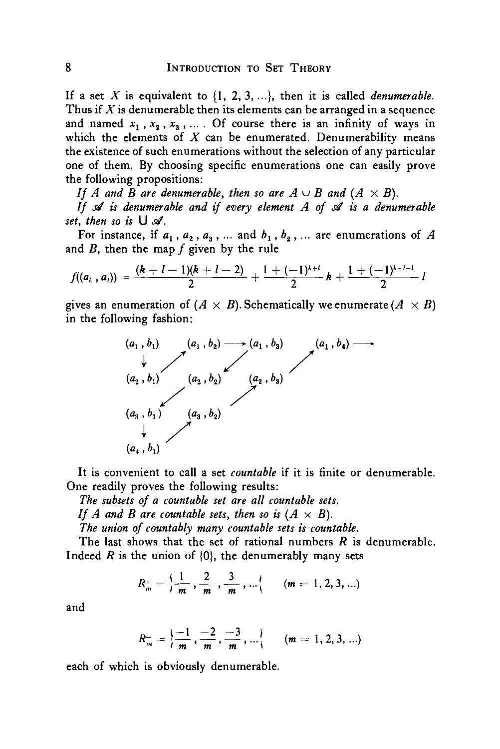
For instance, if al, a2, a3, ... and blt bt, ... are enumerations of A
and B, then the map / given by the rule
/(K » «;)) = 2 1 2 2
gives an enumeration of {A x ß). Schematically we enumerate {A x B)
in the following fashion:
(aj, 6)) (aj, bt) > («!, 63) («!, 6„) ►
^ / /
(a,, 6j) (a,, 62) (a2, b3)
K. bi)
It is convenient to call a set countable if it is finite or denumerable.
One readily proves the following results:
The subsets of a countable set are all countable sets.
If A and B are countable sets, then so is (A X B).
The union of countably many countable sets is countable.
The last shows that the set of rational numbers R is denumerable.
Indeed R is the union of {0}, the denumerably many sets
R« = \^T'i-'-^-'-\ ("»=1.2,3,...)
< m m m \
and
«- = !—, — , — ,•••! («=1.2,3,...)
'" I m m m \
each of which is obviously denumerable.

2. Set Theoretical Equivalence and Denumerability 9
A complex number a is called algebraic over the field of rationals R
if it is the root of an equation
r0 + rrx + ... + fVj*"-1 H *" = 0
where r0 rn_t e R. The lowest admissible degree n is called the
degree of the algebraic number a. The set of ordered n-tuples (r„ rn_ t)
is denumerable and each nth degree equation has at most n distinct
roots. Hence the algebraic numbers of degree at most n form a
denumerable set An . By considering the denumerable union Ax u Ai u ...
we obtain:
The set of all algebraic numbers is denumerable.
A nonalgebraic complex number is called transcendental. Since the
algebraic numbers form a denumerable set the existence of such numbers
can be proved by showing that the set of complex numbers contains
a noncountable subset. For instance, it is sufficient to show that the
set of reals x satisfying 0 < x < 1 is not countable. Every such x
has a unique representation of the form
e, e2 fi
3 -r 32 -r 33
where e,. = 0, 1, or 2 and infinitely many eA's are different from 0.
We are going to prove that every denumerable subset of {x : x e 91
and 0 < x ^ 1} is a proper subset. Since our set is not finite this
will show that it is not countable and so the existence of transcendental
numbers will be proved. Let a definite enumeration xl , x2, ... of such
a denumerable subset be given and let «A1 , eki, ek3, ... be the digits
of xh . We let «,,. = 1 + 2«A.A — e2u so that eA. = 1 if el;k = 0 or 2 and
eK = 2 if «a. = 1. All the eA's are different from 0 and ek. ^ ekk. for
every k = 1, 2, 3 Therefore the real number x (0 < x <" 1)
defined by the infinite series S «A.3_/V is different from every xk and so
{xl, x2 , ...} is indeed a proper subset of {x : x efl and 0 < x ^ 1}.
// si and S are countable sets of sets, then {A u B : A e sf and B e -^}
is also countable.
Proof. Since ,s/ is countable its elements can be arranged in a finite
or infinite sequence {AY , A2 , ...). For any fixed B consider the sequence
(^uB^.ußp..,), By omitting possible repetitions we are led to
an enumeration of the set {A u B : A e si/} where B is a fixed element
of JA. As B varies over the countable set JA we obtain a countable family
of these sets {A u B : A e s/} (B e Jâ). Since each of them is countable,
so is their union.

10
Introduction to Set Theory
For any set A we let Aiin denote the set of those subsets of A which
contain at most n elements. Thus Ai0) = {0}, AiU = {{a}: a e A} and
^(n-rii = {a<n>ua"': a{n) e A{n) and a11' e All)}
for n Js 0. If A is countable, then by the foregoing result so is Ai2].
This in turn shows that A{Z) is a countable set and by induction we see
that A{H) is countable for every n = 0, 1, 2 The union of these
sets A{n) (n = 0, 1,...) is the set of all finite subsets of A. Hence we proved:
// A is countable, then so is the set of all finite subsets of A.
It is interesting to compare this with the earlier result which states
that the set consisting of all subsets of a denumerable set is not countable.
The existence of nonequivalent infinite sets was proved from Cantor's
theorem according to which no set is equivalent to its power set. However,
this theorem alone is not sufficient to prove that there are many non-
equivalent types among infinite sets, for one cannot be certain that X,
0>(X), 0>\X) = 0>(0>(X)), ... are nonequivalent. There are two ways
by which this question can be settled, one of which consists of proving
a stronger version of Cantor's theorem:
No set X is equivalent to ^k{X) for any k = 1,2
Proof. We introduce the notation a° = a and ak = {ak~1} for k > 1
and a e X so that ak consists of the single element ak~l e &k~\X).
The following argument is a straightforward generalization of the one
used in the special case k = 1 : Given a one-to-one correspondence
/ : X -»• &k between X and some subset 2.k of 0>k(X) we define
.J//.-1 = {xk-i. xa-i ejfik-i(X) and xk~i <£/(*)}.
Each J*"-1 e âk is the image of some element of X under the map /,
say J*"1 = /(*), for some x e X. If xk~l ei*"1 = /(*), then **-> £ */k~l
and so j*"'*-1 ^ lk~\ Conversely, if a*""1 £ J*"1 = /(*), then xk-xes^k~x
and again s4k~x ^ J*-1. Therefore s4k~x is not an element of 2.k and
so Hk is a proper subset of &k(X). Hence there can be no one-to-one
correspondence between X and !?k(X).
The foregoing result implies immediately that X; ^(X), 2P\X), ...
are always nonequivalent sets. By choosing X = {1, 2, 3, ...} we obtain
an infinite sequence of sets, no two of which are equivalent. The same
can be proved from the special case k = 1 with the help of the following
important theorem due to Cantor and Bernstein:
// X and X' are arbitrary sets such that X is equivalent to a subset
of X' and also X' is equivalent to a subset of X, then X ~ X'.
Proof. By hypothesis there is a one-to-one mapping / from X onto
a subset of X' and there is another one-to-one mapping g from X'

2. Set Theoretical Equivalence and Denumerability 11
onto a subset of X. Using / and g we divide the sets X and X' into
mutually disjoint subsets such that there is a natural one-to-one
correspondence between the subsets of X and the subsets of X': Given any
element a e AT we define the elements ..., a_.,„ a_2, a0, a2 a2n , ...
belonging to X and ..., a_2,i+1 a_^ , ax a2n_x, ... belonging to
X' by induction as follows: We put a0 = a and ax is defined to be the
image of au under the mapping /; furthermore, a2 is the image of al
under g. In general we let a2n_l (n > 1) be the image of a2n_2 under
/ and a.lH be the image of a2n_1 under g. This construction is valid for
every n — 1,2, ... but it is possible that some of the an's coincide.
For negative indices we define the elements as follows: a_x is defined
to be the element of X' (if there is any such element) whose image
under g is au . If a_, exists, then a_2 is defined to mean the element
belonging to X (if there is such an element) whose image under/is a_j .
In general we define
"—2n+i such that its image under g is fl_2.i+2 provided
such an element exists in X'. Similarly, a_2n is defined to mean the
unique element in X (if it exists) whose image under/ is a_2n+1 . The
set of even elements a2n we denote by [a] and the set of odd elements
will be noted by [a]', so that [a] S X and [a]' S X'.
Since / and g are one-to-one maps, by the definition of [a] any two
sets [a] and [b] are either disjoint or identical. A similar statement holds
for the sets [a]' and [b]'. Hence every element of X belongs to exactly
one set [a] and every element of X' belongs to exactly one set [a]',
namely, a of X belongs to [a] and a' of X' belongs to [a]' where a is
the image of a' under the mapping,». Therefore it is sufficient to construct
a one-to-one map between the elements of each set [a] and the
corresponding [a]' as this will define a one-to-one correspondence between
the sets X and X'.
There are two different types of [a] sets: First, it is possible that
no repetition occurs in the sequence (a2n) and consequently no repetition
takes place in (a2„_!). Then both [a] and [a]' consist of denumerably
many distinct elements and so they can be brought into a one-to-one
correspondence. The other possibility is that there is a repetition in [a],
say a2,„ = a2„ , for some m ^ n. Then a2„)+1 = a2n+i and hence
a2.«+2 = «2^2 and in general a2lu+h = a2nU. for every k = 0, 1
Similarly, a2lll_l = a2„_1 and a2„,_2 = «2„_2 and so a2m_k = a2n_h. for
every k — 0, 1 Given m, choose n such that the elements
Û2». . a2.„+2 a2n-2 are all distinct. Then a2m+1, a2m+3 a2n_x are
distinct elements of X' and
a2m ~~* a2,li+l i a2l,,+2 —* "21/1+3 ' •••> fl2n-2 —* a2n-l
determines a one-to-one correspondence between the elements of [a]

12
Introduction to Set Theory
and [a]'. Consequently one can define a one-to-one map between the
elements of [a] and [a]' for every a in X and these maps automatically
yield a one-to-one map between the elements for X and X'.
We can now easily give a second proof for the existence of infinitely
many nonequivalent infinite sets. It is sufficient to show that a set X
is not equivalent to any of its power sets ^k{X) where k = 1, 2
For k = 1 this proposition holds by Cantor's theorem. We suppose
that none of the sets ^{X), ..., ^(X) are equivalent to X and prove
that X and £?k^ \X) are inecuivalent sets. For on the one hand there
is a natural one-to-one correspondence between X and a subset of
iPk{X) mapping x of X into f(x) = xk. A similar one-to-one map,
called the injection map, exists between ^k{X) and a subset of ^""+1(AT),
namely, each element £>kl~ of SP\X) corresponds to the set {J*-1}
lying in &k+\X). If there were a one-to-one correspondence between
â/"k+\X) and X, then it could be combined with the injection map to
give a one-to-one mzp.g between 0*k(X) and a subset of X. The existence
of the maps f : X-*■ 0>k(X) and g : &\X) -*■ X would imply the
equivalence of X and &\X) which is contradictory to our hypothesis.
Hence X and ^k+\X) are not equivalent sets.
If A and B are sets and if there exists a one-to-one map between A
and some subset of B, then we write A < B and say that the cardinality
of A is at most as large as that of B. Clearly A ~ B implies A < B
and the last theorem states that A < B and -B < A together imply
that A ~ B.lî A < B but .4 and ß are not equivalent, we write A < B
and say that A is of smaller cardinality than ß. Hence A < B takes
place if and only if A can be mapped in a one-to-one fashion onto some
subset of B, but not conversely. For instance, the cardinality of the
rational numbers is smaller than that of the reals.
It follows immediately from the definition of the relation < that
A < B and B < C imply A < C. Moreover, the last theorem shows
that A < B and B < C or A < B and B < C imply A < C. It is
natural to expect that for any pair of sets A, B exactly one of the three
possibilities A < B, A ~ B, and B < A takes place. Since, as we
have already seen, at most one of these relations can hold, the real
problem is to show that at least one of the two possibilities A <" B
and B < A will take place for any two sets A and B. The proof of
this simple sounding fact is considerably harder than anything else
we have seen so far. For the proof essentially depends on an important
and deep axiom of set theory called the axiom of choice. Once we are
familiar with the various equivalent formulations of this axiom the
trichotomy problem "A < B or A ~ B or B < A" will easily be
settled.

3. The Axiom of Choice and Its Equivalents 13
3. The Axiom of Choice and Its Equivalents
The most famous and important axiom of set theory concerns
nonempty sets si whose elements A are themselves nonvoid sets. A function
/ defined on si with values in U si is called a choice function for si
if f(A) e A for every A e si. Indeed such a function / : si -> U si
"chooses" an element f(A) from each of the sets A belonging to si,
and conversely if we claim that there is some process by which an
element can be selected simultaneously from each of the sets A of
the family si, then we merely say that some kind of choice function /
is given. The axiom of choice states:
If neither s/ = {A} nor any of its elements is void, then there exists
at least one choice function for si.
This is a very simple sounding requirement whose validity had never
been questioned until 1904 when Zermelo showed that it has far reaching
consequences, in particular, the so called well-ordering principle can be
derived from it. A linearly ordered set X is called well ordered if every
nonvoid subset A of X has a first element, i.e., an element a such that
a ^ x for every x e A or equivalently a < x for every x ^ a and lying
in A. For instance, the set of natural numbers is well ordered, but
the integers do not form a well-ordered set under their natural ordering.
Cantor firmly believed in the following principle:
Every nonvoid set admits at least one linear ordering which well orders it.
Subsequent studies have shown that the axiom of choice and the
well-ordering principle are actually equivalent propositions, each one
can be derived from the other one by using, also, the more elementary
axioms of set theory. Today, already many equivalent formulations are
known and there are also several important theorems which we cannot
prove without using the axiom of choice or one of its known equivalents.
Some of these theorems, like the Stone representation theorem, might
actually turn out to be equivalents of the axiom of choice.
The closest equivalent of the axiom of choice is the product axiom:
Let / be a nonvoid set and let a nonvoid set Ai be associated with each
element i of/. This means that a set si of nonvoid sets A and a function
<p : I -> si are given, the function values being denoted by At instead
of <p(i). We may suppose that every A in si is attained at some element
i of / so that si is the range of <p : / -> si. The product axiom or
multiplicative axiom states:
// / and the associated sets Ai are not void, then there exists at least
one function /:/-> U^= U A{ such that f(i) e At for every i e I.
The equivalence of the two axioms is clear: On the one hand, the

14
Introduction to Set Theory
axiom of choice concerns the special situation when the associated
sets A{ are all distinct. On the other hand, if si denotes the set of A{'s
then every choice function / : si —>• U si gives rise to a function
/ : / -> U A{, the values of which are given by the rule/(i) = f(A{).
The family of functions / : / -> U si such that f(i) e Ai is a set
which is called the product or Cartesian product of the sets Ai and is
denoted by II At or sometimes by X Ai. The product axiom states
that if none of the sets At is void, then II Ai is not the empty set. The
product Y\Ai is defined also in the degenerate case when at least one
of the sets Ai is void: Then we let II Ai be the empty set 0. It is important
to realize that the family si alone does not yet determine the product.
For instance, if / = {1,2} and if si consists of two elements, then
there are two distinct products II ^4f . In the case of a small finite
index set it is convenient to write Ax X ... X An instead of II At .
Notice that A x X ... X Anis not the set ofordered n-tuples(Al X ... X An).
For Ax x ... X An depends on the particular index set / used while
(A1 X ... X An) is uniquely determined by the ordering (Al, ..., An).
Moreover, the Cartesian product is defined also if the number of factors is
infinite. In practice, one does not distinguish between the set of ordered
n-tuples (Ax x ... X An) and the Cartesian product A1 x ... X An
associated with the standard index set {1, ..., n).
The sets Ai are called the factors of the product II Ai. The typical
element of II Ai is usually denoted by the symbol a, its value at i is
called the ith coordinate of a and is denoted by ai instead of fl(t'). A
particularly simple situation occurs when all the factors are identical,
say A{ = A for every index i. Then the product is uniquely determined
by / and A and it is denoted by A'. For example, ÎRC denotes the set
of all real-valued functions defined over the domain of complex
numbers.
One of the most useful equivalents of the axiom of choice is Zorn's
lemma. If the axiom of choice is needed in the course of a proof, then
the proof can generally be reformulated more elegantly by using Zorn's
lemma instead. A similar pattern was followed by researchers working
before the discovery of Zorn's lemma in 1922 and again in 1935, except
they had to be satisfied by using the well-ordering principle in their
reasonings. Such proofs were said to depend on transfinite induction.
Zorn's lemma concerns partially ordered sets si and it is best to
suppose that the ordering < is reflexive. A linearly ordered subset of
such a set si is usually called a chain of si. By an upper bound of a
chain <"? we mean any element U in si such that C < U for every C
in c€. Thus an upper bound is comparable with each element of ^
and it need not belong to the chain <ë. An element M of si is called

3. The Axiom of Choice and Its Equivalents 15
a maximal element of si if A < M for all those elements A of s/ which
are comparable with M. Zorn's lemma states:
// the partially ordered set si is such that every chain has an upper
bound in s/, then si has at least one maximal element.
In order to show how Zorn's lemma is used in practice, it is best to
discuss a few applications. A simple illustration is obtained by considering
a nonvoid family D of disks d lying in the plane and asking for a
subfamily M such that
( 1 ) the disks d of M are disjoint, and
(2) M is maximal with respect to this property.
After realizing that the solution of the problem requires more than
trying to pick disks one by one until one hits on M, the first thing to
do is to collect all subfamilies A of D satisfying requirement (1) into
one set s/. The second step consists of checking that s/ is not void.
Here this is trivial. Third, it is necessary to introduce a reflexive partial
ordering < in s/ which is suitable for the purpose. In our example the
right partial ordering is given by inclusion, so A1 < A2 if Ax is a
subfamily of A2. The fourth step consists of proving that every chain
^ of s4 has an upper bound U in s/. In our example it is sufficient
to choose as U the union of all families C of disks belonging to the
chain <tf. In more involved applications it might be harder to find an
upper bound U and one should carefully check that U indeed lies in
s/ and not only in some longer partially ordered set enveloping s/.
By Zorn's lemma s/ contains a maximal element M. Since s/ is ordered
by inclusion and it consists of families satisfying (1), M will be a solution
of our problem.
The next illustrative example is an important application as it shows,
among other things, the existence of maximal orthonormal systems.
Let X be a nonvoid set and let R be a reflexive and symmetric binary
relation on X, i.e., let R £ X x X be such that / £ R and R-1 = R.
The object is to determine a subset M of X such that
(1) M X M £ R, i.e., x1 R x2 holds for any x1, x2 e M, and
(2) M is maximal with respect to this property.
In order to prove the existence of such maximal subsets, we apply
Zorn's lemma to the set s/ of all those subsets A of X for which
A X A £ R. The set A is not void as it contains every A = {a}
consisting of a single element a of X. The proper partial ordering of si is
set theoretic inclusion so that A1 < A2 means ^ £ A2. If ^ is a
chain in j/, then any possible upper bound of ^ will necessarily contain
U = U{C :Cef}. We prove that the set U lies in s/: If xlt x2 e U,
then x1 e C1 and x2 e C2 for some sets Cx, C2eeë and "tf being a

16
Introduction to Set Theory
chain either xt , x2e C2 2 C\ OF 1X1 ) 1X0 eC,2 C2. Hence by C1 , C2 e s/
we have in either case xl R x2 and this shows that x1 R x2 holds for
any two elements xx, x2 of U. Since U lies in si and is an upper bound
of ff, Zorn's lemma applies and the existence of a maximal set M follows.
Actually we proved more than is necessary to apply Zorn's lemma:
We proved that every chain <"? has a least upper bound M in si.
A very simple application of the last result is the following: Let X
be the set of all straight lines of the ordinary three-dimensional space
and let R be the perpendicularity-identity relation: x1 R x2 if, and only
if, x1 = x2 or if x1 and x2 are perpendicular. Our result states the
existence of a set of lines M = {x} such that any two lines of the family
M are perpendicular, and if x $ M then x is not perpendicular to at
least one line of the family M. The same type of reasoning shows the
existence of maximal orthonormal systems in inner product spaces.
Let F be a vector space over some field F. For instance, V can be the
set of real numbers, F the field of rationals. For vector addition we can
choose ordinary addition of reals and as multiplication of vectors by
elements of F = R we can use ordinary multiplication of reals by
rationals, A linearly independent set means any subset L of V such that
no nontrivial linear combination of elements of L gives the zero element
of V. In other words, L is linearly independent over F if vY vn eL
andA^ + ,,, + Xnvn = 0 with Xl An inFimply that Xl = ... = An=0.
There exist linearly independent sets; for instance, every set consisting
of one nonzero vector is linearly independent over the scalar field F.
A maximal linearly independent set means a linearly independent set M
which is not contained in any other linearly independent set, i.e.,
M is such that M s L implies L = M. The existence of such maximal
sets M follows from Zorn's lemma: We let si be the set of all linearly
ordered subsets of V and partially order it by inclusion. Each chain
ff of s/ has an upper bound in s/, for U = U{L:Le ff} belongs to s/
and is the least upper bound of <è': If v1 vn e U, then v{ eL{ for
some Liec6 (t = 1 n) and ^ being linearly ordered there is one
among the L/s which contains all the others. Since v1 vn belongs
to this largest Li a linear combination A1z;1 + ,,, -f- Xnvn can vanish
only if Ax = ,,, =. An = 0,
A base for a vector space V over a field F means a subset B of V
such that every element v of V can be expressed in the form
v = Aj^j + ... + A„z.„
where v1 , ...,vne B and Ax, ,,., XneF. Usually one is interested in

3. The Axiom of Choice and Its Equivalents 17
bases B such that the representation of every vector v is unique. The
uniqueness requirement holds if, and only if, B is a linearly independent
set in which case one speaks about a linearly independent base. Every
such base is a maximal linearly independent set. Conversely, if M is a
maximal linearly independent set and v is an arbitrary vector outside
of M, then
Xv + A^! + ... + Anvn = 0
for suitable vl , ..., v„ e M and scalars A, At , ,,,, An not all of which are
0. Since M itself is independent, A ^ 0 and so v is expressible as a
linear combination of v1 , ..., vn . Thus for vector spaces maximal
linearly independent sets and linearly independent bases mean the
same thing. Our earlier reasoning shows the existence of linearly
independent bases for arbitrary vector spaces V over some field F.
The special case when V is the additive group of the reals and F is the
field of rationals is of special interest. The corresponding linearly
independent bases are called Hamel bases, after their discoverer. They
can be used to find discontinuous solutions for the functional equation
f(x + y) — f(x) -\- f(y) or to construct sets which are not measurable
in the Lebesgue sense.
It was mentioned already that the trichotomy law of cardinals follows
from the axiom of choice. As a last illustration of the power and
versatility of this axiom, we derive the trichotomy property from Zorn's
lemma: Given two nonvoid sets Sl and S2 we wish to prove the existence
of a one-to-one map of St into S2 or of S2 into St . If both types of
maps exist, then by the Cantor-Bernstein theorem 5t ~ 52 , otherwise
we shall have Sl < S2 or S2 < Sy . We start with the set se of graphs
F of invertible functions from Sl into 52 . By this we mean functions
whose domain of definition is part of Sl and whose range lies in S2.
Since Sl and 52 are nonvoid, such graphs F exist. We order sf by
letting Fl < F2 if Ft c F2; that is, if the second function is an extension
of the first. If ¥> is a chain in stf, then U {F : F e <ë} is an upper bound
of every F in % and it lies in se'. The hypothesis of Zorn's lemma
being satisfied we can find a maximal element M in se. Let
Mx = {i, : (sj , s2) e M] and A/, = {s2 : (s, , s2) e M\.
Since Mt C 5! and M2 C S2 together contradict the maximality of M,
we have MY = SY or M2 — S2 , possibly both. Thus M is the graph
of a map of 5t into S2 or M_1 is the graph of a map of 52 into 5t .
We proved that 5, ^ S2 or S2 ^ 5! .

18
Introduction to Set Theory
NOTES
The two papers by Cantor mentioned in the beginning are both
entitled "Beiträge zur Begründung der transfiniten Mengenlehre" [1].
They were translated into English and provided with a very interesting
historical introduction and remarks by Philip E. B, Jourdain [2]. The
membership relation which we denote by e was originally introduced
by Peano who used e as an abbreviation for the Greek word «an.
The informal set theory developed here should not be confused with
strictly axiomatic set theories. The axioms mentioned here belong to
the formal systems developed by a number of outstanding
mathematicians. At this stage the reader is urged to continue the present text
and start the study of general topology. Later, however, he might want
to get acquainted with some of the formal axiom systems for set theory.
He might then consult the series of articles by Bernays [3] and the
beginning of Gödel's book [4].
Zermelo wrote two papers on well ordering. His first proof of the
well-ordering theorem [5] is clearer to follow than the second [6],
Although the first proof was correct it had been criticized by several
people and in order to answer these objections Zermelo published the
second version which avoids these critical steps in the reasoning.
There are several closely related variants of Zorn's lemma known as
Kneser's lemma, Kuratowski's lemma, Tukey's lemma, and Hausdorff's
maximal principle. It is fair to point out that Kuratowski's lemma [7]
is not only simple in form ("each chain of a partially ordered set is
contained in some maximal chain") but was also published considerably
earlier than the version due to Zorn [8]. Kneser's formulation is analogous
to Zorn's but his hypothesis is considerably weaker: It is required only
that well-ordered chains should have an upper bound in the partially
ordered set [9]. An even weaker hypothesis appears in Bourbaki' s version [10].
The axiom of choice is needed in the derivation of many interesting
results, or at least it makes the proofs easier. In addition to the
applications already discussed in the text we add the following: The existence
of algebraic closure; Banach limits; Tychonoff's compactness theorem;
the existence of invariant measure; the existence of nonmeasurable
sets; the Hahn-Banach theorem; the existence of noncontinuous solutions
of the functional equation f(x + y) = f(x) +/(y), the Banach-Tarski
paradox and the existence of ultrafilters. Tychonoff's theorem is known
to be equivalent to the axiom of choice while the existence of invariant
measures on topological groups can be proved also without using the
axiom of choice. It was anounced recently that the existence of ultra-
filters can also be proved without applying this axiom.

References
19
References
1. G. Cantor, Math. Ann. 46, 481-512 (1895); 49, 207-246 (1897).
2. G. Cantor, "Contributions to the Founding of the Theory of Transtinite Numbers."
Dover, Xew York.
3. P. Bernays, A system of axiumatic set theory, Parts I—VII. J. Symb. Logic 2, 65-77
(1937); 6, 1-17 (1941); 7, 65-89, 133-145 (1942); 8, 89-106 (1943); 13, 65-79
(1948); 19, 81-96 (1954).
4. K. Gödel, "The Consistency of the Axiom of Choice and of the Generalized
Continuum-Hypothesis with the Axioms of Set Theory" (Ann. Math. Studies, No. 3)
Prineeton Univ. Press, Princeton, New Jersey, 1940.
5. E. Zermelo, Beweis dass jede Menge wohlgeordnet werden kann. Math. Ann, 59,
514-516 (1904).
6. E. Zermelo, Neuer Beweis für die Möglichkeit einer Wohlordnung. Math. Ann. 65,
107-128 (1908).
7. C. Kuratowski, Une méthode d'élimination des nombres transfinis des raisonnements
mathématiques. Fund. Math. 3, 76-108 (1922).
8. M. Zorn, A remark on method in transtinite algebra. Bull. Amer. Math. Soc. 41,
667-670 (1935).
9. H. Kneser, Eine direkte Ableitung des Zornschen Lemmas aus dem Auswahlaxiom.
Math. /.. 53, 110-113 (1950).
10. N. Bourbaki, "Eléments de mathématique." Part 1. Livre I. Théorie des ensembles
(Fascicule de résultats). (Actual. Sei. Ind., no. 846.) Hermann, Paris, 1939.

CHAPTER I
Topological Spaces
1. Open Sets and Closed Sets
We shall deal with mathematical systems which consist of a set X and a
family of subsets of X which are subject to a few simple axioms. These
systems are called topological spaces and the family 6 of subsets is the
family of open sets.
Definition 1. A topological space is a set X and a family of subsets O
called the open sets of the space such that the following axioms are satisfied:
(O.I) aeO and Xe 0.
(0.2) // Ox e 0 and 02 e 0, then 0, n 02 e 0.
(0.3) // O, e0 for every iel, then \J {0{: iel}e 0.
The second axiom implies that 6 contains with every finite collection
01, ..., On also the intersection 01 n ... n On . Infinite intersections
need not belong to 6 even if each factor 0{ is an element of (S. The third
axiom states that 0 contains all finite and infinite unions of sets 0{ e 0.
If a family 0 subject to these axioms is given we say that a topology 3~ is
defined on X. As far as topology is concerned the particular method used
to describe the family 0 is of no importance. We shall often use the
expression X is a topological space. This means that X is a nonvoid set and
a topology 3~ is given on X.
It is possible to define a topological space on any nonvoid set X: One
trivial way of defining open sets is by choosing Q = {a, X}. The space
so obtained is called a nondiscrete topological space. Another trivial choice
is 0 = £P(X), the set of all subsets of X, in which case every subset is
open. Then we speak about a discrete topological space. If X contains
more than one element, then the discrete and nondiscrete topological
spaces formed on X will be distinct. If X is infinite, then we can define
another simple topological space: We put in 6 the set a and all those sets
O whose complement X — O is finite. In this case we say that X is
topologized by the topology of finite complements.
21

22
I. Topological Spaces
The family of all possible topologies for a fixed set X can be ordered as
follows: -Tx is called coarser or weaker than -9~\ and ■Ti is called finer or
stronger than .^"1 if the family G)1 of open sets associated with -Tx is a
subfamily of the family 02 belonging to -T2. In symbols, .Tx ^ <57\2 and
■T% Js .^"1 if and only if Cx c ß>2. It is clear that ^ is a reflexive ordering
relation for the set of all topologies for X. If S\ < ^"2 and ^"2 ^ .^"1,
then .^"i and .57"2 are identical, that is to say, 0t = 02. If ^ <g $~2 but
•^"1 and &'2 are not identical, we say that 9~x is strictly coarser than .5~2 and
.fT2 is sin'cr/y /iner than .^ . We write .^"1 < -T2 and .5T2 > .Tx . For
instance, in case of an infinite set the topology of finite complements is
strictly finer then the nondiscrete topology and it is strictly coarser then
the discrete topology.
Definition 2. The topologies ,T x and -T y formed on the sets X and Y
are called homeomorphic if there is a one-to-one correspondence between the
elements of X and Y such that the open sets of .T x correspond to those of
.Ty and conversely. If -T x and .Tu are homeomorphic we write -T x ~ .Tu .
The existence of a homeomorphism between two topologies formed
on the same set X does not necessarily imply their identity. For example,
let „Ybe a finite set, say {xx,..., xn}, and let the topologies .Tt (i = 1,.... n)
be defined as follows: A nonvoid set O is open if it contains the point xi.
It is clear that these topologies are homeomorphic, but not identical.
The discrete and nondiscrete topologies of a set consisting of more than
one element are not homeomorphic. If the set is infinite, there is a third
nonhomeomorphic topology, namely, the topology of finite complements.
The relation ~ is reflexive, symmetric, and transitive; that is, .Tx ~ S~x\
J'x ~ 3~v implies STy ~ &~xt and if Px ~ STy and 5"S~J., then
srx~3-z.
Definition 3. A set C of a topological space X is called closed if its
complement is open. The family of closed sets is denoted by (ê.
It is obvious that a and X are open and also closed and there might be
other such sets. For example, if the topology is discrete, then every
subset is both open and closed. Sets having this twofold property will
be called open-closed or closed-open sets. If the topology is nondiscrete
or if it is the topology of finite complements on an infinite X, then the
only open-closed sets are a and X. If only the improper subsets a and X
are open-closed, then the topological space is called connected.
Theorem 1. The union of finitely many closed sets is closed. The
intersection of an arbitrary finite or infinite family of closed sets is closed.
Proof. Let {C,-} (i e /) be a family of closed sets. Then c D C{ = U cCt
and c U C{ = C\ cC{ where cC{ is open for every i e I. Using axioms

Exercises
23
(0.2) and (0.3) we see that c D Ct is open and if / is finite then so is
c U C(.
Theorem 2. A family <6 of subsets of a set X is the family of closed sets
of some topology on X if and only if the following axioms are satisfied:
(C.l) be« and Xs<€.
(C.2) // Cje« and C2e'6, then Cj u C2 e "if.
(C.3) // C, e<$ for every iel, then D {C, : ie 1} e 9f.
Proof. Axioms (O.l), (0.2), and (0.3) for the family 0 of sets
O = cC (Ce If) follow from the above axioms by complementation.
The necessity is a consequence of Theorem 1.
Axioms (C.l), (C.2), and (C.3) are often used as a starting point in
place of axioms (O.l), (0.2), and (0.3).
We end this section with a very useful lemma:
Lemma 1. A set A of a topological space X is open if and only if it
contains with each point x an open set Ox containing x.
Proof. If A is open, then we can choose Ox = A for every x e A.
If on the other hand A is such that for every x e A there is an open set
Oj. satisfying x e Ox Ç A, then by A = U {Ox : x e A) the set A is the
union of open sets and so it is open.
EXERCISES
1. Let X be a nonvoid set and let A be a subset of X. Denote by T(A)
the topology on X whose open sets are a and the sets O which contain A.
Show that:
(a) We have -T{AX) > -T(A2) if and only if A1 g A2 and
3T{AX) > .9~(A2) if and only if AXC A2.
(b) If -T is a topology on X such that -T(A{) < S~ for i = 1, ..., n,
then .3T(C\ At) ^ ST.
(c) If .9" is a topology on A' such that ^(^,) ^ 3~ for every i e /, then
■T{\SAX) ^2T.
2. Let X be a set and let m be an infinite cardinal. Show that a and the
subsets O of X which satisfy card cO ^ m form the open sets of a
topology. Determine the closed sets.

24
I. Topological Spaces
3. Let X be a linearly ordered set having the least upper bound
property and let ^ be the family consisting of a and X and of all sets
[x, +00) = {£ : x ^ 1} where x e X. Show that ^ is the family of closed
sets for a topology on X.
4- Find a topology 3~ different from the discrete and nondiscrete
topologies and such that 6 = *€.
(Let X be the set of reals and let O be open if x e O implies —x e O.)
2. Interior, Exterior, Boundary, and Closure
In the special case when X is the real line or the plane with its usual
topology these notions reduce to the well-known concepts which they
generalize.
Definition 1. Let X be a topological space and let A g X. The interior
of A is the union of all open sets contained in A:
A' = U{0: O c A},
The exterior of A is the union of all open sets not intersecting A:
A' = U{0:0 g cA}.
Therefore the interior of A is the largest open set contained in A and
the exterior of A is the largest open set not intersecting A. It is clear that
Ae = (cAf and A* = (cA)e. Both Ai and Ae can be expressed in terms of
closed sets. It is easy to see that A is open if and only if A{ = A and A is
closed if and only if Ae = cA. The exterior and interior never intersect.
Theorem 1. The interior and exterior operators satisfy the following
rules:
0'' = 0; X' = X; A' g A; A" = A'; (A n B)' = A' n B'.
0" = X; Xe = 0; A" s cA; Aee 2 A'; (A u B)e = Ae n Be.
If A ç B, then Ai g B1 and Ae 2 Be.
Proof. Most of these rules are obvious from the definitions. Since Ai is
open Au = {Ay = A1. The inclusion (A n B){ £ A{ n ß1' follows
from A r\ B <=, A and A n B ^ B. The opposite inclusion is also
obvious because Ai g .4 and B{ g ß imply that A'' n B{ is an open set
contained in A n ß. Finally, using the rule on the interior of an
intersection we see that
(A u B)e = (c(A u B)Y = (c.4 n cß)1 = (c.4)'' n (<:ß)' = ^nB»,

2. Interior, Exterior, Boundary, and Closure 25
For infinite unions the equality need not hold and we can assert only the
inclusion (U Ay)e £ f*| Ay. Similarly, for an infinite intersection only
(fl Ayy £ PI A\ holds in general.
Definition 2. A point x e X is a boundary point of the set A if every open
set Ox containing x intersects both A and cA. The set of boundary points is
called the boundary of A and is denoted by Ab.
It is obvious that Ab = (cA)b. Moreover, x is a boundary point of a
set A if and only if x $ Ai u Ae. Therefore the boundary Ab is the
complement of A1 u Ae. Since A1 and Ae are disjoint we obtain:
Theorem 2. For every set A of a topological space X its interior A\
exterior Ae, and boundary Ab are disjoint sets whose union is X. The sets
Ai and Ae are open and Ab is closed.
A simple consequence is:
Theorem 3. A set A is closed if and only if Ab £ A and it is open if and
only if Ab £ cA.
Proof. If A is closed, then cA is open and so cA = Ae = c(A{ u Ab) £ cA"
which shows that Ab £ A. Conversely, if Ab £ A, then Ai u Ab £ A
and using X = Ai u Ab u Ae together with Ae £ cA we see that
A £ A'u Ab. Hence A = A' u Ab and so A = cAe is closed.
Definition 3. The closure A of a set A of a topological space X is the
intersection of all closed sets containing A : A = C\ {C : A £ C}.
Since the intersection of closed sets is closed, A is a closed set. For
closed A we have A = A and conversely. Hence this is a characteristic
property:
Theorem 4. A set A is closed if and only if A = A.
We could have obtained this also from the following:
Theorem 5. For every set A we have A = Ai u Ab.
Proof. Since A = fl {C : A £ C] we see that
cA = U {cC :cC<^cA}=ö{0:Oc CA) = A'.
Therefore by Theorem 2 A = cAe = A1 u Ab.
The basic properties of the closure can be summarized as follows:
Theorem 6. The closure operator satisfies the rules:
0 = 0; X = X; A £ A; A = Ä; ~Ävli = ÄuB.
IfAçB, then A £ B.

26
I. Topological Spaces
Note. We have A1 u ... u An = A1 u ... u J^ for every finite family
of sets, but for an infinite family only U At g U A.: holds in general. By
fl j4,. Ç ^[ g i; (i'e/) we have fl .4, Ç fl i, for any family but
equality need not hold even if the number of sets is finite.
Proof. Rules A Ç A and A Ç B ^> A Ç B are clear from the
definition of the closure. Since 0, X, and A for any A are closed sets we have
0 •= 0, X = X, and A = A. Finally, A u B = A u B can be proved
by showing that Au B S A u ß and ^uß 2 Au B: The first
inclusion follows from the fact that yï u B is a closed set which contains
Au B. To see the second we use A Ç A u ß and B ^ Au B to
obtain ^ gTü~ß and 5 Ç iufi.
Definition 4. .4 /.oini* .* is an accumulation point of a set A if every open
set containing x contains at least one point of A which is different from x.
The set of all accumulation points of a set A is called the derived set of A
and is denoted by A'.
We have the following:
Theorem 7. A set A is closed if and only if A' _= A.
Proof. If A is closed, then cA is open and so no point of cA is an
accumulation point of A. Therefore Ä Ç A. Conversely, if A' £ A,
then for every x e cA there is an open set Ox such that x e Ox c CA and
so by Lemma 1.1 cA is open.
This last result can also be derived from:
Theorem 8. For every A we have A = A u A'.
Proof. It is sufficient to show that a point x £ A is an accumulation point
of A if and only if x e A'1. In fact, if x e A' and Ox is an open
set containing .v, then there is an a ^ x in A such that a e Ox . Hence if
x $ A, then Ox intersects both A and cA and so x e A1'. Conversely, if
.v e A1' but x $ A, then x e A'.
The derived set of X is not necessarily X itself. For instance, if the
topology is discrete, then X' = 0. A point x does not belong to X' if
and only if j.v] is an open set. These are the isolated points of the space X.
The set X' is sometimes called dense part of the space X.
In some cases Ö' = O but not always. For example, let X — {a, b, c)
and let the open sets be 0, {a}, {b}, {a, b], and {a, b, c}. Then the closed
sets are 0, jcj, \a, c), [b, c], and {a, b, c}. The smallest closed set containing
the open set [a, b] is {«, b, c) and so [a, b)' -= {a, b, c). If O is such that
01 — O, then O is called a regular open set. The union of regular open
sets need not be regular, e.g., in the preceding example {a} and {b}

Exercises
27
are regular but {a, b] is not. Occasionally one uses a modified union
operation called regular union which preserves regularity: We define
A u B = (A u B)1 for any pair of sets A, B of a topological space. The
set A u B is always regular open. More generally we have:
Theorem 9. For every A the set A' is regular open.
Proof. We wish to show that A1' = A'. Since A1 2 A\ on the one
hand we have A*1 "2. Au =_A'. On the other hand, A 2 A1 and so
A = À 2 A' and _4"'' 2 A(i.
In a similar fashion we can speak about regular intersections;
AnB = (.4 r\B)1. One can also define regular closed sets; these are
sets such that Cl = C. Later we shall need the following:
Lemma 1. For any pair of sets A, B we have AnBi = Ar\Br\ ß<\
Proof. It is sufficient to show that AnBnB^AnB1 because by
A n B £ A the other inclusion is obvious. If x e A n B' and Ox is an
open set containing x, then Or n ß1 is open and contains x, so by
x e Ait intersects A. Therefore Or n B n Ais not void and so x e A r\ B.
Hence if xe A n B', then * e A n B n B1.
EXERCISES
1. Show that O is open if and only if A n O — o implies yï n O = 0
for every A in X.
2. Show the following: If A\j B =■ A' then iufl' = AT, and if
Jnß = e then .Ï n ß' - 0.
(First, if a: $ A, then there is an open set Ox containing x such
An Or = 0. Hence Or g ß and .v e ß\ Next, if ^ e yî, then for
every Or we have Oj. n A #0 and so Oj. $ ß.)
3. Determine ^', A', A'\ A, A1, and A' for every set .4 when X
is topologized by the topology of finite complements.
(If cA is finite then A' =- A, and if cA is infinite then A' = 0. If ^4 is
finite then A1' = cA, and if A is infinite then Ae = 0. If A is finite then
A1' — A, if both A and f.4 are infinite then A'1 — .Y, and if c.4 is finite
then A1' = cA. H A is finite then A = A, and if A is infinite then
.-Î = X. If .4 is finite then A' = 0, and if .4 is infinite then A'1 = X If
cA is finite then .4' = A, and if c.4 is infinite then A' = 0.)

28
I. Topological Spaces
4. Prove that in every topological space (A u B)' = Ä u B'.
[Clearly (A u B)' 2 A' u B'. If .* e (yî u ß)', then for every open
set Ox the intersection Oxn (A v B) contains a point which is different
from x. If there were open sets Ox and Qx such that Oxn A Ç {,*:} and
Qxn B Q {x}, then O, n Qx would be an open set containing x and such
that (Ox n Qj.) n ( J u i.) ç {je}. Since this is not possible either every
Ox intersects A or every Ox intersects B in some point different from x.
Hence either x e A' or x e B'.]
5. Prove that if points form closed sets then every derived set is closed.
(We show that CÄ is open. If x e cA', then there is an open set Ox
such that A n Ox £ {x}. If y e Ox and Oy is another open set containing
y, then Ox n Oy is open, it contains y, and A n Ox n Ou n c{x] = 0.
Hence y e cÄ and so Ox s c^'. By Lemma 1.1 the set cA' is open.)
6. Let X be the set of reals and let 6 consist of 0, X, and the intervals
( — 00, x) where x e X. Find the derived set of {0} and show that it is not
closed.
7. Give an example of a space and of a family of sets A{ (i e I) such
that U At and U A{ are different.
(Let X be an infinite set and let it be topologized by the topology of
finite complements. Let Al, A2, ... be finite sets whose union is not X.)
8. Verify the following rules: Abb Ç Ab\ {A n Bf ç Ab u Bb;
{A u Bf ç A" u Bb; Ab ç Ab; and ^l'ft ç ^".
[The boundary ^46 is closed and so it contains its own boundary:
Abb g ^
(.4 n ß)6 = ^nfin ^TrvS) ginßn (TZITTF) ç (Ä n ÏA) u (BncB)
= .46 u ß6.
The other inclusion follows by taking complements. Next
ï' = (.4u .40)6 ç ^ u -46(> = -46
and so
A"> = MO6 = (cÄ)" s M)6 = ^6- ]
9. Prove: C is regular closed if and only if cC is regular open.
[If cC is regular open, then cC = (cC)1 and so C = ccC = C*. If C
is regular closed, then C = O — ccC and cC = cccC = (cC)*.]
10. The intersection of finitely many regular open sets is regular open
and the union of finitely many regular closed sets is regular closed.

3. Closure Operators
29
[First (Q, n O.,)' Ç (Ö, n (02)' = Ô,' n Ö2' = O, n 02 . Next
(O, n 02)' 2 (O, n 02)' = O, n 02 The other proposition can be
proved by a similar argument or by taking complements and using the
preceding exercise.]
11. Show that an open set O is regular open if and only if Oh — 0b.
(For Oh = 0 n cO = 0 n K)< = Ô n .:(0 = 0':)
12. Show that a closed set C is regular closed if and only if C' ç C'.
[If C is regular closed, then C' = (7;')'' e C*', and if Cb g C7, then
C -- C'u C ^ OuO ='Ci c C and so C = C = <?.]
3. Closure Operators
There are many practical methods w hich can be used to introduce
topologies on sets. As Kuratowski first proved, the closure operator leads
to such a method. One can also use the interior, exterior, boundary, and
derivation operators since any of these completely determines the
topology of the set. These will be discussed in the exercises at the end
of this section.
Theorem 1. Consider an operator associating with each subset A of
a set X another subset A and subject to the axioms:
(K.l) 0 = u.
(K.2) A c A for every A ç X.
(K.3) A --= Ä for every A ç X.
(K.4) A uß = Au B for every A,B g X.
Then there exists exactly one topology T on X such that the closure of
every set A relative to 3T is A.
Note. Sometimes it is more convenient to use instead of (K.4) the
following pair of axioms:
(K.4a) XUb = A u B whenever A = A and B = B.
(K.4b) A c B whenever A Ç B ç X.
The equivalence will follow easily.
Proof. We define the topology T by specifying the family of closed sets:
Let % be the family of those subsets C of X for which C = C. Then

30
I. Topological Spaces
<6 satisfies axioms (Cl), (C.2), and (C.3) in Theorem 1.2: Indeed, by
(K.l) we have 0 e ^ and by (K.2) we obtain Iglgl, i.e., X = X
and X e *€. Axiom (C.2) is a direct consequence of (K.4). To prove (C.3)
we first show that A g ß whenever A g B. In fact, if A g B, then
B = A u B and so by (K.4) we get B = Au B = Au B 2 A. Now
let {C{} (i e I) be an arbitrary family of sets C{ e <6'. Then fl C, g C,
for every i e I and so 0 Q g C{ = Ct for every ie 1. Therefore
PI Ct g n Q . Since by (K.2) we have fl Cf Ç fl Ct- we see that
fi C{ = fi Q , that is to say, 0 Ct e <€. This shows axiom (C.3).
The reader will notice that axiom (K.3) was not used when we verified
axioms (Cl), (C.2), and (C.3). Hence any operator satisfying (K.l),
(K.2), and (K.4) defines some topology 3~ on the set X. Axiom (K.3)
assures that the closure operator of the topology so obtained is exactly the
operator A: Let Ä denote _the closure of A under the topology S~ having
closed sets Celf. Since Ä = A by (K.3), the set A belongs to "<? and
A S A by (K.2). Thus A = C\ {C : A c C] g A. On the other hand,
if Ce V and if A g C, then A g C= C and so yîg fl {C : A g C}= A.
Therefore A = A for every subset A of X.
Now we show that the axiom systems (K.1)-(K.4) and (K.l)-(K.4a),
(K.4b) are equivalent. First, (K.4a) is a special case of (K.4). Next
if A g B, then B = A u B and so by (K.4) we obtain B = AvB =
AvB^A. Thus (K.4) implies (K.4b). Let us suppose now that
axioms (K.l)-(K.4a) and (K.4b) are satisfied. Then by (K.4b) from
A g Au B and B g A u B we get A g A u B and B g A u ß.
Therefore Au B c Au B. By (K.2) we have ^ g ^ and B Q B so
that ^ ufigiuB. Hence by (K.2), (K.3), and (K.4a) ^ u ß g
Au B = Au B = Au B. This shows that Au B = Au B for any
A ß in X
As an example let X be a linearly ordered set. For every nonvoid set
A in X define A = f\{(—00, x]: a ^ x for all a e A}. U A = 0, then let
0 = 0. It is easy to show that the operator A follows axioms (K. 1)-(K.4)
and so it is the closure operator of some topology on X. The topology .9~
associated with this closure operator will be called the order topology
of the partially ordered set X. (Some authors use the expression "order
topology" for another topology on X. This second topology is the
interval topology of X.)
The use of the Kuratowski axiom system (K.1)-(K.4) is often
inconvenient and sometimes would cause difficulties. However, there are
a number of variants which can often be used with success. For
instance, we can consider the closure operator only on a subset se
of the power set of X and construct a topology on X by using this
skeleton of the closure operator.

Exercises
31
Theorem 2. Suppose that an operator A is defined on a subset s/ of the
power set of X such that the following axioms hold:
(Kb.l) // ae,e/, then 0=0.
(Kb.2) // Ae.a/, then A g Â.
(Kb.3) // A and A belong to ,t/, then A = A.
(Kb .4) // ABei, then AvBesS and A u B = Ä u B.
Then the operator A (A e s/) defines a topology 3~ on X such that the
closure of every Ae s4 is A.
Proof. We define 0 = 0 and S = 0 {A : 5 g A and A e s/}. If there
is no Aesf with Sq A then 5 = X, and if 5 e si then the new and
old definitions of S coincide. We show that S satisfies axioms
(K.l)-(K.4a) and (K.4b) and so a topology can be defined on X such
that the operator S is the closure operator of this topology. Only axiom
(K.4a) needs proving. Suppose that 5X = 5X and S2 = S2. If
x $ Sj^v S2, then there exist Al and A2 in s/ such that * £ yJx 2 Sx and
x $ A2 2 S2 . Hence x $ AY u A2 and so x £ 5X u 52. Therefore 5] u >S'2
A simple special case of the preceding theorem is the one in which s4
is the family of closed sets of a topological space. Then A — A for every
A in s4.
EXERCISES
1. Let an operator A be defined on the set of all subsets of a set X
such that the following axioms are satisfied:
(I) Iü"ß= Au B.
(II) A = A for every set A consisting of a single point.
(Ill) Ä = A for every A in X.
Show that if X contains at least two elements then the operator A
satisfies axioms (K.1)-(K.4) and points are closed sets in the topology
generated by the operator A.
[To show (K.2) let a eA and put A = (A - {a}) u {a}. Then by
(I) and (II) we have A = A - {a} u {a}. Hence a e A and A Ç A. To
prove (K.l) let x e X and let y j^ x in X. Take 0 u {y} — {y} and apply

32 I. Topological Spaces
(I) and (II): {y} = [y] u 0. This shows that x $ 0. Thus 0 = 0. If X
consists of a single point, then one can define 0 = X — X and axioms
(I), (II), and (III) will hold but (K.l) obviously fails.]
2. Let y ; A —»■ y(A) be an operator on the power set of X subject to
the following axioms:
(1) y(a) = 0-
(2) // xey{A), then xey(A — {x}).
(3) y{y{A)) Ç y(A) for every A.
(4) y{A U B) = y(^) U y(B) /or ewry .4, ß.
Show that there is a unique topology on X such that y{A) = .4' for
every set A in X
[Let A = A u y(^4) and verify axioms (K.1)-(K.4) for the operation
A:
A = ÄTTyjÄ) = AU y(A) U y(j4 U y(j4)) = ^ U y(A) U y(y(j4))
= .4U y(^) = ^
and
Au B = A\j Bvy(Av B) = iu y(^4) u ß u y(B) = Au B.
Next show that A' s y(^4): The set
O = c((i4 - {*}) u y(^ - {*})) = c(A - {x}) n cy(^ - {*})
is open and O n A Ç. {*}. Hence if jc e A', then .* £ O and so
xey{A — {*}). Thus xey(^ — {*}) S y(A) and ^' S y(^). To show
that y(A) s A' suppose that x $ A'. Then there is an Ox, say
Ox = c{B u y(ß)), such that O.n^c {*}. Then ,4 - {*} g ß u y(ß)
and y(A - {x}) ç y(ß u y(ß)) = y(5). Since x e Ox = c(B v y(B)) we
have x $ y(B) and so x $ y(A — {x}). Therefore by (2) x $ y(A) and
y(A) g A'.]
3. Consider an operator y(A) for the set of all subsets of a set X subject
to the axioms:
(1) y(X) = X.
(2) y(^) s ,4 /or raery A
(3) yW)) = y(^) /w every A.
(4) y(^ nfi) = y(A) n y(ß).
Find a topology .ff on AT such that y(A) — A1 where the interior is
taken with respect to 2T.
[The family of open sets is ß — {y(A) : A g X}. It is the simplest to
notice that y{A) = cy(cA) satisfies (K.1)-(K.4).]

4. Bases and Subbases
33
4. Bases and Subbases
Here we describe the most common method of introducing topologies
on sets. The basic idea is to define a family of some of the open sets from
which the remaining open sets can be easily constructed. There are two
types of families which are important in practice; the more primitive one
is called a subbase and the other is a base. One can also introduce bases
and subbases for closed sets.
Definition 1. A family 38 of subsets B of a set X is a base for the open
sets of a topology 2T on X if it has the following properties:
(B.l) For each xeX there is a Be3S suchthat xeB.
(B.2) // BltB2e^ and if xeB1r\B2, then there is a Be08 such
that x e B Ç B1n B2.
The family of open sets of 2T is defined as follows:
A nonvoid set O is open if and only if it is the union of some sets B
belonging to 38. The topology 3~ is called the topology generated by the
base 38.
For example, let X be the set of real numbers and let 38 be the set of
all open intervals (a, b) = {x : a < x < b}. Axioms (B.l) and (B.2)
are clearly satisfied. A set O s X is open in the topology generated by 38
if it is the union of an arbitrary family of open intervals (a, b). This is
called the topology of the reals or the "usual topology of the reals."
Theorem 1. A necessary and sufficient condition that the topology
generated by the base ,'M1 be finer than the topology generated by the base 38\
is the following: Given any B2 e 38 2 and any x e B2, there is a Ble3Sl
such that x e B1 ç B2.
Corollary. Two bases 38x and 382 generate the same topology if and only
if given any Ble381 and any x e B1 there is aB2e382 such that x e B2 ç Bl
and also given any B2 e 382 and any x e B2 there is a Bxe38x such that
xe Bt g B2.
Proof. Let O be open with respect to the topology generated by 382.
Then for each x e O there is a B2 e 3$2 such that x e B2 s O.
Hence if the condition holds there is a B1 e 381 such that x e B1 s O.
Consequently O is the union of sets B1 e 38Y and so O is open also with
respect to the topology generated by 381. The necessity is clear.
Theorem 2. A necessary and sufficient condition for 38 to be a base for a
given topology is: Given O e 0 and x e O there is B e 38 such that
xeB g O and if B e ââ, then Bed).

34
I. Topological Spaces
Proof. If 28 is a base for the topology ZF, then every O e 6 is the union
of sets B e 8§ and so the condition is satisfied. Conversely, if the
condition is fulfilled, then on the one hand every O e (9 is the union of sets
B and so every O e 0 is open with respect to the topology generated by
â§. On the other hand, by SS Ç Q and by axiom (0.3) every set which is
open with respect to the topology generated by 88 is also open with
respect to the given topology.
The family 6 of open sets of a topological space is always a base for
the topology of the space and this is the largest possible base. It is often
important to go toward the other extreme, namely, to find bases with
as few elements as possible.
Definition 2. A family Sf of subsets S of a set X is called a subbase for
a topology if for each x e X there is an S e SP such that x e S.
By the topology generated by SP is meant the topology generated by the
base SS which consists of all finite intersections of sets S e SP.
It is easy to see that the family 38 satisfies axioms (B.l) and (B.2) of
a base. Hence indeed Sf determines a topology 2T on the set X and every
5 e £f is open relative to 3~.
There is no difficulty in introducing bases and subbases for closed sets.
The corresponding axioms and the analogs of Theorems 1 and 2 can be
obtained by using complementation.
Consider the set of all topologies on a fixed set X. This set is partially
ordered by inclusion: 2TX ^ ^"2 if G)1 s 62. Using the concept of a
subbase we can easily show that every family {^~i} (i e I) of topologies
has a least upper bound and a greatest lower bound. For let <3i (i e I)
denote the family of open sets of the topology 3~i and let Sf = U (Si.
Denote by lub{^"4} the topology generated on X by the subbase SP.
Since êi Ç SP this topology is finer than any of the topologies ^~i.
On the other hand, if a topology is finer than every 2Tt, then f5(ç(5 for
every i e I and so SP ^ 0. Therefore lub{^",-} is the least fine topology
on X which is at least as fine as the topologies 2Ti (i e I). This is the
least upper bound of the topologies 3'i (i e I). Now consider the family
n<V Axioms (O.l), (0.2), and (0.3) are satisfied, so fltf^ is the
family of open sets of a topology glb{^"i}. This is the finest topology on
X which is at least as coarse as any of the topologies &\ . It is called the
greatest lower bound of the topologies 3~i (i e I).
EXERCISES
1. Let 3~x be the topology on X whose open sets are X and all sets not
containing the point x e X. Determine lub^^ : x e X] and
glb{^ :xeX}.

5. Topologies on Linearly Ordered Sets 35
2. Find an axiom system for bases consisting of closed sets and state the
analogs of Theorems 1 and 2.
3. Let [a, b] denote the closed interval with end points a and b in a
linearly ordered set X. Show that the family of all closed intervals
[a, b] (a, b e X) is a subbase for closed sets. Show also that if X is the set
of real numbers, then this is not the usual topology.
(Relative to the usual topology of the reals there exist disjoint nonvoid
open sets.)
4. Which is the weakest topology in which points form closed sets ?
5. Topologies on Linearly Ordered Sets
A simple but important case where bases are used to introduce a
topology on a set occurs in the definition of topologies on linearly
ordered sets. If X is a linearly ordered set, then for any a < b in X we
denote by (a, b), (a, b], [a, b), and [a, b] the intervals
(a, b) = {x : a < x < b]
{a, b] = \x : a < x s: b)
[a, b) = {x : a < x < b}
[a, b] — {x : a < x < b}.
(a, b) is the open and [a, b] is the closed interval with end points a and b.
The others are the half-open intervals. As usual we let
(— oo, b) = {x : x < b)
(a, -\- oo) = {x : a < x}.
The sets ( — oo, b] and [a, +oo) are defined similarly. Occasionally we
write ( — oo, +oo) instead of X. These sets are the improper intervals
of AT.
In the sequel we define what is meant by the interval topology of a
linearly ordered set and prove an important theorem on the
characterization of the open sets of this topology when the linearly ordered set
has the least upper bound property.
The family Sf of improper open intervals of a linearly ordered set X is a
subbase for a topology which is called the interval topology of X.
In fact, if X consists of at least two elements, then every x e X belongs
to at least one interval of the form (— oo, b) or (a, +oo) and so Sf is a
subbase for a topology on X. If X has no largest nor smallest element
then the topology can be generated by a base which consists of all
proper open intervals (a, b) in X. This is the origin of the name interval
topology. For example, if X is the set of real numbers and if SS is the

36
I. Topological Spaces
family of all proper open intervals, then a topology is generated on X
by 8$ which is called the ordinary or usual topology of the reals. The same
topology can be obtained by different methods, e.g., by introducing a
metric. Similarly we can consider as X subsets of the set of real numbers
and form the interval topologies on these sets. Some of these will be
trivial, for instance, if X is the set of all integers, then the interval
topology is the discrete topology.
A linearly ordered set X is said to have the least upper bound property if
every subset bounded from above has a least upper bound. X itself need
not have a maximal element. The greatest lower bound property is
defined similarly. Either one implies the other. The set of real numbers
and the set of integers for example have the least upper bound property
but the set of rationals does not.
Theorem 1. Let X be linearly ordered such that the least upper bound
property holds. Then a set O is open relative to the interval topology if
and only if it is the union of a family of disjoint open intervals.
Proof. Let xeO and let S Ç O be the set of those points £ e O for
which [x, |] s O. Then S is not void and so it has a proper or improper
least upper bound u. We have S = [x, u] or 5 = [x, u) according as u
does or does not belong to S. If u $ S, we let bx = u so that bx e X or
bx denotes the improper element +00 and S — [x, bx). If u e S, then
u e O and so there is an interval (a, b) such that u e (a, b) S O. It follows
that there exists no £ e X satisfying u < £ < b: For by (a, b) Ç O
such a | would belong to S and so it would be an element larger than the
least upper bound. Therefore choosing bx = b again we have S — [x, bx).
Now we consider the set T Ç O of those points £ e O for which
[I, x] Ç O. In the same way as before we can find a proper or an improper
element ax such that T = (ax , x]. Consequently, for any x e O v/e found
extremal elements ax and bx such that x e S u T = (ax , bx) S O. If
x ^ y, then either ax = ay and bx = by or the open intervals [ax , bx)
and (ay , by) are disjoint. Therefore {{ax , bx)} (x e O) is a family of
disjoint open intervals whose union is the open set O.
The theorem has an important special case:
Theorem 2. Let X be the space of the real numbers with its usual
topology. Then a set O is open if and only if it is the union of countably many
disjoint open intervals.
Proof. Using Theorem 1 we see that any open set O consists of disjoint
open intervals, say {ai, b{), where i e I. For every positive integer n there
are at most denumerably many among these intervals such that

Exercises
37
bt — a{ ^ \jn. Since every interval satisfies this inequality for a
sufficiently large value of n we see that {(a{, bt)} is a countable family.
One can introduce topologies on a linearly ordered set X also by
using the half-open intervals: The family of all intervals [a, b) (a, b e X)
and [a, +00) (a e X) is a base for the open sets of a topology called the
right half-open interval topology &~+ of the ordered set X. The left
half-open interval topology 3~_ is generated by the base consisting of the
intervals (a, b] (a, beX) and ( — 00, b] (b e X). These topologies are
finer than the interval topology because the open intervals (a, b) can be
expressed in the form
(a, b) = U {[<*, b) : a < * < b} = U {(a, ß] : a < ß < b}.
If X is the set of reals, then the half-open interval topologies are strictly
finer than the usual topology. They have many unexpected properties
and so can serve as examples.
EXERCISES
1. Let 6 be the family of those subsets of a linearly ordered set X
which are unions of disjoint open intervals. Prove Theorem 1 by showing
that if X has the least upper bound property, then 6 is the family of open
sets of some topology on X.
2. Let S~+ denote the right half-open interval topology of a linearly
ordered set X having the least upper bound property. Prove the following
representation theorem: A set O is open relative to &"+ if and only if it is
the union of disjoint open and right half-open intervals.
3. A subset O of a partially ordered set X is called a segment if x ^ y
and y e O imply xeO. Show that the family 6 of all segments satisfies
the axioms for open sets. Determine the least upper bound and the
greatest lower bound of the topologies associated with the ordering and
the inverse ordering of X.
4. Let &~ be the least upper bound of the usual topology and of the
topology of countable complements on the set of reals. Show that O is
open relative to 3~ if and only if O = Q — A where Q is open in the
usual sense and A is countable.
(The open sets of the topology of countable complements are 0 and
those sets A whose complement cA is countable.)
5. Let X be a linearly ordered set and let SS consist of X and of all
intervals ( — 00, x) (x e X). Show that SS is a base for a topology. If X has
no maximal element, then X can be dropped from SS.

38
I. Topological Spaces
6. Metric Spaces
These spaces are the classical types of topological spaces. Most of the
fundamental concepts and results of modern analytical topology were
first developed for metric spaces and many important instances of
topological spaces belong to this group.
Definition 1. A metric space is a set X together with a real-valued
function d given on X X X which satisfies the following axioms:
(M.la) d(x,y) ^ 0 for every pair x,yeX andd (x, x) = 0.
(M.lb) d(x,y) = 0 implies '' x — y.
(M.2) d(x,y) = d(y, x) for every x,yeX,
(M.3) d(x,y) + d(y, z) $: d(x, z) for any x,y, z e X.
The first axiom states that the distance from x to y is nonnegative
and it is zero only if the two points coincide. If this second requirement,
i.e., (M.lb), is omitted from the axioms we speak about a pseudometric
space. Axiom (M.2) states that d is symmetric so that we may speak about
the distance between the point pair {x, y) without specifying their
ordering. The inequality which occurs in (M.3) is the so-called triangle
inequality. It is a well-known property of the Euclidean distance in the
plane or in the space.
The set of reals X furnishes some simple examples of metric spaces.
For example, we may define d to be d(x, y) = \ x — y | or d{x, y)
= \/\ x — y |. The function given by d(x, y) = (x — y)2 is not
admissible because it violates axiom (M.3). The set X of all ordered
n-tuples of real numbers becomes a metric space if we set d(x, y) =
I xi ~ J\ I + ••• + I xn ~ yn\- The same definition holds good if X is
the set of all ordered n-tuples of complex numbers.
Theorem 1. Every pseudometric space can be considered as a topological
space by choosing as a base 3$ the set of all sets
Sf[x] = {y : d(x, y) < « }
where e > 0 and x e X. Sf[x] is called the ^-neighborhood of x or the
e-ball with center at x.
Note. When we are speaking about a metric space X it is assumed that X
is a topological space with the topology which we just described. The
expression "e-sphere" is usually reserved for the set {y : d(x, y) = e).
Proof. We must verify axioms (B. 1) and (B.2) of a base. The first of
these is clearly satisfied because, for instance, x e S^x]. To show the

6. Metrie Spaces
39
second let us suppose that x e Sf [yx] and xeSf[y2]. Then by the
definition of these balls, e1 — d(x, yx) > 0 and e2 — d(x, y2) > 0. Let
e > 0 be the smaller one of these positive differences. Now if d(x, y) < e
for some pointy, then by (M.3),
rfCy..y.) < d(y>x) + d(x<yt) < « + d{x,y() < «,.
Hence, if y e S,[x], then y e St[y(] and so S,[x] g S, [yj n 5(Jy2].
The open sets O of any topological space which is defined by a
base 38 are characterized by the property that O contains with each
point x some set B e 38 such that x e B. For a metric space this criterion
states that if x e O, then there is a ball Se[y] about some center y e O
such that x e Sf[y] Ç O. At present, however, the criterion can be
further strengthened:
Lemma 1. A set O Ç X is open relative to a pseudometric topology given
on X if and only if O contains with each point x an e-ball Sf[x] about x as
its center.
Proof. We know that the condition is sufficient. To show its necessity
suppose O is open and x e O. Then there is some ball S,[y] such that
x e Sf[y] e O. By x e Sf[y] we have e — d(x, y) > 0. Consider the
ball with radius r = e — d(x, y) and center x. If z e Sr[x], then
d(x, z) < r = e — d(x, y) and so
d(y, z) < d(y, x) + d(x, z) < e,
that is to say, z e Sf[y]. Hence with each x e O a whole ball Sr[x] belongs
toO.
Different metrics may lead to the same topological space; for instance,
a distance function d and kd for any positive constant k determine the
same topology. There is a simple necessary and sufficient condition under
which two metrics dx and d2 give the same topology.
Lemma 2. The topology 3~x defined by the pseudometric d1 on a set X is
finer than the topology &\ defined by the pseudometric d2 if and only if for
each x e X and e2 > 0 there is an e1 > 0 such that d2(x, y) < e2 whenever
di(x, y) < e, .
Proof. A set O Ç X is open with respect to 3~i if it contains with each
point x an entire ball S\ [x]. Hence if O is open relative to ^"2, then for
each x e O there is a ball S* [x] such that Si [x] ç O. If we choose
e1 > 0 such that d2{x, y) < e2 whenever d^x, y) < e1 , then we get
S,1 [x] S 5£2 [x] Ç O. Therefore O is open relative to the topology 3~x ,
Since S\ [x] is open relative to &\ the necessity of the condition follows

40
I. Topological Spaces
from Lemma 1. The finite-dimensional Euclidean spaces En are important
instances of metric spaces. En is defined to be the metric space formed
by the ordered n-tuples x = (x1 , ..., xn) of arbitrary real numbers
xt, ..., xn when the distance function is
d(x,y) = V\ x, - y, |2 + ... +7*« - y^W-
Axioms (M.la), (M.lb), and (M.2) are obviously satisfied and (M.3)
can be verified, for instance, by using Minkowski's inequality: If p > 1
and if al , ..., an > 0 and bl bn > O, then
((«i + bi)" + - + («n + W" < («i* + ... + a„")1/p + (V + - + b,vyi".
Equality takes place only if the sets of numbers ax an and b1 bn
are proportional. For p — 1 the equality is obvious.
The finite-dimensional Euclidean spaces are special cases of several
other types of metric spaces all having the same topology but different
metrics. For example, if the distance of the ordered n-tuples x and y is
defined to be
d(x,y) = (| *, - yi \" + ... 4- | *„ - yn I")1/",
then by Minkowski's inequality the axioms of a metric space are satisfied
for every p 5s 1 • Let the spaces so obtained be denoted by Enp so that
En2 = En is the n-dimensional Euclidean space. Using Lemma 2 we
can easily see that as far as the topology of Enp is concerned, the specific
value of p "> 1 is irrelevant.
Usually it makes little difference which particular metric is used to
define the topology on a set X. If we wish to emphasize that the topology
was introduced by a certain metric d, we speak about a topological space
with metric d. If the topology Jona set X can be introduced by some
metric and we wish to stress that we have no particular metric in mind,
we say that ^Y is a metrizable space or J is a metrizable topology on X. A
metric d is said to be compatible with a topology .T on a set X if the
topology generated by d is 3~. Similarly, we speak about a topological
space with pseudometric d, about pseudometrizable spaces, and pseudo-
metrizable topologies.
Not every topological space is metrizable. For instance, if X
is an infinite set, then the topology of finite complements is not
metrizable. Indeed, in order that a metric d be compatible with the
topology of finite complements it is necessary that d(x, y) be positive
for any pair of distinct points x, y. This, however, would imply
the existence of disjoint open sets containing x and y, respectively.
For instance, the «-balls Sf[x] and Sf[y] would satisfy this requirement
provided 2« < d(x, y).

Exercises
41
EXERCISES
1. Show that the metric spaces X and Y formed over the integers x
and the ordered pairs of integers y — (yt , y2) by using the metrics
d{x', x") = | x - x" | and d{y', y") = \ yx' - y/' | + | y2' - y2"
are homeomorphic.
2. Let X be the set of integers and let Y be the set of rationals.
Consider in both cases the same metric d defined as d(x\ x") — \ x' — x" j
and d(y',y") = \y' — y" \. Show that the metric spaces X and Y are not
homeomorphic.
3. Let X be a metric space with metric d. Prove that the functions
defined by
d(x,y) \d(x,y) if d(x,y) < 1
&(x,y) = -:—~—^r and Hx,y) = / '•" J ,) i ,
y J' 1 +d(x,y) v J' l\ if d(x,y) ^ 1
satisfy the axioms of a metric. Show that these new metrics generate the
same topology on X as the original d.
4. Let / be a real-valued function defined for d ""> 0 and such that (i)
/(0) = 0; (ii)M) < Rd,) for every dx < d,; (iii)M + rfy) <M)+M)
for every dx , dt ^ 0. Show that if the function d is a metric on the set X,
then f(d) is also a metric for X
Find a necessary and sufficient condition under which the metrics
d and f(d) generate the same topology.
(The functions/and/™1 must be continuous at the origin.)
5. Let S be a nonvoid set in a metric space with metric d and let
xl, x2 be points in X. Prove that if d{xi, S) = g\b{d(x{, x) : x e S] is the
distance of xi (i = 1, 2) from the set S, then
d(xl, S) — d(x2, S) ] <. d(xl, x2).
[We have d(x1 , S) < d(xl , x) for every * e S and given e > 0
there is an x e S such that d(x2, 5) ^ J(.*ä, .-c) — e. Hence
d(xl, S) — d(x.,, S) ^ rf(.V) , x) — rf(x2, x) + e < rf(A.j, jc2) + «.]
6. Consider the set AT of all disks Sr[x] (r > 0, x e E2) lying in the
Euclidean plane. Show that relative to the distance
d(Sri[Xl], i',s[.ic2l) = ] i-j - ra I + | *! - *2 |
the set A" is a metric space which is homeomorphic to the upper half
{x : x3 > 0} of the Euclidean space E3.
7. Show that if dl dn are metrics on X which generate the
topologies -Tx , ..., .Tn , then dl -\- ... + dH and max {d1 dn] generate
lub{.^.}.

42
I. Topological Spaces
(Let d denote either one of the metrics dx + ... + dnznd mzx{dlt..., dn]
and let 3T be the topology generated by d. Since dt < d for every
i=l n we obtain 3~x < 9~ and lub^} < 3~. If O is open relative
to 3~ and x eO, then for some e > 0, £,[.*] £ O. The ball 5*, [x] is an
open set in the topology 2T{; therefore fl 5* [#] is an open set of
lub{^"t-}. Since x e fl Sj [*] S £,[.*] Ç O, O is also open relative to
lub{y4} so that y < lubî^}.)
8. Let {dj} (i e I) be a family of metrics for the set AT having the
property that for every x, y e X there is a positive constant Mxy such that
di{x, y) < Mxy for every i e I. Show that the function d defined by
d(x, y) = \ub{dlx, y) : i e 1} is a metric on X.
Find an example where every di (i e I) generates the same topology 3~
but the topology generated by d is different.
[Only the triangle inequality needs proving. The inequalities
dix, z) ^ dix, y) + dly, z) imply dix, z) < d{x, y) + d(y, z) and so
d(x, z) < d(x, y) + d{y, z). Let AT be the set of real numbers and let for
every u ^ v the metric duv be defined as follows:
<*uv(x,y) =
u — v
if | x — y | < | u — v \
if \x-y\^\u-v\
Then duc(x, y) < 1 for every x, y e X and duc(u, v) = 1. Hence
d(u, v) = 1 for every u ^ v and 2T is the discrete topology. The
topology generated by duv is the usual topology of the reals.]
9. Find an example which shows that in general the closure of the
e-ball S,[x] = {I : d(x, £) < e} is a proper subset of {£ : d(x, £) < e}.
7. Neighborhood Filters
We shall often deal with sets Nx such that a given point x is contained
in the interior of Nx . These sets are called the neighborhoods of the point
x e S. If Nx is an open set, then it is called an open neighborhood of x.
Similarly, if Nx is closed and x e Nx , then Nx is a closed neighborhood
of x. It is possible to give a more primitive definition of neighborhoods
and as a matter of fact it is this alternative definition which one uses in
practice:
Lemma 1. A set Nx is a neighborhood of a point x if and only if there
is an open set Ox such that x e Ox Ç Nx .
The equivalence of the two definitions is obvious from the definition
of the interior of the set 7Vr .

7. Neighborhood Filters
43
Definition 1. The family . \ (x) of all neighborhoods Nx of a point x is
called the neighborhood filter of x.
Let & be a family of subsets F of a set X subject to the following
requirements:
(1) 0$&.
(2) // F^J and F 2 Fx, then Fe&.
(3) // FltF2e^, then FlnF2e^r.
If J*" has these properties, then it is called a filter over X.
It is easy to check that ./T(jc) is a filter and actually (1) holds in the
following strengthened form: xe Nx for every Nx e ./T(^).
The family of open neighborhoods Ox of a point x e X is not a filter in
X because rule (2) does not hold for 0(x). Similarly, the family ^(x)
of closed neighborhoods does not follow rule (2) and so ^(x) is not a
filter. A family 3Ù of sets B Ç X is called a filter base over the set X if
a $31 and if B1, B2 e 3 implies the existence of a set B e .^ such that
B ç ßi n ß2. Every filter base J1 determines a filter .F, called the filter
generated by 38; namely, & is defined to be the family of those sets
F Ç X which contain some set Be f:
& = {F:F^B for some Be3S\.
Rules (1), (2), and (3) can be easily verified.
It is clear that the family G{x) of open neighborhoods Ox of a point x
is a filter base and the filter generated by @{x) is Jf{x). The closed
neighborhoods of x form a family ^(x) which is a filter base but the filter
generated by ^(x) is not necessarily .V{x). This is the case for instance
if X is infinite and its topology is the topology of finite complements.
Then the only closed neighborhood of any point x is the entire space X.
The problem which we discuss here is twofold: First suppose that the
neighborhood filter .A'(x) of each point x of a topological space X is
known. The object is to describe the family of open sets in terms of these
filters. Next, suppose that no topology is given but to each point x in X
there corresponds a filter. V\x) consisting of subsets of X. The problem is
to decide whether or not a topology can be determined by means of these
families such that .V{x) is the neighborhood filter of each xe X. The
answers are contained in the following:
Theorem 1. Suppose that to every point x of a set X there corresponds a
nonvoid family .4 '(x) of subsets Nx . These families .4r(x) are the
neighborhood filters of a topology on X if and only if the following axioms are
satisfied:

44
I. Topological Spaces
(Nb.l) xeNx for every NxEJ^ix).
(Nb.2) // NxeJr{x) and Nx g N, then NeJ<~(x).
(Nb.3) // NxleJ<~(x) and Nx2eJ^(x) then JV.'nJV/e/W.
(Nb.4) // NxejV(x) then there is a subset Ox Ç Nx such that
x eOxe >"(*) and Nx e .W(y) for every yeOx.
If all these axioms are satisfied, then there exists exactly one topology 3~
on X whose neighborhood filters are the families jV{x). A set O is open with
respect to 2T if and only if it contains with each x e O a whole set Nx e jV~(x).
Proof. If X is a topological space and ./f (.*) is the neighborhood filter
of x, then the axioms are satisfied: In (Nb.4) it is sufficient to choose Ox
to be the interior of Nx . Hence the axioms are necessary.
Now suppose that.'f (x) is subject to axioms (Nb.l)-(Nb.4). We prove
that the family G = {0} which is given in the second half of the theorem
satisfies the axioms of a topological space: The sets 0 and X clearly
belong to <£>. If 0{ for each i e I belongs to 6, then so does U Oi because
with every x e Oi also some Nx e jV(x) belongs to Oi and hence to
U Ot. Finally let 01,02eO and let xe01n02. Then there exist
A^1 and Nx in J^x) such that A^1 <= 01 and Nx ç 02. Hence
Nx = Nxl n Nx2 g 01n02 and x e Nx . By axiom (Nb.3) we have
Nx e.'Y(x) and so 01 n 02 contains with each point x an entire set Nx
of ^\x). Therefore if 01 and 02 are in <£>, then Ol n 02 is also an element
of 0. Thus 0 is the family of open sets of a topology 3~.
We must prove that the neighborhood filter of the point x relative to
2T is exactly Jr{x). Let N be a neighborhood of x with respect to 3T.
Then there is an O e 0 such that x e O ç N and so by the definition of
the family 0 there is an Nx in Jf{x) such that Nx Ç O. By Nx ç O g N
and by (Nb.2) we have N e Jf{x). This shows that x has no other
neighborhoods than elements of the family ./T(jc). Conversely, we show that
every NxeJr(x) is a neighborhood of x with respect to 3T\ namely,
we prove the existence of an O e <P such that xeO Ç ./Vj.: In fact, let
0 = {y:NxeJr{y)}.
Then xeO because by our choice NxeJr{x). Moreover, O Ç Nx
because if Nxe.V(y), then by (Nb.l) yeNx. To prove O e (P let
y e O be given. By the definition of O we have Nx e jViy) and so by
(Nb.4) there exists an Oy in Jf(y) such that Nx e jV(z) for every z eOy .
However, if Nxe.V{z), then zeO and so if z e Oy , then z e 0, that
is, Oy Ç O. Therefore O contains with each y a set Oy of ^(y) whence
OeO.
The uniqueness of the topology 2T is obvious from the above reasoning

8. Uniform Structures
45
because the open sets of 2T can be characterized by the families
J \x) (x e X): O is open if and only if it contains with each point x a
neighborhood Nx .
EXERCISES
1. Usually it is more convenient to describe instead of .^'(x) (x e X)
a suitable base 38{x) (x e X) for .'V(x) (x e X). Find a necessary and
sufficient condition that â8{x) (x e X) be a base for some ./f (.*) (x e X).
2. Give a simple description of the neighborhood filters of a point in
the following cases: A metric space, the interval topology, the half-open
interval topologies.
3. Show that âS^x) and 3$£x) generate the same neighborhood filter
A \x) if and only if every Bxl contains some Bx2 and conversely.
4. Prove that in any metric space the closed balls
C,\x] = {y:d(x,y)^e} (* > 0)
form a base for the neighborhood filter of x.
5. Show that the filter ^{x) generated by ^(x) is related to .4/"(x) by
the inclusion ^(x) Ç Ar{x).
8. Uniform Structures
These are natural generalizations of metric spaces. In a metric space
a distance function d is defined on the set X X X and this function
determines a topology on X. In uniform structures a family W of subsets
U of X x X is given and a topology, called the uniform topology
associated with ^, is described in terms of these sets U. The family is
subject to a set of axioms which are analogous to those of a metric. The
importance of these structures lies in the fact that uniform spaces
preserve the main features of metric spaces. For instance, in terms of
these structures one can speak about uniform convergence. Cauchy
sequences, and completeness. If X and Y are sets with uniform
structures, then one can define the uniform continuity of a function
/from X into Y.
Definition 1. A uniform structure for a set X is a nonvoid family °U of
subsets U of X x X such that the following axioms are satisfied:

46
I. Topological Spaces
(U.l) // Ue<%, then U is not void.
(U.2) // U1e<% and if C^ <= C/, then Ue<%.
(U.3) // U1eW and U2e<%, then [/^^e*.
(U.4) // Ue<W, then I ç U.
(U.5) // t/e^, /hew U-le<%.
(U.6) // C/e*, then there is a VeW suchthat V o F g [/.
The sets Ï7 are called uniformities or surroundings.
As usual, / denotes the diagonal: I = {(.v, x) : x e AT}. The first axiom
(U.l) is an immediate consequence of (U.4). The reason for including it
in the axiom system is that axioms (U.r), (U.2), and (U.3) define W to be
a filter. As we shall see, the remaining axioms (U.4), (U.5), and (U.6)
correspond to axioms (M.l), (M.2), and (M.3) of a metric space. The
composition operator o is defined by
U o V = {(x, z) : (x,y) e U and (y, z) e V for some y.}.
A simple consequence of (U.4) is: U Ç: U o U for every uniformity
U e <%. Indeed if (x, y) e U, then by (y, y) e U we have (x, y) e U o U.
As usual U'1 = {{y, x) : (x, y) e U) and a uniformity U is called
symmetric if U = U~l. The axioms imply a sharper form of axiom (U.6):
Lemma 1. Given any Ue tfl there is a symmetric Wetfl such that
W o W g U.
Proof. By (U.6) there is a Fef such that V o V <= U. By (U.5) and
(U.3) W = V n V-1 is symmetric and W o W Ç V o V Ç U. Hence
W has the required properties.
In practice, a uniform structure °U is often described by specifying the
elements F of a filter base tflB instead of giving all the elements of Ql.
It is easy to see that every filter base tylB of a uniform structure <# satisfies
the following axioms, and conversely if tflB is such that axioms
(Ub.3)-(Ub.6) hold, then the filter generated by tflB is a uniform
structure. Thus we have:
Theorem 1. A nonvoid family <%B of subsets V of X x X is a base for a
uniform structure tfl if and only if the following axioms hold:
(Ub.3) // Vi e<%B and F2 e <%„, then there is a Ve<%B such that
Fç Vx n V2.
(Ub.4) // Ve'Wg, then I ç V.
(Ub.5) // Ve'Wg, then there exists a We<%„ suchthat W Ç y-i.
(Ub.6) // Fe«„ there is a We<%B suchthat WoW^V.

8. Uniform Structures
47
If %g satisfies these axioms, <%, the uniform structure associated with °U B ,
is the family of those subsets U of X X X for which V S U for some
VeWB.
Every uniform structure ^ has a symmetric structure base, i.e., a base
tflB consisting of symmetric uniformities. In fact, one can choose for Ql'B
the set of all symmetric uniformities of tfl.
It is possible to define uniform structures also by subbases. The
notion of a subbase is meaningful for every filter but here we use it only
for uniform structures:
Theorem 2. A family %'s of nonvoid subsets S of X x X is a subbase
for a uniform structure if it satisfies the following axioms:
(Us.4) I Ç S for every Se9ts.
(Us.5) // Se<%s, then there exist sets 7\ Tme%s suchthat
7\ n ... n Tm ç S-K
(Us.6) // S e Qls, then there exist sets T,, ..., Tm e <%s such that
(7\ n ... n Tm) o (7\ n ... n Tm) ç S.
The uniform structure generated by °US is determined by the base aUB
consisting of all finite intersections V = ^ n ... n S, where Slt..., Sn e ^ls.
Note. Axioms (Us.5) and (Us.6) can be replaced by a single axiom:
If Se^s, then there exist sets 7\ , ..., Tm e ^ls such that
(7\ n ... n Tm) o (7\ n ... n rm) ç S n S~\
Proof. It is simple to show that QlB satisfies the axioms of a structure
base. In fact, (Ub.3) is a consequence of the definition of QlB and (Ub.4)
is implied by (Us.4). Similarly, (Ub.5) can be derived from (Us.5). To
prove (Ub.6) one needs the relation
(T1 n ... n T") c (7'1 n ... n T") Ç (T1 o 7"1) n ... n (7"» o 7"").
This follows from the definition of the composition operator: If
(x, z) e (T1 n ... n 71") o (T1 n ... n 71"), then there is a y such that
(*, y) and (y, z) belong to T1 n ... n 7"«. Hence (*, ä) e Tk o Tk for
every k = X n, and so (x, z) e (T1 o T1) n ... n (Tn o Tn). Now let
V e <?/B be given. Then V = 5X n ... n 5„ for some 5X , .... 5n e <?/s .
By axiom (Us.6) there exist T-f , ..., T^k e °Vs for every k = 1 n such
that T* =-- Tf n ... n T^ satisfies T« a Tk S Sk . Hence if we put
T = T1 n ... n 71", then by the preceding relation
7" o 7" ç (T1 o 7"1) n ... n (7"" o 7"») gS,n ... n S„ = V.
This shows that axiom (Ub.6) holds.

48
I. Topological Spaces
Next we associate a topology 3~ of X with the uniform structure W:
Theorem 3. Given a uniform structure W on the set X X X consider for
each x e X the family .V(x) of all sets
U[x] = {y : (x, y) e U} where U e <%.
Then each jV~(x) satisfies axioms (Nb.l)-(Nb.4). The topology generated
by these neighborhood filters. ir(x) is called the uniform topology associated
with tfl or the topology derived from W.
Note. Sometimes U[x] is referred to as " U evaluated at x." One defines
U[A] for every A ^ X zs
U[A] = U {U[x] : x e A} = {y : (x, y)e U for some xeA}.
This set is " U evaluated on A." One easily verifies that
{UoV)[A] = V[U[A]].
Proof. Axiom (Nb. 1) is a consequence of (U.4). To show (Nb.2)
let U[x] and TV 2 U[x] be given. We consider the set
V = Uv{(x,y):yeN}.
Since U Ç y we have Fef and by our construction V[x] = N.
Hence if N 2 U[x], then Ne.V(x). Next, in order to prove (Nb.3)
we notice that U n V e Ql for every pair U, V e °U and
U[x]n V[x] = (Un V)[x].
Hence if U[x], V[x] e.V(x), then also U[x] n V[x] e.Ar(x). Finally we
must prove (Nb.4): Given U[x]e.4r(x) consider V e °U such that
V o V Ç U. By axiom (U.6) such a uniformity V exists. The set V[x]
can be chosen as Ox of (Nb.4): In fact, if y e V[x], then V[y] ^ U[x]
because y e V[x] implies (x, y) e V and so if z e V[y], i.e., if (y, z) e V,
then (x, z) e V o V fS U, i.e., z e U[x]. Since V[y] e-4"(jy) we have:
If y e V[x], then U[x] e.V(y). Therefore the families .A"(x) (x e X)
satisfy axioms (Nb.l)-(Nb.4).
Earlier it was mentioned that not every topology can be defined by
a metric. Similarly, there are topologies which are not associated
with any uniform structure. For instance, the topology of finite
complements of the set of integers gives such a space. If a topology can be
derived from some uniform structure W, then it is called a uniformizable
topology and one speaks about a uniformizable space. The expression
uniform space is also used.
Theorem 4. Every pseudometric space is uniformizable.

Exercises
49
Proof. Given a pseudometric d we consider the sets
Vf = {(x,y):d(x,y)<e}
where e > 0. The family °UB of all these sets V, is a base for a uniform
structure a?/: We have F(] n Kfj = F£ where e = min(e1, e2) and so
(Ub.3) holds. Axioms (Ub.4) and (Ub.5) are immediate consequences
of (M.la) and of (M.2), respectively. To see (Ub.6) let W = Vm . The
relation W ^ W £ V is assured by the triangle inequality. Hence by
Theorem 3 there is a topology &~ associated with the uniform structure Ql.
A set O Ç X is open relative to y if and only if it contains with each
point x an entire U[x] where U e Ql. Since U e Ql if and only if U 2 V,
for some e > 0 the set O is open relative to 3T if and only if it contains
with each x a set Vf[x], Thus O is open relative to 3T if and only if it
is open relative to the pseudometric topology derived from d.
The uniform structure aUä generated by the structure base Ql'Bd
consisting of the sets V, = {(x, y) : d(x, y) <«}(«> 0) is called the
uniform structure associated with the pseudometric d. If 9/ is a uniform
structure such that Ql = Ql& for a suitable pseudometric d, then W is
called a pseudometrizable structure.
EXERCISES
1. Let X be a nonvoid set and let Ql consist of the single set X X X.
Show that °ll is a uniform structure for X. It is called the nondiscrete
structure.
[Usually only the last axiom (U.6) needs proving. In the present case
even this is trivial.]
2. Let °Ü be the set of those U Ç X x X which contain the diagonal /.
Show that ■?/ is a uniform structure for X. This is the discrete structure.
3. Let X be the set of reals. Consider for every e > 0 the set
V* = {(■*> y) '• \ x — y \ < e) and verify that <%B = {U,} (e > 0) satisfies
the axioms of a structure base. The structure generated by tflB is the
uniform structure of the additive group of the reals or the "usual" structure
of the reals.
4. Let fJft'B be a structure base for the uniform structure °U. Prove that
the sets V[x] (V e °ltB) form a base for the neighborhood filter
{£/[.*]} (U e 4/) of the point x relative to the uniform topology generated
by*.
(Given U e ^/there is a V e ^satisfying V Ç Uand so V[x] g U[x].)
5. Show that the uniform topology associated with the "usual"
uniform structure of the reals is the usual topology of the reals.

50
I. Topological Spaces
(A base for the complete neighborhood filter of x relative to the uniform
topology consists of the sets
V,[x] = {y : x — e < y < x -\- e} = (x — e, x -\- e).
These are open neighborhoods of x relative to the interval topology.
Conversely, if Nx is a neighborhood of x in the interval topology, then
there is an e > 0 such that V,[x] = (x — e, x + e) Ç TV, . Hence the
base {K»[#]} (« > 0) generates exactly the neighborhoods of x relative
to the interval topology.)
6. Let X be the set of the reals and consider for every a < b the sets
S«h = .(*..v) : both x,y < b or both x,y > a}.
Show that {Sah} (a < b and a, b e X) is a subbase for a uniform structure.
[Only the last axiom (Us.6) needs proving. Given a < b choose reals
c and d such that a < c < d < b. Then T = Sac n Sed n S(lb has the
property To T^ Sub .]
7. Show that the uniform topology associated with the uniform
structure <?/ constructed in the preceding exercise is the usual topology
of the reals.
(If x < a, then 5m6[jc] = {y : y < b}\ if b < x, then
s„b[x] = {y ■ a < y}\
and if a < x < b, then 5„6[jc] = X. Hence every Sllb[x] is open relative
to the interval topology and so {S„6[.*]} £ • I (x). Now given x e X and
an open interval (a, b) containing x we can find real numbers c, d such
that a<c^.x^.d<b. Then S,u.[x] = (a, +oo) and 5,/fc[jc] = ( — oo, b)
so that (5,„, n 5,^)[jc] = (a, b). The sets T[x] where T is a finite
intersection of sets S/lf) (a < b and a, b e X) form a base for the neighborhood
filter of x relative the interval topology of the reals.)
8. Show that the uniform structure constructed in Exercise 6 is
not the usual uniform structure of the reals.
(The following difference between the two structures is very important:
In the case of the structure given in Exercise 6 for every uniformity U
there are finitely many points x1, ..., xm such that
U[Xl] u ... u V[xm] = X;
namely, if U 2 S„ b r> ... n Su b , then it is sufficient to choose
x,- e (fl{, bi) for each i = 1, .... m. In the case of the usual structure there
are uniformities such that U[xj] u ... u £/[.*„,] C X for all choices of
finitely many points.)
9. Show that the metrics d, min(l, d), and dj{\ + d) generate the
same uniform structure.

Exercises
51
[Let Vtl, V2, and Ve3 denote the «-uniformities generated by the
metrics d, min(l, d), and d/(\ + d), respectively. If e < |, then
V,1 Ç Vf3 g Vitx and so {V}\ (e > 0) and {f/}(« > 0) are
equivalent filter bases. If« < 1, then V,1 = Vf2 and so {V,1} (e > 0) and
{Vf2} (« > 0) are also equivalent.]
10. Let X be the set of the reals and let for n = 0, 1, ... the metric dn
be defined by dn{x, y) = \ x2n+l — y2n+l \, Show that the structure
generated by d0 is distinct from every structure generated by d„ (n > 0).
Using a similar argument extend this result to show that the structures
generated by these metrics are all distinct.
[Let Vfn denote the «-uniformity generated by the metric dn . We
show that no Vf° (e > 0) is contained entirely in any Vf for n > 0. For
let x be a large positive number and let y be such that x — y = S where
0 < S < «. Then (x, y) e Vf° but dn(x, y) > 1 if x is sufficiently large
because
d„{x,y) = xin+1 — y2n+1 = x2n(8 -t- y) - y2n+1 = Sx2" -(-y (x2n —y2") > Sx2" .
In general, when m < n are arbitrary positive integers we choose for
a given x > 0 the real number y such that jc2m+1 — yZm+i _ § anj use
the inequality
<4(*>:y) = «*"+1 -y2n+1 > s*2"1-»"
to show that (.*, y) £ Vi" for all sufficiently large vales of x > 0.]
11. Show that the topologies generated by the metrics dn of the
preceding exercise are all the same.
(Compare every topology -Tn with -Tü .)
12. Let X be a linearly ordered set and for every a e X let
S„ = {(x,y) ; both x,y < a or both x,y > a}.
Show that J//s = {S,,} (a e X) is a subbase for a uniform structure
if and the uniform topology associated with J?f is the right half-open
interval topology.
[Axioms (Us.4)-(Us.6) hold trivially because S„ <•' S„ = 5„ for
every « e A\ Given a < b in X v/e have £/„[a] = {y : y Jï tf} and
^'..[fl] — {.)' •' -V <:- *}• Hence ( £7,, n £/,,) [a] = [a, b) and so every element
[a, b) of a base of the right half-open interval topology can be represented
in the form T[a] where T belongs to the structure base generated by
■if s . Since the intersection of finitely many right half-open intervals is
itself a right half-open interval, only such intervals are representable
in the form T[a] (a e X and T e J?fB).]
13. Prove that if X is the set of the real numbers, then every structure

52
I. Topological Spaces
base of the uniform structure °U constructed in the preceding exercise
contains more than countably many elements and so it is not pseudo-
metrizable.
[First we prove that no countable base can be selected from the
structure base aUB generated by the subbase <%s. If V e allB, then
V = Sa n ... n 50n for some ax < ... < an . Suppose that at < a < a{+1 .
Choose x and y such that ai<x<a<y< a{+1 . Then (x, y) e V
but (x, y) $ Sn . The situation is similar if a < a1 or if an < a and so
Sa g V only if a = ai for some index i. Since the set of real numbers is
not countable °UB has no countable subset which is a structure base. If
some other countable structure base existed we could select a countable
base also from °UB .]
9. Simple Results on Uniform Structures and
Uniform Spaces
Here we collect a number of elementary lemmas. We introduce also
an order classification for uniform structures of a given set and define
the least upper bound and the greatest lower bound of a family of
structures formed on a fixed set.
Lemma 1. For every Uetfl the point x lies in the interior of U[x].
Proof. By definition the neighborhood filter of x consists of the sets
U[x] (U e <W). Hence every U[x] contains an open set Ox such that
ïeOxç U[x].
Lemma 2. A point x belongs to the interior of a set A if and only if there
is a Ue <?/ such that U[x] s A.
Corollary. A point x lies in the exterior of A if and only if there is a U
such that U[x] £ cA, and x is a boundary point of A if and only if U[x]
intersects both A and cAfor every U e °i/.
Proof. If there is a U such that U[x] Ç A, then by Lemma 1 we have
x e ï/[*]''ç A1. Conversely, if x e A1, then A1 being open there is a U
in <?/ such that U[x] g A1 and so U[x] g A.
Lemma 3. For every nonvoid open set O in a uniform space X and for
every x eO there is a U such that O = U[x].
Proof. Let xeO and let Fe* be such that V[x] g O. We define
u = {(*,y) ■ y e °} u V- Since Fç U and V e <% by axiom (U.2) we
have Ue9f. Also U[x] = V[x] uO = 0 because V[x] g O.

9. Simple Results on Uniform Structures and Uniform Spaces 53
Lemma 4. If U[A] g B for some I', then A g B\
Proof. By Lemma 1 we have A g £/(/!]'' and so by the hypothesis
A g JB'.
Lemma 5. // U[A] g B for some U, then A g B.
Proof. We may suppose that U is symmetric since there is a symmetric
V such that V[A] g (V V) [A] g V[A}. If x e A, then ae U[x]
for some ae A. Then (x, a) e U and so by the symmetry (a, x) e U and
x e U[a] g U[A] g fl.
The preceding two lemmas can be united in the following stronger
result:
Lemma 6. If LT[A] g B for some L, then A g B1.
Proof. By axiom (U.6) there is a V e J// such that FoFg U.
Therefore V[V[A]] = (V , V) [A] g t/[.d] g ß and so by Lemma 4 we
have F[yî] g B'\ Next we apply Lemma 5 and obtain A g B(.
A useful special case of the last lemma is:
Lemma 7. //' U, V e uti and if there is a We °U such that U o W g V,
then for every A we have U[A] g V[A]'.
Proof. We have >T[t/[^]] = {U - W)[A] g V[A] and hence by the
above lemma U[A] g V[A]'.
Let $/x and ^/2 be uniform structures for the same set X. We define Qlx
to be coarser than ^/2 and ^/2 to be finer than ^ if ^ g <?/2, and we
write J?/x ^ #2 or ^/2 > ^. If fyx c ?/2, then %x is called sin'cr/y
coarser than ^/2 and -^2 is strictly finer than f/^ in symbols, ^ < <^2
and Jl/i > ^/j. This leads to an order classification of the family of all
uniform structures for X. The coarsest structure is the nondiscrete
structure and its finest structure is the discrete one. If <^1 < ^2,
then the uniform topologies -Tx and .T^ are related by 2?\ < &\ . For
O is open relative to S~: if and only if it contains with each point x a
whole set U,[x] where Ut e ^t , and so if O is open relative to °ilx ,
then it is also open relative to ^/2. It is possible that °llx < <&l and
■T^ = .Tz . Moreover, it can happen that °UX and <&t are not
comparable; nevertheless, S~t = .J\ .
Let Wt for every index i e I be a uniform structure for the fixed set X.
A structure J?/ is an upper bound of the family if °il\ < tfl for every
i e/. We prove that there is a least upper bound. In fact, ^s = U {^ :i'e/}
satisfies axioms (Us.4)-(Us.6) of a subbase and the uniform structure
lubf-^/j} generated by J/s satisfies the requirements: On the one hand,

54
I. Topological Spaces
lub{f/t} is finer than every <9fi (i e I), and, on the other hand, if a structure
fy is finer than every <?/( (i e I), then U {^/t : ie 1} s 'W and so
lub{-#(] < J?/. There are families which do not have a greatest lower
bound. As a matter of fact, there are families such that the uniform
topology associated with <&{ is the same for every r, nevertheless, no
greatest lower bound exists for {^J (i e /).
In Lemma 6.2 we gave a simple criterion for the equivalence of metric
topologies formed on the same set X. This result can also be extended to
uniform spaces:
Lemma 8. The topology 3~\ generated on the set X by the uniform
structure ^1 is finer than the topology 3~\ generated by <?/2 if and only if for
each x e X and for every U2 e <W2 there is a Uxetflx such that
Uj[x] £ U2[x].
Note. It is understood that the uniformity U1 e Qlx may depend on
x e X and the lemma can be used only to show that &\ < 3~x. It
tells nothing about the relationship between the uniform structures Qlx
and 4/2.
Proof. If the condition is satisfied, then every set O which is open
relative to .T% is also open relative to 3~x . Hence J~1 is finer than &\ and
the condition is sufficient. Next we suppose that 3~x is finer than 3~2 and
show that the condition is satisfied: Given x and Ui, the point x belongs
to the interior of the set Ut[x]. Let ï/2[*]f denote the interior relative to
J~2. Since Ut[x]1 is open relative to 3~^ and 3TX is finer than ST^, it is
open also relative to ■T1 . Hence there is a uniformity U1 e ^ such that
xe Uj[x] c U^x]' and so U^x] c Ut[x], This proves the necessity
of the condition.
EXERCISES
1. Suppose that the uniform topology associated with f/t is the same
topology S~ for every ie I where / is an arbitrary index set. Show that the
topology associated with lub{^J is also 2T.
(Let 3~x be the topology associated with the least upper bound. Since
^ < lubj^J we have F <, Fx . Let U[x] be a neighborhood of x
relative to 3~x . Then U e lubf^J and so U {<?/; : i e 1} being a subbase
we can find U{ , ..., Ui such that U "2 Ui r\ ... r\ Uf . Hence
U[x] 2 (UHn ... n Uin)[x\ = Uu[x] n ... n Uin[x]
where Ui [x], ..., t/^ [x] are neighborhoods of x relative to 3~. Therefore

10. Subspaces
55
the neighborhood U[x] relative to .j> x is a neighborhood also relative to
■T and J^ < ,T.)
2. Give an example to show that lub^^ , J~2} may be uniformizable
while J~1 and .T2 are not.
[Let the open sets of ,Tt (i = 1, 2) be 0 and all sets containing a fixed
point at (a1 ^ a2). Then S~t is not uniformizable because if x ^ a(
there is a neighborhood of at not containing x but there is no
neighborhood of x not containing a(. In a uniform space this situation is not
possible. Since lub^j, .T2} is the discrete topology it is uniformizable.]
3. Let the uniform topology associated with the uniform structure
Jl/i be .iff. Show that the topology associated with lub{^J is lub^}.
10. Subspaces
Let X be a topological space with topology -T and let F be a nonvoid
subset of X. The family <SY = {On Y}{Oe6) where6is the family of
open sets of X satisfies the axioms for the open sets of a topological space
on F. This topology is called the relativization of ,T to the set Y or the
relative topology or the induced topology and Y under this topology is
called a subspace of X.
Let X be a topological space and let Y and Z be subsets of X such that
Zç KçX Then Z can be considered as a subspace of A" or as a
subspace of the subspace Y. These two topologies on Z are identical.
In fact, if O is open in X, then Or\Z = (OnY)r\Z where by
definition O n F is an open set of the subspace F. A simple consequence
of this rule is the following: If X is a topological space and A and B are
subsets of X, then A r. ß as a subspace of the subspace .4 and A n B
as a subspace of the subspace ß are identical and as a matter of fact, their
topology is the relativization of the topology of X to A n B.
Lern ma 1. Let X be a topological space, let Y be a subspace of X and let S
be a set in Y. Then
(i) the set S is an open set of Y if and only if there is a set O open in X
and such that S = O r. F;
(ii) the set S is a closed set of Y if and only if there is a set C closed in X
and such that S = C n F;
(iii) the closure of S relative to the topology of Y is S n F where S is
the closure of S in X;
(iv) the interior of S relative to the topology of Y contains the interior
of Sin X;

56
I. Topological Spaces
(v) the boundary of S relative to the topology of Y is contained in the
boundary of S in X.
Proof. Statement (i) is the definition of a subspace. The set 5 is closed
in Y if and only if the complement of 5 relative to Y is open in Y, i.e.,
if and only if cY(S) = O n Y where O is open in X. Hence 5 is closed if
and only if 5 = c(0 n Y) n Y = (cO v cY) n Y = cO n Y, i.e., when
S = C n Y where C is closed in X. This proves (ii). Let Sy denote the
closure of 5 with respect to Y. Then by the definition of the closure
Sy = fl (C r\ Y) where the intersection is taken for every closed set C
in X satisfying 5 s C n Y. Therefore by 5 ç F we have
SY= r\{CnY: S s C] = fl {C : Sç C} n Y = S r\ Y.
This proves (iii). Statement (iv) follows similarly:
S<,= U{On Y:OnY s S} 2 U{0: O s S} r\ Y = S' r\ Y = S1.
To see (v) let y e Y be a boundary point of 5 relative to the topology
on Y. Then for every open set O in X containing the point y the set
O n Y intersects both 5 and cy(S). Hence every open O containing y
intersects both 5 and cS and so y is a boundary point of 5 in X.
If the set on which the subspace is formed is an open or closed subset
of the space X, then the results given in the last lemma become much
simpler:
Lemma 2. Let X be a topological space, let Y be a closed subset of X,
and let S be a subset of Y. Then S is a closed set of the subspace Y if and
only if it is closed in X. The closure of S in Y is the same as its closure in X.
Proof. If the set 5 is closed in Y by part (ii) of Lemma 1 we have
S = C n Y where C is closed in X. Since Y is closed in X the set 5
is also closed in X. Conversely, if 5 is closed in X, then by S = S r\ Y
it is closed in the subspace Y. If Y is closed and Sç 7, then S ç Y and
so by (iii) we have 5y = 5 r\ Y = S.
Lemma 3. Let X be a topological space, let Y be an open subset of X and
let S be a subset of Y. Then the set S is open in the subspace Y if and only if
S is open in X. The boundary of S in Y is SbY = Sb r. Y. The interior of
S in Y is the same as in X.
Proof. If 5 is open in Y, then S = O r\ Y where O is open in X
and so 5 is open in X. Conversely, if 5 is open in X, then it is an open
set of the subspace Y. By part (v) of Lemma 1 every boundary point

10. Subspaces
57
of 5 in F is a boundary point of 5 in X and so it is sufficient to show that
Syb 2 Sbr\ Y.HyeSbr\ Y, then every open set O in X which contains
y intersects both 5 and cS. However, every O g Y which is open in Y
is also open in X and so O intersects both 5 and cS. Since O s Y the
set O intersects cY(S) and this shows that y e SYb. The interiors of 5 in
Y and in X are identical because O is open in Y if and only if it is open
inX
Lemma 4. A set N is a neighborhood of a point y e Y in the subspace Y
if and only if N = Ny r. Y where Ny is a neighborhood of y in X.
Proof. If N is a neighborhood of y relative to Y, then there is an open
set in X such that y eO n Y ^ N. Therefore N = Nyn Y where
Ny = N u O. Conversely, if N = Ny n Y where Ny is a neighborhood
of y in X, then there is an open set O in X such that y e O ç Ny and so
yeOr\Y^Nyr\Y=N. Since O n Y is open in Y the set N is
a neighborhood of y in F.
Suppose that X is a metric space with metric d and FçX Then the
restriction of the distance function d to points of F gives a metric on F.
It is easy to see that the topology generated by this metric is the induced
topology of F. More generally, let X be a uniform space with uniform
structure Ql and let F ç X. Then a uniform structure tylY can be defined
for F, namely, ^y consists of the sets U n(Y x F) where Ï7 e W. This
^y is called the relativization of ^ to F. We can look at F as a subspace
of the uniform space X and we can also consider F as a uniform space
relative to the uniform topology associated with % Y . We prove that these
two topologies are identical and so we obtain:
Theorem 1. Every subspace Y of a uniform space X is uniformizable
and if <% is a structure for X, then tK={(/n(Kx Y)}(Ue<%) is a
structure for the subspace Y.
Note. UY = U n(Y X F) is called the trace of U on F x F.
Proof. Let y e Y be fixed. By Lemma 4, the neighborhoods of y
in the subspace F are the neighborhoods of y in X intersected by F,
i.e., they are the sets U[y] n F where U e Ql. The neighborhoods of
F in the uniform topology associated with Ol Y are the sets UY[y] where
UyeWy. However UY = U n (F x F) and so
UY[y] = {r, : r, e Y and (y, v) e U} = U[y] n 7.
This shows that y has the same neighborhoods in both topologies.

58
I. Topological Spaces
EXERCISES
1. Let X be the real line and let Y = {a, b) where a < b. Show that F
as a subspace of X is homeomorphic to X.
2. Determine the topology induced on the set of integers by the usual
topology of the reals.
3. We define the "circle" or "1-sphere" to be the topological space
formed on the plane set Sl = {x : x^ -\- x22 = 1} by the induced
topology. Any topological space homeomorphic to S1 is called a simple
closed path. Show that the circle is not homeomorphic to the real line.
(The complement of a point of S1 relative to S1 is homeomorphic
to the real line. The complement of a point of the real line is not
homeomorphic to the real line because it is the union of two nonvoid open
sets.)
4. Let X be a linearly ordered set topologized by the interval topology
and let F be a subset of X such that if x e X and y e Y where x ^ y
then the open interval determined by x and y contains points of Y.
Show that the topology induced on Y is the interval topology of Y.
[The family {(a, b) n Y] (a, b e X u { — oo, +oo}) is a base for the
induced topology of Y. If the hypothesis is satisfied, every (a, b) n Y
can be expressed as a union of open intervals in Y and the two topologies
are identical.]
5. Let X be a topological space and let F be a nonvoid subset of X.
Define the closure of every set A ç F as Ar = Ä n Y where A denotes
the closure of A in X. Show that the axioms of a closure operator are
satisfied and the topology defined in this way is the induced topology
on F.
11. Product Spaces
Let us consider the Cartesian product X = IIXs of an arbitrary
family of nonvoid sets Xs (s e S). We assume that a topology 3~s is
given on each of the sets Xs and using these we wish to introduce a
topology 2T on the set X. Of course, in general a great number of
topologies can be defined in terms of the topologies 3~a and many of these
will be related to the individual ^"s's in a simple way. We wish to select
one among these which will be called the product of the topologies 3Ts or
concisely the product topology. This topology is distinguished by the
simplicity of its definition and its relation to the individual topologies
3~s, but beyond that the final deciding factor which determines the
product topology is its usefulness.

11. Product Spaces
59
Definition 1. Let X = Y\.XS where S is a finite or infinite index set and
each Xs is a topological space. Denote by Sf the family of all sets
Z(s, 0„) = {x : x e X and xs e Os)
where s e S and Os is open in Xs. Then Sf is a subbase for a topology on X
called the product topology.
A base for the product topology consists of all finite intersections
Z(sltOH)n ...nZ(s„,0,n) = {x:xeX and xHeOSt for i=l,...,n}
where n is arbitrary. These sets are called cylinders with base
O, x ... X 08] . In particular, Z(s, Os) is a cylinder with base Os.
The product topology is the weakest topology on X relative to which
the cylinders Z(s, Os) are open sets. It is natural to ask whether a base
for the product topology should consist of all finite intersections of
cylinders Z(s, Os) or whether, if it should also include all sets of
the form C\ {Z(s, Os) : s e S}. There are several results which indicate
that the first choice is preferable.
Let A be a set in the Cartesian product X = H Xs. We denote
by 7TS(A) or occasionally by As the projection of A in Xs, i.e., tts(A) is the
set of those points £s e Xs for which there is a point x in A whose sth
coordinate is £s:
■ns(A) = {£s : xs = is for some x e A}.
Lemma 1. If O is open in X, then its projection na(0) is open in Xs for
every se S.
Proof. If xs e tts(0), then there is an x in X such that its rth coordinate
is xs. Since O is open we have x e f\ Z(s, Os) ç O for suitable open sets
Os ç ATs such that Os = Xs for all but finitely many indices s e S. Let
all coordinates of y be the same as those of x except for the rth coordinate
ys. If ys e Os, then y e C\ Z(s, Os) s O and so ya e ns(0). Therefore
xs e Os s tt„(0) which shows that tts(0) is open.
Lemma 2. A set of the form H{Os : se S} is open in the product
topology if and only if every Os is open in Xs and if in addition Os = Xs
for all but finitely many indices s e S.
Proof. The condition is sufficient by the definition of the product
topology. Moreover, if II {Os : s e S} = C\ {Z(s, Os) : s e S} is open
and x is contained in it, then there are finitely many indices sx, ..., sn
such that
* e Z{tx, Oh) n ... n Z(sn , OJ c fl {Z(s, Os):se S).

60
I. Topological Spaces
Hence Os = X8 for every s ^ sx, ..., ;?„ and by the preceding lemma
Os is open for all indices including s1, ..., ;?„ .
Lemma 3. If C8 is closed for every se S, then H{C8 : se S} is a closed
set in X.
Proof. Since HC8 = f\ Z(s, C8) it is sufficient to show that Z(s, C8) is
closed for every se S. We have cZ(s, C8) = {x : x e X and x8e cC8}
and this is an open set in X. Hence Z(s, C8) is closed.
It is easy to find closed sets C in a product space such that
77g(C) is not closed. For instance, if X is the Euclidean plane, then
C = {x : x = (x1, x2) and x^2 > 1} is such a set. This shows
that there is no counterpart to Lemma 1 for closed sets.
Lemma 4. If As is a subset of Xs, then JJA8 = H A8.
Corollary. The set U As is closed in X if and only if As is closed in Xs
for each index s e S.
Proof. Since A8 s A8 we see that HA8 g HA8 and so by Lemma 3
IIA8 ç n A8. On the other hand, if x $ ü Ag , then there exists an
open set II Os in X such that
xeU.0, g cUA, ç cYlA,.
There is an index ;? such that Os ç cA8 because if we had Og n Ag # a
for every s, then HOs and HAa would intersect. Now if 0„ s cAa,
then by *„ e Os we get x8 $ As and so x $ ÏIA8. Therefore II A8 ç n A8
and the proposition is proved.
Let Y8 be a subspace of X8 for every s e S. If the topology on Y8
is the topology induced by X8, then Y = Il Y8 can be considered as a
topological space under the product of the topologies given on the
subspace Y8. A second topology can be defined on Y by considering it
as a subspace of the product space X. We have:
Theorem 1. If the topology on Y8 ç X8(se S) is the induced topology,
then the topology of the product space Y = Il Ys is the topology induced on
Y by the product topology of X = HX8.
Proof. A subbase for the product topology of Yconsists of the cylinders
Z(s, Os n Y8) lying in Y where Os is open in Xs. Denote by Z(s, Os) the
cylinder lying in X with base Os. Then by Z(s, Os r. Y8) s Y we have
Z(s, Os r\ Y8) = Z(s, 08) n Y and so {Z(s, Os) n Y) is a subbase for the
product topology on Y. However, {Z(s, 08)} is a subbase for the product

11. Product Spaces
61
topology on X and so{Z(s, Os) n î7}is a subbase for the induced topology
formed on Y. Therefore the two topologies on Y are identical.
Theorem 2. Let S = Sl u S2 where Sx and S2 are disjoint sets and let
Xs be a topological space for every s e S. Choose a point xs in Xs for every
se S2 and consider the set A = II {A„ : s e S} where As = Xs for every
s e 5j and As — {xs} for every s e S2. Then A as a subspace of X is
homeomorphic to the product space II {ATS : ;? e 5t} and a homeomorphism
is given by the natural map £ —»■ (£g) where £s is the sth coordinate of £
for every s e Sx .
Proof. The open sets of A are the sets Q which can be represented in
the form Q = A r. O where O is an open set in X. Therefore Q is open
in A if and only if the following proposition holds for Q: For every £ eQ
and for every se^ there exist open sets Ox in X8 such that only finitely
many of these are different from the corresponding X8 and
i e ri{Os : * e Sx} x II«*,} :seS2} ^Q.
This proposition holds if and only if for every £ e Q, or equivalently for
every (£s) e Q where Q denotes the image of Q under the map
| -+ (|s) (i 6 -Sj), there exist open sets Os in Xs such that only finitely
many of these are different from the corresponding Xs and
(OenfO.neSJ g Q.
This last proposition is equivalent of saying that Q is open in
TUX.-.seSJ.
Product spaces and product topology can be interpreted in the
following way: The elements of X = II {ATS : s e S} are functions x
which map 5 into U {Xs : s e S} and have the property that x(s) e X8
for every s e S. The product topology is defined on the set of all these
functions x e X. The situation is particularly simple when the factor
spaces are all equal to a fixed space Y. Then X is the set of all functions
x mapping 5 into Y and the product topology is called the weak topology
of the function space X or the topology of pointwise convergence.
The weak topology of a function space can be visualized by considering
the example of real-valued functions and describing a base for the
neighborhood filters of its points: Suppose for instance that 5 is the interval
[0, 1] and Y is the space of the reals. We associate a neighborhood of
x e X with every e > 0 and every finite collection of distinct points
s1 , ..., sne S zs follows: A function y e X belongs to the (e; s1, ..., sn)-
neighborhood of x if | y(si) — x(s{)\ < e for every i = 1, ..., n, i.e., if y
passes through each of the open intervals of length 2e placed
symmetrically around the functions values x(sl), .... x(sn). (See Figure 1, p. 62.)

62
I. Topological Spaces
Fig. 1.
EXERCISES
1. Let X1, X2 be metric spaces with metrics d1 , d2. Show that
d = dx -\- d2 is a metric on X± X X2 and the metric topology so obtained
is the product topology.
(If x e O where O is open in X1 x X2 relative to the product topology,
then x eOy x 02 s O for some open sets 01 and 02 and so there is an
e > 0 such that x e S,1^^ x £,2[*2] S Ol x 02 Ç O. Hence for every
* e O there is an e > 0 such that x e S,[x] g S,1^] x -S,2[*2] S O and
so O is open in the metric sense. If O is open relative to the metric d,
then for every x e O there is a ball satisfying x e Sf[x] ç O. Then
je e 5,/j^J x <S,/2[*2] S O and so O is open in the product topology.)
2. Let ä?j and 3S2 be bases for the topologies of the spaces X1 and X2.
Show that the family 3$ = {Bx x ß2} (ßx e 38x and ß2 e J*2) is a base
for the product topology on X1 x AT2. Extend the result to infinite
products.
(If the index set 5 is infinite then not all sets of the form
B = Il {Bs : s e S} are in the base. The set B belongs X.o3è'\i and only if
Bs = Xs for all but finitely many choices of se S. If S is infinite and no
restriction is given on the ß's we obtain a topology which is strictly finer
than the product topology.)
3. Let X be the product space formed by the factor spaces X1 and
X2 and let Al and A2 be sets in Xx and X2, respectively. Show that
(Ai x A2)' = A{ X A2* and (-4, x A2)' = (A^ x 4>) u (Ax X .42').
4. Determine the interior of all sets A of the form A = H {As : s e S}
when the index set 5 is infinite.

Exercises
63
(We have At = II {Aj : s e S} if and only if As = Xs with at most
finitely many exceptions. Otherwise A1 = 0.)
5. Determine the relation between the isolated points of the factor
spaces Xs and the isolated points of the product space X when the number
of factor spaces is finite.
[Using the formula given in Exercise 3 we obtain (Xl x AT2)' =
(AT/ x Xt) u (X1 x AY). Hence x^{X1 x X,)' if and only if
x e cX^ x cX2' and so x is an isolated point if and only if its coordinates
are isolated points of the factor spaces.]
6. Give an example of an infinite product space X containing a point
x with the property that x is not isolated in X although each of its
coordinates is an isolated point of the corresponding factor space.
[Take for Xs the subspace of the reals formed by the interval (1,2)
and the number 0.]
7. The Boolean product topology on X = HXS is defined by the
base 38 = {II Os} (OseOs and s e S) where Os for every s denotes an
arbitrary open set in Xs. Show that a point is an isolated point of X
relative to this topology if and only if each of its coordinates is an isolated
point of the corresponding factor space.
8. Show the following proposition: If As is a subset of X„ for every
index s e S, then HAS= HÄS where on the left the closure is taken
relative to the Boolean product topology.
(The proof given for Lemma 4 holds also in this case.)
9. A subbase for a closure operator on II Xs is given by the rule
y( Il As) = II Äs. Show that the topology defined by this operator
is the product topology. Explain why the Boolean product topology
is not obtained in this way.
(The sets of the form II Cs where C, is closed in Xs form a subbase
for the closed sets of the product topology. This subbase does not contain
sufficiently many closed sets to define the finer Boolean product topology.)
10. Show that the cylinder Z formed by those points (xx , x%, x3)
which satisfy x^ + x^ = r2 is a subspace of E3 which is homeomorphic
to the product of the real line and the circle.
(This is a direct application of Theorem 1 : Let E3 = Ex X Et, let
Yx = Ex , and let F2 be the circle V + x* = r2 in E2. Then Yx x F2
is the cylinder Z.)
11. Define what is meant by a base and a subbase for an interior
operator and give the definition of the topology generated by a base
and by a subbase for an interior operator.
(Compare Theorem 3.2 and Exercise 3.3.)

64
I. Topological Spaces
12. Show that both the product topology and the Boolean product
topology can be introduced by a subbase for a suitable interior
operator.
12. Products of Uniformizable Spaces
In the first half of this section we discuss a result on the product of
metric spaces when there are at most denumerably many factors, then
give a generalization of this result to arbitrary uniformizable spaces by
showing that the product of such spaces is again a uniformizable space.
In the second half of the section we consider product spaces and product
structures in the special case when all the factors are equal and introduce
a new topology and uniform structure.
Theorem 1. The product topology of countably many pseudometric
spaces is pseudometrizable and the product topology of countably many
metric spaces is metrizable.
Proof. Let X1, ..., Xn , ... be pseudometric spaces with pseudometrics
dx, ..., dn , ... . We may assume that dn(xn , yn) < 2~" for any two
points xn , yn of the space Xn: In fact, if 8n is an arbitrary pseudometric
on Xn , then the pseudometric dn = 2-nSn/(l + 8n) induces the same
topology and has the required property. For any pair of points x = (xn)
and y = (yn) in X = UXn the series £ dn(xn , yn) is convergent and
so d = ~Ldn defines a pseudometric on the set X. The axioms of a
pseudometric are clearly satisfied.
Now let O £ X be open in X with respect to the topology induced
by the pseudometric d and let xe O. Then there is an e > 0 such that
S,[x] ç O. We choose a positive integer v such that Sn>, 2~" < e/2,
and define e1, .... e, = e/2v and en = 2~~n for every n > v. Then
2n;si «» < « and so Ü S,n[xn] = C\ Z(n , S.n[xn]) g S,[x] g O. Since
en = lrn for n > v we have Sfn[xn] = Xn for every n > v. Hence the
set II S, [xn] = fi Z(n, S, [xn]) is open relative to the product topology.
We proved that if O is open relative to the pseudometric d, then O is an
open set of the product space. Now let O be open relative to the product
topology and let xe O. Then xe fl {Z(n , On) : n < v} ç o for a
sufficiently large v and for suitable sets On (n = 1, ..., v) which are open
relative to the pseudometric dn . Hence for every n <" v there is a
positive en such that S, [xn] £ On and so
x e fi {Z(n, S,[xn]) : n < v} g fi {Z(n, On) : n < v} s O.

12. Products of Uniformizable Spaces 65
We put e = min{e! , .... e„} and obtain xe S,[x] ç O. This shows that
O is open relative to the pseudometric d. Therefore the pseudometric
topology induced by d is identical with the product topology. Clearly,
d{x* y) = 0 if and only if d{xn , yn) = 0 for every n and so if every Xn
is a metric space then so is X,
The preceding theorem has an analog for uniform spaces. First we
introduce the notion of the product structure:
Definition 1. Let X = Y\.X8 and for every index se S let <WSs be a
subbase for a uniform structure for Xs. Denote by °Us the family of all sets
z(s> U») = ft*.y):x,yeX and (xB,yB) e U„}
where Us e ^Ä . Then <%s is a subbase of a uniform structure Ql for X which
is called the product structure.
The product of the uniform strctures tfls (s e S) is usually denoted by
°U = II fyg. The family {Z(s, Us)} is only a subbase even if U8 varies
over a base or over the whole uniform structure tfls for every s. Similarly,
the family of all finite intersections Z(sy , Us ) n ... r\ Z(sn , Us ) is
only a base of the product structure even if Us varies over every element of
tfls for every se S.
Theorem 2. The product X = TL Xs of an arbitrary family of uniform
spaces is a uniform space, and if <WS (s e S) is a uniform structure for the
topology of Xs, then the product structure tfl = II ^s is a uniform
structure for the product topology.
Note. The product need not be metrizable even if every Xs is metrizable.
Corollary. If the uniform space Xs has a structure base of cardinality us,
then the product space X = Yl Xs has a structure base of cardinality at
most S «g.
Proof. The family {Z(s, Os)} (s e S and Os e 0S) is a subbase for the
product topology. Hence it is sufficient to verify the following statements:
(i) Given x e X and Z(s, Us) e Qls there is an open set Os in Xs such
that x e Z(s, Os) g Z(s, U8)[x].
(ii) Given x e X and an open set Os in Xs which contains the projection
x8 of x there is a Use^s such that xeZ(s, Us)[x] ç Z(s, Os).
In order to satisfy (i) it is sufficient to choose as Os the interior of £/„[*g].
To see the other statement we choose Us such that Ug[xs] ç Os where
xs is the sth coordinate of x. Then Z(s, Us)[x] ç Z(s, Os) and hence the
proof is complete.

66
I. Topological Spaces
The present proof appears to be simpler than the proof of Theorem 1
but this is not surprising since for metric spaces the result is weaker.
Let us suppose now that all factor sets X„ (s e S) of the product
X = Il{Xa : se S) are identical, say Xs = Y for every se S. Let
<?/s (s e S) denote copies of the same uniform structure "f for every
Xs = F. In this special case it is possible to make a slight modification in
the definition of the product structure and of the product topology:
By Definition 1, a base for II c^3 consists of the sets Z(sl , USi) n ...
n Z(sn , £/„n) where U , ..., U^eV. Since U = UH r\ ... n £/,_ is an
element of "f" it follows that the subfamily consisting of the sets
Z(sy , U) r. ... n Z(sn , U) is also a base for the product structure II ^s.
This interpretation of the product structure makes it clear that the
uniform structure which we are going to define now is finer than the
ordinary product structure.
Definition 2. Suppose that the same uniform structure y is associated
with every copy Xs (s e S) of the fixed setX. Then the sets C\sZ(s, V) ( V e ~t~)
form a base of a uniform structure for X = Y\.XS which is called the uniform
product structure for X and is denoted by ~fs. The topology associated with
ys is the topology of uniform convergence relative to Y~.
Later we shall define what is meant by the uniform convergence of a
sequence of functions xn e TL Xs relative to the uniform structure ~fs or,
what is the same thing, relative to the uniform structure TT. This will be
a natural generalization of the notion of uniform convergence for
real-valued functions of a real variable. We shall see then that a sequence
of functions xne YlXs is uniformly convergent relative to f if and
only if it is convergent relative to the topology of uniform convergence
associated with tT.
EXERCISES
1. Let 5 be a noncountable index set (e.g., let 5 = [0, 1]) and let
Xs= Y = {0, 1} for every * e S. The diagonal / = {(0, 0), (1, 1)} of
F X F is a base of the discrete structure °US of Xs = Y. Determine
a subbase for the product structure II ^s and show that there is no
subbase for II ^ls which consists of countably many elements.
[Let U(s) = {(*, y) ; (*,, ys) el}= {{x, y) : *s = ys}. The family
{U(s)}(seS) is a subbase for II ^s and no countable subfamily is a
subbase: For let Ql be the uniform structure generated by the
countable family {U(sn)} (n = 1,2, ...) and let s ^ sx, s2, ... . Consider a
pair of distinct points x, y e X such that xs = ySn for every n = 1, 2, ...

Exercises
67
but xs ^ ys. On the one hand we have (x, y) e U for every U e °U and
on the other hand there is a U in II Ws, namely, U = U(s), such that
(x, y) $ U. Hence the structures W and II ^ls are distinct. It follows
that II °US cannot have any other countable subbase either.]
2. Show that every pseudometrizable structure has a countable
structure base. Consequently the product structure II *%s constructed in
the preceding exercise is not pseudometrizable though X8 = Y is a
metric space for every index s e S.
3. Let Xs for every f = 1, 2, ... be the set of positive integers
topologized by the discrete topology. Show by using continued fractions
that the product space X = II {Xs : ;? = 1, 2, ...} is homeomorphic
to the space formed by the set of irrational numbers exceeding one under
the topology induced by the usual topology of the reals.
(A one-to-one correspondence between the elements of X and the
irrationals | > 1 is given by the continued fraction development of |:
x = (**) — ? = *i -\ r
X(\ -4- ■
*a + • .
A base in X is formed by the sets
B(xx, ..., xn) = {y.yeX and yx = xl, ...,y„ = xn}
where xl , ..., xn are arbitrary positive integers. The image of B(x1,..., xn)
is the set of irrational points in the interval whose end points are the
rationals
.*! -| and x1 -|-
Xo A
1
' + x„ + 1
Hence the images of open sets of X are open relative to the topology
induced on the irrationals. Now suppose that £ e (a, ß) where 1 < a < ß
are real numbers. If n is sufficiently large, then every irrational 17
satisfying y1 — x1, ..., yn = xn also belongs to (a, ß) and so the inverse
image of (a, ß) contains B(x1 , ..., xn). This shows that the inverse
image of an open set is open in X.)
4. Let 5 be a noncountable index set. Suppose that every factor space
Xs (s e S) contains a pair of elements which form a subspace with
discrete induced topology. Prove that II{Xs : se S} is not metrizable.
(Use Theorem 11.1 and the result of Exercise 2.)
• +

68
I. Topological Spaces
5. Determine the closure of UAS when Xs is the same set F for
every se S and the topology onI= II A"a is the topology of uniform
convergence relative to a uniform structure Y~ 0f F.
(The set II As is closed since it is closed in the product topology.
Hence the closure of II As is contained in II A8. Since the closure is the
intersection of all closed sets containing II As and the closure of II As
in the Boolean product topology is H Ä8, its closure in the topology of
uniform convergence contains II As. Hence it is II As.)
6. Suppose that F is a pseudometric space with pseudometric d
where we assume d < 1. Show that the topology of uniform
convergence of II Xs where Xa = Y for every s is a metrizable topology and
if y is the uniform structure generated by d, then i^s is generated by the
pseudometric 8 defined as follows: 8(x,y) = lub{d(xs,ys) : se S).
13. Inverse and Direct Images of Topologies
Here we describe two more methods which are commonly used to
construct new topological spaces by using some known topologies. The
first of these occurs when we have a set X, a topological space Y, and
a function/ which maps X into Y. The object is to introduce a topology
on X by using the topology of Y and the function/. The second method
concerns the case when X is a topological space, F is a set, and / maps
X onto F. Using the topology of X we introduce a topology on F.
Theorem 1. Let f map the set X into the topological space Y with
topology 3~. Then there is a weakest topology on X having the property
that the inverse image of every open set in Y is an open set in X. This
topology is called the inverse image of 2T under f and is denoted by f~\$~).
The family of open sets of f~\3T) consists of the sets f~\0) where O is
open in Y.
Note. We define f~\A) = {x : f(x) e A} for any A ç Y without
regard whether A is in the range of/ or not.
Proof. There exist topologies such that the inverse image of open sets
is open in X. For instance, if X is topologized by the discrete topology,
then/-1(0) is open for every open O of F. If a topology on X has this
property, then the family {/_1(0)} (O e 0) is a subcollection of the
family of its open sets. Since
n/-1^,-) = /-Hfl 0() and U/-HO,) = /-i(U Ot)

13. Inverse and Direct Images of Topologies 69
the family {/-I(0)} (O e 0) satisfies the axioms for the open sets of a
topology on X. Hence f~\3~) exists and its open sets are the sets/_1(0)
where OeO.
The theorem can be extended to the more general situation when a
whole family of functions is given on X;
Theorem 2. Let {f{}(iel) be a family of functions mapping the set X
into the topological space Y. Then there is a weakest topology on X such
that the inverse images {^(O) are open in X for every f{ and every open set
O in Y.
Proof. We consider the inverse images ffl(ß~) (i e I) and take
lubl/f-1^) : iel} where as usual the least upper bound denotes the
weakest topology which is at least as strong as any ff\3~). This topology
has the required properties.
Later when discussing functions and continuity we shall see that a
function / is defined as continuous, or everywhere continuous, relative to a
topology given on its domain and a topology given on its range if the
inverse image of open sets is open. The topology f~\$~) has the property
that the inverse image f~l{0) of open sets is open. Hence f~\$~) is the
weakest topology on X such that /is continuous relative tof~\3~) and 3T.
The topology \\xh{ff\3~) : iel} whose existence is stated in Theorem 2
is the weakest topology on X such that every fi (i e /) is continuous.
Another interesting property of f~\3~) is that the image /(O) of
every open set O in X is an open set of f(X). For if O is open in
t\2T), then O = f~\Q) for some open set Q in Y and so/(0) = Q r\f(X).
If X and Y are topological spaces and / maps X into Y such that the
image of open sets is open, we speak about an open map. Hence f~\3~)
is a topology on X such that /is an open map relative X.of~\3~) and the
relativization of -T to f{X). If C is closed in f~\2T), then C = cf~\Q)
for some open set Q in Y, so/(C) = cQ <^f(X) and/(C) is closed in the
range of/under the induced topology. If a function/maps a topological
space X into another Y such that closed sets are mapped into closed sets
we say that /is a closed map. Hence f~\^~) is a topology on X such that
/ is a closed map relative to /_1(^~) ar>d the relativization of 3~ to f(X).
The formation of the inverse images is a transitive process; that is,
/~1(r1("*")) = (f°gyW)- This follows from the fact that
(/ c g)^1 = £_1 ° /_1 f°r any Pa^r °f functions /: X —>■ Y and g :
Y-»Z.
Let us now consider a topological space X with topology 2T and a
function / mapping X into a set Y. There is at least one topology on Y,
namely, the nondiscrete topology, such that / is continuous. If / is

70
I. Topological Spaces
continuous with respect to some topology on Y, then it is continuous
also with respect to every weaker topology. It is reasonable to ask
whether a strongest topology exists on Y such that / is continuous.
Suppose/is continuous relative to some topology on Y having open sets
Q e J. Then f~\Q) is open for every Q e J and so J is a subfamily of
{Q:Q S Y and f~\Q)eff)
where 0 is the family of open sets of X. This family is closed under the
formation of finite intersections and arbitrary unions. Hence it defines a
topology on Y which has the required property: It is the strongest
among those topologies of Y which make/continuous.
We proved the following:
Theorem 3. Let X be a topological space with topology 3~ and let f map
X into the set Y. Then there is a strongest topology on Y which makes f a
continuous map. This topology is called the direct image of 3~ under f and
is denoted by f(ß~). A set Q is open relative to f{3T) if and only if f~\Q) is
an open set of X.
Since every family of topologies admits a greatest lower bound we
have the following extension of the foregoing result:
Theorem 4. Let {f^{iel) be a family of functions mapping the
topological space X into the set Y. Then there is a strongest topology on Y
which makes every f{ continuous.
An important application of the direct image topology will be studied
in the next section.
EXERCISES
1. Determine/-1^) when X = Y is the set of reals, Y is topologized
in the usual way, and f \ :: —*■ x1.
(A set O is open in X relative \of~\3~) if it is open in the usual sense
and is symmetric with respect to zero.)
2. Determine the greatest lower bound of the topologies f~\3~) and
g-\F) when / : x ->• (* - £)2 and g : x ->■ (x + £)2, X = Y is the set
of reals, and 3~ is the usual topology of the reals.
[By the solution of Exercise 1 a set O is open relative to f~\$~) if
it is open in the usual sense and is symmetric with respect to \. Hence
O is open in the greatest lower bound if it is of the form
O = U{(2n + 1 - Q) u (2n + Q) : n = 0, ±1, ±2,...}
where Q is open in the usual sense.]

14. Quotient Spaces
71
3. Let / be a one-to-one map of the set X onto the topological space
Y with topology S~. Show that if X is topologized by f~\f), then X
and Y are homeomorphic spaces.
4. Prove that the product topology is the weakest topology on
AT = Il ATS such that the projection maps irs : X —»■ Xs are continuous.
5. If X = II Xs has the product topology, is ns : X —»■ Xs an open
map ? Is it closed ?
14. Quotient Spaces
Let X be a topological space with topology 2T and let R be an
equivalence relation for X. We denote by X/R the set of equivalence classes;
{x} is the equivalence class containing the element x e X. Let / be the
function which associates with each x e X the class {x} e XjR. This
function / is called the natural map of X onto XjR. Thus f : X —>■ XjR
where X is a topological space and X/R is a set, a situation studied in
the preceding section. The direct image f{ß~) of 3~ is called the quotient
topology and is denoted by 3~\R. The set XjR endowed with the
topology ^~jR is called a quotient space. By Theorem 13.3 3~\R is the strongest
topology on XjR which makes the natural map / : X-^-XjR a continuous
function.
The process of forming a quotient space is called a topological
identification. This is so because it corresponds to the intuitive idea of identifying
certain points of the space. The points to be identified with each other
form an equivalence class and the equivalence relation R is determined
by these equivalence classes.
We discuss a few instances of topological identification without
actually proving that the spaces so obtained are homeomorphic to
some other spaces already defined. First let X be the closed interval
[0, 1] under the induced topology of the reals. We identify the end
points 0 and 1 and obtain a quotient space which is the homeomorphic
image of a circle S1. The same result can be obtained by choosing for
X the whole real line and identifying any two points which are congruent
modulo 1 ; that is, x ~ y if and only if x — y is an integer.
The same method can be applied in the plane to obtain the cylinder
and the torus: Let X be the plane with its usual topology and let
x = (x1, x2) ~)i = (jn y2) if xx = yx modulo 1 and x2 = y2. The
resulting space is a cylinder and intuitively the process corresponds to
rolling up an infinitely large sheet of paper to form a cylinder. The same
quotient space can be formed by starting from the infinite strip

72
I. Topological Spaces
X = {x : x = (xx, x2) and 0 ^ xx < 1} and identifying the points
(0, *2) and (1, x2) for every x2 . The intuitive process is to glue together
two parallel edges of a paper strip to form a cylinder.
Again let X be the plane and let x ~ y if xx = y1 modulo 1 and
x2 = y2 modulo 1. The quotient space can be easily visualized if we
assume that this identification process can be performed in two successive
steps: First let x~y if x1 = y1 modulo 1 and x2 = y2. Then the
quotient space XjR is the homeomorphic image of a cylinder. Next we
introduce an equivalence relation in X/R: {x} ~ {y} if x2 = y2 modulo 1
where x = (xt , x2) and y = {y1, y2). This second identification
corresponds to inserting one end of the infinitely long cylinder into its other
end and rolling it up by sliding it within itself. The end result is a
torus.
In what follows we are going to prove a theorem which states that
a single complicated identification can be replaced by a sequence of
successive simpler identifications.
Let R1 and R2 be equivalence relations on a set X such that R1
implies R2. Using these relations we can introduce an equivalence
relation R2/Rx on the set XjR1 of equivalence classes modulo R1 . We
say that {x}^^ ~ {y}x modulo R2/Rx if x ~~ y modulo R2. This is a correct
definition because it is independent of the choice of the representatives
x and y: If x1, x2 e {x}^^ and y1, y2 e (y}j, then xl ~ x2 and y1 ~ y2
modulo /?x and so x1 ~ x2 and y1 ~ y2 modulo R2. Hence if xx ~ yx
modulo R2, then also x2 ~ y2 modulo R2.
There is a natural map of the set X/R2 onto (X/R^KRJRy), namely,
one associates with {x}2 e XjR2 the class {{x}j} of those classes in X/R1
which are equivalent to {x^ modulo R2/Ri ■ We prove that this natural
map is a one-to-one correspondence between the elements of X/R2 and
of (X/RJKRJRJ: For if {{*}}, = {{y}},, then {x}, -{y}, modulo RJR,,
then x ~ y modulo R2, and so {*}2 = {y}2.
Theorem 1. Let Rx and R2 be equivalence relations on the topological
space X such that R1 implies R2. Then X/R2 and (X/R^KRJRj) are
homeomorphic spaces and a homeomorphism is given by the natural map
of X/R2 onto (X/RJKRJRJ.
Proof. We have four natural maps:
f:xsX^-{x}1sXjR1,
g : {*}, e X/R, - {{*},} e {XIR^RJR,),
h :xeX^-{x)ieXjRi
k : {*}2 e X/R2 -* {{x},} e (X/R^R^R,).

14. Quotient Spaces
73
The following diagram helps to visualize the situation:
X —1—+ XI Ri
h g
Xj^-tx/RJiRJR,)
These maps have the property that #(/fa) = k(h(x)), for every x in X,
written in our notation as / o g = h o k. Mapping diagrams with this
property are called commutative. Now Q is- open in (Z//?1)/(/?2//?1) if
and only if (g-1 o /_1)(Q) is open in X. However,
(rl of~l)(Q) = (fog)-l(Q) = (A o A)-i(0) = (A-i o /r')(£>) = h-i(k-i(Q))
and /"-1(Q) is open in X/R2if and only if h~l(k-\Q)) is open in X.
Therefore £) is open in (X/R^KRJR,) if and only if k~\Q) is open in XjR2,
Those open sets Q of X which are unions of equivalence classes
modulo R are called saturated open sets. We can easily check that the
family J of saturated open sets satisfies the axioms for the open sets of
a topological space and so it determines a topology 2TR on X. Since
Jc(5 this topology is coarser than 3~ and clearly {$~R)R = 3~ R . The
topologies 2TR on X and 3~\R on X/R are closely related, namely,
3TR is the inverse image of 3~\R relative to the natural map / of X
onto X/R. Often it is more convenient to deal with the original set X
under the topology 3~R instead of the set of equivalence classes XjR
under the quotient topology 3T\R. This is the case for instance when
an algebraic structure is given on X which is not compatible with the
equivalence relation R.
We defined the torus by identifying some points of the plane. It
can be obtained also in another way by forming the product of two
circles which as we saw earlier, can be obtained from the real line
by identification. It is no accident that these two definitions lead
to the same space but rather an instance of a general principle on
identification in product spaces:
If /?! and R2 are equivalence relations for the sets Xl and X2, then
an equivalence relation R1 x R2 can be defined on Xl x X2 as follows:
x = (xx, x2) ~ y = (y1 , y2) modulo R1 X R2 if xl ~ yx and x2 ~ y2.
There is a natural one-to-one correspondence between the elements of
(XJRÙ X (X,JR2) and of (X1 x X^/fa X R2). The map (fa} ,{*,})—
{(*i . ^2)} gives such a one-to-one correspondence because if xY' ~ Xj"
and x2 ~ x2", then fa', x2) ~ fa", x2") and conversely.
If X and Y are sets and / : X —»■ Y is an arbitrary map we call
t\f{A)) = (fof~l)(A) the saturation of A with respect tof:X-^-Y.

74
I. Topological Spaces
In particular, if X is a set, R is an equivalence relation for X and
f:X-+X/R the natural map then f~\f(A)) is called the saturation
of A with respect to R. If X is a topological space and R is such that the
saturation of every open set of X with respect to R is again open, then
the equivalence relation R is said to be compatible with the topology
of AT.
Theorem 2. Let Xx and X2 be topological spaces and let Rx and R2 be
equivalence relations on Xt and X2, respectively. Then the natural map
g ■ ({*l}, {*2» 6 (*l/*l) X (*,/*,) - {(*! , X2)} E (X, X *,)/(*! X *,)
w an open map. Moreover, if R{ is compatible with the topology of Xi
(i = 1, 2) <Aen £ is a homeomorphism.
Proof. Let ft : Xi —*■ XJRt be the natural map. A set Qt is open in
XijRi if and only if Qi = ft (Qt) is a saturated open set in Xi. The
image of
fiiQi) x /i(ß») = {{*i} : *i eÖi} x {{*2} : x2 e02}
under the natural map g is
*(Qi X ßt) = {{(^i, *)} : (*i, x2) eQxx £?2}
where h denotes the natural map of A"\ x X2 onto (Xx x X2)I(R1 X /?2).
Since (^ and Q2 are saturated the inverse image of h(Q1 x Q2) under
h is Qi X Q2 which is an open set of A^ x X2. Therefore h(Qx x Q2)
is an open set of (X1 x AT2)/(/?1 X /?2). The sets /i^) X f2{Q2) form
a base for the open sets of (XJRy) x (X2/R2) and as we just proved
they are mapped into open sets of (X1 x X2)/(R1 x R2) by the natural
map g. Therefore g is an open map. Moreover, if Rl and R2 are
compatible with the corresponding topologies, then the image sets h{Qx x Q2)
also form a base in (X1 x X2)/(R1 x /?2) and so g is a homeomorphism.
EXERCISES
1. Consider the rectangle in the plane with vertices (±1, ±1). Try
to visualize the spaces obtained by the following identifications:
(a) (-x,-\)~(\,x) and (-1, -y) ~(y, 1).
(b) (*,-l)~(*,l) and (-l,y)~(l,y).
(c) (*,-l)~(*,l)
(d) (.ï)_i)_(_^)1).
(e) (*,-1)~(-.*, 1) and (-l,y) ~ (1, -y).
(/) (*,-l)~(*,l) and (-1,^)^(1,-3,).

Notes
75
(Sphere, torus, cylinder, Möbius band, projective plane, Klein
bottle.)
2. Let X be the three-dimensional Euclidean space, the origin being
omitted, and let x ~ y if there is a real number A such that xi = Xy{
(i = 1, 2, 3). Show that the quotient space is homeomorphic to the
space defined in Exercise 1(e).
3. Let X be the set of ordered pairs (z1, z2) of complex numbers,
the pair (0, 0) being omitted. Define w — z; if there is a complex number
A such that ut = Xvt (i = 1, 2). Show that the quotient space is
homeomorphic to the sphere.
NOTES
For further literature on regular open and regular closed sets see
Kuratowski [1].
One says that A is regularly contained in B if A Ç B!.
Axioms (K.1)-(K.4) are equivalent to the following pair of axioms:
(a) i = 0; (b) X u ¥ u Y = X <j Y. These axioms were introduced
by Monteiro [2]. As an exercise the reader should show the equivalence
of axioms (a) and (b) and of axioms (K. 1)-(K.4). Another set of axioms
for a topology can be given in terms of the binary operation
A * B = (A n B)v(B n A) (see Murti [3]). An extensive study of the
definition of abstract spaces by derivative, closure, boundary, interior,
exterior, and other operators was published by Monteiro and Ribeiro [4].
Axioms (B.l) and (B.2) of a base for a topology can be reformulated
as follows:
(B.l') U{ß: Beâé} = X
(B.2') For every B1,Bîe3ù we have Bx n ß2 = U{B : B ç Bx n ß2}.
Topologies and uniform structures for linearly ordered sets were
studied in two notes by Nachbin [5].
The axioms of a metric are equivalent to the following two axioms:
(M') d(x,y) = 0 if and only if x = y.
(M") d(x, y) + d(x, z) > d(y, z) for any x,y,zeX.
These axioms were introduced by Lindenbaum [6].
The condition given in Lemma 6.2 expresses a continuity property
of d2 relative to the topology &~x generated on X by the pseudometric dx:
For each fixed value of x the pseudometric d2 determines the function

76
I. Topological Spaces
d2x : y -*■ d2(x, y). The lemma states that 3~x > 3~2 if and only if
every d2x (x e X) is continuous at x relative to 3TX and the usual topology
of the reals.
The result discussed in Exercise 6.4 is connected with a result of
Sreenivason [7]: A necessary and sufficient condition that d of = f(d)
be a metric whenever d is a metric on X is (i) /(0) = 0; (ii) f(d) > 0
for every d > 0; (iii)/( d) < /(«) + f(v) whenever 0 ^v — « < J < m + a.
If/is strictly increasing and concave, the conditions are satisfied. The
topologies generated by d and d o / need not be the same.
An equivalent definition of product topologies which is not discussed
in the text is due to Efremovic' [8]: Define the closure of every set
A : xeA if given a decomposition A = A1 u ... u An of A there is
an Ak (1 < k < n) such that xseA8k for every s e S. The product
topology is defined by the closure operator A.
An extensive study of Boolean product spaces and of Boolean product
of uniform structures was made by Nöbeling [9].
References
1. C. Kuratowski, "Topologie I," 4th ed., in French. Hafner, New York, 1958.
2. A. Monteiro, Caractérisation de l'opération de fermeture par un seul axiome. Portugal.
Mat. 4, 158-160 (1945).
3. K. Murti, A set of axioms for topological algebra, J. Indian Math. Soc. [N.S.] 4,
116-119 (1940).
4. A. Monteiro and H. Ribeiro, Sur l'axiomatique des espaces, V. Portugal. Math. 1.
275-288 (1940).
5. L. Nachbin, Sur les espaces topologiques ordonnés. C. R. Acad. Sei. Paris 226,
381-382 (1948); Sur les espaces uniformes ordonnés. Ibid. 226, 774-775 (1948).
6. A. Lindenbaum, Contributions à l'étude de l'espace métrique, I. Fund. Math. 8,
209-222 (1926).
7. T. K. Sreenivason, Some properties of distance functions. J. Indian Math. Soc. [N.S.]
11, 38-43 (1947).
8. V. A. EfremoviÈ, Invariant definition of topological product. Uspehi Mat. Nauk
[N.S.] 7(47), 159-161 (1952).
9. G Nöbeling, "Grundlagen der analytischen Topologie."Springer-Verlag, Berlin, 1954.

CHAPTER II
Separation Properties
1. (T0) and (Tt) Axioms, Hausdorff Spaces
The most primitive axiom of separation states that given any pair of
distinct points a and b in a topological space X there exists an open set
O containing one of these points and not containing the other. We do
not care which of the possibilities a e O and b $ O or a $ O and b e O
can be realized; the axiom states only that at least one of these alternatives
can be secured by choosing a suitable O e 6. The axiom is not a
consequence of the axioms of a topological space, as is shown for instance
by the nondiscrete topology of any set X consisting of more than a
single element. This axiom is called (T0) axiom or Kolmogorov's axiom
of separation. If it holds we speak about a (T0) space. One can immediately
see that a topological space X is a (T0) space if and only if_for any pair
of distinct points a and b at least one of the relations a $ {b} and b $ {a}
takes place.
All other axioms of separation are of a similar nature: Two distinct
points or two disjoint sets A and B are given subject to various
conditions, and the axiom states the existence of an open set O or of a pair
of open sets Oa and Ob which in some way or another separate these
points or point sets. For example, a topological space X is called a
(Tt) space if given any pair of distinct points a, b there exist open sets
Or, and Ob such that a e Oa , b £ On and b e Ob , a $ Ob. If AT is a (Tt)
space we say that the (Tt) axiom of separation holds in X. One speaks
also about Fréchet's axiom or Riesz's axiom of separation.
It is clear that every (Tt) space is necessarily a (T0) space. On the
other hand, there exist (T0) spaces which are not (Tx) spaces. For
example, we can choose AT as a set of two elements X = {a, b) and
define the family of open sets as 0 = {0, {a}, {a, b}}.
Theorem 1. The space X is a (Tt) space if and only if any—and thus
each —of the following statements holds:
( 1 ) Every set {a} consisting of a single point a is closed.
77

78
II. Separation Properties
(2) For every A the intersection of all open sets Oa containing A is the
set A.
(3) The intersection of all open sets Oa containing the point a is the set {a}.
(4) Every subset of X is a union of closed sets.
(5) Every nonvoid set contains some nonvoid closed subset.
Proof. We prove the implications (Tx) ->• (1) -> (2) -»• (3) -* (Tx) and
thus obtain the equivalence of (T,), (1), (2), and (3): If (TO holds, {a}
is closed because the complement of {a} is the union of open sets Ob
where b e06. Next, if (1) holds, then given a set A and a point b $ A
there are open sets containing A and not containing b, e.g., X— {b}
is such a set. Hence the intersection of all open sets containing A is A
itself. It is plain that (2) implies (3). Finally, (3) implies the existence
of an open set Oa for each pair of distinct points a, b e X such that
a e Oa and b $ Oa. Hence (3) implies (TJ. The equivalence of (1), (4),
and (5) is obvious.
Theorem 2. If X is- a (Tx) space, then every derived set is closed.
Note. There are (T0) spaces such that not every derived set is closed.
On the other hand, there are spaces for which (T0) fails but nonetheless
every derived set is closed. The nondiscrete topology of a set yields
such a space.
Proof. If a" e A", then in every open set O containing a" there is
an a' e O such that a' e Ä and a! ^ a". Since X is a (Tx) space we
can find an open set Q containing a' and not containing a". The set
5 = O n Q is open, a' e S and a" $ S. By a' e Ä there exists an a in A
which belongs to 5. By a" $ S we have a" ^ a. Thus for every a" e A"
and every open O containing a" there is an a in A, distinct from a"
which belongs to O. Hence a" is an accumulation point of A.
The best-known separation axiom was introduced by Hausdorff:
Given any pair of distinct points a, b e X there exist disjoint open sets
Oa and Ob in X such that aeOa andb e Ob. A topological space satisfying
this axiom is called a Hausdorff space, a (T2) space, or a separated space.
The words separated and separable should not be confused, for the
expression separable space occurs in the literature with a completely
different meaning. If X is a Hausdorff space we say that the (T2) axiom
or Hausdorff's axiom of separation holds in X. Since Oa and Ob are
disjoint, b $ Oa and a $ Ob. Hence (T2) implies (Tx) and so all the
properties discussed above also hold for Hausdorff spaces. As an
additional result we have:

Exercises
79
Theorem 3. A topological space is a Hausdorfj space if and only if for
each point a the intersection of all closed neighborhoods of a is the set {a}.
Proof. Let X be a Hausdorff space and let b ^ a. Choose disjoint open
sets Oa and Ob such that aeOa and b e Ob. Then a e Oa ç cOb but
b $ cOb and so cOb is a closed neighborhood of a not containing b. Hence
the intersection of all closed neighborhoods of a does not contain any
b ^ a. Conversely, if this intersection is {a}, then given any b ^ a
there exist an open Oa and a closed Ca such that ae Oa ç Ca and
b$Ca. Then 06 = cCa is open, beOb, and Oa n 06 = 0. Hence
Hausdorff's axiom holds in AT.
There exist (Tx) spaces which are not (T2) spaces. For instance, let
X be an infinite set and let the topology on X be the topology of finite
complements. For any pair of distinct points a, b the open sets
Ob = X -- {a} and Oa = X — {b} fulfill the requirements of axiom
(Tx) but not of (T2). Since any two non void open sets have a non void
intersection, there exists no pair Oa , Ob which would satisfy the
requirements of axiom (T2).
It is clear that every metric space is a Hausdorff space and it is easy
to see that every pseudometric space satisfying axiom (T0) is a Hausdorff
space. This result can be extended to uniform spaces:
Theorem 4. If axiom (T0) holds in a uniform space, then it is a Hausdorff
space.
Note. If the uniform topology associated with the uniform structure
^ is a Hausdorff topology, then W is called a separated structure.
Proof. Let °U be a uniform structure for the uniform topology on X
and let a and b be distinct points in X. If X is a (T0) space, there is a
U e °U such that a $ U[b] or b $ U[a]. According to Lemma 1.8.1 we
can choose a symmetric uniformity Fet such that V o V Ç. (J.
Then V[a] and V[b] are disjoint: For if x e V[a] and x e V[b], then
(a, x) e V and (b, x) e V, so by the symmetry of V we have
(a, b) e V o V g Uand(b, a) e V o F c {/ which contradicts "a £ U[b]
or b$ U[a]." Therefore the interiors Oa = ¥[0]* and Ob = V[by are
disjoint open sets containing a and b, respectively.
EXERCISES
1. Let / be a real-valued function on some set X. Show that the
pseudometric d : d(x, y) = | f{x) — f(y) | generates a (T0)-space on X
if and only if/is invertible.

80
II. Separation Properties
2. Show that a pseudometric (T0) space is necessarily a Hausdorff
space.
3. Define the equivalence relation R on the topological space X as
follows: a ~ b if and only if a e Ob and b eOa for every Oa e 0(a)
and Oft e 0(b). Show that Z/Ä is a (T0) space and AT and X\R are
topologically isomorphic, i.e., there is a one-to-one correspondence
between their open sets which is an isomorphism with respect to the
operations U and n.
4. Show that the properties (T0), (Tj), and (T2) are topological
invariants, i.e., if X and Y are homeomorphic spaces, then either both
or neither of them have property (Tt) (i = 0, 1, or 2).
5. The spaces X and X/R are homeomorphic if and only if the
equivalence relation constructed in Exercise 3 is the identity relation.
6. If X is a (Tj) space and if 0 = <"?, then the topology on X is discrete.
7. Show that if X is a finite set and its topology is (Tj), then it is
discrete.
8. The following topological space is an example of a (Tx) space
which is not a Hausdorff space: Let X be the set of real numbers and
let C c X be closed if it is bounded and closed in the usual sense.
(Any two nonvoid open sets have a nonvoid intersection and so axiom
(T2) cannot hold. Similar topologies can be constructed by starting from
an arbitrary topology on a set X. This is the topology of compact
complements.)
9. Show the following result: // a (T0) space X has a countable base,
then the cardinality of the set X is at most the cardinality of the continuum.
(Let SS with card J < w be a base. For every x e X let
âSx = {B: BeSS and xeB}.
Then 3SX e $(3S) where %3S) denotes the power set of 3$ and by the
(T0) axiom &Xi ^ J1^ . Hence card X = card{jy < card %@) < 2"\)
2. (T3) Spaces, Regular and Semi regular Spaces
We call a topological space X a (T3) space if given any closed set
A and any point b $ A there exist disjoint open sets Oa and Ob such
that A c Oa and b e Ob. Two simple examples show that axiom (T3)
is independent of axioms (T0), (T^, and (T2): First let X = {a, b, c)
and let the open sets of X be 0, {a}, {b, c), {a, b, c). These sets are also
closed and they are the only closed sets of X. Axiom (T3) is clearly

2. (T3) Spaces, Regular and Semiregular Spaces 81
satisfied in X but axiom (T0) fails because b and c cannot be separated
by open sets. Consequently, axiom (T3) does not imply axiom (T0).
Next consider the following example of a Hausdorff space in which
axiom (T3) does not hold.
Example 1. Let X be the set of reals and let A = {Ijn : n = 1,2, ...}.
We call a set O open if O = Q — B where B ç A and Q is open in the
usual sense. This defines a topology on X which makes X a (T2) space
because it contains more open sets than the usual Hausdorff topology.
However, X is not a (T3) space as can be seen by choosing b = 0 and
the closed set A = {\/n : n = 1,2, ...}: Indeed, if A ç Oa , then Oa
is open in the usual sense and so it contains intervals arbitrarily close to O.
On the other hand, if b = 0 is contained in Ob , then Qb = Ob u Bb
contains an interval (—8, 8) for some S > 0. Hence Oa and Ob
intersect and the (T3) property fails.
Theorem 1. If a topological space satisfies axioms (T0) and (T3), then
it is a Hausdorff space.
Proof. Given any pair of distinct points a, b e X, by axiom (T0) there
exists an open set O which separates these points. We may assume that
a $ O and beO. We apply axiom (T3) with A = cO and find open sets
Oa and Ob such that A ç 0A, beOb , and 0An Ob = 0. Therefore
ae A ^ Oa and b e Ob. This shows that X is a Hausdorff space.
A topological space satisfying axioms (T0) and (T3) is called a regular
topological space. These spaces were first identified by Vietoris. In view
of the foregoing remarks every regular topological space is a Hausdorff
space but not every Hausdorff space is regular. The reader should be
careful because there are several alternative terminologies in the literature
all using the same symbol (T3) and the expression "regular." The best
known among these alternatives is a simple interchange in terminology:
Our (T3) spaces are called regular and our regular spaces are termed
(T3). The strength of the axioms (T0), (Tj), (T2), (T0) -f (T3) is
increasing in their order.
Theorem 2. A topological space X is a (T3) space if and only if any,
and thus each, of the following propositions holds in X:
( 1 ) For every nonvoid open set O and for every x e O there is an open
setQx such that xeQx ç Qx c O.
(2) For every closed A the intersection of all closed neighborhoods of A
is the set A.
(3) For every A and open B satisfying A n B ^ 0 there exists an open
O such that A nO ^ 0 and ôçfl.

82
II. Separation Properties
(4) For every nonvoid A and closed B satisfying A n B = 0 there exist
disjoint open sets Oa and Ob such that A n Oa ^ 0 and B g Ob.
Note. If the set A is contained in the interior of the set NA then
NA is called a neighborhood of A
Proof. We prove the following sequence of implications: (T3) —»-(1)
-»• (2) -»• (3) -»• (4) -»• (T3). This will show the equivalence of any two
of the statements (1), (2), (3), (4), and (T3).
(T3) —»■ (1): Let O be open and x e O. Then cO is closed and x $ cO.
Hence by (T3) there exist open sets Qx and Q such that x eQx , cO g Qt
and Q n Qx = 0. Consequently, ^ Ç cQ Ç O and since cQ is closed
& g cÇ> g O. Therefore xeÇL, g ^ g O and (1) holds for x and O.
(1) —»■ (2): If A is closed and x $ A, then O = cA is open and * e O.
Hence by (1) we have xeQx g Qx g O for some open set Qx. The
set cQx is closed and cQx 2 cj^ ^ cO = A showing that cQx is a closed
neighborhood of .4 which does not contain x. Therefore the intersection
of all closed neighborhoods of A contains no x lying outside of A.
(2) —*■ (3): Let A n B ^ 0 and let ß be open. Then there is an x such
that x e A and xe B. Since * does not belong to the closed set cB, by
(2) there is a closed neighborhood of cB not containing x: Let us say
cB g 0 g C where 0 is open, C is closed, and x $ C. Then O = cC
is an open set which contains x and therefore A n O ^ 0. Moreover,
£0 being closed Ö = cC g cQ g ß. This proves (3) for the sets A and B.
(3) —»■ (4): If A n B = 0 where A is not void and B is closed, then
A n cB yéz 0 and cß is open. Using (3) with cB in place of B we obtain
an open set O such that A n O ^ 0 and O g ö g cß. Hence if we
put Oa = O and Ob = cö, then O,, and Ob are open sets satisfying
A n Oa ^z 0 and ß g Oß. Furthermore, by Ofl = cö g cO = cO,,
the sets Oa and Ofl are disjoint.
(4) —*■ (T3). Applying (4) in the special case when A consists of a
single point a we obtain a pair of disjoint open sets Oa and Ob such that
a e Ou and ß g Oß. Hence if (4) holds, then axiom (T3) is also satisfied
in X. The proof of the theorem is complete.
Perhaps the most useful form of axiom (T3) is form (1) above. Two
simple variants of (1) are also common. The first of these states the
following: "For every x and every neighborhood Nx there is a neighborhood
Qx such that xeQx g Qx g Nx." A base -^ for the open sets of X is
called a regular base if for each ß e S and x e ß there is an open set
Qx such that x eQx g Qx g ß. The second variant of (1) states: "Every
base for the open sets of X is a regular base." It is easy to see that the
existence of one regular base implies that every base is regular.

2. (T3) Spaces, Regular and Semiregular Spaces 83
A topological space X is called a (T3*) space if its regular open sets
form a base for the open sets of X. If in addition X is a Hausdorff space,
then it is called a semiregular topological space. It follows that X can
be a (T3S) space without satisfying axiom (T0). We can easily show that
every (T3) space is a (T3S) space and consequently every regular space
is semiregular: First we prove that the regular open sets of a (T3) space
form a base. Since X itself is regular open, only axiom (B. 2) has to be
verified. We assume that Ol and 02 are regular open sets and xe 01 n 02.
By axiom (T3) there is an open set Q such that xeQ ç Q c Oxn 02.
If we let Ö = Qt, then by Theorem 1.2.9 the set Ö is regular open and
we have xeQ Q Ö s Q s Ox n 02. Hence x e Ö s 01 n 02 and so
(B. 2) holds for 01 and 02. The same argument shows that if O is open
and x e O, then there is a regular open set Ö such that x e Ö £ O.
Hence the regular open sets generate the original topology of the space.
Another separation property which is actually stronger than (T2)
but weaker than regularity was first noticed by Urysohn: A space is
usually called a Urysohn space if any pair of distinct points a, b can be
separated by disjoint closed neighborhoods. On the one hand, this
requirement is clearly at least as strong as Hausdorff's separation axiom.
On the other hand, if a and b are distinct points in a regular space, then
a and b have disjoint open neighborhoods Ou and Ob and so by form (1)
of axiom (T3) there are open sets Qa and Qb such that a e Qa g Qa g Oa
and b e Qb g Qb g Ob. Hence every regular space is a Urysohn space.
Semiregularity and Urysohn's axiom are not comparable: There exist
Urysohn spaces which are not semiregular and also semiregular spaces
which do not satisfy Urysohn's axiom.
A pair of sets A and B satisfying A g cB and B g cA is called
separated. Axioms (T4) and (T5) which will be discussed in the following
sections concern the separation of separated sets by disjoint open sets.
The next theorem shows that in order to find Hausdorff spaces having
property (T3) but not (T4) or else having property (T4) but not (T5),
we must look for rather sophisticated examples.
Theorem 3. If X is regular and if A and B are countable separated sets,
then there exist disjoint open sets Oa and Ob containing A and B, respectively.
Proof. The only interesting case is when both A and B are denumerable
sets. We suppose that A = {an} (n = 1,2,...) and B = {bn} (n = 1,2,
...). Since X is a (T2) space we can find disjoint open sets Oa and Ob
such that û! e 0„ and blsOb . By hypothesis Oa n cB is an open set
containing ax and so by axiom (T3) there is an open neighborhood Qa
of al such that Qa Ç Qa Ç O,, n cB. Similarly, there is an open

84
II. Separation Properties
neighborhood Qb of bl such that Qbi Ç Qb c Ob n cA It is obvious
from the construction that QUi n 5 = 0, 06. n ^ = 0, and
Now we use induction to construct sequences (Qa ) (n = 1, 2, ...) and
(Qb ) (n = 1.2,...) of open neighborhoods such that Qa n B = 0,
Qb n A = 0, and ^a <~^Qb =0 for every jw, n = 1,2,...; for instance,
if Qa , ..., Qan and Qbi, ..., Qbn are already determined in a proper way,
then a„+1 £ Qbi u ... J £„n and" so an+1 e c(B u^u.„u £„n). Similarly,
An+1ec(^u^a u ... vQaJ. By the Hausdorff property we can
determine disjoint open neighborhoods Oa^ and Ob of an+1 and An+1,
respectively. Next, by axiom (T3) there is an open neighborhood
Qan+1 of flB+i such that
««+1 eÖ«n+1 "= Ö«n+1 S c(5 u ßti u ... u g».) n 0„„+i.
The neighborhood Qb can be determined similarly. The sets Oa =
U{Qfln : n = 1,2, ...} and Ob = U{Qbn.n =1,2, ...} are disjoint open
sets containing A and B, respectively.
EXERCISES
1. Give a simple proof for the implication (Tx) -f (T3) —»■ (T2).
2. Prove directly without using any other statements of Theorem
2 that (1) -*. (T,) and also that (1) -- (3) — (1).
3. Let X be any linearly ordered set. Show that the interval topology
of X and also its half-open interval topologies are regular.
(Let x be a point in the open interval (a, b). If [x] = (a, b), then {x}
is both open and closed because the interval topology satisfies axiom
(Tj). Hence Qx = {x} is an open set containing x and Qx ç Qx c (a, b).
If (a, x) ^ 0 but (x, b) = 0, then we can choose a point c in (a, x) and
we see that [c, b) = [c, x] is a closed set. Hence Qx = (c, b) has the
property that x eQx Ç Qx c (a, £). If (a, x) ^ 0 and (je, b) ^ 0, then
we choose a point c in (a, x) and a point d in (jc, A). The open set (c, d)
has the required properties. If X is topologized by the half-open interval
topology, the situation is similar but much simpler.)
4. Show that every uniformizable space is a (T3) space.
(Let ^ be a uniform structure and let x be a point in the open set O.
By Lemma 1.9.2 there is a U e ^ satisfying x e U[x] g O. If F e * is
chosen such that V o V g U, then by Lemma 1.9.7 we have
x e V[x]' g V[x] g */[*] g O.)

3. (T4) Spaces and Normal Spaces
85
5. Show that the topology of finite complements of an infinite set is not
a OV) topology.
(The only regular open sets are 0 and X.)
6. On the set of reals let 3~ be the least upper bound of the usual
topology and of the topology of countable complements. Show that 3~
is not semiregular.
[By Exercise 1.5.4 a set O is open relative to ZT if and only if O = Q
<~\ cA where Q is open in the usual sense and A is countable. We
determine the closure of O relative to -T: The closed sets containing O
are of the form C u B where C is closed in the usual sense and B is
countable. If a $ C then there is an open interval (a, ß) such that
ae(<x,ß) Ç cC. It follows that a $ O; for (a, ß) n Q n cA ç B and
Au B being countable (a, ß) n Q = 0. Hence if O = Q n c^ Ç Cuß,
then OgC and so 0 = 0{C: O ç C}, i.e., the closure of O relative
to S~ is the same as its closure in the usual sense. Since C' = cCe we
see that if C is closed relative to «fT, then its interior is the same as its
interior in the usual sense. Consequently a set O is regular open relative
to J~ if and only if it is regular open in the usual sense. The complement
of the rationals for instance is not the union of regular open sets though
it is open relative to ^".]
7. Give an example of a set X and two topologies 3T\ < 3T\ such that
J\ is regular but ^"2 is not.
(Let X be the set of reals, let 3~x be the usual topology of the reals,
and let &\ be the topology given in the preceding exercise.)
8. Show the following proposition: // {^"J (iel) is a family of (T3)
topologies on a fixed set X, then lub{^",} is also a (T3) topology.
(Let O be open relative to lub{^} and let x e O. Then there are
indices ix , ...,inel and sets Ot open relative to 3Tit such that
xeOhn ...nOh Ç O.
Let Q{ be open relative to &~{ and such that x e Qik g Q.^ c O^ .
The set Q = Q{ n ... ^Qin is open relative to lub^J, its closure is
contained in Qi n ... n ^ , and soïeOç^g O.)
3. (T4) Spaces and Normal Spaces
The (T4) axiom was introduced by Tietze in one of the classic papers
on separation axioms. A topological space X is called a (T4) space if for
any pair of disjoint closed sets A and B there exist disjoint open sets
Oa and Ob such that A g Oa and B g Ob. It is clear that for (Tx)

86
II. Separation Properties
spaces the (T4) axiom is stronger than the (T3) axiom. However, if the
space does not satisfy the (Tx) axiom, then axiom (T4) does not imply
axiom (T3): For example, let X be a set of five elements, say X = {a,
b, c, d, e} and let the open sets of X be {a, b, c, d, e], {a, b, c, d], {a, b, c),
{b, c, d, e}, {b, c, d}, {b, c}, {b}, {b, d, e}, {b, d}, {d, e}, {d}, and 0. One can
easily see that these sets define a topology on X which satisfies axiom
(T0) but not (Tx). The closed sets of X are 0, {e}, {d, e}, {a}, {a, e},
{a, d, e}, {a, c, d, e}, {a, c}, {a, c, e], {a, b, c}, {a, b, c, e}, and X. Let us
now suppose that A and B are disjoint closed proper subsets of X.
Since the only proper closed sets not containing a are {d, e] and {e},
one of A and B must contain a while the other must contain e. Hence
A is [a, b, c}, {a, c], or {a} and B is {d, e] or {e}. In any case we can choose
Oa = {a, b, c) and Ob = {d, e) so that the requirements of axiom (T4)
are satisfied. However, X is not a (T3) space because the only open set
containing the closed set {a, d, e) is X itself. Therefore (T0) and (T4)
do not imply (T3).
Theorem 1. If a topological space satisfies axioms (Tx) and (T4), then
it also satisfies axioms (T2) and (T3).
Proof. This is a simple consequence of Theorems 1.1 and 2.1: In fact,
if X is a (Tx) space, then the set {b} is closed for every b e X and so for
such a space axiom (T3) is a special case of axiom (T4). By the second
theorem, axiom (T2) is a consequence of (Tx) and (T3).
Example 1. Now we construct a topological space in which axioms
(T2) and (T3) hold but (T4) fails. This will show that (T4) is not a
consequence of the preceding axioms (T0), (Tj), (T2), and (T3). Let X be
the "closed upper half plane," that is, the set of ordered pairs (xx , x2)
of real numbers satisfying x2 > 0. We put the set O in the family G
if it contains with each x = (xx, x2); x2 > 0 a disk
{I : (li - *i)* + ((, - X2f < e2}
and if it contains with each (x1, 0) a disk
D.[x] = {I : (& - xj* + (& - *)* < e*}.
The family 6 satisfies the axioms of a topological space and it is obvious
that X is a Hausdorff space in this topology. Using the fact that every
closed disk is a closed set in the present topology we see that form (1)
of axiom (T3) holds.
Now we show that axiom (T4) fails in this space X. For let A =
{(x1} 0) : x1 = rational} and B = {(xl , 0) : xx = irrational}. Every subset

3. (T4) Spaces and Normal Spaces
87
of the real line is closed relative to this topology because its complement
is open. Hence A and B are closed sets. Suppose that Oa and Ob are
open sets containing A and B, respectively. To each x e B there
corresponds an € = ex > 0 such that D,[x] g ob. Let Bn denote the set of
those irrational numbers *! for which ex "> \jn where x = (xl, 0).
Let us suppose that for each n and for each interval / on the real line
A u B there is a subinterval J in I such that Bn n J = 0. Let the rational
numbers be ordered in a single sequence (r0 , rt, ..., rn , ...). Then we
can construct a sequence of closed intervals /„ such that In+1 g Jn .
rH $In , and BH n /(. = 0. By the "principle of nested intervals" there
is a real number p which belongs to all of these intervals. However,
by rn £ In this number is not rational and so it belongs to Bn for a
sufficiently large value of n. Since p e /„ and Bn n /B = 0 this leads to
a contradiction. Hence we proved that for some n there is an interval /
on the real line with the property that every subinterval of / contains
points of Bn. This shows that every point of / is an accumulation point
of Bn. Consequently Bn has a rational accumulation point r. A disk
Dd[(r, 0)] can be given such that Dt,[(r, 0)] S Oa. To each .^ e Bn there
corresponds a disk D^Xj^, 0)] Ç Ofl with radius e = ex ^ \jn. Hence,
ii xl is sufficiently close to the point r, the disks Dà[(r, 0)] and D^x^ , 0)]
intersect. Thus Oa and Ofl are not disjoint and so the requirements of
axiom (T4) cannot be fulfilled.
A topological space satisfying axioms (Tt) and (T4) is called a normal
space. The foregoing results and examples show that every normal space
is regular but there exist regular topological spaces which are not normal.
Therefore axiom (Tx) -f (T4) is stronger than any of the axioms (T0),
(Ti). (Ta). (To) + (T3)- In the literature (T4) spaces are often called
normal but then a normal space need not be regular nor a Hausdorff
space. If this alternative terminology is used, our normal spaces are
identified by the symbol (T4).
Theorem 2. A topological space X is a (T4) space if and only if for
every open set O and every closed subset A of O there exists an open set
Oa such that A <= Oa g ÖA g O.
Proof. First we prove that axiom (T4) implies the present criterion:
Indeed if we set B = cO, then A and B are disjoint closed sets. Hence
by axiom (T4) there exist disjoint open sets Oa and Ob such that A ç Oa
and B Ç Ob. Therefore by Oa ç cOB we have A Ç Oa g QA g cOB
g cB = O. Next we prove axiom (T4) by using the statement of the
criterion: Given any pair of disjoint closed sets A and B we can apply
the statement with A and O = cB. We obtain an open set Oa such that

88
II. Separation Properties
A s Oa s ÖA S O. The open sets Oa and Ob = cöA are disjoint and
A g Oa and B = cO <= cö< = Ofl. Therefore axiom (T4) holds in AT.
EXERCISES
1. Let X — ( — 1, + 1) and let the closed sets of X be 0 and the
intervals [a, ß] = {x : a < x sS" 0} where — 1 <a^0<|3<+ 1. Show
that the axioms for the open sets of a topology are satisfied and the space
is a (T0) + (T4) space but it is not a (T^ space nor a (T3) space.
2. Let X be linearly ordered and topologized by the order topology.
Show that X is neither (Tx) nor (Ts) but it is (T0) and (T4).
3. Show that if F is a nonvoid closed set in a (T4) space X, then Y
is a (T4) space in the induced topology.
(If A g Y is closed relative to the induced topology, then A is a
closed set in X. If A ç y and ß ç y are disjoint closed sets in X,
then there are disjoint open sets Oa and Ob containing A and ß,
respectively. The sets 0Ar\ Y and 0Bn Y are open neighborhoods of
A and ß in Y.)
4. Let Cx, C2, ... be closed sets in a (T4) space such that for every
m = 1,2,... the closure of U{Cn : n ^ m) does not intersect Cm. Show
the existence of disjoint open sets 01, 02, ■■■ such that Cm Ç Om for
every m = 1,2
(Construct the sets Om step by step using Theorem 2.)
5. Modify the space described in Example 1 as follows: O is open
in X if it contains with each x = (xx, x2) where x2 > 0 a disk
and if it contains with each (x1, 0) a sector
{i ■ (ii - *.)2 + &- < *2 and I & - *x |< &}.
Show that the topological space defined in this manner is regular but
not normal.
6. Prove that if X is finite, then (T3) -> (T4).
4. Point-Finite and Star-Finite Open Coverings
The criterion given in Theorem 3.2 can be formulated such that it
leads to useful generalizations: Given any closed set A and a covering
of A by a single open set O there is another covering of A consisting of

4. Point-Finite and Star-Finite Open Coverings 89
one open set Q such that Q Ç Q c O. The question arises whether a
similar statement holds for coverings consisting of more than one open
set. For finite covers the answer is affirmative.
Theorem 1. If X is a (T4) space, A a closed set in X, and {Ox , 02
On} an open covering of A, then there is another open covering {Q^ ,Q2
Qn} of A such that Qt ç Oifor each i = 1,2 n.
Note. If the conclusion of the theorem holds in the special case when
A = X and n = 2, then X is necessarily a (T4) space. This is an easy
consequence of Theorem 3.2: Given a closed set C and an open set O
containing C it is sufficient to consider the open cover of X which
consists of cC and O.
Proof. First we restrict ourselves to the special case when A = X:
Let {01, 02 On} be an open covering of X and let A1 = c(02 u ...
u On). Since we are dealing with a covering of X we see that A1 Ç Ov
We use axiom (T4) in the form which is given in Theorem 3.2 and find
an open set Q1 such that A1 ç Q1 ç Q1 c Ov Then {Q1 , 02 , ..., On}
is an open covering of X because {Al, 02, ..., On} is a covering of X
and A1 Ç". Qv Therefore any open covering {Ox, 02, ..., On} of X can
be replaced by another one {Q1 , 02, ..., On} such that Ql Ç Ov If we
apply this principle n times we obtain an open covering {£), , Q2, ..., Qn}
such that Q{ Ç 0{ for every i = 1,2, ..., n.
Now we prove the theorem in the general case: Given a closed set
A and an open covering {Ox, ..., On} of A we put O0 = cA. Then
{O0 , Ox On} is an open covering of X and in this special case we
may apply the theorem. We obtain an open covering {Q0 , Qx , ..., Qn}
of X satisfying Q0 Ç O0 and Q{ Ç Ot for each i = 1, ..., n. Since
Q0 S <5o S O0 = cA we have A c cQ0 so that the points of A are
covered by the open sets Q1 , ..., Qn. Therefore {Q1 , ..., Qn] is an open
covering of A which satisfies Qt £ Ot for each i= 1, ..., n. This completes
the proof.
A cover At(i e I) of a set X is called point-finite if each point of X is
covered only by finitely many sets A{. The last theorem can be extended
to point-finite open covers by using Zorn's lemma:
Theorem 2. Let X be a (T4) space and let A be a closed set. Consider an
open covering {Ot} (i el) of A such that every point xe X is covered only
by finitely many Ot's. Then there is an open covering {Qt} (i eï) of A such
that Qt £ Ot for each i e I.
Note. There is one special case which is worth mentioning separately:
A cover {At} (i e I) is called star-finite if every A{ intersects only finitely

90
II. Separation Properties
many sets of the family {A{}. Clearly every star-finite cover is point-
finite and so the above statement holds in particular for star-finite open
covers of the closed set A.
First we restrict ourselves to the case when A = X. Let {Ot} (i el)
be an open covering of X which satisfies the hypotheses of the theorem.
We denote by â the family of all open coverings {Qt} (i el) oi X which
have the property that Q{ Ç Ot or Qt = Ot for every i e I. Let J be the
set of those indices iel for which Q{ Ç Ot. Of course, J depends on the
particular covering {Qt} in question. We introduce a reflexive ordering
relation in 2. by saying that {Q{1} < {Q{2} if Q> = Qt2 for every i e J1.
The transitivity of the ordering follows from the remark that J1 ç p
whenever {Qfi < {&»}.
Let 5 be an index set and let {{O/}} (s e S) be a linearly ordered
family of open coverings {Of} e â. We show that the family has an
upper bound in 2. and so the hypothesis of Zorn's lemma is satisfied.
In fact, let J = U Js and for every i e J let Q{ = Of where ;? is arbitrarily
chosen such that i e Js. Since {{O/1}} (s e S) is linearly ordered Qi is
independent of the choice of s. For every i $ J let Q{ = 0{. We show that
{Q{} is an open covering of X: For let x e X be arbitrary. By the hypothesis
of the theorem there exist only finitely many of indices, say i1, ..., in
such that x e 0{ . Since the number of these indices is finite and {Js}
is a linearly ordered family there is an index s e S such that if i„ e J
then i'„ e J". The family {Qf} is a covering of X and so x e Q? for some
i e I, where necessarily i = i„ for some index v. Thus, if i e J, then
i e J" and so Ot = Q( and x e Qt. If i $ J, then by definition Qt = 0{
and so xeQf Ç Ox = Q{. Hence in any case x is covered by {Qt}.
According to the definition of the ordering relation ^ we have {£),•"}
< {Q{} for every s e S because for each i e Ja we have Qf = Ot.
Therefore the hypotheses of Zorn's lemma are satisfied.
By Zorn's lemma there exists an open covering {Qt} e 2. which is
maximal with respect to the given ordering relation. Using axiom
(T4) we can now show that this particular covering satisfies the
requirements of the theorem. Indeed if Qt Ç Ot is not true for some
index i e I, then Ot = 0{ and so C, the complement of U{Qj : j ^ i} is
a closed subset of the open set Ot. Hence by Theorem 3.2 we can replace
Of = 0{ by another open set Qt* such that C Ç Q{* s Qt* ç 0{.
For every; ^ i we define Qj* = Oj. The new family {Q{*} is an open
covering of X because C Ç Q(* and I=Cu U{Qj*:; ^ i}. Morever,
{QÙ < {Qi*} whence {Q^ is not maximal. This completes the proof for
the case when A = X.
If A is an arbitrary closed set in X and {Ot-} (i e /) is an open covering
of A, then we can complete this to a covering of the entire space X by

5. (T5) Spaces and Completely Normal Spaces 91
joining O0 = cA to the family {OJ. Using the theorem in the special
case for which it was already proved we find an open covering {Qt}
(i = 0 or i e I) of X such that Q{ Ç Oi for i' ~ 0 and for every i e I.
The family {Q{} (i e I) gives an open covering of A which has the required
property.
We give one more characterization of (T4) spaces. This one depends
on the following notion of similarity: An ordered n-tuple (A1, ..., An)
of subsets Ax , ..., An of a set X is called similar to an ordered n-tuple
(B1, ..., Bn) of subsets B1, ..., Bn of a set Y if for any selection of the
indices Aj n ... n A{ = a if and only if Bi n ... n Bi = a. We have
the following:
Theorem 4. A topological space X is a (T4) space if and only if for every
ordered n-tuple (Ax , ..., An) of closed sets in X there exists an ordered
n-tuple (Ol, ..., 0„) of open sets in X such that (Ax, ..., An) is similar to
(oi. •••. ÖJ and At <= O; for every i = 1, ..., n.
Proof. First we show that the condition is necessary. Let {A-^ , ..., An)
be given and let A be the union of all those intersections A{ n ... n A{
which do not meet Al . Then A is closed and A n Ax = a, so cA is
open and A1 Ç cA. Hence by Theorem 3.2 there is an open set 01 such
that Ax c Ox c ö1 s cA. The ordered family (öls A2, ...,An) is
similar to {Al, ..., An): First, if we consider intersections which do not
involve A1, then the corresponding sets are identical. Next, if
A1 n A{ n ... n Aik ^ a, then by ^x <= öx also öx n Ati n ... n ^4^ ^ 0.
If ^, n lA{ n ... n ^, = 0, then X n ... n ^, c A and so
c(AH n ... n i4lt) 2 «^ 2 Öi
whence öx n ^4t. n ... n ^ =0.
We proved that if X is a (T4) space and if A1 , ..., An are closed sets in
X, then there is an open set Ot such that (^ , ..., ^4n) is similar to
{ö1, A2 An) and A1 g 01 . If we start from {Al An) and apply
this principle n times we obtain an n-tuple (ö1 , ..., ön) which is similar
to (A1 An) and is such that A{ g Ot for every 1 = 1 n. This
shows the necessity of the condition. The sufficiency is obvious because
if we choose n = 2 and A1, A2 to be disjoint then the condition implies
axiom (T4).
5. (T5) Spaces and Completely Normal Spaces
It is simple to show that every subspace F of a (T{) space X where
1 = 0, 1, 2, or 3 is itself a (T{) space. In particular, every subspace of a
Hausdorff space is a Hausdorff space and every subspace of a regular

92
II. Separation Properties
topological space is regular. For (T4) spaces and normal spaces the
situation is different: There exist normal topological spaces such that
not every subspace satisfies the (T4) axiom. For instance, let Y be the
set of all ordered pairs (xx, x2) of real numbers x1, x2 satisfying x2 "> 0
and let X = Y u (00} where 00 is not an element of Y. We introduce a
topology on X: IfooeO and if O —{00} is open in the space
of Example 3.1 and if O contains all but a finite number of pairs
(x1, 0), then we say that O is open. If 00 £ O, i.e., if O ç Y and
if O is open in the same sense as in Example 3.1, then again we say that
O is open. Under this topology X is a Hausdorff space and it also satisfies
axiom (T4). However, the topology of the subspace Y is the same topology
which was described in Example 3.1 and therefore Y is not a normal
space.
Topological spaces which have the property that every one of their
subspaces is a (T4) space are of special interest. These were first
systematically studied by Urysohn who found that they can be characterized
by a separation axiom which we call the (T5) axiom of separation:
A space X is called a (T5) space if given any pair of separated sets A
and B there exist disjoint open sets Oa and Ob such that A Ç Oa and
B^OB.
It is clear that axiom (T5) implies axiom (T4) so that a (Tx) -f- (T5)
space is necessarily a normal space and as such is a Hausdorff space. A
topological space satisfying axioms (Tx) and (T5) is called completely normal.
The main result concerning (T5) spaces and completely normal
topological spaces is:
Theorem 1. A topological space X is a (T5) space if and only if every
subspace of X is a (T4) space. X is completely normal if and and only if
every subspace of X is normal.
Note. The necessity part of the theorem can actually be strengthened:
If X is a (T5) space, then every subspace of X is also a (T5) space.
Proof. First we suppose that X is a (T6) space and prove that every
subspace Y of X is also a (T5) space. Let A, B be separated sets in Y,
i.e. let A n By = 0 and AY n B = a where AY and BY denote the
closure of A and of B in the subspace Y. By Lemma 1.10.1 the closure
of a set 5 Ç X with respect Y is 5 n Y where S denotes the closure
of 5 with respect to X. Therefore AnBY=AnBnY = AnB
and so A n B = 0 and similarly A n B = 0. Hence by axiom (T5)
we can find disjoint sets Oa and Ob open with respect to X and such
that A Ç Oa and B c Ob. Then the sets 0Ar\Y and 0Bn Y are
disjoint open sets in the subspace Y which contain A and B, respectively.

5. (T5) Spaces and Completely Normal Spaces 93
This shows the necessity in its stronger form as is stated in the foregoing
note.
Now we suppose that every subspace F of a topological space X is
a (T4) space and we prove that X is a (T5) space. For let A and B
denote sets in X satisfying A n B = a and A n B = 0. We consider the
subspace Y = c(A n B). The sets A n Y and 5 n Y are closed sets of F
and they are disjoint because
(A n Y)n (B n Y) = (A n B) n Y = (A nB) n c(A n B) = 0.
Since F is a (T4) space there exist disjoint open sets Oa and Ob in
the subspace Y such that A n 7 c O,, and 5 n 7 c Ofl. Since
Y = c(An B) is open in X, by Lemma 1.10.3 both Oa and Ob are
open in X. Moreover, A ç Oa and B ç Og because for instance
A n Y = A n c(A n B) = (A n cA)v (Â n cB) = A n cB 2 AncB = A.
Therefore Oa and Ob are disjoint open sets of X containing the sets
A and B. Consequently axiom (T5) holds in X,
The following result is of great practical interest:
Theorem 2. Every pseudometric space is a (T5) space and every metric
space is completely normal.
Proof. Let A and B be separated sets in a pseudometric space X. If
a $ B, then cB being open there is an e = ea > 0 such that Sf[a] Ç cB.
Therefore d(a, b) > e„ for every a e A and b e B. Consider the union
Oa of all balls S, 2 [a] where a e A and e = e(l . Then Oa is open and
A Ç O^. Determine the open set Ob in a similar manner so that B Ç Ofl .
The sets Oa and Ofl are disjoint because if we had x e Oa n Ob , then
d(a, x) < ^e„ and d(x, b) < \eb for some a e A and Aeß whence
d{a, b) < max(e„ , eb) which is a contradiction. This shows that X is
a (T5) space. If X is a metric space, then d(a, b) > 0 for any pair of
distinct points a, b e X. Thus if we let e = \d{a, b), then Oa = S.[a]
and Ob = Sf[b] are disjoint open sets containing a and b, respectively.
Therefore every metric space is a Hausdorff space and it is completely
normal.
Theorem 3. // a linearly ordered set has the least upper bound property,
then its interval topology is completely normal.
Proof. Every interval topology satisfies axiom (Tx) and so it is sufficient
to show that axiom (T5) holds in X. Let A and B be separated sets in
X. The set O = c(A u B) is open and so by Theorem 1.5.1 it is the

94
II. Separation Properties
union of disjoint open intervals, say Is = (as, b„) where s e S. We select
a point is from every interval Is which we keep fixed.
If a e A then there is an open interval in cB which contains a. We
determine a special open interval /„ in cB containing a. Let us consider
the following possibilities:
(1) There is an xa > a such that (a, xa) is void. Then we let
Jar = [«. Xa).
(2) There is an xa > a such that [a, xa] £ A n cB. In this case we
let Iar = [a, xa).
(3) There is an xae O and an interval (as, ba) such that (as, b8)
£ [a, xa) £ cB. In this case we choose such an xa and set
hr = [a, »'„)•
If one cannot choose Iar according to (1) or (2) then a e Ö and so the
third choice is possible. Thus an interval Iar is determined for every
a e A such that Iar Ç cB. In a similar fashion we can find a point ya
and construct an interval Ial = (ya , a] or Ial = (is, a] for every a e A such
that /„, ç c5. We put /„ = /„, u /ar and O,, = {/„ : a e A}. Clearly O^ is
open and A Ç O^. Using an analog procedure we construct an open
set Ob which contains B.
Now we show that Oa and Ob are disjoint sets. First we have
Iar n Ibr = Ial n 76( = 0 for every ae^ and ieß because for instance
if a < b, then by /ar c CB and 76, Ç c^ we have b $Iar and a $ Ibl.
Next consider the intersections Iar n 76( where a < b. If /ar comes under
case (2), then by /ar c ^ and Ib, c cJ1, We obtain Iar r\ Ibl = a and the
same holds if Ibl comes under case (2). Let/ar and/6i both come under
case (3), say Iar = [a, is) and Ibl = (i,, b\. Now if xa ^ yb then clearly
ig < i,, and if y6 < xa then by [a, jca] ç c5 and [y6 , b] ç ^ we have
[yb , xa] Ç O and so i, ^ i,. In any case we see that Iar and Ibl do not
intersect. The situation is similar if b < a. Therefore Oa and Og are
disjoint and so X is a (T5) space.
Theorem 4. .4 topological space X is a (T6) space i/ anJ on/y i/ rAe
following proposition holds: If S £ X and if A is a subset of S which
satisfies A Ç Sl and A £ S, then there is an open set Oa such that
A £ OAç0Aç S.
Proof. The sets A and B = cS are separated because
cB = B' = S' 2 A
and cA 2 cS = B. According to axiom (T5) there exist disjoint open
sets Oa and Ob such that A s Oa and B g Ofl . Since O,, s cOB ç CB = S

Exercises
95
the set Oa satisfies the requirements. To prove the converse statement
we suppose that A and B are separated sets. If we let 5 = cB, then
A g cB = (cB)1 = Sf and A <= cB = S. Hence there is an open set
Oa satisfying A g Oa g 0A g 5 = cB. If we let Ob = cÖ^ , then Oa
and Ofl are disjoint open neighborhoods of A and of B, respectively.
A topological space X is called perfectly normal if it is normal and if
every closed set is the intersection of countably many open sets. It can
be shown that every perfectly normal space is completely normal but
there exist completely normal spaceswhich are not perfectly normal. Every
metric space is perfectly normal. This will be shown in Exercise 6 below.
EXERCISES
1. Show that every regular topology on a countable set is completely
normal.
(This follows immediately from Theorem 2.3.)
2. Show that the half-open interval topologies of any linearly ordered
set are completely normal.
(Let A and B be sets in the linearly ordered set X such that
Ar,B = AnB=0 where A and B denote the closure of A and of B
relative to the half-open interval topology .ff+ . If a e A, then aecB
and so there is a point xa e X such that [a, xa) Ç cB. We define
Oa = U{[a, xa) : a e A}. Then Oa is open and A Ç Oa . If we construct
Ob in a similar fashion, then Oa and Ob are disjoint because for instance
if ae A, be B, and a < b, then by [a, xa) S cB we have b $ [a xa)
and so [a, xa) n [b, xb) is void.)
3. Let X be the set of all ordered pairs (m, n) of integers m, n = 0,
± 1, ± 2 Let Ce V if (0, 0) e C or if C n {(«, n) : n = 0, ± 1,
± 2, ...} is finite for all but finitely many values of m = 0, ± 1, ± 2
Show that ^ satisfies the axioms for closed sets and the topology defined
is completely normal.
(Points are closed sets and so X is a (Tx) space. We show that X is a
(T5) space: If A and B are disjoint sets and (0, 0) £ A u B, then A and
B are both open. If (0, 0) e A, then (0, 0) £ B and so ß is open. Then we
can choose Oa = cB and Og = B because if B were not closed, then
by (0, 0) £ ß we would have 5 = ß u {(0, 0)} and by A n 5 = 0 this
is excluded).
4. Prove the conclusion of Theorem 3 without supposing the least
upper bound property. Use Theorems 1, 3 and the result of
Exercise 1.10.4.
[Let 3C be the Dedekind completion of the linearly ordered set X.

96
II. Separation Properties
This consists of intervals (—00, x) and the lower classes/, without upper
bound. If ^4, Be3C and A < B, then there is an xe AT such that x$A but
x e B. It follows that &— {(—00, x)} (x eX) satisfies the conditions given
in Exercise 1.10.4. Hence the interval topology of {( — 00, x)} (x e X) is the
subspace topology. Since 3C has the least upper bound property its
interval topology is completely normal and so by Theorem 1 {(—00, x)}
(x e X) and X itself are also completely normal spaces.]
5. Let X be the set of all ordered pairs (m, n) of real numbers m, n.
Let the topology be defined by specifying the family <£ of closed sets
similarly as in Exercise 3. Show that X is completely normal but not
perfectly normal.
[The point (0, 0) forms a closed set all by itself. This set is not the
intersection of countably many open sets. The neighborhood filter of
(0, 0) does not have a countable base.]
6. Show that in a metric space every closed set is the intersection of
countably many open sets.
(Given C, consider the open sets On = U{5j/n[jc] : x e C). Clearly
C Ç On for every n = 1, 2, ... and if y $ C, then y $ On for a sufficiently
high value of n. For instance, it is sufficient to choose n so large that
1/n < d(y, C) where d(y, C) is the distance of y from the closed set C.)
6. Separated Sets
The condition on the sets A and B which occurs in the (T5) axiom
is particularly important and it deserves the special terminology
introduced in Section 2. We recall that if A and B are sets in a topological space
and Ar\B=AnB = 0, then A and B are called separated. A number
of interesting results hold for separated sets some of which are collected
in this section. First we have a trivial remark:
Lemma 1. If A and B are disjoint and either both open or both closed,
then they are separated.
Proof. If A and B are both closed, then A n B = A n ß = A n B = 0.
If they are both open, then cA and cB are closed sets which contain
B and A, respectively. Hence B Ç cA and A Ç cB, that is, A n B
= A n B = 0.
The preceding lemma can be generalized to also include intersecting
sets:
Lemma 2. If A and B are either both open or both closed, then the relative
complements cA(B) and cB(A) are separated.

6. Separated Sets
97
Proof. We have in general
cA(B) n cB(A) = AncBn BncA ç AncB nß ncÄ.
Therefore the intersection is a subset of both A n cA and of cB n B. If
A is open, then cA is closed and so A n cA = A n cA = 0. Similarly,
if B is closed, then cB r\ B = cB r\ B = 0. Hence cA(B) n cfl(^4) is void
in either case. In the same way we can see that cB(A) n cA(B) is void
whenever B is open or A is closed.
Lemma 3. Let A and B be separated. If A u B is open, then A and B
are open sets, and if A u B is closed, then A and B are closed sets.
Proof. First let A u B be a closed set. Then
Zü~ß = AvB = iu B
and so iç^ufi and B <^ Au B. However, A r\B = 0 and
A n B = 0, so yî Ç .4 and 5 Ç ß. This shows that .4 and B are closed.
Now let Au B be open. Then (^ u ß) n cB is an open set, i.e.
(A n c5) u (fi n J) = ^ is open. Similarly, (^ u B) n d = ß is an
open set.
The foregoing reasoning also demonstrates the validity of the following
statements: If A n B = 0 and .4 u ß is closed, then .4 is closed. If
A n B = 0 and A u B is open, then .4 is open. A simple consequence
of these statements is: If ^4 and B are disjoint closed sets, Ax £ A
Bl Ç B and if Ay u ßt is closed, then Al and ßt are both closed sets.
However, this is a triviality because A1 = A n (AY u ßt) and
ßt = ßn^u ßt).
Theorem 1. // Ot anJ 02 are open sets such that 01v 02 = X, then
the boundary of Ol n 02 w the union of two disjoint closed sets. These are
subsets of {cOtf and (c02)b, respectively.
Proof. For the sake of simplicity we put C1 = cOl and C2 = c02
so that C^nC2 = 0. We have (Ol n 02)b = (c(Ol n 02))b = (Cl u C2f
Ç Q6 u C2b. Since Ct and C2 are disjoint closed sets, C\6 and C2b are
also disjoint and closed. Therefore (Ol n 02)b is the union of the disjoint
closed sets [Ol n 02)b n C\6 and (Ot n 02)6 n C26.
Theorem 2. If A <j B = X and if cA and cB are separated, then for
every set S in X we have
S = {SnAnA)u(SnBnB).

98
II. Separation Properties
Proof. The set on the right-hand side is a subset of S and so it is
sufficient to show that S is contained in it. Starting from the relation
5 = (S n A) u (S n cA) we obtain S = S n A v S n cA and
S n A £ (Sn^n^)ui'nc^. Since cA and cß are separated cAç B
and so 5 n cA s 5nß and 5nc^ c CA imply 5 n cA_<^_S n Bn B.
Therefore we proved that S n A ^ {S n A n A) v (S n B n ß). By
symmetry the same inclusion holds for S n B and hence also for the
union of the sets S r\ A and S n B. However, A u B = X and so this
union is S.
For uniformizable spaces and in particular for pseudometrizable
spaces there are some simple sufficient conditions that two sets be
separated. The following conditions are sufficient but they are not
necessary:
Lemma 4. // A and B are sets in a uniformizable space X and if there
is a uniformity U in some uniform structure tfl of X such that (a, b) $ U
for every a e A and b e B, then A and B are separated sets.
Proof. We choose a symmetric uniformity V e °U such that Fo Fç U.
For every a e A we consider the interior V[a]1 and define
0A= U{V[a]l:aeA}.
Similarly, we let Ob = U{F[A]'': b e B}. Then Oa and Ob are disjoint
open sets because V o V Ç U and (a, b) $ U for any a e A and b e B.
Therefore Oa and Ob are separated and so the subsets A Ç, Oa and
B Ç Ob are also separated.
If A and B are sets in a metric space, we define the distance of these
sets as d(A, B) = glb{d(a, b): a e A and b e B). The distance of
a point a from a set B is defined as d(a, B) = d({a}, B). If A and B
intersect, then d(A, B) = 0, but d(A, B) = 0 does not imply that
A and B have points in common. There are even separated sets A and
B whose distance is null; for instance, if X is the real line, then
A — [x: x < 0} and B = {x: x > 0} are such sets.
Lemma 5. // A and B are sets in a pseudometric space and if
d(A, B) > 0, then A and B are separated.
Proof. We can use the previous lemma because by the hypothesis
(a, b) $ Uf for every e < d(A, B) and a e A, b e B. The use of uniform
structures can, however, be avoided by adapting the proof of Lemma 4
instead of using the lemma itself.

7. Connected Spaces and Sets
99
EXERCISES
1. Let X be an infinite set topologized by the topology of finite
complements. Find a necessary and sufficient condition that A, B Ç X be
separated sets.
2. Let X be a metric space and let âP(X) be the power set of the set X.
Show that d(A, B) is not a pseudometric for &{X).
3. Prove Lemma 5 directly.
7. Connected Spaces and Sets
This is perhaps the proper time to discuss in detail the notion of
connectedness of a topological space and relevant basic theorems. For
connectedness depends on the existence of certain separated sets or
equivalently on the existence of certain disjoint open sets and so this
concept belongs to the group which we call separation properties of the
space. A topological space X is called connected if the only sets in X which
are both open and closed are the improper subsets a and X. Other simple
ways of characterizing connectedness are given in:
Theorem 1. The space X is disconnected if and only if any one of the
following statements holds:
( 1 ) X is the union of two nonvoid separated sets.
(2) X is the union of two nonvoid disjoint open sets.
(3) X is the union of two nonvoid disjoint closed sets.
Proof. If X is not connected, then there exists an open-closed set A
which is different from a and X. Then cA is also open-closed and so the
sets A, cA satisfy the requirements of (1), (2), and (3). Conversely,
suppose that X = Au B where A, B are nonvoid separated sets.
Then X = Akj B being open, by Lemma 6.3 both A and B are open
sets. By cA = B we see that A is an open-closed set and so X is a
disconnected space.
A subset F of a topological space X is called a connected set in X if
the topology induced on F by the topology of X makes F a connected
space. Briefly, F is a connected set if F is a connected subspace of X.
At this point the notion of separated sets really enters into play, for we
have the following:
Theorem 2. A set Y is a connected set in the topological space X if and
only if it cannot be decomposed into two nonvoid separated sets of X.

100
II. Separation Properties
Proof. Let Y = Au B where A n B = 0 and A n 5 =■ 0. By part
(iii) of Lemma 1.10.1 we have Ay=AnY=An(AvB)=AnA
= A. This shows that A is a closed set relative to the topology of the
subspace Y. Similarly, B is a closed set of the subspace Y. By hypothesis
we have Y = A v B, hence if F is a connected set in X, then either
A = 0 or B = 0. Conversely, if Y is not a connected space, then there
exist disjoint closed sets A and B in Y such that Y = Au B. Since .4
is closed in Y we have yjy = A, i.e., yï n Y = A. Therefore A r\ B
= AnYnB = AnB = a and similarly A n 5 = 0. The sets
.4 and ß are separated in X.
Lemma 1. If Y is a connected set in X and if Z is such that Y £ Z ç y.
<Aen Z « connected.
Corollary. // Y is a connected set, then Y is also connected.
Proof. Let Z = A u B where A and B are separated sets. Then
either Y Ç A or Y G B because together with A and B the sets A n Y
and Bn}7 are also separated and their union is Y. Suppose that Y _= A.
Then ? ç A and B = Z nfi ç Pnßcinß = fl.In the same
way we can show that if Y ç B, then A = 0. Consequently, .4 or ß is
void and Z is connected.
Lemma 2. Let Y{ (i el) be connected sets one of which is not separated
from any other Y{ (i el). Then Y = U Y{ is connected.
Corollary 1. // {Y{}(iel) is a family of connected sets and if C\ Y{
is not void, then U Yt is connected.
Corollary 2. If A, B are connected and not separated, then A u B
is connected.
Proof. Let Y = A u B where A and B are separated sets. Since Yt
is connected we have Yt Ç A or Yt ç B for each index i e I. Otherwise
A n Yt and B n Yt would give a decomposition of Yt into nonvoid
separated sets. Suppose for instance that Y0 _= A where Y0 is not
separated from any Yt(iel). Then we have also Yt Ç A for every iel.
Consequently Y = \JY{ ç A and B = 0. This shows that Y is
connected.
Lemma 3. Let {Yt} (i = 1, 2, ...) be a sequence of connected sets such
that Yt and Y{+1 are not separated for i = 1,2 Then Y = \jYt is
connected.

7. Connected Spaces and Sets
101
Proof. It is possible to construct a direct proof by using similar
reasonings as in the proof of Lemma 2 but it is quicker to use the lemma itself:
First by induction on i we see that Yl u ... u Ff is connected for every
i: In fact, Yx u ... u Yt and Yi+l are not separated because Y{ and Yi+l
are not separated and so if Fx u ... u Yt is connected, then by the second
corollary of Lemma 2 (F, u ... u Ff) u Y{+1 is also connected. The
first corollary applies to the sequence {Fx u ... u F;} (i = 1, 2, ...) and
it shows that F = UFf is connected.
For uniformizable spaces one can give a simple and useful necessary
condition that X be connected. Later we shall see that in certain cases
the condition is not only necessary but also sufficient. First we introduce
the concept of a £/-chain where U is a uniformity of a uniform structure
%: Given a set and a uniform structure J// we say that two points a and b
can be connected by a U-chain where U is a uniformity in °U if there exists
a finite sequence xy, ..., xn e X such that xx = a, xn = b, and (x{ ,
xi~ i) e ^' for every i < n. We shall use this definition only in the special
case when U is symmetric.
Theorem 3. // X is a connected uniform space and tfl is any uniform
structure for the topology of X, then any pair of points a, b e X can be
connected by a U-chain for every symmetric U in °U.
Proof. Let U be a symmetric uniformity and let Sa denote the set of
those points x e X which can be connected with a by a £/-chain. Since
a e Sn our set is not void. If we can prove that its boundary is void,
then it is an open-closed set and so by the connectedness of X it must
be X. This will show that every point of X can be connected with a
by a L'-chain. To prove that (Sa)b is void suppose that b e (Sa)h.
Let V e % be symmetric and such that V o V Ç U. The neighborhood
V[b] of b meets both Sa and cSa, say x e Sa n V[b] and y e cSa n V[b].
By the symmetry of V, (x, y) e U. However, in that case any £/-chain
connecting a with x can be extended to a £/-chain connecting
a with y. Since y e cSa this is a contradiction.
Theorem 4. Let X be a linearly ordered set with the least upper bound
property and let X be topologized by its interval topology. Then every
connected set in X is an interval.
If in addition no open interval with distinct end points is void, that is,
if X is densely ordered, then every interval is a connected set in X.
Corollary. A subset of the real line is connected if and only if it is an
interval.
Proof. Let 5 be a set in X such that there exist three distinct points
a < x < b in X with the property that a, b e S but x $ S. Then

102
II. Separation Properties
S = Au B where A = (—00, x) n S and B = (x, 00) n 5 are disjoint
sets. We have A ç (—00, x] and 5 g [#, 4- 00) so A and ß are separated
sets and 5 is not connected. Consequently, if 5 is a connected set and
if a, b € S, then [a, b] Ç S. As usual let a = gib 5 if 5 is bounded from
below and let a be the symbol —00 if 5 has no lower bound. Similarly,
we let ß denote lub 5 or -f 00 according as 5 is bounded from above or
not. The foregoing remark implies that 5 is (a, ß), [a, ß), (a, ß], or
We show that under the additional hypothesis X itself is connected.
Then every interval in X is also connected because it has the property
required in Exercise 1.10.4 and so its interval topology is the subspace
topology induced by X. Suppose that Ol and 02 are nonvoid open
sets in X. By Theorem 1.5.1 these are unions of disjoint open
intervals. Let (a, b) be such a nonvoid interval in Ov First suppose
that a is not the symbol -co, i.e., a is a point of X. If a $ 02, using
a $ Ot we see that Ot u 02 is not a cover of X. If a € 02, then 02 being
open there is an open interval (a, ß) in 02 which contains a. Since X is
densely ordered (a, ß) and (a, b) intersect and so Ot and 02 are not
disjoint sets. Similar reasoning can be applied also in the case when b is
not the symbol +00 but a point of X. Therefore in every case Ot and 02
intersect or their union does not cover X. Hence X is not the union of
disjoint nonvoid open sets and so it is connected.
Theorem 5. A product space II Xs is connected if and only if every
factor Xs is connected.
Proof. Suppose that every Xs (s e S) is a connected space. We show
that any two nonvoid open sets O and Q in X = H X8 whose union
is X have a nonvoid intersection. Let x e O and y e Q. By the definition
of the product topology there are open sets Os (s e S) and Qs (s e S)
such that «eIIO.çO and y e IlQa ç Q and 08 = Qs = X8 for
all except at most the indices slt ..., sn . We choose for every s ^ sl,
..., sn a point ps e Xs and define the sets Ax, ..., An in X as follows: Let
Ax = {£ : £,t = x,t for 1 < i < n and £, = ps for s ^ s1 .?„},
for 1 < k < n let
Ak = {i : £„, = y,x for I < i < k and £âj = x,t for k <i < « and
L = P, for s^sx s„),
and let
A„ = {£: £,, = y.t for 1 < i < n and {, = p„ for s ^ Sl s„}.

Exercises
103
By Theorem 1.11.2 the set Ak considered as a subspace of X is homeo-
morphic to Xs and so it is a connected set in X. Moreover, Ak and
Ak+l intersect for every k (0 < k < n), namely, if £ is the point such
that £S| = y„t for i ^ k, £,_ = xHi for i > k, and £s = ps for every
other s, then tj e Ak r\ Ak+l . By Lemma 3, A ~ A1u ... u ^4n is a
connected set in X. Since O and Q are open and X = O vQ the sets
A n O and A r\Q are open sets in .4 whose union is ^3. By our
construction A n O and A r\Q are not void, and so by the connectedness of A the
nonvoid sets A r\0 and A r\Q must intersect. Therefore O n Q is not
void and so X is connected. This shows that the condition given in the
theorem is sufficient. Its necessity is obvious, because if a factor Xs is
not connected, then there are nonvoid disjoint open sets Os and Qs such
that X, = Os u Qs and so X = {£: £s e 0H) u {£: Çs e Qs) is a de-
composition of AT into a pair of nonvoid disjoint open sets.
We close with a few remarks on terminology: A compact connected
set is usually called a continuum and an open connected set is often called
a domain. Some people prefer to call any closed connected set a
continuum. If X is not connected and X = Au B where A and B are disjoint
open sets, we say that {A, B) is a partition of X. We can also speak
about partitions consisting of more than two parts.
EXERCISES
1. Let Xl and X2 be disjoint sets in X such that their union is dense
in X. Show that if the connected set 5 meets both X1 and X2, then it
meets Xf u X2b.
[Suppose that 5 n (Xf u X2b) is void. Then by X = X^u X2
the set 5 can be decomposed into the union of S1 = S n AT^ and
S2 = S n A"/. The sets 5X and 52 are nonvoid open sets in 5 and so
5 is not connected.]
2. We say that the sets S1 Sn form a chain if Sk n Sk+1 is nonvoid
for every k (0 < k < n). Show that X is connected if and only if given
any two nonvoid sets Oa and O» of an open cover {Oa} of X, there is a
chain of sets St. e {Oa} such that 5X = O^ and 5n = 0^t.
[Let Oj (/ = 1, 2) be the union of all chains whose first set S1 is 0Xj
and let O be the union of those Oa's which do not meet 01 u 02.
Since AT = Ox u 02 u O and AT is connected, O is void and Ox and 02
are identical. The converse statement is obvious from the definition of
a connected space.]
3. Show that the plane under the usual topology remains connected
even after removing a countable set of points from it.

104
II. Separation Properties
(Let 5 be countable and let x, y be points not in S. Consider the points
z of the perpendicular bisector of the segment xy. There is a z such that
neither xz nor zy meets S. The segments xz and zy connect x and y.)
4. Show the following: If A" is a normed vector space over the reals
whose algebraic dimension is at least two, then X remains connected
even after removing a countable set S from X.
[There is a real A ^ \ such that the connected subsets
Sj* = {x : x = ax + n(l — X)ax + fxXa^
and
S2X = {x : x = a2 + fiAû! + ft(l — A)a2}
where -co </n< -foodo not meet 5. Since, save for a constant factor,
S^ and S2* are isometric with the reals and have a common point,
S^ u S2* is connected and contains a1 and a2.]
5. Show that the union of an increasing family of connected sets
is connected.
6. Prove in a simple way that the product of finitely many connected
spaces is connected.
[The sets {£: £x = Xj} and {£: £2 = y2] are connected, have a common
point, and their union contains both (xl, x2) and (yl ,y2).]
7. Let X be the set of the ordered pairs (0, 0), (i, 0), and (i, k) for
every i, k = 1, 2, ... . Define a topology on X by specifying the
neighborhood filters of its points: Let every (i, k) be an isolated point; let the
neighborhoods of (i, 0) be the sets containing a set
{(i,0)}uU{(i,A):A>n}
for some n = 1,2, ...; and let the neighborhoods of (0, 0) be the sets
containing a set {(0, 0)} u U{(i, k): i, k ^ n) for some n = 1, 2
Verify axioms (Nb. 1 ) - (Nb. 4) and show that X is a disconnected
nonregular Hausdorff space.
8. Let X be the set of all ordered pairs (x, y) of rational numbers
such that y ""$ 0. Define a topology on X by specifying the neighborhood
filters: A set iV,„.6) is a neighborhood of (a, b) if besides (a, b) it also
contains a set of the form
(*,0):
^(a + ^)|<e °r k-^-Àlh
vv
for a sufficiently small value of e > 0. Show that this defines a connected
Hausdorff space of denumerably many points.
(Determine the closures of the neighborhoods Niaib).)

8. Maximal Connected Subsets
105
9. Let X be a topological space and let R be an equivalence relation.
Show that X/R is connected if X is connected.
10. Show that X is connected if and only if Ab ^ a for every proper
subset A of X.
8. Maximal Connected Subsets
Here we define what is meant by a component or maximal connected
subset of a topological space and collect the basic information on
components. The definition and the results are very simple: A set A in a
topological space X is called a component of X or a maximal connected
set in X if A is connected and not a subset of any other connected set in X.
Therefore if A is a component and if B is a connected set such that
A c B, then A = B. Distinct components are separated sets because
if A and B are connected sets and if A and B are not separated, then by
Corollary 2 of Lemma 7.2 A u B is a connected set which contains A
and B as proper subsets. This separation property implies that if A
and B are components in X, then either A — B or Ar^B = a. Each
point x of X belongs to some component, namely, to the union of all
connected sets containing x. Hence the set of all components of a space
X determines an equivalence relation on X.
Components are closed nonvoid sets. In fact, sets consisting of a single
point are connected and so a is not a maximal connected set.
Furthermore, if A is a component, then it is connected and so by Lemma 7.1
its closure is also connected. Hence by the maximality property of
components, A = A.
A space X is called totally disconnected if every set [x] consisting of a
single point x is a component of X. Since components are closed sets,
by Theorem 1.1 a totally disconnected space is a (Tx) space. However,
X can be totally disconnected without being discrete. For instance,
0 and all rationals of the form Ijn (n = 1,2,...) form a metric space
X if the distance is defined as d(x, y) = \ x — y \. The topology induced
by this metric d is not the discrete topology because {0} is not an open
set. Nevertheless, the space is totally disconnected: The open-closed
sets {l/n}(n = 1, 2, ...) are themselves components and the only
connected set containing 0 is {0}.
It is clear that a topological space X is connected if and only if it has
only one component. Moreover, if a set 5 is contained in some connected
set of the topological space X, then the union of all connected sets
containing 5 is the unique component of X which contains S.
If X has finitely many components, then every component of X is
both open and closed. For every component is closed, so the complement
of a component is the union of finitely many closed sets and so it is

106
II. Separation Properties
closed. In the case of infinitely many components this proposition may
fail. For example, {0} is a component of the space consisting of 0 and
the rationals \/n(n = 1,2, ...) but {0} is not an open set. This shows
that a component and its complement need not be separated sets. The
following example shows even more:
Example 1. Let X be a subspace of the plane, namely, let X be the
union of the lines L±1 = {(£, 17): 17 = ± 1} and of the boundaries of the
rectangles whose vertices are (i n, ± (n — 1)/») (» = 1,2, ...). Then
L+1 andL_! are components of X and neither of them is open. Moreover,
if A and B are disjoint closed sets in X whose union is X, then either
A or B contains bothL+1andL_1 . HenceL41 andL_x cannot be separated
by a partition of X.
A topological space X is locally connected if for every x e X each
neighborhood Nx contains a connected neighborhood of the point x. In simpler
words, X is locally connected if every point of X has arbitrarily small
connected neighborhoods. The fact that these neighborhoods can be
arbitrarily small is essential because X may have connected
neighborhoods without having any connected neighborhood in a prescribed
small neighborhood Nx .
Example 2. Let X be the union of the following connected sets in the
Euclidean plane: the closed interval / = [—1, + 1], the circles
Cn = {x: d(x, 0) = 1 — (l/n)}(« = 1, 2, ...) where d(x, 0) denotes the
Euclidean distance of the point x from the center 0 = (0, 0), and the
circle C^ = {x: d(x, 0) = 1}. Since each circle intersects the interval
/, by Lemma 7.2 X = /u (UCn) u Cx is connected. There are only
two points on the circle C^ which have connected neighborhoods of
arbitrarily small diameter, namely, the end points of /. Hence X is
connected but not locally connected.
The character of the components of open subspaces affects the local
connectedness of the space. More precisely we have the following:
Theorem 1. A space is locally connected if and only if the components
of every open subspace are open.
Note. Since the subspaces considered are open sets in X a set is open
in the subspace if and only if it is open in X.
Proof. First let a point x and an open subspace Y containing the point
x be given. Then x belongs to some component Kx of Y. By hypothesis
Kx is open and connected in Y. Hence it is open and connected in X.
Therefore X is locally connected. Now suppose that X is locally
connected. Let Y be an open set in X and let K be a component of Y. For every
x e K there is a connected open set Ox in Y which contains x. By

8. Maximal Connected Subsets
107
Corollary 2 of Lemma 7.2, Ox u K is connected in Y and so K being
maximal Oxu K = K, i.e., Ox c A^. Hence A" = {Ox: x e K} which
shows that K is open in Y, and since Y is an open subspace of X, K is
open in X.
Theorem 2. A product space X is locally connected if and only if all
factors are locally connected and all but finitely many factors are connected.
Proof. The condition is sufficient. For let Nx be a neighborhood of
x e X and let x e II Os <= Nx where 0K = XK unless s = sx , ..., sn .
We may choose n so large that for every s z^ s1 sn the spaces Xx
are connected. By the local connectedness of XK (i = 1, .... n) there is
a connected neighborhood A's. of the projection x„ of x in Xs such that
jVs c O, . For every other choice of ;? we set A^ = Xx . Then ILV..
is a neighborhood of x and IIA^ ç Nx . By Theorems 7.5 and 1.11.1
Y\NS is a connected subspace of X. Therefore X is locally connected.
The necessity of the condition can be shown by using:
Lemma 1. If A is a connected set in the product space WX^, then its
projection into every factor space Xs is connected in Xs.
Note. This is a special case of Lemma IV.8.1.
Proof. Suppose that 77,(^4) = As is not connected. Then there is a
partition of AH into disjoint open sets, say A» = (As n Os) u (A„ n Qs)
where Os. and Qs are open sets in Xg. Hence A n {£: |s e Os} and
A <~^ {|: |„ 6 QJ are nonvoid open sets of the subspace A and their union
is A itself. Consequently A is not connected.
Now we show the necessity of the hypotheses in Theorem 2. Given
s, a point xg e XH, and a neighborhood NXf of jcs , let x e X be a point
such that its projection in Xs is ttJ^x) — xs. Moreover, let Nx be a
connected neighborhood of x which is contained in the neighborhood
{£: !„ e AT}. The projection tth(Nx) is then a connected neighborhood
of *s and it is contained in Nx . Hence each Xs is locally connected.
Next, let A be a connected set in AT whose interior is not void. Since X
is locally connected such sets A exist. We choose an open set of the type
Flo, contained in A. Since Oh = XH except for finitely many values of
s, we have tts(A) 2 77s(IIO.s.) = Xs and so irx(A) = Xs. By the preceding
lemma tt^A) is connected, so Xg is connected for all but finitely many
values of the index s.
The expression X is locally connected at a point x is also used. This
means that x has arbitrarily small connected neighborhoods, that is,
for every prescribed Nx there is a connected neighborhood of x which
is entirely contained in Nx .

108
II. Separation Properties
EXERCISES
1. Let Sn (n = 1, 2, ...) be the closed segment in the plane which
connects the points (0,0) and ( 1, 1 /n) and let S*, be a subset of the interval
0 < x < 1. Show that the union of the sets Sn and S*, is a connected
subspace of the plane. Show also that by omitting (0, 0) the sets S1,
S2, ... become components of the remaining set.
2. Determine the components of an open subset of the real line.
(Every open set O is the union of disjoint open intervals. These are
the components of O.)
3. Show that if X is locally connected, then any open subset of X is a
locally connected space.
4. A space X is locally connected if and only if it has a base consisting
of connected open sets.
(The necessity is a consequence of Theorem 1 and the sufficiency of
the condition is obvious from the definition of local connectedness.)
5. Let the plane set X be the union of the y-axis and of the straight
lines y = nx (n —- 1,2, ...). Show that X is connected but not locally
connected.
6. Let C be a connected set in the connected space X and let O be an
open-closed set in X — C. Show that CuOis connected.
[Let C u O = Q1 u Q2 where Qx and 02 are disjoint open-closed
sets in CuO. Then C being connected C Ç Ql or C ç Q2 and so
Q2 S O or Qx ç O. Suppose that Q1 ç O. Since O is open-closed in
X — C and Ql ç O c CC the set Q^ is open-closed in O and so O
being open-closed in X — C we see that Q1 is open-closed also in
X — C. By hypothesis Qx is open-closed also in CuO, so it is open-
closed in (X — C)u(CuO) = X. However, X is connected and so
Qx is void.]
7. Determine the components of ILY, if the components of every
Xs are known.
(Use the theorems on the product of cjnnected spaces and Lemma
7.2 or Lemma 8.1, Theorem 7.5, and Theorem 1.11.1 to show that C
is a component in Il^s if and only if C = Y\.CS where Cs is a component
of Xa for each index s.)
9. (T) Axiom and Complete Regularity
In this section we shall introduce the most important separation axiom
and discuss its relations to the remaining separation axioms. The axiom,

9. (T) Axiom and Complete Regularity 109
which we shall call axiom (T) was first mentioned by Urysohn in a
paper on the problem of finding a metric for a given topology. In another
form it was formally introduced by Tychonoff who discovered its
significance for the process of compactifications. The full importance
of axiom (T) was realized only after Weil proved that a topological
space is uniformizable if and only if axiom (T) holds.
Definition 1. By a scale of open sets with index set D we mean a family
(O,,) (d e D) of open sets 0(l such that the index set D is a dense subset
of the interval [0, 1] and örf( g OlLifor every pair dx < d2 .
For instance, D can be the set of diadic rationals d = mj2n where
m = 0, 1 2" and n = 1,2 In this case we speak about a diadic
scale of open sets. As another example we may choose D to be the set
of all rationals d(0 < d < 1). If X is a metric space and x e X, then
(S(l[x]) (d e D) is a scale of open sets because the closure of the ball
S(l[x] = {£: d(£, x) < d] is Sd[x] g ||: d(Ç, x) < d) g Sd>[x] whenever
d< d'.
Definition 2. A topological space X is called a (T) space if for any closed
set A and for any b $ A there exists a scale of open sets (0(l) (d e D) such
that b e 0(1 g cA for every d e D.
The particular choice of the index set D is of no importance: If the
index set A is a dense subset of [0, 1] and if a scale of open sets exists
for some particular choice of D, then there is a scale also with index
set A. This follows from the following lemma:
Lemma 1. // A and B are disjoint sets in a topological space and if
there exists a scale of open sets (O,,) (d e D) such that B Ç Orf Ç cA
for every de D, then there exists a scale (0() (i e /) of open sets with index
set I = [0, 1] such that B g £>,. g cA for every i (0 < i < 1).
Proof. We define Q{ as the union of all sets Od for which
i < d < \ + 1/2.
Then Qt is an open set and it is defined for every i e I. Since
B s 0(l g cA we have B g Qt g cA for every i e I. Moreover, given
'i < h we can choose d1 and d2 such that
I + i'j/2 <d1 <d2<l + UJ2.
Hence Ot g ö(l g Ofl g Qi . Since öd is closed we obtain Qt g O^ .
This shows that (Qt) (i e I) is a scale of open sets.

no
II. Separation Properties
Hence one can assume that D is fixed, for example, it is no restriction
to say that (Od)(de D) is a diadic scale, i.e., d = mßn for some
m = 0, 1 2" and n = 1, 2
We can easily show that every (T) space is a (T3) space: For let a
closed set A and a point b not belonging to A be given. We choose a
scale (Od) (J £ D) such that be Od g c.4 and select d, d' in D.li d < d',
then A e Od s öd ç Orf< ç c^4 and so the disjoint open sets Oa = cöd
and Ob = Od separate A and b. There exist topological spaces which
are regular but do not satisfy axiom (T). Similarly there are (T) spaces
in which axiom (T4) does not hold. Since every (T) space is a (T3)
space, by Theorem 2.1 we have the following:
Theorem 1. If a topological space satisfies axiom (T0) and (T), then
it is a Hausdorff space.
A Hausdorff space satisfying axiom (T) is called a completely regular
space. In another terminology our (T) spaces are called completely
regular. For Hausdorff spaces satisfying the (T) axiom sometimes the
term "Tychonoff space" is used.
A topological space satisfying axioms (T0) and (T4) is not necessarily
a (T3) space and so axioms (T0) and (T4) together are not strong enough
to imply complete regularity. However, (T3) and (T4) imply axiom (T)
and so we have:
Theorem 2. Every (T3) -f- (T4) space is a (T) space. Therefore every
normal space is completely regular.
Proof. We shall use axiom (T4) in the form stated in Theorem 3.2:
If O is open and if A is a closed subset of O, then there is an open set Oa
such that A Ç Oa ç QA Ç O. Here it is convenient to choose D to
be the set of diadic rationals. Let A be a closed set, let O = cA, and
let a point ieObe given. Since X is a (T3) space there is an open set
O0 such that be O0 c Q0 ç O. We define Ol to be the original set O.
This defines the elements of the diadic scale (Od) (de D) for d = 0
and d = 1. We proceed by induction: Let Dn be the set of those diadic
rationals which are of the form d = mj2n where m is odd and n > 0.
Using axiom (T4) we can find an open set 01/2 such that
O0 g 0llt s Ö1/2 g O, .
Suppose that the sets Od are already defined for every d in
DjUÜjU ... u Dn

Exercises
111
such that öd> S O,,» for every d' < d". We extend the definition for
every d in Dl u D2 ... u Dn u D)l+1: If J' and J" are adjacent elements
of Dt u D2 u ... u Dn and d' ■< d", then using (T4) we choose Od for
d = \(d' + d") such that 0d g O,, g ö„ g <V . In this way we
obtain a diadic scale (Od) (de D) with the property that be Od and
Orf ç O = cA for every de D. Hence X is a (T) space.
If we perform a slight modification in the foregoing proof we obtain
a characterization of (T4) spaces in terms of scales of open sets:
Theorem 3. A topological space X is (T4) space if and only if for every
pair of disjoint closed sets A and B there exists an open scale (Od) (de D)
with the property that B ç Otl ç cA for every de D.
Proof. Using axiom (T4) we can find an open set O0 such that
B ç O0 s ö0 Ç Oa = cA. We choose O0 as the smallest set and
01 = Oa as the largest set of the diadic scale (Orf) (de D). The
remaining sets Otl for 0 < d < 1 are constructed in the same fashion
as in the proof of Theorem 2. This shows that the condition is necessary.
Its sufficiency is obvious.
In Section IV.6 we shall give a similar characterization of a larger
class of spaces which includes both (T) spaces and (T4) spaces.
EXERCISES
1. Show directly that every pseudometric space is a (T) space.
2. Let a commutative group X be topologized such that translates
of open sets are open. Show by a simple example that the topology need
not satisfy axiom (T).
(The topology of finite complements on an infinite group.)
3. Let the linearly ordered set X be densely ordered. Show that its
interval topology is completely regular.
[Let x e X and an open interval (a, b) containing x be given. Determine
for every diadic rational d = m2~H a point pair ad , bd such that
a < a(1 < x < bd < b and ad> < ad<- < bd>< < b(V for every d' < d".
Such pairs can be constructed by induction on n. The open intervals
(ad , b(1) (de D) form a diadic scale and x e (ad , bd) g (a, b).]
4. Show that the interval topology of every linearly ordered set is a
(T) topology.
[Perform the following modifications in the solution of Exercise 3:
Let (a, b) be an open interval containing x. If there is a point a. in (a, x)
such that (a, y) is void for some y > a, then set ad = a for every de D.

112
II. Separation Properties
Similarly, if there is a point ß < b such that (8, ß) is void for some
8 < ß, then set bd = ß for every de D. If such aorjî does not exist,
construct the ad's or bd's as before.]
5. Show by an example that the following situation can occur:
>^"i < ^"2 < -^"3 are topologies on the same set X, 3~x and 3~% are
(T) spaces but .ff 2 is not.
(Let AT be an infinite set, let 3~x be the nondiscrete topology, let .ff 2
be the topology of finite complements, and let J~3 be the discrete topology
of X)
6. Let {S'il (isI) be a family of (T) topologies on the set X. Show
that lub{^"£} also satisfies axiom (T).
[Let x e O where O is open relative to the least upper bound. Then
there exist indices i\ ,..., in and sets O'1, ..., Ol» open relative to the
corresponding topologies 3Ti ,..., S~i and such that
ïeO'm ... n O^s O.
Choose a scale of open sets (Odk) (de D) for every k = 1,..., n such
that .* e Oj* c O'*. Define Od as Orf = O1^ n ... n Oj». Since the
closure of Odk relative to 3Tk is closed relative to lub^J, the closure
0d of Orf relative to lub{^"t} is contained is the closure of Odk taken
relative to 2Tk . Hence örf< ç Od-> for every d' < d".]
7. Show that every family of completely regular topologies formed
on the same set X has a greatest lower bound among its completely
regular lower bounds.
(The greatest lower bound can be strictly coarser than the greatest
lower bound of the family concerned. Its existence follows from Exercise
6.)
8. Let Xs be a (T) space for every index ;? e S. Show that ILY„ is a
(T) space.
[Let x e no, where Os = X„ for all but finitely many indices.
For every Os there is a diadic scale (Of) (d e D) such that
X„ £ 0/ Ç 0„ .
If Os = Xs, we define Of = Zs for every deD.We let Od = LTOsd.
Using Lemma 1.11.4 we see that (O*) (d e D) is a diadic scale and
x e od g nos.]
10. Uniformization and Axiom (T)
The present section is devoted to the proof of Weil's theorem on the
identity of (T) spaces and of uniformizable spaces:

10. Uniformization and Axiom (T)
113
Theorem 1. A topological space X is uniformizable if and only if
axiom (T) holds in X.
Since every normal space is completely regular and every (T3) + (T4)
space satisfies axiom (T) we have the following:
Corollary. // a topological space satisfies axioms (T3) and (T4), then
it is uniformizable. Therefore every normal space is uniformizable.
Proof of Theorem 1. Sufficiency. Let X be a topological space satisfying
axiom (T) and let «5T denote the topology of X. Our object is to find a
uniform structure °U such that the uniform topology associated with
^ is the topology 3T. We shall construct <?/ by determining a subbase
fys for >4t. We associate with every nonvoid set O and every point
| e O a diadic scale (Orf) (de D) such that £ e Od ç O for every de D.
It is convenient to denote the set Od for d = mj2n (m = 0, ..., 2" and
n = 1,2,...) by 0(m, n) and define 0(m,n) also for m = —1 and
m = 2n + I as O(-l.n) = 0 and 0(2" + l,n) = X.
For every m = 0, ..., 2" we put Om" = 0(m + 1, n) n cO(m — 1, n).
Then {O,,,"} (m = 0, ..., 2") 1';? a family of open sets which is a cover
of X. For 0(m - 1, n) Ç 0(m, n) and so Om" 2 0(ot + 1, n) n cO(ot, n)
forO < iw < 2"; moreover, O0n = 0(1, n) and On2„ 2 cO(2", n).
Therefore
O0nu ,..uO;. 2 0(l,n)u...u{0(m -(- 1, «) n cO(m,n)} u ...
u cO(2», «) = A".
Using similar reasonings we can easily show that O^ and OJJ, are
disjoint unless m1 and m2 are adjacent integers: Indeed, for every m we
have Om" ç 0(ot -f 1, n) and if k > 1, then
0"1+fc c cO(m -(- k — 1, «) c cO(m + 1, n),
whence O,,," n 0^+t = 0. A further property of these sets 0,„" which
we shall use is: If mx and mi are adjacent integers, then there is a suitable
integer m such that O^1 u O^1 Ç Omn . For let m1 = 2(x and let
m2 = 2/A + e where e = ± 1, Then
O^t1 = 0(2(1 + 1, n + 1) n cO(2(i - \,n+\)
c 0(ft + 1, «) n cO(ft — 1, n)
because 0(2(i + 1, n + 1) g 0(/x + 1, n) and
0(n- 1,«) Ç 0(2(i- l,n + 1).

114
II. Separation Properties
Similarly,
Ogl, = 0(2fi + € + 1, n + 1) n cO(2,i + e - l,n+ 1)
g 0{ix + \,n)n cO((x- \,n)
because
0(2fi + « + 1, n + 1) g 0(2fi + 2, « + 1) = 0{(x + 1, n)
and
0(n - 1, n) = 0(2fi - 2, « + 1) g 0(2fi + « - 1, n + 1).
Now we determine a subbase ^ of a uniform structure ^ for X;
namely, we define a set S(0, |, n) e ^ for every choice of O, £ e O,
and n as follows:
S(0, |, «) = {(x, y): x,y e Om" /or iome m}.
Axiom (Us. 4) is clearly satisfied because {Omn}(m = 0, 1, ..., 2") is
a cover of X. Axiom (Us. 5) also holds because every S(0, |, n) is
symmetric. In order to verify axiom (Us. 6) it is sufficient to show that
S(0, f, n + l)o S(0, f, n + 1) g S(0, f, n) for every O, f, and n. For
let (*, y) £ S(0, |, n + 1) and (y, z) e S(0, |, n + 1) be given. Then
je, y e 0^+1 for some ml and also j.xeO^1 for some m2. Since y
belongs to both 0£,+1 and 0£,+1 the integers jw1 and m2 must be adjacent
and so 0£,+1 u 0"+' g Omn for a suitable value of m. Consequently,
x e Omn and 2 e O,,," which implies that (x, z) e S(0, |, n). Hence
axiom (Us.6) holds and Qls is a subbase for a uniform structure °ll.
We prove that the uniform topology associated with Ql is the topology
ST. First let Q be open relative to °U. Then for every x eQ there is a
UeW such the £/[.*] g 0. The set Ï7 contains the intersection of finitely
many sets S(0, |, n). Since {O,,."} (ot = 0, 1 2") is a cover of X
we have x e 0„," for some index m and so .* e Om" g S(0, |, n)[x].
Consequently, Q contains with each point x the intersection of finitely
many sets O,,,". These sets are open in 3~ and so Q is open relative to
the topology ST.
Now let Q be open relative to 3~ and let t; eQ. There is a diadic scale
{O,,} (d e D) associated with £ and Q, which determines the sets
S(Q, f, n) e &s . Since £ e O0 = O(0, n) and 0(0, n) g 0(m - 1, n)
for jw > 0 we have £ e O0" and £ £ O,.," for m > 0. This implies that
5(0, f,»)[f] = Ou» = O(l.n) g Q. Hence for every |eO there is
a £/e *, namely, £/ = S(0, f, n), such that £/[£] g Q. Therefore Q
is open relative to the uniform topology. This completes the proof of
the sufficiency in Theorem 1.

10. Uniformization and Axiom (T)
115
Proof of Theorem 1. Necessity. Here we prove that every uniform
topology satisfies axiom (T). Let an open set O and a point x in O be
given. The object is to construct a scale (Od) (d e D) such that
xe Od g O for every de D. Since O is an open set and xe O, there is
a U1 e fy satisfying x e U^x] g O. By Lemma 1.8.1 we can select a
sequence {U2n} (n ~ 0, 1, ...) of symmetric uniformities such that
U2-(n+v o U2-(n+u g t/2_n for every n. For every positive diadic rational
d = 2""- + 2~n- + ... + 2""* we define
£/rf = C/2-»i o ... o C/2-»t.
It is simple to show that Ud c Ud g f/rf +rf for any pair of positive
diadic rationals dx , d2 satisfying dx + d2 < 1. Since the same reasoning
will be used again in the future we state this fact in the form of a lemma:
Lemma 1. Let <% be a uniform structure and let (U2-n) (n = 1,2, ...)
be a sequence of symmetric uniformities in W such that
t/2-(»+i) o £/2-(»+i> c U2-"
for every n = 1, 2, ... . Define Udfor every diadic rational
d = 2-"i -(- ... -(- 2-"*
where 0 < nx < ... <nk as follows:
Ud = U2-nl O ... O Uo-"k .
Then for every pair of positive diadic rationals d1 , d2 satisfying
d1 + d2<A we have U,h o Udi g U,,ii(li .
Proof. We show that Ud o U2-„ g £/,,+2 „ for every diadic rational
d = 2~"1 + ... + 2""1 and for every n ^ 1. This special case can be
proved by induction on k because if n{ =£ n for every i, then by definition
Utl - U2-n = Ud+2-n, and if ni = n for some i, then
Ud r< t/2-~ = Ud_2-" C U2~" O U2~« S Ud_2-n O U2-in-l)
where d — 2~n is a diadic rational of k — 1 terms. The lemma follows.
Now let 0 < dl < d2 be given. From what we just "proved we see
that £/,,. -> Udi_dl s f/^ and so by Lemma 1.9.7 we have U,h[x] Ç ï/rfs[*]'.
Hence if we define Od (0 < d < 1) as Orf = £/„[*]', then Ö,,, g Odî
for any pair of rationals 0 < d1 < d2 < 1. Since ^[tf] g O we have
xe Od g O for every J < 1. Therefore (O,,) (de D) is a scale of open
sets satisfying the requirements of axiom (T). This shows that axiom (T)
holds in every uniform space.

116
II. Separation Properties
EXERCISES
1. Show that the uniform topology associated with a uniform structure
^ is a (T2) topology if and only if C\{U: U e <%} = I.
[If X is a (T0) space under the uniform topology, then for every
distinct pair x, y e X there is a U e ^ such that (x, y) $ U. Hence if X
is a (T0) space, then C\{U: Ue <%} = I. Conversely, if this intersection
is /, then given x =£ y there is a U such that (x, y) $ U. Let V e ^ be
symmetric and let V o V Ç U. Then V[x] and V[y] are disjoint
neighborhoods of x and y, respectively.]
2. Find a necessary and sufficient condition that the uniform topology
be a Hausdorff topology when the uniform structure is given by a
subbase.
(The same as in Exercise 1: !".{£/: Ue <%s} = I.)
3. Show that a topological space X is a (T2) space if and only if the
diagonal / is a closed set in the product space X x X.
[Let X be a (T2) space and let Ox and Oy be disjoint open
neighborhoods of the distinct points x and y, respectively. Then Ox x Oy
is an open neighborhood of (x, y) not intersecting /. Hence ci is open.
Conversely, if / is closed, then for every x ^ y there are open sets
Ox and Oy such that (x, y) e Ox x Oy c CI. The sets Ox and Oy are
disjoint open neighborhoods of x and y, respectively.]
4. Let AT be a metric space with a nonbounded metric d. Show that
the uniform structure constructed in the proof of Theorem 1 is not the
metric structure tfld .
(If U e W, then there are finitely many points x1 , ..., xn e X such
that £/[*!] u ... u U[xn] = X If « > 0, then £/, e ^„ does not have
this property. We call Ql a precompact structure.)
5. Let °U be the structure constructed in the proof of Theorem 1
and let d be a metric for the topology of X satisfying ^lô ^ W. Show
that d is a bounded metric.
11. Axioms of Separation in Product Spaces
Here we discuss some of the necessary and sufficient conditions under
which a particular separation axiom holds in a product space. First
of all we have the following:
Theorem 1. The product space X = Y[XS satisfies the (T^) axiom
(i = 0, 1, or 2) if and only if every factor is a (Tt) space.

11. Axioms of Separation in Product Spaces 117
Proof. First we prove that the conditions are necessary. Let us suppose
that Xs is not a (T^) space for some se S and i < 2. Then there is a
pair of distinct points as and bs in Xs for which the statement of the
(T;) axiom fails to hold. For every index a ^j we choose a point
xa = aa = ba in Xa arbitrarily. Then the statement of axiom (Tt) fails
for the point pair a = {aa}, b = {ba} (a e S).
For instance, if i = 2 and if a e HOa and b e YIQ0, then Y\Oa and
nO„ intersect. Indeed, Os and Qs have a common point xs, and by our
construction xae Oa n Qa for every a ^ s. Thus x = {xa} (a e S)
belongs to both HOa and HQa. If i = 0 or i = 1, the reasoning is
similar.
Next we prove that the conditions given in Theorem 1 are sufficient.
We suppose that Xs is a (Tf) space for every s e S. Let a and A be distinct
points in X. Then there is at least one index s e S such that as =£ bs.
If XK is a (T2) space we can find disjoint open sets Oa and Ob in ATS
such that as e Oa and b„ e Ob>. The cylinders Oa = Z(^, Oa ) and
06 = Z(s, Ob) are disjoint open sets in X; moreover, a e Oa and
be Ob . Hence X is a Hausdorff space. If axiom (T0) or (Tt) holds in Xa
for every se S, then a similar reasoning shows that X is a (T0) space
or a (Tt) space, respectively.
Theorem 2. The product space X = X\Xa satisfies the (T3) axiom if
and only if every factor is a (T3) space.
Corollary. The product X = LIAT., is regular if and only if every
factor X„ is regular.
Proof. First we suppose that Xs is not a (T3) space for some index
s e S and prove that X is not either. If Xs is not a (T3) space, then there
is a point xs e Xs and a closed set As not containing xs such that if Ox
and Oa are open sets and if xs e Ox> and As ç Oa , then
With xs given, we define x in X by choosing xa for every a ^ ;? arbitrarily
and let A denote the closed cylinder Z(s, Aa). Let x e HOx and let Oa
be an open set containing A. Then
0A, = {£ : £ = {&} e °/r û»rf L = *o /^ «»«»'y a ^s}
is an open set in Xs. It is clear that As c O^ and so Ox and O^
intersect. Therefore the open sets HOx and Oa intersect and so x and
A cannot be separated by open sets.

118
II. Separation Properties
Next we prove that the condition is sufficient. Let us suppose that
Xs is a (T3) space for every s s S. Let O be an open set in X and let
x € O. By the definition of the product topology we have x e HOa ç O
where Os is open in Xa and Os = Xs for all but finitely many indices
s e S. H Os = Xs we define Qs = Xa. If OsC Xs, then using axiom
(T3) we can select an open set Qs in Xs such that xs e Qa ç Qa c Os.
Since Qa = Xs for all but finitely many choices of s, the set Q = HQS
is open in X; moreover, by Lemma 1.11.3, HQS is a closed set and
Q S UQa S O. Therefore .* e £> g Q ç. O which shows that X is
a (T3) space.
The product of an arbitrary family of (T) spaces is a (T) space. This
was proved in the solution of Exercise 9.8. It can be proved also by using
Theorem 10.1 and Theorem 1.12.2. In particular, the product of
completely regular spaces is completely regular.
The product of normal topological spaces need not be normal even
if the number of factors is finite. Actually, the product of completely
normal spaces need not be normal even in the case of two equal factors.
This is shown by the following example:
Example 1. Let X be the set of reals topologized by the right half-open
interval topology. It is proved in the solution of Exercise 5.2 that X
is a completely normal space. Now we show that X x X is not normal.
First of all, any subset A of the diagonal line D = {{x, — x) : x e X) is
a closed set in X x X. In fact, if (x, y) $ D, then (x, y) can be enclosed
in a disk which does not intersect D, and if (x, —x) is a point in cA, then
the set {(1,17) : £ ^ x and 17 ^ — x} is an open neighborhood of
(x, —x) which is disjoint from A. Now let A = {(x, — x) : x is rational}
and let B = {(x, —x) : x is irrational}. These are disjoint closed sets
in X x X. Let Oa and Ob be open sets in X x X containing A and B,
respectively. To every (x, —x) e B there corresponds an ex > 0 such
that the square
{(£, rj) : x < £ < x + €x and — x < rj < — x + ex}
belongs entirely to Og . Let Bn be the set of those points in B for which
ex ^ 1/n. Using the same reasoning as in Example 3.1 we can find a
positive integer n and an interval / on the diagonal line D such that
every point of / is an accumulation point of Bn in the Euclidean sense.
Hence Bn has an accumulation point (x, —x) for a rational value of x.
To (x, —x) there corresponds a rectangle which lies entirely in Oa .
If a point of Bn is sufficiently close to (x, —x), then the corresponding
rectangles will intersect. Hence Oa and Og are not disjoint and so
X x X is not a (T4) space.

12. Separable Spaces and Countability Axioms 119
EXERCISES
1. Let X = {oo}u 5 where 5 is an arbitrary set. Let C s X be
closed if oo e C or if C is finite. Show that the topology defined in this
way is completely normal.
2. Define a topology onI = {oo} u 5 where 5 is a noncountable set
by specifying its closed sets: Cç^is closed if oo e Cor if C is countable.
Show that the topology of X is completely normal.
(If oo £ O, then O is open. Hence if A and B are separated sets and
oo ^ u ß, then we can set A = Oa and B = Ob. If oo e A and if A
and B are separated, then ß is open-closed: For ao $ B and B ç {oo}u ß
and so 5 ç ß, Hence we can set Oa = cB and Ofl = B.)
3. Let AT be the topological space defined in Exercise 1. Show that
the sets A = {(x,co): x e S} and B = {(oo, x): x e S} are separated
sets in X X X.
[We have A g {(x,cc): xe X} and 5 g {(oo, x): x e X). Equality
holds if X is infinite.]
4. Using the separated sets A and ß introduced in the preceding
exercise show that X x X is not a (T5) space when 5 is not countable.
[Let Oa and Ob be open sets containing A and B, respectively. If
x € S, then {x} is open in X, and since (jc.oo) e O^ , there is an open set
OxA in X which contains oo and is such that (jc.oo) e {.*} x OxA Ç O^ .
Hence cOxA is finite, say n(x) is the number of elements of cOxA . There
is a noncountable subset S0 of 5 and a positive integer n such that
n(.*) < n for every xe S0 . Choose n + 1 points in B, say (oo,Xj), ...,
(oo, jc„+1). Since cOxB is finite there is an xe S0 such that x $ cO% for
every k = 1, ..., n + 1. This implies that (.*, xk) e Of x {%} for every
k. The set cOx/< contains at most n points and so at least one of the
points (x, X/J must belong to {x} X OxA . Hence Oa and Og intersect.]
5. Suppose that X = HXS is a (T5) space. Show that every
Xs (s e S) is a (T6) space.
(Choose an xa e Xa for every a ^ s. By Theorem 1.11.2 the subspace
{.* : 77„(.*) = xa for every a ^ s} is homeomorphic to ATS. Since AT is
a (T5) space, by Theorem 5.1 this subspace is a (T5) space.)
12. Separable Spaces and Countability Axioms
The axioms introduced in this section are of a very restrictive nature
and so it is very pleasant to deal with spaces which satisfy anyone of these
axioms. When we are faced with a new problem it is always tempting

120
II. Separation Properties
to solve it first in an easy case and relax the hypothesis afterward.
Nevertheless, one should not acquire the habit of trying to solve problems
first for separable spaces or for spaces satisfying one of the countability
axioms. The reasonings will often not generalize or if they do then the
force of these axioms was not used in the first place.
If A is a set in a topological space X and if A = X, then we say
that A is dense in X. If the space X contains a countable dense set
A, then X is called separable. The simplest nontrival example of separable
spaces is furnished by the Euclidean spaces. If the space is finite
dimensional, then the points all of whose coordinates are rational form a
denumerable dense set in X. This can be seen immediately by
considering the open base consisting of the cubical neighborhoods
{x : | xk — ak | < e for k = 1,..., ri)
where each ak is rational. The "infinite-dimensional Euclidean space"
or in other words the "separable Hubert space" is also separable. A
denumerable dense set is formed by those points a = {al , ..., an , 0, ...)
whose coordinates are rationals and only finitely many of these are
different from zero. An example of a nonseparable space is obtained by
considering the discrete topology of a noncountable set. It follows that
nonseparable spaces exist already among metrizable spaces.
A topological space X is said to satisfy the second countability axiom
if the family of its open sets has a countable base. A space satisfying the
second countability axiom is sometimes called a rational space.
Lemma 1. If X has a countable base, then it is separable.
Proof. Let J1 = {Bn} (n = 1,2 ...) be a base for the open sets of the
rational space X. Choose a point an from each Bn . Then A = {an}
(n = 1, 2, ...) is a countable dense subset of X because every nonvoid
open set meets A.
Lemma 2. Every separable pseudometric space has a countable base.
Proof. Let A = {an} (n = 1, 2, ...) be a dense subset of X. For every
m = 1,2,... we consider the open balls Sl/m[an] (n = 1,2, ...). These
form a countable collection of open sets. If O is open and x e O, then
^2/mM - O for a sufficiently large value of m, and since A is dense in
X we have an e «^/„.[.v] for some aH e A. It follows that
xeSllm[an] g S2/m[x] g O
and so the balls ^/.„[a,,] (m, n = 1,2, ...) form a countable base.

12. Separable Spaces and Countability Axioms 121
Theorem 1. A pseudometric space is separable if and only if it satisfies
the second axiom of countability.
Proof. This is an immediate consequence of the preceding two lemmas.
The equivalence of separability and of rationality holds only for
pseudometric spaces. For instance, the right half-open interval topology
of the reals leads to a separable space which does not satisfy the second
countability axiom.
Lemma 3. The product of countably many separable spaces is separable.
Proof. Let X = YlXn and let An = {amn} (m = 1,2, ...) be a dense
subset of Xn for every n = 1, 2,... . Let A be the set of those points
x € X which have the following properties: (1) xn € An for every n = 1,
2, ...; and (2) there is an index n(x) and a positive integer m depending
on x but not on n such that xn = amn for every n > n(x). This set A is
countable and it is dense in the product space X. Indeed, if UOk is a
nonvoid open set, then there is an index n such that Ok = Xk for every
k > n, and since Ak is dense in Xk we can choose an ai k in Ok for each
k < n. We let xk = aikk for k < n and xk = alk for k > n. Then
x = (xx , x2, ...) belongs to LTOn .
The second countability axiom has many interesting consequences.
Earlier, in Exercise 1.9, we proved for instance that if X is a (T0) space
which satisfies the second countability axiom, then the cardinality of
its family of open sets is at most that of the continuum. Later we shall
prove that all regular spaces satisfying the second countability axiom
are metrizable. Here we discuss another remarkable consequence of
this axiom which is known under the name "Lindelöf property."
If a set yçl is covered by a family of open sets Oi (i e /) and if
88 = {B} is a base for 0, then Y can be covered by a subfamily {Bix}
(i e / and x e Ot) of SS where Bix is chosen such that x e Bix ç Ot.
If SS is a countable set, then {Bix} is a countable collection and so choosing
for each Bix one Oj containing it we can replace the original cover
{OJ (i e /) of Y by a subcover consisting only of countably many sets.
Hence we have:
Lemma 4. // X satisfies the second countability axiom and if Y is a
subset of X which is covered by a collection of open sets, then there is a
countable subcollection which covers Y.
This property of rational spaces is called the hereditary Lindelöf
property. If open covers of the whole space X can be replaced by
countable subcovers, we say that X has the Lindelöf property. Hence if X has
the hereditary Lindelöf property, then so does every subspace Y of X.

122
II. Separation Properties
Conversely, if every open set of X has the Lindelöf property, then X
has the hereditary Lindelöf property. Indeed, if Y is not open and
Y ç U04, then UOt- being open we can select a countable subfamily
of {Ot} (isI) which covers \JO{ . Of course this will also cover Y.
A topological space X is said to satisfy the first countability axiom if the
neighborhood filter .A \x) of each point x e X has a countable base
.j$(x) = {Bxn} {n = 1,2, ...). Clearly, if X satisfies the second
countability axiom, then it will also satisfy the first one but not conversely.
Every pseudometric space satisfies the first countability axiom. If the
first countability axiom is satisfied in a (Tx) space, then by Theorem
1.1, for every x there are denumerably many neighborhoods N/,
N/, ... such that DAT," = {x}. Moreover, if A" is a regular space,
then we may assume that these neighborhoods Nxn are closed sets. It is
remarkable that this property can hold for every x e X even if X does
not satisfy the first axiom of countability. An example of such a space
is given in Exercise 5.3.
Theorem 3. // X is a (T3) space and satisfies the second countability
axiom, then it is a (T5) space.
Note. A similar result is stated in Theorem 2.3. The two theorems are
independent even in the special case of Hausdorff topologies: The
cardinality of the reals is not countable and they form a rational space
while the space described in Exercise 5.3 is formed on a countable set
but it does not have a countable base.
Proof. Let A and B be separated sets in X. Since X has a countable
base there exist countable families {On} and {Qn} of open sets covering
A and B, respectively. Since A and B are separated and X is a (T3) space
we can assume that ö„ Ç cß and Qn ç cA. Let O be the union of the
open sets O,, r\ cQl n ... n cQn where n = 1,2,... and let Q be defined
similarly. Since A <= A <= cQn for every n= 1, 2, ... and A s UOn,
we see that A ç O. Similarly, we see that B ç Q, Hence O and Q are
disjoint open sets covering the separated sets A and B, respectively.
EXERCISES
1. Show that every subspace of a separable pseudometric space is
separable.
(It is sufficient to show that Y has a countable base. By Lemma 2 the
original space X has a countable base and so the same holds for Y.)
2. Give a simple proof that the product of finitely many separable
spaces is separable.

Exercises
123
3. Give an example of a nonmetrizable space which satisfies the second
countability axiom.
[The topology of finite complements on a denumerable set has count-
ably many open sets but it is not metrizable. For the space is a (Tx) space
but not a Hausdorff space.]
4. Show that the half-open interval topology 3~ + of the set of reals
does not have a countable base.
5. Show by an example that Lemma 3 cannot be extended to the case
of noncountably many factors.
6. Show that the space described in Exercise 5.3 does not satisfy the
first axiom of countability.
[Let Ox, 02, ... be a sequence of open sets containing (0, 0). By the
definition of the closed sets, for each n there are integers xn , yn "^ n
such that (xn , yn) e On for every n. The set TV = X n c{(xx, yj),
(x2 > Ja)» •■■} is a neighborhood of (0, 0) and none of the On's is a subset
of TV.)
7. Let A* denote the set of those points x of the topological space
X for which Ox n A is an uncountable set for every choice of the open
neighborhood Ox containing x. Show that if A is a noncountable set in
a Lindelöf space X, then A* is not void.
[Suppose that every x e X has an open neighborhood such that Ox n A
is countable. The open cover {OJ (x e X) of X can be replaced by
countable subcover, say by {Ox}{n = 1,2,...). Since Ox n A is
countable it follows that A is at most denumerable.]
8. Show that A* is always closed.
9. Show that the half-open interval topologies of the reals have the
Lindelöf property.
(The intervals [a, b) form a base for the topology 2T + . Given any
open cover of X by such half-open intervals, consider for every integer
m = 0, ± 1. ••• families of half-open intervals [a, ß) such that each of
these intervals is a subinterval of one of the given intervals, they are
mutually disjoint, and their union is a half-open interval of X whose
left end point is m. Zorn's lemma can be applied and the resulting
maximal family is a cover of [m,cc). Since the elements of this family
are disjoint intervals for every n = 1,2,..., there are at most denumerably
many among these intervals whose length is at least l/n. Hence the
family is countable.)
10. Show that a pseudometric space X has the Lindelöf property
if and only if there is a countable dense set in X.
[In other words, show that X is a Lindelöf space if and only if it is

124
II. Separation Properties
separable. For every n = 1, 2, ... consider the open cover S1/n[x] {xe X.)
If X is a Lindelöf space there is a countable subcover with centers,
say at x^, x2n,... . The family {xmn} (m, n -- 1,2, ...) is a countable
dense subset of X. Conversely, if X has a countable dense subset
{xm}(m = 1, 2, ...), then the open balls Sl!n[xm] (m, n = 1, 2, ...)
form a countable base for the open sets of X.]
11. Show the following proposition: If a pseudometric space X has
the Lindelöf property, then so does every subspace of X.
(This is an immediate consequence of Exercise 1 and the preceding
exercise.)
NOTES
The (T3) axiom was introduced by Vietoris [1]. A space is called
(T3) at a point x if for every Ox there is a Qx such that
xeQx ^Qx^Ox.
Theorem 2.3 was first proved by Tietze in his paper on separation in
topological spaces [2]. A second proof of the theorem can be found
in one of Urysohn's articles [3]. Semiregular spaces were discussed by
Stone [4] and in Hewitt's thesis [5]. Hereditary semiregular or completely
semiregular spaces were also studied by Katetov [6]. The result stated
in Exercise 2.8 occurs in a note by Norris [7].
Theorem 4.2 can be found in Nöbeling's book [8], in Lefschetz's
book [9], and in Dieudonné's article on paracompactness [10]. Results
related to similarity of ordered n-tuples of sets first occur in an addendum
by Hurewicz to a joint paper of Hurewicz and Menger [11], A further
generalization of this result was given by Kuratowski [12].
Perfectly normal spaces were introduced by Alexandroff and Urysohn
[13]. The implication (perfectly normal) —*■ (completely normal) is
proved in Urysohn's article [3] (see footnote 41 on p. 286). Perfectly
normal spaces were studied by Katetov [14] who also considered products
of such spaces.
Once Fréchet raised the problem of characterizing the Hausdorff
separation property by means of the derivation operator. The solution
was given by Monteiro [15]: X is a Hausdorff space if and only if for
every A Ç X and points ax, a2e Ä there is a decomposition A = A1^-i A2
with A1n A2 = 0 such that a2 $ A^ and a1 fi A2. Later, similar results
were obtained on regular, normal, and completely normal spaces by
Ribeiro [16].
A closer study of connectivity belongs to algebraic topology. For

References
125
instance the number of components has a simple meaning in homology
theory. However, there are other results which were obtained by different
means. See for instance Borsuk [17]. The following is proved: If A and
B are homeomorphic subspaces of the n-dimensional Euclidean space En ,
then En — A and EH — B have the same number of components. See also
a more recent article by Granas [18].
Exercise 7.7 is due to Urysohn and it was published in the paper
which was mentioned previously [3]. Exercise 7.8 is a more recent
contribution by Bing [19].
We gave no example for a regular not completely regular space in
Section 9. The product space given in Example 11.1 is completely regular
because the factors are completely regular but it is not normal. Another
example can be found for instance in Tychonoff's article [20] where the
notion of complete regularity is introduced. Here one finds also an
example of a (T) space which is not a (T4) space. Other examples of
such spaces are discussed by Hewitt [21]. A further example is discussed
in the text.
The first proof of the sufficiency in Theorem 10.1 is due to A. Weil
who discovered the result. A second proof can be found in Kelley's book
[22] and the proof given in Section 10 is a variant of a proof which can
be found in Nöbeling's book [8], The necessity was proved also by Weil
but for special types of uniformizable spaces, e.g., topological groups,
the result was already known.
The article by Katetov [14] contains some simple but interesting
results on separation in product spaces. For instance we find the
following: If X x Y is completely normal then either every countable subset
of Y is closed or X is perfectly normal.
Separability was introduced by Fréchet in his thesis [23]. Lindelöf's
theorem for the m-dimensional Euclidean space can be found in [24].
The first and second countability axioms were introduced by
Hausdorff. Theorem 12.3 was discovered by Tychonoff [25]. Vijayarag-
havan [26] gave an example of a connected linearly ordered space formed
on a set of cardinality c which is not separable. The character of a space
is defined to mean the least cardinal number of a basis for the open sets
of the space. Rational spaces have character at most tu.
References
1. L. Vietons, Stetige Mengen. Monatsh. Math. 31, 173-204 (1921).
2. H. Tietze, Beiträge zur allgemeinen Topologie. I. Axioms für verschiedene Fassungen
des Umgebungs Begriff. Math. Ann. 88, 290-312 (1923).
3. P. Urysohn, Über die Mächtigkeit der zusammenhangenden Mengen. Math. Ann.
94, 262-295 (1925).

126 II. Separation Properties
4. M. Stone, Applications of the theory of Boolean rings to general topology. Trans,
Amer. Math. Soc. 41, 375-481 (1937); see Section III.l.
5. E. Hewitt, A problem of set-theoretic topology. Duke Math. J. 10, 309-333 (1943).
6. M. Katetov, Remarque sur les espaces topologiques dénombrables. Ann. Soc. Polon.
Math. 21, 120-122 (1948).
7. M. J. Morris, A note on regular and completely regular topological spaces. Proc.
Amer. Math. Soc. 1, 754-755 (1950).
8. G, Nöbeling, "Grundlagen der analytischen Topologie," pp, 84 and 85, Springer-
Verlag, Berlin, 1954.
9. S, Lefschetz, "Algebraic Topology." Amer. Math, Soc. Publications, Vol. 27,
New York, 1942.
10. J, Dieudonné, Une généralisation des espaces compacts, J. Math. Pures Appl. [9]
23, 65-76 (1944).
11. W. Hurewicz and K, Menger, Ein Additionssatz. Math. Ann. 100, 627-633 (1928).
12. C Kuratowski, Sur le prolongement des fonctions continues et les transformations
en polytopes, Fund. Math. 24, 259-268 (1935).
13. P, Alexandroff and P. Urysohn, On compact topological spaces. Trudy Math. Inst.
Stehlov 31, 95 (1950); this is a revised second edition of the original article.
14. M, Katetov, Complete normality of Cartesian products. Fund. Math. 35, 271-274
(1948).
15. A. Monteiro, Caractérisation des espaces de Hausdorff au moyen de l'opération de
dérivation. Portugal. Math. 1, 333-339 (1940),
16. H. Ribeiro, Caractérisation des espaces réguliers normaux et complètement normaux
au moyen de l'opération de dérivation. Portugal. Math. 2, 13-19 (1941).
17. K. Borsuk, Set-theoretic approach to the disconnection theory of the Euclidean
space. Fund. Math. 37, 217-241 (1950),
18. A. Granas, On local disconnection of Euclidean spaces. Fund. Math. 41, 42-48 ( 1954),
19. R, Bing, A connected countable Hausdorff space, Proc. Amer. Math. Soc, 4, 474
(1953).
20. A. Tychonoff, Über die topologische Erweiterung von Räumen, Math. Ann. 102,
544-561 (1929).
21. E. Hewitt, Rings of real-valued continuous functions, I. Trans. Amer. Math. Soc,
64, 45-99 (1948).
22. J, Kelley, "General Topology," Van Nostrand, Princeton, New Jersey, 1955,
23. M. Fréchet, Sur quelques points du calcul fonctionnel. Rend. Cire. Mat. Palermo 22,
1-74(1906),
24. E, Lindelöf, Sur quelques points de la théorie des ensembles, C, R. Acad. Sei.
Paris 137, 697-700(1903),
25. A, Tychonoff, Über einen Metrisationsatz von P. Urysohn. Math. Ann. 95, 139-142
(1926).
26. T. Vijayaraghavan, On two problems relating to linear connected topological spaces,
J. Indian Math. Soc. [N.S.] 11, 28-30 (1947),

CHAPTER III
Compactness and Uniformization
1. Compactness
A topological space X is called compact if from every open cover of X
one can select a finite subcover. Thus if X is compact and X = U Ot,
then there are finitely many sets O^ , ..., Ot among the O/s such that
X — Oti u ... u Ot . Notice that X can be compact without being a
Hausdorff space.
There are very simple examples of compact spaces: If X is finite or if
more generally the family of open sets of X is finite, the space is compact.
The topology of finite complements is compact no matter how large the
cardinality of X may be. Nontrivial examples of compact spaces are the
subspaces formed by closed bounded sets of the real line: We shall see
that the topology induced on any closed bounded set of a
finite-dimensional Euclidean space is compact.
The notion of compactness was first introduced in 1923 by Alexandroff
and Urysohn who used the expression "bicompact." The word
"compact" was already reserved to designate another property of topological
spaces which we now call sequential compactness or compactness in the
Fréchet sense. We shall see that for metric spaces these two notions are
equivalent.
A family {5J (i e /) of subsets of a set X is said to have the finite
intersection property if every finite subfamily of {St} (i e I) has a nonvoid
intersection.
Theorem 1. A topological space X is compact if and only if every
family of closed sets having the finite intersection property has a nonvoid
intersection.
Proof. X is compact if and only if from every open cover of X one can
select a finite subcover. If we replace the open sets by their complements
we see that X is compact if and only if given any family of closed sets
{Ct}(iel) satisfying HQ = 0 there is a finite subfamily Ci , ..., Ci
such that Ci n ... n Cf =0. This is equivalent to the condition stated
in the theorem.
127

128
III. Compactness and Uniformization
A space X is called countably compact if from every countable covering
of X by open sets one can select a finite subcovering. Hence the notion
of compactness is more restrictive than countable compactness. A point
x of a topological space X will be called a 1 -accumulation point of a set
S in X if Nx n S is infinite for every neighborhood of x. This notion was
first introduced by Hausdorff who used the expression ß-accumulation
point.
Theorem 2. A topological space X is countably compact if and only
if every infinite set S Ç X has a 1 -accumulation point in X.
Proof. If X contains an infinite set without 1-accumulation points,
then it contains a denumerable set 5 having no 1-accumulation point.
Then for every x e X we can determine an open set Ox such that Oxn S
is finite. For every finite subset F of S, including the void set a, let
Of = U{Ox: Ox n S = F}. The family of these sets is a countable open
cover of X. Since each Of meets the infinite set 5 in only finitely many
points, the countable cover {Of} admits no finite subcover. Therefore X
is not countably compact.
The sufficiency can be proved by assuming that X is not countably
compact and constructing a denumerable set S = {xx, x2, ...} without
1-accumulation point. Indeed if (On) (n = 1,2, ...) is a family of open
sets covering X and no finite subfamily covers X, then we can choose
a sequence of distinct points xl, x2, ... such that xn $ 01 u ... u On
for every n. No point x of X is a 1-accumulation point of 5 = {xx, x2,...}
because if x e On , then On n S is finite.
Let (xn) (n = 1,2, ...) be a sequence of points in a topological space
X. A point x of X is called a limit point of (xn) if each neighborhood Nx
contains all but finitely many points of the sequence. If (xn) has a limit
point, then it is called a convergent sequence. In a general topological
space a convergent sequence might have more than one limit point but
this is of no importance right now. If a topological space X is such that
from every sequence (xn) of points of X one can select a convergent
subsequence, then X is called sequentially compact. Compactness and
sequential compactness are independent notions: There exist compact
spaces which are not sequentially compact and vice versa.
A point x of a topological space X is called an accumulation point of an
infinite sequence (xn) (n = 1,2, ...) if for every neighborhood of x we
have xn e Nx for infinitely many indices n. For instance, if the point x
occurs infinitely often among the terms of (x„), then x is an accumulation
point. Thus a point x might be an accumulation point of a sequence
(xn) while it is not an accumulation point of the set of points jc1 , x2, ... .

1. Compactness
129
A space X is said to have the Bolzano-Weierstrass property if every
infinite sequence has an accumulation point in X. It is clear that sequential
compactness implies the Bolzano-Weierstrass property. Theorem 2
shows that countable compactness also implies this property. We are
going to prove that conversely the Bolzano-Weierstrass property implies
countable compactness. This will prove the following:
Theorem 3. A topological space X is countdbly compact if and only if
it has the Bolzano-Weierstrass property.
Proof. Suppose X is not countably compact. Then there is a denu-
merable family of open sets On (n = 1,2,...) whose union covers X
but which admits no finite subcover. Hence we can select a sequence
of points xn (n = 1,2, ...) such that xn $ 01 u ... u On . The sequence
(xn) has no accumulation points in X. For, given a point x we have
x eOn for some index n and so at most xlt .... xn_1 belong to On .
Theorem 4. // the first axiom of countability holds in X and if X is
countably compact, then it is sequentially compact.
Proof. Let (xn) (n = 1,2,...) be an infinite sequence of points. By
Theorem 3 this sequence has an accumulation point x. By hypothesis,
the neighborhood filter of x has a countable base. We may assume that
the elements of the base are open sets and they form a decreasing
sequence: Oj 2 02 2 ... . Since x is an accumulation point of (xn), for
every index k we can choose an element xn in Ok . The subsequence
xn , xn , ... is convergent to x: Indeed, given Nx there is a k such that
öl <= Nx and so *„t, x„k+i, ... all belong to Nx .
We conclude this section with a theorem of Haar and König which
gives for instance a complete characterization of the compact subspaces
of the real line:
Theorem 5. A linearly ordered set X is compact in its interval topology
if and only if it is order complete, i.e., if and only if every nonvoid subset
has a least upper bound and a greatest lower bound.
Proof. First let us suppose that X is order complete; then X has a
smallest element a and a largest element b. We prove that X is compact:
For let an open cover {OJ (i e /) be given. Since the set of all proper and
improper open intervals is a base for the interval topology we may assume
that the sets Oi are intervals. We denote by 5 the set of those points
x e X for which the interval [a, x] can be covered by finitely many
intervals of the family {OJ. The set 5 is not empty because a is covered

130
III. Compactness and Uniformization
by some interval Oi = (-co, bt) and so Ot is a nonvoid subset of S.
Let ;? = lub S; then ;? being a point of X, it is covered by an interval
of the family {OJ (i e/), say by (a^ , b}) where b} may be the symbol
-foo. Since a} < s the interval (—00, bj) can also be covered by finitely
many intervals of {Of}(i6/). Thus if we can prove that bj is not an
element of X but the symbol +oo, then it will follow that (-co, +00)
can be covered by finitely many sets of the family {Ot-}. Now suppose
that bj is a point of X. Then there is an interval (ck , dk) in {0{} which
contains bj and so since ck < bj , ( — 00, dk) has a finite cover. However,
(—oo, bj] ç (—oo, dk) and bj exceeds the least upper bound s, so we
have a contradiction.
Now we suppose that X is not order complete and show that the
interval topology of X is not compact: If X contains a nonvoid set
5 without a least upper bound in X, then an open cover of X is given
by the following family of open intervals: (—00, s) for every s e S,
also (u, +00) for every upper bound u of S. This cover cannot contain
any finite subcover since then the largest ;? or the smallest u occurring
in the subcover would be the least upper bound of S. If X contains a
nonvoid set 5 without a greatest lower bound, a similar reasoning shows
that X is not compact.
A simple application of Theorem 5 leads to a necessary and sufficient
condition for the compactness of a well-ordered topological space:
Theorem 6. A well-ordered set X is compact in its interval topology
if and only if it contains a maximal element.
Proof. The necessity of the condition is an immediate consequence of
Theorem 5. The sufficiency follows from Theorem 5 and the concept
of well ordering.
Similarly, the Haar-König theorem shows that a subspace of the real
line is compact if and only if it is a closed and bounded subset.
EXERCISES
1. Let C be a closed set in the compact space X. Show that C is a
compact subspace.
(Every open cover of C can be extended to an open cover of X by
joining the set cC. By hypothesis the extended cover admits a finite
subcover. Discard cC from this finite subcover to obtain a finite subcover
of the original open cover of C.)
2. Let J\ and ^"2 be topologies on the set X. Show that if 3~x is
compact and 3~x ^ 3~%, then 3~% is compact.

Exercises
131
3. Show that the quotient space X/R is compact if X is compact.
(X/R under 3~\R and X under 3~R are topologically isomorphic and
by the preceding exercise the topology 3~R is compact.)
4. A set 5 is called an !Fa set of a topological space if it is the union
of countably many closed sets. Show that if X is compact, then every
&„ set is a Lindelöf space.
5. Let X be a topological space and let 0C be the family consisting
of 0 and of those open sets O e 0 whose complement is compact. Show
that 0C satisfies the axioms for open sets of a topology 3Tc and show that
3~c is compact.
[The union of two compact subspaces of X is compact. This implies
axiom (0.2). Axiom (0.3) follows from Exercise 1.]
6. Show that the right half-open interval topology of a linearly ordered
set X can be compact only if every increasing sequence of points xn e X
contains not more than finitely many distinct points.
[Suppose there is an infinite strictly increasing sequence of distinct
points, say xl < ... < xn < ... . Consider the family of the following
open sets: (— oo, xj, [xn , xn+l) for every n = 1, 2, ... , and [x, oo) for
every x such that xn < x for n = 1,2, ... . This is an open cover of X
and contains no finite subcover.]
7. Show the existence of a compact Hausdorff topology on any nonvoid
set X.
(This follows from the axiom of choice: Well order X such that it has
a maximal element. This is always possible: If X is well ordered and
x is its first element, modify the ordering by specifying x to be the last
element of X. The interval topology of X relative to such an ordering
is compact.)
8. Let 5 be the set of all ordinals less than or equal to the first
uncountable ordinal tu1 . Show that the interval topology of 5 is compact
but 5 is not a hereditary Lindelöf space.
(The compactness follows either from Theorem 5 or from>the fact
that a decreasing sequence of ordinals is necessarily finite: Let œ1 be the
first uncountable ordinal and let 01 be a set of a cover by open intervals
such that tu1 e Ot . Let tu2 be the first element of Ot if this element is
not a-! and otherwise let tu2 be the first element less than tu1 not in 01 .
If tuj e Oy , .... tun e On are determined such that œ1 > tu2 > ... > tun ,
let tunfl be the first element of Ot u ... u On except if this element is
tun in which case let tun+1 be the first element less than tun not in
Oy u ... u On . After a finite number of steps this procedure must stop,
that is, O, u .., u On = 5 for a sufficiently high value of n. Since there
are noncountably many ordinals less than the first uncountable ordinal

132
III. Compactness and Uniformization
which have predecessors, there is a noncountable set in 5 such that its
elements form open sets by themselves. 5 therefore does not have the
Lindelöf property.)
2. Compact Metric Spaces
The main purpose of this section is to prove that for pseudometric
spaces compactness, sequential compactness, countable compactness,
and the Bolzano-Weierstrass property are equivalent notions. We already
know that sequential compactness, countable compactness, and the
Bolzano-Weierstrass property are equivalent in any space satisfying
the first axiom of countability. Since compactness implies countable
compactness it is sufficient to prove that if a pseudometric space is
countably compact, then it is compact. This is an immediate consequence
of the following:
Lemma 1. A countably compact pseudometric space X has a countable
base.
Proof. First we show that for every e > 0 there are finitely many
points *! , .... xm in X such that the balls S,[xk] (k = 1, .... m) cover
X. For if such finite system of points does not exist we can find an
infinite sequence (*„,) (m = 1,2, ...) of distinct points such that S,[xm]
contains no points of (xm) besides the center xn itself. Using this
sequence we construct a countable covering of X by open sets which
contains no finite subcovering: For we consider the ball £,/2[*]
about each point x which is not covered by the union of the balls
5,[jcm]. Then the open set which is the union of all these balls £,/2[*]
together with the family of the balls S,[xm] (m = 1,2, ...) is an open
covering of X. This covering does not contain any finite subcovering
because xm is not covered by any S,[xn] (m ^ n) nor by any of the balls
"S'/ïM which are included in the cover. Hence if the proposition
stated in the beginning of the proof does not hold, then X is not countably
compact.
Now we determine for every e = \/n(n = l,-2. ...) finitely many
points xf, ...", x%,n such that the balls S1/n[xkn](k = \,...,mn) cover
X. These balls form a countable family of open sets. We show that
it is a base: Given an open set O and a point x e O there is an e > 0
such that x e St[x] s O and for any n = 1,2,... there is a point xkn
with the property that x e S1/n[xkn]. If n is so large that 2/n < e, then
-Si/nt**:"] s St[x] and so x is covered by the base element ^/„D^"]
which is entirely contained in O.

2. Compact Metric Spaces
133
We proved the following:
Theorem 1. For pseudometric spaces compactness, sequential
compactness, countable compactness, and the Bolzano-Weietstrass property are
equivalent notions.
Corollary. Every compact subspace of a metric space is a closed bounded
subset.
(This can be obtained also without Theorem 1 : Since every metric
space is a Hausdorff space by Theorem 3.4 only closed subsets can be
compact. The boundedness of compact subsets can be proved directly
from the definition of compactness.)
The boundedness of the compact subspaces is not a statement about
the open sets but it concerns the metric. Nevertheless, it is a topological
property because it is a statement on all metrics compatible with the
topology of the space. In particular, a compact space X has a finite
diameter d(X) relative to every metric d generating its topology. This
is useful information and it shows for instance that finite-dimensional
Euclidean spaces are not compact and that the only possible compact
subspaces are closed bounded subsets. One of the classical results, called
the Heine-Borel theorem, states that actually every such subset is a
compact subspace:
Theorem 2. A subspace of the m-dimensional Euclidean space Em is
compact if and only if it is closed and bounded.
The sufficiency follows from the so called Bolzano-Weierstrass
theorem:
Theorem 3. Every bounded sequence (.*..) (n = 1,2,...) of points xn
in the m-dimensional Euclidean space Em contains a convergent subsequence.
Proof. First we show the result when m = 1. In this case the proof
proceeds according to an old but useful principle. We consider the
intervals — M < x < 0 and 0 < x < M where M > 0 is chosen such
that | xn < M for every n = 1,2,.... At least one of these intervals
contains an infinity of terms of the sequence (xH). If [ — M, 0] contains
infinitely many xn's, we put a0 = —M and b0 = 0. If it contains only
a finite number of terms, then [0, M] contains infinitely many xn's.
In this case we put a0 = 0 and b0 = M. In either case we define the
interval [a0 , b0] such that b0 — a0 = M and it contains infinitely many
terms of (xn).
Now we assume that the interval [ak , bk] is constructed already

134
III. Compactness and Uniformization
such that ak_x < ak < bk < b^; bk — ak = M • 2~k and it contains
infinitely many terms xn . Then we choose
flfc+i = ak and bk+1 = %{ak + bk)
or
ak+i = Uak + bk) and bk+i = bk
according as ak < x < \{ak -f- AA.) contains an infinity of xn's or not.
Hence in either case ak < afc+1 < bk+l < V> Afc+1 — ak+l = M • 2~(k+u
and [afc+1 , Afc+1] contains infinitely many jcn's. In this way we can define
two monotone sequences a0 < al < a2 < ... and b0 ^ bx ^ b2... such
that bk — ak = M ■ 2~~k for every £ = 0, 1, 2, ... and [ak , Afc] contains
an infinity of xn's. Since a0 < ak < bk < b0 both sequences are bounded
and hence convergent. We have (blc — ak) —► 0 and so lim afc = lim bk .
We select a term .*„ from the interval [al , AJ, and in general a term
xn of (.*„) (n = 1,2,...) with nk > nk_l from the interval [ak , bk].
Since each interval contains infinitely many terms this is possible. We
obtain a subsequence (xn ) of (xn) such that ak ^. xn <" Afc for every
k = 1,2,.... Consequently the convergence of (a^.) and (bk) to the same
limit implies that (xn ) is a convergent subsequence of (xn).
Now we generalize the result to Em: Given a bounded sequence of
points xn = (Xn1, .... xnm) in Em the sequence of first coordinates xnl
is bounded and so we can select a subsequence of (xn) such that the
sequence of first coordinates is convergent. Similarly, starting from this
subsequence we can select a second subsequence of (xn) such that the
sequence of the first and also the sequence of the second coordinates
are convergent. In m steps we obtain a subsequence of the original
sequence (xn) such that the sequence of its &th coordinates is convergent
for k = 1,2, ..., m. Therefore (xn) contains a convergent subsequence.
This completes the proof of the Bolzano-Weierstrass theorem.
The method of subdividing an interval in a diadic fashion which
is used in the beginning of the preceding proof is useful also elsewhere;
for instance, in the proof of the intermediate value theorem. At present,
however, we could have easily avoided this method by using instead
the following simple result:
Lemma 2. Every infinite sequence (xn) (n = 1,2,...) of elements xn
of a linearly ordered set X contains a monotonie subsequence.
Proof. Suppose (xn) (n = 1,2, ...) contains no infinite increasing
subsequence. Then there is a first index k such that xk+l < xk for every
/^ 1. We let
xn, = xk and consider the terms xn +1, ... . Again, since

Exercises
135
(xn) contains no increasing subsequence there is a first k ^ 1 such that
Xni+K, i < *,..+/. for every / ""> 1. We let *„2 = xn+k and consider the
terms x„i+l, ... to determine jc„3 , etc. The infinite subsequence
(xni, xni, ...) is decreasing.
EXERCISES
1. Show the following: If X is compact and pseudometrizable, then
its diameter d(X) is finite for every pseudometric d compatible with its
topology.
[The space is covered by the union of the open balls Sx[x] (x e X).
Since X is compact it can be covered by a finite subcollection. Hence
for any x, y e X v/e have d(x, y) < 2 + max{d(xi, x})} where xx , ..., xn
denote the centers of the finitely many balls covering X.]
2. Let the real-valued function / be continuous in the closed interval
[a, b]. Suppose that for every x in [a, b) there is a y in (x, b] such that
/(*)</(y). Show that f(a) < f(b).
[First assume that a y can be found for every x such that the strict
inequality f(x) < f(y) takes place. For every x e [a, b] we determine a
yx such that/(jc) < f(yx). Since/is continuous there is an open subinterval
Ix containing x and not containing b such that /(£) <f(yx) for every
$ e Ij. . Here open means open relative to the subspace [a, b] so that
/„ is a right half-open interval. We determine Ib such that/(£) <f(b) + e
for every £ elb. Since [a, b] is compact there are finitely many intervals
Ia , Ix , ...,/j. ,/6 covering [a, b]. Now determine, a subsequence of
these intervals such that
y a e hki yXti e hki+1 ytkm e h ■
We see that
/(«) </(y.) f(y*k) </(y*1(+1) /(^J </(*) + <•
Hence/(a) </(A).
The general case can be reduced to the present one by considering
instead of/ the function gt: gt(x) = f(x) -f e(x — a).]
3. Prove: A set 5 on the real line is a compact subspace of the reals
under the usual topology if and only if every real-valued function defined
and continuous on 5 has a maximum.
[First let 5 be compact. Determine an interval Ix for every x e S such
that /(£) <f{x) + 1 for every £elxn S. Since the open cover {Ix}
(x e S) contains a finite subcover it follows that / is bounded. Choose

136
III. Compactness and Uniformization
the points xlfxif ... such that/(.*„) > (lub/) — (1/n). If x is an
accumulation point of (xn) (n = 1,2, ...), then f(x) is the maximum value of/.
Next suppose that 5 is not compact. If 5 is not bounded, define / by
f(x) = x and/will not have a maximum. If 5 is bounded, then it cannot
be closed. Let x0 be a boundary point of 5 which does not belong to S.
Define / by f(x) = 1 /(* — x0) for every x e S. Then / is continuous but
not bounded.]
4. Show that a set in a finite-dimensional real or complex normed
vector space is compact if and only if it is closed and bounded.
(The necessity follows from Exercise 1 and Theorem 1. The sufficiency
argument is similar to the proof of the sufficiency in Theorem 3.)
5. The Hubert cube is the set H = {x: x = (xn) and \ xn | < 1/n
for every n — 1,2,...} metrized by d(x, y) = S | xn — yn |2. Show
that H is a compact space.
[We use Theorem 1 : Let (xn) be a sequence of points in H. The
sequence of first coordinates (x^) has an accumulation point xl . We
select a subsequence (xxn) of (xn) such that | 1x1n — x1\ < l/n for every
n = 1,2,.... The sequence of second coordinates (^2") °f C1*") has an
accumulation point x2 . Determine the subsequence (2xn) of (1jc") such
that I 2x2n — x2 | < 1/n for every n = 1,2,.... Using induction
determine the subsequence (mxn) and the real numbers xk such that
I mxkn — xk I < 1/n for every n = 1, 2, ... and for every k = 1, .... m.
The point x = (xk) belongs to H and is an accumulation point of the
sequence (xn).]
6. Let X be a hereditary Lindelöf space and let 5 be a noncountable
closed set in X. Show that 5 can be decomposed as 5 = P u Q where
P is a perfect set, i.e., P = P', and Q is countable. Characterize further
the points of P.
(Call a point x e X on cu-accumulation point of 5 if Nx n 5 is
uncountable for every neighborhood Nx . Let Pbe the set of cu-accumulation
points of 5 and let Q = S — P. By the hereditary Lindelöf property
the set Q is countable. Every p e P is an cu-accumulation point of 5 and
so also of P because Q is countable. Hence P £ P'. We show that P is
closed: If x e P, then Ox n P is not void; say p e Ox n P. Then Ox is a
neighborhood of p and as such it contains noncountably many elements
of P. Hence x is an cu-accumulation point of 5 and so x e P and P ç P.)
7. There are uniformizable Lindelöf spaces X such that not every
subspace of X is a Lindelöf space.
[Let 5 be the set of ordered pairs p = (x, y) of real numbers 0 < x,
y < 1. We order 5 by the ordering relation p = (x, y) < q = («, v)
if x < u or if x = u and y < v. Under this ordering 5 becomes a densely

3. Subspaces and Separation Properties of Compact Spaces 137
and linearly ordered set. It has the least upper bound property and
contains a smallest and a largest element. By Theorem 1.5 the interval
topology of 5 is compact. By Exercise II.9.4 and Theorem II. 10.1 5 is
uniformizable. However, the space is not a hereditary Lindelöf space.
For instance, the open intervals ((x, 0), (x, 1)) (0 < x < 1) form a
noncountable family of mutually disjoint open sets of S.]
8. Use the Heine-Borel theorem to show that the space described
in the preceding exercise is compact.
[Suppose that 5 is covered by a family of open intervals. For every
x (0 < x < 1) there is an interval in the family which covers (x, 0) and
there is another which covers (x, 1). The union of these contains for a
sufficiently small positive value of e the set
((* - €, 0), (* + €, 1)) n c[(x, «), (*, 1 - «)].
The set [(x, e), (x, 1 — e)] is homeomorphic to the closed interval
[e, 1 — e] and so it is covered by finitely many open intervals of the
given family. If x = 0 or x = 1, slight modifications are needed.
Hence for every x (0 <" x <" 1) there is an e > 0 and finitely many open
intervals such that their union covers ((x — e, 0), (x + e, 1)). By the
compactness of the closed interval [0, 1] or by the compactness of 5
under the usual topology of the plane, it follows that finitely many of
these intervals give already a cover of S.]
3. Subspaces and Separation Properties of Compact Spaces
The first half of this section contains the basic results on subspaces
of compact topological spaces and more generally results on compact
subspaces of arbitrary topological spaces. In the second part we shall
study the validity of separation axioms in compact spaces and give some
criteria on connectedness.
Theorem 1. If X is a compact topological space and Y is a closed set
in X, then Y is a compact subspace of X.
Note. A similar proposition holds for countably compact spaces and
for Lindelöf spaces.
Proof. Let {0{} (i e 1) be an open covering of Y. The set O0 = cY
is open and so O0 and the sets O^ (i e /) together form an open covering
of X. By hypothesis there is a suitable finite subfamily {0{} (J e J)
covering X. Since O0 n Y = a those open sets 0{ for which iy ^ 0
form a finite open cover of Y.

138
III. Compactness and Uniformization
Theorem 2. // X is a topological space such that every open subset of X
is a Lindelöf space, then every subset is a Lindelöf space.
Proof. Let 5 be an arbitrary subset of X and let {OJ (i e /) be a cover
of S. Then the family {OJ (i e /) is an open cover of the open set
UjOj-: le/}. Hence by hypothesis there is a countable subfamily
{0{} (je J) which covers UfOjtie/}. This subfamily is also a cover
of the set 5.
Theorem 3. Let X be a topological space and let {Fs} be a finite family
of subsets of X. If every Ys is compact, then UFg is a compact subspace
of X.
Note. A similar proposition holds for countable families of Lindelöf
spaces.
Proof. If {Ot} (iel) is an open cover of Y = UF,, then it is an open
cover of Fs for every s e S. Hence if Fs. is compact, then {Ot} contains
a finite subfamily which is a cover of Fs. The union of these families
is a finite subcover of Y.
Theorem 4. A subset of a compact Hausdorff space is a compact subspace
if and only if it is closed.
Proof. The sufficiency is a consequence of Theorem 1. To prove the
necessity let F be a compact subspace of X and let x e cY. We show the
existence of an open set Ox such that x e Ox s cY. This will prove that
cY is open and F is closed. Since X is a (T2) space for every y e Y there
exist disjoint open sets Oxy and Oy containing x and y, respectively.
By varying y in F we obtain an open cover {Oy} (y e Y) of the compact
space F. Let the sets 0Vi, ..., 0Un form a finite subcover. An open set
Ov/ corresponds to each yk such that 0\k and Oyk are disjoint. Therefore
Ox = Ovxl n ... n Olj." is open, it contains x and
OxnYçOxnoOtk = a.
This shows that cY is open and so F is closed.
Theorem 5. // X is a compact (T3) space, then axiom (T4) also holds
in X.
Note. Notice that no other separation axiom is assumed.
Corollary. Every compact (T3) space is uniformizable.

3. Subspaces and Separation Properties of Compact Spaces 139
Proof. Let A and B be disjoint closed sets in X. The object is to find
disjoint open sets Oa and Ob such that A <=, Oa and B <= Oa. By axiom
(T3), for each b e B there exist disjoint open sets Oa and Ob such that
A ç Oa and be Ob. The family {Ob} (b e B) is an open cover of B which
by Theorem 1 is a compact subspace of X. Hence the open cover {Ob}
(b e B) contains a finite subcover, say {Ob , .... Ob }. Let 0Ak denote
the open set which corresponds to Ob (k = 1, .... n). We define
Oa = Oa1 n ... n 0An and Ob = 06[ u ... u Ok . These are disjoint
open sets, A ^ Oa and B ç. Ob, and so AT is a (T4) space. The corollary
follows from the corollary of Theorem II. 10.1.
Theorem 6. Every compact Hausdorff space is normal.
Corollary. Every compact Hausdorff space is uniformizable.
Proof. In view of the preceding theorem it is sufficient to show that
every compact Hausdorff space X is a (T3) space. The proof of this fact
is identical with the proof of Theorem 5 with the set B replaced by a
point b.
The reasoning used in the proof of Theorem 5 can be improved so
that it leads to a much stronger result which was first obtained by
Tychonoff:
Theorem 7. // the Lindelöf space X is a (T3) space, then axiom (T4)
also holds in X.
Note. This result can be still further strengthened: X is a fully (T4)
space. (See Theorems 6.2 and 7.3.)
Corollary. Every (T3) Lindelöf space is uniformizable.
Proof. Let A and B be disjoint closed sets in X. By Theorem 1, A and
B are also Lindelöf spaces. Since X is a (T3) space we can find for each
b e B an open set 0„ such that Ob n A = <a. The family {Ob}'(b e B)
is an open cover of B and so there is a countable subcover, say {Ob}
(j = 1, 2, ...). We can determine in a similar way a countable open cover
{O,,) (i =1,2, ...) of A such that ö„ n B = 0 for every i. We define
for every positive integer k the open sets 0Ak = O,, n <"(ö6. ^ ... ^ ö6j)
and O/ = (\ n c(ö,(i u ... u ö„). Then O/ and'' Ofl' are disjoint for
every choice of the indices k and / because for instance if k < / then
O/ n <V ç 0,(i n f(Ö((i u ... u Ö,„) s 0,(j n r(0,„) = 0. Therefore
the open sets Oa = UO/ and Ob = UOB' are disjoint; moreover,
A <=, Oa and B Ç Ob because c(ö6 u ... uö(|) 2 .4 and similarly
c{0„ u ... u ö„ ) 2 B. This shows that X is a (T4) space.

140
III. Compactness and Uniformization
The hypothesis of Theorem 5 can be relaxed by replacing compactness
by a weaker notion called paracompactness. Since Lindelöf spaces
satisfying the (T3) axiom are paracompact, Theorem 7 is a corollary of
this extended form of Theorem 5. (See Theorem 6.2.)
The next theorem concerns the corollary of Theorem 5:
Theorem 8. There is at most one uniform structure which is compatible
with a compact topology.
Note. By Theorem 6 every compact Hausdorff space is uniformizable.
However, if X is only a compact (T0) or (Tx) space, then it cannot be
uniformized.
Proof. We prove that if such a structure exists, then it consists of the
neighborhoods Nj of the diagonal / of X x X. Suppose that Ql is a
uniform structure for the compact space X. First given U e tfl we can
determine a symmetric Fe* such that V o V ç U. We set
°x = V[xY so that Ox x Ox <= V[x] x V[x] <= V o V <= U for every
x e X. Clearly U(Ox x Ox) is open in X x Zand of course/ ç U(Ox x Ox)
__"_ U. Hence every U e W majorizes some neighborhood of /.
Next let a neighborhood N, be given. For every x e X there is a
Ux in fy with the property that Ux[x] x t^M Ç A";. If we choose
a symmetric VxeaU such that ^o^çf/,, then {V^xf} (x e X)
is an open cover of X and so there is a finite subcover
{VxfciV ^4*.]*}.
say. Let F = Kj. n ... n F^ . If (x, y) e F, then (jcfc , x) e VXir for some
index k and so by V <= K^ we have (jca. , y) e Vx o K c {/ . Since
Vx ç {/j. we also have (xk , x) e Ux . Therefore
(x,y)eUXt[xk] x UXk[xk] g AT7
and so F Ç 7V7. This shows that every neighborhood N, majorizes
some set V e ffl.
There are also noncompact spaces such that only one uniform structure
is compatible with the topology of the space.
Lemma 1. Let X be a uniform space with uniform structure tfl. If A is
compact and B is closed and disjoint from A, then there is a symmetric
uniformity U in W such that (a, b) $ U for every a e A and b e B.
Proof. Since cB is open and A ____ cB, for every a e A there is a uniform-

3. Subspaces and Separation Properties of Compact Spaces 141
ity Ua e % such that Ua[d\ ____ cB. We choose a symmetric V ae°U such
that V„ c Va ____ Ua. The open sets Vu[a]c (a e A) cover the compact
set A and so there is a finite subcover, say Va [a^1, ..., Va [an]c. If we
let U = V„ n ... n FQn, then (a, b) $ U for every ae^ and ieß:
For a e Va [a,,.]' for some & and so (afc , a) e Va . This shows that
(a, b) $ V0k for every be B because Va o Vat <= Ua and
C/Jfl*] n ß = 0 .
Since (a, b) $ V„ of course (a, b) $ U and so £/ satisfies the requirements.
Lemma 2. Let X be a pseudometric space with pseudometric d. If
A __"_ X is compact and B is closed and disjoint from A, then d(A, B) > 0.
Proof. We can either use the foregoing lemma or give a direct proof
based on Theorem 2.1 : Suppose that there are points ak e A and bk e B
for every k = 1,2,... so that d{ah., bk) < \jk. Since A is compact the
infinite sequence (ak) (k = 1,2,...) has an accumulation point a e A.
Hence for every e > 0 there are infinitely many indices k such that
d(a, ah) < e/2 and so by the triangle inequality
rf(«,M<(«/2) + (l/A)<«
for k sufficiently large. Therefore a is an accumulation point of B, so
either B is not closed or A and B intersect.
If both A and B are compact, then the lemma can be further sharpened:
Lemma 3. If X is a metric space with metric d and A, B are disjoint
compact sets, then there are points a e A and b e B such that
d(a, b) = d(A, B).
Note. Since A n B = a and d is a proper metric d(a, b) > 0, so
d{A, B) > 0.
Proof. There are points ah. e A and bhe B for every k = 1, 2, ... such
that d{ah., bk) < d(A, B) + (1/&). Using the same reasoning as in the
proof of Lemma 2 we can show the existence of a point a e A such that
for every e > 0 there is some point bt satisfying d(a, be) < d(A, B) -f- e.
Choosing« = Ijkfork =1,2, ... we can find another sequence of points
bk e B such that d(a, bk) < d(A, B) + (IIk). The sequence (bk) has an
accumulation point be B and for this point we have d(a, b) <" d(A, B).
Since d(a, b) "^ d(A, B) always holds, we have equality.

142
III. Compactness and Uniformization
Theorem 9. A compact uniform space X is connected if and only if any
pair of points a, b e X can be connected by a U-chain for every symmetric
U in a uniform structure tfl for X.
Proof. The necessity of this condition was proved earlier and it is
stated in Theorem II.7.3. To see the sufficiency suppose that X = Au B
where A and B are disjoint closed sets. Since X is compact so are the
closed sets A and B. Hence by Lemma 1 there is a Uetfl such that
(a, b)$U for every a e A and b e B. It follows that a sequence xy = a,
x2,..., xn satisfying (x{, x{+1) e U cannot leave the set A and so a e A
cannot be connected by a {/-chain with points of B.
Corollary. A compact pseudometric space is connected if and only if
any pair of points can be connected by a finite e-chain for every e > 0.
The finite e-chain condition can be used to show that certain sets which
often occur in practice are connected. For instance, it is plain that a
finite closed interval of the real line satisfies the finite e-chain condition
and so it is connected. More generally a closed n-dimensional interval
or closed n-cell is connected. For the points (jc1 , .... xt, ..., xn) and
(x1, ...,yi, ..., xn) can be connected by the e-chain of points
(*!,..., if",.... x„) (k = \,...,m)
where t-f = xt + {k/m)(y{ — x{) and m > (l/e)^ — x{). Hence any
pair of points x = (xl , ..., xn) and y = (yx, ..., yn) of an n-cell
\x: ai < xi < bt for i = 1, ..., n) can be connected by an e-chain.
Similarly, we can easily show that every closed ball in the n-dimensional
Euclidean space is connected.
EXERCISES
1. Give a simple example of a compact (Tt) space which is not a
Hausdorff space.
2. Prove Theorem 5 by using axiom (T4) in the form as is stated in
Theorem II.3.2.
(Let A be a closed subset of the open set O. For every a e A determine
Oa such that a e Oa g Qa ç O. Let Oa , .... 0„n be a cover of A and
let Oa = Oai u ... u Oan. Then A <= o\ and
Öi, = ö„u...'JÖ1,sO.)
3. Show that if all subsets of a Hausdorff space are compact subspaces,
then its topology is discrete.

Exercises
143
4. Let ST^ be a compact Hausdorff topology on a set X. Show that
(i) if <5f 2 is a compact topology on A' and S~^ ^ <57"2, then 3~x = «5T2
and (ii) if -T2 is a Hausdorff topology on X and $~^ < yt, then
J i = ,5/2 .
[Let C2 be closed relative ,9~2 . By Theorem 1 it is compact relative
to <^~2 • By Exercise 1.2 it is compact relative to the Hausdorff topology
3~x and so by Theorem 4 it is closed relative to ^"1 . This proves (i).
If C\ is closed relative to ^"^ then it is compact relative ^"1 and so by
Exercise 1.2 it is compact also relative to S~2 • Hence by Theorem 4
the set C\ is closed relative to ^~2-]
5. Prove that every compact pseudometric space satisfies the second
countability axiom.
(Consider for every n = 1, 2, ... a finite cover of X by balls SVn[xmn].
These form a denumerable family 3$ of open sets which is a base.)
6. Let X be a (T4) space and let {Ol , ..., On} be a finite open cover
of X. Show the existence of a finite open cover {Q} having the following
property: For every p e X there is an 0{ such that
p*= \J{Q:peQ}^Oi.
(The set p* is called the star of the point p. By Theorem II.4.1 there
is an open cover {Ql, ..., Qn} such that Qt S 0{ . The family
{Olin...nO,mncQim+in...ncQin}
is a finite open covering of X. Let p e X. Then p eQi for some i. If
p eQ = Oh n ... n Oim n cQ^ n ... n <&,, then 0 g O, .)
7. Let AT be a compact (T3) space and let for every finite open cover
{OJ of X the set 5({OJ) glxlbe defined as
S({0,}) = {(*, y) : *, y e O, /or some O, € {O,}}.
Using the result stated in the preceding exercise prove that
(i) the family <%B of all sets 5({OJ) is a structure base for a uniform
structure, and
(ii) the topology associated with °Ua is the given topology of X.
[Axiom (Ub.3) follows from the relation
S({Oi})nS({Qj}) = S({0,nQi}).

144
III. Compactness and Uniformization
Axioms (Ub.4) and (Ub.5) obviously hold. To show axiom (Ub.6)
determine for a given {OJ a finite open cover {Qj} such that x* ç 04
for every x e X where the star of x is taken relative to the finite cover
and a suitable 0{ {Q,}. Then S({0,}) o S({Ç>,}) g 5({OJ). The rest
follows from axiom (T3).]
4. The Product of Compact Topological Spaces
The object of this section is to find a condition which assures the
compactness of a product of topological spaces in the product topology.
The answer to this problem is given by a theorem of Tychonoff which
gives a necessary and sufficient condition that a product space be compact.
First we prove the necessity of Tychonoff's condition:
Lemma 1. If X = T1XS is compact, then every factor Xs is compact.
Proof. Let {OJ (i e /) be a collection of open sets in the space Xs .
Then the collection of cylinders Z(s, 0{) = {x: x e X and xs e Ot}
is a family of open sets in X, and if {Ot} (i e I) is a cover of X8, then
{Z(s, 0{)} covers X. Hence if X is compact, then there is a finite subfamily
{Z(s, Otj)} (j e J) which covers X. Therefore \JO{ = Xs and so Xs is
compact.
Now we are going to prove that if the number of factor spaces Xs is
finite, then the compactness of each Xs implies the compactness of the
product. It will be sufficient to consider the case of two factors:
Theorem 1. The product of two compact spaces X, Y is compact.
Proof. Let {OJ (i e /) be an open cover of X x Y. For every point
(x, y) e X x Y there are open sets Oxv <= X and Ovx <= Y such that
(x, y) e Oxv x Ovx £ Ot for some 0{ containing (x, y). Hence it is
sufficient to show that the family of rectangles Oxv x Oyx (x e X and
y e Y) contains a finite subfamily which is a cover of X x Y. For any
fixed y e Y the sets Oxv (x e X) form an open cover of the compact
space X, so there is a finite subcover consisting, say, of the sets Ovx , ...,
OvXm . Let us consider the sets O*1, ..., O*,™ . Since y e O*,* for every
index k, the intersection Qv = 0%l n ... n 0%«> is a nonvoid open set in
Y which contains y. Therefore the finite family \Ovx x Qy} (k = 1, ...,m)
covers all points of the set {(£, y) : £ e X).
Now we let y vary over Y and consider the family {Qv} (y e Y) which
is an open cover of the compact space Y. There is a finite subfamily
{Qy} (I = 1, .., n) which isacoverof Y. The union of thesets 0£l x Qy
(I fixed and k = 1, ..., m(y,)) covers X x Qy so that the family
\Ovxl x Qv}{k = 1, ..., m(y,) and / = 1, ..., n) is a finite covering of

4. The Product of Compact Topological Spaces 145
X x Y. Since Qy s O**, the family {Oxv x Ovx) has a finite subcover
of x x y.
The preceding theorem implies that the product of finitely many
compact topological spaces is compact. This is a special case of
Tychonoff's theorem. Similar reasoning shows that the product of a
compact space and of a Lindelöf space is always a Lindelöf space.
Example. There are Lindelöf spaces X such that X x X is not a
Lindelöf space. As a matter of fact, there are examples in which X is a
hereditary Lindelöf space: For instance, let X be the set of reals ordered
as usual and let the topology on X be the right half-open interval topology
^"+ . First we show that X is a hereditary Lindelöf space: Given any
family {Ot} (i e I) of open sets we can choose a half-open interval
Ix : x < | < x -f- Sx for every x in O = UO^ such that /,. Ç Oi for some
i e /. The family {Ix} (x e O) is an open cover of O so it is sufficient to
show that there exists a countable subfamily {Ix} in {Ix} such that
U4, = U/x.
We fix a positive integer n and consider the subfamily {//} of those
intervals Ixn e {Ix} for which 8X > 1/n. If £ e/n = \Mxn but is not an
interior point of any Ixn in the usual sense, then there is an interval of
length at least 1/n situated at the left of £ and containing no points x
with 8X > 1/n. Hence the set S of such points £ is countable and can be
covered by the countable family {/jn} (£ e S). If we omit the left end point
of all remaining intervals Ixn we obtain a family of intervals Jxn which
are open in the usual sense. Since the real line is a hereditary Lindelöf
space relative to its usual topology the open set Jn = ÖJxn can be
covered by a countable subfamily of {Jj1}. Thus In has a countable
covering by sets of the family {Ixn}- But Ulx = U/n and so O = \JIX
is also covered by a countable subfamily of {Ix} and hence by a countable
subfamily of {OJ(i'e/).
Now we consider the set X x X in the product topology. In order
to show that X x X is not a Lindelöf space, by Theorem 3.1 it is sufficient
to find a closed subset S of X x X which is not Lindelöf. The diagonal
set S = {(x, — x) : x e X) is such a closed set: The sets {(£, ij) : £ J> *
an J rj ^ —x) for * e AT form an open cover of 5 which has no countable
subcover since each open set of the cover contains only one point
of the uncountable set S. Therefore X x X is not a Lindelöf space.
The following theorem on the compactness of an unrestricted product
of compact spaces is due to Tychonoff. All proofs of the sufficiency of
Tychonoff's condition use the axiom of choice and it is known that the
theorem can hold only in those set theories in which the axiom of choice
is valid.

146
III. Compactness and Uniformization
Theorem 2. The product X = T\.XS of an arbitrary family {Xs}
(s e S) of compact topological spaces is compact.
There are several proofs; the one which is given below is based on a
very remarkable compactness criterion which was discovered by
Alexander. It is both a necessary and sufficient condition but it is the
sufficiency which is important:
Theorem 3. // a topological space X has a subbase S? such that from
every covering of X by elements of if one can select a finite subcovering,
then X is a compact.
Proof. Let si be a family of open sets such that no finite subfamily
of si is a cover of X. The object is to show that si itself is not a cover
of X. We consider families 2 of open sets Q having the property that
si ç 2 and no finite subfamily of 2 covers the space X. Let W be the
set of all such open families 2. Since si e W, the set W is not void.
If we order W by inclusion, then the hypotheses of Zorn's lemma are
satisfied: Indeed, if £ is a linearly ordered subset of S~M, then the family
°U consisting of all open sets Q e 2 e £ is an upper bound of £ and no
finite subfamily of tfl covers the space X. Therefore by Zorn's lemma
there exists a maximal family ~# in %. This maximal family has the
following property:
If M eJl and ifQx , ..., Qn are open sets such that Qx n ... n Qn g M,
then at least one of the sets Qk belongs to Jl.
For if Qk is an open set and Qk $ u?, then J( being maximal there exist
suitable elements Mf , ..., A/J, in Jl such that
ftuM,iu...uM; = I.
Hence if QY, ..., Qn $ J(, then
(Q1n...nQn)v(UMS) = X.
Therefore by Qy n ... n Qn ç M, also M$J(. This proves the foregoing
statement.
Now we consider the family £f n J( where £f is the specific subbase
mentioned in the theorem. If a point x is covered by a set M eJK, then
Sf being a subbase there are sets 5X, ..., Sn e Sf such that
xe S1n ... n Sn <= M.
Since S1, ..., Sn are open sets and S1 ft ... ft Sn __"_ Me ^#, by the
preceding statement we have SiS^f for some index i and so
X G o^ G vf[ .

Exercises
147
Hence if a point x is covered by the family^, then it is also covered by
£f n dt'. However, J( does not contain any finite subcover and so
ynuf cannot contain any finite subcover. Since £f n J( is a subfamily
of £f and every cover by elements of y contains a finite subcover we
see that £f n d( is not a cover of X. Therefore J( is not a cover and
finally by si S ~# we see that ..a«'' is not a cover of X. This finishes the
proof.
Proof of Theorem 2. It is sufficient to find a subbase £f such that every
cover of X by elements of £f contains a finite subcover. Let
S/ = {Z(s,Ob)} (seSzndO.eO,),
i.e., let £f be the family of all cylinders in X with open base in Xs (s e S).
Suppose that 2£ ç £f is a family such that 2£ has no finite subfamily
covering the entire space X. We prove that ü" itself is not a cover of X.
For we fix an s e S and consider the sets Oa such that Z(s, Os) e 2£.
These sets form a family {0„} which contains no finite subcover of Xs,
since otherwise the corresponding cylinders Z(s, Os) would form a
finite subcover of X. Consequently, by the compactness of XM this
family {Osj is not a cover of Xs and so we can choose a point x„ e X„
such that xg is not covered by {Os}. If we put x = (xs) (s e S) where xs
is choosen for every s e S according to the preceding principle, then
x e X is not covered by any set Z(s, Os) of £. Hence 2£ is not a cover
of X and so by Alexander's theorem X is compact.
EXERCISES
1. Show that the torus is compact.
(Use Theorem 1.)
2. Modify the proof of Theorem 1 to obtain the following: // X is
compact and Y is countably compact, then X x Y is countably compact.
3. Using the same reasoning as in the proof of Theorem 1 prove the
following: If A and B are compact sets in the topological spaces X and Y,
respectively, and if O is an open set in X x Y containing A x B, then
there are open sets Oa S X and Ob S Y such that A s Oa , B s Ob,
and Oa X Ob c O.
[For every (x, y) e A x B there are open sets Oxv and Oux such that
(x, y) e O/ x Oux s O. Fix y e B and vary x in A. Select a finite sub-
cover OuXi , ..., 0|n of A. Define Qu = Oxul n ... n 0\r for every y e B
and select a finite subcover of B. Define Ob to be the union of these
sctsQUi,...,QUn.PutOA = nfcU,0#.]

148
III. Compactness and Uniformization
4. Show that the product of countably many countably compact
spaces is countably compact.
[Let S be an infinite set of points x e X = UXn where n = 1,2,...
and let xn denote the projection of x into Xn . Since Xn is countably
compact there is a point £n e Xn whose open neighborhoods Of contain
the projection xn of infinitely many points x e S. Let ! = (!i. !2. •••)•
Then £ is 1-accumulation point of S.]
5. Let Xn = {1,2, ...} for every n = 1,2,... and let Xn be topologized
by the discrete topology. Determine all compact subspaces of X = HXn.
[A set Y g X is compact if and only if it is closed and bounded in the
following sense: There is a bound m(n) > 0 for every n = 1,2,... such
that yn ^ m(n) for every y e Y. The sufficiency of this condition follows
from Theorems 1.11.1 and 2. The necessity can be seen by assuming
that the set {yn} (y e Y) is not bounded for some index n and constructing
a sequence of points y e Y having no accumulation point in X.]
5. Locally Compact Spaces
A topological space is called locally compact if every point has a
neighborhood which is a compact subspace. It is clear that every compact space
is locally compact. Less trivial examples of locally compact spaces are
the finite-dimensional Euclidean spaces. For every closed bounded
subset of En is compact and so for example the closed balls S£x) are
compact neighborhoods of x. A locally compact space need not be a
Hausdorff space.
Theorem 1. If a Hausdorff space is locally compact, then it is regular.
Proof. Let O be an open set in X and let x e O. We show the existence
of an open set Qx such that x e Qx g Qx g O. Then by part (1) of
Theorem II.2.2 it will follow that the space X is a (T3) space and so it is
regular. By the local compactness there is an open set Ox and a compact
subspace Cx of X such that x e Ox ____ Cx . Since X is a Hausdorff space
the compact subspace Cx is a closed set of X. The set O n Ox is an open
subset of the compact Hausdorff space Cx . By Theorem 3.6 the space
Cx is normal and therefore regular. Thus there is a set Qx which is open
in the subspace Cx and is such that x e Qx g Qx g O n Ox , where Qx
denotes the closure of Qx relative to the topology of Cx . The set Qx is
open also in the space X because Qx = Q n Cx for some set Q which
is open in X and so Qx = Q n (O n Ox). Hence it is sufficient to show

5. Locally Compact Spaces
149
that the closure of Qx relative to X is a subset of O. However, Cx is a
closed set in X and so the closure of Qx relative to Cx and relative to X
is the same set Qx .
Theorem 2. Every closed subset of a locally compact topological space
X is a locally compact subspace. If in addition X is a Hausdorff space,
then every open set is also locally compact.
Proof. Let C be a closed set in X and let x e C. There exist an open set
Ox and a compact set Cx with the property that x e Ox g Cx . Then
C r> Cx is a closed set in Cx and so by Theorem 3.1 it is a compact
subspace of Cx . Consider C n Ox; this is an open set in C and
xeCnOx^CnCx.
Hence C is locally compact.
Now let X be a locally compact Hausdorff space and let O be a nonvoid
open set in X. According to Theorem 1 the space X is regular and so for
every x eO there is an open set Qx such that x e Qx ç Qx c O. The
closed set Qx is a locally compact subspace and so there are sets Ox
and Cx in Qx such that x e Ox s Cx . The set Ox is open in Qx and Cx
is a compact subspace of Qx and so also a compact subspace of O. The
set Ox n Qx is open in X because Qx is an open set in X, and Ox being
open in Qx we have Ox = Q n Qx for some open set Q of X. Hence
x eOx nQx Q Cx where Ox n£)_,. is open in O and Cx is a compact
subspace of O. This shows that O is locally compact.
Theorem 3. Every locally compact Hausdorff space is completely regular
and so it is uniformizable.
Proof. The uniformizability follows immediately from Theorem
II. 10.1 and so it is sufficient to deal with the (T) property. In order
to show that X is a (T) space let O be an open set in X and let x e O.
Since X is locally compact there exist an open set Ox and a compact
set Cx such that x e Ox ç Cx . Moreover, X is a (T3) space and so there
is an open set Qx such that x e Qx ç Qx ç O. Obviously we have
xeOx r\Qx c Cxr\Qx ç O. The set Ç,. n$.„ is a closed set of the
compact subspace Cx of X, thus by Theorem 3.1 it is compact. Since
Cx n Qx is a subspace of the (T3) space X it is a (T3) space and therefore
by Theorems 3.5 and II.9.2 it is a (T) space.
The set Ox n Ox is open in X and so it is an open set of the subspace
Cx r\Qx . Since this space Cx n Qx is a (T) space there is a diadic scale

150
III. Compactness and Uniformization
(Otl)(deD) such that x e Od Ç Ox n Qx for every deD. The sets
O,, are open in the subspace Cx n Qx but Ox n Ox being open in X we
see that 0(l is open in X We can also show that the closure of Otl in
Cj. n Çj. is the same as its closure örl in X. For C, is a compact subspace
of the (T2) space X and so by Theorem 3.4 it is a closed set. Hence by
Lemma 1.10.2 the closure of Od with respect to Cx nQr is Ö,,. We
proved that (O,,) (d e D) is a diadic scale not only in the subspace
Cx n 0j. but also in X and .* e Od Ç O. Hence AT is completely regular.
The following lemma is often used:
Lemma 1. If A is a compact set in a Ipcally compact Hausdorff space,
then there is an open set O such that its closure is compact and A Ç O.
Note. If X is a uniform space with uniform structure <$/, then given
any U e 4/ the set O can be chosen such that O ç U[A]. In particular,
if X is a metric space, then there is an O contained in the e-neighborhood
of A.
Proof. We cover A by a family of open sets {Ox} (x e A) such that öx
is compact for every x e A. By the local compactness of X such a cover
exists, Since A is compact there is a finite subcover, say, the union of the
sets Ox(i = 1, ..., n) covers A. Then A s O = UOxand 0 = ÖOx
is compact by Theorem 3.3. If X is a uniform space and U is a
uniformity, then the open sets Ox (x e A) can be all chosen such that Ox s U[x].
Then \JOr c U[A] follows.
Theorem 4. A product space is locally compact if and only if all but
finitely many factors are compact and the remaining ones are locally compact.
Corollary. A finite product is locally compact if and only if every factor
is locally compact.
Proof. First we prove the sufficiency. Given x e X = ILYS we can
find a compact neighborhood Ns of every projection xH of x and we can
assume that Ns = Xs for all but finitely many indices. Then UNS is a
neighborhood of x in X and by Theorems 4.2 and 1.11.1 it is a compact
subspace of X. Hence X is locally compact. The necessity of the
conditions follows equally easily: Given xA e Xs let x be a point in X such that
its projection into Xs is x^. If N is a compact neighborhood of x in X,
then its projection Ns into X„ is a compact neighborhood of xs in Xs.
Hence every factor of X is locally compact. To see the other condition
let x e X be arbitrary and let N be a compact neighborhood of x. Then

Exercises
151
the projection Ns is compact and by the definition of the product topology
Ns = Xs except for at most finitely many choices of ;?.
If X is locally compact, then it is the union of a family of compact
subspaces whose interiors are nonvoid and cover X. If X is the union
of countably many such sets, then X is called a-locally compact. A
space is called o-compact if it is the union of countably many compact
subspaces. For instance, the finite-dimensional Euclidean spaces are
both a-locally compact and a-compact. A a-compact space is of
course always a Lindelöf space. Sometimes the notion of
rim-compactness comes up: X is called rim-compact if each point of X has arbitrarily
small neighborhoods whose boundaries are compact.
EXERCISES
1. Show that an infinite-dimensional Hubert space is not locally
compact.
2. Show that a normed vector space over the reals or over the complex
field is locally compact if and only if its unit sphere is compact.
(First show by considering the product of the unit sphere and the
closed interval [0, 1] that the unit ball is compact if the unit sphere
is compact: For this purpose one needs Theorems 3.1 and 4.1. Next
identify all points of the product whose second coordinate is 0.
Use Exercise 1.3 and show that the quotient space is homeomorphic
to the unit ball of X, The "only if" part follows from Theorem 3.1.)
3. Show the following: A normed vector space over the reals or over
the complex numbers is locally compact if and only if it is finite
dimensional.
[In view of the preceding exercise the necessity follows by proving
that in the infinite-dimensional case the unit sphere is not compact.
This can be seen by constructing a sequence (xm)(m = 1,2,...) of
points such that || xm || = 1 and || .*,,, — xn \\ > \ for every m <n.
The construction of such a sequence can be based on the following
proposition: // X is a normed vector space and Y is a proper complete
linear subspace of X, then for every e > 0 there is an x e X such that
|| x || = 1 and || x — y \\ > 1 — e for every y e Y. For let z $ Y and let
d = glb{|| z — y || : y e Y}. Using the completeness of Y one can easily
see that d > 0. If we choose y e Y such that || z — y || < (1 -\- e) d,
then for every -q e Y we have || z — (y -f- tj) || ^ d > || z — y \\ — ed.
Hence x = (z — y)j\\ z — y \\ satisfies the requirements. The sufficiency
follows from the compactness of the product space: If x1 , ..., xn is a

152
III. Compactness and Uniformization
basis of X, then the points A^ + ... + Xnxn with | Ax | < 1, ..., | An | < 1
form a compact neighborhood of the origin.]
4. Every locally compact subspace of an infinite-dimensional normed
vector space X over the field of real or complex numbers is nowhere
dense in X.
(If F is a compact set in X, then by the previous exercise Y contains
finitely many linearly independent elements. Hence F is a finite-
dimensional subspace of X.)
5. Show that the convex hull of a finite set of points of a real normed
vector space is compact.
[The convex hull of the set {x±, ..., xn) is the set of all points
XjXy + ... + \nxn where At 4- ... 4- An = 1 and 0 <". Af < 1 (i = 1, ...,n).
It follows that the convex hull is a closed bounded set of the finite-
dimensional subspace generated by the elements x1, ..., xn.]
6. Give an example of a locally compact space X and an equivalence
relation such that the quotient space is not locally compact.
(Let X be a locally compact Hausdorff space and let x^, ..., xn , ...
be a sequence of points without accumulation point in X. Identify all
points of the sequence. For instance, X can be the space of reals and we
may identify all integers.)
7. Show that a Hausdorff space is locally compact if and only if there
is an open cover {Ot-} (i e /) of X such that öi is compact for every
iel.
8. Show that the product of finitely many a-compact spaces is a-
compact.
[Let X = ÖAn and Y = ÖBn where An and Bn are compact for
every n = 1,2, ... . By Theorems 4.1 and 1.11.1 the sets Am x Bn are
compact subspaces of X x Y and X x Y = \J(Am x Bn).]
9. Show by an example that the product of denumerably many
a-compact spaces need not be a-compact.
[Let Xn = {1, 2, ...} for every n = 1, 2, ... and let Xn be topologized
by the discrete topology. The product X = YlXn is not a-compact.
For by Exercise 4.5 a set Y Ç X is compact if and only if it is closed
and bounded. Let Yk (k = 1,2, ...) be compact subspaces of X and
let m(n, k) be the bound of the nth coordinate of the points in Yk. The
point whose nth coordinate is m(n, n) 4- 1 for every n — 1,2,... is not
in ÖYk and so \jYk is a proper subset of X.]
10. The unit sphere S of a normed real vector space X is called
strictly convex if ||| x -{- y || < 1 for every pair of distinct points x, y e S.
It is called uniformly convex if for every e > 0 there is a 8 > 0 such

6. Paracompactness and Full-Normality 153
that x,yeS and || x — y \\ > e imply ||| x + y || < 1 — 8. Show that
if X is locally compact and strictly convex, then it is uniformly convex.
[For every pair x, y e S satisfying || x — y \\ > e there are open sets
Ox and Oy in X and a positive 8(x, y) such that \\\ £ + rj || < 1 — 8{x, y)
for every £ e Ox and for every 77 e Oy . The open sets (Oj, x Oy) n (5 x S)
and {(.v, y) : x, y e S and \\ x — y || < e} form an open cover of
S x S. By the compactness of the unit sphere S there is a finite subcover
corresponding, say, to the points (xi ,yi), ...,(xn , yn). Let 8 be the
smallest of the positive numbers 8(xl, y^), ..., 8(xn , y„). Now if |, 77 e 5
and || I — ri || > e, then (Ç, y) e O, x Ov n S x S for some
i'(l ^ i < n) and so ||(| + ti || < 1 - 8.]
6. Paracompactness and Full-Normality
A system of sets Si (i e I) of a topological space AT is called a locally
finite system if every point * e AT has a neighborhood A^ which intersects
only a finite number of the sets S{ (i e I). If \JS{ = X we speak about a
locally finite cover of X. Usually one is interested only in locally finite
covers consisting of open sets. The system {S{\ (i e /) is called star-
finite if every S{ is intersected only by a finite number of sets of the
system. It is called a point-finite system if every x e X belongs to at most
finitely many of the sets Si (i e I). A cover {Qj} (j e J) of X is called a
refinement of the cover {OJ (1 e /) if each Qj is contained entirely in
some Of .
Definition 1. A topological space X is called paracompact if every open
cover of X has a locally finite open refinement.
It is clear that every compact space is paracompact and it is easy to
see that every closed subspace of a paracompact space is paracompact.
Local compactness does not necessarily imply paracompactness. In the
next section we shall prove a theorem on the equivalence of
paracompactness and full-normality. This will immediately imply that every
metric space is paracompact.
Here we prove some of the basic properties of paracompact spaces.
The proofs depend on the following observation:
Lemma 1. If {S:} (iel) is a locally finite system, then US; = U^.
Proof. It is sufficient to show that IJS; S US; . If x e USf, then by
the local-finiteness there is an open set Ox such that Ox n 5; is not void
only for finitely many indices, say, for 1 = ix, ..., in . Since x e USU

154 III. Compactness and Uniformization
every neighborhood Nx of x intersects U5< . Therefore every Nx
intersects Sil u ... u Stn and so
xeS, u... u S, = S„ u ... u 5, g U 5, .
'1 ' » 11 l n '
Lemma 2. Every paracompact Hausdorfj space is regular.
Proof. Let A be a closed set in AT and let x $ A. For every y (y ^ x)
determine a pair of disjoint open sets Oxv and Oy such that .* e Oxv
and 3»eOr Since .4 is closed Oxv can be chosen such that Oxv ç cA.
The family {O/, Otf} (y e X and y 7^ x) is an open cover of X. Let the
cover {Qj} (j e J) be a locally finite refinement of this open cover. If
Q} n A 7^ 0, then £); g Oy for some y 7^ x because Oxv g cA for
every y 7^ x. Hence by x e Oxv ç cöy we get x $ Qj. If we set
Oa = U{Qj-: Qj n A =£ 0}, then A ç Oa and x £ Ö,, because by Lemma
1 we have Ö,, = U{Qj -Qj r* A 7^ 0}. The set .4 and the point x
are separated by the open sets Oa and Ox = cö,, .
Theorem 1. Every paracompact (T3) space satisfies axiom (T4).
Corollary. Every paracompact Hausdorfj space is normal.
Proof. Let A be a closed set in an open set O. Using axiom (T3) we
determine for each a e A an open neighborhood Oa such that
The sets Oa (a e A) and cA form an open cover of X. Let {Qj} (j e J)
be a locally finite refinement. If A n 0^ 7^ 0, then Q^ <= Oa for some
a e A and so£)j g ö„ g O. Hence if we define Oa = UJQ,-: Q,- n A ^ 0},
then by Lemma 1
AçOAçOA= \J[Q,:Q,nA^a) g O.
By Theorem II.3.2, AT is a (T4) space.
Theorem 2. Every Lindelôf (T3) space is paracompact.
Proof. Let {O,} (1 e /) be an open cover of X. For each x there is an
O,. containing x and since AT is a (T3) space we can determine two
open sets Ox and Qx such that
*e0* g-l.gO.gÖ.gO,.
The sets {£).,.} (.* e X) form an open cover of the Lindelôf space X and

6. Paracompactness and Full-Normality 155
so there is a countable subcover consisting, say, of the sets Qx (n = 1,
2, ...). We put S1 = Ox and in general we define
Sn = 0XnncQXin...ncQXn .
so that Sn is open and Sn Ç Oi for some i el. The family {Sn} (n = 1,
2, ...) is a cover of AT: In fact, if x $ Sx = Ox , then there is a first
index n > 1 such that x e Ox .By the choice of n we have
x $ 0Xi u ... u 0Xn _. so x$Qxu... uQXn _t and * e Sn .
The open cover {5n} (n = 1,2, ...) is locally finite. For, if xeQx ,
then ATj. = Qx is a neighborhood of x which intersects at most S1 , ...,
Sn . Hence {£„} (n = 1,2, ...) is a locally finite refinement of the given
open cover {OJ (i el).
Now we turn to the definition of full-normality. If {S{} (i e I) is a
system of sets in a set X, then the star of an element «eXis defined
to be the set x* = \J{S{: x e 5,}. More generally we define the star
of any subset A i= X as A* = \J{x*: x e A) or equivalently as A* =
U{5,-: St n ^ 7t 0}. A system {£),■} (;' e /) of sets Qj g Z is called a (strong)
star refinement of another system {OJ (i e /) if UQ^ = U02- and if for
(every Qj) every .* there is an 0{ such (that Q}* ç O^) that x* ç Ot-.
Definition 2. A topological space X is called a fully (T4) space if every
open cover of X has a star refinement.
The existence of a large class of fully (T4) spaces is assured by the
following:
Theorem 3. // X is pseudomatrizable then every open cover of X admits
strong star refinements.
Corollary. Every pseudometric space is a fully (T3) space.
Proof. Let {O,} (i e /) be an open cover of the pseudometric space X
and let d be any pseudometric which is compatible with the topology
of X. For every x e X there is an Of containing x and there is an
ex (0 < ex < 1 ) such that S9«J.*] S 0{. Let such an ex and O,- be
fixed for every x e X. For each x in X we define
e = e(x) = lub{ez: d(x, y) < ex and d(y, z) < e2 for some y e X).
Clearly the condition on z means that St[z] meets St [x]. We show
that the sets St [x] (x e X) form a star refinement of the given cover
{OJ (i e /). Given x choose a u such that eu > e/2, and d(x, y) < ex

156
III. Compactness and Uniformization
and d(y, u) < eu for some y e X. We prove that the star of Stx [x] is
contained in 59, [«]. The latter is known to be a subset of some
0{ (i e I). In fact, if v belongs to the star of Se [x], then there are points
w and z such that d(x, w) < ex and d(w, z) < ez and d(v, z) < ez.
Consequently, d(x, v) < ex -f- 2ez. By the definition of u we have
d(x,y) < ex and d(y, u) < eu for some y e X. Thus d(x, u) < tx -f «u
and so d(u, v) < 263. + 2ez -f eu ^ 4e -(- eu ^ 9eu . This proves that v
belongs to 59» [a].
Lemma 3. Every fully (T4) ^/»ace is a (T4) ^/»ace.
Proof. Let A and ß be disjoint closed sets in the fully (T4) space X.
The sets cA and cB form an open cover of X. Let {Qj} (j e J) be a star
refinement. We define O^ = .4* and 0B = B* where the stars are
formed relative to the open cover {Qj} (;' e J). The sets 0A and Ob are
disjoint open neighborhoods of A and B, respectively: For suppose
that xeQji n 0^ where Qj n ^ ^ 0 and 0y n ß ^ 0. Then x* $ c^
and also x* $ cß so that {Qj} (j e J) is not a star refinement of the open
cover {cA, cB}.
Definition 3. A fully (T4) space satisfying axiom (Tx) w called fully
normal.
A topological space X is called countably paracompact if every countable
open cover of X admits a locally finite refinement.
EXERCISES
1. Show by an example that Lemma 1 cannot be extended to point-
finite systems even if the sets S{ (i el) are all open.
2. Let C be a closed set in the paracompact space X. Show that C
is paracompact.
[Let {Ot n C} (1 e /) be an open cover of C. Join cC to the family
{0{} (i el} to obtain an open cover of X. If {Qj} (j e J) is a locally finite
open refinement of this cover, then {Qj n C}(j e J) is a locally finite
cover of C which is a refinement of {0{ n C} (1 el).]
3. Show that if every open subspace of a topological space is para-
compact, then every subspace is paracompact.
[Let {Ot n S} (i e I) be an open cover of a subspace 5. Then {0{}
(i el) is an open cover of the open subspace O = \JO{ . If {Qj} (j ej)

Exercises
157
is a locally finite refinement of {Of} (.' e /), then {Q} n S} (j e J) is a
locally finite refinement of the given cover of S.]
4- A space X is called metacompact if every open cover of X admits
a point-finite refinement. Extend the results stated in the preceding two
exercises to metacompact spaces.
5. Using Example II.3.1 and Exercise II.3.5 show that a locally
compact Hausdorff space need not be paracompact.
[The spaces in question are not (T4) spaces and therefore not
paracompact. Every point has a compact neighborhood: If x = (.x^ , x2)
where x2 > 0, then for a sufficiently small value of e > 0 the closed
disk C,[.v], and if x2 = 0, then the closed sector E,[jc] is a compact
neighborhood of x.]
6. A space is called hypocompact if every open cover has a star-finite
refinement. Prove that the right half-open interval topology of any
linearly ordered set with a first element and having the least upper
bound property is hypocompact.
(Every open cover of X admits a refinement consisting of right half-
open intervals. Using the same reasoning as in the solution of Exercise
II. 12.9 we can show the existence of a subfamily of every such refinement
which consists of mutually disjoint sets. The existence of a first element
is not essential and can be replaced by weaker requirements.)
7. Find a paracompact space X such that X x X is not paracompact.
(Consider the set of nonnegative real numbers under the right half-
open interval topology. According to Example II. 11.1 X x X is not
normal, hence it is not paracompact.)
8. Let X be compact and let Y be paracompact (hypocompact or
metacompact). Using the same reasoning as in the proof of Theorem
4.1 show that X x Y is paracompact (hypocompact or metacompact).
9. Using the same reasoning as in the solution of Exercise 4.2 show
the following: If X is compact and Y is countably paracompact, then
X x Y is countably paracompact.
10. A family of sets S{ {i e I) is called a discrete family if every x e X
has a neighborhood Nx which meets at most one of the sets S{(iel).
Show that if {St} {i e I) is a discrete family, then so is {S{} (i e I).
[Let Ox be an open neighborhood of x which meets at most one of
the sets S{{iel). If Ox meets S{, then Ox is a neighborhood of the
common points of Ox and S{, hence Ox must intersect S{ . It follows
that Ox can intersect at most one of the sets S{ (i e I).]
11. A topological space X is called a collection-wise (T4) space if for
every discrete family of (closed) sets S{ (i e I) there exists a family of

158
III. Compactness and Uniformization
disjoint open sets 0{ (i e I) such that S{ s 0{ for every i e I. Show that
every fully (T4) space is a collection-wise (T4) space.
[Let {S{}(iel) be a discrete collection of (closed) sets. For every
x e X there is an open set Ox such that Ox intersects at most one of the
sets S{. Since the space is a fully (T4) space the open cover {Ox} (x e X)
has a star refinement {Qj} (j e J). Define 0{ for every i el as the star of
S{ relative to this refinement. The reasoning used in the proof of Lemma
3 shows that the open sets Oi(ieI) are disjoint: For suppose that
* eQu n Qu where Qu n su ^ 0 and Qu n su ^ 0- Then z*n \ ^ 0
and z* n S{ ^ 0. Since z* e Qj ç Ox for some Ox which meets only
one of the 5,'s it follows that {Qj} (j e J) is not a star refinement.]
12. Show that the following properties of a (T4) space are equivalent:
(i) the space X is countably paracompact; (ii) every countable open
covering of X has a point-finite refinement; (iii) every countable open covering
{On} (n = 1,2, ...) has an open refinement {Qn} (n = 1,2, ...) such that
Qn Ç On for every n = 1,2, ... .
[The implication (i) —> (ii) is obvious because every locally finite
cover is point-finite. Next show that (ii) —> (iii): Let {Qj} (j'e J) be a
point-finite refinement of the countable open cover {On} (n = 1,2, ...).
For every j e J let the positive integer n(j) be the first index such that
Qj g OnU) and let Rn = U{0,: n(j) = n}. The sets Rn (n = 1, 2, ...)
form a point-finite cover of X and /?n g On for every n = 1,2,....
By Theorem II.4.2 there is an open cover {Sn} (n = 1, 2, ...) such that
Sn Ç Rn c On . The equivalence of the three properties follows by
showing that (iii) -> (i): Let {On} (n = 1,2, ...) be given. First construct
an open cover {Qn} (n = 1,2, ...) such that Qn <= On for every n = 1,2,
... . Then use that same construction as in the proof of Theorem 2 to
obtain a locally finite refinement of {On} (n = 1,2, ...).]
13. Show that the space described in Example II.2.1 is not
paracompact.
(This is a Hausdorff space but it is not regular.)
14. The space given in Example II.2.1 is not countably paracompact.
[LetOn = (X-A)u\l,^,...,T^-T,l-\ for every n = 1,2,....
This is a countable open cover of X which admits no locally finite
refinement. For suppose that there is an open neighborhood O0 of 0
which intersects only finitely many sets of the refinement {Qj} (j e J).
Then on the one hand each Qs covers only finitely many points of the
form l/«(« = 1, 2, ...) and on the other hand for n sufficiently large
\jn is covered by Qj only if Qj intersects O0 . Hence {Q}} (j e J) is not a
cover of X.]

7. The Equivalence of Paracompactness and Full-Normality 159
7. The Equivalence of Paracompactness and Full-Normality
The main object of this section is to prove that for uniformizable
spaces the proposition of being a fully (T4) space is equivalent to
paracompactness. The essential part of this result is the implication expressed
in the theorem of A. H. Stone:
Theorem 1. Every fully (T4) space satisfying axiom (T3) is paracompact.
Since every (Tt) + (T4) space is regular we obtain the following:
Corollary. Every fully normal space is paracompact.
The importance of Stone's theorem can be realized by applying it to
pseudometric spaces. Every pseudometric space satisfies axiom (T3)
and by Theorem 6.3 it is a fully (T4) space. Hence we have:
Theorem 2. Every pseudometric space is paracompact.
First we sketch an independent proof of a weaker statement, namely,
we show that every pseudometric space is countably paracompact. The
proof of Theorem 1 is based on the same ideas but the axiom of choice
is needed in the form of the well-ordering theorem. Stone's theorem
is proved in the same way. There is only one new point which requires
some discussion before entering into the technical details of the proof.
Let (Of) (i = 1, 2, ...) be a countable open cover of the pseudometric
space X. Our object is to construct a locally finite refinement. We choose
any pseudometric d which is compatible with the topology of X. Given
any set A g X we define Un[A] = {x : d(x, A) < 2~n} and
I«[A] = {x : S2-n[x] ç A}.
The first is an open neighborhood of A and the second is a closed subset
of A because In[A] = cUn[cA]. These sets are commonly used, for
instance, in the theory of convex bodies and are called the outer and the
inner "parallel domains" of distance 2_n.
First we replace the open cover (Ot) (i = 1, 2, ...) by the refinement
{Qn} (,- = i, 2, ... and n = 1, 2, ...) where 0/ = Im[0{] ^ 0 and
£).» = Un[Qxn-1} for every n > 1. The sets Q{n (n > 1) form an
expanding sequence of open sets whose union Q{ is an open subset of Of.
The process of replacing 0{ by Qt is a well-known geometric operation.
For every n = 1,2,... we define
C{> = /»[&] and C« = I«[ß, - U{C« :j <i}].
The family of open sets Un+3[Cin] (i = 1, 2, ...) is a discrete system

160
III. Compactness and Uniformization
and so by Lemma 6.1 the union of the closures of these sets is a closed
set which we denote by Cn. This assures that the following sets are
open:
Rin = [/<-+2[C1n] and Rtn = Un+i[Cin] n cC1 n ... n cC"-1.
These form again a discrete system but the union of these systems for
n = 1,2,... is an open cover of X. One can easily show that we are
dealing with a refinement of (Ot). Its local finiteness follows by showing
that ï/m+3[.v] for a sufficiently high value of m can meet at most m of the
sets Rtn(n =1,2, ... and i = 1,2, ...).
The preceding reasoning works also when the index set / of (O^
(i el) is not countable. However, the axiom of choice is needed here to
show that the index set/of any open cover {O,} (i e /) can be well-ordered.
If X is not pseudometrizable we must change the definition of the sets
U"[A] and In[A]. The latter can be defined asIn[A] = clIn[cA] provided
£/"[.>î] is meaningful for every A ç X. Since X is a fully (T4) space
satisfying axiom (T3) by the Corollary of Theorem II. 10.1 it is uniform-
izable. We introduce a suitable uniform structure <?/ and select a sequence
of uniformities Un (n = 1,2,...) such that Un+1 o Un+1 g Un. The
choice of these uniformities will depend on the open cover {O,} (i el).
Then as usual we define f/n[^4] to be the uniformity Un evaluated on the
set A. As far as the actual proof is concerned it is not necessary to deal
with the whole of °U but it is sufficient to introduce only the uniformities
Un (n = 1,2, ...) which are needed in the proof. These sets Un form a
subbase for a uniform structure whose topology is weaker than the
original topology of the set X. In the next section we shall prove that
this weaker uniform structure is always a pseudometric structure.
Proof of Theorem 1. Let {Of} (i e I) be an open cover of the fully
(T4) space X. First we construct a sequence of open covers G)1, #2, ...
such that 01 is a star refinement of {OJ (i e I) and 0n+1 is a star
refinement of <Sn for every n > 1. We construct a uniform structure for X by
introducing
Un = {(*, y) : x, y e On for some On e On}.
The family {Un} (n =1,2, ...) satisfies the axioms of a subbase for a
uniform structure: It is plain that Un is symmetric and contains /.
Moreover, U"[x] = (x)n* where (x)n* denotes the star of the point x
relative to the cover <Sn. Axiom (Us. 6) follows from the fact that #n+1
is a star refinement of 6n and so Un+1 o Un+1 Ç Un: Indeed, if
(x,y)e f/n+1

7. The Equivalence of Paracompactness and Full-Normality 161
and (y, z) e Un+\ then x, z e (y)*+1 and (y)*+1 g O» for some On e 0n.
Hence (x, z)e Un.
We define for every iel the sets Qtn (n = 1,2, ...) as follows:
0/ = ct/^cOJ and O» = t/"^"1] for « > 1 .
Since £/"[.*] = (x)n* is open for every x e X, the sets Q{n are open for
every n > 1 and j^1 is closed. If x e Ul[Qtl], then x, y e O1 for some
O1 e 01 where y £ l^cO,]. Hence y e U^x] and so x $ cO{ . This
shows that Q^ g U1^1] g O* . Suppose that Un[Qtn] s O,- for
some n ^ 1. Then
£/"+1[g<-+1] = [/n+1[f/n+1[ÖIn]] = (Un+1o C/«+1)[Ç>îl] g £/n[0n] g Ov
Thus we see that Q{n g O; for every n = 1,2,... and so £>, = UQ,n
is an open subset of 0{.
The family {£)»} (* e^) is an open cover of X: Given x e X there is an
index iel such that U^x] = (x^* g O,-. For this index i we have
* e Qt1 ^ Qi because if x e O1 e 01, then O1 g O, and so
sect/1^.] =ß,1-
We well-order the index set / and define C,n for every i e I by trans-
finite induction as
Q- = cl/'-tcej and C," = cU«[cQ, u U {C/1 :;' < i}].
As Qn g cUn[cQi], by the definition of Un we have f/n[Qn] g Q(.
We show that {C{n} (n =1,2, ... and iel) is a cover of X: Given
.* e AT, let i be the first index such that x e Q(. Then we have x e Qf_1
for a sufficiently high value of«. Clearly Un[x] g Un[Q^-1} = Q,-n g Q(.
We prove that x e C,n: If * £ Ctn for some index i e /, then there is a
y in cQ,, or in U{C,-n :;' < i} such that x, y e On, i.e., y e Un[x] for some
On e <Sn. However, Un[x] g £>,- and so y must belong to U{Cy :;' < i}.
Theny e Cyforsome/ < i and so by x, y e On we have jc e ï/n[C,-n] ^Q}
where j < i. Therefore i is not the first index with the property that x
belongs Q{.
For each fixed n = 1,2,... every On e (Sn intersects at most one of
the sets Q": Indeed, if i > j and xeOn n C,n , then
*£f/"[c0t u \J{C« :;<i'}]
and so by «O» we have On g Q4 n (".{cC/:/ < i} g cCf. Since
0n+2 is a star refinement of 0n it follows that every On+2 e 0n+2 intersects

162
III. Compactness and Uniformization
at most one of the sets Un+i[C?] (i e I) and so #"+2 being an open
cover these sets form a discrete system. The family of open sets
t/"+3 [C{n] (i e 1) is a fortiori discrete and so by Lemma 6.1
O = U Un+3[Cin] is a closed set. For each n = 1,2,... we define by
transfinite induction
Rn = u«+i[Ctn] and R,n = Un+*[C»] n cC1 n ... n cC""1.
Since C" is closed for every n these are open sets in X.
We prove that {R{n}(n =1,2, ... and iel) is a locally finite
refinement of {OJ (i e /). We first show that every x e X belongs to some
/?/: Since {C,-n} (n = 1,2,... and i el) is a cover of AT there are sets
Ctn containing x. Let n be the smallest integer such that t/n+3[C,n]
contains x for some i'e/, Then by Lemma 1.9.7, x e f/n+2[C,n] and
x ecC1 n ... n cCn_1 so that xeRf. This cover is a refinement of
{O,} (i ei) because
Rn ç f7«+2[C,«] ç f/«[C,«] ç f/«[cï7"[co,-]] çg.ç Ov.
Finally, each x e X has a neighborhood which intersects only finitely
many of the sets Rtn (n = 1,2,... and iel): For if x e C{n, then
Un+*[x] ç Un+3[Ctn] Ç Cn and so £/"+3[>] does not intersect any
Rtm with OT > n. U m ^n, then f/n+3[A:] g On+2 Ç Om+2 for some
0«+2 e <!?n+2 and Om+2 e @m+2. Hence f/n+3[^] can meet Rf» for at most
one value of _/' e/. Therefore £/n+3[.*] meets at most n sets of the refined
cover. This completes the proof of Theorem 1.
Theorem 3. Every paracompact (T3) space is fully (T4).
Proof. By Theorem 6.1 every paracompact (T3) space is a (T4) space.
Since every open cover of a paracompact space can be replaced by a
locally finite refinement the result follows from the following:
Lemma 1. Every locally finite open cover of a (T4) space admits a
star refinement.
Proof. Let {O,} (i e /) be a locally finite open cover of X. By Theorem
II.4.1 there exists an open cover {£),-} (iel) such that Qt Ç 0{ for every
i e /. Every x e X has an open neighborhood Ox which intersects only
a finite number of the O/s. Let I(x) be the set of those indices iel
for which x e Qt and let J(x) be the set of those indices j for which Ox
meets Oj but x$Q} . We let
Qx = Ox n (1 {O, : i e /(*)} n 0 {c^; :; e /(*)}.

Exercises
163
We show that the open cover {Qx} (x e X) is a star refinement of {O,}
(i el): Given x e X there is a Q{ which contains x. If x e Qy , then Q{
intersects Qy and so i $ ]{y). Since x eQyn Q{ we have Oy n 0{ ^ 0
and so 1 e/(y) and Qy g Of . Therefore x* g O, .
As a result of Theorems 1 and 3 we have the following:
Theorem 4. A space is fully normal if and only if it is paracompact
and regular.
EXERCISES
1. Show that every regular a-compact space is fully normal.
(This follows immediately from Theorems 6.2 and 3.)
2. Let X be a linearly ordered set with the property that every
increasing sequence has a least upper bound in X. Show that in the
interval topology for each open cover of X there is a point x e X such
that {y : x < y} c x*.
[Given any open cover and a strictly increasing sequence (xn) (n = 1,
2, ...) let x be its least upper bound. There is a set 0{ in the open cover
which contains x and so there is a proper interval (a, x] Ç Oi . Since x
is the least upper bound, (a, x) contains an xn . Hence xn , xn+1 e Ot-
and xn^1e(xn)*. This shows that no strictly increasing sequence
exists with xnil $ (xn)* for every n = 1, 2, ... .]
3. Let X be a topological space and let °1/ be the filter of all
neighborhoods of the diagonal of X x X. Show that <W is a uniform structure
for some topology on X if and only if X has the following property:
Every open cover {OJ (iel) of X has a refinement {Q}) (j e /) such that
the union Qj u Qj of two intersecting Qj , Q} is contained in a suitable
[Every neighborhood of the diagonal contains some neighborhood
of the form U = U(Ot- X 0;) where {OJ (1 e /) is an open covef of X.
For every U there is a F = U(Qy X Qj) such that FoFÇ U if and
only if O^ n Q;. 7^ 0 implies that Q^ u Qy c 0{ for some O,-. Hence
if ^ is a uniform structure, then the condition must hold. Conversely,
if the condition is satisfied, then the sets of the form U(0{ X O,) fulfill
the axioms for a base of a uniform structure.]
4. If X is a (T3) space, the uniform topology associated with the
uniform structure 0ti defined above is the original topology of X. In
other words, if X is uniformizable at all, then Ql is compatible with the
topology of X.

164
III. Compactness and Uniformization
8. Metrizable Uniform Structures and Structure Gages
The uniform structure associated with a pseudometric d is the structure
generated by the base {£/,} (e > 0) where Uf = {(x, y) : d(x,y) < e}.
A uniform structure Ql is called a pseudometric structure if there is a
pseudometric d such that the uniform structure associated with d is the
given °U. If Ql is associated with d, then the sets
Ulln ^ {{x,y) : d{x,y) <\jn)
form a countable structure base for °U. We are going to prove the converse
statement so that we have the following:
Theorem 1. A uniform structure <% for a set X is a pseudometric structure
if and only if tfl has a countable base.
Proof. The necessity is obvious from the above remark. By Lemma
1.8.1 every countable structure base can be replaced by another such
that the elements of the new base are symmetric uniformities and they
form a decreasing sequence with respect to inclusion. Hence in the proof
of the sufficiency we can assume that a given °U has a countable base
tylB = [U{n)}{n = 1, 2, ...) consisting of symmetric uniformities U{n)
and Uin) "2 £/<n+1) for every n > 1. We set U1 = Ull) and select by
induction a sequence of uniformities U2-n from the base tylB such that
U2-n o U2-n S ï/2-(i.-D and U2-n ç f/<n). Next we extend the
definition of Ud for every diadic rational d = 2-"1 + ... + 2~n* where
0 <«!<... < nk as follows:
Ud = t/jj-n, O ... O U2-nk .
Then by Lemma II.10.1, for every pair of positive rationals dx,d2
satisfying d1 + d2 < 1 we have Udi o Udf Ç ^,+,1,.
Now we introduce a pseudometric d on the set X:
,, v _ (1 if {xiy)$U1
a^y) \g\b{d:(x,y)eUd} if (xty)eU1.
The axioms d(x, x) = 0 and d(x, y) = d(y, x) are obviously satisfied.
If d(x, y) + d(y, z) ^ 1, then the triangle inequality holds because
d(x, z) < 1 for every point pair x, z e X. If d(x, y) + d(y, z) < 1,
then we can choose arbitrarily small positive real numbers Sx and 82
such that d(x, y) + 81 and d(y, z) -\- S2 are diadic rationals and
d{x,y) + d(y,z) + 81 + 8i<l.

8. Metrizable Uniform Structures and Structure Gages 165
This follows from the fact that the diadic rationals are dense in the space
of reals under the half-open interval topology -T + . From the definition
of the pseudometric d we see that
(*,y)e£/,,(x.„)..,>. and (y, z)e t/d( „.,,+,, 2.
Hence
(x, Z)G ^dix.y)+àl O t/d( j,.z)+i_, £ i'lHx.V) + d{ti.z)+d1+ô2 ■
This proves that d(x, z) ^ d(x, y) -f d(y, z) + 81 + S2. Since the
positive reals 81 and S2 can be chosen arbitrarily small we obtain the
triangle inequality.
The family {Ua} is a structure base because f/2-n o U2-n Ç ï/2-(»-d
and by £/2->, £ ï/(n) it is equivalent to ')/B . We show that the structure
generated by {U,,} and the structure associated with the pseudometric
d are identical. In fact, if d (0 < d ^ 1 ) is a diadic rational and d(x, y) < J,
then (x, y) e £/,, so that {(*, y) : J(jc, y) < d] Q Ud. On the other hand,
let d(0 < d< 1) be a diadic rational and let (x, y)e £/rf/2. Then
d(x,y) ^d2 and so Ull/2 ç {(*.y)' ^(*, y) < d). Thus the structure
bases ùÏÏB,{Ud}, and {{(.*, y) : d(x, y) < d}} are equivalent. The proof
is complete.
The least upper bound lub{^} of a family of uniform structures
°1/^ (<x€ A) for the same set X is the coarest structure which is at least
as fine as any of the ^/„'s. Its existence is shown in Section 1.9. Let
j/n (n = 1,2, ...) be pseudometric structures for a common set X and
let 3n = {Unk}(k = 1,2,...) be countable bases for the structures
%,, (n = 1,2,...). The family of all finite intersections fit/*" is a
structure base for lub{#„} . This is a countable family and so by the
present theorem lub{^„} is a pseudometric structure. Hence we have:
Lemma 1. The least upper bound of a countable collection of pseudo-
metric structures is pseudometric.
If the collection is finite, say, it corresponds to the pseudometrics
d1, ..., dn , then both d = dx -f ... + dn and d = lubj^ , ..., dn} are
pseudometrics for the least upper bound of tf/d , ..., ^/rfn. This follows
from the inclusion relations
{(x,y) ■ dk{x,y) < e} 2 {(x,y) : d{x,y) < e}
and {(x,y) : dh(x,y) < e/n for k = 1, ..., n} ç {(x, y) : d(x,y) < e}.
The next theorem states that every uniform structure °U can be
described by specifying a family of pseudometrics d. The result gives a
connection between uniform structures and metric structures which
can be very useful in applications.

166
III. Compactness and Uniformization
Theorem 2. For every uniform structure tfl for a set X there is a family
of pseudometrics d on X such that Ql = lubj^} where c^ld is the pseudo-
metric structure generated by d.
Note. There is a largest family of pseudometrics satisfying the
requirements. It consists of all pseudometrics d for which Qld < °U. This
particular family is called the gage of the structure °U. Another family
which satisfies the requirements consists of those pseudometrics d for
which d(X) is finite and ^la ^ Ql. This is called the bounded gage of °U.
(See Exercise 1.8.9.)
Proof. Given Uetfl we construct a sequence tflB = <%B(U) of
symmetric uniformities U2-n e °U such that U1/2 Ç JJ and
£/2-<»+i> o I/j-u+d ç u2-"
for every n = 1,2,.... Then tflB{JJ) is a denumerable base for a uniform
structure <%{U) and Ue<%{U) because U1/2 Ç JJ. By Theorem 1 there
is a pseudometric d .= d(U) on X such that the uniform structure
% generated by d is <%(U). Hence <%d = <%(U) ^ <% and so
lub{^d} st: <%
where the least upper bound is taken for all pseudometrics d(U) (JJ e tfl).
On the other hand, JJ e lub^^} for every JJ e °U because
Ue*alm çlub{^d}.
Therefore % = lub^^} and the theorem is proved.
EXERCISES
1. Suppose that the compact Hausdorff space X has a countable base.
Show that X is metrizable.
[Let J be a countable base for the open sets of X. Associate with
every finite open covering {OJ of X by sets 0{eJ the following set in
X x X:
S({Ol}) = {(x,y):x,yeOi for some 0,e{0,}}.
Then by the statement given in Exercise 3.7 the family of all sets
S({0{}) is a structure base for X which is compatible with the topology
of X. Since this family is countable it generates a pseudometric structure
which by the Hausdorff property is a metric structure.]

9. Metrizability Conditions
167
2. Show that if X has a countable base and it is a fully (T4) space
satisfying axiom (T3), then it is pseudometrizable.
[Consider for each pair of base elements Q ^ Q ^ O the open cover
{O, cQ). Let (Sx be a star refinement of this cover and let 0n+1 for every
n = 1, 2, ... be a star refinement of <Sn . Let
U„ = {(*, y):x,yeOn for some On e &„}.
Here Un depends on the choice of O and Q. The denumerable family of
all these Un is a subbase for a uniform structure which is compatible
with the topology of X.]
3. Show that every (T3) space X having a countable base is
pseudometrizable.
[X is a Lindelöf space and so by Theorem 6.2 it is paracompact.
Theorem 7.3 implies that X is a fully (T4) space, hence by the preceding
exercise it is pseudometrizable.]
4. Let Ibea locally compact Hausdorff space having a countable
base. Show that it is metrizable.
(X is regular; hence the result stated in the preceding exercise applies
to X.)
5. Let X be compact and suppose that the diagonal / of X X X is
the intersection of countably many closed neighborhoods of I. Show that
the filter of all neighborhoods of / has a countable base.
[Let N,1 , N,2, ... be closed neighborhoods of / and let CW/1 = /.
Using the compactness of closed subspaces of X we see that given any
open N, and a point x e X there is an Ox and a suitable N,n where n
depends on x such that N,n[£] £ 7V7[|] for every '£ e Ox . Since X is
compact {Ox} (x e X) contains a finite subcover. If N,p is the intersection
of the corresponding N,n sets, then N,P[Ç] ç 7V7[|] for every £ e X.]
6. Let A" be a compact (T3) space and suppose that the diagonal
I of X x X is the intersection of countably many open sets oflxl.
Show that X is metrizable.
[By Exercise 3.7 the neighborhoods of / form a uniform structure
for the topology of X. Using the (T3) property and the compactness of
/, one proves that every open neighborhood O, contains a suitable
closed neighborhood N,. Thus by the preceding exercise this uniform
structure has a countable base.]
9. Metrizability Conditions
We shall prove here a theorem on the metrization of arbitrary
topological spaces which was discovered independently by Jun-iti Nagata and

168
III. Compactness and Uniformization
Yu. M. Smirnov. A weaker form is also due to R. H. Bing. A number
of sufficient conditions on metrizability were introduced earlier. The
most significant of these is the metrization theorem of Urysohn: // X
satisfies axiom (T3) and has a countable base, then it is pseudometrizable.
The first hypothesis of Urysohn's theorem is a necessary condition.
It is the second hypothesis which Nagata and Smirnov replaced by a
necessary condition.
Theorem 1. A (T3) space is pseudometrizable if and only if it has a base
which is the union of countably many locally finite systems.
By Theorem 7.2 every pseudometrizable space X is paracompact,
hence the open cover formed by the balls Si/n[.*] (x e X) has a locally
finite refinement (Sn. The union of the locally finite covers (Sn is obviously
a base for X. Hence the conditions stated in the preceding theorem are
necessary. Let us now prove that they are also sufficient. By (Sn (n = 1,
2, ...) we denote the locally finite systems whose union is a base for X.
Lemma 1. Every (T3) space X satisfying the Nagata-Smirnov condition
is a (T4) space.
Note. Since every subspace of X satisfies the condition it follows that
X is a (T5) space.
Proof. Let A and B be disjoint closed sets. Since X is a (T3) space we
can determine for every a e A and b e B open sets Oam e Gm and
Obn e <Sn such that a e Oam g (Vs S cB and b e Obn g Of £ cA. Of
course the indices m and n depend on the choice of the points a and b,
respectively. We set Qk = U{Oam : m = k) and QBk = U{06n :n = k).
The family (Sk is locally finite and so Lemma 6.1 can be applied to obtain
Q/ = U{CV" : m = k} g cB and Ç/ = U{0^ :n = *}çci.
Now we define the open sets 0Ak = QAk n cQg1 n ... n cQBk and
0Bk = QBk n cQ2 n ... n cQ/ . The sets Oa = \JOAk and Ob = UO/
are disjoint open neighborhoods of A and B, respectively.
Proof of Theorem 1. We construct a countable family of pseudometrics
for X. Let the positive integers m and n be fixed. Given any Ojn e 0n we
consider
O, = U{O"-:O"-e0m and Ö™ <= O.*}.
Since &"■ is a locally finite system, by Lemma 6.1 we have öt Ç Ot-n.
Using Theorem II.9.3 we can find a diadic scale (Od-i) (d e D) such that
ö{ ç Odi Ç Of for every diadic rational 0 ^ d < 1. For d = 1 we

9. Metrizability Conditions
169
set 0lt = X. Now we define the real-valued function f{ = ftwm.n by
the formula ft(x) = glb{d: x e Odi} so that 0 ^f{(x) ^ 1 for every
x e X. We define the pseudometric dm-n by setting
dm,n{x,y) = lub{|/,(*) -f,(y) | : O.« e 0«}.
By the local finiteness of G)n there are open neighborhoods Ox and Ov
which intersect only finitely many Ot-n sets. Hence f{(x) < 1 or f{(y) < 1
only for finitely many indices i and so the expression lub | ft(x) — ft(y) \
indicates a minimum.
By Lemma 8.1 the least upper bound of the topologies generated
by the pseudometrics dm-n is itself a pseudometric topology. Hence it is
sufficient to prove that this least upper bound 2T is identical with the
original topology of X. For we first show that if a set O is open relative
to the pseudometric dmn , then it is open in the original sense. Essentially
this means that dm-n is a continuous function onZ x X. If x e O, then
there is an e > 0 such that St[x] £ O. We show that St[x] contains a
neighborhood Nx: Let Ox be an open neighborhood of x which
intersects only finitely many of the sets 0{n. Let i be an index such that Ox
intersects Otn. If 0 <ft{x) < 1, we can determine diadic rationals dl
and d2 in D such that
/,(*) ~\<di </,(*) <d2 </,(*) + i .
It follows that | ft{x) — fi(y) \ < e/2 for every point y in the open set
Q{ = cOdlil n Od2,t. . If/,(*) = 0 or if /,(*) = 1, the open set Q{ can
be determined in a similar manner. Hence if y belongs to the intersection
Nx of these finitely many sets Qt, then dm<n(x,y) = \ub{\fi(x)—fi(y)\}
^ e/2. It follows that Nx £ St[x] and O is open in X.
Now we show that if O is open in the original sense, then it is open
relative to the topology 2T. Let O and x e O be given. Since X is a
(T3) space and U#n is a base for AT, there are open sets O/" e 0m and
Oj" e 0n such that .* e Ö/" Ç O^ g O. Therefore we have
for every diadic rational 0 < d < 1. Hence, on the one hand, f{(x) = 0
and, on the other hand, f{(y) = 1 for every y e cO. It follows that
dmn(x,y) = 1 for every y ecO and so {y : dm-n(x, y) < 1} Ç O. Hence
O is open relative to 3~.

170
III. Compactness and Uniformization
EXERCISE
Consider the space described in Exercise 11.5.3 and discussed again in
Exercise II. 12.6. Using this example show the existence of a uniformiz-
able space on a denumerable set X such that no uniform structure
compatible with this topology has a countable base.
NOTES
The Bourbaki group and several other people call a space compact
only if it is a Hausdorff space. The hereditary Lindelöf property was
introduced by Lindelöf [1]. The Lindelöf property itself is due to
Kuratowski and Sierpinski [2]. (See also Sierpinski [3].) A generalization
of compactness, countable compactness, and Lindelöf property, called
(m, n)-compactness, was first published in a famous article dated
1929 [4]. A new edition of this article is available in Russian [5]. These
spaces were extensively studied by Smirnov [6]. A modification of the
notion is due to Gaal [7]. Cantor's principle of nested intervals appears
in a paper [8] where the existence of transcendental numbers is proved
by using a countability argument. The importance of the finite
intersection property was first realized by F. Riesz [9].
Theorem 1.5 was proved by Haar and König [10]. It was stated several
times later. (For instance see Murty [11].) It is a special case of the
following theorem due to Frink [11a]: Every complete lattice is compact
in its interval topology.
Lemma 2.2 is a special case of Ramsey's theorem [12]. (See also
Specker [13].) The result stated in Exercise 2.6 is the so-called Cantor-
Bendixon theorem. This was first published by Cantor in a paper [14]
where perfect sets are introduced. Soon it was extended by Bendixon [15]
and by Lindelöf [16].
By Exercise 1.7 a compact Hausdorff topology .9" exists on any nonvoid
set X. Exercise 3.4 shows that .9 is maximal among the compact
topologies of X and minimal among its Hausdorff topologies. Ramana-
than [17] proved the existence of minimal noncompact Hausdorff
topologies. These are all necessarily semiregular. Similarly, there exist
maximal non-Hausdorff compact spaces. (See Balachadran [18] and
Ramanathan [19].)
Tychonoff's product theorem first occurs in an incomplete form
in the paper where the notion of complete regularity is introduced [20].
Later the theorem was stated explicitly when it was applied to the space
of bounded real-valued functions on an interval [21]. The equivalence

Notes
171
of Tychonoff's product theorem and the axiom of choice was conjectured
by S. Kakutani and proved by Kelley [22]. The product of two countably
compact spaces need not be countably compact even if they are both
regular. An example was published for instance by Novak [23].
Alexander's subbase theorem was first proved by using the well-
ordering principle [24]. The present proof is due to Kelley. It is essentially
a proof based on the use of filter theory: The complements of the elements
of the family 31 form a filter base and we wish to show that its adherence
is not void. We first find an ultrafilter containing this filter base and
verify the "ultrafilter theorem" for this particular ultrafilter.
The result given in Exercise 4.2 and related theorems were published
by several people. (See for instance Michael [25].) They are special
cases of a theorem of Smirnov [26]. The theorem given in Exercise
4.3 is due to A. D. Wallace and the result stated in Exercise 4.5 is a
special case of a theorem of Fâry [27].
Sometimes one speaks about locally n-compact or (1, n)-compact
spaces. In general one can define what is meant by a locally (m, n)-
compact topological space. If X is such a product space, then every
factor is locally (m, «)-compact and all but finitely many of the factors
are (m, n)-compact spaces.
Paracompactness was introduced by Dieudonné [28]. The notion of
countable paracompactness is due to Dowker [29]. Many people call
a space paracompact only if it is a Hausdorff space. The notion of full
normality was introduced by Tukey [30]. A fully (T4) space is often
called fully normal. Spaces with the property that every open cover
admits a strong star refinement may be called strongly paracompact.
To the author's best knowledge, no detailed study of such spaces has
been made to date.
It is not known whether every normal space is countably paracompact.
This problem was first raised by Dowker. tu-fully normal spaces were
introduced by Goldman [31]. Hypocompact spaces were introduced
by S. Hu. The result stated in Exercise 7.6 is due to Iséki [32]. Sbrgenfrey
[33] proved first that the right half-open interval topology of the reals
is paracompact but the product of this space by itself is not normal,
hence it is not paracompact. Exercise 7.7 gives a generalization of the
first half of this result. The proposition stated in Exercise 7.9 is due to
Dowker who proved it in the special case n = tu. His proof has the
disadvantage that it does not generalize easily to the case n > tu. The
notion of a collectionwise (T4) space was introduced by Bing [34].
The equivalence of the propositions stated in Exercise 9.12 was proved
by Dowker in the above-mentioned article [34]. He also proved that
every perfectly (T4) space is countably paracompact. Additional informa-

172
III. Compactness and Uniformization
tion on paracompact spaces can be found in Kelley's book [35], in
Michael's note [25], and in two further papers of Michael [36]. See also
Arens and Dugundji [37]. The notion of metacompactness was
introduced in this paper. One can find several interesting propositions there on
paracompactness and metacompactness: "X is countably compact if
and only if every infinite cover of X by open sets admits a proper sub-
covering." "X is compact if and only if it is countably compact and
metacompact." "If X is paracompact, then X is compact if and only
if it is countably compact."
All results of Section 7 are due to Stone [38]. Stone also proves in the
same paper the following: The following statements about a product of
metric spaces are equivalent: (i) the product is normal; (ii) the product
is fully normal; (iii) all but countably many factors are compact. The result
stated in Exercise 7.2 is a lemma of Dieudonné and it was used by
Mansfield [39] to prove that the interval topology of every linearly
ordered set is tu-fully normal. The result given in Exercise 7.3 was
first enounced by Cohen [40].
Theorem 8.1 is due to Weil [41]. The proposition given in Exercise
8.3 is Urysohn's metrization theorem. (See Urysohn [42] and Tychonoff
[43].) The special case stated in Exercise 8.4 was proved earlier also by
Urysohn [44]. The theorem stated in Exercise 8.6 was published by
Sneider [45]. A third proof was given by I. Namioka who actually
rediscovered it.
The Nagata-Smirnov metrization theorem was discovered
independently by Nagata [46] and by Smirnov [47]. The proof given in the text
was published in Kelley's book [35]. Smirnov also wrote another note
[48] on the metrization of locally compact Hausdorff spaces. His main
results were published in an expository paper which is available also in
English [49]. Bing's paper concerning paracompactness and collection-
wise normality was mentioned earlier [34]. There are many other results
on metrization of which we mention the following: A compact space X
is metrizable if and only if X x X x X is completely normal. (See
Katetov [50].)
References
1. E. Lindelöf, Sur quelques points de la théorie des ensembles. C. R. Acad. Sei.
Paris 137, 697-700 (1903).
2. C. Kuratowski and W. Sierpinski, Le théorème de Borel-Lebesgue dans la théorie
des ensembles abstraits. Fund. Math. 2, 172-178 (1921).
3. W. Sierpinski, Sur l'équivalence de trois propriétés des ensembles abstraits. Fund.
Math. 2, 179-188 (1921).

References
173
4. P. Alexandroff and P. Urysohn, Mémoire sur les espaces topologiques compact dédié
à Monsieur D. Egoroff. Verh. Amsterdam 14, No. 1 (1929).
5. P. Alexandroff and P. Urysohn, On compact topological spaces. Trudy Mat. Inst.
Steklov 31, 95 (1950).
6. Yu. M. Smirnov, On topological spaces compact in a given interval of powers.
Izv. Akad. Nauk SSSR. Ser. Mat. [N.S.] 14, 155-178 (1950); On normally
disposed sets of normal spaces. Mat. Sb. [N.S.] 29 (71), 173-176 (1951).
7. I. S. Gal, On a generalized notion of compactness, I, II. Nederl. Akad. Wetensch.
60 Indag. Math. 19, 421-430, 431-435 (1957); On the theory of (m, w)-compact
topological spaces. Pacific. J. Math. 8, 721-734 (1958).
8. G. Cantor, Über eine Eigenschaft des Inbegriffs aller algebraischen Zahlen. J.
Reine Angew. Math. 77, 258-262 (1874).
9. F. Riesz, Stetigkeitsbegriff und abstrakte Mengenlehre. Atti 4 Congr. Internat.
Mat. Roma 2, 18-24 (1908); footnote b on p. 21.
10. A. Haar and D. König, Über einfach geordnete Mengen. Crelle's J. 139, 16-28(1910).
11. A. S. N. Murty, Simply ordered spaces. J. Indian Math. Soc. [N.S.] 13, 152-158
(1949).
11a. O. Frink, Topology in lattices. Trans. Amer. Math. Soc. 51, 567-582 (1942).
12. F. P. Ramsey, On a problem of formal logic. Proc. London Math. Soc. 30, 264-286
(1930).
13. E. Specker, Teilmengen von Mengen mit Relationen. Comm. Math. Helv. 31, 302-
314 (1956).
14. G. Cantor, Ueber unendliche, lineare Punktmannichfaltigkeiten. Math. Ann. 21,
545-586(1883).
15. I. Bendixon, Quelques théorèmes de la théorie des ensembles. Acta Math. 2, 415-
429(1883).
16. E. Lindelöf, Remarques sur un théorème fondamental de la théorie des ensembles.
Acta Math. 29, 183-190(1905).
17. A. Ramanathan, Maximal-Hausdorff spaces. Proc. Indian Acad. Sei. Sect. A 26,
31-42 (1947).
18. V. K. Balachadran, Minimal-bicompact space. J. Indian Math. Soc. [N.S.] 12,
47-48 (1948).
19. A. Ramanathan, Minimal-bicompact spaces. J. Indian Math. Soc. [N.S.] 12, 40-46
(1948).
20. A. Tychonoff, Über die topo'ogische Erweiterung von Räumen. Math. Ann. 102,
544-561 (1929).
21. A. Tychonoff, Über einen Funktionenraum. Math. Ann. Ill, 762-766 (1935).
22. J. L. Kelley, The Tychonoff product theorem implies the axiom of choice. Fund.
Math. 37, 75-76(1950).
23. J. Novak, On the Cartesian product of two compact spaces. Fund. Math. 40, 106—
112 (1953).
24. J. S. Alexander, Ordered sets, complexes, and the problem of compactification.
Proc. Nat. Acad. Sei. U.S.A. 25, 296-298 (1939).
25. E. Michael, A note on paracompact spaces. Proc. Amer. Math. Soc. 4, 831-838 (1953).
26. Yu. M. Smirnov, On the theory of finally compact spaces. Ukrain. Mat. 2. 3, 52-60
(1951).
27. I. Fàry, Un critère de compacité pour les fonctions continues. C. R. Acad. Sei.
Paris 224, 992-993 (1947).
28. J. Dieudonné, Une généralisation des espaces compacts. J. Math. Pures Appl. [9]
23, 65-76(1944).

174
III. Compactness and Uniformization
29. C. H. Dowker, On countably paracompact spaces. Canad. J. Math. 3, 219-224
(1951).
30. J. W. Tukey, Convergence and uniformity in topology, Ann. of Math. Studies
No. 2 (1940).
31. A. J. Goldman, A Cech fundamental group. Summary of lectures and seminars
of the Summer Institute on Set Theoretic Topology, Madison, Wisconsin, Amer.
Math. Soc. Summer Inst. pp. 107-109 (1955).
32. K. Iséki, A note on hypocompact spaces. Math. Japon. 3, 46-47 (1953).
33. R. H. Sorgenfrey, On the topological product of paracompact spaces. Bull. Amer.
Math. Soc. 53, 631-632 (1947).
34. R. H. Bing, Metrization of topological spaces. Canad. J. Math. 3, 175-186 (1951).
35. J. L. Kelley, "General Topology." Van Nostrand, Princeton, New Jersey, 1955.
36. E. Michael, Another note on paracompact spaces. Proc. Amer. Math. Soc. 8, 822-828
(1957); Yet another note on paracompact spaces. Ibid. 10, 309-314 (1959).
37. M. Arens and J. Dugundji, Remark on the concept of compactness. Portugal. Math.
9, 141-143 (1950).
38. A. H. Stone, Paracompactness and product spaces. Bull. Amer. Math. Soc. 54,
977-982 (1948).
39. M. J. Mansfield, Some generalizations of full normality. Trans. Amer. Math. Soc.
86, 489-505 (1957).
40. H. J. Cohen, Sur urr problème de M, Dieudonné. C. R. Acad. Sei. Paris 234, 290-
292 (1952).
41. A. Weil, "Sur les espaces à structure uniforme." Hermann, Paris, 1937.
42. P, Urysohn, Zum Metrisation problem. Math. Ann. 94, 309-315 (1925).
43. A. Tychonoff, Über einen Metrisationsatz von P. Urysohn. Math. Ann. 95, 139-142
(1926).
44. P. Urysohn, Über die Metrisation der kompakten topologischen Räume. Math.
Ann. 92, 275-293 (1924).
45. V. E. Sneider, Continuous images of Suslin and Borel sets. Metrization theorems.
Dokl. Acad. Nauk SSSR [N.S.] 50, 77-79 (1945).
46. J. Nagata, On a necessary and sufficient condition of metrizability. J. Inst. Polytech.
Osaka City Univ. Ser. A 1, 93-100 (1950).
47. Yu. M. Smirnov, A, necessary and sufficient condition for metrizability of a
topological space. Dokl. Acad. Nauk SSSR [N.S.] 77, 197-200 (1951).
48. Yu. M, Smirnov, On a problem connected with the metrizability of topological
spaces, Ukrain. Math. 2. 3, 161-163 (1951).
49. Yu. M. Smirnov, On metrization of topological spaces. Uspehi Mat, Nauk [N.S.]
6, 100-111 (1951); Amer. Math. Soc. Transi. No. 91 (1953).
50. M. Katetov, Complete normality of Cartesian products, Fund. Math. 35, 271-274
(1948).

CHAPTER IV
Continuity
1. Functional Relations and Functions
In order to give a satisfactory definition of functions in general we
must start from the theory of sets. First we define what is meant by the
graph of a function or by a functional relation. As usual we denote by
(X x F) or more simply by X x F the product of the sets X and
Y, i.e., X x Y is the set of all ordered pairs (x, y) where x e X and
y e Y. Any subset R £ X x Y is called a binary relation on AT x F.
Functional relations are special binary relations:
Definition 1. A nonvoid subset F of the product X x Y of the nonvoid
sets X and Y is called a functional relation with domain in X and range in
Y if for every x e X there is at most one point y e Y such that (x, y) eF.
The sets D = {x : (x, y) eF for some y e Y} and R = {y : (x, y) eF
for some x e X) are called the domain of definition or domain and the
range of F. They are the projections of F into X and Y, respectively. In
practice the set F is called the graph of the function / and that point y
which occurs in the pair (x, y) eF for a given x is denoted by f(x), fx, or
fx instead of the standard notation F[x]. The expressions "y = f(x)
corresponds to x" or "/ maps x into y = f(x)" or "y = f(x) is the image
of x" or "/transforms x into y = f(x)" all mean that (x, y) = (x,f(x)) eF.
If / has domain X and if its range is in Y we write/ : X —»■ Y.
The way we defined choice functions and product sets a function
f : X —>■ F is the same as a point in the product set Yx = H{Yx: x e X}
where Yx = F for every x e X. But even if the power set Yx is defined
differently there is a natural one-to-one correspondence between
functional relations F with domain X and functions/; namely, F corresponds
to/if and only if F[x] = fx for every x e X where fx denotes the projection
of the point / into the coordinate space Yx . This one-to-one
correspondence allows us to prove theorems on functions and interpret them
in terms of functional relations or vice versa.
We shall also use the expressions "/ maps the set D into Y" or "/ maps
D onto R." If A is an arbitrary subset of D, then f(A) will denote the set
175

176
IV. Continuity
of all image points y = f(x) (x e A). The definition is meaningful also
when A is an arbitrary subset of X; in general /(A) is the set F[A n D]
where F denotes the functional relation associated with fe YD. If
f(D) = R = F, then we say that / maps D onto Y or / is surjective ;
otherwise if only/(D) = R S F is known, then/is said to map D into
Y. In particular, if the domain D is X, then / maps X onto Y or into Y
according as/(AT) = R = Y or f(X) = R ç Y. The expressions "/is a
function from X onto Y" or "into Y" are also used. When it is not
important to distinguish between a function and its graph we shall use
the word function and the symbol / to denote either one of them.
When the graph interpretation is essential we shall speak of the function
F or the functional relation F.
If X' and y are sets containing X and Y, respectively, and if
F' Ç X' X y is a function from X' into Y' such that F ç F', then
F' is called an extension of F. We can also say that F is a restriction of F'.
If F is an arbitrary function from X into Y with domain Z) and if A is
any subset of X, then F n (A x F) is the graph of a function with
domain D n A and having the same values as F. It is called the restriction
of F to A. Similarly, if B is a subset of F, then F n (X x B) furnishes a
restriction of F such that its range is in B.
Let F be a function from X into F such that for every y e Y there is at
most one point x with y = f(x). Then F_1, the set of all ordered pairs
(y, x) for which (x, y) eF is itself a function from F into X The domain
of definition of F-1 is R and its range is D. We say that F is invertible
on X and its inverse is F_1. The point which corresponds to y under
F-1 is denoted by f~l(y). Using our previous terminology, we denote
f~\A) as the set of all image points x = f~\y) as y varies over A. It is
clear that F_1 is also invertible and its inverse is (F-1)-1 = F. If F is
invertible, then F defines a one-to-one correspondence between the sets
D and R. If / is invertible, then we call / infective. Moreover if/:
X -> Y is both surjective and injective, i. e., if/ is a one-to-one map
of X onto F, then / is called bijective.
The symbol f~l(A) is defined independently whether F is invertible
or not as the set of those points x e X for which there is a y in A such
that y = f(x). The set/_1(^) is called the inverse image of .4. For any
family of sets Ai ç. Y -wt have
/-l(fU) = n/-HA) and /-i(lU,) = U/-HA).
Let X, Y, and Z be arbitrary sets and let/ and g be functions from AT
into F and from F into Z, respectively. Then one can define a function
from X into Z by forming the composition of the graphs of/ and g:
If F and G are the graphs of/ and g, then F o G is the graph of a function

2. Local Continuity
177
from X into Z; namely, (x, z) belongs to F o G if there is a y e Y such
that (x, y) eF and (y, z) e G, or in other words z = g{y) and y = f(x).
The function associated with F o G is called the composition of the
functions/ and g and is denoted byfog. Of course it is possible that the
range of / and the domain of g do not intersect. In this case / o g is
nowhere defined. The composition/ o g is sometimes called the function
theoretical or diagrammatical product of/ and g and is often denoted by gf.
Let fund g be functions from X into Y and from Y into Z, respectively.
The inverse of G is in general a relation on Z x Y and similarly F-1 is a
relation on Kxl. The composition of these relations determines a
relation on Z x X called G-1 o F~l. Clearly we have (F o G)-1 =
G-1 o F~l and so if .4 is any set in Z, then (F o G)-,[yî], the inverse
image of A under F o G, is the set (G-1 o F-1)[^].
EXERCISES
1. If the function / establishes a one-to-one correspondence between
the sets X and Y, verify that f(c A) = cf(A) for every A s X.
2. Show that/_1(c^4) = cf~\A) for any/ mapping AT onto Y.
3. Verify the relations /"l(U At) = U/"1^) and /-»(fl .4,) =
n/-,(.>îi) where/ is a function from a set X into a set Y and A{ ^ Y
for every i e /.
2. Local Continuity
The general concept of a function is too wide to be of interest in
analysis or in topology because in these fields one usually deals with
functions which are continuous on certain sets of points. This implies
that the sets X, containing the domain of/, and Y, into which/ maps the
domain, are sets with some special structure such that continuity is
meaningful.
The classical concept of continuity is that of metric continuity: Let X
and Y be metric spaces and let/ be a function from X into Y. Then/is
said to be continuous at a point x of its domain if for every "allowance"
e > 0 there is a "tolerance" 8 > 0 such that d(f(x),f(t;)) < e for every £
satisfying d(x, £) < 8. The continuity of / at x is independent of the
metrics used on X and Y and it depends only on the topologies which are
determined by these metrics. This observation leads to the notion of
topological continuity: Let X and Y be topological spaces and let/ be a
function from X into Y. Then/is continuous at the point x of its domain
if for every open set Oy in Y which contains y = f(x) there is an open

178
IV. Continuity
set Ox in X which contains x and is such that/(£) e Ov for every £ e Ox
or in other words f(Ox) Ç Oy . This definition includes metric continuity
as a special case.
The continuity of/ at x is a local property: f can be continuous at .* and
discontinuous at every other point of its domain. The definition involves
only open sets which contain x and y = f(x). In analysis one uses an even
more general continuity concept which can be derived from topological
continuity by rephrasing its definition: The function/from the
topological space X into the topological space Y is continuous at x if for every
neighborhood Nv of y = f(x) there is a neighborhood Nx of x such that
f(Nx) Ç Ny . The family of all neighborhoods of x is a filter on the set X
and x e Nx for every Nx ejV{x). In the definition of continuity only the
filters ^V(x) and Jf(y) occur and so the definition is meaningful even if
no topologies are given on the sets but only these filters are defined.
We arrive at the following definition:
Definition 1. Let f be a function from a set X into a set Y and let x be a
point in the domain of f. Suppose that two filters ^(x) and ^(y) are given
on X and Y such that x e Fx for every Fx e JF(x) and y = f(x) e Fy for
every Fy e ^(y). If for every Fy e ^(y) there is an Fx e ^(x) such that
f{Fx) Ç Fy , then f is said to be continuous at x with respect to the filters
3F{x) and &(y).
Note. If X and Y are topological spaces and if/ is continuous at x with
respect to the neighborhood filters of x andy, then/is called continuous
at x with respect to the topologies given on X and Y.
The continuity of a function is usually verified by considering filter
bases instead of the filters ^(x) and ^{y). This is the situation for
instance when we are dealing with metric continuity and in particular
with real-valued functions of a real variable: According to the so-called
"e - 8 definition of continuity" f is continuous at x if for every e > 0
there is a 8 > 0 such that | /(£) — f(x)\ < e whenever | £ — x \ < 8, i.e.,
7] = /(|) belongs to the interval (y — e, y -f- e) whenever £ belongs to
(x — 8, x -f- 8). As e and 8 vary over the positive real numbers these open
intervals give bases for the neighborhood filters of x and y. As is .well
known, e and 8 can be restricted to the set of positive rationals or to the
set consisting of all rationals of the form 2~" (n = 1,2, ...). The reason
for the possibility of such restrictions is:
Lemma 1. If &{x) andâ§{y) are bases for the filters !F(x) and^(y), and
if for every By e SS{y) there is a Bxe SS{x) such that f(Bx) Ç By , then f
is continuous at x with respect to the filters ^(x) and^(y).
Proof. Given any Fy e &(y) there is a Bu e J^(y) such that Bu s Fv,

2. Local Continuity
179
By hypothesis there is a Bxe SS(x) such that f{Bx) ç By . Since
Fx = Bxe &(x) we found a set Fx e &(x) such that f(Fx) s Fy .
Upper and lower semicontinuity of real-valued functions are the
best-known instances where metric continuity is not sufficient but
filters must be used. Let X be a linearly ordered set and for a given
x e X let .4/"<(jc) be the neighborhood filter of x relative to the order
topology generated by the intervals (a, -\-co)(ae X). Similarly, let
^V>(x) be the neighborhood filter of x in the order topology generated
by the intervals ( — 00, b){be X). By ^V'_(x) and ^T+(^) we denote the
neighborhood filters with respect to the half-open interval topologies
2~_ and ST + .
Now we consider functions/ into a linearly ordered set Y from some
set X with some filter ^(x) defined on it or with some topology given on
X. We say that / is upper semicontinuous at x with respect to ^(x) or
with respect to the topology given on X if / is continuous with respect
to the filters ^(x) and Jf^y) where y = f(x). Similarly, we can speak
about the lower semicontinuity of / at x. If X itself is also a linearly
ordered set, then we can introduce four different types of continuities at
x according as we consider continuity at x with respect to the filters
^V_(.*) and ^r<(y), or jV_{x) and </V>(y), or ^V+(x) and »WK(y), or
*sV+(x) and *>V>(y). These are called in order left lower, left upper,
right lower, and right upper semicontinuities. It is easy to see the following:
If / is left upper semicontinuous and also right upper semicontinuous
at x, then / is upper semicontinuous at x with respect to the interval
topology of X. In particular, if both X and Y are the reals and if /
is left upper semicontinuous and right upper semicontinuous at x,
then / is upper semicontinuous at x with respect to the usual topology
of the reals. If X is linearly ordered and Y is an arbitrary set with a filter
^(y) or if Y is an arbitrary topological space, then we may speak about
the left and right semicontinuity of/at x: The function /from X into Y is
left semicontinuous at x if it is continuous with respect to the filters
,Ar_{x) and &(y) or if it is continuous with respect to ^V Sx) and the
filter i'\'{y) of the pointy = f(x). The right semicontinuity of/ can be
defined similarly.
Lower and upper semicontinuous functions on a metric space are
pointwise limits of monotonie sequences of continuous functions.
This characterization of semicontinuity was discovered by Baire who
proved the following:
Theorem 1. A real-valued function f is lower (upper) semicontinuous on
a metric space X if and only if there exists an increasing (decreasing)
sequence of continuous functions fn (n = 1,2,...) on X such thatfn(x) —*-f(x)
for every x e X.

180
IV. Continuity
Note. The convergence can be interpreted as convergence in the
topological sense. For the pointwise convergence of the sequence (fn)
is equivalent to the convergence of the elementary filter associated with
(/„) in the product topology of Yx where Y denotes the space of the
reals.
Proof. The sufficiency of the condition follows easily: Let e > 0 be
given. Since the functions fn are continuous we can determine open sets
Oxn such that |/n(f) — fn(x)\ < e/2 for every f e Oxn. By hypothesis,
fn(x) —*■ f(x) as n —»■ oo and so we can choose n so large that
/»(*) >/(*) - «/2. Hence /„(f) >/„(*) - (e/2) >/(*) - e for every
f e Oxn. The sequence of functions fn being increasing we have
/(£) > /»(£) for every f e X and so /(f) > fix) - e for every f e O/.
This shows that/is lower semicontinuous at x.
The necessity can be proved as follows: Let d be a metric on X. Using
the lower semicontinuity of / we can fix a Sx > 0 such that
/(£) ^ /(■*) — 1 whenever J(f, x) < 8^.. We define the functions
/„ (n = 1,2, ...) at every *eZas
/«(*) = glb{/(a + **(£ *) : d(i, x) < 8J.
We show that these /n's satisfy all the requirements. For simplicity
let ç>„(!, *) = /(f) + nd(tj, x). Then ç>B(|, x) < 9Vn(£> *) and so
fn(x) </B+i(*). Moreover, /„(*) < /(x) and so lim/B(.x) exists for every
x e X and lim /„ (.*) < / (x). We have
9»n(& *l) — 9»n(& *î) = »Wf *l) — <*(f, X2)) < nrffo , *2)
and so/„(*!) < ç>„(^, *2) + nd(xt , x2) zndfn(Xl) < fn(x2) + nd(xr, x2).
Hence by symmetry \fn(xl) — fn{x2)\ < nd(x1, x2). This shows the
continuity of fn . Now we show that fn(x) —»■ f(x) for every x e X. By
hypothesis, / is lower semicontinuous at x and so there is a 8 > 0
for every e > 0 such that /(f) > f(x) — e for every f eX satisfying
d{è, x) < 8. Hence /(f) -f nd(f, x) >f(x) — e for every f satisfying
<f(!» *) < S. If we choose n so large that «8 > 1 — e then /(f) -f-
nJ(f, x) > f(x) — e whenever Sx "> J(f, #) "> 8, and so for such large
values of n we have
<P,U< x) = /(f) + nd(i, x) >f(x) - €
for every f e X satisfying J(f, x) < 8^.. Therefore /„(*) ^ /(*) — e
which shows that lim/„(.*) = f(x).
The following is a basic result on the continuity of the composition of
two functions:

Exercises
181
Theorem 2. Let f be a function from the set X into the set Y and let g
be a function from Y into the set Z such that the composition f j g is defined
at a point xe X. If f is continuous at x with respect to the filters ^(x) and
^{y) and if g is continuous at y = f(x) with respect to the filters ^(y) and
^(z), then the composition f c g is continuous at x with respect to ^(x) and
&\z).
Proof. The result follows immediately from the definition of continuity:
Given any Fz e &(z) there is an Fv e .^(y) such that g(Fl/) g F2 because
g is continuous at y. Similarly, / being continuous at x we can find a set
Fx e 3F{x) such that f(Fx) <= Fy . Therefore
(fog)(Fr)=g(fm)^g(Fy)^Fz
and so/ j g is continuous at x with respect to ^(x) and ^(z).
EXERCISES
1. Determine all continuous functions f : X —>■ Y when
(a) the topology of X is discrete;
(b) X is nondiscrete and F is a (Tt) space;
(c) Y has the discrete topology and X is connected;
(d) the topology of Y is nondiscrete.
[(a) and (d): Every/is continuous everywhere, (b): If/ is continuous
somewhere, then/ is a constant, (c) For every £ e X there is an Oj such
that / is constant on Ch. Given any point x e X consider the set
Sx = {I : /(|) = f(x)}. It follows that Sx is open and has no boundary
points. Hence Sx = X and/is constant.]
2. Determine all real-valued functions which are continuous on
the noncountable set X when the topology of X is the topology of
finite complements.
[If/ is continuous at x, then /(£) = f(x) for all but countably many
values of | e X: For |/(£) — f(x)\ < \jn for all but finitely many values
of | for each fixed value of n = 1,2,.... Hence/is a constant.]
3. Let X = {oo} u 5 where 5 is a noncountable set and oo is not an
element of 5. We say that O ç X is open if oo £ O or if card cO < tu.
Show that this topology is completely normal.
(If x e S, then {x} is both open and closed. X is a Hausdorff space
because if x, y e S, then Ox = {x} and Oy = {y} are disjoint open
neighborhoods of the distinct points x and y, and if x e S, then
Ox = {x} and Om = c{x} are disjoint open sets containing x and oo,

182
IV. Continuity
respectively. Disjoint separated sets can be separated by open sets: If
oo ^ Au B, then we may choose Oa = A and Ob = B. Suppose that
oo e A and A and B are separated. We show that B is closed and so we
can choose Oa = cB and Ob = B. Indeed B ç {oo} u B and A n B = 0
so that 00 e A implies B = B.)
4. Let X be the space constructed in the preceding exercise. Show that
a real-valued / is lower semicontinuous at 00 if and only if there is an
open set Ox such that/(£) > /(go) for every £ e Om .
[If/is lower semicontinuous at 00, then for every n = 1,2,... there is
an open set 0Mn such that /(£) >/(oo) — (1/n) for every £ e 0Mn.
Hence /(I) >/(oo) — (1/n) for every £ e fl 0Mn and for every
n = 1, 2 It follows that /(£) > /(oo) for every f e Om = fl O«».
Since cOx is countable, Oœ is open.]
5. Using the results stated in the preceding two exercises show that
Baire's theorem cannot be extended to arbitrary uniform spaces.
[A function/ is continuous everywhere if and only if/ is continuous
at 00. Let/(oo) = 0 andf(x) = 1 for every x e S. Then /is lower
semicontinuous everywhere. Let (/„) be an increasing sequence of continuous
functions on X such that /n(co) —*■ 0. Since fn is continuous there is an
open set Oxn such that /„(£) = /n(oo) for every £ e 0Mn. Hence
/n(-r) =/»(o°) for every n = 1, 2, ... and every | e Om = fl O/.
Thus/n(£) —>f(cc) = 0 for every £ e Om and/is not the pointwise limit
of thesquence(/n)(n = 1,2,...).]
6. Let / map X into Y and let Nx be a neighborhood of x e X. Show
that if the restriction of /to TV,, is continuous at x, then/is continuous at x.
[Given Oy , there is an Ox such that/(Ox n Nx) Ç Oj, . Since Ox n TV^.
is a neighborhood of * the function/is continuous at x.]
7. Prove the following: If/is a function of a complex variable and if
/(£) —»• /(^) as £ —»■ 2 along every convex path, then / is continuous at z.
[Suppose there is an Nv such that there are points I arbitrarily close
to z for which /(£) £ Ny . Then determine a polar angle 95 such that for
any small positive angle e there are points \ arbitrarily close to z for
which 9 < arg I < <p -f e and /(£) £ Ny . Either on the ray
{£ : arg £ = 95} or on a convex path tangent to it, /(£) £ 7Vtf for points £
arbitrarily close to 2.]
3. Continuous Functions
The local continuity or continuity at a point is of interest primarily
in analysis. In subjects dealing with more primitive mathematical

3. Continuous Functions
183
structures one is interested only in functions which are continuous
everywhere in their domain of definition. Then we may as well assume
that the domain is the entire set X because points not in the domain can
be discarded without affecting the definitions and the continuity of the
function. These special types of functions are called continuous functions
so that continuity in this context means continuity at every x e X:
Definition 1. A function f mapping a topological space X into another
Y is called continuous if it is continuous at every x e X.
More generally we can speak about the continuity of a function
f : X —>■ Y with respect to two systems of filters {^(x)} (x e X) and
{^(y)} (y e Y) given in the domain set X and the range set Y. We say
that such a function / : X —»■ Y is continuous with respect to these
filter systems if/ is continuous at every x e X with respect to the filters
?F(x) and ^{y). If no confusion can arise, we say simply that / is
continuous on X. In topology X and Y are usually topological spaces and
the filter systems are the neighborhood filters of the points x e X and
y e Y. Then / is called continuous with respect to the topologies given
on X and Y. Many authors reserve the words map and mapping for
everywhere continuous functions.
For continuous functions defined on topological spaces there is a very
useful continuity criterion:
Theorem 1. A function mapping one topological space into another is
continuous if and only if the inverse image of open sets is open.
Proof. The sufficiency of the condition is clear: Given any x e X and
any open set Oy containing the point y = f(x) we can find an open set
Ox such that f(Ox) Ç Oy; namely, Ox =fl(Ou) satisfies the requirement.
As a matter of fact, we have exactly f(Ox) = Oy . The condition is also
necessary: Let / be continuous on X and let Q be an open set in Y. If
y e Q and y = f(x) for some point x e X, then by the continuity of/ at x
there is an open set Ox in X such that x e Ox and f(Ox) ç Q. This
implies Ox Ç f^\Q) and so f~\Q) contains with each point x an
open set Ox . Hence f~\Q) is open.
There is a corollary of Theorem 1 which is an immediate consequence
of the identity f~\cA) = cf~\A); namely, choosing A to be open in
Y we obtain:
Theorem 2. A function mapping one topological space into another is
continuous if and only if the inverse image of closed sets is closed.
A simple application of these theorems leads to a useful lemma:

184
IV. Continuity
Lemma 1. If f is a continuous map of X into Y, then for every set S
in Y we have
f=KS) ç f-\S) and f-\sy 3 f-KS<).
Conversely, if either one of these inclusions holds, then f is a continuous
function.
Proof. Clearly, f~\S) Ç /-1(^) where f~\S) is a closed set in the
space X. Similarly, f~\S) = /_1(5i) where f'^S1) is an open set in X.
Hence the fi#st half of the result follows from the definition of the closure
and of the interior. The converse statement is a consequence of Theorems
1 and 2: In the first case we let 5 be an arbitrary closed set C of Y and
obtain f~\C) Ç f~\C) = f~\C) which show that the inverse image of
each closed set is closed. The second case is similar but 5 has to be
chosen open.
Lemma 2. A function f from a topological space X into another Y is
continuous if and only if for every set S in X we havef(S) Ç f(S).
Proof. Suppose that / is continuous. By Theorem 2, the inverse image
of the closed set f(S) is a closed set in X. Since we have
sçf-Kf(S))çf-KKs))
where /_1(/(^)) is closed, it follows that S c /-^/(Ä)) and so
f(S)^Ks).
Now suppose that the condition is satisfied. Let C be a closed set in Y
and let 5 = f~\C). Then
S ç/-H/(5)) s/-KÄS)) ç/-i(C) =/-i(C) = S.
So S ç 5 and the inverse image of closed sets is closed.
Lemma 3. A function f : X —*■ Y is continuous if and only if there is a
base 3D for the open sets of Y such that f~\B) is open in X for every B e 38.
Proof. Every open set Q ç Y can be expressed in the form Q = UjSj,
Hence if / satisfies the condition then f~\Q) = U/-1(^t) is open for
every open set Q ç y. The necessity is obvious from Theorem 1.
Suppose that/maps X onto Y such that /is invertible, i.e., /defines a
one-to-one correspondence between the elements of X and Y. It is
possible that / is continuous on X, nevertheless, f"1 is not a continuous

4. Homeomorphisms, Open and Closed Maps 185
function. As a matter of fact, in some cases / can be chosen such that
f"1 is discontinuous at every point y e Y; for example, let Y be any set
containing at least two elements and let the open sets of F be 0 and Y
itself. We let X = Y but the topology of X we choose to be discrete.
Then the identity map/: jc —>- jc is continuous on X but f~l is
discontinuous at every y e Y. The reader will notice that the topology on
Y is not a (T0) topology. It is possible to find similar examples where Y
satisfies some axioms of separation; for instance, one can choose Y to
be a Hausdorff space.
EXERCISES
1. Let y be a subbase for the open sets of Y. Show that if f'^S)
is open for every S e Sf, then/is continuous.
2. Let / be a real-valued function and let {x : f(x) > a} be open for
every real a. Show that /is lower semicontinuous.
3. Show that a real-valued / is continuous if and only if the sets
{x : f(x) < a} and {x : f(x) > a} are open for every point a e A of a
dense subset A of the space of real numbers.
4. Use the definition of local continuity to prove that if/ : X —*■ Y is
continuous, then/(5) ç /(S) for every 5 ç X.
[Let x e S and let y = f(x). For every Oy there is an Ox such that
f(Ox) g Oy . Since Ox intersects 5 it follows that Oy intersects f(S) and
so y ef(S).]
5. Let / and g be lower semicontinuous real-valued functions on X.
Show that f t~\g ; x —»■ min {f{x),g(x)} is lower semicontinuous.
6. Let / and g be continuous real-valued functions. Show that
fug : x —»■ max {/(x), £(.*)} and f r\ g : x —»■ min {f(x),g(x)} are
continuous functions.
7. Show that / : X —»■ Y is continuous with respect to the topologies
Px and 3~y if and only if t\^v) < 2TX .
8. Prove that if / : X —»■ Y is continuous with respect to 3~£ and
3~v for each i e I, then / is continuous also with respect to glb^^'}
and 3~v .
4. Homeomorphisms, Open and Closed Maps
Of particular interest are those invertible functions / for which /and
f"1 are both continuous.

186
IV. Continuity
Definition 1. A homeomorphism of one topological space X onto another
Y is an invertib le function f mapping X onto Y such that f and f'1 are both
continuous.
This definition is in complete accordance with Definition 1.1.2
because in view of Theorem 3.1 a one-to-one map of X onto F is a
homeomorphism if and only if it gives rise to a one-to-one correspondence
between the open sets of X and Y.
Evidently if / is a homeomorphism, then so is f~l, and so if X is
homeomorphic to Y, then also Y is homeomorphic to X. In symbols, if
X ~ Y, then Y ~ X. Clearly, we have X ~ X for every topological
space X because the identity map / : x —»■ x is a homeomorphism of X
onto itself. Furthermore, in view of Theorem 2.2, if X ~ Y and Y ~ Z,
then X ~ Z. Therefore the homeomorphism is a symmetric, reflexive,
and transitive relation between topological spaces. For this reason
homeomorphic spaces are often called topologically equivalent.
One of the fundamental problems of topology is to supply a great
number of useful criteria which can be used to determine whether or not
two topological spaces are homeomorphic. The importance of this
question is due to the following: If X ~ Y, then there is a one-to-one
correspondence between the elements of X and Y which induces a
one-to-one correspondence between the open sets of X and Y. In fact,
if / is a homeomorphism of X onto Y, then by Theorem 3.1 the set
f~KQ) ls open for every open set Q in Y and also/(0) is open for every
open set O in X. Consequently, from a purely topological point of view,
X and Y are indistinguishable; if a topological theorem holds for X,
then a corresponding theorem holds also for Y and conversely.
We shall use the expression "topological isomorphism" for another
relation between topological spaces which in general is weaker than
homeomorphism:
Definition 2. The topological spaces X with open sets O e 0 and Y
with open sets Q e 2. are called topologically isomorphic if there is a
one-to-one correspondence f : 0 —»■ 2 such that
(i) /(0) = 0 and f(X) = Y;
(ii) RO^OJ^fiOJnfiO,);
(iii) /(UO,)= U/(0,)
for every choice of the open sets Oly02, and Oi (i e I) in the family (9.
A one-to-one correspondence /:#—»• 2. satisfying the requirements
(i), (ii), and (iii) is called a topological isomorphism of the space X
onto the space Y. It is obvious that if/ is a topological isomorphism of X

4. Homeomorphisms, Open and Closed Maps 187
onto Y, then /_1 is a topological isomorphism of Y onto X. Hence the
topological isomorphism is a symmetric relation between X and Y. The
transitivity can be easily verified. If X and Y are topologically isomorphic
and a statement involving only open and closed sets holds in X, then a
corresponding statement holds in Y.
Lemma 1. Let X and Y be topological spaces, let SS be a base for X
and let f be a one-to-one map of X onto Y. Then f is a homeomorphism if
and only if the family f(38) = {f(B)} (B e 38) is a base for the topology on Y.
Proof. First let/be a homeomorphism. If Q is an open set in Y, then
O = f~\Q) is an open set in X. Therefore O is the union of some sets
BeJ and so Q = f(0) is a union of some of the sets f(B)ef(3S).
Hence f{ß) is a base for the topology on Y. Now let us suppose that
f{ß) is a base for Y. Then the image of every open set O £ X is open-
in Y because O = U Bi for some sets Bi e 3S and so f(0) = \Jf(Bt).
Similarly, if Q ç F is an open set, then Q = U/(ßt) and so f~\Q) =
f\\Jf(B^j) = U B( is open in X. Consequently/is a homeomorphism.
There are a few more standard expressions which we shall use in
the future: If/is a homeomorphism, then so is/-1, the inverse
homeomorphism. A homeomorphism is sometimes called a topological transformation.
If/ is invertible and both/ and/1 are continuous functions, then / is
called a bicontinuous transformation from X into Y.
Definition 3. An open (closed) map of a topological space X into another
Y is a function f on X into Y such that the image of open (closed) sets
under f is open (closed).
For example, the projection tts of the product space X = II Xs onto
the coordinate space AT, is an open map. If / is an open map and C is a
closed set in X, then/(C) need not be closed. A simple example for this
situation can be found in product spaces: Let X = Xl x X2 where
Xl and X2 are copies of the space of real numbers, let/be the projection
tt1 : X —*■ X± and let C = {(x±, x2) : xxx2 ^ 1}. Hence not every
continuous open map is closed. Similarly, a continuous map can be closed
without being open. We can also find open and closed maps which are
not continuous.
Continuous open and closed maps can be characterized by using
the following notion:
Definition 4. A map f of X onto Y is called quasi compact if S is open in
Y whenever f\S) is open in X.

188
IV. Continuity
Since cf-\S) = f-\cS) for any set 5 we have:
Lemma 2. A surjective map f : X—*■ Y is quasi compact if and only if S
is closed in Y whenever f~*(S) is closed in X.
It is clear that every open or closed map is quasi compact but quasi
compactness alone does not imply that/is open or closed. The additional
property needed for a complete characterization of surjective open and
closed maps concerns the decomposition of X into the disjoint sets
f-\y) (y e Y).
Definition 5. Let if = {S{} (i el) be a partition of the topological space
X into disjoint sets S{(iel). S? is called an upper semicontinuous
decomposition if U {S{ : S{ S 0} is open for every open set O. Sf is called a lower
semicontinuous decomposition if U {St : Stn O ^ 0} is open for every
open set O.
Since Sf is a cover of X for every set A ç X we have
X = USt = U{S{ : S{ n A ^ 0} u U{S,: S{ c CA)
where the two unions on the right-hand side are disjoint sets. Choosing
A to be closed or open we obtain:
Lemma 3. A partition £f = {5J (1 e /) is an upper semicontinuous
decomposition of X if and only if U {5f ; S( n C ^ b} is closed whenever
C is a closed set in X and it is lower semicontinuous if and only if
U {S{ : S{ S C} is closed when C is a closed set in X.
We have the following theorem on continuous open and closed maps:
Theorem 1. A continuous mapping f of X onto Y is open (closed) if and
only if it is quasi compact and {f~l(y)}(y e Y) is a lower (upper) semi-
continuous decomposition of X.
Proof. Suppose first that the decomposition {f~\y)}(y e Y) generated
by / is lower semicontinuous. Then for every open O in X the set
f~\{y '■ f~l(y) n O =£ 0}) is open. If/is quasi compact, then
{y:/-Hy)nO^0}=/(O)
is also open. Hence / is an open map and the conditions are sufficient.
Now suppose that / is a continuous open map of X onto Y. Then / is
clearly quasi compact and also f~\f(0)) is open for every open set
O c X. However,
f-\H9)) = {x :f-l(j(x)) nO^0}= U{f-\y) :f-*(y) nO^o).

Exercises
189
Hence / generates a lower semicontinuous decomposition of X. In the
case of closed maps the proof is similar.
Every map / : X —»■ Y generates an equivalence relation R on X:
We say that x± ^^ x% if f^i) ^= f(%2)> ®^ the equivalence classes are
the sets/_1(y) (y e Y). If/ is an open or closed continuous map, then up
to a homeomorphism Y is determined by X and the equivalence
relation R:
Theorem 2. /// is an open (closed) continuous map of X onto Y, then Y
is homeomorphic to the quotient space X R where R denotes the equivalence
relation generated by f.
Proof. We associate with each y e F the equivalence class f~\y)- Under
this one-to-one map a set Q Ç Y corresponds to the set
{f-\y)-yeQ}^xiR.
By the definition of the quotient topology, {f~\y) : y eQ) is open in
XjR if and only if U {f~\y) : y eQ} = f-\Q) is open in X. Since/ is
continuous and open,/_1(Q) is open if and only if Q is an open set in Y.
Therefore the correspondence y —*■ f~\y) between the elements of Y and
XjR is a homeomorphism.
We finish with a simple lemma concerning closed maps:
Lemma 4. If f is a closed map of X onto Y, then for every open set
Oçl and for every y e Y satisfying f~\y) Ç O we have y ef(Oy.
Proof. Since f~\y) sOwe see that y e cf(cO) where f(cO) is a closed
set. Moreover, cf(cO) ç /(O) and so cf(cO) being open we have y ef(Oy.
Corollary. If fis a closed map of X onto Y, then for every set S ^ X and
for every point x e X satisfying f~l{f{x)) Ç Sl we have f(x) e/(5,')i.
EXERCISES
1. Show that the cross formed by the union of the coordinate axes is a
subspace of the plane which is not homeomorphic to the real line.
[If we omit any point from the real line the subspace obtained has two
components. If we omit the point (0,0) of the given space, then the
remaining subspace has four components.]
2. Show that the real line is homeomorphic to the space (—1, 1).
[A homeomorphism of the space of reals onto (— 1, 1 ) is given by the
correspondence x —>■ xj(\ -f- | x |).

190
IV. Continuity
3. Show that the intervals (0,1) and [0,1] are not homeomorphic
subspaces of the reals.
(The closed interval is compact while the open interval is not.)
4. Show that the intervals (0,1] and (0,1) are not homeomorphic.
[If we omit 1 from (0,1], then the rest is connected. If we omit
any point x of (0,1), the rest is not connected.]
5. Show that X = [0,1] and F = {(xl, x2) : 0 < xl, x2 < 1} are
not homeomorphic spaces.
(If we omit three points of X, the remaining subspace will not be
connected. Omitting any three points of F we always obtain a connected
space.)
6. Show the existence of a one-to-one map of the unit interval
X = [0,1] onto the unit square Y = {(jCj , x2) : 0 ^ xl, x2 ^ 1} by
using the correspondence x —»■ y = (x1, x2) where x = Ee^-*";
xy = S «2fe_i4-fc; x2 = S e2A.4-fc, and ek = 0, 1 for every k = 1,2
[Every x e (0, l].can be expressed uniquely in the form x = S efc2-fc
where ek ^ 0 for infinitely many indices k = 1, 2 The given
correspondence leads to a one-to-one map between X and a subset
of Y. Construct a similar one-to-one correspondence between Y and
a subset of X. Then apply the Cantor-Bernstein theorem.]
7. Show by an example that there is no Cantor-Bernstein theorem
for homeomorphisms.
[The problem is to find topological spaces X and Y such that X is
homeomorphic to a subspace of Y and Y is homeomorphic to a subspace
of X but X and Y are not homeomorphic. Let X = {0} u [1, 2] and
let Y = [1, 2], or let X = (0, 1) and let Y = (0, 1) u (2, 3). In the
second case X is homeomorphic to an open subspace of Y and Y is
homeomorphic to an open subspace of X.]
8. Show that a one-to-one map / of X onto F is a homeomorphism
if and only if f(Ä) = f(Ä) for every A Ç X.
[Use Lemma 3.2: By the continuity of/we havef(Ä) ç /(^4)and by
the continuity of f-1 we have f~\f(Ä)) Ç f~l(f(A)) = A so that
/(^)e/(^).]
9. Let/be a closed continuous map of X onto F. Show that if X is a
(T4) space, then so is F.
[Let .4 and B be disjoint closed sets in F. The closed sets/-1(^4) and
f~\B) can be separated by open sets Oa and Ob . Let
Ö.4 = {y -f-'iy) S O^} and QB = {y :/-i(y) £ 0B).

5. Real-Valued Functions
191
These are disjoint sets containing A and B, respectively. By Theorem 1
the sets QA and QB are open.]
10. Show by an example that the closed continuous image of a regular
topological space need not satisfy axiom (T3).
[Let X = Y be the set of reals. Let the topology of X be the discrete
topology and let Y be topologized in the way as is given in Example II.2.1.
Then X is completely normal, F is a Hausdorff space but it is not a
(T3) space.]
11. Show that ii f : X —*■ Y is a one-to-one transformation, then
the following properties are equivalent: (i) / is open; (ii) / is closed;
(iii)/is quasi compact; (iv)/-1 is continuous.
[(i) —*■ (ii) because/(C) = cf(cC); (ii) —*■ (iii) because every surjective
open or closed transformation is quasi compact; (iii) —*■ (iv) since
Cf'YK0) = A°) where f'Kf(°)) = O is open; (iv) -► (i) because
/(O) = (/-1)""1(0) and the inverse image of the open set O under the
continuous/-1 is open.]
12. Suppose that / maps X onto Y and g maps Y onto Z. Show that
if / is continuous and if / o g is open (or closed or quasi compact),
then g is also open (or closed or quasi compact).
[We have g(S) = (f o g) (f-\S)) and (/ o g)~\S) =/"1(r1(5)). Set
S = OorS=C]
13. Let h : Y -> Z be a homeomorphism and let / : X -> Y and
g : X —»■ Z be functions such that (/ o h)(x) = h(f(x)) = g(x) for every
x e X. Show that/is continuous at x if and only if# is continuous there.
14. For any real-valued function / let [/] be defined by the formula
Show that /is continuous at a point x if an only if [/] is continuous at x.
[By Exercise 2 the map h : y —*■ yj{\ -f- | y |) is a homeomorphism.
Hence the result stated in the preceding exercise can be applied.]
15. Extend the result of the preceding exercise to upper and lower
semicontinuous functions.
5. Real-Valued Functions
Real-valued functions defined on topological spaces are particularly
important and deserve special attention. If the topology of the range
space is the usual topology of the reals, these functions are often called

192
IV. Continuity
junctionals. This name is especially common for real-valued functions
defined on linear spaces. Real-valued functions of a real variable will be
referred to as functions of a real variable. This section contains some of
the elementary results concerning functionals and functions of a real
variable.
Theorem 1. Let f be a real-valued function on a topological space X.
Then
(i) / is lower semicontinuous if and only if f~\{a, oo)) =
{x : a < f(x)} is an open set in Xfor every real a.
(ii) / is upper semicontinuous if and only if /-1(( —oo, a)) =
{x : f(x) < a} is open for every real a.
(iii) /// is continuous, then the closures of the open sets {x : a < f(x)} and
{x : f(x) < a} are contained in the closed sets {x : a ^ /(•*)} and
{x : f(x) ^ a}, respectively.
Proof. The first two statements follow from Lemma 3.3. The third is an
immediate consequence of the first and the second.
Theorem 2. A real-valued function f : X -> 5R is lower semicontinuous
if and only if the set L{f) = {(x, r) : f(x) > r) is open in X x 5R
and it is upper semicontinuous if and only if U(f) = {(x, r) : f(x) < r) is
an open set of X x 5R.
Proof. Let/be lower semicontinuous and \ttf(x) > r. Then there is an
open neighborhood Ox such that/(£) > [f(x) -f r]/2 for every £ e Ox .
Hence L(f) contains with each point (x, r) a whole open set
\((,p):(eOx and M+l>p\.
Conversely, if L(f) is open in X x 5R, then given x e X and e > 0, there
is an Ox and a 8 > 0 such that {(£, p) : £ e Ox and f(x) — e -f 8 > p}
is a subset of L{f). Choosing p = f(x) — e we see that/(£) >/(*) — e
for every £ e Ox . Hence / is lower semicontinuous at x. Considering
—/ in place of / we obtain the corresponding result on upper semi-
continuous functions.
Lemma 1. If a real-valued function f-.X—^W. is continuous, then its
graph F = {(x, r) : f(x) = r} is a closed set in the product space X X 5R.

5. Real-Valued Functions
193
Proof. Since L(f) u U(f) is the complement of F in X x 9Î, the lemma
follows from the preceding theorem. It can also be proved directly from
the continuity of/.
It is simple to show that a linear combination of continuous real-valued
functions is again a continuous function. For it is evident from the
definition of continuity that together with/ and g the sum /+ g and the
constant multiple A/ of/are continuous functions. The deeper meaning of
this simple result will be discussed later in Section 9. (See Lemma 9.1.)
Now we turn to real-valued functions of a real variable. The simplest
ones are the monotonie functions and these have a number of interesting
continuity properties. Some properties hold also when the domain X and
the range Y of the monotonie function / are arbitrary linearly ordered
sets and their topology is the interval topology. There are of course some
obvious properties. For instance, an increasing function is left upper and
right lower semicontinuous and a decreasing function is right upper and
left lower semicontinuous. A somewhat less obvious result concerns the
continuity of the inverse function:
Theorem 3. Let f be a strictly monotonie function mapping a linearly
ordered set X onto another linearly ordered set Y. If f is continuous at a
point x e X with respect to the interval topologies of X and Y, then f"1 is
continuous at y = f(x) with respect to the same topologies.
Note. The point of the theorem is that it is sufficient to suppose
continuity at x. If / is continuous everywhere, the result holds also for
other types topological spaces X and Y. (See Lemma 7.3.)
Corollary. // X and Y are linearly ordered and if f : X —*■ Y is a
continuous one-to-one map, then f is a homeomorphism.
Proof. We suppose that / is a strictly increasing function. Then /-1
is also strictly increasing. Let y = f(x) and let (a, b) be an open interval
which contains x. If we set c = f(a) and d = f(b), then / being strictly
increasing we have c < y < d. For the same reason if 77 e (c, d), then
I = f~\rj) e (a, b). Hence (c, d) is an open set which contains y and its
image f~\{c, d)) is a subset of (a, b). Therefore f'1 is continuous at y.
It is well known that a monotonie function of a real variable can be
discontinuous at not more than countably many points. (See the exercises
following this section.) Functions of bounded variation and the so-called
regular functions of a real variable also have this property. We now
define a class of functions called nearly regular functions which includes
all the preceding ones and its elements still have this continuity property.
For the sake of simplicity we shall use the expression "nearly everywhere"

194
IV. Continuity
to abbreviate the phrase "with the possible exception of at most
countably many points."
We assume that the reader is familiar with the concept of one-sided
limits of real-valued functions of a real variable. These notions can also
be defined for real-valued functions on any linearly ordered set X as
follows:
Definition 1. The real number I is called the left limit of f at x and is
denoted by lim{_>.r_0/(£) if for every e > 0 there is a point a < x such that
I /(I) - 11 < (for every £ e [a, x).
The right limit of/can be defined similarly.
Definition 2. The real number I is the left limit superior of f at x and is
denoted by lim sup^a._0/(|) if
(i) for every e > 0 there is a point a < x such that /(£) < / -f- e for
each | e [a, x) and
(ii) for every e > 0 and a < x there is a point £ e [a, x) such that
/(£)>>-'■
Similarly we can define the right limit superior of /at x and also the
left and right limit inferior of/at x. These notions are specially interesting
when X is densely ordered at x; that is, when no interval (a, x) (a < x)
or (x, b) (x < b) is void. The deeper topological meaning of these
notions will be discussed in the next chapter.
Definition 3. A real-valued function f defined on a linearly ordered set X
is called {nearly) regular if the one-sided limits lim4_,x_0/(|) and
lim,^+„/(£) exist [nearly) everywhere in X.
Now we are going to prove two theorems which will imply that
nearly regular functions of a real variable are continuous nearly
everywhere. For functions of a real variable these theorems were first proved
byW. H. Young in 1908.
Theorem 4. Let f be a real-valued function defined on a linearly ordered
set X. If X is a hereditary Lindelöf space with respect to its half-open
interval topologies, then the points x at which lim sup{_,x_0/(|) and
lim supf_,x+.0/(|) are not equal form a countable set.
Note. Notice that there are no conditions given on /. The hereditary
Lindelöf property can be replaced by the following weaker hypothesis:
Every noncountable set 5 Ç X contains an accumulation point of 5.
Several corollaries can be obtained by putting various conditions on
/and on X and also by replacing/by —/ We mention only one of these

5. Real-Valued Functions
195
which immediately implies that monotonie functions of a real variable
are continuous nearly everywhere:
Corollary. If f is a function of a real variable which is left or right upper
semicontinuous and also left or right lower semicontinuous nearly everywhere
in an interval I, then fis continuous nearly everywhere in I.
Note. The direction of approach of the one-sided semicontinuity
can vary from point to point. The herditary Lindelöf property of the
half-open interval topologies of the reals is discussed in Exercise II. 12.9.
Proof. For simplicity we use the symbols A~ = A~(x) and A+ = A+(x)
to denote the one-sided limit superiors of / as £ —»■ x; thus A±(x) —
lim sup^^o/d). We prove the theorem by contradiction. We suppose
that A-(x) ^ A+(x) for every point of a noncountable set Xx g X. We
assume that A~(x) < A+(x) < -f-oo for the points of a noncountable
set X2 g Xx .
If A+(x) < A~(x) < 4-00 for every point of a noncountable set
X2 S Xi, then the contradiction follows by a similar reasoning. If
neither situation takes place, then there is a noncountable set X2 such
that A~(x) < A+(x) = 4-00 for every x e X2 or A+(x) < A~(x) =4-00
for every x e X2. Then the reasoning is similar but considerably
simpler.
Since X2 is not countable there is an e > 0 and a noncountable subset
X3 of X2 such that A~(x) < A+(x) — e for every x e X3: For if this were
not true, then we would have A~(x) < A+(x) — (\/k) for at most
countably many points and so considering k = 1, 2, ... the inequality
A~(x) < A+(x) could hold for at most countably many points x e X2.
Now we consider the set of values A^(x) (x e X3). If a particular value
A+ is attained for the points of a noncountable subset of AT3, then we
choose such a A+ and such a set X4 Ç X3. If this is not the ^case, then
the set of all distinct A+(x) values for x e X3 is not countable and so it
has an tu-accumulation point A+, i.e., an accumulation point A+ each
neighborhood of which meets the set of A+(x) values in uncountably
many points. Hence in both cases we can find a noncountable subset
AT4 <= X3 such that | A+ — A+(x)\ < e/3 for every x e Xt.
The half-open interval topology <^~_ has the hereditary Lindelöf
property and so there is an accumulation point x of Xi with respect to
3~'_ which belongs to X4. Let a < x and let £ e [a, x). By the definition
of A+(Ç) there is an rj e (|, x] such that A+(£) — (e/3) < /(•>?). Since x
is an accumulation point of X4 with respect to 3~_ we can choose £
in Z4 and 17 in (|, x). Hence we have [ A+ — A+(t;)\ < e/3. These

196
IV. Continuity
inequalities imply A+ — (2e/3) < /(17). Since a < x is arbitrary this
shows that A+ — (2e/3) < A~(x). As x e Xi we have
I A+(x) - A+\< s/3,
therefore A+(x) — e < A~{x). However, x e Xt g X1 and so
A~(x) < A+(x) — e. This is a contradiction and the theorem follows.
The next theorem was also first proved by W. H. Young for the
special case of functions of a real variable:
Theorem 5. Let fbe a real-valued function on a hereditary Linde lof and
metrizable space X. Then the points xfor which the closed interval
[limini/(a. Hmsup/(a]
does not contain y = f(x)form a countable set.
Note. In view of Exercise 11.12.10 X is a metrizable space satisfying
the second countability axiom.
Proof. We give an indirect proof. We suppose that there is a non-
countable set Xx Ç X such that for every x e Xx the interval in question
does not contain y = f(x). Then there exist e(x) > 0 and 8(x) > 0 for
every x e Xx with the property that | y — rj | > e(x) for every
ÇeX(t; ^xand-q =/(£))satisfyingd(x, £) < S(x). We may assume that
S(x) and e(x) are of the form e(x) = 1 jm{x) and 8(x) = 1 /n(x) where m(x)
and n(x) are positive integers. Then on the one hand there are only
denumerably many possibilities for the pair m(x), n(x) and on the other
hand there are noncountably many choices for x e Xx . Therefore there
exist e > 0, 8 > 0, and a noncountable subset X2 of Xx such that for
every x e X2 we have | y — -q \ > e whenever £ e X (£ ^ x) satisfies
d(x, |) < 8.
Now we consider the set 5 of ordered pairs (x, y) where x e X2 and
y = f(x). This is a noncountable set. The product of X and of the space
of reals is a hereditary Lindelöf space. (See Lemma II. 12.3 and Exercise
II. 12.11.) Therefore 5 has an accumulation point (|, -q). Hence there is a
point x e X2 (x ^ £) such that d(x, £) < 8 and \ y — rj \ < e where
■q = /(|). Since x e X2 and d(x, £) < 8 we have | y — -q \ > e for every
I e X (| ^ x) satisfying d(x, £) < 8 where y = f(x) and -q = /(£).
This is a contradiction and so the theorem is proved.
The last two theorems imply:
Theorem 6. A nearly regular function defined on an interval of the real
line is continuous nearly everywhere in its domain of definition.

Exercises
197
Proof. By the definition of a regular function the limits lim{_>a._0/(|)
and lirm_,x+.0/(£) exist nearly everywhere and by Theorem 4 they are
equal nearly everywhere. Therefore lim{_,x/(£) exists nearly everywhere.
By Theorem 5 we have/(*) = lirru^/d) for nearly all of these points
and so/is continuous nearly everywhere.
It is possible to extend Theorems 4 and 5 to functions whose domain
and range are metric spaces or uniform spaces satisfying some simple
requirements. Then the limit inferior and limit superior can also be
replaced by more general limiting processes such as, for example,
convergence with respect to systems of filters given in the domain space.
EXERCISES
1. Give an example of a real-valued continuous function / such that
the closures of the sets {x : f(x) > a} and {x : f(x) < a} are proper
subsets of the closed sets {x : f(x) ^ a} and {x : f(x) ^ a}, respectively.
2. Let/ be a real-valued function on X, for simplicity let gib f(A) =
glb{/(a) : ae A}, and let D be that subset of X for which the definition
h{x) = \ub{g\bf{Nx):NxeJr{x)}
is meaningful. Show that / is lower semicontinuous at x if and only if
xe D and f^x) = f(x).
[It is clear thztf^x) < f(x) for every x e D. If/is lower semicontinuous
at x, then for every e > 0 there is a neighborhood Nx such that
g\b f(Nx) ^ f(x) — e. Hence xeD and f^x) = f(x). Conversely, if
x e D and f^x) = f(x), then for every e > 0 there is an Nx such that
gib/ro >/(*)-«.] *•
3. Show that D is an open set in X.
[We have x e D if and only if there is an open set Ox such that glb^O^.)
is finite. Hence with x every £ e Ox belongs to D.]
4. Show that/! is a lower semicontinuous function on D.
[For every e > 0 there is an open set Ox such that/^*) — e < glb^O^).
If ÇeDnOx, then ffâ ^ glb/(Ox). Hence /,(*) - e < ftf) for
every £ e D n Ox .]
5. Suppose that the real-valued function / of the real variable x is
bounded and its graph F = {(,*, y) : f(x) = y} is a closed set in 5R x 5R.
Show that /is continuous.
[Let x e 'J? be given. If for every e > 0 the integer m can be chosen so
large that/(£) > f(x) — e -f (1/jw) for every £ satisfying | x — £ | < 1/m,
then / is lower semicontinuous at x. If for some e > 0 such an integer

198
IV. Continuity
m does not exist, then we can find a sequence of numbers x^, ..., .*„, , ...
such that/(.*,,,) < f{x) — e -f (\/m) for every m and xm —- x as m —>■ oo.
Since the range is a bounded set the function values f(xm) have an
accumulation point y which satisfies the inequality y ^ f(x) — e.
However, F being closed we must have y = f(x). This would lead to a
contradiction. Similarly, we can prove that /is upper semicontinuous.]
6. Prove directly from the definition of continuity: // the real-valued
function of a real variable is monotonie in ( — oo, +00), then it is continuous
nearly everywhere.
[Let / be increasing and let v(x) = limf_>a:+0/(!) - lirm^._0/(£).
If a < x1 < ... < xn < b, then v(xj) + ... + v(xn) </(*) — f(a). Hence
for every e > 0 there are at most finitely many points in (a, b) for which
v(x) "> e. Choose e = \\m for m = 1, 2, ... and a = —n, b = n for
«-= 1,2 ]
7. Prove the theorem on the continuity of regular functions by a
direct argument.
[As usual let f(x ± 0) = li
mt->x±of{£)- Suppose that the set of those
points x at which f(x + 0) ^ f(x) or f(x — 0) ^ /(.*) is not countable.
Then there is an e > 0 and a noncountable set S such that
for every x e 5 or |/(jc — 0) — f(x)\ > e for every xeS. The set S
has a one-sided accumulation point x in the interior of the domain of
definition of/. In every neighborhood of x there are points x^ and x2 on
the same side of x such that j f(xj) — f(xz)\ > e. Hence/ is not regular
at x.]
8. Prove: If fis a real-valued function on a separable metric space X, then
the existence of lim^/d) at nearly every x e X implies the continuity of
f nearly everywhere in X.
(Apply Theorem 5 or prove it directly using reasoning similar to that
in the p-eceding exercise.)
6. Continuity and Axioms of Separation
Constant functions defined on a topological space X are trivially
continuous and so when we are speaking about continuity properties of
functions we assume always that there exist nonconstant continuous
functions on X. Real-valued functions with continuity relative to the
usual topology of the reals form a particularly important instance.
Here having fixed the range space the existence of nonconstant con-

6. Continuity and Axioms of Separation 199
tinuous functions depends only on the topology of the domain X. If the
topology of X is discrete, then of course every real-valued function is
continuous on X and if the only open sets of the space are 0 and X, then
the only continuous real valued functions are the constants.
The object of this section is to classify the relationship between
separation axioms and the existence of nonconstant real-valued
continuous functions. First Urysohn gave an example of an infinite
Hausdorff space X such that every continuous real-valued function is
constant on X. Later Hewitt constructed a regular space in which the
same situation holds. Urysohn and Tychonoff proved also that on
(T)-spaces and on (T4) spaces there exist nonconstant continuous
real-valued functions, and as a matter of fact these functions can be
chosen such that some additional requirements are also satisfied. It is
remarkable that the existence of such special nonconstant functions
implies the corresponding separation axioms (T) and (T4). The proofs
are based on two lemmas:
Lemma 1. Let X be a topological space and let (Od) (de D) be a scale
of open sets in X such that U Od = X. Then the real-valued function f
defined by f(x) — g\b{d : x e O,,} is continuous.
Note. The condition U Od = X is necessary only in order to assure
that the domain of /is the entire space X and the condition öd Ç Orf> is
needed only to show the lower semicontinuity of/. The function is upper
semicontinuous even if (Od) (d e D) is any family of open sets whose
union is X.
Proof. We show that / is continuous by using the definitions of upper
and lower semicontinuity at a point. Let x e X and e > 0 be given.
By the definition of/there is a d e D such that d < f(x) + e and xeOd .
If I e Od , then we have /(£) < d, hence /(£) < f(x) + e for every
I e Od where Od contains x. Therefore / is upper semicontinuous at x.
If f(x) = 0, then / is lower semicontinuous at x because / is non-
negative. If f(x) > 0, then D being dense in [0, 1] we can choose d'
and d" such that f(x) — e < d' < d" < f(x), and this implies that
x $ Od" . Clearly x $ öd> because 0/ £ Od" and thus the open set
cöd> contains x. Now if £ e cöd< , then £ $ Od' and so/(£) "> d' > f(x) - e
for every £ in cöj . As cöd< contains x it follows that / is lower semi-
continuous at x. Therefore/is a continuous function.
Lemma 2. Let A and B be disjoint sets in a topological space X. Then
any one of the following propositions implies the others:
(i) There exists a scale (Od) (d e D) of open sets such that B ç Od Ç cA
for every d e D.

200
IV. Continuity
(ii) There exists a real-valued continuous function f such that
0 </(•*) < 1 for every x e X, f(a) = 1 for every ae A, and
f(b) = Ofor every be B.
(iii) There exists a continuous real-valued function f on X such that
glb{ f(a) :aeA}> lub{ f(b) :beB}.
Proof. It is sufficient to show that (i) implies (ii) and (iii) implies (i)
because (iii) is an obvious consequence of (ii). First we suppose (i) and
show (ii): If 1 e D we replace 01 by X so that using the new meaning of
Oj we have U Od = X. If 1 £ D, then we join 1 to the index set D and
define Ol to be X. In both cases we can apply Lemma 1 to show that the
real-valued function / defined by f{x) = g\b{d : x e Od} is continuous.
It is clear that 0 < f(x) < 1 for every x e X and/(a) = 1 for every ae A
because Od ç cA for every d < 1. Since B ç Od for d e D we have
/(£) = 0 for every b e B. Therefore / satisfies the requirements of
proposition (ii).
Now we suppose (iii) and show that (i) also holds. We prove the
existence of a scale with index set D = I = [0, 1]; namely, we define
for every real number d(0 <" d <" 1) the open set
Ot=\x:xeX and f(x)<^^-d + ^±l-^
where a = glb{/(a) : ae A} and ß = lub{ f(b) : b e B). It is obvious
that B ç Od for every de D and also Od g cA for every de D. The
remaining requirement "öd Ç Orfj for every pair d1 < d2" follows
immediately from Theorem 5.1.
Now we can combine the results which we obtained in this section
with those of Section II .9 to show the existence of nonconstant continuous
functions on topological spaces satisfying various separation axioms.
First we get the following:
Theorem 1. There exist nonconstant continuous real-valued functions on
a topological space X if and only if there is a scale of open sets (Od) (d e D)
such that 0 C OdC Xfor at least two values of d.
Note. If there is a continuous function / such that f(a) ^ f(b), then
there is another continuous function cp such that
93(a) < 93(6) and 93(a) < <p(x) < 9.(6) for every xeX.
Proof. The necessity of the condition follows from Theorem 5.1:
In fact, if there is a continuous / such that f(a) ^ f(b), then there is a

6. Continuity and Axioms of Separation 201
scale of open sets (Od) (d e D) such that b e Od and a $ Od for every
d < 1; for instance, if f(a) > f(b), then we may define
for each d e [0, 1]. Conversely, if there is a scale (Od) (d e D) and indices
d1 < J2 with the property that Od ^ a and Od ^ X, then using the
transformation 8 = (d — d1)j(d2 — d^) we can replace the indices
d (dx < d < J2) by indices 8 (0 < 8 < 1 ) and hence we obtain a scale
(O,,) (Se [0,1]) such that O0 ^ 0 and 01 ^ AT. If we choose a e O0
and A e cOj, then Lemma 2 gives a continuous function 9- which satisfies
9{a) = 0 < ?(*) < 9(A) = 1.
If X is a (T) space or a (T4) space, then by Definition II .9.2 and
Theorem II.9.3 the conditions of the preceding tneorem are satisfied and
so on uniform spaces and on (T4) spaces there exist nonconstant
continuous functions. Actually we can prove much stronger results
which hold if and only if X is a (T) space or a (T4) space, respectively:
Theorem 2. The space X is a (T) space if and only if for every closed set
A and every point b $ A there exists a real-valued continuous function f
such that 0 < f(x) < 1 for every x e X, f(a) = 1 for every ae A, and
Ab) = 0.
Proof. We combine Definition II.9.2 and Lemma 2.
We notice the following:
Corollary. // 3TX and 3T2 are (T) topologies on the set X and if the same
real-valued functions are continuous relative to 3~x and 3~2, then 2TX
and 2T2 are identical.
Proof. Let O ^ 0, X be open relative to a (T) topology 2T. For every
x eO define the continuous function f = fx such that 0 < /(£) ^ 1
everywhere,/^) = 0, and/(£) = 1 for each £ e cO. Then {£ :/(£) < 1}
lies in O and contains x. Conversely, if for each point x of a set O there is
a continuous function/ = fx such that x e {£ : /(£) < 1} Ç O, then O is
open. Hence O is open relative to 3~ if and only if for every x eO there is
a continuous function/ = fx such that
*e{£ :/(£)< 1}çO.
This characterization of an open set depends only on the set of real-valued
functions which are continuous relative to &~.

202
IV. Continuity
We can easily derive the following useful result:
Lemma 3. // X is a (T) space, A is a closed set, and b $ A, then there
is a closed neighborhood Cb ofb and a real-valued continuous function <p such
that 0 < <p{x) < 1 for every xeX, 95(a) = 1 for every a e A, and
(p{x) = Ofor every x e C6 .
Proof. Let/denote the function in Theorem 2. We let <p = 2(/u £) — 1
so that <p(x) = 2 max{/(jc), %} — 1 for every x e X. The requirements are
satisfied with Cb = {x : f(x) < \}.
Theorem 3. The space X is a (T4) space if and only if for every pair of
disjoint closed sets A and B there exists a real-valued continuous function f
such that 0 <" f{x) <" 1 everywhere on X, f(a) = 1 for every ae A, and
f(b) = Ofor every b e B.
Proof. We combine Theorem II.9.3 and Lemma 2.
It is natural to ask whether it is possible to choose the function / in
Theorem 3 such that it takes the value 1 exactly on A and the value 0
exactly on B. Similar questions can be raised concerning the functions
which occur in some of the earlier theorems, e.g., in Theorem 2. We
shall prove that this can be done whenever every closed set can be
represented as the intersection of at most denumerably many open sets.
// a set A is the intersection of countably many open sets, then A is called a
Gi-set. The complement of a Ga-set is called an Fa-set so that Fa-sets are
the unions of countably many closed sets. The proof is based on the following
lemma which extends a well-known real variable theorem to arbitrary
topological spaces:
Lemma 3. If the sequence of the real-valued continuous functions
fn(n = 1> 2» •••) is uniformly convergent on the topological space X then the
limit function f is continuous.
Proof. The object is to find a neighborhood Nx of the arbitrary point
xeX such that |/(£) — f(x)\ < e for every $ in Nx . By the uniform
convergence there is an index n such that [/„(£) —/(I)! < e/3 for every
I in X. By the continuity of /„ at x there is a neighborhood Nx such that
i A(0 - /»(*)! < e/3 for every | e Nx . Hence if | e Nx , then
1/(0 -/(*) I < 1/(0 -US) \ + !/«(£) -/»(*) I + 1/nW -/(*)!<«•
Thus/ is continuous at x.
Let A and B be disjoint closed sets of the (T4) space AT. We prove that
if A is a Gj-set, then there is a real-valued continuous function <p on X

6. Continuity and Axioms of Separation 203
such that 0 < <p(x) < 1 everywhere, cp{b) = 0 for every b e B, and <p
takes the value 1 exactly on A. For let On(n = 1, 2, ...) beopen
neighborhoods of A such that A = C\ On . Since A" is a (T4) space by
Theorem 3 there are continuous functions <pn on X having the following
property: 0 < <pn(x) < 2~n everywhere, <pn(x) = 2~n on A and
<Pn(x) = 0 on cOn . The infinite series *Lcpn(x) is uniformly convergent
and so it defines a continuous function <p. By the construction <p(x) = 1
only if <pn(x) = 2~n for every n = 1,2, ... and so only if .* e c U cOn = A.
The remaining requirements are obviously satisfied. If B is also a Ga-set,
then there is a function \fi such that 0 ^ ifi(x) < 1 everywhere on X,
ifi(a) = 1 for every a e A and ifi takes the value 0 exactly on B. The
continuous function / = ^(<p — ifi + 1) takes the value 1 exactly on A,
the value 0 exactly on B and satisfies 0 < f(x) < 1 everywhere on X.
The next result shows that the preceding remarks do apply in many
cases :
Lemma 4. // X is metrizable then every closed set is a Ga-set and every
open subset is an Fa-set.
Proof. Let d be a metric for X and let C be a nonvoid closed set.
For n = 1, 2, ... we define
On = \x : x e X and d(x,c)<~ for some ceC .
Then On is an open set containing C and soCç f*| On . If x $ C, then C
being closed there is an e > 0 such that d(x, c) "> e for every c e C and
so x $ On for sufficiently high values of n = 1, 2 Therefore
C = fi On and C is a Gd-set. Taking complements we see that open sets
areF0-sets.
We give one more characterization of (T4) spaces in terms of
continuous real-valued functions. This result is known as Tietze's extension
theorem:
Theorem 4. A topological space X is a (T4) space if and only if every
real-valued function which is defined and continuous on a closed subset of X
has a continuous extension to the entire space X.
Note. As far as the sufficiency is concerned it is sufficient to suppose
that bounded continuous functions can be extended. If / is bounded,
then there is an extension ifi which does not increase the least upper
bound of the absolute value of / on the given closed set C. Actually
|0(a|<lub{|/(*)|:*eC}
for every | £ C.

204
IV. Continuity
Proof. The sufficiency is immediate: Let A and B be disjoint closed sets
and let / be 0 on A and 1 on B. By hypothesis / can be extended to a
real-valued continuous function on X. The open sets Oa = {x :f(x) < £}
and Ob = {x : f(x) > %} are disjoint neighborhoods of A and B,
respectively. Hence X is a (T4) space. To prove the necessity of the
condition let us suppose that X satisfies axiom (T4) and/ is a real-valued
continuous function on the closed set C. First we suppose that / is
bounded on C, for the sake of simplicity let |/(*)| < 1 on C, Since
A = {x :f{x) < —-3] and B = {x : f(x) "^ £} are disjoint closed subsets
of the closed subspace C they are closed in X. Hence by Theorem 3
there is a real-valued continuous function 9- on X such that <p(x) = — ^
on A, <p(x) = I on i3, and | <p(x)\ < ^ for every x e X. We let /' = /„,
95 = 9-0 , and/x = /„ — 95,,. By the construction we have | fi(x)\ < § on
C. Using the same process we construct a real-valued continuous function
9-! such that | 9>1(.*)| < ^ • § on X and | /2(x)| < (f)2 where/2 = f1 — <p1 .
In general we can determine cpn (n = 0, 1, ...) such that | <pn(x)\ < i(f)n
on X and |/B+1(*)| < (f)n+1 on C where/B+1 denotes /„ - 9» . We can
easily see that the infinite series
<Po(x) + <Pi(x) + - + fn{x) + ...
converges to a finite limit ifi(x) for every x eX and the limit function ijt
is continuous on X: In fact,
1 <pm(x) +... + <pn(x) 1 < i((tr +... + (t)«) < (t r
and so the series is uniformly convergent. By the preceding Lemma 3
the limit function is continuous and satisfies | i/i(x)\ < 1 on X. Moreover,
on C we have
\f(x) - <p0(x) - ... - <pn(x) I = \fn+1(x) I < (|)«+i
and sof(x) — ifi(x) on C This shows that bounded continuous functions
can be extended to the entire space without increasing the least upper
bound of their absolute value.
If/is not bounded on C, it can be replaced by# = //(l + | / |) without
destroying its continuity. Let 9- be a continuous extension of g to X such
that I cp(x)\ < 1 for every x e X. Since 9- is continuous A = {x : cp{x) =
± 1} is closed and by | g(x)\ < 1 it is disjoint from C. By the(T4) axiom
there is a real-valued continuous function <// on X such that 0 ^ ifi(x) < 1
everywhere, ifi(a) = 0 for every a e A, and ifi(c) = 1 for every ceC.
Thus I <p(x)ifi(x)\ < 1 everywhere on X and <p(x)ifi(x) = g(x) on C.
Hence <p>p/(\ — \ <pifi |) is defined and is continuous on X and on C it
coincides with/.

6. Continuity and Axioms of Separation 205
As an application of Theorem 3 we prove the following result which
is due to C.H. Dowker:
Theorem 5. Let X be a countably paracompact (T4) space. Then we
have: If h is upper semicontinuous and g is lower semicontinuous on X and if
h(x) < g(x) for every x e X, then there is a continuous function f on X
such that h(x) < f(x) < g(x) for every x e X.
By Theorems II.5.2 and III.7.2 the condition holds for every pseudo-
metric space. Hence a continuous function can be inserted between any
upper semicontinuous h and lower semicontinuous g satisfying the
inequality h(x) < g(x) for every point x e X of the pseudometrizable
space X.
Note. Dowker proves also that the conclusion implies that X is a
countably paracompact (T4) space.
Proof. We may suppose that the ranges of h und g are subsets of [0, 1].
For every rational number r e (0, 1 ) let Or = {x : h(x) < r < g(x)}.
The family {Or} is a countable open cover of X. Since X is a countably
paracompact (T4) space, by Exercise III.6.12 there is a locally finite
open cover {Qr} of X such that Qr Ç Or for every r. Similarly there
is an open cover {Rr} such that Rr ____ Qr for every rational r e (0, 1).
By Theorem 3 there is a continuous function fr such that fr(x) = — 1
if x e cQr and fr(x) = r if x e Rr. We define / by the formula
f(x) = lub{/r(.*)}. The cover {Qr} being locally finite there is an open
set Ox which meets only finitely many Qr sets. Hence the restriction of
/ to Ox is the maximum of finitely many continuous functions fr and
so it is continuous on Ox. By Exercise 2.6/is continuous at x relative to
the entire space X. Hence / is a continuous function on X. If x e Rr,
then x eOr and sofr(x) = r < g(x). Therefore {Qr} being locally finite,
f(x) < g(x). Moreover, {Rr} being a cover of X, there is a rational r
suchthat x e Rr and so h(x) < r = fr(x) </(*). Hence h(x) <f(x) <g(x)
for every x e X.
It would take more effort to prove that the conclusion implies countable
paracompactness. The fact that X is then a (T4) space can be proved very
easily: Indeed, let A and B be disjoint closed sets in X. We define h to
be the characteristic function of A : h{x) = 1 if x e A and h(x) = 0 if
x e cA. Moreover, we define^ by the rule: g(x) = 1 if x e B zndg(x) = 2
if x e cB. Then h is upper semicontinuous and^ is lower semicontinuous
on X. Since h(x) < g(x) for every x e X, by the theorem a continuous /
can be inserted between h and#. The open sets Oa = {x : f(x) > 1} and
Ob = {x :f(x) < 1} are disjoint neighborhoods of A and B, respectively.

206
IV. Continuity
EXERCISES
1. Show that the half-open interval topologies of the real line are
completely regular.
[Let A be closed and let x $ A. Choose y such that [x, y) ç cA.
Define / to be 1 on the complement of [x, y) and define /(£) =
(| — x)j(y — x) for every £e [•*,}■). Then / is continuous everywhere
relative to the half-open interval topology .ff+. We have 0 < /(£) < 1
everywhere, f(x) = 0 and/(£) = 1 for every £ e A.]
2. Show that the continuous image Y = f(X) can be a (T^ space
where i = 0, 1,2, 3, 4, or 5 while X itself is not a (T{) space.
[Let Y consist of a single point y.]
3. Let X be completely regular, let A be compact, and let B be
closed and disjoint from A. Show the existence of a real-valued
continuous / on X such that 0 <" f(x) <" 1 everywhere, / is 1 on A and
it is 0 on B.
[Determine for every a e A a. continuous /„ such that 0 < fa{x) < 2
everywhere, fa(a) = 2 and fa(b) = 0 for every b e B. We define
Oa = {x : fa(x) > 1} and find a finite cover of A consisting of sets Oa .
If these correspond to the points al, .... an we let/ =(/„*-' ••• <->fa )nl.
Then/is continuous on X and has the required properties.]
7. Continuity and Compactness
Many important results are known on continuous functions whose
domain or range is in a compact space. We collected here some of the
simplest and most fundamental of these.
Theorem 1. The continuous image of a compact space is compact;
that is, if f is a continuous map of X onto Y and if X is compact then
so is Y.
Note. Compactness can be replaced by countable compactness,
Lindelöf property, or hereditary Lindelöf property.
Proof. Let {Q{} (iel) be an open cover of Y and let Oi = f~\Qt).
Since the domain of / is X the family {Ot} (i e /) is a cover of X and so
by the compactness of X there is a finite subcover {Ot} (j e /). The
corresponding finite family {Q{} (j e /) is a cover of Y because/ maps X

7. Continuity and Compactness
207
onto Y and so for every y e Y there is an x e X such that y = f{x).
Hence every open cover of Y contains a finite subcover.
Lemma 1. The image of a compact space X under a continuous mapping
of X into a Hausdorff space Y is a closed subset of Y.
Proof. This result is an easy consequence of the preceding theorem and
of Theorem III.3.4. In fact, if/ maps X into Y, then/(AT) is a compact
subspace of Y and so Y being a Hausdorff space f(X) is a closed set.
Lemma 2. Let f be a continuous map of the compact space X into the
Hausdorff space Y. Then f is a closed map.
Proof. If C ç X is closed, then by Theorem III.3.1 C is compact and so
/(C) is compact. Since Y is a Hausdorff space by Theorem III.3.4/(C)
is closed. Hence/ maps closed sets of X onto closed sets of Y.
Lemma 3. Let X be compact and let Y be a Hausdorff space. If f is a
continuous one-to-one map of X onto Y, then f is a homeomorphism.
Proof. We must show that / is an open map. Since / is one-to-one
/(O) = cf(cO) for every open set OçX By the preceding lemma
/(O) is open in Y.
In the next section we shall use the following lemma:
Lemma 4. Let f be a continuous map of a compact space X onto a
Hausdorff space Y. Then for every set S Ç X and for every point y e Y
such thatf-^iy) Ç 5* we have y e/(S)\
Proof. The result is an immediate consequence of Lemma 4.4 and
the foregoing Lemma 2.
The next result is not a topological theorem because it involves not
only the topology of the spaces X and Y but also the specific structure
which is used to define the topology on Y. If Y is the set of reals under
its usual topology the result is well known: If /is a real-valued function
on the compact space X, then /is bounded on X, i.e., there is a constant
M > 0 such that |/(*)| < M.
Lemma 5. Suppose that the domain of the continuous function f is a
compact space X and its range lies in a metric space Y. Then given any
metric dfor the topology of Y there is a positive constant M such that
d(f(xx),f(x2)) < M for any pair of points x1 , x2e X.
Note. If the domain of / is a proper subset of the compact space

208
IV. Continuity
X, the conclusion is not necessarily true. Of course, if the metric function
d is bounded on Y X Y, then the conclusion is trivial.
Proof. Since / is continuous at every £ e X there is an open set 0{
such that d(y, -q) < 1 for every x eO£ where y = f(x) and -q = /(£).
The family {0{} (£ e X) is an open cover of the compact space X and so
there are finitely many points |x, ..., £n such that {Of} (i = 1 n) is a
cover of AT. If we choose M so large that M "> 2 + max{J(iy4, iy^)} where
77 =/(£), then the requirements are satisfied: Indeed, given xx, ,*2e AT we
have x-L e Of and jc2 e O^ for some indices i, j and so
«*(?! ,yà < <%i. *) + «%<. 1,) + d(Vs ,yà) < 1 + max{«%,, ij,)} + 1 < M.
The above lemma can be derived in several other ways; for instance,
it is a simple consequence of the following:
Lemma 6. Let f : X—>Y continuously where X is compact and Y is a
uniform space with uniform structure V. Then for every Fef" there is a
decomposition of the range of f into finitely many sets B1, ..., Bn such that
(/,/') e V for every pair y ', y" e Bk(k = 1 n).
Proof. By Theorem 1 the image space f{X) is compact. Thus it is
sufficient to prove the following proposition:
Lemma 7. If X is compact and uniformizable and U is a uniformity of its
unique uniform structure, then X can be represented as the union of finitely
many open sets 01, ..., Onsuch that Ok x Ok £ Ufor k = 1 n.
Proof. Determine a symmetric uniformity V such that V o V £ U.
By the compactness of X there are finitely many points xl, ..., xn
such that the union of the open sets Ok = V[xk]1 is X. Since V is
symmetric V[xk] x V[xk] S V o V S U and so Ok X Ok Ç U for
every k = 1 n.
Theorem 2. If f is a real-valued function on a compact space X, then it
has a maximum and a minimum value on X.
Proof. It is sufficient to show that a maximum exists. The existence of
the minimum follows by considering the maximum of the function —/.
By Lemma 5, / has an upper bound on X. Hence there is a least upper
bound M of the function values f(x) (x e X). We must show that
/(|) = M for some point £ e X. For every n = 1, 2, ... we can find a

7. Continuity and Compactness
209
point xneX such that/(.*n) "^ M — (1/n) and by Theorem III.1.3 the
sequence (xn) (n = 1, 2, ...) has an accumulation point |. Since/ is
continuous at £ for every e > 0 we can find an open set Os such that
1/(1) —/(*)l < e f°r every xeO{. Consequently /(£) > /(*„) — e for
infinitely many indices n. Hence /(£) "^ M — e for every e > 0 which
shows that/(|) "$s M.
Theorem 3. // an upper (lower) semicontinuous real-valued function is
constant on the complement of a compact subspace C of the domain space X,
then it has a maximum (minimum) value on X._
Note. If X is compact, we can choose X itself as C. Hence if/ is upper
(lower) semicontinuous on a compact space, then / has a maximum
(minimum) value on X.
Proof. It is sufficient to prove the theorem in the special case when / is
upper semicontinuous, X is compact, and C = X: In the general case
the restriction of/ (or —f) to C has a maximum value Mon Candsothe
maximum of/ (or —/) on X is either M or it is the constant value of
/(or —/) on cC. To prove the theorem in the special case when/is upper
semicontinuous and X is compact we first show that / is bounded from
above. For every £ e X let the open set Of be determined such that
f(x) < 1 +/(!) for every xeOs. Then {0{} (£ e X) is an open cover
of X and hence there is a finite subcover, say, {Ot 0{ }. Therefore
we have f(x) < 1 + max{/(|,-)} for every x e X and so / is bounded
from above. Let M be the least upper bound of/on X. To show that M
is a function value at some point £ e X we merely repeat the reasoning
given in the proof of Theorem 2: There is a sequence of points
xn(n = 1,2, ...) with the property that/(.*„) ^ M — (1/n) and since X
is compact this sequence has an accumulation point Ç e X. By the upper
semicontinuity of/ at £ we have/(jc) < /(£) + e for every point * of some
open set 0( which may depend on e > 0. Therefore we have
M-(lln)^f(xn)<f(£)+€
for all but finitely many indices n. This shows that M < /(£) + e for
every e > 0 and so/(£) = M.
Any continuous one-to-one image of the interval [0, 1] is called a
simple arc. By Lemma 3 all simple arcs in a Hausdorff space are homeo-
morphic. We give a few examples which indicate how essential is the
one-to-one property of the map. The construction of these examples is
based on the following observation:

210
IV. Continuity
^00 ^01 '10 '11
^000 ^001 ^010 'Oil '100 '101 '110 '111
Yoooo 'mi
be closed sets in a compact metric space having the following properties:
(i) r.,-.. 2 n,..<„o ^ y.,....!
for every n = 1, 2, ... and for every choice of the indices
«i «„ = 0,1.
(ii) The diameter of the sets approaches zero as the number of indices
increases to infinity.
(iii) Any two adjacent sets in the same row have a nonvoid
intersection.
If we define Y1 = Y0 u 7X , Y2 = Y00 u Y01 u Y10 u Yu , ... then
Y = fi Yn is the continuous image of the interval [0, 1]. Indeed, every
x e [0, 1] has a development x = E eA.2~fc where for x > 0 we have
ek — 1 for infinitely many indices k. Since the space is compact by (ii)
and by Theorem III. 1.1 the intersection Y, n Y,, n ... consists of a
single point y. We define f(x) = y. The continuity of the map
/: [0, 1]—»■ Y follows from hypotheses (i) and (ii): For if l^-^l < 2~",
then the value of et en_t is the same for both x1 and x2. Hence
/(*i)>/(*2)e*V •'»_.•
It is now easy to show for instance that a closed right triangle, its
interior included, is a continuous image of the interval [0, 1], For let the
right triangle Y be divided into two congruent triangles Y0 and Yl
by dropping the perpendicular from the right angle. Similarly, divide Y0
and Yt into congruent triangles Y00 , Yol and Y10, Yn , respectively,
and label them such that Y01 and Y10 are adjacent. Continue this process
by constructing Y000, ..., YU1 , etc. It follows that Y is the contipuous
image of the interval [0,1]. It is evident that the same holds for any
figure which is homeomorphic to a triangle. Hence for instance a square
is the continuous image of the line segment [0, 1].
Any continuous image of the closed interval [0, 1] is called a continuous
curve or a Peano curve. For Peano was the first to show that the unit
square is the continuous image of the segment [0, 1]. As can be seen from
Exercise 4.6 the square is also a one-to-one image of the segment.

Exercises
211
However, no one-to-one continuous map can exist between these
figures because by Lemma 3 such a map would be a homeomorphism and
this would contradict the result stated in Exercise 4.5. In the next
sections we shall see that continuous curves preserve a number of
important properties of the line segment [0, 1] such as compactness,
connectedness, local connectedness, and rationality.
EXERCISES
1. A Hausdorff space X with topology 3~ is called a minimal Hausdorff
space if there exists no weaker Hausdorff topology on X than 2T. Prove
that X is a minimal Hausdorff space if and only if continuous Hausdorff
one-to-one images of X are necessarily homeomorphic images.
[Suppose that X is a minimal Hausdorff space with open sets O eO.
Let/ : X -> Y be a continuous one-to-one map. The sets f~\Q) (Q e St)
where Q is open in Y form a Hausdorff topology on X which is at most
as strong as &~. Hence it is &~ and so every O is of the form O = f~\Q)
where Q e 2.. Consequently, f(0) is open for every O e 6 and / is a
homeomorphism. Next suppose that every continuous Hausdorff
one-to-one map is a homeomorphism. Given a Hausdorff topology which
is weaker than 3~ the identity map must be continuous and so the weaker
topology and ?F must coincide.]
2. Prove Lemma 3 by using Exercise III.3.4.
(Compare with the preceding exercise.)
3. Let 01 and G2 be the families of open sets of the topologies 3~x and
y2 on the set X. If (91 Ç ß2 we say that &~x is a contraction of &\ and
2T\ is an expansion of 9~x . Show that no proper contraction of a compact
Hausdorff space is a Hausdorff space and no proper expansion of a
compact Hausdorff space is compact.
(See Lemma 3 and Exercise III.3.4.)
4. Let X be a metric space with metric d having the property that for
any two distinct members of a sequence (xn) (n = 1, 2, ...) we have

212
IV. Continuity
d(x{, Xj) > e > 0. Show the existence of a nonbounded real-valued
continuous function on X.
[Let / be defined by f(x) = (k/e) — (2k/e2)d(x, xk) for every x e X
satisfying d(x, xk) < e/2 and by f(x) = 0 for the remaining points of
X. Then/ is continuous on X and/(.xfc) = k/e for each k = 1,2 ]
5. Let / map X into Y where X is a compact metric space with
metric dx and Y is a metric space with metric dY . Show that if / is
continuous, then for every e > 0 there is a 8 > 0 such that dy(f(A)) < e
for every A £ X satisfying dx{A) < 8.
[For every x e X there is a Sx > 0 such that d(x, £) < 8X implies
d(y, rj) < e/2. Consider a finite subcover of the cover {S.. /2[x]} (x e X)
which corresponds, say, to the points x1, ..., xn . Define
8 = \ minIS,.. 8^}.
If a e A, then there is an xt such that d(x{, a) < ^8X . If dx(A) < 8,
then also dx(x{, £) < \SX -\- & ^L&Xi for every £ e A. Hence dY{y{, 17)
< e/2 for every £ e ^ and so JK(/(^)) < e.]
6. Prove Lemma 5 by using Exercise III.2.1 or the Corollary of
Theorem III.2.1.
[Let <p map X x X into the space of the reals as follows: <p{x^, x2) =
d(f(xi)>f(x2))- Since <p is continuous and X x X is compact, <p(X x AT)
is a compact set and so it is bounded.]
7. Let X and Y be metric spaces and let/ map AT onto Y such that
compact sets of X are mapped onto compact sets of Y. Show that if/ is
discontinuous at a point .*, then there is a sequence of distinct points
xn (n = 1> 2, ...) and a point -q ^ y = f(x) such that .*„ -> .* and
/(*») = V f°r every n = 1,2
[There is an open set Ov and a sequence (xn) (n = 1,2, ...) such that
xn~*x and yn = f(xn)$Oy for every n = 1, 2 Since jc„ —»- jc
the set S = {x, xx , x2, ...} is compact so f(S) = {y, y1 , y2, ...} is also
compact. We have yn $ Oy (n = 1, 2, ...), hence f(S) — {y} =
{y1, y2, ...} is also compact. If f(S) — {y} were an infinite set it would
contain an accumulation point, say, ym . Since S — {xm} is compact,
f(S) — {y, y„,} would be a compact set. However /(S) — {y} contains a
convergent subsequence whose limit is ym. Hence f(S) — {y, ym}
cannot be compact. Therefore f(S) is finite and/(.*„) is the same point -q
for infinitely many indices n = 1,2 ]
8. Let X and Y be metric spaces and let / map X onto Y such that
/(C) is compact for every compact Cçl and/_1(y) is closed for every
y e F. Show that /is continuous.

8. Continuity and Connectedness
213
[This is an immediate consequence of the proposition stated in the
preceding exercise: If/ is not continuous at x, then/_1(iy) is not closed in
X. An interesting special case is obtained by assuming that / is a
one-to-one map: If the one-to-one maps f and /_1 preserve compactness,
then the metric spaces X and Y are homeomorphic]
9. Exhibit a map to show that the J_ shaped plane figure is a
continuous curve.
10. Show that no continuous map of [0, 1] onto a triangle can be a
one-to-one map.
(If it were, Lemma 3 would apply.)
11. Let fi,f2,--- be real-valued nondecreasing functions on a
compact interval [a, b]. Prove that if the family is uniformly bounded,
then there is a subsequence which is convergent on [a, b].
(Let C be the set of real-valued nondecreasing functions /:
[a, b] ->• [-M, M]. Then C is a closed subspace of [—M, MfM in the
product topology. Thus C is a compact Hausdorff space. Its sequential
compactness can be proved by showing that it satisfies the first axiom
of countability.)
8. Continuity and Connectedness
A theorem in classical analysis known as the intermediate value
theorem states that if/ is a continuous function of a real variable on an
interval [a, b] and if f(a) </(A), then in that interval / assumes every
value T] satisfying f(a) < -q < f(b) at least once. This theorem can be
generalized in many directions but here we are interested only in the
topological nature of the theorem and in purely topological
generalizations of it. We describe two proofs of the intermediate value theorem.
First there is the classic proof which leads to the desired result in a
completely elementary way with the least use of topology. Clearly it is
sufficient to show the theorem in the special case when f(a) < 0 < f(b)
and T] = 0. Otherwise/can be replaced by/ — -q. Using the same halving
process which we applied in Section III.2 to prove the Bolzano-
Weierstrass theorem we can construct a sequence ((ak., bk)) (k = 0, 1, ...)
of nested intervals such that a0 = a, b0 = b, bK. — ak = (b — a)2~k
(k — 0, 1, ...), and/(at) < 0 < f{bK) for every k "$s 0. The monotonie
sequences {aK) and (bk) have a common limit £ in [a, b] and hence by the
continuity of/ at this point £ we have lim/(flfc) = limf(bk) =/(£)•
The inequalities f{aK) < 0 </(*,..) imply that/(£) = 0.
The topological proof of the intermediate value theorem is shorter but
no simpler because a number of topological results are used. It does,

214
IV. Continuity
however, show the topological nature of the theorem. We need Theorem
II.7.4 and the following:
Lemma 1. The continuous image of a connected space is connected.
Proof. Let/(AT) = A u B where A and B are disjoint open sets in Y.
Since/is continuous f~\A) and/_1(ß) are open sets. They are disjoint
and their union is X. By hypothesis X is connected and so f~\A) = a
oxf-\B) = a. Consequently, A = 0 or B = 0.
Now let / be continuous on the interval [a, b] and let f(a) < f(b).
Then by the preceding lemma, /([a, b]) is a connected set lying in the
space of the real numbers. Hence by Theorem II.7.4, /([a, b]) is an
interval and so it contains the closed interval [f(a),f(b)]. Therefore
given any rj in this interval there is a £ e [a, b] such that /(£) = rj.
This topological proof can be adapted to show:
Theorem 1. A topological space X is connected if and only if every
real-valued continuous function f defined on X assumes for each pair of
values f(a) < f(b) also every rj satisfying f(a) ^ -q ^ f(b).
Proof. First suppose that there is a continuous / which leaves out a
value -q lying between/(a) and f{b). Then f(X) is not an interval and so
by the corollary of Theorem II.7.4 it is not connected. Since the
continuous image of a connected space is connected this shows that X is
not a connected space. Therefore the condition is necessary. To show
its sufficiency let us suppose that X is not connected. Then there exist
nonvoid open sets Ox and 02 such that X = Ox u 02 and 01n 02 = 0.
We define f(x) = 1 for every x e 01 and f(x) = 2 for every x e 02.
Then / is a continuous function because for every x e X there is an
open set Ox , namely, 01 or 02 according as x e Ol or x e 02, such that
/(I) = f(x) for every £ e Ox . Since 01 and 02 are not void/ assumes the
values 1 and 2 but it leaves out every ry e ( 1, 2). Therefore if X is not
connected then the condition fails.
The connectedness of intervals on the real line can be used in several
other ways to show that a topological space X is connected. For instance
we have:
Lemma 2. If X is a topological space and if for every pair of distinct
points a, b e X there is a continuous function on a closed interval [a, ß]
of the real line with values in X such thatf(<x) = a andf(ß) = b, then X is
connected.
Note. The condition of this lemma is not necessary. If X satisfies the

8. Continuity and Connectedness
215
condition, then it is called pathwise connected. If / can be chosen a
one-to-one map, then X is arcwise connected.
Proof. Let us suppose that X is not connected, say X = A u B where
A and B are nonvoid separated sets. Let a e A and be B and let/ be a
function on an interval [a, ß] with values in X and such that /(a) = a,
f(ß) = b. Then the sets /([a, ß]) n A and f([a, ß]) n B are nonvoid
subsets of the separated sets A and B and hence they are separated.
Their union /([a, ß]) is therefore not a connected set. Since the interval
[a, ß] is connected and the continuous image of a connected set is
connected, we see that/cannot be a continuous function. This shows that
the condition is sufficient.
Extensions of these theorems can be obtained by replacing the space
of reals by some other topological spaces.
Lemma 3. If any two points of X can be enclosed in some connected set,
then X is connected.
Proof. Let x e X be fixed and for every y e X let Sxy be a connected
subspace of X which contains the points x and y. By Lemma II.7.2
the set U {Sxy : y e X} is connected and by hypothesis it is the entire
space X. Hence X is connected.
Theorem 2. A normed vector space over a connected normed field F is
connected.
Note. The topologies of the vector space and of the normed field
F are determined by metrics || x — y || and | A — p |. The connectedness
of F is not a necessary condition.
Proof. We associate with every field element A e F the vector Xx where x
is an arbitrary fixed vector in X. The mapping / : A —»■ Xx is continuous
because if | y. — X | < e, then || y.x — Xx || < e|| x ||. Therefore the set
{Xx : X e F} is connected and it contains Oe X. Now given any two
vectors x and y the sets {Xx : XeF} and {Ay : XeF} are connected and
both contain 0. Hence by Lemma II. 7.2 the union of these sets is also
connected. The result follows from Lemma 3.
The continuous image of a locally connected space need not be
locally connected. However, if the space is compact the situation is
different and we have the following:
Theorem 3. // a Hausdorff space Y is the continuous image of a compact
locally connected topological space X, then Y is locally connected.
Proof. Let / be a continuous function which maps X onto Y. Let a

216
IV. Continuity
point y £ F be given and let Ny be a neighborhood of y. The object is to
find a connected neighborhood of y which is contained in Ny . We choose
a point x which belongs to the inverse image of y : x e/_1(y) S f~\Nv).
Since/ is continuous and y e NJ the set/"1^) is a neighborhood of x.
By the local connectedness of X there is a connected neighborhood
Nx which is contained in f~\Ny). By Lemma Uf(Nx) is a connected set in
Y and f(Nx) ^ Nv . We have x e TV^. so y ef{Nx{) ç AT,, for every
x e/_1(y). Hence Lemma II.7.2 implies that
N= \J{f(Nx):xef-i(y)}
is a connected set in Y. We must show that y belongs to the interior of
the connected set N. For this purpose we can use Lemma 7.4. The set
S = f~\N) contains the complete inverse image of y in its interior
because if x e/_1(y), then by our construction x e NJ ç f-^Ny.
Therefore we have y e/(5)* = N{. Thus N is a connected
neighborhood of y and N ç Ny . This shows that Y is locally connected.
The results of this section and the principles which we used in their
proofs are special instances of important techniques and results of
topology. The process of halving an interval has its counterpart for
higher dimensional Euclidean spaces known as the elementary
subdivision of a simplex. In the plane for instance a simplex is a triangle and
by its elementary subdivision we understand a subdivision into four
triangles such that the three new vertices are the midpoints of the sides
of the original triangle. The process of halving an interval is a special
case of another operation on simplices which is called the baricentric
subdivision of a simplex. In the plane for example the baricentric
subdivision of a triangle consists of the six triangles obtained by connecting
its vertices and the midpoints of its sides to the center of the triangle.
The Corollary of Theorem II.7.4 implies: If a point is omitted from the
real line, then the remainder is not connected but consists of two
components and both of these are homeomorphic to the real line and
their common boundary is the omitted point. This has important
generalizations for the Euclidean plane and also for the n-dimensional
Euclidean space known as the Jordan curve theorem and the Jordan-
Brouwer theorem.
Let / be a continuous function of a real variable which maps the
interval [—1, +1] onto itself. Since f(xt) = —1 and f(x2) = -f-1 for
some points — 1 <" xx, x2 ^ 1 we see that either <p(x) = f(x) — x
vanishes for x = x1 or x = x2, or <p takes on both positive and negative
values in [—1, +1]. If we apply the intermediate value theorem to <p
we obtain a point x such that <p{x) = f(x) — x = 0. Hence if / is a

Exercises
217
continuous map of the closed interval [—1, +1] onto itself, then there is
a fixed point, that is, a point xe[—\, +1], such that f(x) = x. The
same proposition holds even if/ is not surjective. Instead of the interval
[—1, +1] we can consider a disk in the Euclidean plane or more
generally the ball {x : || x || < 1} in the n-dimensional Euclidean space
and ask whether or not every continuous map of this set into itself has a
fixed point. The affirmative answer to this question is given by the
Brouwer fixed point theorem.
EXERCISES
1. Show that every polynomial function with real coefficients and of
odd degree has a real root.
2. Prove the following statement: Let X be connected and let Yx and
Y2 be separated sets in Y. If / maps X continuously into Y and if
f{Xi) £ Y1 and f(x2) e Y2 for suitable x1 , x2e X, then there is a point
x e X such thztf(x) ^Y1uY2-
[By Lemma 1 the set/(AT) is connected.]
3. Show that a metric space X can be connected only if it contains
exactly one element or if it contains more then denumerably many
elements.
[Let a e X. The function da : da(x) = d(a, x) (x e X) is continuous
and so its image da(X) is a connected set in the space of the reals. Hence
either da(X) consists of the single point 0 or it is an interval and so X
is not countable.]
4. Give a simple proof of the following proposition: If/is a continuous
open map of the locally connected space X onto the space Y, then Y is
locally connected.
[Let y = f(x) and let Ny be a neighborhood of y. Then f~\Nv) is a
neighborhood of x and so there is a connected neighborhood Nx contained
mf-\Nv). Then y ef(Nx) g Nv and/ being open/(./Va.) is a connected
neighborhood of y.]
5. Give an example of a connected, locally connected but not arcwise
connected Hausdorff space.
6. Show by an example that the condition given in Theorem 2 is not
necessary.
(Let X be the space of reals normed as usual and let F be the field
of the rational numbers.)
7. Let C denote the cross C = {(f, 0) : | f | < 1} u {(0, r,) : | rj | < 1}
and let/(C) be a homeomorphic image of C in the same plane. Define

218
IV. Continuity
the distance d(i,f) = lub[d{p, f(p)) : p e C} and show that iid(i,f) < 1,
then C and/(C) intersect.
[The image of {(1,0) : | £ | < 1} under / belongs entirely to the
rectangle {(£, 17) : | | | < 2 anJ | 17 | < 1} and it intersects both
Ri = {(6 V): -2 < ( <0 and | ij | < 1}
and
Ä2={(|)1?):0<|<2 and | ij | < 1}.
Since /?! and /?2 are separated while the image of {(£, 0) : | | | < 1} is
connected this image must intersect the segment {(0, -q) : | -q | < 1} which
is a part of C]
8. Let X be a locally connected metric space and let/ map X onto the
metric space Y such that compact sets are mapped onto compact sets
and connected sets onto connected sets. Use the result stated in Exercise
7.7 to show that/is continuous.
[Suppose that/is discontinuous at x. Denote by xn (n = 1, 2,...) and -q
the points described in Exercise 7.7. Since X is locally connected at x
and xn —*■ x there is a subsequence (xn ) and connected neighborhoods
TV/ (* = 1, 2, ...) such that *„t £ TV/ g S1/t[*]. We have y, r, ef(Nxk)
and so by the connectedness oif(Nxk) and Exercise 3 we can determine
a point r]k = f(£k) where £fc e JV/ such that 0 < d(-qk , -q) < \/k. The
set {x, |j, £2, ...} is compact but its image {y, ■ql, -q2, ...} is not.]
9. Continuity in Product Spaces
Several theorems on the continuity of functions from a product
of topological spaces into another topological space are of general
interest. The simplest concerns the restriction of such functions to
various subproducts:
Theorem 1. Let X = II X{ be the product of an arbitrary family
{X{} (i e /) of topological spaces and let f be a function from X into a
topological space Y. Denote by <p the function from a subproduct Y\ X{
into Y defined by the rule
where x{ for i ^ ii is a fixed point of X{ and xt for each j varies over
Xt . Then the continuity off at a point (x{) implies that cp is continuous at
the corresponding {xi ).

9. Continuity in Product Spaces
219
Proof. Consider the subspace S formed by points £ whose i'yth
coordinates are arbitrary for every; e J but every other coordinate £t coincides
with the ith coordinate x{ of the point x = (x{). The restriction of/ to
this subspace 5 is continuous at x. However, by Theorem 1.11.2, 5 is
homeomorphic to the subproduct II Xi and at the corresponding points
/ and <p have the same function values. Therefore <p is continuous at
the point (x{ ).
Simple applications of this theorem frequently occur in the theory
of functions of several real variables: For instance, / with/((jc1, x2)) —
xxx2 + x2 is continuous and so <p with <p(x2) = 3x2 -f- x22 is a continuous
function of the real variable x2. One can raise the question whether the
continuity of all restrictions of/ to proper subproducts would imply the
continuity of the function / itself. This need not be the case even if the
product space X has only a finite number of factors. For example, let
/ be the real-valued function of the real variables xl and x2 such that
/((0. 0)) = 0 and/((jc1, x2)) = x^x^x* + x22) for every (x1, x2) ^ (0, 0).
Then the restrictions of/ to points with x^ = 0 or to points with x2 = 0
vanish identically and so these are continuous functions. However, / is
discontinuous at (0, 0) because f((x, x)) = ^ for every x ^ 0.
The next theorem is a convenient tool in proving theorems such as the
continuity of the sum of continuous functions. It also gives us a deeper
insight to the older proofs of these theorems and leads to important new
mathematical concepts.
Theorem 2. Let X, Yt (itI), and Z be topological spaces.Letfi (isI)
be functions from X into Y{ which are continuous at a fixed x e X and let
g be a function from Y = TlY{ into Z which is continuous at the point
y — iVi) where yt = fi(x). Then the composite function h defined by
h(€) = g((Vi)) = g((fi(h)is continuous at x.
Proof. Let an open set Oz be given in Z such that it contains z = h(x).
The object is to find an open set Ox in X with the property that
h[Ox) Ç Oz. Since g is continuous at y = (y{) there is an Oy in Y = U Y{
such that£(Oj,) Ç 02. By the definition of the product topology there are
open sets Ov Ç Yt such that II Ov< Ç Oy and all but finitely many
factors satisfy Y{ = Oy . As ft is continuous at x we can find an open
set Oxi Ç X such that/^Oj.,-) Ç Oy . For all but finitely many factors we
may choose Oxi = X. Then Ox = C\ Ox{ contains only a finite number
of distinct factors and so Ox is an open set in X. Now if £ e Ox , then
| e Ox{ for every i e /, hence /,-(£) e Oy and so ( /,-(£)) e Oy which shows
that A(£) e 02. Therefore Ox is an open set containing x with the
property that h(Ox) Ç Ot. This shows that h is continuous at x.

220
IV. Continuity
We choose X, Yt (i = 1,..., n), and Z to be the space of reals under the
usual topology. For^ we choose the linear function g((yt)) =y1 + ... + yn
which is clearly continuous on 7X X ... X Yn . An application of the
theorem gives: If the functions/x, ...,/„ of a real variable are continuous
at x, then their sum/j + ... + /„ is also continuous at x. If we choose the
continuous g by g{{y{)) = yx ... yn , then we obtain the corresponding
theorem on the continuity of the product of continuous functions.
Similarly, if we let g be Ay, | y |, y u 0 = max{y, 0}, and y n 0 =
min {y, 0}, we see that A/, \f\,f+ =/u0, and /- =/n0 are
continuous at every point where/is continuous.
It is easy to find natural conditions such that the preceding theorems
on the continuity of sums and products can be generalized. First it is
necessary that sums and products be meaningful, so for instance we can
assume that Y is a semigroup, i.e., an associative binary operation is
defined on Y with values in Y. In order to assure the continuity of the
product f1 .../„ of continuous functions fx , ...,/„ : X —»■ Y at a point
x £ X, it is sufficient to suppose that y1... yn maps Y X ... X Y
continuously into Y. Since the operation is associative we may restrict
ourselves to a product of two factors:
Lemma 1. If a topological space Y is a semigroup such that the product
y-yy2 maps Y x Y continuously into Y, then yi ... yn is a continuous
mapping from Y X ... X Y into Y for every n ^> 1.
Proof. For n = 1 the result is trivial and for n = 2 it reduces to the
hypothesis. For n > 2 we apply induction: Let
y=yi -yn = Cvi -y«-i)y« = y'y«
where y' = y1... yn_j. Given Ov by hypothesis there are open sets
Oy> and Ov such that -q'r]n e Ov for every -q' e Oy- and rjne Oy . By the
induction hypothesis we can find open sets Oy , ..., Oy _ such that
•*7i - In-i e Oy> whenever Vl e 0Ui, ..., ^„^ e 0Vn t. Hence if r]l e 0Vi
..., !?„_! e Oyni and rjn e 0Vn, then -q = (^ ... ■>yn^1)iyn e Oy . Therefore
■q1... r)n is continuous atyx... yn .
The continuity of y^y2 depends on both the algebraic and the
topological structure of the set Y and it must be verified in each specific
instance. A mathematical system which is both a semigroup and a
topological space and in which yxy2 is continuous is called a topological
semigroup. These are among the simplest of the so-called topological
algebraic structures.
We conclude this section with the proof and applications of the
following simple theorem:

9. Continuity in Product Spaces
221
Theorem 3. Let Xs (s e S) and Ys (s e S) be topological spaces and let
f„ map ATS continuously onto Ys. for every s e S. Then the function f:
IlXs->- Uly, defined by f((xs)) = (/„(.*,.)) maps the product U. Xs
continuously onto H Ya.
Proof. Given x — (xs) and a neighborhood Ny of y = (ys) = f(x) =
/((**)) = (/«(**)) we wish to determine Nx such that f(Nx) s Ny . We
can find open sets Oy (s e S) with the property that Oy = ATg for all but
finitely many indices s and II Oy$ Ç Ny . Since fs : Xs -»■ 7Ä is
continuous at xs an open set Ox can be determined such that f(Ox ) <= Oy .
If Otfj = Xs, we may choose Ox = A',,. Then Nx — HOx is an
open neighborhood of x and clearly f(Nx) ____ Il Oy ç Ny .
As usual, we denote by Xs the product II ATS where Xs = X for
every index ;? e 5. Then we have the following:
Corollary. // Y is the continuous image of X, then Ys is the continuous
image of Xs .
The map / constructed in the last theorem is a surjective and injec-
tive provided fs is a one-to-one transformation of Xs onto Ys for every
s e S. Moreover, if /„ and f~x are continuous functions, then by the
theorem / and f'1 are both continuous. This shows that the product
topology has the following invariant property:
Theorem 4. If Xx and Ys are homeomorphic for every s e S, then
II Xs and II Ys are homeomorphic spaces.
Moreover, we have:
Theorem 5. If all factor spaces Xs (se S) and Yn (ae S) are homeomorphic
and if card S = card 2, then II Xs is homeomorphic to II Ya.
Proof. By the preceding theorem it is sufficient to investigate the
special case when Xs ~ Ya — X for every s e S and oeS where AT is a
fixed topological space. If 93 : 5 —»■ S is a one-to-one correspondence
between the index sets 5 and S, then / : (xj —*■ (.*v(s)) is a one-to-one
map of IIX,, onto II Y„ which leads to a one-to-one correspondence
between their open sets. For / gives a one-to-one nnap between the
generalized cubes II O, and II Oa where Os = X and Oa = X for all
but finitely many indices.
As an application of Theorem 3 we shall prove that the n-dimensional
unit cube /", where / = [0, 1], is the continuous image of the interval
/ for every n = 1,2,.... This gives a generalization of the result which
we discussed at the end of Section 7 and it shows that not only the unit
square but any one of the sets /" (n ^ 1 ) can be considered as a continuous

222
IV. Continuity
curve. Moreover, it turns out that/ x I X ... is also a continuous curve
which is homeomorphic to the Hubert cube
H = \x : x = (xn) where | xn | < - for every n = l,2,... .
The topology of H is of course the induced topology of the separable
Hubert space so that d(x, y) = || x — y || where || x ||2 = x^ -\- x22 + ... .
Using earlier results it follows that H is compact, connected, and locally
connected.
First we define what is meant by the Cantor set or by the triadic set of
Cantor: This is a noncountable subset P of the interval [0, 1], namely, it
consists of all real numbers x which can be represented in the form
x = Een3~" where en = 0 or 2 for every n — 1, 2, ... . Although we
speak about the Cantor set P it is understood that P is topologized by the
induced topology of the reals. It is easy to see that P is a closed subset of
the space of real numbers: For if x e [0, 1] but x $ P, then in all possible
triadic developments of x there is an en = 1. But en = 1 for every £
satisfying x — 8 < £ < x -\- 8 where 8 > 0 is sufficiently small and so
(x — 8, x -+- 8) ç cP. It is clear that every neighborhood of a point
xeP contains uncountably many other points of P. Hence the Cantor set
is a perfect set.
Lemma 2. The triadic set of Cantor is homeomorphic to the product
space Xm = X x X x ... where X is a set of two elements topologized by
the discrete topology.
Proof. We choose X = {0, 2}. If p e Xm, then p = (ex, e2, ...) where
en = 0, 2 (n = 1, 2, ...). We define/(/>) = Sen3-" so that/: X» — P
gives a one-to-one correspondence between Xm and P. The map / is
continuous because given e > 0 and/(/>) e P there is an index n such that
we have \ f(q) - f(p)\ < e for every q = (r]l , rj2, ...) satisfying
■»h = «J., •••> Vn — en • Moreover, if e is sufficiently small, then
| /(/>) — f(q)\ < e implies that the first n terms of the triadic development
of f{q) are the same as the corresponding terms in the development of
/(/>). Hence f~x is also continuous and Xa and P are homeomorphic.
(Since P is a HausdorfF space and Xm is compact the continuity of/-1
can be seen also by applying Lemma 7.3.)
Lemma 3. The closed interval I = [0, 1] is a continuous image of the
Cantor set P.
Proof. We map x = Een3-" eP into /(*) = E(£en)2-" el. Then /
is continuous and every point of/ is an image point.

Exercises
223
We need one more lemma:
Lemma 4. For every n = 1, 2, ... and for every topological space X the
spaces AT™, (AT™)", and {Xmy are homeomorphic.
Proof. We show that Xm and {Xw)m are homeomorphic by exhibiting a
bicontinuous one-to-one map as follows: If
then we define <p(x) = (*,,,„) (tw, n = 1, 2, ...) by setting *mn = xmn.
By Theorem 5 the nature of the denumerable index set is irrelevant,
hence {Xm)m is homeomorphic to Xm. The homeomorphism of (Xa)n and
Xm can be proved similarly.
Now we can draw some interesting conclusions: Since / = [0, 1] is the
continuous image of the Cantor set P, by the corollary of Theorem 3,
/* and Pn (I"> and Pu') are related in a similar way. However, P is of the
form Xm and so by the last lemma Pn and Pm are homeomorphic to P.
Consequently the n-dimensional unit cube /* and also the infinite-
dimensional product Ia are continuous images of the Cantor set P.
Moreover, we see that every In (n = 1, 2, ...) and also Im are continuous
curves. For P is a continuous image of the interval / under the map
Sen2-" ->• S2en3-" where e„ = 0 or 1.
EXERCISES
1. Show that the graph of a continuous function/ : X —*■ Y considered
as a subspace of the product space X X Y is homeomorphic to the
domain space X.
[Let F denote the graph of/. The one-to-one map <p : F —*■ X given by
the formula <p((x, y)) = <?((*,/(*)) = x is a homeomorphism: For
given (x, y)eF and a neighborhood Nx we have <p(F n (Nx x Y)) = Nx
where F n (Nx X Y) is a neighborhood of (x, y) in F. The continuity of
/ is used in the proof of the continuity of <p_1: Given a neighborhood of
the form F n (Nx x Nu) of (x, y)eF there is a neighborhood Ox £ ATj.
of x in Z such that f(Ox) ç 7Vy . Hence v-^OJ Çfn^x TVj,).]
2. Let X„ and Fs be homeomorphic for every s e S. Show that
the Boolean products II Xs and II Ys are homeomorphic spaces.
(The map constructed in Theorem 3 is one-to-one provided fs is
one-to-one for every î e 5. By a similar proof/ and/-1 are continuous if
every fs and/71 is continuous.)
3. Show that if Y = Xm, then A" x 7is homeomorphic to Y.

224
IV. Continuity
4. Let X8 = X for every s e S where X is a fixed HausdorfF space
and let / be the diagonal set I = {(xs) : xs = x for every s e S for
some x £ X}. Show that / is a closed set in II Xs which is homeomorphic
to AT.
[We show that ci is open: If (xs) e ci, there are sly s2e S such that
x8 ^z xs . Let the open sets Os and Os be disjoint neighborhoods of
x8 and xs , respectively. The cylinder Z(sy , 0Si) n Z(s2, CLJ does not
intersect I. A homeomorphism is given by the map (xs) —*■ x where x
denotes the common value of the projection of (xs) into the factor
spaces Xs.]
5. Let X be the space of irrational numbers. Show that X°> is
homeomorphic to X.
(By Exercise 1.12.3 X is homeomorphic to a product space of the form
y».)
6. Let the topology on / = [0, 1] be the usual topology of the reals.
Show that Ia is homeomorphic to the Hubert cube.
[Let /„ = [0, 1/n] be topologized by the usual topology of the reals.
The object is to show that the topology induced on H = LT/n by the
metric || x — y \\ is the product topology. The induced topology is
clearly at least as fine as the product topology. The converse follows
from the inequality
n*-3'ii,<]ê(^-3'.y, + X »-■.]
1 n>iV
7. Let the real-valued function / be defined on the interval (0, 1)
by the formula
/(*) = lim supt«! + ... + €„)/2n
where x = Een3~", en = 0, 1, or 2, and en ^ 0 for infinitely many
indices n = 1,2,.... Show that-P = (0, 1) x (0, 1).
[Given £ e (0, 1) we can bring x into any neighborhood of £ by
fixing finitely many indices en in a suitable way. Given -q e (0, 1) we can
make/(jc) = rj by choosing the remaining en's suitably.]
10. Uniform Continuity and Equicontinuity
Uniform continuity is one of the most important concepts of classical
analysis. A function / of a real variable is called uniformly continuous
on a set 5 if for every e > 0 there is a 8 > 0 with property that
\f(xi) ~ f{xi)\ < e f°r every pair of points xx , x2 in 5 which satisfy

10. Uniform Continuity and Equicontinuity 225
I xi — x2 I < 8. For functions of a complex variable and for functions
whose domain and range is a metric space the definition is analogous.
It is obvious from the definition that uniform continuity is a property
which is stronger than the continuity of the restriction of / to 5 in the
topological sense: If / is uniformly continuous, then given any x e S
there is a 8 > 0 such that |/(£) — /(.x)| < e for every £e 5 satisfying
| | — * | < 8. The point in the definition of uniform continuity is that
such a value of 8 can be determined without first specifying x.
The difference between topological continuity and uniform continuity
is deeper than appears at first sight. Topological continuity is a purely
topological concept and as such it is determined by the topologies of the
domain and the range. Although some special concepts which are used to
describe these topologies might appear in the definition of topological
continuity, these concepts are used only for convenience. For instance, as
long as it generates the same topology, a change in the metric does not
affect the continuity of a function. Uniform continuity on the other hand
is not a topological concept but depends intrinsically on the metrics or
other structures which are used to determine the topologies of the domain
space X and of the range space Y. There are only a few special cases when
the two notions of continuity coincide.
The true importance of uniform structures is that they can be used
to define uniform continuity for a wider class of topological spaces than
the class of metric spaces:
Definition 1. Let X and Y be sets and let °U and "f be uniform structures
for X and Y, respectively. A function f from X into Y is called uniformly
continuous on a set S ^ X with respect to the uniform structures °U and
■f" if for every V e V there is a U e <% such that (yt, y2) = {f{xi),f(x2)) e V
whenever xt , x2e S and (xt , x2) e U.
There are a number of equivalent definitions and there are also several
useful criteria for uniform continuity. Of these we mention the following
one which concerns the whole space X:
Lemma 1. A function f is uniformly continuous on the space X with
respect to the uniform structures °U and ÎT if and only if the sets
f-\ V) = {(a,, x2) : xj,, x2 e X and (/(*i)./(*2)) e V}
belong to Ql for every V e ~fs of a subbase Ysfor Y~.
Proof. If / is uniformly continuous on X with respect to ^ and "f",
then for every V eY there is a U e ^ such that (ylt y2)e V for every
X) , x2 e X satisfying (xx, x2) e U. Thus U is contained in/_1(F) and so

226
IV. Continuity
by axiom (U.2) the setf-^V) belongs to <%'. Conversely, \if-\V) belongs
to ^ for every Fefs, then by (U.2) and (U.3) the same holds for
every V e'f and so/is uniformly continuous on X.
It is easy to verify that the sets f~\V) {V&'f) form a base for a
uniform structure independently whether/is continuous or not. Indeed,
it is simple to check that
f-\V) nf~\W) = t\V n W) for any V, We f,
/-i( V)-1 = /"H V-1) for every V e V,
and if W o W Ç V e f\ then also
/-'(WOoZ-W) ^f~\V).
The uniform structure generated by the base {f~\V)} (V ef) is called
the inverse image of y under / and is denoted by /_1C^)- An immediate
consequence of Lemma 1 is the following:
Lemma 2. A function f : X —*■ Y is uniformly continuous with respect
to the uniform structures 4t and ~f if and only iff'1^) < ^.
The relationship between uniform continuity and topological
continuity is the same as in the special case of metric spaces:
Theorem 1. If f is uniformly continuous on the set S with respect to
the uniform structures W andi^, then the restriction of f to S is continuous
with respect to the uniform topologies associated with the structures fy
andV.
Proof. We first notice that {(/n(SxS)}((/et) is a uniform
structure for the uniform topology of the subspace S. Given any Vei^
there is a U e <?/ such that (yl , y2) e V for every xl , x2 satisfying
(*! ,x2)eUn(Sx S) and so f(Un (S x S)[x]) ç V[y] for every
x e S. This means that / is continuous at x with respect to the filters
{(U n (S x S))[x]} (UeW) and {V\y]}{y erT). Since these are the
neighborhood filters J \x) and ^V'(y) relative to the uniform topologies
associated with °U and f the function/is continuous at x.
There are many simple examples which show that continuity with
respect to the uniform topologies associated with the uniform structures
<?/ and 'f does not imply uniform continuity. As a matter of fact, we can
find uniformizable spaces X and Y and functions / from X into Y such
that / is uniformly continuous with respect to some uniform structures
^ and 'f, but these structures can be replaced by others yielding the same
topologies and such that the uniform continuity no longer holds. (See
the exercises at the end of this section.)

10. Uniform Continuity and Equicontinuity 227
Some of the most useful results on uniform continuity are those
theorems which assert that certain continuous functions are necessarily
uniformly continuous. The best known among these concerns continuity
on compact spaces. By Theorem III.3.8 at most one uniform structure
is compatible with the topology of such a space. This uniqueness
property does not a priori imply that continuous functions should be
uniformly continuous, nevertheless, we have the following:
Theorem 2. Let X be a compact uniform space with uniform structure Ql
and let Y be a uniform space with a uniform structure f". If f : X —»■ Y
is continuous relative to the uniform topologies associated with $/ and Y~,
then f is uniformly continuous relative to these uniform structures.
Theorem III.3.8 is included as a simple corollary. For we have the
following:
Lemma 3. If Ql andi^ are uniform structures for X such that the identity
map f : x —*-f{x) = x is uniformly continuous with respect to W and y,
then -T < *.
Proof. This is a special case of the last lemma but it is simpler to give a
direct proof. Given any V ei^,by the definition of the uniform continuity
there is a U e <% such that U Ç V. Hence Fetandf <*.
Now if <% and ~f are both compatible with a compact topology given
on a set X, then by Theorem 2 the identity map is uniformly continuous
relative to ^ andT^" and also relative "V" and °U. Hence by the lemma we
have -f" < ^ and also # < V.
The proof of Theorem 2 is a straightforward generalization of the
proof of Theorem III.3.8 and the same method can be used to obtain the
following extension:
Theorem 3. Letf be a continuous function from one uniform space X into
another uniform space Y. If f is constant on the complement of a closed
compact set, then f is uniformly continuous with respect to any pair of
uniform structures % and 'f compatible with the topologies of X and Y,
respectively.
Proof. Given V e V we choose a symmetric uniformity W such that
W c W Ç V. By the continuity of /, for every point x of the given
closed compact set 5 there is a Ux e W so that f(Ux[x]) ç W[y\. We
choose a symmetric Tx satisfying Tx o Tx Ç Ux . The family of open
neighborhoods Tx[x]' (x e S) is a cover of the compact space 5 and so
there is a finite subcover, say Tx [jc,]f, .... Tx [.*,„]'. We let
U=TX n...r\Tx .

228
IV. Continuity
We are going to prove that (■ql , -q2) e V whenever (|t , £2) e U: If
|t, £2 £ 5, then ^ = iy2 and so (iy1 , iy2) e F. For any point ^ e 5 we
can find an index i such that (^ , x{) e Tx . Now if £2 is a second point
in X such that (^ , £2) e U, then by Ï7 <= Tx we have
(*,, i2) = (*,, &) o (ft, &) 6T„ol/ç T„ o r,( s £/„.
Therefore by the definition of Ux we see that {yi , rj2) e W. Similarly
(li, *<) e 7,a.( <= ï/a.i implies that (t^! , yj e W and so
(% - •%) = (% -^i) ° (J* - %) S B'oW'ç F.
Hence /is uniformly continuous on X.
This is perhaps the proper time to introduce the notion of equicon-
tinuity of a family of functions. First consider a family E of real-valued
functions on a topological space X. If every f e E is continuous at x e AT,
then given e > 0 there is a neighborhood NJ of * such that | rj — y \ < e
for every £ e TV^. In general the neighborhood NJ depends not only
on the choice of e but also on the function / e E. The family E is called
equicontinuous at x if there is a neighborhood Nx such that | -q — y \ < e
for every £ e 7VX and for every / e E.
The equicontinuity of a family £ at a point x is not a topological
property. For when we fix e > 0 we are really specifying a uniformity
U( of the usual uniform structure of the reals and this uniformity
plays a vital part in the definition of equicontinuity. This will be clear
from the following more general and precise:
Definition 2. Let E be a family of functions f which map a topological
space X into a uniform space Y with uniform structure TT. The family E
is called equicontinuous at the point x e X relative to the topology of X
and the uniform structured if for every V e'f there is a neighborhood Nx
such that (rj, y) = (/(£),/(.*)) e V for every feE and £ e Nx .
If E is equicontinuous at every point x of a set S, then the family E is
called equicontinuous on S.
It is clear that if E is an equicontinuous family, then every feEis
continuous at x relative to the topology of X and the uniform topology
associated with "f. On the other hand, we can easily find uniform
structures T'r"1 ând y2 both compatible with the usual topology of the reals and
a family E of real-valued continuous functions of a real variable such
that E is equicontinuous at a point x with respect to "V^ but not
equicontinuous relative to Y\ . Every finite family of continuous functions is
equicontinuous relative to every uniform structure compatible with the
topology of the range space Y. More generally the union of finitely many
equicontinuous families is equicontinuous.

Exercises
229
Equicontinuous families play the main role in Arzelà's theorem:
Theorem 4. Let (/,,) (n = 1, 2, ...) be a sequence of real-valued
continuous functions on a closed interval [a, b] subject to the conditions:
(i) the family {/,,} (n = 1,2, ...) is equicontinuous;
(ii) there is a bound M > 0 such that f'n(x)\ < Mforeveryn = 1,2,...
and for every x e [a, b].
Then there is a subsequence (fnJ (k = 1,2, ...) of (/„) which is uniformly
convergent on the interval [a, b].
This is a very useful theorem and it has many interesting applications.
A careful analysis shows that both the hypotheses and the conclusion are
essentially statements of topological or uniform nature: Let 5 and Y be
topological spaces and let C(S, Y) denote the set of all those continuous
functions which map 5 into Y. We assume that Y is uniformizable and a
uniform structure ir is actually given. In the next section we shall
introduce a topology on the set C(S, Y) called the topology of uniform
convergence. This topology depends not only on the spaces 5 and Y but
also on the choice of the uniform structure 'f. Arzelà's theorem can be
interpreted in terms of the topology of uniform convergence and the new
theorem, known as Ascoli's theorem can be generalized in several
directions. Briefly, Ascoli's theorem gives a necessary and sufficient condition
that a family of functions/ : 5 —»■ Y be a compact set of C(S, Y) when
5 is compact and C(S, Y) is topologized by the topology of uniform
convergence relative to f. We shall see that the new conditions are
modifications of Arzelà's (i) and (ii).
EXERCISES
1. Show that if the real-valued functions / and g are uniformly
continuous on the set 5 with respect to some uniform structure, then
/ + g is also uniformly continuous on 5.
[Use the inequality
I (/(*) + *(*)) - (f(y) + g(y)) I < l/(*) -f(y) I +1 *(*) - g(y) I •]
2. Let / be a real-valued function on X with uniform structure <%
such that for every e > 0 there is a uniformly continuous g satisfying
I /(■*) — S(x)\ "^ e everywhere on X. Show that/is uniformly continuous.
[This follows from the inequality
l/(«) -fiy) I < l/W - j?M I +1 A*) - g(y) I +1 g(y) -MI •
See also Lemma 11.4.]

230
IV. Continuity
3. Show that if the real-valued uniformly continuous functions
fand g are bounded, then fg is uniformly continuous.
[We have the inequality
!/(*)*(*) -f{y)g{y) I < |/(«) -f(y) I • \g(*)-g(y) I + \f(y) I
■\g(x)-g(y)\ + \g(y)\-\f(x)-f(y)\-]
4. Let / be a real-valued function which is uniformly continuous on
X relative to <%. Suppose that |/(*)| ^ e for some e > 0 and for every
x £ X. Show that l//is uniformly continuous on X relative to tfl.
5. Show that if/ and g are uniformly continuous real-valued functions,
then/u£ = max{/,g} and/n g = mm{f, g) are uniformly continuous.
[Verify the inequality
I (/(*) u g(*)) - (f(y) v g(y)) I < l/M -/(>-) I + I A*) - g(y) I •]
6. Show that every continuous periodic real-valued function of a real
variable is uniformly continuous on the space of real numbers.
(Let p > 0 be a period of/. By Theorem 2/is uniformly continuous
on [—/>,/>]• If | x1 — x21 < p we can find an integer n such that
xt + npe[-p,p] (i= 1,2).)
7. A real number /> > 0 is called an almost period relative to the
allowance e > 0 of the real-valued function / of a real variable if
| f(x -\- p) — f(x)\ < e for every number x. The function /is almost periodic
if for every e > 0 there is a length / > 0 such that in every interval of
length /one can find a number p which is an almost period relative to e.
Show that every continuous almost periodic function is bounded.
(By Theorem 7.2/is bounded on the interval [0, /] where /is a length
which corresponds to e = 1. Given any real number x, the interval
[—x, I — x] contains an almost period/) relative to 1. Hence
\f(x) | < \f(x) -f(x +p)\+ \f(x +p)\<\+\f{x+p)\.
Since x + p belongs to [0, /] we have |/(*)| < I + M where M > 0
is a bound of/in [0, /].)
8. Show that every continuous almost periodic function is uniformly
continuous on the space of reals.
[Given e > 0 we determine a length / which corresponds to the
allowance e/3. By Theorem 2/is uniformly continuous on [—1,1 + /]

Exercises
231
and so there is a small 8 > 0 such that \f{x1) — f{x2)\ < e/3 whenever
*!, x2 are in [— 1, 1 + /] and | x1 — x2 | < 8. We prove that
l/(*i)-7(&)l<«
for every pair of real numbers satisfying | £x — £2 | < 8 < 1 : For let p
be an almost period relative to the allowance e/3 in the interval
[—!i i f — £i]. Then *x = ^ -f p belongs to [0, /] and x2 = £2 + />
belongs to [— 1, 1 -f- /]. Hence
IM) "/(A) I < 1/(6) -/(*l) I + l/(*,) ~/(*2) I + l/(*ï) -/(6) I < «•]
9. Find two metrics d1 and J2 compatible with the usual topology of
the real numbers such that some continuous functions of a real variable
are uniformly continuous with respect to d2 but not with respect to dl
when the range space is uniformized by its usual structure.
[Let dx(x, y) =- | x — y | and d2(x, y) = | x3 — y3 |. These metrics
induce the same topology on the set of reals. The function / : jc —>- jc3 is
uniformly continuous with respect to d2 but it is not uniformly continuous
with respect the uniform structure generated by dx .]
10. Find a family E of functions of a real variable and uniform
structures i'\ and ir2 for the space of reals such that E is equicontinuous
relative to /^, but not equicontinuous relative to Y~2.
11. Let d be a metric for the metric space X and let dx for every
x e X be the real-valued function defined by dx{y) = d(x, y) (y e X).
Show that the family {dx} (x e X) is equicontinuous on X relative to d
and the usual structure of the range space.
12. Let X be the set of all homeomorphisms of a compact plane
set C into the same plane. X can be metrized as follows:
d(f,g)=\ub{d(f(p),g(p)):peC}.
Show that if C = {(£, 0) : | f | < 1} u {(0, ij) : | ij | < 1}, then X is
separable.
[Consider the set of those homeomorphic images/(C) which have the
following properties: /(C) is the union of finitely many closed straight
line segments all of whose end points have rational coordinates. These
images yield a denumerable dense subset of X.]
13. A plane set 5 is called a tamely imbedded cross if there is a homeo-
morphism / of the entire plane onto itself which maps the cross C
onto 5. Show the following: Given any tame cross/(C) there is an e > 0

232
IV. Continuity
such that every other tame cross g(C) satisfying d(f(C), g(C)) < e
intersects/(C).
[Consider the restriction of the map /_1 to/(C) u £(C). Since this
restriction has a compact domain /_1 is uniformly continuous. Hence
there is an e > 0 such that d(p, f'^gip))) < 1 whenever
d(f(P),g(p))<<-
The image (g o /_1) (C) = /_1(<?(C)) is a tame cross such that
d(i,g of-1) < 1 where i : C -*■ Cis the identity map. Now Exercise 8.7
can be applied.]
14. Show that it is not possible to embed in a plane more than
denumerably many disjoint tamely embedded crosses.
[By Exercise 12 and Lemmas II. 12.2 and II. 12.4 the set X of tamely
embedded crosses is a hereditary Lindelöf space. Hence by Exercise
II. 12.7, every noncountable set S? of tame crosses contains an
accumulation point, say/(C). By Exercise 13, crossesg(C) eSf which are sufficiently
close to/(C) intersect/(C) and so £f is not a disjoint family.]
11. The Topology of Uniform Convergence
Let 5 be an arbitrary nonvoid set and let Xs = Y\.XS where Xs for
every s e S denotes the same fixed nonvoid set X. The elements of Xs
can be interpreted as functions x : S —»■ X or as points of the product
set UXS. Since later in this section we shall assume that both 5 and X are
topological spaces it is better to visualize these functions by their graphs.
A great deal of work in modern analysis concerns the study of various
topological spaces formed on sets of functions x e Xs. Two such
topologies were introduced earlier in Chapter I: Assuming that a
topology is given on X we can introduce on Xs the product topology or
the Boolean product topology. If X is uniformizable, so are the product
and the Boolean product topologies of Xs. A pair of compatible uniform
structures for Xs is given by the product and the Boolean product of 5
copies of any structure "f which is compatible with the topology of X.
If X is uniformizable and a uniform structured is actually given we can
introduce another uniform structure for Xs, the so-called uniform
product structure. The topology associated with this structure is called
the topology of uniform convergence relative to y. The uniform product
structure was first mentioned in Section 1.12. We repeat the definition in
terms of functions instead of the product Xs:

11. The Topology of Uniform Convergence 233
Definition 1. Let Y~ be a uniform structure for X and let for every
Vet" the set Uy be defined as
Uy = {(x,y) :x,yeXs and (x(s),y(s)) e V for every se S}.
The uniform structure tfl generated by the structure base {UV}(V E'f) is
called the uniform product structure and the topology associated with 4l is
called the topology of uniform convergence relative to "V.
It is important to realize that the topology of uniform convergence
depends not only on the uniform topology associated with "V but on "f"
itself. It is possible to changed without affecting the topology associated
withf^ but changing the topology of uniform convergence. In the case of
the product structure the situation is reversed: Theorem 1.12.2 states that
the topology associated with II ^s is always the same, namely, it is the
product topology. Similarly, the topology associated with the Boolean
product structure is the Boolean product of the topologies of the factor
spaces.
Special instances of the topology of uniform convergence are well
known from the theory of real and complex variables. For instance when
we say that a sequence of real-valued functions xn (n = 1, 2, ...) is
uniformly convergent on a set 5 to a limit function x, we are dealing with
the topology of uniform convergence relative to the usual uniform
structure of the reals. In fact "xn —*■ x uniformly on S" means that given
any e-neighborhood U([x] of x there is an index n(e) such that for every
n > n(e) we have xn e U([x] or in other words | xn(s) — x(s)\ < e for
every real number s e S. The exact relationship between convergence
in the topological sense and the topology of uniform convergence will
be discussed later in Section V. 9. If X is the space of reals and we are
speaking about the topology of uniform convergence without specifying a
uniform structure for X, we shall always mean uniform convergence
relative to the usual uniform structure of the reals given, say, by the
metric d(x, y) = \ x — y \.
Let the uniform structure 'f be a pseudometric structure, say let
"f = "f~d where d is a pseudometric for X. Then the uniform product
structure °U has a denumerable structure base: For instance, the
uniformities U, = {(x, y) : d(x(s), y(s)) < e}fore = 1, £, ... form a base for °U.
Thus by Theorem III.8.1, <ft is a pseudometric structure. In practice,
however, it is usually not worth finding a pseudometric which generates
°U even if a pseudometric is known for Y~. Instead it is more convenient
to deal with another metric function called écart. In fact, if we introduce
the nonnegative function e by setting e(x, y) = \ub{d(x(s), y(s)) : s e S}
whenever this supremum is finite, then this e defines a distance for some
pairs of fui.ctions x, y e Xs which can be used to describe the structure

234
IV. Continuity
for Xs: For if (x, y)e U,, then e(x, y) < e and conversely if e(x, y) < e,
then (x, y)e Uf. Hence we have:
Lemma 1. If V is a pseudometric structure for X, then the uniform
product structure tfl is pseudometrizable and an écart for tfl is given by the
function e(x, y) =- lub{d(x(s), y(s)) : s e S} where d is a pseudometric for y.
To make things clear we define what we mean by an écart for an
arbitrary structure:
Definition 2. A nonnegative function e defined on a set E Ç X x X
is called an écart if E is symmetric and
(i) e(x, x) = 0 for every x e X;
(ii) e(x, y) = e{y, x) for each pair (x, y) e E;
(iii) (x, z)e E whenever (x, y)e E and (y, z) e E, and in this case
e(x, z) < e(x, y) + e(y, z).
The uniform structure associated with e is the structure generated by the
base consisting of the sets Uf = {(x, y) : e(x, y) < e}.
Now we turn to various subspaces of Xs. If X is the space of real or
complex numbers, it is clear what is meant by the boundedness of a
function x : S —»■ X. Hence we can speak about the space of bounded
real- or complex-valued functions topologized by the topology of uniform
convergence. The notion of a bounded function can be extended to the
case when X is an arbitrary set with a uniform structure y so we can
speak about the subspace formed by the bounded functions under the
topology of uniform convergence relative to y. The only question is the
definition of boundedness.
Boundedness is again a uniform notion; a function ,*can be bounded
relative to one uniform structure while it is unbounded relative to
another. A function x : S —*■ X will be called bounded relative to the
uniform structured if the range of x is a "bounded set" in X. Since the
range is the projection of the graph of x into the range space X this
definition corresponds to the intuitive concept of a bounded function.
There remains the definition of bounded sets of X relative to "f. If y is
a pseudometric structure the obvious definition would require that the
diameter of a bounded set be finite. However, every pseudometric
structure can be generated by a bounded metric and so this would lead
to a useless concept. The next obvious requirement would be that the
diameter of a bounded set be finite relative to every pseudometric d
generating the structure y. By Theorem III.2.2 and Lemma 7.5 this
definition would be in accordance with the earlier definition given for

11. The Topology of Uniform Convergence 235
real- or complex-valued functions on S. However, this is not yet the
correct definition.
The proper definition of boundedness is obtained by observing the
following property of bounded sets of real numbers: If B is bounded,
then for every e > 0 it can be decomposed into finitely many sets
Bl , ..., Bn having diameter d{Bk) < e. Conversely, sets satisfying this
requirement are obviously bounded. Moreover, it is clear that this
condition can be reformulated in terms of the uniform structure generated
by the metric d : d(x, y) = \ x — y \. Hence we can introduce the
following:
Definition 3. A set B ç X is called bounded with respect to the uniform
structure f for X if for every V ef~ there is a subdivision of B into finitely
many sets Bk(k = 1, ..., n) such that
(x,y)eV for every x,yeBk (ft = 1,..., n).
If X itself is bounded with respect to y, then V is called a totally
bounded or precompact structure. The exact relationship between pre-
compact structures and compact spaces will be discussed in Section V.6.
There we shall prove that if a space X is bounded relative to a uniform
structure i^, then its diameter d(X) is finite with respect to every
pseudometric d satisfying VA ^ ir.
Now having the correct definition of boundedness we can speak about
the subspace formed by the bounded functions in the topology of uniform
convergence.
Lemma 2. In the topology of uniform convergence the space of bounded
functions x : S —*■ X is a closed subspace of Xs.
Proof. Let x be a function with the property that every neighborhood
of x contains bounded functions. Then given V e'f there is abounded
function y in £/„,[.*] where W is symmetric and Wo W o W Ç V.
Since y is bounded, the range of y is the union of finitely many sets
Bl , ...,Bn such that (y(s),y(t))e W whenever y(s),y{t)eBk for some
index k. Since y belongs to Uw[x] the sets W^-B^, .... W-^-S»] cover the
range of x. Moreover, if x(s), x(t)e W[Bk], then there are points s',
t' e S such that
(x(s),y(s))eW and (x(t),y(f)) £ W where y[s'),y(t')eBk.
Hence by the definition of the sets -B, , ..., Bn we have (y(s'), y(t')) e W
and so {x(s), x(t)) e W c W : W <= V. For a given V e ~f we covered the

236
IV. Continuity
range of x by finitely many sets W[.Bi], •••, W^-ßn] such tnat: ^ x(s)>
x(t) e W[.Bfc], then (x(s), x(t)) e V. Therefore the range of x is bounded.
The space of bounded functions contains all of its accumulation points
and so it is closed.
Further important subspaces of Xs can be defined when 5 is a
topological space. Then we can consider the subspace formed by the
continuous functions and by the bounded continuous functions on 5
with values in X. We prove that both of these are closed subspaces of Xs
and so the bounded continuous functions form a closed subspace of the
space of all continuous functions. To see all this it is sufficient to prove:
Lemma 3. In the topology of uniform convergence the space of continuous
functions x : 5 —*■ X is a closed subspace of Xs.
Proof. Suppose that every neighborhood of x contains continuous
functions. We show that x is continuous at every seS. Let V e'f
be given and let W o W o W Ç V where IF is a symmetric uniformity
in "f. By hypothesis we can find a continuous y such that (x(s), y(s)) e W
for every s e S. Since y is continuous there is a neighborhood Ns such
that {y{s), y(t)) e W for every t e N„. Hence for every t e Ns we have
{x(s), x(t)) e W o Wo W s F or in other words x(t) e K[jc(j)]. Hence x
is continuous at each s e S.
We can also consider the space of functions which are constant on the
complement of some compact set. In general these will not form a closed
subspace of Xs. If X is the set of real or complex numbers, we can
consider the functions which vanish on the complement of some compact
set. These are called functions with compact support or functions with
compact carrier. A set C Ç S containing all points ;> at which x does not
vanish is called a support of x. If 5 is a HausdorfF space and x has a
compact support, then there is a smallest compact support: By Theorem
III.3.4 it is the closure of the set {s : x(s) ^ 0}.
The identically zero function has compact support a. If 5 is locally
compact and uniformizable, then there are also other continuous
functions with compact support. For if Ns is a neighborhood of s e S,
then by Theorem 6.2 there is a real-valued continuous function x on 5
such that x(s) = 1 and x(t) = 0 for every t e cNs. Hence Ns is a support
of x. If 5 is locally compact at ^ the neighborhood Ns can be chosen
compact.
The set of real- or complex-valued continuous functions with a
fixed compact support is a closed subspace of Xs. However, the union
of all these closed sets, that is, the set of all continuous functions having
some compact support, is in general not closed in Xs. Its closure consists
of those continuous functions which "vanish at infinity": We say that

11. The Topology of Uniform Convergence 237
x : S —*■ X vanishes at infinity if for every e > 0 there is a compact set
C in 5 such that | x(s)\ < e for every î ^ C. By Lemma 3 the elements of
the closure are all continuous and by the definition of the topology of
Xs they vanish at infinity. To see the converse first suppose that x is
nonnegative and it vanishes at infinity. Then x u e — e has compact
support and is in the e-neighborhood of x. The general case can be
settled by considering x+ = x u 0 and x~ = x n 0. Similarly, if x is
complex valued, we can approximate its real and imaginary parts
separately by functions having compact support. These subspaces are
most interesting when 5 is a locally compact HausdorfF space.
Suppose that S is not only a topological space but a uniform structure
if is specified for 5. Then we can speak about the uniform continuity
of a function x : 5—*■ X relative to the uniform structures if and "f.
We have the following:
Lemma 4. In the topology of uniform convergence the space of uniformly
continuous functions x : 5 —*■ X is a closed subspace of Xs.
The proof is similar to those of the preceding lemmas and is left to
the reader.
Finally let 5 be compact. Then by Lemma 7.6 every continuous
function is bounded. If in addition 5 is uniformizable, then by Theorem
10.2 every continuous function is uniformly continuous.
We finish this section with Ascoli's theorem. This gives a sufficient
condition for the compactness of a set of continuous functions in the
topology of uniform convergence when 5 is compact. If X is a HausdorfF
space, then the condition is also necessary. First we prove two lemmas:
Lemma 5. Let S be compact and let E be an equicontinuous family in
Xs. Then the topology induced on E by the topology of uniform convergence
of Xs is the same as the topology induced on E by the product topology of Xs.
Proof. Let &~u be the topology of uniform convergence and let 2Tv be
the product topology on Xs. Since 3~p < <57".. the same relation holds for
the trace of 3Tp and 3TU on E. Hence it is sufficient to prove the following:
If Nx ç E is a neighborhood of x e E relative to the trace of 3TU , then
Nx is a neighborhood of x relative to the trace of 3~v . Since Nx is a
neighborhood relative to 3T u there is a V e "f" such that Uv[x] ç Nx .
We choose a symmetric uniformity W such that Wo Wo W Ç V. By
the equicontinuity for every s e S there exists an open set Os in 5 such
that y(Os) ç Wry(.>)] for every y e E. The family {Os} (s e S) being
an open cover of the compact space S, there are points sx , ..., sn such
that the union of the sets Os (k = 1,..., n) covers 5.

238
IV. Continuity
Suppose y £ £ is such that y(s,c) e W[*(fy.)] for every k = 1, ..., n.
Given any se5 we have ;? £ 0St for a suitable k (1 < k < n). By
y(OgJ ç ^IM^/c)] an<i jfe) e W[*(Jt)] for this index k we have
Cy(**).:y(*))e W and {x(sk), y{sk)) e W.
Since * £ £, also *(Os ) ç ^W^t)]. so that (.*($), x(sk)) e W. Hence
(x(s), y(s)) eWoWoW^U where ^ is an arbitrary element of 5. In
other words, y e CVM- We proved that if y(sk) e W^tf^)] for every
k — 1, ..., n, then y e L^k[jc]. Since the set of these y's is a neighborhood
of x in the product topology 2T v , we see that Ï/K[*] and so 7VX are
neighborhoods of x relative to 3~p . Hence 3~u < 3~p on the set E.
Suppose that E is closed relative to 3TV . Since 3Tv < 3~u , the set E is
also closed relative to 2Tu . In general there are sets E which are closed in
2TU but not in 2Tv . The following lemma states that for equicontinuous
families this situation cannot take place:
Lemma 6. Let S be compact. If the equicontinuous family E is closed in
Xs relative to the topology of uniform convergence, then it is closed also in the
product topology.
Proof. We show that cE is open relative to the product topology of Xs-
If x e cE, there is a V e'f such that Uv[x] s cE. Since E is
equicontinuous with respect to "f, for every s e S there is an open set Os such
that y(Os) <= H^s)] where IF is a symmetric uniformity and
W o W o W Ç V. Since 5 is compact there are finitely many points
*!, ..., sn such that {Os^ (k = 1, ..., n) is a cover of 5. Now if y{sK)
e W[*(fy)] for k = 1, ..., n, then by the same reasoning as in the proof of
the preceding lemma we obtain (x(s), y(s)) e W o W o W ^ V.
Therefore y £ Uv[x] <= cE. We found a neighborhood Nx of x e cE relative to
the product topology 2Tp which lies entirely in cE. Hence cE is open
relative to 3Tp .
Now Ascoli's theorem follows easily:
Theorem 1. Let S be compact and let Y~ be a uniform structure for X. Let
E be a set in Xs such that
(i) the cross section E(s) = {x(s) : x £ E) has compact closure for every
seS;
(ii) E is equicontinuous on S relative to Y~\
(iii) E is closed in the topology of uniform convergence on Xs.
Then E is compact relative to the topology of uniform convergence.
Note. Conditions (i) and (ii) are also necessary. If X is a HausdorfF space

Exercises
239
relative to the uniform topology associated with "f", then (iii) is also a
necessary condition.
Proof. By Theorem 1.11.1 and Lemma 1.11.3 the set LI E(s) is a closed
subspace of the product space LI Xs. Since E is equicontinuous and
closed relative to the topology of uniform convergence, by the preceding
lemma it is a closed subspace of the product space II E(s). By Theorem
III.4.2 this product is compact and so by Theorem III.3.1 the trace of the
product topology of UX8 induces a compact topology on the set E.
By Lemma 5 this is the same as the topology induced on E by the
topology of uniform convergence on UXS. Hence the theorem.
Arzelà's Theorem 10.4 is a simple corollary of Ascoli's Theorem 1.
For it is sufficient to show that the uniform closure of an equicontinuous
family is equicontinuous. The proof of this lemma is left for the reader.
(See Exercises 4 and 5 below.)
EXERCISES
1. Let X be the set of reals and let y be the usual uniform structure
generated by the norm | x |. Show that the uniform product structure of
Xs is generated by the écart \ x — y \ = lub{| x(s) — y(s)\ : s e S}.
2. Show that if 5 is compact and X is a normed vector space, then the
norm \\x\\ = lub{|| x(s)\\ : s e S} generates the topology of uniform
convergence on the set of all continuous functions x : 5 —»■ X.
3. Show that the Hubert cube is compact.
4. Show that the closure of an equicontinuous family of functions
defined on a compact space 5 is the same both in the product topology
and the topology of uniform convergence.
[This follows from Lemma 6, or we have the following direct reasoning:
Let Ep and Eu denote the closure of the family E with respect to the
product topology and the topology of uniform convergence, respectively.
We have Eu <= Ep . Let y e Ep . Then [y] u E is equicontinuous and so
there is an O, for every s e S such that (y(s), y(t)) e W and also
(x(s), x(t)) e W for every xe E and t e Os. Let {Os , ..., OsJ be a cover
of S. Since yeEp there is an x e E such that (y(sk), x(sk)) e W for
k = 1, ..., n. Hence {y{s), x(s)) e W o W o W for every s e S and so
y e Eu.]
5. Show that if E is equicontinuous and 5 is compact, then Ep , the
closure of E with respect to the product topology of H Xs, is also
equicontinuous.
[By the preceding exercise Ep = Eu. Given W' eY~ there is an Os
such that (x(s), x(t)) e Wfor every xe E and teOa. If y e Eu , there is an

240
IV. Continuity
xe E such that {y{s), x(s)) e W for every s e S. Therefore we have
(y(s), y(t)) e W o Wo W for every y e Eu .]
6. Let 5 be compact and let E be an equicontinuous family of functions
on 5 relative to f.Show that the trace of the product structure and of the
uniform product structure is the same structure on E X E.
7. Let O be an open set in the n-dimensional Euclidean space and let
E be the family of all harmonic functions u : O —*■ 5R satisfying the
inequality || « || = sup | u(s)\ ^ 1. Show that E is an equicontinuous
family.
[We need the following property of harmonic functions: Let p be a
point in 91" and let 5 be the boundary of the ball Sp[p]. Then there is a
continuous function cp : Sp[p] X 5 —*■ 5R such that for every harmonic
function u : O —*■ 5R whose domain O contains 5 and for every point
q in Sp[p] we have u(q) = J" u(s)<p(q, s) ds. The continuity of <p and
compactness imply the existence of a 8 > 0 such that if | p — q | < 8,
then | <p{p, s) — <p{q, s)\ < e for all s e S. Thus, if | p — q \ < 8, then
for any « in £ we have | u(p) — u(q)\ ^ J | <p(p, s) — <p(q, s)\ ds ^ efx(S)
where n(S) is the Euclidean volume of S.]
8. Let O be an open set in 91" and let H be the set of harmonic
functions u : O —»■ 91. Show that H is a closed subspace of C(0), the space of
all continuous real-valued functions on O, in the topology of uniform
convergence on compact sets.
[Harmonic functions have the following characterization: If
u(p) = $s u(s) ds for every p e O and for every sphere 5 contained in O
and centered around/), then u is harmonic]
9. Let u1 , «2, ... be harmonic functions on an open set O of the
n-dimensional Euclidean space and let their family be uniformly bounded
on compact subsets of O. Then there is a suitable subsequence which is
uniformly convergent on compact subsets of O to a harmonic function.
(The set O is the union of countably many compact sets Cl , C2 , ...
and the restriction of ul , u2, ... is a uniformly bounded family on each
Ck . Thus by Exercise 8 and by Ascoli's theorem the uniform closure of
the set of these functions is compact. The space of bounded continuous
real-valued functions on Ck satisfies the first axiom of countability so
compactness implies sequential compactness. Select a diagonal sequence.)
10. Suppose that the real-valued and continuous fn(n = 1,2, ...)
has compact support and fn—-f uniformly. Show that / has a finite
maximum which is m = lim mn where mn is the maximum of fn .
[Let /„($„) = mn and /x = lub/(;>) which is finite by the uniform
convergence. Choose k such that |/n(s) — /(^)| < /x/8 for every n "> k.

12. The Algebra of Continuous Functions 241
There is an .? such that f(s) > 7/x/8 so there we have fn(s) > 3/x/4 and
/n(0 = mn> 3W4- Since \fn{sn) - fk(sn)\ < M/4 for every n > k, we
see that flc(sn) ^ 0 and so sn belongs to the compact support of fk .
Thus the set of points sn has an accumulation point at which the
maximum /x is attained.]
12. The Algebra of Continuous Functions
In this section we shall state and prove a famous theorem of Weierstrass
on the approximation of continuous functions by polynomials and an
equally famous generalization of this theorem which is due to M. Stone.
Let & and <€ be classes of functions of a real variable, all of them
defined on the same domain 5. In the theory of functions of a real
variable we often ask the following question: Is it possible to approximate
in some sense every function of the class *€ by functions of the class
0>. The oldest among these problems is the one in which 5 is a finite
closed interval, ^ is the class of all continuous functions defined on S,
& is the class of all polynomials in s e S whose coefficients are real
numbers and approximation is understood in the uniform sense. It
was believed that the answer for this question is affirmative and this was
first verified by Weierstrass in 1885:
Theorem 1. Let x be a continuous real-valued function on the finite closed
interval [a, b]. Then for every e > 0 there is a polynomial p with real
coefficients such that \ x(s) — p(s)\ < efor every s e [a, b].
Since the first proof by Weierstrass many simple proofs were given
but the algebraic and topological basis of the theorem has been fully
understood only by M. Stone. We shall prove two theorems of Stone from
which Weierstrass' theorem and its generalizations to functions of
several variables follow as simple corollaries.
Let C(S) denote the class of all continuous real-valued functions x on
the topological space 5. This class C(S) has a number of useful algebraic
properties. For the absolute value | x | and any constant multiple Xx
of a continuous real-valued function x are also continuous and if x and y
are continuous, then so are x u y = max{jc, y}, x n y = min{.*, y), xy,
and x + y. Thus the set C(S) has a rich algebraic structure: It forms a
vector space over the field of reals under the operations Xx and x + y. It
is a commutative ring with respect to the operations x + y and xy. Since
X(xy) = (Xx)y = x(Xy) for every real A and for every x, y e C(S) the set
C(S) is an algebra with respect to the vector operations Xx and x + y and

242
IV. Continuity
the ring multiplication xy. This algebra is commutative and has a unity
1. Finally C(S) is a distributive lattice under the operations xuy and
x ny.lt is easy to see that C(S) is in fact a vector lattice.
Theorem 2. Let L be a sublattice of C(S) where S is compact. Then the
closure ofL relative to the product topology is the same as its closure relative
to the topology of uniform convergence.
Proof. We must prove that if y e C(S) can be approximated by elements
of L on any finite subset of the domain space S, then y can be
approximated uniformly by elements of L on the entire space S. Let e > 0 be
given. First we prove that given u e S there is a function xu e L such that
xu{s) < y{s) + e for every s e S and y(u) — e < xu(u): In fact, given
any v e S, by hypothesis there is an xuv eL such that | xuv(u) — y(u)\ < e
and | xuv(v) — y(v)\ < e. Since xuv and y are continuous functions there
is an open set 0„ containing v such that | xuv(s) — y(s)\ < e for every
s e Ov . The family {O,,} (v e S) is an open cover of the compact space 5
and so there are finitely many points vx, ..., vin e S such that 5 is covered
by O., u ... u 0„ . Now it is easy to see that the function xu defined by
xu — xuv n ••• n xuv satisfies the inequality xu(s) < y(s) + e for every
s e S: For given s e S v/e have ;> e Ot. for some index k (1 ^ k ^ m) and
so xu(s) < xur(s) < y(s) + e. The inequality | xuv(u) — y(u)\ < e implies
that xuv(u) > y(u) — e and so xu(u) > y(u) — e. Since xuv e L for every
v e S andL is a lattice we have xu eL.
Next we construct a function x eL such that | x(s) — y(s)\ < e for
every s e S. We start from the inequality xu(u) > y(u) — e. Since xu
and y are continuous at u there is an open set Ou containing u such that
xu(s) > y(s) — e for every s e Ou. The compactness of 5 implies that
5 can be covered by a finite collection of these open sets Ou (u e S),
say, by O., Ou . The function x = xu u ... u xu satisfies the
inequality x(s) > y(s) — e for every s e S. Moreover, xu(s) < y(s) + e
for every u, s e S, and so x(s) < y(s) -\- e for every s e S. We proved that
I x(s) — y(s)\ < e f°r every s e S, so x approximates y uniformly in 5
with an error less than e > 0. Since x is the maximum of finitely many
functions of the lattice L, the function x itself belongs to L.
Note. In the foregoing proof we did not use the full strength of the
product topology. For instead of assuming that y belongs to the weak
closure of L, it is sufficient to suppose that for every e > 0 and sx,
s2e S there is an xeL such that
I «Ci) - y(h)\ < e and I x(s2) - y(s2)\ < e.

12. The Algebra of Continuous Functions 243
In the proof of Stone's second theorem we need the following lemma
which is actually a very special case of Weierstrass' theorem:
Lemma 1. For every e > 0 and for every M > 0 there is a polynomial p
with real coefficients such that \ \t \ — p(t)\ < e for every real number
te[-M,M].
In the proof of this lemma we shall need the following result which is
due to Dini:
Lern ma 2. If S is compact and (xn) is a decreasing sequence of nonnegative
continuous functions on S whose limit x is continuous, then .*„—>- x uniformly
onS.
Proof. For every s e S there is an index n(s) and an open set Os such
that xMs)(t) — x(t) < e is valid for every teOs. The family {Os} (s e S)
admits a finite subfamily of sets Os , ..., Os whose union covers S:
Hence if n is the largest of the indices n^) n(sm), then we have
xn(t) — x(t) < e for every t e S and this inequality is valid also for every
index larger than n. Therefore x is the uniform limit of (xn).
Proof of Lemma 1. Let x0 be identically 1 on 5R and let for every
n = 1,2,... the function xn be defined by the formula
*»(«) = *(*n-i(<)2 + i - n
Clearly xn is a polynomial in t whose coefficients are reals and 0 ^ ■*„(<) ^ 1
for every t e [— 1, 1]. We can easily show by induction on n that
*»+i(0 ^xn(t)iorte[-\, 1]: Indeed we have xn-xn+1 = \{xn+1 - xn2)
for n = 1,2 Hence (xn(t)) (—1 ^ t < 1) is a convergent sequence
whose limit x(t) can be computed by using the defining relation:
i ,• / x, , 1 - '2 x(ty , 1 - /2
*(/) = ihm *„_!(/)* + -^— = -y" + ~^~ •
Therefore the limit function x(t) satisfies the equation (x(t) — l)2 = t2
hence x(t) = 1 + . or x(t) = 1 — t. Since 0 ^ xn(t) ^ 1 we have
0 ^ x(t) ^ 1. This implies that x(t) = 1 + t for — 1 ^ t ^ 0 and
x(t) = 1 — t for 0 ^ t ^ 1. In other words, lim xn(t) = 1 — | t | for
every te [— 1, 1]. The approximating functions xn(t) are continuous on
the compact set [—1, 1] and their sequence is decreasing. Hence by
Dini's lemma the convergence is uniform in te [—1,1]. Since the
functions xn(t) are polynomials in t we proved that | 11 can be
approximated uniformly by polynomials in [—1, 1]. If we replace t by t/M we
obtain the same result for the interval [ — M, M] where M > 0 is arbitrary.

244
IV. Continuity
Theorem 3. Let Abe a subalgebra of C(S) where S is compact. Then the
closure of A relative to the product topology is the same as its closure
relative to the topology of uniform convergence.
Note. In practice we often use the expression "weak topology" to denote
the product topology of Xs. In this terminology the topology of uniform
convergence is called the strong topology.
Proof. Let Äp and Äu denote the closure of A relative to the product
topology and the topology of uniform convergence, respectively. Since
3~u is finer than 3~v we have Au ç Ap . If we can prove that Äu is a
sublattice of C(S), then by Theorem 2 it will follow that Au is closed
relative to the product topology. Then A s Au will imply that Ap S Au
and the theorem will be proved. Therefore we wish to prove that if
x, y e Äu , then x u y e Au and x r. y e Au . We have in general
xvy = $(x+y + \x—y\) and xny = %(x + y — | x — y |).
Hence it is sufficient to prove the following:
Lemma 3. // A is a subalgebra of C(S) which is closed relative to the
topology of uniform convergence, then \ x | e A for every bounded x e A.
Note. In particular, if 5 is compact, then by Theorem 7.2 we have
| x | e A for every x e A.
Proof. Let | x(s)\ ^ M for every s e S. By Lemma 1 there is a
polynomial function p of the real variable t such that | | t \ — p(t)\ < e for
every t e [-M, M]. Therefore | \x(s)\ - p(x(s))\ = \ \x(s)\ - \x o p)(s)\
< e for every s e S. The function x o p is a polynomial in x
whose coefficients are real numbers. Hence x o p e A and so we proved
that | x | can be approximated uniformly in ^ e 5 by elements of A.
Therefore | x \ e A and the lemma is proved.
We say that a family A of functions x defined on a set S separates the
points of S if to any pair of distinct points .,,i2eS there is a function x
in A such that x(s^ ^ x(s2). Using this notion we have:
Theorem 4. Let Abe a subalgebra of C(S) which separates the points of S.
Then the closure of A relative to the product topology is either C(S) or
the subspace formed by those functions which vanish at a fixed point s e S.
Note. The same theorem holds also if C(S) denotes the algebra of
continuous complex-valued functions on 5.
Proof. Let Zç S be the set of those points at which every x e A
vanishes. By the separation hypothesis, Z is either void or consists of a

12. The Algebra of Continuous Functions 245
single point of 5. First we prove that if s $ Z and if t ^ s, then there is a
u e A such that u(s) ^ 0 and u(t) = 0: If x separates the points s, t and
if x(s) z£ 0, then we can choose u = x2 — x(t)x. If x(s) = 0, then by
J^Zwe can choose ye A such that y(s) ^ 0. Then either z = x + y or
z = x — y separates the points s, t and it has the property z(s) ^ 0.
Hence again u = z2 — z(t)z satisfies the requirements. It follows
that if sx sn $ Z, then there are functions xx xn e A such that
xk(sk) = 1 and xk.(s,) = 0 for every I ^ k. Now let y e C(S), an e > 0
and a set of points sy sn t£ Z be given. Then the function
x = y^Sj) xx + ... + yn(s„) xn
has the property that | y(sK.) — x(s,.)\ < e for every k = 1 n. Actually
we have x(sh) = y(sk) at each sA. (k ='\ n). Hence if y vanishes on Z,
then y e A.
Weierstrass' Theorem 1 is an immediate consequence of the last two
theorems. For let 5 = [a, b] and let A be the class of all polynomial
functions on 5. Then A separates the points of 5 and for every ;> e [a, b]
there is an x e A such that x(s) ^ 0. Hence by Theorem 4 the weak
closure Ajt is C(S). By Theorem 3, Ap = Au and so the uniform closure
of A is C(S).
A second theorem of Weierstrass states that every continuous
277-periodic function x can be approximated uniformly on (-co, +oo)
by trigonometric polynomials t(s) = Sq (ah. cos ks + bk sin ks). Since
x and t are periodic it is sufficient to restrict x and t to the compact
domain 5 = [—77, +77] and prove the approximation there. Here
sin s, cos ^ separate the points of 5 and the constant 1 never vanishes.
The algebra generated by 1, sin s, and cos .? is the algebra of trigonometric
polynomials. Hence Weierstrass' second theorem follows from the
theorems of Stone.
If 5 is a compact set in the n-dimensional Euclidean space with points
^ = (;>! sH) and if A consists of all polynomials in s1 sn with real
coefficients, then A separates the points of 5 and so every continuous
function x can be approximated uniformly on 5 by such polynomials.
This is Weierstrass' approximation theorem for functions of n real
variables. This theorem has several useful generalizations; for instance,
we can replace the n-dimensional Euclidean space by the product of n
compact HausdorfF spaces. We obtain:
Lemma 4. Every real-valued continuous function on the product
S1 X ... X Sn of the compact Hausdorff spaces Sl Sn can be
approximated uniformly by functions x of the form x = S0 xu.... xnh. where m is
arbitrary and xik(i = 1 n) is a real-valued continuous function on S{.

246
IV. Continuity
Proof. Since S{ is a compact Hausdorff space, by Theorem III.3.6
it is normal and so by Theorem 6.2 any pair of distinct points of S{
can be separated by continuous functions. Therefore the family of those
continuous functions on S1 X ... X Sn which depend only on one
variable s{ {i = 1 n) separate the points of S1 x ... X Sn . Stone's
theorem can be applied to the smallest algebra containing these functions.
EXERCISES
1. Let 5 be an arbitrary topological space and let Cb(S) be the space
of bounded continuous functions on 5 topologized by the topology of
uniform convergence. Show that Cb(S) is connected.
[Use Lemma 8.2 to show that Cb(S) is arcwise connected. If
a, be Cb(S), then xr = ra + ( 1 — r)b is bounded and continuous for
every r (0 ^ r ^ 1). The map / : r —»■ xT is a continuous function from
the reals into Cb(S) because || xTj — xTt || ^ (|| a || + || b\\)\ rx — r2\.]
2. Prove that the space C([a, b]) of real-valued continuous functions
on the closed interval [a, b] is separable.
(Consider polynomials in the real variable ;? e [a, b] all of whose
coefficients are rationals.)
3. Let 5 be a compact set in the n-dimensional Euclidean space.
Use Stone's theorem to prove that C(S) is separable.
[The algebra generated over the rationals by the functions 1, xx xn
where xk(s) = sk (k = 1 n) contains denumerably many elements.]
4. Let 5 be a compact Hausdorff space having a countable base.
Show that C(S) is separable.
[By Exercise III.8.1 the space 5 is metrizable and by Theorems III.3.6
and IV.6.3 for any pair of distinct points sx , s2 there is a real-valued
continuous function on 5 such that x(sj) ^ x(s2). Let 0„ and Os be
open sets such that x(tx) ^ x(t2) for every (t1 , t2) eO, x 0Si. The set
{(s1, s2) : d(s1 , s2) > 1/n} is a compact subspace of S x S. Hence it can
be covered by finitely many of the sets Os x Os (s1 , s2e S) and so
{(sl, s2) : Sj ^ s2} can be covered by denumerably many of these sets.
The corresponding functions x1, x2, ... separate the points of 5. The
algebra generated by 1, x1 , x2, ... over the rationals contains denumerably
many elements and is dense in C(5).]
5. Show by an example that compactness is an essential requirement
in the preceding exercise.
[Let 5 = {1, 2, 3, ...} be topologized by the discrete topology. Then 5
is metrizable, separable, and locally compact. Every real-valued function

Notes
247
is continuous on 5. The functions x with x(n) = 0 or 1 (n = 1, 2, 3. ...)
form a noncountable subset of C(S) and cannot be uniformly
approximated by denumerably many functions.]
6. Show by exhibiting a suitable example that in Lemma 2 the word
"decreasing" is essential.
[Let/»«)) = /„(2/n) =/n(l) = 0, let/„(l/n) = 1 and let the graph
of/„ be linear between these points on the closed interval [0, 1].]
7. Let 5 be a compact Hausdorff space and let A be an algebra of
complex-valued functions on 5 over the field of complex numbers
so that if x e A and if A is any complex number, then Xx e A. Suppose
that A separates points and contains with each x also its complex
conjugate x*. Show that the uniform closure of A is C(S) or the space
of those complex-valued continuous functions on 5 which vanish at a
fixed point of 5.
(If x e A, then by x* e A the real and imaginary parts of x also belong
to A. Since A is a separating algebra the real algebra spanned by the real
and imaginary parts is separating and so Theorems 3 and 4 can be applied.)
NOTES
Graphs were introduced by von Neumann [1]. For applications of
graphs see for example pp. 302-307 in the book of Riesz and Nagy [2]
on functional analysis. The problem stated in Exercise 4.7 was first
considered by Kuratowski [3]. Theorem 4.1 and the results stated in
Exercises 4.11 and 4.12 are due to Whyburn [4].
Young's theorems were published first in 1908 [5]. These and also
other interesting theorems can be found in his Paris address [6].
The spaces mentioned in the beginning of Section 6 are described
in Urysohn [7] and in Hewitt [8]. For further results on axioms of
separation in terms of continuous functions see Smirnov [9], and van Est
and Freudenthal [10]. A topological space in which points can be
separated by real-valued continuous functions is often called a Stone
space. This terminology is due to Theorems 12.3 and 12.4 on the
approximation of arbitrary real-valued continuous functions by the
elements of an algebraic system of real-valued continuous functions.
Theorem 6.5 was published by Dowker [11]. The content of Exercise
6.4 first appeared in [12].
There exist noncompact uniformizable spaces X such that all
continuous real-valued functions on X are bounded. Simple examples
were given by Mröwka [13] and Novak [14]. Among many other things
the existence of such spaces is pointed out in Hewitt [15]. See also

248
IV. Continuity
Dieudonné [16], Doss [17], and Gâl [18]. (Note: A result of Hewitt is
incorrectly quoted in the last paper and as a consequence proposition (iii)
on p. 1054 should be omitted.) The content of Exercise 7.11 is essentially
Helly's theorem on functions of bounded variation.
In Michael's second paper [19] the following characterization is given
for paracompactness. X is paracompact if and only if every open cover
of X admits a closure preserving refinement. (A family {S^ of sets is
called a closure preserving family if U^ = U 5{j for every subfamily
of {St}.) This result can be used to prove that the closed continuous image
of a paracompact HausdorfF space is paracompact. The theorem stated in
Exercise 7.1 is due to Ramanathan [20]. The content of Exercise 7.3 can
be found in Hewitt's thesis [21]. Exercises 7.4, 7.7, 7.8, and 8.8 contain
theorems which were proved by Klee and Utz [22]. A number of
interesting theorems on the closed continuous image of a metric space were
published by Vainätein [23]. Among other things the following is
announced: If / is a closed continuous map of a metric space X onto
a metric space Y, then the inverse image/_1(y) has compact boundary
for every y e Y.
The first articles on Peano curves were published by Peano [24] and
Hubert [25]. See also Knopp's article [26] where also continuous nowhere
differentiable functions and Jordan curves with positive measure are
discussed.
A real-valued function/ is called continuous in the Darboux sense, or
/ is said to have the Darboux property, if the range of / is connected.
In other words,/ has the Darboux property if f(X) is an interval. This
is of course not a topological property of the function /. As a matter of
fact, the domain of/ need not even be a topological space. A number of
articles appeared on this subject, e.g., Halperin [27] and Sierpinski [28].
The expository paper of Hopf [29] should be mentioned in connection
with the remarks made at the end of Section 8.
There exist nonhomeomorphic topological spaces X1 and X2 such
that Xx x X1 is homeomorphic to X2 x X2. Moreover, there exist
topological spaces X, Y, and Z such that X x Y ~ X x Z but Y and
Z are not homeomorphic. Examples for this situation can be found in
Fox [30].
Arzelà's theorem was published in Arzelà [31]. Of the many
applications of Arzelà's theorem and of Ascoli's theorem we mention the
following few: The best known is Peano's theorem on the existence of a
solution of the differential equation y' = f(x, y). It can be found in
Birkhoff and Rota [32] or in the booklet of Kolmogoroff and Fomin on
functional analysis [33]. An application to the problem of the vibrating
cord is in the book of Riesz and Nagy [2]. The topological space Q>

References
249
introduced by Schwartz has the Heine-Borel property, that is, a set
C s 3l is compact if and only if it is closed and bounded. The proof of
this proposition is also based on Ascoli's theorem. (See Schwartz [34].)
Ascoli's theorem has many generalizations. A few of these one can
find in Kelley's book [35], pp. 233-234. In some generalizations the
topology of uniform convergence is replaced by other topologies. For
instance, see Fâry [36].
Weierstrass' Theorem 12.1 was first proved in Weierstrass [37]. One
of the best-known proofs is based on an interpolation formula which was
discovered by Bernstein [38]. It can be found in Botts and McShane [39]
or in Lorentz [40]. The least analytic proof prior to the discovery of the
theorems of Stone was given by Lebesgue. A number of proofs can be
found in an article by Fejér [41]. An elegant proof of Weierstrass' second
theorem on approximation by trigonometric polynomials is based on the
sum inability of Fourier series. (See for instance Titchmarsh's book on
the theory of functions [42].) The summability theorem is due to Fejér
[43]. Weierstrass' second theorem is a special case of an important
theorem of Peter and Weyl [44].
The first theorem of Weierstrass can be generalized in another
direction: Muntz' theorem states that every continuous real-valued/on
[a, b] can be uniformly approximated by polynomials of the form
p(s) = a0 + a^1 + .•• + aicsk"< where (kx , k2, ...) is a given sequence
of positive integers, if and only if E^1 = oo (See for example Kaczmarz
and Steinhaus [45] or Müntz [46].)
The Stone-Weierstrass approximation theorem was published by
Stone in his second memoir on Boolean algebras [47]. A number of
simplifications and generalizations appeared subsequently by Dunford
and Segal [48], Hewitt [49], Kakutani [50], Silov [51], and others.
A lucid exposition of the subject was given by Stone [52]. The proof of
Lemma 12.1 is due to Visser.
References
1. J. von Neumann, Über adjungierte Funktionaloperatoren. Ann. of Math. 33, 294—
310(1932).
2. F. Riesz and B. Sz.-Nagy, "Leçons d'Analyse Fonctionelle." Akadémia Kiadö,
Budapest, 1952.
3. C. Kuratowski, On a topological problem connected with the Cantor-Bernstein
theorem. Fund. Math. 37, 213-216 (1950).
4. G. T. Whyburn, Open and closed mappings. Duke Math. J. 17, 69-74 (1950).
5. W. H. Young, On the distinction of right and left at points of discontinuity. Quart.
J. Math. 39,67-83 (1908).
6. W. H. Young, La symétrie de structure des fonctions de variables réelles. Bull. Sei.
Math. [2] 52, 265-280 (1928).

250
IV. Continuity
7. P. Urysohn, Über die Mächtigkeit der zusammenhängenden Mengen. Math. Ann.
94, 262-295 (1925).
8. E. Hewitt, On two problems of Urysohn. Ann. of Math. [2] 47, 503-509 (1946).
9. Yu. M. Smirnov, On the theory of completely regular spaces. Moskov Gos. Univ.
Ul. Zap. 155 Mat. 5, 137-155 (1952).
10. W. T. van Est and H. Freudenthal, Trennung durch stetige Funktionen in topo-
logischen Räumen. Nederl. Akad. Wetensch. Proc. Ser. A 54, 359-368 (1951).
11. C. H. Dowker, On countably paracompact spaces. Canad.J. Math. 3, 219-224(1951).
12. N. Vedenissoff, Sur les fonctions continues dans des espaces topologiques. Fund.
Math. 27, 234-238 (1936).
13. S. Mrôwka, On completely regular spaces. Fund. Math. 41, 105-106 (1954).
14. J. Novâk, On a problem concerning completely regular sets. Fund. Math. 41, 103-104
(1954).
15. E. Hewitt, Rings of real-valued continuous functions, I. Trans. Amer. Math. Soc.
64, 45-99 (1948).
16. J. Dieudonné, Sur les espaces uniformes complets. Ann. Sei. École Norm. Sup. [3]
56, 277-291 (1939).
17. R. Doss, On uniform spaces with a unique structure. Amer. J. Math. 71, 19-23
(1949).
18. I. S. Gâl, Uniformizable spaces with a unique structure. Pacific J. Math. 9, 1053-
1060(1959).
19. E. Michael, Another note on paracompact spaces. Proc. Amer. Math. Soc. 8, 822-
828 (1957).
20. A. Ramanathan, A characterization of maximal Hausdorff spaces. J. Indian Math.
Soc. [N.S.] 11, 73-80 (1947).
21. E. Hewitt, A problem of set-theoretic topology. Duke Math. J. 10, 309-333 (1943).
22. V. L. Klee and W. R. Utz, Some remarks on continuous transformations. Proc.
Amer. Math. Soc. 5, 182-184 (1954).
23. I. A. Vainstein, On closed mappings of metric spaces. Dokl. Akad. Nauk S S SR
[N.S.] 57, 319-321 (1947).
24. G. Peano, Sur une courbe qui remplit toute une plane. Math. Ann. 36, 157-160
(1890).
25. D. Hubert, Über die stetige Abbildung einer Linie auf ein Flächenstück. Math.
Ann. 38, 459-460 (1891).
26. K. Knopp, Einheitliche Erzeigung und Darstellung der Kurven von Peano, Osgood
und v. Koch. Arch. Math. [3] 26, 103-115 (1918).
27. I. Halperin, Discontinuous functions with the Darboux property. Amer. Math.
Monthly 57, 539-540 (1950).
28. W. Sierpinski, Sur une propriété de fonctions réelles quelconques. Math. Catania
8, 43-48 (1953).
29. H. Hopf, Vom Bolzanoschen Nullstellensatz zur algebraischen Homotopietheorie der
Sphären. Jber. Deutsch. Math. Verein. 56, 59-76 (1953).
30. R. H. Fox, On a problem of S. Ulam concerning Cartesian products. Fund'. Math.
34, 278-287 (1947).
31. C. Arzelà, Sulle série di funzioni, I. Mem. Accad. Sei. Bologna 8, 131-186 (1900),
32. G. Birkhoffand G.-C. Rota, "Ordinary Differential Equations." Ginn, Boston, 1962.
33. A. N. Kolmogoroff and S. V. Fomin, "Elements of the Theory of Functions and
Functional Analysis." Vol. 1, "Metric and Normed Spaces." Graylock, New York,
1957.
34. L. Schwartz, "Théorie des distributions," Vol. I, p. 70. Hermann, Paris, 1957.

References
251
35. J. L. Kelley, "General Topology." Van Nostrand, Princeton, New Jersey, 1955.
36. I. Fâry, Un critère de compacité pour les fonctions continues. C. R. Acad. Sei.
Paris 224, 992-993 (1947).
37. K. T. Weierstrass, Über die analytische Darstellbarkeit sogenannter willkürlicher
Funktionen reeller Argumente. S.-B. Deutsch Akad. Wiss. Berlin Kl. Math.
Phys. Tech. 633-639, 789-805 (1885).
38. S. Bernstein, Démonstration du théorème de Weierstrass fondée sur le calcul des
probabilités. Comm. Soc. Math. Kharkoff [2] 13, 1-2 (1912).
39. T. A. Botts and E. J. McShane, "Real Analysis." Princeton Univ. Press, Princeton,
New Jersey, 1959.
40. G. G. Lorentz, "Bernstein Polynomials." Univ. of Toronto Press, Toronto, 1953.
41. L. Fejér, Über Weierstrasssche Approximation, besonders durch Hermitesche
Interpolation. Math. Ann. 102, 707-725 (1930).
42. E. C. Titchmarsh, "Theory of Functions," 2nd ed. Oxford Univ. Press, London
and New York, 1939.
43. L. Fejér, Untersuchungen über Fouriersche Reihen. Math. Ann. 58, 51-69 (1904).
44. F. Peter and H. Weyl, Die Vollständigkeit der primitiven Darstellungen einer
geschlossenen kontinuierlichen Gruppe. Math. Ann. 97, 737-755 (1927).
45. H. Steinhaus, "Theorie der Orthogonalreihen," 2nd ed. Chelsea, New York, 1951.
46. Ch. Müntz, Über den Approximationssatz von Weierstrass. Festschr. H. A. Schwarz,
pp. 303-312 (1914).
47. M. H. Stone, Applications of the theory of Boolean rings to general topology. Trans.
Amer. Math. Soc. 41, 375-481 (1937).
48. N. Dunford and I. E. Segal, Semigroups of operators and the Weierstrass theorem.
Bull. Amer. Math. Soc. 52, 911-917 (1946).
49. E. Hewitt, Certain generalizations of the Weierstrass approximation theorem. Duke
Math. J. 14, 419-427 (1947).
50. S. Kakutani, Concrete representations of abstract (M) spaces (a characterization of
the space of continuous functions). Ann. of Math. [2] 42, 994-1024 (1941).
51. G. E. Silov, On rings of functions with uniform convergence. Ukrain. Math. Z.
3,404^11 (1951).
52. M. H. Stone, The generalized Weierstrass approximation theorem. Math. Mag.
21, 167-184, 237-254 (1948).

CHAPTER V
Theory of Convergence
Ordered convergence in its simplest form occurs when we speak of a
sequence of real numbers. Using the so-called e definition of a limit we
can tell precisely what we mean by the convergence and the limit of
sequences of real numbers but we should not be satisfied by merely
being able to give an exact definition for a concept which we want to
use extensively. A careful analysis of this notion was made only relatively
recently by also considering more general instances of limits and
eliminating the unnecessary special means used in the earlier definitions.
As a result of this analysis we now see that convergence and limits are
purely topological notions and as such can be described by using only
topological concepts.
Another line of development in the theory of convergence centers
around the problem of replacing sequences by more general mathematical
notions for which convergence and limits are meaningful. Several
instances of such generalized limits occur in analysis and a study of
these led to new mathematical concepts which permit far-reaching
generalizations of sequential convergence. On the following pages we
shall introduce these new concepts and define what we mean by
convergence, by adherence or accumulation points, and by limits. The classical
theory of sequential convergence appears as a special case and it will
illustrate the general theory.
We first introduce filters and nets. These are generalizations of
sequences and as far as convergence properties are concerned they are
equivalent notions. Their range of applicability, however, is different.
Filters are very versatile tools in topology while nets are better adapted
to arguments in analysis.
The first successful application of filters was in the theory of compact
spaces. Using filters the theorem on the equivalence of the compactness
and of the Bolzano-Weierstrass property can be extended from metric
spaces to arbitrary topological spaces. Later, similar results were obtained
by using nets instead of filters. A second basic application of filters is
in the theory of complete spaces or more precisely complete uniform
structures. Uniform structures are themselves filters but this is only a
253

254
V. Theory of Convergence
superficial application. It is in the definition of completeness where
filters or nets are indispensible. As a generalization of Cauchy sequences
we introduce Cauchy filters and define completeness in terms of these
filters.
1. Filters and Nets
These two notions are set-theoretical concepts and replace sequences
in the general theory of convergence. Subsequently we shall speak
about the convergence and divergence of filters and of nets, their
adherence points and limit points. It is possible to associate with each
filter a net in such a way that they converge or diverge simultaneously,
have the same accumulation points, and in the case of convergence both
have identical limits. Similarly, we can replace nets by suitable filters
which exhibit the same convergence properties. Hence in the theory we
could restrict ourselves either only to filters or only to nets. This,
however, would be as impractical as trying to forget about infinite series
and to think always in terms of sequences or vice versa. When one uses
filters or nets one should always choose whichever is most natural for
the situation at hand.
We first define filters. In what follows X will denote a nonvoid set
and for the time being we do not require the existence of any structure
on X. Later when discussing convergence we shall assume that X is a
topological space.
Definition 1. A nonvoid family & of subsets F of a set X is called a filter
in X if it satisfies the following axioms:
(F. 1) If F e JF, then F is not void.
(F. 2) lfF1 e& andF1 e F, thenFe&.
(F. 3) IfF1,Fte^,thenFinFie^.
Note. The last axiom can be replaced by a weaker one; namely:
(F. 3a) ljF\ ,F2eSr, then F çf.nfj for some Fe&.
Clearly (F.2) and (F.3a) imply (F.3).
Axiom (F.3) shows that a filter is a nonvoid family of nonvoid sets in
X which has the finite intersection property, that is, Fl , ...,Fne^F
implies FY r\ ... r\ Fn ^ 0. The family also has the property expressed
in axiom (F.2) which can be stated in an equivalent form:
(F. 2a) IfFx e & and ifF2 is a subset of X, then Fl u F2 e &.

1. Filters and Nets
255
This form is not practical but it brings out the algebraic meaning of
this axiom and of the filter itself:
Let SP be the set of all subsets of X. Under the binary operations
Pl u P2 and Pt n P2 the set SP forms a distributive lattice. If a subset
F of SP is closed under these operations, then it is called a sublattice.
If FlnF2e F not only when both Fl, F2e F but also when either
Fl or F2 belongs to F, then the sublattice F is called an ideal in &>.
If Flu F2eF whenever either Fl e F, or F2 e F, or both, then we
speak about a dual ideal in SP. The axiom system (F.l), (F.2a), and
(F.3) shows that a filter F is a dual ideal in SP which does not contain
the element 0.
Usually filters are defined by giving only some of their elements from
which the remaining ones can be found easily. If we discard axiom
(F.2) we obtain the axioms of such a subfamily known as a filter base:
Definition 2. A nonvoid family SS of subsets B of a set X is called a filter
base in X if it satisfies the following axioms:
(Fb. 1) If Beta, then B is not void.
(Fb. 3a) // Bx, ß2 e SS, then B ç ß, n ß2 for some Be 38.
The filter F generated by the filter base tlS is the family of those sets F £ X
which contain some B e J).
Note. Every filter F is a filter base and the filter generated by the
filter base F is F itself.
Definition 3. A subbase y for a filter in a set X is a nonvoid family of
nonvoid sets S e X having the finite intersection property. The filter base
generated by Sf is the family S of all finite intersections B = S1n ... n Sn
of elements Sx Sn of SP. The filter generated by SP is the filter F
generated by :-$.
It is convenient sometimes to speak about finer and coarser or about
stronger and weaker filters and also about refinements of filters and
filter bases. These concepts correspond to the notion of a subsequence.
We say that a filter base ^ is a refinement of another filter base SS2 if
every B2 e .ß2 contains some Bxe SSX. If SSX is a refinement of SS2 we
shall write -JAX > ,^2 or JS2 < ,JAX . The relation SS^ "Js SS2 does not
necessarily imply that sA\ "2 dS2. We define a filter F\ to be finer than a
filter F.,, or in other words, F2 to be coarser than Fy , if Fy "2 F2.
Since filters are filter bases we can also speak about Fl being a refinement
of F2 . It is clear from these definitions that if F\ is finer than F2, then
Fl is a refinement of the filter base F2. It is simple to show that if
Sx "> :ß2, then Fx , the filter generated by SSX, is finer than F2, the

256
V. Theory of Convergence
filter generated by 882 . A necessary and sufficient condition for cFt = ^2
is that the generating bases 8SX and 882 satisfy 88x < 882 and 882 < 88^ .
A filter !F is called countable if it has a base consisting of at most
denumerably many elements. We have:
Lemma 1. Every countable filter has a base of the form {Cn} (n = 1,2,...)
where Ct ^ C2 ^ ... .
Proof. Let 8$ = (Bn) (n = 1, 2, ...) be a countable base for the
filter !F. We consider the sets Cn = Bxr\ ... n Bn(n = 1,2, ...). These
form a decreasing sequence ^ which is a filter base in X. The base ^ is
obviously a refinement of 88 and ^ is also a refinement of ^ because by
axiom (Fb.3) every finite intersection Bt n ... n ßn contains some set
Be 88. Hence the filters generated by 88 and <"? are identical and ^ is a
decreasing base for the filter &.
To adapt the theory of convergent sequences to this treatment we must
first associate with every sequence (xn) (n = 1,2, ...) of points xn e X a
filter !F such that if X is a topological space, then jcn —>• x if and only if
the filter !F is also convergent and its unique limit is the point x. The
filter & is called the elementary filter generated by the sequence (xn).
It is a countable filter and it is defined by giving a decreasing base:
Definition 4. Let (xn) (n = 1, 2, ...) be a sequence in the set X and let
!F be the filter generated by the denumerable base 8S = {Bn} (n — 1,2, ...)
where Bn = {x, : v "Js n). Then !F is called the elementary filter generated
by the sequence (xn).
Note. The elementary filter !F is the set of all subsets F of X which
contain all but finitely many elements of the sequence (xn).
Countable filters are instances of a larger class of special filters: If a
filter !F has a base 88 of cardinality at most n, then 3> is called an n-filter.
The definition of a net involves directed sets. A partially ordered set
D with a reflexive ordering relation <" is called a directed set if for any
pair of elements dl, d2e D there is a d e D with the property that dl < d
and d2 ^ d. For example, linearly ordered sets and lattices are directed
sets. If & is a filter in a set X, then & becomes a directed set by
introducing the following ordering relation: Fl < F2 if and only if F2 £ Fl .
Indeed, given Fj, F2 £ ^ the set F^ p. F2 g S" is an upper bound of
both Fl and F2. This ordering relation is called ordering by inverse
inclusion.
Definition 5. A net or directed system on a directed set D with values in
a set X is a function x defined on D whose function values xd or x(d) belong
to the set X.

Exercises
257
We see immediately that every sequence (xn) (n = 1,2, ...) of points
xn of a set X is a net in the set X and its directed set D is the set of
positive integers n under the usual ordering relation. If the directed set
D of a net (xd) (d e D) is linearly ordered, we say that the net is a linear
net. For instance, sequences are linear nets and every function of a real
variable d with values xd in a set X is a linear net. Functions of two
real variables x, y need not be nets under the customary ordering
"(xi > yù < (*2 > Vi) if xi < x2 and j\ < y2 or if xi ^ *2 an<i ji < y-i ■"
For the domain of the function need not be a directed set. If the domain
is an open rectangle D = {(x, y) : a < x < b and c < y < d), then
every function on D is a net.
Now we define what we mean by the restriction of a net and by a
subnet of a net:
Definition 6. Let (xd) (d e D) be a net and let Dt s D be a directed set.
Then the restriction of the function (xd) (d e D) to the set Dt is called the
restriction of the net to the directed set Dt.
Every subsequence of a sequence is a restriction of the sequence to
the directed set (nx , n2, ...). If we insist that sequences should have
(1,2,...) as index set, then the definition of a subsequence should be
modified as follows: (ym) (m = 1, 2, ...) is a subsequence of
(xn) (n = 1,2, ...) if there is a strictly increasing function (nm)
(m = 1, 2, ...) such that ym = xn for every m = 1, 2, .... A
generalization of this definition leads to subnets:
Definition 7. Let (xd) (d e D) and (y{) (i e I) be nets. Suppose that d is a
function which maps I into D such that:
(i) if ix < i2, then d(i^) < d(i2) and if ix < i2 then d(i^) < d(i2);
(ii) for every d0e D there is an i0 e I such that d0 < d(i0).
If d can be chosen such that y{ = xd(i) for every i e I, then (yt) (i e I) is
called a subnet of (xd) (de D).
Note. Without condition (i) every rearrangement of a sequence would
be a subsequence. This is the reason for including (i). The subset
A = d(I) is itself a directed set and by (ii) for each d e D there is a
o e A such that d ^ o. We say that A is cofinal with D.
EXERCISES
1. The neighborhood filter jV(x) of a point x in a topological space is
a filter. Any base 3&(x) of jV(x) is a filter base for the filter .^(x). For
instance, the family ®(x) of open neighborhoods of x is a filter base for jV(x).

258
V. Theory of Convergence
2. Let X be a nonvoid set and let J({x) be the collection of all subsets
of X which contain the point x. Show that J({x) is a filter and there is
no other filter in X which is finer than J({x).
3. Let X be an infinite set and let 9> be the collection of those subsets
F whose complement is finite. Show that !F is a filter in X. Try to find
a filter 'S which is strictly finer than &.
4. In the plane with polar coordinates r, <p, for every p > 0, let
Fp = l(r> 9") : r < P and a < 9" < ß} where 0 < a < ß < 2ir are fixed
angles. The family {Fp} (p > 0) is a filter base in the plane for a filter
J^ and J^ ^ J^yä if and only if a < y < 8 < j3.
5. If^" and ^ are filters in a set X, then^" n ^, the family of common
elements of .F and 0, is a filter in X. Show that & < ^ if and only if
Jf n ^ = J*\
6. If the family 0 of open sets of a topological space AT is a filter base,
then no point-pair can be separated by disjoint open sets.
7. Show that the neighborhood systems jV(x), 0(x), and <"?(.*) form
directed sets under ordering by inverse inclusion. Show the same for
every base 3&{x) of the neighborhood filter jV(x).
[Any two neighborhoods in 36{x) have a common upper bound,
namely, their intersection contains an element of 3&{x).\
8. A partially ordered set D is called an tu-directed set if every
countable subset of D has an upper bound in D. Give an example to
illustrate that 0(x) need not be an tu-directed set.
(Consider the open neighborhoods 51/n [x] (n = 1,2, ...) of a point x
in the plane. Then fl Si/n [x] = {x} and so there is no open
neighborhood of x contained in every one of these open neighborhoods.)
9. Let X be a topological space and let D be the family of all open
covers {O,-} (i e /) of X. We say that [Q}] is a refinement of {OJ, in
symbols, {OJ < {Qj}, if for every 0{ there is a Qj such that Q} ç o{.
Show that under this ordering D is a directed set. Show the same for the
family of all finite covers and for the family of all locally finite covers
of X.
2. Convergence of Filters, Nets, and Sequences
In this section we consider filters, nets, and sequences of points in a
fixed topological space X. There are two basic notions for sequences
in X: accumulation point and limit point. It is clear that a sequence can
have more than one accumulation point even if A* is a very simple

2. Convergence of Filters, Nets, and Sequences 259
space. The set of accumulation points is called the adherence of the
sequence. It is less obvious that a convergent sequence can have more
than one limit point because in most applications we usually deal only
with Hausdorff spaces and a sequence of points in such a space can have
at most one limit point. However, if X is not a Hausdorff space, a
sequence can converge at the same time to several points of X. The set
of all limit points is called the limit of the sequence. If a convergent
sequence has only one limit point x, then in practice we do not distinguish
between x and the set {x} and simply say that x is the limit of the sequence.
However, strictly speaking the limit is always a set in X. Now we proceed
to give a precise definition of adherence and limit not only for sequences
but also for arbitrary filters and nets in the space X.
Definition 1. The adherence of a filter ^F in the topological space X is
the closed set
adh J"7 = C\{F:FeST}.
The elements of adh & are called the adherence points of the filter !F.
The adherence of !F can be a void set. A point x is an adherence
point of !F if and only if F n Nx ^ a for every set F e !F and for every
neighborhood Nx of x. Let SS be a base for !F. Then by 88 s & we have
fi F Ç C\B and since every F contains some B we see also that
C\B s fi F. Therefore we have:
Lemma 1. If & is a base for the filter &, then adh & = fl {B : B e &}.
Note. We often speak about the adherence of a filter base where the
adherence is defined as adh 8S = C\ {B : B e äl}. By the present lemma
adh SS = adh & where & is the filter generated by J1.
As an illustration we determine the adherence of the elementary filter
!F generated by a sequence (xn) (n = 1,2, ...): By definition x e adh !F
if and only if every neighborhood A/,, intersects every Bn = {x, : v "> n},
that is, if and only if every A^x contains some xv with v "> n where n is
arbitrary. Hence adh !F consists of those points x e X whose
neighborhoods Nx contain an infinity of terms of (xn). This is exactly how
accumulation points of sequences are defined. In terms of accumulation
points of sets we have: A point x is an accumulation point of (xn) if it is
an accumulation point of the set of points xn (n = 1,2, ...) or if x = xn
for an infinity of indices n.
Definition 2. Let !F be a filter in a topological space X. A point x of X
is called a limit point of !F if every neighborhood Nx of x contains some

260
V. Theory of Convergence
F e 9>. The set of all limit points is called the limit of the filter !F and is
denoted by lim &.
A point x is a limit point of !F if and only if !F is finer than the
neighborhood filter Jf{x) or, equivalently, if and only if -^ is a refinement
of wY(x). Obviously, we have lim & Ç adh !F. We can also speak about
the limit points of a filter base 88: We say that x is a limit point of the
filter base 88 if 88 is a refinement of Jf{x). This holds if and only if
each Nx contains some B e $. The set of limit points of 88 is called the
limit of the filter base 38. It follows immediately that lim 88 depends only
on the filter generated by 36:
Lemma 2. The limit of a filter base 38 is identical with the limit of the
filter generated by the base 88.
One often uses the expressions "38 is ultimately in the set S" or u38 is
eventually in the set S" to indicate the existence of a B e 88 such that
B Ç S. Using this terminology x is a limit point of 88 if and only if 88
is eventually in every neighborhood of x. We shall also use all the well-
established terms of the theory of sequences: For example, if x e lim !F,
we say that & converges to x; and we say that !F is divergent or
convergent according as lim & is void or not.
A lemma on sequences of real numbers states: A point x is an
adherence point of a sequence (xn) (n = 1, 2, ...) if and only if there is a
subsequence of (xn) which is convergent to x. If we restrict ourselves
to sequences, then the lemma cannot be extended to sequences on
arbitrary topological spaces, but if we consider also filters on the space
X, then the lemma can be generalized in a natural way:
Lemma 3. A point x is an adherence point of a filter JF in X if and only
if there is a filter in X which is finer than !F and is convergent to x.
Note. The refinement of !F need not be an elementary filter even if !F
itself is elementary.
Proof. Let x be an adherence point of &, Then Nx n F ^ a for every
neighborhood Nx and for every F e IF. Hence the family {Nx n F)
(Nx e <sV'(x) and F e J5") is a filter in X. This filter is now a .refinement
of & and also of ,V"(x) and it is convergent to x. This proves the necessity
of the condition. Next we suppose that there is a filter 0 finer than !F
such that x e lim 0. Then JF < 0 and ^V'(x) < 0 which shows that
F n JVX e 0 for any F in JF and Nx in .A'\x). Thus F n Nx ^ a for every
neighborhood .Vx and so x e F. Since F is arbitrary we obtain x e adh &.
This proves the sufficiency of the condition.
The following result is a generalization of the well-known fact that

2. Convergence of Filters, Nets, and Sequences 261
the only accumulation point of a convergent sequence of real numbers is
its limit:
Theorem 1. If X is a Hausdorff space and !F is a convergent filter in
X, then adh 3F consists of a single point and lim 9> = adh 9>.
Proof. Let x and y be distinct points in X and let Ox and Oy be disjoint
open neighborhoods of x and y, respectively. If x e lim &, then there is
is an F e & such that F <= Ox. Therefore F <= cOv and F Ç cOv. This
shows that y $ Ç\ F = adh &. By lim & Ç adh J^ we get
lim & = adh & = {x}.
The uniqueness of the limit is a characteristic property of Hausdorff
spaces:
Theorem 2. A topological space X is a Hausdorff space if and only if
every filter in X has at most one limit point.
Proof. The necessity of the condition follows from the preceding theorem.
To prove the sufficiency let us suppose that X is not a Hausdorff space.
Then there are distinct points x and y in X such that Nx n Nyis nonvoid
for every Nx e .Ar(x) and Ny e .V(y). Then & = {Nx n Ny} is a filter
in X. Clearly !F is a refinement of both .W(x) and of .W{y) and so x and y
are distinct limit points of !F. Thus lim & is not a single point.
Now we discuss briefly the convergence of elementary filters and show
that it is in perfect agreement with the definition of sequential
convergence: x e lim & if and only if every A/,, e ,4'~(x) includes some
F e & and so x is a limit point of !F if and only if every Nx includes a
Bn = {xv : v "> n) for some n "> 1. Hence x is in lim !F if and only if
every neighborhood Nx contains all but finitely many points of the
sequence (xj (n =1,2, ...).
Definition 3. Let (xd) (de D) be a net in a topological space X. A point
x of X is called an adherence point of (xd) (d e D) if given d0e D and a
neighborhood Nx there is a de D such that d0 < d and xd e Nx. The set of
all adherence points is called the adherence of the net and" is denoted by
adh(jcf/).
If for every d0e D there is a d e D with the property that d0 < d and
x(l e Y, then we say that (xd) (d e D) is frequently in the set Y. Using this
expression we can say that a point x e X is an adherence point of the net
(xd) (d e D) if and only if (xd) (d e D) is frequently in every neighborhood
of x. If there is a d0 e D such that xd e Y for every d satisfying d0 ^ d,
then we say that the net (xd) (d e D) is eventually or ultimately in the set Y.
A point x is called a limit point of the net if it is ultimately in every
neighborhood of x:

262
V. Theory of Convergence
Definition 4. A point x of a topological space X is called a limit point of
a net (xd) (d e D) in X if for every neighborhood Nx of x there is a d0e D
such that xd e Nx for every d satisfying d0 sg d. The set of all limit points
is called the limit of the net and is denoted by lim(jcd).
A net is convergent if it has at least one limit point and is divergent
if it has no limit points. We have in every case lim(A'd) Ç adh(jcd). If X
is a Hausdorff space, then every convergent net has exactly one adherence
point and this is the unique limit point of the net. The converse is harder
to prove and instead of giving a direct proof we are going to show the
exact relationship between the convergence properties of nets and filters.
Theorem 3. Let X be a topological space and let (xd) (d e D) be an
arbitrary net in X. Then there exists a filter IF in X with the property that
adh !F = adh(jcd) and lim !F = lim(jcd).
Proof. For every d e D we define Bd = {xs : d < 8}. Since D is a
directed set the family 8S = {Bd} (d e D) has the finite intersection
property and so it is a filter base in X. Let !F be the filter generated by
88. We show that !F satisfies all requirements.
First, let x e adh(.vd). Then given de D and Nx there is a 8 e D such
that d < 8 and x6 e Nx. Therefore Nx and Bd intersect for every de D
and for every Nx which means that x e adh .F. Now let us assume that
x e adh!F. Let de D and a neighborhood Nx be given. We have
Nx n Bd ^ 0 and so there is an xs e Nx n Bd where 8 satisfies d < 8.
Therefore we found a 8 satisfying d < 8 and such that x6e Nx; so
x e adh(jcd).
Next, let x be a limit point of (xd) (de D). Then for every .Vx there is
a deD such that x6eNx for every 8 satisfying d^.8. Therefore
Bd s Nx and x e lim !F. Conversely, let x be a limit point of !F and let
Nx be a neighborhood of x. Then there is a Bd such that Bd ç JVX and
so Xi e Nx for every 8 satisfying d < 8. In other words, x e lim(jcd).
Theorem 4. Le< JF be a filter in a topological space X. Then there is a
net (xd) (d e D) in X with the property that adh(jcd) = adh !F and
lim(jcd) = lim !F.
Proof. Let us consider the set D of all ordered pairs d = (x, F) where
x eF e.F. We say that dy ^ d2 if Fl 2 F2. Under this ordering D
becomes a directed set and a net can be defined on D by choosing
xd = x for every d = (x, F). Let x e lim !F and let Nx be arbitrary.
Then there is an F e & such that F <= AT,.. We let d = (x, F). Hence if
8 = (|, G) satisfies d < 8, or in other words, if G S F, then
xt=t;eG^FçNx and so x is a limit point of (xd) (d e D). Con-

Exercises
263
versely, let x e lim^,,) and let Nx be given. Then there is a d = (x, F)
such that xA e Nx for every 8 satisfying d < 8. Using this for every
S = (|, F) (| e F) we see that xe = £ e Nx for every £ e F and so F ç jVx.
This shows that x e\imF and lim(.*d) = lim F.
Now we suppose that x e adh F so that Nx r\F ^ 0 for every
neighborhood jVj. and for every Fe J, Given .Vx and d = (x, F) we choose
I in .V,. n F and consider 8 = (|, F). Then J < 8 and «a = £ e .Vx and
so .v e adh(jc(,). On the other hand, if x e adh(jcd), then given Fe J and
N, there is a 8 e D such that d = (*, F) ^ 8 = (|, G) and *« e A/,.. In
other words, x6 = Ce G r\ Nx £ Fn Nx and so F and A/,, intersect
for every Fe^ and for every Nx e .A \x). This proves that x e adh F
and adh(jcri) = adh ,5F.
The last two theorems show that in the study of adherence and limits
we could restrict ourselves to only one of the two concepts, but as was
pointed out earlier it is more convenient to use both filters and nets.
Theorems 3 and 4 immediately imply the counterparts of Theorems 1
and 2 for nets:
Theorem 5. // X is a Hausdorff space and (xd) (d e D) is a convergent
net in X, then adh(jc,,) consist of a single point and lim(jcd) = adh(jcd).
Proof. Use Theorems 1 and 3.
Theorem 6. A topological space X is a Hausdorff space if and only if
every net in X has at most one limit point.
Proof. Use Theorems 2, 3, and 4.
We close this section with a few remarks on the convergence of
subnets. It is well known that every subsequence of a convergent
sequence is convergent to the same limit. The corresponding result
follows easily from the definition of a subnet:
// (y{) (i e I) is a subnet of the net (xlt) (d e D), then lim(y,) 2 lim(jcd)
and adh(yf) s adh(.*,,). A similar proposition holds for filters: IfF\ is
finer than J% , then lim F x 2 lim F2 and adh FY Ç adh F 2. This is
obvious from the definitions of the concepts involved in the statement.
EXERCISES
1. Show that a filter in a pseudometric space is convergent only if
for every e > 0 there is an F e F such that its diameter d(F) < e.
2. Let F be a filter in the space of the real numbers such that for
every e > 0 there is an F e F of diameter d(F) < e. Show that F has

264
V. Theory of Convergence
(i) a nonvoid adherence; (ii) a unique adherence point; (iii) a unique
limit point.
[Construct by induction on k= 1,2, ... a sequence of closed
intervals Ik of length (f)k and a sequence of sets Fke& such that
Fk+l g Fk s Ik Ç 7A._! for every £ > 1 : If Ik andFfc are already given,
then choose G e & of length J(G) < i(|)fc. Since F,c S 4 we may
choose Fk+1 = G n Fk and for /fc+1 we may choose the left or the right
two-thirds of Ik. By the compactness of the interval 7t the intersection
PI Ik determines a unique point which is an adherence point of &.]
3. If F is a subspace of X and if 9> is a filter in Y, then 9> is a filter
base in AT. Show that the adherence of !F in AT is a subset of Y.
4. Show that for every filter !F in a topological space lim ^ = fl adh "^
where the intersection is taken for every 'S "^ !F.
5. Let X be an infinite set and let the topology on X be the topology
of finite complements. Show that a sequence (xn) (n = 1,2, ...) is
convergent if and only if (i) exactly one point x occurs in (xn) an infinite
number of times, or (ii) every point occurs in (xn) at most a finite number
of times. In case (i) the point x is the unique limit and in case (ii) every
point of AT is a limit point.
6. Let X be infinite and let the topology be the topology of finite
complements. Show that every filter in X has a nonvoid adherence. If
P contains finite sets, then adh !F is the smallest finite set in !F and if
every F is an infinite set, then adh !F = X.
7. Show that adh(jcd) is a closed set without using the fact that the
adherence of every filter is closed.
8. Construct a net (xd) (d e D) such that its adherence is the closed
set C given in advance.
[Let D be the set of all ordered pairs d = (n, x) where n = 1, 2, ...
and x e C. If nx < n2 , we say that dy = (tiy, *t) < d2 = (n2, x2) for
every xl, x2e C. For every d = (n, x) we define xa = x. Since xd e C
for every d e D we have adh(jcd) <= C. Given any x e C, a neighborhood
Nx, and any d e D we have xs = xe Nx for every S = (n, x) and so 8 can
be chosen such that d ^ 8. Hence x e zdh(xd).]
3. Ultrafilters and Universal Nets
These concepts have no counterparts in the theory of sequences. It is
possible to form universal nets from sequences but the nets which we
obtain will not be sequences. Similarly, if we consider the elementary

3. Ultrafilters and Universal Nets
265
filters generated by sequences, we can construct some ultrafilters which
are finer than these elementary filters but they are not elementary filters.
Definition 1. An ultrafilter & in a set X is a filter such that there exists
no filter in X which is strictly finer than ZF,
Note. In other words & is an ultrafilter if & is maximal with respect
to the ordering relation < defined by inclusion.
Occasionally we shall also speak about an ultrafilter base 3$. This
means that the filter generated by 88 is an ultrafilter. There is no difficulty
in seeing the existence of ultrafilters in any set X: For instance, the set of
all subsets containing a fixed point x is an ultrafilter. It is more interesting
to show the existence of certain special types of ultrafilters:
Theorem 1. Given any filter ZF in a set X there is an ultrafilter .# in X
which is finer than !F.
Proof. Use Zorn's lemma: Let % be the set of all filters 'S finer than !F.
% ^ 0 since Jeîl, The set % is partially ordered by the ordering
relation '^1 < ^2 and every linearly ordered subfamily £ of % has an
upper bound in %, namely, U{"^ : 'S e £} is a filter in X which is a
refinement of every 'S e 2. Hence Zorn's lemma applies and so there is
a maximal element Je in %. No other filter 'S is finer than Je because if
J( < a?, then & ^ 'S and so 'S e 91 and 'S = J(.
Theorem 2. If & is an ultrafilter in the set X and if Ax u ... u An e !F,
then at least one of the sets Al, ..., An belongs to !F.
Note. Conversely, if ^ is a filter such that for every A in X we have
^eJorc^eJ, then & is an ultrafilter.
Proof. We can restrict ourselves to the case n = 2. Suppose that Al $ JF
but AYv A2e ?F and consider the family 'S of those sets G which have
the property that Ax u G e &. Since A2 e 'S the family is not void and
none of its elements is the void set because A1 $&. The remaining two
axioms (F.2) and (F.3) for a filter are obviously satisfied and so 'S is a
filter in X. By (F.2) we have !F £ 'S and so 9> being an ultrafilter
& = <$. Therefore by Al u A2 e F we have A2 e 'S = &. To prove
the statement of the note let & be a filter satisfying the requirements
and let 5ç^, If G e 'S, then G e F or cG e &', but cG e & g 'S
would imply that G n cG = oe<S. Thus G e &, and so <S <= 3F.
Hence & Ç 'S implies that !F = <& and so & is maximal.
Theorem 3. // fF is an ultrafilter in a topological space X, then
adh & = lim &.

266
V. Theory of Convergence
Proof. This follows from Lemma 2.3: If x e adh &', then there is a filter
in X finer than 3> which is convergent and x is one of its limit points.
Since & is an ultrafilter this filter is 9> itself and so x e lim &. Therefore
adh & ç lim & and so adh & = lim &.
It is possible to introduce a notion also in the theory of nets which
corresponds to the notion of an ultrafilter. The simplest is to base the
definition on the property of ultrafilters which is expressed in Theorem
2 and the note following it: A net (xd) (d e D) with values in a set X is
called a universal net if for every subset A of X there is an index de D
such that either Xô e A whenever d ^ S or xô e cA whenever d ^ 8. In
others words, (xd) (d e D) is a universal net if for every A <= X it is
eventually either in A or in cA.
It is easy to see that lim(.*d) = adh(jcd) for every universal net on a
topological space X: In fact, let x e adh(jcd) and let Ox be an open
neighborhood of x. As x is an adherence point the universal net cannot be
eventually in cOx and so (xd) (d e D) is eventually in Ox. Since Ox is
is arbitrary, x is a limit point. The same result can be obtained by using
Theorem 2.3 and noticing that the filter associated with a universal net
in Theorem 2.3 is an ultrafilter. Similarly, one can show that the net
associated with an ultrafilter in Theorem 2.4 is a universal net. Every
subnet of a universal net is universal. Every net has a universal subnet.
We do not give detailed proofs of these results here as we do not need
them in the sequel.
EXERCISES
1. Let X be the space formed by the closed interval [0, 1] with the
usual topology of the reals. Show that every ultrafilter Je is convergent
in X.
(The interval Iy = [0, 1] belongs to J( and the left or right half of
/, also belongs to Jt'. Construct the sequence (Ik) (k = 1,2, ...) of
intervals such that /fc.rl is the left or right half of Ik and Ik+1 e ,Jt'. Then
PI Ik is a limit point.)
2. Show that if <£ is an ultrafilter in a set X, then fl M contains at
most one point.
3. Show that the neighborhood filter *<V(x) is an ultrafilter if and only
if x is an isolated point of X.
4. If an ultrafilter contains finite sets, then it is the family of all sets
which contain a fixed point.
5. Let an infinite set be topologized by the topology of finite
complements. Show that every ultrafilter is convergent.

4. Bounds, Traces, and Products of Filters 267
6. Let X be a linearly ordered set and let the topology on X be the
order topology, i.e., let O be open if it is 0, X or if it is of the form
{x : a < x) for some a e X. Show: If X has a minimal element, then
every filter is convergent.
7. Show that if & is an ultrafilter, then the net constructed in the
proof of Theorem 2.4 is a universal net.
[If J5" is an ultrafilter, then given a set A there is an F e 3F such that
F ç A or F ç cA. We choose an x eF and put d = (.*, F). Then for
every 8 = (|, G) satisfying J < 8 we have G S F and so^ = f eG çF,
Hence either jca e .4 for every 8; d ^. 8 or Xà e cA for every 8; d ^ 8.]
8. Show that if (xd) (d e D) is a universal net, then the filter constructed
in the proof of Theorem 2.3 is an ultrafilter.
4. Bounds, Traces, and Products of Filters
Here is a collection of useful definitions and some practical results on
filters. Further information can be found in the exercises at the end of
this section.
Every family {^a} of filters &* in the same set X has a lower bound in
X, e.g., the filter consisting of the single set F = X is a lower bound for any
filter in X. Among the lower bounds there is a largest called the greatest
lower bound of the family and denoted by glb{^"a}. It is the intersection
of the families JFa and for this reason it is also called the intersection
filter and can be denoted by C\ ^a.
A family {^a} need not have an upper bound. A finite family
[ßr1 , ..., &~n} has an upper bound if and only if F1 n ... n Fn ^ 0 for
all choices of Fl e ^'l, ..., Fn e ^n. If this condition is satisfied, then the
sets F1n ... nFn form a filter which is the least upper bound of the
family. An infinite family {^"a} has an upper bound if and only if every
finite subfamily has an upper bound. If {^a} has an upper bound, then
there is a least upper bound: It is the filter consisting of the sets f\ Fa
where Fa = X for all but finitely many indices a. The least upper bound
is denoted by lub{^"a}. The family U ^a is a subbase for lub{^"a}
provided the latter exists. If ariy two filters of {^a} are comparable, then
lub{.Fa} exists and it is U &a.
Suppose that the cardinality of {a} is at most n. If in addition every ^"a
is an n-filter and if lub{^"a} exists, then it is an n-filter. In particular,
the least upper bound of a countable family of countable filters is
itself a countable filter. An increasing sequence of elementary filters
&\ < ^2 < ... can always be majorized by an elementary filter. The

268
V. Theory of Convergence
diagonal process applied to the sequences generating the filters !F n leads
to a sequence which generates an upper bound for {Fn}. This upper
bound, however, need not be the least upper bound of {^Fn}.
Let J1 be a filter base in X and let F be a subset of X. The family
88 Y = {B n Y} (B e 88) is called the trace of 88 in F. The trace is a filter
base in Y if and only if B n F is nonvoid for every B e 88. If 88 Y is a
filter base in F, then the filter generated by 88 Y is &Y = {F n F} (F e J^")
where & is the filter generated by 8S: For it is obvious that 8§Y ç <F Y
and so the filter !F Y is finer than the filter generated by 88Y. On the other
hand, if F e &, then there is a B e 88 such that Bgf and so ß n Y e88Y.
This shows that FnF belongs to the filter generated by 8SY. Hence this
filter is exactly !F Y. If &Y is a filter then it is called the filter induced on
F by ^". If J( is an ultrafilter in X, then ^y is a filter in F if and only
if F e Jt. For either F or cY must belong to ^>f. If the induced filter
Jt Y exists, then it is an ultrafilter in F. Indeed, if A lies in F, then A or
cxA belongs to Jt and so by F e Je we have A e ^y or cy^4 e Jt Y.
Let AT be a product set and let a filter ^"s be given in each of its factors
Xs. Then the set of all products TLFS, where Fs e &„ and Fs = ATS for
all but finitely many indices, is a filter base 88 in X. The filter generated
by 88 is called the product of the filters ^s and is denoted by II !F „.
It is the coarsest filter in X such that its projection in Xs is !F „ for every s.
If 88s is a base for &„, then the set of all products II Bs, where Bs = Xs
for all but finitely many indices and B„ e 88s for the rest, is a base for
II &x. If the index set is finite, then the definition is simpler: The set
of all products II Bs is a base for the product filter. It is easy to verify
that the neighborhood filter jV(x) of a point x = (xj e X in the product
topology is the product of the neighborhood filters -A'\x^ of the points
xs in X,.
Now let X be a topological space. If 88 is a filter base in X, then the
the family 88 = [Ë] (B e 88) is also a filter base. If J\ and 882 generate
the same filter, then ~88\ and J^ do also. The filter associated with the
filter base & is called the closure of the filter &. We use the same symbol
& to denote the base {F} (F e IF) and the closure itself. In general
lim W S Hm £F because !F is finer than JF.
Lemma 1. We have lim W = lim ^ /or every filter !F in X if and
only if X is a (T3) space.
Proof. First let X be a (T3) space and let x e X. Then given Ox there
is an open set Qx having the property that x eQx s Qx s Ox. If
x e lim i^, then there is an F e !F such that F <= Qx and so F S 0X S Ox.
Therefore every open neighborhood Ox contains a set F e W and so

5. Applications of Filters and Nets to Compactness 269
x e lim ,W- Next suppose that X is not a (T3) space. Then there is a point
x and an open set Ox containing x with the following property: If Qx is
an open set containing x, then Qx is not contained in Ox. We choose for
y the filter A '(*) of a11 neighborhoods of x. Then {Qx} (Qx e Jr(x)) is
a base for y and no element of this base is contained in Ox. Thus
x $ lim . i '(x) but clearly x e lim .4 ~(x).
EXERCISES
1. A uniform structure for a set AT is a filter in ATx X. Considered as
filters show that every family of uniform structures for a fixed set X
has a least upper bound which is also a uniform structure for X.
2. Considered as filters show that every family of uniform structures
for a fixed set has a greatest lower bound which satisfies axioms
(U.1MU.5).
3. Let F be a subspace of X and let !FY be a filter in Y. Then &'Y
is a filter base in X for a filter &x. Show that Y n lim 3Fx = lim ^y
and Y n adh J5"* = adh ^y.
4. Show that the product II a?/„ of the uniform structures <?/,. for the
sets X„ is a uniform structure for the product set II Xk .
5. Let .Ti (i e /) be a topology on the fixed set X and let .A \{x) be
the neighborhood filter of a point xeX relative to .T t. Show that
. 1 (x) = lub{. < t(A.')} where . 1 (jc) denotes the neighborhood filter of x
relative to -T = lub{.^"t}.
[A set Ox is an open neighborhood of x relative to -T if and only if
Ox = Oxl r\ ... n O'/ for suitable indices il , ..., in and open
neighborhoods 0;> e (9^ , ..., Ol« e €in. Hence Nx e .A \x) if and only if there
are indices il , ..., in and neighborhoods N1^ e . I \ (x), ..., N'x« e . I \ (x)
such that Nx = N'jin ... n Nlx». This shows that Nxe.f (x) if and
only if Nx e lub{. I ',(*)}.]
5. Applications of Filters and Nets to Compactness
Filters and nets are important tools in topology. In the sequel we use
them when discussing compactness and completeness. Among the many
applications of filters these are the most fundamental and incidentally
the first where filters were used.
For metric spaces compactness and the Bolzano-Weierstrass property
are equivalent and so X is compact if and only if every sequence (xn) of

270
V. Theory of Convergence
points xn e X has an adherence point, or in other words X is compact
if and only if every elementary filter in X has a nonvoid adherence.
Using filters this proposition can be extended to arbitrary topological
spaces:
Theorem 1. A topological space X is compact if and only if every filter
& in X has a nonvoid adherence.
In view of Theorems 2.3 and 2.4 this result is equivalent to the
following:
Corollary. X is compact if and only if every net in X has a nonvoid
adherence.
Proof. The necessity follows from Theorem III. 1.1. For if !F = {F} is
a filter in X, then the family {P} (F e 3?) has the finite intersection
property. Hence if X is compact, then Ç\ {P : F e ^} = adh ^ is not
void. The sufficiency can be proved indirectly: Suppose that X is not
compact. Then by Theorem III. 1.1 there is a family SS of closed sets
having the finite intersection property but with total intersection void.
Hence J1 is a filter base in X whose adherence is void.
If every filter has a nonvoid adherence in X, then by Theorem 3.3
every ultrafilter has a nonvoid limit. Conversely, if every ultrafilter
in X is convergent, then every filter in X has a nonvoid adherence because
by Theorem 3.1. a filter !F can be majorized by an ultrafilter Jt and so
lim Je ç adh !F, Hence using the preceding theorem we obtain
another compactness criterion:
Theorem 2. A topological space X is compact if and only if every
ultrafilter in X is convergent.
This condition can be used for instance to prove Tychonoff's theorem
on compactness: We need a few results on filters in product spaces.
Let & = {F} be a filter in the product X = Yl Xs. We denote by F„
the projection of the set F into the coordinate space Xs. Then we have:
Lemma 1. The family & H = {Fs} of all projections Fs (F e &) is a filter
in Xs which is called the projection of & into Xs.
Proof. First F' nf" 2 F implies that F„' nf; 2 F8 and so ßrll is a
filter base. Next if A„ is a set in Xs which contains a projection Fs of a
set Fe J, then the cylinder A = {x : xs e As} contains F and so it
belongs to J5". This shows that As itself is a projection of a set A e^
and so !F„ is a filter.

5. Applications of Filters and Nets to Compactness 271
Lemma 2. If .¥ < <&, then &\ ^ 'Sx for every index s.
Proof. If FK e &'„. is the projection of F e -F, then F e <& and so Fs e <Sg.
Hence ^, < <$s .
Lemma 3. If ^ is an ultrafilter in the product set X, then the projection
of <# into each of the factors Xs is an ultrafilter.
Proof. Let & be a filter in X = Yl Xx and let &K denote the projection
of !F into Xx. Suppose that we can find some filter 'S\ in Xs which is
strictly finer than !FK. Then there is a set Gs in &g such that Fs <f Gs
for every Fs, e & x. We introduce the nonvoid sets q>(F) = {x : xeF
and xs e (?„}. The family JS = {f{F)} (F e &) is a filter base in X which is
not coarser than & because <p(F) g F for every F e &. Moreover, if
F e Jf, then <p(F)x g G, while FK $ (7„ for every F e &. Therefore
no element of & is contained in rp(F) and so S is strictly finer than !F.
Hence J*" is not an ultrafilter.
The preceding lemma does not have a converse. One can easily find
a filter !F in a product set X such that 3- itself is not a ultrafilter but
every projection &H is an ultrafilter: We can choose J5" as the product of
a family of ultrafilters JtH in the factors Xs. For instance, Jt x can be the
family of all sets in Xs which contain a fixed point xs.
Lemma 4. If & is a filter in a product space X, then (adh &\ g adh & s
and (lim &\ g lim 3-'„for every index s.
Proof. Suppose that x e adh J5" so that xs e (adh J5"),.. If -VXj is a
neighborhood of xs in AT.,, then Nx = {Ç : |„ e A^x} is a neighborhood
of x in X. Since x is an adherence point of & we have Nxn F ^ 0
for every Fe J and so .Vx nf. ^ 0 for every Fs e J5",.. Thus xs e adh !F s
and (adh J5"),, g adh &x. If, moreover, x e lim &, i.e., if xs e (lim ^")g,
then there is an Fe & such that F ^ Nx. Therefore Fs g iV^and this
shows that xs e lim ^ .
The second part of this lemma implies that the projections of a
convergent filter !F are convergent filters in the factor spaces. The converse
is also correct:
Lemma 5. If every projection &\ of a filter ZF in a product space is
convergent, then & is a convergent filter.
Proof. For each index s we choose a point xs in lim &'s. Let x e X be
the point whose rth coordinate is x8. We show that x e lim !F. For let
O = no, be an open set in X which contains x. By the definition of
the product topology Os = X8 for all but finitely many indices. For

272
V. Theory of Convergence
each ;? there is an F"eßr such that Fss ç Os because x„ e Os and
xs e lim & g. We may choose Fs = X for all but finitely many indices.
Then F = C\ F8 is a finite intersection and so Fe J, Moreover,
F ç LI F".s Ç LI O, = O. Hence x e lim J^.
The proof actually shows more than is stated in the lemma; namely,
we proved that x e lim !F provided xs e lim &„ for every s. Therefore
lim .^ """". LT lim &s. If we combine this with the second half of Lemma 4
we obtain:
Lemma 6. If ^ is a filter in a product space, then lim !F = Yl lim &„.
It is interesting that the first half of Lemma 4 does not have a true
converse even if the number of factors in the product space is finite.
Hence in general adh !F and II adh !Fs are different sets. For example,
we may choose Xl = X2 to be the set of reals under the discrete topology.
We consider the family !F of all sets F in X = Xy x X2 having the
property that the lines {(^ , x2 ) : ^ e ATJ and {(xl , £2 ) : £2 e X2} are
subsets of F for all but finitely many values of jc1 e Xy and x2 e X2.
The family & is clearly a filter in X and its projections are 9> ^ = {XJ
and J^2 = {X2}. Hence adh &rl = Xl and adh J^2 = X2. The filter &t
however, does not have any adherence point because the set {(jc1 , x2 )}
consisting of the single point (xu x2) is a neighborhood of (xlt x2) and its
complement is an element of !F.
The theorem on the compactness of a product space is an immediate
consequence of Lemmas 3 and 5 and Theorem 2: Let Je be an ultrafilter
in the product space X = XI Xs of compact factor spaces X„. Then by
Lemma 3 the projection Jt\ is an ultrafilter in Xs and so by Theorem 2
it is convergent. Lemma 5 implies that Je is convergent. Since every
ultrafilter J( is convergent, X is compact by Theorem 2. The axiom of
choice is needed, namely, it was used in the proof of Theorem 3.1
which is used to establish Theorem 2.
Countable compactness and the Lindelöf property can also be
characterized in terms of filters. We introduce first an order classification
of filters according to their intersection properties and the cardinalities
of their bases: Let m and n denote infinite cardinals satisfying m < n.
A family of sets is said to have the m-intersection property if every
subset of cardinality at most m has a nonvoid intersection. By an (m, n)-
filter in a set X we understand a filter !F in X such that !F has the
m-intersection property and !F has a base 88 with card 88 ^ n. A filter
having the iw-intersection property is called an (m, oo)-filter and a filter
having a base with cardinality at most n is a (1, n)-filter or an n-filter.
A (1, tu)-filter is usually called a countable filter. A (1, cc)-filter is a filter
in the usual sense.

Exercises
273
Theorem 3. A topological space X is countably compact if and only if
every countable filter in X has a nonvoid adherence.
Proof. Let X be countably compact and let 3) with card 0$ < tu be a
filter base for a countable filter !F in X. Then the family [E} (B e J1)
has the finite intersection property and so by the same reasoning as in
the proof of Theorem III. 1.1 we see that it has the tu-intersection
property. Since card 3$ < tu this implies that fl B = adh J5" is not void.
Conversely, if X is not countably compact, then by the same theorem
there is a family of closed sets 38 with card M < tu and having the finite
intersection property but with total intersection void. Thus 28 is a filter
base for a countable filter & and adh !F = a.
Similarly one can prove that X is a Lindelöf space if and only if every
(tu, oo)-filter in X has a nonvoid adherence.
Another necessary and sufficient condition for countable compactness
was given in Theorem III. 1.3. Combining these we obtain:
Every countable filter in a topological space X has a nonvoid adherence
if and only if every infinite sequence (xn) of points xn e X has an
accumulation point.
This result can also be verified directly without reference to countable
compactness.
EXERCISES
1. Prove by using filters: If Xy and X2 are compact subspaces of a
space X, then Xl u X2 is compact.
2. Show by using filters that the topology of finite complements is
compact.
3. Use filters to prove that an order topology is compact if and only
if the linearly ordered set X has a minimal element.
4. Let m < n be infinite cardinals, let X be a set of cardinality n,
and let J5" be the family of all subsets F of X whose complement has
cardinality at most m. Show that !F is an (m, n)-filter.
5. It is possible to prove without using the axiom of choice that the
product of finitely many compact spaces is compact. Prove this result
by using filters and avoiding the axiom of choice.
[Let .¥ be a filter in Xl x X2 and let Jr1 be the projection of & into
the compact space X^ . Let x^ e adh 5r1 and let 882 be the family of all
sets
B2 = B2(F, 0Xi) = {& : (& ,(s)eF and & e 0Xl)

274
V. Theory of Convergence
where F e !F and Ox is an open neighborhood of x^ in Xl . Then J^
is a filter base in X2. If X2 is compact, then 3$2 has an adherence point x2.
It follows that Ox n B2 ^ 0 for every open neighborhood Ox% of x2.
Hence (Ox x Ox ) n F ^ 0 for every 0Xi in ATt and 0Xi) in X2. In other
words, (jc1 , x2) e adh ^ and Xy x AT2 is compact.]
6. Show the existence of a sequence (xn) in a product space such
that every projection of (xn) has an adherence point but adh(jcn) is
void.
[Let Xl = X2 = {0, 1, 2, ...} and let the topology on ATt and X2 be
discrete. Consider the following sequence of points xn e X = Xl x X2:
((1,0), (0,2), (3,0), (0,4),...).
Every setFm in the projection Jrm (m = 1, 2) of the elementary filter &
generated by (xn) contains 0 and so 0 e adh !Fm. If x = (xy , x2) e X
is a possible adherence point of !F, then both for m = 1 and m = 2
there are arbitrarily high indices n such that xm = xmn. Since xmn is 0 or n
it follows that jc1 = x2 = 0. The point x = (0, 0) is not an adherence
point of & because there is no xn such that xYn = x2n = 0.]
7. If X is not compact, then the complements of compact sets form a
filter base 88. Show that adh 3§ is the set of those points of X which do
not have compact neighborhoods.
[Clearly adh âS = Ç\~cC where the intersection is taken for every
compact set in X. If x e C{ for some compact set C, then cC e SS and
and x $ ~cC- Hence x $ adh 38 and so adh 36 is a subset of the set of those
points which have no compact neighborhoods. Conversely, if x
has no compact neighborhood, then for every compact set
* e c(<?) = OuC = 7C. Therefore * e fl TC = adh 3è. As a
corollary we obtain the following: X is locally compact if adh 3§
is void where 38 is described above.]
6. Cauchy Filters and Complete Spaces
The importance of Cauchy sequences is well known from the theory
of one real variable. If (xn) is a convergent sequence of real numbers,
then it is a Cauchy sequence, that is, | xm — xn | —>• 0 as m,B->oo
simultaneously. A theorem of Cauchy states that, conversely, every
one of these sequences has a limit in the space of the real numbers. The
limit need not be rational even if all elements of the sequence are rational.
The notion of a Cauchy sequence can be immediately extended to
metric spaces : (xn) is a Cauchy sequence relative to the metric d if

6. Cauchy Filters and Complete Spaces 275
d(xm , xn) —>• 0 as m, n —>-oo simultaneously. Every convergent sequence
of points in a metric space is a Cauchy sequence.
If every Cauchy sequence is convergent, then the metric space is
called complete relative to the given metric. The reals form a complete
space under the metric d(x, y) = | x—y | and the space formed by the
rationals is not complete. Completeness is not a topological invariant, a
change in the metric can destroy completeness while the topology is
preserved. For example, the topology generated on the set of reals by
the metric
d{x'y)= 1 +|*| ~ l + \y\
is the usual topology but the space is not complete relative to d because
(1,2, 3, ...) is a Cauchy sequence without a limit. The theory of
completeness can be extended to uniform structures by considering filters instead
of sequences.
Definition 1. A Cauchy filter !F relative to a uniform structure °U
for X is a filter in X such that for every U e ty there is an F e JF satisfying
Fx F g U.
Note. If a family !F is such that for every U etfl there is a nonvoid set
F e JF satisfying F x F Ç U, we say that "JF contains arbitrarily small
sets." A filter & is a Cauchy filter if it contains arbitrarily small sets.
An elementary filter !F generated by a sequence (xn) is a Cauchy
filter if and only if for every U e tfl we can find an integer n( U) such
that (xm , xn)e U for every m, n > n(U). If W is generated by the
metric d, then & is a Cauchy filter relative to <% if and only if & contains
sets of arbitrarily small diameter. An elementary filter generated by a
sequence (xn) is a Cauchy filter if and only if for every e > 0 there is
an n(e) with the property that d(xm , xn) < e for every m,n^ n(e).
More briefly, !F generated by (xn) is a Cauchy filter provided
d(xm , xn) —>■ 0 as jw, n —>■ oo.
The familiar results on Cauchy sequences can all be generalized to
arbitrary Cauchy filters:
// «"F is a Cauchy filter and if ^ <S(S, then 'S is a Cauchy filter.
If & is a Cauchy filter relative to <% and if'f < W, then & is a Cauchy
filter relative to 'f.
Less formally we can say: "The finer the uniform structure the fewer
Cauchy filters exist on it."
If & or <§ is a Cauchy filter and if F n G ^ 0 for every Fe^,Ge^,
then & u y = {F n G} (F e &, G e <S) is a Cauchy filter.

276
V. Theory of Convergence
Lemma 1. If & is a Cauchy filter, then adh & = lim &.
Proof. Let U e <% and let F be a uniformity satisfying FoFç U.
Since & is a Cauchy filter we can choose anFe^ such that F x F c j7.
If x 6 adh Jr, then V[x] being a neighborhood of x, the intersection
F[.x] n F is nonvoid, and so(.x, a) e V for some a eF. ByF x F £ F we
have (a, b) e V for every b e F and so {x, b) e V o V Ç Ï7 for every
6 e F. Therefore given {/[*] with x in adh ^ there is an F satisfying
F <= {/[*]. This shows that x e lim ^ and adh & g lim &.
Lemma 2. // lim & is not void, then & is a Cauchy filter relative to
every uniform structure W compatible with the topology of the space.
Proof. Given U e tff we determine a symmetric uniformity V such that
V o V Ç (J. If x is an arbitrary element of lim !F, then there is an
FeJ satisfying F ç j7[,*]. Hence (jc, a) e V for every a e F and so by
the symmetry (a, b) e V o V for any pair of points, a,beF. Since
V o V s {/ this shows that F x F ç U and so i^ is a Cauchy filter.
Definition 2. .4 uniform structure tfl for a set X is called complete if
every Cauchy filter relative to °U is convergent to some point of the set X.
A pseudometric d on a set X is called complete if the uniform structure
generated by d is a complete structure for X.
It is customary to speak about complete spaces instead of complete
structures although completeness is a property of the structure Ql and
in general is not determined by the uniform topology associated with Of.
Occasionally we follow this practice but it is understood that we always
mean complete structures or complete metrics.
It is necessary to show that for metric structures the earlier definition
of completeness by Cauchy sequences coincides with the present one.
This is the content of the following:
Theorem 1. A pseudometric d is complete if and only if every Cauchy
sequence is convergent relative to the uniform topology induced by d.
Proof. The necessity is obvious. To prove the sufficiency let'^" be a
Cauchy filter relative to the pseudometric d for the set X. Then for
every n = 1,2,... there is a set Fne?F such that its diameter d(Fn) < 1 \n.
We define a sequence (xn) (n = 1,2, ...) by choosing for every n the
point xn in the set Fln...r\Fn. Then d(xm , xn) < \\m for every
m ^ n and so (xn) is a Cauchy sequence. By hypothesis (xn) has a limit
x in X. We show that x e lim 9>. In fact, given e > 0, let n be so large
that \jn < e/2. Since x is a limit point of (xn) we can choose n such
that xn e S,/2[x] and so d(Fn) < \jn and xn eFn imply that Fn ç S,[x].
So every Cauchy filter !F is convergent and %d is a complete structure.

6. Cauchy Filters and Complete Spaces 277
Theorem 2. // 9/ is a complete structure for the set X, then a filter !F
is convergent in the uniform topology associated with 9/ if and only if it is
a Cauchy filter.
The necessity is a consequence of Lemma 2 and the sufficiency is
obvious from the definition of completeness. The completeness of a
structure is a very important property. For the preceding theorem implies
that in complete structures it is possible to decide on the convergence
of a filter without actually determining any of its limit points.
Lemma 3. Iffy is a complete structure for X and if the subset Y is closed
relative to the uniform topology associated with tf/, then the trace of <% is a
complete structure for Y.
Briefly and less accurately: Every closed subspace of a complete space
is complete.
Proof. If & is a Cauchy filter in Y, then & is a filter base for a Cauchy
filter in X. Since X is complete, & has a limit point in X. However,
Fg F for every F e & and so adh 3F = fï F s Y. Therefore & has
a limit point in Y and !F is a convergent filter in Y.
If the uniform space associated with the structure <% is a Hausdorff
space, then we have the following converse:
Lemma 4. Let Jtt be a separated uniform structure for the set X. Then
the completeness of the trace of û// on Y x Y implies that Y is a closed
subset of X relative to the uniform topology associated with the structure W.
Briefly we may say: If X is a Hausdorff space, then every complete
subspace is closed.
Proof. Let y e Y and consider the sets V[y] r\ Y where Fet.
Since y e Y these sets are not void and so 38 = [V[y] n Y} (V e<%)
is a filter base in Y. Given U e °U we have V[y] x V\y] Ç V o V Ç JJ
provided F is a symmetric uniformity such that V o V Ç U. It follows
that (V[y] n F) x [V\y\ n Y) ç Un (F x F) and so J1 is a base for
a Cauchy filter in F. Hence 38 has a limit point t] in F. Since 3) is a filter
base in X, the point tj is a limit point of .^ also in X. The point y is
obviously a limit point of 38 in X and X being a Hausdorff space it is
the only limit point. Therefore t] — y and so y e Y. This proves that
?=Y.
A useful completeness criterion is given by the following:
Lemma 5. Let S be a dense subspace of the uniform space S with uniform
structure T/- If every Cauchy filter in S containing arbitrarily small open sets
converges to some point of S, then S is complete.

278
V. Theory of Convergence
Proof. Let f be a Cauchy filter in S. Consider the family
& = {U[F]nS} (Uety and Feß). Since 5 is dense in S every
U[F] n S is nonvoid and (tvTFJ n S) n (t/[F2] n S) = £7^ n F2] n 5.
Hence ^ is a filter base in 5. SS is a base for a Cauchy filter because if
F x F g F where F is symmetric, then V[F] x F[F] g V o Fo F:
In fact, if x e F[F] and y e V[F], then (x, a) e V and (6, y) e F for some
a, b e F. Thus by (a, b) e F x F g y we have (*, y) =
(x, a) o (a, b) o (b, y) e y o V o V. We prove that êS contains
arbitrarily small open sets: First, the interior of any Fef taken in the
product space S x S is also an element of ^ because for instance
W/ç Vî provided Wo W o W g j7. Given {/ choose F ersuch that
FoFoFg Ï7 and choose feJ such that F x F g F. Then
O = F!'[F] n 5 is open in 5 and O x O g U. By hypothesis, J1 as a
Cauchy filter base in S is convergent to some point x e S. We show that
x e adh !F which is equivalent to saying that x e lim ß~. Given an open
neighborhood Ox of x, there is a U e fy such that U[x] g Ox. We
determine the symmetric V e U such that V o F g f/. Since .* e adh SS and
F[F] n 5 is an element of J1 we have V[x] r\ V[F] n ^ 0 for every Feß.
Hence there is an ^ e 5 and an a e F such that (x, s) e V and (s, a) e V.
Therefore (x, a) g V o F g f/ and a e U[x] r\ F. This shows that U[x]
and F intersect for every U e °U and for every FeJ. Thus x e adh ^".
Theorem 3. // the uniform topology associated with a structure fy for a
set X is compact, then W is a complete structure.
Proof. Since X is compact, by Theorem 5.1 every filter in X has a
nonvoid adherence and so by Lemma 1 every Cauchy filter is convergent
inX
The connection between compact spaces and complete structures can
be given by introducing the notion of a precompact structure:
Definition 3. A uniform structure $1 for a set X is called precompact if
for every U e^U there are finitely many points xl, ..., xn e X such that
U[Xl] u ... u U[xn] = X.
The expression "precompact structure" was introduced with regards
to the following result:
Theorem 4. A uniformizable space X is compact if and only if there is a
precompact and complete structure for X which is compatible with its
topology.
Proof. The necessity is immediate: For every U e °U the family
{£/[.*]*} (x e X) is an open cover of X and so by the compactness of X
there is a finite subcover. Hence ^ is precompact. The sufficiency of
the condition is a consequence of Theorem 5.2 and the following:

Exercises
279
Lemma 6. // -?/ is precompact, then every ultrafilter is a Cauchy filter
with respect to ?/.
Proof. Let ,J( be an ultrafilter in X and let U e <%. We determine a
symmetric V e °1/ such that V o V ç JJ. Since tft is precompact there
are finitely many points x^ xn such that V[x^\ u ... u V[xn] = X.
Then by Theorem 3.2 we have V[xk] e ,£ for some k and so for
M = V[x,] e J( we have M x M g r.
Definition 4. A uniform structure ^ for a set X is called totally bounded
if for every U e JÜ there are finitely many sets Bl Bn in X such that
Bh X Bh <= U and U Bk = X.
Note. One can suppose that Bl , ..., Bn are open sets.
Theorem 5. A uniform structure °ll is precompact if and only if it is
totally bounded.
Proof. If U Bh = X and Bk X Bk g U, then U[xL] 2 Bk for any
xh e Bk and so U U[xk] = X. If °l/ is precompact and U e<%, then
there is a symmetric V e W satisfying V V o V c V ^ U and there
are finitely many points xl xn suchthat U V[xK] = X. Then V[xk] x
V[xk] g V - V and so Bk = (V c K)[.vA]'" (A = 1 n) satisfies the
requirements.
Every uniform structure '-9/ for a set ^ can be extended to an enlarged
set X such that the new structure is complete. Among these extensions
there is a smallest which is called the completion of % or the completion
of X with respect to J?/. A detailed discussion in the special case of metric
structures follows and the general case is studied in Section 9.
EXERCISES
1. Show: If ■■F is a Cauchy filter and & < 'S, then lim F = lim 'S.
(It follows that 'S is a Cauchy filter, so lim !F = adh F and
lim 'S = adh <8. By .<? < 0 we have adh ^" 2 adh ^ and
lim F~ Ç lim V.)
2. Let .v., = Sfr=1 öa2~/' where (^ , a2, ...) is a nonperiodic sequence
of O's and ['s. Show that (xu) is a Cauchy sequence with respect to the
usual metric of the reals but it has no rational limit.
3. Find the Cauchy sequences when X is the set of rationals and the
metric is
dix> y) = .
x — a y — a
where a is irrational.

280
V. Theory of Convergence
(A sequence is a Cauchy sequence with respect to d if and only if it
is a Cauchy sequence in the usual sense and its limit is not a, or if
| xn | —>-oo as n —>-oo.)
4. Show that the function d defined by
d(x,y) =
\/(*2 + l)(y2 + 1)
is a metric for the reals. Determine the Cauchy sequences.
[Notice that
1 1
d(x,y)
X — l y — i
and use the triangle inequality for the complex numbers. A sequence (xn)
is a Cauchy sequence with respect to d if it is a Cauchy sequence
in the usual sense or if | xn | —>-oo as n —>-oo.]
5. Show that °U is precompact if and only if for every Vetfl there are
finitely many sets B1,..., Bn in Xsuch that Bk x Bk Ç {/and U Bk = X.
(One can suppose that Bl, ..., Bn are open sets.)
6. Show that the space of the real numbers is complete with respect
to the metric \ x — y \.
(Apply the result stated in Exercise 2.2 or use Theorem 1 and show
that every Cauchy sequence is convergent.)
7. Show that if J5" is a Cauchy filter in XI Xs with respect to Yl<%s,
then !FS is a Cauchy filter in Xs with respect to tfls.
8. Suppose that the metric d for the set X has the property that
every closed set of finite diameter is compact. Show that d is a complete.
[Let ^ be a Cauchy filter and let F e !F be determined such that
d(F) < 1. Then it follows that d(F) < 1. The family @ = {B : B gF
and B e ?F} is a base for ^ and adh & = C\ B. Since F is compact
and B g F for every B e SS we see that adh !F is not void.]
9. Let X = [0, 1) be metrized by
d(x,y) =
1 1
\ — x 1 — y
Prove that X is complete with respect to d.
10. Prove that if ^ is precompact, then so is its trace on any subset
F X YoiX x X.
(Use the precompactness criterion given in Exercise 5.)

7. Completion of Metric Structures 281
11. Let fys (s e S) be a precompact structure for the set Xg (s e S).
Show that °U — W *%„ is a precompact structure for X = LI Xg.
(If UeQl, then there are finitely many indices sy imeS and
uniformities 7JS] e <%Si /J, e 9/^ such that U 2 LI £/„ where
^s = ^s, f°r every s = s{ and UK = XK x AT, otherwise. Choose
x^ x" e ATS such that U £/[**] = ATS. Here n depends on the index
^. Choose a fixed point *„ in XH for every ;? ■=/-- sY sm and consider
those finitely many points x e X whose sth coordinate is x„ for every ;?
different from sy sm and is one of the x% points for every i = 1 m.
U evaluated on this finite set gives X.)
12. Show that a product structure <% = LI °Us is complete if and only
if every factor °US is complete.
[Exercise 7 and Lemma 5.5 provide the sufficiency. The necessity
follows from Lemma 5.6 and the following remark: If &a is
a Cauchy filter in Xx and aa is fixed in Xa for each a ^ s, then
{x : xse F, and x„ = aa} (Fs e &'„) is the base for a Cauchy filter in X.]
13. Use the results given in the preceding two exercises to show that
the product of compact uniformizable spaces is compact.
14. Carefully examine the preceding proof of Tychonoff's theorem
for uniformizable spaces and list the points where the axiom of choice
is used.
15. Let AT be a (T3) space and let A be a dense subset of X such that
every filter !F in A is a filter base in X with nonvoid adherence. Show
that X is compact.
(Modify the proof of Lemma 5.)
7. Completion of Metric Structures
This section serves a double purpose. First it acquaints the reader
with the notion of completion of metric spaces, and secondly it forms a
background for the general theory of completion and compactification
of uniform spaces. We define what is meant by the completion, describe
the process of completion by using Cauchy sequences, and show that
the completion of a metric space is not determined by the topology but
depends on the given metric.
A metric space is complete with respect to a metric d if every Cauchy
sequence has a limit. This means that d(x„„ xn) —>■ 0 as m, n —>-go
implies the existence of a point x such that d(xm, x) —*■ 0 as m —>-oo.
Two metric spaces X and X with metrics d and à are called isometric
if there is a one-to-one correspondence x <-> x between the elements
of X and X which preserves the distance between points, that is,
d(x, y) = cl(x, y) for any two corresponding point-pairs x, x and y, y.

282
V. Theory of Convergence
Isometric spaces are homeomorphic. This follows from the fact that the
isometric image of a ball S,[x] = {y : d(x,y)< «} is the ball St[x] =
{y : d(x, y) < «} where Je is the point corresponding to the center x.
Definition 1. A metric space X with metric S is called the completion of
the metric space X with metric d if X is complete with respect to the metric
S and if there is a dense set in X which is isometric to X.
Note. Since X and the dense subspace are homeomorphic, X can
be considered as a dense subspace of the completion X and the metric
d can be considered as the restriction of 8 to X.
Theorem 1. Every metric space X has a completion with respect to any
metric d.
Proof. We consider the class of all Cauchy sequences with respect to
the metric d and we introduce an equivalence relation by saying that
(xn) "■*■ (jn) if ^(*n> Vn) ~*" 0 as n ~*"°°- The relation ~ is obviously
reflexive and symmetric and its transitivity follows from the triangle
inequality. Let X be the set of equivalence classes into which the family
of Cauchy sequences is divided by the relation ~. The elements of X
will be denoted by |, 77, £
We can introduce a metric S on X by setting
8(1, v) = lim d(xn . yn)
n-KC
where (xn) and (yn) denote arbitrary representative sequences of the
classes £ and -q, respectively. First we show that the limit exists and is
independent of the choice of the representative sequences. This is an
easy consequence of the triangle inequality: For any four points
a, b, c, d in X we have
| d(a, b) - d(c, d) | < d(a, c) + d(b, d).
Applying this inequality to the points xm, ym, xn, yn of the Cauchy
sequences (xn) and (yn) we see that d(xn,yn) is a Cauchy sequence of
real numbers and so it is convergent. This proves the existence of the
limit. If (xn), (sn) e |, then d(xn, sn) —»■ 0 and similarly if (yn), (tn) e r),
then d(yn, tn) -> 0. Hence by the foregoing inequality
I d(xn , yn) - d(sn , tn) | ) + d{y„, t„)
and so lim,,^ d(xn, yn) = lim,,^ d(sn, tn). Therefore S(|, i?) is
independent of the choice of the representative sequences.

7. Completion of Metric Structures
283
It is clear that 8(|, f) = 0 and 8(|, ij) = 8(ij, f) for every f, -r, el
The triangle inequality follows from the corresponding inequality for
the metric d on X: By the latter we have
d(x„ , z„) < d(xn , yn) + d(yn , z„)
for n = 1,2, ... and so taking the limit on the right and on the left-hand
sides we obtain 8(|,£) < S(|, 77) + 8(77, £). We proved that 8 is a pseudo-
metric on X. 8(|, 77) = 0 if and only if d(xn , yn) —>■ 0 as n —>-oo or equiva-
lently if and only if (xn) ~ (yn), that is, if and only if £ = tj. Therefore
8 is a proper metric and so X is a Hausdorff space.
Every sequence of the form (x, x, ...) where x e X is a Cauchy sequence
and so it determines an equivalence class in X which we denote by x.
Obviously x = y if and only if jc = y so that x <-> x (x e X) is a one-to-
one correspondence between X and the set X of all points x in X.
The distance 8 (Je, y) can be computed by choosing (x, x, ...) and (y, y, ...)
as representatives and it follows that 8(x, y) = d(x, y). This shows that
the one-to-one correspondence x <-> x (x e X) is an isometry.
We show that X is a dense subset of the metric space X: Let e > 0
and I e ^Ç be given. We shall find a point je e X in the «-neighborhood
£,[£] of |. Let (.*!, x2, ...) be any representative sequence of the class |.
Since this is a Cauchy sequence we can choose an index m so large that
d(xm, xn) < e/2 for every n^m. We fix m and define if by the sequence
(*m, *.„, ...). Then
8(i, |) = lim d(xm ,*„)<-
n-*ao 2
and so i e 5,[|]. Therefore X is dense in X.
The proof will be finished by showing that X is complete. First we
present some preliminary remarks on Cauchy sequences: We can select from
any Cauchy sequence a subsequence (£p) such that8(£^, £,,) < 1/3/) for
every p < q. If a subsequence of a Cauchy sequence is convergent, then
the original sequence is convergent to the same limit. Hence in the
proof of the completeness we may restrict ourselves to Cauchy sequences
satisfying 8(£p , |g) < 1/3/) for every p < q. Let p be a positive integer.
By omitting a finite number of terms from the beginning of a Cauchy
sequence we obtain a subsequence (xm) such that d(xm, xn) < 1 /3/> for
every m, n > 1. The resulting sequence is a Cauchy sequence which is
equivalent to the original one.
Now let (|^) be a Cauchy sequence in X such that 8(£p, |s)< 1/3/)
for every /> ^ q. By the last remark we can choose for every index p a
representative sequence (xmj}) for |p such that rf(*mi,, *„j.) < 1/3/) for
every jw, n "^ 1.

284
V. Theory of Convergence
Since
8(£„ . £.) = lim ä(x„„ , xm) < —
n-*ao ip
there is an r depending on p and q for which d(xrp, xrg) < 1 ßp. However,
d{xmp, xni>)< 1/3/) and d{xmq, xnq)< \ßq < \ßp for every m, n > 1 and
so d(xmp, xm) < d(xmp, xrp) + d(xrp, x ) + d(xrq, xnq)< \/p for every
m, n > 1 and ç > p > 1. We define £ e a by the representative sequence
(xm) where x„, = xlm for every m > 1. Then
8(1» . i) = 'im </(*„,„ , xlm) < -
m-x» p
because for m > p > 1 we have d(xmp, xlm) < 1 //>. Consequently,
S(£p, |) —»■ 0 as /) —>-oo and £ is the limit of the Cauchy sequence (£p).
Hence X is a complete space.
If AT is complete with respect to a metric d, then every Cauchy sequence
(xn) is convergent to some limit x e X and so it is equivalent to a sequence
of the form (x, x, ...). Hence every equivalence class is a class x and
X = X. Therefore the completion of a complete space X is isomorphic
to the given space so that the space and its completion can be considered
as identical.
The completion of a metric space X depends on the metric d which
is used to define the Cauchy sequences, their equivalence, and the
distance between the equivalence classes. For instance, let X be the space
of real numbers and consider the metrics
di(x< y) = \x -y\ and 4.(*> y) =
1 + 1*1 i + b!
The first metric leads to Cauchy sequences in the usual sense which are
known to be convergent. Hence X and its completion with respect to
dl are identical. In the second metric there are equivalence classes which
do not correspond to convergent sequences. For instance, (1,2, 3, ...)is
a Cauchy sequence with respect to d2 but it is not convergent to any
real number x because
x
lim S(x, n) = 1 :—- > 0 .
«-»» 1+1*1
It is easy to show that either (xn) is convergent in the ordinary sense or
xn —*■ +00 or xn —*■ -co. Hence only two new equivalence classes
occur, and representatives for them are (1, 2, 3, ...) and(— 1, —2, —3,...),
respectively. The occurence of new equivalence classes does not necessar-

Exercises
285
ily imply that X and X are not isometric or homeomorphic. To see that
this is not the case we must actually exhibit a topological property in
which X and X differ. Compactness or equivalently the Bolzano-Weier-
strass property can serve this purpose. The reader should verify for
himself that every infinite subset of X has an accumulation point in X.
This is a very easy task because the function £ = xj{\ + | x |) occurring
in the definition of the metric d2 is a homeomorphism between the real
line and the open interval (— 1, 1). The completion X of X with respect
to d2 is homeomorphic to the compact interval [— 1, 1].
Let Xy Xk be metric spaces with metrics dY , ...,dk and let the
Cartesian product X = Xx x ... X Xk. be metrized by the distance
d = di + ... + dk:
d{{xx xk), (y1 yk)) = d^x^yj) + ... + dk(xk,yk).
Let XY Xk and X denote the completion of the spaces Xl, ..., Xk>
and X, respectively. The extended metrics on Xl Xk, and X we
denote by Sl Sk , and 8. Then it is simple to show that 8 = 8t + ... + Sk
and X is isometric with the product Xl x ... X Xk metrized by
8 = 8t + ... + 8fc. Briefly:
The completion of a finite Cartesian product is the Cartesian product
of the completion of its factors.
In the proof we may restrict ourselves to the case of two factors.
Then ((xln , x2n)) is a Cauchy sequence in Xy x X2 if and only if (xln)
and (x2n) are Cauchy sequences, and ((*lM , *2n)) ~ ((ylM , y2n)) if and
only if (xln) -^ (yln) and (x2n) -^ (y2n). Hence the correspondence
((xln , x2n)) <-> ((xln), (x2n)) leads to a one-to-one correspondence between
the elements of X and of Xl x X2. The metric on X is given by
Ki, v) = lim d((xu - *2n)> (yin - Ja«))
n-KC
and so using d = dl -f- d2 we see that
8(1, v) = lim ''iC^i« . Ji«) + um ^2(^2«. v2„).
n-»ao n-»x
Hence 8(|, -rj) = 8^ , Vl) + 82(|2, V2).
EXERCISES
1. Find the completion of the rationals when
"(*> y) =
■" x — a y — a
and a is irrational.

286
V. Theory of Convergence
[Cauchy sequences with respect to d are sequences which converge
in the usual sense to a limit different from a or tend to oo. If (xn) is a
Cauchy sequence with respect to d, then it is convergent to its ordinary
limit or to oo. Hence X is in a one-to-one correspondence with the set
of reals different from a and the symbol oo. The distance in X is given by
Kt,v) =
£ — a j] — a
where £ and tj denote the usual limits of (xn) e £ and (yn) e -q, respectively,
and 8(|, oo) = 1/| £ — a |. The space X is homeomorphic to the ordinary
reals.]
2. The function d given by
d(x,y) =
1 + x2 1 + y2
is a metric for the set {x : 1 < x < -f oo}. Determine the completion
of d.
[Bounded Cauchy sequences are Cauchy sequences in the usual
sense and they are equivalent if and only if they have the same limit.
A nonbounded sequence has the Cauchy property if and only if xn—>• +00
and all these sequences are equivalent. Hence X can be identified with the
set {x : 1 < x < 00} where 00 corresponds to the nonbounded Cauchy
sequences. Since 8(x, 00) = 1/(1 +x2), the space X is homeomorphic to
the extended real number system.]
3. Show that the completion of the reals with respect to the metric
d(x,y)
x + 1 y + 1
is homeomorphic to the circle.
[The bounded Cauchy sequences correspond to the reals and all
nonbounded Cauchy sequences are equivalent. If 00 denotes the point
corresponding to the class of the nonbounded Cauchy sequences, then
8(jc,oo) = 1/'| x + i |. Since S(x, 00) —»■ 0 as | x | —»■ 00, the space X is a
circle.]
4. The function d(u, v) = \\ju— \jv\ is a metric for the set of
nonzero complex numbers. Show that the completion of this space is
homeomorphic to the plane.
(First show that X is homeomorphic to the punctured sphere whose
north pole corresponds to the nonbounded Cauchy sequences.)

8. Baire's Category Theorem
287
8. Baire's Category Theorem, the Principles of
Uniform Boundedness and of the Condensation of Singularities
A set A of a topological space X is called nowhere dense if Ai = 0.
Thus if A is nowhere dense, then Nx r. cA ^ 0 for every point x of X and
for any neighborhood Nx. It follows that cA is dense in X. However,
cA can be dense in X without A being nowhere dense, e.g., both the
rationals and irrationals form dense subsets of the space of reals.
Lemma 1. If A is nowhere dense, then A is not the entire space.
Proof. Since X is open and closed we .have X* = X while A being
nowhere dense Ai = 0.
Lemma 2. The union of finitely many nowhere dense sets is nowhere
dense.
Proof. It is sufficient to consider the case of two nowhere dense sets,
say, A and B. For simplicity let O = A u B! so that Ogiufi. Thus
O n cB is an open subset of A and so by A1 = 0 it must be empty.
Hence O c ß and by B' = 0 it follows that O = 0.
Definition 1. A set A of a topological space is called a set of first category
if it can be represented as a countable union of nowhere dense sets. Any
other set is called a set of the second category.
There are many results in real-variable theory and in functional
analysis the proof of which depends on these concepts. For instance, the
existence of a continuous nowhere differentiable function can be most easily
demonstrated by an argument involving categories. Similarly, the concept
of category comes up in one of the proofs showing the existence of a
continuous periodic function whose Fourier series diverges on a dense subset
of the real line. The basis of these proofs is Baire's category theorem:
Theorem 1. If a topological space X can be metrized such that it becomes
complete, then X is of the second category, i.e., it is not expressible as a
countable union of nowhere dense subsets.
Proof. Let d be a complete metric and let Al , A2, ... be nowhere dense
subsets of X. Our object is to show that U An is not the whole space.
To this end we construct a sequence of points xl , x2, ... and a nested
sequence of open balls Ol, 02, ... centered around them by induction as
follows: Since Ax is nowhere dense, by Lemma 1 cAl is not void and so
we can choose a point xY and an open ball Ol of diameter d(0Y) < \ with

288
V. Theory of Convergence
xy as center such that x1e01 s cAv Suppose xl xn_1 and
Ox, ..., On_1 are already determined such that xk. e Ok, d{Ok) < 2~k,
and 0,3Ö23 ... = On_2 = On_2 2 On _t. Since ^4n is nowhere dense
and the open set O,,^ is not void, On_1 $ yïn proving that On_1ncAn is not
empty. We can thus choose xn and an open ball On with center at xn
such that xneön c 0„_! n c.4n and ^(On) < \d(On._^- Clearly d(xm, xn)
<" 2~m for any m <" n and SO #1 ) #o ) ... IS a Cauchy sequence whose limit
we denote by x. We claim that x $ An for every n = 1,2 Indeed,
*,,, e On for m ^n,so xeön proving that x e On_l. Thus by On_1 Ç cAn_l
we have* £ ^n_! for n > 1.
As an application of Baire's category theorem we prove the existence of
continuous nowhere differentiate functions. We let X be the vector space
of real-valued continuous functions x on the interval [—1, 1] satisfying
x{— 1) = x{\) and we topologize X by the metric d(x,y) = || x — y \\
where \\x\\ = lub| x{s) |. Since the uniform limit of continuous functions
is itself continuous it follows that X is complete with respect to the metric
d. We let An denote the set of those elements of X for which there is
some point s at which | x(s + h) — x{s) \ < | h \n for every h satisfying
both — 1 < ;? -f h ^ 1 and | h \ < 1 \n. If x is differentiable at some
point s, then it belongs to An for a sufficiently high value of n. Thus it
is enough to show that U An is a proper subset of X. Moreover, by
Theorem 1 the space X is of second category so it is sufficient to
demonstrate that each An is nowhere dense in X.
We first prove that An is a closed set by showing that its complement
X — An is open. This can be done by using a compactness argument:
If x $ An, then for any ;? e [—1, 1] there is an hs such that | A„ | < 1/n
and | x(s -f- h„) — x(s) \ > | hs | n. Due to the strict inequality and the
continuity of x we thus have
| x{a + A.) - x(a) | > | hs | n + 2«,
for some es >0 and for every a in a suitable open neighborhood Os of s.
Let st, ..., sm be chosen such that the corresponding neighborhoods
0Sjt cover [— 1, 1] and let e be the smallest one among the es 's. Now, if
II * — y II < «» then by the above inequality we have
\y(° + K)-y(a)\>\K\n
for every a e Os proving that y $ An and An is closed.
We complete the proof by showing that the interior of An is void and
consequently An is nowhere dense: Given x e An and e > 0, by the
Weierstrass approximation theorem (Theorem IV. 12.1) there is a
polynomial p such that || x — p \\ < e/2. The derivative of /> is bounded

8. Baire's Category Theorem
289
on [—1, 1] and so by the mean value theorem there is a constant
M such that
I P(s + h) - p(s) | < | A | M
for every s and h satisfying [ h \ < 1/n. Let q be a "sawtooth" function
on [—1, +1] such that \\ q\\ < e/2 and the slope of the linear segments
are greater than M + n. Then p -f- q $ An though p + q belongs to
the «-neighborhood of x. This completes the proof of the existence of
a continuous function x on [—1, 1] satisfying jc( — 1 ) = x(\) and such
that x is nowhere differentiable. By continuing x periodically one obtains
a bounded, continuous, and nowhere differentiable function on
the real line.
In order to discuss the principle of uniform boundedness we must
first study some of the fundamental concepts of functional analysis.
Definition 2. A vector space X over the reals '.R or the field of complex
numbers l£ is called a normed vector space if there is a nonnegative real
valued function \\ ■ \\ : X —»■ 5Î, called its norm such that
(Nv. 1 ) [| x [I = 0 if and only if x is the zero vector 6;
(Nv. 2) |[ Xx || = | A | • |[ x || for every x in X and every field element A;
(Nv. 3) II xx + x2 |K || x, || + |[ x2 || for every x1,x2e X.
Note. One can speak about normed vector spaces also if the field is
not sJl or l£ but any other normed field, e.g., the rationals Q or the field
of p-adic numbers for some prime p.
Every normed vector space carries a natural topology derived from
the metric d(xl, x2) = || jc1 — x2 \\. This topology is such that vector
addition and multiplication of vectors by scalars A are continuous
functions mapping X x X and 5Î x X or 1 x X onto X. A vector
space X over 9=! or (f which is endowed with a topology such that both
of these maps are continuous is called a topological vector space.
A linear transformation a : X —»■ Y of one vector space X into another
Y over the same field is a function a such that <x(x1 + x2) = <x{x^j + <x(x2)
and <x(Àx) = \<x(x) for all choices of xy , x2, x, and A. In other words, a
linear transformation is a vector space homomorphism. If both X and Y
carry topologies, then we can speak about the continuity of a linear
transformation a. The field of complex numbers (f can be interpreted as a
normed vector space over the reals 5Î or over the field l£, and similarly 'IR
can be considered as a normed vector space over itself. If the range
space Y is l£, then any, not necessarily linear, map a : X —>• l£ is called
afunctional. In particular, a might be a linear functional, a real functional,

290
V. Theory of Convergence
a continuous functional, or any combination of these such as, for instance,
a real continuous linear functional.
If X is a vector space over some field, A is a subset of X, and x e X, we
let
A+x = x + A={a + x:aeA}
and similarly, if A is a field element, we let
XA = {Xa : a e A}.
More generally one can define A -\- B, A — B, and AA for subsets
A, B, and A.
Lemma 3. // X and Y are normed vector spaces over the same normed
field F and if the linear transformation a : X —>• Y is continuous at some
point of X, then it is continuous everywhere.
Note. The same holds if X and Y are topological vector spaces but the
proof is somewhat longer as one has to prove that A + x is open for
any open set A and x e X.
Proof. It is sufficient to prove that a linear transformation a is
continuous at a point x if and only if it is continuous at the zero vector 6.
In view of <x(8) = 0, this statement follows immediately from the identity
II <*(£) - <*(*) II = II «(* - x) ||.
Let the map a : X ->• Y be such that || a(A*) || = | A | • || a(*) || although
a need not be necessarily linear. If a is continuous at 6, then there is a
S > 0 such that || <x(x) || < 1 for every x satisfying \\x\\ ^8 and so
|| ix(x) || < 8_1 || x || for any x in X. Conversely, if there exists a positive
constant M such that || <x(x) || < M \\ x |j for every x in X, then a is
continuous. The smallest possible value of M is called the norm of a
and is denoted by || a ||. We have
|| a || = lub l^M = lub || <*(*) || = lub || <*(*) || .
xtO || ay 11*11 «u" v ' " llxli-i " v '"
If a is not continuous at 8 we let || a|| = -f-oo. Thus by the foregoing
lemma we have:
Lemma 4. A linear transformation a : X —*■ Y is continuous if and only
if || a || « finite.
The principle of uniform boundedness concerns sequences of real

8. Principle of Uniform Boundedness 29]
nonnegative functionals an having the same domain space X and
satisfying <xn(Xx) = \ A | ocn(x). If the set of norms || at ||, || a21|, ... is bounded,
then so is the set of values ac^x), <x2(x), ... for each fixed x. (Although
in general the upper bound depends on the choice of x.) The principle
states that in certain cases the converse is true:
Theorem 2. Let X be a normed vector space and let at , <x2, ... be non-
negative continuous functionals on X such that
a„(Xx) = | A j «„(*)
and
«»(•< + y)< <*n(x) + a„(y).
Then the boundedness of the set of values oc^x), <x2(x), ... for each fixed
element x of a second category subset of X implies the boundedness of the
set of norms || a^ ||, || <x21|
Corollary. // X is complete and the set of values a^x), <x2(x), ... is
bounded for every x in X, then the set of norms || at ||, || a21|, ... is bounded.
Note. A complete normed vector space is usually called a Banach space.
Proof. Consider the sets
Ck = {x : av(x) ^ k for every n = 1, 2,...}.
Since <xn is continuous, the sets Ck (k = 1,2, ...) are closed and according
to the hypothesis their union is of second category. Thus at least one
of them is dense somewhere, i.e., C'k ^ 0 for some index k and so there
is a ball S,[x] lying in Ck. If e is sufficiently small, Ck also contains the
closure of S,[x]. Hence if y is an arbitrary element of X having norm
||y || < e, then by the definition of Ck we have
<*n(y) < a«(y + x) + a„(—x) < k + B
where B denotes an upper bound of the numbers ac^x), <x2(x) Thus
for any y satisfying ||y || <" 1 we have
a«(y) < \ (A + B) = M
and so || an \\ < M for n = 1,2, ... .

292
V. Theory of Convergence
The principle of condensation of singularities can be formulated as
follows:
Theorem 3. Let X be a normed vector space and let <xmn(m, n = 1,2, ...)
be nonnegative functionals on X such that
<*mn(^) = I Al <*mn(*)'
<*m«(* + y)< «»«(*) + amn(y);
and the set of norms
II «ml II» Il«m2ll» —
is unbounded for every m = 1,2 Then the set of points x e X for
which the set of values
aml(*)» amt(x), -
is bounded for some m = 1,2,... is a set of the first category.
Corollary. If X is complete, then there is a subset S of second category
in X such that for every x in S and for every m = 1, 2, ... the set of values
is bounded.
Proof. Let Hm be the set of those elements x in X for which the set of
values ocml(x), am2(x), ... is bounded. Then Hm is of first category because
otherwise the principle of uniform boundedness (Theorem 2) would
imply the boundedness of the set of norms || aml ||, || am21| Therefore
H = U Hm is of the first category.
As an application let us discuss the convergence of Fourier series of
continuous functions. Denote by X the vector space of real-valued,
continuous, and 277-periodic functions on the real line. By the periodicity
every element of X is a bounded function and so we can define || x || =
lub|jc(j) |. Since the uniform limit of 277-periodic and continuous
functions is also 277-periodic and continuous it follows that X is complete
with respect to the norm || • ||. For x in X and for some real .number
t we let
1 f2"
*«(*; t) = w~ \ D«(s _ ')*(*) ds
» Jo
where Dn is the Dirichlet kernel, i.e.,
sin(n + j)t
A) sin(*/2)

8. Condensation of Singularities
293
It is well known that sn(x; t) is the value of the nth partial sum of the
Fourier series of the function x at t.
For fixed t the map x —>■ sn(x; t) defines a real linear functional on X
which is continuous because
I*«(*;ol<--^(J |0B(*-oi«fr)ii*ii=i-...i*ii.
This inequality also shows that the norm of the linear functional ;?„(•; t)
does not exceed Ln. The step function sign Dn(s — t) can be uniformly
approximated by elements of X. This implies that the norm of ;?„(•; t) is
at least L„. Therefore
1 ,t»
\sn(-,t)\\=L1l=-^-j IA.M
ds.
The norm Ln is called the nth Lebesgue constant.
It is easy to show that the set of norms LY , L2, ... is not bounded.
Indeed, if
4A + 1 _ „„, 0 4k + 3
then
and so
<**■ = —. J ^" f and ß, = — ;r- TT,
" An + 2 ^h 4n + 2 '
1 ^ f*«, ^ / . , , V24^ r"» dt
2n ftoJ«» 4,rrroJo.t
sin(</2)
. 4* + 3 '
Hence by the principle of uniform boundedness (Theorem 2) there is
an x in X such that the set of numbers s^x; t), s2(x; t), ... is not bounded.
Thus we have proved: There exists a In-periodic and continuous function
whose Fourier series diverges at a given point t.
Consider an arbitrary denumerable set of real numbers t1 , t2, ... and
define
«™W = *»(*. 'm)
so that acmn(x) is the value of the nth partial sum of the Fourier series of
x at t,„. We proved already the existence of a function x in X such that
the set of functional values oc„a(x), am2(jc), ... is not bounded. Therefore
by the principle of condensation of singularities (Theorem 3) we obtain:
Given any denumerable set of points there exists a In-periodic and continuous
function whose Fourier series diverges at the points of the given set.

294
V. Theory of Convergence
Before leaving this subject we shall mention a few more useful facts
about vector spaces. We recall that in a real vector space a set A is called
convex if A contains with any two points al, a2 the segment consisting of
all points A^ + A2a2 where 0 ^ X1, A2 < 1, and X1 + A2 = 1. In
other words, A is convex if A^4 + (1 — \)A Ç A for every A satisfying
0 < A ^ 1. Notice also that O + A is open if O is open. For O + a
is open and O + A = U {O + a : a e A).
Theorem 4. // A is a convex set in a normed real vector space, then
A and A* are convex sets.
Proof. Let äl , ä2 e A. Then for every e > 0 there are points aY , a2 e A
such that \\ä1 — a1|| < e/2 and || ä2 — a2|| < e/2. Hence
|| (Ä!«! + A2â2) - (Ä!«! + A2a2) || < | Ä! | ■ |l «! - «! || + | A, | ■ || â2 -«,|<f
and so A1â1 + A2â2 e A. Next suppose that al, a2 e A{. Then we can
find an e > 0 such that S^aJ Ç A and 5([a2] Ç ^. If 0 < A < 1, then
AS^aJ and (1 — A)5([a2] are open sets so that
O = AS.[fll] + (1 - A) Sf[flJ
is open. Since A is convex and S^aJ, St[a2] Ç ^J. the set O is contained
in A. Therefore O is an open set in A which contains Aat + (1 — A)a2
and so Xal + (1 — A)a2 belongs to the interior of A.
Theorem 5. The finite-dimensional linear subspaces of a normed real or
complex vector space are closed sets.
Proof. We apply induction on the algebraic dimension of the linear
subspace L. Points are closed sets so if L is zero dimensional, then the
theorem holds. Now suppose that the linear subspace L0 is a closed set
in the vector space X and suppose that x is a point not in L0. Let L denote
the linear subspace generated by L0 and x : L = {Xx + y : y eL0}. If z
is a point in the closure of L, then for every m = 1,2,... there exist
scalars Am and points ymeL0 such that || Xmx -\-ym — z \\ < \jm. Hence by
the triangle inequality || (Am - Xn)x + (ym - y„) || < 1/tw + 1/n. Since
L0 is a closed set and x $L0 there is a constant k >0 such that k \ X \ <
|| Xx -\-y || for every A and y eL0. Therefore | Am — An | < (1/jw + \jn)lk
for m, n = 1,2, ... and so (Am) (m = 1,2, ...) is a convergent sequence
of real or complex numbers. If A is the limit of (Am), then || Xx -\- ym — z \\
—»■0 as m —»■ oo and so Xx -f L0 being a closed set z e Xx + L0 £ L.
Therefore L is also a closed linear subspace.

Exercises
295
EXERCISES
1. Let amn (m, n = 1,2, ...) be complex numbers such that for every
convergent sequence of complex numbers x — (x1} x2 , ■■■) the sum
X
<*»(*) = X fl'"""v"
exists. Prove that if the transformed sequence (oc^x), <x2(x), ...) is
convergent for every convergent (xl , x2, ...), then there is a positive bound B
such that
for every m — 1,2
2. Let X be a normed vector space with norm || x || and let Xn be the
set of all ordered n-tuples (.*, xn) where xl xne X. Show that
max{ || xj, || || xn ||} and || Xl || + ... + || *,, || define norms on Xn.
3. Show that
is an inner product for the n-dimensional real vector space, i.e.,
(i) (x, x) ^ 0 and (x, x) = 0 only if x = 0;
(Ü) {x.y) ={y,«)i
(iii) (^-j) = A(*. v);
(iv) (x, y + 2) = (*, y) + (x, z).
[The only hard part is to prove that (x, x) > 0 for every x ^ 6. This
follows from
(*. *) = f (X x"tl)À äti
0 'jr=i
4. Prove that every open ball in a normed vector space over 5R is a
convex set.
(The sets A -\- x and A.4 for A > 0 are convex if and only if A is
convex. Hence it is sufficient to show that the unit ball St[d] is convex.
Now if || xl || < 1 and \\x2\\ < 1, then || A^ + A2.*21| < A! + A2 = 1.)
5. Let A be a convex set and let A Ç B Ç A. Give an example to
show that B need not be convex.

296
V. Theory of Convergence
6. Let 5 be a set in the complex plane and let (pn) (n = 1,2, ...) be a
sequence of polynomials which is uniformly convergent in the usual
sense on 5 to a limit function p. Show that if the sequence of degrees
of the pn's is bounded, then p is a polynomial.
(First suppose that 5 is bounded, \ s \ < r for every s e S. Consider
the complex vector space X formed by the family of all bounded complex-
valued functions x on 5 and introduce || x \\ = lub{| x(s) \ : s e S}.
The polynomials of degree at most m form a finite-dimensional subspace
Lm. By Theorem 5, Lm is a closed set and so p e Lm for a sufficiently high
value of m. Now let r —»-co to cover the general case. The conclusion
is correct even if the convergence is not uniform.)
7. A vector space X over 1 is called a unitary space if a complex-valued
function (x, y) is given on X x X such that
(i) (x, x) ^ 0 and (x, x) = 0 only if x = 0;
(ii) (x,y) = (y,x);
(iii) (Xx,y) = A(x,y);
(iv) (*, y + «) = (*, y) + (*, 2).
Show that a unitary space AT is a normed vector space with norm
II * II = V(x, x).
[First one proves Schwarz's inequality \ (x, y)\ < || x \\ • \\ y || by using
the inequality 0 < (x — Ay, x — Ay) with A = (x, y)j(y, y). Axiom
(Nv. 3) follows from this inequality. In fact, || x -f- y ||2 = (x + y, x -f y) =
(x,x) + (y,y) + (x,y) + (y, x) < || *||2 + \\y \\* + 2| (*,y) | < ( || *|| +
\\y\\)2-]
8. Give a necessary and sufficient condition that two norms || x ||t and
|| jc ||2 generate the same topology on a vector space AT and use this
criterion to show that the norms given in Exercises 2 and 3 generate the same
topology on the n-dimensional real vector space.
(The topology generated by || x ||t is finer than the topology generated
by || x ||2 if for every e2 >0 there is an Cl >0 such that S(2J0] 2 SJJ0].)
9. Completions and Compactifications
It was proved in Section 7 that every metric space X can be embedded
isometrically in a complete metric space X such that X is dense in X
relative to the topology induced on X by the extended metric. In the
present section we generalize this result to arbitrary uniform structures

9. Completions and Compactifications 297
and show that the completion is unique in a certain sense. For the
sake of simplicity we shall speak about pairs X, tft instead of sets X
with uniform structures tfl.
Definition 1. The pairs X, <% and Y, 'V are called uniformly
isomorphic if there is a one-to-one correspondence f : X —*■ Y between the
elements of X and Y such that the map
(Xl,x2)eXxX^ (/(*!)./(*.)) 6 7x7
yields a one-to-one correspondence between the elements of °U and "V.
Any map f having this property is called a uniform isomorphism of X, fy
onto Y, -f".
It is clear that uniform isomorphism of pairs X, Ql is a reflexive,
symmetric, and transitive relation and so as far as the theory of uniform
structures is concerned uniformly isomorphic pairs X, °U can be
considered identical.
Definition 2. A pair X, ~<% is called a completion of the pair X, <%
if # is a complete uniform structure for X and if there is a set X in X
such that
(i) X is dense in X relative to the uniform topology induced on X
by ^, and
(ii) the pair X, *?/ is uniformly isomorphic to X and the relativization
of ty to X.
It is easy to see that if the metric space X with metric S is the
completion of the space X having metric d in the sense described in
Definition 7.1 then X, Ola is a completion of X, °lld in the above sense.
Theorem 1. Every pair X, °U has a completion X, fy.
Proof. We shall consider all those filters SC in X which contain
arbitrarily small open sets. Thus if U e Ql is given then there is some open
set O in SC such that O x O £ U and so every SC is a Cauchy filter.
We call two such filters SCY and SC2 equivalent if they contain the same
open sets, i.e., if SC x r\ (9 = 3C2 r. 0 where <S is the family of open sets
of the uniform topology associated with °U. Since every 3C of a given
class contains the same open sets we may speak about the open sets
of the class itself. The equivalence classes will be denoted in general
by £, -q, ... but we shall also study some particular equivalence classes
associated with points x, y, ... of X and these we shall denote by x, y
Namely, we let x denote the class containing the neighborhood filter
Jf{x) of x in the uniform topology of X. We define X to be the set

298
V. Theory of Convergence
of all equivalence classes £ and we let X denote the subset of special
equivalence classes x where x e X.
In order to define # we consider the set QlB of those symmetric
uniformities U e<% which are open subsets of X x X and for every
Ue<%Bv/e let
0 = {(£, -q) : O x Q £ U for some O e £ and Qerj).
We prove that the family #B of these sets Û is a base for a uniform
structure #. First let Ul and t/2 be open uniformities and let
(|, 17) e t7t n 02. Then Ot- x Q{ £ £/< for some 0^1 and Qt- e 77
where i =1,2 and so (C^ n 02)_x_(g1_r\ Q2) g f/t n f_/2 proving that
(|, 77) e t/jo t/2 and ÜjnÜ, £ U^U2. Therefore by t/t n_f/2 £ tf*
(1 = 1, 2) we have U1n U2 = Oln 02 and so Oy r\ 02 e #B . Since
we considered only symmetric open uniformities the sets Û are also
symmetric and so only the last axiom (Ub.6) remains to be proved.
If U e °U and if F is a symmetric uniformity such that V o V o V £ U
then F s Ul because V[x] x F[y] £ F o F o V £ U for any
(x, y) e F. This shows that the family %B of symmetric open
uniformities is a base for °U. Thus in order to prove (Ub.6) it will be sufficient
to show that V o V £ U implies V o V ç Û. Indeed, if (^, £2) e P
and (£2, £3) e P then O, x 08 £ F and Q2 x £>3 £ V for suitable
Ot e |t ; 02, Q2 e £2 ; and 03 £ £3 . Thus if y is any point in 02 r. £)2
then (.*! ,y) £ F for every xY e Oy and (y, xa) e V for every x3 e 03
which shows that Oy x 03 s V o F s £/. Since Of £ £t- (1 =1,3)
we see that (|t, Ç3) e Û and so F o P £ Û. We proved that <#B is a
structure base for a uniform structure # for X.
The trace of # on X is the natural image of the original structure Ql
because the trace of each Ü e <%B is the uniformity U e °UB used to
construct Û: Indeed, if (x, y) e U then U being open we have Ox x Ov
£ O for suitable open sets Ox e x, Ov ey proving that (x, y) e Û.
Conversely, if (x, y ) £ Û then Ox x Oj,£ U for suitable Ox e x and Ov e y
and so by x e Ox, y £ Oy we have (x, y) e U.
In order to prove that X is dense in X let a point £ £ X and a
neighborhood Ü[£] be given. Since £ £ (?[£] there is an open set O e £ such
that O x O £ £/. If we choose .* in O then O £ a? and so by O e £
and O x O £ £/ we have (f, £) £ Û or in other words x e £7[|]. Hence
X is dense in X. If we prove that every filter 3C containing arbitrarily
small open sets converges to some point of X then the completeness
of # will immediately follow from Lemma 6.5. We claim that the
equivalence class £ containing 9C is in lim 3C and so 9C is indeed
convergent. For any U in %B there is an O £ £ such that O x O £ U

9. Completions and Compactifications 299
and we have O ey for any y e O. Therefore O Ç U[Ç] proving that
every neighborhood of £ contains elements of the filter 3C, i.e., £ e lim 9C.
Therefore # is complete and the proof of the existence of X, # is finished.
Now we turn to the question of separated completions of separated
structures. First suppose that X is a topological space in which
separation axiom (T0) does not necessarily hold. Then an equivalence relation R
can be introduced on X by letting x Ry provided x and y cannot be
separated by open sets, i.e., if every open set O of X either contains
both x and y or it does not contain any one of them. We notice that
the corresponding quotient space XjR will be a (T0) space. This remark
will be used in the following situation:
If °U is a not necessarily separated uniform structure for some set X
then an equivalence relation R can be introduced on X by letting x Ry
provided (x, y) e U for every U e fy. The natural map / : X -> XjR
induces a map of X x X onto (X/R) x (XjR). The images UjR of
the uniformities U of °U form a uniform structure °U\R for XjR and
the uniform topology associated with QljR is the quotient topology STjR
where 2T denotes the uniform topology generated on X by °U. Moreover
x Ry if and only if x and y cannot be separated by open sets. Thus by
the above remark XjR is a (T0) space and so by Theorem II.9.1 °UjR
is a separated structure, called the separated structure associated with °U.
Let / : X —»■ Y be a surjective map and let ^ be a filter in Y. Then
the sets/_1(F) (F e ^) form a filter base for a filter in X which is called
the inverse image of 3? under the map / and is denoted by f~\!F).
Now suppose that /_1(^) is convergent to x and / is continuous at x.
Then for every neighborhood Nv of y = f(x) there is a neighborhood
Nx such that f(Nx) Ç Nv and by x e lim/-1^) there is an f~\F)
contained in Nx . Thus for each Nv there is an F in ^ such that F £ Ny.
Therefore we have:
Theorem 2. If the surjective map f : X —»■ Y is continuous then
/(lim/-1^)) g lim P.
Note. More generally, if / is continuous at x and if x e lim/-1^)
then f(x) e lim &'.
Let us return to the case of a uniform structure tfl and the equivalence
relation R defined on X by ^. We let Y = XjR and / be the natural
map of X onto XjR. Then it is easy to check that the inverse image of
every Cauchy filter in XjR is a Cauchy filter in X. Thus if °U is complete
then by the foregoing theorem every Cauchy filter lying in XjR is
convergent and so the uniform structure tfl\R is complete. Hence we
proved:

300
V. Theory of Convergence
Theorem 3. If tfl is a complete uniform structure then so is the
separated uniform structure associated with °ll.
Let X, # be a completion of X, <% and let X be a subset of X such
that X endowed with the restriction ^ of # is uniformly isomorphic
to X, <%. Let X\R, #//? be the separated uniform structure associated
with X, #. If X, °U is separated then so is its uniformly isomorphic
image X, %, so each x of X forms an equivalence class all by itself
and consequently X, $ is uniformly isomorphic to XjR, Öl\R. This
implies that X, Ql and XjR, %\R are uniformly isomorphic. Moreover
XjR is dense in XjR because X is dense in X. Hence XjR, <%jR is a
completion of X, tfl and °U\R is a separated structure. We proved:
Theorem 4. Every separated uniform structure X, tfl has separated
completions.
Now let X, °U and Y, -f" be uniform structures, let X, # and Y, -f*
be their completions, and let X and Y denote the uniformly isomorphic
images of X and Y, respectively. If £ e X then X being dense in X
the sets Ns = N£n X where Ns e./T(£) form a filter base in X. If
/ is a map of X into Y then / can be interpreted as a map / of X into Y.
The sets/(-/Vf) form a base for a filter in Y which we denote by/(^(|)).
If in addition / is uniformly continuous with respect to the uniform
structures °U and "f" then/(^T(|)) is a Cauchy filter and so Y, -f being
complete it is convergent. If ■f is a separated structure then lim/(./f (£))
consists of a single point rj which we shall call the image of £ under the
extended map and we shall write -q = /(£). This process determines
an extension of the map / : X —»■ Y to a map / : X —»■ Y.
We claim that the extension / is uniformly continuous with respect
to the uniform structures °U and -f^. In fact given P we determine a
symmetric Û and W such that
f((0 o 0 o 0) n (X x X)) ç Wn (Y x ?)
and W oW oW ^ V. Now if (|t , £2) e (7 then by the definition
of iyf (i = 1,2) there is an Nit such that / (Ne) s JPfoJ. Thus X being
dense in X we can find xY,x2eX such that (jc4, ^) eÛ and (y";, iyj) e W.
Then we have (jcj , x2) e £7o (7 o Ü and so (y1( y2) e IT. Hence
('h > Vz) G ^ ° ^ ° ^ - P follows from the hypothesis (^ , £2) e (7
and this shows that / is uniformly continuous. Therefore we have:
Theorem 5. Let f : X —*■ Y be uniformly continuous with respect to a
uniform structure tfl for X and a separated structure "V for Y. Let X, <%
be a completion of X, tfl and let Y, ■f* be a separated completion of Y, "f.

9. Completions and Compactifications 301
Then f admits a unique extension f : X —»■ P which is uniformly continuous
with respect to # and V'
Note. The uniqueness is an easy consequence of the continuity of /.
Theorem 6. Any two separated completions of a separated uniform
structure X, & are uniformly isomorphic.
Proof. Let X, °ü and P, -f be separated completions of X, ÛU and
let X and P be the uniformly isomorphic images of X in X and P,
respectively. The uniform isomorphisms X —>■ X and X —*■ P yield a
uniform isomorphism / : X —»■ P. Thus / is a one-to-one map of X
onto P such that both / and g = /_1 are uniformly continuous. Hence
by Theorem 5 these maps can be extended to uniformly continuous
maps / : X —»■ P and g : P —»■ X. The composition / o g : X —»■ X is
uniformly continuous and on X it is the identity map i. Since the
identity map ï : X —»■ X is an obvious uniformly continuous extension
of i to X it follows that fog — I. Therefore / : X —»■ P is a surjective
injection such that both / and its inverse g are uniformly continuous.
In other words/ and g are uniform isomorphisms.
Theorem 7. // % is a precompact structure then its completions are
compact.
Proof. In view of Theorem 6.4 it is sufficient to prove that <% is
precompact. Given 0 in # choose a symmetric F such that V o V ç 0
and consider V = V r\ (X x X). Since X, °tt is precompact there are
finitely many points xy xn in X such that the union of the sets
V[x{] (i = 1 n) covers X. Now if £ e X then AT being dense in X
we can find x in X such that (|, .*) e P. Since there is an xi such that
(jcj , x) g F we have (|, ï;) ç To Fç £?, and this proves that the
union of the sets 0[x{] (i = 1 n) is X.
Definition 3. // X, <% is precompact then X, # is called a compactifica-
tion of X, <?/.
By Theorem III.3.8 the uniform structure ÛU is completely determined
by the topology of X. However this uniform structure plays an important
role because it appears explicitely in the uniform isomorphism of X
onto X. In general it is possible to embed the space X into the compact
space X as a dense subset in many different ways and two such em-
beddings are considered equivalent if and only if the natural one-to-one
correspondence between these images X is a uniform isomorphism
with respect to the traces of the unique structure of X.

302
V. Theory of Convergence
We finish this section with the construction of three important
uniform structures, two of which lead to compactifications while the
third is generally not precompact. We start from a topological space X
and a family g of real valued, continuous functions / : X ~*■ SR. Every
/eg defines a uniform structure for X, namely the inverse image
Z-1^) of the usual structure °U of the reals under the map /. (See
p. 226.) We define <^5 = \ub{f-\W) : /e g} and so by Lemma IV. 10.2
^g is the weakest uniform structure on X which makes the functions /
uniformly continuous when the range space SR is uniformized by its
usual uniformity <%. Since every / is continuous the uniform topology
associated with ^g is not stronger than the topology originally given
on X and equality might occur only if X is uniformizable.
Lemma 1. If for every point x and for every neighborhood Nx there
is an f in g such that
{M/(fl-/(*)!<«} = #.
for some e > 0 then the uniform topology associated with °U^ coincides
with the topology originally given on X.
Note. A necessary and sufficient condition can be obtained by
considering finite intersections C\ {£ : |/(£) — f(x)\ < e}.
Proof. Every neighborhood Nx contains some uniform neighborhood,
namely Uff[x] £ A^ where
IV ={(*,>?): |/(ft-/fo)| <<}■
Lemma 2. The inverse image of a precompact structure is precompact.
Proof. Let / : X —>■ Y where X is a set and let f be a precompact
uniform structure for Y. By the precompactness of tfl for every U e W
there is a finite set B in Y such that U[B] = Y. If A is a finite set such
that f(A) = B then f~\U)[A\ = X. Since the sets f~\U) {Ue<%)
form a structure base for the inverse image f~l{^) we see that f~\^f)
is precompact.
Lemma 3. Let ^ls be a subbase for a uniform structure tfl such that
for every S e^s there is a finite set A satisfying S[A] = X. Then °U
is a precompact structure.
Proof. If U sty then there are uniformities Sl , ..., Sm in °US such
that U Ç Sy n ... r. Sm . The object is to find a finite set A such that

9. Completions and Compactifications 303
U[A] = X. By hypothesis there exist finite sets Ak such that Sk[Ak] = X
for every k = 1, ..., m. Hence if A = A1 u ... u Am then 5fc[^] = AT
for k = 1 jw and so
t'M 2 (S.n ...n SJM = s,[i4]n ...n Sm[^l = X
Lemma 4. TAe /easi* «/»per bound of precompact structures is precompact.
Proof. Let J?/t (i e /) be precompact structures for X and let
9/ = lub{'#t}. A subbase for °il consists of all finite intersections
5 = L\n ... n f/m where l^ Um çUî;. Since each <%{ is
precompact there are finite sets Al Am such that Uk[Ak] = X for
k = 1 m. Hence for A = ^ u ... u .4.., we have
A'[^] = (l/,n ...n l/M)[^] = U,[A]n ...n um[A] = X
By Lemma 3 the least upper bound ^ is precompact.
Let X be a uniformizable space and let ft be the family of all bounded,
real-valued continuous functions on X. By Lemma 2 every f~l{^) is
a precompact structure for X and so by Lemma 4 lubf/-1^) : /e 5}
is also precompact. We denote this particular uniform structure of the
uniformizable space X by <%sc and call it the Stone-Cech structure of X.
If Oj. is an open neighborhood of x e X then by Theorem IV.6.2 there
is an / in g such that 0 < /(£) < 1 everywhere, /(£) = 0 for every
| e cO and/(*) = 0. Thus £//[*] = {£ : |/(|)| < e} is contained in Ox
for any positive e < 1. Thus by Lemma 1 the Stone-Cech structure
%sc is compatible with the topology of X. Clearly tflSc 1S the weakest
uniform structure compatible with the topology of the uniformizable
space X such that every bounded, real-valued, and continuous function /
is uniformly continuous with respect to ^lsc and any uniform structure "V"
compatible with the topology of the reals. [Indeed since f(X) is compact
by Theorem III.3.8 the particular nature of ~f is irrelevant.] The
completion of X, °Usc is a compactification X, <%sc such that every
real-valued, bounded, and continuous function / has a uniformly
continuous extension to X. (Since X is compact continuity and uniform
continuity are equivalent notions.)
The following proposition shows that among all precompact structures
compatible with the topology of the uniform space X there is a strongest
one, namely the Stone-Cech structure ^lsc'-
Lemma 5. If i' is a precompact structure for X then "f" = lub{ f-l(^)}
where °)l is the usual structure of the reals and f varies over the family 5

304
V. Theory of Convergence
of those real-valued functions on X which are uniformly continuous with
respect to V and <%.
Proof. Let/denote the extension of the function / to the compactifica-
tion X, y. A function /on X is the extension of some / e 5 if and
only if / is continuous. Since X is uniformizable by Theorem IV.6.2
and by Lemma 1 luty/-1^)} is compatible with the topology of X.
However there is only one uniform structure which is compatible
with a compact topology and so lubl/-1^)} is the extension -f
of V- Since the restriction of f~\<%) is J~\^) we see that V =
lub{/-l(*)}.
If X is a locally compact Hausdorff space then by Theorem III.5.3
it is uniformizable. We let g be the family of all continuous functions
/ : X —*■ 5R having compact support and define Q/A = lubl/-1^)} where
tfl is the usual structure of the reals. Given a point x and an open
neighborhood Ox by Theorem IV.6.2 there is a real-valued, continuous
function / such that f(x) = 1 and /(£) = 0 for every £ e cOx . If öx is
compact then /eft and {! : |/(l) —/(*)| < 1} S Ox . Hence by
Lemma 1 <%A = lub{f~l(^)} is compatible with the topology of X.
Moreover, if a uniform structure Y~ is compatible with the topology
of X then every / e g is uniformly continuous with respect to "V and
the usual structure of the reals. Therefore by Lemma IV. 10.2 we have
f~l{ßt) <. "V and so <%A < "f". This proves that the precompact
structure Q/A is the weakest uniform structure compatible with the topology
of the locally compact Hausdorff space X. It is called the Alexandroff
structure of X and the corresponding completion is the Alexandroff
compactification or the one-point compactification of X. One can prove
that if X is uniformizable but not locally compact then there is no
weakest uniform structure among those which are compatible with the
topology of X.
If X is a compact Hausdorff space then X with its unique uniform
structure is its own Alexandroff compactification. If the locally compact
Hausdorff space X is not compact then its one-point compactification
can be constructed very easily as follows: We let X = X u {oo} and
define O to be an open set of X if O is an open set in X or if cO is a
compact set in X.
Finally let X be a uniformizable space and let g be the family of all
real-valued, continuous functions / on the product space X x X.
Then the Weil structure or universal uniform structure tflw is defined
to be ^/w = lub/-1^) where Ql is the usual structure of the reals
and / varies over 5. The importance of Qlw is due to the fact that it is
the strongest uniform structure compatible with the topology of X.

Exercises
305
This can be seen immediately from the following remarkable property
of qiw:
Theorem 8. // Y, "f is arbitrary and if cp : X —*■ Y is continuous
then <p is uniformly continuous with respect to °UW and "f".
Proof. By Theorem III.8.2 we have "f = lubjy^J where d runs
through all pseudometrics satisfying i/~d ^."f.liVe'f" then by Lemma
III.8.1 there is a d such that V e "f"d < "f" and so for some positive
e we have
V 2 {fo, , r,t) : d{Vl , Vt) < e} = Vt .
Let / : X x X -*■ 5R be defined by the following rule:
/(*i. *t) = %(*i), <p(*2))-
Then U = {(fi , £,) :/(^ , |2) < e} belongs to <*wandcp(U) ç F( £ F.
Thus 93 : AT —>• F is uniformly continuous.
EXERCISES
1. Given a prime number p for every integer jw let \ m \p = p~v
where p" is the highest power of p which divides m. For rationals mjn
let I mjn \p = | jw |p/| n \p . Denote by 5Rp the completion of the rationals
Q with respect to the metric d(x, y) = | x — y \p . Prove that addition
and multiplication give uniformly continuous mappings of Q x Q
onto Q. Extend the definition of addition and multiplication to the
completion 9îp . By determining the possible ideals of 5Rp show that
ÏRp is a field, called the field of p-adic numbers. Show that 5Rp is locally
compact.
2. Let 5 be a nonvoid set, let X be a topological space, and let Xs
be the set of all functions x : S —>■ X. Prove the existence of a unique
topology on Xs such that any filter & in Xs is convergent if and only
if its projections &„ (s e S) are convergent in X.
3. Let 5 be a nonvoid set, let X, ~f be a uniform space, and let Xs
be the set of all functions x : S —>■ X. Prove that a filter & in Xs is
uniformly convergent with respect to ~f if and only if J5" is convergent
in the topology of uniform convergence.
[The filter !F is said to converge uniformly to x if for each uniformity
V ff there is an F in F such that (x(s), y(s)) e V for every y e F
and for every ;? e S.]

306
V. Theory of Convergence
4. Prove that the universal uniform structure of a paracompact
Hausdorff space is complete.
NOTES
Filter bases and filters occur in the publications of several early
topologists, e.g., in 1913 Carathéodory constructed prime ends by
describing a base for the neighborhood filters of these ideal points of
a compactification. (See [1] and [2].) As far as I know ultrafilters were
first introduced by Henri Cartan in 1937 [3] but they also appear in a
paper of Wallman which was published approximately at the same
time [4]. It is hard to decide who was the one who first considered nets
because for instance infinite sequences and limits taken along various
paths were considered for a long time. However it is plain that a general
theory of convergence based on the use of directed sets and nets was
first published by E. H. Moore and H. L. Smith in 1922 [5]. Subnets
were introduced by Kelley in 1950 [6].
Cauchy filters are straightforward generalizations of Cauchy sequences
which were indeed first isolated by Cauchy more than a century ago.
Theorem 7.1 on the completion of metric spaces is due to Hausdorff [7].
The proof is an extension of the method used to construct the real
numbers from the rationals by using Cauchy sequences. First and
second category sets were introduced by Baire in 1899 [8] in a long
paper which contains also the proof of Theorem 8.1. The principle
of uniform boundedness and the principle of condensation of
singularities were published in 1927 [9] but special cases of these principles
were known and used much earlier and in the early Twenties several
mathematicians knew the principle of uniform boundedness essentially
in its present form. As I learned from Professor Zygmund, first Banach
and Steinhaus planned to publish a proof based on the use of infinite
series and sequences but soon discovered the proofs given in Section 8.
The old methods were found again by me who needed them to obtain
an extension of these principles. (See [10] and [11].) The principle
of uniform boundedness can be further extended, e.g., it is included
in the principle of equicontinuity [12]. Precompact structures can be
interpreted as a type of binary relations on the power set of X. These
binary relations, called proximity relations were introduced by
V. A. Efremoviè [13] and their equivalence with compactifications was
proved by Smirnov [14, 15]. A readable account on this subject including
a direct proof of the equivalence of proximity relations and precompact
structures can be found in [16].

References
307
The equivalence of filters and nets was first shown by R. G. Bartle
[17] who proved that for every filter (net) there exists a net (filter) with
the same limit. He also proved the corresponding proposition with
respect to adherence. In Section 2 we proved this equivalence in a
stronger form by showing the existence of a net (filter) such that both
its limit and adherence are the same as that of a given filter (net).
REFERENCES
1. C. Carathéodory, Über die Begrenzung einfach zusammenhängender Gebiete.
Math. Ann. 73, 323-370 (1913).
2. I. S. Gâl, Conformally invariant metrics and uniform structures. Nederl. Akad.
Wetensch. Proc. Ser. A 63, 218-244 (I960).
3. H. Cartan, Théorie des filtres, Filtres et ultrafiltres. C. R. Acad. Sei. Paris 205,
595-598 and 777-779 (1937).
4. H. Wallman, Lattices and topological spaces. Ann. of Math. 39, 112-126 (1938).
5. E. H. Moore and H. L. Smith, A general theory of limits. Amer. J. Math. 44, 102-121
(1922).
6. J. L. Kelley, Convergence in topology. Duke Math. J. 17, 277-283 (1950).
7. F. Hausdorff, "Grundzüge der Mengenlehre." Veit, Leipzig, 1914.
8. R. Baire, Sur les fonctions de variables réelles. Ann. di Mat. (3) 3, 1-123 (1899).
9. St. Banach and H. Steinhaus, Sur le principe de la condensation de singularités.
Fund. Math. 9, 50-61 (1927).
10. I. S. Gâl, On sequences of operations in complete vector spaces. Amer. Math. Monthly
60, 527-538 (1953).
11. I. S. Gâl, The principle of condensation of singularities. Duke Math. J. 20, 27-36
(1953).
12. N. Dunford and J. T. Schwartz, "Linear Operators," Vol. I. Wiley (Interscience),
New York, 1958.
13. V. A. Efremovic, The geometry of proximity. Mat. Sb. [N.S.]31 (73), 189-200(1952).
14. Yu. Smirnov, On proximity spaces in the sense of V. A. Efremovic. Dokl. Akad.
Nauk SSSR [N.S.] 84, 895-898 (1952).
15. Yu. Smirnov, On proximity spaces. Mat. Sb. [N.S.] 31 (73), 543-574 (1952).
16. I. S. Gâl, Proximity relations and precompact structures. Nederl. Akad. Wetensch.
Proc. Ser. A 62, 304-326 (1959).
17. R. G. Bartle, Nets and filters in topology. Amer. Math. Monthly 62, 551-557 (1955).

Author Index
Numbers in italics indicate the pages on which the complete references are given.
Alexander, J. S., 171, 173
Alexandroff, P., 124, 126, 170, 173, 304
Arens, M., 172, 174
Arzelà, C, 248, 250
AscoJi, G., 229, 238, 248
Ba're, R., 306, 307
Balachadran, V. K., 170, 173
Banach, St., 306, 307
Bartle R. G., 307
Bend'xon, I., 170, 173
Bernays, P., 18, 19
Bernstein, S., 249, 251
Bing, R., 125, 126, 171, 172, 174
B'rkhoff, G., 248, 250
Borsuk, K., 125, 126
Botts, T. A., 249, 251
Bourbaki, N.. 18, 19
Cantor, G., 18, 19, 170, 173
Carathéodory, C, 306, 307
Cartan, H., 306, 307
Cech, E., 303
Cohen, H. J., 172, 174
D'eudonné, J., 124,126, 171, 173, 248, 250
Doss, R., 248, 250
Dowker, C. H., 171, 174, 247, 250
Dugundji, J., 172, 174
Dunford, N., 249, 251, 306, 307
Efremovic, V. A., 76, 306, 307
Fâry, I., 171, 173, 249, 251
Fejér, L., 249, 251
Fomin, S. V., 248, 250
Fox, R. H., 248, 250
Fréchet, M., 125, 126
Freudenthal, H., 247, 250
Frink, O., 170, 173
Gaal, S., 170, 173, 248, 250, 306, 307
Gödel, K., 18, 19
Goldman, A. J., 171, 174
Granas, A., 125, 126
Haar, A., 170, 173
Halperin, I., 248, 250
Hausdorff, F., 306, 307
Hewitt, E., 124, 125, 126, 247, 248, 249,
250, 251
Hubert, D., 248, 250
Hopf, H., 248, 250
Hurewicz, W., 124, 126
Iséki, K., 171, 174
Kaczmarz, S., 249, 251
Kakutani, S., 249, 251
Katetov, M., 124, 126, 172, 174
Kelley, J. L., 125, 126, 171, 172, 173, 174,
249, 251, 306, 307
Klee, V. L., 248, 250
Kneser, H., 18, 19
Knopp, K., 248, 250
Kolmogoroff, A. N., 248, 250
König, D., 170, 173
Kuratowski, C, 18, 19, 75, 76, 124, 126,
170, 172, 247, 249
Lefschetz, S., 124, 126
Lindelöf, E., 125, 126, 170, 172, 173
Lindenbaum, A., 75, 76
Lorentz, G. G., 249, 251
McShane, E. J., 249, 251
Mansfield, M. J., 172, 174
Menger, K., 124, 126
Michael, E., 171, 172, 173, 174, 248, 250
Monteiro, A., 75, 76, 124,726
Moore, E. H., 306, 307
Mrôwka, S., 247, 250
Müntz, Ch., 249, 251
309

310
Author Index
Murti, K., 75, 76
Murty, A. S. N., 170, 173
Nachb'n, L., 75, 76
Nagata, J., 172, 174
Nagy, B. Sz., 247, 248, 249
Nöbeling, G., 76, 124, 126
Norris, M. J., 124, 126
Novak, J., 171,775,247,250
Peano, G., 248, 250
Peter, F., 249, 251
Ramanathan, A., 170, 173, 248 250
Ramsey, F. P., 170, 173
Ribeiro, H., 75, 76, 124, 126
Riesz, F., 170, 173, 247, 248, 249
Rota, G.-C, 248, 250
Sreenivason, T. K., 76
Steinhaus, H., 249, 251, 306, 307
Stone, A. H., 172, 174
Stone, M. H., 124, 126, 249, 251, 303
Tietze, H., 124, 125
Titchmarsh, E. C, 249, 251
Tukey, J. W., 171, 174
Tychonoff, A., 125, 126, 170, 172, 173, 174
Urysohn, P., 124, 125, 170, 172, 173, 174,
247, 250
Utz, W. R., 248, 250
Vainätein, I. A., 248, 250
van Est, W. T., 247, 250
Vedenissoff, N., 247 (12), 250
Vietoris, L., 124, 125
Vijayaraghavan, T., 125, 126
von Neumann, J., 247, 249
Wallman, H., 306, 307
Weierstrass, K. T., 249, 251
Weil, A., 172, 174, 304
Weyl, H., 249, 251
Why burn, G. T., 247, 249
Young, W. H., 247, 249
Zermelo, E., 18, 19
Zorn, M., 18, 19
Schwartz, J. T., 306, 307
Schwartz, L., 249, 250
Segal, I. E., 249, 251
Sierpinski, W., 170, 172, 248, 250
âilov, G. E., 249, 251
Smirnov, Yu. M., 170, 171, 172, 173, 174,
247, 250, 306, 307
Smith, H. L., 306, 307
Sneider, V. E., 172, 174
Sorgenfrey, R. H., 171, 174
Specker, E., 170, 173

Subject Index
A
Accumulation point, 26, 128, 258
of a sequence, 259
Adherence, 262, 265, 269, 276
of a filter, 259
of a filter base, 259
of a net, 261
Adherence point of a filter, 259
of a net, 261
Alexander's subbase theorem, 146, 147
Alexandroff structure, 304
Algebra of continuous functions, 241
Algebraic number, 9
Allowance, 177
Almost periodic function, 230
Antireflexivity, 6
Antisymmetry, 6
Arcwise connected space, 215
Arzelà's theorem, 229
Ascoli's theorem, 229, 238
Associativity, 3
Axiom of choice, 12, 13, 160,273
B
Binary relation, 5, 175
Bolzano-Weierstrass property, 129, 269
Boolean algebra, 4
Boolean product topology, 63, 223
Bounded function, 235
Bounded gage, 165
Bounded set, 133, 235
Bounded variation, 193
Boundary, 25, 56, 97
Boundary point, 25, 52
Brouwer's fixed point theorem, 217
C
Cantor set, 222
Cantor-Bernstein theorem, 17, 190
Cap, 4
Cardinality, 7, 12
Cartesian product, 14, 58
Cauchy filter, 275, 279, 280
Cauchy sequence, 274, 282
Chain, 14, 103
Character of a space, 125
Choice function, 13
Closed interval, 35
Closed map, 69, 187, 207
Closed set, 22, 55, 138, 149, 183, 197
Closed-open set, 22
Closure, 55, 97, 184, 190
of a filter, 268
Closure operator, 25, 29
Coarser filter, 255
Coarser uniform structure, 59, 227
Cofinal, 257
Collection-wise (T4) space, 157
Commutative diagram, 73
Commutativity, 3, 73
Compatible equivalence relation, 73
Compatible metric, 40
Compact carrier, 236
Compact space, 127, 206, 208, 238, 270,
278, 301
Baire's category theorem, 287
Baire's theorem on semicontinuity, 179, 182
Ball, 38
Banach space, 291
Baricentric subdivision, 216
Base, 16
of a cylinder, 59
filter, 178
for closed sets, 34
for open sets, 33, 59
regular, 82
for a uniform structure, 46
Bicompact, 127
Bicontinuous transformation, 1 87
Bijective, 176
311

312
SUBJECT INDEX
Compact support, 236
Compactification, 301, 304
Complete metric, 275
Complete uniform structure, 276
Complement, 3
Completely normal, 92, 191
Completely regular space, 1 10, 149, 206
Completion, 282, 297
Complex projective line, 74
Component, 105
Composite function, 219
Composition operator, 46, 177, 191
Connected space, 22, 99, 142, 214
Continuous curve, 210
Continuous function, 69, 183, 192, 196,
212, 236
with divergent Fourier series, 293
Continuous nowhere differentiable function
288
Continuum, 103
Contraction, 211
Convergent filter, 260, 270, 276
Convergent sequence, 128
Convex hull, 151
Convex set, 151, 294
Coordinate, 14
Countable, 8
Countable base for open sets, 80, 120, 132
for a uniform structure 164
Countable filter, 256
Countability axioms, 119
Countably compact space, 128, 137, 148,
206, 273
Countably paracompact, 156, 158, 205
Cover, locally finite, 153
point finite, 89
star-finite, 89
Cross, 189, 217
Cup, 4
Cylinder, 59, 74
D
Darboux property, 248
De Morgan's formulas, 3
Decomposition, lower semicontinuous, 188
upper semicontinuous, 188
Denumerable set, 8
Dense part, 26
Dense set, 120
Derived set, 26, 28, 32, 62, 78
Diadic rationals, 109
Diadic scale, 109
Diagonal, 6, 46
Diagram, 73
Diagrammatical product, 177
Dini's lemma, 243
Direct image of a topology, 70
Directed set, 256
Dirichlet kernel, 292
Disconnected, 99
Discrete family, 157
Discrete structure, 49
Discrete topology, 21, 181
Disjoint, 3
Distance, 141
of sets, 98
Distributive lattice, 255
Distributivity, 3
Divergent filter, 260
Domain, 103, 175
of definition, 175
Dual ideal, 255
E
(-ball, 38
Écart 234
f-chain, 142
t-& definition of continuity, 178
Elementary filter, 180, 256
Elementary subdivision, 216
Empty set, 1
«-neighborhood of a set, 38, 150
Enumeration, 8
Equicontinuity at a point, 229
on a set, 228
Equicontinüous family, 228, 237 238
Equivalence relation, 6, 71, 152, 186, 189
Equivalent sets, 7
f-sphere, 38
Euclidean space, 40, 148
f-uniformity, 49
Evaluated, 48
Eventually, 260, 261
Everywhere continuous, 69
Expansion, 211
Extension, 176
Exterior, 24, 52
Exterior operator, 24

SUBJECT INDEX
313
F
Factor, 5, 14
Filter, 43, 254
convergent, 260
countable, 256
divergent, 260
elementary, 180, 256, 259, 260
Filter base, 43, 178, 255
Filter system, 183
Finer filter, 255
Finer structure, 53
Finer topology, 22
Finite diameter, 133
Finite dimensional, 151
Finite e-chain, 142
Finite intersection property, 127, 254
First category set, 287, 291, 292
First countability axiom, 122
First uncountable ordinal, 131
Fourier series, 293
Frequently, 261
Fréchet's axiom, 77
F„-set, 202
Fully normal, 159, 163, 172
Fully (T4) space, 139, 154, 162
Function, 6, 175
Function of a real variable, 192
Function theoretical product, 177
Functional, 192, 289
Functional relation, 175
G
Gage, 166
Gô-set, 202
Graph, 6, 175, 192, 197, 223
Greatest lower bound, 129
of filters, 267
of topologies, 34, 1 85
of uniform structures, 54
H
Half-open interval, 35
Half-open interval topology, 37, 51, 123,
131, 179, 206
Hamel base, 17
Harmonic function, 240
Hausdorff space, 78, 261
Heine-Borel theorem, 133
Hereditary Lindelöf property, 121, 206
Hereditary Lindelöf space, 194, 196
Hubert cube, 136, 222, 224, 239
Hubert space, 151
Homeomorphic, 22, 213
Homeomorphism, 22, 186, 193, 207
Homomorphism, 289
Hypocompact, 157
I
Ideal, 255
Idempotent, 4
Image, 175
Improper interval, 35
Induced filter, 268
Induced topology, 55
Injection map, 12, 176
Injective, 6, 176
Inner product space, 295
Intermediate value theorem, 213
Interior, 24, 32, 52, 55, 62
Interior operator, 22
Intersection, 3
Intersection filter, 267
Interval, closed, 35
half-open, 35
improper, 35
open, 35
Interval topology, 35, 36, 84, 93, 101, 129,
130
Inverse, 5, 176
Inverse function, 6
Inverse homeomorphism, 187
Inverse image, 68, 176, 183, 226, 299
Inverse inclusion, 256
Invertible, 176
Invertible function, 6
Irrational numbers, 67, 224
Isolated point, 26, 266
Isometry, 281
Isomorphic, topologically, 80, 131, 186
Isomorphism, 80
J
Jordan curve theorem, 216
Jordan-Brouwer theorem, 216

314
SUBJECT INDEX
K
Klein bottle, 74
Kolmogorov's axiom, 77
L
Lattice, 242
Least upper bound, 129
of filters, 267
of topologies, 34, 41, 269
of uniform structures, 53, 165, 303
Least upper bound property, 36
Lebesgue constant, 293
Left half-open interval topology, 37
Left limit, 194
Left limit inferior, 194
Left limit superior, 194
Left lower semicontinuous, 179
Left semicontinuity, 179
Left upper semicontinuous, 179
Limit, 262, 265, 269, 272, 276
of a filter, 259, 260
of a filter base, 260
of a net, 262
Limit point, 128
of a filter, 258, 259
of a net, 262
Lindelöf property, 121, 131, 137, 138, 139,
145, 154, 206, 273
Lindelöf space, 121, 131, 137, 138, 139,
145, 154, 206, 273
Linear net, 257
Linear transformation, 290
Linearly independent base, 17
Linearly independent set, 16
Linearly ordered set, 35, 193
Local property, 178
Locally compact space, 148, 167, 274
Locally connected at a point, 107
Locally connected space, 106, 215
Locally finite cover, 153, 162
Locally finite system of sets, 153
Lower semicontinuous, 179, 192, 209
M
Map, 176, 183
Mapping, 183
Maximal connected set, 105
Maximal element, 15
Maximal linearly independent set, 16
Maximal orthonormal system, 15
Maximum, 185, 208, 230
Membership relation, 2
Metacompact, 157
Metric, 38, 41
complete, 276
Metric continuity, 177
Metric space, 38, 48, 64, 93, 120, 132, 155,
159
Metrizable space, 40, 166, 167, 168, 172
Metrizable structure, 49, 164
Metrizable topology, 40
Minimal Hausdorff space, 211
Minimum, 185, 208, 230
Minkowski's inequality, 40
Minnesota, 2
(m, w)-filter, 272, 273
Monotonie function, 193, 198
Monotonie subsequence, 134
Multiplicative axiom, 13
Müntz's theorem, 249
N
Natural map, 71
Nearly everywhere, 193, 194
Nearly regular function, 194
Neighborhood, 42, 57
of a set, 82
of the diagonal, 163
Neighborhood filter, 42, 43, 122, 260
Net, 254
»-cell, 142
».-dimensional interval, 142
w-filter, 267, 272
Nonconstant continuous function, 200
Nondiscrete structure, 49
Nond'screte topology, 21, 181
Nonordered pair, 2
Normal space, 87, 110, 113, 139, 154, 156,
172
Normed vector space, 104, 136, 151, 152,
215, 239, 289
Nowhere dense set, 287
O
u>-directed set, 258
One-point compactification 304
One-to-one correspondence, 6

SUBJECT INDEX
Open interval, 35
Open map, 64, 187
Open neighborhood, 42
Open set, 21, 55
Open-closed set, 22
Operator, closure, 25
exterior, 24
interior, 24
Order complete, 129
Order topology, 30, 88, 179
Ordered w-tuple, 5
Ordered pair, 4, 5
P
p-adic numbers, 289, 305
Paracompact space, 153, 159, 248
Partition, 103, 188
Pathwise connected space, 215
Peano curve, 210
Perfect set, 136, 222
Perfectly normal space, 95
Polynomial function, 241
Point-finite cover, 89, 153
Point-finite system, 153
Pointwise convergence, 61
Power set, 4
Precompact structure, 116,235,278, 279,
302
Prime end, 306
Principle of condensation of singularities,
292
of equicontinuity, 306
of uniform boundedness, 291
Product, 5, 14
Product axiom, 13
Product filter, 268, 280
Product space, 58, 102, 107, 112, 116, 144,
150, 218
Product structure, 65, 285
Product topology, 59, 144
Projection, 59, 71, 271
of a filter, 270, 271
Projective plane, 74
Proper subset, 2
Proximity relation, 306
Pseudometric, complete, 276
Pseudometric space, 38, 48, 64, 93, 120,
132, 155, 159
Pseudometrizable structure, 49, 164
Q
Quasicompact map, 1 87
Quotient space, 71, 105, 131, 152, 189
Quotient topology, 71
R
Range, 175
Rational space, 120
Real line, 130, 189
Refinement of a cover, 153
of a filter base, 255
Reflexive, 6
Regular base, 82
Regular closed set, 27, 28
Regular function, 194
Regular intersection, 27
Regular open set, 26, 28, 83
Regular space, 81, 148, 154, 191
Regular union, 27
Relative difference 3
Relative topology, 55
Relativization of a topology, 55
of a uniform structure, 57
Restriction of a function, 176
of a net 257
Riesz's axiom, 77
Right half-open interval topology, 37
Right limit, 194
Right limit inferior, 194
Right limit superior, 194
Right lower semicontinuous, 179
Right semicontinuity, 179
Right upper semicontinuous, 179
Rim-compact, 151
S
Saturated open set, 73
Scale of open sets, 109, 199
Schwartz's inequality, 296
cr-compact space, 151, 152, 163
Second category set, 287, 291, 292
Second countability axiom, 120, 143
Segment, 37
Semicontinuity, 179
Semigroup, 220
Semiregular space, 83
Separable space, 78, 120, 246

316
SUBJECT INDEX
Separated completion, 299, 300
Separated sets, 83, 96
Separated space, 78
Separated structure, 79, 277, 299
Separating family of functions, 244
Separating function, 200, 244
Separation properties, 137
Sequence, 256, 259
Sequentially compact, 128
Set, 1
of first category, 287, 291, 292
of second category, 287, 291, 292
Similar system of sets, 91
Simple closed path, 58
cr-locally compact, i51
Sphere, 58, 74
Star, 143
Star refinement, 155
Star-finite cover, 89, 153
Star-finite system, 153
Stone-Cech structure, 303
Stone's theorem, 244
Strictly coarser structure, 53
Strictly coarser topology, 22
Strictly convex, 151
Strictly finer structure, 53
Strictly finer topology, 22
Strong star refinement, 155
Strong topology, 244
Stronger filter, 255
Stronger topology, 22
Structure base, 46, 65
Structure gage, 165
Subalgebra, 244
Subbase for closed sets, 34
for a filter, 255
for open sets, 34, 146
for a uniform structure, 47
Sublattice, 242
Subnet, 257
Subproduct, 61, 218
Subset, 2
Subspace, 55, 137
Surjective map, 6, 176
Surrounding, 46
Symmetric difference, 4
Symmetric relation, 6
Symmetric structure base, 47
Symmetric uniformity, 46
System of filters, 1 83
T
Tame cross, 231, 232
(T) axiom, 109, 113, 201
(To) axiom, 77
(TJ axiom, 77
(T,) axiom, 78, 261
(T,) axiom, 80, 138, 139, 154, 162, 168, 268
(T1,) axiom, 82
(Tt) axiom, 85, 138, 139, 154, 156, 158,
168, 190, 202, 203
(Tj) axiom, 122
Tietze's extension theorem, 203
Tolerance, 177
Topological algebraic structures, 220
Topological continuity, 177
Topological identification, 71
Topological isomorphism, 80, 186
Topological semigroup, 220
Topological space, 21
Topological transformation, 187
Topological vector space, 289
Topologically equivalent, 22, 186
Topology, 21
of compact complements, 80
of countable complements, 37
of finite complements, 21, 27, 40, 181,
264, 266
of pointwise convergence, 61, 305
of the reals, 33
of uniform convergence, 229, 305
on compact sets, 240
Torus, 74
Totally bounded structure, 208, 235, 279
Totally disconnected, 105
Trace of a filter, 268
of a uniform structure, 57, 277
of a uniformity, 57
Transformation, 175
Transcendental number, 9
Transfinite induction, 14
Transitive, 6
Transitive process, 69
Triadic set of Cantor, 222
Triangle inequality, 38
Trichotomy, 12, 17
(T) space, 109, 113, 201
(r0) space, 77
(7\) space, 77
(Tj) space, 78, 261

SUBJECT INDEX
317
(r3) space, 80, 138, 139, 154, 162, 168, 268
(T') space, 82
(Tt) space, 85, 138, 139, 154, 156, 158,
168, 190, 202, 203
(Tj) space, 122
Tychonoff space, 110
Tychonoff's theorem, 146, 281
U
U-chain, 101
Ultimately, 260, 261
Ultrafilter, 171, 258, 265, 270, 271, 279
Ultrafilter base, 265
Ultrafilter theorem, 171, 265
Uniform isomorphism, 297
Uniform structure, 45, 140, 275
Uniform product structure, 233
Uniform topology, 45, 48
Uniformly continuous function, 225, 237,
305
Uniformly convergent, 202
Uniformly convex, 151
Uniformity, 46
Uniformizable space, 48, 138, 139, 149
Uniformizable topology, 48
Uniformization, 112
Union, 3
Unit cube, 223
Unit interval, 190
Unit square, 190, 224
Unitary space, 296
Universal net, 266
Universal uniform structure, 304
Upper bound, 14
Upper semicontinuous, 179, 192, 209
Urysohn's metrization theorem, 168
Usual topology of the reals, 33, 36
Usual structure of the reals, 49
V
Vanishing at infinity, 236
Vector space, 104
Void set, 1
w
Weak topology, 41, 244
Weaker filter, 255
Weaker topology, 22, 143
Weaker uniform structure, 227
Weierstrass approximation theorem, 241,
245, 288
Weil structure, 304
Well ordered set, 13, 130
Well-ordering principle, 13, 160
z
Zero element, 3
Zorn's lemma, 14, 146, 265