/


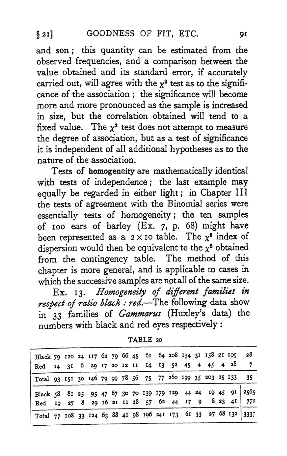
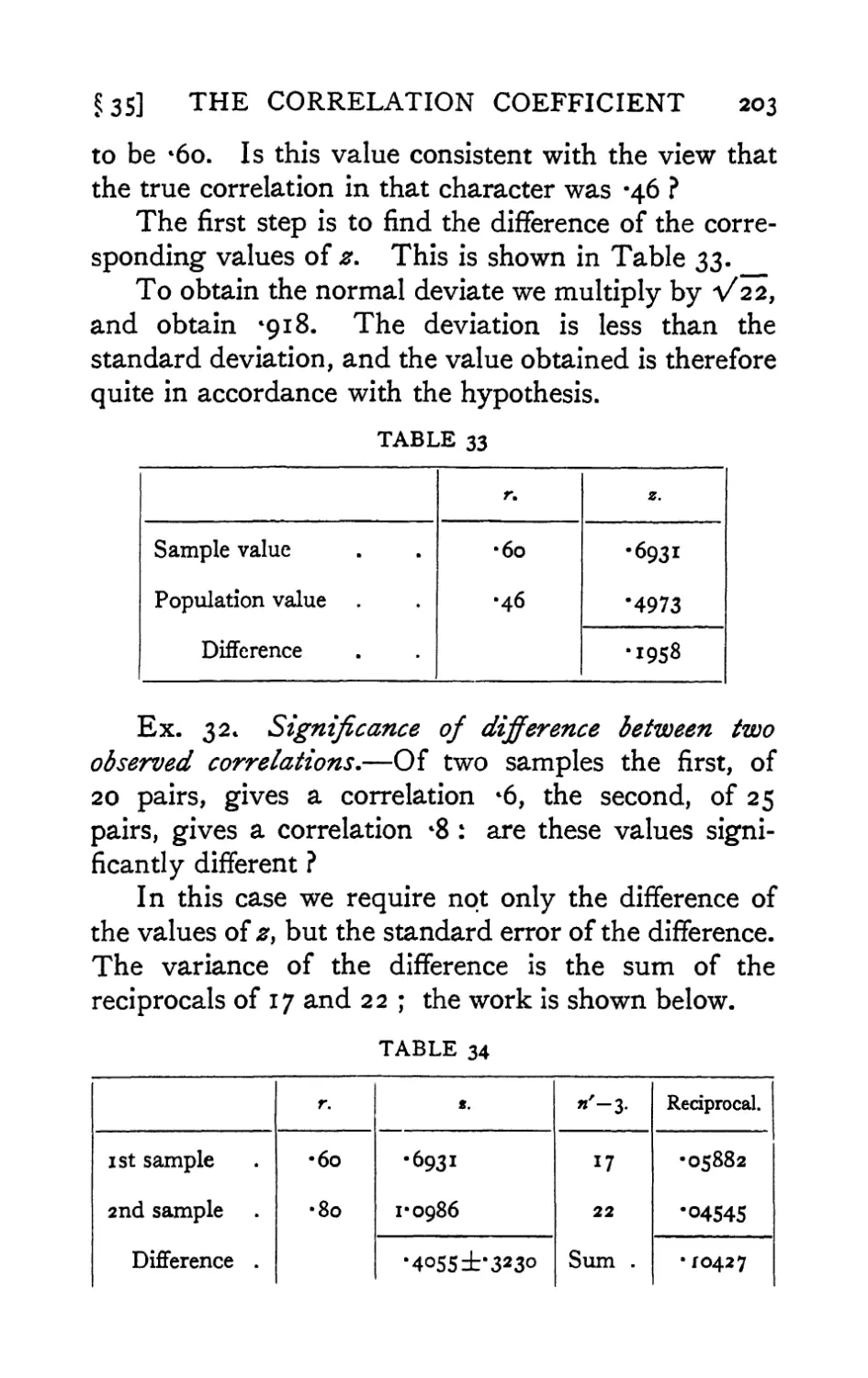


Text
Statistical Methods for
Research Workers
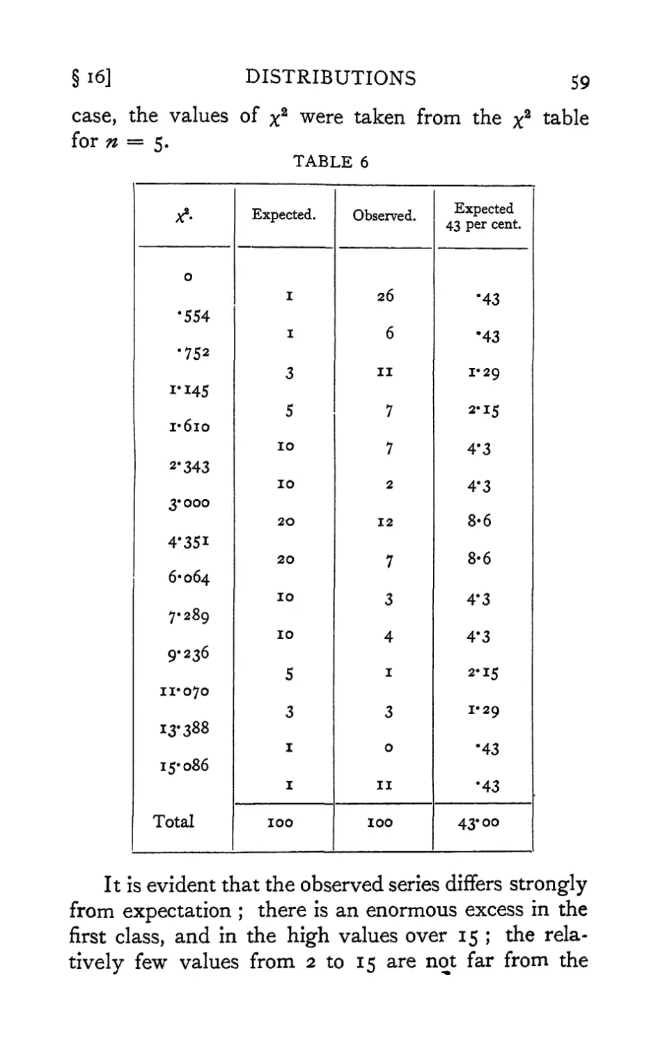
BY
Sir RONALD A. FISHER, sg.d., f.r.s.
D.Sc. (Ames, Chicago, Harvard, London), LL.D. (Calcutta, Glasgow)
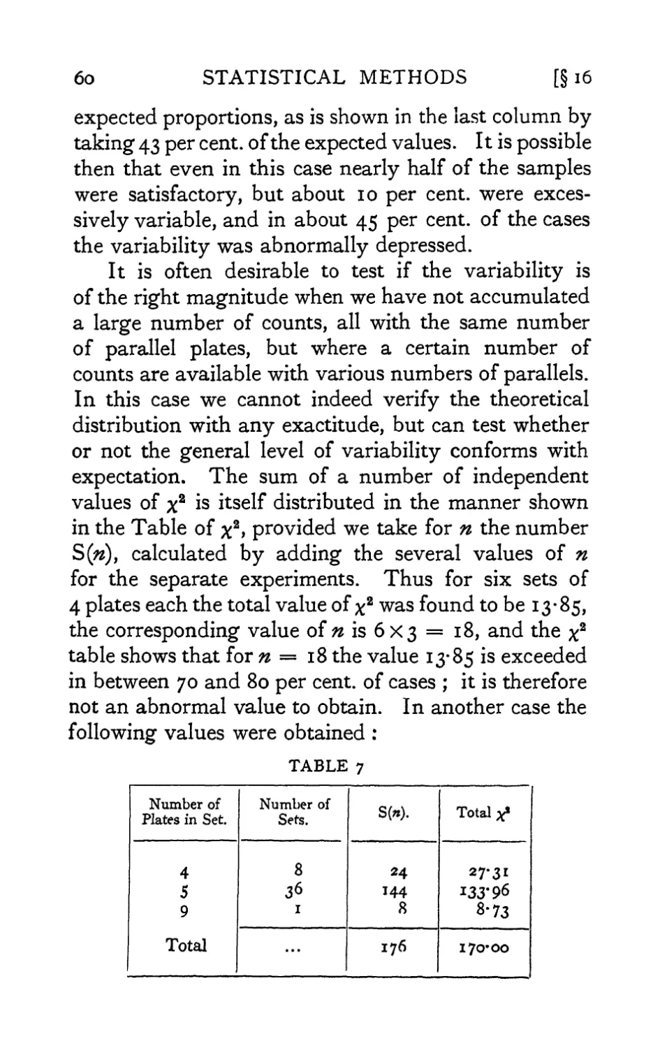
Fellow of Gonville and Caius College, Cambridge
Foreign Associate United States National Academy
of Science and Foreign Honorary Member American
Academy of Arts and Sciences; Foreign Member of
the Royal Swedish Academy of Sciences; Member
of the Royal Danish Academy of Sciences; Foreign
Member American Philosophical Society; formerly
Galton Professor; University of London; Arthur
Balfour Professor of Genetics, University of Cambridge
TWELFTH EDITION—REVISED
EG
HAFNER PUBLISHING COMPANY INC.
NEW YORK
1954
First Published . ..... 1925
Second Edition ... .... 1928
Third Edition 1930
Fourth Edition 1933
Fifth Edition 1934
Sixth Edition 1936
Seventh Edition 1938
Eighth Edition 1941
Ninth Edition 1944
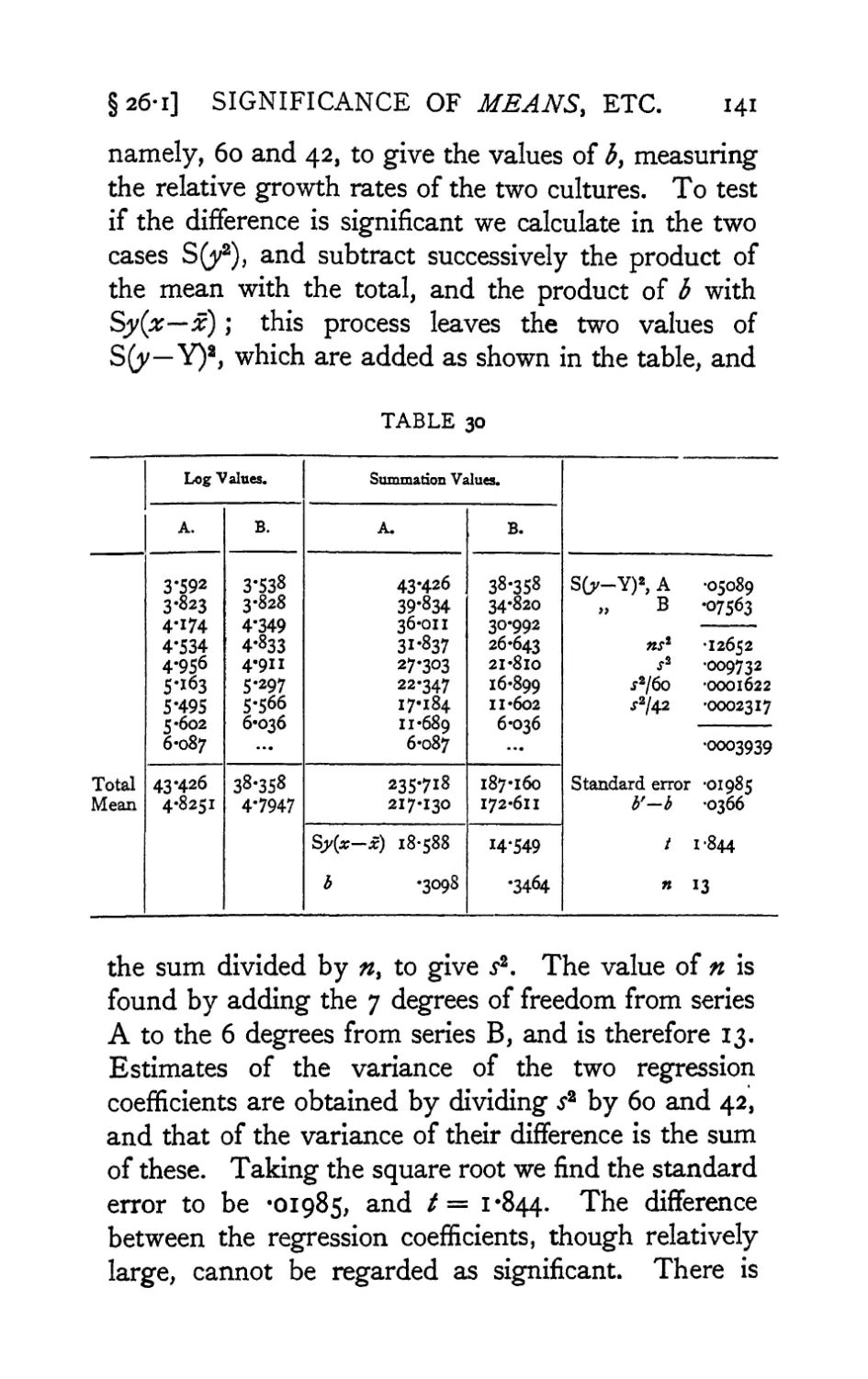
Tenth Edition 1946
Tenth Edition Reprinted 1948
Eleventh Edition 1950
Twelfth Edition 1954
Copyright Translations
French German
Presses Universitaires de France Oliver and Boyd Ltd.
108 Boulevard St Germain Tweeddale Court
Paris 6e, France Edinburgh, Scotland
Italian Spanish
Unione Tipografico Aguilar
Editrice Torinese S.A. de Ediciodes
Corso Raffaello 28 Juan Bravo 38
Torino, Italy Madrid, Spain
Japanm
Messrs Solmnsha
129 1-Chome, Ilinwle-cho,
Toshima-ku, Tokyo, Japan
BY THE SAME AUTHOR
THE GENETICAL THEORY OF NATURAL
SELECTION, 1930, Oxford Univ. Press
THE DESIGN OF EXPERIMENTS, 1935,
1937, 1942, 1947, Oliver and Boyd Ltd.
STATISTICAL TABLES (With Frank Yates),
1938, 1943, 1948, Oliver and Boyd Ltd.
THE THEORY OF INBREEDING, 1949,
Oliver and Boyd Ltd.
CONTRIBUTIONS TO MATHEMATICAL
STATISTICS, 1949, John Wiley and Sons
Inc., New York
PRINTRD AND PUBLISHED IN WKRAT SNITAM BY
OL1VKR AND BOVD LTD., RDlNBtWiH
EDITORS' PREFACE
The increasing specialisation in biological inquiry
has made it impossible for any one author to deal
adequately with current advances in knowledge. It
has become a matter of considerable difficulty for a
research student to gain a correct idea of the present
state of knowledge of a subject in which he himself is
interested. To meet this situation the text-book is
being supplemented by the monograph.
The aim of the present series is to provide
authoritative accounts of what has been done in some of the
diverse branches of biological investigation, and at
the same time to give to those who have contributed
notably to the development of a particular field of
inquiry an opportunity of presenting the results of
their researches, scattered throughout the scientific
journals, in a more extended form, showing their
relation to what has already been done and to
problems that remain to be solved.
The present generation is witnessing " a return to
the practice of older days when animal physiology
was not yet divorced from morphology.1'
Conspicuous progress is now being seen in the field of
general physiology, of experimental biology, and in
the application of biological principles to economic
problems. Often the analysis of large masses of
data by statistical methods is necessary, and the
biological worker is continually encountering advanced
statistical problems the adequate solutions of which
viii
EDITORS' PREFACE
are not found in current statistical text-books. To
meet these needs the present monograph was
prepared, and the early call for the second and later
editions indicates the success attained by the author
in this project.
F. A. E. C.
D. W. C.
PREFACE TO TWELFTH EDITION
For several years prior to the preparation of this
book, the author had been working in somewhat
intimate co-operation with a number of biological
research departments at Rothamsted; the book was
very decidedly the product of this circumstance.
Daily contact with statistical problems as they
presented themselves to laboratory workers stimulated
the purely mathematical researches upon which the
new methods were based. It was clear that the
traditional machinery inculcated by the biometrical
school was wholely unsuited to the needs of practical
research. The futile elaboration of innumerable
measures of correlation, and the evasion of the real
difficulties of sampling problems under cover of a
contempt for small samples, were obviously beginning
to make its pretentions ridiculous. These procedures
were not only ill-aimed, but, for all their elaboration,
not sufficiently accurate. Only by tackling small
sample problems on their merits, in the author's view,
did it seem possible to apply accurate tests to practical
data. With the encouragement of my colleagues, and
the valued help of the late W. S. Gosset (" Student"),
his assistant Mr E. Somerfield, and Miss W. A,
Mackenzie, the first edition was prepared and weathered
the hostile criticisms inevitable to such a venture.
To-day exact tests of significance need no apology.
The demand, steadily increasing over a long period,
for a book designed originally for a much smaller
public has justified at least some of the innovations in
PREFACE TO TWELFTH EDITION
its plan which at first must have seemed questionable.
(The recognition of degrees of freedom ; the use of
fixed probability levels in tabulating the functions
used in tests of significance ; the analysis of variance ;
the need for randomisation in experimental design, etc.)
The author was impressed with the practical
importance of many recent mathematical advances, which to
others seemed to be merely academic refinements.
He felt sure, too, that workers with research experience
would appreciate a book which, without entering into
the mathematical theory of statistical methods, should
embody the latest results of that theory, presenting
them in the form of practical procedures appropriate
to those types of data with which research workers
are actually concerned. The practical application of
general theorems is a different art from their
establishment by mathematical proof. It requires fully as
deep an understanding of their meaning, and is,
moreover, useful to many to whom the other is unnecessary.
To carry out this plan new matter has had to be
added with each new edition, to illustrate extensions
and improvements, the value of which had in the
meantime been established by experience.
In most cases the new methods actually simplify
the handling of the data. The conservatism of some
university courses in elementary statistics, in
stereotyping unnecessary approximations and inappropriate
conventions, still hinders many students in the use of
exact methods. In reading this book they should try
to remember that departures from tradition have not
been made capriciously, but only when they have been
found to be definitely helpful
Especially in the order of presentation, the book
bears traces of the state of the subject when it first
PREFACE TO TWELFTH EDITION
appeared. More recent books have, rightly from
the teacher's standpoint, introduced the analysis of
variance earlier, and given it more space. They have
thus carried further than I the process of abstracting
from the field formerly embraced by the correlation
coefficient, problems capable of a more direct approach.
In excusing myself from the difficult task of a
fundamental rearrangement, I may plead that it is of real
value to understand the problems discussed by earlier
writers, and to be able to translate them into the
system of ideas in which they may be more simply or
more comprehensively resolved. I have therefore
contented myself with indicating the analysis of
variance procedure as an alternative approach in some
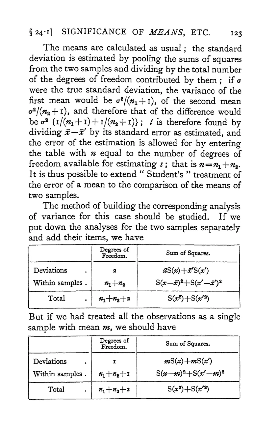
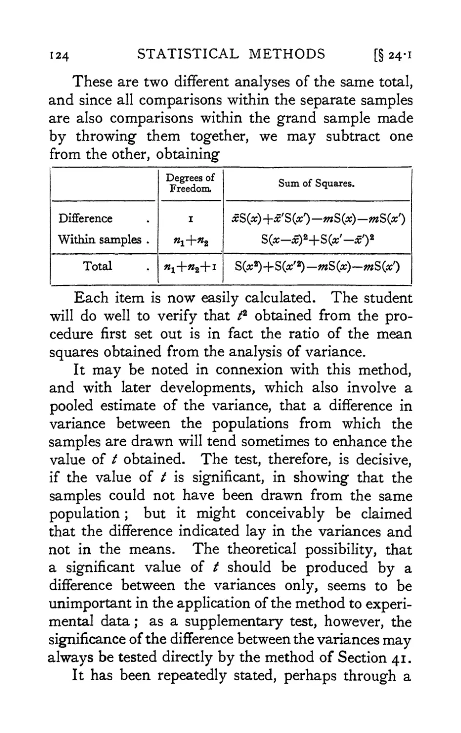
early examples, as in Sections 24 and 24-1.
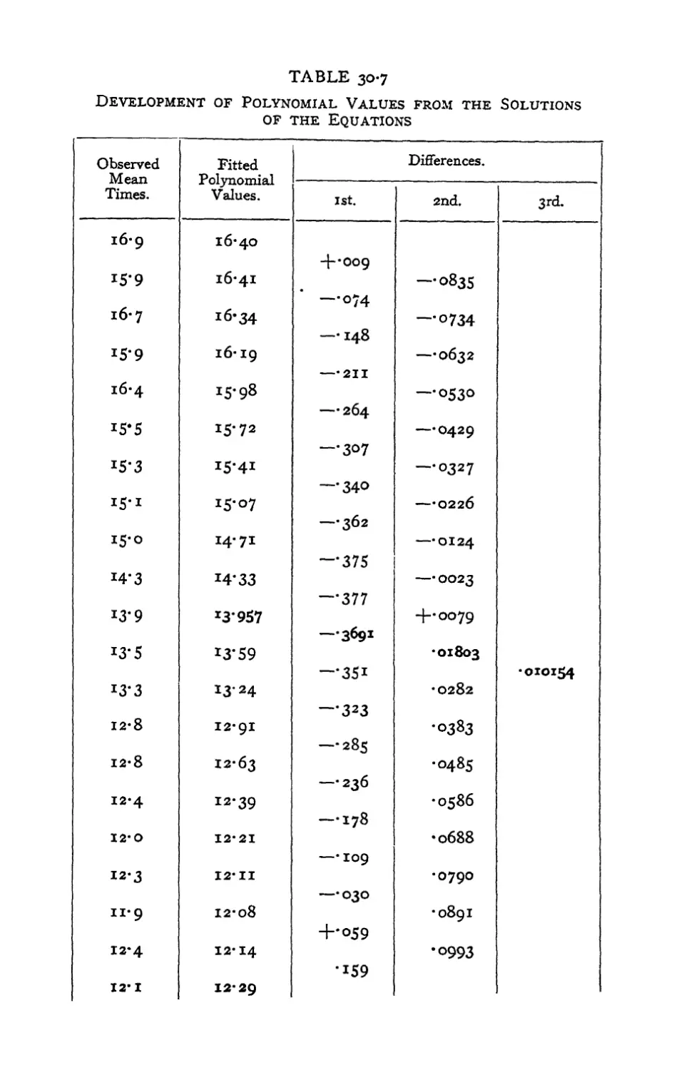
With a class capable of mastering the whole
book, I should now postpone the matter of Sections
30 to 40,. dealing with correlation, until further
experience has been gained of the applications of the
Analysis of Variance, but should later give time to the
ideas of correlation and partial correlation, for their
importance in understanding the literature of quantitative
biology, which has been so largely influenced by them.
In the second edition the importance of providing
a striking and detailed illustration of the principles of
statistical estimation led to the addition of a ninth
chapter. The subject had received only general
discussion in the first edition, and, in spite of its
practical importance, had not yet won sufficient
attention from teachers to drive out of practice the
demonstrably defective procedures which were still
unfortunately taught to students. The new chapter
superseded Section 6 and Example 1 of the first
edition ; in the third edition it was enlarged by two
xii PREFACE TO TWELFTH EDITION
new sections (57.1 and 57.2) illustrating further the
applicability of the method of maximum likelihood,
and of the quantitative evaluation of information.
Later K. Mather's admirable book The Measurement
of Linkage in Heredity has illustrated the appropriate
procedures for a wider variety of genetical examples.
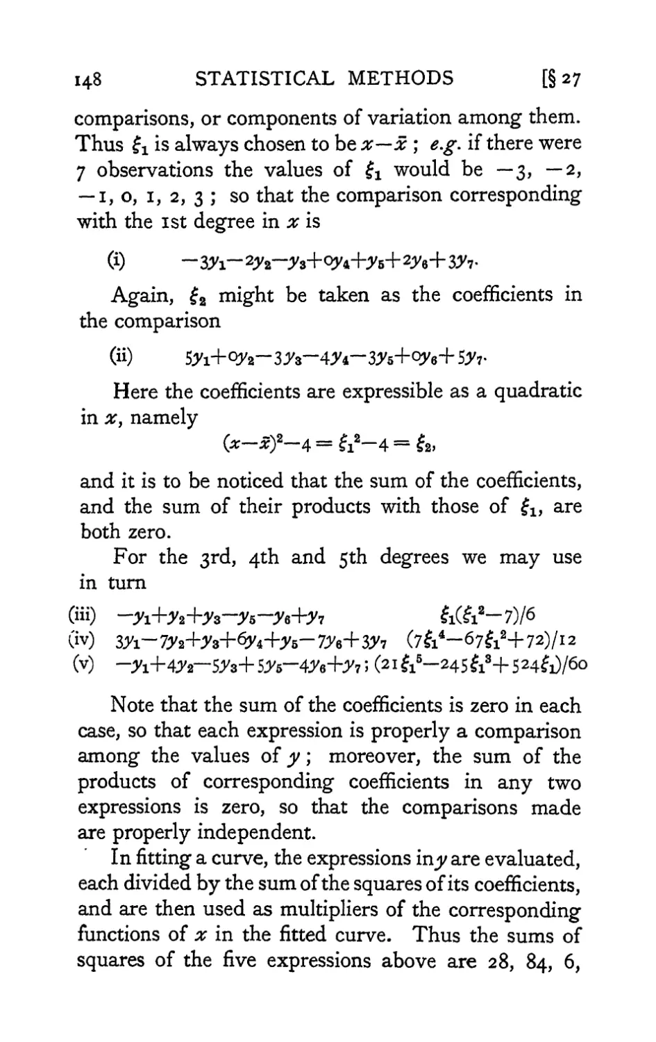
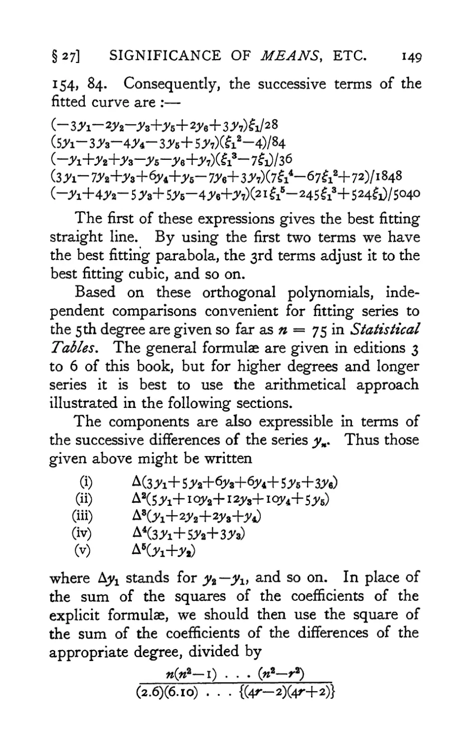
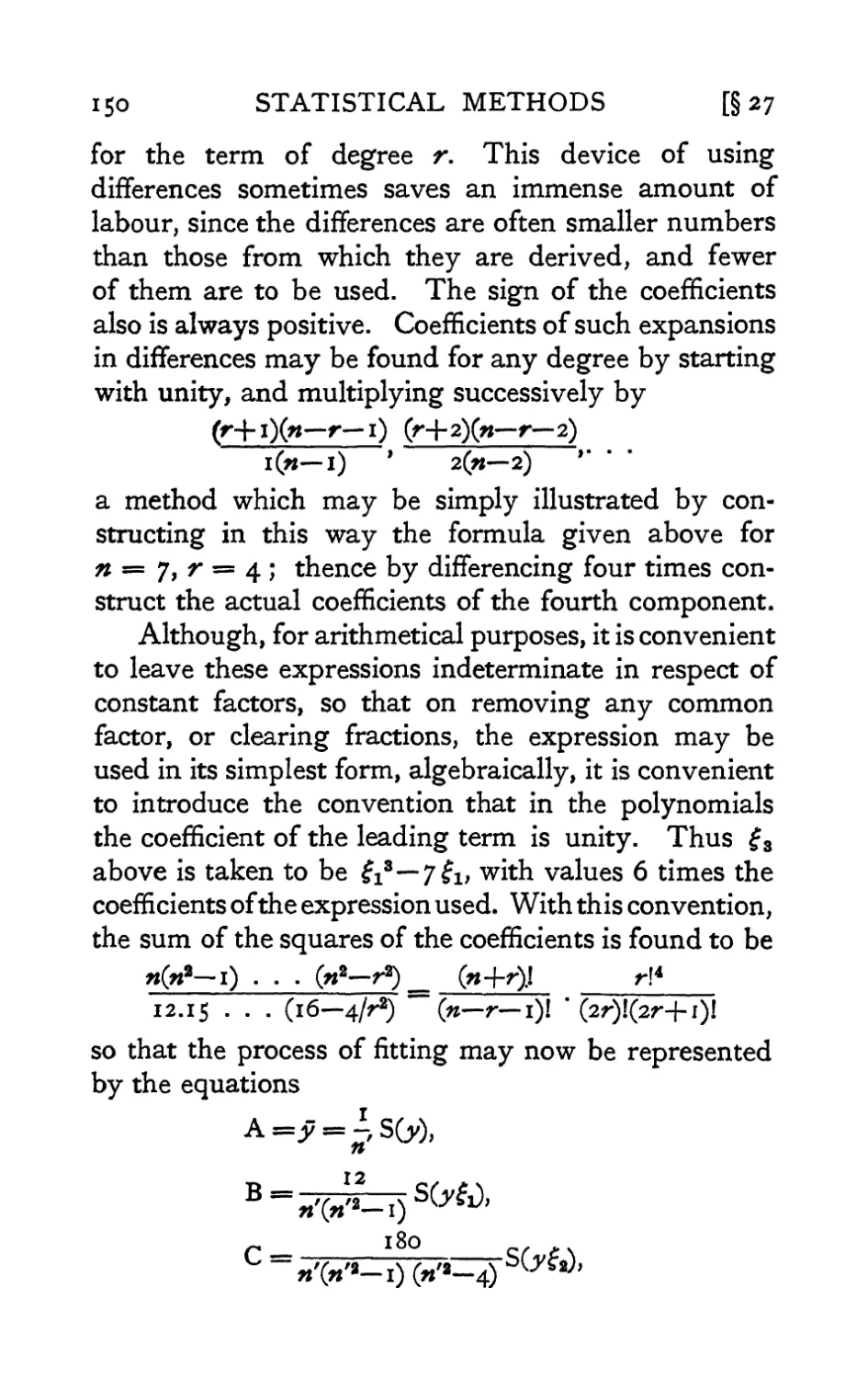
In Section 27 a general method of constructing the
series of orthogonal polynomials was added to the third
edition, in response to the need which is felt, with
respect to some important classes of data, to use
polynomials of higher degree than the fifth. Simple
and direct algebraic proofs of the methods of Sections
28 and 28-1 have been published by Miss F. E. Allan.
In the fourth edition the Appendix to Chapter III,
on technical notation, was entirely rewritten, since
the inconveniences of the moment notation seemed
by that time definitely to outweigh the advantages
formerly conferred by its familiarity. The principal
new matter in that edition was added in response to
the increasing use of the analysis of covariance, which
is explained in Section 49-1. Since several writers
had found difficulty in applying the appropriate tests
of significance to deviations from regression formulae,
this section was further enlarged in the fifth edition.
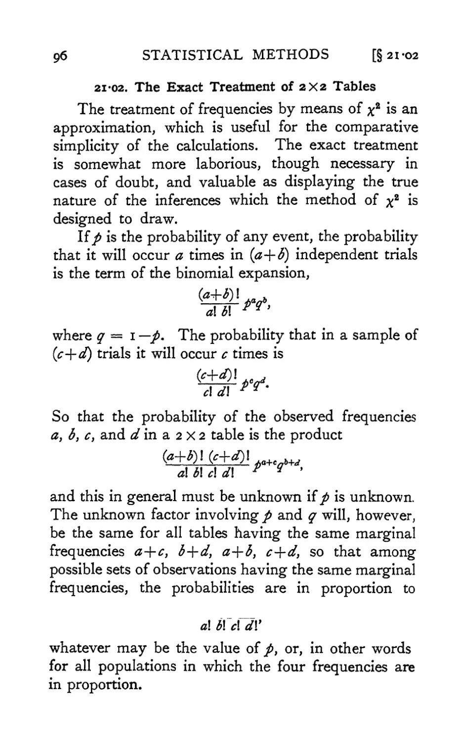
Other new sections in the fifth edition were 21.01,
giving a correction for continuity recently introduced
by F. Yates, and 21 *02 giving the exact tus»t of
significance for 2x2 tables. Workers who are accustomed
to handle regression equations with a large number
of variates will be interested in Section 29*1, which
provides the relatively simple adjustments to be made
when, at a late stage, it is decided that one or more
of the variates used may with advantage be omitted.
The possibility of doing this without laborious
PREFACE TO TWELFTH EDITION xiii
recalculations should encourage workers to make the
list of independent variates included more
comprehensive than has, in the past, been thought advisable.
Section 5, formerly occupied by an account of the
tables available for testing significance, was given to
a historical note on the principal contributors to the
development of statistical reasoning.
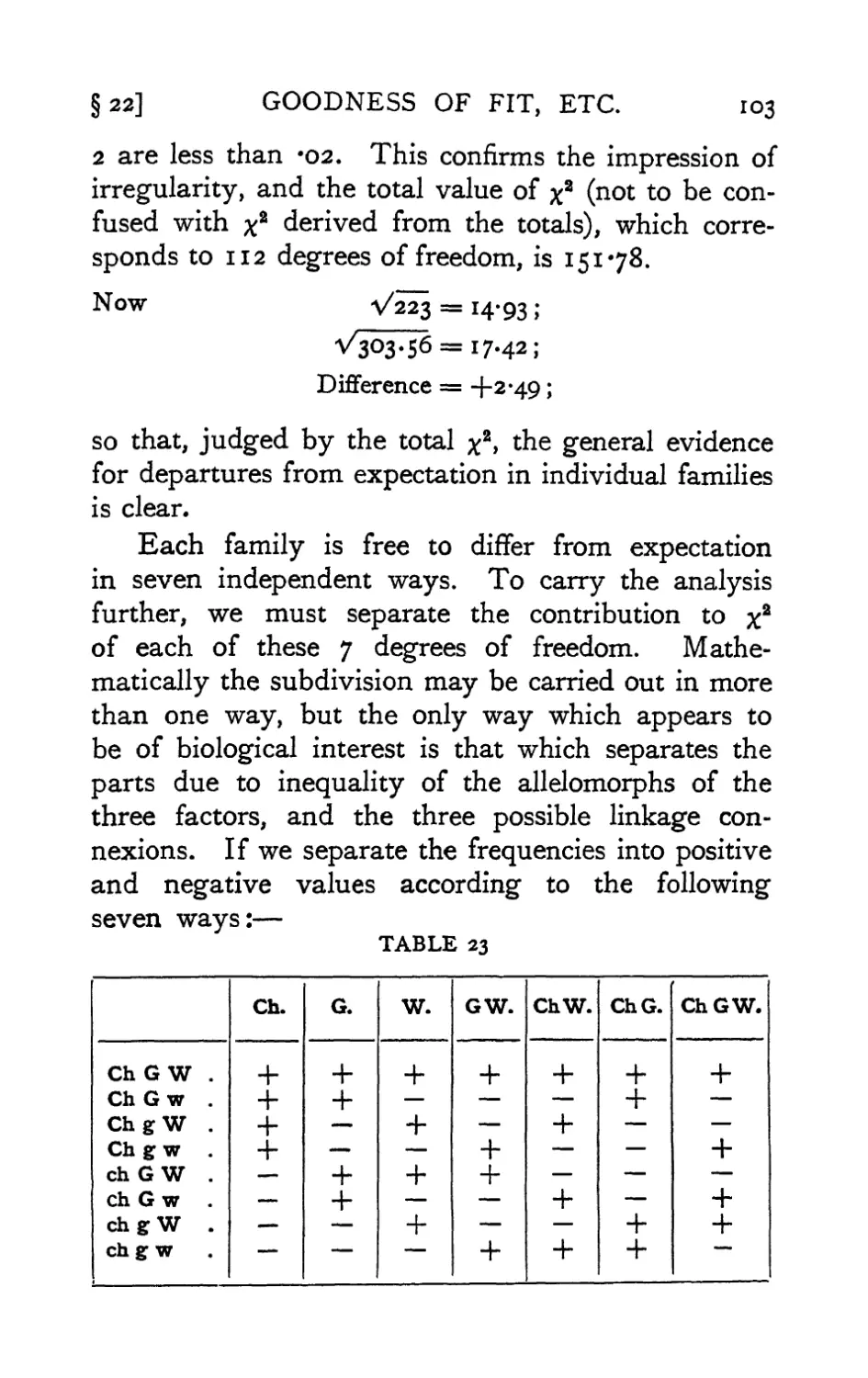
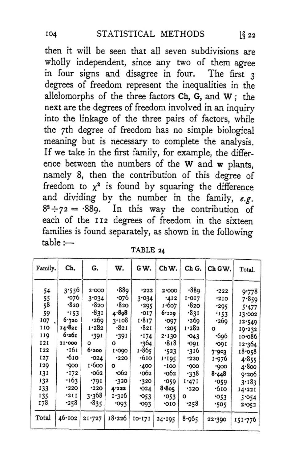
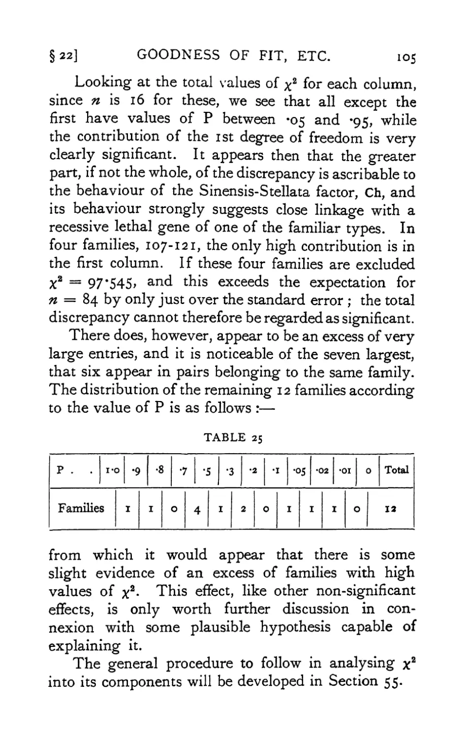
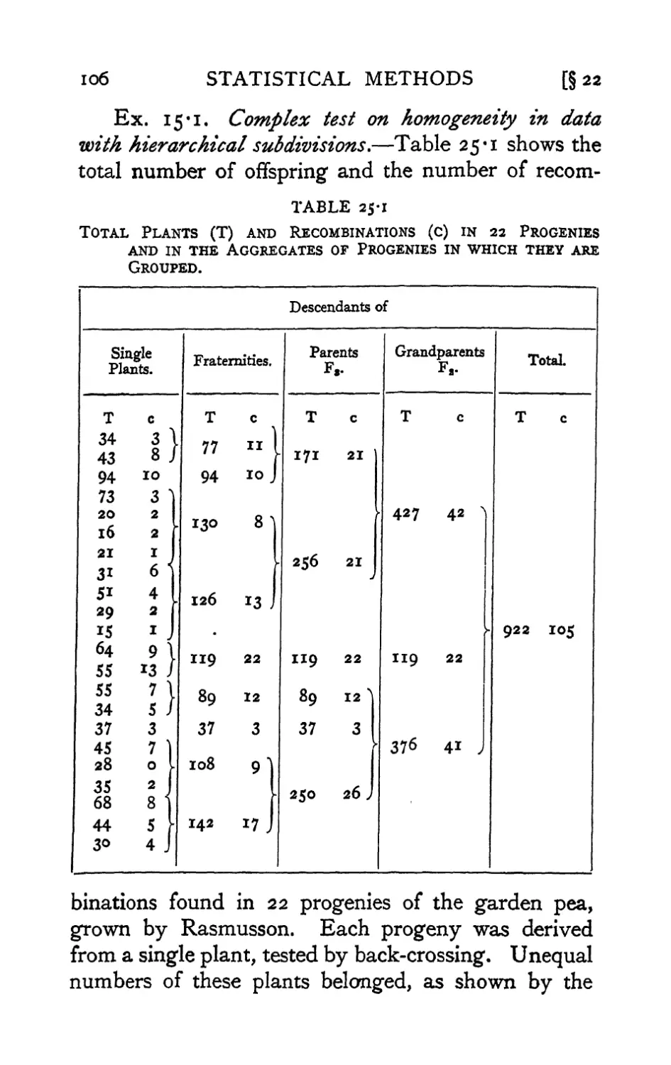
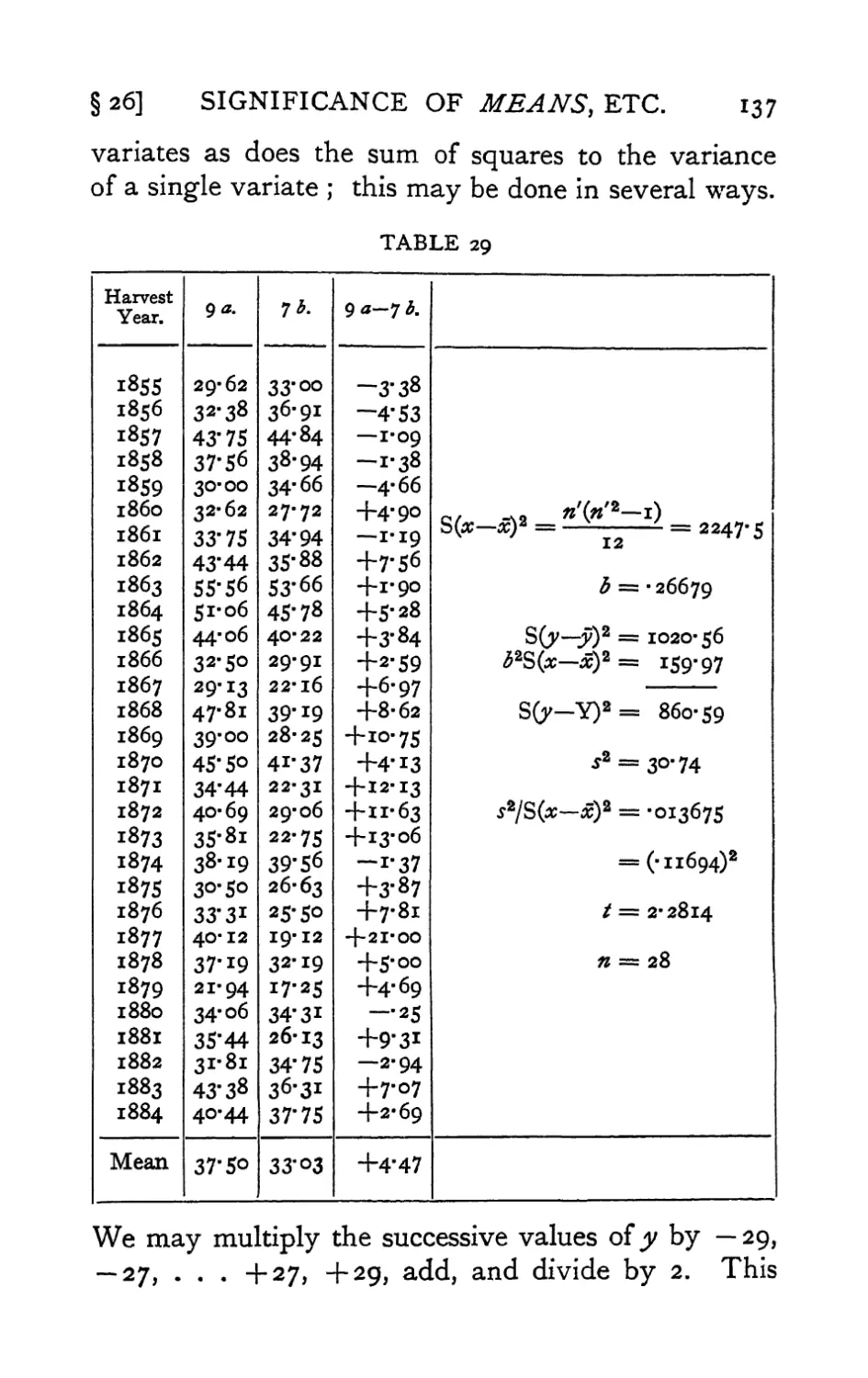
In the sixth edition Example 15*1, Section 22,
gave a new test of homogeneity for data with
hierarchical subdivisions. Attention was also called
to Working and Hotelling's formula for the sampling
error of values estimated by regression, and in Section
29-2 to an extended use of successive summation in
fitting polynomials.
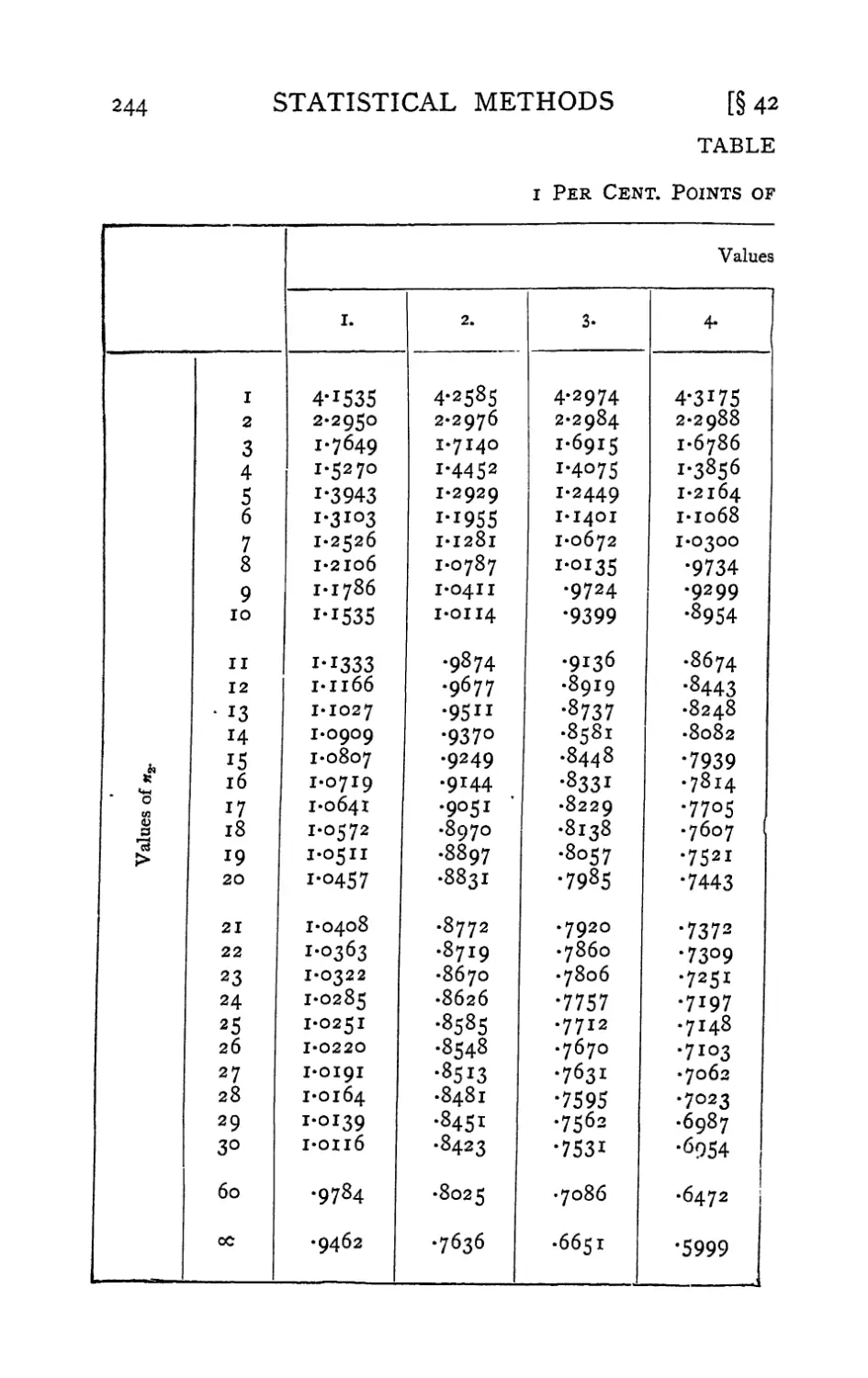
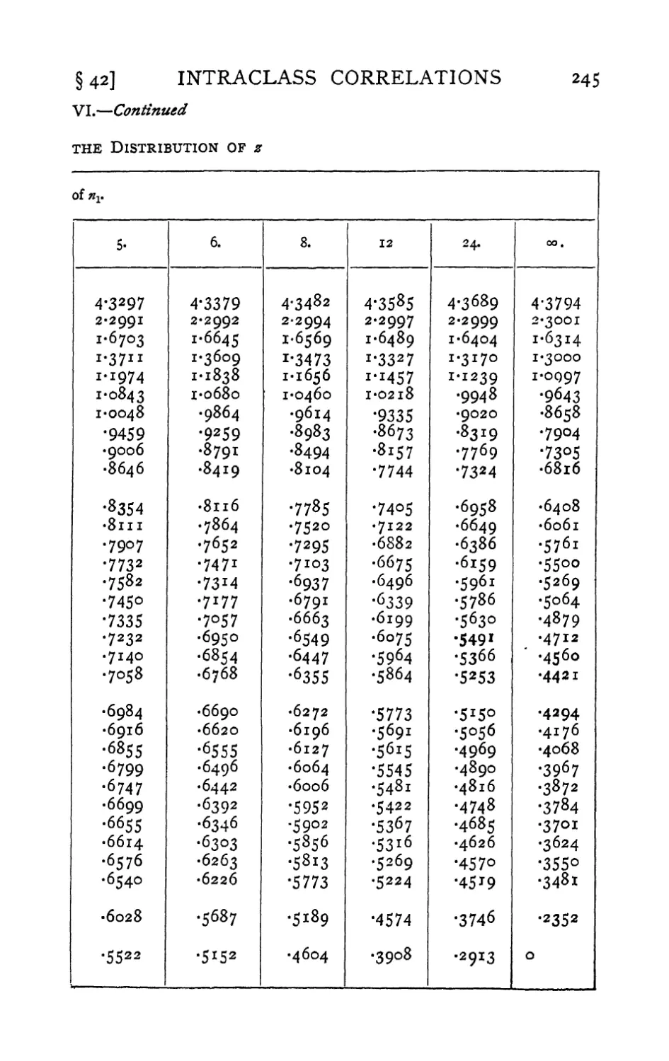
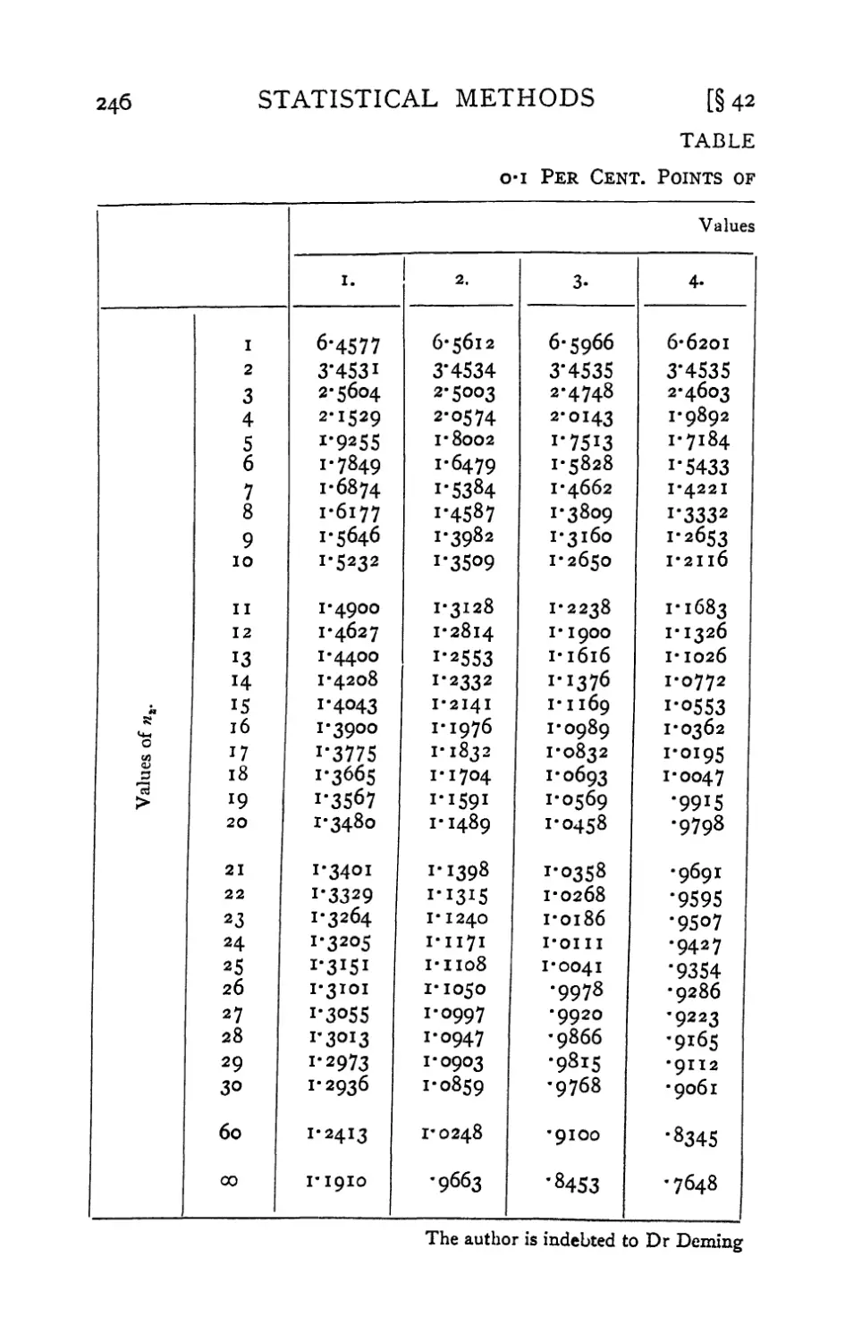
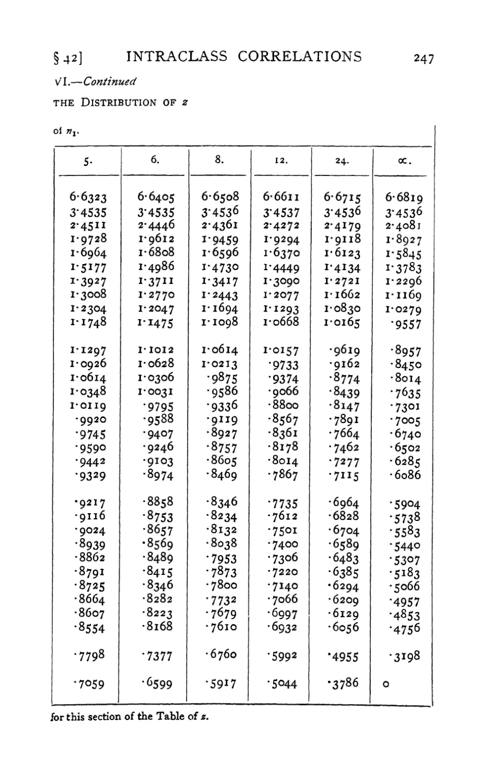
I am indebted to Dr W. E. Deming for the
extension of the Table of 2 to the o-1 per cent, level
of significance. Such high levels of significance are
especially useful when the test we make is the most
favourable out of a number which a priori might
equally well have been chosen.
Two changes in the seventh edition may be
mentioned. Section 27 was expanded so as to give
a fuller introduction to the theory of orthogonal
polynomials, by way of orthogonal comparisons
between observations, which most practical workers
find easier to grasp. The arithmetical construction
is simpler by this path, and the full generality of the
original treatment can be retained without very
complicated algebraic expressions. A useful range of
tables giving the serial values to the fifth degree is
now available in Statistical Tables.
Section 49*2 was added to give an outline of the
important new subject of the use of multiple
measurements to form the best discriminant functions of which
xiv PREFACE TO TWELFTH EDITION
they are capable. The tests of significance appropriate
to this process are approximate and deserve further
study. The diversity of problems which yield to this
method is very striking.
A section new in the ninth edition is given to the
test of homogeneity of evidence used in estimation,
since this subject is the natural and logical
complement to the methods of combining independent
evidence illustrated in the previous examples. In
the tenth edition is an extension of the /-test to find
fiducial limits for the ratio of means or regression
coefficients (Section 26-2).
The sections of Chapter VIII, the Principles of
Experimentation, which have always been too short
to do justice to aspects of the subject other than
the purely statistical, have since developed into an
independent book, The Design of Experiments (Oliver
and Boyd, 1935, l92>7> *94^ *94^ *947> *949> 195*)-
The tables of this book, together with a number of
others calculated for a variety of statistical purposes,
with illustrations of their use, are now available under
the title of Statistical Tables (Oliver and Boyd, 1938,
1943, 1946, 1953). Both of these publications relieve
the present work of claims for expansion in directions
which threatened to obstruct its usefulness as a single
course of study. The serious student should make sure
that these volumes also are accessible to him.
It should be noted that numbers of sections, tables
and examples have been unaltered by the insertion of
fresh material, so that references to them, though not
to pages, will be valid irrespective of the edition used.
Department of Genetics, Cambridge
1954
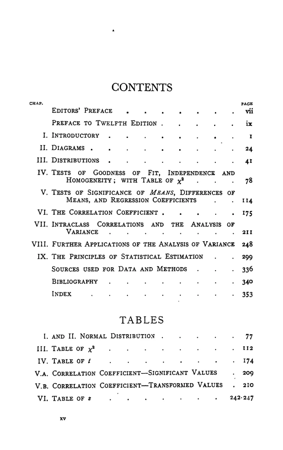
CONTENTS
CHAP. pAGE
Editors' Preface vii
Preface to Twelfth Edition ix
I. Introductory i
II. Diagrams 24
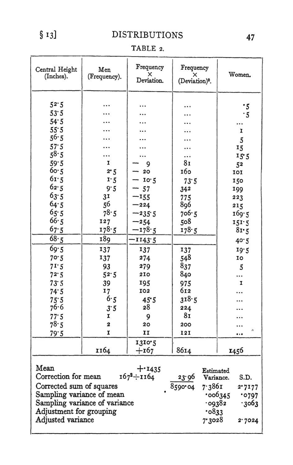
III. Distributions 41
IV. Tests of Goodness of Fit, Independence and
Homogeneity ; with Table of x2 • -78
V. Tests of Significance of Means, Differences of
Means, and Regression Coefficients . .114
VI. The Correlation Coefficient 175
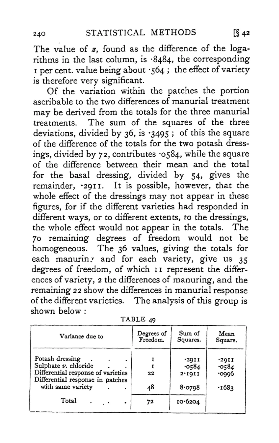
VII. Intraclass Correlations and the Analysis of
Variance 211
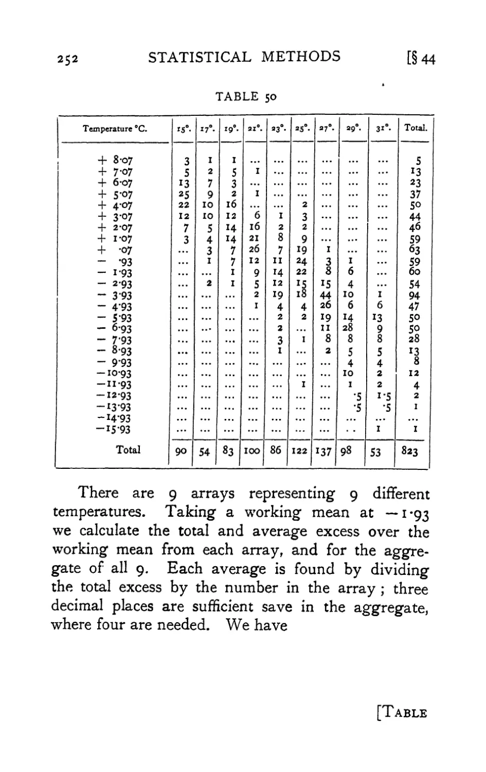
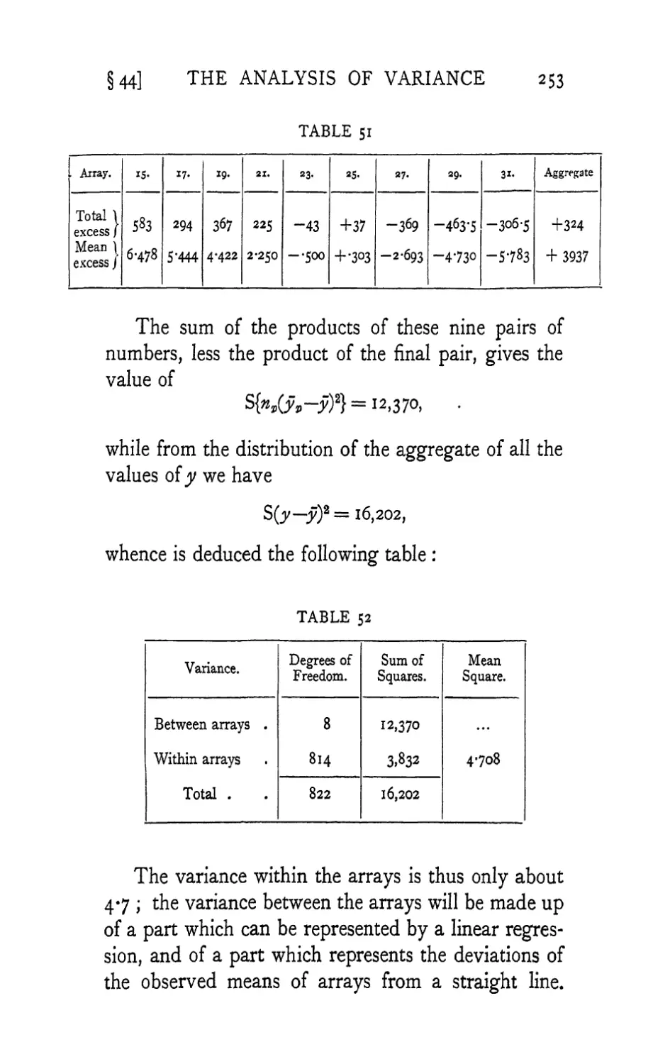
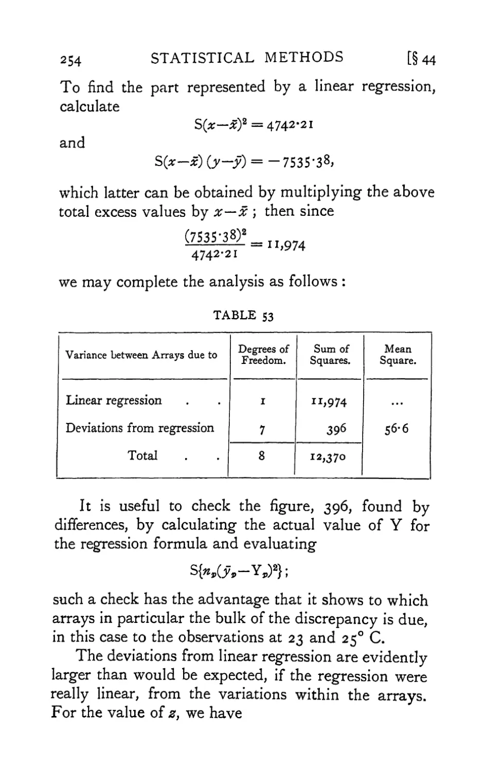
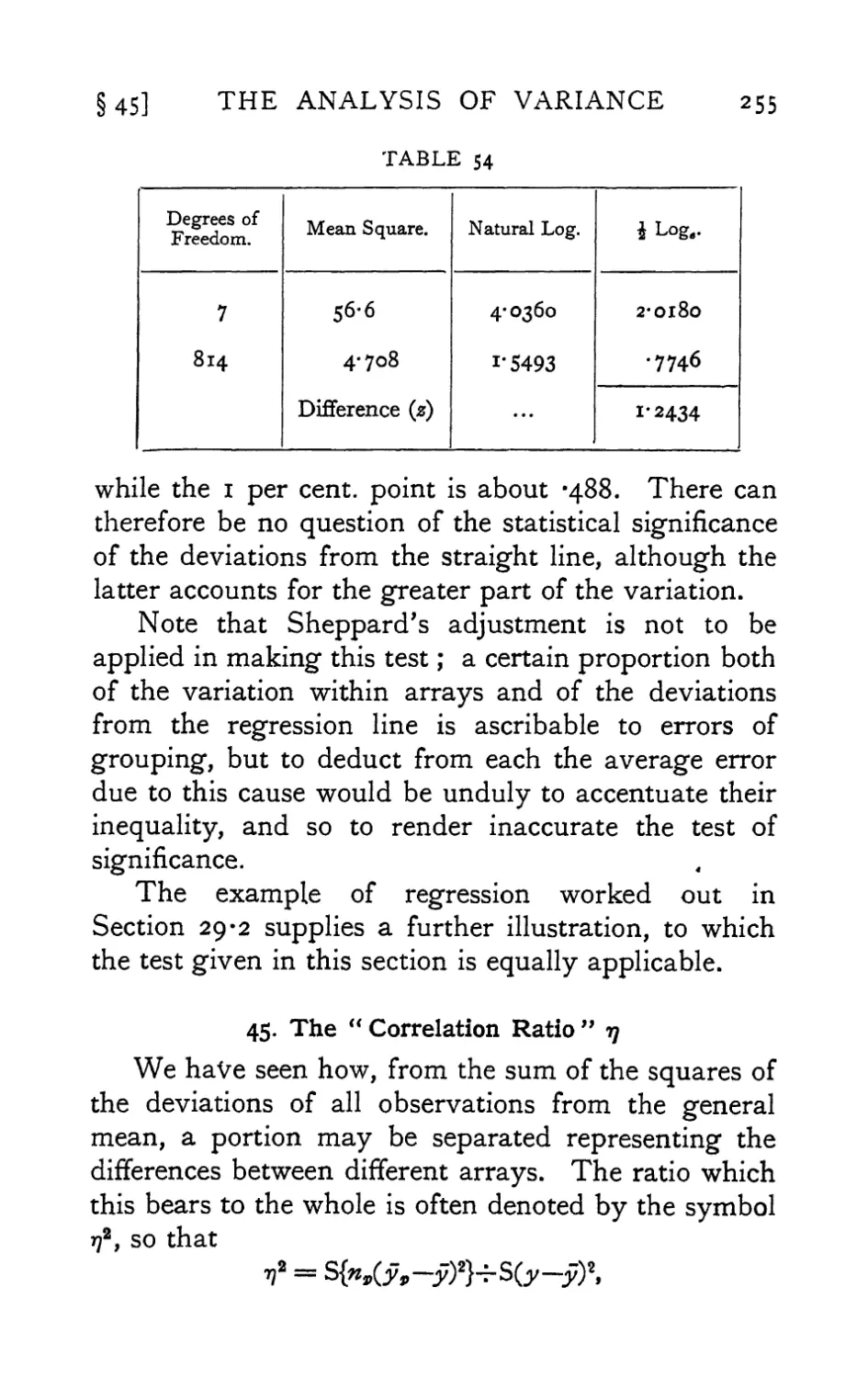
VIII. Further Applications of the Analysis of Variance 248
IX. The Principles of Statistical Estimation . . 299
Sources used for Data and Methods . . .336
Bibliography 340
Index 353
TABLES
I. and II. Normal Distribution 77
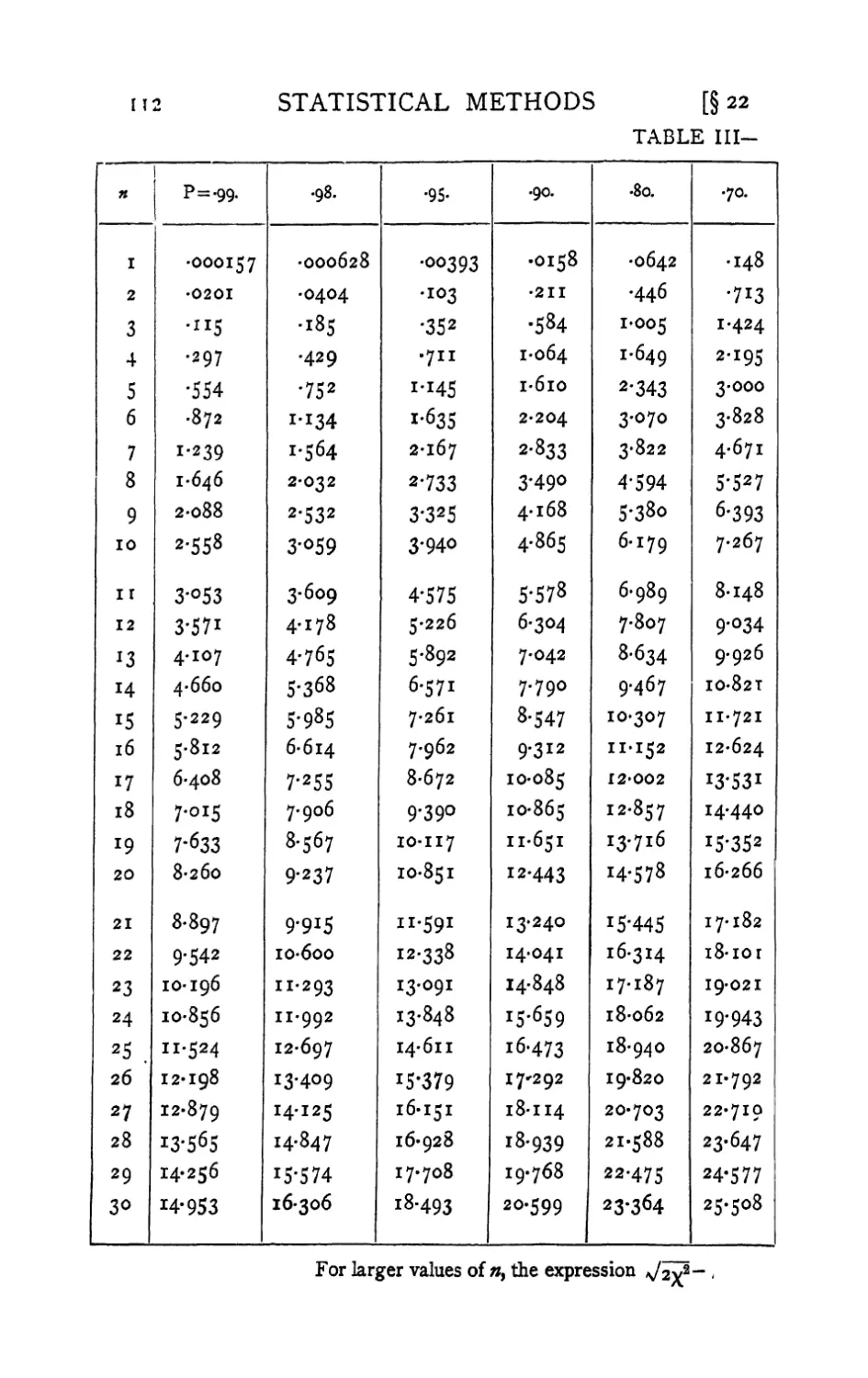
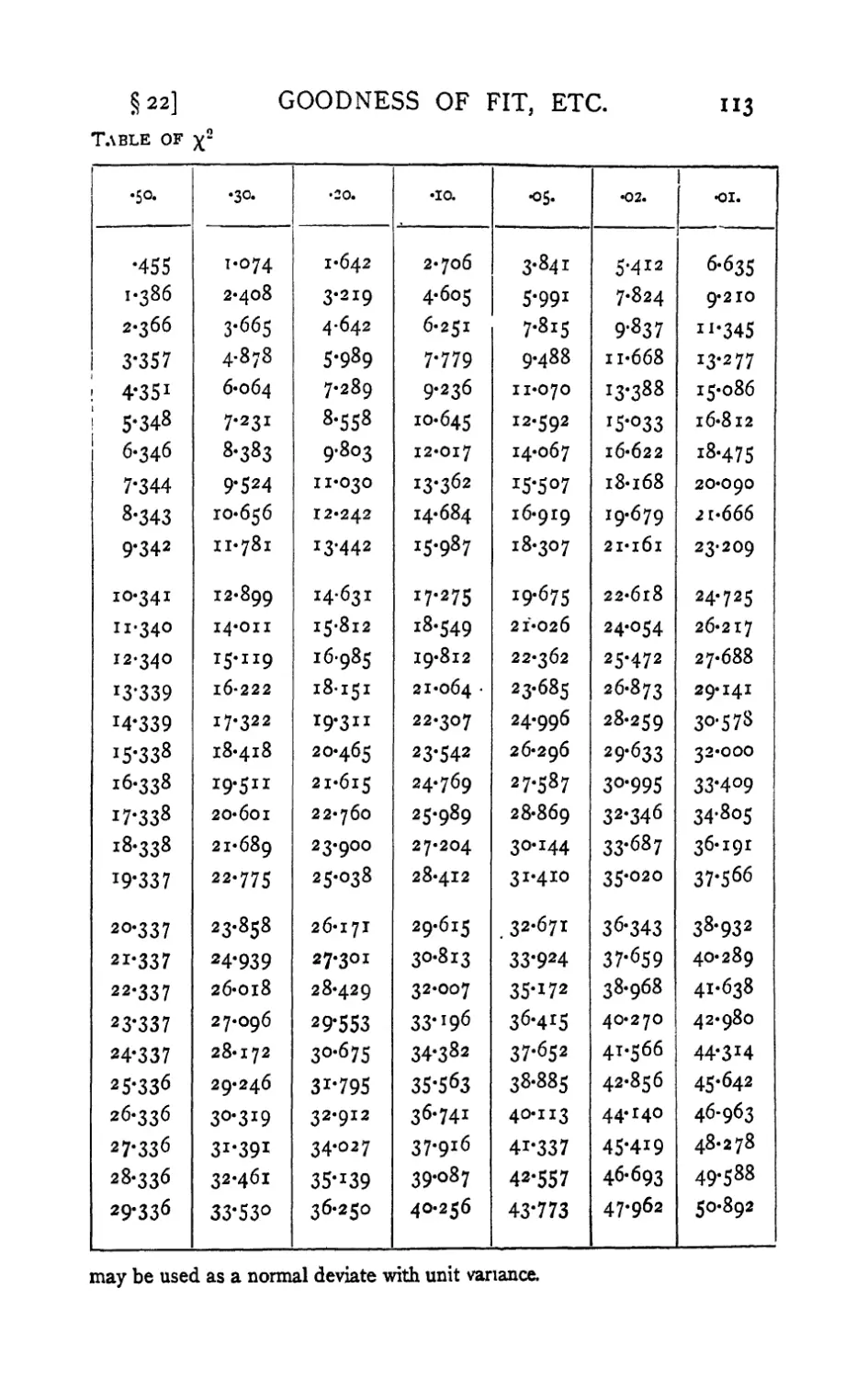
III. Table of x2 II2
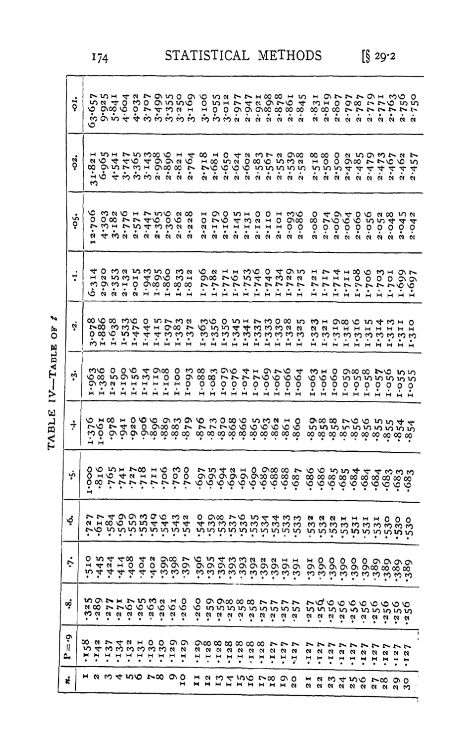
IV. Table of / 174
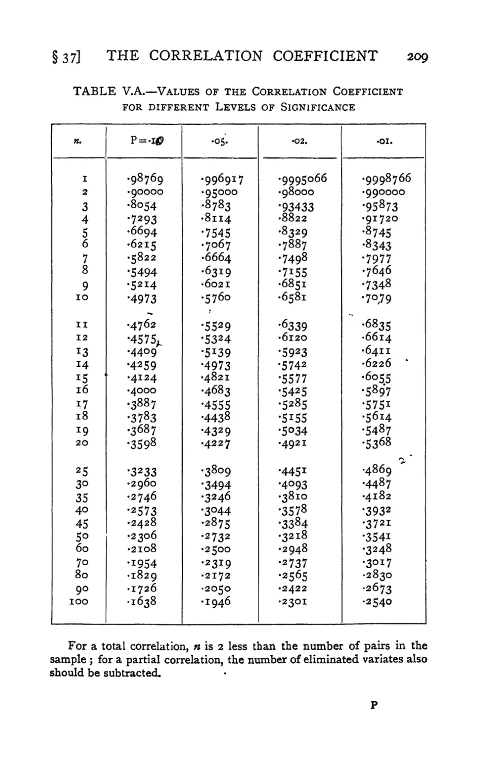
V.a. Correlation Coefficient—Significant Values . 209
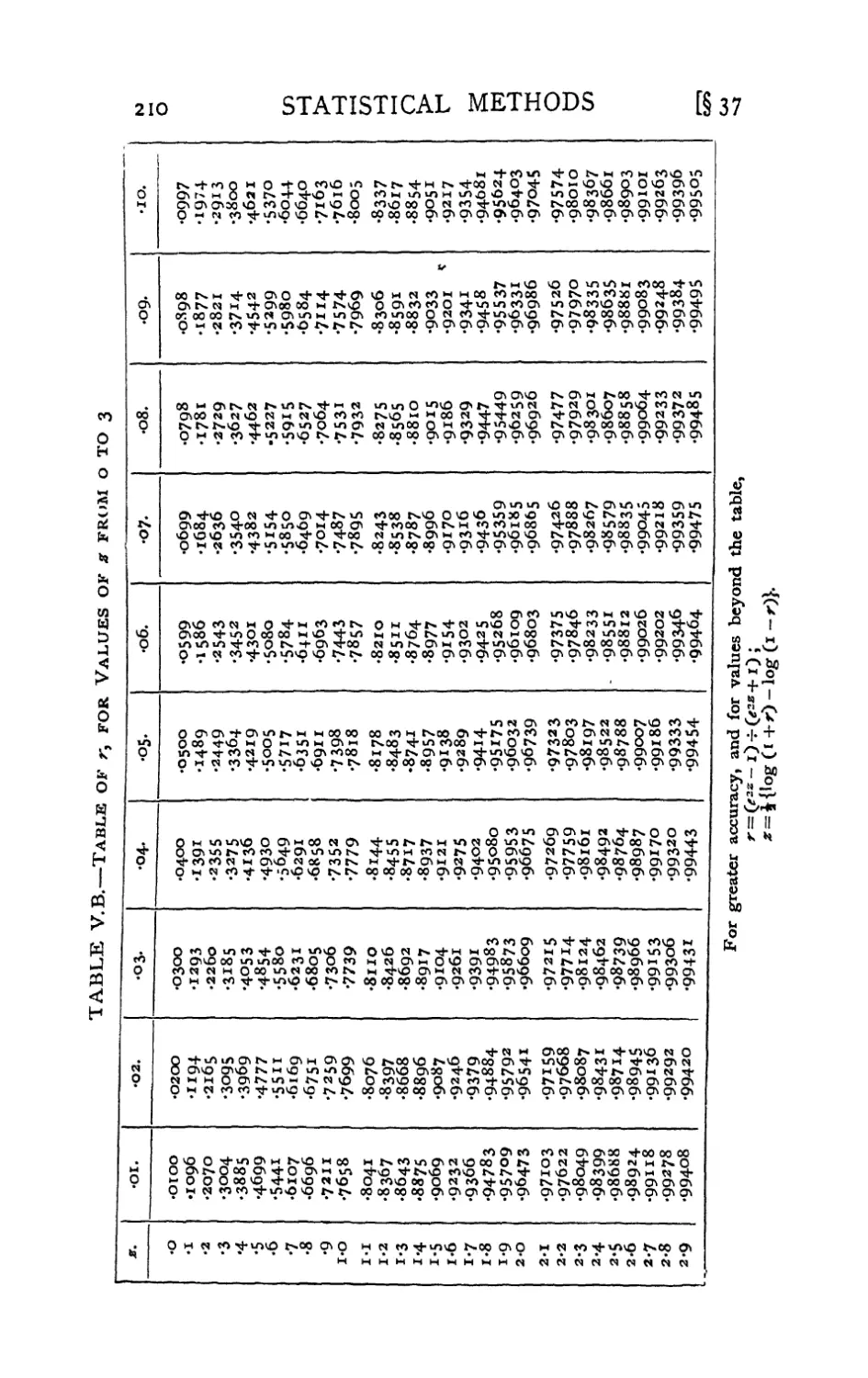
V.b. Correlation Coefficient—Transformed Values . 210
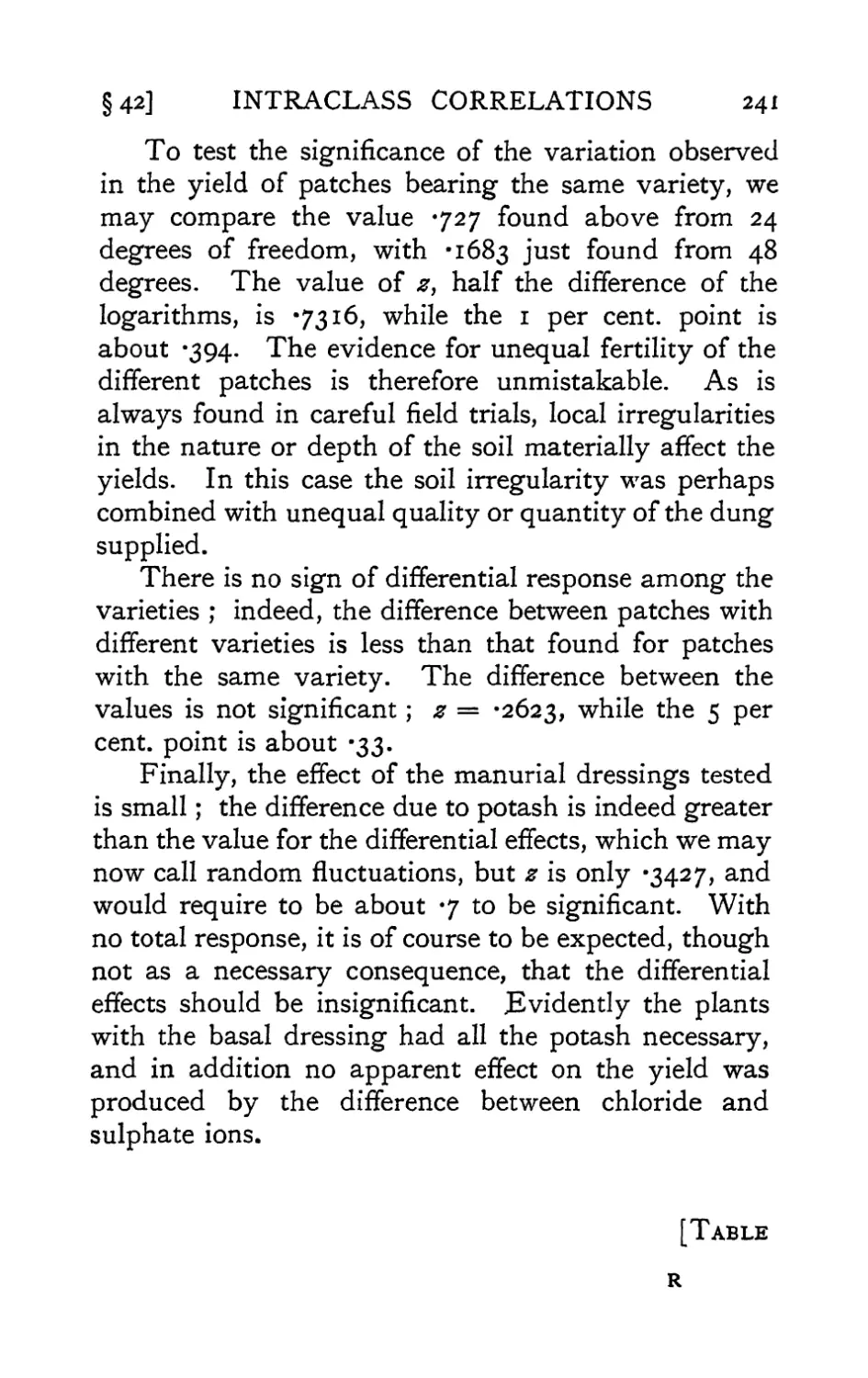
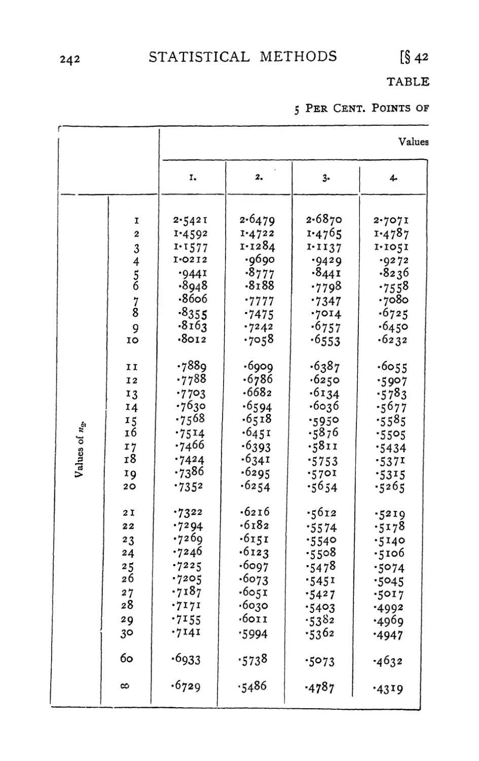
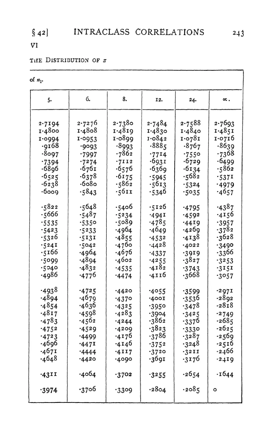
VI. Table of z 242-247
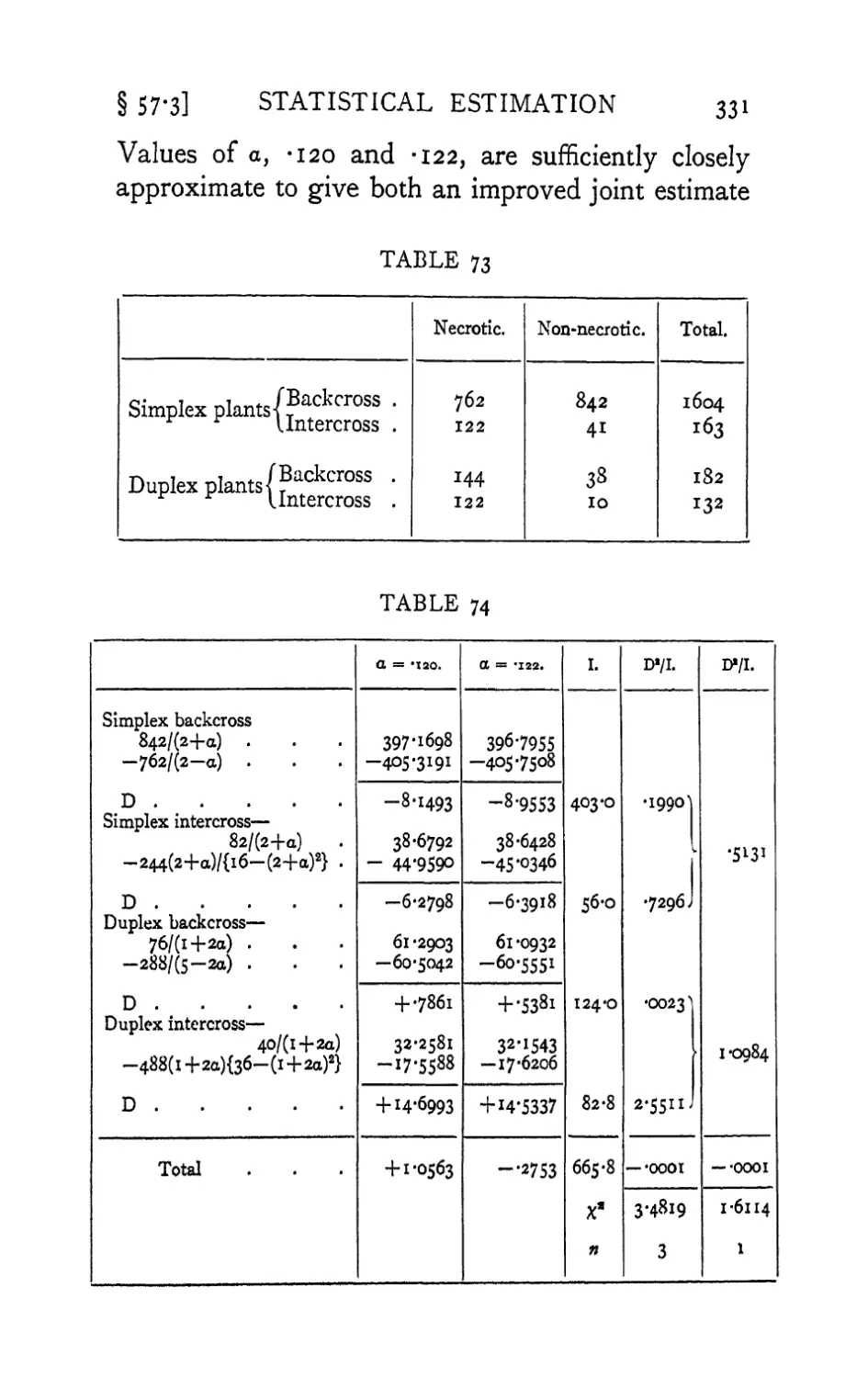
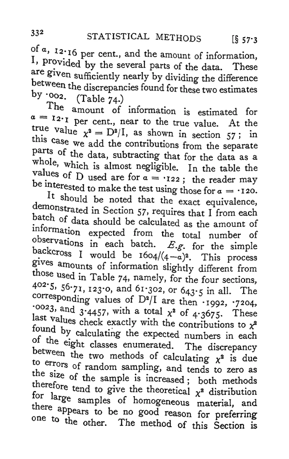
XV
I
INTRODUCTORY
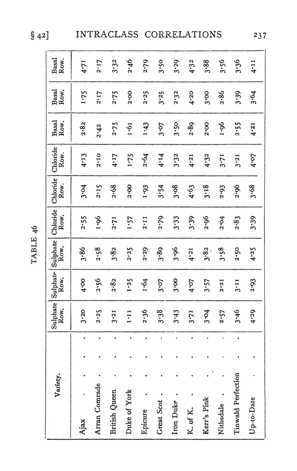
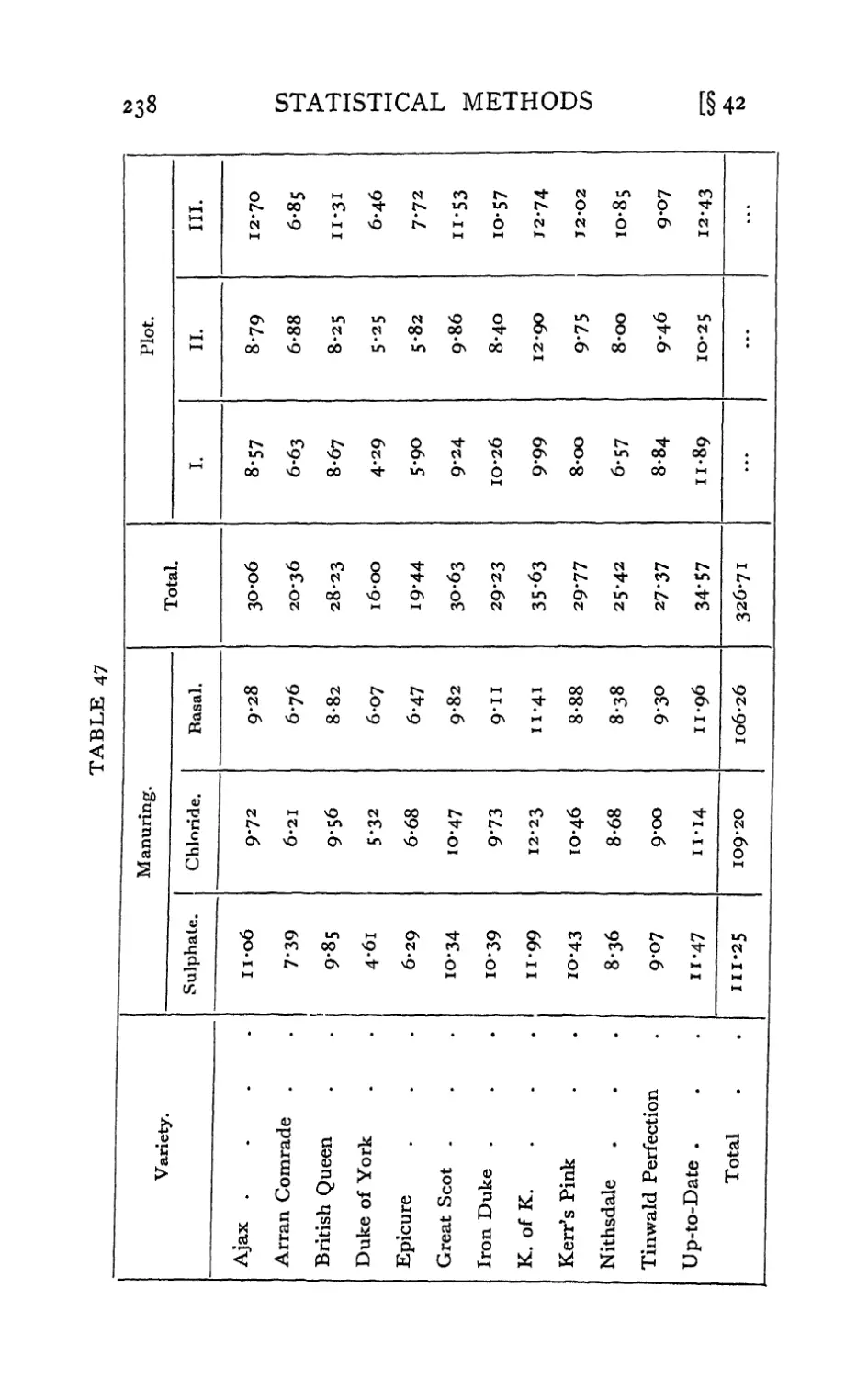
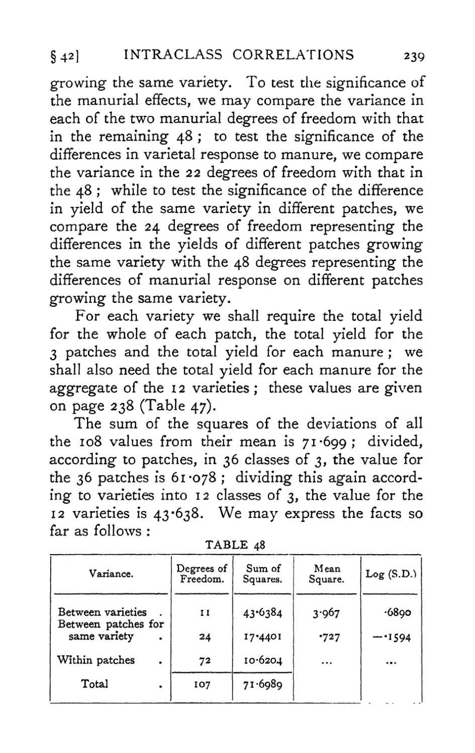
i. The Scope of Statistics
The science of statistics is essentially a branch of
Applied Mathematics, and may be regarded as
mathematics applied to observational data. As in
other mathematical studies, the same formula is equally
relevant to widely different groups of subject-matter.
Consequently the unity of the different applications
had usually been overlooked, the more naturally
because the development of the underlying
mathematical theory had been much neglected. We shall
therefore consider the subject-matter of statistics
under three different aspects, and then show in more
mathematical language that the same types of
problems arise in every case. Statistics may be regarded
as (i) the study of populations, (ii) as the study
of variation, (iii) as the study of methods of the
reduction of data.
The original meaning of the word " statistics "
suggests that it was the study of populations of human
beings living in political union. The methods
developed, however, have nothing to do with the
political unity of the group, and are not confined
to populations of men or of social insects. Indeed,
since no observational record can completely specify
a human being, the populations studied are always
to some extent abstractions. If we have records of
2
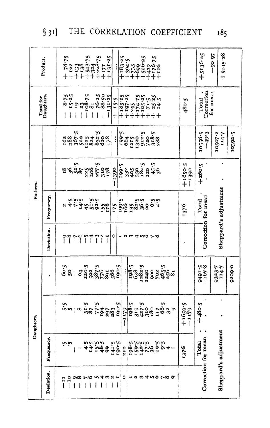
STATISTICAL METHODS [§ i
the stature of 10,000 recruits, it is rather the
population of statures than the population of recruits that is
open to study. Nevertheless, in a real sense, statistics
is the study of populations, or aggregates of
individuals, rather than of individuals. Scientific theories
which involve the properties of large aggregates of
individuals, and not necessarily the properties of the
individuals themselves, such as the Kinetic Theory
of Gases, the Theory of Natural Selection, or the
chemical Theory of Mass Action, are essentially
statistical arguments, and are liable to
misinterpretation as soon as the statistical nature of the argument
is lost sight of. In Quantum Theory this is now
clearly recognised. Statistical methods are essential
to social studies, and it is principally by the aid of
such methods that these studies may be raised to
the rank of sciences. This particular dependence of
social studies upon statistical methods has led to the
unfortunate misapprehension that statistics is to be
regarded as a branch of economics, whereas in truth
methods adequate to the treatment of economic data,
in so far as these exist, have only been developed in
the study of biology and the other sciences.
The idea of a population is to be applied not only
to living, or even to material, individuals. If an
observation, such as a simple measurement, be repeated
indefinitely, the aggregate of the results is a
population of measurements. Such populations are the
particular field of study of the Theory of Errors, one
of the oldest and most fruitful lines of statistical
investigation. Just as a single observation may
be regarded as an individual, and its repetition as
generating a population, so the entire result of an
extensive experiment may be regarded as but one of
§1]
INTRODUCTORY
3
a possible population of such experiments. The
salutary habit of repeating important experiments,
or of carrying out original observations in replicate,
shows a tacit appreciation of the fact that the object
of our study is not the individual result, but the
population of possibilities of which we do our best
to make our experiments representative. The
calculation of means and standard errors shows a deliberate
attempt to learn something about that population.
The conception of statistics as the study of
variation is the natural outcome of viewing the subject as
the study of populations; for a population of
individuals in all respects identical is completely described
by a description of any one individual, together with
the number in the group. The populations which
are the object of statistical study always display
variation in one or more respects. To speak of
statistics as the study of variation also serves to
emphasise the contrast between the aims of modern
statisticians and those of their predecessors. For,
until comparatively recent times, the vast majority
of workers in this field appear to have had no other
aim than to ascertain aggregate, or average, values.
The variation itself was not an object of study, but
was recognised rather as a troublesome circumstance
which detracted from the value of the average. The
error curve of the mean of a normal sample has been
familiar for a century, but that of, the standard
deviation was the object of researches up to 1915. Yet,
from the modern point of view, the study of the causes
of variation of any variable phenomenon, from the
yield of wheat to the intellect of man, should be begun
by the examination and measurement of the variation
which presents itself.
4
STATISTICAL METHODS [§ i
The study of variation leads immediately to the
concept of a frequency distribution. Frequency
distributions are of various kinds ; the number of classes
in which the population is distributed may be finite or
infinite; again, in the case of quantitative variates,
the intervals by which the classes differ may be finite
or infinitesimal. In the simplest possible case, in
which there are only two classes, such as male and
female births, the distribution is simply specified by
the proportion in which these occur, as for example
by the statement that 51 per cent, of the births are
of males and 49 per cent, of females. In other cases
the variation may be discontinuous, but the number
of classes indefinite, as with the number of children
born to different married couples; the frequency
distribution would then show the frequency with
which o, 1, 2 . . . children were recorded, the number
of classes being sufficient to include the largest family
in the record. The variable quantity, such as the
number of children, is called the variate, and the
frequency distribution specifies how frequently the
variate takes each of its possible values. In the
third group of cases, the variate, such as human
stature, may take any intermediate value within its
range of variation; the variate is then said to vary
continuously, and the frequency distribution may be
expressed by stating, as a mathematical function of
the variate, either (i) the proportion of the population
for which the variate is less than any given value,
or (ii) by the mathematical device of differentiating
this function, the (infinitesimal) proportion of the
population for which the variate falls within any
infinitesimal element of its range.
The idea of a frequency distribution is applicable
§1]
INTRODUCTORY
5
either to populations which are finite in number, or to
infinite populations, but it is more usefully and more
simply applied to the latter. A finite population can
only be divided in certain limited ratios, and cannot in
any case exhibit continuous variation. Moreover, in
most cases only an infinite population can exhibit
accurately, and in their true proportion, the whole of
the possibilities arising from the causes actually at
work, and which we wish to study. The actual
observations can only be a sample of such possibilities.
With an infinite population the frequency distribution
specifies the fractions of the population assigned to
the several classes ; we may have (i) a finite number
of fractions adding up to unity as in the Mendelian
frequency distributions, or (ii) an • infinite series of
finite fractions adding up to unity, or (iii) a
mathematical function expressing the fraction of the total
in each of the infinitesimal elements in which the range
of the variate may be divided. The last possibility
may be represented by a frequency curve ; the values
of the variate are set out along a horizontal axis, the
fraction of the total population, within any limits of
the variate, being represented by the area of the curve
standing on the corresponding length of the axis. It
should be noted that the familiar concept of the
frequency curve is only applicable to an infinite
population with a continuous variate.
The study of variation has led not merely to
measurement of the amount of variation present, but
to the study of the qualitative problems of the type, or
form, of the variation. Especially important is the
study of the simultaneous variation of two or more
variates. This study, arising principally out of the
work of Galton and Pearson, is generally known
6 STATISTICAL METHODS [§ 2
under the name of Correlation, or, more descriptively,
as Covariation.
The third aspect under which we shall regard the
scope of statistics is introduced by the practical need
to reduce the bulk of any given body of data. Any
investigator who has carried out methodical and
extensive observations will probably be familiar with
the oppressive necessity of reducing his results to a
more convenient bulk. No human mind is capable of
grasping in its entirety the meaning of any
considerable quantity of numerical data. We want to be able
to express all the relevant information contained in
the mass by means of comparatively few numerical
values. This is a purely practical need which the
science of statistics is able to some extent to meet. In
some cases at any rate it is possible to give the whole
of the relevant information by means of one or a few
values. In all cases, perhaps, it is possible to reduce
to a simple numerical form the main issues which the
investigator has in view, in so far as the data are
competent to throw light on such issues. The number of
independent facts supplied by the data is usually far
greater than the number of facts sought, and in
consequence much of the information supplied by any body
of actual data is irrelevant. It is the object of the
statistical processes employed in the reduction of data
to exclude this irrelevant information, and to isolate the
whole of the relevant information contained in the data.
2. General Method, Calculation of Statistics
The discrimination between the irrelevant
information and that which is relevant is performed as follows.
Even in the simplest cases the values (or sets of
values) before us are interpreted as a random sample
§2]
INTRODUCTORY
7
of a hypothetical infinite population of such values as
might have arisen in the same circumstances. The
distribution of this population will be capable of some
kind of mathematical specifipation, involving a certain
number, usually few, of parameters, or " constants "
entering into the mathematical formula. These
parameters are the characters of the population. If we
could know the exact values of the parameters, we
should know all (and more than) any sample from
the population could tell us. We cannot in fact know
the parameters exactly, but we can make estimates
of their values, which will be more or less inexact.
These estimates, which are termed statistics, are of
course calculated from the observations. If we can
find a mathematical form for the population which
adequately represents the data, and then calculate from
the data the best possible estimates of the required
parameters, then it would seem that there is little,
or nothing, more that the data can tell us ; we shall
have extracted from it all the available relevant
information.
The value of such estimates as we can make is
enormously increased if we can calculate the magnitude
and nature of the errors to which they are subject. If
we can rely upon the specification adopted, this
presents the purely mathematical problem of deducing
from the nature of the population what will be the
behaviour of each of the possible statistics which can
be calculated. This type of problem, with which until
recent years comparatively little progress had been
made, is the basis of the tests of significance by which
we can examine whether or not the data are in harmony
with any suggested hypothesis. In particular, it is
necessary to test the adequacy of the hypothetical
8 STATISTICAL METHODS [§2
specification of the population upon which the method
of reduction was based.
The problems which arise in the reduction of data
may thus conveniently be divided into three types :
(i) Problems of Specification, which arise in the
choice of the mathematical form of the population.
(ii) When a specification has been obtained,
problems of Estimation arise. These involve the
choice among the methods of calculating, from
our sample, statistics fit to estimate the unknown
parameters of the population.
(iii) Problems of Distribution include the
mathematical deduction of the exact nature of the
distributions in random samples of our estimates of the
parameters, and of other statistics designed to test
the validity of our specification (tests of Goodness of
Fit).
The statistical examination of a body of data is
thus logically similar to the general alternation of
inductive and deductive methods throughout the
sciences. A hypothesis is conceived and defined with
all necessary exactitude ; its logical consequences are
ascertained by a deductive argument; these
consequences are compared with the available observations ;
if these are completely in accord with the deductions,
the hypothesis is justified at least until fresh and more
stringent observations are available. The author
has attempted a fuller examination of the logic of
planned experimentation in his book, The Design of
Experiments.
The deduction of inferences respecting samples,
from assumptions respecting the populations from
which they are drawn, shows us the position in
Statistics of the classical Theory of Probability* For
§2]
INTRODUCTORY
9
a given population we may calculate the probability
with which any given sample will occur, and if we
can solve the purely mathematical problem presented,
we can calculate the probability of occurrence of any
given statistic calculated from such a sample. The
problems of distribution may in fact be regarded as
applications and extensions of the theory of
probability. Three of the distributions with which we
shall be concerned, Bernoulli's binomial distribution,
Laplace's normal distribution, and Poisson's series,
were developed by writers on probability. For many
years, extending over a century and a half, attempts
were made to extend the domain of the idea of
probability to the deduction of inferences respecting
populations from assumptions (or observations)
respecting samples. Such inferences are usually
distinguished under the heading of Inverse Probability,
and have at times gained wide acceptance. This is
not the place to enter into the subtleties of a prolonged
controversy; it will be sufficient in this general
outline of the scope of Statistical Science to reaffirm
my personal conviction which I have sustained
elsewhere, that the theory of inverse probability is
founded upon an error, and must be wholly rejected.
Inferences respecting populations, from which known
samples have been drawn, cannot by this method be
expressed in terms of probability, except in the trivial
case when the population is itself a sample of a super-
population the specification of which is known with
accuracy.
The probabilities established by those tests of
significance, which we shall later designate by t and z}
are, however, entirely distinct from statements of
inverse probability, and are free from the objections
10
STATISTICAL METHODS [§3
which apply to these latter. Their interpretation as
probability statements respecting populations
constitutes an application unknown to the classical writers
on probability. To distinguish such statements as to
the probability of causes from the earlier attempts
now discarded, they are known as statements of
Fiducial Probability.
The rejection of the theory of inverse probability
was for a time wrongly taken to imply that we cannot
draw, from knowledge of a sample, inferences
respecting the corresponding population. Such a view would
entirely deny validity to all experimental science.
What has now appeared is that the mathematical
concept of probability is, in most cases, inadequate to
express our mental confidence or diffidence in making
such inferences, and that the mathematical quantity
which appears to be appropriate for measuring our
order of preference among different possible
populations does not in fact obey the laws of probability.
To distinguish it from probability, I have used the
term " Likelihood " to designate this quantity * ; since
both the words " likelihood " and " probability " are
loosely used in common speech to cover both kinds
of relationship.
3. The Qualifications of Satisfactory Statistics
The solutions of problems of distribution (which
may be regarded as purely deductive problems in the
theory of probability) not only enable us to make
critical tests of the significance of statistical results, and
of the adequacy of the hypothetical distributions upon
* A more special application of the likelihood is its use, under the
name of " power function," for comparing the sensitiveness, in some
chosen respect, of different possible tests of significance.
§3]
INTRODUCTORY
II
which our methods of numerical inference are based,
but afford real guidance in the choice of appropriate
statistics for purposes of estimation. Such statistics
may be divided into classes according to the behaviour
of their distributions in large samples.
If we calculate a statistic, such, for example, as the
mean, from a very large sample, we are accustomed to
ascribe to it great accuracy ; and indeed it will usually,
but not always, be true, that if a number of such
statistics can be obtained and compared, the
discrepancies among them will grow less and less, as the
samples from which they are drawn are made larger
and larger. In fact, as the samples are made larger
without limit, the statistic will usually tend to some
fixed value characteristic of the population, and,
therefore, expressible in terms of the parameters of the
population. If, therefore, such a statistic is to be used
to estimate these parameters, there is only one
parametric function to which it can properly be equated.
If it be equated to some other parametric function, we
shall be using a statistic which even from an infinite
sample does not give the correct value; it tends
indeed to a fixed value, but to a value which is
erroneous from the point of view with which it
was used. Such statistics are termed Inconsistent
Statistics ; except when the error is extremely minute,
as in the use of Sheppard's adjustments, inconsistent
statistics should be regarded as outside the pale of
decent usage.
Consistent statistics, on the other hand, all tend
more and more nearly to give the correct values, as
the sample is more and more increased ; at any rate,
if they tend to any fixed value it is not to an incorrect
one. In the simplest cases, with which we shall be
12 STATISTICAL METHODS [§3
concerned, they not only tend to give the correct
value, but the errors, for samples of a given size, tend
to be distributed in a well-known distribution (of which
more in Chap. Ill) known as the Normal Law of
Frequency of Error, or more simply as the normal
distribution. The liability to error may, in such cases,
be expressed by calculating the mean value of the
squares of these errors, a value which is known as
the variance ; and in the class of cases with which we
are concerned, the variance falls off with increasing
samples, in inverse proportion to the number in the
sample.
The foregoing paragraphs specify the notion of
consistency in terms suitable to the theory of Large
Samples, i.e. by means of the properties required as
the sample is increased without limit. Logically it
is important that consistency can also be defined
strictly for small {i.e. finite) samples by the stipulation
that if for each frequency observed its expectation
were substituted, then consistent statistics would be
equal identically to the parameters of which they are
estimates. The method is illustrated in Section 53.
For the purpose of estimating any parameter, such
as the centre of a normal distribution, it is usually
possible to invent any number of statistics such as the
arithmetic mean, or the median, etc., which shall be
consistent in the sense defined above, and each of
which has in large samples a variance falling oflf
inversely with the size of the sample. But for large
samples of a fixed size the variance of these different
statistics will generally be different. Consequently,
a special importance belongs to a smaller group of
statistics, the error distributions of which tend to the
normal distribution, as the sample is increased, with
§3]
INTRODUCTORY
13
the least possible variance. We may thus separate
off from the general body of consistent statistics a
group of especial value, and these are known as
efficient statistics.
The reason for this term may be made apparent by
an example. If from a large sample of (say) 1000
observations we calculate an efficient statistic, A, and
a second consistent statistic, B, having twice the
variance of A, then B will be a valid estimate of the
required parameter, but one definitely inferior to A
in its accuracy. Using the statistic B, a sample of
2000 values would be required to obtain as good an
estimate as is obtained by using the statistic A from
a sample of 1000 values. We may say, in this sense,
that the statistic B makes use of 50 per cent, of the
relevant information available in the observations;
or, briefly, that its efficiency is 50 per cent. The term
" efficient" in its absolute sense is reserved for
statistics the efficiency of which is 100 per cent.
Statistics having efficiency less than 100 per cent,
may be legitimately used for many purposes. It is
conceivable, for example, that it might in some cases be
less laborious to increase the number of observations
than to apply a more elaborate method of calculation
to the results. It may often happen that an inefficient
statistic is accurate enough to answer the particular
questions at issue. There is however, one limitation
to the legitimate use of inefficient statistics which
should be noted in advance. If we are to make
accurate tests of goodness of fit, the methods of fitting
employed must not introduce errors of fitting
comparable to the errors of random sampling; when this
requirement is investigated, it appears that when tests
of goodness of fit are required, the statistics employed
14 STATISTICAL METHODS [§3
in fitting must be not only consistent, but must be of
100 per cent, efficiency. This is a very serious
limitation to the use of inefficient statistics, since in the
examination of any body of data it is desirable to be
able at any time to test the validity of one or more
of the provisional assumptions which have been made.
Numerous examples of the calculation of statistics
will be given in the following chapters, and, in these
illustrations of method, efficient statistics have been
chosen. The discovery of efficient statistics in new
types of problem may require some mathematical
investigation. The researches of the author have led
him to the conclusion that an efficient statistic can
in all cases be found by the Method of Maximum
Likelihood; that is, by choosing statistics so that the
estimated population should be that for which the
likelihood is greatest. In view of the mathematical
difficulty of some of the problems which arise it is also
useful to know that approximations to the maximum
likelihood solution are also in most cases efficient
statistics. Some simple examples of the application
of the method of maximum likelihood, and other
methods, to genetical problems are developed in the
final chapter.
For practical purposes it is not generally necessary
to press refinement of methods further than the
stipulation that the statistics used should be efficient. With
large samples it may be shown that all efficient
statistics tend to equivalence, so that little
inconvenience arises from diversity of practice. There is,
however, one class of statistics, including some of the
most frequently recurring examples, which is of
theoretical interest for possessing the remarkable
property that, even in small samples, a statistic of this
§4]
INTRODUCTORY
IS
class alone includes the whole of the relevant
information which the observations contain. Such statistics
are distinguished by the term sufficient and, in the
use of small samples, sufficient statistics, when they
exist, are definitely superior to other efficient statistics.
Examples of sufficient statistics are the arithmetic
mean of samples from the normal distribution, or
from the Poisson series ; it is the fact of providing
sufficient statistics for these two important types of
distribution which gives to the arithmetic mean its
theoretical importance. The method of maximum
likelihood leads to these sufficient statistics when
they exist. By a further extension, also depending
on a special, but not uncommon, functional
relationship, the advantage of sufficient statistics, namely
exhaustive estimation may be gained by using
ancillary statistics, even when no statistic sufficient
by itself exists.
While diversity of practice within the limits of
efficient statistics will not with large samples lead to
inconsistencies, it is, of course, of importance in all
cases to distinguish clearly the parameter of the
population, of which it is desired to estimate the value
from the actual statistic employed as an estimate of its
value; and to inform the reader by which of the
considerable variety of processes which exist for the
purpose the estimate was actually obtained.
4. Scope of this Book
The prime object of this book is to put into the
hands of research workers, and especially of biologists,
the means of applying statistical tests accurately to
numerical data accumulated in their own laboratories
16 STATISTICAL METHODS [§4
or available in the literature. Such tests are the result
of solutions of problems of distribution, most of wThich
are but recent additions to our knowledge and have
previously only appeared in specialised mathematical
papers. The mathematical complexity of these
problems has made it seem undesirable to do more than
(i) to indicate the kind of problem in question,
(ii) to give numerical illustrations by which the whole
process may be checked, (iii) to provide numerical
tables by means of which the tests may be made
without the evaluation of complicated algebraical
expressions.
It would have been impossible to give methods
suitable for the great variety of kinds of tests which
are required but for the unforeseen circumstance that
each mathematical solution appears again and again
in questions which at first sight appeared to be quite
distinct. For example, Helmert's solution in 1875
of the distribution of the sum of the squares of
deviations from a mean, is in reality equivalent to the
distribution of x2 given by K. Pearson in 1900. It
was again discovered independently by " Student"
in 1908, for the distribution of the variance of a
normal sample. The same distribution was found by
the author for the index of dispersion derived from
small samples from a Poisson series. What is even
more remarkable is that, although Pearson's paper
of 1900 contained a serious error, which vitiated most
of the tests of goodness of fit made by this method
until 1921, yet the correction of this error, when
efficient methods of estimation are used, leaves the
form of the distribution unchanged, and only requires
that some few units should be deducted from one of
the variables with which the Table of x* is entered.
§4]
INTRODUCTORY
17
It is equally fortunate that the distribution of t>
first established by " Student " in 1908, in his study
of the probable error of the mean, should be applicable,
not only to the case there treated, but to the more
complex, but even more frequently needed problem
of the comparison of two mean values. It further
provides an exact solution of the sampling errors of the
enormously wide class of statistics known as regression
coefficients.
In studying the exact theoretical distributions in
a number of other problems, such as those presented
by intraclass correlations, the goodness of fit of
regression lines, the correlation ratio, and the multiple
correlation coefficient, the author has been led repeatedly
to a third distribution, which may be called the
distribution of 2, and which is intimately related to,
and indeed a natural extension of, the distributions
introduced by Pearson and " Student." It has thus
been possible to classify the necessary distributions
covering a very great variety of cases, under these
three main groups ; and, what is equally important,
to make some provision for the need for numerical
values by means of a few tables only. Tables needed
for a wider range of problems, with illustrations of
their use, have since been published separately.
The book has been arranged so that the student
may make acquaintance with these three main
distributions in a logical order, and proceeding from
more simple to more complex cases. Methods
developed in later chapters are frequently seen to
be generalisations of simpler methods developed
previously. Studying the work methodically as a
connected treatise, the student will, it is hoped, not
miss the fundamental unity of treatment under which
c
18 STATISTICAL METHODS [§4
such very varied material has been brought together ;
and will prepare himself to deal competently and with
exactitude with the many analogous problems which
cannot be individually exemplified. On the other
hand, it is recognised that many will wish to use the
book for laboratory reference, and not as a connected
course of study. This use would seem desirable
only if the reader will be at the pains to work
through, in all numerical detail, one or more of the
appropriate examples, so as to assure himself, not
only that his data are appropriate for a parallel
treatment, but that he has obtained a critical grasp
of the meaning to be attached to the processes and
results.
It is necessary to anticipate one criticism, namely,
that in an elementary book, without mathematical
proofs, and designed for readers without special
mathematical training, so much has been included
which from the teacher's point of view is advanced ;
and indeed much that has not previously appeared
in print. By way of apology the author would like to
put forward the following considerations,
(1) For non - mathematical readers, numerical
tables are in any case necessary; accurate tables
are no more difficult to use, though more laborious
to calculate, than inaccurate tables embodying the
approximations formerly current.
(2) The process of calculating a probable or
standard error from one of the established formulae
gives no real insight into the random sampling
distribution, and can only supply a test of significance by
the aid of a table of deviations of the normal curve,
and on the assumption that the distribution is in fact
very nearly normal. Whether this procedure should.
§4]
INTRODUCTORY
19
or should not, be used must be decided, not by the
mathematical attainments of the investigator, but by
discovering whether it will or will not give a sufficiently
accurate answer. The fact that such a process has
been used successfully by eminent mathematicians
in analysing very extensive and important material
does not imply that it is sufficiently accurate for
the laboratory worker anxious to draw correct
conclusions from a small group of perhaps preliminary
observations.
(3) The exact distributions, with the use of which
this book is chiefly concerned, have been in fact
developed in response to the practical problems arising
in biological and agricultural research ; this is true not
only of the author's own contribution to the subject,
but from the beginning of the critical examination of
statistical distributions in " Student's" paper of
1908.
The greater part of the book is occupied by
numerical examples; and these have steadily
increased in number as fresh points needed illustration.
In choosing them it has appeared to the author a
hopeless task to attempt to exemplify the great variety
of subject-matter to which these processes may be
usefully applied. There are no examples from
astronomical statistics, in which important work has
been done in recent years, few from social studies,
and the biological applications are scattered un-
systematically. The examples have rather been
chosen each to exemplify a particular process, and
seldom on account of the importance of the data
used, or even of similar examinations of analogous
data. By a study of the processes exemplified, the
student should be able to ascertain to what questions,
20 STATISTICAL METHODS [§ 5
in his own material, such processes are able to give a
definite answer ; and, equally important, what further
observations would be necessary to settle other
outstanding questions. In conformity with the purpose
of the examples the reader should remember that they
do not pretend to be discussions of general scientific
questions, which would require the examination of
much more extended data, and of other evidence, but
are solely concerned with the critical examination of
the particular batch of data presented.
5. Historical Note
Since much interest has been evinced in the
historical origin of the statistical theory underlying
the methods of this book, and as some
misapprehensions have occasionally gained publicity, ascribing
to the originality of the author methods well known
to some previous writers, or ascribing to his
predecessors modern developments of which they
were quite unaware, it is hoped that the following
notes on the principal contributors to statistical
theory will be of value to students who wish to see
the modern work in its historical setting.
Thomas Bayes' celebrated essay published in
1763 is well known as containing the first attempt
to use the theory of probability as an instrument
of inductive reasoning; that is, for arguing from
the particular to the general, or from the sample
to the population. It was published posthumously,
and we do not know what views Bayes would have
expressed had he lived to publish on the subject.
We do know that the reason for his hesitation to
publish was his dissatisfaction with the postulate
§51
INTRODUCTORY
21
required for the celebrated " Bayes' Theorem." While
we must reject this postulate, we should also recognise
Bayes' greatness in perceiving the problem to be
solved, in making an ingenious attempt at its solution,
and finally in realising more clearly than many
subsequent writers the underlying weakness of his
attempt.
Whereas Bayes excelled in logical penetration,
Laplace (1820) was unrivalled for his mastery of
analytic technique. He admitted the principle of
inverse probability, quite uncritically, into the
foundations of his exposition. On the other hand,
it is to him we owe the principle that the distribution
of a quantity compounded of independent parts shows
a whole series of features—the mean, variance, and
other cumulants (p. 73)—which are simply the sums of
like features of the distributions of the parts. These
seem to have been later discovered independently by
Thiele (1889), but mathematically Laplace's methods
were more powerful than Thiele's and far more
influential on the development of the subject in France
and England. A direct result of Laplace's study
of the distribution of the resultant of numerous
independent causes was the recognition of the normal
law of error, a law more usually ascribed, with some
reason, to his great contemporary, Gauss.
Gauss, moreover, approached the problem of
statistical estimation in an empirical spirit, raising the
question of the estimation not only of probabilities
but of other quantitative parameters. He perceived
the aptness for this purpose of the Method of
Maximum Likelihood, although he attempted to
derive and justify this method from the principle of
inverse probability. The method has been attacked
22 STATISTICAL METHODS [§5
on this ground, but it has no real connection with
inverse probability. Gauss, further, perfected the
systematic fitting of regression formulae, simple and
multiple, by the method of least squares, which, in
the cases to which it is appropriate, is a particular
example of the method of maximum likelihood.
The first of the distributions characteristic of
modern tests of significance, though originating with
Helmert, was rediscovered by K. Pearson in 1900,
for the measure of discrepancy between observation
and hypothesis, known as x2« This, I believe, is the
great contribution to statistical methods by which
the unsurpassed energy of Prof, Pearson's work will
be remembered. It supplies an exact and objective
measure of the joint discrepancy from their
expectations of a number of normally distributed, and mutually
correlated, variates. In its primary application to
frequencies, which are discontinuous variates, the
distribution is necessarily only an approximate one,
but when small frequencies are excluded the
approximation is satisfactory. The distribution is exact
for other problems solved later. With respect to
frequencies, the apparent goodness of fit is often
exaggerated by the inclusion of vacant or nearly
vacant classes which contribute little or nothing to
the observed xz> but increase its expectation, and
by the neglect of the eflfect on this expectation of
adjusting the parameters of the population to fit those
of the sample. The need for correction on this
score was for long ignored, and later disputed, but is
now, I believe, admitted. The chief cause of error
tending to lower the apparent goodness of fit is the
use of inefficient methods of fitting (Chapter IX),
This limitation could scarcely have been foreseen in
is]
INTRODUCTORY
23
1900, when the very rudiments of the theory of
estimation were unknown.
The study of the exact sampling distributions of
statistics commences in 1908 with " Student's " paper
* The Probable Error of a Mean. Once the true
nature of the problem was indicated, a large number
of sampling problems were within reach of
mathematical solution. " Student " himself gave in this and
a subsequent paper the correct solutions for three
such problems—the distribution of the estimate of the
variance, that of the mean divided by its estimated
standard deviation, and that of the estimated
correlation coefficient between independent variates. These
sufficed to establish the position of the distributions
of x2 and of * 'm the theory of samples, though
further work was needed to show how many other
problems of testing significance could be reduced
to these same two forms, and to the more inclusive
distribution of 2. " Student's " work was not quickly
appreciated (it had, in fact, been totally ignored in
the journal in which it had appeared), and from the
first edition it has been one of the chief purposes of
this book to make better known the effect of his
researches, and of mathematical work consequent
upon them, on the one hand, in refining the traditional
doctrine of the theory of errors and mathematical
statistics, and on the other, in simplifying the
arithmetical processes required in the interpretation of
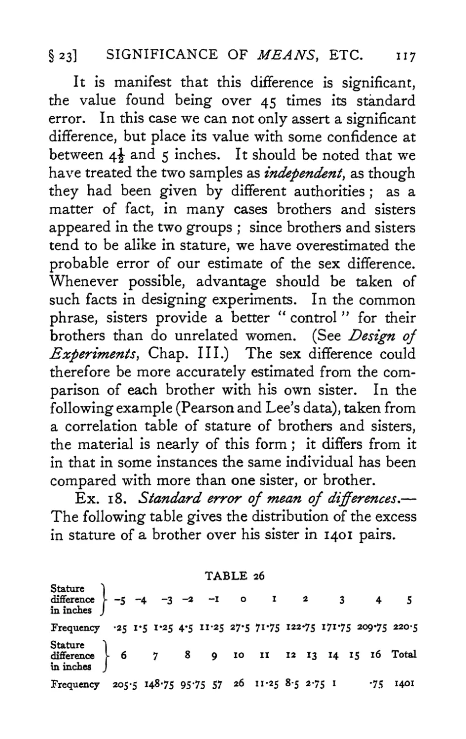
data.
II
DIAGRAMS
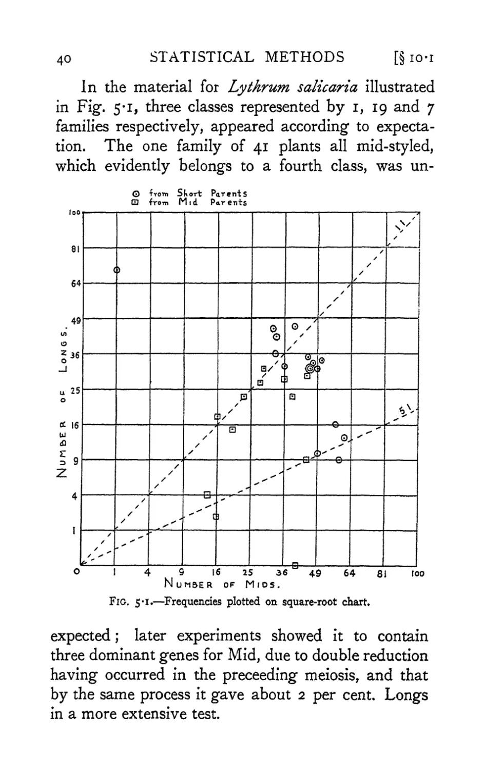
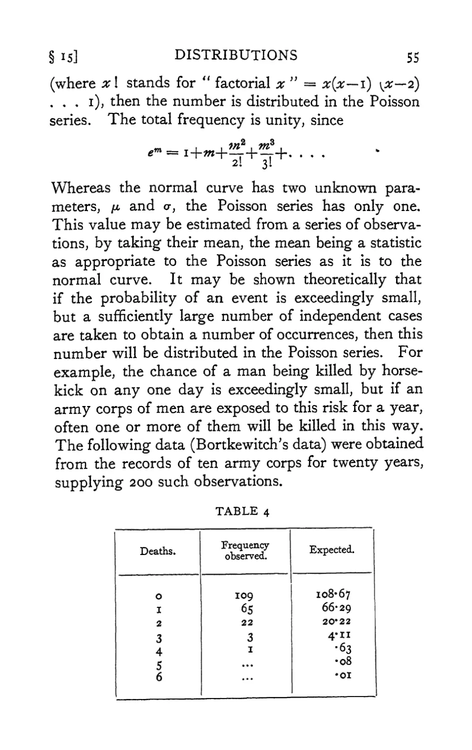
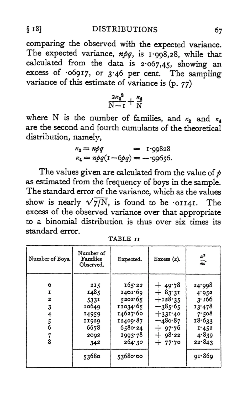
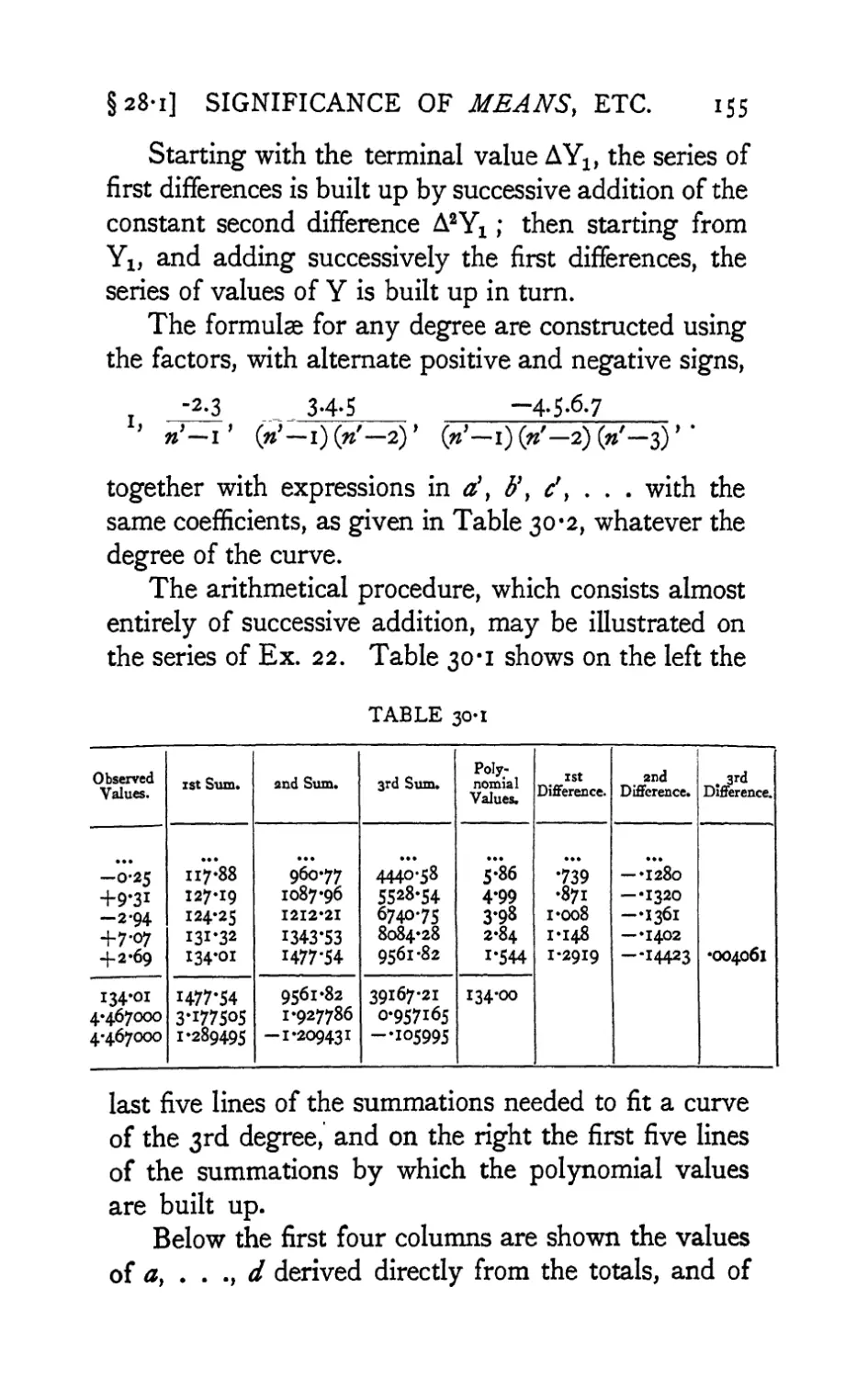
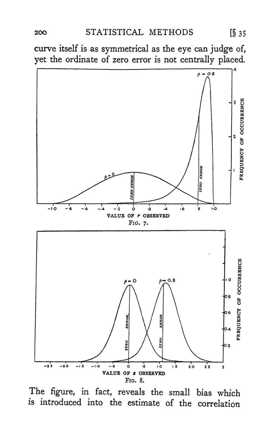
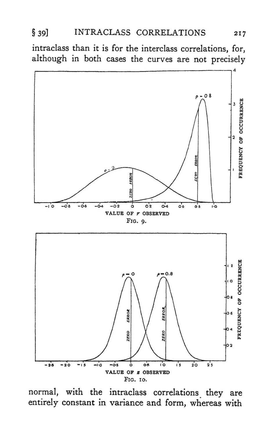
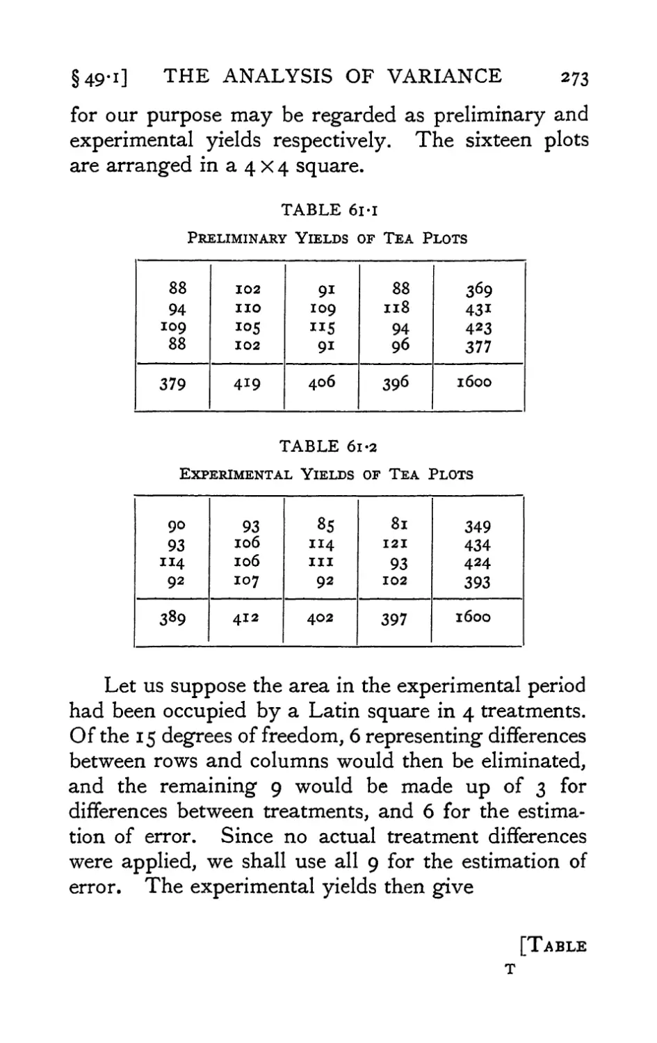
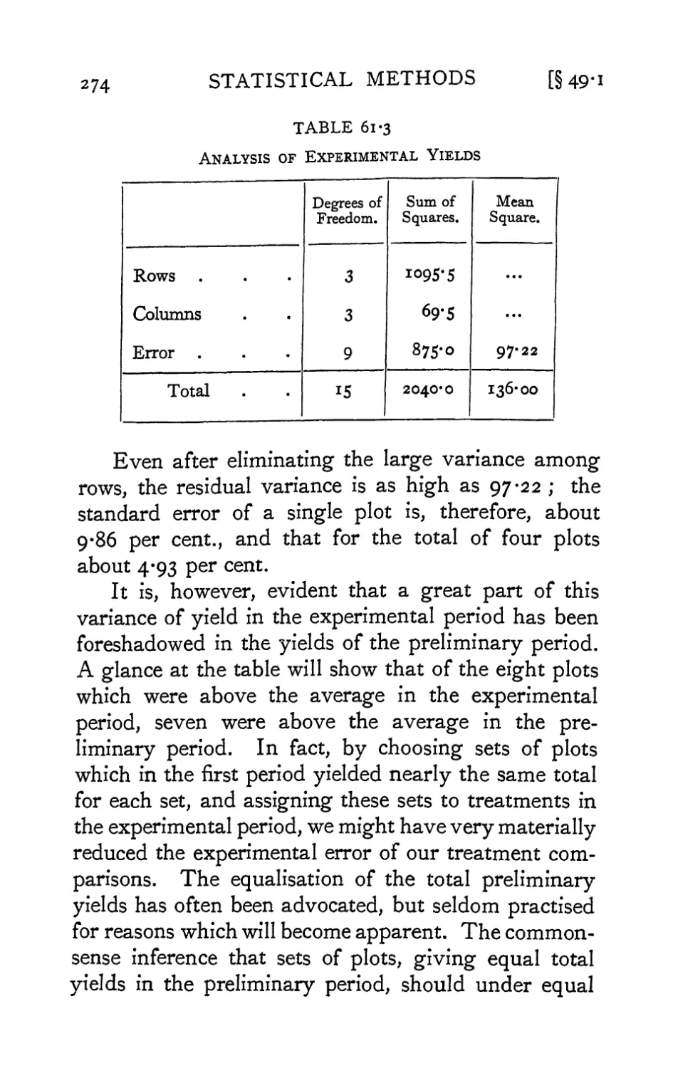
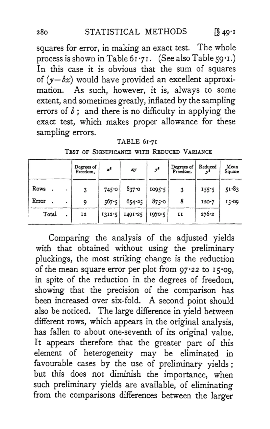
7. The preliminary examination of most data is
facilitated by the use of diagrams. Diagrams prove
nothing, but bring outstanding features readily to the
eye; they are therefore no substitute for such critical
tests as may be applied to the data, but are valuable in
suggesting such tests, and in explaining the conclusions
founded upon them.
8. Time Diagrams, Growth Rate, and Relative
Growth Rate
The type of diagram in most frequent use consists
in plotting the values of a variable, such as the weight
of an animal or of a sample of plants against its age,
or the size of a population at successive intervals of
time. Distinction should be drawn between those
cases in which the same group of animals, as in a
feeding experiment, is weighed at successive intervals
of time, and the cases, more characteristic of plant
physiology, in which the same individuals cannot be
used twice, but a parallel sample is taken at each
age. The same distinction occurs in counts of
microorganisms between cases in which counts are made
from samples of the same culture, or from samples of
parallel cultures. If it is of importance to obtain the
general form of the growth curve, the second method
has the advantage that any deviation from the expected
94
§8]
DIAGRAMS
25
curve may be confirmed from independent evidence
at the next measurement, whereas using the same
material no such independent confirmation is
obtainable. On the other hand, if interest centres on the
growth rate, there is an advantage in using the same
material, for only so are actual increases in weight
measurable. Both aspects of the difficulty can be got
over only by replicating the observations ; by
carrying out measurements on a number of animals under
parallel treatment it is possible to test, from the
individual weights, though not from the means,
whether their growth curve corresponds with an
assigned theoretical course of development, or differs
significantly from it or from a series differently treated.
Equally, if a number of plants from each sample are
weighed individually, growth rates may be obtained
with known probable errors, and so may be used for
critical comparisons. Care should of course be taken
that each is strictly a random sample.
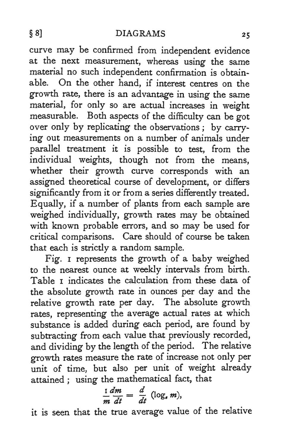
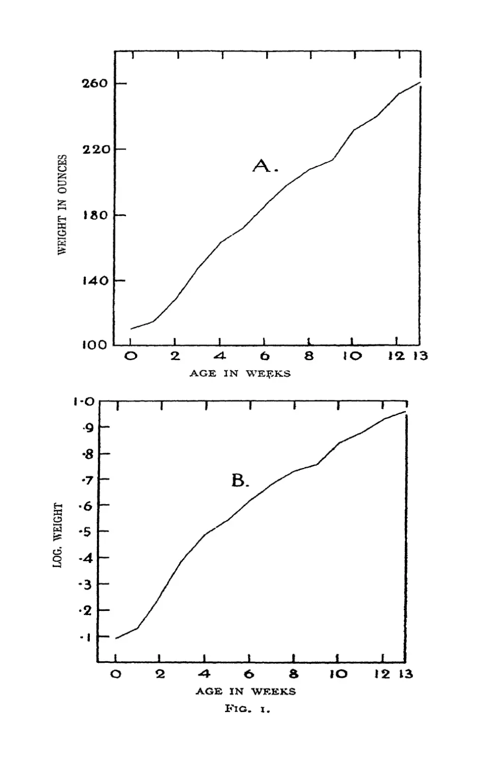
Fig. i represents the growth of a baby weighed
to the nearest ounce at weekly intervals from birth.
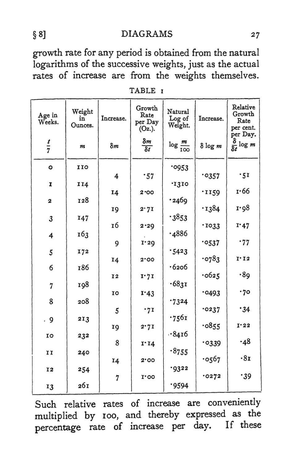
Table I indicates the calculation from these data of
the absolute growth rate in ounces per day and the
relative growth rate per day. The absolute growth
rates, representing the average actual rates at which
substance is added during each period, are found by
subtracting from each value that previously recorded,
and dividing by the length of the period. The relative
growth rates measure the rate of increase not only per
unit of time, but also per unit of weight already
attained ; using the mathematical fact, that
i dm d n v
m at at
it is seen that the true average value of the relative
o
o
260 I-
220h-
o
o
Eh
o
180
140
100
l-O
•9
-8
-7
■6
*5
4
-3
•2
-I
^ 6
AGE IN WEEKS
1
j-
1.1. 1
1
L_
1
B
,,,!
1
L__
1
1
1 i
i I
-4 t> S
AGE IN WEEKS
Fig. x.
IO
12 13
§8]
DIAGRAMS
27
growth rate for any period is obtained from the natural
logarithms of the successive weights, just as the actual
rates of increase are from the weights themselves.
TABLE 1
Age in
Weeks.
t
\ 7
0
I
2
3
4
5
6
7
8
" 9
10
11
12
13
Weight
in
Ounces.
m
IIO
114
128
147
163
172
186
198
208
213
232
240
254
261
Increase.
Sm
4
14
19
16
9
14
12
10
5
19
8
14
7
Growth
Rate
per Day
(Oz.)-
Sm
St
'57
2-00
2'7I
2-29
1-29
2'00
1-71
i'43
•71
2-71
i-14
2'00
I'OO
Natural
Log of
Weight.
log^-
100
•0953
•i3Io
•2469
'3853
•4886
■5423
■6206
•6831
■7324
•7561
•8416
■8755
•9322
■9594
Increase.
8 log m
■0357
'1159
■1384
■1033
■0537 1
■0783
■0625
■0493
-0237
■0855
■0339
•0567
■0272
Relative
Growth
Rate
\ per cent.
per Day. j
k- log m
St *
■51
1-66
1-98
i'47
■77
I-I2
-89
-70
•34
1-22
•48
-8l
■39
Such relative rates of increase are conveniently
multiplied by 100, and thereby expressed as the
percentage rate of increase per day. If these
28 STATISTICAL METHODS [§8
percentage rates of increase had been calculated on
the principle of simple interest, by dividing the actual
increase by the weight at the beginning of the period,
somewhat higher values would have been obtained ;
the reason for this is that the actual weight of the baby
at any time during each period is usually somewhat
higher than its weight at the beginning. The error
introduced by the simple interest formula becomes
exceedingly great when the percentage increases
between successive weighings are large.
Fig. i A shows the course of the increase in
absolute weight; the average slope of such a diagram
shows the absolute rate of increase. In this diagram
the points fall approximately on a straight line,
showing that the absolute rate of increase was nearly
constant at about 1-66 oz. per diem. Fig. i B shows
the course of the increase in the natural logarithm of
the weight; the slope at any point shows the relative
rate of increase, which, apart from the first week, falls
off perceptibly with increasing age. The features of
such curves are best brought out if the scales of the
two axes are so chosen that the graph makes with
them approximately equal angles; writh nearly
vertical, or nearly horizontal lines, changes in the
slope are not so readily perceived.
A rapid and convenient way of displaying the line
of increase of the logarithm is afForded by the use of
graph paper in which the horizontal rulings are spaced
on a logarithmic scale, with the actual values indicated
in the margin (see Fig. 5). The horizontal scale can
then be adjusted to give the line an appropriate slope.
This method avoids the use of a logarithm table,
which, however, will still be required if the values of
the relative rate of increase are needed.
§9]
DIAGRAMS
29
In making a rough examination of the agreement
of the observations with any law of increase, it is
desirable so to manipulate the variables that the law
to be tested will be represented by a straight line.
Thus Fig. 1 A is suitable for a rough test of the law
that the absolute rate of increase is constant; if it
were suggested that the relative rate of increase were
constant, Fig. 1 B would show clearly that this was
not so. With other hypothetical growth curves other
transformations may be used; for example, in the
so-called " autocatalytic " or " logistic " curve the
relative growth rate falls off in proportion to the
actual weight attained at any time. If, therefore,
the relative growth rate be plotted against the actual
weight, the points should fall on a straight line if the
" autocatalytic" curve fits the facts. For this
purpose it is convenient to plot against each observed
weight the mean of the two adjacent relative growth
rates. To do this for the above data for the growth
of an infant may be left as an exercise to the student;
twelve points will be available for weights 114 to
254 ounces. The relative growth rates, even after
averaging adjacent pairs, will be very irregular,
so that no clear indications will be found from these
data. If a straight line is found to fit the data, the
weight at which growth will cease, supposing the
law of growth continues unchanged, is found by
producing the line to meet the axis.
9. Correlation Diagrams
Although most investigators make free use of
diagrams in which an uncontrolled variable is plotted
against the time, or against some controlled factor such
as concentration of solution, or temperature, much
30 STATISTICAL METHODS [§9
more use might be made of correlation diagrams in
which one uncontrolled factor is plotted against
another. When this is done as a dot diagram, a
number of dots are obtained, each representing a single
experiment, or pair of observations, and it is usually-
clear from such a diagram whether or not any close
connexion exists between the variables. When the
observations are few a dot diagram will often tell us
whether or not it is worth while to accumulate
observations of the same sort; the range and extent of our
experience is visible at a glance ; and associations may
be revealed which are worth while following up.
If the observations are so numerous that the dots
cannot be clearly distinguished, it is best to divide up
the diagram into squares, recording the frequency in
each; this semi-diagrammatic record is a correlation
table.
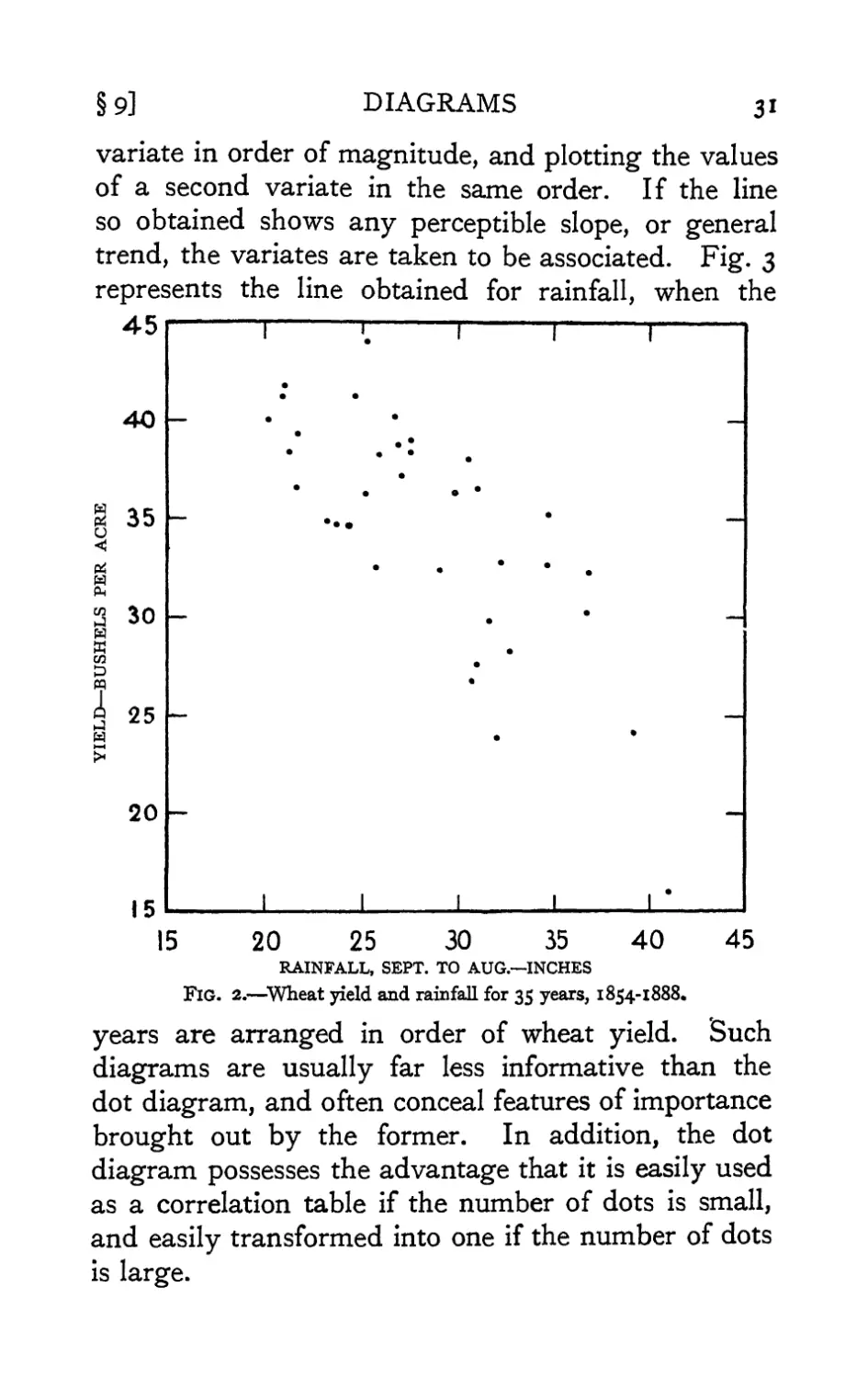
Fig. 2 shows in a dot diagram the yields obtained
from an experimental plot of wheat (dunged plot,
Broadbalk field, Rothamsted) in years with different
total rainfall. The plot was under uniform treatment
during the whole period 1854-1888 ; the 35 pairs
of observations, indicated by 35 dots, show well the
association of high yield with low rainfall. Even
when few observations are available a dot diagram
may suggest associations hitherto unsuspected, or
what is equally important, the absence of associations
which would have been confidently predicted. Their
value lies in giving a simple conspectus of the
experience hitherto gathered, and in bringing to the
mind suggestions which may be susceptible of more
exact statistical or experimental examination.
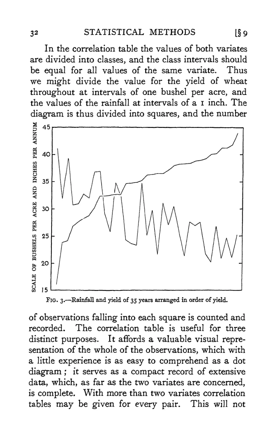
Instead of making a dot diagram the device is
sometimes adopted of arranging the values of one
§9]
DIAGRAMS
3i
variate in order of magnitude, and plotting the values
of a second variate in the same order. If the line
so obtained shows any perceptible slope, or general
trend, the variates are taken to be associated. Fig. 3
represents the line obtained for rainfall, when the
451
15 20 25 30 35
RAINFALL, SEPT. TO AUG.—INCHES
Fig. 2.—Wheat yield and rainfall for 35 years, 1854-1888.
years are arranged in order of wheat yield. Such
diagrams are usually far less informative than the
dot diagram, and often conceal features of importance
brought out by the former. In addition, the dot
diagram possesses the advantage that it is easily used
as a correlation table if the number of dots is small,
and easily transformed into one if the number of dots
is large.
32 STATISTICAL METHODS L§9
In the correlation table the values of both variates
are divided into classes, and the class intervals should
be equal for all values of the same variate. Thus
we might divide the value for the yield of wheat
throughout at intervals of one bushel per acre, and
the values of the rainfall at intervals of a i inch. The
diagram is thus divided into squares, and the number
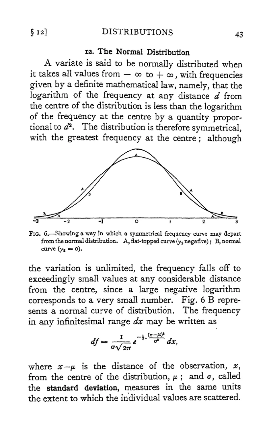
Fig. 3.—Rainfall and yield of 35 years arranged in order of yield.
of observations falling into each square is counted and
recorded. The correlation table is useful for three
distinct purposes. It affords a valuable visual
representation of the whole of the observations, which with
a little experience is as easy to comprehend as a dot
diagram ; it serves as a compact record of extensive
data, which, as far as the two variates are concerned,
is complete. With more than two variates correlation
tables may be given for every pair. This will not
§io]
DIAGRAMS
33
indeed enable the reader to reconstruct the original
data in its entirety, but it is a fortunate fact that for the
great majority of statistical purposes a set of such
twofold distributions provides complete information.
Original data involving more than two variates are
most conveniently recorded for reference on cards,
each case being given a separate card with the several
variates entered in corresponding positions upon
them. The publication of such complete data presents
difficulties but it is not yet sufficiently realised how
much of the essential information can be presented in
a compact form by means of correlation tables. The
third feature of value about the correlation table is
that the data so presented form a convenient basis for
the immediate application of methods of statistical
reduction. The most important statistics which the
data provide, means, variances, and covariance, can
be most readily calculated from the correlation table.
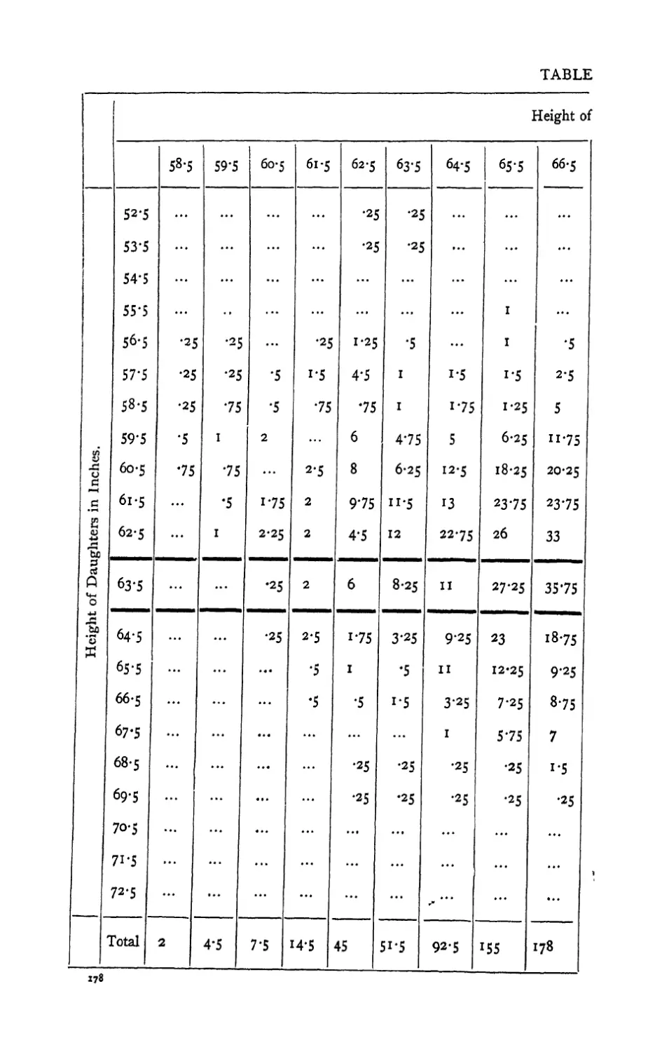
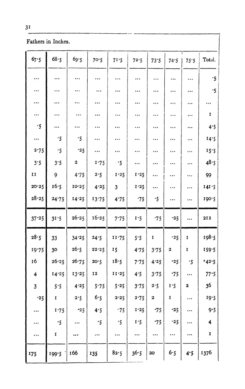
An example of a correlation table is shown in Table 31,
p. 178.
10. Frequency Diagrams
When a large number of individuals are measured
in respect of physical dimensions, weight, colour,
density, etc., it is possible to describe with some
accuracy the population of which our experience may
be regarded as a sample. By this means it may be
possible to distinguish it from other populations
differing in their genetic origin, or in environmental
circumstances. Thus local races may be very different
as populations, although individuals may overlap in
all characters ; or, under experimental conditions, the
aggregate may show environmental effects, on size,
death-rate, etc., which cannot be detected in the
D
34 STATISTICAL METHODS [§ 10
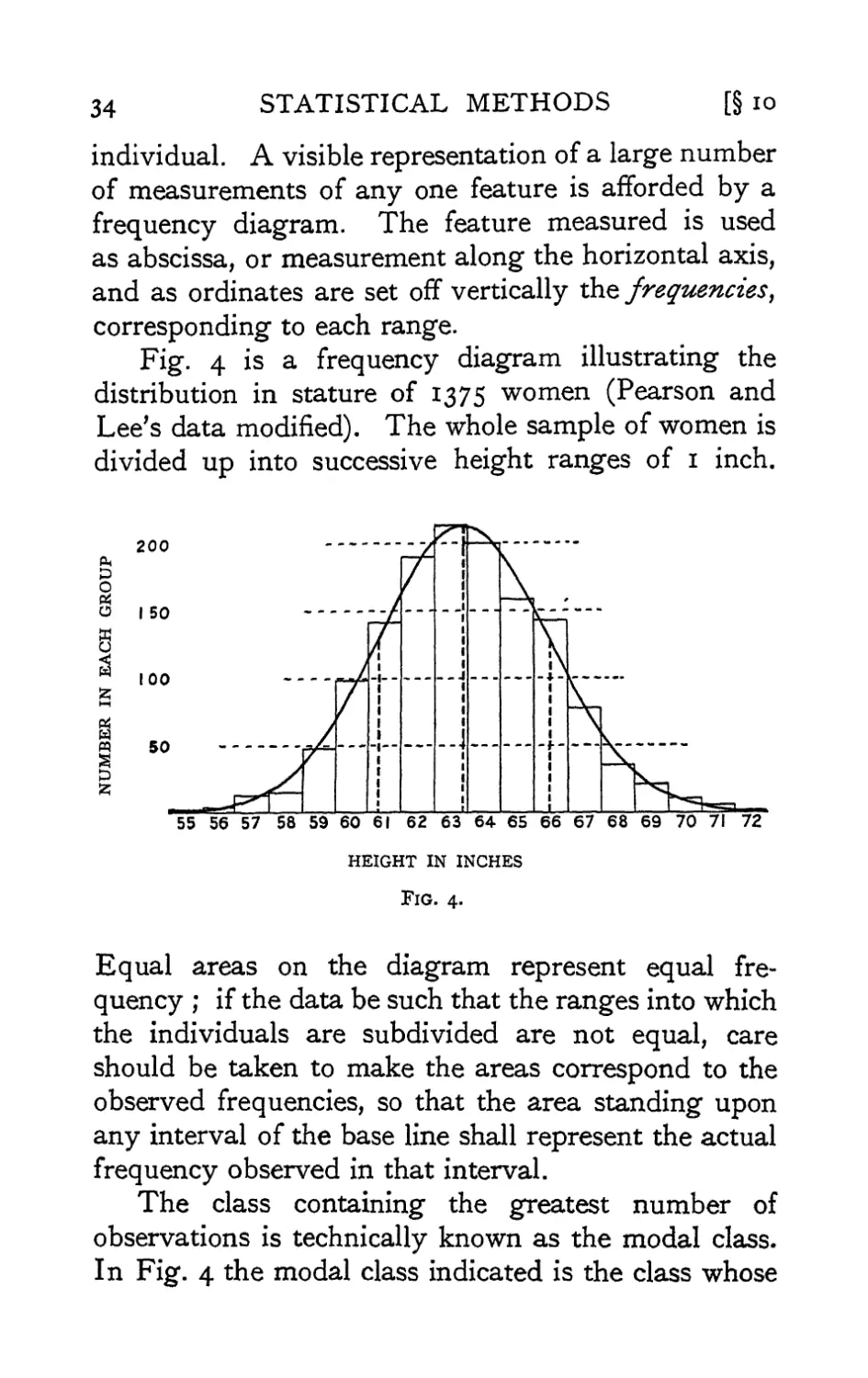
individual. A visible representation of a large number
of measurements of any one feature is afforded by a
frequency diagram. The feature measured is used
as abscissa, or measurement along the horizontal axis,
and as ordinates are set off vertically the frequencies,
corresponding to each range.
Fig. 4 is a frequency diagram illustrating the
distribution in stature of 1375 women (Pearson and
Lee's data modified). The whole sample of women is
divided up into successive height ranges of 1 inch.
Oh
s
o
8
n
S
200
150
100
55 56 57 58 59 60 61 62 63 64 65 66 67 68 69 70 71 72
HEIGHT IN INCHES
Fig. 4.
Equal areas on the diagram represent equal
frequency ; if the data be such that the ranges into which
the individuals are subdivided are not equal, care
should be taken to make the areas correspond to the
observed frequencies, so that the area standing upon
any interval of the base line shall represent the actual
frequency observed in that interval.
The class containing the greatest number of
observations is technically known as the modal class.
In Fig. 4 the modal class indicated is the class whose
§ioJ
DIAGRAMS
35
central value is 63 inches. When, as is very frequently
the case, the variate varies continuously, so that all
intermediate values are possible, the choice of the
grouping interval and limits is arbitrary and will
make a perceptible difference to the appearance of the
diagram. Usually, however, the possible limits of
grouping will be governed by the smallest units in
which the measurements are recorded. If, for
example, measurements of height were made to the
nearest quarter of an inch, so that all values between
66| inches and 67^ were recorded as 67 inches, all
values between 67J and 67I were recorded as 67J,
then we have no choice but to take as our unit of
grouping 1, 2, 3, 4, etc., quarters of an inch, and the
limits of each group must fall on some odd number of
eighths of an inch. For purposes of calculation the
smaller grouping units are more accurate, but for
diagrammatic purposes coarser grouping is often
preferable. Fig. 4 indicates a unit of grouping suitable
in relation to the total range for a large sample ; with
smaller samples a coarser grouping is usually necessary
in order that sufficient observations may fall in each
class.
In all cases where the variation is continuous the
frequency diagram should be in the form of a
histogram, rectangular areas standing on each grouping
interval showing the frequency of observations in that
interval. The alternative practice of indicating the
frequency by a single ordinate raised from the centre
of the interval is sometimes preferred, as giving to the
diagram a form more closely resembling a continuous
curve. The advantage is illusory, for not only is
the form of the curve thus indicated somewhat
misleading, but the utmost care should always be taken
36 STATISTICAL METHODS [§ 10
to distinguish the infinitely large hypothetical
population from which our sample of observations is
drawn, from the actual sample of observations which
we possess ; the conception of a continuous frequency
curve is applicable only to the former, and in
illustrating the latter no attempt should be made to slur over
this distinction.
This consideration should in no way prevent a
frequency curve fitted to the data from being
superimposed upon the histogram (as in Fig. 4) ; the
contrast between the histogram representing the sample,
and the continuous curve representing an estimate of
the form of the hypothetical population, is well brought
out in such diagrams, and the eye is aided in
detecting any serious discrepancy between the observations
and the hypothesis. No eye observation of such
diagrams, however experienced, is really capable of
discriminating whether or not the observations differ
from expectation by more than we should expect from
the circumstances of random sampling. Accurate
methods of making such tests will be developed in
later chapters.
With discontinuous variation, when, for example,
the variate is confined to whole numbers, the reasons
given for insisting on the histogram form have little
weight, for there are, strictly speaking, no ranges of
variation within each class. On the other hand, there
is no question of a frequency curve in such cases.
Representation of such data by means of a histogram
is usual and not inconvenient; it is especially
appropriate if we regard the discontinuous variation as
due to an underlying continuous variate, which
can, however, express itself only to the nearest whole
number.
§ IO'l]
DIAGRAMS
37
io-i.
Transformed Frequencies
It is, of course, possible to treat the values of the
frequency like any other variable, by plotting the
value of its logarithm, or its actual value on loga-
200
100
SO
60
40
55
I
m
15
20
10
8
c
>
<■
>
c
)
<i
&
V
> (
">
6 7 8
NUMBER OF PETALS
Fig. 5.
JO
rithmic paper, when it is desired to illustrate the
agreement of the observations with any particular law
of frequency. Fig, 5 shows in this way the number of
flowers (buttercups) having 5 to 10 petals (Pearson's
38 STATISTICAL METHODS [§ io-i
data), plotted upon logarithmic paper, to facilitate
comparison with the hypothesis that the frequency,
for petals above five, falls off in geometric progression.
Such illustrations are not, properly speaking, frequency
digrams, although the frequency is one of the
variables employed, because they do not adhere to the
convention that equal frequencies are represented by
equal areas.
A useful form, similar to the above, is used to
compare the death-rates, throughout life, of different
populations. The logarithm of the number of
survivors at any age is plotted against the age attained.
Since the death-rate is the rate of decrease of the
logarithm of the number of survivors, equal gradients
on such curves represent equal death-rates. They
therefore serve well to show the increase of death-
rate with increasing age, and to compare populations
with different death-rates. Such diagrams are less
sensitive to small fluctuations than would be the
corresponding frequency diagrams showing the
distribution of the population according to age at death ;
they are therefore appropriate when such small
fluctuations are due principally to errors of random
sampling, which in the more sensitive type of diagram
might obscure the larger features of the comparison.
It should always be remembered that the choice
pf the appropriate methods of statistical treatment
*s quite independent of the choice of methods of
diagrammatic representation.
A need which is felt frequently in Genetics and
occasionally in other studies is to survey the evidence
0n some particular frequency ratio provided by a
number of different samples, which may or may not
be homogeneous in this respect. The classification
§ io-i]
DIAGRAMS
39
of samples, such as progenies of plants or animals,
according to the frequency-ratio they exhibit, and
the homogeneity of the samples classified alike, are
in such studies of critical importance, and the explicit
tests of Chapter IV will usually be needed. A
graphical survey of the evidence gives useful guidance
as to what particular points should be tested, and is
of further value, as a means of presenting the evidence
most simply to the reader.
The frequencies observed of the two alternatives
in each sample may be used as co-ordinates of a
point, so that just so many points are shown as
there are samples. In Fig. 5*1 the useful device has
been adopted of plotting not the absolute frequencies,
but their square roots. Points representing samples
of n observations will then fall on a quadrant of a
circle of radius *fn. Samples showing a frequency
ratio p : q, where p+q = 1, will fall on a radius
vector making an angle <f> with the axis, such that
sin2^ = p, cos2<f> = q.
The device thus allows the diagram to exhibit
a wider range of sample size, and a wider range of
frequency ratio, than would otherwise be possible.
Graph paper embodying this principle has been
designed by F. Mosteller and J. W. Tukey and is
now available.
Since, moreover, the standard error of random
sampling of <£, for given n, is proportional to i/y^
and is independent of <j>, it follows that the scatter of
the observation points on either side of the radii to
which they approximate is nearly equal in all parts
of the diagram, and the eye is .thus materially aided
in recognising homogeneous groups.
4o
STATISTICAL METHODS
[§io-i
in the material for Lythrum salicaria illustrated
in Fig. 5-1, three classes represented by i, 19 and 7
families respectively, appeared according to
expectation. The one family of 41 plants all mid-styled,
which evidently belongs to a fourth class, was un-
G from Sko-rt Parents
GJ irom Mid Parents
<
/
1 / «"
*" .1
)
/
/
/
/
^''
/
/
/
/
^ *•
c
/
/
/
s
n
c
1/
B
I
_J
G
O
_J
0 /
/
/
/
Q
a^
^"
—a
/
/
/
s
©
0,
/
/
/
/
/
•
>x'
fe 1 1 1 1 1 L-e 1 1 1 1
O I 4 9 16 25 36 49 64 81 »00
Number of Mios.
Fig. 5«i.—Frequencies plotted on square-root chart.
expected; later experiments showed it to contain
three dominant genes for Mid, due to double reduction
having occurred in the preceeding meiosis, and that
by the same process it gave about 2 per cent. Longs
in a more extensive test.
Ill
DISTRIBUTIONS
ii. The idea of an infinite population distributed
in a frequency distribution in respect of one or more
characters is fundamental to all statistical work.
From a limited experience, for example, of individuals
of a species, or of the weather of a locality, we may
obtain some idea of the infinite hypothetical
population from which our sample is drawn, and so of the
probable nature of future samples to which our
conclusions are to be applied. If a second sample belies
this expectation we infer that it is, in the language of
statistics, drawn from a different population ; that the
treatment to which the second sample of organisms had
been exposed did in fact make a material difference,
or that the climate (or the methods of measuring it)
had materially altered. Critical tests of this kind
may be called tests of significance, and when such
tests are available we may discover whether a second
sample is or is not significantly different from the
first.
A statistic is a value calculated from an observed
sample with a view to characterising the population
from which it is drawn. For example, the mean of a
number of observations xl9 x2 • • • xn> *s given by
the equation l
x = - SO),
it
where S stands for summation over the whole sample
STATISTICAL METHODS [§n
(this symbol is the one regularly used in our subject),
and n for the number of observations. Such statistics
are of course variable from sample to sample, and
the idea of a frequency distribution is applied with
especial value to the variation of such statistics. If
we know exactly how the original population was
distributed it is theoretically possible, though often a
matter of great mathematical difficulty, to calculate
how any statistic derived from a sample of given size
will be distributed. The utility of any particular
statistic, and the nature of its distribution, both
depend on the original distribution, and appropriate
and exact methods have been worked out for only a
few cases. The application of these cases is greatly
extended by the fact that the distribution of many
statistics tends to the normal form as the size of the
sample is increased. For this reason it is customary
to apply to many cases what is called " the theory of
large samples " which is to assume that such statistics
are normally distributed, and to limit consideration of
their variability to calculations of the standard error.
In the present chapter we shall give some account
of three principal distributions—(i) the normal
distribution, (ii) the Poisson series, (iii) the binomial
distribution. It is important to have a general
knowledge of these three distributions, the
mathematical formulae by which they are represented, the
experimental conditions upon which they occur, and
the statistical methods of recognising their occurrence.
On the latter topic we shall be led to some extent to
anticipate methods developed more systematically in
Chapters IV and V,
§12]
DISTRIBUTIONS
43
12. The Normal Distribution
A variate is said to be normally distributed when
it takes all values from — oo to + oo, with frequencies
given by a definite mathematical law, namely, that the
logarithm of the frequency at any distance d from
the centre of the distribution is less than the logarithm
of the frequency at the centre by a quantity
proportional to d2. The distribution is therefore symmetrical,
with the greatest frequency at the centre; although
Fig, 6,—Showing a way in which a symmetrical frequency curve may depart
from the normal distribution. A, flat-topped curve (y2 negative); B, normal
curve (y2 = o).
the variation is unlimited, the frequency falls off to
exceedingly small values at any considerable distance
from the centre, since a large negative logarithm
corresponds to a very small number. Fig. 6 B
represents a normal curve of distribution. The frequency
in any infinitesimal range dx may be written as
i -j c*-^)'
OV27T
where x— n is the distance of the observation, x,
from the centre of the distribution, \l ; and a, called
the standard deviation, measures in the same units
the extent to which the individual values are scattered.
44
STATISTICAL METHODS [§ 12
Geometrically a is the distance, on either side of the
centre, of the points at which the slope is steepest,
or the points of inflexion of the curve (Fig. 4).
In practical applications we do not so often want to
know the frequency at any distance from the centre
as the total frequency beyond that distance ; this is
represented by the area of the tail of the curve cut
off at any point. Tables of this total frequency,
or probability integral, have been constructed from
which, for any value of {x—\l)\o, we can find what
fraction of the total population has a larger deviation ;
or, in other words, what is the probability that a value
so distributed, chosen at random, shall exceed a given
deviation. Tables I and II have been constructed
to show the deviations corresponding to different
values of this probability. The rapidity with which
the probability falls off as the deviation increases is
well shown in these tables. A deviation exceeding
the standard deviation occurs about once in three
trials. Twice the standard deviation is exceeded only
about once in 22 trials, thrice the standard deviation
only once in 370 trials, while Table II shows that to
exceed the standard deviation sixfold would need
nearly a thousand million trials. The value for which
P = -05, or 1 in 20, is 1-96 or nearly 2 ; it is convenient
to take this point as a limit in judging whether a
deviation is to be considered significant or not.
Deviations exceeding twice the standard deviation are
thus formally regarded as significant. Using this
criterion we should be led to follow up a false indication
only once in 22 trials, even if the statistics were the only
guide available. Small effects will still escape notice
if the data are insufficiently numerous to bring them
out, but no lowering of the standard of significance
would meet this difficultv.
§ 13] DISTRIBUTIONS 45
Some little confusion is sometimes introduced by
the fact that in some cases we wish to know the
probability that the deviation, known to be positive, shall
exceed an observed value, whereas in other cases the
probability required is that a deviation, which is
equally frequently positive and negative, shall exceed
an observed value ; the latter probability is always
half the former. For example, Table I shows that the
normal deviate falls outside the range ±1*598193 in
11 per cent, of cases, and consequently that it exceeds
+ 1-598193 in 5-5 per cent, of cases.
The value of the deviation beyond which half the
observations lie is called the quartile distance, and
bears to the standard deviation the ratio -67449.
It was formerly a common practice to calculate the
standard error and then, multiplying it by this factor,
to obtain the probable error. The probable error is
thus about two-thirds of the standard error, and as
a test of significance a deviation of three times the
probable error is effectively equivalent to one of twice
the standard error. The common use of the probable
error is its only recommendation ; when any critical
test is required the deviation must be expressed in
terms of the standard error in using the tables of
normal deviates (Tables I and II).
Further tables of the normal distribution are given
in Statistical Tables IX and X, and in SkepparcFs
Tables, 1938.
13. Fitting the Normal Distribution
From a sample of n individuals of a normal
population the mean and the standard deviation of
the population may be estimated by using two easily
calculated statistics. The best estimate of fi is x where
46 STATISTICAL METHODS [§ 13
while for the best estimate of a, we calculate i* from
n—i
these two statistics are calculated from the sums
of the first two powers of the observations (see
Appendix, p. 70), and are specially related to the
normal distribution, in that they summarise the whole
of the information which the sample provides as to
the distribution from which it was drawn, provided
the latter was normal. Fitting by sums of powers,
and especially by the particular system of statistics
known as moments, has also been widely applied to
skew (asymmetrical) distributions, and others which
are not normal; but such distributions have not
generally the peculiar properties which make the first
two powers especially appropriate, and where the
distributions differ widely from the normal form the
two statistics defined above may be of little or no use.
Ex. 2. Fitting a normal distribution to a large
sample.—In calculating the statistics from a large
sample it is not necessary to calculate individually
the squares of the deviations from the mean of
each measurement. The measurements are grouped
together in equal intervals of the variate, and the
whole of the calculation may be carried out rapidly as
shown in Table 2, where the distribution of the stature
of 1164 men is analysed.
The first column shows the central height in
inches of each group, followed by the corresponding
frequency. A central group (68- 5*) is chosen as
" working mean." To form the next column the
frequencies are multiplied by 1, 2, 3, etc., according to
their distance from the working mean; this process
being repeated to form the fourth column, which is
§ 13] DISTRIBUTIONS
TABLE 2.
Central Height
(Inches).
5*5
53'5
54*5
55'5
56'5
5T5
58-5
59*5
60-5
6i-5
62-5
f>3'5
64-5
65'5
66-5
67-5
68-5
69*5
70*5
71*5
72*5
73*5
74*5
75*5
76-6
77*5
78-S
79'5
Men
(Frequency).
I
2'5
i*5
9*5
3i
5$
78*5
127
178-5
189
137
137
93
52*5
39
17
t'S
3'5
1
2
1
1164
Frequency
X
Deviation.
~ 9
— 20
~ io-5
~ 57
-*55
—224
-235-5
-254
~i78'5
-1*43'5
137
274
279
210
195
102
45'5
28
9
20
11
1310-5
+167
Mean +-I43S
Correction for mean i672h-ii64
Corrected sum of squares I
Sampling variance of mean
Sampling variance of variance
Adjustment for grouping
Adjusted variance
Frequency
X
(Deviation)2.
81
160
73*5
342
775
896
706-5
508
I78-5
137
548
837
840
975
612
3i8-5
224
81
200
121
8614
23-96
^590*04
Estimatec
Variance
7-386I
Women.
•5
•5
I
5
15
*5'5
52
101
150
199
223
215
169*5
*5*'5
Si'5
40*5
19*5
10
5
1
...
1456
I
S.D.
2-7177
•006345 -0797 |
•09382
•0833
7*3028
•3063
2-7024
48 STATISTICAL METHODS [§ 13
summed from top to bottom in a single operation ;
in the third column, however, the upper portion,
representing negative deviations, is summed separately
and subtracted from the sum of the lower portion.
The difference, in this case positive, shows that the
whole sample of 1164 individuals has in all 167 inches
more than if every individual were 68-5" in height.
This balance divided by 1164 gives the amount
by which the mean of the sample exceeds 68-5".
The mean of the sample is therefore 68-6435".
From the sum of the fourth column is subtracted a
correction to give the value we should have obtained
had the working mean been the true mean. This
correction is the product of the total, 167", and the mean
o-1435" derived from it. The corrected sum of squares
divided by 1163, one less than the sample number,
provides the estimate of the variance, 7-3861 square inches,
which is the basis of all subsequent calculations.
Corresponding to any estimate of a variance, we
have, by taking the square root, the corresponding
estimate of the standard deviation. Thus from the
value 7-3861 square inches, we obtain at once the
estimate 2-7177 inches for the standard deviation.
This, however, represents the standard deviation of
the population as grouped. The process of grouping
may be represented as the addition to any true value
of a grouping error, positive or negative, which takes
all values from — \ to \ of a grouping unit with equal
frequency. The effect of this on the population, and
its average effect upon samples, is to add a constant
quantity & (~°833) to the variance. Sheppard's
adjustment for grouping consists in deducting this
quantity from the estimate of variance of the population
as grouped. This gives 7-3028 square inches for the
§I3J
DISTRIBUTIONS
49
adjusted variance, and 2-702 for the corresponding
estimate of the standard deviation.
Any interval may be used as a unit of grouping ;
and the whole calculation is carried through in such
units, the final results being transformed into other
units if required, just as we might wish to transform
the mean and standard deviation from inches to
centimetres by multiplying by the appropriate factor. It
is advantageous that the units of grouping should be
exact multiples of the units of measurement; so that
if the above sample had been measured to tenths of an
inch, we might usefully have grouped them at intervals
of 0-6" or 0-7".
Regarded as estimates of the mean and the standard
deviation of a normal population of which the above is
regarded as a sample, the values found are affected by
errors of random sampling; that is, we should not
expect a second sample to give us exactly the same
values. The values for different (large) samples of
the same size would, however, be distributed very
accurately in normal distributions, so the accuracy
of any one such estimate may be satisfactorily
expressed by its standard error. These standard errors
may be calculated from the variance of the grouped
population, and in treating large samples we take our
estimate of this variance as the basis of the calculation.
The formulae for the variances of random sampling
of estimates of the mean and of the variance of a
normal population are (as given in Appendix, p. 70)
o& 2<t4
n n—i
Putting our value for k2, 7-3861, in place of a2 in
these formulae, we find that our estimate of the mean
has a sampling variance -006345 square inches, or,
£
SO STATISTICAL METHODS [§ 13
taking the square root, a standard error -0797 inches.
From this value it is seen that our sample shows
significant aberration (± twice standard error) from
any population whose mean lay outside the limits
68*48" to 68*80". It is therefore probable, in the
fiducial sense, that the mean of the population from
which our sample was drawn lay between these limits.
Similarly, our value for the variance of the population
is seen to have a sampling variance -09382, or a
standard error -3063 ; we have therefore equally good
evidence that the variance of the grouped population
from which our sample was drawn lay between
6773 and 7*999 square inches. For the ungrouped
population we should deduct -083 from both limits.
It may be asked, Is nothing lost by grouping ?
Grouping in effect replaces the actual data by fictitious
data placed arbitrarily at the central values of the
groups; evidently a very coarse grouping might
be very misleading. It has been shown that as regards
obtaining estimates of the parameters of a normal
population, the loss of information caused by grouping
is less than 1 per cent., provided the group interval
does not exceed one-quarter of the standard deviation ;
the grouping of the sample above in whole inches is
thus somewhat too coarse; the loss in the estimation
of the standard deviation is 2*28 per cent., or about
27 observations out of 1164 ; the loss in the estimation
of the mean is half as great. With suitable group
intervals, however, little is lost by grouping, and
much labour is saved.
Another way of regarding the loss of information
involved in grouping is to consider how near the
estimates obtained for the mean and the standard
deviation will be to the estimates obtained without
§13]
DISTRIBUTIONS
Si
grouping. From this point of view we may calculate
a standard error of grouping, not to be confused with
the standard error of random sampling which measures
the deviation of the sample values from the population
value. In grouping units, the standard error due to
grouping of both the mean and the standard deviation is
i
V\2n
or in this case -0085". For sufficiently fine grouping
this should not exceed one-tenth of the standard error
of random sampling.
In the analysis of a large sample the estimate of the
variance often employed is
n
which differs from the formula given previously (p. 46)
in that we have divided by n instead of by {n—1). In
large samples the difference between these formulae is
small, and that using n may claim some theoretical
advantage if we wish for an estimate to be used in
conjunction with the estimate of the mean from the same
sample, as in fitting a frequency curve to the data ;
in general it is best to use (« — 1). In small samples
the difference is still small compared to the probable
error, but becomes important if a variance is estimated
by averaging estimates from a number of small samples.
Thus if a series of experiments are carried out each
with six parallels and we have reason to believe that
the variation is in all cases due to the operation of
analogous causes, we may take the average of such
quantities as _j_ = ,
»-i ' S
to obtain an unbiased estimate of the variance, whereas
we should underestimate it were we to divide by 6.
52 STATISTICAL METHODS [§ 14
14. Test of Departure from Normality
It is sometimes necessary to test whether an
observed sample does or does not depart significantly
from normality. For this purpose the third, and
sometimes the fourth powers, are used ; from each of these
it is possible to calculate a quantity, g, the average
value of which is zero for a normal distribution, and
which is distributed normally for large samples—the
standard error being calculable from the size of the
sample. The quantity^, which is calculated from the
third powers, is essentially a measure of asymmetry;
the parameter yls of which it provides an estimate, may
be equated to ± Vftx of Pearson's notation, though
Pearson also used j8x to designate a statistic which is
not the equivalent of g±2 ; g2, calculated from the fourth
powers, is in like manner a measure of departure from
normality, in this case of a symmetrical type, by which
the apex and the two tails of the curve are increased
at the expense of the intermediate portion, or when
negative, the top and tails are depleted and the
shoulders filled out, making a relatively flat-topped
curve. (See Fig. 6, p. 43.)
Ex. 3. Use of higher powers to test normality.—
Departures from normal form, unless very strongly
marked, can only be detected in large samples ;
conversely, they make little difference to statistical tests on
other questions. We give an example (Table 3) of
the calculation for 90 values of the yearly rainfall at
Rothamsted; the process of calculation is similar to
that of finding the mean and standard deviation, but
it is carried two stages further, in the summation of
the 3rd and 4th powers. The formulae by which the
sums are reduced to the true mean and the statistics
TABLE 3
Test of Normality of Yearly Rainfall
Year's rain in
inches.
16
17
18
19
20
21
22
23
24
25
26
1 27
1 28
29
30
31
32
33
34
35
3^
31
38
39
0-
Corrections
to
Mean
S
k
Adjustment
k'
8
Standard
error
Frequency.
I
3
2
3
3
2
12
4
7
4
8
9
6
7
4
4
4
3
1 3
1
90
(
90
—12
-27
—16
—2I
—15
—8
-36 \
—8
~7
8
18
18
28
20
24
28
24
27
11
56
•62
•62
144
243
128
147
75
32
108
16
7
8
3^
54
112
100
144
196
192
i 243
I 121
2106
—34*84
2071*16
23-2715
1 —0833
23-1882
—1728
—2187
—1024
—1029
—375
—128
—324
—32
-7
8
72
162
448
500
864
1372
1536
2187
1331
1646
—393i#2
+43*4
—2241-8
—25-761
—25-761
— 231
±•254
20736
19683
8192
7203
i875
512
972
64
7 |
8 1
144
486
1792
2500
5184
9604
12288
19683
14641
125574
—4°96-7
+4892-2
-~4°'5
126329-0
— 162- 487
+-008
—162-479
— 302
±*5°3
54 STATISTICAL METHODS [§15
k and g are calculated, are gathered in an Appendix,
p. 70. For the k statistics we obtain in terms of
group intervals
it = -62, £2 = 23-2715, £3=-25-76, £4=—162-49,
whence are calculated
g\ = k'z\k'%^ = —231, g\ = k\\k\* = -302.
For samples from a normal distribution the sampling
variances of gx and^*2 are giyen exactly by the formulae
in the Appendix, and the numerical values of the
standard error have been appended in Table 3. It
will be seen that neither are significant, or even
exceeds its standard error. A negative value of ylf
which is suggested but not established by the data,
would indicate an asymmetry of the distribution in
the sense that moderately dry and very wet years
are respectively less frequent than moderately wet
and very dry years.
15. Discontinuous Distributions
Frequently a variable is not able to take all possible
values, but is confined to a particular series of values,
such as the whole numbers. This is obvious when the
variable is a frequency, obtained by counting, such as
the number of cells on a square of a haemacytometer,
or the number of colonies on a plate of culture medium.
The normal distribution is the most important of the
continuous distributions; but among discontinuous
distributions the Poisson series is of the first importance.
If a variate can take the values o, 1, 2, . . ., x, . * .,
and the relative frequencies with which the values occur
are given by the series
-m/ *»2 w8 \
§15]
DISTRIBUTIONS
55
(where x\ stands for " factorial x " = x(x—i) \x—i)
. . . 1), then the number is distributed in the Poisson
series. The total frequency is unity, since
Whereas the normal curve has two unknown
parameters, [a and a, the Poisson series has only one.
This value may be estimated from a series of
observations, by taking their mean, the mean being a statistic
as appropriate to the Poisson series as it is to the
normal curve. It may be shown theoretically that
if the probability of an event is exceedingly small,
but a sufficiently large number of independent cases
are taken to obtain a number of occurrences, then this
number will be distributed in the Poisson series. For
example, the chance of a man being killed by horse-
kick on any one day is exceedingly small, but if an
army corps of men are exposed to this risk for a year,
often one or more of them will be killed in this way.
The following data (Bortkewitch's data) were obtained
from the records of ten army corps for twenty years,
supplying 200 such observations.
TABLE 4
Deaths.
0
I
2
3
4
5
6
Frequency-
observed.
109
65
22
3
I
...
Expected.
108-67
66*29
20*22
4-u
■63 '
•08
•01
56 STATISTICAL METHODS [§15
The average, #, is o*6i, and taking this as an
estimate of m the numbers calculated agree excellently
with those observed.
The importance of the Poisson series in biological
research was first brought out in connexion with the
accuracy of counting with a hsemacytometer. It was
shown that when the technique of the counting process
was effectively perfect, the number of cells on each
square should be theoretically distributed in a Poisson
series ; it was further shown that this distribution
was, in favourable circumstances, actually realised
TABLE S
Number of Cells.
0
I
2
3
4
5
6
7
8
9
10
11
12
13
14
x*
16
Total .
Frequency observed.
20
43
53
1 86
7o
54
37
18
10
5
2
2
...
...
...
...
400
Frequency expected.
3*7i
17*37
40*65
63-41
74*19
69-44
54* 16
36-21
2i-18
II-02
5* 16
2-19
^86
*3i
•10
•03
•01
400-00
in practice. Thus the preceding table (" Student's "
data) shows the distribution of yeast cells in the 400
squares into which one square millimetre was divided.
§I6J
DISTRIBUTIONS
57
The total number of cells counted is 1872, and the
mean number is therefore 4-68. The expected
frequencies calculated from this mean agree well
with those observed. The methods of testing the
agreement are explained in Chapter IV.
When a number is the sum of several components,
each of which is independently distributed in a Poisson
series, then the total number is also so distributed.
Thus the total count of 1872 cells may be regarded as
a sample of one individual from a series, for which m
is not far from 1872. The variance of a Poisson
series, like its mean is equal to m ; and for such large
values of m the distribution of numbers approximates
closely to the normal form ; we may therefore attach
to the number counted, 1872, the standard error
±^1872 = ±43*26, to represent the standard error
of random sampling of such a count. The density of
cells in the original suspension is therefore estimated
with a standard error of 2-31 per cent. If, for instance,
a parallel sample differed by 7 per cent., the technique
of sampling would be suspect.
16. Small Samples of a Poisson Series
Exactly the same principles as govern the accuracy
of a hemacytometer count would also govern a count
of bacterial or fungal colonies in estimating the
numbers of those organisms by the dilution method,
if it could be assumed that the technique of dilution
afforded a perfectly random distribution of organisms,
and that these could develop on the plate without
mutual interference. Agreement of the observations
with the Poisson distribution thus affords in the dilution
method of counting a test of the suitability of the
technique and medium similar to the test afforded of
58 STATISTICAL METHODS [§ 16
the technique of hsemacytometer counts. The great
practical difference between these cases is that from
the hemacytometer we can obtain a record of a large
number of squares with oiily a few organisms on each,
whereas in a bacterial count we may have only 5
parallel plates, bearing perhaps 200 colonies apiece.
From a single sample of 5 it would be impossible to
demonstrate that the distribution followed the Poisson
series ; however, when a large number of such samples
have been obtained under comparable conditions, it
is possible to utilise the fact that for all Poisson series
the variance is numerically equal to the mean.
For each set of parallel plates with x1} x2 . . ., x"
colonies respectively, after finding the mean x} an
index of dispersion may be calculated by the formula
. S(*-*)»
* x '
It has been shown that for true samples of a Poisson
series, x2 calculated in this way will be distributed
in a known manner; Table III (p. 112) shows the
principal values of x2 for this distribution ; entering
the table with n equal to one less than the number
of parallel plates. For small samples the permissible
range of variation of x2 is wide ; thus for five plates
with #=4, x2 will be less than 1-064 in 10 per cent, of
cases, while the highest 10 per cent, will exceed 7-779 ;
a single sample of 5 thus gives us little information ;
but if we have 50 or 100 such samples, we are in
a position to verify with accuracy if the expected
distribution is obtained.
Ex. 4. Test of agreement with Poisson series of
a number of small samples.—From 100 counts of
bacteria in sugar refinery products the following values
were obtained (Table 6); there being 6 plates in each
§ 16] DISTRIBUTIONS 59
case, the values of x2 were taken from the x2 table
for n = 5.
TABLE 6
Xs-
0
•554
•752
i-145
i*6io
2-343
3*000
4-351
6*064
7*289
9*236
11*070
I3-388
15*086
Total
Expected.
I
1
3
5
10
10
20
20
10
10
5
3
1
1
100
Observed.
26
6
11
7
7
2
12
7
3
4
1
3
0
11
100
Expected
43 per cent.
•43
•43
1*29
2-15
4-3
4*3
8-6
8-6
4-3
4*3
2*15
1*29
•43
•43
43*00
It is evident that the observed series differs strongly
from expectation ; there is an enormous excess in the
first class, and in the high values over 15 ; the
relatively few values from 2 to 15 are not far from the
60 STATISTICAL METHODS [§ 16
expected proportions, as is shown in the last column by
taking 43 per cent, of the expected values. It is possible
then that even in this case nearly half of the samples
were satisfactory, but about 10 per cent, were
excessively variable, and in about 45 per cent, of the cases
the variability was abnormally depressed.
It is often desirable to test if the variability is
of the right magnitude when we have not accumulated
a large number of counts, all with the same number
of parallel plates, but where a certain number of
counts are available with various numbers of parallels.
In this case we cannot indeed verify the theoretical
distribution with any exactitude, but can test whether
or not the general level of variability conforms with
expectation. The sum of a number of independent
values of x2 is itself distributed in the manner shown
in the Table of x2, provided we take for n the number
S(n), calculated by adding the several values of n
for the separate experiments. Thus for six sets of
4 plates each the total value of x2 was found to be 13*85,
the corresponding value of n is 6x3 = 18, and the x2
table shows that for n = 18 the value 13-85 is exceeded
in between 70 and 80 per cent, of cases ; it is therefore
not an abnormal value to obtain. In another case the
following values were obtained :
TABLE 7
Number of
Plates in Set.
4
5
9
Total
Number of
Sets.
8
36
I
...
S(n).
24
144
8
176
Total x*
2r3l
I3T96
8-73
170-00
§17]
DISTRIBUTIONS
61
We have therefore to test if x2 = 170 is an
unreasonably small or great value for n = 176. The x2 table
has not been calculated beyond n = 30, but for higher
values we make use of the fact that the distribution of
X becomes nearly normal. A good approximation is
given by assuming that (v^x2 — V2n— 1) is normally
distributed about zero with unit standard deviation.
If this quantity exceeds 2, or even 1-645 f°r the
5 per cent, level, the value of x2 significantly exceeds
expectation. In the example before us
2x2=340, V2?= 18-44
2«—1 = 351, V2n—l = 18-73
Difference — — -29
The set of 45 counts thus shows variability between
parallel plates, very close to that to be expected
theoretically. The internal evidence thus suggests that
the technique was satisfactory.
17. Presence and Absence of Organisms in Samples
When the conditions of sampling justify the use of
the Poisson series, the number of samples containing
0, 1, 2, . . . organisms is, as we have seen, connected
by a calculable relation with the mean number of
organisms in the sample. With motile organisms, or
in other cases which do not allow of discrete colony
formation, the mean number of organisms in the
sample may be inferred from the proportion of fertile
cultures, provided a single organism is capable of
developing. If m is the mean number of organisms in
the sample, the proportion of samples containing none,
that is the proportion of sterile samples, is e~M9 from
which relation we can calculate, as in the following
62 STATISTICAL METHODS [§ 17
table, the mean number of organisms corresponding
to 10 per cent., 20 per cent., etc., fertile samples.
TABLE 8
Percentage of
fertile samples 10 20 30 40 50 60 70 80 90
Mean number
of organisms -1054 -2231 -3567 -5108 -6932 -9163 1-2040 i-6o94 2-3026
In connexion with the use of the table above it
is worth noting that for a given number of samples
tested the frequency ratio of fertile to sterile is most
accurately determined at 50 per cent, fertile, but for
the minimum percentage error in the estimate of the
number of organisms, nearly 80 per cent, fertile or i-6
organism per sample is most accurate. At this point
the standard error of sampling may be reduced to
10 per cent, by taking about 155 samples, whereas at
50 per cent., to obtain the same accuracy, 208 samples
would be required. (See Design of Experiments,
Section 68.)
The Poisson series also enables us to calculate
what percentage of the fertile cultures obtained have
been derived from a single organism, for the percentage
of impure cultures, i.e. those derived from 2 or more
organisms, can be calculated from the percentage of
cultures which proved to be fertile. If e~m are sterile,
me~m will be pure cultures, and the remainder impure.
The following table gives representative values of
the percentage of cultures which are fertile, and the
percentage of fertile cultures which are impure :
TABLE 9
Mean number of organisms
in sample .... -i -2 -3 -4 -5 -6 -7
Percentage fertile . . 9*52 18*13 25*92 32-97 39*35 45*12 50-34
Percentage of fertile
cultures impure . . . 4-92 9*67 14*25 18*67 22-92 27*02 30*95
§18]
DISTRIBUTIONS
63
If it is desired that the cultures should be pure with
high probability, a sufficiently low concentration must
be used to render at least nine-tenths of the samples sterile.
18. The Binomial Distribution
The binomial distribution is well known as the first
example of a theoretical distribution to be established.
It was found by Bernoulli, about the end of the
seventeenth century, that if the probability of an event
occurring were/ and the probability of it not occurring
were ^(=1 —p), then if a random sample of n trial
were taken, the frequencies with which the event
occurred 0, 1, 2, . . ., n times were given by the
expansion of the binomial
Qr+P)n-
This rule is a particular case of a more general
theorem dealing with cases in which not only a simple
alternative is considered, but in which the event may
happen in s ways with probabilities plf p2, . . ., ps;
then it can be shown that the chance of a random
sample of n giving a^ of the first kind, a2 of the second,
. . ., as of the last is
#]j#2* * * * &8*
which is the general term in the multinomial expansion
of (A+^2+ • • • +A)n.
Ex. 5. Binomial distribution given by dice records.
—In throwing a true die the chance of scoring more
than 4 is 1/3, and if 12 dice are thrown together the
number of dice scoring 5 or 6 should be distributed
with frequencies given by the terms in the expansion
of (M)12.
64 STATISTICAL METHODS [§ 18
If, however, one or more of the dice were not true, but
if all retained the same bias throughout the experiment,
the frequencies should be given approximately by
where p is a fraction to be determined from the data.
The following frequencies were observed (Weldon's
data) in an experiment of 26,306 throws.
TABLE 10
Number o1
Dice with
5 or 6.
0
I
2
3
4
5
6
?
8
9
10
11
12
Observed
Frequency.
I85
1149
3265
5475
6114
5194
3067
*33*
403
105
14
4
26306
Expected
True Dice.
202-75
1216-50
3345-37
5575-6i
6272-56
5018-05
2927-20
1254-51
392-04
87-12
13-07
1-19
•05
26306-02
Expected
Biased
Dice.
187-38
1146-51
32I5-24
| 5464-70
6269-35
5II4-65
3042-54
I329-73
423-76
96-03
I4-691
1-36
•06 J
26306-00 I
1 3?
Measure of Divergence —
m
True Dice.
1-554
3-745
1-931
1-815
4-008
6-169
6-677
4-664
•306
3-670
•952
35-491
n =s 10
Biased Dice.
•030
•o°5
•770
•019
3-849
1-231
•197
•001
1-017
•838
•222
8-179
« = 9
It is apparent that the observations are not
compatible with the assumption that the dice were
unbiased. With true dice we should expect more
cases than have been observed of o, 1, 2, 3,4, and fewer
cases than have been observed of 5, 6, . . ., 11 dice
scoring more than four. The same conclusion is more
§18]
DISTRIBUTIONS
65
clearly brought out in the fifth column, which shows
the values of the measure of divergence
»
m
where m is the expected value and x the difference
between the expected and observed values. The
aggregate of these values is x2» which measures the
deviation of the whole series from the expected series
of frequencies, and the actual chance of x2 exceeding
35-49, the value for the hypothesis that the dice are
true, is -oooi. (See Section 20.)
The total number of times in which a die showed
5 or 6 was 106,602, out of 315,672 trials, whereas the
number expected with true dice is 105,224 ; from the
former number, the value of p can be calculated, and
proves to be -337,698,6, and hence the expectations of
the fourth column were obtained. These values are
much more close to the observed series, and indeed fit
them satisfactorily, showing that the conditions of the
experiment were really such as to give a binomial series.
The variance of the binomial series is pqn. Thus
with true dice and 315,672 trials the expected number
of dice scoring more than 4 is 105,224 with variance
70149*3 and standard error 264-9 > dta observed
number exceeds expectation by 1378, or 5-20 times
its standard error ; this is the most sensitive test of
the bias, and it may be legitimately applied, since
for such large samples the binomial distribution
closely approaches the normal. From the table of
the probability integral it appears that a normal
deviation only exceeds 5-2 times its standard error
once in 5 million times.
The reason why this last test gives so much higher
odds than the test for goodness of fit, is that the latter
F
66 STATISTICAL METHODS [§ 18
is testing for discrepancies of any kind, such, for
example, as copying errors would introduce. The
actual discrepancy is almost wholly due to a single
item, namely, the value of p, and when that point
is tested separately its significance is more clearly
brought out.
Ex. 6. Comparison of sex ratio in human families
with binomial distribution.—Biological data are rarely
so extensive as this experiment with dice; Geissler's
data on the sex ratio in German families will serve
as an example. It is well known that male births
are slightly more numerous than female births, so
that if a family of 8 is regarded as a random sample
of 8 from the general population, the number of
boys in such families should be distributed in the
binomial ^+^
where p is the proportion of boys. If, however,
families differ not only by chance, but by a tendency
on the part of some parents to produce males or
females, then the distribution of the number of boys
should show an excess of unequally divided families,
and a deficiency of equally or nearly equally divided
families. The data in Table n show that there is
evidently such an excess of very unequally divided
families.
The observed series differs from expectation
markedly in two respects: one is the excess of unequally
divided families ; the other is the irregularity of the
central values, showing an apparent bias in favour of
even values. No biological reason is suggested for
the latter discrepancy, which therefore detracts from
the value of the data. The excess of the extreme
types of family may be treated in more detail by
§18]
DISTRIBUTIONS
67
comparing the observed with the expected variance.
The expected variance, npq, is 1-998,28, while that
calculated from the data is 2-067,45, showing an
excess of -06917, or 3-46 per cent. The sampling
variance of this estimate of variance is (p. yy)
N-i^N
where N is the number of families, and k2 and *r4
are the second and fourth cumulants of the theoretical
distribution, namely,
k2 = npq * 1 -99828
*4 = npq(i—6pq) = —-99656.
The values given are calculated from the value of p
as estimated from the frequency of boys in the sample.
The standard error of the variance, which as the values
show is nearly V7/N, is found to be -01141. The
excess of the observed variance over that appropriate
to a binomial distribution is thus over six times its
standard error.
TABLE ii
Number of Boys.
0
I
2
1 3
1 4
' 5
6
7
8
Number of
Families
Observed.
215
1485
533*
10649
14959
11929
6678
2092
342
5368o
Expected.
165-22
1401-69
5202-65
11034-65
14627-60
12409-87
6580-24
1993-78
264-30
53680-00
Excess (x).
+ 49-78
+ 83-31
+ 128-35
-3Z5'65
+33IHO
—480-87
+ 97-76
+ 98-22
+ 77-70
**
m
14-998
4-952
3'*66
I3-478
7-5o8
iS'633
x-452
4-839
22-843
91*869
68 STATISTICAL METHODS [§ 19
One possible cause of the excessive variation lies
in the occurrence of multiple births, for it is known
that children of the same birth tend to be of the same
sex. The multiple births are not separated in these
data, but an idea of the magnitude of this effect may
be obtained from other data for the German Empire.
These show about 12 twin births per thousand, of
which I are of like sex and f of unlike, so that one-
quarter of the twin births, 3 per thousand, may be
regarded as " identical " or necessarily alike in sex.
Six children per thousand would therefore probably
belong to such " identical " twin births, the additional
effect of triplets, etc., being small. Now with a
population of identical twins it is easy to see that the
theoretical variance is doubled; consequently, to
raise the variance by 3-46 per cent, we require that
3*46 per cent, of the children should be " identical "
twins; this is more than five times the general
average; and, although it is probable that the
proportion of twins is higher in families of 8 than in the
general population, we cannot reasonably ascribe more
than a fraction of the excess variance to multiple births.
19. Small Samples of the Binomial Series
With small samples, such as ordinarily occur in
experimental work, agreement with the binomial
series cannot be tested with much precision from a
single sample. It is, however, possible to verify that
the variation is approximately what it should be,,
by calculating an index of dispersion similar to that
used for the Poisson series.
Ex. 7. The accuracy of estimates of infestation.—
The proportion of barley ears infested with gout-
fly may be ascertained by examining 100 ears, and
§19]
DISTRIBUTIONS
69
counting the infested specimens; if this is done
repeatedly, the numbers obtained, if the material is
homogeneous, should be distributed in the binomial
where p is the proportion infested, and q the
proportion free from infestation. The following are the data
from 10 such observations made on the same plot
(J. G. H. Frew's data) :
16, 18, 11, 18, 21, 10, 20, 18, 17, 21. Mean 17-0.
Is the variability of these numbers ascribable to
random sampling; i.e. Is the material apparently
homogeneous ? Such data differ from those to which
the Poisson series is appropriate, in that a fixed total
of 100 is in each case divided into two classes, infested
and not infested, so that in taking the variability of
the infested series we are equally testing the variability
of the series of numbers not infested. The modified
form of x2, the index of dispersion, appropriate to the
binomial is ^ ^ S(x-x)* _S(x-&
npq xg
differing from the form appropriate to the Poisson
series in containing the divisor q, or in this case, -83.
The value of x2 is 9-21, which, as the x2 table shows, is
a perfectly reasonable value for n = 9, one less than
the number of values available.
Such a test of the single sample is, of course, far
from conclusive, since x2 niay vary within wide limits.
If, however, a number of such small samples are
available, though drawn from plots of very different
infestation, we can test, as with the Poisson series, if
the general trend of variability accords with the
70 STATISTICAL METHODS [§19
binomial distribution. Thus from 20 such plots the
total x2 is 193*64, while S(#) is 180. Testing as before
(p. 61), we find
^387-28 = 19-68
V359 = i8-95
Difference +-73.
The difference being less than one, we conclude
that the variance shows no sign of departure from that
of the binomial distribution. The difference between
the method appropriate for this case, in which the
samples are small (10), but each value is derived from
a considerable number (100) of observations, and that
appropriate for the sex distribution in families of 8,
where we had many families, each of only 8
observations, lies in the omission of the term
k4 = ^(i-6^)
in calculating the standard error of the variance.
When n is 100 this term is very small compared to
2n2p2$2, and in general the x2 method is highly accurate
if the number in all the observational categories is as
high as 10.
Appendix on Technical Notation and Formulae
A. Statistics derived from sums of powers.
If we have n observations of a variate x, it is easy
to calculate for the sample the sums of the simpler
powers of the values observed; these we may write
sx = S(x) j2 = S(#2)
j3 = S(^) j4 = S(**)
and so on.
It is convenient arithmetically to calculate from
§19]
DISTRIBUTIONS
71
these the sums of powers of deviations from the mean
defined by the equations
S2 = j2— „ *i2
71
3 2
53 = *8--^l+^l8
54 = J4- J Vi+ ^i2- ^1*.
Many statistics in frequent use are derived from these
values.
(i) Moments about the arbitrary origin, x — o;
these are derived simply by dividing the corresponding
sum by the number in the sample; in general if^> stand
for 1, 2, 3, 4, . . ., they are defined by the formula
71
Clearly m\ is the arithmetic mean, usually written #.
(ii) In order to obtain values independent of the
arbitrary origin, and more closely related to the
intrinsic characteristics of the population sampled,
values called " moments about the mean " are widely
used, which are found by dividing the sums of powers
about the mean by the sample number; thus if
P = 2, 3, 4, . . .
1 c
71
these are the moments which would have been obtained
if, as would usually be inconvenient arithmetically, the
arithmetic mean had been chosen as origin.
(iii) A more recent system which has been shown
to have great theoretical advantages is to replace the
72 STATISTICAL METHODS [§19
mean and the moments about the mean by the single
series of ^-statistics
n
k2 = -— S2
ft— 1
b — n c;
^""(»-l)(»-2)'»
h = 7 n / H n / n (*+ 0S4""3 -—- S22 N
It is easy to verify the following relations :
n—i .
m2 =
m» =
n *
(n—1) («—2)
by which the moment statistics, when they are wanted,
may be obtained from the ^-statistics.
(iv) It is of historical interest to note that a series
of statistics, termed half-invariants, were defined by
Thiele, which are related to the moment statistics m'
and m in exactly the same way as the cumulants (see
B below) are related to the moments // and /x. of the
population. Thus if hXi k%) hZi . . . stand for the half-
invariants, we have
hi = 1ft 1 h% = ^2 A3 = W3
and so on. Thiele used the same term " half-
invariants" also to designate the population parameters
§19]
DISTRIBUTIONS
73
of which these statistics may be' regarded as estimates,
just as the single term " moments " has been used in
both senses by Pearson and his followers, so that the
cumulants have been frequently referred to as half-
invariants or semi-invariants of the population, and
even the ^-statistics have been mistakenly called semi-
invariants of the sample. The half-invariants as
originally defined by Thiele are not now of importance,
and are only mentioned here to clear up the confusion
of terminology.
B. Moments and cumulants of theoretical distributions.
Either of the systems of statistics derived from
sums of powers may be regarded as estimates of
corresponding parameters of theoretical distributions,
to which they would usually tend if the sample were
increased indefinitely. These true, or population,
values are designated by Greek letters ; thus m\ is an
estimate of //4, the fourth moment of the population
about an arbitrary origin, m^ is an estimate of /*4, the
fourth moment of the population about its mean, and
kt is an estimate of *4, the fourth cumulant of the
population. The relations between these population
values are simpler than those between m and k, thus
ft4 = k:4+ 3*r22 fi5 = K5+1 Ok3k2
and so on. The general rule for the formation of the
coefficients may be seen from the facts that three
is the number of ways of dividing four objects into
two sets of two each, while ten is the number of ways
of dividing five objects into sets of two and three
respectively.
In respect of the relationship between the estimates
74 STATISTICAL METHODS [§ 19
and the corresponding parameters, the only elementary
point to be noted is that whereas the mean value of
any m* from samples of n is equal to the corresponding
ti and the mean value of any k equal to the
corresponding k, this property is not enjoyed by the series
of moments about the mean m^y m9, mA> . . ., for
_ (»—l)(»—2)
™l~- —% ft
a series of formulae which sufficiently exhibits the
practical inconvenience of using the moments about
the mean, and which is typical of the much heavier
algebra to which the use of these statistics leads, in
comparison with the ^-statistics.
The half-invariants, A, of Thiele suffer from the
same drawback; for, though they may be regarded
as estimates of the cumulants *, their mean values
from the aggregate of finite samples are not equal to
the corresponding values *. In fact,
T *—1
hi -jr
(n2~6n+6)i<4—6nK22K
showing that the higher members of this series suffer
from the same degree of troublesome complexity as do
the moments about the mean.
§19]
DISTRIBUTIONS
75
The table below gives the first four cumulants of
the three distributions considered in this chapter in
terms of the parameters of the distribution :
Mean
Variance
Third cumulant .
Fourth cumulant.
Symbol.
*1
*3
*4
Normal.
a2
o
o
Poisson.
m
m
m
m
Binomial.
np
npq
-npq(p-~q)
npq(i-6pq)
C. Sampling variance of statistics derived from samples of N.
Sampling variances are needed primarily for tests
of significance. The principal use so far developed for
sums of powers higher than the second is in testing
normality. The two simplest measures of departure
from normality are those dependent from the statistics
of the 3rd and 4th degree, defined as
It should be noted that these do not exactly
correspond to the statistics yt and y2 defined in the first
three editions. These Greek symbols are best used not
for statistics, but for the parameters of which gx and gt
are estimates. The sampling variances are shown below.
Variance of
h
g%
General Form.
N
N^N-i
Normal
N
20*
N-i
6N(N-i)
(N-2) (N+i) (N+3)
24N(N-i)a
(N-3) (N-2) (N+3) (N+s)
76 STATISTICAL METHODS f§ 19
D. Adjustments for grouping.
When the sums of powers are calculated from
grouped data, it is desirable for some purposes to
introduce an adjustment designed to annul the average
effect of the grouping process. These adjustments
were worked out for the moment notation by Sheppard,
and affect the sums of even powers about the mean.
Using unit grouping interval, the adjusted values of
the second and fourth ^-statistics, represented by kr2
and k't, may be obtained from the formulae
These adjustments should be used for purposes of
estimation, but not usually for tests of significance.
Thus k\ will be a better estimate of the variance
than &2i but the sampling variance, or standard error,
both of the mean and of the variance, should be
calculated from the unadjusted value, k%.
TABLE I
Table of jt
The deviation in the normal distribution in terms of the standard deviation.
•oo
•IO
•20
•3°
.40
•5o
•6o
*7°
.80
.90
•01.
2.575829
i-598i93
1-253565
1-015222
•823894
.658838
.510073
.371856
.240426
.113039
•02.
2-326348
1-554774
1*226528
•994458
•806421
•643345
•495850
•358459
•227545
.100434
•03.
2.170090
1.514102
1.200359
♦974"4
.789192
•628006
•481727
•345125
•214702
.087845
.04.
2-053749
I-47579I
1.174987
•954I05
•772193
.612813
.467699
•33i853
.20x893
.075270
•05.
1.959964
1.439521
i-i50349
•934589
•755415
.597760
•453762
1 -3l8639
.189118
.062707
.06.
1-880794
1.405072
1.126391
•9*5365
•738847
.582841
•439913
.305481
.176374
.050154
•07.
1-811911
1.372204
1.103063
.896473
.722479
.568051
.426148
•292375
•163658
.037608
.08.
1.750686
I-340755
1.080319
.877896
•706303
•553385
.412463
.279319
.150969
.025069
09.
1.695398
^3^°579
1.058122
.859617
.690309
•538836
•398855
.266311
.138304
•012533
.10.
1.644854
1-281552
1-036433
.841621 I
•674490 !
.524401
•38532°
•253347
.125661
0
The value of P for each entry is found by adding the column heading to the value in the left-hand margin. The
corresponding value of x is the deviation such that the probability of an observation falling outside the range from — xto +x
is P. For example, P = -03 for x — 2.170090; so that 3 per cent, of normally distributed values will have positive or
negative deviations exceeding the standard deviation in the ratio 2.170090 at least.
TABLE II
Values of x for Small Values of P
p
X
•OOI
329053
.000,1
3.89059
.000,01
4-41717
.000,001
4-89164
.000,000,1
5.32672
.000,000,01
5-73073
.000,000,001
6« 10941
IV
TESTS OF GOODNESS OF FIT, INDEPENDENCE
AND HOMOGENEITY; WITH TABLE OF x*
20. The*2 Distribution
In the last chapter some use has been made of the
X2 distribution as a means of testing the agreement
between observation and hypothesis ; in the present
chapter we shall deal more generally with the very wide
class of problems which may be solved by means of
the same distribution.
The element common to these tests is the
comparison of the numbers actually observed to fall into
any number of classes with the numbers which upon
some hypothesis are expected. If m is the number
expected, and m+x the number observed, in any
class, we calculate «
the summation extending over all the classes. This
formula gives the value of #2, and it is clear that the
more closely the observed numbers agree with those
expected the smaller will x2 be; in order to utilise the
table it is necessary to know also the value of n with
which the table is to be entered. The rule for finding
n is that n is equal to the number of degrees of freedom
in which the observed series may differ from the
hypothetical; in other words, it is equal to the number
of classes the frequencies in which may be filled up
78
§20] GOODNESS OF FIT, ETC. 79
arbitrarily, without altering the expectations. Several
examples will be given to illustrate this rule.
For any value of n, which must be a whole number,
the form of distribution of x2 was established by Pearson
in 1900; it is therefore possible to calculate in what
proportion of cases any value of x2 will be exceeded.
This proportion is represented by P, which is
therefore the probability that x2 shall exceed any specified
value. To every value of x2 there thus corresponds a
certain value of P ; as x2 is increased from o to infinity,
P diminishes from 1 to o. Equally, to any value of
P in this range there corresponds a certain value of x2.
Algebraically the relation between these two quantities
is a complex one, so that it is necessary to have a table
of corresponding values, if the x2 test is to be available
for practical use.
An important table of this sort was prepared by
Elderton, and is known as Elderton's Table of
Goodness of Fit. Elderton gives the values of P to six
decimal places corresponding to each integral value
of x2 from 1 to 30, and thence by tens to 70. In place
of n> the quantity ri ( = n+i) was used, since it was
then believed that this could be equated to the number
of frequency classes. Values of ri from 3 to 30 were
given, these corresponding to values of n from 2 to
29. A table for ri = 2, or n = 1, was subsequently
supplied by Yule. Owing to copyright restrictions
we have not reprinted Elderton's table, but have given
a new table (Table III, p. 112) in a form which
experience has shown to be more convenient. Instead of
giving the values of P corresponding to an arbitrary
series of values of x2> we have given the values of x2
corresponding to specially selected values of P. We
have thus been able in a compact form to cover those
80 STATISTICAL METHODS [§20
parts of the distributions which have hitherto not
been available, namely, the values of x2 less than unity,
which frequently occur for small values of n, and the
values exceeding 30, which for larger values of n
become of importance.
It is of interest to note that the measure of
dispersion, Q, introduced by the German economist Lexis,
is, if accurately calculated, equivalent to x2ln of °ur
notation. In the many references in English to the
method of Lexis, it has not, I believe, been noted that
the discovery of the distribution of x2 in reality
completed the method of Lexis. If it were desired to
use Lexis' notation, our table could be transformed
into a table of Q merely by dividing each entry
by n.
In preparing this table we have borne in mind that
in practice we do not want to know the exact value of
P for any observed x2> but, in the first place, whether
or not the observed value is open to suspicion. If P
is between -i and 9 there is certainly no reason to
suspect the hypothesis tested. If it is below -02 it is
strongly indicated that the hypothesis fails to account
for the whole of the facts. We shall not often be astray
if we draw a conventional line at -05, and consider that
higher values of x2 indicate a real discrepancy.
To compare values of x2, or of P, by means of a
" probable error " is merely to substitute an inexact
(normal) distribution for the exact distribution given
by the x2 table.
The term Goodness of Fit has caused some to fall
into the fallacy of believing that the higher the value
of P the more satisfactorily is the hypothesis verified.
Values over -999 have sometimes been reported which,
if the hypothesis were true, would only occur once
§20] GOODNESS OF FIT, ETC. 81
in a thousand trials. Generally such cases are
demonstrably due to the use of inaccurate formulae, but
occasionally small values of x2 beyond the expected
range do occur, as in Ex. 4 with the colony numbers
obtained in the plating method of bacterial counting.
In these cases the hypothesis considered is as definitely
disproved as if P had been -ooi.
When a large number of values of x2 are available
for testing, it may be possible to reveal discrepancies
which are too small to show up in a single value ; we
may then compare the observed distribution of xz with
that expected. This may be done immediately by
simply distributing the observed values of x2 among
the classes bounded by values given in the x2 table,
as in Ex. 4, p. 58. The expected frequencies in
these classes are easily written down, and, if necessary,
the x2 test maY be used to test the agreement of the
observed with the expected frequencies.
It is useful to remember that the sum of any number
of quantities, x2> 1S distributed in the x2 distribution,
with n equal to the sum of the values of n
corresponding to the values of x2 used. Such a test is sensitive,
and will often bring to light discrepancies which are
hidden or appear obscurely in the separate values.
The table we give has values of n up to 30 ;
beyond this point it will be found sufficient to assume
that V2X2 1S distributed normally with unit standard
deviation about a mean V2n—i- The values of P
obtained by applying this rule to the values of x2 given
for n = 30, may be worked out as an exercise. The
errors are small for n = 30, and become progressively
smaller for higher values of n.
Ex. 8. Comparison with expectation of Mendelian
class frequencies.—In a cross involving two Mendelian
82 STATISTICAL METHODS [§20
factors we expect by interbreeding the hybrid (Fx)
generation to obtain four classes in the ratio 9:3:3: 1;
the hypothesis in this case is that the two factors
segregate independently, and that the four classes
of offspring are equally viable. Are the following
observations on Primula (de Winton and Bateson) in
accordance with this hypothesis ?
TABLE 12
Observed (m+x)
Expected (m)
x2/m
Flat Leaves.
Normal
Eye.
328
3*5
•537
Primrose
Queen Eye.
122
105
2-752
Crimped Leaves.
Lee's
Eye.
77
105
7-467
Primrose
Queen Eye.
33
35
•114
Total.
56o
56o
10-870
The expected values are calculated from the
observed total, so that the four classes must agree in
their sum, and if three classes are filled in arbitrarily
the fourth is therefore determinate; hence n = 3 ;
^2 __ 10-87, t^ie chance of exceeding which value is
between -oi and -02 ; if we take P = -05 as the limit
of significant deviation, we shall say that in this case
the deviations from expectation are clearly significant.
Let us consider a second hypothesis in relation
to the same data, differing from the first in that we
suppose that the plants with crimped leaves are to
some extent less viable than those with flat leaves.
Such a hypothesis could of course be tested by means
of additional data ; we are here concerned only with
the question whether or no it accords with the values
before us. The hypothesis tells us nothing of what
degree of relative viability to expect; we therefore take
§2o] GOODNESS OF FIT, ETC. 83
the totals of flat and crimped leaves observed, and
divide each class in the ratio 3:1.
TABLE 13
Observed
Expected
x2/m
Flat Leaves.
Normal
Eye.
328
337'5
•267
Primrose
Queen Eye.
122
H2'5
•802
Crimped Leaves.
Lee's
Eye.
77
82-5
•3^7
Primrose
Queen Eye.
33
27'5
i-100
x».
2-536
The value of n is now 2, since only two entries can
be made arbitrarily; the value of x2, however, is so
much reduced that P exceeds -2, and the departure
from expectation is no longer significant. The
significant part of the original discrepancy lay- in the
proportion of flat to crimped leaves.
It was formerly believed that, in entering the x2
table, n was always to be equated to one less than the
number of frequency classes ; this view led to many
discrepancies, and has since been disproved with the
establishment of the rule stated above. On the old
view, any complication of the hypothesis such as that
which in the instance above admitted differential
viability, was bound to give an apparent improvement
in the agreement between observation and hypothesis.
When the change in n is allowed for, this bias
disappears, and if the value of P, rightly calculated, is
many fold increased, as in this instance, the increase may
safely be ascribed to an improvement in the hypothesis,
and not to a mere increase in the number of
parameters which may be adjusted to suit the observations.
Ex. 9. Comparison with expectation of the Poisson
series and Binomial series.—In Table 5, p. 56, we
H STATISTICAL METHODS [§20
give the observed and expected frequencies in the case
of a Poisson series. In applying the x2 test to such
a series it is desirable that the number expected should
in no group be less than 5, since the calculated
distribution of x2 is not very closely realised for very small
classes. We therefore pool the numbers for 0 and 1
cells, and also those for 10 and more, and obtain the
following comparison :
TABLE 14
Observed
Expected
&\m
oandi 23456789 ^
20 43 53 86 70 54 37 18 10 9
21 -08 40-65 63-41 74-19 69-44 54-16 36-21 21 -18 n-02 8-66
■055 -136 1-709 i-88o -005 »ooo -017 -477 -093 -013
Total
400
400
4385 ]
Using 10 frequency classes we have x2 = 4*385 ; in
ascertaining the value of n we have to remember that
the expected frequencies have been calculated, not
only from the total number of values observed (400),
but also from the observed mean ; there remain,
therefore 8 degrees of freedom, and n = 8. For this value
the x2 table shows that P is between -8 and -9, showing
a close, but not an unreasonably close, agreement with
expectation.
Similarly, in Table 10, p. 64, we have given the
value of x2 based upon 11 classes for the two
hypotheses of " true dice " and " biased dice " ; with
" true dice " the expected values are calculated from
the total number of observations alone, and n = 10, but
in allowing for bias we have brought also the means
into agreement so that n is reduced to 9. In the first
case x2 is far outside the range of the table showing a
§21] GOODNESS OF FIT, ETC. 85
highly significant departure from expectation ; in the
second it appears that P lies between -5 and 7, so that
the value of x2 is within the expected range.
21. Tests of Independence, Contingency Tables
A special and important class of cases where the
agreement between expectation and observation may
be tested comprises the tests of independence. If the
same group of individuals is classified in two (or
more) different ways, as persons may be classified as
inoculated and not inoculated, and also as attacked
and not attacked by a disease, then we may require to
know if the two classifications are independent.
In the simplest case, when each classification
comprises only two classes, we have a 2 x 2 table, or,
as it is often called, a fourfold table.
Ex. 10. The following table is taken from
Greenwood and Yule's data for Typhoid :
TABLE 15
Observed
Inoculated .
Not inoculated .
Total .
Attacked.
56
272
328
Not Attacked.
6,759
n,396
18,155
Total.
6,815
11,668
18,483
TABLE 16
ExrECTED
Inoculated
Not Inoculated .
Total . 1
Attacked.
120-94
207*06
328
Not Attacked.
6,694*06
11,460-94
18,155
Total.
6,815
11,668
18,483
86 STATISTICAL METHODS [§21
In testing independence we must compare the
observed values with values calculated so that the four
frequencies are in proportion; since we wish to test
independence only, and not any hypothesis as to the
total numbers attacked, or inoculated, the " expected "
values are calculated from the marginal totals observed,
so that the numbers expected agree with the numbers
observed in the margins; only one value need be
calculated, e.g.
328X6815
18483" I20-94;
the others are written down at once by subtraction
from the margins. It is thus obvious that the observed
values can differ from those expected in only 1 degree
of freedom, so that in testing independence in a
fourfold table, n = 1. Since x2 = 56-234 the observations
are clearly opposed to the hypothesis of independence.
Without calculating the expected values, x2 may, for
fourfold tables, be directly calculated by the formula
X - (tf+j) (,+flQ (a+c) y+d)>
where a, 3, c, and d are the four observed numbers.
When only one of the classifications is of two
classes, the calculation of x2 may be simplified to some
extent, if it is not desired to calculate the expected
numbers. If a, a' represent any pair of observed
frequencies, and n, ri the corresponding totals, we
may, following Pearson, calculate from each pair
iXfW-<**?>
and the sum of these quantities divided by nri will
bexa.
§21] GOODNESS OF FIT, ETC. 87
An alternative formula, which besides being
quicker, has the advantage of agreeing more closely
with the general method used in the Analysis of
Variance, has been developed by Brandt and Snedecor.
From each pair of frequencies the fraction,
f = al(a+ar),
is calculated, and from the totals
then
$ = nj(n+n');
where ~q = i — p. It is a further advantage of this
method of calculation that it shows the actual fractions
observed in each class ; where there is any great
difference between the two rows it is usually convenient
to use the smaller series of fractions.
Ex. II, Test of independence in a 2 X n
classification.—From the pigmentation survey of Scottish
children (Tocher's data) the following are the numbers
of boys and girls from the same district (No. 1) whose
hair colour falls into each of five classes :
TABLE 17
Hair Colour
Boys
Girls .
Total
Sex Ratio
Fair.
592
544
1136
•52113
Red. Medium.
119 849
97 677
216 1526
■55093 '55636
Dark. Jet Black.
504 36
451 14
955 5o
"52775 -72000
Total.
2100
1783
3SS3
■54082
The sex ratio, proportion of boys, is given under
the total for each hair colour ; multiplying each by the
88 STATISTICAL METHODS [§21
number of boys, and deducting the corresponding
product for the total, there remains 2-603, which on
dividing by pq gives x2 — 10-48.
In this table 4 values could be filled in arbitrarily
without conflicting with the marginal totals, so that
n = 4. The value of P is between -02 and -05, so that
sex difference in the classification by hair colours is
probably significant as judged by this district alone.
It is to be noticed that, with this method, the ratios
must be calculated with somewhat high precision.
Using five decimal places, the value of x2 given is not
quite correct in the second decimal, and to avoid
doubts as to the precision of calculation two more
places would have been desirable. It is evident from
the ratios that the principal discrepancy is due to
the excess of boys in the " Jet Black " class.
Ex. 12. Test of independence in a 4 x 4
classification.—As an example of a more complex contingency
table we may take the results of a series of back-
crosses in mice, involving the two factors Black-
Brown, Self-Piebald (Wachter's data) :
TABLE 18
Coupling—
Fx Males .
Fx Females
Repulsion—
Fx Males .
Fx Females
Total .
Black Self.
88 (85-37)
38 (34-43)
115 (117-00)
96 (lOO"2o)
337
Black Piebald.
82 (75-24)
34 (30-34)
93(103-11)
%% (88-31)
297
Brown Self.
75 (70-93)
30 (28-60)
80(97-21)
95 (83-26)
280
Brown Piebald.
60 (73-46)
21 (29-63)
130 (ioo-68)
79 (86-23)
290
Total.
305 !
123
418
358
I204
The back-crosses were made in four ways,
according as the male or female parents were heterozygous
(Fx) in the two factors, and according to whether the
§21] GOODNESS OF FIT, ETC. 89
two dominant genes were received both from one
(Coupling) or one from each parent (Repulsion).
The simple Mendelian ratios may be disturbed by
differential viability, by linkage, or by linked lethals.
Linkage is not suspected in these data, and if the
only disturbance were due to differential viability of the
four genotypes, these should always appear in the
same proportion ; to test if the data show significant
departures we may apply the x2 test to the whole
4x4 table. The values expected on the hypothesis
that the proportions are independent of the matings
used, or that the four series are homogeneous, are
given, above in brackets. The contributions to x2
made by each cell are given below (Table 19).
TABLE 19
•081
•370
•034
•176
-661
•607
-442
-991
•001
2-041
•234
-069
3-047
rtSS
5'oos
2-466
2-514
8-539
-606
14-125
3-S&&
3-395
12-611
2-438
21-832
The value of x2 is therefore 21-832 ; the value of
n is 9, for we could fill up a block of three rows and
three columns and still adjust the remaining entries to
check with the margins. In general for a contingency
table of r rows and c columns n = (r— 1) (*—1). For
n — 9, the value of x2 shows that P is less than -oi, and
therefore the departures from proportionality are not
fortuitous ; it is apparent that the discrepancy is due
to the exceptional number of Brown Piebalds in the F2
males Repulsion series.
It should be noted that the methods employed in
this chapter are not designed to measure the degree of
90 STATISTICAL METHODS [§21
association between one classification and another, but
solely to test whether the observed departures from
independence are or are not of a magnitude ascribable
to chance. The same degree of association may be
significant for a large sample but insignificant for a
small one ; if it is insignificant we have no reason on
the data present to suspect any degree of association at
all, and it is useless to attempt to measure it. If, on
the other hand, it is significant the value of x2
indicates the fact, but does not measure the degree of
association. Provided the deviation is clearly
significant, it is of no practical importance whether P is »oi
or '00o,ooi, and it is for this reason that we have not
tabulated the value of xz beyond -oi. To measure
the degree of association it is necessary to have some
hypothesis as to the nature of the departure from
independence to be measured. With Mendelian
frequencies, for example, the recombination percentage
may be used to measure the degree of association of
two factors, and the significance of evidence for linkage
may be tested by comparing the difference between the
recombination percentage and 50 per cent, (the value
for unlinked factors), with its standard error. Such a
comparison, if accurately carried out, must agree
absolutely with the conclusion drawn from the x2
test. To take a second example, the values in a
fourfold table may be sometimes regarded as due to the
partition of a normally correlated pair of variates,
according as the values are above or below arbitrarily
chosen dividing-lines ; as if a group of stature
measurements of fathers and sons were divided between those
above and those below 68 inches. In this case
the departure from independence may be properly
measured by the correlation in stature between father
§21]
GOODNESS OF FIT, ETC.
91
and son; this quantity can be estimated from the
observed frequencies, and a comparison between the
value obtained and its standard error, if accurately
carried out, will agree with the x2 test as to the
significance of the association ; the significance will become
more and more pronounced as the sample is increased
in size, but the correlation obtained will tend to a
fixed value. The x2 test does not attempt to measure
the degree of association, but as a test of significance
it is independent of all additional hypotheses as to the
nature of the association.
Tests of homogeneity are mathematically identical
with tests of independence; the last example may
equally be regarded in either light; in Chapter III
the tests of agreement with the Binomial series were
essentially tests of homogeneity; the ten samples
of ioo ears of barley (Ex. 7, p. 68) might have
been represented as a 2 x 10 table. The x% index of
dispersion would then be equivalent to the x2 obtained
from the contingency table. The method of this
chapter is more general, and is applicable to cases in
which the successive samples are notall of the same size.
Ex. 13. Homogeneity of different families in
respect of ratio black : red.—The following data show
in 33 -families of Gammarus (Huxley's data) the
numbers with black and red eyes respectively :
Black 79
Red 14
Total 93
Black 58
Red 19
Total 77
120
31
151
81
27
108
24
6
30
25
8
33
TABLE
117 62 79 66 45 61
29 17 20 12 11 14
146 79 99 78 56 75
95 47 67 30 70 139
29 16 21 11 28 57
124 63 88 41 98 196
20
64 208
13 52
77 260
179 129
62 44
241 173
154 31
45 4
199 35
44 24
17 9
61 33
158 21 105
45 4 28
203 25 133
19 45 9i
8 23 41
27 6$ 132
28
7
35
2565
772
3337
92 STATISTICAL METHODS [§2i-oi
The totals 2565 black and 772 red are distinctly
not in the ratio 3:1; the discrepancy is ascribed to
linkage. The question before us is whether or not all
the families indicate the same ratio between black and
red, or whether the discrepancy is due to a few families
only. For the whole table x2 = 35*620, n = 32. This
is beyond the range of the table, so we apply the
method explained on p. 81 :
V^==8-44;
V2#—i = 7*94;
Difference = + -50 ± 1.
The series is therefore not significantly
heterogeneous ; effectively all the families agree and confirm
each other in indicating the black-red ratio observed
in the total.
Exactly the same procedure would be adopted if
the black and red numbers represented two samples
distributed according to some character or characters
each into ^2> classes. The question " Are these samples
of the same population ? " is in effect identical with
the question " Is the proportion of black to red the
same in each family ? " To recognise this identity
is important, since it has been very widely disregarded.
2i-oi. Yates' Correction for Continuity
The distribution of x2> tabulated as in Table III,
is a continuous distribution. The distribution of
frequencies must, however, always be discontinuous.
Consequently, the use of #2 in the comparison of
observed with expected frequencies can only be of
approximate accuracy, the continuous distribution
§2i-oi] GOODNESS OF FIT, ETC.
93
being in fact the limit towards which the true
discontinuous distribution tends as the sample is made
ever larger. It was in order to avoid the irregularities
produced by small numbers that we have stipulated
above that in no group shall the expected number be
less than five. This safeguard generally ensures that
the number of possible sets of observations shall be
large, each occurring with only a small frequency,
so giving to x2 & distribution closely simulating the
continuous distribution of the table.
A case of special interest arises, however, when
there is only i degree of freedom, and when the
value of x2 c&n, consequently, be calculated from the
number observed in a single class. If the aumber
in this class is small, e.g. 3, the probability of this
number may be by no means negligible compared
with the sum of the probabilities of the more extreme
deviations represented by 2, 1, or o occurrences in
the class. If we want to know whether the observed
number, 3, is so small as to indicate a significant
departure from expectation, we require to know
whether the sum of the probabilities of 3, 2, 1 or o
together is less than a standard value, such as -05 ;
or, in other words, whether the total probability of
obtaining our observed deviation, or any deviation
more extreme, is so small that we should be
unwilling to ascribe the deviation observed to mere
chance.
Our actual problem, therefore, when stated exactly,
concerns a limited number of finite probabilities, which
in simple cases it may be convenient to calculate
directly. The Table of x2, on the other hand, gives
the area of the tail of a continuous curve.
Inasmuch, however, as this curve supplies a close
94 STATISTICAL METHODS [§ ai-oi
approximation to the actual distribution, the area
between the values of x2 corresponding to observed
frequencies of 3I and 2\ will be a good approximation
to the actual probability of observing 3 ; and the area
of the tail beyond the value of x2 corresponding to
3J will be a good approximation to the sum of the
probabilities of observing 3 or less. Thus our actual
problem will best be resolved by entering the table
of x2> not with the value calculated from the actual
frequencies, but with the value it would have if our
observed frequencies had been less extreme than they
really are each by half a unit. This useful adjustment
is due to F. Yates,
Ex. 13*1. Frequency of criminality among the
twin brothers or sisters of criminals.—Among 13
criminals who were monozygotic twins Lange reports
that 10 had twin brothers or sisters who had also
been convicted, while in 3 cases the twin brother had,
apparently, not taken to crime. Among 17 criminals
who were dizygotic twins (of like sex), 2 had convicted
twin brothers or sisters, while those of the other 15
were not known to be criminals. It is argued that
the environmental circumstances are as much alike for
dizygotic twins of like sex as for monozygotic twins,
and that if the latter are more alike in their social
reactions these reactions must be largely conditioned
by genetic factors. Do Lange's data show that
criminality is significantly more frequent among the
monozygotic twins of criminals than among the
dizygotic twins of criminals ?
Our data consist of the four-fold table :—
§2i-oi] GOODNESS OF FIT, ETC. 95
TABLE 20-1
Monozygotic .
' Dizygotic
Total .
. Convicted.
IO
2
12
Not Convicted.
3
15
18
Total.
13
17
30
The difference (ad— be) is 144 and
9 1442.30
^=i2.r8.r3.I7==I3-°32
a very significant value, equivalent to a normal deviate
3*61 times its standard error. The probability of
exceeding such a deviation in the right direction is
about 1 in 6500.
Using Yates* adjustment we should rewrite the
table with the larger frequencies 10 and 15 reduced by
a half, and the smaller frequencies 2 and 3 increased
by half?
The difference between the cross products ad—be
is now reduced to 129, which, it may be noted,
is just 15, or half the total number of observations,
less than its previous value 144. In other respects
the calculation is unchanged. The new value of x2 is
10*458, still a very significant value for 1 degree
of freedom, but now corresponding to a normal
deviation of 3*234 times its standard error, or to odds
of 1 in 1638. The exact odds in this case are 1 in
2150, as will be shown in the next section. The
adjustment has slightly over-corrected the
exaggeration of significance due to using a table of a continuous
distribution.
96 STATISTICAL METHODS [§21-02
21*02. The Exact Treatment of 2X2 Tables
The treatment of frequencies by means of x2 is an
approximation, which is useful for the comparative
simplicity of the calculations. The exact treatment
is somewhat more laborious, though necessary in
cases of doubt, and valuable as displaying the true
nature of the inferences which the method of x2 is
designed to draw.
Up is the probability of any event, the probability
that it will occur a times in (a+6) independent trials
is the term of the binomial expansion,
(a+b)\
a\ b\
■p«q\
where q = 1 —p. The probability that in a sample of
(c+d) trials it will occur c times is
c\d\ Pr'
So that the probability of the observed frequencies
a, b, c, and iina2X2 table is the product
(a+b)l(c+d)\
a\b\c\d\ P q 9
and this in general must be unknown if p is unknown.
The unknown factor involving p and q will, however,
be the same for all tables having the same marginal
frequencies a+c, b+d, a+b, c+d, so that among
possible sets of observations having the same marginal
frequencies, the probabilities are in proportion to
a\ b\c\d\*
whatever may be the value of/, or, in other words
for all populations in which the four frequencies are
in proportion.
§2i-03] GOODNESS OF FIT, ETC.
97
Now the sum of the quantities ija\ b\ c\ dl for all
samples having the same margins is found to be
n\
(a+b)! (c+d)\(a+c)\(J>+d)\
where n = a+6+c+d; so that, given the marginal
frequencies, the probability of any observed set of
entries is
(a+b) 1 (c+d) ! (a+c) 1 (b+d) 1 i
n\ ' a\b\c\d\
In the case considered in Ex. 13-1, we have
therefore
18! 12! 17I 13I f 1 1 1 ]
30! U! 3! 10! 15! ' 2! ul 16! * 1! 12! 17IJ
for the probabilities of the set of frequencies observed,
and the two possible more extreme sets of frequencies
which might have been observed. Without any
assumption or approximation, therefore, the table
observed may be judged significantly to contradict
the hypothesis of proportionality if
J8! 13I , , , N
—f (2992+102+1)
is a small quantity. This amounts to 619/1330665,
or about 1 in 2150, showing that if the hypothesis
of proportionality were true, observations of the kind
recorded would be highly exceptional.
21-03. Exact Tests based on the x2 Distribution
In its primary purpose of the comparison of a
series of observed frequencies with those expected
on the hypothesis to be tested, the x2 test 1S an
H
98 STATISTICAL METHODS [§21-03
approximate one, though validly applicable in an
immense range of important cases. For other cases
where the observations are measurements, instead of
frequencies, it provides exact tests of significance.
Of these the two most important are :—
(i) its use to test whether a sample from a
normal distribution confirms or
contradicts the variance which this distribution
is expected on theoretical grounds to
have, and
(ii) its use in combining the indications drawn
from a number of independent tests of
significance.
Ex. 14. Agreement with expectation of normal
variance.—If xl9 x2, . . ., are a sample of a normal
population, the standard deviation of which population
is a, then
1 S(*-*)2
is distributed in random samples as is #2, taking n
one less than the number in the sample. J. W. Bispham
gives three series of experimental values of the partial
correlation coefficient, each based on thirty
observations of the values of three variates, which he assumes
should be distributed so that i/a2 = 29, but which
properly should have,i/a2=28. The values of S(x—x)2
for the three samples of 1000, 200, 100 respectively
are, as judged from the grouped data,
35-0279, 7'4573> 3*6146,
whence the values of x2 on the two theories are those
given in Table 21.
§2i-i] GOODNESS OF FIT, ETC. 99
TABLE 21
29 S(*-£)2 . .
28 S(x-x)* . .
Expectation (») .
Exp. x.
1015-81
980-78
999
2.
216-26
208-80
199
3-
104-82
101-21
99
Total.
I336-89
I29079
I297
V2*2.
51-71
50-81
50-92
Difference.
+•79
—II
It will be seen that the true formula for the variance
gives slightly the better agreement. That the
difference is not significant may be seen from the last two
columns. About 6000 observations would be needed
to discriminate experimentally, with any certainty,
between the two formulae.
21-i. The Combination of Probabilities from
Tests of Significance
When a number of quite independent tests of
significance have been made, it sometimes happens
that although few or none can be claimed individually
as significant, yet the aggregate gives an impression
that the probabilities are on the whole lower than
would often have been obtained by chance. It is
sometimes desired, taking account only of these
probabilities, and not of the detailed composition of
the data from which they are derived, which may be
of very different kinds, to obtain a single test of the
significance of the aggregate, based on the product
of the probabilities individually observed.
The circumstance that the sum of a number of
values of x2 is itself distributed in the x* distribution
with the appropriate number of degrees of freedom,
may be made the basis of such a test. For in the
particular case when n == 2, the natural logarithm of
the probability is equal to -£x2- If therefore we take
STATISTICAL METHODS [§21-1
the natural logarithm of a probability, change its sign
and double it, we have the equivalent value of x2 for
2 degrees of freedom. Any number of such values
may be added together, to give a composite test,
using the Table of x2 to examine the significance of
the result.
Ex. 14-1. Significance of the product of a number of
independent probabilities.—Three tests of significance
have yielded the probabilities -145, -263, -087 ; test
whether the aggregate of these three tests should be
regarded as significant. We have
P -W.P Degrees of
* log'r Freedom.
•145 1-9310 2
•263 I-3356 2
•087 2*4419 2
5*7085 6
x2 = 11-4170
For 6 degrees of freedom we have found a value
11*417 for x2* The 5 per cent, value is 12*592 while
the 10 per cent, value is 10*645. The probability of
the aggregate of the three tests occurring by chance
therefore exceeds '05, and is not far from '075.
In applying this method it will be noticed that we
require to know from the individual tests not only
whether they are or are not individually significant,
but also, to two or three figure accuracy, what are the
actual probabilities indicated. For this purpose it is
convenient and sufficiently accurate for most purposes
to interpolate in the table given (Table 111), using the
logarithms of the values of P shown. Either natural
or common logarithms may equally be employed. We
may exemplify the process by applying it to find the
probability of x2 exceeding 11*417, when n = 6.
§ 22] GOODNESS OF FIT, ETC.
Our value of x2 exceeds the 10 per cent, point by
772, while the 5 per cent, point exceeds the 10 per
cent, point by 1 -947 ; the fraction
.772
= -397.
1-947 * '
The difference between the common logarithm of 5
and of 10 is -3010, which multiplied by -397 gives -119 ;
the negative logarithm of the required probability is
thus found to be 1-119, and the probability to be -076.
For comparison, the value calculated by exact methods
is -07631.
22. Partition of x2 into its Components
Just as values of x2 may be aggregated together to
make a more comprehensive test, so in some cases it is
possible to separate the contributions to x2 made by
the individual degrees of freedom, and so to test the
separate components of a discrepancy.
Ex. 15. Partition of observed discrepancies from
Mendelian expectation.—The table on p. 102 (de
Winton and Bateson's data) gives the distribution of
sixteen families of Primula in the eight classes obtained
from a back-cross with the triple recessive.
The theoretical expectation is that the eight classes
should appear in equal numbers, corresponding to the
hypothesis that in each factor the allelomorphs occur
with equal frequency, and that the three factors are
unlinked. This expectation is fairly realised in the
totals of the sixteen families, but the individual
families are somewhat irregular. The values of x2
obtained by comparing each family with expectation
are given in the lowest line. These values each
correspond to 7 degrees of freedom, and it appears that
in 6 cases out of 16, P is less than -i, and of these
TABLE 22
Type.
ChGW
ChGw
ChgW
Chgw
chGW
ch G w
chgW
ch g w
Total
X8 •
Family Number.
54-
5
10
4
9
14
10
7
72
978
55-
18
13
10
17
22
16
11
12
119
7-86
58.
17
11
?7
11
20
18
12
16
122
5-48
59-
2
12
3
11
10
9
6
6
59
13-00
107.
12
20
14
13
5
12
7
10
93
12-55
no.
17
16
10
13
5
6
3
8
78
19-23
119. !
9
10
6
9
16
14
18
10
92
10-09
121.
10
7
8
8
2
3
2
4
44
12-36
122.
24
23
19
9
30
16
11
23
155
, 18-06
127.
9
3
5
6
3
5
5
5
41
4-86
129.
3 I
6
5
3
8
7
4
4
40
4-80
131.
16
24
23
12
21
!3
14
22
145
9-21
132.
20
18
18
18
19
14
23
23
153
1 3-18
133.
9
2
10
1
4
4
4
7
4i
14*22
135-
11
13
7
9
9
6
8
76
1 5-05
178.
10
12
12
12
12
10
13
16
97
2-05
Total.
192
200
171
161
199
174
149
181
1427
ISI78
§22]
GOODNESS OF FIT, ETC
103
2 are less than -02. This confirms the impression of
irregularity, and the total value of xa (not to be
confused with x2 derived from the totals), which
corresponds to 112 degrees of freedom, is 15178.
Now V223 = 14-93;
^303.56 = 17.42;
Difference = +2-49;
so that, judged by the total #2, the general evidence
for departures from expectation in individual families
is clear.
Each family is free to differ from expectation
in seven independent ways. To carry the analysis
further, we must separate the contribution to x2
of each of these 7 degrees of freedom.
Mathematically the subdivision may be carried out in more
than one way, but the only way which appears to
be of biological interest is that which separates the
parts due to inequality of the allelomorphs of the
three factors, and the three possible linkage
connexions. If we separate the frequencies into positive
and negative values according to the following
seven ways:—
TABLE 23
ChGW .
ChGw .
ChgW .
Ch g w
chGW .
ch G w
ch g W .
chg w
Ch.
+
+
+
+
—
—.
—
——
G.
+
+
—
—
+
+
—
—
w.
+
—
+
—
+
—
+
—
GW.
+
—
—
+
+
—
—
+
ChW.
+
—
+
—
—
+
—
+
ChG.
+
+
—
—
—
—
+
+
Ch G W.
+ '
—
—
+
—
+
+
—
104 STATISTICAL METHODS L§ 22
then it will be seen that all seven subdivisions are
wholly independent, since any two of them agree
in four signs and disagree in four. The first 3
degrees of freedom represent the inequalities in the
allelomorphs of the three factors Ch, G, and W; the
next are the degrees of freedom involved in an inquiry
into the linkage of the three pairs of factors, while
the 7th degree of freedom has no simple biological
meaning but is necessary to complete the analysis.
If we take in the first family, for example, the
difference between the numbers of the W and w plants,
namely 8, then the contribution of this degree of
freedom to x2 'IS found by squaring the difference
and dividing by the number in the family, e.g.
82-i-72 = '889. In this way the contribution of
each of the 112 degrees of freedom in the sixteen
families is found separately, as shown in the following
Family.
54
SS
58
59
107
no
119
121
122
127
129
131
132
133
135
178
Total
G.
21727
W.
•889
•076
•820
4898
3-io8
•821
•391
0
1*090
•220
0
•062
-320
4*122
I-3I6
•093
18*226
GW.
•222
3-034
•295
•017
1-817
•821
•174
•364
1-865
•610
•400
•062
.320
•024
•053
•093
10-171
ChW.
2*000
•412
I*607
6*119
•097
•205
2*I30
*8l8
•523
1*195
•100
•062
•059
8*805
•053
•010
24*195
ChGW.
•222
•210
•295
•153
•269
0
•696
•091
7-903
1*976
•900
8*448
•059
•610
•053
•505
22*390
Total.
9-778
7-859
5-477
13*002
12*549
19*232
10*086
12*364
18*058
4-855
4*800
9*206
3-183
14*221
5-054
2*052
151*776
Ch.
3-556
•076
•820
•153
6-720
14*821
6*261
11*000
•161
•610
•900
•172
•163
•220
•211
•258
46'102
ChG.
•889
1*017
•820
•831
•269
1*282
•043
•091
•316
•220
•900
•338
1*471
•220
0
•258
8-965
3-556
•076
•820
•153
6-720
14*821
6*261
11*000
•161
•610
•900
•172
•163
•220
•211
•258
2'OOO
3*034
•820
•831
•269
1-282
•391
0
6*200
•024
1*600
•062
•791
•220
3-368
•835
§22]
GOODNESS OF FIT, ETC.
105
Looking at the total values of x2 for each column,
since n is 16 for these, we see that all except the
first have values of P between -05 and -95, while
the contribution of the 1st degree of freedom is very
clearly significant. It appears then that the greater
part, if not the whole, of the discrepancy is ascribable to
the behaviour of the Sinensis-Stellata factor, Ch, and
its behaviour strongly suggests close linkage with a
recessive lethal gene of one of the familiar types. In
four families, 107-121, the only high contribution is in
the first column. If these four families are excluded
X2 = 97#545> and this exceeds the expectation for
n = 84 by only just over the standard error ; the total
discrepancy cannot therefore be regarded as significant.
There does, however, appear to be an excess of very
large entries, and it is noticeable of the seven largest,
that six appear in pairs belonging to the same family.
The distribution of the remaining 12 families according
to the value of P is as follows :—
TABLE 25
p . .
I'O
Families
*9
1
•8
1
•7
0
•5
4
*3
1
•2
2
•1
0
•05
1
•02
1
•01
1
0
0
Total
12
from which it would appear that there is some
slight evidence of an excess of families with high
values of x2- This effect, like other non-significant
effects, is only worth further discussion in
connexion with some plausible hypothesis capable of
explaining it.
The general procedure to follow in analysing x2
into its components will be developed in Section 55.
io6 STATISTICAL METHODS [§22
Ex. 15-1. Complex test on homogeneity in data
with hierarchical subdivisions.—Table 25*1 shows the
total number of offspring and the number of recom-
TABLE 25-1
Total Plants (T) and Recombinations (c) in 22 Progenies
and in the aggregates of progenies in which they are
Grouped.
Descendants of
Single
Plants.
T c
34 3 \
43 8/
94 10
73 3 )
20 2
16 2 f
21 1 J
31 6 1
51 4 I
1 29 2 j
*5 1 J
64 9 \
55 13 /
55 7 \
34 5 /
37 3
45 7 )\
28 0
35 2
68 8 1
44 5
Fraternities.
T
77
94
130
126
119
89
37
108
142
30 4 J
c
"}
10 J
81
x3 J
22
12
3
9]
f
i7 )
Parents
F,.
T c
171 21 ]
>
256 21
J
119 22
89 12 "l
37 3
>
250 26 J
Grandparents
T c
427 42 \
>
119 22
376 41 J
Total.
T c
922 105
binations found in 22 progenies of the garden pea,
grown by Rasmusson. Each progeny was derived
from a single plant, tested by back-crossing* Unequal
numbers of these plants belonged, as shown by the
§22]
GOODNESS OF FIT, ETC.
107
table, to 9 different fraternities, for each of which
the total number of offspring and the total recom-
TABLE 25-2
Values of — for all Groups and Subgroups
Individual
Plants.
0-26471 \
1-48837 J
1-06383
0-12329 "J
0- 20000 1
0-25000 j
0-04762 1
1-16129 |
0-31373 1
0-13793 j
0-06667 J
1-26562 \
3-07273 J
0-89091 \
0-73529/
0-24324
1-08889 |
o-00000 y
0-11429 J
0-94118 ]
0-56818 V
0- 53333 J
14-57110
1-388
13-76
13
Fraternities.
I- 57143 1
1-06383 J
0-49231 ^
*
I-34I27 J
4-06723
1-61798
0-24324
0-75000 ]
2-03521 J
13-18250
60 0- 248^
0 2-462
3
Parents
F8.
2-57895 ^
f
1
1-72266 J
4-06723
1-61798 >
0-24324
[
2-70400 ;
12-93406
14 0- 2649
2*625
3
Grandparents
Fa.
4-I3II5 "I
>■
4-06723
4-47074 ;
12-66912
Total.
11-95770
; n*95770
4 0-71142 Differences.
7-05° x*
2 n
binations are shown in the table. In three cases,
moreover, 2 fraternities had been derived by different
matings of the same parent plants, which had been
io8 STATISTICAL METHODS [§22
bred with a view to this linkage test, so that the
9 fraternities were the offspring of 6 F3 parents,
which in turn were derived from 3 F2 grandparents.
In all, the final generation yielded 922 plants, of which
105 were of the types recognised as recombinations.
It is required to test whether heterogeneity in the
fraction of recombinations obtained occurs at any
of the four stages represented by the groups and
subgroups of progenies.
The method of Brandt and Snedecor is of great
value when adapted to the analysis of data of this
kind. If in any progeny, or group of progenies, we
have c recombinations out of T plants, we may at
once calculate c2JT for each group in the record.
These ratios appear in Table 25-2 arranged to show
the affiliations of the different groups and subgroups.
Whenever the proportion of recombinations observed
is different for different subgroups of the same group,
the values for these subgroups will together exceed
the value for the corresponding group; thus the
five totals shown in Table 25*2 form a diminishing
series, the successive differences between the terms of
which afford measures of the heterogeneity observable.
If such a process were applied to completely
homogeneous material, it would only be necessary to
divide each of these differences by the same quantity,
pq, where p is the proportion of recombinations and
q of old combinations, to obtain values distributed
in x2 distributions. The numbers of degrees of
freedom appropriate to each are the differences between
the numbers of entries in the successive columns.
It is apparent from the values at the foot of the
table that the only apparent heterogeneity in the
linkage values occurs among the F2 plants, or at
§22]
GOODNESS OF FIT, ETC.
109
the earliest stage at which segregation might appear.
Here the value of x2 is 7*050 for 2 degrees of freedom,
a value which lies between the 5 per cent, and the
2 per cent, points. It is probable, therefore, that
segregations affecting linkage occurred at this stage,
and, in consequence, the values we have obtained for
later stages must be revised with this heterogeneity
in view.
TABLE 25-3
Differences among Sister Plants and Subgroups, with
Degrees of Freedom Corresponding
Sister
Plants.
•18165(1) |
•12860(3) \
I -33^35 (3) J
I -27112 (1)
•00822 (i)
•45318 (2) \
•00748 (2) j
Half-sister
Progenies.
•05631 (1) |
•I 1092 (1) J
::: \
•08I2I (i) j
F, Plants.
•17046(1) \
•09448(2) J
F8 Plants.
•71142(2)
A generally applicable procedure would be to
recalculate the divisor, pq, for each of the three
F2 plants. In this case, however, it is evident that
the first and third of these differ but little, having
recombination fractions 9*836 per cent, and 10-904 per
cent, respectively, while both show closer linkage than
is shown by the descendants of the second plant,
which gave 18-487 per cent. We shall, therefore, in
recalculating x2 use the same fraction, 83/803, for the
descendants of the first and third F2 plants, and the
fraction 22/119 for the descendants of the second plant.
no STATISTICAL METHODS [§22
When different factors are to be applied in different
parts of the table a convenient first step is to take
the differences between the total value for the
subgroups, and the value for the group to which they
belong, in each available case, as is shown in
Table 25-3. In this table the whole set of 21 degrees
of freedom has been partitioned among 13 entries.
The values of x2 t0 which these parts correspond
depend on the values of pg, by which they are divided.
In the case of the 2 degrees of freedom among the
F2 plants we must use p = 105/922, obtaining as
before x2 = 7-0498 for 2 degrees of freedom. For the
descendants of the first and third F2 plants we divide
by -0926786, and for the descendants of the second
plant by -1506956, so obtaining the values of x2 shown
in Table 25-4.
TABLE 25-4
X2 for 13 Relevant Subdivisions
Sister
Plants.
1-9600 (1) \
I-3876(3) \
3'6So8(3) /
I-799l(l)
•0887 (7)
4-8898 (2) ^
| -0807(2) /
I3'8567
13
Half-sister
Progenies.
-6076(1) J
r 1968 (1) J
•8763 (1) J
2*6807
3
F4 Plants.
I'8393W \
I« 0194 (2) J
2*8587
3
1
F, Plants.
7-0498(2)
7-0498
2
The totals for the different subdivision stages do
not differ greatly from those shown in Table 25-2, but
§22] GOODNESS OF FIT, ETC in
afford a better test for heterogeneity in these later
stages, once it is suspected that the F2 plants were
not homogeneous. It will be observed, in fact, that
the value of x2 for the 3 degrees of freedom representing
differences between the pairs of half-sister progenies
from the same F3 plants, and that for differences
among the F3 plants, are slightly raised, through using
a smaller divisor for the descendants of the first and
third F2 plants, since in these columns there is no
compensation due to using a larger divisor for the
descendants of the second plant.
The absence of significant values in the first three
columns of Table 25*4 shows that no further
modifications of the divisors are necessary, since there is no
further evidence of heterogeneity.
[Table
STATISTICAL METHODS [§22
TABLE III-
n
I
2
3
4
5
6
7
8
9
10
ir
12
13
14
15
16
17
18
19
20
21
22
23
24
25
26
27
28
29
1 30
P=-99.
•000157
•0201
•us
•297
•554
•872
i-239
' 1-646
2-088
2-55*
3-053
3-57i
4-107
4-660
5-229
5-812
6-408
7-oi5
7-633
8-260
8-897
9-542
10-196
10-856
11-524
12-198
12-879
i3'565
14-256
14-953
.98.
•000628
•0404
•185
•429
•752
i-i34
1-5^4
2-032
2-532
3-^59
3-609
4-178
4-765
5-368
5-985
6-614
7-255
7-906
8-567
9-237
9-9*5
io«6oo
11-293
11-992
12-697
13.409
14-125
14-847
15-574
16-306
•95-
•00393
•i°3
•352
■7ii
i-i45
1-635
2-167
2-733
3-325
3-940
4-575
5-226
5-892
6-57i
7-261
7-962
8-672
9*39°
10-117
10-851
H-59I
12-338
13-091
13-848
14-611
15-379
16-151
16-928
17-708
i8-493
.90.
•0158
•211
■584
1-064
i-6io
2-204
2-833
3-490
4-168
4-865
5-578
6-304
7.042
7.790
8.547
9.312
10-085
10-865
11-651
12-443
13.240
14.041
14-848
I5-659
i6-473
17*292
18-114
18.939
19-768
20-599 1
•80.
•0642
•446
1.005
1-649
2.343
3.070
3.822
4*594
5-38o
6-179
6.989
7-807
8.634
9.467
10.307
11.152
12*002
I2-857
I3-7I6
I4-578
15-445
16-314
17-187
18-062
18-940
19-820
20-703
21-588
22-475
23*364
.70.
•148
•713
1-424
2-195
3.000
3.828
4-671
5-527
6-393
7-267
8-148
9-034
9.926
IO-82T
11-721
I2-624
13-531
14-440
I5-352
l6-266
I7-I82
i8-ior
19-021
19-943
20-867
21-792
22-710
23-647
24*577
25.508
For larger values of », the expression ^2y2- -
§22] GOODNESS OF FIT, ETC.
Table of x2
.50.
•455
1.386
2.366
| 3*357
! 4*351
! 5-348
6.346
7-344
8-343
9*342
10.341
11-340
12-340
r3-339
14-339
*5'33&
16.338
I7-338
rt'33&
19-337
20.337
21-337
22.337
23.337
24-337
25-336
26-336
27-336
28-336
29.336
.30.
1-074
2-408
3-665
4-878
6-064
7.231
^3
9-524
10-656
11-781
12-899
14-011
15-119
l6-222
I7-322
18-418
19.511
20« 601
21-689
22-775
23-858
24.939
26-018
27-096
28-172
29-246
3°*3i9
3i-39i
32-461
33'53o
•20.
1-642
3-219
4-642
5-989
7-289
^
9.803
11*030
T2-242
I3-442
14-631
I5-8I2
16.985
18-151
I^II
2O.465
2I.6I5
22-760
23.9OO
25.O38
26-171
27-30I
28-429
29*553
30-675
3^-795
32-9I2
34-027
35*139
36-250
•10.
2-706
4.605
6-251
7-779
9.236
10.645
12-017
j 13*362
14-684
15.987
17.275
18-549
19.812
21-064 •
22-307
23-542
24.769
25.989
27-204
28-412
29.615
3°-8i3
32-007
33.196
34-382
35-5^3
36.741
37.916
39.087
40.256
05.
3.841
5-99i
7-8i5
9.488
11-070
12-592
14.067
I5-507
16-919
18-307
19.675
21-026
22-362
23-685
24-996
26-296
27.587
28-869
30-144
3i-4io
32-671
33-924
35-172
36-415
37-652
38-885
40-113
41-337
42-557
43*773
•02.
5-412
7-824
9-837
n-668
i3'3^
I5-033
16-622
18-168
19-679
2l«l6l
22«6r8
24.054 !
25-472
26-873
28-259
29.633
30-995
32-346
33'^7
35*020
3^343
37-659
38.968
40-270
41-566
42-856
44-14°
45-419
46-693
47.962
•01.
6'635
9.210
n-345
13.277
15.086
16-812
18.475
20-090
21-666
23-209
24.725
26-217
27-688
29-141
30-57S
32-000
33-409
34-805
36-i9r
37.566
38-932
40-289
41-638
42-980
44*3*4
45-642
46-963
48-278
49-588
50-892
may be used as a normal deviate with unit variance.
V
TESTS OF SIGNIFICANCE OF MEANS,
DIFFERENCES OF MEANS, AND REGRESSION
COEFFICIENTS
23. The Standard Error of the Mean
The' fundamental proposition upon which the
statistical treatment of mean values is based is that—If a
quantity be normally distributed with variance a2, then
the mean of a random sample of n such quantities is
normally distributed with variance <r2/n.
The utility of this proposition is somewhat increased
by the fact that even if the original distribution were
not exactly normal, that of the mean usually tends to
normality, as the size of the sample is increased ; the
method is therefore applied widely and legitimately
to cases in which we have not sufficient evidence to
assert that the original distribution was normal, but
in which we have reason to think that it does not
belong to the exceptional class of distributions for
which the distribution of the mean does not tend
to normality.
If,<therefore, we know the variance of a population,
we can calculate the variance of the mean of a random
sample of any size, and so test whether or not it
differs significantly from any fixed value. If the
difference is many times greater than the standard
error, it is certainly significant, and it is a convenient
convention to take twice the standard error as the
limit of significance ; this is roughly equivalent to
«4
§23] SIGNIFICANCE OF MEANS, ETC.
the corresponding limit P = -05, already used for the
X2 distribution. The deviations in the normal
distribution corresponding to a number of values of P are
given in the lowest line of the Table of t at the end of
this chapter (p. 174). More detailed information has
been given in Table I.
Ex. 16. Significance of mean of a large sample.—
We may consider from this point of view Weldon's
die-casting experiment (Ex. 5, p. 63). The variable
quantity is the number of dice scoring " 5 " or "6"
in a throw of 12 dice. In the experiment this number
varies from zero to eleven, with an observed mean of
4*0524 ; the expected mean, on the hypothesis that
the dice were true, is 4, so that the deviation observe3
is '0524. If now we estimate the variance of the
whole sample of 26,306 values as explained in Ex. 2,
without using Sheppard's correction (for the data are
not grouped, and even with grouped data, since the
mean is affected by grouping errors, its variance
should be estimated without this adjustment), we find
a2 = 2-69826,
whence cPjn = -0001026,
and a/Vn = -01013,
The standard error of the mean is therefore about
•01, and the observed deviation is nearly 5*2 times as
great; thus by a slightly different path we arrive at
the same conclusion as that of p. 65. The difference
between the two methods is that our treatment of
the mean does not depend upon the hypothesis that
the distribution is of the binomial form, but on the
other hand we do assume the correctness of the value
of a derived from the observations. This assumption
breaks down for small samples, and the principal
n6 STATISTICAL METHODS [§23
purpose of this chapter is to show how accurate
allowance can be made in these tests of significance
for the errors in our estimates of the standard
deviation.
To return to the cruder theory, we may often, as
in the example above, wish to compare the observed
mean with the value appropriate to a hypothesis which
we wish to test; but equally or more often we wish to
compare two experimental values and to test their
agreement. In such cases we require the variance of
the difference between two quantities whose variances
are known ; to find this we make use of the
proposition that the variance of the difference of two
independent variates is equal to the sum of their
variances. Thus, if the standard deviations are c^,
cr2, the variances are ax2 and cr22; consequently the
variance of the difference is cr^+o-g2, and the standard
error of the difference is v/cr12+o-22.
Ex. 17. Standard error of difference of means
from large samples.—In Table 2 is given the
distribution in stature of a group of men, and also of a group of
women ; the means are 68-64 and 63*87 inches, giving
a difference of 4*77 inches. The variance obtained
for the men was 7*3861 square inches. Dividing
this by 1164, we find the variance of the mean is
•006345. Similarly, the variance for the women is
67832, which divided by 1456 gives the variance of
the mean of the women as -004659. To find the
variance of the difference between the means, we must
add together these, two contributions, and find in all
•011004 ; the standard error of the difference between
the means is therefore -1049 inches. The sex difference
in stature may therefore be expressed as
4*77db'i05 inches.
§23] SIGNIFICANCE OF MEANS, ETC. 117
It is manifest that this difference is significant,
the value found being over 45 times its standard
error. In this case we can not only assert a significant
difference, but place its value with some confidence at
between 4| and 5 inches. It should be noted that we
have treated the two samples as independent, as though
they had been given by different authorities ; as a
matter of fact, in many cases brothers and sisters
appeared in the two groups ; since brothers and sisters
tend to be alike in stature, we have overestimated the
probable error of our estimate of the sex difference.
Whenever possible, advantage should be taken of
such facts in designing experiments. In the common
phrase, sisters provide a better " control " for their
brothers than do unrelated women. (See Design of
Experiments, Chap. III.) The sex difference could
therefore be more accurately estimated from the
comparison of each brother with his own sister. In the
following example (Pearson and Lee's data), taken from
a correlation table of stature of brothers and sisters,
the material is nearly of this form ; it differs from it
in that in some instances the same individual has been
compared with more than one sister, or brother.
Ex. 18. Standard error of mean of differences.—
The following table gives the distribution of the excess
in stature of a brother over his sister in 1401 pairs.
TABLE 26
Stature \
difference J- -5 -4 -3 -* ~l ° l 2 3 4 5
in inches J
Frequency -25 1-5 1-25 4*5 n,25 27*5 7^75 *22*75 X7i*75 2°9'75 22°'5
Stature ")
difference Y 6 7 8 9 10 II 12 13 14 15 16 Total
in inches J
Frequency 205-5 148-75 95'75 57 2$ n'25 8-5 275 I -75 1401
n8 STATISTICAL METHODS [§23
Treating this distribution as before, we obtain :
mean = 4-895, estimate of variance = 6-5480, variance
of mean = -004674, standard error of mean = -0684 ;
showing that we may estimate the mean sex difference
as 4| to 5 inches.
In the examples given above, which are typical of
the use of the standard error applied to mean values,
we have assumed that the variance of the population
is determined with exactitude. It was pointed out by
" Student" in 1908, with small samples, such as are
of necessity usual in field and laboratory experiments,
where the variance of the population can only be
roughly estimated from the sample, that the errors of
estimation are calculable, and that accurate allowance
can be made for them.
If x (for example the mean of a sample) is a value
normally distributed about zero, and a is its true
standard error, then the probability that x/a exceeds
any specified value may be obtained from the
appropriate table of the normal distribution ; but if we do
not know cr, but in its place have s, an estimate of the
value of a, the distribution required will be that of x/s,
and this is not normal. The true value has been
divided by a factor, s/a, which introduces an error.
We have seen in the last chapter that the distribution
in random samples of s2/<r2 is that of x2lny when n is
equal to the number of degrees of freedom, in the group
(or groups) of which s% is the mean square deviation.
Consequently, the distribution of sfa is calculable,
and although u is unknown, we can use in its place
the fiducial distribution of <? given s to find the
probability of x exceeding a given multiple of s.
Hence the true distribution of x/s is all that is
required. The only modification required in these
§24] SIGNIFICANCE OF MEANS, ETC.
cases depends solely on the number n, representing
the number of degrees of freedom available for the
estimation of or. The necessary distributions were
given by " Student " in 1908 ; fuller tables have since
been given by the same author, and at the end of this
chapter (p. 174) we give the distributions in a similar
form to that used for our Table of #2.
24. The Significance of the Mean of a
Unique Sample
If x1} x2, . . . xn* is a sample of n' values of a
variate x, and if this sample constitutes the whole of
the information available on the point in question,
then we may test whether the mean of x differs
significantly from zero by calculating the statistics
x = - SO),
ft
s2 1
» = »'—I.
Arithmetically, the calculations depend on the
simple fact that the sum of squares of deviations from
the mean may be obtained from the sum of squares
of deviations from zero by deducting the product of
the total and the mean. Thus,.
S(x*) = S(x-x)* + xS(x).
This is a sub-division of the sum of squares of x
into two portions, the first of which represents
variation within the sample, while the second is due only
to the deviation of the observed mean from zero.
The first part has n—i degrees of freedom, and the
second part only 1. The more complex cases treated
120 STATISTICAL METHODS [§24
in later chapters are greatly simplified by setting out
these two sub-divisions, of the sum of squares and of
the degrees of freedom, -in parallel columns and
comparing the mean squares in each class. Thus in
this case we have
Deviation
Within sample
Total
Degrees of
Freedom,
I
n-i
n
Sum of
Squares,
S(tf-tf)2
S(*2) -
Mean Square,
s*
The mean squares are obtained in each class by
dividing the sum of squares by the corresponding
degrees of freedom. The observed ratio of the mean
squares is, in this case, Z2, This useful form of
arrangement is of much wider application than the algebraical
expressions by which the calculations can be expressed,
and is known as the Analysis of Variance,
The distribution of /for random samples of a normal
population distributed about zero as mean is given in
the Table of t for each value of n. The successive
columns show, for each value of n, the values of t for
which P, the probability of falling outside the range
±/, takes the values -9, . . ., *oi, at the head of the
columns. Thus the last column shows that, when
n = 10, just 1 percent, of such random samples will give
values of t exceeding +3*169, or less than —3*169, If
it is proposed to consider the chance of exceeding the
given values of t, in a positive (or negative) direction
only, then the values of P should be halved. It will
be seen from the table that for any degree of certainty
we require higher values of t, the smaller the value
§ 24] SIGNIFICANCE OF MEANS, ETC.
of n. The bottom line of the table, corresponding to
infinite values of n, gives the values of a normally
distributed variate, in terms of its standard deviation,
for the same values of P.
Ex, 19, Significance of mean of a small sample.—
The following figures (Cushny and Peebles' data),
which I quote from " Student's " paper, show the result
of an experiment with ten patients on the effect of
two supposedly soporific drugs, A and B, in producing
s*eeP' TABLE 27
Additional Hours of Sleep gained by the Use
of two tested Drugs.
Patient.
I
2
3
4
5
6
7
8
9
10
Mean (x)
A.
+o-7
—i-6
—0'2
—I'2
—O'l
+3'4
+3*7
+o-8
0*0
+2*0
+•75
B.
+1-9
+o-8
+i-i
+o-i
—0-1
+4-4
+5*5
+i-6
+4-6
+3-4
+2'33
Difference
(B-A).
4-1-2
+3'4
+1-3
+i-3
O'O
+ 1-0
+i-8
4-0-8
+4-6
+i-4
+I-S8
The last column gives a controlled comparison of
the efficacy of the two drugs as soporifics, for the same
patients were used to test each; from the series of
differences we find - , T m „ Q
^/Vio= -3890,
122 STATISTICAL METHODS [§24-1
For n = 9, only one value in a hundred will exceed
3-250 by chance, so that the difference between the
results is clearly significant. By the methods of the
previous chapters we should, in this case, have been led
to the same conclusion with almost equal certainty ;
for if the two drugs had been equally effective, positive
and negative signs would occur in the last column
with equal frequency. Of the 9 values other than
zero, however, all are positive, and it appears from
the binomial distribution,
(Hi)9,
that all will be of the same sign, by chance, only twice
in 512 trials. The method of the present chapter
differs from that in taking account of the actual values
and not merely of their signs, and is consequently
the more sensitive method when the actual values are
available.
24-1. Comparison of Two Means
In experimental work it is even more frequently
necessary to test whether two samples differ
significantly in their means, or whether they may be
regarded as belonging to the same population. In the
latter case any difference in treatment which they may
have received will have shown no significant effect.
If x1} x2, . . ., xHl+i and x\, x'2, . . ., x'^+i be
two samples, the significance of the difference between
their means may be tested by calculating the following
statistics: T T
n = nx-\-n2
§ 24-i] SIGNIFICANCE OF MEANS, ETC.
The means are calculated as usual; the standard
deviation is estimated by pooling the sums of squares
from the two samples and dividing by the total number
of the degrees of freedom contributed by them ; if a
were the true standard deviation, the variance of the
first mean would be or2/(^+i)> of the second mean
<rV(^2 + I)> anc* therefore that of the difference would
beo-2 {1/(^ + 1) + i/(n2 + i)}; t is therefore found by
dividing x—x' by its standard error as estimated, and
the error of the estimation is allowed for by entering
the table with n equal to the number of degrees of
freedom available for estimating s; that is n=n±+n2.
It is thus possible to extend " Student's " treatment of
the error of a mean to the comparison of the means of
two samples.
The method of building the corresponding analysis
of variance for this case should be studied. If we
put down the analyses for the two samples separately
and add their items, we have
Deviations
Within samples .
Total
Degrees of
Freedom.
2
n1+n2
«l+«2+2
Sum of Squares.
xS(x)+xfS(xf)
S(x-x)2+S(x'-x")*
S(*2)+S(*'2)
But if we had treated all the observations as a single
sample with mean m, we should have
Deviations
Within samples .
Total
Degrees of
Freedom.
I
nx+n2+i
nx+n2+2
Sum of Squares.
mS(x)+mS(xr)
S(x—m)*+S(x'-m)*
sm+sm
STATISTICAL METHODS [§24-1
These are two different analyses of the same total,
and since all comparisons within the separate samples
are also comparisons within the grand sample made
by throwing them together, we may subtract one
from the other, obtaining
Difference
Within samples .
Total
Degrees of
Freedom,
I
nx+n2+i
Sum of Squares.
xS(x)+x'S(x')—mS(x)—mS(x')
S(x-x)*+S(x'-xy
S(x*)+S(x'*)-mS(x)-mS(x')
Each item is now easily calculated. The student
will do well to verify that /2 obtained from the
procedure first set out is in fact the ratio of the mean
squares obtained from the analysis of variance.
It may be noted in connexion with this method,
and with later developments, which also involve a
pooled estimate of the variance, that a difference in
variance between the populations from which the
samples are drawn will tend sometimes to enhance the
value of / obtained. The test, therefore, is decisive,
if the value of t is significant, in showing that the
samples could not have been drawn from the same
population; but it might conceivably be claimed
that the difference indicated lay in the variances and
not in the means. The theoretical possibility, that
a significant value of t should be produced by a
difference between the variances only, seems to be
unimportant in the application of the method to
experimental data; as a supplementary test, however, the
significance of the difference between the variances may
always be tested directly by the method of Section 41.
It has been repeatedly stated, perhaps through a
§24-i] SIGNIFICANCE OF MEANS, ETC. 125
misreading of the last paragraph, that our method
involves the " assumption " that the two variances are
equal. This is an incorrect form of statement; the
equality of the variances is a necessary part of the
hypothesis to be tested, namely that the two samples
are drawn from the same normal population. The
validity of the /-test, as a test of this hypothesis, is
therefore absolute, and requires no assumption
whatever. It would, of course, be legitimate to make a
different test of significance appropriate to the
question: Might these samples have been drawn from
different normal populations having the same mean ?
This problem has, in fact, been solved, but in relation
to the real situations arising in biological research, the
question it answers appears to be somewhat academic.
Numerical tables of this test were first calculated by
W. V. Behrens (1929) and much more completely by
P. V. Sukhatme. These are of use, when there is
reason to suspect unequal variances, in removing any
doubt from the interpretation of the test of significance.
{Statistical Tables, Vi and V2.)
Ex. 20 Significance of difference of means of
small samples.—Let us suppose that the figures of
Table 27 had been obtained using different patients
for the two drugs ; the experiment would have been
less well controlled, and we should expect to obtain
less certain results from the same number of
observations, for it is a priori probable, and the above figures
suggest, that personal variations in response to the
drugs will be to some extent similar.
Taking, then, the figures to represent two different
sets of patients, we have
A&+ft)='72io
*=+i-86i,
»= 18.
126 STATISTICAL METHODS [§24-1
The value of P is, therefore, between -i and -05, and
cannot be regarded as significant. This example
shows clearly the value of design in small scale
experiments, and that the efficacy of such design is capable
of statistical measurement.
The use of " Student's " distribution enables us to
appreciate the value of observing a sufficient number
of parallel cases ; their value lies, not only in the fact
that the standard error of a mean decreases inversely
as the square root of the number of parallels, but in
the fact that the accuracy of our estimate of the
standard error increases simultaneously. The need for
duplicate experiments is sufficiently widely realised ;
it is not so widely understood that in some cases, when
it is desired to place a high degree of confidence (say
P = «oi) on the results, triplicate experiments will
enable us to detect differences as small as one-
seventh of those which, with a duplicate experiment,
would justify the same degree of confidence.
The confidence to be placed in a result depends not
only on the magnitude of the mean value obtained,
but equally on the agreement between parallel
experiments. Thus, if in an agricultural experiment a first
trial shows an apparent advantage of 8 bushels to the
acre, and a duplicate experiment shows an advantage
of 9 bushels, we have n — 1, / = 17, and the results
would justify some confidence that a real effect had
been observed; but if the second experiment had
shown an apparent advantage of 18 bushels, although
the mean is now higher, we should place not more but
less confidence in the conclusion that the treatment was
beneficial, for / has fallen to 2*6, a value which for
ft = 1 is often exceeded by chance. The apparent
paradox may be explained by pointing out that the
§24*i] SIGNIFICANCE OF MEANS, ETC.
difference of 10 bushels between the experiments
indicates the existence of uncontrolled circumstances
so influential that in both cases the apparent benefit
may be due to chance, whereas in the former case the
relatively close agreement of the results suggests that
the uncontrolled factors were not so very influential.
Much of the advantage of further replication lies in
the fact that when few tests are made, and these only
duplicated, our estimate of the importance of the
uncontrolled factors is extremely hazardous.
In cases in which each observation of one series
corresponds in some respects to a particular
observation of the second series, it is always legitimate to
take the differences and test them, as in Ex. 19, as
a single sample; but it is not always desirable to do
so. A more precise comparison is obtainable by this
method only if the corresponding values of the two
series are positively correlated, and only if they are
correlated to a sufficient extent to counterbalance the
loss of precision due to basing our estimate of variance
upon fewer degrees of freedom. An example will
make this plain.
Ex. 21. Significance of change in bacterial
numbers. — The following table shows the mean
number of bacterial colonies per plate obtained by
TABLE 28
Method.
A
1 B
C
D
Mean
4 P.M.
29*75
27-50
30*25
27'80
28-825
8 P.M.
39*20
40-60
36-20
42-40
39*6o
Difference.
+9*45
+13*1°
+5*95
+14-60
+io-775
123 STATISTICAL METHODS [§25
four slightly different methods from soil samples taken
at 4 p.m. and 8 p.m. respectively (H. G. Thornton's
data).
From the series of differences we have #= +10775,
i^2 = 3756, t = 5*560, n == 3, whence the table shows
that P is between -oi and -02. If, on the contrary, we
use the method of Ex. 20, and treat the two separate
series, we find £—#'= + 10775, |^2 = 2-i88, ^=7-285,
n = 6 ; this is not only a larger value of n but a larger
value of t} which is now far beyond the range of the
table, showing that P is extremely small. In this
case the differential effects of the different methods
are either negligible, or have acted quite differently
in the two series, so that precision was lost in
comparing each value with its counterpart in the other series.
In cases like this it sometimes occurs that one method
shows no significant difference, while the other brings it
out; if either method indicates a definitely significant
difference, its testimony cannot be ignored, even if
the other method fails to show the effect. When no
correspondence exists between the members of one
series and those of the other, the second method only
is available.
25. Regression Coefficients
The methods of this chapter are applicable not
only to mean values, in the restricted sense of the
word, but to the very wide class of statistics known
as regression coefficients. The idea of regression used
usually to be introduced in connexion with the theory
correlation, but it is in reality a more general,
and a simpler idea; moreover, the regression
coefficients are of interest and scientific importance in
many classes of data where the correlation coefficient,
§25] SIGNIFICANCE OF MEANS, ETC.
if used at all, is an artificial concept of no real utility.
The following qualitative discussion is intended to
familiarise the student with the concept of regression,
and to prepare the way for the accurate treatment of
numerical examples.
It is a commonplace that the height of a child
depends on his age, although, knowing his age, we
cannot accurately calculate his height. At each age
the heights are scattered over a considerable range in
a frequency distribution characteristic of that age ;
any feature of this distribution, such as the mean,
will be a continuous function of age. The function
which represents the mean height at any age is termed
the regression function of height on age ; it is
represented graphically by a regression curve, or regression
line. In relation to such a regression line age is
termed the independent variate, and height the
dependent variate.
The two variates bear very different relations to the
regression line. If errors occur in the heights, this
will not influence the regression of height on age,
provided that at all ages positive and negative errors
are equally frequent, so that they balance in the
averages. On the contrary, errors in age will in
general alter the regression of height on age, so that
from a record with ages subject to error, or classified
in broad age groups, we should not obtain the true
physical relationship between mean height and age
A second difference should also be noted: the
regression function does not depend on the frequency
distribution of the independent variate, so that a true
regression line may be obtained even when the age
groups are arbitrarily selected, as when an
investigation deals with children of " school age." On the
K
130 STATISTICAL METHODS [§25
other hand, a selection of the dependent variate may
change the regression line altogether.
It is clear from these two instances that the
regression of height on age is quite different from the
regression of age on height; and that one may have a
definite physical meaning in cases in which the other
has only the conventional meaning given to it by
mathematical definition. In certain cases both
regressions are of equal standing; thus, if we express in
terms of the height of the father the average adult
height of sons of fathers of a given height, observation
shows that each additional inch of the fathers' height
corresponds to about half an inch in the mean height
of the sons. Equally, if we take the mean height of
the fathers of sons of a given height, we find that each
additional inch of the sons' height corresponds to half
an inch in the mean height of the fathers. No selection
has been exercised in the heights either of fathers
or of sons ; each variate is distributed normally, and
the aggregate of pairs of values forms a normal
correlation surface. Both regression lines are straight,
and it is consequently possible to express the facts of
regression in the simple rules stated above.
When the regression line with which we are
concerned is straight, or, in other words, when the
regression function is linear, the specification of regression
is much simplified, for in addition to the general means
we have only to state the ratio which the increment of
the mean of the dependent variate bears to the
corresponding increment of the independent variate. Such
ratios are termed regression coefficients. The
regression function takes the form
Y = a+6(x-x\
§26] SIGNIFICANCE OF MEANS, ETC.
where b is the regression coefficient of y on x,
and Y is the predicted value of y for each value of x.
The physical dimensions of the regression coefficient
depend on those of the variates ; thus, over an age
range in which growth is uniform we might express
the regression of height on age in inches per annum, in
fact as an average growth rate, while the regression of
father's height on son's height is half an inch per inch,
or simply \. Regression coefficients may, of course,
be positive or negative.
Curved regression lines are of common occurrence ;
in such cases we may have to use such a regression
function as
Y = a+6x+cx2+dx*,
in which all four coefficients of the regression function
may, by an extended use of the term, be called
regression coefficients. More elaborate functions of x may
be used, but their practical employment offers
difficulties in cases where we lack theoretical guidance in
choosing the form of the regression function, and at
present the simple power series (or polynomial in x)
is alone in frequent use. By far the most important
case in statistical practice is the straight regression
line.
26. Sampling Errors of Regression Coefficients
The linear regression formula contains two
parameters which are to be estimated from the data.
If we use the form
Y = a+b(x-~x)
then the value chosen for a will be simply the mean, yy
of the observed values of the dependent variate. This
ensures that the sum of the residuals y—Y shall be
132 STATISTICAL METHODS [§26
zero, for the sum of the values of b(x—x) must be
zero, whatever may be the value of b.
The value given to b} our estimate of the regression
coefficient of y on x, is obtained from the sum of the
products of x and y. Just as with a single variate
we estimate the variance from the sum of squares, first
by deducting nx2, so as to obtain the sum of the
squares of deviations from the mean, in accordance
with the formula,
S{(*-*)2} = S(x*)-nx2,
and then dividing by («— 1) to obtain an estimate of
the variance; so with any two variates x and y, we
may obtain the sum of the products of deviations from
the means by deducting nxy ; for
S{(#—x)(y—y)} = S(xy)—nxy.
The mean product of two variates, thus measured from
their means, is termed their covariance, and, just as in
the case of the variance of a single variate, we estimate
its value by dividing the sum of products by n— 1.
The sum of products from which the covariance is
estimated may evidently be written equally in the forms
Our estimate of b is simply the ratio of the
covariance of the two variates, to the variance of the
independent variate ; or, since we may ignore the factor
(n— 1) which appears in both terms of the ratio, our
method of estimation may be expressed by the formula
'~s{(*-*)V
We thus have estimates calculable from the
observations, of the two parameters, needed to specify the
straight line. The true regression formula, which we
§26] SIGNIFICANCE OF MEANS, ETC.
should obtain from an infinity of observations, may be
represented by
Y = a+j3(*-*)
and the differences a—a, b—/?, are the errors of random
sampling of our statistics.
To ascertain the magnitude of the sampling errors
to which they are subject consider a population of
samples having the same values for x. The variations
from sample to sample in our statistics will be due only
to the fact that for a given value of x the values of y
in the population sampled are not all equal. If <r2
represent the variance of y for a given value of x, then
clearly the error of a is merely the mean of n'
independent errors each having a variance a2, so that
the variance of a is o2[n'. The second statistic b is
also a linear function of the values, y, and its sampling
variance may be obtained by an extension of the same
reasoning. In this case each deviation of y from the
true regression formula is multiplied by x—x; the
variance of the product is therefore a2(x—x)2, and that
of the sum of the products, which is the numerator of
the expression for by must be
<r2S(x-x)2.
To find b we divide this numerator by S{(x—x)2} so
that the variance of b is found by dividing the variance
of the numerator by S2{(#—xf] which gives us the
expression
(T2
S(x-x)2
for the sampling variance of the statistic b.
It will be noticed that the value stated for the
sampling variance of a is not merely the sampling
134 STATISTICAL METHODS [§26
variance of our estimate of the mean of y, but of our
estimate of the mean of y for a given value of x, this
value being chosen at, or near to, the mean of our
sample, and supposed invariable from sample to
sample. The distinction, which at first sight appears
somewhat subtle, is worth bearing in mind. From a
set of measurements of school children we may make
estimates of the mean stature at age ten, and of the
mean stature of the school, and these estimates will
be equal if the mean age of the school children is
exactly ten. Nevertheless, the former will usually be
the more accurate estimate, for it eliminates the
variation in mean school age, which will doubtless contribute
somewhat to the variation in mean school stature.
In order to test the significance of the difference
between b, and any hypothetical value, j3, to which it
is to be compared, we must estimate the value of cr2 ;
the best estimate for the purpose is
found by summing the squares of the deviations of y
from its calculated value Y, and dividing by (^' — 2).
The reason the divisor is (#' — 2) is that from the
ri values of y two statistics have already been
calculated which enter into the formula for Y, consequently
the group of differences, y—Y, represent in reality
only ri — 2 degrees of freedom.
When ri is small, the estimate of s2 obtained above
is somewhat uncertain, and in comparing the difference
£— fi with its standard error, in order to test its
significance we shall have to use " Student's " method, with
n = ri — 2. When ri is large the /-distribution tends
to normality. The value of t with which the table
§26] SIGNIFICANCE OF MEANS, ETC. 135
must be entered is found by dividing (3—jS) by its
standard error as estimated, and is therefore,
s
Similarly, to test the significance of the difference
between a and any hypothetical value a, the table is
entered with
t=± i n=n—2\
s
this test for the significance of a will be more sensitive
than that ignoring the regression, if the variation in
y is to any considerable extent expressible in terms
of that of x, for the value of s obtained from
the regression line will then be smaller than that
obtained from the original group of observations.
On the other hand, 1 degree of freedom is always
lost, so that if b is small, no greater precision is
obtained.
In general, when the mean value of the dependent
variate is estimated for values other than the mean
of the independent variate, we need, as was shown
by Working and Ho telling, to know the sampling
variance of the estimate
Y = a+6(x—£).
Since the sampling errors of a and b are independent,
this is given by
where V(a) and V(b) stand for the sampling variances
of our estimates a and b.
We have, therefore,
136 STATISTICAL METHODS [§26
where <x2 is the true variance of y for given x. For
values of x near the mean, that is, where (x—x) is
small, this variance will not greatly exceed that at
the mean of the observed sample, but for values
more remote from the centre of our experience the
precision of the estimate is naturally lower, and the
second component of error, due to the estimation
of by becomes predominant.
Ex. 22. Effect of nitrogenous fertilisers in
maintaining yield.—The yields of dressed grain in bushels
per acre shown in Table 29 were obtained from two
plots on Broadbalk wheat field during thirty years; the
only difference in manurial treatment was that " 9 a "
received nitrate of soda, while " 7 b " received an
equivalent quantity of nitrogen as sulphate of ammonia.
In the course of the experiment plot " 9 a " appears to
be gaining in yield on plot "7b." Is this apparent
gain significant ?
A great part of the variation in yield from year to
year is evidently similar in the two plots ; in
consequence, the series of differences will give the clearer
result. In one respect these data are especially simple,
for the thirty values of the independent variate form
a series with equal intervals between the successive
values, with only one value of the dependent variate
corresponding to each. In such cases the work is
simplified by using the formula
S(x-x)* = &n'(n'*-i)}
where n' is the number of terms, or 30 in this case.
To evaluate b it is necessary to calculate the sum
of products
S{X*-*)};
which bears the same relation to the covariance of two
§ 26] SIGNIFICANCE OF MEANS, ETC. 137
variates as does the sum of squares to the variance
of a single variate ; this may be done in several ways.
TABLE 29
Harvest
Year.
l85S
1856
1857
1858
1859
i860
1861
1862
1863
1864
1865
1866
1 1867
1868
1869
1870
1871
1872
1873
1874
l87S
1876
1877
1878
1879
1880
1881
1882
1883
1884
Mean
9 a.
29-62
32-38
43-75
37-56
30-00
32-62
33-75
43*44
55' 56
51-06
44-06
32-50
29-13
47-8i
39-oo
45-5o
34-44
40-69
35-8i
38-19
30-50
33' 3i
40-12
37-19
21-94
34-06
35' 44
31-81
43-38
40-44
37-5o
7 b.
33-oo
36-91
44-84
38-94
34-66
27-72
34-94
35-88
53'^
45-78
40-22
29-91
22-l6
39-19
28-25
41-37
22-31
29-06
22-75
39-56
26-63
25-50
19-12
32-19
17-25
34-31
26-13
34-75
36'3*
37-75
33'03
9 «—7 b.
-3-38
-4-53
—1-09
-1-38
-4-66
+4-90
—i-19
+7-56
+1-90
+5-28
+3-84
+2-59
+6-97
+8-62
+10-75
+4-I3
+12-13
+11-63
+13-06
—1-37
+3-87
+7-8i
+ 2I-00
+5-00
+4-69
— 25
+9-31
—2-94
+ 7-07
+2-69
+4-47
S(*-*T = ^^ = 2247-51
12
b = -26679
$(y—y)2 = 1020-56
Z>2S(x-xy= 159-97
S(>-Y)2= 860-59 1
s2 = 3o-74
*2/SO-~aD2 = -013675
= (-ii694)2
/ = 2-2814
n = 28
We may multiply the successive values of y by — 29,
— 27, . . . +27, +29, add, and divide by 2. This
138 STATISTICAL METHODS [§26
is the direct method suggested by the formula. The
same result is obtained by multiplying 1, 2, . . ., 30
and subtracting 15 J | = n "t"11 times the sum of values
of y; the latter method may be conveniently carried
out by successive addition. Starting from the bottom
of the column, the successive sums 2-69, 976, 6-82, . . .
are written down, each being found by adding a new
value of y to the total already accumulated ; the sum
of the new column, less 15^ times the sum of the
previous column, will be the value required. In this
case we find the value 599*615, and dividing by 2247-5,
the value of b is found to be -26679. The yield of
plot " 9 a " thus appears to have gained on that of
" 7 b " at a rate somewhat over a quarter of a bushel
per acre per annum.
To estimate the standard error of b, we require the
value of the sum of squares of the deviations, or
residuals, from the regression formula,
knowing the value of b, it is easy to calculate the thirty
values of Y from the formula
Y=y+(x-x)6;
for the first value, x—x = —14-5, and the remaining
values of Y may be found in succession by adding
b each time. By subtracting each value of Y from the
corresponding yy squaring, and adding, the required
quantity may be calculated directly. This method is
laborious, and it is preferable in practice to utilise the
algebraical fact that
S(y- Y)2 = S(y-y)2-b2S(x-xf
= S(y2)-n'y2-62S(x-x)2.
§26] SIGNIFICANCE OF MEANS, ETC.
The work then consists in squaring the values of y and
adding, then subtracting the two quantities, which can
be directly calculated from the mean value of y and
the value of b. In using this shortened method it
should be noted that small errors in y and b may
introduce considerable errors in the result, so that it is
necessary to be sure that these are calculated accurately
to as many significant figures as are needed in the
quantities to be subtracted. Errors of arithmetic
which would have little effect in the first method
may altogether vitiate the results if the second method
is used. The subsequent work in calculating the
standard error of b may best be followed in the scheme
given beside the table of data ; the estimated standard
error is -1169, so that in testing the hypothesis that
/J = o, that is that plot " 9 a " has not been gaining
on plot " 7 i," we divide b by this quantity and
find / = 2 -2814. Since s was found from 28 degrees of
freedom n = 28, and the result of / shows that P is
between -02 and -05.
The result must be judged significant, though
barely so ; in view of the data we cannot ignore the
possibility that on this field, and in conjunction with
the other manures used, nitrate of soda has conserved
the fertility better than sulphate of ammonia; the
data do not, however, demonstrate this point beyond
possibility of doubt.
The standard error of y, calculated from these
data, is 1*012, so that there can be no doubt that the
difference in mean yields is significant; if we had
tested the significance of the mean, without regard to
the order of the values, that is calculating s2 by
dividing 1020*56 by 29, the standard error would have
been 1 '083. The value of b was therefore high enough
Ho ' STATISTICAL METHODS [§26-1
to have reduced the standard error. This suggests
the possibility that if we had fitted a more complex
regression line to the data the probable errors would
be further reduced to an extent which would put the
significance of b beyond doubt. We shall deal later
with the fitting of curved regression lines to this type
of data.
26-1. The Comparison of Regression Coefficients
Just as the method of comparison of means is
applicable when the samples are of different sizes, if
we obtain an estimate of the error by combining the
sums of squares derived from the two different
samples, so we may compare regression coefficients
when the series of values of the independent variate
are not identical; or if they are identical we can ignore
the fact in comparing the regression coefficients.
Ex. 23. Comparison of relative growth rate of two
cultures of an alga.—Table 30 shows the logarithm
(to the base 10) of the volumes occupied by algal cells
on successive days, in parallel cultures, each taken
over a period during which the relative growth rate
was approximately constant. In culture A nine
values are available, and in culture B eight (Dr
M. Bristol-Roach's data).
The method of finding Sy(x-~x) by summation is
shown in the second pair of columns : the original
values are added up from the bottom, giving successive
totals from 6-087 to 43*426 ; the final value should, of
course, tally with the total below the original values.
From the sum of the column of totals is subtracted the
sum of the original values multiplied by 5 for A and
by 4J for B. The differences are Sy(x—x) ; these
must be divided by the respective values of S(x'—x)2,
§26-i] SIGNIFICANCE OF MEANS, ETC
namely, 60 and 42, to give the values of b, measuring
the relative growth rates of the two cultures. To test
if the difference is significant we calculate in the two
cases $(y), and subtract successively the product of
the mean with the total, and the product of b with
Sy(x—x); this process leaves the two values of
S(y—Y)2, which are added as shown in the table, and
TABLE 30
Total
Mean
Log Values.
A.
3-592
3-823
4-174
4-534
4-956
5-^3
5-495
5-602
6-087
43-426
4-8251
B.
3-538
3-828
4-349
4-833
4-911
5-297
5-566
6-036
38-358
4-7947
Summation Values.
A.
43-426
39-834
36-011
3I-837
27-303
22-347
17-184
11-689
6-087
235718
217-130
Sy{x-x) 18-588
b -3098
B.
38-358
34-820
30-992
26-643
2I-8IO
16-899
11-602
6-036
187-160
172-611
14*549
•3464
SO-Y)2, A -05089
B -07563
nsl -12652
j2 -009732
j2/6o -0001622
j2/42 -0002317
•0003939
Standard error -01985
b'-b -0366
/ 1-844
the sum divided by n> to give s2. The value of n is
found by adding the 7 degrees of freedom from series
A to the 6 degrees from series B, and is therefore 13.
Estimates of the variance of the two regression
coefficients are obtained by dividing s2 by 60 and 42,
and that of the variance of their difference is the sum
of these. Taking the square root we find the standard
error to be -01985, and /= 1*844. The difference
between the regression coefficients, though relatively
large, cannot be regarded as significant. There is
142 STATISTICAL METHODS [§26-2
not sufficient evidence to assert that culture B was
growing more rapidly than culture A.
26-2. The Ratio of Means and Regression Coefficients
Ex. 23-1. When pairs of observations are
available, such as those shown in Table 27 (page 121),
showing as these do a decidedly significant difference
between the means, we have gained some idea of the
magnitude of the true difference between the means,
which we may expect to lie between limits given by the
observed value plus or minus an appropriate multiple
of its standard error. This multiple specifies the level
of significance chosen and, in a sense, the probability
that the true difference should lie between the limits
assigned. Thus this probability is 95 per cent, if
we choose as the appropriate multiplier the 5 per cent,
value of / for the number of degrees of freedom
available, or 2-262 for the 9 degrees of freedom in
that example.
It may well be that the difference between the
average effects of two treatments is of less intrinsic
interest than the ratio of their effects. This will be
so if the effect of each drug is proportional to the
quantity used, but in other cases also the ratio of
the effects may be constant, so that at any dosage
the ratio of the effects provides an estimate of the
potency ratio; while the difference between the
average effects of a chosen dose will depend greatly
on the experimental material used, on the conditions of
the experiment, and on the actual amount of the dose.
It is useful, therefore, to be able to assign similar
limits for a presumed constant ratio between the effects
in place of those for a presumed constant difference.
Now, if x and y are the observed effects of treat-
§ 26-2] SIGNIFICANCE OF MEANS, ETC. 143
ments A and B in any particular case, and a stands
for the potency of A relative to that of B (in the
simplest case, the weight of B equivalent to unit
weight of A), then we may consider the quantity
z = x— ay
as an observed value, variations of which from case
to case may be estimated from the experimental data.
The arithmetic required is nearly the same as that
of Example 20, namely the means and sums of
squares of the variates x and y, with the addition of
their sum of products.
Thus for x we have
S(*2) 34-43
xS(x) 5-625
forjy
S(x-x)2 28-805
so2)
yS(y)
S(y-yf
and, for the product,
Sfc>0
xS(y) = yS(x)
90-37
54-289
36-081
43-n
17-475
S(x—x)(y—y) 25-635.
Then, leaving a still undetermined, it is clear that
S(*) = 7-5-23*3«
and
SO—F)a = 28-805-201(25-635)+a2(36-o8i).
Moreover, the data will show a significant deviation
from the value of a adopted if
2- S2(^>*2S(ir~-i)2.
ro
144 STATISTICAL METHODS [§ 26-2
Taking, for the 5 per cent, point,
t = 2 -262, /2 = 5 • 116644,
then the equation for a becomes
303-9874a2—26-1098(2^—967599 = o,
which is satisfied by the values
a = +-6566 and —-4848.
It is thus clear that no estimate of the relative
potency of drug A compared with drug B exceeding
•6566, or rather less than two-thirds, is compatible
with the data presented. The fact that the other
value is negative shows that these data do not establish
any positive soporific effect at all for drug A at the
significance level used. It might, in fact, have
exerted an antisoporific effect nearly one-half as
potent as the soporific effect of drug B before the
observed difference in efficacy between the two drugs
would be significantly exceeded.
A method very similar in principle may be used
to find limits for the value of the independent
variate at which the regression function attains a
given value, or the value at which two regression
lines intersect.
If ax and a2 are the true means and plf f$2 the
true coefficients of regression of two dependent
variates, then the point of intersection is the value of
the unknown, X, satisfying the condition
a1+(X-^)^ = a,+(X-*,)jBf.
Now the sampling variance of
ai+(X—^i>i—a2—(X—x2)62
\T T\T T c ~T c I »
§ 26-2] SIGNIFICANCE OF MEANS, ETC. 145
where Sx and S2 are the sums of squares of deviations
of the independent variate for the two samples, and
s2 is the mean square deviation of the dependent
variates from the fitted regression lines. Hence if
we equate
{a1—a2—&1x1+Z>2x2+X(i1--62)}2
to
Mi+n-,+1;+1* -■*(£+|)+X!(i+si))'
we shall have a quadratic equation for X of which
the roots are the limiting values possible at the level
of significance represented by the value t.
Ex. 23-2. The age at which girls become taller
than boys.—Karn (1934) gives values derived from
measurements of 4007 school children in the borough
of Croydon.
Boys
Girls
Number
N
I946
2061
Mean age
x (years)
12*2016
12*1300
Mean Height
a (inches)
56-004
56*550
Regression
b (ins./yr.)
1*60
2*45
S(*-*)»
(yr.)x
337-894
382-835
The mean square deviation from the fitted
regression lines, s2, is
8-i79i5>
based on 3991 degrees of freedom. For limits at the
5 per cent, point we may therefore take
t = 1-96
and
^2^ 3I-421.
L
i46 STATISTICAL METHODS [§ 26-2
From the remaining data we have, taking x as the
excess of the age over 12 years,
^2—^1—^2+^1 -55016
fo-^X -85X
w+w+¥+¥ -001163582
Nj N2 Sj, b2
-(S+S)
I2X —ooo936405(2X)
1X2 -oo557i6o(X2).
The quadratic equation for X is therefore
(•547435)X2-f (-497064)2X4--266122 » 0,
of which the roots are
— 1-490, --326
corresponding with ages
10-510 and 11-674 years.
The estimate derived from the means and
regressions given is 11*353 years, much nearer to the
upper than to the lower limit. The children were
nearly all measured in their nth and 12th years,
and the precision of the comparison falls considerably
at the lower ages, with the consequence that the
lower limit differs widely from the direct estimate.
With this number of children a much higher accuracy
would have been obtained had they been measured a
year earlier, or over a wider age-range.
§ 27] SIGNIFICANCE OF MEANS, ETC. 147
27. The Fitting of Curved Regression Lines
But slight use has been made of the theory of
the fitting of curved regression lines, save in the
limited but most important case when the variability
of the dependent variate is the same for all values
of the independent variate, and is normal for each such
value. When this is the case a technique has been
fully worked out for fitting by successive stages any
line of the form
Y = a+6x+cx2+dx*+
we shall give details of the case where the successive
values of x are at equal intervals. The more general
case, when varying numbers of observations occur
at different values of xt is best treated by the method
of Section 29-2 ; when the intervals also are unequal,
the general method of Section 29 is available, using
the powers of x as independent variates.
As it stands the form given would be inconvenient
in practice, in that the fitting could not be carried
through in successive stages. What is required is to
obtain successively the mean of y, an equation linear
in x, an equation quadratic in x, and so on, each
equation being obtained from the last by adding a new
term; this being calculated by carrying a single
process of computation through a new stage. In
order to do this we take
Y-A+B&+C&+D&+ . . .,
where £x, fa> fs shall be functions of x of the 1st, 2nd,
and 3rd degrees, out of which the regression formula
may be built.
These functions of x may be regarded as the
coefficients of the corresponding observations in certain
148 STATISTICAL METHODS [§27
comparisons, or components of variation among them.
Thus £x is always chosen to be x—x ; e.g. if there were
7 observations the values of d would be — 3, — 2,
— 1, o, 1, 2, 3 ; so that the comparison corresponding
with the 1st degree in x is
Again, £2 might be taken as the coefficients in
the comparison
(ii) syi+pya—3^8—4^4—ay«+oye+ syv
Here the coefficients are expressible as a quadratic
in x, namely
and it is to be noticed that the sum of the coefficients,
and the sum of their products with those of £x, are
both zero.
For the 3rd, 4th and 5th degrees we may use
in turn
(iii) -yi+y2+yz~y5-y6+y7 £i(&2- 7)/6
(iv) zyx-7y2+y*+fy4+yi>- 7y&+zyi (7&4—67* x*+ 72)/i 2
(v) -yi+4yr~5^3+5^5-4^6+^7 5 (2i^5-24s^3+S24fi)/6o
Note that the sum of the coefficients is zero in each
case, so that each expression is properly a comparison
among the values of y \ moreover, the sum of the
products of corresponding coefficients in any two
expressions is zero, so that the comparisons made
are properly independent.
In fitting a curve, the expressions my are evaluated,
each divided by the sum of the squares of its coefficients,
and are then used as multipliers of the corresponding
functions of x in the fitted curve. Thus the sums of
squares of the five expressions above are 28, 84, 6,
§27] SIGNIFICANCE OF MEANS, ETC. 149
154, 84. Consequently, the successive terms of the
fitted curve are :—
(-3^1-2^2-^3+^5+2y6+3>,7)fl/28
(5>i—3JV~4JV- 3^5+ Sy7)(fi2-4)/84
(—yi+y%+y*-yB-ye+yi)(£i*~7(dl36
(3^i-7^2+y3+6>/4+>/5-7y6+3^7)(7fi4-67^2+72)/i848
(-yi+4y%- 5 ^3+ 5^5-4^6+^7)(21 £i5-245£13+ 524fi)/S040
The first of these expressions gives the best fitting
straight line. By using the first two terms we have
the best fitting parabola, the 3rd terms adjust it to the
best fitting cubic, and so on.
Based on these orthogonal polynomials,
independent comparisons convenient for fitting series to
the 5th degree are given so far as n = 75 in Statistical
Tables. The general formulae are given in editions 3
to 6 of this book, but for higher degrees and longer
series it is best to use the arithmetical approach
illustrated in the following sections.
The components are also expressible in terms of
the successive differences of the series yn. Thus those
given above might be written
(i) A(3^i+ $y*+fyz+fyi+ 5^5+3^6)
(ii) A*(5 jvf- l°y*+ I2^s+ iqyi+sy*)
(iii) ^iyi+m+zyz+yJ
(iv) A4(3^i+S^2+3y3)
(v) A^+y2)
where Lyx stands for y%—yl9 and so on. In place of
the sum of the squares of the coefficients of the
explicit formulae, we should then use the square of
the sum of the coefficients of the differences of the
appropriate degree, divided by
*(*?—1) . . - (n2-r2)
(2.6)(6.io) . . . {(4r-2)(4r+2)}
150 STATISTICAL METHODS [§27
for the term of degree r. This device of using
differences sometimes saves an immense amount of
labour, since the differences are often smaller numbers
than those from which they are derived, and fewer
of them are to be used. The sign of the coefficients
also is always positive. Coefficients of such expansions
in differences may be found for any degree by starting
with unity, and multiplying successively by
(r+i)(n—r— 1) (r+2)(n—r— 2)
i(»-i) ' 2(11—2) '" " "
a method which may be simply illustrated by
constructing in this way the formula given above for
n = 7, r = 4 ; thence by differencing four times
construct the actual coefficients of the fourth component.
Although, for arithmetical purposes, it is convenient
to leave these expressions indeterminate in respect of
constant factors, so that on removing any common
factor, or clearing fractions, the expression may be
used in its simplest form, algebraically, it is convenient
to introduce the convention that in the polynomials
the coefficient of the leading term is unity. Thus £3
above is taken to be £i3-~7fi> with values 6 times the
coefficients of the expression used. With this convention,
the sum of the squares of the coefficients is found to be
n(n*-i) . . . (^-r2)^ (n+r)}. r\*
12.15 . . . (16-4/r2) (*—r-i)! ' (2r)\(2r+i)\
so that the process of fitting may now be represented
by the equations
It
§28] SIGNIFICANCE OF MEANS, ETC. 151
where, in general, the coefficient of the term of the
rth degree is
(r!)V(«'2-i) . . . («'2-r2) ^W"
As each term is fitted the regression line approaches
more nearly to the observed values, and the sum of the
squares of the deviations
S(y-Y)»
is diminished. It is desirable to be able to calculate
this quantity, without evaluating the actual values of
Y at each point of the series; this can be done by
subtracting from S(y2) the successive quantities
»V*-0 *y*-i)(^-4)
12 l8o
or more simply
AS(y), BS(yfi). CS(y6).
and so on. These quantities represent the reduction
which the sum of the squares of the residuals suffers
each time the regression curve is fitted to a higher
degree; and enable its value to be calculated at any
stage by a mere extension of the process already used
in the preceding examples. To obtain an estimate, s2,
of the residual variance, we divide by n, the number of
degrees of freedom left after fitting, which is found
from n' by subtracting from it the number of constants
in the regression formula. Thus, if a straight line has
been fitted, n = ri—2 ; while if a curve of the 5th
degree has been fitted, n = #' —6.
28. The Arithmetical Procedure of Fitting
The main arithmetical labour of fitting curved
regression lines to data of this type may be reduced to
a repetition of the process of summation illustrated in
STATISTICAL METHODS [§28
Ex. 23. We shall assume that the values of y are
written down in a column in order of increasing values
of Xy and that at each stage the summation is
commenced at the top of the column (not at the bottom, as
in that example). The sums of the successive columns
will be denoted by Sx, S2,... When these values have
been obtained, each is divided by an appropriate divisor,
which depends only on ri, giving us a new series of
quantities a, b, cy . . . according to the following
equations
«V + l)(«'+2)
and so on.
From these a third series of quantities a'', 6', cl'.
. . . are obtained by equations independent of n', of
which we give below the first six, which are enough to
carry the process of fitting up to the 5th degree ;
& = a,
V = a-6,
d* = a-^6&+ioc—sd,
e' —a—io6+30c—3$d+i4e,
/'= ^—15^+70^—140^+126^—42/.
The rule for the formation of the coefficients is to
multiply successively by
<r+i) (r-i)(r+2) (r-2) (r+3)
1.2 ' 2.3 ' 3.4
and so on till the series terminates.
§28] SIGNIFICANCE OF MEANS, ETC. 153
These new quantities are proportional to the
required coefficients of the regression equation and
need only be divided by a second group of divisors to
give the actual values. The equations are
n —1
^-(n'-i)(n'-2)C> u-(n'-i)(n'-2)(n'-3f'
630 '. *=,. S77*,. ,X
(«'-i)(«'-2) ... (*'-4) * ~(»'-i) • • • (»'-S>
the numerical part of the factor being
OH-01
for the term of degree r.
If an equation of degree r has been fitted, the
estimate of the standard errors of the coefficients are
all based upon the same value of sz, i.e.
ri—r—i I 12 y
from which the estimated standard error of any
coefficient such as that of ^, is obtained by dividing by
and taking out the square root. The number of
degrees of freedom upon which the estimate is based
is (V — r— i), and this must be equated to n in using
the Table of t.
A suitable example for using this method may be
obtained by fitting the values of Ex. 22 (p. 136) with
a curve of the 2nd or 3rd degree.
154 STATISTICAL METHODS [§28-1
28-1. The Calculation of the Polynomial Values
The methods of the preceding sections provide an
analysis of a series into the components which can
be represented by polynomial terms of any required
degree, and the remainder which cannot be so
represented. For much work of this kind it is desirable to
carry out this analysis without the labour of calculating
the polynomial values, Y, at each point of the series.
Sometimes, however, it is desirable to have these
values, either to construct a graph, to examine the
deviations in regions of special interest, or because
doing so provides a completely satisfactory check
upon the results calculated.
The very tedious procedure of calculating the
individual values of £, and from them, and the
calculated coefficients, forming the individual values of the
polynomial, may be avoided by building up the whole
series, by a continuous process, from its differences.
The process is obvious when a straight line is fitted.
For the terminal value, and the constant difference
between successive values, we take
AY, = --£-*',
n —1
and build up all the other values of Y by continuous
addition of the constant difference. The method is,
however, applicable to polynomials of high order, and
in such cases appears to save more than three-quarters
of the labour of calculation. For curves of the 2nd
degree the equations are :
Yx=a>+26'+5c>,
AY, = -^(^+50,
A2Y, = — cy
§28-i] SIGNIFICANCE OF MEANS, ETC. 155
Starting with the terminal value AYX, the series of
first differences is built up by successive addition of the
constant second difference A2YX; then starting from
Ylf and adding successively the first differences, the
series of values of Y is built up in turn.
The formulae for any degree are constructed using
the factors, with alternate positive and negative signs,
^3 3*4*5 -4*5*67
together with expressions in a\ b\ ^, . . . with the
same coefficients, as given in Table 30*2, whatever the
degree of the curve.
The arithmetical procedure, which consists almost
entirely of successive addition, may be illustrated on
the series of Ex. 22. Table 30-1 shows on the left the
TABLE 30*1
Observed
Values.
-0-25
+9-31
-2-94
+7-07
+2*69
134-01
4*467000
4-467000
1st Sum.
117*88
I27*I9
124*25
131*32
134-01
H77-54
3-177505
1*289495
2nd Sum.
960*77
1087*96
1212*21
1343-53
H77-54
9561*82
1*927786
-1*209431
3rd Sum.
4440-58
5528*54
6740-75
8084*28
9561-82
39I67-2I
0*957165
—105995
Polynomial
Values.
5*86
4-99
3-98
2*84
1-544
134-00
ISt
Difference.
-739
*87i
1*008
1*148
1-2919
2nd
Difference.
-**I28o
-•1320
-*X36l
— •1402
—I4423
Difference.
•OO406I
last five lines of the summations needed to fit a curve
of the 3rd degree, and on the right the first five lines
of the summations by which the polynomial values
are built up.
Below the first four columns are shown the values
of 0, • . ., d derived directly from the totals, and of
156 STATISTICAL METHODS [§29
#', . . ., d' derived from them. If we want the
values of Y to two decimal places, it will be as well to
calculate Yi to three places, and each difference to
one more place than the last, discarding one place for
the subsequent differences of each series. With this
in view six decimal places will be sufficient for
a, . . ., d. Any further degree of accuracy required
may be obtained merely by retaining additional digits.
The sum of the column of polynomial values, which
must tally with that of those observed, provides an
excellent check of the latter parts of the procedure,
but not of the correctness of the initial summations.
TABLE 30-2
Coefficients of a', b't cf, ... in the Terminal Values of Y
3
1
5
5
1
7
14
7
1
AND
9
30
27
9
1
its Differences
11
SS
11
44
11
1
13
9i
182
156
$5
13
1
15
140
378
45o
275
90
15
1
17
204
7i4
1122
935
442
119
17
1
19
285
1254
2508
2717
1729
665
152
19
1
21
38s
2079
5148
7007
5733
2940
952
189
21
1
The coefficients used in this method in the
expression for Y1; AYl, A2Yi, ... in terms of d', b'', c', . . .
are given in Table 30-2 up to the 10th degree.
29. Regression with several Independent Variates
It frequently happens that the data enable us to
express the average value of the dependent variate y>
in terms of a number of different independent variates
*i> %*> • • • ■*> For example, the rainfall at any
point within a district may be recorded at a number
§ 29] SIGNIFICANCE OF MEANS, ETC. 157
of stations for which the longitude, latitude, and
altitude are all known. If all of these three variates
influence the rainfall, it may be required to ascertain
the average effect of each separately. In speaking
of longitude, latitude, and altitude as independent
variates, all that is implied is that it is in terms of
them that the average rainfall is to be expressed; it
is not implied that these variates vary independently,
in the sense that they are uncorrected. On the
contrary, it may well happen that the more southerly
stations lie on the whole more to the west than do the
more northerly stations, so that for the stations
available longitude measured to the west may be
negatively correlated with latitude measured to the north.
If, then, rainfall increased to the west but was
independent of latitude, we should obtain, merely by
comparing the rainfall recorded at different latitudes,
a fictitious regression indicating that rain decreased
towards the north. What we require is an equation,
taking account of all three variates at each station,
and agreeing as nearly as possible with the values
recorded; this is called a partial regression equation,
and its coefficients are known as partial regression
coefficients.
To simplify the algebra we shall suppose that
y, xl9 x%, #3, are all measured from their mean values,
and that we are seeking a formula of the form
Y = bxxx+b%xz+bzxz.
If S stands for summation over all the sets of
observations we construct the three equations
^iS(^i2)+^2S(^i^2)+^3S(^i^3) = S(*i.y),
b1S(x1xz)+b2S(x2^)+bzS(x2x^) = S(x2y),
b^x^+b^S^x^+b^x^) = S(#8y>»
158 STATISTICAL METHODS [§29
of which the nine coefficients are obtained from the
data either by direct multiplication and addition, or,
if the data are numerous, by constructing correlation
tables for each of the six pairs of variates. The three
simultaneous equations for b1} b2, and bz are solved in
the ordinary way; first bz is eliminated from the first
and third, and from the second and third equations,
leaving two equations for b1 and b2; eliminating b2
from these, i1 is found, and thence by substitution,
b% and bz*
It frequently happens that, for the same set of
values of the independent variates, it is desired to
examine the regressions for more than one set of values
of the dependent variate ; as, for example, if for the
same set of rainfall stations we had data for several
different months or years. In such cases it is
preferable to avoid solving the simultaneous equations
afresh on each occasion, but to obtain a simpler
formula which may be applied to each new case.
This may be done by solving once and for all the
three sets, each consisting of three simultaneous
equations :
^iS(#i2) +h$(xix*) +h$(%i%z) = 1 j o, o,
bi$(%ix%) +<*2SC*22) +b^>(x2pcz) = 0, 1, o,
<*iS(#i#3) +b£>(x*xz) +h$(xz) =0, o, 1;
the three solutions of these three sets of equations may
be written
*1 = Cllf ^12> ^13)
^2 === ^12) ^22> ^23)
f>Z = fl3> ^23) ^33*
Once the six values of c are known, then the partial
regression coefficients may be obtained in any particular
§ 29] SIGNIFICANCE OF MEANS, ETC. 159
case merely by calculating S(x1ji), S(xzy), S(xzy) and
substituting in the formulae,
i2 = c12S(x1y)+c22S(x2y)+c23S(xzy)>
h=Ci*S(x1y)+c2BS(x2y)+c3ZS(x3y).
The ^-values, which are known as the covariance
matrix, also serve to determine the precision of the
regression co-efficients, so that this indirect method of
obtaining them is generally to be recommended.
The method of partial regression is of very wide
application. It is worth noting that the different
independent variates may be related in any way;
for example, if we desired to express the rainfall as
a linear function of the latitude and longitude, and
as a quadratic function of the altitude, the square
of the altitude would be introduced as a fourth
independent variate, without in any way disturbing the
process outlined above, save in such points as that
S(#3#4) =" S(#33) would be calculated directly from the
distribution of altitude.
The analysis of sequences, exhibited in Section 27
and 28 by means of orthogonal polynomials, could
therefore alternatively have been carried out by the
multiple regression method. In the case specially
treated, in which we have a simple sequence of
observations of a dependent variate, one for each of a
series of equally spaced values of the independent
variate, as in annual returns of economic and
sociological data, the use of orthogonal polynomials presents
manifest advantages. When, however, the number of
observations is variable, or the intervals are not equally
spaced, the method of orthogonal polynomials, which
can be generalised to cover such cases, is artificial, and
160 STATISTICAL METHODS [§29
less direct than the treatment of the data by multiple
regression. The equations of multiple regression are
moreover equally applicable to regression equations
involving not merely powers, but other functions such
as logarithms, exponentials or trigonometric functions
of the independent variate.
In estimating the sampling errors of partial
regression coefficients we require to know how nearly
our calculated value, Y, has reproduced the observed
values of y ; as in previous cases, the sum of the squares
of {y—Y) may be calculated by differences, for, with
three variates,
S(y-Y)* = S(y*)-*lS(*1j/)-*1S(*1j/)-*aS(*ay)-
If we had n' sets of observations, and^ independent
variates, we should therefore first calculate
and to test if bx differed significantly from any
hypothetical value, j81, we should calculate
sVcn9
entering the Table of t with n = n'—p—i.
In the practical use of a number of variates it is
convenient to use cards, on each of which is entered the
values of the several variates which may be required.
By sorting these cards in suitable grouping units with
respect to any two variates the corresponding
correlation table may be constructed with little risk of error,
and thence the necessary sums of squares and products
obtained.
Ex. 24. Dependence of rainfall on position and
altitude.—The situations of 57 rainfall stations in
§ 29] SIGNIFICANCE OF MEANS, ETC. 161
Hertfordshire have a mean longitude 12' -4 W., a
mean latitude 510 48' -5 N., and a mean altitude 302
feet. Taking as units two minutes of longitude, one
minute of latitude, and twenty feet of altitude, the
following values of the sums of squares and products
of deviations from the mean were obtained :
S(*i2) = 1934' 1, S(#2*3) = +119'6,
S(*22) = 2889-5, Sfapt) = +924-1,
S(#32) = I7SO-8, S(xxxJ = —772.2.
To find the multipliers suitable for any particular
set of weather data from these stations, first solve the
equations
1934" 1 '11— 772-2 cu+ 924-1 'is = i
—772-2 ^u+2889-s c12+ 119-6 <rls = o
+924-1 cn+ 119-6 ^12+1750^ clz = 0;
using the last equation to eliminate clz from the first
two, we have
2S32-3 '11—1462-5 '12 = 1-7508
-1462-5 ^+5044-6 cn^o\
from these eliminate c12} obtaining
10,635-5 <ru = 8-8321;
whence
'11 = -00083044, c12 = -00024075, ^ <r13 = —00045477,
the last two being obtained successively by substitution.
Since the corresponding equations for c12y c22, c2Z
differ only in changes in the right-hand member, we
can at once write down
— 1462-5 ^+5044-6 ^22 = I'75o8;
whence, substituting for c12 the value already obtained,
c22 = -00041686, c2Z = —00015555 ;
M
162 STATISTICAL METHODS [§29
finally, to obtain czz we have only to substitute in the
equation
924-1 ^3+119*6 czz+\TS°^ czz = 1.
giving
czz =-00082183.
It is usually worth while, to facilitate the detection
of small errors by checking, to retain, as above, one
more decimal place than the data warrant.
The partial regression of any particular weather
data on these three variates can now be found with
little labour. In January 1922 the mean rainfall
recorded at these stations was 3*87 inches, and the
sums of products of deviations with those of the three
independent variates were (taking o*i inch as the unit
for rain)
SfojO = +1 i37*4i Sfoy) = -592-9, S(xzy) = +891 -8;
multiplying these first by cllt c1%i clz and adding, we
have for the partial regression on longitude
^ = •39624;
similarly, using the multipliers c12, c%%i c2z we obtain for
the partial regression on latitude
b% = —-11204;
and finally, by using c1Zi <r23, cZZi
h = -30788
gives the partial regression on altitude.
Remembering now the units employed, it appears
that in the month in question rainfall increased by
•0198 of an inch for each minute of longitude
westwards, it decreased by -0112 of an inch for each minute
of latitude northwards, and increased by '00154 of an
inch for each foot of altitude.
59] SIGNIFICANCE OF MEANS, ETC. 163
Let us calculate to what extent the regression on
:itude is affected by sampling errors. For the 57
:orded deviations of the rainfall from its mean value,
the units previously used
S(y2) = 1786-6;
lence, knowing the values of ilt b29 and b% we
tain by subtraction
S(y-Y)2 = 994.9.
> find s2t we must divide this by the number of
grees of freedom remaining after fitting a formula
solving three variates—that is, by 53—so that
s2 = 18-772 ;
lltiplying this by czz and taking the square root,
sVczz = -12421.
ice n is as high as 53 we shall not be far wrong in
:ing the regression of rainfall on altitude to be in
rking units '308, with a standard error -124; or
inches of rain per 100 feet as '154, with a standard
or -062.
The importance of the procedure developed in
c. 24 lies in the generality of its applications, and
the fact that the same process is used to give in
rcession (a) the best regression equation of a given
■m, and (6) the materials for studying the residual
riation, and the precision of the coefficients of our
uation.
We have illustrated and used the fact that the
npling variance of any coefficient, such as 6l9 is given
multiplying the estimated residual variance, s2, by
* factor clx derived wholly from the independent
riates. In many applications the calculation of the
iltipliers c is of further value owing to the fact that
164 STATISTICAL METHODS [§29-1
the sampling covariance of any two coefficients, such
as bx and b2> is given by multiplying the same estimated
variance by c12. We may, therefore, without repeating
the primary calculations, review the results from a
variety of different points of view. Although it would
be of little interest in the meteorological problem,
it will in other cases be frequently important to
compare the magnitude of two different coefficients,
e.g. to ask if bx is significantly greater than b%. We
need to compare the difference b1 — b2 with its estimated
standard error, and this will be the square root of
S {cix—2£12+^22)>
since the variance of the differences of any two
quantities must be the sum of their variances, less
twice their covariance, as is apparent from the
algebraic identity
{x—yf =%2—2%y+y2.
By the use of the c multipliers, we are thus able to
test the significance of the sum or difference, or indeed
any linear function, of two or more regression
coefficients, by calculating its standard error, and
recognising the ratio it bears to its standard error
as /, having degrees of freedom appropriate to the
estimation of the residual variance.
29-1. The Omission of an Independent Variate
It may happen that after a regression equation
has been worked out, it appears that one of the
independent variates used is of little interest, anu
that it would have been preferable to have omitted
it, and to have calculated the regression on the
others. This could be done by solving anew the set
of equations involving only the squares and products
§29-i] SIGNIFICANCE OF MEANS, ETC. 165
of the remaining variates, but this labour may be
avoided. The omission of a single variate will always
increase the number of residual degrees of freedom
by unity, and correspondingly will increase the sum
of squares of deviations from the regression formula
by a quantity corresponding to this I degree of
freedom. If xz stands for the variate to be omitted,
we may recall that the variance of the corresponding
coefficient bz was given by the expression <y2czz. The
variance of <53/VV33 will therefore be <r2, and
must be the increment added to the sum of squares
by the omission of the variate xz.
Equally, if, in the regression formula, we had
wished to replace bz, not by zero, but by a theoretical
value j83, the increment would have been
We may also wish to adjust the coefficients of
the remaining variates, which have been already
calculated, to what they would have been if any
particular variate, such as xZj had been omitted.
This is easily done by subtracting from 6± the
quantity
^13 7
and applying a similar adjustment of the other
coefficients,
I owe to Professor H. Shultz of Chicago a more
comprehensive application of this method than was
given in the fifth edition. This is to recalculate the
^-matrix from formulae of the form
f C1Z C2S
c n —c12 - .
166 STATISTICAL METHODS [§29-2
The values cf supply the ^-matrix which would
have been obtained had variate (3) been omitted.
These give the variances and covariances of the
adjusted coefficients, and also the means of making
the further adjustments needed should it be desired to
omit a second variate, or indeed more, in succession.
Thus, if the regression of a dependent variate be
worked out on a considerable group of six or more
variates, which are regarded as possibly influential,
it is always possible, with very little labour, if any
one of them is found to be really unimportant, to
obtain from our formula the result which would have
been obtained had this one been omitted from the
original calculations. More laboriously a succession
of unwanted variates may be discarded in turn.
29-2. Polynomial Fitting when the Frequencies
are Unequal
The advantages of the arithmetical procedure of
Sections 28 and 28-1 may still be obtained when it
is desired to fit a polynomial regression curve of any
specified degree to a set of observations of the
dependent variate, the frequencies of which at different
values of the independent variate are unequal Here
we shall not be concerned to obtain a sequence of
polynomials of different degrees, but only to obtain a
single formula, the coefficients of which will not require
separate tests of significance. We shall illustrate the
process in detail for fitting a cubic curve to the times
taken to run 100 yards by 988 boys at various ages
from 9-25 to 19*25 years (H. Gray's data).
The addition process is applied separately to the
frequencies and to the totals of sprinting time.
Table 30-3 shows the frequencies in 21 half-year
§29-2] SIGNIFICANCE OF MEANS, ETC. 167
classes. To fit a cubic, these are summed seven times
(numbered from o to 6), though the last summation
need not be written out. Much labour is saved by-
choosing a " working zero," which we have placed
TABLE 30-3
Abbreviated Summation Process for Frequencies
Age.
9-25
9-75
10-25
10-75
11-25
n-75
12-25
12-75
13-25
13-75
14-25
1 14-75
1 15-25
15-75
16-25
16-75
I 17-25
i 17-75
( 18-25
i8-75
19-25
Frequency.
6
8
10
28
29
46
40
53
54
66
87
71
98
84
85
67
65
44
25
16
6
S
Summation.
0.
6
14
24
52
81
127
167
220
274
340
648
56i
490
392
308
223
156
9i
47
22
6
988
X.
6
20
44
96
177
304
471
691
965
1305
2296
1735
1245
853
545
322
166
75
28
6
991
2.
6
26
70
166
343
647
1118
1809
2774
4079
4975
3240
1995
1142
597
275
109
34
6
9054
3-
6
32
102
268
611
1258
2376
4185
6959
11038
7398
4158
2163
1021
424
149
40
6
-3640
4.
6
38
140
408
1019
2277
4653
8838
15797
26835
7961
3803
1640
619
195
46
6
34796
5-
6
44
184
592
1611
3888
8541
17379
33176
60011
6309
2506
866
247
52
6
-53702
6.
I29IO9
at 14*25 years. Only the frequencies for age groups
younger than this are summed forward. The
frequencies for the older age groups are summed
backward. The first backward summation (number o)
includes the working zero; the others each stop one
step short of the summation before. For the columns
£• »
3>»
§-"
H
Oo
on
on
O
OO
to
w
4>
w
to
on
vo
to
On
-^
1
OO
o\
■4*
Oo
Oo
4>
vo Oo Oo-** *-* On ONOn On 4* 4s"
tO*-*tO*»*IO*-*tO*-*tO*-*tO
ononontnonononononontn
w » UM OOO OOoVO tO
MVOVO^ OOOo Oo*-* O On O
to OO*-* wOO OOOn Oo Oovo
On4=" On to O OoO to 4* On Oo
H4 M tO OO 4* ON*-* OO
to on m oo*-* Oo Oo w w Oo
<tM 0\0 OOtO O OO Oo4^ On
to w Opvo vo O OpOo «-jr (jtl 4^
Os O Cn vj Njtn ta M w owo
w m to to
to Oo 0\ O On w Oo
Oo vo O vo On4> Oo On On
WOjNHHNO^HCh
0\0\h OOOn O On to Oo vo
h MO) On
w Oo *-* Oo 4s- vo w
4^ Oo Oo tO OOOo On m
M H NCn OWO Oo On On
tO On OO O m Oo 4^ Opvo
OnMOowOnOnwOoOn
I
OoOoNtOWMOOvOvO
*-*to*^to*-*to*-*to*-*to
onononononononononon
VO OO OO On**-* 4=^ 4> w w m
4^w0ww*-*4^ONt00
Oi O O MCrtOjlnMS H
OoOOoOOONto6ko4i> 1
On 4* Oo to to w
w to 4^ On O Oo OOOo 10 m
vo on 4** 4* to w4^\o to o
On w w wvo ONOOnOOM
On *-**-* 4>> 4>> 4>> OOOn On4*
tO w w
i O on O *»* 4* to w
4> to vo On vo OOOn *-* Oo w
4* 4s- vo On h OoONtOOo O
to -Jr on Oo to to OnOtl O m
On O Oo On to O04^ On 6 4*
On4> to w w
4^4^vo OoOonto w
*-* Oo O 0 On On*-* h +k m
On w On*-* w O to On Oo O
On4^ M m Oo OnOo -^ w w
OoOo oo O^ to 4* O 4* 4s"
Age
Total
Times.
p
r
^
u>
g
S
ATION
O
H
o
H
>
H
£
w
2
td
r
w
4^>
W
d
3
&
•"1
CD
»1
CD
resente
dby
W p O
C CL -+>
eve
ded
btra
o - p
CD ^ p
0- cr S
mber t
ile for
from
£- C- tr
CD O
a- n> o
So
v> 5* ^ S
Qj P- M-
rr
o»
*
and bac
d numbe
rd total.
* a
H cr g
^ o <-t
CD 3 8
w ^ SJ
c p fr
Uli i-t W>
(yp w cd
»-•
CK
oo
STA
STIC
>
r
METHO
O
rn
C0i
to
vo
to
§29-2] SIGNIFICANCE OF MEANS, ETC. 169
simplicity, the coefficients were obtained by the
solution of simple equations. In this, as in the last
section, the equations are simultaneous. Four will
be needed for the coefficients of a cubic, and we take
the four sums obtained above from the total times
as the right-hand members of them. The coefficients
of the unknowns on the left-hand sides are obtained
from the totals S0 . . • S6, derived from the frequencies,
according to the following scheme :
Oq Oj 02 03
Sx 2S2+Si 3S3+2S2 4S4+3S3
52 3S3+2S2 6S4+6S3+S2 ioS5+i2S4+3S3
53 4S4+3S3 ioS5+i2S4+3S3 2oS6+3oS5+i2S4+S3
This table is not changed, but if necessary extended,
when curves are fitted of degrees other than three.
It is a good intelligence test to write down the next
two or three rows and columns from those given for
a cubic curve. We are brought therefore to the
equations
Right-hand Check
values. Column.
988A + 991B + 9054C — 3640D * 13550*4 20943-4
99lA + I9099B -f 7188C -f I28264D = 8214-4 163756-4
9054A + 7l88B + I95990C — I30388D = 125926*4 207770*4
—3640A + I28264B — I30388C -h 1385032D « —86433-4 1292834-6
where the unknowns A, B, C and D are the polynomial
value at the working zero, and its first three advancing
differences. The process of solution is shown in full
below. Since the coefficients on the left form a
symmetrical matrix, duplicate values may be omitted.
The work in this example is also arranged to exhibit
the use of a check column, which is merely the sum
of the numbers in the same row, irrespective of which
side of the equation they belong to. The numbers in
this column are treated just as are those in the
STATISTICAL METHODS [§ 29-2
adjacent column at each stage of the solution of the
equations, and afford a check for each row of figures
as it is completed. The arithmetical details are given
in Table 30*5 as arranged for machine calculation.
TABLE 30-5
Steps in the Direct Solution of Four Equations
| Coefficients of Unknowns.
988
I-3S5I62
I-992473
34-385737
991
I9099
I-839448
IO-OOI07
I -461470
18-32980
9054
7188
I95990
12-06547
26-67970
254-4514
-364O
128264
-130388
I385032
Right-hand
Side.
13550-4
8214-4
1 125926-4
-86433-4
I8-453I2
22-46350
163-1422
27-27035
I3-63284
Check
Column.
20943-4
163756-4
207770-4
1292834-6
33-7I320
60-98372
45^33^
30-72429
33-424I1
When the number of equations has been reduced to
one, the value of A is calculated ; B is then found by
substitution in the second equation, and a new value
for A from the first of the pair of equations at the
penultimate stage. In the same way C, B and A are
calculated from the trio of equations, and D, C, B and A
from the original equations by substitution for each
unknown always in its appropriate equation. Such a
TABLE 30-6
Solutions Checked by Each Equation
A.
I3-95742
42
42
42
B.
—3690990
90
83
C.
•01802630
49
D.
-01015438
TABLE 30-7
Development of Polynomial Values from the Solutions
of the Equations
Observed
Mean
Times.
16-9
15*9
16-7
15'9
16-4
15*5
15*3
15-1
15-0
14*3
13*9
i3'5
*3'3
12-8
12-8
12-4
12-0
12-3
u-9
12*4
12-1
Fitted
Polynomial
Values.
16-40
16-41
*6'34
16-19
15.98
I5-72 j
i5'4i
15-07
14-71
14-33
*3-957
i3'59
13* 24
12-91
12-63
12-39
12-21
12-11
12-08
12-14
12-29
1st.
+•009
— 074
—• 148
— 211
— 264
— 307
— 340
— 362
— 375
— 377 ;
—3691
— 35*
— 323
— 285
—•236
— 178
—•109
— 030
+•059
•159
Differences.
2nd.
— 0835
— 0734
— 0632
— 0530
— 0429
— 0327
— 0226
— 0124
— 0023
+•0079
•01803
•0282
•0383
•0485
•0586
•0688
•0790
•089I
•0993
3rd.
•010154
172
STATISTICAL METHODS
[§ 29-2
complete system of checking obviates all arithmetical
errors, and from the extent of the variations observed
in the solutions gives an idea of the extent to which
the limited accuracy of the process of solution can
affect the results.
To obtain the fitted polynomial values to 2 decimal
places, we may retain 3, 4, 5 and 6 places in A, B, C, D
and build up the polynomial by successive addition as
in Table 307. It will be understood that in forming
the second differences on a machine, 6 places are visible
at each stage, although only 4 need be written down,
using the nearest integer in the 4th place. For the rest,
the table explains itself.
The sum of the squares of the polynomial values,
multiplied by their appropriate frequencies, is found as
usual by multiplying the solution of the regression
equations by the right-hand values. Since in this
case the regression equations contain an absolute
term, A, this will not give the sum of squares of
deviations from the mean, but from zero. To reduce
to the mean we must deduct (i355o-4)2-7-988, leaving
for 3 degrees of freedom the value 1645*58. Deducting
this from the 20 degrees of freedom for differences
among classes, there remains 31*24 representing
residual deviations from the function fitted.
*
' Regression
Residual differences .
Within age groups .
Total .
Degrees of
Freedom.
3
17
967 |
987
Sum of
Squares.
I645-58
31-24
1620-27
3297-09
Mean
1 Square.
548-53
i-838
1-676
§29-2] SIGNIFICANCE OF MEANS, ETC. 173
The adequacy of the form of curve chosen for
representing the sequence of means observed may be
judged by comparing the mean square derived from
the deviations with that within age classes. The
average sum of squares within age groups, derived
from the standard deviations at each age given by
Gray, is 1620-27. The whole variation among the
988 times recorded has thus been analysed into
three portions (see preceding Table).
Since the mean square for residuals
approximates closely to that observed among runners of
the same age, it is evident that no curve could
fit the data appreciably better. In applying this
test we have anticipated the method explained in
Section 44.
STATISTICAL METHODS [§ 29-2
r-v>H rf n r-CNtoO On no ion t*» r-. h co 00 h to h On **«■ ^ r-' On h conO 0
ION TTO COO C\lO IO NO O IOH NTf W ONt-NO Tf CON 0 O'OO t^t-NO V)V)
NO ONOO VOOr-^CONH HOOONON ONOO 000000 0Oo?o?I^^*^*^>,^^*t,',,
^ONlOrf^cbcOCOCOCOCOCOCONNNNNNN NNNNNNNNNN
NO
H V)H NU1 COCO NOH^fOOHO^NCO^N ONOO 0000 0 N tO ON CO t- N *>•
NNO"«trfNOTrCNONNNO H 00 V) N O 00 NO V) « N HO0ON00r-*"-NONOtO
CO On to t"* CO H ONOOOO r- t^NO NONONO lOiovjtoiO 10 10 U) t ^ t t t 'T 1*
HNO rfCOCOCON N N N
CO
OtWNNNNNNNN NNNNNNNNNN
NO CO N NO H t- VONO <N 00
0 000 NN TTNO 0 NO N
r-tOH r-io^cotON n
On 0 m h 0 0 h conO 0 ^ On rf 0 NO N CO ion
(-•NO rf CO N H 0 ONOO 00 t-NO NO NO tO to rf TT TT
HHHHHHHOO 0000000000
m^conwnwnnn nnnnnnnnnn nnnnnnnnnn
rf 0 CON lOCOlOO CON NO N H H CONO 0 ^ ON lO H t-. Tf- H CO NO ^ H ON t"»
h n 10 co h «t OnnO co h ONOO fr-NO iO t ^ fO « N NHHhOoOOOnOn
CO ON CO H 0 ONOO 000000 r-»r-»r-»r-»tN.r-^fr"»r""»»* N NNN NNN f^VO NO
NO N N N N
00 V0 00 COVQ 0 W-NfON CONO 0 *OH t-COOOO lO f)H ON00 NO tO Th CO H 0
^00 CO CO IN rf H O*00 N \0 lOmt t tOfOfC« « NNHHHHHHHH
OO0NO lO^rfrfcococo cocococococococococo cocococococococococo
VOHHHHHHHHH HHHHHHHHHH HHHHHHHHHH
conO 0 0 NO rf Onco 0 co 00 co OnnO "^ h On t-NO rf CO m 0 ONOO 00 t-NO lo m
NOOO IOON»OCOH 0 O ON00CO t>»r-»t-»t-«NOVONONO NONONO lO lO tO lO tO l/"> tO
OnconhhhhhhO 0000000000 0000000000
nOmcOhOVOnOOncoOnvOcoOCOnOvjconho O»00C0t^NO\Omio^^*
r^NO Nrf « 0 ONOOOO *■<• r-r>.r^vONONONONONONO to^O^i-ntotoiOtoioio
co 0 on On on onoo 000000 00000000000000000000 oooooooooooooooooooo
0 no to h J>-00 hvocOO r- m «t N h 0 O>00 00 r-NONO tOiOThrfrfcoroco
OhnOtj-nhhOOO On On On 0> On OnOO 000000 COOOOOCOOOOOOOOOOOoo
O00t-t^f>.t^r-rs.t-t-\ONONONONONONONONONO nOnOnOnONOnOnOnonOnO
r-r-^ONONcOCTNOcow 0 Onoo *-• no m rf "<t CO co NNNhhhhoOO
n h00*O vjiOt tT tt -Tfrococococococococo cocococococococococo
r»vo to to to 10 m 1010 to ioiotoijQtoioioi/)tnio t-ntoi-oioiomiototriio
0 v> rf rf 00 rf N OnoO ^VOio^fcOcONNNHH hOOOOOOnOnOnOn
httn h 0 0 0 OnOnOn OnO\OnOnO\OnOnOnOnOn On On On On On OnOO 00 CO 00
i0^t',tTt*,,t,|trfcococo cocococococococococo cococococococococoto
iflO^NH MOWN h 0 OOn Onoo 00 00 r-» r-. r- r«» t-»vO* nOnOnOnOnOvOnOVO
NCO t-»t-VONONONONONO NO lOtOtOU")tOtOtOV)tO ^O^tOtO^tOlOlOlOlO
CONNNNNNNNN NNNNNNNNNN NNNNNNNNNN
00Nt-«tNH00ONON ONOO COCOOOOOOO r- r- r- r-r-r-r«.r«.r«.r«.r«.J>t^
lOTfCOCOCOCOcOCONN NNNNNNNNNN NNNNNNNNNN
HHHHHHHHHH HHHHHHHHHH HHMHMMHHm£
h « co t}- tONO t^OO On 0 h n co rf vono c-CO On 0 m
N co «t lONO t-00 ON 0
nnnnnnnnnco
VI
THE CORRELATION COEFFICIENT
30. No quantity has been more characteristic of
biometrical work than the correlation coefficient, and
no method has been applied to such various data
as the method of correlation. Observational data in
particular, in cases where we can observe the
occurrence of various possible contributory causes of
a phenomenon, but cannot control them, has been
given by its means an altogether new importance.
In experimental work proper its position is much
less central; it will be found useful in the exploratory
stages of an inquiry, as when two factors which had
been thought independent appear to be associated
in their occurrence; but it is seldom, with controlled
experimental conditions, that it is- desired to express
our conclusion in the form of a correlation coefficient.
One of the earliest and most striking successes of
the method of correlation was in the biometrical study
of inheritance. At a time when nothing was known
of the mechanism of inheritance, or of the structure of
the germinal material, it was possible by this method
to demonstrate the existence of inheritance, and to
" measure its intensity " ; and this in an organism in
which experimental breeding could not be practised,
namely, Man. By comparison of the results obtained
from the physical measurements in man with those
obtained from other organisms, it was established that
man's nature is not less governed by heredity than
17s
176 STATISTICAL METHODS [§30
that of the rest of the animate world. The scope of
the analogy was further widened by demonstrating
that correlation coefficients of the same magnitude were
obtained for the mental and moral qualities in man
as for the physical measurements.
These results are still of fundamental importance,
for not only is inheritance in man still incapable of
experimental study, and existing* methods of mental
testing" are still unable to analyse the mental
disposition, but even with organisms suitable for experiment
and measurement, it is only in the most favourable
cases that the several factors causing fluctuating
variability can be resolved, and their effects studied,
by Mendelian methods. Such fluctuating variability,
with an approximately normal distribution, is
characteristic of the majority of the useful qualities of domestic
plants and animals ; and although there is strong
reason to think that inheritance in such cases is
ultimately Mendelian, the biometrical method of study
is at present alone capable of holding out hopes of
immediate progress.
That this method was once centred on the
correlation coefficient gives to this statistic a certain
importance, even to those who prefer to develop their
analysis in other terms.
We give in Table 31 an example of a correlation
table. It consists of a record in compact form of the
stature of 1376 fathers and daughters. (Pearson and
Lee's data.) The measurements are grouped in
inches, and those whose measurement was recorded as
an integral number of inches have been split; thus a
father recorded as of 67 inches would appear as J under
66-5 and £ under 67-5. Similarly with the daughters ;
in consequence, when both measurements are whole
§30] THE CORRELATION COEFFICIENT 177
numbers the case appears in four quarters. This
gives the table a confusing appearance, since the
majority of entries are fractional, although they
represent frequencies. The practice of splitting
observations is not to be deliberately imitated. A'
little care in the choice of group limits will avoid
all ambiguity. When many items are split, Sheppard's
corrections are no longer accurate.
The most obvious feature of the table is that cases
do not occur in which the father is very tall and the
daughter very short, and vice versa ; the upper right-
hand and lower left-hand corners of the table are blank,
so that we may conclude that such occurrences are too
rare to occur in a sample of about 1400 cases. The
observations recorded lie in a roughly elliptical figure
lying diagonally across the table. If we mark out the
region in which the frequencies exceed 10 it appears
that this region, apart from natural irregularities, is
similar, and similarly situated. The frequency of
occurrence increases from all sides to the central region
of the table, where a few frequencies over 30 may
be seen. The lines of equal frequency are roughly
similar and similarly situated ellipses. In the outer
zone observations occur only occasionally, and
therefore irregularly; beyond this we could only explore
by taking a much larger sample.
The table has been divided into four quadrants by
marking out central values of the two variates ; these
values, 67-5 inches for the fathers and 63-5 inches for
the daughters, are near the means. When the table
is so divided it is obvious that the lower right-hand
and upper left-hand quadrants are distinctly more
populous than the other two; not only are more
squares occupied, but the frequencies are higher. It
N
TABLE
Height of
!-5 59-5 I 6o-5
6i-5
62-5 63-5
si
o
c
ft
52-5
53*5
54*5
55*5
56-5
57*5
58-5
59*5
60*5
61-5
62-5
63*5
*25
•25
*25|
*5
75 1
•25
•25
75
1 I
75|
'5
*5
*5
i*75|
2*25
•25
i*5
*75
2*5
2
2
•25
•25
1-25
4*5
75
6
8
9*75
4*5
64-5 65-5
66-5
•25
•25
•25
*5
1
1
4*75
6-25
n-5
12
8-25
i*5
1*75
5
12-5
13
22-75
II
I
I
1*5
i*25|
6*25
18-25
23*75 I
26
27*25
64-5
65-5
66-5
67'S
68-5
69*5
70-5
7i*5
72*5
I Total I
•25
2-5
*5
*5
i*75 I 3*25
'5
1-5
•25 I
•25
•25
•25
4-5
7*5
14*5
45
5i*5
9*25
11
3*25
1
•25
•25
92-5
23
12*25 I
7-25
5*75
•25
•25
155
i 178
178
3i
Fathers in Inches.
67-5
•5
275
3*5
ii
20-25
28-25
37*25
28-5
1975
16
4
3
•25
175
68-5
' '5
•5
3'5
9
i6-5
24-75
31*5
33
30
26-25
14-25
5'5
1
i-75
•5
1
199-5 '
69-5
•5
•25
2
475
10-25
14-25
26-25
34-25
26-5
26-75
13-25
4-25
2-5
-25
...
166
70-5
175
2-5
4-25
1375
16-25
24-5
22-25
20-5
12
575
6-5
4-5
•5
135
71-5
•5
1-25
3
475
775
n-75
15
18.5
11-25
5-25
2-25
'75
•5
82-5
72-5
1-25
1-25
75
i-5
5'5
4-75
775
4'5
375
275
1-25
i-5
36-5
73-5
...
•5
•75
1
375
4-25
375
2-5
2
75
75
20
74-5
...
•25
•25
2
-25
75
i'5
1
-25
•25
6-5
| 7S-5
1
1
•5
2
4-5
Totil.
•5
•5
1
4-5
14'5
15-5
48-5 1
99
I4I-5
190-5
212
198-5
159-5
M2-5
77-5
36
19-5
9-5
4
1
1376
1
180 STATISTICAL METHODS [§30
is apparent that tall men have tall daughters more
frequently than the short men, and vice versa. The
method of correlation aims at measuring the degree
to which this association exists.
The marginal totals show the frequency
distributions of the fathers and the daughters respectively.
These are both approximately normal distributions,
as is frequently the case with biometrical data collected
without selection. This marks a frequent difference
between biometrical and experimental data. An
experimenter would perhaps have bred from two
contrasted groups of fathers of, for example, 63 and
72 inches in height; all his fathers would then belong
to these two classes, and the correlation coefficient, if
used, would be almost meaningless. Such an
experiment would serve to ascertain the regression of
daughter's height on father's height and so to
determine the effect on the daughters of selection applied
to the fathers, but it would not give us the correlation
coefficient, which is a descriptive observational feature
of the population as it is, and may be wholly vitiated
by selection.
Just as normal variation with one variate may
be specified by a frequency formula in which the
logarithm of the frequency is a quadratic function
of the variate, so with two variates the frequency
may be expressible in terms of a quadratic function
of the values of the two variates. We then have a
normal correlation surface, for which the frequency
may conveniently be written in the form
'I I r x* 2pxy y* \
df~ e 2(1-/>a) la!2 ox<y% afSdxdy.
27ra,1cr2'v I—p2
In this expression x and y are the deviations of
§ 3o] THE CORRELATION COEFFICIENT 181
the two variates from their means, crt and <r2 are the
two standard deviations, and p is the correlation
between x and y. The correlation in the above
expression may be positive or negative, but cannot
exceed unity in magnitude; it is a pure number
without physical dimensions. If p = o, the expression
for the frequency degenerates into the product of the
two factors
i _£L i _2l
-= e 2C7!2 dx . —r= e 2<rt* dy,
a^w^Tt a2V27T
showing that the limit of the normal correlation
surface, when the correlation vanishes, is merely that of
two normally distributed variates varying in complete
independence. At the other extreme, when /> is +i
or — i, the variation of the two variates is in strict
proportion, so that the value of either may be calculated
accurately from that of the other. In other words, we
cease strictly to have two variates, but merely two
measures of the same variable quantity.
If we pick out the cases in which one variate has
an assigned value, we have what is termed an array ;
the columns and rows of the table may, except as
regards variation within the group limits, be regarded
as arrays. With normal correlation the variation
within an array may be obtained from the general
formula, by giving x a constant value, (say) a, and
dividing by the total frequency with which this value
occurs ; then we have
i i / _ wA1
df=—y=- , ,-« 2(1 -p«)«rtV pai)dyy
<T2V27rVl— p2
showing (i) that the variation of y within the array is
normal; (ii) that the mean value of y for that array is
182 STATISTICAL METHODS [§30
paa2la1} so that the regression of y on x is linear, with
regression coefficient
and (iii) that the variance of y within the array is
o-22(i— P2)> a^d is the same within each array. We
may express this by saying that of the total variance
of y the fraction (1— p2) is independent of x} while
the remaining fraction p2, is determined by, or
calculable from, the value of x.
These relations are reciprocal; the regression of x
on y is linear, with regression coefficient po^/crg; the
correlation p is thus the geometric mean of the two
regressions. The two regression lines representing
the mean value of x for given y, and the mean value of
y for given x} cannot coincide unless p = ±1. The
variation of x within an array in which y is fixed is
normal with variance equal to oi2(i— p2), so that we
may say that of the variance of x the fraction (1— p2)
is independent of y, and the remaining fraction, p2, is
determined by, or calculable from, the value of y.
Such are the formal mathematical consequences of
normal correlation. Much biometric material certainly
shows a general agreement with the features to be
expected on this assumption; though I am not
aware that the question has been subjected to any
sufficiently critical inquiry. Approximate agreement
is perhaps all that is needed to justify the use of the
correlation as a quantity descriptive of the population ;
its efficacy in this respect is undoubted, and it is not
improbable that in some cases it affords, in conjunction
with the means and variances, a complete description
of the simultaneous variation of the variates.
§31] THE CORRELATION COEFFICIENT 183
31. The Statistical Estimation of the Correlation
Just as the variance of a normal population in one
variate may be most satisfactorily estimated from the
sum of the squares of deviations from the mean of
the observed distribution, so, as we have seen, the
only satisfactory estimate of the covariance, when the
variates are normally correlated, is found from the sum
of the products. The estimate used for the correlation
is the ratio of the covariance to the geometric mean of
the two variances. If x andjy represent the deviations
of the two variates from their means, we calculate the
three statistics slf s2, r by the three equations
nsx2 = S(#2), ns22 = S(_y2), nrsxs% = S(xy);
then sx and s% are estimates of the standard deviations
(Ti and a2) and r is an estimate of the correlation p.
Such an estimate is called the correlation coefficient,
or the product moment correlation, the latter term
referring to the summation of the product terms, xy}
in the last equation. The value used for n should
properly be the number of degrees of freedom, or one
less than the number of pairs of observations in the
sample. As far as the value obtained for r is
concerned, however, the value used for n is indifferent,
and it is usually convenient to base the calculation
directly on the sums of squares and products without
dividing by n.
The method of calculation might have been derived
from the consideration that the correlation of the
population is the geometric mean of the two regression
coefficients ; for our estimates of these two regressions
would be s(xy) s^
SO*) ana SCy2)'
i84 STATISTICAL METHODS [§31
so that it is in accordance with these estimates to take
as our estimate of />
S(*y)
Vso2). s^2/
which is in fact the product moment correlation.
Ex. 25. Parental correlation in stature,—The
numerical work required to calculate the correlation
coefficient is shown in Table 32.
The first eight columns require no explanation,
since they merely repeat the usual process of finding
the mean and variance of the two marginal
distributions. It is not necessary actually to find the mean,
by dividing the total of the 3rd column, 480-5,
by 1376, since we may work all through with the
undivided totals. The correction for the fact that
our working mean is not the true mean is performed
by subtracting (48o-5)2-r-i376 in the 4th column;
a similar correction appears at the foot of the 8th
column, and at the foot of the last column. The
correction for the sum of products is performed by
subtracting 480-5 X 260-5 —1376, This correction of
the product term may be positive or negative ; if the
total deviations of the two variates are of opposite sign,
the correction must be added. The sum of squares,
with and without Sheppard's adjustment (1376 — 12),
are shown separately; there is no corresponding
adjustment to be made to the product term.
The 9th column shows the total deviations of the
daughter's height for each of the 18 columns in which
Table 31 is divided. When the numbers are small,
these may usually be written down by inspection of
the table. In the present case, where the numbers
are large, and the entries are complicated by
quartering, more care is required. The total of column 9
Deviation.
— II
—10 1
1 — 9
— 8
- 7
— 6
- 5
— 4
— 3
— 2
1 — Z
O
I
2
3
4
5
6
^
8
1 9
Correctio
Shepparc
Daughters.
Frequency.
•5
•s
i
4-5
14*5
x§*5
48-5
99
i4i*5
1905
212
198-5
159*5
142*5
77-5
36
19-5
9'5
4
1
1376
Total
n for mean
'b adjustmei
5-5
5
—
8
3i-5
87
77'$
194
297
283
190-5
—1179
198-5
3i9
427-5
3IQ
180
117
66-5
32
9
-M659-5
— 1179
. +480-5
.
it
*
605 j
50
—
64
220-5
522
387-5
776
89I
566
IQO-5
...
IQ8-5
638
I282'5
I240
900
702
! 465-5
if
1 9491-5
—167-8
9323-7
114-7
9209-0
Deviation.
—9
—8
-7
—6
-5
—4
—3
—2
—1
0
1
2
3
4
5
6
7
8
Fathers.
Frequency.
2
4*5
7S
14-5
45
5i-5
92-5
I5§
178
i75
199*5
166
82-5
36-5
20
6-5
4-5
1376
Total .
Correction for mean
Sheppard
18
36
52-5
87
225
206
277-5
310
178
— 1390
199*5
332
405
33o
182-5
120
4S-5
36
+ 1650-5
— 1390
+260*5
•
*s adjustment
162
288
367*5
522
1125
824
832-5
620
178
199*5
664
1215
1320
9125
720
3iS'5
288
10556-5
—49-3
10507-2
j 114-7
10392-5
Total for
Daughters.
- 8-75
- 15*25
— 19
— 23
-108-75
— 81
— 76-25
— 88-50
— 131-25
+ 15-5
+ 183*25
+ 197*25
+ 245
+ 174-75
+ 105-25
+ 7i*5
+ 25-25
+ 14-5
480-5
Total .
Correction
for mean
Product.
+ 78-75
+ 122
+ 133
+ 138
+ 543-75
+324
+ 228-75
+ 177
+ 131-25
+ 183-25
+394*5
+735
+699 1
+ 526*25 I
+429
+176-75
+ 116
+ 5136-25
—9o*97
+5045-28
186 STATISTICAL METHODS [§31
checks with that of the 3rd column. In order that it
shall do so, the central entry +15 "5, which does not
contribute to the products, has to be included. Each
entry in the 9th column is multiplied by the paternal
deviation to give the 10th column. In the present
case all the entries in column 10 are positive;
frequently both positive and negative entries occur, and
it is then convenient to form a separate column for
each. A useful check is afforded by repeating the
work of the last two columns, interchanging the
variates ; we should then find the total deviation of
the fathers for each array of daughters, and multiply
by the daughters' deviation. The uncorrected totals,
5136-25, should then agree. This check is especially
useful with small tables, in which the work of the
last two columns, carried out rapidly, is liable to
error.
The value of the correlation coefficient, using
Sheppard's adjustment, is found by dividing 5045-28
by the geometric mean of 9209-0 and 10,392-5 ; its
value is +'5157. If Sheppard's adjustment had not
been used, we should have obtained +-5097. The
difference is in this case not large compared to the
errors of random sampling, and the full effects on the
distribution in random samples of using Sheppard's
adjustment have never been fully examined, but there
can be little doubt that Sheppard's adjustment should
be used, and that its use gives generally an improved
estimate of the correlation. On the other hand, the
distribution in random samples of the uncorrected
value is simpler and better understood, so that the
uncorrected value should be used in tests of significance,
in which the effect of correction need not, of course, be
overlooked. For simplicity coarse grouping should
§32] THE CORRELATION COEFFICIENT 187
be avoided where such tests are intended. The fact
that with small samples the correlation obtained by
the use of Sheppard's adjustment may exceed unity
illustrates the disturbance introduced into the random
sampling distribution.
32. Partial Correlations
A great extension of the utility of the idea of
correlation lies in its application to groups of more than
two variates. In such cases, where the correlation
between each pair of three variates is known, it is
possible to eliminate any one of them, and so find
what the correlation of the other two would be in a
population selected so that the third variate was
constant.
When estimates of the three correlations are
obtainable from the same body of data the process of
elimination shown below will give an estimate of the
partial correlation exactly comparable with a direct
estimate.
Ex. 26. Elimination of age in organic correlations
with growing children.—For example, it was found
(Mumford and Young's data) in a group of boys of
different ages, that the correlation of standing height
with chest girth was +'836. One might expect that
part of this association was due to general growth with
increasing age. It would be more desirable for many
purposes to know the correlation between the variates
for boys of a given age ; but in fact only a few of the
boys will be exactly of the same age, and even if we
make age groups as broad as a year, we shall have
in each group many fewer than the total number
measured. In order to utilise the whole material, we
only need to know the correlations of standing height
188 STATISTICAL METHODS [§32
with age, and of chest girth with age. These are given
as 714 and 708.
The fundamental formula in calculating partial
correlation coefficients may be written
'™ V(i-r132)(i-r232)"
Here the three variates are numbered 1, 2, and 3, and
we wish to find the correlation between 1 and 2, when
3 is eliminated ; this is called the " partial " correlation
between 1 and 2, and is designated by r12.3, to show
that variate 3 has been eliminated. The symbols r12,
fiz> r2z indicate the correlations found directly between
each pair of variates, these correlations being
distinguished as " total " correlations.
Inserting the numerical values in the formula
given we find r123 =* *668, showing that when age is
eliminated the correlation, though still considerable,
has been markedly reduced. The mean value stated
by the above-mentioned authors for the correlations
found by grouping the boys by years, is -653, not a
greatly different value. In a similar manner, two or
more variates may be eliminated in succession ; thus
with four variates, we may first eliminate variate 4,
by thrice applying the formula to find r12.4, r13.4, and
r23.4. Then applying the same formula again, to
these three new values, we have
_ ^12 4—fl3»4?23-4
The labour increases rapidly with the number of
variates to be eliminated. To eliminate .r variates,
the number of operations involved, each one
application of the same formula, is ■Jj(j+i)(j+2) ; for
values of s from 1 to 6 this gives 1, 4, 10, 20, 35, 56
§ 32] THE CORRELATION COEFFICIENT 189
operations. Much of this labour may be saved by using
tables of Vi—r2 such as that published by J. R. Miner.
Like the independent variates in regression, the
variates eliminated in correlation analysis need not be
distributed even approximately in normal distributions.
Equally, and this is most frequently overlooked,
random errors in them introduce systematic errors in
the results. For example, if the partial correlation of
variates (1) and (2) were really zero, so that rl2 were
equal to r13 r2Z, random errors in the measurement or
evaluation of variate (3) would tend to reduce both
rxz and r^ numerically, so that their product must
be numerically less than r12. An apparent partial
correlation between the first two variates will therefore
be produced by random errors in the third.
The meaning of the correlation coefficient should
be borne clearly in mind. The original aim to
measure the " strength of heredity " by this method
was based clearly on the supposition that the whole
class of factors which tend to make relatives alike, in
contrast to the unlikeness of unrelated persons, may
be grouped together as heredity. That this is so for
all practical purposes is, I believe, admitted, but the
correlation does not tell us that this is so ; it merely
tells us the degree of resemblance in the actual
population studied, between father and daughter. It tells
us to what extent the height of the father is relevant
information respecting the height of the daughter, or,
otherwise interpreted, it tells us the relative importance
of the factors which act alike upon the heights of father
and daughter, compared to the totality of factors at
work. If we know that B is caused by A, together
with other factors, independent of A, and that B has
no influence on A, then the correlation between A
190 STATISTICAL METHODS [§32
and B does tell us how important, in relation to the
other causes at work, is the influence of A. If we have
not such knowledge, the correlation does not tell us
whether A causes B, or B causes A, or whether both
influences are at work, with or without the effects of
common causes.
This is true equally of partial correlations. If we
know that a phenomenon A is not itself influential in
determining certain other phenomena B, C, D, . . .,
but on the contrary is probably directly influenced by
them, then the calculation of the partial correlations
A with B, C, D, . . ., in each case eliminating the
remaining values, will form a most valuable analysis
of the causation of A. If on the contrary we choose
a group of social phenomena with no antecedent
knowledge of the causation or absence of causation
among them, then the calculation of correlation
coefficients, total or partial, will not advance us a
step towards evaluating the importance of the causes
at work.
The correlation between .A and B measures, on a
conventional scale, the importance of the factors which
(on a balance of like and unlike action) act alike in
both A and B, as against the remaining factors which
affect A and B independently. If we eliminate a third
variate C, we are removing from the comparison all
those factors which become inoperative when C is
fixed. If these are only those which affect A and B
independently, then the correlation between A and B,
whether positive or negative, will be numerically
increased. We shall have eliminated irrelevant
disturbing factors, and obtained, as it were, a better
controlled experiment. We may also require to
eliminate C if these factors act alike, or oppositely
§32] THE CORRELATION COEFFICIENT 191
on the two variates correlated; in such a case the
variability of C actually masks the effect we wish to
investigate. Thirdly, C may be one of the chain of
events by the mediation of which A affects B, or vice
versa. The extent to which C is the channel through
which the influence passes may be estimated by
eliminating C ; as one may demonstrate the small
effect of latent factors in human heredity by finding
the correlation of grandparent and grandchild,
eliminating the intermediate parent. In no case, however,
can we judge whether or not it is profitable to eliminate
a certain variate unless we know, or are willing to
assume, a qualitative scheme of causation. For the
purely descriptive purpose of specifying a population
in respect of a number of variates, either partial or
total correlations are effective, and correlations of either
type may be of interest.
As an illustration we may consider in what sense the
coefficient of correlation does measure the " strength
of heredity/' assuming that heredity only is concerned
in causing the resemblance between relatives ; that
is, that any environmental effects are distributed at
haphazard. In the first place, we may note that if
such environmental effects are increased in
magnitude, the correlations would be reduced ; thus the
same population, genetically speaking, would show
higher correlations if reared under relatively uniform
nutritional conditions, than they would if the
nutritional conditions had been very diverse, although the
genetical processes in the two cases were identical.
Secondly, if environmental effects were at all influential
(as in the population studied seems not to be indeed the
case), we should obtain higher correlations from a
mixed population of genetically very diverse strains
STATISTICAL METHODS [§33
than we should from a more uniform population.
Thirdly, although the influence of father on daughter
is in a certain sense direct, in that the father
contributes to the germinal composition of his daughter, we
must not assume that this fact is necessarily the cause
of the whole of the correlation ; for it has been shown
that husband and wife also show considerable
resemblance in stature, and consequently taller fathers tend
to have taller daughters partly because they choose, or
are chosen by, taller wives. For this reason, for
example, we should expect to find a noticeable positive
correlation between stepfathers and stepdaughters ;
also that, when the stature of the wife is eliminated,
the partial correlation between father and daughter
will be found to be lower than the total correlation.
These considerations serve to some extent to define the
sense in which the somewhat vague phrase " strength
of heredity " must be interpreted, in speaking of the
correlation coefficient. It will readily be understood
chat, in less well understood cases, analogous
considerations may be of some importance, and should be
critically considered with all possible care.
33. Accuracy of the Correlation Coefficient
With large samples, and moderate or small
correlations, the correlation obtained from a sample of n
pairs of values is distributed normally about the true
value />, with variance,
(1-P2)2
n—1
it is therefore usual to attach to an observed value r.
a standard error (1— r2)/Vn— 1, or (1— r2)/Vn~. This
procedure is only valid under the restrictions stated
§34] THE CORRELATION COEFFICIENT 193
above ; with small samples the value of r is often very
different from the true value, p, and the factor 1—r2f
correspondingly in error ; in addition, the distribution
of r is far from normal, so that tests of significance
based on the large-sample formula are often very
deceptive. Since it is with small samples, less than
100, that the practical research worker ordinarily
wishes to use the correlation coefficient, we shall give
an account of more accurate methods of handling the
results.
In all cases the procedure is alike for total and
for partial correlations. Exact account may be taken
of the differences in the distributions in the two
cases, by deducting unity from the sample number
for each variate eliminated ; thus a partial correlation
found by eliminating three variates, and based on
data giving 13 values for each variate, is distributed
exactly as is a total correlation based on 10 pairs of
values.
34. The Significance of an Observed Correlation
In testing the significance of an observed
correlation we require to calculate the probability that such
a correlation should arise, by random sampling, from
an uncorrelated population. If the probability is low
we regard the correlation as significant. The Table
of t given in the preceding chapter (p. 174) may be
utilised to make an exact test. If ri be the numbers
of pairs of observations on which the correlation is
based, and r the correlation obtained, without using
Sheppard's adjustment, then we take
n = nf—2,
o
194 STATISTICAL METHODS [§34
and it may be demonstrated that the distribution of
/ so calculated, will agree with that given in the table.
It should be observed that this test, as is obviously
necessary, is identical with that given in the last
chapter for testing whether or not the linear regression
coefficient differs significantly from zero.
Table V.A. (p. 209) allows this test to be applied
directly from the value of r} for samples up to 100
pairs of observations. Taking the four definite levels
of significance, represented by P = -io, '05, *02, and
*oi, the table shows for each value of n} from 1 to 20,
and thence by larger steps to 100, the corresponding
values of r.
Ex. 27. Significance of a correlation coefficient
between autumn rainfall and wheat crop.—For the
twenty years 1885-1904, the mean wheat yield of
Eastern England was found to be correlated with the
autumn rainfall; the correlation found was —-629.
Is this value significant ? We obtain in succession
1—r2 = -6044,
\/i^72 = -7774,
r/Vi— r2 = — -8091,
'=-3-433-
For n = 18, this shows that P is less than *oi, and
the correlation is definitely significant. The same
conclusion may be read off at once from Table V.A.
entered with n = 18.
If we had applied the standard error,
we should have
§34] THE CORRELATION COEFFICIENT 195
a much greater value than the true one, very much
exaggerating the significance. In addition, assuming
that r was normally distributed (#=00), the
significance of the result would be even further exaggerated.
This illustration will suffice to show how deceptive, in
small samples, is the use of the standard error of the
correlation coefficient, on the assumption that it will
be normally distributed. Without this assumption
the standard error is without utility. The misleading
character of the formula is increased if n1 is substituted
for ri — 1, as if often done. Judging from the normal
deviate 4*536, we should suppose that the correlation
obtained would be exceeded in random samples from
uncorrected material only 6 times in a million trials.
Actually it would be exceeded about 3000 times in
a million trials, or with 500 times the frequency
supposed.
It is necessary to warn the student emphatically
against the misleading character of the standard error
of the correlation coefficient deduced from a small
sample, because the principal utility of the correlation
coefficient lies in its application to subjects of which
little is known, and upon which the data are
relatively scanty. With extensive material appropriate
for biometrical investigations there is little danger
of false conclusions being drawn, whereas with the
comparatively few cases to which the experimenter
must often look for guidance, the uncritical
application of methods standardised in biometry must be so
frequently misleading as to endanger the credit of this
most valuable weapon of research. It is not true, as
the example above shows, that valid conclusions cannot
be drawn from small samples ; if accurate methods
are used in calculating the probability, we thereby
196 STATISTICAL METHODS [§34
make full allowance for the size of the sample, and
should be influenced in our judgment only by the value
of the probability indicated. The great increase of
certainty which accrues from increasing data is
reflected in the value of P, if accurate methods are
used.
Ex. 28. Significance of a partial correlation
coefficient.—In a group of 32 poor law relief unions,
Yule found that the percentage change from 1881 to
1891 in the percentage of the population in receipt of
relief was correlated with the corresponding change in
the ratio of the numbers given outdoor relief to the
numbers relieved in the workhouse, when two other
variates had been eliminated, namely, the
corresponding changes in the percentage of the population over
65, and in the population itself.
The correlation found by Yule after eliminating
the two variates was +*457; such a correlation is
termed a partial correlation of the second order. Test
its significance.
It has been demonstrated that the distribution in
random samples of partial correlation coefficients may
be derived from that of total correlation coefficients
merely by deducting from the number of the sample
the number of variates eliminated. Deducting 2 from
the 32 unions used, we have 30 as the effective number
of the sample ; hence
n — 28.
Calculating / from r as before, we find
* = 2-719,
whence it appears from the table that P lies between
•02 and -oi. The correlation is therefore significant.
This, of course, as in other cases, is on the assump-
§35] THE CORRELATION COEFFICIENT 197
tion that the variates correlated (but not necessarily
those eliminated) are normally distributed ; economic
variates seldom themselves give normal distributions,
but the fact that we are here dealing with rates of
change makes the assumption of normal distribution
much more plausible. The values given in Table V.A.
for n = 25, and n = 30, give a sufficient indication of
the level of significance attained by this observation.
35. Transformed Correlations
In addition to testing the significance of a
correlation, to ascertain if there is any substantial evidence
of association at all, it is also frequently required to
perform one or more of the following operations, for
each of which the standard error would be used in the
case of a normally distributed quantity. With
correlations derived from large samples the standard
error may, therefore, be so used, except when the
correlation approaches ±1 ; but with small samples
such as frequently occur in practice, special methods
must be applied to obtain reliable results.
(i) To test if an observed correlation differs
significantly from a given theoretical value,
(ii) To test if two observed correlations are
significantly different,
(iii) If a number of independent estimates of a
correlation are available, to combine them
into an improved estimate,
(iv) To perform tests (i) and (ii) with such
average values.
Problems of these kinds may be solved by a method
analogous to that by which we have solved the problem
of testing the significance of an observed correlation.
198 STATISTICAL METHODS [§35
In that case we were able from the given value r to
calculate a quantity / which is distributed in a known
manner, for which tables were available. The
transformation led exactly to a distribution which had
already been studied. The transformation which we
shall now employ leads approximately to the normal
distribution in which all the above tests may be carried
out without difficulty. Let
* = |{log/i+r)-log,(i-r)},
- r+\r*-ty*+ ■ ■ ■■
then as r changes from o to I, z will pass from o to oo.
For small values of r, z is nearly equal to r, but as
r approaches unity, z increases without limit. For
negative values of r, z is negative. The advantage of
this transformation of r into z lies in the distribution of
these two quantities in random samples. The standard
deviation of r depends on the true value of the
correlation, p, as is seen from the formula
Since p is unknown, we have to substitute for it the
observed value r, and this value will not, in small
samples, be a very accurate estimate of p. The
standard error of z is simpler in form, approximately
and is practically independent of the value of the
correlation in the population from which the sample is
drawn.
In the second place, the distribution of r is not
normal in small samples, and even for large samples it
§35] THE CORRELATION COEFFICIENT 199
remains far from normal for high correlations. The
distribution of z is not strictly normal, but it tends to
normality rapidly as the sample is increased, whatever
may be the value of the correlation. We shall give
examples to test the effect of the departure of the z
distribution from normality.
Finally, the distribution of r changes its form
rapidly as /> is changed ; consequently no attempt can
be made, with reasonable hope of success, to allow for
the skewness of the distribution. On the contrary, the
distribution of z is nearly constant in form, and the
accuracy of tests may be improved by small
corrections for departure from normality ; such corrections
are, however, too small to be of practical importance,
and we shall not deal with them. The simple
assumption that z is normally distributed will in all ordinary
cases be sufficiently accurate.
These three advantages of the transformation from
r to z may be seen by comparing Figs. 7 and 8. In
Fig. 7 are shown the actual distributions of r, for 8
pairs of observations, from populations having
correlations o and o-8 ; Fig. 8 shows the corresponding
distribution curves for z. The two curves in Fig. 7
are widely different in their modal heights ; both are
distinctly non-normal curves; in form also they are
strongly contrasted, the one being symmetrical, the
other highly unsymmetrical. On the contrary, in
Fig. 8 the two curves do not differ greatly in height ;
although not exactly normal in form, they come so
close to it, even for a small sample of 8 pairs of
observations, that the eye cannot detect the difference ; and
this approximate normality holds up to the extreme
limits/) = ±1. One additional feature is brought out
by Fig. 8 ; in the distribution for p = o-8, although the
200 STATISTICAL METHODS [§ 35
curve itself is as symmetrical as the eye can judge of,
yet the ordinate of zero error is not centrally placed.
- 2 0 -2 -4
value of t observed
Fig. 7.
-2 5 -20 -t 5 -f-0 ~-5 O -5 10 15 20 2 5 3
VALUE OF Z OBSERVED
Fig. 8.
The figure, in fact, reveals the small bias which
is introduced into the estimate of the correlation
§35] THE CORRELATION COEFFICIENT 201
coefficient as ordinarily calculated: we shall treat
further of this bias in the next section, and in the
following chapter shall deal with a similar bias
introduced in the calculation of intraclass correlations.
To facilitate the transformation we give in Table
V.B. (p. 210) the values of r corresponding to values of
z} proceeding by intervals of *oi, from o to 3. In the
earlier part of this table it will be seen that the values
of r and z do not differ greatly ; but with higher
correlations small changes in r correspond to relatively
large changes in z. In fact, measured on the #-scale,
a correlation of -99 differs from a correlation -95
by more than a correlation *6 exceeds zero. The
values of z give a truer picture of the relative
importance of correlations of different sizes than do the
values of r.
To find the value of z corresponding to a given
value of r, say *6, the entries in the table lying on
either side of *6 are first found, whence we see at once
that z lies between -69 and 70 ; the interval between
these entries is then divided proportionately to find
the fraction to be added to 69. In this case we
have 20/64, or '31* so ^at z = '6931. Similarly, in
finding the value of r corresponding to any value
of z, say -9218, we see at once that it lies between
7259 and 7306 ; the difference is 47, and 18 per
cent, of this gives 8 to be added to the former value,
giving us finally r — 7267. The same table may
thus be used to transform r into z, and to reverse the
process.
Ex. 29. Test of the approximate normality of the
distribution of z.—In order to illustrate the kind of
accuracy obtainable by the use of z, let us take the
case that has already been treated by an exact method
STATISTICAL METHODS [§35
in Ex. 27. A correlation of —-629 has been obtained
from 20 pairs of observations ; test its significance.
For r = — -629 we have, using either a table of
natural logarithms, or the special table for -sr, -sr= — 7398.
To divide this by its standard error is equivalent to
multiplying it by V17. This gives —3-050, which we
interpret as a normal deviate. From the table of
normal deviates it appears that this value will be
exceeded about 23 times in 10,000 trials. The true
frequency, as we have seen, is about 30 times in
10,000 trials. The error tends only slightly to
exaggerate the significance of the result.
Ex. 30. Further test of the normality of the
distribution of z.—A partial correlation + -457 was
obtained from a sample of 32, after eliminating two
variates. Does this differ significantly from zero ?
Here* = *4935 ; deducting the two eliminated variates
the effective size of the sample is 30, and the standard
error of z is 1/V27 ; multiplying z by V27, we have as
a normal variate 2*564. Table I (or the bottom line
of Table IV) shows, as before, that P is just over -oi.
There is a slight exaggeration of significance, but it is
even slighter than in the previous example.
These examples indicate that the z transformation
will give a variate which, for most practical purposes,
may be taken to be normally distributed. In the
case of simple tests of significance the use of the Table
of t is to be preferred ; in the following examples this
method is not available, and the only method available
which is both tolerably accurate and sufficiently rapid
for practical use lies in the use of z.
Ex. 31. Significance of deviation from expectation
of an observed correlation coefficient.—In a sample of
25 pairs of parent and child the correlation was found
$35] THE CORRELATION COEFFICIENT 203
to be c6o. Is this value consistent with the view that
the true correlation in that character was -46 ?
The first step is to find the difference of the
corresponding values of z. This is shown in Table 2>Z-
To obtain the normal deviate we multiply by V22,
and obtain '918. The deviation is less than the
standard deviation, and the value obtained is therefore
quite in accordance with the hypothesis.
TABLE 33
Sample value
Population value
Difference
r.
■60
•46
z.
•6931
•4973
'1958 j
Ex. 32* Significance of difference between two
observed correlations.—Of two samples the first, of
20 pairs, gives a correlation *6, the second, of 25
pairs, gives a correlation *8 : are these values
significantly different ?
In this case we require not only the difference of
the values of z, but the standard error of the difference.
The variance of the difference is the sum of the
reciprocals of 17 and 22 ; the work is shown below.
TABLE 34
1 st sample
2nd sample
Difference .
r.
•60
■80
t.
•6931
1-0986
'4055±"323o
»'-3.
17
22
Sum .
Reciprocal.
•05882
•04545
■ 10427
204 STATISTICAL METHODS [§ 35
The standard error which is appended to the
difference of the values of z is the square root of the
variance found on the same line. The difference does
not exceed twice the standard error, and cannot
therefore be judged significant. There is thus no sufficient
evidence to conclude that the two samples are not
drawn from equally correlated populations.
Ex, 33, Combination of values from smallsamples\
—Assuming that the two samples in the last example
were drawn from equally correlated populations,
estimate the value of the correlation.
The two values of z must be given weight
inversely proportional to their variance. We therefore
multiply the first by 17, the second by 22 and add,
dividing the total by 39, This gives an estimated
value of z for the population, and the corresponding
value of r may be found from the table.
TABLE 35
1 st sample
2nd sample
r.
•60
•80
•7267
z.
•6931
1*0986
•9218
*'-3-
17
22
39
(»'-3)*.
11*7827
24*1692
35'95i9
The weighted average value of z is -9218, to which
corresponds the value r = 7267 ; the value of z so
obtained may be regarded as subject to normally
distributed errors of random sampling with variance
equal to 1/39. The accuracy is therefore equivalent
to that of a single value obtained from 42 pairs of
observations. Tests of significance may thus be
applied to such averaged values of zy as to individual
values.
§36] THE CORRELATION COEFFICIENT 205
36. Systematic Errors
In connexion with the averaging of correlations
obtained from small samples it is worth while to
consider the effects of two classes of systematic errors,
which, although of little or no importance when single
values only are available, become of increasing
importance as larger numbers of samples are averaged.
The value of z obtained from any sample is an
estimate of a true value, £, belonging to the sampled
population, just as the value of r obtained from a
sample is an estimate of a population value, p. If the
method of obtaining the correlation were free from
bias, the values of z would be normally distributed
about a mean 2, which would agree in value with £.
Actually there is a small bias which makes the mean
value of z somewhat greater numerically than £;
thus the correlation, whether positive or negative, is
slightly exaggerated. This bias may effectively be
corrected by subtracting from the value of z the
correction
_P
2~o'-iy
For single samples this correction is unimportant,
being small compared to the standard error of z. For
example, if n' = 10, the standard error of z is- -378,
while the correction is p/18 and cannot exceed -056.
If, however, 2 were the mean of 1000 such values of z,
derived from samples of 10, the standard error of z
is only -012, and the correction, which is unaltered by
taking the mean, may well be of great importance.
The second type of systematic error is that
introduced by neglecting Sheppard's adjustment. In
calculating the value z, we must always take the value of
206 STATISTICAL METHODS [§37
r found without using Sheppard's adjustment, since
the latter complicates the distribution.
But the omission of Sheppard's adjustment
introduces a systematic error, in the opposite direction to
that mentioned above; and which, though normally
very small, appears in large as well as in small samples.
In the case of averaging the correlations from a number
of coarsely grouped small samples, the average 2 should
be obtained from values of r found without Sheppard's
adjustment, and to the result a correction, representing
the average effect of Sheppard's adjustment, may be
applied.
37. Correlation between Series
The extremely useful case in which it is required to
find the correlation between two series of quantities,
such as annual figures, arranged in order at equal
intervals of time, may be regarded as a case of partial
correlation, although it may be treated more directly
by the method of fitting curved regression lines given
in Section 27 (p. 147).
If, for example, we had a record of the number
of deaths from a certain disease for successive years,
and wished to study if this mortality were associated
with meteorological conditions, or the incidence of
some other disease, or the mortality of some other age
group, the outstanding difficulty in the direct
application of the correlation coefficient is that the number
of deaths considered probably exhibits a progressive
change during the period available. Such changes
may be due to changes in the population among which
the deaths occur, whether it be the total population
of a district, or that of a particular age group, or
to changes in the sanitary conditions in which the
population lives, or in the skill and availability of
§37] THE CORRELATION COEFFICIENT 207
medical assistance, or to changes in the racial or
genetic composition of the population. In any case,
it is usually found that the changes are still apparent
when the number of deaths is converted into a death-
rate on the existing population in each year, by which
means one of the direct effects of changing population
is eliminated.
If the progressive change could be represented
effectively by a straight line it would be sufficient to
consider the time as a third variate, and to eliminate
it by calculating the corresponding partial correlation
coefficient. Usually, however, the change is not so
simple, and would need an expression involving the
square and higher powers of the time adequately to
represent it. The partial correlation required is one
found by eliminating not only /, but /2, ^3, £*, . . .,
regarding these as separate variates ; for if we have
eliminated all of these up to (say) the 4th degree, we
have incidentally eliminated from the correlation
any function of the time of the 4th degree,
including that by which the progressive change is best
represented.
This partial correlation may be calculated directly
from the coefficients of the regression function obtained
as in Section 28 (p. 151). \i y and y' are the two
quantities to be correlated, we obtained for y the
coefficients A, B, C, . . ., and fory the corresponding
coefficients A', B', C, . . . ; the sums of the squares of
the deviations of the variates from the curved
regression lines are obtained as before, from the equations
SO-Y)2 = S(y»)-VA2 - "'fo'2-1) b2- . . .,
S(/-Y02 = S(/2WA'2-- ^""^B^- . . .;
208 STATISTICAL METHODS [§37
while the sum of the products may be obtained from
the similar equation
S(O-Y) C/-Y')} = S(>/)-»'AA'- n'(n'2-^ BB'- . . .;
12
the required partial correlation being, then,
__ Sfty-Y) (/-V)}
VS(>-Y)2. S<y-Y')2
In this process the number of variates eliminated
is equal to the degree of t to which the fitting has been
carried ; it will be understood that both variates must
be fitted to the same degree, even if one of them is
capable of adequate representation by a curve of lower
degree than is the other.
Table]
§37] THE CORRELATION COEFFICIENT 209
TABLE V.A.—Values of the Correlation Coefficient
FOR DIFFERENT LEVELS OF SIGNIFICANCE
n.
I
2
3
4
5
6
7
8
9
10
11
12
1 *3
14
1 x5
16
17
18
19
20
25
30
35
40
45
5°
60
7o
80
90
100
P=-i#
98769
90000
8054
7293
6694
6215
5822
5494
52I4
4973
4762
4575^
4409
4259
4124
4000
3887
3783
3687
3598
3233
2960
2746
2573
2428
2306
2108
1954
1829
1726
1638
.05.
.996917
.95000
.8783
.8114
•7545
.7067
.6664
.6319
•6021
.5760
•5529
•5324
•5*39
•4973
.4821
.4683
•4555
•4438
•4329
.4227
.3809
•3494
.3246
•3°44
•2875
.2732
.2500
.2319
•2172
•2050
.1946
.02.
.9995066
.98000
•93433
.8822
•8329
•7887
•7498
•7155
•6851
•6581
•6339
•6120
•5923
•5742
•5577
•5425
•5285
•5i55
•5034
.4921
•4451
•4093
.3810
•3578
•3384
.3218
•2948
•2737
•2565
•2422
•2301
•01.
.9998766
.990000
•95873
.91720
•8745
•8343
•7977
.7646
•7348
•7o79
" -6835
•6614
•6411
•6226 '
•6055
•5897
•575i
.5614
•5487
•5368
•4869
•4487
.4182
•3932
•372i
•3541
.3248
.3017
•2830
•2673
•2540
For a total correlation, n is 2 less than the number of pairs in the
sample j for a partial correlation, the number of eliminated variates also
should be subtracted.
P
STATISTICAL METHODS [§
CO
0
H
0
Values o
AS
0
h
c
0
W
pa
<
>
L
d
0
00
0
**•
o
VO
0
\t
o
CO
0
9
0
**
h +«Ovn ^0 N-h fOH MO >n
r^-t-rOO M 0 "tO fOvO »0 NN'iJ-H N rJ-OQ N 0 ^ Nh<)0 0 O^O Oi 0
C\ f'. m 0 W N t 3-sO *-' 0 (Oh ifliflH i^oO tO m 0 covO ON •-' n co ^
CN 0>ON30 VO CO 0 VD M VO 0 COvO 00 0 N CO rt"W>v0 t^ rN.CO0O0O00ONO>ONON
0 •-• N co ^ invO VO I** t^CO COOOOOOnOnONOnOnONO'* ONONONONONONONONON
MNMnt-NOiO^Tl'^^VOHNWHHCiOCOfOM N NfOCOXOO rJ-00 ON
ONr^NH^ONOOOOMJfxvO 0 O^COfOO -+V|iOCOO^ UlON COVO 00 0 N CO rt"
iy: oow nvj« OMflH mOi Mmoo 0 n W ^mO vo rN.r-N.ooooooONONONON
0 ■-" N CO*Tj-uii/iO.Cs*t^rN. 000000 ON ON ON ON ON ON 01 0>ON01ONONONOnONON
ON ONVO tN. ON h t^OO ^MN m
00 w OlNN M/JN^-h (1 UlmO ^OVO 0> t*. Tj-xAN JT-MOQ U1VO CO t^OO
ON00 NNvONmNVOcOcO t^O " H00 N 4-tN Cft "si* ON COvO CO 0 N CO ^
NNNO t N O* >fl O "1 O* f) UlM 0 H O'T>nO|i0 tN.tN.OOOOCOONONONON
O*-,WCO'^-W1W1VOt^t^'^000000ONONO>»ONONONON ONONONONONONONONON
ONwiuivO00tN.ONvo«ri00ONwi
0\ i±\o 0 « +0 ^^Nxn coco r^vo 0 vO vo m» <o «eoC nm^n itin
onoo co r}-oo mino hco?i Tf- coco on r^. h »o co m oo rj-oo cs ^noo 0 n co •<*•
OvOvO m^Heo ^O ^"00 N m tN. On m cO rj-xnvo vo tN.tN.ooaocoONONONON
0 H N (Ofl \fk\0 tN.tN.tN.00CO0000ONONONONONON ONONONONONONONONON
00 ON CO UTO CO M W VO N VO "^
OwO cONmO^w^'0^ Ow^^-'^n ^ovO 00 Jro^comMMO "^vo
Onoo ThiflOojMHiO'fu'i hm^onioOnnhm coooNvrjooONcO'"^
tOi/Nin»^"COOtN.*+*ON "TOO N U1 N. ON M CO <^" UIVO VO tN.tN.0000COONONONON
O .-■ W CO rh vTl xO<0 VOr^t-OOOOCCOOONONONONONON ONONONONONONONONON
m n ON CO CO *•* N 00 t^vO CO «$■
0 ChON-hON«r>r*.lH W 00 00 00 COHt^OOONTl-t^COCO N 0 ON N 00 QOO CO VO
0 00 «t\0 HO hU)h O^h tN.00 ^tO COOO hh m 0 t^ CO00 H iflNO H tOif
in rf -I" CO « 0 *"> "O OVOOO M ^NO\M N rj-i/J\0^0 t* tN. 00 CO CO ON ON ON ON
0 w w co ^ m u^vo vOf^r^cooooooooNONONONONON ononOnonononononon
0 fOm OiOiH n tNO O to
Q w voiOVO 0 ONm 00 N ON it-tflNNHVOWOOUNN ^ xnvO ONvO M NN >*■
OONvnr^cOro-st-ONU^vrnN. ^uih (ON NO 0 ONvO N nh «tNO^H fOij-
•cJ-COCO W M ONvO HOC rON w ^NOih« ■<*-m v/>VO f"*r««0O00000OONONON
0 M N CO "<*■ •>*■ 'OvO VOtN.tN.00000000aNONONONONON ONONONONONONONONON
CO co On x/> rj- -«J- n Onvo COVO w
O*o0mW^OM vno ft O^Onn^h hoonO mhwvo covO \n o co
0 Onvo oo m moo mo 0 «o hnONhhOvoOn onoo vo wt^M-i-tv.ON<-"co>(-
(ON « H OM ^«00 ION w ThO ONM N CO +mO f^t^OOCOOOOOONONON
0 M CI (O^ Tj-lOVO VOt^^OOOOOOOOONONONONONON ONONONONONONONONON
_ l _ fOH 0*00 t*. M ««$-x/)vO N 0 I
O -+iOirtOiNH ONH ONON VO t^OOVO NVO O>00 ON Tj- \Si\0 00 CO H Tj-CO ON CS I
0 ONVO ONvO NM(0 ifliflO, r^. ONVO ONOO ^i"t^C0tN.vn H(fl 0 ^NOiH N *
NHHOOlNm^NNlO 0 COVO OOQ « fO-t ^OVO t*>r-»00000O00ONONON
OHNCOtOt U1VO VOr%J>»000000C0ONONONONONON ONONONONONONONONON
«-«^_-*^« COONCOCONON ON00 -+00 00 00
2 *fi 0 ^"in °^ 'i t*10 H°° HNtOiflChNlOM 0 N ON +O\MNMN0
0 ONr*O00C\««i-O ONMvn rhvO '^"t^'O covo nn^ H\OOtoOOiH«^
*-OOO0OVOii-MVO«vO 0 COVO OOOMcO^tOvO tN. t>.00 00 00 00 ON ON ON
0 m <si coco rl-»pO vo N ^. op op op op on ON g> On on on on on on On on On on on on
0 h n co r}-iovO noo ON 0 h n co rhmvO t*-oo ON 0 m w co ^xnvO Kco O
.'
VII
INTRACLASS CORRELATIONS AND THE
ANALYSIS OF VARIANCE
38. A type of data, which is of very common
occurrence, may be treated by methods closely analogous
to that of the correlation table, while at the same time
it may be more usefully and accurately treated by the
analysis of variance, that is by the separation of the
variance ascribable to one group of causes from the
variance ascribable to other groups. We shall in this
chapter treat first of those cases, arising in biometry, in
which the analogy with the correlations treated in the
last chapter may most usefully be indicated, and then
pass to more general cases, prevalent in experimental
results, in which the treatment by correlation appears
artificial, and in which the analysis of variance appears
to throw a real light on the problems before us. A
comparison of the two methods of treatment illustrates
the general principle, so often lost sight of, that tests of
significance, in so far as they are accurately carried
out, are bound to agree, whatever process of statistical
reduction may be employed.
If we have measurements of ri pairs of brothers,
we may ascertain the correlation between brothers in
two slightly different ways. In the first place we may
divide the brothers into two classes, as for instance
elder brother and younger brother, and find the
correlation between these two classes exactly as we do with
parent and child. If we proceed in this manner we
shall find the mean of the measurements of the elder
brothers, and separately that of the younger brothers.
Equally the standard deviations about the mean are
STATISTICAL METHODS [§38
found separately for the two classes. The correlation
so obtained, being that between two classes of
measurements, is termed for distinctness an interclass
correlation. Such a procedure would be imperative if the
quantities to be correlated were, for example, the
ages, or some characteristic sensibly dependent upon
age, at a fixed date. On the other hand, we may not
know, in each case, which measurement belongs to the
elder and which to the younger brother, or, such a
distinction may be quite irrelevant to our purpose ; in
these cases it is usual to use a common mean derived
from all the measurements, and a common standard
deviation about that mean. If x1} x\ ; x2, x\ ;...',
xn>, od\> are the pairs of measurements given, we
calculate
* = —/ S(x+x'),
j» = — {S(x-x)*+S(x'-x)2}}
r = ^S{(*-*) (*'-*)}.
When this is done, r is distinguished as an intra-
class correlation, since we have treated all the brothers
as belonging to the same class, and having the same
mean and standard deviation. The intraclass
correlation, when its use is justified by the irrelevance of any
such distinction as age, may be expected to give a more
accurate estimate of the true value than does any of
the possible interclass correlations derived from the
same material, for we have used estimates of the mean
and standard deviation founded on 2n' instead of
on tz' values. This is in fact found to be the case;
the intraclass correlation is not an estimate equivalent
to an interclass correlation, but is somewhat more
accurate. The error distribution is, however, as we
§38] INTRACLASS CORRELATIONS 213
shall see, affected also in other ways, which require the
intraclass correlation to be treated separately.
The analogy of this treatment with that of inter-
class correlations may be further illustrated by the
construction of what is called a symmetrical table.
Instead of entering each pair of observations once
in such a correlation table, it is entered twice, the
co-ordinates of the two entries being, for instance,
(x1} x"x) and (xf1} #x). The total entries in the table
will then be 2n'} and the two marginal distributions
will be identical, each representing the distribution of
the whole 2n' observations. The equations given,
for calculating the intraclass correlation, bear the same
relation to the symmetrical table as the equations for
the interclass correlation bear to the corresponding
unsymmetrical table with ri entries. Although the
intraclass correlation is somewhat the more accurate,
it is by no means so accurate as is an interclass
correlation with 2,n' independent pairs of observations.
The contrast between the two types of correlation
becomes more obvious when we have to deal not with
pairs, but with sets of three or more measurements;
for example, if three brothers in each family have been
measured. In such cases also a symmetrical table
can be constructed. Each trio of brothers will
provide three pairs, each of which gives two entries, so
that each trio provides 6 entries in the table. To
calculate the correlation from such a table is equivalent
to the following equations :
* = -L,S(*+*'+**),
3«
j» = i- S{(^~^)2+(^-^)2+(^-^)2},
3n
STATISTICAL METHODS [§38
In many instances of the use of intraclass
correlations the number of observations in the same
" family " is large, as when the resemblance between
leaves on the same tree was studied by picking 26 leaves
from a number of different trees, or when 100 pods
were taken from each tree in another group of
correlation studies. If k is the number in each family,
then each set of k values will provide k(k— 1) values
for the symmetrical table, which thus may contain an
enormous number of entries, and be very laborious to
construct. To obviate this difficulty Harris introduced
an abbreviated method of calculation by which the
value of the correlation given by the symmetrical table
may be obtained directly from two distributions :
(i) the distribution of the whole group of kri
observations, from which we obtain, as above, the values of
x and s; (ii) the distribution of the nf means of
families. If £x, x2, . . ., xn., represent these means
each derived from k values, then
is an equation from which can be calculated the value
of r, the intraclass correlation derived from the
symmetrical table. It is instructive to verify this fact,
for the case k = 3, by deriving from it the full formula
for r given above for that case.
One salient fact appears from the above relation :
the sum of a number of squares, and therefore the
left hand of this equation, is necessarily positive.
Consequently r cannot have a negative value less than
— i/(A—1). There is no such limitation to positive
values, all values up to +1 being possible. Further,
if &, the number in any family, is not necessarily less
than some fixed value, the correlation in the population
cannot be negative at all For example, in card games,
§39] INTRACLASS CORRELATIONS 215
where the number of suits is limited to four, the
correlation between the number of cards in different suits
in the same hand may have negative values down to
—£ ; but there is probably nothing in the production of
a leaf or a child which necessitates that the number in
such a family should be less than any number however
great, and in the absence of such a necessary
restriction we cannot expect to find negative correlations
within such families. This is in the sharpest contrast
to the unrestricted occurrence of negative values
among interclass correlations, and it is obvious, since
the extreme limits of variation are different in the two
cases, that the distribution of values in random samples
must be correspondingly modified.
39. Sampling Errors of Intraclass Correlations
The case k = 2, which is closely analogous to an
interclass correlation, may be treated by the
transformation previously employed, namely
* = Hlog C1 +r)—i°g C1 ->0);
2 is then distributed very nearly in a normal
distribution, the distribution is wholly independent of the
value of the correlation p in the population from
which the sample is drawn, and the variance of 2
consequently depends only on the size of the sample,
being given by the formula
The transformation has, therefore, the same
advantages in this case as for interclass correlations.
It will be observed that the slightly greater accuracy
of the intraclass correlatiori, compared to an interclass
216 STATISTICAL METHODS [§39
correlation based on the same number of pairs, is
indicated by the use of ri — 3/2 in place of n' — 3. The
advantage is, therefore, equivalent to i\ additional
pairs of observations. A second difference lies in the
bias to which such estimates are subject. For inter-
class correlations the value found in samples, whether
positive or negative, is exaggerated to the extent of
requiring a correction,
P
2(^-1)'
to be applied to the average value of 2. With intra-
class correlations the bias is always in the negative
direction, and is independent of p ; the correction
n'
necessary in these cases being +%log~~, , or,
n — 1
approximately, H } . This bias is characteristic
of intraclass correlations for all values of k, and
arises from the fact that the symmetrical table does
not provide us with quite the best estimate of the
correlation.
The effect of the transformation upon the error
curves may be seen by comparing Figs. 9 and 10.
Fig*. 9 shows the actual error curves of r derived from a
symmetrical table formed from 8 pairs of observations,
drawn from populations having correlations 0 and o-8.
Fig. 10 shows the corresponding error curves for the
distribution of z. The three chief advantages noted
in Figs. 7 and 8 are equally visible in the comparison
of Figs. 9 and 10. Curves of very unequal variance
are replaced by curves of equal variance, skew curves
by approximately normal curves, curves of dissimilar
form by curves of similar form. In one respect the
effect of the transformation is more perfect for the
§39] INTRACLASS CORRELATIONS 217
intraclass than it is for the interclass correlations, for,
although in both cases the curves are not precisely
/ 1
P
/ '
-08
-0-4 -0 2 O 0 2 0-4
VALUE OF r OBSERVED
Fig. 9.
o
u
o
p
o
«
be.
-2-5 -3 0 -15 -1-0 -05 O O* IO 15 20 25
value of z observed
Fig. io.
normal, with the intraclass correlations they are
entirely constant in variance and form, whereas with
218 STATISTICAL METHODS [§39
interclass correlations there is a slight variation in both
respects, as the correlation in the population is varied.
Fig. 10 shows clearly the effect of the bias introduced
in estimating the correlation from the symmetrical
table ; the bias, like the other features of these curves,
is absolutely constant in the scale of z.
Ex. 34. Accuracy of an observed intraclass
correlation.—An intraclass correlation *6ooo is derived
from 13 pairs of observations : estimate the correlation
in the population from which it was drawn, and find
the limits within which it probably lies.
Placing the values of r and z in parallel columns,
we have
TABLE 36
Calculated value .
Correction .
Estimate
Standard error
Upper limit .
L limit .
ower j
r.
+■6000
+■6250
+■8675
+■1423
5.
+ -6931
+ -0400
+ -7331
± -2949
+1-3229
+ -1433
The calculation is carried through in the z column,
and the corresponding values of r found as required
from the Table V.B. (p. 210). The value of r is
obtained from the symmetrical table, and the
corresponding value of z calculated. These values suffer
from a small negative bias, and this is removed by
adding to z the correction ; the unbiased estimate of z
is therefore 7331, and the corresponding value of r,
•6250, is an unbiased estimate, based upon the sample,
of the correlation in the population from which the
sample was drawn. To find the limits within which this
correlation, may be expected to lie, the standard error
of z is calculated, and twice this value is added and
§39] INTRACLASS CORRELATIONS 219
subtracted from the estimated value to obtain the
values of z at the upper and lower limits. From
these we obtain the corresponding values of r. The
observed correlation must in this case be judged
significant, since the lower limit is positive ; we shall
seldom be wrong in concluding that it exceeds -14
and is less than -87.
The sampling errors for the cases in which k
exceeds 2 may be more satisfactorily treated from the
standpoint of the analysis of variance ; but whenever
it is preferred to think in terms of correlation, it is
possible to use an analogous transformation suitable
for all values of k. Let
,-110*1+0= Or
2 & 1— r
a transformation, which reduces to the form previously
used when k = 2. Then, in random samples of sets of
k observations the distribution of errors in z is
independent of the true value, and approaches normality
as ri is increased, though not so rapdily as when k = 2.
The variance of z may be taken, when ri is sufficiently
large, to be approximately
k
2(k-i)(ri-2y
To find r for a given value of z in this
transformation, Table V.B. may still be utilised, as in the
following example.
Ex. 35. Extended use of Table V.B.—Find the
value of r corresponding to z = +1-0605, when
k = 100.
First deduct from the given value of z half the
natural logarithm of (&— 1) ; enter the difference as
" z" in the table and multiply the corresponding
STATISTICAL METHODS [§39
value of " r " by k ; add k—2 and divide by 2(k— 1).
The numerical work is shown below:
z .
£ log(£-
"«" .
tt y, JJ
k"r" =
k-i .
2r(i—1) =
r .
TABLE
.
1) = i log 99 •
* •
100 "r"
.
= 198^
.
37
+1 -0605
2-2975
. —1-2370
— •8446
. —84-46
. 98
13-54
+•0684
Ex. 36. Significance of intraclass correlation
from large samples.—A correlation + -0684 was found
between the " ovules failing* " in the different pods
from the same tree of Cercis Canadensis. 100 pods
were taken from each of 60 trees (Harris's data).
Is this a significant correlation ?
As the last example shows, z = 1 '0605 ; the
standard error of z is -0933. The value of z exceeds
its standard error over 11 times, and the correlation is
undoubtedly significant.
When ri is sufficiently large we have seen that,
subject to somewhat severe limitations, it is possible
to assume that the interclass correlation is normally
distributed in random samples with standard error
Vn'-i
The corresponding formula for intraclass correlations,
using k in a class, is
\/\k(k-i)n'
§4o] INTRACLASS CORRELATIONS 221
The utility of this formula is subject to even more
drastic limitations than is that for the interclass
correlation, for n* is more often small. In addition,
the regions for which the formula is inapplicable, even
when n' is large, are now not in the neighbourhood
of ±i, but in the neighbourhood of +1 and — j^— m
When k is large the latter approaches zero, so that
an extremely skew distribution for r is found not
only with high correlations but also with very low
ones. It is therefore not usually an accurate formula
to use in testing significance. This abnormality in
the neighbourhood of zero is particularly to be noticed,
since it is only in this neighbourhood that much is to
be gained by taking high values of k. Near zero, as
the formula above shows, the accuracy of an intraclass
correlation is with large samples equivalent to that of
\k{k— \)n' independent pairs of observations ; which
gives to high values of k an enormous advantage in
accuracy. For correlations near -5, however great k
be made, the accuracy is no higher than that
obtainable from 9V/2 pairs ; while near +1 it tends to be
no more accurate than would be n' pairs.
40. Intraclass Correlation as an Example of the Analysis
of Variance
A very great simplification is introduced into
questions involving intraclass correlation when we
recognise that in such cases the correlation merely
measures the relative importance of two groups of
factors causing variation. We have seen that in the
practical calculation of the intraclass correlation we
merely obtain the two necessary quantities kns* and
STATISTICAL METHODS [§40
nsz{i + (k— i)r), by equating them to the two
quantities
SO-*)2, kS(xP—x)\
1 1
of which the first is the sum of the squares (kri in
number) of the deviations of all the observations from
their general mean, and the second is k times the sum
of the squares of the ri deviations of the mean of
each family from the general mean. Now it may
easily be shown that
in which the last term is the sum of the squares of
the deviations of each individual measurement from
the mean of the family to which it belongs. The
following table summarises these relations by showing
the number of degrees of freedom involved in each
case, and, in the last column, the interpretation put
upon each expression in the calculation of an intraclass
correlation from a symmetrical table.
TABLE 38
Within families
Between families
Total .
Degrees of
Freedom.
n'k-\
Sum of Squares.
kn'
JbS(*9~ xf
1
kn'
S(*-i?)8
1
ns\k-~\)(\-r)
ns*k
It will now be observed that z of the preceding
section is, apart from a constant, half the difference of
§4o] INTRACLASS CORRELATIONS 223
the logarithms of the two parts into which the sum of
squares has been analysed. The fact that the form
of the distribution of z in random samples is
independent of the correlation of the population sampled,
is thus a consequence of the fact that deviations of
the individual observations from the means of their
families are independent of the deviations of those
means from the general mean. The data provide us
with independent estimates of two variances ; if these
variances are equal the correlation is zero ; if our
estimates do not differ significantly the correlation
is insignificant. If, however, they are significantly
different, we may if we choose express the fact in terms
of a correlation.
The interpretation of such an inequality of variance
in terms of a correlation may be made clear as follows,
by a method which also serves to show that the
interpretation made by the use of the symmetrical table is
slightly defective. Let a quantity be made up of two
parts, each normally and independently distributed ;
let the variance of the first part be A, and that of the
second part B ; then it is easy to see that the variance
of the total quantity is A+B. Consider a sample of
ri values of the first part, and to each of these add a
sample of k values of the second part, taking a fresh
sample of k in each case. We then have n' families of
values with k in each family. In the infinite population
from which these are drawn the correlation between
pairs of members of the same family will be
A
P=A+B-
From such a set of kri values we may make
estimates of the values of A and B, or in other words
we may analyse the variance into the portions
STATISTICAL METHODS [§40
contributed by the two causes; the intraclass
correlation will be merely the fraction of the total
variance due to that cause which observations in the
same family have in common. The value of B may
be estimated directly, for variation within each family
is due to this cause alone, consequently
S(x-xP)*=n'(k-i)B.
The mean of the observations in any family is
made up of two parts, the first part with variance A,
and a second part, which is the mean of k values
of the second parts of the individual values, and
has therefore a . variance B/k; consequently from
the observed variation of the means of the families,
we have *
k$(x,--xY = (»'-i) (*A+B).
Table 38 may therefore be rewritten, writing in the
last column s2 for A+B, and r for the unbiased
estimate of the correlation.
TABLE 39
Within
families
Between
families
Total
Degrees of
Freedom.
«'—I
«'/&— I
Sum of
Squares.
hi
ri(k- i)B = «'*»(*-i)(i-r)
(„'_i)(JA+B) - (a'-i^i + p-ijr}
(*'-i)£A+(»'£-i)B = jV*-i-(*-iW
Comparing the last column with that of Table 38
it is apparent that the difference arises solely from
putting ri for n in the first line and #' — 1 for n in the
§ 4i] INTRACLASS CORRELATIONS 225
second ; the ratio between the sums of squares is altered
in the ratio n' : (n' — 1), which precisely eliminates the
negative bias observed in 2 derived by the previous
method. The error of that method consisted in
assuming that the total variance derived from n' sets
of related individuals could be accurately estimated by
equating the sum of squares of all the individuals from
their mean, to ns2k just as if they were all unrelated ;
this error is unimportant when n' is large, as it usually
is when k = 2, but with higher values of k, data may
be of great value even when n' is very small, and in
such cases serious discrepancies arise from the use of
the uncorrected values.
The direct test of the significance of an intraclass
correlation may be applied to such a table of the
analysis of variance without actually calculating r.
If there is no correlation, then A is not significantly
different from zero ; there is no difference between the
several families which is not accounted for, as a random
sampling effect of the differences within each family. In
fact the whole group of observations is a homogeneous
group with variance equal to B.
41. Test of Significance of Difference of Variance
The test of significance of intraclass correlations
is thus simply an example of the much wider class of
tests of significance which arise in the analysis of
variance. These tests are all reducible to the single
problem of testing whether one estimate of variance
derived from n^ degrees of freedom is significantly
greater than a second such estimate derived from n^
degrees of freedom. This problem is reduced to its
simplest form by calculating z equal to half the
difference of the natural logarithms of the estimates
of the variance, or to the difference of the logarithms
Q
226 STATISTICAL METHODS [§41
of the corresponding standard deviations. Then if P
is the probability of exceeding this value by chance, it
is possible to calculate the value of z corresponding
to different values of P, %, and n^
A full table of this kind, involving three variables,
would be very extensive ; we therefore give tables
for three especially important values of P, and for
a number of combinations of nx and n%, sufficient to
indicate the values for other combinations (Table VI,
pp. 242-247). We shall give various examples of the
use of this table. When both nx and n% are large,
and also for moderate values when they are equal or
nearly equal, the distribution of z is sufficiently near
normal for effective use to be made of its standard
deviation, which may be written
* 2 \7ix n%1*
This includes the case of the intraclass correlation,
wheni = 2, for if we have n' pairs of values, the
variation between classes is based on «' —1 degrees of
freedom, and that within classes is based on n' degrees
of freedom, so that
n1=nf— 1, n2=n',
and for moderately large values of ri we may take z
to be normally distributed as above explained. When
k exceeds 2 we have
these may be very unequal, so that unless n' be quite
large, the distribution of z will be perceptibly
asymmetrical, and the standard deviation will not provide
a satisfactory test of significance.
The values tabulated in Table VI were, even in
the case of the small Table of the first edition (1925)
calculated from the corresponding values of the
§ 4-i] INTRACLASS CORRELATIONS 227
Variance Ratio, e2Z. Later several correspondents
to whom small tables of natural logarithms were
not readily accessible, suggested that logarithms to
the base 10 would be more convenient. In all such
cases I advised in preference the use of the original
variance ratio, and this was tabulated by Mahalanobis
(1932) with the symbol x, and by Snedecor (1934)
with F. The wide use in the United States of
Snedecor's symbol has led to the distribution being
often referred to as the distribution of F. The values
of the variance ratio are tabulated along with those of
z in Statistical Tables (1938). The z values are more
convenient for those who have not a computing
machine at hand, and who possess and know how to
use one of the available tables of natural logarithms.
They are also more accurate for interpolation.
Ex. 37. Sex difference in variance of stature.—
From 1164 measurements of males the sum of squares
of the deviations was found to be 8590 ; while from
1456 measurements of females it was 9870 : is there a
significant difference in absolute variability ?
TABLE 40
Men
Women
Degrees of
Freedom.
1163
1455
Sum of
Squares.
8590
9870
Mean
Square.
7*386
6783
Diffen
Log (Mean
Square).
1-9996
1*9145
snce -0851
1/*.
•0008598
•0006873
Sum -0015471
The mean squares are calculated from the sum of
squares by dividing by the degrees of freedom ; the
difference of the logarithms is -0851, so that z is *0426.
The variance of z is half the sum of the last column,
so that the standard deviation of z is -02781. The
228 STATISTICAL METHODS [§41
difference in variability, though suggestive of a real
effect, cannot be judged significant on these data.
Ex. 38. Homogeneity of small samples.—In an
experiment on the accuracy of counting soil bacteria,
a soil sample was divided into four parallel samples,
and from each of these after dilution seven plates were
inoculated. The number of colonies on each plate is
shown below. Do the results from the four samples
agree within the limits of random sampling ? In
other words, is the whole set of 28 values homogeneous,
or is there any perceptible intraclass correlation ?
TABLE 41
Plate.
I
2
3
4
6
7
Total
Mean
1
Sample.
I.
72
69
*3
59
59
53
5i
426
6o-86
II.
74
! 72
70
69
66
58
52
461
65-86
III.
78
1 74
7o
58
58
56
56
45o
64-28
1 IV*
69
67
! 66
64 1
62
58
54
440
62-86
From these values we obtain
TABLE 42
Within classes
Between classes
Total .
Degrees of
Freedom.
24
3
27
Sum of
Squares.
1446
94-96
1540*96
Mean
Square.
60-25
31-65
57-07
S.D.
7762
5-626
7*55
(Differ*
Log S.D.
2-0493 j
1-7274
—3219
;nce)~2
§4i] INTRACLASS CORRELATIONS 229
The variation within classes is actually the greater,
so that if any correlation is indicated it must be
negative. The numbers of degrees of freedom are
small and unequal, so we shall use Table VI. This
is entered with nx equal to the degrees of freedom
corresponding to the larger variance, in this case 24 ;
also, n% = 3. The table gives 1 '0781 for the 5 per cent,
point; so that the observed difference, ^3219, is really
very moderate, and quite insignificant. The whole set
of 28 values appears to be homogeneous with variance
about 57*07.
It should be noticed that if only two samples had
been present, the test of homogeneity would have been
equivalent to testing the significance of t} as explained
in Chapter V. In fact the values for nt = 1 in the
table of z (p. 242) are nothing but the logarithms of
the values, for P= ^05 and -oi, in the Table of/(p. 174).
Similarly, the values for n2 = 1 in Table VI are the
logarithms of the reciprocals of the values, which would
appear in Table IV under P = *95 and '99. The
present method may be regarded as an extension of
the method of Chapter V, appropriate when we
wish to compare more than two means. Equally it
may be regarded as an extension of the methods of
Chapter IV, for if n% were infinite z would equal
\ log £- of Table III for P = -05 and *oi, and if nx
n
were infinite it would equal — \ log — for P = -95 and
n
•99. Tests of goodness of fit, in which the sampling
variance is not calculable a priori^ but may be
estimated from the data, may therefore be made by
means of Table VI. (See Chap. VIII.)
Ex. 39. Comparison of intraclass correlations.—
STATISTICAL METHODS [§41
The following correlations are given (Harris's data)
for the number of ovules in different pods of the same
tree, 100 pods being counted on each tree {Cercis
Canadensis) :
Meramec Highlands . . 60 trees +-3527
Lawrence, Kansas . - 22 trees + *3999
Is the correlation at Lawrence significantly greater
than that in the Meramec Highlands ?
First we find z in each case from the formula
* = HloS 0 +99^)-log (1 —r)}
(p. 219) ; this gives #=2-0081 for Meramec and 2-1071
for Lawrence ; since these were obtained by the method
of the symmetrical table we shall insert the small
correction i/(2»' — i) and obtain 2-0165 for Meramec,
and 2-1304 for Lawrence, as the values which would
have been obtained by the method of the analysis of
variance.
To ascertain to what errors these determinations
are subject, consider first the case of Lawrence, which
being based on only 22 trees is subject to the larger
errors. We have ^ = 21, ^2 = 22x99 = 2178. These
values are not given in the table, but from the
value for nx = 24, n2 = 00 it appears that positive
errors exceeding -2085 will occur in rather more
than 5 per cent, of samples. This fact alone settles
the question of significance, for the value for
Lawrence only exceeds that obtained for Meramec
by -1139.
In other cases greater precision may be required.
In the Table for z the five values 6, 8, 12, 24, 00 are
chosen for being in harmonic progression, and so
facilitating interpolation, if we use i\n as the variable.
If we have to interpolate both for nx and n2, we proceed
§4i] INTRACLASS CORRELATIONS 231
in three steps. We find first the values of z for nx = 12,
n% = 2178, and for nx = 24, n% = 2178, and from these
obtain the required value for nx = 21, ?22 = 2178.
To find the value for^x = i2, #2 = 2178, observe that
60
for ^2 = 00 we have -2804, and for «2 = 60 a value
higher by -0450, so that -2804+ -0275 x -0450 = -2816
gives the approximate value for n2 = 2178.
Similarly for nx = 24
•2o85+-0275X*o569 = -2101.
From these two values we must find the value for
nx = 21 ; now
21 7
so that we must add to the value for 7zx = 24 one-seventh
of its difference from the value for nx = 12 ; this gives
, '0715
•210H —- = -2203,
which is approximately the positive deviation which
would be exceeded by chance in 5 per cent, of random
samples.
Just as we have found the 5 per cent, point for
positive deviations, so the 5 per cent, point for negative
deviations may be found by interchanging nx and n% ;
this turns out to be -2978. If we assume that our
observed value does not transgress the 5 per cent, point
in either deviation, that is to say that it lies in the
central nine-tenths of its frequency distribution, we
may say that the value of 2 for Lawrence, Kansas,
lies between 1-9101 and 2-4282 ; these fiducial limits
being found respectively by subtracting the positive
STATISTICAL METHODS [§41
deviation and adding the negative deviation to the
observed value.
The fact that the two deviations are distinctly
unequal, as is generally the case when »x and n2 are
unequal and not both large, shows that such a
case cannot be treated accurately by means of a
probable error.
Somewhat more accurate values than the above
may be obtained by improved methods of
interpolation ; the method given will, however, suffice for all
ordinary requirements, except in the corner of the
table where nx exceeds 24 and nz exceeds 30. For cases
which fall into this region, the following formula gives
the 5 per cent, point within one-hundredth of its value.
If h is the harmonic mean of »x and n2i so that
then ,«J^_.7843(2_JL).
Similarly, the 1 per cent, point is given
approximately by the formula
2*3263 /1 1 \
z= , D D —1-235 .
vA—i'4 \«i »2/
For the o-i% point we may use
__ 3-0902 ^ ^ (JL_±\
Z ~ Vh—2-i I#92S Ui ft J '
The modification of the VA— 1, which is good for
the 5% point, used for the higher levels of significance,
is due to W. G. Cochran. For a fuller examination
of approximations of this sort, see Cornish and Fisher,
*937-
Let us apply this formula to find the 5 per cent,
points for the Meramec Highlands, nx — 59, n% = 5940;
the calculation is as follows :
§42] INTRACLASS CORRELATIONS 233
TABLE 43
ifa -01695 V/T^i 10-76
1 fa -00017 i/Vk—i -09294 First term -15288
2lh -01712 ifa — ifa -01678 Second term -01316
1 \h -00856 Difference "1397
k 116-8 Sum -1660
The 5 per cent, point for positive deviations is
therefore '1397, and for negative deviations *i66o ;
with the same standards as before, therefore, we may
say that the value for Meramec lies between 1*8768
and 2*1825 with a fiducial probability of 90 per cent. ;
the large overlap of this range with that of Lawrence
shows that the correlations found in the two districts
are not significantly different.
42. Analysis of Variance into more than Two Portions
It is often necessary to divide the total variance
into more than two portions ; it sometimes happens
both in experimental and in observational data that
the observations may be grouped into classes in more
than one way; each observation belongs to one class
of type A and to a different class of type B. In such
a case we can find separately the variance between
classes of type A and between classes of type B ; the
balance of the total variance may represent only the
variance within each subclass, or there may be in
addition an interaction of causes so that a change in
class of type A does not have the same effect in all
B classes. If the observations do not occur singly in the
subclasses, the variance within the subclasses may be
determined independently, and the presence or absence
of interaction verified. Sometimes also, for example,
if the observations are frequencies, it is possible to
calculate the variance to be expected in the subclasses.
Ex. 40. Diurnal and annual variation of rain
O h)WWWM»-'HHHH^^I-4MI-ll-IM
— 4*. W to x-< O vO OOvl 0<-« ^U M m QvO OOvl Ovi 4»- W to if
I
o
l0WtOWWtOWt0w»-*W'-*W»-*t0WMWWt0MWW'-<
W WOtUJ *■ ON"-1 O 00v| 11 O O v| "-■ W tO 0 OWvOMnJvO
mmhIOhhHHUmNmMmmNHMMmMhhm
00<-n O 0 00 00<jn \0 •"* 00 0 00 m vQ \Q Q W WW OOOvO OO
4»>
O
www toww^wwwwww w •-* w www w w www
0 W W v| 0<-" •-* v| OOvO i^iw HOJ^Otfl OOvyi W W W vl tO ^
85
«-*'itOWWWWWWWWW'-''-*MWWW'-*t-*WWW'-'
\D 00 W W h-i en 4* O 00 (0 00 OOvO 00<-n i-« Ow\ \Q v0 *-" W m sj
wtow»-*wwwwwwww»oto»-*ww»-*wwwto»-*w
04* v0 00 OOW J^W»-*WWW'-nO 004a» 4* \0 W 00O'-' GO •-«
to»-«ww»-«wwwww»owWt-«-'toi-«>-'towwww~
W \0 W 0 00 vj v| •-« OOOvlLnuiWvO W OOOOWW •-« U|» 00
>
w
00
^,^_f-iH-lK)WWt-*tO'-l'-lWl-«»-*-S)W'-IHHtOHHHH
4* •-« 4». 4*. O O h Qui Qw OoO^OC^O O^ (^O 04*
w
WW WWWWWWW W W WWWWWWW4*-4*.WWW tO
W h K)m^ on-vi OOvi 00 OOvO OW •-< vi to O W W \0 Ov| -v|
wwwtowtowwtowwwwwtoww»-*wwtowww
OOOOOvi 0 004».v| -4^\0 " to O^ hvO^ GOOOvi-O hh
o
to www wwwwwwwwwwwwwwwwww ww
vj 00 O\0 vjri hh W 004*. W CO OOUi i-h 4*. 00 h (jj O'-'-l^WvO 00
v|
o
towwtoww^wwwwwwwwwwwwwwwtow
vl-vlvOvO^O WW<-n On W O O O 4* 4s"- *-I 00 COvO O O O 00 O
WWO t^vlw » « O "-• i-Vi4>.000OW<-nt0Ui00OvlO
H
o
^§]
SQOH13IM 1V0IJ.SIXVIS
nz
§42] INTRACLASS CORRELATIONS 235
frequency.—The frequencies of rain at different hours
in different months (Table 44) were observed at
Richmond during 10 years (quoted from Shaw, with
two corrections in the totals).
The variance may be analysed as follows :
TABLE 45
Months
Hours .
Remainder
Total
Degrees of
Freedom.
11
23
253
287
Sum of
Squares.
6,568-58
1,539*33
3,819-58
11,927-50
Mean
Square.
597-144
66-928
15-097
The mean of the 288 values given in the table is
247, and if the original data had represented
independent sampling chances, we should expect the mean
square residue to be nearly as great as this, or greater,
if the rain distribution during the day differs in different
months. Clearly the residual variance is subnormal,
and the reason for this is obvious when we consider
that the probability that it should be raining in the
2nd hour is not independent of whether it is raining
or not in the 1st hour of the same day. Each shower
will thus often have been entered twice or more often,
and the values for neighbouring hours in the same
month will be positively correlated. Much of the
random variation has thus been included in that
ascribed to the months, and probably accounts for
the very irregular sequence of the monthly totals. The
variance between the 24 hours is, however, quite
significantly greater than the residual variance, and
this shows that the rainy hours have been on the
whole similar in the different months, so that the
figures clearly indicate the influence of time of
236 STATISTICAL METHODS [§ 4^
day. From the data it is not possible to estimate the
influence of time of year, or to discuss whether the
effect of time of day is the same in all months.
Ex. 41. Analysis of variation in experimental
field trials.—The table on the following page gives'the
yield in lb. per plant in an experiment with potatoes
(Rothamsted data). A plot of land, the whole of
which had received a dressing of dung, was divided
into 36 patches, on which 12 varieties were grown, each
variety having 3 patches scattered over the area. Each
patch was divided into three lines, one of which received,
in addition to dung, a basal dressing only, containing no
potash, while the other two received additional
dressings of sulphate and chloride of potash respectively.
From data of this sort a variety of information may
be derived. The total yields of the 36 patches give
us 35 degrees of freedom, of which 11 represent
differences among the 12 varieties, and 24 represent
the differences between different patches growing the
same variety. By comparing the variance in these
two classes we may test the significance of the varietal
differences in yield for the soil and climate of the
experiment. The 72 additional degrees of freedom
given by the yields of the separate rows consist of
2 due to manurial treatment, which we can subdivide
into one representing the differences due to a potash
dressing as against the basal dressing, and a second
representing the manurial difference between the
sulphate and the chloride ; and 70 more representing
the differences observed in manurial response in the
different patches. These latter may in turn be divided
into 22 representing the difference in manurial response
of the different varieties, and 48 representing the
differences in manurial response in different patches
TABLE 46
to
Variety.
Ajax
Arran Comrade
British Queen
Duke of York
Epicure
Great Scot .
Iron Duke .
K. of K. .
Kerr's Pink
Nithsdale
Tinwald Perfection
Up-to-Date
| Sulphate
Row.
3-20
2-25
3-21
I-Ii
2-36
3-38
3-43
371
3-04
2.57
3-46
4-29
Sulphate
Row.
4-00
2-56
2-82
1-25
1-64
3-07
3-oo
4-07
3-57
2«2I
3-n
2-93
Sulphate
Row.
3-86
2-58
3-82
2-25
2*29
3-89
3-96
4-21
3-8.2
3-58
2-50
4-25
Chloride
Row.
2-55
1-96
2*71
1-57
2-II
279
3'33
3-39
2*96
2*04
2-83
3-39
Chloride
Row.
3'°4
2-15
2-68
2-00
i-93
3-54
3.08
4-63
3-i8
2-93
2-96
3-68
Chloride
Row.
4-13
2-IO
4-17
175
2-64
4-14
3-32
4-21
4'32
3'7i
3-21
4-07
Basal
Row.
2-82
2-42
2-75
i-6i
1-43
3-07
3'5o
2-89
2-00
1-96
2-55
4-21
Basal
Row.
175
2-17
2-75
2'O0
2'25
3'25
2-32
4-20
3.00
2-86
3-39
3-64
Basal
Row.
471
2-17
3-32
2-46
279
3'5o
3'29
4'32
3-88
3-56
3-3^
4-n
TABLE 47
Variety.
Ajax .
Arran Comrade
British Queen
Duke of York
Epicure
Great Scot -
Iron Duke .
K. of K.
Kerr's Pink
Nithsdale
Tinwald Perfection
Up-to-Date .
Total
Sulphate.
li-o6
7*39
9-85
4*6i
6*29
10-34
IO-39
n-99
IO-43
8-36
9-o7
n-47
111*25
Manuring.
Chloride.
972
6*21
9-56
5*32
6-68
10-47
9*73
12-23
10-46
8-68
9-00
11-14
109-20
Total.
30-06
20-36
28-23
16-00
19-44
30-63
29-23
35*63
29-77
25-42
27-37
34*57
326-71
Plot.
I.
8-57
6-63
8-67
4.29
5 *90
9-24
10-26
9*99
800
6-57
8-84
11-89
II.
8-79
6-88
8*25
5-25
5-82
9-86
8-40
1290
9*75
8-oo
9-46
10-25
...
III.
12-70
6-85
11*31
6-46
7*72
ii*53
10-57
12-74 i
J2-02
IO-85
9-07
12-43
§42] INTRACLASS CORRELATIONS
growing the same variety. To test the significance of
the manurial effects, we may compare the variance in
each of the two manurial degrees of freedom with that
in the remaining 48 ; to test the significance of the
differences in varietal response to manure, we compare
the variance in the 22 degrees of freedom with that in
the 48 ; while to test the significance of the difference
in yield of the same variety in different patches, we
compare the 24 degrees of freedom representing the
differences in the yields of different patches growing
the same variety with the 48 degrees representing the
differences of manurial response on different patches
growing the same variety.
For each variety we shall require the total yield
for the whole of each patch, the total yield for the
3 patches and the total yield for each manure ; we
shall also need the total yield for each manure for the
aggregate of the 12 varieties ; these values are given
on page 238 (Table 47).
The sum of the squares of the deviations of all
the 108 values from their mean is 71*699; divided,
according to patches, in 36 classes of 3, the value for
the 36 patches is 61-078 ; dividing this again
according to varieties into 12 classes of 3, the value for the
12 varieties is 43*638. We may express the facts so
far as follows :
TABLE 48
Variance.
Between varieties .
Between patches for
same variety
Within patches
Total
Degrees of
Freedom.
11
24
72
107
Sum of
Squares.
43-6384
17-4401
10-6204
71-6989
Mean
Square.
3-967
.727
Log (S.D.) i
•6890
-•1594
24o STATISTICAL METHODS [§42
The value of #, found as the difference of the
logarithms in the last column, is -8484, the corresponding
1 per cent, value being about -564 ; the effect of variety
is therefore very significant.
Of the variation within the patches the portion
ascribable to the two differences of manurial treatment
may be derived from the totals for the three manurial
treatments. The sum of the squares of the three
deviations, divided by 36, is -3495 ; of this the square
of the difference of the totals for the two potash
dressings, divided by 72, contributes -0584, while the square
of the difference between their mean and the total
for the basal dressing, divided by 54, gives the
remainder, -2911. It is possible, however, that the
whole effect of the dressings may not appear in these
figures, for if the different varieties had responded in
different ways, or to different extents, to the dressings,
the whole effect would not appear in the totals. The
70 remaining degrees of freedom would not be
homogeneous. The 36 values, giving the totals for
each manuring and for each variety, give us 35
degrees of freedom, of which 11 represent the
differences of variety, 2 the differences of manuring, and the
remaining 22 show the differences in manurial response
of the different varieties. The analysis of this group is
shown below :
TABLE 49
Variance due to
Potash dressing
Sulphate v. chloride
Differential response of varieties
Differential response in patches
with same variety
Total . .
Degrees of
Freedom.
I
I
22
48
72
Sum of
Squares.
•2911
•0584
2-1911
8-0798
10-6204
Mean
Square.
•2911
•0584
•0996
•1683
§42] INTRACLASS CORRELATIONS 241
To test the significance of the variation observed
in the yield of patches bearing the same variety, we
may compare the value 727 found above from 24
degrees of freedom, with -1683 just found from 48
degrees. The value of z, half the difference of the
logarithms, is "7316, while the 1 per cent, point is
about -394. The evidence for unequal fertility of the
different patches is therefore unmistakable. As is
always found in careful field trials, local irregularities
in the nature or depth of the soil materially affect the
yields. In this case the soil irregularity was perhaps
combined with unequal quality or quantity of the dung
supplied.
There is no sign of differential response among the
varieties ; indeed, the difference between patches with
different varieties is less than that found for patches
with the same variety. The difference between the
values is not significant; z = -2623, while the 5 per
cent, point is about -$^.
Finally, the effect of the manurial dressings tested
is small; the difference due to potash is indeed greater
than the value for the differential effects, which we may
now call random fluctuations, but z is only -3427, and
would require to be about 7 to be significant. With
no total response, it is of course to be expected, though
not as a necessary consequence, that the differential
effects should be insignificant. Evidently the plants
with the basal dressing had all the potash necessary,
and in addition no apparent effect on the yield was
produced by the difference between chloride and
sulphate ions.
[Table
r
STATISTICAL METHODS [§42
TABLE
5 Per Cent. Points of
f
i9
*o
1 <°
$
>
\ [
I
2
3
4
5
6
7
8
9
10
11
12
13
! i4
15
16
17
18
19
20
21
22
23
24
25
26
27
28
29
30
60
CO
Values
1.
2-5421
I-4592
1-1577
I-02I2
•9441
■8948
-8606
•8355
•8163
•8012
•7889
1 .7788
•7703
.7630
.7568
■7514
.7466
■7424
.7386
■7352
■7322
■7294
• 7269
.7246
.7225
.7205
.7187
.7171
■7155
.7141
■6933
■6729
2.
2-6479
1-4722
1-1284
•9690
■8777
-8188
•7777
•7475
•7242
.7058
•6909
.6786
.6682
.6594
-6518
•6451
•6393
.6341
•6295 ,
•6254
■6216
■6182
-6151
.6123
■6097
•6073
.6051
•6030
•6011
•5994
•5738 1
•5486
3-
2-6870
I-4765
I-H37
■9429
■8441
.7798
■7347
.7014
•6757
■6553
.6387
1 .6250
.6134
■6036
■595o
-5876
•5811
■5753
.5701
■5654
■5612
■5574
■554o
■5508
■5478
■545i
■5427
■5403
■5382
■53<52
■5°73
.4787 J
4-
2-7071
1.4787
1-1051
-9272
•8236
■7558
- 7080
■6725
-6450
-6232
■6055
■59°7
1 -5783
•5677
•5585
■55°5
■5434
■5371
'53*5
■5265
■5219
■5i78
■5*4°
.5106
•5°74
■5045
•5oi7
.4992
.4969
.4947
•4632
■4319
■3974
1 —
OO
*-*
o
on
4*
Oo
H
H
4>
O
on
4*
ON ON ON«<I MM OOOO OOvO
4^ *<I VO to Cn OOMCnvOOO
OO m OnOo to Oo •»* 4> 4> oo
4*4^4*4*4*4^4*4*4^4*
4* 4* 4* 4* Cn Cn Cn On ON«<i
to 4* *<I vO » OnvO Oo «<r to
O 4> w VO vO *o OO OwO Cn
4*CnCnCnCnCnCnCnCnCn
vO O O m to Oo 4* Cn On OO
0o4* vO On4* to to Oo ON to
On O vO On m OtOo Cn Ot to
•<I OO OOVO O m to Oo 4* ON
■<r Oo vo 0\4* Oo Oo cn 004*
On to 4* 4* to moo O *<r oo
M M to
ON ON ON ON«<I OOVO O 4* *<I
O to Cn OOOO O M vO OO M
O Oo to vO vO vO CnvO O vO
sO Oocn ON4> *<i 00 4*. O 4*
M M bO
Cn ON ON ON«<I M VO O -^ M
OOOOiM tOVO O VO 00 10
4> 0OM ON«<l vO vO Cn O ~-i
Oo O OOh^mUW OO O*
M M K)
OO
Oo
o
VO
Oo
O
to
4*4*4*4*4*4*4*4*4*4*
0MMMt0Mt0O0O04>
vO m 4* *<I 04> OO to «<i to
O "<r On OwO 4* Oo Cn O O
4*4*4*4*4*4*4*CnCnCn
JiCa Oi 0\-0 OOVO O N> 4*
SOJ OM ONCn ON OOOO O
4* Cn to on O cn 4* vo 4* On
Cn Cn On ON«<i m OO O -^ <l
0\ OO M Cn n OOVO OO OOOO
m 0\*<I *<I m OwO vO w OO
m tocn ONto tooovovo O
*-i M tO
to
OO
o
4>
OO
to
Cn
cn
OoOoOoOoOoOoOoOo4*4*
0\M«M *M 00 OOVO vo O O
vO tocn OOto ON O Cn OCn
m o to OnOo to 4* O w cn
4*4*4*4*4*4*4*4>4*Cn
w M to Oo 4* Cn C>k*<IvO w
M OOCn OO to Oo 4* 0O4* to
ON to Cn •<! OOtOVOCn M ON
Cn Cn Cn ON ON«<I WO 4^ M
OO ONVO OO VO *<I OO OO 0O4*
J> H J> ONOO W 004* OO OO
ONOo CnvO M 4* Cn to O 4*
M M »
to
o
OO
cn
O
to
o\
Cn
4>
M
ON
4*.
4*
OOOOOOOOOOOOOOOOOOOO
w to to to Oo Oo 4* 4* cn Cn
•<I M 4> OOOO •<! 10 •<! OO VO
C\ M 0O*<I O CTvCn OO OWO
tOtOtOtOIOtOtOtOlOtO
4- 4* Cn Cn ON 0\M 00 OovO
M ON M OV tO 0O4* HVOM
vO On OWO Cn cn VO OO to m
UUOJU4>4>J>-^J>J>
On*<I OOvO O w ko 4* Cn m
On4* to w tOOo ON w vO VO
OOOO <I vo » OOVO vO » Cn
OoOoOoOoOoOoOoOo4*4>
O w to Oo 4> ON«<i vO w Oo
Cn Cn Cn ONvO to OOCn Cn OO
•<IMO0 OnO OOtO«<l Q\«<I
cn cn cn on on«<i 00 6 4^ vj
OOO OiHsjtn ^jsj OOCn
OO 10 OOOO (0 Cn On 0O4> OO
tn4> to 4* vo 0«<IM O OO
M M »0
J* 4* Cn Cn ON«<I OO O 4* *<I
ONVO Oo Oo4* Oo ON«<r OO ON
Cn m —* ONVO ONOO M Cn VO
MVD H tJVQ OOVO ON M OO
V
c\
00
to
to
8
ft. 1
L j
o —
a
C
H
1—1
O
O
3
n
>
CO
in
o
o
73
x>
tn
\r
>
H
•—+
O
si
CO
to
4-
Oo-
244 STATISTICAL METHODS [§42
TABLE
1 Per Cent. Points of
k
*
O
w
Value
I
2
3
4
5
6
7
8
9
10
11
12
' I3
1 14
15
16
17
18
19
20
21
22
23
24
25
26
27
28
29
3°
60
CC
L
Values
I.
4-1535
2-2950
1.7649
1-5270
1-3943
i-3I03
1-2526
1-2106
1.1786
*'*535
1 I-I333
1.1166
1-1027
1-0909
1-0807
1-0719
1-0641
1-0572
1-0511
I-Q457
1-0408
1-0363
1-0322
1-0285
1-0251
1-0220
I-0I9I
I-OI64
I-OI39
i-oii6
.9784
•9462
2.
4-2585
2-2976
1-7140
I-4452
1-2929
I-I955
1-1281
1-0787
1-0411
1-0114
.9874
.9677
•95"
•937°
| .9249
.9144
.9051
•8970
-8897
•8831
•8772 !
-8719
•8670
-8626
•*5&5
-8548
•3513
•8481
•8451
•8423
-8025
.7636
3-
4-2974
2-2984
1-6915
1-4075
1-2449
1-1401
1-0672
i'°*35
.9724
•9399
•9136
-8919
•8737
-8581
-8448
'^33^
•8229
•8138
•8057
•7985
•7920
.7860
.7806
'7757
.7712
• 7670
-7631
•7595
.7562
•753*
.7086
•6651
4- ,
4-3175
2-2988
1-6786
I-3856
1-2164
1-1068
1-0300
•9734
-9299
•8954
-8674
' -8443
•8248
.8082
•7939
•7814
•7705
•7607
•7521
•7443
•7372
.7309
•7251
•7197
.7148
.7103
•7062
.7023
-6987
•6954 J
•6472 j
•5999
§42] INTRACLASS CORRELATIONS
VI.—Continued
245
the Distribution of g
ofny
5-
4-3297
2*2991
1-6703
1.3711
1.1974
1-0843
1*0048
•9459
.9006
.8646
•3354
.8111
.7907
! '7732
.7582
•745°
'7335
.7232
.7140
.7058
.6984
•6916
! ^855
.6799
.6747
.6699
■6655
•6614
.6576
.6540
-6028
SB*2
6.
4-3379
2*2992
1.6645
1.3609
1.1838
i«o68o
.9864
•9259
.8791
.8419
.8116
.7864
.7652
.7471
-7314
.7177
•7°57
.6950
.6854
.6768
.6690
.6620
-6555
.6496
.6442
.6392
.6346
•6303
•6263
•6226
.5687
•5152
8.
4.3482
2-2994
1.6569
1-3473
1.1656
1.0460
.9614
•8983
.8494
•8104
•7735
.7520
•7295
.7103
.6937
.6791
-6663
•6549
.6447
'6355
.6272
•6196
•6127
.6064
•6006
•5952
■5902
•5356
•53i3
'5773
•5i89
.4604
12
4-3535
2.2997
1-6489
1.3327
i-i457
I«02l8
•9335
•3673
.8157
•7744
•7405
.7122
.6882
'667s
.6496
•6339
.6199
.6075
•5964
.5864
'5773
.5691
•56i5
•5545
.5481
.5422
•5367
•53*6
.5269
•5224
•4574
.3908
24.
4.3689
2.2999
1.6404
1-3170
1-1239
.9948
.9020
.8319
.7769
•7324
.6958
•6649
-6386
.6159
.5961
•5736
'563°
•549i
.5366
•5253
'5*5°
'5°5*
.4969
.4890
.4816
•4743
.4685
.4626
•457o
•45'9
•3746
■2913
00.
4-3794 1
2.3001
1-6314
1.3000
I-OQ97
•9643
•8658
.7904
'73°5
.6816
.6408
•6061
•576i
•55°°
.5269
.5064
.4879
.4712
.4560
.4421
•4294
.4176
.4068
•3967
.3872
•3784
.3701
.3624
'355°
•348i
•2352
0
246 STATISTICAL METHODS [§42
TABLE
o-i Per Cent. Points of
*»
«4-l
O
J2
>
I
2
3
4
5
6
7
8
9
10
11
12
13
14
J5
1 16
17
18
19
20
21 1
22
23
24
25
26
27
28
29
30
60
•
Values
I.
6-4577
3*4531
2-5604
2-1529
I-9255
I-7849
1-6874
1-6177
1-5646
I-5232
1-4900
1-4627
1-4400
1-4208
I-4043
! 1-3900
1-3775
1-3665
I-3567
1-3480
i-34oi
1-3329
1-3264
1-3205
i-3i5i
1-3101
1-3055
1*3013
1-2973
1-2936
1-2413
1-1910
2.
6-5612
3*4534
2-5003
2-0574
i-8002
1-6479
I-5384
I-4587
1-3982
I-3509
1-3128
1-2814
1-2553
1-2332
1-2141
1-1976
1-1832
1-1704
1-1591
1-1489
1-1398
i-i3i5 1
1-1240
1-1171
1-1108
1-1050
1-0997
1-0947
1-0903
1-0859
1-0248
-9663
3-
6-5966
3-4535
2-4748
2-0143
I-75I3
1-5828
1-4662
1-3809
1-3160
1-2650
1-2238
1-1900
1-1616
1-1376
1-1169
1-0989
1-0832
1-0693
1-0569
1-0458
1-0358
1-0268 ■
1-0186
i-oiii
1-0041
-9978
•9920
•9866
•98i5
•9768
•9100
•8453
4-
6-6201
3*4535
2-4603
1-9892
1-7184
1-5433
1-4221
1-3332
1-2653
I-2ll6
1-1683
1-1326
1-1026
1-0772
1-0553
1-0362
1-0195
1-0047
•9915
-9798
-9691
"9595
•9507
•9427
"9354
•9286
•9223
•9x65
•9112
•9061
•8345
•7648
The author is indebted to Dr Deming
§42] INTRACLASS CORRELATIONS 247
VI.—Continued
the Distribution of z
Ol 77j.
5-
6-6323
3*4535
2*45ii
1*9728
1*6964
i*5i77
1*3927
1*3008
1*2304
1*1748
1*1297
1*0926
1*0614
1*0348
1*0119
•9920
*9745
*9590
•9442
•9329
•9217
•9116
* 9°24
*8939
•8862
•8791
•8725
! -8664
•8607
•8554
.7798
•7059
j
6.
6*6405
3^4535
2*4446
1*9612
i* 6808
1*4986
1*3711
1*2770
1*2047
i*i475
1*1012
1*0628
1*0306
1*0031
*9795
•9588
•9407
•9246
•9103
•8974
•8858
*8753
•8657
•8569
•8489
•8415
•8346
•8282
•8223
•8168
*7377
*6599 1
8.
6*6508
3*453<5
2*4361
1*9459
1*6596
1*4730
i*34i7
i*2443
1*1694
1*1098
1*0614
1*0213
•9875
•9586
*9336
•9119
•8927
*8757
•8605
•8469
•8346
•8234
•8132
•8038
*7953
*7873
•7800
*7732
•7679
•7610
•6760
*59i7
12.
6*66ii
3*4537
2*4272
1*9294
1*6370
1*4449
1*3090
1*2077
1*1293
I* 0668
1*0157
*9733
*9374
•9066
•8800
•8567
•8361
•8178
•8014
•7867
*7735
•7612
•7501
•7400
•7306
•7220
•7140
•7066
•6997
•6932
*5992
*5044
24.
6*6715
3*4536
2*4179
1*9118
1 1-6123
1*4134
1-2721
1-1662
1-0830
1-0165
•9619
•9162
•8774
*8439
•8147
•7891
•7664
•7462
.7277
*7H5
•6964
•6828
•6704
•6589
•6483
•6385
•6294
•6209
•6129
•6056
'4955
•3786
oc.
6*6819
3*4536
2*4081
1*8927
1*5845
1*3783
1*2296
1*1169
1*0279
1 *9557
•8957
•8450
•8014
*7635
*730i
•7005
•6740
• 6502
•6285
•6086
*5904
*5738
*5583
*544o
*5307
•5**3
•5066
*4957
•4853
*4756
*3i98
0
for this section of the Table of z.
VIII
FURTHER APPLICATIONS OF THE
ANALYSIS OF VARIANCE
43. We shall in this chapter give examples of the
further applications of the method of the analysis of
variance developed in the last chapter in connexion
with the theory of intraclass correlations. It is
impossible in a short space to give examples of all
the different applications which may be made of this
method; we shall therefore limit ourselves to those
of the most immediate practical importance, paying
especial attention to those cases where erroneous
methods have been largely used, or where no
alternative method of attack has hitherto been put forward.
44. Fitness of Regression Formulae
There is no more pressing need in connexion with
the examination of experimental results than to test
whether a given body of data is or is not in
agreement with any suggested hypothesis. The previous
chapters have largely been concerned with such
tests appropriate to hypotheses involving frequency
of occurrence, such as the Mendelian hypothesis of
segregating genes, or the hypothesis of linear arrange-
ment in linkage groups, or the more general hypotheses
of the independence or correlation of variates. More
frequently, however, it is desired to test hypotheses
involving, in statistical language, the form of regression
248
§44] THE ANALYSIS OF VARIANCE 249
lines. We may wish to test, for example, if the growth
of an animal, plant or population follows an assigned
law, if for example it increases with time in arithmetic
or geometric progression, or according to the so-called
" autocatalytic," or" logistic/' law of increase ; we may
wish to test if with increasing applications of manure,
plant growth increases in accordance with the laws
which have been put forward, or whether in fact the
data in hand are inconsistent with such a supposition.
Such questions arise not only in crucial tests of widely
recognised laws, but 'in every case where a relation,
however empirical, is believed to be descriptive of the
data, and are of value not only in the final stage of
establishing the laws of nature, but in the early stages
of testing the efficiency of a technique. The methods
we shall put forward for testing the Goodness of Fit
of regression lines are aimed both at simplifying the
calculations by reducing them to a standard form,
and so making accurate tests possible, and at so
displaying the whole process that it may be apparent
exactly what questions can be answered by such a
statistical examination of the data.
If for each of a number of selected values of the
independent variate x a number of observations of
the dependent variate y is made, let the number of
values of x available be a ; then a is the number
of arrays in our data. Designating any particular
array by means of the suffix^, the number of
observations in any array will be denoted by npi and the mean
of their values by yv ; y being the general mean of
all the values of y. Then whatever be the nature of
the data, the purely algebraic identity
S(y-y)* = ${nv(yv-y)*}+SS(y-~yp)*
STATISTICAL METHODS [§44
expresses the fact that the sum of the squares of che
deviations of all the values of y from their general
mean may be broken up into two parts, one
representing the sum of the squares of the deviations of the
means of the arrays from the general mean, each
multiplied by the number in the array, while the
second is the sum of the squares of the deviations of
each observation from the mean of the array in which
it occurs. This resembles the analysis used for intra-
class correlations, save that now the number of
observations may be different Jin each array. The
deviations of the observations from the means of the
arrays are due to causes of variation, including errors
of grouping, errors of observation, and so on, which
are not dependent upon the value of x ; the standard
deviation due to these causes thus provides a basis for
comparison by which we can test whether the
deviations of the means of the arrays from the values
expected by hypothesis are or are not significant.
Let Y^ represent in any array the mean value
expected on the hypothesis to be tested, then
will measure the discrepancy between the data and the
hypothesis. In comparing this with the variation
within the arrays, we must of course consider how
many degrees of freedom are available, in which the
observations may differ from the hypothesis. In some
cases, which are relatively rare, the hypothesis specifies
the actual mean value to be expected in each array ;
in such cases a degrees of freedom are available,
a being the number of the arrays. More frequently,
the hypothesis specifies only the form of the regression
line, having one or more parameters to be determined
§44] THE ANALYSIS OF VARIANCE 251
from the observations, as when we wish to test if the
regression can be represented by a straight line, so
that our hypothesis is justified if any straight line fits
the data. In such cases to find the number of degrees
of freedom we must deduct from a the number of
parameters obtained from the data.
Ex. 42. Test of straightness of regression line.—
The following data are taken from a paper by A. H.
Hersh on the influence of temperature on the number
of eye facets in Drosophila melanogaster-, in various
homozygous and heterozygous phases of the " bar "
factor. They represent females heterozygous for
" full " and " double-bar," the facet number being
measured in factorial units, effectively a logarithmic
scale. Can the influence of temperature on facet
number be represented by a straight line, in these
units ?
[Table
STATISTICAL METHODS [§44
TABLE 50
Temperature °C.
! + 8-07
+ 7'07
+ 6-07
+ 5-07
+ 4-o7
+ 3-07
+ 2-07
+ 1-07
+ -07
- '93
- i'93
- 2-93
- 3'93
- 4'93
- S'93
- 6-93
~ 7"93
- 8-93
- 9-93
-i0'93
-"•93
-12-93
-*3'93
! -U-93
-15-93
Total
*5°.
3
5
J3
25
22
12
1 7
3
90
I7°'
1
2
7
9
10
10
5
4
3
1
2
54
|i9°.
I
5
3
2
16
12
14
14
7
7
1
1
...
^7
21°.
I
I
6
16
21
26
12
9
5
2
1
100
|»3°.
I
2
8
7
11
14
12
19
4
2
2
3
1
86
25°.
2
3
2
9
19
24
22
15
18
4
2
1
1
122
j»7".
I
3
8
15
44
26
19
11
8
2
137
1 =9°.
I
6
4
10
6
14
[28
1 8
5
1 4
10
1
•5
•5
~#r
13i°'
1
6
13
9
8
5
4
2
2
i-5
•5
1
53
1 Total.
5
13
23 1
37
50
44
' 46
59
63
59
60
54
94
47
50
50
28
r3
8
12
4
2
1
1
~^T
There are 9 arrays representing 9 different
temperatures. Taking a working mean at —1-93
we calculate the total and average excess over the
working mean from each array, and for the
aggregate of all 9. Each average is found by dividing
the total excess by the number in the array ; three
decimal places are sufficient save in the aggregate,
where four are needed. We have
[Table
§44] THE ANALYSIS OF VARIANCE 253
TABLE 51
. Array.
Total \
excess/
Mean \
excess /
is-
5S3
6-478
17-
294
5'444
19.
367
4-422
21.
225
2-250
23.
-43
— •500
25.
+37
+•303
27.
-369
-2-693
29.
-463-5
-4-730
31.
-306-5
-5783
Aggregate
+324
+ 3937
The sum of the products of these nine pairs of
numbers, less the product of the final pair, gives the
value of
SK(JW)2} = I2>370,
while from the distribution of the aggregate of all the
values of y we have
S(jy—j7)2 = 16,202,
whence is deduced the following table :
TABLE 52
Variance.
Between arrays .
Within arrays
Total .
Degrees of
Freedom.
8
814
822
Sum of
Squares.
12,370
3,832
16,202
Mean
Square.
47o8
The variance within the arrays is thus only about
47 ; the variance between the arrays will be made up
of a part which can be represented by a linear
regression, and of a part which represents the deviations of
the observed means of arrays from a straight line.
254
STATISTICAL METHODS
[§44
To find the part represented by a linear regression,
calculate
S(x—x)2 = 4742-21
and
S(x-x)(y-y) = -7535-38,
which latter can be obtained by multiplying the above
total excess values by x-— x ; then since
(7535'38)2
K/D0D ° J = n,974
4742-21
we may complete the analysis as follows :
TABLE S3
Variance between Arrays due to
Linear regression
Deviations from regression
Total
Degrees of
Freedom.
I
7
8
1 Sum of
Squares.
u,974
39<5
12,370
Mean
Square.
56-6
It is useful to check the figure, 396, found by
differences, by calculating the actual value of Y for
the regression formula and evaluating
such a check has the advantage that it shows to which
arrays in particular the bulk of the discrepancy is due,
in this case to the observations at 23 and 250 C.
The deviations from linear regression are evidently
larger than would be expected, if the regression were
really linear, from the variations within the arrays.
For the value of z} we have
§ 45] THE ANALYSIS OF VARIANCE 255
TABLE 54
Degrees of
Freedom.
7
814
Mean Square.
56-6
4-708
Difference (z)
Natural Log.
4-0360
1*5493
i Log,,.
2-0180
•7746
1*2434
while the i per cent, point is about '488. There can
therefore be no question of the statistical significance
of the deviations from the straight line, although the
latter accounts for the greater part of the variation.
Note that Sheppard's adjustment is not to be
applied in making this test; a certain proportion both
of the variation within arrays and of the deviations
from the regression line is ascribable to errors of
grouping, but to deduct from each the average error
due to this cause would be unduly to accentuate their
inequality, and so to render inaccurate the test of
significance.
The example of regression worked out in
Section 29-2 supplies a further illustration, to which
the test given in this section is equally applicable.
45. The " Correlation Ratio " tj
We haVe seen how, from the sum of the squares of
the deviations of all observations from the general
mean, a portion may be separated representing the
differences between different arrays. The ratio which
this bears to the whole is often denoted by the symbol
rf, so that
256 STATISTICAL METHODS [§45
and the square root of this ratio, rj, is called the
correlation ratio ofy on x. Similarly, if Y is the hypothetical
regression function, we may define R, so that
R2 = S«Y-j7)^S(y~^)2,
then R will be the correlation coefficient between y and
Y, and if the regression is linear, R2 = r2, where r
is the correlation coefficient between x and y. From
these relations it is obvious that rj exceeds R, and thus
that 7j provides an upper limit, such that no regression
function can be found, the correlation of which with
y is higher than 77.
As a descriptive statistic the utility of the
correlation ratio is extremely limited. It will be noticed that
the number of degrees of freedom in the numerator of
rj2 depends on the number of the arrays, so that, for
instance in Example 42, the value of rj obtained will
depend, not only on the range of temperatures explored,
but on the number of temperatures employed within a
given range.
To test if an observed value of the correlation
ratio is significant is to test if the variation between
arrays is significantly greater than is to be expected,
in the absence of differentiation, from the variation
within the arrays; and this can be done from the
analysis of variance (Table 52) by means of the Table
of z. Attempts have been made to test the significance
of the correlation ratio by calculating for it a standard
error, but such attempts overlook the fact that, even
with indefinitely large samples, the distribution of 17
for undifferentiated arrays does not tend to normality,
unless the number of arrays also is increased without
limit. On the contrary, with very large samples,
when N is the total number of observations, Nrj2 tends
§46] THE ANALYSIS OF VARIANCE 257
to be distributed as is x2 when n, the number of degrees
of freedom, is equal to {a— 1), that is, to one less than
the number of arrays.
46. Blakeman's Criterion
In the same sense that rj2 measures the difference
between different arrays, so (t?2— R2)/(i — R2) measures
the aggregate deviation of the means of the arrays
from the hypothetical regression line. The attempt to
obtain a criterion of linearity of regression by
comparing this quantity to its standard error results in
the test known as Blakeman's criterion. In this
test, also, no account is taken of the number of the
arrays, and in consequence it does not provide even
a first approximation in estimating what values of
rj2—r2 are permissible. Similarly with y2 with zero
regression, so with 172 —r2} the regression being linear,
if the number of observations is increased without
limit, the distribution does not tend to normality, but
that of N(y—r2)/(i— r2) tends to be distributed as
is x2 when n = a— 2. Its mean value is then {a—2),
and to ignore the value of a is to disregard the main
feature of its sampling distribution.
In Example 42 we have seen that with 9 arrays
the departure from linearity was very markedly
significant; it is easy to see that had there been 90
arrays, with the same values of rj2 and r2, the departure
from linearity would have been even less than the
expectation based on the variation within each array.
Using Blakeman's criterion, however, these two
opposite conditions are indistinguishable.
As in other cases of testing goodness of fit, so in
testing regression lines it is essential that if any
s
258 STATISTICAL METHODS [§47
parameters have to be fitted to the observations, this
process of fitting shall be efficiently carried out.
Some account of efficient methods has been given
in Chapter V. In general, save in the more
complicated cases, of which this book does not treat, the
necessary condition may be fulfilled by the procedure
known as the Method of Least Squares, by which the
measure of deviation
SKtfp-Y,,)*}
is reduced to a minimum subject to the hypothetical
conditions which govern the form of Y.
In the cases to which it is appropriate this method
is a special application of the Method of Maximum
Likelihood, from which it may be derived, and which
will be more fully discussed in Chapter IX.
47. Significance of the Multiple Correlation Coefficient
If, as in Section 29 (p. 156), the regression of
a dependent variate y on a number of independent
variates xlf x2) #3 is expressed in the form
then the correlation between y and Y is greater than
the correlation of y with any other linear function of
the independent variates, and thus measures, in a sense,
the extent to which the value of y depends upon, or is
related to, the combined variation of these variates.
The value of the correlation so obtained, denoted by R,
may be calculated from the formula
The multiple correlation, R, differs from the
correlation obtained with a single independent variate in that
§47] THE ANALYSIS OF VARIANCE 259
it is always positive ; moreover, it has been recognised
in the case of the multiple correlation that its random
sampling distribution must depend on the number of
independent variates employed. The exact treatment
is in fact strictly parallel to that developed above
(Section 45) for the correlation ratio, with a similar
analysis of variance.
In the section referred to we made use of the fact
that
S(y) = S(y-Y)2+{31S(^1^+32S(^)+^S(^)};
if n' is the number of observations of y, and p the
number of independent variates, these three terms will
represent respectively n' — i, n'—p—i, and p degrees
of freedom. Consequently the analysis of variance
takes the form :
TABLE 55
Variance due to
Regression function
Deviations from the regression
function ....
Total
Degrees of Freedom.
p
n'—p—x
n'-x
Sum of Squares.
*iS(*ij)+ . . .
SO--Y)*
SO8)
it being assumed that y is measured from its mean
value.
If in reality there is no connexion between the
independent variates and the dependent variate y} the
values in the column headed " sum of squares " will
be divided approximately in proportion to the number
of degrees of freedom ; whereas if a significant
connexion exists, then the p degrees of freedom in the
26o STATISTICAL METHODS [§47
regression function will obtain distinctly more than
their share. The test, whether R is or is not significant,
is in fact exactly the test whether the mean square
ascribable to the regression function is or is not
significantly greater than the mean square of
deviations from the regression function, and may be carried
out, as in all such cases, by means of the Table of z.
Ex. 43. Significance of a multiple correlation.—
To illustrate the process we may perform the test
whether the rainfall data of Example 24 was
significantly related to the longitude, latitude, and altitude
of the recording stations. From the values found in
that example, the following table may be immediately
constructed:
TABLE 56
Variance due to
Regression-formula
Deviations .
Total
Degrees of
Freedom.
3
53
56
Sum of
Squares.
791-7
994'9
1786-6
Mean
Square.
263-9
18-77
i Log,
2-7878
1-4661
The value of z is thus 1*3217 while the 1 per cent,
point is about 714, showing that the multiple
correlation is clearly significant. The actual value of the
multiple correlation may easily be calculated from the
above table, for
R2=79i-7^i786-6=-443i,
R--6657;
but this step is not necessary in testing the significance.
§48] THE ANALYSIS OF VARIANCE 261
48. Technique of Plot Experimentation
The statistical procedure of the analysis of variance
is essential to an understanding of the principles
underlying modern methods of arranging field experiments.
This section and the two following illustrate its
application to these methods. Since they were
written the cognate subject of experimental design
has developed rapidly, and a much fuller account of
the principles and logic of experimentation will be
found in The Design of Experiments.
The first requirement which governs all well-
planned experiments is that the experiment should
yield not only a comparison of different manures,
treatments, varieties, etc., but also a means of testing
the significance of such differences as are observed.
Consequently all treatments must at least be
duplicated, and preferably further replicated, in order
that a comparison of replicates may be used as a
standard with which to compare the observed
differences. This is a requirement common to most types
of experimentation ; the peculiarity of agricultural
field experiments lies in the fact, verified in all careful
uniformity trials, that the area of ground chosen for
the experimental plots may be assumed to be markedly
heterogeneous, in that its fertility varies in a systematic,
and often a complicated manner from point to point.
For our test of significance to be valid the differences
in fertility between plots chosen as parallels must be
truly representative of the differences between plots
with different treatment; and we cannot assume that
this is the case if our plots have been chosen in any
way according to a prearranged system; for the
systematic arrangement of our plots may have, and
262 STATISTICAL METHODS [§48
tests with the results of uniformity trials show that it
often does have, features in common with the systematic
variation of fertility, and thus the test of significance
is wholly vitiated.
Ex. 44. Accuracy attained by random
arrangement.—The direct way of overcoming this difficulty
is to arrange the plots wholly at random. For
example, if 20 strips of land were to be used to test
5 different treatments each in quadruplicate, we
might take such an arrangement as the following,
found by shuffling 20 cards thoroughly and setting
them out in order :
TABLE 57
BCACEEEADA
3504 3430 3376 3334 3253 3314 3287 3361 3404 3366
BCBDDBADCE
3416 3291 3244 3210 3168 3195 3330 3118 3029 3085
The letters represent 5 different treatments ; beneath
each is shown the weight of mangold roots obtained by
Mercer and Hall in a uniformity trial with 20 such
strips.
The deviations in the total yield of each treatment
are
A B C D E
+290 +216 —59 —243 —204;
in the analysis of variance the sum of squares
corresponding to " treatment " will be a quarter of the sum
of the squares of these deviations. Since the sum of
the squares of the 20 deviations from the general mean
is 289,766, we have the following analysis :
§48] THE ANALYSIS OF VARIANCE 263
TABLE 58
Variance due to
Treatment
Experimental error .
Total .
Degrees of
Freedom.
4
15
J9
Sum of
Squares,
58,726
231,040
289,766
! Mean
Square.
14,681
15,403
15,251
Standard
Deviation.
121*1
124*1
123*5
It will be seen that the standard error of a single plot
estimated from such an arrangement is 124-1, whereas,
in this case, we know its true value to be 123-5 '> this
is an exceedingly close agreement, and illustrates the
manner in which a purely random arrangement of plots
ensures that the experimental error calculated shall be
an unbiased estimate of the errors actually present.
Ex. 45. Restrictions upon random arrangement.—
While adhering to the essential condition that the
errors by which the observed values are affected shall
be a random sample of the errors which contribute to
our estimate of experimental error, it is still possible
to eliminate much of the effect of soil heterogeneity,
and so increase the accuracy of our observations, by
laying restrictions on the order in which the strips are
arranged. As an illustration of a method which is
widely applicable, we may divide the 20 strips into
4 blocks, and impose the condition that each treatment
shall occur once in each block; we shall then be able
to separate the variance into three parts representing
(i) local differences between blocks, (ii) differences due
to treatment, (iii) experimental errors ; and if the 5
treatments are arranged at random within each block,
our estimate of experimental error will be an unbiased
264 STATISTICAL METHODS [§48
estimate of the actual errors in the differences due to
treatment. As an example of a random arrangement
subject to this restriction, the following was obtained :
AECDB CBEDA ADEBC CEBAD.
Analysing out, with the same data as before, the
contributions of local differences between blocks, and
of treatment, we find
TABLE 59
Variance due to
Local differences
Treatment
Experimental error .
Treatment+error .
Degrees of
Freedom.
3
4
12
16
Sum of
Squares.
154,483
40,859
94,424
135,283
Mean
Square.
51,494
10,215
7,869
8,455
Standard
Deviation.
88-7
92*0
The local differences between the blocks are very
significant, so that the accuracy of our comparisons
is much improved, in fact the remaining variance is
reduced almost to 55 per cent, of its previous value.
The arrangement arrived at by chance has happened
to be a slightly unfavourable one, the errors in the
treatment values being a little more than usual, while
the estimate of the standard error is 88-7 against a
true value 92*0. Such variation is to be expected, and
indeed upon it is our calculation of significance based.
It might have been thought preferable to arrange
the experiment in a systematic order, such as
ABCDE EDCBA ABCDE EDCBA,
and, as a matter of fact, owing to the marked fertility
gradient exhibited by the yields in the present example,
such an arrangement would have produced smaller
§48] THE ANALYSIS OF VARIANCE 265
errors in the totals of the 5 treatments. With such
an arrangement, however, we have no guarantee that
an estimate of the standard error derived from the
discrepancies between parallel plots is really
representative of the differences produced between the
different treatments, consequently no such estimate of
the standard error can be trusted, and no valid test
of significance is possible.
That part of the fertility gradient which is not
included in the differences between blocks may,
however, be eliminated by regarding position within the
blocks, i.e., the ordinal numbers, 1 2, 3, 4, 5, or more
simply —2, —1, o, 1, 2, as an independent variate for
each plot, from which the yield as dependent variate
may be predicted by the regression. An analysis of
covariance of the ordinal numbers (x) and the yields
(jf), as explained in Section 49*1, gives the following
results :—
TABLE 59-1
Analysis of Covariance of Yield (y), and Order
within Block (x)
Blocks
Treatments
Error
Treatments
and Error
Degrees
of
Freedom.
3
4
12
16
X2.
0
5*5
34* 5
40-0
xy.
0
— 268-
—1206-
-I475-
25
75
00
y*.
1544S3
40859
94424
135283
a
yx-
28678
52214
80892
Mean
Square.
7169-5 J
4746-7
5392*8
It will be seen that the precision of the experiment
has been increased. The mean square for treatments
plus error is now 5393 ; in contrast, using blocks only,
it was 8455, while disregarding blocks it was 15251.
If we take as having unit value an experiment
266 STATISTICAL METHODS [§48
giving comparable yields subject to a standard error
of 10 per cent., the value of such an experiment as this,
in quadruplicate, may be found by squaring one-tenth
of the mean yield, multiplying by four (giving 431816),
and dividing by the mean square obtained by each
method of procedure. For randomisation without
blocks we have then
431816 0 0
-^ - = 28-18
15250-8
units of information. Using randomised blocks we
have 51-07, while adjustment for ordinal position
within the block raises the value to 80*07 units.
In this case, as in many others, the lower mean
square is obtained at the expense of some reduction
of the number of degrees of freedom on which the
estimate of error is based. This makes the tests of
significance somewhat less stringent. If n is the
number of degrees of freedom for error, the loss
of information due to this cause is found {Design
of Experiments, xi.) to be the fraction 2/(^+3), so
that, taking this factor into consideration, we may
summarise the results as follows :—
TABLE 59-2
Amounts of Information elicited by Different Methods
Randomisation of 20 plots .
Randomisation in 4 blocks .
Eliminating order in block .
Degrees
of Freedom for
Error.
15
12
11
Units of Information.
Crude.
28-18
51-07
80-07
Adjusted.
25-05 !
44-26
68-63
§49] THE ANALYSIS OF VARIANCE 267
Even when allowance is thus made for the degrees
of freedom absorbed, it is clear that in this case both
the use of blocks, and that of order within the block,
have been exceedingly profitable. The latter, of
course, is due to the exceptionally regular gradient of
fertility which these data exhibit.
49. The Latin Square
The method of laying restrictions on the
distribution of the plots and eliminating the corresponding
degrees of freedom from the variance is, however,
capable of some extension in suitably planned
experiments. In a block of 25 plots arranged in 5 rows and
5 columns, to be used for testing 5 treatments, we can
arrange that each treatment occurs once in each row,
and also once in each column, while allowing free
scope to chance in the distribution subject to these
restrictions. Then out of the 24 degrees of freedom,
4 will represent treatment; 8, representing soil
differences between different rows or columns, may be
eliminated ; and 12 will remain for the estimation of
error. These 12 will provide an unbiased estimate of
the errors in the comparison of treatments, provided
that every pair of plots, not in the same row or column,
belong equally frequently to the same treatment.
Ex. 46. Doubly restricted arrangements. — The
following root weights for mangolds were found by
Mercer and Hall in 25 plots ; we have distributed
letters representing 5 different treatments at random
in such a way that each appears once in each row
and column.
268 STATISTICAL METHODS [§49
TABLE 60
Total
D376
B316
C326
E317
A 321
1656
E371
D338
A 326
B343
C332
1710
C355
E336
B335
A 330
D317
1673
B356
A 356
D343
C327
E318
1700
A 335
C332
E330
D336
B 306
1639
Total of
Row.
1793
1678 1
1660
*£>53 j
1594
8378
Analysing out the contributions of rows, columns,
and treatments we have
TABLE 61
Differences between
Rows .
Columns
Treatments .
Remainder .
Total .
Degrees of
Freedom.
4
4
4
12
24
Sum of
Squares.
4240- 24
701*84
330* 24\
i754'32j
7026*64
Mean
Square.
I3°'3
292*8
S.D.
11*41
17*11
By eliminating the soil differences between different
rows and columns the mean square has been reduced
to less than half, and the value of the experiment as
a means of detecting differences due to treatment is
therefore more than doubled. This method of
equalising the rows and columns may with advantage be
combined with that of equalising the distribution over
different blocks of land, so that very accurate results
may be obtained by using a number of blocks each
arranged in, for example, 5 rows and columns. In
§49] THE ANALYSIS OF VARIANCE 269
this way the method may be applied even to cases
with only 3 treatments to be compared. Further,
since the method is suitable whatever may be the
differences in actual fertility of the soil, the same
statistical method of reduction may be used when, for
instance, the plots are 25 strips lying side by side.
Treating each block of 5 strips in turn as though they
were successive columns in the former arrangement,
we may eliminate, not only the difference between the
blocks, but such differences as those due to a fertility
gradient, which affect the yield according to the order
of the strips in the block. When, therefore, the
number of strips employed is the square of the number
of treatments, each treatment can be not only balanced
but completely equalised in respect to order in the
block, and we may rely upon the (usually) reduced
value of the standard error obtained by eliminating
the corresponding degrees of freedom. Such a double
elimination may be especially fruitful if the blocks of
strips coincide with some physical feature of the
field such as the ploughman's " lands," which often
produce a characteristic periodicity in fertility due
to variations in depth of soil, drainage, and such
factors.
To sum up : systematic arrangements of plots in
field trials should be avoided, since with these it is
usually possible to estimate the experimental error in
several different ways, giving widely different results,
each way depending on some one set of assumptions
as to the distribution of natural fertility, which may
or may not be justified. With unrestricted random
arrangement of plots the experimental error, though
accurately estimated, will usually be unnecessarily
large. I n a well-planned experiment certain restrictions
270 STATISTICAL METHODS [§49-1
may be imposed upon the random arrangement of
the plots in such a way that the experimental error
may still be accurately estimated, while the greater
part of the influence of soil heterogeneity may be
eliminated.
It must be emphasised that when, by an improved
method of arranging the plots, we can reduce the
standard error to one-half, the value of the experiment
is increased at least fourfold ; for only by repeating
the experiment four times in its original form could the
same accuracy have been attained. This argument
really under - estimates the preponderance in the
scientific value of the more accurate experiments,
for, in agricultural plot work, the experiment cannot
in practice be repeated upon identical conditions of
soil and climate.
49-1. The Analysis of Covariance
It has been shown that the precision of an
experiment may be greatly increased by equalising, among
the different treatments to be compared, certain
potential sources of error. Thus in dividing the area
available for an agricultural experiment into blocks,
in each of which all treatments are equally represented,
the differences of fertility between the different blocks
of land, which without this precaution would be a
source of experimental error, have been eliminated from
the comparisons, and, by the analysis of variance, are
eliminated equally from our estimate of error. In the
Latin square any differences in fertility between entire
rows, or between entire columns, have been eliminated
from the comparisons, and from the estimates of
error, so that the real and apparent precision of the
§49"i] THE ANALYSIS OF VARIANCE 271
comparison is the same as if the experiment had been
performed on land in which the entire rows, and also
the entire columns, were of equal fertility.
A strictly analogous equalisation is widely applied
in all kinds of experimental work. Thus in nutritional
experiments the growth rates of males and females may
be distinctly different, while nevertheless both sexes
may be equally capable of showing the advantage of
one diet over another. The effect of sex, on the
growth rates compared, will, therefore, be eliminated
by assigning the same proportion of males to
each experimental treatment, and, what is more
often neglected, eliminating the average difference
between the sexes from the estimate of error. Notably
different reactions are often found also in different
strains or breeds of animals, and for this reason
each strain employed should be used equally for all
treatments. The effect of strain will then be eliminated
from the comparisons, and may be easily eliminated
by the analysis of variance from the estimate of
error. It is sometimes assumed that all the animals
in the same experiment must be of the same strain,
and adequate replication is in consequence believed
to be impossible for lack of a sufficient quantity
of homogeneous material. The examples already
discussed show that this requirement is superfluous,
and adds nothing to the precision of the comparisons
actually attained. Indeed, while adding nothing to
the precision, this course detracts definitely from the
applicability of the results; for results obtained from
a number of strains are evidently applicable to a
wider range of material than results only established
for a single strain ; and, working from highly
homogeneous material, there is a real danger of drawing
272 STATISTICAL METHODS [§49-1
inferences, which, had we had a wider inductive basis,
would have been seen to be insecure.
There are, however, many factors relevant to the
precision of our comparisons, which, while they cannot
be equalised, can be measured, and for which we may
reasonably attempt to make due allowance. Such are
the age and weight of experimental animals, the initial
weight being particularly relevant in experiments on
the growth rate. In field experiments with roots the
yield is often notably affected by the plant number,
and if we have reason to be willing to ignore any
effect our treatments may have on plant number,
it would be preferable to make our comparisons
on plots with an equal number of plants. Again,
although we cannot equalise the fertility of the
plots used for different treatments, the same land
may be cropped in a previous year under uniform
treatment, and the yields of this uniformity trial will
clearly be relevant to the interpretation of our
experimental yields. This principle is of particular
importance with perennial crops, for there is here
continuity, not only of the soil, but of the individual
plants growing upon it; and the much more limited
facilities for confirming results on a new, or unused,
plantation make it especially important to increase
the precision of such material as we have.
Ex. 46-1. Covariance of tea yields in successive
periods.—T. Eden gives data for successive periods
each of fourteen pluckings from sixteen plots of tea
bushes intended for experimental use in Ceylon. The
yields are given in per cent, of the average for each
period, but the process to be exemplified would apply
equally to actual yields. We give below (Tables 61-i,
61-2) data for his second and third periods, which
§49*1] THE ANALYSIS OF VARIANCE 273
for our purpose may be regarded as preliminary and
experimental yields respectively. The sixteen plots
are arranged in a 4 x 4 square.
TABLE 61-I
Preliminary Yields of Tea Plots
88
94
109
88
379
102
no
105
102
419
9i
109
"5
9i
406
88
118
94
96
396
369
431
423
377
1600
TABLE 61-2
Experimental Yields of Tea Plots
90
93
114
92
389
93
106
106
107
412
85
114
in
92
402
81
121
93
102
397
349
434
424
393
1600
Let us suppose the area in the experimental period
had been occupied by a Latin square in 4 treatments.
Of the 15 degrees of freedom, 6 representing differences
between rows and columns would then be eliminated,
and the remaining 9 would be made up of 3 for
differences between treatments, and 6 for the
estimation of error. Since no actual treatment differences
were applied, we shall use all 9 for the estimation of
error. The experimental yields then give
[Table
t
STATISTICAL METHODS [§49*i
TABLE 61*3
Analysis of Experimental Yields
Rows .
Columns
Error .
Total
Degrees of
Freedom.
3
3
9
15
Sum of
Squares.
1095*5
69*5
875*0
2040*0
Mean
Square.
97-22
136*00
Even after eliminating the large variance among
rows, the residual variance is as high as 97*22 ; the
standard error of a single plot is, therefore, about
9-86 per cent., and that for the total of four plots
about 4-93 per cent.
It is, however, evident that a great part of this
variance of yield in the experimental period has been
foreshadowed in the yields of the preliminary period.
A glance at the table will show that of the eight plots
which were above the average in the experimental
period, seven were above the average in the
preliminary period. In fact, by choosing sets of plots
which in the first period yielded nearly the same total
for each set, and assigning these sets to treatments in
the experimental period, we might have very materially
reduced the experimental error of our treatment
comparisons. The equalisation of the total preliminary
yields has often been advocated, but seldom practised
for reasons which will become apparent. The common-
sense inference that sets of plots, giving equal total
yields in the preliminary period, should under equal
§49*i] THE ANALYSIS OF VARIANCE 275
treatment give equal totals in the experimental period,
implies that the expectation of subsequent yield of any
plot is well represented in terms of the preliminary
yield by a linear regression function. The important
point is that the adjustments of the results of the
experiment appropriate to any regression formula (of
which the linear form is obviously the most important)
may be made from the results of the experiment
themselves without taking any notice, in the
arrangement of the plots, of the previous yields. The method
of regression also avoids two difficulties which are
encountered in the equalisation of previous yields,
namely, that the advantage of eliminating differences
between rows and columns (or blocks) would often
have to be sacrificed to equalisation, and that such
equalisation as would be possible would always be
inexact.
The adjustment to be made in the difference in
yield between two plots, the previous yields of which
are known, is evidently the difference to be expected
in the subsequent yields, judged from the difference
observed between plots treated alike. The appropriate
coefficient of linear regression is given by the ratio of
the covariance to the variance of the independent
variate, which in this case is the variance in the
preliminary yields ascribable, in our experimental
arrangement, to error. To find this variance of the
independent variate, the preliminary yields are analysed
in exactly the same way as the experimental yields.
A third table, this time an analysis of the covariance
of the preliminary and the experimental yields, is
constructed by using at every stage, products of the yields
in these two periods in place of squares of yields at
either one period.
276 STATISTICAL METHODS [§49-1
TABLE 61-4
Analysis of Preliminary Yields
Rows .
Columns
Error .
Total .
Degrees of
Freedom.
3
3
9
15
Sum of
Squares.
745-o
213*5
567-5
1526-0
The exact similarity of the arithmetic in
constructing these three tables may be illustrated by taking out
in parallel the contributions of " columns " to each
table. In Tables 61 -i and 61-2 the mean of the
column totals is 400, the deviations in the first columns
are —21 and —11 ; denoting these by x and y> the
squares and products of these pairs of numbers are
written in parallel below :—
TABLE 61-5
X*
441
361
1 16
854
xy
+ 231
+228
+ 12
+ 12
+483
y%
121
144
4
9
278
Dividing these totals each by 4 (the number of
plots contributing to each), we have the corresponding
entries in the triple table :—
§49-1] THE ANALYSIS OF VARIANCE 277
TABLE 61-6
Sums of Squares and Products
Rows
Columns
Error
Total
Degrees of
Freedom.
3
3
9
15
*»
745-0
213-5
567-5
1526-0
xy
837-0
120-75
654-25
1612-00
y%
1095-5
69-5
875-0 1
2040-0
in which the variances of the two variates, and their
covariance are analysed in parallel columns.
Relationships expressed either by regression or by
correlation, between the two variates, may now be
determined independently for the different rows of the
table. In particular we need the ratio 654*25/567*5
representing the regression of y on x, for plots treated
alike, after eliminating the differences between rows
and columns. This is evidently the correct allowance
to be deducted from any experimental yield y, for each
unit by which the corresponding x is in excess of the
average.
The correction, being linear, may be applied to
individual plots, or to the composite totals represented
by rows, columns or treatments. More
comprehensively, the result of applying the correction and
analysing the variance of the adjusted yields, may be
derived directly from the analysis of sums and products
already presented. For, if b stand for the regression
coefficient, comparisons of adjusted yields will be in
fact comparisons of quantities (y— hoc). Now
(y—tx)% = t*x*—26xy+y*;
278 STATISTICAL METHODS [§49-1
so that, to obtain the sum of squares for the adjusted
yields in any line, we need only multiply the entries in
the table already constructed by b2, — 2b and unity, and
add the products.
In the present example b = 1-1529, 62 = 1-3291,
giving :—
TABLE 617
Analysis of Adjusted Yields
Rows .
Columns
Error .
Total
Degrees of
Freedom.
3
3
8
14
Sum of
Squares.
155-8
74-8
120*7
351-3
Mean
Square.
51-93
24-93
15-09
25-09
It will be noticed that the total number of degrees
of freedom has been diminished from 15 to 14, to
allow for the one adjustable constant in the regression
formula, and that this 1 degree has been subtracted
from the particular line from which the numerical
value of the regression has been estimated. In this
line, in fact, b has been chosen so that
bS(x*) = $(xy)
and consequently, so that
S(y-bx)* = S(y>)~S2(^)/S(*2);
showing that the entry in this line is always diminished
by the contribution of 1 degree of freedom. In the
other lines the entry may be either increased or
diminished by the adjustment.
§49'i] THE ANALYSIS OF VARIANCE 279
The value of b used in obtaining the adjusted
yields is a statistical estimate subject to errors of
random sampling. In consequence, although the
quantities y—bx are appropriate estimates of the
corrected yields, they are of varying precision, as shown
in Section 26; the sums of their squares in the lines
of the table from which b has not been calculated do
not therefore supply exact material for testing the
homogeneity of deviations from the simple regression
formula. This test we should wish to make if real
differences of treatment had been given to our plots,
in which case for each variate we should have 3
degrees of freedom assigned to treatments, and only
6 left for error, from which 6 the value of b would
be calculated. In our example there are no real
treatments, and we shall illustrate the test of significance
by applying it to the rows, the significance of which
is in reality of no consequence to the result of the
experiment.
Taking those parts of Table 61 -6 which refer to
rows and error only, we obtain the reduced values
of the sum of squares of the dependent variate y,
respectively for the error and for the total, by
deducting in each case from S(y2), the quantity
S2(*y)/S(**)
derived from the same line. This gives for the
error, the reduced value of the sum of squares of y}
1207, as in Table 617; for the total we have
I970'5 —*694'3 = 276-2, corresponding to 11 degrees
of freedom. Subtracting the first from the second,
we find the reduced sum of squares ascribable to the
3 degrees of freedom for rows to be 155*5, which
is the value to be compared with the reduced sum of
280 STATISTICAL METHODS [§49-1
squares for error, in making an exact test. The whole
process is shown in Table 6171. (See also Table 59*1.)
In this case it is obvious that the sum of squares
of {y—bx) would have provided an excellent
approximation. As such, however, it is, always to some
extent, and sometimes greatly, inflated by the sampling
errors of b ; and there is no difficulty in applying the
exact test, which makes proper allowance for these
sampling errors.
TABLE 61-71
Test of Significance with Reduced Variance
Rows .
Error .
Total .
Degrees of
Freedom.
3
9
12
X*
745*0
567-5
1312-5
xy
837-0
654-25
1491-25
y
1095-5
875-0
1970-5
Degrees of
Freedom.
3
8
II
Reduced
155-5
120-7
276-2
Mean
Square
5I-83
15-O9
Comparing the analysis of the adjusted yields
with that obtained without using the preliminary
pluckings, the most striking change is the reduction
of the mean square error per plot from 97-22 to 15-09,
in spite of the reduction in the degrees of freedom,
showing that the precision of the comparison has
been increased over six-fold. A second point should
also be noticed. The large difference in yield between
different rows, which appears in the original analysis,
has fallen to about one-seventh of its original value.
It appears therefore that the greater part of this
element of heterogeneity may be eliminated in
favourable cases by the use of preliminary yields;
but this does not diminish the importance, when
such preliminary yields are available, of eliminating
from the comparisons differences between the larger
§49"i] THE ANALYSIS OF VARIANCE 281
areas of land, blocks, rows, columns, etc. In fact, the
elimination of rows and columns is more important in
the adjusted yields, where it reduces the mean square
from 24-08 to 15-09, than in the unadjusted yields,
where it reduced it from 136 to 97*2. If, for example,
we take an experiment with 10 per cent, error in the
means of treatments, to have unit value, the elimination
of rows and columns in the unadjusted yields only
increased the value from 2-94 to 4*12, a net gain of
1-18 units ; while the same elimination in the adjusted
yields increases the value from 16*61 to 26*51, a net
gain of 9*90 units, or nearly nine times as much. In
practice, however, especially when the numbers of
degrees of freedom are small, it is desirable to base
such comparisons on the quantity of information
realised, making due allowance for the number of
degrees of freedom available in each of the cases to be
compared as in Table 59*2.
An examination of the process exemplified in
the foregoing example shows that it combines the
advantages and reconciles the requirements of the
two very widely applicable procedures known as
regression and analysis of variance. Once the simple
procedure of building up the covariance tables is
recognised, there will be found no difficulty in applying
the analysis to three or more variates and the complete
set of their covariances, and so making allowance
simultaneously for two or more measurable but
uncontrolled concomitants of "our observations. These
observations are treated as the dependent variate, the
variability of which may be partially accounted for in
terms of concomitant observations, by the method of
multiple regression. Thus, if we were concerned to
study the effects of agricultural treatments upon the
282 STATISTICAL METHODS [§49-1
purity index of the sugar extracted from sugar-beet, a
variate which might be much affected by concomitant
variations in (a) sugar-percentage, and (3) root weight,
an analysis of covariance applied to the three variates,
purity, sugar percentage and root weight, for the
different plots of the experiment, would enable us to
make a study of the effects of experimental treatments
on purity alone ; i.e., after allowance for any effect they
may have on root weight or concentration, without
our needing to have observed in fact any two plots
agreeing exactly in both root weight and sugar
percentage.
In such a research it would again be open to the
investigator to eliminate not merely the mean root
weight of the plots, but, if he judged it profitable, also
its square, so using a regression non-linear in root
weight. Again, if he possessed not merely the mean
root weight for the different plots, but the individual
values of which the mean is the average, he could
eliminate simultaneously mean root weight and mean
square root weight, or, in other words, make his purity
comparisons with corrections appropriate to equalising
both the means and the variances of the roots from
the different plots.
In considering, in respect to any given body of data,
what particular adjustments are worth making, it is
sufficient for our immediate guidance to note their
effect upon the residual error. If, in Example 46-1,
we compare Tables 61*3 and 617, it is apparent that
we may divide the 9 degrees of freedom for error
of unadjusted yields into two parts, one of which
comprises the 1 degree of freedom eliminated by the
regression equation, and the other the 8 degrees of
freedom remaining after this equation has been used
§49'i] THE ANALYSIS OF VARIANCE 283
for adjusting the yields. This analysis of error is
shown below in Table 61-8.
TABLE 61-8
Analysis of Residual Error
Regression ....
Error of adjusted yields .
' Error of unadjusted yields
Degrees of
Freedom.
I
8
9
Sum of
Squares.
754'3
120'7
875-0
Mean
Square.
754-3
I5-09
...
The great advantage of making due allowance for
the preliminary yields is evidently due to the very large
share of the residual error which is contained in the
1 degree of freedom specified by our regression formula.
We need not test the significance of a regression before
using it, but any advantage it may confer will be slight
unless it is in fact significant.
The chief advantage of the analysis of covariance
lies, however, not in its power of getting the most out
of an existing body of data, but in the guidance it is
capable of giving in the design of an observational
programme, and in the choice of which of many
possible concomitant observations shall in fact be
recorded. The example of the tea yields shows that
in that case the value for experimental purposes of a
plantation was increased six-fold by the comparatively
trifling additional labour of recording separately the
yields from different plots for a period prior to the
experiment. With annual agricultural crops, to crop
the experimental area in the previous year is nearly
284 STATISTICAL METHODS [§49-1
to double the labour of the experiment. What is
often more serious, a year's delay is incurred before
the result is made available. Analysis of covariance
on successive yields on uniformly treated land shows
that the value of the experiment is usually increased,
but seldom by more than about 60 per cent., by a
knowledge of the yields of the previous year. It seems
therefore to be always more profitable to lay down an
adequately replicated experiment on untried land than
to expend the time and labour available in exploring
the irregularities of its fertility.
In most kinds of experimentation, however, the
possibilities of obtaining greatly increased precision
from comparatively simple supplementary observations
are almost entirely unexplored, and, indeed, in many
fields the possibility of making a critically valid use
of such observations is scarcely recognised. The
probability that methods of experimentation can be
greatly improved, either by a great increase of
precision, or by a proportionate decrease in the labour
required, is naturally greatest in these fields.
An analysis of covariance always involves the
primary classification of the analysis, in addition to
the relation between a dependent and an independent
variate. Sometimes the classification may be complex,
as is a hierarchical classification in three or more
stages; also there may be more than one dependent
variate, and possibly a number of independent variates
may need to be eliminated. An example involving
these complications, and with the working procedure
exhibited in detail, is referred to in the bibliography
(with B. Day, 1937).
§49'2] THE ANALYSIS OF VARIANCE 285
49-2. The Discrimination of Groups by Means of
Multiple Measurements; Appropriate Scores
A valuable application of the technique of
calculation used in multiple regression consists in finding
which of all possible linear compounds of a set of
measurements will best discriminate between two
different groups. For example, a human mandible or
jaw bone may be found in circumstances in which,
apart from the evidence provided by its form, the sex
of its possessor is unknown. The anthropologist
desires, so far as is possible, to assign the right sex
to such finds. If he has a number of mandibles of
known sex, measurements of these may provide a
clue. Some measurements, in fact, show significant
differences, but, as these are likely to be highly
correlated, the evidence they provide cannot be treated
as independent. For the same reason other
measurements, which by themselves provide no means of
discrimination, may in conjunction with the rest aid
considerably. Only when that particular linear
function is determined which, better than any other,
discriminates mandibles of the two sexes, can we
recognise that some measurements are useless, while
others are of real evidential value.
To illustrate the formal equivalence with multiple
regression let us suppose we have Nx male and N2
female mandibles, on each of which measurements
be made. The mean differences (male
—female) will be represented by <^, . . . dp\ further,
we represent the sums of squares and products of the
measurements, ignoring sex, by
Stf = S (xt—Xi) (xi—Xi)
286 STATISTICAL METHODS [§49-2
Then it has been shown that the solutions 6lt . . .,
bp of the equations
SiA+S1232+ . . . +Sl3,<52, = ^1
will be proportional to the coefficients of that linear
function,
X =£1#1+£2#2+ • • • +&vxv>
which, as judged from the data, will most successfully
discriminate mandibles of unknown sex.
If we had introduced a formal variate jy, equal to
Na/C^ + N.) for all males and to -^/(N^N.) for
all females, the equations for the coefficients of
multiple regression of y on xlt . . ., x9 would in
fact only differ from those written above by a factor
N2N2/(N1 + N2) on the right. The value of the
coefficient of multiple correlation of y with xlt . . ., xv
is therefore given by
r,=sS(W+ ■ ■ ■+w'
Hotelling (1931) has shown that, if the variates x
are normally distributed within groups, the
significance of the correlation can be tested, in an analysis of
variance test, with p, and n—p+i degrees of freedom,
where n is the number of degrees of freedom within
groups. So that
p ' i-Ra*
This, of course, is the basic test as to whether any
significant discrimination has been achieved. We
may also wish to test whether any proposed
discriminant function,
§49'2] THE ANALYSIS OF VARIANCE 287
specifying the ratios of the coefficients, but not their
absolute values, is compatible with the observational
facts. It has been shown that this can be easily done,
merely by finding the correlation coefficient, within
groups, between X and X'. If this is r, the value of
R2 in Hotelling's test may be multiplied by (1 — r2),
and used as before with 1 less degree of freedom
to test the special form of discriminant proposed.
The value of 2 may now be obtained from
j*-*-P+* R/2
when R'2 = R2(i — r2) and the degrees of freedom are
nx = p — 1 and n2 = n—p+i. The test thus rejects
any proposed formula having r so small that the value
of 2 given above is significant.
Instead of the differences between the means of
the variates from two samples, the method may be
applied equally to the regressions of the means of
several samples on any variate characteristic of these
samples. Thus Barnard has used the regressions of
the means of certain measurements of Egyptian skulls
on the approximate date of burial, to ascertain what
linear function of the cranial measurements obtainable
shows the most distinct change with time. An
important application to plant selection has been
made by Fairfield Smith to determine how the different
observable characters of plant progenies should be
combined in selecting for any particular end.
If, in a replicated variety trial, observables x1}
. . ., x9 are recorded from each plot, we may obtain
sums of squares and products, first, for varieties,
which we shall denote t$ and next for errors e^.
Subtracting the second from the first we obtain
288 STATISTICAL METHODS [§49-5
unbiased estimates of the varietal effects giS = t{j — ety.
If, now, the value of a variety, for which xlf . . ., x^
were exactly known, is judged to be correctly assessed
by the formula
where the coefficients a may be positive or negative,
we may at once calculate
for each value of /„ The appropriate scores, il9 . . ., 5P
for rating the selective value of any variety will then
be found from the simultaneous equations
<Vii+ • • • +<Vi*> = Ax,
*2^12 1 • • • 4" *jp^2P == A2J
and so on.
On solving these we compare the values of the
compound score
for each variety, X being the function of the observ-
ables most highly correlated with the true value of the
variety.
The foregoing examples all illustrate the general
principle that we may determine a set of adjustable
coefficients in such a way as to maximise the ratio of
the square of one chosen component to the sum of
squares of a set of other components in an analysis of
variance. The same principle may be applied to
maximise the ratio which the sum of squares for nx
degrees of freedom bears to that of a residue of n%
degrees of freedom. After making the adjustment to
obtain the maximal ratio, involving p adjustable
constants, we shall, as the best available
approximation, test the significance of nx+p compared with
n2— p degrees of freedom.
§49'2] THE ANALYSIS OF VARIANCE 289
When only a single component is to be maximised
relative to the rest, the equations are linear, and the
procedure of multiple regression may be used. Other
cases may lead to equations of higher degree. Thus,
given a two-way table of non-numerical observations
we may ask what values, or scores, shall be assigned
to them in order that the observations shall be as
additive as possible.
Ex. 46-2. The derivation of an additive scoring
system from serological readings.—Twelve samples of
human blood tested with twelve different sera gave
reactions represented by the five symbols —, ?, w,
(+), and +, according to Table 61-9 on next page
(G. L. Taylor, Galton Laboratory).
[Table
u
290 STATISTICAL METHODS [§49-2
£
s
<
<
U
8
o
o
«
M
6
<
S
W
P
o
<N
0
ON
00
***
\o
irj
"*
***
«
M
*
^
+
1
^
^
/x.
+
£
+
£
£
£
H
ru
*
*
*
*
ru
*
t
*
ru
*
ru
«
£
£
*
*
*
*
*
£
*
*
*
*
*0
/x.
*
*
*
*
1
*
*
*
*
*
*
*■
*
*
+
£
+
/x.
£
£
+
*
+
£
10
*
*
+
*
*
/■v.
£
*
+
+
£
£
*
+
+
IS
+
*
+
+
+
+
+
+
t-*
£
+
+
*
+
t
&
+
+
+
tf
00
*
*
+
*
+
£
5
+
+
+
5:
o\
/x.
£
£
£
*
/x.
£
£
£
*
A-
A-
0
£ *
* +
► +
£ £
► +
A. £
► +
* +
► +
+ +
* *
H CSI
1
§49'2] THE ANALYSIS OF VARIANCE
If we arbitrarily assign the value o to the symbol
—, and the value I to the symbol +, the values
corresponding to the symbols ?, w, and (+) may
be given the algebraic values x, y and z. Then by
counting the numbers of the different kinds of symbol
in each row and column, we find the sum of squares
corresponding to rows and columns to be :—
TABLE 61-901
Matrix for Rows and Columns
X
y
z
I
X
718
2
— 672
— I06
y
2
1630
—1416
—218
z
—672
—1416
1944
216
I
—106
—218
216
118 !
where it is convenient to write the quadratic expression
as a symmetrical 4x4 matrix. Thus the coefficient
of x2 is 718, while those of xy and yx are both 2,
making together the term ^xy. The whole has been
multiplied by 144 to avoid fractions. Similarly, the
total sum of squares for 143 degrees of freedom is
found to be :—
TABLE 61-902
Matrix for Total
X
y
z
I
X
1703
—1157
-468
-65
y
-«57
4895
-3204
-445
z
-468
-3204
3888
—180
I
-65
—445
—180
69S
To find the values of x> y and z which will make
the ratio of the first of these expressions to the second
TABLE 6i-9
Non-Numerical Two-Way Table of Serological Readings
Sera
! I
J 2
3
4
1 5
I Cells 6
! 7
8
9
JO
ii
12
I
w
?
w
w
w
w
(+)
w
w
?
w
w
2
w
w
w
w
(+)
w
(+)
+
1 (+)
; ?
! w
(+)
3 \
w
?
w
w
w
(+)
(+)
(+)
(+)
w
(+)
+
4
(+)
w
w
w
(+)
(+)
(+)
(+)
(+)
w
w
! <+)
5
w
w
w
w
w
w
4-
w
1 W
1 w
1
1 w
(+)
6
(+)
w
w
w
w
w
+
(+)
(+)
w
w
(+)
7
?
?
w
—
?
?
1 w
w-
w
1 ?
! >
i
i
| w
8 1
w
w
w
w
(+)
w
(+)
(+)
! <+>
w
w
(+)
9 j
w
w
w
w
w
w
w
w
w
w
w
! w
IO
<+)
w
w
w
(+)
(+)
(+)
(+)
(+)
w
w
(+)
II
w
w
w 1
w
w
w
(+)
(+)
w
w
w
1 +
12
w
?
w
?
w
w
w
w
w
?
w
w
O
§49*2] THE ANALYSIS OF VARIANCE
If we arbitrarily assign the value o to the symbol
—, and the value I to the symbol +, the values
corresponding to the symbols ?, w, and (+) may
be given the algebraic values x, y and z. Then by
counting the numbers of the different kinds of symbol
in each row and column, we find the sum of squares
corresponding to rows and columns to be :—
TABLE 61-901
Matrix for Rows and Columns
1 X
y
z
I
X
718
2
— 672
— I06
y
2
1630
—1416
—218
z
—672
—1416
1944
216
I
—106
—218
216
118
where it is convenient to write the quadratic expression
as a symmetrical 4X4 matrix. Thus the coefficient
of x2 is 718, while those of xy and yx are both 2,
making together the term qxy. The whole has been
multiplied by X44 to avoid fractions. Similarly, the
total sum of squares for 143 degrees of freedom is
found to be :—
TABLE 61-902
Matrix for Total
X
y
z
X
X
*7°3
-"57
-468
~65
y
~"57
4895
-3204
-445
z
-468
—3204
3888
—180
I
-65
—445
— 180
695
To find the values of x} y and z which will make
the ratio of the first of these expressions to the second
STATISTICAL METHODS [§49*2
as large as possible, it is necessary to solve an equation
of the 4th degree. If from each element of the first
matrix a multiple (0) of the corresponding element of
the second matrix is subtracted, the determinant of the
sixteen values so found when equated to zero gives
the equation* What is wanted is this equation's
largest solution.
It is not necessary to calculate the coefficients
of the equation. It is usually more convenient to
evaluate the determinant exactly for chosen values of
9, and to apply the method of divided differences to
calculate the required solution. The following table
shows the values obtained at six chosen values of 9,
simplified by dividing by 3456 :
TABLE 61-91
Trial Values of a Determinant, and their
Divided Differences
9
0
0*2
0-4
o*6
o*8
1*0
Determinant.
429IO6
49982*376
-598370-560
-I,536668-072
4,I2394I-552
30,l8l877
First Divided
Difference.
—1,895618*12
-3,241764*68
—4,691487*56
28,303048*12
130,289677-24
Second Divided
Difference.
-3,365366-4
-3,624307*2
82,486339*2
254,966572 -8
Third
Divided
Difference.
-431568
143,517744
287,467056
Fourth
Divided
Difference.
179,0)36640 I
179,936640
The second column is found by dividing the
successive differences of the first column by 0-2, the
interval between successive values of 9 ; the third
column is likewise found from the second, the divisor
in this case being the difference between values of
9 separated by two steps, which in this table is
constantly 0-4. Since, for any expression of the 4th
degree, the fourth divided difference is constant, the
§49'2] THE ANALYSIS OF VARIANCE
exactitude of the values is checked in the last column,
if enough values of 6 are used.
It is apparent that the value required lies between
o-6 and o-8. Since the fourth difference is constant
whether the intervals are equal or unequal, positive or
negative, the equation may be solved by choosing
successive values of 6 to continue the table so as to
make the determinant approximate to zero. Thus in
calculating the value for 07 a new line is added in
which the third divided difference is increased by the
fourth difference multiplied by 0*3, the multiplier being
simply the new value less the value in the table four
steps back. The new third difference is then
multiplied by o*i, the difference in 9 taken three steps
back, and added to the second difference. The factor
by which the new second difference is multiplied is
—o*i, since the new value of 0 is -i less than that
used two steps back. Finally, the new first difference
is multiplied by —0-3 and added to the value of the
determinant at 1*0 to find its value at 07. In the
table on p. 294 (Table 61-92) this line has been filled in
with exact values. In the subsequent lines sufficient
figures have been retained for a very accurate
determination. Notice that the value chosen for the
third line is too high by 3 units in the fifth place of
decimals, but that this circumstance does not interrupt
the straightforward course of the work. For lower
accuracy fewer figures would be needed in each
column, and the process would be terminated in fewer
steps. For machine calculation, however, the work
shown is not heavy, and completely avoids the
algebraic manipulation of the determinant.
294 STATISTICAL METHODS [§49-2
TABLE 61-92
Steps in the Solution of an Algebraic Equation by Divided
Differences ; Fourth Difference 179,936640 throughout
e
1-0
0*7
0708
0*70869
0*7086593
07086593982
Determinant.
30,l8l877
—231684-844
— 18463*0046
+860*1817
—27600
— *OO02
I St.
130,289677*24
IOI,378539'48
26,652729*92
28,004617*84
28,108851*19
28,I04007*2I
2nd.
254,966572*8
289,111377-6
255,910306*7
155,568230*5
158,096991*4
158,290581*8
3rd.
287,467056
341,448048
360,881205
344,451190
292,028323
293,586466
The value of 8 so obtained is actually the fraction
of the total sum of squares ascribable to rows and
columns, when this fraction is maximised. To obtain
the corresponding score values, #, y and z, the matrix
for total sum of squares is multiplied by this value of
0, and subtracted from that for rows and columns,
to give the following equations :—
—488-8470*+ 821-9189^—340-34748-= 59*9371
821-9i89*-i838-8878>+8s4-S447^ = —97-3534
—340-3474*+ 854-5447^—811-2677^= —343-5587,
of which the solution is
* =-192959,
y =-584453.
* =-958163,
the values appropriate to the symbols ?, w, and (+)
if zero is assigned to —, and unity to +. It will be
observed that the numerical values, of which only the
first two figures need be used, lie between o and 1 in
the proper order for increasing reaction. This is not
a consequence of the procedure by which they have
been obtained, but a property of the data examined.
Without evaluating the scores we may test the
significance of rows and columns directly from the
§49-3] THE ANALYSIS OF VARIANCE
value of 0, for only the ratio of the sums of squares
is needed. An approximate test is supplied by adding
3 degrees of freedom for the 3 unknown adjusted, to
the 22 for rows and columns, and subtracting 3
from the remainder. Thus we have :—
TABLE 61-93
Analysis of Variance of a Non-Numerical Table
Rows and columns .
Remainder
Total
Degrees
of
Freedom.
25
Il8
143
Sums of
Square.
■70866
-29134
I-00000
Mean
Square.
-028346
■ 002469
i Log,
1-6723
■4519 '
z = 1-2204
The differences between different rows and columns
are thus very highly significant. We may infer that
large differences exist in the strengths of the sera, or
in the sensitivities of the different cells used. This is
important, since it is only on this condition that the
scores are worth anything.
49*3. The Precision of Estimated Scores
The numerical values obtained for the scores are,
of course, subject to sampling errors. The notion of
a standard error is not, however, very simply
applicable to such scores, which cannot be used except in
conjunction with the other scores of the system,
including the two which have been assigned arbitrary
values. This difficulty may be overcome
comprehensively by developing a test whether the data
differ significantly from expectation based on any
given system of scores. Thus, retaining the score zero
for a negative reading, we might have given to the
296 STATISTICAL METHODS [§49-3
readings ?, w, (+) and + the scores -25, -50, 75 and
1-oo, or equally 1, 2, 3 and 4. Then a test of
significance exactly analogous to that made above will show
whether such a system is sufficient to explain the whole
of the apparent differentiation of rows and columns.
To perform the test, which is indeed of a kind for
which extensive data, rather than a single table,
should be used, we may denote the new variate by f.
Then in Tables 61*901 and 61-902 (p. 287) we may
make a new column by multiplying the four columns
by 1, 2, 3 and 4 and adding; this gives the two sets of
values :—
Rows and Columns.
—1718
-1858
3192
578
Totals.
— 2275
—2759
4068
1285
If we multiply the four rows by 1, 2, 3 and 4 and
add we shall obtain an analysis of variance for £ ;
equally, if we multiply by the system of scores we
have derived from the data, we shall have an analysis
of covariance for X and f, where X stands for the
system of scores previously derived. Similarly, we
may find the analysis of variance for X, giving :—
TABLE 61-94
Analysis of Covariance for Arbitrary and Empirical Scores
Rows and columns .
Remainder
Total
Stf8)
6454
3097
9551
StfX)
2219*039
912*280
3131*319
S(X*)
770-496
316*762
1087-258 1
§49-3] THE ANALYSIS OF VARIANCE 297
If now we eliminate £ according to the general
procedure, by deducting from S(X2) the square of
S(f X) divided by S(|2), using the lines for remainder
and total, and obtaining that for rows and columns
by subtraction, we find :—
TABLE 61'95
Analysis of Variance of Empirical Scores, Eliminating
Arbitrary Scores
Rows and columns
Remainder
Total .
Degrees of
Freedom.
24
Il8
142
Sum of
Squares.
12*615
48*033
60-648
Mean
Square.
-5256
-4071
z
iLog.
•8297
•6982
•1315
The degrees of freedom have been reduced for
rows and columns, since, after eliminating £, there
are only two values adjustable ; the value of z exceeds
the 20 per cent, point, but falls far short of the 5 per
cent, point. The table of data examined, with its
very few — and + entries, is thus not sufficient to
show that the linear series of scores is inadequate.
In this, as in Table 61-93, the z test is only
approximate, though in both cases it is sufficient to answer
the question at issue. In Table 61-93 the distribution
of the fraction of sums of squares 70866 depends
on the three parameters 22 and 121 for original
degrees of freedom, and 4, the degree of the equation
solved, which is one more than the number of
adjustable scores. In Table 61-95 the corresponding ratio,
•2080, likewise depends on the numbers 22, 120 and 3.
The general solution of this problem of distribution
has been found, but no exact tables are yet available.
298 STATISTICAL METHODS [§49-3
The comprehensive method outlined in this section
is applicable to a great variety of practical problems.
It often happens that the statistician is provided with
data on aggregates which it is required to allocate to
different items. Thus, we may have data on the total
consumption of different households, without knowing
how this consumption is allocated between a man and
his wife, or among children of different ages. If the
composition of each household is known, the relative
importance of each class of consumer may be obtained
by minimising the deviation between the consumption
recorded, and that expected, on assigned scores, from
the composition of the family. Where continuous
variables, such as age, are involved, it is preferable
not to assign a separate unknown score to each age
recorded, but to introduce the age, its square and
possibly its cube, or higher powers, as independent
variates, as in fitting curved regressions. Thus Day
of the U.S. Forest Service has succeeded in allocating
the cost of hauling logs of different diameters, from
data giving only the composition by diameter of
seventy different loads, each load involving the same
haulage cost. An equation, quadratic in the diameter,
was found sufficient to represent the curve of true
cost.
IX
THE PRINCIPLES OF STATISTICAL
ESTIMATION
50. The practical importance of using satisfactory
methods of statistical estimation, and the widespread
use in statistical literature of inefficient statistics, in
the sense explained in Section 3, makes it necessary for
the research worker, in interpreting his own results,
or studying those reported by others, to discriminate
between those conclusions which flow from the nature
of the observations themselves, and those which are
due solely to faulty methods of estimation.
Ex. 47.—As an example which brings out the
main principles of the theory, and which does not
involve data so voluminous that we cannot easily try
out a variety of methods, we shall choose the
estimation of linkage from the progeny of self-fertilised
heterozygotes. Thus for two factors in maize,
Starchy v. Sugary and Green v. White base leaf
we may have (W. A. Carver's data) such
observations as the following seedling counts :—
TABLE 62
Starchy.
; Green.
1997
White.
906
Sugary.
Green,
904
White.
32
Total.
3339
300 STATISTICAL METHODS [§51
51. The Significance of Evidence for Linkage
It is a useful preliminary before making a
statistical estimate, such as one of the intensity of
linkage, to test if there is anything to justify estimation
at all. We therefore test the possibility that the two
factors are inherited independently. If such were the
case the two factors, each segregating in a 3 : 1 ratio,
would give the four combinations in the ratio 9:3:3: 1,
or with expectations, and corresponding contributions
to #2, shown in Table 63.
TABLE 63
Expectation (m) .
Difference {d)
d*jm
2159-4
— 162*4
12*21
7*9-8
+ 186*2
48*17
719-8
+184-2
47-14
239.9
—207*9
180*17
287*69
Since for 3 degrees of freedom the 1 per cent,
point is only 11 -34, the observed values are clearly in
contradiction to the expectations. Such a result would,
however, be produced either by linkage or by a
departure from the 3 : 1 ratios ; the test may be made
specific by analysing x2 'mt0 its components as in
Section 22. For this purpose, designating the four
observed frequencies by a, by c} d, and their total by
n, the deviations from expectation in the ratio of
starchy and sugary will be measured by
that of the other factor by
j/ = (*+*)-3(*+<0«+87,
§52] STATISTICAL ESTIMATION
while to complete the analysis we need
^ = ^—3^—3^+9^= —3I4S-
Then dividing the square of each discrepancy by
its sampling variance, namely 3^ for x and y, and
gn for z, we have the components
x* -$n . . . -784
y2 -3* • • • '657
z2 r$n . . . 286-273
Total . . 287-714
agreeing with the former total as nearly as its limited
accuracy will allow. The conclusion is evident that
neither of the single factor ratios is abnormal, and that
all but an insignificant fraction of the discrepancy is
ascribable to linkage. The principles on which the
deviations x, y, and z are constructed will be made
more clear in Section 55.
52. The Specification of the Progeny Population for
Linked Factors
When, as in the present case, the results are to be
interpreted in terms of a definite theory, the
specification of the population consists merely in following out
the logical consequences of that theory. The theory
we have to consider is that in both male and female
gametogenesis, while each gamete has an equal chance
of bearing the starchy or the sugary genet and again
of bearing the gene for green or white base leaf, yet
the parental combinations Starchy White and Sugary
Green are produced more frequently than the
recombination classes Starchy Green and Sugary White.
If the probability of the two latter classes is^> in female
gametogenesis and pr in male gametogenesis, the
302 STATISTICAL METHODS [§52
probability of the four types of ovules and of pollen
Ovules
Pollen
Starchy.
Green.
White.
Ki-P)
Sugary.
Green.
fc-P')
White.
IP
\P'
The theory further asserts that each grain of
pollen will with equal probability fertilise each ovule,
and that the seeds and seedlings produced will be
equally viable. Then the probability that a seedling
will be the double recessive Sugary White, which can
only happen if both pollen and ovule carry these
characters, will be \pp\ The probability of each of
the other three classes of seedlings may be deduced
at once, for the total probability of the two Sugary
classes is \ irrespective of linkage, which leaves
\{i —pp') for the Sugary Green class. Similarly, the
probability of the Starchy White class is i(i—fip')f
leaving 1(2+pp') for Starchy Green.
Since these probabilities involve only the quantity
pp', it is only of this and not of the separate values of
p and p' that the data can provide an estimate. We
shall therefore illustrate the problem of estimating the
unknown quantity/^', which we may designate by 8.
Up and/>' were equal, then Vd would give the
recombination fraction in both sexes, and if these are unequal
it will still give their geometric mean. The data
before us, however, throw direct light only on the
value of 6. It is to be observed that in the case of
coupling, when both dominant genes are received from
§53] STATISTICAL ESTIMATION
the same grandparent, _exactly the same specification
is used, only it is I — \/0 instead of y/0 which is to be
interpreted as the recombination fraction.
The statistical problem now takes the definite form :
the probabilities of four events are
i(2+0), £(i-0), £(i-0), £0;
estimate the value of the parameter 6 from the observed
frequencies a, b, c, d.
53. The Multiplicity of Consistent Statistics
Nothing is easier than to invent methods of
estimation. It is the chief purpose of this chapter to explain
how satisfactory methods may be distinguished from
unsatisfactory ones. The late development of this
branch of the subject seems to be chiefly due to the
lack of recognition of the number and variety of the
plausible statistics which present themselves. We
shall consider five of these.
In our example we may observe that the probability
of the first and fourth class increases, and that of the
two other classes diminishes as 6 is increased. The
expression a-b-c+d
will therefore afford a convenient estimate of 0. To
make a consistent estimate on these lines, we substitute
the expected values
"(2+O, i-fl, i-0, 0),
4
for a, b, c, and d, and finding the result to be n9, we
define our first estimate, Tx, by the equation
nTx =*a—b—c+d.
Alternatively, we might take the expression for z
in Section 51, which appears there as a measure of
304 STATISTICAL METHODS [§53
linkage for the purpose of testing its significance ; sub-
stituting the expected values, as before, we obtain
71(4.0 — 1), and may define a new estimate, T2, by the
equation , ^ N , , ,
^ »(4Ta—i) = a-^b—y+gd}
or 4«T2 — 2^—2^—2^+10^.
Obviously any number of similar estimates may be
formed by the same method.
Instead of considering the sum of the extreme
frequencies a and d we might have considered their
product. The ratio of the product ad to the product
be clearly increases with 9 ; on substitution we have
an equation for a third estimate in the form
6(2+9) ad
(i-0)2 be9
a quadratic equation of which T3 is taken to be the
positive solution.
As a fourth statistic we shall choose that given by
the method of maximum likelihood. This method
consists in multiplying the logarithm of the number
expected in each class by the number observed,
summing for all classes and finding the value of 9 for which
the sum is a maximum.
Now,
a\og(2+9)+b\og(i-9)+c\og(i-9)+d\og9
may be seen, by differentiating with respect to 9, to be
a maximum if ad b-\-c
Z+B + 6 " 7^9'
leading to the quadratic equation
«02—(<z—2b—2c~~ d)9—2d = o,
of which the positive solution, T4, satisfies the
condition of maximum likelihood.
§54] STATISTICAL ESTIMATION
Finally, for any value adopted for 0, we shall be
able to make a comparison of observed with expected
frequencies, and to calculate the discrepancy, x2,
between them. In fact x2 can be expressed in the form
and the value for which this is a minimum will be the
positive solution of the equation of the 4th degree
(2+0)2 + 02~(i-0)*
a statistic which we shall designate by T5.
54. The Comparison of Statistics by means of the Test
of Goodness of Fit
All the statistics mentioned, except the last, are
easily calculated. The reader should calculate the
first four, and verify that the value of the fifth given
below approximately satisfies its equation. For each
statistic we may calculate the numbers expected in
the four classes of seedlings, and compare them with
those observed. This is done in Table 65, where also
the values of #2 derived from this comparison are
&iven- TABLE 65
Comparison of Five Statistical Estimates of Linkage
Method.
T .
Recombination
per cent.
i
Numbers 1
expected |
I
X* . ■ •
X.
•057046
23-88
1974-25
905-00
905-00
5475
9717
2.
•045194
21*26
1962-875
916-375
916-375
43*375
3-86o
3.
•03S64S
l8'88o
1953-711
925-539
925-539
34*211
2-0158
4.
•035712
18-898
1953775
925-475
925-475
34*275
2-0154
5-
•035785
18-917
1953-845
925-405
925-405
34*345
2'0i53
Obsen ed
1997
906
904
32
...
306 STATISTICAL METHODS [§ 55
In the actual values of the estimates the first three
methods differ considerably, but the last three are
closely alike; so closely that the expectations of
methods (3) and (5) differ from those of (4) by only
about one-fifteenth of a seedling in each class. In the
comparisons between the numbers expected and those
observed, the most important discrepancies are in the
fourth class, where method (2) gives a large and
method (1) a very large discrepancy. The contrast
between the first three methods in the values of x2 is
very striking. For 2 degrees of freedom—not 3
because on fitting a linkage value 1 degree should
be eliminated—a value above 9-21 should only occur
once in a hundred trials. The value given by method
(2) is not in itself significant, but since its value is
nearly double that of methods,^), (4), and (5) we may
be sure that the test of goodness of fit, if correct for
the latter, must be highly erroneous for method (2),
as well as for method (1). The general theorem which
this illustrates is that the test of goodness of fit is only
valid when efficient statistics are used in fitting a
hypothesis to the data; in this case, as will be seen
in the next section, methods (3), (4), and (5) are efficient,
while methods (1) and (2) are not.
55. The Sampling Variance of Statistics
A more searching examination of the merits of
various statistics may be made by calculating the
sampling variance of each. Since the subject of
sampling variance is usually treated by somewhat
elaborate mathematical methods, it will be as well to
give a number of simple formulae by which the majority
of ordinary cases may be treated.
§ 55] STATISTICAL ESTIMATION 30?
First, if x is a linear function of the observed
frequencies, such as
kxa •\-k%b-\-kzc-\-k^di
then, designating the theoretical probability of any
class by p, the mean value of x will be
nS(pJk).
The random sampling variance of x is given by
the formula
~V(*) = SG^)-SW, . . (A)
ft
and if the mean value of x is zero, the variance of x
becomes simply
nS(pk*).
Further, if a second linear function of the
frequencies, jj/, is specified by coefficients, k', then the
covariance of x and y is
nS(pkk').
In view of this theorem the choice of the linear
functions used for analysing x2 in Section 51 will no
longer appear arbitrary, and the values taken for their
sampling variance will be apparent. For the values
of p are
^ (9, 3, 3, i)»
and for x the values of k are
ii 1, —3. —3.
giving
S(^)=o, S(^2) = 3»
so that the variance is 3«, the value adopted. For y
we evidently have the same values, with the additional
308 STATISTICAL METHODS [§55
fact that the mean value of xy is zero. For z again
S(^)=o, S(^2)=9,
while the mean values of xz and j/# are each zero. In
analysing x2 mto lts components we always use linear
functions of the frequencies, the mean value of each
being zero, and such that all the covariances shall
vanish.
It should be noted that the mean of xy is only zero
in the absence of linkage. When linkage is present the
values of/ are ^^ ^ f_^
giving for the covariance of x and y}
nS(pkk')=n(4B—i\
and for the correlation between them,
K40-1).
A statistic used for estimation will not be a linear
function of the frequencies, for it must tend to a finite
value as the sample is increased indefinitely; it will,
however, often be of the form
T =- (ixa+k^5+kzc+iAd)9
n
as in our example are Tx and T2.
For such cases a convenient formula is
«V(T) = S(>£2)-02 . . .(B)
the statistic being supposed to be consistent* Now
for Tlf k is always +1 or — 1, and we have at once
1— 02
v(Ti) = ^
n
while for T2, with k = \, — |-, — |, 2J, and p =
i(?+0, 1—0, i—0, 0) it is easy to find
1+60-40*
§55] STATISTICAL ESTIMATION
These two sampling variances are very different;
if 0 is small (close linkage in repulsion), the variance
of T2 is only a quarter of that of Tu and we may say
that T2 utilises four times as much of the available
information as does Tx. This advantage diminishes,
but persists over the whole range of repulsion linkages,
for at 9 = £ the ratio of the variances is as five to
three. The variances become equal at 6 = J, at
which value the coupling recombination, I — V0, is
about -29, and for closer linkage than this, in the
coupling phase, Tx is the better statistic.
The standard error to which either estimate, T,
is subject is, of course, found by taking the square
root of the variance ; it will be of more practical
interest to find the standard error of the recombination
fraction, Vfl". For this purpose the above variances
are divided by 46, before taking the square root.
Putting 0 = "0357, in the variances, we then have the
two estimates of the recombination percentage,
23'88±4'268 and 2i-26±2-348,
from the first of which we might judge roughly that
the recombination per cent, lay between 15-3 and 32-4,
while the second indicates the much closer limits 16-6
to 26-0.
For any function of the frequencies, whether the
sample number n appears explicitly or not, we can
obtain the approximation to the sampling variance
appropriate to the theory of large samples in the form
a formula which involves the differential coefficients of
the function in question with respect to each observed
frequency, and to the total, n> After differentiation
310 STATISTICAL METHODS [§55
the expectation pn is substituted for each frequency a.
If we apply formula (C) to the function
F = log {ad)- log {be) = log {T3(2+T3)}-2 log (i-T3),
the values of dF/da are
I — I — I I
a V c' d'
while, since n does not appear explicitly, dF/dn = o.
Hence, substituting^ for a, and the known values of
p in terms of 0, we have
4n; 2+0^1-0^0 6(i-6) (2+0)'
To obtain the variance of T3 we must divide this
by the square of dFjdTit putting T3 equal to 6 after
differentiation ,• but
dF _ i _2 j_
hence
20(l-0)(2+0)
*v(Ta)~—1+15—
For the variance of the statistic which satisfies the
conditions of maximum likelihood a very simple and
direct general method is available. The expression
obtained by direct differentiation, and which, equated
to zero, gave the equation for T4 in Section 53, was
a 6+e d
+ 2r
2+0 1-0 ' 0
If this is differentiated again with respect to 0, and
the expected values substituted for a> b, c, and dr we
obtain
.;/_l.+-L. + i\.
§55]
STATISTICAL ESTIMATION
3"
and this is simply equated to — i/V(T4), giving
20(l-0)(2+0)
the same expression as we have obtained for the
sampling variance of T3. This expression is of great
importance for our problem, for it has been proved
that no statistic can have a smaller sampling variance,
in the theory of large samples, than has the solution
of the equation of maximum likelihood. This group
of statistics (to which the minimum x2 solution also
always belongs), which agree in their sampling variance
with the maximum likelihood solution, are therefore of
particular value, and are designated efficient statistics,
on the ground that for large samples they may be
said to make use of the whole of the relevant information
available, whereas less efficient statistics such as Tx and
T2 utilise only a portion of it.
The expression for the minimum variance
20(1-0) (2+6)
(i+20>
represents, therefore, an intrinsic property of the data,
irrespective of the methods of estimation actually used.
For large samples we may interpret its reciprocal
T — (i+2ff)n
20(1-0) (2+0)
as a numerical measure of the total amount of
information, relevant to the value of 0, which the sample
contains ; and it is evident that each seedling observed
contributes a definite amount of information, measured
20(l-0)(2+0V
3i2 STATISTICAL METHODS [§ $$
relevant to the estimation of the value of 0. This
consideration affords a basis for the exact treatment
of sampling problems even for small samples, for once
we know how to calculate the amount of information
in the data, the amount extracted by any proposed
method of analysis may be evaluated likewise, though
this may be difficult, and a comparison of the two
quantities gives an objective measure of the efficiency
of the method proposed in conserving the relevant
information available.
The actual fraction of the information utilised by
inefficient statistics in large samples is obtained by
expressing the random sampling variance of efficient
statistics as a fraction of that of the statistic in question.
Thus for Tx and T2 we have the fractions,
xro-vcr^vcro-^g^j,
which rises to unity at 0 = i, but is less at all other
values; and
Frr n _ vrr v-vrr ^ _ M(i-g)(2+g)
ecto - vct^vto -(l+20)(l+6£_4e2y
which rises to unity at 9 = J, falling to zero if 6 = o,
or 9 = i.
Fig. ii shows the course of these fractions
expressed as a percentage, for all values of the
recombination percentage, V9 for repulsion, and i — V9
for coupling. It will be seen that for our actual value
of about 19 per cent, in repulsion, the efficiency of Tx is
about 13 per cent., while that of T2 is about 44
per cent. The use of Ta wastes about seven-eighths
of the information utilised by T3l T4, and T5, while
the use of T2 wastes more than half of it. In other
words, Tx is only as good an estimate as should be
§55] STATISTICAL ESTIMATION
obtained from a count of 503 seedlings, while T2 is as
good as should be obtained from 1661 out of the 3839
actually counted.
The standard error of the efficient estimates of
recombination value is 1 -545 per cent., giving probable
limits of 15-8 to 22-0 for the true value. The use of
inefficient statistics is therefore liable to give not
merely inferior estimates of the value sought, but
CENT.
00 O
0 0
a 60
EFFICIENCY
3 0 O
; /^
'- / y
- 7 Is
J A_I_|J 1 1 I.I, 1. 1.1.1 J.I L.X.* 1 1 ■ ■ 1 l>
JO
20 3 0 40 5 0 40 30 20
REPULSION COUPLING
RECOMBINATION PER CENT.
10
Fig. II.—Efficiency of Tx and Ta for all values of 6. Ts, T4, and TB
having ioo per cent, efficiency throughout the range, are
represented by the upper line.
estimates which are distinctly contradicted by the
data from which they are derived. The value 23-88
per cent, obtained for Tx differs from the better
estimates by more than three times the standard error
of the latter. It is highly misleading to derive such
an estimate from data which themselves prove it to
be erroneous.
The second respect in which the use of inefficient
statistics is liable to be misleading is in the use of the
X2 test of goodness of fit. Using Tj, we should
STATISTICAL METHODS [§56
naturally be led to conclude that the simple
hypothesis of linked factors was in ill accord with the
observations and that the results must be complicated
by some such additional factor as differential viability.
Finding only 32 double recessives against an
expectation of 55, it would be natural to draw the conclusion
that this genotype suffered from a low viability;
whereas the data rightly interpreted give no significant
indication of this sort. In the second place, whether
the discrepancy were ascribed to differential viability or
not, its existence would provide a very good reason
for distrusting the linkage value obtained from such
data; if, on the contrary, satisfactory methods of
estimation are used, the grounds for this distrust are
seen to fall away.
56. Comparison of Efficient Statistics
It has been seen that the three efficient statistics
tested give closely similar results. This is in accordance
with a general theorem that the correlation between
any two efficient statistics tends to +1, as the sample
is indefinitely increased. The conclusions drawn from
their use will therefore ordinarily be equivalent. It
appears from Fig. 11 that, for special values of 8,
Ti and T2 also rank as efficient.
T2 is efficient when d is J, or in the absence of
linkage. This accords with the use of z in Section 51
for testing the significance of linkage, for we are then
testing the hypothesis that the factors are unlinked,
and the test may be applied simply by seeing whether
or not z% exceeds (say) 36^. Any test based upon an
efficient estimate of linkage compared to its standard
error must agree with this. It is by no means
uncommon to find statistics such as T2 which provide
§56] STATISTICAL ESTIMATION
excellent tests of significance, yet which become
highly inefficient in estimating the magnitude of a
significant effect. An outstanding example of this is
the use of the third and fourth moments to measure
the departure from normality of a frequency curve.
The third and fourth moments provide excellent tests
of the significance of the departure from normality,
but when the distribution is one of the Pearsonian
types differing considerably from the normal, the third
and fourth moments are very inefficient statistics to
use in estimating the form of the curve. This is
the more noteworthy as the method of moments is
ordinarily used for this purpose. The fact is that the
efficiency of each of these statistics rises to ioo per cent,
only for the normal form, just as that of T2 reaches
ioo per cent, only for zero linkage ; but that the
efficiency depends on the form of the curve, just as
that of T2 depends on the value of 0, and falls rapidly
away as we leave the special region of high efficiency.
The statistic, Tlf is fully efficient when 0 = i,
that is, for very high linkage in the coupling phase ;
and therefore, in the theory of large samples, should
give an estimate equivalent to T3, T4, and T5. This
extreme case, 0 = i, is interesting in bringing out a
limitation of the theory of large samples, which it is
sometimes important to bear in mind ; for the theory
is valid only if none of the numbers counted, a} b, cy
and d, is very small. Now for high linkage in
coupling the recombination types, b and c, may be very
scarce. It is true that for any proportion of crossing-
over, however small, it is possible theoretically to take
a sample so big that b and c will be large enough
numbers; and in such cases the theory of large
samples is justified. But it is also true for a sample
316 STATISTICAL METHODS [§57
of any given size, that linkage may be so high that
seedlings of types b and c will be few ; then, it is easy
to see that some of the efficient statistics will fail. If,
for example, either b or c is zero, T3 will necessarily
be unity, indicating complete linkage, whereas two or
three seedlings in the other recombination class will
show that crossing-over has really taken place. In
the same way T5 also fails, for it makes the
recombination fraction proportional to Vfi + c2, while Tx and T4
make it proportional to b+c. In general, the equation
for minimising x2 is never satisfactory when some of
the classes are thinly occupied, as one might expect
from the nature of x2 I the method therefore fails
whenever the number of classes possible is infinite, as it
usually is when we are concerned with the distributions
of continuous variates. The two remaining efficient
statistics T\ and T4 give equivalent estimates
b+c
n
for the recombination fraction, when the linkage is
very high. Of course, as shown by Fig. 11, for any
incomplete linkage the efficiency of Tx is slightly
below 100 per cent., so that the exact value of T4 is
slightly preferable. TXi however, does provide a
distinctly better estimate than T3 or T6 if b and c are
small.
57. The Interpretation of the Discrepancy x2
The statistic obtained by the method of maximum
likelihood stands in a peculiar relation to the measure
of discrepancy, xz> and an examination of this relation
will serve to illuminate the method, using degrees of
freedom, which we have adopted in Chapter IV, and
throughout the book. It has been stated that although
§57] STATISTICAL ESTIMATION
in the distribution of a given number of individuals
among four classes there are 3 degrees of freedom,
yet if, as in the present problem, the expected numbers
have been calculated from those observed by means of
an adjustable parameter (0), then only 2 degrees of
freedom remain in which observation can differ from
hypothesis. Consequently the value of #2 calculated
in such a case is to be compared with the values
characteristic of its distribution for 2 degrees of
freedom. This principle has been disputed, but the
common-sense considerations upon which it was based
have since received complete theoretical verification.
In the present instance we can in fact identify the 2
degrees of freedom concerned. For the observed
numbers in each class will be entirely specified if we
know:
(i) The number in the sample ;
(ii) The ratio of starchy to sugary plants ;
(iii) The ratio of green to white base leaf ;
(iv) The intensity of linkage.
Now if the expected series agrees in items (i) and
(iv), it can only differ in items (ii) and (iii) and these
will be completely given by the two quantities x andy
defined by
specifying the ratios by linear functions of the
frequencies.
The mean values of x and y are zero, and the
random sampling variance of each is %n. In the
absence of linkage their deviations will be independent,
but if linkage is present the mean value of xy has
3T8 STATISTICAL METHODS [§ 57
been found to be
1—40
-3»—.
and the correlation between x and y to be
i-40
P —-J-
The simultaneous deviation of # and _y from zero
will therefore be measured (compare Section 30) by
02 1 (x*—2pxy+y*
y~l-P2l in
= 8,(l-g)(x+2g)W2+32(1-4^]-
This expression, which of course depends upon 0,
is a quadratic function of the frequencies ; in this it
resembles x2, and on comparing term by term the two
expressions it appears that
where I is the quantity of information contained in the
data as defined in Section 55.
This identity has two important consequences: first,
that xz = Q2 f°r the particular value of 0 given by the
equation of maximum likelihood, and for no other
value. At this point, then, even for finite samples,
the deviations between observation and expectation
represent precisely the deviations in the two single
factor ratios.
The second point is, that for any value of 0, x2
is the sum of two positive parts of which one is Q2,
while the other measures the deviation of the value of
0 considered from the maximum likelihood solution ;
this latter part is the contribution to x* of errors of
§ 57] STATISTICAL ESTIMATION 319
estimation, while the discrepancy of observation from
hypothesis, allowing any value of 0, is measured by
Q2 only.
Fig. 12 shows the values of x2 ar*d Q2 over the
region covering the three efficient solutions.
The contact of the graphs at the maximum
likelihood solution makes it evident why the solution based
Fig, 12.—Graphs of x2 and Q2 for varying 6 in the neighbourhood of the
efficient estimates
on minimum x2 should be of no special interest,
although x2 is a valid measure of discrepancy between
observation and hypothesis. As the hypothetical
value, 0, is changed the value of Q2 changes, and,
although this change is very minute, it gives the line
a sufficient slope to make an appreciable shift in the
point of contact.
If we set aside the portion ascribable to errors of
estimation, which satisfactory methods of estimation
320 STATISTICAL METHODS [§57-1
will always reduce to a trifling amount, it is apparent
that the measure of discrepancy, x2> *n our chosen
problem, merely measures the deviation from
expectation of the two single factor ratios, and its significance
must therefore be judged by comparison with
expectation for 2 degrees of freedom. Such a comparison
will give an objective test dependent only on the data,
and independent of our methods of treating it, if and
only if the error of estimation measured from the
maximum likelihood solution is sufficiently small
This, of course, where the theory of large samples is
applicable, will be true if any efficient statistic is used ;
it will always be true for the method of maximum
likelihood.
57-1. Fragmentary Data
It very frequently happens, in a statistical
enumeration, that only a portion of the whole sample is
completely classified, the remaining members showing
various degrees of incompleteness in their classification.
Since the treatment of such data appears extremely
troublesome, it is proper to lay great stress upon
completeness of classification, whenever this is possible.
In many cases, however, some degree of incompleteness
is unavoidable, and the problem of framing an adequate
statistical treatment, which shall utilise the whole of
the information actually available, should be fairly
faced. It will be shown that if approached in the
right manner, and on the basis of a comprehensive
theory of estimation, such problems offer no
insuperable difficulties. We may again find a good example
in the estimation of linkage, remembering that the
type of difficulty to be discussed occurs in statistical
work of all kinds.
§S7"i] STATISTICAL ESTIMATION
Ex. 48. Tedin, working with two linked factors in
Pisum, Ar and Oh, obtained, by selfing the double
heterozygote, a progeny of 216 plants which could be
classified as 99 OhAr 71 ohAr and 46 ar. The
factor Oh could not be discriminated in the last group
of plants, and, as is inevitable with moderate numbers
and high linkage in repulsion, the proportions of this
progeny give little information as to linkage value.
From 63 of the OhAr group progenies were raised by
self-fertilisation, which enabled their parents to be
classified ; 3 were homozygous for Ar but not for Oh,
8 for Oh and not for Ar, while 52 were heterozygous
for both factors. Further, all of these 52 showed
repulsion. Finally, of 47 plants of the ohAr group
the progenies raised showed only 3 to be heterozygous
for Ar, the remaining 44 being homozygous.
We may now set out the distribution of those no
plants which in the end were completely classified
alongside a table showing the relative frequencies with
which plants completely classified should fall into the
several classes, the recombination proportion being
represented by p.
TABLE 66
OhOh
Ohoh
ohoh
Ar
Ar
0
3
44
Ar
ar
8
0 52
3
ar
ar
__
—
— !
[Table 67
Y
322 STATISTICAL METHODS [§57-1
TABLE 67
OhOh
Ohoh
ohoh
Ar
Ar
p*
2p(i-j>)
{i-py
Ar
ar
2p(i-p)
2p2 2(1 —pY
2p(i-p)
ar
ar
(i-/)a
2/(1-/)
p*
Next we have 60 plants, from which progenies
were not grown, but which could be classified by their
appearance as follows :—
TABLE 68
OhOhl
OhohJ
ohoh
Ar Ar
Ar ar
36
24
ar
ar
0 !
0 i
1
TABLE 69
OhOhj
Ohoh j
ohoh
Ar Ar
Ar ar
2+p%
!-/»
ar j
ar |
1
\
P% :
and finally 46 plants, of which the classification is still
less complete:—
57-i] STATISTICAL ESTIMATION
TABLE 70
OhOh^.
Ohoh I
ohoh J
Ar
Ar
Ar
ar
0
ar
ar
46
TABLE 71
OhOhA
Ohoh
ohoh
Ar Ar
Ar ar
3
ar
ar
1
If now it may be assumed that those plants, which,
within any class, are incompletely specified, are a
random sample of the members of that class, we may
apply the method of maximum likelihood, as in Section
53, by multiplying the logarithm of the expectation
in any class by the number recorded in that class,
and adding all classes together, irrespective of the
completeness of classification. When the expectations
of any two classes are the same, the numbers in such
classes may therefore be pooled, and we obtain
(8+3+3) log {2£(i-*)}+52 log {2(i-^)2}+44 log (i-^)2
+36 log (2+^+24 log (1-^)
+46 log (0
STATISTICAL METHODS [§57-1
as the logarithm of the likelihood, which is to be
maximised. Any constant factor, such as 2, in the
expectations makes a constant contribution to this
quantity, independent of p} and may therefore be
ignored. In particular the expectation in the arar
class being entirely independent of p, the number in
that class makes no contribution whatever to our
knowledge of the linkage, and the whole class must be
ignored. With these simplifications, and using the
fact that the logarithm of a product is the sum of
the logarithms of its factors, the expression to be
maximised is reduced to
14 log^+206 log (1-^+36 log (2+p2)+24 log (i-^2).
By differentiating this expression with respect to
p} we obtain the equation of maximum likelihood
in the form
14 206 72P 48/ __
J^i^ + 24^T2~~i--/~0;
the first two terms are due to plants completely
classified, and may be expected to contain the bulk
of the desired information, the latter pair including
the supplementary information due to the 60 Ar
plants less completely classified. From the former
only we should judge that p was nearly 14«- 220,
or between 6 and 7 per cent. The exact estimate
of the method of maximum likelihood may be most
rapidly approached by substituting likely values for
p and interpolating. Thus putting p equal to *o6
and *07 we obtain :—
§57-2] STATISTICAL ESTIMATION 325
TABLE 72
14// .
—206/(1—/)
72 Pl(2+j>*)
-48^/(1-^) .
Totalt •
p = -06.
233-33
—219-15
2-16
— 2-89
+13-45
p = -07.
200-00
—221-51
2-51
-3'3&
—22-38
p = -0638.
219-436
—220-038
2-292
—3-075
-1-385
The result of substituting -o6 being 13-45, while
with *o7 we obtain —22*38, the true value which
gives zero must be near to -o6+-oi (13"45-+35*83),
or -0638. The effect of substituting this value is
shown in the final column, which serves both as a
check to the previous work, and as a basis, if such
were needed, for a more accurate solution. The
improved value is -06345, from which as an exercise
in the method the student may rapidly obtain a still
more accurate value.
57-2. The Amount of Information : Design and Precision
The standard error to be attached to such an
estimate is derived directly from the amount of
information in the data. In cases in which the data
are fragmentary, we proceed as usual in differentiating
the left-hand side of the equation of maximum
likelihood, and in changing the sign of the terms, but
in substituting the expected for the observed frequencies
note should be taken of the basis on which these are
expected, as well as of the expectation in the classes
which do not appear in our sample. Thus in the
classification of the first year the expectations from
216 plants are 54(2+^) OhAr and 54(*-^2) ohAr^
326 STATISTICAL METHODS [§57-2
these will make contributions to the information
available of
.1
»<*%& +TzpS
and this, a very trifling amount numerically, is the
amount of information available from the first year's
classification.
If we now consider the 47 ohAr plants from
which progenies were grown, we have expectations
47(1 —py ~(1 -j£2)ArAr and 47 X 2p(i —p) ~ (1 -p2)
Arar. The additional information which these will
contribute will be
47 ^ (l^)2+94 ^ (i)2-47 (^)2
the expected frequency in each portion being multiplied
by the square of its logarithmic differential, and a like
term deducted for the total; this gives
47\i-p*+Ki+P) (1+/)2
2
= 47
P(i-P)(i+P7
The additional information per plant of this group
is therefore
Finally, the observed distribution of the 63 ArOh
plants into 52 ohAr/Ohar, 11 OhOh/Arar or Ohoh/
§S7"2] STATISTICAL ESTIMATION
ArAr, and o OhOh/ArAr or OhAr/ohar must be
replaced by the expectations
The additional information per plant in this group
is therefore
2+p
or
^i-^(4),+^(,^)(?-T^)a
■*"©■}-(*)'■
I + Xi-i») +I7 (»+*■)*
which may be reduced to
4(2+2/-/*)
Ki-/)(2+/2)2
(C)
At 6'345 per cent, recombination the numerical
contribution per plant under (A), (B) and (C) are
•006051, 2976 and 35*58. The second year's
classifications thus give nearly 5000 and 6000 times
as much information per plant as the first year's
classification. On the actual numbers available the
total information is 3642. The reciprocal of this,
•0002746 is the variance of the recombination fraction ;
whence 2746 is the variance of the recombination
percentage, and 1*657 per cent, is the standard error.
The advantage of examining the amount of
information gained at each stage of the experiment
lies in the fact that the precision attainable in the
majority of experiments is limited by the amount of
land, labour and supervision available, and much
guidance may be gained as to how these resources
should best be allocated, by considering the quantity
328 STATISTICAL METHODS [§57-2
of information to be anticipated. In the experiment
in question, for example, it appears that progenies
from OhAr plants are somewhat more profitable than
those from ohAr plants.
If, on the contrary, our object is merely to assign
a standard error to a particular result, we may estimate
the amount of information available directly by
differentiating the expression for dL/dp in the equation of
maximum likelihood, using the actual numbers
recorded in the classes observed. We should then obtain
14 206 72(2 -/2) 48(1 +/2).
p^d-py (2+^)2 +(i-^)»>
this gives 3725 as the total amount of information
upon which our estimate has been based, and 1-638
as the standard error of the estimate of the
recombination percentage. It should be noted that an estimate
obtained thus is in no way inferior to one obtained
from the theoretical expectations ; only that it gives
no guidance as to the improvement of the conduct
of the experiment. It might be said that owing to
chance the experiment has given a somewhat higher
amount of information than should be expected from
the numbers classified.
The difference between the amount of information
actually supplied by the data and the average value
to be expected from an assigned set of observations
is of theoretical interest, and being often small requires
the rather exact calculations illustrated above. For
the purpose of merely estimating the precision of the
result attained a much briefer method may be indicated.
The values obtained in Table 72 show that for a
change of *oi in p, the value of dL/dp falls by 35-83 ;
from this the amount of information may be estimated
§ S7'3] STATISTICAL ESTIMATION
at once to be 3583 units, and the standard error to
be 1-67 per cent., a sufficiently good estimate for
most purposes.
In some cases this very crude approximation will
not be good enough. It really estimates the amount
of information appropriate to a value about 6*5 per
cent., half-way between the two trial values. We
want its value at 6*345 per cent, the actual value
obtained from our estimate. An improved value
may easily be obtained where three trial values have
been used. From^> = -06 and p = -0638, we have
I3-45+I-385
0-0038 ^ *
zxp = '0619.
From^> = -0638 and^> = -07
-1-385+22.38
0-0062 °J
atp = -0669.
Whence for p = '06345 we should take
•0015 s x 3386+-QQ345 X 3904
•005
= 3743,
corresponding to a standard error 1-635 Per cent.,
a result of amply sufficient accuracy, obtained without
the evaluation of the algebraical expressions for
quantity of information.
57-3. Test of Homogeneity of Evidence used in Estimation
When diverse data throw light on what is
theoretically the same quantity, the evidence from different
sources may be combined, as in the last Section, to
provide a single estimate based on the whole of the
evidence* The need for such methods can scarcely be
overlooked. In practical research, however, it is
330 STATISTICAL METHODS [§ 57-3
often of equal or greater importance to test whether
the different sources of information fully concur in
the estimate towards which they lead, or whether, on
the contrary, this is a compromise between bodies of
evidence which are significantly discrepant. We shall
now show how a x2 test °f homogeneity may be
applied, making use of the same computational
procedure as that employed in finding the combined
estimate.
In tetrasomic inheritance each chromosome is
capable of pairing, not with a single mate, but with
any other of the set of four homologous chromosomes
to which it belongs. If different parts of it pair with
different partners it is possible for the two homologous
genes carried by a single gamete to have been in
origin identical. The proportion of such gametes
will be designated by a, in respect of any particular
factor. It is thus possible for a plant containing one
dominant gene, out of the four present, to transmit
two such genes in the same gamete. The frequencies
with which it transmits o, 1 and 2 dominant genes
being then 2+a, 2—2a, and a out of 4. The
corresponding frequencies for a duplex plant (carrying two
dominant genes) will be x+2a, 4—4a, and i+2a,
out of 6.
For a gene determining top-necrosis of potato
plants grafted with a scion infected with virus X,
Cadman gives data from four sources : the backcross
and intercross progenies of simplex plants, and the
backcross and intercross progenies from duplex plants.
These are as shown in Table 73.
From these data we may estimate the magnitude
of a, and test the homogeneity of the evidence* A
standard form of calculation is shown in Table 74.
§ 57-3]
STATISTICAL ESTIMATION
331
Values of o, -120 and -122, are sufficiently closely-
approximate to give both an improved joint estimate
TABLE 73
Simplex plants(TBackcross •
r r Untercross .
Duplex pIantsf?ackcross •
r r Untercross .
Necrotic.
762
122
144
122
Non-necrotic.
842
41
33
10
Total.
1604
J63
182
132
TABLE 74
Simplex backcross
S42/(24-a) .
-762/(2-a) •
D
Simplex intercross—
82/(2+a) .
i -244(2+a)/{i6-(2-}-a)2} .
D
Duplex backcross—
76/(1+20) .
-288/(5-2a) .
D
Duplex intercross—
40/(1+2a)
-488(1+2a){36-(i+2a)2}
D
Total
a = -i2o.
397-1698
-405-3191
-8-1493
38-6792
- 44*9590
-6-2798
61 -2903
—60-5042
+ •7861
32-2581
-I7-5538
+ 14-6993
+ 1-0563
a = 'i22.
3967955
-405-7508
-8-9553
38-6428
-45-0346
-6-3918
61 -0932
-60-5551
+ -538i
32-i543
—17-6206
+ 14-5337
-•2753
I.
403-0
56-0
124-0
82-8
665-8
X"
n
D»/I.
•1990]
I
•7296 J
•0023)
2-5511J
— -oooi
3-4819
3
D»/I.
•5UI
I -0984
— •0001
1-6114
1
332 STATISTICAL METHODS [§ 57-3
t "' l2.'16 Per cent-» and the amount of information,
' pr?Vlded by the several parts of the data. These
are g1Ven sufficiently nearly by dividing the difference
ween the discrepancies found for these two estimates
byooa. (Table 74.)
he amount of information is estimated for
" l3*i per cent., near to the true value. At the
true value x* = D*/I, as shown in section 57 ; in
S Case we add the contributions from the separate
who? the data' subtracting ^at for the data as a
ie, which is almost negligible. In the table the
be In? °f D USed are f°r ° = '122 ; Ae reader may
nterested to make the test using those for a = • 120.
, l sh°uld be noted that the exact equivalence,
bat hnS?ated In SectIon 57. requires that I from each
# en of data should be calculated as the amount of
ob^^1011 exPected from the total number of
? Rations in each batch. E.g. for the simple
m across I would be 1604/(4-0)2. This process
% s amounts of information slightly different from
se used in Table 74, namely, for the four sections,
*5' 56'7*. I23'°> and 61-302, or 643.5 in all. The
corresponding values of D»/I are then -1992, -7204,
last23' Td 3"4457, Wkh a t0taI x* of 4*3675' These
foundk °heck exactly with the contributions to *»
of th • calculatinS the exPected numbers in each
bet 6lght °laSSes enumerated- The discrepancy
ween the two methods of calculating *a is due
theen:0rs of random sampling, and tends to zero as
theref26 °f the Sample is Increased ; both methods
for 1 t6nd t0 give the the0retical x2 distribution
therearge samPles of hom°geneous material, and
one trtaP?earS t0 be n° g°°d reason for preferring
0 the other. The method of this Section is
§ 58] STATISTICAL ESTIMATION
available, however, when estimation is based on
measurements and not on frequencies, so that no
alternative value based on frequencies can be
calculated.
The test is applied both for all three degrees of
freedom among the four kinds of data, and for the
one degree of freedom contrasting simplex with
duplex parents. On both tests the homogeneity is
satisfactory, though we should perhaps wish to
repeat the test with a larger amount of information
in all than the 665-8 units here available.
58. Summary of Principles
In any problem of estimation innumerable methods
may be invented arbitrarily, all of which will tend to
give the correct results as the available data are
increased indefinitely. Each of these methods supplies
a formula from which a statistic, intended as an
estimate of the unknown, can be calculated from the
observed frequencies. These statistics are of very
different value.
A test of five such statistics in a simple genetical
problem has shown that a particular group of them
give closely concordant results, while the estimates
obtained by the remainder are discrepant. This
discrepancy is particularly marked in the misleading
values found for x%-
An examination of the sampling errors shows that
the concordant group have in large samples a variance
equal to that of the maximum likelihood solution, and
therefore as small as possible. These are efficient
statistics ; the variances of the inefficient statistics are
larger, and may be so large that their values are quite
334 STATISTICAL METHODS [§58
inconsistent with the data from which they are
derived.
Efficient statistics give closely equivalent results if
the samples are sufficiently large, but when the theory
of large samples no longer holds, such statistics, other
than that obtained by the method of maximum
likelihood, may fail.
The measure of discrepancy, x2> maY be divided
into two parts, one measuring the real discrepancy
between observation and hypothesis, while the other
measures merely the discrepancy between the value
adopted and that given by the method of maximum
likelihood. Using this fact, the homogeneity of data
drawn from various sources may be tested in the
process of obtaining the estimate.
The amount of information supplied by the data
is capable of exact measurement, and the fraction of
the information available which is utilised by any
inefficient statistic can thereby be calculated. The
same method may, though more laboriously, be
applied to compare efficient statistics when the sample
of data is small.
The method of maximum likelihood is directly
applicable to fragmentary data, of which part is less
completely classified than the remainder. Each
fraction then contributes to the total amount of
information utilised, according to the completeness
with which it is classified. The knowledge of the
amount of information supplied by the different
fractions may be profitably utilised in planning the
allocation of labour, and other resources, to
observations of different kinds.
It will be readily understood that the thorough
investigation which we have given to three somewhat
§ 58] STATISTICAL ESTIMATION 335
slight genetical examples is not all necessary to their
practical treatment. Its purpose has been to elucidate
principles which are applicable to all problems
involving statistical estimation. In many cases one need
do no more than solve, at least to a good
approximation the equation of maximum likelihood, and calculate
the sampling variance of the estimate so obtained.
SOURCES USED FOR DATA AND METHODS
A. C. Aitken (1931). Note on the computation of determinants.
Trans. Fac. Act, xiii. 12-15.
A. C. Aitken (1932). On the evaluation of determinants, the
formation of their adjugates and the general solution of
simultaneous linear equations. Proc. Edin. Math. Soc, Ser. II,
iii. 207-219.
F. E. Allan. (1930). The general form of the orthogonal
polynomials for simple series, with proofs of their simple
properties. Proc. Roy. Soc. Edin., 1. 310-320.
M. M. Barnard (1935). The secular variations of skull characters
in four series of Egyptian skulls. Annals of Eugenics, vi.
352-37L
T. Bayes (1763). An essay towards solving a problem in the
doctrine of chances. Phil. Trans., liii. 370-418.
W.-V. Behrens (1929). Ein Beitrag zur Fehlen-Berechnung bei
wenigen Beobachtungen. Landw. Jb. 68, 807-837.
J. W. Bispham (1923). An experimental determination of the
distribution of the partial correlation coefficient in samples of
thirty. Metron, it 684-696.
J. Blakeman (1905). On tests for linearity of regression in
frequency distributions. Biometrika, iv. 332.
C. I. Bliss (1935). The calculation of the dosage-mortality curve.
Annals of Applied Biology, xxii. 134-167, particularly
Appendix, 164, by R. A. Fisher.
C. I. Bliss (1935). The comparison of dosage-mortality data.
Annals of Applied Biology, xxii. 307-333.
M. Bristol-Roach (1925). On the relation of certain soil algae to
some soluble organic compounds. Ann. Bot., xxxix, 149-201,
J. Burgess (1895). On the definite integral, etc. Trans, Roy,
Soc. Edin., xxxix. 257-321*
C. H. Cadman (1942). Autotetraploid inheritance in the potato:
some new evidence. Journal of Genetics, xliv. 33-52.
W, A. Carver (1927). A genetic study of certain chlorophyll
deficiencies in maize. Genetics, xii. 415-440.
W. G. Cochran (1940). Note on an approximate formula for
the significance levels of z. Ann, Math. Stats,, xl, 93*96.
C G. Colcord and Lola S. Deming (1936). The o-i per cent.
level of *.
336
SOURCES OF DATA AND METHODS 337
B. B. Day (1937). A suggested method for allocating logging
costs to log sizes. Journal of Forestry, xxxv. 69-71.
T. Eden (1931). Studies in the yield of tea. I. The experimental
errors of field experiments with tea. Journal of Agricultural
Science, xxi. 547-573.
W. P. Elderton (1902). Tables for testing the goodness of fit
of theory to observation. Biometrika, i. 155.
E. C. Fieller (1940). The biological standardisation of
insulin. Supplement to the Journal of the Royal Statistical
Society, vii. 1-53.
R. A. Fisher. See Bibliography, p. 340.
J. G. H. Frew (1924). On Chlorops Tceniopus Meig. (The gout
fly of barley.) Annals of Applied Biology, xi. 175-219.
Geissler (1889). Beitrage zur Frage des Geschlechts ver-
haltnisses der Geborenen. Zeitschrift des K. Sachsischen
Statistischen Bureaus.
J. W. L. Glaisher (1871). On a class of definite integrals. Phil.
Mag., Series IV, xlii. 421-436.
H. Gray (1935). Athletic performance as a function of growth :
speed in sprinting. Journal of Pediatrics, vi. 14-21.
M. Greenwood and G. U. Yule (1915). The statistics of
antityphoid and anticholera inoculations, and the interpretation of
such statistics in general. Proc. Roy. Soc. Medicine ; Section
of epidemiology and State medicine, viii. 113.
R. P. Gregory, D. de Winton, and W. Bateson (1923). Genetics
of Primula Sinensis. Journal of Genetics, xiii. 219-253.
J. A. Harris (1913). On the calculation of intraclass and interclass
coefficients of correlation from class moments when the number
of possible combinations is large. Biometrika, ix. 446-472.
J. A. Harris (19x6). A contribution to the problem of homo-
typosis, Biometrika, xi. 201-214.
F. R. Helmert (1875). Ueber die Berechnung des wahrschein-
lichen Fehlers aus einer endlichen Anzahl wahrer Beabach-
tungsfehler. Zeitschrift fur Mathematik und Physik, xx*
300-303.
A. H. Hersh (1924). The eflfects of temperature upon the
heterozygotes in the bar series of Drosophila. Journal of
Experimental Zoology, xxxix. 55-71.
H, Hotelung (1931). The generalisation of Student's ratio.
Annals of Mathematical Statistics, ii. 360-378.
z
338 SOURCES OF DATA AND METHODS
J. S. Huxley (1923). Further data on linkage in Gammarus
Chevreuxi and its relation to cytology. British Journal of
Exp. Biology, i. 79-96.
M. N. Karn (1934). An investigation of the records of height
and weight taken in school medical inspections in the county
borough of Croydon. Annals of Eugenics, vi. 83-107.
T. L. Kelley (1923). Statistical method. Macmillan and Co.
J. Lange (1931). Crime and destiny. Allen and Unwin.
(Translated by C. Haldane.)
Laplace (1820). Th6orie analytique des probability. Paris.
3rd Edition.
K. Mather (1938). The measurement of linkage in heredity.
Methuen & Co. Ltd., London.
P. C. Mahalanobis (1932). Auxiliary tables for Fisher's z-test
in analysis of variance. Indian Journal of Agricultural Science,
ii. 679-693.
" Mathetes " (1924). Statistical study on the effect of manuring
on infestation of barley by gout fly. Annals of Applied
Biology, xi. 220-235.
W. B. Mercer and A. D. Hall (1911). The experimental error
of field trials. Journal of Agricultural Science, iv. 107-132.
J. R. Miner (1922). Tables of Vi—r* and 1— r2. Johns Hopkins
Press, Baltimore.
F. Mosteller and J. W. Tukey (1949). The uses and usefulness
of binomial probability paper. Journal of the American
Statistical Association, xliv. 174-212.
A. A. Mumford and M. Young (1923). The interrelationships of
the physical measurements and the vital capacity. Biometrika,
xv. 109-133.
K. Pearson (1900). On the criterion that a given system of
deviations from the probable in the case of a correlated system of
variables is such that it can be reasonably supposed to have
arisen from random sampling. Phil. Mag., Series V, 1.157-175.
K. Pearson and A. Lee (1903). Inheritance of physical
characters. Biometrika, ii. 357-462.
J. Rasmusson (1934). Genetically changed linkage values in Pisum.
Hereditas, xix. 323-340.
N.Shaw (1922). The air and its ways. Cambridge University Press.
W. F. Shbppard (1907), Table of deviates of the normal curve,
Biometrika, v. 404-406.
SOURCES OF DATA AND METHODS 339
W. F. Sheppard (1938). Tables of the Probability Integral,
completed and edited by the British Association Committee for
the calculation of Mathematical Tables. British Association
Mathematical Tables, vii.
H. Fairfield Smith (1936). A discriminant function for plant
selection. Annals of Eugenics, vii. 240-250.
G. W. Snedecor (1934). Analysis of variance and covariance.
Collegiate Press, Inc., Ames,, Iowa.
" Student" (1907). On the error of counting with a
hemacytometer. Biometrika, v. 351-360.
" Student" (1908). The probable error of a mean. Biometrika,
vi. 1-25.
u Student" (1925). New tables for testing the significance of
observations. Metron, V, No. 3, 105-120.
P. V. Sukhatm^ (1938). On Fisher and Bern-ens' test of
significance for the difference in means of two normal samples.
Sankyha, iv. 39-48.
H. Tedin and O. Tedin (1928). Contributions to the Genetics of
Pzsum. V, Seed coat colour, linkage and free combination.
Hereditas, xi. n-6 2.
O. Tedin (1931). The influence of systematic plot arrangement
upon the estimate of error in field experiments. Journal of
Agricultural Science, xxi. 191-208.
T. N. Thiele (1903). Theory of observations. C. & E. Layton,
London, 143 pp.
J. F. Tocher (1908). Pigmentation survey of school children in
Scotland. Biometrika, vi. 129-235.
W. L. Wachter (1927). Linkage studies in mice. Genetics, xii.
108-114.
H. Working and H. Hotelling (1929). The application of
the theory of error to the interpretation of trends. Journal
of the American Statistical Association, xxiv. 73-85.
F. Yates (1934). Contingency tables involving small numbers
and the x2 test. Supplement to Journal of the Royal Statistical
Society, i. 217-235.
G. U. Yule (1917). An introduction to the theory of statistics.
C. Griffen and Co., London.
G. U. Yule (1923). On the application of the xa method to
association and contingency tables, with experimental
illustrations. Journal of the Royal Statistical Society, lxxxv. 95-104.
Z2
BIBLIOGRAPHY
The following list includes the statistical publications
of the author up to July 1954, together with a few
other mathematical publications.
19x2
On an absolute criterion for fitting frequency curves. Messenger
of Mathematics, xli. 155-160.
19x5
^ Frequency distribution of the values of the correlation coefficient
in samples from an indefinitely large population. Biometrika,
x. 507-521-
19x8
The correlation between relatives on the supposition of Mendelian
inheritance. Transactions of the Royal Society of Edinburgh,
Hi. 399-433-
19x9
The genesis of twins. Genetics, iv. 489-499.
1920
A mathematical examination of the methods of determining the
accuracy of an observation by the mean error and by the mean
square error. Monthly Notices of the Royal Astronomical
Society, lxxx. 758-770.
1921
Some remarks on the methods formulated in a recent article on
" the quantitative analysis of plant growth." Annals of Applied
Biology, vii. 367-372.
On the mathematical foundations of theoretical statistics.
Philosophical Transactions of the Royal Society of London.
A, ccxxii. 309-368.
Studies in crop variation. I. An examination of the yield of
dressed grain from Broadbalk. Journal of Agricultural Science,
xi. 107-135-
On the " probable error " of a coefficient of correlation deduced
from a small sample, Metron, i, pt, 4, 1-32.
1932
On the interpretation of x* from contingency tables, and the
340
BIBLIOGRAPHY
34i
1922—(contd.)
calculation of P. Journal of the Royal Statistical Society,
lxxxv. 87-94.
The goodness of fit of regression formulae, and the distribution
of regression coefficients. Journal of the Royal Statistical
Society, lxxxv. 597-612.
The systematic location of genes by means of crossover ratios.
American Naturalist, lvi. 406-411.
[with W. A. Mackenzie.] The correlation of weekly rainfall.
Quarterly Journal of the Royal Meteorological Society, xlviii.
234-245-
[with H. G. Thornton and W. A. Mackenzie.] The accuracy
of the plating method of estimating the density of bacterial
populations. Annals of Applied Biology, ix. 325-359.
On the dominance ratio. Proceedings of the Royal Society of
Edinburgh, xlii. 321-341.
1923
[with W. A. Mackenzie.] Studies in crop variation. II, The
manurial response of different potato varieties. Journal of
Agricultural Science, xiii. 311-320.
Statistical tests of agreement between observation and hypothesis.
Economica, iii. 139-147.
Note on Dr Burnside's recent paper on errors of observation.
Proceedings of the Cambridge Philosophical Society, xxi.
1924
The distribution of the partial correlation coefficient. Metron,
iii. 329-332-
[with Sven Od&n.] The theory of the mechanical analysis of
sediments by means of the automatic balance. Proceedings
of the Royal Society of Edinburgh, xliv. 98-115.
The influence of rainfall on the yield of wheat at Rothamsted.
Philosophical Transactions of the Royal Society of London, B,
ccxiii. 89-142.
On a distribution yielding the error functions of several well-
known statistics. Proceedings of the International
Mathematical Congress, Toronto, 1924, pp. 805-813.
The conditions under which x2 measures the discrepancy between
observation and hypothesis. Journal of the Royal Statistical
Society, lxxxvii. 442-449^
A method of scoring coincidences in tests with playing cards.
Proceedings of the Society for Psychical Research, xxxiv.
181-1S5.
342
BIBLIOGRAPHY
1925
Sur la solution de l'equation integrate de M. V. Romanovsky.
Comptes Rendus de l'Academie des Sciences, clxxxi. 88-89.
[with P. R. An sell.] Note on the numerical evaluation of a
Bes sel function derivative. Proceedings of the London
Mathematical Society, xxiv. 54-56. .
The resemblance between twins, a statistical examination of
Lauterbach's measurements. Genetics, x. 569-579.
Statistical methods for research workers. Oliver & Boyd,
Edinburgh, xvi+350. (Editions 1925, 192$, 1930, 1932
1934, 1936, 1938, 1941, 1944, 1946.)
Theory of statistical estimation. Proceedings of the Cambridge
Philosophical Society, xxii. 700-725.
1926
On the capillary forces in an ideal soil; correction of formulae
given by W. B. Haines. Journal of Agricultural Science, xvi.
492-505-
Periodical health surveys. Journal of State Medicine, xxxiv.
446-449.
Applications of " Student's " distribution. Metron, v. pt. 3,
90-104.
Expansion of " Student's " integral in powers of n-\ Metron,
v. pt. 3, 109-112.
On the random sequence. Quarterly Journal of the Royal
Meteorological Society, Hi. 250.
The arrangement of field experiments. Journal of the Ministry
of Agriculture, xxxiii. 503-513.
Bayes' theorem and the fourfold table. The Eugenics Review,
xviii. 32-33.
1927
[with H. G. Thornton.] On the existence of daily changes in
the bacterial numbers in American soil. Soil Science, xxiii.
253-257.
[as Secretary.] Recommendations of the British Association
Committee on Biological Measurements. British Association,
Section D, Leeds, 1927, pp. 13.
[with T. Eden.] Studies in crop variation. IV, The
experimental determination of the value of top dressings with cereals.
Journal of Agricultural Science, xvii. 548-562.
Triplet children in Great Britain and Ireland, Proceedings of
the Royal Society of London, B, ciL 286-311.
BIBLIOGRAPHY
343
1927—{cont.)
[with J. Wishart.] On the distribution of the error of an
interpolated value, and on the construction of tables.
Proceedings of the Cambridge Philosophical Society, xxiii. 912-921.
On some objections to mimicry theory: statistical and genetic.
Transactions of the Entomological Society of London, lxxv.
269-278.
1928
The possible modification of the response of the wild type to
recurrent mutations. American Naturalist, lxii. 115-126.
[with L. H. C. Tippett.] Limiting forms of the frequency
distribution of the largest or smallest member of a sample.
Proceedings of the Cambridge Philosophical Society, xxiv.
180-190.
Further note on the capillary forces in an ideal soil. Journal
of Agricultural Science, xviii. 406-410.
[with Bhai Balmukand.] The estimation of linkage from the
offspring of selfed heterozygotes. Journal of Genetics, xx. 79-92.
[with E. B. Ford.] The variability of species in the Lepidoptera,
with reference to abundance and sex. Transactions of the
Entomological Society of London, lxxvi. 367-384.
Two further notes on the origin of dominance. American
Naturalist, lxii. 571-574.
The general sampling distribution of the multiple correlation
coefficient. Proceedings of the Royal Society of London, A,
cxxi. 654-673.
[with T. N. Hoblyn.] Maximum- and Minimum-correlation
tables in comparative climatology. Geografiska Annaler, iii.
267-281.
On a property connecting the xa measure of discrepancy with the
method of maximum likelihood. Bologna. Atti del Congresso
Internazionale dei Matematici, vi. 94-100.
A preliminary note on the effect of sodium silicate in increasing
the yield of barley. Journal of Agricultural Science, xix.
132-139-
[with T, Eden.] Studies in crop variation. VI, Experiments
on the response of the potato to potash and nitrogen. Journal
of Agricultural Science, xix. 201-213.
The over-production of food. The Realist, i. pt. 4, 45-60.
Tests of significance in harmonic analysis. Proceedings of the
Royal Society of London, A, cxxv. 54-59-
344
BIBLIOGRAPHY
1929—(conf.)
The statistical method in psychical research. Proceedings of
the Society for Psychical Research, xxxix. 189-192.
Moments and product moments of sampling distributions.
Proceedings of the London Mathematical Society (Series 2),
xxx. 199-238.
The evolution of dominance ; reply to Professor Sewall Wright.
American Naturalist, lxiii. 553-556.
The sieve of Eratosthenes. The Mathematical Gazette, xiv.
564-566.
1930
The distribution of gene ratios for rare mutations. Proceedings
of the Royal Society of Edinburgh, 1. 205-220.
The evolution of dominance in certain polymorphic species.
The American Naturalist, lxiv. 385-406.
[with J. Wishart.] The arrangement of field experiments
and the statistical reduction of the results. Imperial Bureau
of Soil Science : Technical Communication No. 10. 24 pp.
Inverse probability. Proceedings of the Cambridge
Philosophical Society, xxvi. 528-535.
The moments of the distribution for normal samples of measures
of departure from normality. Proceedings of the Royal
Society of London, A, cxxx. 16-28.
The genetical theory of natural selection. Oxford : at the
Clarendon Press, 1930, xiv+272
*93*
The evolution of dominance. Biological Reviews, vi. 345-368.
[with J. Wishart.] The derivation of the pattern formulas of
two-way partitions from those of simpler patterns.
Proceedings of the London Mathematical Society (Series 2), xxxiii.
195-208.
The sampling error of estimated deviates, together with other
illustrations of the properties and applications of the integrals
and derivatives of the normal error function. British
Association : Mathematical Tables, vol. 1. xxvi-xxxv.
1933
[with F. R. Immer and O. Tedin.] The genetical interpretation
of statistics of the third degree in the study of quantitative
inheritance. Genetics, xvii. 107-X24,
Inverse probability and the use of likelihood. Proceedings of
the Cambridge Philosophical Society, xxviii. 257-261.
The bearing of genetics on theories of evolution. Science
Progress, xxvii. 273-287,
BIBLIOGRAPHY
345
1933
The concepts of inverse probability of fiducial probability
referring to unknown parameters. Proceedings of the Royal
Society of London, A, cxxxix. 343-348.
On the evidence against the chemical induction of melanism in
Lepidoptera. Proceedings of the Royal Society of London,
B, cxii. 407-416.
Selection in the production of the ever-sporting stocks. Annals
of Botany, clxxxviii. 727-733.
Number of Mendelian factors in quantitative inheritance.
Nature, cxxxi. 400.
The contribution of Rothainsted to the development of statistics.
Rothainsted Experimental Station, Harpenden. Report for
1933, PP. 43-50.
1934
Two new properties of mathematical likelihood. Proceedings
of the Royal Society of London, A, cxliv. 285-307.
[with C. Diver.] Crossing-over in the land snail Cepaa
nemoralis L. Nature, cxxxiii. 834.
Professor Wright on the theory of dominance. The American
Naturalist, Ixviii. 370-374.
Probability, likelihood and quantity of information in the logic
of uncertain inference. Proceedings of the Royal Society of
London, A, cxlvi. 1-8.
[with F. Yates.] The 6x6 Latin squares. Proceedings of
the Cambridge Philosophical Society, xxx. 492-507.
Randomization, and an old enigma of card play. Mathematical
Gazette, xviii. 294-297.
The effect of methods of ascertainment upon the estimation of
frequencies. Annals of Eugenics, vi. 13-25.
The amount of information supplied by records of families as a
function of the linkage in the population sampled. Annals of
Eugenics, vi. 66-70.
The use of simultaneous estimation in the evaluation of linkage.
Annals of Eugenics, vi. 71-76.
*935
The logic of inductive inference. Journal of the Royal Statistical
Society, xcviii. 39-82.
On the selective consequences of East's (1927) theory of
heterostylism in Lythrum. Journal of Genetics, xxx. 369-382.
Some results of an experiment on dominance in poultry, with
special reference to Polydactyly. Proceedings of the Linnean
Society of London, Session 147, pt. 3, 71-88.
346
BIBLIOGRAPHY
*935—{cont.)
The detection of linkage with " Dominant" abnormalities.
Annals of Eugenics, vi. 187-201.
Dominance in poultry. Philosophical Transactions of the Royal
Society of London, B, ccxxv. 195-226.
The mathematical distributions used in the common tests of
significance. Econometrica, iii. 353-365.
The sheltering of lethals. American Naturalist, lxix. 446-455.
The detection of linkage with recessive abnormalities.
Annals of Eugenics, vi. 339-351.
The fiducial argument in statistical inference. Annals of
Eugenics, vi. 391-398.
The design of experiments. Oliver & Boyd, Edinburgh,
xii+236 (Editions 1935, 1937, 1942,1946, 1947, 1949, 1951).
1936
Has Mendel's work been rediscovered? Annals of Science,
i. 115-137-
Heterogeneity of Linkage data for Friedreich's Ataxia and the
spontaneous antigens. Annals of Eugenics, vii. 17-21.
Tests of significance applied to Haldane's data on partial sex
linkage. Annals of Eugenics, vii. 87-104.
The use of multiple measurements in taxonomic problems.
Annals of Eugenics, vii. 179-188.
[with S. Barbacki.] A test of the supposed precision of
systematic arrangements. Annals of Eugenics, vii. 189-193.
The coefficient of racial likeness. Journal of the Royal
Anthropological Institute, Ixvi. 57-63.
Uncertain Inference. Proceedings of the American Academy
of Arts and Sciences, lxxi. 245-258.
[with K. Mather.] A linkage test with mice. Annals of
Eugenics, vii. 303-318.
*937
The relation between variability and abundance shown by the
measurements of the eggs of British-nesting birds.
Proceedings of the Royal Society of London, B, cxxii. 1-26.
Professor Karl Pearson and the Method of Moments. Annals
of Eugenics, vii. 303-318.
On a point raised by M. S. Bartlett on fiducial probability.
Annals of Eugenics, vii. 370-375.
[with B. Day.] The comparison of variability in populations
having unequal means. An example of the analysis of
covariance with multiple dependent and independent variates
Annals of Eugenics, vii. $$$-34^.
BIBLIOGRAPHY
347
*937—icont.)
The wave of advance of advantageous genes. Annals of
Eugenics, vii. 355-369.
[with H. Gray.] Inheritance in man: Boas's data studied by the
method of analysis of variance. Annals of Eugenics, viii. 74-93.
[with E. A. Cornish.] Moments and cumulants in the
specification of distributions. Revue de l'Institut
International de Statistique, 1937, iv. 1-14.
1938
Dominance in Poultry: Feathered Feet, Rose Comb, Internal
Pigment and Pile. Proceedings of the Royal Society, B, cxxv.
25-48.
[with F. Yates.] Statistical Tables. Oliver & Boyd,
Edinburgh (Editions 1938, 1943, 1946, 1953).
The mathematics of experimentation. Nature, 142, 442.
Quelques remarques sur l'estimation statistique. Biotypologie,
vi. 153-159-
On the statistical treatment of the relation between sea-level
characteristics and high-altitude acclimatization.
Proceedings of Royal Society, B, cxxvi. 25-29.
The statistical utilization of multiple measurements. Annals
of Eugenics, viii. 376-386.
Statistical Theory of Estimation. Calcutta University
Readership Lectures. Published by the University of Calcutta.
1939
" Student." Annals of Eugenics, ix. 1-9.
The precision of the product formula for the estimation of
linkage. Annals of Eugenics, ix. 50-54.
Presidential Address. Proceedings of the Indian Statistical
Conference, Calcutta, 1938. Statistical Publishing Society,
Calcutta.
Selective forces in wild populations of Patatettix texanus.
Annals of Eugenics, ix. 109-122.
The comparison of samples with possibly unequal variances.
Annals of Eugenics, ix. 174-180.
[with J. Huxley and E. B. Ford.] Taste-testing the
anthropoid apes. Nature, cxliv. 750.
The sampling distribution of some statistics obtained from
non-linear equations. Annals of Eugenics, ix. 238-249.
Stage of development as a factor influencing the variance in
the number of offspring, frequency of mutants and related
quantities. Annals of Eugenics, ix. 406-408.
348
BIBLIOGRAPHY
1940
Scandinavian influence in Scottish ethnology. Nature, cxlv. 500.
On the similarity of the distributions found for the test of
significance in harmonic analysis, and in Stevens's problem
in geometrical probability. Annals of Eugenics, x. 14-17.
An examination of the different possible solutions of a problem
in incomplete blocks. Annals of Eugenics, x. 52-75.
[with W. H. Dowdeswell and E. B. Ford.] The quantitative
study of populations in the Lepidoptera. 1. Polyommatus
iearus "Rott. Annals of Eugenics, x. 123-135.
The estimation of the proportion of recessives from tests carried
out on a sample not wholly unrelated. Annals of Eugenics,
x. 160-170.
A note on fiducial inference. Annals of Mathematical Statistics,
x. 3S3-3S8.
The precision of discriminant functions. Annals of Eugenics, x.
422-429.
[with K. Mather.] Non-lethality of the mid factor in
Lythrum salicaria. Nature, cxlvi. 521.
1941
The theoretical consequences of polyploid inheritance for the
mid style form of Lythrum salicaria. Annals of Eugenics,
xi. 33>38.
Average excess and average effect of a gene substitution.
Annals of Eugenics, xi. 53-63.
The asymptotic approach to Behrens5 integral with further
tables for the d test of significance. Annals of Eugenics,
xi. 141-172.
The negative binomial distribution. Annals of Eugenics,
xi. 182-187.
194a
The likelihood solution of a problem in compounded
probabilities. Annals of Eugenics, xi. 306-307.
The theory of confounding in factorial experiments in relation
to the theory of groups. Annals of Eugenics, xi. 341-353.
1943
Some combinational theorems and enumerations connected
with the numbers of diagonal types of a Latin Square.
Annals of Eugenics, xi. 395-401.
[with A. S. Corbet and C. B. Williams.] The relation
between the number of species and the number of individuals
in a random sample of an animal population. Journal of
Animal Ecology, xii. 42-58.
BIBLIOGRAPHY
349
1943—{contd.)
[with K. Mather.] The inheritance of style-length in
Lythrum salicaria. Annals of Eugenics, xii. 1-23.
1944
[with S. B. Holt.] The experimental modification of
dominance in Danforth's short-tailed mutant mice. Annals
of Eugenics, xii. 102-120.
Allowance for double reduction in the calculation of genotype
frequencies with polysomic inheritance. Annals of Eugeni cs,
xii. 169-171.
1945
A system of confounding for factors with more than two
alternatives, giving completely orthogonal cubes and
higher powers. Annals of Eugenics, xii. 283-290.
The logical inversion of the notion of the random variable.
Sankhya, vii. 129-132.
X946
A system of scoring linkage data, with special reference to
the pied factors in mice. Amer. Nat., lxxx. 497-592.
The fitting of gene frequencies to data on Rhesus reactions.
Annals of Eugenics, xiii. 150-155, and addendum, Note on
the calculation of the frequencies of Rhesus allelomorphs.
Annals of Eugenics, xiii. 223-224.
1947
The Rhesus factor. A study in scientific method. Amer.
Scientist, xxxv. 95-103.
The theory of linkage in polysomic inheritance. Phil. Trans.
Roy. Soc. B., no. 594? cexxxiii. 55-87.
The analysis of covariance method for the relation between a
part and the whole. Biometrics, iii. 65-68.
[with V. C. Martin.] Spontaneous occurrence in Lythrum
saluaria of plants duplex for the short-style gene. Nature,
clx. 54*•
[with E. B. Ford.] The spread of a gene in natural conditions
in a colony of the moth Panaxia dominula L. Heredity,
i. 143-174-
Number of self-sterility alleles. Nature, clx. 797.
[with M. F. Lyon and A. R. G. Owen.] The sex chromosome
in the house mouse. Heredity, i. 355-365-
1948
Conclusions fiduciaires, Annales de Tlnstitut Henri Poincare*,
x. 191-213,
350
BIBLIOGRAPHY
1948—(conL)
[with Daniel Dugu£.] Un resultat assez inattendu d'arith-
metique des lois de probabilite. Comptes rendus des
stances de rAcademie des Sciences, ccxxvii. 1205-1206.
A quantitative theory of genetic recombination and chiasma
formation. Biometrics, iv. 1-13.
1949
The linkage problem in a tetrasomic wild plant, Lythrum
salicaria. Proceedings of the Eighth International Congress
of Genetics (Hereditas Suppl. Vol. 1949).
[with W. H. Dowdeswell and E. B. Ford.] The quantitative
study of populations in the Lepidoptera, 2. Maniola jurtina
L. Heredity, 3, 67-84.
A preliminary linkage test with agouti and undulated mice.
Heredity, 3, 229-241.
Note on the test of significance for differential viability in
frequency data from a complete three-point test. Heredity,
3> 215-219
A theoretical system of selection for homostyle Primula,
Sankhya, 9, 325-342.
A bibliographical assay of tuberculins. Biometrics, 5, 300-316.
1950
A class of enumerations of importance in genetics. Proceedings
of the Royal Society, B, 136, 509-520.
Polydactyly in mice. Nature, 165, 407.
The significance of deviations from expectation in a Poisson
series. Biometrics, 6, 17-24.
Gene frequencies in a cline determined by selection and
diffusion. Biometrics, 6, 353-361.
A combinatorial formulation of multiple linkage tests. Nature,
167, 520.
Standard calculations for evaluating a blood-group system.
Heredity, 5, 95-102.
[with L. Martin.] The hereditary and familial aspects of toxic
nodular goitre (secondary thyrotoxicosis). Quarterly Journal
of Medicine, New Series, xx, 293-297.
i952
Statistical methods in genetics. [Bateson Lecture lor 1951.]
Heredity, 6, x-12.
1953
The expansion of statistics. (Presidential Address for 1952,)
Journal of the Royal Statistical Society, A, cxvi, j»f>.
BIBLIOGRAPHY 351
1953—(«w*0
Dispersion on a sphere. Proceedings of the Royal Society,
A, 217, 295-305.
The variation in strength of the human blood group P.
Heredity, 7, 81-89.
The linkage of Polydactyly with leaden in the house-mouse.
Heredity, 7, 91-95.
[with W. Landauer.] Sex differences of crossing-over in close
linkage. American Naturalist, lxxxvii, 116.
Note on the efficient fitting of the negative binomial.
Biometrics, 9, 197-200.
Population genetics. (Croonian Lecture.) Proceedings of the
Royal Society, B, 141, 510-523.
1954
The analysis of variance with various binomial transformations.
Biometrics, 10, 130-139.
INDEX
Age, 187
Alga, 140
Altitude, 156 seg.
Analysis of variance, 211 seg.
Arithmetic mean, 14, 41
Array, 181, 249
Association, degree of, 89
Autocatalytic curve, 29
Baby, growth of, 25
Bacteria, 58
Barley, 68
Barnard, 287
Bateson, 82, 101
Bayes, 20
Bernoulli, 9, 63
Binomial distribution, 9, 42, 63
seg.
Bispham, 98
Blakeman, 257
Bortkewitch, 55
Brandt, 87
Bristol-Roach, 140
Broadbalk, 30, 136
Buttercups, 37
Cadman, 330
Cards, 33, 160
Carver, 299
Cercis Canadensis, 220, 230
X1, distribution, 16, 21 seg., 78
seg.
X1, minimum, 305
Chloride of potash, 236
Cochran, 232
Combination of tests of
significance, 99
Consistent statistics, n, 3°3» 3°8
Contingency tables, 85 seg.
353
Contingency 2X2 tables; exact
treatment, 96
Continuity, correction for, 92
Correlation, 6
Correlation coefficient, 22, 175 seg.
Correlation coefficient, tables, 209
Correlation diagrams, 29
Correlation ratio, 16, 255 seg.
Correlation table, 30, 33, 176
Covariance, xii, 132, 270 seg.
Covariation, 6
Criminals, 94
Cumulants, 20, 73, 75
Cushny, 121
Day, 284, 298
Death-rates, 33, 38
Deming, xiii, 246
Dependent variate, 129
De Winton, 82, 101
Diagrams, 24 seg.
Dice records, 63
Dilution method, 57
Discontinuous distributions, 54 seg.
Discontinuous variates, 36
Discriminant function, 285
Dispersion, 80
Dispersion, index of, 16, 58, 69
Distribution, kinds of, 4
Distribution, problems of, 8
Distributions, 41 seg.
Dot diagram, 30
DrosopMlarnelanogasteri 251
Eden, 272
Efficiency, 13, 312 seg.
Efficient statistics, 12, 299, 311,
314
Elderton, 79
354
INDEX
Errors, theory of, 2
Errors of fitting, 13, 319
Errors of grouping, 51
Errors of random sampling, 13,49,
307
Estimation, 8, 22, 299 seq.
Eye facets, 251
Fairfield Smith, 287
Fertility gradient, 265
Fragmentary data, 320 seq.
Frequency curve, 5, 36
Frequency diagrams, 34
Frequency distributions, 4 seq.,
41 seq.
Frew, 69
Fungal colonies, 57
Galton, S
Gammarus, 91
Gases, kinetic theory, 2
Gauss, 21
Geissler, 66
Glaisher, 337
Goodness of fit, 8, 78 seq., 249 seq.
Gout fly, 68
Gray, 166
Greenwood, 85
Grouping, 3$, 46 seq., 76
Growth rate, 24
^-statistics, 75
Hemacytometer, 56
Hair colour, 87
fjalf-invariants, 72, 74
Hall, 262, 267
Harris, 214, 220, 230
Helmert, 15, 21
Heredity, 175 seq.
Hersh, 251
Hertfordshire, i6x
Hierarchical subdivisions, xiii, 106
Histogram, 35
Homogeneity, 78 seq.
Horse-kick, 55
Hotelling, 135, 287
Huxley, 91
Inconsistent statistics, 11
Independence, 85 seq.
Independent variate, 129
Index of dispersion, 16, 58, 69
Information, amount of, 312, 325
seq.
Information, relevance of, 6 seq.
Interclass correlation, 211
Intraclass correlation, 16, 211 seq
Kara, 145
Kinetic theory of gases, 2
^-statistics, 72
Laplace, 9, 21
Latin square, 267 seq.
Latitude, 157 seq.
Lawrence, Kansas, 230
Least squares, 21, 258
Lee, 34, 117, 176
Lethal, 89
Lexis, 80
Likelihood, 10, 14, 304^^.
Linkage, 89, 105, 299 seq.
Logarithmic scale, 28, 251
Logistic, 249
Logs, 298
Longitude, 157 seq.
Maize, 313
Mangolds, 262
Mass action, theory of, 2
Mather, xii
Mean, 14, 41, 114 seq.
Mean, error curve of, 3
Mendelian frequencies, 81, 89 seq.,
300
Meramec Highlands, 230
Mercer, 262
Method of least squares, 21, 25$
Method of maximum likelihood,
14,21,258,304^.
Mice, SS
Miner, 189
INDEX
3SS
Modal class, 34
Moments, 46, 70 seq., 315
Motile organisms, 61
Multiple births, 68
Multiple correlation, 16, 248 seq.
Multiple measurements, 302
Mumford, 187
Natural selection, theory of, 2
Nitrogenous fertilisers, 136
Normal distribution, 9, 12, 43 seq.
Normal distribution, tables, 77
Normality, test of, 52 seq., 315
Omission of variate, 164
Organisms, presence and absence,
61 seq.
Ovules, 220, 230
Parameters, 7, 303
Partial correlation, 198 seq.
Partition of ]?, 101 seq., 300, 307
Pearson, 5, 16, 21, 34, 37, 52, 73>
79,86, 117, 176
Peebles, 121
Pisum, 321
Plant selection, 287
Plot experimentation, 261 seq.
Poisson series, 9, 14, 16, 42, 54^^.
Polynomial, 131, 147 seq.
Poor law relief, 196
Populations, 1 seq., 33, 41
Potatoes, 236, 330
Primula, 82
Probability, theory, 8
Probable error, 18, 45
Product moment, correlation, 183
Pure cultures, 62
Quartile, 45
Rain frequency, 233
Rainfall, 32, 52, 156^., 196
Rasmusson, 106
Ratio, fiducial limits of, 147
Reduction of data, 1
Regression coefficients, 16,128 seq*
Regression formulae, 128 seq., 248
Relative growth rate, 24, 140
Richmond, 233
Rothamsted, 30, 52, 236
Schultz, 165
Selection, theory, 2
Sera, 289
Series, correlation between, 206
Sex difference, 227
Sex ratio, 66
Shaw, 233
Sheppard's adjustment, 48, 76,
186 seq., 200 seq., 255
Significance, 41
Skew curves, 46, 199, 218, 315
Skulls, 287
Small samples, 57 seq., 68 seq.,
119 seq., 134 seq., 192, 228 seq.
Snedecor, 87
Soporifics, 121
Specification, 8, 301
Square-root chart, 39
Standard deviation, 3, 43 seq.
Standard error, 45, 49, 314
Statistic, 1 seq., 6 seq., 41, 303
Stature, 34, 46, 116, 176, 184, 227
"Student," 16. 18. 22, 56, 118,
119, 126
Sufficient statistics, 14
Sugar refinery products, 58
Sukhatme, 125
Sulphate of potash, 236
Summation, 138 seq.
Systematic errors, 205 seq.
t, distribution of, 16, 22, 120, 164
t, use of, Chapter V, 114 seq.
Tables, 77» "2, I74» 209, 246
Taylor, 289
Tea yields, 272
Tedin, 321
Temperature, 251
Tests of significance, meaning of,
4i
Thiele, 20, 72
356
INDEX
Thornton, 128
Tocher, 87
Transformed correlation, 1
215 seq.
Twin births, 68
Twins, 94
Typhoid, 85
Variance, 12, 75
Variate, 4
Variation, 1 seq.
Wachter, 88
Weldon, 64
seq., Wheat, 32 seq.
Working, 135
Working mean, 46
Yates, 92
Yeast, 56
Young, 187
Yule, 79, 85, 196
z distribution, 16, 22, 246 seq.
PRINTED IS GREAT BKHAIN 1JV Ol KTN ANI> BoVD LTD., WlNSffWH